Buoyancy and the sensible heat flux budget within dense

canopies

CAVA D.,CNR - Institute of Atmosphere Sciences and Climate section of Lecce, Lecce, Italy

KATUL G.G.,Nicholas School of the Environment and Earth Sciences, Duke University,Durham, North Carolina, U.S.A.

SCRIMIERI A.,CNR - Institute of Atmosphere Sciences and Climate section of Lecce, Italy;Material Science Department, University of Lecce, Lecce, Italy

POGGI D.,Nicholas School of the Environment and Earth Sciences, also at the Department ofCivil and Environmental Engineering, Duke University, Durham, North Carolina,U.S.A.; also at Dipartimento di Idraulica, Trasporti ed Infrastrutture Civili,Politecnico di Torino, Torino, Italy

CESCATTI A.,Centro di Ecologia Alpina, 38040 Viote del Monte Bondone (Trento), Italy

GIOSTRA U.,Environmental Science Department, University of Urbino, Urbino, Italy

August 3, 2004

Abstract. In contrast to atmospheric surface layer (ASL) turbulence, a linearrelationship between turbulent heat fluxes (FT ) and mean air temperature gradientswithin canopies is frustrated by numerous factors including local variation in heatsources and sinks and large scale eddy motion often connected with the ejection-sweep cycle. Furthermore, how atmospheric stability modifies such a relationshipremains poorly understood, especially in stable canopy flows. To date, no explicitmodel exists for relating FT to the mean air temperature gradient, buoyancy, andthe statistical properties of the ejection-sweep cycle within the canopy volume. Usingthird order cumulant expansion methods (CEM) and the heat flux budget equation,an analytical relationship that links ejections and sweeps and the sensible heat fluxfor a wide range of atmospheric stability classes is derived. Closure model assump-tions that relate scalar dissipation rates with sensible heat flux, and the validity ofCEM in linking ejections and sweeps with the triple scalar-velocity correlations weretested for a mixed hardwood forest in Lavarone, Italy. We showed that when theheat sources (ST ) and FT have the same sign (i.e. canopy is heating and sensibleheat flux is positive), sweeps dominate the sensible heat flux. Conversely, if ST andFT are opposite in sign, standard gradient-diffusion closure model predict ejectionsmust dominate the sensible heat flux.

Keywords: Buoyancy, canopy turbulence, heat flux budget, ejections and sweeps,nonlocal transport, organized eddy motion, second order closure models, and stableflows

c© 2004 Kluwer Academic Publishers. Printed in the Netherlands.

text.tex; 3/08/2004; 11:29; p.1

2

1. Introduction

Over the past two decades, substantial progress was made in linkinglarge scale organized eddy motion to counter- (or zero-) gradient flowswithin canopies (Wilson and Shaw, 1977; Finnigan, 1979; Raupach,1981, 1989a,b; Wilson, 1989; Kaimal and Finnigan, 1994; Finnigan,2000). Unequivocal experimental evidence for the failure of the so-calledK-theory (or gradient-diffusion theory) in canopies came about fromdetailed scalar concentration and flux profile measurements within theUriarra forest by Denmead and Bradely (1985). These measurementsrevealed that co-gradient flow of heat, water vapor, and CO2 do existnear the canopy top but counter- or zero-gradient flow can exist in themid to lower canopy levels. Later studies (e.g. see review in Wilson,1989; Thurtell, 1989; Kaimal and Finnigan, 1994) also revealed thatcounter- and zero-gradient flows primarily occur because 1) the vari-able scalar source distribution (S) within the canopy strongly impactsthe apparent diffusivity (i.e. the ratio of the local flux to the localgradient), as discussed in Raupach (1983; 1987; 1989a,b), Raupach etal. (1986) and Wilson (1989), 2) much of the vertical transport occursby eddy motion whose size is comparable to the canopy height (hc)rather than height from the ground surface (z) (e.g. Corrsin, 1974;Finnigan, 1979; Wilson, 1989), and 3) canopy turbulence lacks any localequilibrium (i.e. a region in which local production of turbulent kineticenergy (TKE) is balanced by local viscous dissipation) as discussed inShaw (1977) and later by Maitani and Seo (1985). The lack of localequilibrium often necessitates the use of higher-order closure modelsfor linking fluxes to gradients.

While this emerging picture appeals to near-neutral canopy flows,much less is known about the role of thermal stratification in modifyingthe relationship between scalar fluxes and mean gradients, especiallyfor mildly stable and stable canopy flows (Mahrt, 1998). How the in-terplay between ejections and sweeps and local thermal stability affectsthe onset of zero- or counter-gradient flow remains an active researchsubject with broad implications to numerous practical problems suchas developing and testing higher order closure models for canopy scalartransport, or inferring S from mean scalar concentration profiles (e.g.,see Raupach, 1989 a,b; Katul et al., 1997a; Katul and Albertson, 1999;Leuning et al., 2000; Siqueira et al., 2002, 2003 for review). What isclearly lacking is an analytical framework, analogous to the Taylor(1959) concept, that predicts the onset of zero- and counter-gradientflows based on the relative importance of ejections and sweeps (i.e.effects of organized eddy motion) and for a wide range of atmosphericstability conditions. Also, such a framework can offer rich diagnostic

text.tex; 3/08/2004; 11:29; p.2

Buoyancy and the heat flux budget within dense canopies 3

tools for testing higher order closure principles within canopies in waysnot previously attempted.

Here, a simplified analytical model that connects the local densitygradients and the relative importance of ejections and sweeps to theflux-gradient relationship of air temperature (T ) within canopies forunstable, mildly stable, and stable flows is derived. Our choice of T asa ”reference” scalar is attributed to the fact that temperature is notpassive as it impacts the turbulent kinetic energy (TKE) budget; hence,atmospheric stability is likely to have more impact on temperaturefluctuations when compared to other scalars (e.g. Katul and Parlange,1994). The analytical model derived here makes use of two principles:1) the turbulent flux budget equation modified to account for thermallystratified flows (e.g. Meyers and Paw U, 1987; Wilson, 1989; Siqueira etal., 2002), 2) an incomplete cumulant expansion formulation proposedby Katul et al. (1997b) and tested by Poggi et al. (2004a) that links theflux transport term to the ejection-sweep cycle. The coupling betweenthe momentum flux transport term and the ejection-sweep cycle wassuccessfully established using cumulant expansion methods (CEM) inopen channel and wind tunnel boundary layer flows (e.g. Nakagawa andNezu, 1977; Raupach, 1981) though its application to scalar transportinside canopies received much less attention. The connection betweenthe ”bursting” phenomena and heat transport via CEM in open channelflows has already been formulated by Nagano and Tagawa (1995) andtheir success serves as a logical starting point to the study objectiveshere.

The main theoretical novelty is the analytical linkage between gradient-diffusion closure schemes applied to the turbulent flux transport termof the heat flux budget equation via CEM and the ejection-sweepeddy motion. We showed that second-order closure models employinggradient-diffusion closure for the triple velocity temperature correla-tion reproduce reasonably well the relative importance of ejections andsweeps within the canopy for unstable and stable flows despite localclosure approximations. The assumptions used in the proposed ap-proach are independently verified using detailed heat flux experimentsconducted within a mixed hardwood forest in Lavarone, Italy, describednext.

2. Experimental facilities

While much of the experimental setup is already presented in Marcollaet al. (2003), a brief review is provided for completeness. The site isan uneven-aged mixed coniferous forest in an alpine plateau (Lavarone,

text.tex; 3/08/2004; 11:29; p.3

4

Italian Alps; 45.96 N, 11.28 E; 1300 m asl). This site is part of a long-term CO2 flux monitoring initiative known as CarboEuroflux (Valentiniet al., 2000). The canopy is primarily composed of Abies alba(70%),Fagus sylvatica (15%), and Picea abies (15%). The mean canopy height(hc) is about 28− 30 m and the lower limit of tree crowns is at about10−12 m. The maximum leaf area index (LAI) is 9.6 m2m−2, expressedas half of the total leaf area per unit ground area (Chen and Black,1992). The data analyzed here were collected as part of a summertimeintensive measurement campaign performed in 2000 (Julian Days 222- 251).

The turbulent statistics and mean temperature gradients were col-lected at a micrometeorological tower situated on a gently rolling plateauand surrounded by homogeneous vegetation for radial distances exceed-ing 1 km (except for a 45 degree section in the S and SW direction forwhich vegetation uniformity is only 300 m). The tower was equippedwith 5 flux instruments situated at 33 m, 25 m, 17.5 m, 11 m and 4m. The flux instrument at the tower top (=33 m) is about 3 − 5 mabove the canopy, the lowest (=4 m) is in the trunk space, while theintermediate three anemometers (25, 17.5, and 11 m) are at the top,in the middle and at the bottom of the crown layer, respectively. Theturbulent wind velocity components, and sonic anemometry tempera-ture were sampled at 20 Hz for the highest and the lowest levels bya Gill R3 ultrasonic anemometers (Gill Instrument, Lymington, UK).At the remaining levels, only turbulent wind velocity components andsonic anemometer temperature were each sampled by Gill R2 ultrasonicanemometers (Gill Instrument, Lymington, UK) at 20.8 Hz. Finally,the half-hourly averaged temperature was sampled by thermocouplesensors at 7 measurement heights (28m, 24 m, 20 m, 16 m, 12 m, 8 m,4 m). Half-hourly mean values of the main turbulence statistics werecomputed for each level following two coordinate rotations to ensurethe mean lateral and vertical velocities were zero. Data were groupedaccording to three atmospheric stability classes using the measuredhc/L (where L is the Obukhov length measured at the canopy top).These classes are labelled as class A for unstable atmospheric conditions(hc/L < 0); class B for near neutral or weakly stable atmosphericconditions (0 < hc/L < 0.5); and class C strongly stable conditions(hc/L > 0.5).

Before computing the ”ensemble” statistics for each stability class,runs exhibiting clear non-stationarity were discarded. Overall, the ex-periment resulted in 50 runs for class A, 46 runs for class B, and 41runs for class C. These data were used to test assumptions employedin the model development.

text.tex; 3/08/2004; 11:29; p.4

Buoyancy and the heat flux budget within dense canopies 5

3. Theory

To address the study objective, a model that links sensible heat flux,mean air temperature gradient, atmospheric stability, and the ejection-sweep eddy motion is developed here. Our starting point is the time andhorizontally averaged sensible heat flux (= 〈w′T ′〉) budget equation,described next.

3.1. Heat Flux Budget Model

For a planar homogeneous, stationary, high Reynolds number, andhigh Peclet number flow (neglecting molecular diffusion), the heat fluxbudget reduces to (Wilson, 1989):

∂〈w′T ′〉∂t

= 0 = −〈w′2〉∂〈T 〉∂z

− ∂〈w′w′T ′〉∂z

− 1ρ〈T ′∂p′

∂z〉+

g

〈T 〉〈T′2〉 (1)

The overbar and 〈·〉 indicate, respectively, time and horizontal averag-ing (Raupach and Shaw, 1982); prime denotes fluctuation from timeaverage; w is the vertical velocity, p is the pressure and ρ is the meanair density. We use both σ2

c and 〈c′c′〉 to indicate the variance of anyturbulent flow variable c′. The terms on the right-hand side of equa-tion (1) represent, respectively, the production of turbulent heat fluxdue to the interaction between turbulence and the mean air tempera-ture gradient (PR), the heat transport by turbulent motion (TR), thedissipation due to the pressure-temperature interaction (D), and thebuoyant production or destruction (B). For simplicity, we neglected theeffect of water vapor concentration fluctuations on B. The terms PR,TR, and B can be estimated at a single tower from standard instru-mentation (e.g. see Experimental Setup). On the other hand, the Dis unknown, difficult to measure, and requires closure approximations.Finnigan (1985) proposed the following model for D:

1ρ〈T ′∂p′

∂z〉 = C4

〈w′T ′〉τ

− 13

g

〈T 〉〈T′2〉 (2)

In equation (2), C4 is a closure constant (2.5 − 3.0) and τ is a Eu-lerian relaxation time scale. Within the literature, two (inconsistent)estimates of τ have been proposed. The first is based on a constantLagrangian time within the canopy (e.g. Raupach, 1989a,b), along witha proportional relationship between this Lagrangian time scale and τderived by relating the Eulerian and Lagrangian spectra within theinertial subrange. The second assumes that the mixing length scale isconstant within the canopy, which logically leads to a height-dependent

text.tex; 3/08/2004; 11:29; p.5

6

τ (Massman and Weil, 1999; Poggi et al., 2004a,b). Detailed laser-doppler anemometery measurements of turbulent kinetic energy (TKE)and its dissipation within a dense canopy in a flume suggested that τis best approximated from a constant mixing length scale argument,which leads to (Poggi et al., 2004b):

τ =

β hcσw

for z/hc < 0.75

k(z−d)u∗σ2

wfor z/hc > 0.75

(3)

where k = 0.4 is the von Karman constant, d is the zero-plane dis-placement height (∼ (2/3)hc) ) and β = 0.1 as suggested by Poggi etal. (2004b) for dense canopies (as is the case here).

Upon combining equations (1) and (2), the sensible heat flux can bewritten as (Wilson, 1989):

〈w′T ′〉 =τ

C4

[−〈w′2〉∂〈T 〉

∂z− ∂〈w′w′T ′〉

∂z+

43

g

〈T 〉〈T′2〉

](4)

The above equation established the well-known conditions for thefailure of gradient-diffusion theory in modelling w′T ′. Only when bothflux transport and buoyant production terms are negligible, the usualflux-gradient relationship is recovered. We examine next the use ofclassical second order closure models for parameterizing 〈w′w′T ′〉, andproceed to explicitly show the connections between sensible heat flux,and ejections and sweeps via a new model for 〈w′w′T ′〉.

3.2. Triple Velocity-Temperature correlations and theirGradient-Diffusion Closure

Consider the simplest gradient-diffusion closure model for 〈w′w′T ′〉given by

〈w′w′T ′〉 = −C5τσ2w

d〈w′T ′〉dz

. (5)

where C5 is a closure constant with reported values ranging from 1.5−8.0. The 1.5 value was reported for a rice canopy by Katul et al.,2001; 3.0 reported for a pine canopy by Siqueira and Katul, 2002; and8.0 reported in Meyers and Paw U, 1987 based on an optimizationconducted by Andre et al., 1979 for a convective tank experiment. Thereason why C5 appears widely variable across studies is perhaps due toτ estimates not being consistent (especially in how the mean turbulentkinetic energy dissipation rate is computed or modelled). The mean

text.tex; 3/08/2004; 11:29; p.6

Buoyancy and the heat flux budget within dense canopies 7

air temperature continuity equation can be used to link the heat fluxprofile to the mean heat source (ST ) using

d〈w′T ′〉dz

= ST (z) (6)

which when combined with equations (5) and (4) results in

〈w′T ′〉 =τ

C4

[−〈w′2〉∂〈T 〉

∂z+ C5

∂τ(z)σ2wST (z)

∂z+

43

g

〈T 〉〈T′2〉

]. (7)

Equation (7) is the Eulerian version of the Lagrangian localized nearfield (LNF ) theory put forth by Raupach (1988; 1989a,b) and it explic-itly demonstrates how local variations in ST and atmospheric stabilityimpact the classical flux-gradient relationship (i.e. analogous to thenear-field effects in LNF ). Equation (7) accounts for the large-scaleeddy motion because the canonical length scale of τ is hc (not z). Inshort, equation (7) appears to account for all three arguments stated inthe introduction as to why zero and counter-gradient flows occur. Nev-ertheless, the connection between the gradient-diffusion closure schemein equation (5) and the ejection-sweep cycle remains implicit (exceptthrough the length scale). Its explicit form is explored next.

3.3. Connecting the Ejection-Sweep Cycle with TurbulentFlux Transport

The flux transport, 〈w′w′T ′〉, can be linked to organized eddy motionfollowing the approach pioneered by Nakagawa and Nezu (1977) formomentum in which −∂〈w′w′T ′〉/∂z varies according to the relativeimportance of ejections and sweeps. The relative importance of ejec-tions and sweeps on the turbulent heat flux is commonly quantifiedvia quadrant analysis. Quadrant analysis refers to the joint scatter oftwo turbulent quantities (e.g u′ and w′ for momentum flux, or T ′ andw′ for heat flux) and is used to assess which two quadrants primarilycontribute to the turbulent flux. By defining the four quadrants by theCartesian axes (abscissa u′ or T ′ and ordinate w′) events in quadrants 2and 4 define, respectively, ejections and sweeps for momentum flux. Forscalars (in particular for temperature) ejections and sweeps structuresare defined by odd or even quadrants depending on the atmosphericstability: for unstable stratification, ejections and sweeps reside in quad-rants 3 and 1, while for stable stratification they reside in quadrants 2and 4, respectively.

One popular measure of the relative importance of ejections andsweeps is the difference in the stress function, defined as (Raupach,1981):

text.tex; 3/08/2004; 11:29; p.7

8

∆So =〈c′w′〉|sweeps − 〈c′w′〉|ejections

〈c′w′〉 (8)

where c′ may be u′ or T ′ for momentum flux or heat flux, respectively.Moreover, the indices defining ejections and sweeps can change withatmospheric stability. To connect these definitions to equation (1), wefollow Nakagawa and Nezu (1977) and Raupach (1981) who proposeda third-order cumulant expansion method (CEM) to link ∆So with TR(for quadrants 2 and 4). In particular, Raupach (1981) showed that

∆So =Rcw + 1Rcw

√2π

[2C1

(1 + Rcw)2+

C2

1 + Rcw

](9)

reproduces measured ∆So for momentum reasonably well in a windtunnel boundary layer flow, where

Rcw =〈c′w′〉σcσw

C1 = (1 + Rcw)[16(M03 −M30) +

12(M21 −M12)

]

C2 = −[16(2−Rcw)(M03 −M30) +

12(M21 −M12)

]

and

Mji =< c′jw′i >

σjcσi

w

, σs =√

< s′2 >.

Katul et al. (1997b) obtained a further simplification to equation (9)by demonstrating that the mixed moments M12 and M21 contribute to∆So much more than the combination of M03 and M30 leading to:

∆So ≈ 12Rcw

√2π

[(M21 −M12)] . (10)

We refer to the expansion in equation (10) as an incomplete CEM orICEM. Again, the above derivation holds for quadrants 2 and 4 (orwhen Rwc < 0); to use this result for quadrants 1 and 3 (or whenRwc > 0), an axis transformation can be employed. This axis trans-formation amounts to reversing the sign of T ′ that leads to M12 andRwT also reversing signs . Moreover, Katul et al. (1997b) reported aproportionality between the measured mixed moments at the canopytop, with M21 = ± | C | ×M12 (where the sign is positive when Rwc > 0

text.tex; 3/08/2004; 11:29; p.8

Buoyancy and the heat flux budget within dense canopies 9

and it is negative when Rwc < 0). Hence, with these revisions, the modelreduces to:

∆So ≈ 1Rcw2

√2π

[γ M12] . (11)

where γ = −(1+ | C |) and with all other variables computed inthe original (or untransformed) axes. In the results section, we dis-cuss the validity of CEM and the approximation leading to equation(11) for a wide range of atmospheric stability conditions. With thisapproximation, the heat flux budget equation reduces to:

〈w′w′T ′〉 =2√

2π∆So〈w′T ′〉γ

σw. (12)

This is an alternative parametrization for the triple moment 〈w′w′T ′〉that explicitly reveals the role of ejections and sweeps in the heatflux budget equation. Note that equation (12) cannot be used for anyprognostic calculations of FT because the profile of ∆So is unknown.Nevertheless, it serves as a diagnostic equation both to explain thefailure of the mean gradient-diffusion model and to elucidate the roleof ejections and sweep on the sensible heat flux budget equation. Uponcombining equations (4) and (12) we obtain a first order ordinarydifferential equation (ODE) given by:

A1(z)∂〈w′T ′〉

∂z+ A2(z)〈w′T ′〉 = A3(z) (13)

where:

A1(z) =∆So2

√2πσw

γ

A2(z) =C4

τ+

∂A1(z)∂z

A3(z) = −σw∂〈T 〉∂z

+43

g

〈T 〉σ2T

Using the integrating factor method, the general solution of this ODEis:

〈w′T ′(z)〉 =∫ z0 Q(z)e

∫ z

0P (z)dzdz + CI

e∫ z

0P (z)dz

(14)

text.tex; 3/08/2004; 11:29; p.9

10

where P (z) = A2(z)A1(z) and Q(z) = A3(z)

A1(z) , and CI is an integration constantthat depends on the boundary condition (i.e. the flux at the forest flooror the canopy top). The solution in equation (14) addresses the studyobjectives as it explicitly relates 〈w′T ′〉 to 〈dT/dz〉, z, velocity statis-tics through σ2

w, ejections and sweeps through ∆So, and atmosphericstability through σ2

T .Equation (14) also highlights several important attributes about

the role of ejections and sweeps on scalar transport for vertically ho-mogeneous flows. For a constant but non-zero P and Q, and for azero-sensible heat flux at the ground surface, the solution reduces to:

〈w′T ′(z)〉 =Q

P

(1− e(−Pz)

)(15)

where P = C4γ/(2√

2πτσw∆So). With γ < 0 and z −→ ∞, 〈w′T ′〉becomes unbounded if ∆So > 0 or when sweeps dominate (i.e. physi-cally impossible), and approaches a constant value =Q/P if ∆So < 0or ejections dominate (i.e. physically realizable). Hence, with heightindependent σw, τ , and ∆So, ejections only appear to yield ”realizable”solutions to the analytical solution. This finding appears consistentwith momentum transport observations for rough-wall boundary lay-ers where σw is nearly constant. When the production of TKE is notentirely balanced by its dissipation (i.e. flux transport term is finite)in the atmospheric surface layer, it is well documented that ejectionsdominate momentum transport (Poggi et al., 2004a). Given that fora vertically homogeneous flow, ejections appear to be the preferredmode of heat transport as in equation 15, it is logical to attribute theexistence of sweeps to large vertical inhomogeneity in the flow statistics,particularly ∆So and σw. Naturally, P (z) and Q(z) are both nonlinearfunctions of z given that almost all the terms in A1, A2, and A3 varyin a nonlinear manner within the canopy.

Up to this point, we explored two possible formulations for 〈w′w′T ′〉,one is prognostic and is based on gradient-diffusion closure, the other isdiagnostic and is based on ∆So. Hence, linking these two formulationstogether permits us to assess what classical closure models predict for∆So, and whether their failure may be connected with its magnitude(and sign).

3.3.1. Connecting the Ejection-Sweep Cycle with thegradient-diffusion closure

If equation (5) is valid, it must be consistent with equation (12). Uponreplacing equations (5) and (6) in equation (11), the resulting ∆So fromsecond-order closure principles is given by:

text.tex; 3/08/2004; 11:29; p.10

Buoyancy and the heat flux budget within dense canopies 11

∆So =−γ × C5

2√

2π× (τσw)× 1

〈w′T ′〉ST (16)

Again, equation (16) highlights several important relationships betweenejections and sweeps, the local heat sources and sinks, and heat fluxeswithin the canopy not previously explored. According to equation (16),sweeps dominate the heat flux when ST /〈w′T ′〉 > 0 for unstable flows.Note, −γ is positive irrespective of the quadrants being considered. Inshort, when the ground heat flux is negligible (〈w′T ′(0)〉 = 0) and theST (z) > 0 profile does not change sign, sweeps must dominate the heatflux according to equation (16) (see Figure 1).

Before proceeding to the Results section, we use overbar hereafterto indicate both time and spatial averaging for notational simplicity.We also note that from tower-based field experiments, only temporalaverages at a point can be measured. The conditions for which thetemporal averages, the ensemble averages, and the spatio-temporalaverages converge are discussed elsewhere (see Katul et al., 2004).

4. Results

To address the study objectives, we first show that the assumptionsand simplifications leading to w′T ′ = f(dT/dz, z, σ2

w, ∆So, σ2T ) are

consistent with the measurements here, where f(.) is given by equation(14). In particular, the closure parameterizations in equation (2), thevalidity of the ICEM approximation in equation (10), the linkage be-tween w′w′T ′ and ∆So in equation (12), and the linearity between M12

and M21 are all explored for the three atmospheric stability classes. Thepredicted ∆So from the second-order closure model is also comparedwith measured ∆So obtained from quadrant analysis for each stabilityclass, a comparison rarely carried out when testing higher order closureprinciples for scalar transport. However, before we proceed with thesediscussions, the effects of atmospheric stability on the heat flux budgetcomponents of equation (1) are explored first to assess their relativemagnitudes.

4.1. Stability Effects on the Heat Flux BudgetComponents

In Figure 2, the effects of atmospheric stability on the profiles of thevertical velocity variance, mean air temperature, sensible heat flux, andflux transport are shown. These profiles are first presented becausethey are needed for estimating PR, TR, and B, and they qualitatively

text.tex; 3/08/2004; 11:29; p.11

12

illustrate the effects of buoyancy and z on the onset of counter- andzero-gradient flows (see panels b and c) both existing in this forest.

From Figure 2, there is no shortage of examples on zero and countergradient flows within each stability class. Notice how for stable condi-tions and for z/hc ∼ 0.3, a clear counter-gradient flow exists. Equallynoticeable is the zero-gradient flow for stable and slightly stable condi-tions for z/hc ∼ 0.6. Another example is the zero heat flux appearingin the trunk space for unstable stability despite the large mean airtemperature gradient and the significant σw/u∗. For the same stabilityclass, a clear counter-gradient flow also exists around z/hc ∼ 0.8.

Using the profiles in Figure 2, we explore the effects of atmosphericstability on the individual components of the sensible heat flux budgetequation in Figure 3. Here, PR, TR, and B are either directly measuredor independently estimated from the data. Linear interpolation wasused to compute gradients of all state variables. The dissipation termD was not measured but was computed as a residual from the budgetequation (also shown in Figure 3). Figure 3 suggests that none of theseterms can be readily neglected across the entire canopy height irrespec-tive of the stability class. For example, while neglecting B is a commonassumption (e.g. Katul and Albertson, 1999; Raupach, 1989a,b), thedata here suggests that B can exceed PR at several levels within thecanopy even for the near-neutral and mildly stable flows.

Figure 3 also demonstrates that B can be the primary term balanc-ing D within the trunk space of the canopy for stable flows. Hence,Figure 3 confirms that any prognostic or diagnostic relationship be-tween the heat flux and temperature gradient must retain all theseterms.

4.2. Testing the Dissipation Closure Model

As discussed in the Theory section, given that D cannot be readilymeasured, it is necessary to link D to ”observable” terms. We testedhow well the dissipation closure model proposed by Finnigan (1985)reproduces the ensemble measured w′T ′ within the canopy for all threestability classes in Figure 4. The vertical variation of the relaxationtime scale τ , also needed in the closure model, is shown in Figure 4. Thevariation of τ remains a subject of debate and clearly is an importantsource of uncertainty in this closure parameterizations. Nonetheless,the closure model reproduces reasonably well the measured sensibleheat flux for a wide range of atmospheric stability conditions whenthe closure constant C4 is set to a value = 2.9, a value comparableto C4 values (=2.5-3.0) already reported in Katul et al. (2001) andSiqueira and Katul (2002). Having verified the heat flux dissipation

text.tex; 3/08/2004; 11:29; p.12

Buoyancy and the heat flux budget within dense canopies 13

closure model in Figure 4, the next logical step towards achieving thestudy objective is testing the linkages between ∆So and w′w′T ′ via theICEM.

4.3. Turbulent Flux Transport, Ejections and Sweeps, andCumulant Expansion Methods

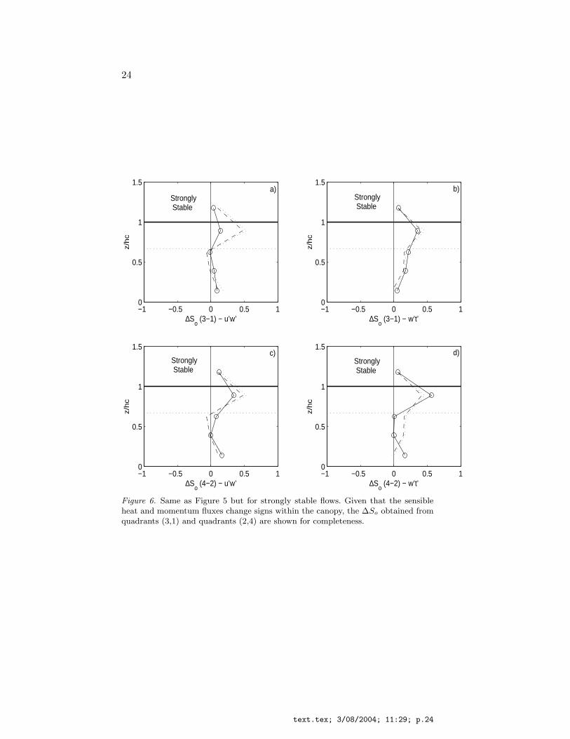
In the Theory section, third order CEM was used to link the ejection-sweep cycle with the heat flux transport term in equation (11). Hence, itis necessary to explore how well third order CEM and ICEM expansionsin equations (9) and (10) reproduce the measured ∆So computed fromequation (8). In Figures 5 and 6, the comparison between measuredand CEM modelled ∆So for both momentum and sensible heat flux areshown for all three stability cases. It is clear that both CEM and ICEMreproduce the measured ∆So profiles reasonably well for momentumand sensible heat flux and for all stability conditions thereby lendingfurther confidence to third order ICEM expansions within canopies(Katul et al., 1997b; Poggi et al., 2004a).

While the ICEM formulation provided the desirable link betweenM12 = w′w′T ′/(σ2

wσT ) and ∆So, it also introduced a new quantity,M21 = w′T ′T ′/(σwσ2

T ). Whether M21 can be related to M12 theoreti-cally remains a challenge, though empirically, few experiments alreadysuggested linearities in momentum (Raupach, 1981) and scalars (Katulet al., 1997b). We tested in Figure 7 whether such a linear relationshipalso holds for the Lavarone canopy for heat and momentum and forthe three stability classes using all the runs. Figure 7 shows that M12

is linearly related to M21 for unstable, slightly stable, and stable flowsconsistent with earlier studies on heat and momentum. Interestingly,the value of | C | (= 0.6) for both heat and momentum and for all threestability classes is the same as evidenced by Figure 7.

We compared modelled ∆So from equation (16) with measured ∆So

determined by quadrant analysis in Figure 8 using C5 = 2.4 for all sta-bility classes. Recall that equation (16) assumes 1) a linear relationshipbetween M12 and M21 with a | C |= 0.6, and 2) a gradient-diffusionclosure for w′w′T ′, and 3) a τ determined from a constant mixing lengthscale (with a β = 0.1). Despite these simplifications and assumptions,the agreement between measured and modelled ∆So is reasonably good.

4.4. Relative Importance of Ejections, Sweeps, andAtmospheric Stability on the Sensible Heat FluxProfile

Re-writing equation (4) as a second-order ODE for the sensible heatflux yields

text.tex; 3/08/2004; 11:29; p.13

14

Ktd2w′T ′

dz+

dKt

dz

dw′T ′

dz− C4

τw′T ′ =

[w′2

∂T

∂z− 4

3g

TT ′2

](17)

where Kt = C5τσ2w. Using measured σw(z), T (z), and σT (z), and

estimating τ from equation (3), the vertical variation of w′T ′(z) wascomputed numerically (see Katul and Albertson, 1999; Siqueira andKatul, 2002 for numerical scheme and details). To investigate the rel-ative importance of ejections and sweeps and atmospheric stability onthe profiles of sensible heat flux, three solutions to equation (17) wereanalyzed. The first retains all the terms in equation (17) and is hereafterlabelled as the ”full solution”, the second neglects atmospheric stabilityby setting T ′2 = 0 and is labelled the ”neutral solution”, and the thirdis a K-theory calculation obtained by setting both T ′2 = 0 and Kt = 0.The resulting sensible heat flux profiles from these three cases are shownin Figure 9.

It is clear that by accounting for all the terms in equation (17) (i.e.the full model), the agreement between measured and modelled w′T ′is superior to predictions made from K-theory. In fact, the zero- andcounter gradient flows noted in section 4.1 are all reasonably reproducedby the full model.

Furthermore, the model inter-comparisons suggest that the effect ofatmospheric stability on the computed sensible heat flux profiles arecomparable to the flux-transport term for unstable and extremely sta-ble conditions. Interestingly, however, accounting for atmospheric sta-bility tended to worsen the agreement between measured and modelledsensible heat flux for mildly stable conditions. One possible explanationis that the mildly stable runs included many near-neutral cases (i.e.stability is not important); furthermore, the measured σT may havebeen contaminated by high frequency noise thereby overestimating thecomputed value of 4

3g

TT ′2 from the data. It appears from Figure 9 that

neglecting stability for slightly stable flows is preferred over the fullmodel.

Figure 9 also shows the agreement between measured and modelledw′w′T ′ and ∆So×w′T ′ = w′T ′sweeps−w′T ′ejections. To our knowledge,testing the skills of second order closure models using quadrant analysis(i.e. measured w′T ′sweeps − w′T ′ejections) was not conducted before forsensible heat. Again, despite theoretical objections to closing w′w′T ′ viaequation (5) (e.g. Wilson, 1989), the good agreement between measuredand modelled w′w′T ′ and ∆So ×w′T ′ for unstable and stable stabilityclasses is rather encouraging. However, the (unexpected) disagreementsfor slightly stable conditions is rather disappointing.

text.tex; 3/08/2004; 11:29; p.14

Buoyancy and the heat flux budget within dense canopies 15

5. Conclusions

Over the past 3 decades, experimental and computational developmentshave led to an extensive understanding of momentum and scalar trans-fer within uniform canopies. Despite this progress, several unresolvedissues remain. The combined effects of buoyancy and ejection-sweepstatistics on scalar transfer is one such issue. To date, no explicit di-agnostic model relating the local turbulent heat flux to the mean airtemperature gradient, buoyancy, and the statistical properties of theejection-sweep cycle within the canopy volume exists. To begin progresson this issue, we combined cumulant expansion methods (CEM) andhigher order closure models and derived explicit linkages between thesensible heat flux, mean temperature profiles, ejection-sweep statistics,and buoyancy. The latter linkages were successfully tested on a data setcollected in a mixed hardwood forest at Lavarone, Italy. Particularly,our analysis and comparisons demonstrated the following:

1) Second order closure models for the heat flux budget equationreproduce reasonably well the eddy-covariance measured profiles ofw′T ′ and w′w′T ′ for unstable and stable flows. For slightly stable flows,neglecting the buoyancy contribution (i.e. σ2

T ) is preferred.2) The cumulant expansion method (CEM) and the incomplete

CEM (ICEM) proposed by Katul et al. (1997b) are sufficient to linkthe triple velocity-temperature correlation (w′w′T ′) to ∆So. We notethat for momentum transfer, Raupach (1981) empirically found a linearrelationship between ∆So and M12 when variations in u2∗/(σuσw) aresmall (in a wind tunnel). Here, we showed that this linkage depends onthe correlation between vertical velocity and scalar concentration.

3) The ICEM, when combined with the heat flux budget equation,leads to an explicit relationship between w′T ′ and dT/dz, z, σ2

w, ∆So,and σ2

T . This relationship must be viewed as diagnostic because the∆So profile is not known a priori. Nonetheless, the relationship canbe used to estimate the dT/dz for which zero-gradient (and countergradient) flow occurs if the ejection-sweep cycle properties are a priorispecified.

4) Second order closure models that utilize gradient-diffusion ap-proximation for w′w′T ′, when combined with the ICEM, can estimate∆So. The fact that closure models can estimate ∆So offers novel waysof diagnosing closure schemes from quadrant analysis and invites newinterpretations to their successes and failures.

5) The resulting closure model formulation for ∆So suggests thatsweeps dominate the heat flux when the ratio of the local heat source(ST ) to w′T ′ is positive irrespective of atmospheric stability. Conversely,ejections dominate the sensible heat flux when ST /w′T ′ < 0. The

text.tex; 3/08/2004; 11:29; p.15

16

dominant role of sweeps for unstable and stable atmospheric condi-tions predicted by the model are consistent with a wide range of fieldexperiments, including the present forest experiment.

From a broader perspective, this study is a necessary first step to-wards progressing on the general problem of how the ejection-sweep cy-cle, thermal stratification, dispersive fluxes, and planar inhomogeneoustransport (e.g. resulting from topographic or planar canopy densityvariation) alter flux-gradient relationships at different closure levelswithin canopies.

Acknowledgements

Katul and Poggi acknowledge the support of the US National ScienceFoundation (NSF-EAR-02− 08258), the Biological and EnvironmentalResearch (BER) Program, U.S. Department of Energy, through theSoutheast Regional Center (SERC) of the National Institute for GlobalEnvironmental Change (NIGEC), and through the Terrestrial CarbonProcesses Program (TCP) and the FACE project. Giostra acknowl-edge the Italian MURST Project ”Sviluppo di tecnologie innovativee di processi biotecnologici in condizioni controllate nel settore dellecolture vegetali: Diagnosi e Prognosi di situazioni di stress idrico perla vegetazione”. Cava acknowledges the CNR for the SHORT-TERMMOBILITY Programme - 2004, and the support of the CNR-ISACfor the Project ’Effetti delle Strutture Coerenti sul Trasporto Turbo-lento in Canopy Vegetale’ (Progetto Giovani Ricercatori CNR-ISAC- 2003). Cescatti acknowledges the support of the Fondazione Cassadi Risparmio di Trento e Rovereto for the Project ’Carbon fluxes andpools in forest ecosystems’ and the Province of Trento, Italy, (grantDG 14616/97, DG 1060/01).

References

Andre , J. C., de Moor, G., Lacarrere, P., Therry, G., and du Vachat, R.: 1979, Theclipping approximation and inhomogeneous turbulence simulations, TurbulentShear Flow , I: 307–318.

Chen, J.M., and Black, T.A.: 1992, ’Defining leaf-area index for non-flat leaves’,Plant Cell and Environment , 15(4): 421–429.

Corrsin, S.: 1974, ’Limitations of gradient transport models inrandom walks and inturbulence’, Adv. Geophys., 18A: 25–60.

Denmead, O.T., and Bradley, E.F.: 1985, ’Flux-gradient realtionship in a forestcanopy’, In: The Forest Atmosphere Interaction, B.A. Hutchinson, B.B. Hicks,eds. - D. Reidel Publ. Co. Dordrecht, pp. 421?-442.

text.tex; 3/08/2004; 11:29; p.16

Buoyancy and the heat flux budget within dense canopies 17

Finnigan, J.J.: 2000, ’Turbulence in plant canopies’, Ann. Rev. Fluid Mech., 32:519–571.

Finnigan, J.J.: 1985, ’Turbulent Transport in Plant Canopies’, In B.A. Hutchinsonand B.B. Hocks (eds.), The Forest-Atmosphere Interactions , D. Reidel, Norwell,MA, pp. 443–480.

Finnigan, J.J.: 1979, ’Turbulence in waving wheat. II. Structure of momentumtransfer’, Boundary-Layer Meteorol., 16: 213–236.

Kaimal J.C., and Finnigan, J.J.: 1994, Atmospheric Boundary Layer Flows: TheirStructure and Measurements New York: Oxford Univ. Press., 289 pp.

Katul, G.G., Cava, D., Poggi, D., Albertson, J.D., and Mahrt, L.: 2004, ’Sta-tionarity, Homogeneity, and Ergodicity in Canopy Turbulence’, Handbook ofMicrometeorology , Chapter 8, Kluwer Academic Publishers, 84–102.

Katul, G.G., Leuning, R., Kim, J., Denmead, O.T., Miyata, A., and Harazono, Y.:2001, ’Estimating CO2 Source/Sink Distributions within a Rice Canopy usingHigher-Order Closure Models’, Boundary-Layer Metereol., 98: 103–125.

Katul, G.G., and Albertson J.D.: 1999, ’Modelling CO2 Sources, Sinks and Fluxeswithin a Forest Canopy’, J. Geophys. Res., 104: 6081–6091.

Katul, G.G., Oren, R., Ellsworth, D., Hsieh, C.I., Phillips, N., and Lewin, K.: 1997a,’A Lagrangian dispersion model for predicting CO2 sources, sinks, and fluxes in auniform Loblolly pine (Pinus taeda L.) stand’, J. Geophys. Res., 102: 9309–9321.

Katul, G.G., Hsieh, C.I., Kuhn, G., and Ellswort, D.: 1997b, ’Turbulent eddy motionat the forest-atmosphere interface’, J. Geophys. Res., 102-D12: 13409–13421.

Katul, G.G., and Parlange, M.B.: 1994, ’On the active role of temperature in surfacelayer turbulence’, J. Atmos. Sci., 51: 2181–2195.

Leuning, R., Denmead, O.T., Miyata, A., and Kim, J.: 2000, ’Source/sink distri-butions of heat, water vapour, carbon dioxide and methane in a rice canopyestimated using Lagrangian dispersion analysis’, Agric. For. Meteorol., 104:233–249.

Maitani, T., and Seo, T.: 1985, ’Estimates of velocity-pressure and velocity-pressure-gradient interactions in the surface layer over plant canopies’, Boundary-LayerMeteorol., 33: 51–60.

Marcolla, B., Pitacco, A., and Cescatti, A.: 2003, ’Canopy architecture and tur-bulence structure in a coniferous forest’, Boundary-Layer Meteorol., 108(1):39–59.

Massman, W.J., and Weil, J.C.: 1999, ’An analytical one-dimensional second-orderclosure model of turbulence statistics and the Lagrangian time scale within andabove plant canopies of arbitrary structure’, Boundary-Layer Meteorol., 91(1):81–107.

Mahrt, L.: 1998, ’Stratified Atmospheric Boundary Layers and Breakdown ofModels’, Theoret. Comput. Fluid Dynamics , 11: 263–279.

Meyers, T., and Paw U, K.T.: 1987, ’Modelling the plant canopy micrometeorologywith higher-order closure principles’, Agric. For. Meteorol., 41: 143–163.

Nagano, Y., and Tagawa, M.: 1995, ’Coherent motions and heat transfer in a wallturbulent shear flow’, J. Fluid Mech., 305: 127–157.

Nakagawa, H., and Nezu, I.: 1977, ’Prediction of the contributions to the Reynoldsstress from bursting events in open channel flows’, J. Fluid Mech., 80: 99–128.

Poggi, D., Katul, G.G., and Albertson, J.D.: 2004a, ’Momentum transfer and tur-bulent kinetic energy budgets within a dense model canopy’, Boundary-LayerMeteorol., 111 (3): 589–614.

text.tex; 3/08/2004; 11:29; p.17

18

Poggi, D., Albertson J., and Katul, G.: 2004b, ’Scalar Dispersion within a ModelCanopy: Measurements and Lagrangian Models’, submitted to Advances in WaterResources.

Raupach, M.R.: 1989a, ’Applying lagrangian fluid-mechanics to infer scalar sourcedistributions from concentration profiles in plant canopies’, Agric. For. Meteorol.,47: 85–108.

Raupach, M.R.: 1989b, ’A practical lagrangian method for relating scalar concen-trations to source distributions in vegetation canopies’, Quart. J. Roy. Meteorol.Soc., 487: 609–632.

Raupach, M.R.: 1988, ’Canopy Transport Processes’, In W. L. Steffen and O. T. Den-mead (eds.), Flow and Transport in the Natural Environment , Springer-Verlag,New York, pp. 95–127.

Raupach, M.R.: 1987, ’A Lagrangian analysis of scalar transfer in vegetationcanopies’, Ann. Rev. Fluid. Mech., 13: 97–129.

Raupach, M.R., Coppin, P.A., and Legg, B.J.: 1986, ’Experiments on Scalar Dis-persion within a Model-Plant Canopy. 1. The Turbulence Structure’, Boundary-Layer Meteorol., 35: 21–52.

Raupach, M.R.: 1983, ’Near-Field Dispersion from Instantaneous Sources in theSurface-Layer’, Boundary-Layer Meteorol., 27: 105–113.

Raupach, M.R., Shaw, R.H.: 1982, ’Averaging procedures for flow within vegetationcanopies’, Boundary-Layer Meteorol., 22: 79–90.

Raupach, M.R.: 1981, ’Conditional statistics of Reynolds stress in rough-wall andsmooth-wall turbulent boundary layers’, J. Fluid Mech., 108: 363–382.

Shaw R.H.: 1977, ’Secondary Wind Speed Maxima inside Plant Canopies’, J. Appl.Meteorol., 16 (5): 514–521.

Siqueira, M., Leuning, R., Kolle, O., Kelliher, F.M., and Katul, G.G.: 2003, ’Model-ing sources and sinks of CO2, H2O and heat within a Siberian pine forest usingthree inverse methods’, Quart. J. Roy. Meteorol. Soc., 129: 1373–1393.

Siqueira, M., Katul, G.G., and Lai, C.T.: 2002, ’Quantifying net ecosystem exchangeby multilevel ecophysiological and turbulent transport models’, Advances inWater Resources, 25: 1357–1366.

Siqueira, M., and Katul, G.G.: 2002, ’Estimating heat sources and fluxes in ther-mally stratified canopy flows using higher-order closure models’, Boundary-LayerMeteorol., 103: 125–142.

Taylor, G.I.: 1959, ’The present position in the theory of turbulent diffusion’, Adv.Geophys., 6: 101–112.

Thurtell., G.W.: 1989, ’Comment on using K-theory within and above the plantcanopy to model diffusion processes’, In: Estimation of Areal Evapotranspiration ,IAHS Plubl., 177: 43–80.

Valentini, R., Matteucci, G., Dolman, A.J., Schulze, E.D., Rebmann, C., Moors,E.J., Granier, A., Gross, P., Jensen, N.O., Pilegaard, K., Lindroth, A., Grelle,A., Bernhofer, C., Grunwald, T., Aubinet, M., Ceulemans, R., Kowalski, A.S.,Vesala, T., Rannik, U., Berbigier, P., Loustau, D., Guomundsson, J., Thorgeirs-son, H., Ibrom, A., Morgenstern, K., Clement, R., Moncrieff, J., Montagnani,L., Minerbi, S., and Jarvis, P.G.: 2000, ’Respiration as the main determinant ofcarbon balance in European forests’, Nature, 404: 861–865.

Wilson, N.R.: 1989, ’Turbulent transport within the plant canopy’, In: Estimationof Areal Evapotranspiration, IAHS Plubl., 177: 43–80.

Wilson, N.R., and Shaw, R.H.: 1977, ’A higher order closure model for canopy flow’,J. Appl. Meteorol., 16: 1197–1205.

text.tex; 3/08/2004; 11:29; p.18

Buoyancy and the heat flux budget within dense canopies 19

z/hc

2

chTw

Tw

′′′′

1

00

DaytimeNightime

0;0 >′′

>′′dz

TwdTw

0;0 <′′

>′′dz

TwdTw

Ejections

Sweeps

All Sweeps

0;0 <′′

<′′dz

TwdTw

Figure 1. Typical sensible heat flux profiles inside and above the canopy for day- andnigh-time conditions from Kaimal and Finnigan (1994). The flux-gradient closuremodel for the triple correlation between velocity and temperature predicts a positive∆So (i.e. sweeps) throughout the canopy except at night-time near the forest floorwhen the flux and its gradient do not share the same sign. These predictions can becompared to measured ∆So from quadrant analysis.

text.tex; 3/08/2004; 11:29; p.19

20

0 0.5 1 1.50

0.5

1

1.5

σw

/u*

z/h

c

−10 −5 0 50

0.5

1

1.5

(T−Thc

)/|T*|

z/h

c

−1.5 −1 −0.5 0 0.5 1 1.50

0.5

1

1.5

w’t’/|w’t’hc

|

z/h

c

−1 −0.5 0 0.5 1 1.50

0.5

1

1.5

w’w’t’/(u*2 |T

*|)

z/h

c

a) b)

c) d)

Figure 2. Variation of normalized flow statistics with normalized height (z/hc) for(a) vertical velocity standard deviation (σw/u∗), (b) mean air temperature differ-

ence (T−T hcT∗ ), (c) sensible heat flux ( w′T ′

|w′T ′hc|), and (d) heat flux transport w′w′T ′

|T∗|u∗2 ,

where Thc is the mean air temperature, T∗ = w′T ′hcu∗ is a normalizing turbulent

temperature scale, and u∗ = (−u′w′hc)1/2 is the friction velocity all defined at the

canopy height hc. The 30-minute data runs are ensemble averaged in three stabilityclasses: unstable (∗), weakly stable (♦), and strongly stable (o)

text.tex; 3/08/2004; 11:29; p.20

Buoyancy and the heat flux budget within dense canopies 21

−60 −40 −20 0 200

0.5

1

1.5

PR/(u*2 |T

*|)

z/h

c

−15 −10 −5 0 5 100

0.5

1

1.5

TR/(u*2 |T

*|)

z/h

c

0 10 20 300

0.5

1

1.5

B/(u*2 |T

*|)

z/h

c

−20 0 20 40 600

0.5

1

1.5

D/(u*2 |T

*|)

z/h

c

a) b)

c) d)

Figure 3. Variation of the normalized components of the sensible heat fluxbudget equation with normalized height (z/hc) for (a) the production term

(PR = −w′w′ dTdz

), (b) the flux transport term TR = dw′w′T ′dz

, (c) the Buoyancy term

B = g

TσT

2, and (d) the scalar dissipation term D = T ′ dp′dz

estimated as a residual

from equation (1). All temperature, velocity, and length scales are normalized byT∗, u∗, and hc, respectively. The three stability classes are as in Figure 2.

text.tex; 3/08/2004; 11:29; p.21

22

0 2 4 6 8 100

0.5

1

1.5

τ / τmin

z/hc

−0.1 −0.05 0 0.05 0.1−0.1

−0.05

0

0.05

0.1

modelled w’t’

mea

sure

d w

’t’

a) b)

Figure 4. (a) Variation of the normalized time scale (τ) with height (z/hc); (b) Com-parison between measured and modelled w′T ′ for all heights and stability classes.The modelled sensible heat flux is based on modelled (τ) and the dissipation closurescheme in equation (2). The three stability classes are as in Figure 2.

text.tex; 3/08/2004; 11:29; p.22

Buoyancy and the heat flux budget within dense canopies 23

−1 −0.5 0 0.5 10

0.5

1

1.5

∆So (4−2) − u’w’

z/h

c

−1 −0.5 0 0.5 10

0.5

1

1.5

∆So (3−1) − w’t’

z/h

c

−1 −0.5 0 0.5 10

0.5

1

1.5

∆So (4−2) − u’w’

z/h

c

−1 −0.5 0 0.5 10

0.5

1

1.5

∆So (4−2) − w’t’

z/h

c

Unstable Unstable

Weakly Stable

Weakly Stable

a) b)

c) d)

Figure 5. Comparison between measured and modelled ∆So for momentum (panelsa, c) and sensible heat (panels b, d) and for unstable and weakly stable stabilityclasses. The measured ∆So is based on equation (8) and the modelled ∆So arebased on third-order CEM (dashed) in equation (9) and the incomplete CEM orICEM (dot-dashed) in equation (10). The subscripts (3−1) and (2−4) indicate thequadrants used to compute ∆So.

text.tex; 3/08/2004; 11:29; p.23

24

−1 −0.5 0 0.5 10

0.5

1

1.5

∆So (3−1) − u’w’

z/h

c

−1 −0.5 0 0.5 10

0.5

1

1.5

∆So (3−1) − w’t’

z/h

c

−1 −0.5 0 0.5 10

0.5

1

1.5

∆So (4−2) − u’w’

z/h

c

−1 −0.5 0 0.5 10

0.5

1

1.5

∆So (4−2) − w’t’

z/h

c

a) b)

c) d)

Strongly Stable

Strongly Stable

Strongly Stable

Strongly Stable

Figure 6. Same as Figure 5 but for strongly stable flows. Given that the sensibleheat and momentum fluxes change signs within the canopy, the ∆So obtained fromquadrants (3,1) and quadrants (2,4) are shown for completeness.

text.tex; 3/08/2004; 11:29; p.24

Buoyancy and the heat flux budget within dense canopies 25

−1 −0.5 0 0.5 1−1

−0.5

0

0.5

1

M2

1(t

,w)

−1 −0.5 0 0.5 1−1

−0.5

0

0.5

1

M2

1(t

,w)

−1 −0.5 0 0.5 1−1

−0.5

0

0.5

1

M2

1(t

,w)

M12(t,w)

−1 −0.5 0 0.5 1−1

−0.5

0

0.5

1

M2

1(u

,w)

−1 −0.5 0 0.5 1−1

−0.5

0

0.5

1M

21

(u,w

)

−1 −0.5 0 0.5 1−1

−0.5

0

0.5

1

M2

1(u

,w)

M12(u,w)

a) b)

c) d)

e) f)

Figure 7. Comparisons between measured M12 and M21 for momentum and sensibleheat for all three stability classes and for all 1/2 hour runs. The three stabilityclasses are: unstable (∗), weakly stable (♦), and strongly stable ( (o) for the levelswhere RwT < 0 and (·) for the levels where RwT > 0 ). The continuous line isM21 = 0.6M12 and the dashed line is M21 = −0.6M12.

text.tex; 3/08/2004; 11:29; p.25

26

−0.2 −0.1 0 0.1 0.2 0.3 0.4 0.5 0.6 0.7 0.8−0.2

−0.1

0

0.1

0.2

0.3

0.4

0.5

0.6

0.7

0.8

modelled ∆ S0

me

asu

red

∆ S

0

Figure 8. Comparison between measured and modelled ∆So for all three stabilityclasses. The modelled ∆So is from equation (16) using the ensemble-averaged mea-sured sensible heat flux and σw profiles. The three stability classes are as before:unstable (∗), weakly stable (♦), and strongly stable (o). For reference, the 1:1 lineis also shown.

text.tex; 3/08/2004; 11:29; p.26

Buoyancy and the heat flux budget within dense canopies 27

−1 0 10

0.5

1

1.5

z/h

c

−1 0 10

0.5

1

1.5

z/h

c

−1 0 10

0.5

1

1.5

w’t’/|w’t’hc

|

z/h

c

−1 0 1 20

0.5

1

1.5

−1 0 1 20

0.5

1

1.5

−1 0 1 20

0.5

1

1.5

w’w’t’

−1 0 1 20

0.5

1

1.5

−1 0 1 20

0.5

1

1.5

−1 0 1 20

0.5

1

1.5

∆ S0 * w’t’

a) b) c)

d) e) f)

g) h) i)

Figure 9. Comparison between measured (symbols) and modelled (line) turbulentstatistics within the canopy for 1) sensible heat flux determined from equation(17) for unstable (panel a), weakly stable (panel d), and strongly stable (panel g)atmospheric stability; 2) triple velocity-temperature correlations for unstable (panelb), weakly stable (panel e), and strongly stable (panel h) atmospheric stability;3) w′T ′sweeps − w′T ′ejections for unstable (panel c), weakly stable (panel f), andstrongly stable (panel i) atmospheric stability. For the model comparisons, the solidline is the full model, the dashed line neglects atmospheric stability (neutral model),and the dotted line is the sensible heat flux estimated from K-theory.

text.tex; 3/08/2004; 11:29; p.27

text.tex; 3/08/2004; 11:29; p.28