Buildings 2020+

Energy sources

Bialystok - Cordoba - Vilnius 2019

2020+BUILDINGS

Editor

Dorota Anna Krawczyk

Buildings 2020+Energy sources

Editor Dorota Anna Krawczyk

Printing House of Bialystok Univesity of TechnologyBialystok – Cordoba – Vilnius 2019

Editor-in-Chief: Dorota Anna Krawczyk

Vice-Editor: Antonio Rodero Serrano

Reviewers:

Alicja Siuta-Olcha, Ph.D., D.Sc. (Eng.), Associate ProfessorManuel Plaza Garcia, Ph.D. (Eng.), Professor

Copy Editor: Alina Domurat (final correction of chapters: 2, 3, 4, 5)Rūta Kalytienė (preliminary correction chapters 3, 4, 6, 7)Javier Martín Párraga (final correction of chapters 1, 6, 7, 8)

Cover of a book: Lorita ButrimienėPhoto on the cover:Antonio Rodero Serrano

© Copyright by Bialystok University of Technology, Bialystok 2019

ISBN 978-83-65596-72-7 eISBN 978-83-65596-73-4https://doi.org/10.24427/978-83-65596-73-4

The publication is available on licenseCreative Commons Recognition of authorship – Non-commercial use – Without dependent works 4.0(CC BY-NC-ND 4.0)Full license content available on the site creativecommons.org/licenses/by-nc-nd/4.0/legalcode.plThe publication is available on the Internet on the site of the Printing House of Bialystok University of Technology

Technical editing, binding:Printing House of Bialystok University of Technology

Printing:EXDRUK s.c.

Printing House of Bialystok University of TechnologyWiejska 45C, 15-351 Białystok e-mail: [email protected]

3

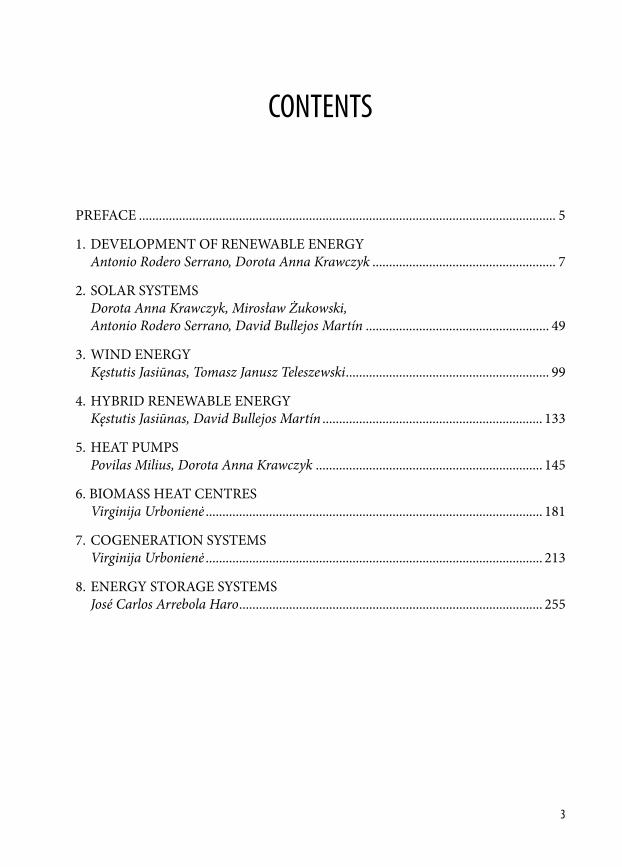
CONTENTS

PREFACE ............................................................................................................................. 5

1. DEVELOPMENT OF RENEWABLE ENERGY Antonio Rodero Serrano, Dorota Anna Krawczyk ....................................................... 7

2. SOLAR SYSTEMS Dorota Anna Krawczyk, Mirosław Żukowski, Antonio Rodero Serrano, David Bullejos Martín ....................................................... 49

3. WIND ENERGY Kęstutis Jasiūnas, Tomasz Janusz Teleszewski ............................................................. 99

4. HYBRID RENEWABLE ENERGY Kęstutis Jasiūnas, David Bullejos Martín .................................................................. 133

5. HEAT PUMPS Povilas Milius, Dorota Anna Krawczyk .................................................................... 145

6. BIOMASS HEAT CENTRES Virginija Urbonienė ..................................................................................................... 181

7. COGENERATION SYSTEMS Virginija Urbonienė ..................................................................................................... 213

8. ENERGY STORAGE SYSTEMS José Carlos Arrebola Haro ........................................................................................... 255

Authors

Arrebola Haro José Carlos, UCO

Bullejos Martín David, UCO

Kęstutis Jasiūnas, VTDK

Krawczyk Dorota Anna, BUT

Milius Povilas, VTDK

Rodero Serrano Antonio, UCO

Teleszewski Tomasz Janusz, BUT

Urbonienė Virginija, VTDK

Żukowski Mirosław, BUT

5

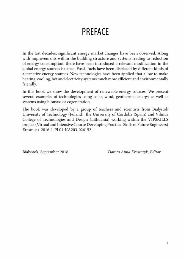
PREFACE

In the last decades, significant energy market changes have been observed. Along with improvements within the building structure and systems leading to reduction of energy consumption, there have been introduced a relevant modification in the global energy sources balance. Fossil fuels have been displaced by different kinds of alternative energy sources. New technologies have been applied that allow to make heating, cooling, hot and electricity systems much more efficient and environmentally friendly.

In this book we show the development of renewable energy sources. We present several examples of technologies using solar, wind, geothermal energy as well as systems using biomass or cogeneration.

The book was developed by a group of teachers and scientists from Bialystok University of Technology (Poland), the University of Cordoba (Spain) and Vilnius College of Technologies and Design (Lithuania) working within the VIPSKILLS project (Virtual and Intensive Course Developing Practical Skills of Future Engineers) Erasmus+ 2016-1-PL01-KA203-026152.

Bialystok, September 2018 Dorota Anna Krawczyk, Editor

7

DOI: 10.24427/978-83-65596-73-4_1

1. DEVELOPMENT OF RENEWABLE ENERGY

1.1. New Energy Landscape

1.1.1. Global landscapeWithout a doubt, the world is immersed in a historical change of its energy systems. Similarly, to the 19th century, which meant the beginning of fossil energy sources, global energy markets are actually in a transitional period. The evolution of energy issues over the past decades provides a change of policies and regulations about this market. An energy market based mainly on traditional fossil energy sources, is now evaluating other alternatives sources, such as renewable energies.

Two are the main issues that are responsible of this evolution: an oil and gas import dependence and the need for diversification in electricity production and climate change by CO2 emission.

The first issue arose in 1970s after the oil crisis which took place during this decade. In this period, oil and gas were used to produce a substantial part of electricity in the world: approximately 46% of the global electricity production and 16%, respectively. Main producers of this energy resources were OPEC’s countries (Fig. 1.1). This means that prices of oils and gas are very dependent on war and conflict in these areas.

Non‐OPEC275.38

billons barrels

OPEC1216.77 billons barrels

302,25

266,21

157,2

148,77

101,5

97,8

48,3637,45 25,24 12,2 9,52 8,27 2

VenezuelaSaudi ArabiaIR iranIraqKwaitUnited Arab EmirtesLybiaNigeriaQatarAlgeriaAngolaEcuadorGabon

OPEC oil reserves (billon barrels)

Fig. 1.1. OPEC share of world crude oils reserves (Source: own elaboration based on Fantini & Quinn, 2017)

8

Buildings 2020+. EnErgy sourcEs

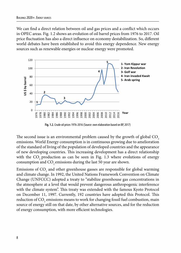
We can find a direct relation between oil and gas prices and a conflict which occurs in OPEC areas. Fig. 1.2 shows an evolution of oil barrel prices from 1976 to 2017. Oil price fluctuation has also a direct influence on economy destabilization. So, different world debates have been established to avoid this energy dependence. New energy sources such as renewable energies or nuclear energy were promoted.

0

20

40

60

80

100

120

1976

1978

1980

1982

1984

1986

1988

1990

1992

1994

1996

1998

2000

2002

2004

2006

2008

2010

2012

2014

2016

1

2

3

4

5 1‐ Yom Kippur war2‐ Iran Revolution3‐ Golf war4‐ Iran invaded Kwait5‐ Arab spring

Year

US $ byba

rrel

Fig. 1.2. Crude oil prices 1976-2016 (Source: own elaboration based on BP, 2017)

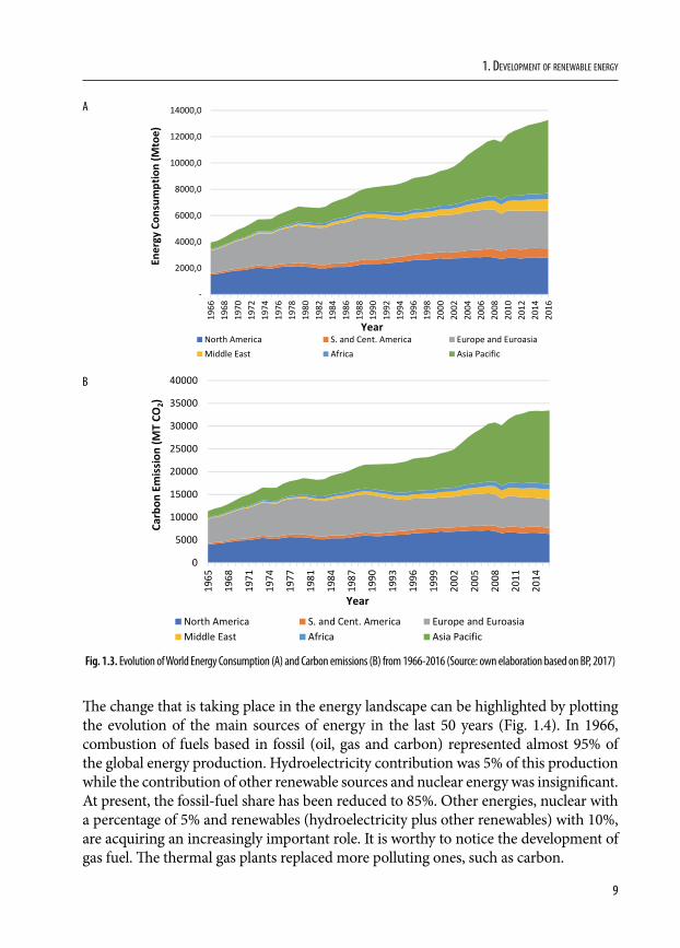
The second issue is an environmental problem caused by the growth of global CO2 emissions. World Energy consumption is in continuous growing due to amelioration of the standard of living of the population of developed countries and the appearance of new developing countries. This increasing development has a direct relationship with the CO2 production as can be seen in Fig. 1.3 where evolutions of energy consumption and CO2 emissions during the last 50 year are shown.

Emissions of CO2 and other greenhouse gasses are responsible for global warming and climate change. In 1992, the United Nations Framework Convention on Climate Change (UNFCCC) adopted a treaty to “stabilize greenhouse gas concentrations in the atmosphere at a level that would prevent dangerous anthropogenic interference with the climate system”. This treaty was extended with the famous Kyoto Protocol on December 11, 1997. Currently, 192 countries have adopted this Protocol. This reduction of CO2 emissions means to work for changing fossil fuel combustion, main source of energy still on that date, by other alternative sources, and for the reduction of energy consumption, with more efficient technologies.

9

1. Development of renewable energy

A

‐

2000,0

4000,0

6000,0

8000,0

10000,0

12000,0

14000,0

1966

1968

1970

1972

1974

1976

1978

1980

1982

1984

1986

1988

1990

1992

1994

1996

1998

2000

2002

2004

2006

2008

2010

2012

2014

2016

North America S. and Cent. America Europe and EuroasiaMiddle East Africa Asia Pacific

Year

Energy Con

sumption (M

toe)

B

0

5000

10000

15000

20000

25000

30000

35000

40000

1965

1968

1971

1974

1977

1981

1984

1987

1990

1993

1996

1999

2002

2005

2008

2011

2014

North America S. and Cent. America Europe and EuroasiaMiddle East Africa Asia Pacific

Year

Carbon

Emiss

ion (M

T CO

2)

Fig. 1.3. Evolution of World Energy Consumption (A) and Carbon emissions (B) from 1966-2016 (Source: own elaboration based on BP, 2017)

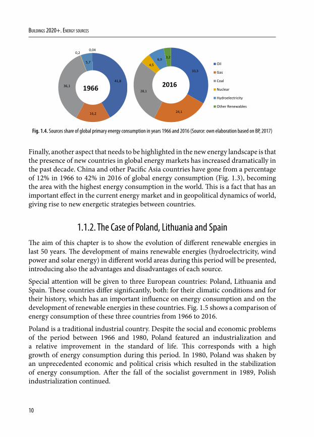
The change that is taking place in the energy landscape can be highlighted by plotting the evolution of the main sources of energy in the last 50 years (Fig. 1.4). In 1966, combustion of fuels based in fossil (oil, gas and carbon) represented almost 95% of the global energy production. Hydroelectricity contribution was 5% of this production while the contribution of other renewable sources and nuclear energy was insignificant. At present, the fossil-fuel share has been reduced to 85%. Other energies, nuclear with a percentage of 5% and renewables (hydroelectricity plus other renewables) with 10%, are acquiring an increasingly important role. It is worthy to notice the development of gas fuel. The thermal gas plants replaced more polluting ones, such as carbon.

10


41,8

16,2

36,1

0,2

5,7

0,04

1966

33,3

24,1

28,1

4,56,9 3,2

Oil

Gas

Coal

Nuclear

Hydroelectricity

Other Renewables

2016

Fig. 1.4. Sources share of global primary energy consumption in years 1966 and 2016 (Source: own elaboration based on BP, 2017)

Finally, another aspect that needs to be highlighted in the new energy landscape is that the presence of new countries in global energy markets has increased dramatically in the past decade. China and other Pacific Asia countries have gone from a percentage of 12% in 1966 to 42% in 2016 of global energy consumption (Fig. 1.3), becoming the area with the highest energy consumption in the world. This is a fact that has an important effect in the current energy market and in geopolitical dynamics of world, giving rise to new energetic strategies between countries.

1.1.2. The Case of Poland, Lithuania and SpainThe aim of this chapter is to show the evolution of different renewable energies in last 50 years. The development of mains renewable energies (hydroelectricity, wind power and solar energy) in different world areas during this period will be presented, introducing also the advantages and disadvantages of each source.

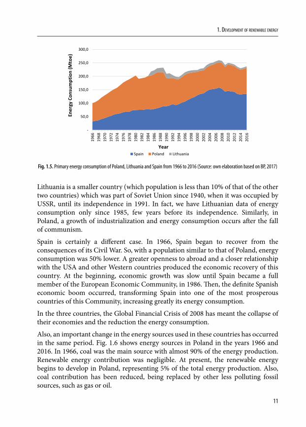
Special attention will be given to three European countries: Poland, Lithuania and Spain. These countries differ significantly, both: for their climatic conditions and for their history, which has an important influence on energy consumption and on the development of renewable energies in these countries. Fig. 1.5 shows a comparison of energy consumption of these three countries from 1966 to 2016.

Poland is a traditional industrial country. Despite the social and economic problems of the period between 1966 and 1980, Poland featured an industrialization and a relative improvement in the standard of life. This corresponds with a high growth of energy consumption during this period. In 1980, Poland was shaken by an unprecedented economic and political crisis which resulted in the stabilization of energy consumption. After the fall of the socialist government in 1989, Polish industrialization continued.

11


‐

50,0

100,0

150,0

200,0

250,0

300,0

1966

1968

1970

1972

1974

1976

1978

1980

1982

1984

1986

1988

1990

1992

1994

1996

1998

2000

2002

2004

2006

2008

2010

2012

2014

2016

Spain Poland LithuaniaYear

Energy Con

sumption (M

toe)

Fig. 1.5. Primary energy consumption of Poland, Lithuania and Spain from 1966 to 2016 (Source: own elaboration based on BP, 2017)

Lithuania is a smaller country (which population is less than 10% of that of the other two countries) which was part of Soviet Union since 1940, when it was occupied by USSR, until its independence in 1991. In fact, we have Lithuanian data of energy consumption only since 1985, few years before its independence. Similarly, in Poland, a growth of industrialization and energy consumption occurs after the fall of communism.

Spain is certainly a different case. In 1966, Spain began to recover from the consequences of its Civil War. So, with a population similar to that of Poland, energy consumption was 50% lower. A greater openness to abroad and a closer relationship with the USA and other Western countries produced the economic recovery of this country. At the beginning, economic growth was slow until Spain became a full member of the European Economic Community, in 1986. Then, the definite Spanish economic boom occurred, transforming Spain into one of the most prosperous countries of this Community, increasing greatly its energy consumption.

In the three countries, the Global Financial Crisis of 2008 has meant the collapse of their economies and the reduction the energy consumption.

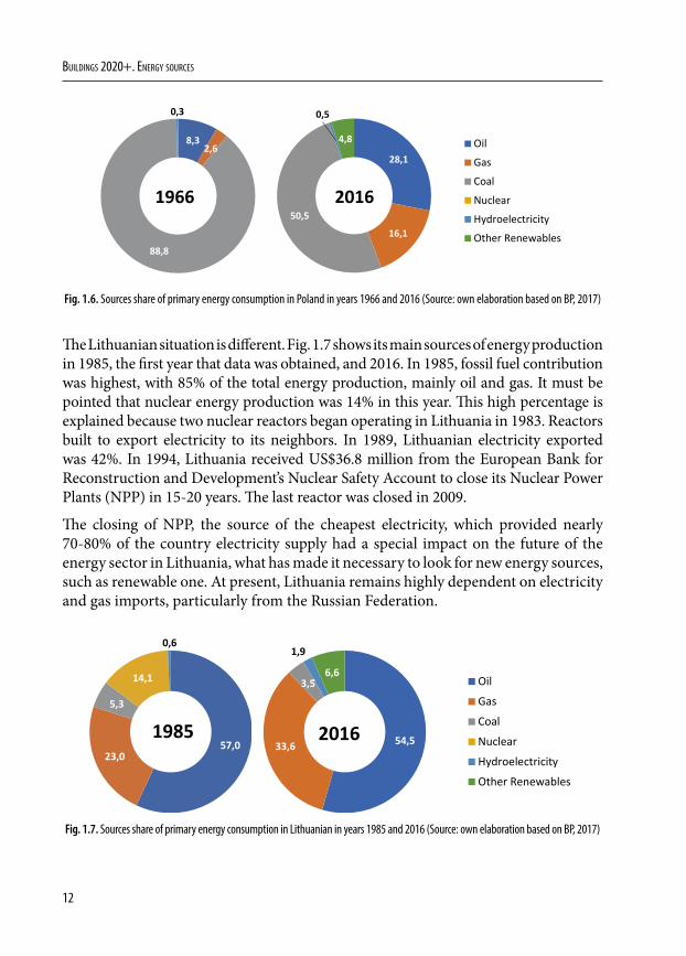
Also, an important change in the energy sources used in these countries has occurred in the same period. Fig. 1.6 shows energy sources in Poland in the years 1966 and 2016. In 1966, coal was the main source with almost 90% of the energy production. Renewable energy contribution was negligible. At present, the renewable energy begins to develop in Poland, representing 5% of the total energy production. Also, coal contribution has been reduced, being replaced by other less polluting fossil sources, such as gas or oil.

12


8,32,6

88,8

0,3

1966

28,1

16,150,5

0,5

4,8 OilGasCoalNuclearHydroelectricityOther Renewables

2016

Fig. 1.6. Sources share of primary energy consumption in Poland in years 1966 and 2016 (Source: own elaboration based on BP, 2017)

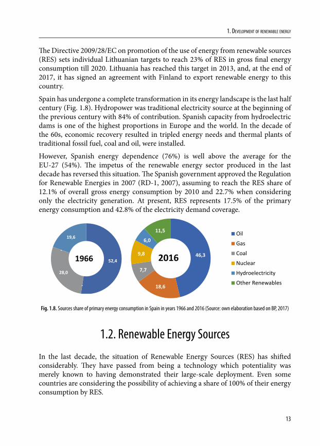
The Lithuanian situation is different. Fig. 1.7 shows its main sources of energy production in 1985, the first year that data was obtained, and 2016. In 1985, fossil fuel contribution was highest, with 85% of the total energy production, mainly oil and gas. It must be pointed that nuclear energy production was 14% in this year. This high percentage is explained because two nuclear reactors began operating in Lithuania in 1983. Reactors built to export electricity to its neighbors. In 1989, Lithuanian electricity exported was 42%. In 1994, Lithuania received US$36.8 million from the European Bank for Reconstruction and Development’s Nuclear Safety Account to close its Nuclear Power Plants (NPP) in 15-20 years. The last reactor was closed in 2009.

The closing of NPP, the source of the cheapest electricity, which provided nearly 70-80% of the country electricity supply had a special impact on the future of the energy sector in Lithuania, what has made it necessary to look for new energy sources, such as renewable one. At present, Lithuania remains highly dependent on electricity and gas imports, particularly from the Russian Federation.

57,023,0

5,3

14,1

0,6

1985

54,533,6

3,5‐

1,9

6,6OilGasCoalNuclearHydroelectricityOther Renewables

2016

Fig. 1.7. Sources share of primary energy consumption in Lithuanian in years 1985 and 2016 (Source: own elaboration based on BP, 2017)

13


The Directive 2009/28/EC on promotion of the use of energy from renewable sources (RES) sets individual Lithuanian targets to reach 23% of RES in gross final energy consumption till 2020. Lithuania has reached this target in 2013, and, at the end of 2017, it has signed an agreement with Finland to export renewable energy to this country.

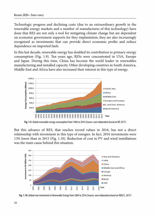
Spain has undergone a complete transformation in its energy landscape is the last half century (Fig. 1.8). Hydropower was traditional electricity source at the beginning of the previous century with 84% of contribution. Spanish capacity from hydroelectric dams is one of the highest proportions in Europe and the world. In the decade of the 60s, economic recovery resulted in tripled energy needs and thermal plants of traditional fossil fuel, coal and oil, were installed.

However, Spanish energy dependence (76%) is well above the average for the EU-27 (54%). The impetus of the renewable energy sector produced in the last decade has reversed this situation. The Spanish government approved the Regulation for Renewable Energies in 2007 (RD-1, 2007), assuming to reach the RES share of 12.1% of overall gross energy consumption by 2010 and 22.7% when considering only the electricity generation. At present, RES represents 17.5% of the primary energy consumption and 42.8% of the electricity demand coverage.

52,4

‐

28,0

‐

19,6

1966

46,3

18,6

7,7

9,8

6,0

11,5 OilGasCoalNuclearHydroelectricityOther Renewables

2016

Fig. 1.8. Sources share of primary energy consumption in Spain in years 1966 and 2016 (Source: own elaboration based on BP, 2017)

1.2. Renewable Energy Sources

In the last decade, the situation of Renewable Energy Sources (RES) has shifted considerably. They have passed from being a technology which potentiality was merely known to having demonstrated their large-scale deployment. Even some countries are considering the possibility of achieving a share of 100% of their energy consumption by RES.

14


Technologic progress and declining costs (due to an extraordinary growth in the renewable energy markets and a number of manufactures of this technology) have done that RES are not only a tool for mitigating climate change but are dependent on economic government supports for they implantation; they are also increasingly recognised as investments that can provide direct economic profits and reduce dependence on imported fuels.

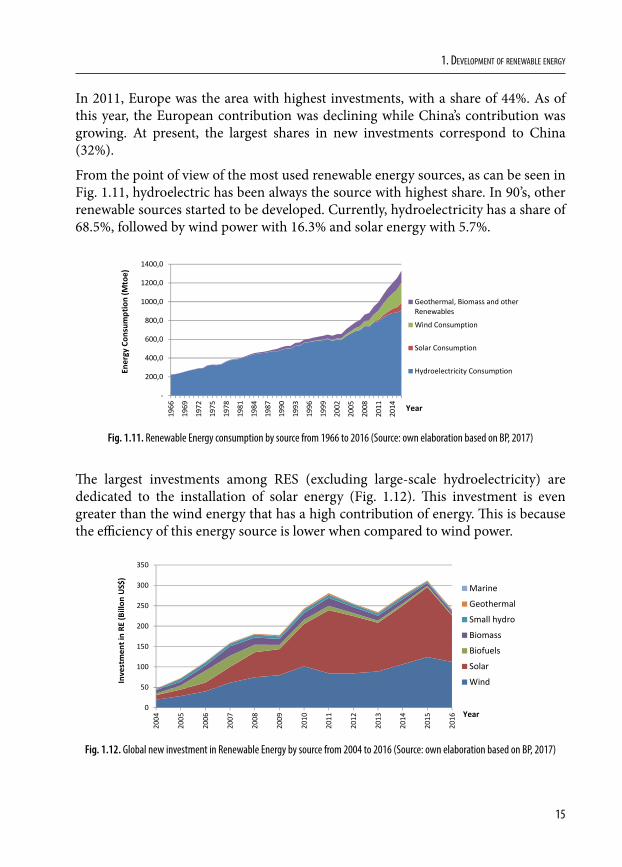
In this last decade, renewable energy has doubled its contribution to primary energy consumption (Fig. 1.9). Ten years ago, RESs were concentrated in USA, Europe and Japan. During this time, China has become the world leader in renewables manufacturing and installed capacity. Other developing countries in South America, Middle East and Africa have also increased their interest in this type of energy.

‐

200,0

400,0

600,0

800,0

1000,0

1200,0

1400,0

1966

1968

1970

1972

1974

1976

1978

1980

1982

1984

1986

1988

1990

1992

1994

1996

1998

2000

2002

2004

2006

2008

2010

2012

2014

2016

Pacific Asia

Africa

Middle East

Europe and Euroasia

S. and Cent. America

North America

Year

Energy Con

sumption (M

toe)

Fig. 1.9. Global renewable energy consumption from 1966 to 2016 (Source: own elaboration based on BP, 2017)

But this advance of RES, that reaches record values in 2016, has not a direct relationship with investment in this type of energies. In fact, 2016 investments were 13% lower than in 2015 (Fig. 1.10). Reduction of cost in PV and wind installations was the main cause behind this situation.

0

50

100

150

200

250

300

350

2004

2005

2006

2007

2008

2009

2010

2011

2012

2013

2014

2015

2016

Asia and OceaniaIndiaChinaMiddle East and AfricaEuropeAmericaBrazilUSA

Year

Investmen

t in RE

(Billon

US$)

Fig. 1.10. Global new investment in Renewable Energy from 2004 to 2016 (Source: own elaboration based on REN21, 2017)

15


In 2011, Europe was the area with highest investments, with a share of 44%. As of this year, the European contribution was declining while China’s contribution was growing. At present, the largest shares in new investments correspond to China (32%).

From the point of view of the most used renewable energy sources, as can be seen in Fig. 1.11, hydroelectric has been always the source with highest share. In 90’s, other renewable sources started to be developed. Currently, hydroelectricity has a share of 68.5%, followed by wind power with 16.3% and solar energy with 5.7%.

‐

200,0

400,0

600,0

800,0

1000,0

1200,0

1400,0

1966

1969

1972

1975

1978

1981

1984

1987

1990

1993

1996

1999

2002

2005

2008

2011

2014

Geothermal, Biomass and otherRenewablesWind Consumption

Solar Consumption

Hydroelectricity Consumption

Year

Energy Con

sumption (M

toe)

Fig. 1.11. Renewable Energy consumption by source from 1966 to 2016 (Source: own elaboration based on BP, 2017)

The largest investments among RES (excluding large-scale hydroelectricity) are dedicated to the installation of solar energy (Fig. 1.12). This investment is even greater than the wind energy that has a high contribution of energy. This is because the efficiency of this energy source is lower when compared to wind power.

0

50

100

150

200

250

300

350

2004

2005

2006

2007

2008

2009

2010

2011

2012

2013

2014

2015

2016

MarineGeothermalSmall hydroBiomassBiofuelsSolarWind

Year

Investmen

t in RE

(Billon

US$)

Fig. 1.12. Global new investment in Renewable Energy by source from 2004 to 2016 (Source: own elaboration based on BP, 2017)

16


1.2.1. HydroelectricityHydropower is the largest source of renewable energy in the world, with a share of 68% of overall RES (368.1 Mtoe of primary energy consumption). It is considered as one of the cheapest energy sources to generate electricity and it is predicted that it will continue leading this sector at least until 2022.

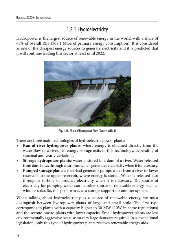
Fig. 1.13. Photo of Hydropower Plant (Source: WEB-1)

There are three main technologies of hydroelectric power plants: • Run-of-river hydropower plants: where energy is obtained directly from the

water flow of a river. No energy storage exits in this technology, depending of seasonal and yearly variations.

• Storage hydropower plants: water is stored in a dam of a river. Water released from dam flows through a turbine, which generates electricity when it is necessary.

• Pumped storage plant: a electrical generator pumps water from a river or lower reservoir to the upper reservoir, where energy is stored. Water is released also through a turbine to produce electricity when it is necessary. The source of electricity for pumping water can be other source of renewable energy, such as wind or solar. So, this plant works as a storage support for another system.

When talking about hydroelectricity as a source of renewable energy, we must distinguish between hydropower plants of large and small scale. The first type corresponds to plants with a capacity higher to 30 MW (10W in some regulations) and the second one to plants with lower capacity. Small hydropower plants are less environmentally aggressive because no very large dams are required. In some national legislation, only this type of hydropower plants receives renewable energy aids.

17


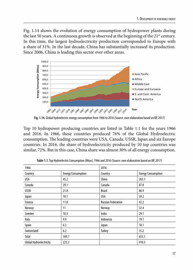
Fig. 1.14 shows the evolution of energy consumption of hydropower plants during the last 50 years. A continuous growth is observed at the beginning of the 21st century. In this time, the largest hydroelectricity production corresponded to Europe with a share of 31%. In the last decade, China has substantially increased its production. Since 2006, China is leading this sector over other areas.

‐

100,0

200,0

300,0

400,0

500,0

600,0

700,0

800,0

900,0

1000,0

Asia PacificAfricaMiddle EastEurope and EuroasiaS. and Cent. AmericaNorth America

Year

Energy Con

sumption (M

toe)

Fig. 1.14. Global hydroelectric energy consumption from 1966 to 2016 (Source: own elaboration based on BP, 2017)

Top 10 hydropower producing countries are listed in Table 1.1 for the years 1966 and 2016. In 1966, these countries produced 76% of the Global Hydroelectric consumption. The leading countries were USA, Canada, USSR, Japan and six Europe countries. In 2016, the share of hydroelectricity produced by 10 top countries was similar, 72%. But in this case, China share was almost 30% of all energy consumption.

Table 1.1. Top Hydroelectric Consumption (Mtoe), 1966 and 2016 (Source: own elaboration based on BP, 2017)

1966 2016

Country Energy Consumption Country Energy Consumption

USA 45.2 China 263.1

Canada 29.1 Canada 87.8

USSR 21.8 Brazil 86.9

Japan 18.1 USA 59.2

Francia 11.8 Russian Federation 42.2

Norway 11 Norway 32.4

Sweden 10.3 India 29.1

Italy 9.9 Indonesia 19.1

Spain 6.3 Japan 18.1

Switzerland 6.2 Turkey 15.2

Total 169.7 653.1

Global Hydroelectricity 223.2 910.3

18


The case of Poland, Lithuania and Spain

Poland is a flatland country with few mountains, a fact which limits the capacity of hydropower plants installation. According to the World Energy Council (2014), gross theoretical capacity of this country is 23 TWh/year, and technically exploitable capability of 12 TWh/year. The actual installed capacity is 955 MW. Moderate values for size of this country: 312,500 km2 surface area.

The majority of Hydropower plants are located in the south-west area, which is more mountainous. Rivers Lusatian Neisse and Bobr concentrate largest hydroelectricity. Except from few pumped storage plants of high capacity, they are mainly small capacity. In fact, no large-scale hydropower plants have been installed in Poland in the last 40 years.

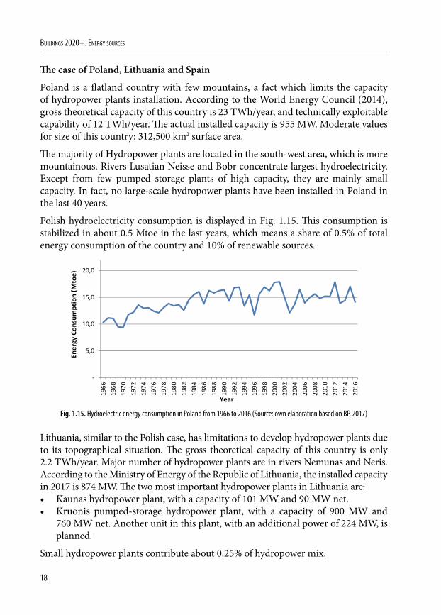
Polish hydroelectricity consumption is displayed in Fig. 1.15. This consumption is stabilized in about 0.5 Mtoe in the last years, which means a share of 0.5% of total energy consumption of the country and 10% of renewable sources.

‐

5,0

10,0

15,0

20,0

1966

1968

1970

1972

1974

1976

1978

1980

1982

1984

1986

1988

1990

1992

1994

1996

1998

2000

2002

2004

2006

2008

2010

2012

2014

2016

Year

Energy Con

sumption (M

toe)

Fig. 1.15. Hydroelectric energy consumption in Poland from 1966 to 2016 (Source: own elaboration based on BP, 2017)

Lithuania, similar to the Polish case, has limitations to develop hydropower plants due to its topographical situation. The gross theoretical capacity of this country is only 2.2 TWh/year. Major number of hydropower plants are in rivers Nemunas and Neris. According to the Ministry of Energy of the Republic of Lithuania, the installed capacity in 2017 is 874 MW. The two most important hydropower plants in Lithuania are:• Kaunas hydropower plant, with a capacity of 101 MW and 90 MW net.• Kruonis pumped-storage hydropower plant, with a capacity of 900 MW and

760 MW net. Another unit in this plant, with an additional power of 224 MW, is planned.

Small hydropower plants contribute about 0.25% of hydropower mix.

19


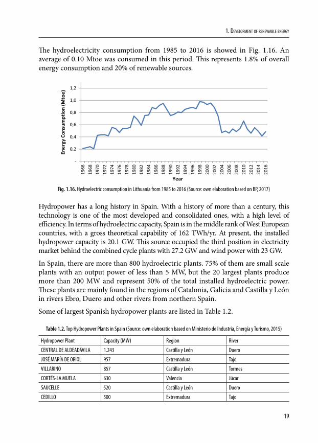
The hydroelectricity consumption from 1985 to 2016 is showed in Fig. 1.16. An average of 0.10 Mtoe was consumed in this period. This represents 1.8% of overall energy consumption and 20% of renewable sources.

‐

0,2

0,4

0,6

0,8

1,0

1,219

6619

6819

7019

7219

7419

7619

7819

8019

8219

8419

8619

8819

9019

9219

9419

9619

9820

0020

0220

0420

0620

0820

1020

1220

1420

16

Year

Energy Con

sumption (M

toe)

Fig. 1.16. Hydroelectric consumption in Lithuania from 1985 to 2016 (Source: own elaboration based on BP, 2017)

Hydropower has a long history in Spain. With a history of more than a century, this technology is one of the most developed and consolidated ones, with a high level of efficiency. In terms of hydroelectric capacity, Spain is in the middle rank of West European countries, with a gross theoretical capability of 162 TWh/yr. At present, the installed hydropower capacity is 20.1 GW. This source occupied the third position in electricity market behind the combined cycle plants with 27.2 GW and wind power with 23 GW.

In Spain, there are more than 800 hydroelectric plants. 75% of them are small scale plants with an output power of less than 5 MW, but the 20 largest plants produce more than 200 MW and represent 50% of the total installed hydroelectric power. These plants are mainly found in the regions of Catalonia, Galicia and Castilla y León in rivers Ebro, Duero and other rivers from northern Spain.

Some of largest Spanish hydropower plants are listed in Table 1.2.

Table 1.2. Top Hydropower Plants in Spain (Source: own elaboration based on Ministerio de Industria, Energía y Turismo, 2015)

Hydropower Plant Capacity (MW) Region River

CENTRAL DE ALDEADÁVILA 1.243 Castilla y León Duero

JOSÉ MARÍA DE ORIOL 957 Extremadura Tajo

VILLARINO 857 Castilla y León Tormes

CORTÉS-LA MUELA 630 Valencia Júcar

SAUCELLE 520 Castilla y León Duero

CEDILLO 500 Extremadura Tajo

20


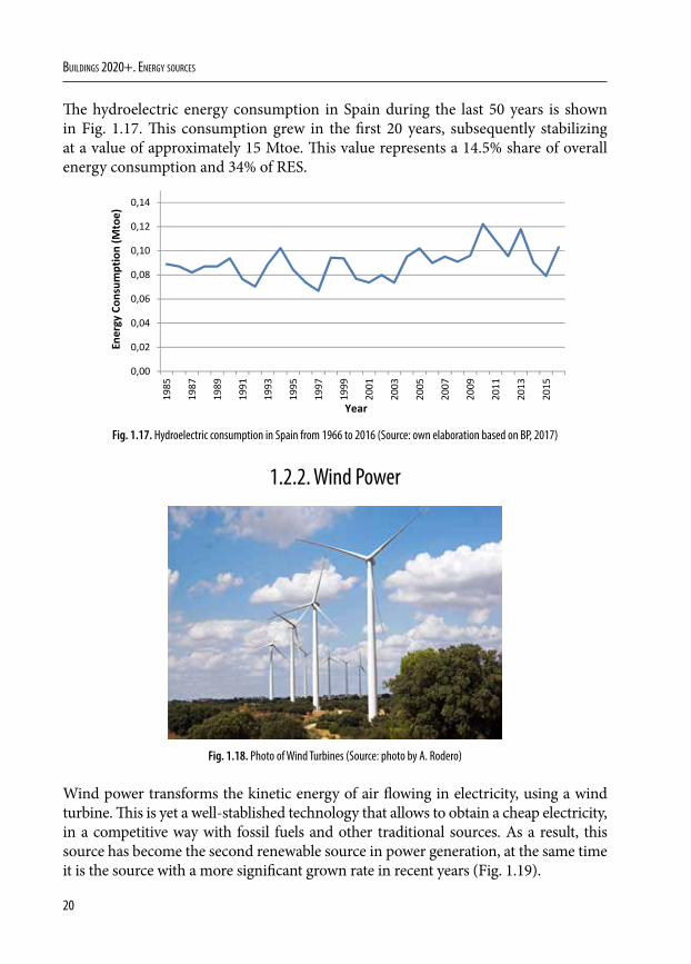
The hydroelectric energy consumption in Spain during the last 50 years is shown in Fig. 1.17. This consumption grew in the first 20 years, subsequently stabilizing at a value of approximately 15 Mtoe. This value represents a 14.5% share of overall energy consumption and 34% of RES.

0,00

0,02

0,04

0,06

0,08

0,10

0,12

0,14

1985

1987

1989

1991

1993

1995

1997

1999

2001

2003

2005

2007

2009

2011

2013

2015

Year

Energy Con

sumption (M

toe)

Fig. 1.17. Hydroelectric consumption in Spain from 1966 to 2016 (Source: own elaboration based on BP, 2017)

1.2.2. Wind Power

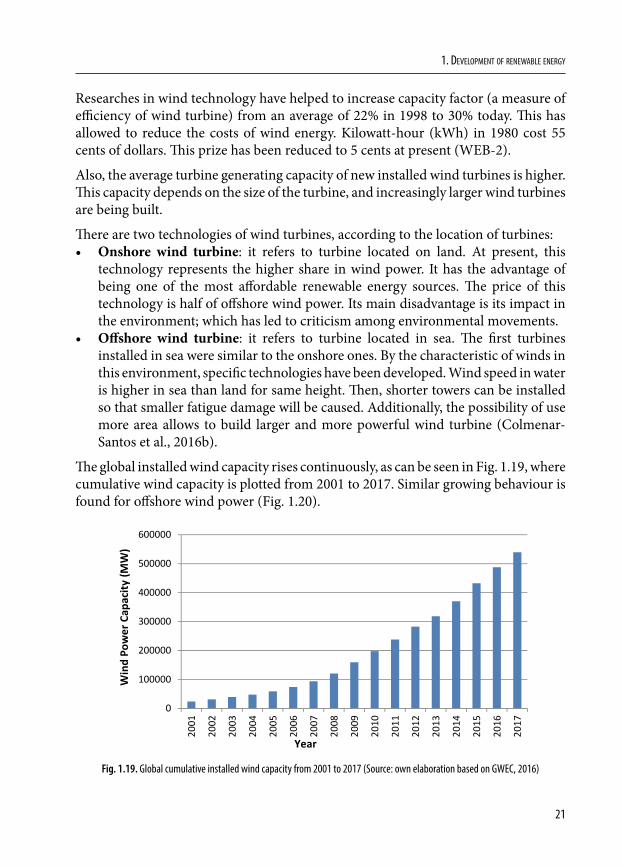
Fig. 1.18. Photo of Wind Turbines (Source: photo by A. Rodero)

Wind power transforms the kinetic energy of air flowing in electricity, using a wind turbine. This is yet a well-stablished technology that allows to obtain a cheap electricity, in a competitive way with fossil fuels and other traditional sources. As a result, this source has become the second renewable source in power generation, at the same time it is the source with a more significant grown rate in recent years (Fig. 1.19).

21


Researches in wind technology have helped to increase capacity factor (a measure of efficiency of wind turbine) from an average of 22% in 1998 to 30% today. This has allowed to reduce the costs of wind energy. Kilowatt-hour (kWh) in 1980 cost 55 cents of dollars. This prize has been reduced to 5 cents at present (WEB-2).

Also, the average turbine generating capacity of new installed wind turbines is higher. This capacity depends on the size of the turbine, and increasingly larger wind turbines are being built.

There are two technologies of wind turbines, according to the location of turbines:• Onshore wind turbine: it refers to turbine located on land. At present, this

technology represents the higher share in wind power. It has the advantage of being one of the most affordable renewable energy sources. The price of this technology is half of offshore wind power. Its main disadvantage is its impact in the environment; which has led to criticism among environmental movements.

• Offshore wind turbine: it refers to turbine located in sea. The first turbines installed in sea were similar to the onshore ones. By the characteristic of winds in this environment, specific technologies have been developed. Wind speed in water is higher in sea than land for same height. Then, shorter towers can be installed so that smaller fatigue damage will be caused. Additionally, the possibility of use more area allows to build larger and more powerful wind turbine (Colmenar-Santos et al., 2016b).

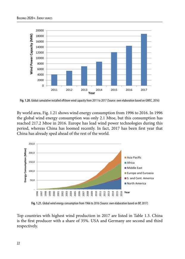
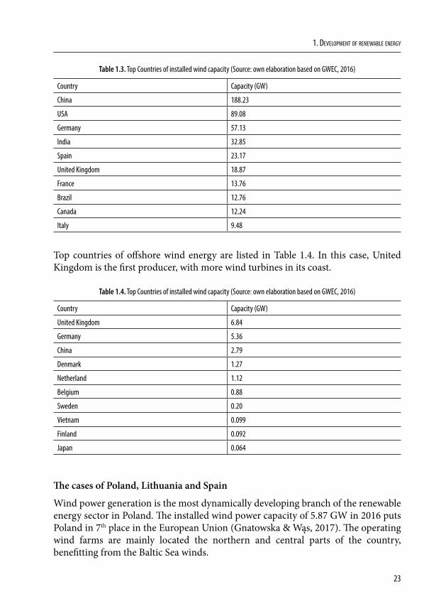
The global installed wind capacity rises continuously, as can be seen in Fig. 1.19, where cumulative wind capacity is plotted from 2001 to 2017. Similar growing behaviour is found for offshore wind power (Fig. 1.20).

0

100000

200000

300000

400000

500000

600000

2001

2002

2003

2004

2005

2006

2007

2008

2009

2010

2011

2012

2013

2014

2015

2016

2017

Year

WindPo

wer Cap

acity

(MW)

Fig. 1.19. Global cumulative installed wind capacity from 2001 to 2017 (Source: own elaboration based on GWEC, 2016)

22


0

2000

4000

6000

8000

10000

12000

14000

16000

18000

20000

2011 2012 2013 2014 2015 2016 2017Year

WindPo

wer Cap

acity

(MW)

Fig. 1.20. Global cumulative installed offshore wind capacity from 2011 to 2017 (Source: own elaboration based on GWEC, 2016)

By world area, Fig. 1.21 shows wind energy consumption from 1996 to 2016. In 1996 the global wind energy consumption was only 2.1 Mtoe, but this consumption has reached 217.2 Mtoe in 2016. Europe has lead wind power technologies during this period, whereas China has loomed recently. In fact, 2017 has been first year that China has already sped ahead of the rest of the world.

‐

50,0

100,0

150,0

200,0

250,0

1996

1997

1998

1999

2000

2001

2002

2003

2004

2005

2006

2007

2008

2009

2010

2011

2012

2013

2014

2015

2016

Asia PacificAfricaMiddle EastEurope and EuroasiaS. and Cent. AmericaNorth America

Year

Energy Con

sumption (M

toe)

Fig. 1.21. Global wind energy consumption from 1966 to 2016 (Source: own elaboration based on BP, 2017)

Top countries with highest wind production in 2017 are listed in Table 1.3. China is the first producer with a share of 35%. USA and Germany are second and third respectively.

23


Table 1.3. Top Countries of installed wind capacity (Source: own elaboration based on GWEC, 2016)

Country Capacity (GW)

China 188.23

USA 89.08

Germany 57.13

India 32.85

Spain 23.17

United Kingdom 18.87

France 13.76

Brazil 12.76

Canada 12.24

Italy 9.48

Top countries of offshore wind energy are listed in Table 1.4. In this case, United Kingdom is the first producer, with more wind turbines in its coast.

Table 1.4. Top Countries of installed wind capacity (Source: own elaboration based on GWEC, 2016)


United Kingdom 6.84

Germany 5.36

China 2.79

Denmark 1.27

Netherland 1.12

Belgium 0.88

Sweden 0.20

Vietnam 0.099

Finland 0.092

Japan 0.064

The cases of Poland, Lithuania and Spain

Wind power generation is the most dynamically developing branch of the renewable energy sector in Poland. The installed wind power capacity of 5.87 GW in 2016 puts Poland in 7th place in the European Union (Gnatowska & Wąs, 2017). The operating wind farms are mainly located the northern and central parts of the country, benefitting from the Baltic Sea winds.

24


Table 1.5 shows installed capacity by Polish province. Five first provinces have 68% of all capacity of country.

Table 1.5. Installed wind power capacity by Polish province (Source: own elaboration based on Energy Regulatory Office, 2017)

Province Capacity (MW) Province Capacity MW)

zachodniopomorskie 1477.2 lubuskie 192.0

Wielkopolskie 686.8 dolnoslaskie 176.4

Pomorskie 684.9 podkarpackie 152.9

kujawsko-pomorskie 592.6 opolskie 138.2

Lódzkie 579.8 lubelskie 134.9

Mazowieckie 378.8 slaskie 33.1

warminsko-mazurskie 353.6 swietokrzyskie 22.3

Podlaskie 197.3 malopolskie 6.7

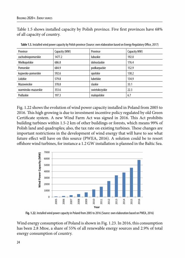
Fig. 1.22 shows the evolution of wind power capacity installed in Poland from 2005 to 2016. This high growing is due to investment incentive policy regulated by old Green Certificate system. A new Wind Farm Act was signed in 2016. This Act prohibits building turbines within 1.5-2 km of other buildings or forests, which means 99% of Polish land and quadruples; also, the tax rate on existing turbines. These changes are important restrictions in the development of wind energy that will have to see what future effect will have on this source (PWEA, 2016). A solution could be to resort offshore wind turbines, for instance a 1.2 GW installation is planned in the Baltic Sea.

0

1000

2000

3000

4000

5000

6000

7000

2005

2006

2007

2008

2009

2010

2011

2012

2013

2014

2015

2016

Year

WindPo

wer Cap

acity

(MW)

Fig. 1.22. Installed wind power capacity in Poland from 2005 to 2016 (Source: own elaboration based on PWEA, 2016)

Wind energy consumption of Poland is shown in Fig. 1.23. In 2016, this consumption has been 2.8 Mtoe, a share of 55% of all renewable energy sources and 2.9% of total energy consumption of country.

25


‐

2,0

4,0

6,0

8,0

10,0

12,0

14,0

1996

1997

1998

1999

2000

2001

2002

2003

2004

2005

2006

2007

2008

2009

2010

2011

2012

2013

2014

2015

2016

Year

Energy Con

sumption (M

toe)

Fig. 1.23. Wind energy consumption in Poland from 1996 to 2016 (Source: own elaboration based on BP, 2017)

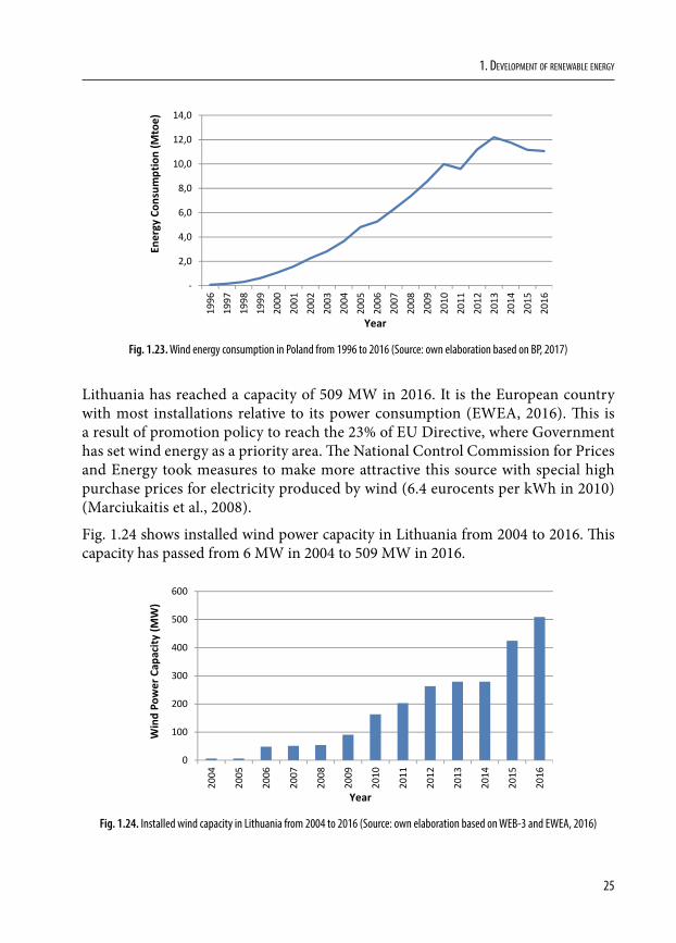
Lithuania has reached a capacity of 509 MW in 2016. It is the European country with most installations relative to its power consumption (EWEA, 2016). This is a result of promotion policy to reach the 23% of EU Directive, where Government has set wind energy as a priority area. The National Control Commission for Prices and Energy took measures to make more attractive this source with special high purchase prices for electricity produced by wind (6.4 eurocents per kWh in 2010) (Marciukaitis et al., 2008).

Fig. 1.24 shows installed wind power capacity in Lithuania from 2004 to 2016. This capacity has passed from 6 MW in 2004 to 509 MW in 2016.

0

100

200

300

400

500

600

2004

2005

2006

2007

2008

2009

2010

2011

2012

2013

2014

2015

2016

Year

WindPo

wer Cap

acity

(MW)

Fig. 1.24. Installed wind capacity in Lithuania from 2004 to 2016 (Source: own elaboration based on WEB-3 and EWEA, 2016)

26


There are about 193 wind farms in Lithuania, the majority of them with power lower 2 MW. But ten top Lithuanian wind farms, located in the North-West border of country, produce 70% of all wind capacity (Table 1.6). First one is Pagėgiai 13 that with a capacity of 73.5 MW is a biggest farm of Baltic countries.

At present, all farms are onshore. Lithuania and other Baltic countries are developing projects to install offshore wind farms in their coast. In the case of Lithuania, the current regulation on seabed exploration licensing crippled progress of this technology.

Table 1.6. Top Wind Farms of Lithuania (Source: own elaboration based on WEB-4)


Pagėgiai 13 73.5

4Energy vėjo elektrinių parkas 60

IKEA Group vėjo elektrinių parkas 45

Čiūtelių vėjo jėgainių parkas 39.1

Benaičių-1 vėjo elektrinių parkas 34

Vydmantų vėjo parkas 30

Rotulių II VE parkas 24

Kreivėnų vėjo elektrinių parkas 20

Laukžemės | VE 16

Didšilių VEP (L-591) 16

Fig. 1.25 shows wind energy consumption in Lithuania from 2000 to 2016. The energy consumption was 0.24 Mtoe in 2016. A share of 4.5% of total energy consumption and 50% of renewable energy consumption.

‐

0,5

1,0

1,5

2,0

2,5

3,0

1996

1997

1998

1999

2000

2001

2002

2003

2004

2005

2006

2007

2008

2009

2010

2011

2012

2013

2014

2015

2016

Year

Energy Con

sumption (M

toe)

Fig. 1.25. Wind energy consumption in Lithuania from 2000 to 2016 (Source: own elaboration based on BP, 2017)

27


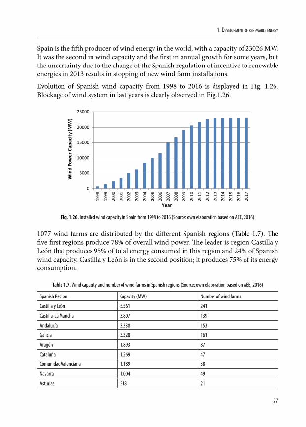
Spain is the fifth producer of wind energy in the world, with a capacity of 23026 MW. It was the second in wind capacity and the first in annual growth for some years, but the uncertainty due to the change of the Spanish regulation of incentive to renewable energies in 2013 results in stopping of new wind farm installations.

Evolution of Spanish wind capacity from 1998 to 2016 is displayed in Fig. 1.26. Blockage of wind system in last years is clearly observed in Fig.1.26.

0

5000

10000

15000

20000

25000

1998

1999

2000

2001

2002

2003

2004

2005

2006

2007

2008

2009

2010

2011

2012

2013

2014

2015

2016

2017

Year

WindPo

wer Cap

acity

(MW)

Fig. 1.26. Installed wind capacity in Spain from 1998 to 2016 (Source: own elaboration based on AEE, 2016)

1077 wind farms are distributed by the different Spanish regions (Table 1.7). The five first regions produce 78% of overall wind power. The leader is region Castilla y León that produces 95% of total energy consumed in this region and 24% of Spanish wind capacity. Castilla y León is in the second position; it produces 75% of its energy consumption.

Table 1.7. Wind capacity and number of wind farms in Spanish regions (Source: own elaboration based on AEE, 2016)

Spanish Region Capacity (MW) Number of wind farms

Castilla y León 5.561 241

Castilla-La Mancha 3.807 139

Andalucía 3.338 153

Galicia 3.328 161

Aragón 1.893 87

Cataluña 1.269 47

Comunidad Valenciana 1.189 38

Navarra 1.004 49

Asturias 518 21

28


Spanish Region Capacity (MW) Number of wind farms

La Rioja 447 14

Murcia 262 14

Canarias 177 56

País Vasco 153 7

Cantabria 38 4

Baleares 4 46

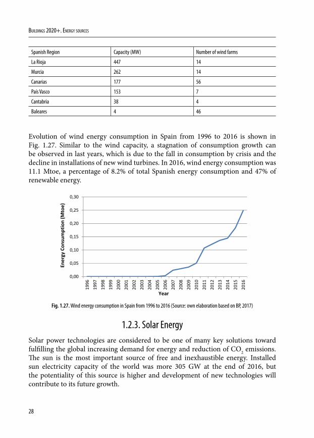
Evolution of wind energy consumption in Spain from 1996 to 2016 is shown in Fig. 1.27. Similar to the wind capacity, a stagnation of consumption growth can be observed in last years, which is due to the fall in consumption by crisis and the decline in installations of new wind turbines. In 2016, wind energy consumption was 11.1 Mtoe, a percentage of 8.2% of total Spanish energy consumption and 47% of renewable energy.

0,00

0,05

0,10

0,15

0,20

0,25

0,30

1996

1997

1998

1999

2000

2001

2002

2003

2004

2005

2006

2007

2008

2009

2010

2011

2012

2013

2014

2015

2016

Year

Energy Con

sumption (M

toe)

Fig. 1.27. Wind energy consumption in Spain from 1996 to 2016 (Source: own elaboration based on BP, 2017)

1.2.3. Solar EnergySolar power technologies are considered to be one of many key solutions toward fulfilling the global increasing demand for energy and reduction of CO2 emissions. The sun is the most important source of free and inexhaustible energy. Installed sun electricity capacity of the world was more 305 GW at the end of 2016, but the potentiality of this source is higher and development of new technologies will contribute to its future growth.

29


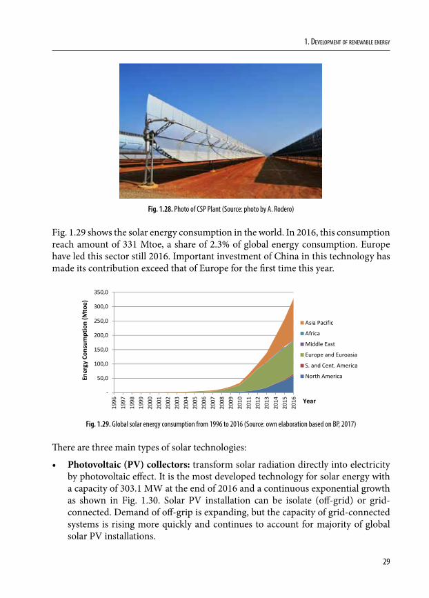
Fig. 1.28. Photo of CSP Plant (Source: photo by A. Rodero)

Fig. 1.29 shows the solar energy consumption in the world. In 2016, this consumption reach amount of 331 Mtoe, a share of 2.3% of global energy consumption. Europe have led this sector still 2016. Important investment of China in this technology has made its contribution exceed that of Europe for the first time this year.

‐

50,0

100,0

150,0

200,0

250,0

300,0

350,0

1996

1997

1998

1999

2000

2001

2002

2003

2004

2005

2006

2007

2008

2009

2010

2011

2012

2013

2014

2015

2016

Asia Pacific

Africa

Middle East

Europe and Euroasia

S. and Cent. America

North AmericaEnergy Con

sumption (M

toe)

Year

Fig. 1.29. Global solar energy consumption from 1996 to 2016 (Source: own elaboration based on BP, 2017)

There are three main types of solar technologies:

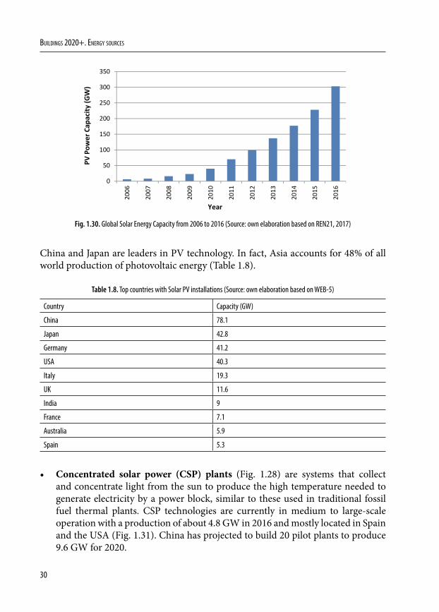
• Photovoltaic (PV) collectors: transform solar radiation directly into electricity by photovoltaic effect. It is the most developed technology for solar energy with a capacity of 303.1 MW at the end of 2016 and a continuous exponential growth as shown in Fig. 1.30. Solar PV installation can be isolate (off-grid) or grid-connected. Demand of off-grip is expanding, but the capacity of grid-connected systems is rising more quickly and continues to account for majority of global solar PV installations.

30


0

50

100

150

200

250

300

350

2006

2007

2008

2009

2010

2011

2012

2013

2014

2015

2016

Year

PV Pow

er Cap

acity

(GW)

Fig. 1.30. Global Solar Energy Capacity from 2006 to 2016 (Source: own elaboration based on REN21, 2017)

China and Japan are leaders in PV technology. In fact, Asia accounts for 48% of all world production of photovoltaic energy (Table 1.8).

Table 1.8. Top countries with Solar PV installations (Source: own elaboration based on WEB-5)


China 78.1

Japan 42.8

Germany 41.2

USA 40.3

Italy 19.3

UK 11.6

India 9

France 7.1

Australia 5.9

Spain 5.3

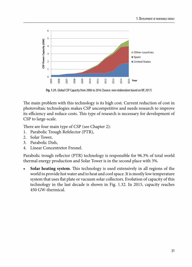
• Concentrated solar power (CSP) plants (Fig. 1.28) are systems that collect and concentrate light from the sun to produce the high temperature needed to generate electricity by a power block, similar to these used in traditional fossil fuel thermal plants. CSP technologies are currently in medium to large-scale operation with a production of about 4.8 GW in 2016 and mostly located in Spain and the USA (Fig. 1.31). China has projected to build 20 pilot plants to produce 9.6 GW for 2020.

31


0

1

2

3

4

5

6

2005

2006

2007

2008

2009

2010

2011

2012

2013

2014

2015

Other countriesSpainUnited States

Year

CSP Po

wer Cap

acity

(GW)

Fig. 1.31. Global CSP Capacity from 2006 to 2016 (Source: own elaboration based on BP, 2017)

The main problem with this technology is its high cost. Current reduction of cost in photovoltaic technologies makes CSP uncompetitive and needs research to improve its efficiency and reduce costs. This type of research is necessary for development of CSP to large-scale.

There are four main type of CSP (see Chapter 2):1. Parabolic Trough Refelector (PTR),2. Solar Tower,3. Parabolic Dish,4. Linear Concentretor Fresnel.

Parabolic trough reflector (PTR) technology is responsible for 96.3% of total world thermal energy production and Solar Tower is in the Second place with 3%.

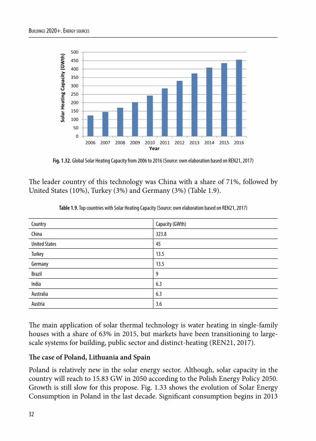
• Solar heating system. This technology is used extensively in all regions of the world to provide hot water and to heat and cool space. It is mostly low temperature system that uses flat plate or vacuum solar collectors. Evolution of capacity of this technology in the last decade is shown in Fig. 1.32. In 2015, capacity reaches 450 GW-thermical.

32


0

50

100

150

200

250

300

350

400

450

500

2006 2007 2008 2009 2010 2011 2012 2013 2014 2015 2016Year

Solar H

eatin

g Ca

pacit

y (GWth)

Fig. 1.32. Global Solar Heating Capacity from 2006 to 2016 (Source: own elaboration based on REN21, 2017)

The leader country of this technology was China with a share of 71%, followed by United States (10%), Turkey (3%) and Germany (3%) (Table 1.9).

Table 1.9. Top countries with Solar Heating Capacity (Source: own elaboration based on REN21, 2017)

Country Capacity (GWth)

China 323.8

United States 45

Turkey 13.5

Germany 13.5

Brazil 9

India 6.3

Australia 6.3

Austria 3.6

The main application of solar thermal technology is water heating in single-family houses with a share of 63% in 2015, but markets have been transitioning to large-scale systems for building, public sector and distinct-heating (REN21, 2017).


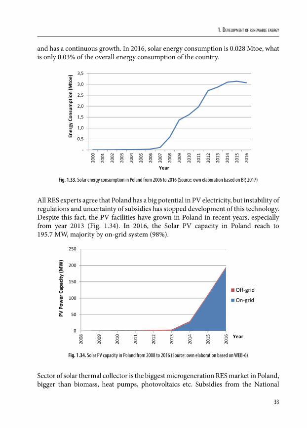
Poland is relatively new in the solar energy sector. Although, solar capacity in the country will reach to 15.83 GW in 2050 according to the Polish Energy Policy 2050. Growth is still slow for this propose. Fig. 1.33 shows the evolution of Solar Energy Consumption in Poland in the last decade. Significant consumption begins in 2013

33


and has a continuous growth. In 2016, solar energy consumption is 0.028 Mtoe, what is only 0.03% of the overall energy consumption of the country.

‐

0,5

1,0

1,5

2,0

2,5

3,0

3,5

2000

2001

2002

2003

2004

2005

2006

2007

2008

2009

2010

2011

2012

2013

2014

2015

2016

Year

Energy Con

sumption (M

toe)

Fig. 1.33. Solar energy consumption in Poland from 2006 to 2016 (Source: own elaboration based on BP, 2017)

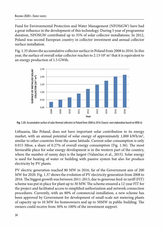
All RES experts agree that Poland has a big potential in PV electricity, but instability of regulations and uncertainty of subsidies has stopped development of this technology. Despite this fact, the PV facilities have grown in Poland in recent years, especially from year 2013 (Fig. 1.34). In 2016, the Solar PV capacity in Poland reach to 195.7 MW, majority by on-grid system (98%).

0

50

100

150

200

250

2008

2009

2010

2011

2012

2013

2014

2015

2016

Off‐grid

On‐grid

Year

PV Pow

er Cap

acity

(MW)

Fig. 1.34. Solar PV capacity in Poland from 2008 to 2016 (Source: own elaboration based on WEB-6)

Sector of solar thermal collector is the biggest microgeneration RES market in Poland, bigger than biomass, heat pumps, photovoltaics etc. Subsidies from the National

34


Fund for Environmental Protection and Water Management (NFOSiGW) have had a great influence in the development of this technology. During 5 year of programme duration, NFOSGW contributed up to 35% of solar collector installations. In 2012, Poland was second European country in collector investment and annual collector surface installation.

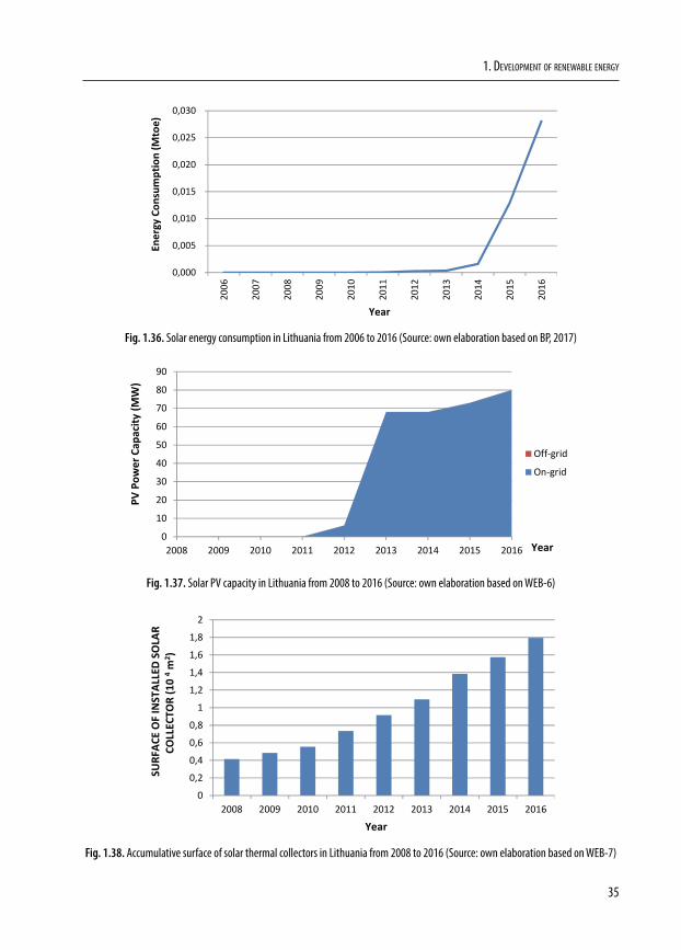
Fig. 1.35 shows the accumulative collector surface in Poland from 2008 to 2016. In this year, the surface of overall solar collector reaches to 2.13⋅106 m2 that it is equivalent to an energy production of 1.5 GWth.

0,00

0,50

1,00

1,50

2,00

2,50

2008

2009

2010

2011

2012

2013

2014

2015

2016

Year

SURF

ACE OF

INSTAL

LED SO

LAR

COLLEC

TOR (10

6m

2 )

Fig. 1.35. Accumulative surface of solar thermal collectors in Poland from 2008 to 2016 (Source: own elaboration based on WEB-6)

Lithuania, like Poland, does not have important solar contribution to its energy market, with an annual potential of solar energy of approximately 1,000 kWh/m2, similar to other countries from the same latitude. Current solar consumption is only 0.015 Mtoe, a share of 0.27% of overall energy consumption (Fig. 1.36). The most favourable place for solar energy development is in the western part of the country, where the number of sunny days is the largest (Valančius et al., 2015). Solar energy is used for heating of water or building with passive system but also for produce electricity by PV plants.

PV electric generation reached 80 MW in 2016, far of the Government aim of 200 MW for 2020. Fig. 1.37 shows the evolution of PV electricity generation from 2008 to 2016. The biggest growth was between 2011-2013, due to generous feed-in tariff (FIT) scheme was put in place for plant up to 30 MW. The scheme ensured a 12-year FIT for the project and facilitated access to simplified authorization and network connection procedures. Currently, with an 80% of commercial installation, a new scheme has been approved by Government for development of small-scale net metering plants of capacity up to 10 MW for homeowners and up to 50MW in public building. The owners could receive from 30% to 100% of the investment support.

35


0,000

0,005

0,010

0,015

0,020

0,025

0,030

2006

2007

2008

2009

2010

2011

2012

2013

2014

2015

2016

Year

Energy Con

sumption (M

toe)

Fig. 1.36. Solar energy consumption in Lithuania from 2006 to 2016 (Source: own elaboration based on BP, 2017)

0

10

20

30

40

50

60

70

80

90

2008 2009 2010 2011 2012 2013 2014 2015 2016

Off‐grid

On‐grid

Year

PV Pow

er Cap

acity

(MW)

Fig. 1.37. Solar PV capacity in Lithuania from 2008 to 2016 (Source: own elaboration based on WEB-6)

00,20,40,60,81

1,21,41,61,82

2008 2009 2010 2011 2012 2013 2014 2015 2016Year

SURF

ACE OF

INSTAL

LED SO

LAR

COLLEC

TOR (10

4m

2 )

Fig. 1.38. Accumulative surface of solar thermal collectors in Lithuania from 2008 to 2016 (Source: own elaboration based on WEB-7)

36


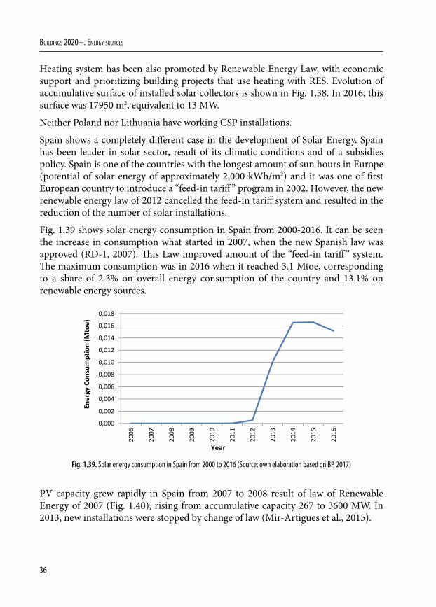
Heating system has been also promoted by Renewable Energy Law, with economic support and prioritizing building projects that use heating with RES. Evolution of accumulative surface of installed solar collectors is shown in Fig. 1.38. In 2016, this surface was 17950 m2, equivalent to 13 MW.

Neither Poland nor Lithuania have working CSP installations.

Spain shows a completely different case in the development of Solar Energy. Spain has been leader in solar sector, result of its climatic conditions and of a subsidies policy. Spain is one of the countries with the longest amount of sun hours in Europe (potential of solar energy of approximately 2,000 kWh/m2) and it was one of first European country to introduce a “feed-in tariff ” program in 2002. However, the new renewable energy law of 2012 cancelled the feed-in tariff system and resulted in the reduction of the number of solar installations.

Fig. 1.39 shows solar energy consumption in Spain from 2000-2016. It can be seen the increase in consumption what started in 2007, when the new Spanish law was approved (RD-1, 2007). This Law improved amount of the “feed-in tariff ” system. The maximum consumption was in 2016 when it reached 3.1 Mtoe, corresponding to a share of 2.3% on overall energy consumption of the country and 13.1% on renewable energy sources.

0,000

0,002

0,004

0,006

0,008

0,010

0,012

0,014

0,016

0,018

2006

2007

2008

2009

2010

2011

2012

2013

2014

2015

2016

Year

Energy Con

sumption (M

toe)

Fig. 1.39. Solar energy consumption in Spain from 2000 to 2016 (Source: own elaboration based on BP, 2017)

PV capacity grew rapidly in Spain from 2007 to 2008 result of law of Renewable Energy of 2007 (Fig. 1.40), rising from accumulative capacity 267 to 3600 MW. In 2013, new installations were stopped by change of law (Mir-Artigues et al., 2015).

37


0

1000

2000

3000

4000

5000

6000

2008

2009

2010

2011

2012

2013

2014

2015

2016

Off‐grid

On‐grid

Year

PV Pow

er Cap

acity

(MW)

Fig. 1.40. Accumulative solar PV capacity in Spain from 2000 to 2016 (Source: own elaboration based on BP, 2017)

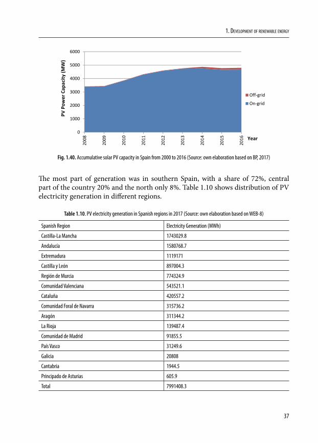
The most part of generation was in southern Spain, with a share of 72%, central part of the country 20% and the north only 8%. Table 1.10 shows distribution of PV electricity generation in different regions.

Table 1.10. PV electricity generation in Spanish regions in 2017 (Source: own elaboration based on WEB-8)

Spanish Region Electricity Generation (MWh)

Castilla-La Mancha 1743029.8

Andalucía 1580768.7

Extremadura 1119171

Castilla y León 897004.3

Región de Murcia 774324.9

Comunidad Valenciana 543521.1

Cataluña 420557.2

Comunidad Foral de Navarra 315736.2

Aragón 311344.2

La Rioja 139487.4

Comunidad de Madrid 91855.5

País Vasco 31249.6

Galicia 20808

Cantabria 1944.5

Principado de Asturias 605.9

Total 7991408.3

38


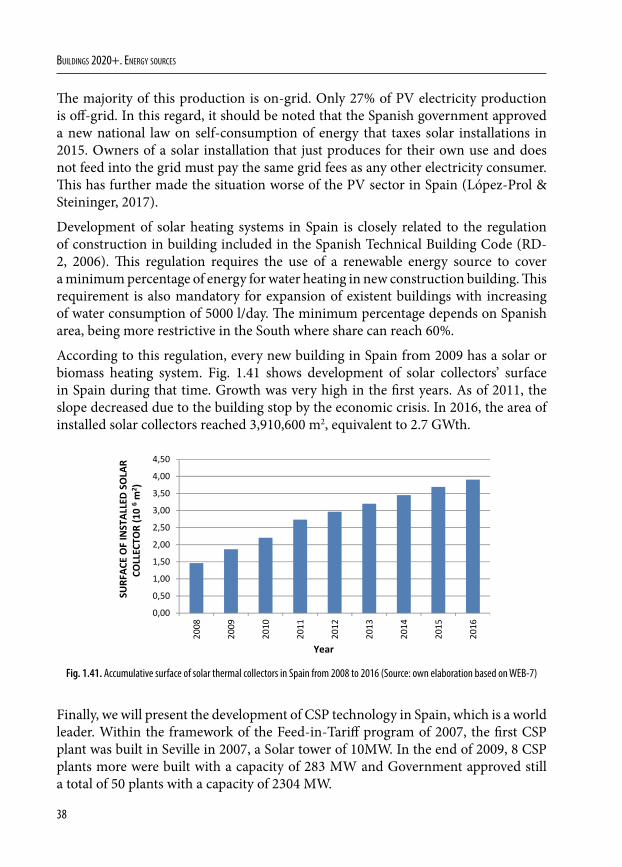
The majority of this production is on-grid. Only 27% of PV electricity production is off-grid. In this regard, it should be noted that the Spanish government approved a new national law on self-consumption of energy that taxes solar installations in 2015. Owners of a solar installation that just produces for their own use and does not feed into the grid must pay the same grid fees as any other electricity consumer. This has further made the situation worse of the PV sector in Spain (López-Prol & Steininger, 2017).

Development of solar heating systems in Spain is closely related to the regulation of construction in building included in the Spanish Technical Building Code (RD-2, 2006). This regulation requires the use of a renewable energy source to cover a minimum percentage of energy for water heating in new construction building. This requirement is also mandatory for expansion of existent buildings with increasing of water consumption of 5000 l/day. The minimum percentage depends on Spanish area, being more restrictive in the South where share can reach 60%.

According to this regulation, every new building in Spain from 2009 has a solar or biomass heating system. Fig. 1.41 shows development of solar collectors’ surface in Spain during that time. Growth was very high in the first years. As of 2011, the slope decreased due to the building stop by the economic crisis. In 2016, the area of installed solar collectors reached 3,910,600 m2, equivalent to 2.7 GWth.

0,00

0,50

1,00

1,50

2,00

2,50

3,00

3,50

4,00

4,50

2008

2009

2010

2011

2012

2013

2014

2015

2016

Year

SURF

ACE OF

INSTAL

LED SO

LAR

COLLEC

TOR (10

6m

2 )

Fig. 1.41. Accumulative surface of solar thermal collectors in Spain from 2008 to 2016 (Source: own elaboration based on WEB-7)

Finally, we will present the development of CSP technology in Spain, which is a world leader. Within the framework of the Feed-in-Tariff program of 2007, the first CSP plant was built in Seville in 2007, a Solar tower of 10MW. In the end of 2009, 8 CSP plants more were built with a capacity of 283 MW and Government approved still a total of 50 plants with a capacity of 2304 MW.

39


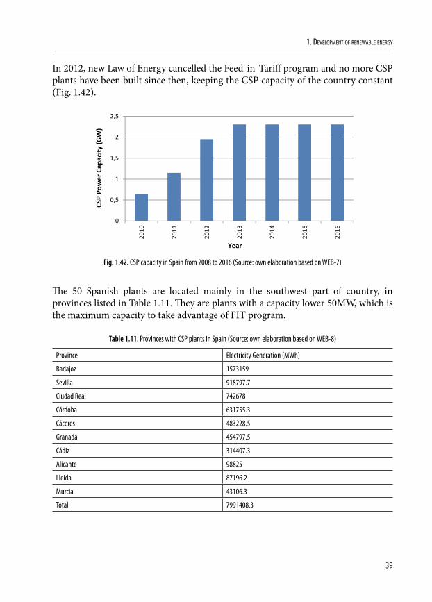
In 2012, new Law of Energy cancelled the Feed-in-Tariff program and no more CSP plants have been built since then, keeping the CSP capacity of the country constant (Fig. 1.42).

0

0,5

1

1,5

2

2,5

2010

2011

2012

2013

2014

2015

2016

Year

CSP Po

wer Cap

acity

(GW)

Fig. 1.42. CSP capacity in Spain from 2008 to 2016 (Source: own elaboration based on WEB-7)

The 50 Spanish plants are located mainly in the southwest part of country, in provinces listed in Table 1.11. They are plants with a capacity lower 50MW, which is the maximum capacity to take advantage of FIT program.

Table 1.11. Provinces with CSP plants in Spain (Source: own elaboration based on WEB-8)

Province Electricity Generation (MWh)

Badajoz 1573159

Sevilla 918797.7

Ciudad Real 742678

Córdoba 631755.3

Cáceres 483228.5

Granada 454797.5

Cádiz 314407.3

Alicante 98825

Lleida 87196.2

Murcia 43106.3

Total 7991408.3

40


Currently, the Feed-in Tariff has been replaced by a complement payment to pool price of electricity to provide to the investor a “reasonable profitability” of 7.5%. We will see how this system works and if there is a resurgence of renewable energy boom in Spain or, at least, a partial recovery (in case these levels are not reached).

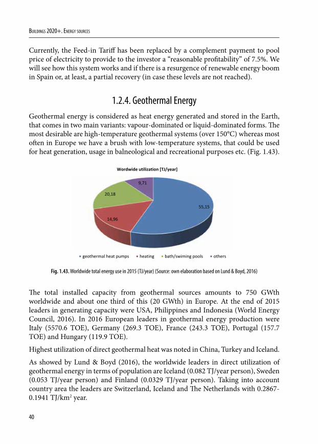
1.2.4. Geothermal EnergyGeothermal energy is considered as heat energy generated and stored in the Earth, that comes in two main variants: vapour-dominated or liquid-dominated forms. The most desirable are high-temperature geothermal systems (over 150°C) whereas most often in Europe we have a brush with low-temperature systems, that could be used for heat generation, usage in balneological and recreational purposes etc. (Fig. 1.43).

55,15

14,96

20,18

9,71

Wordwide utilization [TJ/year]

geothermal heat pumps heating bath/swiming pools others

Fig. 1.43. Worldwide total energy use in 2015 (TJ/year) (Source: own elaboration based on Lund & Boyd, 2016)

The total installed capacity from geothermal sources amounts to 750 GWth worldwide and about one third of this (20 GWth) in Europe. At the end of 2015 leaders in generating capacity were USA, Philippines and Indonesia (World Energy Council, 2016). In 2016 European leaders in geothermal energy production were Italy (5570.6 TOE), Germany (269.3 TOE), France (243.3 TOE), Portugal (157.7 TOE) and Hungary (119.9 TOE).

Highest utilization of direct geothermal heat was noted in China, Turkey and Iceland.

As showed by Lund & Boyd (2016), the worldwide leaders in direct utilization of geothermal energy in terms of population are Iceland (0.082 TJ/year person), Sweden (0.053 TJ/year person) and Finland (0.0329 TJ/year person). Taking into account country area the leaders are Switzerland, Iceland and The Netherlands with 0.2867-0.1941 TJ/km2 year.

41


On the other hand, the largest increase in geothermal energy utilization since 2010 was observed in Thailand, Egypt and Philippines. The biggest annual energy use in MWt (not taking into account heat pumps) was noted in China, Turkey, Japan, Iceland and India. Installations in these countries are estimated as about 68% of the world capacity. Also, in case of geothermal energy used for heat pumps work China is one of leaders, however USA is the first one (Lund & Boyd, 2016).

Geothermal energy is used by applying various technologies for instance:• power generation,• steam field technology (fluid supply system: production wells, separation vessels,

conveyance pipe-work, conditioning vessels, control elements and reinjection systems: fluid conveyance pipe-work, pumps, mineral scale inhibitors, injection wells, and associated controls),

• direct use applications,• ground heat pumps.


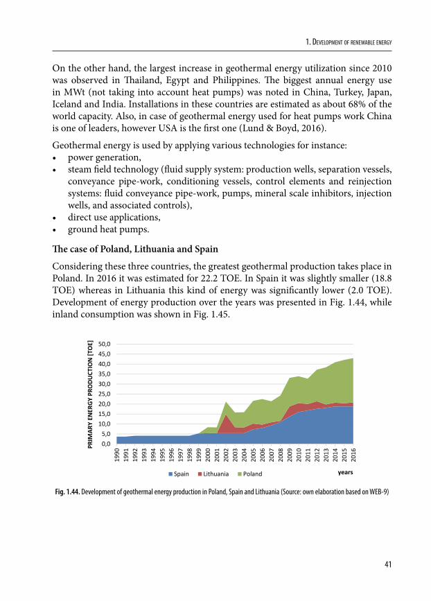
Considering these three countries, the greatest geothermal production takes place in Poland. In 2016 it was estimated for 22.2 TOE. In Spain it was slightly smaller (18.8 TOE) whereas in Lithuania this kind of energy was significantly lower (2.0 TOE). Development of energy production over the years was presented in Fig. 1.44, while inland consumption was shown in Fig. 1.45.

0,0 5,0

10,0 15,0 20,0 25,0 30,0 35,0 40,0 45,0 50,0

1990

1991

1992

1993

1994

1995

1996

1997

1998

1999

2000

2001

2002

2003

2004

2005

2006

2007

2008

2009

2010

2011

2012

2013

2014

2015

2016

PRIM

ARY EN

ERGY

PRO

DUCT

ION [TOE

]

yearsSpain Lithuania Poland

Fig. 1.44. Development of geothermal energy production in Poland, Spain and Lithuania (Source: own elaboration based on WEB-9)

42


0,0

5,0

10,0

15,0

20,0

25,0

1990

1991

1992

1993

1994

1995

1996

1997

1998

1999

2000

2001

2002

2003

2004

2005

2006

2007

2008

2009

2010

2011

2012

2013

2014

2015

2016

Gross inlan

d consum

ption [TOE

]

yearsSpain Lithuania Poland

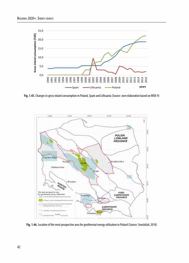
Fig. 1.45. Changes in gross inland consumption in Poland, Spain and Lithuania (Source: own elaboration based on WEB-9)

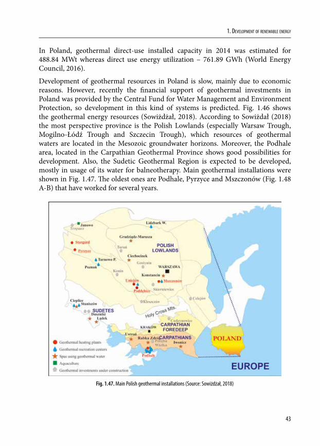
Fig. 1.46. Location of the most prospective area for geothermal energy utilization in Poland (Source: Sowiżdżał, 2018)

43


In Poland, geothermal direct-use installed capacity in 2014 was estimated for 488.84 MWt whereas direct use energy utilization – 761.89 GWh (World Energy Council, 2016).

Development of geothermal resources in Poland is slow, mainly due to economic reasons. However, recently the financial support of geothermal investments in Poland was provided by the Central Fund for Water Management and Environment Protection, so development in this kind of systems is predicted. Fig. 1.46 shows the geothermal energy resources (Sowiżdżał, 2018). According to Sowiżdał (2018) the most perspective province is the Polish Lowlands (especially Warsaw Trough, Mogilno-Łódź Trough and Szczecin Trough), which resources of geothermal waters are located in the Mesozoic groundwater horizons. Moreover, the Podhale area, located in the Carpathian Geothermal Province shows good possibilities for development. Also, the Sudetic Geothermal Region is expected to be developed, mostly in usage of its water for balneotherapy. Main geothermal installations were shown in Fig. 1.47. The oldest ones are Podhale, Pyrzyce and Mszczonów (Fig. 1.48 A-B) that have worked for several years.

Fig. 1.47. Main Polish geothermal installations (Source: Sowiżdżał, 2018)

44


A B

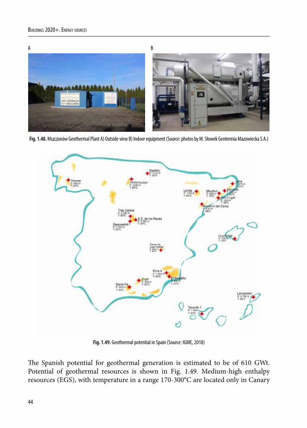
Fig. 1.48. Mszczonów Geothermal Plant A) Outside view B) Indoor equipment (Source: photos by M. Słowek Geotermia Mazowiecka S.A.)

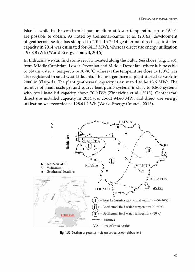
Fig. 1.49. Geothermal potential in Spain (Source: IGME, 2018)

The Spanish potential for geothermal generation is estimated to be of 610 GWt. Potential of geothermal resources is shown in Fig. 1.49. Medium-high enthalpy resources (EGS), with temperature in a range 170-300°C are located only in Canary

45


Islands, while in the continental part medium at lower temperature up to 160°C are possible to obtain. As noted by Colmenar-Santos et al. (2016a) development of geothermal sector has stopped in 2011. In 2014 geothermal direct-use installed capacity in 2014 was estimated for 64.13 MWt, whereas direct use energy utilization –95.80GWh (World Energy Council, 2016).

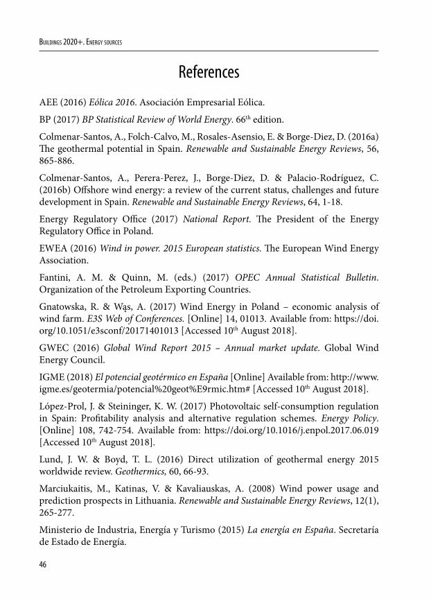
In Lithuania we can find some resorts located along the Baltic Sea shore (Fig. 1.50), from Middle Cambrian, Lower Devonian and Middle Devonian, where it is possible to obtain water at temperature 30-80°C, whereas the temperature close to 100°C was also registered in southwest Lithuania. The first geothermal plant started to work in 2000 in Klaipeda. The plant geothermal capacity is estimated to be 13.6 MWt. The number of small-scale ground source heat pump systems is close to 5,500 systems with total installed capacity above 70 MWt (Zinevicius et al., 2015). Geothermal direct-use installed capacity in 2014 was about 94.60 MWt and direct use energy utilization was recorded as 198.04 GWh (World Energy Council, 2016).

Fig. 1.50. Geothermal potential in Lithuania (Source: own elaboration)

46


References

AEE (2016) Eólica 2016. Asociación Empresarial Eólica.

BP (2017) BP Statistical Review of World Energy. 66th edition.

Colmenar-Santos, A., Folch-Calvo, M., Rosales-Asensio, E. & Borge-Diez, D. (2016a) The geothermal potential in Spain. Renewable and Sustainable Energy Reviews, 56, 865-886.

Colmenar-Santos, A., Perera-Perez, J., Borge-Diez, D. & Palacio-Rodríguez, C. (2016b) Offshore wind energy: a review of the current status, challenges and future development in Spain. Renewable and Sustainable Energy Reviews, 64, 1-18.

Energy Regulatory Office (2017) National Report. The President of the Energy Regulatory Office in Poland.

EWEA (2016) Wind in power. 2015 European statistics. The European Wind Energy Association.

Fantini, A. M. & Quinn, M. (eds.) (2017) OPEC Annual Statistical Bulletin. Organization of the Petroleum Exporting Countries.

Gnatowska, R. & Wąs, A. (2017) Wind Energy in Poland – economic analysis of wind farm. E3S Web of Conferences. [Online] 14, 01013. Available from: https://doi.org/10.1051/e3sconf/20171401013 [Accessed 10th August 2018].

GWEC (2016) Global Wind Report 2015 – Annual market update. Global Wind Energy Council.

IGME (2018) El potencial geotérmico en España [Online] Available from: http://www.igme.es/geotermia/potencial%20geot%E9rmic.htm# [Accessed 10th August 2018].

López-Prol, J. & Steininger, K. W. (2017) Photovoltaic self-consumption regulation in Spain: Profitability analysis and alternative regulation schemes. Energy Policy. [Online] 108, 742-754. Available from: https://doi.org/10.1016/j.enpol.2017.06.019 [Accessed 10th August 2018].

Lund, J. W. & Boyd, T. L. (2016) Direct utilization of geothermal energy 2015 worldwide review. Geothermics, 60, 66-93.

Marciukaitis, M., Katinas, V. & Kavaliauskas, A. (2008) Wind power usage and prediction prospects in Lithuania. Renewable and Sustainable Energy Reviews, 12(1), 265-277.

Ministerio de Industria, Energía y Turismo (2015) La energía en España. Secretaría de Estado de Energía.

47


Mir-Artigues P., Cerdá, E. & Río, P. (2015) Analyzing the impact of cost-containment mechanisms on the profitability of solar PV plants in Spain. Renewable and Sustainable Energy Reviews, 46, 166-177.

PWEA (2016) The State of Wind Energy in Poland in 2016. Polish Wind Energy Association.

RD-1: Boletín Oficial del Estado (2007) Real Decreto 661/2007, de 25 de mayo, por el que se regula la actividad de producción de energía eléctrica en régimen especial. Ministerio de Industria, Turismo y Comercio. «BOE» núm. 126, de 26 de mayo de 2007.

RD-2: Boletín Oficial del Estado (2006) Real Decreto 314/2006, de 17 de marzo, por el que se aprueba el Código Técnico de la Edificación. Ministerio de Vivienda. «BOE» núm. 74, de 28 de marzo de 2006.

REN21 (2017) Renewables 2017. Global Status Report. Renewable Energy Policy Network for the 21st Century.

Sowiżdżał, A. (2018) Geothermal energy resources in Poland – Overview of the current state of knowledge. Renewable and Sustainable Energy Reviews, 82(3), 4020-4027.

Valančius, R., Jurelionis, A., Jonynas, R. & Perednis, E. (2015) Analysis of Medium-Scale Solar Thermal Systems and Their Potential in Lithuania. Energies. [Online] 8(6), 5725-5737. Available from: https://doi.org/10.3390/en8065725 [Accessed 10th August 2018].

WEB-1 https://www.maxpixel.net/Hydro-Power-Dam-Water-Hydroelectricity-Electricity-2492809

WEB-2: U. S. Department of Energy (2018) Office of Energy Efficiency and Renewable Energy. [Online] Available from: htps://www.energy.gov/eere/ [Accessed 10th August 2018].

WEB-3: LWEA (2018) Lithuanian Wind Energy Association [Online] Available from: http://www.lwea.lt/ [Accessed 10th August 2018].

WEB-4: Energy Agency (2018) VĮ Energetikos agentūra [Online] Available from: http://www.ena.lt/en/default.htm [Accessed 10th August 2018].

WEB-5: IDAE (2018) Instituto para la Diversificación y Ahorro de Energía. Ministerio de Industria, Turismo y Comercio. [Online] Available from: http://www.idae.es/ [Accessed 10th August 2018].

48


WEB-6: EurObserv’ER (2018) All Photovoltaic barometers. [Online] Available from: https://www.eurobserv-er.org/category/all-photovoltaic-barometers/ [Accessed 10th August 2018].

WEB-7: EurObserv’ER (2018) All Solar thermal and CSP barometers. [Online] Available from: https://www.eurobserv-er.org/category/all-solar-thermal-and-concentrated-solar-power-barometers/ [Accessed 10th August 2018].

WEB-8: Red Electrica de España (2018) Sistema de Información del Operador del Sistema [Online] Available from: https://www.esios.ree.es/es [Accessed 10th August 2018].

WEB-9: European Comission (2018) Eurostat.Your key to European statistics. [Online] Available from: http://ec.europa.eu/eurostat [Accessed 10th August 2018].

World Energy Council (2014) Energy sector of the world and Poland. – Beginnings, Development, Present State. Polish Member Committee of the World Energy Council.

World Energy Council (2016) World Energy Resources. Geothermal [Online] Available from: https://www.worldenergy.org/wp-content/uploads/2017/03/WEResources_Geothermal_2016.pdf [Accessed 10th August 2018].

Zinevicius, F., Sliaupa, S., Mazintas, A. & Dagilis, V. (2015) Geothermal Energy use in Lithuania. In: International Geothermal Association. Proceedings World Geothermal Congress 2015, Melbourne, Australia, 19-25 April 2015.

49

2. SOLAR SYSTEMS

2.1. Solar irradiation

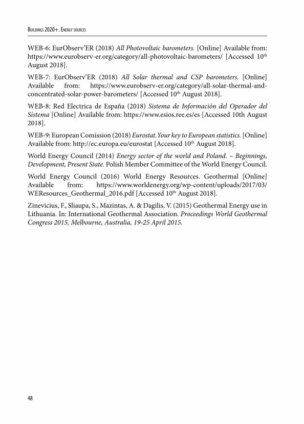
The Sun, as any other active star, is a giant fusion reactor in which every second are generated 600 million tons of helium through the proton-proton cycle, which can be synthesized in the following reaction: 4p→4He + 2e– + νe + 26.2MeV. These processes of nuclear fusion release heating capacity evaluated as 3.86·1023 kWth.

For the exploitation of this energy it is possible to consider the sun as a black body that radiates energy at a temperature of 5780K, because its spectral distribution is very similar to that of the black body for the wavelength range typical of the thermal and photothermic processes.

In Fig. 2.1, there has been presented the spectral distribution of the extraterrestrial radiation and the spectral distribution of the radiation at the sea level.

Fig. 2.1. Intensity of the solar spectrum as a function of the wavelength (Source: Martínez-Val, 2004)

DOI: 10.24427/978-83-65596-73-4_2

50


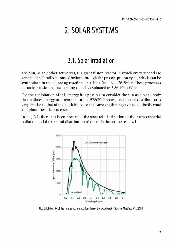
The solar radiation can decompose according to thermal considerations in the spectrum:• ULTRAVIOLET (UV) λ < 0.35 nm 7% transported energy,• VISIBLE 0.35 nm < λ < 0.75 nm 47% transported energy,• INFRARED λ > 0.75 nm 46% transported energy.

Extraterrestrial radiation is the radiation that reaches the Earth from the Sun and has not yet suffered atmospheric attenuation. This radiation is subject to a geometric attenuation (squared proportionally to the distance), so that on the outside of the Earth’s atmosphere, its value is 1.73·1014 kW or, 1.353 kW/m2, as the value of the solar constant, Gsc.

There are two sources of variation of the extraterrestrial solar radiation that must be considered (Duffie & Beckman, 2013). The inherent variation is the radiation emitted by the sun. It represents a very small value compared with atmospheric variations, and because of that, the energy emitted by the sun can be considered constant for engineering applications.

The Earth-Sun distance variation should also be taken into account to produce a variation of the flow of radiation in the range of ±3%. The dependence of the extraterrestrial radiation on the day of the year is given by Eq. (2.1).

G G non SC= ⋅ + ⋅ ⋅

1 0 033 360365

. cos (2.1)

where n is the number of the day of the year, and GSC is the solar constant earlier mentioned, with the value of 1.353 kW/m2.

Through the atmospheric layer, the radiation is released and absorbed, even reflected by molecules suspended in it, as for example the water vapor condensed in clouds.

Some quantity of solar radiation will not find this obstacle. The types of radiation are described below according to their origin and scope:

Direct radiation (also referred to as beam radiation) is the solar radiation received at the Earth’s surface without having undergone any change of direction in its path.

Diffuse radiation is the component of solar radiation received at the Earth’s surface after the dispersion processes (reflection and dissemination) in the atmosphere.

Albedo radiation: is the component of solar radiation reflected from the surface.

The total solar radiation is the sum of direct, diffuse and albedo radiation.

It is possible to affirm that the incidental entire radiation over the Earth´s surface will be subject to variations, some predictable (daily and seasonal) and some unpredictable (the weather, particularly water vapor condensed in the clouds).

51

2. Solar SyStemS

Therefore, as shown in Fig. 2.1, the spectral distribution of solar radiation at the sea level is modified with reference to the extraterrestrial. These variations are a problem for the exploitation of solar thermal energy, which can be mitigated with mechanisms of energy storage.

It should be stressed that the level of solar radiation that reaches the Earth´s surface is relatively moderate and even very low, as for industrial applications. It involves high costs and technology to take advantage of this energy. In situations where the required energy flows are not very high, it is possible to use diffuse radiation, which has the advantage of not requiring any kind of movement of the solar receptors to track the sun throughout the day. On the other hand, if energy applications require higher values of solar radiation, it is possible to concentrate this energy, but only with the direct radiation, which restricts the location of these applications to the locations of large amount of sunlight.

To estimate the production of heat or electricity, a reliable forecast of solar radiation is needed. This forecast is taken two or three days before the generation day and it lets us obtain the best thermal or electrical load production with enough anticipation.

To obtain a good forecast of solar radiation on the Earth’s surface, we ought to consider the solar elevation (solar altitude above the horizon), the cloudiness produced by pollution and radiation absorption gases. Some statistical models, such as the Monte Carlo Method, are considered.

For standard location, the main radiation parameters referred to area unit are:• daily irradiance of solar capitation area kWh/m2,• total heat over solar capitation area kWh/m2,• thermal efficiency peak (%) and daily peak (%),• equivalent full load production hours.

Fig. 2.2 shows the monthly Direct Normal Irradiance (DNI) (kWh/m2) and the sum of DNI for annual solar model in a specific location (South of Spain).

The studies of radiation are based on historical data obtained from public databases [WEB-2] of direct normal radiation through satellite (a minimum of 15 years) in periods of 10 minutes, with the clockwise angle and solar elevation angle.

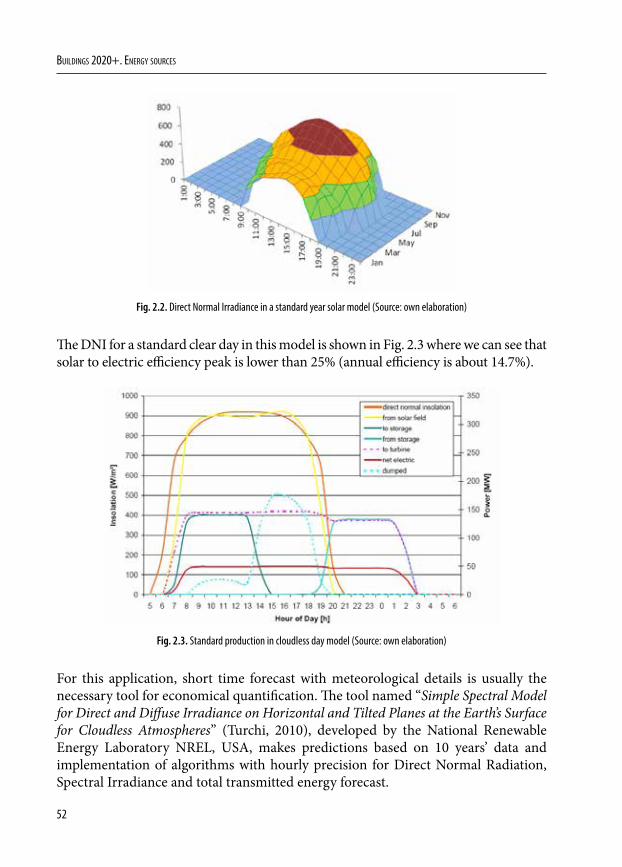
52


Fig. 2.2. Direct Normal Irradiance in a standard year solar model (Source: own elaboration)

The DNI for a standard clear day in this model is shown in Fig. 2.3 where we can see that solar to electric efficiency peak is lower than 25% (annual efficiency is about 14.7%).

Fig. 2.3. Standard production in cloudless day model (Source: own elaboration)

For this application, short time forecast with meteorological details is usually the necessary tool for economical quantification. The tool named “Simple Spectral Model for Direct and Diffuse Irradiance on Horizontal and Tilted Planes at the Earth’s Surface for Cloudless Atmospheres” (Turchi, 2010), developed by the National Renewable Energy Laboratory NREL, USA, makes predictions based on 10 years’ data and implementation of algorithms with hourly precision for Direct Normal Radiation, Spectral Irradiance and total transmitted energy forecast.

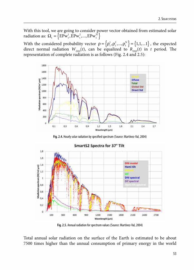
53

2. Solar SyStemS

With this tool, we are going to consider power vector obtained from estimated solar radiation as: Ωt t t t

NEPw EPw EPw= 1 2, ,...,

With the considered probability vector ρ ρ ρ ρ= = t t tN1 2 1 1 1, ,..., , ,... , the expected

direct normal radiation WDNI(t), can be equalized to RDNI(t) in t period. The representation of complete radiation is as follows (Fig. 2.4 and 2.5):

Fig. 2.4. Hourly solar radiation by specified spectrum (Source: Martínez-Val, 2004)

Fig. 2.5. Annual radiation for spectrum values (Source: Martínez-Val, 2004)

Total annual solar radiation on the surface of the Earth is estimated to be about 7500 times higher than the annual consumption of primary energy in the world

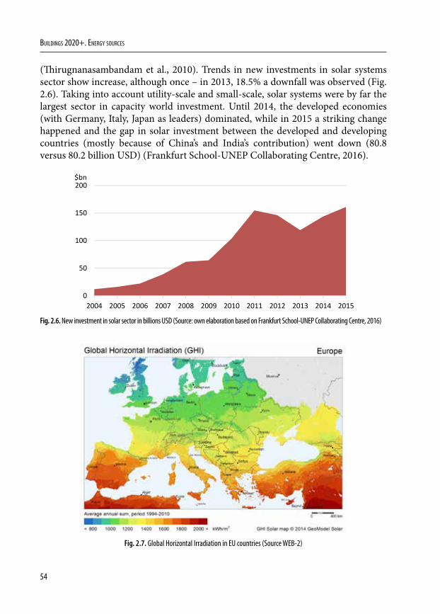
54


(Thirugnanasambandam et al., 2010). Trends in new investments in solar systems sector show increase, although once – in 2013, 18.5% a downfall was observed (Fig. 2.6). Taking into account utility-scale and small-scale, solar systems were by far the largest sector in capacity world investment. Until 2014, the developed economies (with Germany, Italy, Japan as leaders) dominated, while in 2015 a striking change happened and the gap in solar investment between the developed and developing countries (mostly because of China’s and India’s contribution) went down (80.8 versus 80.2 billion USD) (Frankfurt School-UNEP Collaborating Centre, 2016).

0

50

100

150

200

2004 2005 2006 2007 2008 2009 2010 2011 2012 2013 2014 2015

$bn

Fig. 2.6. New investment in solar sector in billions USD (Source: own elaboration based on Frankfurt School-UNEP Collaborating Centre, 2016)

Fig. 2.7. Global Horizontal Irradiation in EU countries (Source WEB-2)

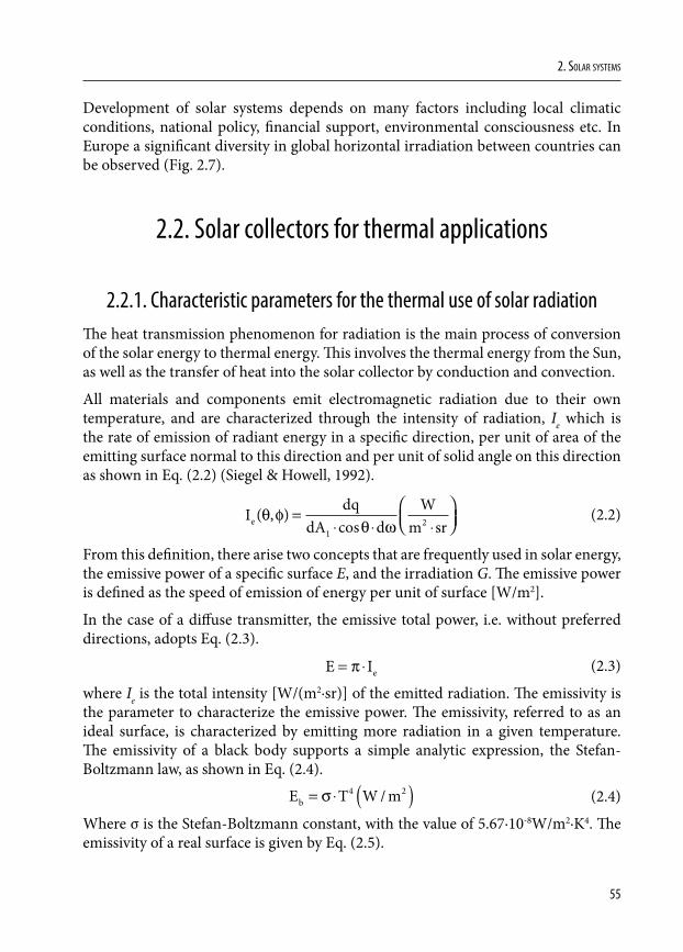
55

2. Solar SyStemS

Development of solar systems depends on many factors including local climatic conditions, national policy, financial support, environmental consciousness etc. In Europe a significant diversity in global horizontal irradiation between countries can be observed (Fig. 2.7).

2.2. Solar collectors for thermal applications

2.2.1. Characteristic parameters for the thermal use of solar radiationThe heat transmission phenomenon for radiation is the main process of conversion of the solar energy to thermal energy. This involves the thermal energy from the Sun, as well as the transfer of heat into the solar collector by conduction and convection.

All materials and components emit electromagnetic radiation due to their own temperature, and are characterized through the intensity of radiation, Ie which is the rate of emission of radiant energy in a specific direction, per unit of area of the emitting surface normal to this direction and per unit of solid angle on this direction as shown in Eq. (2.2) (Siegel & Howell, 1992).

I dqdA d

Wm sre ( , )

cosθ φ

θ ω=

⋅ ⋅ ⋅

1

2 (2.2)

From this definition, there arise two concepts that are frequently used in solar energy, the emissive power of a specific surface E, and the irradiation G. The emissive power is defined as the speed of emission of energy per unit of surface [W/m2].

In the case of a diffuse transmitter, the emissive total power, i.e. without preferred directions, adopts Eq. (2.3).

E Ie= ⋅π (2.3)

where Ie is the total intensity [W/(m2·sr)] of the emitted radiation. The emissivity is the parameter to characterize the emissive power. The emissivity, referred to as an ideal surface, is characterized by emitting more radiation in a given temperature. The emissivity of a black body supports a simple analytic expression, the Stefan-Boltzmann law, as shown in Eq. (2.4).

E T W mb = ⋅ ( )σ 4 2/ (2.4)

Where σ is the Stefan-Boltzmann constant, with the value of 5.67·10-8W/m2·K4. The emissivity of a real surface is given by Eq. (2.5).

56


εσ

T E TE T

E TTb

( ) = =⋅

( )( )

( )4 (2.5)

On the other side, the irradiation G is the incidence of radiant energy per surface unit (W/m2). G is the sum of emissions and reflections from other surfaces including the incident radiation from all directions. The total radiation, considering diffuse radiation, is given by Eq. (2.6).

G Ii= ⋅π (2.6)

In global sense, the incident radiation can be reflected, absorbed or transmitted by the surface of considered material, as shown in Eq. (2.7).

G G G Gabs ref tr= + + (2.7)

The determination of these three components depends on the conditions of the surface, the wavelength of the radiation and the composition of the material considered. Instead of working with the absolute values of these variables, it is preferred to handle proportions referred to the total value. Thus, to consider the absorbed radiation one should apply absorptivity, reflectivity to the amount reflected and transmissivity for the amount transmitted.

Absorptivity determines the fraction of radiation absorbed by a specific surface; the reflectivity is the fraction of radiation reflected by the surface; and the transmissivity is the fraction of radiation that is transmitted through the medium (Duffie & Beckman, 2013). These definitions are reflected in Eq. (2.8).

α ρ τ= = =

GG

GG

GG

abs ref tr (2.8)

The black body, in addition to being the largest emitter for a given temperature, is characterized by the absorption of all of the incident radiation, regardless of the wavelength and the direction of such radiation, as expressed in Eq. (2.9).

α ρ= ≈1 0or ~ (2.9)

Once these concepts of heat transfer by radiation have been introduced, it is necessary to perform a simple calculation to see what the maximum temperature or radiant equilibrium temperature is, T*, which can be achieved in a basic solar collector (Chapman, 1984). For this situation, a flat surface solar collector without solar concentration is considered. The total amount of absorbed energy per time and surface units is given by Eq. (2.10).

S Gc b c= ⋅ ⋅α θcos (2.10)

57

2. Solar SyStemS

Where Gb is the direct irradiation from the Sun, αc is the solar collector absorptivity, and θc is the incidence angle of the solar collector considering its angle of inclination. According to Eq. (2.5), the total amount of emitted energy from the collector surface per time and surface unit is given by Eq. (2.11).

E T Tc( ) = ⋅ ⋅ε σ 4 (2.11)

Assuming, as a simplistic hypothesis, that the solar collector surface may only cool down by its own temperature radiation emission, the temperature T* is given by Eq. (2.12).

ε σ α θ

αε

θσc c b c

c

c

b cT G TG

⋅ ⋅ = ⋅ ⋅ ⇒ = ⋅⋅

* cos *cos4

14

(2.12)

This is the maximum temperature that a flat solar collector without concentration could reach. To increase the value of T*, it is necessary to use materials with a coefficient (αc/εc) higher than one. These kinds of materials are good absorbers in the visible spectrum but not good absorbers in the thermal infrared spectrum. The second way to increase the value of T* is the utilization of solar concentration mainly by the direct irradiation (and small fraction of diffuse radiation). This solar concentration can be made by reflection (mirrors) or refraction (lenses). For photovoltaic applications, the refraction is more usual than reflection. For thermal applications, the reflection is the most frequent solution to concentrate the solar resource (Burlafinger et al., 2015).

2.2.2. Solar thermal technologyThe solar energy collection (mainly in infrared spectrum) and its thermal exploitation by transmission fluid, has three usual active procedures considering the fluid temperature:

LOW TEMPERATURE (<90ºC),

MEDIUM TEMPERATURE (<300ºC),

HIGH TEMPERATURE (<800ºC).

For low temperature heating, the application area for solar thermal energy extends from simply heating water to the so-called combi-systems, which can also be used for room heating, right through to solar thermal cooling and process heating systems. The first two types are used primarily in residential buildings.

The solar collectors without concentration are designed for applications with low temperature demand of energy, around 100ºC or even 130ºC for vacuum tube

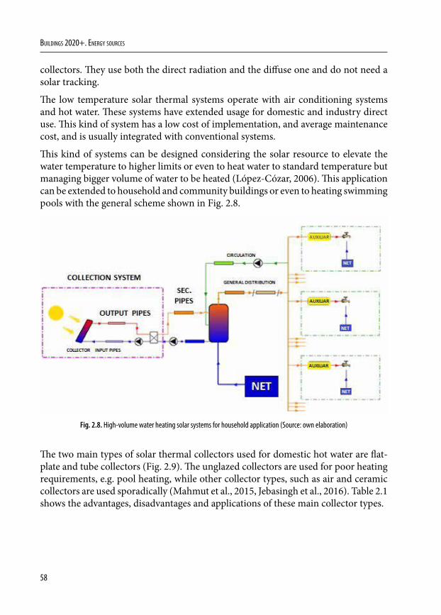
58


collectors. They use both the direct radiation and the diffuse one and do not need a solar tracking.

The low temperature solar thermal systems operate with air conditioning systems and hot water. These systems have extended usage for domestic and industry direct use. This kind of system has a low cost of implementation, and average maintenance cost, and is usually integrated with conventional systems.

This kind of systems can be designed considering the solar resource to elevate the water temperature to higher limits or even to heat water to standard temperature but managing bigger volume of water to be heated (López-Cózar, 2006). This application can be extended to household and community buildings or even to heating swimming pools with the general scheme shown in Fig. 2.8.

Fig. 2.8. High-volume water heating solar systems for household application (Source: own elaboration)

The two main types of solar thermal collectors used for domestic hot water are flat-plate and tube collectors (Fig. 2.9). The unglazed collectors are used for poor heating requirements, e.g. pool heating, while other collector types, such as air and ceramic collectors are used sporadically (Mahmut et al., 2015, Jebasingh et al., 2016). Table 2.1 shows the advantages, disadvantages and applications of these main collector types.

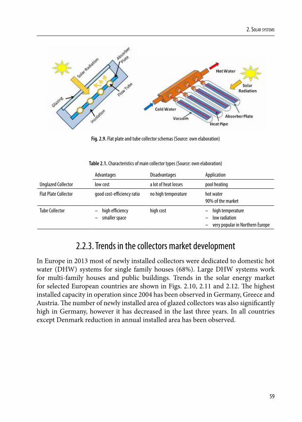
59

2. Solar SyStemS

Fig. 2.9. Flat plate and tube collector schemas (Source: own elaboration)

Table 2.1. Characteristics of main collector types (Source: own elaboration)

Advantages Disadvantages Application

Unglazed Collector low cost a lot of heat losses pool heating

Flat Plate Collector good cost-efficiency ratio no high temperature hot water 90% of the market

Tube Collector – high efficiency – smaller space

high cost – high temperature – low radiation – very popular in Northern Europe

2.2.3. Trends in the collectors market developmentIn Europe in 2013 most of newly installed collectors were dedicated to domestic hot water (DHW) systems for single family houses (68%). Large DHW systems work for multi-family houses and public buildings. Trends in the solar energy market for selected European countries are shown in Figs. 2.10, 2.11 and 2.12. The highest installed capacity in operation since 2004 has been observed in Germany, Greece and Austria. The number of newly installed area of glazed collectors was also significantly high in Germany, however it has decreased in the last three years. In all countries except Denmark reduction in annual installed area has been observed.

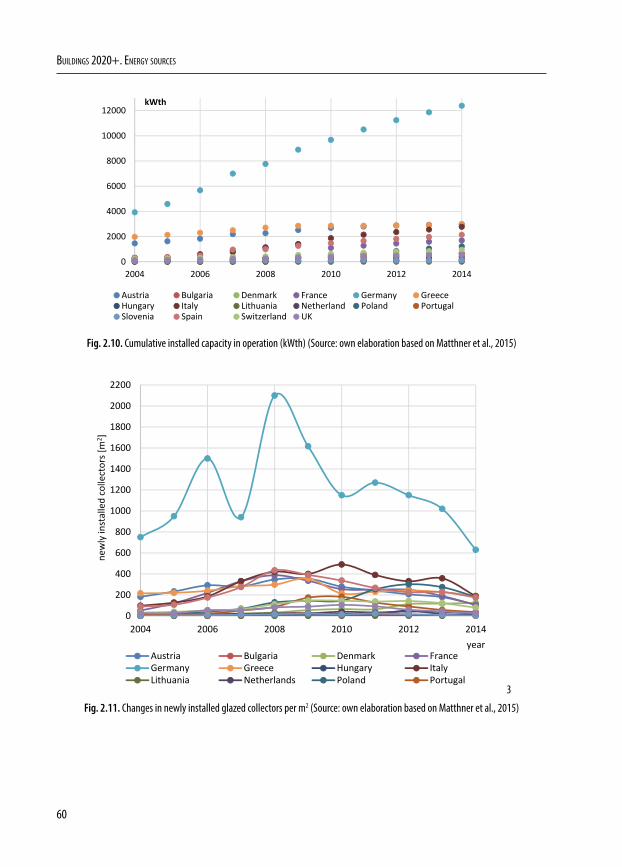
60


0

2000

4000

6000

8000

10000

12000

2004 2006 2008 2010 2012 2014

kWth

Austria Bulgaria Denmark France Germany GreeceHungary Italy Lithuania Netherland Poland PortugalSlovenia Spain Switzerland UK

Fig. 2.10. Cumulative installed capacity in operation (kWth) (Source: own elaboration based on Matthner et al., 2015)

0

200

400

600

800

1000

1200

1400

1600

1800

2000

2200

2004 2006 2008 2010 2012 2014

newly in

stalled collectors [m

2 ]

yearAustria Bulgaria Denmark FranceGermany Greece Hungary ItalyLithuania Netherlands Poland Portugal

3

Fig. 2.11. Changes in newly installed glazed collectors per m2 (Source: own elaboration based on Matthner et al., 2015)

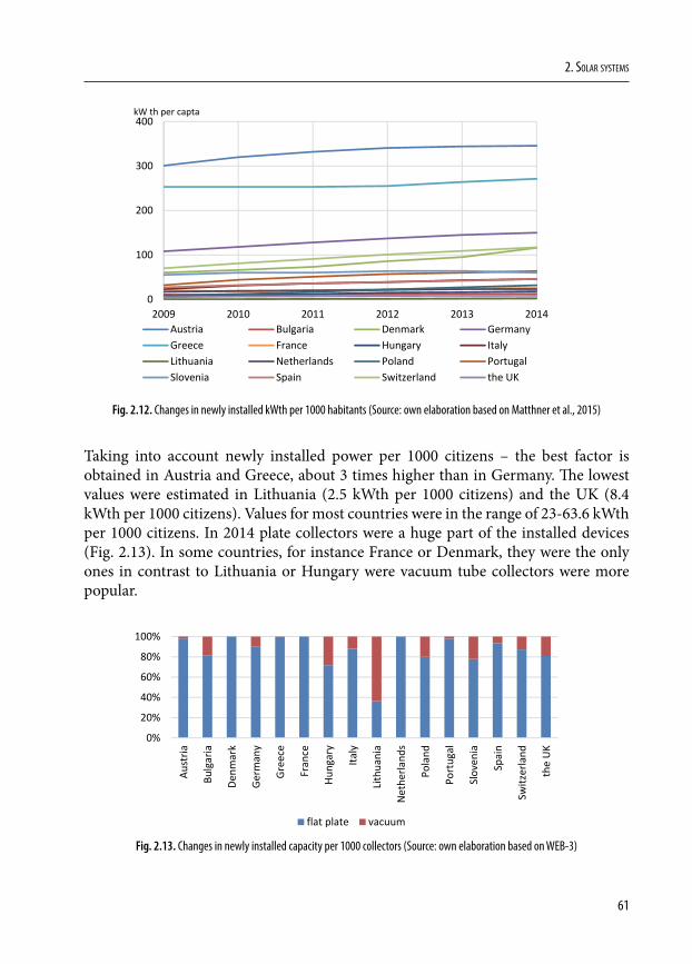
61

2. Solar SyStemS

0

100

200

300

400

2009 2010 2011 2012 2013 2014

kW th per capta

Austria Bulgaria Denmark GermanyGreece France Hungary ItalyLithuania Netherlands Poland PortugalSlovenia Spain Switzerland the UK

Fig. 2.12. Changes in newly installed kWth per 1000 habitants (Source: own elaboration based on Matthner et al., 2015)

Taking into account newly installed power per 1000 citizens – the best factor is obtained in Austria and Greece, about 3 times higher than in Germany. The lowest values were estimated in Lithuania (2.5 kWth per 1000 citizens) and the UK (8.4 kWth per 1000 citizens). Values for most countries were in the range of 23-63.6 kWth per 1000 citizens. In 2014 plate collectors were a huge part of the installed devices (Fig. 2.13). In some countries, for instance France or Denmark, they were the only ones in contrast to Lithuania or Hungary were vacuum tube collectors were more popular.

0%

20%

40%

60%

80%

100%

Austria

Bulgaria

Denm

ark

Germ

any

Gree

ce

Fran

ce

Hung

ary

Italy

Lithu

ania

Netherland

s

Poland

Portug

al

Slov

enia

Spain

Switzerland

the UK

flat plate vacuum

Fig. 2.13. Changes in newly installed capacity per 1000 collectors (Source: own elaboration based on WEB-3)

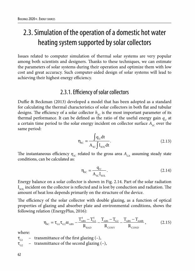
62


2.3. Simulation of the operation of a domestic hot water heating system supported by solar collectors

Issues related to computer simulation of thermal solar systems are very popular among both scientists and designers. Thanks to these techniques, we can estimate the parameters of solar systems during their operation and optimize them with low cost and great accuracy. Such computer-aided design of solar systems will lead to achieving their highest energy efficiency.

2.3.1. Efficiency of solar collectorsDuffie & Beckman (2013) developed a model that has been adopted as a standard for calculating the thermal characteristics of solar collectors in both flat and tubular designs. The efficiency of a solar collector hSC is the most important parameter of its thermal performance. It can be defined as the ratio of the useful energy gain qU at a certain time period to the solar energy incident on collector surface ASC over the same period:

ηSCU

SC SOL

q dt

A I dt= ∫

∫. (2.13)

The instantaneous efficiency ηSC related to the gross area AGA assuming steady state conditions, can be calculated as:

ηSC

U

SC SOL

qA I

= . (2.14)

Energy balance on a solar collector is shown in Fig. 2.14. Part of the solar radiation ISOL incident on the collector is reflected and is lost by conduction and radiation. The amount of heat loss depends primarily on the structure of the device.

The efficiency of the solar collector with double glazing, as a function of optical properties of glazing and absorber plate and environmental conditions, shows the following relation (EnergyPlus, 2016):

η τ τ αSC G G ABSABS G

RAD

ABS G

CONV

ABS AMB

COND

T TR

T TR

T TR

= −−

−−

−−

1 2

42

42 , (2.15)

where:τG1 – transmittance of the first glazing (–),τG2 – transmittance of the second glazing (–),

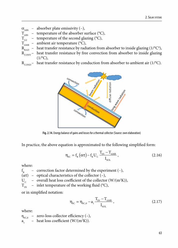
63

2. Solar SyStemS

αABS – absorber plate emissivity (–),TABS – temperature of the absorber surface (°C),TG2 – temperature of the second glazing (°C),TAMB – ambient air temperature (°C),RRAD – heat transfer resistance by radiation from absorber to inside glazing (1/°C4),RCONV – heat transfer resistance by free convection from absorber to inside glazing

(1/°C),RCOND – heat transfer resistance by conduction from absorber to ambient air (1/°C).

Fig. 2.1. Energy balance of gains and losses for a thermal collector.

Fig. 2.14. Energy balance of gains and losses for a thermal collector (Source: own elaboration)

In practice, the above equation is approximated to the following simplified form:

η ατSC R R CIN AMB

SOL

f f UT T

I= ( ) −

−, (2.16)

where:fR – correction factor determined by the experiment (–),(ατ) – optical characteristics of the collector (–),UC – overall heat loss coefficient of the collector (W/(m2K)),TIN – inlet temperature of the working fluid (°C),

or in simplified notation:

η ηSC SCIN AMB

SOL

aT T

I= −

−,0 1 , (2.17)

where:ηSC,0 – zero-loss collector efficiency (–),a1 – heat loss coefficient (W/(m2K)).

64


In order to increase the accuracy of determining the instantaneous efficiency, the following formula (ISO, 2013) was proposed, based on the second-order curve which is mostly used in the modelling of solar systems:

( )2

IN AMBIN AMBSC SC,0 1 2

SOL SOL

T TT Ta a

I I−−

η = η + + , (2.18)

where a2 – temperature dependence of the heat loss coefficient (W/(m2K)).

The values of all the coefficients in the above equation can be found on the website of the Solar Rating & Certification Corporation (ICC-SRCC) arranged by manufacturers of solar collectors.

The transmittance properties of the collector glazing depend on the angle of incidence of solar radiation. In order to take into account the impact of this phenomenon on the characteristic of a collector, there has been proposed an incident angle modifier coefficient Kτα:

K b bτα θ θ= + −

+ −

1 1 1 1 10 1

2

cos cos, (2.19)

where:

b0, b1 – incident angle modifier coefficients (–),θ – angle of incidence of solar radiation (deg).

The values of both coefficients can be found in certification documents prepared by the ICC-SRCC.

2.3.2. Software used for simulation of solar systemsThe most advanced and popular software used for computer simulation of building energy consumption and modelling of solar collector systems are the following tools: ESP-r, DesignBuilder, OpenStudio, EnergyPlus, SUNREL, TRACE 700, TRANSOL – Solar Thermal Energy, HVACSIM+, HEED Home Energy Efficient Design, RETScreen, Polysun, and TRNSYS.

This book provides an example of a year-round modelling of the solar collector system using the verified and fully validated tool – EnergyPlus.

In EnergyPlus, solar radiation is calculated based on the anisotropic (non-uniform) radiance distribution of the sky. In this model the total radiation ISOL is a combination of the direct (beam) IDIR, diffuse IDIF, and reflected IREF solar radiation. These values with a one-hour time step are taken directly from the weather data (WEB-4). Weather

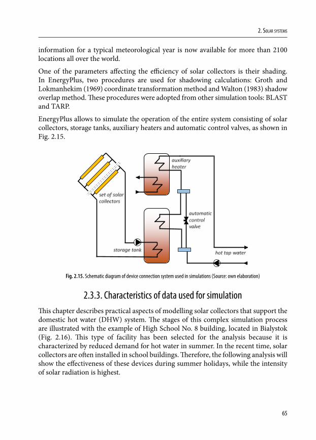
65

2. Solar SyStemS

information for a typical meteorological year is now available for more than 2100 locations all over the world.

One of the parameters affecting the efficiency of solar collectors is their shading. In EnergyPlus, two procedures are used for shadowing calculations: Groth and Lokmanhekim (1969) coordinate transformation method and Walton (1983) shadow overlap method. These procedures were adopted from other simulation tools: BLAST and TARP.

EnergyPlus allows to simulate the operation of the entire system consisting of solar collectors, storage tanks, auxiliary heaters and automatic control valves, as shown in Fig. 2.15.

Fig. 2.2. Diagram of devices connection system used in simulations.

Fig. 2.15. Schematic diagram of device connection system used in simulations (Source: own elaboration)

2.3.3. Characteristics of data used for simulationThis chapter describes practical aspects of modelling solar collectors that support the domestic hot water (DHW) system. The stages of this complex simulation process are illustrated with the example of High School No. 8 building, located in Bialystok (Fig. 2.16). This type of facility has been selected for the analysis because it is characterized by reduced demand for hot water in summer. In the recent time, solar collectors are often installed in school buildings. Therefore, the following analysis will show the effectiveness of these devices during summer holidays, while the intensity of solar radiation is highest.

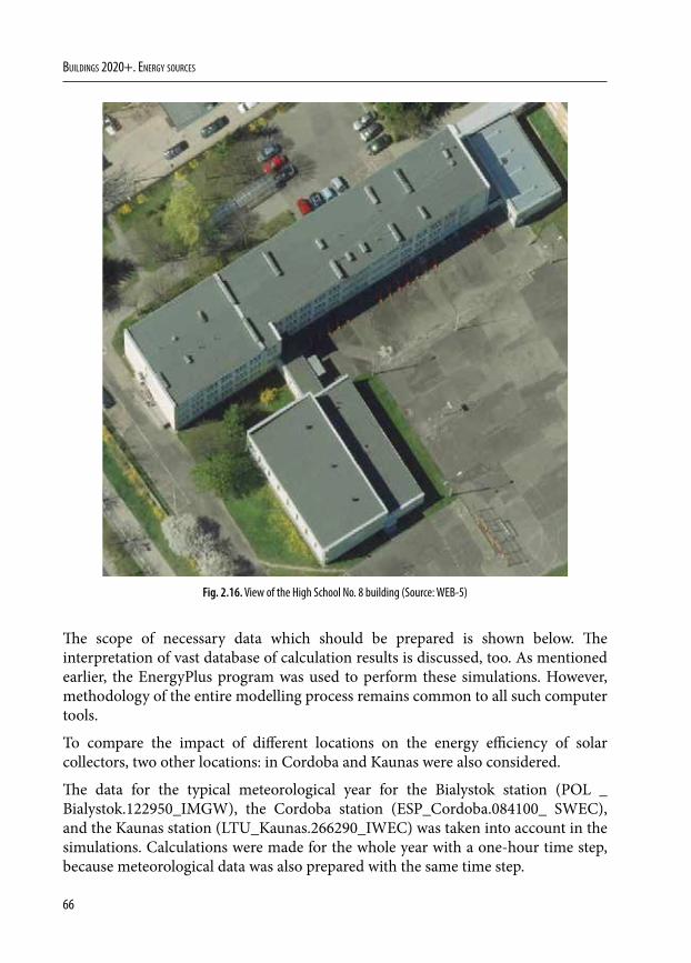
66


Fig. 2.3. View of the VIII high school building (http://www.gisbialystok.pl).

Fig. 2.16. View of the High School No. 8 building (Source: WEB-5)

The scope of necessary data which should be prepared is shown below. The interpretation of vast database of calculation results is discussed, too. As mentioned earlier, the EnergyPlus program was used to perform these simulations. However, methodology of the entire modelling process remains common to all such computer tools.

To compare the impact of different locations on the energy efficiency of solar collectors, two other locations: in Cordoba and Kaunas were also considered.

The data for the typical meteorological year for the Bialystok station (POL _Bialystok.122950_IMGW), the Cordoba station (ESP_Cordoba.084100_ SWEC), and the Kaunas station (LTU_Kaunas.266290_IWEC) was taken into account in the simulations. Calculations were made for the whole year with a one-hour time step, because meteorological data was also prepared with the same time step.

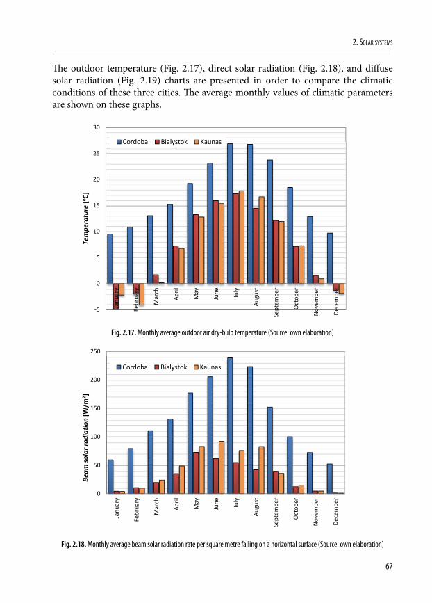
67

2. Solar SyStemS

The outdoor temperature (Fig. 2.17), direct solar radiation (Fig. 2.18), and diffuse solar radiation (Fig. 2.19) charts are presented in order to compare the climatic conditions of these three cities. The average monthly values of climatic parameters are shown on these graphs.

‐5

0

5

10

15

20

25

30

Janu

ary

Februa

ry

March

April

May

June July

Augu

st

Septem

ber

Octobe

r

Novembe

r

Decembe

r

Tempe

rature

[o C]

Cordoba Bialystok Kaunas

Fig. 2.17. Monthly average outdoor air dry-bulb temperature (Source: own elaboration)

0

50

100

150

200

250

Janu

ary

Februa

ry

March

April

May

June July

Augu

st

Septem

ber

Octobe

r

Novembe

r

Decembe

r

Beam

solar rad

iatio

n[W

/m2 ]


Fig. 2.18. Monthly average beam solar radiation rate per square metre falling on a horizontal surface (Source: own elaboration)

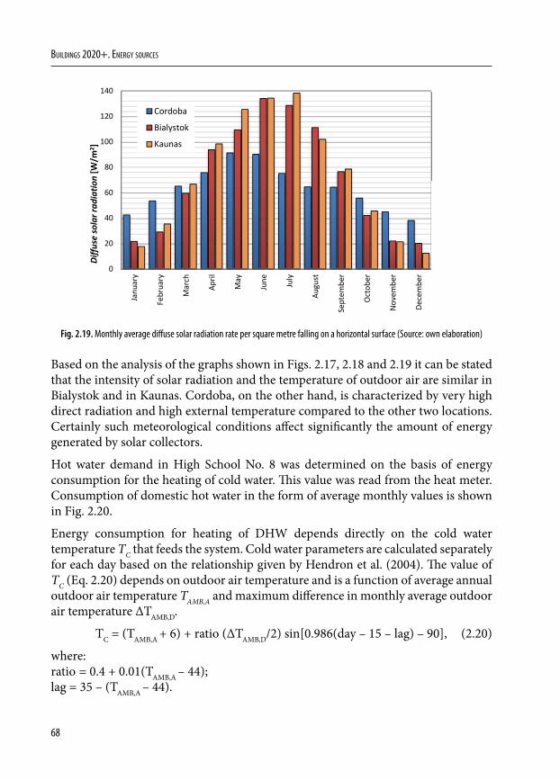
68


0

20

40

60

80

100

120

140

Janu

ary

Februa

ry

March

April

May

June July

Augu

st

Septem

ber

Octobe

r

Novembe

r

Decembe

r

Diffu

sesolar rad

iatio

n[W

/m2 ]

Cordoba

Bialystok

Kaunas

Fig. 2.19. Monthly average diffuse solar radiation rate per square metre falling on a horizontal surface (Source: own elaboration)

Based on the analysis of the graphs shown in Figs. 2.17, 2.18 and 2.19 it can be stated that the intensity of solar radiation and the temperature of outdoor air are similar in Bialystok and in Kaunas. Cordoba, on the other hand, is characterized by very high direct radiation and high external temperature compared to the other two locations. Certainly such meteorological conditions affect significantly the amount of energy generated by solar collectors.

Hot water demand in High School No. 8 was determined on the basis of energy consumption for the heating of cold water. This value was read from the heat meter. Consumption of domestic hot water in the form of average monthly values is shown in Fig. 2.20.

Energy consumption for heating of DHW depends directly on the cold water temperature TC that feeds the system. Cold water parameters are calculated separately for each day based on the relationship given by Hendron et al. (2004). The value of TC (Eq. 2.20) depends on outdoor air temperature and is a function of average annual outdoor air temperature TAMB,A and maximum difference in monthly average outdoor air temperature ΔTAMB,D.

TC = (TAMB,A + 6) + ratio (ΔTAMB,D/2) sin[0.986(day – 15 – lag) – 90], (2.20)

where:ratio = 0.4 + 0.01(TAMB,A – 44);lag = 35 – (TAMB,A – 44).

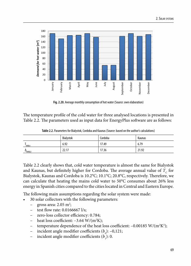
69

2. Solar SyStemS

0

20

40

60

80

100

120

140

160

180

Janu

ary

Februa

ry

March

April

May

June July

Augu

st

Septem

ber

Octobe

r

Novembe

r

Decembe

r

Deman

d for h

ot water [m

3 ]

Fig. 2.20. Average monthly consumption of hot water (Source: own elaboration)

The temperature profile of the cold water for three analysed locations is presented in Table 2.2. The parameters used as input data for EnergyPlus software are as follows:

Table 2.2. Parameters for Bialystok, Cordoba and Kaunas (Source: based on the author’s calculations)

Bialystok Cordoba Kaunas

TAMB,A 6.92 17.49 6.79

ΔTAMB,D 22.17 17.36 21.92

Table 2.2 clearly shows that, cold water temperature is almost the same for Bialystok and Kaunas, but definitely higher for Cordoba. The average annual value of TC for Bialystok, Kaunas and Cordoba is 10.2°C; 10.1°C; 20.8°C, respectively. Therefore, we can calculate that heating the mains cold water to 50°C consumes about 26% less energy in Spanish cities compared to the cities located in Central and Eastern Europe.

The following main assumptions regarding the solar system were made:• 30 solar collectors with the following parameters:

– gross area: 2.05 m2;– test flow rate: 0.0166667 l/s;– zero-loss collector efficiency: 0.784;– heat loss coefficient: –3.64 W/(m2K);– temperature dependence of the heat loss coefficient: –0.00185 W/(m2K2);– incident angle modifier coefficients (b0): –0,121;– incident angle modifier coefficients (b1): 0.

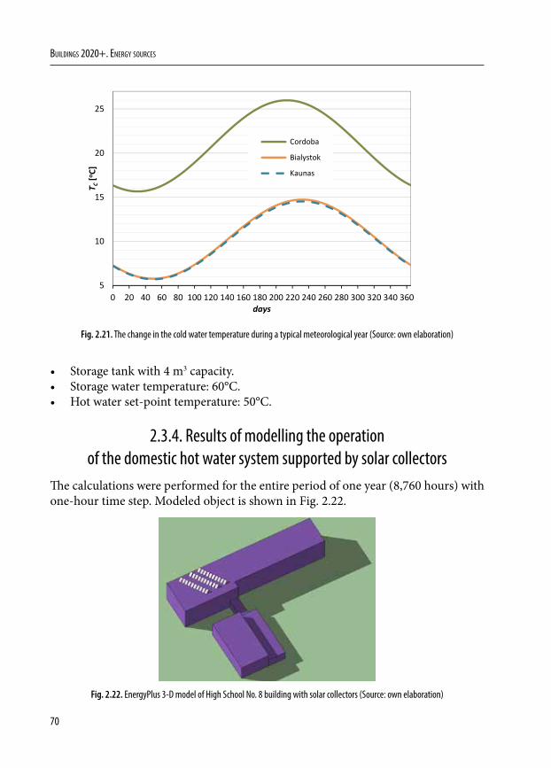
70


5

10

15

20

25

0 20 40 60 80 100 120 140 160 180 200 220 240 260 280 300 320 340 360

T C[o C

]

days

Cordoba

Bialystok

Kaunas

Fig. 2.21. The change in the cold water temperature during a typical meteorological year (Source: own elaboration)

• Storage tank with 4 m3 capacity.• Storage water temperature: 60°C.• Hot water set-point temperature: 50°C.

2.3.4. Results of modelling the operation of the domestic hot water system supported by solar collectors

The calculations were performed for the entire period of one year (8,760 hours) with one-hour time step. Modeled object is shown in Fig. 2.22.

Fig. 2.22. EnergyPlus 3-D model of High School No. 8 building with solar collectors (Source: own elaboration)

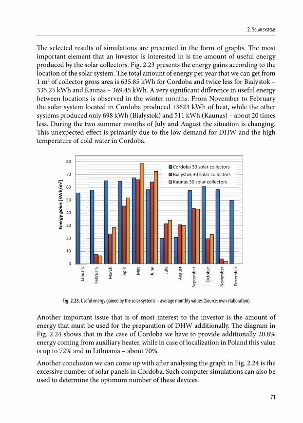
71

2. Solar SyStemS

The selected results of simulations are presented in the form of graphs. The most important element that an investor is interested in is the amount of useful energy produced by the solar collectors. Fig. 2.23 presents the energy gains according to the location of the solar system. The total amount of energy per year that we can get from 1 m2 of collector gross area is 635.85 kWh for Cordoba and twice less for Bialystok – 335.25 kWh and Kaunas – 369.45 kWh. A very significant difference in useful energy between locations is observed in the winter months. From November to February the solar system located in Cordoba produced 13623 kWh of heat, while the other systems produced only 698 kWh (Bialystok) and 511 kWh (Kaunas) – about 20 times less. During the two summer months of July and August the situation is changing. This unexpected effect is primarily due to the low demand for DHW and the high temperature of cold water in Cordoba.

0

10

20

30

40

50

60

70

80

Janu

ary

Februa

ry

March

April

May

June July

Augu

st

Septem

ber

Octobe

r

Novembe

r

Decembe

r

Energy

gains[kW

h/m

2 ]

Cordoba 30 solar collectorsBialystok 30 solar collectorsKaunas 30 solar collectors

Fig. 2.23. Useful energy gained by the solar systems – average monthly values (Source: own elaboration)

Another important issue that is of most interest to the investor is the amount of energy that must be used for the preparation of DHW additionally. The diagram in Fig. 2.24 shows that in the case of Cordoba we have to provide additionally 20.8% energy coming from auxiliary heater, while in case of localization in Poland this value is up to 72% and in Lithuania – about 70%.

Another conclusion we can come up with after analysing the graph in Fig. 2.24 is the excessive number of solar panels in Cordoba. Such computer simulations can also be used to determine the optimum number of these devices.

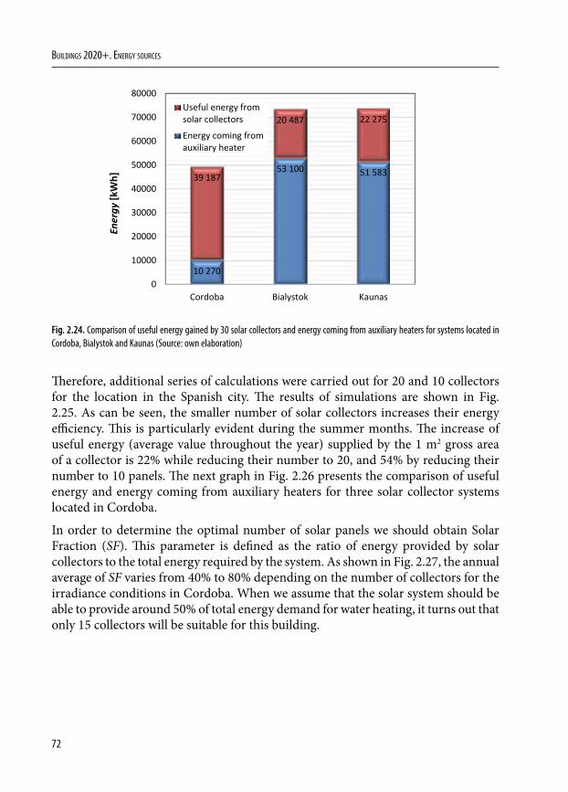
72


10 270

53 100 51 58339 187

20 487 22 275

0

10000

20000

30000

40000

50000

60000

70000

80000


Energy

[kWh]

Useful energy fromsolar collectorsEnergy coming fromauxiliary heater

Fig. 2.24. Comparison of useful energy gained by 30 solar collectors and energy coming from auxiliary heaters for systems located in Cordoba, Bialystok and Kaunas (Source: own elaboration)

Therefore, additional series of calculations were carried out for 20 and 10 collectors for the location in the Spanish city. The results of simulations are shown in Fig. 2.25. As can be seen, the smaller number of solar collectors increases their energy efficiency. This is particularly evident during the summer months. The increase of useful energy (average value throughout the year) supplied by the 1 m2 gross area of a collector is 22% while reducing their number to 20, and 54% by reducing their number to 10 panels. The next graph in Fig. 2.26 presents the comparison of useful energy and energy coming from auxiliary heaters for three solar collector systems located in Cordoba.

In order to determine the optimal number of solar panels we should obtain Solar Fraction (SF). This parameter is defined as the ratio of energy provided by solar collectors to the total energy required by the system. As shown in Fig. 2.27, the annual average of SF varies from 40% to 80% depending on the number of collectors for the irradiance conditions in Cordoba. When we assume that the solar system should be able to provide around 50% of total energy demand for water heating, it turns out that only 15 collectors will be suitable for this building.

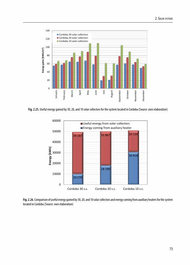
73

2. Solar SyStemS

0

20

40

60

80

100

120

140

Janu

ary

Februa

ry

March

April

May

June July

Augu

st

Septem

ber

Octobe

r

Novembe

r

Decembe

r

Energy gains

[kWh/m

2 ]

Cordoba 30 solar collectorsCordoba 20 solar collectorsCordoba 10 solar collectors

Fig. 2.25. Useful energy gained by 30, 20, and 10 solar collectors for the system located in Cordoba (Source: own elaboration)

10 270

18 199

30 818

39 187 31 867 20 134

0

10000

20000

30000

40000

50000

60000

Cordoba 30 s.c. Cordoba 20 s.c. Cordoba 10 s.c.

Energy [k

Wh]

Useful energy from solar collectorsEnergy coming from auxiliary heater

Fig. 2.26. Comparison of useful energy gained by 30, 20, and 10 solar collectors and energy coming from auxiliary heaters for the system located in Cordoba (Source: own elaboration)

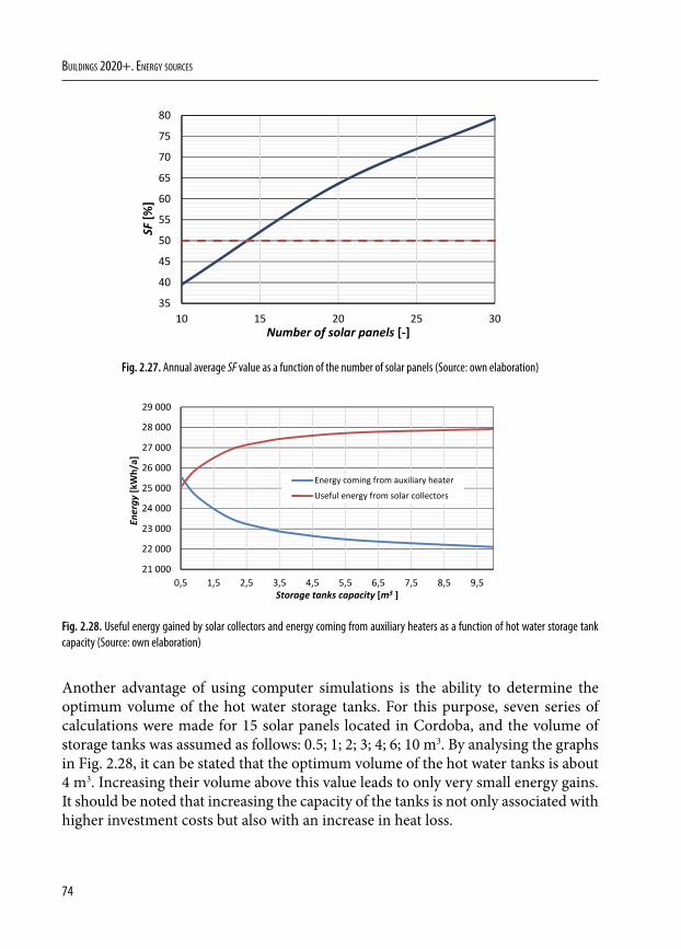
74


35

40

45

50

55

60

65

70

75

80

10 15 20 25 30

SF[%

]

Number of solar panels [‐]

Fig. 2.27. Annual average SF value as a function of the number of solar panels (Source: own elaboration)

21 000

22 000

23 000

24 000

25 000

26 000

27 000

28 000

29 000

0,5 1,5 2,5 3,5 4,5 5,5 6,5 7,5 8,5 9,5

Energy

[kWh/a]

Storage tanks capacity [m3 ]

Energy coming from auxiliary heaterUseful energy from solar collectors

Fig. 2.28. Useful energy gained by solar collectors and energy coming from auxiliary heaters as a function of hot water storage tank capacity (Source: own elaboration)

Another advantage of using computer simulations is the ability to determine the optimum volume of the hot water storage tanks. For this purpose, seven series of calculations were made for 15 solar panels located in Cordoba, and the volume of storage tanks was assumed as follows: 0.5; 1; 2; 3; 4; 6; 10 m3. By analysing the graphs in Fig. 2.28, it can be stated that the optimum volume of the hot water tanks is about 4 m3. Increasing their volume above this value leads to only very small energy gains. It should be noted that increasing the capacity of the tanks is not only associated with higher investment costs but also with an increase in heat loss.

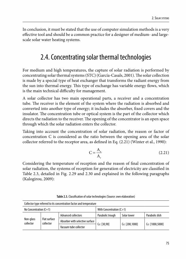
75

2. Solar SyStemS

In conclusion, it must be stated that the use of computer simulation methods is a very effective tool and should be a common practice for a designer of medium- and large-scale solar water heating systems.

2.4. Concentrating solar thermal technologies

For medium and high temperatures, the capture of solar radiation is performed by concentrating solar thermal systems (STC) (García-Casals, 2001). The solar collection is made by a special type of heat exchanger that transforms the radiant energy from the sun into thermal energy. This type of exchange has variable energy flows, which is the main technical difficulty for management.

A solar collector has two main operational parts, a receiver and a concentration tube. The receiver is the element of the system where the radiation is absorbed and converted into another type of energy; it includes the absorber, fixed covers and the insulator. The concentration tube or optical system is the part of the collector which directs the radiation to the receiver. The opening of the concentrator is an open space through which the solar radiation enters the collector.

Taking into account the concentration of solar radiation, the reason or factor of concentration C is considered as the ratio between the opening area of the solar collector referred to the receptor area, as defined in Eq. (2.21) (Winter et al., 1990):

C

AA

a

r

= (2.21)

Considering the temperature of reception and the reason of final concentration of solar radiation, the systems of reception for generation of electricity are classified in Table 2.3, detailed in Fig. 2.29 and 2.30 and explained in the following paragraphs (Kalogirou, 2009):

Table 2.3. Classification of solar technologies (Source: own elaboration)

Collector type referred to its concentration factor and temperature

No Concentration (C=1) With Concentration (C>1)

Non-glass collector

Flat surface collector

Advanced collectors Parabolic trough Solar tower Parabolic dish

Absorber with selective surfaceC∈[30,90] C∈[200,1000] C∈[1000,5000]

Vacuum tube collector

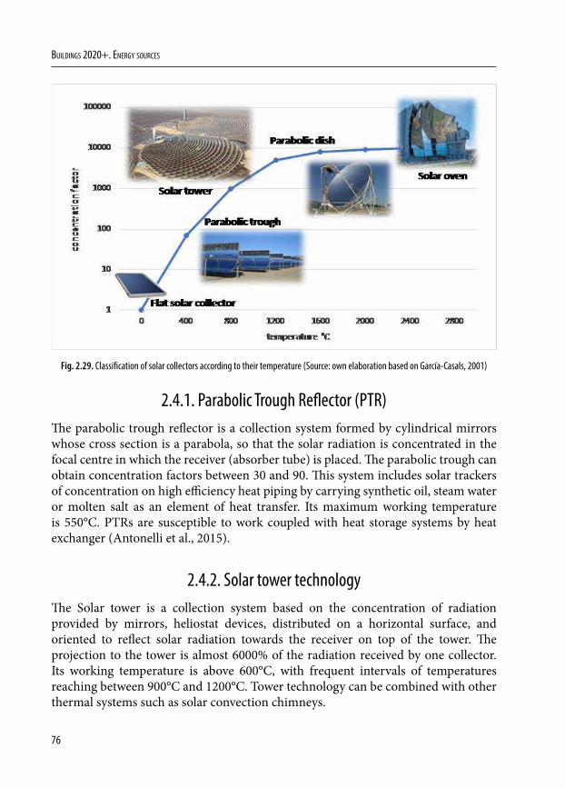
76


Fig. 2.29. Classification of solar collectors according to their temperature (Source: own elaboration based on García-Casals, 2001)

2.4.1. Parabolic Trough Reflector (PTR)The parabolic trough reflector is a collection system formed by cylindrical mirrors whose cross section is a parabola, so that the solar radiation is concentrated in the focal centre in which the receiver (absorber tube) is placed. The parabolic trough can obtain concentration factors between 30 and 90. This system includes solar trackers of concentration on high efficiency heat piping by carrying synthetic oil, steam water or molten salt as an element of heat transfer. Its maximum working temperature is 550°C. PTRs are susceptible to work coupled with heat storage systems by heat exchanger (Antonelli et al., 2015).

2.4.2. Solar tower technology The Solar tower is a collection system based on the concentration of radiation provided by mirrors, heliostat devices, distributed on a horizontal surface, and oriented to reflect solar radiation towards the receiver on top of the tower. The projection to the tower is almost 6000% of the radiation received by one collector. Its working temperature is above 600°C, with frequent intervals of temperatures reaching between 900°C and 1200°C. Tower technology can be combined with other thermal systems such as solar convection chimneys.

77

2. Solar SyStemS

2.4.3. Solar dishParabolic dishes are mirrors with a paraboloid of revolving structure, which are monitored to always maintain their orientation toward the sun. The modular installation of high temperature parabolic troughs (600ºC) is susceptible to coupling in parallel for electricity generation. The generation of electricity is performed using individual Stirling generators. Its main application is the solar collection in irregular extensions or surfaces.

2.4.4. Linear concentrator Fresnel It consists of a primary field of mirrors, an absorber tube and a secondary mirror. The primary field contains rows of flat mirrors that reflect the solar radiation to the absorber tube located several meters above the main field. Above the absorber tube a secondary mirror is located which concentrates the remaining sunlight in the linear absorber tube. This type of installation stands out for the simplicity of its construction and its low cost. Fresnel technology uses flat reflectors, simulating a curved mirror by variation of the adjustable angle of each individual row of mirrors, in relation to the absorber.

Fig. 2.30. Main concentrated solar technologies (Source: own elaboration)

78


Reflectors are constructed with normal glass mirrors and therefore their raw material is very cheap. The curved shape of the parabolic cylinder mirrors makes them 15% more efficient than the Fresnel mirrors, but the reduction of the construction costs compensates the reduction of efficiency.

With any of these four technologies it is possible to concentrate the solar irradiation, which can be considered approximately parallel and incident in a large area (concentrator) over a small one (the receiver). Therefore, the optimum geometry of the concentrator is a paraboloid of revolution with orientation toward the Sun movement. This geometry has the highest concentration values. Thus, parabolic cylinder systems allow to concentrate the solar radiation along an axis. In the central tower systems, the surface of the concentrator is discretized in a series of heliostats as a Fresnel concentrator, i.e. a parabolic reflector through small segments.

Medium and high temperature systems are not used for domestic applications but are desirable for certain industrial applications where large amounts of hot water are needed mainly for producing electricity by steam-driven turbines in solar power plants.

2.5. Electricity applications

2.5.1. Concentrated solar power plantsConcentrated solar power (CSP) plants, also called solar thermal power plants, are systems that collect and concentrate light from the sun to produce high temperature needed to generate electricity. CSP technologies are currently in medium to large-scale operation with a production of about 4.8 GW in 2016, and are mostly located in Spain and the USA (Fig. 2.31), although China has 20 pilot projects to produce 9.6 GW in 2020. Parabolic trough reflector (PTR) technology is responsible for 96.3% of total world thermal energy production and solar tower is in the Second place as shown in Fig. 2.32.

All solar thermal power systems have solar energy collectors with two main components: reflectors (mirrors) that focus solar radiation onto a receiver. A heat-transfer fluid is heated and circulated in the receiver and used to produce steam. The steam is converted into mechanical energy in a steam-driven turbine, which produces electricity by a generator. Optionally, solar thermal power systems have a thermal energy storage or backup system to supply energy when the solar radiation is not strong enough.

79

2. Solar SyStemS

Fig. 2.31. Global Capacity of Concentrated Solar Thermal Power from 2005 to 2016 (Source: own elaboration based on REN21, 2017)

Fig. 2.32. Percentage of installed operational CSP power by technology (Source: own elaboration based on Zhang et al., 2013)

2.5.1.1. Parabolic trough reflector plants

Fig. 2.33. Parabolic trough reflector plant “LA AFRICANA” in Cordoba (Source: photo by A. Rodero)

80


Parabolic trough reflector (PTR) plants (Fig. 2.33) use heat-transfer fluid (HTF) which, when circulating through the tube receiver, absorbs the radiant energy from the Sun in the form of thermal energy, and transports it to the thermal cycle. The type of heat transfer fluid used determines the range of operating temperatures and consequently the efficiency that can be obtained in the power cycle. Fig. 2.34 shows a schema of main parts of a typical PTR plant.

Fig. 2.34. Schema of a concentrated solar plant (Source: own elaboration)

The normal temperature range of HTF is between 150-500ºC. Water can be used as HTF for temperatures below 150ºC. For higher temperatures, the pressure in the pipes is so high that it makes the installation too expensive. Synthetic fluid is used when higher temperatures are needed.

Currently, synthetic aromatic oil based on benzene is used in commercial PTR plants. Main thermodynamic properties of this fluid are shown in Table 2.4. It is a fluid that turns to solid state below 12ºC and flows with difficulty below 25ºC. This means that it is important to avoid lowering the temperature. An additional heating system is necessary to ensure sufficiently high temperatures. This system can use traditional fossil fuel, e.g. natural gas that can supply additional energy when radiation is low.

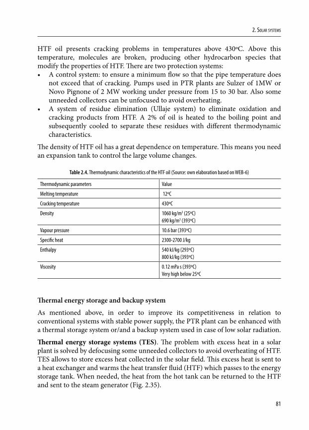
81

2. Solar SyStemS

HTF oil presents cracking problems in temperatures above 430ºC. Above this temperature, molecules are broken, producing other hydrocarbon species that modify the properties of HTF. There are two protection systems:• A control system: to ensure a minimum flow so that the pipe temperature does

not exceed that of cracking. Pumps used in PTR plants are Sulzer of 1MW or Novo Pignone of 2 MW working under pressure from 15 to 30 bar. Also some unneeded collectors can be unfocused to avoid overheating.

• A system of residue elimination (Ullaje system) to eliminate oxidation and cracking products from HTF. A 2% of oil is heated to the boiling point and subsequently cooled to separate these residues with different thermodynamic characteristics.

The density of HTF oil has a great dependence on temperature. This means you need an expansion tank to control the large volume changes.

Table 2.4. Thermodynamic characteristics of the HTF oil (Source: own elaboration based on WEB-6)

Thermodynamic parameters Value

Melting temperature 12ºC

Cracking temperature 430ºC

Density 1060 kg/m3 (25ºC)690 kg/m3 (393ºC)

Vapour pressure 10.6 bar (393ºC)

Specific heat 2300-2700 J/kg

Enthalpy 540 kJ/kg (293ºC)800 kJ/kg (393ºC)

Viscosity 0.12 mPa s (393ºC)Very high below 25ºC

Thermal energy storage and backup system

As mentioned above, in order to improve its competitiveness in relation to conventional systems with stable power supply, the PTR plant can be enhanced with a thermal storage system or/and a backup system used in case of low solar radiation.

Thermal energy storage systems (TES). The problem with excess heat in a solar plant is solved by defocusing some unneeded collectors to avoid overheating of HTF. TES allows to store excess heat collected in the solar field. This excess heat is sent to a heat exchanger and warms the heat transfer fluid (HTF) which passes to the energy storage tank. When needed, the heat from the hot tank can be returned to the HTF and sent to the steam generator (Fig. 2.35).

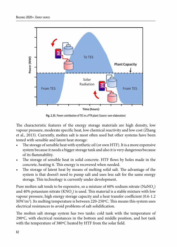
82


Fig. 2.35. Power contribution of TES in a PTR plant (Source: own elaboration)

The characteristic features of the energy storage materials are high density, low vapour pressure, moderate specific heat, low chemical reactivity and low cost (Zhang et al., 2013). Currently, molten salt is most often used but other systems have been tested with sensible and latent heat storage:• The storage of sensible heat with synthetic oil (or own HTF). It is a more expensive

system because it needs a bigger storage tank and also it is very dangerous because of its flammability.

• The storage of sensible heat in solid concrete. HTF flows by holes made in the concrete, heating it. This energy is recovered when needed.

• The storage of latent heat by means of melting solid salt. The advantage of the system is that doesn’t need to pump salt and uses less salt for the same energy storage. This technology is currently under development.

Pure molten salt tends to be expensive, so a mixture of 60% sodium nitrate (NaNO3) and 40% potassium nitrate (KNO3) is used. This material is a stable mixture with low vapour pressure, high energy storage capacity and a heat transfer coefficient (0.6-1.2 MW/m2). Its melting temperature is between 220-250ºC. This means this system uses electrical resistances to avoid problems of salt solidification.

The molten salt storage system has two tanks: cold tank with the temperature of 290ºC, with electrical resistances in the bottom and middle position, and hot tank with the temperature of 380ºC heated by HTF from the solar field.

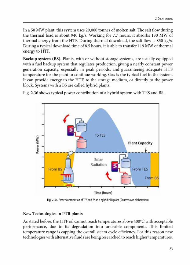
83

2. Solar SyStemS

In a 50 MW plant, this system uses 29,000 tonnes of molten salt. The salt flow during the thermal load is about 940 kg/s. Working for 7.7 hours, it absorbs 130 MW of thermal energy from the HTF. During thermal download, the salt flow is 850 kg/s. During a typical download time of 8.5 hours, it is able to transfer 119 MW of thermal energy to HTF.

Backup system (BS). Plants, with or without storage systems, are usually equipped with a fuel backup system that regulates production, giving a nearly constant power generation capacity, especially in peak periods, and guaranteeing adequate HTF temperature for the plant to continue working. Gas is the typical fuel fo the system. It can provide energy to the HTF, to the storage medium, or directly to the power block. Systems with a BS are called hybrid plants.

Fig. 2.36 shows typical power contribution of a hybrid system with TES and BS.

Fig. 2.36. Power contribution of TES and BS in a hybrid PTR plant (Source: own elaboration)

New Technologies in PTR plants

As stated before, the HTF oil cannot reach temperatures above 400ºC with acceptable performance, due to its degradation into unusable components. This limited temperature range is capping the overall steam cycle efficiency. For this reason new technologies with alternative fluids are being researched to reach higher temperatures.

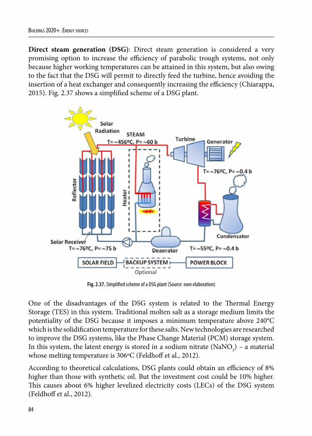
84


Direct steam generation (DSG): Direct steam generation is considered a very promising option to increase the efficiency of parabolic trough systems, not only because higher working temperatures can be attained in this system, but also owing to the fact that the DSG will permit to directly feed the turbine, hence avoiding the insertion of a heat exchanger and consequently increasing the efficiency (Chiarappa, 2015). Fig. 2.37 shows a simplified scheme of a DSG plant.

Fig. 2.37. Simplified scheme of a DSG plant (Source: own elaboration)

One of the disadvantages of the DSG system is related to the Thermal Energy Storage (TES) in this system. Traditional molten salt as a storage medium limits the potentiality of the DSG because it imposes a minimum temperature above 240°C which is the solidification temperature for these salts. New technologies are researched to improve the DSG systems, like the Phase Change Material (PCM) storage system. In this system, the latent energy is stored in a sodium nitrate (NaNO3) – a material whose melting temperature is 306ºC (Feldhoff et al., 2012).

According to theoretical calculations, DSG plants could obtain an efficiency of 8% higher than those with synthetic oil. But the investment cost could be 10% higher. This causes about 6% higher levelized electricity costs (LECs) of the DSG system (Feldhoff et al., 2012).

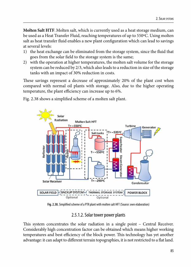
85

2. Solar SyStemS

Molten Salt HTF. Molten salt, which is currently used as a heat storage medium, can be used as a Heat Transfer Fluid, reaching temperatures of up to 550ºC. Using molten salt as heat transfer fluid enables a new plant configuration which can lead to savings at several levels:1) the heat exchange can be eliminated from the storage system, since the fluid that

goes from the solar field to the storage system is the same;2) with the operation at higher temperatures, the molten salt volume for the storage

system can be reduced by 2/3, which also leads to a reduction in size of the storage tanks with an impact of 30% reduction in costs.

These savings represent a decrease of approximately 20% of the plant cost when compared with normal oil plants with storage. Also, due to the higher operating temperature, the plant efficiency can increase up to 6%.

Fig. 2.38 shows a simplified scheme of a molten salt plant.

Fig. 2.38. Simplified scheme of a PTR plant with molten salt HFT (Source: own elaboration)

2.5.1.2. Solar tower power plants

This system concentrates the solar radiation in a single point – Central Receiver. Considerably high concentration factor can be obtained which means higher working temperatures and best efficiency of the block power. This technology has yet another advantage: it can adapt to different terrain topographies, it is not restricted to a flat land.

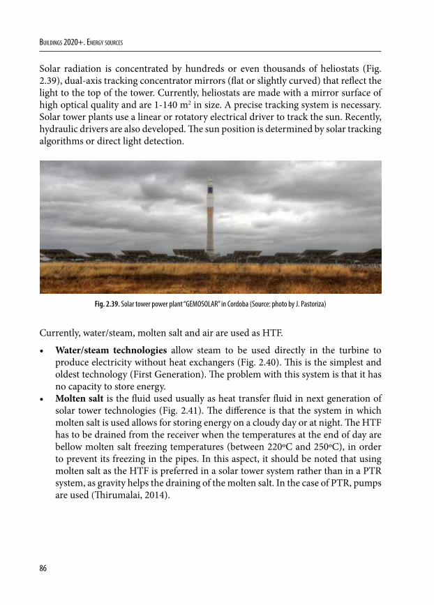
86


Solar radiation is concentrated by hundreds or even thousands of heliostats (Fig. 2.39), dual-axis tracking concentrator mirrors (flat or slightly curved) that reflect the light to the top of the tower. Currently, heliostats are made with a mirror surface of high optical quality and are 1-140 m2 in size. A precise tracking system is necessary. Solar tower plants use a linear or rotatory electrical driver to track the sun. Recently, hydraulic drivers are also developed. The sun position is determined by solar tracking algorithms or direct light detection.

Fig. 2.39. Solar tower power plant “GEMOSOLAR” in Cordoba (Source: photo by J. Pastoriza)

Currently, water/steam, molten salt and air are used as HTF.

• Water/steam technologies allow steam to be used directly in the turbine to produce electricity without heat exchangers (Fig. 2.40). This is the simplest and oldest technology (First Generation). The problem with this system is that it has no capacity to store energy.

• Molten salt is the fluid used usually as heat transfer fluid in next generation of solar tower technologies (Fig. 2.41). The difference is that the system in which molten salt is used allows for storing energy on a cloudy day or at night. The HTF has to be drained from the receiver when the temperatures at the end of day are bellow molten salt freezing temperatures (between 220ºC and 250ºC), in order to prevent its freezing in the pipes. In this aspect, it should be noted that using molten salt as the HTF is preferred in a solar tower system rather than in a PTR system, as gravity helps the draining of the molten salt. In the case of PTR, pumps are used (Thirumalai, 2014).

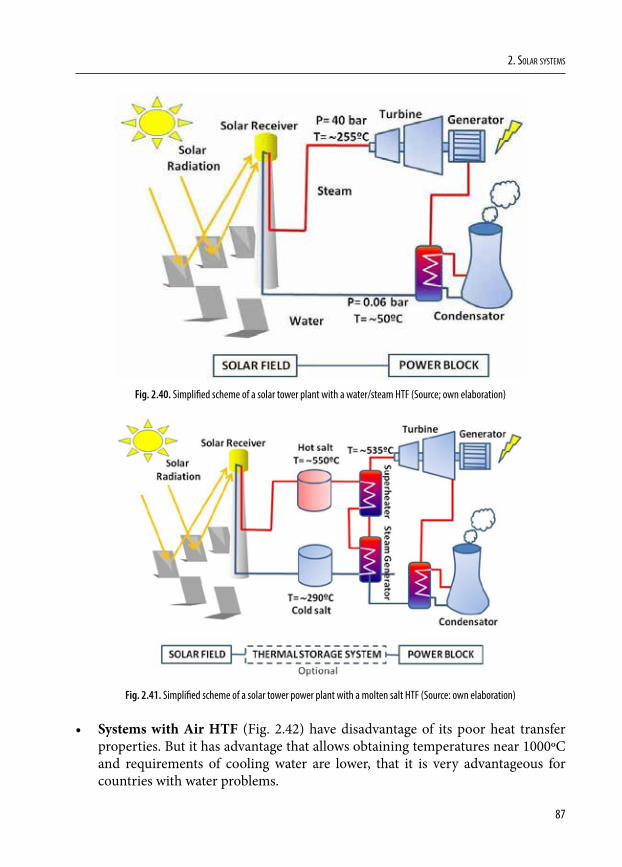
87

2. Solar SyStemS

Fig. 2.40. Simplified scheme of a solar tower plant with a water/steam HTF (Source; own elaboration)

Fig. 2.41. Simplified scheme of a solar tower power plant with a molten salt HTF (Source: own elaboration)

• Systems with Air HTF (Fig. 2.42) have disadvantage of its poor heat transfer properties. But it has advantage that allows obtaining temperatures near 1000ºC and requirements of cooling water are lower, that it is very advantageous for countries with water problems.

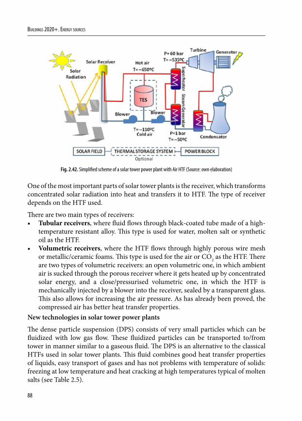
88


Fig. 2.42. Simplified scheme of a solar tower power plant with Air HTF (Source: own elaboration)

One of the most important parts of solar tower plants is the receiver, which transforms concentrated solar radiation into heat and transfers it to HTF. The type of receiver depends on the HTF used.

There are two main types of receivers: • Tubular receivers, where fluid flows through black-coated tube made of a high-

temperature resistant alloy. This type is used for water, molten salt or synthetic oil as the HTF.

• Volumetric receivers, where the HTF flows through highly porous wire mesh or metallic/ceramic foams. This type is used for the air or CO2 as the HTF. There are two types of volumetric receivers: an open volumetric one, in which ambient air is sucked through the porous receiver where it gets heated up by concentrated solar energy, and a close/pressurised volumetric one, in which the HTF is mechanically injected by a blower into the receiver, sealed by a transparent glass. This also allows for increasing the air pressure. As has already been proved, the compressed air has better heat transfer properties.

New technologies in solar tower power plants

The dense particle suspension (DPS) consists of very small particles which can be fluidized with low gas flow. These fluidized particles can be transported to/from tower in manner similar to a gaseous fluid. The DPS is an alternative to the classical HTFs used in solar tower plants. This fluid combines good heat transfer properties of liquids, easy transport of gases and has not problems with temperature of solids: freezing at low temperature and heat cracking at high temperatures typical of molten salts (see Table 2.5).

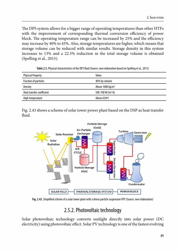
89

2. Solar SyStemS

The DPS system allows for a bigger range of operating temperatures than other HTFs with the improvement of corresponding thermal conversion efficiency of power block. The operating temperature range can be increased by 25% and the efficiency may increase by 40% to 45%. Also, storage temperatures are higher, which means that storage volume can be reduced with similar results. Storage density in this system increases to 13% and a 22.5% reduction in the total storage volume is obtained (Spelling et al., 2015).

Table 2.5. Physical characteristics of the DPS fluid (Source: own elaboration based on Spelling et al., 2015)

Physical Property Value

Fraction of particles 40% by volume

Density Above 1000 kg/m3

Heat transfer coefficient 500-700 W/(m2·K)

High temperature Above 650ºC

Fig. 2.43 shows a scheme of solar tower power plant based on the DSP as heat transfer fluid.

Fig. 2.43. Simplified scheme of a solar tower plant with a dense particle suspension HTF (Source: own elaboration)

2.5.2. Photovoltaic technologySolar photovoltaic technology converts sunlight directly into solar power (DC electricity) using photovoltaic effect. Solar PV technology is one of the fastest evolving

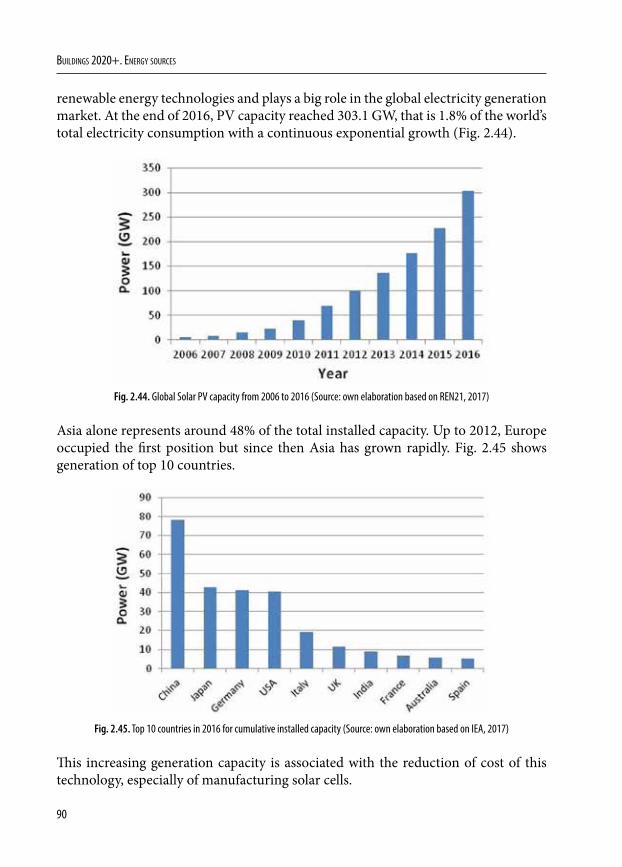
90


renewable energy technologies and plays a big role in the global electricity generation market. At the end of 2016, PV capacity reached 303.1 GW, that is 1.8% of the world’s total electricity consumption with a continuous exponential growth (Fig. 2.44).

Fig. 2.44. Global Solar PV capacity from 2006 to 2016 (Source: own elaboration based on REN21, 2017)

Asia alone represents around 48% of the total installed capacity. Up to 2012, Europe occupied the first position but since then Asia has grown rapidly. Fig. 2.45 shows generation of top 10 countries.

Fig. 2.45. Top 10 countries in 2016 for cumulative installed capacity (Source: own elaboration based on IEA, 2017)

This increasing generation capacity is associated with the reduction of cost of this technology, especially of manufacturing solar cells.

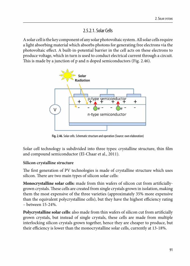
91

2. Solar SyStemS

2.5.2.1. Solar Cells

A solar cell is the key component of any solar photovoltaic system. All solar cells require a light absorbing material which absorbs photons for generating free electrons via the photovoltaic effect. A built-in-potential barrier in the cell acts on these electrons to produce voltage, which in turn is used to conduct electrical current through a circuit. This is made by a junction of p and n doped semiconductors (Fig. 2.46).

Fig. 2.46. Solar cells. Schematic structure and operation (Source: own elaboration)

Solar cell technology is subdivided into three types: crystalline structure, thin film and compound semiconductor (El-Chaar et al., 2011).

Silicon crystalline structure

The first generation of PV technologies is made of crystalline structure which uses silicon. There are two main types of silicon solar cells:

Monocrystalline solar cells: made from thin wafers of silicon cut from artificially-grown crystals. These cells are created from single crystals grown in isolation, making them the most expensive of the three varieties (approximately 35% more expensive than the equivalent polycrystalline cells), but they have the highest efficiency rating – between 15-24%.

Polycrystalline solar cells: also made from thin wafers of silicon cut from artificially grown crystals, but instead of single crystals, these cells are made from multiple interlocking silicon crystals grown together, hence they are cheaper to produce, but their efficiency is lower than the monocrystalline solar cells, currently at 13-18%.

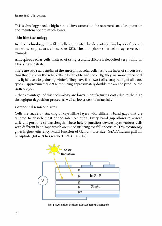
92


This technology needs a higher initial investment but the recurrent costs for operation and maintenance are much lower.

Thin film technology

In this technology, thin film cells are created by depositing thin layers of certain materials on glass or stainless steel (SS). The amorphous solar cells may serve as an example.

Amorphous solar cells: instead of using crystals, silicon is deposited very thinly on a backing substrate.

There are two real benefits of the amorphous solar cell; firstly, the layer of silicon is so thin that it allows the solar cells to be flexible and secondly, they are more efficient at low light levels (e.g. during winter). They have the lowest efficiency rating of all three types – approximately 7-9%, requiring approximately double the area to produce the same output.

Other advantages of this technology are lower manufacturing costs due to the high throughput deposition process as well as lower cost of materials.

Compound semiconductor

Cells are made by stacking of crystalline layers with different band gaps that are tailored to absorb most of the solar radiation. Every band gap allows to absorb different portions of wavelength. These hetero-junction devices layer various cells with different band gaps which are tuned utilizing the full spectrum. This technology gives highest efficiency. Multi-junction of Gallium arsenide (GaAs)/indium gallium phosphide (InGaP) has reached 39% (Fig. 2.47).

Fig. 2.47. Compound Semiconductor (Source: own elaboration)

93

2. Solar SyStemS

2.5.2.2. Solar Modules or Panels

The voltage of a solar cell is low, therefore to reach the necessary operation voltage, a group of cells connected in series is needed. This grouping of solar cells is called PV module or panel (Fig. 2.48).

Fig. 2.48. PV modules in Technologic Campus Rabanales 21 – Córdoba (Source: photo by A. Rodero)

Since the efficiency of the cells is not the same, a breakdown in the cells can occur. At their extreme, such effects can cause destruction of the module resulting from overheating. To avoid this type of problem, protection diodes are installed in every panel.

A window of low-iron high transmission glass protects the surface of the PV material.

2.5.2.3. PV installations

In case of domestic installations two different scenarios need to be considered.

The first one is the PV installation to operate independently (off-grid; not connected to the grid) when the location is remote or far away from the nearest power net. This installation needs PV modules, a load controller/inverter and a storage system (batteries usually).

The second one is the grid-tied PV system as the support to reduce the electricity consumption from the power net. It needs PV modules and load controller /inverter with the interconnection system to the grid.

94


Fig. 2.49 shows the standard structure and components of a photovoltaic grid-tied system.

Fig. 2.49. Standard structure of a photovoltaic grid-tied system: 1 – Inverter, 2 – Generation Meter, 3 – Distribution Board, 4 – Electricity Meter, 5 – To the Grid, 6 – Electricity Supply (Source: own elaboration)

2.5.2.4. Solar PV inverters

All the electricity produced by the solar panels is delivered as direct current (DC). The electricity distributed through the grid which we use in our homes is alternating current (AC). For this reason, most solar photovoltaic systems are now connected up to some type of inverter, which changes the DC to AC, allowing the individual to sell the electricity back to the grid (in grid-tied systems) or to be used easily in the houses.

There are maintenance costs associated with the solar PV installation, including cleaning them at least twice a year to ensure they are working as efficiently as possible. In addition, despite the solar panels having a half-life of 25 years, the inverters have a lifespan of about 10 years.

95

2. Solar SyStemS

References

Abdelhai, A. (coord.) (2015) Integrating Solar Thermal in Buildings – A quick guide for Architects and Builders. United Nations Environment Programme (UNEP) [Online] Available from: http://www.estif.org/fileadmin/estif/content/publications/downloads/UNEP_2015/unep_report_final_v04_lowres.pdf [Accessed 10th August 2018].

Antonelli, M., Baccioli, A., Francesconi, M., Desideri, U. & Martorano, L. (2015) Electrical production of a small size Concentrated Solar Power plant with compound parabolic collectors. Renewable Energy, 83, 1110-1118.

Buker, M. S. & Riffat, S. B. (2015) Building integrated solar thermal collectors – A review. Renewable and Sustainable Energy Reviews, 51, 327-346.

Burlafinger, K., Vetter, A. & Brabec, C. J. (2015) Maximizing concentrated solar power (CSP) plant overall efficiencies by using spectral selective absorbers at optimal operation temperatures. Solar Energy, 120, 428-438.

Chapman, A. J. (1984) Transmisión del calor. 3rd Edition. Madrid, Bellisco.

Chiarappa, T. (2015) Performance of Direct Steam Generator Solar Receiver: Laboratory vs Real Plant. Energy Procedia. [Online] 69, 328-339. Available from: https://doi.org/10.1016/j.egypro.2015.03.037 [Accessed 10th August 2018].

Duffie, J. A. & Beckman, W. A. (2013) Solar Engineering of Thermal Processes. 4th Edition. Hoboken, John Wiley & Sons.

El-Chaar, L., Iamont, L. A. & El-Zeinb, N. (2011) Review of photovoltaic technologies. Renewable and Sustainable Energy Reviews, 15(5), 2165-2175

El-Gharbi, N., Derbal, H. & Bouaichaoui, S. (2011) A comparative study between parabolic trough collector and linear Fresnel reflector technologies. Energy Procedia. [Online] 6, 565-572. Available from: https://doi.org/10.1016/j.egypro.2011.05.065 [Accessed 10th August 2018].

EnergyPlus (2016) EnergyPlus Version 8.7 Documentation. Engineering Reference. U.S. Department of Energy.

Feldhoff, J. F., Schmitz, K., Eck, M., Schnatbaum-Laumann, L., Laing, D., Ortiz-Vives, F. & Schulte-Fischedick, J. (2012) Comparative system analysis of direct steam generation and synthetic oil parabolic trough power plants with integrated thermal storage. Solar Energy, 86(1), 520-530.

Frankfurt School-UNEP Collaborating Centre (2016) Global Trends in Renewable Energy Investment 2016 [Online] Available from: http://fs-unep-centre.org/sites/

96


default/files/publications/globaltrendsinrenewableenergyinvestment2016lowres_0.pdf [Accessed 10th August 2018].

García-Casals, X. (2001) La energía solar térmica de alta temperatura como alternativa a las centrales térmicas convencionales y nucleares.

Groth, C. C. & Lokmanhekim, M. (1969) Shadow – A New Technique for the Calculation of Shadow Shapes and Areas by Digital Computer. In: University of Hawaii. Proceedings of 2nd Hawaii International Conference on System Sciences, Honolulu, Hawaii, 22-24 January 1969.

Hendron, R., Anderson, R., Christensen, C., Eastment, M. & Reeves, P. (2004) Development of an Energy Savings Benchmark for All Residential End-Uses. In: NREL. Proceedings of SimBuild, IBPSA-USA National Conference, Boulder, Colorado, 4-6 August 2004.

IEA (2017) 2016 Snapshot of Global Photovoltaic Markets. Report IEA PVPS T1-31:2017. International Energy Agency – Photovoltaic Power System Programme (IEA-PVPS).

ISO (2013) ISO 9806:2013. Solar energy – Solar thermal collectors – Test methods. International Organization for Standarization.

Jebasingh, V. K. & Joselin-Herbert, G. M. (2016) A review of solar parabolic trough collector. Renewable and Sustainable Energy Reviews, 54, 1085-1091.

Kalogirou, S. (2009) Solar energy engineering: processes and systems. Burlington, Academic Press.

López-Cózar, J. M. (2006) Energía Solar Térmica. Manuales de Energías Renovables, 4. [Online]. IDAE. Available from: http://dl.idae.es/Publicaciones/10374_Energia_solar_termica_A2006.pdf [Accessed 10th August 2018].

Martínez-Val, J. M. (2004) La Energía en sus claves. Madrid, Fundación Iberdrola.

Matthner, F., Weiss, W. & Spörk-Dur, M. (2015) Solar Heat Worldwide. Markets and Contribution to the Energy Supply 2013. AEE INTEC. [Online] Available from: https://www.iea-shc.org/data/sites/1/publications/Solar-Heat-Worldwide-2015.pdf [Accessed 10th August 2018].



Siegel, R. & Howell, J. R. (1992) Thermal Radiation Heat Transfer. 3rd Edition. Washington, Hemisphere Publishing Corp.

97

2. Solar SyStemS

Spelling, J., Gallo, A., Romero, M. & González-Aguilar, J. (2015) A high-efficiency solar thermal power plant using a dense particle suspension as the heat transfer fluid. Energy Procedia. [Online] 69, 1160-1170. Available from: https://doi.org/10.1016/j.egypro.2015.03.191 [Accessed 10th August 2018].

Thirugnanasambandam, M., Iniyan, S. & Goic, R. (2010), A review of solar thermal technologies. Renewable and Sustainable Energy Reviews,14(1), 312-322.

Thirumalai, N. C. (dir.) (2014) Global Review of Solar Tower Technology. Center for Study of Science, Technology and Policy (CSTEP).

Turchi, C. (2010) Parabolic Trough Reference Plant for Cost Modeling with the Solar Advisor Model (SAM). Technical Report NREL/TP-550-47605. National Renewable Energy Laboratory.

Walton, G. N. (1983) Thermal Analysis Research Program Reference Manual. National Bureau of Standards.

WEB-1: International Code Council (2018) Solar Rating & Certification Corporation (ICC-SRCC) [Online] Available from: https://secure.solar-rating.org/Account/CompanySearch.aspx?ctype=Manufacturer [Accessed 10th August 2018].

WEB-2: Solargis (2018) Download solar resource maps and GIS data for 180+ countries [Online] Available from: https://solargis.com/maps-and-gis-data/download/ [Accessed 10th August 2018].

WEB-3: ESTIF (2018) Publications. Archived Statistics. Solar thermal market in Europe. Trends and marked statistics (2004-2015). [Online] Availabe from: http://www.estif.org/publications/statistics/archived_statistics/ [Accessed 10th August 2018].

WEB-4: https://energyplus.net/weather

WEB-5: Geographic Information System (GIS) of Bialystok City [Online] Available: http://www.gisbialystok.pl/

WEB-6: RENOVETEC. El fluido térmico HTC [Online] Available: http://www.centralestermosolares.com/el-fluido-termico-htf

Winter, C. J., Sizmann, R. L. & Vant-Hull, L. L. (eds.) (1991) Solar Power Plants: Fundamentals, Technology, Systems, Economics. Berlin, Springer-Verlag.

Zhang, H. L., Baeyens, J., Degrève, J. & Cacéres, G. (2013) Concentrated solar power plants: Review and design methodology. Renewable and Sustainable Energy Reviews, 22, 466-481.

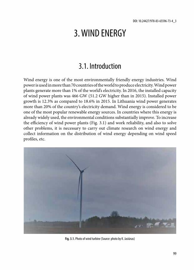
99

3. WIND ENERGY

3.1. Introduction

Wind energy is one of the most environmentally friendly energy industries. Wind power is used in more than 70 countries of the world to produce electricity. Wind power plants generate more than 1% of the world’s electricity. In 2016, the installed capacity of wind power plants was 466 GW (51.2 GW higher than in 2015). Installed power growth is 12.3% as compared to 18.6% in 2015. In Lithuania wind power generates more than 20% of the country’s electricity demand. Wind energy is considered to be one of the most popular renewable energy sources. In countries where this energy is already widely used, the environmental conditions substantially improve. To increase the efficiency of wind power plants (Fig. 3.1) and work reliability, and also to solve other problems, it is necessary to carry out climate research on wind energy and collect information on the distribution of wind energy depending on wind speed profiles, etc.

Fig. 3.1. Photo of wind turbine (Source: photo by K. Jasiūnas)

DOI: 10.24427/978-83-65596-73-4_3

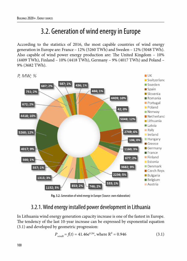
100


3.2. Generation of wind energy in Europe

According to the statistics of 2016, the most capable countries of wind energy generation in Europe are: France – 12% (5260 TWh) and Sweden – 12% (5048 TWh). Also capable of wind power energy production are: The United Kingdom – 10% (4409 TWh), Finland – 10% (4418 TWh), Germany – 9% (4017 TWh) and Poland – 9% (3682 TWh).

Fig. 3.2. Generation of wind energy in Europe (Source: own elaboration)

3.2.1. Wind energy installed power development in LithuaniaIn Lithuania wind energy generation capacity increase is one of the fastest in Europe. The tendency of the last 10-year increase can be expressed by exponential equation (3.1) and developed by geometric progression:

Pwindlt = f(t) = 41.46e0.26t, where R² = 0.946 (3.1)

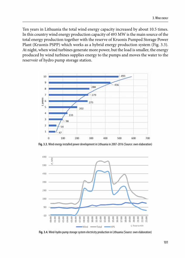
101

3. Wind energy

Ten years in Lithuania the total wind energy capacity increased by about 10.5 times. In this country wind energy production capacity of 493 MW is the main source of the total energy production together with the reserve of Kruonis Pumped Storage Power Plant (Kruonis PSPP) which works as a hybrid energy production system (Fig. 3.3). At night, when wind turbines generate more power, but the load is smaller, the energy produced by wind turbines supplies energy to the pumps and moves the water to the reservoir of hydro pump storage station.

Fig. 3.3. Wind energy installed power development in Lithuania in 2007-2016 (Source: own elaboration)

Fig. 3.4. Wind-hydro pump storage system electricity production in Lithuania (Source: own elaboration)

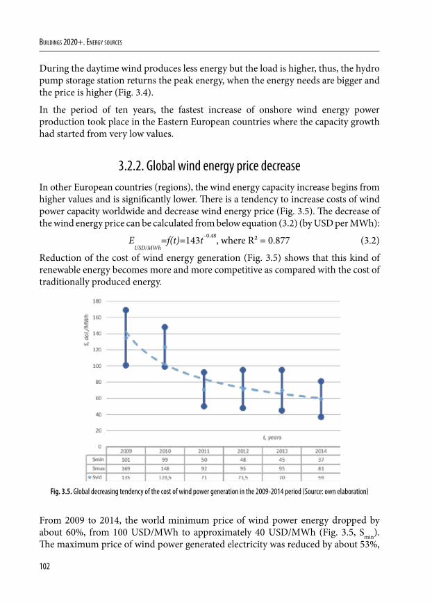
102


During the daytime wind produces less energy but the load is higher, thus, the hydro pump storage station returns the peak energy, when the energy needs are bigger and the price is higher (Fig. 3.4).

In the period of ten years, the fastest increase of onshore wind energy power production took place in the Eastern European countries where the capacity growth had started from very low values.

3.2.2. Global wind energy price decreaseIn other European countries (regions), the wind energy capacity increase begins from higher values and is significantly lower. There is a tendency to increase costs of wind power capacity worldwide and decrease wind energy price (Fig. 3.5). The decrease of the wind energy price can be calculated from below equation (3.2) (by USD per MWh):

EUSD/MWh

=f(t)=143t–0.48, where R² = 0.877 (3.2)

Reduction of the cost of wind energy generation (Fig. 3.5) shows that this kind of renewable energy becomes more and more competitive as compared with the cost of traditionally produced energy.

Fig. 3.5. Global decreasing tendency of the cost of wind power generation in the 2009-2014 period (Source: own elaboration)

From 2009 to 2014, the world minimum price of wind power energy dropped by about 60%, from 100 USD/MWh to approximately 40 USD/MWh (Fig. 3.5, Smin). The maximum price of wind power generated electricity was reduced by about 53%,

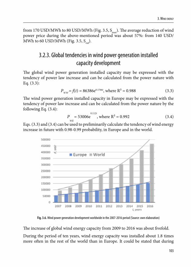
103

3. Wind energy

from 170 USD/MWh to 80 USD/MWh (Fig. 3.5, Smax). The average reduction of wind power price during the above-mentioned period was about 57%: from 140 USD/MWh to 60 USD/MWh (Fig. 3.5, Svid).

3.2.3. Global tendencies in wind power generation installed capacity development

The global wind power generation installed capacity may be expressed with the tendency of power law increase and can be calculated from the power nature with Eq. (3.3):

PWW = f(t) = 86386e0.1766t, where R² = 0.988 (3.3)

The wind power generation installed capacity in Europe may be expressed with the tendency of power law increase and can be calculated from the power nature by the following Eq. (3.4):

PWE

= 53006e0.112t

, where R² = 0.992 (3.4)

Eqs. (3.3) and (3.4) can be used to preliminarily calculate the tendency of wind energy increase in future with 0.98-0.99 probability, in Europe and in the world.

Fig. 3.6. Wind power generation development worldwide in the 2007-2016 period (Source: own elaboration)

The increase of global wind energy capacity from 2009 to 2016 was about fivefold.

During the period of ten years, wind energy capacity was installed about 1.8 times more often in the rest of the world than in Europe. It could be stated that during

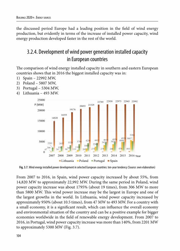
104


the discussed period Europe had a leading position in the field of wind energy production, but evidently in terms of the increase of installed power capacity, wind energy production developed faster in the rest of the world.

3.2.4. Development of wind power generation installed capacity in European countries

The comparison of wind energy installed capacity in southern and eastern European countries shows that in 2016 the biggest installed capacity was in:1) Spain – 22992 MW,2) Poland – 5807 MW,3) Portugal – 5304 MW, 4) Lithuania – 493 MW.

47 54 98 133 202 275 279 288 436 493306 526 709 1108 18002564

3429 3836 48865807

2201 2857 3326 3796 4256 4412 4610 4856 49385304

1482016555

1917620693 21529

22789 22958 22975 22943 22992

0

5000

10000

15000

20000

25000

2007 2008 2009 2010 2011 2012 2013 2014 2015 2016

Lithuania Poland Portugal Spain

P [MW]

Year

Fig. 3.7. Wind energy installed power development in selected European countries: ten-year tendency (Source: own elaboration)

From 2007 to 2016, in Spain, wind power capacity increased by about 55%, from 14,820 MW to approximately 22,992 MW. During the same period in Poland, wind power capacity increase was about 1795% (about 19 times), from 306 MW to more than 5800 MW. This wind power increase may be the largest in Europe and one of the largest growths in the world. In Lithuania, wind power capacity increased by approximately 950% (about 10.5 times), from 47 MW to 493 MW. For a country with a small economy, it is a significant result, which can influence the overall economy and environmental situation of the country and can be a positive example for bigger economies worldwide in the field of renewable energy development. From 2007 to 2016, in Portugal, wind power capacity increase was more than 140%, from 2201 MW to approximately 5300 MW (Fig. 3.7).

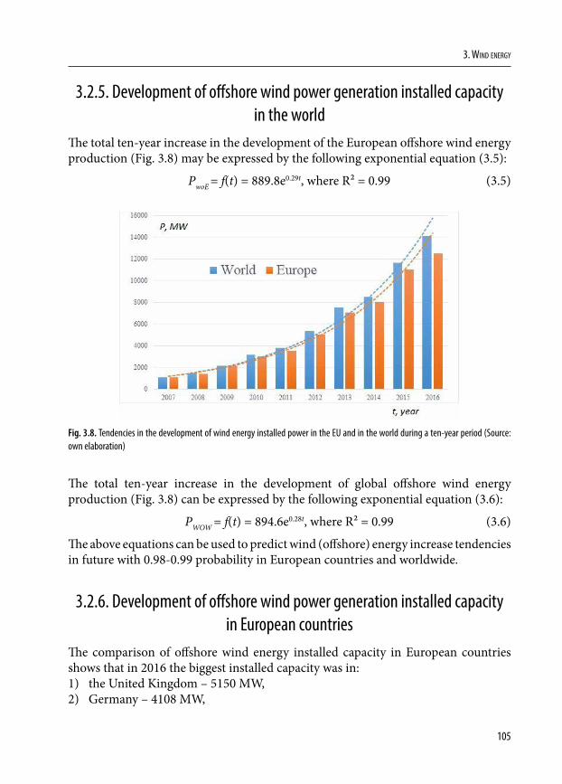
105

3. Wind energy

3.2.5. Development of offshore wind power generation installed capacity in the world

The total ten-year increase in the development of the European offshore wind energy production (Fig. 3.8) may be expressed by the following exponential equation (3.5):

PwoE = f(t) = 889.8e0.29t, where R² = 0.99 (3.5)

Fig. 3.8. Tendencies in the development of wind energy installed power in the EU and in the world during a ten-year period (Source: own elaboration)

The total ten-year increase in the development of global offshore wind energy production (Fig. 3.8) can be expressed by the following exponential equation (3.6):

PWOW = f(t) = 894.6e0.28t, where R² = 0.99 (3.6)

The above equations can be used to predict wind (offshore) energy increase tendencies in future with 0.98-0.99 probability in European countries and worldwide.

3.2.6. Development of offshore wind power generation installed capacity in European countries

The comparison of offshore wind energy installed capacity in European countries shows that in 2016 the biggest installed capacity was in:1) the United Kingdom – 5150 MW, 2) Germany – 4108 MW,

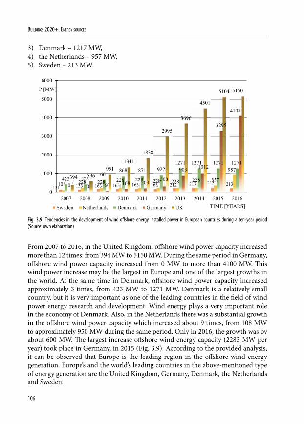
106


3) Denmark – 1217 MW, 4) the Netherlands – 957 MW,5) Sweden – 213 MW.

131 133 163 163 163 163 212 213 213 213108 228 228 228 228 228 228 228 357

957

423 423661

868 871 9221271 1271 1271 1271

0 0 60 168 203 308

903 1012

3295

4108

394 596951

1341

1838

2995

3696

4501

5104 5150

0

1000

2000

3000

4000

5000

6000

2007 2008 2009 2010 2011 2012 2013 2014 2015 2016

P [MW]

TIME [YEARS]Sweden Netherlands Denmark Germany UK

Fig. 3.9. Tendencies in the development of wind offshore energy installed power in European countries during a ten-year period (Source: own elaboration)

From 2007 to 2016, in the United Kingdom, offshore wind power capacity increased more than 12 times: from 394 MW to 5150 MW. During the same period in Germany, offshore wind power capacity increased from 0 MW to more than 4100 MW. This wind power increase may be the largest in Europe and one of the largest growths in the world. At the same time in Denmark, offshore wind power capacity increased approximately 3 times, from 423 MW to 1271 MW. Denmark is a relatively small country, but it is very important as one of the leading countries in the field of wind power energy research and development. Wind energy plays a very important role in the economy of Denmark. Also, in the Netherlands there was a substantial growth in the offshore wind power capacity which increased about 9 times, from 108 MW to approximately 950 MW during the same period. Only in 2016, the growth was by about 600 MW. The largest increase offshore wind energy capacity (2283 MW per year) took place in Germany, in 2015 (Fig. 3.9). According to the provided analysis, it can be observed that Europe is the leading region in the offshore wind energy generation. Europe’s and the world’s leading countries in the above-mentioned type of energy generation are the United Kingdom, Germany, Denmark, the Netherlands and Sweden.

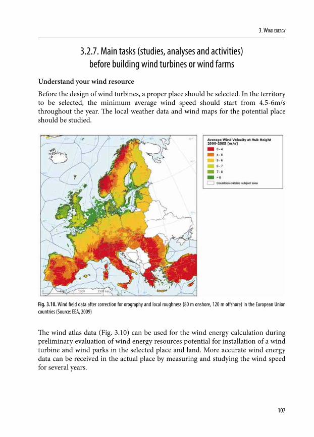
107

3. Wind energy

3.2.7. Main tasks (studies, analyses and activities) before building wind turbines or wind farms

Understand your wind resource

Before the design of wind turbines, a proper place should be selected. In the territory to be selected, the minimum average wind speed should start from 4.5-6m/s throughout the year. The local weather data and wind maps for the potential place should be studied.

Fig. 3.10. Wind field data after correction for orography and local roughness (80 m onshore, 120 m offshore) in the European Union countries (Source: EEA, 2009)

The wind atlas data (Fig. 3.10) can be used for the wind energy calculation during preliminary evaluation of wind energy resources potential for installation of a wind turbine and wind parks in the selected place and land. More accurate wind energy data can be received in the actual place by measuring and studying the wind speed for several years.

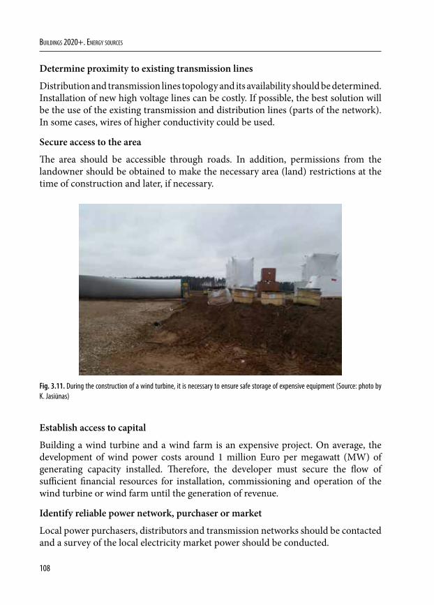
108


Determine proximity to existing transmission lines

Distribution and transmission lines topology and its availability should be determined. Installation of new high voltage lines can be costly. If possible, the best solution will be the use of the existing transmission and distribution lines (parts of the network). In some cases, wires of higher conductivity could be used.

Secure access to the area

The area should be accessible through roads. In addition, permissions from the landowner should be obtained to make the necessary area (land) restrictions at the time of construction and later, if necessary.

Fig. 3.11. During the construction of a wind turbine, it is necessary to ensure safe storage of expensive equipment (Source: photo by K. Jasiūnas)

Establish access to capital

Building a wind turbine and a wind farm is an expensive project. On average, the development of wind power costs around 1 million Euro per megawatt (MW) of generating capacity installed. Therefore, the developer must secure the flow of sufficient financial resources for installation, commissioning and operation of the wind turbine or wind farm until the generation of revenue.

Identify reliable power network, purchaser or market

Local power purchasers, distributors and transmission networks should be contacted and a survey of the local electricity market power should be conducted.

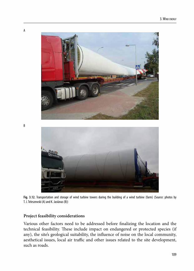
109

3. Wind energy

A

B

Fig. 3.12. Transportation and storage of wind turbine towers during the building of a wind turbine (farm) (Source: photos by T. J. Teleszewski (A) and K. Jasiūnas (B))

Project feasibility considerations

Various other factors need to be addressed before finalizing the location and the technical feasibility. These include impact on endangered or protected species (if any), the site’s geological suitability, the influence of noise on the local community, aesthetical issues, local air traffic and other issues related to the site development, such as roads.

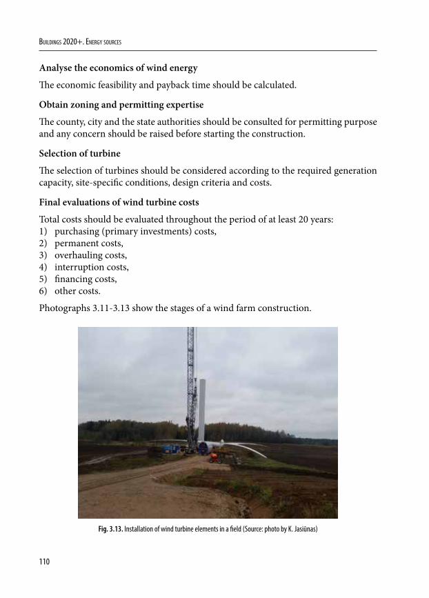
110


Analyse the economics of wind energy

The economic feasibility and payback time should be calculated.

Obtain zoning and permitting expertise

The county, city and the state authorities should be consulted for permitting purpose and any concern should be raised before starting the construction.

Selection of turbine

The selection of turbines should be considered according to the required generation capacity, site-specific conditions, design criteria and costs.

Final evaluations of wind turbine costs

Total costs should be evaluated throughout the period of at least 20 years:1) purchasing (primary investments) costs,2) permanent costs,3) overhauling costs,4) interruption costs,5) financing costs,6) other costs.

Photographs 3.11-3.13 show the stages of a wind farm construction.

Fig. 3.13. Installation of wind turbine elements in a field (Source: photo by K. Jasiūnas)

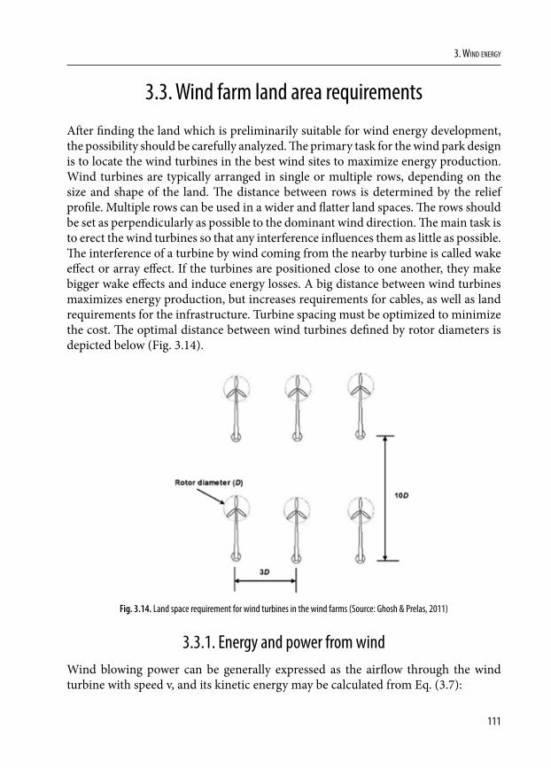
111

3. Wind energy

3.3. Wind farm land area requirements

After finding the land which is preliminarily suitable for wind energy development, the possibility should be carefully analyzed. The primary task for the wind park design is to locate the wind turbines in the best wind sites to maximize energy production. Wind turbines are typically arranged in single or multiple rows, depending on the size and shape of the land. The distance between rows is determined by the relief profile. Multiple rows can be used in a wider and flatter land spaces. The rows should be set as perpendicularly as possible to the dominant wind direction. The main task is to erect the wind turbines so that any interference influences them as little as possible. The interference of a turbine by wind coming from the nearby turbine is called wake effect or array effect. If the turbines are positioned close to one another, they make bigger wake effects and induce energy losses. A big distance between wind turbines maximizes energy production, but increases requirements for cables, as well as land requirements for the infrastructure. Turbine spacing must be optimized to minimize the cost. The optimal distance between wind turbines defined by rotor diameters is depicted below (Fig. 3.14).

Fig. 3.14. Land space requirement for wind turbines in the wind farms (Source: Ghosh & Prelas, 2011)

3.3.1. Energy and power from windWind blowing power can be generally expressed as the airflow through the wind turbine with speed v, and its kinetic energy may be calculated from Eq. (3.7):

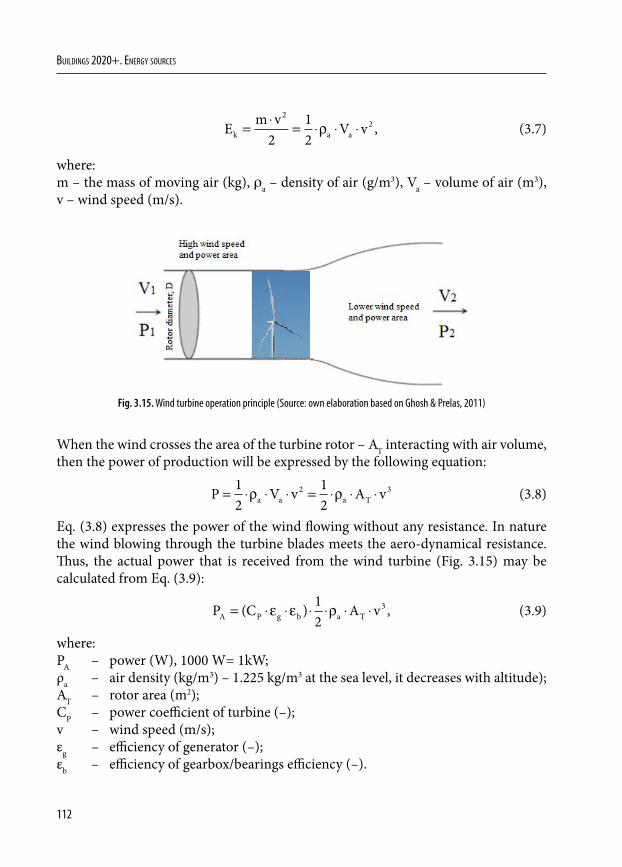
112


E m v V vk a a= ⋅ = ⋅ ⋅ ⋅

22

212

ρ , (3.7)

where:m – the mass of moving air (kg), ρa – density of air (g/m3), Va – volume of air (m3), v – wind speed (m/s).

Fig. 3.15. Wind turbine operation principle (Source: own elaboration based on Ghosh & Prelas, 2011)

When the wind crosses the area of the turbine rotor – AT interacting with air volume, then the power of production will be expressed by the following equation:

P V v A va a a T= ⋅ ⋅ ⋅ = ⋅ ⋅ ⋅12

12

2 3ρ ρ (3.8)

Eq. (3.8) expresses the power of the wind flowing without any resistance. In nature the wind blowing through the turbine blades meets the aero-dynamical resistance. Thus, the actual power that is received from the wind turbine (Fig. 3.15) may be calculated from Eq. (3.9):

P C A vA P g b a T= ⋅ ⋅ ⋅ ⋅ ⋅ ⋅( ) ,ε ε ρ1

23 (3.9)

where:PA – power (W), 1000 W= 1kW;ρa – air density (kg/m3) – 1.225 kg/m3 at the sea level, it decreases with altitude);AT – rotor area (m2);CP – power coefficient of turbine (–);v – wind speed (m/s);εg – efficiency of generator (–);εb – efficiency of gearbox/bearings efficiency (–).

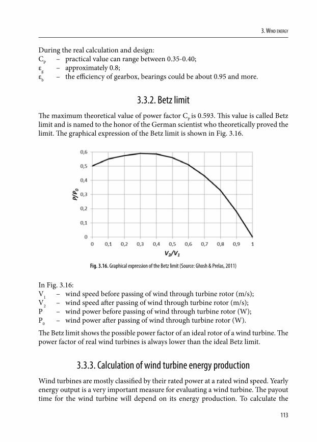
113

3. Wind energy

During the real calculation and design:CP – practical value can range between 0.35-0.40;εg – approximately 0.8;εb – the efficiency of gearbox, bearings could be about 0.95 and more.

3.3.2. Betz limitThe maximum theoretical value of power factor CP is 0.593. This value is called Betz limit and is named to the honor of the German scientist who theoretically proved the limit. The graphical expression of the Betz limit is shown in Fig. 3.16.

Fig. 3.16. Graphical expression of the Betz limit (Source: Ghosh & Prelas, 2011)

In Fig. 3.16:V1 – wind speed before passing of wind through turbine rotor (m/s);V2 – wind speed after passing of wind through turbine rotor (m/s);P – wind power before passing of wind through turbine rotor (W);P0 – wind power after passing of wind through turbine rotor (W).

The Betz limit shows the possible power factor of an ideal rotor of a wind turbine. The power factor of real wind turbines is always lower than the ideal Betz limit.

3.3.3. Calculation of wind turbine energy production Wind turbines are mostly classified by their rated power at a rated wind speed. Yearly energy output is a very important measure for evaluating a wind turbine. The payout time for the wind turbine will depend on its energy production. To calculate the

114


expected energy output, the capacity factor of the turbine should be evaluated. The real wind turbine capacity factor will be from 0.20 to 0.30. A very effective enormous power wind turbine capacity factor could be 0.40. Energy produced from the wind turbine can be calculated using a simple equation:

E C P tP= ⋅ ⋅ , (3.10)

where:E – energy (kWh) ; CP – power factor (–);P – power (kW);t – time (h).

An example of wind turbine energy production calculation:

By multiplying the rated power output by the capacity factor and the number of hours per year (8760 h/year), we can calculate an estimate of annual energy production for 100 kW. If the turbine produces 28 kW at the average wind speed of 6.7 m/s, the energy production per year will be: 100 kW · 0.28 · 8760 = 245,280 kWh.

3.3.4. Influence of land surface type on wind characteristicsThe simple equation may be used to calculate the impact of the ground surface roughness on the speed of the wind:

vv

HH0 0

=

α

, (3.11)

where:v – the wind speed at height H (m/s);v0 – the wind speed at height H0 (could be taken from a wind atlas) (m/s);α – land surface friction factor (–).

The friction factor α depends on the landform where the wind blows. Some values of the friction factor α are stated below:• smooth hard ground, calm water – 0.10;• tall grass on level ground – 0.15;• high crops, hedges and shrubs – 0.20;• wooded countryside, many trees – 0.25;• small towns with trees and gardens – 0.30;• large city with tall buildings – 0.40.

115

3. Wind energy

An example of influence of land surface type on the evaluation of wind characteristics:

According to the wind atlas, an area with crops, hedges and shrubs determinates a 5 m/s wind speed at a height of 10 m above the ground. The velocity and power of the wind at a height of 70 m should be calculated. The environmental conditions: temperature of +15oC and pressure of one atmosphere should be taken into consideration. From the above data, the friction coefficient α for the area with crops, hedges and shrubs, equals 0.20. At the temperature of 15oC and the pressure of 1 atmosphere, the air density equals ρ=1.225 kg/m3. Using the above-mentioned Eq. (3.11), the wind speed at a height of 70 m above the ground equals:

v ms70

0 2

5 7010

7 4= ×

=.

.

and the wind power will amount to:

p v Wm70

3 32

12

0 5 1 225 7 4 248 2= ⋅ ⋅ = × × =ρ . . . .

It was calculated that at 70 m above the ground, the wind power is more than three times bigger than at the height of 10 m (76.5 W/m2).

3.4. Construction and types of wind turbines

Wind energy is a renewable or alternative energy source in relation to conventional energy sources. Apart from the energy expenditure related to the construction of such a power plant, generation of wind energy does not entail the burning of any fuel. In 2016, the global wind power capacity expanded to 486.749 MW (GWEC, 2017). Wind power is already the global leader in green technologies and its usage is constantly growing. A wind power plant is a plant that generates electricity using wind generators. Its main element is a wind turbine or wind rotor converting the kinetic energy of the wind into mechanical work in the form of rotational motion of the rotor. The main elements of a typical wind turbine are (Fig. 3.17): a rotor with blades, main shaft, gearbox, brake, coupling, generator, wind vane/anemometer, housing, tower, and yaw motor/gear.

116


1 3 4 5 6 7

8 9 10

2

Fig. 3.17. Components of a wind turbine: 1 – rotor with blades, 2 – main shaft, 3 – gearbox, 4 – brake, 5 – coupling, 6 – generator, 7 – wind vane/anemometer, 8 – housing, 9 – tower, 10 – yaw motor/gear (Source: own elaboration)

The tower supports the rotor of the wind turbine at the desired height. The main types of towers used in wind turbines are the tubular steel tower, lattice tower, and the guyed tower. Examples of a tubular concrete tower, tubular steel tower, combined lattice tower and guyed tower are shown in Fig. 3.18A, B and C respectively. In large wind power plants, the towers have service shafts and controls for the operation of the plant. An example of the interior of a tubular steel tower is shown in Fig. 3.19.

A B C

Fig. 3.18. Different types of towers: A) tubular concrete tower, B) tubular steel tower, C) combined lattice and guyed tower (Source: photo by T. J. Teleszewski)

As the central element of the drive system, the gearbox converts the low speed of the rotor shaft into a high rotation that drives the generator. The speed of a typical wind turbine rotor can be about 40 rpm, while the optimum speed of the generator can be

117

3. Wind energy

about 1200 rpm (Mathew, 2006). A view of a sample gearbox made by the Winergy company is shown in Fig. 3.20.

A B

Fig. 3.19. The interior of a tubular steel tower A) service ladder, B) control cabinet (Source: photos by T.J. Teleszewski)

Fig. 3.20. View of the gearbox in a wind turbine gondola (Source: photo by T.J. Teleszewski)

A reliable connection of the gearbox to the generator is an important factor in the successful production of wind energy. The coupling not only transmits the torque, but also protects the connected components from overloads and travelling leakage currents. An example of a shielded coupling that connects the gear drive to the generator is shown in Fig. 3.21.

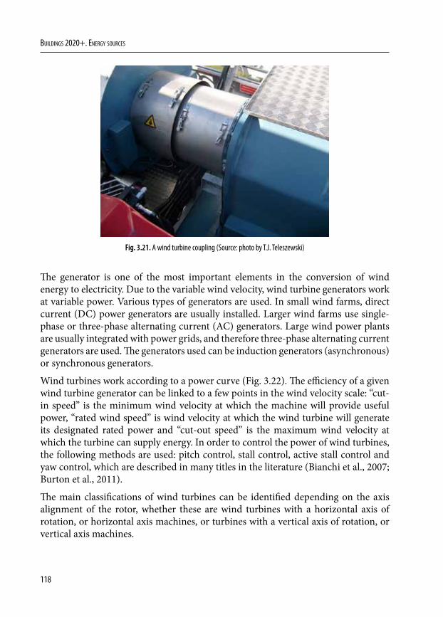
118


Fig. 3.21. A wind turbine coupling (Source: photo by T.J. Teleszewski)

The generator is one of the most important elements in the conversion of wind energy to electricity. Due to the variable wind velocity, wind turbine generators work at variable power. Various types of generators are used. In small wind farms, direct current (DC) power generators are usually installed. Larger wind farms use single-phase or three-phase alternating current (AC) generators. Large wind power plants are usually integrated with power grids, and therefore three-phase alternating current generators are used. The generators used can be induction generators (asynchronous) or synchronous generators.

Wind turbines work according to a power curve (Fig. 3.22). The efficiency of a given wind turbine generator can be linked to a few points in the wind velocity scale: “cut-in speed” is the minimum wind velocity at which the machine will provide useful power, “rated wind speed” is wind velocity at which the wind turbine will generate its designated rated power and “cut-out speed” is the maximum wind velocity at which the turbine can supply energy. In order to control the power of wind turbines, the following methods are used: pitch control, stall control, active stall control and yaw control, which are described in many titles in the literature (Bianchi et al., 2007; Burton et al., 2011).

The main classifications of wind turbines can be identified depending on the axis alignment of the rotor, whether these are wind turbines with a horizontal axis of rotation, or horizontal axis machines, or turbines with a vertical axis of rotation, or vertical axis machines.

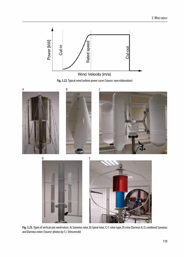
119

3. Wind energy

Fig. 3.22. Typical wind turbine power curve (Source: own elaboration)

A B C

D E

Fig. 3.23. Types of vertical axis wind rotors: A) Savonius rotor, B) Spiral rotor, C) C-rotor type, D) rotor Darrieus H, E) combined Savonius and Darrieus rotors (Source: photos by T.J. Teleszewski)

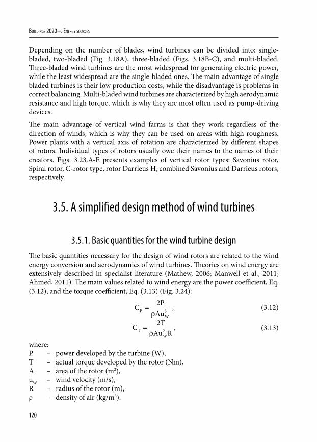
120


Depending on the number of blades, wind turbines can be divided into: single-bladed, two-bladed (Fig. 3.18A), three-bladed (Figs. 3.18B-C), and multi-bladed. Three-bladed wind turbines are the most widespread for generating electric power, while the least widespread are the single-bladed ones. The main advantage of single bladed turbines is their low production costs, while the disadvantage is problems in correct balancing. Multi-bladed wind turbines are characterized by high aerodynamic resistance and high torque, which is why they are most often used as pump-driving devices.

The main advantage of vertical wind farms is that they work regardless of the direction of winds, which is why they can be used on areas with high roughness. Power plants with a vertical axis of rotation are characterized by different shapes of rotors. Individual types of rotors usually owe their names to the names of their creators. Figs. 3.23.A-E presents examples of vertical rotor types: Savonius rotor, Spiral rotor, C-rotor type, rotor Darrieus H, combined Savonius and Darrieus rotors, respectively.

3.5. A simplified design method of wind turbines

3.5.1. Basic quantities for the wind turbine designThe basic quantities necessary for the design of wind rotors are related to the wind energy conversion and aerodynamics of wind turbines. Theories on wind energy are extensively described in specialist literature (Mathew, 2006; Manwell et al., 2011; Ahmed, 2011). The main values related to wind energy are the power coefficient, Eq. (3.12), and the torque coefficient, Eq. (3.13) (Fig. 3.24):

C PAuP

W

= 23ρ

, (3.12)

C TAu RT

W

= 22ρ

, (3.13)

where:P – power developed by the turbine (W),T – actual torque developed by the rotor (Nm),A – area of the rotor (m2),uW – wind velocity (m/s),R – radius of the rotor (m),ρ – density of air (kg/m3).

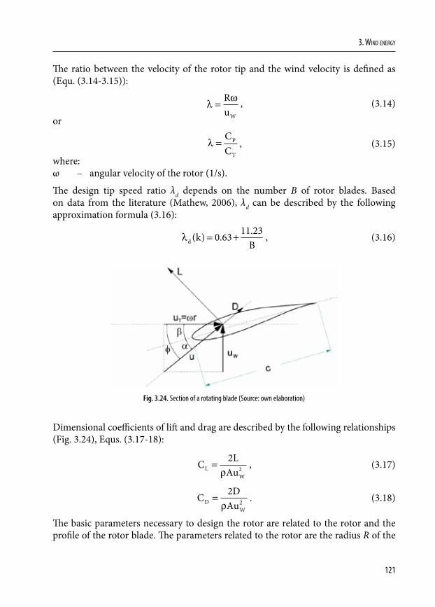
121

3. Wind energy

The ratio between the velocity of the rotor tip and the wind velocity is defined as (Equ. (3.14-3.15)):

λ ω= RuW

, (3.14)

or

λ =CC

P

T

, (3.15)

where:ω – angular velocity of the rotor (1/s).

The design tip speed ratio λd depends on the number B of rotor blades. Based on data from the literature (Mathew, 2006), λd can be described by the following approximation formula (3.16):

λd kB

( ) . .= +0 63 11 23 , (3.16)

Fig. 3.24. Section of a rotating blade (Source: own elaboration)

Dimensional coefficients of lift and drag are described by the following relationships (Fig. 3.24), Equs. (3.17-18):

C LAuL

W

= 22ρ

, (3.17)

C DAuD

W

= 22ρ

. (3.18)

The basic parameters necessary to design the rotor are related to the rotor and the profile of the rotor blade. The parameters related to the rotor are the radius R of the

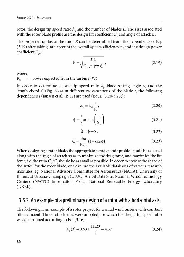
122


rotor, the design tip speed ratio λd and the number of blades B. The sizes associated with the rotor blade profile are the design lift coefficient CL and angle of attack α.

The projected radius of the rotor R can be determined from the dependence of Eq. (3.19) after taking into account the overall system efficiency η, and the design power coefficient CPD:

RP

C uD

PD D

=2

3η ρπ, (3.19)

where:PD – power expected from the turbine (W)

In order to determine a local tip speed ratio λr, blade setting angle β, and the length chord C (Fig. 3.24) in different cross-sections of the blade r, the following dependencies (Jansen et al., 1982) are used (Equs. (3.20-3.23)):

λ λr drR

= , (3.20)

φλ

=

23

1arctanr

, (3.21)

β φ α= − , (3.22)

C rBCL

= −( )8 1π φcos . (3.23)

When designing a rotor blade, the appropriate aerodynamic profile should be selected along with the angle of attack so as to minimize the drag force, and maximize the lift force, i.e. the ratio CD/CL should be as small as possible. In order to choose the shape of the airfoil for the rotor blade, one can use the available databases of various research institutes, eg: National Advisory Committee for Aeronautics (NACA), University of Illinois at Urbana-Champaign (UIUC) Airfoil Data Site, National Wind Technology Center’s (NWTC) Information Portal, National Renewable Energy Laboratory (NREL).

3.5.2. An example of a preliminary design of a rotor with a horizontal axisThe following is an example of a rotor project for a small wind turbine with constant lift coefficient. Three rotor blades were adopted, for which the design tip speed ratio was determined according to Eq. (3.16):

λd ( ) . . .3 0 63 11 233

4 37= + = (3.24)

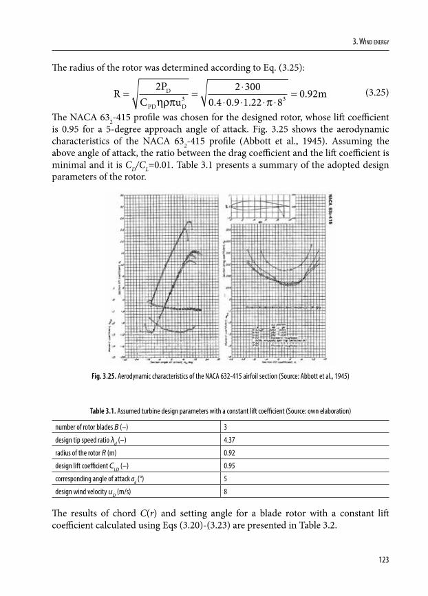
123

3. Wind energy

The radius of the rotor was determined according to Eq. (3.25):

RP

C umD

PD D

= = ⋅⋅ ⋅ ⋅ ⋅

=2 2 300

0 4 0 9 1 22 80 923 3ηρπ π. . .

. (3.25)

The NACA 632-415 profile was chosen for the designed rotor, whose lift coefficient is 0.95 for a 5-degree approach angle of attack. Fig. 3.25 shows the aerodynamic characteristics of the NACA 632-415 profile (Abbott et al., 1945). Assuming the above angle of attack, the ratio between the drag coefficient and the lift coefficient is minimal and it is CD/CL=0.01. Table 3.1 presents a summary of the adopted design parameters of the rotor.

Fig. 3.25. Aerodynamic characteristics of the NACA 632-415 airfoil section (Source: Abbott et al., 1945)

Table 3.1. Assumed turbine design parameters with a constant lift coefficient (Source: own elaboration)

number of rotor blades B (–) 3

design tip speed ratio λd (–) 4.37

radius of the rotor R (m) 0.92

design lift coefficient CLD (–) 0.95

corresponding angle of attack αd (°) 5

design wind velocity uD (m/s) 8

The results of chord C(r) and setting angle for a blade rotor with a constant lift coefficient calculated using Eqs (3.20)-(3.23) are presented in Table 3.2.

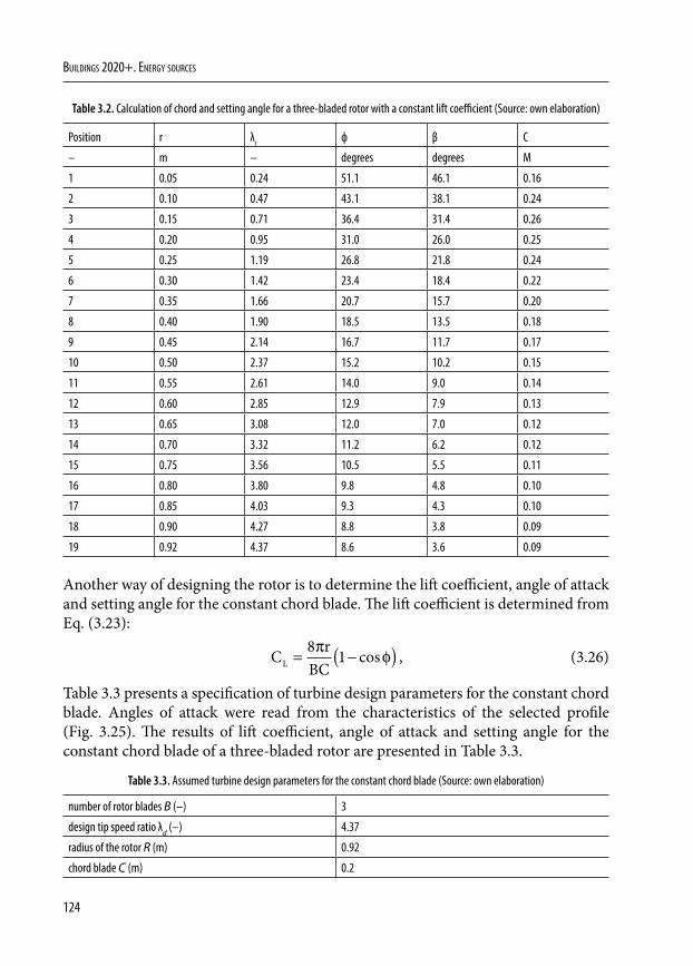
124


Table 3.2. Calculation of chord and setting angle for a three-bladed rotor with a constant lift coefficient (Source: own elaboration)

Position r λr ф β C

– m – degrees degrees M

1 0.05 0.24 51.1 46.1 0.16

2 0.10 0.47 43.1 38.1 0.24

3 0.15 0.71 36.4 31.4 0.26

4 0.20 0.95 31.0 26.0 0.25

5 0.25 1.19 26.8 21.8 0.24

6 0.30 1.42 23.4 18.4 0.22

7 0.35 1.66 20.7 15.7 0.20

8 0.40 1.90 18.5 13.5 0.18

9 0.45 2.14 16.7 11.7 0.17

10 0.50 2.37 15.2 10.2 0.15

11 0.55 2.61 14.0 9.0 0.14

12 0.60 2.85 12.9 7.9 0.13

13 0.65 3.08 12.0 7.0 0.12

14 0.70 3.32 11.2 6.2 0.12

15 0.75 3.56 10.5 5.5 0.11

16 0.80 3.80 9.8 4.8 0.10

17 0.85 4.03 9.3 4.3 0.10

18 0.90 4.27 8.8 3.8 0.09

19 0.92 4.37 8.6 3.6 0.09

Another way of designing the rotor is to determine the lift coefficient, angle of attack and setting angle for the constant chord blade. The lift coefficient is determined from Eq. (3.23):

C rBCL = −( )8 1π φcos , (3.26)

Table 3.3 presents a specification of turbine design parameters for the constant chord blade. Angles of attack were read from the characteristics of the selected profile (Fig. 3.25). The results of lift coefficient, angle of attack and setting angle for the constant chord blade of a three-bladed rotor are presented in Table 3.3.

Table 3.3. Assumed turbine design parameters for the constant chord blade (Source: own elaboration)

number of rotor blades B (–) 3

design tip speed ratio λd (–) 4.37

radius of the rotor R (m) 0.92

chord blade C (m) 0.2

125

3. Wind energy

Table 3.4. Calculation of setting angle, angle of attack and lift coefficient for a three-bladed rotor with a constant chord blade (Source: own elaboration)

Position r λr ф C CL α β

– m – degrees m – degrees degrees

1 0.05 0.24 51.1 0.2 0.78 3.0 48.1

2 0.10 0.48 43.1 0.2 1.13 6.0 37.1

3 0.15 0.71 36.3 0.2 1.22 7.0 29.3

4 0.20 0.95 31.0 0.2 1.19 6.9 24.1

5 0.25 1.19 26.7 0.2 1.12 6.0 20.7

6 0.30 1.43 23.4 0.2 1.03 5.0 18.4

7 0.35 1.66 20.7 0.2 0.94 4.9 15.8

8 0.40 1.90 18.5 0.2 0.87 4.0 14.5

9 0.45 2.14 16.7 0.2 0.80 3.1 13.6

10 0.50 2.38 15.2 0.2 0.73 2.0 13.2

11 0.55 2.61 14.0 0.2 0.68 1.9 12.1

12 0.60 2.85 12.9 0.2 0.63 1.8 11.1

13 0.65 3.09 12.0 0.2 0.59 1.5 10.5

14 0.70 3.33 11.2 0.2 0.55 1.0 10.2

15 0.75 3.57 10.4 0.2 0.52 0.9 9.5

16 0.80 3.80 9.8 0.2 0.49 0.7 9.1

17 0.85 4.04 9.3 0.2 0.46 0.5 8.8

18 0.92 4.37 8.6 0.2 0.43 0.0 8.6

3.6. Location of wind farms

Wind velocity has the most important impact on wind farm efficiency, which depends primarily on the location of the wind power plant in the area (Mathew, 2016). All kinds of terrain obstacles in the form of buildings or trees affect the roughness of the terrain. This translates into a significant reduction in wind velocity and increased turbulence. According to the classification of terrain roughness (Şen, 1999), wind farms should be located in a large, open space, i.e. in cultivated areas or on the open sea (Şen, 1999; Tian et al., 2015). Given the considerable roughness of urban areas, they are not a favourable location for wind farms, especially wind turbines with a horizontal axis, which should be located on the dominant wind directions.

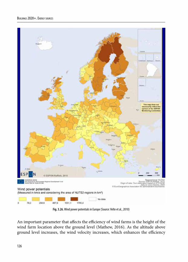
126


Fig. 3.26. Wind power potentials in Europe (Source: Velte et al., 2010)

An important parameter that affects the efficiency of wind farms is the height of the wind farm location above the ground level (Mathew, 2016). As the altitude above ground level increases, the wind velocity increases, which enhances the efficiency

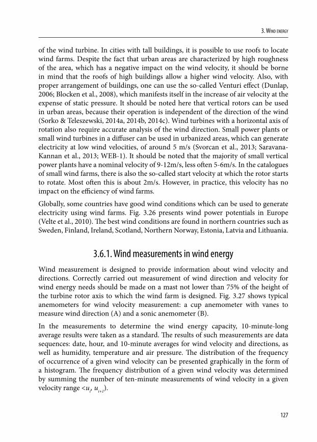
127

3. Wind energy

of the wind turbine. In cities with tall buildings, it is possible to use roofs to locate wind farms. Despite the fact that urban areas are characterized by high roughness of the area, which has a negative impact on the wind velocity, it should be borne in mind that the roofs of high buildings allow a higher wind velocity. Also, with proper arrangement of buildings, one can use the so-called Venturi effect (Dunlap, 2006; Blocken et al., 2008), which manifests itself in the increase of air velocity at the expense of static pressure. It should be noted here that vertical rotors can be used in urban areas, because their operation is independent of the direction of the wind (Sorko & Teleszewski, 2014a, 2014b, 2014c). Wind turbines with a horizontal axis of rotation also require accurate analysis of the wind direction. Small power plants or small wind turbines in a diffuser can be used in urbanized areas, which can generate electricity at low wind velocities, of around 5 m/s (Svorcan et al., 2013; Saravana-Kannan et al., 2013; WEB-1). It should be noted that the majority of small vertical power plants have a nominal velocity of 9-12m/s, less often 5-6m/s. In the catalogues of small wind farms, there is also the so-called start velocity at which the rotor starts to rotate. Most often this is about 2m/s. However, in practice, this velocity has no impact on the efficiency of wind farms.

Globally, some countries have good wind conditions which can be used to generate electricity using wind farms. Fig. 3.26 presents wind power potentials in Europe (Velte et al., 2010). The best wind conditions are found in northern countries such as Sweden, Finland, Ireland, Scotland, Northern Norway, Estonia, Latvia and Lithuania.

3.6.1. Wind measurements in wind energyWind measurement is designed to provide information about wind velocity and directions. Correctly carried out measurement of wind direction and velocity for wind energy needs should be made on a mast not lower than 75% of the height of the turbine rotor axis to which the wind farm is designed. Fig. 3.27 shows typical anemometers for wind velocity measurement: a cup anemometer with vanes to measure wind direction (A) and a sonic anemometer (B).

In the measurements to determine the wind energy capacity, 10-minute-long average results were taken as a standard. The results of such measurements are data sequences: date, hour, and 10-minute averages for wind velocity and directions, as well as humidity, temperature and air pressure. The distribution of the frequency of occurrence of a given wind velocity can be presented graphically in the form of a histogram. The frequency distribution of a given wind velocity was determined by summing the number of ten-minute measurements of wind velocity in a given velocity range <ui, ui+1).

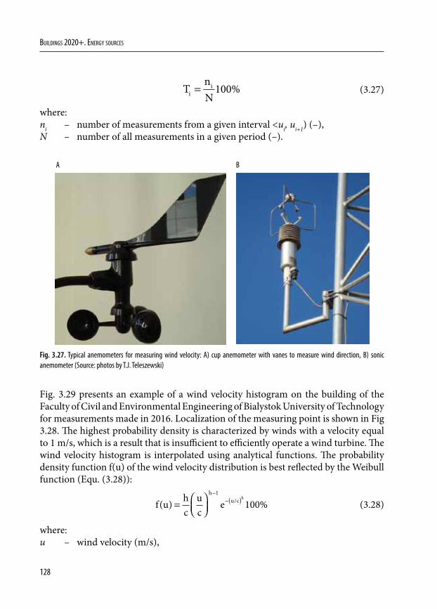
128


TnNi

i= 100% (3.27)

where:ni – number of measurements from a given interval <ui, ui+1) (–),N – number of all measurements in a given period (–).

A B

Fig. 3.27. Typical anemometers for measuring wind velocity: A) cup anemometer with vanes to measure wind direction, B) sonic anemometer (Source: photos by T.J. Teleszewski)

Fig. 3.29 presents an example of a wind velocity histogram on the building of the Faculty of Civil and Environmental Engineering of Bialystok University of Technology for measurements made in 2016. Localization of the measuring point is shown in Fig 3.28. The highest probability density is characterized by winds with a velocity equal to 1 m/s, which is a result that is insufficient to efficiently operate a wind turbine. The wind velocity histogram is interpolated using analytical functions. The probability density function f(u) of the wind velocity distribution is best reflected by the Weibull function (Equ. (3.28)):

f u h

cuc

eh

u c h

( ) %/=

−−( )

1

100 (3.28)

where:u – wind velocity (m/s),

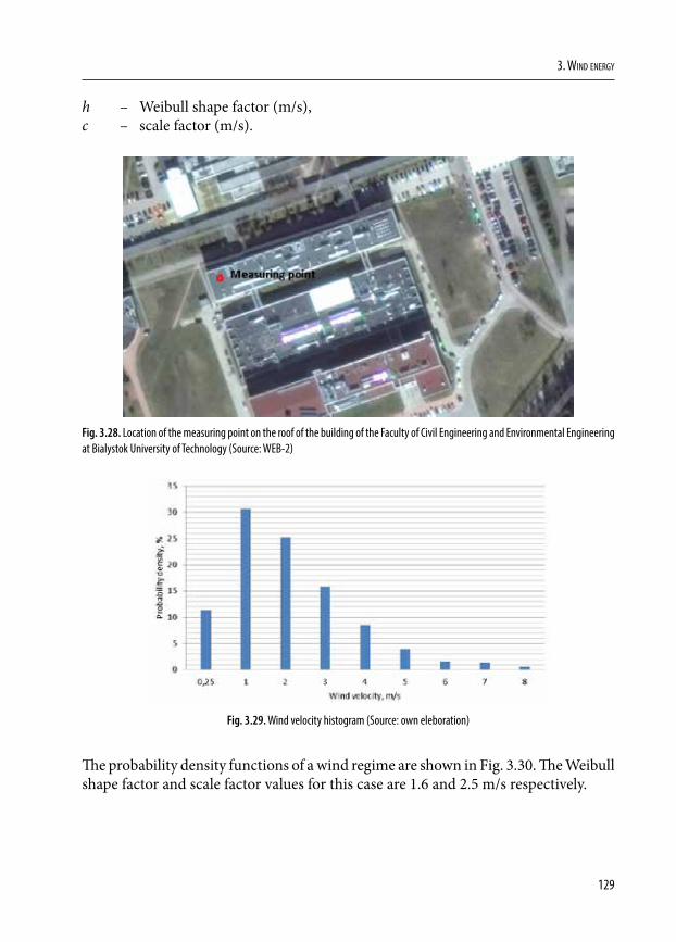
129

3. Wind energy

h – Weibull shape factor (m/s),c – scale factor (m/s).

Fig. 3.28. Location of the measuring point on the roof of the building of the Faculty of Civil Engineering and Environmental Engineering at Bialystok University of Technology (Source: WEB-2)

Fig. 3.29. Wind velocity histogram (Source: own eleboration)

The probability density functions of a wind regime are shown in Fig. 3.30. The Weibull shape factor and scale factor values for this case are 1.6 and 2.5 m/s respectively.

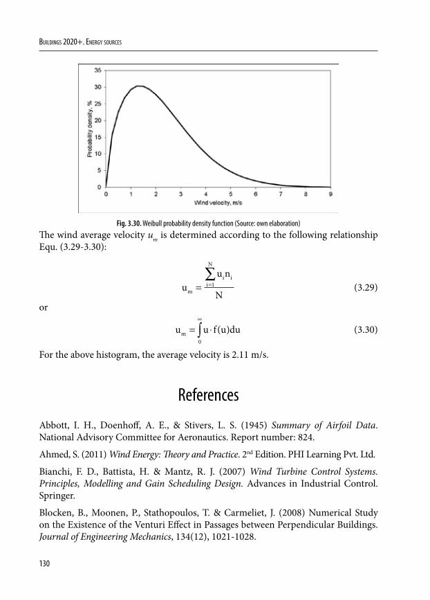
130


Fig. 3.30. Weibull probability density function (Source: own elaboration)The wind average velocity um is determined according to the following relationship Equ. (3.29-3.30):

uu n

Nm

i ii

N

= =∑

1 (3.29)

or

u u f u dum = ⋅∞

∫ ( )0

(3.30)

For the above histogram, the average velocity is 2.11 m/s.

References

Abbott, I. H., Doenhoff, A. E., & Stivers, L. S. (1945) Summary of Airfoil Data. National Advisory Committee for Aeronautics. Report number: 824.

Ahmed, S. (2011) Wind Energy: Theory and Practice. 2nd Edition. PHI Learning Pvt. Ltd.

Bianchi, F. D., Battista, H. & Mantz, R. J. (2007) Wind Turbine Control Systems. Principles, Modelling and Gain Scheduling Design. Advances in Industrial Control. Springer.

Blocken, B., Moonen, P., Stathopoulos, T. & Carmeliet, J. (2008) Numerical Study on the Existence of the Venturi Effect in Passages between Perpendicular Buildings. Journal of Engineering Mechanics, 134(12), 1021-1028.

131

3. Wind energy

Burton, T., Jenkins, N., Sharpe, D. & Bossanyi, E. (2011) Wind Energy Handbook. 2nd Edition. Wiley.

Dunlap, D. W. (2006) At New Trade Center, Seeking Lively (but Secure) Streets. The New York Times. [Online] 7th December, B4. Available from: https://www.nytimes.com/2006/12/07/nyregion/07blocks.html [Accessed 10th August 2018].

EEA (2009) Europe’s onshore and offshore wind energy potential. An assessment of environmental and economic constraints. EEA Technical report. Report number: 6.

Ghosh, T. K. & Prelas, M. A. (2011) Energy Resources and Systems. Volume 2: Renewable Resources. Springer.

GWEC (2017) Global Wind Statistics 2016. Global Wind Energy Council.

Jansen, W. A. M., Smulders, P. J. & Lysen, E. H. (1982) Wind Rotor Design. Renewable Energy Review Journal, 4(1), 14-28.

Manwell, J. F., McGowan, J. G. & Rogers, A. L. (2010) Wind Energy Explained: Theory, Design and Application. 2nd Edition. Wiley.

Mathew, S. (2006) Wind Energy. Fundamentals, Resource Analysis and Economics. Springer.

Saravana-Kannan, T., Mutasher, S. A. & Kenny-Lau, Y.H. (2013) Design and flow velocity simulation of diffuser augmented wind turbine using CFD. Journal of Engineering Science and Technology, 8(4), 372-384.

Şen, Z. (1999) Terrain topography classification for wind energy generation. Renewable Energy, 16, 904-907.

Sorko, S. A. & Teleszewski, T. J. (2014a) Modelowanie parametrów aerodynamicznych urządzeń energetyki wiatrowej I. Aerodynamiczna analiza profili wirników turbin i rotorów wiatrowych. Symulacja w Badaniach i Rozwoju, 5(1), 43-55.

Sorko, S. A. & Teleszewski, T. J. (2014b) Modelowanie parametrów aerodynamicznych urządzeń energetyki wiatrowej II. Analiza aerodynamiczna turbin wiatrowych o poziomej osi obrotu. Symulacja w Badaniach i Rozwoju, 5(1), 57-69.

Sorko, S. A. & Teleszewski, T. J. (2014c) Modelowanie parametrów aerodynamicznych urządzeń energetyki wiatrowej III. Analiza aerodynamiczna rotorów wiatrowych o pionowej osi obrotu. Symulacja w Badaniach i Rozwoju, 5(2), 119-128.

Svorcan, J., Stupar, S., Komarov, D., Peković, O. & Kostić, I. (2013) Aerodynamic design and analysis of a small-scale vertical axis wind turbine. Journal of Mechanical Science and Technology, 27(8), 2367-2373.

132


Tian, W., Ozbay, A. & Hu, H. (2015) Terrain effects on characteristics of surface wind and wind turbine wakes. Procedia Engineering. [Online] 126, 542-548. Available from: https://doi.org/10.1016/j.proeng.2015.11.302 [Accessed 10th August 2018].

Velte, D., Magro, E. & Jiménez, I. (2010) ReRisk. Regions at Risk of Energy Poverty. ESPON 2013.

WEB-1: AENews (2009) Small, low sp,eed wind turbine. Alternative Energy. [Online] Available from: http://www.alternative-energy-news.info/small-low-speed-wind-turbine [Accessed 10th August 2018].

WEB-2: www.google.pl/maps [Accessed 10th August 2018].

133

4. HYBRID RENEWABLE ENERGY

4.1. Introduction

In the energy sector, in recent times, increasing attention has been paid to renewable energy resources because of the rising fossil fuel prices, global climate change and environmental pollution.

Renewable energy is associated with rapid technology development. Renewable resources are an organic alternative to fossil fuels and so there is a constant tendency to maximize the use of the former and minimize the consumption of the latter. Fossil fuel reserves have been reduced and are constantly running out. The European Union has enough of energy resources to meet only half of its needs. This situation creates economic dependence on energy exporting countries. Another equally important issue is the increasing environmental pollution by burning fossil fuels and induced global climate change. The projected global increase in energy consumption means that there will be proportional increase in emissions and hazardous waste.

Using renewable energy systems means facing new challenges, such as the stable power supply. It started to develop hybrid systems that integrate both the previously used traditional energy systems with the new ones. The new system predominantly uses renewable energy sources. Wind, solar, earth and air energy systems could be used as autonomous energy systems.

4.2. Analysis of wind resources

In power systems with a high percentage of wind power, short-term wind power forecast has become a technique used for system operation and for submitting bids in electricity markets whenever wind generators are allowed to make bids. Prediction tools use numerical weather forecasts and one of them also uses real time SCADA data from the wind farms. Starting from these inputs and by means of physical and/or statistical models, hourly predictions for a time horizon of about 48 hours are provided.

DOI: 10.24427/978-83-65596-73-4_4

134


In general, the quality of a prediction depends mainly on two variables, the time between prediction and operation and the forecasting technique. Another important prediction factor is the forecasting process which is of smaller significance, though. Therefore, in general, the probability of over/under prediction might be considered equal.

4.3. Structure hybrid of renewable and conventional energy systems

Hybrid energy systems combine two or more parallel-operated energy conversion systems, two or more types of fuel per generation system to produce electricity or heat.

Hybrid systems combining distributed energy resources could be connected to a network, region or to the autonomous technological system and can be integrated into the residential, commercial and industrial buildings and industrial sectors.

Hybrid energy systems include distributed generation, renewable energy systems, hybrid energy generation technologies, energy storage systems, transmission network, distribution network, management systems, communication technologies and energy measurement systems.

Hybrid systems allow to:• use different fuels more flexibly,• use the energy more efficiently and reliably,• increase the quality of energy supply,• reduce environmental impact of energy generation,• improve economic performance,• increase flexibility of the energy supply according to the energy demand.

The operation of some renewable energy systems is changeable and interruptible. Combining two or more types of energy sources, including the use of energy storage systems, results in the continuous and efficient energy supply system.

Such power supply system is more reliable and the load (generation) schedule could be more stable and independent from a single energy source.

The components of hybrid energy systems:1. Energy from fossil fuels:

• internal combustion engines,• Stirling engines,

135

4. Hybrid renewable energy

• Steam turbines,• Brighton turbines,• micro turbines.

2. Renewable energy sources:• photovoltaic, photovoltaic with concentrators,• water heating with solar energy,• solar power hubs,• wind energy,• earth energy,• water energy.

3. Fuel cells (FC):• solid oxide FC,• proton exchange membranes FC,• phosphoric acid FC,• fused carbon acid FC.

4. Power supplies:• lead acid batteries,• electrochemical accumulators,• reversible fuel cells,• super-capacitors,• electromagnetic field storage,• flywheels,• thermal,• compressed air.

5. Cogeneration power plant.

A hybrid energy system could combine several different energy storage and accumulation systems, as well as other systems that use fossil fuels, such as gas power plants, diesel engines, etc. Hybrid energy system could include a nuclear power plant and all renewable resources such as solar, wind, geothermal energy resources, etc. Together with hybrid energy systems, new technologies like fuel cells, heat pumps, mini-generators etc. are developing fast.

A number of power generators connected to an energy network supply energy to the users or generate the energy as autonomous hybrid energy systems An example of a large hybrid system is shown in the diagram in Fig. 4.1.

The hybrid energy system using two sources of energy is called a double source system whereas the one that uses several sources is referred to as a multi-source system.

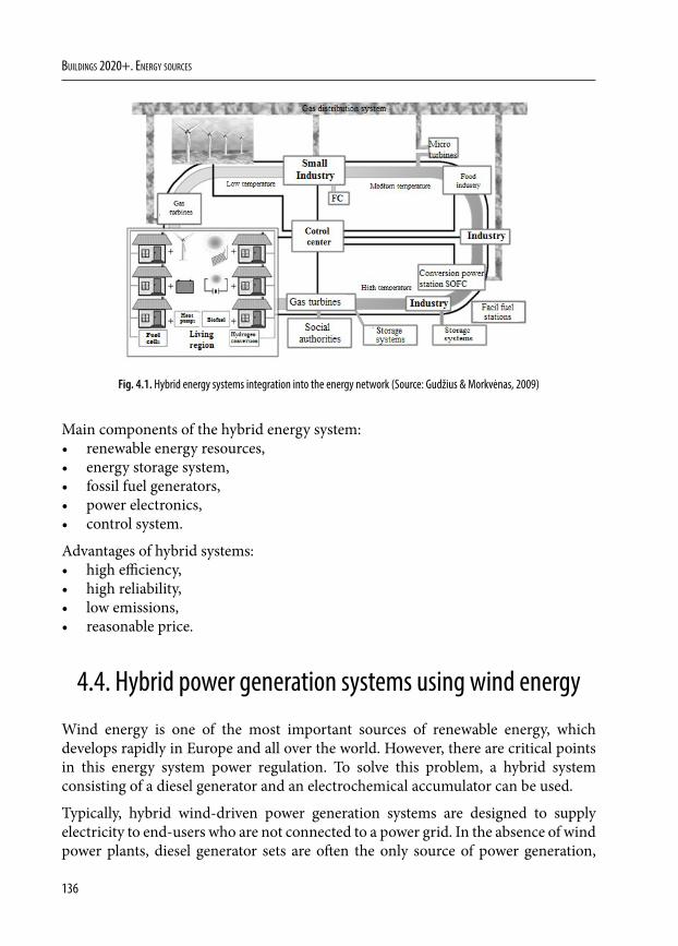
136


Fig. 4.1. Hybrid energy systems integration into the energy network (Source: Gudžius & Morkvėnas, 2009)

Main components of the hybrid energy system:• renewable energy resources,• energy storage system,• fossil fuel generators,• power electronics,• control system.

Advantages of hybrid systems:• high efficiency,• high reliability,• low emissions,• reasonable price.

4.4. Hybrid power generation systems using wind energy

Wind energy is one of the most important sources of renewable energy, which develops rapidly in Europe and all over the world. However, there are critical points in this energy system power regulation. To solve this problem, a hybrid system consisting of a diesel generator and an electrochemical accumulator can be used.

Typically, hybrid wind-driven power generation systems are designed to supply electricity to end-users who are not connected to a power grid. In the absence of wind power plants, diesel generator sets are often the only source of power generation,

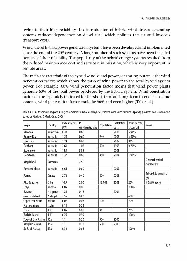
137


owing to their high reliability. The introduction of hybrid wind-driven generating systems reduces dependence on diesel fuel, which pollutes the air and involves transport costs.

Wind-diesel hybrid power generation systems have been developed and implemented since the end of the 20th century. A large number of such systems have been installed because of their reliability. The popularity of the hybrid energy systems resulted from the reduced maintenance cost and service minimization, which is very important in remote areas.

The main characteristic of the hybrid wind-diesel power generating system is the wind penetration factor, which shows the ratio of wind power to the total hybrid system power. For example, 60% wind penetration factor means that wind power plants generate 60% of the total power produced by the hybrid system. Wind penetration factor can be separately indicated for the short-term and long-term intervals. In some systems, wind penetration factor could be 90% and even higher (Table 4.1).

Table 4.1. Autonomous regions using commercial wind-diesel hybrid systems with wind turbines (parks) (Source: own elaboration based on Gudžius & Morkvėnas, 2009)

Region CountryP diesel gen., MW

Pwind parks, MW

PopulationInstalation data

Wind penetr. factor, pik

Notes

Mawson Antarctica 0.48 0.60 2003 >90%Bremer Bay Australia 1.28 0.60 240 2005 >90%Coral Bay Australia 2.24 0.60 2007 93%Denham Australia 2.61 1.02 600 1998 >70%Esperance Australia 14.0 5.85 2003Hopetoun Australia 1.37 0.60 350 2004 >90%

King Island Tasmania 2.50Electrochemical storage sys.

Rottnest Island Australia 0.64 0.60 2005

Ramea Canada 2.78 0.40 600 2003Rebuild. to wind-H2 sys.

Alto Baguales Chile 16.9 2.00 18,703 2002 20% 4.6 MW hydroFrøya Norway 0.05 0.06 100%Batanes Philipines 1.25 0.18 2004Graciosa Island Portugal 3.56 0.80 60%Cape Clear Island Ireland 0.07 0.06 100 70%Fuerteventura Spain 0.15 0.23Foula U.K, 0.05 0.06 31 70%Rathlin Island U. K. 0.26 0.99 100%Toksook Bay, Alaska USA 1.1 0.30 500 2006Kasigluk, Alaska USA 1.1 0.30 500 2006St. Paul, Alaska USA 0.30 0.68 100%

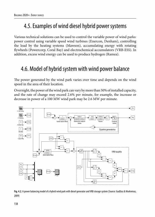
138


4.5. Examples of wind diesel hybrid power systems

Various technical solutions can be used to control the variable power of wind parks: power control using variable speed wind turbines (Enercon, Denham), controlling the load by the heating systems (Mawson), accumulating energy with rotating flywheels (Powercorp, Coral Bay) and electrochemical accumulators (VRB-ESS). In addition, excess wind energy can be used to produce hydrogen (Ramea).

4.6. Model of hybrid system with wind power balance

The power generated by the wind park varies over time and depends on the wind speed in the area of their location.

Overnight, the power of the wind park can vary by more than 50% of installed capacity, and the rate of change may exceed 2.6% per minute, for example, the increase or decrease in power of a 100 MW wind park may be 2.6 MW per minute.

50/60s+1

1

5/60s+1

0.02

720

Talpa VRB

>=

<

<

<

1s

1s

15/60s+1

0.2/60s+1

10

PN dyz. gen.

2

PN VRB

P vejo parko

P nustatyta

P nust.P

min

1s

[Pnust]

[Pv]

[Pg]

[PnVRB]

[PnG]

[PxT]

[Pvrb]

1

[Pvrb]

[Pg]

[Pv]

[Pnust]

[Pnust]

[Pnust]

[PnG]

[PxT]

5/60s+1

2/3600s +10/60s+12

50/60s

50/60s+1

|u|

|u|

|u|

|u|

Aukšto dažnio filtras Elektroninis valdymo blokas

Pavara Dyzelinisvariklis

Žemo dažnio filtras

Dyzelinis generatorius

VRB kaupiklis

Fig. 4.2. A power balancing model of a hybrid wind park with diesel generator and VRB storage system (Source: Gudžius & Morkvėnas, 2009)

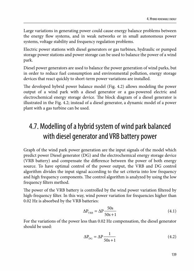
139


Large variations in generating power could cause energy balance problems between the energy flow systems, and in weak networks or in small autonomous power systems, voltage stability and frequency regulation problems.

Electric power stations with diesel generators or gas turbines, hydraulic or pumped storage power stations and power storage can be used to balance the power of a wind park.

Diesel power generators are used to balance the power generation of wind parks, but in order to reduce fuel consumption and environmental pollution, energy storage devices that react quickly to short-term power variations are installed.

The developed hybrid power balance model (Fig. 4.2) allows modeling the power output of a wind park with a diesel generator or a gas-powered electric and electrochemical energy storage device. The block diagram of a diesel generator is illustrated in the Fig. 4.2; instead of a diesel generator, a dynamic model of a power plant with a gas turbine can be used.

4.7. Modelling of a hybrid system of wind park balanced with diesel generator and VRB battery power

Graph of the wind park power generation are the input signals of the model which predict power Diesel generator (DG) and the electrochemical energy storage device (VRB battery) and compensate the difference between the power of both energy source. To have optimal control of the power output, the VRB and DG control algorithm divides the input signal according to the set criteria into low frequency and high frequency components. The control algorithm is analyzed by using the low frequency filters method.

The power of the VRB battery is controlled by the wind power variation filtered by high-frequency filter. In this way, wind power variation for frequencies higher than 0.02 Hz is absorbed by the VRB batteries:

∆ ∆P P s

sVRB =+

5050 1

(4.1)

For the variations of the power less than 0.02 Hz compensation, the diesel generator should be used:

∆ ∆P P

sDG =+

150 1

(4.2)

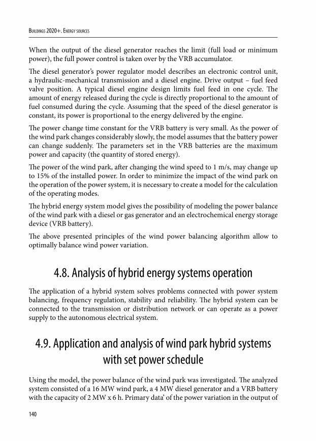
140


When the output of the diesel generator reaches the limit (full load or minimum power), the full power control is taken over by the VRB accumulator.

The diesel generator’s power regulator model describes an electronic control unit, a hydraulic-mechanical transmission and a diesel engine. Drive output – fuel feed valve position. A typical diesel engine design limits fuel feed in one cycle. The amount of energy released during the cycle is directly proportional to the amount of fuel consumed during the cycle. Assuming that the speed of the diesel generator is constant, its power is proportional to the energy delivered by the engine.

The power change time constant for the VRB battery is very small. As the power of the wind park changes considerably slowly, the model assumes that the battery power can change suddenly. The parameters set in the VRB batteries are the maximum power and capacity (the quantity of stored energy).

The power of the wind park, after changing the wind speed to 1 m/s, may change up to 15% of the installed power. In order to minimize the impact of the wind park on the operation of the power system, it is necessary to create a model for the calculation of the operating modes.

The hybrid energy system model gives the possibility of modeling the power balance of the wind park with a diesel or gas generator and an electrochemical energy storage device (VRB battery).

The above presented principles of the wind power balancing algorithm allow to optimally balance wind power variation.

4.8. Analysis of hybrid energy systems operationThe application of a hybrid system solves problems connected with power system balancing, frequency regulation, stability and reliability. The hybrid system can be connected to the transmission or distribution network or can operate as a power supply to the autonomous electrical system.

4.9. Application and analysis of wind park hybrid systems with set power schedule

Using the model, the power balance of the wind park was investigated. The analyzed system consisted of a 16 MW wind park, a 4 MW diesel generator and a VRB battery with the capacity of 2 MW x 6 h. Primary data’ of the power variation in the output of

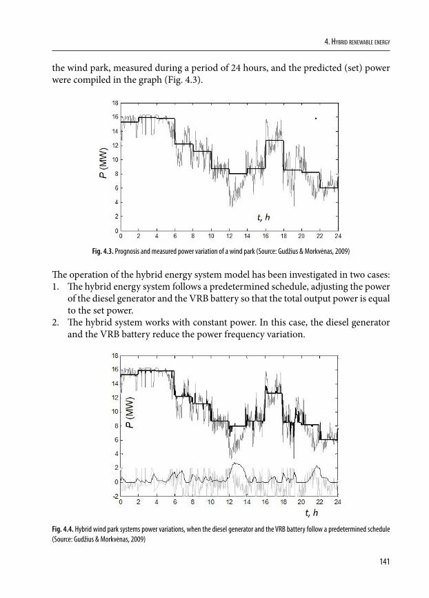
141


the wind park, measured during a period of 24 hours, and the predicted (set) power were compiled in the graph (Fig. 4.3).

Fig. 4.3. Prognosis and measured power variation of a wind park (Source: Gudžius & Morkvėnas, 2009)

The operation of the hybrid energy system model has been investigated in two cases:1. The hybrid energy system follows a predetermined schedule, adjusting the power

of the diesel generator and the VRB battery so that the total output power is equal to the set power.

2. The hybrid system works with constant power. In this case, the diesel generator and the VRB battery reduce the power frequency variation.

Fig. 4.4. Hybrid wind park systems power variations, when the diesel generator and the VRB battery follow a predetermined schedule (Source: Gudžius & Morkvėnas, 2009)

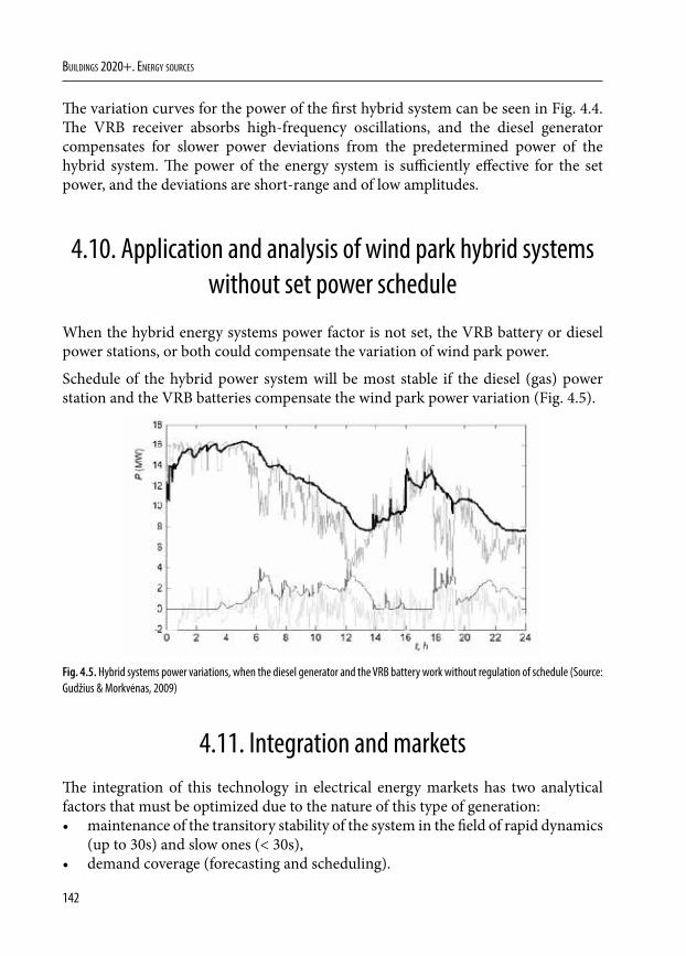
142


The variation curves for the power of the first hybrid system can be seen in Fig. 4.4. The VRB receiver absorbs high-frequency oscillations, and the diesel generator compensates for slower power deviations from the predetermined power of the hybrid system. The power of the energy system is sufficiently effective for the set power, and the deviations are short-range and of low amplitudes.

4.10. Application and analysis of wind park hybrid systems without set power schedule

When the hybrid energy systems power factor is not set, the VRB battery or diesel power stations, or both could compensate the variation of wind park power.

Schedule of the hybrid power system will be most stable if the diesel (gas) power station and the VRB batteries compensate the wind park power variation (Fig. 4.5).

Fig. 4.5. Hybrid systems power variations, when the diesel generator and the VRB battery work without regulation of schedule (Source: Gudžius & Morkvėnas, 2009)

4.11. Integration and marketsThe integration of this technology in electrical energy markets has two analytical factors that must be optimized due to the nature of this type of generation:• maintenance of the transitory stability of the system in the field of rapid dynamics

(up to 30s) and slow ones (< 30s), • demand coverage (forecasting and scheduling).

143


The maintenance of the transient stability must respond to different incidences of this type of generation (voltage failures, massive disconnections, short-circuit currents, permissible margins in frequency, inertia and damping). Voltage failures cause possible massive losses of power not supported by the electrical system in the case of three-phase and two-phase faults.

Regarding the frequency margins, current wind turbine technologies support frequency variations at a sufficient margin to maintain the system security. Concerning the inertia and damping of the electrical system, wind turbines with electronic converters present a power control with an extraordinarily fast power response isolating the mechanical and electrical systems. The high penetration of wind generation and the displacement of the conventional resources would lead to a significant decrease of the inertia in the electrical system.

Regarding the demand coverage, wind energy does not provide a guarantee of power. Its maximum slope of verified power is 10% of the installed power, increasing the requirements of another manageable generation.

Regarding the prediction, wind generation suffers considerable errors if the forecast is made long before the production time (average error referred to production time): 18% within 24 hours and 15% within 12 hours. These forecast errors lead to a stronger engagement of the deviation management service and the power-frequency regulation.

High production of energy with the use of wind resources displaces the manageable generation to provide more complementary services and therefore increasing the costs of these services. The generation through wind systems can also participate in this control of voltage at the connection point by the supervision of the system operator.

The management of these incidents needs to coordinate the generators in controlled groups. These control centers are responsible for managing the congestion in the evacuation of the generated energy, providing stability to voltage gaps, controlling short-circuit power, managing the viability of power balances and managing non-integrated surpluses.

4.12. Analysis of the results

The analysis of the hybrid system consisting of a 16 MW wind park, a 4 MW diesel generator and a VRB battery with the capacity of 2 MW x 6 h shows that the system effectively balances the variation of wind park power. It was determined that both

144


hybrid energy system operation algorithms were the schedule of power generation is predetermined. Both hybrid energy system operation algorithms followed predetermined schedules. When the hybrid energy system operated at constant power, it was efficient and with the stable schedule.

It has been calculated, that the analyzed hybrid energy systems wind park will produce 254 MWh per day. The diesel generator can compensate for power variation and should generate 30 MWh of electrical energy. The VRB batteries energy storage will be 10 MWh.

The analysis of the hybrid system model shows, that diesel generators are not suitable for total compensation of the rapid wind park power changes, as frequent changing of the diesel generators’ load is economically unreasonable. As a sudden power compensation, an energy storage system such as the VRB battery or analogous can be used.

In the case of the autonomous operation of the hybrid energy system, a diesel generator or a gas power station should act as the master generator, to keep all the load when the wind blows. The algorithm of the diesel generators and VRB batteries control should follow not only power schedule but also the changing of the frequency and it should also ensure using and generating power balance.

In the case of switching off the wind park generation, master generators (diesel or gas power stations) should keep all the power of the user load in the autonomous hybrid energy system.

ReferencesAdomavičius, V. (2013) Mažosios atsinaujinančiųjų išteklių energijos sistemos. Kaunas, KTU Technologija.

Ghosh, T. K. & Prelas, M. A. (2011) Energy Resources and Systems. Volume 2: Renewable Resources. Springer.

Gudžius, S. & Morkvėnas, A. (2009) Studija hibridinių energijos šaltinių ir jų sistemų modeliai, KTU.

Petrauskas, G. & Adomavičius, V. (2012a) Saulės energijos naudojimas elektrai gaminti. Kaunas, KTU Technologija.

Petrauskas, G. & Adomavičius, V. (2012b) Vėjo energijos naudojimas elektrai gaminti. Kaunas, KTU Technologija.

REE (2007) Integración de la energía Eólica en condiciones de Seguridad para el sistema. Red eléctrica de España.

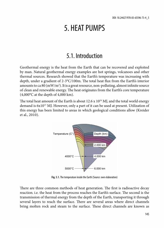
145

5. HEAT PUMPS

5.1. Introduction

Geothermal energy is the heat from the Earth that can be recovered and exploited by man. Natural geothermal energy examples are hot springs, volcanoes and other thermal sources. Research showed that the Earth’s temperature was increasing with depth, under a gradient of 2-3°C/100m. The total heat flux from the Earth’s interior amounts to ca 80 (mW/m2). It is a great resource, non-polluting, almost infinite source of clean and renewable energy. The heat originates from the Earth’s core temperature (4,000°C at the depth of 4,000 km).

The total heat amount of the Earth is about 12.6 x 1024 MJ, and the total world energy demand is 6x1013 MJ. However, only a part of it can be used at present. Utilization of this energy has been limited to areas in which geological conditions allow (Kreider et al., 2010).

5000°C

4000°C

Temperature (C°)

6.000 km

4.000 km

2.000 km

Depth (km)

Fig. 5.1. The temperature inside the Earth (Source: own elaboration)

There are three common methods of heat generation. The first is radioactive decay reaction, i.e. the heat from the process reaches the Earth’s surface. The second is the transmission of thermal energy from the depth of the Earth, transporting it through several layers to reach the surface. There are several areas where direct channels bring molten rock and steam to the surface. These direct channels are known as

DOI: 10.24427/978-83-65596-73-4_5

146


high temperature geothermal heat sources and can be used for electricity generation. The last of the heat generation methods is solar radiation. The earth’s crust absorbs approximately 47% of solar radiation, making it a very low-cost energy source. By some estimates, this low-cost energy geothermal source produces 500 times more energy than humanity uses in a year. The temperatures inside the Earth can be seen in Fig. 5.1.

Geothermal energy is classified according to the temperature: low (<150°C) or high temperature (>150°C). For heating, low temperature heat sources are used. High temperature geothermal energy is utilised for electricity generation. There are four types of geothermal power plants: dry steam power plants, flash power plants, binary power plants and combined flash-binary power plants.

Low temperature heat sources are commonly used for heating. The most useful are three possibilities. The first, direct heating, is one of the oldest and most common ways of geothermal energy use for building heating, e.g. in aquaculture, horticulture, balneological industry and swimming pools. The system is cost-effective, the main costs are generated by well-drilling and installation of transmission pumps, pipelines and other down-hole equipment (Kreider et al., 2010).

The second one is absorption machines technology. These machines are well known and used for heating and cooling. The absorption cycle is a process that uses heat energy instead of compressor work. In the cycle, a mixture of two fluids is used: a refrigerant, which evaporates and condenses, and a secondary fluid as an absorbent. For a cycle above 0°C, lithium bromide is used as the refrigerant and water as the absorbent, whereas for applications below 0°C an ammonia and water mix is used. Geothermal fluids run these machines. The geothermal effluent is usually expelled back into the reservoir from which it was taken to avoid the possible negative effect of the discharge on the environment.

The third possibility is a heat pump, used to transfer low-temperature heat stored in the earth to buildings.

The annual high temperature variability of the ground at the depth of 1.5 m, is nearly unnoticeable at depths of 18 m and more (Fig. 5.2).

The ground-source heat pump (GSHP) is able to use the low grade geothermal energy to heat and cool homes, schools, governmental and commercial buildings. The heat pump uses a relatively small amount of electricity to transport four times more heat energy to heat consumers. The first heat pump principle was described by Lord Kelvin in 1852. Robert Webber from Indianapolis modified the GHSP in 1945. It was first applied in the USA in 1960 and in Europe it has been used since 1970 (Oughton & Wilson, 2015).

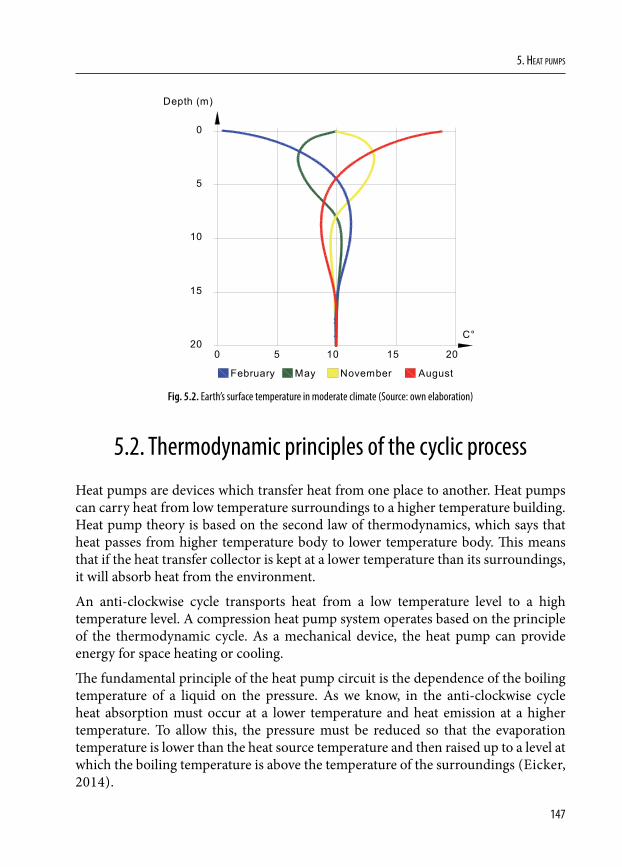
147

5. Heat pumps

1.

Depth (m)

5

10

15

20C°

February May November August

5 10 15 200

0

Fig. 5.2. Earth’s surface temperature in moderate climate (Source: own elaboration)

5.2. Thermodynamic principles of the cyclic process

Heat pumps are devices which transfer heat from one place to another. Heat pumps can carry heat from low temperature surroundings to a higher temperature building. Heat pump theory is based on the second law of thermodynamics, which says that heat passes from higher temperature body to lower temperature body. This means that if the heat transfer collector is kept at a lower temperature than its surroundings, it will absorb heat from the environment.

An anti-clockwise cycle transports heat from a low temperature level to a high temperature level. A compression heat pump system operates based on the principle of the thermodynamic cycle. As a mechanical device, the heat pump can provide energy for space heating or cooling.

The fundamental principle of the heat pump circuit is the dependence of the boiling temperature of a liquid on the pressure. As we know, in the anti-clockwise cycle heat absorption must occur at a lower temperature and heat emission at a higher temperature. To allow this, the pressure must be reduced so that the evaporation temperature is lower than the heat source temperature and then raised up to a level at which the boiling temperature is above the temperature of the surroundings (Eicker, 2014).

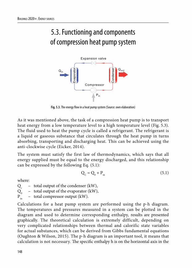
148


5.3. Functioning and components of compression heat pump system

QoutQinEv

apor

ator

Con

dens

er

Pin

Compressor

Expansion valve

Fig. 5.3. The energy flow in a heat pump system (Source: own elaboration)

As it was mentioned above, the task of a compression heat pump is to transport heat energy from a low temperature level to a high temperature level (Fig. 5.3). The fluid used to heat the pump cycle is called a refrigerant. The refrigerant is a liquid or gaseous substance that circulates through the heat pump in turns absorbing, transporting and discharging heat. This can be achieved using the anti-clockwise cycle (Eicker, 2014).

The system must satisfy the first law of thermodynamics, which says that all energy supplied must be equal to the energy discharged, and this relationship can be expressed by the following Eq. (5.1):

QC = Q0 + Pin (5.1)

where:Qc – total output of the condenser (kW),Q0 – total output of the evaporator (kW),Pin – total compressor output (kW).

Calculations for a heat pump system are performed using the p-h diagram. The temperatures and pressures measured in a system can be plotted in the diagram and used to determine corresponding enthalpy, results are presented graphically. The theoretical calculation is extremely difficult, depending on very complicated relationships between thermal and calorific state variables for actual substances, which can be derived from Gibbs fundamental equations (Oughton & Wilson, 2015). The p-h diagram is an important tool, it means that calculation is not necessary. The specific enthalpy h is on the horizontal axis in the

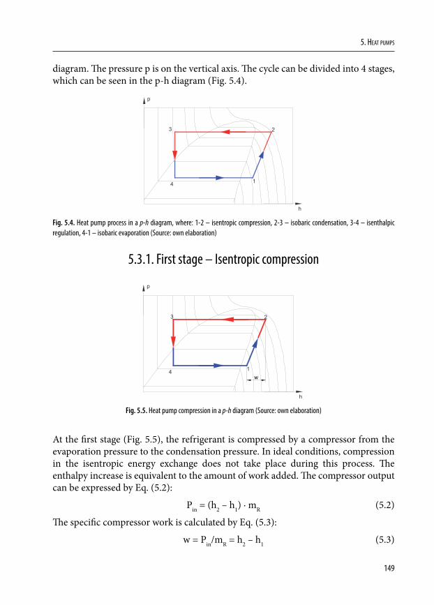
149

5. Heat pumps

diagram. The pressure p is on the vertical axis. The cycle can be divided into 4 stages, which can be seen in the p-h diagram (Fig. 5.4).

h

p

1

23

4

Fig. 5.4. Heat pump process in a p-h diagram, where: 1-2 – isentropic compression, 2-3 – isobaric condensation, 3-4 – isenthalpic regulation, 4-1 – isobaric evaporation (Source: own elaboration)

5.3.1. First stage – Isentropic compression

h

p

1

23

4w

Fig. 5.5. Heat pump compression in a p-h diagram (Source: own elaboration)

At the first stage (Fig. 5.5), the refrigerant is compressed by a compressor from the evaporation pressure to the condensation pressure. In ideal conditions, compression in the isentropic energy exchange does not take place during this process. The enthalpy increase is equivalent to the amount of work added. The compressor output can be expressed by Eq. (5.2):

Pin = (h2 – h1) · mR (5.2)

The specific compressor work is calculated by Eq. (5.3):

w = Pin/mR = h2 – h1 (5.3)

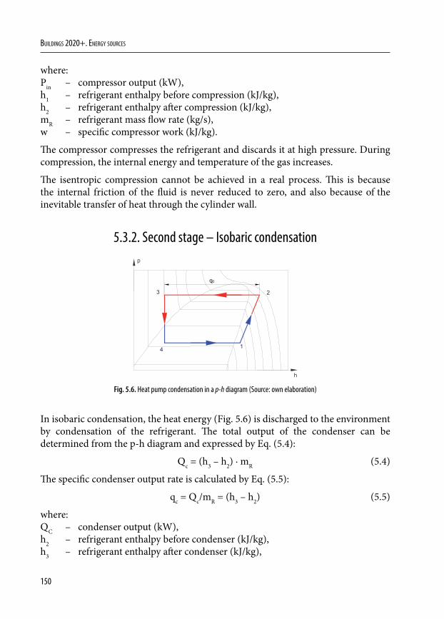
150


where:Pin – compressor output (kW),h1 – refrigerant enthalpy before compression (kJ/kg),h2 – refrigerant enthalpy after compression (kJ/kg),mR – refrigerant mass flow rate (kg/s),w – specific compressor work (kJ/kg).

The compressor compresses the refrigerant and discards it at high pressure. During compression, the internal energy and temperature of the gas increases.

The isentropic compression cannot be achieved in a real process. This is because the internal friction of the fluid is never reduced to zero, and also because of the inevitable transfer of heat through the cylinder wall.

5.3.2. Second stage – Isobaric condensation

h

p

1

23

4

qc

Fig. 5.6. Heat pump condensation in a p-h diagram (Source: own elaboration)

In isobaric condensation, the heat energy (Fig. 5.6) is discharged to the environment by condensation of the refrigerant. The total output of the condenser can be determined from the p-h diagram and expressed by Eq. (5.4):

Qc = (h3 – h2) · mR (5.4)

The specific condenser output rate is calculated by Eq. (5.5):

qc = Qc/mR = (h3 – h2) (5.5)

where:QC – condenser output (kW),h2 – refrigerant enthalpy before condenser (kJ/kg),h3 – refrigerant enthalpy after condenser (kJ/kg),

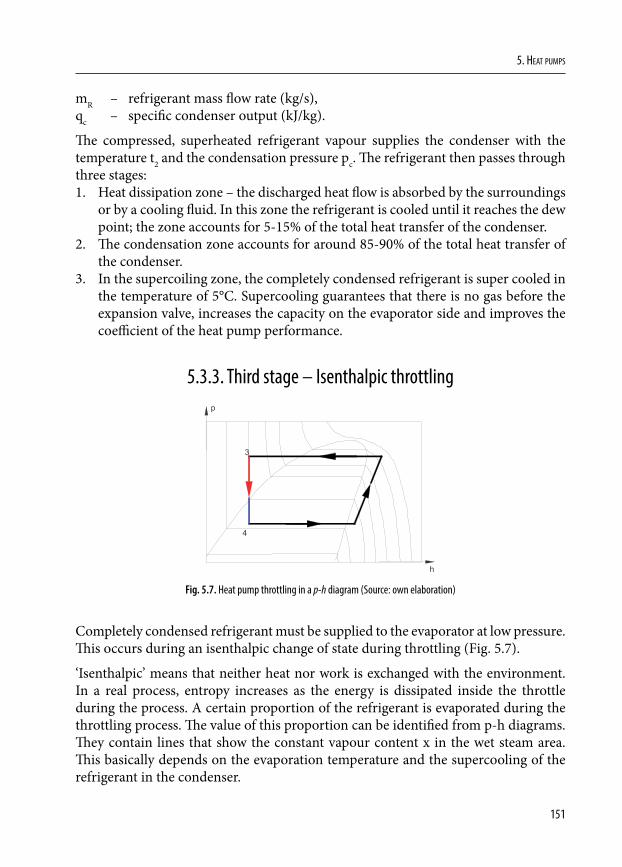
151

5. Heat pumps

mR – refrigerant mass flow rate (kg/s),qc – specific condenser output (kJ/kg).

The compressed, superheated refrigerant vapour supplies the condenser with the temperature t2 and the condensation pressure pc. The refrigerant then passes through three stages: 1. Heat dissipation zone – the discharged heat flow is absorbed by the surroundings

or by a cooling fluid. In this zone the refrigerant is cooled until it reaches the dew point; the zone accounts for 5-15% of the total heat transfer of the condenser.

2. The condensation zone accounts for around 85-90% of the total heat transfer of the condenser.

3. In the supercoiling zone, the completely condensed refrigerant is super cooled in the temperature of 5°C. Supercooling guarantees that there is no gas before the expansion valve, increases the capacity on the evaporator side and improves the coefficient of the heat pump performance.

5.3.3. Third stage – Isenthalpic throttling

h

p

3

4

Fig. 5.7. Heat pump throttling in a p-h diagram (Source: own elaboration)

Completely condensed refrigerant must be supplied to the evaporator at low pressure. This occurs during an isenthalpic change of state during throttling (Fig. 5.7).

‘Isenthalpic’ means that neither heat nor work is exchanged with the environment. In a real process, entropy increases as the energy is dissipated inside the throttle during the process. A certain proportion of the refrigerant is evaporated during the throttling process. The value of this proportion can be identified from p-h diagrams. They contain lines that show the constant vapour content x in the wet steam area. This basically depends on the evaporation temperature and the supercooling of the refrigerant in the condenser.

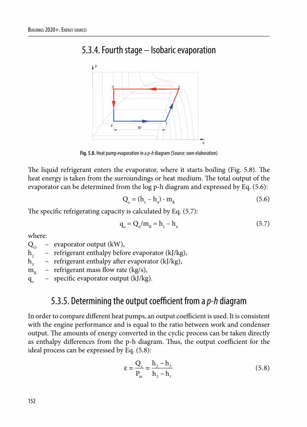
152


5.3.4. Fourth stage – Isobaric evaporation

h

p

1

23

4 q0

Fig. 5.8. Heat pump evaporation in a p-h diagram (Source: own elaboration)

The liquid refrigerant enters the evaporator, where it starts boiling (Fig. 5.8). The heat energy is taken from the surroundings or heat medium. The total output of the evaporator can be determined from the log p-h diagram and expressed by Eq. (5.6):

Qo = (h1 – h4) · mR (5.6)

The specific refrigerating capacity is calculated by Eq. (5.7):

qo = Qo/mR = h1 – h4 (5.7)

where:QO – evaporator output (kW),h2 – refrigerant enthalpy before evaporator (kJ/kg),h3 – refrigerant enthalpy after evaporator (kJ/kg),mR – refrigerant mass flow rate (kg/s),qo – specific evaporator output (kJ/kg).

5.3.5. Determining the output coefficient from a p-h diagram In order to compare different heat pumps, an output coefficient is used. It is consistent with the engine performance and is equal to the ratio between work and condenser output. The amounts of energy converted in the cyclic process can be taken directly as enthalpy differences from the p-h diagram. Thus, the output coefficient for the ideal process can be expressed by Eq. (5.8):

ε = =−−

QP

h hh h

c

in

2 3

2 1

(5.8)

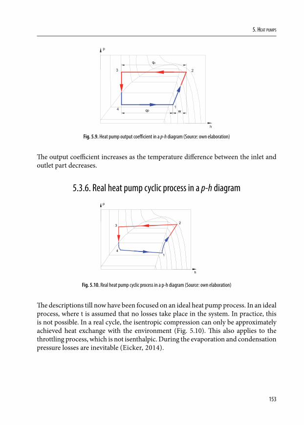
153

5. Heat pumps

h

p

1

23

4

qc

q0 w

Fig. 5.9. Heat pump output coefficient in a p-h diagram (Source: own elaboration)

The output coefficient increases as the temperature difference between the inlet and outlet part decreases.

5.3.6. Real heat pump cyclic process in a p-h diagram

h

p

1

23

4

Fig. 5.10. Real heat pump cyclic process in a p-h diagram (Source: own elaboration)

The descriptions till now have been focused on an ideal heat pump process. In an ideal process, where t is assumed that no losses take place in the system. In practice, this is not possible. In a real cycle, the isentropic compression can only be approximately achieved heat exchange with the environment (Fig. 5.10). This also applies to the throttling process, which is not isenthalpic. During the evaporation and condensation pressure losses are inevitable (Eicker, 2014).

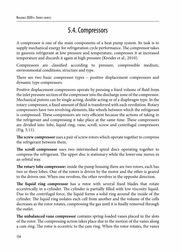
154


5.4. Compressors

A compressor is one of the main components of a heat pump system. Its task is to supply mechanical energy for refrigeration cycle performance. The compressor takes in gaseous refrigerant at low pressure and temperature, compresses it at increased temperature and discards it again at high pressure (Kreider et al., 2010).

Compressors are classified according to pressure, compressible medium, environmental conditions, structure and type.

There are two basic compressor types – positive displacement compressors and dynamic type compressors.

Positive displacement compressors operate by pressing a fixed volume of fluid from the inlet pressure section of the compressor into the discharge zone of the compressor. Mechanical pistons can be single acting, double acting or of a diaphragm type. In the rotary compressor, a fixed amount of fluid is transferred with each revolution. Rotary compressors have two revolving elements, like wheels between which the refrigerant is compressed. These compressors are very efficient because the actions of taking in the refrigerant and compressing it take place at the same time. These compressors are divided into: lobe, liquid ring, vane, scroll, screw and centrifugal compressors (Fig. 5.11).

The screw compressor uses a pair of screw rotors which operate together to compress the refrigerant between them.

The scroll compressor uses two intermeshed spiral discs operating together to compress the refrigerant. The upper disc is stationary while the lower one moves in an orbital way.

The rotary lobe compressor: inside the pump housing there are two rotors, each has two or three lobes. One of the rotors is driven by the motor and the other is geared to the driven one. When one revolves, the other revolves in the opposite direction.

The liquid ring compressor has a rotor with several fixed blades that rotate eccentrically in a cylinder. The cylinder is partially filled with low viscosity liquid. Due to the centrifugal force, the liquid forms a solid ring around the inside of the cylinder. The liquid ring isolates each cell from another and the volume of the cells decreases as the rotor rotates, compressing the gas until it is finally removed through the outlet.

The unbalanced vane compressor contains spring-loaded vanes placed in the slots of the rotor. The compressing action takes place due to the motion of the vanes along a cam ring. The rotor is eccentric to the cam ring. When the rotor rotates, the vanes

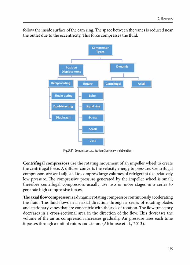
155

5. Heat pumps

follow the inside surface of the cam ring. The space between the vanes is reduced near the outlet due to the eccentricity. This force compresses the fluid.

Compressor Types

Positive Displacement

Dynamic

Reciprocating Rotary Centrifugal Displacement

Axial

Single-acting

Double-acting

Diaphragm

Lobe

Liquid ring

Screw

Scroll

Vane

Fig. 5.11. Compressor classification (Source: own elaboration)

Centrifugal compressors use the rotating movement of an impeller wheel to create the centrifugal force. A diffuser converts the velocity energy to pressure. Centrifugal compressors are well adjusted to compress large volumes of refrigerant to a relatively low pressure. The compressive pressure generated by the impeller wheel is small, therefore centrifugal compressors usually use two or more stages in a series to generate high compressive forces.

The axial flow compressor is a dynamic rotating compressor continuously accelerating the fluid. The fluid flows in an axial direction through a series of rotating blades and stationary vanes that are concentric with the axis of rotation. The flow trajectory decreases in a cross-sectional area in the direction of the flow. This decreases the volume of the air as compression increases gradually. Air pressure rises each time it passes through a unit of rotors and stators (Althouse et al., 2013).

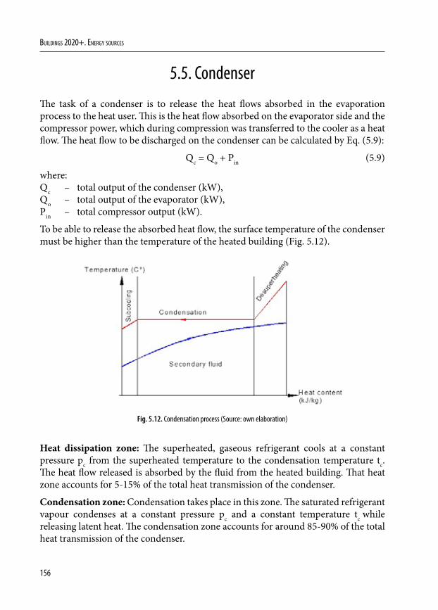
156


5.5. Condenser

The task of a condenser is to release the heat flows absorbed in the evaporation process to the heat user. This is the heat flow absorbed on the evaporator side and the compressor power, which during compression was transferred to the cooler as a heat flow. The heat flow to be discharged on the condenser can be calculated by Eq. (5.9):

Qc = Qo + Pin (5.9)

where:Qc – total output of the condenser (kW),Qo – total output of the evaporator (kW),Pin – total compressor output (kW).

To be able to release the absorbed heat flow, the surface temperature of the condenser must be higher than the temperature of the heated building (Fig. 5.12).

Fig. 5.12. Condensation process (Source: own elaboration)

Heat dissipation zone: The superheated, gaseous refrigerant cools at a constant pressure pc from the superheated temperature to the condensation temperature tc. The heat flow released is absorbed by the fluid from the heated building. That heat zone accounts for 5-15% of the total heat transmission of the condenser.

Condensation zone: Condensation takes place in this zone. The saturated refrigerant vapour condenses at a constant pressure pc and a constant temperature tc while releasing latent heat. The condensation zone accounts for around 85-90% of the total heat transmission of the condenser.

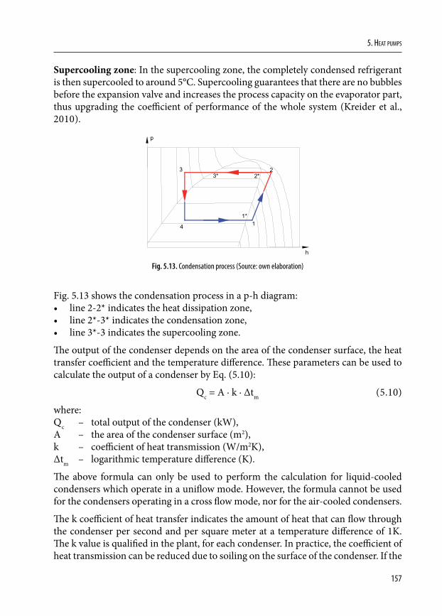
157

5. Heat pumps

Supercooling zone: In the supercooling zone, the completely condensed refrigerant is then supercooled to around 5°C. Supercooling guarantees that there are no bubbles before the expansion valve and increases the process capacity on the evaporator part, thus upgrading the coefficient of performance of the whole system (Kreider et al., 2010).

h

p

1

23

4

1*

3* 2*

Fig. 5.13. Condensation process (Source: own elaboration)

Fig. 5.13 shows the condensation process in a p-h diagram:• line 2-2* indicates the heat dissipation zone,• line 2*-3* indicates the condensation zone,• line 3*-3 indicates the supercooling zone.

The output of the condenser depends on the area of the condenser surface, the heat transfer coefficient and the temperature difference. These parameters can be used to calculate the output of a condenser by Eq. (5.10):

Qc = A · k · ∆tm (5.10)

where:Qc – total output of the condenser (kW),A – the area of the condenser surface (m2),k – coefficient of heat transmission (W/m2K),∆tm – logarithmic temperature difference (K).

The above formula can only be used to perform the calculation for liquid-cooled condensers which operate in a uniflow mode. However, the formula cannot be used for the condensers operating in a cross flow mode, nor for the air-cooled condensers.

The k coefficient of heat transfer indicates the amount of heat that can flow through the condenser per second and per square meter at a temperature difference of 1K. The k value is qualified in the plant, for each condenser. In practice, the coefficient of heat transmission can be reduced due to soiling on the surface of the condenser. If the

158


heat transmission goes down, the temperature difference between the condensation temperature and the fluid temperature rises. As the temperature of the heating is constant, the condensation temperature must be higher. The compressor must operate at a higher pressure ratio when its volumetric efficiency is reduced and creates a risk of overload. To avoid this, the condenser must be constantly cleaned of dirt and soiling.

The logarithmic temperature difference ∆tm between the condensation temperature and the temperature of the heated building is used to calculate the condenser output. The temperature difference between the cooling medium and the refrigerant changes depending on the distance of the flow, but this change is not linear and cannot be used for the calculation.

The temperature difference can be described by Eq. (5.11):

∆∆ ∆

∆∆

tt t

tt

m =−

1 2

1

2

ln (5.11)

Neither heat dissipation nor supercooling is taken into account. The logarithmic temperature difference is therefore the basis for calculations in the condensation area.

The heat flow to be discharged by the condenser is made up of the compressor power intake and the heat resources capacity. If this data is unknown, the condenser output can be recorded by measurement. For the underfloor heating (water cooled) condenser, the output is calculated by Eq. (5.12):

Qc = VF · ρF · cF (tF1 – tF2) (5.12)

where:Qc – total output of the condenser (kW),VF – underfloor heating water flow rate (m3/s),ρF – underfloor heating water density (kg/m3),cF – underfloor heating water specific heat capacity (kJ/(kg∙K)),tF1 – underfloor heating water temperature at condenser inlet (°C),tF2 – underfloor heating water temperature at condenser outlet (°C).

Measuring the output of an air-cooled condenser is similar. It should be noted that the specific heat capacity and density of the air depends on the temperature. Values can only be constant for small temperature differences. The condenser output is calculated using the air flow rate by Eq. (5.13):

Qc = VA · ρA · cA (tA1 – tA2) (5.13)

159

5. Heat pumps

where:Qc – total output of the condenser (kW),VA – air flow rate (m3),ρA – air density (kg/m3),cA – air specific heat capacity (kJ/kg∙K),tA1 – air temperature at condenser inlet (°C),tA2 – air temperature at condenser outlet (°C).

Usually it is difficult to determine the air flow rate because it requires recording the air speed. The air flow rate can be calculated by measuring the dynamic air pressure. The air is normally non homogeneous, temperature and speed distributions from the heat exchanger are also difficult to measure. The real output can be calculated only by measurement of liquid cooling medium (Kreider et al., 2010).

5.6. Throttle valves

A throttle valve reduces the freon pressure from the condenser to the evaporation pressure. The low pressure is required so that the refrigerant can evaporate at low temperatures. It is an important significance in terms of optimum system recovery that the evaporator is always supplied with as much refrigerant as it can process in the correct operating conditions. If too much freon reaches the evaporator, the liquid will not be fully evaporated and liquid lock can occur in the compressor.

If the evaporator is provided with too little refrigerant, it will not operate correctly and excessive overheating of the refrigerant can take place, which will result in too high a final compression temperature.

The change of state in the throttle element can be viewed as isenthalpic. Practically, there is a slight increase in enthalpy in the valve (Althouse et al., 2013).

Expansion valves do not control the evaporation temperature straightforwardly. They regulate the superheating by controlling the mass flow of freon into the evaporator and upholding the pressure difference between the condenser (high pressure) and the evaporator (low-pressure). The evaporation temperature depends on the capacity of the compressor and efficiency of the evaporator.

Throttle elements are divided into three categories depending on their regulation of freon mass flow rate:1. non-regulating throttle elements,;2. mechanical self-regulating throttle elements,3. electric self-regulating throttle elements.

160


Non-regulating throttle elements or capillary tubes are the simplest of all freon flow controls. They contain no moving parts; normally they consist only of a copper pipe with the diameter of 0.5 to 1.5 mm and the length from 1.5 to 4 m. The fall in the pressure of the refrigerant takes place due to the long and narrow tube. The mass flow through the tube depends on the pressure difference between the condensing and evaporating sides. Capillary tubes can be set up on small and high-volume commercial systems if the operating conditions are relatively fixed. Often, the low pressure side has a liquid separator that acts as a receiver in the frontal part of the compressor.

Mechanical self-regulating throttle elements:

A pressure control throttle valve (Fig. 5.14) is a manually operated needle valve. The needle position is fixed, and the mass flow through it depends on the pressure difference over the valve. A manual throttle is a non-regulating valve and it should not be used as an expansion valve with a BPHE (Brazed Plate Heat Exchangers) evaporator, because some changes in functioning conditions would immediately change the evaporation process inside the plate heat exchanger. Regulating the flow manually would require direct regulation, which is not practically executable.

Fig. 5.14. Pressure control throttle valve (Source: own elaboration)

Thermostatic expansion valves (TEVs) are the expansion devices used most commonly with BPHE evaporators. TEVs are good expansion devices due to their relatively good sensitivity in settings. The large choice of expansion valve sizes,

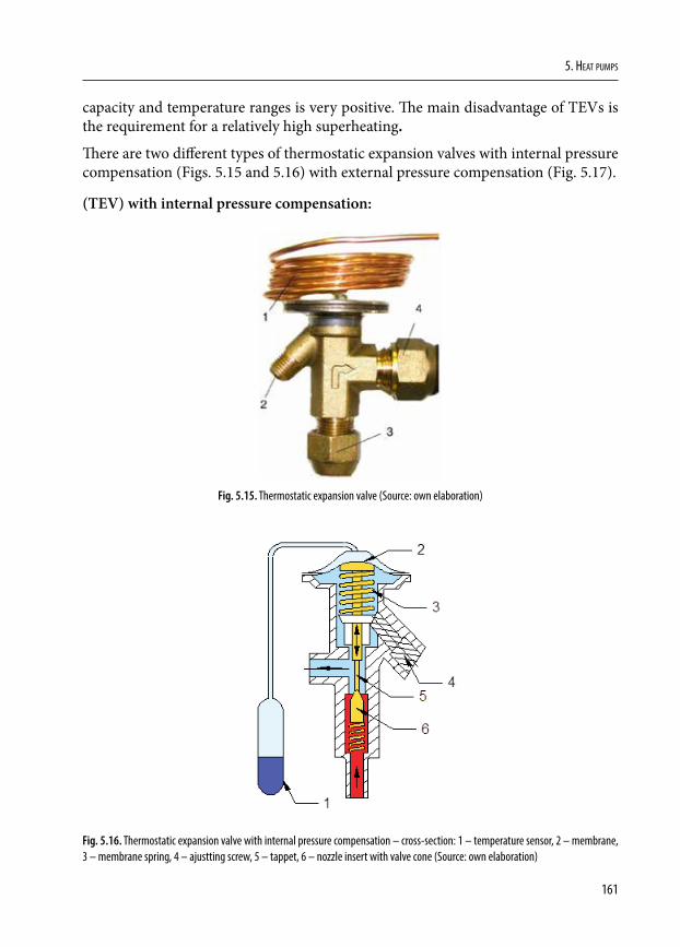
161

5. Heat pumps

capacity and temperature ranges is very positive. The main disadvantage of TEVs is the requirement for a relatively high superheating.

There are two different types of thermostatic expansion valves with internal pressure compensation (Figs. 5.15 and 5.16) with external pressure compensation (Fig. 5.17).

(TEV) with internal pressure compensation:

Fig. 5.15. Thermostatic expansion valve (Source: own elaboration)

Fig. 5.16. Thermostatic expansion valve with internal pressure compensation – cross-section: 1 – temperature sensor, 2 – membrane, 3 – membrane spring, 4 – ajustting screw, 5 – tappet, 6 – nozzle insert with valve cone (Source: own elaboration)

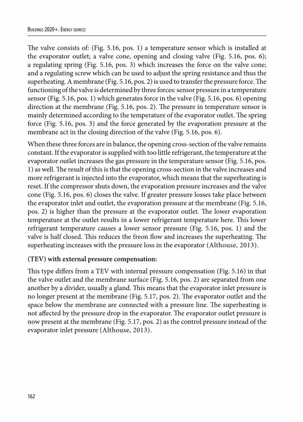
162


The valve consists of: (Fig. 5.16, pos. 1) a temperature sensor which is installed at the evaporator outlet; a valve cone, opening and closing valve (Fig. 5.16, pos. 6); a regulating spring (Fig. 5.16, pos. 3) which increases the force on the valve cone; and a regulating screw which can be used to adjust the spring resistance and thus the superheating. A membrane (Fig. 5.16, pos. 2) is used to transfer the pressure force. The functioning of the valve is determined by three forces: sensor pressure in a temperature sensor (Fig. 5.16, pos. 1) which generates force in the valve (Fig. 5.16, pos. 6) opening direction at the membrane (Fig. 5.16, pos. 2). The pressure in temperature sensor is mainly determined according to the temperature of the evaporator outlet. The spring force (Fig. 5.16, pos. 3) and the force generated by the evaporation pressure at the membrane act in the closing direction of the valve (Fig. 5.16, pos. 6).

When these three forces are in balance, the opening cross-section of the valve remains constant. If the evaporator is supplied with too little refrigerant, the temperature at the evaporator outlet increases the gas pressure in the temperature sensor (Fig. 5.16, pos. 1) as well. The result of this is that the opening cross-section in the valve increases and more refrigerant is injected into the evaporator, which means that the superheating is reset. If the compressor shuts down, the evaporation pressure increases and the valve cone (Fig. 5.16, pos. 6) closes the valve. If greater pressure losses take place between the evaporator inlet and outlet, the evaporation pressure at the membrane (Fig. 5.16, pos. 2) is higher than the pressure at the evaporator outlet. The lower evaporation temperature at the outlet results in a lower refrigerant temperature here. This lower refrigerant temperature causes a lower sensor pressure (Fig. 5.16, pos. 1) and the valve is half closed. This reduces the freon flow and increases the superheating. The superheating increases with the pressure loss in the evaporator (Althouse, 2013).

(TEV) with external pressure compensation:

This type differs from a TEV with internal pressure compensation (Fig. 5.16) in that the valve outlet and the membrane surface (Fig. 5.16, pos. 2) are separated from one another by a divider, usually a gland. This means that the evaporator inlet pressure is no longer present at the membrane (Fig. 5.17, pos. 2). The evaporator outlet and the space below the membrane are connected with a pressure line. The superheating is not affected by the pressure drop in the evaporator. The evaporator outlet pressure is now present at the membrane (Fig. 5.17, pos. 2) as the control pressure instead of the evaporator inlet pressure (Althouse, 2013).

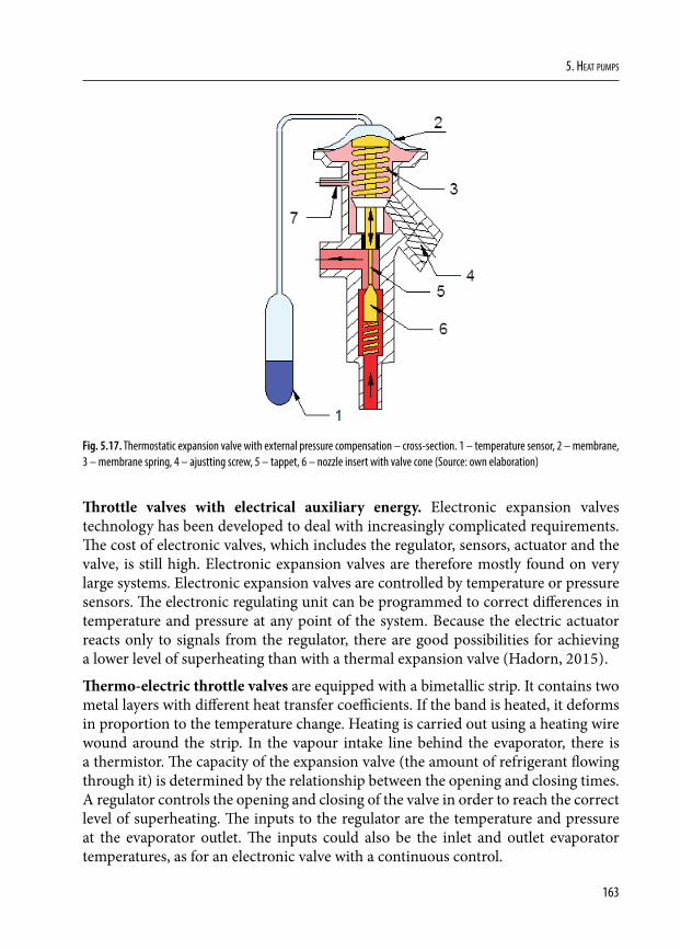
163

5. Heat pumps

Fig. 5.17. Thermostatic expansion valve with external pressure compensation – cross-section. 1 – temperature sensor, 2 – membrane, 3 – membrane spring, 4 – ajustting screw, 5 – tappet, 6 – nozzle insert with valve cone (Source: own elaboration)

Throttle valves with electrical auxiliary energy. Electronic expansion valves technology has been developed to deal with increasingly complicated requirements. The cost of electronic valves, which includes the regulator, sensors, actuator and the valve, is still high. Electronic expansion valves are therefore mostly found on very large systems. Electronic expansion valves are controlled by temperature or pressure sensors. The electronic regulating unit can be programmed to correct differences in temperature and pressure at any point of the system. Because the electric actuator reacts only to signals from the regulator, there are good possibilities for achieving a lower level of superheating than with a thermal expansion valve (Hadorn, 2015).

Thermo-electric throttle valves are equipped with a bimetallic strip. It contains two metal layers with different heat transfer coefficients. If the band is heated, it deforms in proportion to the temperature change. Heating is carried out using a heating wire wound around the strip. In the vapour intake line behind the evaporator, there is a thermistor. The capacity of the expansion valve (the amount of refrigerant flowing through it) is determined by the relationship between the opening and closing times. A regulator controls the opening and closing of the valve in order to reach the correct level of superheating. The inputs to the regulator are the temperature and pressure at the evaporator outlet. The inputs could also be the inlet and outlet evaporator temperatures, as for an electronic valve with a continuous control.

164


5.7. Evaporator

The task of the evaporator is to withdraw heat energy from the heat source by a heat medium. Heat transmission can only take place if there is a temperature difference between the heat medium and the refrigerant. Temperature difference of around 10°C is enough to guarantee heat transmission. The liquid freon enters the evaporator after throttling. The liquid evaporates completely as it passes through the evaporator. During this process, the freon absorbs heat energy from the heat medium.

Depending on the heat source, the heat medium evaporator can be: air-cooled, liquid-cooled and flooded.

Air-cooled evaporators finned tube coil-pipe systems are used as evaporators with the freon flowing through the tubes. The purpose of the fins is to increase the evaporator surface area on the air side. In air-cooled evaporators, the heat transmission on the freon side is higher than on the air side.

Liquid evaporators combine good heat transmission with a compact design. At low outputs, plate and coaxial heat exchangers are used. The refrigerant can either be evaporated in the tubes or flooded in the lateral surface.

Flooded evaporator operates in connection with a receiver. The receiver acts as a separator of gaseous and liquid refrigerant behind the expansion valve and provides 100% of the liquid refrigerant flow to the evaporator. Direct expansion evaporator and the refrigerant are not fully evaporated and superheated at the flooded evaporator outlet. The leaving refrigerant flow is a two-phase mixture containing typically 50-80% of gas (Hadorn, 2015).

5.8. Other components

Filter-dryer – Moisture (water) in the system may freeze the refrigerant control valves. This may clog or partially jam the control. Humidity in some refrigerants at high compressor temperatures can cause decay of the refrigerant to form harmful acids. It may lead to corrosion, or oil mudding, which could result in a motor failure. Refrigerants must be stored in a sealed container and kept dry.

A filter-dryer is a device used to prevent refrigerant contamination in heating and refrigeration cycle systems. The filter can restrict the free flow of refrigerant into the expansion valve. It effectively prevents the impurities from flowing rearwards when

165

5. Heat pumps

the system is having a reversible flow and eliminates moisture or acids during the refrigeration and heating cycles.

The function is based on the very large surface area of ultrafine pores inside the substance. The water absorption of the filter dryer depends on the temperature and it increases as the temperature is reduced. From this point, a filter dryer is fitted in the cold inlet line. Relatively high flow velocities take place in the intake line, filter dryers with a very large volume would have to be used to keep the pressure loss in acceptable limits. That is why, the filter dryer is normally installed in the liquid line between the evaporator and the expansion valve (Althouse, 2013).

Refrigerant receivers are used to store the refrigerant. They allow to maintain the required variable refrigerant amount under various working conditions. The refrigerant receiver also has a supplementary protection function. Because of its position between the condenser and the expansion valve, it can separate vapour bubbles in the refrigerant from the liquid. Receiver volume must ensure all the heat pump freon volume. Therefore the repair work can be carried out by transferring the refrigerant into the refrigerant receiver, and no refrigerant can leak.

The sight glass allows to check if the freon flowing to the throttle valve is liquid. It is necessary to install it before the expansion valve. If vapour bubbles can be seen through the sight glass, it indicates the lack of refrigerant or insufficient supercooling in the system. In addition, sight glasses often include indicators showing the water content in the refrigerant.

Oil separator – the heat pump compressors receive oil from a small amount of special lubricating oil. It is distributed to a variety of compressor components. When the compressor is running, small amounts of oil come in hot, compressed freon vapour. The oil can be separated from the compressed hot steam by installing an oil separator between the compressor outlet and the condenser. The oil in the heat pump system is cooled down to a lower temperature parameter. However, it must be able to maintain high temperature in the compressor. It must remain liquid in all parts of the system. The liquidity of the oil-refrigerant mixture is determined by several factors. These include the temperature, the oil properties, the solubility of the oil in refrigerant and the solubility of the refrigerant in the oil. The internals of good refrigerant oil are:• low wax amount -separation of the wax from the refrigerant oil blend can clog

up the refrigerant control openings;• good thermal stability - it should not form heavy coal deposits at the hot spots

of the compressor;• good chemical stability - there should be little or almost no chemical reaction

with the refrigerant or substances that are commonly found in the system;

166


• low pour point - the ability of the oil to remain in the liquid state at the lowest system temperature;

• low viscosity - the ability of the oil to maintain good lubricating properties at high temperatures, as well as good low temperature viscosity always provides a good lubricating film.

Oil separators are very effective. Very little oil goes into the system. They are usually used in large commercial facilities. Integration of an oil separator is particularly important in systems with a flooded evaporator, as the oil precipitates at the base of the evaporator. Other positive result of the oil separator is that it can compensate pressure pulses in pressure lines.

A liquid line, commonly copper tubing, is used to carry the liquid refrigerant from the condenser to the evaporator. The lines are soldered or brazed to fittings. It is important to avoid pinching or buckling of these lines. They should be regularly maintained to prevent wear or breaking due to vibration (Hadorn, 2015).

5.9. Refrigerant

The refrigerant is responsible for transferring energy in the heat pump system. In theory, any material could be used as the refrigerant, if it can be condensed at technically possible pressures and evaporated at low temperatures. There is no ideal refrigerant for every application. Which refrigerant is used in a system depends on its purpose. The choice of refrigerant is primarily influenced by its physical, chemical and physiological properties. Scientists have found that the release of some refrigerant chlorofluorocarbons (CFCs) may damage the ozone layer.

Most refrigerants used today are classified in four areas:• chlorofluorocarbons (CFCs),• hidrochlorofluorocarbons (HCFCs),• hidrofluorocarbons (HFCs).• Refrigerant blend (azeotropic and zeotropic).

The refrigerant is identified by number (Table 5.1). The number goes under the letter R which means the refrigerant. The refrigerant cylinder is often colour coded to make it easier to identify the type of refrigerant in it.

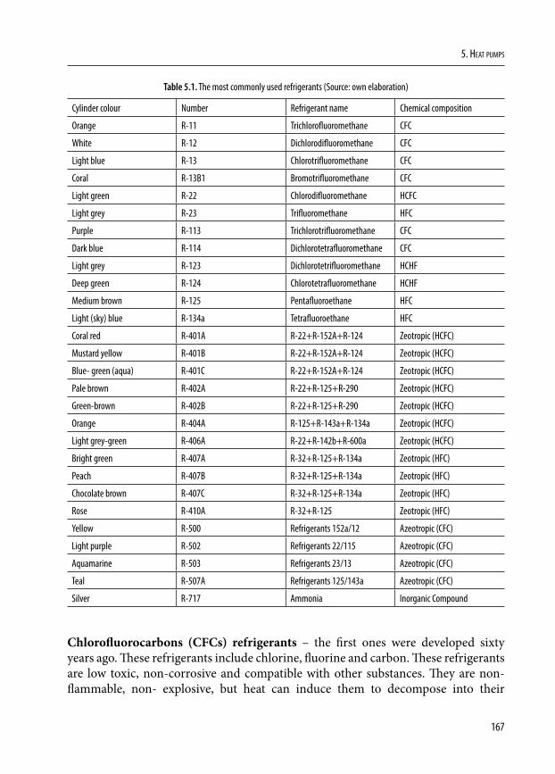
167

5. Heat pumps

Table 5.1. The most commonly used refrigerants (Source: own elaboration)

Cylinder colour Number Refrigerant name Chemical composition

Orange R-11 Trichlorofluoromethane CFC

White R-12 Dichlorodifluoromethane CFC

Light blue R-13 Chlorotrifluoromethane CFC

Coral R-13B1 Bromotrifluoromethane CFC

Light green R-22 Chlorodifluoromethane HCFC

Light grey R-23 Trifluoromethane HFC

Purple R-113 Trichlorotrifluoromethane CFC

Dark blue R-114 Dichlorotetrafluoromethane CFC

Light grey R-123 Dichlorotetrifluoromethane HCHF

Deep green R-124 Chlorotetrafluoromethane HCHF

Medium brown R-125 Pentafluoroethane HFC

Light (sky) blue R-134a Tetrafluoroethane HFC

Coral red R-401A R-22+R-152A+R-124 Zeotropic (HCFC)

Mustard yellow R-401B R-22+R-152A+R-124 Zeotropic (HCFC)

Blue- green (aqua) R-401C R-22+R-152A+R-124 Zeotropic (HCFC)

Pale brown R-402A R-22+R-125+R-290 Zeotropic (HCFC)

Green-brown R-402B R-22+R-125+R-290 Zeotropic (HCFC)

Orange R-404A R-125+R-143a+R-134a Zeotropic (HCFC)

Light grey-green R-406A R-22+R-142b+R-600a Zeotropic (HCFC)

Bright green R-407A R-32+R-125+R-134a Zeotropic (HFC)

Peach R-407B R-32+R-125+R-134a Zeotropic (HFC)

Chocolate brown R-407C R-32+R-125+R-134a Zeotropic (HFC)

Rose R-410A R-32+R-125 Zeotropic (HFC)

Yellow R-500 Refrigerants 152a/12 Azeotropic (CFC)

Light purple R-502 Refrigerants 22/115 Azeotropic (CFC)

Aquamarine R-503 Refrigerants 23/13 Azeotropic (CFC)

Teal R-507A Refrigerants 125/143a Azeotropic (CFC)

Silver R-717 Ammonia Inorganic Compound

Chlorofluorocarbons (CFCs) refrigerants – the first ones were developed sixty years ago. These refrigerants include chlorine, fluorine and carbon. These refrigerants are low toxic, non-corrosive and compatible with other substances. They are non-flammable, non- explosive, but heat can induce them to decompose into their

168


elements and cause harm to human tissue. They are particularly damaging to the respiratory system.

Simple refrigerants (CFCs) include R-11, R -12, R -113, R -114, R -115, R-500, R-502, and R-503. R-500, R-502, and R-503.

Simple refrigerants (CFCs) are thought to be one of the main reasons for ozone depletion. According to the international agreement, since 1995 they have not been produced, but they are still used in the existing units.

Due to laws forbidding the release of CFCs to the atmosphere, the new agent has been developed.

These are used to recover, recycle and reclaim the refrigerants containing (CFCs).

Hydrochlorofluorocarbons (HCFCs) refrigerants. These are molecules that consist of methane or ethane together with halogens. They form a new molecule that is considered partially halogenated. HCFCs refrigerants have shorter lives and cause less ozone depletion than the fully halogenated (CFCs). For this reason, they have reduced impact on the global warming (Althouse, 2013).

5.10. THE ABSORPTION SYSTEMS

5.10.1. IntroductionThe absorption system uses heat energy, not mechanical energy. This heat energy is used to create necessary conditions for the cooling cycle completion. Compression systems use a compressor and a refrigerant to create a heat pump cycle. Absorption heat pump uses a chemical process to change low-temperature vapour into a high-pressure vapour. Most of the vapour compression systems used chlorofluorocarbon refrigerants whose use is now limited due to ozone depletion (Hadorn, 2015). The most commonly used refrigerants for absorption systems are ammonia/water or lithium bromide/water, in which case the absorption system is better. In order to encourage the use of absorption systems, it is necessary to improve their performance and reduce costs. The absorption system can use different sorts of heat sources. The condenser, expansion valve and evaporator are similar to the compression system. The compressor is replaced by a generator and an absorber.

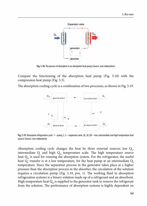
169

5. Heat pumps

QoutQin

Evap

orat

or

Con

dens

er

Expansion valve

generator

absorber

Fig. 5.18. The process of absorption in an absorption heat pump (Source: own elaboration)

Compare the functioning of the absorption heat pump (Fig. 5.18) with the compression heat pump (Fig. 5.3).

The absorption cooling cycle is a combination of two processes, as shown in Fig. 5.19.

a b s o rb e r e v a p o ra to r

g e n e ra to r c o n d e n s e rQ H

Q I Q L

Q I

2

13

1- pump, 2, 3 - expansion valve, QL,QI,QH- low, intermediate and high temperature heat sourcesFig. 5.19. Absorption refrigeration cycle: 1 – pump, 2, 3 – expansion valve, QL, QI, QH – low, intermediate and high temperature heat

sources (Source: own elaboration)

Absorption cooling cycle changes the heat by three external sources; low QL, intermediate QI and high QH temperature scale. The high temperature source heat QH is used for running the absorption system. For the refrigerator, the useful heat QL transfer is at a low temperature, for the heat pump at an intermediate QI temperature. Since the separation process in the generator takes place at a higher pressure than the absorption process in the absorber, the circulation of the solution requires a circulation pump (Fig. 5.19, pos. 1). The working fluid in absorption refrigeration systems is a binary solution made up of a refrigerant and an absorbent. High temperature heat QH is supplied to the generator tank to remove the refrigerant from the solution. The performance of absorption systems is highly dependent on

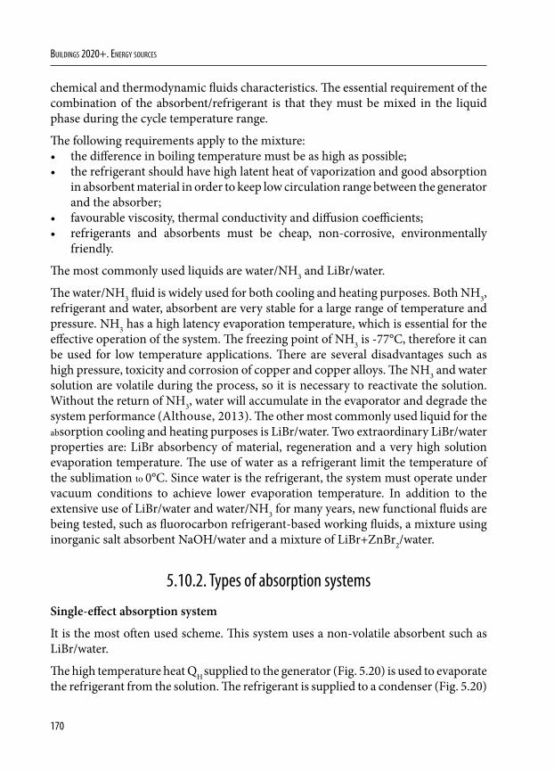
170


chemical and thermodynamic fluids characteristics. The essential requirement of the combination of the absorbent/refrigerant is that they must be mixed in the liquid phase during the cycle temperature range.

The following requirements apply to the mixture:• the difference in boiling temperature must be as high as possible;• the refrigerant should have high latent heat of vaporization and good absorption

in absorbent material in order to keep low circulation range between the generator and the absorber;

• favourable viscosity, thermal conductivity and diffusion coefficients;• refrigerants and absorbents must be cheap, non-corrosive, environmentally

friendly.

The most commonly used liquids are water/NH3 and LiBr/water.

The water/NH3 fluid is widely used for both cooling and heating purposes. Both NH3, refrigerant and water, absorbent are very stable for a large range of temperature and pressure. NH3 has a high latency evaporation temperature, which is essential for the effective operation of the system. The freezing point of NH3 is -77°C, therefore it can be used for low temperature applications. There are several disadvantages such as high pressure, toxicity and corrosion of copper and copper alloys. The NH3 and water solution are volatile during the process, so it is necessary to reactivate the solution. Without the return of NH3, water will accumulate in the evaporator and degrade the system performance (Althouse, 2013). The other most commonly used liquid for the absorption cooling and heating purposes is LiBr/water. Two extraordinary LiBr/water properties are: LiBr absorbency of material, regeneration and a very high solution evaporation temperature. The use of water as a refrigerant limit the temperature of the sublimation to 0°C. Since water is the refrigerant, the system must operate under vacuum conditions to achieve lower evaporation temperature. In addition to the extensive use of LiBr/water and water/NH3 for many years, new functional fluids are being tested, such as fluorocarbon refrigerant-based working fluids, a mixture using inorganic salt absorbent NaOH/water and a mixture of LiBr+ZnBr2/water.

5.10.2. Types of absorption systems

Single-effect absorption system

It is the most often used scheme. This system uses a non-volatile absorbent such as LiBr/water.

The high temperature heat QH supplied to the generator (Fig. 5.20) is used to evaporate the refrigerant from the solution. The refrigerant is supplied to a condenser (Fig. 5.20)

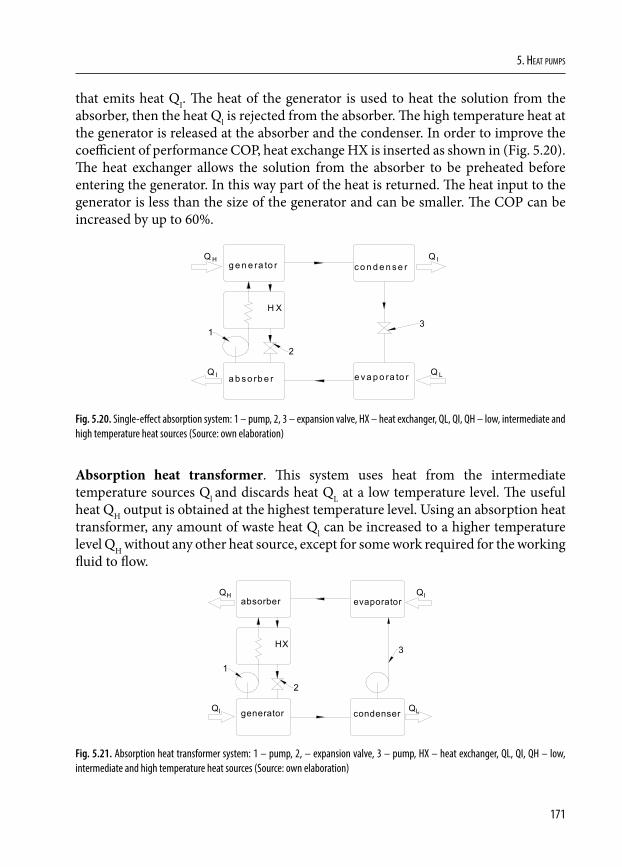
171

5. Heat pumps

that emits heat QI. The heat of the generator is used to heat the solution from the absorber, then the heat Ql is rejected from the absorber. The high temperature heat at the generator is released at the absorber and the condenser. In order to improve the coefficient of performance COP, heat exchange HX is inserted as shown in (Fig. 5.20). The heat exchanger allows the solution from the absorber to be preheated before entering the generator. In this way part of the heat is returned. The heat input to the generator is less than the size of the generator and can be smaller. The COP can be increased by up to 60%.

ab so rbe r e va po ra to r

H X

gene ra to r con dense rQH

Q I Q L

Q I

2

13

1-pump,2, 3 - expansion valve, HX- heat exchanger, QL,QI,QH- low, intermediate and high temperature heat sourcesFig. 5.20. Single-effect absorption system: 1 – pump, 2, 3 – expansion valve, HX – heat exchanger, QL, QI, QH – low, intermediate and

high temperature heat sources (Source: own elaboration)

Absorption heat transformer. This system uses heat from the intermediate temperature sources Ql and discards heat QL at a low temperature level. The useful heat QH output is obtained at the highest temperature level. Using an absorption heat transformer, any amount of waste heat Ql can be increased to a higher temperature level QH without any other heat source, except for some work required for the working fluid to flow.

absorber evaporator

HX

generator condenser

QH

QI QL

QI

2

1

3

1-pump, 2, - expansion valve, 3- pump, HX- heat exchanger, QL,QI,QH- low, intermediate and high temperature

heat sources

Fig. 5.21. Absorption heat transformer system: 1 – pump, 2, – expansion valve, 3 – pump, HX – heat exchanger, QL, QI, QH – low, intermediate and high temperature heat sources (Source: own elaboration)

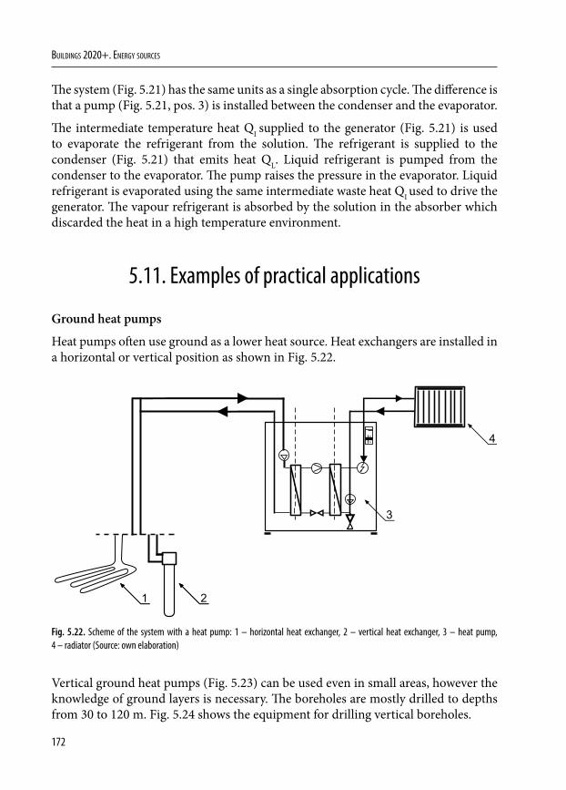
172


The system (Fig. 5.21) has the same units as a single absorption cycle. The difference is that a pump (Fig. 5.21, pos. 3) is installed between the condenser and the evaporator.

The intermediate temperature heat QI supplied to the generator (Fig. 5.21) is used to evaporate the refrigerant from the solution. The refrigerant is supplied to the condenser (Fig. 5.21) that emits heat QL. Liquid refrigerant is pumped from the condenser to the evaporator. The pump raises the pressure in the evaporator. Liquid refrigerant is evaporated using the same intermediate waste heat QI used to drive the generator. The vapour refrigerant is absorbed by the solution in the absorber which discarded the heat in a high temperature environment.

5.11. Examples of practical applications

Ground heat pumps

Heat pumps often use ground as a lower heat source. Heat exchangers are installed in a horizontal or vertical position as shown in Fig. 5.22.

Fig. 5.22. Scheme of the system with a heat pump: 1 – horizontal heat exchanger, 2 – vertical heat exchanger, 3 – heat pump, 4 – radiator (Source: own elaboration)

Vertical ground heat pumps (Fig. 5.23) can be used even in small areas, however the knowledge of ground layers is necessary. The boreholes are mostly drilled to depths from 30 to 120 m. Fig. 5.24 shows the equipment for drilling vertical boreholes.

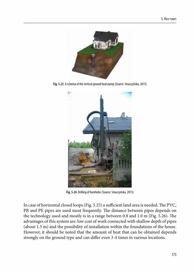
173

5. Heat pumps

Fig. 5.23. A schema of the vertical ground heat pump (Source: Smuczyńska, 2015)

Fig. 5.24. Drilling of boreholes (Source: Smuczyńska, 2015)

In case of horizontal closed loops (Fig. 5.25) a sufficient land area is needed. The PVC, PB and PE pipes are used most frequently. The distance between pipes depends on the technology used and mostly is in a range between 0.8 and 1.0 m (Fig. 5.26). The advantages of this system are: low cost of work connected with shallow depth of pipes (about 1.5 m) and the possibility of installation within the foundations of the house. However, it should be noted that the amount of heat that can be obtained depends strongly on the ground type and can differ even 3-4 times in various locations.

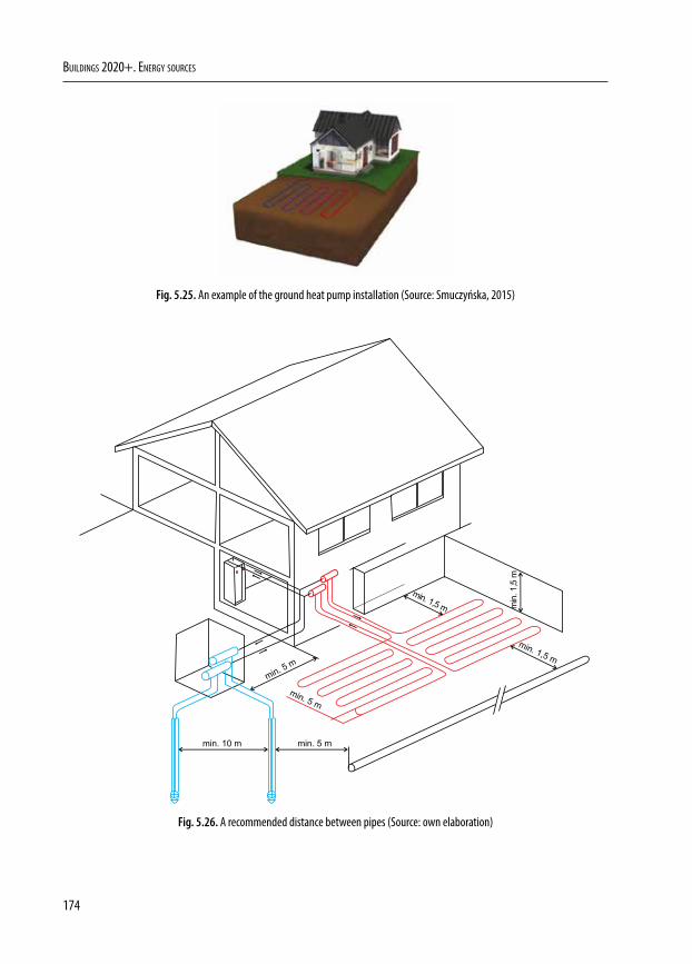
174


Fig. 5.25. An example of the ground heat pump installation (Source: Smuczyńska, 2015)

Fig. 5.26. A recommended distance between pipes (Source: own elaboration)

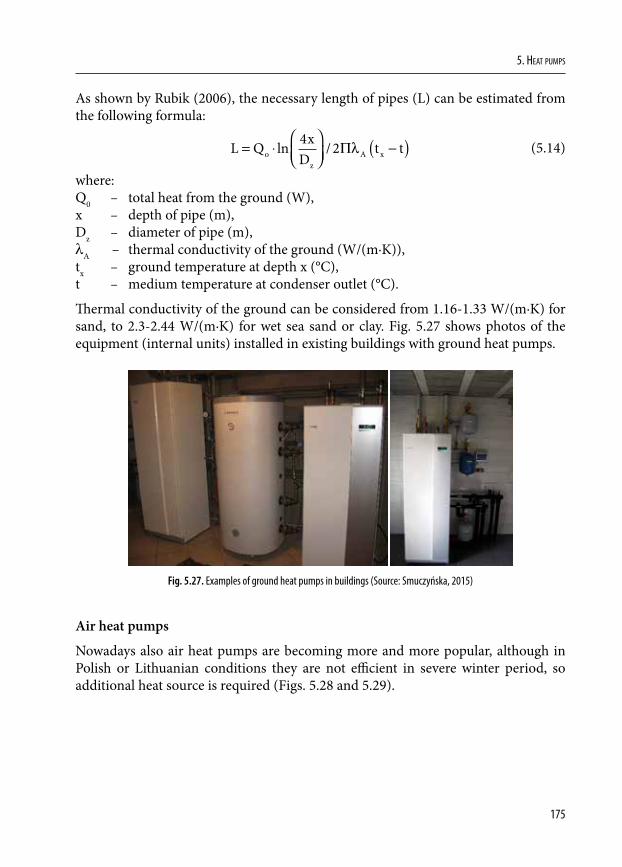
175

5. Heat pumps

As shown by Rubik (2006), the necessary length of pipes (L) can be estimated from the following formula:

L Q xD

t toz

A x= ⋅

−( )ln /4 2Πλ (5.14)

where:Q0 – total heat from the ground (W),x – depth of pipe (m),Dz – diameter of pipe (m),λA – thermal conductivity of the ground (W/(m∙K)),tx – ground temperature at depth x (°C),t – medium temperature at condenser outlet (°C).

Thermal conductivity of the ground can be considered from 1.16-1.33 W/(m∙K) for sand, to 2.3-2.44 W/(m∙K) for wet sea sand or clay. Fig. 5.27 shows photos of the equipment (internal units) installed in existing buildings with ground heat pumps.

Fig. 5.27. Examples of ground heat pumps in buildings (Source: Smuczyńska, 2015)

Air heat pumps

Nowadays also air heat pumps are becoming more and more popular, although in Polish or Lithuanian conditions they are not efficient in severe winter period, so additional heat source is required (Figs. 5.28 and 5.29).

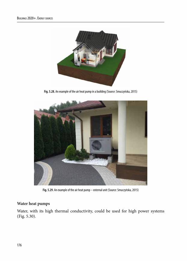
176


Fig. 5.28. An example of the air heat pump in a building (Source: Smuczyńska, 2015)

Fig. 5.29. An example of the air heat pump – external unit (Source: Smuczyńska, 2015)

Water heat pumps

Water, with its high thermal conductivity, could be used for high power systems (Fig. 5.30).

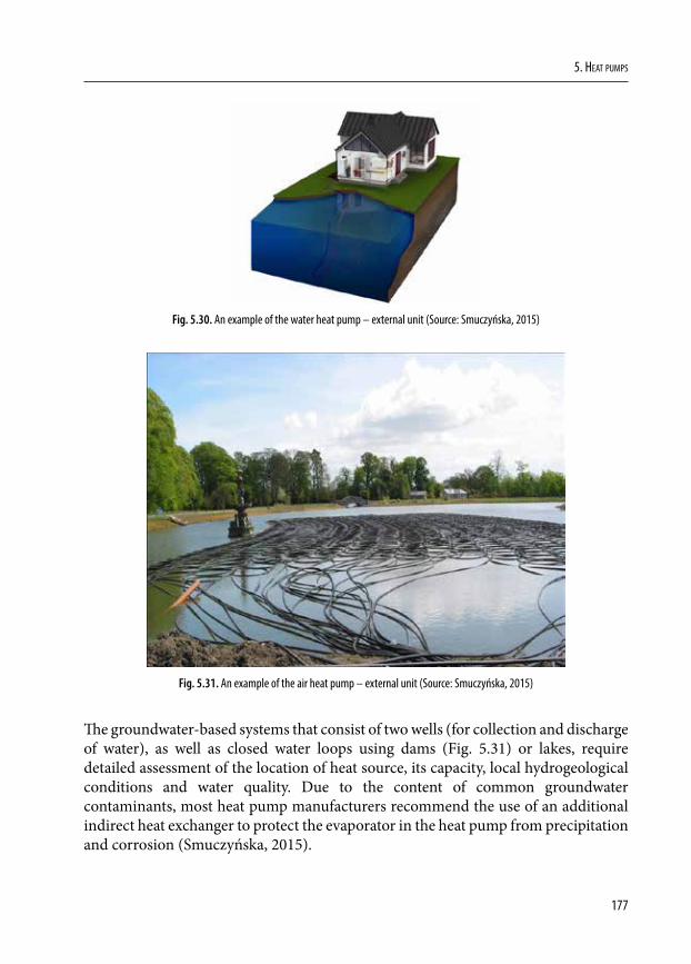
177

5. Heat pumps

Fig. 5.30. An example of the water heat pump – external unit (Source: Smuczyńska, 2015)

Fig. 5.31. An example of the air heat pump – external unit (Source: Smuczyńska, 2015)

The groundwater-based systems that consist of two wells (for collection and discharge of water), as well as closed water loops using dams (Fig. 5.31) or lakes, require detailed assessment of the location of heat source, its capacity, local hydrogeological conditions and water quality. Due to the content of common groundwater contaminants, most heat pump manufacturers recommend the use of an additional indirect heat exchanger to protect the evaporator in the heat pump from precipitation and corrosion (Smuczyńska, 2015).

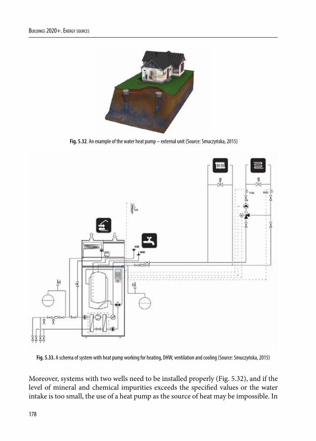
178


Fig. 5.32. An example of the water heat pump – external unit (Source: Smuczyńska, 2015)

Fig. 5.33. A schema of system with heat pump working for heating, DHW, ventilation and cooling (Source: Smuczyńska, 2015)

Moreover, systems with two wells need to be installed properly (Fig. 5.32), and if the level of mineral and chemical impurities exceeds the specified values or the water intake is too small, the use of a heat pump as the source of heat may be impossible. In

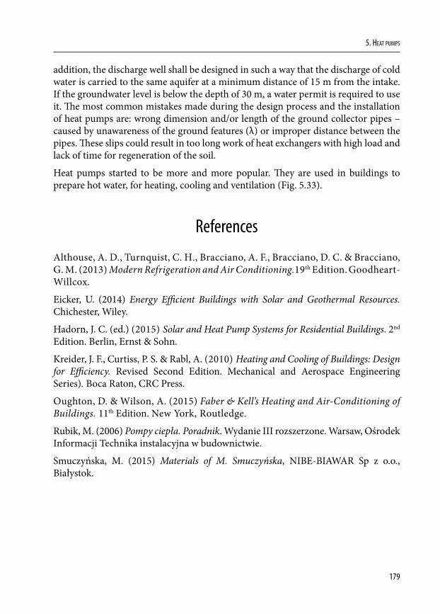
179

5. Heat pumps

addition, the discharge well shall be designed in such a way that the discharge of cold water is carried to the same aquifer at a minimum distance of 15 m from the intake. If the groundwater level is below the depth of 30 m, a water permit is required to use it. The most common mistakes made during the design process and the installation of heat pumps are: wrong dimension and/or length of the ground collector pipes – caused by unawareness of the ground features (λ) or improper distance between the pipes. These slips could result in too long work of heat exchangers with high load and lack of time for regeneration of the soil.

Heat pumps started to be more and more popular. They are used in buildings to prepare hot water, for heating, cooling and ventilation (Fig. 5.33).

References

Althouse, A. D., Turnquist, C. H., Bracciano, A. F., Bracciano, D. C. & Bracciano, G. M. (2013) Modern Refrigeration and Air Conditioning.19th Edition. Goodheart-Willcox.

Eicker, U. (2014) Energy Efficient Buildings with Solar and Geothermal Resources. Chichester, Wiley.

Hadorn, J. C. (ed.) (2015) Solar and Heat Pump Systems for Residential Buildings. 2nd Edition. Berlin, Ernst & Sohn.

Kreider, J. F., Curtiss, P. S. & Rabl, A. (2010) Heating and Cooling of Buildings: Design for Efficiency. Revised Second Edition. Mechanical and Aerospace Engineering Series). Boca Raton, CRC Press.

Oughton, D. & Wilson, A. (2015) Faber & Kell’s Heating and Air-Conditioning of Buildings. 11th Edition. New York, Routledge.

Rubik, M. (2006) Pompy ciepła. Poradnik. Wydanie III rozszerzone. Warsaw, Ośrodek Informacji Technika instalacyjna w budownictwie.

Smuczyńska, M. (2015) Materials of M. Smuczyńska, NIBE-BIAWAR Sp z o.o., Białystok.

181

6. BIOMASS HEAT CENTRES

6.1. Technologies for burning biomass

The classification of solid biofuel depends upon the determination of the fuel origin and it is divided into (LST EN 14961-1):• wood biomass,• herbaceous biomass,• fruit biomass,• biomass mixtures.

Biomass burning is the conversion of accumulated energy. Most part of the energy produced from biomass causes heat, which is gained by burning wood, firewood, wood pellets, wood chips, wood sawdust, etc.

Biofuel is burnt in solid fuel boilers. Their equipment is described below:1. boiler and furnace,2. smoke treatment equipment and chimney flue,3. air supply fan,4. smoke exhauster,5. boiler protection measures,6. fuel warehouse,7. fuel supply equipment.

The main technological parts of the boiler house are the boiler and the furnace.

Direct biomass burning or burning with biomass gasification is included in low power boilers. Direct burning boilers can burn various fractions and biomass (granules or briquettes). In these boilers, fuel can automatically be supplied into the furnace and the power of the boiler can be regulated by altering the amount of fuel and air. Boilers with biomass gasification show a higher energy efficiency. The quality of burnt fuel must be substantially higher (maximum humidity 11-14%). Mass is gasified in a separate area of the boiler itself. In small and medium power biomass boilers several types of furnaces can be applied. The hearth furnace is used for burning dry, well-shredded, low-ash biomass in facilities up to 5 MW. Grade furnaces are applied in medium and high power boilers. Grade furnaces are the most versatile constructions for burning biomass and wood waste.

DOI: 10.24427/978-83-65596-73-4_6

182


Fuels can be defined as substances which are worthwhile to burn, both from technical and economical perspectives, in order to obtain heat. The most common use of bioenergy is heat production.

The biomass burning process consists of three main phases:• 1st – phase: exothermic – combustion with oxygen (oxidation up to 1300°C);• 2nd – phase: endothermic – material decomposition, gasification and combustion

(pyrolysis up to 600°C);• 3rd – phase: biomass drying – water evaporation (up to 150°C).

According to the method employed to supply biomass and its burning conditions, all biomass burning systems are divided into the following categories:1. Fireguard system;2. Lower power systems;3. Supercharged systems;4. Gasification systems;5. Fuel systems of “boiling layer”.

The main technological part of the boiler house is a boiler with a furnace. Burning processes and construction of the furnace are highly dependent on the fuel characteristics (calorific value, amount of volatile substances, humidity and so on). Three main chemical elements appear in the composition of solid fuel: carbon (C), hydrogen (H) and sulphur (S). Heat is released when they burn.

During chemical reactions, these elements burn completely:

C + O2 = CO2 + heat; (6.1)

2H2 + O2 = 2H2O + heat; (6.2)

S + O2 = SO2 + heat. (6.3)

Combustion products are carbon dioxide CO2, water vapour H2O and sulphur dioxide SO2.

Fuel combustion on the grate

When fuel is burnt on the grate (Fig. 6.1), the following processes take place:1. Temperature of the fuel layer starts to rise and the drying process starts;2. When the fuel temperature reaches 100-105°C, volatile substances are separated

(primarily hydrocarbons). Then fuel particles become porous;3. Depending on the type of fuel, it ignites at a temperature of 220-300°C;4. Carbon combustion ceases at 800-900°C. Ash falls down to the grate.

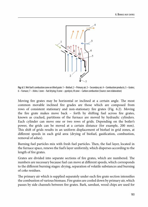
183

6. Biomass heat centres

Fig. 6.1. Wet fuel’s combustion zone on tilted grate: 1 – Biofuel; 2 – Primary air; 3 – Secondary air; 4 – Combustion products; 5 – Grates; 6 – Furnace; 7 – Ashes. I zone – fuel drying; II zone – pyrolysis; III zone – Carbon combustion (Source: own elaboration)

Moving fire grates may be horizontal or inclined at a certain angle. The most common movable inclined fire grades are those which are composed from rows of consistent stationary and non-stationary fire grates (Fig. 6.2). Moving the fire grate makes move back – forth by shifting fuel across fire grates, known as cracked, partitions of the furnace are moved by hydraulic cylinders. Each cylinder can move one or two rows of grids. Depending on the boiler’s power, the grids can be moved at a certain distance (for example, 200 mm). This shift of grids results in an uniform displacement of biofuel in grid zones, at different speeds in each grid area (drying of biofuel, gasification, combustion, removal of ashes).

Burning fuel particles mix with fresh fuel particles. Then, the fuel layer, located in the furnace space, renews the fuel’s layer uniformly, which disperses according to the length of fire grates.

Grates are divided into separate sections of fire grates, which are numbered. The numbers are necessary because fuel can move at different speeds, which corresponds to the different burning stages: drying, separation of volatile substances and burning of coke residues.

The primary air which is supplied separately under each fire grate section intensifies the combustion of various biomass. Fire grates are cooled down by primary air, which passes by side channels between fire grates. Bark, sawdust, wood chips are used for

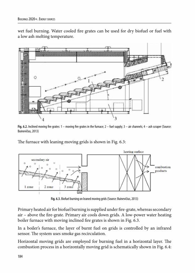
184


wet fuel burning. Water cooled fire grates can be used for dry biofuel or fuel with a low ash melting temperature.

Fig. 6.2. Inclined moving fire grates: 1 – moving fire grates in the furnace; 2 – fuel supply; 3 – air channels; 4 – ash scraper (Source: Buinevičius, 2013)

The furnace with leaning moving grids is shown in Fig. 6.3:

Fig. 6.3. Biofuel burning on leaned moving grids (Source: Buinevičius, 2013)

Primary heated air for biofuel burning is supplied under fire-grate, whereas secondary air – above the fire-grate. Primary air cools down grids. A low-power water heating boiler furnace with moving inclined fire grates is shown in Fig. 6.3.

In a boiler’s furnace, the layer of burnt fuel on grids is controlled by an infrared sensor. The system uses smoke gas recirculation.

Horizontal moving grids are employed for burning fuel in a horizontal layer. The combustion process in a horizontally moving grid is schematically shown in Fig. 6.4:

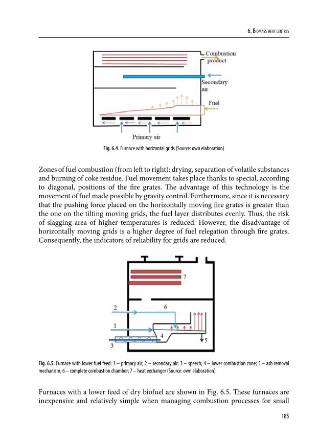
185


Fig. 6.4. Furnace with horizontal grids (Source: own elaboration)

Zones of fuel combustion (from left to right): drying, separation of volatile substances and burning of coke residue. Fuel movement takes place thanks to special, according to diagonal, positions of the fire grates. The advantage of this technology is the movement of fuel made possible by gravity control. Furthermore, since it is necessary that the pushing force placed on the horizontally moving fire grates is greater than the one on the tilting moving grids, the fuel layer distributes evenly. Thus, the risk of slagging area of higher temperatures is reduced. However, the disadvantage of horizontally moving grids is a higher degree of fuel relegation through fire grates. Consequently, the indicators of reliability for grids are reduced.

Fig. 6.5. Furnace with lower fuel feed: 1 – primary air; 2 – secondary air; 3 – speech; 4 – lower combustion zone; 5 – ash removal mechanism; 6 – complete combustion chamber; 7 – heat exchanger (Source: own elaboration)

Furnaces with a lower feed of dry biofuel are shown in Fig. 6.5. These furnaces are inexpensive and relatively simple when managing combustion processes for small

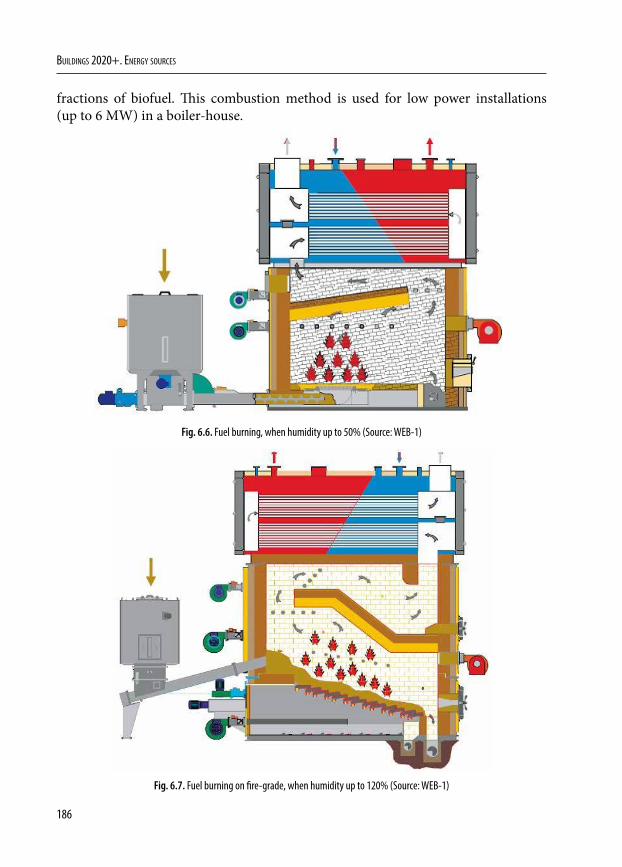
186


fractions of biofuel. This combustion method is used for low power installations (up to 6 MW) in a boiler-house.

Fig. 6.6. Fuel burning, when humidity up to 50% (Source: WEB-1)

Fig. 6.7. Fuel burning on fire-grade, when humidity up to 120% (Source: WEB-1)

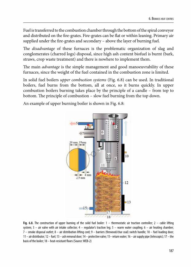
187


Fuel is transferred to the combustion chamber through the bottom of the spiral conveyor and distributed on the fire-grates. Fire-grates can be flat or within leaning. Primary air supplied under the fire-grates and secondary – above the layer of burning fuel.

The disadvantage of these furnaces is the problematic organization of slag and conglomerates (charred logs) disposal, since high ash content biofuel is burnt (bark, straws, crop waste treatment) and there is nowhere to implement them.

The main advantage is the simple management and good manoeuvrability of these furnaces, since the weight of the fuel contained in the combustion zone is limited.

In solid fuel boilers upper combustion systems (Fig. 6.8) can be used. In traditional boilers, fuel burns from the bottom, all at once, so it burns quickly. In upper combustion boilers burning takes place by the principle of a candle – from top to bottom. The principle of combustion – slow fuel burning from the top down.

An example of upper burning boiler is shown in Fig. 6.8:

Fig. 6.8. The construction of upper burning of the solid fuel boiler: 1 – thermostatic air traction controller; 2 – cable lifting system; 3 – air valve with air intake collector; 4 – regulator’s traction leg; 5 – warm water coupling; 6 – air heating chamber; 7 – smoke disposal outlet; 8 – air distribution lifting cord; 9 – barriers (firewood/char coal) switch handle; 10 – fuel loading door; 11 – air distributor; 12 – fuel; 13 – ash removal door; 14 – protective valve; 15– return water; 16 – air supply pipe (telescopic); 17 – the basis of the boiler; 18 – heat-resistant floors (Source: WEB-2)

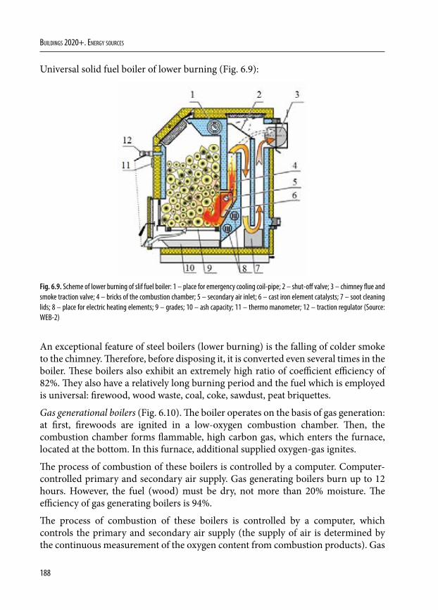
188


Universal solid fuel boiler of lower burning (Fig. 6.9):

Fig. 6.9. Scheme of lower burning of slif fuel boiler: 1 – place for emergency cooling coil-pipe; 2 – shut-off valve; 3 – chimney flue and smoke traction valve; 4 – bricks of the combustion chamber; 5 – secondary air inlet; 6 – cast iron element catalysts; 7 – soot cleaning lids; 8 – place for electric heating elements; 9 – grades; 10 – ash capacity; 11 – thermo manometer; 12 – traction regulator (Source: WEB-2)

An exceptional feature of steel boilers (lower burning) is the falling of colder smoke to the chimney. Therefore, before disposing it, it is converted even several times in the boiler. These boilers also exhibit an extremely high ratio of coefficient efficiency of 82%. They also have a relatively long burning period and the fuel which is employed is universal: firewood, wood waste, coal, coke, sawdust, peat briquettes.

Gas generational boilers (Fig. 6.10). The boiler operates on the basis of gas generation: at first, firewoods are ignited in a low-oxygen combustion chamber. Then, the combustion chamber forms flammable, high carbon gas, which enters the furnace, located at the bottom. In this furnace, additional supplied oxygen-gas ignites.

The process of combustion of these boilers is controlled by a computer. Computer-controlled primary and secondary air supply. Gas generating boilers burn up to 12 hours. However, the fuel (wood) must be dry, not more than 20% moisture. The efficiency of gas generating boilers is 94%.

The process of combustion of these boilers is controlled by a computer, which controls the primary and secondary air supply (the supply of air is determined by the continuous measurement of the oxygen content from combustion products). Gas

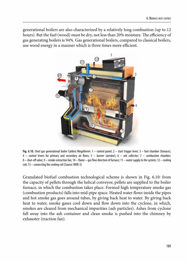
189


generational boilers are also characterized by a relatively long combustion (up to 12 hours). But the fuel (wood) must be dry, not less than 20% moisture. The efficiency of gas generating boilers is 94%. Gas generational boilers, compared to classical boilers, use wood energy in a manner which is three times more efficient.

Fig. 6.10. Steel gas generational boiler Caldera Megatherm: 1 – control panel; 2 – start trigger lever; 3 – fuel chamber (furnace); 4 – control levers for primary and secondary air flows; 5 – burner (aerator); 6 – ash collector; 7 – combustion chamber; 8 – shut-off valve; 9 – smoke extraction fan; 10 – flame – gas flow direction of furnace; 11 – water supply to the system; 12 – cooling coil; 13 – connecting the cooling coil (Source: WEB-3)

Granulated biofuel combustion technological scheme is shown in Fig. 6.10: from the capacity of pellets through the helical conveyor, pellets are supplied to the boiler furnace, in which the combustion takes place. Formed high temperature smoke gas (combustion products) falls into mid-pipe space. Heated water flows inside the pipes and hot smoke gas goes around tubes, by giving back heat to water. By giving back heat to water, smoke gases cool down and flow down into the cyclone, in which, smokes are cleared from mechanical impurities (ash particles). Ashes from cyclone fall away into the ash container and clean smoke is pushed into the chimney by exhauster (traction fan).

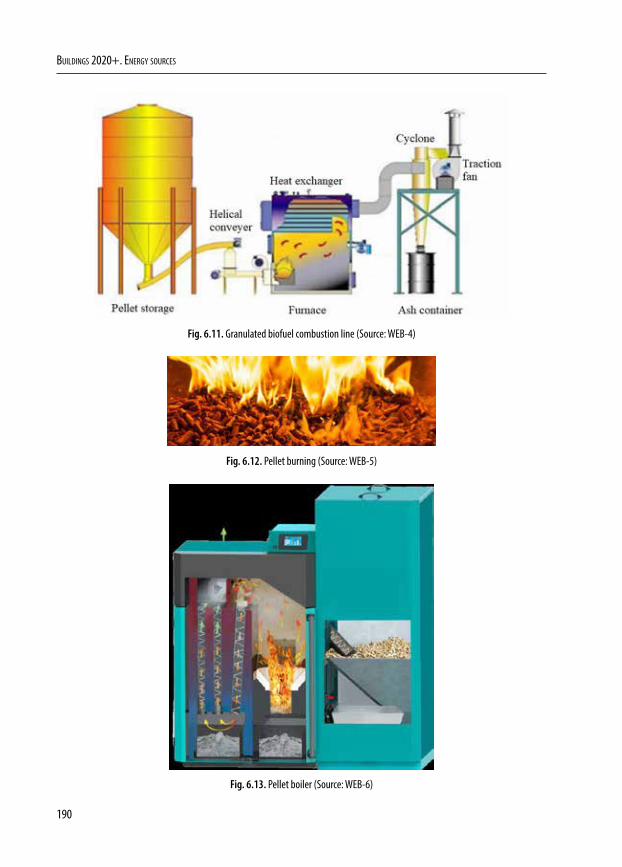
190


Fig. 6.11. Granulated biofuel combustion line (Source: WEB-4)

Fig. 6.12. Pellet burning (Source: WEB-5)

Fig. 6.13. Pellet boiler (Source: WEB-6)

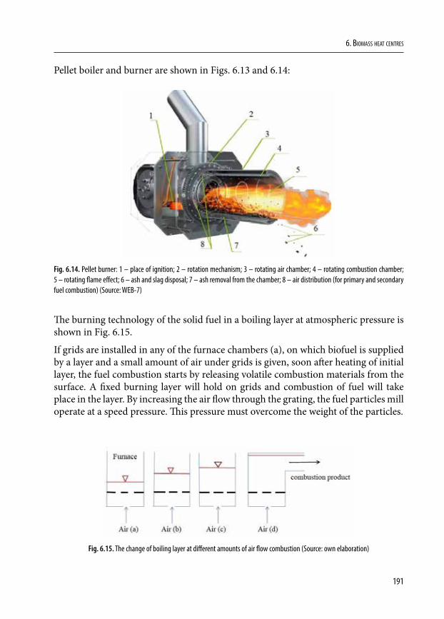
191


Pellet boiler and burner are shown in Figs. 6.13 and 6.14:

Fig. 6.14. Pellet burner: 1 – place of ignition; 2 – rotation mechanism; 3 – rotating air chamber; 4 – rotating combustion chamber; 5 – rotating flame effect; 6 – ash and slag disposal; 7 – ash removal from the chamber; 8 – air distribution (for primary and secondary fuel combustion) (Source: WEB-7)

The burning technology of the solid fuel in a boiling layer at atmospheric pressure is shown in Fig. 6.15.

If grids are installed in any of the furnace chambers (a), on which biofuel is supplied by a layer and a small amount of air under grids is given, soon after heating of initial layer, the fuel combustion starts by releasing volatile combustion materials from the surface. A fixed burning layer will hold on grids and combustion of fuel will take place in the layer. By increasing the air flow through the grating, the fuel particles mill operate at a speed pressure. This pressure must overcome the weight of the particles.

Fig. 6.15. The change of boiling layer at different amounts of air flow combustion (Source: own elaboration)

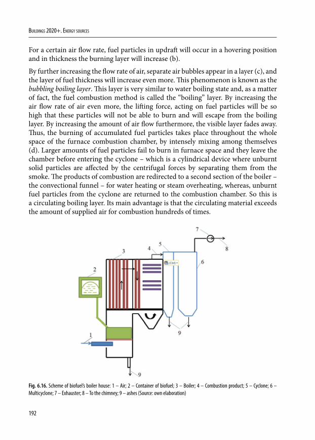
192


For a certain air flow rate, fuel particles in updraft will occur in a hovering position and in thickness the burning layer will increase (b).

By further increasing the flow rate of air, separate air bubbles appear in a layer (c), and the layer of fuel thickness will increase even more. This phenomenon is known as the bubbling boiling layer. This layer is very similar to water boiling state and, as a matter of fact, the fuel combustion method is called the “boiling” layer. By increasing the air flow rate of air even more, the lifting force, acting on fuel particles will be so high that these particles will not be able to burn and will escape from the boiling layer. By increasing the amount of air flow furthermore, the visible layer fades away. Thus, the burning of accumulated fuel particles takes place throughout the whole space of the furnace combustion chamber, by intensely mixing among themselves (d). Larger amounts of fuel particles fail to burn in furnace space and they leave the chamber before entering the cyclone – which is a cylindrical device where unburnt solid particles are affected by the centrifugal forces by separating them from the smoke. The products of combustion are redirected to a second section of the boiler – the convectional funnel – for water heating or steam overheating, whereas, unburnt fuel particles from the cyclone are returned to the combustion chamber. So this is a circulating boiling layer. Its main advantage is that the circulating material exceeds the amount of supplied air for combustion hundreds of times.

Fig. 6.16. Scheme of biofuel’s boiler house: 1 – Air; 2 – Container of biofuel; 3 – Boiler; 4 – Combustion product; 5 – Cyclone; 6 – Multicyclone; 7 – Exhauster; 8 – To the chimney; 9 – ashes (Source: own elaboration)

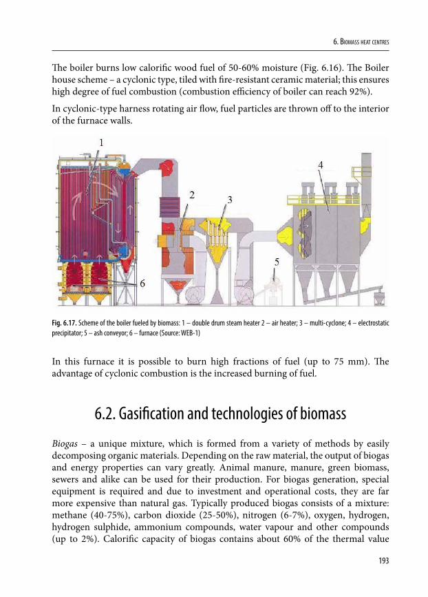
193


The boiler burns low calorific wood fuel of 50-60% moisture (Fig. 6.16). The Boiler house scheme – a cyclonic type, tiled with fire-resistant ceramic material; this ensures high degree of fuel combustion (combustion efficiency of boiler can reach 92%).

In cyclonic-type harness rotating air flow, fuel particles are thrown off to the interior of the furnace walls.

Fig. 6.17. Scheme of the boiler fueled by biomass: 1 – double drum steam heater 2 – air heater; 3 – multi-cyclone; 4 – electrostatic precipitator; 5 – ash conveyor; 6 – furnace (Source: WEB-1)

In this furnace it is possible to burn high fractions of fuel (up to 75 mm). The advantage of cyclonic combustion is the increased burning of fuel.

6.2. Gasification and technologies of biomass

Biogas – a unique mixture, which is formed from a variety of methods by easily decomposing organic materials. Depending on the raw material, the output of biogas and energy properties can vary greatly. Animal manure, manure, green biomass, sewers and alike can be used for their production. For biogas generation, special equipment is required and due to investment and operational costs, they are far more expensive than natural gas. Typically produced biogas consists of a mixture: methane (40-75%), carbon dioxide (25-50%), nitrogen (6-7%), oxygen, hydrogen, hydrogen sulphide, ammonium compounds, water vapour and other compounds (up to 2%). Calorific capacity of biogas contains about 60% of the thermal value

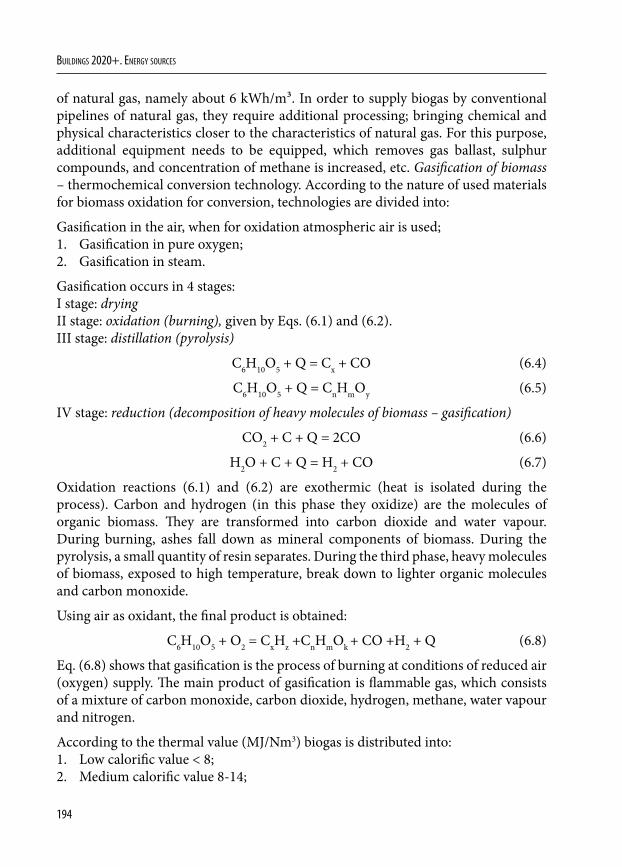
194


of natural gas, namely about 6 kWh/m³. In order to supply biogas by conventional pipelines of natural gas, they require additional processing; bringing chemical and physical characteristics closer to the characteristics of natural gas. For this purpose, additional equipment needs to be equipped, which removes gas ballast, sulphur compounds, and concentration of methane is increased, etc. Gasification of biomass – thermochemical conversion technology. According to the nature of used materials for biomass oxidation for conversion, technologies are divided into:

Gasification in the air, when for oxidation atmospheric air is used;1. Gasification in pure oxygen;2. Gasification in steam.

Gasification occurs in 4 stages:I stage: dryingII stage: oxidation (burning), given by Eqs. (6.1) and (6.2).III stage: distillation (pyrolysis)

C6H10O5 + Q = Cx + CO (6.4)

C6H10O5 + Q = CnHmOy (6.5)

IV stage: reduction (decomposition of heavy molecules of biomass – gasification)

CO2 + C + Q = 2CO (6.6)

H2O + C + Q = H2 + CO (6.7)

Oxidation reactions (6.1) and (6.2) are exothermic (heat is isolated during the process). Carbon and hydrogen (in this phase they oxidize) are the molecules of organic biomass. They are transformed into carbon dioxide and water vapour. During burning, ashes fall down as mineral components of biomass. During the pyrolysis, a small quantity of resin separates. During the third phase, heavy molecules of biomass, exposed to high temperature, break down to lighter organic molecules and carbon monoxide.

Using air as oxidant, the final product is obtained:

C6H10O5 + O2 = CxHz +CnHmOk + CO +H2 + Q (6.8)

Eq. (6.8) shows that gasification is the process of burning at conditions of reduced air (oxygen) supply. The main product of gasification is flammable gas, which consists of a mixture of carbon monoxide, carbon dioxide, hydrogen, methane, water vapour and nitrogen.

According to the thermal value (MJ/Nm3) biogas is distributed into:1. Low calorific value < 8;2. Medium calorific value 8-14;

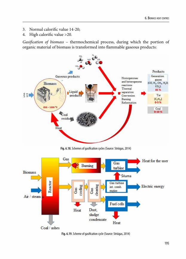
195


3. Normal calorific value 14-20;4. High calorific value >20.

Gasification of biomass – thermochemical process, during which the portion of organic material of biomass is transformed into flammable gaseous products:

Fig. 6.18. Schemes of gasification cycles (Source: Striūgas, 2014)

Fig. 6.19. Scheme of gasification cycle (Source: Striūgas, 2014)

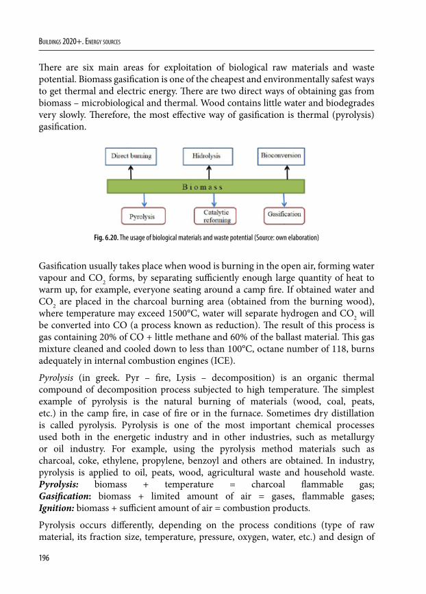
196


There are six main areas for exploitation of biological raw materials and waste potential. Biomass gasification is one of the cheapest and environmentally safest ways to get thermal and electric energy. There are two direct ways of obtaining gas from biomass – microbiological and thermal. Wood contains little water and biodegrades very slowly. Therefore, the most effective way of gasification is thermal (pyrolysis) gasification.

Fig. 6.20. The usage of biological materials and waste potential (Source: own elaboration)

Gasification usually takes place when wood is burning in the open air, forming water vapour and CO2 forms, by separating sufficiently enough large quantity of heat to warm up, for example, everyone seating around a camp fire. If obtained water and CO2 are placed in the charcoal burning area (obtained from the burning wood), where temperature may exceed 1500°C, water will separate hydrogen and CO2 will be converted into CO (a process known as reduction). The result of this process is gas containing 20% of CO + little methane and 60% of the ballast material. This gas mixture cleaned and cooled down to less than 100°C, octane number of 118, burns adequately in internal combustion engines (ICE).

Pyrolysis (in greek. Pyr – fire, Lysis – decomposition) is an organic thermal compound of decomposition process subjected to high temperature. The simplest example of pyrolysis is the natural burning of materials (wood, coal, peats, etc.) in the camp fire, in case of fire or in the furnace. Sometimes dry distillation is called pyrolysis. Pyrolysis is one of the most important chemical processes used both in the energetic industry and in other industries, such as metallurgy or oil industry. For example, using the pyrolysis method materials such as charcoal, coke, ethylene, propylene, benzoyl and others are obtained. In industry, pyrolysis is applied to oil, peats, wood, agricultural waste and household waste. Pyrolysis: biomass + temperature = charcoal flammable gas; Gasification: biomass + limited amount of air = gases, flammable gases; Ignition: biomass + sufficient amount of air = combustion products.

Pyrolysis occurs differently, depending on the process conditions (type of raw material, its fraction size, temperature, pressure, oxygen, water, etc.) and design of

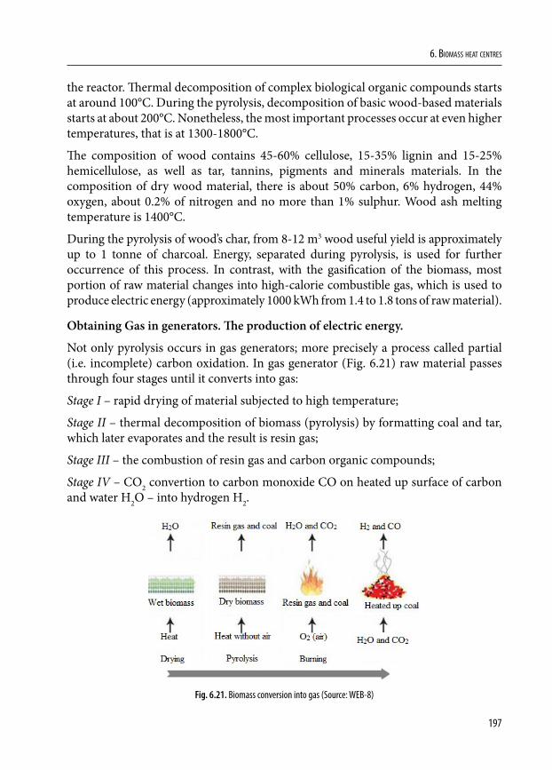
197


the reactor. Thermal decomposition of complex biological organic compounds starts at around 100°C. During the pyrolysis, decomposition of basic wood-based materials starts at about 200°C. Nonetheless, the most important processes occur at even higher temperatures, that is at 1300-1800°C.

The composition of wood contains 45-60% cellulose, 15-35% lignin and 15-25% hemicellulose, as well as tar, tannins, pigments and minerals materials. In the composition of dry wood material, there is about 50% carbon, 6% hydrogen, 44% oxygen, about 0.2% of nitrogen and no more than 1% sulphur. Wood ash melting temperature is 1400°C.

During the pyrolysis of wood’s char, from 8-12 m3 wood useful yield is approximately up to 1 tonne of charcoal. Energy, separated during pyrolysis, is used for further occurrence of this process. In contrast, with the gasification of the biomass, most portion of raw material changes into high-calorie combustible gas, which is used to produce electric energy (approximately 1000 kWh from 1.4 to 1.8 tons of raw material).

Obtaining Gas in generators. The production of electric energy.

Not only pyrolysis occurs in gas generators; more precisely a process called partial (i.e. incomplete) carbon oxidation. In gas generator (Fig. 6.21) raw material passes through four stages until it converts into gas:

Stage I – rapid drying of material subjected to high temperature;

Stage II – thermal decomposition of biomass (pyrolysis) by formatting coal and tar, which later evaporates and the result is resin gas;

Stage III – the combustion of resin gas and carbon organic compounds;

Stage IV – CO2 convertion to carbon monoxide CO on heated up surface of carbon and water H2O – into hydrogen H2.

Fig. 6.21. Biomass conversion into gas (Source: WEB-8)

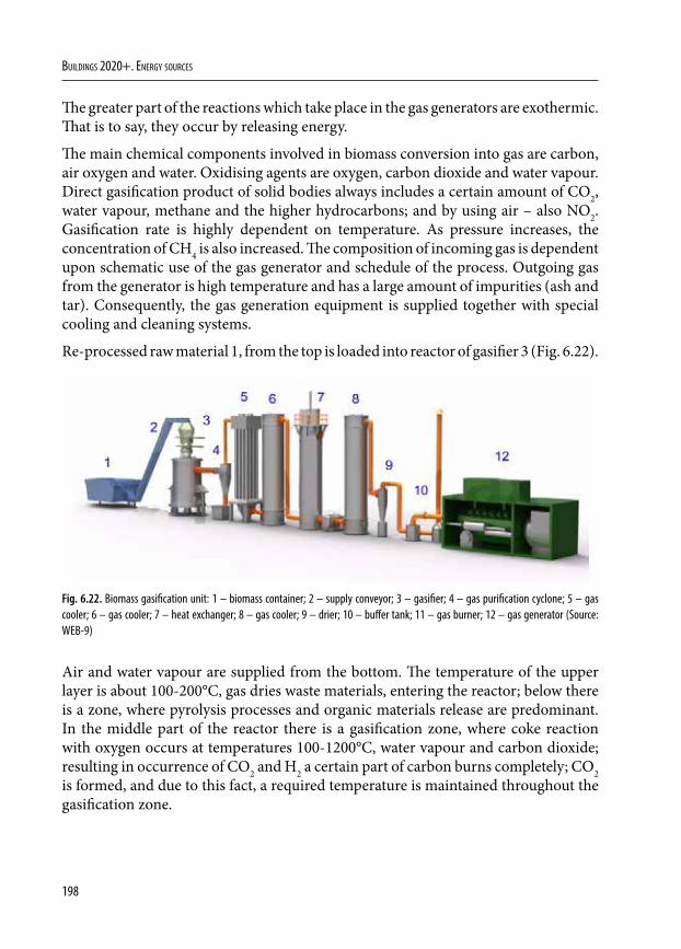
198


The greater part of the reactions which take place in the gas generators are exothermic. That is to say, they occur by releasing energy.

The main chemical components involved in biomass conversion into gas are carbon, air oxygen and water. Oxidising agents are oxygen, carbon dioxide and water vapour. Direct gasification product of solid bodies always includes a certain amount of CO2, water vapour, methane and the higher hydrocarbons; and by using air – also NO2. Gasification rate is highly dependent on temperature. As pressure increases, the concentration of CH4 is also increased. The composition of incoming gas is dependent upon schematic use of the gas generator and schedule of the process. Outgoing gas from the generator is high temperature and has a large amount of impurities (ash and tar). Consequently, the gas generation equipment is supplied together with special cooling and cleaning systems.

Re-processed raw material 1, from the top is loaded into reactor of gasifier 3 (Fig. 6.22).

Fig. 6.22. Biomass gasification unit: 1 – biomass container; 2 – supply conveyor; 3 – gasifier; 4 – gas purification cyclone; 5 – gas cooler; 6 – gas cooler; 7 – heat exchanger; 8 – gas cooler; 9 – drier; 10 – buffer tank; 11 – gas burner; 12 – gas generator (Source: WEB-9)

Air and water vapour are supplied from the bottom. The temperature of the upper layer is about 100-200°C, gas dries waste materials, entering the reactor; below there is a zone, where pyrolysis processes and organic materials release are predominant. In the middle part of the reactor there is a gasification zone, where coke reaction with oxygen occurs at temperatures 100-1200°C, water vapour and carbon dioxide; resulting in occurrence of CO2 and H2 a certain part of carbon burns completely; CO2 is formed, and due to this fact, a required temperature is maintained throughout the gasification zone.

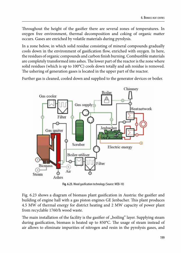
199


Throughout the height of the gasifier there are several zones of temperatures. In oxygen free environment, thermal decomposition and coking of organic matter occurs. Gases are enriched by volatile materials during pyrolysis.

In a zone below, in which solid residue consisting of mineral compounds gradually cools down in the environment of gasification flow, enriched with oxygen. In here, the residues of organic compounds and carbon finish burning. Combustible materials are completely transformed into ashes. The lower part of the reactor is the zone where solid residues (which is up to 100°C) cools down totally and ash residue is removed. The ushering of generation gases is located in the upper part of the reactor.

Further gas is cleaned, cooled down and supplied to the generator devices or boiler.

Fig. 6.23. Wood gasification technology (Source: WEB-10)

Fig. 6.23 shows a diagram of biomass plant gasification in Austria: the gasifier and building of engine hall with a gas piston engines GE Jenbacher. This plant produces 4.5 MW of thermal energy for district heating and 2 MW capacity of power plant from recyclable 1760/h wood waste.

The main installation of the facility is the gasifier of „boiling” layer. Supplying steam during gasification, biomass is heated up to 850°C. The usage of steam instead of air allows to eliminate impurities of nitrogen and resin in the pyrolysis gases, and

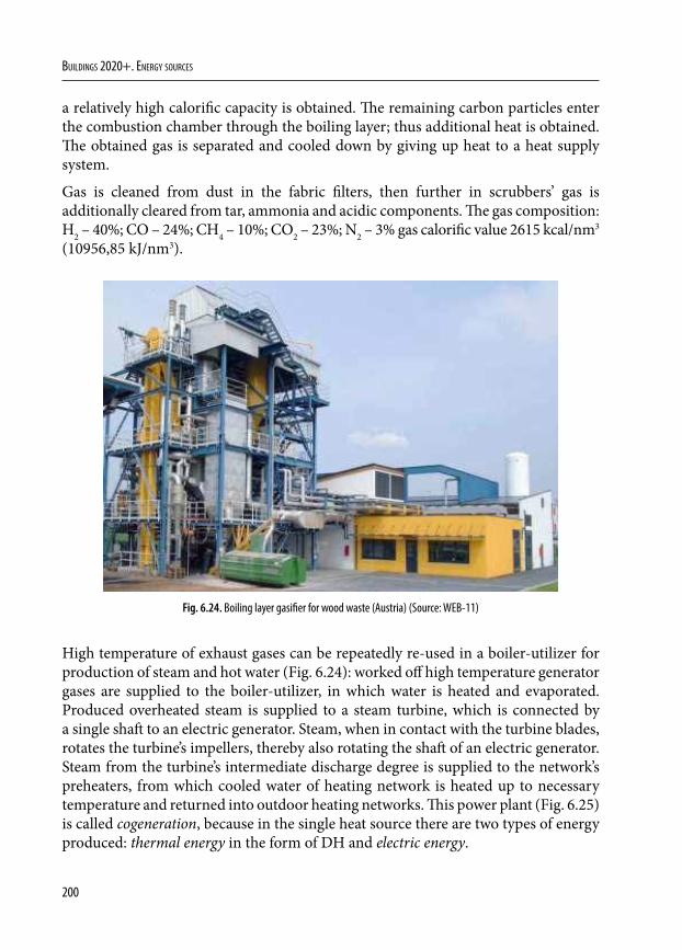
200


a relatively high calorific capacity is obtained. The remaining carbon particles enter the combustion chamber through the boiling layer; thus additional heat is obtained. The obtained gas is separated and cooled down by giving up heat to a heat supply system.

Gas is cleaned from dust in the fabric filters, then further in scrubbers’ gas is additionally cleared from tar, ammonia and acidic components. The gas composition: H2 – 40%; CO – 24%; CH4 – 10%; CO2 – 23%; N2 – 3% gas calorific value 2615 kcal/nm3 (10956,85 kJ/nm3).

Fig. 6.24. Boiling layer gasifier for wood waste (Austria) (Source: WEB-11)

High temperature of exhaust gases can be repeatedly re-used in a boiler-utilizer for production of steam and hot water (Fig. 6.24): worked off high temperature generator gases are supplied to the boiler-utilizer, in which water is heated and evaporated. Produced overheated steam is supplied to a steam turbine, which is connected by a single shaft to an electric generator. Steam, when in contact with the turbine blades, rotates the turbine’s impellers, thereby also rotating the shaft of an electric generator. Steam from the turbine’s intermediate discharge degree is supplied to the network’s preheaters, from which cooled water of heating network is heated up to necessary temperature and returned into outdoor heating networks. This power plant (Fig. 6.25) is called cogeneration, because in the single heat source there are two types of energy produced: thermal energy in the form of DH and electric energy.

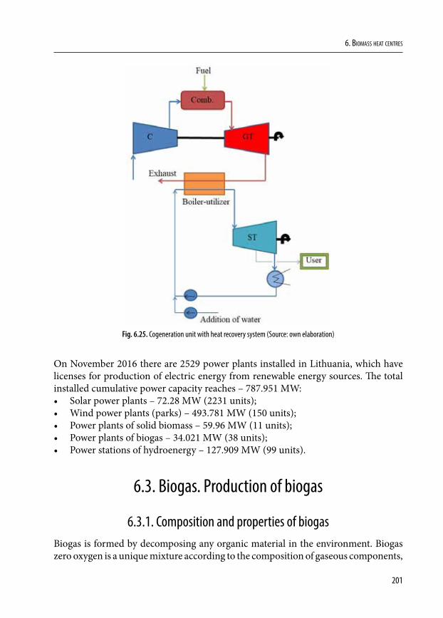
201


Fig. 6.25. Cogeneration unit with heat recovery system (Source: own elaboration)

On November 2016 there are 2529 power plants installed in Lithuania, which have licenses for production of electric energy from renewable energy sources. The total installed cumulative power capacity reaches – 787.951 MW:• Solar power plants – 72.28 MW (2231 units);• Wind power plants (parks) – 493.781 MW (150 units);• Power plants of solid biomass – 59.96 MW (11 units);• Power plants of biogas – 34.021 MW (38 units);• Power stations of hydroenergy – 127.909 MW (99 units).

6.3. Biogas. Production of biogas

6.3.1. Composition and properties of biogasBiogas is formed by decomposing any organic material in the environment. Biogas zero oxygen is a unique mixture according to the composition of gaseous components,

202


which is formed as a result of the final waste of organic part for anaerobic microbial fermentation or chemical reactions between the decomposed parts of wastes.

The main components of biogas are methane (CH4) and carbon dioxide (CO2). In biogas, depending on the composition of raw material, there are very small amounts of hydrogen (H2) hydrogen sulfide (H2S), nitrogen (N) and other materials. Mostly in biogas methane ranges from 55 to 70%, carbon dioxide – from 30 to 45% hydrogen – up to 1% and sulphide up to 3%.

Since biogas is a mixture of methane and carbon dioxide, their flammability concentration limits are slightly different from pure methane and depend on the concentration of the latter in the biogas. Gas ignition concentration limits in the air is a very important indicator. It means when the temperature of gas and air mixture reaches the ignition temperature, if gas concentration in the mixture is between lower and upper concentration limits, the mixture will burn (if the volume of the mixture is sufficiently large – it’ll explode).

The most important property of biogas – the concentration of methane in biogas is determined by thermal value, ignition temperature and concentration limits in air.

6.3.2. Materials for production of biogasBiogas production is a complex biological-chemical process in which organic materials are exposed to different types of bacteria. During this process, complex organic compounds are decomposed into elements, which methanogenic bacteria convert into biogas – combination of methane, carbon dioxide and other gases. Methanogenic bacteria are very sensitive anaerobes. Therefore, temperature, acidity and alkalinity, oxidation reduction potential and other environmental factors must meet certain specific requirements. Metabolic activity and the intensity of methane production also depend on the composition of the processed substrate, supported by temperature and its fluctuations, retention time and inhibiting factors. Microbiological activity in the biogas reactors is most favourable at neutral or slightly alkaline conditions (6,0 < pH <8,5).

In energy of biogas it is accepted to divide process temperatures into three groups: psychrophilic (10-25°C), mesophilic (25-42°C) and thermophilic (52-56°C).

The main raw material for the production of biogas are organic wastes of various origins. Some wastes are difficult to be decomposed and less biogas is obtained from them, in others – higher amount of biogas with a higher methane content can easily be obtained from them.

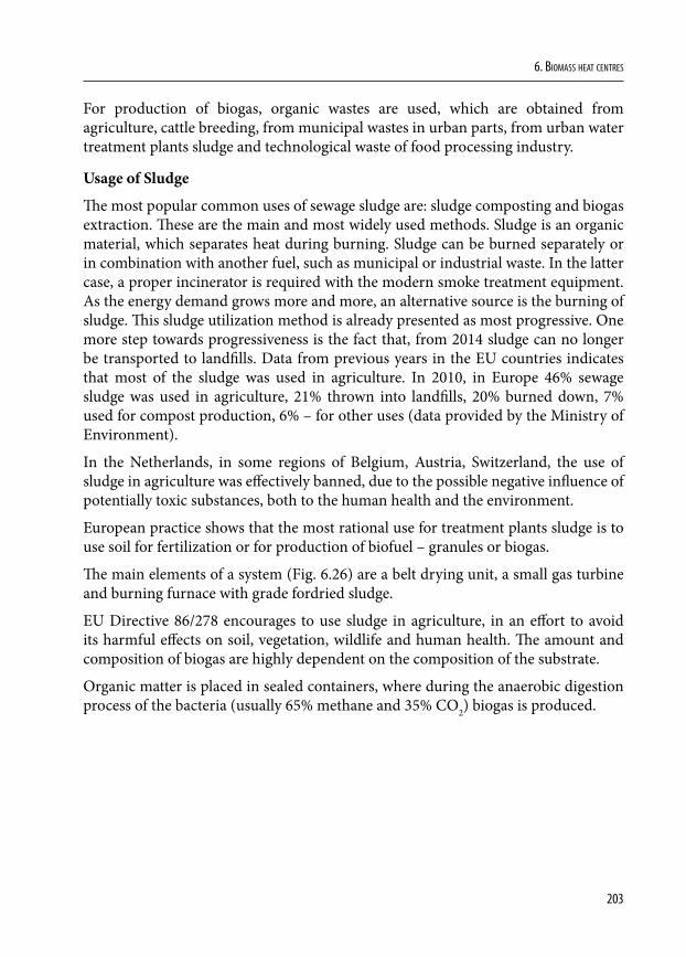
203


For production of biogas, organic wastes are used, which are obtained from agriculture, cattle breeding, from municipal wastes in urban parts, from urban water treatment plants sludge and technological waste of food processing industry.

Usage of Sludge

The most popular common uses of sewage sludge are: sludge composting and biogas extraction. These are the main and most widely used methods. Sludge is an organic material, which separates heat during burning. Sludge can be burned separately or in combination with another fuel, such as municipal or industrial waste. In the latter case, a proper incinerator is required with the modern smoke treatment equipment. As the energy demand grows more and more, an alternative source is the burning of sludge. This sludge utilization method is already presented as most progressive. One more step towards progressiveness is the fact that, from 2014 sludge can no longer be transported to landfills. Data from previous years in the EU countries indicates that most of the sludge was used in agriculture. In 2010, in Europe 46% sewage sludge was used in agriculture, 21% thrown into landfills, 20% burned down, 7% used for compost production, 6% – for other uses (data provided by the Ministry of Environment).

In the Netherlands, in some regions of Belgium, Austria, Switzerland, the use of sludge in agriculture was effectively banned, due to the possible negative influence of potentially toxic substances, both to the human health and the environment.

European practice shows that the most rational use for treatment plants sludge is to use soil for fertilization or for production of biofuel – granules or biogas.

The main elements of a system (Fig. 6.26) are a belt drying unit, a small gas turbine and burning furnace with grade fordried sludge.

EU Directive 86/278 encourages to use sludge in agriculture, in an effort to avoid its harmful effects on soil, vegetation, wildlife and human health. The amount and composition of biogas are highly dependent on the composition of the substrate.

Organic matter is placed in sealed containers, where during the anaerobic digestion process of the bacteria (usually 65% methane and 35% CO2) biogas is produced.

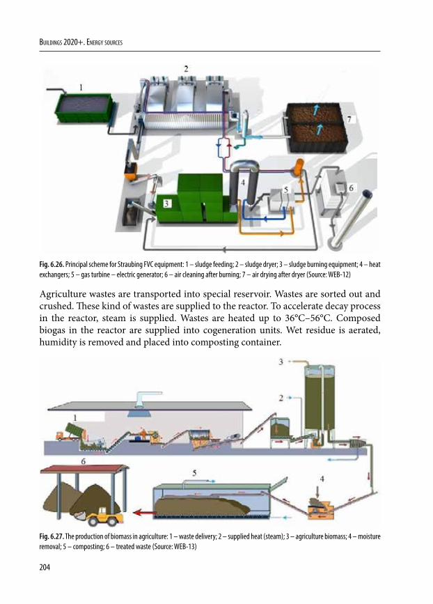
204


Fig. 6.26. Principal scheme for Straubing FVC equipment: 1 – sludge feeding; 2 – sludge dryer; 3 – sludge burning equipment; 4 – heat exchangers; 5 – gas turbine – electric generator; 6 – air cleaning after burning; 7 – air drying after dryer (Source: WEB-12)

Agriculture wastes are transported into special reservoir. Wastes are sorted out and crushed. These kind of wastes are supplied to the reactor. To accelerate decay process in the reactor, steam is supplied. Wastes are heated up to 36°C–56°C. Composed biogas in the reactor are supplied into cogeneration units. Wet residue is aerated, humidity is removed and placed into composting container.

Fig. 6.27. The production of biomass in agriculture: 1 – waste delivery; 2 – supplied heat (steam); 3 – agriculture biomass; 4 – moisture removal; 5 – composting; 6 – treated waste (Source: WEB-13)

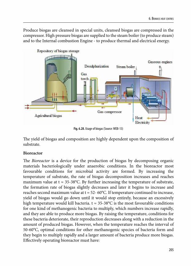
205


Produce biogas are cleansed in special units, cleansed biogas are compressed in the compressor. High pressure biogas are supplied to the steam boiler (to produce steam) and to the Internal combustion Engine - to produce thermal and electrical energy.

Fig. 6.28. Usage of biogas (Source: WEB-13)

The yield of biogas and composition are highly dependent upon the composition of substrate.

Bioreactor

The Bioreactor is a device for the production of biogas by decomposing organic materials bacteriologically under anaerobic conditions. In the bioreactor most favourable conditions for microbial activity are formed. By increasing the temperature of substrate, the rate of biogas decomposition increases and reaches maximum value at t ≈ 35-38°C. By further increasing the temperature of substrate, the formation rate of biogas slightly decreases and later it begins to increase and reaches second maximum value at t ≈ 52- 60°C. If temperature continued to increase, yield of biogas would go down until it would stop entirely, because an excessively high temperature would kill bacteria. t ≈ 35-38°C is the most favourable conditions for one kind of methanogenic bacteria to multiply, which numbers increase rapidly, and they are able to produce more biogas. By raising the temperature, conditions for these bacteria deteriorate, their reproduction decreases along with a reduction in the amount of produced biogas. However, when the temperature reaches the interval of 50-60°C, optimal conditions for other methanogenic species of bacteria form and they begin to multiply rapidly and a larger amount of bacteria produce more biogas. Effectively operating bioreactor must have:

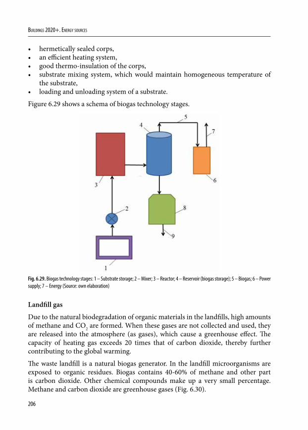
206


• hermetically sealed corps, • an efficient heating system,• good thermo-insulation of the corps,• substrate mixing system, which would maintain homogeneous temperature of

the substrate,• loading and unloading system of a substrate.

Figure 6.29 shows a schema of biogas technology stages.

Fig. 6.29. Biogas technology stages: 1 – Substrate storage; 2 – Mixer; 3 – Reactor; 4 – Reservoir (biogas storage); 5 – Biogas; 6 – Power supply; 7 – Energy (Source: own elaboration)

Landfill gas

Due to the natural biodegradation of organic materials in the landfills, high amounts of methane and CO2 are formed. When these gases are not collected and used, they are released into the atmosphere (as gases), which cause a greenhouse effect. The capacity of heating gas exceeds 20 times that of carbon dioxide, thereby further contributing to the global warming.

The waste landfill is a natural biogas generator. In the landfill microorganisms are exposed to organic residues. Biogas contains 40-60% of methane and other part is carbon dioxide. Other chemical compounds make up a very small percentage. Methane and carbon dioxide are greenhouse gases (Fig. 6.30).

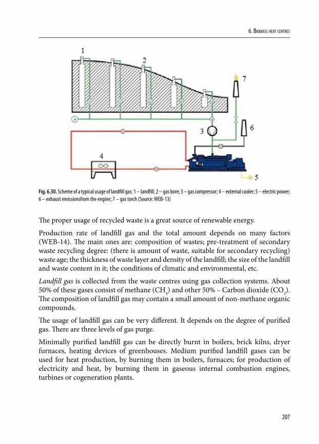
207


Fig. 6.30. Scheme of a typical usage of landfill gas: 1 – landfill; 2 – gas bore; 3 – gas compressor; 4 – external cooler; 5 – electric power; 6 – exhaust emissionsfrom the engine; 7 – gas torch (Source: WEB-13)

The proper usage of recycled waste is a great source of renewable energy.

Production rate of landfill gas and the total amount depends on many factors (WEB-14). The main ones are: composition of wastes; pre-treatment of secondary waste recycling degree: (there is amount of waste, suitable for secondary recycling) waste age; the thickness of waste layer and density of the landfill; the size of the landfill and waste content in it; the conditions of climatic and environmental, etc.

Landfill gas is collected from the waste centres using gas collection systems. About 50% of these gases consist of methane (CH4) and other 50% – Carbon dioxide (CO2). The composition of landfill gas may contain a small amount of non-methane organic compounds.

The usage of landfill gas can be very different. It depends on the degree of purified gas. There are three levels of gas purge.

Minimally purified landfill gas can be directly burnt in boilers, brick kilns, dryer furnaces, heating devices of greenhouses. Medium purified landfill gases can be used for heat production, by burning them in boilers, furnaces; for production of electricity and heat, by burning them in gaseous internal combustion engines, turbines or cogeneration plants.

208


High degree purity gas or pure methane can be supplied into the network of natural gas. From an economic point of view, the most effective way to use the landfill gas is direct burning.

Power plant of biogas

Biogas plant structure and technological scheme depends on various factors: from composition and type of the material, its method of delivery, type and size of bioreactors, process parameters, use of recycled substrate, composition and quantity of produced biogas, type and quantity of energy conversion equipment, produced by energy consumers. Classical biogas plants are equipped with raw material collection, preparation and transportation equipment, bioreactors, produced biogas storages, treatment and incineration equipment, tanks of recycled biomass, separators, process equipment controllers and data loggers, electrical and thermal energy networks and distribution devices.

Biogas plant consists of the following main components:• transportation, storage, pre-treatment of biomass and feed into apparatus of

bioreactors;• bioreactor;• storage and handling facilities of degassed substrate;• the equipment of biogas storage, cleaning and further use.

Depending on the type of biomass it may be necessary to sort raw material, crush, heat up to higher temperature in order to kill disease-carrying microorganisms, or otherwise processed. A degassed solution of biomass can be used in agriculture as liquid fertilizer or as a raw material for the production of dry fertilizer. In the beginning, produced biogas are accumulated in gasholder, whose purpose is to level up the differences between their production and usage.

Biogas can be used in three different ways:• without additional purification burned in furnaces of boilers;• with a minimal cleaning, by removing moisture and hydrogen sulphide, are burnt

in cogeneration devices (usually in internal piston combustion engines);• purified to pure methane and supplied to the grid of natural gas.

The main product of biogas plants – biogas is used for electricity and thermal energy production (Fig. 6.31).

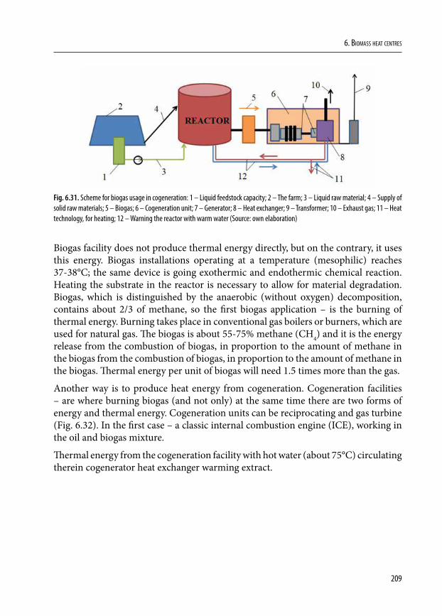
209


Fig. 6.31. Scheme for biogas usage in cogeneration: 1 – Liquid feedstock capacity; 2 – The farm; 3 – Liquid raw material; 4 – Supply of solid raw materials; 5 – Biogas; 6 – Cogeneration unit; 7 – Generator; 8 – Heat exchanger; 9 – Transformer; 10 – Exhaust gas; 11 – Heat technology, for heating; 12 – Warning the reactor with warm water (Source: own elaboration)

Biogas facility does not produce thermal energy directly, but on the contrary, it uses this energy. Biogas installations operating at a temperature (mesophilic) reaches 37-38°C; the same device is going exothermic and endothermic chemical reaction. Heating the substrate in the reactor is necessary to allow for material degradation. Biogas, which is distinguished by the anaerobic (without oxygen) decomposition, contains about 2/3 of methane, so the first biogas application – is the burning of thermal energy. Burning takes place in conventional gas boilers or burners, which are used for natural gas. The biogas is about 55-75% methane (CH4) and it is the energy release from the combustion of biogas, in proportion to the amount of methane in the biogas from the combustion of biogas, in proportion to the amount of methane in the biogas. Thermal energy per unit of biogas will need 1.5 times more than the gas.

Another way is to produce heat energy from cogeneration. Cogeneration facilities – are where burning biogas (and not only) at the same time there are two forms of energy and thermal energy. Cogeneration units can be reciprocating and gas turbine (Fig. 6.32). In the first case – a classic internal combustion engine (ICE), working in the oil and biogas mixture.

Thermal energy from the cogeneration facility with hot water (about 75°C) circulating therein cogenerator heat exchanger warming extract.

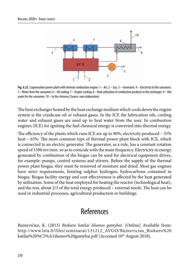
210


Fig. 6.32. Cogeneration power plant with internal combustion engine: 1 – Air; 2 – Gas; 3 – Generator; 4 – Electricity to the consumer; 5 – Water from the consumer; 6 – Oil cooling; 7 – Engine cooling; 8 – Heat utilization of combustion products in the exchanger; 9 – Hot water for the consumer; 10 – to the chimney (Source: own elaboration)

The heat exchanger heated by the heat exchange medium which cools down the engine system is the crankcase oil or exhaust gases. In the ICE the lubrication oils, cooling water and exhaust gases are used up to heat water from the user. In combustion engines (ICE) for igniting the fuel chemical energy is converted into thermal energy.

The efficiency of the plants which runs ICE are up to 90%; electricity produced – 35% heat – 65%. The most common type of thermal power plant block with ICE, which is connected to an electric generator. The generator, as a rule, has a constant rotation speed of 1500 rev/min. so as to coincide with the main frequency. Electricity in energy generated by combustion of the biogas can be used for electrical equipment drives, for example: pumps, control systems and stirrers. Before the supply of the thermal power plant biogas, they must be removed of moisture and dried. Most gas engines have strict requirements, limiting sulphur hydrogen, hydrocarbons contained in biogas. Biogas facility energy and cost effectiveness is affected by the heat generated by utilization. Some of the heat employed for heating the reactor (technological heat), and the rest, about 2/3 of the total energy produced – external needs. The heat can be used in industrial processes, agricultural production or buildings.

References

Buinevičius, K. (2013) Biokuro katilai šilumos gamybai. [Online] Available from: http://www.lsta.lt/files/seminarai/131212_AVGO/Buinevicius_Biokuro%20katilai%20%C5%A1ilumos%20gamybai.pdf [Accessed 10th August 2018].

211


Dzenajavičienė, E. F., Pedišius, N. & Škėma, R. (2011) Darni bioenergetika. Kaunas, Lietuvos energetikos institutas.

EU Directive 86/278 Council Directive 86/278/EEC of 12 June 1986 on the protection of the environment, and in particular of the soil, when sewage sludge is used in agriculture https://eur-lex.europa.eu/legal-content/EN/TXT/?uri=CELEX%3A31986L0278 [Accessed 10th August 2018].

Jakštas, A. (2011) Biomasės panaudojimo galimybės energijos gamybai CŠT sektoriuje. In: Seminaras Biomasės panaudojimas CŠT sektoriujeesama situacija ir kliūtys jos plėtrai, 5th December 2011, Vilnius. AEBIOM & LITBIOMA.

Kilait, L. & Puodžius, R. (2007) Įvairių kogeneracijos technologijų įrengimo galimybių ir sąnaudų bei rekomendacijų dėl šių technologijų diegimo studija parengimas. Ataskaita Nr. 012007. UAB “AF-Enprima” & UAB “Termosistemų projektai”.

Kytra, S. (2006) Atsinaujinantys energijos šaltiniai. Kaunas, Technologija.

LST EN 14961-1. Solid biofuels. Fuel specifications and classes. Part 1: General requirements Avaiable. https://e-seimas.lrs.lt/rs/legalact/TAD/TAIS.456530

Šalčiūnaitė, B. & Pliopaitė-Bataitienė, I. (2015) Forecast of biogas generation in Lithuanian regional land fills / Lietuvos regioniniuose sąvartynuose susidarančio biodujų kiekio prognozė, Mokslas – Lietuvos ateitis / Science – Future of Lithuania. [Online] 7(4), 392-398. Available from: http://dx.doi.org/10.3846/mla.2015.807 [Accessed 10th August 2018].

Striūgas, N. (2014) Pažangios termocheminės technologijos energijos gamybai iš biomasės Tarptautinė biomasės energetikos konferencija, 2014. Available from: http://biokuras.lt/uploads/new_assigned_files/5.%20Nerijus%20Striugas.%20Sekcija%20B.pdf [Accessed 10th August 2018].

Vares, V., Kask, Ü., Muiste, P., Tõnu, P. & Soosaar, S. (2007). Biokuro naudotojo žinynas. Vilnius, Žara.

Vrubliauskas, S. (2001) Sąvartynų dujos ir jų naudojimas. Lietuvos energetikos institutas.

WEB-1: Website of Company GANDRAS [Online]. Available from: http://gandras.net/en/equipment [Accessed 25th August 2018].

WEB-2: Website of Company KALVIS [Online]. Available from: http://www.kalvis.lt/produktai/media/wysiwyg/Skrajutes/LT/Kalvis [Accessed 25th August 2018].

WEB-3: https://www.e-ciupk.lt/caldera-kieto-kuro-duju-generacinis-katilas-mega therm-mt25 [Accessed 17th October 2018].

212


WEB-4: file:///D:/Documents/Downloads/A.%20Gulbinas%20Biokuro%20gamyba %20(3).pdf [Accessed 17th October 2018].

WEB-5: Website of Company ENERGIJOSPARKAS [Online]. Available from: http://energijosparkas.lt/granuliniai-sildymo-katilai/finstar-pro [Accessed 25th August 2018].

WEB-6: Website of Company AUSTROBALTIKA [Online]. Available from: http://austrobaltika.com/pel-tec-pellet-boilers/ [Accessed 25th August 2018].

WEB-7: Website of Company PROTINGA ŠILUMA [Online]. Available from: http://www.protingasiluma.lt/index.php/granuliu-degikliai [Accessed 25th August 2018].

WEB-8: Website of Company INFINITE ENERGY PVT LTD [Online]. Available from: http://www.infiniteenergyindia.com/biomass-gasifiers.html [Accessed 25th August 2018].

WEB-9: Website of Company WUXI TENENG POWER MACHINERY CO., LTD. [Online]. Available from: http://www.wxteneng.com [Accessed 25th August 2018].

WEB-10: http://www.igreenbuild.com/_coreModules/content/contentDisplay.aspx? contentID=266) [Accessed 25th August 2018].

WEB-11: Website of Energy innovation Austria [On line]. Available from: http://www.energy-innovation-austria.at/article/forschungsstandort-guessing/. [Accessed 25th August 2018].

WEB-12: Website of AGROZINIOS.LT [On line]. Available from: http://www.agrozinios.lt/portal/categories/186/1/0/1/article/11593/ar-isnaudosime-energetini-nuoteku-dumblo-potenc. [Accessed 25th August 2018].

WEB-13: http://www.envija.lt/naujienos/kogeneracijos-panaudojimas-zemes-ukyje/) [Accessed 25th August 2018].

WEB-14: Poremo (2018) Biodujos ir gamybos technologija [Online] Available from: http://www.poremo.com/LT/63/Biodujos-ir-gamybos-technologija.htm [Accessed 10th August 2018].

213

7. COGENERATION SYSTEMS

7.1. Introduction

In the 2012/27 Directive of European Parliament (DIR 2012/27 EU, 2012) and Council on energy efficiency is stated that: „<...> high capacity cogeneration units should be installed in order to utilize waste heat generated by producing electric energy. Subsequently, this waste heat could be transferred by district heating networks where it’s needed. <...> high-efficiency cogeneration should be defined as an amount of energy, which is saved instead of separate production of heat and power in pursuance of co-production”.

The directive contains some definitions:• Energy efficiency – the ratio of the created work, services, received goods, energy

and energy consumption;• Cogeneration – simultaneously ongoing production of heat and electric or

mechanical energy;• Utility heat – heat generated during cogeneration, which is economically

purposed for satisfaction of heading and cooling demand;• Cogeneration unit – unit, capable of operating in cogeneration mode;• Low power cogeneration unit – a cogeneration unit with less than 1 MWe installed

capacity.

Cogeneration technologies listed in this directory are: 1. combined cycle gas turbine with heat usage,2. pre-pressured gas turbine,3. condensing steam evaporation turbine,4. gas turbine with heat usage,5. internal combustion engine,6. microturbines,7. Stirling’s engines,8. fuel elements,9. steam engines,10. organic Renkin cycles,11. other types of technologies.

DOI: 10.24427/978-83-65596-73-4_7

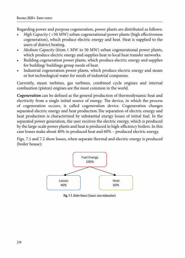
214


Regarding power and purpose cogeneration, power plants are distributed as follows:• High Capacity ( >50 MW) urban cogenerational power plants (high effectiveness

cogeneration), which produce electric energy and heat. Heat is supplied to the users of district heating.

• Medium Capacity (from 1 MW to 50 MW) urban cogenerational power plants, which produce electric energy and supplies heat to local heat transfer networks.

• Building cogeneration power plants, which produce electric energy and supplies for building/ buildings group needs of heat.

• Industrial cogeneration power plants, which produce electric energy and steam or hot technological water for needs of industrial companies.

Currently, steam turbines, gas turbines, combined cycle engines and internal combustion (piston) engines are the most common in the world.

Cogeneration can be defined as the general production of thermodynamic heat and electricity from a single initial source of energy. The device, in which the process of cogeneration occurs, is called cogeneration device. Cogeneration changes separated electric energy and heat production.The separation of electric energy and heat production is characterized by substantial energy losses of initial fuel. In the separated power generation, the user receives the electric energy, which is produced by the large-scale power plants and heat is produced in high-efficiency boilers. In this case losses make about 40% in produced heat and 60% – produced electric energy.

Figs. 7.1 and 7.2 show losses, when separate thermal and electric energy is produced (boiler house):

Fuel Energy 100%

Losses 40%

Heat 60%

Fig. 7.1. Boiler House (Source: own elaboration)

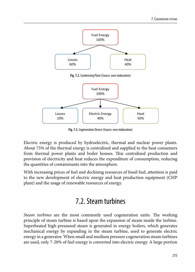
215

7. Cogeneration systems

Fuel Energy 100%

Losses 60%

Heat 40%

Fig. 7.2. Condensing Plant (Source: own elaboration)

Fuel Energy 100%

Losses 10%

Heat 50%

Electric Energy 40%

Fig. 7.3. Cogeneration Device (Source: own elaboration)

Electric energy is produced by hydroelectric, thermal and nuclear power plants. About 75% of the thermal energy is centralized and supplied to the heat consumers from thermal power plants and boiler houses. This centralized production and provision of electricity and heat reduces the expenditure of consumption, reducing the quantities of contaminants into the atmosphere.

With increasing prices of fuel and declining resources of fossil fuel, attention is paid to the new development of electric energy and heat production equipment (CHP plant) and the usage of renewable resources of energy.

7.2. Steam turbines

Steam turbines are the most commonly used cogeneration units. The working principle of steam turbine is based upon the expansion of steam inside the turbine. Superheated high-pressured steam is generated in energy boilers, which generates mechanical energy by expanding in the steam turbine, used to generate electric energy in a generator. When small and medium pressure cogeneration steam turbines are used, only 7-20% of fuel energy is converted into electric energy. A large portion

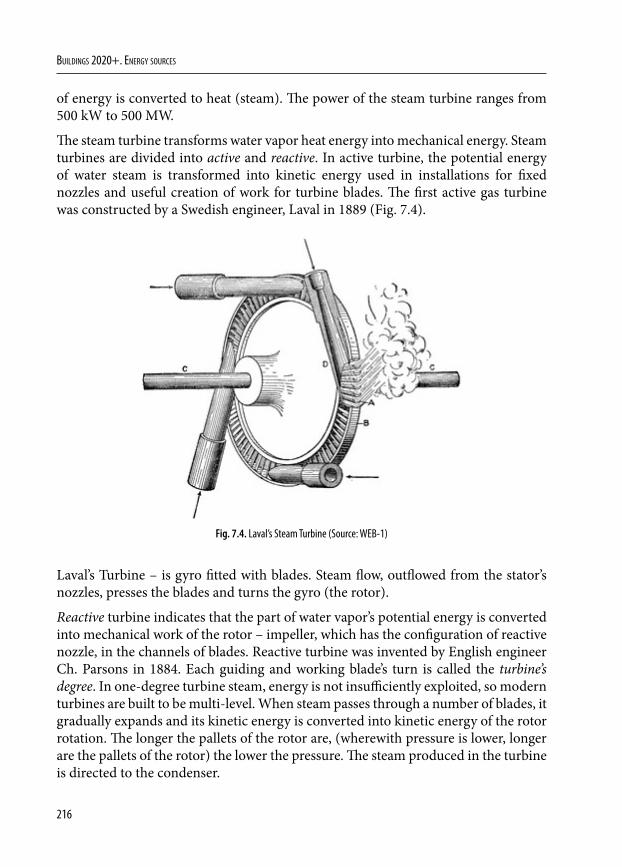
216


of energy is converted to heat (steam). The power of the steam turbine ranges from 500 kW to 500 MW.

The steam turbine transforms water vapor heat energy into mechanical energy. Steam turbines are divided into active and reactive. In active turbine, the potential energy of water steam is transformed into kinetic energy used in installations for fixed nozzles and useful creation of work for turbine blades. The first active gas turbine was constructed by a Swedish engineer, Laval in 1889 (Fig. 7.4).

Fig. 7.4. Laval’s Steam Turbine (Source: WEB-1)

Laval’s Turbine – is gyro fitted with blades. Steam flow, outflowed from the stator’s nozzles, presses the blades and turns the gyro (the rotor).

Reactive turbine indicates that the part of water vapor’s potential energy is converted into mechanical work of the rotor – impeller, which has the configuration of reactive nozzle, in the channels of blades. Reactive turbine was invented by English engineer Ch. Parsons in 1884. Each guiding and working blade’s turn is called the turbine’s degree. In one-degree turbine steam, energy is not insufficiently exploited, so modern turbines are built to be multi-level. When steam passes through a number of blades, it gradually expands and its kinetic energy is converted into kinetic energy of the rotor rotation. The longer the pallets of the rotor are, (wherewith pressure is lower, longer are the pallets of the rotor) the lower the pressure. The steam produced in the turbine is directed to the condenser.

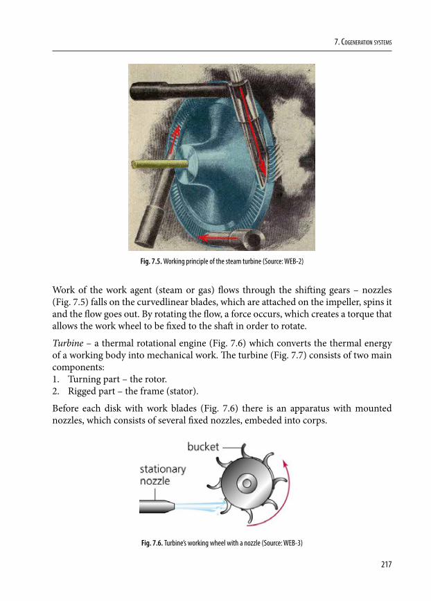
217


Fig. 7.5. Working principle of the steam turbine (Source: WEB-2)

Work of the work agent (steam or gas) flows through the shifting gears – nozzles (Fig. 7.5) falls on the curvedlinear blades, which are attached on the impeller, spins it and the flow goes out. By rotating the flow, a force occurs, which creates a torque that allows the work wheel to be fixed to the shaft in order to rotate.

Turbine – a thermal rotational engine (Fig. 7.6) which converts the thermal energy of a working body into mechanical work. The turbine (Fig. 7.7) consists of two main components:1. Turning part – the rotor.2. Rigged part – the frame (stator).

Before each disk with work blades (Fig. 7.6) there is an apparatus with mounted nozzles, which consists of several fixed nozzles, embeded into corps.

Fig. 7.6. Turbine’s working wheel with a nozzle (Source: WEB-3)

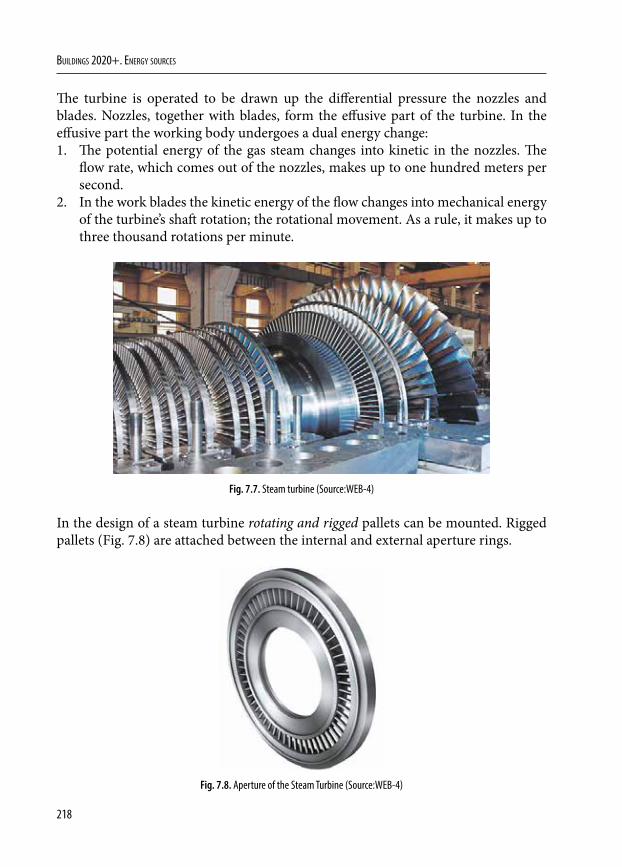
218


The turbine is operated to be drawn up the differential pressure the nozzles and blades. Nozzles, together with blades, form the effusive part of the turbine. In the effusive part the working body undergoes a dual energy change:1. The potential energy of the gas steam changes into kinetic in the nozzles. The

flow rate, which comes out of the nozzles, makes up to one hundred meters per second.

2. In the work blades the kinetic energy of the flow changes into mechanical energy of the turbine’s shaft rotation; the rotational movement. As a rule, it makes up to three thousand rotations per minute.

Fig. 7.7. Steam turbine (Source:WEB-4)

In the design of a steam turbine rotating and rigged pallets can be mounted. Rigged pallets (Fig. 7.8) are attached between the internal and external aperture rings.

Fig. 7.8. Aperture of the Steam Turbine (Source:WEB-4)

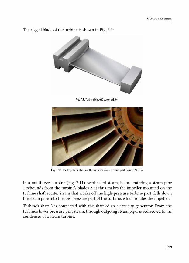
219


The rigged blade of the turbine is shown in Fig. 7.9:

Fig. 7.9. Turbine blade (Source: WEB-4)

Fig. 7.10. The Impeller’s blades of the turbine’s lower pressure part (Source: WEB-6)

In a multi-level turbine (Fig. 7.11) overheated steam, before entering a steam pipe 1 rebounds from the turbine’s blades 2, it thus makes the impeller mounted on the turbine shaft rotate. Steam that works off the high-pressure turbine part, falls down the steam pipe into the low-pressure part of the turbine, which rotates the impeller.

Turbine’s shaft 3 is connected with the shaft of an electricity generator. From the turbine’s lower pressure part steam, through outgoing steam pipe, is redirected to the condenser of a steam turbine.

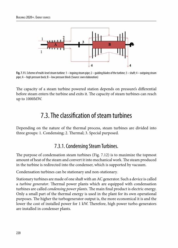
220


Fig. 7.11. Scheme of multi-level steam turbine: 1 – ingoing steam pipe; 2 – guiding blades of the turbine; 3 – shaft; 4 – outgoing steam pipe; A – high pressure bock; B – low pressure block (Source: own elaboration)

The capacity of a steam turbine powered station depends on pressure’s differential before steam enters the turbine and exits it. The capacity of steam turbines can reach up to 1000MW.

7.3. The classification of steam turbines

Depending on the nature of the thermal process, steam turbines are divided into three groups: 1. Condensing; 2. Thermal; 3. Special purposed.

7.3.1. Condensing Steam Turbines.The purpose of condensation steam turbines (Fig. 7.12) is to maximize the topmost amount of heat of the steam and convert it into mechanical work. The steam produced in the turbine is redirected into the condenser, which is supported by vacuum.

Condensation turbines can be stationary and non-stationary.

Stationary turbines are made of one shaft with an AC generator. Such a device is called a turbine generator. Thermal power plants which are equipped with condensation turbines are called condensing power plants. The main final product is electric energy. Only a small part of the thermal energy is used in the plant for its own operational purposes. The higher the turbogenerator output is, the more economical it is and the lower the cost of installed power for 1 kW. Therefore, high power turbo-generators are installed in condenser plants.

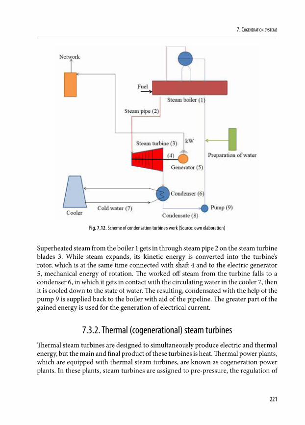
221


Fig. 7.12. Scheme of condensation turbine’s work (Source: own elaboration)

Superheated steam from the boiler 1 gets in through steam pipe 2 on the steam turbine blades 3. While steam expands, its kinetic energy is converted into the turbine’s rotor, which is at the same time connected with shaft 4 and to the electric generator 5, mechanical energy of rotation. The worked off steam from the turbine falls to a condenser 6, in which it gets in contact with the circulating water in the cooler 7, then it is cooled down to the state of water. The resulting, condensated with the help of the pump 9 is supplied back to the boiler with aid of the pipeline. The greater part of the gained energy is used for the generation of electrical current.

7.3.2. Thermal (cogenerational) steam turbinesThermal steam turbines are designed to simultaneously produce electric and thermal energy, but the main and final product of these turbines is heat. Thermal power plants, which are equipped with thermal steam turbines, are known as cogeneration power plants. In these plants, steam turbines are assigned to pre-pressure, the regulation of

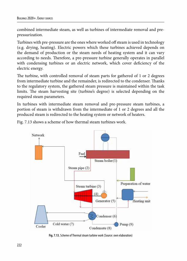
222


combined intermediate steam, as well as turbines of intermediate removal and pre-pressurization.

Turbines with pre-pressure are the ones where worked off steam is used in technology (e.g. drying, heating). Electric powers which these turbines achieved depends on the demand of production or the steam needs of heating system and it can vary according to needs. Therefore, a pre-pressure turbine generally operates in parallel with condensing turbines or an electric network, which cover deficiency of the electric energy.

The turbine, with controlled removal of steam parts for gathered of 1 or 2 degrees from intermediate turbine and the remainder, is redirected to the condenser. Thanks to the regulatory system, the gathered steam pressure is maintained within the task limits. The steam harvesting site (turbine’s degree) is selected depending on the required steam parameters.

In turbines with intermediate steam removal and pre-pressure steam turbines, a portion of steam is withdrawn from the intermediate of 1 or 2 degrees and all the produced steam is redirected to the heating system or network of heaters.

Fig. 7.13 shows a scheme of how thermal steam turbines work.

Fig. 7.13. Scheme of Thermal steam turbine work (Source: own elaboration)

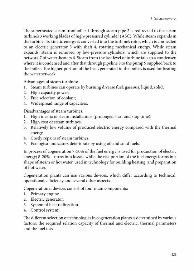
223


The superheated steam fromboiler 1 through steam pipe 2 is redirected to the steam turbine’s 3 working blades of high-pressured cylinder (ASC). While steam expands in the turbine, its kinetic energy is converted into the turbine’s rotor, which is connected to an electric generator 5 with shaft 4, rotating mechanical energy. While steam expands, steam is removed by low-pressure cylinders, which are supplied to the network 7 of water-heaters 6. Steam from the last level of turbine falls to a condenser, where it is condensed and after that through pipeline 8 to the pump 9 supplied back to the boiler. The higher portion of the heat, generated in the boiler, is used for heating the waternetwork.

Advantages of steam turbines:1. Steam turbines can operate by burning diverse fuel: gaseous, liquid, solid;2. High capacity power;3. Free selection of coolant;4. Widespread range of capacities.

Disadvantages of steam turbines:1. High inertia of steam installations (prolonged start and stop time);2. High cost of steam turbines;3. Relatively low volume of produced electric energy compared with the thermal

energy. 4. Costly repairs of steam turbines;5. Ecological indicators deteriorate by using oil and solid fuels.

In process of cogeneration 7-50% of the fuel energy is used for production of electric energy; 8-20% – turns into losses, while the rest portion of the fuel energy forms in a shape of steam or hot water, used in technology for building heating, and preparation of hot water.

Cogeneration plants can use various devices, which differ according to technical, operational, efficiency and several other aspects.

Cogenerational devices consist of four main components:1. Primary engine.2. Electric generator.3. System of heat redirection.4. Control system.

The different selection of technologies in cogeneration plants is determined by various factors: the required relation capacity of thermal and electric, thermal parameters and the fuel used.

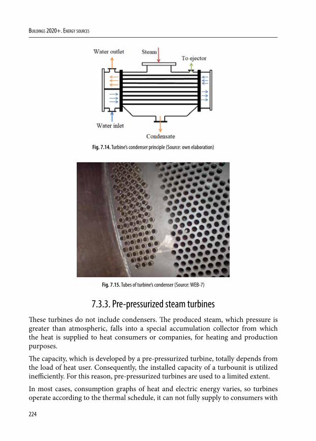
224


Fig. 7.14. Turbine’s condenser principle (Source: own elaboration)

Fig. 7.15. Tubes of turbine’s condenser (Source: WEB-7)

7.3.3. Pre-pressurized steam turbinesThese turbines do not include condensers. The produced steam, which pressure is greater than atmospheric, falls into a special accumulation collector from which the heat is supplied to heat consumers or companies, for heating and production purposes.

The capacity, which is developed by a pre-pressurized turbine, totally depends from the load of heat user. Consequently, the installed capacity of a turbounit is utilized inefficiently. For this reason, pre-pressurized turbines are used to a limited extent.

In most cases, consumption graphs of heat and electric energy varies, so turbines operate according to the thermal schedule, it can not fully supply to consumers with

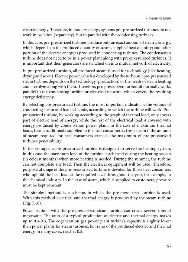
225


electric energy. Therefore, in modern energy systems pre-pressurized turbines do not work in isolation (separately), but in parallel with the condensing turbines.

In this case, pre-pressurized turbines produce only an exact amount of electric energy, which depends on the produced quantity of steam, supplied heat quantity; and other portion of the electric energy is produced in condensing turbines. The condensation turbine does not need to be in a power plant along with pre-pressurized turbines. It is important that their generators are switched on into mutual network of electricity.

In pre-pressurized turbines, all produced steam is used for technology (like heating, drying and so on). Electric power, which is developed by the turbounit pre-pressurized steam turbine, depends on the technology (production) or the needs of steam heating and it evolves along with them. Therefore, pre-pressurized turbounit normally works parallel to the condensing turbine or electrical network, which covers the resulting energy deficiency.

By selecting pre-pressurized turbine, the most important indicator is the volume of conducting steam and load schedule, according to which the turbine will work. Pre-pressurized turbine, by working according to the graph of thermal load, only covers part of electric load of energy; while the rest of the electrical load is covered with energy produced by condensation power plant. In the case of maximum thermal loads, heat is additionaly supplied to the heat consumer as fresh steam if the amount of steam required for heat consumers exceeds the maximum of pre-pressurized turbine’s penetrability.

If, for example, a pre-pressurized turbine is designed to serve the heating system, in this case the maximum load of the turbine is achieved during the heating season (in coldest months) when more heating is needed. During the summer, the turbine can not complete any load. Then the electrical equipment will be used. Therefore, purposeful usage of the pre-pressurized turbine is devoted for those heat consumers who uphold the heat load at the required level throughout the year, for example, in the chemical industry. In the case of steam, which is supplied to customers, pressure must be kept constant.

The simplest method is a scheme, in which the pre-pressurized turbine is used. With this method electrical and thermal energy is produced by the steam turbine (Fig. 7.16).

Power stations with the pre-pressurized steam turbine can create several tons of megawatts. The ratio of a typical production of electric and thermal energy makes up to 0.3-0.5. The cogeneration gas power plant turbine’s capacity is slightly lower than power plants for steam turbines, but ratio of the produced electric and thermal energy, in many cases, reaches 0.5.

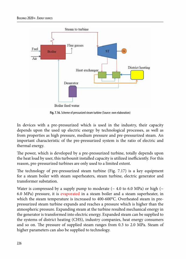
226


Fig. 7.16. Scheme of pressurized steam turbine (Source: own elaboration)

In devices with a pre-pressurized which is used in the industry, their capacity depends upon the used up electric energy by technological processes, as well as from properties as high pressure, medium pressure and pre-pressurized steam. An important characteristic of the pre-pressurized system is the ratio of electric and thermal energy.

The power, which is developed by a pre-pressurized turbine, totally depends upon the heat load by user, this turbounit installed capacity is utilized inefficiently. For this reason, pre-pressurized turbines are only used to a limited extent.

The technology of pre-pressurized steam turbine (Fig. 7.17) is a key equipment for a steam boiler with steam superheaters, steam turbine, electric generator and transformer substation.

Water is compressed by a supply pump to moderate (~ 4.0 to 6.0 MPa) or high (~ 6.0 MPa) pressure, it is evaporated in a steam boiler and a steam superheater, in which the steam temperature is increased to 400-600°C. Overheated steam in pre-pressurized steam turbine expands and reaches a pressure which is higher than the atmospheric pressure. Expanding steam at the turbine resulted mechanical energy in the generator is transformed into electric energy. Expanded steam can be supplied to the systems of district heating (CHS), industry companies, heat energy consumers and so on. The pressure of supplied steam ranges from 0.3 to 2.0 MPa. Steam of higher parameters can also be supplied to technology.

227


Fig. 7.17. The scheme of Thermal pre-pressurized turbine (Source: own elaboration)

The capacity of a steam turbine is usually regulated by a throttle situated against the turbine, which is shifting the pressure of inlet steam, in conjunction with mass flow yield, or injector system, which allows turning on or turning off individual injectors which are in conjunction with the first impeller. The temperature of steam overheating is regulated by collector’s multipal re-heaters by injecting its own condensate; by invoking methods of recirculation of combustion products and reduction of contact temperature.

High electrical efficiency can be achieved only by producing an overheated steam of high parameters (600°C temperature and pressure of 17.0 to 22.7 MPa) uniflow (forced circulation) boilers.

In power plants, which are fueled by biofuels, steam parameters are limited because of the sulfurand chlorine in fuel, which increases the risk of acidic corrosion.

Power plants can burn these fuels: 1. Coal; 2. Oil Products; 3. Biomass and municipal waste; 4. Other fuel, which can be burned in a steam boiler.

In cogeneration plants, which operate on the principle of the pre-pressurized turbine, electrical efficiency only reaches 10-25%, while high capacity modern condensing power plant’s electrical efficiency reaches 40-45%. Total condensing power plants steam turbines combined efficiency reaches up to 85%.

The elimination of pollutant emission quantities and types in the environment are associated with a type of fuel burned in a boiler, construction of combustion chamber and flue gas treatment installations. Nitrogen oxides (NOx), sulfur oxides (SOx), particulate matter (PM), carbon monoxide (CO) and carbon dioxide (CO2) are emitted from a steam boiler.

228


During evaporation in water, salt falls out in form of lime and because of that salt must be removed from water. The products of precipitated salt and pipeline corrosion cause slimewhich must be disposed by continuously and periodicaly blowing out (or alternative word scavenging) the turbine.

Steam turbines are reliable. Their reaching service life is up to 50 years. The CHP plant with production of steam must be clean (no salts) and dry, bearing lubricant – at a suitable temperature, in enough quantity, which must be free from abrasive impurities. Maintenance is required by auxiliary equipment – pumps, coolers, filters, protective systems.

Due to different expansion of thermal coefficient of erratic various elements, turbines need to run relatively slowly.

Application: industrial and electric energy production plants, which electric capacity is from 0.5 to 300 MW and higher.

7.3.4. Condensing turbine housingThe condensation turbine housing is a special outlet, which conveys a non-fully expanded part (medium or low pressure) of steam from the middle part of the turbine. This steam can be used for heating drinking water in industry companies or in centralized heat supply systems.

The operating principle of condensation turbines is parallel to the pre-pressurized steam turbine’s operating principle. The main difference is that in this cycle steam is needed, for heat energy consumers, is used as partially expanded. In this turbine the steam expands in a condenser, in which supported vacuum is higher. Steam in a condenser condenses and is returned to the boiler by feeding pumps, by which it is compressed to the required pressure for the process and additionally is deaerated.

By using this technology, heat and production of electricity can be regulated according to different thermal and electrical energy needs:1. Removable steam pressure is controled by valves, which are in the beginning of a

steam gathering line (thus supported by steam parameters p and t).2. At maximum demand of heat energy, the whole steam can be removed by being

not entirely expanded (turbine middle section). At low demand of heat energy, this turbine can work at frequent cycle of condensation turbine, when the whole steam expands in turbine and condensed in the condenser, waste heat is emitted into atmosphere.

The main scheme of the main condensation turbine operation is shown in Fig. 7.18.

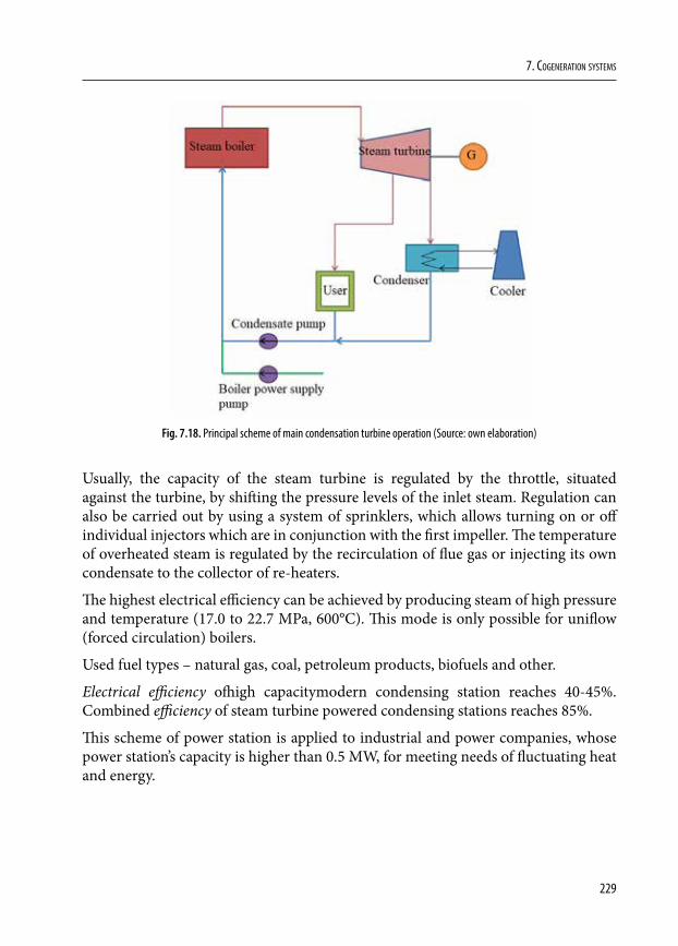
229


Fig. 7.18. Principal scheme of main condensation turbine operation (Source: own elaboration)

Usually, the capacity of the steam turbine is regulated by the throttle, situated against the turbine, by shifting the pressure levels of the inlet steam. Regulation can also be carried out by using a system of sprinklers, which allows turning on or off individual injectors which are in conjunction with the first impeller. The temperature of overheated steam is regulated by the recirculation of flue gas or injecting its own condensate to the collector of re-heaters.

The highest electrical efficiency can be achieved by producing steam of high pressure and temperature (17.0 to 22.7 MPa, 600°C). This mode is only possible for uniflow (forced circulation) boilers.

Used fuel types – natural gas, coal, petroleum products, biofuels and other.

Electrical efficiency ofhigh capacitymodern condensing station reaches 40-45%. Combined efficiency of steam turbine powered condensing stations reaches 85%.

This scheme of power station is applied to industrial and power companies, whose power station’s capacity is higher than 0.5 MW, for meeting needs of fluctuating heat and energy.

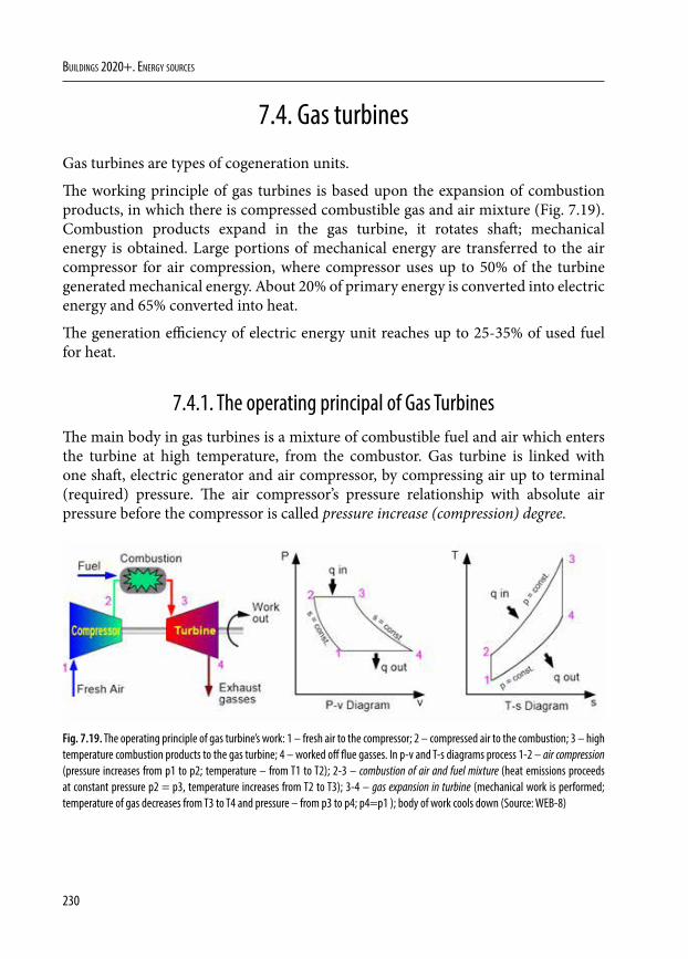
230


7.4. Gas turbines

Gas turbines are types of cogeneration units.

The working principle of gas turbines is based upon the expansion of combustion products, in which there is compressed combustible gas and air mixture (Fig. 7.19). Combustion products expand in the gas turbine, it rotates shaft; mechanical energy is obtained. Large portions of mechanical energy are transferred to the air compressor for air compression, where compressor uses up to 50% of the turbine generated mechanical energy. About 20% of primary energy is converted into electric energy and 65% converted into heat.

The generation efficiency of electric energy unit reaches up to 25-35% of used fuel for heat.

7.4.1. The operating principal of Gas TurbinesThe main body in gas turbines is a mixture of combustible fuel and air which enters the turbine at high temperature, from the combustor. Gas turbine is linked with one shaft, electric generator and air compressor, by compressing air up to terminal (required) pressure. The air compressor’s pressure relationship with absolute air pressure before the compressor is called pressure increase (compression) degree.

Fig. 7.19. The operating principle of gas turbine’s work: 1 – fresh air to the compressor; 2 – compressed air to the combustion; 3 – high temperature combustion products to the gas turbine; 4 – worked off flue gasses. In p-v and T-s diagrams process 1-2 – air compression (pressure increases from p1 to p2; temperature – from T1 to T2); 2-3 – combustion of air and fuel mixture (heat emissions proceeds at constant pressure p2 = p3, temperature increases from T2 to T3); 3-4 – gas expansion in turbine (mechanical work is performed; temperature of gas decreases from T3 to T4 and pressure – from p3 to p4; p4=p1 ); body of work cools down (Source: WEB-8)

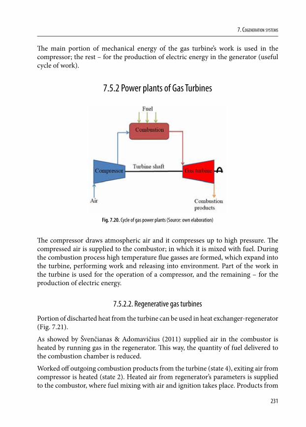
231


The main portion of mechanical energy of the gas turbine’s work is used in the compressor; the rest – for the production of electric energy in the generator (useful cycle of work).

7.5.2 Power plants of Gas Turbines

7.5.2.1. Open cycle gas power plants

Fig. 7.20. Cycle of gas power plants (Source: own elaboration)

The compressor draws atmospheric air and it compresses up to high pressure. The compressed air is supplied to the combustor; in which it is mixed with fuel. During the combustion process high temperature flue gasses are formed, which expand into the turbine, performing work and releasing into environment. Part of the work in the turbine is used for the operation of a compressor, and the remaining – for the production of electric energy.

7.5.2.2. Regenerative gas turbines

Portion of discharted heat from the turbine can be used in heat exchanger-regenerator (Fig. 7.21).

As showed by Švenčianas & Adomavičius (2011) supplied air in the combustor is heated by running gas in the regenerator. This way, the quantity of fuel delivered to the combustion chamber is reduced.

Worked off outgoing combustion products from the turbine (state 4), exiting air from compressor is heated (state 2). Heated air from regenerator’s parameters is supplied to the combustor, where fuel mixing with air and ignition takes place. Products from

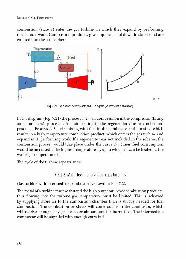
232


combustion (state 3) enter the gas turbine, in which they expand by performing mechanical work. Combustion products, given up heat, cool down to state b and are emitted into the atmosphere.

Fig. 7.21. Cycle of Gas power plants and T-s diagram (Source: own elaboration)

In T-s diagram (Fig. 7.21) the process 1-2 – air compression in the compressor (lifting air parameters); process 2-A – air heating in the regenerator due to combustion products; Process A-3 – air mixing with fuel in the combustor and burning, which results in a high-temperature combustion product, which enters the gas turbine and expand in it, performing work. If a regenerator eas not included in the scheme, the combustion process would take place under the curve 2-3 (then, fuel consumption would be increased). The highest temperature Ta, up to which air can be heated, is the waste gas temperature T4.

The cycle of the turbine repeats anew.

7.5.2.3. Multi-level regenaration gas turbines

Gas turbine with intermediate combustor is shown in Fig. 7.22.

The metal of a turbine must withstand the high temperatures of combustion products, thus flowing into the turbine gas temperature must be limited. This is achieved by supplying more air to the combustion chamber than is strictly needed for fuel combustion. The combustion products will come out from the combustor, which will receive enough oxygen for a certain amount for burnt fuel. The intermediate combustor will be supplied with enough extra fuel.

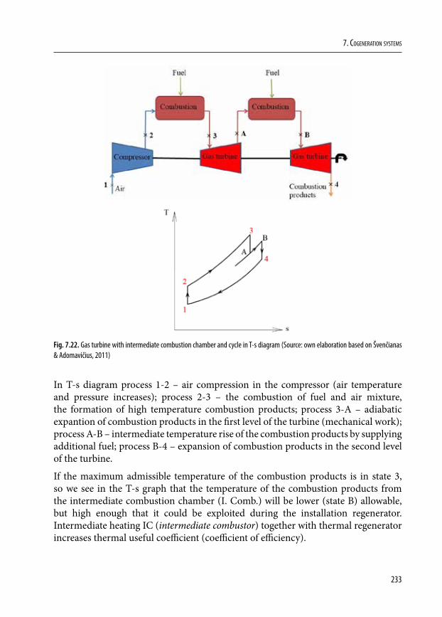
233


Fig. 7.22. Gas turbine with intermediate combustion chamber and cycle in T-s diagram (Source: own elaboration based on Švenčianas & Adomavičius, 2011)

In T-s diagram process 1-2 – air compression in the compressor (air temperature and pressure increases); process 2-3 – the combustion of fuel and air mixture, the formation of high temperature combustion products; process 3-A – adiabatic expantion of combustion products in the first level of the turbine (mechanical work); process A-B – intermediate temperature rise of the combustion products by supplying additional fuel; process B-4 – expansion of combustion products in the second level of the turbine.

If the maximum admissible temperature of the combustion products is in state 3, so we see in the T-s graph that the temperature of the combustion products from the intermediate combustion chamber (I. Comb.) will be lower (state B) allowable, but high enough that it could be exploited during the installation regenerator. Intermediate heating IC (intermediate combustor) together with thermal regenerator increases thermal useful coefficient (coefficient of efficiency).

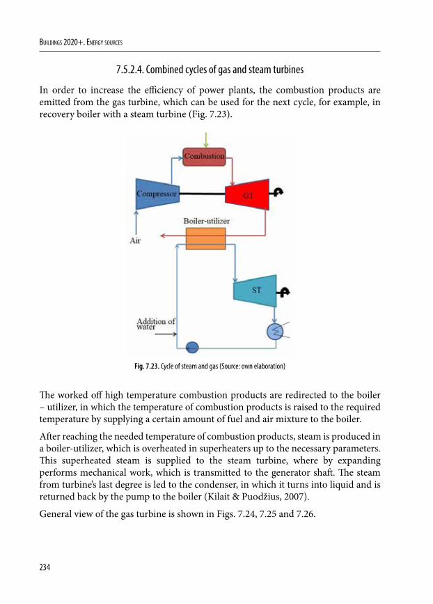
234


7.5.2.4. Combined cycles of gas and steam turbines

In order to increase the efficiency of power plants, the combustion products are emitted from the gas turbine, which can be used for the next cycle, for example, in recovery boiler with a steam turbine (Fig. 7.23).

Fig. 7.23. Cycle of steam and gas (Source: own elaboration)

The worked off high temperature combustion products are redirected to the boiler – utilizer, in which the temperature of combustion products is raised to the required temperature by supplying a certain amount of fuel and air mixture to the boiler.

After reaching the needed temperature of combustion products, steam is produced in a boiler-utilizer, which is overheated in superheaters up to the necessary parameters. This superheated steam is supplied to the steam turbine, where by expanding performs mechanical work, which is transmitted to the generator shaft. The steam from turbine’s last degree is led to the condenser, in which it turns into liquid and is returned back by the pump to the boiler (Kilait & Puodžius, 2007).

General view of the gas turbine is shown in Figs. 7.24, 7.25 and 7.26.

235


Fig. 7.24. General view of the gas turbine: 1 – air falls to the compressor through the intakes of air channels, in which air filters and noise dampersare installed; 2 – compressor rises air pressure to 16 bar; 3 – compressed air is supplied to the burners, installed in the combustor; 4 – gaseous fuel burns in the chamber, in which 24 burners are installed; 6 – the worked off gas is released through the axial diffuser and used for steam production in the steam boiler, from which steam of high parameters is supllied to the turbine; 7 – electric generator is connected with rotor of the gas turbine from the side of the compressor through an intermediate shaft and reductor, which reduces rotional speed of the turbine’s rotor (5400 rot./min.) to the rotional speed of the generator (3000 rpm. or 3600 rpm.) (Source: WEB-9)

Fig. 7.25. Gas turbine (Source:WEB-10)

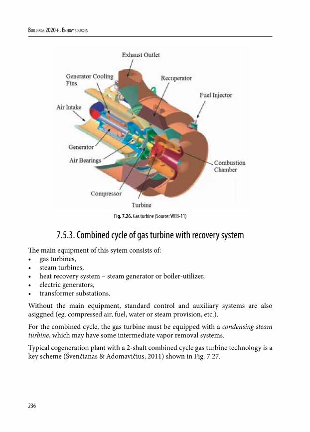
236


Fig. 7.26. Gas turbine (Source: WEB-11)

7.5.3. Combined cycle of gas turbine with recovery systemThe main equipment of this sytem consists of: • gas turbines,• steam turbines,• heat recovery system – steam generator or boiler-utilizer,• electric generators,• transformer substations.

Without the main equipment, standard control and auxiliary systems are also asiggned (eg. compressed air, fuel, water or steam provision, etc.).

For the combined cycle, the gas turbine must be equipped with a condensing steam turbine, which may have some intermediate vapor removal systems.

Typical cogeneration plant with a 2-shaft combined cycle gas turbine technology is a key scheme (Švenčianas & Adomavičius, 2011) shown in Fig. 7.27.

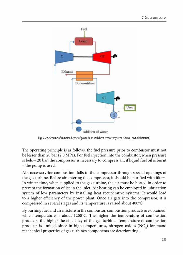
237


Fig. 7.27. Scheme of combined cycle of gas turbine with heat recovery system (Source: own elaboration)

The operating principle is as follows: the fuel pressure prior to combustor must not be lesser than 20 bar (2.0 MPa). For fuel injection into the combustor, when pressure is below 20 bar, the compressor is necessary to compress air, if liquid fuel oil is burnt – the pump is used.

Air, necessary for combustion, falls to the compressor through special openings of the gas turbine. Before air entering the compressor, it should be purified with filters. In winter time, when supplied to the gas turbine, the air must be heated in order to prevent the formation of ice in the inlet. Air heating can be employed in lubrication system of low parameters by installing heat recuperative systems. It would lead to a higher efficiency of the power plant. Once air gets into the compressor, it is compressed in several stages and its temperature is raised about 400°C.

By burning fuel and air mixture in the combustor, combustion products are obtained, which temperature is about 1200°C. The higher the temperature of combustion products, the higher the efficiency of the gas turbine. Temperature of combustion products is limited, since in high temperatures, nitrogen oxides (NOx) for mand mechanical properties of gas turbine’s components are deteriorating.

238


Combustion products expand in a multi-staged turbine. Mechanical energy, produced during this process, is used to rotate the compressor and generator. About 50-60% of the mechanical energy is used to pressurize the air in the compressor. In the gas turbine’s existing outlet, the temperature of combustion products reaches about 500-600°C.

Combustion products fall into the steam’s boiler-utilizer, where they can still be heated additionally by burning fuel up to 1000°C. Since combustion products still contain about 15% oxygen, air for combustion is sufficient.

Cooled fumes from boiler are emitted into the environment. In order for technological process to be effective, the temperature of combustion products should reach 70-80°C. Water vapor, existent in combustion products condenses at lower temperatures, by intensifying the surface corrosion. In addition, the temperature of combustion products should satisfy the consumer’s thermal energy needs. By burning natural gas, the mentioned factors can be fully or partially prevented.

Water, supplied for steam production, is compressed by feeding pumps to required pressure. In steam boiler-utilizer, water is heated in several stages by out-going combustion products from the gas turbine. The steam is separated from the water in the upper drum and unevaporated water is recirculated in the system – that is returned into the drum. Steam in steam superheaters is overheated to 400-600°C and supplied to the steam turbine. Steam, expanding with speed of ~ 700 km/h in the turbine, bounces back into the turbine blades, in which steam’s kinetic energy is converted into mechanical energy of rotation and thus rotates the shaft and it rotates the electricity generator respectively. Partly expanded steam, via dedicated steam drainage holes, could be directed to users or to a heat exchanger, inwhich steam releases its heat for heating thermo admission water. Work off steam from the turbine’s last degree is redirected to the turbine’s condenser, in which it condenses. The condensate is cleaned, deaerated and supplied by feeding pumps back to the boiler.

The capacity of the gas turbine is regulated by changing the amount of fuel supplied to the injectors. The steam turbine is regulated by changing the steam parameters of the steam boiler, which operation mode is directly related to temperature of the combustion products exhaustedfrom the gas turbine. Another way – the turbine can be adjusted by against situated throttle, by shifting pressure of the inlet steam. You can also adjust the sprinkler system – by turning off or turning on individual injectors, situated against the first impeller of the turbine thus adjusting mass flow rate of the steam, and at the same time capacity of the turbine.

From an economic point of view, this type of cogeneration system can be applied only to a thigh demand for electricity.

239


Used types of fuel:• Natural gas;• Low-sulfur petroleum products;• Coal or biomass gasification products.

The electrical efficiency of gas turbine, at the combined cycle, could reach up to 60%, while the overall efficiencyof the power plant – 92.5%. By increasing electrical capacity of the cogeneration power plant, it also increases electrical and the overall efficiency of the system.

7.6. Microturbines

These are small gas turbines, which electrical capacity ranges from 25-30 up to 350 kW. Microturbines have a small number of moving mechanisms. In order to turn them, gas and liquid fuel can be used. By burning fuel in the turbine, rotary motion is created, which is transmitted to the electric generator shaft. Worked of combustion products in the turbine still are high parameters, so they can be used for heating air intake in the heater (or heat production).

The microturbines (Fig. 7.28) operating principle is similar to the gas turbine. It consists of two main components – the compressor and gas turbine. Supply air heater is installed in the microturbines (heat exchanger). Exchanger uses heat of the combustion products for heating air intaking, thereby increasing the efficiency of microturbines.

Air, by initial parameters, falls through the air filter, which is used for air cleaning and reduction of engine power losses. The filtered air, by passing through the generator, cools down the stator (fixed part linked to a movable rotor) windings; this allows rejection of the generator’s cooling system. Compressedto the necessary parameters air falls to the heat exchanger (exchanger). Thanks to the exchanger, electrical efficiency of themicroturbine is increased, allowing the reduction of fuel consumption. Heated and compressed air, supplied through the combustor, mixes with fuel and ignites.

Mixture combustion takes place at a constant pressure (Brayton cycle) and low working temperatures; it allows to achieve minimal emissions of pollutants to the atmosphere.

Energy, produced by ignited mixture, gone through the turbine turns into work. High-temperature hot gases, entered through the turbine nozzles, expand; during expansion thermal energy is converted into kinetic energy. The kinetic energy of the

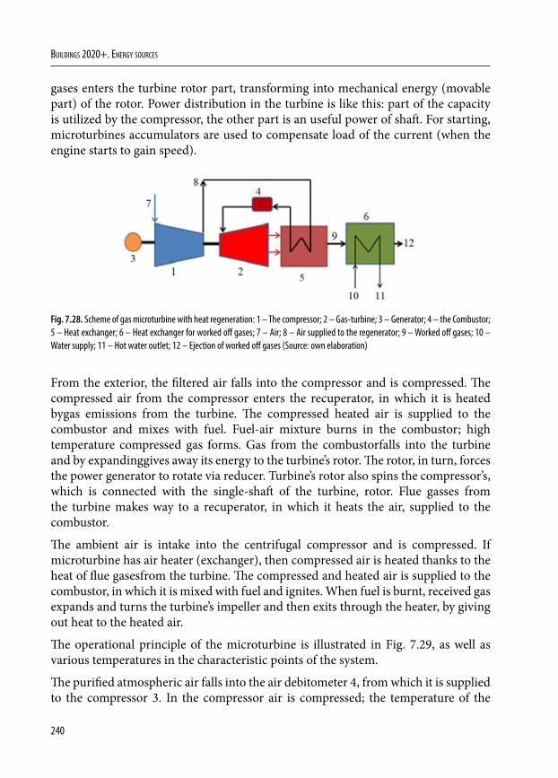
240


gases enters the turbine rotor part, transforming into mechanical energy (movable part) of the rotor. Power distribution in the turbine is like this: part of the capacity is utilized by the compressor, the other part is an useful power of shaft. For starting, microturbines accumulators are used to compensate load of the current (when the engine starts to gain speed).

Fig. 7.28. Scheme of gas microturbine with heat regeneration: 1 – The compressor; 2 – Gas-turbine; 3 – Generator; 4 – the Combustor; 5 – Heat exchanger; 6 – Heat exchanger for worked off gases; 7 – Air; 8 – Air supplied to the regenerator; 9 – Worked off gases; 10 – Water supply; 11 – Hot water outlet; 12 – Ejection of worked off gases (Source: own elaboration)

From the exterior, the filtered air falls into the compressor and is compressed. The compressed air from the compressor enters the recuperator, in which it is heated bygas emissions from the turbine. The compressed heated air is supplied to the combustor and mixes with fuel. Fuel-air mixture burns in the combustor; high temperature compressed gas forms. Gas from the combustorfalls into the turbine and by expandinggives away its energy to the turbine’s rotor. The rotor, in turn, forces the power generator to rotate via reducer. Turbine’s rotor also spins the compressor’s, which is connected with the single-shaft of the turbine, rotor. Flue gasses from the turbine makes way to a recuperator, in which it heats the air, supplied to the combustor.

The ambient air is intake into the centrifugal compressor and is compressed. If microturbine has air heater (exchanger), then compressed air is heated thanks to the heat of flue gasesfrom the turbine. The compressed and heated air is supplied to the combustor, in which it is mixed with fuel and ignites. When fuel is burnt, received gas expands and turns the turbine’s impeller and then exits through the heater, by giving out heat to the heated air.

The operational principle of the microturbine is illustrated in Fig. 7.29, as well as various temperatures in the characteristic points of the system.

The purified atmospheric air falls into the air debitometer 4, from which it is supplied to the compressor 3. In the compressor air is compressed; the temperature of the

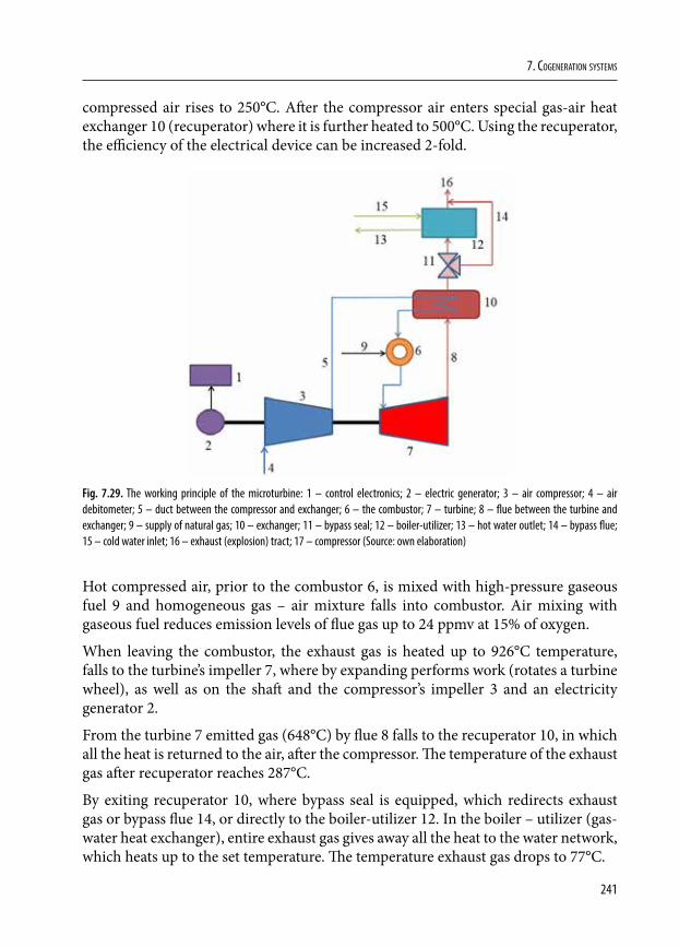
241


compressed air rises to 250°C. After the compressor air enters special gas-air heat exchanger 10 (recuperator) where it is further heated to 500°C. Using the recuperator, the efficiency of the electrical device can be increased 2-fold.

Fig. 7.29. The working principle of the microturbine: 1 – control electronics; 2 – electric generator; 3 – air compressor; 4 – air debitometer; 5 – duct between the compressor and exchanger; 6 – the combustor; 7 – turbine; 8 – flue between the turbine and exchanger; 9 – supply of natural gas; 10 – exchanger; 11 – bypass seal; 12 – boiler-utilizer; 13 – hot water outlet; 14 – bypass flue; 15 – cold water inlet; 16 – exhaust (explosion) tract; 17 – compressor (Source: own elaboration)

Hot compressed air, prior to the combustor 6, is mixed with high-pressure gaseous fuel 9 and homogeneous gas – air mixture falls into combustor. Air mixing with gaseous fuel reduces emission levels of flue gas up to 24 ppmv at 15% of oxygen.

When leaving the combustor, the exhaust gas is heated up to 926°C temperature, falls to the turbine’s impeller 7, where by expanding performs work (rotates a turbine wheel), as well as on the shaft and the compressor’s impeller 3 and an electricity generator 2.

From the turbine 7 emitted gas (648°C) by flue 8 falls to the recuperator 10, in which all the heat is returned to the air, after the compressor. The temperature of the exhaust gas after recuperator reaches 287°C.

By exiting recuperator 10, where bypass seal is equipped, which redirects exhaust gas or bypass flue 14, or directly to the boiler-utilizer 12. In the boiler – utilizer (gas-water heat exchanger), entire exhaust gas gives away all the heat to the water network, which heats up to the set temperature. The temperature exhaust gas drops to 77°C.

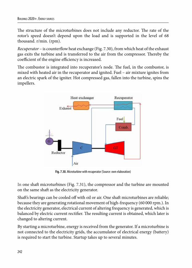
242


The structure of the microturbines does not include any reductor. The rate of the rotor’s speed doesn’t depend upon the load and is supported in the level of 68 thousand. r/min. (rpm).

Recuperator – is counterflow heat exchange (Fig. 7.30), from which heat of the exhaust gas exits the turbine and is transferred to the air from the compressor. Thereby the coefficient of the engine efficiency is increased.

The combustor is integrated into recuperator’s node. The fuel, in the combustor, is mixed with heated air in the recuperator and ignited. Fuel – air mixture ignites from an electric spark of the igniter. Hot compressed gas, fallen into the turbine, spins the impellers.

Fig. 7.30. Microturbine with recuperator (Source: own elaboration)

In one shaft microturbines (Fig. 7.31), the compressor and the turbine are mounted on the same shaft as the electricity generator.

Shaft’s bearings can be cooled off with oil or air. One shaft microturbines are reliable; because they are generating rotational movement of high-frequency (60 000 rpm.). In the electricity generator, electrical current of altering frequency is generated, which is balanced by electric current rectifier. The resulting current is obtained, which later is changed to altering current.

By starting a microturbine, energy is received from the generator. If a microturbine is not connected to the electricity grids, the accumulator of electrical energy (battery) is required to start the turbine. Startup takes up to several minutes.

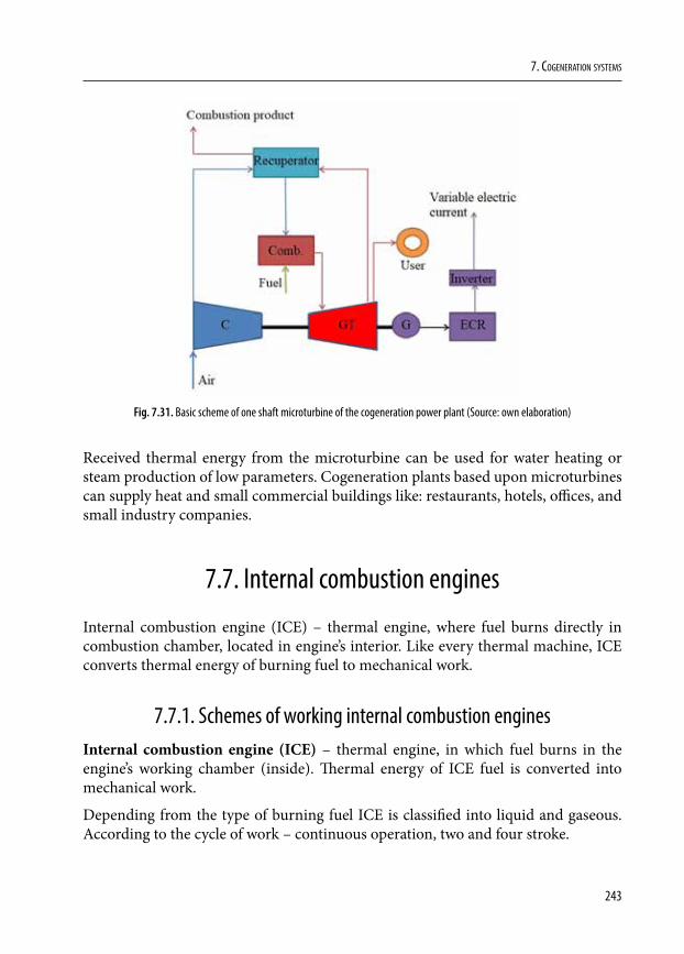
243


Fig. 7.31. Basic scheme of one shaft microturbine of the cogeneration power plant (Source: own elaboration)

Received thermal energy from the microturbine can be used for water heating or steam production of low parameters. Cogeneration plants based upon microturbines can supply heat and small commercial buildings like: restaurants, hotels, offices, and small industry companies.

7.7. Internal combustion engines

Internal combustion engine (ICE) – thermal engine, where fuel burns directly in combustion chamber, located in engine’s interior. Like every thermal machine, ICE converts thermal energy of burning fuel to mechanical work.

7.7.1. Schemes of working internal combustion enginesInternal combustion engine (ICE) – thermal engine, in which fuel burns in the engine’s working chamber (inside). Thermal energy of ICE fuel is converted into mechanical work.

Depending from the type of burning fuel ICE is classified into liquid and gaseous. According to the cycle of work – continuous operation, two and four stroke.

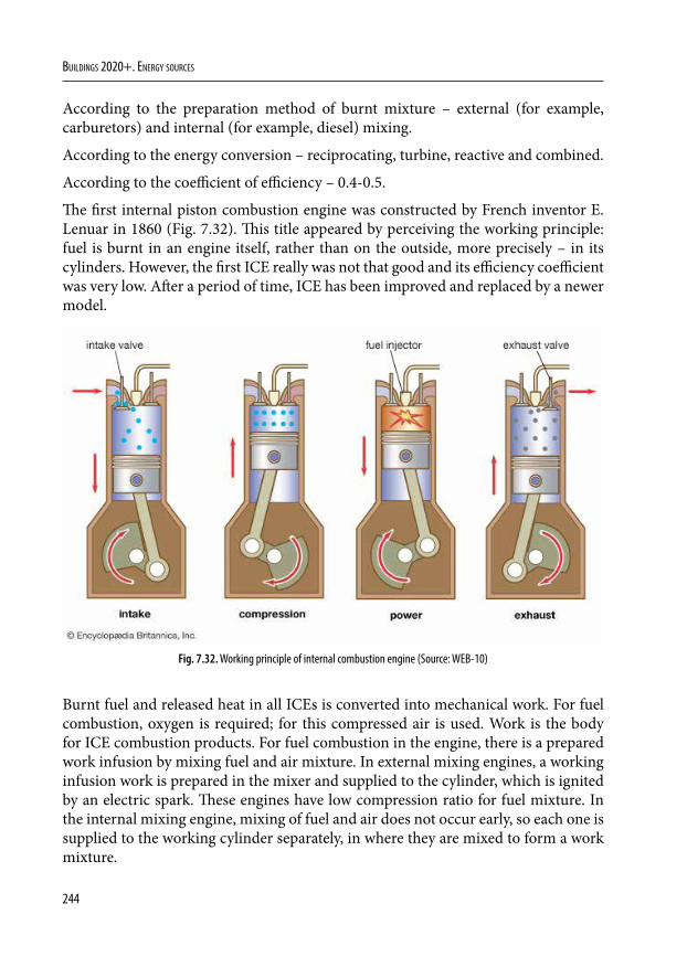
244


According to the preparation method of burnt mixture – external (for example, carburetors) and internal (for example, diesel) mixing.

According to the energy conversion – reciprocating, turbine, reactive and combined.

According to the coefficient of efficiency – 0.4-0.5.

The first internal piston combustion engine was constructed by French inventor E. Lenuar in 1860 (Fig. 7.32). This title appeared by perceiving the working principle: fuel is burnt in an engine itself, rather than on the outside, more precisely – in its cylinders. However, the first ICE really was not that good and its efficiency coefficient was very low. After a period of time, ICE has been improved and replaced by a newer model.

Fig. 7.32. Working principle of internal combustion engine (Source: WEB-10)

Burnt fuel and released heat in all ICEs is converted into mechanical work. For fuel combustion, oxygen is required; for this compressed air is used. Work is the body for ICE combustion products. For fuel combustion in the engine, there is a prepared work infusion by mixing fuel and air mixture. In external mixing engines, a working infusion work is prepared in the mixer and supplied to the cylinder, which is ignited by an electric spark. These engines have low compression ratio for fuel mixture. In the internal mixing engine, mixing of fuel and air does not occur early, so each one is supplied to the working cylinder separately, in where they are mixed to form a work mixture.

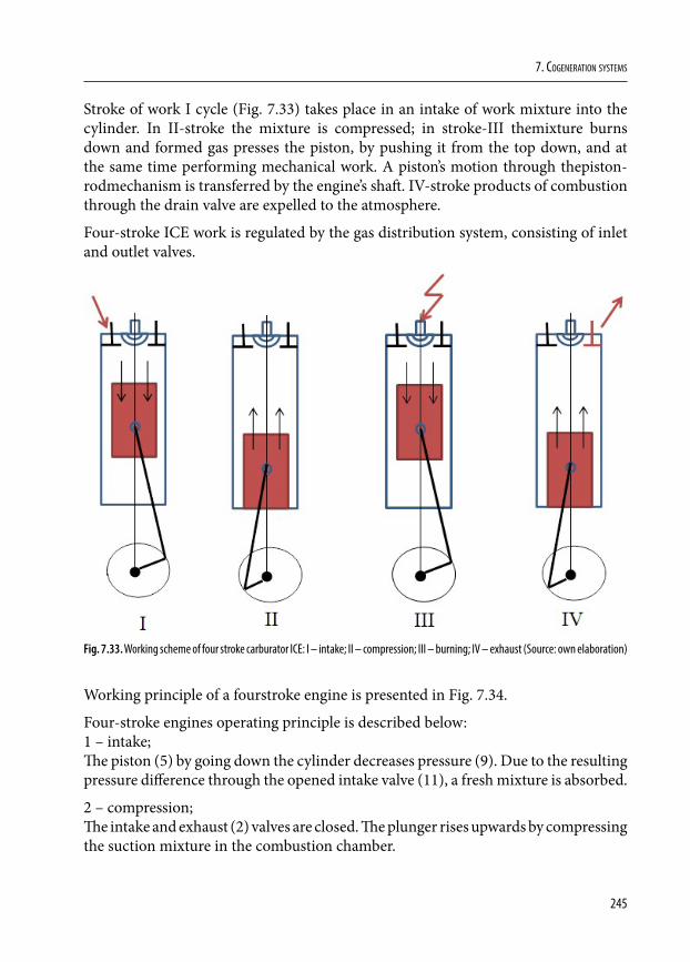
245


Stroke of work I cycle (Fig. 7.33) takes place in an intake of work mixture into the cylinder. In II-stroke the mixture is compressed; in stroke-III themixture burns down and formed gas presses the piston, by pushing it from the top down, and at the same time performing mechanical work. A piston’s motion through thepiston-rodmechanism is transferred by the engine’s shaft. IV-stroke products of combustion through the drain valve are expelled to the atmosphere.

Four-stroke ICE work is regulated by the gas distribution system, consisting of inlet and outlet valves.

Fig. 7.33. Working scheme of four stroke carburator ICE: I – intake; II – compression; III – burning; IV – exhaust (Source: own elaboration)

Working principle of a fourstroke engine is presented in Fig. 7.34.

Four-stroke engines operating principle is described below:1 – intake;The piston (5) by going down the cylinder decreases pressure (9). Due to the resulting pressure difference through the opened intake valve (11), a fresh mixture is absorbed.

2 – compression;The intake and exhaust (2) valves are closed. The plunger rises upwards by compressing the suction mixture in the combustion chamber.

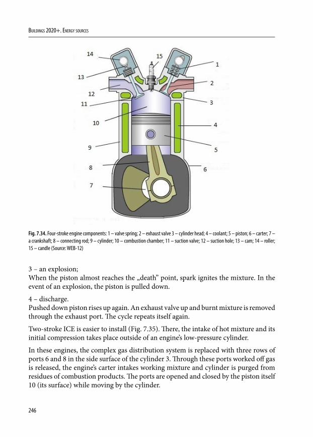
246


Fig. 7.34. Four-stroke engine components: 1 – valve spring; 2 – exhaust valve 3 – cylinder head; 4 – coolant; 5 – piston; 6 – carter; 7 – a crankshaft; 8 – connecting rod; 9 – cylinder; 10 – combustion chamber; 11 – suction valve; 12 – suction hole; 13 – cam; 14 – roller; 15 – candle (Source: WEB-12)

3 – an explosion;When the piston almost reaches the „death” point, spark ignites the mixture. In the event of an explosion, the piston is pulled down.

4 – discharge.Pushed down piston rises up again. An exhaust valve up and burnt mixture is removed through the exhaust port. The cycle repeats itself again.

Two-stroke ICE is easier to install (Fig. 7.35). There, the intake of hot mixture and its initial compression takes place outside of an engine’s low-pressure cylinder.

In these engines, the complex gas distribution system is replaced with three rows of ports 6 and 8 in the side surface of the cylinder 3. Through these ports worked off gas is released, the engine’s carter intakes working mixture and cylinder is purged from residues of combustion products. The ports are opened and closed by the piston itself 10 (its surface) while moving by the cylinder.

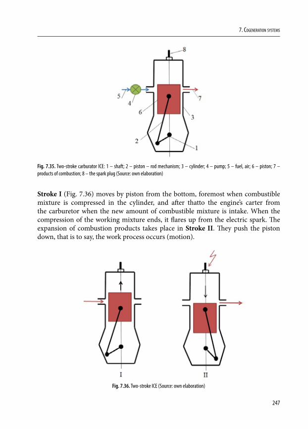
247


Fig. 7.35. Two-stroke carburator ICE: 1 – shaft; 2 – piston – rod mechanism; 3 – cylinder; 4 – pump; 5 – fuel, air; 6 – piston; 7 – products of combustion; 8 – the spark plug (Source: own elaboration)

Stroke I (Fig. 7.36) moves by piston from the bottom, foremost when combustible mixture is compressed in the cylinder, and after thatto the engine’s carter from the carburetor when the new amount of combustible mixture is intake. When the compression of the working mixture ends, it flares up from the electric spark. The expansion of combustion products takes place in Stroke II. They push the piston down, that is to say, the work process occurs (motion).

Fig. 7.36. Two-stroke ICE (Source: own elaboration)

248


When the piston moves from the top down, emissions are released into atmosphere.

In low compression engines, in which light liquid fuel is burnt (eg. petrol) mixing of the mixture takes place in a special device – the carburator.

ICE are widely used in industry, automotive, aviation, marine and rail transport.

The andvantages and disadvantages of fourstroke ICE comparing with twostroke engine:Advantages:1. Four-stroke engines generate considerably higher torque, especially at low speeds;2. Consumes much less fuel; Slower, due to better lubrication;

Disadvantages:1. The four-stroke engine has many rotating and moving parts;2. More complex maintenance and repairs;3. Four-stroke engines are more expensive than two-stroke engines.

7.7.2. Power plant with internal combustion engineInternal combustion engine is a widespread technology, by the means of which the electric power ranges from 2 kW to 5 MW. Internal combustion engines in cogeneration plants without electric energy, also produce hot water or steam of low parameters in boilers-utilizers. In the internal combustion engines, electricity is produced more efficiently than in gas turbines, but usage of surplus heat is more complicated, as it is distributed between the engine’s cooling system and exhaust gas.

There are two main types of internal combustion engines which are suitable for production of electric energy. Engines based upon Otto’s cycle, in which fuel-air mixture is ignited by a spark, and diesel engines, in which fuel and air mixture ignites by itself upon compression, when pressure firmly increases and the temperature of mixture rises up to the threshold of flash.

In most cases, Cogeneration plants (Fig. 7.37), use operating reciprocating internal combustion engines based upon Otto cycle. Fuel energy is transformed into mechanical shaft work due to the volume expansion of the exhaust gas and thermal energy during the combustion of the mixture. The thermal energy can be extracted from the worked off gas and (or) redirected from the cooling environment of the engine.

Gas (natural gas or landfill gas, biogas) or fast evaporating liquid fuel (gasoline, propane) are used in Otto cycle engines. Natural gas fits the most is to produce electric energy.

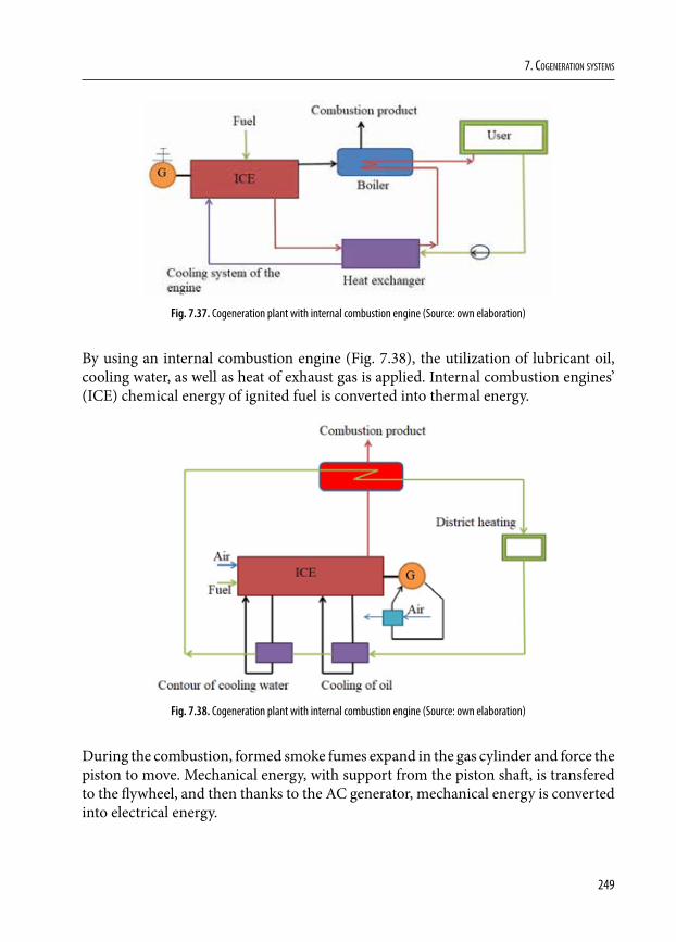
249


Fig. 7.37. Cogeneration plant with internal combustion engine (Source: own elaboration)

By using an internal combustion engine (Fig. 7.38), the utilization of lubricant oil, cooling water, as well as heat of exhaust gas is applied. Internal combustion engines’ (ICE) chemical energy of ignited fuel is converted into thermal energy.

Fig. 7.38. Cogeneration plant with internal combustion engine (Source: own elaboration)

During the combustion, formed smoke fumes expand in the gas cylinder and force the piston to move. Mechanical energy, with support from the piston shaft, is transfered to the flywheel, and then thanks to the AC generator, mechanical energy is converted into electrical energy.

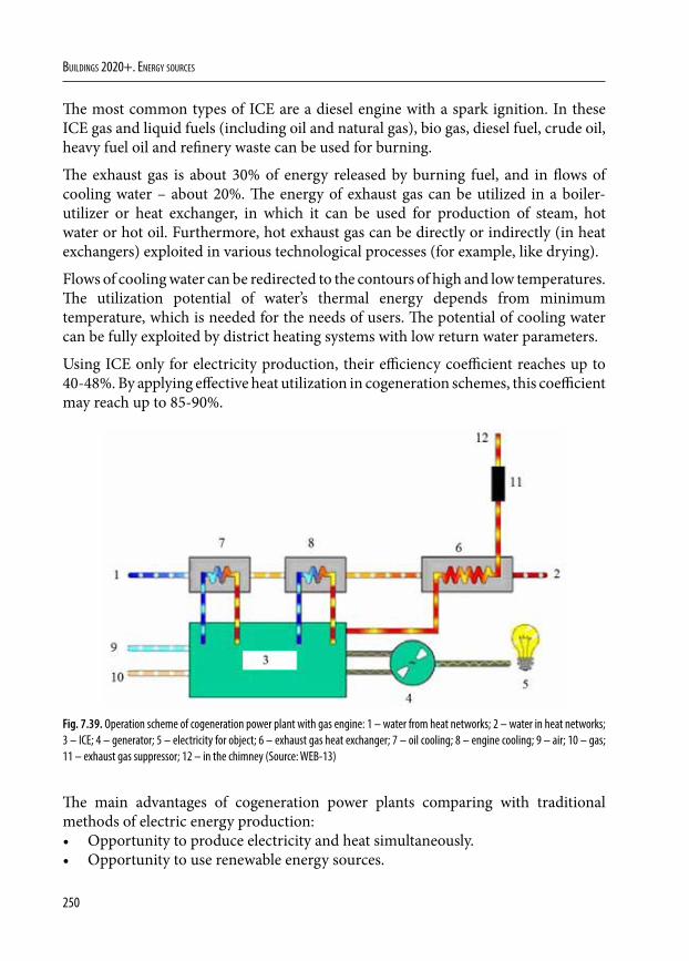
250


The most common types of ICE are a diesel engine with a spark ignition. In these ICE gas and liquid fuels (including oil and natural gas), bio gas, diesel fuel, crude oil, heavy fuel oil and refinery waste can be used for burning.

The exhaust gas is about 30% of energy released by burning fuel, and in flows of cooling water – about 20%. The energy of exhaust gas can be utilized in a boiler-utilizer or heat exchanger, in which it can be used for production of steam, hot water or hot oil. Furthermore, hot exhaust gas can be directly or indirectly (in heat exchangers) exploited in various technological processes (for example, like drying).

Flows of cooling water can be redirected to the contours of high and low temperatures. The utilization potential of water’s thermal energy depends from minimum temperature, which is needed for the needs of users. The potential of cooling water can be fully exploited by district heating systems with low return water parameters.

Using ICE only for electricity production, their efficiency coefficient reaches up to 40-48%. By applying effective heat utilization in cogeneration schemes, this coefficient may reach up to 85-90%.

Fig. 7.39. Operation scheme of cogeneration power plant with gas engine: 1 – water from heat networks; 2 – water in heat networks; 3 – ICE; 4 – generator; 5 – electricity for object; 6 – exhaust gas heat exchanger; 7 – oil cooling; 8 – engine cooling; 9 – air; 10 – gas; 11 – exhaust gas suppressor; 12 – in the chimney (Source: WEB-13)

The main advantages of cogeneration power plants comparing with traditional methods of electric energy production:• Opportunity to produce electricity and heat simultaneously.• Opportunity to use renewable energy sources.

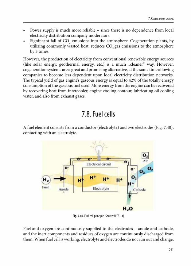
251


• Power supply is much more reliable – since there is no dependence from local electricity distribution company moderators.

• Significant fall of CO2 emissions into the atmosphere. Cogeneration plants, by utilizing commonly wasted heat, reduces CO2 gas emissions to the atmosphere by 3 times.

However, the production of electricity from conventional renewable energy sources (like solar energy, geothermal energy, etc.) is a much „cleaner” way. However, cogeneration systems are a great and promising alternative, at the same time allowing companies to become less dependent upon local electricity distribution networks. The typical yield of gas engine’s gaseous energy is equal to 42% of the totally energy consumption of the gaseous fuel used. More energy from the engine can be recovered by recovering heat from intercooler, engine cooling contour, lubricating oil cooling water, and also from exhaust gases.

7.8. Fuel cells

A fuel element consists from a conductor (electrolyte) and two electrodes (Fig. 7.40), contacting with an electrolyte.

Fig. 7.40. Fuel cell principle (Source: WEB-14)

Fuel and oxygen are continuously supplied to the electrodes – anode and cathode, and the inert components and residues of oxygen are continuously discharged from them. When fuel cell is working, electrolyte and electrodes do not run out and change,

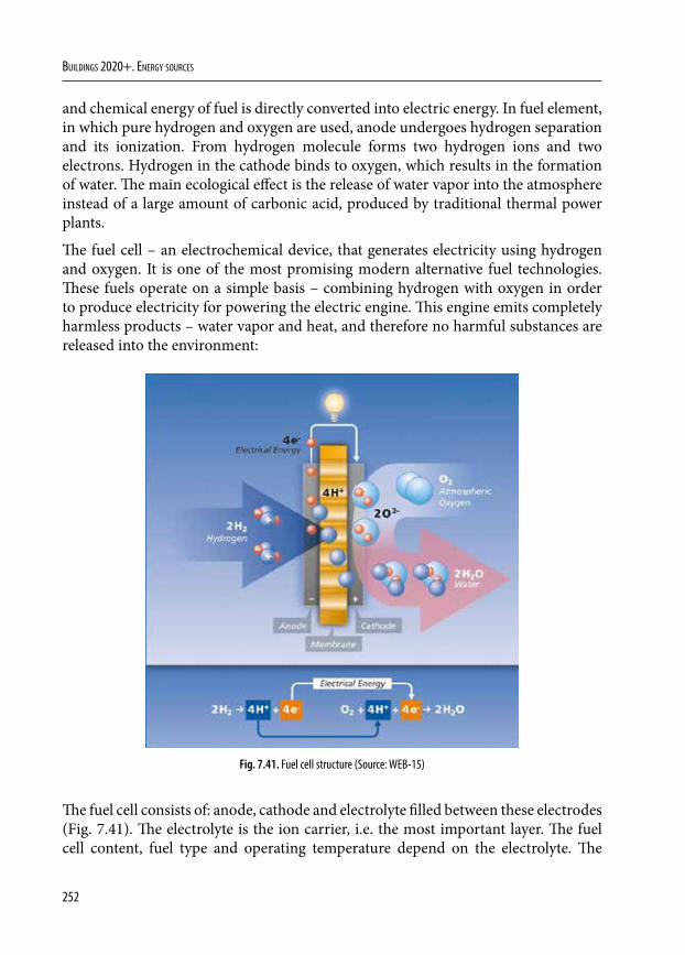
252


and chemical energy of fuel is directly converted into electric energy. In fuel element, in which pure hydrogen and oxygen are used, anode undergoes hydrogen separation and its ionization. From hydrogen molecule forms two hydrogen ions and two electrons. Hydrogen in the cathode binds to oxygen, which results in the formation of water. The main ecological effect is the release of water vapor into the atmosphere instead of a large amount of carbonic acid, produced by traditional thermal power plants.

The fuel cell – an electrochemical device, that generates electricity using hydrogen and oxygen. It is one of the most promising modern alternative fuel technologies. These fuels operate on a simple basis – combining hydrogen with oxygen in order to produce electricity for powering the electric engine. This engine emits completely harmless products – water vapor and heat, and therefore no harmful substances are released into the environment:

Fig. 7.41. Fuel cell structure (Source: WEB-15)

The fuel cell consists of: anode, cathode and electrolyte filled between these electrodes (Fig. 7.41). The electrolyte is the ion carrier, i.e. the most important layer. The fuel cell content, fuel type and operating temperature depend on the electrolyte. The

253


PEMFC electrolyte is a denser polymeric membrane that is very conductive for ions and completely impermeable to electrons and gases. This membrane can be made of a pure polymer or a composition of polymers, for example: a sulfonated fluorocarbon polymer. Electrodes (anode and cathode) have high electrical conductivity. Gas-fired electrodes are made of porous. PEM fuel cell is classified as low temperature (operating temperature – 70-90°C). The anode half of the hydrogen gas is transmitted to the protons and electrons by means of a catalyst. The electrons from the outer circuit travel from the anode to the cathode (thereby generating electricity). Meanwhile, hydrogen ions (protons) travel through the polymer membrane to the cathode. The supply of oxygen (from the air) binds to the protons and the excited electrons. The product of this reaction is water and heat. The efficiency of the fuel element reaches 40-50%.

Fuel element consists of a conductor (electrolyte) and two electrodes, contacting with an electrolyte.

According to the used electrolyte and operating temperature, FE is divided into following basic types: alkalines (AFC), proton exchange membranes (PEMFC), direct methanol (DMFC), phosphoric acid (PAFC), melted carbonates (MCFC), solid oxide (SOFC).

References

DIR 2012/27/EU – Directive 2012/27/EU of the European Parliament and of the Council of 25 October 2012 on energy efficiency, amending Directives 2009/125/EC and 2010/30/EU and repealing Directives 2004/8/EC and 2006/32/EC Text with EEA relevance https://eur-lex.europa.eu/legal-content/en/TXT/?uri=celex%3A32012L0027

Gylys, J. (2012) Garo ir dujų turbinų teoriniai pagrindai. KTU Technologija.

Kilait, L. & Puodžius, R. (2007) Įvairių kogeneracijos technologijų įrengimo galimybių ir sąnaudų bei rekomendacijų dėl šių technologijų diegimo studija parengimas. Ataskaita Nr. 012007. UAB “AF-Enprima” & UAB “Termosistemų projektai”.

Švenčianas, P. & Adomavičius, A. (2011) Inžinerinė termodinamika. KTU Technologija.

WEB-1: Educational Technology Clearinghouse. Available from: https://etc.usf.edu/clipart/77700/77750/77750_dl_trbine.htm. [Accessed 25th August 2018].

254


WEB-2: Woodford Ch., Explain that Stuff. Available from: https://www.explainthatstuff.com/steam-turbines.html [Accessed 25th August 2018].

WEB-3: https://www.quora.com/In-impulse-turbine-why-the-enthalpy-drop-takes-place-in-nozzle-itself-why-there-is-no-enthalpy-drop-in-blade-passage-of-turbine-in-steam-power-plant

WEB-4: https://www.sandvik.coromant.com

WEB-5: https://www.globalsources.com/gsol/I/Steam-turbine/p/sm/1157611943.htm#1157611943

WEB-6: https://www.olympus-ims.com/en/applications/wall-thickness-turbine-blades/

WEB-7: PBS POWER EQUIPMENT. Available from: http://www.pbspe.cz/eng/index.php?action=reference_detail&id=56. [Accessed 25th August 2018].

WEB-8: Available from: http://www.ipieca.org/resources/energy-efficiency-solutions/power-and-heat-generation/open-cycle-gas-turbines/ [Accessed 25th August 2018].

WEB-9: Available from: http://www.stoomturbine.nl/foto_siemens.html. [Accessed 25th August 2018].

WEB-10: Available from: https://www.britannica.com/technology/steam-engine. [Accessed 25th August 2018].

WEB-11: Available from: https://yachtemoceans.com/mme-microturbines-superyacht-generators/ [Accessed 25th August 2018].

WEB-12: Electronic Journal MOTOPRESS [Online]. Available from: http://www.motopress.lt/trumpas-susipazinimas-su-keturtakciu-varikliu/. [Accessed 25th August 2018].

WEB-13: Website of Company GANDRAS [Online]. Available from: http://gandras.net/en/equipment [Accessed 25th August 2018].

WEB-14: Image from website of ScriGroup.com [Online]. Available from: http://www.scrigroup.com/limba/lituaniana [Accessed 25th August 2018].

WEB-15: Website of Company PROTON MOTOR [Online]. Available form: http://www.proton-motor.com [Accessed 25th August 2018].

255

8. ENERGY STORAGE SYSTEMS

8.1. Introduction

This chapter attempts to shed some light on energy storage systems with stationary and building applications. Among these, we must highlight the batteries, from the oldest ones which were employed for these purposes, to those of lead-acid (Reddy & Linden, 2010), or those that harbour a very promising future, the redox flow batteries, RFB (Rajarathnam & Vassallo, 2016; Zhang & Zhang, 2015); finally, we cannot forget the lithium-ion batteries, widely used today (Julien et al., 2016).

Human beings need to store energy to make it available when necessary. The release of this energy can occur in the same form in which it was stored, or in a different manner. There are different methods or systems to store energy: electrical, mechanical, biological, electrochemical... So, for example, capacitors and superconductors are examples of electrical storage systems, while hydraulic pumping or flywheel, are mechanic systems. Regarding biological storage systems, the combustion of matter such as biomass, agricultural waste, oil, natural gas or coal should be mentioned. In these cases, the energy stored in the bonds of the molecules that participate as reagents in the chemical reaction is released under heat form. The reason for this favourable energy release is the energetic difference between the energy of the bonds in reactants (organic matter and oxygen in combustion) and those of the products (water and carbon dioxide). As it happened with the electrochemical systems, the batteries need to be mentioned, including different modalities: conventional batteries, flow batteries, fuel cells.

8.1.1. What is a battery?

A battery is an energy storage system that releases the energy, which is chemically stored, in the form of electricity through a chemical process called redox, that is to say, a chemical reaction of reduction-oxidation. The batteries can be composed of one or more cells. Each cell includes a cathode (positive pole), an anode (negative pole) and an electrolyte (ionic conductor). Batteries accumulate energy during the charging process, which is later released in the discharge process. Depending on the

DOI: 10.24427/978-83-65596-73-4_8

256


reversibility of the charge and discharge processes, there are primary batteries (not rechargeable) and secondary batteries (rechargeable).

The phenomenon responsible for the charge is a certain chemical reaction (which will vary depending on the materials that constitute the cathode and anode. Consequently, the type and subtype of the battery can be classified). The inverse chemical reaction is the responsible for the phenomenon of discharge.

The chemical reaction of the battery during the charge process is shown below:

Cathode: M → M+ + 1e– (oxidation) (8.1)

Anode: N3+ + 1e– → N2+ (reduction) (8.2)

Global: M + N3+ → M+ + N2+

Thus, in the chemical reaction represented, in the charging process, an oxidation semi-reaction would take place at the cathode (the M species loses an electron and becomes positively charged, increasing its oxidation state by +1), while in the anode the semi-reaction reduction takes place (the N3+ species loses an electron, decreasing its oxidation state from +3 to +2). In this case, energy (electrical) is used to store it (in chemical form). In the relevant discharge reaction, inverse processes would occur, releasing energy in the form of electricity.

The chemical reaction of the battery during the discharge process (inverse of the charge reaction) is shown below:

Cathode: M+ + 1e– → M(reduction) (8.3)

Anode: N2+ → N3+ + 1e– (oxidation) (8.4)

Global: M+ + N2+ → M + N3+ As it has been described, the materials that constitute cathode and anode determine the chemical reaction that takes place in the battery. In turn, some parameters of the battery such as the voltage are determined by this: the specific capacity (amount of electricity stored / released per unit mass, expressed in Ah·kg–1), the specific energy (voltage x specific capacity, measured in Wh·kg–1) or the specific power (voltage x current, measured in W·kg–1). Other parameters of the battery are the cycle life (number of battery cycles), cycle efficiency (quotient between the discharge and charge energy), the charge/discharge speed (time required to obtain the full theoretical capacity), the state of charge (SOC, percentage of battery charged), the depth of discharge (DOC, percentage of discharge that can be reached in a battery) among others. It must be considered that certain parameters such as the actual capacity of the battery, average life... can also be affected by different factors such as the design of the battery, the amount of active material, the particle size of the materials that constitute cathode and anode or the presence of additives, among others.

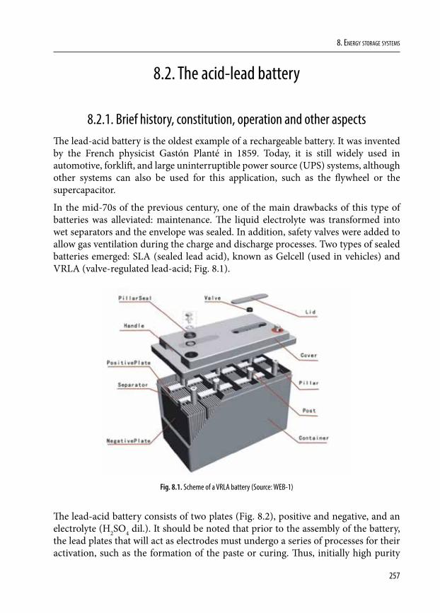
257

8. EnErgy storagE systEms

8.2. The acid-lead battery

8.2.1. Brief history, constitution, operation and other aspectsThe lead-acid battery is the oldest example of a rechargeable battery. It was invented by the French physicist Gastón Planté in 1859. Today, it is still widely used in automotive, forklift, and large uninterruptible power source (UPS) systems, although other systems can also be used for this application, such as the flywheel or the supercapacitor.

In the mid-70s of the previous century, one of the main drawbacks of this type of batteries was alleviated: maintenance. The liquid electrolyte was transformed into wet separators and the envelope was sealed. In addition, safety valves were added to allow gas ventilation during the charge and discharge processes. Two types of sealed batteries emerged: SLA (sealed lead acid), known as Gelcell (used in vehicles) and VRLA (valve-regulated lead-acid; Fig. 8.1).

Fig. 8.1. Scheme of a VRLA battery (Source: WEB-1)

The lead-acid battery consists of two plates (Fig. 8.2), positive and negative, and an electrolyte (H2SO4 dil.). It should be noted that prior to the assembly of the battery, the lead plates that will act as electrodes must undergo a series of processes for their activation, such as the formation of the paste or curing. Thus, initially high purity

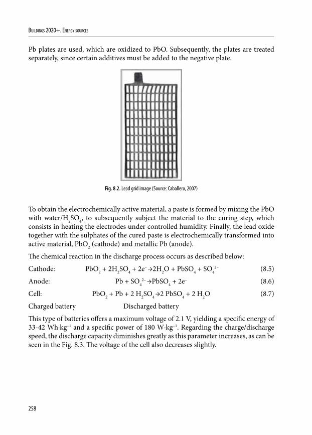
258


Pb plates are used, which are oxidized to PbO. Subsequently, the plates are treated separately, since certain additives must be added to the negative plate.

Fig. 8.2. Lead grid image (Source: Caballero, 2007)

To obtain the electrochemically active material, a paste is formed by mixing the PbO with water/H2SO4, to subsequently subject the material to the curing step, which consists in heating the electrodes under controlled humidity. Finally, the lead oxide together with the sulphates of the cured paste is electrochemically transformed into active material, PbO2 (cathode) and metallic Pb (anode).

The chemical reaction in the discharge process occurs as described below:

Cathode: PbO2 + 2H2SO4 + 2e– →2H2O + PbSO4 + SO42– (8.5)

Anode: Pb + SO42– →PbSO4 + 2e– (8.6)

Cell: PbO2 + Pb + 2 H2SO4 →2 PbSO4 + 2 H2O (8.7)

Charged battery Discharged battery

This type of batteries offers a maximum voltage of 2.1 V, yielding a specific energy of 33-42 Wh·kg–1 and a specific power of 180 W·kg–1. Regarding the charge/discharge speed, the discharge capacity diminishes greatly as this parameter increases, as can be seen in the Fig. 8.3. The voltage of the cell also decreases slightly.

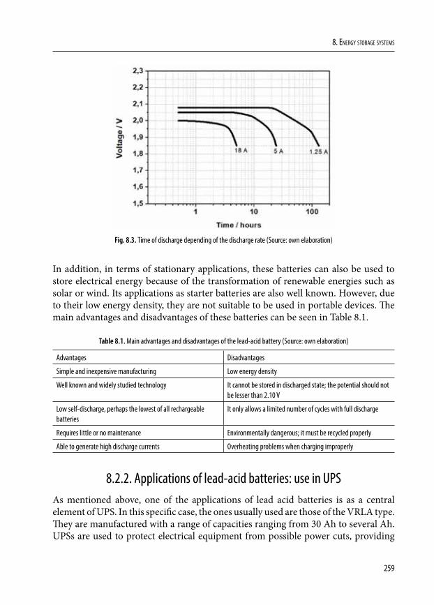
259


Fig. 8.3. Time of discharge depending of the discharge rate (Source: own elaboration)

In addition, in terms of stationary applications, these batteries can also be used to store electrical energy because of the transformation of renewable energies such as solar or wind. Its applications as starter batteries are also well known. However, due to their low energy density, they are not suitable to be used in portable devices. The main advantages and disadvantages of these batteries can be seen in Table 8.1.

Table 8.1. Main advantages and disadvantages of the lead-acid battery (Source: own elaboration)

Advantages Disadvantages

Simple and inexpensive manufacturing Low energy density

Well known and widely studied technology It cannot be stored in discharged state; the potential should not be lesser than 2.10 V

Low self-discharge, perhaps the lowest of all rechargeable batteries

It only allows a limited number of cycles with full discharge

Requires little or no maintenance Environmentally dangerous; it must be recycled properly

Able to generate high discharge currents Overheating problems when charging improperly

8.2.2. Applications of lead-acid batteries: use in UPSAs mentioned above, one of the applications of lead acid batteries is as a central element of UPS. In this specific case, the ones usually used are those of the VRLA type. They are manufactured with a range of capacities ranging from 30 Ah to several Ah. UPSs are used to protect electrical equipment from possible power cuts, providing

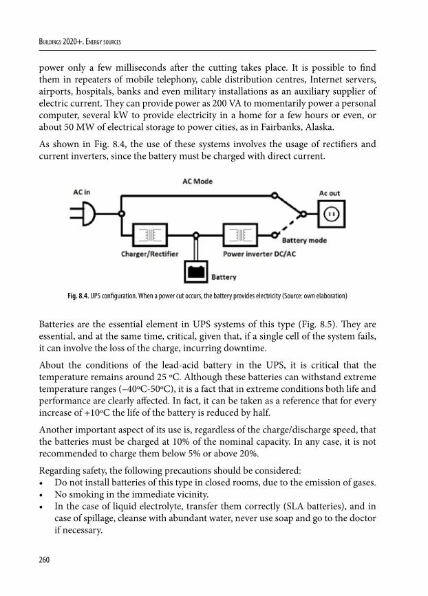
260


power only a few milliseconds after the cutting takes place. It is possible to find them in repeaters of mobile telephony, cable distribution centres, Internet servers, airports, hospitals, banks and even military installations as an auxiliary supplier of electric current. They can provide power as 200 VA to momentarily power a personal computer, several kW to provide electricity in a home for a few hours or even, or about 50 MW of electrical storage to power cities, as in Fairbanks, Alaska.

As shown in Fig. 8.4, the use of these systems involves the usage of rectifiers and current inverters, since the battery must be charged with direct current.

Fig. 8.4. UPS configuration. When a power cut occurs, the battery provides electricity (Source: own elaboration)

Batteries are the essential element in UPS systems of this type (Fig. 8.5). They are essential, and at the same time, critical, given that, if a single cell of the system fails, it can involve the loss of the charge, incurring downtime.

About the conditions of the lead-acid battery in the UPS, it is critical that the temperature remains around 25 ºC. Although these batteries can withstand extreme temperature ranges (–40ºC-50ºC), it is a fact that in extreme conditions both life and performance are clearly affected. In fact, it can be taken as a reference that for every increase of +10ºC the life of the battery is reduced by half.

Another important aspect of its use is, regardless of the charge/discharge speed, that the batteries must be charged at 10% of the nominal capacity. In any case, it is not recommended to charge them below 5% or above 20%.

Regarding safety, the following precautions should be considered:• Do not install batteries of this type in closed rooms, due to the emission of gases.• No smoking in the immediate vicinity.• In the case of liquid electrolyte, transfer them correctly (SLA batteries), and in

case of spillage, cleanse with abundant water, never use soap and go to the doctor if necessary.

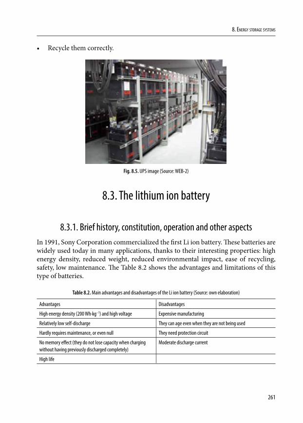
261


• Recycle them correctly.

Fig. 8.5. UPS image (Source: WEB-2)

8.3. The lithium ion battery

8.3.1. Brief history, constitution, operation and other aspectsIn 1991, Sony Corporation commercialized the first Li ion battery. These batteries are widely used today in many applications, thanks to their interesting properties: high energy density, reduced weight, reduced environmental impact, ease of recycling, safety, low maintenance. The Table 8.2 shows the advantages and limitations of this type of batteries.

Table 8.2. Main advantages and disadvantages of the Li ion battery (Source: own elaboration)

Advantages Disadvantages

High energy density (200 Wh·kg–1) and high voltage Expensive manufacturing

Relatively low self-discharge They can age even when they are not being used

Hardly requires maintenance, or even null They need protection circuit

No memory effect (they do not lose capacity when charging without having previously discharged completely)

Moderate discharge current

High life

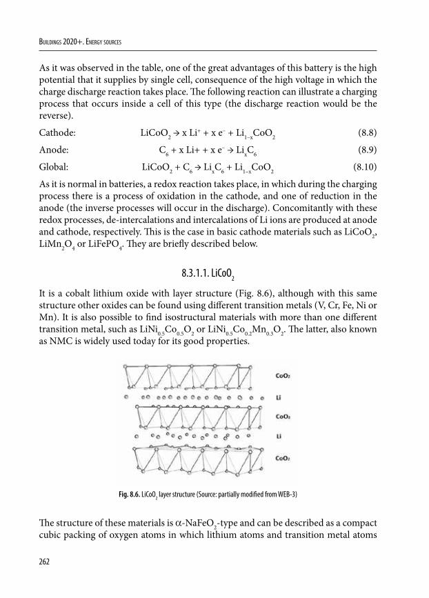
262


As it was observed in the table, one of the great advantages of this battery is the high potential that it supplies by single cell, consequence of the high voltage in which the charge discharge reaction takes place. The following reaction can illustrate a charging process that occurs inside a cell of this type (the discharge reaction would be the reverse).

Cathode: LiCoO2 → x Li+ + x e– + Li1–xCoO2 (8.8)

Anode: C6 + x Li+ + x e– → LixC6 (8.9)

Global: LiCoO2 + C6 → LixC6 + Li1–xCoO2 (8.10)

As it is normal in batteries, a redox reaction takes place, in which during the charging process there is a process of oxidation in the cathode, and one of reduction in the anode (the inverse processes will occur in the discharge). Concomitantly with these redox processes, de-intercalations and intercalations of Li ions are produced at anode and cathode, respectively. This is the case in basic cathode materials such as LiCoO2, LiMn2O4 or LiFePO4. They are briefly described below.

8.3.1.1. LiCoO2

It is a cobalt lithium oxide with layer structure (Fig. 8.6), although with this same structure other oxides can be found using different transition metals (V, Cr, Fe, Ni or Mn). It is also possible to find isostructural materials with more than one different transition metal, such as LiNi0.5Co0.5O2 or LiNi0.5Co0.2Mn0.3O2. The latter, also known as NMC is widely used today for its good properties.

Fig. 8.6. LiCoO2 layer structure (Source: partially modified from WEB-3)

The structure of these materials is α-NaFeO2-type and can be described as a compact cubic packing of oxygen atoms in which lithium atoms and transition metal atoms

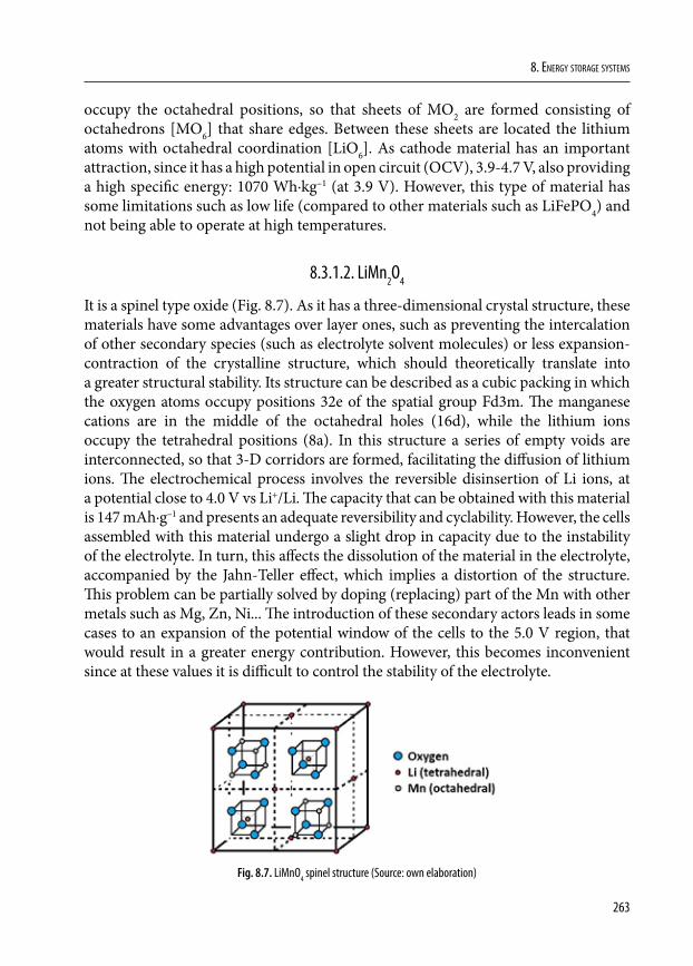
263


occupy the octahedral positions, so that sheets of MO2 are formed consisting of octahedrons [MO6] that share edges. Between these sheets are located the lithium atoms with octahedral coordination [LiO6]. As cathode material has an important attraction, since it has a high potential in open circuit (OCV), 3.9-4.7 V, also providing a high specific energy: 1070 Wh·kg–1 (at 3.9 V). However, this type of material has some limitations such as low life (compared to other materials such as LiFePO4) and not being able to operate at high temperatures.

8.3.1.2. LiMn2O4

It is a spinel type oxide (Fig. 8.7). As it has a three-dimensional crystal structure, these materials have some advantages over layer ones, such as preventing the intercalation of other secondary species (such as electrolyte solvent molecules) or less expansion-contraction of the crystalline structure, which should theoretically translate into a greater structural stability. Its structure can be described as a cubic packing in which the oxygen atoms occupy positions 32e of the spatial group Fd3m. The manganese cations are in the middle of the octahedral holes (16d), while the lithium ions occupy the tetrahedral positions (8a). In this structure a series of empty voids are interconnected, so that 3-D corridors are formed, facilitating the diffusion of lithium ions. The electrochemical process involves the reversible disinsertion of Li ions, at a potential close to 4.0 V vs Li+/Li. The capacity that can be obtained with this material is 147 mAh·g–1 and presents an adequate reversibility and cyclability. However, the cells assembled with this material undergo a slight drop in capacity due to the instability of the electrolyte. In turn, this affects the dissolution of the material in the electrolyte, accompanied by the Jahn-Teller effect, which implies a distortion of the structure. This problem can be partially solved by doping (replacing) part of the Mn with other metals such as Mg, Zn, Ni... The introduction of these secondary actors leads in some cases to an expansion of the potential window of the cells to the 5.0 V region, that would result in a greater energy contribution. However, this becomes inconvenient since at these values it is difficult to control the stability of the electrolyte.

Fig. 8.7. LiMnO4 spinel structure (Source: own elaboration)

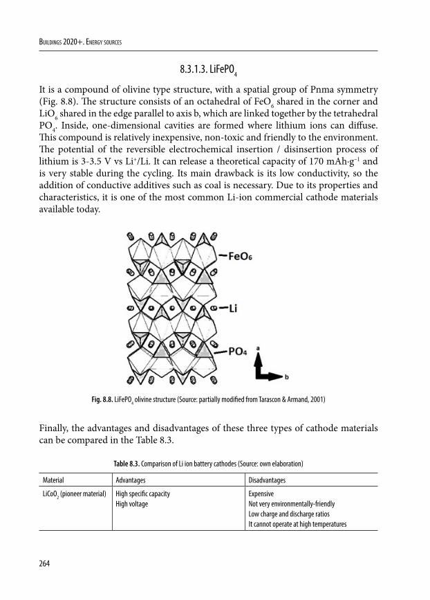
264


8.3.1.3. LiFePO4

It is a compound of olivine type structure, with a spatial group of Pnma symmetry (Fig. 8.8). The structure consists of an octahedral of FeO6 shared in the corner and LiO6 shared in the edge parallel to axis b, which are linked together by the tetrahedral PO4. Inside, one-dimensional cavities are formed where lithium ions can diffuse. This compound is relatively inexpensive, non-toxic and friendly to the environment. The potential of the reversible electrochemical insertion / disinsertion process of lithium is 3-3.5 V vs Li+/Li. It can release a theoretical capacity of 170 mAh·g–1 and is very stable during the cycling. Its main drawback is its low conductivity, so the addition of conductive additives such as coal is necessary. Due to its properties and characteristics, it is one of the most common Li-ion commercial cathode materials available today.

Fig. 8.8. LiFePO4 olivine structure (Source: partially modified from Tarascon & Armand, 2001)

Finally, the advantages and disadvantages of these three types of cathode materials can be compared in the Table 8.3.

Table 8.3. Comparison of Li ion battery cathodes (Source: own elaboration)

Material Advantages Disadvantages

LiCoO2 (pioneer material) High specific capacityHigh voltage

ExpensiveNot very environmentally-friendlyLow charge and discharge ratiosIt cannot operate at high temperatures

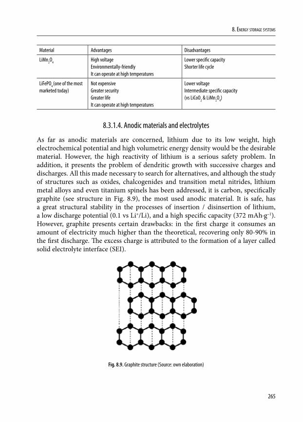
265


Material Advantages Disadvantages

LiMn2O4 High voltageEnvironmentally-friendlyIt can operate at high temperatures

Lower specific capacityShorter life cycle

LiFePO4 (one of the most marketed today)

Not expensiveGreater securityGreater lifeIt can operate at high temperatures

Lower voltageIntermediate specific capacity (vs LiCoO2 & LiMn2O4)

8.3.1.4. Anodic materials and electrolytes

As far as anodic materials are concerned, lithium due to its low weight, high electrochemical potential and high volumetric energy density would be the desirable material. However, the high reactivity of lithium is a serious safety problem. In addition, it presents the problem of dendritic growth with successive charges and discharges. All this made necessary to search for alternatives, and although the study of structures such as oxides, chalcogenides and transition metal nitrides, lithium metal alloys and even titanium spinels has been addressed, it is carbon, specifically graphite (see structure in Fig. 8.9), the most used anodic material. It is safe, has a great structural stability in the processes of insertion / disinsertion of lithium, a low discharge potential (0.1 vs Li+/Li), and a high specific capacity (372 mAh·g–1). However, graphite presents certain drawbacks: in the first charge it consumes an amount of electricity much higher than the theoretical, recovering only 80-90% in the first discharge. The excess charge is attributed to the formation of a layer called solid electrolyte interface (SEI).

Fig. 8.9. Graphite structure (Source: own elaboration)

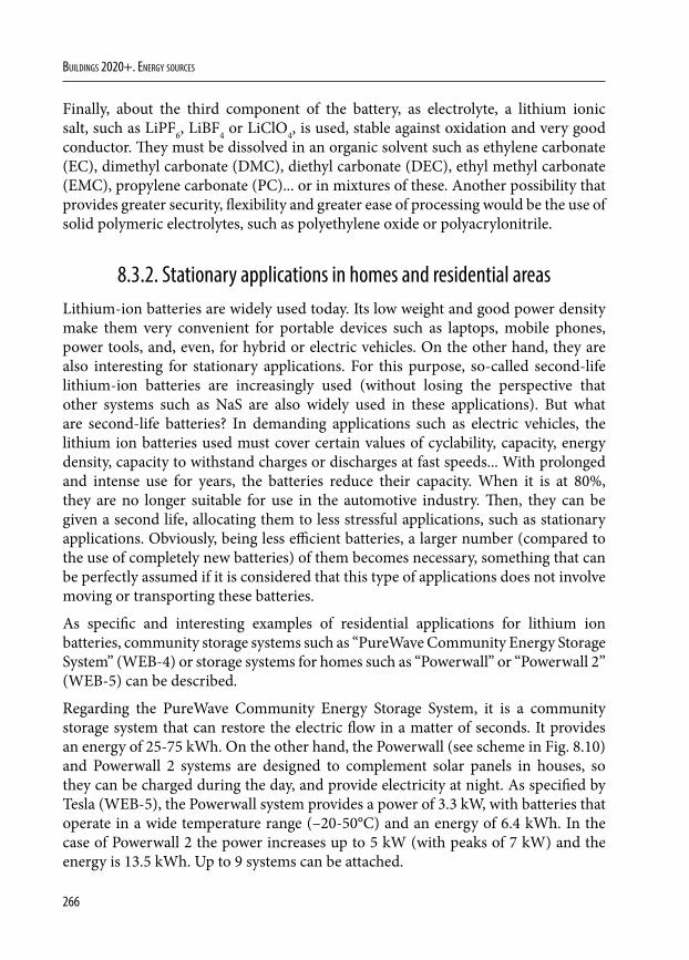
266


Finally, about the third component of the battery, as electrolyte, a lithium ionic salt, such as LiPF6, LiBF4 or LiClO4, is used, stable against oxidation and very good conductor. They must be dissolved in an organic solvent such as ethylene carbonate (EC), dimethyl carbonate (DMC), diethyl carbonate (DEC), ethyl methyl carbonate (EMC), propylene carbonate (PC)... or in mixtures of these. Another possibility that provides greater security, flexibility and greater ease of processing would be the use of solid polymeric electrolytes, such as polyethylene oxide or polyacrylonitrile.

8.3.2. Stationary applications in homes and residential areasLithium-ion batteries are widely used today. Its low weight and good power density make them very convenient for portable devices such as laptops, mobile phones, power tools, and, even, for hybrid or electric vehicles. On the other hand, they are also interesting for stationary applications. For this purpose, so-called second-life lithium-ion batteries are increasingly used (without losing the perspective that other systems such as NaS are also widely used in these applications). But what are second-life batteries? In demanding applications such as electric vehicles, the lithium ion batteries used must cover certain values of cyclability, capacity, energy density, capacity to withstand charges or discharges at fast speeds... With prolonged and intense use for years, the batteries reduce their capacity. When it is at 80%, they are no longer suitable for use in the automotive industry. Then, they can be given a second life, allocating them to less stressful applications, such as stationary applications. Obviously, being less efficient batteries, a larger number (compared to the use of completely new batteries) of them becomes necessary, something that can be perfectly assumed if it is considered that this type of applications does not involve moving or transporting these batteries.

As specific and interesting examples of residential applications for lithium ion batteries, community storage systems such as “PureWave Community Energy Storage System” (WEB-4) or storage systems for homes such as “Powerwall” or “Powerwall 2” (WEB-5) can be described.

Regarding the PureWave Community Energy Storage System, it is a community storage system that can restore the electric flow in a matter of seconds. It provides an energy of 25-75 kWh. On the other hand, the Powerwall (see scheme in Fig. 8.10) and Powerwall 2 systems are designed to complement solar panels in houses, so they can be charged during the day, and provide electricity at night. As specified by Tesla (WEB-5), the Powerwall system provides a power of 3.3 kW, with batteries that operate in a wide temperature range (–20-50°C) and an energy of 6.4 kWh. In the case of Powerwall 2 the power increases up to 5 kW (with peaks of 7 kW) and the energy is 13.5 kWh. Up to 9 systems can be attached.

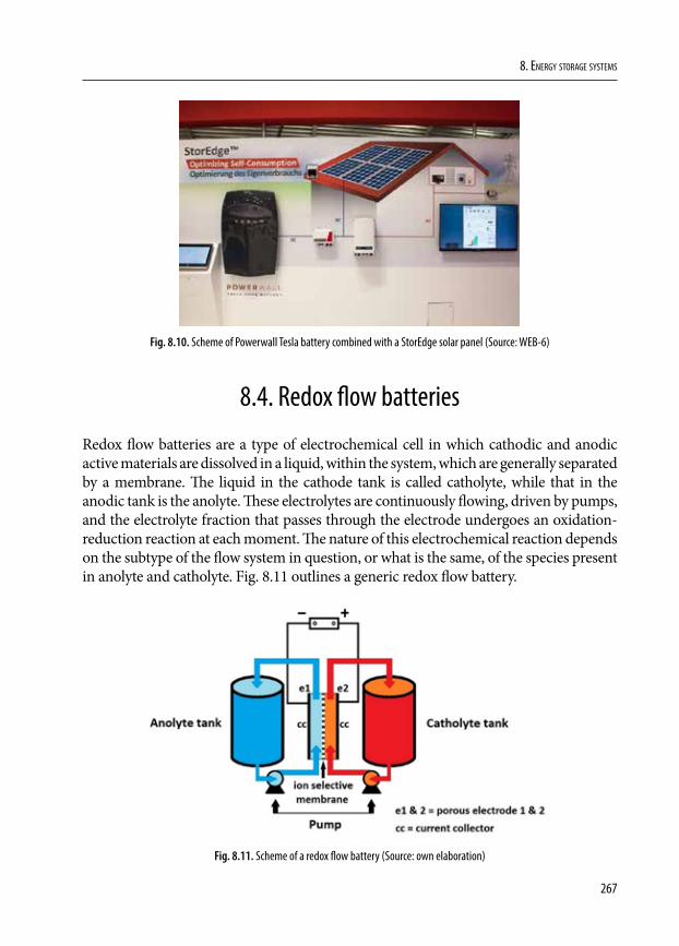
267


Fig. 8.10. Scheme of Powerwall Tesla battery combined with a StorEdge solar panel (Source: WEB-6)

8.4. Redox flow batteries

Redox flow batteries are a type of electrochemical cell in which cathodic and anodic active materials are dissolved in a liquid, within the system, which are generally separated by a membrane. The liquid in the cathode tank is called catholyte, while that in the anodic tank is the anolyte. These electrolytes are continuously flowing, driven by pumps, and the electrolyte fraction that passes through the electrode undergoes an oxidation-reduction reaction at each moment. The nature of this electrochemical reaction depends on the subtype of the flow system in question, or what is the same, of the species present in anolyte and catholyte. Fig. 8.11 outlines a generic redox flow battery.

Fig. 8.11. Scheme of a redox flow battery (Source: own elaboration)

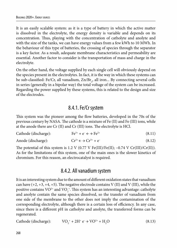
268


It is an easily scalable system: as it is a type of battery in which the active matter is dissolved in the electrolyte, the energy density is variable and depends on its concentration. Thus, playing with the concentration of catholyte and anolyte and with the size of the tanks, we can have energy values from a few kWh to 10 MWh. In the behaviour of this type of batteries, the crossing of species through the separator is a key factor. As a result, adequate membrane characteristics and permeability are essential. Another factor to consider is the transportation of mass and charge in the electrolyte.

On the other hand, the voltage supplied by each single cell will obviously depend on the species present in the electrolytes. In fact, it is the way in which these systems can be sub-classified: Fe/Cr, all vanadium, Zn/Br2, all iron... By connecting several cells in series (generally in a bipolar way) the total voltage of the system can be increased. Regarding the power supplied by these systems, this is related to the design and size of the electrodes.

8.4.1. Fe/Cr systemThis system was the pioneer among the flow batteries, developed in the 70s of the previous century by NASA. The cathode is a mixture of Fe (II) and Fe (III) ions, while at the anode there are Cr (II) and Cr (III) ions. The electrolyte is HCl.

Cathode (discharge): Fe3+ + e– ← → Fe2+ (8.11)

Anode (discharge): Cr2+ ← → Cr3+ + e– (8.12)

The potential of this system is 1.2 V (0.77 V Fe(III)/Fe(II); –0.74 V Cr(III)/Cr(II)). As for the limitations of this system, one of the main ones is the slower kinetics of chromium. For this reason, an electrocatalyst is required.

8.4.2. All vanadium systemIt is an interesting system due to the amount of different oxidation states that vanadium can have (+2, +3, +4, +5). The negative electrode contains V (II) and V (III), while the positive contains VO2+ and VO2

+. This system has an interesting advantage: catholyte and anolyte contain the same species dissolved, so the transfer of vanadium from one side of the membrane to the other does not imply the contamination of the corresponding electrolyte, although there is a certain loss of efficiency. In any case, since there is a different pH in catholyte and anolyte, the transferred forms can be regenerated.

Cathode (discharge): VO2+ + 2H+ e– → VO2+ + H2O (8.13)

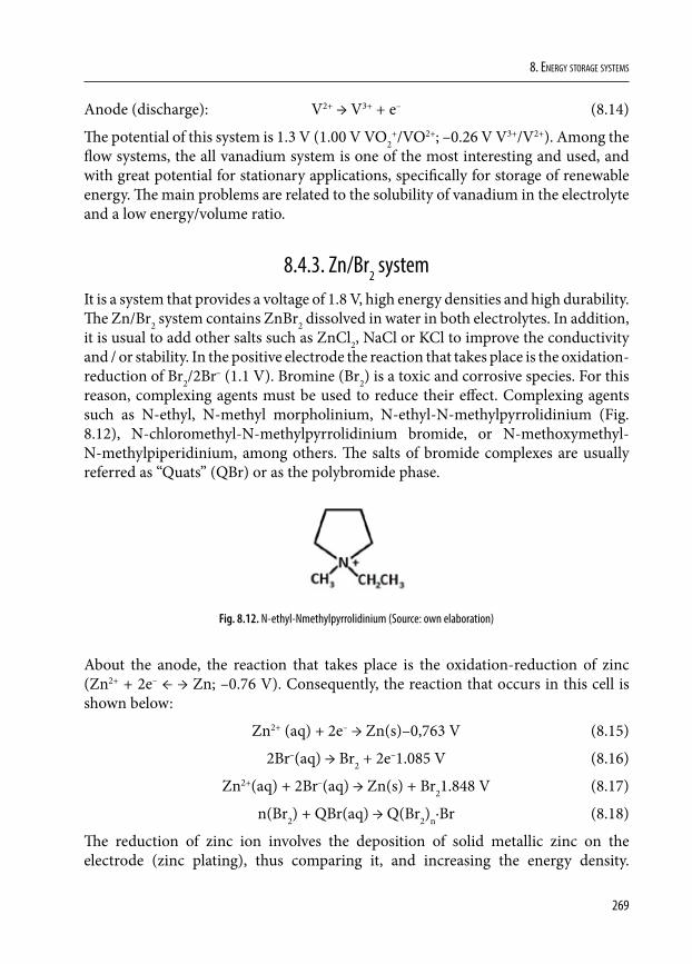
269


Anode (discharge): V2+ → V3+ + e– (8.14)

The potential of this system is 1.3 V (1.00 V VO2+/VO2+; –0.26 V V3+/V2+). Among the

flow systems, the all vanadium system is one of the most interesting and used, and with great potential for stationary applications, specifically for storage of renewable energy. The main problems are related to the solubility of vanadium in the electrolyte and a low energy/volume ratio.

8.4.3. Zn/Br2 systemIt is a system that provides a voltage of 1.8 V, high energy densities and high durability. The Zn/Br2 system contains ZnBr2 dissolved in water in both electrolytes. In addition, it is usual to add other salts such as ZnCl2, NaCl or KCl to improve the conductivity and / or stability. In the positive electrode the reaction that takes place is the oxidation-reduction of Br2/2Br– (1.1 V). Bromine (Br2) is a toxic and corrosive species. For this reason, complexing agents must be used to reduce their effect. Complexing agents such as N-ethyl, N-methyl morpholinium, N-ethyl-N-methylpyrrolidinium (Fig. 8.12), N-chloromethyl-N-methylpyrrolidinium bromide, or N-methoxymethyl-N-methylpiperidinium, among others. The salts of bromide complexes are usually referred as “Quats” (QBr) or as the polybromide phase.

Fig. 8.12. N-ethyl-Nmethylpyrrolidinium (Source: own elaboration)

About the anode, the reaction that takes place is the oxidation-reduction of zinc (Zn2+ + 2e– ← → Zn; –0.76 V). Consequently, the reaction that occurs in this cell is shown below:

Zn2+ (aq) + 2e– → Zn(s)–0,763 V (8.15)

2Br–(aq) → Br2 + 2e–1.085 V (8.16)

Zn2+(aq) + 2Br–(aq) → Zn(s) + Br21.848 V (8.17)

n(Br2) + QBr(aq) → Q(Br2)n·Br (8.18)

The reduction of zinc ion involves the deposition of solid metallic zinc on the electrode (zinc plating), thus comparing it, and increasing the energy density.

270


However, excessive growth of zinc could lead to the perforation of the membrane and the consequent short circuit.

In this type of system, research is still required for its optimization: it is a key aspect that the membrane prevents the transit of species, since it would lead to the consequent recombination to zinc bromide; control over bromine complexation on the one hand, and dendritic growth, on the other, are also essential for the proper development of this technology.

8.4.4. Applications of flow batteries. Are they the best positioned for sta-tionary applications for the future?

The complex design of the flow batteries and the fact that they are not exactly light make their use unfeasible for portable type applications or electric vehicles. However, they can be, if they are not already, a commitment to the future in stationary applications of energy storage. A flow battery developed and optimized, as in the case of all vanadium system, can reach 20 years of life without its capacity being affected over time, and providing a 100% depth of discharge in all cycles. In addition, these batteries have other interesting advantages such as not being flammable or explosive. The high availability of vanadium on Earth is another factor that makes these batteries interesting. Companies like StorEn (WEB-7) are an example of commitment to this technology. Others like the British RedT (WEB-8) can also make us see that the future of batteries with stationary applications of energy storage is in the flow batteries, having installed in the farm of Olde House, United Kingdom, a system to store the excess of solar energy (it could allow the reduction of demand to the electricity network of up to 50%). The system, specifically based on vanadium, has a storage capacity of 1 MWh, a maximum power of 90 kW and a life of 25 years.

References

Caballero, A. (2007) Síntesis y caracterización de materiales nanométricos para su aplicación en baterías recargables de ion-litio y plomo-ácido. Doctoral Thesis. University of Cordoba.

Julien, C., Mauger, A., Vijh, A. & Zaghib, K. (2016) Lithium batteries. Science and Technology. Springer.

271


Rajarathnam, G. P. & Vassallo, A. M. (2016) The Zinc/Bromine Flow Battery. Materials Challenges and Practical Solutions for Technology Advancement. SpringerBriefs in Energy. Springer.

Reddy, T. (ed.) & Linden, D. (2010) Linden’s handbook of batteries. McGraw-Hill Education.

Tarascon, J. M. & Armand, M. (2001) Issues and challenges facing rechargeable lithium batteries. Nature, 414, 359-367.

WEB-1: Website of Company UPS Battery Center [Online]. Available from: http://www.upsbatterycenter.com/blog/valve-regulated-lead-acid-vrla-batteries/ [Accessed 25th August 2018].

WEB-2: Website of Company Electronic Environments Co. LLC. [Online]. Available from: https://blog.eecnet.com/eecnetcom/bid/35069/maintaining-extending-the-life-of-your-data-center-s-ups-batteries [Accessed 25th August 2018].

WEB-3: Image from WIKIPEDIA [Online]. Available from https://en.wikipedia.org/wiki/Lithium_cobalt_oxide#/media/File:Lithium-cobalt-oxide-3D-polyhedra.png. [Accessed 25th August 2018].

WEB-4: S&C Electric Company (2018) S&C Electric Company. Excellence Through Innovation. [Online] Available from: https://www.sandc.com/ [Accessed 10th August 2018].

WEB-5: Tesla (2018) Tesla. [Online] Available from: https://www.tesla.com/powerwall [Accessed 10th August 2018].

WEB-6: Website of Energy Storage News [Online]. Available from https://www.energy-storage.news/news/solaredge-customers-to-get-tesla-powerwall-batteries-within-six-months [Accessed 25th August 2018].

WEB-7: StorEn Technologies (2018) StorEn Technologies. Energy you can depend on. [Online] Available from http://www.storen.tech/ [Accessed 10th August 2018].

WEB-8: RedT energy plc (2018) RedT energy storage. [Online] Available from: http://www.redtenergy.com/ [Accessed 10th August 2018].

Zhang, Z. & Zhang, S. S. (2015) Rechargeable Batteries. Materials, Technology and New Trends. Green Energy and Technology. Springer.

Buildings 2020+

Documents

Transcript of Buildings 2020+