7

CHAPTER 2

LITERATURE REVIEW: PR MANIPULATOR SCALING ISSUES

2.1 Introduction

This chapter offers literature reviews on subjects that are necessary for understanding the workin this thesis. Reviews and historical summaries are presented on PM d.c. motors, friction inservo mechanisms, friction compensation techniques and dimensional analysis. Historical andcontemporary analytical models of the PM d.c. motor with nonlinear friction are presented alongwith the computed torque method which is the principal control strategy used in the thesis. Thechapter concludes with reviews on similitude methods and the Buckingham Pi theorem.Example problems are provided for each technique.

2.2 Review: Brush Commutated PM d.c. Servo Motors

The direct current (d.c.) machine traces its origins to the earliest experiments in electricity andmagnetism. The Barlow wheel, invented around 1822, used electromagnetic forces to produce acontinuous rotating machine (Walker, 1978). Several years later, Michael Faraday's invented hisdisc type machine which is often considered the first direct current motor (Electro-Craft, 1980).

Experiments with permanent magnets in electrical machines were conducted throughout the19th century. Pioneers included J. Henry (1831), H. Pixii (1832), W. Ritchie (1833), F. Watkins(1835), T. Davenport (1837) and M.H. Jacobi (1839). Poor quality magnets forced the earlyabandonment of PM in motors in favor of electromagnetic excitation systems (Gieras and Wing,1997). The rebirth of permanent magnets used in motors began with the development of Alnicomagnets by Bell Laboratories in the 1930's. The 1950's saw the introduction of ceramic or "hardferrite" permanent magnets which are still widely used today (Nasar, Boldea, and Unnewehr,1993).

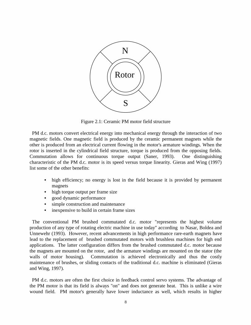
The historical d.c. motor is made up of three principal components. They are: the current-carrying conductors called an armature; a circuit for a magnetic field; and a commutator made ofbrushes or some type of sliding metal contact mechanism (Electro-Craft, 1980). The purpose ofthe commutator is to switch the direction of current in the armature's individual coils so that themotor's shaft will turn continuously. In a PM d.c. motor, the magnetic field is produced bypermanent magnets. Figure 2.1 shows an armature, commutator and a ceramic magnet fieldstructure of a brush commutated PM d.c. motor.

8

N

S

Rotor

Figure 2.1: Ceramic PM motor field structure

PM d.c. motors convert electrical energy into mechanical energy through the interaction of twomagnetic fields. One magnetic field is produced by the ceramic permanent magnets while theother is produced from an electrical current flowing in the motor's armature windings. When therotor is inserted in the cylindrical field structure, torque is produced from the opposing fields.Commutation allows for continuous torque output (Saner, 1993). One distinguishingcharacteristic of the PM d.c. motor is its speed versus torque linearity. Gieras and Wing (1997)list some of the other benefits:

• high efficiency; no energy is lost in the field because it is provided by permanentmagnets

• high torque output per frame size• good dynamic performance• simple construction and maintenance• inexpensive to build in certain frame sizes

The conventional PM brushed commutated d.c. motor "represents the highest volumeproduction of any type of rotating electric machine in use today" according to Nasar, Boldea andUnnewehr (1993). However, recent advancements in high performance rare-earth magnets havelead to the replacement of brushed commutated motors with brushless machines for high endapplications. The latter configuration differs from the brushed commutated d.c. motor becausethe magnets are mounted on the rotor, and the armature windings are mounted on the stator (thewalls of motor housing). Commutation is achieved electronically and thus the costlymaintenance of brushes, or sliding contacts of the traditional d.c. machine is eliminated (Gierasand Wing, 1997).

PM d.c. motors are often the first choice in feedback control servo systems. The advantage ofthe PM motor is that its field is always "on" and does not generate heat. This is unlike a wirewound field. PM motor's generally have lower inductance as well, which results in higher

9

responsiveness. Applications that use PM d.c. motors are numerous. In the early days of thecomputer industry, they were used in peripheral equipment such as digital magnetic tape drives(Walker, 1978). Today, PM motors are found in home appliances, robotics, medical instrumentsand plant automation equipment. Advancements in electronic control continually push PM d.c.motors into an ever expanding application arena.

PM motors have great flexibility in size, shape and geometry. In general, torque available froma "miniature" PM motor is a function of the motor's magnets. More expensive rare-earthmagnets are used in applications where high torque per unit volume is important. For example, asamarium-cobalt servomotor that is 1.3 inches in diameter and 1.9 inches long is capable ofdeveloping a peak torque of 50 oz-in (Nasar, Boldea and Unnewehr, 1993).

Ceramic permanent magnets form another class of PM d.c. motors. They are made from ferriteoxides of strontium or barium. The latter is used primarily in the automotive and electric toyindustry (Gieras and Wing, 1997). These magnets generally demonstrate low magnetic energyproperties, a high resistance to demagnetization, and are widely available at low cost (Nasar,Boldea and Unnewehr, 1993). Because of cost, only ceramic PM motors were considered in thisstudy.

Manufacturers of PM motors provide data sheets to application engineers that list keyparameters that describe the performance of a particular motor. Appendix B defines these termsand derives the generalized transfer function of a PM d.c. motor. At this level, knowledge of themotor's magnetic properties are not directly specified. They are instead inferred through termssuch as the motor's torque constant. It should be noted that this thesis works at this level, anddoes not attempt to nondimensionalize parameters and variables that would be used by motordesigners.

According to Saner (1993), selecting a PM d.c. motor for an application is an iterative process.It begins by selecting a motor frame size based on the application's speed and torquerequirements. Once a frame size is selected, its torque constant is calculated. This value is usedto determine the motor's winding (voltage rating). The motor selection is then confirmed in thefollowing set of motor equations:

T K I Jd

dtD T Tg t f L= = + + +1 1

ω ω (2.1)

V IR Kb= + ω (2.2)

IT

Kg

t

= (2.3)

and

VT R

KKg

tb= + ω (2.4)

10

where Tf is a composite friction torque term, TL is the load torque, and ω is the specified speedfor the application. (Background on the motor equations and variable definitions is offered inAppendix B.) The current calculated in (2.3) and voltage in (2.4) must meet the applicationrequirements and be within the power supply limitations. If these values fall outside thespecifications, another frame size and winding must be selected. The procedure continues untilequations (2.3) and (2.4) are satisfied for the application.

Later in the thesis, it will be shown how dimensional analysis will facilitate the motor selectionprocess for a prototype system. Rather than iteratively working with equations (2.1-2.4), theprototype motor will be quickly sized from a simple set of scaling laws derived fromBuckingham's Pi theorem. The utility of the techniques developed in this study becomeespecially clear when trying to size motors for low velocity applications. It is in this regime thatfriction factors are particularly significant and dimensional analysis is especially useful.

2.3 Review: Friction in Servo Mechanisms

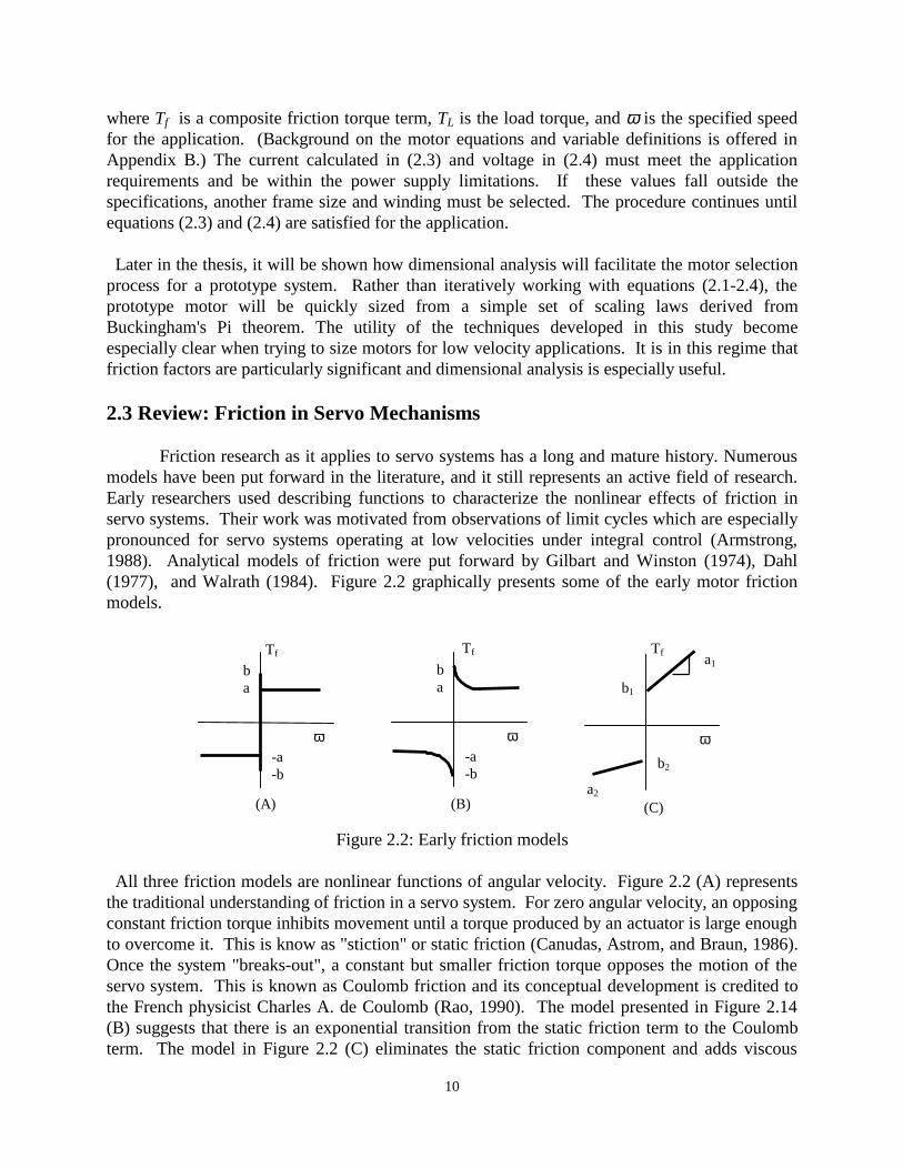
Friction research as it applies to servo systems has a long and mature history. Numerousmodels have been put forward in the literature, and it still represents an active field of research.Early researchers used describing functions to characterize the nonlinear effects of friction inservo systems. Their work was motivated from observations of limit cycles which are especiallypronounced for servo systems operating at low velocities under integral control (Armstrong,1988). Analytical models of friction were put forward by Gilbart and Winston (1974), Dahl(1977), and Walrath (1984). Figure 2.2 graphically presents some of the early motor frictionmodels.

Figure 2.2: Early friction models

All three friction models are nonlinear functions of angular velocity. Figure 2.2 (A) representsthe traditional understanding of friction in a servo system. For zero angular velocity, an opposingconstant friction torque inhibits movement until a torque produced by an actuator is large enoughto overcome it. This is know as "stiction" or static friction (Canudas, Astrom, and Braun, 1986).Once the system "breaks-out", a constant but smaller friction torque opposes the motion of theservo system. This is known as Coulomb friction and its conceptual development is credited tothe French physicist Charles A. de Coulomb (Rao, 1990). The model presented in Figure 2.14(B) suggests that there is an exponential transition from the static friction term to the Coulombterm. The model in Figure 2.2 (C) eliminates the static friction component and adds viscous

(C)

Tf

ba

-a-b

ω

ba

-a-b

ω

b1

ω

a1

b2

a2(A) (B)

Tf Tf

11

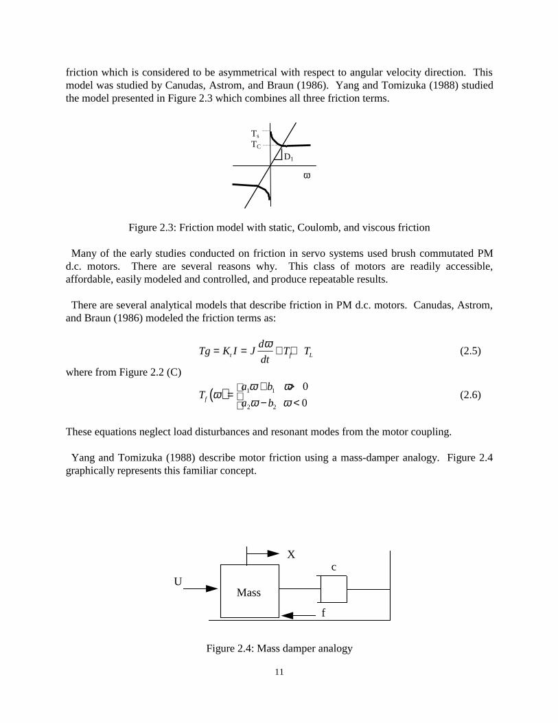
friction which is considered to be asymmetrical with respect to angular velocity direction. Thismodel was studied by Canudas, Astrom, and Braun (1986). Yang and Tomizuka (1988) studiedthe model presented in Figure 2.3 which combines all three friction terms.

Figure 2.3: Friction model with static, Coulomb, and viscous friction

Many of the early studies conducted on friction in servo systems used brush commutated PMd.c. motors. There are several reasons why. This class of motors are readily accessible,affordable, easily modeled and controlled, and produce repeatable results.

There are several analytical models that describe friction in PM d.c. motors. Canudas, Astrom,and Braun (1986) modeled the friction terms as:

Tg K I Jd

dtT Tt f L= = + +ω

(2.5)

where from Figure 2.2 (C)

( )Ta b

a bf ωω ωω ω

=+ >− <

1 1

2 2

0

0

(2.6)

These equations neglect load disturbances and resonant modes from the motor coupling.

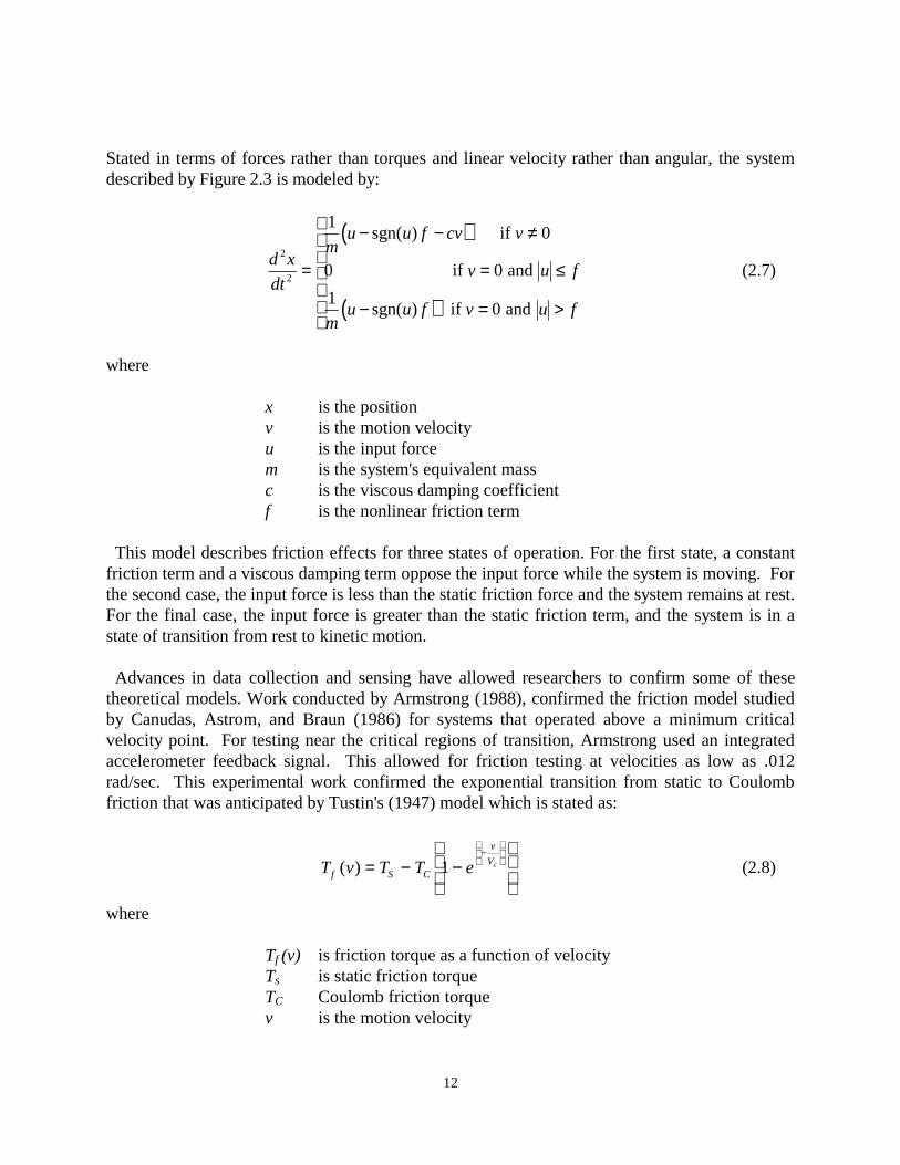
Yang and Tomizuka (1988) describe motor friction using a mass-damper analogy. Figure 2.4graphically represents this familiar concept.

Mass

X

U

f

c

Figure 2.4: Mass damper analogy

Ts

TC

ω

D1

12

Stated in terms of forces rather than torques and linear velocity rather than angular, the systemdescribed by Figure 2.3 is modeled by:

( )

( )

d x

dt

mu u f cv v

v u f

mu u f v u f

2

2

10

0 0

10

=

− − ≠

= ≤

− = >

sgn( )

sgn( )

if

if and

if and

(2.7)

where

x is the positionv is the motion velocityu is the input forcem is the system's equivalent massc is the viscous damping coefficientf is the nonlinear friction term

This model describes friction effects for three states of operation. For the first state, a constantfriction term and a viscous damping term oppose the input force while the system is moving. Forthe second case, the input force is less than the static friction force and the system remains at rest.For the final case, the input force is greater than the static friction term, and the system is in astate of transition from rest to kinetic motion.

Advances in data collection and sensing have allowed researchers to confirm some of thesetheoretical models. Work conducted by Armstrong (1988), confirmed the friction model studiedby Canudas, Astrom, and Braun (1986) for systems that operated above a minimum criticalvelocity point. For testing near the critical regions of transition, Armstrong used an integratedaccelerometer feedback signal. This allowed for friction testing at velocities as low as .012rad/sec. This experimental work confirmed the exponential transition from static to Coulombfriction that was anticipated by Tustin's (1947) model which is stated as:

T v T T ef S C

v

Vc( ) = − −

−

1 (2.8)

where

Tf (v) is friction torque as a function of velocityTs is static friction torqueTC Coulomb friction torquev is the motion velocity

13

VC is the velocity constant where the system transitions from static friction to Coulomb

Armstrong (1988) found better agreement with the experimental data when the exponential termwas squared. He restated (2.8) as:

T v T T ef S C

v

Vc( ) = − −

−

1

2

(2.9)

Research on friction effects in mechanisms has continued throughout the 1990s. C. Canudas deWit, P. Noel, A. Aubin, and B. Brogliato (1991) expanded the model to cover most of the frictioncomponents in robotic manipulators. It generalizes the friction contributions from mechanicallinks, ball bearings, gear boxes, flat surfaces and pulley mechanisms, and is expressed as:

( ) ( )[ ] ( )T v e e vfv v= + + −− −α α αβ β

0 11

221 sgn (2.10)

whereα0 represents Coulomb frictionαi,βi represent asymmetric nonlinearities that are experimentally

determined

For purposes of on-line identification, equation (2.10) was simplified to:

( ) [ ] ( )T v v v vf = + +α α α0 1

1 2

2

/sgn (2.11)

A comprehensive survey of friction in machines is presented by Armstrong-Helouvry, Dupont,and de Wit (1994). According to the authors, the field of tribology has been neglected by therobotics industry. This science of "rubbing contacts" began in England in the 1930s and dealswith basic questions of mechanism wear, surface contact and lubrication. Research in this areassuggests that relatively simple lubrication techniques can vastly assist the problem of controllinga machine where friction is a potential problem.

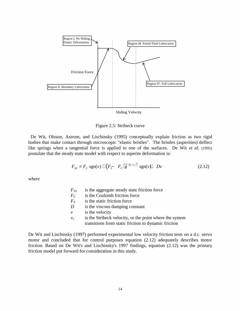
Armstrong-Helouvry, Dupont, and de Wit (1994) use insights gained from tribology to explainthe traditional friction model. It is based on the Stribeck curve, and models the "protuberantfeatures" called asperities as a spring and damper system divided into four regimes of lubrication.Figure 2.5, illustrates the curve and the distinct regions.

14

Figure 2.5: Stribeck curve

De Wit, Olsson, Astrom, and Lischinsky (1995) conceptually explain friction as two rigidbodies that make contact through microscopic "elastic bristles". The bristles (asperities) deflectlike springs when a tangential force is applied to one of the surfaces. De Wit et al. (1995)

postulate that the steady state model with respect to asperite deformation is:

( ) ( )F F v F F e v DvSS C S Cv vs= + − +−sgn( ) sgn( )/ 2

(2.12)

where

FSS is the aggregate steady state friction forceFC is the Coulomb friction forceFS is the static friction forceD is the viscous damping constantv is the velocityvs is the Stribeck velocity, or the point where the system

transitions from static friction to dynamic friction

De Wit and Lischinsky (1997) performed experimental low velocity friction tests on a d.c. servomotor and concluded that for control purposes equation (2.12) adequately describes motorfriction. Based on De Wit's and Lischinsky's 1997 findings, equation (2.12) was the primaryfriction model put forward for consideration in this study.

Friction Force

Sliding Velocity

Region I, No Sliding,Elastic Deformation

Region II. Boundary Lubrication

Region III. Partial Fluid Lubrication

Region IV. Full Lubrication

15

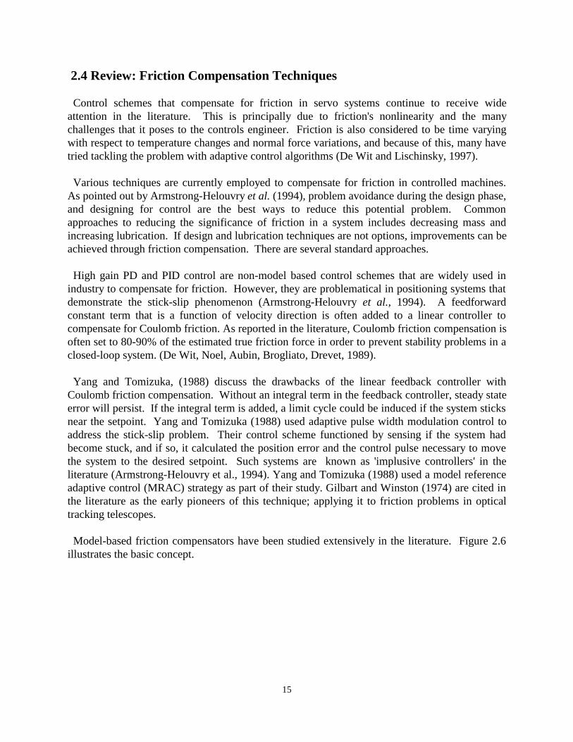
2.4 Review: Friction Compensation Techniques

Control schemes that compensate for friction in servo systems continue to receive wideattention in the literature. This is principally due to friction's nonlinearity and the manychallenges that it poses to the controls engineer. Friction is also considered to be time varyingwith respect to temperature changes and normal force variations, and because of this, many havetried tackling the problem with adaptive control algorithms (De Wit and Lischinsky, 1997).

Various techniques are currently employed to compensate for friction in controlled machines.As pointed out by Armstrong-Helouvry et al. (1994), problem avoidance during the design phase,and designing for control are the best ways to reduce this potential problem. Commonapproaches to reducing the significance of friction in a system includes decreasing mass andincreasing lubrication. If design and lubrication techniques are not options, improvements can beachieved through friction compensation. There are several standard approaches.

High gain PD and PID control are non-model based control schemes that are widely used inindustry to compensate for friction. However, they are problematical in positioning systems thatdemonstrate the stick-slip phenomenon (Armstrong-Helouvry et al., 1994). A feedforwardconstant term that is a function of velocity direction is often added to a linear controller tocompensate for Coulomb friction. As reported in the literature, Coulomb friction compensation isoften set to 80-90% of the estimated true friction force in order to prevent stability problems in aclosed-loop system. (De Wit, Noel, Aubin, Brogliato, Drevet, 1989).

Yang and Tomizuka, (1988) discuss the drawbacks of the linear feedback controller withCoulomb friction compensation. Without an integral term in the feedback controller, steady stateerror will persist. If the integral term is added, a limit cycle could be induced if the system sticksnear the setpoint. Yang and Tomizuka (1988) used adaptive pulse width modulation control toaddress the stick-slip problem. Their control scheme functioned by sensing if the system hadbecome stuck, and if so, it calculated the position error and the control pulse necessary to movethe system to the desired setpoint. Such systems are known as 'implusive controllers' in theliterature (Armstrong-Helouvry et al., 1994). Yang and Tomizuka (1988) used a model referenceadaptive control (MRAC) strategy as part of their study. Gilbart and Winston (1974) are cited inthe literature as the early pioneers of this technique; applying it to friction problems in opticaltracking telescopes.

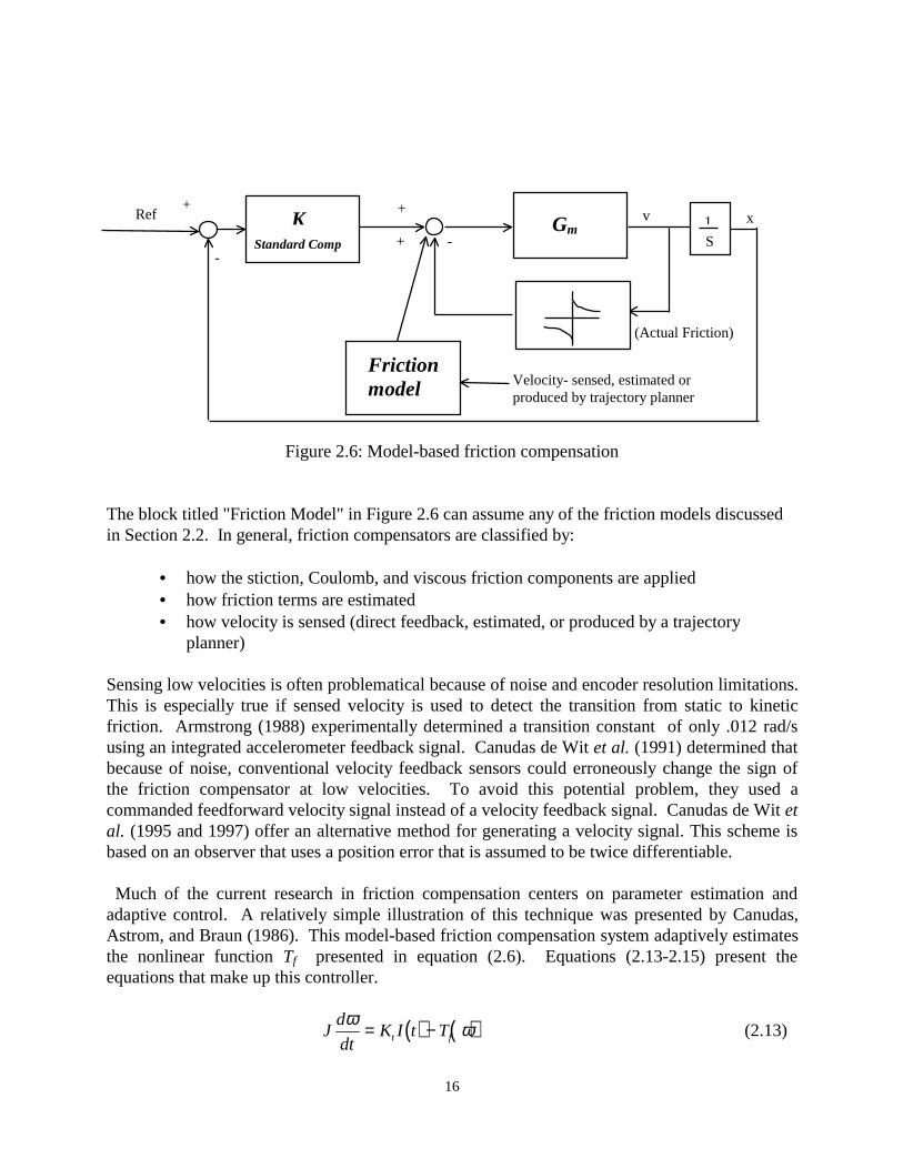
Model-based friction compensators have been studied extensively in the literature. Figure 2.6illustrates the basic concept.

16

Figure 2.6: Model-based friction compensation

The block titled "Friction Model" in Figure 2.6 can assume any of the friction models discussedin Section 2.2. In general, friction compensators are classified by:

• how the stiction, Coulomb, and viscous friction components are applied• how friction terms are estimated• how velocity is sensed (direct feedback, estimated, or produced by a trajectory

planner)

Sensing low velocities is often problematical because of noise and encoder resolution limitations.This is especially true if sensed velocity is used to detect the transition from static to kineticfriction. Armstrong (1988) experimentally determined a transition constant of only .012 rad/susing an integrated accelerometer feedback signal. Canudas de Wit et al. (1991) determined thatbecause of noise, conventional velocity feedback sensors could erroneously change the sign ofthe friction compensator at low velocities. To avoid this potential problem, they used acommanded feedforward velocity signal instead of a velocity feedback signal. Canudas de Wit etal. (1995 and 1997) offer an alternative method for generating a velocity signal. This scheme isbased on an observer that uses a position error that is assumed to be twice differentiable.

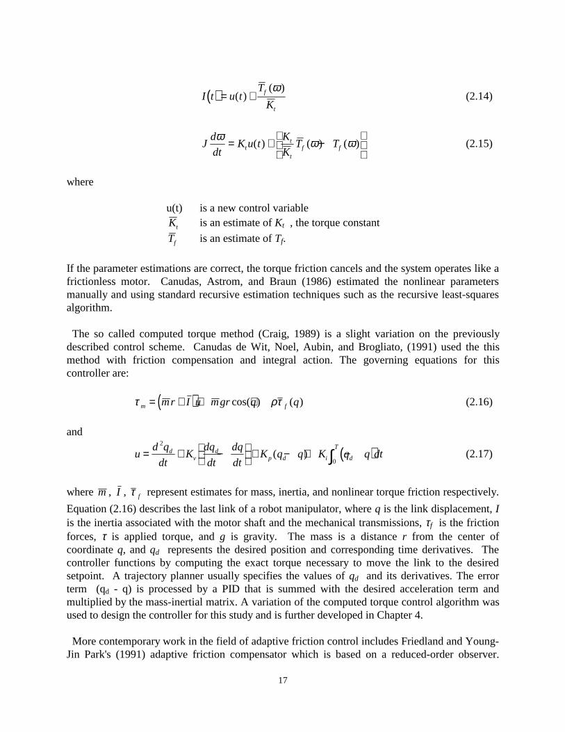
Much of the current research in friction compensation centers on parameter estimation andadaptive control. A relatively simple illustration of this technique was presented by Canudas,Astrom, and Braun (1986). This model-based friction compensation system adaptively estimatesthe nonlinear function Tf presented in equation (2.6). Equations (2.13-2.15) present theequations that make up this controller.

( ) ( )Jd

dtK I t Tt f

ω ω= − (2.13)

GmK

Frictionmodel

+

-

+

-1S+Standard Comp

(Actual Friction)

v x

Velocity- sensed, estimated orproduced by trajectory planner

Ref

17

( )I t u tT

Kf

t

= +( )( )ω

(2.14)

Jd

dtK u t

K

KT Tt

t

tf f

ω ω ω= + −

( ) ( ) ( ) (2.15)

where

u(t) is a new control variableKt is an estimate of Kt , the torque constant

Tf is an estimate of Tf.

If the parameter estimations are correct, the torque friction cancels and the system operates like africtionless motor. Canudas, Astrom, and Braun (1986) estimated the nonlinear parametersmanually and using standard recursive estimation techniques such as the recursive least-squaresalgorithm.

The so called computed torque method (Craig, 1989) is a slight variation on the previouslydescribed control scheme. Canudas de Wit, Noel, Aubin, and Brogliato, (1991) used the thismethod with friction compensation and integral action. The governing equations for thiscontroller are:

( )τ ρτm fmr I u mgr q q= + + +cos( ) ( ) (2.16)

and

( )ud q

dtK

dq

dt

dq

dtK q q K q q dtd

vd

p d i d

T= + −

+ − + −∫2

0( ) (2.17)

where m , I , τ f represent estimates for mass, inertia, and nonlinear torque friction respectively.

Equation (2.16) describes the last link of a robot manipulator, where q is the link displacement, Iis the inertia associated with the motor shaft and the mechanical transmissions, τf is the frictionforces, τ is applied torque, and g is gravity. The mass is a distance r from the center ofcoordinate q, and qd represents the desired position and corresponding time derivatives. Thecontroller functions by computing the exact torque necessary to move the link to the desiredsetpoint. A trajectory planner usually specifies the values of qd and its derivatives. The errorterm (qd - q) is processed by a PID that is summed with the desired acceleration term andmultiplied by the mass-inertial matrix. A variation of the computed torque control algorithm wasused to design the controller for this study and is further developed in Chapter 4.

More contemporary work in the field of adaptive friction control includes Friedland and Young-Jin Park's (1991) adaptive friction compensator which is based on a reduced-order observer.

18

Although no experimental results were presented, results from simulations proved promising.Canudas de Wit, Olsson, Astrom, and Lischinsky (1995) present an adaptive compensator thatuses a friction observer based on position error. Yazdizadeh and Khorasani (1996) offer aLyapunov-based strategy. Simulations for this system were conducted on a single mass systemand on a two link planar robot. Finally, Canudas de Wit and Lischinsky (1997) put forward amodel-based adaptive friction compensation algorithm that is globally stable based on Lyapunovanalysis. Experimental results showed the controller adapted well to temperature and normalload variations.

Although adaptive friction control enjoys much attention in the literature, it is not the focus ofthis study. As will be presented in Chapter 5, friction terms and other motor parameters wereidentified through manual, off-line techniques. The literature also reports that researchers areactively studying friction in low velocity applications. This thesis tests for friction effects at lowvelocities as well, but makes no attempt to directly test for the small Stribeck constant.

In summary, the purpose of the preceding reviews was to glean from the literature the mostcontemporary analytical model of a PM d.c. motor with nonlinear friction. An appropriatecontrol algorithm was also selected from this review. Chapter 3 nondimensionalizes thecandidate analytical motor/friction model reviewed here. The various procedures for doing thisare presented next.

2.5 Review: Dimensional Analysis

2.5.1: Historical Notes

Dimensional analysis has been pursued by mathematicians throughout history. Euler wroteextensively about the subject in the mid-18th century (White, 1986). However, it wasn't until theearly 19th century that its theoretical foundation was developed by Fourier (Staicu, 1982). In1822, Fourier outlined the idea of dimensional homogeneity in his book, "Analytical Theory ofHeat." Others advanced the study throughout the 19th century and early 20th century. Clerk-Maxwell made mathematical contributions to the field in 1871. Lord Rayleigh introduced a"method of dimensions" in his 1877 book, "Theory of Sound". In 1914, E. Buckinghamreformulated the ∏ theorem that had been stated earlier by A. Vaschy in 1892 and D.Riabouchinsky, 1911 (White, 1986 and Staicu, 1982). P.W. Bridgeman published "DimensionalAnalysis" in 1922 which is considered by many to be the single most important work outliningthis subject's general theory.

Dimensional analysis has been traditionally applied to problems in engineering and physics.The most recognizable work has come from the field of fluid mechanics, where the Reynolds andFroude number are widely known. In the latter half of the 20th century, dimensional analysis hasbeen applied to a wide range of disciplines and applications. De Jong, (1967) used dimensionalanalysis to study economics, and Schepartz (1980) applied it to biomedicine. Saunders, Cole andFanin (1996) applied dimensional analysis to study piezostructures. Ghanekar, Wang andHeppler (1995) developed a continuous and discrete-time PD control law for a single flexible

19

link manipulator using nondimensional Buckingham Pi terms. However, this effort only applieddimensional analysis to the flexible link and not to the actuator.

Work more germane to this thesis comes from an example in Ipsen's 1960 book Units,Dimensions, and Dimensionless Numbers, which applies dimensional analysis to an idealized(frictionless) d.c. motor. This example is presented later in the chapter and serves to motivate thework in Chapter 3. Hersey (1966) used empirical research and dimensional analysis tocharacterize friction in lubricated systems. Armstrong and Amin (1996) used dimensionalanalysis to prove that PID position control in a single-degree-of-freedom servo with minimalCoulomb friction and non-zero static friction leads to a "fractional limit cycle for all stabilizingcombinations of P, I, and D parameters." In addition, these researchers formed a dimensionlesslimit cycle equation to indicate the size of the integrator deadband required to eliminate stick-slipas a function of system parameters. Only numerical simulations were offered in this work.

Interestingly, Armstrong and Amin (1996) state that dimensional analysis applied to friction andcontrol has only been studied by "Derjaguin (1957), Shen (1962), Amin (1993) and Armstrong-Helouvry (1993)." Armstrong-Helouvry's (1993) paper was very similar to his work with Aminin 1996. However, Armstrong and Amin (1996) state that, "each of the nondimensionalizationspresented in the cited reports and the present paper is distinct."

The work in this thesis closely parallels Armstrong's and Amin's (1996) efforts. However, thereare several key distinctions. This work nondimensionalizes the mechanical and electricalequations of a d.c. PM motor. Armstrong and Amin (1996) only nondimensionalize themechanical components along with the P, I and D gains of a PID controller. Additionally, onlymass length, and time [M,L,T] are used to form the dimensionless terms. This thesis uses force,length, time, current, voltage, and angle [F,L,T,I,V,A]. Armstrong et al. (1996)nondimensionalized Coulomb friction in terms of mechanical stick-slip parameters andnondimensionalized static friction by dividing it by the Coulomb term. This worknondimensionalizes these terms by dividing both with the motor's stall torque. These distinctionsare presented here simply to illustrate the uniqueness of the thesis. The full meaning of thesedifferences is developed in Chapter 3.

2.5.2 Similar Systems, Dimensions and Units

Dimensional analysis concerns itself principally with the process of nondimensionalizingequations or grouped terms for the purposes of scaling similar systems. Similar systems aredivided into two groups: the "model" and the "prototype." The relationship is explained byBaker, Westine, and Dodge, (1991):

"a model is a device which is so related to a physical system that observations onthe model may be used to predict accurately the performance of a physical systemin the desired respect. The physical system for which the predictions are to bemade is called the prototype."

20

In the traditional sense, model and prototype systems are considered similar if their geometric,kinematic, dynamic, or thermal properties are similar. White (1986) defines the conditions forsimilarity in physical systems as:

1) "A model and a prototype are geometrically similar if and only if all bodydimensions in all three coordinates have the same linear-scale ratio."

2) "The motions of two systems are kinematically similar if homologous particleslie at homologous points at homologous times."

(Homologous as defined by Baker et al. (1991) means "at corresponding, but notnecessarily equal values of a variable." An example of a homologous point is thenose of a plane in a model and prototype system.)

3) "Dynamic similarity exists when model and prototype systems have the samelength-scale ratio, time-scale ratio, and force-scale (or mass-scale) ratio."

If condition 1) is not met, then conditions 2) and 3) are not achievable. The first condition,however, is relaxed for systems that are not generally analyzed or evaluated by their geometricproperties. An electric motor example presented in section 2.4.4 will illustrate the meaning ofthis statement.

For practical purposes, measurable dimensions are finite in number. Staicu (1982) qualitativelyassesses dimensional similarities by asserting that "physical quantities that differ only in measureare of like nature." The most notable dimensions are mass [M] length [L] and time [T]. Theseare commonly refereed to as the Fundamental or Primary Units and are the building blocks forall other dimensional units. From this group, secondary units such as velocity, [LT-1 ] areformed (Schepartz, 1980). However, dimensional analysis allows for some latitude in definingthe fundamental units. For example, force could be considered in terms of [MLT-2], or it couldbe simply defined in terms of itself, [F]. The latter definition sometimes simplifies the analysis.

2.5.3 Dimensional Formulas and Examples

Dimensional analysis serves two useful purposes. As related by Bridgman (1931), it allows forrapid assessment of a physical phenomena without having to derive the governing equations fromfirst principles, and it produces tools for scaling systems. Bridgman lists a general approach totackling a problem using dimensional analysis.

1) List all of the quantities that the answer may depend2) Write down these variables' dimensions3) Assess the functional relationships that hold true for any scaling of the system

Schepartz (1980) offers an example of applying dimensional analysis to a biological system. Theproblem is similar to those encountered in the field of heat and mass transfer and concerns the

21

level of oxygen penetrating a slice of animal tissue. An expression that describes this process isassumed to be:

l kC Aa b1 2 0/ = (2.18)

where

l1/2 is a length of penetration [L]C0 is a concentration [ML-3]A is a rate of consumption or

decrease of concentration [ML-3T-1]k is a dimensionless constant [none]

Stated in terms of its dimensions, equation (2.18) is rewritten as:

[L]1=[ML-3]a[ML-3T-1]b (2.19)

Dimensional homogeneity must be met before dimensional analysis can begin. White (1986)defines the concept as:

"If an equation truly expresses a proper relationship between variables in a physicalprocess, it will be dimensionally homogenous; i.e., each of its additive terms will have thesame dimensions."

To illustrate the idea, consider a falling body. The "true" equation that describes displacement is:

S S V t gt= + +0 021

2(2.20)

Each term in (2.20) has the same dimension [L], and is thus considered dimensionallyhomogenous. Furthermore, integration or differentiation of this equation changes the dimensionsbut not the equation's homogeneity (White, 1986).

Returning to the original problem, it is clear that (2.19) does not state the "proper" relationshipfor the physical process under consideration. This is proven by bringing the left term to the rightside of the equation. These additive terms do not have equivalent dimensions. Adjusting theexponents (a, b) to cancel terms would not remedy the situation. However, incorporating anotherterm, such as a diffusion constant (D) with dimensions of[(MT-1L2)(ML-3)(L-1)] or [L2T-1] would allow the equation under consideration to be dimensionalhomogenous. By doing this, the original equation becomes:

l kC A Da b c1 2 0/ = (2.21)

or stated in terms of its dimensions

22

[ ] [ ] [ ]L ML ML T L Ta b c1 3 3 1 2 1= − − − − (2.21)

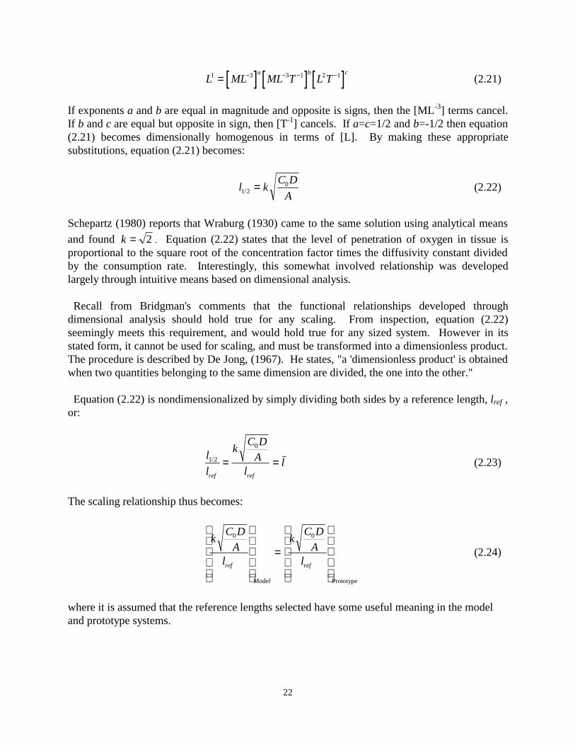
If exponents a and b are equal in magnitude and opposite is signs, then the [ML-3] terms cancel.If b and c are equal but opposite in sign, then [T-1] cancels. If a=c=1/2 and b=-1/2 then equation(2.21) becomes dimensionally homogenous in terms of [L]. By making these appropriatesubstitutions, equation (2.21) becomes:

l kC D

A1 20

/ = (2.22)

Schepartz (1980) reports that Wraburg (1930) came to the same solution using analytical means

and found k = 2 . Equation (2.22) states that the level of penetration of oxygen in tissue isproportional to the square root of the concentration factor times the diffusivity constant dividedby the consumption rate. Interestingly, this somewhat involved relationship was developedlargely through intuitive means based on dimensional analysis.

Recall from Bridgman's comments that the functional relationships developed throughdimensional analysis should hold true for any scaling. From inspection, equation (2.22)seemingly meets this requirement, and would hold true for any sized system. However in itsstated form, it cannot be used for scaling, and must be transformed into a dimensionless product.The procedure is described by De Jong, (1967). He states, "a 'dimensionless product' is obtainedwhen two quantities belonging to the same dimension are divided, the one into the other."

Equation (2.22) is nondimensionalized by simply dividing both sides by a reference length, lref ,or:

l

l

kC D

Al

lref ref

1 2

0

/ = = (2.23)

The scaling relationship thus becomes:

kC D

Al

kC D

Alref ref

0 0

=

Model Prototype

(2.24)

where it is assumed that the reference lengths selected have some useful meaning in the modeland prototype systems.

23

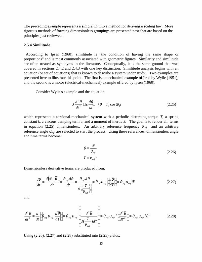
The preceding example represents a simple, intuitive method for deriving a scaling law. Morerigorous methods of forming dimensionless groupings are presented next that are based on theprinciples just reviewed.

2.5.4 Similitude

According to Ipsen (1960), similitude is "the condition of having the same shape orproportions" and is most commonly associated with geometric figures. Similarity and similitudeare often treated as synonyms in the literature. Conceptually, it is the same ground that wascovered in sections 2.4.2 and 2.4.3 with one key distinction. Similitude analysis begins with anequation (or set of equations) that is known to describe a system under study. Two examples arepresented here to illustrate this point. The first is a mechanical example offered by Wylie (1951),and the second is a motor (electrical-mechanical) example offered by Ipsen (1960).

Consider Wylie's example and the equation:

Jd

dtc

d

dtk T t

2

2 0 1

θ θ θ ω+ + = cos (2.25)

which represents a torsional-mechanical system with a periodic disturbing torque T, a springconstant k, a viscous damping term c, and a moment of inertia J. The goal is to render all termsin equation (2.25) dimensionless. An arbitrary reference frequency υref and an arbitraryreference angle θref are selected to start the process. Using these references, dimensionless angleand time terms become:

θ θθ

τ ν

=

=ref

ref t

(2.26)

Dimensionless derivative terms are produced from:

( )d

dt

d

dt

d

dt

d

d

d

dref ref ref

ref

ref ref ref ref

θ θ θ θ θ θ θ

τυ

θ υ θτ

θ υ θ= = =

=

= ′ (2.27)

and

d

dt

d

dt

d

d

d

d d

d

dref ref ref ref

ref

ref ref ref ref

2

2

22

2

2

2θ θ υ θτ

θ υ θτ

ντ

θ υ θτ

θ υ θ=

=

=

= ′′

( )(2.28)

Using (2.26), (2.27) and (2.28) substituted into (2.25) yields:

24

Jd

dc

d

dk Tref ref ref ref ref

ref

θ ν θτ

θ ν θτ

θ θων

τ22

2 01+ + =

cos (2.29)

Dividing through by the coefficient J ref refθ ν 2 produces:

d

d

c

J

d

d

k

J

T

Jref ref ref ref ref

2

2 20

21θ

τ νθτ ν

θθ ν

ων

τ+

+

=

cos (2.30)

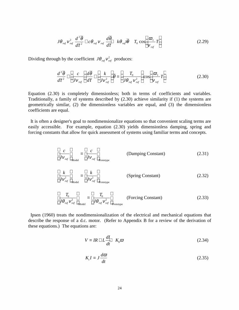
Equation (2.30) is completely dimensionless; both in terms of coefficients and variables.Traditionally, a family of systems described by (2.30) achieve similarity if (1) the systems aregeometrically similar, (2) the dimensionless variables are equal, and (3) the dimensionlesscoefficients are equal.

It is often a designer's goal to nondimensionalize equations so that convenient scaling terms areeasily accessible. For example, equation (2.30) yields dimensionless damping, spring andforcing constants that allow for quick assessment of systems using familiar terms and concepts.

c

J

c

Jref refν ν

=

Model Prototype

(Damping Constant) (2.31)

k

J

k

Jref refν ν2 2

=

Model Prototype

(Spring Constant) (2.32)

T

J

T

Jref ref ref ref

02

02θ ν θ ν

=

Model Prototype

(Forcing Constant) (2.33)

Ipsen (1960) treats the nondimensionalization of the electrical and mechanical equations thatdescribe the response of a d.c. motor. (Refer to Appendix B for a review of the derivation ofthese equations.) The equations are:

V IR LdI

dtKb= + + ω (2.34)

K I Jd

dtt = ω(2.35)

25

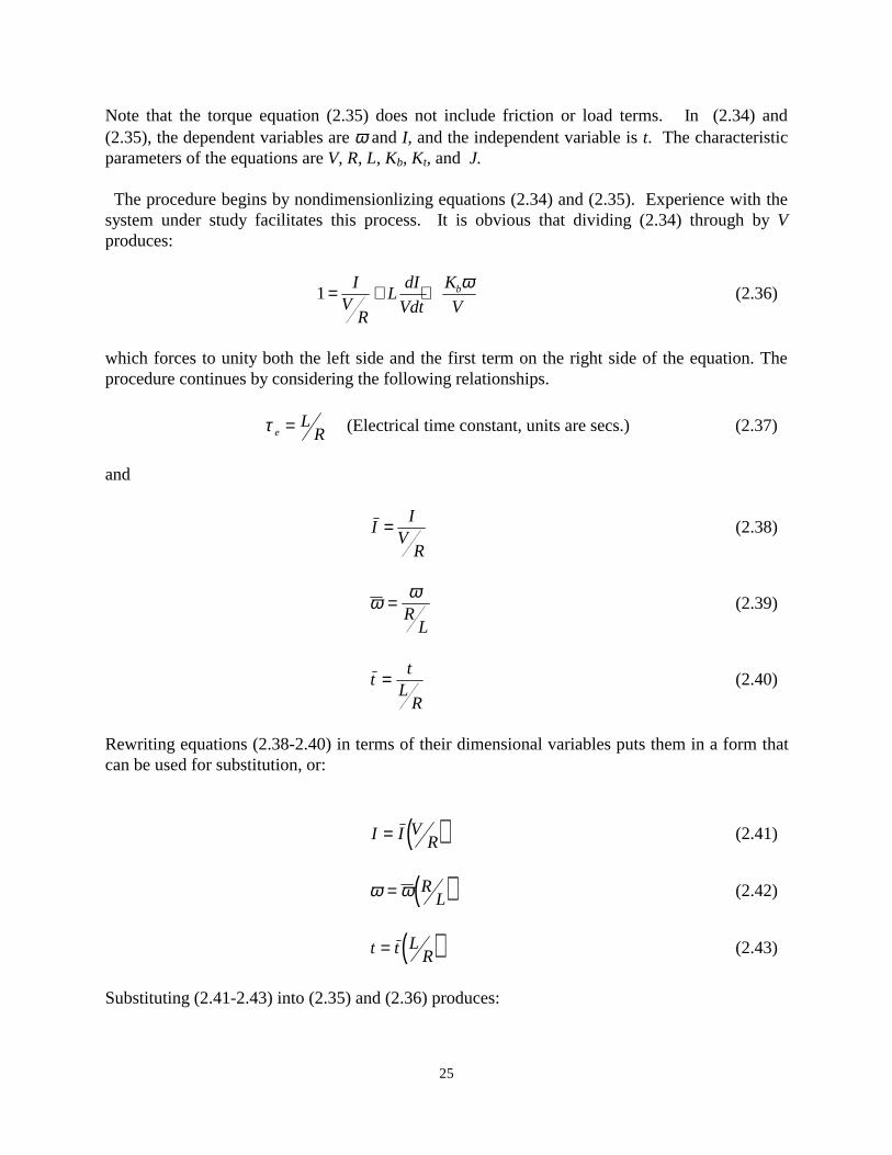
Note that the torque equation (2.35) does not include friction or load terms. In (2.34) and(2.35), the dependent variables are ω and I, and the independent variable is t. The characteristicparameters of the equations are V, R, L, Kb, Kt, and J.

The procedure begins by nondimensionlizing equations (2.34) and (2.35). Experience with thesystem under study facilitates this process. It is obvious that dividing (2.34) through by Vproduces:

1= + +IV

RL

dI

Vdt

K

Vbω (2.36)

which forces to unity both the left side and the first term on the right side of the equation. Theprocedure continues by considering the following relationships.

τ eL

R= (Electrical time constant, units are secs.) (2.37)

and

II

VR

= (2.38)

ω ω=R

L(2.39)

tt

LR

= (2.40)

Rewriting equations (2.38-2.40) in terms of their dimensional variables puts them in a form thatcan be used for substitution, or:

( )I I VR= (2.41)

( )ω ω= RL (2.42)

( )t t LR= (2.43)

Substituting (2.41-2.43) into (2.35) and (2.36) produces:

26

1= + +IdI

dt

K R

LVb ω (2.44)

and

IR J

K VL

d

dtb

=3

2

ω(2.45)

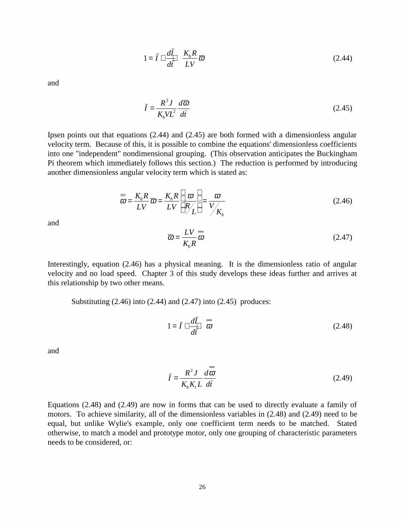
Ipsen points out that equations (2.44) and (2.45) are both formed with a dimensionless angularvelocity term. Because of this, it is possible to combine the equations' dimensionless coefficientsinto one "independent" nondimensional grouping. (This observation anticipates the BuckinghamPi theorem which immediately follows this section.) The reduction is performed by introducinganother dimensionless angular velocity term which is stated as:

ω ω ω ω= =

=K R

LV

K R

LV RL

VK

b b

b

(2.46)

and

ω ω= LV

K Rb

(2.47)

Interestingly, equation (2.46) has a physical meaning. It is the dimensionless ratio of angularvelocity and no load speed. Chapter 3 of this study develops these ideas further and arrives atthis relationship by two other means.

Substituting (2.46) into (2.44) and (2.47) into (2.45) produces:

1= + +IdI

dtω (2.48)

and

IR J

K K L

d

dtb t

=2 ω

(2.49)

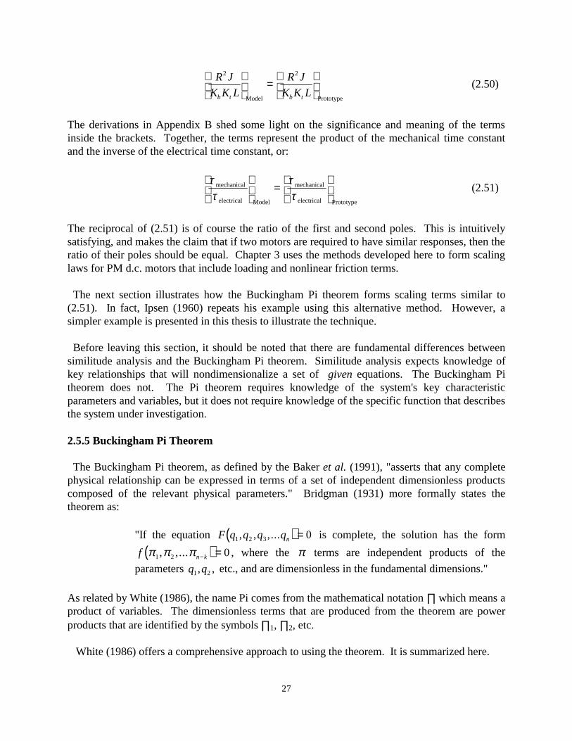
Equations (2.48) and (2.49) are now in forms that can be used to directly evaluate a family ofmotors. To achieve similarity, all of the dimensionless variables in (2.48) and (2.49) need to beequal, but unlike Wylie's example, only one coefficient term needs to be matched. Statedotherwise, to match a model and prototype motor, only one grouping of characteristic parametersneeds to be considered, or:

27

R J

K K L

R J

K K Lb t b t

2 2

=

Model Prototype

(2.50)

The derivations in Appendix B shed some light on the significance and meaning of the termsinside the brackets. Together, the terms represent the product of the mechanical time constantand the inverse of the electrical time constant, or:

ττ

ττ

mechanical

electrical Model

mechanical

electrical Prototype

=

(2.51)

The reciprocal of (2.51) is of course the ratio of the first and second poles. This is intuitivelysatisfying, and makes the claim that if two motors are required to have similar responses, then theratio of their poles should be equal. Chapter 3 uses the methods developed here to form scalinglaws for PM d.c. motors that include loading and nonlinear friction terms.

The next section illustrates how the Buckingham Pi theorem forms scaling terms similar to(2.51). In fact, Ipsen (1960) repeats his example using this alternative method. However, asimpler example is presented in this thesis to illustrate the technique.

Before leaving this section, it should be noted that there are fundamental differences betweensimilitude analysis and the Buckingham Pi theorem. Similitude analysis expects knowledge ofkey relationships that will nondimensionalize a set of given equations. The Buckingham Pitheorem does not. The Pi theorem requires knowledge of the system's key characteristicparameters and variables, but it does not require knowledge of the specific function that describesthe system under investigation.

2.5.5 Buckingham Pi Theorem

The Buckingham Pi theorem, as defined by the Baker et al. (1991), "asserts that any completephysical relationship can be expressed in terms of a set of independent dimensionless productscomposed of the relevant physical parameters." Bridgman (1931) more formally states thetheorem as:

"If the equation ( )F q q q qn1 2 3 0, , ,... = is complete, the solution has the form

( )f n kπ π π1 2 0, ,... − = , where the π terms are independent products of the

parameters q q1 2, , etc., and are dimensionless in the fundamental dimensions."

As related by White (1986), the name Pi comes from the mathematical notation ∏ which means aproduct of variables. The dimensionless terms that are produced from the theorem are powerproducts that are identified by the symbols ∏1, ∏2, etc.

White (1986) offers a comprehensive approach to using the theorem. It is summarized here.

28

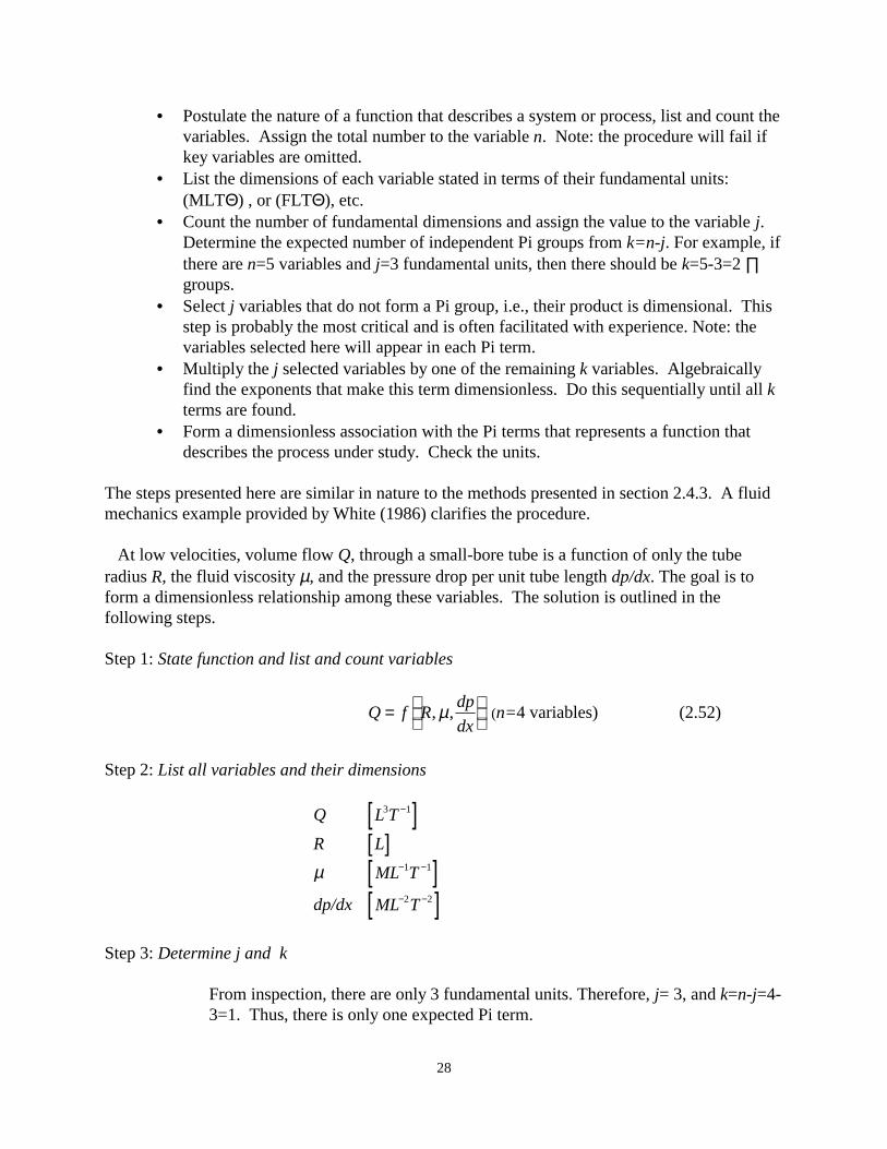
• Postulate the nature of a function that describes a system or process, list and count thevariables. Assign the total number to the variable n. Note: the procedure will fail ifkey variables are omitted.

• List the dimensions of each variable stated in terms of their fundamental units:(MLTΘ) , or (FLTΘ), etc.

• Count the number of fundamental dimensions and assign the value to the variable j.Determine the expected number of independent Pi groups from k=n-j. For example, ifthere are n=5 variables and j=3 fundamental units, then there should be k=5-3=2 ∏groups.

• Select j variables that do not form a Pi group, i.e., their product is dimensional. Thisstep is probably the most critical and is often facilitated with experience. Note: thevariables selected here will appear in each Pi term.

• Multiply the j selected variables by one of the remaining k variables. Algebraicallyfind the exponents that make this term dimensionless. Do this sequentially until all kterms are found.

• Form a dimensionless association with the Pi terms that represents a function thatdescribes the process under study. Check the units.

The steps presented here are similar in nature to the methods presented in section 2.4.3. A fluidmechanics example provided by White (1986) clarifies the procedure.

At low velocities, volume flow Q, through a small-bore tube is a function of only the tuberadius R, the fluid viscosity µ, and the pressure drop per unit tube length dp/dx. The goal is toform a dimensionless relationship among these variables. The solution is outlined in thefollowing steps.

Step 1: State function and list and count variables

Q f Rdp

dx=

, ,µ (n=4 variables) (2.52)

Step 2: List all variables and their dimensions

Q [ ]L T3 1−

R [ ]L

µ [ ]ML T− −1 1

dp/dx [ ]ML T− −2 2

Step 3: Determine j and k

From inspection, there are only 3 fundamental units. Therefore, j= 3, and k=n-j=4-3=1. Thus, there is only one expected Pi term.

29

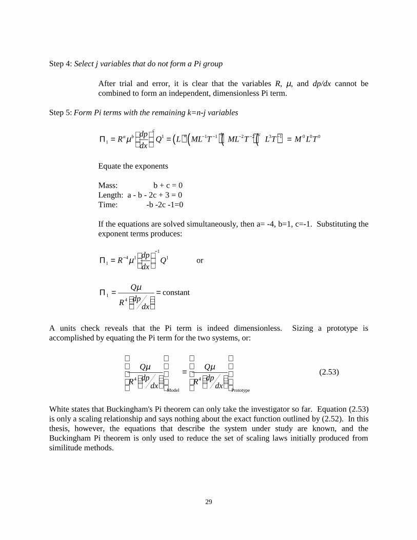
Step 4: Select j variables that do not form a Pi group

After trial and error, it is clear that the variables R, µ, and dp/dx cannot becombined to form an independent, dimensionless Pi term.

Step 5:Form Pi terms with the remaining k=n-j variables

( ) ( ) ( ) ( )Π11 1 1 2 2 3 1 0 0 0=

= =− − − − −Rdp

dxQ L ML T ML T L T M L Ta b

ca b c

µ

Equate the exponents

Mass: b + c = 0Length: a - b - 2c + 3 = 0Time: -b -2c -1=0

If the equations are solved simultaneously, then a= -4, b=1, c=-1. Substituting theexponent terms produces:

Π14 1

11=

−−

Rdp

dxQµ or

Π14

=

=Q

R dpdx

µconstant

A units check reveals that the Pi term is indeed dimensionless. Sizing a prototype isaccomplished by equating the Pi term for the two systems, or:

Q

R dpdx

Q

R dpdx

µ µ4 4

=

Model Prototype

(2.53)

White states that Buckingham's Pi theorem can only take the investigator so far. Equation (2.53)is only a scaling relationship and says nothing about the exact function outlined by (2.52). In thisthesis, however, the equations that describe the system under study are known, and theBuckingham Pi theorem is only used to reduce the set of scaling laws initially produced fromsimilitude methods.

30

2.6 Summary

This chapter provided background summaries and offered literature reviews on subjects that areessential for understanding the work presented in this thesis. Reviews were presented oncommutated PM d.c. motors, analytical servo friction models, and friction compensationtechniques. A considerable segment of the chapter was devoted to developing the concepts ofdimensional analysis. Examples using similitude methods and Buckingham's Pi theorem werepresented to solidify the ideas. The material presented here is by no means comprehensive.Dimensional analysis in particular has numerous applications, and most assuredly, not all of themhave been reported in the literature. Of significant importance, is the relative dearth ofinformation on scaling a PR manipulator or a PM d.c. motor using these techniques. The papersthat were uncovered, however, validate the opportunities that exist in this area of research.