Bruce A. Appleby (_BNIIRAL DYNAMIC| Convair Division 0 _ ,=
248
DYNAMIC LOADS ANALYSIS OF SPACE VEHICLE SYSTEMS LAUNCH AND EXIT PHASE by Raymond H. Schuett Bruce A. Appleby Jack D. Martin GPO PRICE $ CFSTI PRICE(S) $ Hard copy (HC)_, _ "7"_"" Microfiche (MF)__ /-_K_ ff 653 July 65 Report No. GDC-DDE66-012 June 1966 .r ch This work was performed for the Jet Propulsion Laboratory, California Institute of Technology, sponsored by the National Aeronautics and Space Administration under Contract NAS7-100. (_BNIIRAL DYNAMIC| Convair Division 0 _ _'-1 ,= IOg MUO,II X.LI-IIOV,II _,r_ _"
-
Upload
khangminh22 -
Category
Documents
-
view
1 -
download
0
Transcript of Bruce A. Appleby (_BNIIRAL DYNAMIC| Convair Division 0 _ ,=
DYNAMIC LOADS ANALYSIS
OF SPACE VEHICLE SYSTEMS
LAUNCH AND EXIT PHASE
by
Raymond H. Schuett
Bruce A. ApplebyJack D. Martin
GPO PRICE $
CFSTI PRICE(S) $
Hard copy (HC)_, _ "7"_""
Microfiche (MF)__ /-_K_
ff 653 July 65
Report No. GDC-DDE66-012
June 1966.r
ch
This work was performed for the Jet Propulsion Laboratory,California Institute of Technology, sponsored by theNational Aeronautics and Space Administration underContract NAS7-100.
(_BNIIRAL DYNAMIC|
Convair Division
0 __'-1
,=
IOg MUO,II X.LI-IIOV,II
_,r_ _"

FOREWORD
This report was prepared for the Jet Propulsion Laboratory,
Pasadena, California, by the Convair division of General Dy-
namics, San Diego, California. The task was accomplished
under Contract NASA 7-100, Subcontract JPL 950994, entitled
"Engineering Manual on Dynamic Loads Analysis for Space
Launch Vehicles" during the period from July 1965 to June 1966.
The work was initiated by Mr. William Gayman who provided
technical coordination and administration of the task for the Jet
Propulsion Laboratory. The Project Leader for the Convair
division was Mr. C. Desmond Pengelley.
.o°
111

Section
TABLE OF CONTENTS
Page
INTRODUCTION .................. 1-1
ANALYTICAL TECHNIQUES .............. 2-1
2.1 Basic Equations of Motion ......... 2-7
2.2 Mathematical Models ........... 2-8
2.2.1 Lateral Modelof a Cylindrical Liquid Propellant
Vehicle ................. 2-9
2.2.1.1 Mass and Moment of Inertia .......... 2-9
2.2.1.2 Sloshing Propellants ............. 2-10
2.2.1.3 Engine Representation ............ 2-11
2.2.1.4 Branch Beams .............. 2-11
2.2.1.5 Local Structure Effects ........... 2-12
2.2.1.6 Local Nonlinearities ............ 2-13
2.2.1.7 Temperature ............. 2-13
2.2. I.8 Axial Load ............... 2-14
2.2.1.9 Solid Boosters .............. 2-14
2.2. I. I0 Weight and Stiffnes s Lumping ......... 2-15
2.2.1.11 Stiffness and Flexibility Matrices ........ 2-17
2.2.1.11.1 Free Element Stiffness Matrix ......... 2-17
2.2.1.11.2 Coupled Unrestrained Stiffness Matrix ...... 2-22
2.2.1.11.3 Reducing the Stiffness Matrix ........ 2-23
2.2.1.11.4 Calculation of Free-Free Modes ........ 2-25
2.2.1.11.5 Flexibility Matrix ............. 2-28
2.2.1.11.6 Transformed Mass Matrix .......... 2-29
2.2.2 Torsional Model of a Cylindrical Liquid Propellant
Vehicle ................. 2-30
2.2.3 Longitudinal Model of a Cylindrical Liquid
Propellant Vehicle ............. 2-30
2.2.3.1 Fluid Equations for Elastic Tank ........ 2-31
2.2.3.2 Model for Cylindrical Tank with Large Ullage
Volume ................. 2-34
2.2.3.2.1 Basic Single Mass Model ........... 2-34
2.2.3.2.2 Spring Rate for Elliptical Tank Bottom ...... 2-40
2.2.3.2.3 Tank with Stringers and Buckled Skin ....... 2-41
2.2.3.3 Model for Cylindrical Tank with Small Ullage Volume • 2-43
V

Section
2.2.3.4
2.2.4
2.2.5
2.2.6
2.2.7
2.2.8
2.3
2.3.1
2.3.1.1
2.3.1.2
2.3.1.3
2.3.1.4
2.3.2
2.4
2.4.1
2.4.1.1
2.4.1.2
2.4.1.3
2.4.2
2.4.2.1
2.4.2.2
2.5
2.5.2.1
2.5.2.2
2.5.2.3
2.5.2.4
2.6
2.7
TABLE OF CONTENTS, Contd
pag__ e
Multimode Models ............. 2-44
Adding Components Using Mode Synthesis ..... 2-54
Lateral-Torsional-Longitudinal Coupling ..... 2-54Clustered Booster ............. 2-55
Correcting Model Based on Test Results ...... 2-57
Damping Effects ......... 2-58
Derivation of Normal Modes .......... 2-59
Solutions for Characteristics ......... 2-59
Matrix Iteration (Stodola and VianeUo Method) .... 2-59
Holzer-Myklestad Method .......... 2-61
Energy Methods .......... 2-63
Jacobi and Givens Methods ...... 2-65
Modal Quantities .......... 2-68
Response to Time-Varying Forces ........ 2-69
Modal Response ............ 2-70
Numeric Integration ........ 2-70
Laplace Transforms ......... 2-71
Duhamel's Integral ............. 2-74
Vehicle Response ............. 2-75
Mode Displacement Method .......... 2-75
Mode Acceleration Method .......... 2-76
Response to Time-Varying Forces with a Control
System Included .............. 2-76
General Solution ............ 2-76
Example Solution ............. 2-77
Derivation of Equations of Motion ...... 2-77
Derivation of Force Equations ........ 2-79
Derivation of Autoptlot Equations ........ 2-84
Complete Equations ............ 2-86
Random Response ............. 2-88
References .............. 2-96
vi
Section
TABLE OF CONTENTS, Contd
Page
GROUND WIND INDUCED LOADS ............ 3-1
3.1 Statement of the Problem ......... 3-7
3.2 Historical Background .......... 3-8
3.3 Analytical Approach ...... 3-10
3.3.1 Representation of the Wind Velocity and Force. . 3-11
3.3.2 Response of the Vehicle to Ground Winds . . 3-16
3.3.2.1 Mathematical Model ........ 3-16
3.3.2.2 Steady-State Response ....... 3-16
3.3.2.3 Vortex Shedding Response. • 3-16
3.3.2.4 Gust Response .............. 3-18
3.3.3 Resultant Response ........... 3-19
3.3.3.1 Equal Probability ........ 3-19
3.3.3.2 Combined Probability ...... 3-19
3.4 Conclusions ........... 3-22
3.4.1 Wind ............... 3-22
3.4.2 Response ..... 3-22
3.4.3 Recommended Procedure ....... 3-22
3.5 References ........ 3-23
ENGINE START AND SHUTDOWN AND VEHICLE LAUNCH • • • 4-1
4.1
4.2
4.3
4.3.1
4.3.2
4.3.3
4.4
4.4.2.1
4.4.2.2
4.4.2.3
Statement of the Problem ......... 4-5
Historical Background .......... 4-5
Analytical Approach ..... 4-6
Engine Start and Shutdown Analyses ..... 4-6
Liftoff Analysis .
Lateral Loads .
Illustrative Examples ....
Mathematical Models
Longitudinal Loads ....
Engine Start on the Pad • •
Vehicle Liftoff
Inflight Engine Shutdown
.......... 4-8
........ 4-9
• • 4-10
• • 4-10
.... 4-20
• • • 4-20
• 4-20
• • • 4-23
vii
Section
TABLE OF CONTENTS, Contd
Page
4.4.3
4.5
4.5.1
4.5.2
4.5.3
4.5.4
4.5.5
4.5.6
4.6
4.7
Lateral Loads ............... 4-24
Discussion ............. 4-27
Engine Forces ............. 4-27
Method of Launch ......... 4-28
Combination of Loads ........... 4-29
Control System Activation ........... 4-32
Longitudinal Instabilities ......... 4-32
High-Frequency Excitation ........... 4-32
Conclusions and Recommendations . .4-33
References .............. 4-33
ATMOSPHERIC DISTURBANCES ............. 5-i
5.1
5.2
5.3
5.4
5.5
5.5.1
5.5.1.1
5.5.1.2
5.5.1.3
5.5.1.4
5.5.2
5.5.3
5.5.4
5.5.5
5.5.6
5.6
5.7
Statement of the Problem ............ 5-7
Historical Background ......... 5-9
Quasi-Steady Flight Loads .......... 5-12
Analytical Approach ............. 5-12
Illustrative Example ...... 5-24
Gust Response .............. 5-26
Analytical Approach ............ 5-26
Illustrative Example ............ 5-28
Discussion ............... 5-33
Quasi-Steady Flight Loads ......... 5-34
Wind Criteria .............. 5-34
Pitch Program ........... 5-35
Trajectory Simulation ......... 5-35
Elastic Modes .............. 5-35
Gust Loads .............. 5-36
Buffet Loads ............. 5-36
Other Loads ............ 5-36
Combined Loads .............. 5-36
Wind Monitoring .............. 5-37
Conclusions and Recommendations. ....... 5-38
References .............. 5-39
viii
Section
TABLE OF CONTENTS, Contd
Page
FREQUENCY RESPONSE ..... • 6-1
6.1
6.2
6•3
6.4
6•5
6.6
6.7
Statement of the Problem .....
Historical Background • • .
Analytical Approach • •
Illustrative Example .....
Discussion ........
Conclusions and Recommendations•
References ....
• . . 6-5
• • 6-5
• . 6-5
.... 6-7
• • • 6-10
...... 6-10
• 6-i0
STAGING AND JETTISON • • • 7-1
7.1
7.2
7.3
7.3.1
7.3.2
7.4
7.4.1
7.4.2
7.4.3
7.5
7.6
Statement of the Problem .......... 7-5
Historical Background ........... 7-5
Analytical Approach .......... 7-6
Nose Fairing Jettison ......
Illustrative Example .....
Discussion ......
Jettison • • •
Elastic Effects • • •
Staging .....
Conclusions and Recommendations.
References
• • 7-7
• . • 7-11
• • 7-14
....... 7-14
• • 7-14
.... 7-15
• 7-17
7-17
ix

Figure
2.1
2.2
2.3
2.4
2.5
2.6
2.7
2.8
2.9
2. I0
2.11
2.12
2.13
2.14
2.15
2.16
2.17
2.18
2.19
2.20
2.21
2.22
2.23
2.24
LIST OF ILLUSTRATIONS
Titl_____e Ps4___.__e
Example of Branched System .............. 2-12
Typical Weight Distribution ............... 2-15
Typical Stiffness Distribution .............. 2-16
Cantilever Beam in Bending .............. 2-18
Free Beam in Bending and Shear ............. 2-21
Translational and Rotation Springs ............ 2-21
Example of Attachments to a Beam Element ........ 2-22
Stiffness Matrix Layout for Attachment of Two Beams ...... 2-22
Stiffness Matrix Layout for Attachment of Beam with a Spring . . . 2-23
Cylindrical Tank and Liquid .............. 2-31
Partially Filled Tank ................. 2-34
Tank Strains ................... 2-34
Equivalent Tank Model ................ 2-35
Variation of F(f,y) with Depth-to-Radius Ratio for Various Values
of Poisson's Ratio .................. 2-41
Variation of G(f,y) with Depth-to-Radius Ratio for Various Values
of Poisson's Ratio ................. 2-41
Variation of H(f,y) with Depth-to-Radius Ratio for Various Values
of Poisson's Ratio .................. 2-41
Skin-Stringer Cylinder Tank Model ............ 2-42
Skin-Stringer Model with Buckled Skin ........... 2-43
Tank with Small Ullage Volume ............. 2-46
Tank Model for Small Ullage Volume ........... 2-49
Two-Element Tank ................. 2-50
Assumed Forces on Two-Element Tank .......... 2-51
Two-Mass Tank Model ................ 2-53
Titan IIIC .................... 2-56
X
Figure
2.25
2.26
2.27
2.28
2.29
2.30
2.31
2.32
2.33
2.34
2.35
2.36
2.37
3.1
3.2
3.3
3.4
3.5
3.6
3.7
3.8
3.9
3.10
4.1
4.2
4.3
4.4
LIST OF ILLUSTRATIONS, Contd
Title Page
Free-Body Diagram of Vibrating Beam Segment ........ 2-62
Spring Mass System .......
Force Time History .....
General Autopilot Block Diagram .
Gust Response Vehicle Model •
Rotating Eulerian Axes
Aerodynamic Forces •
Engine Thrust Forces.
Slosh Loads ....
Engine and Actuator Model ......
Engine Displacement .........
Autopilot Block Diagram .....
Response and Input Spectra ........
Factors Contributing to Prelaunch Wind Loads
Typical Recording of Ground Wind Velocity and Direction•
95-Percentile Ground Wind Profiles .........
Comparison of Gust Spectra • •
Typical Mathematical Model .....
Representation of Von Karman Vortex Street ....
Equal Probability Combination of Loads ........
Versusafor Pr I(ED ' _L ) is inR I =0.9973K o
Regions, ]F°rmed for Various Values of (_DT/_LT = a, for
Prl!l(ED'EL) isinR| =0.9973
Statistical Combination of Loads ....
Typical Longitudinal Model.
Thrust Decay Time History
. . 2-72
..... 2-72
• . 2-77
• . 2-78
............. 2-78
............... 2-79
• 2-81
• 2-82
• . 2-83
.... 2-84
.... 2-85
...... 2-93
. 3-7
. 3-11
• . 3-12
• • 3-15
3-16
• . 3-17
. 3-19
3-20
. 3-20
...... 3-21
...... 4-6
......... 4-7
Equivalent Thrust Decay Time History ........ 4-7
Longitudinal Model and Forces for Engine Thrust Decay ..... 4-7
xi

Figure
4.5
4.6
4.7
4.8
4.9
4.10
4.11
4.12
4.13
4.14
4.15
4.16
4.17
4.18
4.19
4.20
4.21
4.22
4.23
5.1
5.2
5.3
LIST OF ILLUSTRATIONS, Contd
Title Page
Time Histories of Applied Forces During Engine Thrust Decay • • • 4-7
Longitudinal Liftoff Models .............. 4-8
Atlas/Centaur/Surveyor Longitudinal Model for Atlas Ignition • • 4-11
Atlas/Centaur/Surveyor Longitudinal Model Immediately After
Nose Fairing Jettison ............... 4-12
Atlas/Centaur/Surveyor Lateral Model .......... 4-16
Atlas Engine Thrust Buildup Time Histories ........ 4-21
Centaur/Surveyor Interface Longitudinal Accelerations at Atlas
Engine Thrust Buildup .............. 4-21
Longitudinal Normal-Mode-Coordinate Displacements at Atlas
Engine Thrust Buildup ................ 4-22
Net Atlas Launcher Force During Launcher Release ...... 4-22
Centaur/Surveyor Interface Longitudinal Accelerations at Liftoff • • 4-23
Longitudinal Normal-Mode-Coordinate Displacements at Vehicle
Liftoff ...................... 4-24
Thrust Decay Time History at Sustainer Engine Shutdown .... 4-24
Centaur/Surveyor Interface Longitudinal Accelerations at Sustainer
Engine Shutdow_ .................. 4-24
Longitudinal Normal-Mode-Coordinate Displacements at Sustainer
Engine Shutdown ................ 4-25
Applied Moment Time History at Atlas Engine Thrust Buildup • • • 4-25
Atlas/Centaur Interface Bending Moments at Atlas Thrust Buildup. • 4-25
Centaur/Surveyor Interface Lateral Loadings at Atlas Engine
Thrust Buildup .................. 4-26
Lateral Normal-Mode-Coordinate Displacements at Atlas Engine
Thrust Buildup ................... 4-26
Load Distribution Probability .............. 4-31
Typical Wind Profile ................. 5-8
Coordinate Systems ................. 5-13
Vehicle Force Diagrams ................ 5-14
xii
Figure
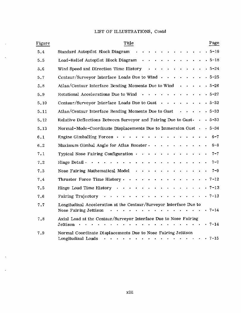
5.4
5.5
5.6
5.7
5.8
5.9
5.10
5,11
5.12
5.13
6.1
6.2
7.1
7.2
7.3
7.4
7.5
7.6
7.7
7.8
7.9
LIST OF ILLUSTRATIONS, Contd
Title Page
Standard Autopilot Block Diagram ............ 5-16
Load-Relief Autopilot Block Diagram ......... 5-18
Wind Speed and Direction Time History ........ 5-24
Centaur/Surveyor Interface Loads Due to Wind ........ 5-25
Atlas/Centaur Interface Bending Moments Due to Wind ..... 5-26
Rotational Accelerations Due to Wind ........... 5-27
Centaur/Surveyor Interface Loads Due to Gust ........ 5-32
Atlas/Centaur Interface Bending Moments Due to Gust ..... 5-33
Relative Deflections Between Surveyor and Fairing Due to Gust. • • 5-33
Normal-Mode-Coordinate Displacements Due to Immersion Gust • • 5-34
Engine Gimballing Forces ............... 6-7
Maximum Gimbal Angle for Atlas Booster .......... 6-8
Typical Nose Fairing Configuration ............ 7-7
Hinge Detail ................... 7-7
Nose Fairing Mathematical Model ............ 7-9
Thruster Force Time History ............. 7-12
Hinge Load Time History ............ 7-13
Fairing Trajectory ................ 7-13
Longitudinal Acceleration at the Centaur/Surveyor Interface Due to
Nose Fairing Jettison ............... 7-14
Axial Load at the Centaur/Surveyor Interface Due to Nose Fairing
Jettison .................... 7-14
Normal Coordinate Displacements Due to Nose Fairing Jettison
Longitudinal Loads ................ 7-15
ooo
Xlll
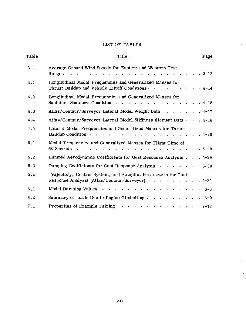
LIST OF TABLES
Table Title Page
3.1
4.1
4.2
4.3
4.4
4.5
5.1
5.2
5.3
5.4
6.1
6.2
7.1
Average Ground Wind Speeds for Eastern and Western Test
Ranges ................... 3-12
Longitudinal Modal Frequencies and Generalized Masses for
Thrust Buildup and Vehicle Liftoff Conditions ......... 4-14
Longitudinal Modal Frequencies and Generalized Masses for
Sustainer Shutdown Condition ............. 4-15
Atlas/Centaur/Surveyor Lateral Model Weight Data ...... 4-17
Atlas/Centaur/Surveyor Lateral Model Stiffness Element Data • • • 4-18
Lateral Modal Frequencies and Generalized Masses for Thrust
Buildup Condition .................. 4-20
Modal Frequencies and Generalized Masses for Flight Time of
60 Seconds ............ 5-29
Lumped Aerodynamic Coefficients for Gust Response Analysis . . • 5-29
Damping Coefficients for Gust Response Analysis ....... 5-30
Trajectory, Control System, and Autopilot Parameters for Gust
Response Analysis (Atlas/Centaur/Surveyor) ........ 5-31
Modal Damping Values ................ 6-8
Summary of Loads Due to Engine Gimballing ......... 6-9
Properties of Example Fairing ............. 7-12
xiv

1/INTRODUCTION
1-1


1/INTRODUCTION
This document constitutes one volume of a two-volume work dealing with the struc-
tural dynamics of space vehicle systems. The overall purpose is twofold, namely toeducate and to coordinate.
This volume considers dynamic loads encountered during the launch and exit phases.
The companion volume, Ref° 1.1, treats the problem of overall system integration, in-
cluding interface communication between contractors and integrating agency, methods
of defining contractual specifications, and logical treatment of dynamic interaction be-
tween major components (such as payload and booster) that are built by separate
organizations.
The work is addressed to graduate students in engineering and mechanics, as well
as practicing engineers and members of technical management. A sound education in
these fields is assumed although references are listed for background study. Specific
knowledge of missile technology is not required. The goal is to provide an overall
practical picture of the current state of the art rather than solutions, and to describe
current methods rather than proofs. A comprehensive bibliography is given from
which formal proofs can be obtained. Numeric examples are used to illustrate pro-
cedures and typical results, the Atlas/Centaur/Surveyor vehicle being used as a model.
Many unsolved problems still exist and empirical - often intuitive - approaches are
used. Comments and suggestions, based on practical judgement and experience, are
presented where possible.
This volume is divided into sections that have their own lists of symbols and
bibliographies. One section covers basic analytical tools common to all phases of
structural dynamic technology. While it offers nothing that does not already exist in
classical texts, it collects and summarizes those techniques applicable to the problem
at hand and presents them in a consistent, convenient form. Subsequent sections con-
centrate on individual problem areas such as ground wind loads, thrust buildup and
launcher induced loads, flight loads, etc. The central theme is on low-frequency
phenomena that include the first five or ten modes of the vehicle, but a brief outline
is included of methods of dealing with random loads, such as buffet, that become sig-
nificant at much higher frequencies in the spectrum.
An analytical obstacle in the past has been the numeric problems involved in
handling and solving the large number of equations required for adequate description
of the vehicle; however, the advent of electronic computers has made possible the
execution of routines involving vast amounts of data. Computer solutions have been
used in preparing the illustrative examples.
1-3

Applied forces in many cases are still not described by firm criteria since datafrom which such criteria could be obtained are still in the formative stage. Examplesinclude the vortex sheddingand gust spectra of groundwinds, the thrust buildup anddecay characteristics of individual rocket engines, and the wind profiles and gusts ofwinds aloft. The first two require test data on the particular vehicle and engine,while the criteria for winds aloft are obtainedfrom freely rising balloons, which yieldvelocity profiles lacking in detail and must be supplementedby gust data obtainedfromaircraft experience.
The application of dynamic analysis to the design and testing of space vehicle
systems, especially the payload or spacecraft, is often grossly simplified, in the
conservative direction, causing unnecessary design penalties and test problems. A
typical example is the vibration test requirements for a payload or spacecraft which,
in the lower frequencies, quite often require input excitation equivalent to the maximum
response the article will see. This problem is caused by inadequate dynamic modeling
of the interfaces between stages built by different contractors, and also the uncertainty
as to exactly how the design or test data will be applied. The inaccuracies so intro-
duced are illustrated in Ref. 1.2 where the vibration testing of a simple model is con-
ducted using oversimplified criteria, as sometimes applied to spacecraft, and is then
duplicated by a more sophisticated simulation of what actually is expected to occur.
The many differences in results are often expressed in orders of magnitude rather
than in percentages.
The work presented herein strives for a better understanding and use of dynamic
analysis data by describing the forces to which a space vehicle system is exposed,
techniques to obtain responses, and application of results.
REFERENCES
1.1 W. H. Gayman and J. A. Garba, Dynamic Load Analyses of Space Vehicle Systems-
Launch and Exit Phase, JPL Technical Memorandum 33-286 (To be published).
1.2 W. H. Gayman, A Note on Boundary Condition Simulation in the Dynamic Testing
of Spacecraft Structures, JPL Technical Report No. 32-938, 15 April 1966.
1-4

2/ANALYTICAL TECHNIQUES
2-1

A
C
CN/0_
CB
CF
CL
C V
D
E
F
G
H(cc)
I
J
K
KE
L
M
N
Nx
P
PE
Q
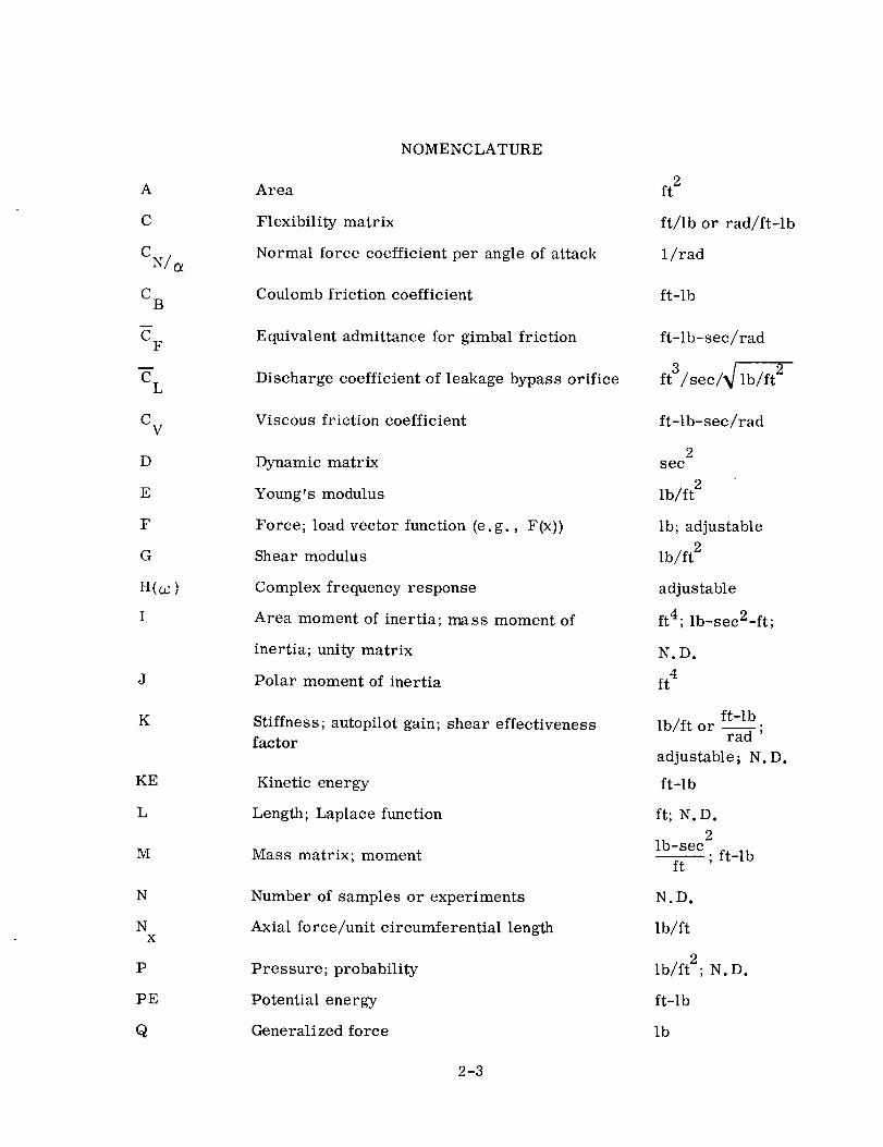
NOMENCLATURE
Area
Flexibility matrix
Normal force coefficient per angle of attack
Coulomb friction coefficient
Equivalent admittance for gimbal friction
Discharge coefficient of leakage bypass orifice
Viscous friction coefficient
Dynamic matrix
Young' s modulus
Force; load vector function (e. g., F(x))
Shear modulus
Complex frequency response
Area moment of inertia; mass moment of
inertia; unity matrix
Polar moment of inertia
Stiffness; autopilot gain; shear effectivenessfactor
Kinetic energy
Length; Laplace function
Mass matrix; moment
Number of samples or experiments
Axial force/unit circumferential length
Pressure; probability
Potential energy
Generalized force
ft 2
ft/lb or rad/ft-lb
1/rad
ft-lb
ft-lb-sec/rad
ft3/sec/4 lb/ft 2
ft-lb-sec/rad
2see
lb/ft 2
lb; adjustable
lb/ft 2
adjustable
ft4; lb-sec2-ft;
N°D.
ft 4
ft-lblb/ft or ra---d-;
adjustable ; N.D.
ft-lb
ft; N.D.
lb-sec 2_ ; ft-lb
ft
N.D°
lb/ff
lb/ft 2. N.D.
ft-lb
lb
2-3

R
S
SO
SR
T
U
V
W
zco )
a
b
d
f
h
i
J
k
m
n
P
q
r
s
t
U
NOMENCLATURE, Contd
Gas constant; radius
Shear
Static moment about fixed point
Reference area
Thrust; time; temperature
Assumed mode shape
Volume; velocity
Weight_ work
Complex impedance
Radius of tank
Minor semi-axis of elliptical tank bottom
Longitudinal flexibility matrix; element of
dynamic matrix
Function, e.g., f(x)
Thickness
Station index; complex number
Station index
Statistical index
Mode index; mass
Mode index; time index
Pressure
Dynamic pressure
Radial coordinate for cylindrical tank
Laplace operator
Time
Displacement; function describing a random
process
2-4
ft/° F; ff
lb
ft-lb
ft 2
lb; see; °F
it/it
ft 3 ; ft/sec
lb; ft-lb
lb/ft
ft
ft
radft/lb or in.-1----_ ; sec2
adjustable
ft
N.D.
N.D.
N.D.
2lb-sec
N.D.;ft
N.D.
lb/ft 2
Ib/ft2
ft
N.D.
see
adjustable

UX
V
_v
Wr
X
Y
z
A
Z
A
Y
6
E
e
k
V
,ff
P
NOMENCLATURE, Contd
Longitudinal displacement of a shell element
Volume
Weight; mode participation factor
Radial displacement of a shell element
Coordinate along neutral axis
Coordinate normal to neutral axis
Coordinate normal to neutral axis (slosh mass)
Increment
Summation
Velocity potential; complete mode shapes
Deflation matrix
Power density spectra; power spectra
Angle of attack
Adiabatic constant; mode participation factor;
shear slope of a mode
Engine gimbal angle; control system coordinate
Strain; iteration convergence criterion
Damping coefficient
Rotation displacement in xy plane
Eigenvalue
Vector to release translation of fixed point;
mean
Poisson's ratio
Normal mode coordinate
3. 1416
Density
ft
ft 3
lb; ft/ft
ft
ft
ft
ft
N.D.
N.D.
ft/sec ;ft/ft
N.D.
adjustable
rad
N.D.; ft; rad/ft
rad; adjustable
in./in. ; N.D.
N.D.
rad
2sec
N.D. adjustable
N°D°
ft/ft
N.D.
lb-sec2-ft 2
2-5

(y
T
¢
m
L]
[]
NOMENCLATURE, Coutd
Stress; standard deviation; modal slopes
Vector to release rotation of fixed point;
autopilot filter value; time lag; period
Modal displacements
Rotation about x-axis
Autocorrelation function
Frequency
Generalized mass
Row matrix
Square matrix
Column matrix
Diagonal matrix
Second derivative with respect to time
First derivative with respect to time
d/ds; transpose
lb/in. 2; adjustable;
rad/ft
ftor N.D.; sec;
see; see
ft/ft
rad
adjusta_e
rad/sec
lb-sec 2
,, d2/ds 2
Proportional to
Conjugate of x
x* Conjugate transpose of x
Also,
A, T,R are transformation matrices
and
A,B,D,E,F,V,W,a,b,c,d,e,f,g,v,w,x,_, fl, 7are used as substitutionsfor
expressions and are defined in the textwhen so used.
2-6
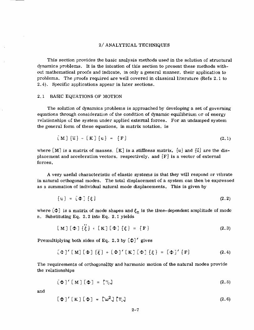
2/ANALYTICAL TECHNIQUES
This section provides the basic analysis methods used in the solution of structural
dynamics problems. It is the intention of this section to present these methods with-
out mathematical proofs and indicate, in only a general manner, their application to
problems. The proofs required are well covered in classical literature (Refs 2.1 to
2.4). Specific applications appear in later sections.
2.1 BASIC EQUATIONS OF MOTION
The solution of dynamics problems is approached by developing a set of governing
equations through consideration of the condition of dynamic equilibrium or of energy
relationships of the system under applied external forces. For an undamped system
the general form of these equations, in matrix notation, is
[M] _] + [K] [u} = IF} (2.1)
where [M] is a matrix of masses, [K] is a stiffness matrix, [u} and [U} are the dis-
placement and acceleration vectors, respectively, and IF} is a vector of external
forces.
A very useful characteristic of elastic systems is that they will respond or vibrate
in natural orthogonal modes. The total displacement of a system can then be expressed
as a summation of individual natural mode displacements. This is given by
(u} = _¢] _ (2.2)
where [_] is a matrix of mode shapes and _n is the time-dependent amplitude of mode
n. Substituting Eq. 2.2 into Eqo 2.1 yields
[M] [¢] {_} + [K] [¢] _} = IF} (2.3)
Premultiplying both sides of Eq. 2.3 by [_)] _ gives
[(_]' [M] [c_] [_'} + [_)]' [K] [_)] {_]} = [_)]' {F} (2.4)
The requirements of orthogonality and harmonic motion of the natural modes provide
the relationships
and
[(_]' [M] [(_] = ['_.J (2.5)
[_]' [K] [¢] = ["002.] _T_.] (2.6)
2-7

Substituting Eqs 2.5 and 2.6 into Eq. 2.4, we obtain
+ = [m.] [¢3, {F} = [1_ ]-1 {Q } (2.7)
Eq. 2.7 is a set of n uncoupled equations in terms of _ n, °°n, the generalized mass
_n' and the generalized force Qn. The solutions of these equations identify the time-
dependent values of _n which are then used in Eq. 2.2 to give complete system re-
sponse. Detailed discussions, derivations, and proofs of the equations of motion,
orthogonality of natural modes, and normal mode theory are given in Refs 2.1 to 2.4.
The use of normal mode theory requires determination of these natural modes of
vibration. If harmonic motion is assumed and the applied forces are equal to zero,
then Eq. 2.1 can be written as
-o_ 2 [M] _u} + [K] {u} = 0 (2.8)
or
[u} = 002 [K] -1 [M] [u}
Each of these equations is in a form suitable for solutions to obtain the orthogonal
modes and their natural frequencies. Many numeric techniques have been developed
to obtain these characteristics and several are discussed in Section 2.3.
The above discussion presents the fundamental approach to structural dynamic re-
sponse analyses. The fact that the response of a linear structural system is adequately
described by superposition of its normal modes indicates the importance of normal
modes. The mathematical model used to represent the physical system, methods em-
ployed to obtain vehicle modes, and techniques achieving response solutions will now
be covered in detail.
2.2 MATHEMATICAL MODELS
The stages of a launch vehicle typically consist of cylindrical tanks (containing
propellants), with engines and other equipment attached at the aft end by means of some
support structure and with either another stage or a payload attached at the forward end.
The payload commonly (though not always) is supported by a truss or adapter and cov-
ered by a fairing. In this case the payload and fairing are each cantilevered from an
attaching ring on the launch vehicle and are not physically connected. The formation of
a mathematical model of such a launch vehicle requires care and a knowledge of the
structure because the accuracy of the analysis of the response of a vehicle to a force
depends largely on the correctness of the mathematical model. This section discusses
in detail the various aspects of modeling.
2.2.1 LATERAL MODEL OF A CYLINDRICAL LIQUID PROPELLANT VEHICLE.
In most instances, the lateral dynamic characteristics of a liquid rocket space vehicle
2-8

system can be considered to be adequatelyrepresented by simple one-dimensionalbeam theory. It is common practice, and certainly more convenient, to replace thecontinuous structure by a lumped parameter idealization. In such an idealization, theanalyst concentrates on those aspects of the system which are felt to be dominant(major masses, major structural elements, propellants). The discrete model is formedby concentrating the distributed mass at selected points along the beam. Thesepointsare ideally the centers of gravity of the distributed masses concentrated at the points.
Elastic properties are expressed in lumped fashion as a set of flexibility coeffi-cients, Cij, or stiffness influence coefficients, Kij. Thesecoefficients have physicalsignificance in that Cij canbe considered as the deflection of point i due to a unit loadat j, and Kij as equatedto the force produced at point i dueto a unit deflection at pointj, if all coordinates other than j are temporarily restrained. (Flexibility and stiffnessinfluence coefficients are covered in more detail in Section 2.2.2. )
The mathematical description of this discrete model is a set of simultaneous and
linear ordinary differential equations. Such equations lend themselves readily to ma-
trix techniques and digital computer computation.
The one-dimensional beam representation is the simplest lateral model and may
not fulfill all necessary requirements for a specific problem. This can necessitate
recognition of nonstructural modes (sloshing), local response characteristics (engines),
or multiple load paths not accounted for in the simple beam analogy. A further
refinement of the model is then necessary.
2.2.1.1 Mass and Moment of Inertia. The distributed mass and moment of inertia
data must be lumped into discrete, point masses, the number of which determine the
degrees of freedom given to the model. The number of mass stations is influenced by
the number of bending modes to be calculated.
It has been found that for one-dimensional beam bending models the required num-
ber of mass stations should be approximately ten times the number corresponding to
the highest elastic bending mode to be calculated. For example, if three elastic bend-
ing modes are to be calculated, then approximately 30 mass stations are required to
represent adequately the bending dynamics of the third mode. This criterion has been
established empirically by calculating mode shape, frequency, and generalized mass
corresponding to the first three elastic bending modes for typical vehicle configurations
in which the number of mass stations used was successively increased from 18 to 40.
As expected, the accuracy increased as additional stations were utilized. However, itwas observed that no further significant increase in accuracy was achieved by usingmore than 30 mass stations. Additional information regarding the number of mass
stations to use is given in Ref. 2.39.
For a more complex model (such as one with branched beams) the above general
rule may not be strictly applicable. For a branched system, the general rule may be
applied to the primary beam of the system, and masses lumped on the secondary
branches in about the same distribution. It must be emphasized that as the model
2-9

diverges from the single beam concept, mass lumping rules becomeless applicable,andmore reliance must be placed uponthe experience of the analyst.
Note that only rigid massesare to be included in this distribution; that is, onlythose masseswhich can be considered to act as an integral part of the unrestrainedbeam during its vibrations. It cannot be over-emphasized that items suchas pumps,equipmentpods, etc., which are actually, or simulated to be, mountedelastically tothe main structure, may significantly alter the bendingcharacteristics of the higherfrequency modes.
Whether or not suchmasses are to be treated as integral to the beam or as sepa-rate elastically attached masses dependsupon: 1} whether or not the frequencies ofthe body modes to be computedare less thanor greater than the mount frequencies ofthe discrete masses, and 2} whether or not these masses are great enoughto materiallyaffect the result.
Accurate representation of the distributed mass at discrete points would requireinclusion of the mass momentof inertia of the distributed mass at that point. Withliquid propellant, the effective momentof inertia is not easily determined. Fortu-nately, these moments of inertia have only a small influence on the modal quantitiesof the first two bendingmodes andcan be neglected, as shownin the work of Ref. 2.5.A better representation could be obtainedby using more mass stations rather thanincluding moments of inertia.
Becauseof the small effect in the lower bendingmodes and the uncertainty of theeffective moment of inertia, it has beencommonpractice to neglect this term. Also,this allows for muchmore efficient computation since this eliminates half the coordinatesin the solution of characteristic equations.
2.2.1.2 Sloshing Propellants. Spacevehicle system propellants constitute a largepercentage of the total system weight. Part of this propellant canbe considered asrigid or distributed mass on the idealized beam while a smaller portion must be allowedto slosh in the lateral model. This sloshing mass becomesmore important in laterflight times whenit becomesa sizeable proportion of total vehicle weight. If the fre-
quencies of the sloshing modes and the frequency of the first structural mode are widely
separated (ratio of 1:3 or greater} the effect of sloshing upon loads is small and in pre-
liminary work can safely be ignored. However, as the separation between the sloshing
frequencies and the structural frequency becomes small the effect of sloshing upon
loads may be significant.
Several methods have been developed to describe propellant sloshing modes and
frequencies. The general approach, as related to lateral models, is to derive the
hydrodynamic equations in a form suitable for a mechanical analogy. It can be shown
for a cylindrical tank that if: I) the tank walls are rigid, 2) the fluid is incompressible
and irrotational, and 3) only small disturbances are admitted, then pendulum or spring
mass analogies can be devised which will reproduce the characteristics of the fundamental
2-10

mode of sloshing oscillation. Attaching the equivalent spring mass to the lateral modelis easily accomplishedand is therefore preferred over the pendulum. The secondandhigher sloshing modes are not generally considered becausethe magnitude of lateralforce contribution from these modes decreases rapidly with increasing order; further-more, test experience indicates that a great deal of turbulent mixing occurs and thatdamping effects are greater in higher modes.
Techniques for deriving the mechanical analogies for slosh and their limitationsare discussed in the literature (Refs 2.6 and 2.7).
2.2.1.3 Engine Representation. Thrust-vector control of liquid-propellant vehiclesis generally maintained by gimballing the rocket engines. Sincethe entire engine isgimballed rather than just the thrust vector, this gimballing action will cause inertialforces as well as thrust forces to act on the missile body. These inertial forces areappreciable, and their lateral componentswill exceedthose of the thrust forces whenthe engine is gimballed sinusoidally at a sufficiently high frequency. The thrust vectordisplacement consists of two components: 1) the displacement contained within theelastic mode (including the flexibility of the engine mounting andactuator structure)while the servo positioning system is locked, and 2) the additional degree of rotationalfreedom addedto represent the motion accompanyingthe action of the positioning servo.
The engine is incorporated into the lateral model by attaching a mass and momentof inertia at the appropriate location on the one-dimensional beam. Sincethe engineitself is quite rigid, the only elasticity normally considered is the mounting structureand actuator system. This structure is generally complex and test dataare often re-quired for proper simulation. Onesuch test would be a vibration test to determine theresonant frequency of the engineon its mounts and use the results to obtain the equiva-lent rotational spring connectingthe engine to the vehicle. This primary frequency isoften low enoughto fall within the range of the lower vehicle bendingfrequencies and asa result could have a significant effect on bendingstability.
Other meansof obtaining thrust vector control are used andmay require enginerepresentation in the lateral model. Control concepts suchas movable nozzles orstream deflection involve little or no additional mass motion and, therefore, only thefixed enginerepresentation would havea significant effect on the lateral modes.
2.2.1.4 Branch Beams. Frequently, vehicle construction will be such that major
portions are cantilevered within another structure or are connected through different
load paths. Examples are: payloads enveloped by fairings, engine compartments of
upper stages suspended in the interstage adapter wells, or multi-engine vehicles
having independent load paths for each engine - such as a center engine supported on the
tank cone and peripheral engines mounted to the cylindrical structure of the vehicle.
Such conditions are illustrated in Fig. 2.1. Realistic representations of these
arrangements are required not only for true definition of gross vehicle response but
2-11
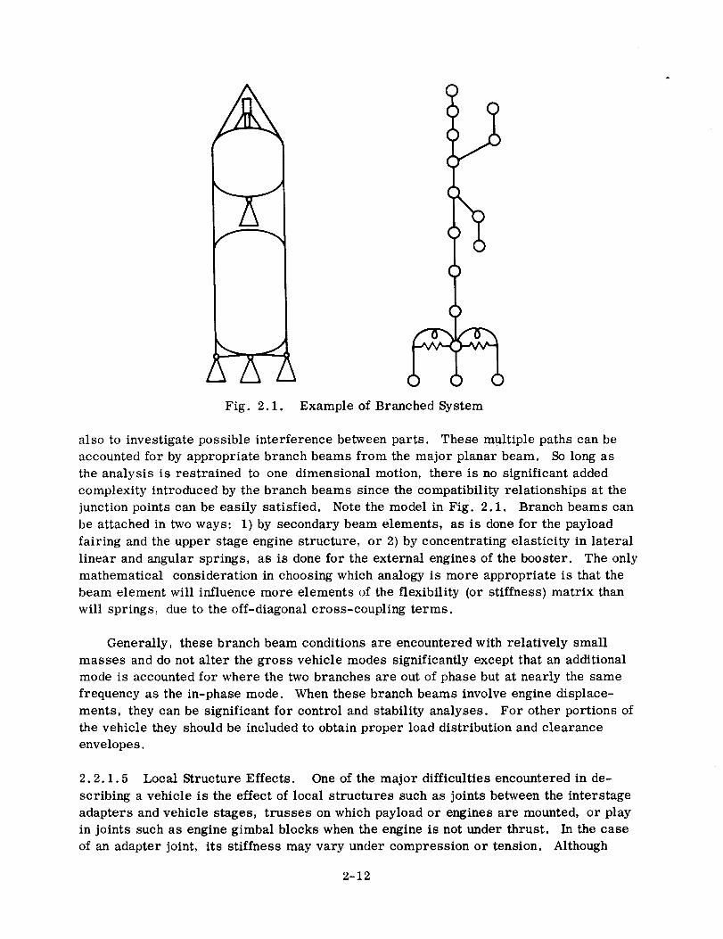
Fig. 2.1.
(
(
(
Example of Branched System
also to investigate possible interference between parts. These multiple paths can be
accounted for by appropriate branch beams from the major planar beam. So long as
the analysis is restrained to one dimensional motion, there is no significant added
complexity introduced by the branch beams since the compatibility relationships at the
junction points can be easily satisfied. Note the model in Fig. 2.1. Branch beams can
be attached in two ways: 1) by secondary beam elements, as is done for the payload
fairing and the upper stage engine structure, or 2) by concentrating elasticity in lateral
linear and angular springs, as is done for the external engines of the booster. The only
mathematical consideration in choosing which analogy is more appropriate is that the
beam element will influence more elements of the flexibility (or stiffness) matrix than
will springs, due to the off-diagonal cross-coupling terms.
Generally, these branch beam conditions are encountered with relatively small
masses and do not alter the gross vehicle modes significantly except that an additional
mode is accounted for where the two branches are out of phase but at nearly the same
frequency as the in-phase mode. When these branch beams involve engine displace-
ments, they can be significant for control and stability analyses. For other portions of
the vehicle they should be included to obtain proper load distribution and clearance
envelopes.
2.2.1.5 Local Structure Effects. One of the major difficulties encountered in de-
scribing a vehicle is the effect of local structures such as joints between the interstage
adapters and vehicle stages, trusses on which payload or engines are mounted, or play
in joints such as engine gimbal blocks when the engine is not under thrust. In the case
of an adapter joint, its stiffness may vary under compression or tension. Although
2-12
these joints are usually in compression, it is possible during the period of maximum
aerodynamic loading for the combination of axial and bending loads to cause one side of
the cylinder to be in tension. Depending on the characteristics of the joint, this could
lead to a significant error in frequency and mode shape. The variation in stiffness of
the joint under these conditions is difficult to determine accurately by analysis and
usually test verification is necessary to determine the significance of this effect. Once
these values are obtained, they can be substituted in the model and used for the modal
calculations.
Similar problems can exist for the local structure supporting engines or payloads
since these structures are often redundant, carrying loads to a flexible shell. It is
possible to obtain these influence coefficients analytically, but a final check with test
results is advisable. The free play occasionally found in connections such as an upper
stage engine gimbal (when not under thrust) during first stage flight is random and diffi-
cult to represent. These can produce some low-frequency pendulum or inverted pen-
dulum modes of significance if the mass involved is appreciable. To determine such
effects some crude pendulum-spring mass analogies can be used to establish whether
or not further consideration is necessary.
The above are a few local effects to be examined in construction of the lateral
model. In general, joints that carry significant loads or components of sizeable mass
should be examined in some detail to establish the degree of representation required in
the lateral model.
2.2.1.6 Local Nonlinearities. If major nonlinearities exist, the system and its re-
sponse cannot be described correctly with conventional normal mode analysis techniques.
The effect of a separation joint possessing nonlinear bending stiffness was investigated
through the use of quasi-normal modes and a Rayleigh - Ritz analysis in the work of
Ref. 2.5. In the analysis, the assumed mode shapes are those of the vehicle having an
infinitely stiff separation joint plus one additional mode having a single concentrated
nonlinear rotational spring located at the separation point with the remainder of the
vehicle considered as rigid. The Lagrange equations produced simultaneous equations
in the normal mode coordinates with inertial coupling between the orthogonal elastic
modes and the nonlinear spring mode.
To the equations of motion developed with the above techniques were added the
control sensors, engine representation, and control system representation for a bend-
ing stability analysis. Because of the nonlinearities in both the vehicle structure and
the engine actuators the solution was obtained with an analog computer. The study
presents an approach for solving problems in structures with nonlinearities using models
modified to account for local peculiarities.
2.2.1.7 Temperature. The primary structure of space vehicle systems is subject to
temperature changes of hundreds of degrees varying from cryogenic levels to the ex-
tremes resulting from aerodynamic heating. This increase in temperature causes a
2-13

reduction in the material moduli which in turn leads to a small reduction in frequenciesand altered mode shapes. For typical systems, temperature considerations are un-important until after the period of maximum aerodynamic pressure and thenonly forcertain portions of the vehicle. Sincethe period of maximum heatingusually occursafter the period of maximum disturbance and only affects parts of the structure, itssignificance is greatly reduced. The heating of various portions of the vehicle can bepredicted within tolerances necessary for modal analyses to establish the resultantvariation in modal parameters.
2.2.1.8 Axial Load. Axial loads causedby longitudinal acceleration of several g'sduring flight will cause a slight decrease in bendingmode frequency through two mecha-nisms: 1) the effect of axial load onbeam vibration, and 2) the reduction in equivalentskin on stringer-skin structure. The first effect can be represented analytically. Thesecondcan be included after calculating or obtaining the equivalent skin from empiricaldata. The total effect of axial loads is generally very small andin nearly all cases canbe ignored.
2.2.1.9 Solid Boosters. The solid propellant grain behavesas a visco-elastic solid.This visco-elastic mass must be represented in somemanner whenthe elastic proper-ties of the booster are calculated. The simplest and most straightforward methodofaccomplishing this is to consider the grain as an inert mass, rigidly attached to thecase. This method, while it has several shortcomings, is in wide use andhas beenfound to yield satisfactory results.
The visco-elastic properties of the grain could beused to provide a more com-prehensive analysis of the elastic motion. There are several analytical models whichadequatelydescribe the dynamic behavior of the visco-elastic solid (Refs 2.8 and 2.9).However, it is generally felt that this area of analysis doesnot needto be consideredfor loads analysis.
There are several reasons why the visco-elastic properties of the solid propellant
grain are not used in calculations of booster elastic properties. First, they are found
to be relatively unimportant for booster vehicles having a reasonable slenderness ratio.
The grain structure, in response to stress, exhibits a complicated behavior which can
be represented as instantaneous elasticity, delayed elasticity, and viscous flow. For
small stresses occurring for short times, the properties could be approximated by
considering only the range from 500 to 2000 psi at an ambient temperature of 70-80 ° F.
Thus, the contribution to the bending stiffness is quite small compared with that of the
vehicle shell, which is commonly referred to as the solid propellant rocket motor case.
A second consideration is the variable nature of the grain properties themselves.
The nature of the approximations which can be used for the model to represent the grain
would vary depending on the stress level within the grain, frequency of the application
of stress, and temperature. The modulus of elasticity is quite temperature-dependent,
exhibiting a change of roughly a factor of 10 for every 40 ° F of change in grain
2-14

temperature. This property alone makes it cumbersome to describe adequately thesolid propellant grain motion. This difficulty in analysis, alongwith the relative un-importance of the visco-elastic effects on lower modes, has prompted most analyststo omit these effects from the model used to describe the lateral elastic motion of thebooster. Bending mode tests run by various motor manufacturers have indicatedthat these omissions donot affect the adequacyof the calculations for lower modes.The aboveshouldnot be taken to imply that the visco-elastic behavior of the solid pro-pellant grain is not important in all problems. It doesbecomequite important undercertain conditions, particularly in the analysis of the longitudinal modes.
From this it follows that aspects important for the liquid cylindrical vehicle lat-eral model are also to be considered for solid boosters. Propellant sloshing, ofcourse, doesnot exist. Becauseof the thicker tank walls of solid boosters, the effectsof adapter stiffness andjoints are more predominant in the lower frequency modes andshouldbe carefully examined.
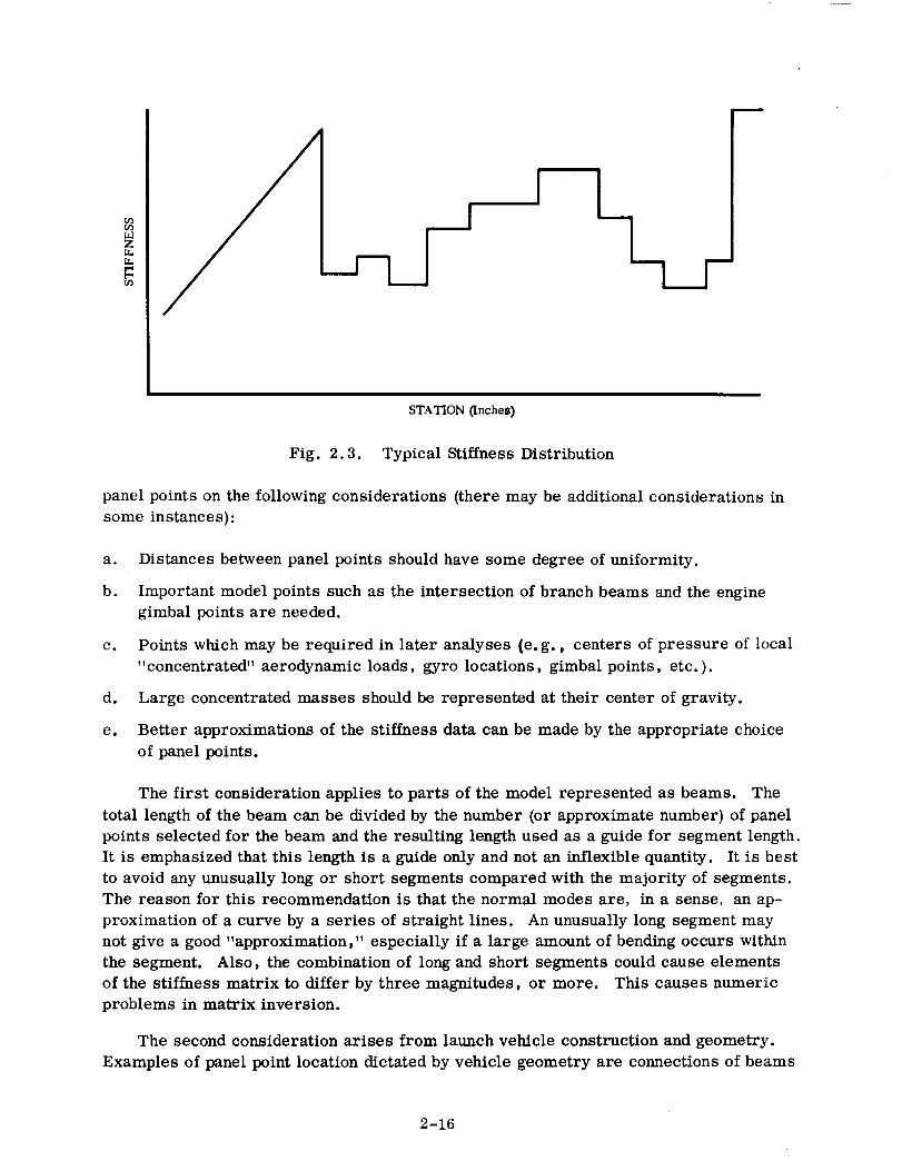
2.2.1.10 Weight and Stiffness Lumping. The weight and stiffness data are usuallygenerated in the form shownin Figs 2.2 and 2.3. From these continuous distributionsthe analyst derives a lumped parameter idealization. While many idealizations arepossible the analyst can enhancethe accuracy of the model and simplify later workwhich uses the modesby his judicious selection of lumping points.
The first step in the idealization is to select the points at which to "lump." Thesewill be referred to as panelpoints andthe beam betweenany two panel points as a seg-ment. The number of panel points to use has been discussed in previous sections. Theconsideration now is where to locate the panel points. The analyst bases his choice of
tn
v
[-,
STATION (Inches)
Fig. 2.2. Typical Weight Distribution
2-15
Z
rT
STATION (Inches)
Fig. 2.3. Typical Stiffness Distribution
panel points on the following considerations (there may be additional considerations in
some instances):
a. Distances between panel points should have some degree of uniformity.
b. Important model points such as the intersection of branch beams and the engine
gimbal points are needed.
c. Points which may be required in later analyses (e. g., centers of pressure of local
"concentrated" aerodynamic loads, gyro locations, gimbal points, etc.).
d. Large concentrated masses should be represented at their center of gravity.
e° Better approximations of the stiffness data can be made by the appropriate choice
of panel points.
The first consideration applies to parts of the model represented as beams. The
total length of the beam can be divided by the number (or approximate number) of panel
points selected for the beam and the resulting length used as a guide for segment length.
It is emphasized that this length is a guide only and not an inflexible quantity. It is best
to avoid any unusually long or short segments compared with the majority of segments.
The reason for this recommendation is that the normal modes are, in a sense, an ap-
proximation of a curve by a series of straight lines. An unusually long segment may
not give a good "approximation," especially if a large amount of bending occurs within
the segment. Also, the combination of long and short segments could cause elements
of the stifflmss matrix to differ by three magnitudes, or more. This causes numeric
problems in matrix inversion.
The second consideration arises from launch vehicle construction and geometry.
Examples of panel point location dictated by vehicle geometry are connections of beams
2-16
with branch beams, engines and sloshing propellants. There may be other items inthis category; inspection of the vehicle geometry will reveal them. The third consider-ation is one that is easily overlooked but yet merits a great deal of attention from theanalyst. The modal deflections and slopes (andfrequently the modal shears and mo-ments) are used in subsequentloads and stability analyses. In these analyses, data atcertain points are required as input and/or output. An example of required input data
is modal deflection and slope at gyro locations for use in stability analyses. An exam-
ple of required output data is moment and shear at critical stations from load analyses.
The analyst should ask himself, "To what use will the model and the modes be put and
how can this use be facilitated by the choice of panel points ?"
The weight of each segment or attached component should be distributed to main-
tain the center of gravity of that segment or component as well as overall center of
gravity. Deviation from this representation will decrease the accuracy of the model.
Stiffness data are generally input at the panel points describing the weight dis-
tribution. Additional points are used for accurate representation to indicate changes
in stiffness. These massless points are eliminated in generation of the stiffness matrix
as described in Section 2.2.2.
2.2.1.11 Stiffness and Flexibility Matrices. The primary purpose of the mathe-
matical model is to obtain a representation of the real system which can then be
represented in mathematical terms. The general approach to dynamic problems, as
given by Eqs 2.1 to 2.8, requires the formation of the mass, stiffness, and dynamic
matrices. Formation of Eq. 2.8 requires the mass matrix and the inverse of the stiff-
ness matrix. Since the inverse of the stiffness matrix is the flexibility matrix, one
may question a method of analysis beginning with the stiffness matrix when a flexibility
matrix can be derived directly. The main advantage of the stiffness approach is the
straightforward manner of deriving a coupled matrix which lends itself toward formula-
tion of computer logic capable of assembling a coupled stiffness matrix for very com-
plicated systems. Also, with high-speed, accurate computers available, the matrix
inversion can usually be accomplished efficiently and accurately. For certain specific
problems it may be desirable to develop the flexibility matrix.
In this section the approach (as presented in Ref. 2.10) for developing the stiff-
ness matrix for a lateral model will be given. The flexibility approach and a mass
coupling technique are also presented.
2.2.1.11.1 Free Element Stiffness Matrix. Bending and shear stiffnesses are identi-
fied at points along the structure, including all mass stations. The nature of the stiff-
ness distributions may justify stiffness definition at an intermediate point between mass
concentrations. Thus the model is formed from a series of connected massless beams,
with mass and inertia concentrations located at some or all the junctions of the beams.
While the stiffness of the vehicle may be distributed in a complex fashion, it may be
2-17

represented with acceptable accuracy by a series of straight line segments. This re-
sults in giving each beam segment a trapezoidal stiffness distribution.
In the approach to be outlined, the 4 x 4 stiffness matrix of each element of the
beam is first obtained by inverting the 4 x 4 flexibility matrix of this element. (The
X
® ®
Fig. 2.4.
S 2
)
Cantilever Beam in Bending
M 2
element stiffness matrices are developed
by this technique because it is easier
mathematically and more accurate. ) The
matrix is then coupled by constructing a
matrix composed of the individual 4 x 4
matrices. In this coupled matrix, the
terms for common points of adjacent ele-
ments are the sum of the terms for the in-
dividual matrices. With this matrix form,
restraints or boundary conditions are im-
posed which will represent the system to
be analyzed. The derivation of the stiff-
ness matrix is now given (see Fig. 2.4).
The bending rigidity, for a value of x, is
(E I)x =,EI 2'EI 1,E1I] (2.9)
The general equation of the elastic curve of a deflected beam is
d 2 M 2 + S2 (L-x)_2 - M
dx 2 E I (EI)x(2.10)
dvIntegrating Eq. 2. 10 and substituting the boundary conditions _ = y = 0 at x = 0,
then Y2 and 0 2, the deflection and slope at x = L, are:
M2L lnl S L3[ ]Y2 = - _ - -- - ln(1 +8)eft2 eft3 2
0 2
M 2 L S2 L 2
eft 2
}(2.11)
2-18

where
e = (E I)2
EI1
fl=EI 12
Substituting the series expansion of In (1 + fl) into Eq. 2.11 (valid for -1< _ _- 1),
2[ f12 ] S2L3M2L 1 fl +-- _ +--
Y2 - e 2 3 4 "'" e
M2L I fl f12 ...] $2L2= i - -- + -- - +%2 e 2 3 e
1 _ + _2 1-{-7 "Y - ""]
]1 _+__ _- ...]
By a similar procedure, the deflection due to shear at x = L is
s2L[ 2 ]y2 =T i_2+Y--_2 3 ''"
e = 02
(2.12)
(2.13)
where
g = (KAG)2
(KAG) 17 = 1
(KAG) 2
K is the shear effectiveness factor for the structure, i.e., that fraction of the cross-
sectional area which is carrying shear load. This can vary widely and depends on the
type of structure. Putting Eqs 2.12 and 2.13 into matrix form,
{y2}[cells2}{}2 C21 C22 M2
(2.14)
where Cll, C12, C21, and C22, the elements of the flexibility matrix, are the coeffi-
cients of Eqs 2.12 and 2.13.
2-19

3[L 1-_. m ,
Cll e 3
_24 5 ... +-g 1--_+--g-...
L2[ 1C12 = C21 - e 2 fl+ f12 ]3 4 "'"
L[- 1 _ _ _2
C22 =e L -_+ 5
By inversion of Eq. 2.14,
ts2}B1[cc2122,1c121{y}, EKl{y2},where
2
B = CllC22 - C12
(2.15)
and [ K ] is the stiffness matrix.
Considering a free element, with the same stiffness as the cantilever beam (as
shown in Fig. 2.5), the equilibrium equations are:
S1 + S2 = 0
+ S L+M 2 = 0M1 1
Also from Fig. 2.5,
Y* = Y2 - Yl - 81L
O*= 8 -O2 1
Eq. 2.15 now becomes:
Is2M 2
= 1[ C22
B [-C12 _c22_c12cl2-Lc2 l{y2}yl01
(2.16)
2-20
Im
QL
S2
®
62
Y2
bv
X
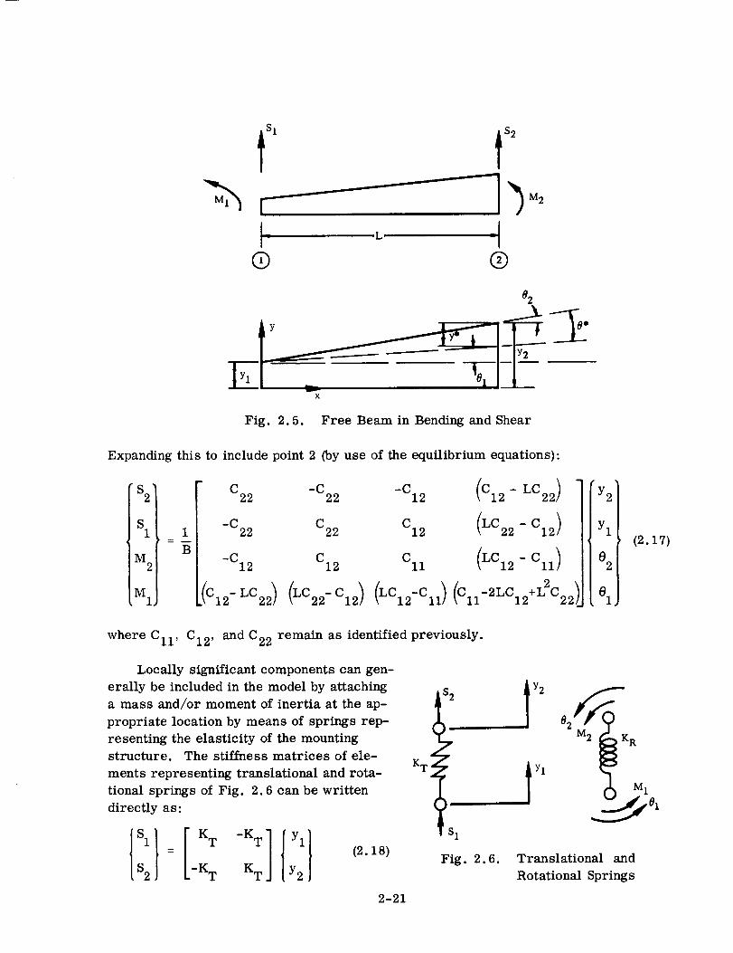
Fig. 2.5. Free Beam in Bending and Shear
Expanding this to include point 2 (by use of the equilibrium equations}:
S 2
S1
M 2
MI.
1
B
C22
-C22
-C12
L(o_2=0_2)0_ 0_ (_0_20_) 02
(_0_20_2)(_0__,_)(0_,_0_2+'_02_)J_
(2.17)
where Cll, C12, and C22 remain as identified previously.
Locally significant components can gen-
erally be included in the model by attaching
a mass and/or moment of inertia at the ap-
propriate location by means of springs rep-
resenting the elasticity of the mounting
structure. The stiffness matrices of ele-
ments representing translational and rota-
tional springs of Fig. 2.6 can be written
directly as:
SI = [ KT
Is2 [-KT
-K T
K T
(2.18)
s. 1'.82# K R
KT I Yl _1 ,01
1
Fig. 2.6. Translational and
Rotational Springs
2-21

I KR -K R ]-K R K R
81
8 2
Coupled Unrestrained Stiffness Matrix.
(2.19)
The unrestrained stiffness matrix
is generated from each beam element, and a 2 × 2 stiffness matrix is generated from
each spring element. Consider a beam element. If an element is attached to a beam,
this element must either be another beam or a spring (Fig. 2.7). When two beam ele-
ments are connected to the same node, coupling with respect to both translation and
rotation occurs.
1l0 0 0 0
1 2 3 2 3
(a) (b)
Fig. 2.7. Example of Attachments to a Beam Element
The stiffness matrix layout corresponding to Fig. 2.7a is given in Fig. 2.8. An
element in the matrix of Fig. 2.8 gives the magnitude of the shear Si or moment M i at
node i due to a unit deflection yj or slope Oj at node j. Notice that the two beam stiff-ness matrices overlap at node 2, indicating node 2 feels theeffect of both beams. An
element in this portion of the matrix is obtained by adding the corresponding element
of the two individual stiffness matrices.
Y l 81 Y2 82 Y3 83
S 1
M 1
S 2
M 2
S 3
M 3
S = SHEAR
M = MOMENT
y = DEFLECTION
8 = SLOPE
Fig. 2.8. Stiffness Matrix Layout for Attachment of Two Beams
2-22
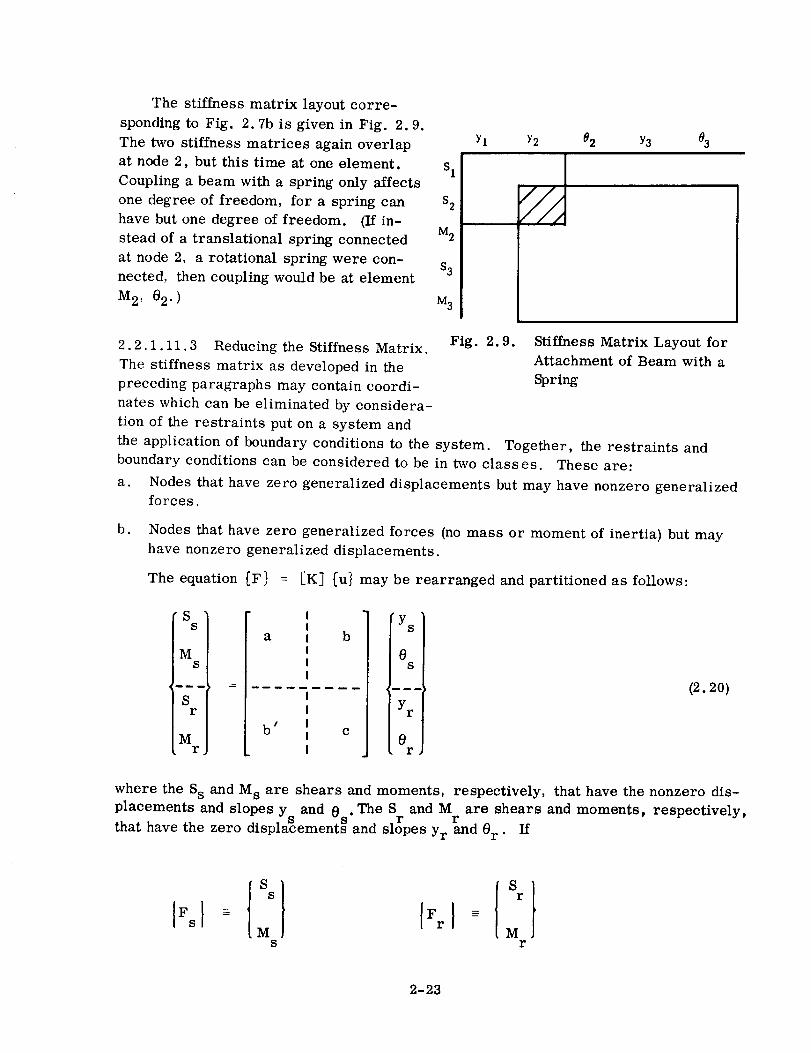
The stiffness matrix layout corre-spondingto Fig. 2.7b is given in Fig. 2.9.
The two stiffness matrices again overlap
at node 2, but this time at one element, s lCoupling a beam with a spring only affects
one degree of freedom, for a spring can s 2
have but one degree of freedom. (If in-stead of a translational spring connected M2
at node 2, a rotational spring were con-S 3
nected, then coupling would be at element
M 2 , 02 • ) M 3
Yl Y2 92 Y3 03
2.2.1.11.3 Reducing the Stiffness Matrix.
The stiffness matrix as developed in the
preceding paragraphs may contain coordi-
nates which can be eliminated by considera-
tion of the restraints put on a system and
the application of boundary conditions to the system.
Fig. 2.9. Stiffness Matrix Layout for
Attachment of Beam with a
Spring
Together, the restraints and
boundary conditions can be considered to be in two classes. These are:
a. Nodes that have zero generalized displacements but may have nonzero generalized
forces.
b. Nodes that have zero generalized forces (no mass or moment of inertia) but may
have nonzero generalized displacements.
The equation [F_ = _K] [u} may be rearranged and partitioned as follows:
!S
rIM
• rJ
a
II
b' II
I
b
c
Ys
es
t mmm
Yr
0. r •
(2.20)
where the Ss and M s are shears and moments, respectively, that have the nonzero dis-
placements and slopes y and e .The S and M are shears and moments, respectively,s s r r
that have the zero displacements and slopes Yr and 0 r . If
S s
Ms
S r
Mr
2-23
and
I®s}Ys
0 s
Yr
0 r
then Eq. 2.20 becomes
I c ](2.21)
Eq. 2.21 is equivalent to the following two matrix equations.
and
If there are no boundary conditions associated with the load vector {Fs}, the ma-
trix [a] is the final stiffness matrix [K] and {_s} is the mode shapes [_}. If there
are also boundary conditions calling for zero generalized forces then matrix Eq. 2.22
is rearranged to become
FuIF
t
! eI
= !
I g!
(2.24)
where the F u are the nonzero generalized forces that have the generalized displace-
ments _u, and the F t are the zero generalized forces that have the generalized
displacements ¢t'
Eq. 2.24 is equivalent to the two matrix equations,
Ed l,,ul+co l®tl--IF.Iand
Therefore,
]-1I®tl :-E_ Ee'_I'_uI (2.25)
2-24

and
]-1= [e'-]] " l*ul/
[gj-l[e ' ]\
In this case (the case of zero generalized forces) the matrix ( [d] - [e] ) is
the final stiffness matrix [K] and {_u] is a mode shape {_}./
2.2.1.11.4 Calculation of Free-Free Modes. The foregoing analysis was made for
a restrained system, one that is fixed at least in one place with respect to both rota-
tion and translation. In the analysis of a free-free system the structure must be re-
strained temporarily at one point. Otherwise, an external force or moment would
cause the whole system to move as a rigid body. The solution to the problem would
then be impossible. It can be shown that the eigenvalue problem reduces to the form:
Ec] [M] [¢] = ,_, [{¢} - {:P'}Yo- {r}0o] (2.27)
In Eq. 2.27 the term - {D}Yo releases the fixed point with respect to translation,
while the term - {r ] 0 o releases the fixed point with respect to rotation. By applying
the principles of linear and angular momentum to the system, Eq. 2.27 can be
expressed as a standard eigenvalue problem
r[c] [M] + ET] + [R]I [¢} = k {¢} (2.28)i.. .I
where, as explained in the foregoing,
[R] {¢} = x[r}o o
and [ [C] [M] + IT] + [R]] is the final dynamic matrix.
[R ] is now given.
The derivation of IT] and
Referring to Eq. 2.27,
#i = 1.0 if point i has a translation degree of freedom
/_i = 0 ff point i has a pitching degree of freedom
7,
1= the perpendicular distance from the pitch axis through point zero
(origin) to point i if point i has a translational degree of freedom
(positive if measured forward of point zero)
_'. = 1.0 if point i has a pitch degree of freedom1
2-25
Applying the conservation of linear momentumyieldsI
moY o + (b_} [M] [_} = 0 (2.29)
where m o is the mass at the restrained point. The conservation of angular momentumyields
I
I 0 + [r} [M] [_} = 0 (2.30)O O
where Io is the moment of inertia at the restrained point.
Multiplying Eq. 2.27 by {/_}' [M] yields
(b_]'[M] {_} - Yo {D}'[M][#] - 0o(D]'[M](I"] = u_2(D}'[M][C][M][_]
Defining
I
[AJ = [D] [M] [C][M]
and substituting from Eq. 2.29,
' ' 2-moY ° - yo[#} [M] [U] - Oo {_] [M]{r} = o_ LAJ(_]
The total mass is
I
M T = mo + (bL} [M](D}
and the static mass moment about a pitch axis through point zero is
I
S = [_} [M] (r}O
Therefore
2
MTY ° + So0 ° = -u) [AJ [_} (2.31)
l
Multiplying Eq. 2.27 by (r } [M] yields
[r}'[M](_} - Yo[r}'[M][#} - 0 ° [r}'[M][r} = u_2(r]'[M][C][M][_}
Defining
I
LBJ : [r} [M] [C] [M]
2-26
and substituting from Eq. 2.30,
-IoOo - Yo[r}'[M][_}2
- 0 [r}'[M] ['r} = ea [BJ{_}0
The mass moment of inertia of total structure about a pitch axis through point zero is
/
IT = I + [r} [M][T}O
Therefore
2IT0o + SoYo = -_ [BJ {_} (2.32)
Solving Eq. 2.32 for 0 o gives
SoY0 + U_2 LB ] [¢ }0 = - (2.33)
o IT
Substituting this in Eq. 2.31 and defining
W = IT M T - S2O
gives
2[_ o ]Yo = _ LBJ-_ LAJ [¢}
Substituting this in Eq. 2.33 gives
Oo = ¢0 [AJ---_-LBJ {¢}
By satisfying
[T] [¢} = k[bt}y °
[_] [¢] -- x{r}o°
(2.34)
(2.35)
2-27

it is seen that the T and R matrices are
[s ][T] = [p.} [BJ -_ LAj
FS MT ]JR] = {r} [W LAJ - _LBJ
(2.36)
2.2.1.11.5 Flexibility Matrix. The inverted stiffness matrix is in reality the flexi-
bility matrix of the system; i.e., it expresses displacements in terms of forces:
= [C][F]
If the model is statically determinate, the development of the flexibility matrix directly
is much simpler than inverting the stiffness matrix. However, if the structure is in-
determinate, the calculation of the elements of the flexibility matrix becomes more
complex, rapidly becoming involved and tedious with increasing numbers of redundan-
cies. The element Cij of the flexibility matrix may be thought of as the deflection atpoint i resulting from a unit load at point j. The principle of reciprocal relations will
force symmetry of the matrix, reducing the quantity of coefficients to be evaluated.
The flexibility matrix is formed by developing individual flexibility matrices for
each element in the system. They are considered as cantilevers.
CII C12
C C21 22
(2.37)
Note that Yi and 0i are relative to the end considered fixed and Si" and _I i are the total
loads applied to the end considered free. Consequently, the total deflection value is
found by transforming Yi and 0i from relative coordinates to absolute coordinates:
Yi
= [T] (2.38)
The total applied loads, Si and M i, can be considered to be functions of the external
loads applied to each mass of the structure, expressed by the transformation
= [R]Si
M i
(2.39)
2-28

Thus the relationship betweentotal deflection (Yi and 8i) and the external loads applied
to each mass (Si and Mi) is developed by substituting the transformed values,
: [c]
m
[ 0 i
= IT] [C] JR]
S i
Mi
= _T] [C] JR]
Si
M i
IT] [C] [R] = [C- ] = coupled flexibility matrix (2.40)
For a redundant structure, the influence coefficients are not so readily attained
and use must be made of an appropriate static analysis such as virtual work or
CastiglianoVs theorem (Ref. 2.11).
2.2.1.11.6 Transformed Mass Matrix. Another alternative technique for forming
the dynamic matrix is to transform the coordinate system from the absolute to the re-
lative sense. The equations of motion formed previously consider the displacements
of the respective coordinates to be referenced to a fixed point, or neutral position.
The displacements may also be expressed relatively, or referenced to an adjacent
coordinate. Furthermore, the inherent relationship between the displacements in
absolute terms, y, and the displacements in relative terms, _, is readily expressed
by a simple transformation matrix:
[y} = [T] [Y}
The kinetic and potential energies of the system can then be written (in matrix notation)in terms of relative coordinates as
2KE = _}'[T]'[M] (y}
2PE = {Y}'[C]-I {9}
2-29

where C is the uncoupledflexibility matrix consisting of 2 x 2 matrices for cantileveredelements. Using Lagrange's equation,
"_d (SK-"'_E/ + 5P"-_E+ 5W - 0 (2.41)dt 5_i / 5y i 5y i
the equations of motion become
[T]'EM]_TJ_y] + _Cj-I{_] : 0 (2.42)
and the dynamic matrix is
I
[C] [TJ [M][TJ {_] = )_{_] (2.43)
This approach is very similar to the method in the previous section with the trans-
formation of coordinates coupling the mass matrix instead of the flexibility matrix.
Note that the modes {_] are in terms of relative coordinates and must be premultiplied
by the transform matrix IT] to obtain absolute vectors.
2.2.2 TORSIONAL MODEL OF A CYLINDRICAL LIQUID PROPELLANT VEHICLE.
The construction of torsional models follows the same principal ground rules estab-
lished for the lateral model. One difference is in the treatment of propellant for liquid
boosters. In the case of the liquid propellant vehicle vibrating in pure torsion, the pro-
pellant is virtually unexcited. Since the only stress condition is that of shear, the liquid
can participate only to the extent allowed by its viscosity. It is most probable that the
fluids in the vehicle tanks can be considered nonviscous, and therefore contribute
nothing to the moment of inertia. It is evident that under these conditions, the quantity
of propellant has no effect on the torsional vibration characteristics of the vehicle.
Hence these characteristics do not vary with time in flight.
The development of the stiffness and flexibility matrices are the same as given for
the lateral beam with the terms representing bending stiffness (EI) set equal to zero.
For terms representing shear stiffness, GJ replaces KAG.
2.2.3 LONGITUDINAL MODEL OF A CYLINDRICAL LIQUID PROPELLANT VEHICLE.
A longitudinal model is a close-coupled system and is similar to the torsional model.
In pure longitudinal cases, it is possible to represent the real system by a model of
masses connected by linear translational springs. The longitudinal case therefore re-
duces to the lateral case with only translational springs. Looking at the model from
another viewpoint, it is the same as the torsional model except that moment of inertia
is replaced by mass and rotational springs are replaced by translational springs.
The tacit assumption of available spring rates has been made in the above dis-
cussion. The development of spring rates is not as easy and straightforward in the
2-30

longitudinal case. Further, two types of structure are considered, i.e., structures
not containing propellants and the propellant tanks. For the case of structures not con-
taining propellants the spring rate development is analogous to the torsional case with
the substitution of A = J and E = G in the stiffness terms. The development of
spring rates (and the model) for propellant tanks is covered in detail in Ref. 2.12.
The major portion of this development is given in the following discussion.
2.2.3.1 Fluid Equations for Elastic Tank. The analysis of a coupled elastic tank and
propellant mass, even for a highly simplified case, becomes a very complicated eigen-
value problem. Specifically, a solution must be obtained that satisfies the differential
equations for the liquid and the elastic shell, as well as appropriate boundary condi-
tions at the tank walls, the tank bottom, and the liquid free surface. A rigorous analy-
sis of this type is reported in Ref. 2.13. The results yield the natural frequencies for
the tank and propellant.
A second analysis of this type, using highly simplified shell equations, is reported
in Ref. 2.14. In this case, the natural frequencies and a forced vibration solution are
obtained for a cylindrical tank.
A number of other analyses have also been attempted for the coupled liquid and
elastic container. Most of these generate a great deal of mathematical analysis that
is of very little use in defining an analytical model for the tank. It is apparent, then,
that other more simplified techniques must be used. The continuous analysis can then
be used as a check on the dynamic characteristics of the simplified representation.
A major building block in the development of a longitudinal structural model is a
lumped parameter model for each propellant tank. In general, such tank models have
been restricted to a single (predominant) mode of the coupled elastic shell and propel-
lant mass. However, there is reason to believe that a single-mode model is not ade-
quate in all cases. Furthermore, the
development of a multimode model for the
propellant tank is feasible.
As a basis for developing a tank model,
first it is necessary to establish a set of
approximate equations for the shell and the
liquid. For example, consider the tank
shown in Fig. 2.10, filled to a height L with
a nonviscous, incompressible liquid, where
the axial acceleration of the base is _. If
it is assumed that the tank shell is thin, that
any effects of preloading can be neglected,
and that the loading is axially symmetric,
the following equations can be developed
(Ref. 2.14).
X
• 2
I"x'
Fig. 2.10.
1L
Cylindrical Tank and Liquid
2-31

h3 d4w JE r Eh v
+--W +--N = P
2 dx 4 2 r a x12(1-u ) a r=a
du 2x I-_ v
- N --- wdx Eh x a r
(2.44)
(2.45)
where
w = the radial displacement of a shell elementr
u = the longitudinal displacement of a shell elementx
N = the axial force/unit circumferential lengthx
p = the liquid pressure
E = Young' s modulus
v = Poisson's ratio
a = the shell radius
h = the shell thickness
Eqs 2.44 and 2.45 are essentially the same as those defined for a cylindrical shell
(Ref. 2.15) and a static loading condition. If, in addition, the shell is very thin, the
d4w----Y-r term contributes very little to the gross deformation of the shell. Neglecting thisdx4
term, Eq. 2.44 becomes
a av Nw - Eh x
r Eh r--a
(2.46)
For a nonviscous, incompressible liquid, the fluid velocities are defined in terms
of a velocity potential _ by Laplace's equation, i.e.,
520 +- + + - 0-- 1 5_ 1 52_ 52_
2 r 5r 2 _b2 25r r 5 5x
(2.47)
2-32

where
8_p dr5r dt
1 5¢ _ rd_._r 55 dt
5¢ dx
5x dt
When all forces applied to the fluid are axially symmetric, _ is not a function of the
coordinate _) and Eq. 2.47 reduces to
28 (_ i 8_ 82(Z)
2 r 8r 25r 8x
0 (2.48)
For small fluid velocities, the total fluid pressure is given by
P = p + _(x-L) (2.49)
Eqs 2.45, 2.46, 2.48, and 2.49 are used along with the appropriate boundary con-
ditions of the liquid surface, tank wall, and tank bottom to form the basis for the
analysis given in Ref. 2.14. In this analysis, the effects of shell inertia for a thin
shell are neglected in comparison to the liquid inertia, such that Eqs 2.45 and 2.46
also apply to the dynamic condition.
In order to further simplify the development of a lumped parameter model, the
velocity potential term in Eq. 2.49 is usually neglected; i.e., the following approxima-tion is made:
P -=" px (L-x) (2.50)
Eqs 2.45, 2.46, and 2.50 are then used to develop the tank model. This neglects
all contributions due to the liquid velocities, as defined by the velocity potential _, and
the liquid-free surface waves.
Eqs 2.45, 2.46, and 2.50 can also be used as a basis for developing a multimode
tank model by dividing the tank into two or more sections. This approach can account
for the higher tank modes as well as variations in tank geometry and skin thickness.
2-33

2.2.3.2 Model for Cylindrical Tanks with Large Ullage Volume. The propellant tankmost commonly encountered is usually an internally pressurized circular cylinder witha rounded bottom. In manycases, the bottom is approximately elliptical in shapeandcan be either concaveupward or downward.
In this section, a basic single-mode tank model is developedfor the caseof alarge tank ullage volume where the pressure essentially remains constant. This modelis then modified to accountfor the individual effects of stringer reinforcement andabuckled skin with stringer reinforcement.
2.2.3.2.1 Basic Single Mass Model. Thetank shownin Fig. 2.11 is partially filledwith an incompressible liquid to a depth Land the tank ullage is pressurized with a gasto someconstant pressure. The tank is anelastic circular cylinder with a radius a anda constant thickness h. The tank bottom, al-so elastic, has an elliptical shape, wherethe major semi-axis is a and the minor semi-axis is b. The bottom canbe either concaveupward or downward. In addition, it is assum-ed that all loading on the tank and liquid isaxisymmetric.
Fig. 2.11. Partially Filled Tank For anaxial acceleration of x, theliquid pressure acting uponthe wetted por-
tion of the tank is given by Eq. 2.50. Hoopstresses are produced in the tank skin dueto this pressure. These stresses result in radial andlongitudinal displacements foreach element of the tank with respect to the bottom. The radial displacement, whichis proportional to the pressure, is shownin Fig. 2.12a.
'x" Nx Nx
l _ II_
n _ I
(a) _)
Fig. 2.12. Tank Strains
2-34

When the tank is assembled with a vehicle, an acceleration of the masses above
the tank results in a longitudinal force acting on the top of the tank. This force pro-
duces an additional axial stress in the tank skin and displaces the tank and the liquid
center of gravity.
A flexibility matrix can be developed relating displacements at the top and center
of gravity of the tank to a force at the top and an effective "liquid inertia force" acting
at the center of gravity of the liquid when the bottom of the tank is fixed as shown in
Fig. 2.12. A stiffness matrix and a corresponding model for the tank can then be
developed. This approach yields the same single-mass tank model as that obtained inRefs 2.14 and 2.16.
The equivalent single-mass model is
indicated in Fig. 2.13. Nodes 1 and 2 of
the lumped parameter model are used to
signify, respectively, the tank top and the
liquid center of gravity. The displacements
of these points relative to the tank bottom
(i.e., relative to x = 0 in Fig. 2.11) are
denoted by x 1 and x 2. The force acting at
the top of the tank is F 1 and the effective
force acting at the center of gravity is F 2.
The force F 2 represents the total inertia
force of the fluid due to the acceleration _,
i.e.,
r" 1
Xl t K 1
x2 _--2 M
!( 2
_ K3
Fig. 2.13. Equivalent Tank Model
F 2 = VDx = Mx (2.51)
where V, p, x, and M are the tank volume, fluid mass density, fluid acceleration,
the fluid mass, respectively. The liquid volume V for the cylindrical tank with an
elliptical bottom is given by
and
where
2V = ?ra LD
D = 12 b
3 L
(2.52)
(2.53)
Therefore
F 2 LDpx
F2
Px - 2?ra LD
(2.54)
(2.55)
2-35
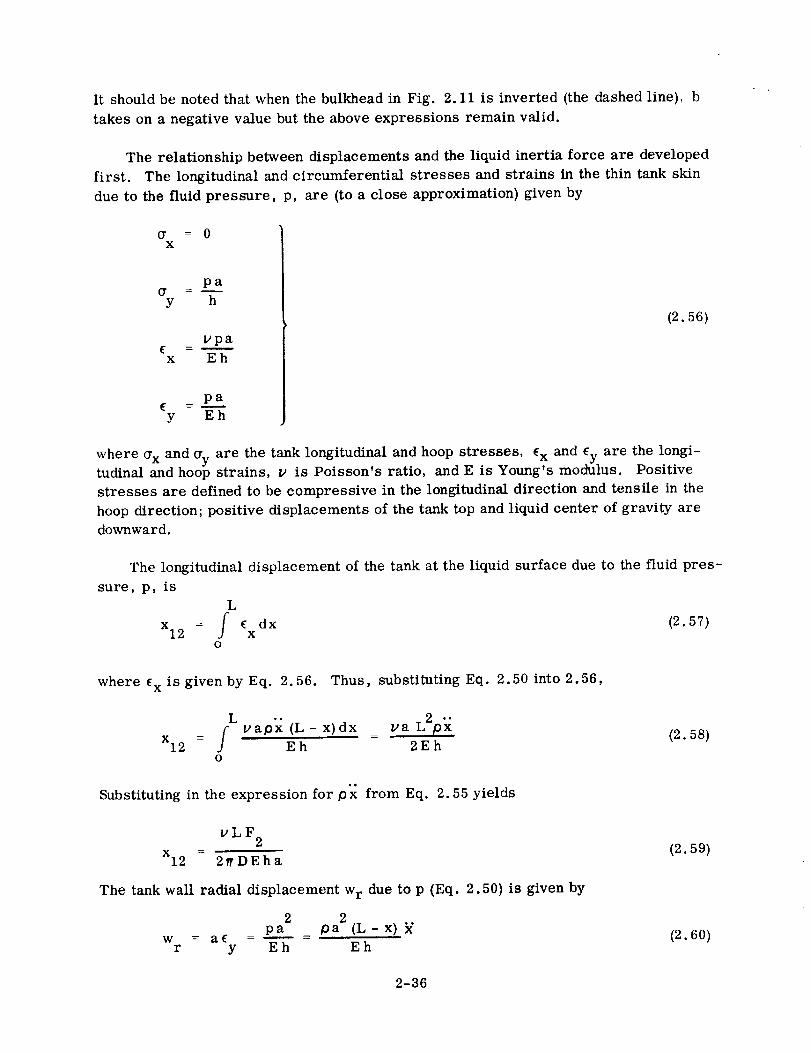
It shouldbe noted that whenthe bulkheadin Fig. 2.11 is inverted (the dashedline), btakes on a negative value but the aboveexpressions remain valid.
The relationship betweendisplacements and the liquid inertia force are developedfirst. The longitudinal andcircumferential stresses and strains in the thin tank skindue to the fluid pressure, p, are (to a close approximation) given by
= 0X
paa -
y h
upa
x Eh
pa
y Eh
(2.56)
where _x and Cry are the tank longitudinal and hoop stresses, Cx and _y are the longi-tudinal and hoop strains, I) is Poisson's ratio, and E is Young's modulus. Positive
stresses are defined to be compressive in the longitudinal direction and tensile in the
hoop direction; positive displacements of the tank top and liquid center of gravity are
downward.
The longitudinal displacement of the tank at the liquid surface due to the fluid pres-
sure, p, is
L
x12 = f (xdX (2.57)0
where Cx is given by Eq. 2.56. Thus, substituting Eq. 2.50 into 2.56,
"" L2_Lvapx (L- x)dx vax12 = / Eh = 2Eh
O
Substituting in the expression for px from Eq. 2.55 yields
(2.58)
vLF2
x12 = 2?rDEha
The tank wall radial displacement w r due to p (Eq. 2.50) is given by
2 2pa pa (L - x)
w = aE =--=r y Eh Eh
(2.59)
(2.60)
2-36
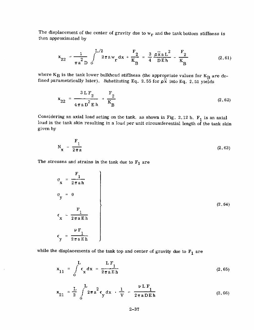
The displacement of the center of gravity due to wr and the tank bottom stiffness isthen approximated by
L 2 F1 rL/2 F2 3 px a 2
x_2_ = _ J] 2_aw dx + _ = + _ (2.61)r K 4 DEh Krra D o B B
where K B is the tank lower bulkhead stiffness (the appropriate values for K B are de-.o
fined parametrically later). Substituting Eq. 2.55 for px into Eq. 2.51 yields
3LF F2 2
- + -- (2.62)x22 4 _"a D2 E h KB
Considering an axial load acting on the tank, as shown in Fig. 2.12 b, F 1 is an axial
load in the tank skin resulting in a load per unit circumferential length of the tank skin
given by
F1
N - (2.63)x 2_a
The stresses and strains in the tank due to F 1 are
F1/O" z -_
x 2yah
(7 = 0Y
¢ = _ FI i
x 2?raEh
_F 1E -
y 2_raEh
while the displacements of the tank top and center of gravity due to F 1 are
L LF
/ 1Xll = _ dx =xO
L vLFL f 2 1 1
x21 =_- J 2_'a E dx • -- =y V 2_'aDEhO
(2.64)
(2.65)
(2.66)
2-37

The axial stiffness of the tank skin is
2?raEhK - (2.67)
L
Then the relationships between forces and displacements from Eqs 2.59, 2.62, 2.65,
and 2.66 are
Xii 1
d _ _
ii F 1 K
X12 v
d12 .... F DK2
X21 v
d21 .... F DK1
X22 3 1
d22 F2 2 D 2 K KB
(2.68)
or, in matrix notation,
[dlld12x 2 d21 d22
= [d] IFI (2.69)
The [d] matrix in Eq. 2.68 can be inverted to obtain a stiffness matrix for the tank.
The springs of the equivalent model for the tank can be obtained from this matrix.
FromEq. 2.68, F 1 and F 2 are
2 D 2 K 23K +
KB 2t;DK
= x 1 - D2 x 2 (2.70)F1 2 D 2 K 2 K3- 2V 2 +_ 3- 2a) 2 +
K B K B
-2u DK 2D2K
= 2 D 2 K Xl + D 2 K x2 (2.71)F2 3- 2_ + 2 _ 3- 2v 2+ 2
K B K B
2-38
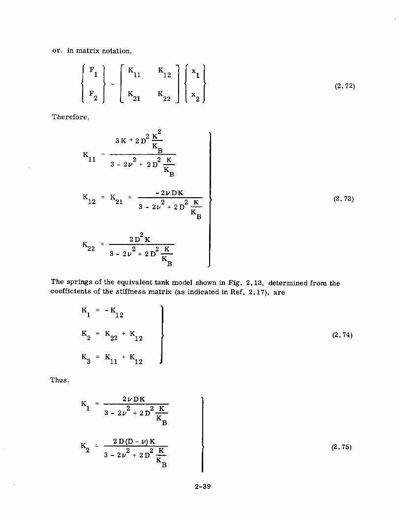
or, in matrix notation,
{::}IKll
K21
K12
K22
Therefore,
Kii
3K +2D 2 KA
K B
2 2 K3-2v +2D --
K B
K = K12 21
-2yDK
3- 2v 2 2D 2 K
K22
2 D2K
2 2 K3-2t_ +2D
KB
(2.72)
(2.73)
The springs of the equivalent tank model shown in Fig. 2.13, determined from the
coefficients of the stiffness matrix (as indicated in Ref. 2.17), are
K -- -K1 12
K2 = K22 + K12
K3 = KII + KI2
(2.74)
Thus,
K1
K 2
2vDK
3 - 2y 2 + 2D 2--_-K
K B
2D(D - y)K
3 - 2_ 2 D 2 K+2K
B
(2.75)
2-39

K 3
3 - 2VD + 2D
3_2v2 2 K+2D m
K B
K (2.75)
(Contd)
2.2.3.2.2 Spring Rate for Elliptical Tank Bottom. In Ref. 2.18, spring constants
are presented for ellipsoidal tank bottoms, as determined from an analysis using
linear membrane theory. Graphs from which the spring constants can be obtained
are reproduced here.
Consider, once again, the tank shown in Fig. 2.11. From Ref. 2.18 the tank
bottom spring rate is given by:
K B = E h B
22rr(3e- 2f)
[ 2 19 H(f, _)- 2eG(f, v)+e F(f, v)
(2.76)
where
E = Young's modulus
h B = bulkhead thickness
a = radius of cylinder
b = bulkhead semiminor axis
L = height of liquid in cylindrical portion of tank
e = L/a
f = b/a
u = Poisson's ratio
The functions H (f, v), G (f, v), and F (f, v) are given in Figs 2.14, 2.15, and 2.16.
These functions are derived in Ref. 2.18.
When the tank bottom is inverted as indicated by the dashed lines in Fig. 2.11 the
expression for the spring rate becomes
2
K' = Eh 27r(3e+ 2f) (2.77)
B B 9 H(f, y) + 2eG(f, y) +e F(f, v)
2-40
_z
2.8
2.4
2.C
1.6
1.2
0._
0.5
Y\ J_.%-- 1,4 I
0.6 0.7 0.8 0.9 1.0
f
Fig. 2.14. Variation of F (f, v) with
Depth-to-Radius Ratio
for Various Values of
Poisson's Ratio
1.4
1.21_
\1.01
\
0.1
0.40.5 0.6
Fig. 2.15.
_J1/4
1/'2
0,7 0.8 0.9
f
Variation of G (f, _) with
Depth-to-Radius Ratio
for Various Values of
Poisson's Ratio
1.0
2.2.3.2.3 Tankwith Stringers and Buckled
Skin. A model cylinder with skin and
stringer construction is shown in Fig. 2.17.
If the stringers have negligible radial stiff-
ness and the skin is unbuckled and can dis-
1.0
0.g
v =
0
place longitudinally and radially, the tank
models described in the preceding sub-
sections can be combined in parallel with
a spring K s, where
K _ (AE) stringerss L
A0.8 I/4 •
" o., .J':
0.6 --
is the total axial stiffness of the stringers
in the cross-section.
When the skin is partially buckled in the
axial direction, the axial stiffness of the
tank skin is
I ,2 9,
0.50.5 0.6 0.7 0.8 0.9 1.0
f
Variation of H (f,u) with
Depth-to-Radius Ratio
for Various Values of
Poisson's Ratio
Fig. 2.16.
2-41
STRINGER, K11
SKIN
TANKCROSS SECTION
Fig. 2.17.
K31 Ks
12"////////,,CYLINDRICAL TANK MODEL
Skin- Stringer Cylinder Tank Model
and the flexibility coefficient dll in Eq. 2.68 becomes
1
dll = +KKBu s
(2.80)
The center-of-gravity displacement due to the axial load FBu carried by the buckled
skin is then (neglecting the bulkhead and liquid compressibility effects)
UFBu
x21 K(2.81)
where K is the axial spring constant for the skin when unbuckled, Eq. 2.67.
portion of the load carried by the buckled skin is given by
KBu F 1
FBu = +KKBu s
That
(2.82)
where F 1 is the total axial load carried by the skin and stringers. Then
and
vK F
Bu 1 (2.83)
x21 = K(KBu + Ks}
x21 v KBu
d21 = Z = K(KBu+Ks)(2.84)
The center-of-gravity displacement due to acceleration of the liquid in the tank is still
(neglecting bulkhead and compressibility effects)
3d22 = -_- (2.85)
2-42

Consequently, the flexibility matrix becomes
[dJ
1 Y KBu
+K K +KBu s (KBu Ks)
vKBu
K (KBu + Ks)
3
2K
(2.86)
After inverting the [dJ matrix and solving for the spring rates, the values for the
model in Fig. 2.18 are
K_*
K**2
K**3
_
2VKBu
22 2 KBu
K (KBu + Ks)
2K- 2v KBu
2 2
2 _ KBu3-
K (KBu + Ks)
(3 - 2v) K + 3KBu s
2 t_2 K 2Bu
3-
K (KBu + Ks)
K?,
(2.87) ME
K2**,
-7
Fig. 2.18.
K3$$
** SEE TEXT
///.
Skin- Stringer
Model with
Buckled Skin
2.2.3.3 Model for Cylindrical Tank with Small Ullage Volume. When the tank ullage
volume is small, any longitudinal oscillation of the structure can produce a correspond-
ing oscillation of significant magnitude in the ullage pressure. This can be the result
of a longitudinal force transient such as thrust buildup or launcher release.
The change in ullage pressure is due to a change in ullage volume and ullage gas
weight (if a pressure regulator is involved). In this section, a single-mode tank model
is developed for such a case. The effect of gas compressibility is included in the model
spring rates while the pressure change associated with a change in gas weight is used
as the forcing function for the tank.
In order to formulate an analytical representation for the perturbation changes in
the tank ullage, the following assumptions are made.
2-43

a. The gas, or mixture of gases, in the tank ullage behaves in a quasi-static manner.
b. The gas process is adiabatic.
c. The perturbation variables are small.
The equation of state for a gas (or a mixture of gases) at low pressure is given to a
close approximation by the equation below:
PV = WR T (2.88)m
where P is pressure, V is volume, W is weight, T is temperature, and R m is the gasconstant for the mixture. In a strict sense, Eq. 2.88 applies to a condition of thermo-
dynamic equilibrium. It also applies (approximately) for a perturbation condition when
the changes in these variables are slow enough, and small enough, such that the gas is
at all times close to thermodynamic equilibrium. The gas is then said to behave in a
quasi- static manner.
For an additional relationship between the variables in the tank ullage, it is con-
venient to assume that the process is adiabatic. In such case,
:Ym- 1/
T _ _ 7m/ (2.89)
where 7m is the adiabatic exponent for the gas. In general, a polytropic exponent
would be used for Eq. 2.89. However, in the frequency range of interest it can be as-
sumed that there is little chance for heat transfer to the gas so that the polytropic
exponent is close to the adiabatic value.
Eqs 2.88 and 2.89 can now be combined to form the following equation:
P = const. V m (2.90)
A given tank may contain a mixture of gases. The total weight is then given by
= + W 2 + .... (2.91)W W 1
2-44

and the effective gas constant, R m, is defined by
W R +W R2+.1 1 2 ""R = (2.92)m W
where R 1, R 2, etc., are the gas constants for the individual gases.
For small perturbations during flight, the change in tank pressure is defined by
the first terms of a Taylor's series, where the partial derivatives are evaluated at
the steady-state (or equilibrium) condition, i.e.,
AP- 5P] 5P]aw + 7 (2.9a)S.S. S.S.
where AW is the change in ullage gas weight and AV the change in ullage volume.
For the steady-state condition,
<WR )Ym: const. _m (2.94)
V
The partial derivatives in Eq. 2.93 can be evaluated by using Eq. 2.94 to define the
proportionality constant, so that
W
A p = Pa Kw--s - KvV (2.95)
where s is the Laplace operator, and
7 9Rm gK =
WWR
m
mK -
v
where Rg is the gas constant for the pressurizing gas and where w = AW, v _- AV,
the bars denote steady-state quantities.
(2.96)
and
2-45
Fig. 2.19 shows a thin skin, cylindrical tank shell with an elliptical bulkhead for
the bottom. The top of the tank is assumed to be rigid and the tank is nearly filled
with liquid. Forces F 1 acting on the top of the tank, an effective inertia force F 2/
acting at the liquid center of gravity, and an ullage pressure change Pa acting in the/
ullage space are also shown. The pressure change Pa represents only that portion of
the total pressure change in the ullage that can be attributed to a change in gas weight.
The compressibility effect, due to a change in ullage volume, is included in the model/
spring rates. Therefore, from Eq. 2.95, Pa is defined by
SPa' : Kw _ (2.97)
or
/
Pa Pa + Kv v (2.98)
SMALL
ULLAGE
VOLUME
2
LIQUID CG
FLEXIBLE BULKHEAD
WITH STIFFNESS KB_
Fig. 2.19. Tank with Small Ullage Volume
2-46

If the displacements of the tank top and liquid center of gravity are x 1 and x2, andthe changein ullage volume is v , then the relationship between forces, pressure, dis-aplacement, and change in ullage volume is given by the matrix equations
X1
X2
Va
m
dll d12 dlv
21 d22 d2v
d-v i dv 2 dw
F 1
F 2
I
Pa
= Ed3 IFI (2.99)
or
x1
x 2
V
a
1
where C =E
d11
d21
dvl
m
d2 I I --vl I d2v dvl I C dr1
dll C +d I d21 C +d Ivv I vv I C +dvv
..... .J .J _
dlv %2 I d 2 II 2v I C dv2
d12 C +d I d22 C +d I C +dVV I W W
tI
C d lv I C d2v I C d wIC+d [C+d I C+d
w I w j w
F1
F 2
I
Pa
is the compliance of the gas in the ullage volume, and
d12
d22
dv2
dlv
d2v
dW
= [d]
(2. 100)
2-47
1K
12
DK
t_
DK
3 1
2 D 2 K KB
I
I 2y a2 (1 _2)I
DK
I2
-I---
K
[ DK\
II
IJ 2
?/a
[ +--k
II 2 rr2 a4( 5- 2v)
] K
[ 2 4
I +K--2-aI KB
(2. 101)
The compliance C could be defined to include flexibility of the tank upper bulkhead.
As the ullage volume increases, C becomes infinite and the model reduces to the basic
tank model.
The [27 matrix can be inverted to obtain a stiffness matrix:
[_]-1 = [K]
-- u
Kll K12 Klv
K21 K22 K2v
K 1 K 2 K VV
(2,102)
A tank model where the ullage gas compressibility is included in the spring rates
and where the applied forces are due to Pa is shown in Fig. 2.20.
2-48

1
l• K 2
The tank spring rates, defined in terms
of the stiffness matrix, are
1 = -K12 _
I¢2 = K22 +
F31 K21
Fig. 2.20. Tank Model for Small I_ + -Ullage Volume 3 = Kll K12
Klv K2v
KVV
K2v Kv i + K22v
KVV
2÷
Klv K2v Klv
KW
(2. 103)
2.2.3.4 Multimode Models. In most analyses of current vehicles, the structural
representations used have been based upon the tank model shown in Fig. 2.13. This
model provides an approximation for the first (predominant) mode of the coupled pro-
pellant and elastic tank. However, it is known that higher modes exist in the tank and
a limited number of these may have a significant energy content, compared to the first,
and they do provide a resonant condition at discrete higher frequencies. This is shownin Ref. 2.14.
This implies one of two conditions. Either the higher tank modes are unimportant
and their omission does not affect the overall structural modes, or certain structural
modes are inaccurate because of this omission. The actual condition, of course, de-
pends upon many factors such as the type of structure, the propellant level, etc.
There has been very little opportunity to determine the accuracy of predicted ve-
hicle modes using current models. It is believed that, in most cases, the first mode
predictions are adequate and that any errors are incurred in the higher modes. This
should be particularly true when the propellant mass is large and represents a majorpart of the vehicle mass.
It is desirable to further explore the importance or contribution of the higher tank
modes by developing a multimode tank model and using it in the structural representa-
tion for the vehicle. The initial results obtained by using this approach are discussedin this subsection.
A discrete model for higher tank modes can be developed in a manner similar to
that used for the single-mass representation. Consider again the cylindrical tank with
an elliptical bulkhead as shown in Fig. 2.21. Assume, for the present, that the bulk-
head is inelastic (rigid) and that the liquid is incompressible.
2-49
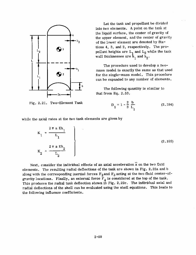
TL 2
L 1
Fig. 2.21.
3
2
•_--h I
.q_----- 2a _
Two-Element Tank
Let the tank and propellant be divided
into two elements. A point on the tank at
the liquid surface, the center of gravity of
the upper element, and the center of gravity
of the lower element are denoted by Sta-
tions 4, 3, and 2, respectively. The pro-
pellant heights are L 1 and L 2 while the tank
wall thicknesses are h 1 and h 2.
The procedure used to develop a two-
mass model is exactly the same as that used
for the single-mass model. This procedure
can be expanded to any number of elements.
The following quantity is similar to
that from Eq. 2.53.
2 b
DI= 1-_ _--1
(2. 104)
while the axial rates at the two tank elements are given by
2_r aEh 1
K1 L 1
2 _r a Eh 2
K 2 = L2
(2. 105)
Next, consider the individual effects of an axial acceleration x on the two fluid
elements. The resulting radial deflections of the tank are shown in Fig. 2.22a and b
along with the corresponding inertial forces F 2 and F 3 acting at the two fluid center-of-
gravity locations. Finally, an external force F 4 is considered at the top of the tank.
This produces the radial tank deflection shown in Fig. 2.22c. The individual axial and
radial deflections of the shell can be evaluated using the shell equations. This leads to
the following influence coefficients.
2-50

3
I!
!!
!
I r, I
(a)
I X
(b) (c)
Fig. 2.22. Assumed Forces on Two-Element Tank
d32
d22
d42
d23
d33
d43
d24
x32 2
F 2 D 1 K 1
x22 3
2F2 2 D 1 K 1
x42 v
F 2 D 1 K 1
x23 2
F 3 D 1 K 1
x33 4 3
F 3 K 1 2 K 2
x43 2 v V
F 3 K 1 K 2
x24 V
F 4 D 1 K 1
(2.106)
2-51

x34 2v Y
d34 - F4 - K1+K--2
x44 K 1 + K 2
d44 = =F 4 K 1 K 2
(2.106
Contd)
The influence matrix is then given by
[d]
d22
= d32
d42
d23 d24
d33 d34
d d43 44
g
- 3 i 2 I v
4D 12K1 Ii DI KI Ii DI KI
I[
2 I __4 + 3___ I 2v v
iD1 K1 I K1 2 K 2 tl K1 K2
I I K 1 + K 2v I 2.__p+ V I
1 K1 I K1 K2 I K1 K2 _
(2.107)
L
where for L 1 = L 2 = _- , Eqs 2. 104 and 2. 105 become
4?raEh 1
K1 = L
4rtaEh 2
K2 = L
4b
D1 = _-3-Z
(2.108)
For a particular tank, the coefficients of the [d] matrix can be evaluated. The [d]
matrix can then be inverted to obtain a stiffness matrix. Fig. 2.23 shows a model which
would correspond to the stiffness matrix given by
2-52

4 K34I
My v3
24 "_t I i .
K23i' / ; KI4
Fig. 2.23. Two-Mass Tank Model
[d]-1
m
K22 K23 K24
K32 K33 K34
K42 K43 K44_
(2. 109)
where the model spring stiffnesses are related to the stiffness matrix by
I_23 = -K23
I_24 = -K24
I_34 = -K34
(2. 110)
I_12 = K22 +K23 +K24
I_13 = K32 +K33 +K34
I_14 = K42 +K43 +K44
This model can be generalized for many degrees of freedom by writing general expres-
sions for the influence coefficients of a multimass model. Also, the effects of a flexible
tank bottom and liquid compressibility can be included in the process.
2-53
2.2.4 ADDING COMPONENTS USING MODE SYNTHESIS. Frequently itis desirable
to make a parameter study to determine the effecton vehicle response resulting from
changes in the characteristics of a specific area or component, e.g., a sloshing mass
or engine system. Rather than make several analyses of the system, changing but a
fraction of the parameters each time, the vibration characteristics of the system ex-
cluding the specific varying parameter may be calculated, and then modified by coupling
the parameter back in through the mode synthesis technique (discussed in Refs 2.19 and
2.20).
The mode synthesis approach may result in a loss of accuracy. The analysis that
considers the most information about the system will be the most accurate. The use
of many modes in the mode synthesis technique will give theoretically more accurate
results than using a minimum number of modes. This aspect is one which must be
handled by discretion born of experience. As an example, in calculating the bending
modes with sloshing propellants, three alternatives are available (all motions are
relative to the undeformed axis of the beam):
a. Include the sloshing mass as an attached spring-mass to the beam in the modes
calculation.
b. Assume the sloshing mass is included in the "rigid" propellants for modes cal-
culation. The sloshing is then included through mode synthesis by adding the
single spring-mass mode and subtracting the sloshing mass effects from the bend-
ing modes. This requires both inertial and elastic coupling in the synthesis.
c. Assume the sloshing mass can be eliminated in the "rigid'fpropellants for modes
calculations. The sloshing is then included through mode synthesis by adding the
simple spring mass mode. This requires only elastic coupling in the synthesis.
These alternatives are listed in order of accuracy of end results following the gen-
eral rule stated previously. There are many examples where there would be little if
any degradation of accuracy. As an example, consider a vehicle with first bending
frequency of 5 cps and first slosh frequency of 1 cps. The sloshing is then essentially
uncoupled from the elastic modes. If the slosh frequency were 4 cps, then consider-
able coupling is possible.
Although sloshing was used as an example, the same is true for any representa-
tion of this type, i.e., engines, payloads, sloshing propellants, any large component,
or a specific parameter under investigation.
2.2.5 LATERAL-TORSIONAL-LONGITUDINAL COUPLING. The typical axisym-
metric-cylindrical space vehicle is analyzed as if lateral, torsional, and longitudinal
motion are not coupled. Actually, these vehicles are not completely symmetric and a
possible coupling mechanism, however slight, can always be found. The importance
of this coupling can vary greatly from vehicle to vehicle and even if it is known to exist
from flight or experimental data, the coupling mechanism is difficult to identify. These
2-54
coupling problems often occur when the modal frequencies of two modes, say, one
lateral and one torsional, are very close together. Then a very small coupling mech-
anism, such as center-of-gravity offset from the supposed line of symmetry, can
result in coupled motion.
A comparison of the frequencies of the modes in the three directions should be
made to determine the existence of modes of nearly equal frequency. If such a condi-
tion exists, it is necessary to examine the condition under which this may cause a
significant problem. As an example, if excitation of a bending mode by an atmospheric
disturbance occurred, could this cause excitation of a critical torsional mode at this
same frequency? In most instances of coupling of this type, a periodic forcing function
is necessary to transmit the energy from one direction to another.
Cylindrical vehicles with unsymmetric upper stages or payloads of large mass can
cause coupling in the various directions in the low-frequency modes. The model and
analysis then become complicated and approach that of the clustered boosters. Re-
presentation of this configuration requires detailed description in the unsymmetric
stages and an analysis as described later for clustered boosters. Preliminary work
would indicate the degree of sophistication to be used for adequate representation for
loads analysis.
2.2.6 CLUSTERED BOOSTERS. One method for obtaining the higher thrust required
for large payloads is to attach rocket engines or motors to a central core; for liquid
boosters a peripheral ring of propellant tanks is attached to a center tank and the
engines are supported on truss members connecting the tanks; for solid boosters, the
motors are attached to a central solid or liquid booster. These clustered tank designs
destroy axial symmetry and quite often planes of symmetry. Such configurations re-
sult in a more complicated lateral model where a number of cylindrical tanks are
coupled by their elastic connections and must be allowed freedom in several directions
for adequate description of vehicle modes (see Fig. 2.24).
For preliminary design it is sufficient to choose approximate planes of symmetry
and analyze the vehicle for bending modes in pitch and yaw planes using branch beams
connected to the central core by translational and rotational springs. Simplified tor-
sional and longitudinal models will also suffice at this stage. These simple models
can be used to identify possible problem areas (such as relative modal frequencies)
and provide design criteria for the connections between tanks.
A complete analysis (or carefully conducted test) should be undertaken to describe
all the primary modes of the clustered vehicle. This analysis would provide transla-
tion and rotation in two mutually perpendicular planes; torsion and longitudinal motion.
The model of the tanks for translation and rotation in each of the two planes would be
very similar to that discussed for the cylindrical booster. Provision must be made to
account for the motion of the outer tanks in these two directions due to the torsional
displacement of the center tank and the elastic connections. It is also possible that
2-55

CENTER CORE
LIQUID
A3_['ACHED
SOLIDS
Fig. 2.24.
1I
l
iIi
i
..
[_"
i--i
B.
f ,
Titan lllC
/
u
!
I
II
longitudinal motion will couple with lateral
and torsional displacement. As an example,
consider a cluster arrangement where the
connection at the bottom provides moment,
shear, and axial restraints while the con-
nection at the top provides only shear res-
traint. Then it is possible to find a mode
where the external tanks are bending, caus-
ing moments and deflections at the connection
to the center core which will result in longi-
tudinal motion of the core. The significance
of these types of modes can be ascertained
only from the analysis (or test) and can vary
greatly from vehicle to vehicle.
The torsional properties in the model
can be represented by the torsional stiff-
ness and roll inertia of each tank. The
tanks must then be connected by the elastic
properties of the truss. The complete model
for the clustered booster then consists of the
axial load, shear, bending moment, and
torque. The top connection transmits onlyshear. Because of the nature of the con-
nections, it can be seen that yaw bending
and longitudinal coupling can occur. Pitch
bending and torsion represent another pos-
sible coupling mechanism. Storey in Ref.
2.21 develops the coupled flexibility mat-
rices for these two conditions. This method
encountered difficulty in that the number of
stations required for adequate representation
of the system with the required transfor-
mations exceeded computer capacity.
The final Titan IIIC analysis presented
in Ref. 2.22 utilizes the mode synthesis ap-
proach. The longitudinal, torsional, and
pitch and yaw bending modes are determined
for each tank and are then coupled by the
elasticity of the connecting elements. The
influence coefficients for these trusses were
obtained experimentally. A comparison of
analytical and i/5-scale experimental re-
sults is given in Ref. 2.23.
2-56

The Saturn I vehicle consists of a center LO 2 tank with eight peripheral tanks for
alternating LO 2 and RP-1. These tanks are connected at top and bottom by trusses
providing axial, shear, and torsion restraint in both planes at the bottom plus moment
restraint in the tangential planes. The top connection provides similar restraint ex-
cept for the fuel tanks which do not transmit axial load. The trusses are not symmetric
with respect to planes of symmetry of the tanks, but this effect is small so that planes
of symmetry as defined by the tanks do not introduce large errors.
Milner (Ref. 2.24} establishes theoretically the uncoupling of pitch, yaw, and
torsion modes for a symmetrical clustered booster and investigates the effect of minor
asymmetry. Results of this study indicate that the effect of such coupling on natural
frequencies is minor; mode shapes are not presented.
Lianis (Ref. 2.25) develops a matrix solution of the dynamics problem of a four-
tank booster without center core. The flexibility matrix of the whole unit, with appro-
priate beam end fixity, is derived. This flexibility matrix together with a suitable
mass matrix is used to derive equations of free vibration in matrix form. The tanks
are assumed to be similar, but the solution can be modified accordingly for the case
of nonsimilar tanks and for other tank configurations. The formulation is general so
as to furnish any complex mode of vibration. Simple modes, however, can be obtained
as particular cases of the general problem.
2.2.7 CORRECTING MODEL BASED ON TEST RESULTS. The final evaluation of
analytical techniques is a comparison with experimental data. Perfect comparisons
are indeed exceptions, since both the analytical model and experimental model are ap-
proximations to some extent. The analytical approximations have been discussed. The
major experimental approximations are centered around suspension system effects and
vehicle modifications required to accommodate the suspension system. No general rule
can be made to obtain better agreement between test and analysis. Careful examination
of the data and the structure will probably indicate several areas where the representa-
tion is inadequate or does not define the test specimen. Possible causes of differences
are:
a. Effects of suspension system on test environment.
b. Stiffness of joints or trusses.
c. Assumed planes of symmetry are incorrect.
d. Effect of large components such as engines.
e. Experimental modes may be impure, i.e., not orthogonal.
f. Effects of moment of inertia.
g. Nonlinearity.
2-57

The work of Ref. 2.26 presents a method for obtaining the flexibility matrix from
experimental mode data. The procedure orthogonalizes the experimental modes, using
an analytical mass distribution, and then derives the flexibility matrix of the structure.
This method can be useful if complete and accurate experimental data are obtained for
a system difficult to model. It can also be used to locate possible discrepancies be-
tween analytical and experimental results.
2.2.8 DAMPING EFFECTS. Dissipative (damping) forces exist in the vibrating
structure as'a result of material strain hysteresis and coulomb friction in structural
joints. The nature of these damping effects is obscure and does not lend itself to
analysis other than an approximate empirical treatment, by which the gross effect of
these scattered dissipative mechanisms is represented as equivalent viscous damping,
added to each mode as appropriate. The damping is thus assumed to produce no cou-
pling between modes. While this mechanization is not entirely realistic, it is justified
by two observations: First, the actual damping is very low and is found by test to pro-
duce little coupling. Thus, nearly pure normal modes of a system may be excited and
the system observed to decay almost harmonically. The indication given is that ve-
locity-dependent coupling is very small. Secondly, if an attempt is made to show a
velocity-dependent coupling, the coefficient would have to be determined experimentally.
Since the direct damping coefficient is itself difficult enough to measure it is clear that
the accuracy of a study cannot be increased by the introduction of still more suspect
data. The structural damping force is a function of the deflection of the generalized
coordinate of the mode but in phase with the velocity of the generalized coordinate of
that mode. To treat this damping as viscous damping requires that the mode oscillate
in a quasi-harmonic manner. This damping force may then be expressed as a damping
factor, _, where 2_n_ n _n is the internal damping force of the nth mode per unit
generalized mass.
Fluid propellant damping forces result from the dissipative nature of a viscous
fluid undergoing shear. Although there are some approximate methods for calculating
damping forces, these forces are most commonly arrived at by testing the actual tank,
in the case of small missiles, and a model tank in the case of large missiles. These
forces may be represented as a propellant damping factor, _n' in the expression
2_nU_n _n which is the damping force per unit sloshing mass and _n is the lateral ve-
locity of the nth sloshing mass.
Aerodynamic damping forces result from lateral velocity of the vehicle which
causes, for any particular point on the vehicle, a small angle of attack. The aero-
dynamic force associated with this angle of attack opposes the lateral motion, thereby
dissipating energy. The.aerodynamic damping forces are easily calculated and are,
of course, a function of _n" Aerodynamic damping on launch vehicles is often not im-
portant for dynamic load analyses; however, for some configurations, e.g., hammer-
head payloads and winged payloads, it may need to be considered.
2-58

2.3 DERIVATION OF NORMAL MODES
2.3.1 SOLUTIONS FOR CHARACTERISTICS. Formulation of the equations of motion
of dynamic systems results in a linear differential equation for the continuous exact
solution or a series of differential equations for the approximate solutions. For lateral
vibration usually only the lower modes are of any significance and therefore the approxi-
mate solutions are of practical importance. Two methods are used to describe the sys-
tem in these approximate solutions: 1) the system is divided into a finite number of
segments connected by massless stiffness, and 2) the system is described in terms of
assumed functions. Solving for the characteristics of the resulting equations can be
categorized into three groups. These are: 1) energy methods, 2) solving the differ-
ential equations, and 3) solving the integral equation. The equations may be written
in general matrix form as follows,
2- 0_ EM7 [u} + [K7 [u] = 0 (diferential equation) (2.111)
2 -1 0j2_u_ = a_ EK7 [M_ _u] = _D7 [u_ (integral equation) (2.112)
The categorizations of the above matrix equations as differential and integral
equations, respectively, follow the practice of Bisplinghoff et.al, in Ref. 2.4.
The most general solution of Eq. 2. 111 involves expansion of the determinant and
solving the polynomial equation. This procedure is adequate for simple systems and
up to four degrees of freedom can be solved easily. Methods for higher order systems
have been developed in Refs 2.27 and 2.28. However, since often only the lower modes
are important some approximate methods have been developed which obtain these modes
and frequencies with sufficient accuracy.
2.3.1.1 Matrix Iteration (Stodola and Vianello Method). The matrix iteration technique
is essentially the Stodola and Vianello method in matrix form. The integral equation is
2 -1[u] = 0¢ [K7 [M_ [u} (2. 113)
It can be seen that o_2 [M_ [Un_ 1] is the load associated with an assumed mode shape,
[Un_ 1] , vibrating at a frequency _ The deflection resulting from this load or the next
approximation of the mode shape is obtained by premultiplication by the influence co-
efficients, or the inverse of the stiffness matrix. Since ¢c2 is a constant it can be as-
sumed to be unity and the equation becomes
[u n] = [K] -1 [M] [Un_l ] (2. 114)
where [ _ _ is a vector normalized on its largest element. Successive iterations of Eq.
2.114 continue until [_ } has converged, i.e., every element in [Un] satisfiesn
2-59
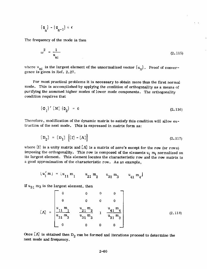
} -{an_ 1}II
The frequency of the mode is then
2 1
Uni
(2. 115)
where Uni is the largest element of the unnormalized vector [Un}. Proof of conver-gence is given in Ref. 2.27.
For most practical problems it is necessary to obtain more than the first normal
mode. This is accomplished by applying the condition of orthogonality as a means of
purifying the assumed higher modes of lower mode components. The orthogonality
condition requires that
{_1 }' [M] [_2} = 0 (2.116)
Therefore, modification of the dynamic matrix to satisfy this condition will allow ex-
traction of the next mode. This is expressed in matrix form as:
_D 2] = [D 1] [[I] - [A]] (2.117)
where [I] is a unity matrix and [A] is a matrix of zero's except for the row (or rows)
imposing the orthogonality. This row is composed of the elements u i m i normalized onits largest element. This element locates the characteristic row and the row matrix is
a good approximation of the characteristic row. As an example,
Lu: mj = LUll m u m m 3 m4 j1 1 21 2 u31 u41
If u31 m 3 is the largest element, thenm
0
0
U m
II 1CA] =u31 m 3
0
0 0 0
0 0 0
u21 m2 u41 m41
u31 m3 u31 m3
0 0 0 _2
(2. 118)
Once [A] is obtained then D 2 can be formed and iterations proceed to determine the
next mode and frequency.
2-60

For improved accuracy and subsequent deflation of the D matrix it is recommended
that iterations be performed on the row matrix, Lu_ M], by post-multiplication by the
dynamic matrix. This removes errors in roundoff in the preceding fundamental mode
and provides a more accurate characteristic. Thus,
Lu_M] [D] = Lu1M]
where ['-] indicates normalization on its largest element. Lu_ M] is then normalized
on its largest element and placed in the [A] matrix. If the characteristic row is found
by this method, the deflated dynamic matrix for successive modes can then be obtained
by
[D 3] = [D 2][[z]-EA2] ]
If the deflated matrix is obtained only from the conditions of orthogonality, then
[Dn] = [D1] [[I] - [An] ] (2.119)
where [A n] satisfies orthogonality between first and n, second and n, ---, and n-1 andn modes.
An alternate method for deflating the matrix is given in Ref. 2.28 and is particularly
useful in application with automatic computers. This deflation method gives
1
[D 2] = [D 1] -'t_'{u 1] Lul] [M]
coI
(2. 120)
where {Ul] is the column of elements of the first mode normalized so that [Ul] [M] {u 1]
= 1. For each succeeding mode the matrix is modified by subtracting the triple matrix
product for the preceding mode from the preceding modified dynamic matrix.
[Dn] = [Dn_l]- {Un_l] [Un_ 1] [M] (2.121)
2.3.1.2 Holzer-Myklestad Method. The Holzer-Myklestad method is extremely suit-
able for obtaining solution of the differential equations of beams represented as con-
centrated masses connected by massless stiffness elements. A principal advantage of
this method is that each mode is obtained independently and therefore all modes are as
accurate as represented by the system analyzed.
The technique proposed by Holzer was originally developed for torsional systems.
It is equally applicable to any close-coupled system, i.e., represented as a spring-
mass system. A frequency is assumed and one element of the mode shape vector is
2-61

taken as unity. Through equilibrium equations, the other elements of the vector are
calculated. There will be one additional equilibrium equation left after the last ele-
ment of the mode shape vector is evaluated, which will be satisfied only if the assumed
frequency is correct. Successive frequency trials are made until the proper value is
obtained. The process is facilitated by plotting net unbalanced force on the final mass
against frequency. At the natural frequency of the system, the curve of net force
passes through zero.
In reality, the Myklestad method is the Holzer method extended to include far-
coupled systems, i.e., beam systems. The slope and deflection at one end of a beam
segment are expressible in terms of the slope and deflection at the other end, the loads
at the other end and the flexibility of the beam segment. The boundary conditions at
one end of the beam give an initial set of values. Two of the four conditions will be un-
known. One is set to unity and the interior values axe determined in terms of the re-
maining unknown.
As an illustration, consider the beam segment in Fig. 2.25.
forces at the right end can be expressed as:
2S 2 = S1 - o_ m 2 Y2
= +S LM2 M1 1
= + + Le 1Y2 Yl +CllS 1 C12M 1
= +C S 1 +02 O 1 21 C22 M1
The deflections and
(2. 122)
Fig. 2.25.
Sl
I-
X
Free-Body Diagram of Vibrating Beam Segment
2-62

The quantities Cll, C12, C21, and C22 are the flexibility influence coefficients ofEq. 2.14. If the left end of the beam segment is the end of the total beam, two of thefour variables at that end canbe determined from the end conditions for a free end.M1 is zero and S1 is equal to the inertia force m1 _2 Yl" Of the two remaining con-ditions, one is assigned a value of unity and analysis is carried out in terms of theother. For the free end, Yl is assigned a unity value (making S1 = m I _c2). The four
variables at point two may be evaluated as."
2= + L81Y2 1 + m 1 ¢c C ll
2
e2 = OI +m 1_c C21
2M2 = ml_c L
2 + Lel]S 2 = m l_c2 - m 2 ¢c2 Ii +m I ¢o CII
If an arbitrary value for _ is assigned, each of the four variables at point two
reduces to an expression involving a constant and a coefficient times e 1.
The variables at the next point on the beam may be expressed in terms of those
just obtained by using Eq. 2. 122 and will also be in linear terms of e I . The evaluations
may thus be propagated across the beam, with the ultimate result that the four vari-
ables at the far end of the beam are expressed as linear functions of e I .
From the end conditions at this point, the va]ues of two of these variables will be
known. One of these known quantities is used to evaluate 81 , which is then substituted
into the expression for the second known variable. For the correct value of ¢c2, the
expression will produce the known value; otherwise, an error term or residual will be
obtained. Several trial values of w2 are made, repeating the propagation process each
time. If the resultant residuals are plotted against _2, the extraction of the proper
values of ¢c2 is facilitated by extrapolation of the curve. The natural frequencies occur
where the curve crosses the axis. Higher frequencies are obtained independently, thus
are independent of any inaccuracies which may exist in calculated lower modes.
2.3.1.3 Energy Methods. Lord Rayleigh's method of evaluating the fundamental fre-
quency of a system is based on the principle of conservation of energy. At the maximum
deformation of the system vibrating in this fundamental frequency, all the energy of the
system is in a potential energy form E =7 _ EI(d2y_ 2dx_ But at the instant the sys-\dx2/ /"
tem passes through the equilibrium position, its energy is entirely in kinetic form (KE
_-_ m} 2 dx). If energy is conserved, the maximums of those two values may be equat-
ed. A deflection shape is assumed and for harmonic motion, y = U sin at, and hence,
2-63
= _}U cos o_t
(2. 123)
and thus
02 --
mU2 dx
dx
(2. 124)
It can be shown that close approximations to the fundamental frequency are ob-
tained even if the assumed deflection shape is not very close to the true shape.
The Rayleigh method was generalized by Ritz to give more accurate values for the
frequencies as well as to give estimates for several mode frequencies at one time.
Basically, Ritz suggested that the assumed deflection curve be expressed as the sum
of several functions in the form
y = _f (X)_n (2. 125)n
The more functions and constants introduced the more accurate the value of the funda-
mental frequency. Also, if n functions are introduced then estimates on the first n
mode frequencies will be obtained. Having expressed the assumed deflection curve in
terms of n functions f (x), the kinetic and potential energies (omitting shear and mo-
ments of inertia) are expressed as
2 KE = /m (x) _2 (x, t)dx (2. 126)
/ _bX22 PE = (x)\ d x2/ dx
(2. 127)
Substituting Eq. 2. 125 into Eqs 2. 126 and 2. 127,
n n
i=1 j=l miJi J
n n
2 PE = _ _ Kij_i_j (2. 129)i=1 j=l
2-64
where
and
mi jm[fi(x)l[ j'x)l
K1j = fEI d2 d2(x)l I 'x)l
Substituting Eqs 2. 128 and 2. 129 into Lagrange's equation gives the differential equation,
n n
m.._i+ _ K.._.j=l lJ j=l lJ 1
= 0 (2. 130)
I
Putting as a solution, _j = { sin u_t,
n
(% 2 _)_j=l
= 0 (2. 131)
or a set of algebraic equations equal in number to the number of unknown coefficients.
The determinental equation for the set will yield frequencies for the first n modes of
vibration and eigenvectors which when multiplied by the assumed functions give ap-
proximate mode shapes.
The result gives good accuracy in frequency but poor agreement with mode shape.
Using the mode shape obtained as a second approximation improves frequency accuracy
and greatly improves mode shape.
Also, expressing the strain energy in terms of inertial loading rather than the as-
sumed deflections increases the flexibility of this method in that shear deformation and
moments of inertia are then easily included.
2.3.1.4 Jacobi and Givens Method. The Jacobi method solves Eq. 2.112 by diagonal-
izing the dynamic matrix, [D_, by means of orthogonal transformations. The new dia-
gonals contain the eigenvalues, and the orthogonal transformations used in diagonalization
contain the eigenvectors. Bodewig (Ref. 2.27) explains the method as follows. First,
it is assumed the matrix is symmetric. Eq. 2. 112 can be expressed in the form,
[D_ [u] = IV]
2-65

u is subjected to the orthogonal transformation [A] and
[u} = [hi {w}
Then, to preserve symmetry, the system is multiplied by [A] _
[A] _ [D] [hi {w} = [A] _ _v}
Making the substitutions
[B] = [hi _ [D] [hi
Ix} = [hi' Iv}
then
[B] Iv} = {:x}
To eliminate the coefficients d12 and d21 (the first off-diagonal terms of [D]) put
[A] =I
:i
where [T] is a two-rowed orthogonal transformation. By choosing
[T]
[sin c_ -cos
one also gets [T]' = [T] and [A]' = [A],
Then
[B] = -i- [D] _-
:iJ I
or, when in [D] a top left corner matrix [D2] of order 2 is detached,
[D]
2-66

with [C] = [C]'. But then
[B] = _'TID2T T_I= [B]'
Thus [B] differs from [A] only in the first two rows and columns and
2bll = dllCOS _ +d12 sin2_ +d22 sin 2
b12 = (dll-d22) sins cos_-dl2 (cos 2_-sin20t) = b 21
2 2 2b22 = dll sin _-d12 sin 2_ +d22 cos ot
Now, for _ arbitrary,
b + b = d + d11 22 11 22
and b = 0 if12
1--tan 2_ =2
d12
dll - d22
Then
1
bll = _(dll +d12) +
1b22 = _-(dll + d22) -
where
dll - d22 t 2 d2F = _ + 12
2-67
The sign of _ dependson the quadrant of 20_and follows from
d - d22 d12J-F-F = 11 =
2 cos 2_ sin 2_
The above procedure has altered the first two rows and columns. The procedure is
repeated on succeeding pairs of rows and columns for the entire matrix. The matrix
is operated on in this manner until it is sufficiently diagonalized.
Jacobi worked out his method originally to speed up convergence of iteration pro-
blems. It was later that its usefulness in eigenvalue problems was realized. Bodewig
expounds in more detail on the application of Jacobi's method to eigenvalue problems
and its usefulness.
The Givens method has the general form of Jacobi's method, i.e., making off-
diagonal terms small compared to diagonal terms by means of orthogonal transfor-
mations. Givens uses a transformation that makes all off--diagonal terms except the
upper and lower parallel of the diagonal equal to zero. Solutions for eigenvalues and
eigenvectors are then effected. Bodewig (Ref. 2.27, p. 336-340) gives details of the
Givens method.
2.3.2 MODAL QUANTITIES. Solutions to the characteristic equations give either the
squares or the reciprocals of the squares of the circular frequencies and also the mode
shapes of the restrained system. The linear frequencies of vibration are obtained from
the circular frequencies. If each mode shape [_}n is considered to be the nth column
of a matrix [_] of all the mode shapes, then [_] _ [M] [_] is an orthogonality check of
the mode shapes. The diagonal element ([_]'[MJ[_n,_ is called the generalized mass
of the system for mode n. In this discussion the vector [_} was stated to be the mode
shape of the structural system. For a restrained system, (_} is relative to the re-
strained point(s) and is, therefore, the final mode shape. For a free-free system, [¢_}
is relative to the temporarily restrained point (which has translation, Yo, and rotation,
0o) ; hence the effect of Yo and eo must be included to obtain the final mode shape.
The slope of a node of a beam as computed by the foregoing is the slope due to
beam bending, i.e., the slope of the elastic axis. To obtain the total slope, the shear-
ing slope of the beam must be added to the slope due to beam bending. This is done by
defining
[(Y}= [0} + [y} (2.132)
where
{y}= [cs] {r }
2-68

Having obtainedthe modal response, the yahicle response (i.e., displacement, ac-celeration, force, moment, etc.) canbe calculated. The two steps, obtaining modalresponse andthen vehicle response, will be discussed separately.
2.4.1 MODAL RESPONSE. While Eq. 2. 135is easily written the actual numericsolution is often more difficult to obtain. If the forcing function is a simple analyticalfunction the solution is easier; however, the forcing function is often presented to theanalyst in graphical form and probably requires an elaborate analytical function whichmay be unwieldy. Three methods of obtaining a solution will be discussed. Whilethese are not necessarily the only methods, they are the most widely used today.
2.4.1.1 Numeric Integration. The most common method of solving Eq. 2. 135is tosimply mechanize it oneither a digital or analog computer. Standardnumeric inte-gration techniques are employed whenusing the digital computer. As an example, theAdams four-point formula will be shown. The integration interval is defined as At anda subscript n is equal to t/At. The Adams four-point formula is
+At I55_ -59 _ +37_ -9_ ] (2.136)_n+l = _n 2-'4 n n-1 n-2 n-3
_n+l is obtained by the same equation. Eq. 2. 135 is then used to obtain "'_n+l. However,
Eq. 2. 136 cannot be used until n=4. This necessitates special starting formulas. At
n=l, three approximations to _ 1 and _1 are made. After each approximation, _" 1 is ob-
tained by Eq. 2. 135. The first approximation is
_(1) = { +At_1 o o
_(1) = _ +At _"1 o o
The second approximation is
_(2) =_ + +1 o -_ 1 o
The third approximation is
I 1 _i
2-70
{a}
{s}
[F} =
[Cs]=
= total slopes of a beam element
= bending slopes of a beam element
= shearing slopes of a beam element
internal forces on a beam element
shear flexibility matrix
The matrix [C s] is a diagonal matrix whose elements are 1/KAG at the nodes of abeam element.
The various load quantities (shear, bending moment, torque, force) associated
with each mode are often required in dynamic loads analyses. The generalized forces
of a restrained system are obtained from either Eq. 2.22 or Eq. 2.26, depending upon
whether or not there are any zero generalized force boundary conditions. Another
approach for obtaining the generalized forces is to represent these forces in terms of
the inertial loading under vibration.
2 (2.133){F}n =-O_n [M]{_}n
Either Eq. 2.22, 2.26, or 2.133 is used to define the generalized forces. The load
quantities are then obtained by classical summation methods.
Another approach for derivation of load quantities considers each stiffness element
(beam or spring) individually. In this approach the load quantities are obtained by
multiplying the stiffness matrix of the element by the relative translation and/or rota-
tion between the ends of the element. For example, the shear and bending moment ofa beam element are
where
{st[K] = stiffness matrix
= relative translation between the two ends
= relative rotation between the two ends
(2.134)
For a free-free system the same approaches are employed; however, the mode
shape must be the final mode shape.
2.4 RESPONSE TO TIME-VARYING FORCES
The determination of the response of a launch vehicle to a time-varying force
first requires the solving of Eq. 2.7, which, with damping included, becomes
+2_n_n _ + a'2_n = ]_-1 Qn (t)'n n n (2.135)
2-69
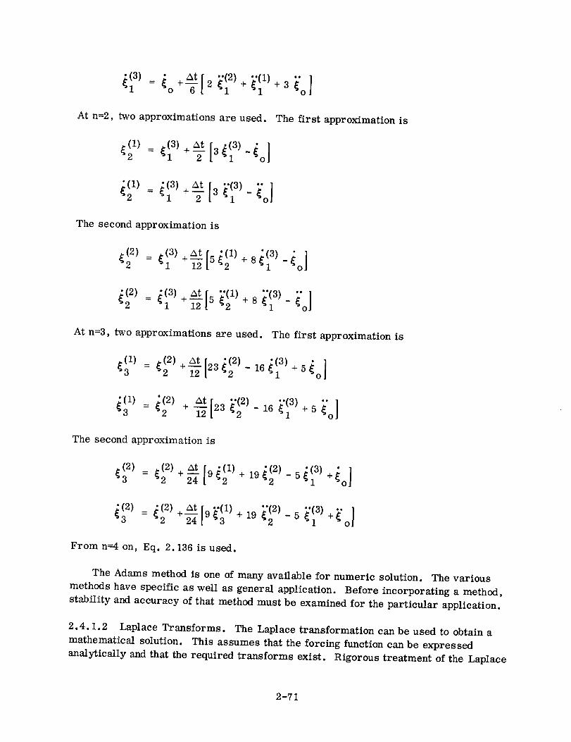
1 o _1 71
At n=2, two approximations are used.
2 _1 -1
The second approximation is
At n=3,
]+3_ o
The first approximation is
2 *i _-_ 5 +8 -72 *i o
_(_ = i(_ +_t[_ _.(_+__.(___.]2 *1 12 _2 _1 o
two approximations are used. The first approximation is
(31 (2)+ At [23_(2 ) 16_(3)+ 5_ ]) :_2 i-_ _2 - -1 o
3 2 _t -2 {1 + _ }'o
The second approximation is
(2) +_t [9 }.(1) + 19 }'(2)-5 }'(3) +_'o]
From n=4 on, Eq. 2. 136 is used.
The Adams method is one of many available for numeric solution. The various
methods have specific as well as general application. Before incorporating a method,
stability and accuracy of that method must be examined for the particular application.
2.4.1.2 Laplace Transforms. The Laplace transformation can be used to obtain a
mathematical solution. This assumes that the forcing function can be expressed
analytically and that the required transforms exist. Rigorous treatment of the Laplace
2-71

transformation is given in many textbooks. Refs 2.29 and 2.30 derive anddiscussLaplace transforms at length.
The Laplace transformation associates with a given function F(t) a second function
f(s) according to the relation
CO
-stf(s) = L IF(t)} = e F(t) dt
0
(2.137)
The inverse transformation is
F(t) = L-1 [f(s)} (2.138)
and simply means that F(t) is a function whose Laplace transform is f(s). A property
of the Laplace transformation which contributes greatly to its success in handling dif-
ferential equations is that the transform of the derivative can be expressed in terms
of the transform of the function itself, i.e.,
L[F'(t)_ = s L{F(t)} - F (0)
2L[F_I(t)] = s L{F(t)} -s F (0)- F'(0)
An example will now be worked out using Laplace transforms.
in Fig. 2.26 will be used and F(t) as shown in Fig. 2.27.
(2.139)
The system shown
The differential equation is
M_(t) +Kx(t) = F(t)
F (t)
F
Tt
Fig. 2.26. Spring Mass System Fig. 2.27. Force Time History
If the initial conditions are x (0) = 0 and x (0) = 0 the equation in the transform x(s) is
M s 2x(s) +Kx (s) = f(s) (2.140)
2-72

where f(s) is the transform of F(t).canbe written
2The natural frequency is o_ and K = M 0¢ so it
x(s) = f(s)M (s 2 + o_2)
Considering the time period 0 g t _ T then
Af(s) -
S
(2. 141)
and
x(s)A
Ms (s 2 + ¢o2)
Now
111 jlL = _ (1 - cos o_t)s (s 2 + o_2) cc
and it follows that
A
x(t) = -_ (1 - cos u_t) (2. 142)
If the response for the time period t > T is desired the solution with nonzero initial
conditions is needed. With the initial conditions of x(T) and _(T) Eq. 2. 140 becomes
[s_ 1M x(s)- sx(t) -_(T) +Kx(s) = f(s)
and Eq. 2. 141 becomes
s 2 +o_ s 2 +o_ s 2 +¢c
However, f(s) = 0 so the inverse transform is
x(t) = x(T) cos ¢c (t - T) + _(T___)sin u)(t - T)
2-73
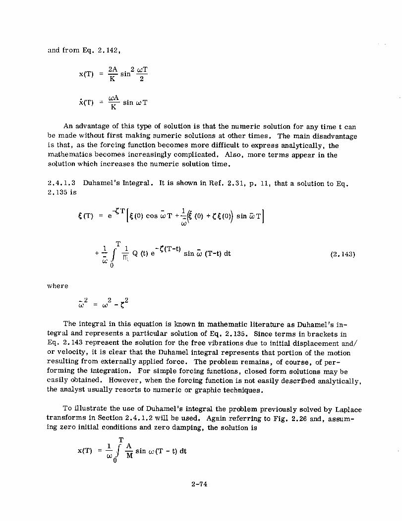
and from Eq. 2. 142,
2A . 2 coTx(T) - sinK 2
wA_(T) - sin u_T
K
An advantage of this type of solution is that the numeric solution for any time t can
be made without first making numeric solutions at other times. The main disadvantage
is that, as the forcing function becomes more difficult to express analytically, the
mathematics becomes increasingly complicated. Also, more terms appear in the
solution which increases the numeric solution time.
2.4.1.3 Duhamel's Integral. It is shown in Ref. 2.31, p. 11, that a solution to Eq.
2. 135 is
{(T) = e-_T[_(0)cos_T +1_ (0)+_(0))sin_T]
T1 1 -_(T-t)
+-- f -_ Q (t) e
0
sin _ (T-t) dt (2. 143)
where
_2 = c02 _ (2
The integral in this equation is known in mathematic literature as Duhamel's in-
tegral and represents a particular solution of Eq. 2. 135. Since terms in brackets in
Eq. 2. 143 represent the solution for the free vibrations due to initial displacement and/
or velocity, it is clear that the Duhamel integral represents that portion of the motion
resulting from externally applied force. The problem remains, of course, of per-
forming the integration. For simple forcing functions, closed form solutions may be
easily obtained. However, when the forcing function is not easily described analytically,
the analyst usually resorts to numeric or graphic techniques.
To illustrate the use of Duhamel's integral the problem previously solved by Laplace
transforms in Section 2.4.1.2 will be used. Again referring to Fig. 2.26 and, assum-
ing zero initial conditions and zero damping, the solution is
T
x,T) sA-_ sin co (T - t) dt
2-74

Expanding the sine function
x(T)
TA
- Ma_/ (sin
0
a_ T cos o_t - cos cc T sin cot) dt
Evaluating the integral and simplifying,
A
x(T) =_ (1-coso_T)
This checks with the solution obtained by using Laplace transforms.
2.4.2 VEHICLE RESPONSE. In the design and stress analysis of launch vehicles cer-
tain loads are required. In addition, the displacements of certain parts of the structure
are needed. The loads usually required (where applicable) are acceleration, bending
moment, shear, torque and force. These are calculated using mode displacement or
mode acceleration methods, modal quantities, and modal response. Some loads, such
as aerodynamic loads, increase due to displacement. This amplification of applied loads
is discussed in detail in Section 5 and is not considered here.
2.4.2.1 Mode Displacement Method. The deflection of a structure under load is the
summation of the deflection of each of its normal modes. Similarly, the loading or
stress in the structure is the summation of the load or stress in each of its normal
modes. Thus
k
= _ CinChYin = 1
k
M. = _ M. _n (2.144)1 inn=l
k
s.=Zs1 in n
n=l
In this method the rigid body loads and vibratory loads are obtained as a function
of the normal mode displacement. The advantages of the mode displacement method
are: 1) ability to handle steady-state and elastic response loads for redundant
structures, and 2) simplicity of computation. The first advantage is readily
apparent after examination of the mode acceleration method for redundant structures.
The mode displacement method can handle redundant structures as easily as nonre-
dundant structures. The second advantage is seen by Eq. 2. 144. Once the modal mo-
ments and shears have been calculated (a one-time operation) the computations are
quite simple. The disadvantage of the modal displacement method is a determination
2-75

of accuracy. Theoretically, all the modes are required to obtain correct shears and
moments. However, the summations of Eq. 2. 144 are actually summations of series
of which only the lower {frequency) modes significantly affect the total. The problem
is, then, to determine the number of terms (modes} needed for accurate results.
This is usually determined by trial and error.
2.4.2.2 Mode Acceleration Method. An alternate method of determining loads would
be separate calculation of the rigid body and vibratory loads. In this method the
vehicle is first treated as a rigid structure and shears and moments are determined
from the applied forces, external and inertial, on the vehicle in equilibrium. The
vibratory loads are then obtained from the inertial loads due to the acceleration of
the modes. The total loads would be
k M.
M :x 2 ni n= 1 o_
n
k SS. = S - E in
1 RB _ n
i n=l w n
(2.145)
The advantage of the mode acceleration method is high accuracy with few modes.
In this method the loads due to the rigid body response are calculated separately from
elastic response; hence their contribution (which is highly significant) is explicit. How-
ever, in the mode displacement method the loads due to rigid body response are im-
plicit in the loads due to elastic mode response. Since the load contribution of each
mode is much less for the mode acceleration method, far fewer modes are needed for
accurate results. The disadvantage of the mode acceleration method is the additional
computation required to obtain the rigid body loads, particularly with redundant struc-
tures. However, with present day computer capability this is not a serious problem.
The desirable feature of convergence with a small number of modes is often of more
importance than the computation time required for the rigid body loads.
2.5 RESPONSE TO TIME-VARYING FORCES WITH A CONTROL SYSTEM INCLUDED
The previous section discussed the response to time-varying forces for the case
where no attempt was made to control the vehicle as it responded. The solution will
now be expanded to show the inclusion of a control system.
2.5.1 GENERAL SOLUTION. The control system for a launch vehicle {typically re-
ferred to as the autopilot) usually controls the vehicle attitude with respect to some
frame of reference. While the position in space is all-important, other means (guid-
ance) are used to determine where the vehicle is and the proper maneuver to correct
2-76

the position. This results in commands to the autopilot to alter the vehicle attitude
and thus (assuming powered flight) to change its position in space. The autopilot must
also maintain the desired attitude and correct any errors due to external or internal
disturbances. Thus the autopilot has two functions: 1) to maintain vehicle stability
and attitude, and 2) perform the steering maneuvers prescribed by guidance.
The autopilot is usually described in block diagram form. The vehicle attitude
with respect to some axis is defined as 0, the control system coordinate as 5, and the
guidance command as 0 c. The general form of the autopilot is shown in Fig. 2.28.
The solution for the forced vibration response as given by Eq. 2. 135 is expanded to
include the control system. In matrix form this is
' I
li'] +f-i-t l+[-i--ll:I =I--i--t-1 l_t)l(2.146)
The upper left partitions are the coeffi-
cients of the equations for vehicle dy-
namics. The upper right partitions re-
present the effect of the control system
upon the vehicle and the lower left parti-
tions represent the vehicle input to the
control system. The lower right parti-
tions are the coefficients of the control
system dynamic equations. While the
discussion has been about a fairly specific
situation, i.e., launch vehicle with auto-
pilot and in powered flight, Fig. 2.28 and
VEHICLE [ O.DYNAMICS
CONTROL SYSTEMDYNAMICS
Fig. 2.28. General Autopilot Block
Diagram
Eq. 2. 146 are general forms applicable to any situation of a vehicle with a control sys-
tem. Once Eq. 2. 146 is set up the solution proceeds as discussed in Section 2.4.
2.5.2 EXAMPLE SOLUTION. To illustrate the above solution the case of a launch
vehicle subjected to a gust will now be solved. A schematic of the vehicle model is
shown in Fig. 2.29.
2.5.2.1 Derivation of Equations of Motion. The dynamic response is obtained by the
superposition of the rigid body and elastic responses. Use is made of rotating Eulerian
axes which coincide with the axes of the vehicle at any instant. Figure 2.30 shows the
position of the axes at times t and t + At. A time-slice analysis is used, i.e., mass
and trajectory parameters are considered constant.
2-77

Fig. 2.29. Gust Response Vehicle Model
Yt+At
Fig. 2.30. Rotating Eulerian Axes
a&_F = ma = nv-- =x x At
At-.0[ At ]In= [_' +0_]m_' m
_F = ma = m_-y y At
lim [Ay' AE}_IAte0 t At +"_='l
m = [_' +ex] m
_Mlira A_
At-. 0 At
Ge
81(2. 147)
2-78
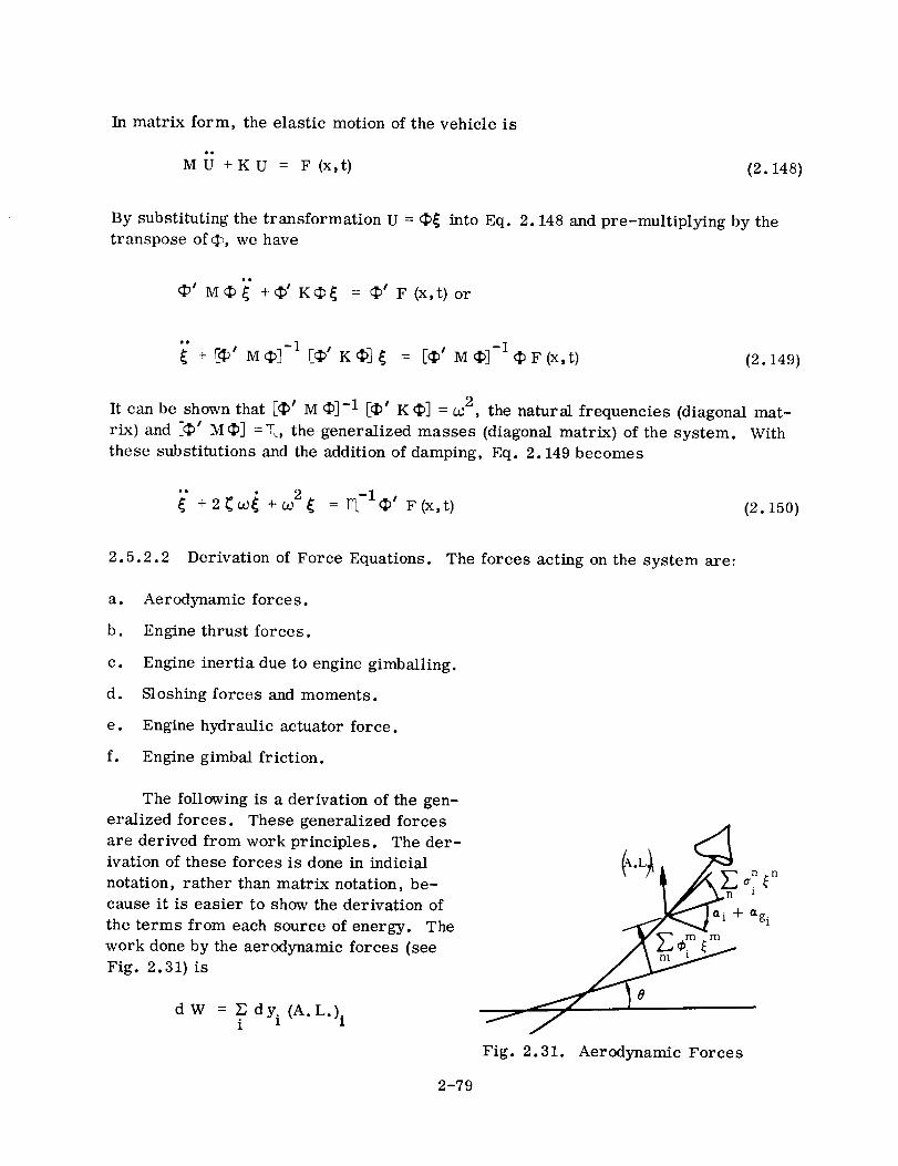
In matrix form, the elastic motion of the vehicle is
MU +KU = F (x,t) (2. 148)
By substituting the transformation U = _ into Eq. 2. 148 and pre-multiplying by thetranspose of_, we have
• ' M _) _" + _' K_ = _' F (x,t) or
_" + [_' M(_] -1 [_' K_]_ = [_' M_-l_F(x,t) (2.149)
It can be shown that [_ M _J-1 [_ K _] = ¢c2, the natural frequencies (diagonal mat-
rix) and E_ _ M_] =_, the generalized masses (diagonal matrix) of the system. With
these substitutions and the addition of damping, Eq. 2. 149 becomes
_" +2_0z_ +a) 2_ = _-1_, F(x,t) (2. 150)
2.5.2.2 Derivation of Force Equations.
a. Aerodynamic forces.
b. Engine thrust forces.
c. Engine inertia due to engine gimballing.
d. Sloshing forces and moments.
e. Engine hydraulic actuator force.
f. Engine gimbal friction.
The following is a derivation of the gen-
eralized forces. These generalized forces
are derived from work principles. The der-
ivation of these forces is done in indicial
notation, rather than matrix notation, be-
cause it is easier to show the derivation of
the terms from each source of energy. The
work done by the aerodynamic forces (see
Fig. 2.31) is
d W = ._ dy i (A.L.)i1
The forces acting on the system are:
2-79
JjFig. 2.31. Aerodynamic Forces

dW= qSR_d[ yl+i (xi-_) e+_mcm_m]
(2.151)
where ff is the center of gravity on the x axis. The generalized forces are:
+_ +z _ {ndy_ = qSRi_ N/0_ i
dW -x CN/t_ i+t_ +_ a. _nd e - qSR i_ xi gi n 1
d_m - qSR • i gi n i
where
(X'v') ]i _n
(_i = - + -
The work done by the thrust force of the booster engines (see Fig. 2.32) is
dW= FBdY
(2.152)
(2.153)
The generalized forces are
dW
dy _
dW
de
dW
m
d_
n _n__]_[_ _
_ n _n_6_](xr
- TB aEB xT
2-80
(2.154)

Fig. 2.32. Engine Thrust Forces
For the generalized forces due to the sustainer engine, substitute subscript S for B inI
the above equations. Since the sustainer engine is not gimballed, 6 S = O.
For purposes of autopilot control, the motion of the engine is comprised of two
functions. The first, _n a_B _n, represents the motion of the engine associated with
the modes of vibration when the control system is locked. The other, 6 e, repre-
sents the gimballing control with respect to these modes° For analysis, the system is
assumed to have a perfect actuator and is later compensated for its structural elastic-
ity, bypass orifice characteristics, etc. The work done by engine inertia is
dW = -mEB[(y" +VS)+(XEB -x) 0" +_n CEBn _'n
xd[y' +(x -x)O+E m _m 6']EB m CEB + LEB
m
-IEBIg+Gn nO'EB%'n- 6"']dlS+_O'EB{m-6 '1
+ LEB 6"']
[ (x) ]m= -m (y' +Ve) + __ }. +G n _'n+ 6 SEBd {m EB EB n CEB LEB
n mn aEB (;EB(2. 155)
All the terms except 6" can be placed on the left side of the equations and according to
the orthogonality principle, the n _ m terms will cancel and the n = m terms will be-
come part of the generalized mass. This generalized force then becomes
2-81

dw md_m B°'EB -mEB
LEB CEB
dW [ • n _.n+d-"_ = -mEB LEB ( _' +V0) + (XEB -x) 0"+_ CEB LEBn
nB n (fEB -
(2. 156)
Moving the 6"' terms to the left side of the equation results in
IR6" + ..... mEB LEB[ (y'+V_)+{xEB-_) _ +_nn _EB _'n]
+-['_ +_ n _'n]IEB n ffEB(2. 157)
where
= +IR B mEB LEB
Although the actuator is described by a linear equation in this program, the system is
nonlinear. Linearization of the 6', 6 ' , and 6 c coefficients is discussed in Section
2.5.2.3.
The sloshing analogy used is the spring-mass analogy. The slosh loads consist
of a lateral force applied at the spring attach point, and a moment applied at the equiv-
alent tank bottom (Fig. 2.33).
9
x*0
Fig. 2.33. Slosh Loads
2-82

The work doneby the slosh forces is
dW = EF dy sS S
= EK z d[ECm_ ms s s [m s
dW m
-EK z Csd_ m s s s
dWdO - EK z (x s -_)
S S S
dW, -EK z
dy s s s
+y' + (x s
(2. 158)
The work done by the slosh moments is
._.dW =E xm
S S
z +MS S Zsl omsm+°1
'2dW -E xm
d_ m s s
z +MS S mS S
dw s[XmzdO s s s s
(2. 159)
The pressure PL developed by the actuator times the actuator piston area supplies the
force to gimbal the engine. The work done on the engine (see Fig. 2.34) is
dW = (PLAR) dS'
dW PL AR 160)---7 = (2.d6
d W _ dW _ dW
d_m dO dyT = 0
because 6 ' is measured relative to the
vehicle.
L A = FO:CE
Fig. 2.34. Engine and Actuator Model
2-83
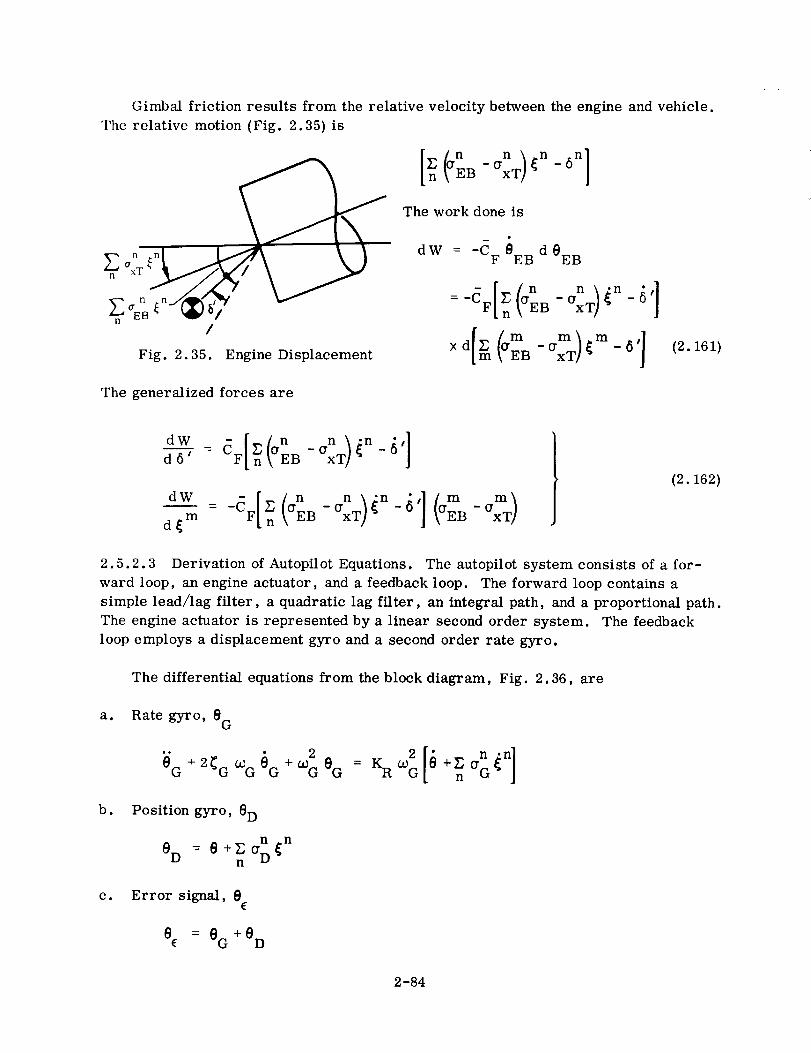
Gimbal friction results from the relative velocity betweenthe engine and vehicle.The relative motion (Fig. 2.35) is
_ [_n(aEB - Or:T){n - 6nl
The work doneis
_n a*r ! dW = -CF _EB d 0EB
_n a:s}n_b '_/ _ =-CF[_(aEB-axnT)_n-6 ']
Fig. 2.35. Engine Displacement ffxTEB - 6 (2.16I)
The generalized forces are
dW
d6'
dW
d_ m
(2.162)
2.5.2.3 Derivation of Autopilot Equations. The autopilot system consists of a for-
ward loop, an engine actuator, and a feedback loop. The forward loop contains a
simple lead/lag filter, a quadratic lag filter, an integral path, and a proportional path.
The engine actuator is represented by a linear second order system. The feedback
loop employs a displacement gyro and a second order rate gyro.
The differential equations from the block diagram, Fig. 2.36, are
a. Rate gyro, e G
b. Position gyro, OD
8D = e+_O.D _nn
c. Error signal, eE
e = eG + eD
2-84

22_cOJc s ÷ a¥
KRW G s
2s2* 2_G_GS+_ G
VEHICLE
f(_ ,e) [RESPONSE J--
2w T
+ 2 (T _,'T
d. Feedback signal, OF
el
Fig. 2.36. Autopilot Block Diagram
fG
rlead0 +e¢ = rlag0F +eF
Engine actuator command signal, 5C
2 [ 20F5" +2_ a_ 5 +w 6 = -i A CccC C C C C C + KI _c2c _ eF dt]
Engine actuator response, 5 *. The engine actuator equation for engines-in-the-
modes model is
n n / n2 2 _ 2 KE _ axTB (r5' +2 _T _'r _ + _T 5' = ¢_T 6c U_T n - EB
- ( ( - .) ooCF n gEn n _n_ 1 _ mEB LE BCEB_ IEBIR _n axTB-aE IR n
LEB mEB(2. 163)
2-85

where
%K E -
KD+K H
57.3 CF
2
_cN
(AR)2 q_L
1.11 h CL
_/K 2_CT = C °2N
2 _T COTC -
T 2oo T
Since the above terms are frequency and amplitude dependent, they have been linearized
to the frequency of the gust, i e., _ = 2_t/_" _, and to a large engine amplitude, say- - " gust
= 1.0 degree. C F and PL are calculated as follows:
4 CB 2 C B rgus tCF = Cv + - - Cv _
_'_6 _t2_
27r6
I_L = CF ARtgust
(2. 164)
2.5.2.4 Complete Equations. The complete equations, assembled from Sections
2.5.2.1, 2.5.2.2, and 2.5.2.3, are given by Eq. 2.165. These can be put in the form
of Eq. 2. 146 and solved. The forcing function in this case is the angle of attack in-
duced by the gust, t_g.
2-86

thm Elastic Mode
_m,,m ;ml_m{_n,.0,]_'m + 2_m¢C +w -m m EB CxTB _EB
m[_nn lI _ - m]_',+ TES CxTS (rES _n _ mEB LEB _EB - IEB (_EB
q
+_ +Eft. +E m zi i gi n * s s
+Ms s
s s s s EB -axT n aEB-axTB _n
Rotation
-[mEB LEB(XEB-X)-IEB]6" +qSRi _ [(CN/0t)i((_i+_g i
n")<x, Ix+_ _. { - +_ mn * s s
z +Ms s ZsJ s s
Tr ansi ati on
,1 / T E n+ V8 M T TB °'EB S n- aES - mEB LEB
Sloshing
s
+qSRI_ +_ +_a. _ +_ K zi N/¢_ i gi n 1 s s s
2+0_ z =-
+ 2_s u_ s s s s (y' + V{9) + (xs -.x) 0 +_n ¢n _.n]s
(2. 165)
2-87

Engine Output
+mEBLEB' '+[mE LEB(xEB-Engine Command
2 [ 20F5"c +2_c02c _c +O_c5c = KA ¢Cc
Rate Gyro
[ ]eG 2 2 n+ w G + 0 G = KR_ G e+_O'G _n_'G 2_G COG n
Position Gyro
OD = O+_aD _nn
(2.165
Contd)
2.6 RANDOM RESPONSE
The analysis presented here is from the field of endeavor referred to as generalized
harmonic analysis. This subject is treated in many texts and articles. Crandall (Ref.
2.32) gives a comprehensive bibliography of the material published prior to 1959. Refs
2.33 through 2.38 are a partial list of the more recent material. Lee (Ref. 2.33) gives
a complete discussion of the general theory of harmonic analysis. The monograph by
Crandall and Mark (Ref. 2.34) covers the subject as applied to mechanical systems.
The subject is also often covered in texts or handbooks on control and/or servomechanisms,
The fundamental difference between deterministic analyses and those involving
random variables is that instantaneous values are no longer meaningful. When a sys-
tem is being excited by randomly varying forces, it follows that its response will also
vary in a random manner. Consequently, a statistical description of the excitation is
required in which expected values of response replace the usual instantaneous time
values. The analysis is quite complicated in its general form. As a result, certain
assumptions are made which, although not strictly true, are required to permit analysis.
2-88

These assumptions are that the excitation is an ergodic process and that its amplitudehas a normal or Gaussiandistribution. The first assumption merely states that thetime average of the excitation is equal to the statistical average and dependentonlyuponwhere it is measured. The secondassumption of normal distribution is one oftenmadeto aid in interpreting the results and as a requirement for application of somestatistical techniques. A brief review of the analysis follows; the reader is directedto various references for proofs andderivations.
Consider a random process described by the time function uk (t), where the sub-script k is used to denote one experiment in a large number of identical experiments ofthe same random process. The statistical or "ensemble average" is defined as
N1u (tl) =--_ k___luk(tl)
(2. 166)
which is also called the mean. The u k (tl) is the value of the k th ensemble member at
an arbitrary time t 1. The amplitude probability density of u may also be determined
at time t 1. If the amplitude probability density of the ensemble is independent of time
t 1, then the process is said to be stationary.
More often than not, the data available for analysis consist of a few samples, rather
than a large number, and the ensemble average is not meaningful. The averaging may
be carried out in time in this case, rather than across the small ensemble. The time,
or temporal, average of an ensemble member is
limit 1 f t +TO
{_k (t) = T -_ _ _-_ J u k (t) dt (2. 167)
t -TO
w
If the process is stationary, then uk(t ) is independent of t o. If the amplitude probabilitydensity of the ensemble member is the same as that of the ensemble, then the process
is also said to be ergodic and u k (tl) = u k (t). Thus, an ergodic process is, by defin-
ition, stationary, but a stationary process is not necessarily ergodic. It can be seen
that by making the ergodic assumption the analysis can be performed over the ensemble
or over an ensemble member with equal validity. It will be understood that the re-
mainder of the discussion covers only ergodic random processes.
A statistical quantity of considerable importance is known as the autocorrelation
function and is defined as
T
limit 1 -_T_kk (r) = T -_ co 2-T u k (t) u k (t + "r) dt (2. 168)
2-89

which represents multiplying the value of the function at a time t by its value at a time
_" later, integrating the result, and averaging. It can be seen that the autocorrelation
function is independent of t and is a function of the time lag _" only. For zero lag time,
Eq. 2. 169 reduces to the mean-square value,
limit 1 f T 2_bkk (0) = U2k(t) = W-_ _ _-_j u k(t) dt (2. 169)
-T
Another useful quantity related to the correlation function by means of the Fourier
Transform is the power density spectrum, defined as
_ 1 /_ -ioJr_kk (02) 2_r _bkk (_') e dr (2. 170)
and the inverse relationship,
_kk if) = f _kk(Cc) e i02r dw--CD
(2.171)
This relationship is known as the Wiener Theorem of autocorrelation, or Wiener-
Khinchin Theorem (see Ref. 2.33, Chapter 2). If we now set T = 0, Eq. 2. 171 becomes
GO
2 / _kk_bkk (0) = u k(t) = (o_)dcc (2". 172)
or the mean-square value.
A useful relationship, proved in Ref. 2.32 (p. 333), between the response and
excitation power spectra for any linear system is
_out in(02) = Hk (02) Hk (02)¢_kk (02)kk
or
(2.173)
_out 2 inkk (02) = [ Hkk ( 02)[ _kk (02)
where H (02) is the complex frequency response and I_ (co) is the conjugate. H (02) is a
general expression for the relationship between input and output and must be defined in
detail for specific cases. For example, the displacement response spectrum of a linear
single-degree-of-freedom system to an ergodic random force spectrum is (Ref. 2.34,
p. 73 - 75)
2-90

_in_out (co) = (co) (2.174)
_2[( u2 -¢c2) 2 +4_2 W2n¢c2]
where wn is the system's natural frequency, m its mass, and _ the damping ratio. It
is easily seen that the denominator is the absolute value of the square of the complex
impedance, Z (w), and that
IH (cc)12 = 1 (2.175)
[z
The general case for the response of a multidegree-of-freedom system is discussed
next.
It is now necessary to consider another property of the excitation, the continuity
of its distribution in space. If the random force f (x, t) can be separated such that
F (x, t) = g (x) f (t), then the field is homogeneous. This means that when there is a
change in force at x i, there is a simultaneous proportional change at xj. This isanalogous to the stationary property in time. If the spatial distribution is not deter-
minable, then the field is inhomogeneous and its is necessary to determine the statis-
tical relation of happenings between all points on the system under consideration.
The required statistical properties for inhomogeneous fields are the crosscor-
relations and cross-power density spectra. The crosscorrelation function _)ij (T)between a random process occurring at point i in space and a different random process
occurring at point j in space is defined as
limit 1 jfT T_ij (r) = W-+ _ _ ui(t)uj (t+T) dt (2.176)m
which represents taking the value of the function at point i at time t, multiplying by the
value of the function at point j at a time r later, integrating the result, and averaging.
Applying the Wiener-Khinchin Theorem,
_ 1 /o_ -iwT<_ij(co) 2rr _ij (7")e dT (2.177)
The cross-power density spectrum (i _ j) is, in general, a complex quantity, of which
the real part is referred to as the co-spectrum and the imaginary part is called the
quadrature spectrum. The inverse transform relations between the crosscorrelation
and cross-power spectra are
2-91
co
- i/_ij_ij (oo) 2 rr_
-i_Tif) e d 1" (2. 178)
co
f_ iccTaij (r) : ij (co) ew_
d _c (2.179)
Taking all combinations of ij for the system under study, a matrix of cross-power
density spectra can be formed. This matrix, [_ij],. is of a Hermitian form which
contains real terms (power spectra) on the diagonal and complex terms (cross-power
spectra) on the off diagonals. It can be shown (Ref. 2.33, p. 74) that
$ij (r) = Sji (-'r) (2. 180)
so that from Eq. 2. 179,
_ji (w) = _'*'1] (u_) (2. 181)
where the asterisk indicates the conjugate transpose of_ij (_c). Consequently, the
matrix E_ij _ is symmetric in the real parts and skew symmetric in the imaginaryparts. Eq. 2. 173 is now written in the more general form,
_out _)in I_jij (w) = H.I (w) ij (w) (w) (2. 182)
which gives the response spectrum at point i due to an excitation at point j. It is
obvious that the cross-power density spectrum of the response must be derived for all
points in the system.
Botman (Ref. 2.36) has derived the integral and matrix forms for the response of
a mechanical system to an inhomogeneous field. Since the integral form is only ap-
plicable to systems for which all_ij (w) are known analytically, and this is not theusual case, only the matrix form is presented here.
Assuming that the excitation is homogeneous in the interval x i - _ to x i + E, theresponse power spectra matrix for a lumped parameter system is given by
[_iTt(w)] = [_n][Tnt[¢iJ(_ [7jm ] [_m](2. 183)
The Z n and Z m are the complex impedance and transpose, and the _ni and Vjm are themode participation factors, given by
2-92

nl
xi+ 1 - x. 1
X.1 - xi-I
xj+ 1 - x.j
TJ m = / 2
X° --
J Xj_l
2
(x) dxn
Cm (x) dx
(2. 184)
where the ¢(x) are the normalized mode shapes.
By equating
Eq. 2. 183 is rewritten as
[(_icjut (w_ = [t_ni (02] [_)ii_ (02_ [Hjm (02)] (2. 185)
This equation is the matrix extension of the simple relation (Eq. 2. 173) between the
input spectra, the system impedance, and the response spectra.
A representative plot of the response spectrum for point i due to an excitation
spectrum at point j is shown in Fig. 2.37.
¢'4
i l 1 1_) O0 50 O0
1 2 3 4
¢o (rps)
a. Response Spectrum
l-i
._ _:_
_(rps)
b. Input Spectrum
Fig. 2.37. Response and Input Spectra
2-93
It will be found that the peaks in the response spectrum correspond to system naturalfrequencies. The quantity
2of _out
(t) = Wn_P.. (o_) dce (2.187)uij U
represents the contribution of all frequencies less than 0¢n to the mean-square response.
By extension, the mean-square response at point i to excitation at all points on the
system is
u 2 u 2 (t)i (t) = _ ij
(2.188)
Theoretically the integration would have to be extended to infinity to obtain the
mean-square response, but for practical cases the contribution of the power spectrum
to the mean-square value becomes negligible at higher frequencies. For lightly damp-
ed systems, the energy content of the power spectrum is concentrated mainly about the
natural frequencies and falls off sharply to very low magnitudes between them.
The matrix multiplication of Eq. 2. 182 is required for a considerable number of
frequencies to obtain a smooth curve such as shown in Fig. 2.37 for each point. Con-
sequently, it would probably be best not to use a constant interval for the w's but
rather a small interval near resonant frequencies and a considerably larger one be-
tween them.
The above discussion has presented the general form for the solution of mean-
square response. In practice, further assumptions are often made which can greatly
simplify the solution. Ref. 2.37 contains an excellent example of this. In this case
the damping is small so the impedance will undergo a large change near the resonant
frequency ¢Cn; and if the variation in the power density spectrum is of lesser extent inthis vicinity, then the mean-square response can be approximated by
Din( w 2 ¢2"2" _r °_n) n n
u (t) = 2--_-_ _2 3n o3n n
(2. 189)
where w n is the mode participation of the load and is given by
Wn
L _)in (°°n' xi ) Cn (xi) dx
0
L
f Din (o_a, xi) dx0
2-94
It now remains to attach statistical significance to the mean-square response. Theassumption of a normal (or Gaussian)probability distribution is quite reasonable for arandom function. The normal probability density function is given by
f (x) = exp - _<x< _ (2. 190)
r 2_ 2
where r is the random variable, x is the range of the variable, # is the mean, and (_2
is the variance. The mean and variance are given by
= x (t) (2. 191)
2 2 m= x (t) - x (t) (2. 192)
(See Eqs 2. 167, 2. 168, and 2. 188). The cumulative distribution is given by
fY 1 [-(x _)21P (y) = _ exp (2.193)
r __o 2_ 2
which states that the probability of r being equal to or less than y is Pr(Y)"sub stitution
If the
is made in Eqs 2. 190 and 2. 193, the density function and cumulative distributions are
normalized, which is the form usually found in tables.
If the excitation has zero mean, then so will the response. In this case, the
variance is
2 2_. = u. (t)
1 1
The standard deviation of the response is the square root of the mean-square
response, or
ei = (t) (2. 194)
Eqs 2. 190 and 2. 191 can now be used to establish the response corresponding to the
desired probability. For a particular case, data may indicate another probability
2-95

distribution to be more applicable. In that event the expressions for the appropriatedistribution are used in place of Eqs 2. 190and 2. 191. Discussion and information onprobability canbe found in anyhandbookor textbook on the subject.
2.7 REFERENCES
2.1 R.H. Scanlanand Robert Rosenbaum, Introduction to the Study of Aircraft
Vibration and Flutter, The Macmillian Company, New York, N. Y., 1951.
2.2 N.O. Myklestad, Fundamentals of Vibration Analysis, McGraw-Hill Book
Company, New York, N. Y., 1956.
2.3 W. T. Thomson, Mechanical Vibrations, Prentice-Hall, Inc., Englewood Cliffs,
N. J., 1953.
2.4 R.A. Bisplinghoff, H. Ashley, and R. L. Halfman, Aeroelasticity, Addison-
Wesley Publishing Company, Reading, Mass., 1955.
2.5 F.I. Backus, SLV-3 Bending Stability Analysis of the Atlas/Agena Spring Band
Separation Joint, Convair Division Report GD/A-DDE64-054, 17 August 1964.
2.6 D.O. Lomen, Liquid Propellant Sloshing in Mobile Tanks of Arbitrary Shape,
NASA CR-222, Marshall Space Flight Center, Huntsville, Alabama, April 1965.
2.7 D.O. Lomen, Digital Analysis of Liquid Propellant Sloshing in Mobile Tanks
With Rotational Symmetry, NASA CR-230, Marshall Space Flight Center,
Huntsville, Alabama, May 1965.
2.8 J.T. Bergen, Visco-Elasticity Phenomenological Aspects, Academic Press,
1960.
2.9 D.R. Bland, Theory of Linear Viscoelasticity, Pergamon Press, 1960.
2.10 R. K. Gieseke, B. Appleby, and W. Tonelli, General Missile Vibration Program,
Convair Division Report GD/A-DDE64-050, 20 August 1964.
2.11 S. Timoshenko and G. L. MacCullough, Elements of Strength of Materials,
D. Van Nostrand Company, Inc., Princeton, N. J., 1949.
2.12 R. G. Rose, J. A. Staley, and A. K. Simson, A Study of System-Coupled
Longitudinal Instabilities in Liquid Rockets, Part I -Analytic Model, AFRPL-TR-65-163, AFSC, Edwards, California, September 1965.
2-96
2.13 L. L. Fontenot and G. Lianis, The Free Vibrations of Thin Elastic Pressurized
Cylindrical Shells with a Free and Incompressible Liquid Having a Free Surface,
International Symposium on Space Technology and Science, Paper No. 6-6-8,
1963.
2.14 R. G. Rose, Dynamics of the Atlas 5-CPS Longitudinal Oscillation Following
Launch as Related to the Tank Pressure Regulation System, Convair Division
Report GDA63-0712, Volumes I and H, Contracts AF 04(694)-196 and AF 04
(695)-240.
2.15 S. Timoshenko, Theory of Plates and Shells, McGraw-Hill Book Company,
Inc., First Edition, 1940.
2.16 J. D. Wood, Survey on Missile Structural Dynamics, Report 7102-0041-NU-000,
Contract No. AF 04(647)-619, 1 June 1961.
2.17 M. J. Turner, R. W. Clough, H. C. Martin, and L. J. Topp, "Stiffness and
Deflection Analysis of Complex Structures", Journal of the Aeronautical
Sciences, Vol. 23, No. 9, September 1956.
2.18 L. D. Pinson, Longitudinal Spring Constants for Liquid-Propellant Tanks with
Ellipsoidal Ends, NASA Technical Note D-2220, November 1964.
2.19 W. H. Gayman and J. A. Garba, Dynamics Loads Analysis of Space Vehicle Systems -
Launch and Exit Phase, JPL Technical Memorandum 33-286. (To be published.)
2.20 W. C. Hurty, Dynamic Analysis of Structural Systems by Component Mode
Synthesis, TR 32-530, Jet Propulsion Laboratory, Pasadena, California,
January 1964.
2.21 R. E. Storey, "Dynamic Analysis of Clustered Boosters with Application to
Titan III", AIAA 1963 Summer Meeting, Paper No. 63-208, June 1963.
2.22 Bodley, Ikard, and Schulta, Vibration Analysis Report, Program 624A, Con-
fisxlration C, Flight Plan VIII, Air Force Report No. SSD-CR-65-1, January1965.
2.23 I. J. Jaszlics, Program 624A 20%-Scale Dynamic Model Ground Vibration
Survey, Final Test Report, Vol. III, SSD-CR-65-47, Martin Company, Denver,
Colorado, May 1965.
2.24 J. L. Milner, Three Dimensional Multiple Beam Analysis of a Saturn 1 Vehicle,
NASA TM X-53098, July 1964.
2-97

2.25 G. Lianis, Matrix Analysis of Vibrations of Clustered Boosters, Convair
Division Report AE61-0858, September 1961.
2.26 S. I. Gravitz, "An Analytical Procedure for Orthogonalization of Experimentally
Measured Modes", Journal of the Aerospace Sciences, November 1958.
2.27 E. Bodewig, Matrix Calculus, North Holland Publishing Co., Amsterdam, 1959.
2.28 V. N. Faddeeva, Computational Methods of Linear Algebra, Dover Publications,
N. Y., 1959.
2.29 R. V. Churchill, Operational Mathematics, McGraw-Hill Book Company, Inc.,
New York, 1958.
2.30 R.E. Gaskell, Engineering Mathematics, Henry Hold & Co., New York, 1958.
2.31 H. N. Abramson, The Dynamics of Airplanes, The Ronald Press Co., New
York, 1958.
2.32 S. H. Crandall, '_Random Vibration", Applied Mechanics Reviews, Vol. 12,
No. 11, pp. 739 -742, November 1959.
2.33 Y. W. Lee, Statistical Theory of Communication, John Wiley and Sons, Inc.,
New York, 1960.
2.34 S. H. Crandall and W. D. Mark, Random Vibration in Mechanical Systems,
Academic Press, New York, 1963.
2.35 S. H. Crandall, editor, Random Vibrations, Technology Press of M.I.T.,
1958, Vol. II, 1963.
2.36 M. Boteman, "The Response of Linear Systems to Inhomogeneous Random
Excitation", AIS Paper No. 61-32, IAS 29th Annual Meeting, New York,
January 23 - 25, 1961.
2.37 W. T. Thomson and M. V. Barton, "The Response of Mechanical Systems to
Random Excitation", Journal of Applied Mechanics, Vol. 24, pp. 248 -251,
June 1957.
2.38 J. S. Bendat and A. G. Piersol, Measurement and Analysis of Random Data,
John Wiley and Sons, Inc., New York, 1965.
2.39 V. L. Alley, Jr. and A. H. Gerringer, A Matrix Method for the Determination
of the Natural Vibrations of Free-Free Unsymmetrical Beams With Application
to Launch Vehicles, NASA TN D-1247, April 1962.
2-98

3/ GROUNDWIND INDUCEDLOADS
3-1


A
C
CC
CDG
C v
D
D(x)
K
L
rn n
Na
I
(Mb) 1
Mn
Pr ( )
Re
S
SD(f)
SL(f)
SDL(f)
V
Area
Damping
NOMENCLATURE
Critical damping
Aerodynamic drag coefficient for gusts
Vortex shedding coefficient
(see Eq. 3.15)
Reference diameter
Diameter
Coefficient, defined in text
Vehicle length, support to tip
Generalized mass for the nth natural mode
of the vehicle
Generalized mass of the fluid media,
defined as DD 3
Modal bending moment of the first natural
mode of the model
Bending moment at model base
Probability of the statement ( ) being true
Reynolds number, VDp/D
Strouhal number, fD/V
Power density spectrum of the gust velocity
in the drag direction
Power density spectrum of the gust velocity
in the lift direction
Cross-power density spectrum for the gusts
Wind speed
ft 2
lb-sec
ft
lb-sec
ft
ND
ND
ft
ft
adjustable
ft
slugs
slugs
in.-Ib
ft
in. -lb
ft
N.D.
N. D.
N, D,
(ft/sec) 2
cps
(ft/sec) 2
cps
(ft/sec) 2
cps
if/see
3-3

Ve
V01)
V
2V
V R
V_7
n
a
f
h
h R
q
U
x
Uniform wind speed equivalent to a non-uniform
profile wind (see Eq. 3.13)
Wind profile (see Eq. 3.1)
Mean wind speed
Mean-square wind speed (see Eqs 3.9
and 3.11)
Mean (or average) wind speed at the reference
height
Mode participation of the load for the nth mode
J_L 12 D V2(x) _n (x) D(x) dx
2 0V2(x) D(x) dx
Ratio of the standard deviation of the random
drag load to the standard deviation of the
random lift load, (YDT/(_LT
g I
Distance between vortices in the Von Karman
Vortex Street
Frequency
Height above ground
Reference height
Gust wave length, VR/f
Dynamic pressure
Displacement
Coordinate along neutral axis
Power density spectra of the square of the
gust velocity (see Eqs 3.10 and 3.12)
ft/sec
ft/sec
ft/sec
(ft/sec) 2
ft/sec
No D,
No Do
ft
cps
ft
ft
ft
lb/ft 2
ft
ft
4(ft/sec) /cps
CD
E L
Expectation value of the random drag response
Expectation value of the random lift response
ft
ft
3-4

¢
P
CrDG
aLG
aDT
_LT
#n(x)
D
e
G
L
max
n
R
S
T
V
1
Damping coefficient
Dummy frequency variable
Absolute viscosity
Density
Standard deviation of the gust velocity
in the drag direction
Standard deviation of the gust velocity
in the lift direction
Standard deviation of the random drag response
Standard deviation of the random lift response
thNormalized displacement of the n mode
Frequency
SUBSCRIPTS
Drag
Equivalent
Gust
Lift
Maximum or "3-sigma" value
Mode index
Reference
Steady state
Total
Vortex shedding
First mode
3-5
N, D,
cps
lb-sec/ft 2
slugs/ft a
ft/sec
ft/sec
ft
ft
ft/ft
rad/sec

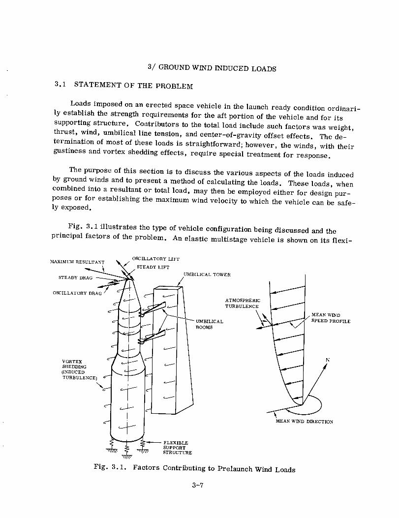
3/ GROUNDWIND INDUCEDLOADS
3.1 STATEMENT OF THE PROBLEM
Loads imposed on an erected space vehicle in the launch ready condition ordinari-ly establish the strength requirements for the aft portion of the vehicle and for itssupporting structure. Contributors to the total load include such factors was weight,thrust, wind, umbilical line tension, and center-of-gravity offset effects. The de-termination of most of these loads is straightforward; however, the winds, with theirgustiness and vortex sheddingeffects, require special treatment for response.
The purpose of this section is to discuss the various aspectsof the loads inducedby groundwinds and to present a method of calculating the loads. These loads, whencombined into a resultant or total load, may then be employed either for designpur-poses or for establishing the maximum wind velocity to which the vehicle canbe safe-ly exposed.
Fig. 3.1 illustrates the type of vehicle configuration being discussed andtheprincipal factors of the problem. An elastic multistage vehicle is shownon its flexi-
OSCILLATORY LIFT
MAXIMUM RESULTANT
STEADYD _R_
OSCILLATORY DRAG "
VORTEX
SHEDD_G
(INDUCED
TURBULENCE)
_J/ STEADY LIFT
UMBILICAL TOWER
/
ATMOSPHERIC
TURBULENCE
UMBILICAL
BOOMS
FLEX_LE
SUPPORT
STRUCTURE
MEAN WIND
SPEED PROFILE
N
MEAN WIND DIRECTION
Fig. 3.1. Factors Contributing to Prelaunch Wind Loads
3-7

blc support structure, with umbilical lines connectedfrom the umbilical tower. Thewind velocity is represented by the profile of the meanwind and its direction azimuth,uponwhich are superimposed the horizontal componentsof the random turbulence nor-mal andparallel to the meanwind. Turbulence generated by the flow about the umbili-cal tower andthe vehicle is indicated by vortex shedding. The response of the vehicleto the mean andturbulent componentsof the wind is composedof a mean (steady)de-flection plus oscillatory motion. Thesedeflections can have componentsparallel andnormal to the meanwind direction. The directions parallel and normal to the meanwind are analogousto the drag and lift directions on an aerodynamic surface and here-after are referred to as such.
It must be pointedout that the discussion and analytical techniques that follow aregenerally applicable only to those vehicles for which wind tunnel data are available.The effect of nose shape, external piping, and protuberances is such that the vortexsheddingmay vary by large amounts due to changeswhich, at first glance, might beconsidered negligible. For example, it has been shown(Ref. 3.1) that the addition ofa single conduit with a diameter of 1/60 of the vehicle diameter can increase the vor-tex sheddingresponse by a factor of three whenthe conduit is at the upstream stagna-tion point on the lower stage. It is apparent that small protuberances cannot be ig-nored, especially if they are on the forward end. While the current state of the artdoes not provide for analytical prediction of the effect of changesin nose shapeor pro-tuberances, wind tunnel data provide for a qualitative evaluation of relative severityof configurations.
3.2 HISTORICAL BACKGROUND
The method of treating groundwind induced loads has followed a somewhatdevi-ous route in its developmentto its current state. Methodshave varied from consid-eration of only steadydrag to treatments using multipoint random pressure input.While civil engineers have beenconcernedfor years with the effect of wind on an elas-tic body, especially since the collapse of the Tacoma Narrows Bridge, this effect wasnot fully investigated for missiles until Goldman's investigation for the Vanguard (Ref.3.2). Since that time, wind tunnel tests have beena part of the developmentprogramof nearly all launchvehicles.
Following identification of the vortex sheddingproblem during the Vanguardtests,several programs were initiated to obtain useful data. These included the literaturesurvey by Midwest Research Institue (Ref. 3.3), which effectively summarized theliterature published prior to 1958; the two dimensional cylinder tests of Fung (Ref.3.4); the work of Roshko(Ref. 3.5); and a rather comprehensive test program at theNASAAmes Research Center 12-Foot Pressure Tunnel.
Publication of Fung's work in 1960led to several approachesfor predicting thevortex sheddingloads onexisting vehicles. Oneof the most prevalent approacheswas
3-8
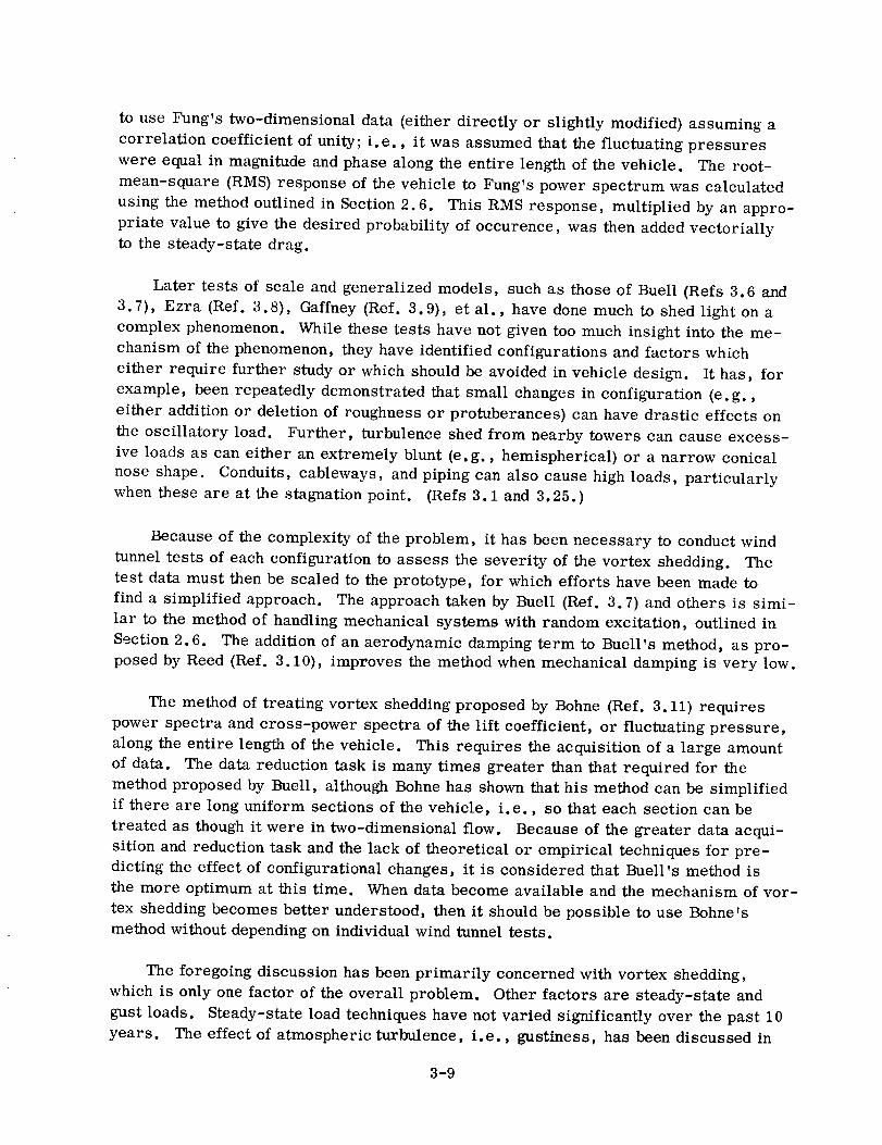
to use Fung's two-dimensional data (either directly or slightly modified) assuming acorrelation coefficient of unity; i.e., it was assumedthat the fluctuating pressureswere equal in magnitude and phasealong the entire length of the vehicle. The root-mean-square (RMS)response of the vehicle to Fung's power spectrum was calculatedusing the method outlined in Section2.6. This RMSresponse, multiplied by an appro-priate value to give the desired probability of occurence, was then addedvectoriallyto the steady-state drag.
Later tests of scale and generalized models, suchas thoseof Buell (Refs 3.6 and3.7), Ezra (Ref. 3.8), Gaffney (Ref. 3.9), et al., have donemuch to shed light on acomplex phenomenon. While these tests have not given too much insight into the me-chanism of the phenomenon,they have identified configurations and factors whicheither require further study or which should be avoided in vehicle design. It has, forexample, beenrepeatedly demonstrated that small changesin configuration (e.g.,either addition or deletion of roughnessor protuberances) can have drastic effects onthe oscillatory load. Further, turbulence shedfrom nearby towers can cause excess-ive loads as can either an extremely blunt (e. g., hemispherical) or a narrow conicalnose shape. Conduits, cableways, andpiping can also causehigh loads, particularlywhenthese are at the stagnationpoint. (Refs 3.1 and 3.25.)
Becauseof the complexity of the problem, it has beennecessary to conductwindtunnel tests of each configuration to assess the severity of the vortex shedding. Thetest data must then be scaled to the prototype, for which efforts have been madetofind a simplified approach. The approach taken by Buell (Ref. 3.7) and others is simi-lar to the methodof handling mechanical systems with random excitation, outlined inSection2.6. The addition of an aerodynamic damping term to Buell's method, as pro-posedby Reed(Ref. 3.10), improves the method whenmechanical damping is very low.
The method of treating vortex sheddingproposed by Bohne(Ref. 3.11) requirespower spectra and cross-power spectra of the lift coefficient, or fluctuating pressure,along the entire length of the vehicle. This requires the acquisition of a large amountof data. The data reduction task is many times greater than that required for themethod proposed by Buell, although Bohnehas shownthat his method can be simplifiedif there are long uniform sections of the vehicle, i.e., so that each section can betreated as thoughit were in two-dimensional flow. Becauseof the greater data acqui-sition and reduction task andthe lack of theoretical or empirical techniques for pre-dicting the effect of configurational changes, it is considered that Buell's method isthe more optimum at this time. Whendata becomeavailable and the mechanism of vor-tex sheddingbecomesbetter understood, then it should be possible to use Bohne'smethodwithout dependingon individual wind tunnel tests.
The foregoing discussion has beenprimarily concerned with vortex shedding,which is only one factor of the overall problem. Other factors are steady-state andgust loads. Steady-state load techniques have not varied significantly over the past 10years. The effect of atmospheric turbulence, i.e., gustiness, has beendiscussed in
3-9

the literature with various solutions proposed. These discussions have concernedthemselves with the direct effect of the turbulence without trying to predict interactionswith vortex shedding. The solutions have employedvarious gust power spectra andcorrelation techniques.
Early treatment of gust loads consisted simply of calculating steady-state dragbasedon the peak wind speedand assuming that this load would encompassany dyna-mic load. Later, discrete gusts were proposed (Refs 3.12 and 3.13) for which dyna-
mic response could be determined. As random response techniques became more pre-
valent, the use of gust power density spectra became the preferred approach.
Wind gustiness has been studied in a statistical manner only in recent years. The
first such investigations were for aircraft gust loading wherein the emphasis was on
the vertical component. However, erected space-launch vehicles are loaded by the
horizontal components of the turbulence and these data have only recently been made
available in a form suitable for loads analysis (see Refs 3.14 through 3.17). The
work of Lumley and Panofsky (Ref. 3.16) provides a thorough treatment of atmosphe-
ric turbulence. Their bibliography covers the significant literature published prior to
1964. Henry's gust spectrum (Ref. 3.15) has been employed by Fontenot (Ref. 3.18),
Bohne (Ref. 3.19), and others in their treatment of gust loads. The method proposed
by Reed (Ref. 3.10) is similar to Bohne's vortex shedding response method and is a
refinement of earlier treatments in that it accounts for spatial correlation of gusts
along the length of the vehicle.
The method of combining the various components of the load has not been dis-
cussed to any great extent in the literature. Fontenot's (Ref. 3.18) statistical combin-
ation of loads tends to give a combined load that has a lower probability of being ex-
ceeded than do the component loads, e.g., the total load may be exceeded only once in
10,000 cycles when the vortex shedding component is set to be exceeded three times
in 1000 cycles (3-sigma value). The root-sum-square technique for combining random
variables also tends to be conservative when the component loads have the desired
"sigma" level. A method employing a bivariant distribution is presented in Section
3.3.3.2 of this report.
3.3 ANALYTICAL APPROACH
Procedures for ground wind loads analysis require a development of mathematical
descriptions of the applied wind forces and the structure to be analyzed. With these
simulations, a set of equations can be written and solved, using the response solutions
of Section 2, to obtain vehicle loads. Because of the random nature of winds and the
different types of loads (such as steady, vortex shedding, gusts, and others), there is
the added task of combining these loads, obtained from separate response calculations,
into a form that can be used for stress analysis. Procedures and analytical techniques
to be used for loads analysis are discussed in this section.
3-10
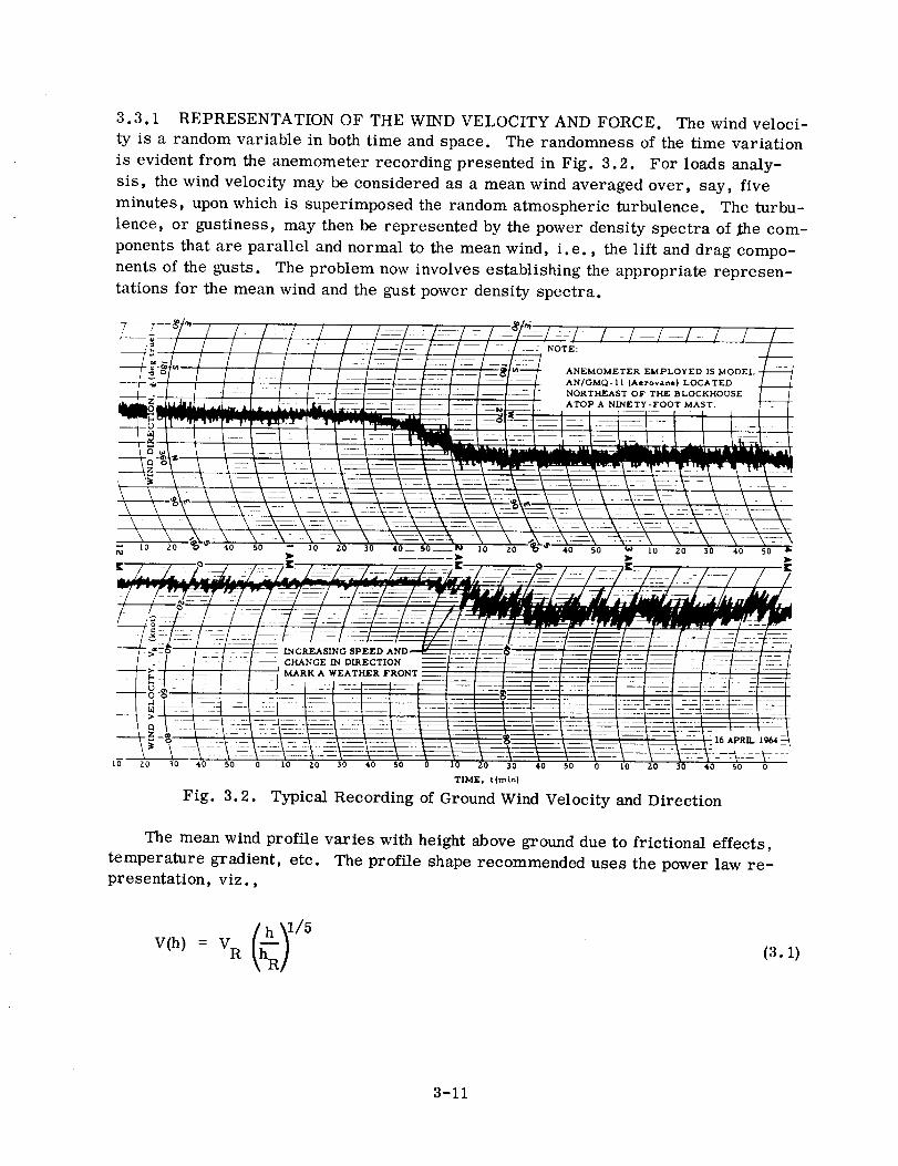
3.3.1 REPRESENTATION OF THE WIND VELOCITY AND FORCE. The wind veloci-
ty is a random variable in both time and space. The randomness of the time variation
is evident from the anemometer recording presented in Fig. 3.2. For loads analy-
sis, the wind velocity may be considered as a mean wind averaged over, say, five
minutes, upon which is superimposed the random atmospheric turbulence. The turbu-
lence, or gustiness, may then be represented by the power density spectra of _he com-
ponents that are parallel and normal to the mean wind, i.e., the lift and drag compo-
nents of the gusts. The problem now involves establishing the appropriate represen-
tations for the mean wind and the gust power density spectra.
TIME, t {rain}
Typical Recording of Ground Wind Velocity and Direction
The mean wind profile varies with height above ground due to frictional effects,
temperature gradient, etc. The profile shape recommended uses the power law re-presentation, viz.,
(3.1)
3-11
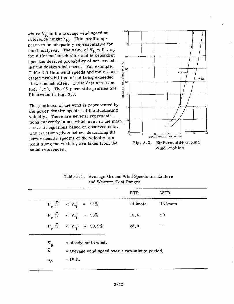
20O
where V R is the average wind speed at
reference height h R . This profile ap-
pears to be adequately representative for m
most analyses. The value of V R will vary
for different launch sites and is dependent 150
upon the desired probability of not exceed-
ing the design wind speed. For example, =
Table 3.1 lists wind speeds and their asso- _ ,25
ciated probabilities of not being exceeded o
at two launch sites. These data are from _ 100
Ref. 3.20. The 95-percentile profiles are:¢
illustrated in Fig. 3.3. _ 75
The gustiness of the wind is represented by5O
the power density spectra of the fluctuating
velocity. There are several representa-
tions currently in use which are, in the main, 25
curve fit equations based on observed data.
The equations given below, describing the 00
power density spectra of the velocity at a
point along the vehicle, are taken from the
noted references.
E
/
I
_WTR
I0 15 20 25
WIND PROFILE, V(h) (Knots}
Fig. 3.3. 95-Percentile Ground
Wind Profiles
3O
Table 3.1. Average Ground Wind Speeds for Eastern
and Western Test Ranges
E TR WTR
Pr (_/ < VR) = 95% 14 knots 16 knots
Pr (_Z < VR) = 99% 18.4 20
p (_r < 99.9% 23.0r VR) = --
V R
h R
= steady-state wind.
= average wind speed over a two-minute period.
=10ft.
3-12

Drag Component
-4SD(f) = (1.28 × 10 )
8/3fV
R
2 4/3
SD(f)=(5.67 × 10⁻³)__VR7 tl/3h2f5 tanh
(Ref. 3.14)
(Ref. 3.15)
(3.2)
(3.3)
SD(f) = D
3-4 V
(3. 036 x 10 ) R
VR D/262.8 +f2
(Ref. 3.10) (3.4)
SD(f ) = (2.15 x 10 -2 ) VR 5/2
Lift Component
+ f2\2 _h]
(Ref. 3.17) (3.5)
SL(f)
SL(0
V 2 2
= (4.56 xlO -4) VR L3k_.8D/ + f
--1.4 SD(f)
(Ref. 3.10)
(Ref. 3.17)
(3.6)
(3.7)
3-13

The gust power density spectra for the drag componentsare illustrated in Fig. 3.4for the following conditions:
VR = 10 ft/sec and 40 ft/sec (10-foot reference height)
D = 10 ft
h = 100 ft
f = is in cycles/second
The equation given by Davenport (Eq. 3.2) appears to give the most conservative spec-
trum. It may be simplified for all reasonable values of V R, viz.,
V(_f5R___ ) 1/3SD(f) =(1.28 x 10⁻⁴) (3.8)
The wind force is proportional to the square of the velocity, so that the power
density spectrum of the square of the wind velocity is required, rather than just the
power density spectrum of the velocity. Bohne (Ref. 3.19), Fontenot (Ref. 3.18), and
Wood (Ref. 3.21) have derived the spectrum of the drag force, ignoring the lateral
gusts. In a manner similar to that of the appendix of Ref. 3.21, the square of the total
wind velocity at a given height is found to have the form given below.
The mean-square wind velocity, V 2, is
(VR + 2 2 +(_DG) +2 VR2(:r2 G (_4 G2 2
+ 2 (?DGO'LG
I/2(3.9)
The power density spectrum, _) (f), is
O0
4 V R SD(f)+ _ SD(X)SD(f-X)dXO_
f°SDL(X) SDL(I-X)dX+_" SL(X) SL(f-_)dX(3.10)
The first term in the mean-square velocity and the first and third terms in the spec-
trum will be recognized as the same as those given by Bohne, Fontenot, and Wood for
the drag direction. Bohne and Fontenot have indicated that the convolution integral of
the drag spectrum is negligible, so it can be expected that the convolution integral of
the lift spectrum and of the cross-power spectrum will also be small. The variances
will usually be much smaller than V 2, so that the above expressions can be well
approximated by
3-14

IOOG --_ ....
_. - .-- ,EV3 o- \ _ ' - ------ REF 3, 15 •
k_- • i ....... REF3,1_ .,\\ ---7-----'--
\ !
\ x\
0 0.5 1 1,5 2 2.5
FREQUENCY (cps)
2 +2 o]I/2v Iv +2 Do ,3.11,
• (f)--_ 4V 2 SD(f) (3.12)
Cross-power density spectra for vertically
separated points are not presented since
these are not, as yet, well defined. It is
known, however, that there is little correla-
tion between gusts at points separated by
more than one-quarter wavelength (Refs
3.14 and 3.17), where the wavelength is
found by dividing the mean wind speed by
the frequency, i.e., X = VR/f. Further,
the cross-power density spectra and the
eovarianee between drag and lift compo-
nents of the gusts have not yet been estab-
lished, although Reed (Ref. 3.10) has de-
rived a theoretical expression for the drag
and lift cress-power density spectra.Fig. 3.4. Comparison of
Gust Spectra The aerodynamic coefficients for a cir-
cular cylinder in a fluctuating flow are not
well known. Lacking pertinent data, one is left with the choice of using steady-state
coefficients or estimating them. The use of steady-state coefficients is recommended
until more is known about the problem.
Vortex shedding coefficients will ordinarily have been obtained in a wind tunnel
wherein the wind velocity is essentially steady state, i.e., the turbulence is very small
(Ref. 3.10 discusses this subject). The analyst must, therefore, establish an "equiva-
lent" steady-state wind for loads analysis purposes. The equivalent wind should repre-
sent a uniform profile, i.e., V(h) = constant, and produce the same response to vortex
shedding as the real wind. The latter criterion is difficult to establish because little is
known about the effect of gusts on vortex shedding. Therefore, it is not unreasonable
to use an equivalent mean-square wind based on steady-state loads as given below,
V (h) D(h) x(h) dh
V 2 = L (3.13)
e f D (h) x(h) dh
3-15
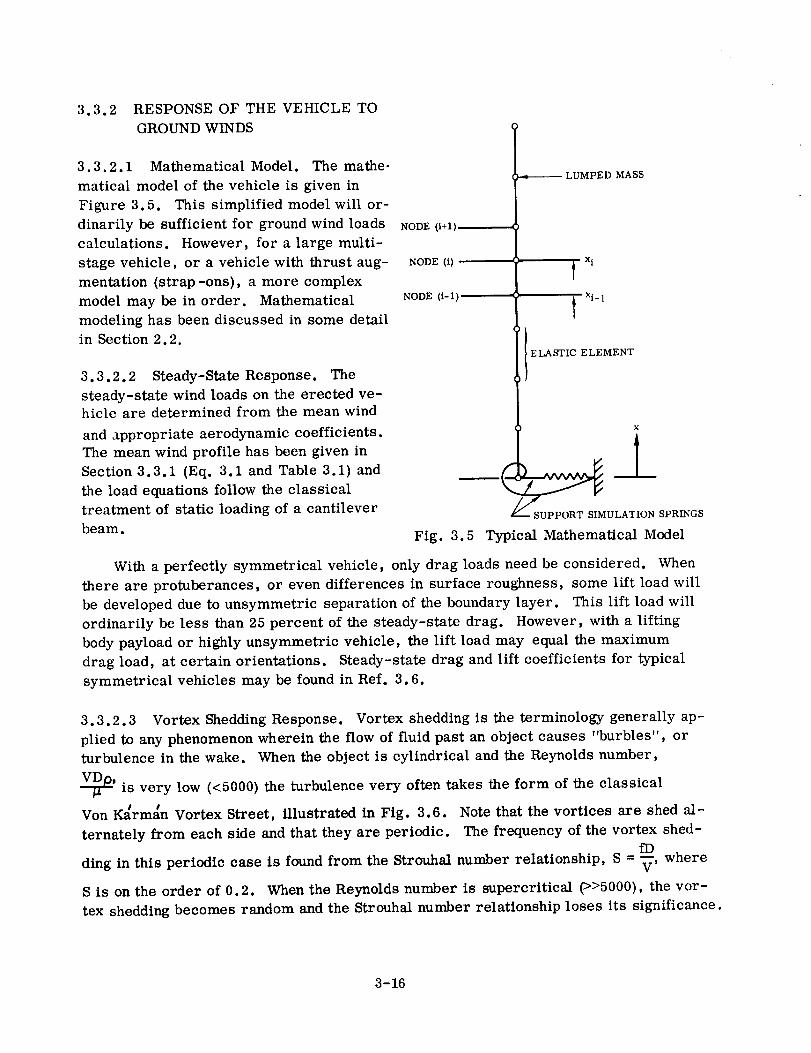
3.3.2 RESPONSEOF THE VEHICLE TOGROUNDWINDS
3.3.2.1 Mathematical Model. The mathe-matical model of the vehicle is given inFigure 3.5. This simplified model will or-dinarily be sufficient for groundwind loadscalculations. However, for a large multi-stagevehicle, or a vehicle with thrust aug-mentation (strap-ons), a more complexmodel may be in order. Mathematicalmodeling has beendiscussed in some detailin Section 2.2.
3.3.2.2 Steady-StateResponse. Thesteady-state wind loads on the erected ve-hicle are determined from the meanwindand appropriate aerodynamic coefficients.The meanwind profile has been given inSection 3.3.1 (Eq. 3.1 and Table 3.1) andthe load equations follow the classicaltreatment of static loading of a cantileverbeam.
NODE (i+l)
NODE (1)
NODE (i-l)
_--_------LUMPED MASS
i xi
i xi- 1
I ELASTIC ELEMENT
Fig. 3.5 Typical Mathematical Model
With a perfectly symmetrical vehicle, only drag loads need be considered. When
there are protuberances, or even differences in surface roughness, some lift load will
be developed due to unsymmetric separation of the boundary layer. This lift load will
ordinarily be less than 25 percent of the steady-state drag. However, with a lifting
body payload or highly unsymmetric vehicle, the lift load may equal the maximum
drag load, at certain orientations. Steady-state drag and lift coefficients for typical
symmetrical vehicles may be found in Ref. 3.6.
3.3.2.3 Vortex Shedding Response. Vortex shedding is the terminology generally ap-
plied to any phenomenon wherein the flow of fluid past an object causes "burbles", or
turbulence in the wake. When the object is cylindrical and the Reynolds number,
'is often takes the form of the classicalvery low (<5000) the turbulence very
Von K_rma'n Vortex Street, illustrated in Fig. 3.6. Note that the vortices are shed al-
ternately from each side and that they are periodic. The frequency of the vortex shed-fD
ding in this periodic case is found from the Strouhal number relationship, S = _-, where
S is on the order of 0.2. When the Reynolds number is supercritical (>>5000), the vor-
tex shedding becomes random and the Strouhal number relationship loses its significance.
3-16

The shedding of the vortices causes fluctu-
ations in pressure near the separation point. This
fluctuating pressure has force components that are
parallel and normal to the approach velocity. The
lift (normS) component is the more significant ef-
fect. If the structure is elastic, the fluctuating
pressures will produce oscillatory motion in the
lift ,and drag direction. Further, if an elastic body
is in the turbulent wake of another body, it will be
excited by that turbulence as well as by its own
vortex shedding. The presence of an umbilical
tower can have a very pronounced effect on the
oscillatory load. The location is usually dictated
by considerations other than load, but if it is
practical, relocating the tower about two diameters
from the vehicle will result in lower loads than at
one diameter (Ref. 3.25). The data of Ref. 3.25
also show that the load can be reduced by increas-
ing the effective width of the tower.
Space launch vehicles are seldom clean bodies
of revolution. Antennas, equipment pods, and
other protuberances have localized effects on vor-
tex shedding that are generally not predictable by
analytical means. Each vehicle configuration shouldtherefore be tested to determine the vortex shed-
ding effects. The test program should adopt good
modeling techniques, such as discussed in Ref.
11111
• D L _f
Fig. 3.6. Representation ofI I
Von Karman Vortex
Street
3.22. Briefly, the model should be scaled such that
the Reynolds number VDp reduced frequency,--_ damping ratio, C/C c, and mass_l n ' bL ,
ratio, , are simulated, and such that geometric features, including roughness, are
properly scaled.
The most usable form of wind tunnel data is the envelope of the drag and lift bend-
ing moments at the model base. This envelope may be obtained by making the two bend-
ing moments the X and Y inputs to an oscilloscope and taking a time exposure of the re-
sultant trace. The trace will have the form of a Lissajous figure with an elliptic en-
velope. The maximum bending moments in the drag and lift directions are then taken
from the time-exposed photograph of the oscilloscope traces.
Data from the various wind tunnel tests indicate that the response is predominate-
ly in the first structural mode. The response equations are therefore written in terms
of only the first mode. The response of the vehicle to the wake turbulence of the um-
bilical tower may include higher modes, which would require a modification of the
3-17

response equationspresented below. Further, it is assumedthat the motion of the ve-hicle does not affect the aerodynamics. While there is some evidenceto the contrary(Refs 3.10 and 3.25), it is considered that the proposed method adequatelyaccountsfor this phenomenon.
The maximum lift anddrag loads on the model are sealed to the prototype by useof the following relationships *(Ref. 3.6):
u <x> 1..... (3.14)e 2 L 2 ?r V e _lJFull Scale
_1 ¢Cl
CV = L''(M b)l qA2Wl _;D ]Model (3.15)
Eqs 3.14 and 3.15 are applicable to both the lift and drag directions with the appropri-
ate parameters. If the full-scale damping ratio is very low, say on the order of 0.5
percent of critical, the use of an aerodynamic damping term as discussed in Ref. 3.10
may be advisable.
Bohne (Ref. 3.11) presents a method using multipoint random input in terms of
pressures. This method requires cross-power density spectra in addition to the usual
power density spectra. A great deal of data must be obtained and reduced; hence the
test program is more complicated than that of the method presented above.
3.3.2.4 Gust Reponse. Reed (Ref. 3.10) has presented a method of calculating the
response to gusts which includes cross-power density spectra. In this method, the re-
sponse power density spectra have the form of Eq. 2. 181 of Section 2.6, which are
then simplified. However, since the cross-power density spectra have not been veri-
fied, it is probably best to continue using a homogeneous gust-type solution; that is,
assume that the gust envelopes the vehicle. In this case, the mean-square response
has the form of Eq. 2.185 of Section 2.6, viz.,
2 c 2 /1 1uG (x) = DG t_p7 I._2-_
¢2 ix)W 2 _(fn)n n
m 2 (217 fn) 2n
(3.16)
This equation is applicable to both the lift and drag gust components.
*The load equations are written in terms of displacement. Any other item of interest
may be found by the appropriate substitution for ¢ Ix).
3-18

The aerodynamic coefficients for a cylinder in a fluctuating flow are not wellknown. It is therefore recommendedthat steady drag coefficients beused for the gustresponse, unless more specific data are available. The square root of Eq. 3.16 ismultiplied by three to obtain the "three-sigma" displacement.
3.3.3 RESULTANT RESPONSE. The total resultant load on the vehicle in the launch-ready condition includes the various groundwind components, the axial gravity load,loads due to tank pressurization, and, at ignition, thrust-induced loads. Thrust-in-ducedloads are discussed in Section 4 alongwith the method for combining all the on-the-pad loads. The axial gravity load and tank pressurization load are determined byclassical static analyses. The manner in which the various ground wind load compo-nents may be combined is discussed in this section.
The groundwind load is a function of vehicle tanking, as well as a function of thewind. The loads at the supports will ordinarily be most severe for the fully tankedvehicle. However, at some other point the loads may be more severe for some parti-ally tanked condition. To be sure that the worst case has beenfound for the design,it is advisable to calculate groundwind loads for each possible tanking condition.
3.3.3.1 Equal Probability. Onemethod of com-bining the individual loads into a resultant is tovectorially addthe vortex sheddingand gust loadsof the desired probability-of-occurrence level tothe steady-state loads. This technique, illus-trated in Fig. 3.7, tends to be conservative asthe probability of the resultant beingexceededislower than the probability of a componentload be-ing exceeded. Secondaryloads due to deflectionshouldbe accountedfor.
3.3.3.2 CombinedProbability. Data of Ref.3.10 indicate that the envelopeof the steady-state andvortex sheddingloads tends to be anellipse. The eccentricity of this ellipse is afunction of the ratio of the vortex sheddinglift anddrag loads. Using the aboveobserveddistribution of load and assuming that the vor-tex sheddingand gust loads are independent,normally distributed, andhave zero correl-ation it is possible to develop a methodwhere-in the resultant load has the desired probabilityof occurrence.
The combination of the random loads inthe lift anddrag direction is assumedto be
SECONDARY AND
MISCELLANEOUSEFFECTS
Equal Probability
Combination of Loads
3-19
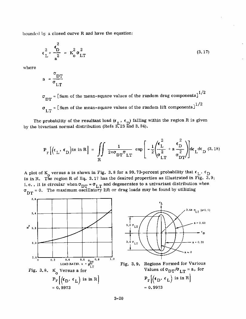
boundedby a closed curve R and havethe equation:
2
2 (D _ K 2 2eL+ 2 o aLT
a
(3.17)
where
aDTa = --
aLT
= [Sum of the mean-square values of the random drag components] 1/2
= [Sum of the mean-square values of the random lift componentsJ 1/2
The probability of the resultant load (e L, _D) falling within the region R is givenby the bivariant normal distribution (Refs 3.23 and 3.24).
r 2rrGDTfTLTR
-_ _ +a d_
aLT aDT/J
Ld_D (3.18)
A plot of K ° versus a is shown in Fig. 3.8 for a 99.73-percent probability that (L' _Dis in R. The region R of Eq. 3.17 has the desired properties as illustrated in Fig. 3.9;
i.e., it is circular when aDT = (_LT and degenerates to a univariant distribution when
_DT = 0. The maximum oscillatory lift or drag loads may be found by utilizing
3.6
3.4
M°3.2
3.0
2.80
Fig. 3.8.
J
0.2
J
0.4 0.6 0.8_DT
LOAD RATIO, a = _L'LT
K Versus a forO
= 0.9973
eL
3.44 _LT (a=l'O)
•1.0 __a_ 0
Fig. 3.9. Regions Formed for Various
Values of _DT/_LT = a, for
Pr I((D' eL)is in R]
= 0.9973
3-20
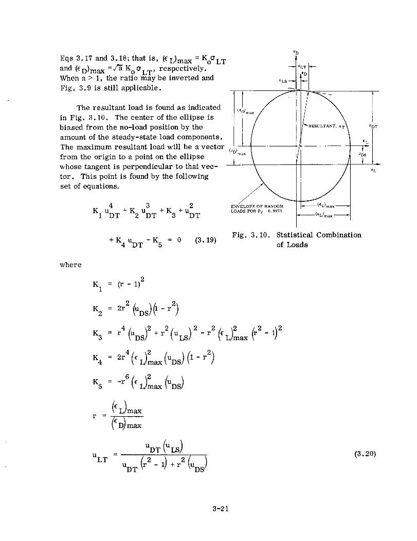
Eqs 3.17 and 3.18; that is, (EL)max = KoaLT
and (ED)max = ¢_ Ko aLT, respectively.When a > I, the ratio may be inverted and
Fig. 3.9 is stillapplicable.
The resultant load is found as indicated
in Fig. 3.10. The center of the ellipse is
biased from the no-load position by the
amount of the steady-state load components.
The maximum resultant load will be a vector
from the origin to a point on the ellipse
whose tangent is perpendicular to that vec-
tor. This point is found by the following
set of equations.
(UD),,na x
uD
"RESULTANT. UDT
uL
4 3 2
+ K 2 + K 3 + uK1 UDT UDT DT
ENVELOPE OF RANDOM
LOADS FOR Pr : 0. 9973
+K 4uDT +K 5 = 0 (3.19)Fig. 3.10. Statistical Combination
of Loads
where
K 1 = (r - 1)2
K2 = 2r 2 (uDS)(1-r2)
4 r 2 2 2 2K3 = r (aDS)2+ (uLS) -r (¢ (r 2 -
K4 = 2r4(¢i)2ax(UDs)(1-r2 )
= 6 (¢ 2
(_ L)maxr --
ULTUDT(r2- 1) +r2(UDs )
(3.20)
3-21
Eq. 3.19 is a fourth order equation andwill therefore yield four roots. For the caseat hand, the four roots are" one maximum, one minimum, andtwo imaginary. Themaximum root is the root of interest. Oncethe resultant drag, UDT is found, it issubstituted into Eq. 3.20 to solve for the resultant lift, ULT. The total resultant isthen
jCuo 2 (3.21)
3.4 CONCLUSIONS
3.4.1 WIND. The statistical variation of the mean wind and the representation of
the profile are adequately defined, and there is reasonable agreement on the power
density spectrum of the gusts. The cross-power density spectra for vertically sepa-
rated drag and lift gusts are required as is the cross-power density spectrum between
the drag and lift gusts. Further, since the vehicle may respond in a steady-state
manner to low-frequency gusts (half-period on the order of 30 seconds), the probabili-
ty of occurrence of the gust wave length should also be determined.
3.4.2 RESPONSE. The general form of the response is well known, even for a ran-
dom force. The real problem here is in defining the forcing function. The total
force applied to the vehicle is complicated due to the fact that it is made up of several,
possible interacting, random forces, in addition to the steady-state force. The general
practice taken in the literature has been to isolate one, or possibly two, aspects of
the overall problem and concentrate on obtaining a reasonable solution to that portion
alone. What is needed is an integrated treatment of the overall problem, in which an
attempt is made to account for all known and suspected force terms and interactions.
Such a solution is not immediately obtainable due to lack of data. Additional research
is required to obtain a tractable solution that contains the effects of all parameters
and their components simultaneously. This solution would then, of course, need to be
verified by full-scale tests.
3.4.3 RECOMMENDED PROCEDURE. Within the scope of the present state of the
art in ground wind loads analysis, it is recommended that the following procedures
be used for design loads.
a. Vehicles that are clean bodies of revolution.
The first requirement is to establish the desired wind speed for design purposes.
This wind speed is determined from the wind data at the launch site and the
desired probability of launching on a specific date.
For the design wind speed, calculate steady-state loads using classical static
loads analysis techniques, the mean-square wind speed of Eq. 3.11 and the wind
profile of Eq. 3.1. Lift and drag aerodynamic coefficients can be obtained from
Ref. 3.6.
3-22
b.
Calculate gust loads using Eq. 3.16, the gust spectrum of Eq. 3.12, and steady-
state aerodynamic coefficients.
Calculate vortex shedding loads using Eq. 3.14 for a wind speed, Ve, and Eq.
3.13. Applicable coefficients can be obtained from Ref. 3.6.
Combine the stead-state, gust, and vortex shedding loads using the methods of
Section 3.3.3.1 or 3.3.3.2. Secondary bending loads, other random loads, and
basic vehicle loads such as weight, thrust, etc., must be included.
Vehicles that are not clean bodies of revolution.
The procedure is the same as for the clean bodies of revolution except for the
vortex shedding loads. It will be necessary to search the literature to deter-
mine or estimate vortex shedding coefficients to be used in preliminary de-
sign. As soon as possible, wind tunnel tests should be run to determine vor-
tex shedding coefficients for the vehicle.
3.5 REFERENCES
3.1 D.A. Buell, "Some Sources of Ground-Wind Loads in Launch Vehicles," AIAA
Fifth Annual Structures and Materials Conference, Palm Springs, California,
April 1-3, 1964.
3.2 R. Goldman, The Generation and Suppression of Von Karman Vortex Forces,
Martin Co. Report No. 8984, July 1957.
3.3 D.E. Somerville and D. R. Kobett, Research and Development Services
Covering Wind-Induced Oscillations of Vertical Cylinders, Midwest
Research Institute, Phase Report No. 1, 1958.
3.4 Y.C. Fung, "Fluctuating Lift and Drag Acting on a Cylinder in a Flow at Super-
critical Reynolds Numbers, " Journal of Aerospace Sciences, Vol. 27, No. 11,
pp. 801-804, November 1960.
3.5 A. Roshko, "Experiments on the Flow Past a Circular Cylinder at Very High
Reynolds Number," Journal of Fluid Mechanics, Vol. 10, Pt. 3, pp. 345-356,
May 1961.
3.6 D.A. Buell, G. B. McCullough, and W. J. Steinmetz, A Wind Tunnel Investi-
gation of Ground-Winds Loads on Axisymmetric Launch Vehicles, NASA TN-D-
3.7
1893, October 1963.
D° A° Buell and G. C. Kenyon, The Wind -Induced Loads on a Dynamically
Scaled Model of a Large Missile in Launching Position, NASA TMX-109,
December 1959.
3-23
3.8 A. A. Ezra, Wind Induced Oscillations of the Titan Missile, The Martin Co.
Report No. WDD-M-MI-59-7, March 1959.
3.9 E. Gaffney, Ground Wind Loads Wind Tunnel Tests on Several Atlas Vehicles,
3.10
3.11
3.12
3.13
3.14
3.15
3.16
3.17
3.18
3.19
Convair Division Report No. GD/A63-0999, April 1964.
W. H. Reed III, "Models for Obtaining Effects of Ground Winds on Space Vehicle
Erected on The Launch Pad," Conference on the Role of Simulation in Space
Technology, Virgina Polytechnic Institute, August 17-21, 1964.
Q. R. Bohne, ',Ground Wind Induced Loads on Axisymmetric Launch Vehicles,"
AIAA Fifth Annual Structures and Materials Conference, Palm Spring, Califor-
nia, April 1964.
Handbook of Geophysics, Rev. Ed., The MacMillian Co., New York, 1960.
J.R. Scogglns et al., Low Level Wind Profiles Applicable for the Study of Ver-
tically Rising Vehicle Performance Between 3 Meters and 120 Meters, Cape
Canaveral (Atlantic Missile Range), Florida, George C. Marshall Space Flight
Center, MTP-AERO-60-26, December 1960.
A. G. Davenport, "The Spectrum of Horizontal Gustiness Near the Ground in
High Winds," Quarterly Journal of Met. Soc., Vol. 87, 1961.
R. M. Henry, A Study of the Effects of Wind Speed, Lapse Rate, and Attitude
on the Spectrum of Atmospheric Turbulence at Low Altitude, IAS Preprint No.
59-43, January 1959.
J. L. Lumley and H. A. Panopky, The Structure of Atmospheric Turbulence,
Intensive Publishers Division of John Wiley & Sons, New York, 1964.
J. K. Zbrozek, The Relationship between The Discrete Gust and Power Spectra
Presentations of Atmospheric Turbulence, with a Suggested Model for Low Al-
titude Turbulence, Technical Note No. AERO 2682, ASTIA Document AD-242944,
March 1960, and Addendum, AD-242945, July 1960 (Royal Aircraft Establish-
ment, Bedford).
L. L. Fontenot, "The Response of a Flexible Missile to Ground Winds, " Ai___[
ForceSurveys in Geophysics No. 140, Proceedings of the National Symposium
on Winds for Aerospace Vehicle Design, Vol. I, USAF Geophysics Directorate,
AFCRL-62-273(I), March 1962.
Q. R. Bohne, "Power Spectral Considerations on the Launch Pad, " Air Force
Surveys in Geophysics No. 140, Proceedings of the National Symposium on
Winds for Aerospace Vehicle Design, Vol. I, USAF Geophysic Directorate,
AFCRL-62-273 (I), March 1962.3-24

3.20 G. E° Daniels, Terrestrial Environment {Climatic) Criteria Guidelines for Use
in Space Vehicle Development, 1964 Revision, NASA TMX053023, March 13,1964.
3.21 J. D. Wood and J. C. Barry, "Random Excitation of Missiles Due to Winds, "
Air Force Surveys in Geophysics No. 140, Proceedings of the National Sympo-
sium on Winds for Aerospace Vehicle Design, Vol. I, USAF Geophysics Directo-
rate, AFCRL-62-273 (I), March 1962.
3.22 Henry L. Langhaar, Dimensional Analysis & Theory of Models, John Wiley &
Sons, Inc., New York, 1951.
3.23 A. M. Mood, Introduction to the Theory of Statistics, McGraw-Hill Book Co.,
New York, 1950.
3.24 S. O. Rice, "Mathematical Analysis of Random Noise," Selected Papers on
Noise and Stochastic Processes, Edited by Nelson Wax, Dover Publications,
Inc., New York, 1954.
3.25 G. B. McCullough and W. J. Steinmetz, A Wind Tunnel Study of Ground-Wind
Loads on Launch Vehicles Including the Effects of Conduits and Adjacent Struc-
tures, NASA TN D-2889, July 1965.
3-25


4/ENGINE START AND SHUTDOWNAND VEHICLE LAUNCH
4-1

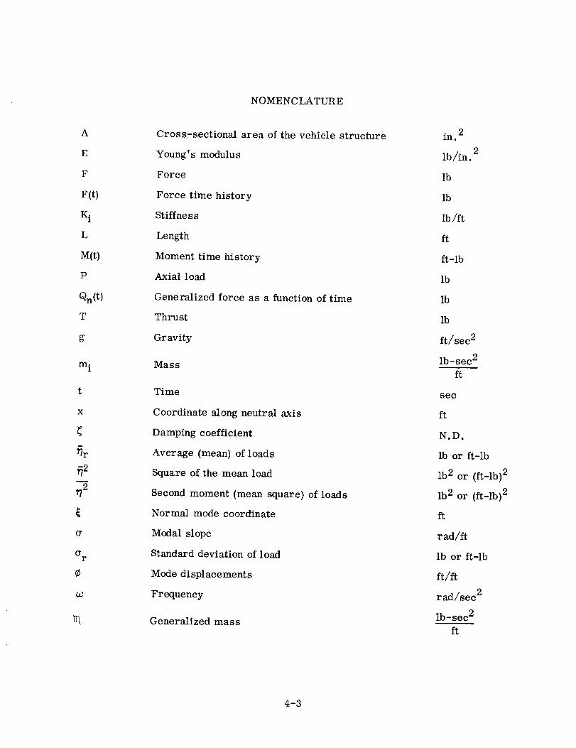
A
E
F
F(t)
iqL
M(t)
P
Qn(t)
T
g
m i
t
x
O"
(Yr
¢
r_
NOMENCLATURE
Cross-sectional area of the vehicle structure
Young' s modulus
Force
Force time history
Stiffne s s
Length
Moment time history
Axial load
Generalized force as a function of time
Thrust
Gravity
Mass
Time
Coordinate along neutral axis
Damping coefficient
Average (mean) of loads
Square of the mean load
Second moment (mean square) of loads
Normal mode coordinate
Modal slope
Standard deviation of load
Mode displacements
Frequency
Generalized mass
2in.
lb/in. 2
lb
lb
lb/ft
ft
ft-lb
lb
lb
lb
ft/sec 2
lb-sec 2
ft
see
ft
N.D.
lb or ft-lb
lb 2 or (ft-lb} 2
lb 2 or (ft-lb) 2
ft
rad/ft
lb or ft-lb
ft/ft
rad/sec 2
lb-sec 2
ft
4-3


4/ENGINE START AND SHUTDOWNAND VEHICLE LAUNCH
4.1 STATEMENT OF THE PROBLEM
The largest forces acting on spacelaunch vehicles are those produced by thrustof the engines. These thrust loads, and attendantlongitudinal inertial loads, designor contribute to the design of almost every part of the vehicle structure. Longitudinalload conditions to be analyzedinclude rigid body and vibratory loads at engine startand shutdown, liftoff from the launch pad, and steady-state loads between these times.In the case of multiple engines, there exists the possibility of lateral loading inducedby unsymmetrical engine start and shutdown. Also, unsymmetrical launcher releasecan cause lateral loads.
The major problems encounteredin the analysis are the adequatedescription of:1) a longitudinal mathematical model, and 2) the time history of applied forces. Thedifficulties in synthesizing the mathematical model are associatedwith the represen-tation of the propellant in a dynamic model. The procedure of Section 2.2.3 providesa goodrepresentation for cylindrical tanks but doesnot provide goodmodels for tanksapproaching spheres or oblate spheriods.
Description of applied forces is difficult becauseof the random nature of enginestarting characteristics. These characteristics vary not only amongengines of agiven model, but also amongfirings of the same engine. Two methods of obtainingdesign loads are: 1) to determine a worst-case buildup (or decay) curve anduse thisin the analysis for the design condition, or 2) to calculate responsesusing a largenumber of engine thrust time histories and obtain design loads from a statisticalevaluation of the calculated responses. In multiple engine systems, the time at whichdifferent engines receive the start (or shutdown)signal has tolerances that addto therandom nature of applied forces. For the liftoff problem, tolerances in engine timingand mechanical, pneumatic, or pyrotechnic operation of the release mechanism mustbe understood for a complete description of forces acting uponthe vehicle.
Vehicle total loads must include those of other sources that can coincide withthrust forces. Typical examples are groundwinds andwinds aloft, effects of controlsystem response to vehicle motion, and vehicle design and assembly misalignments.Combining these loads can be straightforward based onworst-case combinations or itcanbe a statistical combination including the random occurrences of all these forces.
4.2 HISTORICAL BACKGROUND
A dynamic analysis of spacevehicles for their response to thrust forces usuallyuses data obtainedfrom enginetests to describe the applied forces and employs
4-5

normal-mode theory in the response calculations. Development necessary for the
analysis has been mostly in the modeling of the propellant and its containers. The
works of Li (Ref. 4.1) and Wood (Ref. 4.2) were among the first attempts to obtain
a model representing the first mode of a cylindrical tank. These works either as-
sumed a rigid tank bottom or test data were available to describe the tank bottom
effects. Pinson in Ref. 4.3 gives methods for obtaining effective spring rates of
the bulkheads at the ends of each tank. Rose (Ref. 4.4) modifies the model by add-
ing the effective spring rate of gases in the propellant tanks. He also proposes a
method for representation of more than one propellant mode. The propellant tank
model development is given in Section 2.2.3.
4.3 ANALYTICAL APPROACH
Analyses to obtain vehicle response to engine transients follow general normal-
mode theory. However, there are several details, not necessary in the general ap-
plication, that are required for satisfactory solutions of responses to these transients.
4.3.1 ENGINE START AND SHUTDOWN ANALYSES. Consider the simple longitudinal
model of Fig. 4.1. Masses 2 through 4 represent major vehicle components, connect-
K 4
q
[K 3
K]T_KI
Fig. 4. I. Typical
Longitudinal
Model
ed by springs K 3 and K4. Mass 1 is the engine connected
to the vehicle through spring K 2. The vehicle is held to
the ground by spring K 1. The thrust, T, is applied bythe engine. The loads for this condition can easily be
analyzed with normal-mode theory by first obtaining the
modes with the vehicle fixed to the ground and then
writing the equations of motion in terms of normal-mode
coordinates. For the n th mode,
Q (t)
_'n+2_nO 2 _ +a2_ = n....p.._ (4 1)n n n n mn
wherein the product of instantaneous thrust and the modal
displacement of the engine is the generalized force, Qn(t).Simultaneous solution of the "n" equations and use of
either mode displacement or acceleration methods will
give vehicle load and acceleration distributions. The
loads due to gravity must be added to obtain total loads.
Such is a typical analysis for engine thrust buildup on a vehicle held to ground by
a "launcher." An analysis for engine shutdown in the launcher can be approximated
by the same procedure but with the force time history equal to full thrust minus the
thrust decay, That is, if the decay is represented by T(t) of Fig. 4.2 then the force
time history used in the analysis is T o - T(t) as shown in Fig. 4.3. This represen-tation would give good results for the transient loads.
4-6
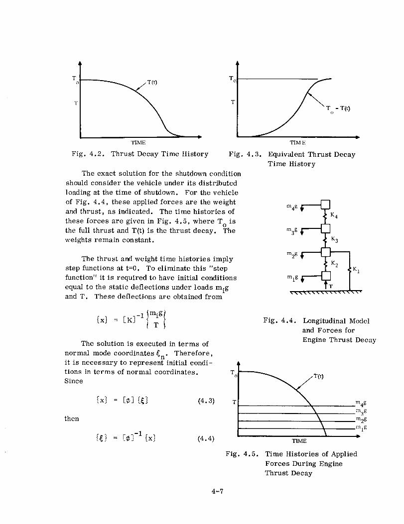
T
TIME
Fig. 4.2. Thrust Decay Time History
T
Fig. 4.3.
The exact solution for the shutdownconditionshouldconsider the vehicle under its distributedloading at the time of shutdown. For the vehicleof Fig. 4.4, these applied forces are the weightandthrust, as indicated. The time histories ofthese forces are given in Fig. 4.5, where T isothe full thrust and T(t) is the thrust decay. Theweights remain constant.
The thrust andweight time histories implystep functions at t=0. To eliminate this "stepfunction" it is required to have initial conditionsequal to the static deflections under loads migand T. Thesedeflections are obtainedfrom
__o - T(t)
TIME
Equivalent Thrust DecayTime History
m4gK4
m3gK3
m2g
mlg
D
:K 1
IThe solution is executed in terms of
normal mode coordinates _n" Therefore,it is necessary to represent initial condi-
tions in terms of normal coordinates.
Since
{x] = [¢] [_] (4.3)
then
(_] = E¢_ -1 {x] (4.4)
T
T
Fig. 4.4. Longitudinal Model
and Forces for
Engine Thrust Decay
TIME
m4g
m3gm2g
mlgD
Fig. 4.5. Time Histories of Applied
Forces During Engine
Thrust Decay
4-7

Initial deflections in terms of _ can also be obtained directly from Eq. 4.5.
[_} = [r_ -I _'co2_ -1 [¢]' [F} (4.5)
The initial conditions and force time histories are now defined and the solution can
be effected. Total loads, including gravity, for engine start could be similarly
simulated.
The analyses for inflight engine start and shutdown are similar except that free-
free modes replace the fixed modes, the applicable rigid-body modes must be included,
and the force due to gravity is replaced by the inertial force of m i x, where _ is the
steady-state acceleration under thrust.
4.3.2 LIFTOFF ANALYSIS. Liftoff analysis introduces several additional consider-
ations since it involves a model transition from "fixed" to "free" and also entails
changes in the model such as elimination of the launcher. The procedure for liftoff
analysis is indicated by the case of a free launch, i.e., a vehicle held down only by
gravity, which will lift from its launcher when the thrust exceeds the weight. Fig.
4.6 presents a simplified model of vehicle and launcher. The analysis begins with the
fixed model in Fig. 4.6a and proceeds as in the buildup and decay analysis above.
When the force in K 1 is zero, then the vehicle is free and the analysis switches to thefree modes of Fig. 4.6b. Because of oscillations, the vehicle and the launcher can
make contact after initial liftoff; to represent this chatter condition the fixed modes
of the launcher alone are required. The system is defined by two sets of modes, fixed
and free:
: K4
m3g: K3
m2g _-'-_ ',_K
KI' _
msg _ _ mlg
m4g _K 4
m3g _-_K 3
m2g _
mlg _@ K2
a. Fixed b. Free
Fig. 4.6. Longitudinal Liftoff Models
4-8

{xvL} (fixed modes) (4.6)
{::} 011, / (free modes) (4.7)
where Xv, x L are displacements of the vehicle and launcher, and CV are free-free
(including rigid-body) modes of the vehicle and ¢L is the fixed mode of the launcher
by itself.
The force in spring K 1 is zero when the relative deflection between masses 2 and
5 is greater than or equal to zero. Computerized monitoring of this quantity deter-Initial conditions for the second setmines the time of switching between mode sets.
of mode shapes are obtained by
i°](4.8)
The solution then continues with this set of modes. Forces and accelerations are ob-
tained by either the mode-displacement or mode-acceleration method.
Simulation of an instantaneous release launch is achieved by obtaining initial
conditions for the free-free vehicle modes under the thrust, the gravity, and the
launcher forces. The forces in the response solution are the thrust and weight time
histories. The inclusion of the launcher forces in the initial displacements, but with
omission of launcher forces in the response solution, provides the force step-function
of instantaneous launcher release. If the launcher force is applied at the same point
as the thrust forces, then the solution follows the same procedure, with liftoff being
represented by a step change, equal to the launcher force, in effective force at the
point of engine-launcher force application.
A controlled-release launch is more complicated since it must include the mech-
anics of the control. It is often sufficient to follow the procedure of the instantaneous
launch with the force time history of launcher load release applied to the free-free
modes. This treatment is an approximation because the vehicle is not free until the
launcher force is zero. A detailed analysis, with representation of the launcher
mechanism modeled, is necessary if loads for this condition are surmised to be
critical. The significance of these loads can be investigated by assuming various re-
lease time histories for evaluation of important parameters.
4.3.3 LATERAL LOADS. Lateral loads during engine start, shutdown, and vehicle
liftoff are caused by misalignment of the thrust vector, unsymmetrical start and shut-
down in the case of a multiple engine system, and unsymmetric launcher release. The
4-9

analytical approach is identical to that for longitudinal loads with moments and lateral
forces replacing the axial forces and, of course, a lateral model replacing the longi-
tudinal model. For thrust misalignment the generalized force in the n th mode is
n
Qn (t) = CE F(t)
where ¢_ is the modal deflection at the point of thrust application and F(t) is the lateral
component of the thrust vector. In the case of unsymmetrical engine start the general-
ized force is
n
Qn(t) = a E M(t)
where _E is the modal slope at the point of thrust application and M(t) is the productof differential thrust and the distance of the engines from the eenterline of the vehicle.
At liftoff, M(t) is the moment due to unsymmetrical release. The analysis then fol-
lows the mechanics of the longitudinal loads analysis. For most practical systems
the lateral deflection due to center-of-gravity offset and gravity can be ignored in the
computation of lateral transient loads.
4.4 ILLUSTRATIVE EXAMPLES
Typical analyses and results of engine start and shutdown and vehicle liftoff are
presented in this section. The Atlas/Centaur/Surveyor vehicle has multiple engine
systems in both the Atlas and Centaur stages. The Atlas stage has three engines, two
engines with high thrust called booster engines, and one engine, the sustainer engine,
of lower thrust. The booster engines, which are more efficient at sea level, are
jettisoned at high altitude and flight is maintained by the more efficient sustainer
engine (shutdown and jettison of the booster engines also reduce the maximum axial
acceleration as propellant is depleted). The Centaur stage has two engines of nominally
identical performance.
4.4.1 MATHEMATICAL MODELS. Models shown in Figs 4.7 and 4.8 are the longi-
tudinal models that will be used for: 1) engine thrust buildup on the launch pad, 2)
liftoff, and 3) sustainer shutdown. The model forward of Mass 11 is identical for all
three conditions except for a reduction in Masses 5 and 7 to include the effect of
jettisoning the nose fairing and insulation panels prior to sustainer engine shutdown.
The spring-mass systems attached above Mass 4 represent Surveyor spacecraft modes
that are coupled with totaled vehicle modes using the analytical techniques described
in Ref, 4.5. The masses include structure and propellant as indicated in the figures.
Spring constants for the LH 2 tank are obtained by application of the cylindrical tank
model developed in Section 2.2.3. The model for the Centaur oblate spheroid LO 2tank is obtained from test data interpreted to fit a cylindrical tank model. For pur-
poses of this example the ullage pressure effects are not included and the bulkhead is
assumed to be rigid.
4-10

TI:I
_I +'+'+'+'_-r+r'r.
• , , . , _ , _ .......... _ _ _
T '??<?'_T_T~~ _<L,L
_ --_ _ t_- • t_ _ •
_.1
i
+ _+<_._'+, .... g +++ + + <
+ -+,, M+-_
M 5'+ '-+--+ i! II ii
0.I--4
° _"I
'i i
©
>
I
4-11
_J _
_ "r, 7"TTT'T
_1 _ __ _-
i
_J
,c
©
Z
<
Or/l
N?
0
Z
"8N
@
@
r..)
r/1
4
4-12
Below Mass 11 the models for on-the-pad transients and for liftoff are the same
except that the launcher has been eliminated for liftoff when the analysis is performed
with free modes. In this model the propellant tank representations are as developed
in Section 2.2.3. Again ullage pressure effects are omitted and the bulkhead is as-
sumed to be rigid. That part of the fuel in the conical section of the tank is assumed
to be a rigid mass lumped with structure at Mass 17. The sustainer engine (Mass 18)
is connected to Mass 17 by spring rate AE/L of the conical tank structure. The
booster section and its engines (Mass 19) are attached by a spring, the stiffness of
which was determined from tests. The launcher-arm mass is included with Mass 19,
since it is rigidly attached to the booster and the effective spring rate (19-20) of the
launcher is below the arms. The remaining launcher mass is represented at Mass 20,
which is connected to ground. The spring rates 20-19 and 20-21 were obtained from
static load-deflection tests. For the liftoff condition the masses of LO 2 and fuel areslightly reduced, the mass of the launcher arm is removed from Mass 19, and the
vehicle is "freed" (spring 19-20 and the model below are omitted). The modal fre-
quencies and generalized masses are given in Table 4.1.
The sustainer shutdown model has eliminated Mass 19 because it was jettisoned
earlier in flight. The fuel is depleted to the extent that all of it is in the conical sec-
tion. The spring between the conical section and the intermediate bulkhead is the
AE/L of the cylindrical fuel tank. The LO 2 level has subsided to Station 918 and the
model between Stations 918 and 960 is obtained from Section 2.2.3 by considering the
propellant tank extending from Station 918 to 960. The spring from nodes 12 to 11 is
the AE/L of the cylindrical tank above Station 918. The modal frequencies and gen-
eralized masses corresponding to the representation are given in Table 4.2.
Development of the lateral model of Fig. 4.9 is a straightforward process fol-
lowing the guidelines of Section 2.2. The spring-mass systems attached at Station 173
are derived from modal vibration surveys of the spacecraft. Aft of Station 1133 the
model follows two paths, one down the conical portion of the tank to the sustainer
engine, the other down the wall of the booster engine section. The wall of the booster
section is represented by Masses 46 and 54-59. Masses 60-62 represent the thrust
beam, with effective spring rates to the booster wall of K F (60-54) and KA (62-56).
Mass 63 is the vehicle side of the gimbal point, and Mass 64 is the engine side. The
rotational spring between 63-64 is the effective rotational stiffness of the engine
actuator system and backup structure, while the lateral spring, 63-64, is the effec-
tive stiffness, normal to the thrust axis, of the gimbal block. For convenience, the
masses and springs of the two engines are lumped as one. The vehicle is tied to
ground by the experimentally determined launcher spring rates between Masses 70
and 71. Tables 4.3 and 4.4 list the stiffness element data and weight data pertaining
to the lateral model of Fig. 4.9. The modal frequencies and generalized masses for
the lateral model are given in Table 4.5.
4-13

0
°_
oo_
o
c$
No_
°_
8
0
_°
4-14
Table 4.2. Longitudinal Modal Frequencies and Generalized Masses for Sustainer
Shutdown Condition
MODE GENERALIZED MASS FREQUENCY
NO. 0b-sec2/in.) (cps)
1 142.3 0
2 0. 0003580 8.44
3 0.4123 16.40
4 0.001115 16.78
5 0. 005482 23.42
6 1.737 30.30
7 0.3638 33.64
8 0. 002060 35,88
9 1. 169 39.16
10 0.3107 40.39
11 0,009863 48.00
12 18,44 51.00
13 0.000005655 51.75
14 0.05187 57.62
15 5. 122 87.52
16 33.13 89.26
17 1.642 148.8
18 5. 544 163.5
19 0,001556 189.6
20 2. 195 368.9
21 3. 123 643.3
4-15
i............I
ST\ -11.0"
65 BOOSTER ,58 LAUNCtlERLONGERON
MAIN ENGINE _59
BOOSTER
SttROUD
1
MASS STATION
_ RATE GYHO LOCATION
NOSE FAIRING 4 100104 103 102
:,_ARD BULKHEAD-- 4 200
15' - -
16
17
TANK _'18
ILO 2 TANK AND _ ;__1_lCENTAUR ENGINES
IINTERSTAGE
ADAPTER
25
b26
t27
i28129
130
)31
)32
33
i LO 2 TANK -- '54
_35
t36
t37
138
39
14o
,41
-- 3O0
19
69
2°1_ -- 400
0o
@°72 68
24- -- 5OO
-- G(H)
-- 7O0
-- _00
-- 900
-- I000
FUEL TANK-- _42 43
7_44 -- 1100
_1 45
....... [-4 46
COmCALSECTION| _::_4S
SUSTAINER _ 53ENGINE
--1300
Fig. 4.9. Atlas/Centaur/Surveyor Lateral Model
^
z
¢_f-<
4-16

Table 4.3. Atlas/Centaur/Surveyor Lateral Model Weight Data
NODE
NO.
1
2
3
4
5
6
7
12
13
14
15
16
17
18
19
20
21
69
66
67
68
22
23
24
25
26
27
28
29
30
31
32
33
34
35
36
37
38
39
4O
STATION
(in.)
-20
10
50
100
145
173
200
173
192
200
219
250
280
315
345
375
412
388
438
453.5
477.7
438
47O
5O0
525
555
57O
60O
630
667
696
725
754
784
812
840
871
900
929
960
WE IGHT
(Hundreds
of pounds)
1.933833
1.489122
1.739427
2.432240
4.121724
3.22951O
3.028173
7.576172
2 874967
3.685906
11.310
11.118
11.635
11. 188
10.4267
9.2762
112.686
51. 7704
61. 54664
10.96110
8. 1286
2. 079684
1.912255
2. 191229
3. 124462
24. 17955
98.44672
132.0887
147.1717
144. 9370
127.2731
127. 1857
129. 5109
127. 1721
122.6780
129.3658
131.6285
125.0831
89.67365
99.33865
MOMENT OF
INERTIA NODE STATION
(lb-in. 2) NO. (in.)
41 992
42 1025
43 1057
44 1090
45 1122.5
46 1133
47 1150
395,280 48 1160
49 1180
50 1198
51 1210
52 1210
53 1240
54 1160
55 1176
56 1206
57 1212
58 1242
59 1267
70 1190
71 1190
60 1160
61 1176
62 1206
63 1212
64 1212
101 70.24
102 78.91
103 -2.22
104 131.87
110 115
76 203.88
77 383.7
1 78 573.1
79 950.6
1 80 203.88
81 383.7
82 573.1
83 950.6
65 1242
WEIGHT
(Hundreds
of pounds)
104. 2039
104.2527
104. 1664
103.3811
69.42969
46. 27086
37. 80067
28.46361
19. 06233
6.795801
3. 585753
0.0
11. 150
3.27047
8.8812
13.05785
11.47866
7. 56912
6.25061
0.0
0.0
0.0
2.0
0.0
0.0
0.0
0.74729
0.26777
0. 000085
2. 3902
17.6685
3.644
33.245
101. 546
52. 066
0.0
0.0
0.0
0.0
1846.0
MOMENT OF
INERTIA
(lb-in. 2)
884,400
28,000
1,707,288
4-17

Table 4.4.
_EGINNING ENDING
NODE NODE
101 12
102 12
103 12
104 12
110 12
1 2
2 3
3 4
4 5
5 6
6 7
7 15
12 13
13 14
14 80
80 15
80 76
15 16
16 17
17 18
18 19
19 20
20 21
81 69
81 77
69 21
21 66
66 67
67 68
21 22
22 23
23 24
24 25
25 26
26 27
27 82
82 28
82 78
28 29
29 30
30 31
31 32
'YPE
B
B
B
B
B
B
B
B
B
B
B
B
B
B
B
B
TS
B
B
B
B
B
B
B
TS
B
B
B
B
B
B
B
B
B
B
B
B
TS
B
B
B
B
Atlas/Centaur/Surveyor Lateral Model Stiffness Element
Data
EI AT
BEGINNING
NODE OR
SPRING CONSTANT
(lb-in. 2 lb/in.,
or lb-in./rad)
1.95251 +08
2.14179 +08
8. 72389 _08
7. 29353 +08
1.0 +14
0.5 +10
1.0 +I0
3.0 +I0
7.5 +10
14.0 + 10
14.0 +10
14.0 +10
4.5 +10
7.00 +10
11.0 +10
16,20 +10
11,31
25.5 +10
25.5 +I0
25.5 +i0
25.5 +10
25.5 +i0
25.5 +10
10.0 +10
178.94
14.0 + i0
32.0 +10
10.5 +i0
56.5 +I0
43.5 +10
43.5 +I0
43.5 +I0
43.5 +10
43.5 +10
43.5 +I0
25.6 +i0
25.6 +10
441.9
25.6 +10
25.6 +10
27.6 +10
31.2 +10
El AT
ENDING NODE
(Ib-in.2)
1.95251 +08
2. 14179 +08
8. 72389 +05
7.29353 +08
1.0 +14
1.0 +I0
3.0 +i0
7.5 +I0
14.0 +10
14.0 +10
14.0 +I0
14.0 +10
16.7 +I0
11.0 +10
16.20 +I0
25.0 +10
25.0 +10
25.5 +10
25.5 +10
25.5 +10
25.5 +10
25.5 +10
15.0 +10
25.5 +10
10.5 +10
18.2 +10
6.28 +10
43.5 +10
43.5 +10
43.5 +10
43.5 +10
43.5 +10
43.5 +10
25.6 +10
25.6 +10
25.6 +10
25.6 +10
27.6 +10
31.2 +10
KAG AT
BEGINNING NODE
(Millions
of pounds)
0.3
0.5
0.7
1.5
2.5
2.5
2.5
10.5
19.0
20.5
25.1
28.9
28.9
28.9
28.9
28.9
28.9
21.0
22.58
37.5
30.0
214.0
45.5
45.5
45.5
45.5
45.5
45.5
29.0
29.0
29.0
29.0
31.0
35.0
KAG AT
ENDING NODE
(M ill ions
of pounds)
0.5
0.7
1.5
2.5
2.5
2.5
2.5
19.0
20.5
25.1
22.7
28.9
28.9
28.9
28.9
28.9
28.9
22.5
29.0
30.0
15.0
21.4
45.5
45.5
45.5
45.5
45.5
45.5
29.0
29.0
29.0
29.0
31.0
35.0
4-18
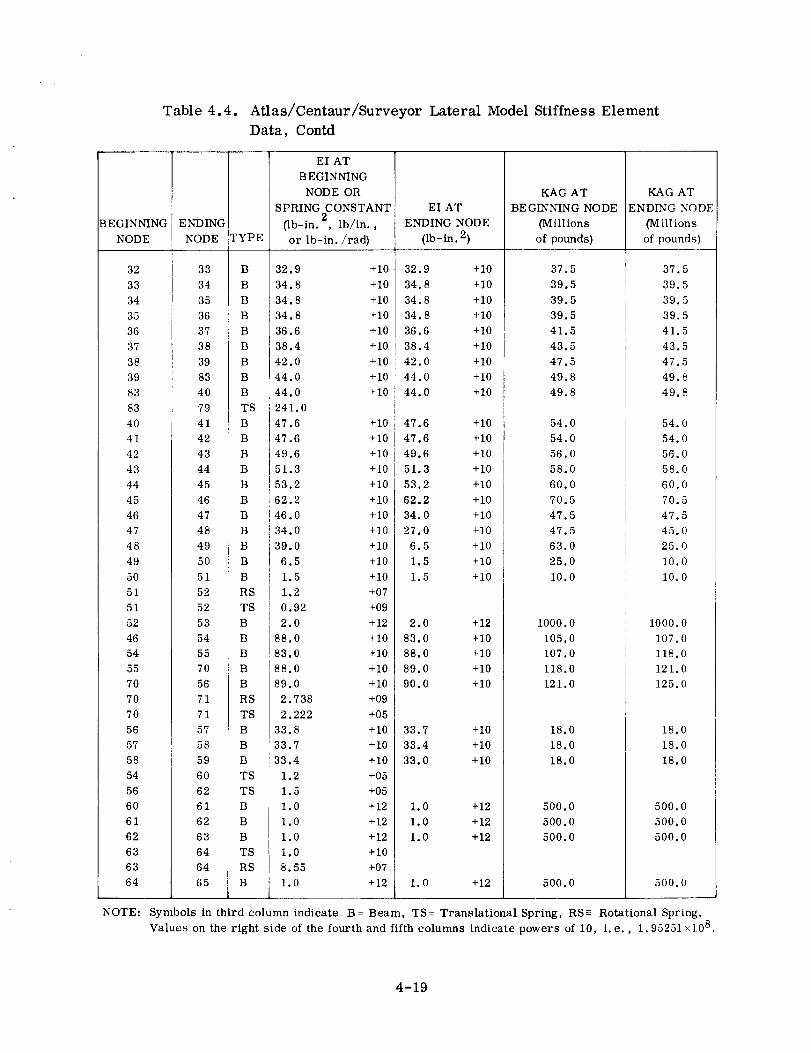
Table 4.4. Atlas/Centaur/Surveyor Lateral Model Stiffness Element
Data, Contd
BEGINNING
NODE
32
33
34
35
36
37
38
39
83
83
40
41
42
43
44
45
46
47
48
49
5O
51
51
52
46
54
55
7O
7O
7O
56
57
58
54
56
6O
61
62
63
63
64
E NDING
NODE TYPE
33 B
34 B
35 B
36 B
37 B
38 B
39 B
83 B
40 B
79 TS
41 B
42 B
43 B
44 B
45 B
46 B
47 B
48 B
49 B
5O B
51 B
52 RS
52 TS
53 B
54 B
55 B
70 B
56 B
71 RS
71 TS
57 B
58 B
59 B
60 TS
62 TS
61 B
62 B
63 B
64 TS
64 RS
65 B
EI AT
BEGINNING
NODE OR
SPRING CONSTANT2
(lb-in. , lb/in.,
or lb-in./rad)
EI AT
ENDING NODE
(lb-in. 2)
32.9
34.8
34.8
34.8
36.6
38.4
42.0
44.0
44.0
241.0
47.6
47.6
49.6
51.3
53.2
62.2
46.0
34.0
39.0
6.5
1.5
1.2
0.92
2.0
88.0
83.0
88.0
89.0
2. 738
2.222
33.8
33.7
33.4
1.2
1.5
1.0
1.0
1.0
1.0
8.55
1.0
+10 32.9 +10
+10 34.8 +10
+10 34.8 +10
+10 34.8 +10
+10 36.6 +10
+10 38.4 +10
+10 42.0 +10
+10 44.0 +10
+10 44.0 +10
+10 47.6 +10
+10 47.6 +10
+10 49.6 +10
+10 51.3 +10
+10 53.2 +10
+10 62.2 +10
+10 34.0 +10
+10 27.0 +10
+10 6.5 +10
+10 1.5 +10
+10 1.5 +10
+O7
+09
+12 2.0 +12
+10 83.0 +10
+10 88.0 +10
+10 89.0 +10
+10 90.0 +10
+09
+O5
+10 33.7 +10
+10 33.4 +10
+10 33.0 +10
+05
+O5
+12 1.0 +12
+12 1.0 +12
+12 i.0 +12
+10
+07
+12 1.0 +12
KAG AT
BEGINNING NODE
(Millions
of pounds)
37.5
39.5
39.5
39.5
41.5
43.5
47.5
49.8
49.8
54.0
54.0
56.0
58.0
60.0
70.5
47.5
47.5
63.0
25.0
10.0
i000.0
105.0
107.0
118.0
121.0
18.0
18.0
18.0
500.0
500.0
500.0
500.0
KAG AT
ENDING NODE
(Millions
of pounds)
37.5
39.5
39.5
39.5
41.5
43.5
47.5
49.8
49.8
54.0
54.0
56.0
58.0
60.0
70.5
47.5
45.0
25.0
10.0
10.0
1000.0
107.0
118.0
121.0
125.0
18.0
18.0
18.0
500.0
500.0
500.0
500.0
NOTE: Symbols in third column indicate B= Beam, TS= Translational Spring, RS -= Rotational Spring.
Values on the right side of the fourth and fifthcolumns indicate powers of 10, i.e., 1. 95251 ×108.
4-19

Table 4.5. Lateral Modal Frequencies and Generalized Masses For Thrust
Buildup Condition
MODE GENERALIZED MASS FREQUENCY
NO. (lb-sec 2/in. ) (cps)
1 63.12 0.315
2 0.9614 0. 553
3 36.05 0.668
4 21.86 0.675
5 10.36 0.750
6 28.26 1.85
7 19.07 4.51
8 8.666 6.93
9 6. 572 7.7O
10 0.2075 8.44
11 7.264 9.13
12 8.944 10.12
13 2. 079 11.88
14 8.995 13.91
15 0. 07172 16.83
4.4.2 LONGITUDINAL LOADS
4.4.2.1 Engine Start on the Pad. The analysis for this condition uses the longitudinal
model of Fig. 4.7. For longitudinal load analyses the initial deflections due to gravity
were calculated and used as initial conditions for the response solution. Gravity forces
on each mass were also imposed for the response solution to obtain total loads, in-
cluding gravity. The engine forces used are shown in Fig. 4.10. These engine thrust
buildup curves are envelopes of maximum buildup rates and peak thrusts obtained
during manufacturers test runs. (The buildup analysis could be done without gravity
forces and initial deflections. The gravity loads would then be added to the transient
loads. )
The results of the response calculations using Adam's method of Section 2.4 are
given in Figs 4.11 and 4.12. The transient acceleration at the Centaur/Surveyor
interface, Station 173, is shown in Fig. 4.11. (The acceleration does not include
gravity. ) The normal-mode-coordinate displacements in Fig. 4.12 show that the re-
sponse is primarily in the first four modes. Fifteen modes were used in the analysis
but only the first eight are plotted. The initial deflections and gravity loads are seen
represented at time zero.
4.4.2.2 Vehicle Liftoff. Liftoff analysis is undertaken using the free-free modes of
the model in Fig. 4.7. Initial deflections due to thrust, gravity, and launcher forces
are calculated and used as initial conditions. In the response solution the gravity
4-20
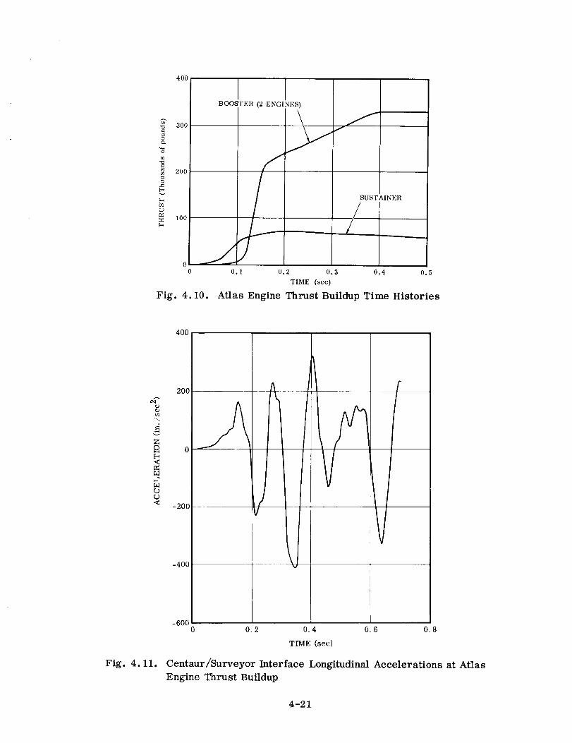
BOOSTER
300 [
200
0 ___...___-._0 O.
(2 ENGINES)
O. O.
TIME (see)
Fig. 4. I0.
SUSTAINER
0.4 0.5
Atlas Engine Thrust Buildup Time Histories
400
O)
i
Z
<
_9[9<
Fig. 4. II.
200
-200
-400
-600
t
0.2 0.4 0.6 0.8
TIME (sec)
Centaur/Surveyor Interface Longitudinal Accelerations at Atlas
Engine Thrust Buildup
4-21

1.2
0.8 -- -
'_ 0.4
=
[....Z
N 0
r_<
-0.8
-1.2
-1.60
"\ ,' / "J __
0. I 0.2 0.3 0.4 0.5 0.6 0.7
TIME (sec}
x:
_9rr
Fig. 4.12. Longitudinal Normal-Mode-Coordinate Displacements at Atlas
Engine Thrust Buildup
40 r
20 -- _
0 ........ i
-20 -- _ _i_+ •-40[--
-80-60 ___ i
ri
i
k
0.2
-100
_ r_ --
0.4 0.6
TIME (see)
o:8 _'.o
Net Atlas Launcher Force
During Launcher Release
Fig. 4.13.
forces are applied to each mass, the steady
engine thrusts at Masses 18 and 19, and the
launcher force at Mass 19. The time history
of the net launcher force is given in Fig.
4.13. The net launcher force is the sum-
mation of four forces exerted by the launcheron the vehicle. These forces are the hold-
down launcher arm force, the auxiliary
launcher-arm force, the rise-off disconnect
force, and the inertial force of the launcher
arms. Initially, all these forces are acting;
however, as the vehicle moves upward, all
are removed. The holddown launcher-arm
force is the force exerted by pneumatic cy-
linders (in the Atlas system) to restrain
the vehicle. To accomplish the vehicle re-
lease the pressure in the cylinders is re-
leased. When the pressure drops below that
required to restrain the vehicle the vehicle
begins to move upward. When the pressure
has dropped sufficiently the arms are
4-22

disconnected. In Fig. 4.13, vehicle motion begins at 0.1 second and the arms are
disconnected at 0.6 second. The step at 0.6 second represents a small residual pres-
sure at arm disconnect. The auxiliary arm force is a constant upward force for the
first 0. 102 second of motion and is then rein oved. This removal is seen at 0.202
second in Fig. 4.13. The rise-off disconnect force is a constant upward force for the
first 0. 164 second of motion. Its removal is seen at 0.264 second in Fig. 4.13. The
weight of the launcher arms is a downward force; it is assumed constant from 0 to
1.0 second.
With the model and applied forces described, the response is calculated using
Adam's numeric integration. The acceleration at Station 173 is shown in Fig. 4.14
and the normal-mode-coordinate displacements are given in Fig. 4.15. in contrast to
the thrust buildup condition, there is significant response in higher modes caused by
the abrupt changes in the applied force.
4.4.2.3 Inflight Engine Shutdown.
Engine shutdown in flight is illustrated with80
the model of Fig. 4.8. The initial conditionsfor this analysis are the quasi-steady in- g_ertial loads on the masses, the sustainer
Z
thrust at altitude, and the associated de- _ 40
flections. The sustainer engine shutdown
characteristics are given in Fig. 4.16, __ 2o
6OO
400
• 200
Z
<r.-
,--" 0M
r..)<
-200
-400
Fig. 4.14.
f
7
0.4 0.8 1.2 1.
TIME (sec)
Centaur/Surveyor Interface
Longitudinal Accelerations
at Liftoff
1,21
0.8
C0 0.2
._o.4g
_-0.4
Ne_
-0.8
//
MODE 1//
.J
J_.4 0.6 0,8
TIME (sec)
/
1.O 1,2 1.4
MODE // _ / _<A r
, Vh/ /vv
6- WV
-2.00
3-
0,1
Fig. 4.15.
0.2 0.3 0.4 0.5 0.6 0.7
TIME (sec)
Longitudinal Normal-Mode-
Coordinate Displacements at
Vehicle Liftoff
4-23
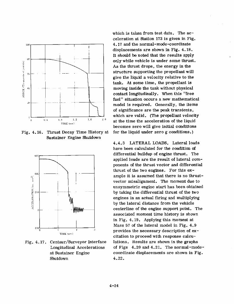
(J
I00
8O
60--
40
20
0
pr
II
!
iII
j0.4 0.8 1.2
TIME (see)
Fig. 4.16. Thrust Decay Time History at
Sustainer Engine Shutdown
o 2oo
<
h_
<0
-200J1 3
TIME (see)
Fig. 4.17. Centaur/Surveyor Interface
Longitudinal Accelerations
at Sustainer Engine
Shutdown
which is taken from test data. The ac-
celeration at Station 173 is given in Fig.
4.17 and the normal-mode-coordinate
displacements are shown in Fig. 4.18.
It should be noted that the results apply
only while vehicle is under some thrust.
As the thrust drops, the energy in the
structure supporting the propellant will
give the liquid a velocity relative to the
tank. At some time, the propellant is
moving inside the tank without physical
contact longitudinally. When this "free
fuel" situation occurs a new mathematical
model is required. Generally, the items
of significance are the peak transients,
which are valid. (The propellant velocity
at the time the acceleration of the liquid
becomes zero will give initial conditions
for the liquid under zero g conditions.)
4.4.3 LATERAL LOADS. Lateral loads
have been calculated for the condition of
differential buildup of engine thrust. The
applied loads are the result of lateral com-
ponents of the thrust vector and differential
thrust of the two engines. For this ex-
ample it is assumed that there is no thrust-
vector misalignment. The moment due to
unsymmetric engine start has been obtained
by taking the differential thrust of the two
engines in an actual firing and multiplying
by the lateral distance from the vehicle
centerline of the engine support point. The
associated moment time history is shown
in Fig. 4.19. Applying this moment at
Mass 57 of the lateral model in Fig. 4.9
provides the necessary description of ex-
citation to proceed with response calcu-
lations. Results are shown in the graphs
of Figs 4.20 and 4.21. The normal-mode-
coordinate displacements are shown in Fig.
4.22.
4-24
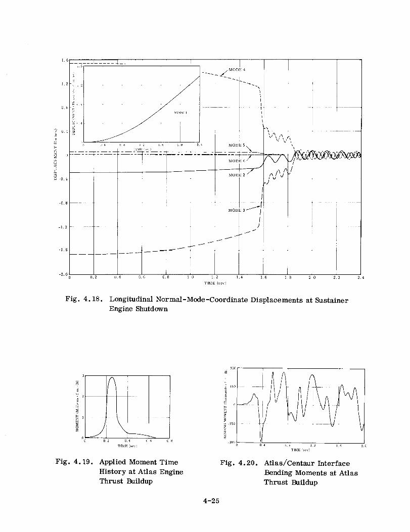
16
12
0 B
O, 4
.=
F-
<
i-0.4
-1.6
-2,0
...... E..... 2__1.6
_ 12
7
I I
MOI)b: 1
i
I
__ ___--__0,2 (J.4 0,6 13.8 1,0 1,2 1.4 1.6 1.8 20 2. _"--"'_. 4
TIME (set')
Fig. 4.18. Longitudinal Normal-Mode-Coordinate Displacements at Sustainer
Engine Shutdown
3
0 02 C,4 (i,_ 08
TIME (see)
Fig. 4.19. Applied Moment Time
History at Atlas Engine
Thrust Buildup
Fig. 4.20. Atlas/Centaur Interface
Bending Moments at Atlas
Thrust Buildup
4-25
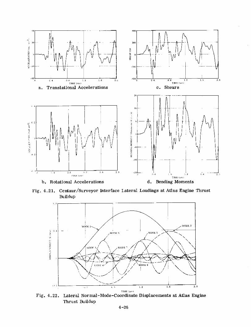
_0
< i
- 30 i< ,
-60 --
0 4 0.8 1,2 1.6 2. b
TIME {see)
a. Translational Accelerations
6OO
3OO
o
-300
-600
!J_
04 0.8 1,2 1.6 2.0
TIME Ist'('}
c. Shears
&- O
}
-(L
_A
Iiii
iz
-16
1.6 20 -24
16
f,
+iI
ii
i"04 08 I
(14 L B 12T_,;E (s,'t')
TIME (se(')
b. Rotational Accelerations d. Bending Moments
I1,6 2(;
Fig. 4.21. Centaur/Surveyor Interface Lateral Loadings at Atlas Engine Thrust
Buildup
U. _!;
- o 4
M
L_c_,<
m
_El 4
Fig. 4.22.
_ 4 U 8 1_2 1.6 2.0
TIME (st'c)
Lateral Normal-Mode-Coordinate Displacements at Atlas Engine
Thrust Buildup
4-26

4.5 DISCUSSION
From the preceding examples it is evident that the thrust-transient loads analyses
are relatively straightforward after the mathematical model and applied forces are
defined. Comments on the model development are given in Sections 2.2.3 and 4.4.1.
In this discussion comments will be related to applied forces, resulting loads, and
combinations of loads. Special considerations to be examined for vehicles include
engine-vehicle stability and high-frequency transients. It must be remembered that
these comments are general and that often in practice what could be done and what is
done are dependent on schedule, available information, and relative importance of
various aspects of the total vehicle program. As an example, design loads can be
determined from worst-case combinations or from a statistical evaluation of all the
loads. From a schedule standpoint, it may not be possible to gather all the data
necessary for a statistical study (or the data are just not available) to provide design
loads; therefore, the expedient and conservative worst-case combination approach is
indicated.
Other problems, such as Pogo (discussed in Section 4.5.5), have occurred on
some vehicles but not on others. Possible behavior of this nature should be examined
in enough detail such that the probability of surprise is small.
4.5.1 ENGINE FORCES. Liquid-propellant rocket-engine characteristics during
starting and shutdown are dependent on propellant temperatures, head pressure,
manufacturing tolerances, and other parameters. As a result, the engine thrust
buildup and decay curves have significant variations from run to run on one engine
and also among different engines. These variations are compounded with launch ve-
hicle configurations using multiple-engine systems because timing delays, variations
in plumbing, thrust-vector alignment, and variations in engine performance all have
tolerances. No single thrust time history accurately describes the propulsive excitation
applied to the vehicle. For longitudinal loads analyses, either of two basic approaches
is used to derive the design loads. In the first approach, a few response analyses are
made with typical thrust time histories to determine significant parameters. From
this preliminary analysis with available thrust time histories, a synthetic force time
history is developed to represent a worst-case envelope. The significant parameters
are usually rise rate, peak transient thrust, and frequency content. The envelope so
derived is then used for loads analysis.
The second approach is a statistical study of response to a large number of thrust
time histories. A response analysis is performed for every available (or a very large
sample) thrust time history, or in the case of multiple-engine systems, combinations
selected at random. A statistical study of the response will then give the mean and the
variance of loads from which design loads are specified. This approach involves the
expenditure of considerable execution time which must be repeated whenever there is
a significant design change in the vehicle.
4-27
Inputs for lateral responses are obtainedby similar procedures. Thrust mis-alignment canbe the maximum allowed by the manufacturer or it canbe a statisticaldistribution of the tolerance. With multiple engines, there is the addedconsiderationof combining the direction of misalignment of individual engines. Also, with multiple-engine systems, the enginesundoubtedlywill have different thrust time histories whichwill produce a time-varying application of moment to the vehicle. Establishment of thethrust differential constituting the applied momentmay, again, be developedfromworst-case combinations. A Monte-Carlo technique, using enginetest curves selectedat random, can provide a methodfor describing the response statistically. The vari-ation in the time at which the different engines receive the start signal must also beconsidered in establishing meaningful boundson the differential thrust. In general,secondary loads, such as produced by lateral response to thrust-vector misalignmentand differential engine thrust are small comparedwith total loads on the vehicle. Aworst-case simulation is often adequatefor establishing a "design" load associatedwiththe mode of "loads addition." For somevehicles, the start time is deliberately stagger-ed to reduce transient effects. The staggered start time must be examined in great de-tail, including performance tolerances in the separate engine systems, to obtain thesystem-peculiar loads criteria defining input forces andresponse. It is, indeed,possible to select a staggered start which will reduce vehicle elastic response, but isit also possible to select a start sequencewhich will result in more critical loads thana simultaneous start with random engine characteristics.
The reduction in transient longitudinal load by staggeredstart or by statisticalstudy of responsecan be significant in designingcertain parts of the vehicle andlaunchersystem. It is necessary to examine all the relevant loading conditions during vehiclelife and then to establish a compatible structural design. An evaluation of this type oftendetermines the detail of the analysis. Also, other phenomenamay be a controllingvariable. As an example, a simultaneous start of all enginescan produce pressurewaves in the exhaust ducts which could be harmful to the vehicle. The design signifi-canceof the pressure wave is subject to reduction by a staggered start. This considera-tion could be the predominant factor in deciding betweenstaggered andsimultaneousstarts and could be important in establishing the stagger time. Deciding what has to bedoneand what canbe doneis often more difficult than performing the analysis.
4.5.2 METHODOF LAUNCH. Two methods are employedfor launch of space ve-
hicles. Most commonly, a vehicle is held down until its engines are at full thrust.
It is released at some specified time interval after full thrust. The release is com-
monly "instantaneous" or "controlled." One other method is the "free launch," where-in the vehicle is not held down and will lift off when the thrust is equal to the weight.
The holddown is used for almost all space launches, while the free launch is used in
weapon systems. Free launch eliminates complicated launcher and control mechanism
and thus is better from maintenance and operations standpoints. Holddown permits
abort if initial engine and vehicle operation is not satisfactory. Thereby, it adds a
safety factor in the success of a specific payload mission.
4-28

Advantagesanddisadvantagesbetweenthe two methods related to vehicle loads
are dependent on vehicle and engine characteristics. With a holddown, minimum
tr_msient loads are incurred during engine thrust buildup if the launcher tiepoints are
close to points of engine load application and the stiffness of the launcher is great so
that most of the thrust forces are reacted by the launcher with small deflection. The
same effect is obtained in a free launch system if the vehicle structure from the engine
to the ground support point is very stiff. This permits a transition from gravity loads
being supported by ground to support by engine thrust without significant change in de-
flections and, in turn, no large transient loads to upper parts of the vehicle.
The liftoff loads are determined by the rate that thrust minus launcher forces
exceeds the weight of the vehicle. An instantaneous release would give a step change
and the most severe liftoff transients. The free launch would give a liftoff transient
determined by the engine thrust time history. One disadvantage of free launch is that
the engine buildup and liftoff transients are in fact one condition. With a holddown
these transients are separated slightly and some relief, due to damping and phasing,
can be expected because of the time interval.
In general, a holddown and controlled release will result in minimum vehicle
loads. The amount of load reduction will depend on the vehicle and launcher character-
istics. Indeed, launcher characteristics can be specified as a function of vehicle loads.
These characteristics may be effective spring rate, tie-down point, and rate and stroke
of release.
4.5.3 COMBINATION OF LOADS. A complete description of loads at engine ignition
and vehicle liftoff would include longitudinal and lateral steady-state and transient
loads discussed in the preceding sections, wind loads, vehicle misalignment or center-
of-gravity offset, vehicle loads incurred due to controlling the vehicle, or any other
load that is imposed at this time. Adding the worst-case conditions of all the above
loads is often used to obtain the total load. Certainly for ground equipment this is
the only reasonable approach. For parts of the vehicle designed by this total load
some weight saving could be gained by statistical combination of loads but, generally,
the weight saving is small in terms of pounds of payload and the applied forces are
not too well described so that a good statistical analysis cannot be made. Therefore,
it is recommended that worst-case combinations be used to specify design loads forvehicles.
There are occasions when a designed vehicle is to be used with a new stage or
payload. In order to minimize modification costs it may be necessary to determine
whether the vehicle is able to sustain the loads. In this case the reduction in load by
a statistical combination of loads is justified.
For purposes of statistical analyses the loads to be combined are assumed to be
independent and normally distributed. The quantities required for analyses are (from
Ref. 4.6)
4-29

17r average of load r (mean)
a - variance or standard deviation of load rr
_2_Tr = square of the mean
--2 e second moment (mean square)rl r
-_ 2 2_r = r_r + ar
Probability theory shows that for any number of random variables _r, the combined
values rl are obtained by
_-2 = _rrlr +_Z;_rrs _s[r_s
a2 _- ___2
2 _ _ -2: _ +_ +_r_slr_s r'r-_s_r_slr_sr r r s r
2=_
r r
The three-sigma combined load is then _ + 3a.
As an example, consider combining vertical and lateral loads due to thrust rise
with ground wind loads. The probability distributions of these loads are illustrated
in Fig. 4.23. The lateral loads are to be considered as expressed in terms of equiv-
alent axial loads. Also, the three loading conditions are assumed to be independent.
The sum of the mean loads is
PAVE = A + C + E
and the combined variance is
(O2z+2ap = +
2 \1/2
(4.9)
(4.10)
4-30
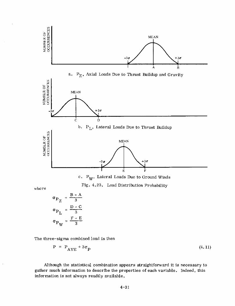
O
e#_J_n
Z
L_O
en
Z
where
MEAN
B
a. PZ, Axial Loads Due to Thrust Buildup and Gravity
bq_a
MEAN
8
C D
©
Ixl
b. PL' Lateral Loads Due to Thrust Buildup
MEAN
c. Pw' Lateral Loads Due to Ground Winds
Fig. 4.23. Load Distribution Probability
B-A
aP Z - 3
D-C
aP L - 3
F-E
(_PW - 3
The three-sigma combined load is then
P = PAVE + 3(rp (4. ii)
Although the statistical combination appears straightforward it is necessary to
gather much information to describe the properties of each variable. Indeed, this
information is not always readily available.
4-31
4.5.4 CONTROL SYSTEM ACTIVATION. The disturbances of engine thrust buildup
or decay and vehicle liftoff can cause an error in vehicle orientation with respect to
the desired trajectory and can also excite the bending modes. Upon activation of the
control system it will command the engines to correct vehicle attitude. Also, the
control system may respond to the sensed vehicle bending. Loads corresponding to
the attitude correction can be obtained from control studies which would give an en-
velope of commanded engine gimbal angle required for the correction. Applying this
amplitude (as a force), with a time history compatible with maximum possible engine
gimbal rate, to the vehicle will give the vehicle loads. The control system should be
designed so that it does not aggravate these initial bending moments. However, if a
limit-cycle* instabilityshould occur because of bending mode feedback from the sensor,
the magnitude of load during this limit cycle can be determined by the frequency re-
sponse solution presented in Section 6.
4.5.5 LONGITUDINAL INSTABILITIES. The combined vehicle system of
structure, mass, pneumatic system, propellant ducting, and propulsion system can
couple to produce instabilities and limit cycles. An example is the 5-cps limit cycle
shortly after liftoff on the Atlas vehicle. This phenomenon is due to coupling between
the vehicle modes and the pneumatic sensing and feed systems. Another example is
the Pogo problem of the Titan and Thor vehicles where limit cycles later in flight were
caused by coupling of the vehicle, propellant ducting, and engine systems. Problems
of this nature are very dependent on characteristics of each system. These character-
istics can vary considerably from one vehicle to another. The work of Ref. 4.4 dis-
cusses these problems and gives methods for analyses which can be used for predesign
evaluation on the existence of the problem and for identification of significant
parameter s.
4.5.6 HIGH-FREQUENCY EXCITATION. The discussion in the previous sections
pertains to excitation of the low-frequency modes of the vehicle. Perturbations in
some of the vehicle systems can also excite the higher frequency modes of the vehicle
or its systems. Sources of the excitation can be high-frequency pressure oscillations
in the thrust chambers, pump speeds, and operation of other mechanical equipment.
These phenomena are not amenable to analysis because of unsatisfactory mathematical
models for representation of the higher modes. In these higher modes there gener-
ally is coupling between lateral, longitudinal, torsion, shell, and individual compo-
nent modes. The problem can be attacked by two methods. One, the vibration tests
for components should include provision for adequate levels in the suspect frequency
regions. Two, using test data describing input, response, or vehicle modes an ap-
proximate analysis can be made that will give some information on loads. As an ex-
ample, a 70-cps transient of a few cycles in duration exists in booster engine chamber
pressure during the shutdown of the Atlas engines. From flight data it was found that
*Limit cycle is a term describing an "instability" which reaches a peak amplitude but
does not diverge beyond this peak, usually because of system nonlinearities.
4-32

a torsional modewas excited by this transient. Physical coupling between longitudinalexcitation andtorsion response of a magnitude indicated by the flight data could not beestablished. Therefore, using theoretical torsion modes and flight response data,a fictitious forcing function was derived which gavethe recorded response. To eval-uate the accuracy of this analysis a physical changein the vehicle was made on asucceedingflight andthe changein response was found to agree with predicted change.This established somevalidity in the analysis.
The solution of these problems is not straightforward and does require test datato identify the problem andcontrolling variables. Wherever possible, the conditionsshouldbe treated analytically so that subsequentvehicle changesdo not require ex-pensive test programs to verify the effect of the change.
4.6 CONCLUSIONSAND RECOMMENDATIONS
Methodsof analysis for response to enginetransients are well developed for cy-lindrical-tank liquid-propellant launchvehicles. For propellant tank shapesotherthan cylindrical, developmentwork is necessary to obtain a satisfactory mathematicalmodel representing the vehicle.
The recommendedprocedure is as follows.
1. Develop a mathematical model as given in Sections 2.2.4.3 and 4.3.
2. Obtain a description of applied force time history from engine test data.
3. Use a worst-case condition for design loads. If the worst-case condition isdetrimental to vehicle performance then a statistical analysis of engine character-istics and vehicle response shouldbe attempted.
4. Perform analyses for lateral loads due to engine misalignment and, in the case ofmulti-engine systems, unsymmetrical start. A worst-case analysis is usuallysufficient.
5. Obtain liftoff responseby the methods of Section4.3.2. A more detailed simu-lation maybe necessary for some controlled-release launches.
6. Combine thrust-transient loads with other loads imposed on the vehicle using themethods of Section4.5.3.
4.7 REFERENCES
4.1 T. Li, Spring Constants, C.G. Location, and Volume Increment of aMissile, General Dynamics/Convair Report ZU-7-056-TN, April 1956.
4.2 J. D. Wood, Survey on Missile Structural Dynamics, Report 7102-0041-
NU-000, Contract No. AF 04(647)-619, 1 June 1961.
4-33

4.3 L. D. Pinson, Longitudinal Spring Constants for Liquid Propellant
Tanks with E11ipsoidal Ends, NASA Technical Note D-2220, November
1964.
4.4 R. G. Rose, A Study of System-Coupled Longitudinal Instabilitiesin
Liquid Rockets, AFRPL-TR-65-163, September 1965.
4.5 W. H. Gayman and J. A. Garba, Dynamics Loads Analyses of Space
Vehicle Systems-Launch and Exit Phase, JPL Technical Memorandum
33-286 {To Be Published).
4.6 Y. W. Lee, Statistical Theory of Communication, John Wiley & Sons,
Inc., New York, pp 155-176, 1960.
4-34

5/ATMOSPHERIC DISTURBANCES
5-1


NOME NC LATUR E
A
C
CD
CN/o_
CNO
Cy/
Cyo
CS_
CSO
CM_
CMO
CMz"
CM_
CS A
F
G
I
K
Actuator piston area; cross-sectional area of the
vehicle structure
Flexibility matrix
Drag coefficient
Normal force coefficient per pitch plane angle
of attack
Normal force coefficient at zero pitch plane
angle of attack
Yaw force coefficient per yaw plane angle ofattack
Yaw force coefficient at zero yaw plane angleof attack
Shear coefficient per pitch plane angle of attack
Shear coefficient at zero pitch plane angle ofattack
Shear coefficient per unit normal acceleration
Shear coefficient per unit pitch plane rotational
acceleration
Moment coefficient per pitch plane angle ofattack
Moment coefficient at zero pitch plane angle
of attack
Moment coefficient per unit normal acceleration
Moment coefficient per unit pitch plane rotational
acceleration
Static aeroelastic coefficient
Force
Shear Modulus
Moment of inertia
Stiffness; shear effectiveness factor
ft 2
ft/lb
N.D.
1/rad
N°D°
1/rad
N.Do
1/rad
N°D°
lb/ft/sec 2
lb/rad/sec 2
ft/rad
ft
ft-lb/ft/sec 2
ft-lb/rad/see 2
N.D.
lb
lb/ft 2
lb-sec2-ft
lb/ft or _"ft-lbrad ' N.D.
5-3
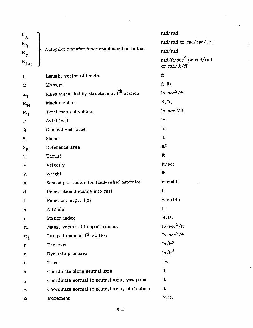
KAtKR
K C
KLR
L
M
Mi
M N
M T
P
Q
S
SR
T
V
W
X
d
f
h
i
m
m i
P
q
t
X
Y
Z
A
Autopilot transfer functions described in text
Length; vector of lengths
Moment
Mass supported by structure at i th station
Mach number
Total mass of vehicle
Axial load
Generalized force
Shear
Reference area
Thru st
Velocity
Weight
Sensed parameter for load-relief autopilot
Penetration distance into gust
Function, e.g., f(x)
Altitude
Station index
Mass, vector of lumped masses
Lumped mass at i th station
Pressure
Dynamic pressure
Time
Coordinate along neutral axis
Coordinate normal to neutral axis, yaw plane
Coordinate normal to neutral axis, pitch plane
Increment
5-4
rad/rad
rad/rad or rad/rad/sec
rad/rad
rad/ft/sec 2 or rad/rad
or rad/lb/ft 2
ft
ft-lb
lb-sec2/ft
N.D.
lb -sec2/ft
lb
lb
lb
ft 2
lb
ft/sec
lb
variable
ft
variable
ft
N.D.
lb -sec2/ft
lb-sec2/ft
lb/ft 2
lb/ft 2
sec
ft
ft
ft
N.D.

_g
3/
6
E
m
0
P
(Y
¢
02
LA
[]
EB
Angle of attack, pitch plane
Angle of attack, gust
Angle of attack, yaw plane
Flight path angle (angle between local
horizontal and velocity vector)
Engine gimbal angle
Iteration convergence tolerance
Damping coefficient
Average of load
Angle between local horizontal and vehicle
centerline; angle between undeformed axis and
deformed axis
Gust length
Normal mode coordinate
3.1416
Density
Standard deviation of load; modal slopes
Modal displacements
Angle between launch azimuth and vehicle
centerline
Frequency
Generalized mass
Row matrix
Column matrix
Square matrix
First derivative with respect to time
Second derivative with respect to time
rad
rad
rad
rad
rad
N.D.
N.D.
lb or ft-lb
rad
ft
ft
N.D.
lb-sec2/ft 3ff
lb or ft-lb; rad/ft
ft/ft
rad
rad/sec 2
lbmsec2/ft
5-5

5/ATMOSPttERIC DISTURBANCES
5.l STATEMENT OF THE PROBLEM
The powered phase of flight through the atmosphere is a condition that oftendictates design of a significant portion of the vehicle structure. Axial and lateralloads imposed during this period are functions of axial acceleration, atmosphericdisturbances (winds andgusts), vehicle shape, Mach number, trajectory, and atmos-pheric density. Axial loads are primarily drag loads and inertial loads of the quasi-steady acceleration. Lateral loads are the result of vehicle (or structure) orientationwith respect to the relative air velocity, which is called the angle of attack. Themagnitudes of lateral loads are functions of angle of attack and dynamic pressure.Ttle angle-of-attack magnitudeis primarily a result of vehicle trajectory and atmos-pheric disturbances. Vehicle shape, Machnumber, and atmospheric density deter-mine the distribution of drag andlateral loads. Also, vehicle shapeand Machnumberdetermine the type of air flow andcan lead to phenomenasuchas buffeting.
Axial load values are relatively straightforward computations of trajectory param-eters such as acceleration, Machnumber, altitude, dynamic pressure, andweight.Lateral load calculations are also straightforward computations of these parameterswith the addition of angle of attack; however, the angle of attack is a function of atmos-pheric disturbances which are random in nature. Thus, the major problem in lateralloads is the determination of wind criteria. Oncethese are established, analyticaltechniques are used to obtain the loads.
Winds are large-scale movements of air persisting for a period of time consider-ably longer than the vehicle flight and extending over a significant altitude range.Fig. 5. la presents a detailed wind profile taken by the smoke-trail method. Fig.5. lb showsthe samewind as measuredby a balloon system and also the averaged(smoothed)smoke-trail data.
Wind speedsat launch are small (comparedto wind speedsat altitude) and increasewith altitude in anunevenmanner, reaching a peak in the 25,000- to 40,000-foot-altitude range. The wind speedthen decreasesup to approximately 100,000 feet whereit starts to increase. Little data are available onwind speedsabove60,000 feet; how-ever, loading dueto wind abovethis altitude is quite small becuaseof low dynamicpressure and is rarely considered. Gusts are defined as short-period disturbancesin the air and are usually considered to account for the profile detail not measuredbythe balloon system (seeFig. 5.1). For highly accurate wind profiles only the elasticresponse to gust is generally considered. For most launch vehicles the time spanofexposure to a discrete gust is on the order of less than one second. While data ongusts are meager they are usually considered to exist in the samealtitudes in whichhigh wind speedis prevalent.
5-7
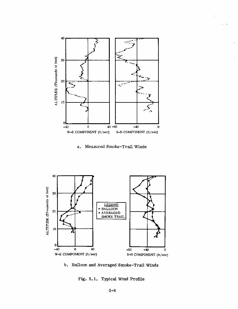
X:)
0
B1.-,
<
40
30
20
I0
,,f
o.....,
•o_o'° ,k_'W'°'*
'...._.
4'.O_o_o
,l..,J
oo _ °...° ° -• ;o.
.>--_, oo •
°.e-
°."°°
0
-40 0 40 -80 -40 0
W-E COMPONENT (ft/sec) S-N COMPONENT (ft/sec)
a. Measured Smoke-Trail Winds
4O
30
_ 20
oOO_
q_ p-*"
,!J
j _( ....._
,.r""___.
-4O 0 40
W-E COMPONENT (ft/sec)
LEGEND [
oB_ I= AVERAGED [
SMOKE TRAIL[
/'C
-80 -4( 0
S-N COMPONENT (ft/sec)
b. Balloon and Averaged Smoke-Trail Winds
Fig. 5.1. Typical Wind Profile
5-8

The general procedure for calculation of lateral loads consists of a trajectory
simulation through a specified wind and gust profile (or profiles) to obtain the re-
quired parameters for loads. Generally rigid-body plus aeroelastic loads due to wind
arc obtained and added to the loads due to elastic response to a gust.
In the transonic region (0.8 < MN _ 1.2) shock waves begin to build up and areas
of random turbulence form aft of points where the geometry changes. This random
turbulence is referred to as buffet. Buffet is first discernible as the transonic region
is entered, builds up sharply in the region 0.8 <- M N _ 1.0, and then somewhat slowly
decreases with increasing Mach number. Hence buffet is strongly dependent on Mach
number. Buffet loads analysis is accomplished by random response analysis of ex-
perimental pressure distribution data or by scaling of experimental response data.
In summary, the loads due to atmosphere come from two principal sources: 1)
wind and gusts, and 2) buffet. The angle of attack due to wind and gust reaches a
maximum value during the period of flight when dynamic pressure is near its peak,
i.e., at a 25,000- to 40,000-foot altitude. This produces a critical condition for this
type of loading. The buffet loads are mostly local loads although some response of
the complete vehicle may occur. The maximum buffet condition occurs in the tran-
sonic region which for most space vehicles is earlier than the maximum wind and gust
loads; however, the combination of maximum buffet loads and all other loads at that
time may be critical. Other minor loads may occur while in the atmosphere; these
will be discussed in detail later. Guidance steering is not usually used while in the
atmosphere; however, if used it may produce another critical condition.
5.2 HISTORICAL BACKGROUND
The historical background of analysis of loads due to atmospheric disturbances
centers around efforts first to obtain accurate wind and gust data and then to derive
useful, accurate criteria from the data. It became apparent early in the history of
launch vehicles that the wind profile (wind speed vs altitude) that would be encountered
was important. It was also recognized that the available wind data, especially the
wind shear (the rate of change of speed with altitude), were inaccurate. The need for
methods to reduce the data to criteria that were accurate, yet economical and simple
in application, was also recognized.
The bulk of wind data obtained in the 1950Vs was taken with the AN/GMD-1 balloon
system. This system used data radioed from the balloon to compute altitude and then
used the cotangent of the elevation angle to obtain horizontal distance. At low elevation
angles the errors could be large, errors in wind shear sometimes approaching the
value of the wind shear. The AN/GMD-2 balloon system was developed in the late
1950's to provide better data. In this system the slant range is obtained by a radio-
ranging attachment and sine and cosine are used to compute altitude and horizontal
distance. This system is approximately six times more accurate then the AN/GMD-1
system. Comparisons of the two systems are made in Refs 5.1 and 5.2. However,
5-9

both systems yield accurate data at 1000-foot-altitude increments. To provide ac-
curate data at shorter altitude increments the FPS-16 Radar/Spherical Balloon sys-
tem was developed. This system yields data at 25-meter-altitude increments and is
several times more accurate than the AN/GMD-2 system. An evaluation of the sys-
tem is given in Ref. 5.3. Two other methods of obtaining wind data have been tried
on an experimental basis. One of these is the smoke-trail method. In this method a
rocket leaves a continuous trail of smoke as it ascends, photographs are taken at
given times, and the dispersions of the trail are analyzed to provide wind data. Ref.
5.4 discusses the application of the method and some experimental results. The other
method uses a doppler radar system to track a column of chaff. The dispersions of
the chaff column are used to obtain wind velocity profiles. Ref. 5.5 describes the
method and some experimental results obtained from it. Neither system is, nor is
planned to be, operational.
The development of wind criteria has taken two approaches. One approach is to
do a statistical analysis of the wind data and then develop synthetic wind profiles.
Loads are then obtained by application of these profiles. Synthetic profiles have been
generated by many persons involved in wind criteria. The first widely used profile
was the Sissenwine profile developed in the early 1950's. It is given in Ref. 5.6 and
has since been modified by Ref. 5.7. Currently, the most widely used synthetic pro-
file criteria are the Marshall Space Flight Center (MSFC) criteria. MSFC has develop-
ed a computer analysis of wind data that yields, for a given launch site and azimuth,
wind speed and shear data from which synthetic profiles are constructed. Refs 5.8 and
5.9 are examples of the criteria generated by MSFC.
The second approach is to obtain loads for each wind sounding in a set of sound-
ings and then do a statistical analysis of the loads. This approach is referred to as a
statistical load survey. The original development of this approach was done by Avidyne
Research, Inc., and reported in Refs 5.10, 5.11, and 5.12. The approach requires a
trajectory simulation for each sounding; this approach entails a considerable amount of
computer time. To decrease the computer time involved, several approximate metohds
have been developed. The influence coefficient method uses an influence coefficient
matrix derived from 'basic" profiles, i.e., triangular spike, ramp, etc. The vector
of wind speeds from a particular wind sounding is multiplied by an appropriate in-
fluence coefficient matrix to obtain loads for that sounding. The method was studied
by Avidyne and the results are given in Ref. 5.13. Clingan (Ref. 5.14) uses a closed-
form trajectory solution to reduce computer time for the statistical load survey. The
trajectory solution is obtained by using perturbation equations and neglecting rotational
rate and acceleration. Van der Maas (Ref. 5.15) developed a method that uses two
basic parameters of a wind sounding to obtain loads on a vehicle. The parameters are
maximum wind velocity and the integral of the wind velocity from ground to the altitude
of the maximum wind velocity.
The statistical load survey, as developed by Avidyne, is the most accurate method
since no assumptions are made concerning either the trajectory simulation or the
5-10
correlation betweenwind data and resulting loads (as is done for synthetic profiles).Avidyne investigated the several methods and compared them, using the statisticalload survey as the standard of comparison. The results are given in Ref. 5. l'_. Inorder of decreasing accuracy, Avidyne ranked the methods as follows: influence co-efficient method, ClinganTsmethod, discrete profiles, and Vander Maas method.
The data available onwhich to base gust criteria are sparse. Refs 5.16 and 5.17give some of the available data. Thesedata were gatheredby aircraft flying horizon-tally andthen measuring the aircraft vertical accelerations. Randomnessof the datais not necessarily established andcorrelation with wind speedis lacking. Also, mostof the data were taken below a 20,000-foot altitude; however, peak launch vehicle loadsgenerally occur in the 25,000- to 40,000-foot-altitude range. Thus, assumptions haveto be madewhen applying these data to launch vehicles. Currently, the gust criteriacover any short-period disturbance not adequatelymeasuredduring the wind sounding.As wind soundingsbecomemore accurate, and especially as the incremental altitude
for measurement becomes smaller, the wind sounding will include more and more of
what is now included as gust. Thus the question of improving gust criteria will pro-
bably be resolved not by gust measurements but by highly accurate wind soundings.
Analysis for loads due to atmospheric disturbances consists of a five or six
degree-of-freedom rigid-body trajectory simulation through the design wind profile.
The parameters from the simulation are used to calculate vehicle loads. With large
boosters the trajectory simulation should include the low-frequency bending modes
(less than 2 cps) since these modes can be excited by the wind profile. As wind pro-
file representation improves, it will be necessary to include elastic modes for most
vehicles in the trajectory simulation. Ref. 5.18 presents work examining the in-
clusion of elastic modes in the simulation with detailed wind profiles. Here the pro-
blem is not one of methodology but one of determining a sufficiently accurate procedure
with economical execution.
The gust effects are added by either of two methods: 1) adding the gust profile
to the wind profile to obtain rigid-body gust loads, and performing an elastic analysis
with the gust only to obtain those loads due to elastic response, and 2) calculating
rigid and elastic body gust loads independently of the wind profile and adding these to
the loads resulting from the wind profile. The end result is essentially the same and
use of either method is usually at the discretion of the analyst.
The buffeting during the transonic regime of flight is not an atmospheric dis-
turbance, but a phenomenon caused by the shape of the vehicle. It is mentioned here
because loads caused by buffeting must be considered in combination with wind loads
for total vehicle loads. Ref. 5.19 gives a complete discussion on buffeting historical
background and state of the art. Ref. 5.20 contains criteria for determining whether
or not a particular configuration is buffet prone. Both references have their own
extensive lists of references on the subject.
5-11

5.3 QUASI-STEADY FLIGHT LOADS
The term, "quasi-steady flight loads," is used to describe loads and/or response
produced by long-period maneuvers and disturbances. The primary sources are winds
and steering to accomplish a desired trajectory, either by a predetermined pitch pro-
gram or by a guidance system. The period is sufficiently long that the vehicle is
characterized elastically as deflecting statically and possibly responding in its lower
frequency normal modes. The gross wind speed changes take place during altitude
spans of several thousand feet; however, recent wind data are providing wind detail
for altitude spans of less than a hundred feet.
5.3.1 ANALYTICAL APPROACH. The initial step in obtaining quasi-steady flight
loads is to simulate, analytically, the trajectory so that the required trajectory
parameters can be obtained. While all trajectory simulations have the same basic
analytical features, they usually differ in the detail of these features. Factors in-
fluencing the detail composition of a trajectory simulation include optional ways of
calculating some parameters, the intended use of the simulation (loads analysis, per-
formance analysis, etc.), the degree of complexity deemed necessary to provide ac-
curate results, and the coordinate system(s) used. With this in mind, the basic form
and equations will now be outlined. The vehicle coordinate system is shown in Fig.
5.2. The vehicle forces are illustrated in Fig. 5.3.
The equations of motion for the trajectory of a launch vehicle are derived in Ref.
5.21. An inertial reference frame, usually having its origin at and fixed to the center
of the earth, is used. However, forces on the vehicle are expressed in body axes. It
is also desirable to fix the vehicle position relative to the launch site. Thus several
coordinate systems and the accompanying coordinate transformations are needed. The
range of launch vehicles while in the atmosphere is usually on the order of 20-30 miles;
hence a flat nonrotating earth will suffice for determining quasi-steady flight loads.
The acceleration of the vehicle is obtained by consideration of the thrust, aerodynamic,
gravitational, and centrifugal forces. The resultant acceleration produces, over its
time integral, a vehicle velocity, V, which is relative to still air and a fixed launch
point. The flight path angle, _/, is defined as the angle between the horizontal datum
at a fixed launch point and the vehicle velocity vector. The altitude is given by
h = /V sinv dt (5.1)
In vehicle coordinates, the axial, lateral, and vertical velocities with respect to the
atmosphere are (assuming a flat nonrotating earth and _ and B to be small)
= V-V H cos e /
= Vsin/9-V Lcos
= Vsin_-V Hsine
(5.2)
5-12
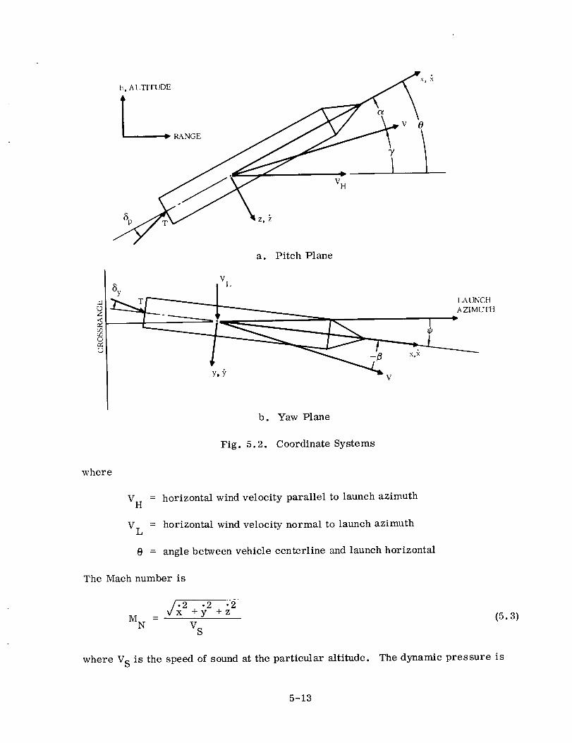
1ALTITUDE
a. Pitch Plane
18y I__1 _ T_ LAUNCH
g
b. Yaw Plane
Fig. 5.2. Coordinate Systems
where
V H = horizontal wind velocity parallel to launch azimuth
V L = horizontal wind velocity normal to launch azimuth
@ = angle between vehicle centerline and launch horizontal
The Mach number is
M N
Cx •2 • 22 +Y +z
V S
(5.3)
where V S is the speed of sound at the particular altitude. The dynamic pressure is
5-13
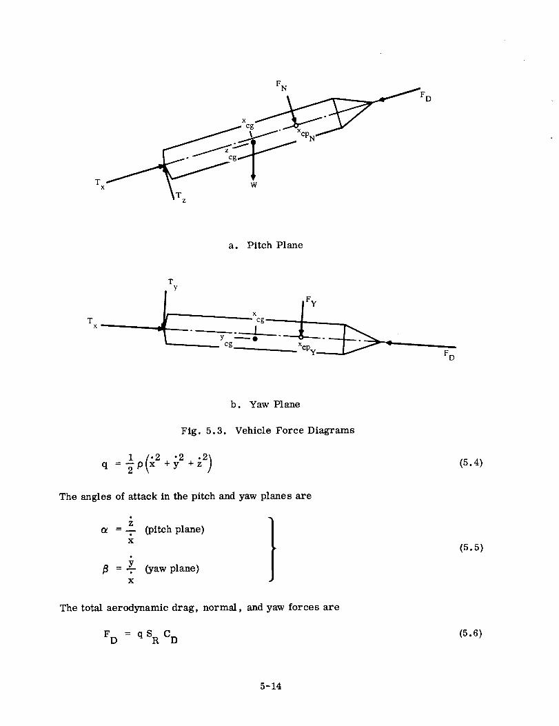
F N
x FD
T x W
Z
a. Pitch Plane
TX
TY
b. Yaw Plane
Fig. 5.3.
1('2 "_ _2/q ='_p x +y +
Vehicle Force Diagrams
(5.4)
The angles of attack in the pitch and yaw planes are
-- (pitch plane)x
= _ (yaw plane)
x
} (5.5)
The total aerodynamic drag, normal, and yaw forces are
F D = q SR C D (5.6)
5-14
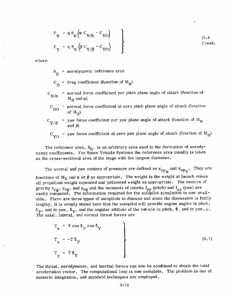
where
(5.6
Contfl)
S = aerodynamic reference areaR
CD = drag coefficient (function of MN)
CN/_
CNO
Cy/8
Cyo
= normal force coefficient per pitch plane angle of attack (function of
M N and _)
= normal force coefficient at zero pitch plane angle of attack (function
of MN)
= yaw force coefficient per yaw plane angle of attack (function of M N
and B)
= yaw force coefficient at zero yaw plane angle of attack (function of MN)
The reference area, SR, is an arbitrary area used in the derivation of aerody-namic coefficients. For Space Vehicle Systems the reference area usually is taken
as the cross-sectional area of the stage with the largest diameter.
The normal and yaw centers of pressure are defined as Xep N and Xcp Y. They are
functions of M N and _ or B as appropriate. The weight is the weight at launch minus
all propellant weight expended and jettisoned weight as appropriate. The centers of
gravity Xcg, Ycg, and Zcg and the moments of inertia Iyy (pitch) and Izz (yaw) areeasily computed. The information required for the aufdpilot simulation is now avail-
able. There are three types of autopilots to discuss and since the discussion is fairly
lengthy, it is simply stated here that the autopilot will provide engine angles in pitch,
6p, and in yaw, 6y, and the angular attitude of the vehicle in pitch, O, and in yaw, _.The axial, lateral, and normal thrust forces are
T = T cos 6p cos 6yX
T = -T 6z P
T = T6yY
(5.7)
The thrust, aerodynamic, and inertial forces can now be combined to obtain the total
acceleration vector. The computational loop is now complete. The problem is one of
numeric integration, and standard techniques are employed.
5-15
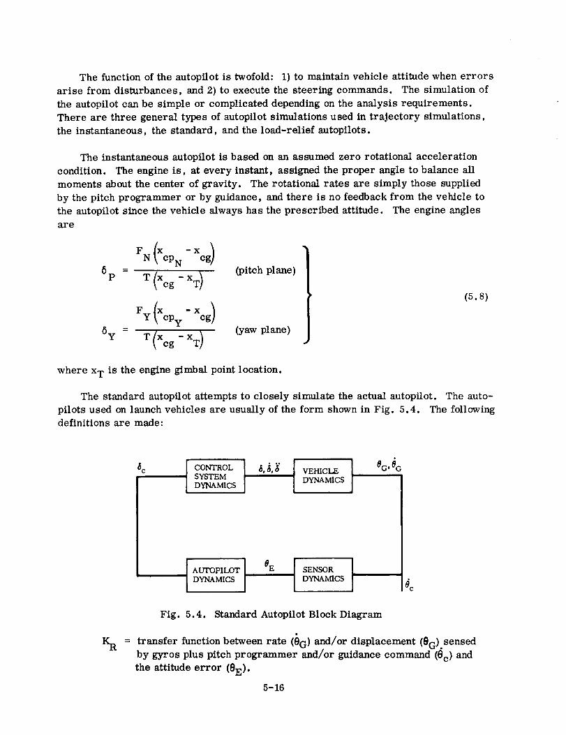
The function of the autopilot is twofold: 1) to maintain vehicle attitude when errors
arise from disturbances, and 2) to execute the steering commands. The simulation of
the autopilot can be simple or complicated depending on the analysis requirements.
There are three general types of autopilot simulations used in trajectory simulations,
the instantaneous, the standard, and the load-relief autopilots.
The instantaneous autopilot is based on an assumed zero rotational acceleration
condition. The engine is, at every instant, assigned the proper angle to balance all
moments about the center of gravity. The rotational rates are simply those supplied
by the pitch programmer or by guidance, and there is no feedback from the vehicle to
the autopilot since the vehicle always has the prescribed attitude. The engine angles
are
_K - Xcg /FN cPN
5p = T (Xcg - XT) (pitch plane)
xo )(5.8)
where x T is the engine gimbal point location.
The standard autopilot attempts to closely simulate the actual autopilot. The auto-
pilots used on launch vehicles are usually of the form shown in Fig. 5.4. The following
definitions are made:
c lVEHC }O McsS 'EM00 O
AUTOPILOTDYNAMICSc
Fig. 5.4. Standard Autopilot Block Diagram
transfer function between rate (SG) and/or displacement (8G).sensed
by gyros plus pitch programmer and/or guidance command (8c) and
the attitude error (8E).
5-16
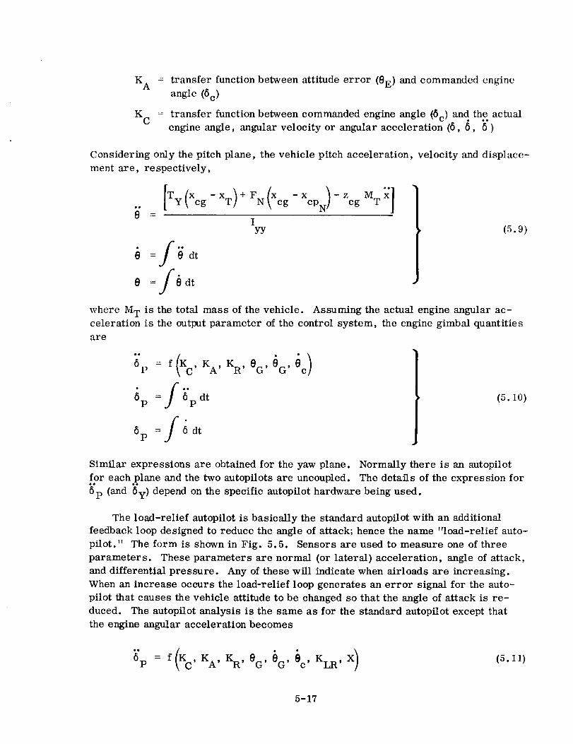
K A = transfer function between attitude error (0E) and commanded engine
angle (6 c)
transfer function between commanded engine angle (6c) and the actualKC engine angle, angular velocity or angular acceleration (6, 6, 6")
Considering only the pitch plane, the vehicle pitch acceleration, velocity and displace-
ment are, respectively,
[Ty(XcgxT) N(XcgXcp )zo Mx]
dt
0 =/0 dt
IYY (5.9)
where M T is the total mass of the vehicle. Assuming the actual engine angular ac-
celeration is the output parameter of the control system, the engine gimbal quantities
are
6p = f , ' 0G'
_p = f "5"p dt (5.10)
Similar expressions are obtained for the yaw plane. Normally there is an autopilot
for each.plane and the two autopilots are uncoupled. The details of the expression for
6"p (and 6y) depend on the specific autopilot hardware being used.
The load-relief autopilot is basically the standard autopflot with an additional
feedback loop designed to reduce the angle of attack; hence the name "load-relief auto-
pilot." The form is shown in Fig. 5.5. Sensors are used to measure one of three
parameters. These parameters are normal (or lateral) acceleration, angle of attack,
and differential pressure. Any of these will indicate when airloads are increasing.
When an increase occurs the load-relief loop generates an error signal for the auto-
pilot that causes the vehicle attitude to be changed so that the angle of attack is re-
duced. The autopilot analysis is the same as for the standard autopilot except that
the engine angular acceleration becomes
6"p = f(%, KA, KR, 0G, 0G, ec, KLR, X ) (5.11)
5-17

CONTROLSYSTEMDYNAMICS
VEHICLEi
DYNAMICS
X
LoAojSENSOR
DYNAMICS
AUTOPILOT ] 0E SENSOR IDYNAMICS : DYNAMICS
C
where
Fig. 5.5. Load-Relief Autopilot Block Diagram
KLR
X
= transfer function between the sensed parameter (X) and the error
signal to the autopilot (0E)
= zorcxorAp
With the trajectory parameters available the shear and bending moment distri-
butions for the vehicle can now be calculated. Two approaches can be taken in cal-
culating rigid-body shear and bending moment due to airloads. One approach is to
apply the airloads due to ¢Xq (or _q) from the trajectory and to balance moments with
the engine, so that the rotational acceleration and rate are zero. This approach, re-
ferred to as the "trimmed vehicle condition," is a good approximation and is widely
used. Here, the aerodynamic normal force distribution along the vehicle is lumped
at panel points in the same manner as the weight is lumped (see Section 2). The re-
quired engine angle is
FN (XcPN-Xcg)
6 = T(XT_Xcg ) (5.12)
The normal acceleration is
.. T6 +F N
z - MT (5.13)
5-18
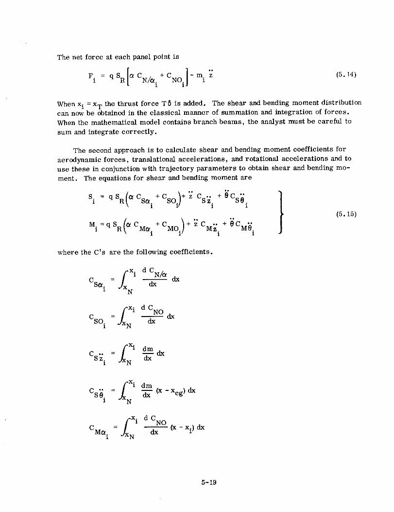
The net force at eachpanel point is
CN CNOi] ""F. = qS _ + -m z (5.14)x R /_. i
1
When x i = x T the thrust force T5 is added. The shear and bending moment distributioncan now be obtained in the classical manner of summation and integration of forces.
When the mathematical model contains branch beams, the analyst must be careful to
sum and integrate correctly.
The second approach is to calculate shear and bending moment coefficients for
aerodynamic forces, translational accelerations, and rotational accelerations and to
use these in conjunction with trajectory parameters to obtain shear and bending mo-
ment. The equations for shear and bending moment are
s., = q sR _ Cs_"+Cso Cs_ Csiii i
M.=qSR(_ +CMoi )+z + 01 CM_. CMz" CM0"1 i i
(5.15)
where the C's are the following coefficients.
x. d
=_x i CN/tXCS_. dx1 N
dx
= f°:i d CNO
CSO i .JXN _ dx
i dmCsz i : -_-- a_
=9(Ni dmCS_ i -_- (x - Xcg ) dx
= f"i d CNO
CMC_i _x N _ (x - xi) dx
5-19

= f_i d CN/{2
C MO i _x N _x(x - xi) dx
_( xi dmCMz i = -_- (x-xi) dx
N
CMe i fXN i -_"= dm (x - Xcg ) (x - xi) dx
and where x N is the vehicle nose station.
The quasi-steady axial loads come from the vehicle axial acceleration and aero-
dynamic drag. The axial load at the i th station is
P'I = M.1 x +qS R CD. (5.16)1
where
Mo
1
CD.1
= the mass supported by the structure of the ith station
= cumulative drag coefficient to the ith station
The foregoing discussion on loads has been for a rigid vehicle. Aerospace ve-
hicles are usually sufficiently flexible to have considerable deflection under limit
(design) load. In the case of air loads, this deflection causes changes in local angle
of attack and, in turn, the load distribution on the vehicle. The change in load dis-
tribution again changes the local angle of attack. Thus an iterative process is begun
which rapidly converges on a suitable airload distribution. Experience to date indi-
cates that inclusion of quasi-static aeroelastic effects in analysis can give loads for
aerospace vehicles of 5 to 20 percent over rigid vehicle loads.
Two methods employed for obtaining static aeroelastic effects are: I) finding
deflections and changes in load using the flexibility matrix and 2) obtaining deflections
and changes in load by using normal mode theory. In the first method, the restrained
stiffness matrix of Eq. 2.34 is inverted to obtain the flexibility matrix, C. Since the
configuration under study is a free-free vehicle, the displacements of the fixed point
must be added to obtain the total displacements. Also, vehicle slope due to shear
should be added if these slopes are significant terms for the vehicle under consider-
ation. The total displacement is
5-20
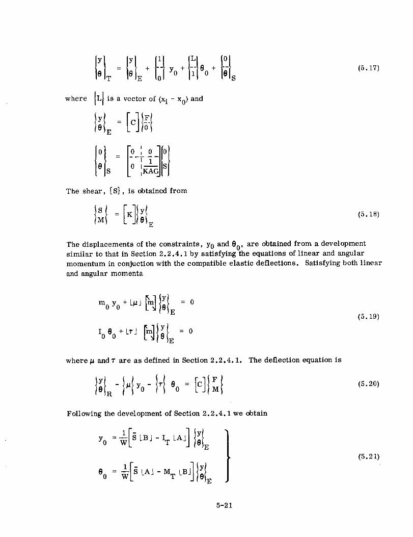
= + YO+ O0+lOT OE S
where IL] is a vector of (xi-x 0) and
The shear, IS], is obtained from
(5. i7)
(5.18)
The displacements of the constraints, Y0 and 0 0, are obtained from a developmentsimilar to that in Section 2.2.4.1 by satisfying the equations of linear and angular
momentum in conjuction with the compatible elastic deflections. Satisfying both linear
and angular momenta
_mlI'f0m0 Y0 + L#J 0 E
i0_0+_EmJI_f°(5.19)
where _ and r are as defined in Section 2.2.4.1.
l_l_-l_f,o-t,f_o;I_]l_1The deflection equation is
(5.20)
Following the development of Section 2.2.4.1 we obtain
YO W 0 E
1[ _]I'l0 0 = _ S LAJ - M T LB 0 E
(5.21)
5-21
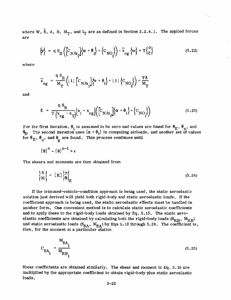
where W, §, A, B, MT, and IT are as defined in Section 2.2.4.1. The applied forces
are
where
(5.22)
and
Zcg MT El] ¢_ + 0 i MT
;/ 1%1)5 = (T Xcg- T)_('-Xcx1 N/O_ _+ei + (5.23)
For the first iteration, e i is assumed to be zero and values are found for OE, Oo, and
0S. The second iteration uses {_ + 0 i} in computing airloads, and another set of values
for 0 E, 0o, and 0S are found. This process continues until
{0] n - {0} n-1 < e
The shears and moments are then obtained from
(5.24)
If the trimmed-vehicle-condition approach is being used, the static aeroelastic
solution just derived will yield both rigid-body and static aeroelastic loads. If the
coefficient approach is being used, the static aeroelastic effects must be handled in
another form. One convenient method is to calculate static aeroelastic coefficients
and to apply these to the rigid-body loads obtained by Eq. 5.15. The static aero-
elastic coefficients are obtained by calculating both the rigid-body loads (SRB , MRB )
and static aeroelastic loads (SsA , MSA ) by Eqs 5.13 through 5.28. The coefficient is,then, for the moment at a particular station
MSA.1
CSA i - lVIRB. (5.25)1
Shear coefficients are obtained similarly. The shear and moment in Eq. 5.15 are
multiplied by the appropriate coefficient to obtain rigid-body plus static aeroelasticloads.
5-22
If the normal modes are available an alternate method of solution exists.
2. 163 states that
For static loads the derivatives are set equal to zero
_.a_2_ [_} = _]-1 [Q]
Eq.
(5.26)
(5.27)
where
[Q}
+q St_¢]' [CN/c_ i][a] [_}(5.28)
The engine angle is
0--_(__x__s_I{o_o,1+_o,}I_q SR
+ [C ][_] [_} (5.29)T(Xcg - XT) LLJ N/O_i
where LLJ is a vector of (x i - Xcu ). Substituting Eq. 5.29 for 6 in [Q] and rearrang-
ing terms and solving for [_ } in _q. 5.27, we have
qSR LLJ [C ][_]-qS RXcg - x T N/_ i
[_ l_ }I+x sR_]'_%/_.}_+{%5 -- _XTXcg x T
The deflection, slope, shear, and bending moment are then obtained by mode displace-
ment (Eq. 2. 179).
5-23
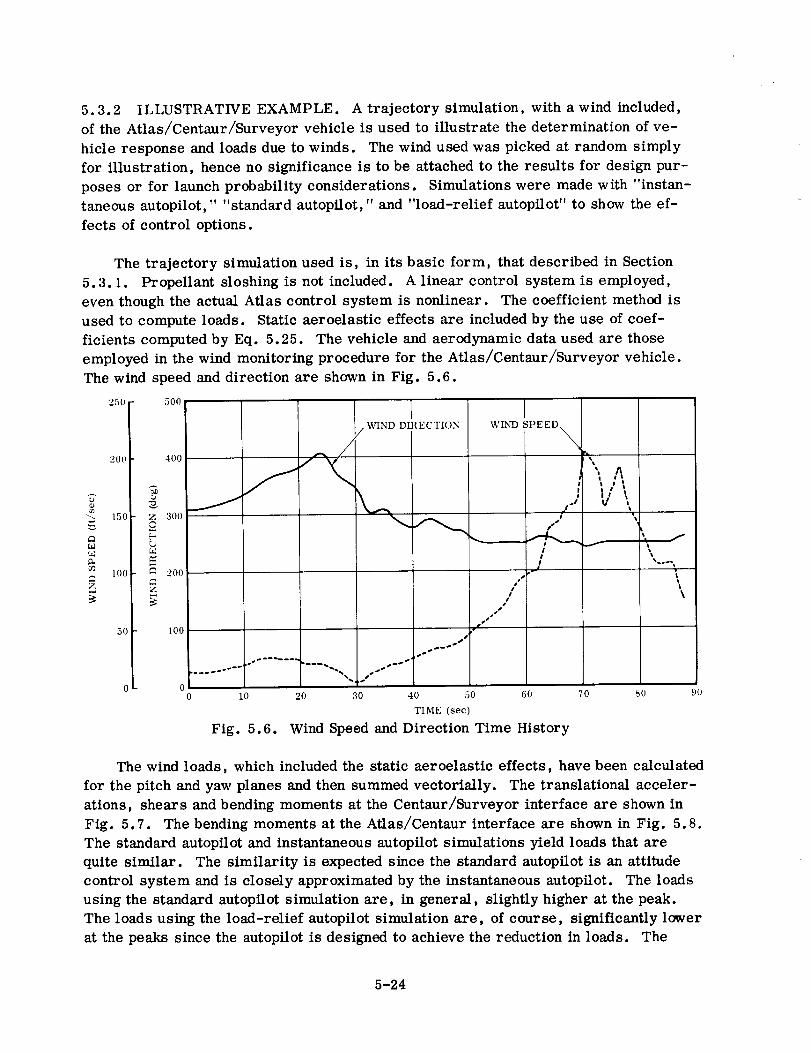
5.3.2 ILLUSTRATIVE EXAMPLE. A trajectory simulation, with a wind included,of the Atlas/Centaur/Surveyor vehicle is used to illustrate the determination of ve-hicle response and loads due to winds. The wind used was picked at random simplyfor illustration, henceno significance is to be attachedto the results for design pur-poses or for launch probability considerations. Simulations were madewith "instan-taneousautopilot," "standard autopilot," and "load-relief autopilot" to show the ef-fects of control options.
The trajectory simulation used is, in its basic form, that described in Section5.3.1. Propellant sloshing is not included. A linear control system is employed,even thoughthe actual Atlas control system is nonlinear. The coefficient method isused to computeloads. Static aeroelastic effects are included by the use of coef-ficients computedby Eq. 5.25. The vehicle and aerodynamic data used are thoseemployed in the wind monitoring procedure for the Atlas/Centaur/Surveyor vehicle.Thewind speedanddirection are shownin Fig. 5.6.
250 500
200
150
_2
100
5O
"_ 400
_ 300
200
100
/ WIND DIRECTION
WIND SPEED_
!
s I
,s
/!
A
O"
S
•S
f-"
_os S_
,Q_-_f _ _ s S o
s
00 10 20 30 40 50
TIME (sec)
Fig. 5.6.
V \\
l
\
60 70 80 90
Wind Speed and Direction Time History
The wind loads, which included the static aeroelastic effects, have been calculated
for the pitch and yaw planes and then summed vectorially. The translational acceler-
ations, shears and bending moments at the Centaur/Surveyor interface are shown in
Fig. 5.7. The bending moments at the Atlas/Centaur interface are shown in Fig. 5.8.
The standard autopilot and instantaneous autopilot simulations yield loads that are
quite similar. The similarity is expected since the standard autopilot is an attitude
control system and is closely approximated by the instantaneous autopilot. The loads
using the standard autopilot simulation are, in general, slightly higher at the peak.
The loads using the load-relief autopilot simulation are, of course, significantly lower
at the peaks since the autopilot is designed to achieve the reduction in loads. The
5-24

[).25
0.20
%0
z
o.15
--I
%5 0.10%).<
0.05 ; \
!
o54 58 62 66 70 74
TIME (sec)
78
a. Translational Acceleration
0.35
0.30
0.25
0.200
0.15
0.10
0.05
/
\
;i
I f
28
054 58 62 66
TIME (sec)
70 74 78
24 !I,
_ "
16
-'",.j _.'_
Z fl ""
,
b. Shear
LEGEND
STANDARD A/P
INSTANTANEOUS A/P
LOAD-RELIEF A/'P
54 58 62 66 70 74
TIME (sec)
78
e. Bending Moment
Fig. 5.7. Centaur/Surveyor Interface Loads Due to Wind
5-25
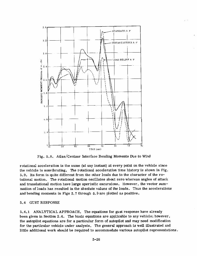
3.6
3.2
28
.=22.4 t__. i I t S
o j_ /
_2. o _'_'
01.6
e_ZM
1.2
b._ ----
6.4
[ STANDARD A P
I
!IIq
,,I
:,!!\
%; ,,jt.,i
C54 58 62 66 70 74 _8 82
TIME (sec)
Fig. 5.8. Atlas/Centaur Interface Bending Moments Due to Wind
rotational acceleration is the same (at any instant) at every point on the vehicle since
the vehicle is nonvibrating. The rotational acceleration time history is shown in Fig.
5.9. Its form is quite different from the other loads due to the character of the ro-
tational motion. The rotational motion oscillates about zero whereas angles of attack
and translational motion have large aperiodic excursions. However, the vector sum-
mation of loads has resulted in the absolute values of the loads. Thus the accelerations
and bending moments in Figs 5.7 through 5.9 are plotted as positive.
5.4 GUST RESPONSE
5.4.1 ANALYTICAL APPROACH. The equations for gust response have already
been given in Section 2.4. The basic equations are applicable to any vehicle; however,
the autopilot equations are for a particular form of autoptlot and may need modification
for the particular vehicle under analysis. The general approach is well illustrated and
little additional work should be required to accommodate various autopilot representations.
5-26
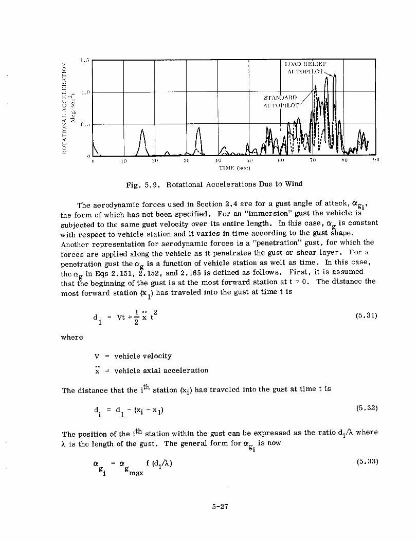
',' :x}
Y.
1.5
1 .0
U.5
10 3O
LOAD l1 E'LIE F
AUTOPI !_O'F _.._A
t, lll,lIISTANI) AIID
AUTOPlLOT lI_._ Wi'wJ!40 50 60 70 9O
TIME (see)
Fig. 5.9. Rotational Accelerations Due to Wind
The aerodynamic forces used in Section 2.4 are for a gust angle of attack, _gi'the form of which has not been specified. For an "immersion" gust the vehicle is
subjected to the same gust velocity over its entire length. In this case, _giS constant
with respect to vehicle station and it varies in time according to the gust shape.
Another representation for aerodynamic forces is a "penetration" gust, for which the
forces are applied along the vehicle as it penetrates the gust or shear layer. For a
penetration gust the _g is a function of vehicle station as well as time. In this case,
the _g in Eqs 2. 151, 2. 152, and 2. 165 is defined as follows. First, it is assumedthat the beginning of the gust is at the most forward station at t = 0. The distance the
most forward station (x l) has traveled into the gust at time t is
1 .. 2 (5.31)d I = Vt +_ x t
where
V = vehicle velocity
x = vehicle axial acceleration
The distance that the ith station (xi) has traveled into the gust at time t is
d i = d 1- (x i-x1)(5.32)
The position of the i th station within the gust can be expressed as the ratio diA where
X is the length of the gust. The general form for (_gi is now
= _ f (di/k) (5.33)gi gmax
5-27
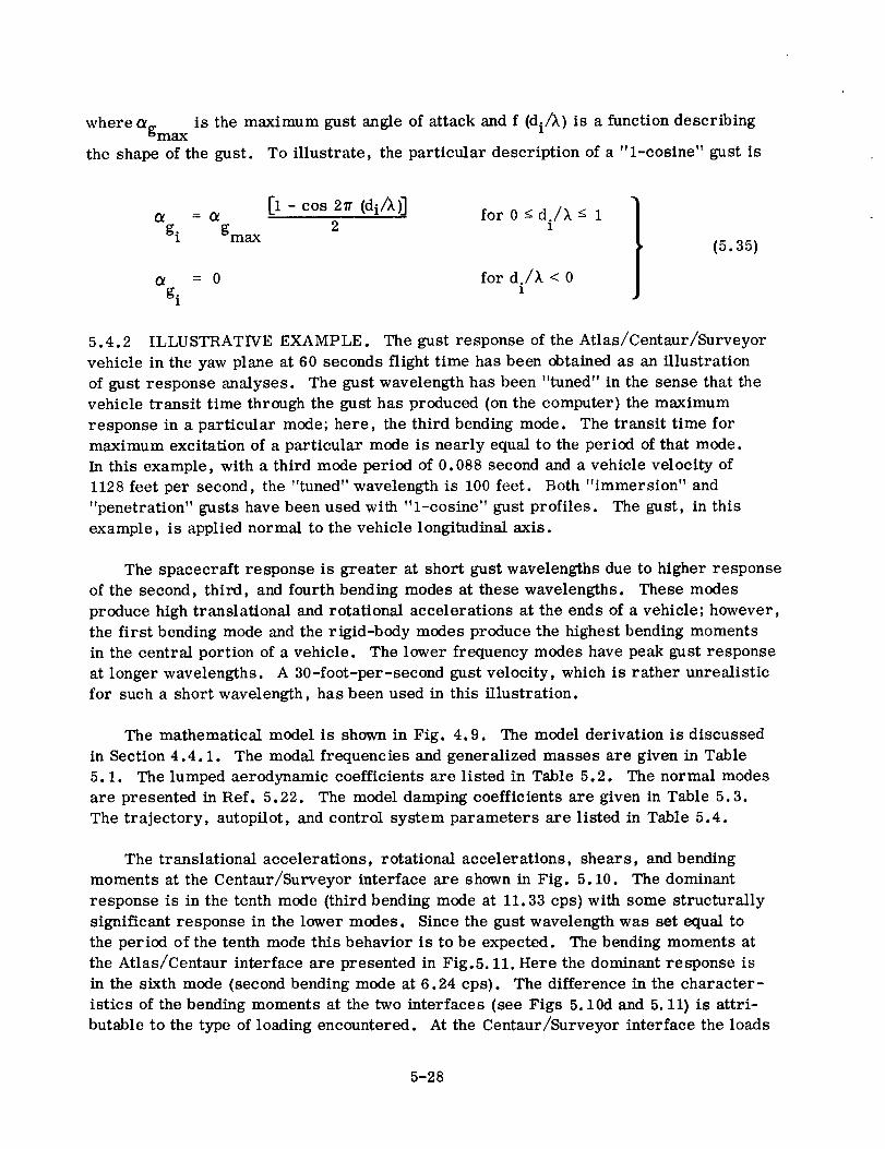
where _gmax is the maximum gust angle of attack and f (di/_) is a function describing
the shape of the gust. To illustrate, the particular description of a "l-cosine" gust is
o_ = o_ [1 - cos 2y (di/k)] for 0 < d./_ _ 1 ]
gi gmax 2 1 I= 0 ford./k<0
gi
(5.35)
5.4.2 ILLUSTRATIVE EXAMPLE. The gust response of the Atlas/Centaur/Surveyor
vehicle in the yaw plane at 60 seconds flight time has been obtained as an illustration
of gust response analyses. The gust wavelength has been "tuned" in the sense that the
vehicle transit time through the gust has produced (on the computer) the maximum
response in a particular mode; here, the third bending mode. The transit time for
maximum excitation of a particular mode is nearly equal to the period of that mode.
In this example, with a third mode period of 0. 088 second and a vehicle velocity of
1128 feet per second, the "tuned" wavelength is 100 feet. Both "immersion" and
"penetration" gusts have been used with "l-cosine" gust profiles. The gust, in this
example, is applied normal to the vehicle longitudinal axis.
The spacecraft response is greater at short gust wavelengths due to higher response
of the second, third, and fourth bending modes at these wavelengths. These modes
produce high translational and rotational accelerations at the ends of a vehicle; however,
the first bending mode and the rigid-body modes produce the highest bending moments
in the central portion of a vehicle. The lower frequency modes have peak gust response
at longer wavelengths. A 30-foot-per-second gust velocity, which is rather unrealistic
for such a short wavelength, has been used in this illustration.
The mathematical model is shown in Fig. 4.9. The model derivation is discussed
in Section 4.4.1. The modal frequencies and generalized masses are given in Table
5.1. The lumped aerodynamic coefficients are listed in Table 5.2. The normal modes
are presented in Ref. 5.22. The model damping coefficients are given in Table 5.3.
The trajectory, autopilot, and control system parameters are listed in Table 5.4.
The translational accelerations, rotational accelerations, shears, and bending
moments at the Centaur/Surveyor interface are shown in Fig. 5.10. The dominant
response is in the tenth mode (third bending mode at 11.33 cps) with some structurally
significant response in the lower modes. Since the gust wavelength was set equal to
the period of the tenth mode this behavior is to be expected. The bending moments at
the Atlas/Centaur interface are presented in Fig.5.11. Here the dominant response is
in the sixth mode (second bending mode at 6.24 cps). The difference in the character-
istics of the bending moments at the two interfaces (see Figs 5.10d and 5.11) is attri-
butable to the type of loading encountered. At the Centaur/Surveyor interface the loads
5-28
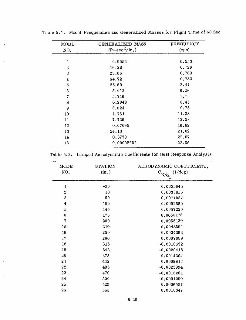
Table 5.1. Modal Frequencies and Generalized Masses for Flight Time of 60 Sec
MODE GENERALIZED MASS FREQUENCYNO. (Ib-sec2/in.) (cps)
1 0.9555 0.553
2 16.28 0. 729
3 28.66 0.763
4 64.72 0.783
5 28.69 2.47
6 5.012 6.26
7 5. 746 7.78
8 0. 2048 8.45
9 8.624 9.75
10 1.761 11.33
11 7.729 12.58
12 0. 07099 16.82
13 24.13 21.02
14 0. 3779 22.07
15 0. 00002202 23.66
Table 5.2. Lumped Aerodynamic Coefficients for Gust Response Analysis
MODE STATION AER ODYNAMIC COE FFICIE NT,
NO. (in.) CN/(_i (1/deg)
1 -20 0.0035045
2 10 0.0038855
3 50 0.0071037
4 100 0.0092550
5 145 0,0057220
6 173 0.0058178
7 200 0.0058139
15 219 0.0043591
16 250 0.0034393
17 280 0.0007659
18 315 -0.0016652
19 345 -0,0020418
20 375 0.0014364
21 412 0.0009813
22 438 -0.0025994
23 470 -0.0018201
24 500 0.0001090
25 525 0.0006557
26 555 0.0010347
5-29

Table 5.2. LumpedAerodynamic Coefficients for Gust ResponseAnalysis (Contd)
MODE STATION AERODYNAMICCOEFFICIENT,
NO. (in.) CN/_i (I/deg)
27 570
28 600
29 630
30 667
31 696
32 725
33 754
34 784
35 812
36 840
37 871
38 900
39 929
40 960
41 992
42 1025
43 1057
44 1090
45 1122
46 1133
54 1160
55 1176
56 1206
57 1212
58 1242
59 1267
0.0011025
O.O0O1349
-0.0000769
0.0001674
0.0002750
0.0002886
0.0002550
0.0002483
0.0000707
0.0007345
0. 0031814
0.0024361
0.0018514
0.0000527
-0.0015103
0.0000362
0.0028011
0.0064948
00046974
-00013529
-00010350
0.0020909
0.0039168
0.0055976
0.0089609
0.0055240
Total 0. 0927500
Table 5.3. Damping Coefficients for Gust Response Analysis
MODE
NO.
DAMPING COEFFICIENT MODE
(% Critical) NO.
DAMPING COEFFICIENT
(% Critical)
1 0.02 9 1.00
2 O.02 10 1.50
3 0.02 11 1.00
4 0.02 12 3.00
5 1.25 13 1.00
6 1.50 14 4.0O
7 1.00 15 4.00
8 2.00
5-30

Table 5.4.
SYMBOL
V
q
SR
TB
TS
CV
CB
C L
A
R
K C
K E
KA
K I
rlag
W e
_C
x G
x D
Trajectory, Control System, and Autopilot Parameters for Gust Response
Analysis (Atlas/Centaur/Surveyor)
PARAMETER (see Section 2.5 for
further definition)
Velocity
Dynamic pressure
Reference area
Longitudinal acceleration
Thrust of booster engines
Thrust of sustainer engine
Engine gimbal angle used in linearization
of control system
Viscous friction coefficient
Coulomb friction coefficient
Discharge coefficient of leakage bypassorifice
Actuator piston area
Engine moment arm
No-load open-velocity gain
Ratio of hydraulic compliance to hydraulic
plus structural compliance
Autopilot rate gain
Integrator loop gain
Rate gyro loop gain
Time constant, lag filter
Natural frequency of second order lag filter
in autopilot
Damping ratio of second order lag filter in
autopilot
Natural frequency of rate gyro
Damping ratio of rate gyro
Station at which rate gyro is located
Station at which displacement gyro is located
VALUE
1128
674
78.5
58.7
352,900
72,176
1.0
63
565
0.00000478
0. 0247
1.769
36.18
0. 104
1.8
0.178
0.45
0.0116
15.5
0.5
157
0.6
600
991
UNITS
ft/sec
Ib/ft2
ft2
ft/sec2
Ib
Ib
deg
ft-lb-sec/deg
ft-lb
ft3/sec/_
ft 2
ft
1/sec
N.D.
deg/deg
1/sec
see
see
rad/sec
N.D.
rad/sec
N.D.
in.
in.
5-31

o t;
,q II
<
J[
J
tI, i
I!/,_ '_,
!
i ] ;.EGEND ]
IMMERSION Gusr
---- PENETRATION GUST
IU, 0,2 3 04
riME (bye)
b5
a. Translational Accelerations
(L6
ma:
ks
Jo
I
! "1)I
/O, I
i,!
0.2 0,3 0.4
TIME (se(')
[
_J
b5 b6
b. Rotational Accelerations
3
2
I
i
= i
'V;Ol
+ -/q
02 0,3 54
TIME {sec)
4%II _
;/I
0.5 0.6
c. Shears
J
2 40
i °
7.40
-8O
/"1
]I"
0.1 0.2 6.3
T_E (see)
0.4 05
d. Bending Moments
O. 6
Fig. 5.10. Centaur/Surveyor Interface Loads
Due to Gust
5-32

are inertial loads due to spacecraft response
whereas at the Atlas/Centaur interface the
dominant load is aerodynamic loading on the
nose fairing. This illustrates the variation
in response characteristics that can occur
for various points on the vehicle. The loads
from both the "immersion" and "penetration"
gusts shown for the Atlas/Centaur/Surveyor
vehicle are quite similar; however, there is
no reason to expect this similarity for other
atmospheric descriptions or space vehicle
configurations.
The relative deflection between the pay-
load and fairing (at a critical point} is shown
in Fig. 5.12. Here the peak response is at
approximately 8.45 cps, the frequency of
the eighth mode (payload "first mode"}. Of
note here is that the maximum loads occur
on the first or second peak but the maximum
relative deflection occurs on the fourth peak.
The reason is the phasing of the response of
the fifth, sixth, and eighth modes. These
three modes contribute most of the relative
deflection. Initially, the fifth and sixth
modes subtract from the eighth mode re-
sponse, then cancel each other, and, at the
peak, add to the eighth mode response.
The process is then reversed.
The normal-mode displacements for
the immersion gust are presented in Fig.
5.13. Where the displacements are not
shown, the response was negligible. The
displacements for the penetration gust are
not presented due to the similarity of re-
sults for the particular configuration sub-
jected to exemplary analysis.
5.5 DISCUSSION
1,2
0.8---¸ J
II
d
o.4---
-- ii
_ -o.4 .... 1
-0.8
-1.20 1
Fig. 5.11.
LEGEND
-- IMMERSION GUST
J" ------PENETRATION GUST
/ _
/' /
iii
0.2 0.3 0.4 05
TIME (sec
Atlas/Centaur Interface
Bending Moments Due to
Gust
1.2
08 i
04 ,,_
12_ I 02
Fig. 5.12.
\i
06
7 T
LEGEND
-- IMM ERSION GUST
_ _-- -- PENETRATION GUSTI ,
H ./,' /r," I z ¢, "1, liI I I f: _ I' I'1
, I/ lili v,/
b 3 4 L 5 C _
T_tE (see}
Relative Deflections Be-
tween Surveyor and FairingDue to Gust
The importance of loads due to atmospheric disturbances on the design of space
launch vehicles will depend upon the particular vehicle systems. The lower portion
of the first stage is generally designed by thrust buildup conditions. Structural design
of the upper portions of second and third stages is usually governed by the maximum
5-33

TRANSLATION
iR IGID- BODY
ROTATION 1
MODE 2!
i
MODE I
: i
MODE 6MODE
MODE
-0._
_s L
L012 03 0.4 u5 0_6 G 01 0.2 U3 04 45
TIME (sec) TIME Isec)
Normal-Mode-Coordinate Displacements Due to Immersion Gust
O6
accelerations at first stage burnout. The design of the structure between these two
areas may be dictated by the predicted loads due to atmospheric disturbances. These
considerations suggest only general trends which may apply to a particular system.
Such considerations are mentioned here to place the proper perspective on the pro-
blem areas discussed below.
5.5.1 QUASI-STEADY FLIGHT LOADS. Loads imposed during flight in the atmosphere
are axial loads due to drag and vehicle acceleration and lateral loads due to winds and
vehicle trajectory. The axial loads are essentially static loads determined from thrust,
weight, and vehicle drag. Disturbances affecting longitudinal loads at this time are
very small and can be neglected.
The lateral loads are predominantly those due to winds but the pitch program (tra-
jectory) contributions can be a significant parameter. The nominal performance tra-
jectory (without winds) for most missions demands only a small angle of attack through
the period of maximum dynamic pressure. This required angle of attack is approxi-
mately one-fifth or less of the total angle of attack. The remainder is due to winds.
5.5.1.1 Wind Criteria. Development of wind criteria to be used for design of a ve-
hicle has been discussed in Section 5.2. For an operational system to be launched at
many sites and at many azimuths, it is generally practical only to apply synthetic
wind profiles as headwincls, tailwinds, and crosswinds to the vehicle. The synthetic
5-34
profiles should be an envelope of the wind speeds and shears which can be expected
within a required probability of successful launch for that operational system.
Vehicles to be launched from one site with small deviation in azimuth can make
use of more detailed wind criteria. Examples are the directional criteria for Eastern
Test Range developed by MSFC. These criteria result in significantly lower loads
compared to loads obtained by applying the maximum profile in any direction. Another
wind criterion is a set of actual wind profiles for that launch site, statistically sampled
as in Refs 5.10 to 5.12. A statistical load survey can be accomplished by simulation
of the vehicle flight through these profiles.
In the wind profiles, the wind shear (the change in velocity with altitude) is as
important as the wind speed. As the vehicle rises, the wind causes the vehicle to
drift and build up a lateral velocity. The lateral velocity reduces the angle of attack
induced by the wind. For low wind shear, e.g., a profile increasing linearly with
altitude, the vehicle has considerable time to build up the lateral velocity. However,
for high wind shear the vehicle has much less time to build up a lateral velocity. It
is apparent, then, that the wind shear has an important effect on the angle of attack.
5.5.1.2 Pitch Program. For vehicles launched from a single site at constant azi-
muth it is possible to fly a trajectory that will give an angle of attack, without wind,
opposite in direction to the angle of attack induced by the critical wind. Thus, a pro-
perly preselected pitch-program can provide some reduction in load. The reduction is
usually in the area of 5 to 15 percent. Selection of this pitch program is mostly by
trial and error to produce the best compromise of payload capability, thermodynamic
effects, and aerodynamic loads.
5.5.1.3 Trajectory Simulation. The degree of physical representation in the tra-
jectory simulation is open to question with the shortcomings in wind criteria. Gen-
erally a fiat, nonrotating earth is sufficient for the earth model. The vehicle can be
represented as a rigid body for determination of significant trajectory parameters with
the present available wind criteria. The vehicle autopilot can be simplified to its
rigid-body terms. Actually, a trimmed vehicle condition would be sufficient for loads
analysis; however, it is advisable to include a simplified version of the autopilot to
insure against a significant increase in loads because of the autopilot. Loads can be
calculated by either the coefficient method or trimmed condition of Section 5.3.1.
Usually the trimmed method will be used with synthetic profiles and the coefficient
method with actual wind profiles.
5.5.1.4 Elastic Modes. A good comparison of wind loads with and without inclusion
of elastic modes in the simulation has not been made at this time. The wind criteria,
either synthetic profiles or actual wind soundings, are not sufficiently detailed to include
the transients that would produce modal excitation. With more detailed wind data
available, inclusion of elastic modes may be necessary. However, flight data to date
do not show significant response in any elastic modes.
5-35

5.5.2 GUSTLOADS. Gust loads are the lateral loads due to short-period wind speedvariations. For wind data taken at large altitude intervals, the gust treatment accountsfor the loads due to that wind profile detail not measuredby the wind-measuring sys-tem. With more detailed wind data, the gust loads may reflect only the elastic re-sponseto the measuredwind profile detail. Gusts are random in nature. Thereforethey have a probability of occurrence (though ill-defined) for a given gust velocity.
There are insufficient data to establish a correlation between gust velocity and wind
velocity; hence peak gusts and winds are generally considered to act simultaneously.
An immersion gust is generally used although insufficient investigations have been
made to indicate a preference between analytical usage of "immersion" and "penetra-
tion" gusts. As with trajectory simulations, the degree of physcial representation is
open to question. Generally rigid-body, slosh, and elastic modes will be considered.
The complete autopilot representation will be needed, but the engine control system
nonlinearities can usually be ignored.
5.5.3 BUFFET LOADS. Buffet is loading of a structure by an unsteady aerodynamic
flow. The flow is usually measured as a fluctuating pressure and exists at all fre-
quencies. Buffet is usually significant only in those areas where a change of vehicle
radius occurs or a protruberance exists. It is especially severe in, and downstream
from, the transition region from a larger diameter to a smaller diameter. Ref. 5.20
contains criteria for determining whether or not a vehicle shape is a clean body of re-
volution or is buffet prone. The response analysis is done using the techniques dis-
cussed in Section 2.6. The input spectra to use can be difficult to obtain. Either wind
tunnel tests must be made, or estimates must be derived from tests of similar con-
figurations. The analysis is usually conservative because of the unknown validity of
the chosen assumptions. Buffet can be important for the design of local structure and
of components mounted on structure affected by buffet. Theoretically, some overall
vehicle response can occur, but flight data do not indicate any significant response of
the gross vehicle to buffet.
5.5.4 OTHER LOADS. The previous discussions have covered the major loads ap-
plied to the vehicle. There are minor loads applied which, depending on the particular
case, may need to be considered. One of these is the center-of-gravity offset load
due to the center of gravity not being on the vehicle centerline. A similar load is the
load due to angular misaligument of various stages of the vehicle. These loads are
quite small compared to axial loads, wind loads, and gust loads and therefore need
not be considered unless a large amount of unsymmetry exists. Dispersions in tra-
jectory parameters, principally in angle of attack, dynamic pressure, and axial ac-
celeration, cause additional axial and lateral loading. Again these loads are small
compared to the major loads and are also random. When they are combined statisti-
cally with the gust loads, the loads virtually disappear.
5.5.5 COMBINED LOADS. The loads discussed previously need to be combined for
design purposes and for comparison with allowable loads. It is to be noted that loads
other than dynamic loads may be important for the complete load analysis of the space
vehicle. Examples are assembly pre-loads, internal tank pressures and differential
5-36
pressures associated with nose fairing venting systems. Suchloads are outside thescopeof this report. The combination of loads is discussed in Section 4.5.3. Eqs 4.9and 4.10 become, in this case,
rl = rIXI + _XD + _Ycg +rlyw +rlYB +_TYG
2 2 2 2 2 2 2= +(_XD + +(_YB +(_ CrXI _Ycg + Cryw (_YG
where the subscripts are defined as follows:
X = axial loading
Y = lateral loading
I = inertial load due to axial acceleration
D = drag load
cg = center-of-gravity offset and misalignment load
W = wind and pitch program loads
B = buffet load
G = gust load
Since some loads are axial loads and some are lateral loads, itis necessary either
to convert axial loads to equivalent bending moment, or vice versa. This conversion
is usually easily accomplished.
5.5.6 WIND MONITORING. The usual procedure for space launches is to take wind
soundings on launch day and determine if the launch is acceptable from the standpoint
of loads. The entire process is referred to as the wind-monitoring procedure or simply
wind monitoring. The basic steps of the procedure are
1. Calculate, in advance, all loads except those due to wind.
2. Obtain the wind sounding at the launch site and transmit it to the engineering
facility.
3. Obtain the loads due to the wind.
4. Compare applied loads with the allowable load either by: 1) comparing the total
load with the allowable, or 2) subtracting the loads obtained in step 1 from the
allowable load and comparing this with the wind load.
5. Transmit the results of this comparison to the person(s) authorized to decide
whether to continue with the launch.
The procedure (except step 1) is repeated several times, beginning 1-3 days prior
to launch and becoming more frequent as launch time approaches. A small allowance
is usually made for the wind changing during the time between the wind sounding and
5-37

the launch. The changein wind velocity over a period of 2-8 hours is approximately5-10%and to somedegree, canbe predicted. This persistence also exists, to alesser extent, over a period of days. A strong wind condition will generally persistfor a period of 2-8 days.
In connectionwith spacelaunches the term "launch probability" is frequentlyused. Launchprobability is the probability of not having a delayed launch due to windsaloft. If the vehicle is being designed, this corresponds to the probability of winds notexceedingthe wind criteria used. If the vehicle is already designed, the launch pro-bability corresponds to the probability of winds not exceedingthe maximum winds thatthe vehicle is capable of withstanding.
Launchprobability is usually stated with reference to launch on a given day. How-ever, the launchopportunity (window)for space launchesusually extends over severalconsecutivedays. The probability of a launch sometime during the launch window ishigher than the probability of launch on a given day and, for some launch vehicles, thisincrease may be significant. An example of this applying to the Atlas/Centaur vehicleis Ref. 5.23; for onecase the launch probability for oneday was approximately 50%butthe launch probability for a five-day window was 95%.
5.6 CONCLUSIONSAND RECOMMENDATIONS
5.6.1 WIND CRITERIA. Wind soundingshave, in the past, beentaken at relativelylarge altitude intervals. As a result, the actual wind profile hasbeen effectivelysmoothedandfiltered to the extent that the profile detail for short altitude intervals(especially less than 1000feet) hasbeenlost. To correct this, the FPS-16 Radar/Spherical Balloon system is being used to obtain more accurate wind soundingsandis providing data for an altitude interval of 25 meters. Thesedata are becomingavailable in quantity and the wind and gust criteria shouldbe changedto reflect thenew data.
5.6.2 ANALYSIS. The "state of the art" of the analysis of vehicle response to windsand gusts is regarded to be sufficiently advancedat this time. With the advent ofmore detailed wind soundings, the elastic mode(s)will probably be required in thetrajectory simulation. This does not require any newanalytical techniques, beingmerely another application of existing techniques.
5.6.3 PROCEDURE. With present available wind criteria the following procedureshouldbe followed for calculating loads causedby atmospheric disturbance.
1. Wind and gust criteria for design must be specified.
2. Proceed with rigid trajectory simulation using a nonrotating fiat earth model and
a simplified rigid-body autopilot.
3. Calculate wind loads using a trimmed vehicle condition or the coefficient method
of Section 5.3.
5-38

4. Calculate gust loads using the methods of Section 2.4 and 5.4.1 with immersionor penetration gust.
5. Calculate axial inertial anddrag loads.
6. Calculate other loads suchas center-of-gravity offset and misalignment effectsand trajectory dispersions (if necessary).
7. Combineloads using the methodsof Section 4.5.3.
8. Set up launchwind-monitoring procedures as discussed in Section 5.5.6.
5.7 REFERENCES
5.1 Dvoskin andSissenwine, Evaluation of AN/GMD-2 Wind Shear Data for
Development of Missile Design Criteria, AFCRC-TN-58-259, April 1958.
5.2 Salmela and Sissenwine, A Note Comparing 1-km Vertical Wind Shears
Derived from Simultaneous AN/GMD-1A and AN/GMD-2 Winds Aloft
5.3
5.4
5.5
5.6
Observations, AFCRC TN-59-496, November 1959.
Scoggins, An Evaluation of Detail Wind Data as Measured by the FPS-16
Radar/Spherical Balloon Technique, NASA TN D-1572, May 1963.
Tolefson and Henry, "A Method of Obtaining Detailed Wind Shear Measure-
ments for Application to Dynamic Response Problems of Missile Systems,"
Journal of Geophysical Research, Volume 66, No. 9, September 1961,
pages 2849-2862.
Jiusto, High Resolution Wind and Wind Shear Measurement With Doppler
Radar, CAL Report No. 1H-1525-p-1, June 1962.
Sissenwine, Windspeed Profile, Windshear, and Gusts for Design of
Guidance Systems for Vertical Rising Air Vehicles, AFCRC TN-54-22,November 1954.
Sissenwine, Revised 1% Sythetie Wind Profile, AFCRC, June 1959.
Scoggins and Vaughan, Description of Wind Shears Relative to a Missile/
Space-Vehicle Axis and a Presentation of the Cape Canaveral, Florida,
95 and 99 Percent Probability Level Standardized Wind Profile Envelopes
(1-80 km) and Associated Wind Shears for use in Design and Performance
5.9
Studies, MSFC MTP-Aero-61-48, June 8, 1961.
Daniels, Revision of Natural Environmental Design Criteria, In-Flight
Wind Conditions, Saturn C-1, Block II Vehicle, MSFC M-Aero-G-35-62,
October 19, 1962.
5-39

5.10 L. L. Mazzola, N. P. Hobbs, and E. S. Criscione, Wind, Wind Shear,
and Gust Design Criteria for Vertically-Rising Vehicles as Recommended
5.11
on the Basis of Montgomery, Ala., Wind Data (U), WADD TR 61-99 (AD
333174), Avidyne Research, Inc., August 1962 (Secret).
L. L. Mazzola, J. Putukian, E. S. Criscione, and N. P. Hobbs, Wind,
Wind Shear, and Gust Design Criteria for Vertically-Rising Vehicles as
Recommended on the Basis of Wind Data from Eleven United States and
5.12
5.13
Forei_n Locations HI, ADS-TDR-62-908 (AD 338892), Avidyne Research,
Inc., June 1963 (Secret).
N. P. Hobbs, E. S. Criscione, L. L. Mazzola, and G. J. Frassinelli,
Development of Interim Wind, Wind Shear, and Gust Design Criteria
for Vertically-Rising Vehicles (U), WADC TR 59-504 (AD 316913), Avidyne
Research, Inc., July 1959 (Secret).
Hobbs, Criscione, and Ayvazian, Simplified Analytical Methods For Use
in Preliminary Design of Vertically-Rising Vehicles Subjected to Wind
5.14
5.15
5.16
Shear Loads, FDL-TDR-64-8 Part 1, Avidyne Research, Inc., May 1964.
B. E. Clingan, "A Rapid Method for Determining Wind Shear DesignLoads Based on a Set of Measured Profiles," Proceedings of the National
Symposium on Winds for Aerospace Vehicle Design, Vol II, pp 49-69,
Air Force Surveys in Geophysics No. 140 (AD 275846), AFCRL-62-273
(II), March 1962.
C. J. Van Der Maas, High Altitude Wind Response of Missile Systems,
Lockheed Aircraft Corporation, Missile Systems Division, Report No.
LMSC-A062400 (AD 408258), 30 October 1962.
Press, Meadows, and Hadlock, Estimates of Probability Distribution of
RMS Gust Velocity of Atmospheric Turbulence from Operational Gust-
5.17
5.18
5.19
Load Data by Random Process Theory, NASA TN 3362, March 1955.
Walker and Copp, Summary of VGH and V-G Data Obtained from Piston-
Engine Transport Airplanes from 1947 to 1958, NASA TN D-29, September
1959.
B. E. Clingan, R. M. Gates, and J. S. Andrews, Dynamic Loads During
Boosted Flight, The Boeing Company, ADD-TDR-63-302, May 1963.
A. G. Rainey, "Progress on the Launch-Vehicle Buffeting Problem,"
Fifth Annual AIAA Structures and Materials Conference, April 1964.
5-40
5.20 NASA Space Vehicle Design Criteria - Buffeting During Launch and Exit,
NASA SP-8001, May 1964.
5.21 A. L. Greensite, Design Criteria for Control of Space Vehicles, Vol. I,
Part 3, Trajectory Equations, GDC-DDE65-058, November 1965.
5.22 W. H. Gayman and J. A. Garba, Dynamics Loads Analyses of Space
Vehicle Systems - Launch and Exit Phase, JPL Technical Memorandum
33-286 (To Be Published).
5.23 Surveyor Mission Launch Wind Constraints Study for Month of March,
Space Technology Laboratories, Inc., 8414-6121-RU-000, October 1963.
5-41


6/FREQUENCY RESPONSE
PRECEDING PAGE BLANK NOT FILMED.
"G]It,_I"II:I ION )INv'1_ ]DYd DNIC.::ID3_'cl
6-1

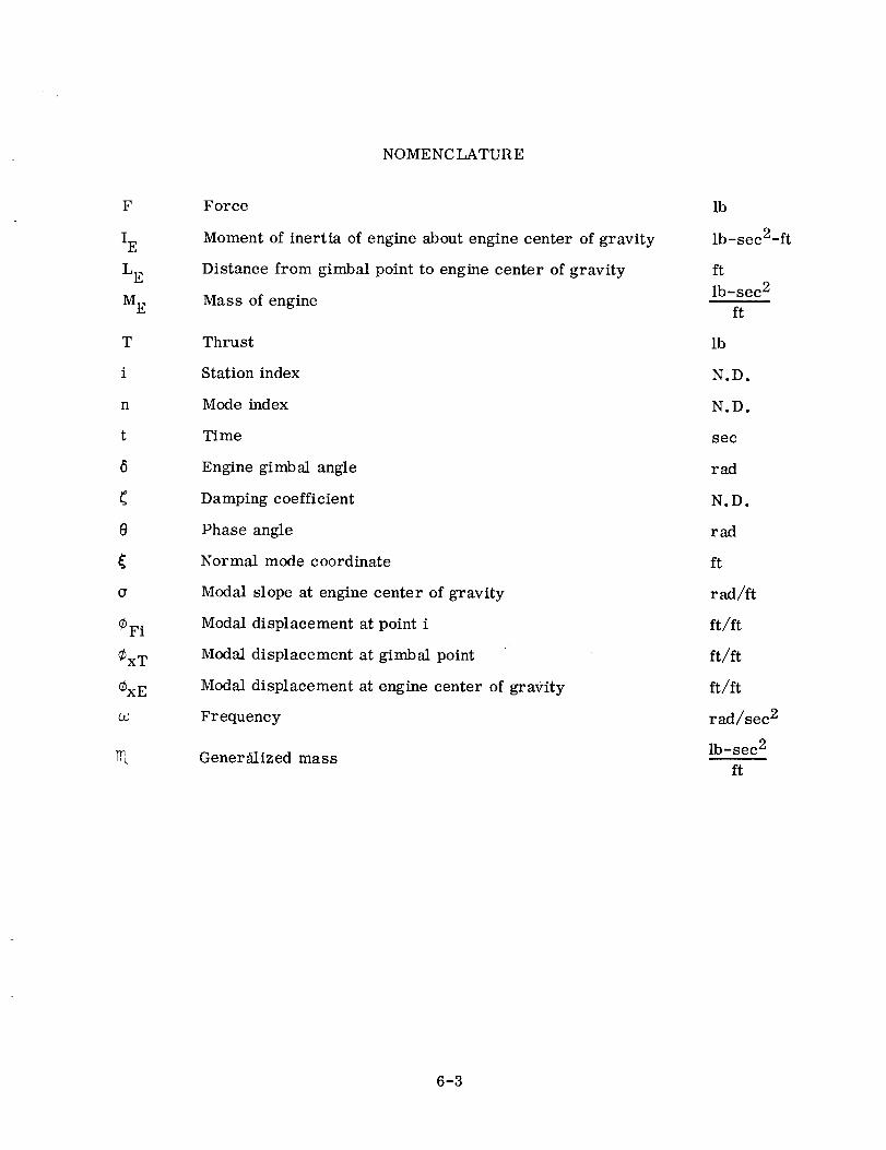
NOME NC LATUR E
F
I E
L E
M E
T
i
n
t
6
e
a
CFi
CxT
CxE
R
Force
Moment of inertia of engine about engine center of gravity
Distance from gimbal point to engine center of gravity
Mass of engine
Thrust
Station index
Mode index
Time
Engine gimbal angle
Damping coefficient
Phase angle
Normal mode coordinate
Modal slope at engine center of gravity
Modal displacement at point i
Modal displacement at gimbal point
Modal displacement at engine center of gravity
Frequency
Gener£lized mass
lb
lb-sec2-ft
ft
lb-sec 2
ft
Ib
N.D.
N.D.
sec
rad
N.D.
rad
ft
rad/ft
ft/ft
ft/ft
ft/ft
rad/sec 2
lb-sec 2
ft
6-3

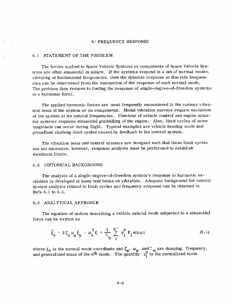
6/ FREQUENCYRESPONSE
6.1 STATEMENT OF THE PROBLEM
The forces applied to SpaceVehicle Systemsor componentsof SpaceVehicle Sys-tems are often sinusoidal in nature. If the systems respond in a set of normal modes,vibrating at fundamental frequencies, then the dynamic response at discrete frequen-cies can be determined from the summation of the responseof each normal mode.The problem then reduces to finding the responseof single-degree-of-freedom systemsto a harmonic force.
The applied harmonic forces are most frequently encounteredin the various vibra-tion tests of the system or its components. Modal vibration surveys require excitationof the system at its natural frequencies. Checkoutof vehicle control and engineactua-tor systems requires sinusoidal gimballing of the engine. Also, limit cycles of somemagnitudecan occur during flight. Typical examples are vehicle bending modeandpropellant sloshing limit cycles causedby feedbackto the control system.
The vibration tests andcontrol systems are designedsuch that these limit cyclesare not excessive; however, response analysis must be performed to establishmaximum limits.
6.2 HISTORICAL BACKGROUND
The analysis of a single-degree-of-freedom system's response to harmonic ex-citation is developedin many text books on vibration. Adequatebackgroundfor controlsystem analysis related to limit cycles and frequency response canbe obtained inRefs 6.1 to 6.5.
6.3 ANALYTICAL APPROACH
The equation of motion describing a vehicle natural mode subjected to a sinusoidalforce can be written as
2 1 _i cn+ 2_n¢C _ + _ _ =_n . F. sincot (6.1)_n n n n . 1 1
where _n is the normal mode coordinate and _n' COn' and _n are damping, frequency,n is the normalized modeand generalized mass of the n th mode. The quantity ¢i
6-5
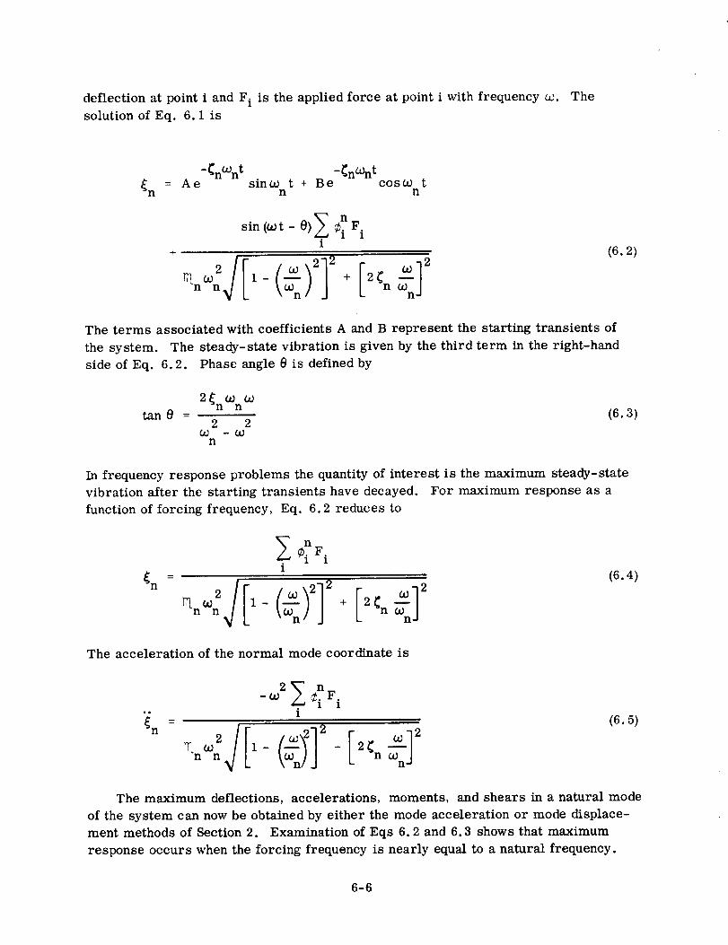
deflection at point i and F i is the applied force at point i with frequency _. The
solution of Eq. 6.1 is
-Cn_nt -CnU_n t= Ae sinu_ t + Be cos_ t
in n n
E nsin (_t - 0) ¢i F.1i
_nU_:J[ I- (_n)2] 2 + [2_ n u_n]2
(6.2)
The terms associated with coefficients A and B represent the starting transients of
the system. The steady-state vibration is given by the third term in the right-hand
side of Eq. 6.2. Phase angle 0 is defined by
2_n_n _tan 0 = (6.3)
2 2¢d -4D
n
In frequency response problems the quantity of interest is the maximum steady-state
vibration after the starting transients have decayed. For maximum response as a
function of forcing frequency, Eq. 6.2 reduces to
nF.1
i
in = (6.4)
_n _n 1 - _ + 2 _n _n
The acceleration of the normal mode coordinate is
_n = i (6.5)
J[ Ej2U_2 1- ('_'_ + 2; n U_rr nn Wn/J
The maximum deflections, accelerations, moments, and shears in a natural mode
of the system can now be obtained by either the mode acceleration or mode displace-
ment methods of Section 2. Examination of Eqs 6.2 and 6.3 shows that maximum
response occurs when the forcing frequency is nearly equal to a natural frequency.
6-6
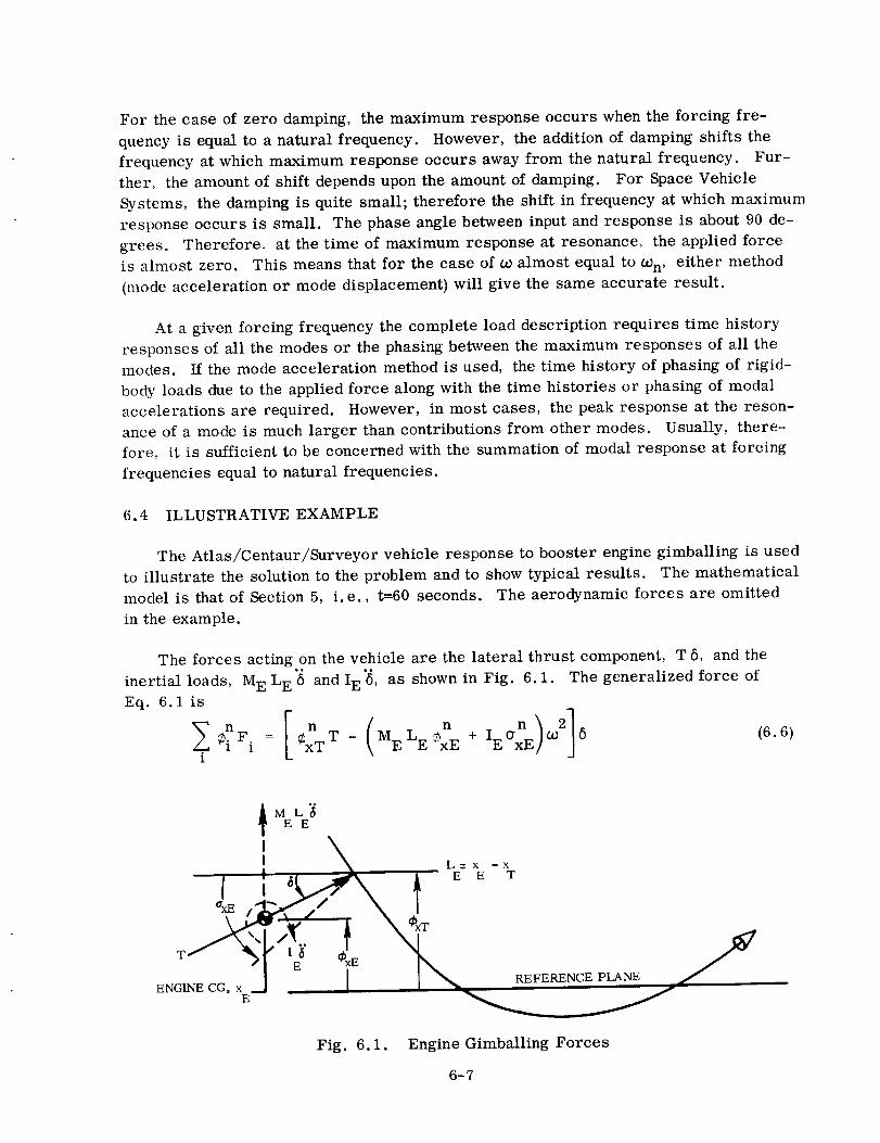
For the case of zero damping, the maximum response occurs whenthe forcing fre-quencyis equal to a natural frequency. However, the addition of damping shifts thefrequency at which maximum response occurs away from the natural frequency. Fur-ther, the amount of shift dependsuponthe amountof damping. For SpaceVehicleSystems, the dampingis quite small; therefore the shift in frequency at which maximumresponseoccurs is small. The phaseangle betweeninput and response is about 90 de-grees. Therefore, at the time of maximum response at resonance, the applied forceis almost zero. This means that for the case of _ almost equal to _n, either method(modeacceleration or mode displacement) will give the same accurate result.
At a given forcing frequency the complete load description requires time historyresponsesof all the modes or the phasing betweenthe maximum responses of all themodes. If the modeacceleration method is used, the time history of phasing of rigid-body loads dueto the applied force alongwith the time histories or phasing of modalaccelerations are required. However, in most cases, the peak response at the reson-ance of a mode is much larger than contributions from other modes. Usually, there-
fore, it is sufficient to be concerned with the summation of modal response at forcing
frequencies equal to natural frequencies.
6.4 ILLUSTRATIVE EXAMPLE
The Atlas/Centaur/Surveyor vehicle response to booster engine gimballing is used
to illustrate the solution to the problem and to show typical results. The mathematical
model is that of Section 5, i.e., t=60 seconds. The aerodynamic forces are omitted
in the example.
The forces acting on the vehicle are the lateral thrust component, T 8, and the
inertial loads, M E L E'5 and I E'6, as shown in Fig. 6.1. The generalized force of
Eq. 6.1 is
_ n [ n ( n n) ] 6 (6.6)i _i Fi = CxTW - MELECxE + IEqxE u_2
axe
ENGINE CG, xE
I
L= x -xE E T
REFERENCE PLANE
Fig. 6.1. Engine Gimballing Forces
6-7

.A
z
<
I2 4
Fig. 6.2.
6 8
FREQUENCY (cps)
Maximum Gimbal Angle
for Atlas Booster
I0
The available engine gimbal angle, as
a function of frequency, is established by
displacement, velocity, and acceleration
characteristics of the engine-actuator sys-
tem. The maximum gimbal displacement
is set by mechanical stops in the actuator.
Engine velocity is limited by the flow rate
of the hydraulic fluid to and from the actua-
tor piston. The maximum displacement,
as limited by velocity, is a function of fre-
quency since the time available to gimbal
depends on the gimballing frequency. En-
gine acceleration is limited by the torque
available from the actuator system. The
maximum displacement, as limited by ac-
celeration, is also a function of frequency.
Plotting the three limits and selecting the
lowest limit at each frequency yields the
maximum gimbal angle as a function of
frequency, shown in Fig. 6.2.
Table 6.1. Modal Damping Values
MODE
NUMBER
1
2
3
4
5
6
7
8
9
10
11
12
13
14
15
DAMPING
COEFFICIENT,
0
0
0
0
0. 025
0.015
0.010
0. 010
0. 010
0.015
0.010
0.010
0.010
0.010
0. 010
The thrust of the two booster engines
at t = 60 seconds is 352,900 pounds. The
mass of the booster engines, the distance
from the gimbal point to the engine center
of gravity, and the moment of inertia of the
engines about their centers of gravity are
57.5 slugs, 2.5 feet, and 368 slug-ft 2,
respectively. The damping values used
are given in Table 6.1.
Calculations were made at frequencies
corresponding to those of the fifth, sixth,
and the eighth through eleventh modes.
These modes are vehicle bending and
booster engine rotation modes. (Modes
one through four are propellant sloshing
modes. Mode seven is the sustainer en-
gine rotation mode. For this example,
excitation at their frequencies was not per-
formed although significant loads can re-
sult from limit cycles at the sloshing
frequencies. ) At each forcing frequency
the peak responses of the first 17
6-8

vehicle modes (including two rigid-body modes)were summedto obtain total vehicleresponse. The responses, in terms of translational acceleration, rotational accelera-tion, moment, and shear at the Centaur/Surveyor interface (Station 173) andthe Atlas/
Centaur interface (Station 412) are listed in Table 6.2. Nearly all the response at a
particular frequency came from the mode with a natural frequency equal to the exciting
frequency. The much larger response at 2.47 cps is mainly due to the larger engine
capability at that frequency. Above 8 cps, where engine capability is nearly constant,
the variation in response is due to modal quantities such as generalized force,
generalized mass, and mode shape.
It must be remembered that this example does not represent a flight condition.
However, it does point out that engine gimballing up to the full capability of the engine
Table 6.2. Summary of Loads Due to Engine Gimballing
LOCATION
0
0
FREQUENCY
(cps)
2.47
6.26
8.45
9.75
11.33
12.58
2.47
6.26
8.45
9.75
11.33
12.58
TRANSLATIONA L
ACCELERATION
(g's)
3.76
0.09
0.02
0.10
0.18
0.12
0.73
0.06
0.01
0.12
0.04
0.05
ROTATIONAL
ACCE LERATION
(rad/sec 2)
12.50
0.24
0.03
0.31
0.27
0.19
9.75
0.08
O. 02
0.40
0.22
0.04
SHEAR
(lb)
13,300
340
6O
170
550
370
38,950
76O
5O
2,670
120
450
BENDING
MOMENT
(in. -lb)
579,00O
16,000
5,200
5,500
22,600
15,800
8,450,000
223,000
17,000
271,000i
100,000
81,000
6-9

system at frequencies greater than 6 cps does not produce excessive vehicle loads.
Below 5 cps, large response can occur and this illustrates the reason control design
is concerned primarily with rigid-body, sloshing, and first and second vehicle bending
modes in a system with hydraulic engine actuators.
6.5 DISCUSSION
The analyst is interested in the vehicle response as a function of the forcing fre-
quency. From this response the acceptability of forces at certain frequencies and
amplitudes can be determined. It is seen from Eq. 6.4 that the response will peak
sharply at the modal frequencies, i.e., _ = _-_n. The response will decrease rapidly
when u_ is unequal to a_n, even if by a small amount. Since only the peak values are ofinterest in most cases, it is often necessary to make numeric solutions only at the
modal frequencies.
The response is a function of modal quantities (generalized mass, frequency,
shape), forcing frequency, force amplitude, and damping. All but damping are usually
available with sufficient accuracy for analysis. Damping can be obtained only by test;
since response is inversely proportional to damping, care must be exercised to obtain
and use correct damping values.
6.6 CONCLUSIONS AND RECOMMENDATIONS
The analysis for frequency response is straightforward if vehicle modes are avail-
able. Damping of the system is very important in the response solution and therefore
importance of this quantity cannot be overemphasized. In the analysis it is usually
sufficient to determine the response of the nth mode with an excitation frequency equal
to the mode frequency. These results will indicate areas needing further investigation.
6.7 REFERENCES
6.1 J.G. Truxal, Control System Ssnthesis_. McGraw-Hill Book Company, Inc.,1955.
6.2 J.G. Truxal, Control Engineers' Handbook, McGraw-Hill Book Company,
Inc., 1958.
6.3 J.C. Gille, et al., Feedback Control Systems, McGraw-Hill Book Company,
Inc., 1959.
6.4 R.L. Gosgriff, Nonlinear Control Systems, McGraw-Hill Book Company, Inc.,
1958.
6.5 D.R. Lukens, et al., Approximate Transfer Functions for Flexible-Booster-
and Autopilot Analyses, WADD TR-61-93, 1961.
6-10J

7/STAGING AND JETTISON
P_EC[':DING PAGE BLANK NOr FIL/H_D,
7-1


a
D 1
D 2
F = F (t, O)
FHY
FHX
Ky
L 1
L 2
M
M =M (t,e)F F
X, Y
X, Y
z_cg
:_F' "TF
XH' YH
t
_ ; e (t, 0)
O
NOMENCLATURE
Vehicle acceleration
Base diameter of fairing
Diameter at the base of the forward cone
of the fairing
Thruster force
Hinge reaction load, radial
Hinge reaction load, axial
Radial hinge spring
Axial hinge spring
Length of aft section of fairing
Length of forward cone of fairing
Mass of the fairing
Moment due to eccentricity of the thruster force
Reference frame centered at hinge point
Rotating axes centered at hinge point
Location of center of gravity
Point of application of thruster force
Displacement of hinge point
Time
Angle of thruster force from :K axis
Initial angle of )_ and X axes
Rotation angle of )_ axis
First derivative with respect to time
Second derivative with respect to time
ft/sec 2
ft
ft
lb
lb
lb
lb/ft
lb/ft
ft
ft
slugs
ft-lb
ft
ft
ft
sec
rad
rad
rad
PRECEDING PAGE BLANK NOT FILMFD.7-3

7/STAGING AND JETTISON
7.1 STATEMENT OF THE PROBLEM
The problems associated with separation are as varied as the number of possible
systems or techniques used to accomplish it. Separation can be classed according to
t_vo objectives: 1) staging to separate a spent stage, and 2) jettison to separate a part
of a stage, such as a fairing, after it has accomplished its mission. Each of these can
be divided into several operational phases for dynamics analysis. First is the actual
disconnect of the two parts. This disconnection can be accomplished by explosive bolts
or clamps, pneumatic latches, or an explosive shaped charge which actually cuts a
separation plane. Problems at this time generally are related to shocks of high fre-
quency and amplitude content.
The second operational phase is the force which actually causes relative motion.
This may be in the form of retrorockets, pneumatic thruster bottles, energy stored in
springs or structure, rocket thrust of the next stage, plus others. The loads of primary
concern at this time would be the local loads at the points of application and reaction.
These loads generally are low and do not excite the overall vehicle significantly. If
devices such as guide rails or hinges are employed to assure proper clearance, then
loads on these structures are also a consideration.
A third operational phase involves clearance and vehicle control during separation.
Adequate clearance is often maintained by the use of guide rails or hinges, although
adequate clearance may be obtained without them. Control during this phase is gen-
erally of two types, inactive and active. With inactive control separation, the vehicle
is trimmed prior to disconnect and then the control system is re-activated after sepa-
ration is complete. Re-activation of control should be accomplished in such a manner
that it does not cause significant disturbing forces to the overall vehicle. An active
control separation would maintain the vehicle in proper trim condition throughout the
maneuver. During staging it is possible that either control method could be employed
on either, or both, of the stages.
This section will present a typical rigid-body analysis for jettisoning of a fairing
and will discuss elastic effects as well as the typical problems involved with separation
in general.
7.2 HISTORICAL BACKGROUND
The early ballistic missiles were single stage vehicles with only one separation
problem, that of separating the warhead from the vehicle, and sometimes even this
was not a requirement. Attempts were made to minimize errors in rates and attitude
due to separation but generally this was not critical since total errors of guidance,
7-5
control, and propulsion were large compared to the errors encountered with separation.
With the advent of the ICBM, additional problems were caused by the separation of
various stages. Also, the attitude and rate errors due to separation became more
critical because of increased accuracy of guidance, control, and propulsion. Sophis-
ticated scientific payloads require protective fairings that are usually jettisoned after
the period of maximum heating to optimize performance.
The analysis for clearance and control is quite often satisfied by solution of the
rigid-body equations of motion. A parametric study is usually necessary for consider-
ation of possible combinations of the variables such as thrust, weight and center of
gravity, aerodynamics, installation tolerances, and timing tolerances. Where possible,
the worst-case combination of the above is used for design. If this imposes a severe
restriction on design, then a more complete statistical study may be required, although
this is an exception rather than a general procedure. Examples of the various condi-
tions and combinations to be analyzed are given in Refs 7.1 and 7.2, which provide
clearance studies for the Titan IIIC and Atlas/FIRE vehicles, respectively.
Loads and deflections for rails and hinges which may be used for the separation
sequence are usually obtained by normal mode theory. Again, the worst-case analysis
is usually sufficient although many parameters require evaluation to determine the
worst case. The analysis for ejection of flexible fairings requires use of modes for
half or quarter shells to determine loads at hinge points (if used) and also to obtain
separation velocity if the separation force is a short-duration impulse. Methods for
calculating modes for these partial shells are still in the development stage. Refs 7.3
and 7.4 are examples of efforts to develop these methods. As a result, this type of
problem is solved by tests to determine modes and tests to determine separation
velocities.
The shocks resulting from the activation of the disconnect systems are not amena-
ble to analytical solutions; however, data have been obtained from ground tests and from
flight data to adequately describe shocks and shock tests. The data of Ref. 7.5 give
results from several types of systems. Refs 7.6 and 7.7 present results for shaped
charge systems.
7.3 ANALYTICAL APPROACH
The detail of analysis is oiten determined by the properties and parameters of
importance for the specific event. In staging and jettison this detail can vary from a
planar rigid-body analysis to a multidirectional rigid and elastic body representation.
The analytical technique employs the equations of motion describing the event to the
required degree of detail. A solution for nose fairing jettison is presented in the next
section to illustrate the approach taken on this type of problem. The general case of
a rigid fairing on an elastic hinge is discussed and then a specific fairing is analyzed
to illustrate the type of results that may be obtained.
7-6

7.3.1 NOSEFAIRING JETTISON. Nosefairing jettison has three problem areasthat require investigation:
a. Loadsdue to activation of the separation system.
b. Loadsdue to action of thrusters and/or motion of the fairing.
c. Clearance.
Loads due to activation of the separation system are not generally amenableto ana-lytical techniques and are usually evaluated by tests. Effects of thruster gas impinge-ment oncomponentsare also handledby tests. Loads due to thruster force and theclearance evaluation canbe handled analytically. The remainder of this section isdevotedto developmentof the fairing trajectory equations. For this development, thefairing will be considered rigid, but mountedon an elastic hinge.
The type of nose fairing configuration under discussion is illustrated in Fig. 7.1.The fairing is composedof two halves which are separatedby explosive bolts, latchpins, a shapedcharge, or a combination of these. Eachhalf rotates about a singlehingepoint during initial rotation and is released from the hinge at an angle such thatits center of gravity is outboard of the hinge. A typical hinge is detailed in Fig. 7.2.The impulse to rotate the fairing may be provided by springs or other thruster systems.The vehicle is assumedto be trimmed during jettison andthe dynamic pressure is as-sumedto be negligible.
L1
AFT JOINT
Fig. 7.1.
I
I
//
//
/
,PART
L_E
D 1
Typical Nose Fairing
Configuration
7-7
TANK WALL-......_
._......_ FAIRING
__ HINGE YOKE
Ii
Hinge Detail

The mathematical model is illustrated in Fig. 7.3. The basic coordinate systemand those values which will usually be knownare given in Fig. 7.3a. The Y, X co-ordinate system is the reference frame and moveswith the vehicle, which has a con-stant linear acceleration of a ft/sec 2. This system was chosen since the items ofinterest are relative to the vehicle. The center of gravity of the fairing mass (Mslugs) is located at Yc._, X in the fixed coordinates, and at 0, X-- on the rotatingcg _axes. The rotating :_ axis passes through the center of gravity and the hinge, and
rotates with the fairing. The fairing is supported throughthe hinge by springs Ky and
Kxand is rotated by thruster force F(t, e)which acts at YF, XF at an angles (t, e)from the X axis. The force and the angle at which it acts may be a function of only
time t or rotation angle e, but they can be a complicated function of both.
Fig. 7.3b shows the model and free-body diagram at t=0. The fairing is repre-
sented by the rigid beam 0, 0 to 0, X F. To simplify the representation, the thrusterforce has been moved to the :_ axis and the moment
M F (t, O) = YF F (t, O) cos_ (t, e) (7.1)
added to compensate for moving the force from its line of action. The hinge reaction
loads are given by
FHy = -KyY H
FHX = -Kx X H
(7.2)
where YH' XH are the displacements of the hinge, as indicated in Fig. 7.3c. This
figure also indicates the rotation angle e, which is taken from the rest position of the
X axis,at atime after actuation of the thruster force. The angular velocity _ and ac-
celeration e are also indicated. The items of interest are the forces at the hinge,
FHy and FHX, and rotation angle e (t).
The solution is now obtained by classical rigid-body analysis, e.g., application of
Newton's second law or LaGrange's equation. The Newtonian approach is taken here.
It is assumed that all forces lie in the same plane so that only planar motion need be
considered. Thus, the motion of the fairing is completely described by three coordi-
nates. The translation in the reference plane of a point on the body and the angle the
axis makes with some reference position will provide the three coordinates, viz.,
XH' YH' and e. The notation of t and e will be dropped from F (t, e), M F (t, e), and(t, e) for simplicity but it will be understood that these are explicit functions of time
and/or angle of rotation.
7-8

XPOINT OF
APPLICATION
OF FORCE
YF ON FAIRING
YF, XF; YF, XF
F(t,O)
t,O) \
\
\
\
\
I \I \
II
I
III
_ FAIRING
OUTLINE
II
IL--
HINGE
SPRINGS
K X
X
MF (t,0)
a(t,0)
F(t,0j
/ Xcg
c. Free-Body Diagram at t > 0
Ma
FHy
FHX
Free-Body Diagram at t = 0
ROTATING
AXES
AXES_Y
a. Schematic at t = 0
Fig. 7.3. Nose Fairing Mathematical Model
7-9

The sum of the moments about the hinge (Fig. 7.3c) is given by
MH; IH 8 = M F +FXF sin_ +MaI_cgSin(e-_)
+ M XH Xcg sin (e - _) - M YH Xcg cos (e - _} (7.3)
The sums of the forces along the X and Y directions are
FX;•. _ _2
MX H MXcg cos (8-_)- MXcg _'sin (8-_) +Ma
= FHX - F cos [_ - (8 -_)_ (7.4)
Fy;•" _ _2
M YH M Xcg sin (e - _) + M Xcg
= F + F sin [(_ - (e -_)]HY
cos
(7.5)
Substituting for MF, FHX , and FHy, and collecting terms with one second order de-rivative on the left, Eqs 7.3 through 7.5 become:
= F + sinai + cg
- YH cos ({}-B)I (7.6)
cos (e-_) + 8 sin (e-_])l - MC°S (_+_-8)XH = Xcg _2 F
KX X Ha
- M
-i .. IF= Xcg _2 sin(e -B) + {9cos (8-_) +_-sin (_ +B-8)
(7.7)
Ky YH
M (7.8)
It can be seen that these equations are coupled at the hinge, that is, either X H or YHappear in all three equations. It will also be noted that a Coriolis acceleration term
does not appear due to the conditions of a nonrotating reference frame. Damping in
the hinge has been assumed to be negligible.
7-10
Eqs 7.6 through 7.8 can be solved by standard numeric techniques. Several methods
are avilable {Section 2.4) and the choice will be dependent on the desired accuracy.
The velocities and displacements are found by integration of the accelerations.
Referring to Eq. 7.6, it will be noted that when F=0, the fairing weight, Ma, will tend
to rotate the fairing. This rotation is restrained by the opposite fairing half and the
base of the fairing in the real case. For the simplified model being used, however,
equilibrium must be obtained by addition of a ficticious thruster force or moment at the
hinge. The ficticious hinge moment will yield more realistic initial conditions. This
reaction moment (MR) is found by solving Eq. 7.3 for XH = _; H = _)" = F = 0, viz.,
MR = Ma Xeg sin _ (7.9)
This moment goes to zero when the thruster moment equals MR .
Eqs 7.6 through 7.8 apply to the fairing prior to hinge release. After hinge re-
lease, a similar set of equations is required for motion of and about the center of
gravity. The initial conditions for these equations are those existing at the instant of
hinge release. The item of interest here is the motion of the fairing relative to the
vehicle. Thus, the same reference frame may be employed as above.
7.3.2 ILLUSTRATIVE EXAMPLE. An example of fairing jettison is given in this
section to illustrate the type of information obtained from a typical analysis. The
fairing used in this example is that used on the Atlas/Centaur/Surveyor. The dimensions
are (see Fig. 7.1) D 1 =D 2 = 10ft, L 1 =6 ft, L 2 = 16.1ft. The hinge design is that il-
lustrated in Fig. 7.2, which forces the pin from the yoke at about 35 degrees of rotation.
The inertial and dimensional quantities necessary for the analysis are given in Table
7.1. The nominal thruster force, supplied by a cold-gas jet, is shown in Fig. 7.4.
The variations in thrust angle are caused initially by pressure buildup within the fairing
and then, as the fairing halves separate, by gas impingement upon the fairing. The
vehicle acceleration at the time of thruster activation was 46 ft/sec 2 (1.43g).
The results of the analysis are presented in Figs 7.5 and 7.6. The hinge loads of
Fig. 7.5 indicate that the maximum radial and axial loads occur at about 0.01 and 0.02
second, respectively. From Fig. 7.6, it can be seen that the fairing clears the ve-
hicle during all phases of the trajectory. A close examination of the displacement of
the hinge point near the time of hinge release may be necessary to establish that the
hinge assembly does not strike the vehicle.
7-11
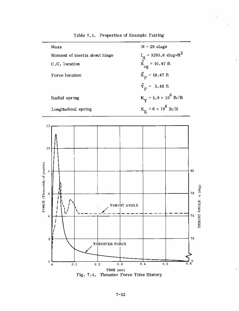
Table 7.1. Properties of Example Fairing
Mass
Moment of inertia about hinge
C.G. location
Force location
Radial spring
Longitudinal spring
M = 29 slugs
I H = 3293.6 slug-ft 2
= 10.47 ftcg
= 19.47 ftF
YF 5.42 ft
Ky = 1.8 x 10⁶ lb/ft
K X--6 × 10⁶ lb/ft
©
c-
Oe-
©
12
10
6
4
2
I
ii r,1 _jl
/l
82
/THRUST ANGLE
78 v
Z<
74
7O
THRUSTER FORCE
0.1 0.2 0.3 0.4 0.5
TIME (sec)
Fig. 7.4. Thruster Force Time History
00.6
7-12

60
O
t_
O
c_
_3z
12 !
RADIAL, FHy
10 .... AXIAL, FHX
8 I _II II I
6 ;'_ i i: AI ..; ,^,
v\
-2
-40 0.02 0.04 0.06 0.08 0.10
TIME (see)
Fig. 7.5. Hinge Load Time History
4O
gz©F-_J
20
z
r,1
>©
_0
-20-80
0.34
"_ t=0 SEC
-60 -40 -20 0
MOVEMENT IN X DIRECTION (ft)
Fig. 7.6. Fairing Trajectory
2O 4O
7-13

The radial hinge loads of the two fairing halves will nearly balance each other so
that there will be little, if any, excitation of lateral vehicle modes. However, the
vertical loads act together and can excite longitudinal vehicle modes. To investigate
these longitudinal loads, the free longitudinal model of Section 4.3 was employed with
the force time history equal to twice the axial load of Fig. 7.5. This load was applied
to mass number 5 of the model shown in Fig. 4.5, when the vehicle was under 1.43g
acceleration.
TEADY STATE
0 0.10
Fig. 7.7.
0, 20 0.30 0.40 0.50
TIME (sec}
Longitudinal Acceleration
at the Centaur/Surveyor
Interface Due to Nose
Fairing Jettison
The results of this analysis are pre-
sented in Figs 7.7 through 7.9. The oscilla-
tory motion due to the nose fairing jettison
load is superimposed on that due to steady-
state vehicle acceleration. The acceler-
ations at the Centaur/Surveyor interface
(Fig. 7.7) are important in that the oscil-
lations may excite the payload significantly.
The axial load at the Centaur/Surveyor inter-
face is shown (Fig. 7.8) to illustrate that,
due to the flexible spacecraft, the acceler-
ation at the interface times the spacecraft
weight does not necessarily yield the load
at the interface. The normal coordinate
displacements presented in Fig. 7.9 indicate
the contribution of each mode to the total re-
sponse. Nearly all modes are excited be-
cause of the high-frequency pulse loading.
-4
2
£
-12
I ,
L
Fig. 7.8.
I
V vivvv!vv\
i
. lu u20 3O u 4O
TIME _scc)
Axial Load at the Centaur/
Surveyor Interface Due to
Nose Fairing Jettison
7.4 DISCUSSION
7.4.1 JETTISON. The effective force of a
gas thruster is more than just the thrust of
the nozzle. Prior to actual opening of the
fairing, there will be a pressure buildup in
the cavity. There is also the gas impinge-
ment force from the jet of the opposite fair-
ing half. Both these forces are effective
only during the first few degrees of rotation,
but they can increase the impulse signifi-
cantly. These factors make prediction of
the thrust time history a difficult task. Other
types of thrusters, such as springs, may be
more predictable.
7.4.2 ELASTIC EFFECTS. When a fairing and/or its hinge support are relatively
flexible, a rigid-body analysis may not suffice for hinge loads and initial angular
7-14
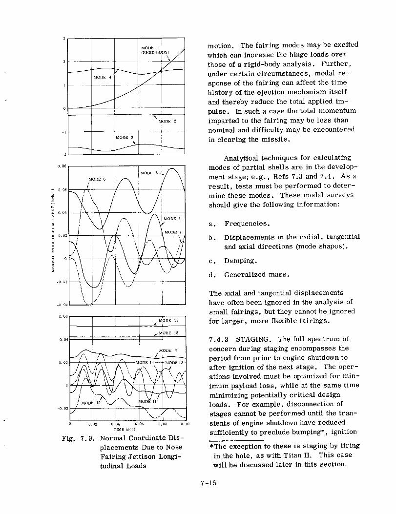
-2
0.08
O. 06
a=
0.04
<.
0.02
0
< 0
0Z
-0.02
-0, 04
0.06
0.04
0,02
MODE 1
(RIGID BO_
I \MODE 2
-0.02
MODE 3
_ ..._..______._/_'_ ---------_
MODE 8
/
/ /\
I
,,
MODE 5
6
] 1 MODE 7
, , / ,it _. ttt_t t ' /''_ MODE 14--
o // \\'l-// \>'
"MODEIO ./ _ , ,I
O. 02 O. 04 O. 06 O. 08 O.
TIME (see)
Fig. 7.9. Normal Coordinate Dis-
placements Due to Nose
Fairing Jettison Longi-tudinal Loads
I MODE 15
j, MODE 12
ti
MODE 9
MODE 13 -
'4 '\\ ,-'\\ I
motion. The fairing modes may be excited
which can increase the hinge loads over
those of a rigid-body analysis. Further,
under certain circumstances, modal re-
sponse of the fairing can affect the time
history of the ejection mechanism itself
and thereby reduce the total applied im-
pulse. In such a case the total momentum
imparted to the fairing may be less than
nominal and difficulty may be encountered
in clearing the missile.
Analytical techniques for calculating
modes of partial shells are in the develop-
ment stage; e.g., Refs 7.3 and 7.4. As a
result, tests must be performed to deter-
mine these modes. These modal surveys
should give the following information:
a. Frequencies.
b. Displacements in the radial, tangential
and axial directions (mode shapes).
c. Damping.
d. Generalized mass.
The axial and tangential displacements
have often been ignored in the analysis of
small fairings, but they cannot be ignored
for larger, more flexible fairings.
7.4.3 STAGING. The full spectrum of
concern during staging encompasses the
period from prior to engine shutdown to
after ignition of the next stage. The oper-
ations involved must be optimized for min-
imum payload loss, while at the same time
minimizing potentially critical design
loads. For example, disconnection of
stages cannot be performed until the tran-
sients of engine shutdown have reduced
sufficiently to preclude bumping*, ignition
*The exception to these is staging by firing
in the hole, as with Titan II. This case
will be discussed later in this section.
7 -15

of the next stagecannot occur until separation is complete, and control reactivationshouldnot produce excessive engine gimbal angles andresultant vehicle loads. Theeffects of engine shutdownandthrust buildup havebeendiscussed in Section4. Theoptimization of sequencingof operations is beyond the scope of this report.
The majority of the current space launch vehicles are multistage and it is possible
that more than one type of system will be encountered on a single vehicle. The staging
system consists of two parts:
a. That required to sever the structural and mechanical connection, i.e., a dis-
connect system.
b. That required to produce relative displacement, i.e., a thruster system.
Types of disconnect systems include latches, explosive bolts, linear shaped charge,
and Marman-type clamp arrangements. Latches may be activated by high-pressure
gas or by pyrotechnic devices such as pin pullers. Explosive bolts, shaped charge,
and clamp arrangements require investigation of possible damage from loose frag-
ments ranging in weight from milligrams to possibly several pounds. Structure and
equipment must be protected from the high-velocity particles that can result from the
detonation of pyrotechnic devices. Nearly all the above systems have some shock as-
sociated with their activation.
Once the spent stage has been separated, the problem then becomes one of assur-
ing that there is no collision and to minimize turning rates to the rejected stage and the
following stage. Guide rails are often employed to eliminate any possibility of collision
during staging. The problem here is to define the loads on the rails so that deflections
and weight are optimized. The selection of a thrust system to provide relative dis-
placement may be straightforward or may require statistical analysis, depending on
the variables involved. Thrust systems that may be encountered include springs, gas
thrusters, monopropellant or hypergolic engines, solid-propellant rockets, or firing
of the upper stage engines. These devices may be on the upper or lower stage or in
combination.
Loads that must be considered during staging include shock due to disconnect and
those associated with the thruster system. Shocks range from as high as 3000g in the
immediate vicinity of shaped charges to less than 50g for latches. The shock amplitude,
frequency content, and propagation through the structure will depend upon the device
used and the type of structure. Analysis of loads due to thruster activation is usually
straightforward. The impulse resulting from release of restrained elastic energy
(pretensioning, for example) should not be overlooked.
The case of staging by "firing in the hole" presents some rather special problems,
although it does represent the most efficient method. For example, there is a greater
7-16


k
possibility of explosion at engine ignition due to trapped gases in the interstage adapter.
Moreover, the thermal environment in the engine compartment may be more severe
than with other methods, and the vibration and acoustic environment may be moresevere.
7.5 CONCLUSIONS AND RECOMMENDATIONS
The analytical techniques required to determine staging and jettison loads are, for
the most part, well developed. While the Newtonian approach was used to develop the
analysis of Section 7.3.1, the Lagrangian approach is more suitable for more compli-
cated systems. When the elastic effects are considered in the analysis, Lagrange's
equation has a decided advantage. It may also be desirable to derive the equations
initially with respect to the center of gravity and then, if necessary, transform them
into another set having the desired variables.
Shock and gas impingement loads must ordinarily be determined from tests.
Methods for calculating modes of partial shells require further development for
direct project support applications. In order to reliably predict hinge loads and fairing
deflections the flexibility of the fairing and hinge must be taken into account.
7.6 REFERENCES
7.1 Program 624A Standard Space Launch Vehicle Staging Dynamics Analysis Report,
7.2
Flight Test Plan VIII, Martin Company Report SSD-CR-65-35, February 1965.
R. L. Goble, Analytical Investigation of the Motion of a Clamshell-Type Heat
Shield on Deployment From a Parent Vehicle in the Atmosphere, NASA TN D-3280,March 1966.
7.3 T.E. Lang, Summary of the Functions and Capabilities of the Structural Analysis
7.4
System Computer Program, Jet Propulsion Laboratory, TM 33-220, June 1965.
L. E. Penzes, Frequency, Dynamic Response and Jettison Analysis for Jettison-
able Payload Shrouds, with Application to the Orbital Astronomical Observatory
7.5
7.6
(OAO) Fairing, Institute of Environmental Sciences, 1966.
Separation Joint Test Program, Lockheed Missiles and Space Company ReportLMSC/A639047, April 15, 1964.
R. L. Batten, and E. C. Noble, Jr., "Shaped Charge Shock Environment for
Centaur Vehicle Components", 35th Symposium on Shock and Vibration, NewOrleans, La., October 1965.
7-17
7.7
7.8
Centaur Insulation Panel Unlatch Shock Measur_ts, General Dynamics Convair
Division Report RAC ZZA-65-303, 22 September 1965.
"G" Series Centaur Forward Bulkhead Vibration Response Test, General Dynamics
Convair Division Report RAC ZZA-65-130, 19 March 1965.
7-18