Broadband Geo-Acoustic Inversion From Sparse Data Using Genetic Algorithms

Journal of Computational Acoustics�fc IMACS

BROADBAND GEO�ACOUSTIC INVERSION FROM SPARSE DATAUSING GENETIC ALGORITHMS

MARTIN SIDERIUS

Saclant Undersea Research Centre

Viale S� Bartolomeo �� La Spezia� Italy

PETER GERSTOFTMarine Physical Laboratory� Scripps Institute of Oceanography

University of California� San Diego

San Diego� CA ��

PETER NIELSENSaclant Undersea Research Centre

Viale S� Bartolomeo �� La Spezia� Italy

Received �to be insertedRevised by Publisher�

Matched �eld acoustic inversion techniques were investigated using data from sparsely populatedvertical receiving arrays and a single receiver element� The purpose of considering sparse datasets is to investigate� under simulation� the feasibility of reducing the number and complexity ofacoustic measurements needed for geo�acoustic inversion� The entire bandwidth of the �� Geo�Acoustic Inversion Workshop provided data �� Hz� was used which compensates for lackingspatial information when a limited number of receivers is considered� Forward model PROSIMand inversion code SAGA were applied to benchmark cases sd� wa� and n� The inversion resultsgenerally showed good agreement with the ground truth for full arrays� sparse arrays and singlereceiver elements� With a simple two layer model� an e�ective sound speed pro�le in the bottomwas determined which produced a good �t between model and observed pressure �elds for themulti�layer case n�

�� Introduction

Acoustic signals propagating in shallow water can have many interactions with the ocean

bottom resulting in a strong dependency between received signals down range and bottom

type� In recent years� matched �eld processing based inversion methods have been devel�

oped which infer properties of the bottom from acoustic measurements��In matched �eld

inversions� a large number of bottom types are modeled until suitable agreement is found

between the observed and modeled �elds� Matched �eld methods generally �nd an average

or e�ective bottom type which� in the model� will reproduce the observed acoustic �eld�

�

Siderius et al�

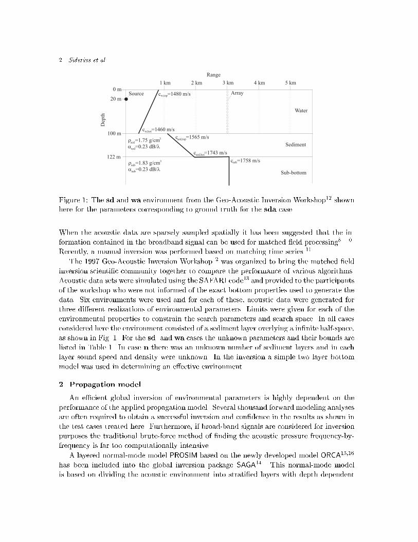
Figure �� The sd and wa environment from the Geo�Acoustic Inversion Workshop�� shownhere for the parameters corresponding to ground truth for the sda case�

When the acoustic data are sparsely sampled spatially it has been suggested that the in�

formation contained in the broadband signal can be used for matched �eld processing��

Recently� a manual inversion was performed based on matching time series ��

The �� Geo�Acoustic Inversion Workshop�� was organized to bring the matched �eld

inversion scienti�c community together to compare the performance of various algorithms�

Acoustic data sets were simulated using the SAFARI code�� and provided to the participants

of the workshop who were not informed of the exact bottom properties used to generate the

data� Six environments were used and for each of these� acoustic data were generated for

three di�erent realizations of environmental parameters� Limits were given for each of the

environmental properties to constrain the search parameters and search space� In all cases

considered here the environment consisted of a sediment layer overlying a in�nite half�space�

as shown in Fig� �� For the sd and wa cases the unknown parameters and their bounds are

listed in Table �� In case n there was an unknown number of sediment layers and in each

layer sound speed and density were unknown� In the inversion a simple two layer bottom

model was used in determining an e�ective environment�

�� Propagation model

An ecient global inversion of environmental parameters is highly dependent on the

performance of the applied propagation model� Several thousand forward modeling analyses

are often required to obtain a successful inversion and con�dence in the results as shown in

the test cases treated here� Furthermore� if broad�band signals are considered for inversion

purposes the traditional brute�force method of �nding the acoustic pressure frequency�by�

frequency is far too computationally intensive�

A layered normal�mode model PROSIM based on the newly developed model ORCA��

has been included into the global inversion package SAGA�� This normal�mode model

is based on dividing the acoustic environment into strati�ed layers with depth dependent

Broadband Inversion �

Table �� Parameter search bound for the sd and wa case� Each parameter was discretizedinto �� values�

Parameter Lower bound Upper bound

Sediment case sd and wa�Thickness m� �� Sound speed top m�s� �� Sound speed bottom m�s� �� Density g�cm��

Bottom case sd and wa�Sound speed m�s� �� Density g�cm��

Geometric case wa�Water depth m� �� Source depth m� �� Source range m� � ��

properties assuming a ��c��linear sound speed pro�le� The acoustic �eld within each layer

is described analytically by using a sum of Airy functions� An eigenvalue equation is estab�

lished considering continuity of the acoustic �eld and its derivative across layer interfaces�

and by ful�lling the boundary conditions at the sea surface and the bottom of the waveguide�

This equation is solved for the eigenvalues of the speci�c problem� Only the eigenvalues on

the real axis are considered here to increase the computation speed� and the attenuation

in the sediment layers and sub�bottom is treated by a perturbation theory� The eigenval�

ues are found by an ecient search algorithm� which only requires about �� iterations to

determine each individual mode��

The computation speed is shown to be linearly dependent on frequency for single fre�

quency analysis by using the layered model� whereas the computation speed depends quadrat�

ically on frequency using the traditional normal�mode models based on numerical integration

of mode functions� However� the computation speed increases as the number of layers in the

model increases� whereas the speed of the traditional models is almost independent of the

depth discretization of the environment� For certain shallow water environments the lay�

ered model is shown to be more than �� times faster at higher frequencies than traditional

models��

In the ORCA broad�band model� calculations are performed by dividing the frequency

band of interest into sub�bands of ��Hz� At the limits of the sub�bands the eigenvalues and

mode functions are determined exactly as mentioned above� Furthermore� at the subband

limits the �rst and second order derivative of the wavenumbers with respect to frequency

are calculated analytically� The real part of the wavenumbers is interpolated within the

sub�bands by applying a �th�order polynomial�� The eigenvalue equation is applied to the

interpolated wavenumbers to evaluate the accuracy of the interpolation� If the interpolation

of the wavenumbers has been performed successfully the mode functions are interpolated

� Siderius et al�

within the frequency subband using a cubic �t� The coecients of the cubic polynomial

are found by the value of the mode functions and their analytical derivatives with respect

to frequency at the subband limits� The attenuation is interpolated linearly within the fre�

quency subband� The above procedure is repeated until the acoustic pressure is established

for the entire frequency band of interest� and the technique becomes more ecient at �ner

frequency sampling of the acoustic pressure�

The real�axis version of ORCA embedded in SAGA has been modi�ed and is called

PROSIM� which is a broad�band� range�dependent propagation model based on the adi�

abatic approximation� The range�dependent acoustic environment is divided into range�

independent segments by assuming the eigenvalues and mode functions vary linearly as a

function of range within each segment�

The transfer function of shallow�water� range�independent waveguides covering the fre�

quency band from �� to �� Hz involving more than �� modes and �� frequency

components can be obtained by using PROSIM in less than � minutes on an DEC ALPHA

�� workstation� This performance is obtained partly by utilizing a discretization of

the frequency band of interest into sub�bands of di�erent sizes� The frequency sub�bands

are larger at higher frequencies and decrease towards the lower frequencies� For a weak

range�dependent environment including �� modes� �� frequency components and ��

range�segments� PROSIM is �� times faster than the coupled�mode model C�SNAP�� Ex�

cellent agreement between the two models was found by comparing the received time series

for this environment� This indicates that PROSIM is well suited for broadband inversion�

�� Matched �eld Inversion

�� Objective function

Two objective functions� were used in the analysis of the benchmark problems� In the case

of a full array of hydrophones the objective function is the incoherent sum of the Bartlett

power in depth for each frequency as given by Eq� �� That is� a correlation is computed

in depth between observed and modeled �elds and the powers are averaged over frequency

to determine the objective function� Both observed and modeled data are complex pressure

�eld vectors referred to here as p and q� respectively� The coherent objective function in

depth is given by�

�d � ��

NrangeNfreq

NrangeXk�

NfreqXi�

jPNdepth

j� pijkq�ijkj

�

PNdepth

j� jpijkj�PNdepth

j� jqijkj��

where � indicates the complex conjugation operation� Ndepth is the number of receivers in

depth� Nfreq is the number of frequencies considered and Nrange is the number of receivers

in range� From Eq� �� the addition of data in range and frequency are summed in an

incoherent fashion sum of Bartlett powers�� When processing coherent in depth several

di�erent choices for objective function have been proposed��

For sparse arrays� correlation in depth may not be meaningful and the correlation is


performed in the frequency domain which� is followed by a summation of the power in the

spatial domain� The objective function is given by�

�f � ��

NrangeNdepth

NrangeXk�

NdepthXj�

jPNfreq

i� pijkq�ijkj

�

PNfreq

i� jpijkj�PNfreq

i� jqijkj��

A classical matched �lter is performed by correlating in the time domain and the above

expression in frequency domain gives a nearly identical result� as discussed further in the

Appendix� where also other choices for objective functions are presented�

�� Genetic algorithms

The global optimization method genetic algorithms GA� is used for the optimization� The

basic principle of GA is simple� From all possible parameter vectors� an initial population

of members is randomly selected� The ��tness� of each member is computed on the basis of

the value of the objective function� Based on the �tness of the members a set of �parents�

are selected and through a randomization a set of �children� is produced� These children

replace the least �t of the original population and the process iterates to develop an overall

more �t population� In geo�acoustic inversion� the parameter vectors are the environmental

properties such as sediment and sub�bottom sound speed and a population consists of one

realization of environmental properties� A more detailed description of genetic algorithms

and their application to parameter estimation is given by Gerstoft��

�� Convergence

Three indicators are used to determine the quality of the estimated environmental pa�

rameters� Due to the non�uniqueness of the inversion it is not guaranteed that the correct

solution is found even when all the three criteria are satis�ed� The three considered criteria

are as follows�

a�Value of objective function� For a good match the objective function should approach a

certain value� In particular� for the present inversion� where the parameterization is known

a priori� it is known that �d � � or �f � �� for a good match�

b� Plotting of the observed and modeled data with the best match� A visual comparison

of the observed and modeled data can often identify problems in the inversion� Often the

same data� as used in the inversion� are used when comparing the match� but also data that

have not been used in the inversion could be used�

c� A posteriori distributions� The purpose of the inversion is to determine an optimal

set of environmental parameters� and thus it is important to have an indication of how well

each parameter has been determined� Based on the samples obtained during the inversion�

statistics of the convergence for each parameter are computed� Using a Bayesian framework

this can be interpreted as a Monte Carlo integration of the likelihood function�� However�

often the likelihood function is not available� and then a practical weighting of the objective

function is performed to give an estimate of the a posteriori distributions�� Due to

this ad hoc weighting� the a posteriori probability should be interpreted with care� The


Table �� Case sd� Results for full arrays at all ranges �� km and for a single hydrophoneat range � km and depth �� m�

Parameter Case Full Arrays One Hydrophone Ground Truth

Sediment thickness m� a �� b �� c ��

Sediment speed top m�s� a �� b �� c ��

Sediment speed bottom m�s� a �� b �� c ��

Sediment density g�cm�� a �� b �� c ��

Bottom sound speed m�s� a �� b �� c ��

Bottom density g�cm�� a �� b �� c ��

relative importance of the parameters in the same inversion is precise� but the comparison

of inversion results based on di�erent data or approaches should be interpreted with care�

�� Results for the benchmark problems

Inversions were performed on the observed data from cases sd� wa and n� In all cases� a

total of �� forward models are computed with PROSIM for the full frequency band from

�� Hz in � Hz increments� The inversion time was from �� minutes to � hours on a

DEC ALPHA �� The observed data were provided at ranges of �� and � km

and along an array at depths from � to �� m in increments of � m� Several combinations

of receiver ranges and depths as well as number of receivers used will be described in the

following sub�sections�

�� Benchmark case� sd

Case sd had � unknown parameters� Upper and lower sediment sound speed� sediment

thickness� sediment density� bottom sound speed and bottom density� Acoustic data were

given for three sets of di�erent environmental parameters� i�e� three realizations of the

environment� in this case denoted as sda� sdb and sdc� An inversion was performed on

each realization using the data from all observed data points in range and depth� That is�

data were used from �ve vertical arrays with � m depth sampling and at ranges from the

Broadband Inversion

10 15 20 25 30 35 40 45 50Sediment depth (m)

1500 1520 1540 1560 1580 1600Sediment sound speed (m/s)

1550 1600 1650 1700 1750Sediment sound speed (m/s)

1600 1650 1700 1750 1800Bottom sound speed (m/s)

1.4 1.45 1.5 1.55 1.6 1.65 1.7 1.75 1.8 1.85Sediment density (g/cm3)

1.6 1.65 1.7 1.75 1.8 1.85 1.9 1.95 2Bottom density (g/cm3)

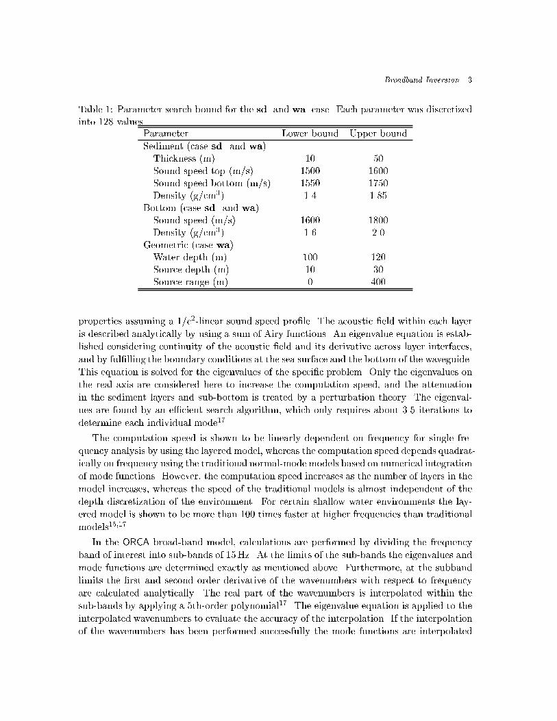
Figure �� The a posteriori distributions for each of the inverted environmental parametersfor case sda�

source of �� and � km� In a second inversion� only data from a single hydrophone at

range � km and depth �� m is included� Table � shows the values found by the inversion

using data from all the vertical arrays� the single hydrophone results and the ground truth

for sda� sdb and sdc�

The sd results show good agreement between the inverted environmental parameters

and ground truth even for the single hydrophone measurement� In general there was little

sensitivity to the density parameter in both the sediment and sub�bottom and the sub�

bottom sound speed appeared to be less sensitive than the sound speeds in the sediment�

The sensitivity of parameters� or� the degree of con�dence given to each parameter found

through the inversion process can be summarized using the a posteriori distributions as

shown for case sda in Fig� �� From the distributions� there are features that appear

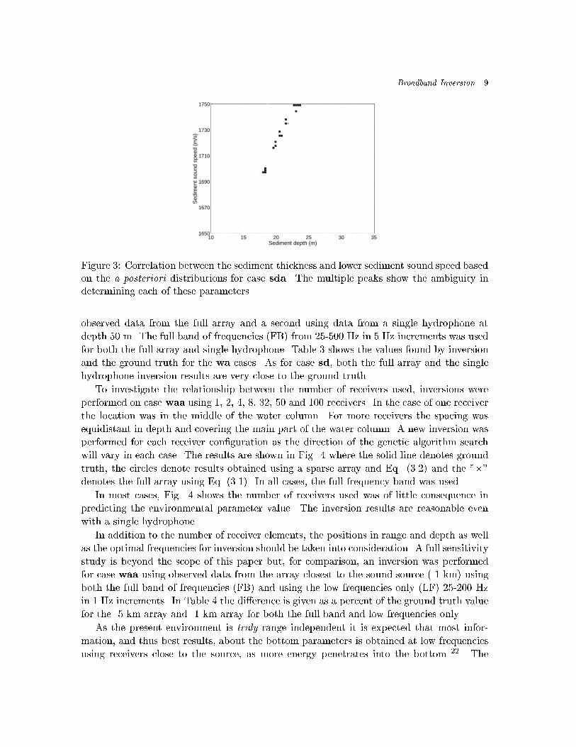
throughout all test cases including wa and n� The bottom density is not well determined�

and there is a correlation between the sound speed in the sediment at the sediment�bottom

interface and the sediment depth thickness�� The ��D marginal a posteriori distributions

are given in Fig� � as a function of sediment thickness and lower sediment sound speed as

produced by SAGA� The correlation is apparent from the �gure and this indicates that these

two parameters might more eciently be expressed in terms of a single parameter possibly

searching for a sound speed gradient instead��

�� Benchmark case� wa

Case wa has nine unknown parameters� The �rst six are the same as for sd with additional

unknowns� Water depth� source range and source depth� Again� there were three realiza�

tions of the environment given� waa� wab and wac� Two inversions were made� one using


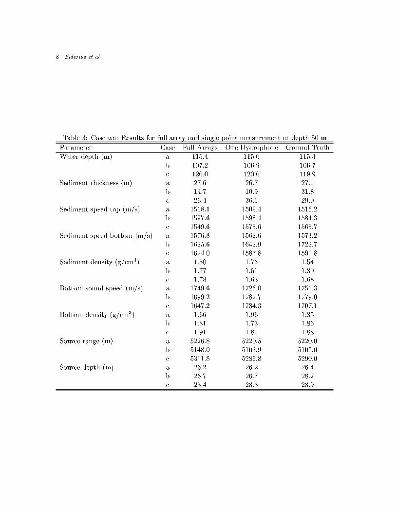
Table �� Case wa� Results for full array and single point measurement at depth �� m�

Parameter Case Full Arrays One Hydrophone Ground Truth

Water depth m� a �� b �� c ��

Sediment thickness m� a �� b �� c ��

Sediment speed top m�s� a �� b �� c ��

Sediment speed bottom m�s� a �� b �� c ��

Sediment density g�cm�� a �� b �� c ��

Bottom sound speed m�s� a �� b �� c ��

Bottom density g�cm�� a �� b �� c ��

Source range m� a �� b �� c ��

Source depth m� a �� b �� c ��


10 15 20 25 30 351650

1670

1690

1710

1730

1750

Sediment depth (m)

Sed

imen

t sou

nd s

peed

(m

/s)

Figure �� Correlation between the sediment thickness and lower sediment sound speed basedon the a posteriori distributions for case sda� The multiple peaks show the ambiguity indetermining each of these parameters�

observed data from the full array and a second using data from a single hydrophone at

depth �� m� The full band of frequencies FB� from �� Hz in � Hz increments was used

for both the full array and single hydrophone� Table � shows the values found by inversion

and the ground truth for the wa cases� As for case sd� both the full array and the single

hydrophone inversion results are very close to the ground truth�

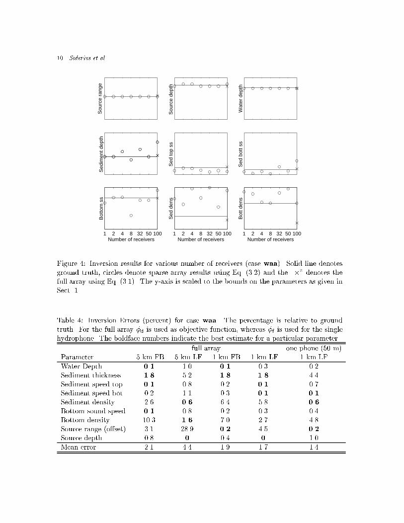
To investigate the relationship between the number of receivers used� inversions were

performed on case waa using �� and �� receivers� In the case of one receiver

the location was in the middle of the water column� For more receivers the spacing was

equidistant in depth and covering the main part of the water column� A new inversion was

performed for each receiver con�guration as the direction of the genetic algorithm search

will vary in each case� The results are shown in Fig� � where the solid line denotes ground

truth� the circles denote results obtained using a sparse array and Eq� �� and the ��

denotes the full array using Eq� �� In all cases� the full frequency band was used�

In most cases� Fig� � shows the number of receivers used was of little consequence in

predicting the environmental parameter value� The inversion results are reasonable even

with a single hydrophone�

In addition to the number of receiver elements� the positions in range and depth as well

as the optimal frequencies for inversion should be taken into consideration� A full sensitivity

study is beyond the scope of this paper but� for comparison� an inversion was performed

for case waa using observed data from the array closest to the sound source � km� using

both the full band of frequencies FB� and using the low frequencies only LF� �� Hz

in � Hz increments� In Table � the di�erence is given as a percent of the ground truth value

for the � km array and � km array for both the full band and low frequencies only�

As the present environment is truly range independent it is expected that most infor�

mation� and thus best results� about the bottom parameters is obtained at low frequencies

using receivers close to the source� as more energy penetrates into the bottom �� The

�� Siderius et al�

Sou

rce

rang

e

Sou

rce

dept

h

Wat

er d

epth

Sed

imen

t dep

th

Sed

top

ss

Sed

bot

t ss

1 2 4 8 32 50 100Number of receivers

Bot

tom

ss


Sed

den

s


Bot

t den

s

Figure �� Inversion results for various number of receivers case waa�� Solid line denotesground truth� circles denote sparse array results using Eq� �� and the �� denotes thefull array using Eq� �� The y�axis is scaled to the bounds on the parameters as given inSect� ��

Table �� Inversion Errors percent� for case waa� The percentage is relative to groundtruth� For the full array �d is used as objective function� whereas �f is used for the singlehydrophone� The boldface numbers indicate the best estimate for a particular parameter�

full array one phone �� m�Parameter � km FB � km LF � km FB � km LF � km LF

Water Depth �� Sediment thickness �� Sediment speed top �� Sediment speed bot� ��

Sediment density ��

Bottom sound speed �� Bottom density �� Source range o�set� ��

Source depth ��

Mean error ��

Broadband Inversion ��

40 60 80 100 120 140 160 180 200 75

70

65

60

55

50

45

Frequency (Hz)

Tra

nsm

issi

on L

oss

(dB

)

Figure �� Transmission loss for the waa�LF case for one hydrophone at � km� The fullline is the observed data and dotted line the modeled data with the best environment� Theagreement is very good�

results in Table � imply that for both objective functions using only the low frequencies and

array position at � km gives the best results in terms of percentage error� Individual param�

eters may be estimated better using other con�gurations of array position and frequency

content� This can be observed by noting the boldface numbers in the table indicating the

best estimate for a particular parameter� In general a thorough analysis would be required

to determine optimal frequencies and array position for inversion�

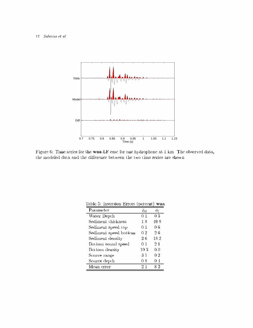
The best obtained �t for the waa�LF case for one hydrophone at � km is shown both in

frequency Fig� �� and time domains Fig� �� The transmission loss is produced directly

from SAGA� whereas the time series �rst requires a Fourier Transform of the data� The

dissimilarities between observed benchmark� and modeled data is due to not �nding the

exact environment and to di�erences between forward models PROSIM and SAFARI� Based

on simulations� it is expected that a signi�cant part of the deviation in Fig� � is due to only

considering the real axis eigenvalues� It should be noted that in the matched �eld approach

used here� only the relative phase across all frequencies is determined� To compare the

time series� the average phase di�erence between the observed and computed data was

determined� The time series have been convolved with a Ricker wavelet second derivative

of the Gaussian function� with a center frequency of �� Hz�

The two objective functions �d given by Eq� �� and �f given by Eq� �� produce

slightly di�erent results� Again� considering case waa� the error in the inversion results

using �d and �f is compared� Table � shows the percent error for each parameter and the

mean error over all parameters for full arrays at � km and using the full band of frequencies�

In general� �d performs better than �f as it produces less error when all parameters are


0.7 0.75 0.8 0.85 0.9 0.95 1 1.05 1.1 1.15

Diff.

Model

Data

Time (s)

Figure �� Time series for the waa�LF case for one hydrophone at � km� The observed data�the modeled data and the di�erence between the two time series are shown�

Table �� Inversion Errors percent� waa

Parameter �d �fWater Depth �� Sediment thickness �� Sediment speed top �� Sediment speed bottom �� Sediment density �� Bottom sound speed �� Bottom density �� Source range �� Source depth ��

Mean error ��


considered� However� �f outperforms �d in estimating the source position and the bottom

density� The improved prediction of the bottom density using �f is most likely a chance

result in that the con�dence level in the density predictions were low as was indicated in

the a posteriori distributions for case sda in Fig� �� These results comparing �d with �fcan also be seen from Fig� ��

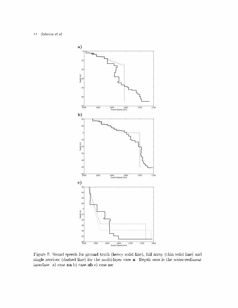
�� Benchmark case� n

The �nal case considered was n which was the same as case sd except rather than having

two layers� n has an unknown number of bottom layers� A simple approach was used and

the multi�layer problem was solved as if only two layers exist� The top layer in the two layer

model is allowed to have a sound speed gradient and a representative sound speed pro�le

was determined� The sound speed pro�le match is shown for the three realizations of test

case n in Fig� for both the full array and the single receiver� It is seen that although the

simpli�ed model does not capture the complex shape of the sound speed pro�le� it �ts the

curve well in a least squared sense� The single receiver performed well� giving a reasonable

�t to the sound speed pro�le� The simple two layer model predicts the sediment sound

speed well at the top� and seems to approximately determine the sound speed gradient�

The inverted bottom sound speed value appears to be an average value across all the layers�

�� Discussion and conclusions

For the benchmark cases considered here� the inversion results agree well with ground�truth�

The computational eciency of PROSIM� the broadband� normal mode forward model made

it possible to consider the entire frequency content of the observed data between �� and

�� Hz� The genetic algorithms package SAGA produced good inversion results from ��

forward models for each set of observed data�

Two objective functions have been used� either a coherent summation in depth or a

coherent summation in frequency� In the Appendix it is discussed how the latter could

equally well be performed in the time domain� The coherent summation in frequency has

the advantage that only one hydrophone need be used� In practice a few phones are probably

required�

The single hydrophone inversions produced results that agreed well with ground truth�

The results in both Fig� � and Table � indicate that for the benchmark cases� one receiver

is sucient if a coherent processor in frequency is used� The broadband single hydrophone

inversion results demonstrate that a few receivers may be sucient to determine ocean

bottom properties�

The multi�layer case n provided simulated acoustic data in a more realistic environment�

In the inversion a simple two layer model provided a good estimate of the bottom parameters

for both the full array and the single hydrophone� This approach is practical since it is

impossible to solve for all the acoustic properties that make up the complex structure of

the ocean bottom�


a�

1500 1550 1600 1650 1700 175060

50

40

30

20

10

0

Dep

th (

m)

Sound Speed (m/s)

b�

1500 1550 1600 1650 1700 175060

50

40

30

20

10

0

60

50

Dep

th (

m)

Sound Speed (m/s)

c�

1500 1550 1600 1650 1700 1750 180060

50

40

30

20

10

0

60

50

40

30

Dep

th (

m)

Sound Speed (m/s)

Figure � Sound speeds for ground truth heavy solid line�� full array thin solid line� andsingle receiver dashed line� for the multi�layer case n� Depth zero is the water�sedimentinterface� a� case na b� case nb c� case nc�


Acknowledgments

The development of the PROSIM normal mode code was partly funded by the EC un�

der the MAST�III project PROSIM� contract number MAS��CT�� Christoph Meck�

lenbr�auker has supplied invaluable comments to the Appendix�

Appendix A

Objective functions in time and frequency domain

In this Appendix it is shown that an objective function based on simple correlation in

the time domain can be seen as similar to the coherent summation over frequency� For

simplicity only a single observed p t� and modeled q t�m� time series as functions of time

t are used in the beginning� The unknown environmental parameters are included in the

model vector m� In the time domain the correlation objective function to be optimized is

given by

� m� ��

Z �

��p t� ��q t�m�dt�� A��

where � is the time delay between the two signals� In order to obtain a perfect match from

Eq� A�� the absolute timing of the synthetic and measured waveforms must be identical�

This requires that both the source and the receiver are monitored� In general the absolute

timing of the transmitted source signal and the received signal at the array is not available

and thus the absolute arrival time of the two signals is unknown� One way of treating this

problem is by searching for a unknown time delay � � Clearly� for cases where this time

delay is known it should be set to zero�

Using the de�nitions of Fourier transform the following expressions are obtained

� m� ��

��

��

Z �

��

�Z �

��

�p ��ei�� ei�t

�d�q t�m�

�dt

��

�

��

��

Z �

��

�p ��ei��

Z �

��

�q t�m�ei�t

�dt

�d�

��

�

��

��

Z �

��p ��q� ��m�ei��d�

�� A��

where � is complex conjugate� In order to only optimize for the shape of the signal we nor�

malize Eqs� A��A�� with the power of the two signalsR�� p� t�dt and

R�� q� t�m�dt� By

use of Parsevals theorem this can be done equivalently in the time or frequency domain� In

the following the factor �� will be neglected� as it is just a constant which is unimportant

for the optimization� Also the objective function � is modi�ed to a function � so that it

becomes a minimization problem with an absolute minimum of zero and the maximum is

arbitrary�

For data on a vertical array pj � j � � � � � Ndepth Ndepth is the number of hydrophones in

depth� there are two ways to do the summation� either

�t� m� ��

Ndepth

NdepthXj�

hR�� pj t� ��qj t�m�dt

i�R�� p�j t�dt

R�� q�j t�m�dt

A��


or

�t� m� ��

NdepthXj�

Z �

��p�j t�dt�

hPNdepth

j�

R�� pj t� ��qj t�m�dt

i�PNdepth

j�

R�� q�j t�m�dt

� A��

In the above equations the same time delay is common to all hydrophones� There are two

di�erences between �� and �� The main di�erence is that the numerator of �� is squared

before the summation� whereas in the numerator of �� the summation is done �rst� Thus in

�� there are cross terms between the time series� whereas �� does not contain cross terms�

Also� �� gives equal emphasis to the received signal on each phone� whereas �� weights

each phone according to its energy� If some of the hydrophones have little signal� either it

could be malfunctioning or it could be placed at a null� then �� is preferred� However� if

the phones have di�erent unknown gain then �� should be used�

In the frequency domain the above equations become

�f� m� ��

Ndepth

NdepthXj�

jR�� pj ��q

�j ��m�ei��d�j�R�

�� jpj ��j�d�R�� jqj ��m�j�d�

A��

and

�f� m� ��

NdepthXj�

Z �

��jpj ��j

�d� �jPNdepth

j�

R�� pj ��q

�j ��m�ei��d�j�PNdepth

j�

R�� jqj ��m�j�d�

� A��

For discrete frequencies it is seen that Eq� A�� corresponds to Eq� ��

For real data the objective functions are best computed in terms of the ensemble covari�

ance matrix across both frequency and depth� This is computed by �rst ordering all the

observations across N frequencies and Ndepth depths into one vector�

g � �p� �� p� �N �� p� �� pNdepth �N ��

T � A��

Based on Nobs observations of this vector the ensemble covariance matrix is formed�

C ��

Nobs

NobsXn

gngyn� A��

where y is the complex transpose� This covariance matrix contains elements corresponding

to all frequencies and phones� It might thus be quite large and it might be more practical

to just use the eigenvector corresponding to the largest eigenvalue of the covariance matrix

and then base the processing on Eq� A��

Similar to Eq� A�� the synthetic data is ordered into one vector given by

b � �q� ��ei�� q� �N �e

i�N � � q� ��ei�� qNdepth

�N �ei�N � �T � A��

where also the phase shift due to the unknown arrival time is incorporated�


An objective function corresponding to Eq� A�� now becomes

�� m� �� trC�byCb

byb� A��

where tr is the trace of the covariance matrix C�

For synthetic data the time delay is known and thus it is not necessary to search for the

time delay � � but for real data without precise synchronization of source and receiver it is

treated as a parameter to be optimized� For noise free data it is not necessary to form a

covariance matrix� and thus Eq� A�� or Eq� A�� can be used directly�

References

�� M� D� Collins and W� A� Kuperman� �Focalization� Environmental focusing and source localiza�tion�� J� Acoust� Soc� Am� ��

� M� D� Collins� W� A� Kuperman and H� Schmidt� �Nonlinear inversion for ocean bottom proper�ties�� J� Acoust� Soc� Am� ��

�� C� E� Lindsay and N� R� Chapman� �Matched �eld inversion for geophysical parameters usingadaptive simulated annealing�� IEEE J� Oceanic Eng� ��

�� S� E� Dosso� M� L� Yeremy� J� M� Ozard and N� R� Chapman� �Estimation of ocean bottomproperties by matched��eld inversion of acoustic �eld data�� IEEE J� Oceanic Eng� ��

�� P� Gerstoft� �Inversion of seismo�acoustic data using genetic algorithms and a posteriori proba�bility distributions�� J� Acoust� Soc� Am� ��

�� A� Tolstoy� Matched Field Processing for Underwater Acoustics World Scienti�c Pub� Co� RiverEdge� New Jersey ��

�� J� P� Hermand and P� Gerstoft� �Inversion of broadband multi�tone acoustic data from the YellowShark summer experiments�� IEEE J� Oceanic Eng� ��

�� N� L� Frazer and P� I� Pecholcs� �Single�Hydrophone localization�� J� Acoust� Soc� Am� ��

� J� P� Hermand and R� J� Soukup� �Broadband inversion experiment Yellow Shark �� Modellingthe transfer function of a shallow�water environment with range�dependent soft clay bottom��Third European conference on underwater acoustics� edited by J�S� Papadakis� �� CreteUniversity Press� Crete� ��

�� Z�H� Michalopoulou and M�B� Porter and J�P� Ianniello� �Broadband source localization in theGulf of Mexico�� J� of Computational Acoustics � ��

�� D�P� Knobles and R�A� Koch� �A time series analysis of sound propagation in a strongly multipathshallow water environment with an adiabatic normal mode approach�� IEEE J� Oceanic Eng� ��

� � A� Tolstoy and R� Chapman� �The matched��eld processing benchmark problems�� Journal ofComputational Acoustics� this issue ��

�� H� Schmidt� �SAFARI� Seismo�acoustic fast �eld algorithm for range independent environments�User�s guide�� SACLANT Undersea Research Centre� SR�� La Spezia� Italy� ��

�� P� Gerstoft��SAGA Users guide �� an inversion software package�� SACLANT Undersea Re�search Centre� SM�� La Spezia� Italy� ��

�� S�J� Levinson� E�K� Evans� R�A� Koch� S�K� Mitchell� and C�V� Sheppard� �An e�cient and robustmethod for underwater acoustic normal�mode computation�� J� Acoust� Soc� Am� ��


�� E� K� Westwood� C� T� Tindle� and N� R� Chapman� �A normal mode model for acousto�elasticocean environments�� J� Acoust� Soc� Am� ��

�� E�K� Westwood� �Improved narrow band and broadband normal mode algorithms for �uid oceanenvironments�� Presentation at the ��st Meeting of the Acoustical Society of America� Paper�aUW�� May ��

�� C� M� Ferla� M�B� Porter and F�B� Jensen� �C�SNAP� Coupled SACLANTCEN normal modepropagation loss model�� SACLANTCEN Undersea Research Centre� SM� �� La Spezia� Italy��

�� G� Haralabus and P� Gerstoft� �Stability of parameter estimates using multi�frequency inversiontechniques�� SACLANT Undersea Research Centre� SM�� La Spezia� Italy� ��

�� P� Gerstoft and C�F� Mecklenbr�auker� �Ocean acoustic inversion with estimation of a posterioriprobability distributions�� submitted to J� Acoust� Soc� Am� �May ��

�� P� Gerstoft� �Global Inversion by genetic algorithms for both source position and environmentalparameters�� J� of Computational Acoustics � ��

� P� Ratilal� P� Gerstoft� J�T� Goh �Subspace approach to inversion by genetic algorithms involvingmultiple frequencies�� J� of Computational Acoustics� This issue ��

Broadband Geo-Acoustic Inversion From Sparse Data Using Genetic Algorithms

Documents

Transcript of Broadband Geo-Acoustic Inversion From Sparse Data Using Genetic Algorithms