BOUNDARY LAYER FLOW AND HEAT TRANSEFER OF DUSTY FLUID OVER A STRETCHING SHEET WITH HEAT SOURCE/SINK

[Rauta&Mishra, 4(4):April, 2015] ISSN: 2277-9655

Scientific Journal Impact Factor: 3.449

(ISRA), Impact Factor: 2.114

http: // www.ijesrt.com© International Journal of Engineering Sciences & Research Technology

[302]

IJESRT INTERNATIONAL JOURNAL OF ENGINEERING SCIENCES & RESEARCH

TECHNOLOGY

BOUNDARY LAYER FLOW AND HEAT TRANSEFER OF DUSTY FLUID OVER

A STRETCHING SHEET WITH HEAT SOURCE/SINK A.K.Rauta &.S.K.Mishra

Lecturer, Department of Mathematics, S.K.C.G.College, Paralakhemundi, Odisha, India

Adjunct Professor, Department of Mathematics, CUT M, Paralakhemundi, Odisha, India

__________________________________________________________________________________

ABSTRACTIn this paper, we contemplate to study the unsteady dusty fluid problem over a continuous Impermeable

stretching sheet in the presence of heat source / sink. The highly non-linear, coupled partial differential

equations governing the momentum and heat transfer equations are reduced to a system of coupled non-linear

ordinary differential equations by applying suitable similarity transformation. These non-linear coupled ordinary

differential equations are solved numerically by Runge-Kutta method along with shooting technique for

different values of the parameters. These includes the effect of unsteady parameter, heat source/sink parameter,

Froud number, Grashof number, Prandtl number, Eckert number, Volume fraction, fluid interaction parameter

etc. The velocity and temperature distributions are discussed numerically and presented through graphs. Skin-

friction coefficient and the Nusselt number at the sheet are derived, discussed numerically and their numerical

values for various values of physical parameters are presented through tables. A numbers of qualitatively

distinct potential scenarios are predicted. It is believed that the results obtained from the present investigation

will provide useful information for application and also serve as a complement to the previous investigations.

AMS classification 76T10, 76T15

KEYWORDS: Heat source/sink parameter ,Unsteady parameter, Volume fraction, Fluid – particle interaction

parameter,Boundarylayerflow,Stretchingsheet.

______________________________________________________________________________________

INTRODUCTION In reality, most of the fluids such as molten

plastics, polymers, suspension, foods, slurries,

paints, glues, printing inks used in the industrial

applications are non-Newtonian in nature,

especially in polymer processing and chemical

engineering processes etc. That is, they might

exhibit dramatic deviation from Newtonian

behavior depending on the flow configuration

and/or the rate of deformation. These fluids often

obey nonlinear constitutive equations, and the

complexity of their constitutive. The momentum

and Heat transfer in the laminar boundary layer

flow on a moving surface is important for both

practical as well as theoretical point of view

because of their wide applications such as ; in heat

removal from nuclear fuel debris, the aerodynamic

extrusion of plastic sheet, glass blowing, cooling or

drying of papers, drawing plastic films, extrusion

of polymer melt-spinning process and rolling and

manufacturing of plastic films and artificial fibers,

waste water treatment, combustion, paint spraying

etc. During the manufacture of these sheets, the

melt issues from a slit and is subsequently stretched

to achieve the desired thickness. The mechanical

properties of the final product strictly depend on

the stretching and cooling rates in the process. The

study of boundary layer flow and heat transfer over

a stretching sheet has generated much interest in

recent years in view of above numerous industrial

applications .The study of the boundary layer flow

over a stretched surface moving with a constant

velocity was initiated by Sakiadis B.C.[4] in 1961.

However, according to Wang [23], Sakiadis’

solution was not an exact solution of the Navier-

Stokes (NS) equations. Then many researchers

extended the above study with the effect of heat

transfer by considering various aspects of this

problem and obtained similarity solutions. A

similarity solution is one in which the number of

independent variables is reduced by at least one,

usually by a coordinate transformation. Grubka

et.al [9] investigated the temperature field in the

flow over a stretching surface when subject to

uniform heat flux. Chen [8] investigated mixed

convection of a power law fluid past a stretching

surface in presence of thermal radiation and

magnetic field .Crane [13] has obtained the

Exponential solution for planar viscous flow of

http://www.ijesrt.com/





[303]

linear stretching sheet. B.J. Gireesha et.al [7] have

studied the effect of hydrodynamic laminar

boundary layer flow and heat Transfer of a dusty

fluid over an unsteady stretching surface in

presence of non uniform heat source/sink .They

have examined the Heat Transfer characteristics for

two type of boundary conditions namely variable

wall temperature and variable Heat flux. B.J.

Gireesha et.al [6] also studied the mixed convective

flow a dusty fluid over a stretching sheet in

presence of thermal radiation, space dependent heat

source/sink. R.N.Barik et.al. [19] have investigated

the MHD flow with heat source .Swami

Mukhopdhya [20] has studied the Maxwell fluid

with heat source and sink. The problem of two

phase suspension flow is solved in the frame work

of a model of a two-way coupling model or a two-

fluid approach. M.S.Uddin [14] et al. has studied

MHD Stagnation-Point Flow towards a Heated

Stretching Sheet. Anoop Kumar [3] et.al. have

studied the Impact of Soret and Sherwood Number

on stretching sheet using Homotopy Analysis

Method. Tie gang et.al [21] have studied Viscous

Flow with Second-Order Slip Velocity over

a stretching sheet. P.K. Singh et.al [17] have

analyzed MHD flow with viscous dissipation and

chemical reaction over a stretching porous plate in

porous medium. Noura S. Al-sudais [16] has

investigated the thermal radiation effects on MHD

fluid flow near stagnation point of linear stretching

sheet with variable thermal conductivity. N.

Bachok [15] et al.have studied the flow and heat

transfer over an unsteady stretching sheet in a

micro polar fluid with prescribed surface heat flux.

K. V. Prasad [12] et.al have investigated the

momentum and heat transfer of a non-Newtonian

eyring-powell fluid over a non-isothermal

stretching sheet. A.Adhikari [1] et.al have

investigated the heat transfer on MHD viscous flow

over a stretching sheet with prescribed heat flux.

Hitesh Kumar [11] has studied the heat transfer

over a stretching porous sheet subjected to power

law heat flux in presence of heat source.All of the

above mentioned studies dealt with stretching sheet

where the unsteady flows of dusty fluid due to a

stretching sheet have received less attention; a few

of them have considered the two phase flow.

Motivated by the above investigations, in this

paper the study of effect of different flow

parameters of unsteady boundary layer and heat

transfer of a dusty fluid over a stretching sheet

have investigated. Here, the particles will be

allowed to diffuse through the carrier fluid i.e. the

random motion of the particles shall be taken into

account because of the small size of the particles.

This can be done by applying the kinetic theory of

gases and hence the motion of the particles across

the streamline due to the concentration and

pressure diffusion. We have considered the terms

related to the heat added to the system to slip-

energy flux in the energy equation of particle

phase, The momentum equation for particulate

phase in normal direction, heat due to conduction

and viscous dissipation in the energy equation of

the particle phase have been considered for better

understanding of the boundary layer

characteristics. The effects of volume fraction on

skin friction, heat transfer and other boundary layer

characteristics also have been studied. Further we

consider the temperature dependent heat

source/sink in the flow. The governing partial

differential equations are reduced into system of

ordinary differential equations and solved by

Shooting Technique using Runge-Kutta Method.

To the best of our knowledge this problem has not

been considered before, so that the reported results

are new.

2. Mathematical formulation and solution:

Thermal x boundar layer

g u

v

δ

δT

Momentum

boundary layer y O

Fig.2.1: Flow analysis & co-ordinate system

Consider an unsteady two dimensional laminar

boundary layer of an incompressible viscous

dusty fluid over a vertical stretching sheet .The

flow is generated by the action of two equal and

opposite forces along the x-axis and y-axis being

normal to the flow .The sheet being stretched with

the velocity U w(x) along the x-axis, keeping the

origin fixed in the fluid of ambient temperature 𝑇∞

. Both the fluid and the dust particle clouds are

suppose to be static at the beginning. The dust

particles are assumed to be spherical in shape and

uniform in size throughout the flow.

The governing equations of unsteady two

dimensional boundary layer incompressible flows

of dusty fluids are given by






[304]

𝜕𝑢𝑓

𝜕𝑡+

𝜕

𝜕𝑥�⃗�(𝑢𝑓) +

𝜕

𝜕𝑦�⃗�(𝑢𝑓) + 𝐻(𝑢𝑓)

= 𝑆(𝑢𝑓, 𝑢𝑝, 𝑇, 𝑇𝑝) (2.1)

𝜕𝑢𝑝

𝜕𝑡+

𝜕

𝜕𝑥�⃗�(𝑢𝑝) +

𝜕

𝜕𝑦�⃗�(𝑢𝑝) + 𝐻(𝑢𝑝) =

𝑆𝑝(𝑢𝑓, 𝑢𝑝, 𝑇, 𝑇𝑝) (2.2)

Where �⃗�(𝑢𝑓) = [

𝑢(1 − 𝜑)𝜌𝑢2

𝜌𝑐𝑝𝑢𝑇],

�⃗�(𝑢𝑓) = [

𝑣(1 − 𝜑)𝜌𝑢𝑣

𝜌𝑐𝑝𝑣𝑇] , �⃗�(𝑢𝑝) =

[

𝜌𝑝𝑢𝑝

𝜌𝑝𝑢𝑝2

𝜌𝑝𝑢𝑝𝑣𝑝

𝜌𝑝𝑐𝑠𝑢𝑝𝑇𝑝

] ,

�⃗�(𝑢𝑝) =[

𝜌𝑝𝑣𝑝𝜌𝑝𝑢𝑝𝑣𝑝

𝜌𝑝𝑣𝑝2

𝜌𝑝𝑐𝑠𝑣𝑝𝑇𝑝

],𝐻(𝑢𝑓) = 0 , 𝐻(𝑢𝑝) = 0

𝑆(𝑢𝑓, 𝑢𝑝, 𝑇, 𝑇𝑝)

=

[

0

𝜇𝜕2𝑢

𝜕𝑦2−

𝜌𝑝

𝜏𝑝

(𝑢 − 𝑢𝑝) + 𝑔𝛽∗ (𝑇 − 𝑇∞)

𝑘 (1 − 𝜑)𝜕2𝑇

𝜕𝑦2+

𝜌𝑝𝑐𝑠

𝜏𝑇

(𝑇𝑝 − 𝑇) + 𝜌𝑝

𝜏𝑝

(𝑢𝑝 − 𝑢)2+ 𝜇(1 − 𝜑) (

𝜕𝑢

𝜕𝑦)

2

+ (1 − 𝜑)𝑄(𝑇 − 𝑇∞) ]

𝑆𝑝(𝑢𝑓, 𝑢𝑝, 𝑇, 𝑇𝑝) =

[

0𝜕𝜕𝑦

(𝜑𝜇𝑠

𝜕𝑢𝑝

𝜕𝑦) +

𝜌𝑝

𝜏𝑝(𝑢 − 𝑢𝑝) + 𝜑(𝜌𝑠 – 𝜌)𝑔

𝜕

𝜕𝑦 (𝜑𝜇𝑠

𝜕𝑣𝑝

𝜕𝑦) +

𝜌𝑝

𝜏𝑝

(𝑣 − 𝑣𝑝)

𝜕

𝜕𝑦(𝜑𝑘𝑠

𝜕𝑇𝑝

𝜕𝑦) −

𝜌𝑝

𝜏𝑝

(𝑢 − 𝑢𝑝)2+ 𝜑𝜇𝑠 (𝑢𝑝

𝜕2𝑢𝑝

𝜕𝑦2+ (

𝜕𝑢𝑝

𝜕𝑦)

2

) − 𝜌𝑝𝑐𝑠

𝜏𝑇 (𝑇𝑝 − 𝑇)

]

With boundary conditions

𝑢 = 𝑈𝑤(𝑥, 𝑡) =𝑐𝑥

1−𝑎𝑡 , 𝑣 = 0 𝑎𝑠 𝑦 → 0

𝜌𝑝 = 𝜔𝜌, 𝑢 = 0 , 𝑢𝑝 = 0 , 𝑣𝑝 → 𝑣 𝑎𝑠 𝑦 → ∞ (2.3)

Where 𝜔 is the density ratio in the main stream.

In order to solve (2.1) and (2.2), we consider non –

dimensional temperature boundary conditions as

follows

𝑇 = 𝑇𝑤 = 𝑇∞ + 𝑇0𝑐𝑥2

𝜈(1−𝑎𝑡)2 𝑎𝑠 𝑦 → 0

𝑇 → 𝑇∞ , 𝑇𝑝 → 𝑇∞ 𝑎𝑠 𝑦 → ∞ (2.4)

For most of the gases 𝜏𝑝 ≈ 𝜏𝑇 , 𝑘𝑠 = 𝑘𝑐𝑠

𝑐𝑝

𝜇𝑠

𝜇

if 𝑐𝑠

𝑐𝑝=

2

3𝑃𝑟

Introducing the following non dimensional

variables in equation (2.1) and (2.2)

𝑢 = 𝑐𝑥

1 − 𝑎𝑡𝑓′(𝜂) , 𝑣 = −√

𝑐𝜈

1 − 𝑎𝑡𝑓(𝜂)

𝜑𝜌𝑠

𝜌=

𝜌 𝑝

𝜌= 𝜌𝑟 = 𝐻(𝜂) , 𝑢𝑝 =

𝑐𝑥

1 − 𝑎𝑡𝐹(𝜂)

𝑣𝑃 = √𝑐𝜈

1−𝑎𝑡 𝐺(𝜂) , 𝜂 = √

𝑐

𝜈(1−𝑎𝑡) 𝑦, 𝑃𝑟 =

𝜇𝑐𝑝

𝑘 ,

𝛽 =1−𝑎𝑡

𝑐𝜏𝑝 , 𝜖 =

𝜈𝑠

𝜈, 𝜑 =

𝜌 𝑝

𝜌𝑠, A =

𝑎

𝑐 , 𝐸𝑐 =

𝑐𝜈

𝐶𝑝𝑇0

𝐺𝑟 =𝑔𝛽∗(𝑇𝑤−𝑇∞)(1−𝑎𝑡)2

𝑐2𝑥 , 𝐹𝑟 =

𝑐2𝑥

𝑔(1−𝑎𝑡)2 , 𝛾 =

𝜌𝑠

𝜌 ,

𝜈 =𝜇

𝜌 ,𝛿 =

𝑄𝑘

𝜇𝑐𝑝

𝑅𝑒𝑥

(𝑅𝑒𝑘)2 , 𝑅𝑒𝑥 =

𝑥𝑈𝑤

𝜈 , 𝑅𝑒𝑘 =

√𝑘𝑈𝑤

𝜈 ,

𝜃(𝜂) =𝑇−𝑇∞

𝑇𝑤−𝑇∞ , 𝜃𝑝(𝜂) =

𝑇𝑝−𝑇∞

𝑇𝑤−𝑇∞ (2.5)

Where

𝑇 − 𝑇∞ = 𝑇0𝑐𝑥2

𝜈(1−𝑎𝑡)2𝜃 , 𝑇𝑝 − 𝑇∞ = 𝑇0

𝑐𝑥2

𝜈(1−𝑎𝑡)2𝜃𝑝

The equations (2.1) and (2.2) become

𝐻′ = −(𝐻𝐹 + 𝐻𝐺′)/ (𝐴𝜂

2+ 𝐺) (2.6)






[305]

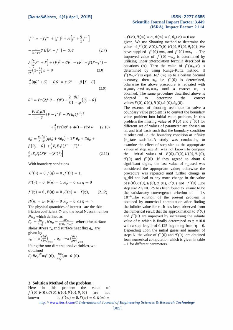
𝑓′′′ = −𝑓𝑓′′ + [𝑓′]2 + 𝐴 [𝑓′ +𝜂

2𝑓′′ ]

−1

(1−𝜑)𝛽 𝐻[𝐹 − 𝑓′ ] − 𝐺𝑟𝜃 (2.7)

𝐴 [𝜂

2𝐹′ + 𝐹] + (𝐹)2 + 𝐺𝐹′ − 𝜖𝐹′′ + 𝛽(𝐹−𝑓′) −

1

𝐹𝑟(1–

1

𝛾) 𝑔 = 0 (2.8)

𝐴

2[𝜂𝐺′ + 𝐺] + 𝐺𝐺′ = 𝜖 𝐺′′ − 𝛽 [𝑓 + 𝐺]

(2.9)

𝜃′′ = 𝑃𝑟(2𝑓′𝜃 − 𝑓𝜃′) −2

3

𝛽𝐻

1 − 𝜑(𝜃𝑝 − 𝜃)

−𝑃𝑟𝐸𝑐𝛽𝐻

1 − 𝜑(𝐹 − 𝑓′)2 − 𝑃𝑟𝐸𝑐(𝑓

′′)2

+𝐴

2𝑃𝑟(𝜂𝜃′ + 4𝜃) − 𝑃𝑟𝛿 𝜃 (2.10)

𝜃𝑝 ′′ =

𝑃𝑟

𝜖[𝐴

2(𝜂𝜃𝑝

′ + 4𝜃𝑝) + 2𝐹 𝜃𝑝 + 𝐺𝜃𝑝′ +

𝛽(𝜃𝑝 − 𝜃) +3

2𝐸𝑐𝑃𝑟𝛽(𝑓′ − 𝐹)2 −

3

2𝜖𝐸𝑐𝑃𝑟(𝐹𝐹′′+(𝐹′)2)] (2.11)

With boundary conditions

𝐺′(𝜂) = 0, 𝑓(𝜂) = 0 , 𝑓′(𝜂) = 1 ,

𝐹′(𝜂) = 0 , 𝜃(𝜂) = 1 , 𝜃𝑝′ = 0 𝑎𝑠 𝜂 → 0

𝑓′(𝜂) = 0 , 𝐹(𝜂) = 0 , 𝐺(𝜂) = −𝑓(𝜂), (2.12)

𝐻(𝜂) = 𝜔 , 𝜃(𝜂) = 0 , 𝜃𝑝 = 0 𝑎𝑠 𝜂 → ∞

The physical quantities of interest are the skin

friction coefficient 𝐶𝑓 and the local Nusselt number

𝑁𝑢𝑥 which defined as

𝐶𝑓 =𝜏𝑤

𝜌𝑈𝑤2 , 𝑁𝑢𝑥 =

𝑥𝑞𝑤

𝑘(𝑇𝑤−𝑇∞)𝚤 where the surface

shear stress 𝜏𝑤and surface heat flux 𝑞𝑤 are given by

𝜏𝑤 = 𝜇 (𝜕𝑢

𝜕𝑦)

𝑦=0 , 𝑞𝑤=−𝑘 (

𝜕𝑇

𝜕𝑦)

𝑦=0

Using the non dimensional variables, we obtained

𝐶𝑓 𝑅𝑒𝑥1/2

=𝑓"(0), 𝑁𝑢𝑥

𝑅𝑒𝑥1/2=−𝜃′(0).

3. Solution Method of the problem:

Here in this problem the value of

𝑓 ′′(0), 𝐹(0), 𝐺(0),𝐻(0), 𝜃′(0), 𝜃𝑝(0) are not

known but𝑓 ′(∞) = 0, 𝐹(∞) = 0, 𝐺(∞) =

−𝑓(∞), 𝐻(∞) = 𝜔, 𝜃(∞) = 0, 𝜃𝑝(∞) = 0 are

given. We use Shooting method to determine the

value of 𝑓 ′′(0), 𝐹(0), 𝐺(0),𝐻(0), 𝜃′(0), 𝜃𝑝(0) .We

have supplied 𝑓 ′′(0) =∝0 and 𝑓 ′′(0) =∝1 . The

improved value of 𝑓 ′′(0) =∝2 is determined by

utilizing linear interpolation formula described in

equations (A). Then the value of 𝑓 ′(∝2, ∞) is

determined by using Runge-Kutta method. If

𝑓 ′(∝2, ∞) is equal to𝑓 ′(∞) up to a certain decimal

accuracy, then ∝2 i.e 𝑓 ′′(0) is determined,

otherwise the above procedure is repeated with

∝0=∝1 𝑎𝑛𝑑 ∝1=∝2 until a correct ∝2 is

obtained. The same procedure described above is

adopted to determine the correct

values 𝐹(0), 𝐺(0),𝐻(0), 𝜃′(0), 𝜃𝑝(0). The essence of shooting technique to solve a

boundary value problem is to convert the boundary

value problem into initial value problem. In this

problem the missing value of 𝜃′(0) and 𝑓 ′′(0) for

different set of values of parameter are chosen on

hit and trial basis such that the boundary condition

at other end i.e. the boundary condition at infinity

(η∞)are satisfied.A study was conducting to

examine the effect of step size as the appropriate

values of step size ∆η was not known to compare

the initial values of 𝐹(0), 𝐺(0),𝐻(0), 𝜃𝑝(0),

𝜃′(0) and 𝑓 ′′(0) .If they agreed to about 6

significant digits, the last value of η∞

used was

considered the appropriate value; otherwise the

procedure was repeated until further change in

η∞

did not lead to any more change in the value

of 𝐹(0), 𝐺(0),𝐻(0), 𝜃𝑝(0), 𝜃′(0) and 𝑓 ′′(0) .The

step size ∆η =0.125 has been found to ensure to be

the satisfactory convergence criterion of 1×10−6.The solution of the present problem is

obtained by numerical computation after finding

the infinite value for . It has been observed from

the numerical result that the approximation to 𝜃′(0) and 𝑓 ′′(0) are improved by increasing the infinite

value of which is finally determined as =10.0

with a step length of 0.125 beginning from = 0.

Depending upon the initial guess and number of

steps N. the value of 𝑓 ′′(0) and 𝜃′(0) are obtained

from numerical computation which is given in table

– 1 for different parameters.






[306]

Graphical Representations

-0.05

0

0.05

0.1

0.15

0.2

0 5 10

F(η

)---

----

--->

Fig-1 η----------->

Variation of Up w.r.t.βEc=1.0,Fr=10,Pr=0.71,A=0.2

δ=0.1,є=3.0,Gr=0.01,γ=1200,φ=0.01

β=0.01

β=0.02

β=0.03

-0.05

0

0.05

0.1

0.15

0.2

0 5 10

F(η

)---

----

----

--->

Fig-2 η------------>

Variation of Up w.r.t.AEc=1.0,Fr=10,Pr=0.71,β=0.01

δ=0.1,є=3.0,Gr=0.01,γ=1200,φ=0.01

A=0.1

A=0.2

A=0.3

-0.20

0.20.40.60.8

11.2

0 5 10

θ(η

)---

----

----

--->

Fig-3 η------------->

Variation of θ w.r.t.EcPr=0.71,Fr=10,Gr=0.01,A=0.2

δ=0.1,є=3.0,β=0.01,γ=1200,φ=0.01

Ec=1.0

Ec=2.0

Ec=3.0

-0.2

0

0.2

0.4

0.6

0.8

1

1.2

0 5 10

θ(η

)---

----

----

--->

Fig-4 η---------->

Variation of θ w.r.t.PrEc=1.0,Fr=10,Gr=0.01,A=0.2

δ=0.1,є=3.0,β=0.01,γ=1200,φ=0.01

Pr=0.1

Pr=0.71

Pr=1.0

-0.2

0

0.2

0.4

0.6

0.8

1

1.2

0 5 10

θ(η

)---

----

----

--->

Fig-5 η------------>

Variation of θ w.r.t.AEc=1.0,Fr=10,Pr=0.71,β=0.01

δ=0.1,є=3.0,Gr=0.01,γ=1200,φ=0.01

A=0.1

A=0.2

A=0.3

-0.2

0

0.2

0.4

0.6

0.8

1

1.2

0 2 4 6

θ(η

)---

----

----

----

-->

Fig-6 η------------->

Variation of θ w.r.t.δEc=1.0,Fr=10,Pr=0.71,β=0.01

A=0.2,є=3.0,Gr=0.01,γ=1200,φ=0.01

δ=-0.5

δ=0.1

δ=0.5






[307]

0

0.01

0.02

0 5 10

θp

(η)-

----

----

----

----

>

Fig-7 η----------->

Variation of θp w.r.t.EcPr=0.71,Fr=10,Gr=0.01,A=0.2

δ=0.1,є=3.0,β=0.01,γ=1200,φ=0.01

Ec=1.0

Ec=2.0

Ec=3.0

-0.005

0

0.005

0.01

0.015

0 5 10

θp

(η)-

----

----

--->

Fig-8 η------------>

Variation of θp w.r.t.PrEc=1.0,Fr=10,Gr=0.01,A=0.2

δ=0.1,є=3.0,β=0.01,γ=1200,φ=0.01

Pr=0.1

Pr=0.71

Pr=1.0

00.0020.0040.0060.008

0 10

θp

(η)-

----

----

----

>

Fig-9 , η---------------->

Variation of θp w.r.t.GrEc=1.0,Fr=10,Pr=0.71,β=0.01

A=0.1,є=3.0,=0.1,γ=1200,φ=0.01

Gr=0.01

Gr=0.03

0

0.005

0.01

0 5 10

θp

(η)-

----

----

----

----

>

Fig-10 η------------->

Variation of θp w.r.t.φEc=1.0,Fr=10,Pr=0.71,A=0.2

δ=0.1,є=3.0,β=0.01,γ=1200,Gr=0.01

φ=0.01

φ=0.02

φ=0.03

0

0.005

0.01

0 5 10θp

(η)-

----

----

->

Fig-11 η----------->

Variation of θp w.r.t.βEc=1.0,Fr=10,Pr=0.71,A=0.2

δ=0.1,є=3.0,Gr=0.01,γ=1200,φ=0.01

β=0.01

β=0.02

β=0.03

00.005

0.010.015

0 10

θp

(η)-

----

>

Fig-12 η-------->

Variation of θp w.r.t.AEc=1.0,Fr=10,Pr=0.71,β=0.01

δ=0.1,є=3.0,Gr=0.01,γ=1200,φ=0.01

A=0.1

A=0.2

A=0.3

0

0.005

0.01

0 10

θp

(η)-

-->

Fig -13 , η------------>

Variation of θp w.r.t.Ec=1.0,Fr=10,Pr=0.71,β=0.01

A=0.1,є=3.0,Gr=0.01,γ=1200,φ=0.01

δ=-0.5

δ=0.5






[308]

TABLE-1:

Showing initial values of wall velocity gradient −𝒇′′(𝟎) and temperature gradient −𝜽′(𝟎)

β

δ

𝑨

𝑷𝒓

𝑬𝒄

𝝋

𝑮𝒓

−𝒇′′(𝟎)

𝒖𝒑(𝟎)

−𝒗𝒑(𝟎)

H(0)

−𝜽′(𝟎)

𝜽𝒑(𝟎)

0.01 0.1 0.2 0.71 0.00 0.00 0.00 1.079240 - - - 1.220351 -

0.01 0.1 0.2 0.71 1.0 0.01 0.01 1.06546 0.155785 0.72388 0.111942 0.91126 0.002570

2.0 1.06387 0.155974 0.72078 0.111477 0.65741 0.003480

3.0 1.06316 0.154302 0.72444 0.113379 0.40258 0.004134

0.1 1.07968 0.147611 0.66129 0.101754 0.60059 0.003714

0.71 1.06546 0.155785 0.72388 0.111942 0.91126 0.002570

1.0 1.06502 0.15601 0.72381 0.112103 1.08932 0.002659

0.01 1.06546 0.155785 0.72388 0.111942 0.91126 0.002570

0.02 1.05924 0.156032 0.72392 0.111544 0.91468 0.003406

0.03 1.05391 0.15605 0.72408 0.112407 0.91917 0.003333

0.01 1.06546 0.155785 0.72388 0.111942 0.91126 0.002570

0.02 1.0654 0.155788 0.72386 0.112043 0.91127 0.003237

0.03 1.06445 0.156009 0.72387 0.112045 0.91249 0.00337

0.2 1.06546 0.155785 0.72388 0.111942 0.91126 0.002570

0.25 1.08142 0.147379 0.66143 0.103394 0.94028 0.005855

0.3 1.09796 0.14156 0.06073 0.091406 0.96766 0.008102

0.01 1.06546 0.155785 0.72388 0.111942 0.91126 0.002570

0.02 1.06479 0.159391 0.72175 0.111343 0.91334 0.005865

0.03 1.06520 0.161470 0.72005 0.110756 0.91210 0.008342

-0.5 1.06509 0.155667 0.72401 0.111083 1.12736 0.002973

0.1 1.06546 0.155785 0.72388 0.111942 0.91126 0.002570

0.5 1.06358 0.154876 0.72408 0.112433 0.72180 0.004256

RESULT AND DISCUSSION The set of non linear ordinary differential

equations (2.6) to (2.11) with boundary condition

(2.12) were solved using well known Runge-Kutta

forth order algorithm with a systematic guessing of

𝐹(0), 𝐺(0),𝐻(0), 𝜃𝑝(0), 𝑓 ′′(0) and 𝜃′(0) by the

shooting technique until the boundary condition at

infinity are satisfied.The step size 0.125 is used

while obtaining the numerical solution accuracy up

to the sixth decimal place i.e. 1× 10−6, which is

very sufficient for convergence. In this method we

choose suitable finite values of 𝜂 → ∞ which

depends on the values of parameter used. The

computations were done by the computer language

FORTRAN-77.The shear stress( Skin friction

coefficient)which is proportional to 𝑓 ′′(0) and rate

of heat transfer(Nusselt Number) which is

proportional to 𝜃′(0) are tabulated in Table-1 for

different values of parameter used .It is observed

from the table that shear stress and rate of heat

transfer decreases on the increase of Ec , whereas it

is increasing for increasing values of Pr. The

Nusselt number decreases on the increasing of

unsteady parameter ‘A’. The temperature of both

phases increase on the increase of δ.

Fig-1 demonstrates the effect of β which infers that

increasing of β increases the particle phase

velocity. Fig-2 shows that velocity profile of

particle phase is decreasing on the increase of

unsteady parameter.Fig-3 witnesses that increasing

values of Ec, the temperature of fluid phase also

increases, it means the frictional heating is

responsible for storing heat energy in the fluid.Fig-

4 depicts the effect of Pr on temperature profile of

fluid phase. From the figure we observe that, when

Pr increase the temperature of fluid phase decreases

which states that the viscous boundary layer

thickness increases and thermal boundary layer

thickness decreases.Fig-5 explains that the

temperature of fluid phase decreases with

increasing unsteady parameter ‘A’. This implies it

may take less time for cooling during the unsteady

flow .Fig-6 explains that the temperature of fluid

phase increases with increasing heat generation

and decrease on the decrease of heat absorption

parameter δ.Fig-7 illustrates the effect of Ec on

temperature profile of particle phase. It is evident

that the increasing of Ec increases the

temperature.Fig-8 explains the effect of Pr on

particle phase temperature, when Pr is increasing

there is significantly increasing the temperature of

particle phase. It means the thermal boundary layer

thickness is decreasing.Fig-9 depicts the effect of






[309]

Gr on particle phase temperature profile which

indicates that the increasing of Gr has significant

effect on particle phase temperature, enhancing Gr,

increases the temperature of particle phase.Fig-10

shows the effect of 𝜑 on temperature of particle

phase. It is evident that increasing in volume

fraction increases the temperature of particle phase

.Fig-11 illustrates the increasing β, increases the

temperature of dust particle.Fig-12 describes that

the temperature profile of particle phase increases

on the increase of unsteady parameter.Fig-13

describes the effect of δ on particle phase

temperature which explains that temperature profile

is same as that of fluid phase.

CONCLUSIONS In this work, it is concluded that, the particle-laden

dusty fluid model may predict the following

significant conclusions:

i. The increasing value of unsteady parameter A

decreases the temperature profiles of fluid

phase and increase the dust phase. Also

increase value of A decreases velocity of

particle phase.

ii. The temperature profile of both phases

increases with the increase of heat source

/sink parameter δ.

iii. Increasing value of Ec is enhancing the

temperature of both fluid phase as well as

particle phase which indicates that the heat

energy is generated in fluid due to frictional

heating.

iv. The thermal boundary layer thickness

decreases on the effect of Pr. The temperature

decreases at a faster rate for higher values of

Pr which implies the rate of cooling is faster

in case of higher prandtl number.

v. The momentum boundary layer thickness

decreases and thermal boundary layer

thickness reduces on the effect of Gr. If Gr =0

the present study will represent the horizontal

stretching sheet.

vi. Increasing β increases the particle phase

velocity and but temperature profile of

particle phase increases.

vii. The effect of φ is negligible on velocity

profile but significant effect on temperature

profile.

viii. The rate of cooling is much faster for higher

values of unsteady parameter but it takes long

times for cooling during the steady flow.

ix. Also the local Nusselt number increases with

increase of unsteady parameter.

x. We have investigated the problem using the

values γ=1200.0 , Fr=10.0 ,є=3.0

Nomenclature: Q heat source/sink

𝐸𝑐 eckert number

𝐹𝑟 froud number

𝐺𝑟 grashof number

𝑃𝑟 prandtl number

𝑇∞ temperature at large distance from the

wall.

𝑇𝑝 temperature of particle phase.

𝑇𝑤 wall temperature

𝑈𝑤(𝑥) stretching sheet velocity

𝑐𝑝 specific heat of fluid

𝑐𝑠 specific heat of particles

𝑘𝑠 thermal conductivity of particle

𝑢𝑝 , 𝑣𝑝 velocity component of the particle

along x-axis and y-axis

A unsteady parameter

c stretching rate

g acceleration due to gravity

k thermal conductivity of fluid

l characteristic length

T temperature of fluid phase.

u,v velocity component of fluid along x-axis

and y-axis

x,y cartesian coordinate

Greek Symbols:

δ heat source/sink parameter

φ volume fraction

β fluid – particle interaction parameter

𝛽∗ volumetric coefficient of thermal

expansion

ρ density of the fluid






[310]

𝜌𝑝 density of the particle phase

𝜌𝑠 material density

η similarity variable

θ fluid phase temperature

𝜃𝑝 dust phase temperature

𝜇 dynamic viscosity of fluid

ν kinematic viscosity of fluid

𝛾 ratio of specific heat

𝜏 relaxation time of particle phase

𝜏𝑇 thermal relaxation time i.e. the time

required by the dust particle to adjust its

temperature relative to the fluid.

𝜏𝑝 velocity relaxation time i.e. the time

required by the dust particle to adjust its

velocity relative to the fluid.

ε diffusion parameter

ω density ratio

REFERENCES [1]. A.Adhikari and D.C.Sanyal[2013], “Heat

transfer on MHD viscous flow over a

stretching sheet with prescribed heat flux”,

Bulletin of International Mathematical

Virtual Institute, ISSN 1840-4367,Vol.3, 35-

47.

[2]. A.M. Subhas and N.Mahesh[2008], “Heat

transfer in MHD visco-elastic fluid flow

over a stretching sheet with variable thermal

conductivity, non-uniform heat source and

radiation” ,Applied Mathematical

odeling,32,1965-83.

[3]. Anoop Kumar, Phool Singh, N S Tomer and

Deepa Sinha[2014], “Study the Impact of

Soret and Sherwood Number on stretching

sheet using Homotopy Analysis Method”,

International Journal of Emerging

Technology and Advanced Engineering

Website: www.ijetae.com (ISSN 2250-2459)

Volume 4, Issue 1.

[4]. B.C[1961] Sakiadis, “Boundary Layer

behavior on continuous solid surface ;

boundary layer equation for two

dimensional and axisymmetric flow”

A.I.Ch.E.J,Vol.7, pp 26-28.

[5]. B.J.Gireesha ,H.J.Lokesh ,G.K.Ramesh and

C.S.Bagewadi[2011], “Boundary Layer flow

and Heat Transfer of a Dusty fluid over a

stretching vertical surface” , Applied

Mathematics,2,475-

481(http://www.SciRP.org/Journal/am)

,Scientific Research.

[6]. B.J.Gireesha, A.J. , S.Manjunatha and

C.S.Bagewadi[2013], “ Mixed convective

flow of a dusty fluid over a vertical

stretching sheet with non uniform heat

source/sink and radiation” ; International

Journal of Numerical Methods for Heat and

Fluid flow,vol.23.No.4, pp.598-612.

[7]. B.J.Gireesha,G.S.Roopa and C.S.Bagewadi

[2013],“Boundary Layer flow of an unsteady

Dusty fluid and Heat Transfer over a

stretching surface with non uniform heat

source/sink ” , Applied Mathematics,3,726-

735. (http://www.SciRP.org/Journal/am)

,Scientific Research.

[8]. C.H.Chen[1998], “Laminar Mixed

convection Adjacent to vertical continuity

stretching sheet, “Heat and Mass

Transfer,vol.33,no.5-6,pp.471-476.

[9]. Grubka L.J. and Bobba K.M[1985], “Heat

Transfer characteristics of a continuous

stretching surface with variable temperature”

, Int.J.Heat and Mass Transfer , vol.107,,

pp.248-250.

[10]. H.Schlichting[1968], “Boundary Layer

Theory” , McGraw-Hill , New York,.

[11]. Hitesh Kumar[2011], “Heat transfer over a

stretching porous sheet subjected to power

law heat flux in presence of heat

source”.Thermal Science Vol.15,suppl.2,

pp.5187-5194. [12]. K. V. Prasad , P. S. Datti and B. T. Raju

[2013], “Momentum and Heat Transfer of a

Non-Newtonian Eyring-Powell Fluid Over a

Non-Isothermal Stretching Sheet”,

International Journal of Mathematical

Archive-4(1), 230-241 sgjrfIMA Available

online through www.ijma.info ISSN 2229 – 5046

[13]. L.J.Crane[1970], “Flow past a stretching

plate” , Zeitschrift fur Angewandte

Mathematik and physic

ZAMP,VOL.2,NO.4, PP.645-647.

[14]. M.S.Uddin, M. Wahiduzzman,

M.A.KSazad and W. AliPk.[2012],


http://www.ijetae.com/

http://www.scirp.org/Journal/am)

http://www.scirp.org/Journal/am)

http://www.ijma.info/





[311]

“MHD Stagnation-Point Flow towards a

Heated Stretching Sheet”, Journal of

Physical Sciences, Vol. 16, 93-105

ISSN:0972-8791,

www.vidyasagar.ac.in/journal

[15]. N. Bachok, A. Ishak, and R.

Nazar[2010], “Flow and heat transfer

over an unsteady stretching sheet in a

micropolar fluid with prescribed surface

heat flux”, International Journal of

Mathematical Models and Methods in

Applied Sciences ,Issue 3, Volume 4.

[16]. Noura S. Al-sudais[2012], “Thermal

Radiation Effects on MHD Fluid Flow

Near Stagnation Point of Linear Stretching

Sheet with Variable Thermal

Conductivity” International Mathematical

Forum, Vol. 7, no. 51,

2525 – 2544

[17]. P.K. Singh, ,J Singh[2012], “MHD flow

with viscous dissipation and chemical

reaction over a stretching porous plate in

porous medium”. Int.J. of Engineering

Research and Applications.Vol.2, No.2,

pp.1556-1564.

[18]. P.T.Manjunath,B.J.Gireesha and

G.K.Ramesh[2014], “MHD flow of fluid-

particle suspension over an impermeable

surface through a porous medium with non

uniform heat source/sink. TEPE, Vol.3,

issue 3 august, pp.258-265.

[19]. R.N.Barik,G.C.Das and P.K.Rath[2012],

“Heat and mass transfer on MHD flow

through porous medium over a stretching

surface with heat source”, Mathematical

Theory and Modeling, ISSN 2224-5804,

2012,Vol.2,No.7,

[20]. Swami Mukhopadhayay[2012], “Heat

transfer analysis of unsteady flow of

Maxwell fluid over stretching sheet in

presence of heat source/sink.

CHIN.PHYS.LETT.Vol.29,No.5054703.

[21]. Tiegang Fang and Abdul Aziz [2010],

“Viscous Flow with Second-Order Slip

Velocity over a Stretching Sheet”, 0932-

0784 / 10 / 1200-1087, Verlag der

Zeitschriftfur Naturforschung, Tubingen

http://znaturforsch.com.

[23].C. Y. Wang [1991], Ann. Rev. Fluid Mech. 23, 159.


http://www.vidyasagar.ac.in/journal

http://znaturforsch.com/

BOUNDARY LAYER FLOW AND HEAT TRANSEFER OF DUSTY FLUID OVER A STRETCHING SHEET WITH HEAT SOURCE/SINK

Documents

Transcript of BOUNDARY LAYER FLOW AND HEAT TRANSEFER OF DUSTY FLUID OVER A STRETCHING SHEET WITH HEAT SOURCE/SINK