Botanical richness and endemicity patterns of Borneo derived fromspecies distribution models

Niels Raes, Marco C. Roos, J. W. Ferry Slik, E. Emiel van Loon and Hans ter Steege

N. Raes (Raes@nhn.leidenuniv.nl) and M. C. Roos, National Herbarium of the Netherlands, Leiden Univ. branch, Einsteinweg 2, NL-2300RA, Leiden, the Netherlands. � J. W. F. Slik, Ecological Evolution Group, Xishuangbanna Tropical Botanical Garden, Yunnan, China. � E. E.van Loon, Inst. for Biodiversity and Ecosystems Dynamics, Univ. van Amsterdam, Nieuwe Achtergracht 166, NL-1018WV Amsterdam, theNetherlands. �H. ter Steege, Inst. of Environmental Biology, Section Plant Ecology and Biodiversity, Utrecht Univ., Sorbonnelaan 14, NL-3584CA, Utrecht, the Netherlands.

This study provides a Borneo-wide, quantitative assessment of botanical richness and endemicity at a high spatialresolution, and based on actual collection data. To overcome the bias in collection effort, and to be able to predict thepresence and absence of species, even for areas where no collections have been made, we constructed species distributionmodels (SDMs) for all species taxonomically revised in Flora Malesiana. Species richness and endemicity maps were basedon 1439 significant SDMs. Mapping of the residuals of the richness-endemicity relationship identified areas with higherlevels of endemicity than can be expected on the basis of species richness, the endemicity hotspots. We were able toidentify one previously unknown region of high diversity, the high mountain peaks of East Kalimantan; and twoadditional endemicity hotspots, the Muller Mountains and the Sangkulirang peninsula. The areas of high diversity andendemicity were characterized by a relatively small range in annual temperature, but with seasonality in temperatureswithin that range. Furthermore, these areas were least affected by El Nino Southern Oscillation drought events. Theendemicity hotspots were found in areas, which were ecologically distinct in altitude, edaphic conditions, annualprecipitation, or a combination of these factors. These results can be used to guide conservation efforts of the highlythreatened forests of Borneo.

Borneo, the third largest island of the world, is thebotanically most diverse part of the Sundaland hotspot,one of the world’s 25 biodiversity hotspots (Myers et al.2000). Southeast Asia as a whole faces an estimated loss ofthree quarters of its original forest area by 2100, and up to42% of its biodiversity (Sodhi et al. 2004). For Borneo,currently only 57% of its land surface remains forested, andannual deforestation averages 1.7% (FAO 2006, Langneret al. 2007). Even more worrying is the fact that 56% ofKalimantan’s (Indonesian Borneo) protected lowland for-ests has been lost between 1985 and 2001 (Curran et al.2004, Stibig et al. 2007). Ca 37% of Borneo’s 15 000vascular plant species (Roos et al. 2004) are thought to beendemic (van Welzen et al. 2005), with an estimatednumber of 10 000 species occurring in the WWF Borneolowland rain forests ecoregion alone (Wikramanayake et al.2002, Kier et al. 2005).

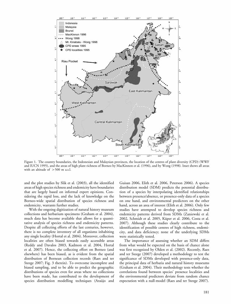
Considering the exceptional richness and concentrationof endemic, or narrow ranged, species on Borneo, surpris-ingly little is known about the spatial distribution of bothcomponents. Only in 1995 the WWF and IUCN (1995)introduced the ‘‘Centres of plant diversity’’ (CPD) forAustralasia. In this contribution they argued that on Borneo

most endemic plant species can be found in smaller areas inthe north, the central mountain chain, and in the south-eastern Meratus Mountains (Fig. 1). A view largelysupported by MacKinnon et al. (1996). Wong (1998)added to this list the ‘‘Riau Pocket’’, which consists of twoareas. One of these is similar to the north-western Sarawakbiogeographical unit of MacKinnon et al. (1996), the otheris the most western tip of Borneo (Fig. 1). Wong (1998)further suggests that Mount Kinabalu is a hotspot of plantdiversity (Fig. 1), which is confirmed by its ca 5000documented vascular plant species (Beaman 2005, Grytnesand Beaman 2006). Furthermore, Wong (1998) reports acomparatively lower diversity in the remaining area ofBorneo, mainly consisting of the Kalimantan provinces.

These findings are partly confirmed by the only quanti-tative Borneo-wide study of lowland dipterocarp forest (Sliket al. 2003). Based on data of 28 plots, at genus level, and fortrees with a diameter of ]10 cm, Slik et al.’s (2003) resultsonly confirmed the biodiversity hotspots of the south-easternMeratus Mountains and the north-western Sarawak biogeo-graphical units. Their analysis did not support the compara-tively lower diversity in the Kalimantan provinces of Wong(1998), however. Except for the flora of Mount Kinabalu,

Ecography 32: 180�192, 2009

doi: 10.1111/j.1600-0587.2009.05800.x

# 2009 The Authors. Journal compilation # 2009 Ecography

Subject Editor: Jens-Christian Svenning. Accepted 13 January 2009

180

and the plot studies by Slik et al. (2003), all the identifiedareas of high species richness and endemicity have boundariesthat are largely based on informal expert opinions. Con-sidering the rapid loss, and the lack of knowledge on theBorneo-wide spatial distribution of species richness andendemicity, warrants further studies.

With the ongoing digitization of natural history museumcollections and herbarium specimens (Graham et al. 2004),much data has become available that allows for a quanti-tative analysis of species richness and endemicity patterns.Despite all collecting efforts of the last centuries, however,there is no complete inventory of all organisms inhabitingany single locality (Hortal et al. 2004). Moreover, collectionlocalities are often biased towards easily accessible areas(Reddy and Davalos 2003, Kadmon et al. 2004, Hortalet al. 2007). Hence, the collecting effort on Borneo (andelsewhere) has been biased, as is evident from the spatialdistribution of Bornean collection records (Raes and terSteege 2007; Fig. 3 therein). To overcome incomplete andbiased sampling, and to be able to predict the geographicdistributions of species even for areas where no collectionshave been made, has contributed to the development ofspecies distribution modelling techniques (Araujo and

Guisan 2006, Elith et al. 2006, Peterson 2006). A speciesdistribution model (SDM) predicts the potential distribu-tion of a species by interpolating identified relationshipsbetween presence/absence, or presence-only data of a specieson one hand, and environmental predictors on the otherhand, across an area of interest (Elith et al. 2006). Only fewstudies have attempted to develop species richness andendemicity patterns derived from SDMs (Zaniewski et al.2002, Schmidt et al. 2005, Kuper et al. 2006, Costa et al.2007). Although these studies clearly contribute to theidentification of possible centres of high richness, endemi-city, and data deficiency; none of the underlying SDMswere statistically tested.

The importance of assessing whether an SDM differsfrom what would be expected on the basis of chance alonewas first recognized by Olden et al. (2002). Recently, Raesand ter Steege (2007) developed a methodology to test thesignificance of SDMs developed with presence-only data,the principal data of herbaria and natural history museums(Graham et al. 2004). Their methodology tests whether thecorrelations found between species’ presence localities andthe environmental predictors deviate from random chanceexpectation with a null-model (Raes and ter Steege 2007).

Figure 1. The country boundaries, the Indonesian and Malaysian provinces, the location of the centres of plant diversity (CPD) (WWFand IUCN 1995), and the areas of high plant richness of Borneo by MacKinnon et al. (1996), and by Wong (1998). Inset shows all areaswith an altitude of �500 m a.s.l.

181

To contribute to the conservation of botanical diversityof Borneo, we set out to model the patterns of botanicalrichness and endemicity, based on all significant SDMs at 5arc-minute (�10�10 km at the equator) spatial resolutionfor all species treated in Flora Malesiana (Anon. 1959�2007) occurring on Borneo. Then, based on these patterns,we identify areas with higher levels of endemicity than canbe expected on the basis of species richness. Finally, weanalyse which environmental factors best explain thebotanical richness and endemicity patterns.

Methods

Species data

We extracted all georeferenced species records from Borneobelonging to families treated in Flora Malesiana (Anon.1959�2007) from the BRAHMS database of the NationalHerbarium of the Netherlands. To this dataset we addedthe georeferenced records of revised genera of the Annona-ceae, Euphorbiaceae, and Orchidaceae. In total this datasetcomprised 66 262 georeferenced records belonging to 108plant families representing 4674 species. From this set ofgeoreferenced records, we recorded species presences foreach 5 arc-minute grid cell, avoiding duplicate speciesrecords in one grid cell. We used a 5 arc-minute spatialresolution because this is the available resolution of theFAO soil property predictors (see below), and becausegeoreferencing at a higher spatial resolution is not realistic.Furthermore, a species had to be represented in at least fivegrid cells to be modelled. These requirements were met for2273 species represented by 44 106 unique records, rangingfrom 5 to 202 unique records per species.

Environmental predictors

To model the species distributions, we initially selected 37environmental predictors. We downloaded the altitude (inm) and the 19 bioclimatic predictors (1950�2000) of theWORLDCLIM dataset (/<www.worldclim.org/>) for Bor-neo at 5 arc-minute resolution (Hijmans et al. 2005).

Additionally, we selected 15 soil predictors from the FAOdatabase for poverty and insecurity mapping (FAO 2002),shown in Table 1. To this dataset we added a layer with theelevation range, defined as the difference between the lowestand highest altitude within a 5 arc-minute grid cell based onthe 90m SRTM altitude data (/<srtm.csi.cgiar.org/>).Finally, a data-layer, reflecting the El Nino SouthernOscillation (ENSO) event drought impact, was added.ENSO drought impact was defined as the relative averageannual difference in ‘‘normalized difference vegetationindex’’ (NDVI) values (/<ftp://ftp.glcf.umiacs.umd.edu/glcf/GIMMS/Geographic//>) between months of a severeENSO (07/1982�06/1983), and a non-ENSO year (07/1981�06/1982). These NDVI data were the oldest dataavailable, and are therefore least affected by deforestationand land use change. We retained only grid cells with datafor all data-layers, resulting in 8577 grid cells for Borneo.Records on the coast-line, falling just outside the grid cellsdue to the 5 arc-minute resolution, were shifted to theirclosest grid cell. Data-layer manipulations were performedwith Manifold GIS (Manifold Net).

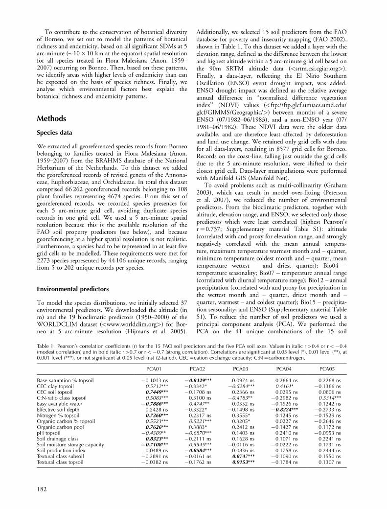
To avoid problems such as multi-collinearity (Graham2003), which can result in model over-fitting (Petersonet al. 2007), we reduced the number of environmentalpredictors. From the bioclimatic predictors, together withaltitude, elevation range, and ENSO, we selected only thosepredictors which were least correlated (highest Pearson’sr�0.737; Supplementary material Table S1): altitude(correlated with and proxy for elevation range, and stronglynegatively correlated with the mean annual tempera-ture, maximum temperature warmest month and � quarter,minimum temperature coldest month and � quarter, meantemperature wettest � and driest quarter); Bio04 �temperature seasonality; Bio07 � temperature annual range(correlated with diurnal temperature range); Bio12 � annualprecipitation (correlated with and proxy for precipitation inthe wettest month and � quarter, driest month and �quarter, warmest � and coldest quarter); Bio15 � precipita-tion seasonality; and ENSO (Supplementary material TableS1). To reduce the number of soil predictors we used aprincipal component analysis (PCA). We performed thePCA on the 41 unique combinations of the 15 soil

Table 1. Pearson’s correlation coefficients (r) for the 15 FAO soil predictors and the five PCA soil axes. Values in italic r�0.4 or rB�0.4(modest correlation) and in bold italic r�0.7 or rB�0.7 (strong correlation). Correlations are significant at 0.05 level (*), 0.01 level (**), at0.001 level (***), or not significant at 0.05 level (ns) (2-tailed). CEC�cation exchange capacity; C:N�carbon:nitrogen.

PCA01 PCA02 PCA03 PCA04 PCA05

Base saturation % topsoil �0.1013 ns �0.8429*** 0.0974 ns 0.2864 ns 0.2268 nsCEC clay topsoil 0.5712*** �0.3342* �0.5284*** 0.4161* �0.1366 nsCEC soil topsoil 0.7449*** �0.1708 ns 0.2366 ns 0.0295 ns 0.0806 nsC:N-ratio class topsoil 0.5083*** 0.3100 ns �0.4183** �0.2982 ns 0.5314***Easy available water �0.7886*** 0.4747** 0.0332 ns �0.1926 ns 0.1242 nsEffective soil depth 0.2428 ns �0.3322* �0.1498 ns �0.8224*** �0.2733 nsNitrogen % topsoil 0.7360*** 0.2317 ns 0.3555* 0.1245 ns �0.1529 nsOrganic carbon % topsoil 0.5523*** 0.5221*** 0.3205* 0.0227 ns �0.2646 nsOrganic carbon pool 0.7626*** 0.3883* 0.2412 ns �0.1427 ns 0.1172 nspH topsoil �0.4389** �0.6870*** 0.1403 ns 0.2410 ns �0.0953 nsSoil drainage class 0.8323*** �0.2111 ns 0.1628 ns 0.1071 ns 0.2241 nsSoil moisture storage capacity �0.7108*** 0.5545*** �0.0116 ns �0.0222 ns 0.1731 nsSoil production index �0.0489 ns �0.8584*** 0.0836 ns �0.1758 ns �0.2444 nsTextural class subsoil �0.2891 ns �0.0161 ns 0.8747*** �0.1090 ns 0.1550 nsTextural class topsoil �0.0382 ns �0.1762 ns 0.9153*** �0.1784 ns 0.1307 ns

182

predictors values observed for the 8577 grid cells of Borneo.We selected the first five PCA-axes as our soil propertypredictors (PCA01-05), which together explained 83% ofthe variance in the soil data. Pearson’s correlation was usedto determine which of the original 15 FAO soil predictorswere significantly correlated to each of the five PCA axes(Table 1). This resulted in a reduction from 37 to 11uncorrelated predictors, which were used to model thespecies distributions (Supplementary material Table S1,Fig. S1).

Species distribution model (SDM) building andtesting with a bias corrected null-model

To model the species distributions we selected the model-ling application Maxent (ver. 3.0.4; /<www.cs.princeton.edu/�shapire/maxent//>) (Phillips et al. 2006). Maxentwas specifically developed to model species distributionswith presence-only data, has shown to outperform mostother modelling applications (Elith et al. 2006, Pearson etal. 2007), is least affected by location errors in occurrences(Graham et al. 2008), and best performs when few presencerecords are available (Wisz et al. 2008). Maxent was set touse all species presence records for model building(explained below), by setting the ‘‘random test percentage’’to zero. The modelling rules were set to use linear features,whenB10 records were available, adding quadratic featuresfor SDMs developed with 10�14 records, and includinghinge features for species with 15, or more, records (Raesand ter Steege 2007). For each of the 2273 species an SDMwas developed based on its unique presence records and the11 environmental predictors.

As measure of SDM accuracy we used the thresholdindependent and prevalence insensitive area under the curve(AUC) of the receiver operating characteristic (ROC) plot(Fielding and Bell 1997, McPherson et al. 2004, Raes andter Steege 2007), produced by Maxent. All measures ofSDM accuracy require absences (Fielding and Bell 1997).When these are lacking, as is the case here, they are replacedby pseudo-absences or sites randomly selected at localitieswhere no species presence was recorded (Ferrier et al. 2002,Phillips et al. 2006). However, when SDM accuracymeasures are based on presence-only data and pseudo-absences, the standard measures of accuracy (e.g. the oftenused measure AUC�0.7) do not apply (Raes and ter Steege2007). Therefore, we used the method presented in Raesand ter Steege (2007) to test the AUC value of an SDMdeveloped with all presence records against a bias correctednull-model of AUC values expected by chance. The AUCvalue of an SDM developed with n records is tested againstthe upper 95% one-sided confidence interval (CI) AUCvalue derived from the AUC values of 1000�n randomlydrawn and modelled points. The random points weredrawn from cells where in the past collections were made,and hence were corrected for any geographical samplingbias. For Borneo this was the case for 1837 (21.4%) of thetotal of 8577 grid cells (Raes and ter Steege 2007).

We developed null-distributions for 5�35 records (31distributions), for 40�50 records with intervals of 5 records(3 distributions), for 60�100 records with intervals of 10records (5 distributions), and from 150 to 250 with

intervals of 50 records (3 distributions). For each of thesedistributions we assessed the upper 95% one-sided CI AUCvalue, by ranking the 1000 AUC values and selecting the950th value. We developed three series of CI valuesdependent on the modelling rules used by Maxent; 5�9(only linear), 10�14 (linear and quadratic), and ]15(linear, quadratic and hinge) records. We applied a curve-fitto each of the three series against which the AUC values forall 2273 SDMs were tested. For further analyses only thesignificant SDMs were retained. To assess whether speciesrepresented by few records were not proportionally moreoften rejected than species with many records, we plottedthe relative species abundance values against the relativespecies ranks. Similar shaped curves indicate that the sampleis representative.

Additionally, we tested whether the 1837 collectionlocalities were biased in environmental predictor space. Foreach of the 11 predictors we divided predictor space into 10equal-interval bins based on the ranges observed for Borneo(8577 grid cells) (Loiselle et al. 2008). Then we testedwhether the frequency distributions represented by the1837 collection localities differed from all 8577 grid cellsusing a Chi-square test.

Botanical richness and endemicity patterns

In order to develop patterns of botanical richness andendemicity, a threshold was set to convert the continuousMaxent SDM predictions, which range from 0 to 100, todiscrete presence/absence values. Although species identifi-cations, and georeferencing of the collection localities, werecarried out with the greatest possible accuracy, we found itreasonable to assume that 10% of the records were eitherwrongly identified, or georeferenced. Therefore, for allSDMs represented by ] 10 records we used the fixed ‘‘10percentile presence’’ threshold. This threshold uses theMaxent value of the 10 percentile species presence record todefine all areas with a lower predicted Maxent value asabsent, and with a higher value as present. For those speciesrepresented by 5�9 records we used either the ‘‘sensitivity-specificity equality’’ or the ‘‘sum maximization’’ threshold(Liu et al. 2005), dependent on which of the twocorresponding omission rate values was closest to 10%.

Once the thresholds were set, the botanical richnesspattern was developed by superimposing all significantSDMs. To develop the endemicity pattern we used theweighted endemism index (Crisp et al. 2001, Kier andBarthlott 2001, Kuper et al. 2006, Slatyer et al. 2007). Thisindex weighs species richness according to the range sizes ofthe species present, and is calculated by summing theinverse of the range sizes of the species present in each gridcell. A species with a range of 10 grid cells has a weight of1/10 in every grid cell where it is present. We developed theendemicity pattern by summing the weights of all sig-nificant SDMs for all grid cells.

Data analyses

We first assessed whether the modelled species richness didnot under-predict the actual number of species collected incorresponding cells. This was done by plotting the

183

predicted number of species against the collected number ofspecies for all 8577 grid cells. To plot the data at log-logscale, ‘‘the collected number of species’’ was transformed tothe logarithm of ‘‘the collected number of species�1’’.

The hotspots of endemic species were identified bymapping the relative residuals of the species richness �weighted endemism relationship. The relationship wasassessed with a curve-fit procedure, evaluating severalpolynomial functions. The residuals of this relation weredivided by their predicted weighted endemism values,resulting in a measure of relative residual weightedendemism.

To study which environmental predictors best explainedspecies richness, weighted endemism, and their relativeresiduals we used a technique known as variation partition-ing (Legendre 2008). Variation partitioning is a techniquethat partitions the variation of a response variable betweentwo sets of explanatory variables, here a set of environ-mental predictors and a set of spatial predictors. As spatialpredictors we used the nine terms of the third orderpolynomial trend-surface regression equation of latitudeand longitude (Borcard et al. 1992, Lobo and Martin-Piera2002, Legendre 2008). To account for possible non-lineareffects between the diversity patterns and the original set of11 environmental predictors, we added the quadratic termsof those predictors uncorrelated with the original predictors(rB0.7). This was the case for PCA02, PCA04 and PCA05(Supplementary material Table S1). The variation waspartitioned by performing a forward-backward stepwisemultiple regression analysis for the three diversity measuresand 1) the environmental predictors, 2) the spatialpredictors, and 3) a combined matrix of both predictorsets. This allowed us to assess which proportion of thevariation was attributed to only environmental predictors(a), to spatially structured environmental predictors (b), tospatial predictors (c), and to unexplained (residual) varia-tion (d) (see Legendre 2008 for methodological details).

Multiple regression analyses applied to macroecologicaldata which are driven by structured biological processes,may result in residual spatial autocorrelation (RSA). Thepresence of RSA is a violation of the assumption thatresiduals should be independent and identically distributed,and results in inflated type I errors (Dormann et al. 2007).It was recently shown, however, that short-distance RSA,while causing inflated type I errors, does not seriously affectthe interpretation of the regression coefficients estimated byordinary least squares regressions (Diniz-Filho et al. 2007,Hawkins et al. 2007). To establish whether RSAwas present in our regression residuals we assessed theMoran’s I values with SAM � spatial analysis in macro-ecology /<www.ecoevol.ufg.br/sam/> (Rangel et al. 2006).Since only a small proportion of the variation was explainedby the spatial predictors alone (Results), we estimated theregression coefficients for the three biodiversity measuresbased on the significant environmental predictors only.Model performances were tested with a 10-fold cross-validation procedure; using 90% to train the model withthe significant environmental predictors selected by the full-model, and test the model with the remaining 10%,repeated 10 times. All regression analyses were performedusing SPSS ver. 15.

It can be argued that this approach has a certain degreeof circularity in reasoning, since the same predictors wereused to develop the underlying SDMs. We argue,however, that Maxent identifies correlations with theenvironmental predictors independently for each species.Even if for two species the same predictors are selected asbeing the most important to predict their distributions,these two species can have another optimum in theirresponse. So we posit that the significant SDMs under-lying the superimposed species richness, weighted ende-mism, and relative residual weighted endemism patternsare essentially independent.

Results

From the 2273 species which were modelled, 1439 (63.3%)had a distribution pattern that differed significantly from arandom one. The frequency distributions of the environ-mental conditions represented by the collection localitiesdid not significantly differ from the distributions for all8577 grid cells of Borneo (Supplementary material Fig. S2).The relative species rank abundance curves (Supplementarymaterial Fig. S3) for the records of all 2273 species, and forthe records of the 1439 significant species, were largelysimilar in shape. This indicated that in terms of thefrequency distributions of records, the 1439 speciesrepresented by a significant SDM are a representativesample of the total of 2273 modelled species.

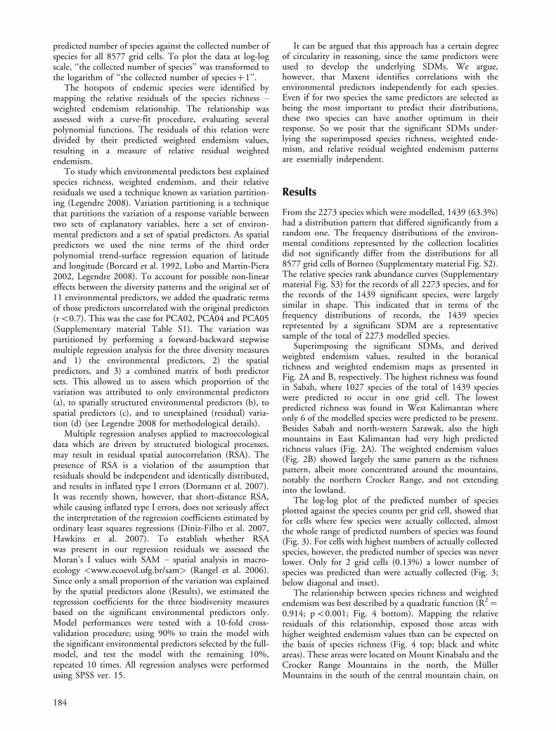
Superimposing the significant SDMs, and derivedweighted endemism values, resulted in the botanicalrichness and weighted endemism maps as presented inFig. 2A and B, respectively. The highest richness was foundin Sabah, where 1027 species of the total of 1439 specieswere predicted to occur in one grid cell. The lowestpredicted richness was found in West Kalimantan whereonly 6 of the modelled species were predicted to be present.Besides Sabah and north-western Sarawak, also the highmountains in East Kalimantan had very high predictedrichness values (Fig. 2A). The weighted endemism values(Fig. 2B) showed largely the same pattern as the richnesspattern, albeit more concentrated around the mountains,notably the northern Crocker Range, and not extendinginto the lowland.

The log-log plot of the predicted number of speciesplotted against the species counts per grid cell, showed thatfor cells where few species were actually collected, almostthe whole range of predicted numbers of species was found(Fig. 3). For cells with highest numbers of actually collectedspecies, however, the predicted number of species was neverlower. Only for 2 grid cells (0.13%) a lower number ofspecies was predicted than were actually collected (Fig. 3;below diagonal and inset).

The relationship between species richness and weightedendemism was best described by a quadratic function (R2�0.914; pB0.001; Fig. 4 bottom). Mapping the relativeresiduals of this relationship, exposed those areas withhigher weighted endemism values than can be expected onthe basis of species richness (Fig. 4 top; black and whiteareas). These areas were located on Mount Kinabalu and theCrocker Range Mountains in the north, the MullerMountains in the south of the central mountain chain, on

184

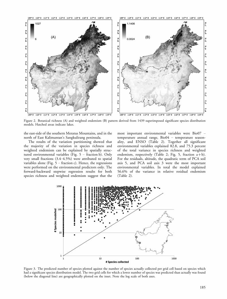
the east-side of the southern Meratus Mountains, and in thenorth of East Kalimantan’s Sangkulirang peninsula.

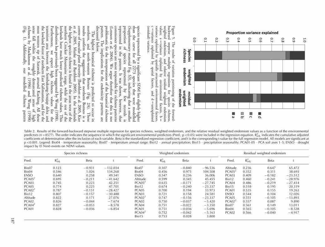
The results of the variation partitioning showed thatthe majority of the variation in species richness andweighted endemism can be explained by spatially struc-tured environmental variables (Fig. 5 � fraction b). Onlyvery small fractions (3.4�4.5%) were attributed to spatialvariables alone (Fig. 5 � fraction c). Hence, the regressionswere performed on the environmental predictors only. Theforward-backward stepwise regression results for bothspecies richness and weighted endemism suggest that the

most important environmental variables were Bio07 �temperature annual range, Bio04 � temperature season-ality, and ENSO (Table 2). Together all significantenvironmental variables explained 82.8, and 75.3 percentof the total variance in species richness and weightedendemism, respectively (Table 2; Fig. 5, fraction a�b).For the residuals, altitude, the quadratic term of PCA soilaxis 5, and PCA soil axis 3 were the most importantenvironmental variables. In total the model explained56.6% of the variance in relative residual endemism(Table 2).

Figure 3. The predicted number of species plotted against the number of species actually collected per grid cell based on species whichhad a significant species distribution model. The two grid cells for which a lower number of species was predicted than actually was found(below the diagonal line) are geographically plotted on the inset. Note the log scale of both axes.

Figure 2. Botanical richness (A) and weighted endemism (B) pattern derived from 1439 superimposed significant species distributionmodels. Hatched areas indicate lakes.

185

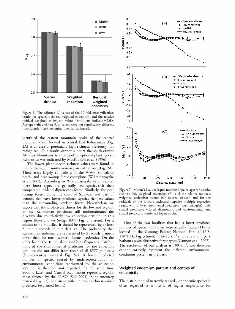
The 10-fold cross-validation results of the modelsobtained through stepwise regression showed that theaverage R2

adj. values of the test-data partitions were notsignificantly different from the average training-datapartition values (Fig. 6), implying that the models werenot over-parameterized. The Moran’s I values of theregression residuals of species richness and weightedendemism indicated that some RSA was still present forthe first three lags (Fig. 7).

Discussion

Botanical richness pattern

The richness pattern is based on 1439 significant SDMs, ca10% of the estimated number of 15 000 species expected tooccur on Borneo. This is the largest dataset available todayand represents all life-form represented by 102 plantfamilies. The relative species rank abundance curve of the

Figure 4. The relationship between bo-tanical richness and weighted endemism.Light grey dots represent grid cells withnegative relative residual weighted ende-mism values; dark grey dots positiverelative residual endemism values be-tween 0 and 50%, white dots between50 and 100%, and black dots �100%.Residual classes are mapped in the topimage.

186

species

represen

tedb

ya

significan

tSD

Mlies

slightly

high

erth

anth

ecu

rvefor

all2

27

3sp

eciesth

atw

erem

odelled

(Sup

plem

entary

material

Fig.

S3),

ind

icating

that

asm

allerp

roportio

nof

species

represen

tedb

yfew

record

sis

represen

tedin

the

pattern

.It

was

show

n,

how

ever,th

atcom

mon

ersp

eciesare

most

respon

sible

forrich

ness

pattern

s(L

enn

onet

al.2

00

4).

We

argue

therefore

that

this

isn

otp

roblem

aticfo

rth

ein

terpretation

ofth

eb

otanical

richn

essp

attern.

Th

eim

plication

sfor

the

end

emicity

pattern

sare

discu

ssedb

elow.

Th

eh

ighest

botan

icalrich

ness

isp

redicted

tooccu

rin

north

ern,

and

north

-western

Born

eo(F

ig.2

A).

Th

eseresu

ltsco

nfirm

the

suggestion

that

north

ernB

orneo

isa

centre

ofvascu

larp

lant

diversity

(Barth

lottet

al.2

00

5,

Kier

etal.

20

05

,M

utke

and

Barth

lott

20

05

).In

the

lowlan

ds

the

high

estsp

eciesrich

ness

isfou

nd

inth

eareas

west

ofth

en

orth

ernC

rockerM

oun

tains

range,

wh

ileth

erest

ofth

elow

land

sh

avem

uch

lower

pred

ictedrich

ness

values.

Th

isd

istribu

tionh

asp

reviously

been

suggested

by

Won

g(1

99

8).

Fu

rtherm

ore,w

eexp

ecth

ighrich

ness

values

forth

etran

sition

areab

etween

the

Semb

akun

g-Sesajapd

eltaan

dth

elo

wlan

dfo

restof

north

ernE

astK

aliman

tan,

and

forth

em

ostw

esterntip

ofSaraw

ak,arou

nd

Ku

chin

g.A

llth

eseareas

fallw

ithin

the

rough

lyd

emarcated

areasof

high

richn

essb

yM

ackinn

onet

al.(1

99

6)

and

Won

g(1

99

8)

(Fig.

1).

Ad

dition

ally,ou

rm

odelled

richn

essp

attern

Figu

re5

.T

he

results

ofvariation

partition

ing

ofth

eforw

ard-

backw

ardstep

wise

mu

ltiple

regressions

forsp

eciesrich

ness,

weigh

teden

dem

ism,

and

relativeresid

ual

weigh

teden

dem

ismvalu

es;a�

variance

explain

edb

yen

vironm

ental

factors,b�

variance

explain

edb

ysp

atiallystru

ctured

environ

men

talfactors,

c�varian

ceexp

lained

by

spatial

factors,an

dd�

un

explain

ed(resid

ual)

variance.

Table 2. Results of the forward-backward stepwise multiple regression for species richness, weighted endemism, and the relative residual weighted endemism values as a function of the environmentalpredictors (n�8577). The order indicates the sequence in which the significant environmental predictors (Pred.; pB0.05) were included in the regression equation. R2

adj. indicates the cumulative adjustedcoefficients of determination after the inclusion of each variable. Beta is the standardized regression coefficient, and t is the corresponding t-value for the full regression model. All models are significant atpB0.001. Legend: Bio04 � temperature seasonality; Bio07 � temperature annual range; Bio12 � annual precipitation; Bio15 � precipitation seasonality; PCA01-05 � PCA soil axes 1�5; ENSO � droughtimpact by El Nino events on NDVI values.

Species richness Weighted endemism Residual weighted endemism

Pred. R2adj. Beta t Pred. R2

adj. Beta t Pred. R2adj. Beta t

Bio07 0.123 �0.931 �132.034 Bio07 0.107 �0.840 �96.536 Altitude 0.236 0.647 65.472Bio04 0.546 1.026 134.268 Bio04 0.456 0.975 104.508 PCA052 0.352 0.311 38.693ENSO 0.640 0.258 49.341 ENSO 0.547 0.236 36.006 PCA03 0.409 �0.182 �23.512PCA052 0.695 �0.211 �41.642 Altitude 0.599 0.345 45.455 Bio12 0.460 �0.241 �28.976PCA03 0.745 0.223 42.251 PCA052 0.635 �0.171 �27.745 PCA04 0.486 �0.219 �27.414PCA05 0.774 0.225 47.701 Bio12 0.674 �0.240 �23.337 Bio15 0.518 0.195 20.319PCA022 0.787 �0.151 �28.427 PCA05 0.700 0.194 33.973 PCA01 0.535 0.155 19.263Bio12 0.807 �0.157 �30.488 PCA03 0.721 0.158 24.581 ENSO 0.544 0.104 12.026Altitude 0.822 0.171 27.076 PCA022 0.747 �0.156 �23.337 PCA05 0.551 �0.105 �13.893PCA02 0.826 �0.044 �7.674 PCA02 0.750 �0.037 �5.420 PCA022 0.557 0.087 9.890PCA042 0.827 �0.053 �8.578 PCA04 0.751 �0.022 �3.350 Bio07 0.561 0.149 13.011PCA01 0.828 �0.036 �6.854 PCA01 0.751 �0.036 �5.696 Bio04 0.565 �0.105 �8.528

PCA042 0.752 �0.042 �5.163 PCA02 0.566 �0.040 �4.917Bio15 0.753 0.028 3.8001

87

identified the eastern mountain peaks of the centralmountain chain located in central East Kalimantan (Fig.2A) as an area of potentially high richness, previously notrecognized. Our results cannot support the south-easternMeratus Mountains as an area of exceptional plant speciesrichness as was indicated by MacKinnon et al. (1996).

The lowest plant species richness values were found inthe southern, and south-western parts of Borneo (Fig. 2A).These areas largely coincide with the WWF Sundalandheath- and peat swamp forest ecoregions (Wikramanayakeet al. 2002). According to Wikramanayake et al. (2002)these forest types are generally less species-rich thancomparable lowland dipterocarp forest. Similarly, the peatswamp forests along the coast of Sarawak, and part ofBrunei, also have lower predicted species richness valuesthan the surrounding lowland forest. Nevertheless, weexpect that the predicted richness for the lowland regionsof the Kalimantan provinces still underestimates thediversity due to relatively low collection densities in thisregion (Raes and ter Steege 2007; Fig. 3 therein). For aspecies to be modelled it should be represented by at least5 unique records in our data set. The probability thatKalimantan endemics are represented by 5 records is muchlower than for north-western Borneo endemics. On theother hand, the 10 equal-interval bins frequency distribu-tions of the environmental predictors for the collectionlocalities did not differ from those of all 8577 grid cells(Supplementary material Fig. S2). A lower predictednumber of species caused by underrepresentation ofenvironmental conditions represented by the collectionlocalities is therefore not expected. At the same timeSouth-, East-, and Central Kalimantan represent regionsmost affected by the ENSO (Slik 2004) (Supplementarymaterial Fig. S1), consistent with the lower richness valuespredicted (explained below).

One of the two localities that had a lower predictednumber of species (95) than were actually found (117) islocated in the Gunung Palung National Park (1815?S,110810?E; Fig. 3 (inset)). The 15 km2 study site in this parkharbours seven distinctive forest types (Cannon et al. 2007).The resolution of our analysis is 100 km2, and thereforecannot correctly represent the different environmentalconditions present in the park.

Weighted endemism pattern and centres ofendemicity

The distribution of narrowly ranged-, or endemic species isoften regarded as a metric of higher importance for

Figure 6. The adjusted R2 values of the 10-fold cross-validationresults for species richness, weighted endemism, and the relativeresidual weighted endemism values. Error-bars indicate92SD.Average train and test R2

adj. values were not significantly different(two-sample t-tests assuming unequal variances).

Figure 7. Moran’s I values (equal number of pairs lags) for: speciesrichness (A), weighted endemism (B), and the relative residualsweighted endemism values (C) (closed circles); and for theresiduals of the forward-backward stepwise multiple regressionresults with only environmental predictors (open triangles), onlyspatial predictors (closed diamonds), and environmental andspatial predictors combined (open circles).

188

conservation planning than species richness (Reid 1998,Myers et al. 2000). The fact that a larger proportion ofspecies represented by few collections is not represented bythe significant SDMs (Supplementary material Fig. S3),implicates that endemicity values are expected to be evenhigher than presented in this study. The northern CrockerMountains range with Mount Kinabalu, and the highmountains of central East Kalimantan have the highestweighted endemism values (Fig. 2B). The latter havereceived little collecting effort so far, and deserve furtherattention since they potentially harbour many new species.

Similar to our data (Fig. 4), a curvilinear relationshipbetween richness and endemicity was also found for thebirds of Africa (Jetz et al. 2004), indicating that moreendemic species can be expected in species rich assemblages(Witt and Maliakal-Witt 2007). Spatial mapping of therelative residuals of this relationship revealed the centres ofendemicity on Borneo (Fig. 4): the Crocker Mountainsrange with Mount Kinabalu; the northern parts of thecentral mountain range; the high mountain peaks in eastSabah; the southern extrusions of the central mountainrange (Muller Mountains); the lowland east of the southernMeratus Mountains; and the eastern Sangkulirang penin-sula of East Kalimantan. It is notable that our results addthe Muller Mountains and the Sangkulirang peninsula tothe previously known list of biologically important sites onBorneo (Fig. 1).

Besides the entire central mountain range having positiveresidual weighted endemism values, this is also the case forsouth-west Sarawak, the southern, and south-western areasof Borneo, and around the great lakes in southern EastKalimantan. Although the absolute richness and weightedendemism values for these areas are low, they apparentlyharbour species which are very characteristic for those areas,and are not found elsewhere (Fig. 4). These areas largelycoincide with the WWF peat swamp-, freshwater swamp-,and heath forest ecoregions of Borneo (Wikramanayakeet al. 2002).

Botanical richness, weighted endemism, and centresof endemicity explained

The results of the variation partitioning showed that for allthree diversity measures only a very small proportion of thevariance is explained by spatial predictors only, and that forspecies richness and weighted endemism the majority isexplained by spatially structured environmental variables(Fig. 5). Although the Moran’s I values of the residualsfrom the partial regressions with only environmentalvariables were slightly higher than for the models includingonly spatial-, or spatial and environmental variablescombined (Fig. 7), they do fall well within the rangesreported by Hawkins et al. (2007). They concluded that forthese ranges of RSA regression coefficients were notseriously affected. Therefore we analysed the diversitypatterns with the environmental predictor dataset only(Supplementary material Table S1, Fig. S1). The 10-foldcross validation results suggest that the predictive modelsfor the three diversity measure performed well and were notover-parameterized, since none of the average test R2

adj.

values differed from the average training values (Fig. 6).

The most important variable, when tested alone,explaining most of the richness pattern was the annualtemperature range (Table 2; Bio07). The negative correla-tion with this variable suggests that the highest richnessvalues were found under relative stable annual temperatureconditions. The variable explaining most of the variance inspecies richness was temperature seasonality (Table 2;Bio04). This variable was positively correlated with speciesrichness, which suggests that seasonality in temperature maybe a driving factor of species richness. It should be notedhowever, that temperature seasonality, expressed as thestandard deviation of weekly mean temperatures as apercentage of the mean annual temperatures, only rangedfrom 1.11 to 5.378C. The same two variables alsoaccounted for almost 50% of the total explained varianceof the weighted endemism pattern (Table 2).

Stable climatic conditions maintaining high richness andendemicity values have been found for various organismson different continents. For the birds of Africa, lowseasonality, best captured through the annual temperaturerange, was found to be the second most importantpredictor for centres of endemism (Jetz et al. 2004). ForAmazonia, the highest botanical richness was found in areaswith the shortest dry season length (ter Steege et al. 2003).It can be argued that habitats which face a long dry seasonhave a larger difference in temperature between dry and wetmonths than habitats which remain wet throughout theyear. For reptiles and amphibians in Europe, bothtemperature and precipitation stability were found to beimportant predictors of high species richness (Araujo et al.2008). Araujo et al. (2008) even showed that it is not onlycontemporary climatic stability which maintains highspecies richness, but that stability in climate since the lastglacial maximum (LGM) is an even better predictor.Similar results were found for the Australian wet tropics,predicting the highest number of species for a number oftaxonomic vertebrate groups in areas which have remainedclimatically stable since the LGM (Graham et al. 2006).For Borneo there are only indirect suggestions that the areasof high richness and endemicity have been stable intemperature and precipitation over longer time-scales.Geomorphic evidence suggests drier, cooler, and moreseasonal climates during the LGM (Verstappen 1997),which resulted in a savanna corridor running from thesouthern, and south-western areas of Borneo, through thepresent-day Java sea and Karimata street, into south-eastAsian mainland during that period (Heaney 1991, Gath-orne-Hardy et al. 2002, Bird et al. 2005). There are strongindications, however, that northern Sarawak, Brunei, Sabahand East Kalimantan up to the Barito river remainedforested, with everwet conditions in northern Borneo andlowland rainforest surviving around montane rainforestpatches (Gathorne-Hardy et al. 2002). These are the areaswhich coincide with the areas where the highest richnessand endemicity values are predicted today.

The mechanism by which temperature seasonality(Bio04) drives high species richness and endemicity valuesremains speculative. There is a possible relation to pheno-logical diversity driven by seasonal differences in abioticconditions such as temperature and humidity (Sakai 2001).Temporal segregation of flowering minimizes interspecificoverlap in flowering times, and thus ineffective pollination,

189

or competition for pollinators. This hypothesis in known asthe shared pollinator hypothesis (Sakai 2001). Whetherseasonality in temperature (Bio04) within areas with a smallannual temperature range (Bio07) has a clear seasonalpattern remains to be investigated, however.

Another factor of importance, explaining 9.4 and 9.1%of the variance in species richness and weighted endemism,respectively, was the ENSO drought predictor (Table 2,Supplementary material Fig. S1). The highest richnessvalues were found in areas least affected by ENSO, whichcould indicate that severe ENSO drought impact leads tolocal extinction. This could also explain why the richnessvalues for the Kalimantan lowland areas are lower than forthose in north-, and north-west Borneo. These findings aresupported by plot studies in East Kalimantan that founddisproportionate mortality of certain species groups and treesize classes during the severe ENSO event of 1997/1998(Slik 2004).

The lower species richness values in the southern, andsouth-western areas of Borneo identified by the WWF asSundaland heath- and peat swamp forest ecoregions(Wikramanayake et al. 2002), are explained by variablesPCA052 and PCA03 (Table 2). Heath forests, or kerangas,are commonly found on soils known as white-sand soils,and are often covered by a layer of peat or humus. Peatswamp forests form when sediments and organic matterbuilds up behind mangroves. The peat deposits can extendup to 20 m (Wikramanayake et al. 2002). Besides along thesouthern coast, peat swamp habitats are also found in westSarawak, Brunei, and around the lakes in south EastKalimantan. The variable PCA05 was positively correlatedwith the C:N-ratio of the topsoil (Table 1). The negativerelation of PCA052 to species richness indicates thatintermediate carbon content over nitrogen, characteristicfor peat swamps, may have a negative effect on speciesrichness. PCA03 was positively correlated with the texturalclass of the top- and subsoil (Table 1). The identified areashave low values for both predictors, which corresponds withcoarse-textured sandy soils (FAO 2002), characteristic forkerangas and peat swamps (Whitmore 1984). Poor soilconditions, relative isolation, and the likely presence of asavanna corridor during the LGM may have resulted in lowpresent day richness values.

The factor accounting for most of the explained variancein relative residual endemism values is the DEM (Table 3,Fig. 4). Amongst others, the altitudinal range is correlatedwith this variable (Methods). A large altitudinal range wasalso identified as the most important variable explaining thecentres of African (Jetz et al. 2004), and South-Americanbird endemism (Rahbek et al. 2007). Jetz et al. (2004)argued that topographic heterogeneity might be betterviewed as ‘‘a rough surrogate variable reflecting historicalopportunities for allopatric speciation’’, which can result incentres of endemism. The mechanism suggested to drivespeciation is the occurrence of narrow homothermalelevation bands serving as past and present dispersal barriers(Jetz et al. 2004). Other variables explaining a substantialportion of the variance in residual endemism values werePCA052, PCA03, and annual precipitation (Bio12). WherePCA052 and PCA03 explained low species richness values,the signs of the relation of these variables to relative residualendemism values were inverse, suggesting that the corre-

sponding conditions promote speciation, resulting inpositive residual weighted endemism values for the heath-and peat swamp forests (Table 2). Although annualprecipitation (Table 2; Bio12) only explained 5.1% of thevariance, the annual precipitation pattern (Supplementarymaterial Fig. S1; Bio12) showed large similarities with thepattern of the centres of endemicity (Fig. 4). High relativeresidual endemism values were found in areas with thelowest annual precipitation. All the areas are separated bywetter areas, effectively isolating the dryer areas, whichmight have promoted speciation.

With this study, we quantitatively analysed the Borneowide, high-resolution botanical diversity and endemicitypatterns. We showed that herbarium records can effectivelybe used to develop these patterns, covering areas that neverhave been botanically sampled. The analysis predicted anadditional centre of high diversity and endemicity for themountains in East Kalimantan, and two additional centresof endemicity; the southern extrusions of the centralmountain chain, the Muller Mountains, and another onthe Sangkulirang peninsula. Furthermore, our resultsquantitatively confirmed many of the previously recognizedareas of high botanical richness and endemicity, which werebased on informal expert opinions. The variables explainingmost of the variance of the three biodiversity measures werecomparable to other macroecological diversity studies, anindication for the reliability of our results. Additionally, ourresults suggested that the centres of endemicity were bestexplained by ecological isolation. The variables involvedwere altitude, soil types, and annual precipitation.

Although we are confident that the estimated patternsreflect the true richness and endemicity patterns, we alsostress that areas with lower values for the three diversitymeasures are not necessary less important for conservation.These areas may harbour species not found elsewhere, orhave a forest composition, which is different from the onesfound in the ‘‘hotspots’’. We hope that our results willguide conservation efforts for the severely threatened forestsof Borneo.

Acknowledgements � We like to thank Jaap Vermeulen to share hisorchid database, the NWO-Groot ‘‘Building databases for life’’-project (Grant# 175.010.2003.010) for funding the digitization ofall Borneo collections used for this research, and two anonymousreviewers for valuable comments on the manuscript.

References

Anonymous 1959�2007. Flora Malesiana, series II, Pteridophyta.� Nationaal Herbarium Nederland, Univ. Leiden branch.

Araujo, M. B. and Guisan, A. 2006. Five (or so) challenges forspecies distribution modelling. � J. Biogeogr. 33: 1677�1688.

Araujo, M. B. et al. 2008. Quaternary climate changes explaindiversity among reptiles and amphibians. � Ecography 31:8�15.

Barthlott, W. et al. 2005. Global centers of vascular plantdiversity. � Nova Acta Leopold. 342: 61�83.

Beaman, J. H. 2005. Mount Kinabalu: hotspot of plant diversityin Borneo. � Biol. Skr. 55: 103�127.

Bird, M. I. et al. 2005. Palaeoenvironments of insular southeastAsia during the Last Glacial Period: a savanna corridor inSundaland? � Quat. Sci. Rev. 24: 2228�2242.

190

Borcard, D. et al. 1992. Partialling out the spatial component ofecological variation. � Ecology 73: 1045�1055.

Cannon, C. H. et al. 2007. Long-term reproductive behaviour ofwoody plants across seven Bornean forest types in the GunungPalung National Park (Indonesia): suprannual synchrony,temporal productivity and fruiting diversity. � Ecol. Lett. 10:956�969.

Costa, G. C. et al. 2007. Squamate richness in the BrazilianCerrado and its environmental-climatic associations. � Divers.Distrib. 13: 714�724.

Crisp, M. D. et al. 2001. Endemism in the Australian flora. � J.Biogeogr. 28: 183�198.

Curran, L. M. et al. 2004. Lowland forest loss in protected areas ofIndonesian Borneo. � Science 303: 1000�1003.

Diniz-Filho, J. A. F. et al. 2007. Are spatial regression methods apanacea or a Pandora’s box? A reply to Beale et al. (2007). �Ecography 30: 848�851.

Dormann, C. F. et al. 2007. Methods to account for spatialautocorrelation in the analysis of species distributional data: areview. � Ecography 30: 609�628.

Elith, J. et al. 2006. Novel methods improve prediction of species’distributions from occurrence data. � Ecography 29: 129�151.

FAO 2002. Terrastat; global land resources GIS models anddatabases for poverty and food insecurity mapping. � Land andWater Digital Media Series #20.

FAO 2006. Global Forest Resource Assessment 2005. � FAO.Ferrier, S. et al. 2002. Extended statistical approaches to modelling

spatial pattern in biodiversity in northeast New SouthWales. I. Species-level modelling. � Biodivers. Conserv. 11:2275�2307.

Fielding, A. H. and Bell, J. F. 1997. A review of methods for theassessment of prediction errors in conservation presence/absence models. � Environ. Conserv. 24: 38�49.

Gathorne-Hardy, F. J. et al. 2002. Quaternary rainforest refugia insouth-east Asia: using termites (Isoptera) as indicators. � Biol.J. Linn. Soc. 75: 453�466.

Graham, C. H. et al. 2004. New developments in museum-basedinformatics and applications in biodiversity analysis. � TrendsEcol. Evol. 19: 497�503.

Graham, C. H. et al. 2006. Habitat history improves prediction ofbiodiversity in rainforest fauna. � Proc. Nat. Acad. Sci. USA103: 632�636.

Graham, C. H. et al. 2008. The influence of spatial errors inspecies occurrence data used in distribution models. � J. Appl.Ecol. 45: 239�247.

Graham, M. H. 2003. Confronting multicollinearity in ecologicalmultiple regression. � Ecology 84: 2809�2815.

Grytnes, J. A. and Beaman, J. H. 2006. Elevational speciesrichness patterns for vascular plants on Mount Kinabalu,Borneo. � J. Biogeogr. 33: 1838�1849.

Hawkins, B. A. et al. 2007. Red herrings revisited: spatialautocorrelation and parameter estimation in geographicalecology. � Ecography 30: 375�384.

Heaney, L. R. 1991. A synopsis of climatic and vegetationalchange in southeast Asia. � Clim. Change 19: 53�61.

Hijmans, R. J. et al. 2005. Very high resolution interpolatedclimate surfaces for global land areas. � Int. J. Climatol. 25:1965�1978.

Hortal, J. et al. 2004. Butterfly species richness in mainlandPortugal: predictive models of geographic distribution pat-terns. � Ecography 27: 68�82.

Hortal, J. et al. 2007. Limitations of biodiversity databases: casestudy on seed-plant diversity in Tenerife, Canary Islands. �Conserv. Biol. 21: 853�863.

Jetz, W. et al. 2004. The coincidence of rarity and richness and thepotential signature of history in centres of endemism. � Ecol.Lett. 7: 1180�1191.

Kadmon, R. et al. 2004. Effect of roadside bias on the accuracy ofpredictive maps produced by bioclimatic models. � Ecol. Appl.14: 401�413.

Kier, G. and Barthlott, W. 2001. Measuring and mappingendemism and species richness: a new methodologicalapproach and its application on the flora of Africa. � Biodivers.Conserv. 10: 1513�1529.

Kier, G. et al. 2005. Global patterns of plant diversity and floristicknowledge. � J. Biogeogr. 32: 1107�1116.

Kuper, W. et al. 2006. Deficiency in African plant distributiondata � missing pieces of the puzzle. � Bot. J. Linn. Soc. 150:355�368.

Langner, A. et al. 2007. Land cover change 2002�2005 in Borneoand the role of fire derived from MODIS imagery. � GlobalChange Biol. 13: 2329�2340.

Legendre, P. 2008. Studying beta diversity: ecological variationpartitioning by multiple regression and canonical analysis. � J.Plant Ecol. 1: 3�8.

Lennon, J. J. et al. 2004. Contribution of rarity and commonnessto patterns of species richness. � Ecol. Lett. 7: 81�87.

Liu, C. et al. 2005. Selecting thresholds of occurrence in theprediction of species distributions. � Ecography 28: 385�393.

Lobo, J. M. and Martin-Piera, F. 2002. Searching for a predictivemodel for species richness of Iberian dung beetle based onspatial and environmental variables. � Conserv. Biol. 16: 158�173.

Loiselle, B. A. et al. 2008. Predicting species distributions fromherbarium collections: does climate bias in collection samplinginfluence model outcomes? � J. Biogeogr. 35: 105�116.

MacKinnon, K. et al. 1996. The ecology of Kalimantan. � PeriplusEditions.

McPherson, J. M. et al. 2004. The effects of species’ range sizes onthe accuracy of distribution models: ecological phenomenon orstatistical artefact? � J. Appl. Ecol. 41: 811�823.

Mutke, J. and Barthlott, W. 2005. Patterns of vascular plantdiversity at continental to global scales. � Biol. Skr. 55: 521�531.

Myers, N. et al. 2000. Biodiversity hotspots for conservationpriorities. � Nature 403: 853�858.

Olden, J.D. et al. 2002. Predictive models of fish speciesdistributions: a note on proper validation and change predic-tions. � Trans. Am. Fish. Soc. 131: 329�336.

Pearson, R. G. et al. 2007. Predicting species distributions fromsmall numbers of occurrence records: a test case using crypticgeckos in Madagascar. � J. Biogeogr. 34: 102�117.

Peterson, A. T. 2006. Uses and requirements of ecological nichemodels and related distributional models. � Biodivers. Inform.3: 59�72.

Peterson, A. T. et al. 2007. Transferability and model evaluationin ecological niche modeling: a comparison of GARP andMaxent. � Ecography 30: 550�560.

Phillips, S. J. et al. 2006. Maximum entropy modeling of speciesgeographic distributions. � Ecol. Model. 190: 231�259.

Raes, N. and ter Steege, H. 2007. A null-model for significancetesting of presence-only species distribution models. � Eco-graphy 30: 727�736.

Rahbek, C. et al. 2007. Predicting continental-scale patterns ofbird species richness with spatially explicit models. � Proc. R.Soc. B 274: 165�174.

Rangel, T. F. L. V. B. et al. 2006. Towards an integratedcomputational tool for spatial analysis in macroecology andbiogeography. � Global Ecol. Biogeogr. 15: 321�327.

Reddy, S. and Davalos, L. M. 2003. Geographical sampling biasand its implications for conservation priorities in Africa. � J.Biogeogr. 30: 1719�1727.

Reid, W. V. 1998. Biodiversity hotspots. � Trends Ecol. Evol. 13:275�280.

191

Roos, M. C. et al. 2004. Species diversity and endemism of fivemajor Malesian islands: diversity-area relationships. � J.Biogeogr. 31: 1893�1908.

Sakai, S. 2001. Phenological diversity in tropical forests. � Popul.Ecol. 43: 77�86.

Schmidt, M. et al. 2005. Herbarium collections and field data-based plant diversity maps for Burkina Faso. � Divers. Distrib.11: 509�516.

Slatyer, C. et al. 2007. An assessment of endemism and speciesrichness patterns in the Australian Anura. � J. Biogeogr. 34:583�596.

Slik, J. W. F. 2004. El Nino droughts and their effects on treespecies composition and diversity in tropical rain forests.� Oecologia 141: 114�120.

Slik, J. W. F. et al. 2003. A floristic analysis of the lowlanddipterocarp forests of Borneo. � J. Biogeogr. 30: 1517�1531.

Sodhi, N. S. et al. 2004. Southeast Asian biodiversity: animpending disaster. � Trends Ecol. Evol. 19: 654�660.

Stibig, H. J. et al. 2007. A land-cover map for south and southeastAsia derived from SPOT-VEGETATION data. � J. Biogeogr.34: 625�637.

ter Steege, H. et al. 2003. A spatial model of tree alpha-diversityand tree density for the Amazon. � Biodivers. Conserv. 12:2255�2277.

van Welzen, P. C. et al. 2005. Plant distribution patterns and platetectonics in Malesia. � Biol. Skr. 55: 199�217.

Verstappen, H. T. 1997. The effect of climatic change onsoutheast Asian geomorphology. � J. Quat. Sci. 12: 413�418.

Whitmore, T. C. 1984. Tropical rain forests of the Far East.� Clarendon Press.

Wikramanayake, E. et al. 2002. Terrestrial ecoregions of the Indo-Pacific: a conservation assessment. � Island Press.

Wisz, M. S. et al. 2008. Effects of sample size on the performanceof species distribution models. � Divers. Distrib. 14: 763�773.

Witt, C. C. and Maliakal-Witt, S. 2007. Why are diversity andendemism linked on islands? � Ecography 30: 331�333.

Wong, K.M. 1998. Patterns in plant endemism and rarity inBorneo and the Malay Peninsula. � In: Peng, C.-I. and LowryII, P.P. (eds), Rare, threatened and endangered floras of Asiaand the Pacific rim. Vol. 16. Inst. of Botany, Academia SinicaMonograph Series, Taiwan, pp. 139�169.

WWF and IUCN 1995. Centres of plant diversity, a guide andstrategy for their conservation; Vol. 2 Asia, Australasia and thePacific. � The world Wide Fund for Nature (WWF) and theIUCN � The World Conservation Union.

Zaniewski, A. E. et al. 2002. Predicting species spatial distribu-tions using presence-only data: a case study of native NewZealand ferns. � Ecol. Model. 157: 261�280.

Download the Supplementary material as file E5800 from /

<www.oikos.ekol.lu.se/appendix/>.

192