Book 2 - Rainfall Estimation - ARR Project Reports and Data

A G U I D E T O F L O O D E S T I M A T I O N

BOOK 2 - RAINFALL ESTIMATION

The Australian Rainfall and Runoff: A guide to flood estimation (ARR) is licensed under the Creative Commons Attribution 4.0 International Licence, unless otherwise indicated or marked. Please give attribution to: © Commonwealth of Australia (Geoscience Australia) 2019. Third-Party Material The Commonwealth of Australia and the ARR’s contributing authors (through Engineers Australia) have taken steps to both identify third-party material and secure permission for its reproduction and reuse. However, please note that where these materials are not licensed under a Creative Commons licence or similar terms of use, you should obtain permission from the relevant third-party to reuse their material beyond the ways you are legally permitted to use them under the fair dealing provisions of the Copyright Act 1968. If you have any questions about the copyright of the ARR, please contact: [email protected] c/o 11 National Circuit, Barton, ACT ISBN 978-1-925848-36-6 How to reference this book: Ball J, Babister M, Nathan R, Weeks W, Weinmann E, Retallick M, Testoni I, (Editors) Australian Rainfall and Runoff: A Guide to Flood Estimation, © Commonwealth of Australia (Geoscience Australia), 2019. How to reference Book 9: Runoff in Urban Areas: Coombes, P., and Roso, S. (Editors), 2019 Runoff in Urban Areas, Book 9 in Australian Rainfall and Runoff - A Guide to Flood Estimation, Commonwealth of Australia, © Commonwealth of Australia (Geoscience Australia), 2019.

PREFACE Since its first publication in 1958, Australian Rainfall and Runoff (ARR) has remained one of the most influential and widely used guidelines published by Engineers Australia (EA). The 3rd edition, published in 1987, retained the same level of national and international acclaim as its predecessors. With nationwide applicability, balancing the varied climates of Australia, the information and the approaches presented in Australian Rainfall and Runoff are essential for policy decisions and projects involving:

• infrastructure such as roads, rail, airports, bridges, dams, stormwater and sewer systems;

• town planning; • mining; • developing flood management plans for urban and rural communities; • flood warnings and flood emergency management; • operation of regulated river systems; and • prediction of extreme flood levels.

However, many of the practices recommended in the 1987 edition of ARR have become outdated, and no longer represent industry best practice. This fact, coupled with the greater understanding of climate and flood hydrology derived from the larger data sets now available to us, has provided the primary impetus for revising these guidelines. It is hoped that this revision will lead to improved design practice, which will allow better management, policy and planning decisions to be made. One of the major responsibilities of the National Committee on Water Engineering of Engineers Australia is the periodic revision of ARR. While the NCWE had long identified the need to update ARR it had become apparent by 2002 that even with a piecemeal approach the task could not be carried out without significant financial support. In 2008 the revision of ARR was identified as a priority in the National Adaptation Framework for Climate Change which was endorsed by the Council of Australian Governments. In addition to the update, 21 projects were identified with the aim of filling knowledge gaps. Funding for Stages 1 and 2 of the ARR revision projects were provided by the now Department of the Environment. Stage 3 was funded by Geoscience Australia. Funding for Stages 2 and 3 of Project 1 (Development of Intensity-Frequency-Duration information across Australia) has been provided by the Bureau of Meteorology. The outcomes of the projects assisted the ARR Editorial Team with the compiling and writing of chapters in the revised ARR. Steering and Technical Committees were established to assist the ARR Editorial Team in guiding the projects to achieve desired outcomes.

Assoc Prof James Ball Mark Babister ARR Editor Chair Technical Committee for ARR Revision Projects ARR Technical Committee: Chair: Mark Babister Members:

Associate Professor James Ball Professor George Kuczera Professor Martin Lambert Associate Professor Rory Nathan Dr Bill Weeks Associate Professor Ashish Sharma Dr Bryson Bates Steve Finlay Related Appointments: ARR Project Engineer: Monique Retallick ARR Admin Support: Isabelle Testoni Assisting TC on Technical Matters: Erwin Weinmann, Dr Michael Leonard ARR Editorial Team: Editors:James Ball

Mark Babister Rory Nathan Bill Weeks Erwin Weinmann Monique Retallick Isabelle Testoni

Associate Editors for Book 9 - Runoff in Urban Areas Peter Coombes Steve Roso

Editorial assistance: Mikayla Ward

Status of this document This document is a living document and will be regularly updated in the future. In development of this guidance, and discussed in Book 1 of ARR 1987, it was recognised that knowledge and information availability is not fixed and that future research and applications will develop new techniques and information. This is particularly relevant in applications where techniques have been extrapolated from the region of their development to other regions and where efforts should be made to reduce large uncertainties in current estimates of design flood characteristics. Therefore, where circumstances warrant, designers have a duty to use other procedures and design information more appropriate for their design flood problem. The Editorial team of this edition of Australian Rainfall and Runoff believe that the use of new or improved procedures should be encouraged, especially where these are more appropriate than the methods described in this publication. Care should be taken when combining inputs derived using ARR 1987 and methods described in this document. What is new in ARR 2019? Geoscience Australia, on behalf of the Australian Government, asked the National Committee on Water Engineers (NCWE) - a specialist committee of Engineers Australia - to continue overseeing the technical direction of ARR. ARR's success comes from practitioners and researchers driving its development; and the NCWE is the appropriate organisation to oversee this work. The NCWE has formed a sub-committee to lead the ongoing management and development of ARR for the benefit of the Australian community and the profession. The current membership of the ARR management subcommittee includes Mark Babister, Robin Connolly, Rory Nathan and Bill Weeks. The ARR team have been working hard on finalising ARR since it was released in 2016. The team has received a lot of feedback from industry and practitioners, ranging from substantial feedback to minor typographical errors. Much of this feedback has now been addressed. Where a decision has been made not to address the feedback, advice has been provided as to why this was the case. A new version of ARR is now available. ARR 2019 is a result of extensive consultation and feedback from practitioners. Noteworthy updates include the completion of Book 9, reflection of current climate change practice and improvements to user experience, including the availability of the document as a PDF.

Key updates in ARR 2019

Update ARR 2016 ARR 2019

Book 9 Available as “rough” draft Peer reviewed and completed

Guideline formats

Epub version

Web-based version

Following practitioner feedback, a pdf version of ARR 2019 is now available

User experience

Limited functionality in web-based version Additional pdf format available

Climate change

Reflected best practice as of 2016 Climate Change policies

Updated to reflect current practice

PMF chapter Updated from the guidance provided in 1998 to include current best practice

Minor edits and reflects differences required for use in dam studies and floodplain management

Examples Examples included for Book 9 Figures Updated reflecting practitioner feedback As of May 2019, this version is considered to be final.

BOOK 2

Rainfall Estimation

Rainfall Estimation

Table of Contents1. Introduction ........................................................................................................................ 1

1.1. Scope and Intent .................................................................................................... 11.2. Application of these Guidelines .............................................................................. 11.3. Climate Change ...................................................................................................... 11.4. Terminology ............................................................................................................ 21.5. References ............................................................................................................. 2

2. Rainfall Models .................................................................................................................. 32.1. Introduction ............................................................................................................. 32.2. Space-Time Representation of Rainfall Events ...................................................... 42.3. Orographic Enhancement and Rain Shadow Effects on Space-Time Patterns ...... 72.4. Conceptualisation of Design Rainfall Events .......................................................... 8

2.4.1. Event Definitions .......................................................................................... 82.4.2. Rainfall Event Duration ................................................................................ 92.4.3. Event Rainfall Depth (or Average Intensity) ................................................. 92.4.4. Temporal Patterns of Rainfall ....................................................................... 92.4.5. Spatial Patterns of Rainfall .......................................................................... 9

2.5. Spatial and Temporal Resolution of Design Rainfall Models .................................. 92.6. Applications Where Flood Estimates are Required at Multiple Locations ............ 112.7. Climate Change Impacts ...................................................................................... 112.8. References ........................................................................................................... 12

3. Design Rainfall ................................................................................................................ 133.1. Introduction ........................................................................................................... 133.2. Design Rainfall Concepts ..................................................................................... 133.3. Climate Change Impacts ...................................................................................... 143.4. Frequent and Infrequent Design Rainfalls ............................................................ 15

3.4.1. Overview .................................................................................................... 153.4.2. Rainfall Database ...................................................................................... 173.4.3. Extraction of Extreme Value Series ........................................................... 283.4.4. Regionalisation .......................................................................................... 333.4.5. Gridding ..................................................................................................... 353.4.6. Outputs ...................................................................................................... 37

3.5. Very Frequent Design Rainfalls ............................................................................ 373.5.1. Overview .................................................................................................... 373.5.2. Rainfall Database ...................................................................................... 383.5.3. Extraction of Extreme Value Series ........................................................... 393.5.4. Ratio Method ............................................................................................. 413.5.5. Gridding ..................................................................................................... 413.5.6. Outputs ...................................................................................................... 42

3.6. Rare Design Rainfalls ........................................................................................... 423.6.1. Overview .................................................................................................... 423.6.2. Rainfall Database ...................................................................................... 433.6.3. Extraction of Extreme Value Series ........................................................... 443.6.4. Regionalisation .......................................................................................... 453.6.5. Gridding ..................................................................................................... 453.6.6. Outputs ...................................................................................................... 45

3.7. Probable Maximum Precipitation Estimates ......................................................... 463.7.1. Overview .................................................................................................... 463.7.2. Estimation of PMPs ................................................................................... 463.7.3. Generalised Methods for Probable Maximum Precipitation Estimation ..... 463.7.4. Generalised Method of Probable Maximum Precipitation Estimation ........ 48

clxxv

3.8. Uncertainty in Design Rainfalls ............................................................................. 493.9. Application ............................................................................................................ 50

3.9.1. Design Rainfalls ......................................................................................... 503.9.2. Frequent and Infrequent Design Rainfalls (IFDs) ...................................... 523.9.3. Very Frequent Design Rainfalls ................................................................. 533.9.4. Rare Design Rainfalls ................................................................................ 543.9.5. Probable Maximum Precipitation Estimates .............................................. 56

3.10. Acknowledgements ............................................................................................ 573.11. References .......................................................................................................... 57

4. Areal Reduction Factors .................................................................................................. 614.1. Introduction ........................................................................................................... 614.2. Derivation of Areal Reduction Factors .................................................................. 614.3. Areal Reduction Factor Recommendations .......................................................... 62

4.3.1. Areal Reduction Factors for Catchments up to 30 000 km2, Durations up to 7 days and Events More Frequent than 0.05% AEP .................................. 624.3.2. Events That are Rarer than 0.05% Annual Exceedance Probability ......... 664.3.3. Catchments with Areas Greater than 30 000 km2 ..................................... 66

4.4. Worked Example .................................................................................................. 664.5. Limitations and Recommended Further Research ............................................... 664.6. Recommended Further Research ........................................................................ 67

4.6.1. Areal Reduction Factors ............................................................................ 674.7. References ........................................................................................................... 68

5. Temporal Patterns ........................................................................................................... 705.1. Introduction ........................................................................................................... 705.2. Temporal Pattern Concepts .................................................................................. 70

5.2.1. Storm Components .................................................................................... 705.2.2. Pattern Variability ....................................................................................... 725.2.3. History of Design Temporal Pattern Development ..................................... 74

5.3. Storm Database .................................................................................................... 775.3.1. Data Quality ............................................................................................... 795.3.2. Event Selection and Analysis .................................................................... 795.3.3. Regional Characteristics ............................................................................ 80

5.4. Pre Burst Rainfall and Antecedent Conditions ..................................................... 835.5. Design Point Temporal Patterns ........................................................................... 855.6. Temporal Patterns for Areal Rainfall Bursts .......................................................... 88

5.6.1. Areal Rainfall Time Series Grid for All Australia ........................................ 885.6.2. Average Areal Rainfall Calculation ............................................................ 885.6.3. Areal Temporal Pattern Selection .............................................................. 895.6.4. Design Areal Temporal Patterns ................................................................ 90

5.7. Other Temporal Pattern Options ........................................................................... 915.7.1. Use of Historical Temporal Patterns .......................................................... 915.7.2. Complete Storm Patterns .......................................................................... 915.7.3. Continuous Data ........................................................................................ 92

5.8. Climate Change Impacts ...................................................................................... 925.9. Temporal Pattern Application and Pre-burst ......................................................... 93

5.9.1. General ...................................................................................................... 935.9.2. Ensemble Considerations .......................................................................... 935.9.3. Upscaling of Patterns ................................................................................. 945.9.4. Dealing with Inconsistencies and Smoothing of Results ........................... 945.9.5. Practical Issues .......................................................................................... 945.9.6. Point and Areal Temporal Pattern Meta-Data ............................................ 965.9.7. Very Rare Point Temporal Patterns ........................................................... 96

Rainfall Estimation

clxxvi

5.9.8. Region Considerations .............................................................................. 965.9.9. Pre-burst .................................................................................................... 97

5.10. Example .............................................................................................................. 975.11. References .......................................................................................................... 99

6. Spatial Patterns of Rainfall ............................................................................................ 1036.1. Introduction ......................................................................................................... 1036.2. Methods for Deriving Spatial Patterns of Rainfall for Events .............................. 103

6.2.1. Precipitation Observation Methods and Uncertainties Associated with Reconstructing Space-Time Rainfall Patterns ................................................... 1036.2.2. Data Availability ....................................................................................... 1046.2.3. Construction of Space-Time Patterns from Rainfall Gauge Networks ..... 1056.2.4. Space-Time Patterns for Calibration ........................................................ 108

6.3. Spatial and Space-Time Patterns for Design Flood Estimation .......................... 1086.3.1. Guidance for Catchments up to and Including 20 km2: Single Uniform Spatial Pattern ................................................................................................... 1096.3.2. Guidance for Catchments Greater than 20 km2: Single Non-Uniform Spatial Pattern ................................................................................................... 1096.3.3. Alternative Approach: Monte Carlo Sampling from Separate Populations of Spatial and Temporal Patterns ................................................... 1106.3.4. Alternative Approach: Monte Carlo Sampling from Single Population of Space-Time Patterns .......................................................................................... 1116.3.5. Spatial Patterns for Pre-Burst and Post-Burst Rainfall ............................. 1116.3.6. Spatial Patterns for Continuous Rainfall Series ........................................ 111

6.4. Potential Influences of Climate Change on Areal Reduction Factors, Spatial and Space-Time Patterns .......................................................................................... 1136.5. Worked Examples ............................................................................................... 113

6.5.1. Catchment Used for Worked Examples ................................................... 1136.5.2. Worked Example 1: Interpolation of Spatial Patterns for an Event Using Various Methods ................................................................................................ 1146.5.3. Worked Example 2: Calculation of Catchment Average Design Rainfall Depths and Areal Reduction Factors ................................................................. 1196.5.4. Worked Example 3: Calculation of Spatial Pattern for Design Flood Estimation .......................................................................................................... 1236.5.5. Worked Example 4: Application to Design Flood Estimation ................... 127

6.6. Recommended Further Research ...................................................................... 1286.6.1. Deriving Spatial and Space-Time Patterns of Rainfall for Events ............ 1286.6.2. Space-Time Patterns for Calibration of Rainfall Runoff Models to Historical Floods ................................................................................................ 1296.6.3. Spatial and Space-Time Patterns for Design Flood Estimation ............... 1296.6.4. Potential Influences of Climate Variability and Climate Change .............. 130

6.7. References ......................................................................................................... 1307. Continuous Rainfall Simulation ..................................................................................... 132

7.1. Use of Continuous Simulation for Design Flood Estimation ............................... 1327.2. Rainfall Data Preparation ................................................................................... 134

7.2.1. Errors in Rainfall Measurements ............................................................. 1347.2.2. Options for Catchments with no Rainfall Records ................................... 1377.2.3. Missing Rainfall Observations ................................................................. 138

7.3. Stochastic Rainfall Generation Philosophy ......................................................... 1407.4. Rainfall Generation Models ................................................................................ 140

7.4.1. Daily Rainfall Generation ......................................................................... 1407.4.2. Sub-daily Rainfall Generation .................................................................. 1537.4.3. Identifying ‘Nearby’ Stations - Application to Sydney Airport ................... 162

Rainfall Estimation

clxxvii

7.4.4. Modification of Generated Design Rainfall Attributes .............................. 1637.4.5. Example of Daily and Sub-Daily Rainfall Generation .............................. 166

7.5. Implications of Climate Change .......................................................................... 1707.6. References ......................................................................................................... 170

Rainfall Estimation

clxxviii

List of Figures2.2.1. Conceptual Diagram of Space-Time Pattern of Rainfall .............................................. 5

2.2.2. Conceptual Diagram of the Spatial Pattern and Temporal Pattern Temporal and Spatial Averages Derived from the Space-Time Rainfall Field ...................................... 6

2.2.3. Conceptual Diagram Showing the Temporal Pattern over a Catchment and the Spatial Pattern Derived over Model Subareas of the Catchment .................................. 7

2.3.1. Classes of Design Rainfalls ....................................................................................... 14

2.3.2. Frequent and Infrequent (Intensity Frequency Duration) Design Rainfall Method .... 16

2.3.3. Daily Read Rainfall Stations and Period of Record ................................................... 20

2.3.4. Continuous Rainfall Stations and Period of Record .................................................. 21

2.3.5. Daily Read Rainfall Stations Used for ARR 1987 and ARR 2016 Intensity Frequency Duration Data ...................................................................................... 22

2.3.6. Continuous Rainfall Stations Used for ARR 1987 and ARR 2016 Intensity Frequency Duration Data ............................................................... 23

2.3.7. Length of Available Daily Read Rainfall Data ............................................................ 24

2.3.8. Length of Available Continuous Rainfall Data ........................................................... 24

2.3.9. Number of Long-term Daily Read Stations Used for ARR 1987 and ARR 2016 Intensity Frequency Duration Data ....................................................................... 25

2.3.10. Length of Record of Continuous Rainfall Stations Used for ARR 1987 and ARR 2016 Intensity Frequency Duration Data ............................................................... 26

2.3.11. Analysis Areas Adopted for the BGLSR .................................................................. 32

2.3.12. Daily Read Rainfall Stations and Continuous Rainfall Stations Used for Very Frequent Design Rainfalls ......................................................................................... 39

2.3.13. Procedure to Derive Very Frequent Design Rainfall Depth Grids From Ratios ....... 42

2.3.14. Daily Read Rainfall Stations with 60 or More Years of Record ............................... 44

2.3.15. Generalised Probable Maximum Precipitation Method Zones ................................ 47

2.3.16. Design Rainfall Point Location Map Preview ........................................................... 51

2.3.17. IFD Outputs ............................................................................................................. 52

2.3.18. Very frequent Design Rainfall Outputs .................................................................... 53

2.3.19. Rare design rainfall outputs ..................................................................................... 54

2.3.20. Design Rainfall Output Shown as Table .................................................................. 55

2.3.21. Design Rainfall Output Shown as Chart .................................................................. 56

2.4.1. Area Reduction Factors Regions for Durations 24 to 168 Hours ............................. 65

2.5.1. Typical Storm Components ....................................................................................... 71

2.5.2. Two Different Storm Events with Similar Intensity Frequency Duration Characteristics (Sydney Observatory Hill) – Two Hyetographs plus Burst Probability Graph ............ 73

2.5.3. Ten 2 hr Dimensionless Mass Curves ....................................................................... 74

2.5.4. Decay Curve of Ten Dimensionless Patterns and AVM Patterns .............................. 75

2.5.5. Pluviograph Stations Record Lengths ....................................................................... 77

2.5.6. Pluviograph Stations used Throughout South-Eastern Australia with Record Lengths 78

clxxix

2.5.7. Temporal Pattern Regions ......................................................................................... 81

2.5.8. Example of Front, Middle and Back Loaded Events ................................................ 82

2.5.9. Pre-burst Rainfall ....................................................................................................... 84

2.5.10. Pre-burst to burst ratio ............................................................................................. 84

2.5.11. Standardised pre-burst to burst ratio distributions ................................................... 85

2.5.12. Temporal Pattern Ranges ........................................................................................ 86

2.5.13. Combinations of Aspect Ratio and Rotation for Hypothetical Catchments ............. 89

2.5.14. Comparison of Point Temporal Patterns and Areal Temporal Patterns - East Coast South Region - 1 Day ......................................................................................................... 90

2.5.15. Comparison of Areal Temporal Patterns and the Temporal Pattern of the Closest Pluviograph for the Same Event ................................................................................ 91

2.5.16. Tennant Creek Catchment ....................................................................................... 98

2.5.17. Duration Box plot for the 1% AEP ........................................................................... 99

2.6.1. Stanley River Catchment, Showing Runoff-routing Model Subcatchments and the Locations of Daily rainfall and pluviograph gauges ................................................................. 114

2.6.2. Rainfall totals (mm) Recorded at Rainfall Gauges for the January 2013 Event in the Vicinity of the Stanley River Catchment .................................................................. 115

2.6.3. Application of Thiessen Polygons- Rainfall Totals for the January 2013 Event - Stanley River Catchment ......................................................................................... 116

2.6.4. Application of Inverse Distance Weighting - Rainfall Totals for the January 2013 Event - Stanley River Catchment ............................................................................ 117

2.6.5. Application of Ordinary Kriging - Rainfall Totals for the January 2013 Event - Stanley River Catchment ......................................................................................... 118

2.6.6. Observed Semi-variogram and Fitted Linear Semi-variogram for the January 2013 Rainfall Event for Stanley River catchment, Applied in the Ordinary Kriging Algorithm ................................................................................................................. 119

2.6.7. Non-dimensional Spatial Pattern (percentage of catchment average design rainfall depths) for Events with AEP of 1% and more Frequent for Stanley River to Woodford (top panel) and Stanley River to Somerset Dam (bottom panel) .................................... 125

2.6.8. Design Spatial Pattern of Design Rainfall Depths 1% AEP 24 hour Event for Stanley River to Woodford (top panel) and Stanley River to Somerset Dam (bottom panel) 126

2.6.9. Flood Frequency Curves for Stanley River at Somerset Dam Inflow Derived from Analysis of Estimated Annual Maxima and from RORB Model Simulations .......................... 128

2.7.1. Flood Events for a Typical Australian Catchment - Scott Creek, South Australia ... 133

2.7.2. Double Mass Curve Analysis for Rainfall at Station A (from World Meteorological Organisation (1994)) ........................................................... 136

2.7.3. Total Rainfall Amounts for Rainfall Station 009557 over the Period 1956-1962 (from Viney and Bates (2004)) ........................................................................................ 137

2.7.4. Rainfall Stations used in Table 2.7.1 for the Transition Probability Model (Srikanthan et al., 2003) ........................................................... 146

2.7.5. Identification of “Similar” Locations for Daily Rainfall Generation using RMMM ................................................................................................................. 151

Rainfall Estimation

clxxx

2.7.6. Generation of Daily Rainfall Sequences using the Regionalised Modified Markov Model Approach .................................................................................................. 152

2.7.7. Disaggregated Rectangular Intensity Pulse Model (extracted from Heneker et al. (2001)) ......................................................................................... 155

2.7.8. Schematic of Non-dimensional Random Walk used in DRIP disaggregate pulses . 156

2.7.9. Heneker et al. (2001) Model Fitted to Monthly Inter-event Time Data for Melbourne in January ............................................................................................ 157

2.7.10. Heneker et al. (2001) Model Fitted to Monthly Storm Duration Data for Melbourne in May .................................................................................................. 158

2.7.11. State-based Method of Fragments Algorithm used in the Regionalised Method of Fragments Sub-daily Rainfall Generation Procedure ............................................ 159

2.7.12. Sydney Airport and nearby pluviograph stations .................................................. 163

2.7.13. Main Steps Involved in the Adjustment of Raw Continuous Rainfall Sequences to Preserve the Intensity Frequency Duration relationships ...................................... 165

2.7.14. Annual Rainfall Simulations for Alice Springs using 100 Replicates ..................... 167

2.7.15. Intensity Frequency relationship for 24 hour Duration. ......................................... 167

2.7.16. 6 minute (left column) and 6 hour (right column) Annual Maximum Rainfall against Exceedance Probability for Alice Springs. ............................................................ 169

2.7.17. Intensity Duration Frequency Relationships for Target and Simulated Rainfall before and after Bias Correction at Alice Springs ............................................................. 170

Rainfall Estimation

clxxxi

List of Tables2.3.1. Classes of Design Rainfalls ....................................................................................... 14

2.3.2. Frequent and Infrequent (Intensity Frequency Duration) Design Rainfall Method .................................................................................................................... 17

2.3.3. Rainfall Reporting Methods ....................................................................................... 18

2.3.4. Restricted to Unrestricted Conversion Factors ......................................................... 29

2.3.5. Intensity Frequency Duration Outputs ....................................................................... 37

2.3.6. Very Frequent Design Rainfall Method ...................................................................... 38

2.3.7. Very Frequent Design Rainfall Outputs ..................................................................... 42

2.3.8. Rare Design Rainfall Method .................................................................................... 43

2.3.9. Rare Design Rainfall Outputs .................................................................................... 45

2.4.1. ARF Procedure for Catchments Less than 30 000 km2 and Durations up to and Including 7 Days ....................................................................... 62

2.4.2. ARF Equation (2.4.2) Coefficients by Region for Durations 24 to 168 hours Inclusive .......................................................................................................... 65

2.5.1. Number of Pluviographs by Decade .......................................................................... 78

2.5.2. Regions- Number of Gauges and Events ....................................................................................................................... 80

2.5.3. Burst Loading by Region and Duration ..................................................................................................................... 82

2.5.4. Regional Temporal Pattern Bins ................................................................................ 86

2.5.5. Temporal Pattern Durations ....................................................................................... 86

2.5.6. Temporal Pattern Selection Criteria ........................................................................... 87

2.5.7. Areal Rainfall Temporal Patterns - Catchment Areas and Durations ........................ 88

2.5.8. Minimum Number of Pluviographs Required for Event Selection for Each Catchment Area .......................................................................... 89

2.5.9. Areal Temporal Pattern Sets for Ranges of Catchment Areas .................................. 93

2.5.10. Alternate Regions Used for Data ............................................................................. 95

2.5.11. Flows for the 1% Annual Exceedance Probability for Ten Burst Events .................. 99

2.6.1. Calculation of Weighted Average of Point Rainfall Depths for the 1% AEP 24 hour Design Rainfall Event for the Stanley River at Woodford ...................................... 120

2.6.2. Stanley River Catchment to Woodford: Calculation of Catchment Average Design Rainfall Depths (bottom panel) from Weighted Average of Point Rainfall Depths (top panel) and Areal Reduction Factors (middle panel) ........................................................... 121

2.6.3. Stanley River Catchment to Somerset Dam: Calculation of Catchment Average Design Rainfall Depths (bottom panel) from Weighted Average of Point Rainfall Depths (top panel) and Areal Reduction Factors (middle panel) ........................................................... 122

2.6.4. Calculation of Design Spatial Pattern for Stanley River at Woodford ...................... 123

2.6.5. RORB Model Scenarios Run for Worked Example on Stanley River Catchment to Somerset Dam ......................................................................................................................... 127

2.7.1. Alternative Methods for Stochastic Generation of Daily Rainfall ............................. 141

clxxxii

2.7.2. Number of States used for Different Rainfall Stations in the Transition Probability Model (Srikanthan et al., 2003) ......................................................... 145

2.7.3. State Boundaries for Rainfall Amounts in the Transition Probability Model ................................................................................................................... 146

2.7.4. Daily Scale Attributes used to Define Similarity between Locations ....................... 149

2.7.5. Commonly used Sub-daily Rainfall Generation Models .......................................... 153

2.7.6. Sub-daily Attributes used to Define Similarity between Locations .......................... 160

2.7.7. Logistic Regression Coefficients for the Regionalised Method of Fragments Sub-daily Generation Model ................................................................................ 161

2.7.8. Statistical Assessment of Daily Rainfall from RMMM for Alice Springs using 100 Replicates 67 years Long .................................................................................... 166

2.7.9. Performance of extremes and representation of zeroes (for 6 minute time-steps) from the sub-daily rainfall generation using RMOF for at-site generation using observed sub-daily data (option 1), at-site disaggregation using observed daily data (option 2), and the purely regionalised case (option 3). ...................................... 168

Rainfall Estimation

clxxxiii

List of Equations2.4.1. Short duration ARF Equation .................................................................................... 64

clxxxiv

Chapter 1. IntroductionMark Babister, Monique Retallick

Chapter Status Final

Date last updated 14/5/2019

1.1. Scope and IntentNearly all design flood estimation techniques rely on rainfall inputs to estimate flood quantiles. These methods use catchment modelling techniques to estimate the flood quantiles that would be derived from Flood Frequency Analysis if a long-term gauge record was available. While simple methods just use rainfall intensity frequency duration data more complex approaches require temporal and spatial rainfall information and continuous simulation approaches require long-term rainfall sequences. Irrespective of the approach, it is important to understand how the design rainfall inputs were derived and how they vary from observed events.

Despite the advances in flood estimation many design inputs are assumed to be much simpler than real or observed events. The more complex methods continue to make assumptions including the use storm burst instead of a complete storm and spatial uniform temporal patterns. For these reasons actual rainfall events tend to show considerably more variability than design events and often have different probabilities at different locations.

This book describes the different rainfall inputs can be derived and how they can be used. Book 2, Chapter 2 provides an introduction to rainfall models. Book 2, Chapter 3 details the development of the design rainfalls (Intensity Frequency Duration data) by the Bureau of Meteorology. Book 2, Chapter 4 and Book 2, Chapter 5 discuss the spatial and temporal distributions of rainfall respectively. Book 2, Chapter 7 covers the development of continuous rainfall time series for use in continuous simulation models.

1.2. Application of these GuidelinesThe application of the design inputs discussed in this Book to Very Rare and Extreme floods is discussed in Book 8.

1.3. Climate ChangeThese guidelines apply to the current climate. Statistically significant increases in rainfall intensity have been detected in Australia for short duration rainfall events and are likely to become more evident towards the end of the 21st century (Westra et al., 2013). Changes in long duration events are expected to be smaller and harder to detect, but projections analysed by CSIRO and Australian Bureau of Meteorology (2007) show that an increase in daily precipitation intensity is likely under climate change. It is worth noting that a warming climate can lead to decreases in annual rainfall along with increases in flood producing rainfall.

The IFD’s presented in this chapter can be adjusted for future climates using the method outlined in Book 1, Chapter 6 Which recommends an approach based on temperature scaling using temperature projections from the CSIRO future climates tool. Scaling based on temperature is recommended, as climate models are much more reliable at producing temperature estimates than individual storm events.

1

The impact of climate change on storm frequency, mechanism, spatial and temporal behaviour is less understood. Work by (Abbs and Rafter, 2009) suggests that increases are likely to be more pronounced in areas with strong orographic enhancement. There is insufficient evidence to confirm whether this result is applicable to other parts of Australia. Work by (Wasco and Sharma, 2015) analysing historical storms found that, regardless of the climate region or season, temperature increases are associated with patterns becoming less uniform, with the largest fractions increasing in rainfall intensity and the lower fraction decreasing.

1.4. TerminologyThe terminology for frequency descriptor described in Figure 1.2.1 applies to all chapters of this book other than Book 2, Chapter 3 Design Rainfall.

1.5. ReferencesAbbs, D. and Rafter, T. (2009), Impact of Climate Variability and Climate Change on Rainfall Extremes in Western Sydney and Surrounding Areas: Component 4 - dynamical downscaling, CSIRO.

CSIRO and Australian Bureau of Meteorology (2007), Climate Change in Australia, CSIRO and Bureau of Meteorology Technical Report, p: 140. www.climatechangeinaustralia.gov.au

Wasko, C. and Sharma, A. (2015), Steeper temporal distribution of rain intensity at higher temperatures within Australian storms, Nature Geoscience, 8(7), 527-529.

Westra, S., Evans, J., Mehrotra, R., Sharma, A. (2013), A conditional disaggregation algorithm for generating fine time-scale rainfall data in a warmer climate, Journal of Hydrology, 479: 86-99

Introduction

2

Chapter 2. Rainfall ModelsJames Ball, Phillip Jordan, Alan Seed, Rory Nathan, Michael Leonard,

Erwin Weinmann



2.1. IntroductionThe philosophical basis for use of a catchment modelling approach is the generation of data that would have been recorded if a gauge were present at the location(s) of interest for the catchment condition(s) of interest. For reliable and robust predictions of design flood estimates with this philosophical basis, there is a need to ensure that rainfall characteristics as one of the major influencing factors are considered appropriately.

There are many features of rainfall to consider when developing a rainfall model for design flood prediction; exploration of these features can be undertaken using historical storm events as a basis. In using this approach, there is a need to acknowledge that consideration of historical events is an analysis problem and not a design problem. Nonetheless, insights into the characteristics of rainfall events for design purposes can be obtained from this review.

Rainfall exhibits both spatial and temporal variability at all spatial and temporal scales that are of interest in flood hydrology. High resolution recording instruments have identified temporal variability in rainfall from time scales of less than one minute to several days (Marani, 2005). Similarly, observations of rainfall from high resolution weather radar and satellites have demonstrated spatial variability in rainfall at spatial resolutions from 1 km to more than 500 km (Lovejoy and Schertzer, 2006).

While it is important to be aware of this large degree of variability, for design flood estimation based on catchment modelling it is only necessary to reflect rainfall variability at space and time scales that are influential in the formation of flood events. The main focus is generally on individual storms or bursts of intense rainfall within storms that cover the catchment extent. However, it needs to be recognised that, depending on the design problem (e.g. flood level determination in a system with very large storage and small outflow capacity), the relevant ‘event’ to be considered may consist of rainfall sequences that include not just one storm but extend over several months or even years.

Rainfall models are designed to capture in a simplified fashion those aspects of the spatial and temporal variability of rainfall that a relevant to specific applications. A broad distinction between different rainfall models can be made on the basis of their scope. Commonly rainfall models consider only the temporal dimension by neglecting the spatial dimension. Inclusion of the spatial dimension together with the temporal dimension results in an alternative form of a rainfall model. This leads to the following categorisation of rainfall models:

• Models that concentrate on significant rainfall events (storms or intense bursts within storms) at a point or with a typical spatial pattern that have the potential to produce floods;

• Models that attempt to simulate rainfall behaviour over an extended period at a point, producing essentially a complete (continuous) rainfall time series incorporating flood

3

producing bursts of rainfall, low intensity bursts of rainfall and the dry periods between bursts of rainfall(Book 2, Chapter 7); and

• Models that attempt to replicate rainfall in both the spatial and temporal dimensions. Currently, models in this category are being researched and are not in general usage. There are, however, many problems where rainfall models of this form may be applicable.

Rainfall models that concentrate on the flood producing bursts of rainfall have the inherent advantage of conciseness (from a flood perspective, only the interesting bursts of rainfall are considered). Hence, there is great potential to consider interactions of rainfall with other influential flood producing factors but they also need to allow for the impact of varying initial conditions.

Continuous rainfall models (Book 2, Chapter 7) have the inherent advantage of allowing the initial catchment conditions (e.g. soil moisture status and initial reservoir content) at the onset of a storm event to be simulated directly. However, the need to model the rainfall characteristics of both storm events (intense rainfall) and inter-event periods (no rainfall to low intensity rainfall) adds significant complexity to continuous rainfall models. The greater range of events these models cover tends to be achieved at the cost of reduced ability to represent rarer, higher intensity rainfall events. Additionally, very long sequences of rainfall observations are required to properly sample rarer events. These issues make continuous rainfall models more suitable for simulation of frequent events.

Rainfall data are mostly obtained from individual gauges (daily read gauges or pluviographs) and only provide data on point rainfalls. However, for catchment simulation the interest is on rainfall characteristics over the whole catchment. Rainfall models thus are needed to allow extrapolation of rainfall characteristics from the point scale to the catchment scale. In extrapolating rainfall characteristics from a point to a catchment or subcatchment, there is a need to ensure that the extrapolation does not introduce bias into the predictions. This applies to both continuous rainfall models and event rainfall models.

2.2. Space-Time Representation of Rainfall EventsWhen combined, the spatial and temporal variability of rainfall will be referred to as the space-time variability of rainfall. The space-time pattern of rainfall over a catchment or study area is therefore defined in three dimensions: two horizontal dimensions, which are normally latitude and longitude (or easting and northing in a projected coordinate system) and one temporal dimension. In practice, the space-time pattern of rainfall will often be described as a three dimensional matrix, with the value in each element of the matrix representing either the accumulated rainfall or the mean rainfall intensity for a grid cell over the catchment and a specified period of time within the event, as shown in Figure 2.2.1.

Rainfall Models

4

Figure 2.2.1. Conceptual Diagram of Space-Time Pattern of Rainfall

If the space-time pattern of rainfall is considered as a field defined in three dimensions, then the temporal and spatial patterns of rainfall that have conventionally been used in hydrology can be considered as convenient statistical means of summarising that field. The temporal pattern of rainfall over a catchment area is derived by taking an average in space (over one or more grid elements) of the rainfall depth (or mean intensity) over each time increment of the storm. The spatial pattern of rainfall for an event is defined by taking an average in time (over one or more time periods) of the rainfall depth (or mean intensity) over each grid cell of the catchment. Derivation of spatial and temporal patterns is demonstrated with the conceptual diagram in Figure 2.2.2. Commonly, the spatial pattern is defined by averaging over each subarea to be used in a model of the catchment or study area as shown in Figure 2.2.3. The application of some catchment modelling systems (for example, rainfall-on-grid models commonly used to simulate floods in urban areas), however, require grid based spatial patterns of rainfall. In these situations, each grid element can be considered as a subarea or subcatchment.

The space-time pattern of rainfall varies in a random manner between events and within events influenced by spatial and temporal correlation structures that are an inherent observed property of rainfall. The random space-time variability may make it difficult to specify typical or representative spatial patterns for some catchments. Umakhanthan and Ball (2005) in a study of the Upper Parramatta River Catchment in NSW showed the variation in the temporal and spatial correlation between storm events on that catchment.

However, there are often hydrometeorological drivers, as discussed in Book 2, Chapter 4 that cause some degree of similarity in spatial and space-time patterns of flood producing rainfall between events for a particular catchment. This similarity increases for the rarer events and decreases for the more frequent events.

Rainfall Models

5

Figure 2.2.2. Conceptual Diagram of the Spatial Pattern and Temporal Pattern Temporal and Spatial Averages Derived from the Space-Time Rainfall Field

Rainfall Models

6

Figure 2.2.3. Conceptual Diagram Showing the Temporal Pattern over a Catchment and the Spatial Pattern Derived over Model Subareas of the Catchment

2.3. Orographic Enhancement and Rain Shadow Effects on Space-Time PatternsOrographic precipitation, also known as relief precipitation, is precipitation generated by a forced upward movement of air upon encountering a physiographic upland. This lifting can be caused by two mechanisms:

• Upward deflection of large scale horizontal flow by the topography; or

• Anabatic or upward vertical propagation of moist air up an orographic slope caused by daytime heating of the mountain barrier surface.

Upon ascent, the air that is being lifted will expand and cool. This adiabatic cooling of a rising moist air parcel may lower its temperature to its dew point, thus allowing for condensation of the water vapour contained within it, and hence the formation of a cloud. Rainfall can be generated from the cloud through a number of physical processes (Gray and Seed, 2000). The cloud liquid droplets grow through collisions with other droplets to the size where they fall as rain. Rain drops from clouds at high altitude may fall through the clouds near the surface that have formed because of the uplift due to topography and grow as a result of collisions with the cloud droplets. Air may also become unstable as it is lifted over higher areas of terrain and convective storms may be triggered by this instability. These influences combine to typically produce a greater incidence of rainfall on the upwind side of hills and mountains and also typically larger rainfall intensities on the upwind side than would otherwise occur in flat terrain.

Rainfall Models

7

The space-time pattern will vary between every individual rainfall event that occurs in a catchment. In catchments that are subject to orographic influences, there will commonly be similarity in the space-time pattern of rainfall between many of the different events that are observed over the catchment. This will typically be the case for catchments that are subject to flood producing rainfall events that have similar hydrometeorological influences. For example, the spatial patterns of rainfall for different events may often demonstrate similar ratios of total rainfall depth in the higher elevations of the catchment to total rainfall depth at lower elevations.

The spatial patterns of rainfall in catchments that are influenced by orographic effects represent a systematic bias away from a completely uniform spatial pattern. The influence of this systematic bias in spatial pattern of rainfall should be explicitly considered in design flood estimation. Other hydrometeorological influences, such as the distance from a significant moisture source like the ocean may also give rise to systematic bias in the spatial pattern of rainfall.

2.4. Conceptualisation of Design Rainfall EventsIdeally, the space-time variation of rainfall over a catchment would be represented as a moving space-time field of rainfall at the appropriate spatial and temporal resolution. However, while current developments are progressing in that direction (for example, stochastic-space-time rainfall models developed by (Seed et al., 2002; Leonard et al., 2008), the rainfall models widely used in practice are based on a more reductionist approach, dealing separately with the spatial and temporal variability of rainfall. A result of this reductionist approach is that rainfall bursts are assumed to be stationary; in other words, the storm does not move during the period of rainfall.

For ease of modelling, storm events can be conceptualised and represented by four main event characteristics that are analysed and modelled separately:

• Duration of storm or burst event;

• Total rainfall depth (or average intensity) over the event duration, at a point or over a catchment;

• Spatial distribution (or pattern) of rainfall over the catchment during the event; and

• Temporal distribution (or pattern) of rainfall during the event.

These rainfall event characteristics are discussed in Book 2, Chapter 2, Section 4. to Book 2, Chapter 2, Section 4

2.4.1. Event DefinitionsThe modelling of rainfall events first requires a clear definition of what constitutes an event (Hoang et al., 1999). Given the variation of rainfall in time and space, it is not immediately apparent when an event starts and ends. Start and end points of rainfall events need to be defined by rainfall thresholds or separation in time from preceding/subsequent rainfall. For an event to be significant, it may also need to exceed a total event rainfall threshold.

Two different types of rainfall events are relevant for design flood estimation: complete storm events and internal bursts of intense rainfall. While complete storm events are the theoretically more appropriate form of event for flood simulation, the internal rainfall bursts of given duration, regardless of where they occur within a storm event, lend themselves more

Rainfall Models

8

readily for statistical analysis. The Intensity Frequency Duration (IFD) data covered in Book 2, Chapter 3 are thus for rainfall burst events.

2.4.2. Rainfall Event DurationActual storm events vary in their duration, from local thunderstorms lasting minutes to extended rainfall events lasting several days. This variation occurs in a random fashion, and rainfall event duration for a particular region can be characterised by a probability distribution. However, for practical design flood estimation, the occurrence of rainfalls of different durations within an appropriate range is generally assumed to have equal probability, and the ‘critical rainfall duration’ is then determined as the one that maximises the value of the design flood characteristic of direct interest.

The design rainfall data provided in ARR covers the range of rainfall burst durations from 1 minute to 7 days.

2.4.3. Event Rainfall Depth (or Average Intensity)The basic methods for estimating design rainfall depths (or average intensities) for different durations are discussed in Book 2, Chapter 3 for both point rainfalls . The principal modelling approach used is to fit a probability distribution to series of rainfall depth observations (annual maximum or peak over threshold) for the selected event duration at sites with long, reliable rainfall records. The results of these at-site analyses are then generalised over regions with similar rainfall characteristics and mapped over the whole of Australia. The conversion of point design rainfalls to average catchment design rainfalls is modelled through rainfall areal reduction factors is discussed in Book 2, Chapter 4.

2.4.4. Temporal Patterns of RainfallThere are two distinct model representations of the temporal variability of rainfall within events (for complete storms or internal bursts), depending on whether the model only reflects the central tendency of different observed patterns or the variability of patterns for different events is also modelled. These differences in modelling approach are further discussed in Book 2, Chapter 2, Section 5 and Book 2, Chapter 5.

2.4.5. Spatial Patterns of RainfallIn larger catchments and where there is a consistent spatial trend in observed rainfall depths, (see Book 2, Chapter 2, Section 4) this needs to be represented by a non-uniform spatial rainfall pattern. . The models for representing the typical spatial variability of rainfall are based either on the analysis and generalisation of historical storms or on spatial trends derived from analysis of design rainfall depths (IFD maps). The application of these models is explained in Book 2, Chapter 6, Section 4

In the following, a number of different approaches to model the space-time characteristics of event rainfall for design flood estimation are introduced briefly.

2.5. Spatial and Temporal Resolution of Design Rainfall ModelsThe space-time pattern of rainfall for an individual flood event will often have an appreciable influence on the flow hydrograph generated at the outlet of a catchment. Two rainfall events may have identical total volumes over a defined catchment area and duration but differences

Rainfall Models

9

in their space-time patterns may produce very different hydrographs at the outlet of the catchment. Both the runoff generation and runoff-routing processes in catchments are typically non-linear, so a space-time pattern that exhibits more variability will normally generate a higher volume of runoff and larger peak flow at the catchment outlet than a space-time pattern that is more uniform.

Variability in hydrographs introduced by space-time variability in rainfall will be accentuated in catchments that have spatial and temporal variability in runoff generation and routing processes. For example, in a partly urbanised catchment, a rainfall event with a spatial pattern that has larger depths on the urban part of the catchment than the rural part would normally produce both a larger volume of runoff and flood peak at the catchment outlet than a storm of the same depth and duration that has a spatially uniform rainfall pattern. Other factors in catchments that may accentuate the influence of the space-time rainfall pattern on the variability in hydrographs produced at the catchment outlet include:

• the presence of reservoirs and lakes, for which all rainfall on the water surface is converted to runoff;

• the presence of dams, weirs, drains and other flow regulating structures;

• significant variations in soil type;

• significant variations in vegetation type, such as forested and cleared areas;

• the arrangement of the drainage network of the catchment the dependency of alternative flow paths on event magnitude and differences in contributing area with length of network;

• significant variations in stream channel and floodplain roughness;

• significant variations in slope of stream channels and floodplains;

• significant variations in antecedent climatic conditions across the catchment prior to the events; and

• variations in elevation, snowpack depth, density and temperature in those catchments subject to rain-on-snow flood events.

The required resolution of rainfall models to adequately reflect the variability of rainfall in historical rainfall events has been investigated by (Umakhanthan and Ball, 2005) for the Upper Parramatta River catchment. (Umakhanthan and Ball, 2005) categorised the variability of recorded storm events in the spatial and temporal domains and confirmed that the degree of spatial and temporal resolution of rainfall inputs to flood estimation models can have a significant impact on resulting flood estimates. A range of other studies have come to similar conclusions but have found it difficult to give more than qualitative guidance on the required degree of spatial and temporal resolution of rainfall for different modelling applications. The conclusions can be summarised in qualitative terms as:

• “Spatial rainfall patterns are understood to be a dominant source of variability for very large catchments and for urban catchments but for other hydrological contexts, results vary. Much of this knowledge is either site specific or is expressed qualitatively” (Woods and Sivapalan, 1999).

• Where short response times are involved in urban catchments, inadequate representation of temporal variability of rainfall can lead to significant underestimation of design flood peaks (Ball, 1994). More generally, the importance of temporal variability of rainfall in flood

Rainfall Models

10

modelling depends on the degree of ‘filtering’ of shorter term rainfall peaks through catchment routing processes (ie. the amount of storage in the catchment system) and the interaction of flood contributions from different parts of a catchment system.

Sensitivity analyses can be applied to determine for a specific application the influence of the adopted spatial and temporal resolution of design rainfalls on flood estimates and their uncertainty bounds.

2.6. Applications Where Flood Estimates are Required at Multiple LocationsDesign flood estimates are often required at multiple locations within a catchment or study area. Ideally, flood simulation (e.g. using Monte Carlo approaches) should consider a large number of complete storm events that cover the whole AEP spectrum of interest and have internal characteristics which automatically reproduce the critical rainfall bursts over a range of temporal and spatial scales. Unfortunately, such comprehensive ensembles of synthetic storm events are not currently available, and combined system wide analysis is thus not yet feasible. Instead, separate analysis at the different locations (subcatchments) of interest is required, using design rainfall events for the relevant space and time scales. To this end, it is necessary to derive design rainfall inputs for the catchment upstream of each required location. This involves:

• Deriving average values of the point design rainfalls for the total catchment upstream of each location;

• Conversion of average point design rainfall values to areal estimates by multiplying by the ARF applicable to the total catchment area upstream of each location; and

• Adoption of space-time patterns of rainfall relevant to the total catchment area upstream of each location.

It is commonly found that design flood estimates are required at one or more locations in a catchment where flow gauges are not located. If so, it will be necessary to use the above procedure to derive design rainfalls for the catchment upstream of each gauge location so that the rainfall-based design floods estimates can be verified against estimates derived from Flood Frequency Analysis at each flow gauge. Different sets of design rainfall intensities, ARF and space-time patterns should be calculated for the each of the catchments draining to the other locations of interest, which are not at flow gauges.

2.7. Climate Change ImpactsStatistically significant increases in rainfall intensity have been detected in Australia for short duration rainfall events and are likely to become more evident towards the end of the 21st century (Westra et al., 2013). Changes in long duration events are expected to be smaller and harder to detect, but projections analysed by CSIRO and Australian Bureau of Meteorology (2007) show that an increase in daily precipitation intensity is likely under climate change. It is worth noting that a warming climate can lead to decreases in annual rainfall along with increases in flood producing rainfall.

The impact of climate change on storm frequency, mechanism, spatial and temporal behaviour is less understood.

Work by Abbs and Rafter (2009) suggests that increases are likely to be more pronounced in areas with strong orographic enhancement. There is insufficient evidence to confirm whether

Rainfall Models

11

this result is applicable to other parts of Australia. Work by Wasco and Sharma (2015) analysing historical storms found that, regardless of the climate region or season, temperature increases are associated with patterns becoming less uniform, with the largest fractions increasing in rainfall intensity and the lower fraction decreasing.

The implications of these expected climate change impacts on the different design rainfall inputs to catchment modelling are discussed further in the relevant sub-sections of the following chapters.


Ball, J.E. (1994), 'The influence of storm temporal patterns on catchment response', Journal of Hydrology, 158(3-4), 285-303.

CSIRO and Australian Bureau of Meteorology (2007), Climate Change in Australia, CSIRO and Bureau of Meteorology Technical Report, p: 140. www.climatechangeinaustralia.gov.au

Gray, W. and Seed, A.W. (2000), The characterisation of orographic rainfall, Meteorological Applications, 7: 105-119.

Hoang, T.M.T., Rahman, A., Weinmann, P.E., Laurenson, E.M. and Nathan, R.J. (1999), Joint Probability Description of Design Rainfalls. 25th Hydrology and Water Resources Symposium, Brisbane, 2009, Brisbane.

Leonard, M., Lambert, M.F., Metcalfe, A.V. and Cowpertwait, P.S.P. (2008), A space-time Neyman-Scott rainfall model with defined storm extent. Water Resources Research, 44(9), 1-10, http://doi.org/10.1029/2007WR006110

Lovejoy, S. and D. Schertzer, 2006: Multifractals, cloud radiances and rain, J. Hydrology, 322: 59-88.

Marani, M., 2005: Non-power-law-scale properties of rainfall in space and time, Water Resour. Res., 41, W08413, doi:10.1029/2004WR003822.

Seed, A.W., Srikanthan, R., and Menabde, M. (2002), Stochastic space-time rainfall for designing urban drainage systems. Proc. International Conference on Urban Hydrology for the 21st Century, pp: 109-123, Kuala Lumpur.

Umakhanthan, K. and Ball, J.E. (2005), Rainfall models for catchment simulation. Australian Journal of Water Resources, 9(1), 55-67.



Woods and Sivapalan (1999), A synthesis of space-time variability in storm response: rainfall, runoff generation and routing. Water Resources Research, 35(8), 2469-2485.

Rainfall Models

12

Chapter 3. Design RainfallJanice Green, Fiona Johnson, Catherine Beesley, Cynthia The



3.1. IntroductionObtaining an estimated rainfall depth for a specified probability is an essential component of the design of infrastructure including gutters, roofs, culverts, stormwater drains, flood mitigation levees, retarding basins and dams.

If sufficient rainfall records are available, at-site frequency analysis can be undertaken to estimate the rainfall depth corresponding to the specified design probability in some cases. However, limitations associated with the spatial and temporal distribution of recorded rainfall data necessitates the estimation of design rainfalls for most projects.

The purpose of this chapter is to outline the processes used to derive temporally and spatially consistent design rainfalls for Australia by the Bureau of Meteorology. The classes of design rainfall values for which estimates have been developed are described in Book 2, Chapter 3, Section 2. The practitioner is advised that this chapter uses different frequency descriptors (Table 2.3.1) used to describe events to other the rest of this Guideline (which use Figure 1.2.1).

Book 1, Chapter 6 summarises the current recommendations on how climate change should be incorporated into design rainfalls for those situations where the design life of the structure means that it could be affected by climate change.

Book 2, Chapter 3, Section 4 summarises the steps involved in deriving the frequent and infrequent design rainfalls (also known as the Intensity Frequency Duration (IFD) design rainfalls) for Australia. Book 2, Chapter 3, Section 5 and Book 2, Chapter 3, Section 6 describe how the very frequent and rare design rainfalls were estimated. The methods adopted are only briefly outlined in these sections, with additional references provided to facilitate access to further technical information for interested readers. More detail on each of the methods is provided in Bureau of Meteorology (2016).

In Book 2, Chapter 3, Section 7 a summary of the methods adopted for the estimation of Probable Maximum Precipitation is provided. Book 2, Chapter 3, Section 8 provides information on the uncertainties associated with the design rainfalls and Book 2, Chapter 3, Section 9 explains how to access estimates of each of the design rainfall classes.

3.2. Design Rainfall ConceptsDesign rainfalls are a probabilistic or statistically-based estimate of the likelihood of a specific rainfall depth being recorded at a particular location within a defined duration. This is generally classified by an Annual Exceedance Probability (AEP) or Exceedances per Year (EY) (as defined in Book 1, Chapter 2, Section 2). Design rainfalls are therefore not real (or observed) rainfall events; they are values that are probabilistic in nature.

There are five broad classes of design rainfalls that are currently used for design purposes, generally categorised by frequency of occurrence. These are summarised below and

13

presented graphically in Figure 2.3.1. However, it should be noted that there is some overlap between the classes. Different methods and data sets are required to estimate design rainfalls for the different classes and these are discussed in the following sections. The practitioner is advised that this chapter uses different frequency descriptors (Table 2.3.1) used to describe events to other the rest of this Guideline (which use Figure 1.2.1).

Table 2.3.1. Classes of Design Rainfalls

Design Rainfall Class Frequency of Occurrence Probability RangeVery Frequent Design

RainfallsVery frequent 12 EY to 1 EY

Intensity Frequency Duration (IFD

Frequent 1 EY to 10% AEPInfrequent 10% to 1% AEP

Rare Design Rainfalls Rare 1 in 100 AEP to 1 in 2000 AEP

Probable Maximum Precipitation (PMP)

Extreme < 1 in 2000 AEP

Figure 2.3.1. Classes of Design Rainfalls

3.3. Climate Change ImpactsThe design rainfalls provided as part of these guidelines are based on observed rainfall data that represent, primarily, the climate of the 20th century. In order to assess the impact of future climates an adjustment must be made to the design rainfalls provided in this chapter.

Design Rainfall

14

As part of the ARR revision projects a summary of the scientific understanding of how projected changes in the climate may alter the behaviour of factors that influence the estimation of the design floods was undertaken. Climate change research undertaken as part of the ARR revision projects has lead to an interim recommendation to factor the design rainfalls based on temperature scaling using temperature projections from the CSIRO future climates tool. Advice on how to adjust design rainfalls for climate change is detailed in Book 1, Chapter 6.

3.4. Frequent and Infrequent Design Rainfalls

3.4.1. OverviewThis section summarises the steps involved in deriving frequent and infrequent designs rainfalls (Intensity Frequency Duration (IFDs)) for the probabilities from 1EY to 1% AEP. These classes of design rainfalls constitute the traditional IFD design rainfalls (Table 2.3.1 ). The main steps involved in the derivation of the frequent and infrequent design rainfalls include the collation of a quality controlled database, extraction of the extreme values series, frequency analysis, regionalisation and gridding processes. These steps are discussed in more detail in Book 2, Chapter 3, Section 4 to Book 2, Chapter 3, Section 4 and summarised in Figure 2.3.2 and in Table 2.3.2. The Sections in which each of the steps is discussed are shown in Figure 2.3.2.

Design Rainfall

15

Figure 2.3.2. Frequent and Infrequent (Intensity Frequency Duration) Design Rainfall Method

Design Rainfall

16

Table 2.3.2. Frequent and Infrequent (Intensity Frequency Duration) Design Rainfall Method

Step Method/DataNumber of rainfall stations Daily read - 8074 gauges

Continuous – 2280 gaugesPeriod of record All available records up to 2012

Length of record used in analyses Daily read ≥ 30 yearsContinuous > 8 years

Source of data Organisations collecting rainfall data across Australia

Series of Extreme values Annual Maximum Series (AMS)Frequency analysis Generalised Extreme Value (GEV)

distribution fitted using L-momentsExtension of sub-daily rainfall statistics to

daily read stationsBayesian Generalised Least Squares

Regression (BGLSR)Regionalisation Region of Influence (ROI)

Gridding Regionalised at-site distribution parameters gridded using ANUSPLIN

3.4.2. Rainfall Database

Integral to the estimation of design rainfalls was the creation of a database containing data from all available rainfall stations across Australia. These rainfall data were collected at rainfall stations operated by various organisations using a range of types of collecting methods and instrumentation. Further information on the collection and archiving of rainfall data can be found in Book 1, Chapter 4, Section 9.

3.4.2.1. Types of Rainfall Data

Rainfall data are collected using a number of different types of instrumentation. These provide different temporal and spatial resolutions of rainfall data, depending on the instrument type and reporting method used. A brief summary of each of the main types of rainfall data are provided below. Table 2.3.3 summarises the types of rainfall reporting methods used and indicates their use in the estimation of the design rainfalls. Most of the rainfall data used to derive the design rainfalls were recorded by a daily read, pluviograph or Tipping Bucket Rain Gauge (TBRG) (Table 2.3.3).

3.4.2.1.1. Daily Read Rainfall Gauges

Daily read rainfall gauges are read at 9:00 am each day and a total rainfall depth for the previous 24 hours is reported (refer to Book 1, Chapter 4, Section 9).

3.4.2.1.2. Continuous Rainfall Gauges

Continuous rainfall stations measure rainfall depth at much finer time intervals. In Australia there have been two main types of continuous rainfall stations as discussed below.

i. Dines Tilting Syphon Pluviographs

Design Rainfall

17

Dines Tilting Syphon Pluviographs (DINES) record rainfall on a paper chart which is then digitised manually. Due to the limitations in the digitisation process, the minimum interval at which rainfall data could be accurately provided was 5 or 6 minutes.

ii. Tipping Bucket Raingauges (TBRG)

Since the 1990s the majority of Dines pluviographs have been replaced by Tipping Bucket Raingauges (TBRG) which typically have a 0.2 mm bucket capacity. Each time the bucket is filled the gauge tips creating an electrical impulse which is logged. Rainfall data from TBRGs can be accurately provided for intervals of less than one minute (refer to Book 1, Chapter 4, Section 9).

3.4.2.1.3. Event-Reporting Radio Telemetry Systems

The Event-Reporting Radio Telemetry Systems (ERTS) network consists of over 1000 stations across Australia, operated by the Bureau of Meteorlogy, local government and other water agencies. As the purpose of these gauges is to provide information for use in flood forecasting and warning, the location and calibration of these gauges is not necessarily in accordance with the procedures adopted for the main rainfall station networks. However, the data from the ERTS stations do provide an additional source of information on large rainfall events.

3.4.2.1.4. Radio Detection and Ranging

The Bureau of Meteorology's network of Radio Detection and Ranging (RADAR) provides near-real time estimates of rainfall accumulations which can be used in weather forecasting, flood modelling and flash flood warning. It also provides information on the spatial extent of rainfall events and can be used in combination with rainfall station measurements to improve estimates of rainfall in areas between rainfall stations.

However, because of the relatively sparse spatial distribution of the RADAR network across Australia and the short period of record, data from RADAR were not able to be used in the estimation of the design rainfalls.

3.4.2.1.5. Meta-data

Meta-data provides essential information about the rainfall station such as the location of the rainfall station, the type of instrumentation and data collection method. It therefore provides context for the rainfall data collected at a station and an indication of its quality. At a minimum, meta-data relating to location in terms of latitude and longitude were collated for each rainfall station. However, any additional meta-data that were available including elevation, details on siting and clearance and photographs were also collated.

Table 2.3.3. Rainfall Reporting Methods

Type Reporting Recording Resolution

Reporting Interval

Reporting Method

Used for Design

RainfallsDaily Daily 24 hour totals

(9:00 am – 9:00 am)

Daily to monthly

Paper Yes

DINES Pluviograph

Continuous 5-6 minutes Daily to weekly

Digitised Yes

Design Rainfall

18

Type Reporting Recording Resolution

Reporting Interval

Reporting Method

Used for Design

RainfallsTBRG Continuous On

occurrenceHourly to six

monthlyLogger Yes

ERTS Event On occurrence

On occurrence

Electronic Some

RADAR Spatial 10 minutes 10 minutes Digital No

3.4.2.2. Sources of Data

The rainfall database used for the estimation of the design rainfalls included rainfall data collected at rainfall stations operated by organisations around Australia. There were two main sources of data; the Australian Data Archive for Meteorology and Australian Water Resources Information System (more detail on these data sources can be found in Book 1, Chapter 4, Section 9).

Rainfall data collected by the Bureau of Meteorology are stored in the Australian data Archive for Meteorology (ADAM) which contains approximately 20 000 daily read rainfall stations (both open and closed) starting in 1800; and nearly 1500 continuous rainfall stations – using both DINES and TBRG instrumentation.

Under the terms of the Water Regulations 2008, water information (including rainfall data) collected by organisations across Australia are required to be provided to the Bureau of Meteorology. The rainfall data collected by organisations including local and state government water agencies, hydropower generators and urban water utilities are stored in the Australian Water Resources Information System (AWRIS) together with other water information. At present, AWRIS contains:

• approximately 350 daily read rainfall stations; and

• approximately 2500 continuous rainfall stations.

Of particular importance to design rainfall estimation are the dense networks of continuous rainfall stations operated by urban water utilities which provide data in areas of steep rainfall gradients and urban areas.

3.4.2.3. Spatial Distribution of Rainfall Data

3.4.2.3.1. Daily Read Rainfall Stations

The location and period of record of the daily read rainfall stations operated by the Bureau of Meteorology are shown in Figure 2.3.3.

Figure 2.3.3 depicts the spatial coverage of the daily read rainfall stations across Australia is reasonably good, especially over the eastern states and around the coast. Gaps in the spatial coverage of the daily read rainfall station network occur in the eastern half of Western Australia; the western and north eastern parts of South Australia; and the parts of the Northern Territory that are removed from the road and rail networks.

Design Rainfall

19

Figure 2.3.3. Daily Read Rainfall Stations and Period of Record

3.4.2.3.2. Continuous Rainfall Stations

The location and period of record of the continuous rainfall stations operated by the Bureau of Meteorology and other organisations are shown in Figure 2.3.4. The sparseness of the network of continuous rainfall stations across Australia can be seen from Figure 2.3.4, especially when compared to the spatial distribution of the daily read rainfall stations. In spite of the significant improvement in the spatial coverage of the continuous rainfall stations by the inclusion of rainfall stations operated by other organsiations, there are still large areas of Australia with either no or very few continuous rainfall stations.

Design Rainfall

20

Figure 2.3.4. Continuous Rainfall Stations and Period of Record

3.4.2.3.3. Increase in Spatial Coverage

The increase in the spatial coverage of the daily read and continuous rainfall stations used for the design rainfalls in this edition of ARR compared to the spatial coverage available for the IFDs provided in ARR 1987 (Pilgrim, 1987) are shown in Figure 2.3.5 and Figure 2.3.6.

Design Rainfall

21

Figure 2.3.5. Daily Read Rainfall Stations Used for ARR 1987 and ARR 2016 Intensity Frequency Duration Data

The increase in daily read rainfall stations is due to the increased number of stations that met the minimum period of record criterion.

Figure 2.3.6 shows the inclusion of data from continuous rainfall stations operated by other organisations has resulted in a significant increase in the spatial coverage of these data. In particular, the spatial coverage along the east coast of Australia; the west coast of Tasmania; and large areas in Western Australia has been improved.

Design Rainfall

22

Figure 2.3.6. Continuous Rainfall Stations Used for ARR 1987 and ARR 2016 Intensity Frequency Duration Data

3.4.2.4. Temporal Distribution of Rainfall Data


Official daily read rainfall data are available from the early 1800s with the longest rainfall records in Australia being approximately 170 years. Some of these early rainfall stations are still open. The Bureau of Meteorology’s ADAM database contains approximately 3000 daily read rainfall stations with more than 100 years of record.

In Figure 2.3.7 the distribution of record lengths for daily read rainfall stations is shown. It can be seen that, although there are a reasonable number of long term stations, approximately half of the daily read rainfall stations have less than 10 years of record.

Design Rainfall

23

Figure 2.3.7. Length of Available Daily Read Rainfall Data


While there are a small number of continuous rainfall stations with more than 70 years of record, the majority of stations have less than 40 years of record and a high proportion have less than 10 years of record. Figure 2.3.8 shows the distribution of available length of record for the continuous stations.

Figure 2.3.8. Length of Available Continuous Rainfall Data

Design Rainfall

24

3.4.2.4.3. Increase in Length of Available Record Compared to ARR 1987

The inclusion of nearly 30 years additional daily read rainfall data since the estimation of the ARR 1987 IFDs has increased both the amount of data available for the frequent and infrequent design rainfalls (IFDs) as well as the number of daily read rainfall stations which now met the minimum length of record criterion as shown in Figure 2.3.9.

Figure 2.3.9. Number of Long-term Daily Read Stations Used for ARR 1987 and ARR 2016 Intensity Frequency Duration Data

For the continuous rainfall data, the inclusion of stations operated by other organisations and the nearly 30 years of additional data resulted in a significant increase in both the length of record available and the number of rainfall stations that met the minimum record length criterion (Figure 2.3.10).

Design Rainfall

25

Figure 2.3.10. Length of Record of Continuous Rainfall Stations Used for ARR 1987 and ARR 2016 Intensity Frequency Duration Data

3.4.2.5. Quality Controlling Data

In addition to ensuring that as much data as possible was used in estimating the design rainfalls, it was also necessary that the rainfall data be quality controlled. In light of the volume of data that needed to be quality controlled, automated procedures were developed for the identification of suspect data and, as far as possible, the correction of these data. However, the quality controlling of the data could only be automated so far and a significant amount of data was required to be manually checked.

The quality controlling undertaken of both the daily read and continuous rainfall data is summarised below (refer to Green et al. (2011) for more information). The quality controlled database prepared for the estimation of the design rainfalls will be archived in AWRIS and made available from the Bureau of Meteorology’s website via the Water Data Online product.


For the daily read rainfall data automated quality controlling procedures were developed in order to:

• infill missing data;

• disaggregate flagged accumulated daily rainfall totals;

• detect, identify and correct suspect data;

• unflagged accumulated totals; and

• time shifts.

• identify gross errors - data inconsistent with neighbouring records but not captured by either of the above two categories.

Design Rainfall

26

Manual correction of gross errors identified during the automated quality controlling procedures was facilitated through the use of the Bureau of Meteorology’s Quality Monitoring System. The Bureau of Meteorology’s Quality Monitoring System is a suite of programs that has functionalities to map the suspect value in relation to nearby stations and to link to Geographic Information System (GIS) data from other systems including RADAR, Satellite Imagery and Mean Sea Level Pressure Analysis.


The automated quality control procedures for continuous rainfall data used comparisons with other data sources including the Australian Water Availability Project (AWAP) gridded data, daily read rainfall stations, automatic weather stations, and synoptic stations to identify spurious and missing data.

In order to reduce the amount of continuous rainfall data that needed to be quality controlled to a manageable volume, only a subset of the largest rainfall events was quality controlled. The subset was created by extracting the number of highest rainfall records equal to three times the number of years of record at each site for each duration being considered.

Each continuous rainfall value in the data subset that was flagged as being spurious by the automated quality controlling procedures was subjected to manual quality controlling. The manual quality controlling of the data was undertaken in order to determine whether the flagged value was correct or not. The manual quality controlling procedure adopted involved comparing 9:00 am to 9:00 am continuous rainfalls with daily (also 9:00 am to 9:00 am) rainfalls at the co-located daily read rainfall station. For continuous rainfall sites with no co-located daily site, the continuous rainfall record was compared with the daily rainfall record of the nearest site. The continuous rainfall value was not modified in any way - the comparison with daily values was made in order to assess whether it was valid or not. Where it was assessed that the flagged value was definitely incorrect it was excluded from the analyses, otherwise values were retained in the continuous rainfall database.

3.4.2.5.3. Meta-data

The meta-data associated with each of the rainfall stations were also checked. For the Bureau of Meteorology operated rainfall stations, the Bureau of Meteorology’s meta-data database, SitesDB, includes details of the station’s location in latitude and longitude, and elevation. For rainfall stations operated by other organisations, meta-data were provided with the rainfall data and stored in AWRIS. Gross error checks on station locations and elevation were performed by comparing elevations derived using a Digital Elevation Model (DEM) to those recorded in the station’s meta-data. Checks of latitude and location were also carried out by plotting the latitudes and longitudes in GIS. Revisions to station locations or elevations were carried out using Google Earth and information on the station provided in the Bureau of Meteorology’s station meta-data catalogue.

For the limited number of closed stations for which an elevation was not included in the meta-data, the station elevation was extracted from the Geoscience Australia 9 second DEM1 based on the latitude and longitude.

3.4.2.6. Stationarity Assessment

The quality controlled database that was established contained rainfall data for the period extending from the 1800s to the present. However, if climate change has caused non-

1http://www.ga.gov.au/metadata-gateway/metadata/record/gcat_66006

Design Rainfall

27

http://www.ga.gov.au/metadata-gateway/metadata/record/gcat_66006

stationarity in the recorded rainfalls, then possibly only a portion of the observed record should have been used in deriving the design rainfalls. This is because a key assumption in the statistical methods adopted for the derivation of the design rainfalls is that the data are stationary. In order to determine whether the complete period of available rainfall records could be adopted in estimating the design rainfalls, it was necessary to assess the degree of non-stationarity present in the historic record at rainfall stations across Australia (Green and Johnson, 2011).

Two methods were used to establish if there are trends in the Annual Maximum Series of rainfalls for Australia. The first examined the records at individual stations which were tested to assess trends in the time series of the annual maximum rainfalls and changes in the probability distributions fitted to the annual maxima to estimate design rainfall quantiles. The second method used an area averaged approach to check for regional trends in the number of exceedances of pre-determined thresholds. The approach was based on that carried out by Bonnin et al. (2010) to assess trends in large rainfall events in the USA as part of the revisions by the National Oceanic and Atmospheric Administration to design rainfalls.

It was concluded that although some stations showed strong trends in the annual maximum time series, particularly for short durations and more frequent events, the magnitude of these changes was within the expected accuracy of the fitted design rainfall relationships. It was therefore considered appropriate to assume stationarity and use the complete period of record at all stations in the estimation of the design rainfalls.

3.4.3. Extraction of Extreme Value SeriesRainfall frequency analysis was an integral part of the estimation of the design rainfalls as it enabled rainfall depths corresponding to a probability quantile to be ascertained. In estimating the frequent and infrequent design rainfalls it is large rainfalls that were being considered and therefore it was the extreme value series that was of interest.

The extreme value series can be defined using the Annual Maximum Series (AMS) or the Partial Duration Series (PDS) (also known as Peak over Threshold) (more information can be found in Book 3, Chapter 2). For the frequent and infrequent design rainfalls, the AMS was used to define the extreme value series because of its lack of ambiguity in defining the series; its relatively simple application and the problem of bias associated with the PDS for less frequent AEPs.

It should be noted that in extracting the AMS, the focus was on obtaining the largest rainfall depth in each year for each of the durations considered. Therefore the extracted depths comprised both total storm depths and bursts within storms.

In order to reduce the uncertainty in the design rainfall estimates, minimum station record lengths were adopted. The criteria were:

• 30 or more years of record for daily read rainfall stations; and

• More than 8 years of record for continuous rainfall stations.

These criteria were selected on the basis of optimising the spatial coverage of the rainfall stations while ensuring that there were sufficient AMS values at each site to undertake frequency analysis.

The daily read rainfall data are for the restricted period from 9:00 am to 9:00 am rather than for the actual duration of the event. As this may not lead to the largest rainfall total, it was

Design Rainfall

28

necessary to convert these ‘restricted’ daily read rainfall depths to unrestricted rainfall depths. In order to do this, ‘restricted’ to unrestricted conversions factors were estimated using co-located daily read and continuous rainfall gauges at a number of locations around Australia of differing climatic conditions. The resultant factors are shown in Table 2.3.4.

Table 2.3.4. Restricted to Unrestricted Conversion Factors

Duration 1 Day 2 Days 3 Days 4 Days 5 Days 6 Days 7 DaysFactor 1.15 1.11 1.07 1.05 1.04 1.03 1.02

3.4.3.1. At-Site Frequency Analysis

In order to assess the most appropriate distribution to adopt across Australia for the AMS, a range of distributions was trialled using single site analysis. Five distributions – Generalised Extreme Value (GEV), Generalised Logistic (GLO), Generalised Normal (GNO), Log Pearson III (LP III) and Generalised Pareto (GPA) – were fitted to the AMS extracted from the available long-term continuous rainfall stations for a range of durations. The goodness of fit of each distribution was assessed using the approach recommended by Hosking and Wallis (1997). It was found that the Generalised Extreme Value (GEV) distribution produced the best fit to the AMS on an at-site analysis. The comparison of distributions was subsequently repeated for regional estimates with the same results (Green et al., 2012b).

3.4.3.2. Estimation of L-moments

The linear combinations of the data (L-moments) (Hosking and Wallis, 1997) of mean, variation (L-CV) and skewness (L-Skewness) were used to summarise the statistical properties of the extreme value series data at each station location. L-moments are commonly used in rainfall and Flood Frequency Analysis (Hosking and Wallis, 1997) due to their efficiency in fitting the data and lack of bias in the sample estimates, particularly in the higher order moments, when compared to ordinary moments.

While for durations of one day and longer this was a fairly straightforward approach, for sub-daily durations the scarcity of long-term continuous rainfall records meant that an alternative approach was needed to supplement the available data. For the IFD revision project, a Bayesian Generalised Least Squares Regression (BGLSR) approach was adopted, a summary of which is provided in Book 2, Chapter 3, Section 4; more details can be found in Johnson et al. (2012a) and Haddad et al. (2015).

3.4.3.2.1. Daily Durations

For daily read rainfall stations with 30 or more years of record, the mean, L-CV and L-Skewness, were determined from the at-site extreme value series for each duration.

3.4.3.2.2. Sub-Daily Durations – at Continuous Rainfall Stations

For continuous rainfall stations with more than eight years of record, the mean, L-CV and L-Skewness, were determined from the at-site extreme value series for each duration.

The spatial coverage of sub-daily rainfall stations is considerably less than that of the daily read stations (refer to Figure 2.3.4 and Figure 2.3.5 ). Therefore, a method was needed to improve the spatial coverage of the sub-daily data. This is most commonly done using information from the daily read stations with statistics of sub-daily data being inferred from those of the daily data. Previously, adopted techniques for predicting rainfall depths at durations below 24 hours from those for the 24, 48 and 72 hour durations have been

Design Rainfall

29

factoring of the 24 hour IFDs; principal component analysis followed by regression; and Partial Least Squares Regression. However, a major weakness of these previously adopted approaches is their inability to account for variation in record lengths from site to site and inter-station correlation.

The approach adopted for the frequent and infrequent design rainfalls was Bayesian Generalised Least Squares Regression (BGLSR) as it accounts for possible cross-validation and unequal variance between stations by constructing an error co-variance matrix and can explicitly account for sampling uncertainty and inter-site dependence. Details of the BGLSR approach can be found in Reis et al. (2005), Madsen et al. (2002) and Madsen et al. (2009). In Australia, Haddad and Rahman (2012a) used BGLSR to obtain regional relationships to estimate peak streamflow in ungauged catchments and for pilot studies for the design rainfall project (Haddad et al., 2009; Haddad et al., 2011; Haddad et al., 2015).

3.4.3.2.3. Bayesian Generalised Least Squares Regression – Overview

BGLSR is an extension of Ordinary Least Squares (OLS) regression such that the predictor and (dependent variable) is calculated from a linear combination of a number of predictor variables (independent variables) with a suitable error model. In general the predictions for the rainfall statistic, y, of interest for site i, are made according to Equation (2.3.1).

�� = �0+ ∑j−1� ��ij+ ��+ �� (2.3.1)

Where Xij (j = 1,…,k) are the k predictor variables, βjare the parameters of the model that must be estimated, ε is the sampling error and δ is the model error.

A further advantage of the BGLSR is that the Bayesian formulation allows for the separation of sampling and statistical modelling errors. This is important because it was found that the sampling errors dominate the total error in the statistical model. The BGLSR produces estimates of the standard error in:

• the regression coefficients;

• the predicted values at-site used in establishing the regression equations; and

• the predicted values at new sites (that is, sites not used in deriving the regression). In the application of the BGLSR these are the daily rainfall stations where the predictions of sub-daily rainfalls statistics are required.

The error variances for the predictions are comprised of the regional model error and the sampling variance.

The errors in the BGLSR model are assumed to have zero mean and the co-variance structure described in Equation (2.3.2).

�� , �� = ��2 ,��,� = �� ≠ �;�� , �� = ��2,0, � = �� ≠ � (2.3.2)

Where ��2 is the sampling error variance at site i, �� is the correlation coefficient between

sites i and j, ��2 is the model error variance. For the Bayesian framework introduced by Reis et al. (2005), the parameters of the model (β) are modelled with a multivariate normal

Design Rainfall

30

distribution using a non informative prior. A quasi analytic approximation to the Bayesian formulation of the GLSR has been developed by Reis et al. (2005) to solve for the posterior distributions of the mean and variance for β.

3.4.3.2.4. Application of Bayesian Generalised Least Squares Regression

The aim of the BGLSR is to predict sub-daily rainfall statistics at the location of daily rainfall stations. As discussed previously, L-moments have been used to summarise the statistical properties of the AMS data (Hosking and Wallis, 1997) because L-moments are relatively robust against outliers in the datasets. The statistics that are required for the project are:

• Mean of the AMS (also called the index rainfall);

• L-coefficient of variation (L-CV); and

• L-Skewness.

These three statistics can then be used to define the parameters of any appropriate probability distribution which in the case of the design rainfalls had been shown to be the GEV distribution.

The initial work required to apply the BGLSR was to determine the appropriate predictors (i.e. X from Equation (2.3.1)) to estimate the three rainfall statistics listed above. A review of literature and meteorological causative mechanisms selected a number of site and rainfall characteristics for use as possible predictors as reported in Johnson et al. (2012a). These predictors were:

• Latitude and longitude;

• Elevation;

• Slope;

• Aspect;

• Distance from the coast;

• Mean annual rainfall; and

• Rainfall statistics (mean, L-CV and L-Skewness) for the 24, 48 and 72 hour duration events.

Haddad and Rahman (2012b) provide extensive details of the cross-validated predictor selection process for each of the study areas. It was found that the most important predictor is the 24 hour rainfall statistic. However performance of the model was not changed significantly by including all predictors so this approach was adopted.

As well as determining the optimum combination of predictor variables, the testing for the BGLSR needed to determine the number of stations to contribute to each regression equation. Ideally, the number of stations in each analysis area would be maximised to improve the accuracy of the regression equations. However the number of stations is limited to approximately 100 by the requirement for the error co-variance matrices to be invertible. The delineation of the analysis areas thus needed to balance these two competing requirements.

Design Rainfall

31

It was also important that stations were grouped into analysis areas where the causative mechanisms for large rainfall events are similar. The rainfall stations were grouped primarily according to climatic zones by considering the seasonality of rainfall events and mean annual rainfalls. Australian drainage divisions were also used to guide the division of larger climatic zones into smaller areas over which the BGLSR calculations are tractable, such as in the northern tropics where three analysis areas have been adopted (NT, GULF and NORTH_QLD). The final analysis areas are shown in Figure 2.3.11. The South East Coast and South Western WA areas are considered Regions of Interest. A 0.2 degree buffer has been used in assigning stations to each analysis area to provide a smooth transition between adjacent areas.

For each analysis area, a regression relationship was developed which could be applied to all stations within the analysis area. Where the density of stations was high, a Region Of Influence (ROI) approach (Burn, 1990) was adopted such that each station has its own ROI. This allowed the regression equations to smoothly vary across the data dense analysis areas. For sparser analysis areas, a clustering, or fixed region, approach was adopted such that stations were grouped by spatial proximity into analysis areas with rigid boundaries. All stations in each analysis area were used to derive one regression equation that was then adopted for the predictions at those stations.

Figure 2.3.11. Analysis Areas Adopted for the BGLSR

To improve the predictions from the BGLSR it was desirable that the distribution of each predictor variable was relatively symmetric and preferably approximately normally distributed. For each analysis area the distribution of the predictor variables from all sites in the area were examined using histograms and quantile-quantile plots. For predictors that appeared to be strongly skewed, a range of transformations were trialled to attempt to reduce the skewness of the variable. The transformations included a natural logarithm,

Design Rainfall

32

square root transformation and Box-Cox (i.e. power) transformation. In general the log transformation and the Box-Cox transformation were successful in reducing the skewness of the predictors.

After determining the regression coefficients for the analysis areas, these coefficients were combined with the set of predictors for the daily station locations to produce the estimates of the sub-daily rainfall statistics. There are no observations of the sub-daily rainfall statistics to which these predictions at daily sites can be compared. However “sanity” checks on the values were carried out by comparing the estimates to the 24 hour rainfall statistics and to the possible range of values for L-CV and L-Skewness (both limited to -1 to 1).

The result of using estimated sub-daily rainfall statistics was that the number of locations with sub-daily information was increased from approximately 2300 to approximately 9700 when both the daily and continuous rainfall stations locations are used. This substantially increased density of sub-daily rainfall data assisted in the subsequent gridding of the rainfall quantiles across Australia described in Book 2, Chapter 3, Section 4.

3.4.4. Regionalisation

Regionalisation recognises that for stations with short records, there is considerable uncertainty when estimating the parameters of probability distributions and short records can bias estimates of rainfall statistics. To overcome this, it is assumed that information can be combined from multiple stations to give more accurate estimates of the parameters of the extreme value probability distributions. One approach that is widely used to reduce the uncertainty and overcome bias in estimating rainfall quantiles is regional frequency analysis, also known as regionalisation.

For the design rainfalls, regionalisation was used to estimate the L-CV and L-Skewness with more confidence. The regionalisation approach adopted is generally called the “index flood procedure” (Hosking and Wallis, 1997). This approach assumes that sites can be grouped into homogenous regions, such that all sites in the region have the same probability distribution, other than a scaling factor. The scaling factor is termed the index flood or in this case, since the regionalisation is of rainfall data, the “index rainfall”. The index rainfall is the mean (that is, first L-moment) of the extreme value series data at the station location.

The homogenous regions for the frequency analysis can be defined in a number of ways. Cluster and partitioning methods divide the set of all stations into a fixed number of homogenous groups (Hosking and Wallis, 1997) where generally every site is assigned to one group. Alternatively, a ROI approach (Burn, 1990) can be adopted, such that for each station an individual homogenous region is defined. Each ROI will contain a potentially unique set of sites, with each site possibly contributing to multiple ROIs.

For the design rainfalls, the station point estimates were regionalised using a ROI as the advantage of this approach is that the region sizes can be easily varied according to station density and the available record lengths. The assumptions of the approach are, firstly, that the specified probability distribution (GEV in the case of the AMS) is appropriate; that the region is truly homogenous; and, finally, that sites are independent or that their dependence is quantified.

In the application of the ROI method, it was first necessary to establish how big the ROIs should be. The size of the ROI can be defined in two ways; either using the number of stations included in the region or alternatively by calculating the total number of station-years in the region as the sum of the record lengths of the individual stations included in the ROI.

Design Rainfall

33

Region sizes from 1 to 50 stations and from 50 to 5000 station-years were investigated to establish the optimum ROIs for estimating rainfall quantiles across Australia using a simple circular ROI and the Pooled Uncertainty Measure (PUM) (Kjeldsen and Jones, 2009). The minimum PUM values occur where there is an optimum size in the trade-off between bias and variance of generally lead to the minimum PUM value. When considering the region defined using the number of stations it was found that a region of 8 stations performed best. Given that the average record length for stations used in the analysis was 66 years, a region of 8 stations will have on average 528 years of data which is consistent with the region size using the station-year criteria. The findings were generally independent of rainfall event duration and frequency.

Defining regions in terms of station-years is attractive as this approach can adapt to different station densities and station record lengths. Given the similar results from both methods, the station-years definition for the region size was adopted.

After finalising the optimum region size, a number of geographic and non-geographic similarity measures were investigated as methods to define membership of each ROI. Three different alternatives for defining the ROIs using geographical similarity were investigated:

• Distance between sites (in kilometres) defined using latitude and longitude;

• Euclidean distance between sites where distance was defined using latitude, longitude and scaled elevation (Hutchinson, 1998); and

• Nearest neighbours defined using distance in kilometres inside an elliptical ROI.

Non-geographic characteristics were selected based on their potential influence on the properties of large rainfall events at a site (Johnson et al., 2012a). The site characteristics that were trialled were:

• Location (latitude and longitude);

• Elevation;

• Mean Annual Rainfall;

• Aspect;

• Slope;

• Distance from the coast;

• Mean date of AMS (seasonality); and

• Variability of AMS occurrence (seasonality).

The results of the trialling showed that the best results were provided using:

• a circular ROI; and

• distances defined in three dimensions using latitude; longitude and elevation.

3.4.4.1. Regionalisation - Application

To undertake the regionalisation the following procedure was followed initially using the 24 hour rainfall data:

Design Rainfall

34

• For each station location, a circular ROI was expanded until 500 stations years of record was achieved. The resultant region was tested for homogeneity using the H measure of (Hosking and Wallis, 1997);

• If the region was not homogenous the stations in the regions were checked according to the discordancy measures of Hosking and Wallis (1997) and the region membership revised where appropriate;

• The average L-CV for each region was calculated using a weighted average of the L-CV at all stations in the region, with the weights proportional to the station lengths. This was repeated for the L-Skewness; and

• The regionalised L-CV and L-Skewness were used to estimate the scale (α) and shape (κ) parameters of the growth curve (scaled GEV distribution) at each location.

The regions defined for the 24 hour duration rainfall data were used for all daily and sub-daily durations. More details on the regionalisation can be found in Johnson et al. (2012b).

3.4.5. GriddingThe regionalisation process resulted in estimates of the GEV parameters at all station locations, which were combined with the mean of the extreme value series at that site to estimate rainfall quantiles for any required exceedance probability. However frequent and infrequent design rainfall estimates are required across Australia, not just at station locations and therefore the results of the analyses needed to be extended in some way to ungauged locations.

3.4.5.1. Selection of Approach to be Adopted for Gridding

For the design rainfalls, the software package ANUSPLIN (Hutchinson, 2007) was chosen to grid the GEV parameters so that frequent and infrequent design rainfall estimates are available for any point in Australia. ANUSPLIN applies thin plate smoothing splines to interpolate and smooth multi-variate data. The degree of smoothing of the fitted functions was determined through generalised cross-validation. The splines are fitted using three independent variables; latitude, longitude and elevation. The elevation scale was exaggerated by a factor of 100 to represent the importance that elevation has on precipitation patterns (Hutchinson, 1998).

3.4.5.2. Selection of Parameters to be Gridded

The GEV parameters were gridded in ANUSPLIN rather than the rainfall depths, as testing showed little difference in the resulting quantile estimates irrespective of whether point GEV parameters or point rainfall depths were gridded. Gridding the GEV parameters provided more flexibility in the choice of exceedance probabilities that could be extracted and enables the provision of a greater number of AEPs.

3.4.5.3. Optimisation of Gridding

In undertaking the gridding, a considerable number of iterations was required to achieve an optimum outcome that represented the observed rainfalls but which did not place too much significance on short rainfall records or from poorly located rainfall stations. The appropriate degree of smoothing of the fitted functions was determined through generalised cross-validation with the number of knots and transformation adopted varied to achieve optimal results. In addition to the statistical tests to determine the appropriate degree of smoothing,

Design Rainfall

35

qualitative assessments were also conducted by preparing maps which compared the index rainfall derived from at-site frequency analysis of rainfall records, the length of record available at each station, and the spatial density of the rainfall gauge network to the gridded index rainfalls produced by ANUSPLIN for daily durations.

The final IFD grids were produced by the application of ANUSPLIN using a 0.025 degree DEM resolution and adopting 3570 knots with no transformation of the data. More details on the gridding approach adopted can be found in The et al. (2012), The et al. (2014) and Johnson et al. (2015).

3.4.5.4. Calculation of Growth Factors and Rainfall Depths

The outputs of the ANUSPLIN analysis were grids across Australia of index rainfall and the GEV scale (�) and shape (�) parameters for each duration. These were then processed to firstly estimate the growth factors for each grid location and then the rainfall depths for each exceedance probability, according to the following equations:� = 1− � 1− �(1 + �) /� (2.3.3)

where � is the location parameter for the regionalised growth curve and � represents the Gamma function. �(�) = �+ � 1− (− log(�))� /� (2.3.4)

where �(�) is the quantile function of the growth curve for the cumulative probability �.�(�) = ��(�) (2.3.5)

where �(�) is the quantile function of the scaled growth curve, which is multiplied by the index rainfall �.

3.4.5.5. Derivation of Sub-Hourly Rainfall Depths

To derive frequent and infrequent design rainfalls for durations of less than one hour to one minute the ‘simple scaling’ model developed by Menabde et al. (1999) was adopted. The model was calibrated using the AMS from the Bureau of Meteorology’s continuous rainfall stations with more than eight years of data. For each continuous rainfall station the scaling factor, η, was determined and the at-site η values gridded to provide estimates for all grid locations. The model was then applied to the one hour duration rainfall depth grids to estimate the rainfall depths for the 1 minute to 30 minute rainfall events according to the following equation:

�� = �� (2.3.6)

Where �� is the sub-hourly rainfall intensity for duration � , �� is the 60 minute rainfall intensity (ie. duration � is 60 minutes).

3.4.5.6. Consistency Checking and Smoothing

In order to reduce inconsistencies across durations and smooth over discontinuities in the gridded data (unevenly spaced differences in design rainfall estimates at neighbouring durations) arising from application of the method, a smoothing process was undertaken. This

Design Rainfall

36

was done by applying a sixth order polynomial to each grid point to all the standard durations from one minute up to seven days.

Although polynomials up to order 12 were investigated, a sixth order polynomial was adopted as investigations showed that this order polynomial gives adequate results.

Inconsistencies with respect to duration (rainfall depths at lower durations exceeding those at higher durations) were also found and were addressed.

Inconsistencies were detected by subtracting each grid from a longer duration grid at the same probability and checking for negative values. Inconsistencies were addressed by adjusting the longer duration rainfall upwards so that the ratio of shorter duration rainfall to the longer duration rainfall equals 0.99 orRainfall depth at the shorter durationRainfall depth at the longer duration = 0.99The smoothing procedure was applied first to the original grids and the smoothed grids adjusted for inconsistencies. The grids were smoothed once again and a final adjustment for inconsistencies across durations was performed. The final grids were also checked for inconsistencies across AEP.

Grids of the polynomial coefficients were prepared in order to enable IFDs for any duration to be determined.

3.4.6. OutputsThe method described in Book 2, Chapter 3, Section 4 produced frequent and infrequent design rainfall estimates across Australia. The design rainfall estimates are provided both as rainfall depths in millimetres (mm) and rainfall intensities in millimetres per hour (mm/hr) for the standard durations and standard probabilities described in Table 2.3.5.

Table 2.3.5. Intensity Frequency Duration Outputs

Output Values UnitsStandard durations 1, 2, 3, 4, 5, 10, 15, 30 Minutes

1, 2, 3, 6, 12 Hours1, 2, 3, 4, 5, 6, 7 Days

Standard probabilities 1 EY63.2%, 50%, 20%, 10%, 5%,

2%, 1%AEP

3.5. Very Frequent Design Rainfalls

3.5.1. OverviewThe previous section summarised the steps involved in deriving the frequent and infrequent design rainfall values (IFDs) for probabilities from 1EY to 1% AEP. This range of probabilities is suitable for most design situations, however, many stormwater quality or Water Sensitive Urban Design guidelines recommend a flow threshold of Q3month for the design of stormwater quality treatment devices.

Design rainfalls for the three month Average Recurrence Interval (or 4 EY) have not been previously available, with agencies giving their own advice on the approach for estimating

Design Rainfall

37

very frequent design rainfalls. To address this need, estimates for probabilities more frequent than 1 EY have been derived.

To ensure consistency between the very frequent design rainfalls and the frequent and infrequent design rainfall, the overall approach adopted for the very frequent design rainfalls was very similar to that adopted for the frequent and infrequent design rainfall. However, some modifications to the approach were necessary because of the increased frequency of occurrence that was being considered. A summary of the method is presented in Table 2.3.6 and in Book 2, Chapter 3, Section 5 to Book 2, Chapter 3, Section 5. Further details can be found in The et al. (2015).

Table 2.3.6. Very Frequent Design Rainfall Method

Step MethodNumber of Rainfall Stations Daily read – 15 364

Continuous – 2722Period of Record All available records up to 2012

Length of Record used in Analyses Daily read > 5 years

Continuous > 5 yearsSource of Data Organisations collecting rainfall data across

AustraliaExtreme Value Series Partial Duration Series (PDS)Frequency Analysis Generalised Pareto (GPA) distribution fitted

using L-momentsRatios Ratio X EY to 50% AEP

Gridding Regionalised at-site distribution parameters gridded using ANUSPLIN

3.5.2. Rainfall DatabaseThe data adopted consisted of the stations used for the frequent and infrequent design rainfalls (Green et al., 2011) and an additional 7290 stations with shorter periods of record, which have undergone the same rigorous quality controlling as the frequent and infrequent design rainfall database (Green et al., 2011; Green et al., 2012a). The locations of the stations used for the estimation of the very frequent design rainfalls are shown in Figure 2.3.12.

Additional stations could be used as the minimum number of years of record was reduced from 30 (for the frequent and infrequent design rainfalIs) to five years for the very frequent design rainfalls. A threshold of five effective years was selected for daily and sub-daily sites as this was deemed to be statistically acceptable given the high frequency of the estimated exceedances compared to the previous 1 EY. The shorter record length ensures greater use of available sites but also ensures that there is sufficient information available to derive the more frequent probabilities from 12 EY to 2 EY.

Design Rainfall

38

Figure 2.3.12. Daily Read Rainfall Stations and Continuous Rainfall Stations Used for Very Frequent Design Rainfalls

3.5.3. Extraction of Extreme Value Series

A Partial Duration Series (PDS) approach was adopted to estimate probabilities for events occurring more frequently than once a year. The advantage of using the PDS is that it extracts as much information as possible about large events and produces more accurate estimates for very frequent probabilities. As a PDS was used for the at-site series the selection of independent events was based on rank rather than temporal periods, thus completeness of record was not a consideration.

As a PDS approach was being adopted it was necessary to define the threshold above which all events will be included. It was important to identify the number of values per year that are required to accurately estimate the more frequent IFD's. Given that the most frequent probability is 12 EY, a minimum of 12 events per year was used to adequately represent the at-site distribution for these higher frequency events.

An assumption of the method, is that the events in the PDS are independent. In order to ensure that the events in the PDS were independent, a method that provided a consistent and meteorologically rigorous approach to defining independence of rainfall events across Australia was developed. The event independence testing criteria used were based on the Minimum Inter-event Time (MIT) approach (Xuereb and Green, 2012). The analyses suggested that a MIT that varied from two to six days with latitude across Australia was appropriate for event durations up to three days while, for durations longer than three days the MIT adopted was zero. For durations of less than one day, the MIT for the one day duration was adopted (Green et al., 2015).

Design Rainfall

39

3.5.3.1. At-Site Frequency Analysis

The approach adopted effectively treated the PDS as a Monthly Partial Duration Series or, more correctly for the current dataset, a Monthly Exceedance Series (MES) (PDS where number of values = number of effective months: 12 nE). While the extracted PDS is the same, the averaging duration is changed, representing the time in months rather than years. The selection of an MES rather than an annual series allowed significantly more records to be included from each site to establish the at-site rainfall distribution, capturing the more frequent rainfall patterns.

As discussed in Book 2, Chapter 3, Section 4 and Green et al. (2012b), testing of the most appropriate distribution to adopt for both the AMS and the PDS was undertaken as part of the derivation of the IFDs with results identifying the GEV distribution as the most appropriate for the AMS and the GPA distribution for the PDS. However, as a monthly exceedance data series was adopted for the very frequent design rainfalls there is some added uncertainty; to address this, a comparison was conducted of the GEV and GPA distributions. Twenty-four geographically distributed test sites with medium to long record lengths were selected for assessing the relative fit of the distributions to the at-site data. The test sites indicated that the GPA provides a closer fit to the site data in the majority of cases. On the basis of this, the very frequent design rainfalls used the GPA distribution fitted to the PDS for all stations which met the required record length.

3.5.3.2. Estimation of L-moments

Regional frequency analysis was undertaken using L-moments extracted from each of the at-site frequency distributions for sub-daily and daily data. The L-moments were used to estimate the parameters of the selected GPA distribution.

Extracting 12 independent events per year of record for the MES introduced the issue of zero values included in the PDS at some sites. This particularly occurred through the arid areas of central Australia to the west coast, where annual rainfall is highly variable and strong seasonality can occur. These areas have short wet seasons and can fail to have 12 rain events on average that are independent of one another for every year. However, given the previously defined minimum number of events being 12, these zero values events are considered as part of the distribution. To manage the occurrence of the zero values in the extreme value series, Hosking and Wallis (1997) suggest using a ‘mixed distribution’ or more correctly a conditional probability adjustment that gives a probability of a zero value, and cumulative distribution for the non-zero values as seen in Equation (2.3.7) (Guttman et al., 1993). �(�) = �+ (1− �)�(�) (2.3.7)

Where � is the probability of a zero rainfall value which is estimated by dividing the numbers of zeros by the total number of events and �(�) is the cumulative distribution function of the non-zero rainfall events. Using this approach, if the Non-Exceedance Probability (NEP) of interest is less than � , then the quantile estimate is zero and if the NEP is greater than �, the quantile is estimated from �(�) using the adjusted NEP shown in Equation (2.3.8).�� = (�� − �)/(1− �) (2.3.8)

For series with a small proportion of zeros, the impact on the distribution and resulting quantiles was negligible. For records with less than 10% zeros, there is very little difference and for up to nearly 20% zeros there is less than 10% average difference in the quantile

Design Rainfall

40

depths. However, the differences become much more significant when the proportion of zeros increases.

3.5.4. Ratio MethodThe parameters of the GPA distribution derived from the L-moments were used to calculate at-site quantiles. The parameters or quantiles could be gridded in a similar method to the frequent and infrequent design rainfalls and smoothed or rescaled to integrate them with the design rainfalls less frequent than 1 EY. Alternatively, as adopted, a ratio method was applied to derive the very frequent design rainfall estimates. A general ratio approach is currently used by various councils and authorities in Australia and internationally (Huff and Angel, 1992). It involves using the at-site data to determine the ratio of the various very frequent design rainfall values to either the 1 EY or 50% AEP gridded design rainfalls.

The ratio method adopted involves estimating at-site quantiles, using the at-site 50% AEP as the reference values for the ratios and gridding the calculated ratios. The advantage of this approach and using the at-site 50% AEP, was that it allows for the spatial variability in the ratios. In addition, the ratio was generally a more accurate representation of the X EY to 50% AEP ratio since it was calculated from the same dataset and resulted in a smooth spatial pattern. Consistency was also inherent since the ratios would always decrease with increasing probability. Since the ratios were spatially consistent, the final very frequent design rainfall depths follow the frequent and infrequent 50% AEP depths closely. These depth estimates were calculated using the gridded ratios, and multiplying by the 50% AEP design rainfall.

3.5.5. GriddingAs with the frequent and infrequent design rainfalls the ratios for all durations and EYs were gridded using the splining software ANUSPLIN (Hutchinson and Xu, 2013). To determine the most appropriate method to adopt for the gridding of the ratios a range of tests was undertaken of combinations of variates and different knot sets. The final case adopted was a spline that incorporated latitude, longitude and elevation using 4000 knots for the daily dataset and 1000 knots for the sub-daily dataset. The 0.025 degree Digital Elevation Model of Australia was used to provide the elevation data which were the same as that used in the derivation of the frequent and infrequent grids (The et al., 2014).

3.5.5.1. Depth Estimates

Very frequent design rainfall depth estimates for each duration and EY were calculated by multiplying the ratio grids with the corresponding 50% AEP design rainfall grids (Figure 2.3.13). As the frequent and infrequent design rainfall grids were based on AMS estimates, an AMS/PDS conversion factor was applied to account for the lower estimates (Green et al., 2012b).

The grids were smoothed to reduce any inconsistencies across durations and to smooth over discontinuities in the gridded data. A sixth order polynomial was applied to each grid point for all the standard durations from 1 minute up to 7 days. Grids were also checked for inconsistencies across EY.

Design Rainfall

41

Figure 2.3.13. Procedure to Derive Very Frequent Design Rainfall Depth Grids From Ratios

3.5.6. OutputsThe method described in Book 2, Chapter 3, Section 5 to Book 2, Chapter 3, Section 5 produced very frequent design rainfall estimates across Australia. The very frequent design rainfall estimates are provided both as rainfall depths in millimetres (mm) and rainfall intensities in millimetres per hour (mm/hr) for the standard durations and standard probabilities in Table 2.3.7:

Table 2.3.7. Very Frequent Design Rainfall Outputs

Output Values UnitsStandard Durations 1, 2, 3, 4, 5, 10, 15, 30 Minutes

1, 2, 3, 6, 12 Hours1, 2, 3, 4, 5, 6, 7 Days

Standard Probabilities 12, 6, 4, 3, 2, 1, 0.5, 0.2 EY

3.6. Rare Design Rainfalls

3.6.1. OverviewRare design rainfalls (for 1 in 100 to 1 in 2000 AEP) are used by engineers, hydrologists, and planners for a range of purposes including:

• the design of dams that fall into the Significant and Low Flood Capacity Category where the Acceptable Flood Capacity is the 1 in 1000 AEP design flood (ANCOLD, 2000);

• the design of bridges, where the ultimate limit state adopted in the Australian bridge design code is defined as ‘the capability of a bridge to withstand, without collapse, the design flood associated with a 2000 year return interval’ (Austroads, 1992);

• the incorporation of climate change into IFDs in accordance with Book 1, Chapter 6 which recommends that if the design probability for a structure is 1% AEP, then the possible impacts of climate change should be assessed using 0.5% and 0.2% AEP (Bates et al., 2015); and

• the undertaking of spillway adequacy assessments of existing dams as the Dam Crest Flood (DCF) of many dams lies between the 1% AEP flood and the Probable Maximum Flood (as defined by the Probable Maximum Precipitation, PMP). Rare design rainfalls enable more accurate definition of the design rainfall and flood frequency curves between the 1% AEP and Probable Maximum Events.

Unlike the derivation of very frequent, frequent and infrequent design rainfalls which are based on observed rainfall events that lie within the range of probabilities being estimated, rare design rainfalls are an extrapolation beyond observed events. The longest period for which daily read rainfall records are available is around 170 years (Figure 2.3.3 and

Design Rainfall

42

Figure 2.3.7) however rare design rainfalls are required for probabilities much rarer than this. As a consequence it is difficult to validate the resultant rare design rainfalls and therefore the method adopted needs to be based on a qualitative assessment that the assumptions made in the method are reasonable and that the adopted approach is consistent with methods used to derive more frequent design rainfalls where the results can be validated.

The method adopted for deriving the rare design rainfalls was based on the data and method adopted for the more frequent design rainfalls but places more weight on the largest observed rainfall events which are of most relevance to rare design rainfalls. The adopted regional LH-moments approach is summarised in Table 2.3.8 and Book 2, Chapter 3, Section 6 to Book 2, Chapter 3, Section 6. More detail can be found in Green et al. (2015) and Bureau of Meteorology (2016).

Table 2.3.8. Rare Design Rainfall Method

Step MethodNumber of rainfall stations Daily read – 8074 for index value

Daily read – 3955 for LCV and LSKPeriod of record All available records up to 2012

Length of Record Used in Analyses Daily read ≥ 30 years for index value

Daily read ≥ 60 years for LCV and LSKSource of Data Bureau of Meteorology

Extreme Value Series Annual Maximum Series (AMS)Frequency Analysis Generalised Extreme Value (GEV)

distribution fitted using LH(2)-momentsRegionalisation Region of Influence

Gridding Regionalised GEV parameters gridded using ANUSPLIN

3.6.2. Rainfall DatabaseThe quality controlled rainfall database established for the derivation of the more frequent design rainfalls was used as the basis for the database used for the rare design rainfalls. However, as the estimation of rare design rainfalls relies on long-term records, only those stations with more than 60 years of record were selected. This reduced to data set to approximately 4000 stations, the locations of which are shown in Figure 2.3.14. In order to ensure consistency with the more frequent design rainfalls, the index values were derived using the same dataset as the more frequent design rainfalls.

Design Rainfall

43

Figure 2.3.14. Daily Read Rainfall Stations with 60 or More Years of Record

3.6.3. Extraction of Extreme Value SeriesThe AMS was extracted from all daily read rainfall stations with 60 or more years of record. The AMS was used to define the extreme value series for the rare design rainfalls as the focus is on the largest recorded events.

As discussed in Book 2, Chapter 3, Section 4, the GEV distribution was adopted for AMS for the frequent and infrequent design rainfalls following extensive testing of a range of candidate distributions. On the basis of these trials and similar results found by Nandakumar et al. (1997) and Schaefer (1990), the GEV distribution was adopted for the rare design rainfall analyses.

In keeping with the approach adopted for the more frequent design rainfalls, the statistical properties of the at-site data were estimated and then translated into the relevant GEV distribution parameters. However, whereas L-moments were used for the more frequent design rainfalls, for the rare design rainfalls LH-moments were adopted (Wang, 1997). LH-moments were adopted as they more accurately fit the upper tail (rarer probabilities) of the distribution.

LH-moments are a generalisation of L-moments and allow the distribution to be increasingly focused on the larger data values depending on the value of ƞ, where ƞ=0 is equivalent to L-moments. The equations for deriving LH-moments and the associated GEV parameters are given in Wang (1998). LH-moments with a ƞ=2 were selected as a compromise between providing a better fit to the tail of the at-site distribution without giving too much influence to the high outliers. LH-moments (ƞ=2) were derived for all stations with greater than 60 years AMS.

Design Rainfall

44

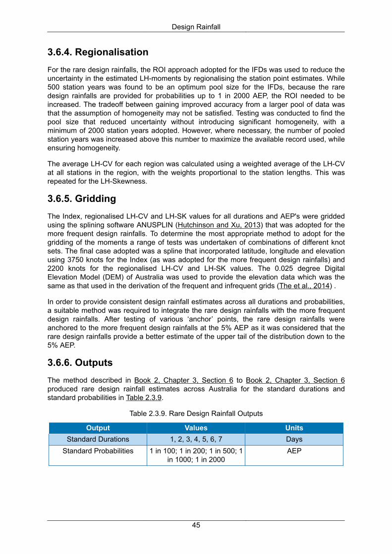
3.6.4. RegionalisationFor the rare design rainfalls, the ROI approach adopted for the IFDs was used to reduce the uncertainty in the estimated LH-moments by regionalising the station point estimates. While 500 station years was found to be an optimum pool size for the IFDs, because the rare design rainfalls are provided for probabilities up to 1 in 2000 AEP, the ROI needed to be increased. The tradeoff between gaining improved accuracy from a larger pool of data was that the assumption of homogeneity may not be satisfied. Testing was conducted to find the pool size that reduced uncertainty without introducing significant homogeneity, with a minimum of 2000 station years adopted. However, where necessary, the number of pooled station years was increased above this number to maximize the available record used, while ensuring homogeneity.

The average LH-CV for each region was calculated using a weighted average of the LH-CV at all stations in the region, with the weights proportional to the station lengths. This was repeated for the LH-Skewness.

3.6.5. GriddingThe Index, regionalised LH-CV and LH-SK values for all durations and AEP's were gridded using the splining software ANUSPLIN (Hutchinson and Xu, 2013) that was adopted for the more frequent design rainfalls. To determine the most appropriate method to adopt for the gridding of the moments a range of tests was undertaken of combinations of different knot sets. The final case adopted was a spline that incorporated latitude, longitude and elevation using 3750 knots for the Index (as was adopted for the more frequent design rainfalls) and 2200 knots for the regionalised LH-CV and LH-SK values. The 0.025 degree Digital Elevation Model (DEM) of Australia was used to provide the elevation data which was the same as that used in the derivation of the frequent and infrequent grids (The et al., 2014) .

In order to provide consistent design rainfall estimates across all durations and probabilities, a suitable method was required to integrate the rare design rainfalls with the more frequent design rainfalls. After testing of various ‘anchor’ points, the rare design rainfalls were anchored to the more frequent design rainfalls at the 5% AEP as it was considered that the rare design rainfalls provide a better estimate of the upper tail of the distribution down to the 5% AEP.

3.6.6. OutputsThe method described in Book 2, Chapter 3, Section 6 to Book 2, Chapter 3, Section 6 produced rare design rainfall estimates across Australia for the standard durations and standard probabilities in Table 2.3.9.

Table 2.3.9. Rare Design Rainfall Outputs

Output Values UnitsStandard Durations 1, 2, 3, 4, 5, 6, 7 Days

Standard Probabilities 1 in 100; 1 in 200; 1 in 500; 1 in 1000; 1 in 2000

AEP

Design Rainfall

45

3.7. Probable Maximum Precipitation Estimates

3.7.1. Overview

The design rainfalls classes described in Book 2, Chapter 3, Section 4 and Book 2, Chapter 3, Section 5 were derived using frequency analysis. However, extreme rainfalls events such as the Probable Maximum Precipitation (PMP), lie beyond both any directly observed events and the limit to which observed data can be extrapolated. As a result, estimation of extreme rainfall events is based on the broadest understanding of extreme events and the meteorological processes that produce them.

The Probable Maximum Precipitation (PMP) is defined as ‘the theoretical greatest depth of precipitation that is physically possible over a particular catchment’ (World Meteorological Organisation, 1986). The PMP assumes the simultaneous occurrence in one storm of maximum amount of moisture and the maximum conversion rate of moisture to precipitation (maximum efficiency).

3.7.2. Estimation of PMPs

The Bureau of Meteorology has been providing PMP estimates for over 70 years, however, the methods adopted have changed with time, as the understanding of extreme storms and the mechanisms which produce them have developed, and the databases of observed extreme storms have expanded. These methods include:

• In Situ Maximisation Method: During the 1950’s to 1970’s PMP estimates were based on the maximisation of the moisture content of storms which had been observed over the catchment of interest. The limitation of this method was that the differing lengths of rainfall records and occurrence or non-occurrence of an extreme storm led to inconsistent PMP estimates for catchments within the same region.

• Storm Transposition Method: During the late 1960’s and early 1970’s the size of the extreme storm sample for a specific catchment was increased by the transposition to the catchment of interest of extreme storms which had been observed over nearby catchments which had similar hydrometeorological and topographic features. Although this improved the within-region consistency of PMP estimates, the method was limited, as only storms from a similar topographic region could be transposed, and the selection of storms introduced a significant level of subjectivity.

• Generalised Methods: From the mid-1970’s generalised methods were introduced into Australia. Generalised methods make use of all available storm data for a large region by making adjustments for moisture availability and differing topographic effects. The generalised methods currently adopted in Australia are described in Book 2, Chapter 3, Section 7.

3.7.3. Generalised Methods for Probable Maximum Precipitation Estimation

There are three main generalised methods used for PMP estimation in Australia. These methods and their area of applicability are shown in Figure 2.3.15 and described in Book 2, Chapter 3, Section 7 to Book 2, Chapter 3, Section 7. There are two regional methods (Book 2, Chapter 3, Section 7, Book 2, Chapter 3, Section 7).

Design Rainfall

46

Figure 2.3.15. Generalised Probable Maximum Precipitation Method Zones

3.7.3.1. Generalised Short-Duration Method

The Generalised Short Duration Method (GSDM) is applicable across Australia for catchment areas less than 1000 km2 and for durations up to three hours or six hours depending on the location within of Australia (Bureau of Meteorology, 2003).

3.7.3.2. Generalised South-east Australia Method

The Generalised South-east Australia Method (GSAM) is applicable to the southern third of Australia where it is assumed that the causative mechanism of the PMP would not be tropical. The GSAM method is applicable for durations from 12 hours to 120 hours (Bureau of Meteorology, 2006; Minty et al., 1996).

3.7.3.3. Revised General Tropical Storm Method

The Revised Generalised Tropical Storm Method (GTSMR) is applicable to the northern two-thirds of Australia where it is assumed that the causative mechanism of the PMP would be a tropical storm. The GTSMR method is applicable for durations from 12 hours to 120 hours (Bureau of Meteorology, 2005; Walland et al., 2003).

3.7.3.4. West Coast Tasmania Method Zone

The West Coast Tasmania Method Zone applies to the west coast region of Tasmania which is outside the region of applicability of the Tasmanian GSAM coastal zone. It is applicable for durations between 24 and 72 hours (Xuereb et al., 2001).

Design Rainfall

47

3.7.3.5. GSAM-GTSMR Coastal Transition Zone

The GSAM-GTSMR Coastal Transition Zone method to the coastal area in NSW where is it considered that PMPs could be caused by either tropical or non-tropical storms.

3.7.4. Generalised Method of Probable Maximum Precipitation EstimationAlthough each of the three generalised methods has specific features, the generalised method can be summarised as follows:

3.7.4.1. Development of Storm Database

The ten highest one to seven day rainfalls which were common to a number of stations were selected and the storms prioritised according to the rarity of the event in order to identify the 100 or more largest storms. For each storm the following analyses were undertaken.

• The rainfall totals for the total storm duration were plotted on a topographic map and isohyets drawn to determine the spatial extent and distribution of each storm.

• To determine the storm temporal distribution, parallelograms were drawn around the storm centre for standard areas of 100; 500; 1 000; 2 500; 10 000; 40 000 and 60 000 km2. The average daily rainfall depths within a parallelogram were determined using Thiessen weights. For each standard area, the percentage of the total storm that fell during each 24 hour period was determined. These daily data were supplemented by pluviograph and 3 hourly synoptic charts.

• The representative dew point temperature for each storm was determined using a number of sources including the Australian Region Mean Sea Level charts, National Climate Centre Archives and Observers’ Logbooks.

3.7.4.2. Generalisation of Storm Database

The ‘site specific’ attributes of each storm were removed in order to attain a homogenous data set.

The effects of storm type were removed from the data set by the dividing of Australia into the GSAM and GTSMR regions on the basis of the type of storm that produces the largest observed rainfall depths. The two regions were further divided into Coastal and Inland Zones on the basis that different mechanisms produce the largest rainfall depths in each of the zones (refer Figure 2.3.15).

The specification of each storm in terms of depth-area-duration curves as done previously effectively removed the storm specific spatial distribution.

The removal of the site specific topographic effects was undertaken using 72 hour, 50 year ARI ‘flat land’ rainfall intensity field in order to produce the convergence component of each storm.

3.7.4.3. Removal of the Site-Specific and Storm-Specific Moisture Content

To remove the storm-specific moisture content from each storm and simultaneously to maximise the moisture content, the convergence depths were multiplied by a moisture

Design Rainfall

48

maximisation factor. The moisture maximisation factor is defined as the ratio of extreme precipitable water associated with the extreme dew point temperature at the storm location.

The site-specific moisture content of each storm was removed by transposition to a single location which for the GSAM was chosen as Brisbane and for GTSMR as Broome. For each location, representative seasonal extreme 24 hour persisting dew point temperatures were selected and the moisture content for each storm standardised.

3.7.4.4. Determination of ‘Storm’ of Maximum Moisture Content

The moisture maximisation factor and the standardised convergence depths were combined to estimate the maximised standardised convergence depths. To determine a single hypothetical storm of maximum moisture content, an envelope curve was drawn to the set of maximised, standardised convergence depth-area curves.

3.7.4.5. Determination of Catchment Specific Probable Maximum Precipitation

The envelope curves represent the maximised convergence component of the PMP at the standardising locations (Brisbane for the GSAM and Broome for GTSMR). To obtain an estimate of the PMP for a specific catchment it is necessary to build in the moisture content and topographic influences specific to the catchment of interest. The moisture content of the standard PMP convergence depth is adjustment using a Moisture Adjustment Factor (MAF) such that: MAF=EPWcatchment/EPWstd (2.3.9)

where MAF = Moisture Adjustment Factor; EPWcatchment is the Extreme Precipitable Water associated with the catchment extreme dew point temperature; EPWstd is the Extreme Precipitable Water associated with the standard extreme dew point temperature for appropriate season.

The Topographic Enhancement Factor (TEF) for the catchment PMP is estimated in the same manner as the topographic component of the storms in the database using the 72 hour 50 year ARI rainfall intensities.

The total PMP for a specific catchment for each of the standard durations is estimated as:PMPcatchment=MCDstd*MAFcatchment*TEFcatchment (2.3.10)

3.8. Uncertainty in Design RainfallsThe design rainfalls described in this Chapter are the best estimates currently available and have been derived using an extensive rainfall database which has been analysed using the most appropriate techniques.

However, there are uncertainties associated with the design rainfalls which arise from various sources including:

• errors in the data due to short record length, instrumentation errors, gaps in the data, unidentified errors in the data;

• sampling errors including network sparsity, poorly placed gauges, non-representativeness of gauging networks; and

Design Rainfall

49

• limitations in the adopted methods including delineation of regions, lack of homogeneity in regions, selection of distribution, parameter and quantile estimation, and extrapolation of data to ungauged locations.

These uncertainties need to be taken into consideration when the design rainfalls are being used in conjunction with other design flood inputs. Quantification of the uncertainties associated with the design rainfalls is described in Bureau of Meteorology (2016) as well as advice on how to incorporate uncertainty when using the design rainfalls.

3.9. Application

3.9.1. Design RainfallsThe very frequent, frequent, infrequent, and rare design rainfalls are available via the Bureau of Meteorology’s website2.

3.9.1.1. Input Data Requirements and Options

To estimate a design rainfall for a point location it is necessary to enter the co-ordinate of the location in one of three co-ordinate format options:

• Decimal degrees;

• Degrees, Minutes, Seconds; and

• Easting, Northing, Zone.

The location of the entered co-ordinate can be seen by using the map preview option and a location label can also be entered (see Figure 2.3.16).

2http://www.bom.gov.au/water/designRainfalls/ifd/index.shtml

Design Rainfall

50

http://www.bom.gov.au/water/designRainfalls/ifd/index.shtml

Figure 2.3.16. Design Rainfall Point Location Map Preview

Determine the design rainfall class for which design rainfalls are required:

• Very frequent

• Frequent and infrequent (IFDs)

• Rare

Determine the durations for which design rainfalls are required:

• Standard

• Non-standard

Determine the units in which the design rainfalls will be provided:

• Depths as millimetres (mm)

• Intensities as millimetres per hour (mm/hr)

Design Rainfall

51

3.9.2. Frequent and Infrequent Design Rainfalls (IFDs)

Figure 2.3.17. IFD Outputs

Design Rainfall

52

3.9.3. Very Frequent Design Rainfalls

Figure 2.3.18. Very frequent Design Rainfall Outputs

Design Rainfall

53

3.9.4. Rare Design Rainfalls

Figure 2.3.19. Rare design rainfall outputs

3.9.4.1. Output Options

The design rainfall information for the selected location can be seen in either tabular form (Figure 2.3.20) or graphical form (Figure 2.3.21).

Design Rainfall

54

Figure 2.3.20. Design Rainfall Output Shown as Table

Design Rainfall

55

Figure 2.3.21. Design Rainfall Output Shown as Chart

3.9.4.2. Export OptionsThe table can be exported as a .csv file for ease of incorporation into software and the chart as a .png to facilitate integration into reports.

3.9.5. Probable Maximum Precipitation EstimatesProbable Maximum Precipitation estimates for the GSDM can be estimated using the method contained in Bureau of Meteorology (2003) which can be downloaded from the Bureau of Meteorology’s website.

Design Rainfall

56

Guides for the application of the GSAM and GTSMR methods are available from the Bureau of Meteorology (Bureau of Meteorology, 2005; Bureau of Meteorology, 2006).

3.10. AcknowledgementsThe authors would like to acknowledge the contributions made by the following people during the IFD Revision Project:

• Dr Louise Minty and Dr Ian Prosser for their direction of the project

• Andrew Frost, Khaled Haddad, Catherine Jolly, Garry Moore, Scott Podger, Ataur Rahman, Lionel Siriwardena and Karin Xuereb for their contribution during various stages of the project

• Professor Mike Hutchinson for his ongoing advice on the application of ANUSPLIN

• Erwin Jeremiah, Deacon McKay, Scott Podger and Michael Sugiyanto for their cheerful quality controlling of the data

• Dr George Kuczera, Dr Nanda Nandakumar; Dr Rory Nathan and Erwin Weinmann for their sage advice on the rare design rainfalls

• Martin Chan, Damian Chong, Ceredwyn Ealanta Murray Henderson, Chris Lee, Quentin Leseney, Maria Levtova, Max Monahon, Julian Noye, and William Tall for the webpages.

3.11. ReferencesANCOLD (Australian National Committee on Large Dams) (2000), Guidelines on Selection of Acceptable Flood Capacity for Dams. Australian National Committee on Large Dams.

AUSTROADS (1992) '92 AUSTROADS Bridge Design Code.

Bates, B.C., McLuckie, D., Westra, S., Johnson, F., Green, J., Mummery, J. and Abbs, D. (2015), Revision of Australian Rainfall and Runoff - The Interim Climate Change Guideline. Presented at National Floodplain Management Authorities Conference, Brisbane, Qld, May.

Bonnin, G., Maitaria, K. and Yekta, M. (2010), Trends in Heavy Rainfalls in the Observed Record in Selected Areas of the U.S. IN PALMER, R. N. (Ed.) World Environmental and Water Resources Congress 2010: Challenges of Change. Providence, Rhode Island, American Society of Civil Engineers.

Bureau of Meteorology (2016), Design rainfalls for Australia: data, methods and analyses. Bureau of Meteorology, Melbourne, VIC.

Bureau of Meteorology (2003), The Estimation of Probable Maximum Precipitation in Australia: Generalised Short-Duration Method, [Online] Bureau of Meteorology, Melbourne, Australia, June 2003, (p: 39). Available at: http://www.bom.gov.au/water/designRainfalls/pmp/gsdm_document.shtml.

Bureau of Meteorology (2006), Guidebook of the Estimation of Probable Maximum Precipitation: Generalised Southeast Australia Method, included on the compact disc 'Guide to the Estimation of Probable Maximum Precipitation: Generalised Southeast Australia Method', Hydrometeorological Advisory Service, Bureau of Meteorology, October.

Bureau of Meteorology (2005), Guidebook of the Estimation of Probable Maximum Precipitation: Generalised Tropical Storm Method, Included on compact disc 'Guide to the

Design Rainfall

57

Estimation of Probable Maximum Precipitation: Generalised Tropical Storm Method', Hydrometeorological Advisory Service, Bureau of Meteorology, September.

Burn, D.H. (1990), An appraisal of the 'region of influence' approach to flood frequency analysis, Hydrological Sciences - Journal-des Sciences Hydrologiques, 35(2), 149-165.

Green, J. and Johnson, F.J. (2011), Stationarity Assessment of Australian Rainfall, Internal Bureau of Meteorology Report.

Green, J.H., Xuereb, X. and Siriwardena, L. (2011), Establishment of a Quality Controlled Rainfall Database for the Revision of the Intensity-Frequency Duration (IFD) Estimates for Australia. Presented at 34th IAHR Congress, Brisbane, Qld, June.

Green, J.H., Beesley, C., Frost, A., Podger, S. and The, C. (2015), National Estimates of Rare Design Rainfall. Presented at Hydrology and Water Resources Symposium, Hobart, Tas, December 2015.

Green, J.H., Johnson, J., McKay, D., Podger, P., Sugiyanto, M. and Siriwardena, L. (2012a), Quality Controlling Daily Read Rainfall Data for the Intensity-Frequency Duration (IFD) Revision Rainfall Project. Presented at Hydrology and Water Resources Symposium, Sydney, NSW, November.

Green, J.H., Xuereb, K., Johnson, J., Moore, G. and The, C. (2012b), The Revised Intensity-Frequency Duration (IFD) Design Rainfall Estimates for Australia - An Overview. Presented at Hydrology and Water Resources Symposium, Sydney, NSW, November.

Guttman, N.B., Hosking, J.R.M. and Wallis, J.R. (1993), Regional precipitation quantile values for the continental U. S. computed from L-moments. Journal of Climate, 6: 2326-2340.

Haddad, K. and Rahman, A. (2012a), Regional flood frequency analysis in eastern Australia: Bayesian GLS regression-based methods within fixed region and ROI framework: quantile regression vs parameter regression technique. Journal of Hydrology, 430: 142-161.

Haddad, K. and Rahman, A. (2012b), A Pilot Study on Design Rainfall Estimation in Australia using L-moments and Bayesian Generalised Least Squares Regression: Comparison of Fixed Region, Facets and Region of Influence Approach, EnviroWater Sydney.

Haddad, K., Johnson, F., Rahman, A., Green, J. and Kuczera, G. (2015), Comparing three methods to form regions for design rainfall statistics: Two case studies in Australia. Journal of Hydrology, 527: 62-76.

Haddad, K., Pirozzi, J., McPherson, G., Rahman, A. and Kuczera, G. (2009),'Regional flood estimation technique for NSW: application of generalised least squares quantile regression technique', Proc. 32nd Hydrology and Water Resources Symp., Newcastle, pp: 829-840.

Haddad, K., Rahman, A. and Green, J. (2011), Design Rainfall Estimation in Australia: A Case Study using L moments and Generalized Least Squares Regression, Stochastic Environmental Research & Risk Assessment, 25(6), 815-825.

Hosking, J.R.M. and Wallis, J.R. (1997), Regional Frequency Analysis: An Approach Based on L-Moments. CambridgeUniversity Press, Cambridge, UK. p: 224.

Huff, F.A. and Angel, J.R. (1992), Rainfall Frequency Atlas of the Midwest. Illinois State Water Survey, Champaign, Bulletin 71, 1992.

Design Rainfall

58

Hutchinson, M.F. (1998), Interpolation of rainfall data with thin plate smoothing splines - part 2: Analysis of topographic dependence, Journal of Geographic Information and Decision Analysis, 2(2), 152-167.

Hutchinson, M.F. (2007), ANUSPLIN version 4.37 User Guide, The Australian National University, Centre for Resources and Environmental Studies, Canberra.

Hutchinson, M.F. and Xu, T. (2013), ANUSPLIN Version 4.4 User Guide, The AustralianNationalUniversity. FennerSchool of Environment and Society, Canberra, Australia.

Johnson, F., Hutchinson, M.F., The, C., Beesley, C. and Green, J. (2015), Topographic relationships for design rainfalls over Australia. Accepted for publication Journal of Hydrology.

Johnson, F., Xuereb, K., Jeremiah, E. and Green, J. (2012a), Regionalisation of Rainfall Statistics for the IFD Revision Project. Presented at Hydrology and Water Resources Symposium, Sydney, NSW, November 2012.

Johnson, F., Haddad, K., Rahman, A., and Green, J. (2012b), Application of Bayesian GLSR to Estimate Sub Daily Rainfall Parameters for the IFD Revision Project. Presented at Hydrology and Water Resources Symposium, Sydney, NSW, November 2012.

Kjeldsen, T.R. and Jones, D.A. (2009), A formal statistical model for pooled analysis of extreme floods, Hydrology Research, 40(5), 465-480.

Madsen, H., Mikkelsen, P.S., Rosbjerg, D. and Harremoes, P. (2002), Regional estimation of rainfall intensity duration curves using generalised least squares regression of partial duration series statistics. Water Resources Research, 38(11), 1239.

Madsen, H., Arnbjerg-Neilsen, K. and Mikkelsen, P.S. (2009), Update of regional intensity-duration-frequency curves in Denmark: Tendency towards increased storm intensities. Atmospheric Research, 92: 343-349.

Menabde, M., Seed, S. and Pegram, G. (1999), A simple scaling model for extreme rainfall. Water Resources Research, 35: 335-339

Minty, L.J., Meighen, J. and Kennedy, M.R. (1996), Development of the Generalised Southeast Australia Method for Estimating Probable Maximum Precipitation, [Online] HRS Report No. 4, Hydrology Report Series, Bureau of Meteorology, Melbourne, Australia, August 1996, p: 48. Available at: http://www.bom.gov.au/water/designRainfalls/pmp/gsam.shtml

Nandakumar, N., Weinmann, P.E., Mein, R.G. and Nathan, R.J. (1997), Estimation of Extreme Rainfalls for Victoria using the CRCFORGE Method, CRC for Catchment Hydrology.

Pilgrim, DH (ed) (1987) Australian Rainfall and Runoff - A Guide to Flood Estimation, Institution of Engineers, Australia, Barton, ACT, 1987.

Reis Jr., D.S., Stedinger, J.R. and Martins, E.S. (2005), Bayesian GLS regression with application to LP3 regional skew estimation. Water Resour Res. 41, W10419, (1) 1029.

Schaefer, M.G. (1990), Regional analysis of precipitation annual maxima in Washington State, Water Resoures Research, 26(1), 119-131.

Design Rainfall

59

The, C., Johnson, F., Hutchinson, M., and Green, J. (2012), Gridding of Design Rainfall Parameters for the IFD Revision Project for Australia. Presented at Hydrology and Water Resources Symposium, Sydney, NSW, November.

The, C., Hutchinson, M., Johnson, F., Beesley, C. and Green, J. (2014), Application of ANUSPLIN to produce new Intensity-Frequency-Duration (IFD) design rainfalls across Australia. Presentated at Hydrology and Water Resources Symposium, Perth, WA, February 2014.

The, C., Beesley, C., Podger, S., Green, J., Hutchinson, M. and Jolly, C. (2015), Very frequent design rainfalls - an enhancement to the new IFDs. Accepted for presentation at Hydrology and Water Resources Symposium, Hobart, TAS, December 2015.

Walland, D.J., Meighen, J., Xuereb, K.C., Beesley, C.A. and Hoang, T.M.T. (2003), Revision of the Generalised Tropical Storm Method for Estimating Probable Maximum Precipitation [Online], HRS Report No.8, Hydrology Report Series, Bureau of Meteorology Melbourne, Australia, available at: http://www.bom.gov.au/water/designRainfalls/hrs8.shtml.

Wang, Q.J. (1997), LH moments for statistical analysis of extreme events. Water Resources Research, 33(12), 2841-2848.

Wang, Q.J. (1998), Approximate goodness-of-fit tests of fitted generalised extreme value distributions using LH moments. Water Resources Research, 34(12), 3497-3502.

World Meteorological Organisation (1986), 'Manual for Estimation of Probable Maximum Precipitation'. Second Edition. Operational Hydrology Report No.1, WMO - No.332, Geneva.

Xuereb, K. and Green, J. (2012), Defining Independence of Rainfall Events with a Partial Duration Series Approach. Presented at Hydrology and Water Resources Symposium, Sydney, NSW, November 2012.

Xuereb, K.C., Moore, G.J., and Taylor, B.F. (2001), Development of the Method of Storm Transposition and Maximisation for the West Coast of Tasmania. HRS Report No.7, Hydrology Report Series, Bureau of Meteorology, Melbourne, Australia, January 2001.

Design Rainfall

60

Chapter 4. Areal Reduction FactorsPhillip Jordan, Rory Nathan, Scott Podger, Mark Babister, Peter

Stensmyr, Janice Green



4.1. IntroductionDesign rainfall information for flood estimation generally is made available in the form of rainfall Intensity Frequency Duration (IFD) date (Book 2, Chapter 3) that relates to specific points in a catchment rather than to the whole catchment area. However, most flood estimates are required for catchments that are sufficiently large that design rainfall intensities at a point are not representative of the areal average rainfall intensity across the catchment. The ratio between the design values of areal average rainfall and point rainfall, computed for the same duration and Annual Exceedance Probability (AEP), is called the Areal Reduction Factor (ARF). This allows for the fact that larger catchments are less likely than smaller catchments to experience high intensity storms simultaneously over the whole of the catchment area.

It should be noted that the ARF provides a correction factor between the catchment rainfall depth (for a given combination of AEP and duration) and the mean of the point rainfall depths across a catchment (for the same AEP and duration combination). Applying an ARF is a necessary input to computation of design flood estimates from a catchment model that preserves a probability neutral transition between the design rainfall and the design flood characteristics. The ARF merely influences the average depth of rainfall across the catchment, it does not account for variability in the spatial and/or space-time patterns of its occurrence over the catchment.

Recommendations for ARF to be adopted are provided in Book 2, Chapter 4, Section 3.

4.2. Derivation of Areal Reduction FactorsThe method adopted for the derivation of areal reduction factors is a modified version of Bell’s method (Bell, 1976; Siriwardena and Weinmann, 1996). ARFs derived by this method have been widely used for some time and have been shown to provide effective estimates of areal design rainfall for deriving rainfall-based flood frequency curves. The method allows the dependence between ARF and catchment area to be determined, as well as the variation with AEP. The method has been applied with data collected and processed for the estimation of IFDs; they thus provide for a more comprehensive and consistent set of estimates than were prepared by Jordan et al. (2013).

The modified Bell’s method involves defining hypothetical circular catchments in areas with sufficient data and creating an areal rainfall time series for each catchment by weighting point rainfall values based on Thiessen polygon areas (or an equivalent weighting method). The frequency quantiles calculated from the areal rainfall time series are divided by the weighted point frequency quantiles for the sites within the catchment, yielding an ARF estimates for the given catchment area and a range of AEPs. Once ARFs have been calculated for the required catchment areas, durations and AEPs for as many locations as possible, they are averaged across these attributes and an equation is fitted to provide a prediction model for the selected region.

61

The adopted methodology is described in more detail in Podger et al. (2015a), Podger et al. (2015b) and Stensmyr et al (2014).

4.3. Areal Reduction Factor Recommendations

4.3.1. Areal Reduction Factors for Catchments up to 30 000 km2, Durations up to 7 days and Events More Frequent than 0.05% AEPAreal Reduction Factors (ARF) for catchments with areas up to 30 000 km2, for durations up to and including 168 hours (7 days) and for AEP more frequent than 0.05% (1 in 2000) Annual Exceedance Probability (AEP) are recommended based on the values derived by Podger et al. (2015a), Podger et al. (2015b) and Stensmyr et al (2014). This guidance should be adopted unless rigorous subsequent research or catchment-specific investigations have been conducted to define a more appropriate, locally specific, ARF.

The design areal rainfall to be applied in a design flood simulation is the average rainfall over the total catchment area to the point of interest. Consequently, the ARF should be computed for the total catchment upstream of each location of interest where a design flood estimate is required. The ARF should not be computed independently for each subarea in a runoff-routing model of the catchment of interest, as this would result in systematic overestimation of catchment rainfalls and simulated design flood hydrographs.

The ARF to be applied to design rainfall is a function of the total area of the catchment, the duration of the design rainfall event and it’s AEP. The ARF should be computed using the relevant procedure described in Table 2.4.1.

If the duration of interest is greater than 12 hours, Equation (2.4.2) will be required as part of the calculation procedure and the coefficients of Equation (2.4.2) vary regionally across Australia. The applicable ARF region should be selected by referring to Figure 2.4.1. Where a catchment overlaps the boundary between regions, the ARF should be selected for the region that has the largest overlap with the boundary of the catchment. The coefficients to be applied with Equation (2.4.2) should be selected from the appropriate region from Table 2.4.2.

Table 2.4.1. ARF Procedure for Catchments Less than 30 000 km2 and Durations up to and Including 7 Days

Catchment Area Duration ≤ 12 hours Duration Between 12 and 24 hours

Duration ≥ 24 Hours (1 Day) and ≤ 7 Days

(168 hours)≤ 1 km2 ARF = 1

Between 1 and 10 km2

1. Compute ARF(10 km2) using

Equation (2.4.1) for area = 10 km2 and selected duration

2. Interpolate ARF for catchment area

and selected

1. Compute ARF(24 hr, 10 km2) using

Equation (2.4.2) for area = 10 km2 and

duration = 1440 min

2. Compute ARF(12 hr, 10 km2) using

Equation (2.4.1) for

1. Compute ARF(10 km2) using

Equation (2.4.2) for area = 10 km2


and selected duration using

Equation (2.4.4)

Areal Reduction Factors

62

Catchment Area Duration ≤ 12 hours Duration Between 12 and 24 hours

Duration ≥ 24 Hours (1 Day) and ≤ 7 Days

(168 hours)duration using

Equation (2.4.4)area = 10 km2 and duration = 720 min

3. Interpolate ARF(10 km2) for selected

duration using Equation (2.4.4)


and selected duration using

Equation (2.4.3)Between 10 and

1000 km2• Compute ARF

using Equation (2.4.1) for

catchment area and selected duration

1. Compute ARF(24 hr) using Equation

(2.4.2) for catchment area and duration =

1440 min

2. Compute ARF(12 hr) using Equation

(2.4.1) for catchment area

and duration = 720 min

3. Interpolate ARF for selected duration using Equation

(2.4.3)

• Compute ARF using Equation

(2.4.2) for catchment area and

selected durationBetween 1000 and

30 000 km2Generalised

equations not applicable

>30 000 km2 Generalised equations not applicable. It is recommended that the practitioner should perform a frequency analysis of catchment

rainfall data for the catchment of interest.

Notes on Table 2.4.1:

• Equation (2.4.1), Equation (2.4.2) and Equation (2.4.3) require the selected duration to be provided in minutes.

• There has been limited research on ARF applicable to catchments that are less than 10 km2. The recommended procedure is to adopt an ARF of unity for catchments that are less than 1 km2, with an interpolation to the empirically derived equations for catchments that are between 1 and 10 km2 in area (refer to Equation (2.4.3)).

• The ARF equations derived by Podger et al. (2015a), Podger et al. (2015b) and Stensmyr et al (2014) were derived for the 50% to 1% AEPs. Although these have been recommended for use for a wider range of AEP, (out to 0.05% AEP), further verification is ongoing on the validity of this approach. As a result, the coefficients of Equation (2.4.2) (from Table 2.4.2) and/or the regional boundaries (refer to Figure 2.4.1) may be revised.


63

Short Duration ARF Equation

Equation (2.4.1)

�� = �� 1, 1− 0.287(��0.265− 0.439log10(��)) .��−0.36+2.26 x 10−3 x ��0.226 .��0.125(0.3 + log10(��))+0.0141 x ��0.213x 10−0.021 �� − 180 21440 (0.3 + log10(��))where Area is in km2, Duration is in minutes and AEP is a fraction (between 0.5 and 0.0005).

Long Duration ARF Equation

�� = �� 1, 1− �(��− �log10��)��−�+��(0.3 + log10��)+ℎ10��1440 (0.3 + log10��)] (2.4.2)

where Area is in km2, Duration is in minutes and AEP is a fraction (between 0.5 and 0.0005).

Interpolation Equation for Durations between 12 and 24 hours�� = ��12ℎ��+ ��24ℎ��− ��12ℎ�� − 720720 (2.4.3)

where Duration is in minutes.

ARF Equation for Areas between 1 and 10 km2

�� = 1− 0.6614 1− ��10��2 �0.4− 1 (2.4.4)

where Area is in km2


64

Figure 2.4.1. Area Reduction Factors Regions for Durations 24 to 168 Hours

Table 2.4.2. ARF Equation (2.4.2) Coefficients by Region for Durations 24 to 168 hours Inclusive

Region1 a b c d e f g h iEast Coast North 0.327 0.241 0.448 0.36 0.000

960.48 -0.21 0.012 -0.001

3Semi-arid Inland

Queensland0.159 0.283 0.25 0.308 7.3E-

071 0.039 0 0

Tasmania 0.0605

0.347 0.2 0.283 0.00076

0.347 0.0877

0.012 -0.00033

South-West Western Australia

0.183 0.259 0.271 0.33 3.85E-06

0.41 0.55 0.00817

-0.00045

Central New South Wales

0.265 0.241 0.505 0.321 0.00056

0.414 -0.021 0.015 -0.00033

South-East Coast 0.06 0.361 0 0.317 8.11E-05

0.651 0 0 0

Southern Semi-arid 0.254 0.247 0.403 0.351 0.0013

0.302 0.058 0 0

Southern Temperate 0.158 0.276 0.372 0.315 0.000141

0.41 0.15 0.01 -0.0027

Northern Coastal 0.326 0.223 0.442 0.323 0.0013

0.58 -0.374 0.013 -0.0015


65

Region1 a b c d e f g h iInland Arid 0.297 0.234 0.449 0.344 0.001

420.216 0.129 0 0

1These values are provided on the ARR Data Hub for the relevant region when queried (Babister et al (2016), accessible at http://data.arr-software.org/)

4.3.2. Events That are Rarer than 0.05% Annual Exceedance ProbabilityThe ARF equations are only recommended for use for events more frequent than 0.05% AEP. For more extreme events, the procedures recommended in Book 8, Chapter 3, Section 5 should be used to determine catchment average design rainfall depths. The interpolation procedure recommended in Book 8, Chapter 3, Section 5 uses the catchment average design rainfall depth for 0.05% AEP, which would be calculated using the average of the point design intensities across the catchment multiplied by the ARF estimates recommended above and the PMP depth, which is already estimated as a catchment average value.

4.3.3. Catchments with Areas Greater than 30 000 km2

The largest (circular) catchments used by Podger et al. (2015a) to estimate ARF were 30 000 km2 and which set the upper limit of applicability of the ARF equations. As the catchment area increases beyond 30 000 km2, it becomes increasingly likely that storm events would only influence part of the overall catchment area, which increases the uncertainty associated with adjusting point design intensities using an ARF.

Design rainfall depths for catchments larger than 30 000 km2 should be derived from frequency analysis of catchment average rainfall depths over the specific catchment. The design rainfall depths from the catchment-specific frequency analysis should be checked by dividing them by the average of the point rainfall depths from point IFD analysis for the catchment (Bureau of Meteorology, 2013) to infer the ARF for the catchment for each rainfall duration and AEP. It would be expected that for a catchment larger than 30 000 km2, the ARF inferred from this check for each duration and AEP should be less than the ARF calculated from the regional method Equation (2.4.2) for the corresponding duration and AEP combination. It would also be expected that the inferred ARF (for a given AEP) should increase with rainfall duration.

For catchments larger than 30 000 km2, it becomes increasingly likely that rainfall events that would give rise to flooding would be concentrated in one part of the catchment. For catchments larger than 30 000 km2 it is strongly recommended that partial area storms are explicitly modelled (using Monte Carlo or other joint probability approaches). Explicit modelling of partial area storms should also be considered for catchments in the range between 5 000 km2 and 30 000 km2.

4.4. Worked ExampleA worked example for the calculation of the ARF and the areal design rainfall for a catchment in Queensland is provided in Book 2, Chapter 6, Section 5.

4.5. Limitations and Recommended Further ResearchThe ARF equations developed in Australia have been derived using data driven and empirical methods, with limited theoretical underpinning. ARF values for a particular


66

http://data.arr-software.org/

catchment would derive from a combination of the mixture of storm types causing heavy rainfall within a region, the direction and speed of movement of those storms and the spatial and temporal characteristics of those storms. Analysis by a hydrometeorologist of the prevalence of different storm types within different parts of Australia and the advection, temporal and spatial characteristics of those storms is likely to provide an understanding of the causes of variations in ARF. Such understanding is difficult to infer directly, on its own, from the empirically derived ARF equations that are currently recommended for use in Australia. It is recommended that hydrometeorologists are engaged to investigate the causes of variations in ARF.

Once the hydrometeological analysis recommended above has been undertaken, the outcomes of that work may enable further research and improvements in the following specific areas:

• Clarification of how well the ARFs derived using an empirical method such as Bell’s method, compare with those derived from a suitable theoretical method that may better account for hydrometeorological understanding of the drivers of variability in ARFs.

• There are some areas within each of the regions where the ARF values determined empirically for the circular catchments demonstrated a trend toward being larger or smaller than obtained from the ARF equations fitted to the mean ARF values from all circular catchments within the region for a given area, duration and AEP. Hydrometeorological understanding may enable definition of smaller sub-regions, combining of existing regions (with the existing regions largely defined using state and territory boundaries), or definition of new regions in order to reduce the uncertainty introduced by this variability.

• Seasonality was found to be a significant driver of ARFs in Western Australia but has not been investigated for other parts of Australia. Hydrometeorological understanding may guide the regions where seasonal dependence in ARF would be likely, the start and end dates of seasons and how transition periods between seasons should be handled.

It is recommended that after an appropriate study has been undertaken to determine the hydrometeorological causes of variations in ARF that further studies are then scoped and prioritised according to areas where the hydrometeorological causes can be best exploited to reduce residual uncertainty in ARFs.

4.6. Recommended Further Research

4.6.1. Areal Reduction FactorsThe ARF equations developed in Australia have been derived using data driven and empirical methods, with limited theoretical underpinning. ARF values for a particular catchment would derive from a combination of the mixture of storm types causing heavy rainfall within a region, the direction and speed of movement of those storms and the spatial and temporal characteristics of those storms. Analysis by a hydrometeorologist of the prevalence of different storm types within different parts of Australia and the advection, temporal and spatial characteristics of those storms is likely to provide an understanding of the causes of variations in ARF. Such understanding is difficult to infer directly, on its own, from the empirically derived ARF equations that are currently recommended for use in Australia. It is recommended that hydrometeorologists are engaged to investigate the causes of variations in ARF.

Once the hydrometeological analysis recommended above has been undertaken, the outcomes of that work may enable further research and improvements in the following areas:


67

• how well the ARFs derived using an empirical method such as Bell’s method, compare with those derived from a suitable theoretical method that may better account for hydrometeorological understanding of the drivers of variability in ARFs.

• There are some areas within each of the regions where the ARF values determined empirically for the circular catchments demonstrated a trend toward being larger or smaller than the fitted ARF equations, which were fitted to the mean ARF values from all circular catchments within the region for a given area, duration and AEP. Hydrometeorological understanding may enable definition of smaller sub-regions, combining of existing regions (with the existing regions largely defined using state and territory boundaries), or definition of new regions in order to reduce the uncertainty introduced by this variability.

• Seasonality was found to be a significant driver of ARFs in Western Australia but has not been investigated for other parts of Australia. Hydrometeorological understanding may guide the regions where seasonal dependence in ARF would be likely, the start and end dates of seasons and how transition periods between seasons should be handled.

It is recommended that after an appropriate study has been undertaken to determine the hydrometeorological causes of variations in ARF that further studies are then scoped and prioritised according to areas where the hydrometeorological causes are best exploited to reduce residual uncertainty in ARFs.

4.7. References

Babister, M., Trim, A., Testoni, I. and Retallick, M. 2016. The Australian Rainfall and Runoff Datahub, 37th Hydrology and Water Resources Symposium Queenstown NZ

Bell, F.C. (1976), The areal reduction factors in rainfall frequency estimation. Natural Environmental Research Council (NERC), Report No. 35, Institute of Hydrology, Wallingford, U.K.

Bureau of Meteorology (2013), Revised Design Rainfall Intensity Frequency Duration Estimates for Australia. Available at: http://www.bom.gov.au/water/designRainfalls/revised-ifd/, Accessed [July 2015].

Jordan, P., Weinmann, P.E., Hill, P. and Wiesenfeld, C. (2013), Collation and Review of Areal Reduction Factors from Applications of the CRC-FORGE Method in Australia, Final Report, Australian Rainfall and Runoff Revision Project 2: Spatial Patterns of Rainfall, Engineers Australia, Barton, ACT.

Podger, S., Green, J., Jolly, C., The, C. and Beesley, C. (2015a),Creating long duration areal reduction factors for the new Intensity-Frequency-Duration (IFD) design rainfalls, Proc. Engineers Australia Hydrology and Water Resources Symposium, Hobart, Tasmania, Australia.

Podger, S., Green, J., Stensmyr, P. and Babister, M. (2015b), Combining long and short duration areal reduction factors, Proc. Engineers Australia Hydrology and Water Resources Symposium, Hobart, Tasmania, Australia.

Siriwardena, L. and P.E. Weinmann, (1996), Derivation of areal reduction factors for design rainfalls in Victoria, 96(4), 60.


68

Stensmyr, P., Babister, M. and Retallick, M. (2014), Australian Rainfall and Runoff Revision Project 2: Spatial Patterns of Rainfall: Stage 2 Report, Short Duration Areal Reduction Factors, ARR Report Number P2/S2/019, ISBN 978-085825-9614.


69

Chapter 5. Temporal PatternsMark Babister, Monique Retallick, Melanie Loveridge, Isabelle Testoni,

Scott Podger



5.1. IntroductionThe majority of hydrograph estimation methods used for flood estimation require a temporal pattern that describes how rainfall falls over time as a design input. Traditionally a single burst temporal pattern has been used for each rainfall event duration. The use of a single pattern has been questioned for some time (Nathan and Weinmann, 1995) as the analysis of observed rainfall events from even a single pluviograph shows that a wide variety of temporal patterns is possible.

The importance of temporal patterns has increased as the practice of flood estimation has evolved from peak flow estimation to full hydrograph estimation. There has been a strong move toward storage-based mitigation solutions in urban catchments which require realistic temporal patterns that reproduce total storm volumes as well as the temporal distribution of rainfall within the event.

This chapter discusses use of temporal patterns for design flood estimation where a fixed temporal pattern is applied over the entire catchment. Book 2, Chapter 6 discusses the more complex case of space-time patterns.

This chapter is structured as follows:

• Book 2, Chapter 5, Section 2 – discusses fundamental temporal pattern concepts and how the concept of using ensembles of temporal pattern developed;

• Book 2, Chapter 5, Section 3 – discusses the storm database that was used to develop temporal patterns;

• Book 2, Chapter 5, Section 4 – describes the estimation of pre-burst rainfall;

• Book 2, Chapter 5, Section 5 – describes the development of ensembles of design temporal patterns;

• Book 2, Chapter 5, Section 6 – discusses areal temporal patterns;

• Book 2, Chapter 5, Section 8 – discusses possible effects of climate change on temporal patterns; and

• Book 2, Chapter 5, Section 9 – discusses the application of design temporal patterns;

5.2. Temporal Pattern Concepts

5.2.1. Storm ComponentsIn order to properly understand the temporal patterns it is necessary to understand the components of a storm event and how they relate to Intensity Frequency Duration Data (IFD)

70

and catchment response. Figure 2.5.1 depicts a typical storm pattern and how components of the storm can be characterised. It is important to note the components can be characterised either by IFD relationships or by catchment response and are highly dependent on the definitions used. The components of a storm include:

• antecedent rainfall - is rainfall that has fallen before the storm event and is not considered part of the storm but can affect catchment response. This is not considered in this chapter but is introduced for completeness.

• pre-burst rainfall - is storm rainfall that occurs before the main burst. With the exception of relatively frequent events, it generally does not have a significant influence on catchment response but is very important for understanding catchment and storage conditions before the main rainfall burst.

• the burst - represents the main part of the storm but is very dependent on the definition used. Bursts have typically been characterised by duration. The burst could be defined as the critical rainfall burst , the rainfall period within the storm that has the lowest probability, or the critical response burst that corresponds to the duration which produces the largest catchment response for a given rainfall Annual Exceedance Probability (AEP).

• post-burst rainfall - is rainfall that occurs after the main burst and is generally only considered when aspects of hydrograph recession are important. This could be for drawing down a dam after a flood event or understanding how inundation times affect flood recovery, road closures or agricultural land.

Figure 2.5.1. Typical Storm Components

If the critical response burst is not the same as the critical rainfall burst then the critical response burst is either:

• part of a longer critical rainfall burst; or

• a storm that contains rarer shorter duration bursts.

Rarer shorter duration bursts within a burst are typically called embedded bursts and can cause problems in modelling as, while the intention may be to assess the catchment

Temporal Patterns

71

response to a burst of a defined duration and probability, the response to a rarer shorter duration burst is also being assessed.

The distinction between a burst and a complete storm is important as complete storms are used for calibration and bursts are typically used for design. Though this difference is less important for catchments with long duration responses, as the bursts typically represent nearly the entire storm event.

5.2.2. Pattern VariabilityIt has been well recognised that temporal patterns exhibit significant variability between rainfall events of similar magnitude, and the adopted pattern can have a significant effect on the estimated peak flow. Askew (1975), Milston (1979), Brown (1982), Wood and Alvarez (1982), Cordery et al. (1984) give examples of differences of up to 50% in flood peaks resulting from different assumed temporal patterns. Ball (1994) discusses how catchment peak flow tends to increase as the variability of the pattern increases.

Pilgrim et al. (1969) describe the variability of patterns:

“In nature, a wide range of patterns is possible. Some storms have their period of peak intensity occur early, while other storms have the peak rainfall intensity occur towards the end of the storm period and a large number have a tendency for the peak to occur more or less centrally.”

Figure 2.5.2 depicts two very different storms from Sydney Observatory Hill that have similar IFD characteristics from 15 min to 12 hrs and a 2 hr critical rainfall burst, however on other criteria they are very different. The first pattern has 182 mm before the 2 hr burst, while the second pattern has 16 mm. For the 2nd event the commencement of runoff will be closely aligned with the main burst while the former event is likely to have significant runoff prior to the main burst. The rainfall burst also exhibits significant variability, Figure 2.5.3 presents the temporal patterns (as dimensionless mass curves) of ten 2 hr bursts of similar probability that show the variability described by Pilgrim et al. (1969).

Temporal Patterns

72

Figure 2.5.2. Two Different Storm Events with Similar Intensity Frequency Duration Characteristics (Sydney Observatory Hill) – Two Hyetographs plus Burst Probability Graph

Temporal Patterns

73

Figure 2.5.3. Ten 2 hr Dimensionless Mass Curves

Most of the historical research on temporal patterns has assumed that the central tendency of the pattern is more important than the variability, with the aim of producing a typical, representative or median pattern. French (1985) describes how a pattern can be considered a two dimensional quantity with most methods breaking the pattern into two manageable one dimensional quantities that describe the magnitude of the element and the order of the elements. This can be described as a rank order vector and a decay curve that describes how the magnitude decreases between ranks.

Monte Carlo and ensemble modelling techniques try to overcome the problems associated with this simplification by using an ensemble of temporal patterns. A short history of temporal patterns helps explain that, while the complexity of temporal patterns has been well understood for a long time, it has been difficult to produce a simple set of design patterns.

5.2.3. History of Design Temporal Pattern DevelopmentAustralian Rainfall and Runoff 1977 (Pattison, 1977; Institution of Engineers, Australia., 1977) notes that there has historically been a slow change in the application of temporal distributions of rainfall in hydrologic studies from more arbitrary approaches to approaches that reproduce the IFD characteristics (Keifer and Chu (1957) and Huff (1967)). The modern interpretation is the duration independent storm (Varga et al., 2009). These approaches reproduce the IFD loading and at best can reproduce aspects of a single storm. Such approaches have some applicability for peak flow estimation but cannot reproduce realistic hydrographs.

Other early approaches included in the development of patterns based on observed pluviograph records were for complete storms rather than bursts. Such approaches require the scaling of complete storms. Other methods have allowed the arbitrary rearrangement of patterns to maximise peak discharge. Such approaches are very far removed from concept of probability neutrality.

The development of the Average Variability Method by Pilgrim et al. (1969) and Pilgrim and Cordery (1975) analysed the variability of patterns by separating the analysis of the

Temporal Patterns

74

magnitude or the ranks from the analysis of rank order. This approach is only applicable to bursts and was applied in ARR 1977 and in a very detailed way in ARR 1987. A variation of this approach was developed by Hall and Kneen (1973). During the finalisation of ARR 1987 some problems where found with the use of the patterns and extensive testing was carried out which resulted in some changes to remove some embedded bursts, including some arbitrary rank order changes. It has been assumed that an AVM pattern would preserve probability neutrality. Single burst per duration AVM patterns have been extensively used since ARR 1987 and appear to have performed reasonable well for peak flow estimation.

By their very nature AVM patterns do preserve the average rank magnitudes. Figure 2.5.4 plots the magnitude or decay curve for the ten dimensionless curves in Figure 2.5.3 and the AVM curve from these events and all 10 events that would be considered in a AVM analysis.

Figure 2.5.4. Decay Curve of Ten Dimensionless Patterns and AVM Patterns

The issues that have arisen have been discussed in Retallick et al. (2009):

• Specific durations tend to dominate;

• Big changes in pattern and corresponding peak flow occur at some region boundaries;

• The burst only approach has made conversion of observed losses to burst losses difficult;

• The design patterns often contain significant embedded bursts; and

• Filtering to remove embedded bursts that was recommended in ARR 1987 (Pilgrim, 1987) has had a mixed uptake and sometimes produces unrealistically long critical durations.

The AVM approach also works best when there is a dominant typical pattern shape. As part of the AVM approach the average and standard deviation of the rank of each period is

Temporal Patterns

75

calculated, when there is no dominant pattern these averages can be very similar and the resultant AVM pattern need not bare any resemblance to any of the observed patterns.

The complexity of producing a representative or median pattern has led many practitioners to question the concept and ask whether it is better to specifically account for this variability by modelling an ensemble of temporal patterns.

The problems with the AVM method and other median or representative patterns is that it assumes the variability of actual patterns is much less important than their central tendency. Such an approach does not account for how temporal patterns interact with catchments to produce peak flows and hydrographs. The response can be very catchment-specific, and there is no guarantee that a representative pattern will produce the medium response from an ensemble of patterns that properly captures the variability of observed patterns. These problems can become more pronounced when changes are made to the catchment response or storage characteristics. Phillips and Yu (2015) examined the impact of storage on an ensemble of events for the lot, neighbourhood and subcatchment scale.

It is unclear who first proposed the concept of running an ensemble of temporal patterns to account for the variability of patterns. Practitioners have a long history of comparing the peak flow estimates from design patterns to estimates from patterns extracted from real storms that occurred on that catchment of interest. The development of Monte Carlo methods (Hoang et al., 1999; Rahman et al., 2002; Weinmann et al., 2000) that stochastically sample from observed events based on complete storms and embedded bursts of maximum intensity (“storm cores”) is well documented and has helped highlight the value of using ensembles. Others, such as Nathan et al. (2002) have used ensembles of storm bursts based on observed point and areal storms to facilitate their use directly with design IFD information. The development of the Bureau of Meteorology significant storm database (Meighen and Kennedy, 1995) enabled practitioners to easily test ensembles of areal patterns and how they affected other flood characteristics; examples include Webb McKeown and Associates (2003). While there is a long history of testing ensembles of temporal patterns, Sih et al. (2008) is the first example of detailed testing of ensemble patterns as a design input outside a Monte Carlo environment. This long development history of ensemble simulation can probably be explained by the fact that the concept could not be confirmed until rigorous Monte Carlo techniques became available for validation.

Parallel to the development of ensemble and Monte Carlo approaches, practitioners have become concerned with using burst patterns where complete storm volume is important. Rigby and Bannigan (1996) suggest the entire burst approach needed to be reviewed and design storms needed to replace design bursts. For the Wollongong area Rigby and Bannigan (1996) demonstrated that historically most short duration events were embedded in longer duration events. They recommended that short duration events could be embedded in a 24 hour event of the same probability. They particularly cautioned against using bursts on catchments with significant natural or man-made storages. Phillips et al. (1994) had found similar problems in the upper Parramatta River and suggested embedded storms were more realistic, and that basin storages would be underestimated with a burst approach unless the embedded nature of events was factored into the starting volumes. Rigby et al. (2003) extended the earlier work to include guidance on using the embedded design storms. Roso and Rigby (2006) recommended a storm based approach be used when there are significant storages or diversions present in the catchment. Kuczera et al. (2003), inspired by Rigby and Bannigan (1996), explored basin performance using a theoretical catchment at Observatory Hill, Sydney in a continuous simulation approach and found similar problems with peak flow being underestimated by a similar amount when

Temporal Patterns

76

storages were present. All of these studies were based on catchments less than 110 km2

that are close to Sydney.

5.3. Storm DatabaseAs part of the IFD revision (Book 2, Chapter 3) the Bureau of Meteorology produced a quality controlled pluviograph database, containing 2280 stations with more than 8 station years (refer toBook 2, Chapter 3 and Book 1, Chapter 4). The average station record length is 25 years, with a combined record length of 57 000 years. A total of 754 of the stations are owned by the Bureau of Meteorology and the other 1526 are owned by other data agencies throughout Australia. This data was provided by the Bureau of Meteorology, who undertook quality controlling to identify suspect data, such as missing data, accumulated totals and time shifts (Green et al., 2011). All station data was provided as time series data sampled at a 5 minute time step. In addition to the rainfall depths, each data point had a quality code indicating the quality of the data. Figure 2.5.5 below depicts the geographical distribution of the pluviographs across Australia. Each station is represented as a circle, with the size of the circle indicating the record length of the station.

Figure 2.5.5. Pluviograph Stations Record Lengths

Table 2.5.1 presents the maximum number stations available in any year for decadal periods. Table 2.5.1 demonstrates that most of the pluviograph record is from 1960 onwards. Though overall the data comes from a period that starts before 1900, over half of the data is from the period from 1993 onwards.

Temporal Patterns

77

Table 2.5.1. Number of Pluviographs by Decade

Decade Maximum Number of Pluviographs in any Year

<1900 21900-1940 241940-1960 1541960-1970 3921970-1980 9231980-1990 12731990 -2000 19262000-2010 1837a

aNot all data was available from 2009 onwards

As shown in Figure 2.5.5 the highest density of pluviograph stations is typically found along coastal areas of Australia around key population centres. In Figure 2.5.6, the pluviograph stations are seen to be clustered around urban areas, such as Sydney, Wollongong, Melbourne and Canberra. Less data is available in central Australia, with the exception of the Alice Springs area. Large areas of central Western Australia contain no data.

Figure 2.5.6. Pluviograph Stations used Throughout South-Eastern Australia with Record Lengths

Temporal Patterns

78

5.3.1. Data Quality

Where a single station is being analysed it is important that it has a reasonably long record (preferably longer than 30 years) and only a small percentage of missing data. However, for studies that pool data the quality of the data is a bigger issue than record length. It is however, important to remember that most of the pluviograph data is from the last few decades.

The pluviograph database contains a significant number of events with long periods of apparently uniform rainfall. While some of this could be from events with relatively uniform rainfall, most appears to be the result of disaggregating accumulated rainfall totals uniformly. Even if rainfall is uniform, a tipping bucket rain gauge recording at 5 minutes will only record uniform rainfall over an extended period if the depth in each five minute period is equal or slightly larger than an integer multiple of the tipping bucket capacity. It was concluded that most of the periods of uniform rainfall are probably caused by digitisation and resampling at different time steps. Events with large periods of uniform rainfall were disregarded, while events were kept if the uniform period was only a small portion of the entire event.

In addition, several other issues with the data quality were found. Some records contained significant periods of missing data. There were also periods of interpolated data, where several data points were indicated as interpolated from a later point, presumably at the end of an event. Events where a significant part of the rainfall was interpolated were excluded from further analysis. There were also sections where the rainfall was uniform over many intervals within an event, indicating that the data points were interpolated, even though the quality control value did not specify that to be the case. Since storms generally do not have uniform rainfall at the local scale, events that had a significant part of their total rainfall depth occurring in consecutive identical intervals were also excluded.

5.3.2. Event Selection and Analysis

Once the data quality checking was complete, all events with a burst greater than 1 Exceedance per Year (EY) using the 2013 IFD and which were not flagged with problems were extracted for further analysis. For each event the start and finish of the event was defined using the methodology described in ARR Revision Project 3 - Temporal Patterns of Rainfall Report Part 1 (WMAwater, 2015a), which was consistent with the storm event definition used in the ARR Revision Project 6 - Losses (Hill et al., 2014). Once all events with a burst greater than 1EY were defined for every duration, the following properties where calculated:

• burst rainfall depth probabilities for each duration;

• start and finish time for each burst;

• time when 50% of the burst depth occurred (ie. burst loading);

• pre-burst rainfall depth for each burst duration;

• pre-burst to burst rainfall ratio for each duration; and

• Post-burst depth.

For each event the rarest or critical rainfall burst (of any duration and location within the overall event) was also calculated.

Temporal Patterns

79

5.3.3. Regional CharacteristicsTo assess the regional characteristics, 12 temporal pattern regions were defined based on the 54 Natural Resource Management (NRM) sub-regions used for investigating the impacts of climate change (CSIRO and Australian Bureau of Meteorology, 2015). The adopted regions follow drainage basin boundaries. Figure 2.5.7 depicts the adopted temporal pattern regions. Table 2.5.2 summarises the number of rainfall gauges and storm events that exist in each region.

Table 2.5.2. Regions- Number of Gauges and Events

Region Number of Gauges

Number of Station Years

Number of Events

Average Number of Events per

Station YearSouthern Slopes

(Tasmania)110 2954 3477 1.18

Southern Slopes (mainland)

356 8536 20581 2.41

Murray Basin 233 6316 18399 2.91Central Slopes 118 2767 7167 2.59

East Coast South 331 8067 19856 2.46East Coast North 210 5187 12123 2.34

Wet Tropics 99 2474 5437 2.20Monsoonal North 211 5054 12287 2.43

Rangelands West

93 2334 5391 2.31

Rangelands 226 5561 12618 2.27Flatlands West 349 9113 26402 2.90Flatlands East 56 1401 3450 2.46

Temporal Patterns

80

Figure 2.5.7. Temporal Pattern Regions

The term ‘burst loading’ refers to the distribution of rainfall within a burst and is a defining characteristic of a rainfall event. For each event the burst loading was calculated as the percentage of the time taken for 50% of the burst depth to occur. The burst loading can be used as a simple measure of when the heaviest part of the burst occurs and can be used to categorise events as ‘front’, ‘middle’ or ‘back’ loaded. Events where categorised into three groups, depending on where 50% of the burst rainfall occurs:

• front loaded – 0 to 40% of the time;

• middle loaded – 40 to 60% of the time; and

• back loaded – 60 to 100% of the time.

Figure 2.5.8 depicts a typical event from each category.

Temporal Patterns

81

Figure 2.5.8. Example of Front, Middle and Back Loaded Events

This simple categorisation provides a pragmatic means of capturing when the peak loading occurs, as described by Pilgrim et al. (1969), though it is worth recognising that for a double peaked event, when most of the rainfall is in the early and later part of the burst, the loading can somewhat illogically fall into the middle category.

Each region was characterised by its burst loading distribution, which describes the percentage of front, middle and back loaded events for different durations. The proportion of front/middle/back loading for each region was determined for less than and greater than 6 hours duration (Table 2.5.3). The proportion was assumed to be constant across all AEPs.

Table 2.5.3. Burst Loading by Region and Duration

Region Duration Front Loaded (%)

Middle Loaded (%)

Back Loaded (%)

Southern Slopes (Tasmania)

≤ 6hr 21.5 64.1 14.4> 6hr 20.5 60.0 19.5


≤ 6hr 30.1 53.0 16.9> 6hr 22.7 53.7 23.6

Murray Basin ≤ 6hr 28.3 53.8 17.9> 6hr 24.7 52.5 22.7

Central Slopes ≤ 6hr 31.0 53.3 15.7> 6hr 27.0 46.9 26.1

East Coast South ≤ 6hr 26.5 57.1 16.4

Temporal Patterns

82

Region Duration Front Loaded (%)

Middle Loaded (%)

Back Loaded (%)

> 6hr 17.1 58.6 24.3East Coast North ≤ 6hr 28.9 56.5 14.6

> 6hr 23.4 48.5 28.1Wet Tropics ≤ 6hr 16.0 71.8 12.2

> 6hr 18.7 58.1 23.2Monsoonal North ≤ 6hr 27.6 63.7 8.8

> 6hr 27.5 41.4 31.2Rangelands

West≤ 6hr 23.7 62.5 13.8> 6hr 23.6 49.2 27.2

Rangelands ≤ 6hr 29.0 56.6 14.3> 6hr 24.4 49.2 26.4

Flatlands West ≤ 6hr 30.8 49.3 19.9> 6hr 31.4 48.9 19.7

Flatlands East ≤ 6hr 27.6 52.4 20.0> 6hr 17.4 54.4 28.2

5.4. Pre Burst Rainfall and Antecedent ConditionsThe events database allowed the pre-burst behaviour of rainfall events to be characterised, regionalised and mapped. Temporal Patterns report 2 WMAwater (2015a) presents the detailed analysis, regionalisation and mapping of pre-burst behaviour for Australia. Due to the relatively short pluviograph records, the approach assumes that this behaviour can be pooled to develop reasonably sized samples by transferring storms from nearby locations with similar IFD characteristics. This was done on a Region of Influence basis and not a fixed region basis, as the ratio of pre-burst rainfall has some correlation with Intensity Frequency Duration characteristics. In many parts of Australia the pre-burst rainfall generally represents a very small amount of the event and generally does not contribute to the runoff response, so it can be treated in a relatively simply manner. However, in some parts of the country pre-burst rainfall can represent a significant part of the rainfall event and runoff response. Pre-burst can also be important in urban catchments with large directly connected impervious areas (Book 5). Storage strategies need to account for this additional runoff when sizing storage tanks and basins (Book 9). The pre-burst was characterised based on the rarest rainfall duration burst within the storm using the 2013 IFDs. Hill et al. (2015) found this approach gave a biased estimate of the average pre-burst, systematically underestimating the depth of the pre-burst. Following from this work and the expected update of the IFDs from the Bureau of Meteorology in 2016 this work will be updated and Figure 2.5.9, Figure 2.5.10 and Figure 2.5.11 will be updated accordingly.

Figure 2.5.9 and Figure 2.5.10 depict the median ratio of the pre-burst to burst and the depth of pre-burst in mm for the 6hr duration and probabilities mapped across Australia. The full data set of maps is available online at the ARR data repository (http://data.arr-software.org/).

Figure 2.5.11 shows the probability distribution of the pre-burst rainfall for each region.

Temporal Patterns

83


Figure 2.5.9. Pre-burst Rainfall

Figure 2.5.10. Pre-burst to burst ratio

Temporal Patterns

84

Figure 2.5.11. Standardised pre-burst to burst ratio distributions

The manner in which pre-burst rainfall is treated depends on the magnitude of the pre-burst rainfall, how this compares to losses and whether pre-burst runoff is likely and will have a significant effect on hydrograph volumes. As longer duration bursts tend to represent most of the storm events, it is generally only an issue for smaller catchments. If pre-burst rainfall is unlikely to affect the runoff responses, it is best treated in a simple manner with losses. For simple urban cases pre-burst rainfall can be used to condition storage starting conditions. Where pre-burst is influential for flood response, it can be sampled from its distribution and applied with a typical pre-burst temporal pattern.

5.5. Design Point Temporal PatternsAs part of the ARR Revision Project 3 - Temporal Patterns of Rainfall (WMAwater, 2015b) a series of temporal pattern techniques were trialled. A total of 35 test catchments were adopted across Australia, ranging in area from 30 to 80 km2. The aims of the testing were to assess the performance of the design method using best estimates of the revised inputs and to determine what influence the temporal patterns have on design estimates. Temporal pattern ensembles were tested within a Monte Carlo framework and a simpler quantile ensemble framework. Two methods were trialled, the regional temporal patterns (as discussed in Book 2, Chapter 5, Section 3) along with a Region of Influence (ROI) approach. Three event types were trialled being burst only, burst plus pre-burst and complete storm events (for ROI only). A range of initial loss approaches were trailed, including burst and storm losses, combined with the median value or a distribution of values. The nature of regional temporal pattern ensembles requires AEP bins to be derived. The ensembles for each AEP bin were trialled across all AEPs to assess the sensitivity of the AEP bins.

Temporal Patterns

85

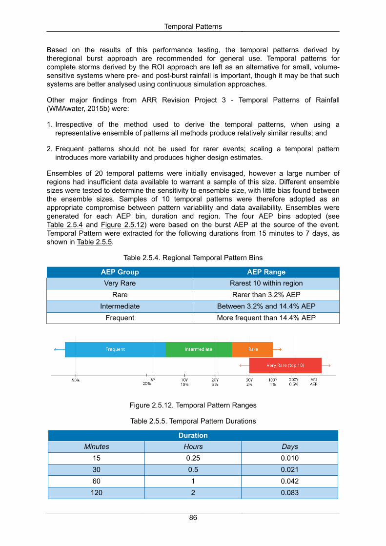
Based on the results of this performance testing, the temporal patterns derived by theregional burst approach are recommended for general use. Temporal patterns for complete storms derived by the ROI approach are left as an alternative for small, volume-sensitive systems where pre- and post-burst rainfall is important, though it may be that such systems are better analysed using continuous simulation approaches.

Other major findings from ARR Revision Project 3 - Temporal Patterns of Rainfall (WMAwater, 2015b) were:

1. Irrespective of the method used to derive the temporal patterns, when using a representative ensemble of patterns all methods produce relatively similar results; and

2. Frequent patterns should not be used for rarer events; scaling a temporal pattern introduces more variability and produces higher design estimates.

Ensembles of 20 temporal patterns were initially envisaged, however a large number of regions had insufficient data available to warrant a sample of this size. Different ensemble sizes were tested to determine the sensitivity to ensemble size, with little bias found between the ensemble sizes. Samples of 10 temporal patterns were therefore adopted as an appropriate compromise between pattern variability and data availability. Ensembles were generated for each AEP bin, duration and region. The four AEP bins adopted (see Table 2.5.4 and Figure 2.5.12) were based on the burst AEP at the source of the event. Temporal Pattern were extracted for the following durations from 15 minutes to 7 days, as shown in Table 2.5.5.

Table 2.5.4. Regional Temporal Pattern Bins

AEP Group AEP RangeVery Rare Rarest 10 within region

Rare Rarer than 3.2% AEPIntermediate Between 3.2% and 14.4% AEP

Frequent More frequent than 14.4% AEP

Figure 2.5.12. Temporal Pattern Ranges

Table 2.5.5. Temporal Pattern Durations

DurationMinutes Hours Days

15 0.25 0.01030 0.5 0.02160 1 0.042

120 2 0.083

Temporal Patterns

86

Duration180 3 0.125270 4.5 0.188360 6 0.250540 9 0.375720 12 0.5001080 18 0.7501440 24 12160 36 1.52880 48 24320 72 35760 96 47200 120 58640 144 610080 168 7

When selecting a small ensemble of temporal patterns it is important to capture the typical variability of the observed events. A methodology was therefore adopted that samples from observed events with the intent of generating a representative ensemble in terms of the variability of actual events, with no obvious bias. Whilst it is difficult to quantify or verify the achievement of this objective, steps have been undertaken to ensure the samples are broadly representative, including a visual check of all ensembles.

There are a large number of frequent events from which to select, however, the choice is more limited for rarer events.

For each AEP and duration bin the sampling of an ensemble of 10 patterns used the preferred criteria in Table 2.5.6. The relaxed criteria were used where less than 10 suitable patterns could be found using the preferred criteria.

Table 2.5.6. Temporal Pattern Selection Criteria

Preferred Criteria (for Data Rich Regions) Relaxed Criteria (for Data Sparse Regions)

No rarer embedded bursts n/aNo events overlapping in time n/a

Loading characteristics enforced Loading characteristics ignoredEvents from within a region Sampled from within region and

neighbouring region with similar climatic characteristics

While patterns containing embedded rarer bursts at their recording location were not selected, events can still have embedded bursts at other locations within the region. The presence of major embedded bursts may warrant filtering of patterns.

Temporal Patterns

87

5.6. Temporal Patterns for Areal Rainfall BurstsAs part of ARR Revision Project 3 - Temporal Patterns of Rainfall a series of areal average temporal patterns have been produced for different sized hypothetical catchments. These patterns average the spatial variability of rainfall in each time step which does remove some of the variability of actual space-time rainfall fields. The process of calculating areal temporal patterns involves identifying high rainfall areal events and calculating areal temporal patterns. A brief summary is provided in this chapter (refer to Podger et al. (2016) for more detail). Areal rainfall temporal patterns were calculated for the area and duration combinations listed in Table 2.5.7.

Table 2.5.7. Areal Rainfall Temporal Patterns - Catchment Areas and Durations

Variable Catchment Area (km2) 100, 200, 500, 1000, 2500, 5000, 10 000, 20

000, 40 000Durations (Hours) 12, 18, 24, 36, 48, 72, 96, 120, 144, 168

5.6.1. Areal Rainfall Time Series Grid for All AustraliaTo create sets of areal temporal patterns an areal rainfall grid was derived for 30 minute time steps using the events database (described in Book 2, Chapter 5, Section 3, ie. 2280 pluviographs). Rainfall values from these pluviographs were further filtered for long disaggregations and erroneously high rainfall values. A grid resolution of 0.025° identical to the grid cell size used for the design rainfalls (Book 2, Chapter 3) was chosen for simplicity of use. A natural neighbours algorithm, which is a variant of Thiessen polygons, was used to interpolate rainfall values from the pluviograph stations to each grid cell with rainfall values for each time step from January 1960 to December 2010.

5.6.2. Average Areal Rainfall CalculationThe approach aims to identify the largest set of independent areal rainfall events within the Temporal Pattern Regions shown in Figure 2.5.7 by not restricting catchments to a particular shape. For each combination of duration and area, a set of rectangular hypothetical catchments were used to sample the areal rainfall time series and create catchment average rainfalls. At each catchment centroid, 12 hypothetical catchments were trialled using the combinations of 3 aspect ratios (1.5, 2.3 and 3.6) and 4 rotations (0, 45, 90 and 135 degrees) shown in Figure 2.5.13. To best represent Australian catchments, the aspect ratios were chosen by selecting the 20th, 50th and 80th percentiles of shape factors calculated for the 798 catchments that were adopted for the RFFE method described in Book 3, Chapter 3. Average areal rainfall was calculated for a hypothetical catchment’s each time step simply by averaging the rainfall of all the grid cells with midpoints within the catchment area. To lessen computational requirements, larger time steps were used for larger catchment areas.

Temporal Patterns

88

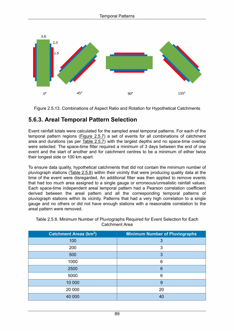
Figure 2.5.13. Combinations of Aspect Ratio and Rotation for Hypothetical Catchments

5.6.3. Areal Temporal Pattern Selection

Event rainfall totals were calculated for the sampled areal temporal patterns. For each of the temporal pattern regions (Figure 2.5.7) a set of events for all combinations of catchment area and durations (as per Table 2.5.7) with the largest depths and no space-time overlap were selected. The space-time filter required a minimum of 3 days between the end of one event and the start of another and for catchment centres to be a minimum of either twice their longest side or 100 km apart.

To ensure data quality, hypothetical catchments that did not contain the minimum number of pluviograph stations (Table 2.5.8) within their vicinity that were producing quality data at the time of the event were disregarded. An additional filter was then applied to remove events that had too much area assigned to a single gauge or erroneous/unrealistic rainfall values. Each space-time independent areal temporal pattern had a Pearson correlation coefficient derived between the areal pattern and all the corresponding temporal patterns of pluviograph stations within its vicinity. Patterns that had a very high correlation to a single gauge and no others or did not have enough stations with a reasonable correlation to the areal pattern were removed.

Table 2.5.8. Minimum Number of Pluviographs Required for Event Selection for Each Catchment Area

Catchment Areas (km2) Minimum Number of Pluviographs100 3200 3500 31000 62500 65000 6

10 000 920 000 2040 000 40

Temporal Patterns

89

Given that events were chosen simply based on their total rainfall depth, many of the longer duration patterns selected represented a shorter duration. Using the same procedure implemented in defining event extents in the events database, events that had extents less than the duration shorter than the duration of interest were removed.

5.6.4. Design Areal Temporal PatternsDue to the constraints on data quality, a full set of areal temporal patterns for every region, duration and area could not be generated. Therefore, to use areal temporal patterns for data sparse regions, it is necessary to sample patterns from climatically similar or nearby regions. This is especially a problem for longer durations, with some durations such as the 7 days not having enough patterns in any region. For these durations patterns must therefore be sampled from all of Australia, although data dense areas contain the majority of these events.

Like the point temporal patterns, meta-data on each pattern has been provided that allows practitioners to track the location and time of the event. Figure 2.5.14 compares the cumulative mass curves for 24 hour point and area temporal patterns. This demonstrates how the spatial averaging produced by areal temporal patterns reduces the variability. Figure 2.5.15 compares areal temporal patterns to the temporal patterns of the pluviograph closest to the area’s centroid, further highlighting a reduction in variability with the areal temporal patterns.

Figure 2.5.14. Comparison of Point Temporal Patterns and Areal Temporal Patterns - East Coast South Region - 1 Day

Temporal Patterns

90

Figure 2.5.15. Comparison of Areal Temporal Patterns and the Temporal Pattern of the Closest Pluviograph for the Same Event

5.7. Other Temporal Pattern Options

5.7.1. Use of Historical Temporal PatternsOn a large catchment with good quality temporal rainfall data it is not uncommon to have a reasonable number of historical patterns for events rarer than the 20% AEP event. Where there is a reasonable amount of local temporal data of appropriate AEPs across the catchment, it is appropriate to use this local data in place of regional temporal patterns. On large catchments, local point patterns will exhibit more variability and generally produce higher flow estimates than locally derived areal temporal patterns and should be used with caution. Some guidance on the use of local temporal patterns is provided in Book 2, Chapter 6.

Book 2, Chapter 6 provides advice on the assignment of historical temporal patterns when modelling observed events for calibration or analysis.

5.7.2. Complete Storm PatternsThe methodology developed for the pre-burst estimation pooled storm events from nearby catchments based on distance and IFD similarity. This approach was extended to develop ensembles of complete storms based on their critical burst duration by selecting events that can be put in a site specific duration probability bin with minimal scaling. The approach is somewhat experimental and has performed as well as burst approaches in limited testing. While categorising events on the basis of critical storm burst solves a lot of event selection problems but it is different from more traditional burst approaches. Aspects of the approach are described in ARR Revision Project 3 – Temporal Patterns of Rainfall Report (WMAwater, 2015c).

Temporal Patterns

91

The major differences are:

• Events are selected and duration binned on the basis of the critical rainfall duration;

• An event can only be used in one duration so a large storm sample is required;

• Duration bins represent a range of storm durations instead of a fixed duration;

• Event filtering is not required; and

• A new sample needs to be created at each location so a regional approach is not possible.

The process of binning events on the basis of their critical rainfall duration means that events that produce a catchment response because of rainfall over a certain duration can be placed in a bin of a very different duration. This means that under a critical duration approach these event are unlikely to influence the design estimate even if they produce the largest catchment response. This problem would not occur in a Monte Carlo framework that samples across durations.

Despite these limitations, a complete storm approach has the advantage of producing realistic rainfall storm events that have the correct burst IFD and storm volume characteristics. Coombes et al. (2015) showed considerable difference in basin performance on a small urban catchment between burst and complete storm approaches.

5.7.3. Continuous Data

While continuous simulation is generally more appropriate for modelling very frequent events there are some situations where event models might be appropriate. For these situations temporal patterns could be sampled from a local pluviograph or sampled from a generated continuous sequence using the techniques described in Book 2, Chapter 7.

5.8. Climate Change ImpactsVery little information is known about how climate change will affect storm or burst temporal patterns. The most definitive work is by Wasco and Sharma (2015) which analysed the relationship between burst patterns from 79 Australian rainfall gauges and temperature variations. This study found that, regardless of the climate region or season, temperature increases are associated with patterns becoming less uniform, with the largest fractions increasing in rainfall intensity and the lower fraction decreasing. The scaling of the largest fractions was more pronounced in short duration bursts, and rainfall gauges to the north of the country showed more pronounced changes. While this work is based on the present climate, it provides an insight into how patterns could change under a future warming. Such climate changes would also affect IFD characteristics.

Westra et al. (2013) proposed rainfall sequences for future climates could be constructed by sampling historical rainfall patterns corresponding to warmer days at the same location, or from locations which have an atmospheric profile more reflective of expected future climate. Such an approach could conceptually be applied in the selection of design burst patterns but would require significant testing.

It is currently not possible to provide practical advice to practitioners on this aspect of temporal patterns. It is recommended that until further studies are completed, for simulations

Temporal Patterns

92

applying projected climate change, the temporal patterns applied should be those derived for existing climatic conditions but recognising the additional uncertainty in simulation results.

5.9. Temporal Pattern Application and Pre-burst

5.9.1. GeneralFor the majority of problems, the practitioner needs to select a temporal pattern based on the area and probability of the event they are modelling. For Very Rare and Extreme events specific advice is provided in Book 8. The derivation of long duration events (both point or areal temporal patterns) present a number of challenges. Many of the events selected in the IFD Annual Maxima Series were from shorter duration events and can not be selected as longer duration temporal patterns. Some long duration events are more like consecutive events with none or little rainfall in between shorter events. For this reason, in most locations, it was necessary to borrow temporal patterns (point and areal) from adjoining regions. Daily rainfall gauges located in the catchment of interest should give a good insight into the applicability of longer duration temporal patterns approaching 7 days.

Point temporal patterns should be used for catchments less than 75 km2. Areal temporal patterns have been derived for a number of different catchment areas. Table 2.5.9 provides a guide to applying the areal patterns. Both point and areal temporal pattern sets can be downloaded from the ARR Data Hub (Babister et al (2016), accessible at http://data.arr-software.org/)

Table 2.5.9. Areal Temporal Pattern Sets for Ranges of Catchment Areas

Range of Target Catchment Areas (km2) Catchment Area of Designated Areal Temporal Pattern Set (km2)

75 – 140 100140 – 300 200300 – 700 500700 – 1600 10001600 – 3500 25003500 – 7000 5000

7000 – 14,000 10,00014,000 – 28,000 20,000

28,000 + 40,000

5.9.2. Ensemble ConsiderationsThe use of an ensemble of 10 temporal patterns as discussed in Book 2, Chapter 5, Section 5 is recommended. The temporal patterns have been chosen to represent the variability in observed patterns. Given the run times of two dimensional hydraulic models it is not practical to run all 10 patterns (for multiple durations). A more practical approach would be to run a separate hydrological modelling process of the whole catchment of interest in order to determine the average pattern in terms of peak flow or volume depending on the problem (Book 2, Chapter 5, Section 10). It is not recommended that the temporal pattern that represents the worst (or best) case be used by itself for design. Testing has demonstrated that on most catchments large number of events in the ensemble patterns are clustered around the mean and median.

Temporal Patterns

93



When selecting a single representative (average) pattern the practitioner needs to look at the whole catchment response hydrograph and not local inflow hydrographs.

The ensemble of 10 pattern provides a range of plausible answers. The practitioner should consider the benefits of investigating multiple temporal patterns or Monte Carlo for sensitive designs and solutions.

Running an ensemble of ten temporal patterns through a two dimensional model could be time consuming. One option is to double the grid cell size which will decrease run time 8 fold.

5.9.3. Upscaling of PatternsPractitioners are cautioned to avoid or minimise upscaling patterns from frequent events to rare events. In some locations the dominate rainfall mechanism might change with probability and frequent events can exhibit more variability than rarer events. While there are good meteorological reasons for very rare events to exhibit less variability then frequent events (need reference) the causes are probably more complex than a single reason and somewhat region specific. Testing carried out as part of the ARR Revision Project 3 – Temporal Patterns of Rainfall has shown that in some locations that upscaling can be a significant issue (Loveridge et al., 2015) while in other locations results were insensitive. In nearly all testing locations results were relatively insensitive to down scaling of patterns.

5.9.4. Dealing with Inconsistencies and Smoothing of ResultsTesting has demonstrated that inconsistent results can sometimes occur with AEP when the bin patterns are drawn from changes particularly between the frequent and intermediate bins. The problem was more pronounced in drier regions where a large part of the rainfall was taken up by losses. In some cases, flood magnitude decreased for rarer AEPs while in others the change with AEP was very stepped. On some catchments, the critical duration varied inconsistently with AEP. Where problems are mainly caused by the pattern bin changing two simple options are suggested, either:

1. Draw from both bins at the boundary effectively doubling the ensemble size which effectively smooths the results; or

2. Replacing the frequent probability bin with the intermediate bin to ensure a smooth catchment response with rainfall.

Consideration should be given to filtering out (or excluding) embedded bursts of lower AEP by re-distributing rainfalls of high intensity to other time increments proportionally to their magnitude (e.g. Herron et al. (2011)). In some situations results will still need to be smoothed.

5.9.5. Practical IssuesIf modelling events greater than 5 day, the practitioner should look at the daily rainfall gauge totals for gauges within the catchment and confirm what the 7 day events look like in the catchment compared to the regional patterns.

If 10 temporal patterns are not available for a given region, duration and frequency bin then patterns were taken from other similar regions (Table 2.5.10). For 7 day events there was not

Temporal Patterns

94

enough patterns and all regions were pooled. Local knowledge can be used to add events to the ensemble that weren’t selected in the regional sample.

Table 2.5.10. Alternate Regions Used for Data

Region Alternate Region

Southern Slopes (Tasmania)

Southern Slopes (mainland),

Murray BasinSouthern Slopes

(mainland)Murray Basin,

Southern Slopes (Tasmania),

Central Slopes, East Coast South

Murray Basin Central Slopes, Southern Slopes

(mainland), Flatlands East,

East Coast SouthCentral Slopes Murray Basin,

East Coast South, East Coast North,


East Coast South East Coast North, Central Slopes, Murray Basin, Southern

Slopes (mainland)

East Coast North East Coast South, Wet

Tropics, Central Slopes, Murray

BasinWet Tropics Monsoonal

North, East Coast North

Monsoonal North Wet Tropics, East Coast

North, Rangelands

WestRangelands

WestRangelands,

Flatlands West

Temporal Patterns

95

Region Alternate Region

Rangelands Flatlands West, Flatlands East, Flatlands West

Flatlands West Flatlands East, Rangelands

WestFlatlands East Flatlands West,

Flatlands West, Rangelands

5.9.6. Point and Areal Temporal Pattern Meta-DataMeta-data is provided (accessed via http://data.arr-software.org/) which describes where the regional point and areal temporal patterns were originally located and when they occurred. This includes:

• Event ID - Unique ID given to each pattern;

• Region - The region in which the pattern applies;

• Region (Source) - The region the temporal pattern occurred in;

• Burst Loading - Classified events as front, middle or back (see Book 2, Chapter 5, Section 3);

• Burst Loading (%) - The percentage of the event that falls into the loading category;

• Burst Depth - Source temporal pattern burst depth. This is the total depth the original pattern had, patterns are given in percentages and not original depths;

• AEP (source) - The source temporal pattern AEP at the location it was recorded. This AEP is based of the 2016 IFDs and the burst depth of the event;

• Burst Start - The time and date at which the burst began;

• Burst End - The time and date at which the burst ended; and

• Pluviograph number - The ID of the pluviograph as from the Bureau of Meteorology.

There will be events that weren’t picked up in the regional sample however, local experience will allow them to be used in the ensemble (note when doing this the front, middle and back loading of the regional needs to be considered).

5.9.7. Very Rare Point Temporal PatternsFor point temporal patterns 4 bins are provided (Figure 2.5.12). The very rare bin contains the rarest ten patterns within the region. These patterns may not feature in the rare bin for the region as the rare bin is sampled randomly.

5.9.8. Region ConsiderationsThe regional point temporal patterns have been sourced from various locations throughout the region and due to IFD gradients within the regions embedded bursts may occur.

Temporal Patterns

96


Depending on the severity of the embedded burst, filtering of rarer bursts is recommended. When minor embedded bursts occur in only a few of the 10 patterns in the ensemble filtering can be neglected. Testing has shown with the 2013 Intensity Frequency Duration data that there are some locations where all observed temporal patterns would have embedded bursts.

Locations close to region boundaries might experience storm mechanisms represented by both regions. In these cases it is recommended to run a larger ensemble of all patterns, ie. All 10 patterns from each neighboring region.

5.9.9. Pre-burstThe treatment is dependent on the approach taken to model losses and the magnitude of the pre-burst. In most cases practitioners will use just the median pre-burst and median storm initial loss. However, in some cases the practitioner may sample from distributions of pre-burst and initial loss. As pre-burst varies with location, duration and probability the adopted approach will vary, but it is probably sensible to adopt a consistent approach across durations and probabilities being assessed. Pre-burst for a specific location can be downloaded from the ARR Data Hub (Babister et al (2016), accessible at http://data.arr-software.org/).

In locations and for durations that do not have significant pre-burst (Figure 2.5.10), the pre-burst depth can be ignored when applying a temporal pattern. Therefore the Burst IL (ILb) can be taken as the Storm IL (ILs). In those locations where the pre-burst is significant a number of approaches are possible:

• Storm IL is greater than Pre-burst – Pre-burst should be taken out of the storm IL

ie. ILs – Pre-burst = ILb;

• Storm IL is approximately equal to Pre-burst – In the case where storm IL and pre-burst are close to equal IL is satisfied and no IL needs to be taken from the burst temporal pattern;

• Pre-burst is greater than storm IL - In the case where pre-burst is larger than the storm IL there are a number of options:

• Apply a pre-burst temporal pattern after taking out the Storm IL. There is little research that has investigated pre-burst temporal patterns;

• Test the sensitivity of pre-burst on the resultant flood estimate and determine if it can be ignored;

• Apply a complete storm approach instead of a burst approach e.g. Coombes et al. (2015).

5.10. ExampleThe Tennant Creek Catchment is located in the Northern Territory and was used for the ARR research Projects 3 and 6. The catchment and catchment location is shown in Figure 2.5.16. It is located in the Rangeland Region for temporal patterns. The temporal pattern data for the region can be extracted at http://data.arr-software.org/. In this particular example a RORB model was set up for the catchment. The model was previously calibrated with an ILb=0 and a CL=7 mm/hr. As the catchment area is 72.3 km2 it was decided that the critical duration would be between 60 minutes and 1440 minutes (1 day).

Temporal Patterns

97




Figure 2.5.16. Tennant Creek Catchment

For this example only the 1% AEP patterns were run through the hydrologic model. 10 patterns from the rare AEP bin and the Rangelands region were run for each of the following durations:

• 60 minute

• 120 minute

• 180 minute

• 270 minute

• 360 minute

• 540 minute

• 720 minute

• 1080 minute

• 1440 minute

Figure 2.5.17 is a presentation of the results in a box plot. The results are also presented in Table 2.5.11, it should be noted that even though the columns are labelled bursts 1 to 10 they are not the same storms across the durations. The box plot presents clearly that the 180 minute duration is critical. The average peak flow of the 180 minute duration bursts (277.35 m3/s) should then be taken as the 1% AEP flow. If a practitioner wanted to run a

Temporal Patterns

98

pattern through a hydraulic model and it was not practical to run all 10 patterns, the pattern closest to the average (shown in Table 2.5.11) is Burst number 1.

Figure 2.5.17. Duration Box plot for the 1% AEP

Table 2.5.11. Flows for the 1% Annual Exceedance Probability for Ten Burst Events

Duration 1% AEP Peak Flow (m3/s)Burst 1 Burst

2Burst

3Burst

4Burst

5Burst

6Burst

7Burst

8Burst

9Burst

10Average Median

60 146.9 173.8 179.6 145.7 157.2 159.6 169.4 141.6 148.8 150.2 157.28 153.7120 221.5 230.2 261.9 238.1 260.3 259.5 233 240.2 244.9 262.6 245.22 242.55180 279.4 264.8 279.6 274.4 263.5 273.5 264.1 272.8 273.1 268.3 277.35 273.95270 262.5 241.1 284.1 288.5 306.6 264.7 266.8 261.2 287.8 254.4 271.77 265.75360 255.5 285.5 214.4 243.9 199.7 223.2 246.3 246.3 269.8 283.9 246.85 246.3540 230.9 163.1 168.7 195.4 254.7 203.2 236.6 235.6 177.5 259.7 212.54 217.05720 193.7 173.5 188.1 143.8 254.9 243.6 195.2 210.3 172.3 224.2 199.96 194.45

1080 197.7 159.2 103.8 239 179.1 151.3 191.2 160.5 148.1 151.5 168.14 159.851440 177.9 113.5 144 108.8 222.5 103.4 173.2 156.9 272 130.5 160.27 150.45

5.11. ReferencesAskew, A.J. (1975), Use of Risk Premium in Chance-Constrained Dynamic Programming. Water Resources Research, 11(6): 862-866.

Temporal Patterns

99

Babister, M., Trim, A., Testoni, I. and Retallick, M. 2016. The Australian Rainfall and Runoff Datahub, 37th Hydrology and Water Resources Symposium Queenstown NZ

Ball, J.E. (1994), 'The influence of storm temporal patterns on catchment response', Journal of Hydrology, 158(3-4), 285-303.

Brown, J.A.H. (1982), A Review of flood estimation procedures, Proceedings of the workshop on spillway design, Department of National Development and Energy, AWRC Conference Series No.6.

CSIRO and Bureau of Meteorology (2015), Climate Change in Australia Information for Australia's Natural Resource Management Regions: Technical Report, CSIRO and Bureau of Meteorology, Australia.

Coombes, P., Babister, M. and McAlister, T. (2015).Is the Science and Data underpinning the Rational Method Robust for use in Evolving Urban Catchments, Proceedings of the 36th Hydrology and Water Resources Symposium Hobart 2015.

Cordery, I., Pilgrim D.H. and Rowbottom I.A. (1984), Time patterns of rainfall for estimating design floods on a frequency basis. Wat. Sci. Tech., 16(8-9), 155-165.

French, R.H. (1985), Open Channel Hydraulics, McGraw-Hill Book Company, New York.

Green, J.H., Xuereb, K. and Siriwardena, L. (2011), Establishment of a Quality Controlled Rainfall Database for the Revision of the (IFD) Estimates for Australia, Proceedings of 34th IAHR World Congress, Brisbane, 26 June-1st July 2011.

Hall, A.J. and Kneen, T.H. (1973), Design Temporal Patterns of Storm Rainfall in Australia, Proc. Hydrology Symposium, Inst. Eng. Aust., pp: 77-84

Herron, A., Stephens, D., Nathan, R. and Jayatilaka, L. (2011), Monte Carlo Temporal Patterns for Melbourne. In: Proc 34th World Congress of the International Association for Hydro- Environment Research and Engineering: 33rd Hydrology and Water Resources Symposium and 10th Conference on Hydraulics in Water Engineering. Barton, A.C.T.: Engineers Australia, pp: 186-193.

Hill, P.H., Graszkiewicz, Z., Taylor, M. and Nathan, R. (2014), Australian Rainfall and Runoff Revision Project 6: Loss Models for Catchment Simulation, Phase 4, October 2014, Report No. P6/S3/016B.

Hill, P.I., Graszkiewicz, Z., Loveridge, M., Nathan, R.J. and Scorah, M. (2015), Analysis of loss values for Australian rural catchments to underpin ARR guidance. Hydrology and Water Resources Symposium 2015, Hobart, 9-10 December 2015.

Hoang, T.M.T., Rahman, A., Weinmann, P.E., Laurenson, E. and Nathan, R. (1999) Joint Probability description of design rainfall, Water 99 Joint congress, Brisbane.

Huff, A. (1967), Time distribution in heavy storms, Water Resources Research, 3: 1007-1019.

IEAust. (1977), Australian Rainfall and Runoff: flood analysis and design. The Institution of Engineers Australia. Canberra.

Keifer, C.J. and Chu, H.H. (1957), Synthetic storm pattern for drainage design, ASCE Journal of the Hydraulics Division, 83(4), 1-25.

Temporal Patterns

100

Kuczera, G., Lambert, M., Heneker, T., Jennings, S., Frost, A. and Coombes, P. (2003) Joint Probability and design storms at the cross roads, Proceedings of the 28th International Hydrology and Water Resources Symposium, Wollongong.

Loveridge, M., Babister, M., Retallick, M. and Testoni, I. (2015). Testing the suitability of rainfall temporal pattern ensembles for design flood estimation, Proceedings of the 36th Hydrology and Water Resources Symposium Hobart 2015.

Meighen, J. and Kennedy, M.R. (1995), Catalogue of Significant Rainfall Occurrences over Southeast Australia , HRS Report No. 3, Hydrology Report Series, Bureau of Meteorology, Melbourne, Australia, October.

Milston, A.K. (1979), The influence of temporal patterns of design rainfall in peak flood discharge, Thesis (M.Eng.Sci.), University of New South Wales.

Nathan, R.J. and Weinmann, P.E. (1995), The estimation of extreme floods - the need and scope for revision of our national guidelines. Aus J Water Resources, 1(1), 40-50.

Nathan, R.J., Weinmann, P.E. and Hill, P.I. (2002), Use of a Monte-Carlo framework to characterise hydrologic risk. Proc., ANCOLD conference on dams, Adelaide.

Nathan, R., Weinmann, E., Hill, P. (2003) Use of Monte Carlo Simulation to Estimate the Expected Probability of Large to Extreme Floods, Proc. 28th Int. Hydrology and Water Res. Symp., Wollongong, pp: 1.105-1.112.

Pattison, A, (ed) 1977, Australian Rainfall and Runoff: Flood Analysis and Design, The Institution of Engineers Australia

Phillips, P. and Yu, S. (2015), How robust are OSD and OSR Systems?, 2015 WSUD & IECA, Sydney.

Phillips, B.C., Lees, S.J. and Lynch, S.J. (1994), Embedded Design Storms - an Improved Procedure for Design Flood Level Estimation?. In: Water Down Under 94: Surface Hydrology and Water Resources Papers; Preprints of Papers. Barton, ACT: Institution of Engineers, Australia, 235-240. National conference publication (Institution of Engineers, Australia), No.94/15.

Pilgrim, DH (ed) (1987) Australian Rainfall and Runoff - A Guide to Flood Estimation, Institution of Engineers, Australia, Barton, ACT, 1987.

Pilgrim, D.H. and Cordery, I. (1975), Rainfall temporal patterns for design floods, Journal of the Hydraulics Division, 101(1), 81-95.

Pilgrim, D.H., Cordery, I. and French, R. (1969), Temporal patterns of design rainfall for Sydney, Institution of Engineers, Australia, Civil Eng. Trans., CE11: 9-14.

Podger, S., Babister, M., Brady, P. (2016), Deriving Temporal Patterns for Areal Rainfall Bursts, Proceedings of the 37th Hydrology and Water Resources Symposium Queenstown 2016.

Rahman, A., Weinmann, P.E., Hoang, T.M.T. and Laurenson, E.M. (2002), Monte Carlo simulation of flood frequency curves from rainfall. Journal of Hydrology.

Retallick, M., Babister, M., Varga, C., Ball, J. and Askew, A. (2009), Do Filtered patterns resemble real patterns? Proceedings of the Hydrology and Water Resources Symposium, Newcastle 2009, Engineers Australia.

Temporal Patterns

101

Rigby, E. and Bannigan, D. (1996), The Embedded design storm concept - A critical review, 23rd Hydrology and Water Resources Symposium Hobart.

Rigby, E., Boyd, M., Roso, S. and Van Drie, R. (2003), Storms, Storm bursts and flood estimation- A need for review of the AR&R procedures, Proceedings of the 28th International Hydrology and Water Resources Symposium, Wollongong.

Roso, S. and Rigby, E. (2006), The impact of embedded design storms on flows within a catchment, Proceedings of the 30th Hydrology and Water Resources Symposium Launceston 2006.

Sih, K., Hill, P. and Nathan, R. (2008), Evaluation of Simple Approaches to Incorporating Variability in Design Temporal Patterns. In: Lambert, Martin (Editor); Daniell, TM (Editor); Leonard, Michael (Editor). Proceedings of Water Down Under 2008. Modbury, SA: Engineers Australia; Causal Productions, pp: 1049-1059.

Varga, C., Ball, J., Babister, M. (2009), An Alternative for Developing Temporal Patterns, Proceedings of the Hydrology and Water Resources Symposium, Newcastle 2009, Engineers Australia

WMAwater (2015a), Australian Rainfall and Runoff Revision Project 3: Temporal Patterns of Rainfall, Part 1 - Development of an Events Database, Stage 3 Report, October 2015.

WMAwater (2015b), Australian Rainfall and Runoff Revision Project 3: Temporal Patterns of Rainfall, Part 3 - Preliminary Testing of Temporal Pattern Ensembles, Stage 3 Report, October 2015.

WMAwater (2015c), Australian Rainfall and Runoff Revision Project 3: Temporal Patterns of Rainfall, Part 3 - Preliminary Testing of Temporal Pattern Ensembles, Stage 3 Report, October 2015.


Webb McKeown and Associates, (2003), Assessment of the variability of rates of rise for hydrographs on the Hawkesbury Nepean River, December 2003.

Weinmann, P., Rahman, A., Hoang, T., Laurenson, E., Nathan, R. (2000), Monte Carlo Simulation of flood Frequency Curves, Proceedings of Hydro 2000, 3rd International hydrology and water resources symposium, Perth, Inst. Of Engineers Australia, pp: 564-569.


Wood, J.F. and Alvarez, K. (1982), Review of Pindari Dam Design Inflow Flood Estimate, Proceedings of the workshop on spillway design, Department of National Development and Energy, AWRC Conference Series No.6.

Temporal Patterns

102

Chapter 6. Spatial Patterns of RainfallPhillip Jordan, Alan Seed, Rory Nathan



6.1. IntroductionAs discussed in Book 2, Chapter 2, the description of rainfall events used in most currently applied design flood estimation methods is based on a reductionist approach, where the temporal and spatial variations of rainfall within an event are represented separately by typical temporal patterns and spatial patterns of event rainfall.

This chapter provides practitioners with recommendations on the derivation and application of spatial patterns of rainfall for use in design flood estimation using representations of varying complexity. This includes recommendations for reconstructing the space-time patterns of rainfall for the observed events used in the calibration of hydrologic catchment models.

There are a number of items where the authors recognise that the guidance adopted in this chapter is uncertain and where benefit would be obtained from further research to better quantify and potentially reduce the impact of those uncertainties on design flood estimation practice. Section 6 lists and briefly discusses the residual uncertainties relating to various aspects of the derivation and application of spatial and space-time patterns of rainfall, and recommends potential areas of future investigation.

6.2. Methods for Deriving Spatial Patterns of Rainfall for Events

6.2.1. Precipitation Observation Methods and Uncertainties Associated with Reconstructing Space-Time Rainfall PatternsThere is no accepted method for determining the space-time pattern of rainfall that is not influenced by the resolution and accuracy of networks of rainfall observations.

Rainfall gauges provide data on the rainfall depths observed at the point location of the rainfall gauge over different periods of time. Daily reporting rainfall gauges provide rainfall depths recorded at the gauge over the preceding day period, with the Bureau of Meteorology’s typical practice being that these gauges report at 9:00 am local time on each day. Pluviograph or tipping bucket rainfall gauges can provide rainfall depths observed at a point location for sub-daily temporal resolution. They can provide rainfall depths with temporal resolutions down to less than one minute.

Rainfall gauges are subject to some observational errors but they typically provide relatively accurate measurements of the time series of rainfall recorded at a point location. They can under-record rainfall during periods of high winds, particularly for snow or for when rainfall intensities are low. There can be errors associated with estimating rainfall rates from tipping bucket rainfall gauges over defined periods of time from the recorded times of the bucket tips. During periods of very high rainfall intensity, tipping bucket rainfall gauges can be subject to errors induced by the bucket failing to tip or tipping when it is partially full. Rainfall

103

gauges can also be subject to errors in manual recording of the data or electronic transmission of data from telemetered rainfall sites.

The chief uncertainty introduced by a network of rainfall gauges is in accurately observing the space-time pattern of rainfall across an area because they cannot observe variations in rainfall patterns between the gauges (Seed and Austin, 1990; Barnston, 1991; Bradley et al., 1997).

Remote sensing approaches can provide estimates of rainfall intensity observed on a spatial grid across a wide observation domain for a given period of time. The two most commonly available remote sensing approaches for rainfall estimation are ground-based weather radar and satellite observing systems.

Weather radars measure the reflectivity returned by rain drops, hail stones or snow, which are converted into a rainfall intensity estimate. There are several different types of errors in this process that degrade the accuracy of the radar rainfall measurement (Joss and Waldvogel, 1990; Collier, 1996). The analysis of radar data to derive space-time patterns requires specialist expertise that lies outside the scope of these guidelines. However, such analysis could be considered for large or high risk studies which are able to secure the specialist expertise required. Weather radar approaches typically provide estimates of rainfall intensities that are more accurate on a relative basis within the space-time field of the event than in absolute magnitude terms.

6.2.2. Data AvailabilityRainfall gauge observations are available at many locations across Australia for very long time periods, with data available at some sites since the middle of the 19th century (refer to Book 2, Chapter 3). By contrast, reliable archives of data from remote sensing (weather radar and satellite based instruments) are only available from about the mid 1990s. For many events, the only data that will be available to the practitioner to reconstruct the space-time pattern of rainfall will be from rainfall gauges.

The practitioner should make use of the available data to reconstruct the space-time pattern of rainfall across the catchment or study area for the events that are to be utilised in model calibration and design flood simulation. The practitioner should assess the suitability of the rainfall data that is available for the event for reconstructing the space-time pattern, including rainfall gauges and any data that is available from remote sensing.

The practitioner should consider the events that are to be used for constructing the space-time patterns of rainfall. Factors that should be considered in selecting events are the:

• Number of sites and locations, relative to the catchment, of daily rainfall gauges;

• Number of sites and locations, relative to the catchment, of continuous rainfall gauges;

• Existence or otherwise of remotely sensed data;

• Likely accuracy of quantitative rainfall estimates derived from remotely sensed data;

• Purpose of estimating the space-time rainfall pattern, whether it is for hydrological model calibration, deriving a space-time pattern or spatial pattern for inclusion in design flood simulation or both;

• Existence and quality of recorded flood levels, flood extents and gauged flows for the event, which make it a candidate for model calibration; and

Spatial Patterns of Rainfall

104

• Estimated AEP of the flood event or the rainfall total for the event over the catchment of interest, relative to the AEP of the design floods that are to be estimated.

The practitioner may need to make judgements between using the space-time pattern for an older event, for which there is no remote sensing data and relatively poor coverage of rain gauge data but which produced higher flood levels and a more recent event that has remotely sensed data and/or better coverage of rain gauge data but which produced a smaller flood.

6.2.3. Construction of Space-Time Patterns from Rainfall Gauge Networks

When estimating the space-time pattern of rainfall from rainfall gauges there is an uncertainty introduced to the estimates in the interpolation of the unobserved rainfall at locations between the gauges (for example, Urbonas et al. (1992) and Ball and Luk (1998)).

The conventional approach applied in flood estimation for approximating the space-time pattern of rainfall from gauge networks has been:

1. To estimate the spatial pattern of rainfall for the whole rainfall event; and

2. To disaggregate the rainfall accumulation for each part of the spatial domain, often a model subarea or subcatchment, using the temporal pattern observed at a particular rainfall gauge.

The conventional approach is a valid method in most situations but it may be that a more sophisticated approach involving construction of different spatial patterns for different increments of the event are required when spatial or temporal variability of the rainfall pattern for the event is large (Umakhanthan and Ball, 2005). Considerations for application of each of the two steps are discussed in Book 2, Chapter 6, Section 2 and Book 2, Chapter 6, Section 2. Potential alternative approaches are discussed in Book 2, Chapter 6, Section 2.

6.2.3.1. Construction of Spatial Patterns

The spatial pattern should be constructed using rainfall totals from daily rainfall gauges and where available continuous rainfall gauges. Gauges should be obtained from both within the catchment or study area and for a region around the catchment. As an indicative value, the region used for constructing the spatial pattern should extend to include gauges that are within at least 10 km of the catchment or study area boundary or further if internal catchment gauges are further from the boundary.

There is no preferred technique for constructing a spatial pattern of rainfall for an event. Hand drawing of rainfall contours informed by the rainfall totals at the gauges remains a valid approach that will produce acceptable results for many rainfall events.

Spatial interpolation techniques using a computer usually involve interpolation between the point observations onto a grid, defined in either a geographic or projected Cartesian coordinate system. The grid resolution should be sufficiently fine to capture the spatial variability in the rainfall field at a meaningful scale for the catchment. It is recommended that the resolution of the grid should be 1 km (for a projected grid) or 0.01° (for a geographic grid) or finer. There are many potential approaches that have been developed for spatial interpolation (Verworn and Haberlandt (2011) and the references therein), including:


105

• Construction of Thiessen polygons, which is equivalent to adopting the rainfall depth from the nearest neighbour rainfall gauge when applied using a grid;

• Weighting of rainfall using the inverse of the square of the distances to the gauges;

• Natural neighbours;

• Spline interpolation algorithms;

• Ordinary Kriging; and

• Variants on Kriging, such as indicator Kriging, regression Kriging and Kriging with external drift.

Some Kriging and spline interpolation algorithms allow for the use of a covariate in the interpolation algorithm, which may improve the accuracy of the interpolation. Either elevation or design rainfall intensities for a relevant AEP and duration may provide appropriate covariates that improve the accuracy of the interpolation, particularly in catchments or study areas that are subject to appreciable and consistent orographic effects.

Gridded daily rainfall data sets are available from SILO and the Australian Water Availability Project (Jones et al., 2009). These data sets may be useful for providing spatial patterns of rainfall events but they should be used with caution as they were not derived with the intention of being used for design flood estimation (refer to Book 1, Chapter 4, Section 9 and Book 2, Chapter 7, Section 2).

Regardless of the approach that is used to produce the spatial pattern, the practitioner should check the spatial pattern produced by mapping it against the point values observed at rainfall gauges. If the mapping reveals anomalies in the interpolation approach, an alternative method should be adopted. Where large gaps in rainfall gauge coverage exist (particularly in mountainous areas) careful review of the simplifying assumptions made in the interpolation procedure should be undertaken by the practitioner to avoid unrealistic spatial patterns.

Rainfall totals for each model subarea should be estimated from the spatially interpolated rainfall field for the event by averaging the rainfall totals at all grid cells that intersect with the spatial extent of the model subarea. Mathematically, this is represented by:

�� = ∑�, �� ∩ �, ��, �∑�, �� ∩ �, � (2.6.1)

where Ss is the rainfall depth for the total event applied to model subarea, s, �� ∩ �, �is the area of overlap between grid cell at coordinate location (i,j) in the interpolated grid and the model subarea s, and ��, �is the interpolated rainfall total for the grid cell.

For rainfall events that extend for a period longer than 24 hours, it may be useful to construct spatial patterns for separate time periods of the event to investigate the temporal evolution of the event.


106

6.2.3.2. Disaggregation Using Temporal Patterns from Observed Pluviograph Data

A conventional approach adopted is to disaggregate the total rainfall for each subarea of a rainfall runoff model using the temporal pattern recorded at a recording rain gauge, using the formula:

��, � = ��, �∑��, � (2.6.2)

Where Rs,i is the rainfall depth applied to model subarea, s, for model time increment, i; SS is the total event rainfall for model subarea s; rg,i is the rainfall depth recorded at gauge, g , for model time increment, i; and the summation is formed for all time increments over the event.

Where data is available from more than one recording rainfall gauge, this provides options to the practitioner on which gauge to select to provide the temporal pattern for each subarea of the model. An assumption is often made that the most appropriate pattern would be provided by the recording rainfall gauge that is located closest, by horizontal distance, from the centroid of the model subarea. Whilst the closest gauge by physical distance makes intuitive sense, it is not necessarily the case that it must provide the most appropriate pattern for allocating the temporal pattern of a particular subarea. The practitioner may consult other information, such as catchment topography, data on wind velocities during the event or remote sensing data to guide the selection of an alternative to the nearest gauge for providing the temporal pattern. The practitioner may also use other information on the meteorology of the event to justify use of an adjusted temporal pattern for disaggregation. For example, if information was available that a particular rainfall event was moving in a particular direction at an average velocity of 15 km/h and a model subarea was located 30 km downwind of a rainfall gauge, it may be justified to adjust the temporal pattern recorded at this gauge by moving it backward in time by two hours, to represent the estimated travel time of the storm from the rainfall gauge to the model subarea.

The time series of rainfall at each recording gauge should be checked before it is used for disaggregation. The event total rainfall at each recording gauge should be checked, where available, against the event total rainfall at other daily recording and continuously rainfall gauges in the vicinity. A gauge should not be used if significant anomalies are identified in the recorded data for the site.

6.2.3.3. Alternative Approaches to Construction of Space-Time Patterns

A potential alternative approach to construct the space-time pattern of rainfall for an event from rainfall gauge data only is to construct a three dimensional space-time pattern grid. In this approach, the overall event spatial pattern would be interpolated onto a grid, using one of the potential approaches discussed in Book 2, Chapter 6, Section 2. The total rainfall for each grid cell would then be disaggregated using the temporal pattern from an assigned rainfall gauge, using a similar method as discussed in Book 2, Chapter 6, Section 2. For each time increment, a summation is formed for all of the grid cells that intersect spatially with each model subarea. Each subarea would then have its own, potentially unique, temporal pattern for the event.

In a catchment that is well instrumented with rainfall gauges, it is possible to perform a spatial interpolation on to a grid for each time increment. The gridded rainfall for each time


107

increment would then be summed to produce a temporal pattern for each model subarea. If this approach is used, the total rainfall across the event should be calculated for each subarea and then compared to the rainfall computed from spatially interpolating the event total rainfall only. Adjustments should be considered to the approach if the totals for any subarea differ by more than 5%.

6.2.4. Space-Time Patterns for Calibration

Simulation of historical flood events for calibration purposes includes reconstruction of the space-time pattern of rainfall over the catchment by the practitioner. The values of the apparent optimum set of model parameters for a given event can be influenced by the approach taken to estimate the space-time pattern of rainfall for the event. For example, if a catchment is simulated using an initial loss-continuing loss runoff generation model, then if all other parameters and inputs are the same a lower continuing loss rate is likely to be required to generate the same volume of runoff if a uniform spatial pattern is adopted compared with a non-uniform spatial pattern. The practitioner should consider and articulate the influence of assumptions made in deriving the space-time pattern of rainfall for the event on the values of the runoff-routing model parameters calibrated for the event.

The spatial coverage of pluviographs around a catchment may be relatively sparse. This introduces uncertainty into the estimation of the actual temporal pattern of rainfall for any given subarea or grid cell of a model. Whilst a reasonable assumption may be that the temporal pattern for a given model subarea would be defined by the pluviograph that is nearest in horizontal distance, this may not necessarily produce the most accurate temporal pattern for the model subarea. As discussed in Book 2, Chapter 6, Section 2, a more accurate representation of the space-time rainfall pattern over a model subarea may be produced by judicious adjustment of the temporal pattern observed at a gauge or selection of a temporal pattern from a gauge that is not physically closest to the subarea centroid. Adjusting the assignment of temporal patterns to subareas in this manner may assist the practitioner in achieving a more robust calibration of the model parameters to the event. Adjustment of temporal patterns and temporal pattern assignment is therefore allowable, particularly if meteorological evidence is provided to support the decision.

The spatial or space-time pattern should be interpolated on to a regular grid that is constructed over the catchment. The resolution of the grid should be sufficiently fine to allow for spatial variations to be adequately represented. In most situations, the grid resolution should be selected so that there are at least 4 grid cells overlapping with the smallest subcatchment to be adopted in the model.

Remote sensing data, where available, may be used to estimate the space-time rainfall field of an event for catchment modelling system calibration. If used, the space-time rainfall field should be corrected using data from rainfall gauges, using a recommended approach for adjusting for the mean field bias.

6.3. Spatial and Space-Time Patterns for Design Flood EstimationThe aim of a design flood estimation should be to provide a probability neutral transformation between the design rainfall inputs and design flood characteristics

The space-time pattern or set of space-time patterns adopted for design flood estimation should be chosen in a manner that, when coupled with other aspects of the catchment


108

modelling system, preserves the AEP of the design flood when derived from its causative rainfall.

6.3.1. Guidance for Catchments up to and Including 20 km2: Single Uniform Spatial PatternCatchments with areas up to and including 20 km2 are sufficiently small that there is little available data to derive a spatial pattern. For these catchments, it is usually acceptable to adopt a uniform spatial pattern.

If there is sufficient density of continuously rainfall gauges that have recorded a number of rainfall events, using this data to derive alternative (non-uniform) design spatial patterns may be considered.

6.3.2. Guidance for Catchments Greater than 20 km2: Single Non-Uniform Spatial PatternAs a minimum, it is recommended that a single non-uniform spatial pattern is applied to catchments with an area greater than 20 km2. The non-uniform spatial pattern should be derived with the aim of replicating the systematic variation in spatial variability that would be expected across the catchment during rainfall events of similar AEP to the design floods that are being estimated.

For estimation of design flood events more frequent than and including the 1% AEP event, the spatial pattern should be estimated using the spatial pattern derived from the design rainfall grids (as discussed in Book 2, Chapter 3) across the catchment for the relevant IFD surface for the AEP and duration. In many cases there will be little relative variation in spatial distribution between probabilities or adjacent duration. Different spatial patterns could be applied for different durations. Alternatively, one spatial pattern may be estimated for the critical duration and this single spatial pattern may then be applied for all durations.

For estimation of design flood events rarer than 1% AEP with durations of 6 hours and less on catchment areas less than 1000 km2, the spatial pattern should be derived in accordance with Woolhiser (1992) for the relevant duration. Use of different spatial patterns for different AEP ranges may introduce inconsistencies at the adjacent limits of each method, and if this is the case then any such inconsistencies should be smoothed in an appropriate fashion.

For estimation of design flood events rarer than 1% AEP with durations of 9 hours and greater or on catchment areas greater than 1000 km2, the spatial pattern should be derived from the Topographic AdjustmentFactor (TAF) database derived from the generalised PMP method that is relevant for zone that the catchment is located in. Use of different spatial patterns for different AEP ranges may introduce inconsistencies at the adjacent limits of each method, and if this is the case then any such inconsistencies should be smoothed in an appropriate fashion.

For large studies and particularly for large catchments the practitioner should investigate and analyse the variability in spatial patterns between events. Where topography is dominant or large events are generally produced by a single rainfall mechanism there is likely to be only moderate variability between events but for some catchments there can be significant variations in space-time patterns between events. The practitioner should prepare and examine maps of the spatial pattern of rainfall for each event as a whole and for time slices, for example each 24 hour period, using an approach described in Book 2, Chapter 6, Section 2. These spatial patterns should be compared to rainfall accumulations from


109

Intensity Frequency Duration analysis for a relevant duration and AEP (refer to Jordan et al., 2015 for an example of this approach). Consistency in spatial patterns between events may reveal that it is acceptable to apply a single spatial pattern for all design flood estimates, particularly if it is consistent with the design rainfall analysis.

As discussed in Book 2, Chapter 4, Section 3, partial area storms should always be explicitly considered for catchments with an area exceeding 30 000 km2 and it should be considered for catchments larger than 5000 km2.

6.3.3. Alternative Approach: Monte Carlo Sampling from Separate Populations of Spatial and Temporal PatternsA more advanced approach that may be justified would be Monte Carlo simulation by sampling from a set of space-time rainfall patterns across the catchment of interest. There are two potential options that may be considered for implementing this approach: (1) sampling from separate populations of spatial and temporal patterns for the catchment; or (2) sampling from a single set of “linked” space-time patterns for the catchment.

The first approach requires the assembly of:

• A set (or population) of spatial patterns across the catchment of interest from a number of observed rainfall events; and

• A set of temporal patterns from a number of observed rainfall events.

The spatial pattern of rainfall should be assembled for each event in the population, in accordance with the methods discussed in Book 2, Chapter 6, Section 2. The catchment average rainfall accumulation should be computed for each event and continuously rainfall gauges located in or near the catchment should be used to estimate the duration over which most of the total rainfall accumulation was likely to have fallen in the catchment. The estimated catchment average depth for the event and the estimated rainfall event duration should be used with the table of design rainfall estimates for the catchment, after application of the applicable ARF, to estimate the AEP of the rainfall for each event.

Similarly, the temporal pattern of rainfall should be assembled for each event in the population. The temporal pattern may be assembled at a single continuously rainfall gauge or from a combination of a number of continuously rainfall gauges located in the vicinity of the catchment or study area. The temporal pattern should be analysed to extract the maximum burst for a number of different durations. The rainfall accumulations over these bursts should be compared to the design rainfall estimates at the location of the rainfall gauge, without the application of the ARF, to estimate the AEP of the rainfall for each event.

A sample of patterns for use in the Monte Carlo simulation should be selected from the set of historical events that are available. A sufficient number of events should be selected to allow for a meaningfully large sample in the Monte Carlo simulation. It is expected that a minimum of five patterns would be required each of the sets of spatial and temporal patterns. However, events should only be selected for inclusion in the sample if they are relatively similar in terms of the AEP of the rainfall to the range of AEP that design flood estimates are being produced. Ideally, the spatial patterns and temporal patterns of events selected for the Monte Carlo sample should have an estimated AEP that is between 1/10 and ten times the AEP of the design flood event to be simulated. Adding more historic spatial patterns to an ensemble does not necessarily improve the simulation accuracy of a Monte Carlo model, as the additional patterns that are most likely to be added would be at the more common end of the AEP range. In many catchments, design floods of interest are caused by rainfall events


110

with a specific hydrometeorological mechanism, which is then associated with a range of space-time rainfall patterns that are different to those observed in rainfall events caused by more commonly occurring hydrometeorological conditions.

Unless there is hydrometeorological evidence to the contrary, all potential spatial and temporal patterns in the sets available for sampling should be given equal probability of selection in the Monte Carlo simulation.

After the spatial and temporal patterns for the design rainfall burst have been selected stochastically, the patterns should be scaled so that the catchment average rainfall depth for the design rainfall burst matches the depth generated stochastically by the sampling scheme.

There has been limited assessment on methods for selection of space-time patterns for use in Monte Carlo simulation for design flood estimation. Further research should be conducted in this area to provide more robust guidance on the minimum number of temporal and spatial patterns in the sampling populations, the range of AEP represented by the populations of spatial and temporal patterns to be sampled compared to the AEP of the depth of the rainfall burst and the relative probabilities to be applied in the selection of spatial and temporal patterns.

6.3.4. Alternative Approach: Monte Carlo Sampling from Single Population of Space-Time PatternsThe foregoing approach ignores the potential dependency that exists between the temporal and spatial characteristics of storms. According, an alternative approach would involve sampling the space-time pattern for the event from a single population of space-time rainfall patterns over the catchment. The sample of space-time patterns may be assembled from space-time patterns of rainfall observed during historical rainfall events in the catchment. The space-time patterns should be assembled in accordance with the methods discussed in Book 2, Chapter 6, Section 2. The estimated catchment average depth for different burst durations within the event and the estimated rainfall event duration should be used with the table of design rainfall estimates for the catchment, after application of the applicable ARF, to estimate the AEP of the rainfall for each event.

It may be an option to transpose space-time rainfall patterns from an area with a good observational network for rainfall to a catchment with a poorer observational network. If this is done, the practitioner should only transpose (non-dimensional) space-time rainfall patterns from an area that is subject to rainfall events that are driven by similar hydrometeorological processes. The transposition region should be subject to similar orographic influences. In some cases, the space-time patterns may need to be rotated to maintain consistency between the spatial gradients in the space-time patterns and orographically influenced gradients in the design rainfall gridded data.

6.3.5. Spatial Patterns for Pre-Burst and Post-Burst RainfallIf pre-burst or post-burst rainfall is to be applied, it is recommended that, unless there is evidence to the contrary, the spatial pattern applied to the pre-burst or post-burst rainfall should be the same as the spatial pattern applied for the design rainfall burst.

6.3.6. Spatial Patterns for Continuous Rainfall SeriesBook 2, Chapter 7 discusses the production of continuous rainfall time series for production of design flood estimation using continuous simulation approaches. Book 2, Chapter 7


111

includes an approach to post-process the sequence of generated rainfall data for the catchment of interest so that the characteristics of the large and extreme rainfall events in the sequence reflect the Intensity Frequency Duration (IFD) statistics for the catchment of interest. If such an adjustment is conducted then it is recommended that the IFD statistics used as the basis of the adjustment are calculated for the catchment of interest after multiplying by the ARF that is applicable for the catchment area.

Book 2, Chapter 7 recommends that the IFD adjustment is applied for a set of target durations of either 6 minutes, 1 hour and 3 hours or for a set of durations of 6 minutes, 30 minutes, 1 hour, 3 hours, 6 hours and 12 hours. It is recommended therefore that the following procedure is adopted:

1. The IFD statistics for each of the target durations are calculated as the average of the point IFD statistics across the catchment, for each of the standard AEP (1EY to 1% AEP);

2. The ARF are computed for each of the target durations, at each of the standard AEP, for the total area of the catchment to be modelled;

3. The catchment IFD statistics are computed for each of the target durations, at each of the standard AEP, as the product of the point IFD statistics (from step 1) and the ARF (from step 2);

4. The catchment IFD statistics (from step 3) are applied in the modification procedure as the depths at the selected target durations.

The practitioner may be adopting a catchment model that allows for spatial distribution of the simulated rainfall sequence across the catchment. If this is the case, it is recommended that the generated sequence of rainfall is scaled for each portion of the model (subcatchment or grid cell as applicable to the particular model) to reflect the spatial distribution of rainfall that would be typically observed across the catchment. Parts of the catchment that are typically wetter would have rainfall depths applied in the model that are larger than the generated mean rainfall depth across the catchment but with the same timing and sequencing. Conversely, parts of the catchment that are typically drier would have rainfall depths applied in the model that are smaller than the generated mean rainfall depth across the catchment but with the same timing and sequencing.

Selection of an appropriate means of deriving the spatial pattern for a continuous simulation model that includes spatial distribution depends upon the AEP of the design events that are of most interest and the flood response characteristics of the catchment:

• When the focus is on estimation of floods with relatively frequent AEP (around 10% or more common) and for catchments with large moisture stores having significant relation between antecedent rainfall and the annual maximum flood, it is recommended that the spatial pattern applied in the model should be estimated from contours of mean annual rainfall;

• However when the focus is on estimation on floods with rarer AEP (5% or rarer) and for catchments where the influence of large moisture stores are less significant, it is recommended that the spatial pattern should be selected in a manner that is consistent with the recommendation for design event simulation (refer to Book 2, Chapter 6, Section 3 and Book 2, Chapter 6, Section 3 above).


112

6.4. Potential Influences of Climate Change on Areal Reduction Factors, Spatial and Space-Time PatternsThere is very little credible guidance on how climate change is projected to influence ARF, spatial patterns or space-time patterns of rainfall events used in design flood estimation. Abbs and Rafter (2009) used dynamic downscaling using a regional climate model to identify that increases in rainfall intensity are likely to be greater in those areas of south-east Queensland that are subject to orographic enhancement than those areas that are not. There is insufficient evidence to confirm whether this projection is an artefact of the downscaling approach and whether it would still apply if the dynamic downscaling model were forced with Global Circulation Model results from the more recent Intergovernmental Panel on Climate Change (2013). Even if it were proven for Southeast Queensland, it is not clear that the guidance would be more generally applicable to other parts of Australia.

It is recommended that until credible further studies are completed showing otherwise, for simulations applying projected climate change ARF, spatial patterns and space-time patterns of design rainfall should be the same as derived under existing climatic conditions.

6.5. Worked ExamplesAll of the worked examples in this chapter use data for the Stanley River catchment, which is in the upper part of the Brisbane River basin in Southeast Queensland. Worked example 1 demonstrates three different mathematical algorithms for estimating the spatial pattern of design rainfall for a particular rainfall event that occurred in January 2013. Worked examples 2 through 4 demonstrate the process for design flood estimation, from calculation of ARF and catchment average design rainfall estimates (Worked example 2), through calculation of a representative spatial pattern (Worked example 3), to production of design flood estimates using a runoff-routing model (Worked example 4).

6.5.1. Catchment Used for Worked Examples

The Stanley River catchment drains into Somerset Dam, which is in the upper part of the Brisbane River basin in South-east Queensland. Figure 2.6.1 shows a map of the 1324 km2

shows the catchment area, with Somerset Dam located in the southwestern corner. For this worked example, the Stanley River catchment is modelled using a runoff-routing model with 76 subcatchments, with subareas as shown in Figure 2.6.1.

Design rainfall estimates are developed for the Stanley River at Woodford, which has a catchment area of 245 km2. The catchment to Woodford is the north-eastern portion of the catchment to Somerset Dam and for this worked example it includes fifteen subcatchments in the runoff-routing model.

A significant feature of the Stanley River catchment is the appreciable gradient in rainfall that is typically observed during large rainfall events. Tropical cyclones, ex-Tropical Cyclones, East Coast Lows and other rainfall producing systems typically feed moisture into the catchment from the Pacific Ocean. Since the north-eastern part of the catchment is only 20 km from the coast but the western side of the catchment is almost 70 km from the coast, the typical direction of storm movement and typical direction of flow of warm moist air from the ocean results in a gradient of rainfall totals that reduce from east to west across the catchment in most rainfall events. The strength of the rainfall gradient is enhanced by orographic effects with the highest totals typically also occurring in the north-eastern part of the catchment.


113

Figure 2.6.1. Stanley River Catchment, Showing Runoff-routing Model Subcatchments and the Locations of Daily rainfall and pluviograph gauges

6.5.2. Worked Example 1: Interpolation of Spatial Patterns for an Event Using Various MethodsTropical Cyclone Oswald generated heavy rainfall in the Stanley River catchment between 23 and 29 January 2013, generating flooding in the catchment. Rainfall totals were observed at 20 continuous rainfall gauges around the Stanley River catchment, as shown in Figure 2.6.2 (rainfall data supplied by SeqWater). The blue circles are scaled in proportion to the rainfall depth recorded at the gauge.


114

Figure 2.6.2. Rainfall totals (mm) Recorded at Rainfall Gauges for the January 2013 Event in the Vicinity of the Stanley River Catchment

The January 2013 rainfall event was used in this worked example to demonstrate various approaches to interpolation of spatial patterns of historical rainfall events, for the purpose of calibration of runoff-routing models. For all of the algorithms, the rainfall totals were first interpolated onto a 0.5 km resolution grid over the catchment. Rainfall totals for each of the 76 runoff-routing model subcatchments were then computed from the average of the rainfall totals at the grid cells that overlapped each subcatchment.

Rainfall totals were spatially interpolated using:

1. Thiessen polygons, as shown in Figure 2.6.3. Observed totals at gauges are shown as blue circles in both panels. The top panel shows interpolation to a 0.5 km grid (red shading), whilst the bottom panel shows calculated subcatchment average depths in mm (red circles);

2. Inverse distance weighting, as shown in Figure 2.6.4. Observed totals at gauges are shown as blue circles in both panels. The top panel shows interpolation to a 0.5 km grid (red shading), whilst the bottom panel shows calculated subcatchment average depths in mm (red circles); and

3. Ordinary Kriging, as shown in Figure 2.6.5. Ordinary Kriging was applied using a linear semi-variogram that was fitted to observed rainfall totals at the 20 gauges from the January 2013 event, as shown in Figure 2.6.6.Observed totals at gauges are shown as blue circles in both panels. The top panel shows interpolation to a 0.5 km grid (red shading), whilst the bottom panel shows calculated subcatchment average depths in mm (red circles).


115

Figure 2.6.3. Application of Thiessen Polygons- Rainfall Totals for the January 2013 Event - Stanley River Catchment


116

Figure 2.6.4. Application of Inverse Distance Weighting - Rainfall Totals for the January 2013 Event - Stanley River Catchment


117

Figure 2.6.5. Application of Ordinary Kriging - Rainfall Totals for the January 2013 Event - Stanley River Catchment


118

Figure 2.6.6. Observed Semi-variogram and Fitted Linear Semi-variogram for the January 2013 Rainfall Event for Stanley River catchment, Applied in the Ordinary Kriging Algorithm

6.5.3. Worked Example 2: Calculation of Catchment Average Design Rainfall Depths and Areal Reduction FactorsDesign rainfall intensities were extracted at the centroids of each of the fifteen runoff-routing model subcatchments in the catchment of the Stanley River to Woodford from for the 1% AEP and 24 hour duration. The weighted average of the point rainfall depths was computed, as shown in Table 2.6.1.

The catchment area for the Stanley River to Woodford is 245.07 km2. The ARF for 24 hour duration was computed by applying Equation (2.4.2), with the relevant coefficients for the East Coast North region (from the 1st row of Table 2.4.2). For the 1% AEP event the relevant ARF is given by:�� = �� 1, [1− �(��− �log10��)��−�+��(0.3 + log10��)+ℎ10��1440 (0.3 + log10��)]

(2.6.3)


119

�� = �� 1, [1− 0.327(245.070.241− 0.448log10(1440))1440−0.36+0.00096 x 245.070.481440−0.21(0.3 + log10(0.01))+0.012 x 10−0.001 x 245.07 x 14401440(0.3 + log100.01)](2.6.4)

�� (24ℎ��) = 0.929 (2.6.5)

Table 2.6.1. Calculation of Weighted Average of Point Rainfall Depths for the 1% AEP 24 hour Design Rainfall Event for the Stanley River at Woodford

Centroid Latitude (°)

Centroid Longitude (°)

Area (km2) 1% AEP, 24 hour Design Point

Rainfall Depth at Centroid

(mm)

Design Depth x Area (ML)

-26.8467 152.8510 5.66 511.4 2896.0-26.8060 152.8320 17.31 518.5 8973.2-26.7895 152.8776 16.84 570.4 9605.7-26.8201 152.8719 16.55 530.9 8787.9-26.8631 152.8756 16.25 517.7 8414.3-26.8110 152.8000 15.10 527.0 7956.5-26.8135 152.9077 15.01 551.3 8276.7-26.8998 152.7978 23.45 467.1 10954.8-26.8828 152.8459 22.74 493.3 11218.6-26.9171 152.7620 17.78 454.2 8076.1-26.8557 152.7656 16.34 490.0 8007.1-26.9190 152.8552 16.24 502.6 8164.3-26.8568 152.8185 15.62 484.6 7571.4-26.9354 152.8096 15.12 465.2 7031.9-26.8445 152.7889 15.04 508.9 7654.0

Totals 245.07 123588.6Weighted Average = 123588.6 / 245.07 504.3

The catchment average design rainfall depth for 1% AEP, 24 hour duration for the Stanley River at Woodford was therefore computed by multiplying the ARF by the weighted average of the design point rainfall depths:Catchment ave. design rainfall depth (24 ℎ��, 1%��) = ARF (24 ℎ�) × Weighted ave. of design point rainfall depths (24 ℎ�, 1%��) (2.6.6)

Catchment average design rainfall depth(24ℎ��, 1%��)=0.929 × 504.3 mm (2.6.7)Catchment average design rainfall depth(24ℎ��, 1%��)=468.6 mm (2.6.8)


120

The calculation was repeated for the catchment of the Stanley River to Woodford for each combination of standard durations between 3 and 72 hours and the 1 Exceedance per Year to the 1% AEP. These computations are shown for the Stanley River catchment to Woodford in Table 2.6.2.

The catchment area for the Stanley River to Somerset Dam is 1324 km2. The calculation of catchment average design rainfall intensities, after application of areal reduction factors, is shown in Table 2.6.3. Comparing the top panels of Table 2.6.2 and Table 2.6.3, for the corresponding AEP and durations the weighted averages of the point rainfall depths for the catchment to Somerset Dam are less than those for Woodford, due to the gradient in the IFD grids. Comparing the middle panels of Table 2.6.2 and Table 2.6.3, for the corresponding AEP and durations the ARF catchment to Somerset Dam are less than those for Woodford because the catchment area to Somerset Dam is larger. Hence comparing the bottom panels of Table 2.6.2 and Table 2.6.3, for the corresponding AEP and durations the catchment average design rainfall depths to Somerset Dam are less than those for Woodford.

Table 2.6.2. Stanley River Catchment to Woodford: Calculation of Catchment Average Design Rainfall Depths (bottom panel) from Weighted Average of Point Rainfall Depths (top

panel) and Areal Reduction Factors (middle panel)

Weighted Average of Point Rainfall Depths (mm)Duration (hours)

1 Exceedance per

Year

Annual Exceedance Probability

50% 20% 10% 5% 2% 1%3 54.1 61.6 85.7 102.8 120.0 143.5 162.16 70.5 81.5 117.3 142.8 168.7 204.6 233.312 94.4 110.8 164.9 203.8 243.8 299.5 344.524 128.1 152.0 231.4 289.5 349.8 434.8 504.348 170.2 202.2 310.5 391.2 476.1 598.0 699.372 195.5 231.7 355.3 448.5 547.6 691.4 812.1

Areal Reduction FactorDuration (hours)

1 Exceedance per

Year


50% 20% 10% 5% 2% 1%3 0.841 0.835 0.812 0.794 0.776 0.753 0.7356 0.879 0.876 0.864 0.854 0.845 0.832 0.82312 0.909 0.907 0.901 0.896 0.891 0.884 0.87924 0.945 0.944 0.940 0.938 0.935 0.932 0.92948 0.959 0.959 0.957 0.955 0.954 0.951 0.95072 0.966 0.966 0.964 0.963 0.962 0.961 0.959

Catchment Average Design Rainfall Depth (mm)


121

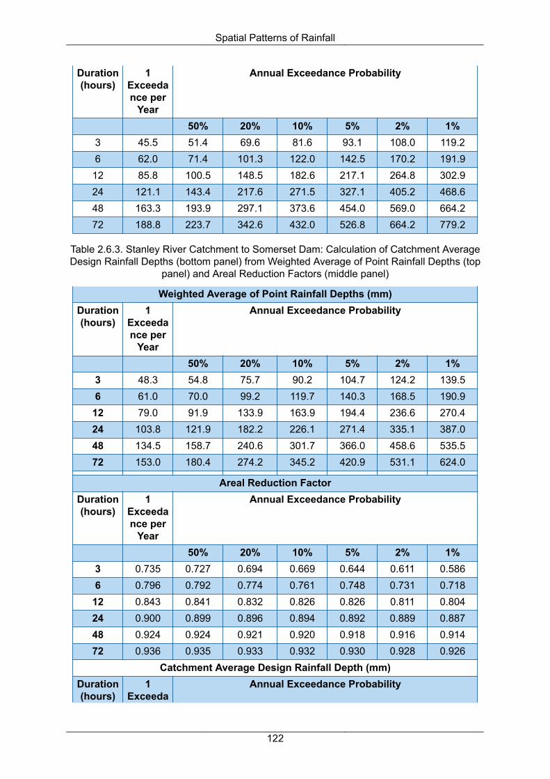
Duration (hours)

1 Exceedance per

Year


50% 20% 10% 5% 2% 1%3 45.5 51.4 69.6 81.6 93.1 108.0 119.26 62.0 71.4 101.3 122.0 142.5 170.2 191.912 85.8 100.5 148.5 182.6 217.1 264.8 302.924 121.1 143.4 217.6 271.5 327.1 405.2 468.648 163.3 193.9 297.1 373.6 454.0 569.0 664.272 188.8 223.7 342.6 432.0 526.8 664.2 779.2

Table 2.6.3. Stanley River Catchment to Somerset Dam: Calculation of Catchment Average Design Rainfall Depths (bottom panel) from Weighted Average of Point Rainfall Depths (top

panel) and Areal Reduction Factors (middle panel)

Weighted Average of Point Rainfall Depths (mm)Duration (hours)

1 Exceedance per

Year


50% 20% 10% 5% 2% 1%3 48.3 54.8 75.7 90.2 104.7 124.2 139.56 61.0 70.0 99.2 119.7 140.3 168.5 190.912 79.0 91.9 133.9 163.9 194.4 236.6 270.424 103.8 121.9 182.2 226.1 271.4 335.1 387.048 134.5 158.7 240.6 301.7 366.0 458.6 535.572 153.0 180.4 274.2 345.2 420.9 531.1 624.0

Areal Reduction FactorDuration (hours)

1 Exceedance per

Year


50% 20% 10% 5% 2% 1%3 0.735 0.727 0.694 0.669 0.644 0.611 0.5866 0.796 0.792 0.774 0.761 0.748 0.731 0.71812 0.843 0.841 0.832 0.826 0.826 0.811 0.80424 0.900 0.899 0.896 0.894 0.892 0.889 0.88748 0.924 0.924 0.921 0.920 0.918 0.916 0.91472 0.936 0.935 0.933 0.932 0.930 0.928 0.926

Catchment Average Design Rainfall Depth (mm)Duration (hours)

1 Exceeda



122

nce per Year

50% 20% 10% 5% 2% 1%3 35.5 39.9 52.5 60.4 67.4 75.9 81.86 48.6 55.4 76.8 91.1 105.0 123.2 137.012 66.6 77.3 111.4 135.3 159.3 191.8 217.424 93.3 109.6 163.3 202.2 242.1 298.1 343.448 124.3 146.6 221.7 277.5 336.0 420.0 489.572 143.2 168.7 255.9 321.6 391.5 492.9 578.1

6.5.4. Worked Example 3: Calculation of Spatial Pattern for Design Flood Estimation

Book 2, Chapter 6, Section 3 recommends that estimation of design flood events of 1% AEP and more frequent, the spatial pattern for design event should be estimated using the spatial pattern derived from the design rainfall grids across the catchment for the 1% AEP and for a duration that is anticipated to correspond to the duration of the rainfall burst that is likely to be critical at the specified location.

For the Stanley River catchment, this approach was demonstrated using the 24 hour duration IFD data. For the catchment to Woodford, point rainfall depths at each of the subcatchment centroids were divided by the weighted average of the point rainfall depths to derive the non-dimensional spatial pattern, as computed in Table 2.6.4 and mapped in the top panel of Figure 2.6.7. To model the 1% AEP 24 hour design flood event for the catchment, the non-dimensional spatial pattern was multiplied by the catchment average design rainfall depth to Woodford for this duration (468.6 mm, after application of the ARF), as computed in Table 2.6.4 and mapped in the top panel of Figure 2.6.8.

The process was repeated for the Stanley River to Somerset Dam, with the map of the non-dimensional spatial pattern shown in the bottom panel of Figure 2.6.7 and the map of the design depths for the 1% AEP, 24 hour duration event in the bottom panel of Figure 2.6.8.

Table 2.6.4. Calculation of Design Spatial Pattern for Stanley River at Woodford



1% AEP, 24 hour Design Point


(mm)

Point Rainfall Depth Divided by Weighted Average of

Point Rainfall Depths (%)

Depth to be Applied to

Model 1% AEP, 24 hour Design

Event (mm)

-26.8467 152.8510 511.4 101.4 475.2-26.8060 152.8320 518.5 102.8 481.8-26.7895 152.8776 570.4 113.1 530.0-26.8201 152.8719 530.9 105.3 493.3-26.8631 152.8756 517.7 102.7 481.0-26.8110 152.8000 527.0 104.5 489.7-26.8135 152.9077 551.3 109.3 512.3


123



1% AEP, 24 hour Design Point


(mm)

Point Rainfall Depth Divided by Weighted Average of

Point Rainfall Depths (%)

Depth to be Applied to

Model 1% AEP, 24 hour Design

Event (mm)

-26.8998 152.7978 467.1 92.6 434.0-26.8828 152.8459 493.3 97.8 458.4-26.9171 152.7620 454.2 90.1 422.0-26.8557 152.7656 490.0 97.2 455.3-26.9190 152.8552 502.6 99.7 467.0-26.8568 152.8185 484.6 96.1 450.3-26.9354 152.8096 465.2 92.2 432.3-26.8445 152.7889 508.9 100.9 472.9

Weighted Average 504.3 100.0 468.6


124

Figure 2.6.7. Non-dimensional Spatial Pattern (percentage of catchment average design rainfall depths) for Events with AEP of 1% and more Frequent for Stanley River to Woodford

(top panel) and Stanley River to Somerset Dam (bottom panel)


125

Figure 2.6.8. Design Spatial Pattern of Design Rainfall Depths 1% AEP 24 hour Event for Stanley River to Woodford (top panel) and Stanley River to Somerset Dam (bottom panel)


126

6.5.5. Worked Example 4: Application to Design Flood EstimationDesign flood peak estimates were produced for the Stanley River at its outlet (inflow to Somerset Dam) using a RORB runoff-routing model of the catchment. A more complete description of this case study is contained in Jordan et al. (2015).

Design peak flow estimates at Somerset Dam inflow were produced from a number of Monte Carlo simulations that were implemented within RORB. There were a number of common elements to all of these simulations:

• all adopted the same catchment average design IFD information multiplied by the areal reduction factor for the applicable duration from Jordan et al. (2013);

• all were run using the stratified Monte Carlo sampling scheme that is implemented within RORB (Laurenson et al., 2010);

• all were run for rainfall burst durations of 6, 9, 12, 18, 24, 36 and 48 hours, with the peak flow defined by the highest flow from among these durations at each AEP;

• all simulations sampled from the same non-dimensional probability distribution of initial loss values defined by Ilahee (2005), scaled by a median initial loss of 40 mm;

• all adopted a constant continuing loss rate of 1.7 mm/hour across all subcatchments;

• all adopted a RORB non-linearity parameter, m, value of 0.8; and

• all simulations adopted RORB delay parameter, kc , values of 20 for the catchment upstream of Peachester, 20 for the catchment between Peachester and Woodford, 16 for the catchment upstream of Mount Kilcoy and 45 for the residual catchment to Somerset Dam inflow.

The Monte Carlo simulations differed from one another in their approach to sampling of spatial, temporal and space-time patterns across the catchment, as shown in Table 2.6.5.

Table 2.6.5. RORB Model Scenarios Run for Worked Example on Stanley River Catchment to Somerset Dam

Case Spatial Pattern(s) Temporal Pattern(s)1 Single spatial pattern derived

from IFD analysis, 1% AEP 24 hour spatial pattern

Random sampling from a set of 13 temporal patterns for each duration, derived from

the bursts of the corresponding duration within the 13 selected events listed

in Table 1 of Jordan et al. (2015)

2 Random sampling from a set of 13 space-time patterns for each duration, derived from the bursts of the corresponding

duration within the 13 selected events listed in Table 1 of Jordan et al. (2015)

Sinclair Knight Merz (2013) fitted a Generalised Extreme Value (GEV) distribution to the estimated annual maxima inflows to Somerset Dam over the period between 1955 and 2013.


127

The estimated inflow flood peak for the 1893 flood of 6200 m³/s was included as a censored flow in the analysis. The distribution fitted to the estimated observed inflows was used to test the performance of the RORB model simulations.

Figure 2.6.9 shows that both cases of RORB model simulations all provide an excellent match to the fitted flood frequency quantiles across the range between 5% and 0.2% AEP. Design peak inflow floods to Somerset Dam were insensitive to whether space-time patterns are randomly sampled or only temporal patterns are randomly sampled in the Monte Carlo simulation (case 1 versus case 2).

Figure 2.6.9. Flood Frequency Curves for Stanley River at Somerset Dam Inflow Derived from Analysis of Estimated Annual Maxima and from RORB Model Simulations

6.6. Recommended Further Research

6.6.1. Deriving Spatial and Space-Time Patterns of Rainfall for EventsThe capacity to collect and archive remotely sensed rainfall estimates and to provide that information to practitioners is growing. It is recommended that the Bureau of Meteorology continues to invest in routinely archiving remotely sensed rainfall data, particularly from its network of ground based weather radars. It is recommended that the Bureau of Meteorology continues to expand the provision of quality controlled and bias corrected space-time rainfall estimates to practitioners, for use across the industry. It is recommended that tools should be further developed and disseminated to practitioners to facilitate the use of remotely sensed rainfall data.


128

It is recommended that further research is conducted into quality control of remotely sensed estimates of the space-time pattern of rainfall.

It is recommended that further research is conducted to improve methods for mean field bias correction of remotely sensed rainfall data. The recommendations on the approaches that should be adopted for mean field bias correction should be updated in these guidelines in accordance with the findings from this research.

At the time of writing, there was not an agreed optimum method for deriving space-time rainfall patterns from rainfall gauge data for Australian catchments, although Verworn and Haberlandt (2011) provide reasonable guidance. It is recommended that further research is conducted to identify a superior method (or set of potential methods) that are demonstrated to reliably produce more accurate estimation of the space-time rainfall field from gauge observations. It may be that the optimum method depends upon meteorological characteristics of the storm, density of rainfall gauges, orographic characteristics of the region or other factors. It is recommended that further research is conducted to explore these influences on the selection of optimum spatial and space-time interpolation methods for flood model calibration and design flood estimation.

6.6.2. Space-Time Patterns for Calibration of Rainfall Runoff Models to Historical Floods

As discussed in Book 2, Chapter 6, Section 2, the calibrated parameter values for a rainfall runoff model for a particular flood event may be sensitive to the method used to derive the space-time rainfall field for the event, particularly where the field is interpolated from a network of rain gauges only. It is recommended that further research is conducted into the sensitivity of rainfall-runoff routing model parameter estimation to assumptions made in the process of estimating the space-time rainfall field gauged rainfall data.

6.6.3. Spatial and Space-Time Patterns for Design Flood Estimation

It is recommended that further research is conducted into hydrometeorological drivers for space-time rainfall patterns that lead to flood events across different regions of Australia. The research should be used to inform practitioners on how they may choose between the space-time patterns of rainfall from different historical rainfall events to form the populations of space-time, spatial and temporal patterns in design flood simulation schemes. Research may investigate seasonal influences on space-time patterns of rainfall for use in design flood estimation.

There has been limited assessment on methods for selection of space-time patterns for use in Monte Carlo simulation schemes for design flood estimation. Further research should be conducted in this area, to provide more robust guidance on:

• The minimum number of space-time or temporal and spatial patterns in the sampling population(s);

• The range of AEP represented by the populations of space-time or spatial and temporal patterns to be sampled compared to the AEP of the depth of the rainfall burst; and

• The relative probabilities to be applied in the selection of patterns from the relevant populations.


129

It is recommended that further research is conducted into the validity of transposing space-time patterns from one location to another. The research should assist in defining valid regions over which transposition of space-time patterns is acceptable and conversely boundaries between regions over which transposition should not occur. The research should also consider other aspects of transposition, such as the validity or otherwise of rotating space-time patterns and the maximum recommended angles for rotation.

Further research should be conducted into methods for stochastic generation of space-time rainfall patterns. The research should investigate how orographic influences should be incorporated into the stochastic generation algorithms in a way that replicates the space-time variability of rainfall observed in historic rainfall events. Research should also develop more definitive guidance on appropriate statistical tests to demonstrate that the stochastically generated space-time rainfall patterns replicate the space-time statistical characteristics of historical rainfall events that are sufficiently large to have caused flood events.

6.6.4. Potential Influences of Climate Variability and Climate ChangeClimatic variability at inter-decadal scales is likely to influence the relative occurrence and severity of different types of heavy rainfall events. Hydrometeorological understanding of the connection between storm types and ARFs may enable predictions of the future trend in ARFs that will occur as the climate changes over coming decades. Hydrometeorological understanding of the connection between storm types and space-time rainfall patterns may also allow for more accurate guidance to practitioners on the potential changes in space-time patterns that is predicted as a result of climate change.


Ball, J.E. and Luk, K.C. (1998), Modelling spatial variability of rainfall over a catchment, J. Hydrologic Engineering, 3(2), 122-130.

Barnston, A.G., (1991), An empirical method of estimating raingauge and radar rainfall measurement bias and resolution, J. Applied Meterology, 30: 282-296.

Bradley, S.G., Gray, W.R., Pigott, L.D., Seed, A.W., Stow, C.D. and Austin, G.L. (1997), Rainfall redistribution over low hills due to flow perturbation, J. Hydrology, 202, 33-47.

Collier, C.G. (1996), Applications of Weather Radar Systems: A Guide to Uses of Radar in Meteorology and Hydrology. 2d ed. John Wiley, p: 383

Ilahee, M. (2005), Modelling Losses in Flood Estimation, A thesis submitted to the School of Urban Development Queensland University of Technology in partial fulfilment of the requirements for the Degree of Doctor of Philosophy, March 2005.

Intergovernmental Panel on Climate Change, (2013), Climate Change 2013: The Physical Science Basis, Contribution of Working Group I to the Fifth Assessment Report of the Intergovernmental Panel on Climate Change [Stocker,T.F., D. Qin, G.-K. Plattner, M. Tignor, S.K. Allen, J. Boschung, A. Nauels, Y. Xia, V. Bex and P.M. Midgley (eds.)]. Cambridge University Press, Cambridge, United Kingdom and New York, NY, USA, p: 1535.


130

Jones, D., Wang, W. and Fawcett, R. (2009), High-quality spatial climate data-sets for Australia, Australian Meteorological and Oceanographic Journal, 58: 233-248.

Jordan, P., Nathan, R. and Seed, A. (2015), Application of spatial and space-time patterns of design rainfall to design flood estimation. Engineers Australia, Hydrology and Water Resources Symposium 2015.

Jordan, P., Weinmann, P.E., Hill, P. and Wiesenfeld, C. (2013), Collation and Review of Areal Reduction Factors from Applications of the CRC-FORGE Method in Australia, Final Report, Australian Rainfall and Runoff Revision Project 2: Spatial Patterns of Rainfall, Engineers Australia, Barton, ACT.

Joss, J. and Waldvogel, A. (1990), Precipitation measurement and hydrology, in Radar in Meteorology, D. Atlas, Ed., American Meteorological Society, pp: 577-606.

Laurenson, E.M., Mein, R.G. and Nathan, R.J. (2010), RORB Version 6, Runoff Routing Program, User Manual, Version 6.14, Monash University and Sinclair Knight Merz, Melbourne, Victoria.

Seed, A.W. and Austin, G.L. (1990), Sampling errors for raingauge derived mean-areal daily and monthly rainfall, J. Hydrology, 118: 163-173.

Sinclair Knight Merz, (2013), Brisbane River Catchment Dams and Operational Alternatives Study, Generation of Inflow Hydrographs and Preliminary Flood Frequency Analysis, Revision 1, Brisbane, Queensland.

Umakhanthan, K. and Ball, J.E. (2005), Rainfall models for catchment simulation. Australian Journal of Water Resources, 9(1), 55-67.

Urbonas, B.R., Guo, J.C.Y. and Janesekok, M.P. (1992), Hyetograph density effects on urban runoff modelling, Proc. International Conference on Computer Applications in Water Resources, Tamkang University, Tamsui, Taiwan, pp: 32-37.

Verworn, A. and Haberlandt, U. (2011), Spatial interpolation of hourly rainfall - effect of additional information, variogram inference and storm properties, Hydrology and Earth System Sciences, 15: 569-584.

Woolhiser, D.A. (1992), Modeling daily precipitation - progress and problems, in Statistics in the environmental and earth sciences, edited by A.T. Walden and P. Guttorp, p: 306, Edward Arnold, London, U.K.


131

Chapter 7. Continuous Rainfall Simulation

Ashish Sharma, Ratnasingham Srikanthan, Raj Mehrotra, Seth Westra, Martin Lambert



7.1. Use of Continuous Simulation for Design Flood EstimationDesign floods can be estimated based on either historical flood data using at-site Flood Frequency Analysis or Regional Flood Frequency Estimation, or derived using rainfall data and a suitable hydrologic model to simulate flows. When using a hydrologic model, two options exist. The first is the event-based approach which converts the design rainfall storm to a corresponding design flood using a hydrologic model. The second is the continuous simulation approach, which converts a continuous rainfall time series to a flow time series using a hydrologic model, followed by the application of a frequency analysis on the flows to estimate the design flood. The generation of the rainfall time series for this latter approach is the focus of this chapter.

While a clear case is often present when deciding between a Flood Frequency Analysis and an event-based approach for estimating the design flood, it is less clear when a continuous simulation approach should be used in place of an event-based approach. In general, the primary benefits of continuous simulation approaches arise when the relationship between the catchment’s antecedent moisture stores and the flood-producing rainfall event are not independent of each other, or change over time (Blazkova and Beven, 2002; Boughton and Droop, 2003; Cameron et al., 2000; Lamb and Kay, 2004). Continuous simulation allows an explicit representation of the joint probability of antecedent moisture conditions and flood-producing rainfall data, which can be challenging for event-based approaches. Therefore key areas where continuous simulation approaches are likely to be useful include the following:

• Catchments with large moisture stores which have a significant relationship between antecedent rainfall and the annual maximum flood (Pathiraja et al., 2012);

• Examining the joint probability of flooding arising from the confluences of streams which are subject varying spatial rainfall distributions;

• Situations where the relationship between historical antecedent conditions and flood-producing rainfall are not representative of the design period. This is may occur as a result of climate change, but may also be relevant when calibrating over a period that is over-represented in terms of El Niño or La Niña events (e.g. Pui et al. (2011));

• Situations requiring a quantification of the uncertainty of flood quantities, where continuous simulation approaches can provide a natural method for representing the dependence between flood-producing rainfall and the antecedent conditions;

• Situations where the initial level of flood and reservoir storages are unknown and these influence the resulting downstream flood flows; and

132

• When using a virtual laboratory to test proposed simpler event-based approaches.

Consider the example in Figure 2.7.1 which uses data for a South Australian catchment to illustrate the workings of the three approaches used for design flood estimation. While Figure 2.7.1 uses the 90 day antecedent rainfall to illustrate its relation with the extreme rainfall, similar joint relationships could exist between antecedent rainfall for longer periods, or other more subtle rainfall characteristics that are difficult to summarise using a simple metric.

The first two panels illustrate the working of a flood frequency or event-based modelling approach for design flood estimation. The last panel illustrates a continuous simulation model that attempts to capture the strong relationship in extreme rainfall with the 90 day Antecedent rain.

Figure 2.7.1. Flood Events for a Typical Australian Catchment - Scott Creek, South Australia

As highlighted in Figure 2.7.1, continuous simulation approaches for design flood estimation require continuous rainfall sequences as the primary data input. Although continuous rainfall data exist in some locations for periods of several decades or longer, for most locations in Australia the continuous data is either unavailable, too short or of insufficient quality to support continuous rainfall-runoff modelling. This chapter therefore presents the basis and techniques for stochastically generating continuous rainfall records in a catchment. Also discussed are:

i. Generic issues regarding the accuracy of rainfall observations and methods for identifying errors in rainfall time series;

Continuous Rainfall Simulation

133

ii. Approaches for infilling rainfall data at a point location;

iii. When to generate multi-site data as compared to lumped or single site rainfall;

iv. Approaches for generating data at locations where rainfall records are not available; and

v. Implications of non-stationarity in the rainfall record as a result of urbanisation and climate change.

Book 2, Chapter 7, Section 2 discusses the approaches used to prepare rainfall data for use in stochastic generation or other modelling studies. Book 2, Chapter 7, Section 3 discusses a conceptual framework that underlies stochastic rainfall generation at point or multiple locations. Alternatives for generation of daily rainfall are discussed Book 2, Chapter 7, Section 4, while Book 2, Chapter 7, Section 4 discusses alternatives for disaggregation of daily rainfall to sub-daily time scales. Alternatives that generate continuous rainfall sequences without reference to a daily total at point and multiple locations conclude the presentation. Worked examples illustrating the applications of some of the models presented are included to assist with practical implementations (Refer to Book 2, Chapter 7, Section 4).

7.2. Rainfall Data Preparation

7.2.1. Errors in Rainfall MeasurementsStochastic rainfall generation aims to generate continuous rainfall sequences that are representative of the underlying climate. Hence, it is important that the observed rainfall is a true representation of the underlying climate, and is not influenced by potential measurement or sampling inaccuracies that may lead to biased rainfall sequences. The first step of stochastic rainfall generation is to identify and correct for noticeable errors in the observed rainfall record.

Rainfall measurements can be susceptible to a range of errors:

• Effect of wind, wetting, evaporation and splashing on daily rainfall measurements – The World Meteorological Organisation (World Meteorological Organisation, 1994) states that these factors can result in the measured daily rainfall being less than the true rainfall by anywhere between three and 30%.

• Errors in tipping bucket measurements – Tipping bucket rainfal gauges are the preferred means of continuous rainfall measurement over the world. While reasonably accurate at low rainfall intensities, tipping bucket rainfall gauges can underestimate the rainfall when intensities are high due to the water lost as a result of the tipping motion of the rainfall gauge. Typical errors for intensities greater than 200 mm/hr can range from 10-15% of the true rainfall (La Barbera et al., 2002). A simple model for characterising gauge measurement errors was proposed by Ciach (2003), marking them inversely proportional to the measured rainfall intensity.

• Homogeneity of rainfall measurements - The double mass curve is a commonly used technique to identify and correct for changes in the exposure or location of the gauge, changes in the manner in which data is collected, or any other changes that result in a systematic bias in the measurements compared to the general trend in nearby locations. An example of such change is illustrated in Figure 2.7.2 for a hypothetical rainfall record, where the change appears to have occurred around 1955 with the slope of the mass curve changing from 0.95 to 0.75 from that point onwards. Changes such as those illustrated in Figure 2.7.2 should be investigated in greater detail and corrective measures (e.g.


134

multiplicative scaling) may need to be used. Note that similar comparative checks can also be used in the context of identifying ‘odd’ rainfall gauge locations from the regional average (slope of the double mass curve will be significantly different to 1).

• Homogeneity of gridded rainfall – An important source of error in gridded rainfall data is related to the use of varying number of rainfall gauges over time in the process of reconstructing records. (Hasan et al., 2014) investigated at the extent of this variability in the context of radar rainfall estimation expressed this as a function of the grid size and the density of gauges within the grid. Using daily gauge data for Sydney, the coefficient of variation of the rainfall for a 1 km x 1 km grid cell having a single gauge was estimated as 1.35, with reductions in this value as more gauges were included, and increases when extended to larger grid sizes. This error was found to be considerably larger than the measurement error discussed before (Ciach, 2003). While there is no clear way of addressing this error, its variation over time can be factored in the specification of any model that is developed using this as inputs (Chowdhury and Sharma, 2007).

• Effect of untagged multi-day accumulations in daily rainfall data – As nearly a third of the long-term daily rainfall records are recorded at Post Offices and other public buildings, the occurrence of multi-day readings (representing Saturday to Monday) recorded on the first working day after the weekend is frequent. An example of one such station is illustrated in Figure 2.7.3. Viney and Bates (2004) outline a hypothesis test for identifying the periods in a rainfall record that reflect significant multi-day accumulations. While there is no simple corrective procedure that can be employed, common-sense alternatives such as comparing with data at nearby locations (after ascertaining that they do not suffer from the same problem), and using the persistence structure of the non-accumulated data to disaggregate the accumulated values, should be adopted. It should be noted that while such accumulations may not affect calculations in yield or water balance studies, their implications in flood estimation studies can be significant.


135

Figure 2.7.2. Double Mass Curve Analysis for Rainfall at Station A (from World Meteorological Organisation (1994))


136

Figure 2.7.3. Total Rainfall Amounts for Rainfall Station 009557 over the Period 1956-1962 (from Viney and Bates (2004))

7.2.2. Options for Catchments with no Rainfall RecordsOne of the advantages of event-based approaches for design flood estimation, is the availability of design rainfall data in different parts of Australia. These data are derived through spatial interpolation of Intensity Frequency Duration (IFD) parameters, with assumptions on the changes one would expect from gauged to ungauged locations. In contrast, continuous simulation either requires observed rainfall time series at each location of interest, or a procedure to generate such series based on data from nearby locations. For situations where observed rainfall data are not available, the following alternatives can be considered:

• Use of gridded rainfall products -Given the need to use catchment averages of rainfall and potential evapotranspiration in a range of hydrologic studies, datasets of gridded rainfall and temperature have been produced for Australia and elsewhere. Two gridded datasets used routinely in Australia are the SILO and the Australian Water Availability Project (AWAP) daily rainfall 5 km x 5 km gridded datasets. The SILO project (Jeffrey et al., 2001) by the Queensland Centre for Climate Applications, Department of Natural Resources, aimed to develop a comprehensive archive of key meteorological variables (Maximum and Minimum Temperature, Rainfall, Class-A pan Evaporation, Solar Radiation and Vapour Pressure) through interpolation on a 0.05° grid extending from latitude 10°S to 44°S and longitude 112°E to 154°E. The project has also resulted in a patched daily rainfall series at 4600 locations extending back to 1890. In addition, the AWAP dataset was produced by the CSIRO and the Bureau of Meteorology (Jones et al., 2009) at the same resolution using a different averaging procedure. These datasets have been compared (Beesley et


137

al., 2009) and found to be similar in many respects, while still resulting in a dampening of high extremes due to averaging, as well as a over-simulation of the number of wet days in a year. Similar biases occur in the representation of persistence attributes, possibly distorting the specification of antecedent conditions prior to large rainfall events. Care must be taken when using such datasets, especially if the intention is to simulate flow extremes for the catchment.

• Use of radar or satellite derived rainfall measurements - While the above mentioned gridded data are based on spatial interpolation of gauged rainfall alone, another option that has been pursued with success is to combine gauge and remotely sensed rainfall, which is known to improve accuracy especially in remote locations with limited gauge coverage. Examples of approaches that have produced and assessed such combined datasets include (Chappell et al., 2013). While they suffer from the same problems as other gridded datasets, the advantages they offer in remote locations should be taken into consideration.

• Use of statistical interpolation techniques based on nearby daily and sub-daily gauge records - Refer to the alternatives for continuous simulation at ungauged locations presented later in the chapter. These alternatives use separate approaches for daily and sub-daily continuous generation at ungauged locations. The daily alternative amounts to identifying nearby gauges that “mirror” key characteristics that would be expected of daily rainfall at the location of interest. These nearby gauge records are then transformed to the current location by adjusting for any difference in their annual mean. Each nearby gauge is assigned a probability depending on how “similar” it may be to the location of interest, which allows characterisation of the uncertainty associated with this procedure. In the sub-daily case, a second step is adopted. Once the daily record has been generated, it is disaggregated using data on sub-daily fragments based on a different set of characteristics that define the sub-daily climate of the location. More details on these procedures are presented later.

7.2.3. Missing Rainfall ObservationsRainfall records often contain missing observations that need to be filled using appropriate techniques. This problem is often compounded when records from multiple sites are to be used for analysis. The World Meteorological Organisation (World Meteorological Organisation, 1994) expresses caution against filling more than 10% of the rainfall records as the aggregate rainfall information may be influenced by interpretation. Some of the methods recommended for filling short gaps in the rainfall record are as follows:

• Normal Ratio Method – This method estimates the missing rainfall �� at gauge � as a weighted average of the measured rainfall at nearby rainfall gauges:

�� = ∑� = 1� ��─��─ �� (2.7.1)

where G represent the total number of rainfall gauges, ��─ and ��─ the average annual rainfall at gauges g and i respectively, and �� the rainfall at gauge i for the time period being filled. Care must be taken to ensure that the “host” rainfall gauges have similar climatic conditions as the gauge where the missing observations are being infilled.

• Quadrant Method – This method is related to the Normal Ratio method, but aims to account for the proximity of the rainfall gauges to the target location. The missing rainfall


138

�� at gauge g is estimated as a weighted average of observations at four rainfall gauges, one in each quadrant using north-south and east-west lines that intersect the location of gauge g. The rainfall is estimated as:

�� = ∑� = 14 1��2��∑� = 14 1��2 (2.7.2)

where di is the Euclidean distance between gauges i and g.

• Isohyetal Method – This method involves drawing isohyets (lines of equal rainfall) for the storm duration over the network of rainfall gauges available, and inferring the rainfall at the missing rainfall gauge by interpolation. The accuracy of the Isohyetal method depends significantly on the number of rainfall gauges used and the interpolation algorithm being used to construct the isohyets.

• Copula based interpolation – Bárdossy and Pegram (2014) presented an alternative for interpolating existing data to infill missing values at a station of interest. They used a copula-based specification of the conditional probability distribution of the missing rainfall based on values at nearby gauges. They compared their approach with both regression and other spatial interpolation based alternatives and found it to perform better using daily rainfall data from South Africa. Another advantage of their approach is that it can include conditioning on exogenous variables which could include atmospheric fields that are common to all stations in the area of interest, thereby allowing additional information on the nature of precipitation.

The above methods are fairly intuitive and modifications of the basic logic outlined are common. For instance, in situations where data from nearby rainfall gauges are hard to find, the interpolation is often from previous years of record at the same rainfall gauge, the period being chosen to represent the same season and similar antecedent rainfall conditions.

The methods suggested above should be used with care, with consideration for the distributional changes that occur as a result of the interpolation. For instance, if the stations used for spatial averaging are at significant distances to the station where the interpolation is required, then the interpolated rainfall is likely to be ‘smoother’ than the rainfall that would have occurred at that location, potentially leading to an overestimation of wet days and an underestimation of peak rainfall. Similarly, if the interpolation is performed at each time step independently, the dependence of rainfall from one time to the next may not be accurately represented. These considerations attain importance particularly when short time steps (daily and sub-daily) are considered, and when the missing periods are a significant portion of the overall record.

Missing data within historical rainfall records can be a serious problem, the amount of which can affect the type of model structure considered. Few researchers explain adequately how this is dealt with. Cowpertwait (1991) described a replacement strategy to handle missing data but it is not apparent that this approach will be adequate with significant missing or rejected data. Katz and Parlange (1995) and Gyasi-Agyei (1999) ignore and discard months with any missing data. As a result, valuable information could be lost, particularly if there is limited data in the first place. For some months of the year Gyasi-Agyei (1999) discarded up to half of the available data. With an event-based approach, discarding storm events or inter-event times containing missing intervals should introduce no significant bias into the


139

calibration, provided the occurrence of this corrupted data is random. Therefore, if part of a month of data is missing it does not invalidate the remaining good quality data in that month.

7.3. Stochastic Rainfall Generation PhilosophyStochastic generation of daily or sub-daily rainfall sequences requires the specification of a probabilistic model of rainfall over time. Such a probability model should account for the following features of daily or sub-daily rainfall:

• The significant probability mass for zero values (no rain);

• The seasonality of a range of rainfall statistics, including wet/dry days, averages and extremes;

• The low-frequency variability, which causes below- or above-average rainfall to persist for multiple consecutive years;

• The short-range (day-to-day and within-day) persistence of wet and dry periods; and

• The highly skewed distribution of rainfall, with the rainfall features often of most interest in a design flood estimation context being located at the tail of the distribution.

Simulation of these aspects of rainfall requires careful formulation of the rainfall generation model, often by using conditional variables that enforce this variability at multiple timescales.

Finally, although the current chapter does not discuss the case of stochastic generation at multiple locations, this added consideration would require the specification of multivariate conditional probability distributions characterising both the temporal evolution of the process, as well its links in space.

In general, single site rainfall generation approaches fall into the following categories:

1. Daily rainfall generation;

2. Sub-daily rainfall generation; and

3. Sub-daily rainfall generation through disaggregation of daily rainfall.

Many alternative models exist for each of these categories, as do their extensions to ungauged or partly gauged locations. Readers are referred to Sharma and Mehrotra (2010) for a review on these alternatives. A subset of these alternatives is discussed in Book 2, Chapter 7, Section 4. It should be noted that some of the sub-daily models simulate daily rainfall very well when aggregated to daily (refer to Frost et al. (2004)).

7.4. Rainfall Generation Models

7.4.1. Daily Rainfall Generation

7.4.1.1. Overview of Daily Rainfall Generation Techniques

Generation of daily rainfall sequences requires the formulation of procedures for generating rainfall occurrences (wet or dry) and amounts (for the wet days). As rainfall occurs in bursts, it is important to represent the day-to-day persistence in the rainfall. This can be accomplished by assuming rainfall is a Markovian process, with the nature of persistence


140

defined by the order of Markovian dependence. A first-order Markovian process assumes rainfall depends only on the rainfall (amount or occurrence) on the previous day.

Assuming first or low-order dependence can result in the number of wet days in a year being similar from one year to the next. This is contrary to the nature of rainfall in Australia and elsewhere, with considerable variations from one year to the next often modulated by low-frequency climatic anomalies such as the El Nino Southern Oscillation (ENSO) phenomenon. This inability of rainfall generation models to simulate observed variability at aggregated (annual or longer) scales is referred to as “over-dispersion” (Katz and Parlange, 1998).

In addition to the representation of persistence, a rainfall generation model needs to also allow for seasonal variation. This is often accomplished by allowing model parameters to be estimated on a seasonal or monthly basis. While these distributions are characterised by sample parameter estimates at locations with sufficient observational records, these can also be regionalised for use in ungauged locations.

Table 2.7.1 (adapted from Sharma and Mehrotra (2010)) summarises the approaches used for generation of daily rainfall. The higher-order Markov approaches listed are especially relevant for Australia, given the significant low-frequency variability that characterises Australian rainfall. Misrepresentation of this variability can have serious implications in the representation of pre-burst antecedent conditions, as well as the relationship between the rainfall extremes and the longer-range antecedent rainfall, given both are known to be modulated by climatic anomalies responsible for such variability in rainfall time series.

Table 2.7.1. Alternative Methods for Stochastic Generation of Daily Rainfall

Model Description/Advantages/Drawbacks

References

Daily Rainfall Occurrence GenerationLow-order Markov Chain

ModelsBased on wet day

probabilities. For some regions generates rainfall

series with too few long dry spells.

(Buishand, 1977; Caskey, 1963; Feyerherm and Bark, 1965; Feyerherm and Bark,

1967; Gabriel and Neumann, 1962; Hopkins and Robillard,

1964; Racsko et al., 1991; Selvalingam and Miura,

1978; Stern and Coe, 1984; Wilks, 1998; Chapman,

1997)Higher-order Markov Chain

ModelsBased on wet day probabilities of few

consecutive days. The approach increases the

length of the Markov model’s ‘memory’ of antecedent wet

and dry days. The number of parameters (i.e., transition

probabilities) required increases exponentially as

the order increases, being 2k for a kth-order chain. These

(Coe and Stern, 1982; Dennett et al, 1983; Gates and Tong, 1976; Jones and Thornton, 1997; Mehrotra

and Sharma, 2007a; Mehrotra and Sharma,

2007b; Mehrotra et al., 2012; Pegram, 1980; Singh and

Kripalani, 1986)


141


References

models improves the representation of observed interannual variance in the simulations but still fell short

of observed climatic variability on average.

‘Hybrid-order’ Markov Models The Markov ‘memory’ extends further back in time

for the dry spells only.

(Stern and Coe, 1984; Wilks, 1999a)

Alternating Renewal Process Based Models

These spell-length models operate by fitting probability

distributions to observed relative frequencies of wet and dry spell lengths. The

approach may not be suited in arid regions or in cases with less than 25 years of

observations.

(Buishand, 1977; Racsko et al., 1991; Roldan and

Woolhiser, 1982; Woolhiser, 1992; Wilks, 1999a)

Non-parametric wet-dry spell length models.

(Lall et al., 1996; Sharma and Lall, 1999)

Daily Rainfall Generation including AmountParametric Precipitation

Amounts ModelsBased on some distribution like a two parameter gamma distribution, exponential and

mixed exponential distribution. These models assume that precipitation amounts on wet days are

independent, and follow the same distribution.

(Wilks, 1999b; Coe and Stern, 1982; Richardson,

1981; Woolhiser and Pegram, 1979; Woolhiser

and Roldán, 1982; Woolhiser and Roldán, 1986)

Wet Spell Based Precipitation Amount Models

These models allow different probability distributions for

precipitation amounts depending on that day’s position in a wet spell

(separate models for start, mid and end of a wet spell).

(Chapman, 1997; Buishand, 1977; Chin and Miller, 1980;

Cole and Sheriff, 1972; Wilks, 1999b)

Non-parametric Precipitation Amount Models

A non-parametric kernel density estimation based

procedure is used to simulate the rainfall conditional on

previous time step value of rainfall and/or other

variables.

(Harrold et al., 2003a; Mehrotra and Sharma, 2006;

Oriani et al., 2014)

Multi-state Markov Models These Markov models simulate both precipitation

occurrence and amounts, by

(Boughton, 1999; Gregory et al., 1993; McMahon and

Srikanthan, 1983; Srikanthan


142


References

defining different ranges of precipitation amounts as

constituting distinct states. The outcome of this

approach depends on the choice of the number of

states, their ranges and on the distributions used for wet

day amounts in any given state. These models involve comparatively large numbers

of parameters, and thus require quite long data records in order to be

estimated well.

and McMahon, 1985; Haan et al., 1976)

Cluster Based Point Processes Models

Rainfall process is described using cluster of rectangular

pulses. In the approach, storms arrive according to a

Poisson process and are represented by clusters of

rainfall cells temporally displaced from the storm

centre.

(Evin and Favre, 2012; Kavvas and Delleur, 1981;

Kim et al., 2014; Leblois and Creutin, 2013; Leonard et al.,

2008; Onof et al., 2000; Ramirez and Bras, 1985;

Rodriguez-Iturbe et al., 1984; Rodriguez-Iturbe et al., 1987; Rodriguez-Iturbe et al., 1988; Waymire and Gupta, 1981a; Waymire and Gupta, 1981b;

Wheater et al., 2000)Copula Theory Based

ModelsMulti-variate copulas are

used to describe the spatial structure of rainfall amounts

and occurrences.

(Bárdossy and Pegram, 2009; Serinaldi, 2009)

Multi-fractal Simulation Techniques

These models characterise rainfall by scale invariant

(scaling) and fractal properties.

(Seed et al., 1999; Menabde et al, 1997; Jha et al., 2015)

Conditioning on Co-variates Monthly statistics of rainfall, long-range forecasts of the monthly statistics, random

numbers or a ‘hidden’ mixture approach to capture some inter-annual variability.

(Jones and Thornton, 1997; Katz et al., 2003; Wilks,

1999a)

Conditioning on Previous Time History of Simulated

Rainfall

Rainfall occurrences and amounts are simulated

conditional on the recent past rainfall behaviour.

(Harrold et al., 2003b; Harrold et al., 2003a;

Mehrotra and Sharma, 2007a; Mehrotra and

Sharma, 2007b; Sharma and O'Neill , 2002)


143


References

Conditioning on Some Aspect of Large-scale

Atmospheric Circulation/Weather Patterns

Using the Lamb Weather Type weather classification, monthly Southern Oscillation Index (SOI), North Atlantic Oscillation Index (NAOI), North Atlantic sea surface

temperature (SST) anomalies and other atmospheric

predictors.

(Katz and Parlange, 1998; Hay et al., 1991; Charles et

al., 1999; Hughes and Guttorp, 1994; Woolhiser,

1992; Wilby et al., 1998; Kim et al., 2014; Kim et al., 2012;

Wallis and Griffiths, 1997; Bárdossy and Plate, 1992; Serinaldi and Kilsby, 2014; Kleiber et al., 2012; Carey-Smith et al., 2014; Heaps et

al., 2015)Model Nesting at Multiple

Time ScalesRainfall amounts are

adjusted at monthly/seasonal and annual time scales to

maintain the desired variability at higher time

scales.

(Boughton, 1999; Srikanthan and Pegram, 2009; Wang

and Nathan, 2007; Lambert et al., 2003; Thyer and

Kuczera, 2003a; Thyer and Kuczera, 2003b)

The daily generation models in Table 2.7.1 are often formulated using high quality observed rainfall records, and then regionalised for use anywhere. Regionalisation of a rainfall generation model is accomplished either by interpolating model parameters for use at ungauged locations, or by sampling data from other locations as representative for the location of interest. In the discussion that follows, two methods - the regionalised Nested Transition Probability Model (N-TPM) and the Regionalised Modified Markov Model (RMMM), are summarised due to their widespread use in Australia and the availability of software to facilitate implementation within the country.

7.4.1.2. Nested Transition Probability Matrix Approach

The Transition Probability Model (TPM) offers a simple and effective characterisation of Markov order-one persistence in the daily rainfall generation process (Srikanthan et al., 2003). In the TPM, the daily rainfalls are divided into a maximum of seven states. State 1 is dry (no rainfall) and the other states are wet. The rainfall amounts in the largest state are generated using a Gamma distribution. The model operates by estimating the transition probability of sampling a state given the state of the preceding time step. Hence, if seven states are used, a 7 x 7 transition probability matrix needs to be estimated from the data. As only Markov order-one dependence is assumed, a correction is needed to ensure that simulated rainfall exhibits sufficient variability at an annual time scale. This correction occurs by rescaling of the daily rainfall amounts, thereby inflating the variability of rain on each day, while keeping the fraction of wet days in a year constant.

The TPM has been applied in a number of studies, and exists in a regionalised form for use anywhere in Australia. The computer program for the TPM can be obtained from the Stochastic Climate Library as part of the e-Water Toolkit (http://toolkit.net.au/Tools/SCL ). Parameters for major city centres and recommendations for ungauged locations are provided within the software. Table 2.7.2 and Table 2.7.3 present the number of states and the rainfall amount associated with highest state used for major city centres in Australia. If the number of states is less than seven the upper limit of the last state is infinite. Figure 2.7.4


144

http://toolkit.net.au/Tools/SCL

provides regional extents that are used in applying the method to other locations not included in the tables.

Table 2.7.2. Number of States used for Different Rainfall Stations in the Transition Probability Model (Srikanthan et al., 2003)

Station Latitude °S

Longitude °E

J F M A M J J A S O N D

Melbourne

37 49 144 58 6 6 6 6 6 6 6 6 6 6 6 6

Lerderderg

37 30 144 22 6 6 6 6 6 6 6 6 6 6 6 6

Monto 24 51 151 01 6 6 6 6 6 6 6 6 6 6 6 6Cowra 33 49 148 42 6 6 6 6 6 6 6 6 6 6 6 6Adelaid

e34 56 138 35 6 6 6 6 6 6 6 6 6 6 6 6

Perth 31 57 115 51 6 6 6 6 6 6 6 6 6 6 6 6Sydney 33 52 151 12 7 7 7 7 7 7 7 7 7 7 7 7Brisban

e27 28 121 06 7 7 7 7 7 7 7 7 7 7 7 7

Mackay 21 06 149 06 7 7 7 7 7 7 7 7 7 7 7 7Kalgoorl

ie30 47 21 27 5 5 5 5 5 5 5 5 5 5 5 5

Alice Springs

23 49 133 53 4 4 4 4 4 4 4 4 4 4 4 4

Onslow 21 40 115 07 4 4 4 3 4 3 4 3 3 3 3 3Bambo

o Springs

22 03 119 38 6 6 6 5 5 5 2 2 2 2 2 2

Broome 17 57 122 15 7 7 7 3 3 3 3 3 3 3 3 4Darwin 12 27 130 48 7 7 7 7 3 2 2 2 3 7 7 7


145

Figure 2.7.4. Rainfall Stations used in Table 2.7.1 for the Transition Probability Model (Srikanthan et al., 2003)

Table 2.7.3. State Boundaries for Rainfall Amounts in the Transition Probability Model

State Number Upper State Boundary Limit (mm)1 0.02 0.93 2.94 6.95 14.96 30.97 ∝

As the Transition Proability Method requires a correction for the misrepresentation of low-frequency variability, several alternatives have been developed to address this limitation. The Nested Transition Probability Method (Srikanthan and Pegram, 2009) operates by aggregating the sequences of rainfall from the TPM to first a monthly and then to an annual time scale. Once aggregated, rainfall is modelled as a Markov order-one process at the aggregated time scale, accounting for the lag-one auto-correlation and variability that is manifested in the aggregated process. This offers an effective means of correcting variability in rainfall across a range of time scales, making the generated series more useable for hydrological applications. As with the TPM, the computer program for the Nested TPM can be obtained from the Stochastic Climate Library as part of the e-Water Toolkit (http://toolkit.net.au/Tools/SCL ).


146



7.4.1.3. Regionalised Modified Markov Model

The Regionalised Modified Markov Model (RMMM) offers a non-parametric basis for daily rainfall generation at any location in Australia in a manner that ensures generated sequences mimic observed rainfall in its representation of distributional features as well as low-frequency variability. The RMMM is a regionalised version of the Modified Markov Model (MMM) (Mehrotra and Sharma, 2007a) which simulates rainfall by characterising the rainfall occurrence by a variable-order Markovian process that is designed to simulate low-frequency variability. This variable-order Markov process is defined by assuming that daily rainfall occurrence depends on the rainfall state on the previous day as well as the aggregated rainfall for the past 30 and 365 days. The use of the aggregated rainfall conditioning variables allows the generated sequences to reflect the dependence there exists in observed rainfall across different temporal scales. Furthermore, use of aggregated variables allows invoking of the Central Limit Theorem and approximating their probability distribution as a Gaussian distribution, thereby simplifying parameter estimation and implementation. As a result of using the aggregated variables, the number of wet days in a year exhibit variability that is consistent with the observed record, in contrast to the Nested TPM approach that offers similar variability with rainfall amounts alone. Once the rainfall occurrences have been generated, rainfall amounts are generated using a non-parametric kernel density estimation approach.

The algorithm for generating daily rainfall using the Modified Markov Model is presented in Algorithm for step-wise daily rainfall generation using Modified Markov Model (Mehrotra and Sharma, 2007a) .


147

Algorithm for step-wise daily rainfall generation using Modified Markov Model (Mehrotra and Sharma, 2007a)

1. For all calendar days of the year calculate the transition probabilities of the standard first-order Markov model using the observations falling within the moving window of 31 days centered on each day. Denote these transition probabilities as p11 for previous day being wet and p01 for previous day being dry.

2. Also estimate the means, variances and co-variances of the higher time scale predictor variables separately for occasions when current day is wet/day and previous day is wet/dry. Mehrotra and Sharma (2007a), identified 2 variables namely, previous 30 and 365 days wetness state)

3. Consider a day. Ascertain appropriate critical transition probability to the day t based on previous day’s rainfall state of the generated series. If previous day is wet, assign critical probability p as p11 otherwise assign p01.

4. Calculate the values of the 30 and 365 days wetness state for the day t and the available generated sequence (Jo). To have values of wetness state in the beginning of the simulation randomly pickup a year from the historical record and calculate values of 30 and 365 days wetness states.

5. Modify the critical transition probability p of step 3 using the following equation and, conditional means, variances, co-variances and tth day value of higher time scale predictors for the generated day t. Denote the modified transition probability as �.

� = �1i � −12 �� − �1, � �1, �−1 �� − �1, � ’det �1, �� − 12 �� − �1, � �1, �−1 �� − �1, � ’det �1, � �1i + � −12 �� − �1, � �1, �−1 �� − �1, � ’det �1, � 1− �1i

where �� is the predictor set at time t, the �1, � parameters represent the mean � �� = 1, �� − 1 = � and �1, � is the corresponding variance-co-variance matrix. Similarly, �0, � and �0, � represent, respectively, the mean vector and the variance-co-variance matrix of � when �� − 1 = � and �� = 0 . The �1i parameters represent the baseline transition probabilities of the first order Markov model defined by � �� = 1 �� − 1 = � and det represents the determinant operation.

6. Compare � with the uniform random variate �� for station k. If �� ≤ � , assign rainfall occurrence, Jo� for the day t as 1 otherwise zero.

7. Move to the next date in the generated sequence and repeat steps 2-5 until the desired length of generated sequence is obtained.

Readers are referred to Mehrotra and Sharma (2007a) for details of the Modified Markov Model rainfall generation algorithm. A R-package to generate daily rainfall at multiple locations given observed rainfall time series has been developed Mehrotra et al. (2015) and is available for download from Hydrology@UNSW Software website (http://


148

http://www.hydrology.unsw.edu.au/download/software/multisite-rainfall-simulator

www.hydrology.unsw.edu.au/download/software/multisite-rainfall-simulator). The package exists as a Multi-site Rainfall Simulator (abbreviated MRS), offering the capability to generate rainfall at multiple locations of interest while maintaining their spatial dependence attributes in sequences, but simplifies to the Modified Markov Model when used to generate rainfall for a single location.

7.4.1.3.1. Regionalisation

The Modified Markov Modelrequires a representative sample of daily rainfall for generation to proceed. This restricts its application only to locations having long-length observed records. An attempt to regionalise the Modified Markov Model was presented in Mehrotra et al. (2012), using a similar approach to the regionalised sub-daily generation model Westra et al. (2012) in Book 2, Chapter 7, Section 4. Unlike the regionalised version of the Nested TPM (Book 2, Chapter 7, Section 4), here the regionalisation involved identifying rainfall records for locations deemed ‘similar’ to the target, followed by rescaling to adjust for changed climatology, and then pooling to take account of relative similarities each nearby location bears to the target location. This pooled record was then used as the basis for generating the daily rainfall sequences.

As the regionalised approach relies on using data from nearby rainfall stations, it is necessary to:

1. identify metrics to determine whether two stations are ‘similar’; and

2. predict the probability that stations within a ‘neighbourhood’ of the target site are similar by regressing against physiographic indicators such as the difference in latitude, longitude, elevation and relative distance to coast between station pairs.

The relative distance to coast is obtained by dividing the difference in distance to coast between two stations by the distance to coast of the target site. This is done to account for the fact that the relative influence of distance to coast is likely to be greater for two stations having greater proximity to the coastline.

‘Similarity’ between any two sites was assessed based on the similarity in the bivariate probability distributions of a daily-scale attribute of interest, and the annual rainfall total. Table 2.7.3 outlines the attributes used in formulation of the RMMM. Each of the attributes listed were used to define similarity between stations based on a two sample, 2 dimensional Kolgomorov-Smirnov test (Fasano and Fanceschini, 1987). The resulting classification of similarity (‘1’ for similar and ‘0’ for dissimilar) for each attribute was pooled in a logistic regression framework, using the difference in latitude for the two stations, difference in longitude, and difference in the relative distance to coast as covariates.

Table x presents Daily scale attributes used to define similarity between locations. Each of these variables were estimated for each location and each year of record, and then paired to assess the best basis for defining ‘similarity’ between stations. Using 2708 separate rain gauge stations with at least 25 years of data, this resulted in a total of 3,665,278 station pairs.

Table 2.7.4. Daily Scale Attributes used to Define Similarity between Locations

Daily Maxima Daily Maximum rainfall for DJF, MAM, JJA, SON

7 Day Maxima Maximum 7-day total rainfall for each season


149

http://www.hydrology.unsw.edu.au/download/software/multisite-rainfall-simulator

Wet/Dry Spell Lengths Maximum Wet/Dry spell length for each season

Rainfall Amount per Spell Total Rainfall in maximum wet spell for each season

Daily Averages • Average rainfall amount per wet day for year

• Average rainfall amount per day (wet or dry) for each season

Number of Wet Days • Total number of wet days each year

• Total number of wet days each season

This logistic regression framework can then be used to determine the similarity between any two stations for the attribute of interest. Therefore, for a given target location where rainfall is to be generated, one can now rank stations with data from most similar to least similar for each attribute. The approach adopted in RMMM is to form an average rank using all attributes for all nearby stations, and use the lowest S ranks to identify the stations to use as the basis of rainfall generation. To account for the relative similarity across these S stations, each station is selected with a probability equal to:

�� = 1 ��∑� = 1� 1 �� (2.7.3)

where wi represents the weight associated with the ith station and ri the rank associated with that station, used as the basis for probabilistically selecting nearby stations in the Modified Markov Model. Lower ranked stations, which, by definition have rainfall attributes which are most statistically similar to the target site, attain higher weight and therefore a higher probability of being used in MMM. This rationale is summarised in Figure 2.7.5.


150

Figure 2.7.5. Identification of “Similar” Locations for Daily Rainfall Generation using RMMM

Once the ‘similar’ S stations have been identified, the generation of rainfall sequences at the target location proceeds as per the generation algorithm for MMM in Algorithm for step-wise daily rainfall generation using Modified Markov Model (Mehrotra and Sharma, 2007a), with the inclusion of two additional steps. The first of these steps involves a rescaling of the “similar” locations identified as described in Figure 2.7.5. The second of these steps is a probabilistic selection of the “similar” locations, based on the weights associated with each location. These steps are summarised in Figure 2.7.6.


151

Figure 2.7.6. Generation of Daily Rainfall Sequences using the Regionalised Modified Markov Model Approach

It should be noted that the low frequency variable states (30 and 365 day wetness states in MMM) are ascertained based on the generated sequence, and hence represent the probabilistic average from the collation of the locations that have been selected as “similar” for the generation procedure. The software first identified “similar" locations to the target location of interest, and then estimates the parameters of the MMM for these locations. As the criterion for selecting “similar” locations is defined as a function of differences in latitude, longitude, elevation and rescaled distances from the coast, a new location with daily observations can be included for the procedure to work. The parameters of the logistic regression model have been ascertained using high quality daily rainfall observations, and will be updated with significant updates in the daily rainfall datasets available in Australia.

It should also be noted that use of actual rainfall data from similar locations is followed by a rescaling approach to account for changed climatology results in maximal use of observed rainfall. The use of MMM has been shown to produce generated rainfall with low frequency variability and extremes that are consistent with observations. Given not one but multiple similar locations are used, the likelihood of over sampling rainfall attributes from a misclassified similar location is reduced. An assessment by Mehrotra et al. (2012) indicates that the method is able to capture the important attributes that define daily rainfall in both gauged and ungauged locations in Australia.


152

7.4.2. Sub-daily Rainfall GenerationWhile considerable research has been done on the generation of daily rainfall sequences for design flood estimation, information is often required at a sub-daily time scale. Sub-daily rainfall sequences are generated using two approaches. In the first case, rainfall is generated assuming a model formulated based on sub-daily rainfall observations. In the second case, sub-daily rainfall is generated conditional to daily rainfall through a disaggregation algorithm, the aim being to utilise the value of the much longer daily rainfall data and adopt a sensible approach to convert it to finer time steps. Table 2.7.5 summarises many of the sub-daily rainfall generation approaches available in the literature.

Table 2.7.5. Commonly used Sub-daily Rainfall Generation Models


References

Poisson Cluster Process Based Models

Represents rainfall events as clusters of rain cells where each cell is considered a

pulse with a random duration and random intensity. A

rainfall generation model, however, can also be used for rainfall disaggregation.

(Cowpertwait, 2010; Cowpertwait et al., 2002;

Leonard et al., 2008; Koutsoyiannis et al., 2003; Onof and Townend, 2004;

Wheater et al., 2000; Gyasi-Agyei, 2013; Rodriguez-

Iturbe et al., 1987; Rodriguez-Iturbe et al., 1988; Eagleson, 1978; Heneker et al., 2001; Koutsoyiannis and Pachakis, 1996; Menabde

and Sivapalan, 2000)Scale Invariance Theory

Based ModelsUtilises the moment scaling function and an appropriate

probability distribution for the weights.

(Waymire and Gupta, 1981a; Menabde et al, 1997; Seed et

al., 1999; de Lima and Grasman, 1999; Deidda et

al., 1999; Gupta and Waymire, 1993; Schertzer

and Lovejoy, 1987; Sivakumar et al., 2001;

Lovejoy and Schertzer, 1990; Molnar and Burlando, 2005;

Olsson and Berndtsson, 1998; Over and Gupta, 1996)

Parametric and non-parametric stochastic

disaggregation models

Based on disaggregation of daily rainfall based on distribution of sub-daily rainfall statistics/ rainfall

values.

(Arnold and Williams, 1989; Connolly et al., 1998;

Cowpertwait et al., 1996; Econopouly et al, 1990;

Hershenhorn and Woolhiser, 1987; Sharma and

Srikanthan, 2006; Westra et al., 2012; Koutsoyiannis, 2001; Koutsoyiannis and

Onof, 2000)


153

Book 2, Chapter 7, Section 4 and Book 2, Chapter 7, Section 4. discuss two approaches recommended for use in Australia. Both approaches exist in a regionalised form and can be adopted at any location within the country. The Disaggregated Rainfall Intensity Pulse approach represents a sub-daily rainfall generator that is calibrated using sub-daily data and parameters regionalised for use anywhere, while the Regionalised Method of Fragments is a daily to sub-daily disaggregation approach that relies on either the observed daily rainfall or a generated daily rainfall sequence to convert to a sub-daily scale.

7.4.2.1. Disaggregated Rainfall Intensity Pulse

Also known as ‘alternating renewal’ or ‘profile-based’ models, event-based models break the rainfall process into a series of events characterised by inter-arrival time, storm duration and mean storm intensity. Early work on such models by Eagleson (1978) involved simulating rainfall arrivals using a Poisson distribution, the time between events and the event duration using an exponential distribution, and the storm event depth using a gamma distribution. Since this time these models have undergone significant development, including the elucidation of the self-similarity concept, in which storms are found to exhibit similar internal structure despite differing durations and storm depths, thus providing a basis for the disaggregation of storm events into within-storm temporal patterns (Koutsoyiannis, 2001; Garcia-Guzman and Aranda-Oliver, 1993), and the development of a generalised exponential distribution for representing inter-storm and storm durations (Lambert and Kuczera, 1998).

The Disaggregated Rectangular Intensity Pulse (DRIP) model was developed by (Heneker et al., 2001) with the view to addressing several perceived deficiencies in existing event-based models, particularly with regard to the simulation of extreme rainfall and aggregation statistics. The DRIP modelling process is divided into two stages. The generation stage (Figure 2.7.7) is represented by three random variables: dry spell or inter-event time ta, the wet spell or storm duration td, and the average intensity i, with ta and tdboth described by a generalised exponential distribution and the intensity (i) described by a Generalised Pareto distribution. In the second stage, the individual events are disaggregated through a constrained random walk (Figure 2.7.7b) to represent the rainfall temporal pattern for each event.


154

Figure 2.7.7. Disaggregated Rectangular Intensity Pulse Model (extracted from Heneker et al. (2001))

The random walk through a non-dimensional time-depth space is illustrated in Figure 2.7.2. This is then used to disaggregate the rectangular pulse to time steps of the order of six or fewer minutes. Time during the storm is non-dimensionalised by � = � �� where t is the time

since the start of the storm and depth is non-dimensionalised by � = � � �� where � � is the cumulative rainfall up to time t. The random walk progresses in discrete time intervals ��from coordinate (0,0) to (1,1) in Figure 2.7.8, always with a non-negative slope. There are two possibilities for a jump from � to �+ ��:1. An internal dry spell (represented by a horizontal segment in Figure Figure 2.7.8) whose

probability of occurrence is defined by a probability distribution; or

2. A rainfall burst (represented by a sloping segment in Figure Figure 2.7.8) whose non-dimemsional depth �� is sampled from a probability distribution.


155

Figure 2.7.8. Schematic of Non-dimensional Random Walk used in DRIP disaggregate pulses

To fit a probability distribution to the observed inter-event time ta and storm duration tdpopulations, a procedure was employed to extract independent events from the continuous historical record. After analysis of correlation results, Heneker et al. (2001) adopted a minimum inter-event time of 2 hours to distinguish independent storms and inter-storm periods. This value provides a balance between ensuring consecutive events are sufficiently independent and the need to have as much calibration storm data as possible within a fixed length historical record. While different minimum inter-event times have been reported (e.g. (Grace and Eagleson, 1966; Sariahmed and Kisiel, 1968; Koutsoyiannis and Xanthopoulos, 1990; Heneker et al., 2001)), Heneker et al. (2001) showed that 2 hours was shown to assure independence of storm events across numerous Australian sites.

The generalised exponential distribution developed by (Lambert and Kuczera, 1998) was used to model the distributions of inter-event time and storm duration. The generalised exponential distribution takes the form:


156

� � �� = � � ≤ � �� = 1− � −�� ,�� , � > 0 (2.7.4)

where X is an independently distributed random variable and �� is a parameter vector which may be dependent ont defined as the time at the start of the storm or inter-event time, and �� is a kernel function. The kernel chosen by Heneker et al. (2001) to best fit the data was a combination of functions based on the Generalised Pareto Distribution (Rosjberg et al., 1992) and the power law:

log� 1− � � �� = −� �,�� = 1�1 log� 1− �1 ��2 − �3��4,�1 < 0,�2,�3,�4 > 0 (2.7.5)

The parameter vector �� is estimated using maximum likelihood techniques. The DRIP parameters are usually calibrated for each month of the year to capture seasonal variability in the rainfall process. Figure 2.7.9 and Figure 2.7.10 illustrate observed and fitted probability distributions for inter-event and storm durations for Melbourne for select months and demonstrate the good fit typically achieved by the generalized exponential distribution. Noting that exponentially distributed data would plot as a straight line in Figure 2.7.9 and Figure 2.7.10, the use of an exponential distribution for inter-event and storm durations would be clearly inappropriate. A detailed comparison of the DRIP model with other point process models is given in Frost et al. (2004).

Figure 2.7.9. Heneker et al. (2001) Model Fitted to Monthly Inter-event Time Data for Melbourne in January


157

Figure 2.7.10. Heneker et al. (2001) Model Fitted to Monthly Storm Duration Data for Melbourne in May

Recently, DRIP has been extended to any location where sufficient daily data is available, thus greatly augmenting the domain of the approach. The basis of this regionalisation is a ‘master-target’ scaling relationship in which model calibration is undertaken at a ‘master’ site with a long pluviograph record which is then updated and scaled to the ‘target’ site of interest using the information from either a short pluviograph or daily rainfall record (Jennings, 2007), with testing providing encouraging results for separations of up to 190 km between the master and the target.

The software for DRIP is available via the Stochastic Climate Library as part of the e-Water Toolkit (http://toolkit.net.au/Tools/DRIP).

7.4.2.2. Regionalised Method of Fragments

The regionalised method of fragments offers a mechanism to disaggregate observed or generated daily rainfall sequences to a sub-daily time scale. The disaggregation rationale for the method is patterned after the Method of Fragments (Boughton, 1999) that resamples the observed near-continuous fractions (or fragments) of daily accumulated rainfall for use with any daily total that is closest in magnitude. This approach assumes that the sub-daily rainfall structure depends solely on the daily rainfall, an assumption that can lead to discontinuities in the generated sub-daily sequences between two adjacent days. Taking this on board, Westra et al. (2012) modified the basic Method of Fragments approach in two ways. The first modification was to the traditional fragments approach to work at ungauged locations. The second modification was the use of a “state-based” conditioning approach (Sharma and Srikanthan, 2006) that makes use of information about the state of rainfall on the preceding and the next day, in an attempt to reduce the disconnect in sub-daily rainfall attributes across daily boundaries.


158

http://toolkit.net.au/Tools/DRIP

Figure 2.7.11 illustrates the rationale behind the regionalised version of the state-based Method of Fragments procedure used in Westra et al. (2012). A sub-daily time-step of 6-minutes is used in Figure 2.7.11, although no change in the procedure is needed if an alternate sub-daily time-step is to be adopted. Here, I(Rt) represents the state (wet or dry) of the rainfall on day t. Conditioning the selection of a “similar” day in the historical record involves selecting from a subset of days that (a) fall within a calendar window representative of the season (chosen equal to +/-15 days in Westra et al. (2012)), and (b) represent the same state � �� − 1 , � �� = 1 , � ��+ 1 . Once these sub-sets of days are identified, they are ranked based on their similarity with the rainfall amount that is sought to be disaggregated. This forms the sample of days the fragments can be resampled from. Resampling proceeds probabilistically using the k-nn resampling approach of Lall and Sharma (1996). Once the fragments have been resampled, they are scaled back to rainfall amounts by multiplication with the daily rainfall total for the day being disaggregated.

Figure 2.7.11. State-based Method of Fragments Algorithm used in the Regionalised Method of Fragments Sub-daily Rainfall Generation Procedure

The logic used to regionalise the method is similar to that adopted in case of the Regionalised Modified Markov Model (RMMM) (Book 2, Chapter 7, Section 4). Here, the importance of regionalisation is all the more given the paucity of sub-daily rainfall records in most parts of Australia (and the world). However, here the aim of the regionalisation is not to


159

identify locations having similar rainfall attributes as the target, but a similar daily to sub-daily disaggregation relationships. As with the daily rainfall generation, a range of criteria were used to characterise this relationship. These are listed in Table 2.7.6. Each of these variables were estimated for each location, and then paired to assess the best basis for defining ‘similarity’ between stations.

Table 2.7.6. Sub-daily Attributes used to Define Similarity between Locations

Maximum Sub-daily Intensity Maximum Intensity Fraction for each day for 6, 12, 30, 60, 120, 180 and 360 minute

durations.Fraction of Zeroes Fraction of zero rainfall time-steps within

each day at a 6 minute time scale.Timing of Maximum Intensity The timing associated with the maximum

intensity fraction for the day for 6, 12, 30, 60, 120, 180 and 360 minute time steps.

Using 232 separate rain gauge stations with at least 30 years of data, a total of 26 796 station pairs were formulated for each attribute. The similarity in each attribute across each pair was then assessed using a two sample two dimensional Kolmogorov Smirnov test. Using a significance level of 5%, this allowed the identification of pairs where the attributes were similar. This then allowed the identification of covariates that could be used to distinguish “similar” locations to allow the regionalisation to proceed. Use of attributes pertaining to the maximum sub-daily fractions at multiple durations, as well as the timing of the maximum, allowed similarity to be defined taking both diurnal pattern characterisation and rainfall magnitudes into account. The use of fraction of zeroes allowed distinction between locations having dominantly convective extremes from those that were spread over the day.

The results of the significance testing described above were used as the basis for formulating a logistic regression relationship for each attribute, with regression coefficients being allowed to vary with season. The predictor variables found to be significant in defining the relationship were the differences in latitude, longitude, elevation and the relative distance to the coast. Based on this relationship, given any location in Australia, the user can identify a subset of sub-daily locations having attributes that are most similar to the target location sequences are needed at. This information is expressed as a probability, which is then used to identify a defined number of sub-daily locations for use in the RMOF procedure.

The logistic regression of the binomial (0 for insignificant and 1 for a significant test outcome) response for each sub-daily attribute can be expressed as:

Pr � = 1 = logit � = ��+ 1 (2.7.6)

The logit function transforms the continuous predictor variables in Table 2.7.7 to the range [0,1] as required when modelling a binomial response. In this equation, z is defined as:

� = �0+ �1�1+ ... + �5�5 (2.7.7)

with β representing the regression coefficients in Table 2.7.7 for the five predictor variables used.


160

Table 2.7.7. Logistic Regression Coefficients for the Regionalised Method of Fragments Sub-daily Generation Modela

Logistic Regression CoefficientsSeason Sub-daily

Rainfall Attribute

Intercept Latitude Longitude LatitudexLongitude

DistanceCoast

Elevation

DJF 6 min intensity

0.426 -0.345 -0.0377 0.0064 -0.186 -0.00089

DJF 1 hr intensity

0.823 -0.333 -0.0425 0.0093 -0.231 -0.00075

DJF Fraction of zeros

-0.375 -0.253 -0.0318 0.0075 -0.242 -0.00065

DJF 6 min time

0.0979 -0.137 -0.0099 0.0022 -0.453 -0.00141

MAM 6 min intensity

-0.067 -0.192 -0.0065 NS -0.218 -0.00130

MAM 1 hr intensity

0.308 -0.178 -0.0074 NS -0.107 -0.00098

MAM Fraction of zeros

-0.806 -0.157 -0.0105 0.0025 -0.165 -0.00060

MAM 6 min time

1.256 -0.140 -0.0226 -0.0034 -0.227 -0.00092

JJA 6 min intensity

-0.197 -0.097 -0.0110 0.0034 -0.096 -0.00198

JJA 1 hr intensity

0.471 -0.0102 -0.0204 0.0033 NS -0.00335

JJA Fraction of zeros

-0.365 -0.073 -0.0171 0.0031 -0.101 -0.00116

JJA 6 min time

2.078 -0.098 -0.0321 0.0037 -0.156 -0.00069

SON 6 min intensity

0.474 -0.387 -0.0722 0.0129 NS -0.00146

SON 1 hr intensity

0.824 -0.325 -0.0835 0.0135 NS -0.00132

SON Fraction of zeros

-0.382 -0.239 -0.0623 0.0104 -0.087 -0.00095

SON 6 min time

1.028 -0.162 -0.0287 0.0042 -0.317 NS

aAll predictors were found to be statistically significant (usually with a p-value <0.001 level), with the exception of several predictors labelled as NS (Not Significant). Seasons include December-January-February (DJF), March-April-May (MAM), June-July-August (JJA) and September-October- November (SON).

This allows the identification of the most to least similar sub-daily locations for each attribute of interest, which forms the basis for identification of a subset of locations used to sample the fragments. As multiple sub-daily attributes are considered in this choice, this subset is selected based on a common rank averaged across all the attributes for each season. The


161

number of locations the fragments are pooled from depend on their respective data lengths as a total of 500 years of data (including zeroes) is needed for the approach to work.

7.4.3. Identifying ‘Nearby’ Stations - Application to Sydney AirportBook 2, Chapter 7, Section 4 provides a demonstration of a single application of the approach at one location: Sydney Airport (Gauge number 066037). This location represents a relatively long-record pluviograph station, and therefore provides a useful record for verification of the method.

The approach to identifying ‘nearby’ stations is as follows:

• For all the 1396 pluviograph stations in Australia (excluding the Sydney Airport gauge), calculate each of the regression predictors; namely, difference in latitude, longitude, latitude*longitude, elevation and normalised distance to coast, relative to the Sydney Airport station;

• Having developed the 1396 x 5 predictor matrix, apply the regression model presented in Equation (2.7.6) and Equation (2.7.7) using the regression coefficients shown in Table 2.7.2 for each season and attribute to calculate the probability Pr(u =1);

• Separately for each season and attribute, rank the probabilities from highest to lowest;

• For each season calculate the average rank for each station across all attributes;

• Select the S lowest ranked stations for inclusion in the disaggregation model.

This algorithm yields different choices of stations for each season, as physiographic influences may vary depending on the dominant synoptic systems occurring and different times of the year. It is noted that the selection of the size of S represents a somewhat subjective decision, as larger values of S increase the probability of selecting stations which are statistically different to the target station, whereas smaller values of S will result in small sample sizes. For this case we a total of 500 years of data (including zero rainfalls) distributed over the 13 stations (S=13).

These lowest ranked 13 stations for the summer season are shown in Figure 2.7.12. As expected, the lowest ranked stations (i.e. those with the greatest chance of being ‘similar’ to Sydney Airport, brown dots) are those which are most proximate to this station, generally within a small distance to coast, and all are at low coastal elevations. In this case, therefore, the stations appear to be selected over a wide range of latitudes, which is probably due to the strong increases in elevation and relative distance to coast with changing longitude.


162

Figure 2.7.12. Sydney Airport and nearby pluviograph stations

It should be noted that the RMOF approach can be expanded to use more sub-daily data than the 1306 stations used in the example for Sydney Airport presented above. New data can be included without the need to update the coefficients of the logistic regression model unless these inclusions are substantial enough to change the distributional characteristics of the data being used. This allows improvements in the representativeness of the continuous simulations as more data over time.

It should also be noted that the RMOF can be used at completely locations having no sub-daily or daily rainfall observations, or to disaggregate daily rainfall records at locations where sub-daily data is not available. In the first case, the use of a daily generation approach is recommended such as the RMMM to generate daily sequences that should then be disaggregated using RMOF. In the latter case, the observed daily sequence can be used directly as the basis for disaggregation.

The software for the RMOF approach is available on request from the authors at this stage, and will be uploaded to the Hydrology@UNSW Software website after a formal review process (http://www.hydrology.unsw.edu.au/download/software/). This document will be updated to reflect the full location once the download of the software is completed.

7.4.4. Modification of Generated Design Rainfall AttributesThe stochastic nature of the algorithms described in previous sections mean that the stochastic sequences will also produce stochastic estimates of design rainfall. In many cases this is a desirable outcome of the approach, as it enables the representation of uncertainty associated with design rainfall. However, in some situations, it may be desirable to post process the design rainfall characteristics obtained through stochastic generation in order to reflect published Intensity Frequency Duration curves. This is likely to be particularly useful when conducting comparisons between the outputs of continuous versus event-based


163

http://www.hydrology.unsw.edu.au/download/software/

models, or when seeking to understand the role of a catchment’s antecedent moisture content conditional to pre-specified design rainfall features.

For cases where it is necessary to have consistency between the Bureau of Meteorology IFDs and the IFDs derived from continuous simulation, a modification in the generation algorithms for RMMM and RMOF was proposed. The main steps involved as illustrated in Figure 2.7.13. First, annual extreme rainfall is corrected at multiple durations so that the IFD based on the generated rainfall matches up with the observed IFD (henceforth referred as ‘target IFD’). Second, the non-extreme rainfall (i.e. rainfall that is not part of the annual extreme series) is corrected in such a way that the cumulative rainfall before and after correction is maintained. The dry periods are kept the same before and after bias correction, hence no correction is required for dry periods. As the majority of the data is in the non-extreme category, the corrections are markedly smaller for the non-extreme case.

Due to the inter-dependence of the extreme rainfall across various durations, it is necessary to apply the above corrections in a recursive manner, with each recursion repeating the above steps using a new set of durations exhibiting the maximum difference between the generated and target intensities. This recursion is applied until the following objective function reaches a minimum:

RMAEAEP = IFDAEP� − IFDAEP�IFDAEP� (2.7.8)

where the objective to be minimised is a dimensionless standardised error measure referred as Relative Mean Absolute Error (RMAE) for consistent comparison across various durations and exceedance probabilities. The RMAE at each of the Annual Exceedance Probabilities (AEP) is estimated through the mean of the absolute difference between the target IFD (IFDAEP� ) and generated IFD (IFDAEP� ) scaled by the target IFD.

Minimisation of the RMAE in Equation (2.7.8) requires the specification of the set of target durations to be used in its adjustment. The choice of durations is governed by the dependence that the extremes for one duration have with the extremes for another. For instance, it is more likely for 6 minute extremes to be a subset of 30 minute extremes than 6 hour extremes (say). In such a case, the durations should be selected keeping an interval that maximises the independence between the extremes being evaluated. In practice, the procedure uses two recursions with separate durations. For both recursions, three target durations, i.e. D = 6 min, 1 hr and 3 hrs are considered, which keeps the distance between the durations far enough to reduce the dependence between them. Options exist to use a broader set of durations in the second iteration (6 min, 30 min, 1 hr, 3 hr, 6 hr, 12 hr) although assessment with data for selected city centres in Australia indicated the benefits from this were not significant.


164

Figure 2.7.13. Main Steps Involved in the Adjustment of Raw Continuous Rainfall Sequences to Preserve the Intensity Frequency Duration relationships

The software for the post-processing approach described above is available on request from the authors at this stage, and will be uploaded to the Hydrology@UNSW Software website after a formal review process (http://www.hydrology.unsw.edu.au/download/software/). This document will be updated to reflect the full location once the download of the software is completed.


165

http://www.hydrology.unsw.edu.au/download/software/

7.4.5. Example of Daily and Sub-Daily Rainfall GenerationThis example presents the generation of daily, sub-daily and corrected sub-daily rainfall for Alice Springs, including the case where it is assumed that data for the location is not available. Hence, the results here represent a typical example practitioners may face when generating rainfall sequences for any ungauged location in Australia.

Alice Springs is an arid region with average annual rainfall of 280 mm. The observed record at Alice Springs Airport exists for 67 years (1942-2008) and the sub-daily record for 57 years (1951-2007, with missing periods). Each of the statistics presented are based on 100 realisations of length 67 years.

7.4.5.1. Daily Rainfall Generation

For daily rainfall generation, two options are considered;

a. observed rainfall record at the location is available (at-site generation); and

b. no daily rainfall record is available i.e. location is ungauged (regionalised generation).

Table 2.7.8. Statistical Assessment of Daily Rainfall from RMMM for Alice Springs using 100 Replicates 67 years Long

Attribute Observed SimulatedAt-site Regionalised

Average Annual Wet Days (Nos)

41 40 31

Average Annual Rainfall (mm)

279 297 306

Average Standard Deviation of Annual

Wet Days (Nos)

13 12 15

Average Standard Deviation of Annual

Rainfall (mm)

152 160 189

Figure 2.7.14 presents annual rainfall simulations for Alice Springs using 100 replicates. The probability distribution of annual rainfall is well represented even in the case of the regionalised simulation where at-site data was not used. This indicates a reasonable representation of the inter-annual variability that characterises Australian rainfall.


166

Figure 2.7.14. Annual Rainfall Simulations for Alice Springs using 100 Replicates

As with the annual rainfall in Figure 2.7.13, the extremes are reasonably well simulated even for the regionalised case, except for the most extreme event on record, which the model under-simulates in the regionalised setting (Figure 2.7.15).

Figure 2.7.15. Intensity Frequency relationship for 24 hour Duration.

It should be noted that the results of the RMMM approach use 2708 daily rainfall stations with long records, instead of the complete daily rainfall observation dataset for Australia. One can expect better representation of underlying rainfall attributes as better and longer datasets are used.

7.4.5.2. Sub-Daily Rainfall Generation

Sub-daily rainfall generation is based on the Regionalised Method of Fragments approach (RMOF) in Book 2, Chapter 7, Section 4. Keeping in mind data availability scenarios for sub-daily rainfall generation, the following generation options are possible:

A. Daily and sub-daily rainfall record at the location of interest is available- Daily time series are disaggregated using available at-site sub-daily time series. To obtain multiple simulations, the same daily rainfall time series is used (at-site daily and at-site sub-daily).


167

B. Only a daily rainfall record at the location of interest is available - Daily time series is disaggregated using sub-daily time series from nearby locations (regionalised sub-daily). To obtain multiple simulations, the same daily rainfall time series is used (at-site daily and regionalised sub-daily).

C. No daily or sub-daily rainfall record at the location of interest is available - First multiple realisations of daily time series are obtained using regionalised daily model. In the second step, each daily time series is disaggregated using sub-daily time series from nearby locations (regionalised sub-daily) (regionalised daily and regionalised sub-daily).

Selected results from this assessment are presented in Table 2.7.9 and Figure 2.7.15. The deterioration in the representation of extremes in the shorter duration case, is observed, when regionalised options are considered, especially for the smallest duration (6 minute).

Table 2.7.9. Performance of extremes and representation of zeroes (for 6 minute time-steps) from the sub-daily rainfall generation using RMOF for at-site generation using observed sub-

daily data (option 1), at-site disaggregation using observed daily data (option 2), and the purely regionalised case (option 3).

Average Annual Maximum Rainfall (mm) in Spell ofDuration Observed Option A Option B Option C

6 min 5.5 6.75 6.77 8.0230 min 16.71 18.07 18.23 20.97

1 hr 22.14 24.19 24.17 26.563 hr 32.58 34.77 33.56 34.946 hr 39.61 41.73 39.79 40.7412 hr 48.18 47.65 46.5 46.78

Percentage of zeros

98.54 98.62 98.78 98.68

Top panel presents results for option A, at-site daily rainfall and fragments, middle panel presents results for option B, regionalised daily rainfall at-site fragments, while the bottom panel presents results for option C, regionalised results using ‘nearby’ daily as well as sub-daily records. Dark Blue dots represent observed data, the solid line represents the median of 100 simulations, and dashed lines represent the 5 and 95 percentile simulated values


168

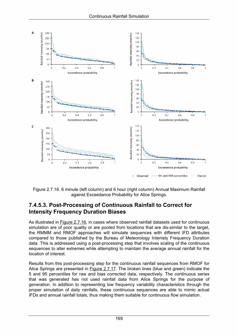
Figure 2.7.16. 6 minute (left column) and 6 hour (right column) Annual Maximum Rainfall against Exceedance Probability for Alice Springs.

7.4.5.3. Post-Processing of Continuous Rainfall to Correct for Intensity Frequency Duration Biases

As illustrated in Figure 2.7.16, in cases where observed rainfall datasets used for continuous simulation are of poor quality or are pooled from locations that are dis-similar to the target, the RMMM and RMOF approaches will simulate sequences with different IFD attributes compared to those published by the Bureau of Meteorology Intenisty Frequency Duration data. This is addressed using a post-processing step that involves scaling of the continuous sequences to alter extremes while attempting to maintain the average annual rainfall for the location of interest.

Results from this post-processing step for the continuous rainfall sequences from RMOF for Alice Springs are presented in Figure 2.7.17. The broken lines (blue and green) indicate the 5 and 95 percentiles for raw and bias corrected data, respectively. The continuous series that was generated has not used rainfall data from Alice Springs for the purpose of generation. In addition to representing low frequency variability characteristics through the proper simulation of daily rainfalls, these continuous sequences are able to mimic actual IFDs and annual rainfall totals, thus making them suitable for continuous flow simulation.


169

Figure 2.7.17. Intensity Duration Frequency Relationships for Target and Simulated Rainfall before and after Bias Correction at Alice Springs

7.5. Implications of Climate ChangeThe implications of climate change on design rainfall have been discussed in Book 1, Chapter 6 and are not repeated here. The focus of this section is to discuss how the procedures for continuous simulation described here may be altered to account for climate change. This may be particularly important if there are changes in extreme rainfall, in antecedent rainfall, or in the dependence between the two, all of which will have significant impacts on the resulting design flood.

Both the daily and the sub-daily continuous simulation alternatives discussed here will be affected by climate change. Practitioners may need to use daily rainfall sequences that are representative of future warmer climates, and are referred to the statistical downscaling extensions of the RMMM daily generation approach discussed in Mehrotra and Sharma (2010) for an alternative for generating daily sequences for any location of interest. This generation requires selection of appropriate Global Climate Models (GCMs) and atmospheric predictors, followed by sensible correction of GCM simulations to remove known biases. Practitioners are referred to (Sharma et al., 2013) for a review of the approaches used commonly for these purposes.

Generation of sub-daily sequences will require modification of the RMOF to alternatives that take into account changes to extremes at sub-daily timescales (Westra et al., 2014) as well as changes to associated temporal patterns (Wasko and Sharma, 2015). An alternative that can be used to accommodate these changes is presented in (Westra et al., 2013). In general, approaches for stochastically generating continuous (sub-daily) rainfall sequences under a future climate are a rapidly evolving area of research, and detailed advice on theory and approaches for continuous simulation under a future climate are outside of the scope of this document.

7.6. ReferencesArnold, J.G. and Williams, J.R. (1989), Stochastic Generation of Internal Storm Structure at a Point, Transactions of the ASAE, 32(1), 161-0167.

Beesley, C.A., Frost, A.J. and Zajaczkowski, J. (2009), A comparison of the BAWAP and SILO spatially interpolated daily rainfall datasets, paper presented at 18th World IMACS / MODSIM Congress, MSSANZ, Cairns, Australia.


170

Blazkova, S. and Beven, K. (2002), Flood frequency estimation by continuous simulation for a catchment treated as ungauged (with uncertainty), Water Resources Research, Volume 38(8).

Boughton, W.C. (1999), A daily rainfall generating model for water yield and flood studiesRep. Report 99/9, 21pp pp, CRC for Catchment Hydrology, Monash University, Melbourne.

Boughton, W. and Droop, O. (2003), Continuous simulation for design flood estimation - a review, Environmental Modelling & Software, 18(4), 309-318.

Buishand, T.A. (1977), Stochastic modeling of daily rainfall sequences, Meded. Landbouwhogesch. Wageningen, 77(3), 211.

Bárdossy, A. and Pegram, G. (2014), Infilling missing precipitation records - A comparison of a new copula-based method with other techniques, Journal of Hydrology, 519, Part A, pp: 1162-1170.

Bárdossy, A. and Pegram, G.G.S. (2009), Copula based multisite model for daily precipitation simulation, Hydrol. Earth Syst. Sci., 13(12), 2299-2314.

Bárdossy, A. and Plate, E.J. (1992), Space-time model for daily rainfall using atmospheric circulation patterns, Water Resources Research, 28(5), 1247-1259.

Cameron, D., Beven, K., Tawn, J. and Naden, P. (2000), Flood frequency estimation by continuous simulation (with likelihood based uncertainty estimation), Hydrology and Earth System Sciences, 4(1), 23-34.

Carey-Smith, T., Sansom, J. and Thomson, P. (2014), A hidden seasonal switching model for multisite daily rainfall, Water Resources Research, 50(1), 257-272.

Caskey, J.E. (1963), A MARKOV CHAIN MODEL FOR THE PROBABILITY OF PRECIPITATION OCCURRENCE IN INTERVALS OF VARIOUS LENGTH, Mon. Wea. Rev., 91(6), 298-301.

Chapman, T.G. (1997), Stochastic models for daily rainfall in the Western Pacific, Mathematics and Computers in Simulation, 43: 351-358.

Chappell, A., Renzullo, L.J., Raupach, T.H. and Haylock, M. (2013), Evaluating geostatistical methods of blending satellite and gauge data to estimate near real-time daily rainfall for Australia, Journal of Hydrology, 493: 105-114.

Charles, S.P., Bates, B.C. and Hughes, J.P. (1999), A spatiotemporal model for downscaling precipitation occurrence and amounts, Journal of Geophysical Research-Atmospheres, 104(D24), 31657-31669.

Chin, E.H. and Miller, J.F. (1980), On the Conditional Distribution of Daily Precipitation Amounts, Mon. Wea. Rev., 108(9), 1462-1464.

Chowdhury, S. and Sharma, A. (2007), Mitigating Parameter Bias in Hydrological Modelling due to Uncertainty in Covariates, Journal of Hydrology, 340(3-4), 197-204.

Ciach, G.J. (2003), Local random errors in tipping-bucket rain gauge measurements, Journal of Atmospheric and Oceanic Technology, 20(5), 752-759.


171

Coe, R. and Stern, R.D. (1982), Fitting Models to Daily Rainfall Data, Journal of Applied Meteorology, 21(7), 1024-1031.

Cole, J.A. and Sherriff, J.D.F. (1972), Some single- and multi-site models of rainfall within discrete time increments, Journal of Hydrology, 17(1-2), 97-113.

Connolly, R.D., Schirmer, J. and Dunn, P.K. (1998), A daily rainfall disaggregation model, Agricultural and Forest Meteorology, 92(2), 105-117.

Cowpertwait, P.S.P. (1991), Further developments of the Neyman‐Scott clustered point process for modeling rainfall. Water Resources Research, 27: 1431-1438.

Cowpertwait, P.S.P. (2010), A spatial-temporal point process model with a continuous distribution of storm types, Water Resources Research, 46(12).

Cowpertwait, P.S.P., Kilsby, C.G. and O'Connell, P.E. (2002), A space-time Neyman-Scott model of rainfall: Empirical analysis of extremes - art. no. 1131, Water Resources Research, 38(8), 1131-1131.

Cowpertwait, P.S.P., O'Connell, P.E., Metcalfe, A.V. and Mawdsley, J.A. (1996), Stochastic point process modelling of rainfall. II. Regionalisation and disaggregation, Journal of Hydrology, 175(1-4), 47-65.

Das, D., Kodra, E., Obradovic, Z. and Ganguly, A.R. (2012), Mining extremes: Severe rainfall and climate change, in Frontiers in Artificial Intelligence and Applications, edited, pp: 899-900.

Deidda, R., Benzi, R. and Siccardi, F. (1999), Multifractal modeling of anomalous scaling laws in rainfall, Water Resources Research, 35(6), 1853-1867.

Dennett, M.D., Rodgers, J.A. and Stern, R.D. (1983), Independence of Rainfalls through the Rainy Season and the Implications for the Estimation of Rainfall Probabilities, Journal of Climatology, Volume 3(4), pp.375-384.

Eagleson, P.S. (1978), Climate, Soil, and Vegetation 2. The Distribution of Annual Precipitation Derived From Observed Storm Sequences, Water Resources Research, 14(5), 713-721.

Econopouly, T.W., Davis, D.R. and Woolhiser, D.A. (1990), Parameter transferability for a daily rainfall disaggregation model, Journal of Hydrology, 118(1-4), 209-228.

Evin, G., and Favre, A.C. (2012), Further developments of a transient Poisson-cluster model for rainfall, Stochastic Environmental Research and Risk Assessment, 27(4), 831-847.

Fasano, G. and Franceschini, A. (1987), A Multidimensional Version of the Kolmogorov-Smirnov Test, Mon Not R Astron Soc, 225(1), 155-170.

Feyerherm, A.M. and Bark, L.D. (1965), Statistical Methods for Persistent Precipitation Patterns, Journal of Applied Meteorology, 4(3), 320-328.

Feyerherm, A.M. and Bark, L.D. (1967), Goodness of Fit of a Markov Chain Model for Sequences of Wet and Dry Days, Journal of Applied Meteorology, 6(5), 770-773.

Frost, A., R. Srikanthan, and P. Cowpertwait (2004), Stochastic generation of point rainfall data at subdaily timescales: a comparison of DRIP and NSRP, Technical report 04/09, Cooperative Research Centre - Catchment Hydrology, Melbourne, Australia.


172

Gabriel, K.R. and Neumann, J. (1962), A Markov chain model for daily rainfall occurrence at Tel Aviv, Q.J Royal Met. Soc., 88(375), 90-95.

Garcia-Guzman, A., and Aranda-Oliver, E. (1993), A stochastic model of dimensionless hyetograph, Water Resources Research, 29(7), 2363-2370.

Gates, P. and Tong, H. (1976), On Markov Chain Modeling to Some Weather Data, Journal of Applied Meteorology, 15(11), 1145-1151.

Grace, R.A. and Eagleson, P.S. (1966). The Synthesis of Short-Time-Increment Rainfall Sequences, Hydrodynamics Lab. Report 91, Dept. of Civil Engineering, Massachusetts Institute of Technology, Cambridge, MA.

Gregory, J.M., Wigley, T.M.L. and Jones, P.D. (1993), Application of Markov models to area-average daily precipitation series and interannual variability in seasonal totals, Clim. Dyn., 8: 299-310.

Gupta, V.K. and Waymire, E.C. (1993), A Statistical Analysis of Mesoscale Rainfall as a Random Cascade, Journal of Applied Meteorology, 32(2), 251-267.

Gyasi‐Agyei, Y. (1999), Identification of regional parameters of a stochastic model for rainfall disaggregation. Journal of Hydrology. 223: 148-163.

Gyasi-Agyei, Y. (2013), Evaluation of the effects of temperature changes on fine timescale rainfall, Water Resources Research, 49(7), 4379-4398.

Haan, C.T., Allen, D.M. and Street, J.D. (1976), A Markov chain model of daily rainfall, Water Resour. Res., 12: 443-449.

Harrold, T.I., Sharma, A. and Sheather, S.J. (2003a), A nonparametric model for stochastic generation of daily rainfall amounts - art. no. 1343, Water Resources Research, 39(12), 1343-1343.

Harrold, T.I., Sharma, A. and Sheather, S.J. (2003b), A nonparametric model for stochastic generation of daily rainfall occurrence - art. no. 1300, Water Resources Research, 39(10), 1300-1300.

Hasan, M.M., Sharma, A., Johnson, F., Mariethoz, G., Seed, A. (2014), Correcting bias in radar Z-R relationships due to uncertainty in point raingauge networks. Journal of Hydrology 519(B), 1668-1676.

Hay L.E., McCabe G.J., Wolock D.M. and Ayers M.A. (1991), Simulation of precipitation by weather type anaylsis. Water Resources Research, 27: 493-501.

Heaps, S.E., Boys, R.J. and Farrow, M. (2015), Bayesian modelling of rainfall data by using non-homogeneous hidden Markov models and latent Gaussian variables, Journal of the Royal Statistical Society: Series C (Applied Statistics), 64(3), 543-568.

Heneker, T.M., Lambert, M.F. and Kuczera, G. (2001), A point rainfall model for risk-based design, Journal of Hydrology, 247(1-2), 54-71.

Hershenhorn, J. and Woolhiser, D.A. (1987), Disaggregation of daily rainfall, Journal of Hydrology, 95(3-4), 299-322.

Hopkins, J.W. and Robillard, P. (1964), Some Statistics of Daily Rainfall Occurrence for the Canadian Prairie Provinces, Journal of Applied Meteorology, 3(5), 600-602.


173

Hughes, J.P. and Guttorp, P. (1994), Incorporating Spatial Dependence and Atmospheric Data in a Model of Precipitation, Journal of Applied Meteorology, 33(12), 1503-1515.

Jeffrey, S.J., Carter, J.O., Moodie, K.B. and Beswick, A.R. (2001), Using spatial interpolation to construct a comprehensive archive of Australian climate data, Environmental Modelling & Software, 16(6), 309-330.

Jennings S. (2007). A High Resolution Point Rainfall Model Calibrated to Short Pluviograph or Daily Rainfall Data, PhD Thesis, The University of Adelaide, Australia.

Jha, S.K., Mariethoz, G., Evans, J., McCabe, M.F. and Sharma, A. (2015), A space and time scale dependent non-linear geostatistical approach for downscaling daily precipitation and temperature, Water Resources Research, available at: http://onlinelibrary.wiley.com/doi/10.1002/2014WR016729/full accesses [20 July 2015].

Jones, P.G. and Thornton, P.K. (1997), Spatial and temporal variability of rainfall related to a third-order Markov model, Agricultural and Forest Meteorology, 86(1-2), 127-138.

Jones, D., Wang, W.and Fawcett, R. (2009), High-quality spatial climate data-sets for Australia, Australian Meteorological and Oceanographic Journal, 58: 233-248.

Katz, R. and Parlange, M.B. (1995), Generalizations of chain-dependent processes: Application to hourly precipitation. Water Resour. Res., 31: 1331-1341.

Katz, R.W. and Parlange, M.B. (1998), Overdispersion phenomenon in stochastic modeling of precipitation, Journal of Climate, 11(4), 591-601.

Katz, R.W., Parlange, M.B. and Tebaldi, C. (2003), Stochastic modeling of the effects of large-scale circulation on daily weather in the southeastern US, Climatic Change, 60(1-2), 189-216.

Kavvas, M.L. and Delleur, J.W. (1981), A stochastic cluster model of daily rainfall sequences, Water Resources Research, 17(4), 1151-1160.

Kim, D., Kim, J. and Cho, Y.-S. (2014), A Poisson Cluster Stochastic Rainfall Generator That Accounts for the Interannual Variability of Rainfall Statistics: Validation at Various Geographic Locations across the United States, Journal of Applied Mathematics, 2014, pp: 1-14.

Kim, Y., Katz, R.W. Rajagopalan, B., Podestá, G.P. and Furrer, E.M. (2012), Reducing overdispersion in stochastic weather generators using a generalized linear modeling approach, Climate Research, 53(1), 13-24.

Kleiber, W., Katz, R.W. and Rajagopalan, B. (2012), Daily spatiotemporal precipitation simulation using latent and transformed Gaussian processes, Water Resources Research, 48(1).

Koutsoyiannis, D. (2001), Coupling stochastic models of different timescales, Water Resources Research, 37(2), 379-391.

Koutsoyiannis, D. and Onof, C. (2000), A computer program for temporal rainfall disaggregation using adjusting procedures, paper presented at 25th General Assembly of the European Geophysical Society, EGS, Nice.


174

Koutsoyiannis, D. and Pachakis, D. (1996), Deterministic chaos versus stochasticity in analysis and modeling of point rainfall series, Journal of Geophysical Research, 101(D21), 26441-26451.

Koutsoyiannis, D. and Xanthopoulos, T. (1990). A dynamic model for short-scale rainfall disaggregation, Hydrological Sciences Journal, 35(3), 303-322.

Koutsoyiannis, D., Onof, C. and Wheater, H.S. (2003), Multivariate rainfall disaggregation at a fine timescale - art. no. 1173, Water Resources Research, 39(7), 1173-1173.

La Barbera, P., Lanza, L.G. and Stagi, L. (2002), Tipping bucket mechanical errors and their influence on rainfall statistics and extremes, Water Science and Technology, 45(2), 1-10.

Lall, U. and Sharma, A. (1996), A nearest neighbor bootstrap for time series resampling, Water Resources Research, 32(3), 679-693.

Lall, U., Rajagopalan, B. and Tarboton. D.G. (1996), A nonparametric wet/dry spell model for resampling daily precipitation, Water Resources Research, 32(9), 2803-2823.

Lamb, R., and Kay, A.L. (2004), Confidence intervals for a spatially generalized, continuous simulation flood frequency model for Great Britain, Water Resources Research, 40(7).

Lambert, M., and Kuczera, g. (1998), Seasonal generalized exponential probability models with application to interstorm and storm durations, Water Resources Research, 34(1), 143-148.

Lambert M.F., Whiting J.P. and Metcalfe, A.V. (2003). A non-parametric hidden Markov model for climate state identification. Hydrology and Earth Systems Sciences, 7(5), pp. 652-667.

Leblois, E., and Creutin J.-E. (2013), Space-time simulation of intermittent rainfall with prescribed advection field: Adaptation of the turning band method, Water Resources Research, 49(6), 3375-3387.

Leonard, M., Lambert, M.F. Metcalfe, A.V. and Cowpertwait, P.S.P. (2008), A space-time Neyman-Scott rainfall model with defined storm extent, Water Resources Research, 44(9).

Lovejoy, S. and Schertzer, D. (1990), Multifractals, universality classes and satellite and radar measurements of cloud and rain fields, J. Geophys. Res., 95(D3), 2021-2034.

McMahon, T.A. and Srikanthan, R. (1983), Statistical characteristics of Australian Rainfall and EvaporationRep.

Mehrotra, R., and Sharma, A. (2006), A nonparametric stochastic downscaling framework for daily rainfall at multiple locations, Journal of Geophysical Research-Atmospheres, 111(D15101), doi:10.1029/2005JD006637.

Mehrotra, R., and Sharma, A. (2010), Development and Application of a Multisite Rainfall Stochastic Downscaling Framework for Climate Change Impact Assessment, Water Resources Research, 46.

Mehrotra, R., and Sharma, A. (2007a), Preserving low-frequency variability in generated daily rainfall sequences, Journal of Hydrology, 345(1-2), 102-120.


175

Mehrotra, R. and Sharma, A. (2007b), A semi-parametric model for stochastic generation of multi-site daily rainfall exhibiting low-frequency variability, Journal of Hydrology, 335(1-2), 180-193.

Mehrotra, R., Westra, S., Sharma, A. and Srikanthan, R. (2012), Continuous rainfall simulation: 2 - A regionalised daily rainfall generation approach, Water Resources Research, 48(1), W01536

Mehrotra, R., Li, J., Westra, S. and Sharma, A. (2015), A programming tool to generate multi-site daily rainfall using a two-stage semi parametric model Environmental Modelling & Software, 63: 230-239.

Menabde, M. and Sivapalan, M. (2000), Modeling of rainfall time series and extremes using bounded random cascades and Levy-stable distribution, Water Resources Research, 36(11), 3293-3300.

Menabde, M., Seed, D., Harris and Austin, G. (1997), Self-similar random fields and rainfall simulation, J. Geophys. Res., 102(D12), 13509-13515.

Micevski, T. and Kuczera, G. (2009), Combining Site and Regional Flood Information Using a Bayesian Monte Carlo Approach, Water Resources Research(doi:10.1029/2008WR007173), available at: online on http://www.agu.org/journals/wr/papersinpress.shtml.

Molnar, P. and Burlando, P. (2005), Preservation of rainfall properties in stochastic disaggregation by a simple random cascade model, Atmospheric Research, 77(1-4), 137-151.

Olsson, J. and Berndtsson, R. (1998), Temporal rainfall disaggregration based on scaling properties, Water Science and Technology, 37(11), 73-79.

Onof, C. and Townend, J. (2004), Modelling 5-minute rainfall extremes, paper presented at British Hydrological Society International Conference, London.

Onof, C., Chandler, R.E. Kakou, A., Northrop, P., Wheater, H.S. and Isham, V. (2000), Rainfall modelling using Poisson-cluster processes: a review of developments, Stochastic Environmental Research and Risk Assessment, 14(6), 384-411.

Oriani, F., Straubhaar, J., Renard, P. and Mariethoz, G. (2014), Simulation of rainfall time series from different climatic regions using the direct sampling technique, Hydrology and Earth System Sciences, 18(8), 3015-3031.

Over, T. M. and Gupta, V.K. (1996), A space-time theory of mesoscale rainfall using random cascades, J. Geophys. Res., 101(D21), 26319.

Pathiraja, S., Westra, S. and Sharma, A. (2012), Why Continuous Simulation? The Role of Antecedent Moisture in Design Flood Estimation, Water Resources Research, 48(W06534).

Pegram, G.G.S. (1980), An Autoregressive Model for Multilag Markov Chains, Journal of Applied Probability, 17(2), 350.

Pui, A., Lal, A. and Sharma, A. (2011), How does the Interdecadal Pacific Oscillation affect design floods in Australia?, Water Resources Research, 47(5).


176

Pui, A., Sharma, A., Santoso, A. and Westra, S. (2012), Impact of the El Niño Southern Oscillation, Indian Ocean Dipole, and Southern Annular Mode on daily to sub-daily rainfall characteristics in East Australia, Monthly Weather Review, 140: 1665-1681.

Racsko, P., Szeidl, L. and Semenov, M. (1991), A serial approach to local stochastic weather models, Ecological Modelling, 57(1-2), 27-41.

Ramirez, J. A. and Bras, R.L. (1985), Conditional Distributions of Neyman-Scott Models for Storm Arrivals and Their Use in Irrigation Scheduling, Water Resources Research, 21(3), 317-330.

Richardson, C.W. (1981), Stochastic Simulation of Daily Precipitation, Temperature, and Solar-Radiation, Water Resources Research, 17(1), 182-190.

Rodriguez-Iturbe, I., Gupta, V.K. and Waymire, E. (1984), Scale considerations in the modeling of temporal rainfall, Water Resources Research, 20(11), 1611-1619.

Rodriguez-Iturbe, I., Cox, D.R. and Isham, V. (1987), Some Models for Rainfall Based on Stochastic Point Processes, Proceedings of the Royal Society A: Mathematical, Physical and Engineering Sciences, 410(1839), 269-288.

Rodriguez-Iturbe, I., Cox, D.R. and Isham, V. (1988), A Point Process Model for Rainfall: Further Developments, Proceedings of the Royal Society A: Mathematical, Physical and Engineering Sciences, 417(1853), 283-298.

Roldan, J., and Woolhiser, D.A. (1982), Stochastic daily precipitation models 1. A comparison of occurrence models, Water Resources Research, 18(5), 1451-1459.

Rosjberg, D., Madsen, H. and Rasmussen, P. F. (1992). Prediction in Partial Duration Series with Generalized Pareto-Distirbuted Exceedences, Water Resources Research, 28(11), 3001-3010.

Sariahmed, A. and Kisiel, C.C. (1968). Synthesis of sequences of summer thunderstorm volumes for the Atterbury watershed in the Tucson area. Proceedings International Association Hydrologic Sciences Symposium on Use of Analog and Digital Computers in Hydrology, 2: 439-447.

Schertzer, D. and Lovejoy, S. (1987), Physical modeling and analysis of rain and clouds by anisotropic scaling multiplicative processes, J. Geophys. Res., 92(D8), 9693.

Seed, A.W., Srikanthan, R. and Menabde, M. (1999), A space and time model for design storm rainfall, Journal of Geophysical Research-Atmospheres, 104(D24), 31623-31630.

Selvalingam, S. and Miura, M. (1978), STOCHASTIC MODELING OF MONTHLY AND DAILY RAINFALL SEQUENCES, J Am Water Resour As, 14(5), 1105-1120.

Serinaldi, F. (2009), A multisite daily rainfall generator driven by bivariate copula-based mixed distributions, J. Geophys. Res., 114(D10).

Serinaldi, F. and Kilsby, C.G. (2014), Simulating daily rainfall fields over large areas for collective risk estimation, Journal of Hydrology, 512: 285-302.

Sharma, A. and Lall, U. (1999), A nonparametric approach for daily rainfall simulation, Mathematics and Computers in Simulation, 48(4-6), 361-371.


177

Sharma, A. and Mehrotra, R. (2010), Rainfall Generation, in Rainfall: State of the Science, edited by F.Y. Testik and M. Gebremichael, p: 287, American Geophysical Union, San Francisco.

Sharma, A. and O'Neill, R. (2002), A nonparametric approach for representing interannual dependence in monthly streamflow sequences - art. No.1100, Water Resources Research, 38(7), 1100-1100.

Sharma, A. and Srikanthan, R. (2006), Continuous Rainfall Simulation: A Nonparametric Alternative, paper presented at 30th Hydrology and Water Resources Symposium, Institution of Engineers (Australia), Launceston.

Sharma, A., Mehrotra, R. and Johnson, F. (2013), A New Framework for Modeling Future Hydrologic Extremes: Nested Bias Correction as a Precursor to Stochastic Rainfall Downscaling (invited), in Climate Change Modeling, Mitigation, and Adaptation, edited by R.Y. Surampalli, T.C. Zhang, C.S.P. Ojha, B.R. Gurjar, R. D. Tyagi and C.M. Kao, p: 698, American Society of Civil Engineers, Reston, Virginia.

Singh, S.V. and Kripalani, R.H. (1986), Analysis of persistence in daily monsoon rainfall over India, Journal of Climatology, 6(6): 625-639.

Sivakumar, B., Berndtsson, R., Olsson, J. and Jinno, K. (2001), Evidence of chaos in the rainfall-runoff process, Hydrological Sciences Journal, 46(1), 131-145.

Srikanthan, R. and McMahon, T.A. (1985), Stochastic generation of rainfall and evaporation data, Tech. Paper No. 84, Aust. Water Resour. Council, Canberra, 1985, Australian Water Resources Council, Technical Paper No.84.

Srikanthan, R. and Pegram, G. (2009), A Nested Multisite Daily Rainfall Stochastic Generation Model, Journal of Hydrology, Available at: http://www.science-direct.com/ until publication.

Srikanthan, R., McMahon, T., Harrold, T. and Sharma, A. (2003), Stochastic Generation of Daily Rainfall DataRep., CRC for Catchment Hydrology Technical Report 03, Melbourne, Australia.

Steinschneider, S., and Lall, U. (2015), A hierarchical Bayesian regional model for nonstationary precipitation extremes in Northern California conditioned on tropical moisture exports, Water Resources Research, 51(3), 1472-1492.

Stern, R.D. and Coe, R. (1984), A Model Fitting Analysis of Daily Rainfall Data, Journal of the Royal Statistical Society. Series A (General), 147(1), 1-34.

Thyer, M. and Kuczera, G. (2003a), A hidden Markov model for modelling long-term persistence in multi-site rainfall time series 1. Model calibration using a Bayesian approach Journal of Hydrology, 275(1-2), 12-26.

Thyer, M. and Kuczera, G. (2003b), A hidden Markov model for modelling long-term persistence in multi-site rainfall time series. 2. Real data analysis Journal of Hydrology, 275(1-2), 27-48.

Viney, N.R. and Bates, B.C. (2004), It never rains on Sunday: The prevalence and implications of untagged multi-day rainfall accumulations in the Australian high quality data set, International Journal of Climatology, 24: 1171-1192.


178

Wallis, T.W.R. and Griffiths, J.F. (1997), Simulated meteorological input for agricultural models, Agricultural and Forest Meteorology, 88(1-4), 241-258.

Wang, Q. J. and Nathan, R.J. (2007), A method for coupling daily and monthly time scales in stochastic generation of rainfall series, Journal of Hydrology, 346(3-4), 122-130.


Waymire, E. and Gupta, V.K. (1981a), The mathematical structure of rainfall representations: 1. A review of the stochastic rainfall models, Water Resources Research, 17(5), 1261-1272.

Waymire, E., and Gupta, V.K. (1981b), The mathematical structure of rainfall representations: 2. A review of the theory of point processes, Water Resources Research, 17(5), 1273-1285.

Westra, S., Mehrotra, R., Sharma, A. and Srikanthan, R. (2012), Continuous rainfall simulation: 1 - A regionalised sub-daily disaggregation approach, Water Resources Research, 48(1), W01535.

Westra, S., Fowler, H.J., Evans, J.P., Alexander, L.V., Berg, P., Johnson, F., Kendon, E.J., Lenderink, g. and Roberts, N.M. (2014), Future changes to the intensity and frequency of short-duration extreme rainfall, Rev Geophys, 52.

Westra, S., Evans, J.P., Mehrotra, R. and Sharma, A. (2013), A conditional disaggregation algorithm for generating fine time-scale rainfall data in a warmer climate, Journal of Hydrology, 479: 86-99.

Wheater, H. S., Isham, V.S., Cox, D.R., Chandler, R.E., Kakou, A., Northrop, P.J., Oh, L., Onof, C. and Rodriguez-Iturbe, I. (2000), Spatial-temporal rainfall fields: modelling and statistical aspects, Hydrology and Earth System Sciences, 4(4), 581-601.

Wilby, R. L., Wigley, T.M.L., Conway, D., Jones, P.D., Hewitson, B.C., Main, J. and Wilks, D.S. (1998), Statistical Downscaling of General Circulation Model Output - a Comparison of Methods, Water Resources Research, 34(11), 2995-3008.

Wilks, D.S. (1998), Multisite generalization of a daily stochastic precipitation generation model, Journal of Hydrology, 210: 178-191.

Wilks, D.S. (1999a), Multisite downscaling of daily precipitation with a stochastic weather generator, Climate Research, 11(2), 125-136.

Wilks, D.S. (1999b), Simultaneous stochastic simulation of daily precipitation, temperature and solar radiation at multiple sites in complex terrain, Agricultural and Forest Meteorology, 96(1-3), 85-101.

Woolhiser, D.A. (1992), Modeling daily precipitation - progress and problems, in Statistics in the environmental and earth sciences, edited by A.T. Walden and P. Guttorp, p: 306, Edward Arnold, London, U.K.

Woolhiser, D.A. and Pegram, G.G.S (1979), Maximum Likelihood Estimation of Fourier Coefficients to Describe Seasonal Variations of Parameters in Stochastic Daily Precipitation Models, Journal of Applied Meteorology, 18(1), 34-42.

Woolhiser, D.A. and Roldán J. (1982), Stochastic daily precipitation models: 2. A comparison of distributions of amounts, Water Resources Research, 18(5), 1461-1468.


179

Woolhiser, D.A. and Roldán, J. (1986), Seasonal and Regional Variability of Parameters for Stochastic Daily Precipitation Models: South Dakota, U.S.A, Water Resources Research, 22(6), 965-978.

World Meteorological Organisation (WMO) (1994), WMO Guide to Hydrological Practices, World Meteorological Organisation, Geneva, p: 770.

de Lima, M.I.P. and Grasman, J. (1999), Multifractal analysis of 15-min and daily rainfall from a semi-arid region in Portugal, Journal of Hydrology, 220(1-2), 1-11.


180

11 national Circuit BARTON ACT 2600

e | [email protected]

Book 2 - Rainfall Estimation - ARR Project Reports and Data

Documents

Transcript of Book 2 - Rainfall Estimation - ARR Project Reports and Data