Bond Graphs for Modelling, Control and Fault Diagnosis of ...
680
Wolfgang Borutzky Editor Bond Graphs for Modelling, Control and Fault Diagnosis of Engineering Systems Second Edition
-
Upload
khangminh22 -
Category
Documents
-
view
0 -
download
0
Transcript of Bond Graphs for Modelling, Control and Fault Diagnosis of ...

Wolfgang Borutzky Editor
Bond Graphs for Modelling, Control and Fault Diagnosis of Engineering Systems Second Edition

Bond Graphs for Modelling, Control and FaultDiagnosis of Engineering Systems

Wolfgang BorutzkyEditor
Bond Graphs for Modelling,Control and Fault Diagnosisof Engineering Systems
Second Edition
123

EditorWolfgang BorutzkyBonn-Rhein-Sieg University of Applied
SciencesDepartment of Computer ScienceSankt Augustin, Germany
ISBN 978-3-319-47433-5 ISBN 978-3-319-47434-2 (eBook)DOI 10.1007/978-3-319-47434-2
Library of Congress Control Number: 2016955827
© Springer International Publishing Switzerland 2011, 2017This work is subject to copyright. All rights are reserved by the Publisher, whether the whole or part ofthe material is concerned, specifically the rights of translation, reprinting, reuse of illustrations, recitation,broadcasting, reproduction on microfilms or in any other physical way, and transmission or informationstorage and retrieval, electronic adaptation, computer software, or by similar or dissimilar methodologynow known or hereafter developed.The use of general descriptive names, registered names, trademarks, service marks, etc. in this publicationdoes not imply, even in the absence of a specific statement, that such names are exempt from the relevantprotective laws and regulations and therefore free for general use.The publisher, the authors and the editors are safe to assume that the advice and information in this bookare believed to be true and accurate at the date of publication. Neither the publisher nor the authors orthe editors give a warranty, express or implied, with respect to the material contained herein or for anyerrors or omissions that may have been made.
Printed on acid-free paper
This Springer imprint is published by Springer NatureThe registered company is Springer International Publishing AGThe registered company address is: Gewerbestrasse 11, 6330 Cham, Switzerland

Foreword
Prof. Borutzky has asked me to write a foreword to this second edition of thebook Bond Graph Modelling of Engineering Systems. This put me in mind ofthe time when Ronald C. Rosenberg and I, as Assistant Professors at MIT, usedto stop at a bar in Harvard Square to wait for the traffic to subside on our wayhome from work. (Ron’s doctoral thesis resulted in the ENPORT program, the firstbond graph processor, which, although restricted to linear systems, would solve theproblems associated with differential causality in simulation.) We often discussedwhat technical areas we should work on in the future and we came to the conclusionthat bond graphs, recently invented by our advisor, Prof. Henry M. Paynter, wereworthy of being better known to the general world rather than just to MIT graduatestudents.
The result was our first book intended for self-study of bond graph methods,Analysis and Simulation of Multiport Systems: The Bond Graph Approach toPhysical System Dynamics, The MIT Press, 1968. When the book was finished,Prof. Paynter asked us if he could provide a Foreword in the form of a HistoricalNote. We naturally agreed and the result is a fascinating two page history ofPaynter’s thought starting, he says, in high school. His personal references go backto the 1950s, but his references to chemical structure graphs go back another 100years.
His final paragraph of his Historical Note is as follows:
Thus were devised on April 29, 1959, the two ideal 3-port energy junctions (0,1) to renderthe system of bond graphs a complete and formal discipline. The complete system was thenfirst published in 1961.
As you can see, Prof. Paynter was thinking of his reputation in the future.The publication mentioned was the MIT press book Analysis and Design of
Engineering Systems, 1961, was in fact a paperback compilation of class notes takenby a graduate student and, as Paynter admitted, the glued together book tended tofall apart as its pages were turned. (This was a great disadvantage to slow learners.)Thus, bond graphs remained for a while only known to those who had studied atMIT.
v

vi Foreword
Professor Paynter would certainly be gratified to see the interest in bond graphsthat has developed in the past 60 years. The present volume is a testimony to largenumber of researchers who are presently contributing to extensions of bond graphtechniques and to new application areas. He also might be surprised to learn that his“complete and formal discipline” has been extended in directions he never wouldhave thought possible.
There is, of course, some danger in extending bond graph techniques to includeidiosyncratic notation and manipulations that apply to ever more special cases. Inthe early years, those of us interested in promoting bond graph methods had to fightthose who liked the force-current analogy better than the force-voltage analogy sincethey produced bond graphs with 0’s and 1’s and I’s and C’s interchanged, whichprovided a barrier to those newcomers interested in learning the benefits of bondgraph methods. This volume is an example of the correct approach in which theauthors take pains to make clear why special notation or special manipulations ona bond graph are necessary to provide insight into problems which don’t yield tostandard bond graph techniques.
When I contemplate Paynter’s contribution to physical system dynamics, and ofthose of present day engineers who continue to advance bond graph techniques asevidenced by the present volume, I think of the well-known quote from Goethe’sFaust:
Was du ererbt von deinen Vätern hast, erwirb es, um es zu besitzen.
(That which you inherit from your fathers, you must earn in order to possess.)
The authors of the present volume have clearly taken this advice to heart.
Davis, CA, USA Dean KarnoppJuly 2016
Preface
By the beginning of 2011, Springer published a compilation text of a number ofresearchers from all over the world on Bond Graph Modelling of EngineeringSystems. The book covers theoretical and methodological topics as well as someapplications and the use of software for bond graph modelling and simulation. Theaim was to present the state of the art in bond graph modelling by addressing latestdevelopments and integrating various works in a unified manner. In summer 2014,the editor was invited to prepare a second edition of the 2011 compilation text. Dueto the active ongoing research of my colleagues, their commitment, their expertise,and their contributions the outcome of this new book project, in my view, hasbecome more than a revision of the first edition. This new book again covers sometheoretical issues, applications and software support as the first edition. However,the focus of the second edition is on latest topics as well as on subjects that haven’tbeen covered in the first edition. Moreover, new young excellent researchers havejoined the team together with co-authors who have been using bond graph in theirresearch and in teaching for a long time. Therefore, the result of this project may beconsidered a novel book that reflects the active research in the bond graph modellingcommunity and latest achievements over a rather short period of the past five years.A number of the contributed chapters have arisen from recently finished PhD theses.
Bond graphs were devised by Professor H. Paynter some 60 years back at theMassachusetts Institute of Technology (MIT) in Cambridge, Massachusetts, USA,and were developed into a methodology by his former PhD students ProfessorD. Karnopp and Professor D. Margolis (University of California at Davis) andProfessor R. Rosenberg (Michigan State University, East Lansing, Michigan). Sincethen the bond graph approach to physical system modelling and simulation has beenadopted by many researchers. The contributions to this book well demonstrate thattoday, 60+ years later, the bond graph methodology has spread from MIT all overthe world and is successfully used in various engineering fields.
The book is organised into five parts. Each of them starts with an introductionthat motivates the subjects and establishes relations between the chapters of a part.
The contributed chapters show that bond graphs are more than just a method-ology for modelling and simulation of multidisciplinary systems described by
vii

viii Preface
continuous time models. Beyond that application area, bond graphs can also beused to represent hybrid models with continuous time and discrete state variables.Furthermore, bond graph modelling has proven useful in control and as one possiblestarting point for model-based fault diagnosis and fault prognosis in engineeringsystems. These areas become more and more important with an increase of thecomplexity of today’s mechatronic systems and a trend to at least partly autonomoussystems. Representing hybrid models in a bond graph framework and bond graphmodel-based fault diagnosis and fault prognosis are topics in the focus of this newbook. Accordingly, the title of the first edition has been adapted.
Another topic that is not new but of still ongoing interest is the question ofhow open thermodynamic subsystems with compressible fluid flow and mechanicalsubsystems described by a distributed parameter model can be integrated in alumped parameter model of a complex overall system. Part III presents an extensionof common bond graphs for modelling thermodynamic subsystems introduced byProfessor Brown that can be combined with conventional bond graphs for other partsof an engineering system and is supported by a mature modelling and simulationsoftware environment newly developed over the past years. As to distributedparameter subsystems, an approach based on finite segments and an activity metricis presented that aims at a lumped parameter model of reduced order sufficientlyaccurate.
Part IV illustrates the remarkable wide range of applications in which bondgraphs have been used for modelling mechatronic systems of current interest bycontributed chapters ranging from a wheelchair, to robots for in vivo surgery, orwalking machines that can be used for operations in hazardous fields, to windturbines in the area of renewable energy sources.
Professor Henry Paynter, the inventor of bond graphs, envisaged applications ofbond graph modelling to chemistry, electrochemistry and biochemistry already backin 1992. Since then not too many researchers have used bond graphs for modellingchemical reactions. One chapter in Part IV extends bond graph modelling evento biomolecular systems of living organisms. As the latter ones are open systemsthat are not at thermodynamic equilibrium, bond graph representations of theirbiomolecular systems are not evident. The chapter introduces appropriate bondgraph variables. Molecular species are represented by a nonlinear C element andreactions by a nonlinear two-port R element. As a result, bond graph modelling as agraphical approach gives more intuitive insight than purely numerical approaches.
As to the results of simulation runs, it has become common that some softwareprovides a postprocessing module that enables a visualisation of mechanical motionin 3D under different angles of views. The last chapter of this compilation textpresents a novel approach that links a bond graph modelling and simulation programto a program for the geometrical design of complex multibody systems such asrobots with several degrees of freedom so that the 3D motion of a robot is visualisedsimultaneously with some little delay to its numerical computation.
Although this contributed book aims to reflect the current state of the art inbond graph modelling by presenting and discussing advanced recent topics, allchapters have been written in such a way that newcomers to the methodology

Preface ix
with some knowledge of the basics may easily get into the vast fascinating andopen field of advanced bond graph modelling. Readers who may want to have acloser look at bond graph fundamentals may find references to latest monographsand textbooks. Furthermore, each chapter provides many references to conferencepapers, journal articles and PhD theses on advanced topics. This multiple authorsbook well complements latest monographs and textbooks on bond graph modellingand may serve as a guide for further self-study and as a reference.
Bond Graphs for Modelling, Control and Fault Diagnosis of EngineeringSystems continues the presentation of its predecessor titled Bond Graph Modellingof Engineering Systems and like the latter one addresses readers in academia as wellas practising engineers in industry and invites experts in related fields to considerthe potential and the state of the art of bond graph modelling. It is hoped that thebond graph methodology may contribute to more insight into physical processes andto the development of useful models in their engineering field.
Acknowledgements
This volume would not have been possible without the commitment, the expertiseand the efforts of my colleagues. I would like to take this opportunity to thankall my co-authors for their contributed chapters. Likewise, I wish to thank allcolleagues who kindly took the time to read the chapters. Their valuable commentsand suggestions are gratefully acknowledged.
My special thanks go to Professor Dean Karnopp, University of California atDavis, one of the leading pioneers of the bond graph methodology, who kindlyhonoured all authors of this compilation text by writing the foreword with somepersonal notes.
Also, I appreciate the support this multiple author book project received fromProfessors Yuri Merkuryev, Riga Technical University, Latvia; David Murray-Smith, University of Glasgow, Scotland, UK; Ronald Rosenberg, Michigan StateUniversity, East Lansing, MI, USA and Gregorio Romero, Universidad Politécnicade Madrid, Spain.
Last but not least, I wish to thank my Editor with Springer at New York, NY,USA, Mary James, for her invitation to this book project, for her kind constantsupport during this book project and Brinda Megasyamalan, Project Coordinator,Sasi Reka, Project Manager, for the cooperation throughout the book production.
Sankt Augustin, Germany Wolfgang BorutzkyJuly 2016
Contents
Part I Bond Graph Theory and Methodology
1 Decomposition of Multiports . . . . . . . . . . . . . . . . . . . . . . . . . . . . . . . . . . . . . . . . . . . . . . 5Peter C. Breedveld
2 A Method for Minimizing the Set of Equations in BondGraph Systems with Causal Loops . . . . . . . . . . . . . . . . . . . . . . . . . . . . . . . . . . . . . . . 27Jesus Felez
3 Controlled Switched Structures for Bond-GraphModelling and Simulation of Hybrid Systems . . . . . . . . . . . . . . . . . . . . . . . . . . . 47Matías A. Nacusse and Sergio J. Junco
4 Dynamic Causality in Hybrid Bond Graphs . . . . . . . . . . . . . . . . . . . . . . . . . . . . 87Rebecca Margetts and Roger F. Ngwompo
Part II Bond Graph Modelling for Fault Diagnosis, FaultTolerant Control, and Prognosis
5 Integrating Bond Graph-Based Fault Diagnosis and FaultAccommodation Through Inverse Simulation. . . . . . . . . . . . . . . . . . . . . . . . . . . 139W. Borutzky
6 Model-Based Diagnosis and Prognosis of HybridDynamical Systems with Dynamically Updated Parameters . . . . . . . . . . 195Om Prakash and A.K. Samantaray
7 Particle Filter Based Integrated Health Monitoringin Bond Graph Framework . . . . . . . . . . . . . . . . . . . . . . . . . . . . . . . . . . . . . . . . . . . . . . . 233Mayank S. Jha, G. Dauphin-Tanguy, and B. Ould-Bouamama
xi
xii Contents
Part III Thermodynamic Systems and Distributed ParameterSystems
8 Convection Bond Graphs for Thermodynamic Systems . . . . . . . . . . . . . . . 275Forbes T. Brown
9 Finite Element Formulation for Computational FluidDynamics Framed Within the Bond Graph Theory . . . . . . . . . . . . . . . . . . . . 311Jorge Luis Baliño
10 Model Complexity of Distributed Parameter Systems:An Energy-Based Approach . . . . . . . . . . . . . . . . . . . . . . . . . . . . . . . . . . . . . . . . . . . . . . . 359L.S. Louca
Part IV Applications
11 Bond Graph Modeling and Simulation of a VibrationAbsorber System in Helicopters . . . . . . . . . . . . . . . . . . . . . . . . . . . . . . . . . . . . . . . . . . 387Benjamin Boudon, François Malburet,and Jean-Claude Carmona
12 Manual Driven Wheelchair Bond Graph Modelling . . . . . . . . . . . . . . . . . . . 431Abdennasser Fakri and Japie Petrus Vilakazi
13 Bond Graph Modelling and Control of Hyper-RedundantMiniature Robot for In-Vivo Biopsy . . . . . . . . . . . . . . . . . . . . . . . . . . . . . . . . . . . . . . 451Mihir Kumar Sutar and Pushpraj Mani Pathak
14 Bond graph Modeling and Control of Compliant LeggedQuadruped Robot . . . . . . . . . . . . . . . . . . . . . . . . . . . . . . . . . . . . . . . . . . . . . . . . . . . . . . . . . . 497M.M. Gor, P.M. Pathak, A.K. Samantaray, J.M. Yang,and S.W. Kwak
15 Modeling and Control of a Wind Turbine . . . . . . . . . . . . . . . . . . . . . . . . . . . . . . . 547R. Tapia Sánchez and A. Medina Rios
16 Bond-Graph Modelling and Causal Analysis ofBiomolecular Systems . . . . . . . . . . . . . . . . . . . . . . . . . . . . . . . . . . . . . . . . . . . . . . . . . . . . . . 587Peter J. Gawthrop
Part V Software
17 Multibody System Modeling, Simulation, and 3D Visualization . . . . . . 627Vjekoslav Damic and Majda Cohodar
Appendix A Some Textbooks on Bond Graph Modelling. . . . . . . . . . . . . . . . . . 673
Index . . . . . . . . . . . . . . . . . . . . . . . . . . . . . . . . . . . . . . . . . . . . . . . . . . . . . . . . . . . . . . . . . . . . . . . . . . . . . . . 675

Contributors
xiii
Jorge Luis Baliño Escola Politécnica, Universidade de São Paulo, São Paulo-SP,Brazil
W. Borutzky Bonn-Rhein-Sieg University of Applied Sciences, Sankt Augustin,Germany
Benjamin Boudon Université Aix-Marseille, Marseille, France
Peter C. Breedveld Twente University, Enschede, The Netherlands
Forbes T. Brown Lehigh University, Bethlehem, PA, USA
Jean-Claude Carmona Ecole Nationale Supérieure d’Arts et Métiers, Centred’Aix-en-Provence, Aix-en-Provence, France
Majda Cohodar University of Sarajevo, Sarajevo, Bosnia and Herzegovina
Vjekoslav Damic University of Dubrovnik, Dubrovnik, Croatia
G. Dauphin-Tanguy Ecole Centrale de Lille, Villeneuve d’Ascq, France
Abdennasser Fakri Université Paris-Est, Marne-la-Vallée, France
Jesus Felez Universidad Politécnica de Madrid (UMP), Madrid, Spain
Peter J. Gawthrop University of Melbourne, Parkville, VIC, Australia
M.M. Gor G.H. Patel College of Engineering & Technology, Gujarat, India
Mayank S. Jha Institut National des Sciences Appliquées de Toulouse (INSA),Toulouse, France
Sergio J. Junco Universidad Nacional de Rosario, Rosario, Argentina
S.W. Kwak Keimyung University, Daegu, South Korea
L.S. Louca University of Cyprus, Nicosia, Cyprus

xiv Contributors
François Malburet Ecole Nationale Supérieure d’Arts et Métiers, Centre d’Aix-en-Provence, Aix-en-Provence, France
Rebecca Margetts University of Lincoln, Lincoln, UK
Matías A. Nacusse Universidad Nacional de Rosario, Rosario, Argentina
Roger F. Ngwompo University of Bath, Bath, UK
B. Ould-Bouamama Ecole Polytechnique de Lille, Villeneuve d’Ascq, France
Pushpraj Mani Pathak Indian Institute of Technology, Roorkee, Uttarakhand,India
Om Prakash Indian Institute of Technology, Kharagpur, India
A. Medina Rios Universidad Michoacana de San Nicolás de Hidalgo, Morelia,Mexico
A.K. Samantaray Indian Institute of Technology, Kharagpur, India
R.Tapia Sánchez Universidad Michoacana de San Nicolás de Hidalgo, Morelia,Mexico
Japie Petrus Vilakazi Tshwane University of Technology, Pretoria, Republic ofSouth Africa
J.M. Yang Kyungpook National University, Daegu, South Korea

Abbreviations
ANN Artificial Neural NetworkARR Analytical Redundancy RelationAVP Angular Velocity PropagationBD Block DiagramBDF Backward Differentiation FormulaBEM Blade Element MomentumBG Bond GraphBGD Bond graph in preferred derivative causalityBG-LFT Bond Graph in Linear Fractional TransformationCBM Condition Based MaintenanceCFD Computational Fluid DynamicsCG Centre of GravityCJ Controlled JunctionCKC Closed Kinematic ChainCTF Coordinate Transformation BlockDAE Differential-Algebraic EquationDBG Diagnostic Bond GraphDC Direct CurrentDFIG Doubly Fed Induction GeneratorDFIM Doubly Fed Induction MotorDHBG Diagnostic Hybrid Bond GraphDM Degradation ModelDOF Degree of FreedomDPP Degradation Progression ParameterDSCAP Dynamic Sequential Causality Assignment ProcedureEJS Euler Junction StructureEOL End of LifeEPPW Electric Power Propelled WheelchairFDI Fault Detection and IsolationFDM Finite Difference MethodFEM Finite Element Method
xv

xvi Abbreviations
FROI Frequency Range of InterestFSA Finite State AutomatonFSM Finite Signature MatrixFTC Fault Tolerant ControlFVM Finite Volume MethodGARR Global Analytical Redundancy RelationGFSM Global Fault Signature MatrixGFSSM Global Fault Sensitivity Signature MatrixGSJ Generalized Switched JunctionGYS GyristorHBG Hybrid Bond GraphHJSM Hybrid Junction Structure MatrixHyPA Hybrid Process AlgebraJSM Junction Structure MatrixLCP Linear Complementarity ProblemLCS Linear Complementarity SystemLFT Linear Fractional Transformation FormLL Leg LiftLTI Linear Time Invariant systemLWR Lighthill, Whitham and RichardsMBDP Model-Based Diagnosis and PrognosisMBG Multibond GraphMBS Multibody SystemMCSM Mode Change Signature MatrixMCSSM Mode Change Sensitivity Signature MatrixMDM Mechatronic Drive ModularMDMW Modular Driven Manual WheelchairMFC Microsoft Foundation ClassMGB Main Gear BoxMIMO Multiple Input Multiple Output systemMODA Model Order Reduction AlgorithmMORA Model Order Deduction AlgorithmMPW Manual Propelled WheelchairMSC Machine Side ConverterNSC Network Side ConverterODE Ordinary Differential EquationPD Proportional DerivativePDE Partial Differential EquationPDF Probability Density FunctionPF Particle FilterPI Proportional IntegralPID Proportional, Integral and DerivativePL Prismatic LinkRA Relative AccuracyRANS Reynolds-averaged Navier-Stokes

Abbreviations xvii
RMSE Root Mean Square ErrorRP Revolute-prismaticRUL Remaining Useful LifeSARIB Système anti-résonateur intégré à barresSBG Sensitivity Bond GraphSCAP Sequential Causality Assignment ProcedureSCR Silicon Controlled RectifierSIR Sampling Importance ResamplingSIS Sequential importance samplingSISO Single Input Single Output systemSL Step LengthSOH State of HealthSPJ Switched Power JunctionSS-Bond Switchable Structure BondSSF Set of Suspected FaultSwBG Switched Bond GraphTCP Tool Centre PointTTF Time to FailureTVP Translational Velocity PropagationUIO Unknown Input ObserverVTK Visualization ToolkitZC Zero ComplianceZCP Zero-order Causal PathZE Zero EffortZF Zero Flow
Part IBond Graph Theory and Methodology
In the first part of this multi-author book, Chap. 1 discusses fundamentals of bondgraph modelling of multi-domain physical systems by starting from the considera-tion of symmetries, first principles and key concepts. It is shown that the commonnine basic elements of bond graph modelling result from fundamental principles ofphysics, that a bond graph originates from a multiport storage, effort sources, anda power continuous multiport, and that multiports with linear constitutive relationscan be decomposed in terms of the nine basic elements. The presentation in Chap. 1clearly demonstrates that bond graph modelling is based on a sound theory.
Once the system components have been represented by ideal bond graph (BG)elements and the energy exchange between power ports has been captured bybonds, various procedures are available to extend an acausal bond graph intoa causal one from which a mathematical model can be derived in a systematicmanner. To that end, the well-known Sequential Causality Assignment Procedure(SCAP), introduced by Karnopp and Rosenberg, is widely used. Depending onthe resulting causal pattern the mathematical model can take a state-space formor more generally the form of a set of Differential-Algebraic Equations (DAEs).Other known approaches try to assign derivative causalities to all storage elements(all-derivative procedure), use relaxed causalities at junctions, or derive Lagrangeequations. If the inspection of causal paths in a BG reveals that a state space modelcan be derived, then it is well known that also transfer functions can be directlyderived from the BG. In case causal paths indicate that the mathematical model isof the form of a DAE system, known approaches are to either account for smallstorage effects which turn the DAE system into a stiff ODE system and increase thenumber of equations, or to introduce Lagrange multipliers, or to determine tearingvariables that break algebraic loops. In the area of modelling multibody systems,the joint coordinate method is used which provides a minimal set of ODEs equal tothe number of degrees of freedom (DOFs) by means of a velocity transformation.
Chapter 2 addresses the derivation of a minimal set of equations derived from aBG representing a continuous time model. A minimal set of equations to be solvedagain and again in the simulation loop is important for real-time simulation. To that
2 I Bond Graph Theory and Methodology
end, this chapter considers small examples of causal BGs with different types ofso-called Zero-Order-Causal Paths (ZCPs). In the case of a causal path between astorage port in integral causality and a port of another storage element in derivativecausality, a procedure equivalent to the joint coordinate method is used. For BGswith a ZCP of another class or with a combination of several ZCPs of differenttype it is shown that ZCPs or at least some of them disappear if the preferredintegral causality of storage elements in appropriate places is changed into derivativecausality. As a result, either a set of ODEs for the independent storage elements canbe read out or a DAE system with a reduced number of break variables.
The next two chapters of Part I address BG representations of hybrid systemmodels and the generation of a hybrid DAE system from a BG. Over the pastdecades, various bond graph representations of hybrid models have been proposedin the literature. All of them have their pros and cons and it appears that none ofthem has become a generally accepted standard in bond graph modelling so far.
Like some other approaches, the one presented in Chap. 3 aims at a single BGrepresentation of which the structure and causalities remain fixed for all systemmodes. To that end, Chap. 3 introduces two new concepts that capture structuralmodel changes. One of them is inspired by the switched bond introduced byBroenink and Wijbrans and is called switchable structure bond (SS-bond). Theother one, called generalised switched junction (GSJ) structure is an extension ofthe standard 0- and 1-junctions and is inspired by the Switched Power Junctions(SPJs) introduced by Umarikar. It is shown that the switchable structure bond aswell as the generalised switched junction structure can be implemented by meansof standard BG elements and residual sinks. The latter ones in combination witha boolean modulated transformer were proposed by the Editor of this book. In thenew BG structures proposed in Chap. 3 they ensure correct boundary conditions atpower ports and avoid so-called dangling junctions. Chapter 3 demonstrates that theswitched bond as well as the ideal switch introduced by Söderman can be consideredspecial cases of the switched structure bond while the generalised switched junctionencompasses the switched power junction as well as the controlled junction intro-duced by Mosterman and Biswas. Moreover, non-ideal switching can be capturedif residual sinks are replaced by parasitic storage elements in combination with aresistor.
Chapter 4 adopts controlled junctions opposed to switches used in Chap. 5 fora bond graph representation of hybrid models. A local automaton associated witha controlled junction decides when it is on and when it is switched off, i.e. whena junction connects or disconnects model parts. That is, causality at the ports ofa controlled junction depends on its discrete state. Causality changes at controlledjunctions may affect the causality at storage or resistive ports. That is, preferredintegral causality at a storage port may change into derivative causality. Accord-ingly, the authors of Chap. 4 distinguish between static and dynamic causality andvisualise the latter one by assigning a causal stroke at one end of a bond and adashed causal stroke at the other end. Storage elements with dynamic causality areassigned two pairs of effort and flow variables, i.e. there is a state variable if thestorage element is in integral causality and a so-called pseudo-state variable if the

I Bond Graph Theory and Methodology 3
element is in derivative causality. For the descriptor vector of state and pseudo-state variables, an implicit hybrid DAE can be derived from a BG that holds forall system modes of operation. The descriptor vector is pre-multiplied by a matrixwith coefficients that are functions of the discrete states of controlled junctions. TheBG representation of hybrid models proposed in Chap. 4 may be used for structuralanalysis as well as for simulation. The chapter is based on a PhD thesis of the firstauthor that was supervised by the second author.
Chapter 1Decomposition of Multiports
Peter C. Breedveld
1.1 Introduction
This chapter expects from its reader some basic port-based modeling knowledgeand the ability to express these concepts in terms of bond graphs. This means thatthe reader is supposed to be familiar with the basics of the bond graph notation asexplained, for instance, in [13, 16], in particular the nine basic node types C, I, Se,Sf, R, TF, GY, 0, and 1 (cf. Tables 1.1 and 1.2 show the block diagram expansionsof their causal instantiations) and their multiport realizations.
As a bond graph is a labeled di-graph, its structure is purely topological. Thismeans that any configuration information of a model has to be added separately.This is the reason that bond graphs are often used for mechanical systems in linearmotion and/or with fixed axis rotation, i.e., where the spatial configuration part isfixed, such that scalar variables are sufficient to describe the dynamic behavior. Ifplanar or spatial effects need to be described, then the information about the chosencoordinate frames of the power variables has to be added to the model separately. Inthat case bond graphs still give an advantage due to the fact that velocity relationsfound from position relations can be used to find the relations between the conjugateforces without the need to use free-body diagrams, thus reducing the chance of signerrors.
Given that bonds in a bond graph represent bilateral relations between portsthat describe specific concepts, there is thus no need for these concepts to bespatially separated. In other words: the interconnection structure of concepts ina model can itself be a mere conceptual structure without any meaning for theactual configuration. From this perspective we will show in the following by meansof multiport decomposition [3, 4] how the nine basic concepts that are used in
P.C. Breedveld (�)University of Twente, Enschede, Netherlandse-mail: [email protected]
© Springer International Publishing Switzerland 2017W. Borutzky (ed.), Bond Graphs for Modelling, Control and FaultDiagnosis of Engineering Systems, DOI 10.1007/978-3-319-47434-2_1
5

6 P.C. Breedveld
Table 1.1 Basic one-port elements, linear block diagram implementation examples
a common bond graph follow from the temporal properties of a physical model,as well as the need to represent the influence of the environment, conceptualinterconnection, and basic concepts like reversible and irreversible transduction(link between domains).
A decomposition of a multiport may have multiple purposes:
(1) Getting a better insight in the dynamic properties of a model, as loop gains ofcausal paths can be easily identified
(2) Getting a better insight in potential simplifications of a multiport due toresulting constitutive parameters that are negligible
(3) Being able to recognize how bond graph fragments can be composed intomultiports or other types of basic elements, for instance, to eliminate causalloops
(4) Being able to use techniques for direct linear analysis on a bond graph, likeMason’s rule, etc.
(5) Conversion of a bond graph containing multiports into a block diagram or a setof differential equations in state space form in a straightforward manner
(6) Being able to use the graphical input of a simulation package with a bondgraph editor that does not support multiport elements

1 Decomposition of Multiports 7
Table 1.2 Basic two- and multiport elements, with linear block diagram implementation examples
First the fundaments of a dynamic model are discussed: energy storage andpositive entropy production. Multiport storage is analyzed on the basis of theproperties of energy. Next it is discussed that interaction between stored quantitiesrequires the concept of a power continuous multiport and how the relation tothe environment can be represented. This approach is able to resolve the analogyparadox and after this is done, irreversible transduction is discussed and its relationto the paradoxal concept of “energy dissipation.” Then the power continuousmultiport is decomposed and it is motivated that a nonlinear, internally modulatedtransducer that is able to represent irreversible transduction deserves to be treated asa separate basic concept. Finally the canonical decompositions into basic elementsare discussed.
1.2 Dynamic System Models of Multidomain PhysicalSystems: The Key Role of Time
The key concepts used in modeling the dynamic behavior of physical systems arethe concepts of state and (rate of) change (of state). State and change are dialecticconcepts: it is impossible to perceive what a state is if it can never change andat the same time it is impossible to understand change without the concept of

8 P.C. Breedveld
state, i.e., some property that may change from one state into the other. In fact,all measurements of time are based on a repetitive change of some state, resultingin a time base.
A dynamic model is not only depending on time, but it should also be “transfer-able” in time, in other words: it should not lose its competence to describe relevantaspects of reality the moment it is made. This means that some property of themodel of a system has to remain constant over time or the variations of this propertyshould be completely determined by a change in the environmental influences onthat system, commonly called its boundary conditions. This property that remainsconstant is called energy. This “transferability” in time of a model is called thetime translation symmetry requirement and Noether [15] proved that all symmetriesresult in some form of a conservation principle that should hold for such a model,in this case energy conservation, also known as the first principle (or first “law”) ofthermodynamics. Thermodynamics is often wrongly considered as a mere theory ofheat, but its approach of multiport storage of energy [9] can be considered the firstsystematic approach to multidomain physics, even if no heat or entropy is taken intoaccount. This is why these two principles should not be limited to thermodynamics,but should be the basis of all models of physical systems: without at least oneconserved quantity any model would lose its time translation symmetry and whichharms its predictive or explaining value.
It is human experience that most (not all!) dynamic processes that we tryto describe are characterized by “the arrow of time,” i.e., if we would play amovie of the process backwards, it would appear unrealistic. This time-reflectionasymmetry corresponds to the violation of a conservation principle, viz., that ofentropy conservation and results in the positive entropy production principle, alsocalled the second principle (or second “law”) of thermodynamics. However, in orderto properly describe the behavior of entropy, we also need to assign a state to it andconsequently the concept of reversible storage. This also corresponds to the remarkthat not all processes seem irreversible: in some cases friction and other losses candisregarded and the entropy production can be considered to be approximately zero.
1.3 Multiport Storage
All sorts of symmetry principles lead to other conserved quantities, like momentum,angular momentum, electric charge, magnetic flux, and matter (in the incompress-ible case expressed in its volume or in the flexible case by a strain or displacement,like that of a spring) that can all serve to describe the state of a physical systemin which these quantities play a role. When these conserved quantities, representedby a state vector q, can be used to characterize the complete state of a system,there will always be an energy related to them: E(q), which should be a first-degree homogenous function when the extensive states that can also serve as aboundary criterion, viz., amount of matter (moles) and/or available volume, evenif they remain constant, are considered as states. This is why all energy density

1 Decomposition of Multiports 9
functions, i.e., energy functions in which the extent defining variable (volume oramount of matter) is set to unity and not considered as a state, are second-degreehomogeneous and mostly quadratic. Kinetic energy, for example, is a first-degreehomogenous function of momentum p and amount of moles N
E .˛p; ˛N/ D ˛2p2
2M˛ND ˛1
p2
2MND ˛E .p;N/ (1.1)
where M stands for molar mass and ˛ is an arbitrary parameter to check the degreeof the homogenous function. However, the kinetic energy density (per unit mole) is
E .p; 1/ D ".p/ (1.2)
which is second-degree homogenous (in this case quadratic), because
" .˛p/ D ˛2p2
2MD ˛2".p/ (1.3)
Obviously, if the amount of moles is assumed to remain constant and not considereda state, then the kinetic energy also appears to be second-degree homogeneous, evenquadratic and, as explained later, this leads to a linear constitutive relation that isfirst-degree homogenous.
If a system is observed in which all these conserved quantities remain constant,i.e., dq/dt D 0 and thus dE/dt D 0, the system is said to be in equilibrium (or instatic state or in stationary state) and thus not representing any dynamic behavior.In dynamic processes that are not influenced by their environment we commonlyobserve that they reach an equilibrium state after a certain period of time. Thesimplest situation of non-equilibrium is if the system can be thought to consist oftwo parts that are internally in equilibrium such that an energy can be assignedto each of them, while these part are not in equilibrium with respect to each other.After reaching the equilibrium state the conserved states variables of these two parts,including their energies, do not have to be equal in value. A criterion for equilibriumthat will be explained later in more detail is that the rates of change of the energywith respect to the conserved state under consideration qi have to be equal:
@E .q/
@q1iD @E .q/
@q2i(1.4)
for all states qi. Obviously, these partial derivatives are related to the total change ofthe energy in time, the power P(t):
P.t/ D dE .q.t//dt
DX
i
@E .q/@qi
dqi
dtDX
i
ei .q.t// fi.t/ D etf (1.5)

10 P.C. Breedveld
where @E.q/@qi
D ei .q/ is defined as a generalized effort, dqidt D fi as a generalized flow
and e and f are the column matrices of these efforts and flows, respectively, suchthat etf represents an inner product.
These generalized efforts are homogenous functions of all states themselves and1ı lower than the degree of the homogeneous energy function:
@E .˛q/@˛qi
D ˛n@E .q/˛@qi
D ˛n�1ei .q/ (1.6)
and form the constitutive relations of a multiport storage element, in a bond graphrepresented by a multiport C. Some authors use the terminology “C-field” insteadof multiport C. As a “field” in physics also has a completely different meaning, itis not used herein to prevent confusion. As the stored energy in a multiport C is aconserved quantity, its mixed second derivatives should be equal
@2E .q/@qi@qj
D @2E .q/@qj@qi
(1.7)
or
@ei .q/@qj
D @ej .q/@qi
(1.8)
In other words: the Jacobian of e(q(t)) has to be symmetric according to the principleof energy conservation. This is called Maxwell reciprocity or Maxwell symmetry.
1.4 Resolution of an Analogy Paradox
Most (bond graph) modelers will immediately make the objection that the abovedefinitions of effort and flow are not in line with what they consider to be an effortand a flow: they, together with many other engineers and scientists, consider aforce, for example, to be an effort, while a force can indeed be not only the partialderivative of a potential energy with respect to a displacement (deformation ofmatter or distance in a gravitational field), but also the rate of change of a conservedquantity, viz., the momentum. Others have used the latter argument to consider aforce as a flow, leading to an everlasting analogy discussion that highly complicatesinsight and education [10, 19]. This is why the attribute “generalized” is used: inthe generalized bond graphs introduced in [3–5] a force is the generalized effortof the potential domain and the generalized flow of the kinetic domain, while thecoupling between these domains is made explicit. In order to come up with onechoice for the combination of the kinetic and the potential domains, the so-calledmechanical domain, the role of effort and flow in one of these domains has to beinverted, in other words: this domain has to be dualized, i.e., the roles of effort and
1 Decomposition of Multiports 11
flow are interchanged. Obviously, either one of the two domains can be dualized,which causes the just described analogy paradox if the dualization remains implicit.A unit gyrator can be considered an explicit “dualizer” as it equates the flow ofeach port to the effort of the other port. However, the coupling between the kineticand the potential domain can only under a certain condition be represented by adualizing coupling, a unit gyrator called symplectic gyrator [1], viz., the conditionthat the system is described with respect to an inertial frame, because only thenNewton’s second law holds. Likewise, a voltage is considered the generalized effortof the electric domain, i.e., the partial derivative of the energy with respect to theelectric charge, and the generalized flow of the magnetic domain, i.e., the rate ofchange of magnetic flux linkage to a number of windings. In this case the additionalassumptions that are required to be able to link the electric and the magneticdomains in this way are even more obvious: the rotation operations in Maxwell’sequations are only reduced to a simple gyrating relation when the system is assumedquasi-stationary, in other words: when an electric circuit may be assumed not toexchange energy by electromagnetic radiation which would require a third port ofthis coupling with an irreversible nature. In retrospect, we can also see the quasi-stationary requirement as an additional assumption for the coupling between thepotential and the kinetic domain: such a mechanical system also has to be in a quasi-stationary state as it should not radiate acoustic energy. In both cases the radiatedpower would violate the power continuity of the symplectic gyrator that is assumedto be the interdomain coupling.
1.5 Properties of an Irreversible Transducer
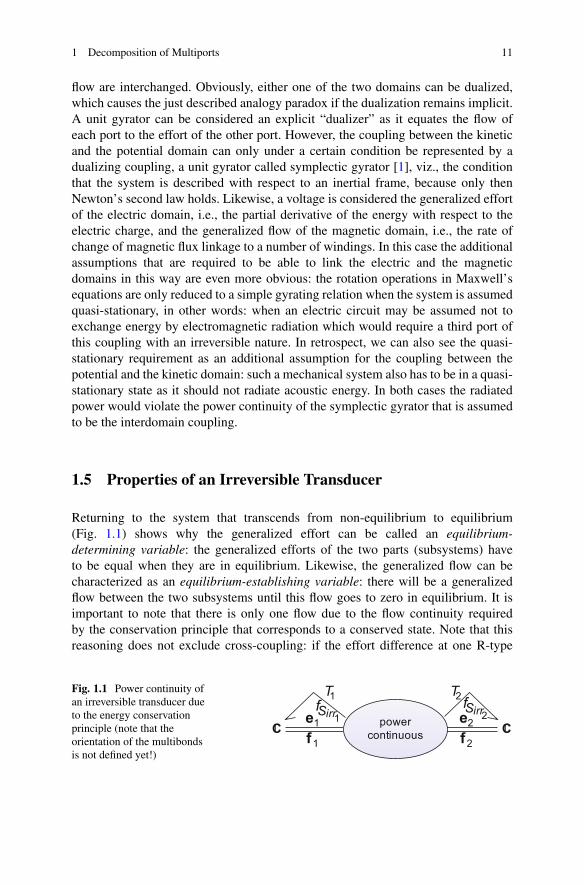
Returning to the system that transcends from non-equilibrium to equilibrium(Fig. 1.1) shows why the generalized effort can be called an equilibrium-determining variable: the generalized efforts of the two parts (subsystems) haveto be equal when they are in equilibrium. Likewise, the generalized flow can becharacterized as an equilibrium-establishing variable: there will be a generalizedflow between the two subsystems until this flow goes to zero in equilibrium. It isimportant to note that there is only one flow due to the flow continuity requiredby the conservation principle that corresponds to a conserved state. Note that thisreasoning does not exclude cross-coupling: if the effort difference at one R-type
Fig. 1.1 Power continuity ofan irreversible transducer dueto the energy conservationprinciple (note that theorientation of the multibondsis not defined yet!)
f1irrS
f2f1
e2Sirr2f
T1 T2
C Cpowercontinuous
1e

12 P.C. Breedveld
port of a multiport irreversible transducer is zero, its flow may still be non-zerodue to a non-zero effort difference at another R-type port. However, if all effortdifference are zero, all flows are zero.
We thus see that the non-equilibrium situation of each of the domains ischaracterized by one generalized flow, out of one subsystem and into the other,so corresponding with rates of change of the respective conserved states that havean opposite sign (Fig. 1.1), while two generalized efforts with different values areconverging to the same value. In other words: there has to be a relation betweenthese efforts and the flow between the subsystems. We also know that during sucha process entropy has to be generated in principle and that this entropy is also oneof the states. The production can thus be represented by a generalized flow and itsconjugate effort is the partial derivative of the energy with respect to the entropywhich is known as an absolute temperature @E
@S D T [9]. Due to the global energyconservation principle and the fact that the concept describing this irreversibleprocess cannot store energy as this would be a “contradictio in terminis,” the conceptdescribing the transition from a non-equilibrium into an equilibrium state should bepower continuous. If we just consider an irreversible transducer with one entropyproducing port which will be labeled as an S-type port, because it act as an entropysource and one R-type port for reasons of simplicity:
�e1f1 � e2f2 � TfSirr D 0 (1.9)
or, as f1 D �f2 due to flow continuity:
.e1 � e2/ f2 D TfSirr � 0 (1.10)
As the absolute temperature T is positive and the entropy production is zero orpositive we can conclude that the generalized effort difference e1 � e2 D�e hasto have the same sign as the generalized flow f2, in other words: the generalizedflow is always directed from a higher generalized effort to a lower generalizedeffort, except for cross-coupling effects. At this point it is important to recognizethat some efforts, like voltage, have a relative reference, while others, like absolutetemperature, pressure, force, or chemical potential, have an absolute reference. Incase of a relative reference the flow can only depend on the effort difference andthis results in a property called “nodicity” [17]. In non-nodic models like chemicalreaction networks the flow can be a function in which the individual values ofthe efforts are required: this means that such a relation has to be described by anelement with at least 2 R-type ports with a nonlinear constitutive relation for whichan additional flow continuity constraint holds.
The above conclusion that the generalized effort difference e1 � e2 D�e has tohave the same sign as the generalized flow f2 can also be formulated as follows:the relation between this generalized flow and this generalized effort difference hasto lie in the first and third quadrant and thus has to pass through the origin. Thisexplains why the equality of the generalized efforts (the partial derivatives of theenergy with respect to their states) is an equilibrium criterion as mentioned before.This means that the slope of this relation, which is commonly called a resistance, is
1 Decomposition of Multiports 13
positive in the origin, but may have any value outside of the origin, which explainswhy the concept of a negative differential resistance does not violate the principleof positive entropy production.
Relation (1.10) can also be written for all n states:
nX
iD1.e1i � e2i/ f2i D
nX
iD1�eif2i D �etf D TfSirr � 0 (1.11)
We can also conclude that the power port that represents the irreversibly producedthermal power cannot have a linear constitutive relation, even when all other portsare linear and can be characterized by a resistance matrix R, because
fSirr D �etfT
D ftRtfT
� 0 (1.12)
As only the symmetric part of the resistance matrix contributes to this quadraticform:
fSirr D ftRsfT
� 0 (1.13)
and
ftRaf D 0 (1.14)
where Rs D RCRt
2and Ra D R�Rt
2, such that
R D R C Rt
2C R � Rt
2D Rs C Ra (1.15)
The symmetry of the part of the relations that contributes to the entropy productionis called Onsager symmetry. This symmetry relates the Peltier effect to the Seebeckeffect, for example [9]. The other part can be identified as a multiport gyrator thatis power continuous as a result of (1.14) and of which we have seen that it containsthe dualizing interdomain couplings described earlier.
1.6 Influence of the Environment
It was not discussed yet that energy can also be exchanged with as well as stored inthe environment of a system. Typical for the concept of an environment of a systemis that there is no information available about its extent: the influence of conservedproperties that are exchanged with the environment on the behavior of the systemis neglected because no information about these extensive quantities is available:the state of the environment can only be characterized by an intensive state, i.e., ageneralized effort that can be considered independent of its conjugate generalizedflow. If this is not a valid assumption, the system boundary has to be changed such

14 P.C. Breedveld
that it is valid. The environment can thus be seen as a storage element that is solarge with respect to the storage in the system, that it can be considered infinitelylarge, such that the rate of change of extensive state does not influence the intensivestate in a relevant manner. Such an element that represents a boundary condition is ageneralized effort source Se. In contrast to a storage element, for which modulationwould mean a violation of the energy conservation principle, an effort source can bemodulated (MSe). When modulated storage elements are used after all, this impliesthe implicit assumption that the energy exchange due to modulation is at all timesnegligible compared to the energy exchange (power) through each of its ports.
If the energy storage of a system is described by a (multiport) storage elementand the influence of the environment by effort sources, then all other elementshave to be power continuous as a result of the energy conservation principle. Thecommon concept of dissipation, which seems to violate this statement, does notrefer to energy, but to one of its Legendre transforms [9, 18], viz., the free energyF . Qq;T/ D E . Qq; S/ � TS, where Qq is the state vector of all states q from which theentropy S has been eliminated. Furthermore,
dF . Qq;T/ DX
i
@E . Qq; S/@qi
dqi � SdT DX
i
ei . Qq;T/ dqi � SdT (1.16)
which means that the contribution from the thermal domain to a change in freeenergy is zero when the temperature is constant. If free energy is assumed to bedissipated in a (multiport) resistor, we thus intrinsically assume that interaction withthe thermal domain does not lead to additional dynamic properties of the model,even though temperature variations may influence the system via an activated bond,i.e., modulation by the temperature. In those cases the thermal port is not included inthe model. This is the only way to obtain linear models, as the model that describesthe entropy production port necessarily has a nonlinear constitutive equation, aswe will confirm later. The solvability of linear models explains the “popularity” ofmodels in which the above assumption about the thermal domain is made and whereall energy is in fact free energy that can be dissipated.
1.7 Co-Energy
The quadratic representation of the kinetic energy of a constant amount of massdiscussed earlier is equal in value to the sign inverse of its Legendre transform withrespect to the momentum, i.e., �LŒE.p/�p, which is a so-called co-energy E*(v), afunction in which the momentum is replaced by the velocity as function argument:
�LŒE.p/�p D ��
p2
2m� dE
dpp
�D vp � p2
2mD mv2 � 1
2mv2 D 1
2mv2 D E�.v/
(1.17)
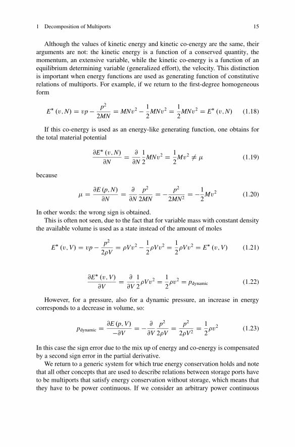
1 Decomposition of Multiports 15
Although the values of kinetic energy and kinetic co-energy are the same, theirarguments are not: the kinetic energy is a function of a conserved quantity, themomentum, an extensive variable, while the kinetic co-energy is a function of anequilibrium determining variable (generalized effort), the velocity. This distinctionis important when energy functions are used as generating function of constitutiverelations of multiports. For example, if we return to the first-degree homogeneousform
E� .v;N/ D vp � p2
2MND MNv2 � 1
2MNv2 D 1
2MNv2 D E� .v;N/ (1.18)
If this co-energy is used as an energy-like generating function, one obtains forthe total material potential
@E� .v;N/@N
D @
@N
1
2MNv2 D 1
2Mv2 ¤ � (1.19)
because
� D @E .p;N/
@ND @
@N
p2
2MND � p2
2MN2D �1
2Mv2 (1.20)
In other words: the wrong sign is obtained.This is often not seen, due to the fact that for variable mass with constant density
the available volume is used as a state instead of the amount of moles
E� .v;V/ D vp � p2
2�VD �Vv2 � 1
2�Vv2 D 1
2�Vv2 D E� .v;V/ (1.21)
@E� .v;V/@V
D @
@V
1
2�Vv2 D 1
2�v2 D pdynamic (1.22)
However, for a pressure, also for a dynamic pressure, an increase in energycorresponds to a decrease in volume, so:
pdynamic D @E .p;V/
�@VD � @
@V
p2
2�VD p2
2�V2D 1
2�v2 (1.23)
In this case the sign error due to the mix up of energy and co-energy is compensatedby a second sign error in the partial derivative.
We return to a generic system for which true energy conservation holds and notethat all other concepts that are used to describe relations between storage ports haveto be multiports that satisfy energy conservation without storage, which means thatthey have to be power continuous. If we consider an arbitrary power continuous
16 P.C. Breedveld
multiport, it may have mixed causality, in other words its constitutive relation mayhave the form:
�e1
f2
�D ‰
��f1
e2
��(1.24)
where stands for ‰ an arbitrary function. Hogan and Fasse [11] demonstrated bymeans of scattering variables that such a power continuous constitutive relation canonly be of a multiplicative form, i.e.,
�e1
f2
�D J.:/
�f1
e2
�(1.25)
where the matrix J can still depend on any variable.As a result of power continuity
P D �et
1 ft2
� � f1
e2
�D �
ft1 et
2
�Jt
�f1
e2
�D 0 (1.26)
We obtain
J D �Jt (1.27)
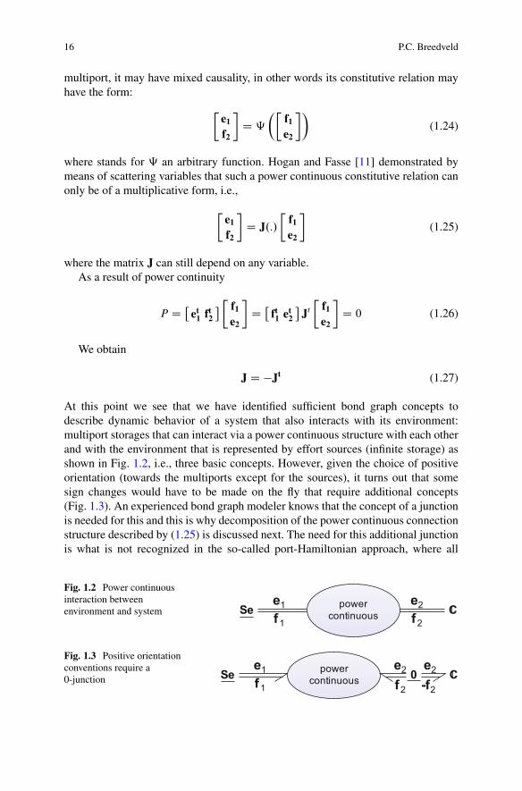
At this point we see that we have identified sufficient bond graph concepts todescribe dynamic behavior of a system that also interacts with its environment:multiport storages that can interact via a power continuous structure with each otherand with the environment that is represented by effort sources (infinite storage) asshown in Fig. 1.2, i.e., three basic concepts. However, given the choice of positiveorientation (towards the multiports except for the sources), it turns out that somesign changes would have to be made on the fly that require additional concepts(Fig. 1.3). An experienced bond graph modeler knows that the concept of a junctionis needed for this and this is why decomposition of the power continuous connectionstructure described by (1.25) is discussed next. The need for this additional junctionis what is not recognized in the so-called port-Hamiltonian approach, where all
Fig. 1.2 Power continuousinteraction betweenenvironment and system f2f1
e2Se C1e powercontinuous
Fig. 1.3 Positive orientationconventions require a0-junction
e2
2-ff2f1
e2Se C1e powercontinuous 0
1 Decomposition of Multiports 17
orientations to a power continuous structure are chosen positive inward, all positiveorientations of multiport storage and dissipation are chosen outward (resulting inan uncommon minus sign in the constitutive relations, but when junction structureshave to be combined this results in an anomaly, because junctions have not beendefined separately, which may result in error prone sign manipulation at the equationlevel.
1.8 Decomposition of the Power Continuous Multiport
A quadratic form of a matrix is only zero if it is skew symmetric, cf. (1.27), so itcan be decomposed as follows:
�e1
f2
�D J
�f1
e2
�D�
Ge Tt
� T Gf
� �f1
e2
�(1.28)
where
Ge D �Gte
Gf D �Gtf
(1.29)
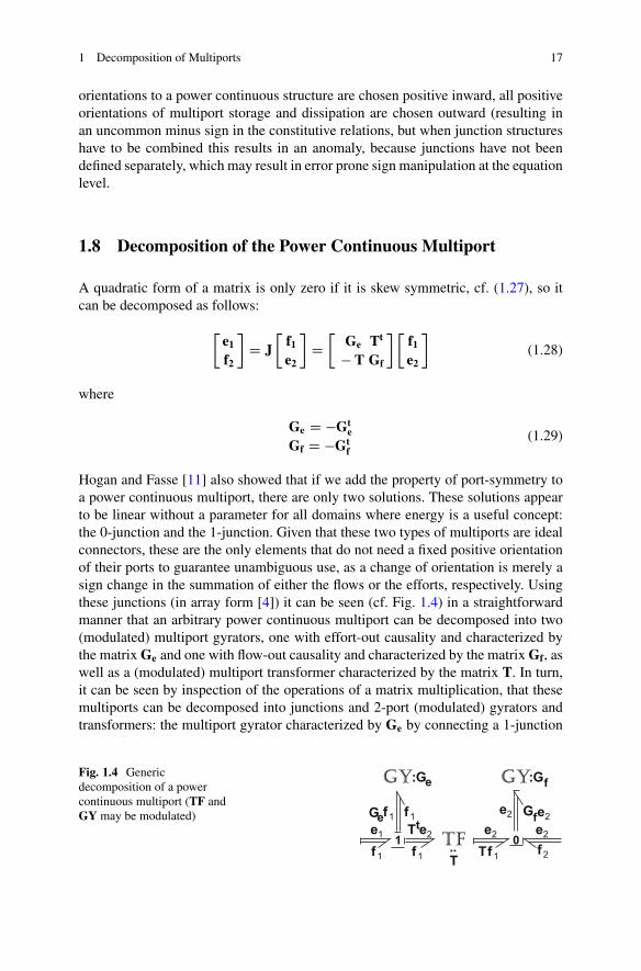
Hogan and Fasse [11] also showed that if we add the property of port-symmetry toa power continuous multiport, there are only two solutions. These solutions appearto be linear without a parameter for all domains where energy is a useful concept:the 0-junction and the 1-junction. Given that these two types of multiports are idealconnectors, these are the only elements that do not need a fixed positive orientationof their ports to guarantee unambiguous use, as a change of orientation is merely asign change in the summation of either the flows or the efforts, respectively. Usingthese junctions (in array form [4]) it can be seen (cf. Fig. 1.4) in a straightforwardmanner that an arbitrary power continuous multiport can be decomposed into two(modulated) multiport gyrators, one with effort-out causality and characterized bythe matrix Ge and one with flow-out causality and characterized by the matrix Gf, aswell as a (modulated) multiport transformer characterized by the matrix T. In turn,it can be seen by inspection of the operations of a matrix multiplication, that thesemultiports can be decomposed into junctions and 2-port (modulated) gyrators andtransformers: the multiport gyrator characterized by Ge by connecting a 1-junction
Fig. 1.4 Genericdecomposition of a powercontinuous multiport (TF andGY may be modulated) Gfe2e2Gef1 f1
e2
f1f1
f:Ge:G
tT e2
f1
e2
f2
1e
T.. Ttf
gygy
1 0
18 P.C. Breedveld
to each port and next connecting each of these ports to all other ports by 2-portgyrators, the multiport gyrator characterized by the matrix Gf by connecting a 0-junction to each port and next connecting each of these ports to all other ports by2-port gyrators and finally the multiport transformer characterized by the matrix Tby connecting a 1-junction to each port with effort-out causality and a 0-junctionto each port with flow-out causality and next connecting each 1-junction to all 0-junctions by means of 2-port transformers. In this way each 2-port gyrator or 2-porttransformer has one of the independent matrix elements of the matrix J as ratio. Asdiscussed in more detail in [3, 4], these are canonical, immediate decompositions.
Note that a gyrators and transformers, except for unit transformers that are in factequal to bonds, cannot exist inside one domain, as they would violate generalizedflow continuity: generalized flows are the rates of change of the conserved quantitythat characterizes the domain and neither a transformer nor a gyrator are flowcontinuous. In other words: they are interdomain couplings. When the objectionis made that transformers in mechanical systems seem to violate this reasoning, oneshould realize that each coordinate in a mechanical model should be considered aseparate domain, because a bond graph cannot represent configuration properties:the coordinate frames have to be represented separately and are linked to the scalarvalues that are used in the topological representation that a bond graph is.
In [3, 4] it was shown that a linear multiport storage element can be decomposedin many ways using a multiport transformer by making use of the congruenceproperties of its constitutive matrix with a diagonal matrix. However, there isonly one congruence decomposition that is canonical, i.e., in which the number ofindependent parameters of the decomposition is equal to the number of independentparameters of the multiport storage element: the transformation matrix is triangular,such that less 2-port transformers are required. Just like the immediate decompo-sitions of the multiport gyrator and transformer that were just discussed (Fig. 1.4)and that appeared to be canonical, a linear multiport storage element also has suchan immediate decomposition: in preferred integral causality all ports are connectedto a 1-junction and next each 1-junction is connected to all others via a 0-junction.Finally each junction is connected to a 1-port C. In differential causality the junctiontypes have to be interchanged.
Just like a multiport C, a multiport gyrator also has a congruence decompositionas any skew symmetric matrix is congruent with a block-diagonal matrix with 2 � 2symplectic matrices as blocks.
So far we have identified that all models in which energy is a relevant variablecan be constructed from 1-port storage elements (C), 1-port effort sources (Se), 2-port (modulated) transformers and gyrators, and 0- and 1-junctions, i.e., 6 basicelements. Given that a unit gyrator can be combined with a 1-port element, dualstorage elements (I) and dual sources (Sf) can also be defined, but one shouldbe aware that the asymmetry is then lost between effort and flow as equilibrium-determining and equilibrium-establishing variable, respectively. We then haveidentified eight basic elements and bond graph modelers will notice that the resistoris still missing: an R-element contradicts energy conservation and can only be usedif the influence of the thermal domain on the dynamic properties of a system can bedisregarded.
1 Decomposition of Multiports 19
f2f1
e21e
powercontinuous
J=
switching condition
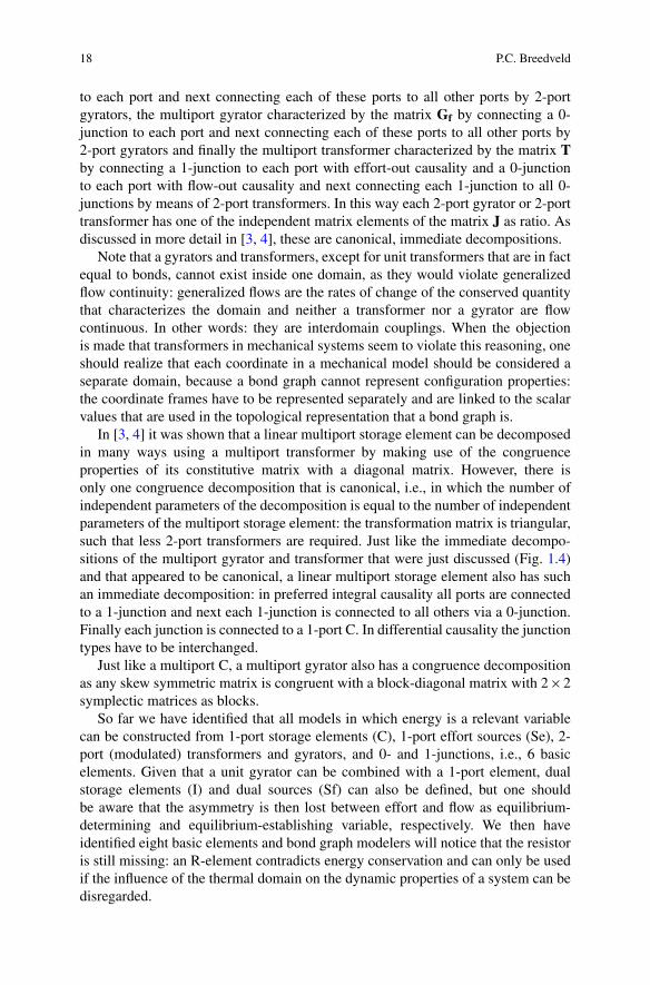
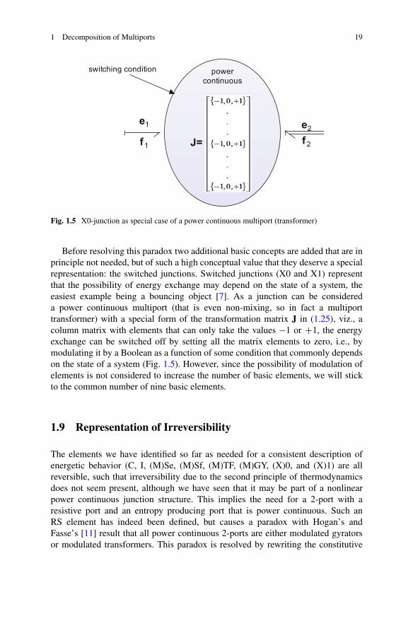
Fig. 1.5 X0-junction as special case of a power continuous multiport (transformer)
Before resolving this paradox two additional basic concepts are added that are inprinciple not needed, but of such a high conceptual value that they deserve a specialrepresentation: the switched junctions. Switched junctions (X0 and X1) representthat the possibility of energy exchange may depend on the state of a system, theeasiest example being a bouncing object [7]. As a junction can be considereda power continuous multiport (that is even non-mixing, so in fact a multiporttransformer) with a special form of the transformation matrix J in (1.25), viz., acolumn matrix with elements that can only take the values �1 or C1, the energyexchange can be switched off by setting all the matrix elements to zero, i.e., bymodulating it by a Boolean as a function of some condition that commonly dependson the state of a system (Fig. 1.5). However, since the possibility of modulation ofelements is not considered to increase the number of basic elements, we will stickto the common number of nine basic elements.
1.9 Representation of Irreversibility
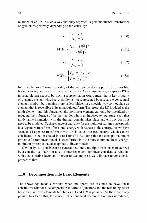
The elements we have identified so far as needed for a consistent description ofenergetic behavior (C, I, (M)Se, (M)Sf, (M)TF, (M)GY, (X)0, and (X)1) are allreversible, such that irreversibility due to the second principle of thermodynamicsdoes not seem present, although we have seen that it may be part of a nonlinearpower continuous junction structure. This implies the need for a 2-port with aresistive port and an entropy producing port that is power continuous. Such anRS element has indeed been defined, but causes a paradox with Hogan’s andFasse’s [11] result that all power continuous 2-ports are either modulated gyratorsor modulated transformers. This paradox is resolved by rewriting the constitutive
20 P.C. Breedveld
relations of an RS in such a way that they represent a port-modulated transformeror gyrator, respectively, depending on the causality:
RS W�
e D e.f /fSirr D ef
T
(1.30)
MTF W8<
:fSirr D
e.f /T
f
e D
e.f /T
T
(1.31)
RS W�
f D f .e/fSirr D ef
T
(1.32)
MGY W8<
:fSirr D
f .e/T
e
f D
f .e/T
T
(1.33)
In principle, an effort-out causality of the entropy producing port is also possible,but not shown, because this is a rare possibility. As a consequence, a separate RS isin principle not needed, but such a representation would mean that a key propertyof dynamic system, viz., irreversibility, is not represented by a separate conceptualelement symbol, but remains more or less hidden in a specific way to modulate anelement that is reversible in its unmodulated form. Therefore, the RS is added as theninth element and this fundamentally nonlinear element can only be linearized byreducing the influence of the thermal domain to an imposed temperature, such thatno dynamic interaction with the thermal domain takes place and entropy does notneed to be modeled. Such a change of causality for the multiport storage correspondsto a Legendre transform of its stored energy with respect to the entropy. As we haveseen, this Legendre transform F D E–TS is called the free energy, which can beconsidered to be dissipated in a resistor (R). By doing this the entropy-maximumprinciple for nonlinear models is transformed into the more common (free!) energy-minimum principle that also applies to linear models.
Obviously, a 1-port R can be generalized into a multiport resistor characterizedby a constitutive matrix or a set of interdependent nonlinear constitutive relationswith a constitutive Jacobian. In order to decompose it we will have to consider itsproperties first.
1.10 Decomposition into Basic Elements
The above has made clear that when multiports are assumed to have linearconstitutive relations, decomposition in terms of junctions and the remaining sevenbasic one- and two-elements (cf. Tables 1.1 and 1.2) is possible. As there are manypossibilities to do this, the concept of a canonical decomposition was introduced,
1 Decomposition of Multiports 21
which means that the decomposition does require the same number of independentconstitutive parameters as the original multiport [3, 4]. Two types of canonicaldecomposition are possible, the so-called congruence canonical decompositions thatare based on the congruence properties of the constitutive matrix and immediatecanonical decompositions that follow from direct inspection of the constitutiverelations. For 2-ports it has been shown that these two types are exhaustive whichstrongly suggests that this is also the case for arbitrary multiports [6]. In [3, 4] itwas also shown that decomposition of most elements with nonlinear constitutiverelations can also be realized by means of internal modulation, with the exceptionof nonlinear multiport storage elements, as this would introduce multiport artifactsthat need to compensate the gyristors that would be caused by the modulation, whichwould destroy the simplifying nature of a decomposition.
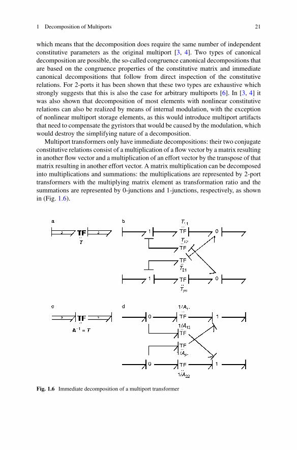
Multiport transformers only have immediate decompositions: their two conjugateconstitutive relations consist of a multiplication of a flow vector by a matrix resultingin another flow vector and a multiplication of an effort vector by the transpose of thatmatrix resulting in another effort vector. A matrix multiplication can be decomposedinto multiplications and summations: the multiplications are represented by 2-porttransformers with the multiplying matrix element as transformation ratio and thesummations are represented by 0-junctions and 1-junctions, respectively, as shownin (Fig. 1.6).
Fig. 1.6 Immediate decomposition of a multiport transformer
22 P.C. Breedveld
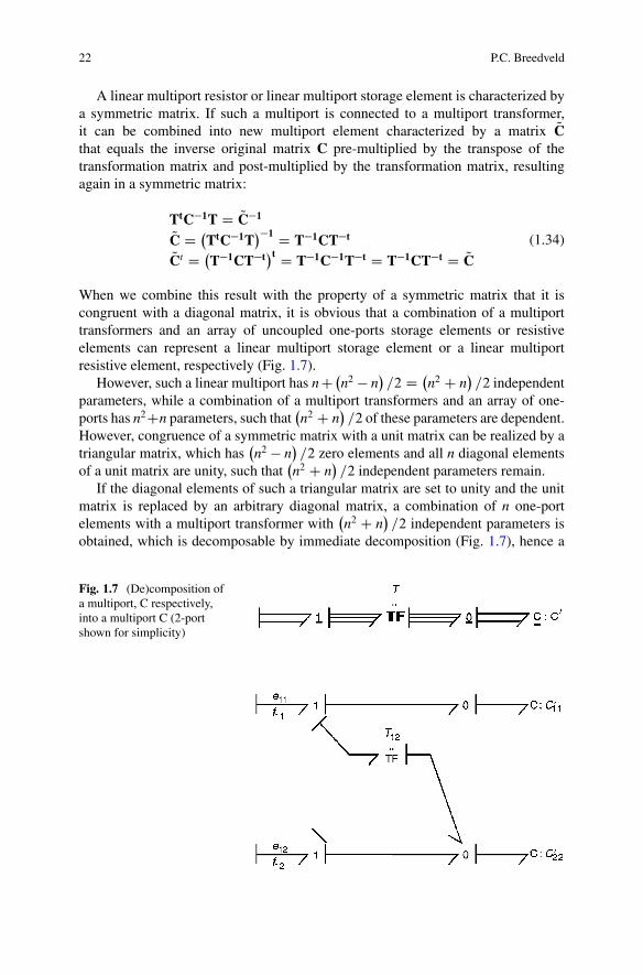
A linear multiport resistor or linear multiport storage element is characterized bya symmetric matrix. If such a multiport is connected to a multiport transformer,it can be combined into new multiport element characterized by a matrix QCthat equals the inverse original matrix C pre-multiplied by the transpose of thetransformation matrix and post-multiplied by the transformation matrix, resultingagain in a symmetric matrix:
TtC�1T D QC�1
QC D �TtC�1T
��1 D T�1CT�t
QCt D �T�1CT�t
�t D T�1C�1T�t D T�1CT�t D QC(1.34)
When we combine this result with the property of a symmetric matrix that it iscongruent with a diagonal matrix, it is obvious that a combination of a multiporttransformers and an array of uncoupled one-ports storage elements or resistiveelements can represent a linear multiport storage element or a linear multiportresistive element, respectively (Fig. 1.7).
However, such a linear multiport has nC �n2 � n
�=2 D �
n2 C n�=2 independent
parameters, while a combination of a multiport transformers and an array of one-ports has n2Cn parameters, such that
�n2 C n
�=2 of these parameters are dependent.
However, congruence of a symmetric matrix with a unit matrix can be realized by atriangular matrix, which has
�n2 � n
�=2 zero elements and all n diagonal elements
of a unit matrix are unity, such that�n2 C n
�=2 independent parameters remain.
If the diagonal elements of such a triangular matrix are set to unity and the unitmatrix is replaced by an arbitrary diagonal matrix, a combination of n one-portelements with a multiport transformer with
�n2 C n
�=2 independent parameters is
obtained, which is decomposable by immediate decomposition (Fig. 1.7), hence a
Fig. 1.7 (De)composition ofa multiport, C respectively,into a multiport C (2-portshown for simplicity)
1 Decomposition of Multiports 23
canonical decomposition. However, one should keep in mind that the decompositionof a multiport transformer depends on its causality: causal inversion of the decom-posed form leads to algebraic loops.
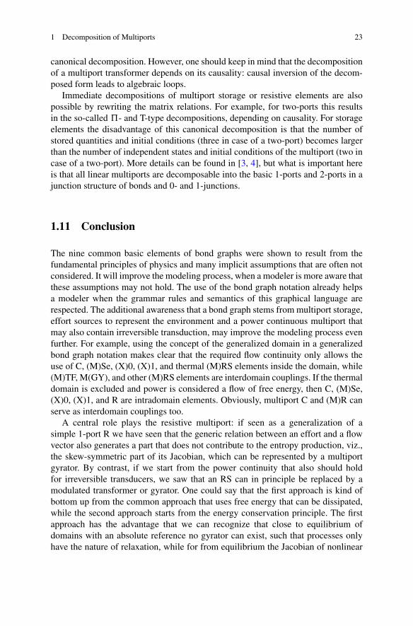
Immediate decompositions of multiport storage or resistive elements are alsopossible by rewriting the matrix relations. For example, for two-ports this resultsin the so-called …- and T-type decompositions, depending on causality. For storageelements the disadvantage of this canonical decomposition is that the number ofstored quantities and initial conditions (three in case of a two-port) becomes largerthan the number of independent states and initial conditions of the multiport (two incase of a two-port). More details can be found in [3, 4], but what is important hereis that all linear multiports are decomposable into the basic 1-ports and 2-ports in ajunction structure of bonds and 0- and 1-junctions.
1.11 Conclusion
The nine common basic elements of bond graphs were shown to result from thefundamental principles of physics and many implicit assumptions that are often notconsidered. It will improve the modeling process, when a modeler is more aware thatthese assumptions may not hold. The use of the bond graph notation already helpsa modeler when the grammar rules and semantics of this graphical language arerespected. The additional awareness that a bond graph stems from multiport storage,effort sources to represent the environment and a power continuous multiport thatmay also contain irreversible transduction, may improve the modeling process evenfurther. For example, using the concept of the generalized domain in a generalizedbond graph notation makes clear that the required flow continuity only allows theuse of C, (M)Se, (X)0, (X)1, and thermal (M)RS elements inside the domain, while(M)TF, M(GY), and other (M)RS elements are interdomain couplings. If the thermaldomain is excluded and power is considered a flow of free energy, then C, (M)Se,(X)0, (X)1, and R are intradomain elements. Obviously, multiport C and (M)R canserve as interdomain couplings too.
A central role plays the resistive multiport: if seen as a generalization of asimple 1-port R we have seen that the generic relation between an effort and a flowvector also generates a part that does not contribute to the entropy production, viz.,the skew-symmetric part of its Jacobian, which can be represented by a multiportgyrator. By contrast, if we start from the power continuity that also should holdfor irreversible transducers, we saw that an RS can in principle be replaced by amodulated transformer or gyrator. One could say that the first approach is kind ofbottom up from the common approach that uses free energy that can be dissipated,while the second approach starts from the energy conservation principle. The firstapproach has the advantage that we can recognize that close to equilibrium ofdomains with an absolute reference no gyrator can exist, such that processes onlyhave the nature of relaxation, while for from equilibrium the Jacobian of nonlinear
24 P.C. Breedveld
Fig. 1.8 Historic [1] multibond decomposition (except MTF and MGY)
relation may result in gyrating couplings that, for instance, can explain chemicaloscillations or the use of a transistor to create an oscillator while biased into a non-equilibrium operating point.
Finally, a picture from the author’s master thesis [1] (Fig. 1.8: ignore the Dutchand the uncommon choice of some symbols, like the G referring to a resistive port inconductive causality, no addition of an S to the symbol of an irreversible transducerand a direct sum definition that allowed a sign change) is shown to demonstrate thata multibond representation of a generic decomposition (except for the MTF’s andMGY’s of which immediate decomposition is straightforward) has been availablefor over 35 years. The rather cryptic symbols for effort and flow variables, bonddimensions, and constitutive matrices are the result of the fact that this multibondgraph tried to represent and extend an analysis by [12] of the power continuousconceptual structure in thermodynamic systems. Obviously, it was not recognized atthat time that the RS is just a part of the power continuous interconnection structureand, as such, a nonlinear “constraint.”

1 Decomposition of Multiports 25
References
1. Breedveld, P. C. (1979). Irreversibele Thermodynamica en Bondgrafen: EEN synthese metenige praktische toepassingen (in Dutch). Master thesis, 1241.2149, University of Twente,Enschede, Netherlands.
2. Breedveld, P. C. (1982). Thermodynamic bond graphs and the problem of thermal inertance.Journal of Franklin Institute, 314(1), 15–40. doi:10.1016/0016-0032(82)90050-3.
3. Breedveld, P. C. (1984). Physical systems theory in terms of bond graphs. Ph.D. thesis,University of Twente, Faculty of Electrical engineering, ISBN 90-9000599-4.
4. Breedveld, P. C. (1984). Decomposition of multiport elements in a revisedmultibond graph notation. Journal of the Franklin Institute, 318(4), 253–273.doi:10.1016/0016-0032(84)90014-0. ISSN 0016-0032.
5. Breedveld, P. C. (1985). Multibond graph elements in physical systems theory. Journal of theFranklin Institute, 319(1–2), 1–36. doi:10.1016/0016-0032(85)90062-6. ISSN 0016-0032.
6. Breedveld, P. C. (1995) Exhaustive decompositions of linear two-ports. In: In F. E. Cellier &J. J. Granda (Eds.), Proceedings of the SCS 1995 International Conference on Bond GraphModeling and Simulation (ICBGM’95), SCS Simulation Series, 27(1), 11–16, Las Vegas, 15–18 January, ISBN 1-56555-037-4.
7. Breedveld, P. C. (1996). The context-dependent trade-off between conceptual and computa-tional complexity illustrated by the modeling and simulation of colliding objects. In P. Borneet al. (Eds.), Proceedings of the Computational Engineering in Systems Applications ‘96IMACS/IEEE-SMC Multiconf., 48–54, Lille, France, 9–12 July 1996, Late Papers.
8. Breedveld, P. C. (1999). On state-event constructs in physical system dynamics modeling. Sim-ulation Practice and Theory, 7(5–6), 463–480. doi:10.1016/S0928-4869(99)00017-8. ISSN0928-4869.
9. Callen, H. B. (1985). Thermodynamics and an introduction to thermostatistics. New York, NY:Wiley.
10. Firestone, F. A. (1933). A new analogy between mechanical and electrical systems. The Journalof the Acoustical Society of America, 4, 249–267.
11. Hogan, N., & Fasse, E. D. (1988). Conservation principles and bond-graph junction structures.In L. R. C. Rosenberg & R. Redfield (Eds.), Automated modeling for design (pp. 9–13). NewYork, NY: ASME.
12. Jongschaap, R. J. J. (1978). About the role of constraints in the linear relaxational behaviourof thermodynamic systems. Physica A: Statistical Mechanics and Its Applications, 94(3–4),521–544. doi:10.1016/0378-4371(78)90085-7.
13. Karnopp, D. C., Margolis, D. L., & Rosenberg, R. C. (1990). System dynamics: A unifiedapproach. New York, NY: Wiley.
14. Maschke, B. M., van der Schaft, A. J., & Breedveld, P. C. (1992). An intrinsic hamiltonianformulation of network dynamics: Non-standard poisson structure and gyrators. Journal of theFranklin Institute, 329(5), 923–966. doi:10.1016/S0016-0032(92)90049-M. ISSN 0016-0032.
15. Noether, E. (1918). Invariante varlationsprobleme. Nachr. D. König, Gesellsch. D. Wiss, ZuGöttingen, Math-phys. Klasse, pp. 235–257. English translation Travel M. A. (1971) TransportTheory and Statistical Physics 1(3), 183–207.
16. Paynter, H. M. (1961). Analysis and design of engineering systems. Cambridge, MA: MIT.17. Paynter, H. M. (1972). The dynamics and control of eulerian turbomachines. J Dynamic
Systems Measurement and Control, 94(3), 198–205.18. Strang, G. (1986). Introduction to applied mathematics. Wellesley, MA: Wellesley-Cambridge.19. Trent, H. M. (1954). Isomorphisms between oriented linear graphs and lumped physical
systems. The Journal of the Acoustical Society of America, 27, 500–527.
Chapter 2A Method for Minimizing the Set of Equationsin Bond Graph Systems with Causal Loops
Jesus Felez
Abbreviations
BDF Backward differential formulaeDAE Differential algebraic equationsEJS Eulerian junction structureGYS GyristorMBG Multi-bond graphMBS Multibody systemsMGY Modulated gyratorMTF Modulated transformerODE Ordinary differential equationsZC Zero complianceZCP Zero-order causal path
2.1 Introduction
The objective of this paper is to establish an improved formulation able to be used inreal time simulations. Simulation requires integrating the dynamic equations. Thesize, complexity, and type of these equations are fundamental in order to reducethe simulation time if real time is to be achieved. This problem is very importantin the real time simulation of mechanical systems, such as in a complex multibodymodel of a vehicle used in a driving simulator, where a great number of differentialequations and constraint equations are used to build the model in a systematic way.
J. Felez (�)Mechanical Engineering Department, Universidad Politécnica de Madrid, Madrid, Spaine-mail: [email protected]
© Springer International Publishing Switzerland 2017W. Borutzky (ed.), Bond Graphs for Modelling, Control and FaultDiagnosis of Engineering Systems, DOI 10.1007/978-3-319-47434-2_2
27
28 J. Felez
In recent years, the generation of dynamic equations of systems modeled withbond graphs has been the topic of considerable research. These equations have beenpresented in a variety of forms. Classical formulations express these equations interms of a large number of flows associated with inertances and displacementsassociated with compliances. In order to obtain these equations it is necessary toestablish the causality in the model. Several procedures have been developed toachieve this. Sequential Causality Augmentation Procedure (SCAP) [10] has beentraditionally the way to implement causality in bond graph models. Causal cyclesare a consequence of the problems raised from this implementation. They appearwhen the SCAP procedure drives to indeterminacy in the application of causality.The following step is the appearance either of a causal cycle or a causal violation[17, 18]. How to deal with these causal problems has been an important aim in thepast [8]. Karnopp and Margolis [11] contributed with the stiff compliance approach,where high stiffness compliances are introduced in the model to eliminate the causalloops between integral and derivative causal storage ports. In this case, a set ofdifferential equations is obtained, including as variables the flows associated withthe previous inertances, displacements associated with the previous compliances,and the corresponding variables associated with the new stiff elements introduced,seriously increasing the number of differential equations to be solved. Usually, thisapproach needs the use of special numerical solvers for stiff differential equations,requiring very small integration step times. For these reasons, this procedure is notappropriate for simulation in real time.
Another approach was the introduction of Lagrange multipliers in the model [2,5, 20]. Some other authors [7] introduce residual sinks and sources in a similarsolution to the Lagrange approach. When Lagrange multipliers are used to breakcausal paths, a set of differential algebraic equations is obtained, composed of anumber of differential equations equal to the number of inertances plus compliances,and a number of algebraic (or constraint) equations equal to the number of Lagrangemultipliers. The number of equations is the same as with the previous method, it alsobeing inappropriate for real time. Nevertheless, this approach presents importantformulation advantages that must be considered.
Previous methods prevent the existence of causal loops, but it is necessary topre-analyze the model and to modify the model in a subsequent operation. Anotherapproach to solve the problem [3, 4] is the use of break variables to open the causalloops. Causal loops always present an algebraic character. Algebraic loops relatetheir internal variables by means of algebraic relationships. It means that these loopsdo not involve integration operations. This fact leads to the definition of Zero-orderCausal Paths (ZCPs) [4, 17]. The mathematical model obtained from bond graphswith ZCPs and opened with break variables is also a differential algebraic equationset (DAE).
This last approach reduces the number of equations to a number equal to thenumber of inertances plus compliances plus break variables.
The use of Lagrange multipliers or the introduction of break variables implies thenecessity of new variables and the appearance of constraint equations, considerably
2 A Method for Minimizing the Set of Equations in Bond Graph Systems. . . 29
increasing the number of involved variables and the number of equations tobe solved. These procedures are very useful to obtain the system equations in asystematic way, but they have to be improved or modified for their use in real timesimulation.
Another approach is to obtain the dynamic equations in terms of a minimumset of variables, related with the degrees of freedom of the system. There areseveral developed procedures, mainly in multibody analysis. The most popularmethod is Kane’s formulation [9], which uses a minimum number of generalizedvelocities. The numerical integration of these equations is much more efficient thanthe previous one because it needs only a reduced number of equations. However,simplicity in the formulation and the ease of manipulation of dynamic equations arelost with this method.
The method presented in this paper is based on a velocity transformationprocess used in multibody dynamics [12, 13, 19], extending the methodology tothe bond graph specificities. This method has the advantages of the simplicity in itsformulation and the computational efficiency of Kane’s method. In this procedurestate variables can be established as in the classical bond graph formulation. Next,according to the system causality and the ZCPs class 1 that appear in the system, aset of independent state variables are chosen obtaining the relationships betweenthe dependent and the independent ones. The dynamic equations will then betransformed into a reduced set. The resultant equations are equal in number to thenumber of degrees of freedom of the system.
This paper discusses the procedure applied to each type of ZCP and the way tomanipulate the causal assignments in order to obtain the minimal set of differentialequations. In this way, no algebraic equations appear in the set of equations obtainedand only a small number of differential equations appear (ODEs corresponding tothe system’s degrees of freedom).
The way to solve ZCPs class 2, 3, and 4 is based on the idea to assign derivativecausality to the storage elements to eliminate the causal loops [15]. Nevertheless inclass 2, 3, and 4, except class with unity gain, the break variables can be eliminatedand the equations reduced and written without any break variable and constraintequations, but this elimination must be done by hand and no automatic procedurescan be used. For this reason the procedures shown in this paper have been developedin order to systematize the way to obtain the system equations in an optimized form,with the aim of implementing them in a computer program. In Ref. [14] algorithmsare shown along with the procedures for symbolically obtaining the transformationsneeded for the different cases put forward.
Sueur and Dauphin-Tanguy [16] describe the set of conditions for the methodwhen applying a derivative causality for linear systems.
An interesting reference is presented in [1] where Borutzky considers anextension of the bond graph methodology showing its application for multibodysystems, presenting also an interesting formulation of a reduced set of equations ofmotion.
The paper is based on the previous work of Felez et al. [6]. Some examples arepresented to illustrate the different cases. These examples are very simple and their

30 J. Felez
only aim is to show the procedure for each ZCP. For each example, a comparisonbetween the use of break variables and the reduced formulation proposed has beendone, showing the differences between both cases.
2.2 Zero-Order Causal Paths
A causal path is a sequence of causal bonds between two vertices of the bond graph.The causal strokes must be attached to each bond at the “same relative position.”
A ZCP is a causal path with topological loops whose variables are related tothemselves by means of algebraic assignments [17].
The classification of ZCPs originates from the research work carried out byVan Dijk and Breedveld [17] and was completed by Cacho et al. [4]. The specificprocedure to break each ZPC type is shown in detail in [4].
2.3 ZCP Class 1
ZCP class 1 is set between storage ports with integral causality and storage portswith differential causality.
The proposed approach is based on a velocity transformation and needs theuse of Lagrange multipliers in order to break the causal loops. Once the Lagrangemultipliers have been introduced, the equations obtained are simplified and reducedby means of the velocity transformation.
This procedure is shown in the following example (Fig. 2.1). Figure 2.1represents a single pendulum composed of a bar of inertia J with respect to the centerof mass and, additionally, a concentrated mass M at the same point. Its movement isdefined by three displacements (x, y, ®) and their corresponding velocities (u, v, !).
Fig. 2.1 A single pendulum
a
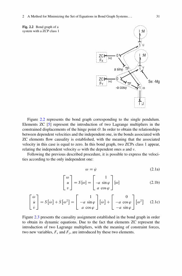
2 A Method for Minimizing the Set of Equations in Bond Graph Systems. . . 31
Fig. 2.2 Bond graph of asystem with a ZCP class 1
Figure 2.2 represents the bond graph corresponding to the single pendulum.Elements ZC [5] represent the introduction of two Lagrange multipliers in theconstrained displacements of the hinge point O. In order to obtain the relationshipsbetween dependent velocities and the independent one, in the bonds associated withZC elements flow causality is established, with the meaning that the associatedvelocity in this case is equal to zero. In this bond graph, two ZCPs class 1 appear,relating the independent velocity ! with the dependent ones u and v.
Following the previous described procedure, it is possible to express the veloci-ties according to the only independent one:
! D :' (2.1a)
2
4!
uv
3
5 D S Œ!� D2
41
–a sin'a cos'
3
5 Œ!� (2.1b)
2
4:!:u:v
3
5 D S� :!�C :
S�!2� D
2
41
�a sin'a cos'
3
5� :!�C
2
40
�a cos'�a sin'
3
5�!2�
(2.1c)
Figure 2.3 presents the causality assignment established in the bond graph in orderto obtain its dynamic equations. Due to the fact that elements ZC represent theintroduction of two Lagrange multipliers, with the meaning of constraint forces,two new variables, Fx and Fy, are introduced by these two elements.

32 J. Felez
Fig. 2.3 Introduction ofLagrange multipliers
With this causality assignment, ZCPs class 1 disappears and the dynamicequations result in three differential and two algebraic equations:
2
4J 0 0
0 M 0
0 0 M
3
5
2
4:!:u:v
3
5C2
4�a sin' a cos'
� 1 0
0 �1
3
5�
FX
FY
�D2
40
0
�Mg
3
5 (2.2a)
u C a! sin' D 0
v � a! cos' D 0(2.2b)
But these equations can be reduced to only one using the previously describedmethod. Then pre-multiplying (2.2a) by
�1; �a sin'; a cos'
�:
�J; �Ma sin' Ma cos'
�2
4:!:u:v
3
5C �0 0
� �FX
FY
�D �Mga cos ' (2.3)
Substituting in (2.3) the acceleration vector by its expression (2.1c):
�J �Ma sin' Ma cos'
�2
41
�a sin'a cos'
3
5� :!�C
C �J �Ma sin' Ma cos'
�2
40
�a cos '�a sin'
3
5�!2� D �Mga cos '
(2.4)
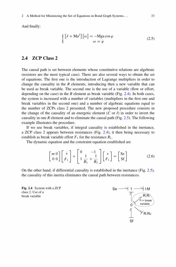
2 A Method for Minimizing the Set of Equations in Bond Graph Systems. . . 33
And finally:
� �J C Ma2
� � :!� D �Mga cos '
! D :'
(2.5)
2.4 ZCP Class 2
The causal path is set between elements whose constitutive relations are algebraic(resistors are the most typical case). There are also several ways to obtain the setof equations. The first one is the introduction of Lagrange multipliers in order tochange the causality in the R elements, introducing then a new variable that canbe used as break variable. The second one is the use of a variable (flow or effort,depending on the case) in the R element as break variable (Fig. 2.4). In both cases,the system is increased with a number of variables (multipliers in the first one andbreak variables in the second one) and a number of algebraic equations equal tothe number of ZCPs class 2 presented. The new proposed procedure consists inthe change of the causality of an energetic element (C or I) in order to invert thecausality in one R element and to eliminate the causal path (Fig. 2.5). The followingexample illustrates the procedure.
If we use break variables, if integral causality is established in the inertance,a ZCP class 2 appears between resistances (Fig. 2.4), it then being necessary toestablish as break variable effort F1 for the resistance R1.
The dynamic equation and the constraint equation established are
�m 0
0 0
�" :v:
F1
#C2
40 �111
R1C 1
R2
3
5�v
F1
�D�
SeSf
�(2.6)
On the other hand, if differential causality is established in the inertance (Fig. 2.5),the causality of this inertia eliminates the causal path between resistances.
Fig. 2.4 System with a ZCPclass 2. Use of abreak variable
1Se I:M
R:R2
0
Sf
R:R1
F1= break variable
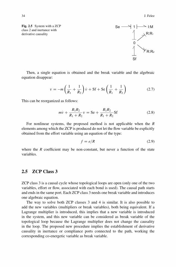
34 J. Felez
Fig. 2.5 System with a ZCPclass 2 and inertance withderivative causality
R:R2
Sf
Se
0
R:R1
1 I:M
Then, a single equation is obtained and the break variable and the algebraicequation disappear:
v D �m
�1
R1C 1
R2
�:v C Sf C Se
�1
R1C 1
R2
�(2.7)
This can be reorganized as follows:
m:v C R1R2
R1 C R2v D Se C R1R2
R1 C R2Sf (2.8)
For nonlinear systems, the proposed method is not applicable when the Relements among which the ZCP is produced do not let the flow variable be explicitlyobtained from the effort variable using an equation of the type:
f D e=R (2.9)
where the R coefficient may be non-constant, but never a function of the statevariables.
2.5 ZCP Class 3
ZCP class 3 is a causal cycle whose topological loops are open (only one of the twovariables, effort or flow, associated with each bond is used). The causal path startsand ends in the same port. Each ZCP class 3 needs one break variable and introducesone algebraic equation.
The way to solve both ZCP classes 3 and 4 is similar. It is also possible toadd the new variables (multipliers or break variables), both being equivalent. If aLagrange multiplier is introduced, this implies that a new variable is introducedin the system, and this new variable can be considered as break variable of thetopological loop because the Lagrange multiplier does not change the causalityin the loop. The proposed new procedure implies the establishment of derivativecausality in inertance or compliance ports connected to the path, working thecorresponding co-energetic variable as break variable.
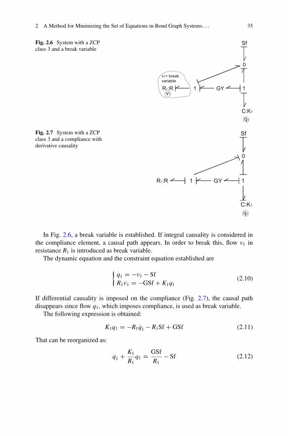
2 A Method for Minimizing the Set of Equations in Bond Graph Systems. . . 35
Fig. 2.6 System with a ZCPclass 3 and a break variable
GY 1
Sf
R1:R
0
1v1
C:K1
q1
v1= break variable
Fig. 2.7 System with a ZCPclass 3 and a compliance withderivative causality
1R1:R 1GY
C:K1
q1
Sf
0
In Fig. 2.6, a break variable is established. If integral causality is considered inthe compliance element, a causal path appears. In order to break this, flow v1 inresistance R1 is introduced as break variable.
The dynamic equation and the constraint equation established are
� :q1 D �v1 � SfR1v1 D �GSf C K1q1
(2.10)
If differential causality is imposed on the compliance (Fig. 2.7), the causal pathdisappears since flow q1, which imposes compliance, is used as break variable.
The following expression is obtained:
K1q1 D �R1:q1 � R1Sf C GSf (2.11)
That can be reorganized as:
:q1 C K1
R1q1 D GSf
R1� Sf (2.12)
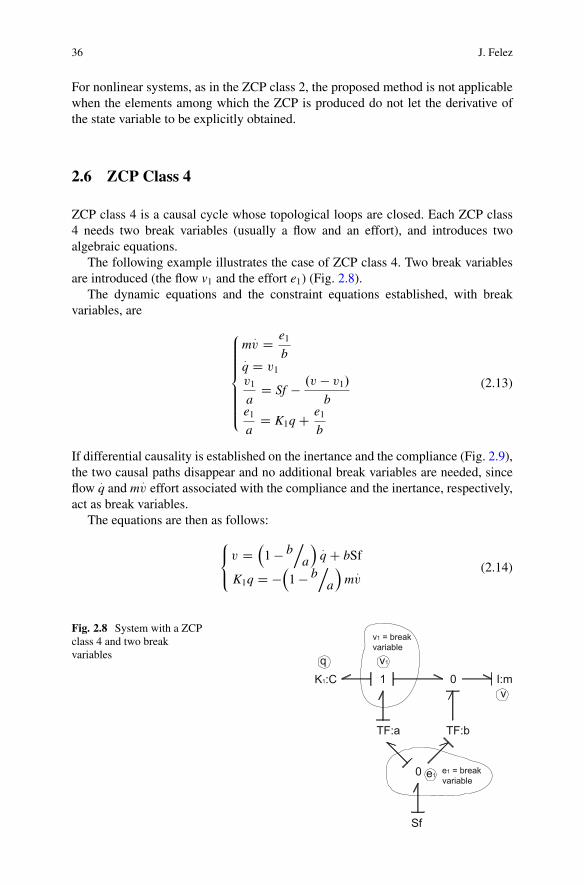
36 J. Felez
For nonlinear systems, as in the ZCP class 2, the proposed method is not applicablewhen the elements among which the ZCP is produced do not let the derivative ofthe state variable to be explicitly obtained.
2.6 ZCP Class 4
ZCP class 4 is a causal cycle whose topological loops are closed. Each ZCP class4 needs two break variables (usually a flow and an effort), and introduces twoalgebraic equations.
The following example illustrates the case of ZCP class 4. Two break variablesare introduced (the flow v1 and the effort e1) (Fig. 2.8).
The dynamic equations and the constraint equations established, with breakvariables, are
8ˆˆ<
ˆˆ:
m:v D e1
b:q D v1v1
aD Sf � .v � v1/
be1a
D K1q C e1b
(2.13)
If differential causality is established on the inertance and the compliance (Fig. 2.9),the two causal paths disappear and no additional break variables are needed, sinceflow
:q and m
:v effort associated with the compliance and the inertance, respectively,
act as break variables.The equations are then as follows:
8<
:v D
1 � b
.a
:q C bSf
K1q D �1 � b
.a
m:v
(2.14)
Fig. 2.8 System with a ZCPclass 4 and two breakvariables
K1:C 01q
I:m
0
TF:a TF:b
Sf
v
v1
e1
v1 = break variable
e1 = break variable
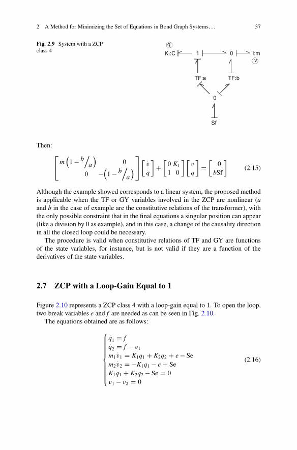
2 A Method for Minimizing the Set of Equations in Bond Graph Systems. . . 37
Fig. 2.9 System with a ZCPclass 4 I:m1 0K1:C
TF:b
Sf
TF:a
0
v
q
Then:2
4m1 � b
.a
0
0 �1 � b
.a
3
5� :v:q
�C�0 K11 0
� �v
q
�D�0
bSf
�(2.15)
Although the example showed corresponds to a linear system, the proposed methodis applicable when the TF or GY variables involved in the ZCP are nonlinear (aand b in the case of example are the constitutive relations of the transformer), withthe only possible constraint that in the final equations a singular position can appear(like a division by 0 as example), and in this case, a change of the causality directionin all the closed loop could be necessary.
The procedure is valid when constitutive relations of TF and GY are functionsof the state variables, for instance, but is not valid if they are a function of thederivatives of the state variables.
2.7 ZCP with a Loop-Gain Equal to 1
Figure 2.10 represents a ZCP class 4 with a loop-gain equal to 1. To open the loop,two break variables e and f are needed as can be seen in Fig. 2.10.
The equations obtained are as follows:
8ˆˆ<
ˆˆ:
:q1 D f:q2 D f � v1m1
:v1 D K1q1 C K2q2 C e � Se
m2
:v2 D �K1q1 � e C Se
K1q1 C K2q2 � Se D 0
v1 � v2 D 0
(2.16)

38 J. Felez
Fig. 2.10 System with a ZCPclass 4 and loop-gain equal to1 with two break variables
C:K2
C:K1
I:m2m1:Iv1
0 0
1
q2
1
q1
v2
ef
Se
Fig. 2.11 System with aZCP class 4 and loop-gainequal to 1
m1:I I:m200
C:K2
1
q2
C:K1
1
v1
q1
v2
Se
The problem with these equations is that they are differential algebraic equations oforder 2 that cannot be solved numerically if they are not derived and the nilpotencyindex reduced.
However, if the proposed method of inverting the causality of elements C and I isused by assigning them differential causality, the ZCP class 4 disappears (Fig. 2.11).
The following equations are obtained:
2
664
1 �1 0 0
1 �1 0 0
0 0 m1 m2
0 0 m1 m2
3
775
2
664
:q1:q2:v1:v2
3
775C
2
664
0 0 �1 0
0 0 0 �1K1 0 0 0
0 �K2 0 0
3
775
2
664
q1q2v1v2
3
775 D
2
664
0
0
Se0
3
775 (2.17)
In this case, these equations can be simplified because if the first two rows aresummed, it is obtained that:
v1 D v2 (2.18)

2 A Method for Minimizing the Set of Equations in Bond Graph Systems. . . 39
and (2.17) can be reduced to:
2
42m1 0 0
0 1 �10 0 0
3
5
2
4:v2:q1:q2
3
5C2
40 0 �K2
� 1 0 0
0 K1 K2
3
5
2
4v2q1q2
3
5 D2
40
0
Se
3
5 (2.19)
The above Eq. (2.19) are differential algebraic equations and do not present anyadditional break variables.
2.8 Combinations of Several ZCPs
The objective of this section is to show the application of the proposed method whenseveral ZCPs simultaneously appear. The idea is quite simple. First step is to applya procedure to assign causality like the shown in [1, 4] developed by Felez et al.to detect the different ZCPs that appear in the model. In this step, when ZCPs areidentified, causality is assigned and creak variables are used to solve and break thedifferent identified ZCPs.
Because the aim of this work is to show the way of applying the proposedmethod, very simple and academic examples are proposed. The focus is not thephysical interpretation of the bond graph models. The main focus is to show how,with a bond graph structure that presents combination of ZCPs, the proposed methodcan obtain a more reduced set of equations by eliminating break variables when itis possible.
Let’s analyze two different cases. In both cases, several ZCPs simultaneouslyappear, several storage elements, I and C, appear and for each case, equationsobtained by using break variables and preferred causality for I and C elements areshowed in comparison with the proposed method that inverts the causality of I andC in order to reduce the number of equations.
Equations are obtained with the assumption of linear behavior, but the procedurecan be applied in the same way for nonlinear components behavior, taking intoaccount that in this case several causality constraints may be taken into account.
2.8.1 Combination Between Two ZCPs Class 3
Figure 2.12 shows an example that includes one C element (energy storage element)and two R elements. If causality assignment procedure is applied, C element isassigned with preferred causality and two break variables, f1 and f2, are needed inorder to solve the two ZCPs class 3 that appear.
Expression (2.20) shows the obtained equations. They are composed by a set ofthree equations. This first one is a differential one, related with the C element, andthe last two ones are algebraic equations related with the two R elements and thetwo class 3 ZCPs. Variables in the set of equations are q, f1, and f2.
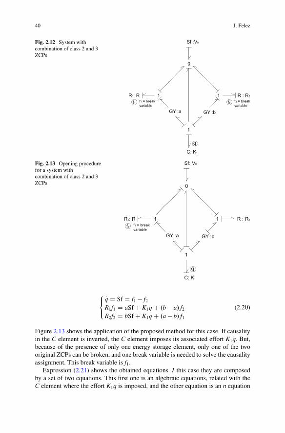
40 J. Felez
Fig. 2.12 System withcombination of class 2 and 3ZCPs
Fig. 2.13 Opening procedurefor a system withcombination of class 2 and 3ZCPs
8<
:
:q D Sf D f1 � f2R1f1 D aSf C K1q C .b � a/ f2R2f2 D bSf C K1q C .a � b/ f1
(2.20)
Figure 2.13 shows the application of the proposed method for this case. If causalityin the C element is inverted, the C element imposes its associated effort K1q. But,because of the presence of only one energy storage element, only one of the twooriginal ZCPs can be broken, and one break variable is needed to solve the causalityassignment. This break variable is f1.
Expression (2.21) shows the obtained equations. I this case they are composedby a set of two equations. This first one is an algebraic equations, related with theC element where the effort K1q is imposed, and the other equation is an n equation
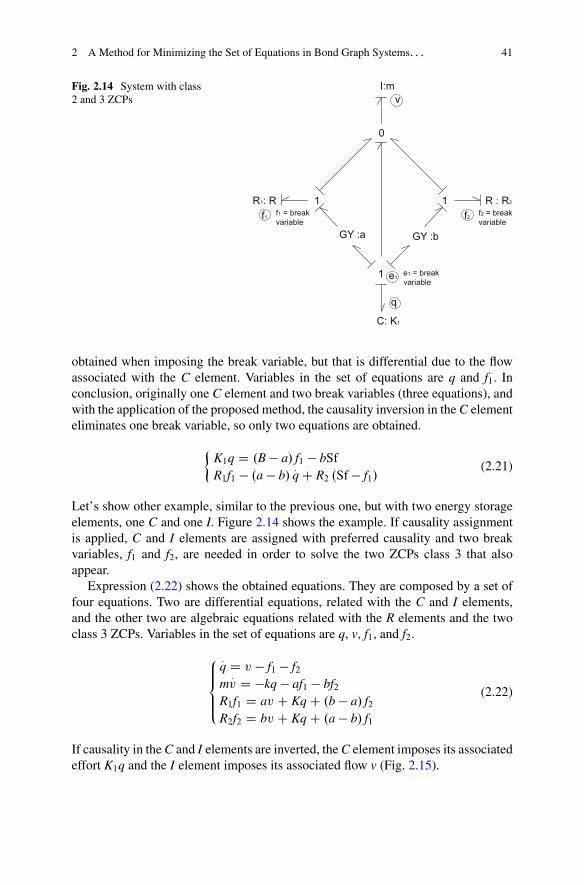
2 A Method for Minimizing the Set of Equations in Bond Graph Systems. . . 41
Fig. 2.14 System with class2 and 3 ZCPs
obtained when imposing the break variable, but that is differential due to the flowassociated with the C element. Variables in the set of equations are q and f1. Inconclusion, originally one C element and two break variables (three equations), andwith the application of the proposed method, the causality inversion in the C elementeliminates one break variable, so only two equations are obtained.
�K1q D .B � a/ f1 � bSfR1f1 � .a � b/
:q C R2 .Sf � f1/
(2.21)
Let’s show other example, similar to the previous one, but with two energy storageelements, one C and one I. Figure 2.14 shows the example. If causality assignmentis applied, C and I elements are assigned with preferred causality and two breakvariables, f1 and f2, are needed in order to solve the two ZCPs class 3 that alsoappear.
Expression (2.22) shows the obtained equations. They are composed by a set offour equations. Two are differential equations, related with the C and I elements,and the other two are algebraic equations related with the R elements and the twoclass 3 ZCPs. Variables in the set of equations are q, v, f1, and f2.
8ˆ<
ˆ:
:q D v � f1 � f2m:v D �kq � af1 � bf2
R1f1 D av C Kq C .b � a/ f2R2f2 D bv C Kq C .a � b/ f1
(2.22)
If causality in the C and I elements are inverted, the C element imposes its associatedeffort K1q and the I element imposes its associated flow v (Fig. 2.15).
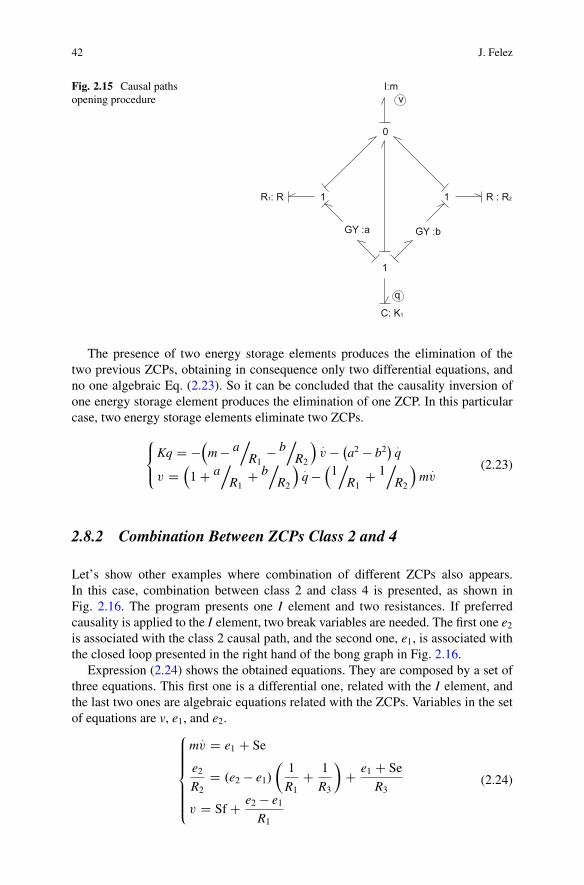
42 J. Felez
Fig. 2.15 Causal pathsopening procedure
The presence of two energy storage elements produces the elimination of thetwo previous ZCPs, obtaining in consequence only two differential equations, andno one algebraic Eq. (2.23). So it can be concluded that the causality inversion ofone energy storage element produces the elimination of one ZCP. In this particularcase, two energy storage elements eliminate two ZCPs.
8<
:Kq D �
m � a
.R1
� b.
R2
:v � �
a2 � b2� :
q
v D1C a
.R1
C b.
R2
:q �
1.
R1C 1
.R2
m:v
(2.23)
2.8.2 Combination Between ZCPs Class 2 and 4
Let’s show other examples where combination of different ZCPs also appears.In this case, combination between class 2 and class 4 is presented, as shown inFig. 2.16. The program presents one I element and two resistances. If preferredcausality is applied to the I element, two break variables are needed. The first one e2
is associated with the class 2 causal path, and the second one, e1, is associated withthe closed loop presented in the right hand of the bong graph in Fig. 2.16.
Expression (2.24) shows the obtained equations. They are composed by a set ofthree equations. This first one is a differential one, related with the I element, andthe last two ones are algebraic equations related with the ZCPs. Variables in the setof equations are v, e1, and e2.
8ˆˆ<
ˆˆ:
m:v D e1 C Se
e2R2
D .e2 � e1/
�1
R1C 1
R3
�C e1 C Se
R3
v D Sf C e2 � e1R1
(2.24)
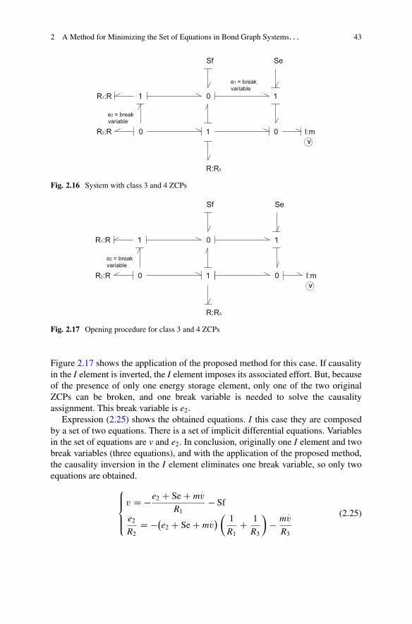
2 A Method for Minimizing the Set of Equations in Bond Graph Systems. . . 43
Fig. 2.16 System with class 3 and 4 ZCPs
Fig. 2.17 Opening procedure for class 3 and 4 ZCPs
Figure 2.17 shows the application of the proposed method for this case. If causalityin the I element is inverted, the I element imposes its associated effort. But, becauseof the presence of only one energy storage element, only one of the two originalZCPs can be broken, and one break variable is needed to solve the causalityassignment. This break variable is e2.
Expression (2.25) shows the obtained equations. I this case they are composedby a set of two equations. There is a set of implicit differential equations. Variablesin the set of equations are v and e2. In conclusion, originally one I element and twobreak variables (three equations), and with the application of the proposed method,the causality inversion in the I element eliminates one break variable, so only twoequations are obtained.
8ˆ<
ˆ:
v D �e2 C Se C m:v
R1� Sf
e2R2
D ��e2 C Se C m:v� � 1
R1C 1
R3
�� m
:v
R3
(2.25)

44 J. Felez
Fig. 2.18 System with class 3 and 4 ZCPs
Now, other similar example is presented, but with two I elements. Figure 2.18 showsthe example. If causality assignment is applied, both I elements are assigned withpreferred causality and two break variables, e1 and e2, are needed in order to solvethe two ZCPs that also appear.
Expression (2.26) shows the obtained equations. They are composed by a setof four equations. Two are differential equations, related with the I elements, andthe other two are algebraic equations related with the R element and ZCP class 4.Variables in the set of equations are v1, v2, e1, and e2.
8ˆˆ<
ˆˆ:
m1
:v1 D e1 C Se
m2
:v2 D e2
e2R2
D �v2 � .e2 � e1/
�1
R1C 1
R3
�C e1 C Se
R3
Sf C .e2 � e1/
�1
R1C 1
R3
�� e1 C Se
R3D v1 � e2 � e1
R3C e1 C Se
R3
(2.26)
And finally, Fig. 2.19 shows the application of the proposed method for this case.If causality in the I elements is inverted, the I element imposes its associated effortand both ZCPs disappear.
Expression (2.27) shows the obtained equations. They are composed by a set oftwo differential equations.
8ˆ<
ˆ:
v1 D Sf C m2
:v2 � m1
:v1 C Se
R1
v2 D �m2
:v2
R2� �
m2
:v2 � m1
:v1 C Se
� � 1R1
C 1
R3
�C m1
:v1 � Se
R3
(2.27)

2 A Method for Minimizing the Set of Equations in Bond Graph Systems. . . 45
Fig. 2.19 Opening procedure
2.9 Conclusions
In this work, a method to eliminate the additional break variables needed when ZCPsappear in a bond graph is presented. This method has been developed with the aimof obtaining a minimal set of the dynamic equations of a system modeled with bondgraphs. The method is based on an assignment of causality consisting in applyingdifferential causality of I and C elements when ZCPs appear. With this causalityassignment, ZCPs disappear and no break variables are needed.
The developed procedure allows the reduction of the number of equations in thedynamic system, obtaining the equations only in terms of the number of independentinertance and compliance elements of the system. A systematic analysis of eachZCP class has shown the way to apply the procedure. Some examples have beenpresented in order to show the application of the proposed method. The finalequations are in most of the case purely ODEs, but in several particular cases, DAEequations remain.
Several examples are also provided in order to demonstrate the applicability ofthe proposed method when combination of different ZCOs appear simultaneouslyin the model.
The results obtained with this formulation are clearly superior, from the pointof view of computational time, to those obtained with the classical bond graphformulation with break variables.
References
1. Borutzky, W. (2010). Bond graph methodology: Development and analysis of multidisciplinarydynamic system models. London: Springer. ISBN 978-1-84882-881-0.
2. Bos, A. M. (1986). Modeling multibody systems in terms of multibond graphs. Ph.D. thesis,Twente University, Enschede, The Netherlands.
3. Cacho, R., Félez, J., & Vera, C. (1997). Deriving simulation models from bond graphs with anycombination of topological loop classes. International Conference on Bond Graph Modelingand Simulation ICBGM’97 (Vol. 29, No. 1, pp. 85–93). Phoenix, AZ: SCS Publishing,Simulation Series.

46 J. Felez
4. Cacho, R., Félez, J., & Vera, C. (2000). Deriving simulation models from bond graphs withalgebraic loops. The extension to multibond graph systems. Journal of the Franklin Institute,337, 579–600.
5. Félez, J., Vera, C., San José, I., & Cacho, R. (1990). BONDYN: A Bond Graph basedsimulation program. Transactions of the ASME Journal of Dynamic Systems, Measurement,and Control, 112, 717–727.
6. Felez, J., Romero, G., Maroto, J., & Martinez, M. L. (2011). Simulation of multi-body systemsusing multi-bond graphs. In Bond graph modelling of engineering systems (pp. 323–354).New York: Springer. doi:10.1007/978-1-4419-9368-7_9. Print ISBN: 978-1-4419-9367-0,Online ISBN: 978-1-4419-9368-7.
7. Gawthrop, P. J., & Smith, L. S. (1992). Causal augmentation of Bond Graphs with algebraicloops. Journal of the Franklin Institute, 329(2), 291–303.
8. Granda, J. (1984). Bond Graph modeling solutions of algebraic loops and differential causalityin mechanical and electrical systems. Proceedings IASTED Applied Simulation and ModelingConference, San Fancisco, pp. 188–193.
9. Kane, T. R., & Levinson, D. A. (1985). Dynamics theory and applications. New York,NY: McGraw-Hill.
10. Karnopp, D. C. (1983). Alternative bond graph causal patterns and equation formulation fordynamic systems. Transactions of the ASME Journal of Dynamic Systems, Measurement, andControl, 105, 58–63.
11. Karnopp, D. C., & Margolis, D. L. (1979). Analysis and simulation of planar mechanismsystems using Bond Graph. Journal of Mechanical Design, 101(2), 187–191.
12. Kim, S. S., & Vanderploeg, M. J. (1986). A general and efficient method for dynamicanalysis of mechanical systems using velocity transformations. ASME Journal of Mechanism,Transmissions, and Automation in Design, 108, 176.
13. Nikravesh, P. E. (1990). Systematic reduction of multibody equations of motion to a minimalset. Journal of Non-Linear Mechanics, 25(2–3), 143–151.
14. Romero, G., Felez, J., & Vera, C. (2005). Optimised procedures for obtaining the symbolicequations of a dynamic system by using the bond graph technique. International Conferenceon Bond Graph Modeling and Simulation ICBGM’05 (Vol. 37, No. 1, pp. 51–58). New Orleans,Phoenix, AZ: SCS Publishing, Simulation Series.
15. Rosenberg, R. C., & Andry, A. N. (1979). Solvability of bond graph junction structures withloops. IEEE Transactions on Circuits and Systems, 26, 130–137.
16. Sueur, C., & Dauphin-Tanguy, G. (1991). Bond-graph approach for structural analysis ofMIMO linear systems. Journal of Franklin Institute, 328(1), 55–70.
17. Van Dijk, J., & Breedveld, P. (1991). Simulation of system models containing Zero-orderCausal Paths-I. Classification of Zero-order Causal Paths. Journal of the Franklin Institute,328(5/6), 959–979.
18. Van Dijk, J., & Breedveld, P. C. (1991). Simulation of system models containing Zero-orderCausal Paths—II. Numerical implications of class 1 Zero-order Causal Paths. Journal of theFranklin Institute, 328(5/6), 959–979.
19. Wittenburg, J. (1977). Dynamics of systems of rigid bodies. Stuttgart: B.G. Teubner.20. Zeid, A., & Overholt, J. (1995). Singularly perturbed Bond Graph models for simulation of
multibody systems. Transactions of the ASME Journal of Dynamic Systems, Measurement,and Control, 117(3), 401–410.
Chapter 3Controlled Switched Structures for Bond-GraphModelling and Simulation of Hybrid Systems
Matías A. Nacusse and Sergio J. Junco
3.1 Introduction
Hybrid dynamical systems are mathematical abstractions involving continuous-and/or discrete-time and discrete-event models [37]. More precisely, a hybrid systemcan be viewed as a finite set of subsystems called modes, each of them describedby a differential equation (implying continuous-valued variables on a continuous-time domain) or a difference equation (involving continuous-valued variables on adiscrete-time domain), and a discrete-event system acting as a switching supervisor.These modes evolve or are active once at a time and succeed each other in responseto a switching sequence of discrete events happening at any time instant accordingto the rules defined by the supervisor. The discrete-event sequence is restricted to afinite number of them in any finite time interval [38].
More technically, and taking the case of switching among continuous modesdescribed by state equations to fix ideas affine to the subject of this chapter, ahybrid system is usually presented as a collection of a finite number of vectorfields ffi; i D 1; : : : ;mg ; and a rule dictating the switching among the dynamicmodes
:x.t/ D fi .x.t/; u.t//, with the restriction mentioned above. Correspondingly,
one can notice that just the simple happening of abrupt parameter changes in asystem suffices to define a hybrid system. But in engineering, switching is broadlyunderstood as involving structural or topological changes in a technical system, anoccurrence that can cause more than just parametric changes: even if in many casesthis technical switching can be captured by a collection of state equations like theabove, in the more general situation DAE-systems, implicit differential equations
M.A. Nacusse (�) • S.J. JuncoLaboratorio de Automatización y Control, Departamento de Control, Facultad de CienciasExactas, Ingeniería y Agrimensura, Universidad Nacional de Rosario, Ríobamba 245 Bis,S2000EKE Rosario, Argentinae-mail: [email protected]
© Springer International Publishing Switzerland 2017W. Borutzky (ed.), Bond Graphs for Modelling, Control and FaultDiagnosis of Engineering Systems, DOI 10.1007/978-3-319-47434-2_3
47
48 M.A. Nacusse and S.J. Junco
and even different sets of state variables are necessary to capture the admittedphenomena. See [10] for a comprehensive mathematical classification of hybrid andswitched systems (put forward in the context of addressing tools for the analysis oftheir stability).
Yet another situation could arise due to the occurrence of abrupt changes in theinterconnection structure of a system: discontinuities or instantaneous jumps in thestate variables of its model could be induced by the switching [23]. Even if this is notallowed in physics, in engineering models this is frequently admitted, mainly dueto the fact that the phenomena in which engineers are interested evolve over a timescale much bigger than the time scale of the change, and that the details inside thetime window of the change are not relevant for the problem under study. Therefore,ignoring the dynamics driving the abrupt changes or commutations, and just takinginto account their initial and final states, brings significant simplifications for themodel builder and system analyst. Thus, modelling tools for switched systemsshould be capable to capture abrupt topological changes in the interconnectionstructure and be endowed with the ability to manage state jumps occurrences.
This chapter discusses in detail two simulation-oriented bond-graph modellingdevices for hybrid systems satisfying these requirements. They are the Switchable-Structure Bond and the Generalized Switched Junction or, for short, SS-Bond [25]and GSJ [26]. The SS-Bond allows to represent all commutation modes betweentwo power ports with a precise definition of their associated power variables. TheGSJ, a controlled switched bond-graph structure, comes in two dual versions andcan represent all the interconnections enforced by commutations involving bond-graph elements around otherwise standard 0- or 1-junctions. Besides illustratingtheir properties with simple examples, some technical applications are addressed.Related results previously presented in the bond-graph literature either as hybrid-,switched or variable-topology systems are reviewed and shown to be representableby these two new formalisms, so that the formers can be considered as special ofparticular cases of the latter.
In the bond-graph domain, the critical topics summarized above as implied bymodelling hybrid systems manifest themselves mainly as changes in the powerinterconnection structure, the constituent elements and/or their constitutive relation-ships, and the causality assignment. In this sense, dealing with these questions, bothswitched structures, SS-Bonds as well as GSJs, have been conceived in order to yielda single bond graph, with fixed causality and a unique interconnection structure,simultaneously representing or capturing all the commutation modes. This singleall-mode bond graph, that depending on the problem could contain both types ofswitched structures, is called Switched Bond Graph, or SwBG, for short. It shouldbe noted that this name is kept despite the fact that switched systems are mostlyunderstood as the subclass of hybrid systems where state jumps or discontinuitiesare not allowed [34]. It is so done because this is the most commonly used name inthe bond-graph literature addressing commutations and, also, because it evokes theestablished usage of the word switching in engineering to refer to technical systemssubjects to structural commutations.
3 Controlled Switched Structures for Bond-Graph Modelling and Simulation. . . 49
Fixed causality is strived to as it is an important feature from a simulationperspective. Indeed, some modelling and simulation (M&S) software do not allowchanges in the causality of the model during the simulation. Considering structuralcommutations happening instantaneously is the source of causal constraints thatgenerate causality changes at some components. A very common approach to breakthese causal constraints is the adroit addition of parasitic elements in the model,see [19, 30, 31] therein. In the sequel, this approach to obtain models with fixedcausality will be called non-ideal or soft-switching modelling, in opposition to theformer approach, that will be designed as ideal or hard-switching modelling. Bothformalisms discussed here, SS-Bonds and GSJs, can be set for modelling hard aswell as soft-switching phenomena. The key tool allowing to achieve the all-modesingle SwBG with fixed causality and unique power interconnection structure whenmodelling commutations as hard-switching is the integration of residual sinks intothe internal structure of the formalisms. In the case of modelling with the soft-switching approach, the same effect is achieved incorporating parasitic componentsin place of the residual sinks.
It should also be noticed that, unlike many other tools, both devices can beemployed in situations where the set of state variables is not the same in all ofthe switching modes as well.
With the sequence of modes being properly defined by a set of control variablesin the switching supervisor, a SwBG featuring the above-mentioned propertiesis ready for a one-shot simulation, without need of interrupting and restarting itat any switching instant. This is possible even in the presence of state jumps,as a prescription is provided to calculate the necessary re-initialization of thediscontinuous state variables, either offline, previous to the simulation, and to theintegration of the results into the model, or at run-time. The key concept supportingthis is the principle of charge and impulse conservation.
The next section briefly summarizes the most relevant devices introduced to dealwith commutation phenomena in the bond-graph domain and some auxiliary toolsused in the constitution of both SS-Bonds and GSJs. These two formalisms areaddressed in detail, including application examples and some simulation results, inSects. 3.3 and 3.4, respectively. In both cases the devices are introduced in theirideal- or hard-switching version. The non-ideal or soft-switching form is discussedin Sect. 3.5. Finally, the conclusions are presented in Sect. 3.6.
3.2 Summary Review of Some Bond-Graph Devicesfor Modelling Switching Systems and Auxiliary Tools
Originally, bond graphs have been introduced assuming the continuity and smooth-ness properties of classic physics. In order to cope with abrupt changes in thestructure of physical systems, many bond-graph devices have been proposed thatallow to face some of the challenges presented by hybrid systems includingswitching among the continuous modes.
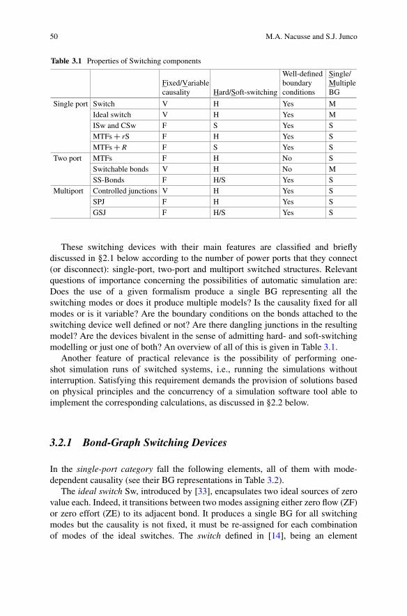
50 M.A. Nacusse and S.J. Junco
Table 3.1 Properties of Switching components
Fixed/Variablecausality Hard/Soft-switching
Well-definedboundaryconditions
Single/MultipleBG
Single port Switch V H Yes MIdeal switch V H Yes MISw and CSw F S Yes SMTFsC rS F H Yes SMTFsCR F S Yes S
Two port MTFs F H No SSwitchable bonds V H No MSS-Bonds F H/S Yes S
Multiport Controlled junctions V H Yes SSPJ F H Yes SGSJ F H/S Yes S
These switching devices with their main features are classified and brieflydiscussed in §2.1 below according to the number of power ports that they connect(or disconnect): single-port, two-port and multiport switched structures. Relevantquestions of importance concerning the possibilities of automatic simulation are:Does the use of a given formalism produce a single BG representing all theswitching modes or does it produce multiple models? Is the causality fixed for allmodes or is it variable? Are the boundary conditions on the bonds attached to theswitching device well defined or not? Are there dangling junctions in the resultingmodel? Are the devices bivalent in the sense of admitting hard- and soft-switchingmodelling or just one of both? An overview of all of this is given in Table 3.1.
Another feature of practical relevance is the possibility of performing one-shot simulation runs of switched systems, i.e., running the simulations withoutinterruption. Satisfying this requirement demands the provision of solutions basedon physical principles and the concurrency of a simulation software tool able toimplement the corresponding calculations, as discussed in §2.2 below.
3.2.1 Bond-Graph Switching Devices
In the single-port category fall the following elements, all of them with mode-dependent causality (see their BG representations in Table 3.2).
The ideal switch Sw, introduced by [33], encapsulates two ideal sources of zerovalue each. Indeed, it transitions between two modes assigning either zero flow (ZF)or zero effort (ZE) to its adjacent bond. It produces a single BG for all switchingmodes but the causality is not fixed, it must be re-assigned for each combinationof modes of the ideal switches. The switch defined in [14], being an element

3 Controlled Switched Structures for Bond-Graph Modelling and Simulation. . . 51
Table 3.2 Iconic representation of properties of single-port switched structures
Switch Ideal Switch ISw and CSw MTFs+rS MTFs+RIc
onic
rep
rese
ntat
ion
:0
:0m
m
MTF
rSe
1/m
MTF
rSf
1/m
MTF
R
m
MTF
R:Ron :Roff
Table 3.3 Iconic representation of properties of two-port switched structures
SS-BondsSwitchable bondsMTF
Iconic representation m
MTF
m U uu
u
commutating between a zero-valued current source and a zero-valued voltage source(its introduction is restricted to electric circuits), is just an explicit version of theprevious tool. Both are hard-switching devices.
The ISW and CSW, introduced in [16], belong to the category of dynamic soft-switching approximations of hard-switching, introduced with the aim of producinga single BG with fixed causality in all modes. The external port of the ISW isinternally connected through a 1� junction to an I� element in integral causalityand an ideal Sw, so that it is an effort-out element, behaving like an I when theswitch is ON and like a ZF-source when the switch is OFF. Featuring a C� elementinstead of an I, its complementary device, the CSW, is explained dualizing all theprevious terms.
Other one-port elements with fixed causality are the combination of an MTF(modulated by a gain taking the values 0 or 1) with a residual sink [3], and thecombination of an MTF with a R-element [2, 9, 15], which is commonly used inthe literature to represent a non-ideal switch. Both are static switching devices, theformer modelling hard- and the latter soft-switching.
The simplest structure in the two-port category is the MTF modulated with again being either 0 (switch open) or 1 (switch closed) [2, 4, 20]. This use of theMTF results in a fixed causality representation of the switch element. In some caseswhen the switch is open, the boundary conditions may not be well defined, sincethis representation imposes zero flow or zero effort to the attached power ports andthis condition may fail to disconnect the subsystems [33].
The switchable bond, introduced in [11] proposes conditionally present bonds.The boundary conditions on its adjacencies are not always explicitly defined in allthe switching modes, which results in the dangling junction problem [32], see theirBG representations in Table 3.3.
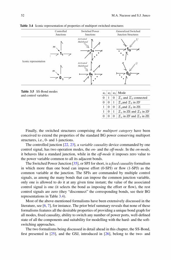
52 M.A. Nacusse and S.J. Junco
Table 3.4 Iconic representation of properties of multiport switched structures
ControlledJunctions
Switched PowerJunctions
Generalized SwitchedJunction Structures
Iconic representation
|
m
ActivatedMultibond
1G
m
ActivatedMultibond
0G
Table 3.5 SS-Bond modesand control variables
u1 u2 u3 Mode
0 1 0 ˙a and ˙b connected0 0 1 ˙aand ˙b in ZF1 0 0 ˙aand ˙b in ZE1 0 1 ˙a in ZE and ˙b in ZF0 0 0 ˙a in ZF and ˙b in ZE
Finally, the switched structures comprising the multiport category have beenconceived to extend the properties of the standard BG power conserving multiportstructures, i.e., 0- and 1-junctions.
The controlled junction [22, 23], a variable causality device commanded by onecontrol signal, has two operation modes, the on- and the off-mode. In the on-mode,it behaves like a standard junction, while in the off-mode it imposes zero value tothe power variable common to all its adjacent bonds.
The Switched Power Junction [35], or SPJ for short, is a fixed causality formalismin which more than one bond can impose effort (0-SPJ) or flow (1-SPJ) as thecommon variable at the junction. The SPJs are commanded by multiple controlsignals, as among the many bonds that can impose the common junction variable,only one is allowed to do it at any given time instant; the value of the associatedcontrol signal is one (it selects the bond as imposing the effort or flow), the restcontrol signals are zero (they “disconnect” the corresponding bonds, see their BGrepresentations in Table 3.4).
Most of the above-mentioned formalisms have been extensively discussed in theliterature, see [6, 7], for instance. The prior brief summary reveals that none of theseformalisms features all the desirable properties of providing a unique bond graph forall modes, fixed causality, ability to switch any number of power ports, well-definedstate of all the components and suitability for modelling with the hard- and the soft-switching approaches.
The two formalisms being discussed in detail ahead in this chapter, the SS-Bond,first presented in [25], and the GSJ, introduced in [26], belong to the two- and
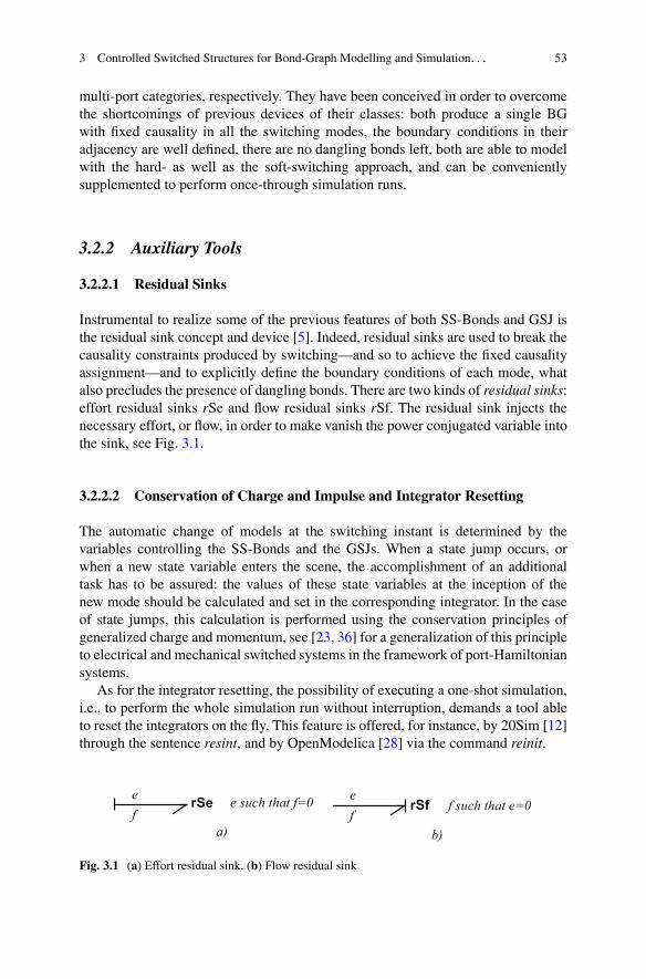
3 Controlled Switched Structures for Bond-Graph Modelling and Simulation. . . 53
multi-port categories, respectively. They have been conceived in order to overcomethe shortcomings of previous devices of their classes: both produce a single BGwith fixed causality in all the switching modes, the boundary conditions in theiradjacency are well defined, there are no dangling bonds left, both are able to modelwith the hard- as well as the soft-switching approach, and can be convenientlysupplemented to perform once-through simulation runs.
3.2.2 Auxiliary Tools
3.2.2.1 Residual Sinks
Instrumental to realize some of the previous features of both SS-Bonds and GSJ isthe residual sink concept and device [5]. Indeed, residual sinks are used to break thecausality constraints produced by switching—and so to achieve the fixed causalityassignment—and to explicitly define the boundary conditions of each mode, whatalso precludes the presence of dangling bonds. There are two kinds of residual sinks:effort residual sinks rSe and flow residual sinks rSf. The residual sink injects thenecessary effort, or flow, in order to make vanish the power conjugated variable intothe sink, see Fig. 3.1.
3.2.2.2 Conservation of Charge and Impulse and Integrator Resetting
The automatic change of models at the switching instant is determined by thevariables controlling the SS-Bonds and the GSJs. When a state jump occurs, orwhen a new state variable enters the scene, the accomplishment of an additionaltask has to be assured: the values of these state variables at the inception of thenew mode should be calculated and set in the corresponding integrator. In the caseof state jumps, this calculation is performed using the conservation principles ofgeneralized charge and momentum, see [23, 36] for a generalization of this principleto electrical and mechanical switched systems in the framework of port-Hamiltoniansystems.
As for the integrator resetting, the possibility of executing a one-shot simulation,i.e., to perform the whole simulation run without interruption, demands a tool ableto reset the integrators on the fly. This feature is offered, for instance, by 20Sim [12]through the sentence resint, and by OpenModelica [28] via the command reinit.
rSe rSf
a) b)
e such that f=0 f such that e=0ef
ef
Fig. 3.1 (a) Effort residual sink. (b) Flow residual sink
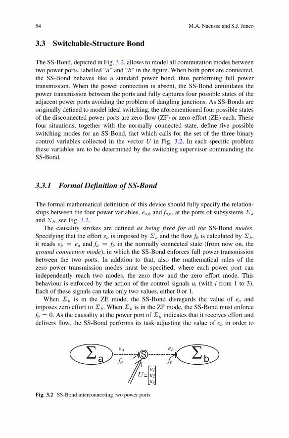
54 M.A. Nacusse and S.J. Junco
3.3 Switchable-Structure Bond
The SS-Bond, depicted in Fig. 3.2, allows to model all commutation modes betweentwo power ports, labelled “a” and “b” in the figure. When both ports are connected,the SS-Bond behaves like a standard power bond, thus performing full powertransmission. When the power connection is absent, the SS-Bond annihilates thepower transmission between the ports and fully captures four possible states of theadjacent power ports avoiding the problem of dangling junctions. As SS-Bonds areoriginally defined to model ideal switching, the aforementioned four possible statesof the disconnected power ports are zero-flow (ZF) or zero-effort (ZE) each. Thesefour situations, together with the normally connected state, define five possibleswitching modes for an SS-Bond, fact which calls for the set of the three binarycontrol variables collected in the vector U in Fig. 3.2. In each specific problemthese variables are to be determined by the switching supervisor commanding theSS-Bond.
3.3.1 Formal Definition of SS-Bond
The formal mathematical definition of this device should fully specify the relation-ships between the four power variables, ea,b and fa,b, at the ports of subsystems ˙a
and ˙b, see Fig. 3.2.The causality strokes are defined as being fixed for all the SS-Bond modes.
Specifying that the effort ea is imposed by ˙a and the flow fb is calculated by ˙b,it reads eb D ea and fa D fb in the normally connected state (from now on, theground connection mode), in which the SS-Bond enforces full power transmissionbetween the two ports. In addition to that, also the mathematical rules of thezero power transmission modes must be specified, where each power port canindependently reach two modes, the zero flow and the zero effort mode. Thisbehaviour is enforced by the action of the control signals ui (with i from 1 to 3).Each of these signals can take only two values, either 0 or 1.
When ˙b is in the ZE mode, the SS-Bond disregards the value of ea andimposes zero effort to ˙b. When ˙b is in the ZF mode, the SS-Bond must enforcefb D 0. As the causality at the power port of ˙b indicates that it receives effort anddelivers flow, the SS-Bond performs its task adjusting the value of eb in order to
ea eb
fa fbΣa Σb
U uu
u
Fig. 3.2 SS-Bond interconnecting two power ports
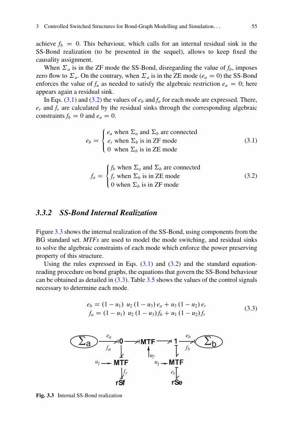
3 Controlled Switched Structures for Bond-Graph Modelling and Simulation. . . 55
achieve fb D 0. This behaviour, which calls for an internal residual sink in theSS-Bond realization (to be presented in the sequel), allows to keep fixed thecausality assignment.
When ˙a is in the ZF mode the SS-Bond, disregarding the value of fb, imposeszero flow to˙a. On the contrary, when˙a is in the ZE mode (ea D 0) the SS-Bondenforces the value of fa as needed to satisfy the algebraic restriction ea D 0; hereappears again a residual sink.
In Eqs. (3.1) and (3.2) the values of eb and fa for each mode are expressed. There,er and fr are calculated by the residual sinks through the corresponding algebraicconstraints fb D 0 and ea D 0.
eb D8<
:
ea when †a and †b are connecteder when †b is in ZF mode0 when †b is in ZE mode
(3.1)
fa D8<
:
fb when †a and †b are connectedfr when †b is in ZE mode0 when †b is in ZF mode
(3.2)
3.3.2 SS-Bond Internal Realization
Figure 3.3 shows the internal realization of the SS-Bond, using components from theBG standard set. MTFs are used to model the mode switching, and residual sinksto solve the algebraic constraints of each mode which enforce the power preservingproperty of this structure.
Using the rules expressed in Eqs. (3.1) and (3.2) and the standard equation-reading procedure on bond graphs, the equations that govern the SS-Bond behaviourcan be obtained as detailed in (3.3). Table 3.5 shows the values of the control signalsnecessary to determine each mode.
eb D .1 � u1/ u2 .1 � u3/ ea C u3 .1 � u2/ er
fa D .1 � u1/ u2 .1 � u3/ fb C u1 .1 � u2/ fr(3.3)
Σa Σb
Fig. 3.3 Internal SS-Bond realization
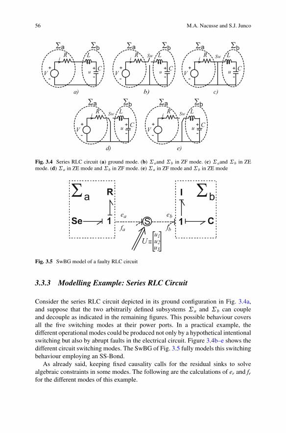
56 M.A. Nacusse and S.J. Junco
R
VC
i
u
L
a)
Σa ΣbR
VC
i
u
L
b)
Σa ΣbR
VC
i
u
L
c)
Σa Σb
R
VC
i
u
L
d)
Σa ΣbR
VC
i
u
L
e)
Σa Σb
Sw Sw
SwSw
Fig. 3.4 Series RLC circuit (a) ground mode. (b) ˙aand ˙b in ZF mode. (c) ˙aand ˙b in ZEmode. (d) ˙a in ZE mode and ˙b in ZF mode. (e) ˙a in ZF mode and ˙b in ZE mode
Σa Σbea eb
fa fb
U uu
u
Fig. 3.5 SwBG model of a faulty RLC circuit
3.3.3 Modelling Example: Series RLC Circuit
Consider the series RLC circuit depicted in its ground configuration in Fig. 3.4a,and suppose that the two arbitrarily defined subsystems ˙a and ˙b can coupleand decouple as indicated in the remaining figures. This possible behaviour coversall the five switching modes at their power ports. In a practical example, thedifferent operational modes could be produced not only by a hypothetical intentionalswitching but also by abrupt faults in the electrical circuit. Figure 3.4b–e shows thedifferent circuit switching modes. The SwBG of Fig. 3.5 fully models this switchingbehaviour employing an SS-Bond.
As already said, keeping fixed causality calls for the residual sinks to solvealgebraic constraints in some modes. The following are the calculations of er and frfor the different modes of this example.
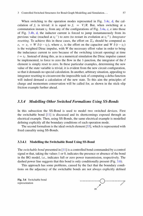
3 Controlled Switched Structures for Bond-Graph Modelling and Simulation. . . 57
When switching to the operation modes represented in Fig. 3.4c, d, the cal-culation of fr is trivial: it is equal to fr D V=R. But, when switching at acommutation instant tC from any of the configurations of Fig. 3.4a, c, e into thoseof Fig. 3.4b, d, the inductor current is forced to jump instantaneously from itsprevious value (reached at tC�) to zero (to restart its evolution at tCC). Integratorresetting. To achieve this in these cases, the effort on ˙b should be computed aser D ec C W ı .t � tC/, where ec is the effort on the capacitor and W ı .t � tC/is the weighted Dirac impulse, with W the necessary effort value in order to bringthe inductance current to zero because of the switching (circuit opening) at timet D tC. Instead of doing this, as in a numerical simulation the Dirac impulse cannotbe implemented, to force to zero the flow in the 1-junction, the integrator of the Ielement is simply reset to zero. In these particular examples, determining the newvalue of the state variable is trivial, it is evident from the new circuit configuration,so that it demands no special calculation. In another, arbitrary situation, appealing tointegrator resetting to circumvent the impossible task of computing a delta-functionwill indeed demand a calculation of the new state. To this aim the principles ofcharge and momentum conservation will be called for, as shown in the stick–slipfriction example further ahead.
3.3.4 Modelling Other Switched Formalisms Using SS-Bonds
In this subsection the SS-Bond is used to model two switched devices. Firstthe switchable bond [11] is discussed and its shortcomings exposed through anelectrical example. Then, using SS-Bonds, the same electrical example is modelleddefining explicitly all the boundary conditions of each operation mode.
The second formalism is the ideal switch element [33], which is represented withfixed causality using SS-Bonds.
3.3.4.1 Modelling the Switchable Bond Using SS-Bond
The switchable bond presented in [11] is a controlled bond commanded by a controlsignal m that, taking the values 1 or 0, indicates the presence or absence of the bondin the BG model, i.e., indicates full or zero power transmission, respectively. Thedashed power line suggests that this bond is only conditionally present (Fig. 3.6).
This approach has some problems, caused by the fact that the boundary condi-tions on the adjacency of the switchable bonds are not always explicitly defined
Fig. 3.6 Switchable bondrepresentation
m
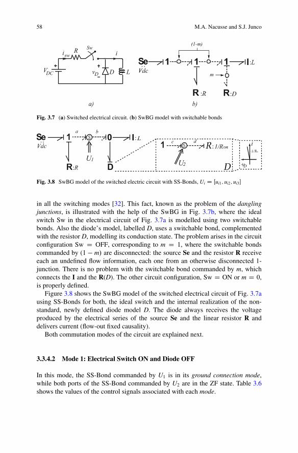
58 M.A. Nacusse and S.J. Junco
LVDC
iRiswSw
Dv
Fig. 3.7 (a) Switched electrical circuit. (b) SwBG model with switchable bonds
c d
U U
a b
12
i
v
Fig. 3.8 SwBG model of the switched electric circuit with SS-Bonds, Ui D Œui1; ui2; ui3�
in all the switching modes [32]. This fact, known as the problem of the danglingjunctions, is illustrated with the help of the SwBG in Fig. 3.7b, where the idealswitch Sw in the electrical circuit of Fig. 3.7a is modelled using two switchablebonds. Also the diode’s model, labelled D, uses a switchable bond, complementedwith the resistor D, modelling its conduction state. The problem arises in the circuitconfiguration Sw D OFF, corresponding to m D 1, where the switchable bondscommanded by (1 � m/ are disconnected: the source Se and the resistor R receiveeach an undefined flow information, each one from an otherwise disconnected 1-junction. There is no problem with the switchable bond commanded by m, whichconnects the I and the R(D). The other circuit configuration, Sw D ON or m D 0,is properly defined.
Figure 3.8 shows the SwBG model of the switched electrical circuit of Fig. 3.7ausing SS-Bonds for both, the ideal switch and the internal realization of the non-standard, newly defined diode model D. The diode always receives the voltageproduced by the electrical series of the source Se and the linear resistor R anddelivers current (flow-out fixed causality).
Both commutation modes of the circuit are explained next.
3.3.4.2 Mode 1: Electrical Switch ON and Diode OFF
In this mode, the SS-Bond commanded by U1 is in its ground connection mode,while both ports of the SS-Bond commanded by U2 are in the ZF state. Table 3.6shows the values of the control signals associated with each mode.

3 Controlled Switched Structures for Bond-Graph Modelling and Simulation. . . 59
Table 3.6 SS-Bond modes and control variables for Mode 1 of elec-trical circuit
Mode 1 SS-Bond mode Ui ui1 ui2 ui3
Electrical switch ON ˙a and ˙b connected U1 0 1 0Diode OFF ˙ c and ˙d in ZF U2 0 0 1
Table 3.7 SS-Bond modes and control variables for Mode 2 of electri-cal circuit
Mode 2 SS-Bond mode Ui ui1 ui2 ui3
Electrical switch OFF ˙aand ˙b in ZF U1 0 0 1Diode ON ˙ c and ˙d connected U2 0 1 0
c d
a b
i
v
Fig. 3.9 BG model of the switched electrical circuit in mode 1
The power variables of the SS-Bond modelling the electrical switch are eb D ea
and fa D fb, while the power variables of the SS-Bond in the diode are ed D er
and fc D 0. As the conduction state of the diode is modelled as a (negative-slope)resistance, then er D 0 to enforce fd D 0.
3.3.4.3 Mode 2: Electrical Switch OFF, Diode ON
In this mode, as the electric parallel of inductance I and diode D always receivethe voltage from the power port b of the SS-Bond commanded by U1, the powervariables of the SS-Bond of the electrical switch are eb D er (the power port b isconnected via an effort residual sink) and fa D 0, while the power variables of thediode’s SS-Bond are ed D ec and fc D fd. Table 3.7 shows the values of the controlsignals associated with each mode.
To better understand how the SwBG model of Fig. 3.8 commutates betweenmodes, the SS-Bond expanded model of Fig. 3.3 can be used: Figs. 3.9 and 3.10show the equivalent BGs enforced on the single BG of Fig. 3.8 by the (hypothetical,not shown) external switching supervisor imposing the values 0 and 1 on m for eachof the modes.
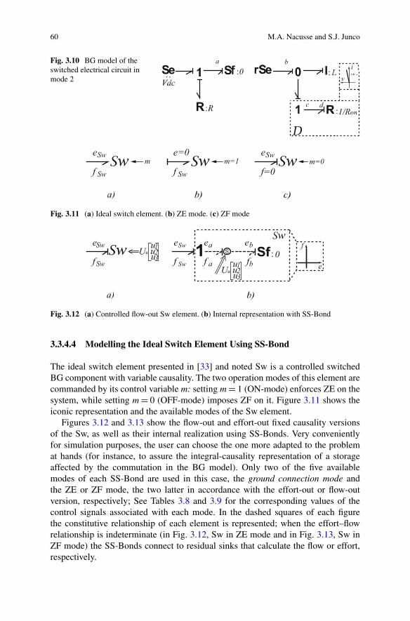
60 M.A. Nacusse and S.J. Junco
Fig. 3.10 BG model of theswitched electrical circuit inmode 2
c d
a bi
v
eSw
f Sw
e=0
f Sw
eSw
f=0m=0m=1m
Fig. 3.11 (a) Ideal switch element. (b) ZE mode. (c) ZF mode
U uuu
U uuuea eb
f a fb
eSw
f Sw
eSw
fSw0:
Fig. 3.12 (a) Controlled flow-out Sw element. (b) Internal representation with SS-Bond
3.3.4.4 Modelling the Ideal Switch Element Using SS-Bond
The ideal switch element presented in [33] and noted Sw is a controlled switchedBG component with variable causality. The two operation modes of this element arecommanded by its control variable m: setting m D 1 (ON-mode) enforces ZE on thesystem, while setting m D 0 (OFF-mode) imposes ZF on it. Figure 3.11 shows theiconic representation and the available modes of the Sw element.
Figures 3.12 and 3.13 show the flow-out and effort-out fixed causality versionsof the Sw, as well as their internal realization using SS-Bonds. Very convenientlyfor simulation purposes, the user can choose the one more adapted to the problemat hands (for instance, to assure the integral-causality representation of a storageaffected by the commutation in the BG model). Only two of the five availablemodes of each SS-Bond are used in this case, the ground connection mode andthe ZE or ZF mode, the two latter in accordance with the effort-out or flow-outversion, respectively; See Tables 3.8 and 3.9 for the corresponding values of thecontrol signals associated with each mode. In the dashed squares of each figurethe constitutive relationship of each element is represented; when the effort–flowrelationship is indeterminate (in Fig. 3.12, Sw in ZE mode and in Fig. 3.13, Sw inZF mode) the SS-Bonds connect to residual sinks that calculate the flow or effort,respectively.
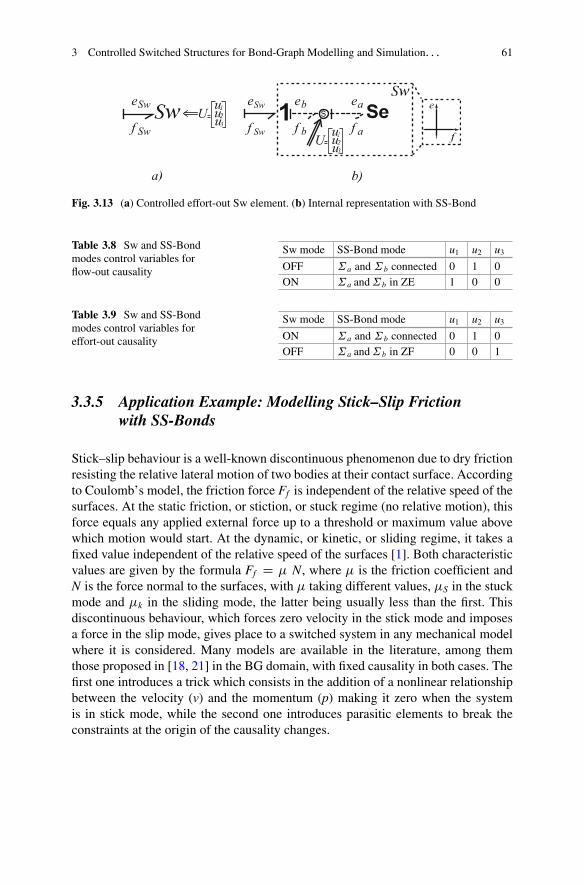
3 Controlled Switched Structures for Bond-Graph Modelling and Simulation. . . 61
U uuu
U uuueaeb
f af b
eSw
f Sw
eSw
f Sw
Fig. 3.13 (a) Controlled effort-out Sw element. (b) Internal representation with SS-Bond
Table 3.8 Sw and SS-Bondmodes control variables forflow-out causality
Sw mode SS-Bond mode u1 u2 u3
OFF ˙a and ˙b connected 0 1 0ON ˙a and˙b in ZE 1 0 0
Table 3.9 Sw and SS-Bondmodes control variables foreffort-out causality
Sw mode SS-Bond mode u1 u2 u3
ON ˙a and ˙b connected 0 1 0OFF ˙a and˙b in ZF 0 0 1
3.3.5 Application Example: Modelling Stick–Slip Frictionwith SS-Bonds
Stick–slip behaviour is a well-known discontinuous phenomenon due to dry frictionresisting the relative lateral motion of two bodies at their contact surface. Accordingto Coulomb’s model, the friction force Ff is independent of the relative speed of thesurfaces. At the static friction, or stiction, or stuck regime (no relative motion), thisforce equals any applied external force up to a threshold or maximum value abovewhich motion would start. At the dynamic, or kinetic, or sliding regime, it takes afixed value independent of the relative speed of the surfaces [1]. Both characteristicvalues are given by the formula Ff D � N, where � is the friction coefficient andN is the force normal to the surfaces, with � taking different values, �S in the stuckmode and �k in the sliding mode, the latter being usually less than the first. Thisdiscontinuous behaviour, which forces zero velocity in the stick mode and imposesa force in the slip mode, gives place to a switched system in any mechanical modelwhere it is considered. Many models are available in the literature, among themthose proposed in [18, 21] in the BG domain, with fixed causality in both cases. Thefirst one introduces a trick which consists in the addition of a nonlinear relationshipbetween the velocity (v) and the momentum (p) making it zero when the systemis in stick mode, while the second one introduces parasitic elements to break theconstraints at the origin of the causality changes.
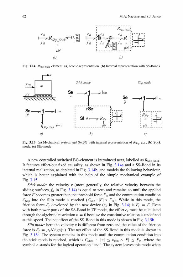
62 M.A. Nacusse and S.J. Junco
feSlip_Stick
RSlip_Stick
μN
R 1
a) b)
S
123
U uuu
123
U uuueb ea
f b f a
eR
f R
eR
f RμN
R
Fig. 3.14 RSlip_Stick element. (a) Iconic representation. (b) Internal representation with SS-Bonds
1Se rSe
RSlip_Stick
I
1
Stick mode
RSlip
μN
1
Slip mode
μN
a) b) c)
m
v
F(t)
f F Se I
Sf
Se I
RSlipFm: :
m:F
:
0:
m:F
:
ef f
e
Fig. 3.15 (a) Mechanical system and SwBG with internal representation of RSlip_Stick, (b) Stickmode, (c) Slip mode
A new controlled switched BG-element is introduced next, labelled as RSlip_Stick.It features effort-out fixed causality, as shown in Fig. 3.14a and a SS-Bond in itsinternal realization, as depicted in Fig. 3.14b, and models the following behaviour,which is better explained with the help of the simple mechanical example ofFig. 3.15.
Stick mode: the velocity v (more generally, the relative velocity between thesliding surfaces, fR in Fig. 3.14) is equal to zero and remains so until the appliedforce F becomes greater than the threshold force Fth and the commutation conditionCSlip into the Slip mode is reached
�CSlip W jFj > Fth
�. While in this mode, the
friction force Ff developed by the new device (eR in Fig. 3.14) is Ff D F. Evenwith both power ports of the SS-Bond in ZF mode, the effort er must be calculatedthrough the algebraic restriction v D 0 because the constitutive relation is undefinedat this speed. The net effect of the SS-Bond in this mode is shown in Fig. 3.15b.
Slip mode: here the velocity v is different from zero and the value of the frictionforce is Ff D �kNsign.v/. The net effect of the SS-Bond in this mode is shown inFig. 3.15c. The system remains in this mode until the commutation condition intothe stick mode is reached, which is CStick W jvj � vmin ^ jFj � Fth, where thesymbol ^ stands for the logical operation “and”. The system leaves this mode when
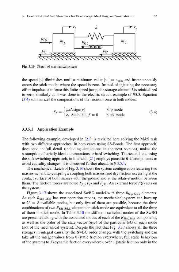
3 Controlled Switched Structures for Bond-Graph Modelling and Simulation. . . 63
Fig. 3.16 Sketch of mechanical system
the speed jvj diminishes until a minimum value jvj D vmin and instantaneouslyenters the stick mode, where the speed is zero. Instead of injecting the necessaryeffort impulse to enforce this finite speed jump, the storage element I is reinitializedto zero, similarly as it was done in the electric circuit example of §3.3. Equation(3.4) summarizes the computations of the friction force in both modes.
Ff D��kNsign.v/ slip modeer Such that f D 0 stick mode
(3.4)
3.3.5.1 Application Example
The following example, developed in [21], is revisited here solving the M&S taskwith two different approaches, in both cases using SS-Bonds. The first approach,developed in full detail (including simulations in the next section), makes theassumption of strictly ideal commutations or hard-switching. The second one, usingthe soft-switching approach, in line with [21] employs parasitic R-C components toavoid causality changes; it is discussed further ahead, in § 3.5.1.
The mechanical sketch of Fig. 3.16 shows the system configuration featuring twomasses, m1 and m2, a spring k coupling both masses, and dry friction occurring at thecontact surface of both masses with the ground and at the relative motion betweenthem. The friction forces are noted Ff 1, Ff 2 and Ff 12. An external force F(t) acts onthe system.
Figure 3.17 shows the associated SwBG model with three RSlip_Stick elements.As each RSlip_Stick has two operation modes, the mechanical system can have upto 23 D 8 available modes, but only five of them are possible, because the threecombinations of two RSlip_Stick elements in stick mode are equivalent to all the threeof them in stick mode. In Table 3.10 the different switched modes of the SwBGare presented along with the associated modes of each of the RSlip_Stick components,as well as the order of the state vector (nSV) of the particular BG of each mode(not of the mechanical system). Despite the fact that Fig. 3.17 shows all the threestorages in integral causality, the SwBG order changes with the switching and cantake all the integer values from 0 (static friction everywhere, full static behaviourof the system) to 3 (dynamic friction everywhere), over 1 (static friction only in the
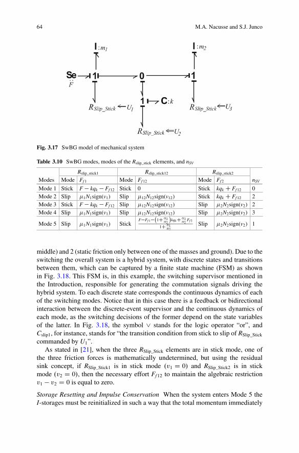
64 M.A. Nacusse and S.J. Junco
1
2
3
Fig. 3.17 SwBG model of mechanical system
Table 3.10 SwBG modes, modes of the Rslip_stick elements, and nSV
Rslip_stick1 Rslip_stick12 Rslip_stick2
Modes Mode Ff 1 Mode Ff 12 Mode Ff 2 nSV
Mode 1 Stick F � kqk � Ff12 Stick 0 Stick kqk C Ff12 0Mode 2 Slip �1N1sign(v1) Slip �12N12sign(v12) Stick kqk C Ff12 2Mode 3 Stick F � kqk � Ff12 Slip �12N12sign(v12) Slip �2N2sign(v2) 2Mode 4 Slip �1N1sign(v1) Slip �12N12sign(v12) Slip �2N2sign(v2) 3
Mode 5 Slip �1N1sign(v1) StickF�Ff1�
1C
m1m2
kqkC
m1m2
Ff2
1Cm1m2
Slip �2N2sign(v2) 1
middle) and 2 (static friction only between one of the masses and ground). Due to theswitching the overall system is a hybrid system, with discrete states and transitionsbetween them, which can be captured by a finite state machine (FSM) as shownin Fig. 3.18. This FSM is, in this example, the switching supervisor mentioned inthe Introduction, responsible for generating the commutation signals driving thehybrid system. To each discrete state corresponds the continuous dynamics of eachof the switching modes. Notice that in this case there is a feedback or bidirectionalinteraction between the discrete-event supervisor and the continuous dynamics ofeach mode, as the switching decisions of the former depend on the state variablesof the latter. In Fig. 3.18, the symbol _ stands for the logic operator “or”, andCslip1, for instance, stands for “the transition condition from stick to slip of RSlip_Stick
commanded by U1”.As stated in [21], when the three RSlip_Stick elements are in stick mode, one of
the three friction forces is mathematically undetermined, but using the residualsink concept, if RSlip_Stick1 is in stick mode .v1 D 0/ and RSlip_Stick2 is in stickmode .v2 D 0/, then the necessary effort Ff 12 to maintain the algebraic restrictionv1 � v2 D 0 is equal to zero.
Storage Resetting and Impulse Conservation When the system enters Mode 5 theI-storages must be reinitialized in such a way that the total momentum immediately
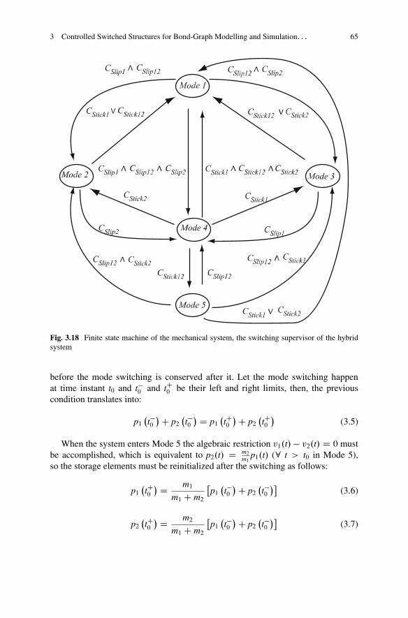
3 Controlled Switched Structures for Bond-Graph Modelling and Simulation. . . 65
Fig. 3.18 Finite state machine of the mechanical system, the switching supervisor of the hybridsystem
before the mode switching is conserved after it. Let the mode switching happenat time instant t0 and t�0 and tC0 be their left and right limits, then, the previouscondition translates into:
p1�t�0�C p2
�t�0� D p1
�tC0�C p2
�tC0�
(3.5)
When the system enters Mode 5 the algebraic restriction v1.t/ � v2.t/ D 0 mustbe accomplished, which is equivalent to p2.t/ D m2
m1p1.t/ (8 t > t0 in Mode 5),
so the storage elements must be reinitialized after the switching as follows:
p1�tC0� D m1
m1 C m2
�p1�t�0�C p2
�t�0��
(3.6)
p2�tC0� D m2
m1 C m2
�p1�t�0�C p2
�t�0��
(3.7)
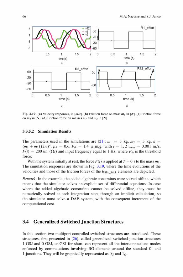
66 M.A. Nacusse and S.J. Junco
Fig. 3.19 (a) Velocity responses, in [m/s]. (b) Friction force on mass m1 in [N]. (c) Friction forceon m2 in [N]. (d) Friction force on masses m1 and m2 in [N]
3.3.5.2 Simulation Results
The parameters used in the simulations are [21]: m1 D 5 kg, m2 D 5 kg, k D.m1 C m2/ .2�/
2, �k D 0:6, Fth D 1:4 �kmig; with i D 1; 2 vmin D 0:001 m=s,F.t/ D 200 sin .�t/ and input frequency equal to 1 Hz, where Fth is the thresholdforce.
With the system initially at rest, the force F(t) is applied at T D 0 s to the mass m1.The simulation responses are shown in Fig. 3.19, where the time evolutions of thevelocities and those of the friction forces of the RSlip_Stick elements are depicted.
Remark In the example, the added algebraic constraints were solved offline, whichmeans that the simulator solves an explicit set of differential equations. In casewhere the added algebraic constraints cannot be solved offline, they must benumerically solved at each integration step, through an implicit calculation, sothe simulator must solve a DAE system, with the consequent increment of thecomputational cost.
3.4 Generalized Switched Junction Structures
In this section two multiport controlled switched structures are introduced. Thesestructures, first presented in [26], called generalized switched junction structures1-GSJ and 0-GSJ, or GSJ for short, can represent all the interconnections modesenforced by commutations involving BG-elements around the standard 0- and1-junctions. They will be graphically represented as 0G and 1G.
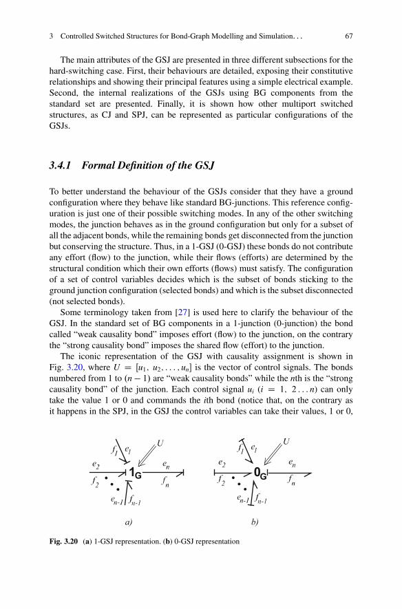
3 Controlled Switched Structures for Bond-Graph Modelling and Simulation. . . 67
The main attributes of the GSJ are presented in three different subsections for thehard-switching case. First, their behaviours are detailed, exposing their constitutiverelationships and showing their principal features using a simple electrical example.Second, the internal realizations of the GSJs using BG components from thestandard set are presented. Finally, it is shown how other multiport switchedstructures, as CJ and SPJ, can be represented as particular configurations of theGSJs.
3.4.1 Formal Definition of the GSJ
To better understand the behaviour of the GSJs consider that they have a groundconfiguration where they behave like standard BG-junctions. This reference config-uration is just one of their possible switching modes. In any of the other switchingmodes, the junction behaves as in the ground configuration but only for a subset ofall the adjacent bonds, while the remaining bonds get disconnected from the junctionbut conserving the structure. Thus, in a 1-GSJ (0-GSJ) these bonds do not contributeany effort (flow) to the junction, while their flows (efforts) are determined by thestructural condition which their own efforts (flows) must satisfy. The configurationof a set of control variables decides which is the subset of bonds sticking to theground junction configuration (selected bonds) and which is the subset disconnected(not selected bonds).
Some terminology taken from [27] is used here to clarify the behaviour of theGSJ. In the standard set of BG components in a 1-junction (0-junction) the bondcalled “weak causality bond” imposes effort (flow) to the junction, on the contrarythe “strong causality bond” imposes the shared flow (effort) to the junction.
The iconic representation of the GSJ with causality assignment is shown inFig. 3.20, where U D Œu1; u2; : : : ; un� is the vector of control signals. The bondsnumbered from 1 to .n � 1/ are “weak causality bonds” while the nth is the “strongcausality bond” of the junction. Each control signal ui (i D 1; 2 : : : n) can onlytake the value 1 or 0 and commands the ith bond (notice that, on the contrary asit happens in the SPJ, in the GSJ the control variables can take their values, 1 or 0,
1G 0G
)b)a
Fig. 3.20 (a) 1-GSJ representation. (b) 0-GSJ representation
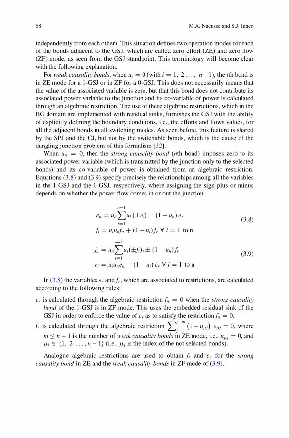
68 M.A. Nacusse and S.J. Junco
independently from each other). This situation defines two operation modes for eachof the bonds adjacent to the GSJ, which are called zero effort (ZE) and zero flow(ZF) mode, as seen from the GSJ standpoint. This terminology will become clearwith the following explanation.
For weak causality bonds, when ui D 0 (with i D 1; 2 : : : ; n�1), the ith bond isin ZE mode for a 1-GSJ or in ZF for a 0-GSJ. This does not necessarily means thatthe value of the associated variable is zero, but that this bond does not contribute itsassociated power variable to the junction and its co-variable of power is calculatedthrough an algebraic restriction. The use of these algebraic restrictions, which in theBG domain are implemented with residual sinks, furnishes the GSJ with the abilityof explicitly defining the boundary conditions, i.e., the efforts and flows values, forall the adjacent bonds in all switching modes. As seen before, this feature is sharedby the SPJ and the CJ, but not by the switchable bonds, which is the cause of thedangling junction problem of this formalism [32].
When un D 0, then the strong causality bond (nth bond) imposes zero to itsassociated power variable (which is transmitted by the junction only to the selectedbonds) and its co-variable of power is obtained from an algebraic restriction.Equations (3.8) and (3.9) specify precisely the relationships among all the variablesin the 1-GSJ and the 0-GSJ, respectively, where assigning the sign plus or minusdepends on whether the power flow comes in or out the junction.
en D un
n�1X
iD1ui .˙ei/˙ .1 � un/ er
fi D uiunfn C .1 � ui/ fr 8 i D 1 to n
(3.8)
fn D un
n�1X
iD1ui.˙fi/i ˙ .1 � un/ fr
ei D uiunen C .1 � ui/ er 8 i D 1 to n
(3.9)
In (3.8) the variables er and fr, which are associated to restrictions, are calculatedaccording to the following rules:
er is calculated through the algebraic restriction fn D 0 when the strong causalitybond of the 1-GSJ is in ZF mode. This uses the embedded residual sink of theGSJ in order to enforce the value of er as to satisfy the restriction fn D 0.
fr is calculated through the algebraic restrictionXjDm
jD1�1 � u�j
�e�j D 0, where
m � n � 1 is the number of weak causality bonds in ZE mode, i.e., u�j D 0, and�j 2 f1; 2; : : : ; n � 1g (i.e., �j is the index of the not selected bonds).
Analogue algebraic restrictions are used to obtain fr and er for the strongcausality bond in ZE and the weak causality bonds in ZF mode of (3.9).
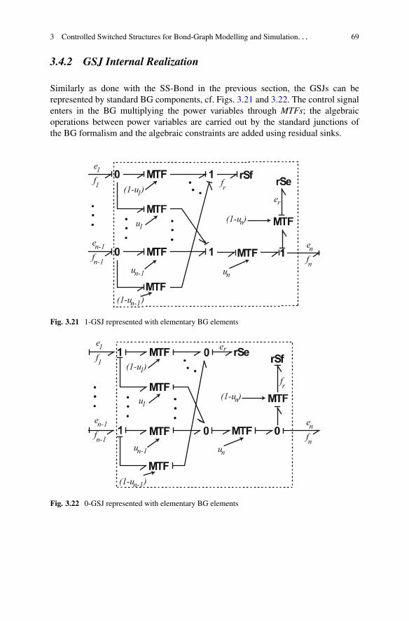
3 Controlled Switched Structures for Bond-Graph Modelling and Simulation. . . 69
3.4.2 GSJ Internal Realization
Similarly as done with the SS-Bond in the previous section, the GSJs can berepresented by standard BG components, cf. Figs. 3.21 and 3.22. The control signalenters in the BG multiplying the power variables through MTFs; the algebraicoperations between power variables are carried out by the standard junctions ofthe BG formalism and the algebraic constraints are added using residual sinks.
e
u
f(1-u )
1
1
1
1
e
uf
(1-u )
n-1
n-1n-1
n-1
e
uf
(1-u )
n
nn
n
frer
Fig. 3.21 1-GSJ represented with elementary BG elements
e
u
f(1-u )
1
1
1
1
e
uf
(1-u )
n-1
n-1n-1
n-1
e
uf
(1-u )
n
nn
n
er
fr
Fig. 3.22 0-GSJ represented with elementary BG elements
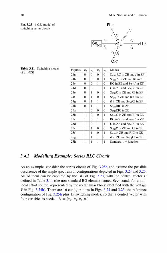
70 M.A. Nacusse and S.J. Junco
Fig. 3.23 1-GSJ model ofswitching series circuit
1G
Table 3.11 Switching modesof a 1-GSJ
Figures u4 u3 u2 u1 Modes
24a 0 0 0 0 SeNI RC in ZE and I in ZF24b 0 0 0 1 SeNI C in ZE and RI in ZF24c 0 0 1 0 RC in ZE and SeNII in ZF24d 0 0 1 1 C in ZE and SeNIRI in ZF24e 0 1 0 0 SeNIR in ZE and CI in ZF24f 0 1 0 1 SeNI in ZE and RIC in ZF24g 0 1 1 0 R in ZE and SeNICI in ZF24h 0 1 1 1 SeNIRIC in ZF25a 1 0 0 0 SeNIRIC in ZE25b 1 0 0 1 SeNIC in ZE and RI in ZE25c 1 0 1 0 RC in ZE and SeNII in ZE25d 1 0 1 1 C in ZE and SeNIRI in ZE25e 1 1 0 0 SeNIR in ZE and CI in ZE25f 1 1 0 1 SeNIin ZE and RIC in ZE25g 1 1 1 0 R in ZE and SeNICI in ZE25h 1 1 1 1 Standard 1� junction
3.4.3 Modelling Example: Series RLC Circuit
As an example, consider the series circuit of Fig. 3.25h and assume the possibleoccurrence of the ample spectrum of configurations depicted in Figs. 3.24 and 3.25.All of them can be captured by the BG of Fig. 3.23, with the control vector Udefined in Table 3.11 (the non-standard BG element named SeNI stands for a non-ideal effort source, represented by the rectangular block identified with the voltageV in Fig. 3.24h). There are 16 configurations in Figs. 3.24 and 3.25, the referenceconfiguration of Fig. 3.25h plus 15 switching modes, so that a control vector withfour variables is needed: U D Œu1; u2; u3; u4�.
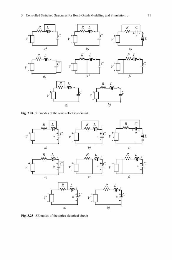
3 Controlled Switched Structures for Bond-Graph Modelling and Simulation. . . 71
R
VC
LR
VC
L
R
VC
L R
VC
L
R
VC
LR
VC
L R
VC
L
R
V
C
uL
a) b) c)
d) e) f)
g) h)
Fig. 3.24 ZF modes of the series electrical circuit
R
VC
i
u
L R
VCu
L
R
VC
i
u
L R
VC
i
u
L
)b)a
R
V
C
u
iL
c)
d)
R
VC
i
u
L R
VC
i
u
L
)f)e
g) h)
R
VC
i
u
L
i
Fig. 3.25 ZE modes of the series electrical circuit
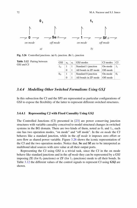
72 M.A. Nacusse and S.J. Junco
:0 :0on mode off mode on mode off mode
a) b)
Fig. 3.26 Controlled junctions. (a) 01-junction. (b) 11-junction
Table 3.12 Pairing betweenGSJ and CJ
GSJ un ui GSJ modes CJ modes CJ
1G 1 1 Standard 1-junction On-mode 11
0 1 All bonds in ZF mode Off-mode0G 1 1 Standard 0-junction On-mode 01
0 1 All bonds in ZF mode Off-mode
3.4.4 Modelling Other Switched Formalisms Using GSJ
In this subsection the CJ and the SPJ are represented as particular configurations ofGSJ to expose the flexibility of the latter to represent different switched structures.
3.4.4.1 Representing CJ with Fixed Causality Using GSJ
The Controlled Junctions (CJ) presented in [23] are power conserving junctionstructures with variable causality conceived to model structural changes in switchedsystems in the BG domain. There are two kinds of them, noted as 01 and 11, eachone has two operation modes, “on mode” and “off mode”. In the on mode the CJbehaves like a standard junction, while in the off mode it imposes zero effort orzero flow as shared power variable. Figure 3.26 shows the iconic representation ofthe CJ and the two operation modes. Notice that, Se and Sf are to be interpreted asmultibond ideal sources with zero value at all their output ports.
Representing the CJ using GSJ is a trivial task, since the CJ in the on modebehave like standard junctions and in the off mode they can be represented by a GSJimposing ZE (for 01-junctions) or ZF (for 11-junctions) mode to all their bonds. InTable 3.12 the different values of the control signals to represent CJ using GSJ areshown.
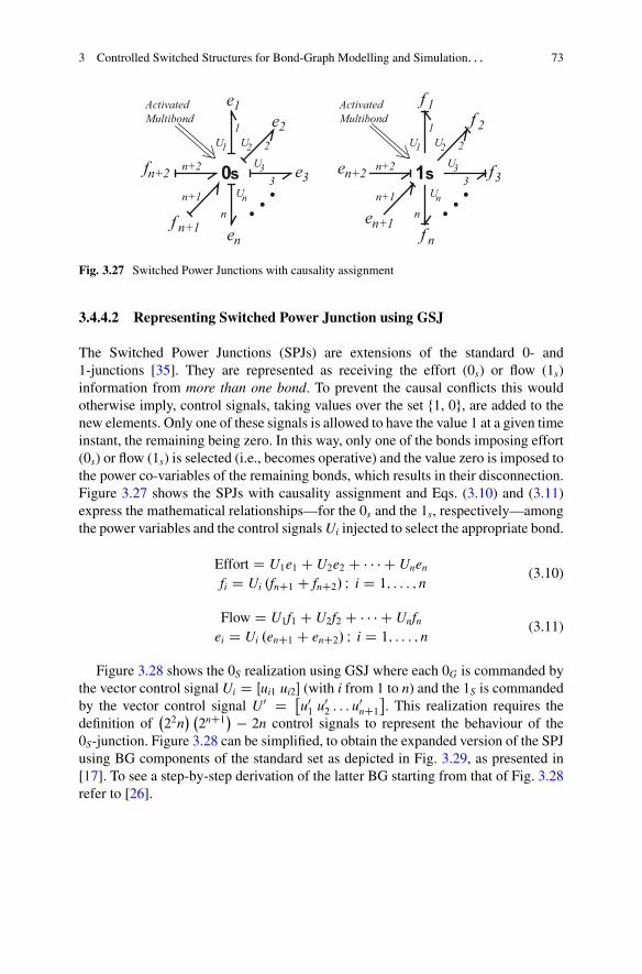
3 Controlled Switched Structures for Bond-Graph Modelling and Simulation. . . 73
e1e2
e3
enf n+1
fn+2 3
nn+1
n+2
12U2U1
U3
Un
ActivatedMultibond
f 1f 2
f3
f nen+1
en+2 3
nn+1
n+2
12U2U1
U3
Un
ActivatedMultibond
Fig. 3.27 Switched Power Junctions with causality assignment
3.4.4.2 Representing Switched Power Junction using GSJ
The Switched Power Junctions (SPJs) are extensions of the standard 0- and1-junctions [35]. They are represented as receiving the effort (0s) or flow (1s)information from more than one bond. To prevent the causal conflicts this wouldotherwise imply, control signals, taking values over the set f1, 0g, are added to thenew elements. Only one of these signals is allowed to have the value 1 at a given timeinstant, the remaining being zero. In this way, only one of the bonds imposing effort(0s) or flow (1s) is selected (i.e., becomes operative) and the value zero is imposed tothe power co-variables of the remaining bonds, which results in their disconnection.Figure 3.27 shows the SPJs with causality assignment and Eqs. (3.10) and (3.11)express the mathematical relationships—for the 0s and the 1s, respectively—amongthe power variables and the control signals Ui injected to select the appropriate bond.
Effort D U1e1 C U2e2 C � � � C Unen
fi D Ui .fnC1 C fnC2/ I i D 1; : : : ; n(3.10)
Flow D U1f1 C U2f2 C � � � C Unfnei D Ui .enC1 C enC2/ I i D 1; : : : ; n
(3.11)
Figure 3.28 shows the 0S realization using GSJ where each 0G is commanded bythe vector control signal Ui D Œui1 ui2� (with i from 1 to n) and the 1S is commandedby the vector control signal U0 D �
u01 u02 : : : u0nC1�. This realization requires the
definition of�22n
� �2nC1� � 2n control signals to represent the behaviour of the
0S-junction. Figure 3.28 can be simplified, to obtain the expanded version of the SPJusing BG components of the standard set as depicted in Fig. 3.29, as presented in[17]. To see a step-by-step derivation of the latter BG starting from that of Fig. 3.28refer to [26].
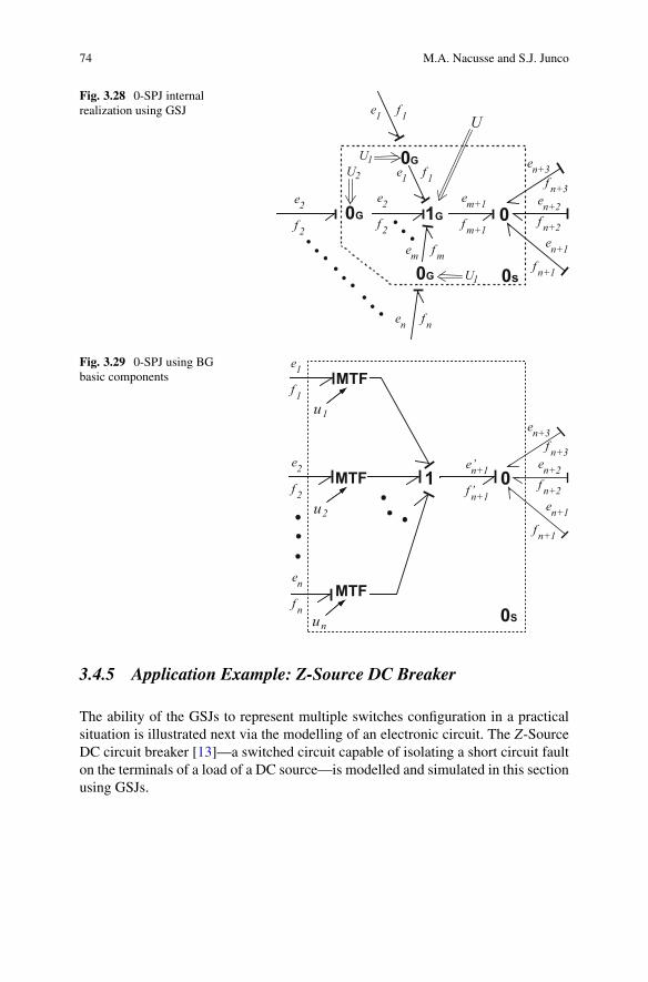
74 M.A. Nacusse and S.J. Junco
Fig. 3.28 0-SPJ internalrealization using GSJ
1G0G
0G
0G
eU1
1
0
f 1
e2
f 2
en f n
0s
U2U
1U
en+3f n+3
en+1
f n+1
en+2f n+2
e1 f 1
em f m
e2
f 2
em+1
f m+1
Fig. 3.29 0-SPJ using BGbasic components
1MTF
e1
f 1
e2
f 2
en
f n
e’n+1
f’n+10
en+3f n+3
en+1
fn+1
en+2f n+2
u2
MTF
un
MTF
u1
0S
3.4.5 Application Example: Z-Source DC Breaker
The ability of the GSJs to represent multiple switches configuration in a practicalsituation is illustrated next via the modelling of an electronic circuit. The Z-SourceDC circuit breaker [13]—a switched circuit capable of isolating a short circuit faulton the terminals of a load of a DC source—is modelled and simulated in this sectionusing GSJs.

3 Controlled Switched Structures for Bond-Graph Modelling and Simulation. . . 75
L
U
L
C
SCR
C 2
2
1
1
s
RD
RD
Load
ild
ic1
if
iSCRic2
vo
iovld
Fig. 3.30 Z-Source DC circuit breaker
3.4.5.1 Z-Source DC Circuit Breaker
The Z-Source DC circuit breaker was introduced as a mean to protect the powersource from short circuit faults in DC buses. This circuit, inspired in the Z-Sourceinverter presented by [29], consists in an SCR in series with a LC network placedbetween the voltage source and the load as it is shown in Fig. 3.30. The main featureof the inverter application inspiring this circuit breaker is that in the former the Z-Source network allows the simultaneous closing of the two transistors on the sameleg, which would be impossible in a classic inverter circuit. This quality was usedin [13] to handle fault in medium voltage DC power systems. In the BG domain, aSwBG model of a monophasic Z-Source inverter was presented in [24] where SPJand residual sinks were used to model the power switches and enforced integralcausality in all the storage elements, respectively.
The behaviour of the Z-Source DC breaker will be analysed with the help ofFig. 3.31 where the four commutation modes are depicted. In steady state andnormal operation, i.e., in the absence of faults or fault free mode, the SCR is in ON-state and, in steady state, each of the capacitors is charged at the source voltage (seeFig. 3.31a). A short circuit fault occurring at the load terminals (see Fig. 3.30) wouldtry to equalize the sum of the two capacitor voltages, satisfying Uc1 C Uc2 D 2 Us
immediately before the fault, to Us, the voltage at the source terminals. As thisis obviously a situation inconsistent with Kirchhoff’s second law, that imposesUc1CUc2 D Us, this constraint would attempt to produce a current impulse from thecapacitors to the voltage source, to obey the principle of charge conservation. Thisphenomenon does not happen with the SCR in the circuit; instead, this attempt ofnegative current provokes the SCR to switch into the OFF-state isolating the voltagesource from the fault. The transition from the ON-state to the OFF-state of the SCRcan be analysed at the light of both, the hard- and soft-switching approaches:
In a hard-switching approach, this transition will occur instantaneously, so thatthe circuit switches from the fault free mode to the fault mode 1 without enteringany transient mode. In a soft-switching approach, i.e., when neither the SCR nor
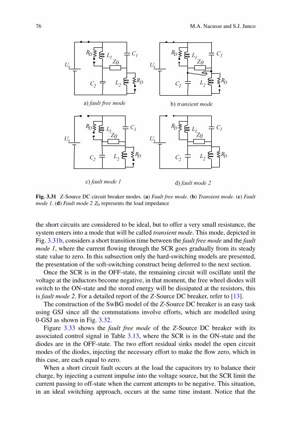
76 M.A. Nacusse and S.J. Junco
a) fault free mode
d) fault mode 2
b) transient mode
c) fault mode 1
LU
LC
CZ0
s
1 1
2 2
RD
RD
LU
LC
CZ0
s
1 1
2 2
RD
RD
LU
LC
C
s
1 1
2 2
RD
RD
LU
LC
C
s
1 1
2 2
RD
RD
Z0Z0
Fig. 3.31 Z-Source DC circuit breaker modes. (a) Fault free mode. (b) Transient mode. (c) Faultmode 1. (d) Fault mode 2 Z0 represents the load impedance
the short circuits are considered to be ideal, but to offer a very small resistance, thesystem enters into a mode that will be called transient mode. This mode, depicted inFig. 3.31b, considers a short transition time between the fault free mode and the faultmode 1, where the current flowing through the SCR goes gradually from its steadystate value to zero. In this subsection only the hard-switching models are presented,the presentation of the soft-switching construct being deferred to the next section.
Once the SCR is in the OFF-state, the remaining circuit will oscillate until thevoltage at the inductors become negative, in that moment, the free wheel diodes willswitch to the ON-state and the stored energy will be dissipated at the resistors, thisis fault mode 2. For a detailed report of the Z-Source DC breaker, refer to [13].
The construction of the SwBG model of the Z-Source DC breaker is an easy taskusing GSJ since all the commutations involve efforts, which are modelled using0-GSJ as shown in Fig. 3.32.
Figure 3.33 shows the fault free mode of the Z-Source DC breaker with itsassociated control signal in Table 3.13, where the SCR is in the ON-state and thediodes are in the OFF-state. The two effort residual sinks model the open circuitmodes of the diodes, injecting the necessary effort to make the flow zero, which inthis case, are each equal to zero.
When a short circuit fault occurs at the load the capacitors try to balance theircharge, by injecting a current impulse into the voltage source, but the SCR limit thecurrent passing to off-state when the current attempts to be negative. This situation,in an ideal switching approach, occurs at the same time instant. Notice that the
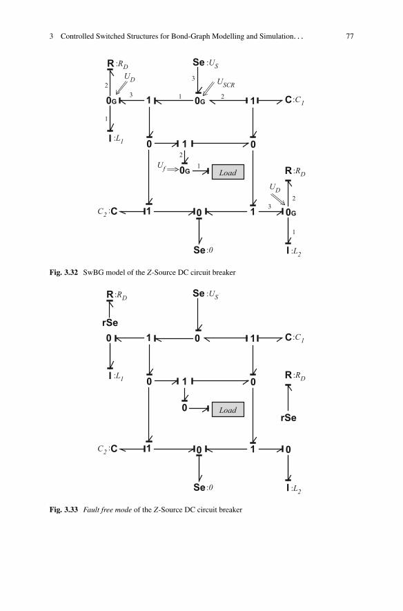
3 Controlled Switched Structures for Bond-Graph Modelling and Simulation. . . 77
1
C
0G 1 C
R
Se
0G
1
0
0
1 1
Se
0
0G
I
R
I
0G
USCRUD
UD
Uf
:US
Load
:0
:C1
C2
:RD
:L1
:RD
:L2
:
1
2
1 2
3
1
23
1
23
Fig. 3.32 SwBG model of the Z-Source DC circuit breaker
1
C
0 1 C
R
Se
0
1
0
0
1 1
Se
0
0
I
I
0
:US
Load
:0
:C1
C2
:RD:L1
:L2
:
rSe
R :RD
rSe
Fig. 3.33 Fault free mode of the Z-Source DC circuit breaker
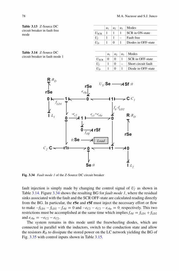
78 M.A. Nacusse and S.J. Junco
Table 3.13 Z-Source DCcircuit breaker in fault freemode
u1 u2 u3 Modes
USCR 1 1 1 SCR in ON-stateUf 1 1 – Fault freeUD 1 0 1 Diodes in OFF-state
Table 3.14 Z-Source DCcircuit breaker in fault mode 1
u1 u2 u3 Modes
USCR 0 0 1 SCR in OFF-stateUf 1 0 – Short circuit faultUD 1 0 1 Diode in OFF-state
1
C
0 1 C
R
rSe
0
1
0
0
1 1
Se
0
0
I
I
0
:0
:C1
C2
:RD:L1
:L2
:
rSe
R :RD
rSe
US
LoadSe0:
rSf
Se: Sf :0
fLD1-fLD2f0
erSe
frSf
-ec2 ec1+erSe
Fig. 3.34 Fault mode 1 of the Z-Source DC circuit breaker
fault injection is simply made by changing the control signal of Uf as shown inTable 3.14. Figure 3.34 shows the resulting BG for fault mode 1, where the residualsinks associated with the fault and the SCR OFF-state are calculated reading directlyfrom the BG. In particular, the rSe and rSf must inject the necessary effort or flowto make �fLD1 � fLD2 � frSf D 0 and �eC2 � eC2 � erSe D 0, respectively. This tworestrictions must be accomplished at the same time which implies frSf D fLD1 C fLD2
and erSe D �eC2 � eC2.The system remains in this mode until the freewheeling diodes, which are
connected in parallel with the inductors, switch to the conduction state and allowthe resistors RD to dissipate the stored power on the LC network yielding the BG ofFig. 3.35 with control inputs shown in Table 3.15.
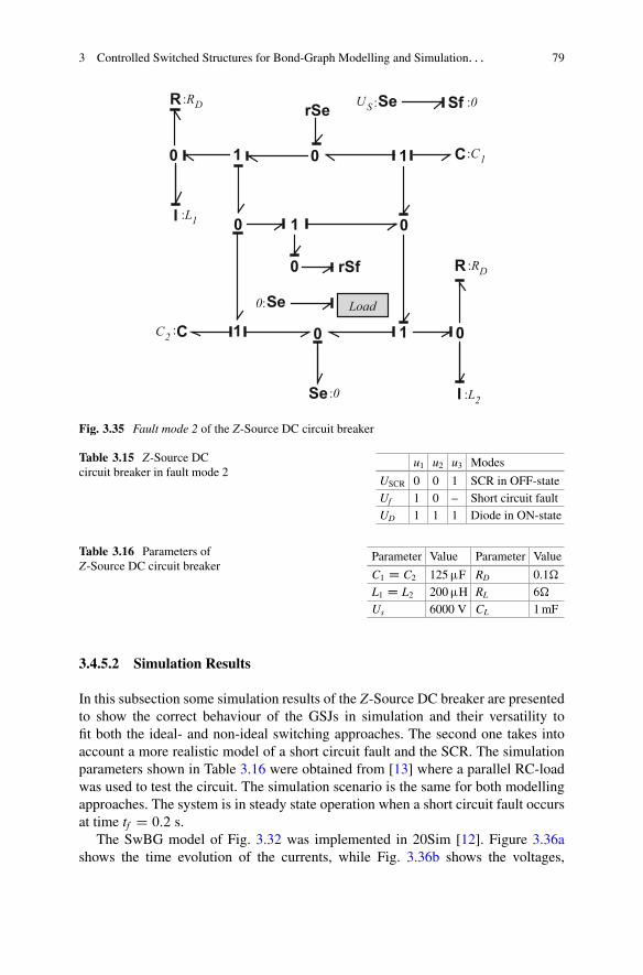
3 Controlled Switched Structures for Bond-Graph Modelling and Simulation. . . 79
1
C
0 1 C
R
rSe
0
1
0
0
1 1
Se
0
0
I
I
0
:0
:C1
C2
:RD
:L1
:L2
:
R :RD US
LoadSe0:
rSf
Se: Sf :0
Fig. 3.35 Fault mode 2 of the Z-Source DC circuit breaker
Table 3.15 Z-Source DCcircuit breaker in fault mode 2
u1 u2 u3 Modes
USCR 0 0 1 SCR in OFF-stateUf 1 0 – Short circuit faultUD 1 1 1 Diode in ON-state
Table 3.16 Parameters ofZ-Source DC circuit breaker
Parameter Value Parameter Value
C1 D C2 125�F RD 0.1�L1 D L2 200�H RL 6�Us 6000 V CL 1 mF
3.4.5.2 Simulation Results
In this subsection some simulation results of the Z-Source DC breaker are presentedto show the correct behaviour of the GSJs in simulation and their versatility tofit both the ideal- and non-ideal switching approaches. The second one takes intoaccount a more realistic model of a short circuit fault and the SCR. The simulationparameters shown in Table 3.16 were obtained from [13] where a parallel RC-loadwas used to test the circuit. The simulation scenario is the same for both modellingapproaches. The system is in steady state operation when a short circuit fault occursat time tf D 0:2 s.
The SwBG model of Fig. 3.32 was implemented in 20Sim [12]. Figure 3.36ashows the time evolution of the currents, while Fig. 3.36b shows the voltages,
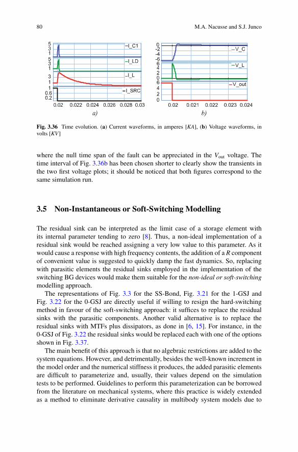
80 M.A. Nacusse and S.J. Junco
Fig. 3.36 Time evolution. (a) Current waveforms, in amperes [KA], (b) Voltage waveforms, involts [KV]
where the null time span of the fault can be appreciated in the Vout voltage. Thetime interval of Fig. 3.36b has been chosen shorter to clearly show the transients inthe two first voltage plots; it should be noticed that both figures correspond to thesame simulation run.
3.5 Non-Instantaneous or Soft-Switching Modelling
The residual sink can be interpreted as the limit case of a storage element withits internal parameter tending to zero [8]. Thus, a non-ideal implementation of aresidual sink would be reached assigning a very low value to this parameter. As itwould cause a response with high frequency contents, the addition of a R componentof convenient value is suggested to quickly damp the fast dynamics. So, replacingwith parasitic elements the residual sinks employed in the implementation of theswitching BG devices would make them suitable for the non-ideal or soft-switchingmodelling approach.
The representations of Fig. 3.3 for the SS-Bond, Fig. 3.21 for the 1-GSJ andFig. 3.22 for the 0-GSJ are directly useful if willing to resign the hard-switchingmethod in favour of the soft-switching approach: it suffices to replace the residualsinks with the parasitic components. Another valid alternative is to replace theresidual sinks with MTFs plus dissipators, as done in [6, 15]. For instance, in the0-GSJ of Fig. 3.22 the residual sinks would be replaced each with one of the optionsshown in Fig. 3.37.
The main benefit of this approach is that no algebraic restrictions are added to thesystem equations. However, and detrimentally, besides the well-known increment inthe model order and the numerical stiffness it produces, the added parasitic elementsare difficult to parameterize and, usually, their values depend on the simulationtests to be performed. Guidelines to perform this parameterization can be borrowedfrom the literature on mechanical systems, where this practice is widely extendedas a method to eliminate derivative causality in multibody system models due to
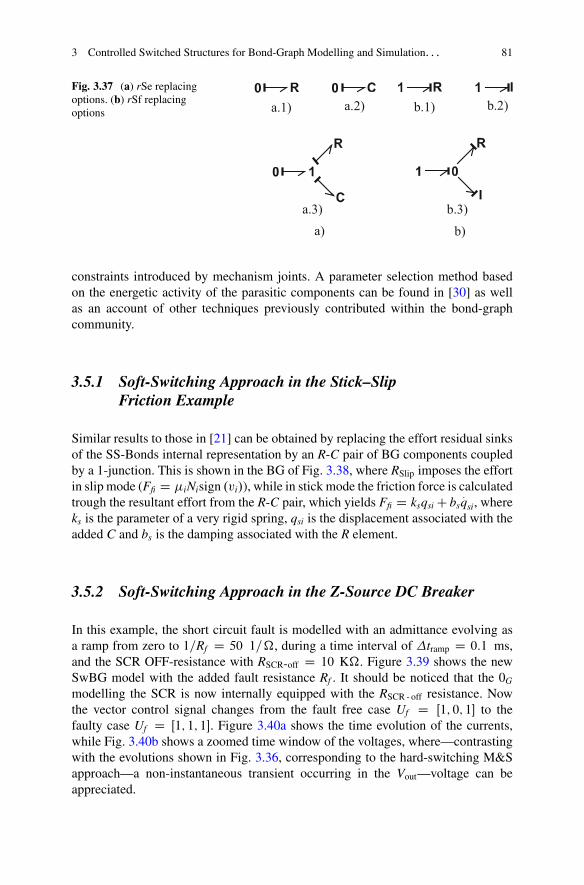
3 Controlled Switched Structures for Bond-Graph Modelling and Simulation. . . 81
Fig. 3.37 (a) rSe replacingoptions. (b) rSf replacingoptions
a) b)
a.1) a.2)
b.3)a.3)
b.1) b.2)
constraints introduced by mechanism joints. A parameter selection method basedon the energetic activity of the parasitic components can be found in [30] as wellas an account of other techniques previously contributed within the bond-graphcommunity.
3.5.1 Soft-Switching Approach in the Stick–SlipFriction Example
Similar results to those in [21] can be obtained by replacing the effort residual sinksof the SS-Bonds internal representation by an R-C pair of BG components coupledby a 1-junction. This is shown in the BG of Fig. 3.38, where RSlip imposes the effortin slip mode (Ffi D �iNisign .vi/), while in stick mode the friction force is calculatedtrough the resultant effort from the R-C pair, which yields Ffi D ksqsi C bs
:qsi, where
ks is the parameter of a very rigid spring, qsi is the displacement associated with theadded C and bs is the damping associated with the R element.
3.5.2 Soft-Switching Approach in the Z-Source DC Breaker
In this example, the short circuit fault is modelled with an admittance evolving asa ramp from zero to 1=Rf D 50 1=�, during a time interval of tramp D 0:1 ms,and the SCR OFF-resistance with RSCR-off D 10 K�. Figure 3.39 shows the newSwBG model with the added fault resistance Rf . It should be noticed that the 0G
modelling the SCR is now internally equipped with the RSCR - off resistance. Nowthe vector control signal changes from the fault free case Uf D Œ1; 0; 1� to thefaulty case Uf D Œ1; 1; 1�. Figure 3.40a shows the time evolution of the currents,while Fig. 3.40b shows a zoomed time window of the voltages, where—contrastingwith the evolutions shown in Fig. 3.36, corresponding to the hard-switching M&Sapproach—a non-instantaneous transient occurring in the Vout—voltage can beappreciated.
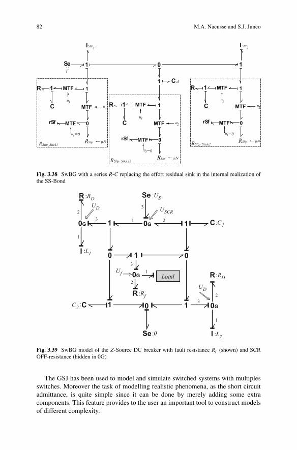
82 M.A. Nacusse and S.J. Junco
1Se
I
0 1
1 C
I
RSlip_Stick1
:m2:m2
:k
:
F
3
2
0
1
uu
rSf
MTF
MTF
MTF
1u
1
C
R
RSlip μN
=0
RSlip_Stick2
3
2
0
1
uu
rSf
MTF
MTF
MTF
1u
1
C
R
RSlip μN
=0
RSlip_Stick12
3
2
0
1
uu
rSf
MTF
MTF
MTF
1u
1
C
R
RSlip μN
=0
Fig. 3.38 SwBG with a series R-C replacing the effort residual sink in the internal realization ofthe SS-Bond
1
C
0G 1 C
R
Se
0G
1
0
0
1 1
Se
0
0G
I
R
I
0G
USCRUD
UD
Uf
:US
Load
:0
:C1
C2
:RD
:L1
:RD
:L2
:
1
2
1 2
3
1
23
1
23
3
R :Rf
Fig. 3.39 SwBG model of the Z-Source DC breaker with fault resistance Rf (shown) and SCROFF-resistance (hidden in 0G)
The GSJ has been used to model and simulate switched systems with multiplesswitches. Moreover the task of modelling realistic phenomena, as the short circuitadmittance, is quite simple since it can be done by merely adding some extracomponents. This feature provides to the user an important tool to construct modelsof different complexity.
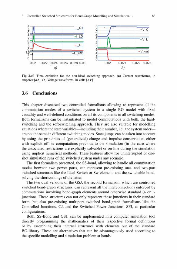
3 Controlled Switched Structures for Bond-Graph Modelling and Simulation. . . 83
Fig. 3.40 Time evolution for the non-ideal switching approach. (a) Current waveforms, inamperes [KA], (b) Voltage waveforms, in volts [KV]
3.6 Conclusions
This chapter discussed two controlled formalisms allowing to represent all thecommutation modes of a switched system in a single BG model with fixedcausality and well-defined conditions on all its components in all switching modes.Both formalisms can be instantiated to model commutations with both, the hard-switching and the soft-switching approach. They are also suitable for modellingsituations where the state variables—including their number, i.e., the system order—are not the same in different switching modes. State jumps can be taken into accountby using the principles of (generalized) charge and impulse conservation, eitherwith explicit offline computations previous to the simulation (in the case wherethe associated restrictions are explicitly solvable) or on-line during the simulationusing implicit numerical methods. These features allow for uninterrupted or one-shot simulation runs of the switched system under any scenario.
The first formalism presented, the SS-bond, allowing to handle all commutationmodes between two power ports, can represent pre-existing one- and two-portswitched structures like the Ideal Switch or Sw-element, and the switchable bond,solving the shortcomings of the latter.
The two dual versions of the GSJ, the second formalism, which are controlledswitched bond-graph structures, can represent all the interconnections enforced bycommutations involving bond-graph elements around otherwise standard 0- or 1-junctions. These structures can not only represent these junctions in their standardform, but also pre-existing multiport switched bond-graph formalisms like theControlled Junctions, CJ, and the Switched Power Junctions, SPJ, as particularconfigurations.
Both, SS-Bond and GSJ, can be implemented in a computer simulation tooldirectly programming the mathematics of their respective formal definitionsor by assembling their internal structures with elements out of the standardBG-library. These are alternatives that can be advantageously used according tothe specific modelling and simulation problem at hands.
84 M.A. Nacusse and S.J. Junco
The advantage of hard-switching yielding a simulation with fixed causalitycomes with a drawback: each residual sink component adds an algebraic constraintwhich implies the dynamics being described by a DAE system. These constraintsmust be calculated numerically at each integration step. When it can be solvedanalytically offline prior to the simulation, only an explicit computation has to beperformed at each step. Otherwise, it must be done implicitly, with the subsequentincrement of the computational cost. On the other hand, soft-switching modellingachieved with the inclusion of R, C and/or I elements, i.e., adding parasitic dissi-pation and/or dynamics, results in numerically stiff models with higher dynamicorder that will increase the simulation time. Moreover, in many cases the parasiticcomponents are not related to any physical attribute of the system, what complicatesthe task of parameterizing them. Thus, the choice between implementing these toolsaccording to the ideal or hard-switching paradigm or the non-ideal or soft-switchingapproach, even co-existing in a same model, is left to the user’s best convenience.It would be the result of a trade-off among the overall computational costs associatedwith each of the implementations.
References
1. Armstrong-Hélouvry, B., Dupont, P., & Wit, C. C. D. (1994). A survey of models, analysistools and compensation methods for the control of machines with friction. Automatica, 30(7),1083–1138.
2. Asher, G. (1993). The robust modeling of variable topology circuits using bond graphs. Pro-ceedings ICBGM’93, the International Conference on Bond Graph Modeling and Simulation,San Diego, CA.
3. Borutzky, W. (1995). Representing discontinuities by means of sinks of fixed causality. 1995International Conference on Bond Graph Modeling, ICBGM’95, Proceedings of the 1995Western Simulation Multiconference.
4. Borutzky, W. (1995). Discontinuities in a bond graph framework. Journal of the FranklinInstitute, 332(2), 141–154.
5. Borutzky, W. (2004). Bond graphs—A methodology for modelling multidisciplinary dynamicsystems (Vols. %1 de %2FS-14). Erlangen, San Diego, CA: SCS Publishing House.
6. Borutzky, W. (2010). Bond graph methodology—Development and analysis of multidisciplinaydynamic system models (pp. XXII, 662). London: Springer-Verlag.
7. Borutzky, W. (2015). Bond graph model-based diagnosis of hybrid systems. Switzerland:Springer.
8. Borutzky, W., & Cellier, F. E. (1996). Tearing algebraic loops in bond graphs. Transactions ofthe Society for Computer Simulation International, 13(2), 102–115.
9. Borutzky, W., Dauphin-Tanguy, G., & Thoma, J. U. (1995). Advances in bond graph modelling:Theory, software, applications. Mathematics and Computers in Simulation, 39(5), 465–475.
10. Branicky, M. S. (1998). Multiple Lyapunov functions and other analysis tools for switched andhybrid systems. IEEE Transactions on Automatic Control, 43(4), 475–482.
11. Broenink, J., & Wijbrans, K. (1993). Describing discontinuities in bond graphs. ProceedingsICBGM’93, the International Conference on Bond Graph Modeling and Simulation, SanDiego, CA.
12. Controllab Products, B. V. (2013). 20-sim. [En línea]. Available from http://www.20sim.com.

3 Controlled Switched Structures for Bond-Graph Modelling and Simulation. . . 85
13. Corzine, K. A., & Ashton, R. W. (2010). A new z-source dc circuit breaker. IndustrialElectronics (ISIE), 2010 IEEE International Symposium on.
14. Demír, Y., Poyraz, M., & Kösal, M. (1997). Derivation of state and output equations for systemscontaining switches and a novel definition of a switch using the bond graph model. Journal ofthe Franklin Institute, 334(2), 191–197.
15. Garcia, J., Dauphin-Tanguy, G., & Rombaut, C. (1997). A bond graph approach for modelingswitching losses of power semiconductor devices. International Conference on Bond GraphModeling and Simulation (ICBGM’97), Phoenix.
16. Gawthrop, P. J. (1997). Hybrid bond graphs using switched I and C components. TechnicalReport CSC-97005. Glasgow: Faculty of Engineering, University of Glasgow.
17. Junco, S., Diéguez, G., & Ramírez, F. (2007). On commutation modeling in Bond Graphs.Proceedings of the International Conference on Bond Graph Modeling and Simulation, SanDiego, CA.
18. Karnopp, D. (1985). Computer simulation of stick–slip friction in mechanical dynamicsystems. Journal of Dynamic Systems, Measurement, and Control, 107(1), 100–103.
19. Karnopp, D., & Margolis, D. (1979). Analysis and simulation of planar mechanism systemsusing bond graphs. ASME Journal of Mechanical Design, 2(101), 187–191.
20. Karnopp, D., Margolis, D. L., & Rosenberg, R. C. (2006). System dynamics: Modeling andsimulation of mechatronic systems (4th ed.). New York, Chichester: Wiley.
21. Margolis, D. (2005). Fixed causality slip–stick friction models for use in simulation of non-linear systems. Proceedings of the Institution of Mechanical Engineers, Part I: Journal ofSystems and Control Engineering, 219(3), 199–206.
22. Mosterman, P., & Biswas, G. (1995). Behaviour generation using model switching. A hybridbond graph modeling technique. Proceedings ICBGM’95, the International Conference onBond Graph Modeling and Simulation, Las Vegas, NV.
23. Mosterman, P., & Biswas, G. (1998). A theory of discontinuities in physical system models.Journal of the Franklin Institute, 335(3), 401–439.
24. Nacusse, M., & Junco, S. (2011). Simplifying switched bond graphs using residual sinks toenforce causality: Application to modeling the z-source inverter. Mecánica ComputacionalIndustrial Applications (B), 30(33), 2533–2548.
25. Nacusse, M., & Junco, S. (2013). Switchable structured bond: A bond graph device formodeling power coupling/decoupling of physical systems. Journal of Computational Science,5(3), 450–462.
26. Nacusse, M. A., & Junco, S. J. (2015). Generalized controlled switched bond graph junctions.Proceedings of the Institution of Mechanical Engineers, Part I: Journal of Systems and ControlEngineering, 229(9), 851–866.
27. Ort, J. R., & Martens, H. R. (1973). The properties of bond graph junction structure matrices.Journal of Dynamic Systems, Measurement, and Control, 1, 362–367.
28. OSMC (2016). The open source modelica consortium. https://www.openmodelica.org/ [Enlínea]. Available from https://www.openmodelica.org/.
29. Peng, F. Z. (2003). Z-source inverter. IEEE Transactions on Industry Applications, 39(2),504–510.
30. Rideout, G., & Stein, J. L. (2003). An energy-based approach to parameterizing parasiticelements for eliminating derivative causality. Proceedings of the ICBGM’03, the InternationalConference on Bond Graph Modeling and Simulation, Orlando, FL.
31. Rosenberg, R. C., & McCalla, J. (1991). Power to the user in formulating model equations.American Society of Mechanical Engineers, Dynamic Systems and Control Division (Publica-tion) DSC, 34, 25–35, Publ by ASME.
32. Strömberg, J. (1994). A mode switching modelling philosophy. Ph.D. thesis, LinköpingUniversity, Sweden.
33. Strömberg, J., Top, J. & Söderman, U. (1993). Variable causality in bond graph caused bydiscrete effects. Proceedings of the ICBGM’93, the International Conference on Bond GraphModeling and Simulation, San Diego, CA.

86 M.A. Nacusse and S.J. Junco
34. Sun, Z., & Ge, S. S. (2011). Stability theory of switched dynamical systems. London: Springer.S. L. Limited, Ed.
35. Umarikar, A. C., & Umanand, L. (2005). Modelling of switching systems in bond graphs usingthe concept of switched power junctions. Journal of the Franklin Institute, 342(2), 131–147.
36. van der Schaft, A. J., & Camlibel, M. K. (2009). A state transfer principle for switching port-Hamiltonian systems. Decision and Control, 2009 held jointly with the 2009 28th ChineseControl Conference. CDC/CCC 2009. Proceedings of the 48th IEEE Conference on.
37. van der Schaft, A. J., & Schumacher, J. M. (2000). Introduction to hybrid dynamical systems.London: Springer. Springer, Ed.
38. Xu, X., & Zhai, G. (2005). Practical stability and stabilization of hybrid and switched systems.IEEE Transactions on Automatic Control, 50(11), 1897–1903.
Chapter 4Dynamic Causality in Hybrid Bond Graphs
Rebecca Margetts and Roger F. Ngwompo
4.1 Introduction
In constructing dynamic systems models, it is frequently desirable to abstract rapidlychanging, highly nonlinear behaviour to a discontinuity. When rapidly changingbehaviour is described by a continuous differential equation, it must be integratedusing very small time steps in order to achieve any level of accuracy. Abstractingrapidly changing behaviour to a discontinuous equation can therefore aid solvabilityand improve computer simulation times. In addition, a user may find it intuitive tothink of certain elements (like an electrical switch or hydraulic valve) or phenomena(such as contact, dry friction or breakage) as discontinuous.
Hybrid models are those containing any continuous and any discontinuousbehaviour. They can be visualised as continuous modes on areas of state space linkedby a discontinuous state mapping [42], and described as a hybrid automaton, i.e. onethat contains both finite and continuous state spaces [58]. The dynamics consist ofdiscrete transitions plus an evolution of the continuous part in each location.
Definition 4.1. Hybrid Model: any model which describes both continuous anddiscontinuous behaviour.
The terms ‘hybrid’ and ‘switched’ system are used almost interchangeably in thebond graph literature, but there is a subtle difference. Switching models ‘comprisea family of dynamical subsystems together with a switching signal determiningthe active system at a current time’ [61]. They are a subset of hybrid systems,
R. Margetts (�)School of Engineering, University of Lincoln, Brayford Pool, Lincoln LN6 7TS, UKe-mail: [email protected]
R.F. NgwompoDepartment of Mechanical Engineering, University of Bath, Claverton Down, Bath BA2 7AY, UKe-mail: [email protected]
© Springer International Publishing Switzerland 2017W. Borutzky (ed.), Bond Graphs for Modelling, Control and FaultDiagnosis of Engineering Systems, DOI 10.1007/978-3-319-47434-2_4
87
88 R. Margetts and R.F. Ngwompo
where there is some discontinuous behaviour modelled by an on/off switch orother binary signal. Switched models can be used to describe multimodal systemsand variable-structure systems. The hybrid bond graph therefore usually yields aswitched system, and some variants are referred to as switching bond graphs.
Definition 4.2. Switching Model: a subset of hybrid model, which contains con-tinuous equations and binary switching devices. The ‘switches’ select the activecontinuous equation(s) or behaviours at a given time.
Branicky et al. [7] categorise hybrid models into Switching and Impulse models,which can be Controlled or Autonomous. Switching models are defined as thosewhere the vector field changes discontinuously when the state hits a boundary.Impulse models are those where the continuous state changes impulsively on hittingprescribed regions of state space, i.e. there is a ‘jump’ between the continuousequations in state space. The classic example is Newton’s Collision law, wherethe state of a body changes from positive to negative velocity on impact, and anydissipative effects are accounted for by a coefficient of restitution. These types ofmodels have been created by some hybrid bond graph practitioners [36, 65].
Definition 4.3. Impulse Model: a subset of hybrid model where the state changesimpulsively, i.e. there is an impulse loss on commutation.
Variable topology systems are those where the size of the state equation matriceschanges, such as contact (Fig. 4.1). They are frequently represented by impulsemodels [7] such as Newton’s Collision Law with restitution. This type of modelexhibits an impulsive ‘jump’ in state space on commutation, which violates theconservation of energy fundamental to the bond graph. The state variables areunknown after commutation, necessitating the use of state reinitialisation [35, 36]and state estimation techniques [45].
A number of hybrid and switching bond graphs have been proposed to modeldiscontinuities in the bond graph framework. From early on in the development ofbond graphs, there was a need to model discontinuities in the form of elementslike switches and valves. Borutzky gives an overview in his text [6], and Margettspresents a survey and discussion [29]. The different methods appear to reflectthe different backgrounds and motivations of the users, with switched sourcesand controlled/switched junctions falling into more common usage than the othermethods. One of the main differences between methods is the treatment of dynamiccausality, and its consequences for analysis and computation.
4.1.1 Dynamic Causality
Bond graphs are constructed as acausal models, and an ideal computational causalityis assigned to the model once complete. However, in a hybrid system the ideal causalassignment can change with commutation. For example, two rigid bodies might
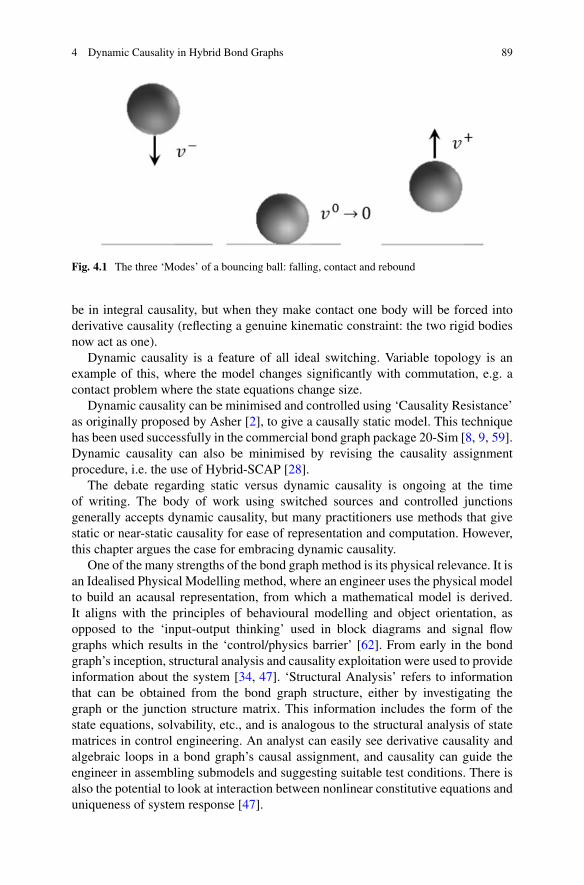
4 Dynamic Causality in Hybrid Bond Graphs 89
Fig. 4.1 The three ‘Modes’ of a bouncing ball: falling, contact and rebound
be in integral causality, but when they make contact one body will be forced intoderivative causality (reflecting a genuine kinematic constraint: the two rigid bodiesnow act as one).
Dynamic causality is a feature of all ideal switching. Variable topology is anexample of this, where the model changes significantly with commutation, e.g. acontact problem where the state equations change size.
Dynamic causality can be minimised and controlled using ‘Causality Resistance’as originally proposed by Asher [2], to give a causally static model. This techniquehas been used successfully in the commercial bond graph package 20-Sim [8, 9, 59].Dynamic causality can also be minimised by revising the causality assignmentprocedure, i.e. the use of Hybrid-SCAP [28].
The debate regarding static versus dynamic causality is ongoing at the timeof writing. The body of work using switched sources and controlled junctionsgenerally accepts dynamic causality, but many practitioners use methods that givestatic or near-static causality for ease of representation and computation. However,this chapter argues the case for embracing dynamic causality.
One of the many strengths of the bond graph method is its physical relevance. It isan Idealised Physical Modelling method, where an engineer uses the physical modelto build an acausal representation, from which a mathematical model is derived.It aligns with the principles of behavioural modelling and object orientation, asopposed to the ‘input-output thinking’ used in block diagrams and signal flowgraphs which results in the ‘control/physics barrier’ [62]. From early in the bondgraph’s inception, structural analysis and causality exploitation were used to provideinformation about the system [34, 47]. ‘Structural Analysis’ refers to informationthat can be obtained from the bond graph structure, either by investigating thegraph or the junction structure matrix. This information includes the form of thestate equations, solvability, etc., and is analogous to the structural analysis of statematrices in control engineering. An analyst can easily see derivative causality andalgebraic loops in a bond graph’s causal assignment, and causality can guide theengineer in assembling submodels and suggesting suitable test conditions. There isalso the potential to look at interaction between nonlinear constitutive equations anduniqueness of system response [47].

90 R. Margetts and R.F. Ngwompo
It is therefore logical that a hybrid bond graph should continue to uphold thesevalues and be suitable for qualitative analysis. Although causally dynamic modelsmay at first appear difficult to simulate, they do provide valuable information to theuser. Constraining causality is a move away from the real physics of the system.Adding parasitic elements or causality resistance can create an overly complexmodel with undesirable high-frequency dynamics [11]. The use of switched ormodulating resistance and transformer components wrongly implies that switchingis dissipative [38]. And there is a danger that compliances and resistances may beadded purely to aid computation with no consideration of the physical system: amodeller can unwittingly create physically meaningless or computationally ineffi-cient models. In contrast, a causally dynamic model offers engineering insight [14].
4.1.2 Categorising Discontinuities
A discontinuity is an abstraction made in order to simplify a model. It is possibleto model any system using continuous functions. Discontinuities are thereforeartificial, and made at the discretion of the user. Their purpose is to simplifythe equations used to describe a system’s behaviour; where a system’s behaviourchanges rapidly with time, describing that change as a discontinuity can improvesimulation time, and aid engineering insight and analysis. They usually describehighly nonlinear behaviour which would be difficult to describe and time-consumingto compute using continuous functions. They can also describe variable topologyproblems, which are where the equations used for each mode of operation changesignificantly, with varying numbers of states and boundary conditions (for example,contact).
The term ‘discontinuity’ is fairly vague, and so a classification is made toaid application to engineering problems. Discontinuities are often classified asideal (no losses) or non-ideal (associated with an energy loss) [46], switching orimpulse [7] or according to whether they are autonomous or externally controlled.If they are assumed to be controlled by some form of automaton, they can beclassified according to whether the controlling automata are time-scale dependant orparameter dependent [40]. Here, an additional distinction is made between structuraland parametric discontinuities [29]. This distinction is necessary to describe wherein the model (and underlying equations) the discontinuity should occur: betweenelements or internal to an element.
Definition 4.4. Structural Discontinuities: discontinuities which occur when partsof the model are connected or disconnected, interrupting power flow betweencomponents. These discontinuities often give rise to variable topology models.
Engineering examples of this type of discontinuity are the hydraulic valve,mechanical clutch, ideal electrical switch or contact between bodies.

4 Dynamic Causality in Hybrid Bond Graphs 91
Definition 4.5. Parametric Discontinuities: discontinuities which occur when anelement has a highly nonlinear constitutive equation, and the user has abstractedthis to a piecewise-continuous function. The structure of the model is unchanged, itis the equation describing the behaviour of an element which changes.
Common examples of parametric discontinuities are dry friction, tyre forces, anonlinear damper ‘breaking out’ or saturation of an electrical capacitor or hydraulicaccumulator.
These two types of discontinuity can be represented differently in a hybrid bondgraph: a controlled junction with dynamic causality for structural switching and acontrolled element for parametric switching.
In many cases—particularly the mechanical domain—the distinction betweenstructural and parametric switching is clear. However, there are cases where it isless so. An electrical switch is physically an element which the user inserts intoa circuit, and is often visualised in control theory as a discontinuous input, hencethe use of switching sources and elements in the literature. Consequently, there is acase for treating it as parametric switching. Here the dynamic causal assignment iskey: disconnecting a voltage or current source can force electrical storage elementsto discharge, which is consistent with them switching to derivative causality. Thecontrolled junction proposed for structural switching clearly shows where structureis disconnected and ideal causality assignment changes with commutation.
4.2 Structural Discontinuities
Structural switching activates or deactivates part of a system, and a controlledjunction can be used to (dis)connect or (de)activate part of the model accordingly.Controlled junctions as described by Mosterman and Biswas [39] are selected torepresent structural switching because they clearly show where structure connectsand disconnects, and breaks the path of power flow. They are preferable to the useof switched sources which imply the switch is an energy-processing element whenit is, in fact, a control element [6, 37]. This is not only important from the pointof view of engineering insight, but also the controlled junction lends itself to beingrepresented in the junction structure matrix and hence developing hybrid systemequations.
4.2.1 The Controlled Junction
A controlled junction behaves as a normal 1- or 0-junction when ON and a sourceof zero flow or effort (respectively) when OFF. A controlled 1-junction is thereforeused to break or inhibit flow (for example, an electrical switch which breaks theflow of current) and a controlled 0-junction is used to inhibit effort (for example,a clutch or other physical non-contact in a mechanical system). This always gives

92 R. Margetts and R.F. Ngwompo
e1 e1e2 e2
f1 f1f2 f2X1:λ X0:λ
Fig. 4.2 Bond graph representation of switched junctions X1 and X0
rise to dynamic causality on one of the attached bonds. The commonly acceptednotation for controlled junctions is X1 and X0, which will be used in this paper.
Based on the above description, controlled junctions X1 and X0 can be formallydefined as elements with associated Boolean parameters. They are initially definedas 2-ports for clarity, and the definition can easily be extended to more than 2ports. The bond graph representations of controlled junctions X1 and X0 are asshown in Fig. 4.2, and their defining relationships are given by Eqs. (4.1) and (4.2),respectively.
8ˆ<
ˆ:
f1 D f2;.e1 � e2/ D 0;
Nf1 D 0;Nf2 D 0
(4.1)
8ˆ<
ˆ:
e1 D e2;.f1 � f2/ D 0;
Ne1 D 0;Ne2 D 0
(4.2)
The Boolean parameter selects the set of equations that are valid given thestate of the switch: 1 when the switch is ON and 0 when the switch is OFF. For eachcontrolled junction, the defining Eqs. (4.1) and (4.2) lead to three possible causalconfigurations:
• Two causal configurations when the switch is ON, i.e. (first two equationsequivalent to a normal 1 or 0 junction)
• a unique causal configuration when the switch is OFF, i.e. (last two equationsequivalent to null sources of flow or null sources of effort imposed by the elementto both power ports with conjugate variables externally imposed to the element).
In switching between ON and OFF states, the causal assignment around acontrolled junction must change. In the ON state, where it behaves as a regularjunction, there must be a causal input (i.e. a bond with a causal stroke definingthe common effort for a 0-junction or common flow for a 1-junction). In the OFFstate, where the controlled junction becomes a null source on each incident bond,there is no causal input and the causal assignment on that one bond changes. This isknown as dynamic causality, and using this definition of a controlled junction it isunavoidable.

4 Dynamic Causality in Hybrid Bond Graphs 93
4.2.2 Simplification of the Hybrid Bond Graph
If a bond graph is constructed from the schematic diagram of a system, there is oftenpotential to simplify the bond graph model. Since a controlled junction only behavesas a junction in one state, it cannot be eliminated and the rules for simplifying bondgraphs must be augmented as follows:
Rule 1: 2-Port Controlled JunctionsA controlled junction with only two ports cannot be removed and replaced witha single bond (whereas a regular junction could).
A regular junction with 2-ports can be replaced by a single bond, since theefforts and flows on the two incident bonds are equal. A controlled junction with2-ports connects and disconnects its incident bonds with commutation: in principlelike a switching bond or Boolean-modulated transformer (with dynamic causality).Removing the controlled junction would result in the surrounding structure beingconnected at all times.
Rule 2: Neighbouring Junctions: Controlled and Regular JunctionsWhen a regular junction and controlled junction of the same type are neighbour-ing, they can be merged into a single controlled junction.That is, when a 1-junction and X1-junction are next to each other, they can bemerged into a single X1-junction.Likewise, a 0-junction and X0-junction next to each other can be merged into asingle X0-junction.
When two like regular junctions are next to each other, they can be mergedinto a single junction. When one of those junctions is controlled, the commutatingbehaviour must be retained. This simplification results in elements being discon-nected with commutation, whereas they would have remained connected to somesubstructure without the simplification (shown in Fig. 4.3).
Rule 3: Neighbouring Junctions: Multiple Controlled JunctionsWhen neighbouring controlled junctions have two ports only, they can becombined into a single controlled junction. This controlled junction is ON onlywhen the states of both the constituent controlled junctions are ON.When neighbouring controlled junctions have more than two ports, they cannotbe combined. This is because the power to the incident elements or subsystemsdepends on the state of the individual controlled junction.
Fig. 4.3 An example subsystem with neighbouring regular and controlled junctions: unsimplified(left) and simplified (right)
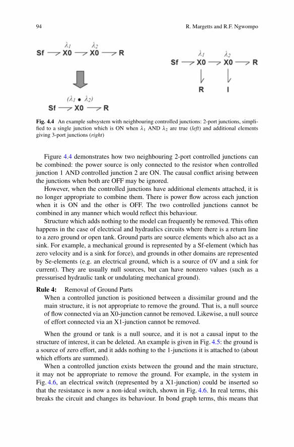
94 R. Margetts and R.F. Ngwompo
Fig. 4.4 An example subsystem with neighbouring controlled junctions: 2-port junctions, simpli-fied to a single junction which is ON when 1 AND 2 are true (left) and additional elementsgiving 3-port junctions (right)
Figure 4.4 demonstrates how two neighbouring 2-port controlled junctions canbe combined: the power source is only connected to the resistor when controlledjunction 1 AND controlled junction 2 are ON. The causal conflict arising betweenthe junctions when both are OFF may be ignored.
However, when the controlled junctions have additional elements attached, it isno longer appropriate to combine them. There is power flow across each junctionwhen it is ON and the other is OFF. The two controlled junctions cannot becombined in any manner which would reflect this behaviour.
Structure which adds nothing to the model can frequently be removed. This oftenhappens in the case of electrical and hydraulics circuits where there is a return lineto a zero ground or open tank. Ground parts are source elements which also act as asink. For example, a mechanical ground is represented by a Sf-element (which haszero velocity and is a sink for force), and grounds in other domains are representedby Se-elements (e.g. an electrical ground, which is a source of 0V and a sink forcurrent). They are usually null sources, but can have nonzero values (such as apressurised hydraulic tank or undulating mechanical ground).
Rule 4: Removal of Ground PartsWhen a controlled junction is positioned between a dissimilar ground and themain structure, it is not appropriate to remove the ground. That is, a null sourceof flow connected via an X0-junction cannot be removed. Likewise, a null sourceof effort connected via an X1-junction cannot be removed.
When the ground or tank is a null source, and it is not a causal input to thestructure of interest, it can be deleted. An example is given in Fig. 4.5: the ground isa source of zero effort, and it adds nothing to the 1-junctions it is attached to (aboutwhich efforts are summed).
When a controlled junction exists between the ground and the main structure,it may not be appropriate to remove the ground. For example, in the system inFig. 4.6, an electrical switch (represented by a X1-junction) could be inserted sothat the resistance is now a non-ideal switch, shown in Fig. 4.6. In real terms, thisbreaks the circuit and changes its behaviour. In bond graph terms, this means that
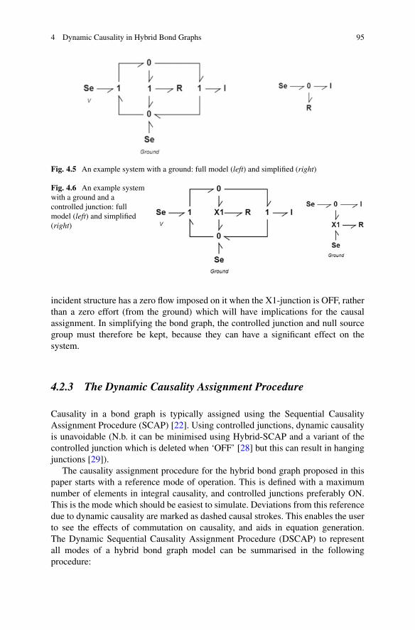
4 Dynamic Causality in Hybrid Bond Graphs 95
Fig. 4.5 An example system with a ground: full model (left) and simplified (right)
Fig. 4.6 An example systemwith a ground and acontrolled junction: fullmodel (left) and simplified(right)
incident structure has a zero flow imposed on it when the X1-junction is OFF, ratherthan a zero effort (from the ground) which will have implications for the causalassignment. In simplifying the bond graph, the controlled junction and null sourcegroup must therefore be kept, because they can have a significant effect on thesystem.
4.2.3 The Dynamic Causality Assignment Procedure
Causality in a bond graph is typically assigned using the Sequential CausalityAssignment Procedure (SCAP) [22]. Using controlled junctions, dynamic causalityis unavoidable (N.b. it can be minimised using Hybrid-SCAP and a variant of thecontrolled junction which is deleted when ‘OFF’ [28] but this can result in hangingjunctions [29]).
The causality assignment procedure for the hybrid bond graph proposed in thispaper starts with a reference mode of operation. This is defined with a maximumnumber of elements in integral causality, and controlled junctions preferably ON.This is the mode which should be easiest to simulate. Deviations from this referencedue to dynamic causality are marked as dashed causal strokes. This enables the userto see the effects of commutation on causality, and aids in equation generation.The Dynamic Sequential Causality Assignment Procedure (DSCAP) to representall modes of a hybrid bond graph model can be summarised in the followingprocedure:

96 R. Margetts and R.F. Ngwompo
Procedure 1: Dynamic Sequential Causality Assignment Procedure(DSCAP) for hybrid bond graph
Step 1. Assign causality according to SCAP with preferred integralcausality, stopping when a controlled junction is reached. That is, start byassigning causality to a source element, and propagate causality throughoutthe bond graph as far as any controlled junctions. Repeat for other sourceelements, and then for any storage elements which have not yet beenassigned causality. If causal conflict occurs in this stage, the model shouldbe changed.The causal assignment from step 1 may dictate whether some switches areON or OFF.Step 2. Choose a controlled junction which does not have its causality fullyassigned. Assign causality around the controlled junctions assuming theswitch to be ON and propagate as far as possible. Repeat this stage untilall controlled junctions have their causality fully assigned.Step 3. Finish propagating causality throughout the bond graph to anyresistance elements or remaining bonds and propagate as far as possible.Step 4. Taking each controlled junction in turn, consider the causalityassignment when it is in the other state to the reference configuration.Mark this causality assignment with a dashed causal stroke, and propagatethroughout the bond graph. If causal conflict occurs in this stage, then theother state of the controlled junction is not allowed.
Remark. Causal propagations in step 2 and step 4 of the algorithm abovemay dictate the state (ON or OFF) of some controlled junctions as a resultof the assigned state of others. This reveals some constraints in the state ofswitches indicating the allowed configurations or physically feasible modesof operation.
Figure 4.7 shows a simple example of the effect of the causality assignmentaround a controlled junction when ON and OFF.
4.2.4 Dynamic Causality Notation and the ReferenceConfiguration
The dynamic causality notation differs from that typically used [5] as it is designedto aid structural analysis and equation generation by hand. A reference configurationis used which indicates the mode of operation where most storage elements arein integral causality (giving information about model order and solvability). Thedashed causal stroke notation aids the user in identifying regions of dynamic
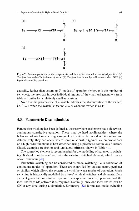
4 Dynamic Causality in Hybrid Bond Graphs 97
Fig. 4.7 An example of causality assignments and their effect around a controlled junction. (a)The junction in the ON (reference) mode. (b) The junction shown by null sources when OFF. (c)Dynamic causality notation
causality. Rather than assuming 2n modes of operation (where n is the number ofswitches), the user can inspect individual regions of the chart and generate a truthtable or similar for a relatively small subsystem.
Note that the parameter of a switch indicates the absolute state of the switch,i.e. D 1 when the switch is ON and D 0 when the switch is OFF.
4.3 Parametric Discontinuities
Parametric switching has been defined as the case where an element has a piecewise-continuous constitutive equation. These may be hard nonlinearities, where thebehaviour of an element changes so quickly that it can be considered instantaneous.Alternatively, they can occur where some relationship (gained via empirical dataor a high-order function) is best described using a piecewise-continuous function.Classic examples are friction and tyre lateral stiffness, shown in Table 4.1.
The controlled element is recommended for the modelling of parametric switch-ing. It should not be confused with the existing switched element, which has anon/off behaviour [20].
Parametric switching can be considered as mode switching, i.e. a collection ofcontinuous modes of operation. These are controlled by an automaton, petri-netor similar, which allows the system to switch between modes of operation. Modeswitching is historically modelled by a ‘tree’ of ideal switches and elements. Eachelement gives the constitutive equation for a specific mode of operation, and theideal switches (de)activate it as required. Naturally, only one ideal switch can beON at any time during a simulation. Strömberg [52] formulates mode switching
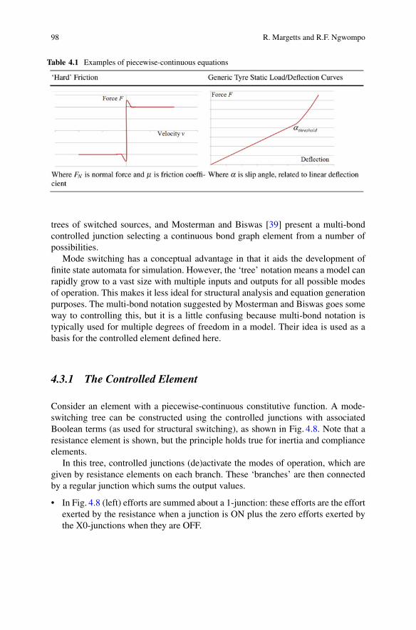
98 R. Margetts and R.F. Ngwompo
Table 4.1 Examples of piecewise-continuous equations
trees of switched sources, and Mosterman and Biswas [39] present a multi-bondcontrolled junction selecting a continuous bond graph element from a number ofpossibilities.
Mode switching has a conceptual advantage in that it aids the development offinite state automata for simulation. However, the ‘tree’ notation means a model canrapidly grow to a vast size with multiple inputs and outputs for all possible modesof operation. This makes it less ideal for structural analysis and equation generationpurposes. The multi-bond notation suggested by Mosterman and Biswas goes someway to controlling this, but it is a little confusing because multi-bond notation istypically used for multiple degrees of freedom in a model. Their idea is used as abasis for the controlled element defined here.
4.3.1 The Controlled Element
Consider an element with a piecewise-continuous constitutive function. A mode-switching tree can be constructed using the controlled junctions with associatedBoolean terms (as used for structural switching), as shown in Fig. 4.8. Note that aresistance element is shown, but the principle holds true for inertia and complianceelements.
In this tree, controlled junctions (de)activate the modes of operation, which aregiven by resistance elements on each branch. These ‘branches’ are then connectedby a regular junction which sums the output values.
• In Fig. 4.8 (left) efforts are summed about a 1-junction: these efforts are the effortexerted by the resistance when a junction is ON plus the zero efforts exerted bythe X0-junctions when they are OFF.
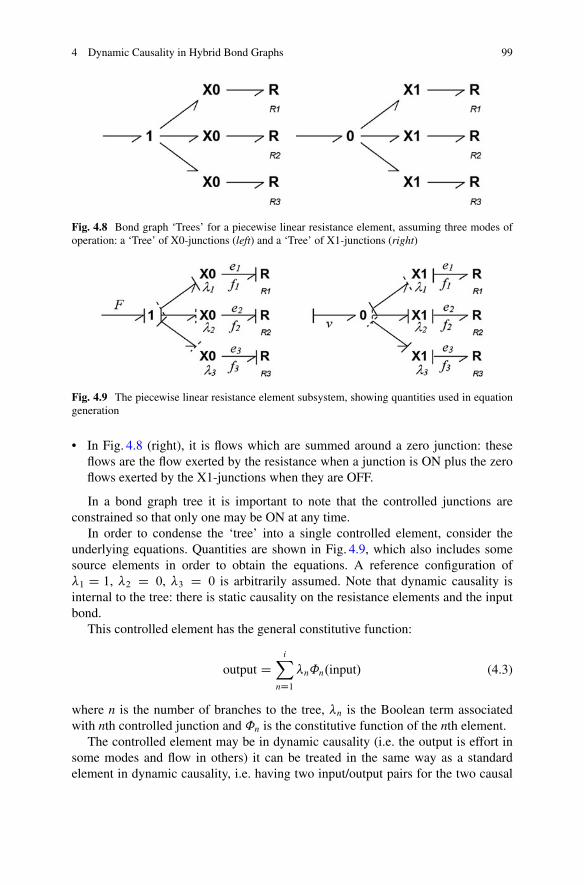
4 Dynamic Causality in Hybrid Bond Graphs 99
Fig. 4.8 Bond graph ‘Trees’ for a piecewise linear resistance element, assuming three modes ofoperation: a ‘Tree’ of X0-junctions (left) and a ‘Tree’ of X1-junctions (right)
Fig. 4.9 The piecewise linear resistance element subsystem, showing quantities used in equationgeneration
• In Fig. 4.8 (right), it is flows which are summed around a zero junction: theseflows are the flow exerted by the resistance when a junction is ON plus the zeroflows exerted by the X1-junctions when they are OFF.
In a bond graph tree it is important to note that the controlled junctions areconstrained so that only one may be ON at any time.
In order to condense the ‘tree’ into a single controlled element, consider theunderlying equations. Quantities are shown in Fig. 4.9, which also includes somesource elements in order to obtain the equations. A reference configuration of1 D 1, 2 D 0, 3 D 0 is arbitrarily assumed. Note that dynamic causality isinternal to the tree: there is static causality on the resistance elements and the inputbond.
This controlled element has the general constitutive function:
output DiX
nD1n˚n.input/ (4.3)
where n is the number of branches to the tree, n is the Boolean term associatedwith nth controlled junction and ˚n is the constitutive function of the nth element.
The controlled element may be in dynamic causality (i.e. the output is effort insome modes and flow in others) it can be treated in the same way as a standardelement in dynamic causality, i.e. having two input/output pairs for the two causal

100 R. Margetts and R.F. Ngwompo
assignments [32]. For example, a hydraulic accumulator is a compliance elementwith an effort output in normal operation, but when it saturates it becomes a sourceof zero flow.
4.4 Deriving the Mixed-Boolean State Equation
Generating a state equation from a bond graph is well established. Here, a similarprocess is used to show that a causally dynamic hybrid bond graph can be used togenerate a state equation which is mixed-Boolean.
4.4.1 Pseudo-States and Dynamic Causality
For a regular (causally static) bond graph, the inputs and outputs to the system fromthe various elements are used in generating equations. Specifically, the inputs tothe system from the storage fields (i.e. the outputs of the compliance and inertiaelements in integral causality) are usually taken as the time-derivatives of thestate variables. The state variables are consequently displacement (for complianceelements) and momentum (for inertia elements).
When elements are in derivative causality, the state equations are no longerindependent: there are dependent states associated with the elements in derivativecausality which yield algebraic equations. Pseudo-state variables (associated witheach element in derivative causality) have therefore been used to generate an implicitmathematical model containing the relevant algebraic constraints [12, 53].
When causality is dynamic, storage elements may switch from integral toderivative causality, and the inputs and outputs of the resistance elements mayconsequently reverse. The resulting state space matrices can change size dependingon the mode. Storage elements in dynamic causality are therefore described usinga variable for each of the two possible causal assignments: a state variable forthe integral causality case and a pseudo-state variable for derivative causality. Themodel then describes all possible modes of operation by including input and outputvariables for both possible states of an element in dynamic causality. These are(de)activated in the appropriate modes of operation.
4.4.2 The General Hybrid Bond Graph
A causal bond graph model can be represented in matrix format, as a JunctionStructure Matrix (JSM) consisting of ones and zeros which relate the system inputsand outputs. The JSM based on the Paynter Junction Structure is used here, sinceit has reached common use in bond graph structural analysis. The coefficients in

4 Dynamic Causality in Hybrid Bond Graphs 101
Input Field, UInput Field, U
Sf Se
C
C
R R R R
I
I
C
C
I
I
Sf Se
ModifiedJunctionStructure
JunctionStructure
S(0, 1, TF,GY) S(λ, 0, 1, TF,
GY)
Dissipative Field, D
Sto
rage
Fie
ld, X
, Z
Sto
rage
Fie
ld, X
, Z
Dissipative Field, D
Fig. 4.10 The junction structure matrix and generalised bond graph: general junction structure(left) and hybrid junction structure incorporating switching coefficients and dynamic causality(right)
the transformer field (representing any transformer or gyrator elements, sometimesexpressed outside the junction structure matrix) are brought inside the JSM to giveterms other than one and zero.
The General Bond Graph structure is shown in Fig. 4.10, with a modified ‘hybrid’version to capture structural switching behaviour and the induced dynamic causality.There are two significant differences:
1. Using the Dynamic Sequential Causality Assignment Procedure (DSCAP), thecausal hybrid bond graph displays some elements with static causality and somewith dynamic causality (represented by dashed causal strokes, as shown inFig. 4.10). The Hybrid Junction Structure Matrix (relating all possible systeminputs and outputs) and state equation can be derived from this representation.
2. The Hybrid Junction Structure Matrix S contains Boolean parameters indi-cating the state of controlled junctions (used to describe structural switching).These Boolean ‘switching terms’ in the submatrices of S will therefore be carriedthrough into the state equations derived from it.
Note that the Boolean terms appearing in the Junction Structure Matrix reflectcontrolled junctions between elements, and indicate where casual paths are severedor connected with commutation. There may be additional Boolean terms in thestorage and resistance fields where parametric discontinuities exist within controlledelements.
Figure 4.11 shows the key variables used in the causally dynamic hybrid bondgraph, which are defined as follows. Note that the inputs to the elements are theoutputs from the junction structure, and vice versa.
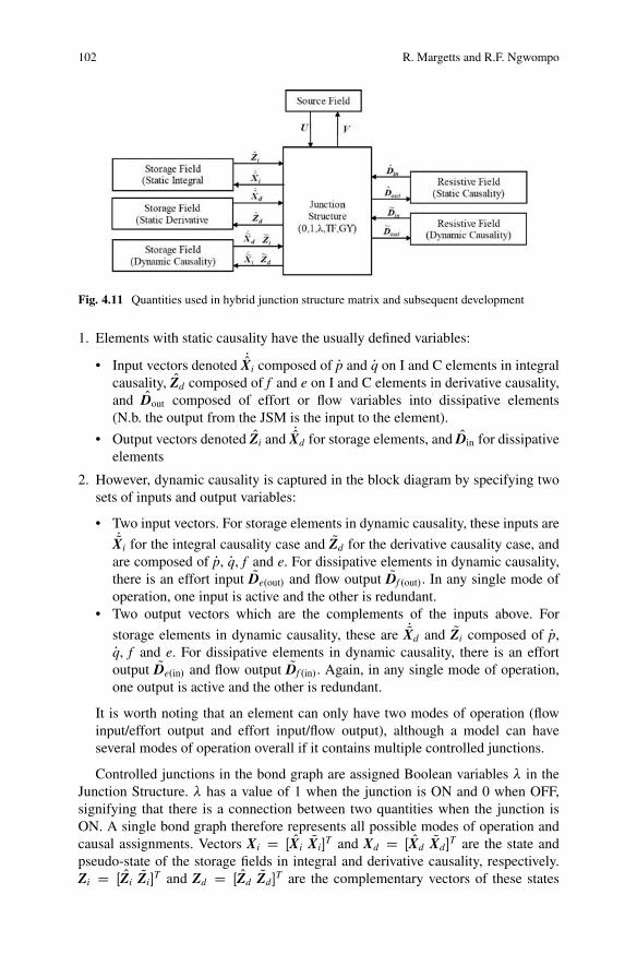
102 R. Margetts and R.F. Ngwompo
Fig. 4.11 Quantities used in hybrid junction structure matrix and subsequent development
1. Elements with static causality have the usually defined variables:
• Input vectors denoted POXi composed of Pp and Pq on I and C elements in integralcausality, OZd composed of f and e on I and C elements in derivative causality,and ODout composed of effort or flow variables into dissipative elements(N.b. the output from the JSM is the input to the element).
• Output vectors denoted OZi and POXd for storage elements, and ODin for dissipativeelements
2. However, dynamic causality is captured in the block diagram by specifying twosets of inputs and output variables:
• Two input vectors. For storage elements in dynamic causality, these inputs arePQXi for the integral causality case and QZd for the derivative causality case, and
are composed of Pp, Pq, f and e. For dissipative elements in dynamic causality,there is an effort input QDe.out/ and flow output QDf .out/. In any single mode ofoperation, one input is active and the other is redundant.
• Two output vectors which are the complements of the inputs above. For
storage elements in dynamic causality, these are PQXd and QZi composed of Pp,Pq, f and e. For dissipative elements in dynamic causality, there is an effortoutput QDe.in/ and flow output QDf .in/. Again, in any single mode of operation,one output is active and the other is redundant.
It is worth noting that an element can only have two modes of operation (flowinput/effort output and effort input/flow output), although a model can haveseveral modes of operation overall if it contains multiple controlled junctions.
Controlled junctions in the bond graph are assigned Boolean variables in theJunction Structure. has a value of 1 when the junction is ON and 0 when OFF,signifying that there is a connection between two quantities when the junction isON. A single bond graph therefore represents all possible modes of operation andcausal assignments. Vectors Xi D Œ OXi QXi�
T and Xd D Œ OXd QXd�T are the state and
pseudo-state of the storage fields in integral and derivative causality, respectively.Zi D Œ OZi QZi�
T and Zd D Œ OZd QZd�T are the complementary vectors of these states
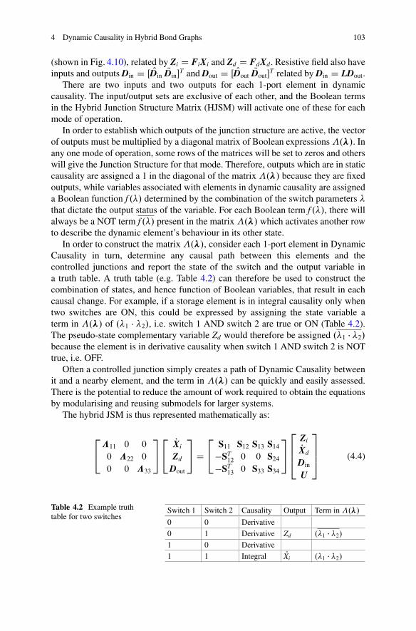
4 Dynamic Causality in Hybrid Bond Graphs 103
(shown in Fig. 4.10), related by Zi D FiXi and Zd D FdXd. Resistive field also haveinputs and outputs Din D Œ ODin QDin�
T and Dout D Œ ODout QDout�T related by Din D LDout.
There are two inputs and two outputs for each 1-port element in dynamiccausality. The input/output sets are exclusive of each other, and the Boolean termsin the Hybrid Junction Structure Matrix (HJSM) will activate one of these for eachmode of operation.
In order to establish which outputs of the junction structure are active, the vectorof outputs must be multiplied by a diagonal matrix of Boolean expressions�.�/. Inany one mode of operation, some rows of the matrices will be set to zeros and otherswill give the Junction Structure for that mode. Therefore, outputs which are in staticcausality are assigned a 1 in the diagonal of the matrix �.�/ because they are fixedoutputs, while variables associated with elements in dynamic causality are assigneda Boolean function f ./ determined by the combination of the switch parameters that dictate the output status of the variable. For each Boolean term f ./, there willalways be a NOT term f ./ present in the matrix �.�/ which activates another rowto describe the dynamic element’s behaviour in its other state.
In order to construct the matrix �.�/, consider each 1-port element in DynamicCausality in turn, determine any causal path between this elements and thecontrolled junctions and report the state of the switch and the output variable ina truth table. A truth table (e.g. Table 4.2) can therefore be used to construct thecombination of states, and hence function of Boolean variables, that result in eachcausal change. For example, if a storage element is in integral causality only whentwo switches are ON, this could be expressed by assigning the state variable aterm in �.�/ of .1 � 2/, i.e. switch 1 AND switch 2 are true or ON (Table 4.2).The pseudo-state complementary variable Zd would therefore be assigned .1 � 2/because the element is in derivative causality when switch 1 AND switch 2 is NOTtrue, i.e. OFF.
Often a controlled junction simply creates a path of Dynamic Causality betweenit and a nearby element, and the term in �.�/ can be quickly and easily assessed.There is the potential to reduce the amount of work required to obtain the equationsby modularising and reusing submodels for larger systems.
The hybrid JSM is thus represented mathematically as:
2
4�11 0 0
0 �22 0
0 0 �33
3
5
2
4PXi
Zd
Dout
3
5 D2
4S11 S12 S13 S14
�ST12 0 0 S24
�ST13 0 S33 S34
3
5
2
664
ZiPXd
Din
U
3
775 (4.4)
Table 4.2 Example truthtable for two switches
Switch 1 Switch 2 Causality Output Term in �.�/
0 0 Derivative
0 1 Derivative Zd .1 � 2/1 0 Derivative
1 1 Integral PXi .1 � 2/
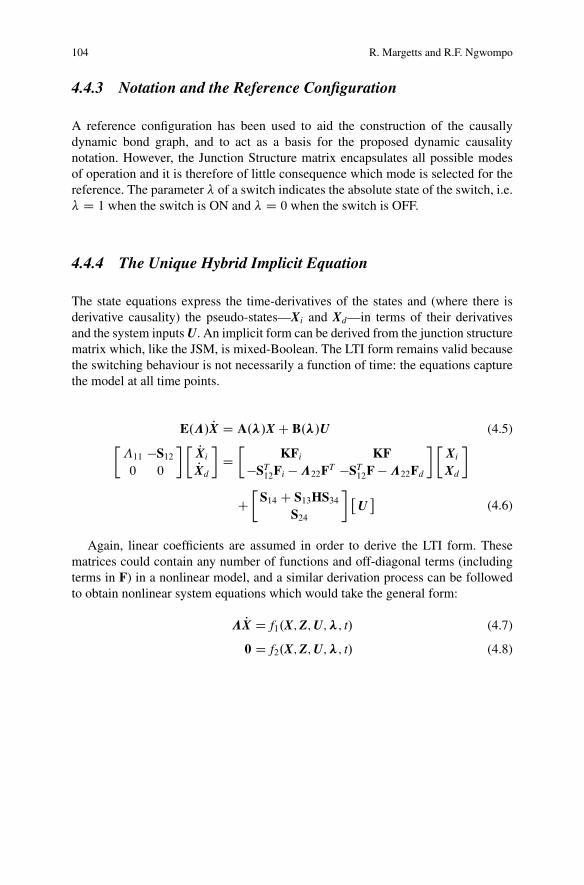
104 R. Margetts and R.F. Ngwompo
4.4.3 Notation and the Reference Configuration
A reference configuration has been used to aid the construction of the causallydynamic bond graph, and to act as a basis for the proposed dynamic causalitynotation. However, the Junction Structure matrix encapsulates all possible modesof operation and it is therefore of little consequence which mode is selected for thereference. The parameter of a switch indicates the absolute state of the switch, i.e. D 1 when the switch is ON and D 0 when the switch is OFF.
4.4.4 The Unique Hybrid Implicit Equation
The state equations express the time-derivatives of the states and (where there isderivative causality) the pseudo-states—Xi and Xd—in terms of their derivativesand the system inputs U. An implicit form can be derived from the junction structurematrix which, like the JSM, is mixed-Boolean. The LTI form remains valid becausethe switching behaviour is not necessarily a function of time: the equations capturethe model at all time points.
E.�/ PX D A.�/X C B.�/U (4.5)��11 �S120 0
� � PXiPXd
�D�
KFi KF�ST
12Fi � �22FT �ST12F � �22Fd
� �Xi
Xd
�
C�
S14 C S13HS34S24
� �U�
(4.6)
Again, linear coefficients are assumed in order to derive the LTI form. Thesematrices could contain any number of functions and off-diagonal terms (includingterms in F) in a nonlinear model, and a similar derivation process can be followedto obtain nonlinear system equations which would take the general form:
� PX D f1.X;Z;U;�; t/ (4.7)
0 D f2.X;Z;U;�; t/ (4.8)

4 Dynamic Causality in Hybrid Bond Graphs 105
To obtain the implicit system equation (4.6) the following procedure is proposed:
Procedure 2: A Procedure for finding the implicit system equations of ahybrid bond graph
1. Construct the diagonal matrix �
– Consider each 1-port element in dynamic causality in turn, and deter-mine all paths of dynamic causality between these elements and thecontrolled junctions.
– Use a truth table to construct the combination of states, and hencefunction of Boolean variables, that result in each causal change.
2. Construct the Hybrid Junction Structure Matrix (HJSM) in form ofEq. (4.13).
– The HJSM relates system inputs to outputs. For elements in staticcausality, there will be one input and one output. For elements indynamic causality, there are two inputs (effort and flow) and twooutputs.
– For static causality, the HJSM is constructed by using 1’s and 0’s todenote whether quantities are related or not.
– Where a path between two elements crosses a TF or GY element, avariable or function other than one may appear in the Hybrid JunctionStructure Matrix.
– Where a path between two elements crosses a controlled junction, a (or function of ) is used to show that the relationship only occurs whenthe junction is ON (or OFF).
– Where an element is in dynamic causality (shown by a dotted causalstroke in addition to the solid one) each variable will only be an inputto the system in certain modes of operation. Referring to the truth tableconstructed in step 1, assign a function of which denotes the modesin which the variable is an input.
– Recall that the matrix should be skew-symmetric, and submatrices S22,S23 and S32 should be zeros.
3. Derive the LTI Implicit form.
– Find matrices L and F from the (linear) relationships in the 1-portelements.
– Take the submatrices of S and � from the Junction Structure Matrixequation, and insert them into the general implicit LTI form in Eq. (4.6).
– Simplify this equation to give the state equations plus some additionalequations relating to the pseudo-states.
106 R. Margetts and R.F. Ngwompo
4.5 Solving the Hybrid Mathematical Model
Solving hybrid models by computer is not a new concept: there has been atremendous amount of work in this area. However, the mixed-Boolean state modelgenerated from the causally dynamic hybrid bond graph is particularly simple toimplement.
4.5.1 Background
There is a body of work on simulation of hybrid bond graphs using causally staticmodels (e.g. the use of causality resistance in 20-Sim), transforming the modelsto other environments such as the acausal modelling language Modelica [44], itscommercial GUI Dymola [50], and formalising the transformation of bond graphmodels into block diagrams for simulation in SIMULINK [3, 4, 13, 21]. HybridProcess Algebra (HyPA) has been applied to bond graphs [15, 16]. The potentialfor cosimulation of bond graphs and block diagrams has been explored [54], as hasderiving input/output port-Hamiltonian models which allow the bond graph modelto be embedded in or cosimulated with other environments [55–57]. These movesmake sense from a computational point of view (and much of the research here wasconducted by computer scientists) but lose the graphical advantages and relationto the physical system which are important to the systems engineer. This work inother software packages typically using controlled junctions also yielded results inthe field of FDI [18, 43] where the focus was on efficient simulation rather thanexploiting the bond graph [23, 45, 49].
4.5.2 Simulating the Mixed-Boolean State Model
At the time of writing, there are no commercial environments for simulating causallydynamic hybrid bond graphs (although there are controlled junctions in the latestversions of 20-Sim). The user therefore has two options:
• insert an equational subsystem into a Bond Graph environment (e.g. 20-Sim)• transfer the mixed-Boolean state model to a programming environment (e.g.
Modelica, Matlab).
Matlab has been used successfully to simulate the mixed-Boolean State Model[30]. Conditional statements and loops can be used to assign values to the Booleanparameters at any given time step, and the system can then be solved using regularsolvers. Where the model is implicit in some modes of operation, an implicit solversuch as BDF or ode15i (in Matlab) must be used. An example Matlab script isprovided in the appendix.
4 Dynamic Causality in Hybrid Bond Graphs 107
Immediately after a discontinuity, the state (or pseudo-state) variable is assignedthe same value that the corresponding state (or pseudo-state) had immediately beforethe discontinuity. This is because the model is inherently a switching model, andthe causally dynamic hybrid bond graph described here guides the user towardsdeveloping a switching model rather than an impulsive one. There are no unknownenergy losses, and hence no need for state reinitialisation. This is discussed in moredetail in Sect. 4.6.6.
There is a body of literature on the simulation of hybrid and nonsmoothdynamical systems which has developed in parallel with the hybrid bond graph.A number of issues merit consideration [1]:
• Switching must always occur at the end of a time step, in order to be captured.This usually motivates an event-driven method. However, this can be impracticalwhere there is a large number of switching instants or it is not known where theyoccur.
• Chattering may occur where a sliding mode cannot be reached due to numericalapproximation.
• A procedure for accurately finding the location of events may be required, alongwith some method for reinitialising states after the event.
• Where there are a number of events, there may be a finite accumulation pointpast which the event-driven method cannot progress.
• There may be an impulsive term on commutation giving a Dirac or Steltjesmeasure. For example, the differential measure of velocity which manifests onimpact between bodies.
Acary and Brogliato [1] suggest the use of discrete-time Moreau’s second-ordersweeping process for solving problems such as the bouncing ball discussed here.There are no detection times, and hence no accumulation point. Nonsmoothmeasures are treated rigorously with no ‘jump’ in acceleration, and hence noimpulse losses or need to reinitialise states.
4.5.3 Developing an Impulse Model
Where a mode of operation is very short (e.g. the ‘in contact with the ground’ modeof a bouncing ball) it can be computationally inefficient to simulate it. This is whythese kinds of problems are often abstracted to impulsive models. The problemwith impulsive models is that the impulse loss on commutation is unknown, andthe values of state variables after the discontinuity are consequently unknown. Theimpulse must be explicitly modelled (as in Impulse Bond Graphs [65]) or the statesmust be reinitialised using some algorithm [36, 45].
The [switching] hybrid bond graph can be used to generate an impulsive model,with the benefit of allowing the impulse loss to be calculated rather than simplyestimated. For example, in the bouncing ball problem, the model can be simplified togive Newton’s Collision Law (an impulsive model) with a coefficient of restitutioncalculated from the model [31].
108 R. Margetts and R.F. Ngwompo
4.6 Structural Analysis in Causally Dynamic HBGs
Here the term ‘structural analysis’ refers to the qualitative analyses that can becarried out on the bond graph prior to simulation. They can guide the user inrevisiting their modelling assumptions or even the design of the system. Theywill also provide some information about computation, such as whether the modelis explicit or implicit. The structural analyses mirror those carried out on stateequations, because the bond graph and state model are closely linked.
4.6.1 State and Implicit Models
Control properties are usually found from the state space representation of the modelwith causality assigned (i.e. the input/output model). An overview is given by themost standard control textbooks such as Sontag [51]. Although there have beensignificant developments in control theory since that time, these basic parametersare still widely taught and used today, often in the context of the explicit lineartime-invariant (LTI) state space equation. Authors typically strive to obtain theexplicit regular state space system for ease of both computation and analysis. Sincestate equations are easily derived from the bond graph, it follows that controlproperties normally found from the state equations are reflected in the bond graph’sstructure and causal assignment. A body of work by Sueur, Dauphin-Tanguy andothers brings the notions of structural analysis and exploiting causality closertogether. These properties (controllability, stability, (in)finite structure, etc.) aid withinstrumentation for experimentation and fault diagnosis and identification (FDI).
However, implicit systems in various forms appear to arise naturally whenlooking at interconnected systems, and Lewis [25] argues that they are more suitablefor signal processing and modelling tasks than explicit state space models. Specificimplicit forms which have been investigated in detail are singular systems, semistatesystems and descriptor systems. Yip and Sincovec [64] establish properties of thedescriptor system, and Verghese et al. [60] develop a generalised theory for singularsystems: both essentially present control properties for implicit systems whichmirror those established for explicit ones. Lewis [24–26] gives a useful review ofimplicit systems and techniques for analysing them, and Dai [17] looks specificallyat matrix-rank criteria for singular systems. Their results will be extended to theequations generated by the causally dynamic hybrid bond graph here.
The main considerations for a singular system are the presence and treatment ofimpulsive modes, and of causality. Causality in this sense refers to whether a valuecan be calculated from past values (causal) or depends on both past and forwardvalues (noncausal): implicit systems are by nature noncausal. This allows them tobe manipulated into a state space form and perhaps more significantly they can beconsidered as behavioural models. Willems [62, 63] demonstrates that control can

4 Dynamic Causality in Hybrid Bond Graphs 109
be studied from a behavioural point of view without introducing inputs and outputs.Lewis and Ozcaldiran [27] therefore investigate the geometric properties of implicitmodels referencing Willems, arguing that they give increased engineering insight.
4.6.2 Observations on the Dynamic Causality Assignment
The dynamic causality notation was designed to give some insight into the modeland be more usable than existing notation [5]. This section presents a series ofobservations on dynamic causality manifesting in the hybrid bond graph.
An immediate observation is that paths of dynamic causality between controlledjunctions and elements can be identified, and these clearly show the elementsaffected by commutation of a controlled junction. This means that compiling atruth table for the model and constructing the�-matrix for any subsequent equationderivation is greatly simplified. Rather than constructing a truth table for the wholemodel with 2i possible modes of operation (where i is the number of controlledjunctions), a series of smaller truth tables can be constructed for each segment ofthe model in dynamic causality.
Additional observations on the paths of dynamic causality can be made in linewith those already made for causally static bond graphs, such as Margolis andRosenberg’s work on exploiting causality [34, 47] and Rosenberg and Andry’s workon solving causal loops [48].
The number of storage elements in dynamic causality is a measure of thevariation in model size. Recall that elements in integral causality provide the statevariables in deriving the state equations. Therefore, when all of storage elementsare in integral causality, the maximum number of states is active. In a well-constructed model, there are no elements in static derivative causality and thismode (the reference mode) gives a fully explicit state space model. Likewise, themode of operation where most storage elements are in derivative causality givesthe minimum number of state variables (and the maximum number of pseudo-states which yield additional algebraic equations). Dynamic causality on resistanceelements does not affect the model size.
If dynamic causality is not controlled, it can be exploited in much the sameway as static causality. Causal paths between elements (in the reference or othermodes) can be traced, and signify various types of algebraic or kinematic constraint.In addition to identifying these paths in the case of dynamic causality, it is possibleto further classify them.
The classic variable topology problem—ideal ‘hard’ contact resulting incoalescence—is visible via a controlled junction which is OFF in the referencemode and results in a kinematic constraint between rigid bodies (i.e. a causal pathbetween two I-elements, one of which will be in derivative causality) when it isON. This usually manifests as a path of dynamic causality between a controlledjunction and I-element, shown in Fig. 4.12. It is also possible for complianceelements to become kinematically constrained. A user may choose to break thekinematic constraint by revising modelling assumptions: the classic approach is

110 R. Margetts and R.F. Ngwompo
Fig. 4.12 Example of a type 1 discontinuity: ‘Hard’ contact resulting in a kinematic constraintbetween bodies 1 and 2 (top), compliant contact (middle) and compliant contact with resistance(lower)
to redefine a hard contact problem as stiff contact, by adding a stiff compliancebetween the inertia elements. This may not always be appropriate, especially ifa ‘proper model’ or model devoid of high-frequency stiff dynamics is required.If the mode(s) of operation for which the constraint exists were to be consideredin isolation, the constrained storage elements could be lumped together: this maybe laborious by hand, but a computer programme could feature an algorithm forlumping constrained elements or using relaxed causalities [22] in the appropriatemodes of operation.
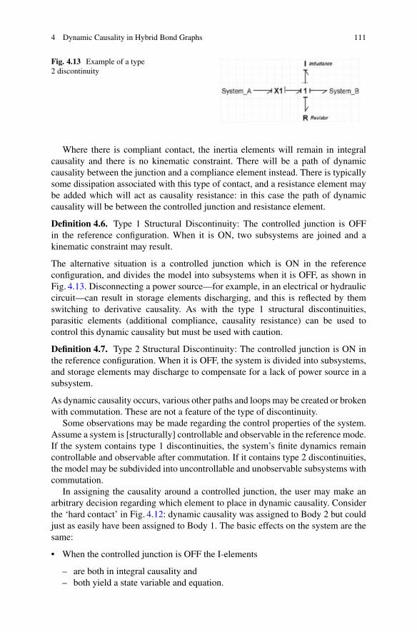
4 Dynamic Causality in Hybrid Bond Graphs 111
Fig. 4.13 Example of a type2 discontinuity
Where there is compliant contact, the inertia elements will remain in integralcausality and there is no kinematic constraint. There will be a path of dynamiccausality between the junction and a compliance element instead. There is typicallysome dissipation associated with this type of contact, and a resistance element maybe added which will act as causality resistance: in this case the path of dynamiccausality will be between the controlled junction and resistance element.
Definition 4.6. Type 1 Structural Discontinuity: The controlled junction is OFFin the reference configuration. When it is ON, two subsystems are joined and akinematic constraint may result.
The alternative situation is a controlled junction which is ON in the referenceconfiguration, and divides the model into subsystems when it is OFF, as shown inFig. 4.13. Disconnecting a power source—for example, in an electrical or hydrauliccircuit—can result in storage elements discharging, and this is reflected by themswitching to derivative causality. As with the type 1 structural discontinuities,parasitic elements (additional compliance, causality resistance) can be used tocontrol this dynamic causality but must be used with caution.
Definition 4.7. Type 2 Structural Discontinuity: The controlled junction is ON inthe reference configuration. When it is OFF, the system is divided into subsystems,and storage elements may discharge to compensate for a lack of power source in asubsystem.
As dynamic causality occurs, various other paths and loops may be created or brokenwith commutation. These are not a feature of the type of discontinuity.
Some observations may be made regarding the control properties of the system.Assume a system is [structurally] controllable and observable in the reference mode.If the system contains type 1 discontinuities, the system’s finite dynamics remaincontrollable and observable after commutation. If it contains type 2 discontinuities,the model may be subdivided into uncontrollable and unobservable subsystems withcommutation.
In assigning the causality around a controlled junction, the user may make anarbitrary decision regarding which element to place in dynamic causality. Considerthe ‘hard contact’ in Fig. 4.12: dynamic causality was assigned to Body 2 but couldjust as easily have been assigned to Body 1. The basic effects on the system are thesame:
• When the controlled junction is OFF the I-elements
– are both in integral causality and– both yield a state variable and equation.

112 R. Margetts and R.F. Ngwompo
Fig. 4.14 Hard contact with a causal path (indicated by arrow): Body 2 in dynamic causality (top)and Body 1 in dynamic causality (lower)
C
Spring Body2
qs pB1 pB2FB
vA
lSubsystem_BSubsystem_A
Body1
0 1 X0 1
II
Fig. 4.15 Notation used in equation derivation for the hard contact example
• When the controlled junction is ON,
– one of the I-elements switches to derivative causality,– the order of the model is reduced by one and– the elements yield one state variable and equation, and an additional pseudo-
state providing an algebraic constraint between the two bodies.
The only time that the choice of element to place in derivative causality may besignificant is when there is an existing causal path between an element and someother structure. This will still be captured via the new causal paths, but may beless immediately obvious to the user and computationally inefficient. An example isshown in Fig. 4.14.
The causality assignment in Fig. 4.14 (top) results in a static causal path betweenBody 1 and the spring. The equally legitimate causality assignment in Fig. 4.14(lower) does not have this static causal path. Instead, there is a causal path betweenthe spring and Body 1 only when the controlled junction is OFF. When thecontrolled junction is ON, this path no longer exists but another causal path appearsbetween the spring and Body 2. Inspecting the structure and causality of the systems(using the notation in Fig. 4.15) yields the equations in Table 4.3. It can be seen thatthe first set of equations is more elegant and concise. The second set still relates
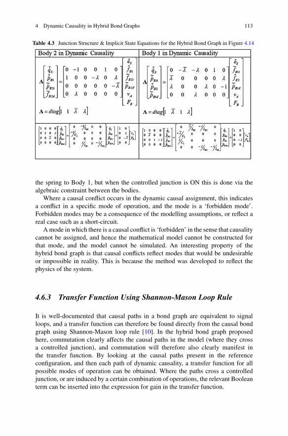
4 Dynamic Causality in Hybrid Bond Graphs 113
Table 4.3 Junction Structure & Implicit State Equations for the Hybrid Bond Graph in Figure 4.14
the spring to Body 1, but when the controlled junction is ON this is done via thealgebraic constraint between the bodies.
Where a causal conflict occurs in the dynamic causal assignment, this indicatesa conflict in a specific mode of operation, and the mode is a ‘forbidden mode’.Forbidden modes may be a consequence of the modelling assumptions, or reflect areal case such as a short-circuit.
A mode in which there is a causal conflict is ‘forbidden’ in the sense that causalitycannot be assigned, and hence the mathematical model cannot be constructed forthat mode, and the model cannot be simulated. An interesting property of thehybrid bond graph is that causal conflicts reflect modes that would be undesirableor impossible in reality. This is because the method was developed to reflect thephysics of the system.
4.6.3 Transfer Function Using Shannon-Mason Loop Rule
It is well-documented that causal paths in a bond graph are equivalent to signalloops, and a transfer function can therefore be found directly from the causal bondgraph using Shannon-Mason loop rule [10]. In the hybrid bond graph proposedhere, commutation clearly affects the causal paths in the model (where they crossa controlled junction), and commutation will therefore also clearly manifest inthe transfer function. By looking at the causal paths present in the referenceconfiguration, and then each path of dynamic causality, a transfer function for allpossible modes of operation can be obtained. Where the paths cross a controlledjunction, or are induced by a certain combination of operations, the relevant Booleanterm can be inserted into the expression for gain in the transfer function.

114 R. Margetts and R.F. Ngwompo
Fig. 4.16 A causal pathcrossing a controlled junction
Fig. 4.17 A causal path in dynamic causality
In constructing the transfer function, causal paths between elements and sourcesare used to generate gain terms in the determinant. Where that path crosses acontrolled junction, it only exists in the ON state. Multiplying the gain term bythe Boolean factor ensures it is sent to zero when OFF. An example of this situationis shown in Fig. 4.16, where the causal path indicated by the arrow has a gain of �
s2IC .Where a causal path is dynamic or partially dynamic, the gain is factored by the
Boolean function (term in �) which activates the path to give the signal loop underconsideration.
Where a path between two elements is in dynamic causality, the complete pathonly exists in a certain mode of operation. For the example in Fig. 4.17, the causalpath between the I- and R-elements (shown by the arrow) is partially in dynamiccausality. This means that there is a path between the two elements in some modesof operation only (those where the I-element is in integral causality). Hence, theBoolean function associated with activating integral causality of the I-element mustbe used as a factor in the gain, giving � .1˚2/R
sI . When the I-element is in derivativecausality, there is no causal path and the gain term is sent to zero.
The general form of the transfer function is therefore identical to that of thestandard bond graph:
hij D 1
X
k
Gkk (4.9)
where k denotes the kth path between input and output, and the graph determinantis
D 1 �X
i
Gi CX
i;j
GiGj �X
i;j;k
GiGjGk C � � � (4.10)

4 Dynamic Causality in Hybrid Bond Graphs 115
However, for the hybrid bond graph G is not only a function of any resistance,inertia or compliance coefficients relating to elements in the loop, but can alsocontain Boolean terms.
Where a controlled junction breaks/joins the causal paths in a model, the dynamicbehaviour of the system is affected with commutation. The following points followlogically:
• If a controlled junction is in a path, then a Boolean term will be present in thegraph determinant and hence the denominator of the transfer function. The rootsof the denominator are the eigenvalues of the system, so it follows that the systemwill lose/gain one or more poles with commutation.
• If a controlled junction is in a path which does not ‘touch’ the input–output path(i.e. the paths do not share any nodes), then the ‘reduced determinant’ and hencethe numerator of the transfer function will also contain a Boolean term. It followsthat the system will lose/gain zeros with commutation.
• If a controlled junction is on the input–output path, the gain of the system willbe affected. The numerator of the transfer function will again contain a Booleanand the system will lose/gain zeros with commutation.
• Where elements are in derivative causality, a path will only be present in somemodes of operation and a Boolean function will denote this. Some paths willnever touch because they are in exclusive modes of operation, and this must betaken into account when calculating the determinants.
4.6.4 The LTI Full Descriptor System
The states of the bond graph model can be used to generate an implicit systemequation from the junction structure. For models where all storage elements arein integral causality, E D I (i.e. E is non-singular) and the well-known explicitor regular state space equation is generated. For models where some storageelements are in derivative or dynamic causality, E is singular and the system isimplicit [26]. Hybrid bond graphs with storage elements in dynamic causality willalways generate implicit equations, because the derivative causality cases generatealgebraic equations with no differential term (and hence a zero term in E) and theconstraints they represent give off-diagonal coupling terms in E.
The LTI implicit equation forms one part of a descriptor system (4.11), the otherpart being given by the output equation (4.12).
E.�/ PX D A.�/X C B.�/U (4.11)
Y D C.�/X C D.�/U (4.12)
The A, B, C, D and E matrices of these equations are used in defining controlparameters such as controllability and observability, usually using matrix-rankcriteria [17].
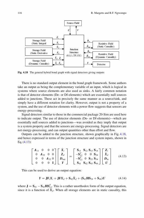
116 R. Margetts and R.F. Ngwompo
Fig. 4.18 The general hybrid bond graph with signal detectors giving outputs
There is no standard output element in the bond graph framework. Some authorstake an output as being the complementary variable of an input, which is logical insystems where source elements are also used as sinks. A fairly common notationis that of detector elements (De- or Df-elements) which are essentially null sourcesadded to junctions. These act in precisely the same manner as a source/sink, andsimply have a different notation for clarity. However, output is not a property of asystem, and the use of detector elements with a power flow suggests that sensors areenergy-processing.
Signal detectors similar to those in the commercial package 20-Sim are used hereto indicate output. The use of detector elements (De- or Df-elements)—which areessentially null sources added to junctions—was avoided as they imply that outputis a system property and that the sensors are energy-processing. Signal detectors arenot energy-processing, and can output quantities other than effort and flow.
Outputs can be added to the junction structure, shown graphically in Fig. 4.18,and hence expressed in terms of the junction structure and system inputs, shown inEq. (4.13):
2
664
�11 0 0 0
0 �22 0 0
0 0 �33 0
0 0 0 I
3
775
2
664
PXi
Zd
Dout
Y
3
775 D
2
664
S11 S12 S13 S14�ST
12 0 0 S24�ST
13 0 S33 S34S41 S42 S43 S44
3
775
2
664
ZiPXd
Din
U
3
775 (4.13)
This can be used to derive an output equation:
Y D JFiXi C JFXd C S42 PXd C .S43HS34 C S44/U (4.14)
where J D S41 � S43HST13. This is a rather unorthodox form of the output equation,
since it is a function of PXd. When all storage elements are in static causality, this
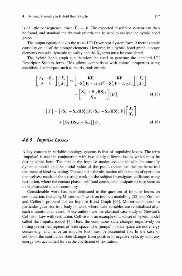
4 Dynamic Causality in Hybrid Bond Graphs 117
is of little consequence, since PXd D 0. The expected descriptor system can thenbe found, and standard matrix-rank criteria can be used to analyse the hybrid bondgraph.
The output equation takes the usual LTI Descriptor System form if there is staticcausality on all of the storage elements. However, in a hybrid bond graph, storageelements can take dynamic causality and the PXd term must be considered.
The hybrid bond graph can therefore be used to generate the standard LTIDescriptor System form. This allows comparison with control properties usingestablished techniques such as matrix-rank criteria.
��11 �S120 0
� � PXiPXd
�D�
KFi KF�ST
12Fi � �22FT �ST12F � �22Fd
� �Xi
Xd
�
C�
S14 C S13HS34S24
� �U�
(4.15)
�Y� D �
.S41 � S43HST13/Fi .S41 � S43HST
13/F� � Xi
Xd
�
C �S43HS34 C S44
� �U�
(4.16)
4.6.5 Impulse Losses
A key concept in variable topology systems is that of impulsive losses. The term‘impulse’ is used in conjunction with two subtly different issues which must bedistinguished here. The first is the impulse modes associated with the causallydynamic model and the initial value of the pseudo-state: i.e. the mathematicaltreatment of ideal switching. The second is the abstraction of the modes of operationthemselves: much of the existing work on the subject investigates collisions usingrestitution, where the contact phase itself (and consequent dissipation) is so short asto be abstracted to a discontinuity.
Considerable work has been dedicated to the question of impulse losses oncommutation, including Mosterman’s work on implicit modelling [35] and Zimmerand Cellier’s proposal for an Impulse Bond Graph [65]. Mosterman’s work inparticular gave rise to a body of work where state variables are reinitialised aftereach discontinuous event. These authors use the classical case study of Newton’sCollision Law with restitution. Collision is an example of a subset of hybrid modelcalled the Impulse model [7]. Here, the continuous state changes impulsively onhitting prescribed regions of state space. The ‘jumps’ in state space are not energyconserving: and hence an impulse loss must be accounted for. In the case ofcollision, the continuous state changes from positive to negative velocity with anyenergy loss accounted for via the coefficient of restitution.
118 R. Margetts and R.F. Ngwompo
The use of a Boolean controlled junction in the hybrid bond graph dictates theway a discontinuity is abstracted: a switch must be ON or OFF, contact TRUE orFALSE, etc. In the case of a collision, this means that the short ‘in contact’ phaseis modelled (whereas Newton’s collision law neglects this). Any energy dissipationis modelled on the bond graph during this phase: there is no restitution. The hybridbond graph with structural switching is always a ‘Switching model’ as defined byBranicky et al. [7], i.e. the vector field changes discontinuously when the state hitsa boundary, but these changes are not impulsive.
4.6.6 Impulse Modes
Impulse modes (also referred to as infinite frequency modes) are a feature ofhybrid systems. They occur where a storage element switches from integral toderivative causality, giving a step change in the value of the state. When allelements are in integral causality, E is an identity matrix and the model is in theexplicit state space form. When a storage element changes to derivative causalitywith commutation, an algebraic constraint is typically set up and a non-diagonalterm manifests in E. This term, which changes instantaneously from zero to afinite factor of a state variable on commutation, is what gives the impulse mode[60]. Recall the implicit equation (4.15), and compare it to the standard implicitequation. There is a time-varying term PXd in the algebraic equations yielded by thepseudo-states of the storage elements in derivative causality. This is multiplied byzero (by the lower portion of E) to give an algebraic constraint. However, wherestorage elements in derivative causality are coupled to the states (i.e. S12, andtherefore E12 in the implicit equation, are nonzero), a PXd term is present and thepseudo-state is differentiated across the commutation. The pseudo-state is nominallyassumed to have a zero initial value, and take a nonzero value on commutation.This means that there is a step increase in the pseudo-state between the initialcondition (incrementally before commutation) and the finite value it holds at timet (incrementally after commutation). The first row of (4.15) after commutationtherefore gives
�11PXi � S12 PXd D KFiXi C KFXd C .S14 C S13HS34/U (4.17)
where:
PXd D .Xd/t � .Xd/0
dt(4.18)
Differentiating this step change over zero time yields a mode of infinite frequency:this is the impulse mode.
dt ! 0 ) PXd ! 1 (4.19)
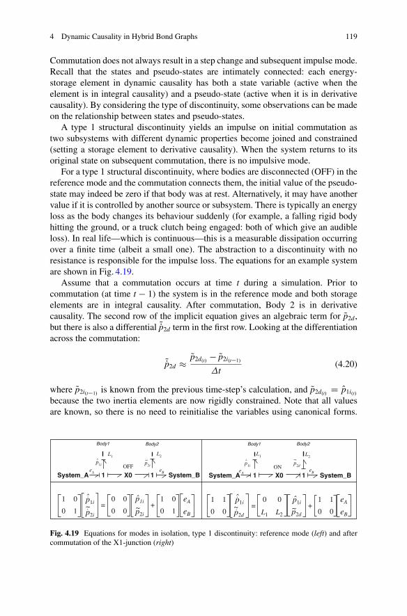
4 Dynamic Causality in Hybrid Bond Graphs 119
Commutation does not always result in a step change and subsequent impulse mode.Recall that the states and pseudo-states are intimately connected: each energy-storage element in dynamic causality has both a state variable (active when theelement is in integral causality) and a pseudo-state (active when it is in derivativecausality). By considering the type of discontinuity, some observations can be madeon the relationship between states and pseudo-states.
A type 1 structural discontinuity yields an impulse on initial commutation astwo subsystems with different dynamic properties become joined and constrained(setting a storage element to derivative causality). When the system returns to itsoriginal state on subsequent commutation, there is no impulsive mode.
For a type 1 structural discontinuity, where bodies are disconnected (OFF) in thereference mode and the commutation connects them, the initial value of the pseudo-state may indeed be zero if that body was at rest. Alternatively, it may have anothervalue if it is controlled by another source or subsystem. There is typically an energyloss as the body changes its behaviour suddenly (for example, a falling rigid bodyhitting the ground, or a truck clutch being engaged: both of which give an audibleloss). In real life—which is continuous—this is a measurable dissipation occurringover a finite time (albeit a small one). The abstraction to a discontinuity with noresistance is responsible for the impulse loss. The equations for an example systemare shown in Fig. 4.19.
Assume that a commutation occurs at time t during a simulation. Prior tocommutation (at time t � 1) the system is in the reference mode and both storageelements are in integral causality. After commutation, Body 2 is in derivativecausality. The second row of the implicit equation gives an algebraic term for Qp2d,but there is also a differential QPp2d term in the first row. Looking at the differentiationacross the commutation:
QPp2d � Qp2d.t/ � Qp2i.t�1/
t(4.20)
where Qp2i.t�1/ is known from the previous time-step’s calculation, and Qp2d.t/ D Op1i.t/because the two inertia elements are now rigidly constrained. Note that all valuesare known, so there is no need to reinitialise the variables using canonical forms.
Body1
OFF
L1L2
p2ip1i
p1i p1i~ ~ ~p2i p2i
eA eAeB eB
eA eB
~ˆ
ˆ ˆ ˆ.
.p1i p1i~p2d p2d
.
.
.
System_A System_B1 1X0ON
L1 L2
p2dp1ieA eB
~ˆ
System_A System_B1 1X0
Body2 Body1 Body2
1 0= + = +
0 1
1 0
0 1
1 1 0 0
0 L1 L20
1 1
0 0
0 0
0 0
Fig. 4.19 Equations for modes in isolation, type 1 discontinuity: reference mode (left) and aftercommutation of the X1-junction (right)
120 R. Margetts and R.F. Ngwompo
The time step is also nonzero and known, and governed by the integrator parametersused for computation. A large step change (compared to the time step) may causecomputational difficulties at this point as the left-hand side of the state equation canbecome large. In this case it may be advantageous to set QPp2d.t/ D 0, Qp2d.t/ D Op1i.t/ andneglect the impulse. This naturally violates conservation of energy but would easecomputation considerably.
If the reverse situation is true, i.e. there is a type 2 structural discontinuity wherethe bodies are connected in the reference mode and the commutation disconnectsthem, the initial value of the pseudo-state is not zero.
A type 2 structural discontinuity does not yield an impulse on initial commu-tation. In this case, the state of the storage element which switches to derivativecausality is identical to its value immediately before commutation. Hence there isno step change in state variable and no energy loss.
When the system returns to its original state on subsequent commutation, thereis a step change in state variable. However, this does not manifest as an impulsiveoff-diagonal term in the E matrix: it is simply the newly activated PXi term. This termis the output calculated from the state variables and inputs at the current time, andthere has been no differentiation over a zero time step. Hence there is no impulse.
In this case, the initial value of the pseudo-state is equal to the [usuallyfinite] value of the corresponding state variable immediately before commutation.Furthermore, after commutation the pseudo-state is not sent to zero. The behaviourof the element may be controlled by some other system, or may tend to zeroover time (for example, a clutch disconnecting a load which free-wheels untilit finally reaches rest). In this case there is no step change in variable and noimpulse. However, when commutation occurs again and the disconnected body isreconnected to the system (going from zero to a finite value), a step change in statevariable may then occur. Consider a system with one element in dynamic causality,which has just commutated back to the mode in which it is in integral causality. Row1 of the implicit equation (which is now explicit) gives
I PXi D KFiXi C .S14 C S13HS34/U (4.21)
Although a step change may have occurred, there is no impulsive term in theequation.
Hence each term in E12 potentially represents an impulse mode, but in realitythere is only an impulse loss where there are type 1 discontinuities. Any algorithmfor computing impulsive modes must take the variety of possible cases into account.
The use of pseudo-states means that the state variable never needs to bereinitialised. In type 1 systems, the pseudo-state variable arises because there isa kinematic constraint between two elements, and the pseudo-state of one is equalto the state of the other. In type 2 systems, there is no step change on the initialcommutation, but a subsequent commutation may result in a step change: this doesnot result in an impulsive term in the equations because the differential term isexplicit.
4 Dynamic Causality in Hybrid Bond Graphs 121
A mathematical impulse has infinite magnitude and zero width, hence there isno actual energy loss. In reality, there can be dissipation in the form of an audiblenoise, spark or heat loss. This can be represented on the bond graph via a resistanceelement, or neglected in which case conservation of energy does not hold true.Mosterman [41] suggests that conservation of state is the important concept insystem modelling, and the impulse energy dissipated during discontinuous eventsis ‘free energy’.
Each mode change is a sliding mode change and the implicit equation can alwaysbe used because one side of it is always known. The use of impulse models likeNewton’s collision law (i.e. restitution) are a different case. In impulse models thereis a jump in state space between modes of operation and an associated energyloss. This type of impulsive loss should not be confused with the impulse modesdescribed above.
4.6.7 Control Properties
The term ‘control properties’ refers to those properties obtained from the modelwhich can benefit the control engineer. These are typically stability, controllabil-ity/observability, solvability and related properties which can aid the engineer inassessing a design and defining instrumentation and stabilising controllers.
Analysis of the state and implicit equations using matrix-rank criteria—with orwithout transforming the model to various canonical forms—is well establishedand perhaps the most common form of system analysis. The use of matrix-rankcriteria necessitates an input–output model, i.e. they must be applied after causalityhas been assigned. The validity of this approach has been called into question.A more promising approach, in keeping with the ideals of physical and behaviouralmodelling, might be a geometric one as proposed by Lewis [26] and Willems [63].This is recommended as a topic for further study.
It is well established that a controllability matrix can be constructed for anLTI descriptor system, which has rank equal to model order when the system iscontrollable. This controllability matrix is a function of the A and B matrices, whichare in turn comprised from the submatrices of S. Controllability can hence be seenon the bond graph by analysing the causal paths, or established from the junctionstructure matrix S. Previous work on hybrid bond graphs (using switched sources)has investigated R-controllability and Impulse-controllability , relating to the finiteand impulse modes, respectively. The same distinction is made here.
Recall that the order of the model, and hence the number of finite modes ofthe system, is given by the number of storage elements in integral causality. Ittherefore follows that the maximum number of finite modes occurs when moststorage elements are in integral causality, i.e. the reference mode. The maximumnumber of finite modes is given by the order of the model in the reference mode.This is the maximum number of storage elements in integral causality: dimŒXi�.R-controllability of these finite modes is an intuitive concept, fundamentally

122 R. Margetts and R.F. Ngwompo
the same as the structural controllability defined for a continuous LTI system.The model is R-controllable when independent relationships in the equations—corresponding to causal paths on the bond graph which exist both when preferredintegral and preferred derivative causality are applied—are present between eachstorage element and a source element.
When there is a controlled junction in a causal path, that path is severed or ceasedto exist when the junction is OFF. It is intuitive that when a controlled junctionoccurs between the storage element in integral causality and a source element:
• a Boolean term occurs in the underlying equations which sets the relationship tozero when the junction is OFF, and
• the dynamic causality around the junction clearly shows that the causal path isbroken when the junction is OFF.
There are two possible outcomes when this happens. The first is that the storageelement remains in integral causality, in which case it may be controlled by anothersource, or it may be uncontrolled, i.e. there is an uncontrolled finite mode. Theother outcome is that the storage element changes its causal assignment and thefinite mode ceases to exist: in this case the impulse controllability must be assessed.
There may also be instances where a nearby controlled junction(s) results indynamic causality on a causal path between the storage element in integral causalityand a source element. The controlled junction(s) does not physically sever the causalpath, but still clearly affects controllability because the relationship between thesource and storage elements is nonexistent in some modes of operation.
A hybrid bond graph is structurally R-controllable iff:
1. There is a causal path between each storage element in integral causality and asource element in all modes of operation, i.e.:
(a) the causal path does not cross a controlled junction or,(b) there is another path between it and a storage element crossing a controlled
junction which operates in a mutually exclusive manner with the first, or,(c) the causal path crosses a controlled junction which forces the storage element
into derivative causality when it is OFF.
2. In the reference mode, the rank of the controllability matrix is equal to themodel order: i.e. the number of storage elements in integral causality whenpreferred integral causality is applied is equal to the number of storage elementsin derivative causality when preferred derivative causality is applied (allowingdualisation of source elements).
This is an extension of R-controllability for a static bond graph, acknowledgingthe observations made for structural switching and dynamic causality, i.e. thatrelationships in the model can be dependent on commutation.
Impulse controllability has been established by hybrid bond graph practitionerssuch as Rahmani and Dauphin-Tanguy [46] by inspecting the switching sources,which is clearly not applicable here as there are none. An equivalent criteria ofestablishing causal paths between controlled junctions and storage elements couldbe stated. However, the impulse modes in the underlying equations no longer relate
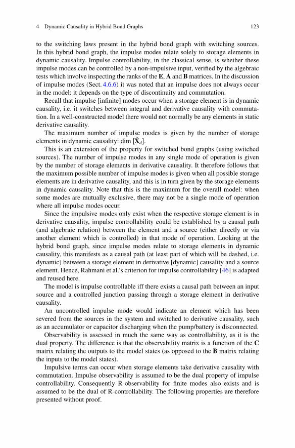
4 Dynamic Causality in Hybrid Bond Graphs 123
to the switching laws present in the hybrid bond graph with switching sources.In this hybrid bond graph, the impulse modes relate solely to storage elements indynamic causality. Impulse controllability, in the classical sense, is whether theseimpulse modes can be controlled by a non-impulsive input, verified by the algebraictests which involve inspecting the ranks of the E, A and B matrices. In the discussionof impulse modes (Sect. 4.6.6) it was noted that an impulse does not always occurin the model: it depends on the type of discontinuity and commutation.
Recall that impulse [infinite] modes occur when a storage element is in dynamiccausality, i.e. it switches between integral and derivative causality with commuta-tion. In a well-constructed model there would not normally be any elements in staticderivative causality.
The maximum number of impulse modes is given by the number of storageelements in dynamic causality: dim Œ QXd�.
This is an extension of the property for switched bond graphs (using switchedsources). The number of impulse modes in any single mode of operation is givenby the number of storage elements in derivative causality. It therefore follows thatthe maximum possible number of impulse modes is given when all possible storageelements are in derivative causality, and this is in turn given by the storage elementsin dynamic causality. Note that this is the maximum for the overall model: whensome modes are mutually exclusive, there may not be a single mode of operationwhere all impulse modes occur.
Since the impulsive modes only exist when the respective storage element is inderivative causality, impulse controllability could be established by a causal path(and algebraic relation) between the element and a source (either directly or viaanother element which is controlled) in that mode of operation. Looking at thehybrid bond graph, since impulse modes relate to storage elements in dynamiccausality, this manifests as a causal path (at least part of which will be dashed, i.e.dynamic) between a storage element in derivative [dynamic] causality and a sourceelement. Hence, Rahmani et al.’s criterion for impulse controllability [46] is adaptedand reused here.
The model is impulse controllable iff there exists a causal path between an inputsource and a controlled junction passing through a storage element in derivativecausality.
An uncontrolled impulse mode would indicate an element which has beensevered from the sources in the system and switched to derivative causality, suchas an accumulator or capacitor discharging when the pump/battery is disconnected.
Observability is assessed in much the same way as controllability, as it is thedual property. The difference is that the observability matrix is a function of the Cmatrix relating the outputs to the model states (as opposed to the B matrix relatingthe inputs to the model states).
Impulsive terms can occur when storage elements take derivative causality withcommutation. Impulse observability is assumed to be the dual property of impulsecontrollability. Consequently R-observability for finite modes also exists and isassumed to be the dual of R-controllability. The following properties are thereforepresented without proof.

124 R. Margetts and R.F. Ngwompo
A hybrid bond graph is structurally R-observable iff:
1. There is a causal path between each storage element in integral causality and adetector element in all modes of operation, i.e.
(a) the causal path does not cross a controlled junction or,(b) there is another path between it and a detector element crossing a controlled
junction which operates in a mutually exclusive manner with the first, or,(c) the causal path crosses a controlled junction which forces the storage element
into derivative causality when it is OFF.
2. In the reference mode, the rank of the observability matrix is equal to themodel order: i.e. the number of storage elements in integral casuality whenpreferred integral causality is applied is equal to the number of storage elementsin derivative causality when preferred derivative causality is applied (allowingdualisation of detector elements).
The model is impulse observable iff there exists a causal path between an detectorand a controlled junction passing through a storage element in derivative causality.
Asymptotic stability is typically established by finding the solutions of thecharacteristic polynomial. The roots for all possible modes of operation can beobtained and plotted: roots with positive real parts indicate unstable behaviour. Thisis a numeric approach rather than a structural one, and outside the scope of structuralanalysis.
Where asymptotic stability does not exist, it indicates the presence of ‘zeromodes’ (eigenvectors with vanishing eigenvalues). Recall that ‘structurally nullmodes’ (i.e. eigenvalues which are zero, or the poles at the origin) are given by thestorage elements which are in integral causality when preferred derivative causalityis assigned [19].
For the hybrid bond graph this philosophy can be extended to the number of I-and C-elements which have to stay in [static] integral causality plus the numberof I- and C-elements in dynamic causality when a preferred derivative causality isassigned to the bond graph model.
The maximum possible number of structurally null modes is given by the numberof storage elements which can take integral causality when preferred derivativecausality is assigned to the bond graph.
This is the number of storage elements in [static] integral causality, plus thenumber of storage elements in dynamic causality in the BGD (Bond graph inpreferred derivative causality).
D0 D .dimŒ OXi�C dimŒ QXi�/BGD (4.22)
This property is a logical extension of the procedure for finding structurally nullmodes in a static bond graph. Recall that placing the bond graph in preferredderivative causality yields a mathematical model in an alternative form including theinverse of the system matrices. When storage elements remain in integral causality,it means that A is singular and there are no unique solutions to the system ofequations. In particular, inspection of the characteristic equation reveals that there
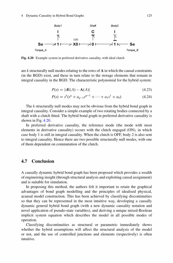
4 Dynamic Causality in Hybrid Bond Graphs 125
Fig. 4.20 Example system in preferred derivative causality, with ideal clutch
are k structurally null modes relating to the rows of A in which the causal constraints(in the BGD) exist, and these in turn relate to the storage elements that remain inintegral causality in the BGD. The characteristic polynomial for the hybrid system:
P.s/ D jsE.�/ � A.�/j (4.23)
P.s/ D sk.sq C aq�1sq�1 C � � � C a1s1 C a0/ (4.24)
The k structurally null modes may not be obvious from the hybrid bond graph inintegral causality. Consider a simple example of two rotating bodies connected by ashaft with a clutch fitted. The hybrid bond graph in preferred derivative causality isshown in Fig. 4.20.
In preferred derivative causality, the reference mode (the mode with mostelements in derivative causality) occurs with the clutch engaged (ON), in whichcase body 1 is still in integral causality. When the clutch is OFF, body 2 is also sentto integral causality. Hence there are two possible structurally null modes, with oneof them dependent on commutation of the clutch.
4.7 Conclusion
A causally dynamic hybrid bond graph has been proposed which provides a wealthof engineering insight (through structural analysis and exploiting causal assignment)and is suitable for simulation.
In proposing this method, the authors felt it important to retain the graphicaladvantages of bond graph modelling and the principles of idealised physical,acausal model construction. This has been achieved by classifying discontinuitiesso that they can be represented in the most intuitive way, developing a causallydynamic general hybrid bond graph (with a new dynamic causality notation andnovel application of pseudo-state variables), and deriving a unique mixed-Booleanimplicit system equation which describes the model in all possible modes ofoperation.
Classifying discontinuities as structural or parametric immediately showswhether the hybrid assumptions will affect the structural analysis of the modelor not, and the use of controlled junctions and elements (respectively) is oftenintuitive.
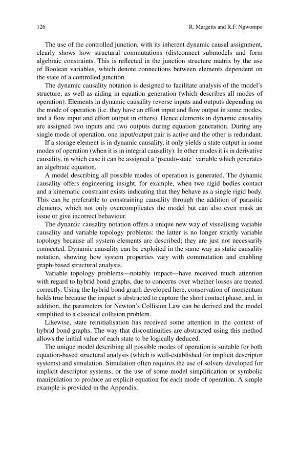
126 R. Margetts and R.F. Ngwompo
The use of the controlled junction, with its inherent dynamic causal assignment,clearly shows how structural commutations (dis)connect submodels and formalgebraic constraints. This is reflected in the junction structure matrix by the useof Boolean variables, which denote connections between elements dependent onthe state of a controlled junction.
The dynamic causality notation is designed to facilitate analysis of the model’sstructure, as well as aiding in equation generation (which describes all modes ofoperation). Elements in dynamic causality reverse inputs and outputs depending onthe mode of operation (i.e. they have an effort input and flow output in some modes,and a flow input and effort output in others). Hence elements in dynamic causalityare assigned two inputs and two outputs during equation generation. During anysingle mode of operation, one input/output pair is active and the other is redundant.
If a storage element is in dynamic causality, it only yields a state output in somemodes of operation (when it is in integral causality). In other modes it is in derivativecausality, in which case it can be assigned a ‘pseudo-state’ variable which generatesan algebraic equation.
A model describing all possible modes of operation is generated. The dynamiccausality offers engineering insight, for example, when two rigid bodies contactand a kinematic constraint exists indicating that they behave as a single rigid body.This can be preferable to constraining causality through the addition of parasiticelements, which not only overcomplicates the model but can also even mask anissue or give incorrect behaviour.
The dynamic causality notation offers a unique new way of visualising variablecausality and variable topology problems: the latter is no longer strictly variabletopology because all system elements are described; they are just not necessarilyconnected. Dynamic causality can be exploited in the same way as static causalitynotation, showing how system properties vary with commutation and enablinggraph-based structural analysis.
Variable topology problems—notably impact—have received much attentionwith regard to hybrid bond graphs, due to concerns over whether losses are treatedcorrectly. Using the hybrid bond graph developed here, conservation of momentumholds true because the impact is abstracted to capture the short contact phase, and, inaddition, the parameters for Newton’s Collision Law can be derived and the modelsimplified to a classical collision problem.
Likewise, state reinitialisation has received some attention in the context ofhybrid bond graphs. The way that discontinuities are abstracted using this methodallows the initial value of each state to be logically deduced.
The unique model describing all possible modes of operation is suitable for bothequation-based structural analysis (which is well-established for implicit descriptorsystems) and simulation. Simulation often requires the use of solvers developed forimplicit descriptor systems, or the use of some model simplification or symbolicmanipulation to produce an explicit equation for each mode of operation. A simpleexample is provided in the Appendix.

4 Dynamic Causality in Hybrid Bond Graphs 127
The derivations and analyses presented in this thesis largely assume a linear time-invariant model, in order to facilitate comparison with existing control literature.However, the same derivations can be followed with nonlinear functions in place ofthe linear coefficients during equation generation.
Appendix
In this case study, a simple power converter connected to a DC Motor (an exampleused repeatedly in the literature) [30, 33] was populated with generic data and usedto investigate a discontinuous event. A constant input was used, and the simulationwas halted at the event time at which point the load was disconnected and then runagain. The states are not reinitialised at the event time: they are simply taken tobe the same as at the last time step (which is reasonable since they have reachedsteady state). N.b. it is possible to simplify this code by specifying event times as anintegrator option.
% Run simulation until eventtspan1 = [0:1e-3:(5-(1e-3))];y01 = [20 0 0]’;yp01 = zeros(1,3)’;[t1, y1] = ode15i(@hbg, tspan1, y01, yp01);
% Run simulation from eventtspan2 = [5:1e-3:10];y02 = y1((length(t1)),:)’;yp02 = ((y1((length(t1)),:) - y1((length(t1)-1),:))/1e-5)’;[t2, y2] = ode15i(@hbg, tspan2, y02, yp02);
% Concatenate results vectorst = [t1; t2];y = [y1; y2];
where the functions are
function out = hbg(t, y, yp)
if t == [0:0.2],[0.4:0.6];% Change this statement depending on the problem under investigationl1=0;l2=1;l3=1;hsm = hss(l1, l2, l3);elsel1=1;l2=0;l3=1;hsm = hss(l1, l2, l3);end

128 R. Margetts and R.F. Ngwompo
d = length(hsm(:,1));w = length(u(:,1));A = hsm(:,1:d);B = hsm(:,d+1:d+w);E = hsm(:,d+w+1:d+w+d);u = [12;0];
out = A*y + B*u - E*yp;
end
---------------------------------function hsm = hss(l1, l2, l3)
% Define coefficientsL1 = 10e-3;L2 = 2.25e-7 ;L3 = 1e-5 ;R1 = 1.73 ;R2 = 2e-5 ;a = 0.00902;
% Populate matrices for this modeA = [-1*xor(l1,l2)/(L1*R1) -a*xor(l1,l2)/L20 0 0a*xor(l1,l2)/L1 -l3/(L2*R2) 0 0 00 0 ~l3/(L3*R2) 0 00 0 0 ~xor(l1,l2)/L1 00 l3/L2 0 0 -l3/L3];B = [l1 l20 00 00 00 0];E = [xor(l1,l2) 0 0 0 00 1 0 0 l30 0 ~l3 0 00 0 0 0 00 0 0 0 0];
% Remove null lines/columnsorder = length(A(1,:));z = zeros(1,order);i = 1;for n = (1:order)if sum(A(n,:)) == 0 % Delete rows of zeroselseAred1(i,:) = A(n,:);Bred1(i,:) = B(n,:);Ered1(i,:) = E(n,:);i = i+1;end;end;

4 Dynamic Causality in Hybrid Bond Graphs 129
0 2 4 6 8 10−0.1
−0.05
0
0.05
0.1
0.15
0.2
0.25
Time (s)
p1‘ Voltage on Inductor
Fig. 4.21 Voltage on example power converter: constant input, load disconnected during operation
i = 1;for n = (1:order) % Delete Columns of zerosif sum(Ared1(:,n)) == 0elseAred2(:,i) = Ared1(:,n);Bred2 = Bred1;Ered2(:,i) = Ered1(:,n);i = i+1;end;end;
hsm = [Ared2 Bred2 Ered2];end
Some results are shown in Figs. 4.21 and 4.22 for illustration. The load is discon-nected 5 s into the simulation. The model runs quickly, and shows a ‘spike’ involtage immediately after the event. The torque on the motor is increased after theevent, consistent with the absence of the load.
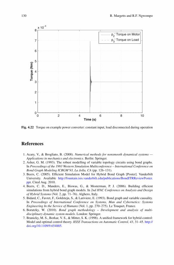
130 R. Margetts and R.F. Ngwompo
0 2 4 6 8 100
1
2
3
4
5
6
7
8x 10
−4
Time (s)
To
rqu
e (N
m)
p2‘ Torque on Motor
p3‘ Torque on Load
Fig. 4.22 Torque on example power converter: constant input, load disconnected during operation
References
1. Acary, V., & Brogliato, B. (2008). Numerical methods for nonsmooth dynamical systems —Applications in mechanics and electronics. Berlin: Springer.
2. Asher, G. M. (1993). The robust modelling of variable topology circuits using bond graphs.In Proceedings of the 1993 Western Simulation Multiconference – International Conference onBond Graph Modeling ICBGM’93, La Jolla, CA (pp. 126–131).
3. Beers, C. (2005). Efficient Simulation Model for Hybrid Bond Graph [Poster]. VanderbiltUniversity. Available http://fountain.isis.vanderbilt.edu/publications/BondITRReviewPoster.ppt. Cited Aug. 2010.
4. Beers, C. D., Manders, E., Biswas, G., & Mosterman, P. J. (2006). Building efficientsimulations from hybrid bond graph models. In 2nd IFAC Conference on Analysis and Designof Hybrid Systems (Vol. 2, pp. 71–76). Alghero, Italy.
5. Bidard, C., Favret, F., Goldztejn, S., & Lariviere, E. (1993). Bond graph and variable causality.In Proceedings of International Conference on Systems, Man and Cybernetics: SystemsEngineering In the Service of Humans (Vol. 1, pp. 270–275). Le Touquet, France.
6. Borutzky, W. (2010). Bond graph methodology – Development and analysis of multi-disciplinary dynamic system models. London: Springer.
7. Branicky, M. S., Borkar, V. S., & Mitter, S. K. (1998). A unified framework for hybrid control:Model and optimal control theory. IEEE Transactions on Automatic Control, 43, 31–45. http://doi.org/10.1109/9.654885.

4 Dynamic Causality in Hybrid Bond Graphs 131
8. Breedveld, P. C. (2000). An alternative model for static and dynamic friction in dynamicsystem simulation. In 1st IFAC Conference on Mechatronic Systems, Darmstadt, Germany(pp. 717–722).
9. Breedveld, P. C. (2002). Modelling and simulation of bouncing objects: Newton’s Cradlerevisited. In Proceedings of the Mechatronics.
10. Brown, F. T. (1972). Direct application of the loop rule to bond graphs. Transactions ASMEJournal of Dynamic Systems, Measurement and Control, 94(3), 253–261.
11. Buisson, J. (1993). Analysis and characterization of hybrid systems with bond-graphs.In Proceedings of the International Conference on Systems, Man and Cybernetics: SystemsEngineering in the Service of Humans, Le Touquet, France (pp. 264–269).
12. Buisson, J., Cormerais, H., & Richard, P. Y. (2002). Analysis of the bond graph model of hybridphysical systems with ideal switches. Proceedings of the Institution of Mechanical Engineers,Part I: Journal of Systems and Control Engineering, 216, 47–63.
13. Calvo, J. A., Boada, M. J., Roman, J. L. S., & Olmeda, E. (2010). BONDSYM: Simulink basededucational software for analysis of dynamic system. Computer Applications in EngineeringEducation, 18, 238–251. http://doi.org/10.1002/cae.20246.
14. Cellier, F. E., Otter, M., & Elmqvist, H. (1994). Bond graph modeling of variable structuresystems. Simulation Series, 27, 49.
15. Cuijpers, P. J. L., & Reniers, M. A. (2005). Hybrid process algebra. Journal of Logic andAlgebraic Programming, 62(2), 191–245.
16. Cuijpers, P. J. L., Broenink, J. F., & Mosterman, P. J. (2008). Constitutive hybrid processes:A process-algebraic semantics for hybrid bond graphs. Simulation: Transactions of theSociety for Modeling and Simulation International, 84, 339–358. http://doi.org/10.1177/0037549708097215.
17. Dai, L. (1989). Impulsive modes and causality in singular systems. International Journal ofControl, 50(4), 1267–1281.
18. Daigle, M. J., et al. (2009). A qualitative event-based approach to continuous systemsdiagnosis. IEEE Transactions on Control Systems Technology, 17(4), 780–793.
19. Dauphin-Tanguy, G., & Sueur, C. (2002). Bond graph for modelling, analysis, control design,fault diagnosis [Presentation Slides]. Available www.fceia.unr.edu.ar/~kofman/seminario/Argentine-nov02.ppt. Cited Dec. 2010.
20. Gawthrop, P. J. (1997). Hybrid Bond Graphs Using Switched I and C Components (CSC Report97005). Centre for Systems and Control, University of Glasgow.
21. Geitner, G. H. (2006). Power flow diagrams using a bond graph library under SIMULINK.In 32nd Annual Conference on IEEE Industrial Electronics IECON 2006, Paris, France(pp. 1359–1365).
22. Karnopp, D. C., Margolis, D. L., & Rosenberg, R. C. (2006). System dynamics modeling andsimulation of mechatronic systems. New York, NY: Wiley.
23. Lattmann, Z. (2010). A Multi-domain Functional Dependency Modeling Tool Based onExtended Hybrid Bond Graphs. Dept. Electrical Engineering, Vanderbilt University.
24. Lewis, F. L. (1986). Survey of linear singular systems. Circuits, Systems and Signal Processing,5(1), 3–36.
25. Lewis, F. L. (1992). Review of 2-D implicit systems. Automatica, 28(2), 345–354.26. Lewis, F. L. (1992). A tutorial on the geometric analysis of linear time-invariant implicit
systems. Automatica, 28(1) 119–137.27. Lewis, F. L., & Ozcaldiran, K. (1989). Geometric structure and feedback in singular systems.
IEEE Transactions on Automatic Control, 34(4), 450–455.28. Low, C. B., Wang, D., Arogeti, S., & Zhang, J. B. (2010). Causality assignment and model
approximation for hybrid bond graph: Fault diagnosis perspectives. IEEE Transactions onAutomation Science and Engineering, 7, 570–580.
29. Margetts, R. (2013). Modelling and analysis of hybrid dynamic systems using a bond graphapproach. University of Bath Dept. Mechanical Engineering. Available via OPUS. http://opus.bath.ac.uk/48041/. Cited 3 June 2016.

132 R. Margetts and R.F. Ngwompo
30. Margetts, R., Boudon, B., & Ngwompo, R. F. (2017). Simulation of causally dynamic hybridbond graphs, with application to a power converter. In The 36th IASTED International Confer-ence on Modelling, Identification and Control (MIC 2017). Innsbruck: IASTED (accepted).
31. Margetts, R., & Ngwompo, R. F. (2014) Hybrid bond graphs for contact, using controlledjunctions and dynamic causality. In Proceedings of the Summer Simulation Multiconference,Monterey, CA.
32. Margetts, R., & Ngwompo, R. F. (2015). Mode switching in causally dynamic hybrid bondgraphs. Mechatronics. doi:10.1016/j.mechatronics.2015.04.013.
33. Margetts, R., Ngwompo, R. F., & da Cruz, M. F. (2013). Modelling a drop test of a landinggear using a hybrid bond graph. In E. P. Klement, W. Borutzky, T. Fahringer, M. H. Hamza,& V. Uskov (Eds.), Proceedings of the IASTED International Conference on Modelling,Identification and Control (pp. 312–317). Innsbruck: ACTA Press. http://doi.org/10.2316/P.2013.794-072.
34. Margolis, D. L. (1987). Exploiting causality for structured models using bond graphs. In 1987American Control Conference, Minneapolis, MN (pp. 1457–1461).
35. Mosterman, P. J. (2000). Implicit modeling and simulation of discontinuities in physical systemmodels. In 4th International Conference on Automation of Mixed Processes: Hybrid DynamicSystems ADPM2000, Dortmund, Germany (pp. 35–40).
36. Mosterman, P. J. (2002). HyBrSim — A modelling and simulation environment for hybridbond graphs. Proceedings of the IMechE Part I: Journal of Systems and Control Engineering,216(11), 35–46.
37. Mosterman, P. J., & Biswas, G. (1995). Modeling discontinuous behavior with hybrid bondgraphs. In 9th International Workshop on Qualitative Reasoning about Physical Systems,Amsterdam, Netherlands (pp. 139–147).
38. Mosterman, P. J., & Biswas, G. (1996). A theory of discontinuities in physical system models.Journal of The Franklin Institute, 335B(3), 401–439.
39. Mosterman, P. J., & Biswas, G. (1997). Formal specifications for hybrid dynamical systems.In Proceedings of the 15th International Joint Conf. Artificial Intelligence IJCAI-97, Nagoya,Japan (pp. 568–573).
40. Mosterman, P. J., & Biswas, G. (1998). Hybrid automata for modeling discrete transitionsin complex dynamic systems. In 7th IFAC Symposium on Artificial Intelligence in Real-TimeControl, Grand Canyon National Park, AR (pp. 43–48).
41. Mosterman, P. J., & Biswas, G. (2000). A comprehensive methodology for building hybridmodels of physical systems. Artificial Intelligence, 121(1–2), 171–209.
42. Mosterman, P. J., Zhao, F., Biswas, G., & Amer Assoc Artificial, I. (1998). An ontology fortransitions in physical dynamic systems. In 15th National Conference on Artificial Intelligence(AAAI 98) (pp. 219–224). Madison, WI: American Association Artificial Intelligence.
43. Narasimhan, S. (2002). Model-Based Diagnosis of Hybrid Systems. Dept. Computer Science,Vanderbilt University.
44. Otter, M., Remehle, M., Engell, S., & Mosterman, P. (2000). Hybrid models of physicalsystems and discrete controllers. AT - Automatisierungstechnik, 48, 35–40.
45. Podgursky, B., Biswas, G., & Koutsoukos, X. D. (2010). Efficient tracking of behavior incomplex hybrid systems via hybrid bond graphs. In Annual Conference of the Prognosticsand Health Management Society. Portland.
46. Rahmani, A., & Dauphin-Tanguy, G. (2006). Structural analysis of switching systems modelledby bond graph. Mathematical and Computer Modelling of Dynamical Systems, 12(2–3),235–247.
47. Rosenberg, R. C. (1987). Exploiting bond graph causality in physical system models.Transactions on ASME Journal of Dynamic Systems, Measurement and Control, 109(4),378–383.
48. Rosenberg, R. C., & Andry, A. N., Jr. (1979). Solvability of bond graph junction structureswith loops. IEEE Transactions on Circuits and Systems, 26(2), 130–137.
49. Roychoudhury, I., Daigle, M. J., Biswas, G., & Koutsoukos, X. D. (2011). Efficient simulationof hybrid systems: A hybrid bond graph approach. Simulation, 87, 467–498.

4 Dynamic Causality in Hybrid Bond Graphs 133
50. Shiva, A. (2004). Modeling Switching Networks Using Bond Graph Technique. Dept.Aerospace and Mechanical Engineering, University of Arizona.
51. Sontag, E. D. (1998). Mathematical control theory — Deterministic finite dimensional systems.Textbooks in Applied Mathematics (Vol. 6). New York: Springer.
52. Strömberg, J. E. (1994). A Mode Switching Philosophy (Dissertation No. 353). LinköpingUniversity.
53. Sueur, C., & Dauphin-Tanguy, G. (1989). Structural controllability/observability of linearsystems represented by bond graphs. Journal of The Franklin Institute, 326(6), 869–883.
54. Tudoret, S., Nadjm-Tehrani, S., Benveniste, A., & Stromberg, J. E. (2000). Co-simulation ofhybrid systems: Signal-simulink. In M. Joseph (Ed.), Proceedings of the 6th InternationalSymposium on Formal Techniques in Real-Time and Fault-Tolerant Systems FTRTFT 2000(Vol. 1926, pp. 134–151). Pune, India.
55. Van Der Schaft, A. (2005). Theory of Port-Hamiltonian Systems Chapter 1: Port-Hamiltonianformulation of network models; the lumped-parameter case. Dutch Institute of Systems andControl (DISC). Available http://www.math.rug.nl/~arjan/teaching.html. Cited May 2010.
56. Van Der Schaft, A. (2006). Port-Hamiltonian systems — An introductory survey. In Proceed-ings of the International Congress of Mathematicians, Madrid, Spain (pp. 1339–1365).
57. Van Der Schaft, A. (2009). Port-Hamiltonian systems: From geometric network modeling tocontrol [Lecture notes for the EECI Graduate Course, LSS-Supelec, Gif-sur-Yvette]. Availablehttp://www.math.rug.nl/~arjan/teaching.html. Cited May 2010.
58. Van Der Schaft, A. J., & Schumacher, J. M. (1999). An introduction to hybrid dynamicalsystems. Lecture notes in control and information sciences (Vol. 251). London: Springer.
59. Van Kampen, D. (2003). Paper path modeling case in 20-SIM (Report 2003CE025). Depart-ment of Electrical Engineering, University of Twente, Enschede, The Netherlands.
60. Verghese, G. C., Levy, B. C., & Kailath, T. (1981). A generalized state-space for singularsystems. IEEE Transactions on Automatic Control, 26, 811–831. http://doi.org/10.1109/tac.1981.1102763.
61. Vu, L., & Liberzon, D. (2008). Invertibility of switched linear systems. Automatica, 144,949–958.
62. Willems, J. C. (2007). The behavioural approach to open and interconnected systems. IEEEControl Systems Magazine, 27(6), 46–99. http://doi.org/10.1109/MCS.2007.906923.
63. Willems, J. C. (2008). Modeling interconnected systems. In 2008 3rd International Sympo-sium on Communications, Control and Signal Processing ISCCSP2008, St. Julians, Malta(pp. 421–424).
64. Yip, E. L., & Sincovec, R. F. (1981). Solvability, controllability and observability of continuousdescriptor systems. IEEE Transactions on Automatic Control, 26(3), 702–707.
65. Zimmer, D., & Cellier, F. E. (2007). Impulse-bond graphs. In Proceedings of the 2007International Conference on Bond Graph Modeling (ICBGM 2007), San Diego, CA(pp. 3–11).
Part IIBond Graph Modelling for Fault Diagnosis,
Fault Tolerant Control, and Prognosis
One of the major topics of this compilation text besides BG representations ofhybrid models and the generation of equations is the integration of bond graph-basedfault diagnosis with fault accommodation and with fault prognosis, respectively.In the past decade, quite a number of publications have demonstrated that the BGmethodology can also support model-based Fault Detection and Isolation (FDI).Analytical Redundancy Relations (ARRs) can be derived off-line from a BG of aphysical model in a systematic manner and ARR residual, their numerical evaluationin real-time, can serve as fault indicators. At first, BG model-based FDI focusedon systems described by a continuous time model but has meanwhile extended tosystems described by a hybrid model.
The first chapter in Part II combines fault diagnosis based on ARRs derivedfrom a BG representing a mode switching linear time-invariant model with thereconstruction of a system input through inverse simulation that accommodatesfor a severe fault. The chapter starts with an approach to a BG representation ofhybrid system models and the derivation of a hybrid DAE system, briefly addressesa possible alternative derivation of a linear complementarity system formulationfrom the BG of a mode switching LTI model, discusses ARR-based as well asobserver-based FDI, and presents an inverse simulation based approach to faultaccommodation that uses the residuals of ARRs established for FDI.
A forward model with nominal parameters derived from a BG of the healthysystem is considered as reference model. If it is coupled to the real faulty systemor to its replacement by a behavioural BG model through residual sinks, then theoutputs of these coupling sinks are inputs into the reference model in addition tothe control input and force it to behave as the faulty system model. They can serveas fault indicators. Given the residual sink outputs and the desired system output,the forward model of the adapted reference model with nominal parameters can beconsidered a hybrid DAE that determines the system input to be reconstructed. Theforward model of the healthy system and the input reconstruction module constitutea feedforward controller in addition to the nominal feedback controller of a closedloop system. Depending on its type, the latter one can compensate minor parametric
136 II Bond Graph Modelling for Fault Diagnosis, Fault Tolerant Control, and Prognosis
faults in the plant and in actuators so that they are not detected by monitoringsystem outputs. Slightly faulty monitored values of a controlled variable due to asmall sensor offset are also not detected. Input reconstruction is thus important foraccommodation of severe faults. An advantage of the presented approach is that theforward model of the healthy system, the evaluation of ARRs, and the inverse modelcan be computed in parallel, that fault isolation and estimation is not needed, andthat neither ARRs nor the reconstructed input is needed in analytical form.
Another topic of current relevance that BG modelling has been recently address-ing is fault prognosis. In the context of Condition Based Management (CBM)of complex engineering systems it is important to constantly monitor a system’sbehaviour and to detect and isolate progressive faults. If the magnitude of anincipient fault is still below an alarm threshold, the question then is how fast adegradation of the system behaviour progresses due to that fault, i.e. when thefault magnitude will reach its alarm level so that maintenance becomes necessarybecause a critical failure value of a parameter, a failure threshold is reached to avoida component or system failure.
Previous chapters demonstrate that BGs are suited to represent hybrid modelsof multi-energy domain systems and can support model-based FDI. As to faultprognosis, so far, a rather small number of works using a BG approach havebeen reported in the literature. They assume that a single component parametervalue continuously drifts with time according to a known degradation model whileall other parameter values remain within given uncertainty limits. Estimation ofthe component’s Remaining Useful Life (RUL) is performed by incorporating thedegradation model into the ARRs. However, systems represented by a hybrid modeloperate in various modes. Accordingly, ARRs and the RUL of a component aremode dependent.
The subject of Chap. 6 is an approach to an integrated model-based faultdiagnosis and fault prognosis for systems represented by a hybrid model. If a hybridmodel is in use, discrete faulty mode transitions may occur in addition to parametricfaults that cause a degradation of a component’s behaviour over time. The approachpresented in Chap. 6 can detect and isolate discrete mode faults as well as parametricfaults. If the latter ones are progressive, the component’s RUL is predicted.
To overcome the problem that a fault may affect a subsequently occurring fault,the model is updated after each fault identification. For RUL estimation not onesingle degradation model is used but a sequence of mode dependent degradationmodels obtained by identification.
Finally, the integrated approach presented in Chap. 6 makes use of extensions ofthe Fault Signature Matrix (FSM) and the Mode Change Signature Matrix (MCSM)to reduce the set of possible fault candidates after a fault has been detected.
The chapter is based on a recently defended PhD thesis of the first author thatwas supervised by the second author.
Chapter 7 combines FDI based on ARRs with uncertain parameters obtainedfrom a BG of a continuous time model with Bayesian estimation techniques fordiagnosis and prognosis of incipients parametric faults in an integrated real-timehealth monitoring approach that exploits model-based and data-driven techniques

II Bond Graph Modelling for Fault Diagnosis, Fault Tolerant Control, and Prognosis 137
and enables a prediction of the RUL of a faulty system component or of a systemgiven various uncertainties such as parameter uncertainties or sensor noise.
BGs in Linear Transformation Form (LTF) are used for modelling a systemwith uncertain parameters, while Particle Filters (PFs) based on a sequential MonteCarlo method are used for estimation of the state of health of a real closed-loopfeedback system. The chapter assumes that a single system parameter is a candidatefor progressive degradation, that this parameter has been isolated and that a modelfor the degradation process is known a priori. Robust fault detection determines thebeginning of the degradation process as a parametric fault, while measurement noiseand noise in the degradation process are taken into account in the estimation of thestate of health and in RUL prediction by means of particle filters.
Chapter 7 is also based on a recently defended PhD thesis of the first author thatwas supervised by the second and third author.

Chapter 5Integrating Bond Graph-Based Fault Diagnosisand Fault Accommodation Through InverseSimulation
W. Borutzky
5.1 Introduction
Today’s closed-loop engineering systems are more and more equipped with commu-nicating smart sensors and actuators, embedded systems and software so that theycan operate autonomously to some extent. However, their increase in complexitymakes them more vulnerable to malfunctions and faults that can lead to a componentor a system failure if not properly dealt with in a timely manner. Safety andreliability of complex systems require that they are able to react autonomouslyto some faults. This can be achieved either in a passive approach by designinga controller that ensures stability and control objectives in the presence of faultsfrom a certain class of anticipated faults, or by an active, reconfigurable fault-tolerant control approach in which only the control law is changed known as faultaccommodation, or even the control loop is restructured because some sensorsor actuators have become faulty so that the system remains operational and anacceptable performance in the presence of a persisting fault can be maintained.A prerequisite for fault tolerant control (FTC) is that a system is constantlymonitored and faults are detected and isolated.
Approaches to fault detection and isolation (FDI) can be roughly categorised intodata-driven and model-based methods. Among the latter ones are techniques basedon bond graphs that derive analytical redundancy relations (ARRs) from a bondgraph (BG) and check their residuals against thresholds in order to decide whethera fault has occurred [13, 26, 63, 69, 75]. An elaborated presentation of fault tolerantcontrol may be found in [10, 45]. An excellent survey is given in [4, Chap. 2].
Bond graph model-based approaches to passive as well as to active FTC havebeen presented in [2, 42, 50, 63]. In active FTC, changing the controller law after
W. Borutzky (�)Department of Computer Science, Bonn-Rhein-Sieg University of Applied Sciences, 53754 SanktAugustin, Germanye-mail: [email protected]
© Springer International Publishing Switzerland 2017W. Borutzky (ed.), Bond Graphs for Modelling, Control and FaultDiagnosis of Engineering Systems, DOI 10.1007/978-3-319-47434-2_5
139

140 W. Borutzky
a fault has occurred requires system inversion, i.e. to find an input so that thefaulty system produces a desired output. One way to decide whether a model isinvertible and to determine an input required to produce a desired output is to assignbicausalities to a BG [33, 42, 52, 53].
The subject of this chapter is an integrated bond graph model-based approachto FDI and to FTC. Fast switching electronic devices, hydraulic check valves orfast stops (hard limits) in mechanical motion suggest to adopt the abstraction ofinstantaneous, discrete state transitions, especially in the modelling of complexmechatronic systems. Therefore, hybrid models and their bond graph representationare considered. For illustration, simple switched power electronic systems are usedthroughout the chapter. The presented bond graph approaches may, however, beapplied to other systems represented by a hybrid model as well. Power electronicdevices are subject to fast switching. Over current surge, voltage overswings aswell as short-circuit or open-circuit faults in transistors may happen. Therefore,FDI in power electronic circuits is important for FTC and for protection of complexmechatronic systems, especially when used in safety critical systems.
This chapter is organised into three sections. The next section addresses themodelling abstraction of instantaneous state transitions, its consequences withregard to a combined symbolic-numerical solution of a hybrid model and a bondgraph representation of hybrid models.
Subsequently, a simple pragmatic approach to a causal bond graph representationof hybrid models is proposed that can use either ideal or non-ideal switchesand exploits the features of the declarative modelling language Modelica®1 [47].The burden of a symbolic preprocessing and a numerical solution of a set ofhybrid Differential Algebraic Equations (DAEs) is left to a software such as thesophisticated open-source modelling and simulation software OpenModelica [56].The language allows for acausal mathematical equations and the software is able toreformulate equations as necessary and to sort the equations of a DAE system bymeans of the Tarjan algorithm and by using tearing [18, 32]. Therefore, the standardSequential Causality Assignment Procedure (SCAP) is applied to a bond graph ofa hybrid model. Causal strokes at switch ports result from causality assignment atstorage ports and ports of resistors with a non-invertible characteristic in previoussteps of the procedure and just reflect switch states in one specific system modeof operation when a maximum number of storage ports has got integral causality.Accordingly, causal equations are derived from a BG except for switches. Theswitches in the BG of a hybrid model are described by an implicit mathematicalequation relating their two conjugate port variables. The Modelica implementationof switches accounts for their operating mode. If there are causal paths betweenresistors in a BG and/or storage elements in derivative causality then it is well knownthat they also contribute implicit equations. If the purpose of a study is to simulatethe dynamic behaviour and if equations are formulated in Modelica, actually, one
1Modelica® is a registered trademark of the Modelica Association.
5 Integrating Fault Diagnosis and Fault Accommodation Through Inverse Simulation 141
could even start from an acausal BG and read out all equations in implicit formas the OpenModelica software can determine the computational causalities of allequations and can automatically choose state variables.
If the implicit equation of a switch is not part of a subset of m algebraic equationswith m unknowns, i.e. the switch does not belong to an algebraic loop, if thesymbolic preprocessing of all model equations or if the numerical solution of thesymbolically preprocessed equations by means of a BDF solver fails with a singularmatrix in one mode of operation, then a small modification of the model is required.This problem occurs when the closing of an ideal switch turns the hybrid DAEsystem of the model into a higher index system. Modelica assumes that a hybridDAE representation is structurally time invariant, i.e. that the set of variables andthe set of equations remain fixed during simulation. Conditional equations, however,can turn some equations off or on so that the number of active equations can varyat run-time [32]. Physical insight into the problem combined with an account of thepurpose of the model can help to add an auxiliary element of appropriate parametervalue in the right place or to turn an ideal switch into a non-ideal one. An advantageof this approach is that causalities can be assigned once independent of switchstates. Dynamic reassignment of causalities during simulation is taken into accountautomatically by the switch models implemented in Modelica. The approach isillustrated by application to a thyristor controlled half-wave rectifier circuit as asimple example of a hybrid system but is not limited to power electronic systems.
Section 5.3 discusses fault detection and isolation (FDI). It is assumed that ahybrid model of a system is given. Effective, correct and fast FDI is a prerequisitefor fault accommodation which is the subject of the last section in this chapter.A contribution of bond graph modelling to FDI is that Analytical RedundancyRelations (ARRs) serving as fault indicators can be derived from a BG based onphysical insight into a system in a systematic manner. It is shown that in some simplecases, ARR residuals can even be used for isolation and estimation of parametricfaults. The chapter also presents an offline simulation of a fault scenario in which ashort-circuit fault is deliberately introduced into an example circuit.
The last section in this chapter presents a bond graph-based fault accommodationapproach that uses inverse simulation for reconstructing the input required for faultrecovery.2 In this approach, a DAE system is derived from a bond graph of the faultysystem. Replacing its output by the one of the healthy system, the DAE systemdetermines the input into the faulty system required for fault accommodation. Inother words, a forward model deduced from a BG is considered a DAE system ofthe inverse model. The output of the healthy system model is considered the desiredoutput for which an input must be reconstructed after a fault has happened.
Moreover, it is shown that ARR residuals can not only be used for FDI butalso for input reconstruction. Advantages of an input reconstruction by inversesimulation are that there is no need for an analytical determination of the required
2First ideas have been presented in a paper at the 8th International Conference on IntegratedModelling and Analysis in Applied Control and Automation (IMAACA 2015) [14].
142 W. Borutzky
input in closed form and that existing software for the combined symbolic-numericalsolution of DAE systems can be used. Disadvantages are that, in general, thesolution of a DAE system of the inverse model is not guaranteed and that the inversemodel is not guaranteed to be stable. One possible remedy is to slightly modify aplant model before it is inverted and to use an approximate inverse model in thecontroller.
The approach is applied to a buck-converter driven DC-motor. For this applica-tion to a simple often used example of a power electronic system, the hybrid modelof the converter is replaced by a model with variables averaged over the switchingtime period. As a fault scenario, an abrupt increase of the armature resistance in theDC-motor and the recovery from this fault is studied.
5.2 Hybrid Models
Depending on a system or process to be modelled and the objectives of a study itmay be appropriate to abstract fast state transitions into instantaneous ones, i.e. somestate variables are assumed to change discontinuously at some time instances. Forinstance, if the purpose is to analyse the electronic behaviour of a small circuit withsome few transistors in detail, then dynamic continuous time state transitions are ofinterest and a single set of Ordinary Differential Equations (ODEs) may be solvedby using a variant of the well-known circuit simulator Spice. For larger circuitswith many fast switching electronic devices, for power electronic systems or whenan electronic circuit with fast dynamics is part of a mechatronic systems, it maybe more appropriate to model fast switching devices as ideal, or non-ideal on-offswitches. In the mechanical part of a mechatronic system, clutches or phenomenasuch as stick-slip friction may be represented by switches. As a result of thismodelling abstraction, a model captures discrete events as well as the continuoustime behaviour of a system in various modes of operation. The discrete events areeither controlled by local automata or take place autonomously and cause systemmode changes. Such models are usually called hybrid system models. In general,they can be described by a set of Differential Algebraic Equations (DAEs) that holdfor the time interval between two consecutive discrete events and depend on thediscrete states m.j/
k .t/, k D 1; : : : ; n, of all n switches which are constant during the
time interval Ij when the system is in mode j, m.j/k 2 f0; 1g 8 k D 1; : : : ; n. Every
feasible combination of discrete switch states represents an operational systemmode j.
Let nf � 2n denote the number of all physically feasible system modes and
m.j/ WD Œm.j/1 ; : : : ;m
.j/n �
T , let � be the vector of all parameters, then a hybrid modelcan be described by a set of DAEs
Fj.x.t/; Px.t/;u.t/; y.t/;� ;m.j// D 0 ; j D 1; : : : ; nf (5.1)

5 Integrating Fault Diagnosis and Fault Accommodation Through Inverse Simulation 143
together with a set of conditions
j D C.t; x.t/; i/ (5.2)
where F denotes a vector-valued function, t the time, x the vector of unknownvariables composed of state variables and algebraic variables, u the vector of knowninputs and y the vector of outputs. In condition (5.2), j denotes the current systemmode and i the previous one. Evaluation of the function C at the advent of adiscrete event determines which DAE system is to be used to describe the dynamicbehaviour for the duration of the next system mode, i.e. an instantaneous statetransition from system mode i to mode j happens when x.t/ reaches the surfaceSij WD fxjC.x.t/; i/ D jg. A system (5.1)–(5.2) is often termed a system of hybridDAEs (see also [37, 43]).
A special case of hybrid system models is given by mode switching lineartime invariant (LTI) systems that describe the dynamic continuous time behaviourbetween two consecutive discrete events i and j by means of a LTI system.
Px.t/ D A.� ;m.j//x.t/C B.� ;m.j//u.t/; j D 1; : : : ; nf (5.3)
where the coefficients of the matrices A;B are constant, but their values depend onthe discrete switch states m.j/ in system mode j.
A formal definition of hybrid models may be found in [60, 74].
5.2.1 Solution of Hybrid Models
The abstraction of instantaneous state changes entails a number of consequenceswith regard to the symbolic-numerical solution of a hybrid model.
• As switches connect and disconnect parts of a hybrid model, the latter one is ofvariable structure. The connection of model parts by means of an ideal switchmay lead to structural singularities and as result to a higher-index problem.
• The number of state variables, the index of a DAE system and the equations forfault indicators may be mode-dependent.
• Re-initialisation of the numerical integration is necessary at the advent ofdiscontinuous state changes.
• Ideal switches entail variable computational causalities and may result in modelequations that cannot be numerically computed by means of the widely usedDASSL solver so that appropriate small modifications of the model may becomenecessary that require physical insight.
• Non-ideal switches replace instantaneous discontinuous state changes by fastcontinuous state transitions and thus lead to stiff model equations in general.
• Pantelides algorithm [59] for the determination of a set of consistent initialconditions cannot be used for a reduction of the index of a hybrid DAE system
144 W. Borutzky
as it requires that the index does not change [19]. Index reduction could beapplied to a DAE system valid for the time span between two discrete events.This, however, would mean not only to re-initialise numerical integration at theadvent of a discrete event but also to interrupt numerical integration, to applyindex reduction to the DAE system for the following time span, to generate newcode and to resume simulation with a new modified DAE system of index � 1which is inefficient.
Another possible approach is to generate a unique hybrid DAE system validfor all modes of operation from a BG, to identify all physically feasible switchcombinations, to establish DAE systems for all admissible modes of operationand to apply index reduction if the index of one of the DAE systems is greaterthan one. The result then is a set of DAE systems of index � 1 obtained offline.Simulation of the dynamic behaviour then switches from one preprocessed DAEsystem to another when the mode of operation changes according to a finite stateautomaton (FSA) capturing all system modes and the discrete transitions betweenthem. For mode switching LTI models with ideal switches, Cormerais et al.developed a program that determines all physically feasible modes of operationand establishes an implicit state-space system in symbolic form for each modeof operation starting from a reference configuration by using Mathematica®
[23, 76].In the case of a LTI model with ideal switches, yet another two options could
be to express the port variables of the switches by means of state variables andtime derivatives of state variables and to substitute these expressions into theimplicit equations of the switches. The result then is a DAE system of index �1 depending on the mode of operation. Or finally, one could solve the hybridvariable index DAE system for all modes of operation by a program that detectsdiscrete events during the evaluation of the current continuous time model, re-initialises the numerical integration and computes the DAE system for the timespan between two consecutive discrete events by means of the implicit Runge–Kutta code RADAU5 [35] that can solve linear implicit DAE systems M Px.t/ Df.t; x.t// of index 1; 2 or 3 where M is a square constant coefficient.
A declarative modelling language that is based on the synchronisation of DAEsand discrete equations [30, 57] and that offers constructs suited for the descriptionof hybrid models is Modelica® [47]. It is supported, e.g., by the sophisticated opensource modelling and simulation software OpenModelica [56]. The software acceptsacausal equations and their combined symbolic and numerically solution featuresinclude
• symbolic preprocessing of equations,• discrete event detection during the evaluation of a continuous time model for the
current system mode,• initialisation at start time and re-initialisation of the numerical integration at
discrete state events.
5 Integrating Fault Diagnosis and Fault Accommodation Through Inverse Simulation 145
The language features and its software support enable the following approach.
• The Standard Causality Assignment Procedure (SCAP) is applied to a bond graphof a hybrid model. The port of a switch obtains its causality either as possible oras required by other elements independent of the state of the switch.
• Switches may be either ideal or non-ideal. The Modelica implementation of theirstatic behaviour accounts for their two discrete states.
• For models of medium complexity, equations may be derived directly from acausal bond graph in a systematic manner. In this process, unknown variables areeliminated by following causal paths except port variables of switches.
• For switches, an implicit algebraic equation relating their port variables by meansof a discrete state variable is written. Based on the value of the discrete state of aswitch its Modelica implementation determines the output variable of the switch.
If an ideal switch causes a problem because of an inertia element in series withthe switch or because two storage elements become dependent when the switch isclosed, a possible remedy is to turn it into a non-ideal switch. Another option inthe first case is to replace the differential equation of the inertia by a numericalintegration formula. In circuit simulation, the result is known as companion modelof the storage element [15]. This is also supported in Modelica® and is calledinline integration [19, 31]. The problem of dependent storage elements whichCellier denotes as a structural singularity means that the DAE system is of higherindex which may be resolved in OpenModelica by symbolic index reduction ifthe index is time-independent. As a result, in some cases, the symbolic-numericalsolution of a hybrid model in OpenModelica needs some help from the modeller.Recently, because of the limitations of handling variable structure models in theModelica framework, Zimmer has extended Modelica concepts and has developedan experimental dynamic DAE processor that can handle changes in the set ofequations at run time and is thus more suited for the solution of variable structuremodels [78, 79].
Modelica® and OpenModelica have been used for the subsequent examples inthis chapter. For medium scale bond graph models, equations can be immediatelyread out from a hierarchical causal bond graph eliminating intermediate variablesby following causal paths and can be directly formulated in Modelica. An equation-based description of hybrid models allows to directly exploit the features of anobject-oriented acausal modelling language such as Modelica and to make use offunctional blocks available from the free Modelica Standard Library. The resultcan be a concise efficient model description with a reduced set of equations to besolved repeatedly in a simulation loop. On the other hand, bond graph elements andthe interconnection of their ports can be described in Modelica [11, Chap. 11.5].Accordingly, the freely available library BondLib developed by Cellier [20] may be

146 W. Borutzky
used for a graphical creation of bond graph models in OpenModelica.3 The libraryis suited for the development of bond graphs for hybrid models as it contains modelsfor the ideal and the non-ideal switch as well as for diodes. Models created eithergraphically or directly formulated in Modelica undergo a symbolic preprocessing,i.e. a flattening of the model hierarchy, a sorting and optimisation of equationsbefore C++ code is generated.
Furthermore, as to the numerical computation of hybrid models described inModelica, ongoing research work is reported in the literature [8] that allows toapply Quantised State System (QSS) Solvers developed by Kofman [40] withoutprior manual modification of the Modelica description. It appears that numericalcomputation of hybrid models based on state quantisation offers advantages overtraditional solvers that use time discretisation such as DASSL and performs betterthan the latter ones.
5.2.2 Bond Graphs of Hybrid Models
Various approaches to a bond graph representation of hybrid models have beenproposed in the literature. A comprehensive survey may be found in [13]. Twomain different routes can be distinguished. The dynamic behaviour of fast switchingdevices, fast state transitions may be roughly approximated by means of either idealor non-ideal switches. Both approaches do have their pros and cons.
In [13], a non-ideal switch representation introduced by Ducreux et al. [29] backin 1993 has been used. The current, iD, versus voltage drop, uD, characteristic of adiode is approximated by a linear one in the ON- as well as in the OFF-mode. In thelatter mode, the conductance is neglected (cf. Fig. 5.1).
This bond graph representation has a number of advantages for modelling andsimulation of fault scenarios.
• There is a clear one-to-one mapping between a switching device in an initialsystem schematic and its representation in a bond graph.
• There is one single bond graph that holds for all system modes. The currentsystem mode is determined by the Boolean values of the MTFs of all switches.
3The library, BondLib v2.3, is encoded in Modelica 2.2.1 while version 1.9.3 of the OpenModelicasoftware supports Modelica 3.2.1. To use BondLib in the OpenModelica editor OMEdit it isnecessary to have the library converted to Modelica 3.x.
A feature of the library somewhat uncommon to bond graph modellers is that bonds areto be picked and placed like BG elements. Bonds and BG elements have got connectors thatare displayed by little grey dots and are to be connected in a rubber band manner. In bondgraph modelling environments such as 20sim® [22], bonds with proper attributes are created byconnecting power ports. Connecting connectors may lead to errors that show up not before themodel hierarchy has been flattened so that error messages may not indicate the cause for a problem.Therefore, a modification of the connectors used in BondLib has been recently proposed [25].
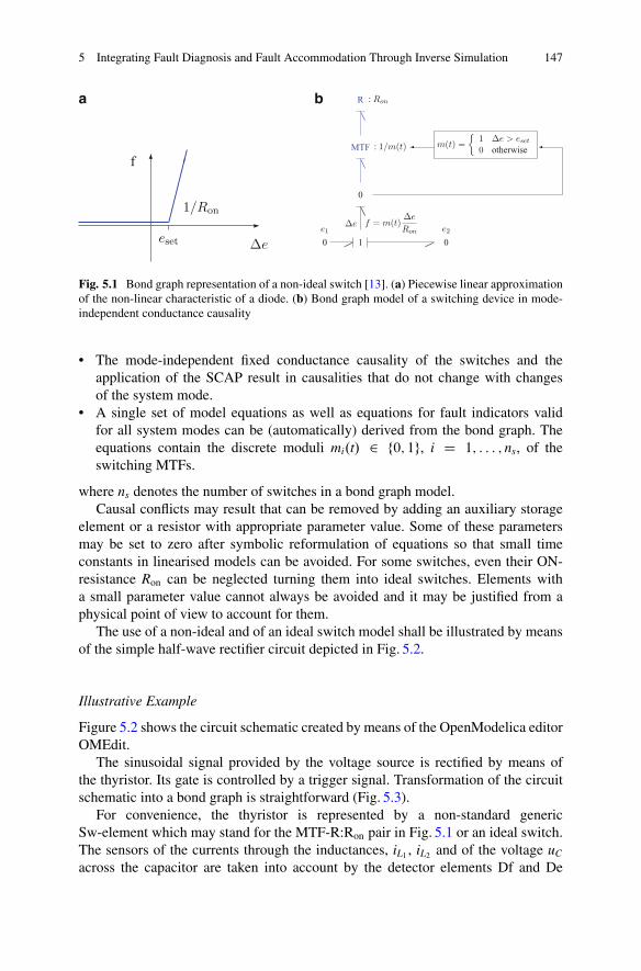
5 Integrating Fault Diagnosis and Fault Accommodation Through Inverse Simulation 147
�
�
������f
a b
eset Δe
1/Ron
0
e1
�� 1
��Δe f = m(t)
Δe
Ron
0
��
MTF : 1/m(t)
��
R : Ron
�� m(t) ={
1 Δe > eset0 otherwise
�� 0
e2
Fig. 5.1 Bond graph representation of a non-ideal switch [13]. (a) Piecewise linear approximationof the non-linear characteristic of a diode. (b) Bond graph model of a switching device in mode-independent conductance causality
• The mode-independent fixed conductance causality of the switches and theapplication of the SCAP result in causalities that do not change with changesof the system mode.
• A single set of model equations as well as equations for fault indicators validfor all system modes can be (automatically) derived from the bond graph. Theequations contain the discrete moduli mi.t/ 2 f0; 1g, i D 1; : : : ; ns, of theswitching MTFs.
where ns denotes the number of switches in a bond graph model.Causal conflicts may result that can be removed by adding an auxiliary storage
element or a resistor with appropriate parameter value. Some of these parametersmay be set to zero after symbolic reformulation of equations so that small timeconstants in linearised models can be avoided. For some switches, even their ON-resistance Ron can be neglected turning them into ideal switches. Elements witha small parameter value cannot always be avoided and it may be justified from aphysical point of view to account for them.
The use of a non-ideal and of an ideal switch model shall be illustrated by meansof the simple half-wave rectifier circuit depicted in Fig. 5.2.
Illustrative Example
Figure 5.2 shows the circuit schematic created by means of the OpenModelica editorOMEdit.
The sinusoidal signal provided by the voltage source is rectified by means ofthe thyristor. Its gate is controlled by a trigger signal. Transformation of the circuitschematic into a bond graph is straightforward (Fig. 5.3).
For convenience, the thyristor is represented by a non-standard genericSw-element which may stand for the MTF-R:Ron pair in Fig. 5.1 or an ideal switch.The sensors of the currents through the inductances, iL1 , iL2 and of the voltage uC
across the capacitor are taken into account by the detector elements Df and De
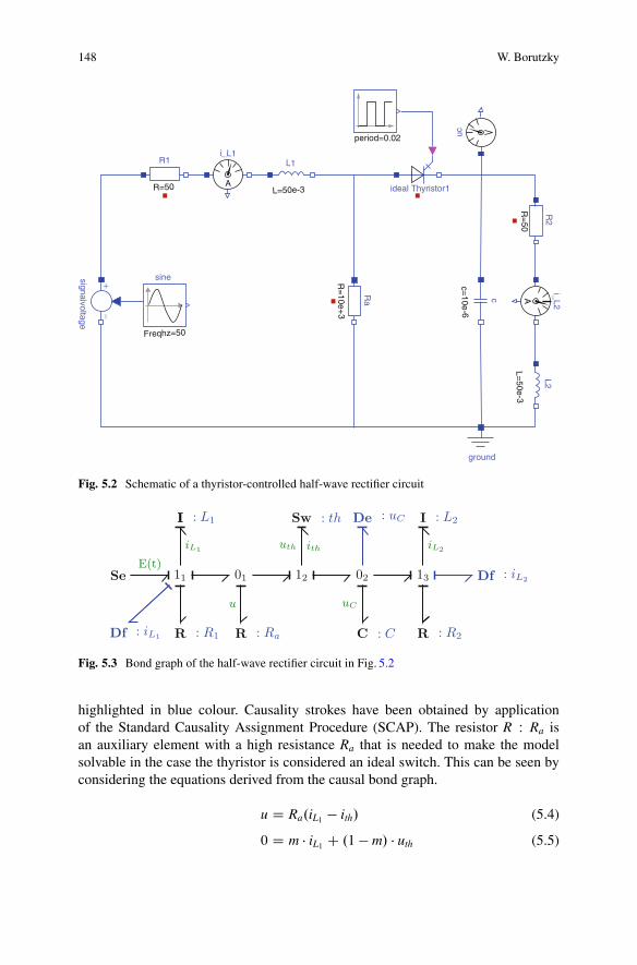
148 W. Borutzky
ground
sine+
−
R1
signalvoltage
L2i_L2
L1i_L1
c
R2
Ra
L=50e-3
c=10e-6
A
A
R=
50
R=
10e+3
Freqhz=50
R=50 L=50e-3
period=0.02
ideal Thyristor1
uc
Fig. 5.2 Schematic of a thyristor-controlled half-wave rectifier circuit
Se
Df : iL1
11
II : L1
R : R1
01
R : Ra
12
Sw : th
02
C : C
De : uC
13
I : L2
R : R2
Df : iL2
E(t)
iL1
u
uth ith
uC
iL2
Fig. 5.3 Bond graph of the half-wave rectifier circuit in Fig. 5.2
highlighted in blue colour. Causality strokes have been obtained by applicationof the Standard Causality Assignment Procedure (SCAP). The resistor R W Ra isan auxiliary element with a high resistance Ra that is needed to make the modelsolvable in the case the thyristor is considered an ideal switch. This can be seen byconsidering the equations derived from the causal bond graph.
u D Ra.iL1 � ith/ (5.4)
0 D m � iL1 C .1 � m/ � uth (5.5)
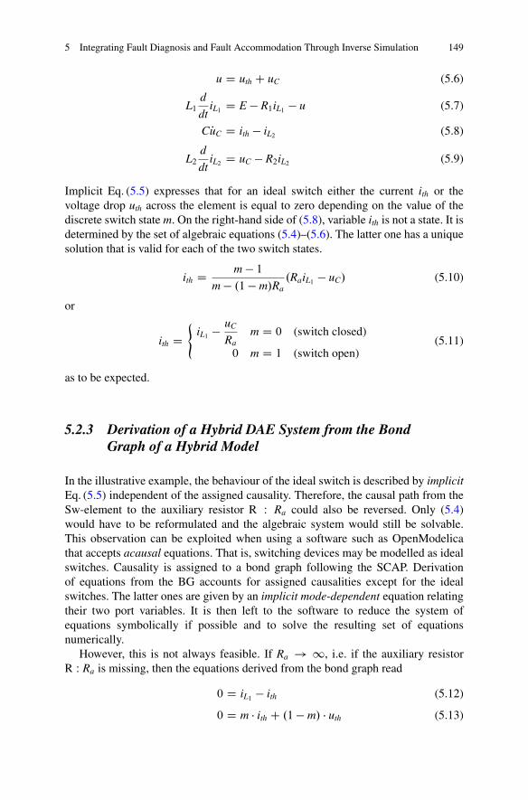
5 Integrating Fault Diagnosis and Fault Accommodation Through Inverse Simulation 149
u D uth C uC (5.6)
L1d
dtiL1 D E � R1iL1 � u (5.7)
C PuC D ith � iL2 (5.8)
L2d
dtiL2 D uC � R2iL2 (5.9)
Implicit Eq. (5.5) expresses that for an ideal switch either the current ith or thevoltage drop uth across the element is equal to zero depending on the value of thediscrete switch state m. On the right-hand side of (5.8), variable ith is not a state. It isdetermined by the set of algebraic equations (5.4)–(5.6). The latter one has a uniquesolution that is valid for each of the two switch states.
ith D m � 1m � .1 � m/Ra
.RaiL1 � uC/ (5.10)
or
ith D(
iL1 � uC
Ram D 0 (switch closed)
0 m D 1 (switch open)(5.11)
as to be expected.
5.2.3 Derivation of a Hybrid DAE System from the BondGraph of a Hybrid Model
In the illustrative example, the behaviour of the ideal switch is described by implicitEq. (5.5) independent of the assigned causality. Therefore, the causal path from theSw-element to the auxiliary resistor R W Ra could also be reversed. Only (5.4)would have to be reformulated and the algebraic system would still be solvable.This observation can be exploited when using a software such as OpenModelicathat accepts acausal equations. That is, switching devices may be modelled as idealswitches. Causality is assigned to a bond graph following the SCAP. Derivationof equations from the BG accounts for assigned causalities except for the idealswitches. The latter ones are given by an implicit mode-dependent equation relatingtheir two port variables. It is then left to the software to reduce the system ofequations symbolically if possible and to solve the resulting set of equationsnumerically.
However, this is not always feasible. If Ra ! 1, i.e. if the auxiliary resistorR W Ra is missing, then the equations derived from the bond graph read
0 D iL1 � ith (5.12)
0 D m � ith C .1 � m/ � uth (5.13)
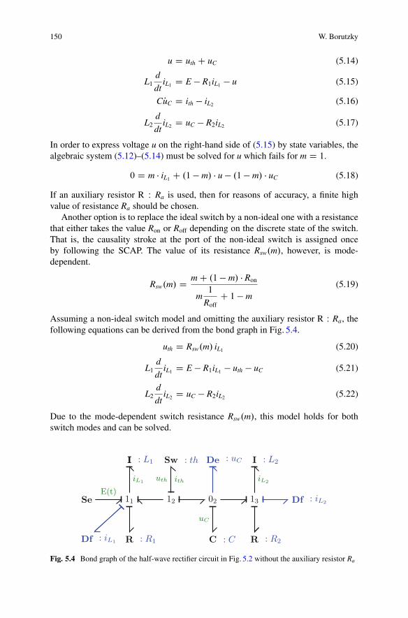
150 W. Borutzky
u D uth C uC (5.14)
L1d
dtiL1 D E � R1iL1 � u (5.15)
C PuC D ith � iL2 (5.16)
L2d
dtiL2 D uC � R2iL2 (5.17)
In order to express voltage u on the right-hand side of (5.15) by state variables, thealgebraic system (5.12)–(5.14) must be solved for u which fails for m D 1.
0 D m � iL1 C .1 � m/ � u � .1 � m/ � uC (5.18)
If an auxiliary resistor R W Ra is used, then for reasons of accuracy, a finite highvalue of resistance Ra should be chosen.
Another option is to replace the ideal switch by a non-ideal one with a resistancethat either takes the value Ron or Roff depending on the discrete state of the switch.That is, the causality stroke at the port of the non-ideal switch is assigned onceby following the SCAP. The value of its resistance Rsw.m/, however, is mode-dependent.
Rsw.m/ D m C .1 � m/ � Ron
m1
RoffC 1 � m
(5.19)
Assuming a non-ideal switch model and omitting the auxiliary resistor R W Ra, thefollowing equations can be derived from the bond graph in Fig. 5.4.
uth D Rsw.m/ iL1 (5.20)
L1d
dtiL1 D E � R1iL1 � uth � uC (5.21)
L2d
dtiL2 D uC � R2iL2 (5.22)
Due to the mode-dependent switch resistance Rsw.m/, this model holds for bothswitch modes and can be solved.
Se
Df : iL1
11
II : L1
R : R1
12
Sw : th
02
C : C
De : uC
13
I : L2
R : R2
Df : iL2
E(t)
iL1 uth ith
uC
iL2
Fig. 5.4 Bond graph of the half-wave rectifier circuit in Fig. 5.2 without the auxiliary resistor Ra
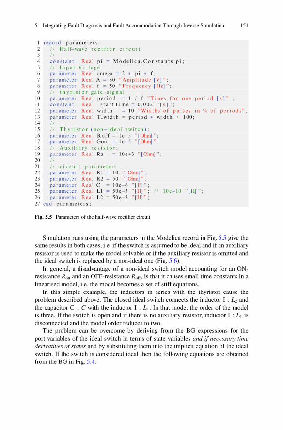
5 Integrating Fault Diagnosis and Fault Accommodation Through Inverse Simulation 151
1 record pa r ame t e r s2 / / Ha l f−wave r e c t f i e r c i r c u i t3 / /4 cons tan t Real p i = Mod e l i c a . Con s t a n t s . p i ;5 / / I npu t Vo l tage6 parameter Real omega = 2 * p i * f ;7 parameter Real A = 30 ”Ampl i tude [V] ” ;8 parameter Real f = 50 ”Frequency [ Hz] ” ;9 / / t h y r i s t o r g a t e s i g n a l
10 parameter Real p e r i od = 1 / f ”Times f o r one p e r i od [ s ] ” ;11 cons tan t Real s t a r t T ime = 0 .002 ” [ s ] ” ;12 parameter Real width = 10 ”Widths of p u l s e s i n % of p e r i o d s” ;13 parameter Real T width = pe r i od * width / 100 ;14 / /15 / / T h y r i s t o r ( non− i d e a l sw i t ch ) :16 parameter Real Roff = 1e−5 ” [Ohm] ” ;17 parameter Real Gon = 1e−5 ” [Ohm] ” ;18 / / Aux i l i a r y r e s i s t o r :19 parameter Real Ra = 10e+3 ” [Ohm] ” ;20 / /21 / / c i r c u i t p a r ame t e r s22 parameter Real R1 = 10 ” [Ohm] ” ;23 parameter Real R2 = 50 ” [Ohm] ” ;24 parameter Real C = 10 e−6 ” [ F] ” ;25 parameter Real L1 = 50 e−3 ” [H] ” ; / / 10 e−10 ” [H] ” ;26 parameter Real L2 = 50 e−3 ” [H] ” ;27 end pa r ame t e r s ;
Fig. 5.5 Parameters of the half-wave rectifier circuit
Simulation runs using the parameters in the Modelica record in Fig. 5.5 give thesame results in both cases, i.e. if the switch is assumed to be ideal and if an auxiliaryresistor is used to make the model solvable or if the auxiliary resistor is omitted andthe ideal switch is replaced by a non-ideal one (Fig. 5.6).
In general, a disadvantage of a non-ideal switch model accounting for an ON-resistance Ron and an OFF-resistance Roff, is that it causes small time constants in alinearised model, i.e. the model becomes a set of stiff equations.
In this simple example, the inductors in series with the thyristor cause theproblem described above. The closed ideal switch connects the inductor I W L2 andthe capacitor C W C with the inductor I W L1. In that mode, the order of the modelis three. If the switch is open and if there is no auxiliary resistor, inductor I W L1 isdisconnected and the model order reduces to two.
The problem can be overcome by deriving from the BG expressions for theport variables of the ideal switch in terms of state variables and if necessary timederivatives of states and by substituting them into the implicit equation of the idealswitch. If the switch is considered ideal then the following equations are obtainedfrom the BG in Fig. 5.4.
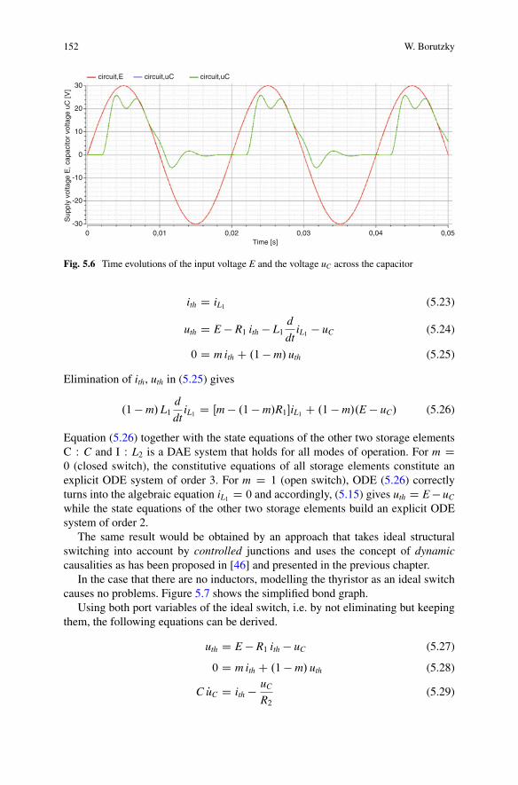
152 W. Borutzky
circuit,E30
-300 0,01 0,02 0,03
Time [s]0,04 0,05
Sup
ply
volta
ge E
, cap
acito
r vo
ltage
uC
[V]
20
-20
10
-10
0
circuit,uC circuit,uC
Fig. 5.6 Time evolutions of the input voltage E and the voltage uC across the capacitor
ith D iL1 (5.23)
uth D E � R1 ith � L1d
dtiL1 � uC (5.24)
0 D m ith C .1 � m/ uth (5.25)
Elimination of ith, uth in (5.25) gives
.1 � m/L1d
dtiL1 D Œm � .1 � m/R1�iL1 C .1 � m/.E � uC/ (5.26)
Equation (5.26) together with the state equations of the other two storage elementsC W C and I W L2 is a DAE system that holds for all modes of operation. For m D0 (closed switch), the constitutive equations of all storage elements constitute anexplicit ODE system of order 3. For m D 1 (open switch), ODE (5.26) correctlyturns into the algebraic equation iL1 D 0 and accordingly, (5.15) gives uth D E � uC
while the state equations of the other two storage elements build an explicit ODEsystem of order 2.
The same result would be obtained by an approach that takes ideal structuralswitching into account by controlled junctions and uses the concept of dynamiccausalities as has been proposed in [46] and presented in the previous chapter.
In the case that there are no inductors, modelling the thyristor as an ideal switchcauses no problems. Figure 5.7 shows the simplified bond graph.
Using both port variables of the ideal switch, i.e. by not eliminating but keepingthem, the following equations can be derived.
uth D E � R1 ith � uC (5.27)
0 D m ith C .1 � m/ uth (5.28)
C PuC D ith � uC
R2(5.29)

5 Integrating Fault Diagnosis and Fault Accommodation Through Inverse Simulation 153
Fig. 5.7 Bond graph of therectifier with no inductances
Se 1
R : R1
Sw : th
0
C : C
R : R2
E(t)
uth ith
uC
Fig. 5.8 Time evolutions of voltages E and uC for a rectifier with no inductances
The algebraic equations (5.27)–(5.28) can be solved for ith.
ith D m � 1m � .1 � m/R1
.E � uc/ (5.30)
This expression is valid for both switch states. Figure 5.8 shows the time evolutionsof voltages E and uC for a rectifier with no inductances.
Finally, the partial listing in Fig. 5.9 shows a widely used Modelica descriptionof a thyristor considered as a non-ideal switch [18, 58, 67]. The variable s denotesan independent curve parameter of the current versus voltage drop characteristicof a diode indicating whether the diode is blocking or conducting. In contrast to adiode, a thyristor is only conducting if the voltage drop is positive and if the triggersignal at its gate is positive. The Boolean variable fire is determined by the triggersignal. The Boolean variable Off indicates whether the discrete state of the switchis off, pre(off) refers to the previous state.
The Modelica description of a thyristor can be easily turned into that of an idealswitch by setting Gon D Roff D 0:0. The equations in lines 12 and 13 of Fig. 5.9then read
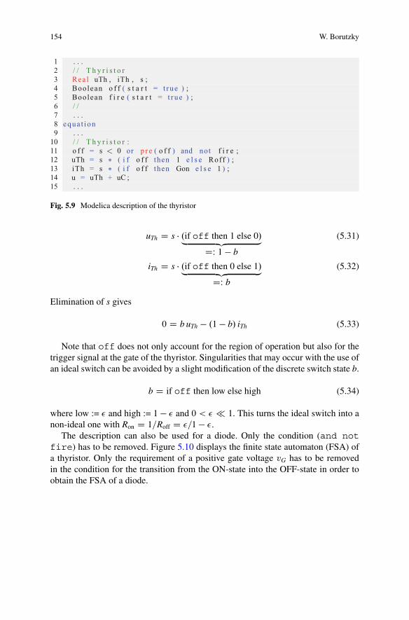
154 W. Borutzky
1 . . .2 / / T h y r i s t o r3 Rea l uTh , iTh , s ;4 Boolean o f f ( s t a r t = t rue ) ;5 Boolean f i r e ( s t a r t = t rue ) ;6 / /7 . . .8 equa t ion9 . . .10 / / T h y r i s t o r :11 o f f = s < 0 or p r e ( o f f ) and not f i r e ;12 uTh = s * ( i f o f f then 1 e l s e Roff ) ;13 iTh = s * ( i f o f f then Gon e l s e 1 ) ;14 u = uTh + uC ;15 . . .
Fig. 5.9 Modelica description of the thyristor
uTh D s � .if off then 1 else 0/„ ƒ‚ …DW 1 � b
(5.31)
iTh D s � .if off then 0 else 1/„ ƒ‚ …DW b
(5.32)
Elimination of s gives
0 D b uTh � .1 � b/ iTh (5.33)
Note that off does not only account for the region of operation but also for thetrigger signal at the gate of the thyristor. Singularities that may occur with the use ofan ideal switch can be avoided by a slight modification of the discrete switch state b.
b D if off then low else high (5.34)
where low := � and high := 1 � � and 0 < � � 1. This turns the ideal switch into anon-ideal one with Ron D 1=Roff D �=1 � �.
The description can also be used for a diode. Only the condition (and notfire) has to be removed. Figure 5.10 displays the finite state automaton (FSA) ofa thyristor. Only the requirement of a positive gate voltage vG has to be removedin the condition for the transition from the ON-state into the OFF-state in order toobtain the FSA of a diode.
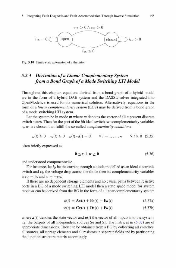
5 Integrating Fault Diagnosis and Fault Accommodation Through Inverse Simulation 155
open closedith = 0
vth > 0 ∧ vG > 0
ith ≤ 0
ith > 0
Fig. 5.10 Finite state automaton of a thyristor
5.2.4 Derivation of a Linear Complementary Systemfrom a Bond Graph of a Mode Switching LTI Model
Throughout this chapter, equations derived from a bond graph of a hybrid modelare in the form of a hybrid DAE system and the DASSL solver integrated intoOpenModelica is used for its numerical solution. Alternatively, equations in theform of a linear complementarity system (LCS) may be derived from a bond graphof a mode switching LTI system.
Let the system be in mode m where m denotes the vector of all n present discreteswitch states. Then for the port of the ith ideal switch two complementarity variableszi;wi are chosen that fulfill the so-called complementarity conditions
zi.t/ � 0 wi.t/ � 0 zi.t/wi.t/ D 0 8 i D 1; : : : ; n 8 t � 0 (5.35)
often briefly expressed as
0 � z ? w � 0 (5.36)
and understood componentwise.For instance, let iD be the current through a diode modelled as an ideal electronic
switch and vD the voltage drop across the diode then its complementarity variablesare z D iD and w D �vD.
If there are no dependent storage elements and no causal paths between resistiveports in a BG of a mode switching LTI model then a state space model for systemmode m can be derived from the BG in the form of a linear complementarity system
Px.t/ D Ax.t/C Bz.t/C Eu.t/ (5.37a)
w.t/ D Cx.t/C Dz.t/C Fu.t/ (5.37b)
where x.t/ denotes the state vector and u.t/ the vector of all inputs into the system,i.e. the outputs of all independent sources Se and Sf. The matrices in (5.37) are ofappropriate dimensions. They can be obtained from a BG by collecting all switches,all sources, all storage elements and all resistors in separate fields and by partitioningthe junction structure matrix accordingly.

156 W. Borutzky
Discretising the time derivative of the state x.t/ by means of the numericalbackward Euler integration method and substituting (5.37a) into (5.37b) yields thelinear complementarity problem (LCP)
wkC1 D MzkC1 C qk ; wkC1 � 0 ^ zkC1 � 0 ; wTkC1zkC1 D 0 (5.38)
to be solved for each discrete time tk, k 2 N. That is, given matrix M and vector q,find vectors z and w such that (5.38) is fulfilled.
The study of the linear complementarity problem and the description of hybridmodels in the complementarity formalism has produced a body of theoretical results(see for instance [7, 17, 70]) and computational methods reported in the literature.One of the results is that the LCP (5.38) has a unique solution if and only if allminors of the matrix M are positive. For a numerical solution of the LCP, thesoftware Siconos, for instance, may be used [1].
5.3 Fault Diagnosis
According to a list of definitions compiled by the Safeprocess Technical Committeeof IFAC, the International Federation of Automation and Control [10, 39], faultdiagnosis means to detect and to isolate faults and to analyse their type and theirmagnitude. Methods for fault diagnosis may be classified into those that exploitprocess history, or make use of qualitative models or are based on quantitativemodels [71–73]. A brief survey of fault detection methods may be found in [13].With regard to their occurrence, faults can be categorised into abrupt, incipient,progressive or intermittent parametric faults and into discrete mode faults.
In the following, bond graph-based fault detection in hybrid models focuses onfaults that change the model structure such as short circuit or open circuit faults, i.e.discrete event faults that cause a failure of a switching element and on faults thatcan be mapped onto parameter changes.
5.3.1 ARR-Based Fault Detection
Fault indicators can be obtained by evaluation of analytical constraints betweenknown input signals into a system and measured output signals called AnalyticalRedundancy Relations (ARRs) in the literature. The result of an ARR evaluationis termed an ARR residual. Let u.t/; y.t/ be the input and the output signalrespectively, m.j/.t/ the vector of all discrete switch states at time t when the systemis in mode j, � the vector of parameters, and fk a real-valued function. The discreteswitch states are constant while the system is in mode j and take values m.j/
2 f0; 1g, D 1; : : : ; ns, where ns denotes the number of switches. Then, in system mode j,the kth residual takes the form
rk.t/ D fk.u.t/; y.t/;� ;m.j// (5.39)
5 Integrating Fault Diagnosis and Fault Accommodation Through Inverse Simulation 157
Some components of the parameter vector � may take constant nominal values,others may be uncertain or slowly time varying in comparison to the time history ofthe state variables, or a parameter value, i.e. may abruptly jump to another constantvalue in the case of an abrupt parametric fault.
If these ARR residuals are close to zero for the time interval Ij in which thesystem is in operating mode j, then the system is in a healthy state for that timeinterval.
jrk.t/j < �jk 8 k 8 t 2 Ij (5.40)
where �jk denotes an admissible small error bound for rk.t/ in system mode j that
accounts for e.g. numerical inaccuracies.If there is at least one ARR residual ri that exceeds a given fault threshold thrj
i
in system mode j, where thrji depends on user defined specifications accounting for
modelling and parameter uncertainties, measurement uncertainties and noise, thenthis indicates that at least one single fault has happened. In hybrid system models,parameters as well as the structure of the model equations and thus the structure ofARRs may change when a fault occurs due to discrete switch states included in theequations. If a switch fails then a part of an ARR may be permanently enabled ordisabled which may lead to residuals exceeding their fault thresholds.
9 i 9 Iji R
C such that jri.t/j � thrji 8 t 2 Ij
i (5.41)
Moreover, parameters can be uncertain, i.e. values may deviate from their nominalvalues. In order to avoid false alarms, fault indicators should be insensitive toparameter variations but sensitive to true faults. For fault detection robust withregard to uncertain system parameters, adaptive mode-dependent fault detectionthresholds thrj
k.t/ can be determined [12, Chap. 5], [27]. If an ARR residual hasreached such a fault detection threshold due to a time varying parameter, �.t/,a supervisory system may decide to still tolerate the progressive fault, but failureprognosis will start to determine the remaining useful life (RUL) of the componentand to decide when maintenance actions are to be taken.
One of the contributions of bond graph modelling to fault detection and isolation(FDI) is that ARRs for fault diagnosis can be derived from a bond graph in asystematic way. The bond graph used for FDI has been termed diagnostic bondgraph (DBG) in the literature [62]. First, a bond graph with detectors accounting forthe available sensors is set up. Computational causalities are then assigned in such away that detectors are in inverted causalities and storage elements are in derivativecausality. The reason for this modification of the SCAP is that outputs of sensorsattached to a real system are measured quantities and thus can be considered knowninputs into the DBG model. Furthermore, if the BG model is connected to a realsystem, it is difficult to reconstruct initial values for ODEs if storage elements arein integral causality. A drawback is that measured inputs are to be differentiated.As measurements are overloaded with noise, they should be properly filtered anddifferentiation is to be performed in discrete time.
158 W. Borutzky
ARRs are obtained from a DBG by summing power variables at those junctionsto which a detector is attached. If constitutive element equations permit to eliminateunknown variables by following causal paths then ARRs in explicit form can beobtained. An ARR could be established by summing the power variables at ajunction with no detector attached as it can be algebraically obtained from ARRs ofdetector junctions. In any case, the number of ARRs equals the number of availablesensors. Generation of ARRs from a BG has been implemented in the commercialsoftware Symbols® [38].
The information which component parameter contributes to which ARR in somesystem mode can be expressed in a structural Fault Signature Matrix (FSM) thatis called All-mode FSM [13] or Global FSM [41] for hybrid system models withrows for the component parameters or components such as sources and sensorsand columns for the ARRs. A parameter fault can be detected if the parametercontributes to an ARR in some system mode. Detectability of a fault is usuallyindicated in an additional column. As it is likely that there are more parameters thanavailable sensors, i.e. the FSM is not square, there are component fault signaturesthat are not unique in some system modes. As a result, parameter faults cannot beisolated by just inspecting the structure of a FSM. However, information can beimproved if entries in a structural FSM are replaced by parameter sensitivities ofARR residuals turning the matrix into a sensitivity fault signature matrix, and ifthose parameters that contribute only weakly to an ARR are set to zero.
ARRs can be established off-line. Clearly, their evaluation giving residuals hasto be performed in real-time if measured inputs into a DBG model are obtainedfrom an engineering system. Moreover, in order to avoid that false alarms are sentto a supervisory system, ARR residuals as fault indicators should be insensitiveto parameter variations but should clearly indicate a fault that has happened. ARRbased fault detection robust with regard to uncertain parameters can be supportedby bond graphs in linear fractional transformation (LFT) form [12, Chap. 3] or byincremental bond graphs [13].
Example. Consider the bond graph of the thyristor-controlled half-wave rectifier inFig. 5.2. The thyristor is modelled as an ideal switch. Summation of power variablesat junctions with a detector attached yields the following ARRs r1; r2; r3.
ith D 1 � m
.1 � m/Ra � m.RaiL1 � uC/ (5.42)
u D Ra .iL1 � ith/ (5.43)
r1 D E � R1iL1 � L1d
dtiL1 � u (5.44)
r2 D ith � C PuC � iL2 (5.45)
r3 D uC � R2iL2 � L2d
dtiL2 (5.46)

5 Integrating Fault Diagnosis and Fault Accommodation Through Inverse Simulation 159
Table 5.1 FSM for thethyristor controlled half-waverectifier circuit in Fig. 5.2
Component Parameter/output r1 r2 r3 Db Ib
R W R1 R1 1 0 0 1 0
L W L1 L1 1 0 0 1 0
R W Ra Ra 1 1 0 1 0
Sw W Thy m 1 1 0 1 0
C W C C 0 0 1 1 1
R W R2 R2 0 0 1 1 0
L W L2 L2 0 0 1 1 0
Se E.t/ 1 0 0 1 0
Df W iL1 iL1 .t/ 1 1 0 1 0
De W uC uC.t/ 0 1 0 1 0
Df W iL2 iL2 .t/ 0 0 1 1 0
A structural fault signature matrix in Table 5.1 accordingly indicates whichcomponent parameter contributes to which ARR.
In Table 5.1, the last four rows can be omitted if sensors can be consideredfaultless and if measurement noise can be neglected. The last but one column onthe right side with the heading Db indicates that all possible faults can be detected.The most right column with the heading Ib indicates that none of them can beisolated with the given set of sensors except a fault in the capacitance C. This is notsurprising as there is only a sensor for the current through resistor R W R1, inductorI W L1, and the thyristor connected in series. The voltage sensor across the capacitorand the current sensor in the series connection of elements R W R2, inductor I W L2 inparallel to the capacitor are not sufficient to isolate a fault in these three elements.
Off-Line Simulation of a Single Fault Scenario
For an off-line simulation of a fault scenario, the real world rectifier circuit isreplaced by a behavioural bond graph model. The latter one is coupled to adiagnostic bond graph as displayed in Fig. 5.11. The detector elements in thecouplings of the two models denote virtual sensors of the ARR residuals. Todistinguish them from sensors of real measurements, they are marked with a star(). The behavioural model provides substitutes for real measurements that are fedinto a diagnostic bond graph model. The latter one provides the residuals serving asfault indicators (cf. Fig. 5.12).
The fault scenario assumes that the trigger signal at the gate of the thyristor isfaultless but that the thyristor is short-circuited as of te D 0:055 s.
Figure 5.13 displays the time evolution of voltages E and uC and of residualsr1; r2; r3. As can be seen from Fig. 5.13a, there is no rectification of the sinusoidalinput voltage E.t/ any more as of te D 0:055.
Figure 5.13b–d indicates that residuals r1; r2 are sensitive to a short-circuit in thethyristor while residual r3 is not which is in accordance with the FSM in Table 5.1.
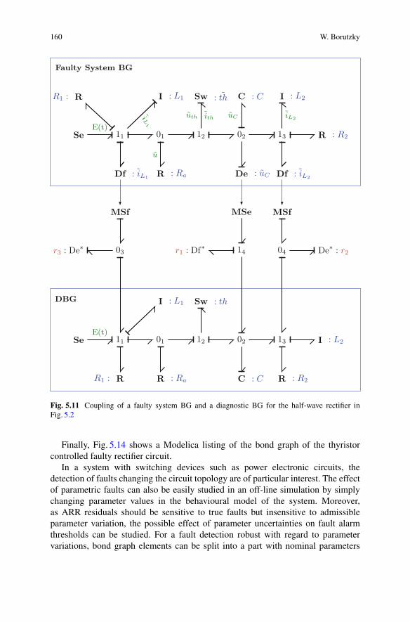
160 W. Borutzky
Faulty System BG
DBG
Se 11
Df : iL1
01
I : L1RR1 :
R : Ra
12
Sw : th
02
C : C
De : uC
13
I : L2
Df : iL2
R : R2
Se 11
MSf
03r3 : De∗
01
I : L1
RR1 : R : Ra
12
Sw : th
02
MSe
14r1 : Df∗
13
MSf
04 De∗ : r2
C : C
I : L2
R : R2
E(t)
iL1
u
uth ith uC iL2
E(t)
Fig. 5.11 Coupling of a faulty system BG and a diagnostic BG for the half-wave rectifier inFig. 5.2
Finally, Fig. 5.14 shows a Modelica listing of the bond graph of the thyristorcontrolled faulty rectifier circuit.
In a system with switching devices such as power electronic circuits, thedetection of faults changing the circuit topology are of particular interest. The effectof parametric faults can also be easily studied in an off-line simulation by simplychanging parameter values in the behavioural model of the system. Moreover,as ARR residuals should be sensitive to true faults but insensitive to admissibleparameter variation, the possible effect of parameter uncertainties on fault alarmthresholds can be studied. For a fault detection robust with regard to parametervariations, bond graph elements can be split into a part with nominal parameters
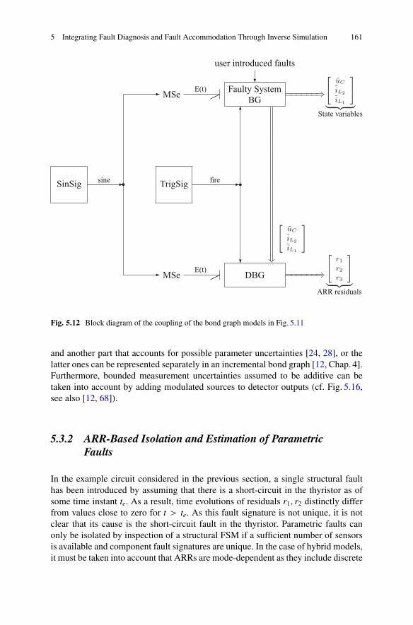
5 Integrating Fault Diagnosis and Fault Accommodation Through Inverse Simulation 161
SinSig �sine• •
�
�
MSe ��E(t)
MSe ��E(t)
DBG ======⇒
⎡⎣ r1
r2r3
⎤⎦
︸ ︷︷ ︸ARR residuals
�
user introduced faults
Faulty SystemBG
======⇒
⎡⎣
uC
iL2
iL1
⎤⎦
︸ ︷︷ ︸State variables
TrigSig �fire
�
�����������������������������
⎡⎣
uC
iL2
iL1
⎤⎦
Fig. 5.12 Block diagram of the coupling of the bond graph models in Fig. 5.11
and another part that accounts for possible parameter uncertainties [24, 28], or thelatter ones can be represented separately in an incremental bond graph [12, Chap. 4].Furthermore, bounded measurement uncertainties assumed to be additive can betaken into account by adding modulated sources to detector outputs (cf. Fig. 5.16,see also [12, 68]).
5.3.2 ARR-Based Isolation and Estimation of ParametricFaults
In the example circuit considered in the previous section, a single structural faulthas been introduced by assuming that there is a short-circuit in the thyristor as ofsome time instant te. As a result, time evolutions of residuals r1; r2 distinctly differfrom values close to zero for t > te. As this fault signature is not unique, it is notclear that its cause is the short-circuit fault in the thyristor. Parametric faults canonly be isolated by inspection of a structural FSM if a sufficient number of sensorsis available and component fault signatures are unique. In the case of hybrid models,it must be taken into account that ARRs are mode-dependent as they include discrete
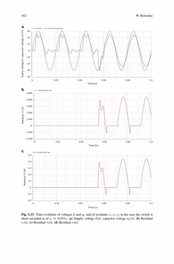
162 W. Borutzky
a
b
c
Fig. 5.13 Time evolution of voltages E and uC and of residuals r1; r2; r3 in the case the switch isshort-circuited as of te D 0:055 s. (a) Supply voltage E.t/, capacitor voltage uC.t/. (b) Residualr1.t/. (c) Residual r2.t/. (d) Residual r3.t/
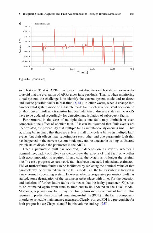
5 Integrating Fault Diagnosis and Fault Accommodation Through Inverse Simulation 163
d
Fig. 5.13 (continued)
switch states. That is, ARRs must use current discrete switch state values in orderto avoid that the evaluation of ARRs gives false residuals. That is, when monitoringa real system, the challenge is to identify the current system mode and to detectand isolate possible faults in real-time [5, 41]. In other words, when a change intoanother valid system mode or a discrete mode fault such as a persistent open circuitor short circuit fault in a transistor has been identified, discrete states in the ARRshave to be updated accordingly for detection and isolation of subsequent faults.
Furthermore, in the case of multiple faults one fault may diminish or evencompensate the effect of another fault. If it can be assumed that fault events areuncorrelated, the probability that multiple faults simultaneously occur is small. Thatis, it may be assumed that there are at least small time delays between multiple faultevents, but their effects may superimpose each other and one parametric fault thathas happened in the current system mode may not be detectable as long as discreteswitch states disable the parameter in the ARRs.
Once a parametric fault has occurred, it depends on its severity whether anominal feedback controller can compensate the effects of that fault or whetherfault accommodation is required. In any case, the system is no longer the originalone. In case a progressive parametric fault has been detected, isolated and estimated,FDI of further future faults can be facilitated by replacing the nominal value of thatparameter by the estimated one in the DBG model, i.e. the faulty system is treated asa new normally operating system. However, when a progressive parametric fault hasstarted, some degradation of the parameter takes place with time. For the detectionand isolation of further future faults this means that the faulty parameter, �.t/, hasto be estimated again from time to time and to be updated in the DBG model.Moreover, a progressive fault may eventually turn into a component failure. Thisrequires to predict the so-called remaining useful life (RUL) of the faulty componentin order to schedule maintenance measures. Clearly, correct FDI is a prerequisite forfault prognosis (see Chaps. 6 and 7 in this volume and e.g. [75]).
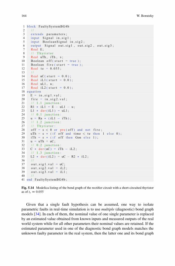
164 W. Borutzky
1 block Faul tySystemBG4b2 / /3 ex tends p a r ame t e r s ;4 inpu t S i g n a l i n s i g 1 ;5 inpu t Boo l e anS i gna l i n s i g 2 ;6 output S i g n a l o u t s i g 1 , o u t s i g 2 , o u t s i g 3 ;7 Rea l E ;8 / / T h y r i s t o r9 Rea l uTh , iTh , s ;10 Boolean o f f ( s t a r t = t rue ) ;11 Boolean f i r e ( s t a r t = t rue ) ;12 Rea l t e = 0 .055 ;13 / /14 Rea l uC ( s t a r t = 0 . 0 ) ;15 Rea l iL1 ( s t a r t = 0 . 0 ) ;16 Rea l uL1 , u ;17 Rea l iL2 ( s t a r t = 0 . 0 ) ;18 equa t ion19 E = i n s i g 1 . v a l ;20 f i r e = i n s i g 2 . v a l ;21 / / 1 1 j u n c t i o n :22 R1 * iL1 = E − uL1 − u ;23 L1 * de r ( iL1 ) = uL1 ;24 / / 0 1 j u n c t i o n :25 u = Ra * ( iL1 − iTh ) ;26 / / 1 2 j u n c t i o n :27 / / T h y r i s t o r :28 o f f = s < 0 or p r e ( o f f ) and not f i r e ;29 uTh = s * ( i f o f f and t ime < t e then 1 e l s e 0 ) ;30 iTh = s * ( i f o f f then Gon e l s e 1 ) ;31 u = uTh + uC ;32 / / 0 2 j u n c t i o n :33 C * de r ( uC ) = iTh − iL2 ;34 / / 1 3 j u n c t i o n :35 L2 * de r ( iL2 ) = uC − R2 * iL2 ;36 / /37 o u t s i g 1 . v a l = uC ;38 o u t s i g 2 . v a l = iL2 ;39 o u t s i g 3 . v a l = iL1 ;40 / /41 end Faul tySystemBG4b ;
Fig. 5.14 Modelica listing of the bond graph of the rectifier circuit with a short-circuited thyristoras of te D 0:055
Given that a single fault hypothesis can be assumed, one way to isolateparametric faults in real-time simulation is to use multiple (diagnostic) bond graphmodels [34]. In each of them, the nominal value of one single parameter is replacedby an estimated value obtained from known inputs and measured outputs of the realworld system while for all other parameters their nominal values are retained. If theestimated parameter used in one of the diagnostic bond graph models matches theunknown faulty parameter in the real system, then the latter one and its bond graph

5 Integrating Fault Diagnosis and Fault Accommodation Through Inverse Simulation 165
model should produce outputs and their difference should be close to zero. In otherwords, ARR residuals as outputs of the DBG should be close to zero. A drawbackof this approach is that the more complex a system is the more models are neededalthough the latter ones can be evaluated in parallel on a multiprocessor system.
In the case of multiple parametric faults, parameter estimation can be used forfault isolation. A comparison of estimated parameter values with their nominal onesisolates the faulty parameters [13, 63, 75]. However, if discrete switch states areconsidered as parameters then parameter estimation would result in meaninglessreal values for the discrete switch states. Therefore, in [3], it is proposed to performa parameter estimation for each feasible combination of switch state combinations.The switch combination that results in the lowest of all optimal values for the costfunction then identifies the actual current system mode and the minimisation of thefunctional provides estimated values for the continuous parameters.
Estimation of all parameters can also be used to isolate a single switch state fault.If all estimated parameter values match their nominal ones then it must be the switchstate that is faulty.
In the following, it is shown that ARRs that have been derived offline from aDBG and that are evaluated in real-time can not only be used to detect parametricfaults but also be used for estimation of their magnitude in some simple cases.
In the first case it is assumed that
• a single fault hypothesis can be adopted,• the fault can be mapped onto a faulty parameter,• the parameter has a unique structural fault signature in the FSM and thus can be
isolated.
As an example, consider the fragment of a DBG in Fig. 5.15 and assume that theresistor R W Rn in the real system has become faulty. As of some time instant, itsparameter value is QR D Rn C R. Accordingly, an effort Qe.t/ is measured and isinput into the DBG.
Fig. 5.15 Part of a diagnosticbond graph with themeasured input Qe
01
11
MSe
Df∗ : r1
R : Rn
C : Cn
f
e
0
f1
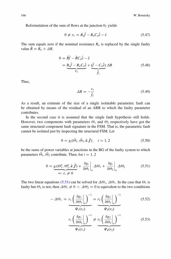
166 W. Borutzky
Reformulation of the sum of flows at the junction 01 yields
0 ¤ r1 D RnQf � RnCn PQe � Qe (5.47)
The sum equals zero if the nominal resistance Rn is replaced by the single faultyvalue QR D Rn CR.
0 D QRQf � QRCn PQe � QeD RnQf � RnCn PQe„ ƒ‚ …
r1
C .Qf � Cn PQe/„ ƒ‚ …Qf1
R (5.48)
Thus,
R D � r1Qf1
(5.49)
As a result, an estimate of the size of a single isolatable parametric fault canbe obtained by means of the residual of an ARR to which the faulty parametercontributes.
In the second case it is assumed that the single fault hypothesis still holds.However, two components with parameters �1 and �2 respectively have got thesame structural component fault signature in the FSM. That is, the parametric faultcannot be isolated just by inspecting the structural FSM. Let
0 D gi. Q�1; Q�2; Qe; Qf /; i D 1; 2 (5.50)
be the sums of power variables at junctions in the BG of the faulty system to whichparameters Q�1; Q�2 contribute. Then, for i D 1; 2
0 D gi.�n1; �
n2 ; Qe; Qf /„ ƒ‚ …
DW ri ¤ 0
C @gi
@�1
ˇˇn
�1 C @gi
@�2
ˇˇn
�2 (5.51)
The two linear equations (5.51) can be solved for �1, �1. In the case that �1 isfaulty but �2 is not, then �1 ¤ 0 ^ �2 D 0 is equivalent to the two conditions
��1 D r1
�@g1@�1
ˇˇn
��1
„ ƒ‚ …�1.r1/
D r2
�@g2@�1
ˇˇn
��1
„ ƒ‚ …�2.r2/
(5.52)
r1
�@g1@�2
ˇˇn
��1
„ ƒ‚ …�3.r1/
¤ r2
�@g2@�2
ˇˇn
��1
„ ƒ‚ …�4.r2/
(5.53)
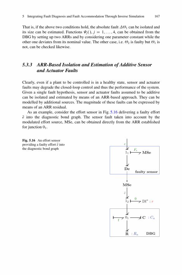
5 Integrating Fault Diagnosis and Fault Accommodation Through Inverse Simulation 167
That is, if the above two conditions hold, the absolute fault�1 can be isolated andits size can be estimated. Functions �j. /, j D 1; : : : ; 4, can be obtained from theDBG by setting up two ARRs and by considering one parameter constant while theother one deviates from its nominal value. The other case, i.e. �2 is faulty but �1 isnot, can be checked likewise.
5.3.3 ARR-Based Isolation and Estimation of Additive Sensorand Actuator Faults
Clearly, even if a plant to be controlled is in a healthy state, sensor and actuatorfaults may degrade the closed-loop control and thus the performance of the system.Given a single fault hypothesis, sensor and actuator faults assumed to be additivecan be isolated and estimated by means of an ARR-based approach. They can bemodelled by additional sources. The magnitude of these faults can be expressed bymeans of an ARR residual.
As an example, consider the effort sensor in Fig. 5.16 delivering a faulty effortQe into the diagnostic bond graph. The sensor fault taken into account by themodulated effort source, MSe, can be obtained directly from the ARR establishedfor junction 01.
Fig. 5.16 An effort sensorproviding a faulty effort Qe intothe diagnostic bond graph
DBG
faulty sensor
11
De
MSe
12 Df∗ : r
MSe
01 C : Cn
R : Rn
e
e
Fe
0
f
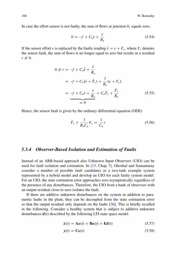
168 W. Borutzky
In case the effort sensor is not faulty, the sum of flows at junction 01 equals zero.
0 D �f C Cn Pe C e
Rn(5.54)
If the sensor effort e is replaced by the faulty reading Qe D e C Fe, where Fe denotesthe sensor fault, the sum of flows is no longer equal to zero but results in a residualr ¤ 0.
0 ¤ r D �f C Cn PQe C QeRn
D �f C Cn.Pe C PFe/C 1
Rn.e C Fe/
D �f C Cn Pe C e
Rn„ ƒ‚ …D 0
C Cn PFe C Fe
Rn(5.55)
Hence, the sensor fault is given by the ordinary differential equation (ODE)
PFe C 1
RnCnFe D 1
Cnr (5.56)
5.3.4 Observer-Based Isolation and Estimation of Faults
Instead of an ARR-based approach also Unknown Input Observers (UIO) can beused for fault isolation and estimation. In [13, Chap. 7], Ghoshal and Samantarayconsider a number of possible fault candidates in a two-tank example systemrepresented by a hybrid model and develop an UIO for each faulty system model.For an UIO, the state estimation error approaches zero asymptotically regardless ofthe presence of any disturbances. Therefore, the UIO from a bank of observers withan output residual close to zero isolates the fault.
If there are additive unknown disturbances on the system in addition to para-metric faults in the plant, they can be decoupled from the state estimation errorso that the output residual only depends on the faults [36]. This is briefly recalledin the following. Consider a healthy system that is subject to additive unknowndisturbances d.t/ described by the following LTI state space model
Px.t/ D Ax.t/C Bu.t/C Ed.t/ (5.57)
y.t/ D Cx.t/ (5.58)
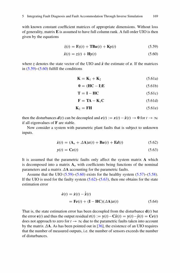
5 Integrating Fault Diagnosis and Fault Accommodation Through Inverse Simulation 169
with known constant coefficient matrices of appropriate dimensions. Without lossof generality, matrix E is assumed to have full column rank. A full order UIO is thengiven by the equations
Pz.t/ D Fz.t/C TBu.t/C Ky.t/ (5.59)
Ox.t/ D z.t/C Hy.t/ (5.60)
where z denotes the state vector of the UIO and Ox the estimate of x. If the matricesin (5.59)–(5.60) fulfill the conditions
K D K1 C K2 (5.61a)
0 D .HC � I/E (5.61b)
T D I � HC (5.61c)
F D TA � K1C (5.61d)
K2 D FH (5.61e)
then the disturbances d.t/ can be decoupled and e.t/ WD x.t/� Ox.t/ ! 0 for t ! 1if all eigenvalues of F are stable.
Now consider a system with parametric plant faults that is subject to unknowninputs.
Px.t/ D .An CA/x.t/C Bu.t/C Ed.t/ (5.62)
y.t/ D Cx.t/ (5.63)
It is assumed that the parametric faults only affect the system matrix A whichis decomposed into a matrix An with coefficients being functions of the nominalparameters and a matrix A accounting for the parametric faults.
Assume that the UIO (5.59)–(5.60) exists for the healthy system (5.57)–(5.58).If the UIO is used for the faulty system (5.62)–(5.63), then one obtains for the stateestimation error
Pe.t/ D Px.t/ � POx.t/D Fe.t/C .I � HC/.A/x.t/ (5.64)
That is, the state estimation error has been decoupled from the disturbance d.t/ butthe error e.t/ and thus the output residual r.t/ WD y.t/�COx.t/ D y.t/� Oy.t/ D Ce.t/does not approach to zero for t ! 1 due to the parametric faults taken into accountby the matrixA. As has been pointed out in [36], the existence of an UIO requiresthat the number of measured outputs, i.e. the number of sensors exceeds the numberof disturbances.

170 W. Borutzky
In [21], Chen et al. use an UIO to decouple unknown disturbances from the outputresidual for an LTI system with possible additive sensor and actuator faults.
5.4 Fault Accommodation Based on Inverse Simulation
Fault accommodation aims at an automatic controller reconfiguration in order toprevent that a severe fault that has been detected by monitoring and fault diagnosisleads to a system or a component failure and to make sure that the dynamicbehaviour of the closed-loop system remains close to a required reference dynamicbehaviour despite of a persistent fault. Fault accommodation is an active FaultTolerant Control (FTC) technique that changes the controller law after a fault hasoccurred and relies on a faultless operation of the sensors and the actuators [10,Appendix 5], [9, 64]. That is, a system that has become faulty as of some timeinstant is not repaired immediately and remains in operation due to a modifiedcontrol signal. The control objective is still achieved, the performance of the faultysystem may, however, show some degradation. The conceptual fault accommodationscheme in Fig. 5.17 displays the interplay of fault diagnosis and controller redesign.
If some sensors fail, the system becomes partially unobservable and informationneeded by the controller gets lost. On the other hand, some actuator faults maymake the system partially uncontrollable. As a result, a real-time re-adjustment ofthe controller law linking the same controller inputs and outputs in use before thefault event is not possible any more. Some sensor information into the controller aswell as some actuators may not be available any more, that is, some control loopsare broken so that both a change of the control-loop structure and a new control laware required that account for the changed configuration. This more general activeFTC strategy is termed control reconfiguration in the literature. ReconfigurableFTC requires a fast fault diagnosis and that the system remains observable andcontrollable with the sensors and actuators still in operation. Nevertheless, it alwaystakes some time to detect and to isolate a fault. Accordingly, there is a time span,
SensorsPlantActuatorsController �u(t)
��
�
Controllerparameters /Control law
� � �
�
�−�
e(t)�ref
w(t) y(t)
Faultdiagnosis
Controllerredesign
Fault information
���
f
�
d(t)
Fig. 5.17 Conceptual fault accommodation scheme [13, 45]

5 Integrating Fault Diagnosis and Fault Accommodation Through Inverse Simulation 171
the time to reconfiguration, in which the system behaviour is faulty but the inputrequired to compensate the fault hasn’t been reconstructed yet. Depending on a fault,its severity and its location, it may happen that the control objective can be achievedneither by fault accommodation nor by control reconfiguration. What remains insuch a case is to change the control objective. A discussion of reconfigurable FTCtechniques may be found in [44, 45]. In this chapter it is assumed that sensors andactuators do not fail. Faults may only occur in the plant (Fig. 5.17).
5.4.1 Input Reconstruction Using Identified Faulty Parameters
Assume that an abnormality in the dynamic behaviour of a multiple input, multipleoutput (MIMO) system has been observed at time instant t1 and that it is due to asingle parametric fault. Once the fault has been isolated and its magnitude has beenestimated, it can be accommodated by designing an input into the faulty system sothat the fault is compensated and the system produces an output close to a desiredoutput behaviour despite the fault. In other words, the considered fault recovery isbased on a preceding successful fault diagnosis.
For closed loop systems with a nominal feedback controller, FDI (robust withregard to uncertain parameters) is not an easy task as its objectives are oppositeto those of the controller so that there is a trade-off between good closed loopperformance and good fault detection. The problem of FDI in closed loop systemshas been addressed for instance in [6, 54].
Small multiplicative faults in the plant and additive faults in its actuators as wellas small disturbances on the system are compensated by the feedback controller andwill thus not be detected by monitoring the system output and the control error aslong as the latter one is forced to values close to zero with time. Slightly faultymonitored values of a controlled variable due to a small sensor offset are also notdetected in case there are no redundant sensors so that a voting among multiplesensors of the same signal is not possible. The feedback controller will make acontrolled variable provided by a faulty sensor equal to the reference.
Passive fault tolerant control uses a controller that has been designed so that itensures stability and the control objectives in the presence of a number of anticipatedfaults from a certain class. Large faults either in the plant or in its sensors andactuators may exceed the robustness of the feedback controller and can lead to adegradation of the normal dynamic closed-loop behaviour and can impair safetyor reliability so that an active FTC is required for a fast recovery from a severefault and for maintaining stability and accuracy. Once a large fault has occurred,the nominal closed-loop controller aims at compensating the fault which takes sometime. During this time, a fault indicator will exceed a fault threshold so that thereis time to detect the fault. However, it is important that fault detection, isolationand input reconstruction are fast. If there are disturbances on the system in additionto parametric faults in the plant, an unknown input observer (UIO) can be used todecouple them from the faults so that the observer generated residual only dependson the faults as has been outlined in Sect. 5.3.4.
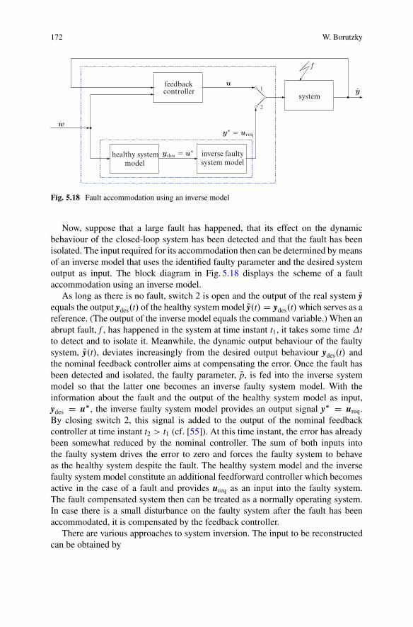
172 W. Borutzky
� healthy systemmodel
�ydes = u∗ inverse faultysystem model
�
y∗ = ureq�w
�feedbackcontroller
�u
�1
2
system �y
�
���
f
Fig. 5.18 Fault accommodation using an inverse model
Now, suppose that a large fault has happened, that its effect on the dynamicbehaviour of the closed-loop system has been detected and that the fault has beenisolated. The input required for its accommodation then can be determined by meansof an inverse model that uses the identified faulty parameter and the desired systemoutput as input. The block diagram in Fig. 5.18 displays the scheme of a faultaccommodation using an inverse model.
As long as there is no fault, switch 2 is open and the output of the real system Qyequals the output ydes.t/ of the healthy system model Qy.t/ D ydes.t/which serves as areference. (The output of the inverse model equals the command variable.) When anabrupt fault, f , has happened in the system at time instant t1, it takes some time tto detect and to isolate it. Meanwhile, the dynamic output behaviour of the faultysystem, Qy.t/, deviates increasingly from the desired output behaviour ydes.t/ andthe nominal feedback controller aims at compensating the error. Once the fault hasbeen detected and isolated, the faulty parameter, Qp, is fed into the inverse systemmodel so that the latter one becomes an inverse faulty system model. With theinformation about the fault and the output of the healthy system model as input,ydes D u�, the inverse faulty system model provides an output signal y� D ureq.By closing switch 2, this signal is added to the output of the nominal feedbackcontroller at time instant t2 > t1 (cf. [55]). At this time instant, the error has alreadybeen somewhat reduced by the nominal controller. The sum of both inputs intothe faulty system drives the error to zero and forces the faulty system to behaveas the healthy system despite the fault. The healthy system model and the inversefaulty system model constitute an additional feedforward controller which becomesactive in the case of a fault and provides ureq as an input into the faulty system.The fault compensated system then can be treated as a normally operating system.In case there is a small disturbance on the faulty system after the fault has beenaccommodated, it is compensated by the feedback controller.
There are various approaches to system inversion. The input to be reconstructedcan be obtained by

5 Integrating Fault Diagnosis and Fault Accommodation Through Inverse Simulation 173
• designing a feedback system (proper inversion) [16, 49],• numerical solution of a DAE system [66],• application of bicausality to a bond graph [33, 42, 51]
A review of inverse simulation methods may be found in [48, Chap. 4]. All of themhave their pros and cons.
This chapter presents an approach to fault accommodation based on the numeri-cal solution of a hybrid DAE system.
5.4.1.1 Fault Accommodation in Open-Loop Systems
In the following, first, fault accommodation in open-loop is considered. Assume thatthe dynamic behaviour of a healthy system may be captured by a mode switchinglinear time-invariant multiple input, multiple output (MIMO) forward model derivedfrom a BG.
Px.t/ D Ax.t/C Bu.t/ (5.65a)
y.t/ D Cx.t/ (5.65b)
where x.t/ 2 Rn denotes the vector of state variables, u.t/ 2 R
m the known inputvector and y.t/ 2 R
p the output vector. The matrices A;B;C are of appropriatedimensions. Their coefficients are constant for the time intervals between twodiscrete events, i.e. for the duration of a system mode. It is assumed that the pencil.sI � A/ is regular, i.e. that the determinant det.sI � A/ is not identical zero fors 2 C.
Suppose that there are no disturbances on the system and that a single parametricfault that has occurred at t1 has been isolated and identified as of t2 > t1. Then fort > t2 an input ureq.t/ to be determined is required that forces the faulty system toproduce the output of the healthy system as the desired output despite the presenceof the fault, i.e. ydes.t/ D y.t/. The equations of the faulty system then read
PQx.t/ D QAQx.t/C QBureq.t/ (5.66a)
ydes.t/ D QCQx.t/ (5.66b)
or
�I 00 0
� � PQxPureq
�D� QA QB
QC 0
� � QxQureq
�C�
0�ydes
�(5.67)
where Qx.t/ denotes the unknown state of the faulty system and ureq.t/ the input to bedetermined. As the faulty parameter may affect the coefficients of all matrices, thelatter ones are distinguished from the ones of the healthy system by a tilde.
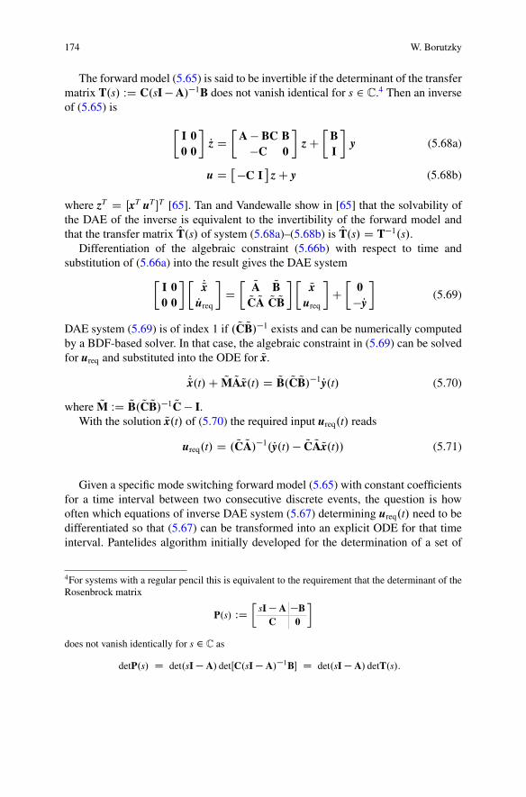
174 W. Borutzky
The forward model (5.65) is said to be invertible if the determinant of the transfermatrix T.s/ WD C.sI � A/�1B does not vanish identical for s 2 C.4 Then an inverseof (5.65) is
�I 00 0
�Pz D
�A � BC B
�C 0
�z C
�BI
�y (5.68a)
u D ��C I�
z C y (5.68b)
where zT D ŒxT uT �T [65]. Tan and Vandewalle show in [65] that the solvability ofthe DAE of the inverse is equivalent to the invertibility of the forward model andthat the transfer matrix OT.s/ of system (5.68a)–(5.68b) is OT.s/ D T�1.s/.
Differentiation of the algebraic constraint (5.66b) with respect to time andsubstitution of (5.66a) into the result gives the DAE system
�I 00 0
� � PQxPureq
�D� QA QB
QC QA QC QB� � Qx
ureq
�C�
0�Py�
(5.69)
DAE system (5.69) is of index 1 if . QC QB/�1 exists and can be numerically computedby a BDF-based solver. In that case, the algebraic constraint in (5.69) can be solvedfor ureq and substituted into the ODE for Qx.
PQx.t/C QM QAQx.t/ D QB. QC QB/�1 Py.t/ (5.70)
where QM WD QB. QC QB/�1 QC � I.With the solution Qx.t/ of (5.70) the required input ureq.t/ reads
ureq.t/ D . QC QA/�1.Py.t/ � QC QAQx.t// (5.71)
Given a specific mode switching forward model (5.65) with constant coefficientsfor a time interval between two consecutive discrete events, the question is howoften which equations of inverse DAE system (5.67) determining ureq.t/ need to bedifferentiated so that (5.67) can be transformed into an explicit ODE for that timeinterval. Pantelides algorithm initially developed for the determination of a set of
4For systems with a regular pencil this is equivalent to the requirement that the determinant of theRosenbrock matrix
P.s/ WD�
sI� A �BC 0
�
does not vanish identically for s 2 C as
detP.s/ D det.sI� A/ detŒC.sI� A/�1B� D det.sI� A/ detT.s/:
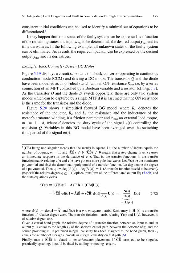
5 Integrating Fault Diagnosis and Fault Accommodation Through Inverse Simulation 175
consistent initial conditions can be used to identify a minimal set of equations to bedifferentiated.5
It may happen that some states of the faulty system can be expressed as a functionof the remaining states, the input ureq to be determined, the desired output ydes and itstime derivatives. In the following example, all unknown states of the faulty systemcan be eliminated. As a result, the required input ureq can be expressed by the desiredoutput ydes and its derivatives.
Example: Buck Converter Driven DC Motor
Figure 5.19 displays a circuit schematic of a buck-converter operating in continuousconduction mode (CCM) and driving a DC motor. The transistor Q and the diodehave been modelled as a non-ideal switch with an ON-resistance Ron, i.e. by a seriesconnection of an MFT controlled by a Boolean variable and a resistor (cf. Fig. 5.3).As the transistor Q and the diode D switch oppositely, there are only two systemmodes which can be captured by a single MTF if it is assumed that the ON resistanceis the same for the transistor and the diode.
Figure 5.20 shows a simplified forward BG model where RL denotes theresistance of the inductor, Ra and La the resistance and the inductance of themotor’s armature winding, b a friction parameter and �load an external load torque,m WD 1 � d, where d denotes the duty cycle of the signal u.t/ controlling thetransistor Q. Variables in this BG model have been averaged over the switchingtime period of the signal m.t/.
5. QCQB/ being non-singular means that the matrix is square, i.e. the number of inputs equals thenumber of outputs, m D p, and . QCQB/ ¤ 0. . QCQB/ ¤ 0 means that a step change in u.t/ causesan immediate response in the derivative of y.t/. That is, the transfer functions in the transferfunction matrix relating u.t/ and y.t/ have got one more pole than zeros. Let N.s/ be the nominatorpolynomial and.s/ the denominator polynomial of a transfer function. Let deg denote the degreeof a polynomial. Then, % WD deg..s//� deg.N.s// D 1. (A transfer function is said to be strictlyproper if the relative degree % � 1.) Laplace-transform of the differentiated output Eq. (5.66b) andthe state equations yields
sY.s/ D Œ. QCQB/.sI� QA/�1 QBC . QCQB/�U.s/D Œ. QCQB/adj.sI� QA/QBC . QCQB/.s/� 1
.s/U.s/ D N.s/
.s/„ƒ‚…DW H1.s/
U.s/ (5.72)
where .s/ WD det.sI � QA/ and N.s/ is a p � m square matrix. Each entry in H1.s/ is a transferfunction of relative degree zero. The transfer function matrix relating Y.s/ and U.s/, however, isof relative degree one.Given a causal bond graph, the relative degree of a transfer function between an input ui and anoutput yi is equal to the length Li of the shortest causal path between the detector of yi and thesource providing ui. If preferred integral causality has been assigned to the bond graph, then Li
equals the number of storage elements in integral causality on that path [61].Finally, matrix . QCQB/ is related to sensor/actuator placement. If QCQB turns out to be singular,practically speaking, it could be fixed by adding or moving sensors.
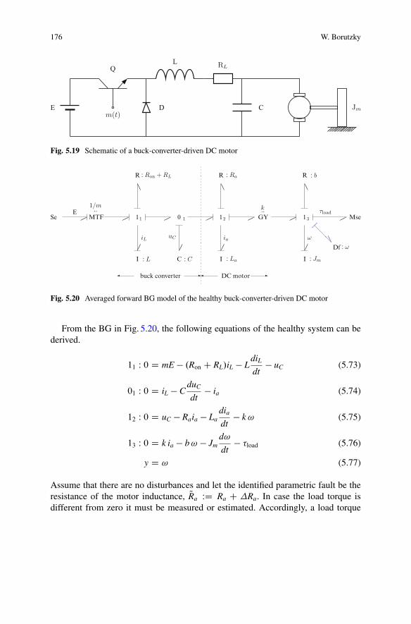
176 W. Borutzky
Em(t)
Q
D
L RL
C Jm
Fig. 5.19 Schematic of a buck-converter-driven DC motor
Se ��E
MTF
1/m..
�� 11
��
R : Ron + RL
��
iL
I : L
�� 0 1 ��
��
uC
C : C
�buck converter� � DC motor �
12
��
R : Ra
��
ia
I : La
�� GY
k..�� 13
��Df : ω
��
R : b
��
ω
I : Jm
��τload
Mse
Fig. 5.20 Averaged forward BG model of the healthy buck-converter-driven DC motor
From the BG in Fig. 5.20, the following equations of the healthy system can bederived.
11 W 0 D mE � .Ron C RL/iL � LdiLdt
� uC (5.73)
01 W 0 D iL � CduC
dt� ia (5.74)
12 W 0 D uC � Raia � Ladiadt
� k! (5.75)
13 W 0 D k ia � b! � Jmd!
dt� �load (5.76)
y D ! (5.77)
Assume that there are no disturbances and let the identified parametric fault be theresistance of the motor inductance, QRa WD Ra C Ra. In case the load torque isdifferent from zero it must be measured or estimated. Accordingly, a load torque
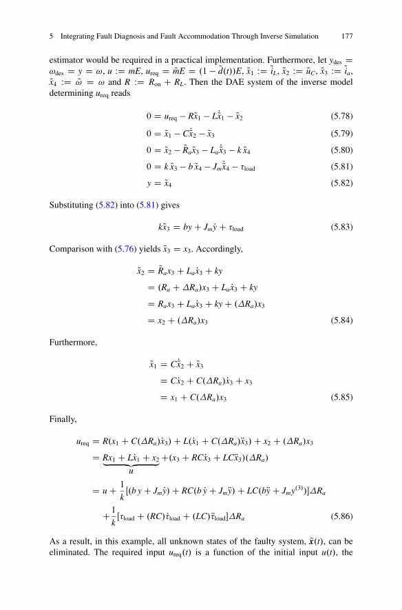
5 Integrating Fault Diagnosis and Fault Accommodation Through Inverse Simulation 177
estimator would be required in a practical implementation. Furthermore, let ydes D!des D y D !, u WD mE, ureq D QmE D .1 � Qd.t//E, Qx1 WD QiL, Qx2 WD QuC, Qx3 WD Qia,Qx4 WD Q! D ! and R WD Ron C RL. Then the DAE system of the inverse modeldetermining ureq reads
0 D ureq � RQx1 � LPQx1 � Qx2 (5.78)
0 D Qx1 � CPQx2 � Qx3 (5.79)
0 D Qx2 � QRa Qx3 � La PQx3 � k Qx4 (5.80)
0 D k Qx3 � b Qx4 � Jm PQx4 � �load (5.81)
y D Qx4 (5.82)
Substituting (5.82) into (5.81) gives
kQx3 D by C Jm Py C �load (5.83)
Comparison with (5.76) yields Qx3 D x3. Accordingly,
Qx2 D QRax3 C La Px3 C ky
D .Ra CRa/x3 C La Px3 C ky
D Rax3 C La Px3 C ky C .Ra/x3
D x2 C .Ra/x3 (5.84)
Furthermore,
Qx1 D CPQx2 C Qx3D CPx2 C C.Ra/Px3 C x3
D x1 C C.Ra/x3 (5.85)
Finally,
ureq D R.x1 C C.Ra/Px3/C L.Px1 C C.Ra/Rx3/C x2 C .Ra/x3
D Rx1 C LPx1 C x2„ ƒ‚ …u
C.x3 C RCPx3 C LCRx3/.Ra/
D u C 1
kŒ.b y C Jm Py/C RC.b Py C Jm Ry/C LC.bRy C Jmy.3//�Ra
C1
kŒ�load C .RC/ P�load C .LC/ R�load�Ra (5.86)
As a result, in this example, all unknown states of the faulty system, Qx.t/, can beeliminated. The required input ureq.t/ is a function of the initial input u.t/, the

178 W. Borutzky
load torque �load and its derivatives, and of the desired output y and its derivatives.The derivatives of y in (5.86) can be expressed by the output y, the state variablesof the healthy system model, the load torque �load and its time derivatives. Ifthere is no analytical function for the time history of the load torque, �load.t/, butmeasured values carrying noise then a state variable filter (SVF) can provide filteredderivatives of �load.t/ [10, 77].
Py D 1
Jm.kia � by � �load/ (5.87)
Ry D k
JmLa.uc � Raia � ky/ � b
J2m.kia � by � �load/ � 1
JmP�load (5.88)
y.3/ D k
JmLa
�1
C.iL � ia/ � Ra
La.uC � Raia � ky/ � kPy
�
� b
J2m
�k
La.uC � Raia � ky/ � bPy � P�load
�� 1
JmR�load (5.89)
In the case of no fault Ra, the required input equals the initial input.
5.4.1.2 Fault Accommodation in Closed-Loop Systems
Let K. / denote the function of the feedback controller and let uK.t/ D K.w.t/ �Qy.t// be its output. The equations of the faulty closed loop system then read
PQx.t/ D QAQx.t/C QBŒureq.t/C uK.t/� (5.90a)
Qy.t/ D QCQx.t/ (5.90b)
Differentiation of (5.90b) with respect to time yields for ureq.t/
. QC QB/ureq.t/ D PQy.t/ � QC QAQx.t/C QC QAuK.t/ (5.91)
Again, if QC QB is non-singular, then substituting ureq.t/ into (5.90a) yields for the stateof the faulty system the ODE
PQx.t/C QM QAQx.t/ D QB. QC QB/�1 PQy.t/ � QMBuK (5.92)
These results coincide with Eqs. (5.70), (5.71) for an open loop system if thecontroller output uK.t/ is identical equal to zero, i.e. if the system is in open-loop.
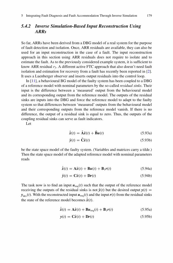
5 Integrating Fault Diagnosis and Fault Accommodation Through Inverse Simulation 179
5.4.2 Inverse Simulation-Based Input Reconstruction UsingARRs
So far, ARRs have been derived from a DBG model of a real system for the purposeof fault detection and isolation. Once, ARR residuals are available, they can also beused for an input reconstruction in the case of a fault. The input reconstructionapproach in this section using ARR residuals does not require to isolate and toestimate the fault. As to the previously considered example system, it is sufficient toknow ARR residual r3. A different active FTC approach that also doesn’t need faultisolation and estimation for recovery from a fault has recently been reported in [2].It uses a Luenberger observer and inserts output residuals into the control loop.
In [11], a behavioural BG model of the faulty system has been coupled to a DBGof a reference model with nominal parameters by the so-called residual sinks. Theirinput is the difference between a ‘measured’ output from the behavioural modeland its corresponding output from the reference model. The outputs of the residualsinks are inputs into the DBG and force the reference model to adapt to the faultysystem so that differences between ‘measured’ outputs from the behavioural modeland their corresponding outputs from the reference model vanish. If there is nodifference, the output of a residual sink is equal to zero. Thus, the outputs of thecoupling residual sinks can serve as fault indicators.
Let
PQx.t/ D QAQx.t/C QBu.t/ (5.93a)
Qy.t/ D QCQx.t/ (5.93b)
be the state space model of the faulty system. (Variables and matrices carry a tilde.)Then the state space model of the adapted reference model with nominal parametersreads
PQx.t/ D AQx.t/C Bu.t/C B1r.t/ (5.94a)
Qy.t/ D CQx.t/C Dr.t/ (5.94b)
The task now is to find an input ureq.t/ such that the output of the reference modelreceiving the outputs of the residual sinks is not Qy.t/ but the desired output y.t/ Dydes.t/. With the reconstructed input ureq.t/ and the input r.t/ from the residual sinksthe state of the reference model becomes POx.t/.
POx.t/ D AOx.t/C Bureq.t/C B1r.t/ (5.95a)
y.t/ D COx.t/C Dr.t/ (5.95b)
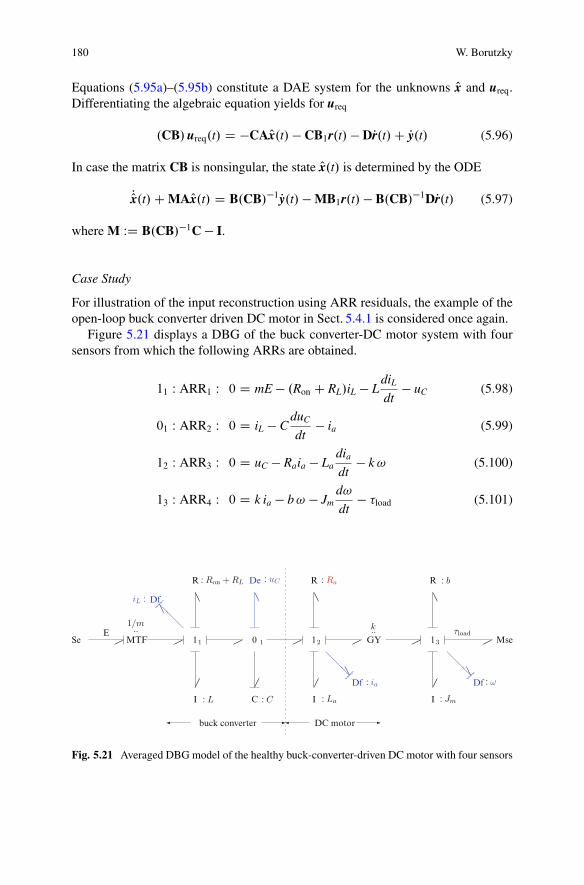
180 W. Borutzky
Equations (5.95a)–(5.95b) constitute a DAE system for the unknowns Ox and ureq.Differentiating the algebraic equation yields for ureq
.CB/ureq.t/ D �CAOx.t/ � CB1r.t/ � DPr.t/C Py.t/ (5.96)
In case the matrix CB is nonsingular, the state Ox.t/ is determined by the ODE
POx.t/C MAOx.t/ D B.CB/�1 Py.t/ � MB1r.t/ � B.CB/�1DPr.t/ (5.97)
where M WD B.CB/�1C � I.
Case Study
For illustration of the input reconstruction using ARR residuals, the example of theopen-loop buck converter driven DC motor in Sect. 5.4.1 is considered once again.
Figure 5.21 displays a DBG of the buck converter-DC motor system with foursensors from which the following ARRs are obtained.
11 W ARR1 W 0 D mE � .Ron C RL/iL � LdiLdt
� uC (5.98)
01 W ARR2 W 0 D iL � CduC
dt� ia (5.99)
12 W ARR3 W 0 D uC � Raia � Ladiadt
� k! (5.100)
13 W ARR4 W 0 D k ia � b! � Jmd!
dt� �load (5.101)
Se ��E
MTF
1/m..
�� 11
��DfiL : ��
R : Ron + RL
��
I : L
�� 0 1
��
De : uC
��
��
C : C
�buck converter� � DC motor �
12
��Df : ia
��
R : Ra
��
I : La
�� GY
k..�� 13
��Df : ω
��
R : b
��
I : Jm
��τload
Mse
Fig. 5.21 Averaged DBG model of the healthy buck-converter-driven DC motor with four sensors

5 Integrating Fault Diagnosis and Fault Accommodation Through Inverse Simulation 181
Table 5.2 Structural faultsignature matrix of the BGmodel in Fig. 5.21 withsensors Df W iL and De W uC ,Df W ia, Df W !
Component ARR1 ARR2 ARR3 ARR4 Db Ib
Sw : Ron 1 0 0 0 1 0
R : RL 1 0 0 0 1 0
I : L 1 0 0 0 1 0
C : C 0 1© 0 0 1 1©R : Ra 0 0 1 0 1 0
I : La 0 0 1 0 1 0
GY : k 0 0 1© 1© 1 1©R : b 0 0 0 1 1 0
I : Jm 0 0 0 1 1 0
�load 0 0 0 1 1 0
In the case of a non-faulty voltage supply and non-faulty sensors, the structuraldependencies of the ARRs from the component parameters are captured by the FSMin Table 5.2.
Assume that the DC-motor armature resistance Ra abruptly jumps to a valueQRa D 2Ra at time instant t1 D 1:0 s and stays at that increased constant value. Thenthis fault cannot be simply identified by inspection of the FSM (Table 5.2). If theabsolute value of residual r3 of ARR3 exceeds a given threshold thr3, i.e. jr3j > thr3,then a look at the FSM in Table 5.2 indicates that component parameters Ra;La andthe motor constant k have to be considered as potential fault candidates. If residualr4 of ARR4 is within admissible bounds, i.e. jr4j < thr4, then k can be excluded asa fault candidate leaving Ra and La as fault candidates. If a single fault hypothesiscan be adopted, only one of the two parameters will be faulty.
The healthy motor driven by a healthy buck converter is considered as thereference system. The desired angular velocity !des.t/ is the one of the healthymotor. An abrupt change in the armature resistance Ra or in the inductance La att D ts leads to a different angular velocity Q!.t/. ARR3 then reads
QuC D RaQia C Lad
dtQia C k Q! C r3 (5.102)
with a residual r3 exceeding a threshold thr3: jr3j > thr3.In order to maintain the desired steady state angular velocity !des, the output
voltage of the buck converter driving the motor must be adapted for t > ts. Therequired voltage Qu0C D Vreq can be obtained from the ARRs.
Vreq.t/ D RaQi0a.t/C Lad
dtQi0a.t/C k!des.t/C r3 (5.103)
kQi0a D Jm P!des C b!des C �load (5.104)
The right-hand side of (5.104) is determined by !des and �load. If the load torque hasnot changed, Qi0a equals the current ia in the non-faulty system obtained from a model

182 W. Borutzky
of the non-faulty system. Hence, for t > ts
Vreq D Raia C Ladiadt
C k!des C r3
D uc C r31 (5.105)
and
ureq D QmE D .Ron C RL/QiL C LdQiLdt
C Vreq (5.106)
QiL D C PVreq C Qi0a D C PVreq C ia
D C PuC C CPr3 C ia D iL C CPr3 (5.107)
Substituting (5.107) and (5.105) into (5.106) yields
ureq D QmE D .m Cm/E
D mE C .r3 C RCPr3 C LCRr3/ (5.108)
where R WD Ron C RL.As a result, the required input, ureq, depends on ARR residual r3 and its
derivatives with respect to time. If the inputs into an ARR are not obtained byoffline simulation of the faulty system behaviour but are sampled measured outputsof the real system then derivatives are to be computed in discrete time, or by use ofinterpolation polynomials, or by a state variable filter [10, 77] which is a nth orderlow-pass filter that provides a filtered signal and its derivatives up to the nth order.
In steady state, (5.108) becomes
.1 � Qd/E D .1 � d/E C r3 (5.109)
and thus
Qd D d � r3E
(5.110)
In case it is known that the fault is due to a faulty armature resistance QRa DRa CRa, residual r3 can be analytically determined in this example.
r3 D .Ra/ia (5.111)
In this case, (5.108) then reads
QmE D .m Cm/E (5.112)
D mE C�
ia C RCdiadt
C LCd2iadt2
�Ra (5.113)
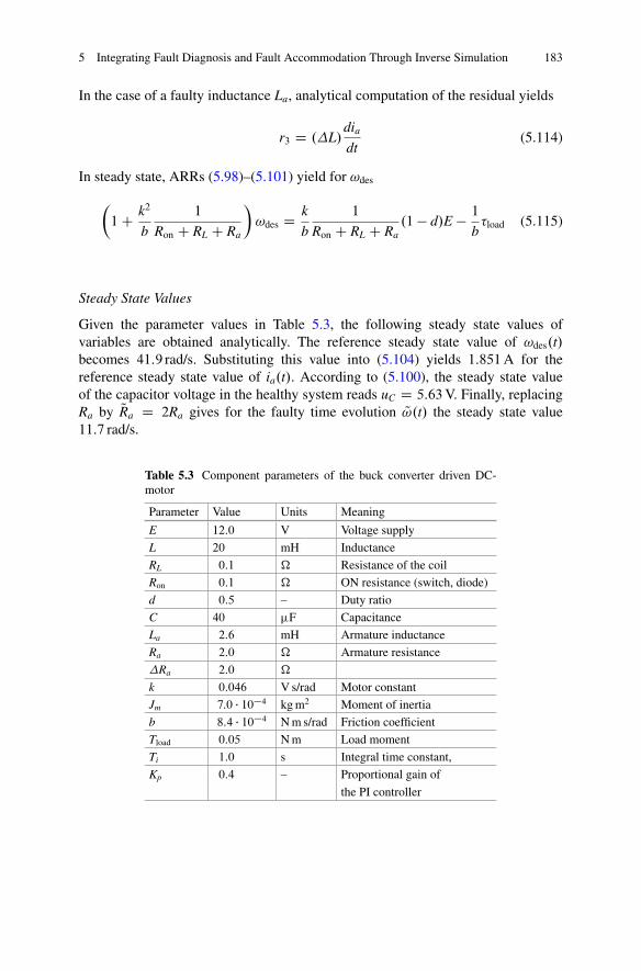
5 Integrating Fault Diagnosis and Fault Accommodation Through Inverse Simulation 183
In the case of a faulty inductance La, analytical computation of the residual yields
r3 D .L/diadt
(5.114)
In steady state, ARRs (5.98)–(5.101) yield for !des
�1C k2
b
1
Ron C RL C Ra
�!des D k
b
1
Ron C RL C Ra.1 � d/E � 1
b�load (5.115)
Steady State Values
Given the parameter values in Table 5.3, the following steady state values ofvariables are obtained analytically. The reference steady state value of !des.t/becomes 41:9 rad/s. Substituting this value into (5.104) yields 1:851A for thereference steady state value of ia.t/. According to (5.100), the steady state valueof the capacitor voltage in the healthy system reads uC D 5:63V. Finally, replacingRa by QRa D 2Ra gives for the faulty time evolution Q!.t/ the steady state value11:7 rad/s.
Table 5.3 Component parameters of the buck converter driven DC-motor
Parameter Value Units Meaning
E 12:0 V Voltage supply
L 20 mH Inductance
RL 0:1 � Resistance of the coil
Ron 0:1 � ON resistance (switch, diode)
d 0:5 – Duty ratio
C 40 �F Capacitance
La 2:6 mH Armature inductance
Ra 2:0 � Armature resistance
Ra 2:0 �
k 0:046 V s/rad Motor constant
Jm 7:0 � 10�4 kg m2 Moment of inertia
b 8:4 � 10�4 N m s/rad Friction coefficient
Tload 0:05 N m Load moment
Ti 1:0 s Integral time constant,
Kp 0:4 – Proportional gain of
the PI controller

184 W. Borutzky
omega : Ra = 2 Ohm
omeg
a [r
ad/s
]
50
40
30
20
10
0
-100 0,5 1 1,5
Time [s]2 2,5
omega : Ra = 4 Ohm
Fig. 5.22 Drop of the angular velocity !.t/ in the case of an increase of armature resistance Ra
5.4.2.1 Simulation of a Fault Scenario
In an offline simulation, the equations of the real system model are solvednumerically and sensor outputs from the model are used in the evaluation of ARRs.As of time instant t1 D 1:0 s the system is assumed to become faulty and thereconstructed signal Qm.t/ (5.108) instead of m.t/ is used to control the switchingof the transistor Q so that the faulty system is forced to resume the angular velocity!des of the healthy system.
Figure 5.22 indicates that the steady state value of !.t/ of the open-loop systemsignificantly drops from 42 to 12 rad/s in the case Ra increases from 2� to 4� inaccordance with analytical results above.
If the angular velocity of the motor shall be !des despite a faulty armatureresistance QRa, then the duty cycle d must be changed. In this case, (5.115) reads
�.Ron C RL C QRa/b C k2
�!des D k.1 � Qd/R � .Ron C RL C QRa/�load (5.116)
The steady state value Qd D d � iaRa=E obtained from (5.110) and (5.111)satisfies (5.116).
In the considered fault scenario, it has been assumed that resistance Ra hasbecome faulty as of t1 D 1:0 s. As the presented input reconstruction uses ARRresiduals an isolation of the fault by means of parameter estimation is not necessary.

5 Integrating Fault Diagnosis and Fault Accommodation Through Inverse Simulation 185
omega : Ra = 4 Ohm omega : Ra = 2 Ohm omega : u = ureq50
40
30
20
10
0
-10
omeg
a [r
ad/s
]
0 0,5 1 1,5Time [s]
2 2,5
Fig. 5.23 Angular velocity !.t/ of the faulty motor with fault compensation
The evaluation of ARR residuals for some further time steps concurrently to theperformance of an engineering system, however, takes some time and causes atime delay especially if ARRs cannot be established in closed form and an entireDBG model has to be re-evaluated instead in order to compute the ARR residuals.In addition, fault detection requires residual signals to be checked against theiradmissible fault thresholds. Therefore, accounting for some time delay in FTCdue to fault detection and input reconstruction, the correction term .m/E thatcompensates the fault in Ra is assumed to become effective as of t2 D 1:02 s, i.e.20 ms after the fault has happened. The result is depicted in Fig. 5.23.
It depends on the time needed for fault detection and input reconstruction howmuch the faulty angular velocity Q!.t/ will progressively deviate from the desiredtime evolution !des.t/. In other words, the state of the system drifts away from thecurrent desired state to a faulty state the longer it takes to provide the new systeminput that compensates for the parametric fault. When the new system input becomeseffective it depends on the transient behaviour of the faulty system, i.e. on its timeconstants, how fast the system will recover from the faulty state and how fast itsoutput will reach the desired trajectory. With the assumed delay in FTC of 20 msand the given parameter values of the example system it takes about 1 s for theangular velocity to reach again its desired time history. If the input into the faultyopen loop system is not corrected, Q!.t D 2 s/ would deviate about 25:9 rad/s orabout 62 % from its desired value 1 s after the occurrence of the fault.
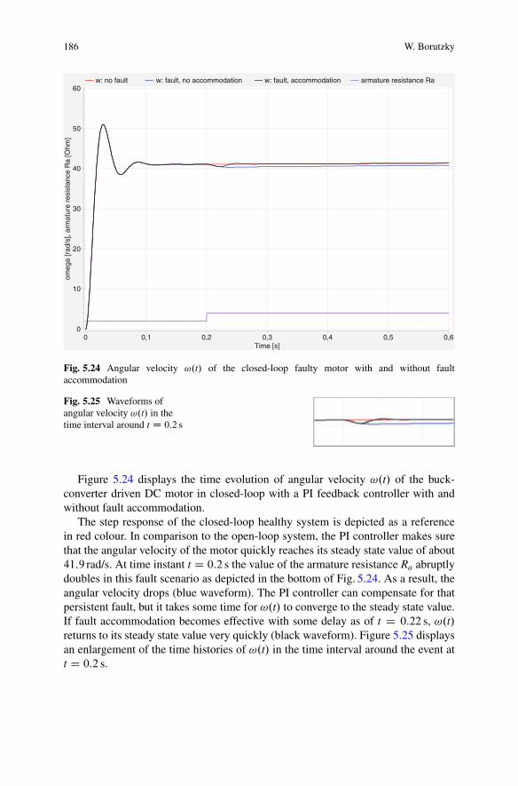
186 W. Borutzky
w: no fault w: fault, no accommodation w: fault, accommodation armature resistance Ra
50
60
40
30
20
10
0
omeg
a [r
ad/s
], ar
mat
ure
resi
stan
ce R
a [O
hm]
0 0,1 0,2 0,3Time [s]
0,4 0,5 0,6
Fig. 5.24 Angular velocity !.t/ of the closed-loop faulty motor with and without faultaccommodation
Fig. 5.25 Waveforms ofangular velocity !.t/ in thetime interval around t D 0:2 s
Figure 5.24 displays the time evolution of angular velocity !.t/ of the buck-converter driven DC motor in closed-loop with a PI feedback controller with andwithout fault accommodation.
The step response of the closed-loop healthy system is depicted as a referencein red colour. In comparison to the open-loop system, the PI controller makes surethat the angular velocity of the motor quickly reaches its steady state value of about41:9 rad/s. At time instant t D 0:2 s the value of the armature resistance Ra abruptlydoubles in this fault scenario as depicted in the bottom of Fig. 5.24. As a result, theangular velocity drops (blue waveform). The PI controller can compensate for thatpersistent fault, but it takes some time for !.t/ to converge to the steady state value.If fault accommodation becomes effective with some delay as of t D 0:22 s, !.t/returns to its steady state value very quickly (black waveform). Figure 5.25 displaysan enlargement of the time histories of !.t/ in the time interval around the event att D 0:2 s.
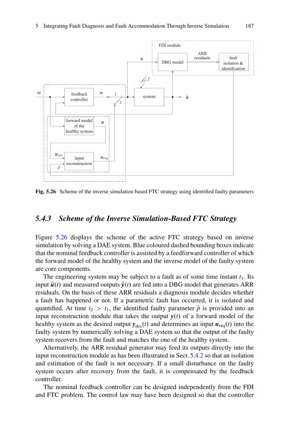
5 Integrating Fault Diagnosis and Fault Accommodation Through Inverse Simulation 187
inputreconstruction�
p
ydes
�
ureq
◦
forward modelof the
healthy system
y
�
system � y
�
�◦ �
�u
2
1feedbackcontroller
�w
�u
◦
�
DBG model �
ARRresiduals fault
isolation &identification
FDI module
���
f
Fig. 5.26 Scheme of the inverse simulation based FTC strategy using identified faulty parameters
5.4.3 Scheme of the Inverse Simulation-Based FTC Strategy
Figure 5.26 displays the scheme of the active FTC strategy based on inversesimulation by solving a DAE system. Blue coloured dashed bounding boxes indicatethat the nominal feedback controller is assisted by a feedforward controller of whichthe forward model of the healthy system and the inverse model of the faulty systemare core components.
The engineering system may be subject to a fault as of some time instant t1. Itsinput Qu.t/ and measured outputs Qy.t/ are fed into a DBG model that generates ARRresiduals. On the basis of these ARR residuals a diagnosis module decides whethera fault has happened or not. If a parametric fault has occurred, it is isolated andquantified. At time t2 > t1, the identified faulty parameter Qp is provided into aninput reconstruction module that takes the output y.t/ of a forward model of thehealthy system as the desired output ydes.t/ and determines an input ureq.t/ into thefaulty system by numerically solving a DAE system so that the output of the faultysystem recovers from the fault and matches the one of the healthy system.
Alternatively, the ARR residual generator may feed its outputs directly into theinput reconstruction module as has been illustrated in Sect. 5.4.2 so that an isolationand estimation of the fault is not necessary. If a small disturbance on the faultysystem occurs after recovery from the fault, it is compensated by the feedbackcontroller.
The nominal feedback controller can be designed independently from the FDIand FTC problem. The control law may have been designed so that the controller
188 W. Borutzky
is robust against some modelling uncertainties and against anticipated faults froma certain class of faults. The forward model is a BG that can be developed offlineon the basis of a physical understanding of the system. The DAE system derivedfrom that BG may be considered as a DAE system of the inverse model. Symbolicprocessing features such as reformulation of equations, symbolic differentiation,index reduction (given the DAE index is not mode-dependent) and code generationof a Modelica modelling and simulation environment such as OpenModelica canbe exploited for an automatic offline construction of the inverse model [66]. Arequirement for the use of an inverse plant model in a controller is that its DAEsystem has a unique solution and that the inverse model is stable. However, even ifthe DAE system for the inverse model can be solved numerically, it is not guaranteedthat the inverse model is stable in a region around all possible operating points.If an inverse model is unstable, or if equations cannot be inverted, or if there areactuator limits, the forward model may be modified before inversion. For instance,if the system behaviour can be described by a single-input, single-output (SISO)system, unstable zeros in its transfer function could be omitted. In any case, anappropriate modification of a forward model that captures the dynamic systembehaviour sufficiently accurate results in an approximate inverse model. Its output,however, will not fully compensate a fault in the system.
5.5 Conclusion
A contribution of bond graph modelling to FDI is that ARRs serving as faultindicators can be derived from a DBG of a system in a systematic manner.This chapter shows that beyond FDI these ARRs can also be used for an inputreconstruction through inverse simulation. The presented integrated approach hasthe following advantages.
• The offline generated DBG model, a forward model of the healthy system andthe DAE system of the inverse model can be computed numerically in parallel ona multiprocessor system concurrently to the operation of the engineering system.
• Once a fault has occurred, values of the reconstructed input into the faulty systemare available with little time delay which enables a fast recovery from a fault.
• Neither ARRs nor the reconstructed input are needed in closed analytical form.• Existing sophisticated modelling and simulation software such as OpenModelica
can be used for the construction of the inverse model in case the DAE index isnot mode-dependent.
In this chapter it is assumed that the dynamic behaviour of the engineering systemunder consideration can be described sufficiently accurate by a mode switching LTImultiple-input, multiple-output model. The latter one is a special case of a hybridmodel that is of interest in various applications. The presented approach is notlimited to this subset of hybrid models. In the more general case, nonlinear hybridDAE systems of the DBG model, the forward and the inverse models are to be
5 Integrating Fault Diagnosis and Fault Accommodation Through Inverse Simulation 189
solved numerically. However, the existence of a nonlinear inverse model, i.e. aunique solution of the DAE system describing the inverse model is not guaranteedin general. Moreover, to be used in a controller, the inverse model must be stable. Ifthe inverse model does not exist or is not stable, modifications of the forward modelbefore inversion may be a remedy. For mode switching LTI models, the numericalintegration based on the BDF solver may fail due to structural singularities causedby switches. In such cases small modifications of a hybrid model based on physicalunderstanding in consideration of the purpose of a simulation become necessary. Inthe case of a complex hierarchical model the problem is to start from a program’serror message in mathematical terms and to identify the part of the model that hascaused the computational problem.
An engineering system may be subject to modelling uncertainties, parametervariations and disturbances besides faults. Sensor signals carry measurement noise.Therefore, the latter ones should be appropriately filtered before used in theevaluation of ARRs. To avoid false alarms caused by parameter variations, adaptivethresholds for ARR residuals can be obtained from a DBG in LFT form or from anincremental BG. As long as ARR residuals are within their time-dependent adaptivebounds, no adaption of system input values is necessary. Zero values are fed into theconstantly active reconstruction module. As a result, the input into the system is notchanged.
For systems operating in various modes, their dynamic behaviour in one modemay be quite different from that in another mode. Accordingly, given a hybridmodel, active FTC using ARRs requires for system mode identification in orderto use the correct values for the discrete switch state variables in the ARRs or inthe equations derived from the DBG. That is, input reconstruction actually is modedependent.
Acknowledgements The author would like to thank Peter Gawthrop from Melbourne School ofEngineering for reading of the draft of this chapter and for his valuable feedback that helped toimprove some aspects.
References
1. Acary, V., Bremond, M., Huber, O., Perignon, F., & Pissard-Gibollet, R. (2016). Siconos. http://siconos.gforge.inria.fr/users_guide/lcp_solvers.html
2. Allous, M., & Zanzouri, N. (2014). Active fault tolerant control based on bond graphapproach. Advances in Electrical Engineering. Article ID 216153. http://dx.doi.org/10.1155/2014/216153
3. Alvari, M., Luo, M., Wang, D., & Zhang, D. (2011). Fault diagnosis for power electronicinverters: A model-based approach. In Proceedings of 2011 IEEE International Symposium onDiagnostics for Electric Machines, Power Electronics and Drives (SDEMPED) (pp. 221–228).Bologna, Italy: IEEE. doi:10.1109/DEMPED.2011.6063627.
4. Alwi, H., Edwards, C., & Pin Tan, C. (2011). Fault detection and fault-tolerant control usingsliding mode. New York: Springer. http://www.springer.com/978-0-85729-649-8

190 W. Borutzky
5. Arogeti, S. A., Wang, D., & Low, C. B. (2010). Mode identification of hybrid systems in thepresence of fault. IEEE Transactions on Industrial Electronics, 57(4), 1452–1467.
6. Baïkeche, H., Marx, B., Maquin, D., & Ragot, J. (2006). On parametric and nonparametricfault detection in linear closed-loop systems. In Workshop on Advanced Control and Diagnosis,ACD’2006, Nancy, France, CDROM.
7. Battle, C., Fossas, E., Merrillas, I., & Miralles, A. (2005). Generalized discontinuous con-ductionmodes in the complementarity formalism. IEEE Transactions on Circuits and Systems,52(8), 447–451.
8. Bergero, F., Floros, X., Fernández, J., Kofman, E., & Cellier, F. E. (2012). Simulating modelicamodels with a stand-alone quantized state systems solver. In Proceedings of 9th InternationalModelica Conference, Munich, Germany (pp. 237–246).
9. Blanke, M., Frei, C., Kraus, F., Patton, R., & Staroswiecki, M. (2000). What is fault-tolerant control? Aalborg University, Department of Control Engineering. http://www.iau.dtu.dk/secretary/pdf/safeprocess_02h.pdf
10. Blanke, M., Kinnaert, M., Lunze, J., & Staroswiecki, M. (2006). Diagnosis and fault-tolerantcontrol. Berlin: Springer.
11. Borutzky, W. (2010). Bond graph methodology – Development and analysis of multidisci-plinary dynamic system models. London, UK: Springer. ISBN: 978-1-84882-881-0 (print).
12. Borutzky, W. (Ed.). (2011). Bond graph modelling of engineering systems – Theory, applica-tions and software support. New York, NY, USA: Springer.
13. Borutzky, W. (2015). Bond graph model-based fault diagnosis of hybrid systems. Switzerland:Springer International Publishing.
14. Borutzky, W. (2015). Fault accommodation by inverse simulation through solving a differentialalgebraic system obtained from a bond graph. In A. Bruzzone, G. Dauphin-Tanguy, S. Junco, &F. Longo (Eds.), Proceedings of the 8th International Conference on Integrated Modelling andAnalysis in Applied Control and Automation (IMAACA 2015), part of the I3M Multiconference,Bergeggi, Italy (pp. 29–38).
15. Borutzky, W., & Cellier, F. E. (1996). Tearing algebraic loops in bond graphs. Transactions ofthe SCS, 13(2), 102–115.
16. Buchholz, J. J., & von Grünhagen, W. (2008). Inversion impossible? Tech. rep., BremenUniversity of Applied Sciences and DLR Braunschweig, Germany.
17. Camlibel, K., Iannelli, L., & Vasca, F. (2004). Modelling switching power converters ascomplementarity systems. In IEEE Conference on Decision and Control (pp. 2328–2333).Piscataway: IEEE.
18. Cellier, F. E., & Kofman, E. (2006). Continuous system simulation. New York: Springer.19. Cellier, F. E., & Krebs, M. (2007). Analysis and simulation of variable structure systems
using bond graphs and inline integration. In Proceedings of ICBGM 07, 8th SCS InternationalConference on Bond Graph Modeling and Simulation, San Diego, CA, USA (pp. 29–34).
20. Cellier, F. E., & Nebot, A. (2005). The Modelica bond graph library. In Proceedings of 4thInternational Modelica Conference, Hamburg, Germany (Vol. 1, pp. 57–65).
21. Chen, J., Patton, R., & Zhang, H. (1996). Design of unknown input observers and robust faultdetection filters. Journal of Control, 63(1), 85–105. doi:10.1080/00207179608921833
22. Controllab Products. (n.d.). 20-sim the power in modeling. http://www.20sim.com23. Cormerais, H., Buisson, J., Leirens, S., & Richard, P. Y. (2002). Calcul symbolique de
l’ensemble des équations d’état pour les graphs en commutation. In Personnel of CIFA 2002,Nantes, France.
24. Dauphin-Tanguy, G., & Kam, C. (1999). How to model parameter uncertainties in a bond graphframework. In G. Horton, D. Möller, & U. Rüde (Eds.), Simulation in Industry, 11th EuropeanSimulation Symposium, ESS’99, Erlangen, Germany (pp. 121–125).
25. de la Calle, A., Cellier, F., Yebra, L., & Dormido, S. (2013). Improvements in bondlib, themodelica bond graph library. In Proceedings of the 8th EUROSIM Congress on Modelling andSimulation (pp. 282–287). Cardiff: IEEE.
26. Djeziri, M., Merzouki, R., Ould Bouamama, B., & Dauphin-Tanguy, G. (2007). Bond graphmodel based for robust fault diagnosis. In Proceedings of the 2007 American ControlConference (pp. 3017–3022). New York City, USA: IEEE.

5 Integrating Fault Diagnosis and Fault Accommodation Through Inverse Simulation 191
27. Djeziri, M. A. (2007). Diagnostic des Systèmes Incrementains par l’Approche Bond Graph.Ph.D. thesis, Ecole Centrale de Lille, France. http://hal.archives-ouvertes.fr/docs/00/20/00/30/PDF/These-Djeziri-07-12-2007.pdf
28. Djeziri, M. A., Ould Bouamama, B., & Merzouki, R. (2009). Modelling and robust FDI ofsteam generator using uncertain bond graph model. Journal of Process Control, 19, 149–162.
29. Ducreux, J., Dauphin-Tanguy, G., & Rombaut, C. (1993). Bond graph modelling of commu-tation phenomena in power electronic circuits. In J. Granda & F. Cellier (Eds.), InternationalConference on Bond Graph Modeling, ICBGM’93, Proceedings of the 1993 Western Simula-tion Multiconference. Simulation Series (Vol. 25, No. 2, pp. 132–136). San Diego, CA, USA:SCS Publishing. ISBN: 1-56555-019-6.
30. Elmqvist, H., Cellier, F. E., & Otter, M. (1993). Object-oriented modeling of hybrid systems.In Proceedings of the 1993 European Simulation Symposium, Ghent (pp. xxxi–xli).
31. Elmqvist, H., Otter, M., & Cellier, F. E. (1995). A new mixed symbolic/numeric approachfor solving differential-algebraic equations systems. In Proceedings of European SimulationMulticonference, ESM’95, Prag (pp. xxiii–xxxiv).
32. Fritzson, P. (2004). Principles of object-oriented modeling and simulation with Modelica 2.1.Hoboken: Wiley. ISBN: 0-471-47163-1.
33. Gawthrop, P. (1995). Bicausal bond graphs. In F. Cellier & J. Granda (Eds.), ICBGM’95,International Conference on Bond Graph Modeling and Simulation: Vol. 27(1). Simulationseries (pp. 83–88). San Diego: SCS Publishing.
34. Ghoshal, S., Samantaray, A., & Mukherjee, A. (2005). Improvements to single fault isolationusing estimated parameters. In J. Granda, & F. Cellier (Eds.) Proceeding of the InternationalConference on Bond Graph Modeling, ICBGM’05, SCS Publishing, New Orleans, LA, USA:Vol. 37. Simulation series (No. 1, pp. 301–306). ISBN: 1-56555-287-3.
35. Hairer, E., & Wanner, G. (1996). Solving ordinary differential equations II, stiff anddifferential-algebraic problems (2nd ed.). Berlin: Springer-Verlag.
36. Hao-Yuan Chou, H. (2000). Fault diagnosis of a heat exchanger system using unknown inputobservers. Master’s thesis, University of Toronto, Graduate Department of Electrical andCornputer Engineering.
37. Heemels, W. P. M. H., Lehmann, D., Lunze, J., & De Schutter, B. (2009). Chapter: Introductionto hybrid systems. In Handbook of hybrid systems control: Theory, tools, applications.Cambridge: Cambridge University Press (pp. 4–30).
38. HighTec Consultants. (n.d.). SYMBOLS Sonata™ . http://www.htcinfo.com/39. Isermann, R., & Ballé, P. (1997). Trends in the application of model-based fault detection and
diagnosis of technical processes. Control Engineering Practice, 5(5), 709–719.40. Kofman, E. (2004). Discrete event simulation of hybrid systems. SIAM Journal on Scientific
Computing, 25(5), 1771–1797. doi:10.1137/S1064827502418379. http://dx.doi.org/10.1137/S1064827502418379
41. Levy, R., Arogeti, S., & Wang, D. (2013). Improving mode-change and fault isolation of hybridsystems using instantaneous sensitivity matrices. In Proceeding of the 1st International and16th National Conference on Machines and Mechanisms (iNaCoMM2013) (pp. 116–123).
42. Loureiro, R. (2012). Bond graph model based on structural diagnosability and recoverabilityanalysis: Application to intelligent autonomous vehicles. Ph.D. thesis, L’ Université Lille 1.
43. Lundvall, H., Fritzson, P., & Bachmann, B. (2008). Event handling in the OpenModelicacompiler and runtime system. Tech. rep., Linköping University, Department of Computerand Information Science, PELAB - Programming Environment Laboratory, Series: Technicalreports in Computer and Information Science. ISSN 1654-7233; 2.
44. Lunze, J. (2004). Control reconfiguration. In Control systems, robotics and automation (Vol.XVI, pp. 320–333). Oxford, UK: Eolss Publishers [Encyclopedia of Life Support Systems(EOLSS) edn.].
45. Lunze, J., & Richter, H. (2008). Reconfigurable fault-tolerant control: A tutorial introduction.European Journal of Control, 5, 359–386.
46. Margetts, R. (2013). Modelling and analysis of hybrid dynamic systems using a bond graphapproach. Ph.D. thesis, University of Bath, UK.

192 W. Borutzky
47. Modelica Association. (n.d.). Modelica and the modelica association. http://www.modelica.org
48. Murray-Smith, D. (2012). Modelling and simulation of integrated systems in engineering –Issues of methodology, quality, test and application. Cambridge, UK: Woodhead Publishing.
49. Murray-Smith, D. J. (2011). Feedback methods for inverse simulation of dynamic modelsfor engineering systems applications. Mathematical and Computer Modelling of DynamicSystems, 17(5), 515–541.
50. Nacusse, M., & Junco, S. J. (2011). Passive fault tolerant control: A bond graph approach.In: A. Bruzzone, G. Dauphin-Tanguy, S. Junco, & M. A. Piera (Eds.), Proceedings of the5th International Conference on Integrated Modelling and Analysis in Applied Control andAutomation (IMAACA 2011), DIPTEM Università di Genova, Rome, Italy (pp. 75–82).
51. Ngwompo, R., Scavarda, S., & Thomasset, D. (1996). Inversion of linear time-invariant SISOsystems modelled by bond graph. Journal of the Franklin Institute, 333(B)(2), 157–174.
52. Ngwompo, R., Scavarda, S., & Thomasset, D. (2001). Physical model-based inversion incontrol systems design using bond graph representation part 1: Theory. Proceedings of theIMechE Part I Journal of Systems and Control Engineering, 215(2), 95–103.
53. Ngwompo, R., Scavarda, S., & Thomasset, D. (2001). Physical model-based inversion incontrol systems design using bond graph representation part 2: Applications. Proceedings ofthe IMechE Part I Journal of Systems and Control Engineering, 215(2), 105–112.
54. Niemann, H., & Stoustrup, J. (1997). Robust fault detection in open loop vs. closed loop. InProceedings of the 36th IEEE Conference on Decision and Control (Vol. 5, pp. 4496–4497).
55. Noura, H., Sauter, D., Hamelin, F., & Theilliol, D. (2000). Fault-tolerant control in dynamicsystems: Application to a winding machine. Control Systems 20(1), 33–49. doi:10.1109/37.823226.
56. OpenModelica Consortium. (n.d.). OpenModelica. https://www.openmodelica.org/57. Otter, M., Elmqvist, H., & Mattson, S. E. (1999). Hybrid modeling in modelica based on the
synchronous data flow principle. In Proceedings of the 1999 IEEE Symposium on Computer-Aided Control System Design, CACSD’99, IEEE Control Systems Society, HI, USA
58. Otter, M., Elmqvist, H., & Mattsson, S. E. (1999). Modeling of mixed continuous/discretesystems in modelica. Tech. rep.
59. Pantelides, C. (1988). The consistent initialization of differential-algebraic systems. SIAM,Journal of Scientific and Statistical Computation, 9, 213–231.
60. Provan, G. (2009). Model abstractions for diagnosing hybrid systems. In Proceedings ofthe 20th International Workshop on Principles of Diagnosis, DX-09, Stockholm, Sweden(pp. 321–328). http://www.cs.ucc.ie/ccsl/GP-papers/2009/Provan_DX_2009_2.pdf
61. Rahmani, A., Sueur, C., & Dauphin-Tanguy, G. (1992). Formal determination of controllabil-ity/observability matrices for multivariable systems modelled by bond graph. In Proceedingof IMACS/SICE International Symposium of Robotics, Mechatronics and Manufacturing,System’92 (pp. 573–580)
62. Samantaray, A., Medjaher, K., Ould Bouamama, B., Staroswiecki, M., & Dauphin-Tanguy, G.(2006). Diagnostic bond graphs for online fault detection and isolation. Simulation ModellingPractice and Theory, 14(3), 237–262.
63. Samantaray, A., & Ould Bouamama, B. (2008). Model-based process supervision – A bondgraph approach. Advances in industrial control. London: Springer.
64. Staroswiecki, M. (n.d.). Fault tolerant systems. In Control systems, robotics and automation(Vol. XVI). Oxford, UK: Eolss Publishers [Encyclopedia of Life Support Systems (EOLSS)edn.].
65. Tan, S., & Vandewalle, J. (1988). Inversion of singular systems. IEEE Transactions on Circuitsand Systems, 35(5), 583–587.
66. Thümmel, M., Looye, G., Kurze, M., Otter, M., & Bals, J. (2005). Nonlinear inverse modelsfor control. In Proceedings of the 4th International Modelica Conference, Hamburg, Germany(pp. 267–279).
67. Tiller, M. (2001). Introduction to physical modeling with modelica. Boston, MA: KluwerAcademic Publishers. ISBN: 0-7923-7367-7.

5 Integrating Fault Diagnosis and Fault Accommodation Through Inverse Simulation 193
68. Touati, Y., Merzouki, R., & Ould Bouamama, B. (2011). Fault detection and isolation inpresence of input and output uncertainties using bond graph approach. In A. Bruzzone, G.Dauphin-Tanguy, S. Junco, & M. Piera (Eds.), Proceedings of the 5th International Conferenceon Integrated Modeling and Analysis in Applied Control and Automation (IMAACA 2011),DIPTEM University of Genoa (pp. 221–227).
69. Touati, Y., Merzouki, R., Ould Bouamama, B., & Loureiro, R. (2012). Detectability andisolability conditions in presence of measurement and parameter uncertainties using bondgraph approach. In 8th IFAC Symposium on Fault Detection, Supervision and Safety ofTechnical Processes (SAFEPROCESS), Mexico City, Mexico (pp. 958–963).
70. van der Schaft, A. J., & Schuhmacher, M. (1998). Complementarity modeling of hybridsystems. IEEE Transactions on Automatic Control, 43(4), 483–490.
71. Venkatasubramanian, V., Rengaswamy, R., Yin, K., & Kavuri, S. (2003). A review of processfault detection and diagnosis, part I: Quantitative model-based methods. Computers andChemical Engineering, 27, 293–311.
72. Venkatasubramanian, V., Rengaswamy, R., Yin, K., & Kavuri, S. (2003). A review of processfault detection and diagnosis, part II: Qualitative models and search strategies. Computers andChemical Engineering, 27, 313–326.
73. Venkatasubramanian, V., Rengaswamy, R., Yin, K., & Kavuri, S. (2003). A review of processfault detection and diagnosis, part III: Process history based methods. Computers and ChemicalEngineering, 27, 327–346.
74. Wainer, G. A. (2009). Discrete-event modeling and simulation – A practitioner’s approach.Boca Raton, FL, USA: CRC Press, Taylor and Francis Group.
75. Wang, D., Yu, M., Low, C., & Arogeti, S. (2013). Model-based health monitoring of hybridsystems. New York: Springer.
76. Wolfram, S. (2003). The mathematica book (5th ed.). Champaign: Wolfram Media, Inc.77. Young, P. C. (1981). Parameter estimation for continuous-time models – A survey. Automatica,
17(1), 23–39.78. Zimmer, D. (2010). Equation-based modeling of variable-structure systems. Ph.D. dissertation
no. 18924, ETH Zürich.79. Zimmer, D. (2013). A new framework for the simulation of equation-based models with
variable structure. Simulation, 89(8), 935–963.

Chapter 6Model-Based Diagnosis and Prognosis of HybridDynamical Systems with Dynamically UpdatedParameters
Om Prakash and A.K. Samantaray
6.1 Introduction
Fault detection and isolation (FDI) and prognosis for large complex processengineering systems are important research areas of industrial importance in orderto improve the safety, reliability and availability of critical machineries/processes.In condition-based maintenance (CBM), FDI is intended for prompt detection,isolation and classification of any fault in a system and to quantify the severityof fault; whereas prognosis is intended to predict the remaining useful life (RUL)of faulty component or subsystem based on the current health status of the systemand its past degradation profile or trend provided by diagnosis. Precise prediction ofRUL assists the plant technicians to plan the future maintenance activities. Sincediagnosis and prognosis both are concerned with the health monitoring of theindustrial system, subsystems or components; it is logical to integrate them in acommon framework for process supervision. There are generally two types of faultsituations, namely anticipated or unanticipated types. An anticipated fault situationis generally known in advance based upon the history of system behaviour andpast experience; but, the unanticipated or unexpected fault situation is generally notknown in advance and that must be detected during process monitoring to maintainthe safety and reliability of the system. Nowadays, many modern integrated systemsor processes such as chemical plants, automobiles and airplanes use embeddedsystem architecture where electronics and communication systems play importantroles. These systems contain various dynamical components or subsystems whichexhibit both continuous and discrete dynamics and are hence called hybrid systems.In a hybrid dynamical system, faulty discrete events may occur in addition toparametric faults and occurrence of these may be unknown in advance. Most of the
O. Prakash • A.K. Samantaray (�)Systems, Dynamics and Control Laboratory, Department of Mechanical Engineering,Indian Institute of Technology-Kharagpur, 721302 Kharagpur, Indiae-mail: [email protected]; [email protected]; [email protected]
© Springer International Publishing Switzerland 2017W. Borutzky (ed.), Bond Graphs for Modelling, Control and FaultDiagnosis of Engineering Systems, DOI 10.1007/978-3-319-47434-2_6
195

196 O. Prakash and A.K. Samantaray
model-based diagnosis and prognosis methods available in literature are intendedfor continuous systems and these approaches cannot be easily applied to hybriddynamical systems as the supervision of such systems need tracking of continuousas well as discrete state variables.
Generally two types of fault sources may occur in a hybrid dynamical system.The first one is a parametric fault related to some component degradation and thesecond one is due to some unexpected transition of nominal mode of the system, i.e.,discrete fault (e.g., valve stuck on or stuck off fault, controller transition commandfailure, etc.). Hybrid dynamics contain two types of discrete transitions: supervisorycontrolled discrete transition and autonomous mode discrete transition. Usually, thesupervisory controlled discrete input to the plant is implemented in software and it ispossible to measure the discrete input signals issued by the controller at the interfacebetween the supervisory controller and the plant. So, we assume that the supervisorycontrolled discrete input signals to the plant are directly observed and known tous. Another way to determine controlled mode transitions is to use the model ofthe supervisory controller to predict such transitions. Even when the supervisorycontrolled mode change information is known to us; a discrete fault may be possiblelike valve stuck on or stuck off fault and pump stuck on or pump stuck off fault,etc., and such faults should also be detected and isolated. In contrast to supervisedcontrolled discrete transition, autonomous mode discrete transitions are usually notknown and may not be directly measurable. However, the conditions for autonomousmode transitions are known either in terms of measured plant output variables orin terms of state variables. So, the autonomous mode transitions can be known todiagnosis module based on the measurement of the outputs.
Most of the existing diagnosis and prognosis approaches are based on single faulthypothesis. These assume that the system or subsystem is immediately repairedonce a fault is detected and isolated. However, a simple fault can lead to a sequenceof other catastrophic faults and it may not be possible to repair each fault withinavailable time. Moreover, some faults may be tolerated and the process operationmay be continued in the presence of one or more known faults and RUL ofsuch faults should be known to plant technician so that maintenance activities canbe scheduled accordingly. Detection of mode transition and any subsequent fault(which may be serious) after a few known minor faults should also be possible. FDImethod based on single fault hypothesis fails to predict the actual fault candidateswhen next fault occurs after the first fault because effects of one fault may beconcealed or compensated by the effects of another fault. One solution to thisproblem is to use a lot of sensors to decouple fault effects. However, this is a costlyapproach and each process variable may not be measurable. Other approaches relyon building observers or a bank of observers (including unknown input observers) ofthe system and tapping measurements/inconsistencies from the observer. However,observer-based approaches cannot be easily applied to hybrid and often non-lineardynamical systems.
For better planning and scheduling of maintenance activities, a good supervisionsystem should detect and isolate small faults and should predict the RUL offaulty/degraded components. Without isolation of correct faults and their types,
6 Model-Based Diagnosis and Prognosis of Hybrid Dynamical Systems 197
RUL estimation is not possible. Hence, it is needed to develop a method havingability to correctly detect and isolate the actual fault of unknown type and unknowndegradation behaviour and at the same time, it should provide some informationabout the severity of the fault and predict the RUL of the faulty components keepingthe system level performance constraints in the view.
In a hybrid dynamical system, various components or subsystems operate indifferent modes or environmental conditions. This results in varying degradationrate of the components throughout the system’s life cycle. In fact, the prognosis ofhybrid systems is challenging due to the fact that the same component can exhibitdifferent degradation behaviours in different operating modes. Traditionally, RULestimation is performed by utilizing a single degradation model which assumes thatdegradation rate parameters used in the degradation model are constants. Althougha single degradation model may be enough for a particular degradation pattern, itdoes not suffice when components or subsystems have different operational profiles.Utilization of multiple degradation models which include operational modes asadditional control parameter and evolve through degradation model identificationis suggested in this chapter. Note that identifying appropriate multiple degradationmodels is a challenging task when components have dynamic degradation patterns.
This chapter precisely deals with the afore-mentioned problem faced in diagnosisand prognosis of hybrid systems. The premise of the solution proposed in thischapter is a basic assumption that there is a very rare chance of occurrence ofsimultaneous faults. Even apparent simultaneous faults are separated by a small timeinterval and we assume that time interval is large enough to carry out the necessaryparametric fault or mode identification, degradation pattern identification and modelupdating steps. We assume that infinite mode transitions in a finite time do not occurand only partial parametric faults occur in a system. For RUL estimation, it is alsoassumed that mode of operation of each hybrid component is known in advance.
Different approaches for model-based diagnosis and prognosis have been devel-oped depending on the kind of knowledge used to describe the process model.Usually, a specific methodology is applied for a specific process. Diagnosis methodsmay be broadly classified into two types: model-based methods and data-driven-based methods. Likewise, prognosis methods intended for RUL estimation can alsobe classified into three types: model-based prognosis, data-driven prognosis andexperience or probability-based prognosis [1]. Every method has its own advantagesand disadvantages. In the present chapter, bond graph model-based diagnosis andprognosis (MBDP) scheme is proposed.
For model-based process supervision, a precise and reliable mathematical modelof the actual plant behaviour is required. A unified multi-energy domain Bond Graph(BG) [2, 3] and its extended form Hybrid Bond Graph (HBG) [4–6] are well-suitedfor modelling of continuous and hybrid dynamical behaviours, respectively. BGtool is also useful in the design and development of model-based FDI for bothcontinuous and hybrid dynamical systems [6, 7]. A considerable amount of literaturecan be found related to model-based FDI for hybrid dynamical systems [8–11];but, very few works are reported on integration of both diagnosis and prognosis ofhybrid dynamical system in a common framework. Also, very few literatures are

198 O. Prakash and A.K. Samantaray
available for prognosis of hybrid dynamical systems. In model-based diagnosis, theBG model is used to derive a set of consistency rules called analytical redundancyrelations (ARRs). ARRs are constraints expressed in terms of measurable processvariables and nominal parameters of plant [7]. These constraints remain valid untila system operates according to its normal operation model. A fault is detectedby monitoring the trend of the residuals. For consistency checking, residual mustbe tested with predetermined fixed threshold value or an adaptive threshold value[6–8]. Diagnostic Bond Graph (DBG) method has been introduced in [12], so thatresiduals are directly obtained by making use of the current and few past measuredsample data even when ARRs cannot be obtained in explicit symbolic form. DBGhas been extended to Diagnostic Hybrid Bond Graph (DHBG) and adapted for FDIof hybrid systems [6, 8]. Few works related to the prognosis, which are based on BGapproach, can be found in [13–16]. In [13, 14], it is assumed that degradation modelsof the faulty components are known beforehand and RUL estimation is performedby incorporating the degradation model into constrained ARRs equation. Further,it is assumed that a single component’s parameter value continuously drifts withthe evolution of time and all other components behave normally. In [15, 16], aBG framework is utilized for FDI but the RUL estimation is performed by usingthe Monte Carlo framework (particle filter technique). The existing model-basedprognosis methods are intended for continuous systems and those cannot be easilyapplied to hybrid dynamical systems.
Components may degrade due to both internal stresses (load, torque, speed,etc.) and external stresses (wind, temperature, humidity, etc.). In order to accu-rately predict the RUL, it is necessary to take into account how and where thecomponents will be used and what will be the mode of operation. According todomain knowledge about the considered system and its components, and knownenvironmental and operational conditions, degradation model of the deterioratingcomponents can be identified by understanding the physics of degradation in amodel-based prognosis framework. A degradation model of a component may beobtained by accelerated life tests method and then that degradation model may beused to track the degradation of component once an incipient fault is detected by FDImodule; whereupon only the coefficients of model need to be estimated and RULcan be predicted [14]. Thus, identification of precise dynamic degradation modeland specification of a well-defined failure threshold for RUL estimation are the mainchallenges in model-based prognosis of hybrid system. In this regard, this chaptermakes the following contributions:
• A unified sequential multiple fault diagnosis and prognosis method based onDHBG approach is developed for hybrid dynamical systems by introducing theconcept of model updating after each fault identification. The proposed methodis able to diagnose faults whose effect may be masked due to previously existingfaults and also predicts the RUL of the faulty component if the isolated fault isof progressive type.
• RUL estimation uses the common framework, i.e., BG modelling approach, thathas been used for system modelling, virtual prototyping, fault diagnosis rule
6 Model-Based Diagnosis and Prognosis of Hybrid Dynamical Systems 199
development, and parameter and system identification. Utilization of multipledegradation models for RUL estimation is suggested which include operationalmodes as additional control parameter and evolve through degradation modelidentification. Same DHBG model of the system as used in FDI module isused in a modified form to identify the degradation pattern of the componentsafter detection of parametric fault. Models are continually evolved with time byadapting to the new information of the state of degradation of the monitoredsystem to provide accurate RUL with bounded uncertainty value.
• Instantaneous fault sensitivity signature for both parametric and discrete faultsis used for minimizing the set of suspected faults (SSF), which also providesthe expected directions of corresponding parameter deviations. Accordingly,constrained parameter estimation is proposed for improving the diagnosis andprognosis tasks of hybrid system.
• The proposed approach can detect and isolate both parametric and discrete faultsand can diagnose different types of fault like abrupt, incipient and progressivefaults. However, the method may also detect and isolate the intermittent faultsif there is a sufficient time window for parameter estimation. The proposedapproach can also track the discrete mode transitions even in presence of oneor more faults in a system.
6.2 Model-Based Diagnosis and Prognosisfor Hybrid Systems
The performance of model-based diagnosis and prognosis (MBDP) approachesdepend on the accuracy or quality of the model of the considered system. Modelsserve as knowledge representation of a large amount of structural, functional andbehavioural information and their relationship. This knowledge representation iscapitalized to create complex cause-effect reasoning leading to construction ofpowerful and robust automatic process supervision tools. The model developmentfor a large complex system is a challenging task, especially for a hybrid dynamicalsystem whose dynamical behaviour changes with the change of operating modeof the system. Assumptions taken during modelling, exclusion of minor dynamicsand inclusion of major dynamics and the used modelling technique always affectthe accuracy or quality of diagnosis and prognosis outcomes. If an appropriatemodel of a system which provides the expected behaviour of the real system innormal healthy condition is developed, then it can be utilized for the processsupervision of the system. However, there is always some mismatch between theoutputs of the behavioural model with the real system measurements even if thereis no fault present in the real system. This generally happens because of mod-elling uncertainties, parameter uncertainties, unknown disturbances, measurementuncertainties, etc. For robust supervision, these factors must be taken into account.BG modelling is a good approach to deal with a multi-energy domain system

200 O. Prakash and A.K. Samantaray
which may have continuous and discrete dynamical behaviours with differentuncertainties. Also, BG modelling can be used as a common framework for systemmodelling, virtual prototyping, fault diagnosis rule development, parameter andsystem identification, and RUL estimation.
Generally, BG model-based diagnosis is broadly classified into qualitative andquantitative approaches [7]. In qualitative model-based method, model considersthe cause and effect relationships, and the functional relationships between theoutputs and inputs of a system are represented in terms of qualitative functions.In quantitative model-based method, dynamic behaviour of a system is generallyobtained from the first principles and the functional relationships between theoutputs and inputs of a system are represented in terms of mathematical equations.However, for MBDP, quantitative method is preferred as it provides the commonframework for both diagnosis and prognosis module development. Further, thisquantitative method may be classified as observer-based, parity relation-based,parameter estimation-based and ARRs-based [8]. These methods can be used togenerate the residuals which are the primary step in the process supervision ofa system. Among these methods, ARR-based methods are more popular for thedevelopment of process supervision. ARRs are constraints expressed in terms ofmeasurable process variables and nominal parameters of plant [7]. These constraintsremain valid until a system operates according to its normal operation model.A fault is detected by monitoring the trend of the residuals. Quantitative ARRs-based methods can be further classified as symbolic and numerical methods. Insymbolic methods, symbolic ARRs are obtained from BG model to evaluate theresiduals; whereas, in numerical methods, residuals can be numerically evaluatedusing the DBG/DHBG model approach.
Quantitative BG model-based fault diagnosis method consists of two main steps:generation of residual or a DBG/DHBG model and evaluation of residual. Thegeneration of residual is a technique for constructing ARRs using the BG model ofthe system. In the residual evaluation step, the trends of the residuals are interpretedto check any inconsistency. The inconsistency which indicates presence of one ormore faults is detected by testing whether each residual is enveloped by a prescribedadaptive threshold, which in turn is defined based on the known uncertaintiesin parameter estimation, operating mode information and statistical parametersof measurement noise and unknown disturbances. Once any inconsistency in theresiduals is found, the fault identification module is triggered to determine theseverity of the fault and its nature/type. After information of severity of fault isobtained, the system may be reconfigured or fault may be accommodated. In case ofincipient fault, RUL must be estimated to assists the plant technicians for planningthe future maintenance activities. In the following sections, basic concepts in model-based diagnosis and prognosis are introduced.

6 Model-Based Diagnosis and Prognosis of Hybrid Dynamical Systems 201
6.2.1 Basic Framework of Fault Diagnosis
The global ARR, GARR(MD,� , U, Y), of an uncertain hybrid system may bewritten as
GARRn ˙ D 0 (6.1)
where MD represents the controlled junction mode vector, � represents a knownparameter vector, U represents known control or input vector and Y representssensor output vector. Online evaluation of each nominal part, GARRn, and uncertainpart, , using MD, � , U and Y provides residual r and adaptive threshold " D jj,respectively. The usual approach to detect fault induced inconsistencies is to testwhether the numerical value of GARRn at corresponding mode remains boundedbetween ˙". Residual (r) and adaptive threshold (") may be evaluated directlyfrom DBG [12] or DHBG model in linear fractional transformation (LFT) form[6–8]. A binary coherence vector (C) is used to represent the signature for afault; whose standard form is C D Œc1; c2; : : : ; cn� where ci (i D 1; 2; : : : ; n)are obtained from a decision procedure, ‚, which is used to generate the alarms,i.e., C D Œ‚.r1/;‚.r2/; : : : ; ‚.rn/�. For robust FDI, each residual ri(t) is checkedagainst the time varying adaptive threshold "i(t) as follows:
ci D � .ri/ D�0; if � "i.t/ � ri.t/ � "i.t/1; otherwise
(6.2)
During online monitoring, the coherence vector (C) is obtained at each and everysampled time for consistency checking. An alarm is raised if one or more than oneelements of the coherence vector show nonzero value, i.e., C ¤ Œ0; 0 : : : 0�. Afterdetection of fault, the coherence vector is matched with the fault signature matrix(FSM) at corresponding mode for isolation of actual fault candidate [7]. A fault in acomponent is detectable/monitorable, if at least one of the residual is sensitive to thisfault, i.e., its monitorability index represented by Mb D 1. A fault in a componentcan be isolated only when it is monitorable and its fault signature (a correspondingrow in FSM) is unique; which is represented by isolability index Ib D 1.
6.2.1.1 FSM, GFSM, GFSSM and MCSM, MCSSM
An FSM, S, represents the relation between a set of parametric faults and theirassumed signatures. It is used to detect and isolate the actual faults. The elements ofFSM are either 1 or 0 as determined from
Sji D�1; if ri is a function of Pj
0; otherwise(6.3)
202 O. Prakash and A.K. Samantaray
where ri is the residual of the ith column, Pj is the parameter of the jth row in FSM,and i D .1; 2 : : : n/, j D .1; 2 : : : p/, n is number of residuals and p is number ofparameters.
Hybrid system dynamics contains both continuous and discrete modes. So, FSMsfor such system are mode dependent and need to be separately derived for eachmode. Global fault signature matrix (GFSM), GS, is derived in a global form [6, 8],whose elements are obtained from
GSji D8<
:
f .a1; : : : ; am/; if ri is a function of Pj depending on the values a1; : : : ; am;
1; if ri is a function of Pj at all modes;0; otherwise
(6.4)
where f represents a logical function of controlled junction in a bond graph modeland a1; : : : ; am; represent the controlled junction state variables, and m is the numberof controlled junctions.
Global fault sensitivity signature matrix (GFSSM) is an extension of GFSM,which has capability to differentiate between increasing .Pj "/ and decreasing.Pj #/ parametric fault. Its elements are updated at each and every instant by usingthe instantaneous sign of each residual sensitivity with respect to the componentparameters [9]. The elements of the GFSSM, GSS, are determined from
GSSji D
8ˆˆ<
ˆˆ:
�sign.@ri=@Pj/; if ri is a function of Pj and Pj is expected toincrease due to fault;
Csign.@ri=@Pj/; if ri is a function of Pj and Pj is expected todecrease due to fault;
0; otherwise
(6.5)
This new kind of signature is termed here sensitivity signature as it can be anal-ysed by sensitivity theory and this residual sensitivity can be derived numericallyby using Sensitivity Bond Graph (SBG) approach as in [17–19], where GARRs inclosed symbolic form may or may not be derivable.
Residuals are also sensitive to discrete mode fault in a hybrid system and anyinconsistency in actual mode may be identified by using mode change signaturematrix (MCSM). The elements of the MCSM are determined from
MCSMki D�1; if ri is a function of ak
0; otherwise(6.6)
Mode change sensitivity signature matrix (MCSSM) is an extension of MCSMwith capability to differentiate between of an increasing .ak "/ and decreasing.ak #/ mode fault. Its elements are updated at each and every instant by using theinstantaneous sign of each residual sensitivity with respect to the mode [9]. Theelements of the MCSSM are determined from

6 Model-Based Diagnosis and Prognosis of Hybrid Dynamical Systems 203
MCSSMki D
8ˆˆ<
ˆˆ:
�sign.@ri=@ak/; if ri is a function of ak and ak is expectedto change from 0 to 1;
Csign.@ri=@ak/; if ri is a function of ak and ak is expectedto change from 1 to 0;
0; otherwise
(6.7)
where ak represents the controlled junction state variables of the kth row of MCSMor MCSSM, and ak 2 .0; 1/, k 2 .1; 2; : : :m/.
6.2.1.2 Adaptive Thresholds for Robust FDI
Adaptive thresholds are used to achieve robustness in FDI by accounting forthe process and measurement uncertainties and also the mode transitions so thatsupervision system can minimize false alarms and misdetections. An uncertainty ona particular parameter value �j can be introduced as
�j D �jn.1C ı�j/ (6.8)
or �j D �jn C�j (6.9)
where �j 2 .I;C;R;TF;GY/ corresponds to parameters associated with the model,and ı�j D .�j=�jn/ and �j are the relative and the absolute deviations of nominalparameter value �jn.
Adaptive thresholds using BG-LFT method [7, 8] can be used, in which systemuncertainties in parameters are detached from their nominal parameters modeland modelled as feedback loops of internal variables. For instance, when the realparameter value of a capacitance C is not accurately identified, it can be expressedas Cn ˙ C D Cn.1 ˙ ıC/, where Cn is represented as nominal parameter valueand ˙C D ˙ıCCn is the uncertainty part of the parameter. If the C element ismodelled in derivative causality, then its constitutive relation is given as
f D 1
Cn ˙CPe D 1
Cn
�1� ı1=C
� Pe D PeCn
� w1=C (6.10)
where .�ı1=C=Cn/Pe D � w1=C is the extra contribution of flow because of uncertainpart of parameter and may be treated as a disturbance. Note that ı1=C is theuncertainty in estimating the value of 1=C. The C element in derivative causalityand parameter uncertainty can be modelled in BG-LFT form as given in Fig. 6.1.
Similarly, for the non-linear resistive R element modelled in conductive causalityfor representing the flow through a non-linear valve, the constitutive relationincluding uncertainty is written as
f D 1
Rn ˙R
pe D 1
Rn
�1� ı1=R
�pe
D .Cd �Cd/p
e D Cd.1� ı1=R/p
e D Cdp
e � w1=R (6.11)
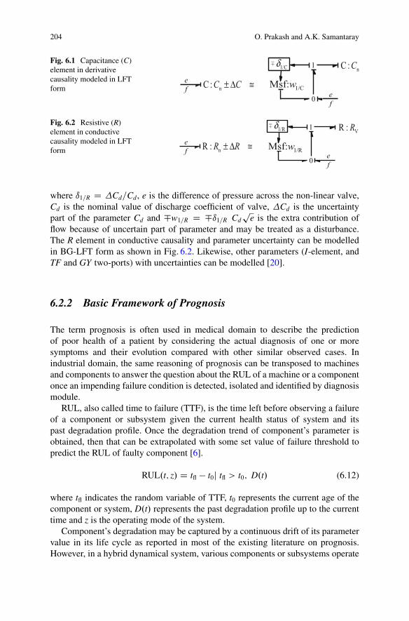
204 O. Prakash and A.K. Samantaray
Fig. 6.1 Capacitance (C)element in derivativecausality modeled in LFTform 1/CMsf:
+−
w0
1/Cδ 1
nC : C C± Δ
nC : C
≅ef
ef
Fig. 6.2 Resistive (R)element in conductivecausality modeled in LFTform
0
1/Rδ 1
nR : R R± Δ
VR : R
≅ 1/RMsf:wef
ef
+−
where ı1=R D Cd=Cd, e is the difference of pressure across the non-linear valve,Cd is the nominal value of discharge coefficient of valve, Cd is the uncertaintypart of the parameter Cd and �w1=R D �ı1=R Cd
pe is the extra contribution of
flow because of uncertain part of parameter and may be treated as a disturbance.The R element in conductive causality and parameter uncertainty can be modelledin BG-LFT form as shown in Fig. 6.2. Likewise, other parameters (I-element, andTF and GY two-ports) with uncertainties can be modelled [20].
6.2.2 Basic Framework of Prognosis
The term prognosis is often used in medical domain to describe the predictionof poor health of a patient by considering the actual diagnosis of one or moresymptoms and their evolution compared with other similar observed cases. Inindustrial domain, the same reasoning of prognosis can be transposed to machinesand components to answer the question about the RUL of a machine or a componentonce an impending failure condition is detected, isolated and identified by diagnosismodule.
RUL, also called time to failure (TTF), is the time left before observing a failureof a component or subsystem given the current health status of system and itspast degradation profile. Once the degradation trend of component’s parameter isobtained, then that can be extrapolated with some set value of failure threshold topredict the RUL of faulty component [6].
RUL.t; z/ D tfl � t0j tfl > t0; D.t/ (6.12)
where tfl indicates the random variable of TTF, t0 represents the current age of thecomponent or system, D.t/ represents the past degradation profile up to the currenttime and z is the operating mode of the system.
Component’s degradation may be captured by a continuous drift of its parametervalue in its life cycle as reported in most of the existing literature on prognosis.However, in a hybrid dynamical system, various components or subsystems operate

6 Model-Based Diagnosis and Prognosis of Hybrid Dynamical Systems 205
at different modes or environmental conditions which result in varying degradationrate of the components throughout the system’s life cycle. Utilization of multipledegradation models which include operational modes as additional control parame-ter and evolve through degradation model identification is suggested in this chapter.Models are continually evolved with time by adapting to the new information of thestate of degradation of the monitored system to provide accurate RUL with boundeduncertainty value. This overcomes the drawback of other similar models, where theparameters of the model are estimated only once and then the estimated degradationpattern is kept fixed irrespective of subsequent new available observations. RULestimation and scheduling maintenance activities of component/subsystem basedon single pre-identified degraded state are not an optimal solution, especially forhybrid systems that operate under variable modes. Intelligent prognosis must adaptaccording to change of the state of degradation of the constantly monitored system.
The proposed approach for RUL prediction requires simultaneous monitoringof both degradation and operating modes of the system. Let �j.t; z/ 2 � bethe parameter associated with jth component of a system which has started todegrade detectably at time t0, as determined (detected and isolated) by FDI module.Figure 6.3 shows the different known operating modes (z) of the system and thejth component’s (�j) degradation behaviour evolution in response to the operatingmode changes. It is shown that the change points, denoted by t.i/, (i = 1, 2,. . . )
za
b
(t)
Time (t)t(1) t(2)
z(1)
z(2)
….t0
….
θj(k+Δ)
Time (t)t(1) t(2)
M(1)
M(2) M(3)
t0 t1 tk tk+Δ
Δθj
fl
Degradation measurement
Time to change operating mode
θj(t, z)
θj(k)
tfl
z(3)
….
….
z(i)
M(i)
t(i)
…. t(i)
Fig. 6.3 (a) Different operating mode (b) degradation behaviour evolution at various operatingmode of the component (�j)
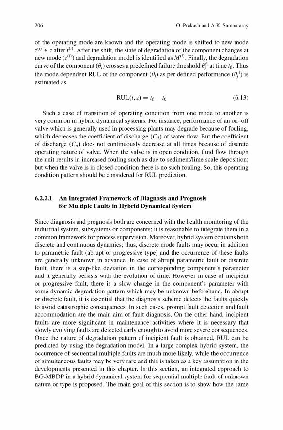
206 O. Prakash and A.K. Samantaray
of the operating mode are known and the operating mode is shifted to new modez.i/ 2 z after t.i/. After the shift, the state of degradation of the component changes atnew mode (z.i/) and degradation model is identified as M.i/. Finally, the degradationcurve of the component (�j) crosses a predefined failure threshold �fl
j at time tfl. Thusthe mode dependent RUL of the component (�j) as per defined performance (�fl
j ) isestimated as
RUL.t; z/ D tfl � t0 (6.13)
Such a case of transition of operating condition from one mode to another isvery common in hybrid dynamical systems. For instance, performance of an on–offvalve which is generally used in processing plants may degrade because of fouling,which decreases the coefficient of discharge .Cd/ of water flow. But the coefficientof discharge .Cd/ does not continuously decrease at all times because of discreteoperating nature of valve. When the valve is in open condition, fluid flow throughthe unit results in increased fouling such as due to sediment/lime scale deposition;but when the valve is in closed condition there is no such fouling. So, this operatingcondition pattern should be considered for RUL prediction.
6.2.2.1 An Integrated Framework of Diagnosis and Prognosisfor Multiple Faults in Hybrid Dynamical System
Since diagnosis and prognosis both are concerned with the health monitoring of theindustrial system, subsystems or components; it is reasonable to integrate them in acommon framework for process supervision. Moreover, hybrid system contains bothdiscrete and continuous dynamics; thus, discrete mode faults may occur in additionto parametric fault (abrupt or progressive type) and the occurrence of these faultsare generally unknown in advance. In case of abrupt parametric fault or discretefault, there is a step-like deviation in the corresponding component’s parameterand it generally persists with the evolution of time. However in case of incipientor progressive fault, there is a slow change in the component’s parameter withsome dynamic degradation pattern which may be unknown beforehand. In abruptor discrete fault, it is essential that the diagnosis scheme detects the faults quicklyto avoid catastrophic consequences. In such cases, prompt fault detection and faultaccommodation are the main aim of fault diagnosis. On the other hand, incipientfaults are more significant in maintenance activities where it is necessary thatslowly evolving faults are detected early enough to avoid more severe consequences.Once the nature of degradation pattern of incipient fault is obtained, RUL can bepredicted by using the degradation model. In a large complex hybrid system, theoccurrence of sequential multiple faults are much more likely, while the occurrenceof simultaneous faults may be very rare and this is taken as a key assumption in thedevelopments presented in this chapter. In this section, an integrated approach toBG-MBDP in a hybrid dynamical system for sequential multiple fault of unknownnature or type is proposed. The main goal of this section is to show how the same
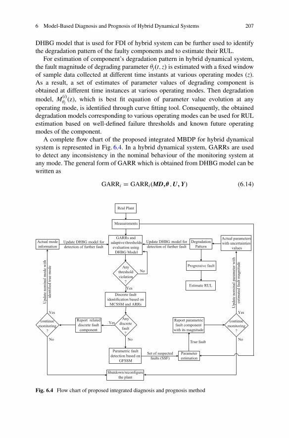
6 Model-Based Diagnosis and Prognosis of Hybrid Dynamical Systems 207
DHBG model that is used for FDI of hybrid system can be further used to identifythe degradation pattern of the faulty components and to estimate their RUL.
For estimation of component’s degradation pattern in hybrid dynamical system,the fault magnitude of degrading parameter �j.t; z/ is estimated with a fixed windowof sample data collected at different time instants at various operating modes (z).As a result, a set of estimates of parameter values of degrading component isobtained at different time instances at various operating modes. Then degradationmodel, M.i/
�j(z), which is best fit equation of parameter value evolution at any
operating mode, is identified through curve fitting tool. Consequently, the obtaineddegradation models corresponding to various operating modes can be used for RULestimation based on well-defined failure thresholds and known future operatingmodes of the component.
A complete flow chart of the proposed integrated MBDP for hybrid dynamicalsystem is represented in Fig. 6.4. In a hybrid dynamical system, GARRs are usedto detect any inconsistency in the nominal behaviour of the monitoring system atany mode. The general form of GARR which is obtained from DHBG model can bewritten as
GARRi D GARRi.MD;�;U; Y/ (6.14)
Set of suspected faults (SSF)
Update DHBG model for detection of further fault
Update DHBG model for detection of further fault
Upd
ate
nom
inal
par
amet
er w
ith
estim
ated
faul
t mag
nitu
de
Report parametric fault component
with its magnitude
Real Plant
GARRs and adaptive hresholdsevaluation using
DHBG Model
tActual modeinformation
Anythresholdviolation
?
Yes
No
Discrete fault identification based on
MCSSM and ARRs
Anydiscrete
fault?
Yes
NoNo
Yes
Parametric fault detection based on
GFSSM
Parameter estimation
No
Yes
Upd
ate
nom
inal
mod
e w
ithid
entif
ied
true
mod
e
Report related discrete fault component
Actual parameters with uncertainties
valuesDegradation
Pattern
Progressive fault
Estimate RUL
Measurements
continuemonitoring
?
continuemonitoring
?
True fault
Shutdown/reconfigure the plant
Fig. 6.4 Flow chart of proposed integrated diagnosis and prognosis method
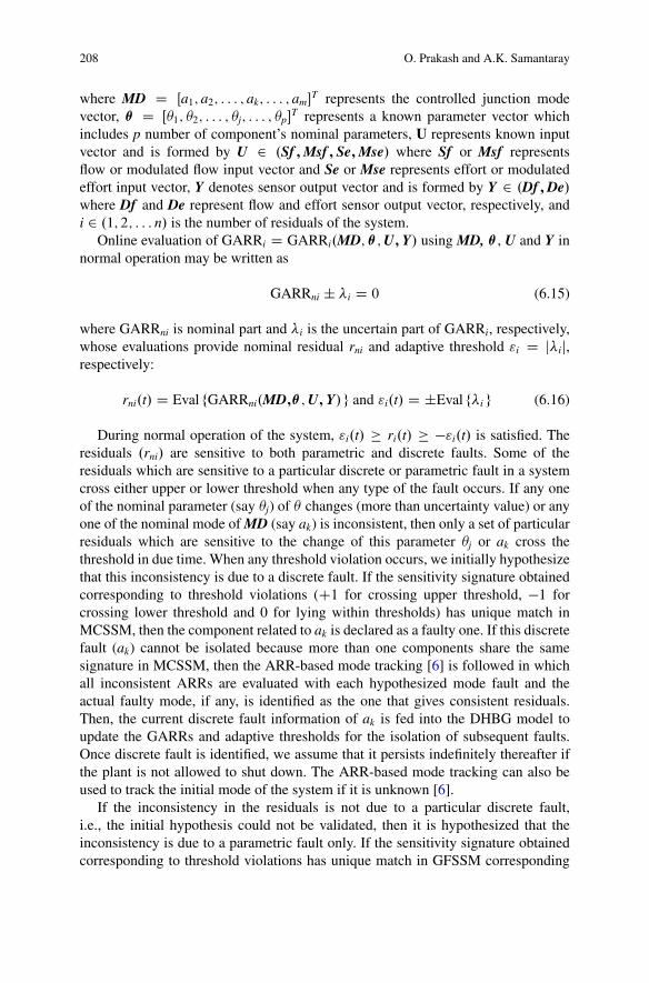
208 O. Prakash and A.K. Samantaray
where MD D Œa1; a2; : : : ; ak; : : : ; am�T represents the controlled junction mode
vector, � D Œ�1; �2; : : : ; �j; : : : ; �p�T represents a known parameter vector which
includes p number of component’s nominal parameters, U represents known inputvector and is formed by U 2 .Sf ; Msf ; Se; Mse/ where Sf or Msf representsflow or modulated flow input vector and Se or Mse represents effort or modulatedeffort input vector, Y denotes sensor output vector and is formed by Y 2 .Df ; De/where Df and De represent flow and effort sensor output vector, respectively, andi 2 .1; 2; : : : n/ is the number of residuals of the system.
Online evaluation of GARRi D GARRi.MD;�;U; Y/ using MD, � , U and Y innormal operation may be written as
GARRni ˙ i D 0 (6.15)
where GARRni is nominal part and i is the uncertain part of GARRi, respectively,whose evaluations provide nominal residual rni and adaptive threshold "i D jij,respectively:
rni.t/ D Eval fGARRni.MD;�;U; Y/g and "i.t/ D ˙Eval fi g (6.16)
During normal operation of the system, "i.t/ � ri.t/ � �"i.t/ is satisfied. Theresiduals .rni/ are sensitive to both parametric and discrete faults. Some of theresiduals which are sensitive to a particular discrete or parametric fault in a systemcross either upper or lower threshold when any type of the fault occurs. If any oneof the nominal parameter (say �j) of � changes (more than uncertainty value) or anyone of the nominal mode of MD (say ak) is inconsistent, then only a set of particularresiduals which are sensitive to the change of this parameter �j or ak cross thethreshold in due time. When any threshold violation occurs, we initially hypothesizethat this inconsistency is due to a discrete fault. If the sensitivity signature obtainedcorresponding to threshold violations (C1 for crossing upper threshold, �1 forcrossing lower threshold and 0 for lying within thresholds) has unique match inMCSSM, then the component related to ak is declared as a faulty one. If this discretefault (ak) cannot be isolated because more than one components share the samesignature in MCSSM, then the ARR-based mode tracking [6] is followed in whichall inconsistent ARRs are evaluated with each hypothesized mode fault and theactual faulty mode, if any, is identified as the one that gives consistent residuals.Then, the current discrete fault information of ak is fed into the DHBG model toupdate the GARRs and adaptive thresholds for the isolation of subsequent faults.Once discrete fault is identified, we assume that it persists indefinitely thereafter ifthe plant is not allowed to shut down. The ARR-based mode tracking can also beused to track the initial mode of the system if it is unknown [6].
If the inconsistency in the residuals is not due to a particular discrete fault,i.e., the initial hypothesis could not be validated, then it is hypothesized that theinconsistency is due to a parametric fault only. If the sensitivity signature obtainedcorresponding to threshold violations has unique match in GFSSM corresponding
6 Model-Based Diagnosis and Prognosis of Hybrid Dynamical Systems 209
to component (�j), then the FDI module detects the degradation of component (�j)(say at time t0) and component (�j) is isolated as degrading component at modez D z.i/ (say). On the other hand, if the degrading component (�j) cannot be isolatedbecause of more than one components share the same signature in GFSSM, then aset of suspected fault (SSF) is hypothesized for further course of action.
After postulation of faults candidates in SSF, a targeted parameter estimationtechnique is triggered for identification of true fault and its degradation pattern. Thismodule tries to quickly estimate only a few possible parameters from which the truefault candidate (�j) can be isolated [7, 8, 17, 18, 21]. Now the parameter �j is finallydeclared as a degrading faulty parameter and is represented by �j.t; z.i// at mode z.i/.The estimated fault magnitude of degrading parameter �j.t; z.i// at kth instant of timeis represented by � f
j .k; z.i//. If the nominal part of each GARRni is evaluated again
with the estimated fault magnitude � fj .k; z
.i// (real value of degrading parameterof plant/system at that instance), and adaptive thresholds are also updated, thenthe corresponding evaluated residuals do not cross the corresponding residualthresholds [8]. So, the original vector � is updated by replacing the nominal �j
by the estimated fault magnitude, � fj .k; z
.i// of the real plant. Now updated � atkth instant is assumed to be the new nominal parameter vector that is used toupdate DHBG model in LFT form to predict further degradation pattern of faultycomponent �j.t; z.i//. Note that a large deviation in a parameter value is consideredas an abrupt fault. Likewise, any discrete (mode) fault is also treated as abrupt fault.
If the detected parametric fault (�j) is of progressive type, then the component’sparameter �j.t; z.i// is degrading slowly according to operating mode z.i/. Thus, thesame set of residuals which are sensitive to the change of this parameter �j.t; z.i//would cross the adaptive threshold again after some more time. Again, parameter(�j) is estimated and its estimated value at .kC/th instant of time is represented by�
fj .k C; z.i//. Since up to the current time only two data points of fault magnitude
of degrading parameter are known, a linear degradation model may be assumed forthe initial estimation of RUL which alerts the maintenance engineer for schedulingthe maintenance activities or other tasks. This initial linear degradation model isfurther adapted with modified model when more parameter estimates are obtainedduring monitoring. For accurate estimation of degradation pattern, sufficient numberof data points should be obtained at particular mode z.i/ and then the degradationmodel is identified by using the curve fitting tools at corresponding mode z.i/. Ifthe jth operating change point occurs at time instant t.j/ corresponding to new modez.j/ during data collection for estimating the parameter value in previous operatingmode z.i/, then the fresh data of a fixed window size corresponding to new mode z.j/
are collected and fault magnitude is estimated in this new mode z.j/. This process isrepeated until the true degradation model, M.i/
�j(z), is obtained for parameter �j.t; z/
at different operating modes. Then the obtained true model M.i/�j
(z) is further usedin prognosis module to predict RUL of faulty component (�j) with the future known
operating mode by extrapolating the model M.i/�j
(z). Also, the finally obtained true

210 O. Prakash and A.K. Samantaray
degradation model M.i/�j
(z) of the component (�j) is fed into the DHBG model, so thatthe subsequent faults can be detected and isolated. In the case of sequential multipleprogressive faults, RUL is estimated for each progressive fault component and theRUL of the component which has least value is the significant for the maintenanceengineer.
6.3 Application to a Two-Tank Benchmark System
6.3.1 Description of a Two-Tank Hybrid System
The benchmark hybrid two-tank system is adapted from [11]. Its process andinstrumentation diagram and hybrid bond graph (HBG) model are shown in Figs. 6.5and 6.6, respectively. This system consists of two tanks (T1 and T2) that areconnected with pipes and valves (V1 and V2). Cdvi is the coefficient of dischargeof non-linear valve Vi, i D 1; 2. The liquid level in tank T1 is regulated by ahydraulic pump which is controlled by a PI-controller installed in this system andtries to maintain water level of 0.5 m. The flow of pump (QP) is proportional to theoutput of the PI-controller (UPI). Two drainage pipes (L1 and L2) with coefficients ofdischarge CdL1 and CdL2, respectively, showing linear behaviour are also used. Thissystem shows the hybrid dynamics and includes both autonomous and supervisorycontroller transition modes. Valve V1 is switched to on and then off state accordingto command input given by the supervisory controller. When water level in tankT1 exceeds level HL1 then the water starts flowing from tank T1 to tank T2 throughdrainage pipe L1 (autonomous mode, a1). Similarly, when water level in tank T2exceeds level HL2 then the water starts flowing from tank T2 to atmosphere through
HL1 HL2
T1 T2
H1 H2
PI
Qp V1
VLeak1 VLeak2
L1
γ
V2Qo
L2
Supervisory Controller
ON-OFF
Fig. 6.5 Schematic diagram of a two-tank hybrid system

6 Model-Based Diagnosis and Prognosis of Hybrid Dynamical Systems 211
T2C:1/C V2R:RV1R:RT1C:1/C
11 0
: 0
1 1C2
1H
TF: gρ
:Msf
PQ
:SeL1gHρ−
:Se0P
L1R:R VLeak1R:R
De
10
:0
1 1C3
2H
TF: gρ
:SeL2gHρ−
:Se
0P
L2R:R VLeak2R:R
De
Msf
C2f
:
PI:Se
0PC1
'Df:
C2f
Fig. 6.6 HBG model of a two-tank hybrid system
drainage pipe L2 (autonomous mode, a2). Leakage fault can be introduced in tankTi using imaginary valve VLeaki having coefficient of discharge CdLeaki, i D 1; 2.
Two level sensors H1 and H2 and one flow sensor QP are installed in the systemfor measuring the water levels in tanks T1 and T2 and water input flow by pump,respectively. The atmospheric pressure is assumed to be the reference pressure. Thesmall angle � , volume of water in the drainage pipe and inertia effect of water floware neglected in this system; with the former two being considered as part of theuncertainties in tank capacities. This way of simplified model building by neglectingminor dynamics improves the speed of diagnosis without unduly complicating theprocess of development of the supervision system.
Pump saturation characteristic (QP) and PI-controller output law (ˆPI) are,respectively, given as
QP D8<
:
UPI; 0 � UPI � fmax
0; UPI � 0
fmax; UPI � fmax
D ˆP .UPI/ (6.17)
UPI D KP.Spt � � � g � H1.t//C KI
Z.Spt � � � g � H1.t//dt
D ˆPI .H1.t// (6.18)
where fmax is the maximum flow from the pump, Spt is a pressure (or level) set pointand KP and KI are the proportional and integral gains, respectively. In this work, wedo not consider the actuator, controller and sensor faults; they may be diagnosedwith additional hardware/sensor redundancies and hence are not relevant for thisstudy.
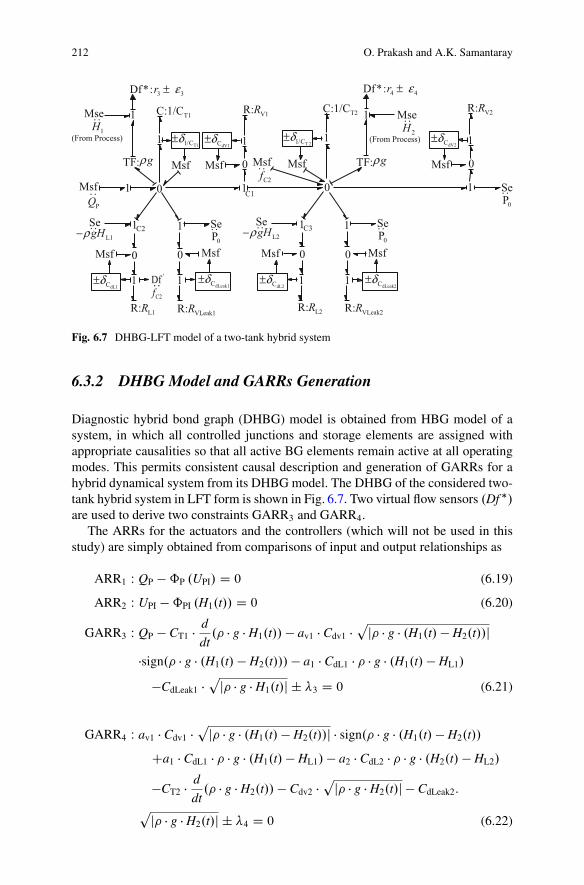
212 O. Prakash and A.K. Samantaray
1
1
dV1Cδ±T11/Cδ±
11 0
: 1
1 1C2
Msf
1H(From Process)
V1R:RT1C:1/C
Df*: 3 3r ε±
TF: gρ
:MsfPQ
:SeL1gHρ−
:Se0P
L1R:R VLeak1R:R
1
Mse
Msf
1
10:1
1
Msf
2H(From Process)
T2C:1/C
Df*: 4 4r ε±
TF: gρ
:SeL2gHρ−
:Se0P
L2R:R VLeak2R:R
Mse
1
Msf:
C2f
1
Msf
dL1Cδ± 1 1 1
Msf MsfMsf
T 21/Cδ±dV2Cδ±
dLeak1Cδ±dLeak2Cδ±
dL2Cδ±
C3
:Se0PC1
'Df:
C2f
0 Msf 0
0 0 0 0
V2R:R
Fig. 6.7 DHBG-LFT model of a two-tank hybrid system
6.3.2 DHBG Model and GARRs Generation
Diagnostic hybrid bond graph (DHBG) model is obtained from HBG model of asystem, in which all controlled junctions and storage elements are assigned withappropriate causalities so that all active BG elements remain active at all operatingmodes. This permits consistent causal description and generation of GARRs for ahybrid dynamical system from its DHBG model. The DHBG of the considered two-tank hybrid system in LFT form is shown in Fig. 6.7. Two virtual flow sensors .Df �/are used to derive two constraints GARR3 and GARR4.
The ARRs for the actuators and the controllers (which will not be used in thisstudy) are simply obtained from comparisons of input and output relationships as
ARR1 W QP �ˆP .UPI/ D 0 (6.19)
ARR2 W UPI �ˆPI .H1.t// D 0 (6.20)
GARR3 W QP � CT1 � d
dt.� � g � H1.t// � av1 � Cdv1 �
pj� � g � .H1.t/ � H2.t//j
�sign.� � g � .H1.t/ � H2.t/// � a1 � CdL1 � � � g � .H1.t/ � HL1/
�CdLeak1 �p
j� � g � H1.t/j ˙ 3 D 0 (6.21)
GARR4 W av1 � Cdv1 �p
j� � g � .H1.t/ � H2.t//j � sign.� � g � .H1.t/ � H2.t//
Ca1 � CdL1 � � � g � .H1.t/ � HL1/ � a2 � CdL2 � � � g � .H2.t/ � HL2/
�CT2 � d
dt.� � g � H2.t// � Cdv2 �
pj� � g � H2.t/j � CdLeak2:
pj� � g � H2.t/j ˙ 4 D 0 (6.22)
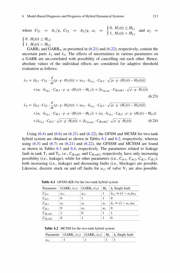
6 Model-Based Diagnosis and Prognosis of Hybrid Dynamical Systems 213
where CT1 D A1=g, CT2 D A2=g, a1 D�0; H1.t/ � HL1
1; H1.t/ > HL1and a2 D
�0; H2.t/ � HL2
1; H2.t/ > HL2
GARR3 and GARR4, as presented in (6.21) and (6.22), respectively, contain theuncertain parts 3 and 4. The effects of uncertainties in various parameters ona GARR are un-correlated with possibility of cancelling out each other. Hence,absolute values of the individual effects are considered for adaptive thresholdevaluation as follows:
3 D jıC1 � CT1 � d
dt.� � g � H1.t//j C jav1 � ıCdv1 � Cdv1 �
pj� � g � .H1.t/ � H2.t//jj
Cja1 � ıCdL1 � CdL1 � � � g � .H1.t/ � HL1/j C jıCdLeak1 � CdLeak1 �p� � g � H1.t/j
(6.23)
4 D jıC2 � CT2 � d
dt.� � g � H2.t//j C jav1 � ıCdv1 � Cdv1 �
pj� � g � .H1.t/ � H2.t//jj
Cja1 � ıCdL1 � CdL1 � � � g � .H1.t/ � HL1/j C ja2 � ıCdL2 � CdL2 � � � g � .H2.t/ � HL2/jCjıCdv2 � Cdv2 �
p� � g � H2.t/j C jıCdLeak2 � CdLeak2 �
p� � g � H2.t/j (6.24)
Using (6.4) and (6.6) on (6.21) and (6.22), the GFSM and MCSM for two-tankhybrid system are obtained as shown in Tables 6.1 and 6.2, respectively; whereasusing (6.5) and (6.7) on (6.21) and (6.22), the GFSSM and MCSSM are foundas shown in Tables 6.3 and 6.4, respectively. The parameters related to leakagefault in tank T1 and T2, i.e., CdLeak1 and CdLeak2, respectively, have only increasingpossibility (i.e., leakage), while for other parameters (i.e., Cdv1, Cdv2, CdL1, CdL2),both increasing (i.e., leakage) and decreasing faults (i.e., blockage) are possible.Likewise, discrete stuck on and off faults for av1 of valve V1 are also possible.
Table 6.1 GFSM (GS) for the two-tank hybrid system
Parameter GARR3 .r3/ GARR4 .r4/ Mb Ib Single fault
Cdv1 av1 av1 1 Nav1 D .1� a1/av1
Cdv2 0 1 1 0
CdL1 a1 a1 a1 Na1 D .1� av1/a1CdL2 0 a2 a2 0
CdLeak1 1 0 1 1
CdLeak2 0 1 1 0
Table 6.2 MCSM for the two-tank hybrid system
Parameter GARR3 .r3/ GARR4 .r4/ Mb Ib Single fault
av1 1 1 1 1

214 O. Prakash and A.K. Samantaray
Table 6.3 GFSSM (GSS) for the two-tank hybrid system
Parameter GARR3 .r3/ GARR4 .r4/
Cdv1 " av1sign.H1.t/� H2.t// �av1sign.H1.t/� H2.t//
Cdv1 # �av1sign.H1.t/� H2.t// av1sign.H1.t/� H2.t//
Cdv2 " 0 C1Cdv2 # 0 �1CdL1 " a1 �a1CdL1 # �a1 a1CdL2 " 0 a2CdL2 # 0 �a2CdLeak1 " C1 0
CdLeak2 # 0 C1
Table 6.4 MCSSM for the two-tank hybrid system
Parameter GARR3 .r3/ GARR4 .r4/
av1 " sign.H1.t/� H2.t// �sign.H1.t/� H2.t//
av1 # �sign.H1.t/� H2.t// sign.H1.t/� H2.t//
These possibilities, called technological specifications which are derived from deepknowledge of the system, are considered in Tables 6.3 and 6.4, respectively.
Note that the sensitivity signatures presented in GFSSM and MCSSM [9] aresimplified expressions derived from GARRs. These can be numerically obtainedfrom SBG model if GARRs cannot be symbolically derived. For example, if weconsider the sensitivity signature element GSS Cdv1"
1;1 due to the fault Cdv1 ", then thecorresponding element in the GFSSM is calculated as
GSS Cdv1"1;1 D �sign.@GARR3=@Cdv1/
D �sign� � av1Cdv1
pj�g.H1.t/ � H2.t//j
�
D av1sign.H1.t/ � H2.t// (6.25)
6.3.3 Simulation Study and Results
In this section, an integrated MBDP method for sequential multiple faults ofunknown nature/type in a hybrid dynamical system is tested through simulation.Also, model-based process supervision scheme using the most recent existingapproach [9] which considers single fault hypothesis and the newly proposedapproach which considers sequential multiple faults hypotheses, along with com-parison between these two approaches are presented. This section also shows thatthe methods which are based on single fault hypothesis fail to predict the actual faultcandidates in case of sequential multiple faults and without correct isolation of fault
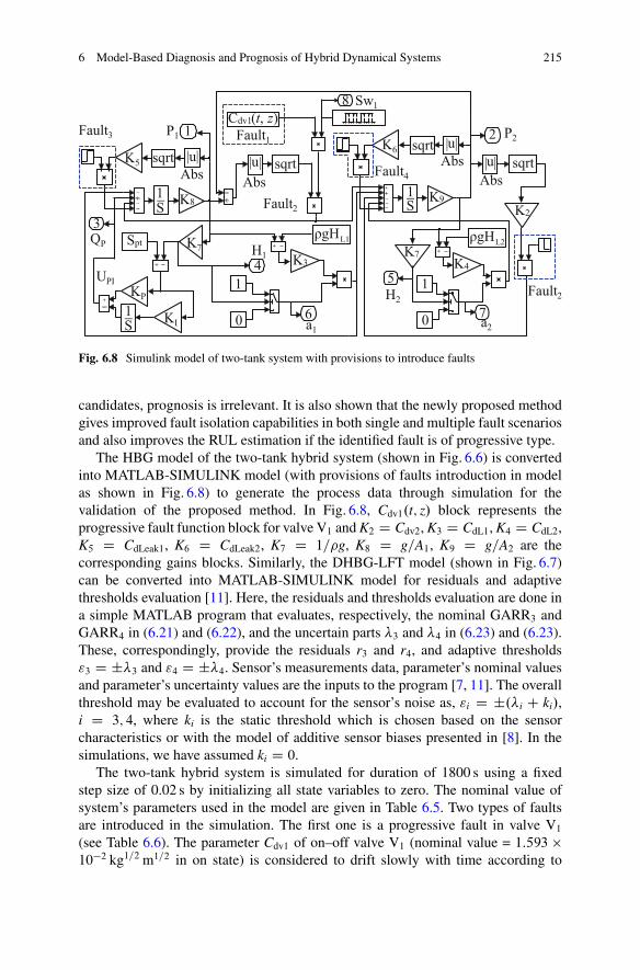
6 Model-Based Diagnosis and Prognosis of Hybrid Dynamical Systems 215
S1
UPI
a27
a16
H2
54
QP
3
P22P1 1
Spt
sqrtsqrtsqrt sqrt
Fault2
Fault2
Abs|u| Abs
|u|
Abs|u|
Abs|u|
0
1
0
1
L1ρgHL2ρgH
+ −
+ −
+ −
+−
H1
−+−−
++−−−
1−S
1−S−
KP
KI
K7
K8 K9
K3K7
K4
+−
K5
K6
Fault3
Fault4
K2
Cdv1(t, z)Sw1
Fault1
8
Fig. 6.8 Simulink model of two-tank system with provisions to introduce faults
candidates, prognosis is irrelevant. It is also shown that the newly proposed methodgives improved fault isolation capabilities in both single and multiple fault scenariosand also improves the RUL estimation if the identified fault is of progressive type.
The HBG model of the two-tank hybrid system (shown in Fig. 6.6) is convertedinto MATLAB-SIMULINK model (with provisions of faults introduction in modelas shown in Fig. 6.8) to generate the process data through simulation for thevalidation of the proposed method. In Fig. 6.8, Cdv1.t; z/ block represents theprogressive fault function block for valve V1 and K2 D Cdv2, K3 D CdL1, K4 D CdL2,K5 D CdLeak1, K6 D CdLeak2, K7 D 1=�g, K8 D g=A1, K9 D g=A2 are thecorresponding gains blocks. Similarly, the DHBG-LFT model (shown in Fig. 6.7)can be converted into MATLAB-SIMULINK model for residuals and adaptivethresholds evaluation [11]. Here, the residuals and thresholds evaluation are done ina simple MATLAB program that evaluates, respectively, the nominal GARR3 andGARR4 in (6.21) and (6.22), and the uncertain parts 3 and 4 in (6.23) and (6.23).These, correspondingly, provide the residuals r3 and r4, and adaptive thresholds"3 D ˙3 and "4 D ˙4. Sensor’s measurements data, parameter’s nominal valuesand parameter’s uncertainty values are the inputs to the program [7, 11]. The overallthreshold may be evaluated to account for the sensor’s noise as, "i D ˙.i C ki/,i D 3; 4, where ki is the static threshold which is chosen based on the sensorcharacteristics or with the model of additive sensor biases presented in [8]. In thesimulations, we have assumed ki D 0.
The two-tank hybrid system is simulated for duration of 1800 s using a fixedstep size of 0.02 s by initializing all state variables to zero. The nominal value ofsystem’s parameters used in the model are given in Table 6.5. Two types of faultsare introduced in the simulation. The first one is a progressive fault in valve V1
(see Table 6.6). The parameter Cdv1 of on–off valve V1 (nominal value = 1:593 �10�2 kg1=2 m1=2 in on state) is considered to drift slowly with time according to

216 O. Prakash and A.K. Samantaray
Table 6.5 Nominal parameters of the hybrid two-tank
Symbol Description Nominal value
KP Proportional gain of controller 1 ms
KI Integral gain of controller 5� 10�2 m
Spt Set point of the PI-controller 0.5 m
fmax Maximum outflow from pump 1 kg/s
Ai Cross-sectional area of tank Ti.i D1; 2/
1:472� 10�2 m2
Cdvi Discharge coefficient of valve Vi
including connected pipe (i D 1; 2)1:593� 10�2 kg1=2 m1=2
CdLi Discharge coefficient of drainagepipe Li (i D 1; 2)
1� 10�3 ms
CdLeaki Discharge coefficient of VLeaki.i D1; 2/
0 kg1=2 m1=2
HL1 Height of the drainage pipe L1 oftank T1 from datum
0.58 m
HL2 Height of the drainage pipe L2 oftank T2 from datum
0.40 m
P0 Atmospheric pressure 0 N=m2
� Density of water 1000 kg=m3
g Acceleration due to gravity 9:81m=s2
Table 6.6 Simulated faults in the model
Parameter Description Degradation nature Start time, tfi (s) End time
Cdv1 Valve blockage Progressive type as per (6.26) 225 1800
Cdv2 Valve blockage Abrupt type as per (6.27) 1475 1800
operating mode (z D z.i/ D av1) as shown in Fig. 6.9b. Second one is an abrupt faultin valve V2. In the simulation, we have introduced the fault in parameters Cdv1 andCdv2 at a time instants tf1 D 225 s and tf2 D 1475 s, respectively, as defined throughthe functions given in (6.26) and (6.27), respectively.
Cdv1.t; z/ D�
Cdv1n.z/ � av1; t < tf1Cdv1n.z/
�e�r.z/�ton
� � av1; t � tf1(6.26)
Cdv2.t; z/ D�
Cdv2n.z/; t < tf20:9Cdv2n.z/; t � tf2
(6.27)
where Cdvin.z/ is the nominal parameter value of valve Vi.i D 1; 2/ at correspondingoperating mode .z/; r.z/ D 1:0 � 10�4 s�1 at z D z.1/ D av1 D 1, with eachz.1/ for 80 s and r.z/ D 0 s�1 at z D z.2/ D av1 D 0, with each z.2/ for 30 s,
ton DtR
tf1
av1 � dt, and tf1 and tf2 are the time instances when the first and second
faults start, respectively.

6 Model-Based Diagnosis and Prognosis of Hybrid Dynamical Systems 217
0
1
a bSu
perv
isor
y m
ode,
a V1
0 2 4 6 8 10 12 14 16 18Time (s) x 102
z(1)
z(2)
z(1) z(1) z(1)
z(2) z(2)
….….….…….….….…….….….
….….….…….….….…….….…. z(2)
z(1) = 1 for 80 sz(2) = 0 for 30 s
225 260 300
0
5
10
15
x 10-3
CdV
1(t,
z ) (k
g1/2 m
1/2 )
0 2 4 6 8 10 12 14 16 18Time (s) x 102
Fig. 6.9 (a) Operating mode (b) introduced degradation of on–off valve V1
0.3
0.4
0.5
0.6
0.7
0.8
( QP)
(kg/
s)
0 2 4 6 8 10 12 14 16 18x 102Time (s)
0 2 4 6 8 10 12 14 16 18x 102
0
0.2
0.4
0.6H
1 (m
)
Time (s)
0 2 4 6 8 10 12 14 16 18x 102
0
0.1
0.2
H2 (m
)
Time (s)
0
1
Auto
nom
ous m
ode,
a 1
0 2 4 6 8 10 12 14 16 18x 102Time (s)
ba
dc
Fig. 6.10 Time responses of measurements (a) Pump flow (b) Water level in tank T1 (c) Waterlevel in tank T2 and (d) Autonomous mode of drainage pipe L1
Note that parameter Cdv1 is considered to drift slowly only in on state of thevalve, while there is no drift of parameter Cdv1 during off state as the flow is zero inthat state. The drifting of parameter Cdv1 just after tf1 D 225 s is clearly shown inenlarged view of a portion of Fig. 6.9b. The failure threshold (Cfl
dv1) is considered ashalf of the nominal value in on state.
The measurements (i.e., QP, H1 and H2) from the simulated model at a samplingrate of 0.02 s are fed to the residuals and thresholds evaluation program. The timeresponses of measured input (QP), outputs (H1, H2) and obtained autonomous mode(a1) are shown in Fig. 6.10. The transition of mode a1 from 0 to 1 subjected to givenconditions (when H1.t/ exceeds HL1 D 0:58m) corresponding to drainage pipe L1is clearly noticeable. However, no autonomous mode change is found for drainagepipe L2; hence a2 D 0 throughout the simulation period.

218 O. Prakash and A.K. Samantaray
Table 6.7 GFSSM (GSS) for the two-tank hybrid system
Parameter GARR3 .r3/ GARR4 .r4/ Mb Ib Single fault
Cdv1 " av1 �av1 av1 Nav1 D .1� a1/av1
Cdv1 # �av1 av1 av1 Nav1 D .1� a1/av1
Cdv2 " 0 C1 1 0
Cdv2 # 0 �1 1 Na2 D .1� a2/
CdL1 " a1 �a1 a1 Na1 D .1� av1/a1CdL1 # �a1 a1 a1 Na1 D .1� av1/a1CdL2 " 0 a2 a2 0
CdL2 # 0 �a2 a2 0
CdLeak1 " C1 0 1 1
CdLeak2 " 0 C1 1 0
Table 6.8 MCSSM for the two-tank hybrid system
Parameter GARR3 .r3/ GARR4 .r4/ Mb Ib Single fault
av1 " C1 �1 1 1
av1 # �1 C1 1 1
6.3.3.1 Implementation of Integrated Diagnosis and Prognosis Approach
In practice, the elements of GFSSM and MCSSM have to be updated at each andevery instant by using the instantaneous measurement data. It is observed fromFig. 6.10 that the measurement H1 is always greater than H2, so the obtained GFSSMand MCSSM during the duration of observation (0–1800 s) for the considered two-tank hybrid system can be simplified to the forms given in Tables 6.7 and 6.8,respectively. The response of residuals (r3 and r4) and adaptive thresholds obtainedfrom DHBG-LFT model using previously existing method [9] and the newly pro-posed method with dynamically updated parameter and updated adaptive thresholdsare shown in Figs. 6.11 and 6.12, respectively (solid lines indicate residuals anddashed/dotted lines indicate adaptive thresholds). The response of residuals (r3 andr4) and adaptive thresholds during normal operation (up to t D 225 s) and duringidentification of degradation behaviour of valves V1 and V2 using proposed method(after t D 225 s) is clearly shown in Fig. 6.12. Note that the first two columns ofthe coherence vector related to actuator and controller faults, which are irrelevant inthis study, have been dropped from the analysis.
A discussion on fault isolation capabilities using existing FDI methods consid-ering single fault hypothesis is presented here. From the simulated faults listed inTable 6.6, both valves V1 and V2 are faulty between 1475 and 1800 s as the fault invalve V1 is not repaired. The observed coherence vector (C) just after 225 s (afterinitiation of blockage fault in V1) is obtained from Fig. 6.11a, b as C D Œ1 1� (ifnot considering residual sensitivity signature) or C D Œ�1 C 1� (if consideringthe residual sensitivity signature). According to coherence vector C D Œ1 1� orC D Œ�1C1�, the set of suspected faults (SSF) is Cdv1 and av1 using GFSM/GFSSM
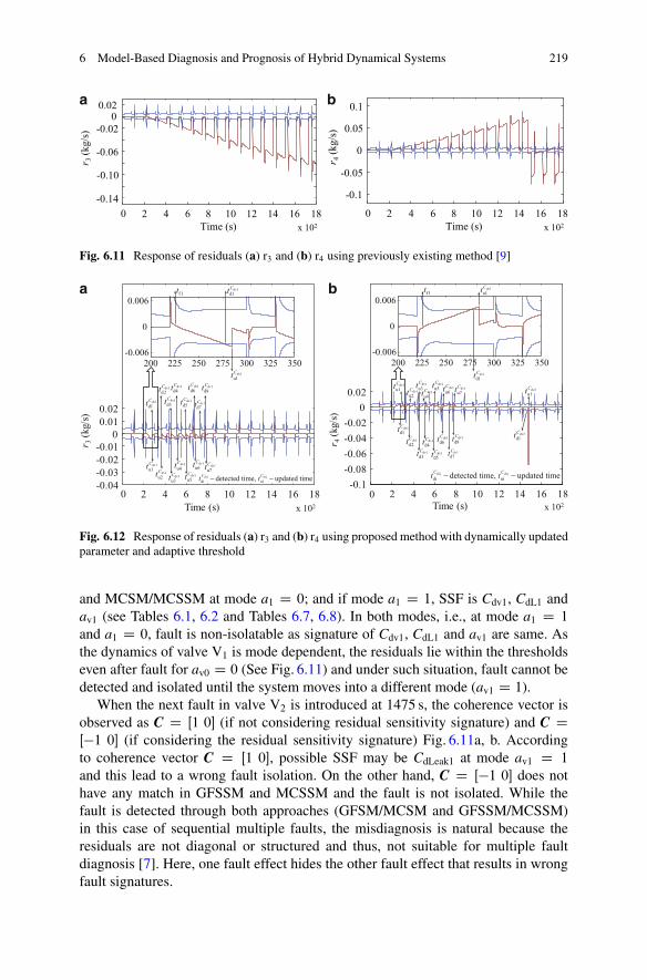
6 Model-Based Diagnosis and Prognosis of Hybrid Dynamical Systems 219
-0.14
-0.10
-0.06
-0.020
0.02
r 3(k
g/s)
0 2 4 6 8 10 12 14 16 18Time (s) x 102
-0.1
-0.05
0
0.05
0.1
r 4(k
g/s)
0 2 4 6 8 10 12 14 16 18Time (s) x 102
a b
Fig. 6.11 Response of residuals (a) r3 and (b) r4 using previously existing method [9]
-0.04-0.03-0.02-0.01
00.010.02
r 3(k
g/s)
0 2 4 6 8 10 12 14 16 18Time (s) x 102
dv1d1Ct
dv1d2Ct
dv1d3Ct
dv1d4Ct
dv1d5Ct
dv1d6Ct
dv1d7Ct
dv1d8Ct
dv1u1Ct
dv1u2Ct dv1
u3Ct
dv1u4Ct
dv1u5Ct
dv1u6Ct dv1
u7Ct
dvj dvjdi uidetected time, updated time− −CCt t
dv1d1Ct
200 225 250 275 300 325 350-0.006
0
0.006
dv1u1Ct
f1t
0 2 4 6 8 10 12 14 16 18-0.1
-0.08-0.06-0.04-0.02
00.02
Time (s)
r 4(k
g/s)
x 102
dv1u1Ct
dv1u2Ct dv1
u4Ct
dv1u5Ct dv1
u6Ct dv1
u7Ct
dv1u3Ct
dv1d1Ct
dv1d2Ct
dv1d3Ct
dv1d4Ct
dv1d5Ct
dv1d6Ct
dv1d7Ct
dv1d8Ct
dv2u1Ct
dv2d1Ct
dvj dvjdi uidetected time, updated time− −CCt t
200 225 250 275 300 325 350-0.006
0
0.006
dv1d1Ct
dv1u1Ctf1tba
Fig. 6.12 Response of residuals (a) r3 and (b) r4 using proposed method with dynamically updatedparameter and adaptive threshold
and MCSM/MCSSM at mode a1 D 0; and if mode a1 D 1, SSF is Cdv1, CdL1 andav1 (see Tables 6.1, 6.2 and Tables 6.7, 6.8). In both modes, i.e., at mode a1 D 1
and a1 D 0, fault is non-isolatable as signature of Cdv1, CdL1 and av1 are same. Asthe dynamics of valve V1 is mode dependent, the residuals lie within the thresholdseven after fault for av0 D 0 (See Fig. 6.11) and under such situation, fault cannot bedetected and isolated until the system moves into a different mode (av1 D 1).
When the next fault in valve V2 is introduced at 1475 s, the coherence vector isobserved as C D Œ1 0� (if not considering residual sensitivity signature) and C DŒ�1 0� (if considering the residual sensitivity signature) Fig. 6.11a, b. Accordingto coherence vector C D Œ1 0�, possible SSF may be CdLeak1 at mode av1 D 1
and this lead to a wrong fault isolation. On the other hand, C D Œ�1 0� does nothave any match in GFSSM and MCSSM and the fault is not isolated. While thefault is detected through both approaches (GFSM/MCSM and GFSSM/MCSSM)in this case of sequential multiple faults, the misdiagnosis is natural because theresiduals are not diagonal or structured and thus, not suitable for multiple faultdiagnosis [7]. Here, one fault effect hides the other fault effect that results in wrongfault signatures.
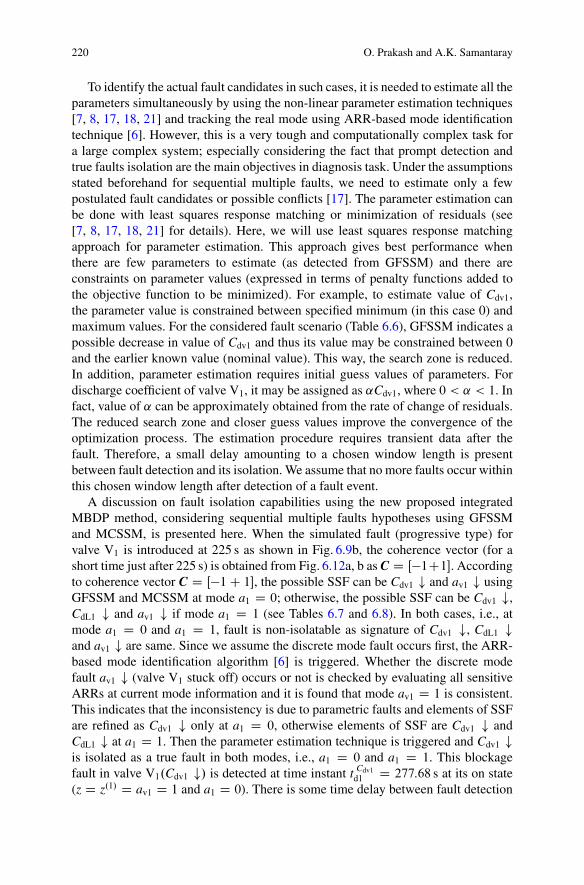
220 O. Prakash and A.K. Samantaray
To identify the actual fault candidates in such cases, it is needed to estimate all theparameters simultaneously by using the non-linear parameter estimation techniques[7, 8, 17, 18, 21] and tracking the real mode using ARR-based mode identificationtechnique [6]. However, this is a very tough and computationally complex task fora large complex system; especially considering the fact that prompt detection andtrue faults isolation are the main objectives in diagnosis task. Under the assumptionsstated beforehand for sequential multiple faults, we need to estimate only a fewpostulated fault candidates or possible conflicts [17]. The parameter estimation canbe done with least squares response matching or minimization of residuals (see[7, 8, 17, 18, 21] for details). Here, we will use least squares response matchingapproach for parameter estimation. This approach gives best performance whenthere are few parameters to estimate (as detected from GFSSM) and there areconstraints on parameter values (expressed in terms of penalty functions added tothe objective function to be minimized). For example, to estimate value of Cdv1,the parameter value is constrained between specified minimum (in this case 0) andmaximum values. For the considered fault scenario (Table 6.6), GFSSM indicates apossible decrease in value of Cdv1 and thus its value may be constrained between 0and the earlier known value (nominal value). This way, the search zone is reduced.In addition, parameter estimation requires initial guess values of parameters. Fordischarge coefficient of valve V1, it may be assigned as ˛Cdv1, where 0 < ˛ < 1. Infact, value of ˛ can be approximately obtained from the rate of change of residuals.The reduced search zone and closer guess values improve the convergence of theoptimization process. The estimation procedure requires transient data after thefault. Therefore, a small delay amounting to a chosen window length is presentbetween fault detection and its isolation. We assume that no more faults occur withinthis chosen window length after detection of a fault event.
A discussion on fault isolation capabilities using the new proposed integratedMBDP method, considering sequential multiple faults hypotheses using GFSSMand MCSSM, is presented here. When the simulated fault (progressive type) forvalve V1 is introduced at 225 s as shown in Fig. 6.9b, the coherence vector (for ashort time just after 225 s) is obtained from Fig. 6.12a, b as C D Œ�1C1�. Accordingto coherence vector C D Œ�1C 1�, the possible SSF can be Cdv1 # and av1 # usingGFSSM and MCSSM at mode a1 D 0; otherwise, the possible SSF can be Cdv1 #,CdL1 # and av1 # if mode a1 D 1 (see Tables 6.7 and 6.8). In both cases, i.e., atmode a1 D 0 and a1 D 1, fault is non-isolatable as signature of Cdv1 #, CdL1 #and av1 # are same. Since we assume the discrete mode fault occurs first, the ARR-based mode identification algorithm [6] is triggered. Whether the discrete modefault av1 # (valve V1 stuck off) occurs or not is checked by evaluating all sensitiveARRs at current mode information and it is found that mode av1 D 1 is consistent.This indicates that the inconsistency is due to parametric faults and elements of SSFare refined as Cdv1 # only at a1 D 0, otherwise elements of SSF are Cdv1 # andCdL1 # at a1 D 1. Then the parameter estimation technique is triggered and Cdv1 #is isolated as a true fault in both modes, i.e., a1 D 0 and a1 D 1. This blockagefault in valve V1.Cdv1 #/ is detected at time instant t Cdv1
d1 D 277:68 s at its on state(z D z.1/ D av1 D 1 and a1 D 0). There is some time delay between fault detection

6 Model-Based Diagnosis and Prognosis of Hybrid Dynamical Systems 221
and its occurrence because of slow evolution of fault and the uncertainties includedin residual threshold evaluation.
Since the direction of parameter variation of Cdv1 is known by GFSSM (decreasein value of Cdv1), this information is used in constrained parameter estimationtechnique for degradation model identification. This makes degradation modelidentification fast, which is one of the main requirements in CBM. For theestimation of fault magnitude of Cdv1, a small time window of 7 s transient dataafter the fault has been selected. Now the fault magnitude of degrading parameterCdv1 is estimated after detecting the fault at time instant t Cdv1
d1 D 277:68 s. Theestimated parameter value is known at time instant t Cdv1
u1 D 277:68 s C 7 s D284:68 s and is represented by Cf
dv1.tCdv1
u1 ; z.1//, whose value is Cfdv1.t
Cdv1u1 ; z.1// D
1:584 � 10�2 kg1=2 m1=2. Now, the DHBG model is updated by replacing thenominal value Cdv1 D 1:593 � 10�2 kg1=2 m1=2 by the estimated fault magnitudeCf
dv1.tCdv1
u1 ; z.1// D 1:584 � 10�2 kg1=2 m1=2 of the real plant. Now the residuals andadaptive thresholds evaluation obtained through updated nominal part of GARRsand updated uncertainties parts obtained from the updated DHBG model in LFTform force the residuals to lie within the updated adaptive thresholds (see Fig. 6.12where this updated time instant is denoted as t Cdv1
u1 ). Since, the parameter Cdv1 isdegrading progressively at mode z D z.1/ D av1 D 1, again a set of residuals (r3 andr4) which are sensitive to the change of this parameter, Cdv1, cross the adaptivethreshold with the evolution of time (marked as t Cdv1
d2 D 364:02 s in Fig. 6.12)and again the new fault magnitude of degrading parameter Cdv1 is estimated andknown at new time instant t Cdv1
u2 D 364:02 s C 7 s D 371:02 s and represented byCf
dv1.tCdv1
u2 ; z.1//, whose value is Cfdv1.t
Cdv1u2 ; z.1// D 1:575 � 10�2 kg1=2 m1=2. Since
only two data points are known up to the current time a linear degradation modelis assumed for the initial estimation of RUL to alert the maintenance engineer. Theobtained data points at different time instances .t Cdv1
u1 and t Cdv1u2 / corresponding to
mode z D z.1/ D av1 D 1 are used to find the linear degradation mathematical modelfor the parameter Cdv1 using the curve fitting tool in Matlab-Simulink and is shownin Fig. 6.13a. For curve fitting, ton is used as a time reference in abscissa. Initialestimated value of RUL using the linear degradation model at on state of valve V1
and no degradation at off state based on defined failure threshold .Cfldv1 D 0:5Cdv1/
and known future operating modes of valve V1 is found as 6822.19 s (see Fig. 6.14a).This initial degradation model is further adapted with modified model when morenew information of data points are obtained during monitoring. In Fig. 6.14, t Cdv1
u1 isconsidered as a zero time reference for RUL estimation.
Note that at different time instances, the valve V1 is switched to off state as perthe command input given by the controller. In this duration, there is no flow throughthe valve V1. Although valve V1 is isolated as a faulty element, residuals r3 and r4become zero (see Fig. 6.12) at the corresponding off state (z D z.2/ D av1 D 0)which provides Cdv1.t; z.2// D 0 kg1=2 m1=2.
For accurate estimation of degradation pattern, sufficient data points shouldbe used. As the monitoring is continued, newer information of degradation datais obtained. Estimated magnitude of degrading parameter Cdv1 at the same mode
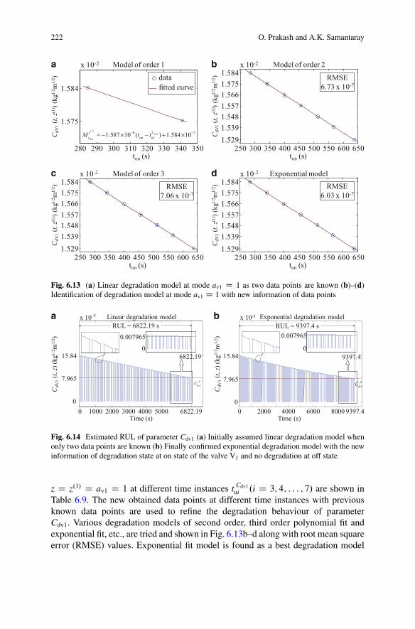
222 O. Prakash and A.K. Samantaray
a b
c d
280 290 300 310 320 330 340 350
1.575
1.584
Model of order 1x 10⁻²
ton (s)
datafitted curve
CdV
1( t,
z(1) )
(kg1/
2 m1/
2 )
(1)dv1
dv1
26on u1 = 1.587 10 ( ) 1.584 10Cz
cM t t −−− × − + ×
250 300 350 400 450 500 550 600 650
CdV
1(t,
z(1) )
(kg1/
2 m1/
2 )
1.539
1.5751.584
Model of order 2x 10⁻²
1.5661.5571.548
1.529
ton (s)
RMSE6.73 x 10-7
250 300 350 400 500 550 600 650
CdV
1(t,
z(1) )
(kg1/
2 m1/
2 )
1.539
1.5751.584
Model of order 3x 10⁻²
1.5661.5571.548
1.529450
ton (s)
RMSE7.06 x 10-7
250 300 350 400 500 550 600 650
CdV
1( t,
z(1) )
(kg1/
2 m1/
2 )
1.539
1.5751.584
Exponential modelx 10-2
1.5661.5571.548
1.529450
ton (s)
RMSE6.03 x 10-7
Fig. 6.13 (a) Linear degradation model at mode av1 D 1 as two data points are known (b)–(d)Identification of degradation model at mode av1 D 1 with new information of data points
0 1000 2000 3000 4000 5000 6822.190
7.965
15.84
a b
Time (s)
CdV
1(t,
z) (k
g1/2 m
1/2 )
RUL = 6822.19 s
dv1flC
Linear degradation modelx 10-3
6822.190
0.007965
0 2000 4000 6000 8000 9397.4Time (s)
0
7.965
15.84
CdV
1(t,
z ) (k
g1/2 m
1/2 )
RUL = 9397.4 s
dv1flC
Exponential degradation modelx 10-3
9397.40
0.007965
Fig. 6.14 Estimated RUL of parameter Cdv1 (a) Initially assumed linear degradation model whenonly two data points are known (b) Finally confirmed exponential degradation model with the newinformation of degradation state at on state of the valve V1 and no degradation at off state
z D z.1/ D av1 D 1 at different time instances t Cdv1ui .i D 3; 4; : : : ; 7/ are shown in
Table 6.9. The new obtained data points at different time instances with previousknown data points are used to refine the degradation behaviour of parameterCdv1. Various degradation models of second order, third order polynomial fit andexponential fit, etc., are tried and shown in Fig. 6.13b–d along with root mean squareerror (RMSE) values. Exponential fit model is found as a best degradation model
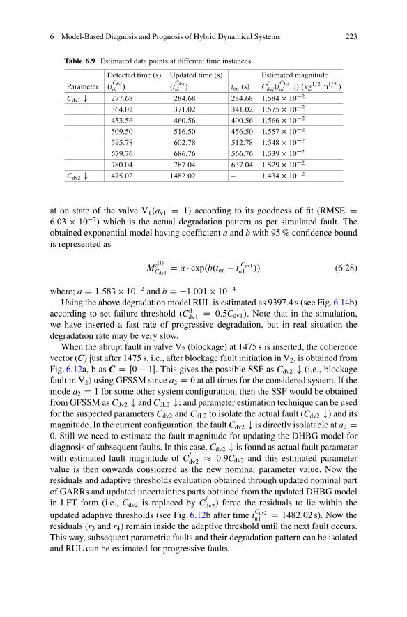
6 Model-Based Diagnosis and Prognosis of Hybrid Dynamical Systems 223
Table 6.9 Estimated data points at different time instances
Detected time (s) Updated time (s) Estimated magnitude
Parameter .tCdvj
di / .tCdvj
ui / ton (s) Cfdvj.t
Cdvj
ui ; z/ .kg1=2 m1=2 )
Cdv1 # 277:68 284:68 284:68 1:584� 10�2
364:02 371:02 341:02 1:575� 10�2
453:56 460:56 400:56 1:566� 10�2
509:50 516:50 456:50 1:557� 10�2
595:78 602:78 512:78 1:548� 10�2
679:76 686:76 566:76 1:539� 10�2
780:04 787:04 637:04 1:529� 10�2
Cdv2 # 1475:02 1482:02 – 1:434� 10�2
at on state of the valve V1.av1 D 1/ according to its goodness of fit (RMSE D6:03 � 10�7) which is the actual degradation pattern as per simulated fault. Theobtained exponential model having coefficient a and b with 95 % confidence boundis represented as
Mz.1/
Cdv1D a � exp.b.ton � t Cdv1
u1 // (6.28)
where; a D 1:583 � 10�2 and b D �1:001 � 10�4Using the above degradation model RUL is estimated as 9397.4 s (see Fig. 6.14b)
according to set failure threshold .Cfldv1 D 0:5Cdv1/. Note that in the simulation,
we have inserted a fast rate of progressive degradation, but in real situation thedegradation rate may be very slow.
When the abrupt fault in valve V2 (blockage) at 1475 s is inserted, the coherencevector (C) just after 1475 s, i.e., after blockage fault initiation in V2, is obtained fromFig. 6.12a, b as C D Œ0 � 1�. This gives the possible SSF as Cdv2 # (i.e., blockagefault in V2) using GFSSM since a2 D 0 at all times for the considered system. If themode a2 D 1 for some other system configuration, then the SSF would be obtainedfrom GFSSM as Cdv2 # and CdL2 #; and parameter estimation technique can be usedfor the suspected parameters Cdv2 and CdL2 to isolate the actual fault (Cdv2 #) and itsmagnitude. In the current configuration, the fault Cdv2 # is directly isolatable at a2 D0. Still we need to estimate the fault magnitude for updating the DHBG model fordiagnosis of subsequent faults. In this case, Cdv2 # is found as actual fault parameterwith estimated fault magnitude of Cf
dv2 � 0:9Cdv2 and this estimated parametervalue is then onwards considered as the new nominal parameter value. Now theresiduals and adaptive thresholds evaluation obtained through updated nominal partof GARRs and updated uncertainties parts obtained from the updated DHBG modelin LFT form (i.e., Cdv2 is replaced by Cf
dv2) force the residuals to lie within theupdated adaptive thresholds (see Fig. 6.12b after time tCdv2
u1 D 1482:02 s). Now theresiduals (r3 and r4) remain inside the adaptive threshold until the next fault occurs.This way, subsequent parametric faults and their degradation pattern can be isolatedand RUL can be estimated for progressive faults.
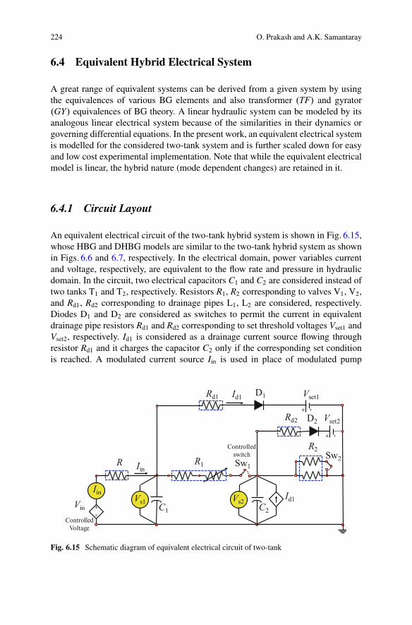
224 O. Prakash and A.K. Samantaray
6.4 Equivalent Hybrid Electrical System
A great range of equivalent systems can be derived from a given system by usingthe equivalences of various BG elements and also transformer .TF/ and gyrator.GY/ equivalences of BG theory. A linear hydraulic system can be modeled by itsanalogous linear electrical system because of the similarities in their dynamics orgoverning differential equations. In the present work, an equivalent electrical systemis modelled for the considered two-tank system and is further scaled down for easyand low cost experimental implementation. Note that while the equivalent electricalmodel is linear, the hybrid nature (mode dependent changes) are retained in it.
6.4.1 Circuit Layout
An equivalent electrical circuit of the two-tank hybrid system is shown in Fig. 6.15,whose HBG and DHBG models are similar to the two-tank hybrid system as shownin Figs. 6.6 and 6.7, respectively. In the electrical domain, power variables currentand voltage, respectively, are equivalent to the flow rate and pressure in hydraulicdomain. In the circuit, two electrical capacitors C1 and C2 are considered instead oftwo tanks T1 and T2, respectively. Resistors R1, R2 corresponding to valves V1, V2,and Rd1, Rd2 corresponding to drainage pipes L1, L2 are considered, respectively.Diodes D1 and D2 are considered as switches to permit the current in equivalentdrainage pipe resistors Rd1 and Rd2 corresponding to set threshold voltages Vset1 andVset2, respectively. Id1 is considered as a drainage current source flowing throughresistor Rd1 and it charges the capacitor C2 only if the corresponding set conditionis reached. A modulated current source Iin is used in place of modulated pump
Vset1
C2C1
+ -
+ -
Vs2Vs1
Iin
Vin
Controlled Voltage
+-
R R1
Rd1
Rd2
Iin
Id1
Vset2
Id1
Sw2
R2
D2
D1
Sw1
Controlled switch
Fig. 6.15 Schematic diagram of equivalent electrical circuit of two-tank
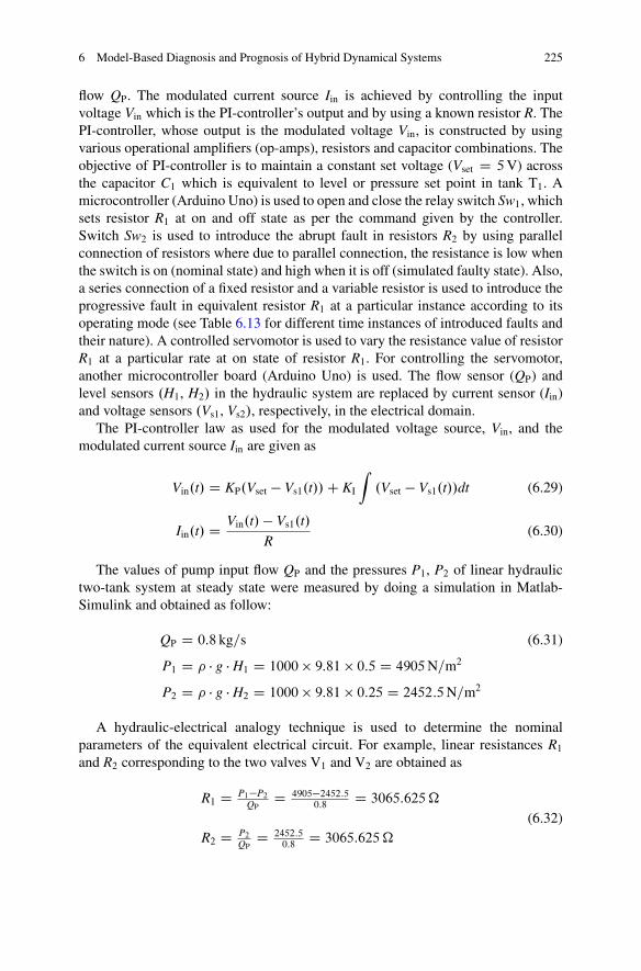
6 Model-Based Diagnosis and Prognosis of Hybrid Dynamical Systems 225
flow QP. The modulated current source Iin is achieved by controlling the inputvoltage Vin which is the PI-controller’s output and by using a known resistor R. ThePI-controller, whose output is the modulated voltage Vin, is constructed by usingvarious operational amplifiers (op-amps), resistors and capacitor combinations. Theobjective of PI-controller is to maintain a constant set voltage (Vset D 5V) acrossthe capacitor C1 which is equivalent to level or pressure set point in tank T1. Amicrocontroller (Arduino Uno) is used to open and close the relay switch Sw1, whichsets resistor R1 at on and off state as per the command given by the controller.Switch Sw2 is used to introduce the abrupt fault in resistors R2 by using parallelconnection of resistors where due to parallel connection, the resistance is low whenthe switch is on (nominal state) and high when it is off (simulated faulty state). Also,a series connection of a fixed resistor and a variable resistor is used to introduce theprogressive fault in equivalent resistor R1 at a particular instance according to itsoperating mode (see Table 6.13 for different time instances of introduced faults andtheir nature). A controlled servomotor is used to vary the resistance value of resistorR1 at a particular rate at on state of resistor R1. For controlling the servomotor,another microcontroller board (Arduino Uno) is used. The flow sensor (QP) andlevel sensors .H1, H2/ in the hydraulic system are replaced by current sensor (Iin)and voltage sensors .Vs1, Vs2/, respectively, in the electrical domain.
The PI-controller law as used for the modulated voltage source, Vin, and themodulated current source Iin are given as
Vin.t/ D KP.Vset � Vs1.t//C KI
Z.Vset � Vs1.t//dt (6.29)
Iin.t/ D Vin.t/ � Vs1.t/
R(6.30)
The values of pump input flow QP and the pressures P1, P2 of linear hydraulictwo-tank system at steady state were measured by doing a simulation in Matlab-Simulink and obtained as follow:
QP D 0:8 kg=s (6.31)
P1 D � � g � H1 D 1000 � 9:81 � 0:5 D 4905N=m2
P2 D � � g � H2 D 1000 � 9:81 � 0:25 D 2452:5N=m2
A hydraulic-electrical analogy technique is used to determine the nominalparameters of the equivalent electrical circuit. For example, linear resistances R1and R2 corresponding to the two valves V1 and V2 are obtained as
R1 D P1�P2QP
D 4905�2452:50:8
D 3065:625�
R2 D P2QP
D 2452:50:8
D 3065:625�
(6.32)
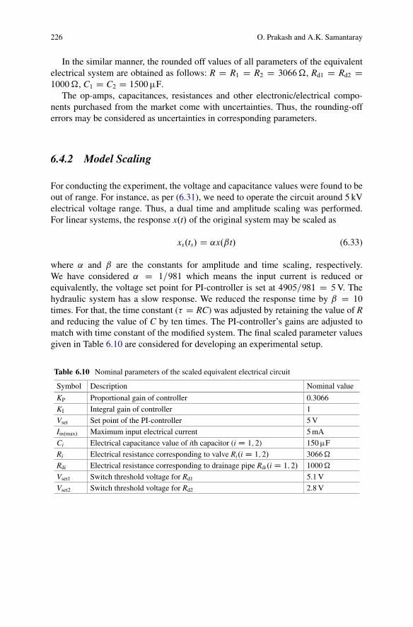
226 O. Prakash and A.K. Samantaray
In the similar manner, the rounded off values of all parameters of the equivalentelectrical system are obtained as follows: R D R1 D R2 D 3066�, Rd1 D Rd2 D1000�, C1 D C2 D 1500�F.
The op-amps, capacitances, resistances and other electronic/electrical compo-nents purchased from the market come with uncertainties. Thus, the rounding-offerrors may be considered as uncertainties in corresponding parameters.
6.4.2 Model Scaling
For conducting the experiment, the voltage and capacitance values were found to beout of range. For instance, as per (6.31), we need to operate the circuit around 5 kVelectrical voltage range. Thus, a dual time and amplitude scaling was performed.For linear systems, the response x.t/ of the original system may be scaled as
xs.ts/ D ˛x.ˇt/ (6.33)
where ˛ and ˇ are the constants for amplitude and time scaling, respectively.We have considered ˛ D 1=981 which means the input current is reduced orequivalently, the voltage set point for PI-controller is set at 4905=981 D 5V. Thehydraulic system has a slow response. We reduced the response time by ˇ D 10
times. For that, the time constant (� D RC) was adjusted by retaining the value of Rand reducing the value of C by ten times. The PI-controller’s gains are adjusted tomatch with time constant of the modified system. The final scaled parameter valuesgiven in Table 6.10 are considered for developing an experimental setup.
Table 6.10 Nominal parameters of the scaled equivalent electrical circuit
Symbol Description Nominal value
KP Proportional gain of controller 0.3066
KI Integral gain of controller 1
Vset Set point of the PI-controller 5 V
Iin.max/ Maximum input electrical current 5 mA
Ci Electrical capacitance value of ith capacitor (i D 1; 2) 150�F
Ri Electrical resistance corresponding to valve Ri.i D 1; 2/ 3066�
Rdi Electrical resistance corresponding to drainage pipe Rdi.i D 1; 2/ 1000�
Vset1 Switch threshold voltage for Rd1 5.1 V
Vset2 Switch threshold voltage for Rd2 2.8 V

6 Model-Based Diagnosis and Prognosis of Hybrid Dynamical Systems 227
6.5 Experimental Study
An experimental setup of equivalent electrical hybrid system is shown in Fig. 6.16a.The circuit in the breadboard is the equivalent electrical hybrid system of thesimulated two-tank hybrid system in reduced scale whose dynamics is nearly similarto the two-tank hybrid system dynamics. The schematic diagram of equivalentelectrical circuit of two-tank hybrid system is already shown in Fig. 6.15. Thevarious components of the circuit including PI-controller and the microcontrollerare marked in Fig. 6.16b.
The experimental data were collected at a fixed sampling rate of 0.002 s fromthe current sensor Iin and voltage sensors Vs1 and Vs2 using a data-acquisition card(NI-USB6211). For computation of residuals, thresholds, mode identification andparameter estimation, LabVIEW-Matlab interface was used. The experimentallycollected data were fed into the DHBG-LFT model of the electrical hybrid systemfor evaluation of residuals and adaptive thresholds. The GFSSM and MCSSM ofthe equivalent electrical system presented in Tables 6.11 and 6.12, respectively,are nearly same as that of the hydraulic two-tank system; only the correspondingparameter’s nomenclature is changed. The coefficient of discharge parameter Cdi #is considered equivalent to 1/Ri #, where Ri is the linear resistance in electricaldomain, i.e., the signature of Cdi # is replaced by Ri ". Similarly, the signature ofCdi " is replaced by Ri #.
As in the simulation, two types of faults were introduced in the experimentalmodel. First one is a progressive fault in resistor R1 as per Eq. (6.34) in its on state.The second one is an abrupt fault in resistor R1 as per Eq. (6.35) (see Table 6.13).The failure threshold (Rfl
1) of resistor R1 is considered as twice of its nominal valueat on state for RUL estimation.
Fig. 6.16 (a) An experimental setup of electrical hybrid system (b) Enlarge view of breadboardshowing different components within dotted boxes: (1) PI-controller, (2) R, (3) C1, (4) C2, (5)Variable resistor (R1) with microcontroller, (6) R2, (7) Relay switch (Sw1) with microcontroller,(8) Sw2, (9) Id1, (10) D1, Rd1 and Vset1, (11) D2, Rd2 and Vset2, (12) Buffers
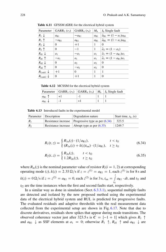
228 O. Prakash and A.K. Samantaray
Table 6.11 GFSSM (GSS) for the electrical hybrid system
Parameter GARR3 .r3/ GARR4 .r4/ Mb Ib Single fault
R1 # aR1 �aR1 aR1 NaR1 D .1� a1/aR1
R1 " �aR1 aR1 aR1 NaR1 D .1� a1/aR1
R2 # 0 C1 1 0
R2 " 0 �1 1 Na2 D .1� a2/
Rd1 # a1 �a1 a1 Na1 D .1� aR1/a1Rd1 " �a1 a1 a1 Na1 D .1� aR1/a1Rd2 # 0 a2 a2 0
Rd2 " 0 �a2 a2 0
RLeak1 # C1 0 1 1
RLeak2 # 0 C1 1 0
Table 6.12 MCSSM for the electrical hybrid system
Parameter GARR3 .r3/ GARR4 .r4/ Mb Ib Single fault
aR1 " +1 -1 1 1
aR1 # -1 +1 1 1
Table 6.13 Introduced faults in the experimental model
Parameter Description Degradation nature Start time, tfi, (s)
R1 Resistance increase Progressive type as per (6.34) 323.5
R2 Resistance increase Abrupt type as per (6.35) 1249.7
R1.t; z/ D�
R1n.z/ � .1=aR1/; t < tf1.R1n.z/C k.z/ton/ � .1=aR1/; t � tf1
(6.34)
R2.t; z/ D�
R2n.z/; t < tf21:2R2n.z/; t � tf2
(6.35)
where Rin.z/ is the nominal parameter value of resistor Ri.i D 1; 2/ at correspondingoperating mode (z/; k.z/ D 2:35�=s if z D z.1/ D aR1 D 1, each z.1/ is for 8 s and
k.z/ D 0�=s if z D z.2/ D aR1 D 0, each z.2/ is for 3 s, ton DtR
tf1
aR1 � dt, and tf1 and
tf2 are the time instances when the first and second faults start, respectively.In a similar way as done in simulation (Sect. 6.3.3.1), sequential multiple faults
are detected and isolated by the new proposed method using the experimentaldata of the electrical hybrid system and RUL is predicted for progressive faults.The evaluated residuals and adaptive thresholds with the real measurement datacollected from the experimental setup are shown in Fig. 6.17. Note that due todiscrete derivatives, residuals show spikes that appear during mode transitions. Theobserved coherence vector just after 323.5 s is C D Œ�1 C 1� which gives R1 "and aR1 # as SSF elements at a1 D 0; otherwise R1 ", Rd1 " and aR1 # are

6 Model-Based Diagnosis and Prognosis of Hybrid Dynamical Systems 229
0 250 500 750 1000 1250 1500
-2
0
2
Time (s)
r 3(m
A)
1u1Rt 1
u2Rt 1
u3Rt 1
u4Rt
1d1Rt 1
d2Rt 1
d3Rt 1
d4Rt
-2
0
2
r 4(m
A)
0 250 500 750 1000 1250 1500Time (s)
1u1Rt 1
u2Rt 1
u3Rt 1
u4Rt
1d1Rt 1
d2Rt 1
d3Rt 1
d4Rt
2u1Rt
2d1Rt
ba
Fig. 6.17 Response of residuals (a) r3 and (b) r4 using proposed method with dynamically updatedparameter and adaptive threshold
Table 6.14 Estimated data points at different time instances
Estimated magnitude
Parameter Detected time (s) .tRj
ui / Updated time (s) .tRj
ui / ton (s) Rfj .t
Rj
ui ; z/ .�/
R1 " 399.768 402.768 402.768 3326.53
565.572 568.572 523.572 3605.01
749.380 752.380 656.380 3917.57
938.692 941.692 794.692 4250.02
R2 " 1249.702 1252.702 – 3740.5
SSF elements at a1 D 1. Consistency in mode aR1 D 1 is found by evaluatingthe all sensitive ARRs at current mode information which indicates the observedinconsistency is due to parametric fault. Upon parameter estimation and successiveupdation of DHBG model at various time instances, it is confirmed that the faultR1 " is of progressive nature (see Fig. 6.17 where residuals r3 and r4 are updatedat various time instances during degradation pattern identification of R1). Theestimated magnitude of degrading resistance R1 at the mode z D z.1/ D aR1 D 1 atdifferent time instances tR1
ui .i D 1; 2; 3; 4/ is shown in Table 6.14.Initially, the obtained data points at time instances .tR1
u1 / and .tR1u2 / corresponding
to mode z D z.1/ D aR1 D 1 are used to find the linear degradation model forthe resistor R1 as presented in Fig. 6.18a. Initial estimated value of RUL using thelinear degradation model at on state of resistor R1 and infinite resistance value at offstate is found as 1672.92 s (see Fig. 6.19a). This initial degradation model is furtherupdated with modified model when newer information of parameter estimates areobtained during monitoring.
As the monitoring is continued, the new information of degradation data ofresistor R1.t; z/ is obtained via parameter estimation at time instances tR1
ui , (i D 3; 4)at the same mode z D z.1/ D aR1 D 1, which are presented in Table 6.14. Various

230 O. Prakash and A.K. Samantaray
400 420 440 460 480 500 5203200
3300
3400
3500
3600
3700a b
R 1( t,
z(1) )
( Ω)
(1)1
1 on u1 =2.305( ) 3327RzRM t t− +
ton (s) 400 500 600 700 8003200
340036003800400042004400
ton (s)
(1)1
1 on u1 =2.357( ) 3323RzRM t t− +
RMSE4.49
Fig. 6.18 (a) Linear degradation model at mode aR1 D 1 as two data points are known, (b) finallyidentified degradation model at mode aR1 D 1 with new information of data points
0 400 800 1200 1600 2000300035004000450050005500
6132
a b
Time (s)
R 1(t,
z) (Ω
)
RUL = 1672.92sLinear degradation model at on state
1630 1672.926075
61321flR
1flR
0 400 800 1200 1600 2000300035004000450050005500
6132
Time (s)
RUL = 1635.77sLinear degradation model at on state
1flR
1595 1635.77
61321flR
Fig. 6.19 Estimated RUL of parameter R1 (a) With initially assumed linear degradation modelwhen only two data points are known (b) with finally confirmed linear degradation model with thenew information of degradation state at on state of resistor R1, and considering infinite resistancein off state
degradation models are tried and linear degradation model was found as a best fitmodel for on state of the resistor R1.aR1 D 1) according to goodness of fit (RMSE =4.49). Indeed, this is the actual degradation introduced in the experiment. The finallinear degradation model having coefficient P1 and P2 with 95 % confidence boundis given as
Mz.1/
R1D P1.ton � t R1
u1 /C P2 (6.36)
where P1 D 2:357 and P2 D 3323.Using the degradation model (6.36), the RUL is estimated as 1635.77 s (see
Fig. 6.19b) according to set failure threshold (Rfl1 D 2R1).
When the abrupt fault in resistor R2 at 1249.7 s is inserted, the coherence vector(C) just after 1249.7 s, i.e., after fault initiation in resistor R2, is obtained fromFig. 6.17a, b as C D Œ0�1�. This gives the possible SSF as R2 " (i.e., increasing faultin resistor R2) using GFSSM since a2 D 0. Even though the fault R2 " is directlyisolable at a2 D 0, we still need to estimate the fault magnitude for updating the
6 Model-Based Diagnosis and Prognosis of Hybrid Dynamical Systems 231
DHBG model for diagnosis of subsequent faults. In this case, R2 " is found as actualfault parameter with estimated fault magnitude of Rf
2 � 1:2R2 at .tR2u1 / D 1252:702 s
and this estimated parameter value is then onwards considered as the new nominalparameter value.
6.6 Conclusions
This chapter proposes a strategy for fault diagnosis and prognosis of hybriddynamical system by using bond graph modelling as a common framework forsystem modelling, virtual prototyping, fault diagnosis rule development, parameterand system identification, and RUL estimation. The proposed approach detects andisolates sequential multiple faults of different types, i.e., discrete mode faults, abruptand progressive parametric faults; and also predicts the RUL if the detected faultis due to progressive parameter drift. The developed method is first applied to asimulated benchmark problem and then it is experimentally validated on a scaledequivalent electrical circuit model.
The response time (time constant) of the system and the time taken fordegradation model are the two critical parameters that govern the applicability ofthis diagnosis and prognosis scheme. For processes or systems with slow responsetime, the time spent for parameter estimation is not significant. However, for fastsystems like the equivalent electrical system considered in this study, the parameterestimation needs to be faster. This is achieved by narrowing down the numberof suspected faults and using sensitivity signature for information regarding faultdirection. Global fault sensitivity signatures of the hybrid dynamical system are usedto identify the possible fault directions from the residual responses. The informationof operating mode, possible fault candidates and directions of correspondingparameter deviations are used in a constrained least square error minimization-based estimation of fault parameters. It was found that richer information gleanedfrom sensitivity signatures allows quicker and reliable identification of faults anddegradation model for RUL estimation.
For RUL estimation, use of multiple degradation models which include opera-tional modes as additional control parameter and evolve through degradation modelidentification is considered in this study for hybrid dynamical system. Models arecontinually evolved with time by adapting to the new information of the stateof degradation of the monitored system to provide accurate RUL with boundeduncertainty value. This overcomes the drawbacks of various existing methods.
References
1. Vachtsevanos, G., Lewis, F. L., Roemer, M., Hess, A., & Wu, B. (2006). Intelligent faultdiagnosis and prognosis for engineering systems. Hoboken: Wiley.
2. Mukherjee, A., Karmakar, R., & Samantaray, A. K. (2006). Bond graph in modelling,simulation and fault identification. New Delhi: I. K. International Pvt. Ltd.

232 O. Prakash and A.K. Samantaray
3. Borutzky, W. (2010). Bond graph methodology: Development and analysis of multidisciplinarydynamic system models. London: Springer.
4. Mosterman, P. J., & Biswas, G. (1995). Behavior generation using model switching: A hybridbond graph modelling technique. Transactions of The Society for Computer Simulation, 27(1),177–182.
5. Roychoudhury, I., Daigle, M. J., Biswas, G., & Koutsoukos, X. (2010). Efficient simulationof hybrid systems: A hybrid bond graph approach. Simulation: Transactions of the Society forModeling and Simulation International, 87(6), 467–498.
6. Wang, D., Yu, M., Low, C. B., & Arogeti, S. (2013). Model-based health monitoring of hybridsystems. New York: Springer.
7. Samantaray, A.K., & Bouamama, B. O. (2008). Model-based process supervision: A bondgraph approach. London: Springer.
8. Borutzky, W. (2015). Bond graph model-based fault diagnosis of hybrid systems. Switzerland:Springer.
9. Levy, R., Arogeti, S., Wang, D., & Fivel, O. (2015). Improved diagnosis of hybrid systemsusing instantaneous sensitivity matrices. Mechanism and Machine Theory, 91, 240–257.
10. Narasimhan, S., & Biswas, G. (2007). Model-based diagnosis of hybrid systems. IEEETransactions on Systems, Man, and Cybernetics, Part A: Systems and Humans, 37(3), 348–361.
11. Ghoshal, S. K., Samanta, S., & Samantaray, A. K. (2012). Robust fault detection and isolationof hybrid systems with uncertain parameters. Proceedings of the Institution of MechanicalEngineers, Part I: Journal of Systems and Control Engineering, 226(8), 1013–1028.
12. Samantaray, A. K., Medjaher, K., Bouamama, B. O., Staroswiecki, M., & Dauphin-Tanguy, G.(2006). Diagnostic bond graphs for online fault detection and isolation. Simulation ModellingPractice and Theory, 14, 237–262.
13. Medjaher, K., & Zerhouni, N. (2009). Residual-based failure prognostic in dynamic systems.In The 7th IFAC Symposium on Fault Detection, Supervision and Safety of Technical ProcessesHeld in Barcelona, Spain (pp. 716–721).
14. Medjaher, K., & Zerhouni, N. (2013). Hybrid prognostic method applied to mechatronicsystems. International Journal of Advanced Manufacturing Technology, 69(1–4), 823–834.
15. Ming, Y., Wang, D., & Luo, M. (2015). An integrated approach to prognosis of hybrid systemswith unknown mode changes. IEEE Transactions on Industrial Electronics, 62(1), 503–515.
16. Jha, M. S., Dauphin-Tanguy, G., & Bouamama, B. O. (2016). Particle filter based hybridprognostics for health monitoring of uncertain systems in bond graph framework. MechanicalSystems and Signal Processing, 75, 301–329.
17. Samantaray, A. K., & Ghoshal, S. K. (2007). Sensitivity bond graph approach to multiplefault isolation through parameter estimation. Proceedings of the Institution of MechanicalEngineers. Part-I: The Journal of Systems and Control Engineering, 221(4), 577–587.
18. Gawthrop, P. J. (2000). Sensitivity bond graphs. Journal of the Franklin Institute, 337(7),907–922.
19. Borutzky, W. (2011). Incremental bond graphs. In Bond graph modelling of engineeringsystems (pp. 135–176). New York: Springer.
20. Merzouki, R., Samantaray, A. K., Pathak, P. M., & Bouamama, B. O. (2012). Intelligentmechatronic systems: Modeling, control and diagnosis. New York: Springer Science andBusiness Media.
21. Low, C. B., Wang, D., Arogeti, S., & Luo, M. (2009). Fault parameter estimation for hybridsystems using hybrid bond graph. In Proceedings of the 3rd IEEE Multi-Conference on Systemsand Control, Saint Petersburg, Russia, July 8–10 (pp. 133–134).
Chapter 7Particle Filter Based Integrated HealthMonitoring in Bond Graph Framework
Mayank S. Jha, G. Dauphin-Tanguy, and B. Ould-Bouamama
7.1 Introduction
Besides the abrupt faults that have been considered in the previous chapters,incipient system faults and degradations of the system parameters pose significanthurdles in efficient maintenance of the system. For example, fatigue enabled wear inturbine blades, incipient leakage in valves of process engineering systems, frictioninduced jamming of rod in aircraft actuators, etc., pose great threat to systemreliability and safety. Such problems are efficiently resolved when addressed underthe realm of the so-called condition based maintenance (CBM) and prognosticsand health management (PHM) [34]. The latter represent a predictive maintenancephilosophy that has emerged only recently on contrary to the traditional strategiesbased upon preventive and corrective maintenance.
The main feature of CBM is the consideration of the “actual” condition of systemcomponent for designing maintenance actions rather than on an elapsed time orrunning hours’ basis. Thus, CBM primarily depends upon current assessment ofsystem health or state and involves real time data monitoring and processing. Thetwo basic aspects of CBM are diagnostics and prognostics. As seen in the previouschapters, Diagnostics involves detection of fault and thereby, identification andquantification of the root cause of a problem. Prognostics involves prediction ofthe future health of the equipment either before or after a problem occurred [34,
M.S. Jha (�)Ecole Centrale de Lille, Toulouse, Francee-mail: [email protected]; [email protected]
G. Dauphin-TanguyEcole Centrale de Lille, Villeneuve-d’Ascq, France
B. Ould-BouamamaEcole Polytech de Lille, Villeneuve d Ascq cedex, France
© Springer International Publishing Switzerland 2017W. Borutzky (ed.), Bond Graphs for Modelling, Control and FaultDiagnosis of Engineering Systems, DOI 10.1007/978-3-319-47434-2_7
233

234 M.S. Jha et al.
60]. As stated in [33], prognostics is “estimation of time to failure and risk for oneor more existing and future failure modes.”
The Remaining Useful Life (RUL) becomes a reliable estimate of the time tofailure; it denotes how long system can function safely/reliably and within theprescribed limits of system functionalities. Thus, assessment of RUL involvespredictions in future. In this context, the major motivation remains in providingsufficient lead-time between detection of a fault (diagnostic step) and occurrenceof the system/component failure so that pro-active maintenance actions can bestrategized in advance [62].
RUL prediction is not a trivial task as it involves future predictions whichnot only require precise information of current health, but also remain sensitiveto various types of uncertainties to a large degree. These uncertainties involvestochastic evolution of incipient degradations, failure modes, varying operationalconditions, measurement noise, etc. In face of all such uncertainties, the prognosticprocedure must be able to accurately assess the rapidity of system degradationtill failure and novel events that may significantly influence the assumed/learntdegradation trend. Due to inherent stochastic phenomena and uncertainty involved,evaluation of confidence on RUL predictions is given a significant weightage. Infact, several business decisions are based upon confidence limits associated withRUL predictions rather than the specific value of RUL itself [59]. In essence,determination of accurate and precise RUL estimate forms the core objective ofany prognostics procedure.
On the other hand, the term PHM describes the systems that implement a CBMphilosophy [62]. However, in the context of PHM, prognostics gains a wider mean-ing encompassing the tasks of fault detection, fault-identification, current healthassessments, performance monitoring, and RUL predictions [34]. Thus, diagnosticsand prognostics form building blocks of any CBM enabled PHM architecture. Whenthese two essential tasks are achieved in an integrated manner, such a commonparadigm may be given the designation of integrated health monitoring framework[9, 35].
In BG framework, diagnostics and prognostics task can be achieved in an inte-grated way by exploiting the properties of Analytical Redundancy Relations (ARRs)and their numerical evaluations or residuals. In this context, due to deterministicnature of ARRs, most of the existing works have neglected the inherent randomnessin damage progression [20, 23, 48, 49], which in turn has led to RUL predictionsthat do not incorporate associated uncertainties and inherent stochasticity.
This chapter details ARR based integrated health monitoring methodology wherethe benefits of BG in Linear Fractional Transformations (BG-LFTs) have beenintegrated with advantages of Bayesian inference techniques to obtain accurateand precise estimate of parametric health in probabilistic domain. The inherentrandomness in degradation progression is effectively managed by using sequentialMonte Carlo based particle filters (PF) for estimation of state of a system parameterand subsequent RUL prediction in probabilistic domain.
After this introduction, Sect. 7.2 details various approaches of prognostics, BG-LFT method, and non-linear Bayesian inference technique using PFs. Section 7.3
7 Particle Filter Based Integrated Health Monitoring in Bond Graph Framework 235
discusses degradation models (DM). The method of prognostics is described inthe next section. Sections 7.4 and 7.5 discuss the integrated health monitoringstrategy and evaluation metrics, respectively. Section 7.6 details the applicationof methodology on a mechatronic system in real system. Section 7.7 drawsconclusions.
7.2 Background and Techniques
This section discusses different techniques of prognostics. Moreover, BG-LFTtechnique of modelling uncertain systems and associated fault detection techniqueis discussed briefly. The latter is employed for detection of degradation initiationfor the integrated health monitoring purposes. Additionally, non-linear Bayesianfiltering using particle filters (PF) is described as it plays a significant role in theprognostics method presented in this chapter.
7.2.1 Approaches of Prognostics
Last decade has witnessed an extensive surge in development of various prognosticstechniques and its application in diverse technical domains. Due to the inherentversatility, approaches of prognostics have been attempted to be classified indifferent ways [33, 34, 43, 45, 62], etc. Here, the authors have preferred to adaptthe classification presented in [60].
Probabilistic Life-Usage Models These approaches depend upon the statisticalinformation collected to assess the historical failure rate of the components anddevelop life-usage models [6, 30, 53]. Various functions can be applied to modelstatistical failure data such as exponential, normal, lognormal, and Weibull functions[39]. Moreover, the RUL is described as a probability density function (PDF)[60, 62]. Accurate assessment of RUL demands huge sets of failure database andextensive testing.
Data-Driven Prognostics The data associated with system functionality, degrada-tion patterns, etc., are exploited using machine learning techniques to extract systemsignals and features which can be used to obtain behavior of damage progression,health index, etc. Broadly, two major strategies can be identified as discussed below.
Degradation Trend Extrapolation and Time Series Predictions In broad terms, thesignals that indicate the state of the system are mapped as function of time andextrapolated in future using various techniques until a prefixed failure thresholdis reached/crossed [27]. Mainly time series forecasting techniques are borrowedfor this purpose such as: linear/non-linear regression techniques, autoregressivemodels [63], exponential smoothing techniques [10], autoregressive moving average

236 M.S. Jha et al.
(ARMA), and autoregressive integrated moving average (ARIMA) [8]. The ARMAmodels and associated variants prove efficient for short-term predictions. Due tonoise and inefficient uncertainty management, they prove less reliable for long termpredictions.
Learning Damage Progression The degradation trends, failure patterns, etc., arelearnt for training mathematical models. The latter in turn is used to model therelationship between damage progression and RUL. Employment of artificial neuralnetworks (ANNs) and their numerous variants fall under this category. Feed-forwardANNs are extensively employed to estimate the current degradation index (state) byusing system features (extracted signals, feature pattern, etc.) as inputs. Then, onestep ahead prediction is generated by using previous state of degradation values(degradation index). The next iteration uses this prediction to produce long termpredictions [31]. Major drawback in this context is that the efficiency of predictionsremain limited in face of variable degradation trends, novel failure modes, etc. Assuch, accurate RUL predictions are not obtained on individual component unit tounit basis, but rather over large sets of component population. A comprehensiveupdated review of data-driven techniques can be found in [3, 61].
Model Based Prognostics Under this category, physics-of-failure models or degra-dation models (DM) are typically used to assess the damage progression and state ofhealth (SOH). These DMs are derived from the first principles of physics. As such,they possess the capability of attaining maximum accuracy and versatility (scope ofadaptation under varying degradation trend). There is a clear understanding of theunderlying degradation process. There exists vast literature such as fatigue modelsfor modelling initiation and propagation of cracks in structural components [65],electrolytic overstress aging [12], Arrhenius equation for prediction of resistancedrift [41], physics-inspired power model [47] or log-linear model for degradationof current drain [46], and physics-inspired exponential degradation model foraluminum electrolytic capacitors [42].
Given the behavioral model of damage progression, the current SOH is popularlyobtained in probabilistic domain with the help of Bayesian estimation techniques.Based upon the current SOH estimate, prediction of RUL is done. Such a prob-abilistic framework involving recursive Bayesian techniques efficiently addressesthe main issues related to SOH under variable degradation; efficient managementof uncertainty, environmental noise, future loading conditions, and associatedconfidence limits for RUL predictions [15, 16, 18, 54]. Filter for estimation andprediction process is chosen based upon the modelling hypothesis and desiredperformances [19]. Well-known Kalman filter, an optimal estimator for linearsystems, has been used for prognostics in [12]. Extended Kalman filter (EKF)or unscented Kalman filter may also be used for joint state-parameter estimationas presented in [13, 52], respectively. However, they remain restricted to additive

7 Particle Filter Based Integrated Health Monitoring in Bond Graph Framework 237
Gaussian noise. Additionally, EKF being sub-optimal diverges quickly if the initialestimate of state is different from the reality by big measure or the model consideredfor estimation is not correct [57].
Set in Monte Carlo framework, PFs form a suitable filter choice in this context [4,25]. PF can be applied to non-linear systems corrupted with non-Gaussian noises,for which optimal solutions may be unavailable or intractable. Comprehensive com-parison of filters for prognostic purposes is found in [3, 19, 57]. Recently, PFs havebeen extensively for prognostic purposes [50]. Significant works include predictionof end of life (EOL) in lithium-ion batteries [55], battery health monitoring [56],prediction of battery grid corrosion [1], estimation and prediction of crack growth[11], fuel cell prognostics [37], application to damage prognostics in pneumaticvalve [15, 17], estimation–prediction of wear as concurrent damage problem incentrifugal pumps with a variance control algorithm [18], employment in distributedprognosis [54], and uncertainty management for prognostics [5]. Particle filtersattract considerable attention [2], owing to the ever growing efforts being madefor betterment in performances and computational efficiency, such as the use ofcorrection loops [51], fixed–lag filters [14], and kernel smoothing method [32].
The major issue in this type of approach is the accurate and reliable modellingof underlying degradation progression. Often, such accurate degradation models arenot available.
Hybrid Prognostics The problem of non-availability of highly accurate degradationmodels is alleviated by fusing the advantages of model based and data-driven tech-niques. This way, there is significant amelioration in the overall prognostic approach[36, 37]. The basic philosophy remains in capturing the damage progression usingDMs that can be: (1) based upon physics of failure, first principles of behavioralphysics (2) derived using machine learning techniques, and (3) obtained statisticallyby finding a mathematical model that best fits a given set of degradation data suchas linear model D.t/ D at C b, logarithmic model D.t/ D a ln.t/C b, power modelD.t/ D bta, exponential model D.t/ D b � eat with D(t) as an index representing thedegradation (change, percentage change, etc.), and a and b as the model parameters.In this context, significant works are obtaining capacitance loss DM using non-linearleast square regression [12], relevance vector machine regression performed overaging tests data [57], DM approximated by a linear part and logarithmic/exponentialpart [37], and residual based statistical DM [36]. Once the DM has been obtainedwith acceptable accuracy, recursive Bayesian techniques as discussed previouslycan be employed to estimate SOH and obtain subsequent RUL predictions. Thisway, benefits of Bayesian estimators are integrated with data-driven approaches tolearn the DM as the current information arrives sequentially.
238 M.S. Jha et al.
7.2.2 Prognostics in BG Framework
Almost all of the existing attempts in BG framework for prognostics have been ARRbased and deterministic in nature. Moreover, DMs are considered deterministicso that the SOH and subsequent RUL predictions are obtained deterministically[20, 23, 35, 48, 49, 64]. Being restricted in deterministic domain, the randomnessassociated with variable damage progression, novel events, noises, etc., are simplyignored. As such, this leads to an inefficient management of the uncertainty inprognostication process and renders the RUL predictions without confidence limits.Recently, Jha et al. [36] proposed a methodology of hybrid prognostics where thebenefits of Bayesian filtering techniques and BG enabled ARRs are integrated forefficient prognostics in probabilistic domain. In fact, this chapter is inspired by thework detailed in [36].
7.2.3 Bond Graph in Linear Fractional Transformations
BG-LFT is an efficient and systematic way of representing parametric uncertaintyover nominal models. An uncertainty on a parameter value � can be introducedunder either an additive form or a multiplicative one, as shown in (7.1) and (7.2),respectively.
� D �n ˙� I � � 0 (7.1)
� D �n . 1˙ ı� / I ı� D �
�n(7.2)
where � and ı� are, respectively, the absolute and relative deviations around thenominal parametric value �n. When the element characteristic law is written in termsof 1
�, (7.2) becomes:
1
�D 1
�n� �1C ı1=�
� I ı1=� D –�
�n C�(7.3)
7.2.3.1 Representation on BG
The representation technique is illustrated briefly by taking a pedagogical exampleof R-element in resistance causality. The characteristic law corresponding to R-element in the linear case (see Fig. 7.1) is given as,
eR D R � fR (7.4)

7 Particle Filter Based Integrated Health Monitoring in Bond Graph Framework 239
Fig. 7.1 (a) R-element in resistance causality. (b) Uncertain R-element in resistance causality inLFT form
In case of uncertainty on R, (7.4) becomes
eR D Rn .1C ıR/ � fR D Rn � fR C ıR � Rn � fR D eRn C eRunc (7.5)
Constitutive Eq. (7.5) can be represented as uncertain R-element as shown inFig. 7.1b, wherein a modulated source MSe is introduced. The latter is associatedwith auxiliary input wR and a virtual effort sensor which is associated withauxiliary output zR. It must be noted that negative (�) sign appears in the BG-LFT representation (see Fig. 7.1) due to the convention of power conservation.Moreover, the symbol De * represent virtual detectors. The virtual detectors are usedto represent the information exchange/transfer.
Similarly, parametric uncertainty on the other passive elements can be repre-sented. The technique remains similar for various other BG elements.
7.2.3.2 BG-LFT Based Robust Fault Detection
Fault diagnosis in BG-LFT framework is mainly dependent upon ARR generation[22]. ARRs are constraint relationships involving only known variables. In thecontext of BG modelling, an ARR W f
�SSe.t/;SSf.t/;Se.t/;Sf.t/; ™) D 0, where ™
is vector of system parameters.
Generation of Uncertain ARRs The generation of robust analytical redundancyrelations from an observable bond graph model is explained by the following steps:
First Step: Preferred derivative causality is assigned to the nominal model anddetectors De (Df) are dualized to SSe (SSf); wherever possible. The BG-LFTmodel is constructed.

240 M.S. Jha et al.
Second Step: The candidate ARRs are generated from “1” or “0” junction, wherepower conservation equation dictates that sum of efforts or flows, respectively, isequal to zero, as:
• For 0-junction:
Xsi � fi;n C
XSf C
Xsiwi D 0 (7.6)
• For 1-junction:
Xsi � ei;n C
XSe C
Xsiwi D 0 (7.7)
with s being the sign rendered to the bond due to energy convention, wi is theuncertain effort (flow) brought by the multiplicative parametric uncertainty ı�i
associated with ith system parameter � i, at 1(0) junction.
Third Step: The unknown effort or flow variables are eliminated using coveringcausal paths from unknown variables to known (measured) variables (dualizeddetectors), to obtain the ARRs which are sensitive to known variables as,
R D ˚nX
Se;X
Sf;SSe;SSf;Rn;Cn; In;TFn;GYn;RSn;X
wi
o(7.8)
where subscript n represents the nominal value of the corresponding BG element.
Generation of Adaptive Thresholds The ARR derived in (7.8) consists of twoperfectly separable parts due to the properties of the BG-LFT model: a nominalpart noted r shown in (7.9) and an uncertain part noted b D
Xwi shown in (7.10).
r D ˚ fSe;Sf;SSe;SSf;Rn;Cn; In;TFn;GYn;RSng (7.9)
b DX
wi
wi D ˚ fSe;Sf;SSe;SSf;Rn;Cn; In;TFn;GYn;RSn; ıR; ıI ; ıC; ıTF; ıGY; ıRSg(7.10)
The uncertain part generates the adaptive threshold over the nominal part. From(7.8), (7.9), and (7.10), following may be obtained:
r C b D 0
r D �b D �X
wi(7.11)
The thresholds are formed in form of envelop as:
�a < r < a (7.12)
7 Particle Filter Based Integrated Health Monitoring in Bond Graph Framework 241
where
a DX
jwij (7.13)
The use of absolute values to generate the thresholds of normal operation ensures therobustness of this algorithm to false alarms. BG-LFT technique is well developedand detailed in literature. Readers are referred to [21, 22] for details.
7.2.4 Non-Linear Bayesian Inference Using Particle Filters
Consider a dynamic system whose state at time step tk is represented by the vectorxk. The evolution of the system state is described by a state space model,
xk D f k .xk�1; vk�1/ (7.14)
yk D hk .xk;wk/ (7.15)
where
• fk W RNx � R
Nv ! RNx is a non-linear state transition function.
• hk W RNx � R
Nw ! RNy is observation function describing the sequence of
measurements yk, obtained sequentially at successive time steps tk.• vk 2 R
Nv is the process noise sequence of known distribution assumedindependent and identically distributed (i.i.d).
• wk 2 RNw is i.i.d measurement noise sequence of known distribution.
Equations (7.14) and (7.15) can be equivalently represented as,
xk D f k .xk�1; vk�1/ $ p
xk
ˇˇxk�1
(7.16)
yk D hk .xk;wk/ $ p
yk
ˇˇxk�1
(7.17)
where p
xk
ˇˇxk�1
represents the state transition probability, p
yk
ˇˇxk�1
is the
likelihood function which signifies the probability of the observation of yk, giventhe current estimate of xk.
Objective of filtering procedure is to obtain estimates of xk, based upon allof the available measurement sequences y1Wk D fyk; k D 1; 2; ::::kg. From theperspectives of Bayesian inference, the objective remains in recursive calculationof state distribution xk, given the set of observations y1 : k up to time tk, with some
degree of belief. Construction of PDF p
xk
ˇˇy1Wk
, known as the filtered posterior
state PDF, provides all the information about xk, inferred from the measurementsy1 : k and the initial state PDF p(x0). The latter p(x0) is assumed to be known. Given
242 M.S. Jha et al.
p
xk�1ˇˇy1 k�1
at time tk�1, theoretically, the posterior state can be estimated in a
recursive way via two sequential steps: prediction and update.
Prediction Application of Chapman–Kolmogorov equation over p
xk�1ˇˇy1 W k�1
at time k–1 gives the estimation of prior state PDF p
xk
ˇˇy1 W k�1
at time tk as,
p
xk
ˇˇy1 W k�1
DZ
p
xk
ˇˇxk�1; y1 W k�1
p
xk�1ˇˇy1 W k�1
DZ
p
xk
ˇˇxk�1
p
xk�1ˇˇy1 W k�1
dxk�1
(7.18)
Here, p
xk
ˇˇxk�1
is obtained from (7.16), where the system is assumed to follow
first order Markov dynamics.
Update Bayes rule is used to update the prior as the new measurement yk arrives,to obtain the posterior distribution of xk as,
p
xk
ˇˇy1 W k
D
p
xk
ˇˇy1 W k�1
p
yk
ˇˇxk
p
yk
ˇˇy1 W k�1
(7.19)
with the normalizing constant being,
p
yk
ˇˇy1 W k�1
DZ
p
xk
ˇˇy1 W k�1
p
yk
ˇˇxk
dxk (7.20)
This step incorporates the latest measurement into a priori state PDF p
xk
ˇˇy1 W k�1
to estimate the posterior state PDF p
xk
ˇˇy1 W k
. The exact Bayesian solution
obtained from recurrence relations (7.18) and (7.19) forms the basis of optimalBayesian inference. This procedure remains tractable and produces best results forideal systems such as linear Gaussian state space models. For the latter, it leadsto the formation of classical Kalman filter. In general, optimal and closed formsolutions for non-linear systems with non-Gaussian noises cannot be analyticallydetermined. For non-linear state space models with additive Gaussian noises, sub-optimal Extended Kalman filter (EKF) has been developed. To obtain optimalsolutions for non-linear systems, one resorts to Monte Carlo Methods. One suchpopular method is described below.
Particle filter (PF) is a type of Sequential Monte Carlo method [25], usedfor obtaining recursive Bayesian inferences via Monte Carlo simulations. Basicphilosophy rests in representing the posterior state PDF by a set of random samplesor “particles” where each of the particles has an associated weight based upon whichthe stateestimates are computed [26]. Sequential importance sampling (SIS) PF is
7 Particle Filter Based Integrated Health Monitoring in Bond Graph Framework 243
one of the most popular PFs in which posterior state PDF p
x0Wkˇˇy1Wk
by a set of N
number of weighted particles [4],
˚�xi0Wk�;wi
k
N
iD1 (7.21)
where˚xi0Wk; i D 1; : : :N
is the set of particles representing the state value with
corresponding associated importance weights as˚wi
k; i D 1; : : :N . Moreover,
x0 W k D ˚xj; j D 0; ::::; k
is the set of all states up to time k. It should be noted
that these weights are the approximations of relative posterior probabilities of theparticles normalized such that,
X
i
wik D 1 (7.22)
The posterior PDF is approximated as,
p
x0Wkˇˇy1 W k
�
NX
iD1wi
k � ı �x0Wk � xi0Wk�
(7.23)
where ı denotes the Dirac delta function. This gives discrete weighted approxi-
mation to the true posterior state distribution p
x0Wkˇˇy1 W k
. As N tends to large
numbers, the Monte Carlo approximation becomes an equivalent representation tothe posterior state PDF.
7.2.5 Importance Sampling
Obtaining the particle weight(s) is not a trivial task. It becomes virtually impossible
to sample from a posterior state p
x0Wkˇˇy1 W k
without a closed form distribution.
To resolve this issue, principle of importance sampling is used [4]. Here, a proposaldistribution q(x), known as importance density, is chosen such that p.x/ / q.x/ andq(x) is a PDF from which samples can be easily drawn. For example, if a set ofsamples xi � q.x/; i D 1; : : : ;N is generated from the proposal distribution q(x),then the weighted approximation of the density p(x) is given as,
p.x/ �NX
iD1wi � ı �x � xi
�(7.24)
244 M.S. Jha et al.
where normalized weight can be obtained as,
wi � p�xi�
q .xi/(7.25)
For a set of samples˚xi0Wk; i D 1; : : :N
, this leads to weights being defined as,
wik /
p
x0Wkˇˇy1Wk
q
x0Wkˇˇy1Wk
(7.26)
For online implementation, a recursive estimation procedure is sought. In other
words, distribution p
x0Wkˇˇy1Wk
at time tk must be estimated from p
x0Wk�1
ˇˇy1Wk�1
at time tk�1, in a sequential manner. To this end, a constraint on importance densityis placed so that it is factorable as,
q
x0Wkˇˇy1 W k
D q
xk
ˇˇx0Wk�1; y1 W k
q .x0Wk�1; y1 W k�1/ (7.27)
Then, the new state xi0Wk � q
xk
ˇˇx0Wk�1; y1Wk
can be appended with existing samples
xi0Wk�1 � q
x0Wk�1
ˇˇy1Wk�1
to obtain new sets of samples xi
0Wk � q
x0Wkˇˇy1Wk
. This
is followed by update of particle weights. The posterior state PDF is expressed as,
p
x0Wkˇˇy1 W k
D p
x0Wk�1
ˇˇy0 W k�1
p
yk
ˇˇxk
p
xk
ˇˇxk�1
p .yk; y1 W k�1/(7.28)
Then, using (7.26), (7.27), and (7.28), particles are updated recursively as,
wik /
p
x0Wkˇˇy1Wk
q
x0Wkˇˇy1Wk
/p
x0Wk�1ˇˇy0 W k�1
p
yk
ˇˇxk
p
xk
ˇˇxk�1
q
xk
ˇˇx0Wk�1; y1 W k
q .x0Wk�1; y1 W k�1/
/ wik�1
p
yk
ˇˇxk
p
xk
ˇˇxk�1
q
xk
ˇˇx0Wk�1; y1 W k
(7.29)
In SIS PF, the importance density is set equal to a priori PDF of state, i.e.,
q
x0 W k
ˇˇx0 W k�1
D p
xk
ˇˇxk�1
D fk
xk
ˇˇxk�1
. This translates to the fact that
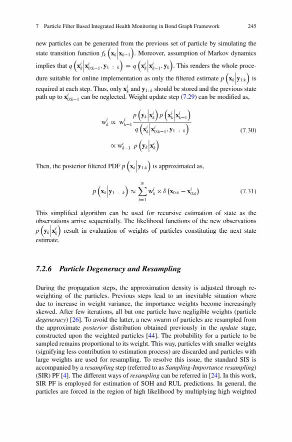
7 Particle Filter Based Integrated Health Monitoring in Bond Graph Framework 245
new particles can be generated from the previous set of particle by simulating the
state transition function fk
xk
ˇˇxk�1
. Moreover, assumption of Markov dynamics
implies that q
xik
ˇˇxi0Wk�1; y1 W k
D q
xi
k
ˇˇxi
k�1; yk
. This renders the whole proce-
dure suitable for online implementation as only the filtered estimate p
xk
ˇˇy1Wk
is
required at each step. Thus, only xik and y1 : k should be stored and the previous state
path up to xi0Wk�1 can be neglected. Weight update step (7.29) can be modified as,
wik / wi
k�1p
yk
ˇˇxi
k
p
xik
ˇˇxi
k�1
q
xik
ˇˇxi0Wk�1; y1 W k
/ wik�1 p
yk
ˇˇxi
k
(7.30)
Then, the posterior filtered PDF p
xk
ˇˇy1Wk
is approximated as,
p
xk
ˇˇy1 W k
�
NX
iD1wi
k � ı �x0Wk � xi0Wk�
(7.31)
This simplified algorithm can be used for recursive estimation of state as theobservations arrive sequentially. The likelihood functions of the new observations
p
yk
ˇˇxi
k
result in evaluation of weights of particles constituting the next state
estimate.
7.2.6 Particle Degeneracy and Resampling
During the propagation steps, the approximation density is adjusted through re-weighting of the particles. Previous steps lead to an inevitable situation wheredue to increase in weight variance, the importance weights become increasinglyskewed. After few iterations, all but one particle have negligible weights (particledegeneracy) [26]. To avoid the latter, a new swarm of particles are resampled fromthe approximate posterior distribution obtained previously in the update stage,constructed upon the weighted particles [44]. The probability for a particle to besampled remains proportional to its weight. This way, particles with smaller weights(signifying less contribution to estimation process) are discarded and particles withlarge weights are used for resampling. To resolve this issue, the standard SIS isaccompanied by a resampling step (referred to as Sampling-Importance resampling)(SIR) PF [4]. The different ways of resampling can be referred in [24]. In this work,SIR PF is employed for estimation of SOH and RUL predictions. In general, theparticles are forced in the region of high likelihood by multiplying high weighted
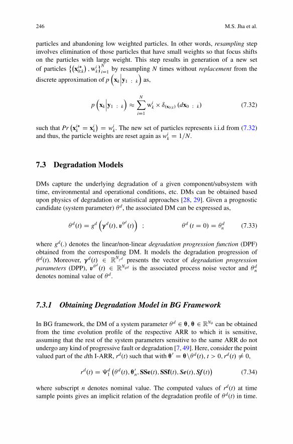
246 M.S. Jha et al.
particles and abandoning low weighted particles. In other words, resampling stepinvolves elimination of those particles that have small weights so that focus shiftson the particles with large weight. This step results in generation of a new setof particles
˚�xi�0Wk�;wi
k
N
iD1 by resampling N times without replacement from the
discrete approximation of p
xk
ˇˇy1 W k
as,
p
xk
ˇˇy1 W k
�
NX
iD1wi
k � ı.x0Wk/ .dx0 W k/ (7.32)
such that Pr�xi�
k D xik
� D wik. The new set of particles represents i.i.d from (7.32)
and thus, the particle weights are reset again as wik D 1=N.
7.3 Degradation Models
DMs capture the underlying degradation of a given component/subsystem withtime, environmental and operational conditions, etc. DMs can be obtained basedupon physics of degradation or statistical approaches [28, 29]. Given a prognosticcandidate (system parameter) �d, the associated DM can be expressed as,
�d.t/ D gd”d.t/; v™
d.t/
I �d .t D 0/ D �dn (7.33)
where gd(.) denotes the linear/non-linear degradation progression function (DPF)obtained from the corresponding DM. It models the degradation progression of�d(t). Moreover, ”d.t/ 2 R
N�d presents the vector of degradation progressionparameters (DPP), v�
d.t/ 2 R
N�d is the associated process noise vector and �dn
denotes nominal value of �d.
7.3.1 Obtaining Degradation Model in BG Framework
In BG framework, the DM of a system parameter �d 2 ™, ™ 2 RN� can be obtained
from the time evolution profile of the respective ARR to which it is sensitive,assuming that the rest of the system parameters sensitive to the same ARR do notundergo any kind of progressive fault or degradation [7, 49]. Here, consider the pointvalued part of the dth I-ARR, rd(t) such that with ™0 D ™n�d.t/, t > 0; rd.t/ ¤ 0,
rd.t/ D ‰d1
��d.t/; ™0n;SSe.t/;SSf.t/;Se.t/;Sf .t/
�(7.34)
where subscript n denotes nominal value. The computed values of rd(t) at timesample points gives an implicit relation of the degradation profile of �d(t) in time.
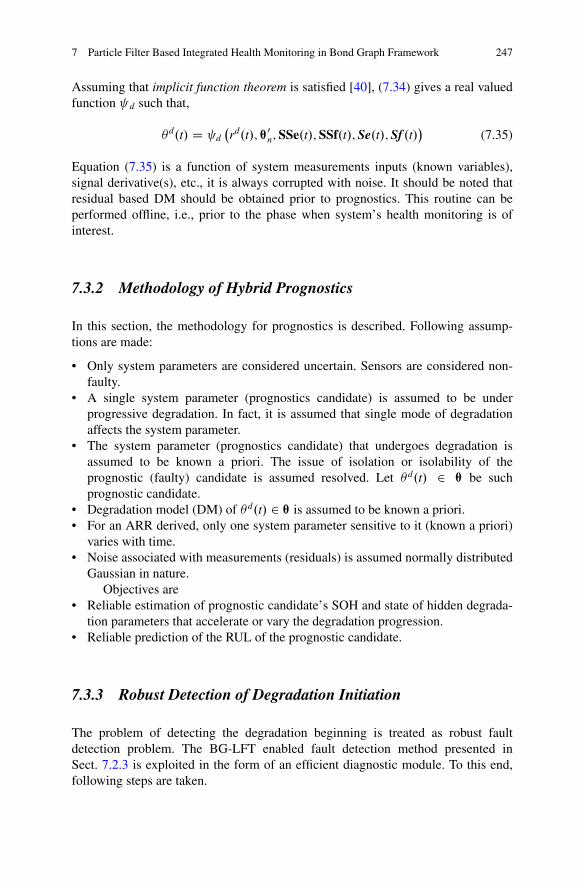
7 Particle Filter Based Integrated Health Monitoring in Bond Graph Framework 247
Assuming that implicit function theorem is satisfied [40], (7.34) gives a real valuedfunction d such that,
�d.t/ D d�rd.t/; ™0n;SSe.t/;SSf.t/;Se.t/;Sf .t/
�(7.35)
Equation (7.35) is a function of system measurements inputs (known variables),signal derivative(s), etc., it is always corrupted with noise. It should be noted thatresidual based DM should be obtained prior to prognostics. This routine can beperformed offline, i.e., prior to the phase when system’s health monitoring is ofinterest.
7.3.2 Methodology of Hybrid Prognostics
In this section, the methodology for prognostics is described. Following assump-tions are made:
• Only system parameters are considered uncertain. Sensors are considered non-faulty.
• A single system parameter (prognostics candidate) is assumed to be underprogressive degradation. In fact, it is assumed that single mode of degradationaffects the system parameter.
• The system parameter (prognostics candidate) that undergoes degradation isassumed to be known a priori. The issue of isolation or isolability of theprognostic (faulty) candidate is assumed resolved. Let �d.t/ 2 ™ be suchprognostic candidate.
• Degradation model (DM) of �d.t/ 2 ™ is assumed to be known a priori.• For an ARR derived, only one system parameter sensitive to it (known a priori)
varies with time.• Noise associated with measurements (residuals) is assumed normally distributed
Gaussian in nature.Objectives are
• Reliable estimation of prognostic candidate’s SOH and state of hidden degrada-tion parameters that accelerate or vary the degradation progression.
• Reliable prediction of the RUL of the prognostic candidate.
7.3.3 Robust Detection of Degradation Initiation
The problem of detecting the degradation beginning is treated as robust faultdetection problem. The BG-LFT enabled fault detection method presented inSect. 7.2.3 is exploited in the form of an efficient diagnostic module. To this end,following steps are taken.
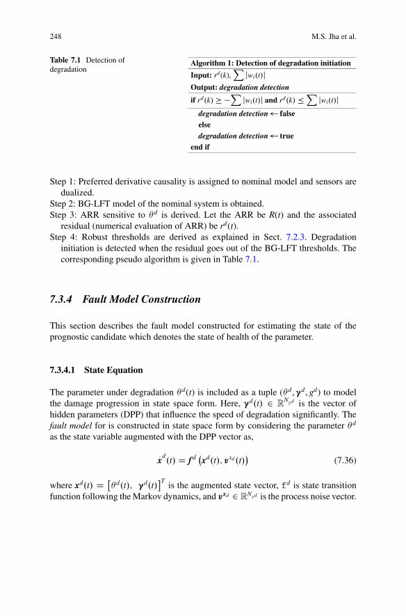
248 M.S. Jha et al.
Table 7.1 Detection ofdegradation
Algorithm 1: Detection of degradation initiation
Input: rd(k),X jwi.t/j
Output: degradation detection
if rd.k/ � �X jwi.t/j and rd.k/ �X jwi.t/jdegradation detection falseelsedegradation detection true
end if
Step 1: Preferred derivative causality is assigned to nominal model and sensors aredualized.
Step 2: BG-LFT model of the nominal system is obtained.Step 3: ARR sensitive to �d is derived. Let the ARR be R(t) and the associated
residual (numerical evaluation of ARR) be rd(t).Step 4: Robust thresholds are derived as explained in Sect. 7.2.3. Degradation
initiation is detected when the residual goes out of the BG-LFT thresholds. Thecorresponding pseudo algorithm is given in Table 7.1.
7.3.4 Fault Model Construction
This section describes the fault model constructed for estimating the state of theprognostic candidate which denotes the state of health of the parameter.
7.3.4.1 State Equation
The parameter under degradation �d(t) is included as a tuple (�d, ”d, gd) to modelthe damage progression in state space form. Here, ”d.t/ 2 R
N�d is the vector ofhidden parameters (DPP) that influence the speed of degradation significantly. Thefault model for is constructed in state space form by considering the parameter �d
as the state variable augmented with the DPP vector as,
:x
d.t/ D f d
�xd.t/; vxd .t/
�(7.36)
where xd.t/ D ��d.t/; ”d.t/
�Tis the augmented state vector, fd is state transition
function following the Markov dynamics, and vxd 2 RNvd is the process noise vector.
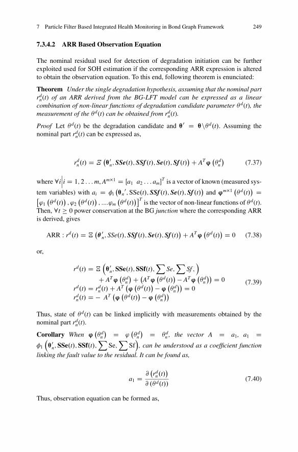
7 Particle Filter Based Integrated Health Monitoring in Bond Graph Framework 249
7.3.4.2 ARR Based Observation Equation
The nominal residual used for detection of degradation initiation can be furtherexploited used for SOH estimation if the corresponding ARR expression is alteredto obtain the observation equation. To this end, following theorem is enunciated:
Theorem Under the single degradation hypothesis, assuming that the nominal partrd
n(t) of an ARR derived from the BG-LFT model can be expressed as a linearcombination of non-linear functions of degradation candidate parameter �d(t), themeasurement of the �d(t) can be obtained from rd
n(t).
Proof Let �d(t) be the degradation candidate and ™0 D ™n�d.t/. Assuming thenominal part rd
n(t) can be expressed as,
rdn.t/ D �
�™0n;SSe.t/;SSf .t/;Se.t/;Sf .t/
�C AT®��d
n
�(7.37)
where 8iˇˇi D 1; 2 : : :m, Am�1 D Œa1 a2 : : : am�
T is a vector of known (measured sys-
tem variables) with ai D �i�™n0;SSe.t/;SSf .t/;Se.t/;Sf .t/
�and ®m�1 ��d.t/
� D�'1��d.t/
�; '2
��d.t/
�; ::::'m
��d.t/
��Tis the vector of non-linear functions of �d(t).
Then, 8t � 0 power conservation at the BG junction where the corresponding ARRis derived, gives
ARR W rd.t/ D „�� 0n; SSe.t/;SSf .t/;Se.t/;Sf .t/
�C AT®��d.t/
� D 0 (7.38)
or,
rd.t/ D „™0n;SSe.t/;SSf.t/;
XSe;
XSf ;
C AT®��d
n
�C �AT®
��d.t/
� � AT®��d
n
�� D 0
rd.t/ D rdn.t/C AT
�®��d.t/
� � ®��d
n
�� D 0
rdn.t/ D � AT
�®��d.t/
� � ®��d
n
��(7.39)
Thus, state of �d(t) can be linked implicitly with measurements obtained by thenominal part rd
n(t).
Corollary When ®��d
n
� D '��d
n
� D �dn , the vector A D a1, a1 D
�1
™0n;SSe.t/;SSf.t/;
XSe;
XSf
, can be understood as a coefficient function
linking the fault value to the residual. It can be found as,
a1 D @�rd
n.t/�
@ .�d.t//(7.40)
Thus, observation equation can be formed as,
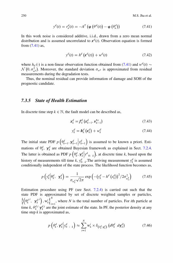
250 M.S. Jha et al.
yd.t/ D rdn.t/ D �AT
�®��d.t/
� � ®��d
n
��(7.41)
In this work noise is considered additive, i.i.d., drawn from a zero mean normaldistribution and is assumed uncorrelated to xd(t). Observation equation is formedfrom (7.41) as,
yd.t/ D hd�xd.t/
�C wd.t/ (7.42)
where hd .�/ is a non-linear observation function obtained from (7.41) and wd.t/ �N �
0; 2wd
�. Moreover, the standard deviation wd is approximated from residual
measurements during the degradation tests.Thus, the nominal residual can provide information of damage and SOH of the
prognostic candidate.
7.3.5 State of Health Estimation
In discrete time step k 2 N, the fault model can be described as,
xdk D f d
k
�xd
k�1; vxdk�1�
(7.43)
ydk D hd
k
�xd
k
�C wdk (7.44)
The initial state PDF p™d
k�1;”dk�1ˇˇyd
k�1
is assumed to be known a priori. Esti-
mations of ™dk , ”d
k are obtained Bayesian framework as explained in Sect. 7.2.4.
The latter is obtained as PDF p™d
k ;”dk
ˇˇyd
0W k
, at discrete time k, based upon the
history of measurements till time k, yd0 : k.The arriving measurement yd
k is assumedconditionally independent of the state process. The likelihood function becomes as,
p
ydk
ˇˇ™d
k ; ”dk
D 1
wdk
p2�
exp��yd
k � hd�xd
k
��2=2 2
wdk
(7.45)
Estimation procedure using PF (see Sect. 7.2.4) is carried out such that thestate PDF is approximated by set of discrete weighted samples or particles,n™d
k;i; ”d
k;i;wi
k
oN
iD1, where N is the total number of particles. For ith particle at
time k, �dk
,i ”dk
,i are the joint estimate of the state. In PF, the posterior density at anytime step k is approximated as,
p�d
k ;”dk
ˇˇyd0 W k
�
NX
iD1wi
k � ı.�dk ;”
dk/�d™d
k d”dk
�(7.46)
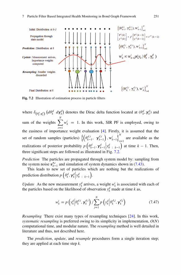
7 Particle Filter Based Integrated Health Monitoring in Bond Graph Framework 251
Fig. 7.2 Illustration of estimation process in particle filters
where ı.™dk ;”
dk/�d�d
k d”dk
�denotes the Dirac delta function located at (�d
k , ”dk ) and
sum of the weightsNX
iD1wi
k D 1. In this work, SIR PF is employed, owing to
the easiness of importance weight evaluation [4]. Firstly, it is assumed that the
set of random samples (particles)n�
d;ik�1; ”
d;ik�1;wi
k�1oN
iD1 are available as the
realizations of posterior probability p�d
k�1;”dk�1ˇˇyd0 W k�1
at time k � 1. Then,
three significant steps are followed as illustrated in Fig. 7.2.
Prediction The particles are propagated through system model by: sampling fromthe system noise v
xdk�1 and simulation of system dynamics shown in (7.43).
This leads to new set of particles which are nothing but the realizations of
prediction distribution p�d
k ;”dk
ˇˇyd0 W k�1
.
Update As the new measurement ydk arrives, a weight wi
k is associated with each ofthe particles based on the likelihood of observation yd
k made at time k as,
wik D p
yd
k
ˇˇ�d;i
k ;”d;ik
=
NX
jD1p
ydk
ˇˇ�d;j
k ;”d;jk
(7.47)
Resampling There exist many types of resampling techniques [24]. In this work,systematic resampling is preferred owing to its simplicity in implementation, O(N)computational time, and modular nature. The resampling method is well detailed inliterature and thus, not described here.
The prediction, update, and resample procedures form a single iteration step;they are applied at each time step k.
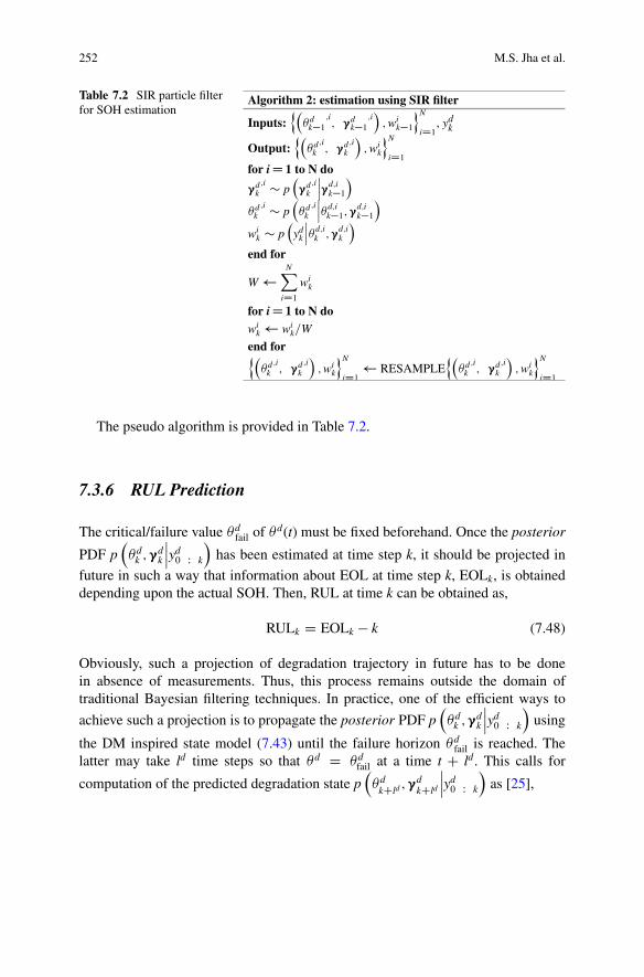
252 M.S. Jha et al.
Table 7.2 SIR particle filterfor SOH estimation
Algorithm 2: estimation using SIR filter
Inputs:n�d
k�1
;i; ”d
k�1
;i;wi
k�1
oN
iD1, yd
k
Output:n�d
k;i; ”d
k;i;wi
k
oN
iD1
for iD 1 to N do
”dk;i � p
”d
k;iˇˇ”d;i
k�1
�dk;i � p
�d
k;iˇˇ�d;i
k�1;”d;ik�1
wik � p
yd
k
ˇˇ�d;i
k ;”d;ik
end for
W NX
iD1
wik
for iD 1 to N dowi
k wik=W
end forn�d
k;i; ”d
k;i;wi
k
oN
iD1 RESAMPLE
n�d
k;i; ”d
k;i;wi
k
oN
iD1
The pseudo algorithm is provided in Table 7.2.
7.3.6 RUL Prediction
The critical/failure value �dfail of �d(t) must be fixed beforehand. Once the posterior
PDF p�d
k ;”dk
ˇˇyd0 W k
has been estimated at time step k, it should be projected in
future in such a way that information about EOL at time step k, EOLk, is obtaineddepending upon the actual SOH. Then, RUL at time k can be obtained as,
RULk D EOLk � k (7.48)
Obviously, such a projection of degradation trajectory in future has to be donein absence of measurements. Thus, this process remains outside the domain oftraditional Bayesian filtering techniques. In practice, one of the efficient ways to
achieve such a projection is to propagate the posterior PDF p�d
k ;”dk
ˇˇyd0 W k
using
the DM inspired state model (7.43) until the failure horizon �dfail is reached. The
latter may take ld time steps so that �d D �dfail at a time t C ld. This calls for
computation of the predicted degradation state p�d
kCld;”d
kCld
ˇˇyd0 W k
as [25],
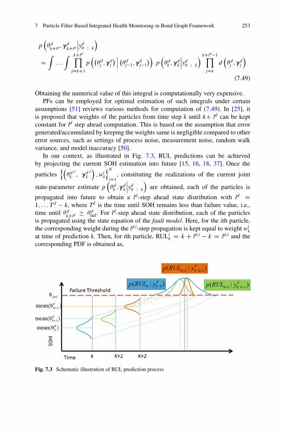
7 Particle Filter Based Integrated Health Monitoring in Bond Graph Framework 253
p�d
kCld;”d
kCld
ˇˇyd0 W k
DZ: : :
Z kCldY
jDkC1p��d
j ;”dj
� ˇˇ��d
j�1;”dj�1�
p�d
k ;”dk
ˇˇyd0 W k
kCld�1Y
jDk
d�d
j ;”dj
(7.49)
Obtaining the numerical value of this integral is computationally very expensive.PFs can be employed for optimal estimation of such integrals under certain
assumptions [51] reviews various methods for computation of (7.49). In [25], itis proposed that weights of the particles from time step k until kC ld can be keptconstant for ld step ahead computation. This is based on the assumption that errorgenerated/accumulated by keeping the weights same is negligible compared to othererror sources, such as settings of process noise, measurement noise, random walkvariance, and model inaccuracy [50].
In our context, as illustrated in Fig. 7.3, RUL predictions can be achievedby projecting the current SOH estimation into future [15, 16, 18, 37]. Once the
particlesn�d
k;i; ”d
k;i;wi
k
oN
iD1, constituting the realizations of the current joint
state-parameter estimate p�d
k ;”dk
ˇˇyd0 W k
are obtained, each of the particles is
propagated into future to obtain a ld-step ahead state distribution with ld D1; : : : Td � k, where Td is the time until SOH remains less than failure value, i.e.,time until �d
kCld� �d
fail. For ld-step ahead state distribution, each of the particlesis propagated using the state equation of the fault model. Here, for the ith particle,the corresponding weight during the ld,i-step propagation is kept equal to weight wi
kat time of prediction k. Then, for ith particle, RULi
k D k C ld;i � k D ld;i and thecorresponding PDF is obtained as,
Fig. 7.3 Schematic illustration of RUL prediction process
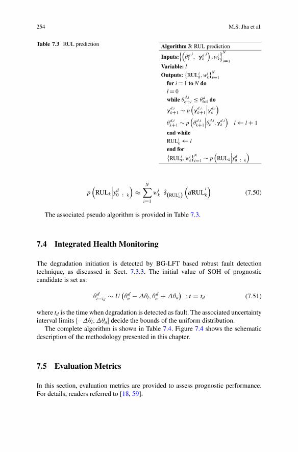
254 M.S. Jha et al.
Table 7.3 RUL prediction Algorithm 3: RUL prediction
Inputs:n�d
k;i; ”d
k;i;wi
k
oN
iD1
Variable: l
Outputs:˚RULi
k;wik
N
iD1
for iD 1 to N dolD 0
while �d;ikCl � �d
fail do
”d;ikC1 � p
”
d;ikC1
ˇˇ”d;i
k
�d;ikC1 � p
�
d;ikC1
ˇˇ�d;i
k ;”d;ik
l lC 1
end whileRULi
k l
end for˚RULi
k;wik
N
iD1� p
RULk
ˇˇyd0 W k
p
RULk
ˇˇyd0 W k
�
NX
iD1wi
k ı.RULik/
dRUL
i
k
(7.50)
The associated pseudo algorithm is provided in Table 7.3.
7.4 Integrated Health Monitoring
The degradation initiation is detected by BG-LFT based robust fault detectiontechnique, as discussed in Sect. 7.3.3. The initial value of SOH of prognosticcandidate is set as:
�dtDtd � U
��d
n ��l; �dn C�u
� I t D td (7.51)
where td is the time when degradation is detected as fault. The associated uncertaintyinterval limits Œ��l; �u� decide the bounds of the uniform distribution.
The complete algorithm is shown in Table 7.4. Figure 7.4 shows the schematicdescription of the methodology presented in this chapter.
7.5 Evaluation Metrics
In this section, evaluation metrics are provided to assess prognostic performance.For details, readers referred to [18, 59].
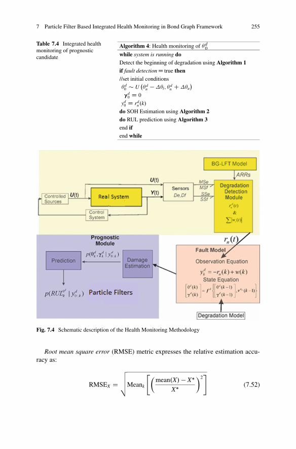
7 Particle Filter Based Integrated Health Monitoring in Bond Graph Framework 255
Table 7.4 Integrated healthmonitoring of prognosticcandidate
Algorithm 4: Health monitoring of �d0
while system is running doDetect the beginning of degradation using Algorithm 1if fault detectionD true then//set initial conditions
�d0 � U
��d
n ��l; �dn C�u
�
”d0 D 0
yd0 D rd
n.k/
do SOH Estimation using Algorithm 2do RUL prediction using Algorithm 3end ifend while
Fig. 7.4 Schematic description of the Health Monitoring Methodology
Root mean square error (RMSE) metric expresses the relative estimation accu-racy as:
RMSEX DvuutMeank
"�mean.X/ � X�
X�
�2#(7.52)
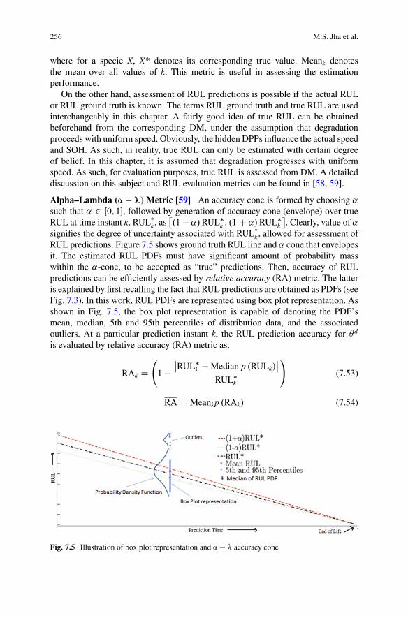
256 M.S. Jha et al.
where for a specie X, X* denotes its corresponding true value. Meank denotesthe mean over all values of k. This metric is useful in assessing the estimationperformance.
On the other hand, assessment of RUL predictions is possible if the actual RULor RUL ground truth is known. The terms RUL ground truth and true RUL are usedinterchangeably in this chapter. A fairly good idea of true RUL can be obtainedbeforehand from the corresponding DM, under the assumption that degradationproceeds with uniform speed. Obviously, the hidden DPPs influence the actual speedand SOH. As such, in reality, true RUL can only be estimated with certain degreeof belief. In this chapter, it is assumed that degradation progresses with uniformspeed. As such, for evaluation purposes, true RUL is assessed from DM. A detaileddiscussion on this subject and RUL evaluation metrics can be found in [58, 59].
Alpha–Lambda (’ � œ) Metric [59] An accuracy cone is formed by choosing ˛such that ˛ 2 Œ0; 1�, followed by generation of accuracy cone (envelope) over trueRUL at time instant k, RUL*
k , as�.1 � ˛/RUL�k ; .1C ˛/RUL�k
�. Clearly, value of ˛
signifies the degree of uncertainty associated with RUL*k , allowed for assessment of
RUL predictions. Figure 7.5 shows ground truth RUL line and ˛ cone that envelopesit. The estimated RUL PDFs must have significant amount of probability masswithin the ˛-cone, to be accepted as “true” predictions. Then, accuracy of RULpredictions can be efficiently assessed by relative accuracy (RA) metric. The latteris explained by first recalling the fact that RUL predictions are obtained as PDFs (seeFig. 7.3). In this work, RUL PDFs are represented using box plot representation. Asshown in Fig. 7.5, the box plot representation is capable of denoting the PDF’smean, median, 5th and 95th percentiles of distribution data, and the associatedoutliers. At a particular prediction instant k, the RUL prediction accuracy for �d
is evaluated by relative accuracy (RA) metric as,
RAk D 1 �
ˇRUL�k � Median p .RULk/
ˇ
RUL�k
!(7.53)
RA D Meankp .RAk/ (7.54)
Fig. 7.5 Illustration of box plot representation and ’� accuracy cone

7 Particle Filter Based Integrated Health Monitoring in Bond Graph Framework 257
where RUL*k denotes the true RUL at time k for �d. The overall accuracy is
determined by RA as shown in (7.53), where RAk is averaged over all the predictionpoints.
7.6 Application on Mechatronic System in Real Time
This section describes the application of the method over a mechatronic system [36]shown in Fig. 7.6. Real time implementation is achieved through 20 SIM 4C 2.1.The SOH estimation and RUL prediction algorithms are written in Matlab FunctionBlock in Simulink. The embedded code is generated through Simulink Coder inMatlab2013a
®.
7.6.1 Nominal System
The functional schematic model of the mechatronic system [38] is shown in Fig. 7.6.The designation of system variables and associated values are listed in Table 7.5.The system consists of the Maxon
®servo motor that provides the controlled
actuation (rotation) to disks (Fig. 7.7). The high stiffness transmission belt providestorque the transmission ratio of kbelt to the motor disk. The motor disk is connectedto load disk through a flexible shaft that constitutes the drive train. The shaft ismodelled as spring-damper element. The friction in the bearings of the motor diskand load disk are modelled as viscous friction. Friction arising due to belt is lumpedwith viscous friction coefficient at motor disk bMd. The setup is equipped with motorencoder and load encoder that measure angular position of motor shaft and load disk(2000 pulses per revolution), respectively (Fig. 7.8). Angular position motor disk isobtained by dividing the motor encoder counts by belt ratio. The BG model of the
Fig. 7.6 Mechatronic torsion bar 1.0 system
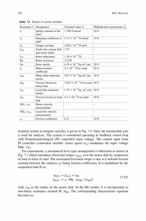
258 M.S. Jha et al.
Table 7.5 Details of system variables
Parameter � Designation Nominal value �n Multiplicative uncertainty ı�ks Spring constant of the
shaft1.786 N m/rad 10 %
bs Damping coefficient ofshaft
5:11� 10�4 N m/rad 10 %
km Torque constant 3:89� 10�4 N m/A –kbelt Teeth ratio (motor disk
and motor shaft)3.75 –
La Rotor inductance 1:34� 10�3 H –Ra Rotor resistance 1.23˝ –Jm Rotor inertia 6:76� 10�6kg m2=rad 20 %fm Motor friction
coefficient2� 10�6 N m s/rad 20 %
JMd Motor disk rotationalinertia
9:07� 10�4kg m2=rad 10 %
bMd Viscous friction inmotor disk
5:025� 10�3 N m s/rad 20 %
JLd Load disk rotationalinertia
1:37� 10�3kg m2=rad 20 %
bLd Viscous friction in loaddisk
2:5� 10�5N m s/rad 20 %
SSf1 :!m Motor velocitymeasurement
– –
SSf2 :!Ld Load disk velocitymeasurement
– –
� Friction coefficient 0.27 10 %
nominal system in integral causality is given in Fig. 7.9. Only the monitorable partis used for analysis. The system is considered operating in feedback closed loopwith Proportional-Integral (PI) controlled input voltage. The control input fromPI controller (controlled variable: motor speed !m) modulates the input voltageMSe: UPI.
For experiments, a mechanical lever type arrangement is fabricated as shown inFig. 7.7 which introduces frictional torque �Mech over the motor disk by suspensionof load in form of sand. The associated frictional torque is due to Coulomb frictionexisting between the surfaces (� being friction coefficient). It is modulated by thesuspended load M as,
�Mech D fmech � rMd
fmech D � Mg .!Md= j!Mdj/ (7.55)
with rMd as the radius of the motor disk. In the BG model, it is incorporated asnon-linear resistance element R: bMd. The corresponding characteristic equationbecomes as,

7 Particle Filter Based Integrated Health Monitoring in Bond Graph Framework 259
Fig. 7.7 Fabricatedmechanical lever typearrangement for load (mass)suspension
Fig. 7.8 Schematic model of the mechatronic system
Fig. 7.9 BG model (preferred integral causality) of the nominal system
R D bMd C � � M.t/ � rMdg= j!j (7.56)
e8 D R .f8/ D bMd!Md C � � M.t/ � rMdg � .!Md= j!Mdj/ (7.57)
Involving only non-destructive experiments, � is assumed undergoing no wear.
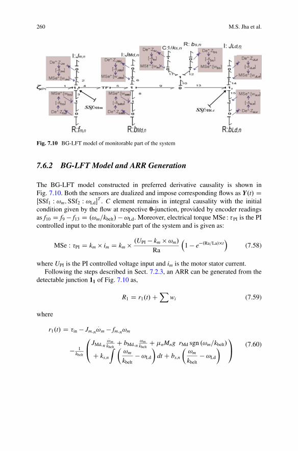
260 M.S. Jha et al.
Fig. 7.10 BG-LFT model of monitorable part of the system
7.6.2 BG-LFT Model and ARR Generation
The BG-LFT model constructed in preferred derivative causality is shown inFig. 7.10. Both the sensors are dualized and impose corresponding flows as Y.t/ DŒSSf1 W !m;SSf2 W !Ld�
T . C element remains in integral causality with the initialcondition given by the flow at respective 0-junction, provided by encoder readingsas f10 D f9 � f13 D .!m=kbelt/ � !Ld. Moreover, electrical torque MSe : �PI is the PIcontrolled input to the monitorable part of the system and is given as:
MSe W �PI D km � im D km � .UPI � km � !m/
Ra
1 � e�.Ra=La/�t
(7.58)
where UPI is the PI controlled voltage input and im is the motor stator current.Following the steps described in Sect. 7.2.3, an ARR can be generated from the
detectable junction 11 of Fig. 7.10 as,
R1 D r1.t/CX
wi (7.59)
where
r1.t/ D �in � Jm;n:!m � fm;n!m
� 1kbelt
0
@JMd;n
:!mkbelt
C bMd;n!mkbelt
C �nMng rMd sgn .!m=kbelt/
C ks;n
Z �!m
kbelt� !Ld
�dt C bs;n
�!m
kbelt� !Ld
�1
A(7.60)
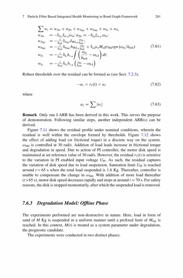
7 Particle Filter Based Integrated Health Monitoring in Bond Graph Framework 261
Xwi D wJm C wfm C wJMd C wbMd C wks C wbs
wJm D �•Jm Jm;n:!mI wfm D �•fm fm;n:!mI
wJMd D � 1kbelt•JMd JMd;n
:!mkbelt
IwbMd D � 1
kbelt•bMd;bMd;n
!mkbelt
C •��nMngrMdsgn .!m=kbelt/
wks D � 1kbelt•ks ks;n
Z �!m
kbelt� !Ld
�dtI
wbs D � 1kbelt•bs bs;n
!mkbelt
� !Ld
(7.61)
Robust thresholds over the residual can be formed as (see Sect. 7.2.3),
�a1 < r1.t/ < a1 (7.62)
where
a1 DX
jwij (7.63)
Remark Only one I-ARR has been derived in this work. This serves the purposeof demonstration. Following similar steps, another independent ARR(s) can bederived.
Figure 7.11 shows the residual profile under nominal conditions, wherein theresidual is well within the envelope formed by thresholds. Figure 7.12 showsthe effect of adding load (or frictional toque) in a discrete way on the system.!Md is controlled at 30 rad/s. Addition of load leads increase in frictional torqueand degradation in speed. Due to action of PI controller, the motor disk speed ismaintained at set reference value of 30 rad/s. However, the residual r1(t) is sensitiveto the variation in PI enabled input voltage UPI. As such, the residual capturesthe variation of disk speed due to load suspension. Saturation limit UPI is reachedaround t D 65 s when the total load suspended is 1.6 Kg. Thereafter, controller isunable to compensate the change in !Md. With addition of more load thereafter(t > 65 s), motor disk speed decreases rapidly and stops at around t D 70 s. For safetyreasons, the disk is stopped momentarily, after which the suspended load is removed.
7.6.3 Degradation Model: Offline Phase
The experiments performed are non-destructive in nature. Here, load in form ofsand of M Kg is suspended in a uniform manner until a prefixed limit of Mfail isreached. In this context, M(t) is treated as a system parameter under degradation,the prognostic candidate.
The experiments were conducted in two distinct phases:
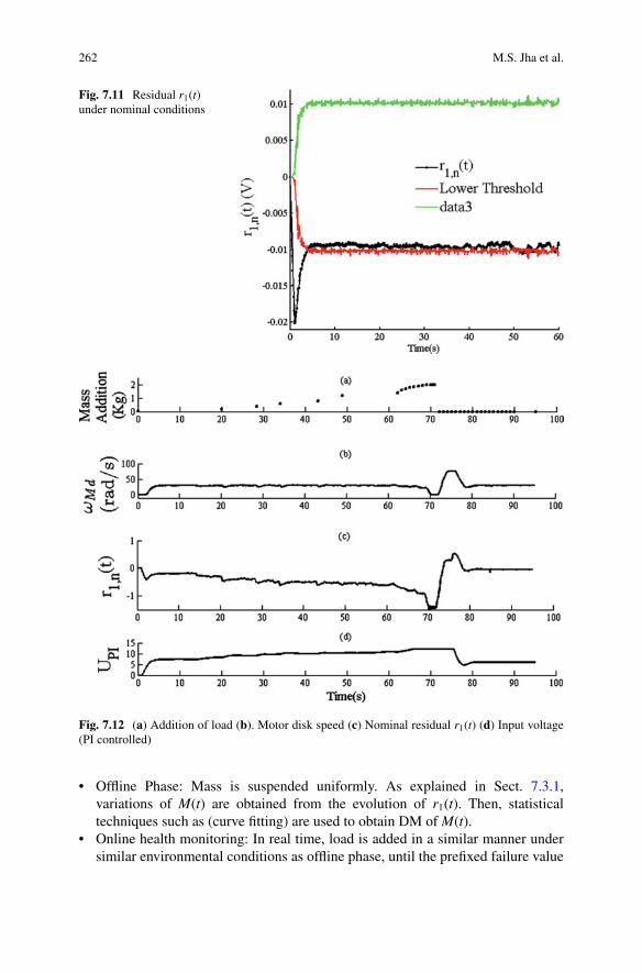
262 M.S. Jha et al.
Fig. 7.11 Residual r1(t)under nominal conditions
Fig. 7.12 (a) Addition of load (b). Motor disk speed (c) Nominal residual r1(t) (d) Input voltage(PI controlled)
• Offline Phase: Mass is suspended uniformly. As explained in Sect. 7.3.1,variations of M(t) are obtained from the evolution of r1(t). Then, statisticaltechniques such as (curve fitting) are used to obtain DM of M(t).
• Online health monitoring: In real time, load is added in a similar manner undersimilar environmental conditions as offline phase, until the prefixed failure value
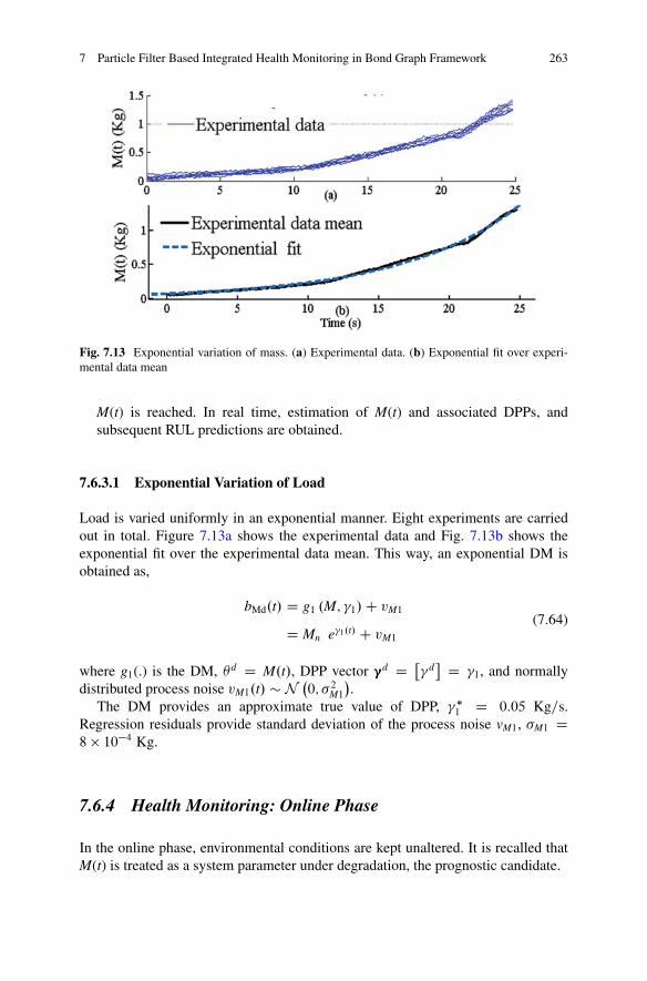
7 Particle Filter Based Integrated Health Monitoring in Bond Graph Framework 263
Fig. 7.13 Exponential variation of mass. (a) Experimental data. (b) Exponential fit over experi-mental data mean
M(t) is reached. In real time, estimation of M(t) and associated DPPs, andsubsequent RUL predictions are obtained.
7.6.3.1 Exponential Variation of Load
Load is varied uniformly in an exponential manner. Eight experiments are carriedout in total. Figure 7.13a shows the experimental data and Fig. 7.13b shows theexponential fit over the experimental data mean. This way, an exponential DM isobtained as,
bMd.t/ D g1 .M; �1/C vM1
D Mn e�1.t/ C vM1
(7.64)
where g1(.) is the DM, �d D M.t/, DPP vector ”d D ��d� D �1, and normally
distributed process noise vM1.t/ � N �0; 2M1
�.
The DM provides an approximate true value of DPP, ��1 D 0:05 Kg=s.Regression residuals provide standard deviation of the process noise vM1, M1 D8 � 10�4 Kg.
7.6.4 Health Monitoring: Online Phase
In the online phase, environmental conditions are kept unaltered. It is recalled thatM(t) is treated as a system parameter under degradation, the prognostic candidate.
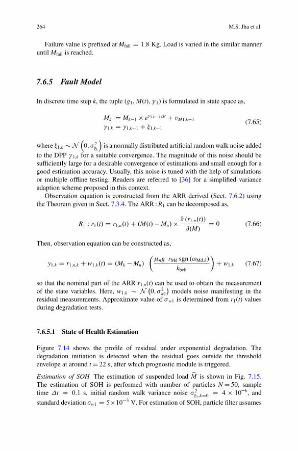
264 M.S. Jha et al.
Failure value is prefixed at Mfail D 1:8 Kg. Load is varied in the similar manneruntil Mfail is reached.
7.6.5 Fault Model
In discrete time step k, the tuple (g1, M(t), �1) is formulated in state space as,
Mk D Mk�1 � e�1;k�1t C vM1;k�1�1;k D �1;k�1 C �1;k�1
(7.65)
where �1;k � N0; 2�1
is a normally distributed artificial random walk noise added
to the DPP �1,k for a suitable convergence. The magnitude of this noise should besufficiently large for a desirable convergence of estimations and small enough for agood estimation accuracy. Usually, this noise is tuned with the help of simulationsor multiple offline testing. Readers are referred to [36] for a simplified varianceadaption scheme proposed in this context.
Observation equation is constructed from the ARR derived (Sect. 7.6.2) usingthe Theorem given in Sect. 7.3.4. The ARR : R1 can be decomposed as,
R1 W r1.t/ D r1;n.t/C .M.t/ � Mn/ � @ .r1;n.t//
@.M/D 0 (7.66)
Then, observation equation can be constructed as,
y1;k D r1;n;k C w1;k.t/ D .Mk � Mn/
��ng rMd sgn .!Md;k/
kbelt
�C w1;k (7.67)
so that the nominal part of the ARR r1,n(t) can be used to obtain the measurementof the state variables. Here, w1;k � N �
0; 2w1�
models noise manifesting in theresidual measurements. Approximate value of w1 is determined from r1(t) valuesduring degradation tests.
7.6.5.1 State of Health Estimation
Figure 7.14 shows the profile of residual under exponential degradation. Thedegradation initiation is detected when the residual goes outside the thresholdenvelope at around t D 22 s, after which prognostic module is triggered.
Estimation of SOH The estimation of suspended load bM is shown in Fig. 7.15.The estimation of SOH is performed with number of particles N D 50, sampletime t D 0:1 s, initial random walk variance noise 2�1;kD0 D 4 � 10–6, and
standard deviation w1 D 5�10�3 V. For estimation of SOH, particle filter assumes
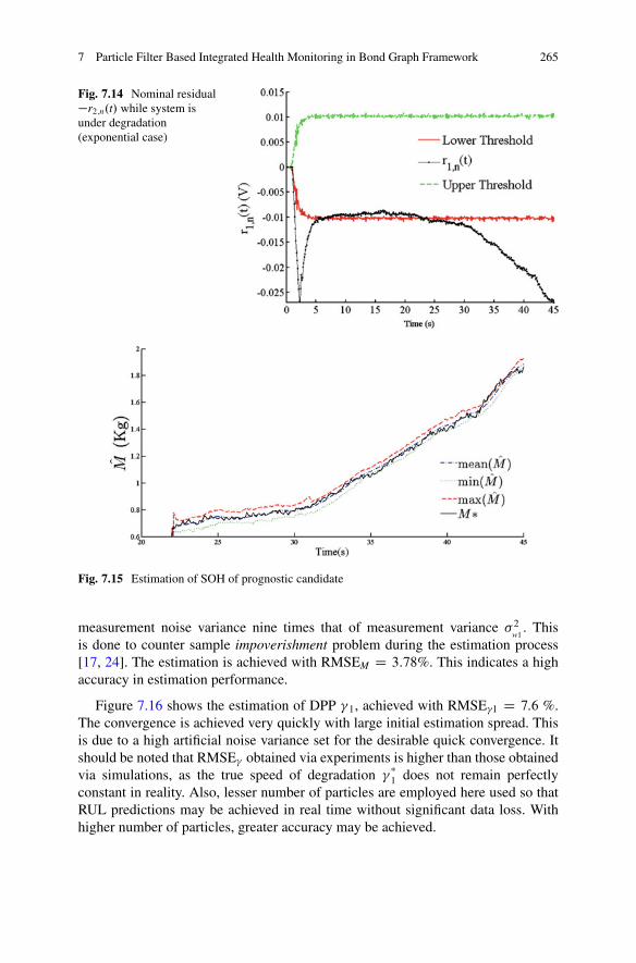
7 Particle Filter Based Integrated Health Monitoring in Bond Graph Framework 265
Fig. 7.14 Nominal residual�r2;n.t/ while system isunder degradation(exponential case)
Fig. 7.15 Estimation of SOH of prognostic candidate
measurement noise variance nine times that of measurement variance 2w1
. Thisis done to counter sample impoverishment problem during the estimation process[17, 24]. The estimation is achieved with RMSEM D 3:78%. This indicates a highaccuracy in estimation performance.
Figure 7.16 shows the estimation of DPP �1, achieved with RMSE�1 D 7:6 %.The convergence is achieved very quickly with large initial estimation spread. Thisis due to a high artificial noise variance set for the desirable quick convergence. Itshould be noted that RMSE� obtained via experiments is higher than those obtainedvia simulations, as the true speed of degradation �*
1 does not remain perfectlyconstant in reality. Also, lesser number of particles are employed here used so thatRUL predictions may be achieved in real time without significant data loss. Withhigher number of particles, greater accuracy may be achieved.
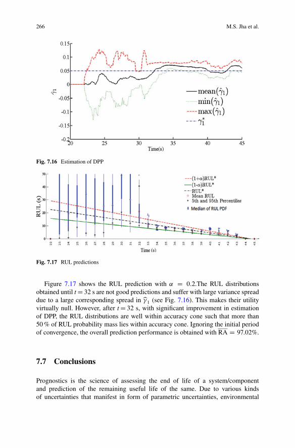
266 M.S. Jha et al.
Fig. 7.16 Estimation of DPP
Fig. 7.17 RUL predictions
Figure 7.17 shows the RUL prediction with ˛ D 0:2.The RUL distributionsobtained until t D 32 s are not good predictions and suffer with large variance spreaddue to a large corresponding spread in b�1 (see Fig. 7.16). This makes their utilityvirtually null. However, after t D 32 s, with significant improvement in estimationof DPP, the RUL distributions are well within accuracy cone such that more than50 % of RUL probability mass lies within accuracy cone. Ignoring the initial periodof convergence, the overall prediction performance is obtained with RA D 97:02%.
7.7 Conclusions
Prognostics is the science of assessing the end of life of a system/componentand prediction of the remaining useful life of the same. Due to various kindsof uncertainties that manifest in form of parametric uncertainties, environmental
7 Particle Filter Based Integrated Health Monitoring in Bond Graph Framework 267
conditions, sensor noises, uncertain future conditions, etc., RUL prediction becomesa very challenging issue. In this work, benefits of BG-LFT modelling basedrobust fault detection are integrated with the advantages of Bayesian estimationmethod for efficient prognostics. In particular, particle filters are exploited foroptimal estimations of actual state of the prognostic candidate and subsequent RULpredictions. In this chapter, a single system parameter is chosen as the prognosticcandidate and RULs are obtained with respect to that parameter. As such, thework presented here paves the future path for development of efficient system levelprognostics in BG framework.
The ARR based BG-LFT technique is employed for robust detection of degra-dation beginning. The same ARR is then exploited for prognostic purposes. Beingsensitive to the control inputs, nominal residual is able to capture the parametricdegradation profile even while the system outputs remain in feedback closedloop regime. This aspect renders the approach appropriate for system level healthmanagement. Approximation of noise distribution present in residuals can bedifficult or impossible, due to presence of derivative or integral terms in the ARRfunction arguments. As such, particle filter algorithms form the best choice in thisregard as they are not restricted by non-Gaussian noises. Moreover, degradation ofnon-linear nature can be efficiently estimated using particle filters. Additionally,this method also demonstrates that fusion of BG-LFT framework and MonteCarlo framework leads to efficient management of various types of uncertainties.While parametric uncertainties are modelled and managed by using BG-LFT forefficient detection of degradation initiation; degradation process noise, measurement(residual) noise, etc., are efficiently accounted for, by PF for estimation of SOH andRUL predictions.
References
1. Abbas, M., Ferri, A. A., Orchard, M. E., & Vachtsevanos, G. J. (2007). An intelligent diagnos-tic/prognostic framework for automotive electrical systems. Intelligent Vehicles Symposium,2007 IEEE. IEEE, pp. 352–357.
2. An, D., Choi, J.-H., & Kim, N. H. (2013). Prognostics 101: A tutorial for particle filter-basedprognostics algorithm using Matlab. Reliability Engineering and System Safety, 115, 161–169.
3. An, D., Kim, N. H., & Choi, J.-H. (2015). Practical options for selecting data-driven or physics-based prognostics algorithms with reviews. Reliability Engineering and System Safety, 133,223–236.
4. Arulampalam, M. S., Maskell, S., Gordon, N., & Clapp, T. (2002). A tutorial on particlefilters for online nonlinear/non-Gaussian Bayesian tracking. IEEE Transactions on SignalProcessing, 50(2), 174–188.
5. Baraldi, P., Mangili, F., & Zio, E. (2013). Investigation of uncertainty treatment capability ofmodel-based and data-driven prognostic methods using simulated data. Reliability Engineeringand System Safety, 112, 94–108.
6. Blischke, W. R., & Murthy, D. P. (2011). Reliability: Modeling, prediction, and optimization(Vol. 767). New York, NY: John Wiley & Sons.
7. Borutzky, W. (2015). Failure prognosis for hybrid systems based on ARR residuals. In W.Borutzky (Ed.), Bond graph model-based fault diagnosis of hybrid systems (pp. 221–233).New York: Springer.

268 M.S. Jha et al.
8. Box, G. E., Jenkins, G. M., & Reinsel, G. C. (2011). Time series analysis: Forecasting andcontrol (Vol. 734). Hoboken, NJ: John Wiley & Sons.
9. Bregon, A., Daigle, M., & Roychoudhury, I. (2012). An integrated framework for model-baseddistributed diagnosis and prognosis. DTIC Document.
10. Byington, C. S., & Roemer, M. J. (2002). Prognostic enhancements to diagnostic systems forimproved condition-based maintenance [military aircraft]. Aerospace Conference Proceedings,2002. IEEE. IEEE, vol. 2816, pp. 6-2815-2816-2824.
11. Cadini, F., Zio, E., & Avram, D. (2009). Monte Carlo-based filtering for fatigue crack growthestimation. Probabilistic Engineering Mechanics, 24(3), 367–373.
12. Celaya, J., Kulkarni, C., Biswas, G., Saha, S., & Goebel, K. (2011). A model-based prognosticsmethodology for electrolytic capacitors based on electrical overstress accelerated aging. InAnnual Conference of the Prognostics and Health Management Society (PHM), Montreal.
13. Daigle, M. J., Bregon, A., & Roychoudhury, I. (2014). Distributed prognostics based onstructural model decomposition. IEEE Transactions on Reliability, 2(63), 495–510.
14. Daigle, M., & Goebel, K. (2009). Model-based prognostics with fixed-lag particle filters.Conference of the PHM Society.
15. Daigle, M., & Goebel, K. (2010). Model-based prognostics under limited sensing. AerospaceConference, 2010 IEEE. IEEE, pp. 1–12.
16. Daigle, M. J., & Goebel, K. (2011). A model-based prognostics approach applied to pneumaticvalves. International Journal of Prognostics and Health Management, 2(2), 1–16.
17. Daigle, M. J., & Goebel, K. (2011). A model-based prognostics approach applied to pneumaticvalves. International Journal of Prognostics and Health Management, 2(color), 84.
18. Daigle, M. J., & Goebel, K. (2013). Model-based prognostics with concurrent damageprogression processes. IEEE Transactions on Systems, Man, and Cybernetics: Systems, 43(3),535–546.
19. Daigle, M., Saha, B., & Goebel, K. A. (2012). Comparison of filter-based approaches formodel-based prognostics. Aerospace Conference, 2012 IEEE. IEEE, pp. 1–10.
20. Djeziri, M., Ananou, B., & Ouladsine, M. (2013). Data driven and model based faultprognosis applied to a mechatronic system. Power Engineering, Energy and Electrical Drives(POWERENG), 2013 Fourth International Conference on. IEEE, pp. 534–539.
21. Djeziri, M. A., Bouamama, B. O., Dauphin-Tanguy, G., & Merzouki, R. (2011). LFT bondgraph model-based robust fault detection and isolation. In W. Borutzky (Ed.), Bond graphmodelling of engineering systems (pp. 105–133). New York: Springer.
22. Djeziri, M. A., Merzouki, R., Bouamama, B. O., & Dauphin-Tanguy, G. (2007). Robust faultdiagnosis by using bond graph approach. IEEE/ASME Transactions on Mechatronics, 12(6),599–611.
23. Djeziri, M., Toubakh, H., & Ouladsine, M. (2013) Fault prognosis based on fault reconstruc-tion: Application to a mechatronic system. Systems and Control (ICSC), 2013 3rd InternationalConference on. IEEE, pp. 383–388.
24. Douc, R., & Cappé, O. (2005). Comparison of resampling schemes for particle filtering. Imageand Signal Processing and Analysis, 2005. ISPA 2005. Proceedings of the 4th InternationalSymposium on. IEEE, pp. 64–69.
25. Doucet, A., De Freitas, N., & Gordon, N. (2001). An introduction to sequential Monte Carlomethods. New York, NY: Springer.
26. Doucet, A., & Johansen, A. M. (2009). A tutorial on particle filtering and smoothing: Fifteenyears later. Handbook of Nonlinear Filtering, 12, 656–704.
27. Engel, S. J., Gilmartin, B. J., Bongort, K., & Hess, A. (2000). Prognostics, the real issuesinvolved with predicting life remaining. Aerospace Conference Proceedings, 2000 IEEE. IEEE,pp. 457–469.
28. Gebraeel, N., & Pan, J. (2008). Prognostic degradation models for computing and updatingresidual life distributions in a time-varying environment. IEEE Transactions on Reliability,57(4), 539–550.
29. Guo, H., & Liao, H. (2015). Practical approaches for reliability evaluation using degradationdata. Annual Reliability and Maintainability Symposium.

7 Particle Filter Based Integrated Health Monitoring in Bond Graph Framework 269
30. Helton, J. C. (1993). Uncertainty and sensitivity analysis techniques for use in performanceassessment for radioactive waste disposal. Reliability Engineering and System Safety, 42(2),327–367.
31. Herzog, M. A., Marwala, T., & Heyns, P. S. (2009). Machine and component residual lifeestimation through the application of neural networks. Reliability Engineering and SystemSafety, 94(2), 479–489.
32. Hu, Y., Baraldi, P., Di Maio, F., & Zio, E. (2015). A particle filtering and kernel smoothing-based approach for new design component prognostics. Reliability Engineering and SystemSafety, 134, 19–31.
33. Hitchcock, L. (2006). ISO standards for condition monitoring. In Engineering asset manage-ment (pp. 606–613). London: Springer.
34. Jardine, A. K., Lin, D., & Banjevic, D. (2006). A review on machinery diagnostics andprognostics implementing condition-based maintenance. Mechanical Systems and SignalProcessing, 20(7), 1483–1510.
35. Jha, M., Dauphin-Tanguy, G., & Ould Bouamama, B. (2014). Integrated diagnosis andprognosis of uncertain systems: A bond graph approach. Second European Conference ofthe PHM Society 2014-Nantes France, 2014. European Conference of the PHM Society 2014Proceedings, pp. 391–400.
36. Jha, M. S., Dauphin-Tanguy, G., & Ould-Bouamama, B. (2016). Particle filter based hybridprognostics for health monitoring of uncertain systems in bond graph framework. MechanicalSystems and Signal Processing, 75, 301–329.
37. Jouin, M., Gouriveau, R., Hissel, D., Péra, M.-C., & Zerhouni, N. (2014). Prognostics of PEMfuel cell in a particle filtering framework. International Journal of Hydrogen Energy, 39(1),481–494.
38. Kleijn, C. (2011). 20 SIM 4C 2.1 Reference Manual. Enschede, Controllab Products B.V. ISBN978-90-79499-14-4.
39. Klutke, G.-A., Kiessler, P. C., & Wortman, M. (2003). A critical look at the bathtub curve.IEEE Transactions on Reliability, 52(1), 125–129.
40. Krantz, S. G., & Parks, H. R. (2012). The implicit function theorem: History, theory, andapplications. New York, NY: Springer.
41. Kuehl, R. W. (2010). Using the Arrhenius equation to predict drift in thin film resistors.Proceedings CARTS Europe, pp. 121–133.
42. Kulkarni, C. S., Celaya, J., Biswas, G., & Goebel, K. (2012). Physics based electrolytic capac-itor degradation models for prognostic studies under thermal overstress. In First EuropeanConference of the Prognostics and Health Management Society (Vol. 3, p. 9). Dresden.
43. Lee, J., Ni, J., Djurdjanovic, D., Qiu, H., & Liao, H. (2006). Intelligent prognostics tools ande-maintenance. Computers in Industry, 57(6), 476–489.
44. Li, T., Sun, S., Sattar, T. P., & Corchado, J. M. (2014). Fight sample degeneracy andimpoverishment in particle filters: A review of intelligent approaches. Expert Systems withapplications, 41(8), 3944–3954.
45. Liao, S.-H. (2005). Expert system methodologies and applications—a decade review from1995 to 2004. Expert Systems with Applications, 28(1), 93–103.
46. Lu, J.-C., Park, J., & Yang, Q. (1997). Statistical inference of a time-to-failure distributionderived from linear degradation data. Technometrics, 39(4), 391–400.
47. Maricau, E., & Gielen, G. (2009). A methodology for measuring transistor ageing effectstowards accurate reliability simulation. On-Line Testing Symposium, 2009. IOLTS 2009. 15thIEEE International. IEEE, pp. 21–26.
48. Medjaher, K., & Zerhouni, N. (2009). Residual-based failure prognostic in dynamic systems.7th IFAC International Symposium on Fault Detection, Supervision and Safety of TechnicalProcesses, SAFE PROCESS’09, vol sur CD ROM. IFAC, p. 6.
49. Medjaher, K., & Zerhouni, N. (2013). Hybrid prognostic method applied to mecha-tronic systems. The International Journal of Advanced Manufacturing Technology, 69(1–4),823–834.

270 M.S. Jha et al.
50. Orchard, M. E. (2007). A particle filtering-based framework for on-line fault diagnosis andfailure prognosis. Georgia Institute of Technology.
51. Orchard, M., Kacprzynski, G., Goebel, K., Saha, B., & Vachtsevanos, G. (2008). Advancesin uncertainty representation and management for particle filtering applied to prognostics.Prognostics and health management, 2008. phm 2008. International conference on. IEEE, pp.1–6.
52. Plett, G. L. (2004). Extended Kalman filtering for battery management systems of LiPB-basedHEV battery packs: Part 3. State and parameter estimation. Journal of Power sources, 134(2),277–292.
53. Rausand, M., & Høyland, A. (2004). System reliability theory: Models, statistical methods,and applications (Vol. 396). Hoboken, NJ: John Wiley & Sons.
54. Roychoudhury, I., & Daigle, M. (2011). An integrated model-based diagnostic and prognosticframework. Proceedings of the 22nd International Workshop on Principle of Diagnosis(DX’11), Murnau, Germany.
55. Saha, B., & Goebel, K. (2009). Modeling Li-ion battery capacity depletion in a particle filteringframework. Proceedings of the annual conference of the prognostics and health managementsociety, pp. 2909–2924.
56. Saha, B., Goebel, K., Poll, S., & Christophersen, J. (2009). Prognostics methods for batteryhealth monitoring using a Bayesian framework. IEEE Transactions on Instrumentation andMeasurement, 58(2), 291–296.
57. Saha, B., Goebel, K., & Christophersen, J. (2009). Comparison of prognostic algorithms forestimating remaining useful life of batteries. Transactions of the Institute of Measurement andControl, 31(3/4), 293–308.
58. Saxena, A., Celaya, J., Saha, B., Saha, S., & Goebel, K. (2009). Evaluating algorithmperformance metrics tailored for prognostics. In 2009 IEEE Aerospace Conference (pp. 1–13).IEEE.
59. Saxena, A., Celaya, J., Saha, B., Saha, S., & Goebel, K. (2010). Metrics for offline evaluationof prognostic performance. International Journal of Prognostics and Health Management,1(1), 21.
60. Sikorska, J., Hodkiewicz, M., & Ma, L. (2011). Prognostic modelling options for remaininguseful life estimation by industry. Mechanical Systems and Signal Processing, 25(5), 1803–1836.
61. Tsui, K. L., Chen, N., Zhou, Q., Hai, Y., & Wang, W. (2015). Prognostics and healthmanagement: A review on data driven approaches. Mathematical Problems in Engineering,2015, 79316.
62. Vachtsevanos, G., Lewis, F., Roemer, M., Hess, A., & Wu, B. (2007). Intelligent fault diagnosisand prognosis for engineering systems. Hoboken, NJ: John Wiley & Sons.
63. Wu, W., Hu, J., & Zhang, J. (2007) Prognostics of machine health condition using an improvedarima-based prediction method. Industrial Electronics and Applications, 2007. ICIEA 2007.2nd IEEE Conference on. IEEE, pp. 1062–1067.
64. Yu, M., Wang, D., Luo, M., & Huang, L. (2011). Prognosis of hybrid systems with multipleincipient faults: Augmented global analytical redundancy relations approach. IEEE Transac-tions on Systems, Man and Cybernetics, Part A: Systems and Humans, 41(3), 540–551.
65. Zio, E., & Peloni, G. (2011). Particle filtering prognostic estimation of the remaining usefullife of nonlinear components. Reliability Engineering and System Safety, 96(3), 403–409.

Part IIIThermodynamic Systems and Distributed
Parameter Systems
Bond graph modelling of thermodynamic systems as part of an overall system andthe modelling of mechanical subsystems to be considered as distributed parametersystems have been addressed in many publications in the past. Nevertheless, bothtopics are still subject of ongoing research.
Modelling open thermodynamic systems, especially those including compress-ible fluid and phase changes, has often been considered difficult. Accordingly,various approaches in the bond graph framework are known. To be closer tofamiliar notions of temperature, heat flow and relations used in practice, oneapproach dismisses the fundamental principle of energy exchange between portsand adopts temperature and heat flow as the covariables of a bond. Besides an easierunderstanding another advantage is that much of the bond graph methodology canbe retained with regard to the systematic construction of so-called pseudo-bondgraphs, the assignment of causalities and the derivation of equations. A disadvantageis that pseudo BGs cannot easily be coupled with standard BGs of other parts of anoverall system.
Alternatively, since the beginning of bond graph modelling, bond graphs oftentermed true bond graphs have been developed for thermodynamic problems that usetemperature and the time derivative of entropy as effort and flow variables for heattransfer and comply with physical conservation laws.
Instead of accounting for the different energy components carried by a flowbetween two ports by four conventional bonds, a third approach introduced byProfessor Brown quite some time back in the past and recalled in the first chapterof this part uses so-called convection bonds with two efforts and one flow. Byignoring heat conduction through a port, the three remaining components ofenergy propagation in a fluid flow are described by three instead of six variablesin a convection BG which leads to less complex bond graph representations ofthermodynamic systems. It appears that convection BGs haven’t been much usedin the past because there was no software supporting them so that they can be usedin conjunction with conventional bond graphs for other parts of an overall system.Ultimately, Professor Brown’s efforts have resulted in such a simulation software

272 III Thermodynamic Systems and Distributed Parameter Systems
called THERMOSIM® and a user-friendly graphical interface BondGrapher® thatallows for a compatible mix of conventional BGs and convection BGs, thus offeringa novel convenient and promising mean to include thermodynamic subsystemswith compressible fluid flow into the bond graph modelling of an overall system.Chapter 8 presents the theoretical basis as well as the newly developed supportingsoftware.
Chapter 9 develops a true multibond graph for a single-phase, single-component,multidimensional compressible fluid flow that accounts for viscosity and thermaleffects. The rigorous theoretical step-by-step development starts from the totalenergy per volume as a function of independent variables. Its time derivative isformulated as a sum of products of generalised potentials and the time derivativesof the independent variables. Balance equations are derived from conservation lawsthat are formulated as Partial Differential Equations (PDEs). A space discretisationis obtained by application of the Finite Element Method (FEM), i.e. by introducingtime-dependent nodal values of the independent variables and position-dependentinterpolation functions (shape functions) and by introducing nodal state variablesand nodal potential. The resulting equations can be represented by a multibondgraph that expresses the conservation equations for the nodal values of linearmomentum, mass and entropy. The presentation in Chap. 9 demonstrates that it isnot necessary to escape to a pseudo-BG representation of a thermofluid subsystem,that a true BG can be developed and that BG modelling can be combined withwidely used Computational Fluid Dynamics (CFD) techniques.
Many mechanical systems incorporate parts that are to be considered as dis-tributed parameter systems, e.g. the arm of a robot, the blades of a wind turbine or ofa helicopter, or the outrigger of a crane. The dynamic behaviour of such a subsystemis mathematically given by a boundary value problem. Often a cantilever beam isconsidered and either the Euler-Bernoulli or the Timomoshenko theory is applied.Two approaches, namely the modal analysis and the finite element discretisation arewell known. Results of both approaches lead to a lumped parameter approximationthat can be well represented by a bond graph and thus can be used in a bond graphmodel of an overall system. For both approaches the model complexity necessary toensure a sufficient accuracy is an important question. As to the modal analysis, theuser defined frequency range of interest (FROI) determines the frequencies that areimportant for a specific scenario, i.e. modes with frequencies within that range areretained in a model of reduced order and modes outside this range are eliminated.For a finite element approach, the model accuracy improves with an increase ofthe number of segments. However, it is difficult to predict the number of segmentsrequired to achieve a required accuracy.
An approach aiming at a lumped parameter model of reduced order developedin the past and promoted by the author of the third chapter in Part III and otherresearchers is to consider all energetic elements in a lumped parameter model, toquantify their contribution by a so-called activity metric, and to eliminate elementsthat do not contribute significantly to the dynamic behaviour. The approach is basedon a model reduction algorithm that is supported by software. As to distributed

III Thermodynamic Systems and Distributed Parameter Systems 273
parameter systems, the activity metric-based model reduction algorithm can beused for a finite segment approximation and can be used to determine when andin which segment shear and rotary inertial effects of the Timoshenko theory are tobe included in the model in order to ensure a sufficient accurate prediction of thedynamic behaviour.
The use of an energy-based activity metric in order to decide which energeticelements are to be kept in a lumped parameter model suggests to use a bond graphrepresentation from which needed power variables can be easily computed.
Chapter 8Convection Bond Graphs for ThermodynamicSystems
Forbes T. Brown
8.1 Introduction
In his development of bond graphs, Henry Paynter focused on systems most familiarto engineers who dealt with the dynamics of mechanical and electrical systems,in effect postponing consideration of thermodynamic systems which are inherentlymore difficult. Nevertheless, he envisioned these graphs to express the dynamics ofgeneral physical systems in a graphical language based on the principles of energy.Thermodynamics is the science of energy, so the author believes that inclusion ofthermodynamic systems into the scope of bond graphs is necessary for these graphsto assume the status of a universal language for the dynamics of physical systems.The challenge is that conventional bonds with their single effort and single flowvariables are very awkward when dealing with the flows of highly compressiblefluids.
One result of the enormous complexity of thermodynamic systems has beenemphasis on steady-state behavior. Many engineers and scientists devote theircareers to expanding knowledge of heat transfer or the thermodynamic and transportproperties of the substances employed in thermodynamic systems. Since bondgraphs are used almost exclusively for dynamic behavior, this means that few peopleactive in the field are conversant with thermodynamics. In order to add the additionallayer of dynamics to thermodynamic analysis effectively requires a willingness toforgo a degree of accuracy in the treatment of the steady-state behavior, which theauthor long ago accepted as a necessary compromise. It is now time for the bondgraph community to roll up its sleeves and dig in to the field of thermodynamicsystems, with the aim of expediting the approximate modeling and simulation oftheir dynamic behavior, which can be crucial for design success.
F.T. Brown (�)Lehigh University, Bethlehem, PA, USAe-mail: [email protected]
© Springer International Publishing Switzerland 2017W. Borutzky (ed.), Bond Graphs for Modelling, Control and FaultDiagnosis of Engineering Systems, DOI 10.1007/978-3-319-47434-2_8
275
276 F.T. Brown
The physical property of entropy and its corollary exergy—sometimes called“availability”—is essential to thermodynamic systems, but not to the mechanicaland electrical systems originally addressed by Paynter. Attempts to shoehornthermodynamic models with entropy into conventional bond graphs have resulted,in the authors opinion, in discouraging and unnecessary complexity. The author’sapproach is to extend the bond graphs themselves by allowing a new kind of bondcalled a convection bond [1, 5], and new elements which employ these bonds, oftenin conjunction with the traditional—“simple”—bonds. The result can be calledgeneral bond graphs; bond graphs with no convection bonds become a subset ofthese, which could be called “traditional” bond graphs. The presentation belowstarts with an introduction to convection bonds and elements that employ them,and proceeds to the determination of the properties of thermodynamic substancesbefore addressing practical systems.
THERMOSIM®
[8], which employs a graphical interface called BondGrapher,is available without charge on the author’s website [9], also on which a radicallyrevised Users’ Manual should become available before this book is published.
8.2 General Bond Graphs
The conventional or simple bond was conceived to represent the interconnectionbetween two physical entities so as to represent the “effort” and “flow” variableswhich when multiplied together give the instantaneous power being transferred.Examples include force and velocity, electric voltage and current, and pressureand—for incompressible fluids—the volume flow rate. Four such pairs are neededto completely represent the flow of a compressible pure substance through a port,three of which are significant: pressure and the volume flow rate for the “flowpower,” internal energy and the mass flow rate for the transport of internal energy,and kinetic energy and the mass flow rate for the transport of kinetic energy. Thefourth pair is absolute temperature and entropy flux for heat conduction throughthe port. This fourth mode is so small, due to a small temperature gradient, it isalmost universally ignored in the examples given in thermodynamics textbooks, andthe author also ignores it. Heat transfer through conduction from the fluid to itssurroundings, transverse to the flow, is a totally different issue, however; it is centralto the operation of nearly all thermodynamic systems.
What the author has done is combine the three significant modes of energypropagation for flow through a port, with its three bonds, into a single bond withtwo independent efforts and one flow, replacing six bond variables with only three.A great simplification results. The flow is the mass flow rate,
:m: Ignoring for the
moment the sometimes small mode for transport of kinetic energy, the power factoreffort is the enthalpy of the fluid, h. Enthalpy is the sum of the internal energy, u,and the product of the absolute pressure, P, and the specific volume, v, or inverse ofdensity. The first mode gives the transport of internal energy and the second givesthe pressure-flow power. According to the state postulate of thermodynamics, the
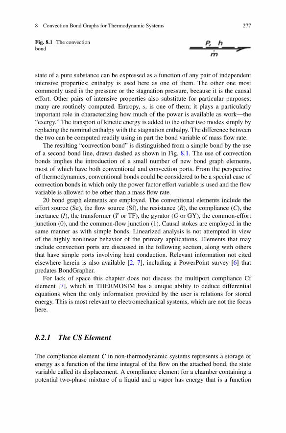
8 Convection Bond Graphs for Thermodynamic Systems 277
Fig. 8.1 The convectionbond
state of a pure substance can be expressed as a function of any pair of independentintensive properties; enthalpy is used here as one of them. The other one mostcommonly used is the pressure or the stagnation pressure, because it is the causaleffort. Other pairs of intensive properties also substitute for particular purposes;many are routinely computed. Entropy, s, is one of them; it plays a particularlyimportant role in characterizing how much of the power is available as work—the“exergy.” The transport of kinetic energy is added to the other two modes simply byreplacing the nominal enthalpy with the stagnation enthalpy. The difference betweenthe two can be computed readily using in part the bond variable of mass flow rate.
The resulting “convection bond” is distinguished from a simple bond by the useof a second bond line, drawn dashed as shown in Fig. 8.1. The use of convectionbonds implies the introduction of a small number of new bond graph elements,most of which have both conventional and convection ports. From the perspectiveof thermodynamics, conventional bonds could be considered to be a special case ofconvection bonds in which only the power factor effort variable is used and the flowvariable is allowed to be other than a mass flow rate.
20 bond graph elements are employed. The conventional elements include theeffort source (Se), the flow source (Sf), the resistance (R), the compliance (C), theinertance (I), the transformer (T or TF), the gyrator (G or GY), the common-effortjunction (0), and the common-flow junction (1). Causal stokes are employed in thesame manner as with simple bonds. Linearized analysis is not attempted in viewof the highly nonlinear behavior of the primary applications. Elements that mayinclude convection ports are discussed in the following section, along with othersthat have simple ports involving heat conduction. Relevant information not citedelsewhere herein is also available [2, 7], including a PowerPoint survey [6] thatpredates BondGrapher.
For lack of space this chapter does not discuss the multiport compliance Cfelement [7], which in THERMOSIM has a unique ability to deduce differentialequations when the only information provided by the user is relations for storedenergy. This is most relevant to electromechanical systems, which are not the focushere.
8.2.1 The CS Element
The compliance element C in non-thermodynamic systems represents a storage ofenergy as a function of the time integral of the flow on the attached bond, the statevariable called its displacement. A compliance element for a chamber containing apotential two-phase mixture of a liquid and a vapor has energy that is a function
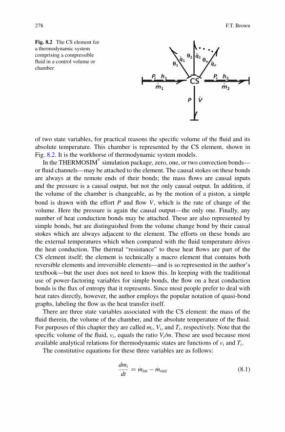
278 F.T. Brown
Fig. 8.2 The CS element fora thermodynamic systemcomprising a compressiblefluid in a control volume orchamber
of two state variables, for practical reasons the specific volume of the fluid and itsabsolute temperature. This chamber is represented by the CS element, shown inFig. 8.2. It is the workhorse of thermodynamic system models.
In the THERMOSIM®
simulation package, zero, one, or two convection bonds—or fluid channels—may be attached to the element. The causal stokes on these bondsare always at the remote ends of their bonds; the mass flows are causal inputsand the pressure is a causal output, but not the only causal output. In addition, ifthe volume of the chamber is changeable, as by the motion of a piston, a simplebond is drawn with the effort P and flow
:
V , which is the rate of change of thevolume. Here the pressure is again the causal output—the only one. Finally, anynumber of heat conduction bonds may be attached. These are also represented bysimple bonds, but are distinguished from the volume change bond by their causalstokes which are always adjacent to the element. The efforts on these bonds arethe external temperatures which when compared with the fluid temperature drivesthe heat conduction. The thermal “resistance” to these heat flows are part of theCS element itself; the element is technically a macro element that contains bothreversible elements and irreversible elements—and is so represented in the author’stextbook—but the user does not need to know this. In keeping with the traditionaluse of power-factoring variables for simple bonds, the flow on a heat conductionbonds is the flux of entropy that it represents. Since most people prefer to deal withheat rates directly, however, the author employs the popular notation of quasi-bondgraphs, labeling the flow as the heat transfer itself.
There are three state variables associated with the CS element: the mass of thefluid therein, the volume of the chamber, and the absolute temperature of the fluid.For purposes of this chapter they are called mi, Vi, and Ti, respectively. Note that thespecific volume of the fluid, vi, equals the ratio Vi/m. These are used because mostavailable analytical relations for thermodynamic states are functions of vi and Ti.
The constitutive equations for these three variables are as follows:
dmi
dtD :
mini � :mouti (8.1)
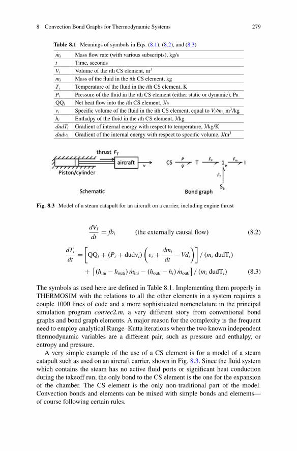
8 Convection Bond Graphs for Thermodynamic Systems 279
Table 8.1 Meanings of symbols in Eqs. (8.1), (8.2), and (8.3):
mi Mass flow rate (with various subscripts), kg/st Time, secondsVi Volume of the ith CS element, m3
mi Mass of the fluid in the ith CS element, kgTi Temperature of the fluid in the ith CS element, KPi Pressure of the fluid in the ith CS element (either static or dynamic), PaQQi Net heat flow into the ith CS element, J/svi Specific volume of the fluid in the ith CS element, equal to Vi/mi, m3/kghi Enthalpy of the fluid in the ith CS element, J/kgdudTi Gradient of internal energy with respect to temperature, J/kg/Kdudvi Gradient of the internal energy with respect to specific volume, J/m3
Fig. 8.3 Model of a steam catapult for an aircraft on a carrier, including engine thrust
dVi
dtD fbi .the externally causal flow/ (8.2)
dTi
dtD�
QQi C .Pi C dudvi/
�vi C dmi
dt� Vdi
��= .mi dudTi/
C �.hini � houti/
:mini � .houti � hi/
:mouti
�= .mi dudTi/ (8.3)
The symbols as used here are defined in Table 8.1. Implementing them properly inTHERMOSIM with the relations to all the other elements in a system requires acouple 1000 lines of code and a more sophisticated nomenclature in the principalsimulation program convec2.m, a very different story from conventional bondgraphs and bond graph elements. A major reason for the complexity is the frequentneed to employ analytical Runge–Kutta iterations when the two known independentthermodynamic variables are a different pair, such as pressure and enthalpy, orentropy and pressure.
A very simple example of the use of a CS element is for a model of a steamcatapult such as used on an aircraft carrier, shown in Fig. 8.3. Since the fluid systemwhich contains the steam has no active fluid ports or significant heat conductionduring the takeoff run, the only bond to the CS element is the one for the expansionof the chamber. The CS element is the only non-traditional part of the model.Convection bonds and elements can be mixed with simple bonds and elements—of course following certain rules.

280 F.T. Brown
Fig. 8.4 A tank being charged with a fluid from a source through a restriction
8.2.2 The RSc Element
A model for an independent source of fluid—in effect a chamber of infinite size—connected to a fluid chamber through a restriction such as valve or an orifice isshown in Fig. 8.4. The source is called the convection Se element, sometimeswritten as Sec. The restriction is called the convection RSc element, which is highlyirreversible despite the fact that the power flows on the two bonds are identicaland equal to h
:m. In THERMOSIM the RSc element is treated as an equivalent
orifice with upstream flow that is reversible but an expansion that is not. The fluidupstream and/or downstream could be a saturated mixture of vapor and liquid,which introduces a complication because the effect of gravity on whichever chamberis upstream—has the higher pressure—may separate the liquid from the vapor,depending on the elevation of the physical port. One also does not know in generalfrom which end the fluid is emitted; it may even change in the middle of a run.Therefore, the user must choose one of the following nine possibilities:
(1) No gravity separation for liquid or vapor. (This is the default choice.)(2) Only vapor passes into the input side (for forward flow); there is no restriction
for flow passing into the output side (for reverse flow).(3) Only liquid passes into the input side (for forward flow); there is no restriction
for flow passing into the output side (for reverse flow).(4) Only vapor passes into the output side (for reverse flow); there is no restriction
for flow passing into the input side (for forward flow)(5) Only liquid passes into the output side (for reverse flow); there is no restriction
for flow passing into the input side (for forward flow).(6) Only vapor passes in both directions.(7) Only liquid passes into the input side (for forward flow); only vapor passes into
the output side (for reverse flow).(8) Only vapor passes into the input side (for forward flow); only liquid passes into
the output side (for reverse flow).(9) Only liquid passes in both directions.
THERMOSIM employs a special function file convecRS2.m to compute the massflow rate and enthalpy of the flow through a general compressible fluid through avena contracta, which the user characterizes by an equivalent orifice area. The flowupstream of the vena contracta is assumed to be adiabatic and isentropic (reversiblewith constant entropy). The expanding flow downstream of the vena contracta isassumed to have the downstream pressure, and therefore is highly irreversible. Theflow at the throat can be subsonic or choked. The function file has as independent
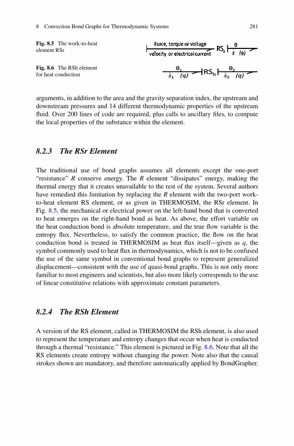
8 Convection Bond Graphs for Thermodynamic Systems 281
Fig. 8.5 The work-to-heatelement RSr
Fig. 8.6 The RSh elementfor heat conduction
arguments, in addition to the area and the gravity separation index, the upstream anddownstream pressures and 14 different thermodynamic properties of the upstreamfluid. Over 200 lines of code are required, plus calls to ancillary files, to computethe local properties of the substance within the element.
8.2.3 The RSr Element
The traditional use of bond graphs assumes all elements except the one-port“resistance” R conserve energy. The R element “dissipates” energy, making thethermal energy that it creates unavailable to the rest of the system. Several authorshave remedied this limitation by replacing the R element with the two-port work-to-heat element RS element, or as given in THERMOSIM, the RSr element. InFig. 8.5, the mechanical or electrical power on the left-hand bond that is convertedto heat emerges on the right-hand bond as heat. As above, the effort variable onthe heat conduction bond is absolute temperature, and the true flow variable is theentropy flux. Nevertheless, to satisfy the common practice, the flow on the heatconduction bond is treated in THERMOSIM as heat flux itself—given as q, thesymbol commonly used to heat flux in thermodynamics, which is not to be confusedthe use of the same symbol in conventional bond graphs to represent generalizeddisplacement—consistent with the use of quasi-bond graphs. This is not only morefamiliar to most engineers and scientists, but also more likely corresponds to the useof linear constitutive relations with approximate constant parameters.
8.2.4 The RSh Element
A version of the RS element, called in THERMOSIM the RSh element, is also usedto represent the temperature and entropy changes that occur when heat is conductedthrough a thermal “resistance.” This element is pictured in Fig. 8.6. Note that all theRS elements create entropy without changing the power. Note also that the causalstrokes shown are mandatory, and therefore automatically applied by BondGrapher.
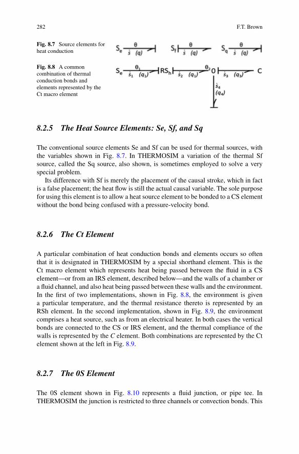
282 F.T. Brown
Fig. 8.7 Source elements forheat conduction
Fig. 8.8 A commoncombination of thermalconduction bonds andelements represented by theCt macro element
8.2.5 The Heat Source Elements: Se, Sf, and Sq
The conventional source elements Se and Sf can be used for thermal sources, withthe variables shown in Fig. 8.7. In THERMOSIM a variation of the thermal Sfsource, called the Sq source, also shown, is sometimes employed to solve a veryspecial problem.
Its difference with Sf is merely the placement of the causal stroke, which in factis a false placement; the heat flow is still the actual causal variable. The sole purposefor using this element is to allow a heat source element to be bonded to a CS elementwithout the bond being confused with a pressure-velocity bond.
8.2.6 The Ct Element
A particular combination of heat conduction bonds and elements occurs so oftenthat it is designated in THERMOSIM by a special shorthand element. This is theCt macro element which represents heat being passed between the fluid in a CSelement—or from an IRS element, described below—and the walls of a chamber ora fluid channel, and also heat being passed between these walls and the environment.In the first of two implementations, shown in Fig. 8.8, the environment is givena particular temperature, and the thermal resistance thereto is represented by anRSh element. In the second implementation, shown in Fig. 8.9, the environmentcomprises a heat source, such as from an electrical heater. In both cases the verticalbonds are connected to the CS or IRS element, and the thermal compliance of thewalls is represented by the C element. Both combinations are represented by the Ctelement shown at the left in Fig. 8.9.
8.2.7 The 0S Element
The 0S element shown in Fig. 8.10 represents a fluid junction, or pipe tee. InTHERMOSIM the junction is restricted to three channels or convection bonds. This
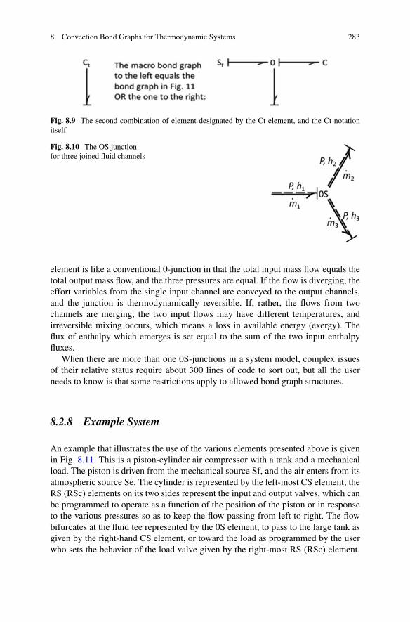
8 Convection Bond Graphs for Thermodynamic Systems 283
Fig. 8.9 The second combination of element designated by the Ct element, and the Ct notationitself
Fig. 8.10 The OS junctionfor three joined fluid channels
element is like a conventional 0-junction in that the total input mass flow equals thetotal output mass flow, and the three pressures are equal. If the flow is diverging, theeffort variables from the single input channel are conveyed to the output channels,and the junction is thermodynamically reversible. If, rather, the flows from twochannels are merging, the two input flows may have different temperatures, andirreversible mixing occurs, which means a loss in available energy (exergy). Theflux of enthalpy which emerges is set equal to the sum of the two input enthalpyfluxes.
When there are more than one 0S-junctions in a system model, complex issuesof their relative status require about 300 lines of code to sort out, but all the userneeds to know is that some restrictions apply to allowed bond graph structures.
8.2.8 Example System
An example that illustrates the use of the various elements presented above is givenin Fig. 8.11. This is a piston-cylinder air compressor with a tank and a mechanicalload. The piston is driven from the mechanical source Sf, and the air enters from itsatmospheric source Se. The cylinder is represented by the left-most CS element; theRS (RSc) elements on its two sides represent the input and output valves, which canbe programmed to operate as a function of the position of the piston or in responseto the various pressures so as to keep the flow passing from left to right. The flowbifurcates at the fluid tee represented by the 0S element, to pass to the large tank asgiven by the right-hand CS element, or toward the load as programmed by the userwho sets the behavior of the load valve given by the right-most RS (RSc) element.

284 F.T. Brown
Fig. 8.11 Piston-cylinder air compressor with tank and load

8 Convection Bond Graphs for Thermodynamic Systems 285
The air in the load tank gets hot. Heat is conducted to the walls of the tank, where itis stored, and from there to the environment; these features are all represented in themacro Ct element. The output piston and cylinder is represented by the CS elementtoward the upper-right. The attached T element transforms the volume change rateto velocity. The weight of the load is represented by the uppermost Se element,its mass or inertia by the I element, and an effective dashpot by the R element.The transformer element T near the bottom of the bond graph transforms the rateof change of the piston volume to velocity, and the RSr element there uses thisvelocity, v, and the temperature of the 0-junction, � c, to compute the friction forceon the piston, F, and the heat generated thereby, qf . Some of this heat goes to theenvironment Se through the thermal resistance RSh, some goes to heat the wallsof the cylinder—which gets quite hot—and some passes back into the air in thecylinder.
8.2.9 The 1- and 1S-Junction Elements with Convection Bonds
The only work interaction between convection and non-convection parts of a systempresented thus far is through the volume change bond of the CS element. The 1S-junction and the generalized 1-junction perform the other work interactions.
The traditional 1-junction is a mainstay of non-convection bond graphs; it canhave any number of bonds which are forced to share a common flow. In THER-MOSIM it is restricted to three bonds; additional junctions are used when needed.Precisely two of the bonds are allowed to be convection bonds, leaving the thirdas a simple bond. Since the flow on convection bonds is always a mass flow, thismeans that all the flow on all three bonds of any such 1-junction must be the samemass flow. Further, the junction is defined so as to represent thermodynamicallyreversible behavior, so the entropies on its two convection bonds must equal oneanother. Since energy is also conserved, as with the traditional 1-junction, the efforton the simple or mechanical bond equals the difference between the enthalpies ofthe two convection bonds—assuming their power convention arrows are aligned thesame way.
Sometimes one desires to have a common-flow junction with two convectionbonds having equal pressures rather than equal entropies. This is the definition of1S-junction, which thereby becomes thermodynamically irreversible. Use of the 1-and 1S-junctions is illustrated by the model for the heart of a positive-displacementcompressor shown in Fig. 8.12.
Part (a) of the figure shows an ideal or lossless compressor (100 % volumetricand adiabatic efficiencies) with torque M and angular velocity
:
�. The modulus ofthe transformer Tm is the ratio of the mass flow to the angular velocity, which isthe product of the density of the entering fluid times the volumetric displacementper radian or rotation. Part (b) shows how to represent compressors with less than100 % volumetric and adiabatic efficiencies. The modulus of the transformer T can

286 F.T. Brown
Fig. 8.12 Bond graphs (a) and (b) for a positive-displacement compressor or pump
Fig. 8.13 The IRS element
be shown to be T D �v=�ad, where �v is the volumetric efficiency and �ad is theadiabatic efficiency. The modulus of the transformer Ts can be shown to be Ts D�v= .1 � �ad/.
Note that elements in THERMOSIM containing the letter S in their names aredefined to be at least potentially irreversible.
8.2.10 The IRS Element
The final element with convection ports is the IRS element, first introduced in 2003[4] with a major update in 2016 [10]. This represents a fluid channel with fluidfriction, inertia and heat transfer to its surroundings—normally the walls. Suchchannels are the principal way engineers achieve critical heat transfer in the systemsthey design; the most common are round tubes. There are two versions of thiselement in THERMOSIM, one for nominal liquids such as water or a hydraulicfluid, and a second for general compressible substances. Both are represented by thebond graph notation shown in Fig. 8.13, and employ the momentum of the streamas its single state flow variable. The multiple heat conduction bonds shown are forthe general case. Often, however, none or only one such bond is used.
The principal parameters are the length of the channel and its area, whichis assumed to be uniform. In keeping with the philosophy that lumped bondgraph elements should use approximate constitutive relations in order to achieve

8 Convection Bond Graphs for Thermodynamic Systems 287
a reasonable compromise between accuracy and computational efficiency, the wallfriction models assume an equivalent steady or equilibrium velocity profile acrossthe channel. Further, a round cross-section—that is a tube—or its equivalentusing the concept of a hydraulic diameter is assumed. Implementing this requirescomputation of the effective Reynolds number of the flow—or for two-phase flow,separate Reynolds numbers for the liquid and vapor phases. This is turn requiresknowledge of the viscosity or viscosities of the fluid. For purposes of relating massflow to the momentum, a slug-flow approximation is employed, so that the massflow is taken as the ratio of the momentum to the length. The rate of change ofthe momentum is proportional to the pressure difference between the two ends ofthe element minus the pressure drop due to wall shear, with a correction for thedifference between the pressures associated with the momentum fluxes at the twoends.
The compliance of the fluid in the channel is not included within the IRS element,but rather is modeled by CS elements that may be placed at its ends. This means thatwhen compressibility effects are especially important—often they are not—such aswhen wave propagation effects are of interest, multiple IRS elements interspersedwith CS elements should be used. Normally, the compliance of the fluid in the tubeis split between the two adjacent CS elements by assigning half of its volume toeach.
The simple bonds in Fig. 8.13 are for the heat conduction to the surroundings,as with the CS element. It may be attached to a Ct macro element or a moreprimitive combination of heat conduction bonds and elements. Many scientists andengineers devote their careers to modeling such heat transfer. The author [10] hasselected what he hopes are the most useful but reasonably simple set of heat-transfercorrelations available in the literature, but the user may prefer to substitute others.
The IRS model for liquid media is simpler than that for general compressiblesubstances, and is vastly simpler when there is no heat conduction bond or only one.The hydraulic system pictured schematically in Fig. 8.14 with the correspondingbond graph in Fig. 8.15 illustrates its use when there is one heat conduction bond.BondGrapher, which is introduced in Sect. 8.4, created this figure in which theselected element CS22 is highlighted with color.
Note the incorporation of the model in Fig. 8.12 for the pump, allowing foradiabatic and volumetric efficiencies less than 100 %. The two fluid tees arerepresented by the two 0S elements. The elements CS18 and CS36 represent thehydraulic sides of the low-pressure and high-pressure accumulators, respectively,while CS22 and CS31 represent the nitrogen sides. Se23 and Se33 representthe temperature of the environment with which the accumulators interact, whileR21 and R27 represent resistances associated with the motion of the accumulatorinterfaces, which are necessary for computational causality purposes although theyare too small to have a significant effect. CS6 and CS9 represent small fixed volumesalong the fluid lines to accommodate the small effects of compressibility and tosatisfy computational causality. The friction and inertia effects of the fluid linesare represented by IRS7, IRS10, and IRS16; the latter two are quite long—4 m—and also exchange heat with their surroundings through the use of elements Ct34

288 F.T. Brown
Fig. 8.14 Schematic for the hydraulic system (using fluid power symbols)
Fig. 8.15 Bond graph for the hydraulic system
and Ct35. RS25 models a spring-loaded check valve that partially opens when theupstream, pressure exceeds 20 MPa, preventing overpressure. RS12 is a valve thatopens when the user wishes to move the double-sided piston-cylinder actuator,which operates with a hydraulic fluid. Further discussion including simulationresults is given in Sect. 8.4.3.
For long channels the properties of the fluid and the wall temperatures may varyconsiderably from one end to the other. This is particularly true when the fluid isa highly compressible substance, but also applies to pure liquids with significant

8 Convection Bond Graphs for Thermodynamic Systems 289
Fig. 8.16 Segmentation of the IRS element
Fig. 8.17 Bond graph for the hot water shower system
transport time from one end to the other and significant thermal interaction withthe channel walls. The author models such situations by segmenting the channel,as shown in Fig. 8.16. Each such segment has one of the heat conduction bondsshown in Fig. 8.13 which is assumed to be attached to a Ct element. EachCt element also has its thermal compliance and state variable for the averagetemperature of the wall at that location. The users draws only one Ct element withthe BondGrapher interface, however; the rest are inferred by a designation of thenumber of the segments N(I), where I is the index number of the IRS element,avoiding what otherwise could be a very messy bond graph. The user assigns theoverall thermal compliance of the tube to this element, represented here as C; theprogram automatically divides C by N to give the compliance of the individualsegments.
Along with the N state variables for the wall temperatures of the segments thereare an additional N state variables for the average fluid temperatures within thesegments. Thus the IRS element has a total of 2 N C 1 state variables, the 1 beingfor the momentum or mass flow rate. The wall shear is also computed separately foreach segment, but this requires no further state variables. Temperatures of the walland the fluid are computed for both the segments and at the interfaces.
A person wants to take a quick shower; how long does he have to wait for the hotwater emerging from a hot water heater 10 m away to reach him, at location Sec6,and of necessity also warm the walls of the copper pipe? A bond graph model forthis system is shown in Fig. 8.17. The hot water emerges from the element Sec1.Cold water also emerges from Sec8 to mix with the hot water at pipe tee 0S5. Thevalves from the two sources, RSc4 and RSc7, are abruptly opened at time zero. Theelement IRS2 is the long pipe modeled with 20 segments, and CS3 is a small volumerepresenting the mixing of new water with old and the slight compressibility of thewater in the pipe, and satisfying causal requirements. This example is continued,with simulation results, in Sect. 8.4.4.

290 F.T. Brown
Fig. 8.18 A model for a fluid channel containing a compressible fluid using unsegmented IRSelements
When a channel contains a compressible fluid, the state of that fluid can changeradically along its length, potentially being a liquid at one end, a saturated mixturein the middle, and a pure vapor at the other end. A proper lumped model of thischannel contains a long cascade of alternating lumped IRS and CS elements, partof which is shown in Fig. 8.18; the CS elements represent the fluid compliance andthe IRS elements represent the wall friction and inertia and thermal interaction withthe walls of the channel via the attached single Ct elements. An especially difficultsituation arises when the segment of fluid line represented by the element is partly acompressed liquid and partly a saturated mixture, since the properties of the fluid inthese two phases are radically different. The length of the cascade would have to beexceedingly long to accommodate this occurrence, imposing a huge computationalburden. A radical structural simplification is proposed to reduce this complexitywithout overly compromising accuracy.
Experience has shown that the mass flow rates approach equilibrium vastlyquicker than the temperatures of the fluid and the channel wall. This is associatedwith the fact that the effect of the mechanical compliance—the compressibility ofthe fluid—is effectively over an order of magnitude smaller than the effect of thethermal compliance—heat capacity—of the walls. This suggests approximating achannel with at least a modest span of fluid states by a single IRS segmented elementwith its uniform mass flow rate, allowing the heat transfer to the walls and the stateof the fluid to vary along its length. The resulting number of IRS elements needed torepresent a channel adequately should be reduced radically, sometimes to only one.
The first-generation IRS element required the user to specify the thermalconductance between the wall and the environment, and was implemented only forrefrigerant R12. Further, the temperature of the tube wall was not allowed to varyquite properly along its length in response to varying heat-transfer rates. A finaldifficult problem was the danger that the phase of the fluid would change in themiddle of a segment to or from liquid or to or from vapor—the other state being asaturated mixture—producing gross errors in key properties that determine the heattransfer for that segment. To combat this frequent occurrence, the transition wasanticipated and the segment sizes adjusted so that the transition would occur verynear the end of a segment. This caused great complication and on some occasionseven caused the program to abort.
The new segmentation also has a key advantage of allowing efficient treatmentof the problem of sudden changes in phase in the middle of a segment. It also allowsa sudden change from boiling to condensation to be treated efficiently.
8 Convection Bond Graphs for Thermodynamic Systems 291
The calculations for the IRS element are coded in the 1000-plus-line script fileIRS4.m, which also calls the function file viscosity.m for the thermal conductivitiesas well as the viscosity, and the function file boiling.m. The file IRS4.m is calledby the main simulation program for potentially multiphase fluids, convec2.m. Thedifferential equation for the state (or temperature) for the wall segment k is
dxk
dtD �
Te � Tseg .I; k/� H .I; k/ � QIs .I; k/ (8.4)
in which H(I, k) is the thermal conductance of the “thermal resistance” of the Ctelement for the kth segment. This conductance is based on the properties of theenvironmental—or “alternative” fluid—and certain properties. It is computed in anew relatively short function file CtH.m also called by IRS4.m, which can also becalled to compute the heat transfer associated with CS elements.
The differential equation for the temperature of the fluid in a segment is
dxNCk
dtD ..Te � xkCN .I; k// Pm C QI2 .I; k/ =dh=dt/=.m=N/ (8.5)
in which I is the index of the IRS element, k is the index of the segment, QI2 is theheat flux from the wall to the fluid for the segment, dh/dt is the specific heat of thefluid, and m/N is the mass of the fluid in one segment. This version of the equationhas been specialized for pure liquids to speed up execution with negligible error.
CS elements are nominally considered to represent physical volumes with largeenough dimensions that the interior velocities of the fluid are small enough not toproduce dynamic heads of significance. For example, a CS element bonded to an 0S-junction is assumed to give that junction a static pressure common to all of its bonds.The hydraulic system above is an example. IRS elements, by contrast, nominallyhave such a small cross-sectional area that the dynamic head is indeed significant.What does it mean, then, when a CS element is bonded to an IRS element? Forthe nominal case, including the hydraulic system, it means that the interior areaof the CS element through which fluid is passing is presumed to be significantlylarger than that of the attached IRS element. Clearly, however, that is not the casefor the cascade of IRS and CS elements depicted in Fig. 8.18. In effect, a differentkind of CS element is needed there, which produces a total dynamic pressure onthe joining bond rather than a static pressure. This is called a “total-pressure CSelement,” for which the dynamic head on the connecting bond is simply added tothe static pressure to give the proper total pressure. It is necessary for the user todesignate that this is what he wants, however; BondGrapher has been modified toask the modeler’s choice, with the default being the “static pressure CS element.”
292 F.T. Brown
8.3 Thermodynamic and Physical Propertiesof Common Substances
Starting in 1999 [3] and continuing until the present [3, 5, 8, 9] the author has devel-oped practical code for modeling the properties of gaseous, liquid, and saturatedmixtures thereof of 30 common pure substances that are identified as potentiallybeing in the vapor state or saturated mixture state—ammonia, argon, butane, carbondioxide, cesium, ethane, ethylene, helium, heptane, hexane, hydrogen, isobutene,isopentane, mercury, methane, neon, nitrogen, octane, oxygen, propane, propylalcohol, propylene, the refrigerants 12, 13, 134a, 22, 23, 502, and 503, rubidium,and water. Prominent amongst his sources is the work of Reynolds [12]. Gaseous airis treated as a mixture of nitrogen, oxygen, and argon. He has also focused on fouradditional substances identified as liquids—liquid water and the hydraulic fluidsMIL H 5606, MIL PRF 27601, and MIL PRF 83282.
In the spirit of a compromise between accuracy and complexity he has avoideduse of the most accurate models available for some substances, particularly for waterwhere lifetimes of effort have produced very accurate but extremely complex modelsthat would drastically retard the speed of simulation, favoring instead a modelthat was once considered generally excellent. He has also forgone some availableaccuracy in the region of the critical point; should this especially complex regionbecome critical, making an improvement ought to be considered.
Any pair of independent properties are necessary and sufficient to specify thestate of a pure substance. For the pure liquids, the most practical pair is temperatureand pressure. For the general substances, as is pointed out in Sect. 2.1, the pair thatis effectively mandated by the available data is temperature and specific volume—the inverse of mass density. This use of specific volume can be problematical inthe compressed liquid state, however, since liquids have nearly constant specificvolume. Depending on the substance, approximate values may not be computedunless one specifies a value for the bulk modulus, which is an option.
Analytic models taken from the literature are used to compute the dependentthermodynamic properties, which include enthalpy, internal energy, specific heat,entropy, the quality of saturated mixtures—the author extends the definition ofquality to make it useful also for the compressed liquid and vapor states—specificvolume, enthalpy and entropy of a saturated liquid at the given temperature, andthese same properties for a saturated vapor at the given temperature. The listis of course expanded by absolute pressure for the general substances and massdensity for the pure liquids. Further, simulation programs used by THERMOSIMemploy several Runge–Kutta iterations that are expedited if the gradients of the non-saturation dependent properties with respect to the two independent properties arealso available in analytic form. The author therefore derived analytical derivativesof the available empirical relations for pressure, internal energy, enthalpy andentropy, plus the gradient of quality with respect to temperature, adding nine moredependent variables to the list for the general substance. When the phase changesbetween pure liquid and saturated vapor, these gradients change abruptly by orders
8 Convection Bond Graphs for Thermodynamic Systems 293
of magnitude, requiring special treatment. Abrupt changes in heat-transfer and wallfriction domains also are cause for special smoothing.
Separate simulation programs are employed for systems in which the principalfluid is a liquid or is a general substance.
The transport properties of viscosity and thermal conductivity are also needed ifone is to compute heat transfer and fluid friction. Critically important dimensionlessgroups including Reynolds and Nusselt numbers depend on these. Analyticalexpressions for viscosity and thermal conductivity as functions of temperature andspecific volume are difficult to find or deduce, unfortunately, so at this writing theauthor has only limited results. He managed to convert into the needed form someraw data for the four liquids listed above. For general substances he has results forwater, nitrogen, oxygen, argon, air as a vapor, and an approximate form for therefrigerant R12. It is not easy to find appropriate correlations in the literature; muchmore work remains. See also Sect. 8.5 below.
8.4 The Graphical Interface BondGrapher and Examples
Each system model is coded in a MATLAB®
system file that, when called by theuser, directs the desired dynamic simulation. In practice, this system file is mostconveniently produced with the help of a graphical interface called BondGrapher
®,
which was written by the author’s son, Scott A. Brown. All the files needed to carryout the simulation except for BondGrapher, assuming one has access to MATLAB,are freely downloadable from the author’s website [9]. The prospective user shouldalso download the extensive Users’ Manual (make sure it is Version 4), whichprovides the details and many examples of the procedure. BondGrapher includeshelp files, but only the ones that pertain to drawing bond graphs are useful as of thiswriting. To acquire BondGrapher, which also is free for the foreseeable future, oneshould email the author and include a commitment not to transmit the program to athird party without permission.
The structure of the computational part of the THERMOSIM package issuggested in Fig. 8.19.
8.4.1 BondGrapher and the Steam Catapult System
BondGrapher has a main screen and a screen called Global Options. The mainscreen with the bond graph for the aircraft catapult of Fig. 8.3 drawn is shownin Fig. 8.20. The graph may have been entered directly, or downloaded from anexisting system file created and saved earlier using a name of the user’s choice.The procedure to draw a new bond graph involves placing symbols for elementsover node locations, and placing bonds between nodes by clicking on the elementat one end of the bond and then double-clicking the node at the other end. The
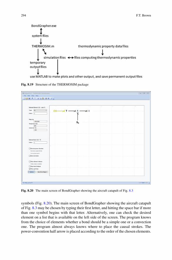
294 F.T. Brown
Fig. 8.19 Structure of the THERMOSIM package
Fig. 8.20 The main screen of BondGrapher showing the aircraft catapult of Fig. 8.3
symbols (Fig. 8.20). The main screen of BondGrapher showing the aircraft catapultof Fig. 8.3 may be chosen by typing their first letter, and hitting the space bar if morethan one symbol begins with that letter. Alternatively, one can check the desiredelement on a list that is available on the left side of the screen. The program knowsfrom the choice of elements whether a bond should be a simple one or a convectionone. The program almost always knows where to place the causal strokes. Thepower-convention half arrow is placed according to the order of the chosen elements.
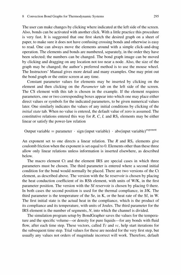
8 Convection Bond Graphs for Thermodynamic Systems 295
The user can make changes by clicking where indicated at the left side of the screen.Also, bonds can be activated with another click. With a little practice this procedureis very fast. It is suggested that one first sketch the desired graph on a sheet ofpaper, to make sure it does not have confusing crossing bonds and otherwise is easyto read. One can always move the elements around with a simple click-and-dragoperation. The elements and bonds are numbered, separately, in the order they havebeen selected; the numbers can be changed. The bond graph image can be movedby clicking and dragging on any location not too near a node. Also, the size of thegraph may be changed; the author’s preferred method is to use the mouse wheel.The Instructors’ Manual gives more detail and many examples. One may print outthe bond graph or the entire screen at any time.
Constant parameter values for elements may be inserted by clicking on theelement and then clicking on the Parameter tab on the left side of the screen.The CS element with this tab is chosen in the example. If the element requiresparameters, one or two corresponding boxes appear into which one may place eitherdirect values or symbols for the indicated parameters, to be given numerical valueslater. One similarly indicates the values of any initial conditions by clicking of theinitial state tab. When no value is entered, the default value of zero is assumed. Theconstitutive relations entered this way for R, C, I, and RSr elements may be eitherlinear or satisfy the power-law relation
Output variable D parameter � sign .input variable/ � abs.input variable/exponent
An exponent set to one directs a linear relation. The R and RSr elements givecoulomb friction when the exponent is set equal to 0. Elements other than these threeallow only linear relations unless information is inserted elsewhere, as describedbelow.
The macro element Ct and the element IRS are special cases in which threeparameters must be chosen. The third parameter is entered where a second initialcondition for the bond would normally be placed. There are two versions of the Ctelement, as described above. The version with the Se reservoir is chosen by placingthe heat conduction coefficient of its RSh element, with units of W/K, in the firstparameter position. The version with the Sf reservoir is chosen by placing 0 there.In both cases the second position is used for the thermal compliance, in J/K. Thethird parameter is the temperature of the Se, in K, or the heat rate of the Sf, in W.The first initial state is the actual heat in the compliance, which is the product ofits compliance and its temperature, with units of Joules. The third parameter for theIRS element is the number of segments, N, into which the channel is divided.
The simulation program setup by BondGrapher saves the values for the tempera-ture and the specific volume—or density for pure liquids—for any bonds with fluidflow, after each time step. These vectors, called Tc and vc, help start iterations forthe subsequent time step. Trial values for these are needed for the very first step, butusually any values not orders of magnitude incorrect will work. Therefore, default
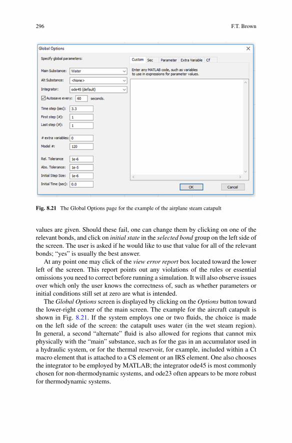
296 F.T. Brown
Fig. 8.21 The Global Options page for the example of the airplane steam catapult
values are given. Should these fail, one can change them by clicking on one of therelevant bonds, and click on initial state in the selected bond group on the left side ofthe screen. The user is asked if he would like to use that value for all of the relevantbonds; “yes” is usually the best answer.
At any point one may click of the view error report box located toward the lowerleft of the screen. This report points out any violations of the rules or essentialomissions you need to correct before running a simulation. It will also observe issuesover which only the user knows the correctness of, such as whether parameters orinitial conditions still set at zero are what is intended.
The Global Options screen is displayed by clicking on the Options button towardthe lower-right corner of the main screen. The example for the aircraft catapult isshown in Fig. 8.21. If the system employs one or two fluids, the choice is madeon the left side of the screen: the catapult uses water (in the wet steam region).In general, a second “alternate” fluid is also allowed for regions that cannot mixphysically with the “main” substance, such as for the gas in an accumulator used ina hydraulic system, or for the thermal reservoir, for example, included within a Ctmacro element that is attached to a CS element or an IRS element. One also choosesthe integrator to be employed by MATLAB; the integrator ode45 is most commonlychosen for non-thermodynamic systems, and ode23 often appears to be more robustfor thermodynamic systems.
8 Convection Bond Graphs for Thermodynamic Systems 297
Another choice selected on the left side of the Global Options screen is howlong each time segment in a run should be, and how many time segments are tobe run. If the numbers of the “first step” and the “last step” are both 1, as withthe catapult, there is only one time segment and the “time step” is its duration inseconds. The simulation stores the history of the states through the most recent timestep in a file TSIMdata.mat, which the MATLAB command load TSIMdata allowsthe user to access. If the “first step” is chosen to be 1 and the “last step” is a largerthan the “first step,” the states at the ends of each time segment are stored in afile dataX.mat, which can be accessed by the command load dataX. This providesa data compression feature that may be attractive if a run would otherwise producedata files that are longer than one would prefer. In practice, however, the most usefulfeature of the data compression mode is the ability to interrupt a simulation at anypoint, look at the results up to that point, and then resume the simulation. This isalso helpful if the simulation is very slow, or if one wishes to change one or moreparameters in the middle of an overall run. Following an interruption in a simulationand commanding load dataX, one can determine the number of the last time segmentcompleted with the command size(time) or size(state). To resume the simulation, oneenters this number as the “first step” of the continuation.
Finally, the bottom of the left side of the Global Options page allows the user tochoose the relative and absolute tolerance of the simulation, and the initial step size.See MATLAB help for detailed information.
The Steam Catapult system uses only one of the six tabs on the right side of theGlobal Options page, that called Custom. This tab is used to provide the values ofany constants indicated elsewhere only by symbols. The only such symbol for thissystem is the temperaureT00, used in the definition of Tc. Other uses of the rightside of the Global Options page are discussed in the context of other systems below.
After running the system file, you may enter MATLAB commands to plot, print,or save whatever results you wish. Selected results from the simulation of the steamcatapult system are shown in Fig. 8.22.
8.4.2 The Piston-Cylinder air Compressor and ProgrammingNonlinearities and Special Functions
The main page of the BondGrapher that produced the MATLAB system fileaircompsys2.m is shown in Fig. 8.23, with the element C and the parameter tabclicked. On the screen the element is highlighted in color. The exponent of theconstitutive relation for this compliance is given as 1, indicating a linear relation,of several either directly given or computed in the Custom tab on the right side ofthe Global Options page, as shown in Fig. 8.24, using standard MATLAB coding.
There are four more tabs to the right of the Custom tab. The most importantof these are the Parameter tab and the Extra variable tab, which are discussedpresently. First, however, it is necessary to know something about a matrix calledel(i, j).

298 F.T. Brown
Fig. 8.22 Selected results of the steam catapult system
Fig. 8.23 Main page of BondGrapher for the piston-cylinder air compressor

8 Convection Bond Graphs for Thermodynamic Systems 299
Fig. 8.24 Global Options page of BondGrapher for the air compressor system
The matrix el is the repository of the order and content of all the elements ina system model. It is a prominent part of the system file created by BondGrapher.It has one row for each element, in the order of their element numbers. Each rowhas three members. The first member is a code number designating which of the 20types the element is. The other two members are both zero for the four junctions.Their content for the remaining 16 element types is given in a table in Sect. 1.6 ofthe Users’ Manual (version 4) which is too large to reproduce here.
In the Parameter tab the parameters are defined by the user in one of thefollowing forms, in which X refers to the quality of the fluid and Pb refers to thepressure on bonds:
el .i; 2/ D function .t; x;P;X; h; s;Pb/ .for multiphase substancess/or el .i; 2/ D function .t; x;Pb; h; s/ .for liquids/
el .i; 3/ D function .t; x;P;X; h; s;Pb/ .for multiphase substances/or el .i; 3/ D function .t; x;Pb; h; s/ .for liquids/
Here i is the number of the bond and the 2 or 3 refers to the parameter as identified inthe table. Look at the Parameter tab for the air compressor system given in Fig. 8.25.Its first line specifies the sinusoidally varying angular velocity of the input shaft; thetable says that the value of the flow for Sf elements is given in the third position,
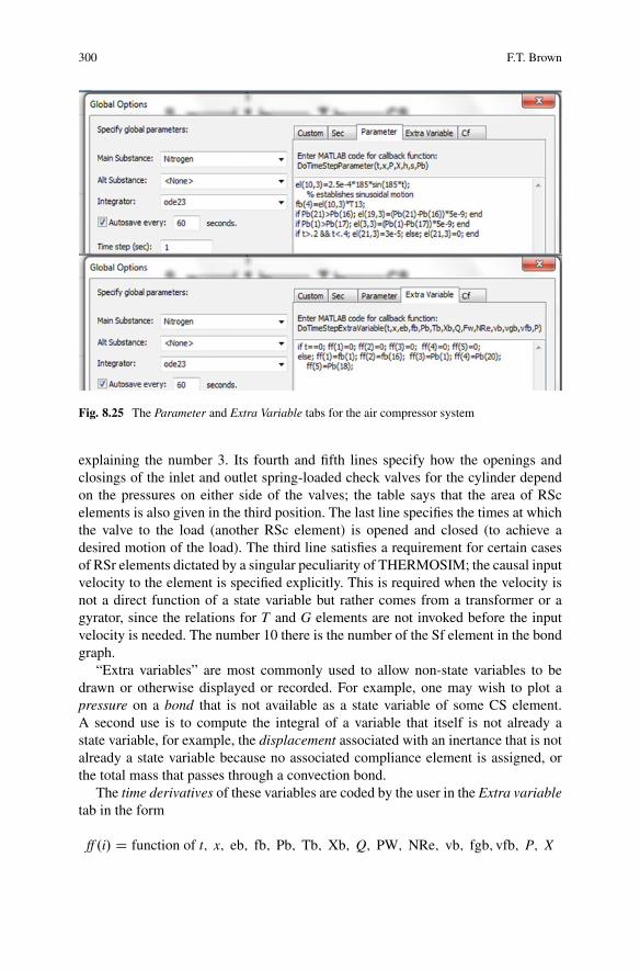
300 F.T. Brown
Fig. 8.25 The Parameter and Extra Variable tabs for the air compressor system
explaining the number 3. Its fourth and fifth lines specify how the openings andclosings of the inlet and outlet spring-loaded check valves for the cylinder dependon the pressures on either side of the valves; the table says that the area of RScelements is also given in the third position. The last line specifies the times at whichthe valve to the load (another RSc element) is opened and closed (to achieve adesired motion of the load). The third line satisfies a requirement for certain casesof RSr elements dictated by a singular peculiarity of THERMOSIM; the causal inputvelocity to the element is specified explicitly. This is required when the velocity isnot a direct function of a state variable but rather comes from a transformer or agyrator, since the relations for T and G elements are not invoked before the inputvelocity is needed. The number 10 there is the number of the Sf element in the bondgraph.
“Extra variables” are most commonly used to allow non-state variables to bedrawn or otherwise displayed or recorded. For example, one may wish to plot apressure on a bond that is not available as a state variable of some CS element.A second use is to compute the integral of a variable that itself is not already astate variable, for example, the displacement associated with an inertance that is notalready a state variable because no associated compliance element is assigned, orthe total mass that passes through a convection bond.
The time derivatives of these variables are coded by the user in the Extra variabletab in the form
ff .i/ D function of t; x; eb; fb; Pb; Tb; Xb; Q; PW; NRe; vb; fgb; vfb; P; X
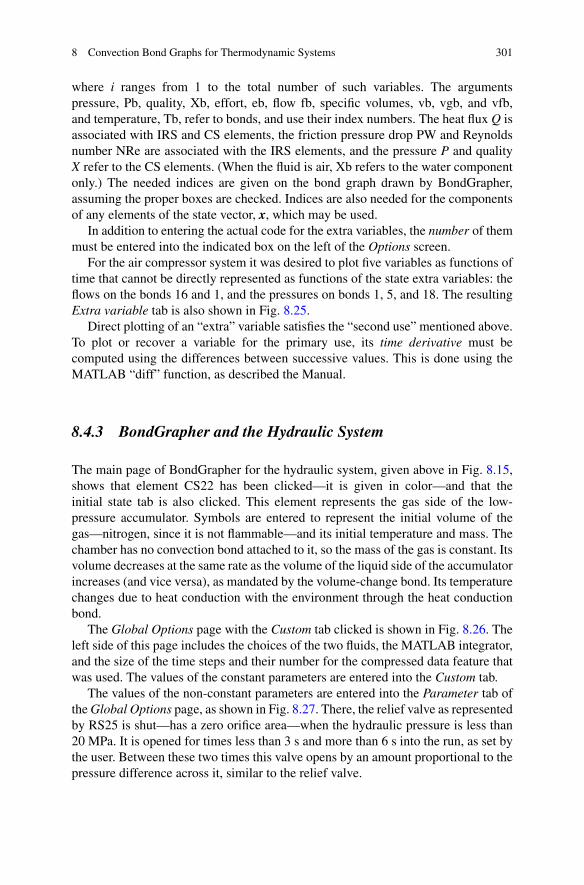
8 Convection Bond Graphs for Thermodynamic Systems 301
where i ranges from 1 to the total number of such variables. The argumentspressure, Pb, quality, Xb, effort, eb, flow fb, specific volumes, vb, vgb, and vfb,and temperature, Tb, refer to bonds, and use their index numbers. The heat flux Q isassociated with IRS and CS elements, the friction pressure drop PW and Reynoldsnumber NRe are associated with the IRS elements, and the pressure P and qualityX refer to the CS elements. (When the fluid is air, Xb refers to the water componentonly.) The needed indices are given on the bond graph drawn by BondGrapher,assuming the proper boxes are checked. Indices are also needed for the componentsof any elements of the state vector, x, which may be used.
In addition to entering the actual code for the extra variables, the number of themmust be entered into the indicated box on the left of the Options screen.
For the air compressor system it was desired to plot five variables as functions oftime that cannot be directly represented as functions of the state extra variables: theflows on the bonds 16 and 1, and the pressures on bonds 1, 5, and 18. The resultingExtra variable tab is also shown in Fig. 8.25.
Direct plotting of an “extra” variable satisfies the “second use” mentioned above.To plot or recover a variable for the primary use, its time derivative must becomputed using the differences between successive values. This is done using theMATLAB “diff” function, as described the Manual.
8.4.3 BondGrapher and the Hydraulic System
The main page of BondGrapher for the hydraulic system, given above in Fig. 8.15,shows that element CS22 has been clicked—it is given in color—and that theinitial state tab is also clicked. This element represents the gas side of the low-pressure accumulator. Symbols are entered to represent the initial volume of thegas—nitrogen, since it is not flammable—and its initial temperature and mass. Thechamber has no convection bond attached to it, so the mass of the gas is constant. Itsvolume decreases at the same rate as the volume of the liquid side of the accumulatorincreases (and vice versa), as mandated by the volume-change bond. Its temperaturechanges due to heat conduction with the environment through the heat conductionbond.
The Global Options page with the Custom tab clicked is shown in Fig. 8.26. Theleft side of this page includes the choices of the two fluids, the MATLAB integrator,and the size of the time steps and their number for the compressed data feature thatwas used. The values of the constant parameters are entered into the Custom tab.
The values of the non-constant parameters are entered into the Parameter tab ofthe Global Options page, as shown in Fig. 8.27. There, the relief valve as representedby RS25 is shut—has a zero orifice area—when the hydraulic pressure is less than20 MPa. It is opened for times less than 3 s and more than 6 s into the run, as set bythe user. Between these two times this valve opens by an amount proportional to thepressure difference across it, similar to the relief valve.
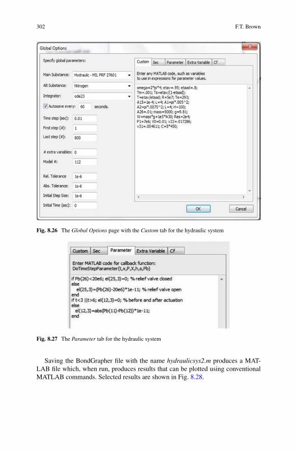
302 F.T. Brown
Fig. 8.26 The Global Options page with the Custom tab for the hydraulic system
Fig. 8.27 The Parameter tab for the hydraulic system
Saving the BondGrapher file with the name hydraulicsys2.m produces a MAT-LAB file which, when run, produces results that can be plotted using conventionalMATLAB commands. Selected results are shown in Fig. 8.28.
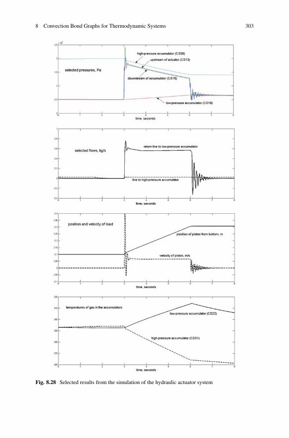
8 Convection Bond Graphs for Thermodynamic Systems 303
Fig. 8.28 Selected results from the simulation of the hydraulic actuator system

304 F.T. Brown
Fig. 8.29 The Global Options screen with the Custom tab for the shower system
8.4.4 BondGrapher and Segmented IRS Elements
For segmented IRS elements for liquids the user must provide the initial temper-atures of the N wall temperatures and N fluid temperatures. This is done in theCustom tab of the Global Options screen. This screen is shown in Fig. 8.29 forthe shower problem introduced in Sect. 8.2.10 and Fig. 8.17. Note that all theseinitial temperatures are set equal to the environmental temperature (Te). The onlyhigher initial temperature is that of the water heater, which is set 44 K higher in theparameter tab for Sec1 on the main screen of BondGrapher. The Custom tab alsoestablishes the values of all the parameters. The inner diameter of the copper pipeis 0.01 m, its outer diameter is 0.012 m, and its length is 10 m. The effective orificearea of the two valves is one-fifth that of the inside of the pipe.
The main simulation program for pure liquids is convecliq4.m, which callsthe script file IRSliq4.m to handle whatever IRS elements are present. This latterprogram also calls the function file CtH.m to treat the implicit Ct elements. Forgeneral highly compressible substances the respective files are convec4.m, IRS4.mand (again) CtH.m.
Selected results of a simulation of the start-up transient are shown in Fig. 8.30.For the specified valve settings, the mass flow rate reaches its equilibrium value ofabout 0.13 kg/s in under 0.2 s, giving a fluid velocity of about 1.7 m/s. Thus it takesabout 6 s for a particle of water to traverse the pipe. It takes longer for the outputstream to reach its equilibrium value, partly since the walls of the pipe absorb heatand partly because of the mixing in the pipe as represented by the CS volume whichis set to equal half of the total volume of the pipe. The output temperature felt by theperson showering was computed using the extra variable option; the temperature isthat of bond 5, or Tb5. The computed rises in the temperatures of the water and thetube are slower than an exact analysis would give, and demonstrate some oscillation,due to the finite sizes of the segments, but the filtering effect of the fluid complianceis greater. The final temperature of the shower is lukewarm, despite the two valves
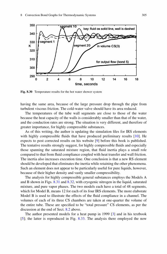
8 Convection Bond Graphs for Thermodynamic Systems 305
Fig. 8.30 Temperature results for the hot water shower system
having the same area, because of the large pressure drop through the pipe fromturbulent viscous friction. The cold-water valve should have its area reduced.
The temperatures of the tube wall segments are close to those of the waterbecause the heat capacity of the walls is considerably smaller than that of the water,and the conduction rates are strong. The situation is very different, and therefore ofgreater importance, for highly compressible substances.
As of this writing, the author is updating the simulation files for IRS elementswith highly compressible fluids that have produced preliminary results [10]. Heexpects to post corrected results on his website [9] before this book is published.The tentative results strongly suggest, for highly compressible fluids and especiallythose spanning the saturated mixture region, that fluid inertia plays a small rolecompared to that from fluid compliance coupled with heat transfer and wall friction.The inertia also increases execution time. One conclusion is that a new RS elementshould be developed that eliminates the inertia while retaining the other phenomena.Such an element does not appear to be particularly useful for pure liquids, however,because of their higher density and vastly smaller compressibility.
The analysis for highly compressible general substances employs the Models Aand B shown in Figs. 8.31 and 8.32, with cryogenic nitrogen in the liquid, saturatedmixture, and pure vapor phases. The two models each have a total of 48 segments,which for Model B, means 12 for each of its four IRS elements. The more elaborateModel B is used to illustrate the effects of the fluid compliance in a channel. Thevolumes of each of its three CS chambers are taken at one-quarter the volume ofthe entire tube. These are specified to be “total pressure” CS elements, as per thediscussion at the end of Sect. 8.2 above.
The author presented models for a heat pump in 1999 [3] and in his textbook[5]; the latter is reproduced in Fig. 8.33. The analysis there employed the now

306 F.T. Brown
Fig. 8.31 Model A for afluid channel withcompressible flow
Fig. 8.32 Model B of the same channel
Fig. 8.33 Bond graph model of a heat pump system using IRS elements
discontinued first generation of the IRS element for compressible fluid flow, andis on the author’s agenda for updating using the new IRS element.
The right side of this bond graph shows a compressor driven by an inductionmotor represented by Se23 and rotational inertia represented by I25 and transfer and1- and 1S-junction elements that impart less than 100 % volumetric and adiabaticefficiencies, as with other systems above. The critical heat transfers take place on theinside and outside of tubes, represented by the four IRS elements and their attachedCt elements. The part of the evaporator that conducts heat—and exhibits fluid inertiaand critical wall shear friction—is represented by CS1, IRS2, Ct12 which has thecold side thermal reservoir, and CS3. An electrical heater—used to insure thatvapor enters the compressor—is modeled by the element Sq18. The thermal energystorage in the fluid there is represented by the elements CS1 and CS2, which splitthe volume of the tube equally. The evaporator is represented by the elements CS6,

8 Convection Bond Graphs for Thermodynamic Systems 307
IRS7, Ct16, CS8, IRS9, Ct15, CS10, IRS11, Ct14, and CS12; the Ct elements therehave the hot-side thermal reservoir. The expansion device is a simple orifice-typerestriction, represented by the element RSc13.
Assuming the compressed-data option is used, THERMOSIM records time inthe time vector, the momentum of the flow (product of length and mass flow rate),the state of the CS element, the temperatures and the thermal displacements of thewall (product of thermal compliance and temperatures) for each segment in the statematrix, the history of the wall temperatures for the interfaces in the historyTwj array,the history of the fluid temperatures for the segments in the historyTfj array, thehistory of the overall pressure drop due to wall shear in the historyPWc matrix,and the history of the overall heat-transfer rate between the fluid and the wall inthe historyQQc matrix. Any number of other variables can be computed using the“extra variables” option.
8.5 Correlations for Viscosity, Thermal Conductivity,and Heat Transfer
The program viscosity.m addresses the thermal conductivity and viscosity of water,argon, nitrogen, oxygen, gaseous air, and somewhat restricted results for refrigerantR12. Three hydraulic fluids and liquid water are addressed separately. As of thiswriting the viscosity and thermal conductivity of many other fluids remain to beinserted into THERMOSIM; it is not easy to find appropriate correlations in theliterature.
Heat transfer is an enormously complicated subject for which many people havedevoted entire careers. For purposes of THERMOSIM, only a few commonly usedapproximations for equilibrium conditions have been incorporated for general use;the user can introduce others. Relations for heat conduction for simple shapessuch as cylinders and tubes have been coded for several systems, using theCustom or Parameter tabs. The Parameter tab has also been used for convectioncorrelations. Correlations for twelve different convection modes are incorporatedinto the program IRS4.m for internal and external convective heat transfer in tubes,which can also be borrowed for use with CS elements. Which applies depends onwhether the fluid is a pure liquid, a mixture of liquid and vapor or a pure vapor,the Reynolds number of the flow and sometimes on the possible two phases of theflow, and whether there is heating or cooling. The correlations and their sources arelisted [10]; the user may wish to substitute different correlations. Perhaps the mostcomplex cases is boiling, for which the program has been adapted from a widelyusable approximation given by Kandlikar [11]. Application is limited so far to onlya few substances. A short function file CtH.m expedites approximating the externalconvective heat transfer between a tubular structure and the environment.
308 F.T. Brown
8.6 Conclusions
Convection bonds are non-traditional bonds having two efforts rather than onein order to represent simply and effectively the flow of a compressible fluid,particularly a highly compressible fluid. Their use is compatible with simple bonds,and introduces new bond graph elements that typically employ both types of bonds.THERMOSIM is a simulation package for the dynamic simulation of physicalsystems based on bond graphs with or without convection bonds. Its use is expeditedby an exceptional graphical interface called BondGrapher, which the author himselfcould not have written.
THERMOSIM efficiently computes fairly accurately the thermodynamic prop-erties of 35 different substances, using where necessary iterations based on analyticexpressions for the gradients of properties derived by the author from availablemodels of those substances. Nevertheless, for some practical models the necessarycomplexity of the software can make execution rather slow. The program alsocomputes transport properties of several substances necessary for the calculationof fluid friction and heat transfer, but the list is far from complete.
Most systems that can be treated with other bond graph modeling and simulationsoftware can also be treated by THERMOSIM, including models with activatedbonds. Analysis of linear or linearized models such as the production of lineartransfer functions or frequency-response analysis not included, however. Theobjective is simply the dynamic simulation of models, since the systems of primaryinterest are so highly nonlinear that linearized models are of little utility.
As of this writing the IRS element has been fully developed only for use with pureliquids; complete implementation for general substances should become availablebefore this book is published. The results of the preliminary study of IRS elementsfor general substances nevertheless suggest that a new convection-bond elementshould be developed, similar to the IRS element but without the inertia. Thisconclusion does not apply to liquids.
One unique feature of THERMOSIM for non-thermodynamic systems whichis of particular value to modeling and simulating electromechanical systems is itsability to deduce automatically the constitutive equations for nonlinear multiportcompliances defined merely by expressions for their stored energy [7]. The Sym-bolic Math Toolbox of MATLAB is used.
The author is nearing the end of his career, and would welcome the interestof anyone who would like to investigate the possibility of contributing toTHERMOSIM or eventually succeeding as its manager. One needn’t be athermodynamicist—the author is not—but have some interest in the subject.

8 Convection Bond Graphs for Thermodynamic Systems 309
References
1. Brown, F. T. (1991). Convection bond graphs. Journal of the Franklin Institute, 328(5/6), 871–886.
2. Brown, F. T. (1999). Applications of convection bonds. In: J. J. Granda & F. E. Cellier (Eds.),1999 International Conference on Bond Graph Modeling and Simulation (pp. 24–29). SanFrancisco, CA: The Society for Computer Simulation International (SCS).
3. Brown, F. T. (1999). Simulating thermodynamic systems. In: J. J. Granda & F. E. Cellier (Eds.),1999 International Conference on Bond Graph Modeling and Simulation (Vol. 31, no. 1, pp.196–201). San Francisco, CA: The Society for Computer Simulation International (SCS).
4. Brown, F. T. (2003). Kinetic energy in convection bond graphs. In: F. E. Cellier & J. J. Granda(Eds.), 2003 International Conference on Bond Graph Modeling and Simulation (pp. 2,191–197). Orlando, FL: The Society for Computer Simulation International (SCS).
5. Brown, F. T. (2007). Engineering system dynamics: A graph-centered approach (2nd ed.). BocaRaton, FL: CRC Press, Taylor and Francis.
6. Brown, F. T. (2007). Bond graph modeling and simulation of thermodynamic systems.PowerPoint presentation. Available from: www.lehigh.edu/~inmem.
7. Brown, F. T. (2012). Extension of simulation software for thermodynamic and other systemsincluding energy-based modeling. Procedings, 2012 International Conference on Bond GraphModeling and Simulation, The Society for Computer Simulation International (SCS), Mon-terey, CA.
8. Brown, F. T. (2014). Improved simulation of thermodynamic and other systems using a newgraphical interface. In: J. J. Granda & D. C. Karnopp (Eds.), 2014 International Conferenceon Bond Graph Modeling and Simulation (pp. 157–168). Monterey, CA: The Society forComputer Simulation International (SCS).
9. Brown, F. T. (2014, to be updated 2016). Website: www.lehigh.edu/~inmem click on faculty,emeritus, and Forbes T. Brown.
10. Brown, F. T. (2016). A new convection bond element for multiphase flow through a channel. In:J. J. Granda & D. C. Karnopp (Eds.), 2016 International Conference on Bond Graph Modelingand Simulation, Montreal, Canada: The Society for Computer Simulation International (SCS).
11. Kandlikar, S. G. (1990). A general correlation for saturated two-phase boiling heat transferinside horizontal and vertical tubes. Journal of Heat Transfer, 112, 219–228.
12. Reynolds, W. C. (1979). Thermodynamic properties in SI. Stanford, CA: Department ofMechanical Engineering, Stanford University.
Chapter 9Finite Element Formulation for ComputationalFluid Dynamics Framed Within the BondGraph Theory
Jorge Luis Baliño
9.1 Introduction
9.1.1 The Bond Graph Formalism
Since the invention of the Bond Graph (BG) formalism by Henry Paynter in 1959,this technique has become a powerful tool for modeling and simulating dynamicsystems. Used in the beginning in the fields of Electrical and Mechanical Engineer-ing, applications in different areas such as Thermodynamics and Electrodynamicshave been successful [13–16, 18, 22, 29, 32, 39, 43].
Once the BG representation of a system has been obtained, there is a systematicprocedure for: (a) determining a set of state variables; (b) defining the input variablesby means of generalized effort and flow sources; (c) assigning causality, whichassures the mathematical well-posedness of the state equations; and (d) obtainingthe state equations and output variables.
In this way, the BG formalism can be regarded as a filter through whichmathematical inconsistencies can be detected in the modeling process from thebeginning.
9.1.2 Numerical Methods for Computational Fluid Dynamics
An important fraction of the problems in Fluid Mechanics falls within what is calledComputational Fluid Dynamics (CFD). This branch of the human knowledge has
J.L. Baliño (�)Departamento de Engenharia Mecânica, Escola Politécnica, Universidade de São Paulo,Av. Prof. Mello Moraes, 2231, Cidade Universitária, CEP 05508-900 São Paulo-SP, Brazile-mail: [email protected]
© Springer International Publishing Switzerland 2017W. Borutzky (ed.), Bond Graphs for Modelling, Control and FaultDiagnosis of Engineering Systems, DOI 10.1007/978-3-319-47434-2_9
311
312 J.L. Baliño
nurtured the development of various numerical approaches, being the most popularones the Finite Element Method (FEM) [23, 34, 47], the Finite Volume Method(FVM) [35], and the Finite Difference Method (FDM) [42].
Although a separate comprehensive introduction to these numerical approachesis not attempted, it can be said that all these methods try to solve the problemby discretizing the continua, that is, by replacing the continuous variables by acombination of a finite set of nodal values and interpolating functions. The resultis a (generally nonlinear) algebraic problem, instead of the original differential orintegro-differential one. No matter what kind of numerical method is selected, theyall end up with an algebraic system of a large number of unknowns.
The members of this family of methods, called CFD solvers, have all advantagesand disadvantages with respect to each other. Some of them are easy to understandand usually also easy to implement, but may lack of generality, like the FDM. Onthe other hand, some methods may lead to more general solvers but are in turntheoretically more involved, like the FEM or the FVM.
9.1.3 Motivation
In the field of Fluid Dynamics, the potential benefits of BG have not been yetfully exploited. The applications to fluid dynamic systems were not orientedto a systematic spatial discretization of flow fields, typical of CFD problems.Fluid Dynamics is a challenging area for bondgraphers, because these systemsare rigorously described by nonlinear partial differential equations (PDEs) withimportant spatial effects and exhibit couplings between different energy domains.
In [16] the concept of convection bond was introduced, as a way of dealing withthe coupling between mechanical and thermal energy domains in a compressibleflow. A convection bond has two independent variables to describe the effort(pressure and stagnation enthalpy) and a flow variable (mass flow). The true effortvariable is the stagnation enthalpy, being pressure an auxiliary variable. Full upwind(upstream value) is used for the evaluation of the stagnation enthalpy.
A pioneer contribution linking BG to CFD appeared in [26], although theformulation was restricted to prescribed shape functions and nodalization. Besides,heat conduction (which leads to advection-diffusion problems) was not modeled.A systematic procedure, within the frame of the BG theory, for integrating involume the power conservation equations in order to get the state equations would bedesirable, in order to bridge the gap between the continuous (distributed parameter)formulation of the conservation equations and a discretized (lumped parameter)numerical scheme.
It is well known that the BG representation depicts in a very elegant wayconservation of energy in the various forms in which it may appear in a givendynamic, lumped-parameter system. The definition of suitable generalized effortand flow variables, based on the system total energy, allows to obtain the stateequations in an orderly fashion.

9 FEM Formulation for CFD Framed Within the BG Theory 313
Another characteristic of the BG approach is the natural representation ofdynamic systems with mixed energy domains. This feature is interesting whendealing with CFD problems because in a multidimensional, viscous, compressibleflow with heat transfer, the right understanding of the transformation of mechanicalenergy into thermal energy, as well as the generation of irreversibility, is essential toassure mathematical well-posedness and realistic results.
CFD solvers share many well-known nodalization-related difficulties [35].Advection dominated flows may give rise to numerical instabilities that requireupwinding or other stabilization techniques. Checkerboard pressure fields are alsoa common problem, requiring the use of staggered grids or equal-order methods.It would be interesting to find out whether a BG approach suffers from thesedifficulties (as well as many others) and if it is so, how they are handled and whattools are rendered to solve them.
The methodology presented in this chapter has the following characteristics,briefly described as follows:
1. The methodology is based on the representation of the total energy per unitvolume as a function of a set of independent variables. The time derivativeof the total energy per unit volume is represented at the continuum level bya summation of products of generalized potentials (constitutive relations) andtime derivatives of the independent variables. This representation satisfies theMaxwell relations [17].
2. The balance equations, corresponding to each one of the terms appearing in thetime derivative of the total energy rate per unit volume, are derived based onthe PDEs representing the conservation laws; in this way, all physical effectscan naturally be taken into account. The balance equations represent the powerstructure of the system at the continuum level, showing three type of terms:(a) Divergence terms, related to the boundary conditions; (b) Source terms, and(c) Coupling terms, related to the power transfer between the different energydomains, appearing as terms with opposite signs in pairs of balance equations.
3. The discretization is made in terms of time-dependent nodal values of the inde-pendent variables and position-dependent interpolation functions, characteristicof the FEM. Nodal state variables and associated nodal potentials are definedin a straightforward manner. In this way, all the properties are kept for theenergy representation at the discretized level, resulting generalized effort andflow variables characteristic of true BG.
4. The state equations are obtained by establishing weak formulations of thecontinuous problem, as done in the FEM. The chosen test functions are the shapefunctions for the momentum conservation equation and weight functions for themass and/or entropy conservation equations, resulting respectively a Galerkinand a Petrov–Galerkin method. The weight functions are suitable for introducingupwind or other numerical schemes, depending on the mathematical nature ofthe problem.
314 J.L. Baliño
Consequently, the formulation links two areas, namely the BG methodologyand CFD. It is interesting to see that, although temperature and entropy rate arethe natural BG variables in thermal problems, bondgraphers resort to pseudo-BGor other non-BG elements when modeling thermofluid flow problems [32, 43], asif there were some intrinsic difficulty in incorporating naturally all the relevantphysical effects.
As the BG approach allows the easy interconnection of systems of differentenergy domains, it is foreseeable that the findings of this contribution could be usedfor problems such as fluid-structure interaction, Magnetohydrodynamics, etc.
9.1.4 Organization
The organization of this contribution is outlined as follows. In Sect. 9.2 themethodology is applied to a single-phase, single-component, multidimensionalcompressible flow with viscosity and thermal effects. In Sect. 9.3 the methodologyis applied to a flow in which the incompressibility constraint is set, showing thedifferences with the general case. In Sect. 9.4 numerical applications obtained withthe methodology outlined above are shown, as well as the extension of the BGmethodology to other flow problems. Finally, Sect. 9.5 shows the main conclusionsand perspectives that can be drawn from the work done so far.
9.1.5 Notation
In the following, bold letters will be used to define vectors (V, pv , etc.). With regardto matrix notation, column vectors associated with nodal values will be denoted bysingle underscored plain or bold type (m, S, V, '�, etc.) while multidimensionalmatrices will be identified by double underscored type (M, ˝�, etc.). Second order
tensors will be denoted by double underscored type (� , I, etc.). In some cases, itwill be convenient to express an entity either as a column vector or as a matrix (forinstance,� and�). The superscript T will be used to denote the transpose. Einsteinconvention of summation over repeated indices is not used. All the variables will bedefined as they appear in the contribution.
9.2 Compressible Flows
Compressible flow is a branch of Fluid Mechanics that studies flows in which thereare significant changes in the fluid density. When the fluid velocity is comparable tothe speed of sound, compressibility effects become important [40].

9 FEM Formulation for CFD Framed Within the BG Theory 315
An important parameter in compressible flows is the Mach number Ma, whichis the ratio of the particle speed to the local speed of sound; as a rule of thumb,compressibility effects must be taken into account when Ma > 0:3. Mass,momentum, and energy conservation equations are coupled and an equation of stateis needed to close the problem. As this condition is frequently encountered in gassystems (usually the fluid is considered as an ideal gas), the object of study is knownas gas dynamics.
Basic studies of compressible pipe flows assume that viscous and heat transfereffects are negligible, leading to isentropic flows; performance of converging andconverging-diverging nozzles are typical examples studied with this approximation.More sophisticated studies take into account wall shear stresses (Fanno flows) andheating/cooling (Rayleigh flows). Distinctive effects in compressible flows are thelimitation of the mass flow rate when the local velocity equals the sound of speed(choking) and existence of very thin discontinuities in the flow properties, associatedwith irreversibilities (shock waves). The study of compressible flow is relevant tohigh-speed aircraft, jet engines, rocket motors, gas pipelines, and many other fields.
In this section a single-phase, single-component, multidimensional compressibleflow with viscosity and thermal effects is considered for the application of the BGmethodology [9, 10].
9.2.1 Continuum Formulation
In this section the representation of the power structure and physical model ispresented at the continuum level, that is, for a control volume of differential size.The dynamic equations are presented in a form that is suitable to be framed, afterintegration in the system volume, within the BG theory.
9.2.1.1 Energy and Power Representation
The total energy per unit volume ev (ev D � Oe, where � is the density and Oe is thetotal energy per unit mass) is defined as the sum of the internal energy per unitvolume uv (uv D � Ou, where Ou is the internal energy per unit mass) and the kineticcoenergy per unit volume t�v :
ev D uv .�; sv/C t�v (9.1)
It is assumed that the internal energy per unit volume is a function of density andentropy per unit volume sv (sv D � Os, where Os is the entropy per unit mass). Thekinetic coenergy per unit volume is defined as:
t�v D 1
2�V2 (9.2)

316 J.L. Baliño
where V is the velocity. The following potentials are defined [17]:
pv D�@t�v@V
�
�
D �V (9.3)
� D�@t�v@�
�
VD 1
2V2 (9.4)
� D�@uv@sv
�
�
(9.5)
D�@uv@�
�
sv
D 1
�.uv C P � � sv/ (9.6)
where pv , �, � , , and P are respectively the linear momentum per unit volume, thekinetic coenergy per unit mass, the absolute temperature, the Gibbs free energy perunit mass, and the absolute pressure. The time derivative of the total energy per unitvolume can be written as:
@ev@t
D . C �/@�
@tC pv � @V
@tC �
@sv@t
(9.7)
Notice that the energy and power representation is made independently of theapproximations and fluid constitutive laws chosen for the conservation equations;the same representation could be used, for instance, for a newtonian or non-newtonian fluid. Besides, the right-hand side of Eq. (9.7) determines the power termsthat must be defined from the physical flow model.
An alternative formulation can be derived by taking pv instead of V as inde-pendent variable. In this case, the formulation would be symmetric, in a sense thatthe volume integrals of the independent variables would result in the system mass,linear momentum, and entropy. Nevertheless, velocity is chosen because it is morepopular as discretized variable and because the resulting expressions are easier tocalculate.
A comment should be made concerning the existence of the potentials forincompressible flows. For this particular case, as density is a constant, the internalenergy per unit volume is a function of the entropy per unit volume only, beingthe pressure an external function which must adjust to satisfy the incompressibilitycondition. Thus, pressure is no longer a thermophysical property and Eq. (9.6) isno longer valid. Incompressible flows deserve a special treatment, presented inSect. 9.3.
9.2.1.2 Constitutive and Maxwell Relations
The resulting constitutive relations come from the first derivatives of the total energyper unit volume:
C � D .�; sv/C � .V/ (9.8)
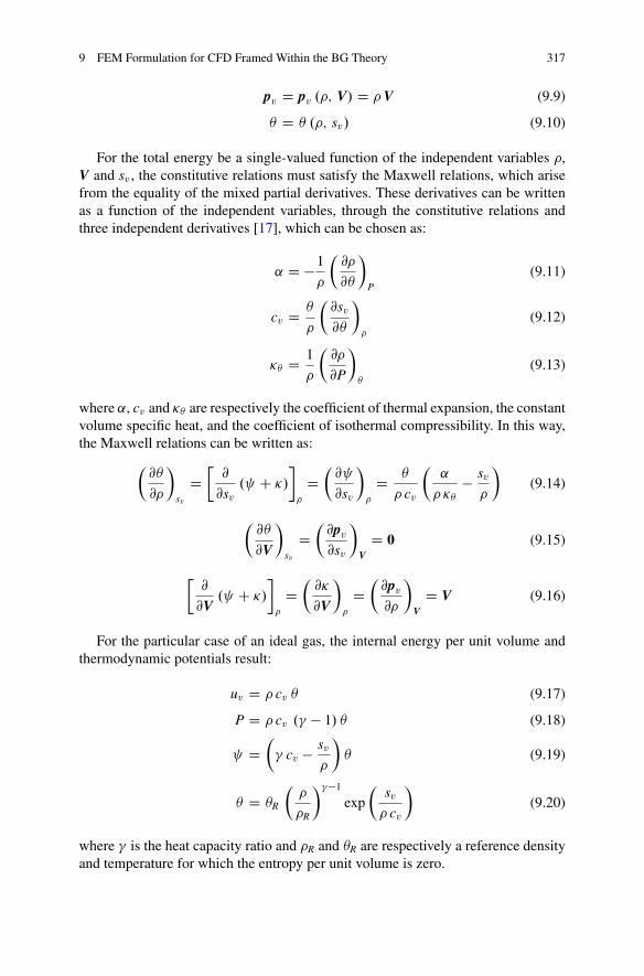
9 FEM Formulation for CFD Framed Within the BG Theory 317
pv D pv .�; V/ D �V (9.9)
� D � .�; sv/ (9.10)
For the total energy be a single-valued function of the independent variables �,V and sv , the constitutive relations must satisfy the Maxwell relations, which arisefrom the equality of the mixed partial derivatives. These derivatives can be writtenas a function of the independent variables, through the constitutive relations andthree independent derivatives [17], which can be chosen as:
˛ D �1�
�@�
@�
�
P
(9.11)
cv D �
�
�@sv@�
�
�
(9.12)
�� D 1
�
�@�
@P
�
�
(9.13)
where ˛, cv and �� are respectively the coefficient of thermal expansion, the constantvolume specific heat, and the coefficient of isothermal compressibility. In this way,the Maxwell relations can be written as:
�@�
@�
�
sv
D�@
@sv. C �/
�
�
D�@
@sv
�
�
D �
� cv
�˛
� ��� sv�
�(9.14)
�@�
@V
�
sv
D�@pv@sv
�
VD 0 (9.15)
�@
@V. C �/
�
�
D�@�
@V
�
�
D�@pv@�
�
VD V (9.16)
For the particular case of an ideal gas, the internal energy per unit volume andthermodynamic potentials result:
uv D � cv � (9.17)
P D � cv .� � 1/ � (9.18)
D�� cv � sv
�
�� (9.19)
� D �R
��
�R
���1exp
�sv� cv
�(9.20)
where � is the heat capacity ratio and �R and �R are respectively a reference densityand temperature for which the entropy per unit volume is zero.
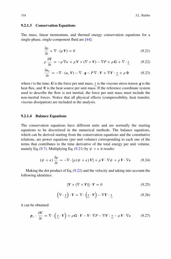
318 J.L. Baliño
9.2.1.3 Conservation Equations
The mass, linear momentum, and thermal energy conservation equations for asingle-phase, single-component fluid are [44]:
@�
@tC r � .�V/ D 0 (9.21)
�@V@t
D ��r� C �V � .r � V/ � rP C �G C r � � (9.22)
@uv@t
D �r � .uv V/ � r � q � P r � V C rV W � C �ˆ (9.23)
where t is the time, G is the force per unit mass, � is the viscous stress tensor, q is theheat flux, and ˆ is the heat source per unit mass. If the reference coordinate systemused to describe the flow is not inertial, the force per unit mass must include thenon-inertial forces. Notice that all physical effects (compressibility, heat transfer,viscous dissipation) are included in the analysis.
9.2.1.4 Balance Equations
The conservation equations have different units and are normally the startingequations to be discretized in the numerical methods. The balance equations,which can be derived starting from the conservation equations and the constitutiverelations, are power equations (per unit volume) corresponding to each one of theterms that contributes to the time derivative of the total energy per unit volume,namely Eq. (9.7). Multiplying Eq. (9.21) by C � it results:
. C �/@�
@tD �r � Œ� . C �/V�C �V � r C �V � r� (9.24)
Making the dot product of Eq. (9.22) and the velocity and taking into account thefollowing identities:
ŒV � .r � V/� � V D 0 (9.25)
r � �
� V D r �
� � V
� rV W � (9.26)
it can be obtained:
pv � @V@t
D r �� � V
C �G � V � V � rP � rV W � � �V � r� (9.27)

9 FEM Formulation for CFD Framed Within the BG Theory 319
Finally, from Eqs. (9.5), (9.6), (9.21), and (9.23) it results:
�@sv@t
D �r � q � r � .� sv V/C �ˆ � �V � r C V � rP C rV W � (9.28)
As stated before, one of the key issues in modeling fluid dynamic systemswith viscous, compressible, and thermal effects is the right understanding of thetransformation of mechanical to thermal energy, and the generation of irreversibility.The balance equations show one of the advantages of this methodology, that is,the representation of the power structure of the system. In the balance equationsthere can be identified three type of terms: divergence, source, and coupling terms.The divergence terms take into account the power introduced in the system throughthe boundary conditions. The source terms constitute the different power sources,external to the system. Finally, the coupling terms represent power transfer betweenthe velocity, mass, and entropy balance equations; these coupling terms appear, withopposite signs, in pairs of balance equations.
The power transfer between the velocity and entropy balance equations isrepresented by the irreversible term rV W � � 0 (also known as viscous dissipationfunction) and the reversible term V � r P. The power transfer between the velocityand mass balance equations is represented by the term �V � r�, while the powertransfer between the mass and entropy balance equations is represented by the term�V � r .
Taking into account Eq. (9.7), it can be verified that coupling terms cancel outwhen the balance equations are added, resulting the conservation of total energy:
@ev@t
C r � .ev V/ D r �h
�P I C �
� Vi
� r � q C �G � V C �ˆ (9.29)
The cancelation of the coupling terms means that they influence the powerdistribution among the different energy domains but not the total power in thesystem.
The pressure and Gibbs free energy gradients can be written as a function of theindependent variables as:
rP D�@P
@sv
�
�
rsv C�@P
@�
�
sv
r�
D �
� cv
˛
��
�rsv C
�cv˛ �
C ˛
� ��� sv�
�r��
(9.30)
r D�@
@sv
�
�
rsv C�@
@�
�
sv
r�
D �
� cv
�˛
� ��� sv�
�rsv C
"1
�2 ��C �
� cv
�˛
� ��� sv�
�2#r� (9.31)
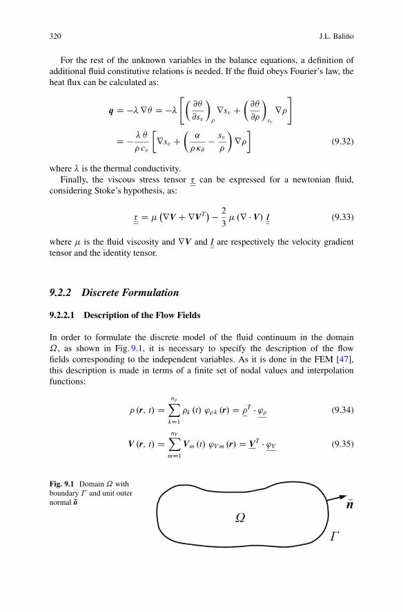
320 J.L. Baliño
For the rest of the unknown variables in the balance equations, a definition ofadditional fluid constitutive relations is needed. If the fluid obeys Fourier’s law, theheat flux can be calculated as:
q D �r� D �"�
@�
@sv
�
�
rsv C�@�
@�
�
sv
r�#
D � �
� cv
�rsv C
�˛
� ��� sv�
�r��
(9.32)
where is the thermal conductivity.Finally, the viscous stress tensor � can be expressed for a newtonian fluid,
considering Stoke’s hypothesis, as:
� D ��rV C rVT
� � 2
3� .r � V/ I (9.33)
where � is the fluid viscosity and rV and I are respectively the velocity gradienttensor and the identity tensor.
9.2.2 Discrete Formulation
9.2.2.1 Description of the Flow Fields
In order to formulate the discrete model of the fluid continuum in the domain˝, as shown in Fig. 9.1, it is necessary to specify the description of the flowfields corresponding to the independent variables. As it is done in the FEM [47],this description is made in terms of a finite set of nodal values and interpolationfunctions:
� .r; t/ Dn�X
kD1�k .t/ '� k .r/ D �T � '� (9.34)
V .r; t/ DnVX
mD1Vm .t/ 'V m .r/ D VT � 'V (9.35)
Fig. 9.1 Domain ˝ withboundary � and unit outernormal Ln

9 FEM Formulation for CFD Framed Within the BG Theory 321
sv .r; t/ DnSX
lD1sv l .t/ 'S l .r/ D sv
T � 'S (9.36)
where � (size n�), V (size nV ) and sv (size nS) are time-dependent nodal vectors,while '�, 'V and 'S are the corresponding position-dependent nodal interpolationor shape functions. The interpolation functions have the following properties:
n�X
kD1'� k .r/ D 1 8 r 2 ˝ (9.37)
nVX
mD1'V m .r/ D 1 8 r 2 ˝ (9.38)
nSX
lD1'S l .r/ D 1 8 r 2 ˝ (9.39)
For simplicity in the treatment of the boundary conditions, it is also required forthe interpolation functions to be equal to one at the reference node, and to be equalto zero at the rest of the nodes, that is:
'� k .rn/ D ık n, for a density node located at position rn (9.40)
'V m .rn/ D ım n, for a velocity node located at position rn (9.41)
'S l .rn/ D ıl n, for an entropy node located at position rn (9.42)
In Eqs. (9.40)–(9.42), ık n is the Kronecker’s delta (ık n D 1 if k D n, ık n D 0
otherwise).The representation of the flow fields in terms of nodal values and interpolation
functions allows to define the corresponding values at any position within˝, so it ispossible to calculate univocally all the integrals corresponding to the state equations;this is not evident for other methodologies like FDM or FVM, where only nodalvalues are defined and additional considerations must be made in order to integratethe differential equations. Besides, the chosen representation can make use of theconsiderable amount of computational tools already available for the popular FEM.
9.2.2.2 Integrated Variables
Nodal vectors of integrated values are defined, related to the discretized ones as:
m D ˝� � � (9.43)
S D ˝S � sv (9.44)
322 J.L. Baliño
The diagonal volume matrices ˝� and ˝S, respectively associated with the
density and entropy per unit volume, are defined as:
˚˝�
k n D ˝� k ık n (9.45)
f˝Sgl n D ˝S l ıl n (9.46)
where:
˝� k DZ
˝
'� k d˝ (9.47)
˝S l DZ
˝
'S l d˝ (9.48)
The system mass m and entropy S are related to the integrated variables asfollows:
m DZ
˝
� d˝ Dn�X
kD1mk (9.49)
S DZ
˝
sv d˝ DnSX
lD1Sl (9.50)
9.2.2.3 System Total Energy
The system total energy E is defined as the sum of the system internal energy U andthe system kinetic coenergy T�:
E D U .m; S/C T� .m; V/ (9.51)
where:
E DZ
˝
ev d˝ (9.52)
U DZ
˝
uv d˝ (9.53)
T� DZ
˝
t�v d˝ (9.54)
From Eqs. (9.35) and (9.54), it can be easily shown that the system kineticcoenergy can be expressed as the following bilinear form:
T� D 1
2VT � M � V (9.55)
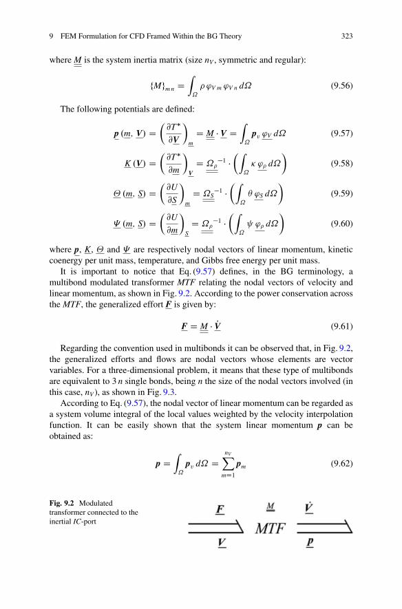
9 FEM Formulation for CFD Framed Within the BG Theory 323
where M is the system inertia matrix (size nV , symmetric and regular):
fMgm n DZ
˝
� 'V m 'V n d˝ (9.56)
The following potentials are defined:
p .m; V/ D�@T�
@V
�
m
D M � V DZ
˝
pv 'V d˝ (9.57)
K .V/ D�@T�
@m
�
VD ˝�
�1 ��Z
˝
� '� d˝
�(9.58)
� .m; S/ D�@U
@S
�
m
D ˝S�1 �
�Z
˝
� 'S d˝
�(9.59)
� .m; S/ D�@U
@m
�
S
D ˝��1 �
�Z
˝
'� d˝
�(9.60)
where p, K, � and � are respectively nodal vectors of linear momentum, kineticcoenergy per unit mass, temperature, and Gibbs free energy per unit mass.
It is important to notice that Eq. (9.57) defines, in the BG terminology, amultibond modulated transformer MTF relating the nodal vectors of velocity andlinear momentum, as shown in Fig. 9.2. According to the power conservation acrossthe MTF, the generalized effort F is given by:
F D M � PV (9.61)
Regarding the convention used in multibonds it can be observed that, in Fig. 9.2,the generalized efforts and flows are nodal vectors whose elements are vectorvariables. For a three-dimensional problem, it means that these type of multibondsare equivalent to 3 n single bonds, being n the size of the nodal vectors involved (inthis case, nV ), as shown in Fig. 9.3.
According to Eq. (9.57), the nodal vector of linear momentum can be regarded asa system volume integral of the local values weighted by the velocity interpolationfunction. It can be easily shown that the system linear momentum p can beobtained as:
p DZ
˝
pv d˝ DnVX
mD1pm (9.62)
Fig. 9.2 Modulatedtransformer connected to theinertial IC-port
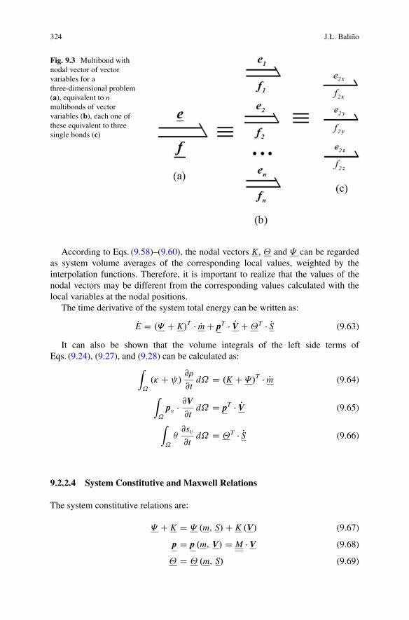
324 J.L. Baliño
Fig. 9.3 Multibond withnodal vector of vectorvariables for athree-dimensional problem(a), equivalent to nmultibonds of vectorvariables (b), each one ofthese equivalent to threesingle bonds (c)
According to Eqs. (9.58)–(9.60), the nodal vectors K, � and � can be regardedas system volume averages of the corresponding local values, weighted by theinterpolation functions. Therefore, it is important to realize that the values of thenodal vectors may be different from the corresponding values calculated with thelocal variables at the nodal positions.
The time derivative of the system total energy can be written as:
PE D .� C K/T � Pm C pT � PV C�T � PS (9.63)
It can also be shown that the volume integrals of the left side terms ofEqs. (9.24), (9.27), and (9.28) can be calculated as:
Z
˝
.� C /@�
@td˝ D .K C �/T � Pm (9.64)
Z
˝
pv � @V@t
d˝ D pT � PV (9.65)
Z
˝
�@sv@t
d˝ D �T � PS (9.66)
9.2.2.4 System Constitutive and Maxwell Relations
The system constitutive relations are:
� C K D � .m; S/C K .V/ (9.67)
p D p .m; V/ D M � V (9.68)
� D � .m; S/ (9.69)

9 FEM Formulation for CFD Framed Within the BG Theory 325
The Maxwell relations corresponding to the system total energy arise from theequality of the mixed partial derivatives of the system total energy expressed as afunction of the independent variables m, V, and S, regarded as the state variables forthe BG formalism:
�@�
@m
�
S
D�@
@S.� C K/
�T
m
D�@�
@S
�T
m
D ˝S�1 � MS � �˝�
�1 (9.70)
�@�
@V
�
S
D�@p
@S
�T
VD 0 (9.71)
�@p
@m
�
VD�@
@V
C K
�T
m
D�@K
@V
�T
m
D MV � �˝��1 (9.72)
where the matrices MS � (nS rows and n� columns) and MV � (nV rows and n�
columns) result:
˚MS �
l k D
Z
˝
�
� cv
�˛
� ��� sv�
�'S l '� k d˝ (9.73)
˚MV �
m k D
Z
˝
V 'V m '� k d˝ (9.74)
The constitutive relations (9.67)–(9.69) and the Maxwell relations (9.70)–(9.72)define a multibond IC-field associated with the system total energy, as shown inFig. 9.4. This field has an inertial port (the velocity port) and two capacitive ports(the entropy and the mass ports). The generalized effort variables associated withthese ports are respectively PV,� and .� C K/, while the generalized flow variablesare respectively p, PS and Pm.
In Fig. 9.4, the generalized efforts and flows of the multibonds connected to thecapacitive ports are nodal vectors whose elements are scalar variables; these typeof multibonds are equivalent to n (in this case, n� or nS) single bonds, as shown inFig. 9.5.
Fig. 9.4 System IC-fieldrepresenting energy storage

326 J.L. Baliño
Fig. 9.5 Multibond withnodal vector of scalarvariables (a), equivalent to nsingle bonds (b)
9.2.3 State Equations
9.2.3.1 Mass Port
Nodal density weight functions w� k .r; t/ are introduced, with the followingproperties:
n�X
kD1w� k .r; t/ D 1 8 r 2 ˝; 8 t (9.75)
w� k .rn; t/ D ık n, for a density node located at position rn (9.76)
The nodal density weight functions are introduced to satisfy the power inter-changed by the system through the boundary conditions, as well as to share theimportance of different power terms among neighboring nodes. These functionscan be used to introduce numerical schemes, for instance controlled upwind, incompressible CFD problems.
As it is done in the Petrov–Galerkin method [47], each term of the mass balanceequation (9.24) is multiplied by the test function w� k; then, the resulting terms areintegrated over the domain ˝ and Green’s theorem is applied whenever necessary,obtaining:
Pm D Pm.� /W C PmW C PmU C PmK (9.77)
9 FEM Formulation for CFD Framed Within the BG Theory 327
where the different nodal vectors of mass rates are:
Pm.� /W D �
� C K
�1 ��Z
�
w� � . C �/V � Ln d�
�(9.78)
PmW D� C K
�1 ��Z
˝
� . C �/V � rw� d˝
�(9.79)
PmU D� C K
�1 ��Z
˝
w� �V � r d˝
�(9.80)
PmK D� C K
�1 ��Z
˝
w� �V � r� d˝
�(9.81)
The square matrices � and K (size n�) are defined as:
f�gk j D 1
˝� j
Z
˝
w� k '� j d˝ (9.82)
fKgk j D 1
˝� j
Z
˝
� w� k '� j d˝ (9.83)
The nodal vectors � and K are the sum of the corresponding matrix columns:
�j D Pn�kD1 f�gk j (9.84)
Kj D Pn�kD1 fKgk j (9.85)
Taking into account Eqs. (9.84) and (9.85) it can be verified that the product.� C K/T � PmX , where PmX is any nodal vector of mass rate, recovers the correspond-
ing power term integrated in the system. So, the product .� C K/T � Pm.� /W recovers
the power due to the flux of Gibbs free energy plus kinetic coenergy through thesystem boundary � , while .� C K/T � PmW is a power term that vanishes, because of
Eq. (9.75). Notice that Pm.� /W k may be nonzero only for the nodes located at the system
boundary. Making the product of �CK times Eq. (9.77), it can be easily shown thatthe integral mass balance equation is satisfied, that is:
Z
˝
. C �/@�
@td˝ D �
Z
�
� . C �/V � Ln d� CZ
˝
�V �r d˝CZ
˝
�V �r� d˝
(9.86)
9.2.3.2 Velocity Port
As it is done in the Galerkin method [47], the momentum conservation equation ismultiplied by the test function 'V m and integrated over the domain ˝. ApplyingGreen’s theorem whenever necessary, it can be obtained:

328 J.L. Baliño
PV D M�1 �
F.� /V C FG C FR � FP � FV � FK
(9.87)
where the different nodal vectors of forces are:
F.� /V DZ
�
� � Ln
'V d� (9.88)
FG DZ
˝
�G'V d˝ (9.89)
FR DZ
˝
�V � .r � V/ 'V d˝ (9.90)
FP DZ
˝
rP'V d˝ (9.91)
FV DZ
˝
� � r'V d˝ (9.92)
FK DZ
˝
�r� 'V d˝ (9.93)
Adding the nodal components of Eq. (9.87) it can be easily shown that theintegral momentum equation is satisfied, that is:
Z
˝
�DVDt
d˝ DZ
�
�P I C �
� Ln d� C
Z
˝
�G d˝ (9.94)
The reason why the Galerkin method was chosen is that the dot product FXT � V,
where FX is any nodal vector of force, recovers the corresponding power term
integrated in the system. It can be observed that the dot product F.� /V
T � V recoversthe power due to the flux of the viscous stress through the system boundary, whilethe dot product FV
T � V recovers the power dissipation. Notice that F.� /V m may benonzero only for the nodes located at the system boundary.
Making the dot product of Eq. (9.87) and V and taking into account Eq. (9.25), itcan be easily shown that the integral velocity balance equation is satisfied, that is:
Z
˝
pv � @V@t
d˝ DZ
�
� � V
� Ln d� C
Z
˝
�G � V d˝ �Z
˝
V � rP d˝
�Z
˝
rV W �
d˝ �
Z
˝
�V � r� d˝ (9.95)
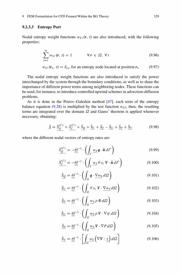
9 FEM Formulation for CFD Framed Within the BG Theory 329
9.2.3.3 Entropy Port
Nodal entropy weight functions wS l .r; t/ are also introduced, with the followingproperties:
nSX
lD1wS l .r; t/ D 1 8 r 2 ˝; 8 t (9.96)
wS l .rn; t/ D ıl n, for an entropy node located at position rn (9.97)
The nodal entropy weight functions are also introduced to satisfy the powerinterchanged by the system through the boundary conditions, as well as to share theimportance of different power terms among neighboring nodes. These functions canbe used, for instance, to introduce controlled upwind schemes in advection-diffusionproblems.
As it is done in the Petrov–Galerkin method [47], each term of the entropybalance equation (9.28) is multiplied by the test function wS l; then, the resultingterms are integrated over the domain ˝ and Gauss’ theorem is applied whenevernecessary, obtaining:
PS D PS.� /Q C PS.� /C C PSQ C PSC C PSF � PSU C PSP C PSV (9.98)
where the different nodal vectors of entropy rates are:
PS.� /Q D ���1 ��Z
�
wS q � Ln d�
�(9.99)
PS.� /C D ���1 ��Z
�
wS � sv V � Ln d�
�(9.100)
PSQ D ��1 ��Z
˝
q � rwS d˝
�(9.101)
PSC D ��1 ��Z
˝
� sv V � rwS d˝
�(9.102)
PSF D ��1 ��Z
˝
wS �ˆ d˝
�(9.103)
PSU D ��1 ��Z
˝
wS �V � r d˝
�(9.104)
PSP D ��1 ��Z
˝
wS V � rP d˝
�(9.105)
PSV D ��1 ��Z
˝
wS
rV W �
d˝
�(9.106)

330 J.L. Baliño
In Eqs. (9.99)–(9.106) the temperature matrix � results:
f�gl j D 1
˝S j
Z
˝
� wS l 'S j d˝ (9.107)
The nodal vector of temperature is the sum of the temperature matrix columns:
�j DnSX
lD1f�gl j (9.108)
Taking into account Eq. (9.108) it can be verified that the product �T � PSX , wherePSX is any nodal vector of entropy rate, recovers the corresponding power integrated
in the system. Thus, the products �T � PS.� /Q and �T � PS.� /C recovers respectively the
power due to heat flux and entropy advection, while �T � PSQ and �T � PSC are power
terms that vanish, because of Eq. (9.96). Notice that PS.� /Q l and PS.� /C l may be nonzeroonly for the nodes located at the system boundary. Making the product of Eq. (9.98)times�, it can be easily shown that the integral entropy balance equation is satisfied,that is:
Z
˝
�@sv@t
d˝ D �Z
�
.q C � sv V/ � Ln d� CZ
˝
�ˆ d˝ �Z
˝
�V � r d˝
CZ
˝
V � rP d˝ CZ
˝
rV W �
d˝ (9.109)
9.2.4 Coupling Matrices
Once defined the generalized effort and flow variables, it is necessary to representthe power coupling (appearing in the balance equations per unit volume shown inSect. 9.2.1.4) to a discretized level. This representation is performed through thecoupling matrices, which relate generalized variables whose product gives rise topower terms appearing in pairs of multiports. Depending on the variables beingrelated, it will be seen that these matrices define modulated transformers MTF, amodulated resistance-entropy source field MRS or a modulated gyrator MGY. As thenodal vectors may have different size, the coupling matrices are rectangular, thussetting a restriction in the allowable causalities.
9.2.4.1 Coupling Between the Velocity and Mass Ports
From Eqs. (9.81) and (9.93):
PmK D�� C K
�1 � MK
�� V (9.110)
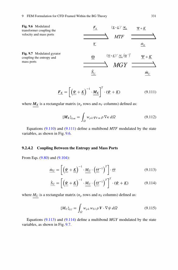
9 FEM Formulation for CFD Framed Within the BG Theory 331
Fig. 9.6 Modulatedtransformer coupling thevelocity and mass ports
Fig. 9.7 Modulated gyratorcoupling the entropy andmass ports
FK D�� C K
�1 � MK
�T
� .� C K/ (9.111)
where MK is a rectangular matrix (n� rows and nV columns) defined as:
fMKgk m DZ
˝
w� k 'V m �r� d˝ (9.112)
Equations (9.110) and (9.111) define a multibond MTF modulated by the statevariables, as shown in Fig. 9.6.
9.2.4.2 Coupling Between the Entropy and Mass Ports
From Eqs. (9.80) and (9.104):
PmU D�� C K
�1 � MU ���1
T�
�� (9.113)
PSU D�� C K
�1 � MU ���1
T�T
� .� C K/ (9.114)
where MU is a rectangular matrix (n� rows and nS columns) defined as:
fMUgk l DZ
˝
w� k wS l �V � r d˝ (9.115)
Equations (9.113) and (9.114) define a multibond MGY modulated by the statevariables, as shown in Fig. 9.7.
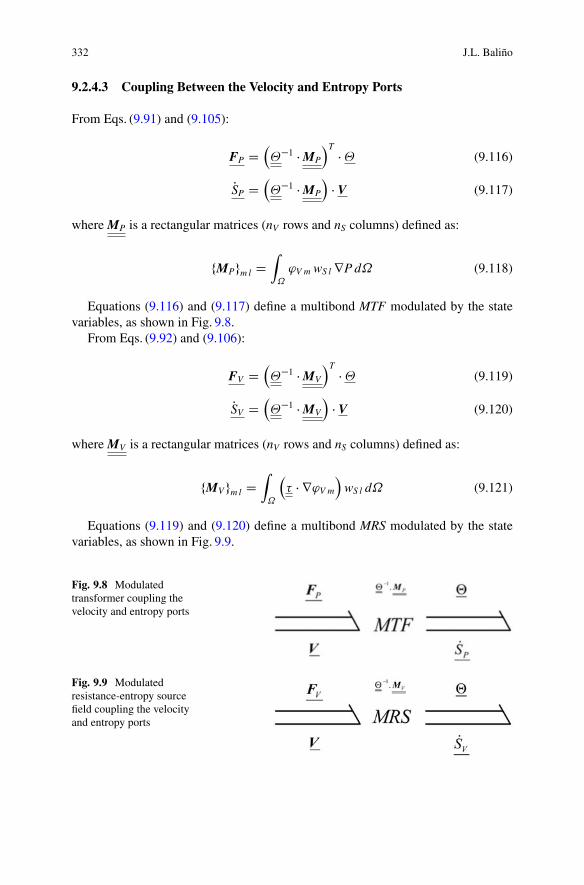
332 J.L. Baliño
9.2.4.3 Coupling Between the Velocity and Entropy Ports
From Eqs. (9.91) and (9.105):
FP D��1 � MP
T �� (9.116)
PSP D��1 � MP
� V (9.117)
where MP is a rectangular matrices (nV rows and nS columns) defined as:
fMPgm l DZ
˝
'V m wS l rP d˝ (9.118)
Equations (9.116) and (9.117) define a multibond MTF modulated by the statevariables, as shown in Fig. 9.8.
From Eqs. (9.92) and (9.106):
FV D��1 � MV
T �� (9.119)
PSV D��1 � MV
� V (9.120)
where MV is a rectangular matrices (nV rows and nS columns) defined as:
fMVgm l DZ
˝
� � r'V m
wS l d˝ (9.121)
Equations (9.119) and (9.120) define a multibond MRS modulated by the statevariables, as shown in Fig. 9.9.
Fig. 9.8 Modulatedtransformer coupling thevelocity and entropy ports
Fig. 9.9 Modulatedresistance-entropy sourcefield coupling the velocityand entropy ports
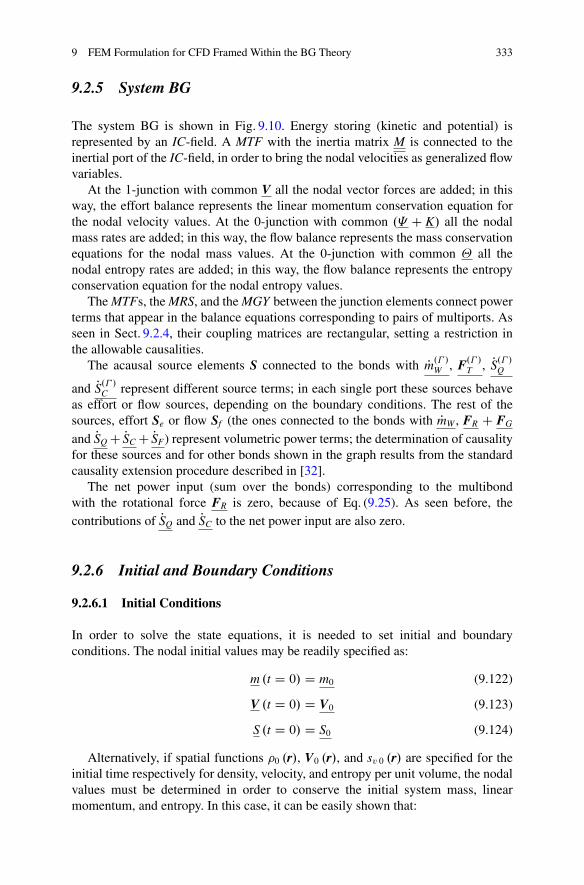
9 FEM Formulation for CFD Framed Within the BG Theory 333
9.2.5 System BG
The system BG is shown in Fig. 9.10. Energy storing (kinetic and potential) isrepresented by an IC-field. A MTF with the inertia matrix M is connected to theinertial port of the IC-field, in order to bring the nodal velocities as generalized flowvariables.
At the 1-junction with common V all the nodal vector forces are added; in thisway, the effort balance represents the linear momentum conservation equation forthe nodal velocity values. At the 0-junction with common .� C K/ all the nodalmass rates are added; in this way, the flow balance represents the mass conservationequations for the nodal mass values. At the 0-junction with common � all thenodal entropy rates are added; in this way, the flow balance represents the entropyconservation equation for the nodal entropy values.
The MTFs, the MRS, and the MGY between the junction elements connect powerterms that appear in the balance equations corresponding to pairs of multiports. Asseen in Sect. 9.2.4, their coupling matrices are rectangular, setting a restriction inthe allowable causalities.
The acausal source elements S connected to the bonds with Pm.� /W , F.� /T , PS.� /Q
and PS.� /C represent different source terms; in each single port these sources behaveas effort or flow sources, depending on the boundary conditions. The rest of thesources, effort Se or flow Sf (the ones connected to the bonds with PmW , FR C FG
and PSQ C PSC C PSF) represent volumetric power terms; the determination of causalityfor these sources and for other bonds shown in the graph results from the standardcausality extension procedure described in [32].
The net power input (sum over the bonds) corresponding to the multibondwith the rotational force FR is zero, because of Eq. (9.25). As seen before, thecontributions of PSQ and PSC to the net power input are also zero.
9.2.6 Initial and Boundary Conditions
9.2.6.1 Initial Conditions
In order to solve the state equations, it is needed to set initial and boundaryconditions. The nodal initial values may be readily specified as:
m .t D 0/ D m0 (9.122)
V .t D 0/ D V0 (9.123)
S .t D 0/ D S0 (9.124)
Alternatively, if spatial functions �0 .r/, V0 .r/, and sv 0 .r/ are specified for theinitial time respectively for density, velocity, and entropy per unit volume, the nodalvalues must be determined in order to conserve the initial system mass, linearmomentum, and entropy. In this case, it can be easily shown that:
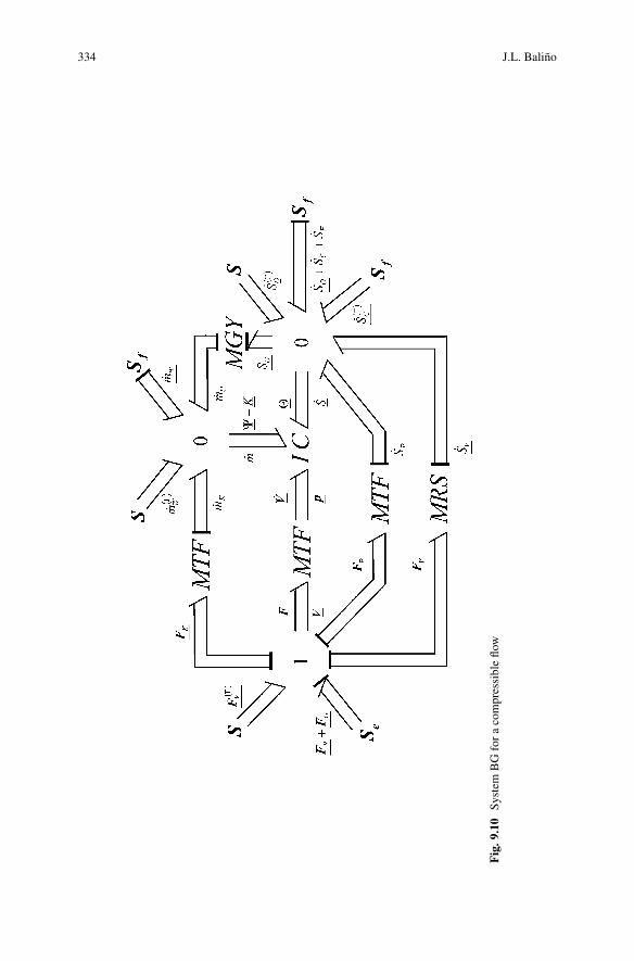
334 J.L. Baliño
Fig
.9.1
0Sy
stem
BG
for
aco
mpr
essi
ble
flow
9 FEM Formulation for CFD Framed Within the BG Theory 335
m0 k DZ
˝
�0 .r/ '� k d˝ (9.125)
V0m DR˝�0 .r/V0 .r/ 'V m d˝R˝�0 .r/ 'V m d˝
(9.126)
S0 l DZ
˝
sv 0 .r/ 'S l d˝ (9.127)
9.2.6.2 Boundary Conditions
The boundary conditions establish relationships among the variables at the boundary� . At a discretized level, the boundary conditions can be regarded, in the BGmethodology, as the input variables. It is necessary, for the model being mathemati-cally well defined, that the boundary conditions allow to determine the causality forall the bonds in the resulting BG. The boundary conditions are introduced throughthe bonds corresponding to the superficial source terms Pm.� /
W , F.� /T , PS.� /Q , and PS.� /C .
All boundary conditions can be described in terms of generalized effort or flowsources.
In a general boundary value problem, boundary conditions can be classified inessential, natural, and mixed.
In an essential boundary condition (often called Dirichlet boundary condition),independent variables are specified at a part of the boundary. Typical examples inCFD can be problems in which the flow conditions (velocity and/or thermophysicalproperties) are specified at the inlet or outlet of a flow passage section or whennormal and tangential components are specified at a wall satisfying the no-normalor no-slip condition. For these cases, a derivative causality will result for someboundary bonds belonging to the IC-field.
Natural boundary conditions (often called Neumann boundary conditions) arethose that are automatically satisfied after solution of the problem. These boundaryconditions appear when gradients of the independent variables are specified at a partof the boundary. In a CFD problem, natural boundary conditions are associated withimposed components of the viscous stress tensor or heat flux at the boundary. Forthese cases, integral causality will result for the boundary nodes belonging to theIC-field.
Finally, mixed boundary conditions are those that involve gradients as well asvalues of the independent variables at a part of the boundary. For these cases, integralcausality will also result for the boundary nodes belonging to the IC-field. Newton’scooling law, relating the normal component of the heat flux to the difference betweenthe boundary and a reference temperature, is a typical example.
336 J.L. Baliño
9.2.6.3 Considerations for Pure Advective Flows
If heat conduction effects are neglected in the conservation equation (9.23), themultibonds corresponding to PS.� /Q and PSQ disappear. This approximation makes
the entropy balance equation first order and has consequences in the causalityassignment. In particular, for pure advective flows only thermophysical properties atparts of the boundary can be specified. In this case, the entropy boundary conditionsare introduced through the bonds corresponding to the superficial source term PS.� /C .
9.2.6.4 Considerations for Inviscid Flows
If the viscous stress tensor is neglected in the conservation equation (9.22),the multibond corresponding to F.� /T disappears. This approximation makes themomentum balance equation first order and has consequences in the causalityassignment. For instance, only the normal component of the velocity field can bespecified at a wall, while the other components are part of the problem solution.
9.2.6.5 Procedure for Causality Assignment
In [32] a sequential causal assignment procedure is described. Sources are chosenfirst, the required causality is assigned, and the causal implications are extendedthrough the graph as far as possible, using the constraint elements (in this case 0-junctions, 1-junctions, MTFs, MRS and MGY). Then, the ports corresponding to thestorage elements (in this case, the IC-field) are chosen, integral causality is assigned,and, again, the causal implications are extended through the graph as far as possible.
In a grid generated for a CFD problem usually there is a huge amount of nodes.The domain is divided in cells, the volume integrations are performed locally ineach cell, and the results are assembled to build the system integrals. For doingthis, it is necessary to know what is called the connectivity information, that is, theinformation needed to completely identify each cell and all of the neighbors of thatcell in a computational grid.
As a result of the calculation procedure, the resulting matrices are sparse, that is,have a few nonzero elements. Regarding causality extension through the MTFs,MRS, and MGY elements, the constitutive laws are sets of linear relationshipsamong the variables involved. Thus, causality can be extended for a bond with avariable only when the bonds corresponding to the rest of the variables in the linearrelationship have assigned causalities.
It is worth noting that, as the interpolation functions are zero at the boundary� for inner nodes, causality is assigned by definition at these bonds. Thus, a zero-effort source is connected to an inner F.� /V m, and respectively zero-flow sources are
connected to an inner Pm.� /W k , PS.� /Q l and PS.� /C l .

9 FEM Formulation for CFD Framed Within the BG Theory 337
As there are only energy storing and conserving elements, all bonds should havecausality assigned after the procedure detailed above. The order of the system is thenumber of bonds connected to the energy storing elements, resulting with integralcausality. This causality procedure can be implemented automatically, knowing theconnectivity of the computational grid, as a way of checking the correctness of theboundary conditions in the problem.
As a consequence of the causality extension, the sources connected to the bondswith FG C FR always behave as effort sources, and the sources connected to the
bonds with PSQ C PSC C PSF, PS.� /C , and PmW always behave as flow sources. Besides,causality for the bonds connected to the coupling MTFs, MRS, and MGY is alsodefined. For the MTFs and the MRS, it always results V the input and respectivelyPmK , PSP and PSV outputs. For the MGY, it always results� the input and PmU the output.
The resulting causality for the coupling MTFs and MRS indicate that fluid motiongenerates the entropy rate (both reversible and irreversible) and mass rates, inagreement with the Second Principle of Thermodynamics. Besides, � and � C Kalways result inputs to the coupling MTFs and MRS, indicating that thermophysicalproperties influence the corresponding output forces.
9.3 Incompressible Flows
An interesting type of problems are those in which the fluid is incompressible, thatis, density is constant.
When viscosity variations with temperature are small, the traditional incompress-ible form of the Navier–Stokes (N–S) equation is usually selected for the analysis.A set of equations (continuity, momentum, and thermal energy) results with threeunknowns, for which usually velocity, pressure, and temperature are chosen; thisis known as the primitive-variable approach. Other alternatives have a limitationto bi-dimensional flows (vorticity-stream function approach), or are less attractivefor three-dimensional flows (vector potential approach); consequently, the N–Sequations are often solved in their primitive variable form.
For constant viscosity, the energy equation can be uncoupled, so the temperaturefield can be obtained after the velocity field has been computed. As the nonlinearitiesare related to the convective term, the attention is focused on the solution of thecontinuity and momentum equations.
An important characteristic of the N–S equations is that no time derivative ofpressure appears. Pressure is no longer a thermophysical property, but a functionthat must act in such a way that the resulting velocity field has divergence zero. Inan incompressible flow pressure perturbations propagate at infinite speed, obeyingan elliptic, Poisson’s type partial differential equation, where the source term is afunction of the velocity field.
A strategy often employed for the numerical solution of the incompressible N–Sequations is the pressure correction approach, in which a derived equation is used to
338 J.L. Baliño
determine the pressure field. Typically, the momentum equations are solved for thevelocity components using linearized expressions in which time-lagged values areused for the variables other than the unknown, including pressure. In this step, theobtained velocity field does not satisfy the continuity equation. Next, the solutionis substituted in the discretized continuity equation and often a Poisson equation isdeveloped for the pressure (or pressure changes), from which a new pressure field isobtained. This pressure field is used to calculate a new velocity field until a solutionis produced that satisfies both the momentum and the continuity equations. Theliterature on numerical schemes using the pressure correction approach is extensive,differing the methods in the algorithms used to solve the component equations andthe improved pressure field. A review of these methods can be found in [42].
In this section a single-phase, single-component, multidimensional incompress-ible flow with viscosity and thermal effects is considered for the application ofthe BG methodology [5, 7]. Main characteristics of the methodology explained inSect. 9.2 will not be repeated here; only the new concepts will be stressed.
9.3.1 Continuum Formulation
9.3.1.1 Energy and Power Representation
For an incompressible fluid, the density �0 is no longer a state variable. The totalenergy per unit volume ev can be written as:
ev D uv .sv/C t�v .V/ (9.128)
For a single-phase, single-component fluid with constant specific heat cv , thekinetic coenergy and internal energy per unit volume can be written as:
t�v D 1
2�0 V2 D �0 � (9.129)
uv D uv R C �0 cv �R
�exp
�sv�0 cv
�� 1
�(9.130)
where uv R and �R are respectively reference values of internal energy per unitvolume and absolute temperature, for which the entropy per unit volume is zero.The linear momentum per unit volume and the absolute temperature are defined as:
pv D dt�vdV
D �0 V (9.131)
� D duvdsv
D �R exp
�sv�0 cv
�(9.132)
The time derivative of Eq. (9.128) can be written as:
@ev@t
D pv � @V@t
C �@sv@t
(9.133)

9 FEM Formulation for CFD Framed Within the BG Theory 339
As the internal energy per unit volume is only a function of the entropy per unitvolume and the kinetic coenergy per unit volume is only a function of the velocity,these two energy domains can be decoupled.
9.3.1.2 Conservation Equations
For an incompressible fluid the continuity, linear momentum, and thermal energyconservation equations are [44]:
r � V D 0 (9.134)
�0@V@t
D ��0 r� C �0 V � .r � V/ � rP C �0 G C r � � (9.135)
@uv@t
D �r � q � ruv � V C rV W � C �0 ˆ (9.136)
For a newtonian, incompressible fluid and assuming Fourier’s law, the viscousstress and the heat flux can be written as:
� D ��rV C rVT
�(9.137)
q D �r� D � �
�0 cvrsv (9.138)
9.3.1.3 Balance Equations
Transforming the conservation equations in the same fashion as it was made inSect. 9.2.1.4, it can be obtained:
pv � @V@t
D r �� � V
� r � .P V/ � �0 r� � V C �0 G � V � rV W � (9.139)
�@sv@t
D �r � q � r � .� sv V/C sv r� � V C �0 ˆC rV W � (9.140)
The only coupling term rV W � represents the power transfer (mechanical energydissipation) between the velocity and entropy equations; this coupling term appears,with opposite signs, in the balance equations. Adding the balance equations, it canbe easily obtained the conservation of total energy:
�0DOeDt
D r �h
�P I C �
� V � qi
C �0 G � V C �0 ˆ (9.141)
where Oe D OuC 12
V2 is the total energy per unit mass and DDt is the material derivative.
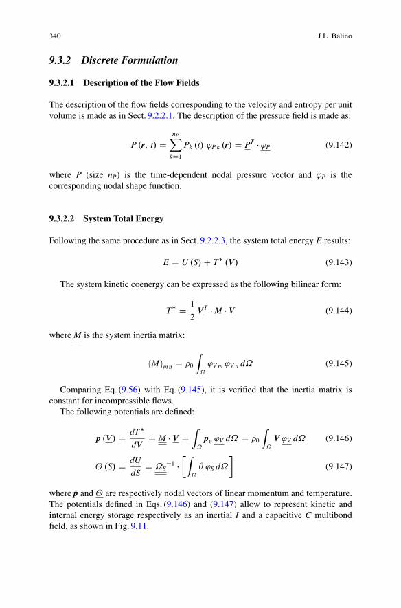
340 J.L. Baliño
9.3.2 Discrete Formulation
9.3.2.1 Description of the Flow Fields
The description of the flow fields corresponding to the velocity and entropy per unitvolume is made as in Sect. 9.2.2.1. The description of the pressure field is made as:
P .r; t/ DnPX
kD1Pk .t/ 'P k .r/ D PT � 'P (9.142)
where P (size nP) is the time-dependent nodal pressure vector and 'P is thecorresponding nodal shape function.
9.3.2.2 System Total Energy
Following the same procedure as in Sect. 9.2.2.3, the system total energy E results:
E D U .S/C T� .V/ (9.143)
The system kinetic coenergy can be expressed as the following bilinear form:
T� D 1
2VT � M � V (9.144)
where M is the system inertia matrix:
fMgm n D �0
Z
˝
'V m 'V n d˝ (9.145)
Comparing Eq. (9.56) with Eq. (9.145), it is verified that the inertia matrix isconstant for incompressible flows.
The following potentials are defined:
p .V/ D dT�
dVD M � V D
Z
˝
pv 'V d˝ D �0
Z
˝
V 'V d˝ (9.146)
� .S/ D dU
dSD ˝S
�1 ��Z
˝
� 'S d˝
�(9.147)
where p and� are respectively nodal vectors of linear momentum and temperature.The potentials defined in Eqs. (9.146) and (9.147) allow to represent kinetic andinternal energy storage respectively as an inertial I and a capacitive C multibondfield, as shown in Fig. 9.11.
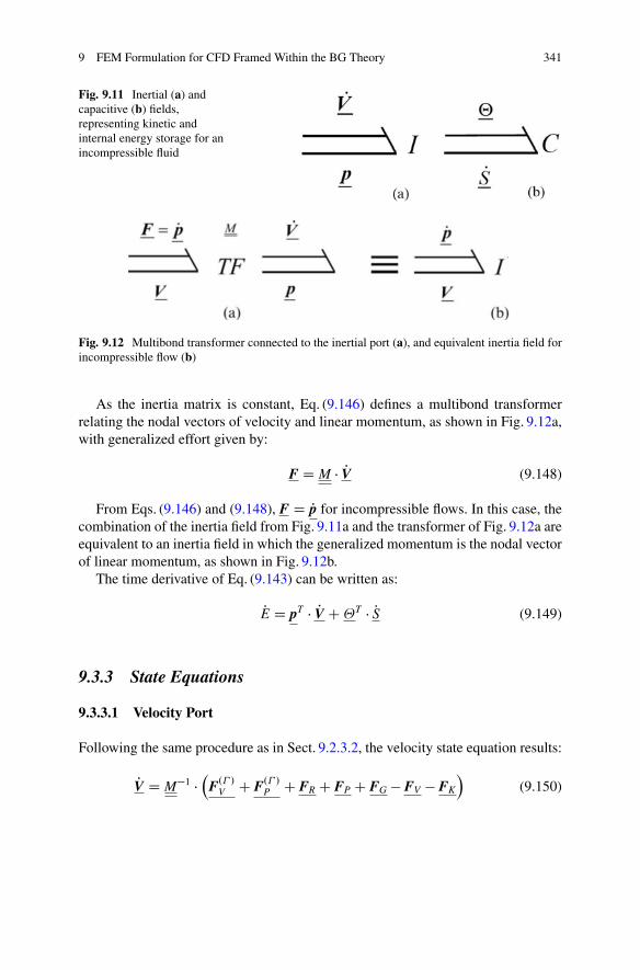
9 FEM Formulation for CFD Framed Within the BG Theory 341
Fig. 9.11 Inertial (a) andcapacitive (b) fields,representing kinetic andinternal energy storage for anincompressible fluid
Fig. 9.12 Multibond transformer connected to the inertial port (a), and equivalent inertia field forincompressible flow (b)
As the inertia matrix is constant, Eq. (9.146) defines a multibond transformerrelating the nodal vectors of velocity and linear momentum, as shown in Fig. 9.12a,with generalized effort given by:
F D M � PV (9.148)
From Eqs. (9.146) and (9.148), F D Pp for incompressible flows. In this case, thecombination of the inertia field from Fig. 9.11a and the transformer of Fig. 9.12a areequivalent to an inertia field in which the generalized momentum is the nodal vectorof linear momentum, as shown in Fig. 9.12b.
The time derivative of Eq. (9.143) can be written as:
PE D pT � PV C�T � PS (9.149)
9.3.3 State Equations
9.3.3.1 Velocity Port
Following the same procedure as in Sect. 9.2.3.2, the velocity state equation results:
PV D M�1 �
F.� /V C F.� /P C FR C FP C FG � FV � FK
(9.150)
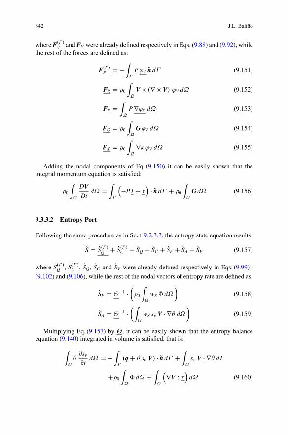
342 J.L. Baliño
where F.� /V and FV were already defined respectively in Eqs. (9.88) and (9.92), whilethe rest of the forces are defined as:
F.� /P D �Z
�
P'V Ln d� (9.151)
FR D �0
Z
˝
V � .r � V/ 'V d˝ (9.152)
FP DZ
˝
P r'V d˝ (9.153)
FG D �0
Z
˝
G'V d˝ (9.154)
FK D �0
Z
˝
r� 'V d˝ (9.155)
Adding the nodal components of Eq. (9.150) it can be easily shown that theintegral momentum equation is satisfied:
�0
Z
˝
DVDt
d˝ DZ
�
�P I C �
� Ln d� C �0
Z
˝
G d˝ (9.156)
9.3.3.2 Entropy Port
Following the same procedure as in Sect. 9.2.3.3, the entropy state equation results:
PS D PS.� /Q C PS.� /C C PSQ C PSC C PSF C PSA C PSV (9.157)
where PS.� /Q , PS.� /C , PSQ, PSC and PSV were already defined respectively in Eqs. (9.99)–
(9.102) and (9.106), while the rest of the nodal vectors of entropy rate are defined as:
PSF D ��1 ���0
Z
˝
wS ˆ d˝
�(9.158)
PSA D ��1 ��Z
˝
wS sv V � r� d˝
�(9.159)
Multiplying Eq. (9.157) by �, it can be easily shown that the entropy balanceequation (9.140) integrated in volume is satisfied, that is:
Z
˝
�@sv@t
d˝ D �Z
�
.q C � sv V/ � Ln d� CZ
˝
sv V � r� d�
C�0Z
˝
ˆ d˝ CZ
˝
rV W �
d˝ (9.160)
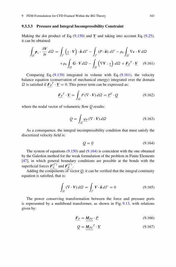
9 FEM Formulation for CFD Framed Within the BG Theory 343
9.3.3.3 Pressure and Integral Incompressibility Constraint
Making the dot product of Eq. (9.150) and V and taking into account Eq. (9.25),it can be obtained:
Z
˝
pv � @V@t
d˝ DZ
�
� � V
� Ln d� �
Z
�
.P � Ln/ d� � �0Z
˝
r� � V d˝
C�0Z
˝
G � V d˝ �Z
˝
rV W �
d˝ C FP
T � V (9.161)
Comparing Eq. (9.139) integrated in volume with Eq. (9.161), the velocitybalance equation (conservation of mechanical energy) integrated over the domain˝ is satisfied if FP
T � V D 0. This power term can be expressed as:
FPT � V D
Z
˝
P .r � V/ d˝ D PT � Q (9.162)
where the nodal vector of volumetric flow Q results:
Q DZ
˝
'P .r � V/ d˝ (9.163)
As a consequence, the integral incompressibility condition that must satisfy thediscretized velocity field is:
Q D 0 (9.164)
The system of equations (9.150) and (9.164) is coincident with the one obtainedby the Galerkin method for the weak formulation of the problem in Finite Elements[47], in which general boundary conditions are possible at the bonds with thesuperficial forces F.� /V and F.� /P .
Adding the components of vector Q, it can be verified that the integral continuityequation is satisfied, that is:
Z
˝
.r � V/ d˝ DZ
�
V � Ln d� D 0 (9.165)
The power conserving transformation between the force and pressure portsis represented by a multibond transformer, as shown in Fig. 9.13, with relationsgiven by:
FP D MPV � P (9.166)
Q D MPVT � V (9.167)
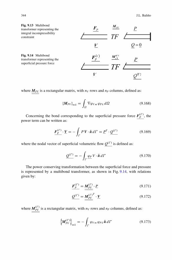
344 J.L. Baliño
Fig. 9.13 Multibondtransformer representing theintegral incompressibilityconstraint
Fig. 9.14 Multibondtransformer representing thesuperficial pressure force
where MPV is a rectangular matrix, with nV rows and nP columns, defined as:
fMPVgm k DZ
˝
r'V m 'P k d˝ (9.168)
Concerning the bond corresponding to the superficial pressure force F.� /P , thepower term can be written as:
F.� /P � V D �Z
�
P V � Ln d� D PT � Q.� / (9.169)
where the nodal vector of superficial volumetric flow Q.� / is defined as:
Q.� / D �Z
�
'P V � Ln d� (9.170)
The power conserving transformation between the superficial force and pressureis represented by a multibond transformer, as shown in Fig. 9.14, with relationsgiven by:
F.� /P D M.� /PV � P (9.171)
Q.� / D M.� /PV
T � V (9.172)
where M.� /PV is a rectangular matrix, with nV rows and nP columns, defined as:
nM.� /
PV
o
m kD �
Z
�
'V m 'P k Ln d� (9.173)
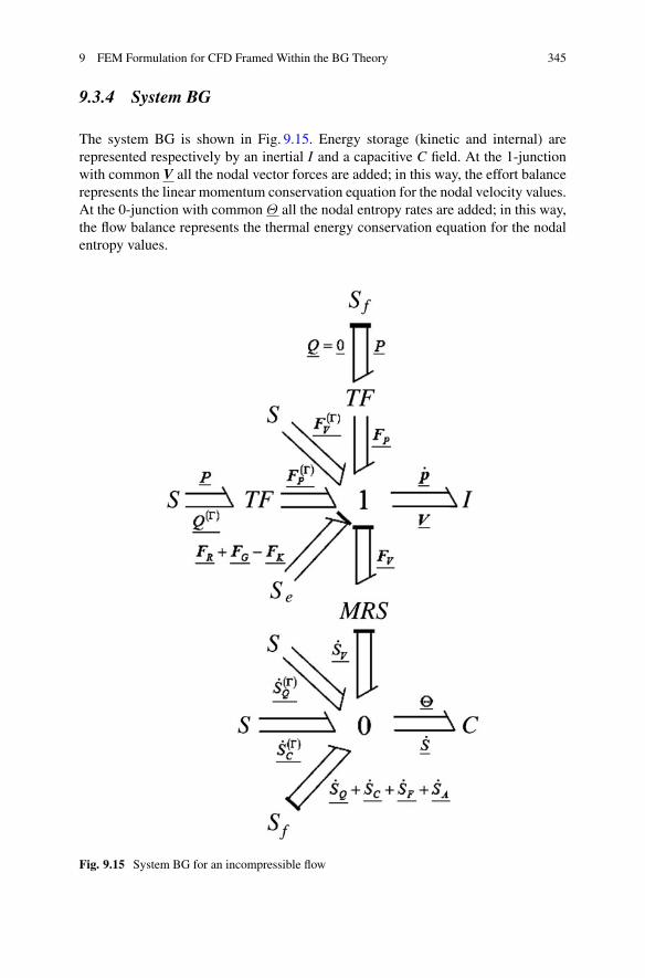
9 FEM Formulation for CFD Framed Within the BG Theory 345
9.3.4 System BG
The system BG is shown in Fig. 9.15. Energy storage (kinetic and internal) arerepresented respectively by an inertial I and a capacitive C field. At the 1-junctionwith common V all the nodal vector forces are added; in this way, the effort balancerepresents the linear momentum conservation equation for the nodal velocity values.At the 0-junction with common� all the nodal entropy rates are added; in this way,the flow balance represents the thermal energy conservation equation for the nodalentropy values.
Fig. 9.15 System BG for an incompressible flow
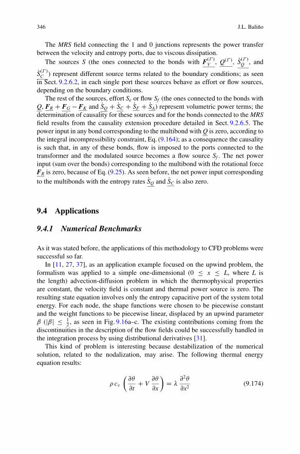
346 J.L. Baliño
The MRS field connecting the 1 and 0 junctions represents the power transferbetween the velocity and entropy ports, due to viscous dissipation.
The sources S (the ones connected to the bonds with F.� /V , Q.� /, PS.� /Q , and
PS.� /C ) represent different source terms related to the boundary conditions; as seenin Sect. 9.2.6.2, in each single port these sources behave as effort or flow sources,depending on the boundary conditions.
The rest of the sources, effort Se or flow Sf (the ones connected to the bonds withQ, FR C FG � FK and PSQ C PSC C PSF C PSA) represent volumetric power terms; thedetermination of causality for these sources and for the bonds connected to the MRSfield results from the causality extension procedure detailed in Sect. 9.2.6.5. Thepower input in any bond corresponding to the multibond with Q is zero, according tothe integral incompressibility constraint, Eq. (9.164); as a consequence the causalityis such that, in any of these bonds, flow is imposed to the ports connected to thetransformer and the modulated source becomes a flow source Sf . The net powerinput (sum over the bonds) corresponding to the multibond with the rotational forceFR is zero, because of Eq. (9.25). As seen before, the net power input correspondingto the multibonds with the entropy rates PSQ and PSC is also zero.
9.4 Applications
9.4.1 Numerical Benchmarks
As it was stated before, the applications of this methodology to CFD problems weresuccessful so far.
In [11, 27, 37], as an application example focused on the upwind problem, theformalism was applied to a simple one-dimensional (0 � x � L, where L isthe length) advection-diffusion problem in which the thermophysical propertiesare constant, the velocity field is constant and thermal power source is zero. Theresulting state equation involves only the entropy capacitive port of the system totalenergy. For each node, the shape functions were chosen to be piecewise constantand the weight functions to be piecewise linear, displaced by an upwind parameterˇ (jˇj � 1
2, as seen in Fig. 9.16a–c. The existing contributions coming from the
discontinuities in the description of the flow fields could be successfully handled inthe integration process by using distributional derivatives [31].
This kind of problem is interesting because destabilization of the numericalsolution, related to the nodalization, may arise. The following thermal energyequation results:
� cv
�@�
@tC V
@�
@x
�D
@2�
@x2(9.174)

9 FEM Formulation for CFD Framed Within the BG Theory 347
Fig. 9.16 Entropy test functions. In dashed line, the shape functions and, in solid line, the weightfunctions [11]. (a) Inner node. (b) First node. (c) Last node
As stated in Sect. 9.2.6.5, the resulting equation is second order and two spaceboundary conditions are needed. Considering the boundary conditions � .0; t/ D �0,� .L; t/ D �L and � .x; 0/ D �0, the nondimensional steady state solution ��1is [35]:
��1�x�� D �1 � �0
�L � �0 D exp .x� PeL/ � 1exp .PeL/ � 1 (9.175)
PeL D � cv V L
(9.176)
where V is the velocity and PeL is the Peclet number. The transient nondimensionaltemperature
�� D � � �0�L � �0 (9.177)
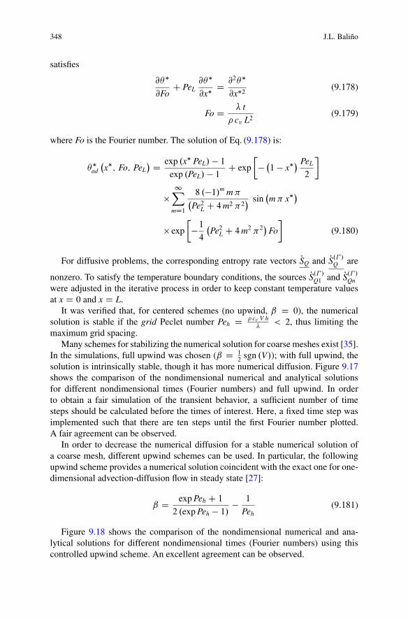
348 J.L. Baliño
satisfies
@��
@FoC PeL
@��
@x�D @2��
@x�2(9.178)
Fo D t
� cv L2(9.179)
where Fo is the Fourier number. The solution of Eq. (9.178) is:
��ad
�x�; Fo; PeL
� D exp .x� PeL/ � 1exp .PeL/ � 1 C exp
�� �1 � x�
� PeL
2
�
�1X
mD1
8 .�1/m m��Pe2L C 4m2 �2
� sin�m� x�
�
� exp
��14
�Pe2L C 4m2 �2
�Fo
�(9.180)
For diffusive problems, the corresponding entropy rate vectors PSQ and PS.� /Q are
nonzero. To satisfy the temperature boundary conditions, the sources PS.� /Q1 and PS.� /Qnwere adjusted in the iterative process in order to keep constant temperature valuesat x D 0 and x D L.
It was verified that, for centered schemes (no upwind, ˇ D 0), the numericalsolution is stable if the grid Peclet number Peh D � cv V h
< 2, thus limiting the
maximum grid spacing.Many schemes for stabilizing the numerical solution for coarse meshes exist [35].
In the simulations, full upwind was chosen (ˇ D 12
sgn .V/); with full upwind, thesolution is intrinsically stable, though it has more numerical diffusion. Figure 9.17shows the comparison of the nondimensional numerical and analytical solutionsfor different nondimensional times (Fourier numbers) and full upwind. In orderto obtain a fair simulation of the transient behavior, a sufficient number of timesteps should be calculated before the times of interest. Here, a fixed time step wasimplemented such that there are ten steps until the first Fourier number plotted.A fair agreement can be observed.
In order to decrease the numerical diffusion for a stable numerical solution ofa coarse mesh, different upwind schemes can be used. In particular, the followingupwind scheme provides a numerical solution coincident with the exact one for one-dimensional advection-diffusion flow in steady state [27]:
ˇ D exp Peh C 1
2 .exp Peh � 1/ � 1
Peh(9.181)
Figure 9.18 shows the comparison of the nondimensional numerical and ana-lytical solutions for different nondimensional times (Fourier numbers) using thiscontrolled upwind scheme. An excellent agreement can be observed.
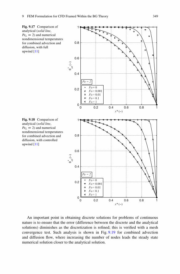
9 FEM Formulation for CFD Framed Within the BG Theory 349
Fig. 9.17 Comparison ofanalytical (solid line,PeL D 2) and numericalnondimensional temperaturesfor combined advection anddiffusion, with fullupwind [11]
0 0.2 0.4 0.6 0.8 10
0.2
0.4
0.6
0.8
1
x* (−)
θ ad*(−
)
Fo = 0 Fo = 0.001 Fo = 0.01 Fo = 0.1 Fo = 1
Pe = 2
Fig. 9.18 Comparison ofanalytical (solid line,PeL D 2) and numericalnondimensional temperaturesfor combined advection anddiffusion, with controlledupwind [11]
0 0.2 0.4 0.6 0.8 10
0.2
0.4
0.6
0.8
1
x* (−)
θ ad*(−
)
Fo = 0 Fo = 0.001 Fo = 0.01 Fo = 0.1 Fo = 1
Pe = 2
An important point in obtaining discrete solutions for problems of continuousnature is to ensure that the error (difference between the discrete and the analyticalsolutions) diminishes as the discretization is refined; this is verified with a meshconvergence test. Such analysis is shown in Fig. 9.19 for combined advectionand diffusion flow, where increasing the number of nodes leads the steady statenumerical solution closer to the analytical solution.
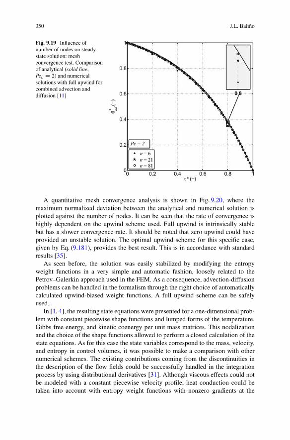
350 J.L. Baliño
Fig. 9.19 Influence ofnumber of nodes on steadystate solution: meshconvergence test. Comparisonof analytical (solid line,PeL D 2) and numericalsolutions with full upwind forcombined advection anddiffusion [11]
A quantitative mesh convergence analysis is shown in Fig. 9.20, where themaximum normalized deviation between the analytical and numerical solution isplotted against the number of nodes. It can be seen that the rate of convergence ishighly dependent on the upwind scheme used. Full upwind is intrinsically stablebut has a slower convergence rate. It should be noted that zero upwind could haveprovided an unstable solution. The optimal upwind scheme for this specific case,given by Eq. (9.181), provides the best result. This is in accordance with standardresults [35].
As seen before, the solution was easily stabilized by modifying the entropyweight functions in a very simple and automatic fashion, loosely related to thePetrov–Galerkin approach used in the FEM. As a consequence, advection-diffusionproblems can be handled in the formalism through the right choice of automaticallycalculated upwind-biased weight functions. A full upwind scheme can be safelyused.
In [1, 4], the resulting state equations were presented for a one-dimensional prob-lem with constant piecewise shape functions and lumped forms of the temperature,Gibbs free energy, and kinetic coenergy per unit mass matrices. This nodalizationand the choice of the shape functions allowed to perform a closed calculation of thestate equations. As for this case the state variables correspond to the mass, velocity,and entropy in control volumes, it was possible to make a comparison with othernumerical schemes. The existing contributions coming from the discontinuities inthe description of the flow fields could be successfully handled in the integrationprocess by using distributional derivatives [31]. Although viscous effects could notbe modeled with a constant piecewise velocity profile, heat conduction could betaken into account with entropy weight functions with nonzero gradients at the

9 FEM Formulation for CFD Framed Within the BG Theory 351
100
101
102
10−8
10−7
10−6
10−5
10−4
10−3
10−2
n
max
( |θ∗ ad−
θ∗ TH
|θ
∗ TH
)
β = 0β = ePe+1
2(ePe−1) − 1Pe
β = 12
Fig. 9.20 Mesh convergence analysis for different upwind schemes. Relative deviation of numer-ical and analytical steady state solutions for combined advection and diffusion as a function ofnumber of nodes [11]
discontinuities. The density and entropy weight functions, which are elements ofthis approach, were capable of taking into account the upwind nature of the fluidequations. Based on the linearized expressions of the state equations, a comparisonwas made with a finite-volume and with a finite-difference numerical scheme,obtaining an interpretation of the density and entropy weight functions appearingin the BG formalism. It was found that the density and entropy weight functions canbe regarded as weight factors in the calculation of the corresponding fluxes withina control volume, while the gradient of the entropy weight function come out tobe proportional to the weight factors in the calculation of the conductive entropyfluxes. Based on the Second Principle of Thermodynamics, it was also shown thatthe entropy weight functions must decrease as the distance to the correspondingnode position increases.
In [28] the methodology was used to solve the so-called shock tube problem[45]. Concerning the shape functions, constant piecewise were adopted for densityand entropy, while continuous linear were adopted for velocity, in order to be ableto model viscous effects. As weight functions, linear piecewise were adopted for theentropy, while linear continuous were adopted for the density. Lumped forms of the
352 J.L. Baliño
temperature, Gibbs free energy, and kinetic coenergy per unit mass matrices werealso chosen. No-flow and adiabatic boundary conditions were specified at both tubeends. Comparing the numerical and analytical solutions a reasonable agreement wasfound, being the numerical results a bit diffusive because of the artificial viscosityintroduced. Although more work would be needed in the selection of weight andshape functions, the simple ones chosen in this work have shown to be adequate fordealing with a complex nonlinear problem involving all physical effects.
9.4.2 Extension to Other Flow Problems
9.4.2.1 Multicomponent Flows
In [2, 3] the methodology was extended to single-phase, multicomponent flows.A classical mixture, or solution, is a material in which the components are notphysically distinct, that is, the mixing is at molecular level. In this case, whendescribed using Continuum Theory, all the components of the solution are able tooccupy the same region of space at the same time [25] and can be assumed to bein thermodynamic equilibrium. In a solution, each component has its own velocity,density, and internal energy. The balance principles for the components resemblethose for a single component, except that they are allowed to interact with oneanother.
Two approximations were studied: the multivelocity model [2] and the diffusionmodel [3]. It was shown that, for the multivelocity model, the resulting independentvariables are the densities and velocities of the components and the mixture entropyper unit volume. In the diffusion model, the dynamics of a multicomponent solutionis described in terms of the average (center of mass) velocity of the mixture andthe mass flux of each component relative to the average velocity, thus reducing thenumber of state variables. These relative mass fluxes are modeled using diffusiontheory.
The diffusive mass fluxes consist of different contributions associated with thedriving forces (mechanical or thermal) existing in the system [12]. In ordinarydiffusion, the mass flux depends in a complicated way on the concentration gradientsof the present components; in most of the problems, this is the most importantcontribution. The pressure diffusion indicates that there may be a differentialnet movement of a component in the mixture if there is a pressure gradientimposed to the system; this effect is important in centrifuge separation, in whichtremendous pressure gradients are established. The forced diffusion appears whenthe components are under different external forces, as in the case of ionic systemsin the presence of electric fields. Finally, the thermal diffusion describes thetendency for the components to separate under the influence of a temperaturegradient. Although this effect is small, it can be enhanced by producing very steeptemperature gradients.
9 FEM Formulation for CFD Framed Within the BG Theory 353
The relative fluxes are assumed to be dependent on the entropy per unit volumeand the component densities. This functional dependence allows to deal withordinary (concentration driven) diffusion, pressure diffusion, forced diffusion (withsteady forces), and thermal diffusion [12].
9.4.2.2 One-Dimensional Incompressible Pipe Flow
Incompressible pipe flow is a classic branch of Hydraulics which addresses liquidand low velocity gas flows within a closed conduit, without a free surface. Thebehavior of pipe flow is governed mainly by the Reynolds number, measuring therelative influence of inertial and viscous forces.
The one-dimensional analysis demands that suitable average values of all flowparameters are assumed to be functions of time and the coordinate along the lengthof the pipe. Small changes in pipe direction and cross-sectional area are allowed, aslong as they do not create flow separation or secondary flows. In order to reintroducethe information lost in the averaging process, closure laws for wall momentum andheat transfer, as well as suitable profile correction factors, must be defined.
For incompressible flows, the volumetric flow is independent of position. Theresulting effort balance at the inertial port results in the generalized Bernoulli equa-tion, showing transient, convective, and frictional contributions to the piezometricpressure drop.
The BG methodology was applied to the PDEs corresponding to the one-dimensional approximations for incompressible pipe flows in [6]. In [11, 37]different transient problems were numerically implemented and simulated: advec-tive heating of a fluid flow due to constant wall heat flux and due to constantwall temperature, advective heating of a fluid flow due to viscous dissipation andcombined advection-diffusion. Viscous dissipation is of particular interest as it is notmodeled in other BG formulations, which decouples the inertial and thermal ports.Also, combined advection-diffusion is important given that other BG formulationsonly take into account advection effects. For each simulation the complementaryeffects were suppressed for a correct comparison against analytical benchmarksolutions. Finally, a unit cell BG representation was shown by enforcing a lumpingapproximation (summing over the rows or columns) in the matrices associatedwith the transient terms; comparisons were made for simulations run with thisapproximation, showing no deterioration of the obtained solutions.
9.4.2.3 Traffic Flow
Traffic flow was regarded, in the pioneer works [33, 38], as a compressible flowwhose behavior is described by a density transport equation and a constitutivealgebraic equilibrium law relating density and velocity. The so-called Lighthill,Whitham, and Richards (LWR) model has some limitations, being the mostimportant the impossibility of describing problems in which boundary conditionsare established at both ends of a traffic pathway (stop-and-go waves [41]).

354 J.L. Baliño
To overcome the limitations of the LWR model, two-equation models weredeveloped by adding a velocity transport equation [36]. As it was pointed out in[24], a vehicle can be regarded as a particle that responds to frontal stimuli, whichmeans that the characteristic directions (eigenvalues) of the hyperbolic system ofequations cannot be greater than the local velocity. Besides, the velocity cannotchange sign (wrong-way-travel). Many models do not satisfy these requirements; asa consequence, they can lead to unrealistic results [24]. In [30] a continuum trafficflow model based on an improved car-following model was developed; the resultingsystem of equations is hyperbolic and doesn’t suffer wrong-way-travel problems,making it suitable for the study of diverse nonlinear dynamical phenomena observedin freeway traffic. This model was extended to simulate the flow in two lanes [19].
In [20, 21] the BG methodology was used to frame traffic flow models, by makingan analogy between traffic flow and compressible flow. Two-equation traffic flowmodels were framed within the BG methodology and some transient simulationscorresponding to propagation of shock and rarefaction waves were successfully run.
9.4.2.4 One-Dimensional Compressible Pipe Flow
In [8] the BG methodology was used to model compressible one-dimensional pipeflows with rigid walls. All physical effects compatible with the one-dimensionalapproximation such as shear wall and normal stresses, wall and axial heatconduction, and flow passage area changes can be modeled naturally. The BGrepresentation is similar to the one obtained in Sect. 9.2. Although only thetheoretical aspects were presented, the model is suitable to study isentropic, Fannoor Rayleigh flows, as well as nozzle performance.
9.5 Conclusions and Perspectives
The present contribution addresses the theoretical development of a general trueBG approach for CFD. The system state equations are obtained in terms of statevariables.
For single-phase, single-component compressible flows the state variables resultnodal values of mass, velocity, and entropy. The set of generalized effort and flowvariables was derived based on energy considerations, while the state equationswere obtained as a Galerkin formulation of the momentum conservation equationand Petrov–Galerkin formulations of the mass and entropy balance equations; as aconsequence, the computational tools developed for the FEM, as well as for othernumerical methods, can be used to solve the resulting state equations. It is interestingto notice that the matrices resulting for the mass and entropy state equations(respectively � C K and�) are different to the ones found when other formulationsfor the mass and thermal energy conservation equations are discretized.
9 FEM Formulation for CFD Framed Within the BG Theory 355
For single-phase, single-component incompressible flows the state variablesresult nodal values of pressure, velocity, and entropy. The resulting representationshows the role of pressure as external function acting to satisfy the incompressibilitycondition and the coupling between the inertial and thermal ports through thepower dissipation term. The state equations for momentum and continuity equationsare coincident with the one obtained by using the Galerkin method for the weakformulation of the problem in the FEM. The integral incompressibility constraintwas derived based on the integral conservation of mechanical energy. The weakformulation for thermal energy equation was modeled with true BG elements,resulting a Petrov–Galerkin method. Again, the matrix resulting for entropy stateequation � is different to the ones found when other formulations for the thermalenergy conservation equation are discretized.
Regarding the power interaction between the system and the external environ-ment, this is made through the boundary source terms Pm.� /
W and PS.� /C (related to fluid
flow across the boundary), F.� /V (related to viscous stresses applied at the boundary),
and PS.� /Q (related to heat power at the boundary). Other (more subtle) interaction
could be established through the force per unit mass G, which may include non-inertial or electrodynamic forces, as in Magnetohydrodynamics.
As a result of a combination of BG concepts with elements of numerical methods,a new approach was developed, which is a foundation of a bridge between BGs andCFD. As the formulation is based on the definition of nodal discretized variables,different numerical schemes can be obtained by means of the appropriate choice ofthe interpolation and weight functions.
For the applications of the methodology made so far (single-phase, single ormulticomponent systems) the modeling and determination of the state equationscan be made based on Continuum Theory, conservation laws, Thermodynamicsof equilibrium, and constitutive laws coming from the molecular theory. Thedifficulties in the resolution of a problem are limited, in these cases, to discretizationand numerical aspects. Besides framing these flows within the BG theory, thecontributions coming from the methodology in these problems are related to theestablishment of acceptable boundary conditions satisfying causality.
For more sophisticated flows, like turbulent [46] or multiphase [25], the situationis different. Due to the closure problem in the Reynolds-averaged Navier–Stokes(RANS) equation approach for incompressible turbulence, for instance, it doesn’texist a theory for all turbulent flows, but models with restricted validity. Thesemodels differ in order (algebraic or with a variable number of transport equations),definition of independent variables and fundamentals, so there is no equivalencebetween them. The situation is far more complex for multiphase flows, where theexistence of interfaces makes indispensable the definition of statistical averagesrelated to the existence of a phase (component indicator function); new variablessuch as the void fraction or the interfacial volumetric area are vital in the descriptionof multiphase systems.
It is interesting to notice that the state of the art in multiphase modeling is notsufficient to guarantee well-posed equations. For one-dimensional bubbly flow, there
356 J.L. Baliño
exist complex eigenvalues for a range of working parameters, which is physicallyunacceptable. These complex characteristics seem to arise from the unsuccessfulmodeling of the coupling terms between the momentum equations for each phase[25], being the systematic inclusion of terms soundly based on Physics the remedyto yield an appropriate working model. The concept of balance equations in the BGmethodology, with coupling terms between ports, would render a new perspectiveto deal with this problem.
It becomes evident that the difficulties in the resolution of complex flows liketurbulent or multiphase is related to modeling as well as to discretization. Thus, amethodology synthesizing properties of dynamic systems is very useful to framedifferent models, as well as to develop new ones. Obviously, BG theory does notreplace Physics, but works as a structure that allows to discover mathematical incon-sistencies from the beginning of the modeling process. A BG based methodologycontributes to answer questions such as what the independent variables are, whatequations must be satisfied in order to guarantee conservation of energy in thesystem, and how the boundary conditions are introduced.
This contribution shows that starting from the governing PDEs and usingdiscretization techniques coming from CFD is the right strategy for producinggeneral models, framed within the BG theory, for fluid dynamic systems. The authorhopes that the findings of this contribution encourage other researchers to use thisformalism in more complex problems.
References
1. Baliño, J. L. (2002). Bond-graph approach for computational fluid dynamics: A comparisonwith other numerical methods. In Second IEEE International Conference on System, Man andCybernetics (SMC 2002), Paper TA1B3, 6 pp.
2. Baliño, J. L. (2003). BG-CFD methodology for multicomponent solutions. Part I: Multivelocitymodel. In 2003 International Conference on Bond Graph Modeling and Simulation (ICBGM2003) (pp. 41–46).
3. Baliño, J. L. (2003). BG-CFD methodology for multicomponent solutions. Part II: Diffusionmodel. In 2003 International Conference on Bond Graph Modeling and Simulation (ICBGM2003) (pp. 47–52).
4. Baliño, J. L. (2003). Bond-graph formulation of CFD problems with constant piecewise shapefunctions. International Journal of Heat and Technology, 21(1), 59–66.
5. Baliño, J. L. (2005). Bond graph modeling of incompressible flows. In 17th IMACS WorldCongress, Scientific Computation, Applied Mathematics and Simulation (IMACS 2005), 8 pp.
6. Baliño, J. L. (2006). Modeling one-dimensional incompressible duct flows. In 20th EuropeanConference on Modelling and Simulation (ECMS 2006), Paper 76, 6 pp.
7. Baliño, J. L. (2009). Galerkin finite element method for incompressible thermofluid flowsframed within the bond graph theory. Simulation Modelling Practice and Theory, 17, 35–49.
8. Baliño, J. L. (2016). True bond graph formulation for compressible thermofluid duct flows. InThe 9th International Conference on Integrated Modeling and Analysis in Applied Control andAutomation (IMAACA 2016) (pp. 24–31).
9. Baliño, J. L., Larreteguy, A. E., & Gandolfo, E. F. (2001). A general bond graph approachfor computational fluid dynamics. Part I: Theory. In 2001 International Conference on BondGraph Modeling and Simulation (ICBGM 2001) (pp. 41–46).

9 FEM Formulation for CFD Framed Within the BG Theory 357
10. Baliño, J. L., Larreteguy, A. E., & Gandolfo, E. F. (2006). A general bond graph approach forcomputational fluid dynamics. Simulation Modelling Practice and Theory, 14, 884–908.
11. Baliño, J. L., & Pellegrini, S. P. (2016, in press). True bond graph formulation for one-dimensional incompressible pipe flows. Modeling and applications. Journal of the BrazilianSociety of Mechanical Sciences and Engineering.
12. Bird, R. B., Stewart, W. E., & Lightfoot, E. N. (1960). Transport phenomena. New York: Wiley.13. Borutzky, W. (2004). Bond graphs. A methodology for modelling multidisciplinary dynamic
systems. San Diego, CA: SCS Publishing House.14. Borutzky, W. (2010). Bond graph methodology. Development and analysis of multidisciplinary
dynamic systems models. New York: Springer.15. Borutzky, W. (2011). Bond graph modelling of engineering systems. Theory, applications and
software support. New York: Springer.16. Brown, F. T. (2006). Engineering system dynamics. A unified graph-centered approach. Boca
Raton, FL: CRC Press.17. Callen, H. B. (1960). Thermodynamics. New York: Wiley.18. Cellier, F. E. (1991). Continuous system modeling. New York: Springer.19. Chang-Fu. T., Jiang. R., & Qing-Song, W. (2007). Extended speed gradient model for traffic
flow on two-lane freeways. Chinese Physics, 16, 1570–1575.20. Chera, C. M., Baliño, J. L., & Dauphin-Tanguy, G. (2010). Two-equation traffic flow models
framed within the bond graph theory. In 2010 International Conference on Bond GraphModeling and Simulation (ICBGM 2010), 8 pp.
21. Chera, C. M., Baliño, J. L., & Dauphin-Tanguy, G. (2013). Bond graph and computational fluiddynamics in traffic flow. In 2nd International Conference on Systems and Computer Science(ICSCS 2013), 6 pp.
22. Crandall, S. H., Karnopp, D. C., Kurtz, E. F., & Pridmore-Brown, D. C. (1968). Dynamics ofmechanical and electromechanical systems. New York: MacGraw-Hill.
23. Cuvelier, C., Segal, A., & van Steenhoven, A. A. (1986). Finite element methods and Navier-Stokes equations. Dordrecht: D. Reidel Publishing Company.
24. Daganzo, C. F. (1995). Requiem for second-order fluid approximations of traffic flow.Transportation Research Part B, 29B, 277–286.
25. Drew, D. A., & Passman, S. L. (1999). Theory of multicomponent fluids. New York: Springer.26. Fahrenthold, E. P., & Venkataraman, M. (1996). Eulerian bond graphs for fluid continuum
dynamics modeling. ASME Journal of Dynamic Systems, Measurement, and Control, 118,48–57.
27. Gandolfo Raso, E. F., Larreteguy, A. E., & Baliño, J. L. (2001). A general bond graph approachfor computational fluid dynamics. Part II: Applications. In 2001 International Conference onBond Graph Modeling and Simulation (ICBGM 2001) (pp. 47–52).
28. Gandolfo Raso, E. F., Larreteguy, A. E., & Baliño, J. L. (2002). Modeling of 1-D compressibleflows. In Second IEEE International Conference on System, Man and Cybernetics (SMC 2002),Paper TA1B4, 6 pp.
29. Gawthrop, P. J., & Smith, L. P. S. (1996). Metamodelling: Bond graphs and dynamic systems.London: Prentice-Hall.
30. Jiang, R., Wu, K. S., & Zhu, Z. J. (2001). A new continuum model for traffic flows andnumerical tests. Transportation Research Part B, 36, 405–419.
31. Kanwal, R. P. (1998). Generalized functions: Theory and technique. Boston: Birkhëuser.32. Karnopp, D. C., Margolis, D. L., & Rosenberg, R. C. (2012). System dynamics: Modeling,
simulation and control of mechatronic systems. New York: Wiley.33. Lighthill, M. J., & Whitham, G. B. (1955). On kinematic waves II. A theory of traffic flow on
long crowded roads. Proceedings of the Royal Society of London, Series A, 229, 317–345.34. Löhner, R. (2001). Applied CFD techniques: An introduction based on finite element methods.
New York: Wiley.35. Patankar, S. V. (1980). Numerical heat transfer and fluid flow. Washington: Hemisphere
Publishing Corporation.

358 J.L. Baliño
36. Payne, H. J. (1971). Models of freeway traffic and control. Mathematical Models of PublicSystem, 1, 51–61.
37. Pellegrini, S. P., & Baliño, J. L. (2014). Application of a true bond graph formulation forincompressible thermofluid duct flows. In 2014 International Conference on Bond GraphModeling and Simulation (ICBGM 2014), 10 pp.
38. Richards, P. I. (1956). Shock waves on the highway. Operations Research, 4, 42–51.39. Rosenberg, R. C., & Karnopp, D. C. (1983). Introduction to physical system dynamics. New
York: McGraw-Hill.40. Schapiro, A. V. (1953). The dynamics and thermodynamics of compressible fluid flow (Vol. I).
New York: The Ronald Press Company.41. Schönhof, M., & Helbing, D. (2007). Empirical features of congested traffic state and their
implications for traffic modeling. Transportation Science, 41, 135–166.42. Tannehill, J. C., Anderson, D. A., & Pletcher, R. H. (1997). Computational fluid mechanics
and heat transfer. Washington, DC: Taylor & Francis.43. Thoma, J., & Ould Bouamama, B. (2000). Modelling and simulation in thermal and chemical
engineering. A bond graph approach. Berlin: Springer.44. Whitaker, S. (1977). Fundamental principles of heat transfer. New York: Pergamon Press.45. Whitham, G. B. (1999). Linear and nonlinear waves. New York: Wiley.46. Wilcox, D. C. (2000). Turbulence modeling for CFD. La Canada, CA: DCW Industries, Inc.47. Zienkiewicz, O. C., Taylor, R. L., & Nithiarasu, P. (2005). The finite element method for fluid
dynamics. Boston: Elsevier.
Chapter 10Model Complexity of Distributed ParameterSystems: An Energy-Based Approach
L.S. Louca
10.1 Introduction
Modeling and simulation have yet to achieve wide utilization as commonplaceengineering tools. One reason for this is that current modeling and simulationtechniques are inadequate. Specifically, a major disadvantage is that they requiresophisticated users who are often not domain experts and thus lack the ability toeffectively utilize the model and simulation tools to uncover the important designtrade-offs. Another drawback is that models are often large and complicated withmany parameters, making the physical interpretation of the model outputs, even bydomain experts, difficult. This is particularly true when “unnecessary” features areincluded in the model.
A variety of algorithms have been developed and implemented to help auto-mate the production of proper models of dynamic systems. Wilson and Steindeveloped Model Order Deduction Algorithm (MODA) that deduces the requiredsystem model complexity from subsystem models of variable complexity using afrequency-based metric [25]. They also defined proper models as the models withphysically meaningful states and parameters that are of necessary but sufficientcomplexity to meet the engineering and accuracy objectives. Additional work ondeduction algorithms for generating proper models in an automated fashion hasbeen reported by previous research [4, 5, 24]. The above algorithms have also beenimplemented in an automated modeling computer environment [22].
In an attempt to overcome the limitations of the frequency-based metrics, theauthor introduced a new model reduction technique that also generates propermodels [16]. This approach uses an energy-based metric (element activity) that
L.S. Louca (�)Department of Mechanical and Manufacturing Engineering, University of Cyprus,Nicosia 1678, Cypruse-mail: [email protected]
© Springer International Publishing Switzerland 2017W. Borutzky (ed.), Bond Graphs for Modelling, Control and FaultDiagnosis of Engineering Systems, DOI 10.1007/978-3-319-47434-2_10
359
360 L.S. Louca
in general can be applied to nonlinear systems, and considers the importance ofall energetic elements (generalized inductance, capacitance, and resistance) [17].The contribution of each energy element in the model is ranked according to theactivity metric under specific excitation. Elements with small contributions areeliminated in order to produce a reduced model using a systematic methodologycalled Model Order Reduction Algorithm (MORA). The activity metric was alsoused as a basis for even further reduction, through partitioning the model intosmaller and decoupled submodels [19].
Such modeling approaches should be able to handle real mechanical systemsthat typically include distributed parameter (continuous) components, e.g., rods,beams, plates, etc. Frequently, modeling objectives and assumptions allow thelumping of continuous component properties into ideal energy elements that leadto a dynamic model described by a set of ordinary differential equations. However,when property lumping is not acceptable, modeling of a continuous componentrequires a different approach since its inertial, compliance, and resistive propertiesare spatially distributed and cannot be lumped into single equivalent elements.The dynamic behavior of continuous components is thus described by partialdifferential equations with derivatives in both time and space. Another approachthat is considered in this work is the modeling of a continuous component withfinite segments that are spatially distributed. This is an approximation for which theaccuracy is a function of the number of segments. The model accuracy improvesas the number of segments increases. Model accuracy and the required number ofsegments can be addressed using a frequency-based metric [5].
Beyond the physical-based modeling, modal decomposition is also used tomodel and analyze continuous and discrete systems [18]. One of the advantages ofmodal decomposition is the ability to straightforwardly adjust (i.e., reduce) modelcomplexity since all modes are orthogonal to each other. The reduction of suchmodal decomposition models is mostly based on frequency, and the user-definedFrequency Range Of Interest (FROI) determines the frequencies that are importantfor a specific scenario. In this case, modes with frequencies within the FROI areretained in the reduced model and modes outside this range are eliminated. Asexpected, mode truncation introduces error in the predictions that can be measuredand adjusted based on the accuracy requirements [9, 10].
Element activity is another metric that has more flexibility than frequency-basedmetrics, which address the issue of model complexity by only adding compliantelements, leaving unaccounted the importance of inertial and resistive elements. Incontrast, the activity metric considers the importance of all energetic elements, andtherefore, the significance of all energy elements in the model can be quantified.It is the purpose of this work to develop a new methodology using the activitymetric for addressing the model complexity of distributed parameter systems andspecifically cantilever beams. The methodology is specifically developed using thefinite segment approximation and the goal is to identify the physical phenomena tobe included in each segment in order to accurately predict the dynamic behavior.
The chapter starts with providing background on the energy-based activity metricalong with the reduction algorithm. Next, the equation formulation for a finite
10 Model Complexity of Distributed Parameter Systems: An Energy-Based Approach 361
segment Timoshenko beam is presented along with the closed form expressions forsteady state element activities. Then, the complexity of a cantilever beam is analyzedunder various conditions using MORA. Finally, in the last section, discussion andconclusions are provided.
10.2 Background
The original work on the energy-based metric for model reduction is brieflydescribed here for convenience. More details, extensions, and applications of thismethodology can be found in previous publications [13–15, 17]. The main ideabehind this model reduction technique is to evaluate the “element activity” ofindividual energy elements in a full system model under a stereotypical set of inputsand initial conditions. The activity of each energy element establishes a hierarchyof importance for all elements in a system. Those below a user-defined threshold ofacceptable level of activity are eliminated from the model. A reduced model is thengenerated and a new set of governing differential equations is derived.
The activity metric has been formulated originally for systems with nonlinearitiesin both the element constitutive laws and kinematics. In this work, the activity metricis applied to linear systems for which analytical expressions for the activity canbe derived, and therefore, avoid the use of numerical time integration that couldbe cumbersome. The analysis is further simplified if, in addition to the linearityassumption, the system is assumed to have a single sinusoidal excitation, and onlythe steady state response is studied. These assumptions are motivated from Fourieranalysis where an arbitrary function can be decomposed into a series of harmonics.Using this frequency decomposition, the activity analysis can be performed as afunction of frequency in order to study the frequency dependency of element activityin a dynamic system.
10.2.1 Element Activity for Linear Systems
A measure of the power response of a dynamic system, which has physical meaningand a simple definition, is used to develop the modeling metric, element activity (orsimply “activity”). Element activity, A, is defined for each energy element as:
A DZ �
0
jP.t/jdt (10.1)
where P(t) is the element power and � is the time over which the model has toaccurately predict the system behavior. The activity has units of energy, representingthe amount of energy that flows in and out of the element over the given time � . Theenergy that flows in and out of an element is a measure of how active this element
362 L.S. Louca
is (how much energy passes through it), and consequently the quantity in (10.1) istermed activity. Activity can be defined independent of the energy domain, type ofenergy element, or nonlinearities.
The activity is calculated for each energy element based on the system responsethat is calculated from the system’s state equations. In the case that the system ismodeled using a bond graph formulation, the state equations are derived using themulti-port bond graph representation [2, 3, 7, 21]. In addition, when the system haslinear junction structure and constitutive laws and a single input, the state equationsare linear time invariant and have the following general form:
:x D Ax C bu (10.2)
where, A 2 Rm�m;b 2 R
m are the state space matrices, x 2 Rm is the state variable
vector, u 2 R is the input, and m is the number of independent states.For the above system appropriate outputs are defined in order to effortlessly
calculate the power of each energy element in the model using the constitutive lawof each element. For convenience, the outputs are selected to be the generalizedflow, effort, and flow for inertial, compliant, and resistive elements, respectively.The dual effort or flow variables needed for calculating the power are derived fromthe output variables and constitutive laws. The output vector for this set of variableshas the form:
y D8<
:
fI
eC
fR
9=
; (10.3)
where y 2 Rk and fI 2 R
kI ; eC 2 RkC ; and fR 2 R
kR . The variables kI , kC, and kR
represent the number of inertial, compliant, and resistive elements, respectively. Thetotal number of energy elements is k D kI C kC C kR. Note that the output vector isdefined such that the required variables of the inertial elements are first followed bythe variables of compliant and then resistive elements.
Each output variable is a linear function of the state variables, and possibly input,given that they have linear constitutive laws. Using the output variables set in (10.3),the output equations are written as:
y D Cx C du (10.4)
where C 2 Rk�m;d 2 R
k are the output state space matrices.Given this set of output variables the missing efforts or flows, needed for
calculating the element power, are computed from the linear constitutive laws ofeach type of energy element as shown below:
I W pI D rIfI () eI D :pI D rI
:
f I
C W qC D rCeC () fC D :qC D rC
:eC
R W eR D rRfR
(10.5)
10 Model Complexity of Distributed Parameter Systems: An Energy-Based Approach 363
where rI , rC, rR are known constants representing the linear constitutive lawcoefficients of inductance, compliance, and resistance, respectively. For derivingcompact expressions in the analysis, a vector, r 2 R
k, with all the linear constitutivelaw coefficients is introduced as shown below:
r D8<
:
rI
rC
rR
9=
; (10.6)
where rI 2 RkI , rC 2 R
kC , and rR 2 RkR are the constant constitutive law
coefficients.Finally, the power needed for calculating the activity of each element, as defined
in (10.1), is computed as the product of generalized effort and flow. By using (10.5)the following expressions for the power of each element type are derived:
I W PI D eIfI D rIfI:
f I
C W PC D eCfC D rCeC:eC
R W PR D eRfR D rRfRfR D rRf 2R
(10.7)
The expressions for element power in (10.7) are generalized with the use of thedefined structure of the output vector in (10.3) and parameter vector in (10.6). Thus,the power for energy storage elements (inertial and compliant) is given by (10.8)and for energy dissipation elements (resistive) in (10.9).
Pi D riyi:yi; i D 1; : : : ; kI C kC (10.8)
Pi D riy2i ; i D kI C kC C 1; : : : ; k (10.9)
The above element power is then used to calculate the element activity basedon its definition in (10.1). Element parameters are assumed to be constant thus theactivity for the energy storage elements is given in (10.10) and for energy dissipationelement in (10.11).
Ai DZ �
0
jPij D ri
Z �
0
ˇyi:yi
ˇdt; i D 1; : : : ; kI C kC (10.10)
Ai DZ �
0
jPij D ri
Z �
0
ˇy2iˇdt D ri
Z �
0
y2i dt; i D kI C kC C 1; : : : ; k (10.11)
10.2.2 Activity for Single Harmonic Excitation
The time response of the output vector, y(t), in (10.3) and (10.10) is required in orderto complete the calculation of element power. For nonlinear systems, numericalintegration is typically used to calculate the system response; however, in this case

364 L.S. Louca
linear system analysis can be used to obtain closed form expressions. In addition,for the purposes of this work, the excitation is assumed to be a single harmonicgiven by:
u.t/ D U sin .!t/ (10.12)
where U 2 R is the amplitude of the excitation and ! is the excitation frequency.The steady state response of the linear system in (10.2) and (10.4) under theharmonic excitation in (10.12) is calculated using linear system analysis theory. Theresponse is given by the following closed form expression:
yi .t; !/ D UYi .!/ � sin .!t C 'i .!// ; i D 1; : : : ; k (10.13)
where Yi(!) and ®i(!) are the steady state amplitude and phase shift, respectively,that can be easily calculated using linear system analysis.
Within the context of this analysis, the output yi(t,!) in (10.13) is either aneffort or a flow that is used for calculating the power of each element in (10.8)and (10.9). Finally, the activity can be calculated by (10.10) and (10.11), but firstthe upper bound, � , of this integral must be specified. For this case, the steady stateand periodicity features of the response are exploited. A periodic function repeatsitself every T seconds, and therefore, a single period of this function contains thenecessary information about the response. Thus, the upper bound of the integral isset to one period of the excitation, � D T D 2�=!. Therefore, the steady stateactivity for energy storage elements is given by:
Assi .!/ D ri
Z T
0
ˇyi:yi
ˇdt
D 1
2riU
2Y2i .!/ !Z T
0
jsin .2 .!t C 'i .!///jdt
) Assi .!/ D 2riU
2Y2i .!/
(10.14)
and for energy dissipation elements by:
Assi .!/ D ri
Z T
0
y2i dt
D riU2Y2i .!/
Z T
0
sin2 .!t C 'i .!//dt
) Assi .!/ D �riU2Y2i .!/
!
(10.15)
The above simple closed form expressions can be used to calculate the activityof energy elements for a given single harmonic excitation. These expressions areproportional to the square of the amplitude; however, they have no dependency onthe phase shift that is eliminated through the integration. The superscript “ss” in
10 Model Complexity of Distributed Parameter Systems: An Energy-Based Approach 365
(10.14) and (10.15) denotes the activity under a steady state harmonic response.Note that the activity for both energy storage and energy dissipation elements is afunction of the excitation frequency but not the phase shift.
10.2.3 Activity Index and MORA
The activity as defined in (10.1) is a measure of the absolute importance of anelement as it represents the amount of energy that flows through the element overa given time period. In order to obtain a relative measure of the importance, theelement activity is compared to a quantity that represents the “overall activity” ofthe system. This “overall activity” is defined as the sum of all the element activitiesof the system, is termed total activity (ATotal), and is given by:
ATotal .!/ DkX
iD1Ai .!/ (10.16)
where Ai is the activity of the ith element given by (10.14) and (10.15). Thus anormalized measure of element importance, called element activity index or justactivity index, is defined as:
AIssi .!/ D Ass
i .!/
ATotal .!/D Ass
i .!/
kX
iD1Ass
i .!/
(10.17)
The activity index, AIssi (!), is calculated for each element in the model and it
represents the portion of the total system energy that flows through a specificelement. The input amplitude, U, does not appear in any of the element activityindices since all element activities are proportional to the square of the amplitude.
With the activity index defined as a relative metric for addressing elementimportance, the Model Order Reduction Algorithm (MORA) is constructed. Thefirst step of MORA is to calculate the activity index for each element in the systemas defined in (10.17). Next, the activity indices are sorted to identify the elementswith high activity (most important) and low activity (least important). With theactivity indices sorted, the model reduction proceeds given the desired engineeringspecifications. These specifications are defined by the modeler who then convertsthem into a threshold ˇ of the total activity (e.g., 99 %) that he or she wants toinclude in the reduced model. This threshold defines the borderline between theeliminated and retained elements in the model. The elimination process is shownin Fig. 10.1 where the sorted activity indices are summed starting from the mostimportant element until the specified threshold is reached. The element which, whenincluded, increments the cumulative activity index above the threshold, is the lastelement to be included in the reduced model. The elements that are above thisthreshold are removed from the model, e.g., when using the bond graph formulation,

366 L.S. Louca
β
Fig. 10.1 Activity index sorting and elimination
delete the corresponding low activity energy element. The junction structure of thebond graph is retained in the reduced model, and therefore, the reduced modelrealization is the same as the full model, so its physical meaning and relation tothe physical system are retained.
10.3 Cantilever Beam Model
The state space model used in the previous section assumes a lumped parametersystem representation, where individual components exhibit only inertial, compli-ant, or resistive behavior. This means that the dynamic behavior of a componentcan be lumped and modeled as a single inertial, compliant, or resistive energyelement. This can be a valid assumption for many components; however, real systemcomponents can possess all dynamic properties (inertial, compliant, and resistive)simultaneously. In addition, these properties may vary or be distributed spatially.In these cases, a lumped parameter modeling approach cannot be used since it willresult in an incorrect model and produce inaccurate predictions. An example of suchcomponent is a beam and more specifically a cantilever beam that is widely usedin engineering applications. Therefore, these components must be considered asdistributed parameter or continuous, which require a different modeling approach.
Models of continuous systems are developed using solid mechanics theory,which instead of Ordinary Differential Equations, lead to Partial Differential
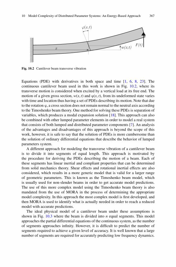
10 Model Complexity of Distributed Parameter Systems: An Energy-Based Approach 367
xF(t)
w(x,t)
ϕ(x,t)
Fig. 10.2 Cantilever beam transverse vibration
Equations (PDE) with derivatives in both space and time [1, 6, 8, 23]. Thecontinuous cantilever beam used in this work is shown in Fig. 10.2, where itstransverse motion is considered when excited by a vertical load at its free end. Themotion of a given gross section, w(x, t) and ®(x, t), from its undeformed state varieswith time and location thus having a set of PDEs describing its motion. Note that dueto the rotation ®, a cross section does not remain normal to the neutral axis accordingto the Timoshenko beam theory. One method for solving these PDEs is separation ofvariables, which produces a modal expansion solution [18]. This approach can alsobe combined with other lumped parameter elements in order to model a real systemthat consists of both lumped and distributed parameter components [7]. An analysisof the advantages and disadvantages of this approach is beyond the scope of thiswork, however, it is safe to say that the solution of PDEs is more cumbersome thanthe solution of ordinary differential equations that describe the behavior of lumpedparameters system.
A different approach for modeling the transverse vibration of a cantilever beamis to divide it into segments of equal length. This approach is motivated bythe procedure for deriving the PDEs describing the motion of a beam. Each ofthese segments has linear inertial and compliant properties that can be determinedfrom solid mechanics theory. Shear effects and rotational inertial effects are alsoconsidered, which results in a more generic model that is valid for a larger rangeof geometric parameters. This is known as the Timoshenko beam model, whichis usually used for non-slender beams in order to get accurate model predictions.The use of this more complex model using the Timoshenko beam theory is alsomandated from the use of MORA in the process of determining the appropriatemodel complexity. In this approach the most complex model is first developed, andthen MORA is used to identify what is actually needed in order to reach a reducedmodel with accurate predictions.
The ideal physical model of a cantilever beam under these assumptions isshown in Fig. 10.3 where the beam is divided into n equal segments. This modelapproaches the partial differential equations of the continuous system, as the numberof segments approaches infinity. However, it is difficult to predict the number ofsegments required to achieve a given level of accuracy. It is well known that a largenumber of segments are required for accurately predicting low frequency dynamics.
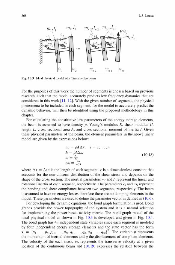
368 L.S. Louca
cn-1
wn-2 wn-1 wn
csn-1 csn
cnc1
w1
m1,I1 m2,I2 mn-2,In-2 mn-1,In-1
mn,In
w2
cs1cs2
c2
...
F(t)
Fig. 10.3 Ideal physical model of a Timoshenko beam
For the purposes of this work the number of segments is chosen based on previousresearch, such that the model accurately predicts low frequency dynamics that areconsidered in this work [11, 12]. With the given number of segments, the physicalphenomena to be included in each segment, for the model to accurately predict thedynamic behavior, will then be identified using the proposed methodology in thischapter.
For calculating the constitutive law parameters of the energy storage elements,the beam is assumed to have density �, Young’s modulus E, shear modulus G,length L, cross sectional area A, and cross sectional moment of inertia I. Giventhese physical parameters of the beam, the element parameters in the above linearmodel are given by the expressions below:
mi D �A�x; i D 1; : : : ; nIi D �I�x;ci D �x
EIcsi D �x
�GA
(10.18)
where �x D L=n is the length of each segment, � is a dimensionless constant thataccounts for the non-uniform distribution of the shear stress and depends on theshape of the cross section. The inertial parameters mi and Ii represent the linear androtational inertia of each segment, respectively. The parameters ci and csi representthe bending and shear compliance between two segments, respectively. The beamis assumed to have no energy losses therefore there are no damping elements in themodel. These parameters are used to define the parameter vector as defined in (10.6).
For developing the dynamic equations, the bond graph formulation is used. Bondgraphs provide the power topography of the system and it is a natural selectionfor implementing the power-based activity metric. The bond graph model of theideal physical model as shown in Fig. 10.3 is developed and given in Fig. 10.4.The bond graph has 4n independent state variables since each segment is modeledby four independent energy storage elements and the state vector has the formx D fp1; : : : ; pn; pI1; : : : ; pIn; q1; : : : ; qn; qs1; : : : ; qsngT . The variable p representsthe momentum of inertial elements and q the displacement of compliant elements.The velocity of the each mass, vi, represents the transverse velocity at a givenlocation of the continuous beam and (10.19) expresses the relation between the
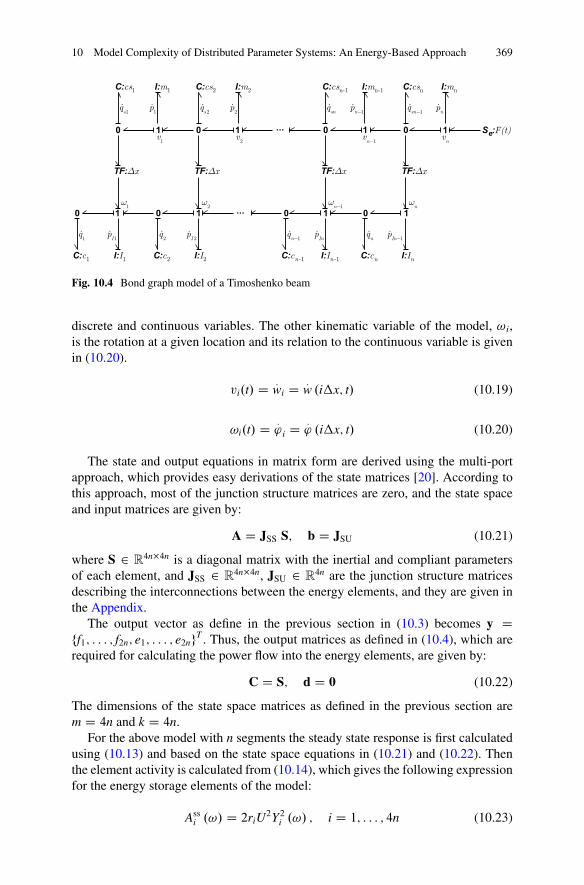
10 Model Complexity of Distributed Parameter Systems: An Energy-Based Approach 369
0 1
Se:F(t)
C:c1
I:m1
TF:Δx
...
...1 10
1
TF:Δx
0
q1
qn
pn
p1
C:cs1 C:cs2 C:csn-1 C:csnI:m2
v1
vn
0
C:c2
v2
p2
1
I:mn-1
TF:Δx
1 10
1
TF:Δx
0
I:mn
0
q2
C:cn
0
C:cn-1
vn−1
pn−1
qn−1
I:I1 I:I2 I:In-1 I:In
pI1
pI 2
pIn
pIn−1
qs1
qs2
qsn
qsn−1
ω1
ω2
ωn−1
ωn
Fig. 10.4 Bond graph model of a Timoshenko beam
discrete and continuous variables. The other kinematic variable of the model, ! i,is the rotation at a given location and its relation to the continuous variable is givenin (10.20).
vi.t/ D :wi D :
w .i�x; t/ (10.19)
!i.t/ D :' i D :
' .i�x; t/ (10.20)
The state and output equations in matrix form are derived using the multi-portapproach, which provides easy derivations of the state matrices [20]. According tothis approach, most of the junction structure matrices are zero, and the state spaceand input matrices are given by:
A D JSS S; b D JSU (10.21)
where S 2 R4n�4n is a diagonal matrix with the inertial and compliant parameters
of each element, and JSS 2 R4n�4n, JSU 2 R
4n are the junction structure matricesdescribing the interconnections between the energy elements, and they are given inthe Appendix.
The output vector as define in the previous section in (10.3) becomes y Dff1; : : : ; f2n; e1; : : : ; e2ngT . Thus, the output matrices as defined in (10.4), which arerequired for calculating the power flow into the energy elements, are given by:
C D S; d D 0 (10.22)
The dimensions of the state space matrices as defined in the previous section arem D 4n and k D 4n.
For the above model with n segments the steady state response is first calculatedusing (10.13) and based on the state space equations in (10.21) and (10.22). Thenthe element activity is calculated from (10.14), which gives the following expressionfor the energy storage elements of the model:
Assi .!/ D 2riU
2Y2i .!/ ; i D 1; : : : ; 4n (10.23)
370 L.S. Louca
The above analysis enables the calculation of the element activity for a givensingle harmonic excitation. The activity index that is used by MORA is independentof the excitation amplitude, as shown in (10.17), and therefore can be set to anarbitrary value, e.g., set to one (1) for simplicity. Model complexity and whichphysical phenomena need to be included, can be determined given the elementactivity in (10.23) and MORA. The complexity of the beam is investigated in thenext section in order to identify the significant elements based on beam length andelement location. A series of analysis is performed in order to get more insight intothe important beam dynamics under different scenarios.
10.4 Beam Complexity Based on Activity
The activity metric and MORA is applied to a steel cantilever beam with parameters� D 7860 kg=m3, E D 210 GPa, G D 80 GPa, A D 3 � 10�3 m2,I D 2:5 � 10�6 m4, � D 0:85. The length of the beam is varied, L D 0.2–2.0 m,in order to study the variation of element significance. The methodology is easyand computationally inexpensive to implement due to the simple and closed formexpressions used for calculating the state space matrices, frequency response, andactivity.
First, the beam length is set to 2.0 m such that the beam is considered to beslender. The number of segments is set to n D 30 and therefore there are a total of120 energy storage elements modeling the beam. In this case the modeling targetis set to accurately predict static behavior of low frequency dynamics, thus, theexcitation frequency is set to 95 % of the first natural frequency (122.7 rad/s).
The results of the activity analysis using (10.23) and under these assumptionsare shown in Fig. 10.5 where the activity index of all 120 elements is shown.Element numbers 1–30 represent the activity index of the linear inertia (mi) and31–60 the activity index of the rotational inertia (Ii) of each segment. Next, elementnumbers 61–90 and 91–120 represent the activity index of the bending (ci) and shear(csi) compliance, respectively. For each range of elements the smallest numbersrepresent elements that are next to the fixed end of the beam. It is clear from theactivity analysis that the most important elements are related to the linear inertiaand the bending stiffness of the beam. On the contrary, the elements related withthe rotary inertia and shear stiffness have very low activity and thus are insignificantunder these conditions. This initial activity analysis agrees with common practice,in which a slender beam is modeled using the Euler–Bernoulli theory that neglectsrotational inertia and shear stress effects.
Model complexity is systematically addressed using MORA as it is describedin Sect. 10.2.3. Elements are ranked according to their activity index as shownin Fig. 10.6 where the sorted activity indices along with the cumulative activityindex are plotted. According to the activity analysis, 40 of the 120 elements accountfor almost 99 % of the energy flows through the model. This is a significant resultverifying that unnecessary complexity is included in the model; however, the figuredoes not directly depicts the elements that are insignificant and could be eliminatedfrom the model.
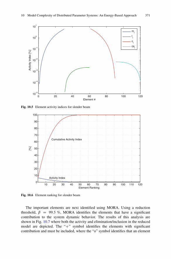
10 Model Complexity of Distributed Parameter Systems: An Energy-Based Approach 371
0 20 40 60 80 100 12010
−5
10−4
10−3
10−2
10−1
100
101
Element #
Act
ivity
Inde
x [%
]m
i
li
ci
csi
Fig. 10.5 Element activity indices for slender beam
10 20 30 40 50 60 70 80 90 100 110 1200
10
20
30
40
50
60
70
80
90
100
Element Ranking
[%]
Activity Index
Cumulative Activity Index
Fig. 10.6 Element ranking for slender beam
The important elements are next identified using MORA. Using a reductionthreshold, ˇ D 99:5 %, MORA identifies the elements that have a significantcontribution to the system dynamic behavior. The results of this analysis areshown in Fig. 10.7 where both the activity and elimination/inclusion in the reducedmodel are depicted. The “C” symbol identifies the elements with significantcontribution and must be included, where the “o” symbol identifies that an element
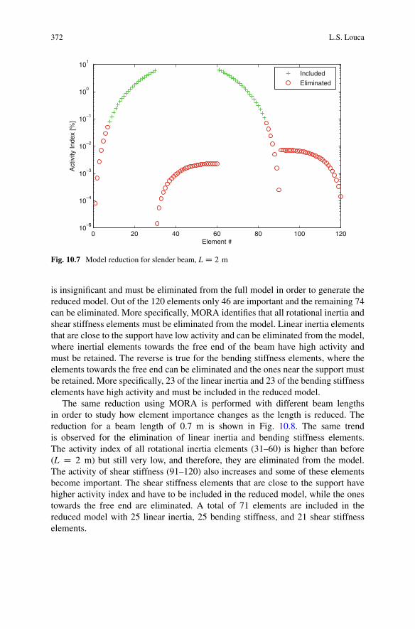
372 L.S. Louca
0 20 40 60 80 100 12010
−55
10−4
10−3
10−2
10−1
100
101
Element #
Act
ivity
Inde
x [%
]Included
Eliminated
Fig. 10.7 Model reduction for slender beam, L D 2 m
is insignificant and must be eliminated from the full model in order to generate thereduced model. Out of the 120 elements only 46 are important and the remaining 74can be eliminated. More specifically, MORA identifies that all rotational inertia andshear stiffness elements must be eliminated from the model. Linear inertia elementsthat are close to the support have low activity and can be eliminated from the model,where inertial elements towards the free end of the beam have high activity andmust be retained. The reverse is true for the bending stiffness elements, where theelements towards the free end can be eliminated and the ones near the support mustbe retained. More specifically, 23 of the linear inertia and 23 of the bending stiffnesselements have high activity and must be included in the reduced model.
The same reduction using MORA is performed with different beam lengthsin order to study how element importance changes as the length is reduced. Thereduction for a beam length of 0.7 m is shown in Fig. 10.8. The same trendis observed for the elimination of linear inertia and bending stiffness elements.The activity index of all rotational inertia elements (31–60) is higher than before(L D 2 m) but still very low, and therefore, they are eliminated from the model.The activity of shear stiffness (91–120) also increases and some of these elementsbecome important. The shear stiffness elements that are close to the support havehigher activity index and have to be included in the reduced model, while the onestowards the free end are eliminated. A total of 71 elements are included in thereduced model with 25 linear inertia, 25 bending stiffness, and 21 shear stiffnesselements.

10 Model Complexity of Distributed Parameter Systems: An Energy-Based Approach 373
0 20 40 60 80 100 12010
−4
10−3
10−2
10−1
100
101
Element #
Act
ivity
Inde
x [%
].
Included
Eliminated
Fig. 10.8 Model reduction for L D 0:7 m
0 20 40 60 80 100 12010
−4
10−3
10−2
10−1
100
101
Element #
Act
ivity
Inde
x [%
]
.
Included
Eliminated
Fig. 10.9 Model reduction for L D 0:2 m
The beam length is further reduced to 0.2 m in order to examine if more elementsbecome important. The activity index of the linear inertia and bending stiffnessremains almost unchanged as shown in Fig. 10.9. However, the activity index ofthe rotational inertia and shear stiffness is further increased such that some of therotational inertia elements also become important. More specifically the rotational

374 L.S. Louca
0.2 0.4 0.6 0.8 1 1.2 1.4 1.6 1.8 20
10
20
30
40
50
60
70
80
90
100
Beam length [m]
Incl
uded
Ene
rgy
Ele
men
t [#]
Totalm
i
Ii
ci
csi
Fig. 10.10 Model reduction for length variation
inertia elements that are towards the free end are important and the ones near thefixed end are eliminated. A total of 96 elements out of 120 are included in thereduced model with 24 linear inertia, 21 rotational inertia, 24 bending stiffness,and 27 shear stiffness elements.
The variation of beam length showed that the total number of important elementsincreases as the beam length decreases. This variation is investigated in moredetail by varying the beam length from 0.2 to 2 m with a step of 20 mm. Thenumber of included linear and rotational inertia, and bending and shear stiffnessis recorded along with the total number of elements. The results of this analysis areshown in Fig. 10.10. The total number of elements is monotonically increasing asthe beam length is decreased. The number of linear inertia and bending stiffnessremains almost constant as the length changes. On the contrary, the number of shearstiffness elements is zero until about 1.2 m where it becomes important and startsincreasing. Further reduction in length results in a monotonic increase in the numberof included shear stiffness element. A similar behavior is observed for the numberof the rotational inertia elements; however, they become important at a lower beamlength of about 0.6 m.
The validity of the generated reduced models is verified by analyzing theaccuracy of the model. Specifically the steady state response amplitude for thevelocity at the free end and the torque at the fixed end are calculated. Thecomparison is made with the corresponding response of the full model and overthe range of beam lengths used before. The accuracy for both variables, as shownin Fig. 10.11, varies as the beam length is changed, with averages around 91.5 %.The discrete variation in accuracy is due to the change of model complexity asdifferent elements are added or removed in the reduced model according to theactivity metric.
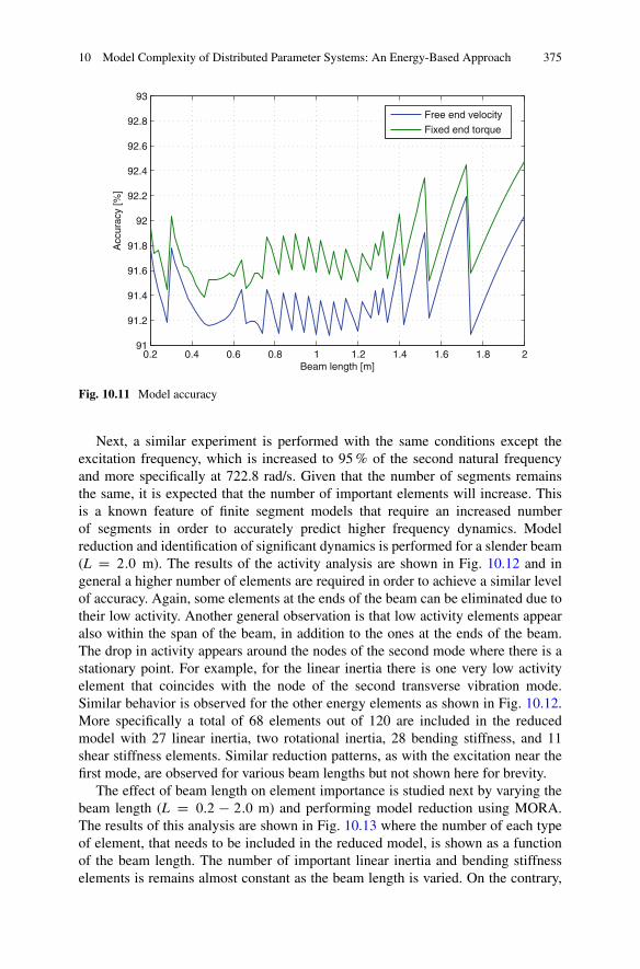
10 Model Complexity of Distributed Parameter Systems: An Energy-Based Approach 375
0.2 0.4 0.6 0.8 1 1.2 1.4 1.6 1.8 291
91.2
91.4
91.6
91.8
92
92.2
92.4
92.6
92.8
93
Beam length [m]
Acc
urac
y [%
]Free end velocity
Fixed end torque
Fig. 10.11 Model accuracy
Next, a similar experiment is performed with the same conditions except theexcitation frequency, which is increased to 95 % of the second natural frequencyand more specifically at 722.8 rad/s. Given that the number of segments remainsthe same, it is expected that the number of important elements will increase. Thisis a known feature of finite segment models that require an increased numberof segments in order to accurately predict higher frequency dynamics. Modelreduction and identification of significant dynamics is performed for a slender beam(L D 2:0 m). The results of the activity analysis are shown in Fig. 10.12 and ingeneral a higher number of elements are required in order to achieve a similar levelof accuracy. Again, some elements at the ends of the beam can be eliminated due totheir low activity. Another general observation is that low activity elements appearalso within the span of the beam, in addition to the ones at the ends of the beam.The drop in activity appears around the nodes of the second mode where there is astationary point. For example, for the linear inertia there is one very low activityelement that coincides with the node of the second transverse vibration mode.Similar behavior is observed for the other energy elements as shown in Fig. 10.12.More specifically a total of 68 elements out of 120 are included in the reducedmodel with 27 linear inertia, two rotational inertia, 28 bending stiffness, and 11shear stiffness elements. Similar reduction patterns, as with the excitation near thefirst mode, are observed for various beam lengths but not shown here for brevity.
The effect of beam length on element importance is studied next by varying thebeam length (L D 0:2 � 2:0 m) and performing model reduction using MORA.The results of this analysis are shown in Fig. 10.13 where the number of each typeof element, that needs to be included in the reduced model, is shown as a functionof the beam length. The number of important linear inertia and bending stiffnesselements is remains almost constant as the beam length is varied. On the contrary,
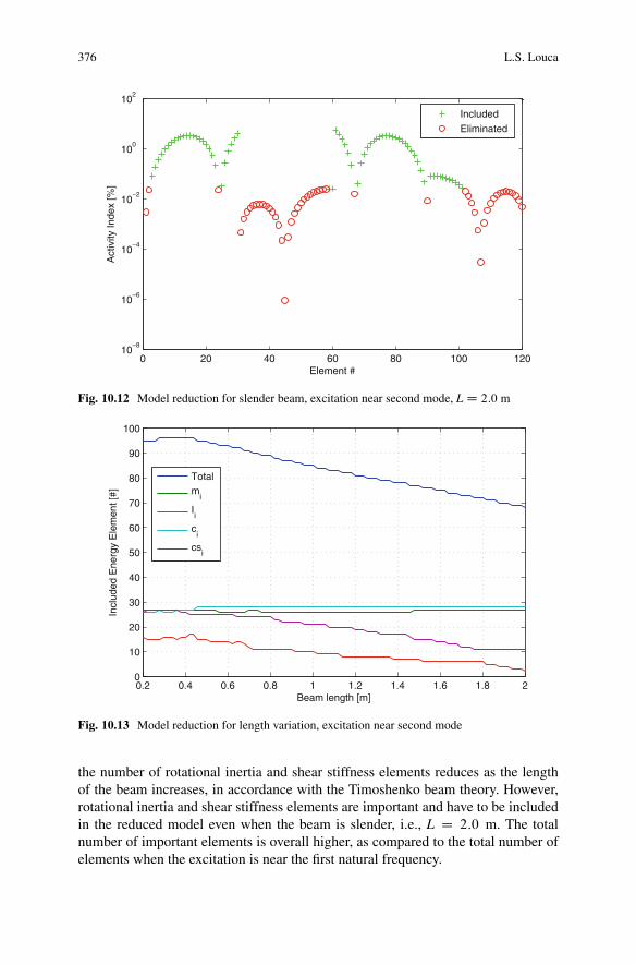
376 L.S. Louca
0 20 40 60 80 100 12010
−8
10−6
10−4
10−2
100
102
Element #
Act
ivity
Inde
x [%
]-
Included
Eliminated
Fig. 10.12 Model reduction for slender beam, excitation near second mode, L D 2:0 m
0.2 0.4 0.6 0.8 1 1.2 1.4 1.6 1.8 20
10
20
30
40
50
60
70
80
90
100
Beam length [m]
Incl
uded
Ene
rgy
Ele
men
t [#]
Totalm
i
Ii
ci
csi
Fig. 10.13 Model reduction for length variation, excitation near second mode
the number of rotational inertia and shear stiffness elements reduces as the lengthof the beam increases, in accordance with the Timoshenko beam theory. However,rotational inertia and shear stiffness elements are important and have to be includedin the reduced model even when the beam is slender, i.e., L D 2:0 m. The totalnumber of important elements is overall higher, as compared to the total number ofelements when the excitation is near the first natural frequency.
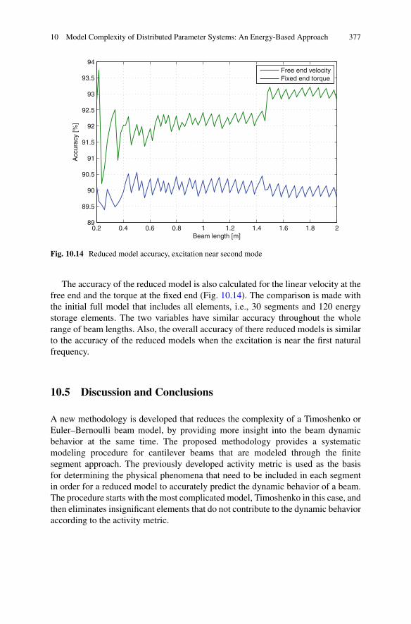
10 Model Complexity of Distributed Parameter Systems: An Energy-Based Approach 377
0.2 0.4 0.6 0.8 1 1.2 1.4 1.6 1.8 289
89.5
90
90.5
91
91.5
92
92.5
93
93.5
94
Beam length [m]
Acc
urac
y [%
]Free end velocityFixed end torque
Fig. 10.14 Reduced model accuracy, excitation near second mode
The accuracy of the reduced model is also calculated for the linear velocity at thefree end and the torque at the fixed end (Fig. 10.14). The comparison is made withthe initial full model that includes all elements, i.e., 30 segments and 120 energystorage elements. The two variables have similar accuracy throughout the wholerange of beam lengths. Also, the overall accuracy of there reduced models is similarto the accuracy of the reduced models when the excitation is near the first naturalfrequency.
10.5 Discussion and Conclusions
A new methodology is developed that reduces the complexity of a Timoshenko orEuler–Bernoulli beam model, by providing more insight into the beam dynamicbehavior at the same time. The proposed methodology provides a systematicmodeling procedure for cantilever beams that are modeled through the finitesegment approach. The previously developed activity metric is used as the basisfor determining the physical phenomena that need to be included in each segmentin order for a reduced model to accurately predict the dynamic behavior of a beam.The procedure starts with the most complicated model, Timoshenko in this case, andthen eliminates insignificant elements that do not contribute to the dynamic behavioraccording to the activity metric.
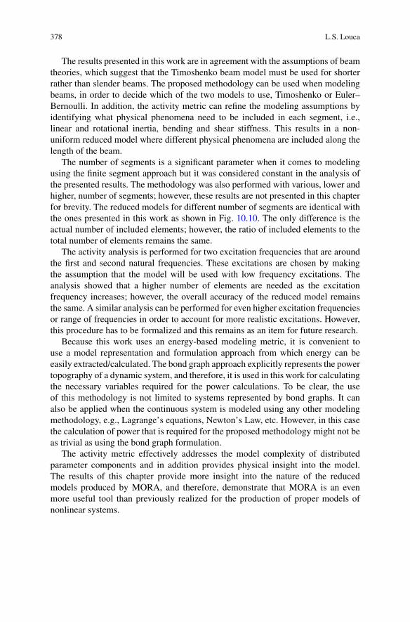
378 L.S. Louca
The results presented in this work are in agreement with the assumptions of beamtheories, which suggest that the Timoshenko beam model must be used for shorterrather than slender beams. The proposed methodology can be used when modelingbeams, in order to decide which of the two models to use, Timoshenko or Euler–Bernoulli. In addition, the activity metric can refine the modeling assumptions byidentifying what physical phenomena need to be included in each segment, i.e.,linear and rotational inertia, bending and shear stiffness. This results in a non-uniform reduced model where different physical phenomena are included along thelength of the beam.
The number of segments is a significant parameter when it comes to modelingusing the finite segment approach but it was considered constant in the analysis ofthe presented results. The methodology was also performed with various, lower andhigher, number of segments; however, these results are not presented in this chapterfor brevity. The reduced models for different number of segments are identical withthe ones presented in this work as shown in Fig. 10.10. The only difference is theactual number of included elements; however, the ratio of included elements to thetotal number of elements remains the same.
The activity analysis is performed for two excitation frequencies that are aroundthe first and second natural frequencies. These excitations are chosen by makingthe assumption that the model will be used with low frequency excitations. Theanalysis showed that a higher number of elements are needed as the excitationfrequency increases; however, the overall accuracy of the reduced model remainsthe same. A similar analysis can be performed for even higher excitation frequenciesor range of frequencies in order to account for more realistic excitations. However,this procedure has to be formalized and this remains as an item for future research.
Because this work uses an energy-based modeling metric, it is convenient touse a model representation and formulation approach from which energy can beeasily extracted/calculated. The bond graph approach explicitly represents the powertopography of a dynamic system, and therefore, it is used in this work for calculatingthe necessary variables required for the power calculations. To be clear, the useof this methodology is not limited to systems represented by bond graphs. It canalso be applied when the continuous system is modeled using any other modelingmethodology, e.g., Lagrange’s equations, Newton’s Law, etc. However, in this casethe calculation of power that is required for the proposed methodology might not beas trivial as using the bond graph formulation.
The activity metric effectively addresses the model complexity of distributedparameter components and in addition provides physical insight into the model.The results of this chapter provide more insight into the nature of the reducedmodels produced by MORA, and therefore, demonstrate that MORA is an evenmore useful tool than previously realized for the production of proper models ofnonlinear systems.
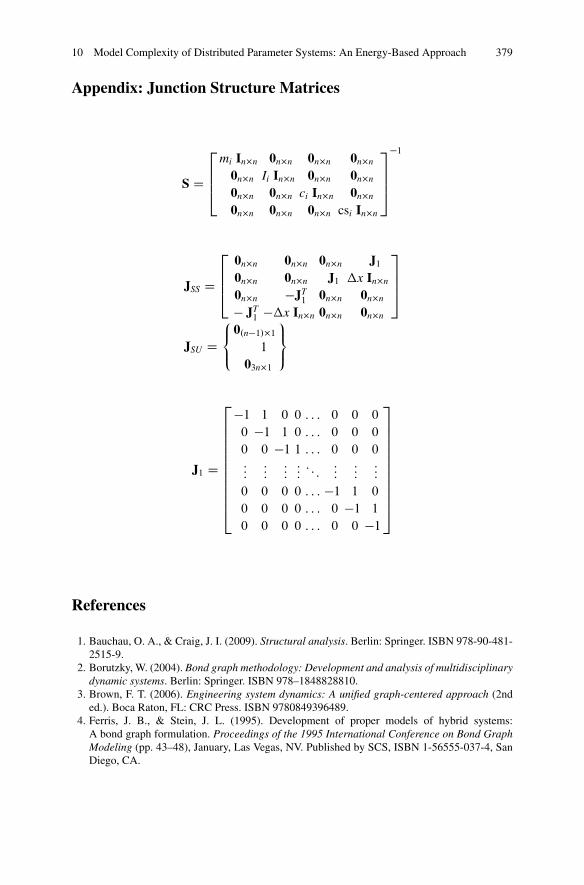
10 Model Complexity of Distributed Parameter Systems: An Energy-Based Approach 379
Appendix: Junction Structure Matrices
S D
2
664
mi In�n 0n�n 0n�n 0n�n
0n�n Ii In�n 0n�n 0n�n
0n�n 0n�n ci In�n 0n�n
0n�n 0n�n 0n�n csi In�n
3
775
�1
JSS D
2
664
0n�n 0n�n 0n�n J10n�n 0n�n J1 �x In�n
0n�n �JT1 0n�n 0n�n
� JT1 ��x In�n 0n�n 0n�n
3
775
JSU D8<
:
0.n�1/�11
03n�1
9=
;
J1 D
2
66666666664
�1 1 0 0 : : : 0 0 0
0 �1 1 0 : : : 0 0 0
0 0 �1 1 : : : 0 0 0:::
:::::::::: : :
::::::
:::
0 0 0 0 : : : �1 1 0
0 0 0 0 : : : 0 �1 1
0 0 0 0 : : : 0 0 �1
3
77777777775
References
1. Bauchau, O. A., & Craig, J. I. (2009). Structural analysis. Berlin: Springer. ISBN 978-90-481-2515-9.
2. Borutzky, W. (2004). Bond graph methodology: Development and analysis of multidisciplinarydynamic systems. Berlin: Springer. ISBN 978–1848828810.
3. Brown, F. T. (2006). Engineering system dynamics: A unified graph-centered approach (2nded.). Boca Raton, FL: CRC Press. ISBN 9780849396489.
4. Ferris, J. B., & Stein, J. L. (1995). Development of proper models of hybrid systems:A bond graph formulation. Proceedings of the 1995 International Conference on Bond GraphModeling (pp. 43–48), January, Las Vegas, NV. Published by SCS, ISBN 1-56555-037-4, SanDiego, CA.

380 L.S. Louca
5. Ferris, J. B., Stein, J. L., & Bernitsas, M. M. (1998). Development of proper models of hybridsystems. Transactions of the ASME, Journal of Dynamic Systems, Measurement, and Control,120(3), 328–333.
6. Genta, G. (2009). Vibration dynamics and control. Dordrecht: Springer. ISBN 978-0-387-79579-9.
7. Karnopp, D. C., Margolis, D. L., & Rosenberg, R. C. (2006). System dynamics: Modeling andsimulation of mechatronic systems (4th ed.). New York: Wiley. ISBN 978-0-471-70965-7.
8. Li, X. F. (2008). A unified approach for analyzing static and dynamic behaviors of functionallygraded Timoshenko and Euler–Bernoulli beams. Journal of Sound and Vibration, 318(4–5),1210–1229.
9. Li, D. F., & Gunter, E. J. (1981). Study of the modal truncation error in the component modeanalysis of a dual-rotor. Transactions of the ASME, Journal of Engineering for Gas Turbinesand Power, 104(3), 525–532.
10. Liu, D.-C., Chung, H.-L., & Chang, W.-M. (2000). Errors caused by modal truncation instructure dynamic analysis. Proceedings of the International Modal Analysis Conference—IMAC, v 2 (pp. 1455–1460). Bethel, CT: Published by Society for Experimental MechanicsInc., ISSN 1046–6770.
11. Louca, L. S. (2014). Complexity of distributed parameter bond graph models. Proceedings ofthe 11th International Conference on Bond Graph Modeling and Simulation—ICGBM’2012(pp. 789–797), Monterey, CA, USA. San Diego, CA: Published by the Society for ComputerSimulation International.
12. Louca, L. S. (2015). Finite segment model complexity of an Euler-Bernoulli beam. Proceed-ings of the 8th International Conference on Mathematical Modeling (pp. 334–340). Vienna,Austria: Published by the International Federation of Automatic Control-IFAC.
13. Louca, L. S., Rideout, D. G., Stein, J. L., & Hulbert, G. M. (2004). Generating proper dynamicmodels for truck mobility and handling. International Journal of Heavy Vehicle Systems(Special Issue on Advances in Ground Vehicle Simulation), 11(3/4), 209–236. Published byInderscience Enterprises Ltd., ISSN 1744�232X, St. Helier, United Kingdom.
14. Louca, L. S., & Stein, J. L. (2002). Ideal physical element representation from reducedbond graphs. Journal of Systems and Control Engineering, 216(1), 73–83. Published by theProfessional Engineering Publishing, ISSN 0959–6518, Suffolk, United Kingdom.
15. Louca, L. S., & Stein, J. L. (2009). Energy-based model reduction of linear systems.Proceedings of the 6th International Symposium on Mathematical Modeling, Vienna, Austria.Published in the series ARGESIM-Reports No. 35, ISBN 978-3-901608-35-3, Vienna, Austria.
16. Louca, L. S., Stein, J. L., Hulbert, G. M., & Sprague, J. K. (1997). Proper model generation: Anenergy-based methodology. Proceedings of the 1997 International Conference on Bond GraphModeling (pp. 44–49), Phoenix, AZ. Published by SCS, ISBN 1-56555-103-6, San Diego, CA.
17. Louca, L. S., Stein, J. L., & Hulbert, G. M. (2010). Energy-based model reduction methodologyfor automated modeling. Journal of Dynamic Systems Measurement and Control, 132(6),061202 (16 pages). Published by the American Society of Mechanical Engineers, ISSN Print0022–0434, ISSN Online 1528–9028, New York, NY.
18. Meirovitch, L. (1967). Analytical methods in vibrations. New York, NY: Macmillan PublishingInc.
19. Rideout, D. G., Stein, J. L., & Louca, L. S. (2007). Systematic identification of decouplingin dynamic system models. Journal of Dynamic Systems Measurement and Control, 129(4),503–513. Published by the American Society of Mechanical Engineers, ISSN Print 0022–0434,ISSN Online 1528–9028, New York, NY.
20. Rosenberg, R. C. (1971). State-space formulation for bond graph models of multiport systems.Transactions of the ASME, Journal of Dynamic Systems, Measurement, and Control, 93,36–40.
21. Rosenberg, R. C., & Karnopp, D. C. (1983). Introduction to physical system dynamics. NewYork: McGraw-Hill. ISBN 0070539057.
22. Stein, J. L., & Louca, L. S. (1996). A template-based modeling approach for systemdesign: Theory and implementation. Transactions of the Society for Computer SimulationInternational. San Diego, CA: Society for Computer Simulation International. Published bySCS, ISSN 0740-6797/96.

10 Model Complexity of Distributed Parameter Systems: An Energy-Based Approach 381
23. van Rensburg, N. F. J., & van der Merwe, A. J. (2006). Natural frequencies and modes of aTimoshenko beam. Wave Motion, 44(1), 58–69.
24. Walker, D. G., Stein, J. L., & Ulsoy, A. G. (1996). An input–output criterion for linear modeldeduction. Transactions of the ASME, Journal of Dynamic Systems, Measurement, and Control,122(3), 507–513.
25. Wilson, B. H., & Stein, J. L. (1995). An algorithm for obtaining proper models of distributedand discrete systems. Transactions of the ASME, Journal of Dynamic Systems, Measurement,and Control, 117(4), 534–540.

Part IVApplications
The chapters in Part IV demonstrate that bond graphs are well suited for modellingand analysis of a wide range of mechatronic systems that are of current interest andof importance in their field of application.
The first chapter in this part presents a multibond graph modelling and simulationcase study of a vibration absorber system in a helicopter. The subject is interestingand important from a practical, industrial as well as from a bond graph modellingpoint of view. Vibrations transmitted from the rotor to the fuselage affect the flight,the comfort of the crew and in the long run cause fatigue of the mechanical parts.In the helicopter considered in this study, a reduction of the transmitted vibrationsis achieved by a semi-active suspension system between the helicopter’s main gearbox and the fuselage that creates an anti-resonance effect.
From a modelling point of view, the considered vibration absorber system is ofinterest as it is a complex 3D-multibody system with 14 rigid bodies, 18 kinematicjoints of different type and four closed kinematic chains. For practitioners inindustrial projects it might be interesting to see that for a complex 3D-multibodysystem an overall BG model can be developed in a systematic and structuredapproach at a graphical level provided that BG library models have been developedfor a rigid body and various standard types of joints. BG modelling and simulationsoftware can automatically derive the equations of motion from a hierarchical BGof a complex mechatronic system and solve them numerically. It is well knownthat the way joints are modelled will have an effect on the form of the generatedmathematical model and on the problems that may occur with its numericalcomputation. These aspects are also addressed in Chap. 11 which is based on a PhDthesis of the first author that was supervised by the second and third author.
In an aging population there is an increasing demand for various types ofwheelchairs not only in hospitals and homes for the elderly but in general formobility disabled people to allow for independence. The case study in Chap. 12analyses how an auxiliary electric power system fitted to a manually operatedwheelchair can improve its mobility with regard to a given trajectory and time. Theoccupant of a wheelchair as well as an aid walking behind the chair will benefit

384 IV Applications
from a cost-effective design of a wheelchair equipped with an additional electricdrive module. That is, the subject of this study is a clearly relevant one and bondgraphs are well suited for modeling such a mechatronic system.
Chapter 12 presents the step-by-step development of a causal bond graph modelof the motorised wheelchair from which state-space equations are derived andnumerically computed by a block-diagram based simulation program. Subject ofthe simulation study is the accuracy of the motion along a prescribed trajectory andits speed.
The subject of Chap. 13 is also interesting and of great practical importance.The design of a miniaturised robot for in-vivo biopsy, its manufacturing and its testcan be considered a significant contribution to an improvement of minimal invasivetechniques in surgery that clearly offers a number of promising advantages suchas a reduction of patients’ discomfort and a facilitation of endoscopy tasks. Therobot considered in this chapter is a four degree-of-freedom, miniaturised externallycontrolled wire actuated in-vivo robot equipped with articulated links, a light sourceand a camera which may provide improved visibility and better maneuverability. Aforce sensor and a force control in conjunction with a trajectory control can helpavoid the damage of healthy tissue by limiting the interaction force between therobot’s tip and the tissue.
The robot is a tree-like multibody systems. Its study comprises the analysisof its forward kinematic, the development of a scalar bond graph, an inversekinematic analysis essential for placing the surgical robot tip at the desired pointof interest with minimum error, the design of a trajectory and a force control,and experiments for the validation of simulation results. The chapter is based ona recently successfully defended PhD thesis of the first author supervised by thesecond author.
Chapter 14 studies a completely different robot for a different application, abiologically inspired walking machine with four compliant legs meant to operateautonomously off-road in remote, hazardous rough terrain that is inaccessible towheeled mobile robots. As the studied robot has got legs, its locomotion requires acoordinated actuation of the legs to ensure a required gait pattern and to make surethat the robot moves along a given trajectory. Each of the four legs has got a hipjoint and a knee joint that must be operated in a coordinated way by controlling thejoint motors. The lower link of the legs is equipped with a spring to improve therobot’s locomotion. The practical importance of this application is also evident andbond graphs are well suited for modelling the controlled robot.
The research presented in Chap. 14 comprises the development of a threedimensional dynamic bond graph model, an experimental setup, a robot controlin workspace, a posture control, and strategies for sensor and actuator failures.Simulation experiments indicate that a robot with compliant legs performs moreenergy efficient in trot gait than a robot with rigid legs.
According to their task, mobile robots should be able to react to a failure inthe presence of limited or no hardware redundancy. As the robot is a legged one,two types of essential component failures are considered, namely a locked jointrestricting the workspace of a leg tip and a joint that does not react to the torque of

IV Applications 385
its motor. Chapter 14 is based on the PhD thesis of the first author supervised by thesecond author.
Renewable energy sources is another application area that is highly relevant andimportant from an ecological as well as from an economic point of view. Windturbines are complex controlled mechatronic systems composed of mechanicalcomponents such as the blades, a gear box, an induction motor, and a powerelectronic converter. The blades are to be considered distributed parameter systemswith aerodynamic wind forces acting on them. Chapter 15 studies a variable speedwind turbine with torque control and power control. The blades are consideredcantilever beams and are modelled by means of C fields and R fields. Simulationsof the dynamic behaviour of the overall systems carried out by means of the 20sim®
software consider a constant as well as a varying wind profile with real wind data. Amajor contribution of Chap. 14 is that the study of such a complex systems accountsfor all its components.
The last chapter in Part IV introduces the bond graph modelling of biomolecularsystems being part of living organisms. Some researchers have already used bondgraphs in the past for the modelling of chemical reactions. Their application tobiomolecular systems, however, is, to the Editors knowledge, still quite new. Asliving systems are neither at thermodynamic equilibrium nor closed, a bond graphapproach to the modelling of biomolecular systems is not evident. Therefore,Chap. 16 first recalls some thermodynamic basics, then introduces appropriatebond graph covariables, a nonlinear C storage element for representing molecularspecies and a non-linear R element for reactions. The chapter considers a numberof examples. Furthermore, causal analysis is used to examine the properties ofthe junction structure of the bond graphs set up for biomolecular systems. It isshown how causal properties of the BG junction structure are related to resultsof stoichiometric analysis of biomolecular systems. By this way, new insights areprovided into the dynamics of biomolecular systems.

Chapter 11Bond Graph Modeling and Simulationof a Vibration Absorber System in Helicopters
Benjamin Boudon, François Malburet, and Jean-Claude Carmona
Notation
Subscripts
i Relative to the i loop (i D 1 : : : 4)j Relative to the body j (j D MGB, SBi, MBi, F)MGB Relative to the body MGBSBi Relative to the body SARIB bar iMBi Relative to the body MGB bar iF Relative to the body fuselage
Mechanical Notation
Generality
��!MN
hVector associated with the bipoint (MN) expressed in the Rh frame
�!P pes!j
0
Weight vector of body j expressed in the inertial reference frame R0
B. Boudon (�)Aix-Marseille Université, CNRS, ISM UMR 7287,13288, Marseille Cedex 09, Francee-mail: [email protected]
F. Malburet • J.-C. CarmonaArts-et-Métiers ParisTech, CNRS, LSIS, 2 Cours des Arts-et-Métiers,13617, Aix-en-Provence, France
© Springer International Publishing Switzerland 2017W. Borutzky (ed.), Bond Graphs for Modelling, Control and FaultDiagnosis of Engineering Systems, DOI 10.1007/978-3-319-47434-2_11
387
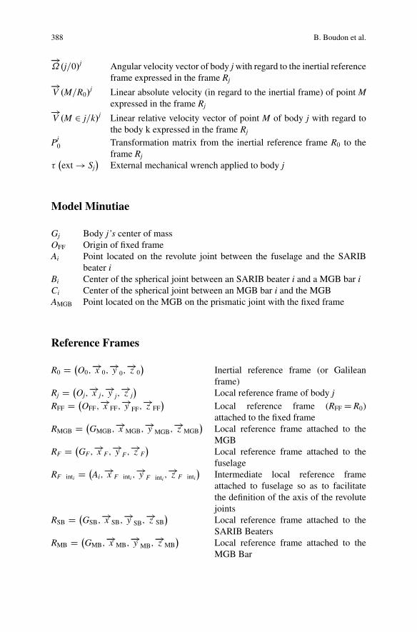
388 B. Boudon et al.
�!.j=0/j Angular velocity vector of body j with regard to the inertial reference
frame expressed in the frame Rj�!V .M=R0/
j Linear absolute velocity (in regard to the inertial frame) of point Mexpressed in the frame Rj�!
V .M 2 j=k/j Linear relative velocity vector of point M of body j with regard tothe body k expressed in the frame Rj
Pj0 Transformation matrix from the inertial reference frame R0 to the
frame Rj
��ext ! Sj
�External mechanical wrench applied to body j
Model Minutiae
Gj Body j’s center of massOFF Origin of fixed frameAi Point located on the revolute joint between the fuselage and the SARIB
beater iBi Center of the spherical joint between an SARIB beater i and a MGB bar iCi Center of the spherical joint between an MGB bar i and the MGBAMGB Point located on the MGB on the prismatic joint with the fixed frame
Reference Frames
R0 D �O0;
�!x 0;�!y 0;
�!z 0
�Inertial reference frame (or Galileanframe)
Rj D �Oj;
�!x j;�!y j;
�!z j�
Local reference frame of body j
RFF D �OFF;
�!x FF;�!y FF;
�!z FF�
Local reference frame (RFF D R0)attached to the fixed frame
RMGB D �GMGB;
�!x MGB;�!y MGB;
�!z MGB�
Local reference frame attached to theMGB
RF D �GF;
�!x F;�!y F;
�!z F�
Local reference frame attached to thefuselage
RF inti D �Ai;
�!x F inti ;�!y F inti ;
�!z F inti
�Intermediate local reference frameattached to fuselage so as to facilitatethe definition of the axis of the revolutejoints
RSB D �GSB;
�!x SB;�!y SB;
�!z SB�
Local reference frame attached to theSARIB Beaters
RMB D �GMB;
�!x MB;�!y MB;
�!z MB�
Local reference frame attached to theMGB Bar
11 Bond Graph Modeling and Simulation of a Vibration Absorber System. . . 389
Model Variables
xj, yj, zj Positional parameters of body j’s center of mass (m)˛j,ˇj, � j Angular parameters of the body j with regard to the inertial reference
frame (rad)
Model Parameters
� Rotational velocity of the main rotor (rad.s�1)b Number of rotor’s blades (adim)mj Body j’s mass (kg)IGj Body j’s Inertia matrix (kg m2)
11.1 Introduction
In the 1990s, thanks to the multibond graph formalism (an extension of bondgraphs where the scalar power bonds become vectors bonds and the elementsmultiports), the bond graph was extended to the study of multibody systemswith three dimensions [7, 29]. Nevertheless, few complex multibody systems withkinematic closed loops have been simulated. In the last 20 years, computer scienceand software dedicated to bond graphs such as 20-sim software have progressedconsiderably and contributed greatly to the development of bond graphs [1]. First,the graphical aspect of bond graphs can be fully exploited. Indeed, friendly envi-ronments enable the entering, modifying, or interpreting of bond graphs. Secondly,the automatic generation of equations from a bond graph enables engineers toavoid solving equations. Consequently, this step is less cumbersome and prone toerrors. Moreover, the simulation software mentioned is now equipped with efficientnumerical solvers.
This chapter presents a bond graph model and the associated simulations of acomplex multibody system: a vibration absorber system in helicopters. The systemmodel is a complex multibody system (according to the definitions given in [28])because of the numerous bodies and joints and the presence of several kinematicloops.
The operation of a helicopter’s rotor causes important vibration levels affecting,namely the flight handling, the fatigue of the mechanical parts, and the crew’scomfort. The considered vibrations created by the aerodynamic and inertia forcesacting on the rotor excite the main gearbox then the fuselage at a specific frequencyb˝ where b is the number of blades of the main rotor and ˝ the rotational velocityof the main rotor. Suspensions between the main gear box (MGB) and the fuselagehelp to filter these problematic vibrations. Different passive technical solutions exist
390 B. Boudon et al.
for the completion of this joint. The role of the studied vibration absorber system isto reduce the efforts transmitted from the rotor to the fuselage at the b˝ frequencyby creating an anti-resonance phenomenon. The principle of this system will bedescribed in Sect. 11.4.
The design and the analysis of such complex systems are usually conductedwith analytical methods based on physical equations or signal-flow methods basedon transfer functions written with block diagrams form. Unfortunately, these twoclassical approaches may cause a loss of the physical sense and the visibility of themodeling assumptions [2, 33]. Moreover, reusing models and taking into account theincreasing complexity can be cumbersome and prone to errors because of the needof manual transformations so as to build physics-based model libraries with blockdiagrams [33]. In this context, we present a bond graph (BG) approach [23] thatpermits a structural and modular approach of a complex mechatronic system. Thesewell-known features [5, 27]: graphic, object-oriented, multiphysic, and acausalcan be exploited for this class of multibody system with embedded electronics.Mainly with its graphical nature, the bond graph brings a more global view andcomprehension of complex mechatronic systems which lead to more sustainablesolutions. Based on oriented-object and acausal features, bond graphs also permita modular approach which allows a better knowledge capitalization to better storeand reuse your modeling works. Moreover, it would facilitate the automation of themodeling task.
The objective of this chapter is to model and simulate a helicopter’s vibrationabsorber system with bond graphs. Particular attention will be given in showing theinterest of the bond graph tool relative to more conventional tools.
This chapter is organized as follows. In Sect. 11.2, we review the modelingand simulation methods of multibody systems based on a bond graph approach.Section 11.3 is dedicated to the presentation of the vibration absorber system.Section 11.4 starts by describing the kinematic structure and the mechanicalassumptions retained for the suspension model. After, the modeling and simulationframework is applied and the construction of the bond graph model of the vibrationabsorber system detailed. Simulation results will be presented in Sect. 11.5. Finally,in the last section, the conclusion will be given.
11.2 BG Modeling and Simulation of Multibody Systems
11.2.1 Brief Review on the BG Modeling of Multibody Systems
The aim of this section is to recall the main contributors concerning methodologiesfor modeling the dynamics of three-dimensional multibody systems (MBS). Moredetailed reviews specifying applications of BG modeling for MBS can be found in[5, 13, 27].
11 Bond Graph Modeling and Simulation of a Vibration Absorber System. . . 391
The first bond graph models of multibody systems have been proposed by D.C.Karnopp and R.C. Rosenberg [16, 26], thanks to an analytical approach based on anappropriate choice of generalized coordinates, the construction of junction structurefor the formulation of the kinematic laws, and a Lagrangian formulation.
In the 1990s, thanks to the multibond graph (MBG) formalism [4, 9] (anextension of bond graphs where the scalar power bonds become vector bonds andthe elements multiports), the application fields of the bond graph were extended tothe study of multibody systems with three-dimensional movements.
The bond graph approach used for multibody systems was introduced by A. M.Bos [7, 29]. In his PhD, he developed bond graph models for three-dimensionalmultibody systems and discussed how to derive the equations of motion fromthe bond graph in several forms. At this time, although he managed to conductsimulations of a 3D motorcycle, the equations had been derived with a manualprocess.
Library models for a rigid body and for various types of joints have been providedin [34] so that bond graph models of rigid multibody systems can be assembled in asystematic manner.
Felez [14] developed a software that helps with modeling multibody systemsusing bond graphs. To handle derivative causalities with this software, he proposesa way to introduce Lagrange multipliers into the system so as to eliminate derivativecausality.
In [30, 31], different methods for simulating BG models have been presented.These simulations have been conducted with a predecessor of 20-sim software andnumerically compared between themselves mainly between the computing timeand accuracy. Even if the possibility of using multibond graphs was evocated,the difficulty of implementing bond graphs with vector bonds was not mentioned.This point will be detailed in Sect. 11.2.4.
11.2.2 Approach Chosen: The Tiernego and Bos Methodwith a 3D Model and Vector Bonds
Bond graph construction based on multibody dynamic equations can be establishedeither with the Newton–Euler equations or by using Lagrange equations. Dependingon the starting point, several bond graph construction methods have been devel-oped:
– the “Tiernego and Bos” method from the application of the Newton–Eulerequations,
– the “Karnopp and Rosenberg” method from the application of the Lagrangeequations.
In order to keep a modular approach, the more appropriated method for modelingmultibody systems with bond graphs is the Bos and Tiernego method [29].
392 B. Boudon et al.
This method enables a multibody system to be built in bond graphs as an assemblyof bodies and joints. The principle of this method is based on the use of absolutecoordinates systems and Newton–Euler equations. Indeed, in such a way, thedynamic equations of a rigid body depend on, obviously, its mass/inertia parametersand also on geometric parameters that are defined only for the considered body.The kinematic joints impose a set of constraints on the effort and flow vectors of thearticulation points involved in the assembly of two bodies so that the desired relativemotion can be achieved. Consequently, the dynamic equations of the completesystem consist of the dynamic equations of each body depending only on its ownparameters and the constraint equations of each joint.
From the authors’ point of view, a good approach, in the first preliminary designstage and still, in the frame of a modular approach, is to use in a more generalway: a 3D model and vector bonds so as to obtain a synthetic model. The useof vector bond graphs (also called multibond graphs) requires multibond graphelements (multibond or vector bond, junctions, multiport energy storage elements,multiport transformers, and gyrators) which are supposed to be known and directlyused in this paper. Readers can refer to [13] to find the details of the modeling ofthose elements.
11.2.3 Rigid Body Modeling
Let us remember the architecture of a rigid body multibond graph model based on[5, 7, 20, 22].
This bond graph architecture is based on the Newton–Euler equations (Eqs.(11.1) and (11.2)) with the inertia matrix (modeled with a multiport energy storeelement
�ISj;Gj
�j
in the upper part) associated with gyroscopic terms, respectively(modeled with a multiport gyrator element also called Eulerian Junction Structureabout mass-center of body j expressed in its frame
�EJSGj
�j
and the mass matrixmodeled with a multiport energy store element [mj]0 in the lower part).
X
h
�!F h!j
0 C �!P pes!j
0 D mjd
dt
�!V�Gj=R0
�0
0(11.1)
X
h
�!MG
j D �IGj
�j�
d
dt
�!.j=0/j
0
�j
C �!.j=0/j ^
�IGj
�j�!.j=0/j
(11.2)
The upper part of the bond graph represents the rotational dynamic part expressedin the body frame while the lower part is for the translational dynamic part expressedin the inertial reference frame (or Galilean frame). Notice that the power bondscorresponding to the rotational quantities are in purple while the power bondscorresponding to the translational quantities are in green. The two corresponding1-junctions arrays correspond, respectively, to the angular velocity vector of body
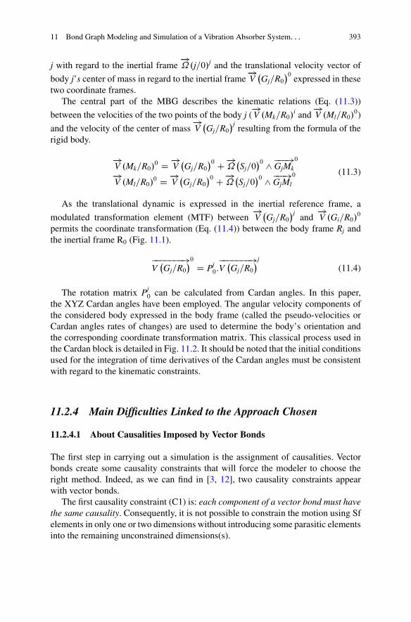
11 Bond Graph Modeling and Simulation of a Vibration Absorber System. . . 393
j with regard to the inertial frame�!.j=0/j and the translational velocity vector of
body j’s center of mass in regard to the inertial frame�!V�Gj=R0
�0expressed in these
two coordinate frames.The central part of the MBG describes the kinematic relations (Eq. (11.3))
between the velocities of the two points of the body j (�!V .Mk=R0/
i and�!V .Ml=R0/
0)
and the velocity of the center of mass�!V�Gj=R0
�jresulting from the formula of the
rigid body.
�!V .Mk=R0/
0 D �!V�Gj=R0
�0 C �!�Sj=0
�0 ^ ���!GjMk
0
�!V .Ml=R0/
0 D �!V�Gj=R0
�0 C �!�Sj=0
�0 ^ ���!GjMl
0 (11.3)
As the translational dynamic is expressed in the inertial reference frame, a
modulated transformation element (MTF) between�!V�Gj=R0
�jand
�!V .Gi=R0/
0
permits the coordinate transformation (Eq. (11.4)) between the body frame Rj andthe inertial frame R0 (Fig. 11.1).
�������!V�Gj=R0
�0 D Pj0:
�������!V�Gj=R0
�j
(11.4)
The rotation matrix Pj0 can be calculated from Cardan angles. In this paper,
the XYZ Cardan angles have been employed. The angular velocity components ofthe considered body expressed in the body frame (called the pseudo-velocities orCardan angles rates of changes) are used to determine the body’s orientation andthe corresponding coordinate transformation matrix. This classical process used inthe Cardan block is detailed in Fig. 11.2. It should be noted that the initial conditionsused for the integration of time derivatives of the Cardan angles must be consistentwith regard to the kinematic constraints.
11.2.4 Main Difficulties Linked to the Approach Chosen
11.2.4.1 About Causalities Imposed by Vector Bonds
The first step in carrying out a simulation is the assignment of causalities. Vectorbonds create some causality constraints that will force the modeler to choose theright method. Indeed, as we can find in [3, 12], two causality constraints appearwith vector bonds.
The first causality constraint (C1) is: each component of a vector bond must havethe same causality. Consequently, it is not possible to constrain the motion using Sfelements in only one or two dimensions without introducing some parasitic elementsinto the remaining unconstrained dimensions(s).
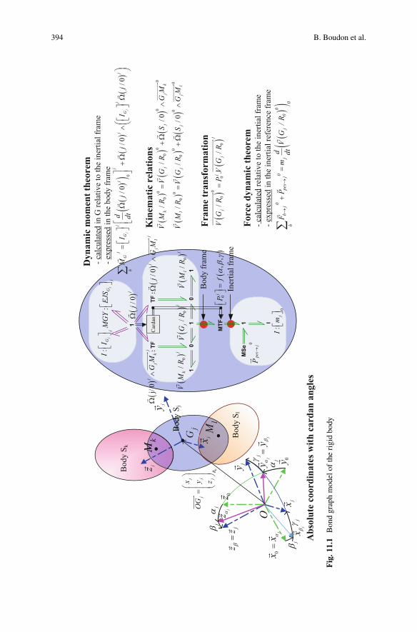
394 B. Boudon et al.
Fig
.11.
1B
ond
grap
hm
odel
ofth
eri
gid
body
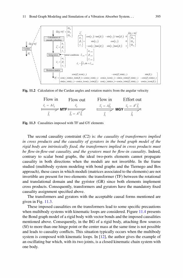
11 Bond Graph Modeling and Simulation of a Vibration Absorber System. . . 395
Initial conditions
( )j/ 0jx
jjy
jz
é ùWê ú
W = Wê úê úWë û
�
� ( ) ( ) ( ) ( )( ) ( )
( ) ( ) ( ) ( )
( )�/ 0/ / 0
cos 0
cos tan sin tan
sin
cos tan si 1n tan
jj
j jj jx
j j j jy
j jzj j
j j
j j
jb b
b b
eg ga
b g gg g g
Wé ùé ù é ùWê úê ú ê úê ú= Wê ú ê úê úê ú ê úWê úë û ë û
-
-ë û
��� ��
��
�j
j j
j
ae b
g
é ùê ú
= ê úê úë û
���� ��
�
j
j j
j
ae b
g
é ùê ú
= ê úê úë û
�jj j inidue e e= +ò�� ��
Calculation of pseudo-velocities
Intégration
Rotation matrix
0
cos( )cos( ) cos( )sin( ) sin( )cos( )sin( )sin( ) cos( )sin( ) cos( )cos( ) sin( )sin( )sin( ) cos( )sin( )sin( )sin( ) cos( )cos( )sin( ) cos( )sin( ) cos( )sin( )sin( ) c
j j j j j
j j j j j j j j j j j j
j j j j j j j j j j
jPb g b g b
g a b a g a g a b g b aa g a g b g a a b g
-+ - -
- +=
os( )cos( )j ja b
é ùê úê úê úë û
j ini
j ini j ini
j ini
a
e b
g
é ùê ú
= ê úê úê úë û
�
Cardan
0jP
( )j/ 0 jW�
Fig. 11.2 Calculation of the Cardan angles and rotation matrix from the angular velocity
1 2e Ae=� �
2e�
1f�
2 1Tf A f=
� �1 2e Af=
��2 1
Te A f=��
1f�
2f�MTF MGY
Fig. 11.3 Causalities imposed with TF and GY elements
The second causality constraint (C2) is: the causality of transformers impliedin cross products and the causality of gyrators in the bond graph model of therigid body are intrinsically fixed, the transformers implied in cross products mustbe flow-in-flow-out causality, and the gyrators must be flow-in causality. Indeed,contrary to scalar bond graphs, the ideal two-ports elements cannot propagatecausality in both directions when the moduli are not invertible. In the framestudied (multibody system modeling with bond graphs and the Tiernego and Bosapproach), these cases in which moduli (matrices associated to the elements) are notinvertible are present for two elements: the transformer (TF) between the rotationaland translational domain and the gyristor (GR) since both elements implementcross products. Consequently, transformers and gyrators have the mandatory fixedcausality assignment specified above.
The transformers and gyrators with the acceptable causal forms mentioned aregiven in Fig. 11.3.
These imposed causalities on the transformers lead to some specific precautionswhen multibody systems with kinematic loops are considered. Figure 11.4 presentsthe Bond graph model of a rigid body with vector bonds and the imposed causalitiesmentioned above. Consequently, in the BG of a rigid body, attaching flow sources(Sf) to more than one hinge point or the center mass at the same time is not possibleand leads to causality conflicts. This situation typically occurs when the multibodysystem is composed with kinematic loops. In [12], the author gives the example ofan oscillating bar which, with its two joints, is a closed kinematic chain system withone body.
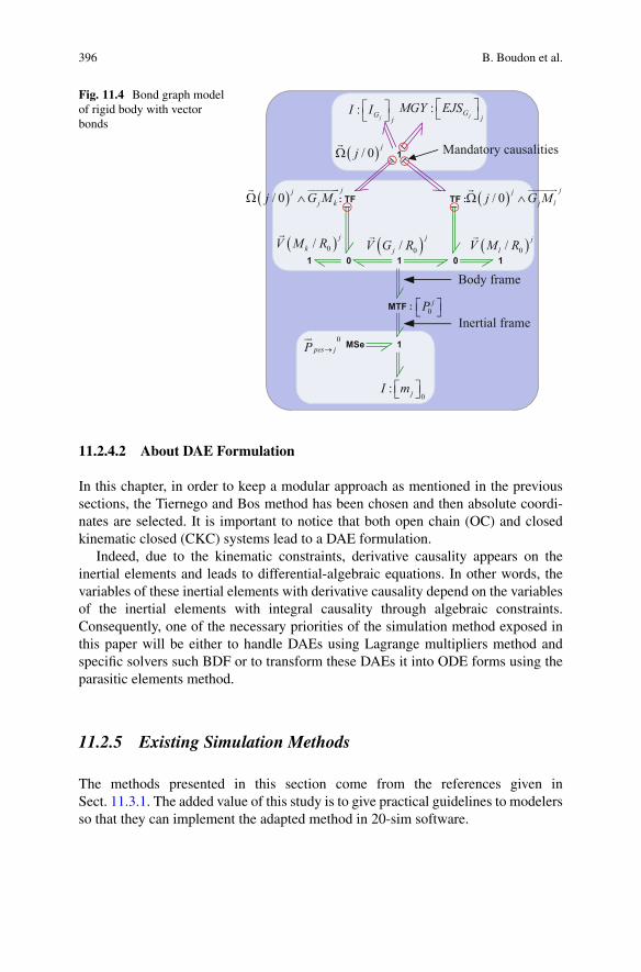
396 B. Boudon et al.
Fig. 11.4 Bond graph modelof rigid body with vectorbonds
0 0
1
: TF TF :
MSe
111
1
MTF :
:jG j
I Ié ùë û
:jG j
MGY EJSé ùë û
( )0/j
jV G R�
( )/ 0 jjW�
( )0/ jlV M R
�( )0/ jkV M R
�
( )/ 0jj
j lj G MW �������
( )/ 0jj
j kj G MW ��������
0jPé ùë û
0: jI mé ùë û
0pes jP ®
��Inertial frame
Body frame
Mandatory causalities
11.2.4.2 About DAE Formulation
In this chapter, in order to keep a modular approach as mentioned in the previoussections, the Tiernego and Bos method has been chosen and then absolute coordi-nates are selected. It is important to notice that both open chain (OC) and closedkinematic closed (CKC) systems lead to a DAE formulation.
Indeed, due to the kinematic constraints, derivative causality appears on theinertial elements and leads to differential-algebraic equations. In other words, thevariables of these inertial elements with derivative causality depend on the variablesof the inertial elements with integral causality through algebraic constraints.Consequently, one of the necessary priorities of the simulation method exposed inthis paper will be either to handle DAEs using Lagrange multipliers method andspecific solvers such BDF or to transform these DAEs it into ODE forms using theparasitic elements method.
11.2.5 Existing Simulation Methods
The methods presented in this section come from the references given inSect. 11.3.1. The added value of this study is to give practical guidelines to modelersso that they can implement the adapted method in 20-sim software.
11 Bond Graph Modeling and Simulation of a Vibration Absorber System. . . 397
11.2.5.1 ZCP Method
General Aspects
Bond graphs are composed of different types of causal paths. The closed causalpaths without integration operations are called zero-order causal paths (ZCP) [11,13, 25, 30]. The mathematical models with ZCPs lead to DAEs. There is a direct linkbetween the nature of the ZCPs in the bond graphs and the index of the DAE’s index.The definitions of ZCPs used are those presented in [13] and are the following:
Class 1 ZCPs: The causal path is set between storage ports with integral causalityand storage ports with differential causality. The associated topological loops areflat.
Class 2 ZCPs: The causal path is set between elements whose constitutive relationsare algebraic (resistors are the most typical case). The topological loops are flat.
Class 3 ZCPs: It is a causal cycle whose topological loops are open. The causal pathstarts and ends in the same port of an element.
Class 4 ZCPs: The Class-4 ZCPs are defined as causal cycles whose topologicalloops are closed.
Only Class 4 ZCPs lead to DAEs with an index of 2. When the DAE’s index isinferior to 2, a Backward Differentiation Formula (BDF) solver (such as the one in20-sim) can handle these equations. In some cases (scalar bonds or vector bondswith no kinematic loops), the simulation can thus be conducted without the additionof specific elements.
Pros
The advantages of the ZCP method are as follows. First, this method enablessimulations to be conducted directly from the model without requiring the additionof elements (R/C elements or controlled effort sources) at the correction location.The initial physical model is therefore not changed contrary to the R/C elements.Secondly, as we will see in Sect. 11.4, this method is faster than the two followingmethods (R/C elements and controlled effort sources).
Cons
When multibody systems with kinematic loops are modeled, the bond graph maycontain Class-4 ZCPs which lead to a DAE formulation with an index superior to 1and, then, the BDF solver often encounters difficulties in the numerical computationof the model. The ZCP opening method consists of opening the Class-4 ZCP, thanksto the use of break variables. This technique can be done at an equation level or ata graphical level. The classic technique is to add modulated sources (MSe) at 1-junctions of the Class-4 ZCPs so as to open them. Without a systematic approach to
398 B. Boudon et al.
the detection of the Class-4 ZCPs, this method may be difficult to use when dealingwith a case that involves complex multibody systems. This method was thus notused in this chapter in the case of multibody systems with kinematic loops.
11.2.5.2 R/C or Parasitic Elements
General Aspects
The R/C elements (or parasitic elements) method is based on the introduction of:compliances and resistances in the BG models of the joints. This method has beenused for a long time. It appeared for the first time with the denomination “Stiff-compliance” approach in [17]. In the literature, other’s terminologies can be foundfor this method: virtual springs [32] or also singular perturbation [35].
In the framework of this chapter (focused on the simulation of multibodysystems), this method can have two objectives: eliminating the kinematic constraintsand also consequently eliminating the derivative causality or algebraic loops so thatan explicit solver may be used. As we have previously mentioned (in Sect. 11.3.1.1),the nature of vector bond graphs imposes some supplementary causality constraints(C1 and C2). For the enforcement of these constraints, the flow sources (Sf)can lead to causal conflicts because of their flow-out causality. The enforcementof constraints with parasitic elements (R and C elements) can circumvent theseconstraints (C1 and C2) instead of flow sources (Sf), thanks to their effort-outcausalities. Firstly, it allows the preservation of the same causality assignments forall of the bonds of a multibond (C1 respected). Secondly, it allows the suppressionof the causality conflict which may appear because of the imposed causality of thetransformers implied in the cross product and gyrators (C2 respected).
Moreover, the use of R/C elements into joint models decouples the energy storeelements associated with the inertia of the rigid bodies. All these energy storeelements are then kept with integral causalities.
The values of the compliant elements must be chosen carefully. To our knowl-edge, two methods for selecting these elements exist: (1) the eigenvalues decouplingbetween the parasitic frequency and the system frequency, (2) the use of activitymetric [24]. These parameters can be chosen so as to model the joint complianceswhich exist in all mechanical joints. Thus, this point gives to this method a physicalsignificance. The stiffnesses introduced should be high enough so as not to changethe dynamic of the system but not too high so as to prevent the numerical difficultiesof stiff problems (with high-frequency dynamics). This method leads to a necessarycompromise between the accuracy of the results and the simulation time: the stifferthe system is, the more numerical errors are reduced but the more simulation timeremains important. However, the increase of the simulation time can be balancedby parallel processing as the mass matrix in a block-diagonal form can be used to
11 Bond Graph Modeling and Simulation of a Vibration Absorber System. . . 399
decouple the system as it is explained in [32]. As T. Rayman recommends, addinga damping element (R resistive element) in parallel with the stiff spring (C energystore element) enables the dampening of the high eigen frequency associated withthe high stiffness. The exact influence of these parameters still remains a topic ofresearch in which the authors are particularly interested in.
Pros
With the RC elements method, all the derivative causalities are removed. This leadsto an explicit ODE model which can be solved with a fixed step solver such asRunge Kutta 4.
Contrary to the Lagrange multipliers methods, some slight imprecisions could bemade on the initial conditions. Moreover, overconstrained (also called hyperstatic)systems can be simulated without any difficulties.
Cons
This method introduces new elements (R and C elements) in the initial bond graphwhose parameters and initial conditions associated with the C store elements needto be specified. The values of the compliant elements must be chosen carefully so asto model the joint compliances which exist in all mechanical joints. The stiffnessesthat are used should be high enough so as not to change the dynamics of the systemand should be able to sufficiently approximate the constraints. However, too highstiffnesses introduce numerical difficulties of stiff problems (with high-frequencydynamics). Indeed, these kinds of problems force the solvers to take very smallintegration steps to meet the tolerance criteria and, consequently, the simulation isslowed. This method leads to a necessary compromise between the accuracy of theresults and the simulation time: the stiffer the system is, the more numerical errorsare reduced but the more the simulation time remains important.
Implementation
Even if explicit solvers can be used, the authors recommended the use of the implicitModified Backward Differentiation Formula (MBDF) solver for two reasons. Thefirst reason is that the BDF solver guarantees the numerical stability of the solution.The second reason is that, with the controlled effort sources, only the MBDF solvercan be used. Also, using an MBDF solver with the R/C Elements is a good way tofacilitate comparison between R/C elements and controlled effort sources methods.
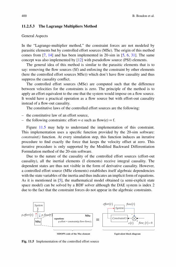
400 B. Boudon et al.
11.2.5.3 The Lagrange Multipliers Method
General Aspects
In the “Lagrange-multiplier method,” the constraint forces are not modeled byparasitic elements but by controlled effort sources (MSe). The origin of this methodcomes from [7, 14] and has been implemented in 20-sim in [5, 6, 31]. The sameconcept was also implemented by [12] with pseudoflow source (PSf) elements.
The general idea of this method is similar to the parasitic elements that is tosay: removing the flow sources (Sf) and enforcing the constraint by other elements(here the controlled effort sources MSe)) which don’t have flow causality and thussuppress the causality conflict.
The controlled effort sources (MSe) are computed such that the differencebetween velocities for the constraints is zero. The principle of the method is toapply an effort equivalent to the one that the system would impose on a flow source.It would have a practical operation as a flow source but with effort-out causalityinstead of a flow-out causality.
The constitutive laws of the controlled effort sources are the following:
– the constitutive law of an effort source,– the following constraints: effort D e such as flow(e) D f.
Figure 11.5 may help to understand the implementation of this constraint.This implementation uses a specific function provided by the 20-sim software:constraint() function. At every simulation step, this function induces an iterativeprocedure to find exactly the force that keeps the velocity offset at zero. Thisiterative procedure is only supported by the Modified Backward DifferentiationFormulation method of the 20-sim software.
Due to the nature of the causality of the controlled effort sources (effort-outcausality), all the inertial elements (I elements) receive integral causality. Thedependent states are thus not visible in the form of derivative causality. However,a controlled effort source (MSe elements) establishes itself algebraic dependencieswith the state variables of the inertia and thus indicates an implicit form of equations.As it is mentioned in [5], the mathematical model obtained (a semi-explicit statespace model) can be solved by a BDF solver although the DAE system is index 2due to the fact that the constraint forces do not appear in the algebraic constraints.
System( )flow t
+
-
( ) 0=cflow t( )e t
( )effort t
Constraint()MSe
MSe
1
( )p.effort t ( )p.flow t
System
equationsp.effort = constraint(p.flow-flowc); º
SIDOPS code of the Mse element Equivalent block diagram
Fig. 11.5 Implementation of the controlled effort source
11 Bond Graph Modeling and Simulation of a Vibration Absorber System. . . 401
Pros
Contrary to the parasitic elements method, the modulated sources (MSe) don’t needadditional tuning because no additional parameters are added to the system. Inother words, the order of the system is not modified because no new states (withassociated parameters and initial conditions) are introduced. Moreover, the absenceof supplementary parameters makes a bond graph that describes the system ideallyin the limit of the numerical tolerance on the constraints equations.
Even if, during the simulation, iterations are required at each time step tosatisfy the constraint equations, the computational load is comparable or better incomparison to the parasitic elements method where the differential equations aretruly explicit but very stiff.
Cons
The bond graph obtained with this approach leads to implicit differential equations,so explicit integration algorithms cannot be used. Moreover, during the simulationthe constraints can only be met within some numerical tolerances.
Consequently, the implementation of this method requires special care, which isdescribed hereafter.
Implementation
The Lagrange multipliers method is more difficult to implement than the useof RC elements because the kinematic constraints imposed by the joints mayproduce computational conflicts. This issue occurs on closed kinematic chainswith overconstrained multibody systems. Due to the topology of the system, morethan one joint could impose the same constraint on the system, in which case thesimulation will no longer be possible. In other ways, more practically, the numberof the controlled effort sources must not exceed the degrees of freedom that needto be eliminated. In order to solve this problem, the redundant constraints must beremoved.
In addition, there may be the inconsistent initial conditions. Indeed, initialconditions of the system should be consistent with constraints. If a controlledeffort source is attached to a 1-junction to keep the velocity at zero and a non-zero initial velocity to the I element connected to the same 1-junction is imposed,then a simulation cannot be conducted. We can notice at this point that 20-simdoes not offer an automatic correction of inconsistent initial conditions but, a BGmodeler can always code the calculation of consistent initial conditions to handle itautomatically.
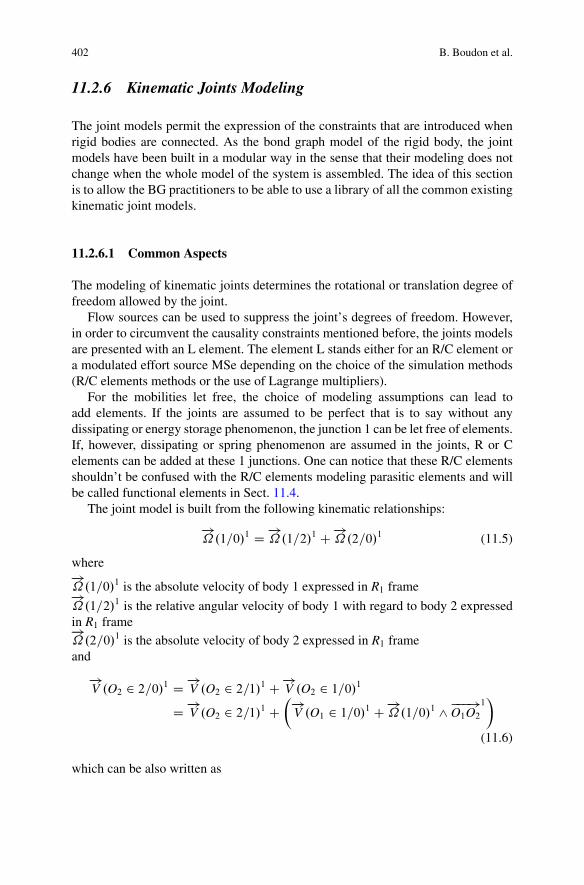
402 B. Boudon et al.
11.2.6 Kinematic Joints Modeling
The joint models permit the expression of the constraints that are introduced whenrigid bodies are connected. As the bond graph model of the rigid body, the jointmodels have been built in a modular way in the sense that their modeling does notchange when the whole model of the system is assembled. The idea of this sectionis to allow the BG practitioners to be able to use a library of all the common existingkinematic joint models.
11.2.6.1 Common Aspects
The modeling of kinematic joints determines the rotational or translation degree offreedom allowed by the joint.
Flow sources can be used to suppress the joint’s degrees of freedom. However,in order to circumvent the causality constraints mentioned before, the joints modelsare presented with an L element. The element L stands either for an R/C element ora modulated effort source MSe depending on the choice of the simulation methods(R/C elements methods or the use of Lagrange multipliers).
For the mobilities let free, the choice of modeling assumptions can lead toadd elements. If the joints are assumed to be perfect that is to say without anydissipating or energy storage phenomenon, the junction 1 can be let free of elements.If, however, dissipating or spring phenomenon are assumed in the joints, R or Celements can be added at these 1 junctions. One can notice that these R/C elementsshouldn’t be confused with the R/C elements modeling parasitic elements and willbe called functional elements in Sect. 11.4.
The joint model is built from the following kinematic relationships:
�!.1=0/1 D �!
.1=2/1 C �!.2=0/1 (11.5)
where�!.1=0/1 is the absolute velocity of body 1 expressed in R1 frame�!.1=2/1 is the relative angular velocity of body 1 with regard to body 2 expressed
in R1 frame�!.2=0/1 is the absolute velocity of body 2 expressed in R1 frame
and
�!V .O2 2 2=0/1 D �!
V .O2 2 2=1/1 C �!V .O2 2 1=0/1
D �!V .O2 2 2=1/1 C
��!V .O1 2 1=0/1 C �!
.1=0/1 ^ ���!O1O2
1�
(11.6)
which can be also written as

11 Bond Graph Modeling and Simulation of a Vibration Absorber System. . . 403
Fig. 11.6 General kinematicjoint model
0
01
1
MTF
( )11 01 /V O R∈�
( )11 / 0Ω�
( )12 / 0Ω�
( ( ))12 02 /V O R∈ ∈�
( )00 2 11 / R O OΩ ∧
�������
( )12 2 /1V O ∈�
�
1
1
MTF
MTF
( )22 / 0Ω�
22 2 / 0V O
21P1
0P 20P
1
1
( )12 /1Ω�
1
�!V .O2=0/
1 D �!V .O2 2 2=1/1 C
��!V .O1=0/
1 C �!.1=0/1 ^ ���!
O1O2
1�
(11.7)
where�!V .O2=0/
1 is the absolute velocity of point O2�!V .O2=0/
1 is the absolute velocity of point O1�!V .O2 2 2=1/1 is the relative velocity of point O2 with regard to the frame R1�!.1=0/1 ^ ���!
O1O2
1
is the velocity component due to the rotation of frame R1 withregard to the inertial reference frame
The general kinematic joint model is then detailed in Fig. 11.6.In the general kinematic joint model, MTF elements modulated by coordinate
transformation matrix are used so as to express the kinematic quantities in theappropriate frame associated with the body where they are connected to.
11.2.6.2 Joint Models
Based on the general kinematic joint model, the models of the common kinematicsjoints are given in Figs. 11.7, 11.8, and 11.9.
11.3 Presentation of the Vibration Absorber System
11.3.1 Context
The rotor of a helicopter can generate various vibration phenomena. Let usconsider:
– forced vibrations,
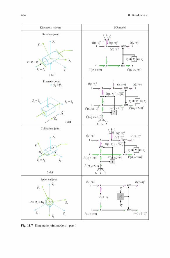
404 B. Boudon et al.
L
MTF
MTF0
0
L
BG modelKinematic scheme
Revolute joint
Prismatic joint
Cylindrical joint
Spherical joint
( )12 / 0Ω�
( )11 / 0Ω�
( )22 / 0Ω�
( )12 /1Ω�
21P1
0P 20P
0
0
21
1
1
MTF
( )11 1 / 0V O ∈�
( )11 / 0V O ∈�
( )22 / 0V O ∈�
( )11 / 0Ω�
( )12 / 0Ω�
( )12 2 / 0V O ∈� ( )22 2 / 0V O ∈
�
( ) 110 2 11 / R O OΩ ∧
�������
( )12 2 /1V O ∈�
1
1
L
L
( )11 / 0Ω�
( )11 / 0V O∈�
( )22 / 0Ω�
( )22 / 0V O∈�
12P( )12 /1Ω
�
MTF
MTF
1
0
01 1
1 1
10P
20P
L
1
11
1
MTF
MTF
( )22 / 0Ω�
21P1
0P 20P
1
1
LL
1
1
0
0
321
1
1
MTF
( )11 1 / 0V O ∈�
( )11 / 0Ω�
( )12 / 0Ω�
( )12 2 / 0V O ∈� ( )22 2 / 0V O ∈
�
( ) 110 2 11 / R O OΩ ∧
�������
( )12 2 /1V O ∈�
1
1
MTF
MTF
( )22 / 0Ω�
21P1
0P 20P
1
1
LL 1
1 2z z=� �
1y�
1x�
2x�
2y�
1x�
2x�
2y�
2z�1z
�
= =1 2O O O
1y�
3
21 3
1 2z z=� �
1y�
1x�
2x�
2y�
1O
2O
L
( )12 /1Ω�
L 121 3
1 2y y=� �
1 2z z=� �
1 2x x=� �
1O
2O
1 dof
1 dof
2 dof
= =1 2O O O
Fig. 11.7 Kinematic joint models—part 1
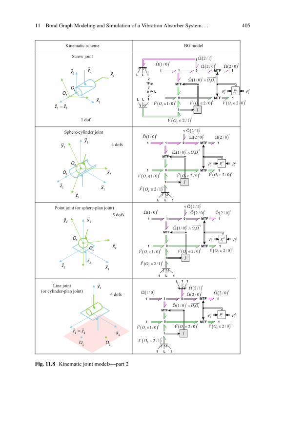
11 Bond Graph Modeling and Simulation of a Vibration Absorber System. . . 405
BG modelKinematic scheme
Screw joint
Sphere-cylinder joint
Point joint (or sphere-plan joint)
Line joint(or cylinder-plan joint)
0
0
21
1
1
MTF
( )11 1 / 0V O ∈�
( )11 / 0Ω�
( )12 / 0Ω�
( )12 2 / 0V O ∈� ( )22 2 / 0V O ∈
�
( ) 112 11 / 0 O OΩ ∧�������
( )12 2 /1V O ∈�
1
1
MTF
MTF
( )22 / 0Ω�
21P1
0P 20P
1
1
LL 13
0
0
32
1
1
1
MTF
( )11 1 / 0V O ∈�
( )11 / 0Ω�
( )12 / 0Ω�
( )12 2 / 0V O ∈�
( )22 2 / 0V O ∈�
( ) 112 11 / 0 O OΩ ∧�������
( )12 2 /1V O ∈�
1
0
MTF
MTF
( )22 / 0Ω�
21P1
0P 20P
1
1LL 1
L
( )12 /1Ω�
L 121 3
1y�
2x�
2y�
1x�
2z�
1z�
1O2O
1 2z z=� �
1y�
1x�
2x�
2y�
1O2O
L
TF:p
1
1x�
2x�
2y�
2z�
1z�
1y�
1O
2O
1 2z z=� �
1y�
1x�
1O 2O
( )12 /1Ω�
1
0
0
21
1
1
MTF
( )11 1 / 0V O ∈�
( )11 / 0Ω�
( )12 / 0Ω�
( )12 2 / 0V O ∈� ( )22 2 / 0V O ∈
�
( ) 112 11 / 0 O OΩ ∧�������
1
1
MTF
MTF
( )22 / 0Ω�
21P1
0P 20P
1
1
L1 13
( )12 /1Ω�
1
0
0
321
1
1
MTF
( )11 1 / 0V O ∈�
( )11 / 0Ω�
( )12 / 0Ω�
( )12 2 / 0V O ∈�
( )22 2 / 0V O ∈�
( ) 112 11 / 0 O OΩ ∧�������
( )12 2 /1V O ∈�
1
1
MTF
MTF
( )22 / 0Ω�
21P1
0P 20P
1
1
L1 1
1
( )12 /1Ω�
L 121 3
1 dof
( )12 2 /1V O ∈�
4 dofs
5 dofs
4 dofs
Fig. 11.8 Kinematic joint models—part 2
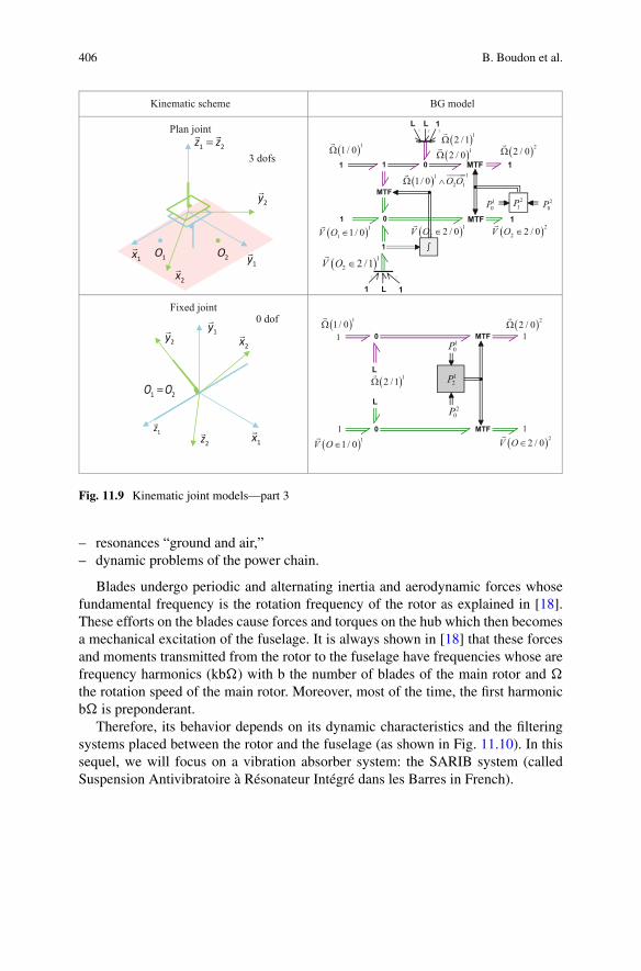
406 B. Boudon et al.
BG modelKinematic scheme
Plan joint
Fixed joint
0
0
321
1
1
MTF
( )11 1 / 0V O ∈�
( )11 / 0Ω�
( )12 / 0Ω�
( )12 2 / 0V O ∈�
( ) 112 11 / 0 O OΩ ∧�������
( )12 2 /1V O ∈�
1
1
MTF
MTF
( )22 / 0Ω�
21P1
0P 20P
1
1
L1 1
L
( )12 /1Ω�
L 121 3
1y�
1x�
1 2z z=� �
2x�
2y�
1O 2O
�1z
1y�
1x�
2x�
2y�
=1 2O O
�2z
( )11 / 0Ω�
( )11 / 0V O∈�
( )22 / 0Ω�
( )22 / 0V O∈�
12P( )12 /1Ω
�
MTF
MTF
0
01 1
1 1
10P
20P
L
L
( )22 2 / 0V O ∈
�
3 dofs
0 dof
Fig. 11.9 Kinematic joint models—part 3
– resonances “ground and air,”– dynamic problems of the power chain.
Blades undergo periodic and alternating inertia and aerodynamic forces whosefundamental frequency is the rotation frequency of the rotor as explained in [18].These efforts on the blades cause forces and torques on the hub which then becomesa mechanical excitation of the fuselage. It is always shown in [18] that these forcesand moments transmitted from the rotor to the fuselage have frequencies whose arefrequency harmonics (kb�) with b the number of blades of the main rotor and �the rotation speed of the main rotor. Moreover, most of the time, the first harmonicb� is preponderant.
Therefore, its behavior depends on its dynamic characteristics and the filteringsystems placed between the rotor and the fuselage (as shown in Fig. 11.10). In thissequel, we will focus on a vibration absorber system: the SARIB system (calledSuspension Antivibratoire à Résonateur Intégré dans les Barres in French).

11 Bond Graph Modeling and Simulation of a Vibration Absorber System. . . 407
Fig. 11.10 Helicopter suspension between the MGB and the aircraft structure
Fig. 11.11 (a) Flexible classical MGB-fuselage suspension, (b) MGB-fuselage suspension withSARIB system
11.3.2 Interest and Functions
The MGB-fuselage suspension must ensure several important functions. Firstly, thejoint allows the transmission of the static force necessary to the sustentation of thehelicopter with a limited static displacement. Moreover, the suspension helps toreduce the mechanical vibrations transmitted to the fuselage according to the forceand displacement aspects. In this paper, we will focus on this latter function.
11.3.3 Operating Principle
The classical MGB-fuselage suspension is composed of four MGB bars and amain membrane as shown in Fig. 11.11a. The MGB bars can rigidly suspend thefuselage without flexibility to the rotor and thus transmit the lift from the rotor tothe structure.
The membrane is a flexible suspension with the following observed behavior:
– a low stiffness for angular movements around the roll and pitch axes and thelinear vertical pumping displacement,
– a very high stiffness for linear movements perpendicular to the vertical directionand for the yaw movement.

408 B. Boudon et al.
Thus, the membrane allows the angular movement of the MGB around the pitchand roll axes. The flexibility of the membrane around these axes allows a strongfiltration of the dynamic moments around these axes. In addition, the membranetransmits the main rotor torque, thanks to its very high stiffness around the yaw axis.In conclusion, the conventional suspensions allow filtering pitch and roll dynamicmoments without filtering the pumping dynamic efforts.
The suspension equipped with SARIB system is a tuned-mass vibration absorber.Its purpose is to render the filtering of these pumping dynamic efforts possible. Onthe SARIB solution, beaters with flapping masses are added between the MGB barsand the fuselage (Fig. 11.11b). They permit a vertical degree of freedom to theMGB with regard to the fuselage. The principle of the SARIB system is to tune, foran accurate defined frequency, these flapping masses on each SARIB bar so as tocreate inertial forces on the fuselage opposite to the force of the MGB bars on thebeaters. Moreover, the specificity of the SARIB system among the class of tuned-mass absorbers comes from the fact that a rotating SARIB bar works as a mechanicalgear ratio that makes the resonating flapping mass appear larger. More details on thisoperating principle are given in [15] through the equilibrium of an SARIB bar. Inother words, there is an anti-resonance phenomenon on the transmissibility functionbetween the excitation applied to the MGB. Hence, the forces transmitted to thefuselage can be strongly reduced at this anti-resonance frequency.
11.3.4 Use of the Experimental Setup
To analyze the simulation results, an experimental setup on a small scale has beenused. The geometry and mass properties correspond to a light helicopter with a scaleof approximately ½. The model proposed in this chapter has been simulated with thenumerical data of this experimental setup detailed in [8].
The experimental setup has to represent the flight behavior of the helicopter indifferent operating phases: hover, up/down, or turn. In these operating phases, theMGB is subjected to pumping, pitch, and roll excitements. On the experimentalsetup, the rotor action, provided by the aerodynamic forces and the blades stiffness,applied to the MGB will be approximated by a sinusoidal excitation at the frequencyb� obtained with a vibration equipment. The experimental setup was performed bymaintaining the architecture of a real device (Fig. 11.12).
The correspondence between the different mechanical elements of a helicopterand the experimental setup will be detailed hereafter.
To reproduce the effects of the rotor lift, the set fBTP-link-fuselageg has beensuspended from the fixed frame (Fig. 11.12). This joint has to lift up the entireweight suspended by analogy to the static force of lift, it was performed by theuse of pneumatic components. They were designed so that the natural frequencyinduced by the overall stiffness is below 2 Hz.
The fuselage was replaced by a rigid mass called fuselage mass (Fig. 11.12).
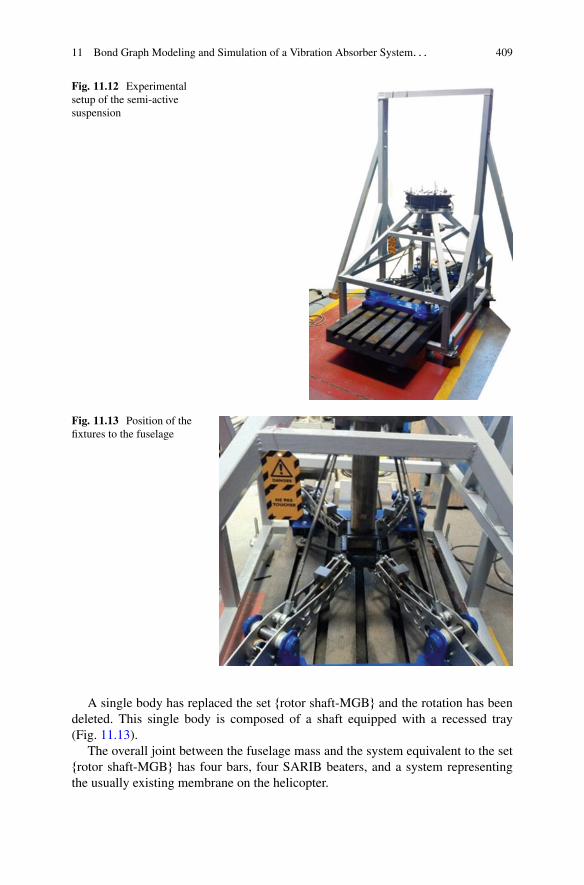
11 Bond Graph Modeling and Simulation of a Vibration Absorber System. . . 409
Fig. 11.12 Experimentalsetup of the semi-activesuspension
Fig. 11.13 Position of thefixtures to the fuselage
A single body has replaced the set frotor shaft-MGBg and the rotation has beendeleted. This single body is composed of a shaft equipped with a recessed tray(Fig. 11.13).
The overall joint between the fuselage mass and the system equivalent to the setfrotor shaft-MGBg has four bars, four SARIB beaters, and a system representingthe usually existing membrane on the helicopter.

410 B. Boudon et al.
Fig. 11.14 Revolute jointbetween an SARIB beaterand the fuselage
The MGB bars consist of threaded rods that have a spherical joint withoutbacklash at each end.
Each SARIB beater is linked by a revolute joint to the fuselage, which arethemselves clamped to the fuselage mass as shown in Fig. 11.13. Each SARIB beateris fitted with a moving mass (Fig. 11.14) connected with a prismatic joint along theSARIB beater. It should be noted that, for the passive suspension presented in thischapter, the moving masses are fixed on the SARIB beaters.
11.4 Modeling of the Vibration Absorber Suspension
The bond graph modeling steps described above will now be applied to model theMGB-fuselage suspension equipped with the SARIB device. First, the mechanicalmodel of the MGB-fuselage suspension and the associated assumptions will bepresented. Secondly, the construction of the bond graph model of the MGB-fuselagesuspension will be detailed.
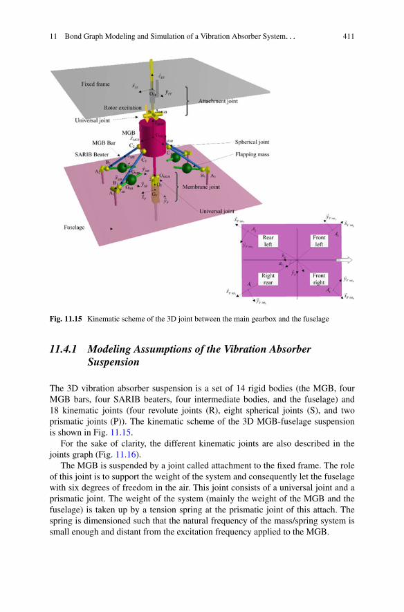
11 Bond Graph Modeling and Simulation of a Vibration Absorber System. . . 411
Fig. 11.15 Kinematic scheme of the 3D joint between the main gearbox and the fuselage
11.4.1 Modeling Assumptions of the Vibration AbsorberSuspension
The 3D vibration absorber suspension is a set of 14 rigid bodies (the MGB, fourMGB bars, four SARIB beaters, four intermediate bodies, and the fuselage) and18 kinematic joints (four revolute joints (R), eight spherical joints (S), and twoprismatic joints (P)). The kinematic scheme of the 3D MGB-fuselage suspensionis shown in Fig. 11.15.
For the sake of clarity, the different kinematic joints are also described in thejoints graph (Fig. 11.16).
The MGB is suspended by a joint called attachment to the fixed frame. The roleof this joint is to support the weight of the system and consequently let the fuselagewith six degrees of freedom in the air. This joint consists of a universal joint and aprismatic joint. The weight of the system (mainly the weight of the MGB and thefuselage) is taken up by a tension spring at the prismatic joint of this attach. Thespring is dimensioned such that the natural frequency of the mass/spring system issmall enough and distant from the excitation frequency applied to the MGB.

412 B. Boudon et al.
Fuselage
MGB
MGB Bar 1
SARIB beater 1
MGB Bar 2
SARIB beater 2
MGB Bar 3
SARIB beater 3
MGB Bar 3
SARIB beater 4
Int 2
Int 1
Fixed frame
Int 2
Int 1
( )11, F intA y�
( )A ,MGB Batiy�AMGB
OFF
OF
OMGB
OMGB
OMGB
OMGB
( )O ,MGB int Mx�
C1
AMGB
AMGB
B1
B1
A1
A1 A2 A4( )22 , F intA y�
( )A ,MGB int Ax�
( ),FF BatiO z�AMGB
C2
B2
B2
A2
B3
A3
B4
A4
C3
B3
C4
B4
( )33 , F intA y� ( )44 , F intA y�
( )O ,MGB int Mx�
( )O ,F Fz�
Attachment joint
Membrane joint
P
R
R
SC1 C2 C3 C4
AMGB
S
S
R
R
R S
S S
S
P R RR
OMGB
S
A3
Fig. 11.16 Joints graph of the 3D vibration absorber suspension
The structure of the suspension consists of four identical legs and a centralmembrane. Each leg consists of SARIB beaters and an MGB bar connected bya spherical joint. The upper ends of these legs are connected to the MGB withspherical joints and the lower ends of these legs are connected to the fuselagethrough revolute joints. The revolute joints between SARIB beaters and the fuselagehave a torsion spring dimensioned such that the anti-resonance frequency in theefforts transmitted to the fuselage is positioned on the rotor excitation frequencywhile taking up enough effort to lift the helicopter with a small displacementbetween the MGB and fuselage.
Given the physical phenomena observed, the main membrane between the MGBand the fuselage is modeled by two revolute joints with orthogonal axes (also calleduniversal joint) and a prismatic joint in serial. The flexibilities of the membranein pumping, roll, and pitch are modeled by the degrees of freedom of these jointscombined with stiffness. A torsion spring with low stiffness at each revolute jointof the universal joint and a linear spring also with low stiffness along the z-axis willmodel the filtering carried out by the membrane. The rigidities of the membrane aremodeled by rigid joints or, in other words, by a lack of degree of freedom around oralong the movements considered.
These bodies are assumed to be rigid. The intermediate parts (called Int1 andInt2) are supposed with negligible masses. As previously mentioned, absolutecoordinates have been chosen for modularity reasons. Some local moving referenceframes are attached to these bodies:

11 Bond Graph Modeling and Simulation of a Vibration Absorber System. . . 413
RFF D �OFF;
�!x FF;�!y FF;
�!z FF�
attached to the fixed frame,RMGB D �
GMGB;�!x MGB;
�!y MGB;�!z MGB
�attached to the MGB,
RSBi D �GSBi ;
�!x SBi ;�!y SBi
;�!z SBi
�attached to the SARIB Beaters,
RMBi D �GMBi ;
�!x MBi ;�!y MBi
;�!z MBi
�attached to the MGB Bar,
RF D �GF;
�!x F;�!y F;
�!z F�
attached to the fuselage and RF inti D �Ai;
�!x F inti ;�!y F inti ;�!z F inti
�also attached to fuselage so as to facilitate the definition of the
axis of the revolute joints.
11.4.2 Modeling Assumptions of the Suspension Environment
As previously mentioned in Sect. 11.3, the action of the rotor on the MGB in theexperimental setup is approximated by a sinusoidal excitation with a frequency b�.
The external mechanical actions applied to the MGB are the forces applied bythe vibrating shakers. The description of the experimental setup shall be specifiedin Sect. 11.5.2 of this paper. These excitations will be applied along or around thejoints of the “attach” joint between the fixed frame and the MGB. They allow theMGB to be subjected to pumping, pitch, and roll excitations. These mechanicalactions will only consist of a dynamic component to analyze the vibration behaviorof the suspension.
For the pumping excitation, the wrench applied by the actuator at the mobility ofthe prismatic joint is
� .actuator along vertical axis ! prismatic joint/
D OFF
(f .t/�!z FF�!0
)avec f .t/ D F � g.t/ (11.8)
For roll excitation, the wrench applied by the actuator at the mobility of the revolutejoint around roll axis is
� .Actuator around roll axis ! roll revolute joint/
D AMGB
( �!0
mr.t/�!y FF
)avec mr.t/ D M � g.t/ (11.9)
For pitch excitation, the wrench applied by the actuator at the mobility of therevolute joint around pitch axis is
� .actuator around pitch axis ! pitch revolute joint/
D AMGB
( �!0
mp.t/�!x int A
)avec mp.t/ D M � g.t/ (11.10)
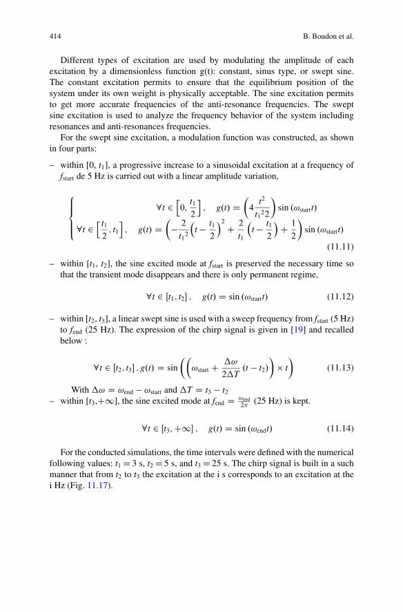
414 B. Boudon et al.
Different types of excitation are used by modulating the amplitude of eachexcitation by a dimensionless function g(t): constant, sinus type, or swept sine.The constant excitation permits to ensure that the equilibrium position of thesystem under its own weight is physically acceptable. The sine excitation permitsto get more accurate frequencies of the anti-resonance frequencies. The sweptsine excitation is used to analyze the frequency behavior of the system includingresonances and anti-resonances frequencies.
For the swept sine excitation, a modulation function was constructed, as shownin four parts:
– within [0, t1], a progressive increase to a sinusoidal excitation at a frequency offstart de 5 Hz is carried out with a linear amplitude variation,
8ˆ<
ˆ:
8t 2h0;
t12
i; g.t/ D
�4
t2
t122
�sin .!startt/
8t 2h t12; t1i; g.t/ D
�� 2
t12
t � t1
2
2C 2
t1
t � t1
2
C 1
2
�sin .!startt/
(11.11)
– within [t1, t2], the sine excited mode at fstart is preserved the necessary time sothat the transient mode disappears and there is only permanent regime,
8t 2 Œt1; t2� ; g.t/ D sin .!startt/ (11.12)
– within [t2, t3], a linear swept sine is used with a sweep frequency from fstart (5 Hz)to fend (25 Hz). The expression of the chirp signal is given in [19] and recalledbelow :
8t 2 Œt2; t3� ; g.t/ D sin
��!start C �!
2�T.t � t2/
�� t
�(11.13)
With �! D !end � !start and �T D t3 � t2– within [t3,C1], the sine excited mode at fend D !end
2�(25 Hz) is kept.
8t 2 Œt3;C1� ; g.t/ D sin .!endt/ (11.14)
For the conducted simulations, the time intervals were defined with the numericalfollowing values: t1 D 3 s, t2 D 5 s, and t3 D 25 s. The chirp signal is built in a suchmanner that from t2 to t3 the excitation at the i s corresponds to an excitation at thei Hz (Fig. 11.17).

11 Bond Graph Modeling and Simulation of a Vibration Absorber System. . . 415
30time {s}
-2
-1
0
1
2
( )g t
[s]t
Progressive increaseof magnitude
Sweep frequency
Excited mode at 5Hz Excited mode at 25 Hz0 3 5 25
Fig. 11.17 Modulation function of the excitation g(t)
11.4.3 The Simulation Approach Chosen: The R/C or ParasiticElements Methods
The bond graph simulation with the R/C or parasitic elements method is quite easyto implement compared to conventional techniques since there are no kinematicconstraints to deal with. The R/C or parasitic elements method allows to tacklederivative causalities which can appear on some inertial elements and causalitiesconstraints due to vector bonds. Moreover, this method, from our point of view,keeps a physical insight and permits the modeling with a modular approach.
11.4.4 Construction of the Bond Graph Modelof the MGB-Fuselage Joint
11.4.4.1 Components Modeling
The components modeling (rigid bodies and kinematic joints) of the system willnow be presented.
Rigid Bodies
The MGB
The MBG representation of the construction is given in Fig. 11.18. The bond graphrepresentation shows as many branches in the structure junctions as kinematicjoints for the determination of the velocities of corresponding points. From thelinear velocity of the center of mass GMGB and the instant rotation velocity�!.MGB=Fixed frame/, the linear velocity of the point OMGB, the linear velocity of
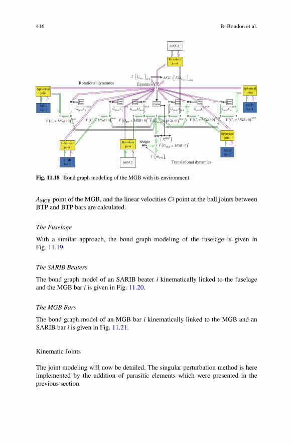
416 B. Boudon et al.
( )MGB/ 0 MGB�
( )1 / 0 MGBV C MGB∈�
MTF
1
111 1 1 1 1
MSeWeight
TFTFTF TF TFTF
1
0 00000
( )2 / 0 MGBV C MGB∈�
( )3 / 0 MGBV C MGB∈�
( )4 / 0 MGBV C MGB∈�
1
MGB
MGBG C��������
2
MGB
MGBG C��������� MGB
MGB MGBG O�����������
IntA 2
Revolute joint
Spherical joint
MGB bar 1
Revolute joint
IntM 2
4
MGB
MGBG C���������MGB
MGB MGBG A�����������
( )/ 0 MGBBTPV O MGB∈
�( )/ 0 MGB
MGBV G MGB∈�
( )0/ 0MGBV G MGB∈�
0MGBP⎡ ⎤⎣ ⎦
[ ]0: MGBI m
:MGBG MGB
I I⎡ ⎤⎣ ⎦ :MGBG MGB
MGY EJS⎡ ⎤⎣ ⎦
3
MGB
MGBG C��������
Spherical joint
MGB bar 2
Spherical joint
MGB bar 2
Spherical joint
MGB bar 4
Cardan
Rotational dynamics
Translational dynamics
Fig. 11.18 Bond graph modeling of the MGB with its environment
AMGB point of the MGB, and the linear velocities Ci point at the ball joints betweenBTP and BTP bars are calculated.
The Fuselage
With a similar approach, the bond graph modeling of the fuselage is given inFig. 11.19.
The SARIB Beaters
The bond graph model of an SARIB beater i kinematically linked to the fuselageand the MGB bar i is given in Fig. 11.20.
The MGB Bars
The bond graph model of an MGB bar i kinematically linked to the MGB and anSARIB bar i is given in Fig. 11.21.
Kinematic Joints
The joint modeling will now be detailed. The singular perturbation method is hereimplemented by the addition of parasitic elements which were presented in theprevious section.

11 Bond Graph Modeling and Simulation of a Vibration Absorber System. . . 417
MTF
1
11
1
1 1 1
MSe
TFTF TF TF TF
1
0 0000
Spherical joint
SARIB beater 1
SARIB beater 2
SARIB beater 3
SARIB beater 4
IntM 1
Prismatic joint
Rotational dynamics
Translational dynamics
( )/ 0 FusFus�
Weight
1
Fus
FusG A�������
( )1 / 0 FusV A Fus∈�
( )/ 0 FusFusV G Fus∈
�
[ ]0: FusI m
: ⎡ ⎤⎣ ⎦FusG FusI I : ⎡ ⎤⎣ ⎦FusG Fus
MGY EJS
2
Fus
FusG A������� Fus
Fus FusG O���������
3
Fus
FusG A�������
4
Fus
FusG A�������
( )0/ 0FusV G Fus∈�
( )2 / 0 FusV A Fus∈�
( )3 / 0 FusV A Fus∈�
( )4 / 0 FusV A Fus∈�
0FusP⎡ ⎤⎣ ⎦
Cardan
Spherical joint
Spherical joint
Spherical joint
Fig. 11.19 Bond graph model of the fuselage with its environment
MTF
1
1 1 1
MSeWeight
TFTF
1
00
0BSiP⎡ ⎤⎣ ⎦
( )iBS / 0 iBS�
BSi
BSi iG B�������
( )/ 0 BSiiV A BSi∈
�( )/ 0 iBS
BSi iV G BS∈�
( )0/ 0BSiV G BSi∈�
[ ]0: BSiI m
: ⎡ ⎤⎣ ⎦BSiG BSiI I : ⎡ ⎤⎣ ⎦BSiG BSi
MGY EJS
( )/ 0 BSiiV B BSi∈
�
BSi
BSi iG A�������
Fuselage
MGB bar i
Spherical joint
Revolute joint
Cardan
Fig. 11.20 Bond graph model of an SARIB beater i kinematically linked to its environment
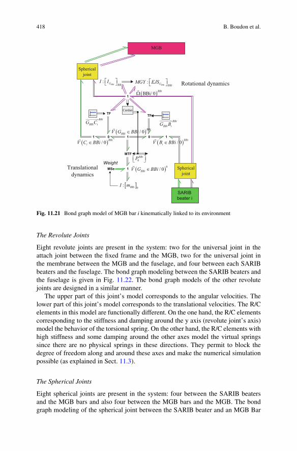
418 B. Boudon et al.
MTF
1
1 1 1
MSe
TFTF
1
00
Spherical joint
SARIBbeater i
( )BBi/ 0 BBi�
Weight
BBi
BBi iG C�������
( )/ 0 BBiiV C BBi∈
�( )/ 0 BBi
BBiV G BBi∈�
( )0/ 0BBiV G BBi∈�
[ ]0: BBiI m
: ⎡ ⎤⎣ ⎦BBiG BBiI I : ⎡ ⎤⎣ ⎦BBiG BBi
MGY EJS
( )/ 0 BBiiV B BBi∈
�
BBi
BBi iG B�������
0BBiP⎡ ⎤⎣ ⎦
MGB
Spherical joint
Rotational dynamics
Translationaldynamics
Cardan
Fig. 11.21 Bond graph model of MGB bar i kinematically linked to its environment
The Revolute Joints
Eight revolute joints are present in the system: two for the universal joint in theattach joint between the fixed frame and the MGB, two for the universal joint inthe membrane between the MGB and the fuselage, and four between each SARIBbeaters and the fuselage. The bond graph modeling between the SARIB beaters andthe fuselage is given in Fig. 11.22. The bond graph models of the other revolutejoints are designed in a similar manner.
The upper part of this joint’s model corresponds to the angular velocities. Thelower part of this joint’s model corresponds to the translational velocities. The R/Celements in this model are functionally different. On the one hand, the R/C elementscorresponding to the stiffness and damping around the y axis (revolute joint’s axis)model the behavior of the torsional spring. On the other hand, the R/C elements withhigh stiffness and some damping around the other axes model the virtual springssince there are no physical springs in these directions. They permit to block thedegree of freedom along and around these axes and make the numerical simulationpossible (as explained in Sect. 11.3).
The Spherical Joints
Eight spherical joints are present in the system: four between the SARIB beatersand the MGB bars and also four between the MGB bars and the MGB. The bondgraph modeling of the spherical joint between the SARIB beater and an MGB Bar

11 Bond Graph Modeling and Simulation of a Vibration Absorber System. . . 419
C
C C C
MTF
MTF
1 1
1
1
31
2
R
R R R
1
0
0
( )/ 0 iSBiSBΩ
�( )/ 0 iFus intiFus intΩ
�
�
1( )/ 0 iFus int
iSB�
( )/ iFus inti iSB Fus intΩ
�
/ 0 iFus inti iV A Fus int
Parasitic elements (or virtual springs)
i
i
Fus intBSP
1
1
Functionalspring
1
0iFus intP
0iSBP
( )∈�
/ 0 iSBi iV A SB( )∈
Fig. 11.22 Bond graph model of the revolute joint between the SARIB beaters and the fuselage
( )/ 0 SBiRiSBΩ
�
( )0/ BSiRi iV B BS R∈
�
( )/ 0 MBiRiMBΩ
�
( )0/ MBiRi iV B MB R∈
�
ii
BSMBP( )/ SBiR
i iMB SB�
MTF
MTF
1
R
R
1
0
01 1
1 1
C
Parasitic elements
Functional spring
0iBSP
0iMBP
Fig. 11.23 Bond graph model of the spherical joint between an MGB bar i and an SARIB beater i
is described in Fig. 11.23. The latter shows the blocking of the translational degreeof freedom in which the relative translational velocities are close to zero, thanks tothe virtual springs. The other spherical joints are built in the same manner.
The Prismatic Joints
The bond graph model of the prismatic joint between the MGB and an intermediatebody is given in Fig. 11.24.
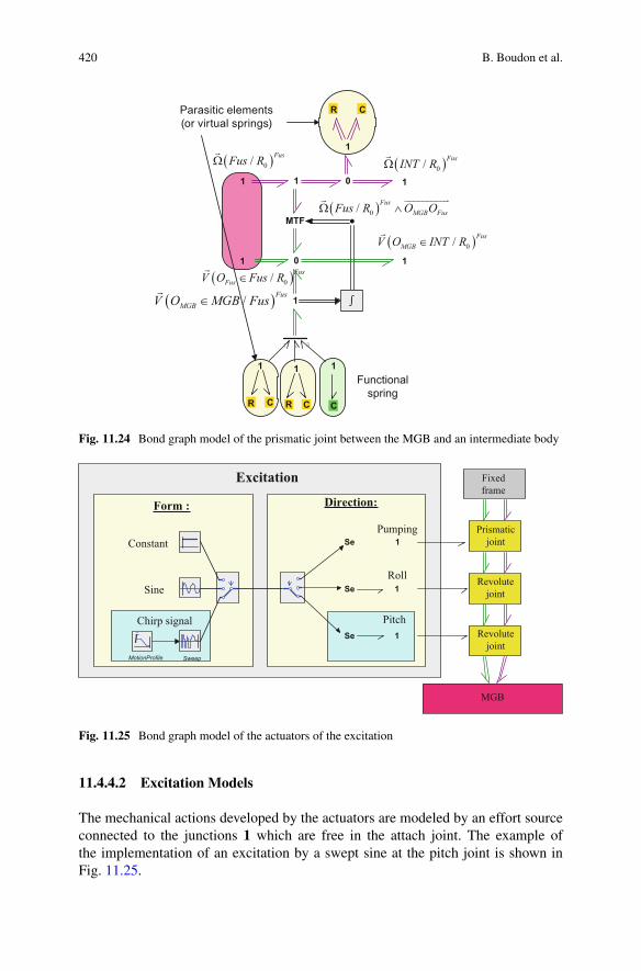
420 B. Boudon et al.
0
0
RR
R
321
1
1
11
1
1
MTF
CC C
C
( )0/ FusFusV O Fus R∈
�
( )0/ FusFus R�
( )0/ FusINT R�
( )0/ FusMGBV O INT R∈
�
( )0/ FusMGB FusFus R O OΩ ∧�����������
( )/ FusMGBV O MGB Fus∈
�
Parasitic elements(or virtual springs)
Functionalspring
1
1
1
1
Fig. 11.24 Bond graph model of the prismatic joint between the MGB and an intermediate body
Excitation Fixed frame
MGB
Prismatic joint
Revolute joint
Revolute joint
Chirp signal
Direction:Form :
Constant
Sine
Pitch
Sweep
1
1
1
MotionProfile
Se
Se
SePumping
Roll
Fig. 11.25 Bond graph model of the actuators of the excitation
11.4.4.2 Excitation Models
The mechanical actions developed by the actuators are modeled by an effort sourceconnected to the junctions 1 which are free in the attach joint. The example ofthe implementation of an excitation by a swept sine at the pitch joint is shown inFig. 11.25.
11 Bond Graph Modeling and Simulation of a Vibration Absorber System. . . 421
Depending on the selected excitation direction (pumping, roll, or pitch), thissource will be, respectively, connected either to the free junction of the prismaticjoint, or the revolute joints around the roll or pitch axis. Three choices of excitationforms may also be selected: constant for a natural mode excitation (if this constantis zero) or a static study, sinusoidal, or swept sine for excited modes.
The practical realization of these actuators will be conducted using vibrationshakers as we will detail in the experimental validation section.
11.4.4.3 Assembly
These rigid bodies and joints models, as described above, are then connectedtogether according to the architecture defined in the kinematic diagram. The bondgraph model of the 3D MGB-fuselage suspension is given below in Fig. 11.26. Asexpected, the structural aspect of the model is explicit in so far as the structure ofthe model is similar to the joints graph of the system.
11.4.4.4 Simulation Protocol
Getting Equations
The step of generating the mechanical equations is fully automated and transparentto the user using the 20-sim software. In this step, the solver reads data correspond-ing to the bond graph model and builds a mathematical problem: the equations ofthe system.
Resolution of the Equations
The used bond graph software (20-sim) then solves the equations. With the methodof singular perturbation, this step resolution can be performed simply using classicalintegration schemes for solving differential equations ODE solver such as RungeKutta 4 (RK4). However, the integration scheme that has been used is the BackwardDifferentiation Formula (BDF). It was preferred as it allows a simulation of astiff problem which is much faster than explicit solvers (like RK4). It is Gear’sbackward differentiation formula which is an implicit multi-step variable-ordermethod. The implementation of the integrator is based on the Dassl library whichhas been developed in [10]. This simulation algorithm has required two parameters:the absolute and relative integration which has been tuned on the default values(absolute integration error D e-5 and relative integration error D e-5). This methodchooses the step and the order in function of the error. Moreover, the BDF solverguarantees the numerical stability of the solution. From the mathematical solution,the solver computes and communicates the results requested by the user. 20-sim
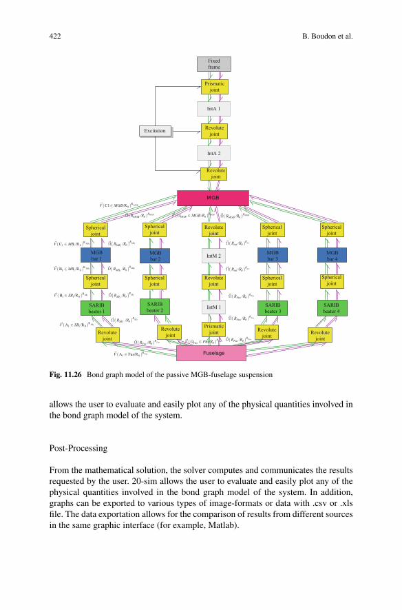
422 B. Boudon et al.
Fixedframe
Prismaticjoint
IntA 1
IntA 2
RevolutejointExcitation
Revolutejoint
Revolutejoint
Sphericaljoint
Sphericaljoint
Sphericaljoint
MGBbar 1
SARIBbeater 1
SARIBbeater 2
SARIBbeater 3
SARIBbeater 4
IntM 1
MGBbar 2
MGBbar 3
MGBbar 4IntM 2
Sphericaljoint
Revolutejoint
Revolutejoint
Revolutejoint
Revolutejoint
Fuselage
Revolutejoint
Prismaticjoint
Sphericaljoint
Sphericaljoint
Sphericaljoint
Sphericaljoint
Fig. 11.26 Bond graph model of the passive MGB-fuselage suspension
allows the user to evaluate and easily plot any of the physical quantities involved inthe bond graph model of the system.
Post-Processing
From the mathematical solution, the solver computes and communicates the resultsrequested by the user. 20-sim allows the user to evaluate and easily plot any of thephysical quantities involved in the bond graph model of the system. In addition,graphs can be exported to various types of image-formats or data with .csv or .xlsfile. The data exportation allows for the comparison of results from different sourcesin the same graphic interface (for example, Matlab).

11 Bond Graph Modeling and Simulation of a Vibration Absorber System. . . 423
11.5 Simulation and Verification of the Vibration AbsorberSuspension Model
11.5.1 Use of MapleSim for BG Model Verification
So as to verify the BG suspension model, simulation results conducted withMapleSim software (which contains a library dedicated to multibody systems) havebeen used. The simulation parameters used for both Bond graph conducted with20-sim and MapleSim are summarized in Table 11.1.
11.5.2 Comparison of Simulation Numerical Results
The vibration analysis of the system is mainly evaluated by analyzing the acceler-ation of the fuselage points and forces transmitted from the MGB to the fuselageat the SARIB beater/ fuselage joint. Simulation results with different types ofexcitation (pumping, roll, and pitch) are the following and will permit to analyzethe dynamic behavior of the suspension. The results presented were compared witha multibody software MapleSim.
11.5.2.1 Dynamic Behavior with Pumping Excitation
Acceleration of the Point OF of the Fuselage
The point OF is defined as the intersection of the MGB’s axis and the upper planeof the fuselage. It is a central point on the fuselage that can be measured.
The vertical component of the acceleration of this point is given in Fig. 11.27
Table 11.1 Simulationcomparison Software MapleSim
Bond graph conductedwith 20-sim
Solver Rosenbrock (stiff) Backwarddifferentiationformula (BDF)
Method Linear graph theory Singular perturbationNumber ofcoordinates
84 (14 bodies) 84 (14 bodies)
Number ofconstraints
74 (8 spherical joints,8 revolute joints, 2prismatic joints)
0
DoF 10 (6C 4) 84
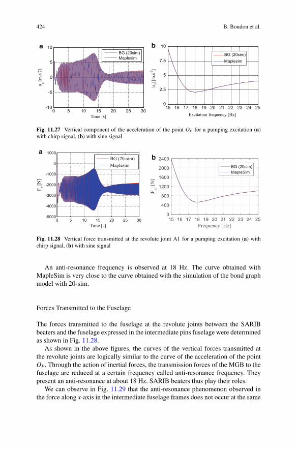
424 B. Boudon et al.
0 5 10 15 20 25 30-10
-5
0
5
10a ba z [m
.s- 2]
Time [s]
BG (20sim)Maplesim
15 16 17 18 19 20 21 22 23 24 25Excitation frequency [Hz]
0
2.5
5
7.5
10
|a z| [m
.s-2]
BG (20sim)Maplesim
Fig. 11.27 Vertical component of the acceleration of the point OF for a pumping excitation (a)with chirp signal, (b) with sine signal
0 5 10 15 20 25 30-5000
-4000
-3000
-2000
-1000
0
1000ab
Time [s]
F z [N]
BG (20-sim)Maplesim
Fig. 11.28 Vertical force transmitted at the revolute joint A1 for a pumping excitation (a) withchirp signal, (b) with sine signal
An anti-resonance frequency is observed at 18 Hz. The curve obtained withMapleSim is very close to the curve obtained with the simulation of the bond graphmodel with 20-sim.
Forces Transmitted to the Fuselage
The forces transmitted to the fuselage at the revolute joints between the SARIBbeaters and the fuselage expressed in the intermediate pins fuselage were determinedas shown in Fig. 11.28.
As shown in the above figures, the curves of the vertical forces transmitted atthe revolute joints are logically similar to the curve of the acceleration of the pointOF. Through the action of inertial forces, the transmission forces of the MGB to thefuselage are reduced at a certain frequency called anti-resonance frequency. Theypresent an anti-resonance at about 18 Hz. SARIB beaters thus play their roles.
We can observe in Fig. 11.29 that the anti-resonance phenomenon observed inthe force along x-axis in the intermediate fuselage frames does not occur at the same
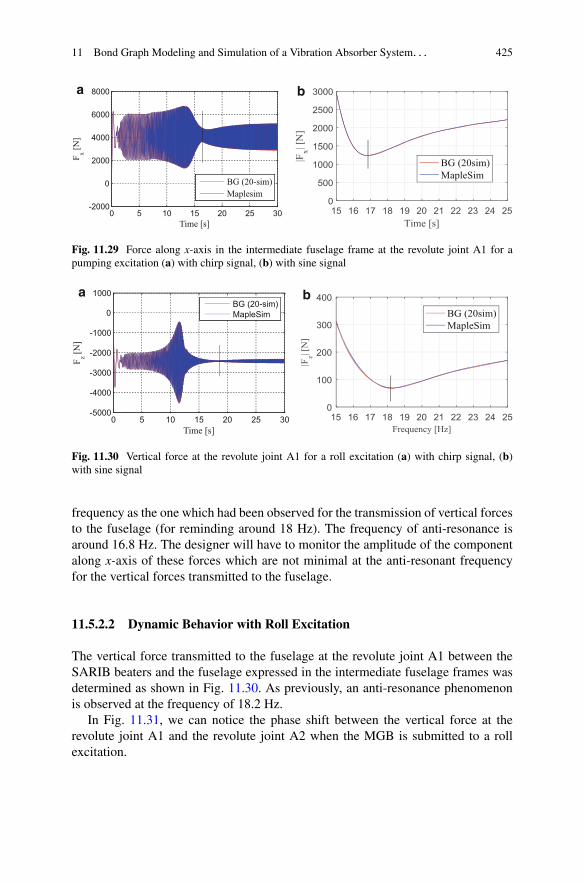
11 Bond Graph Modeling and Simulation of a Vibration Absorber System. . . 425
0 5 10 15 20 25 30-2000
0
2000
4000
6000
8000a b
Time [s]
F x [N]
BG (20-sim)Maplesim
Fig. 11.29 Force along x-axis in the intermediate fuselage frame at the revolute joint A1 for apumping excitation (a) with chirp signal, (b) with sine signal
0 5 10 15 20 25 30-5000
-4000
-3000
-2000
-1000
0
1000a b
Time [s]
F z [N]
BG (20-sim)MapleSim
Fig. 11.30 Vertical force at the revolute joint A1 for a roll excitation (a) with chirp signal, (b)with sine signal
frequency as the one which had been observed for the transmission of vertical forcesto the fuselage (for reminding around 18 Hz). The frequency of anti-resonance isaround 16.8 Hz. The designer will have to monitor the amplitude of the componentalong x-axis of these forces which are not minimal at the anti-resonant frequencyfor the vertical forces transmitted to the fuselage.
11.5.2.2 Dynamic Behavior with Roll Excitation
The vertical force transmitted to the fuselage at the revolute joint A1 between theSARIB beaters and the fuselage expressed in the intermediate fuselage frames wasdetermined as shown in Fig. 11.30. As previously, an anti-resonance phenomenonis observed at the frequency of 18.2 Hz.
In Fig. 11.31, we can notice the phase shift between the vertical force at therevolute joint A1 and the revolute joint A2 when the MGB is submitted to a rollexcitation.
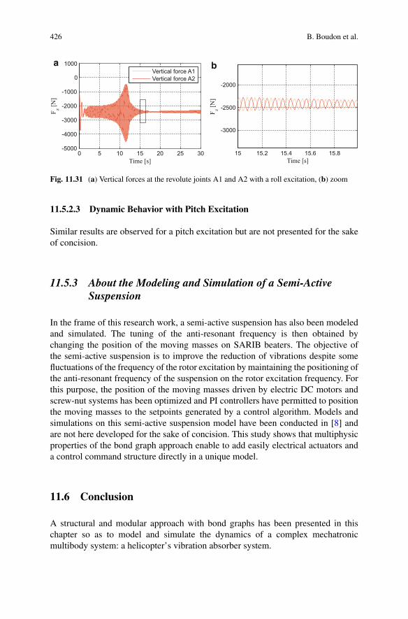
426 B. Boudon et al.
0 5 10 15 20 25 30-5000
-4000
-3000
-2000
-1000
0
1000a b
Time [s]
F z [N]
Vertical force A1Vertical force A2
15 15.2 15.4 15.6 15.8
-3000
-2500
-2000
Time [s]
F z [N]
Fig. 11.31 (a) Vertical forces at the revolute joints A1 and A2 with a roll excitation, (b) zoom
11.5.2.3 Dynamic Behavior with Pitch Excitation
Similar results are observed for a pitch excitation but are not presented for the sakeof concision.
11.5.3 About the Modeling and Simulation of a Semi-ActiveSuspension
In the frame of this research work, a semi-active suspension has also been modeledand simulated. The tuning of the anti-resonant frequency is then obtained bychanging the position of the moving masses on SARIB beaters. The objective ofthe semi-active suspension is to improve the reduction of vibrations despite somefluctuations of the frequency of the rotor excitation by maintaining the positioning ofthe anti-resonant frequency of the suspension on the rotor excitation frequency. Forthis purpose, the position of the moving masses driven by electric DC motors andscrew-nut systems has been optimized and PI controllers have permitted to positionthe moving masses to the setpoints generated by a control algorithm. Models andsimulations on this semi-active suspension model have been conducted in [8] andare not here developed for the sake of concision. This study shows that multiphysicproperties of the bond graph approach enable to add easily electrical actuators anda control command structure directly in a unique model.
11.6 Conclusion
A structural and modular approach with bond graphs has been presented in thischapter so as to model and simulate the dynamics of a complex mechatronicmultibody system: a helicopter’s vibration absorber system.
11 Bond Graph Modeling and Simulation of a Vibration Absorber System. . . 427
Three main methods (ZCP, R/C elements, and Lagrange Multipliers) of simu-lating BG models of multibody systems have been presented. Both the conditionsof application and practical rules for applying these methods with graphical bondgraph software, such as 20-sim software, have been given.
The proposed methodology consists of the assembly of modules (these com-ponents are rigid bodies and compliant kinematic joints) in a similar manner tothe real structure of the physical system. This assembly can be easily conductedwith the help of a well-structured library of components. Therefore, the constructedmultibody dynamic model permits the representation of a complex system and thebond graph model highlights the topology of systems.
The parasitic compliant elements in the kinematic joints have been used toavoid dealing with kinematic constraint equations and consequently to have onlyODE systems to solve instead of DAEs. Moreover, this method has suppressed theconstraints linked to the causality imposed by the use of vector bonds.
The simulation results of the bond graph model of the studied suspension havebeen conducted with dedicated software for bond graphs such as 20-sim andhave been verified with another multibody tool (MapleSim) for three excitations(pumping, roll, and yaw). These simulations have permitted the identification andquantification of the anti-resonance which were sought so as to filter the vibrationscoming from the rotor to the fuselage.
It has been shown than the BG should permit a structural and modular modelingof complex 3D mechatronic systems. It is worthwhile to note that the most recentstructural commercial modeling tools such as MapleSim and others could also beused for the modeling of the studied suspension. However, to take benefit from theunified power-based approach and exploit specific properties of BG, bond graphshave been chosen as the modeling language. Future works are being conducted soas to exploit two promising BG exploitations which are the analysis of energeticflow transiting among components and the control of multibody systems by meansof inversion techniques permitted by BG structural analysis [21].
Acknowledgments This research work received support from the Chair “Dynamics of complexmechanical systems - EADS Corporate Foundation - Arts et Métiers ParisTech and Ecole Centralede Marseille.” Special thanks to Paul B.T. Weustink who works at Controllab Products for his helpwith the use of complementary tools from 20-sim software.
References
1. Abadie, V., Guillemard, F., & Rault, A. (2000). Apport du bond graph dans la démarchemécatronique appliquée à l’automobile. In G. Dauphin-Tanguy (Ed.), Les bond graphs. Paris:Hermès Sciences Europe Ltd. ISBN:2-7462-0158-5.
2. Amerongen, J. V., & Breedveld, P. (2003). Modelling of physical systems for the design andcontrol of mechatronic systems. Annual Reviews in Control, 27(1), 87–117.
3. Behzadipour, S., & Khajepour, A. (2005). Causality in vector bond graphs and its applicationto modeling of multi-body dynamic systems. Simulation Modelling Practice and Theory, 14,279–295.
428 B. Boudon et al.
4. Bonderson, L. S. (1975). Vector bond graphs applied to one-dimensional distributed systems.Journal of Dynamic Systems, Measurement, and Control, 1, 75–82.
5. Borutsky, W. (2010). Bond graph methodology—Development and analysis of multidisci-plinary dynamic system models (Springer ed.th ed.). London: Springer.
6. Borutzky, W. (1995). Representing discontinuities by means of sinks of fixed causality. In:Proceedings of the 1995 Western Simulation Multiconference, Las Vegas, Nevada.
7. Bos, A. M. (1986). Multibody systems in terms of multibond graphs with application to amotorcycle multibody system. PhD thesis, University of Twente, Enschede, The Netherlands.
8. Boudon, B., Malburet, F., & Carmona, J. C. (2016). Simulation of a helicopter’s main gearboxsemiactive suspension with bond graphs. Multibody System Dynamics, 1–31.
9. Breedveld, P. C. (1985). Multibond graph elements in physical systems theory. Journal of theFranklin Institute, 319, 1–36.
10. Brenan, K. E., Campbell, S. L., & Petzold, L. R. (1996). Numerical solution of initial-valueproblems in differential-algebraic equations. SIAM. ISBN:978-0-89871-353-4.
11. Cacho, R., Felez, J., & Vera, C. (2000). Deriving simulation models from bond graphs withalgebraic loops: The extension to multibond graph systems. Journal of the Franklin Institute,337, 579–600.
12. Ersal, T., Stein, J. L., & Louca, L. S. (2004). A bond graph based modular modeling approachtowards an automated modeling environment for reconfigurable machine tools. In Internationalconference on integrated modeling and analysis in applied control and automation (2004).
13. Felez, J., Romero, G., Maroto, J., & Martinez, M. L. (2011). Simulation of multi-body systemsusing multi-bond graph. In W. Borutsky (Ed.), Bond graph modeling of engineering systems.Springer. ISBN:978-1-4419-9367-0.
14. Felez, J., Vera, C., San Jose, I., & Cacho, R. (1990). BONDYN: A bond graph based simulationprogram for multibody systems. Journal of Dynamic Systems, Measurement, and Control, 112,717–727.
15. Henderson, J.-P. (2012). Vibration isolation for rotorcraft using electrical actuation. PhDthesis, Mechanical Engineering, University of Bath.
16. Karnopp, D. (1969). Power-conserving transformations: Physical interpretations and applica-tions using bond graphs. Journal of the Franklin Institute, 288, 175–201.
17. Karnopp, D. C., & Margolis, D. L. (1979). Analysis and simulation of planar mechanismssystems using bond graphs. Journal of Mechanical Design, Transactions of the ASME, 101,187–191.
18. Krysinski, T., & Malburet, F. (2006). Mechanical vibrations: Active and passive control.London: Wiley-ISTE.
19. Lalanne, C. (2014). Mechanical vibration and shock analysis. London: Wiley-ISTE.20. Marquis-Favre, W. (1997). Contribution à la représentation bond graph des systèmes
mécaniques multicorps. PhD thesis, INSA de Lyon.21. Marquis-Favre, W., & Jardin, A. (2011). Bond graphs and inverse modeling for mechatronic
system design. In: W. Borutsky (Ed.), Bond graph modeling of engineering systems. Berlin:Springer.
22. Marquis-Favre, W., & Scavarda, S. (1998). Bond graph representation of multibody systemswith kinematic loops. Journal of the Franklin Institute, 335B, 643–660.
23. Paynter, H. M. (1961). Analysis and design of engineering systems. Cambridge: MIT Press.24. Rideout, G. (2004). System partitioning and physical domain proper modeling through
assessment of power-conserving model structure. PhD thesis, University of Michigan.25. Romero, G., Felez, J., Maroto, J., & Cabanellas, J. M. (2007). A minimal set of dynamic
equations in systems modelled with bond graphs. Proceedings of the Institution of MechanicalEngineers, Part I: Journal of Systems and Control Engineering, 221(1), 15–26.
26. Rosenberg, R. C. (1972). Multiport models in mechanics. Journal of Dynamic Systems,Measurement, and Control, 94, 206–212.

11 Bond Graph Modeling and Simulation of a Vibration Absorber System. . . 429
27. Sass, L., McPhee, J., Schmitke, C., Fisette, P., & Grenier, D. (2004). A comparison of differentmethods for modelling electromechanical multibody systems. Multibody System Dynamics, 12,209–250.
28. Schiehlen, W. (2007). Research trends in multibody system dynamics. Multibody SystemDynamics, 18, 3–13.
29. Tiernego, M. J. L., & Bos, A. M. (1985). Modelling the dynamics and kinematics of mechanicalsystems with multibond graphs. Journal of the Franklin Institute, 319, 37–50.
30. van Dijk, J., & Breedveld, P. C. (1991). Simulation of system models containing zero-ordercausal paths—I. Classification of zero-order causal paths. Journal of the Franklin Institute,328, 959–979.
31. van Dijk, J., & Breedveld, P. C. (1991). Simulation of system models containing zero-ordercausal paths—II Numerical implications of class 1 zero-order causal paths. Journal of theFranklin Institute, 328, 981–1004.
32. Wang, J., Gosselin, C., & Cheng, L. (2001). Modeling and simulation of robotic systems withclosed kinematic chains using the virtual spring approach. Multibody System Dynamics, 7,145–170.
33. Xu, W., Liu, Y., Liang, B., Wang, X., & Xu, Y. (2010). Unified multi-domain modelling andsimulation of space robot for capturing a moving target. Multibody System Dynamics, 23,293–331.
34. Zeid, A., & Chung, C.-H. (1992). Bond graph modeling of multibody systems: a library ofthree-dimensional joints. Journal of the Franklin Institute, 329, 605–636.
35. Zeid, A., & Overholt, J. L. (1995). Singularly perturbed formulation: Explicit modeling ofmultibody systems. Journal of the Franklin Institute, 332.
Chapter 12Manual Driven Wheelchair Bond GraphModelling
Abdennasser Fakri and Japie Petrus Vilakazi
12.1 Introduction
The motivation for this work derives from attempts to employ few portablemechatronic drive modules (MDM) that can be coupled when necessary to a largescale of manual propelled wheelchair (MPW) systems with the aims of improvingpropulsion efficiency. The engagement of such a module on MPW is illustrated inFig. 12.1. This yields good advantage to the system since the weight of the moduleis imposed on the module itself, thus prevents deformation of the structure. In thenext, the modelling of such a system is presented in terms of Bond graphs.
Indeed, the investigation on improving specifically the ordinary MPW propulsionmethod [9] (wheelchairnet.org) has become increasingly imperative. This is due tothe growing population of the manual wheelchair users and the requirements forefficient mobility to maintain a quality of live equivalent to the general population.
Currently, when creating a physical device, one of the major tasks is the imple-mentation of the model that integrates the control system, sensors, and actuators’dynamics in order to allow the simulation software tools to be integrated in themodelling process. The Bond graph methodology is a very well-suited graphicaltool for modular modelling approach based on energy transfer in multi-domainsystems [8]. We assume that the reader has some knowledge on the BG modellingmethod employed; therefore a brief review is given below.
A. Fakri (�)ISYS Lab ESIEE Paris Département Systèmes Electroniques, Université Paris-Est,Cite Descartes, Bd Blaise Pascal – BP 99, 93162 Noisy le Grand Cedex, Francee-mail: [email protected]
J.P. VilakaziTshwane University of Technology, 993 Khama Street, Standerton 2430, South Africae-mail: [email protected]
© Springer International Publishing Switzerland 2017W. Borutzky (ed.), Bond Graphs for Modelling, Control and FaultDiagnosis of Engineering Systems, DOI 10.1007/978-3-319-47434-2_12
431
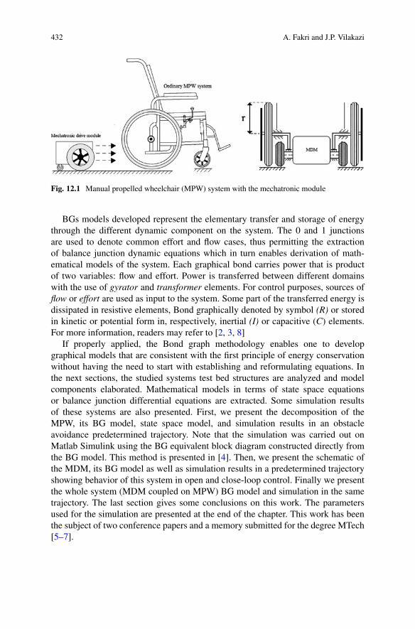
432 A. Fakri and J.P. Vilakazi
Fig. 12.1 Manual propelled wheelchair (MPW) system with the mechatronic module
BGs models developed represent the elementary transfer and storage of energythrough the different dynamic component on the system. The 0 and 1 junctionsare used to denote common effort and flow cases, thus permitting the extractionof balance junction dynamic equations which in turn enables derivation of math-ematical models of the system. Each graphical bond carries power that is productof two variables: flow and effort. Power is transferred between different domainswith the use of gyrator and transformer elements. For control purposes, sources offlow or effort are used as input to the system. Some part of the transferred energy isdissipated in resistive elements, Bond graphically denoted by symbol (R) or storedin kinetic or potential form in, respectively, inertial (I) or capacitive (C) elements.For more information, readers may refer to [2, 3, 8]
If properly applied, the Bond graph methodology enables one to developgraphical models that are consistent with the first principle of energy conservationwithout having the need to start with establishing and reformulating equations. Inthe next sections, the studied systems test bed structures are analyzed and modelcomponents elaborated. Mathematical models in terms of state space equationsor balance junction differential equations are extracted. Some simulation resultsof these systems are also presented. First, we present the decomposition of theMPW, its BG model, state space model, and simulation results in an obstacleavoidance predetermined trajectory. Note that the simulation was carried out onMatlab Simulink using the BG equivalent block diagram constructed directly fromthe BG model. This method is presented in [4]. Then, we present the schematic ofthe MDM, its BG model as well as simulation results in a predetermined trajectoryshowing behavior of this system in open and close-loop control. Finally we presentthe whole system (MDM coupled on MPW) BG model and simulation in the sametrajectory. The last section gives some conclusions on this work. The parametersused for the simulation are presented at the end of the chapter. This work has beenthe subject of two conference papers and a memory submitted for the degree MTech[5–7].

12 Manual Driven Wheelchair Bond Graph Modelling 433
12.2 Manual Propelled Wheelchair
12.2.1 Description and Test Bed
MPW is required in hospitals and old age institutions to transport patients who aretoo unwell to walk [1]. The user can maneuver the chair by turning the hand pushrims attached to the rear wheels, as shown in Fig. 12.1. For users who cannot operatethe MPW, handles are made available for assistance from an attendant.
An illustration of an ordinary MPW test bed structure used in this modellingis depicted in Fig. 12.2. It essentially consists of two casters and manual rearwheels. An approach of a two wheel drives robotic system has been applied inthis modelling with the caster wheels lumped together and assumed to be imposingresistive force to the systems flow. VCG and !CG represent the center of massvelocity and inertial mass rotation, ! l and !r indicate the angular velocity of theleft and right wheels, respectively, and rear manual wheel radius and wheelchairwidth are represented by (r) and (Lw), respectively. The below matrices (12.1) showthe kinematic mathematical model of the system, where � is the orientation angle, xand y show the systems geometric position, respectively:
2
4xy�
3
5 D r
2
4cos �2
cos �2
sin �2
sin �2
2Lw
�2Lw
3
5�!r!l
�(12.1)
The components contributing to the dynamic behavior of this ideal MPW systemhave been identified from the point at which torque (Se) is applied and foundto be:
• Wheels rotational inertia, Inertial moment• Wheel spokes stiffness: this refers to the spring/damper imposed by the air
inflated rear wheels. This exists from the center of the wheel to the ground.
Fig. 12.2 Top view of manual propelled wheelchair (MPW) system

434 A. Fakri and J.P. Vilakazi
• Frictional losses: the frictional losses were considered and said to exist at the rearwheels circumference to ground. The resistive force (loss of energy) imposed bythe front caster wheels during rotation was also considered.
• Mass: includes weight of the chair and the assumed mass of the user. This pointis located at the center of gravity where the systems average mass is obtained. Inreducing the complexity of the model, the center of gravity has been assumed tobe occurring at the same x-axis with the rear propulsion wheels, thus permittingrotation of the system with reference to that pivot as indicated by !cg in Fig. 12.2.Point A was considered as the initial (x0, y0) and reference position of thewheelchair, and the system said to have moved h distance and rotated at thecenter of gravity as depicted in the same figure.
The left and right wheels’ displacements with reference to point A are given byEqs. (12.2) and (12.3), respectively.
S1 D h � Lw
2sin � (12.2)
Sr D h C Lw
2sin � (12.3)
From the BG analogies, integration of the flow equations yields the displacementequations of the system. Therefore using the above equations, we obtained therequired flow Eqs. (12.4) and (12.5) to construct the BG model of the wheelchairstructure.
!r D :
Sr D :
h �:
�Lw
2cos � (12.4)
!r D :
Sr D :
h C:
�Lw
2cos � (12.5)
Using the constitutive laws of the one-port I-element we describe the motion interms of the velocity of center of gravity (VCG) and the angular velocity !CG D P�as depicted in Fig. 12.2. The average force on the wheelchair is equal to the rateof change of linear momentum that is related to VCG by the systems total mass inEq. (12.6).
VCG D PCG
m(12.6)
The average torque at the center of gravity is equal to the rate of change of angularmomentum which is related to !CG D P� by the systems moment of inertia in Eq.(12.7).
!CG D P�Jchair
(12.7)
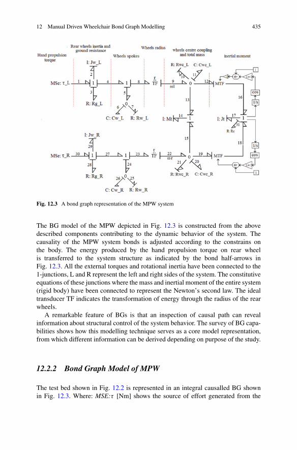
12 Manual Driven Wheelchair Bond Graph Modelling 435
Fig. 12.3 A bond graph representation of the MPW system
The BG model of the MPW depicted in Fig. 12.3 is constructed from the abovedescribed components contributing to the dynamic behavior of the system. Thecausality of the MPW system bonds is adjusted according to the constrains onthe body. The energy produced by the hand propulsion torque on rear wheelis transferred to the system structure as indicated by the bond half-arrows inFig. 12.3. All the external torques and rotational inertia have been connected to the1-junctions, L and R represent the left and right sides of the system. The constitutiveequations of these junctions where the mass and inertial moment of the entire system(rigid body) have been connected to represent the Newton’s second law. The idealtransducer TF indicates the transformation of energy through the radius of the rearwheels.
A remarkable feature of BGs is that an inspection of causal path can revealinformation about structural control of the system behavior. The survey of BG capa-bilities shows how this modelling technique serves as a core model representation,from which different information can be derived depending on purpose of the study.
12.2.2 Bond Graph Model of MPW
The test bed shown in Fig. 12.2 is represented in an integral causalled BG shownin Fig. 12.3. Where: MSE:� [Nm] shows the source of effort generated from the
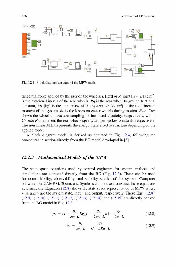
436 A. Fakri and J.P. Vilakazi
Fig. 12.4 Block diagram structure of the MPW model
tangential force applied by the user on the wheels, L [left] or R [right], Jw_L [kg m2]is the rotational inertia of the rear wheels, Rg is the rear wheel to ground frictionalconstant, Mt [kg] is the total mass of the system, Jt [kg m2] is the total inertialmoment of the system, Rc is the losses on caster wheels during motion, Rwc, Cwcshows the wheel to structure coupling stiffness and elasticity, respectively, whilstCw and Rw represent the rear wheels spring/damper spokes constants, respectively.The non-linear MTF represents the energy transferred to structure depending on theapplied force.
A block diagram model is derived as depicted in Fig. 12.4, following theprocedures in section directly from the BG model developed in [3].
12.2.3 Mathematical Models of the MPW
The state space equations used by control engineers for system analysis andsimulations are extracted directly from the BG (Fig. 12.3). These can be usedfor controllability, observability, and stability studies of the system. Computersoftware like CAMP-G, 20sim, and Symbols can be used to extract these equationsautomatically. Equation (12.8) shows the state space representation of MPW wherex, u, and y are the system state, input, and output, respectively. These Eqs. (12.8),(12.9), (12.10), (12.11), (12.12), (12.13), (12.14), and (12.15) are directly derivedfrom the BG model in Fig. 12.3.
:p2 D � l � p2
Jw_LRg_L � q11
Cwc_Lk1 � q6
Cw_L(12.8)
:q6 D p2
Jw_L� q6
Cw_LRw_L(12.9)
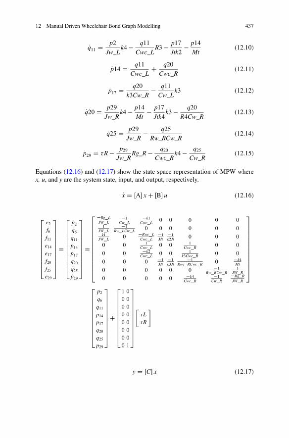
12 Manual Driven Wheelchair Bond Graph Modelling 437
:q11 D p2
Jw_Lk4 � q11
Cwc_LR3 � p17
Jtk2� p14
Mt(12.10)
:p14 D q11
Cwc_LC q20
Cwc_R(12.11)
:p17 D q20
k3Cw_R� q11
Cw_Lk3 (12.12)
:q20 D p29
Jw_Rk4 � p14
Mt� p17
Jtk4k3 � q20
R4Cw_R(12.13)
:q25 D p29
Jw_R� q25
Rw_RCw_R(12.14)
:p29 D �R � p29
Jw_RRg_R � q20
Cwc_Rk4 � q25
Cw_R(12.15)
Equations (12.16) and (12.17) show the state space representation of MPW wherex, u, and y are the system state, input, and output, respectively.
:x D ŒA� x C ŒB� u (12.16)
2
666666666664
e2f6f11e14e17f20f25e29
3
777777777775
D
2
666666666664
:p2:q6:q11:p14:p17:q20:q25:p29
3
777777777775
D
2
66666666666664
�Rg_LJW_L
�1Cw_L
�k1Cwc_L 0 0 0 0 0
1JW_L
�1Rw_LCw_L 0 0 0 0 0 0
k1JW_L 0
�Rwc_LCwc_L
�1Mt
�1k2Jt 0 0 0
0 0 1Cwc_L 0 0 1
Cwc_R 0 0
0 0 �k2Cwc_L 0 0 1
k3Cwc_R 0 0
0 0 0 �1Mt
�1k3Jt
�1Rwc_RCwc_R 0 �k4
Mt
0 0 0 0 0 0 �1Rw_RCw_R
1JW_R
0 0 0 0 0 �k4Cwc_R
�1Cw_R
�Rg_RJW_R
3
77777777777775
2
666666666664
p2q6q11p14p17q20q25p29
3
777777777775
C
2
666666666664
1 0
0 0
0 0
0 0
0 0
0 0
0 0
0 1
3
777777777775
"�L�R
#
y D ŒC� x (12.17)
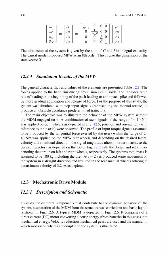
438 A. Fakri and J.P. Vilakazi
2
664
!L
!R
VCG
�CG
3
775 D
2
664
f4f27f14f17
3
775 D
2
6664
1Jw_L 0 0 0
0 1Jw_R 0 0
0 0 1Mt 0
0 0 0 1Jt
3
7775
2
664
p2p29p14p17
3
775
The dimension of the system is given by the sum of C and I in integral causality.The causal model proposed MPW is an 8th order. This is also the dimension of thestate vector X.
12.2.4 Simulation Results of the MPW
The general characteritics and values of the elements are presented Table 12.1. Theforces applied to the hand rim during propulsion is sinusoidal and includes rapidrate of loading in the beginning of the push leading to an impact spike and followedby more gradual application and release of force. For the purpose of this study, thesystem was simulated with step input signals (representing the manual torque) toproduce an obstacle avoidance predetermined trajectory.
The main objective was to illustrate the behavior of the MPW system withoutthe MDM engaged on it. A combination of step signals in the range of 4–10 Nmwas applied on both wheels as depicted in Fig. 12.5, position and orientation (withreference to the x-axis) were observed. The profile of input torque signals (assumedto be produced by the tangential force exerted by the user) within the range of 2–10 Nm was applied on the MPW rear wheels and depending on the desired lateralvelocity and rotational direction, the signal magnitude alters in order to achieve thedesired trajectory as depicted on the top of Fig. 12.5 with the dotted and solid linesdenoting the torque on left and right wheels, respectively. The systems total mass isassumed to be 100 kg including the user. At t D 2 s is produced some movement onthe system in a straight direction and resulted in the rear manual wheels rotating ata maximum velocity of 3.2 r/s as depicted.
12.3 Mechatronic Drive Module
12.3.1 Description and Schematic
To study the different components that contribute to the dynamic behavior of thesystem, a separation of the MDM from the structure was carried out and basic layoutis shown in Fig. 12.6. A typical MDM is depicted in Fig. 12.6. It comprises of adirect current (DC) motor converting electric energy (from batteries in this case) intomechanical energy. Velocity reduction mechanical gears are used and the manner inwhich motorized wheels are coupled to the system is illustrated.

12 Manual Driven Wheelchair Bond Graph Modelling 439
Table 12.1 Systemparameters
Parameter Description Value
Manual propelled wheelchair (MPW)
MSe:£ Rear wheel propulsion torque (Nm) 12Jw Rear wheel rotational inertia (kg m2) 0.005Mt Systems mass (kg) 100Jt Systems inertial moment (kg m2) 64Rg Wheel to ground resistance 0.006Cw Wheel spoke spring 0.0021Rw Wheel spoke damper 12r Rear wheel radius (m) 0.30226Lw Wheelchair width (m) 0.8Mechatronic drive module (MDM)
Ie Electric motor inductance (H) 0.0033Re Electric motor resistance (�) 0.9Jr Rotor rotational inertia (kg m2) 0.078Rb Motor bearing damper (Nm-s/rad) 0.008Mt Module mass (kg) 30Jt Module inertial moment (kg m2) 7.5Lw Module width (m) 0.6Cs Motor to gear shaft torsion (Nm/rad) 0.00237Rs Motor to gear shaft damper 11k1, k8 Motor torque constant (Nm/A) 0.288k2, k7 Mechanical gear ration 0.18k3, k6 Motorized wheels radius (m) 0.127MSe:L Control input voltage (V) 24Modular driven manual wheelchair (MDMW)
J Manual wheels (kg m2) 0.005k9, k10 manual wheels radius (m) 0.30226Mt Combined systems total mass (kg) 130Jt Total inertial moment (kg m2) 83.5
The small values of rotational dampers and torsion springs on the shafts havebeen lumped together and represented by Rs and Cs, respectively. The differentcomponents contributing to the dynamic behavior of the MDM are identified as:
• Electric inductance of the motor windings.• Rotational inertia of the armature.• Stiffness of the shaft coupling power motor to the mechanical gears.• Rotational inertia of the motorized wheels.• Mass of the MDM system, inertial moment, and the stiffness at the wheels
connection to the body.
From this we hence construct the relevant BG model as depicted in Fig. 12.7.Notice that it only represents the components contributing to the dynamic behaviorof the MDM system (depicted in Fig. 12.6b) extracted from the EPPW.
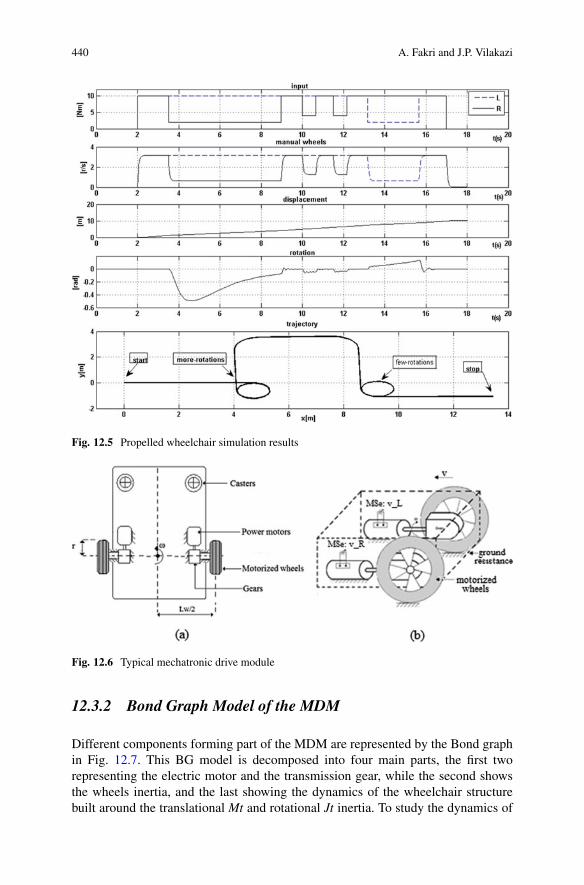
440 A. Fakri and J.P. Vilakazi
Fig. 12.5 Propelled wheelchair simulation results
Fig. 12.6 Typical mechatronic drive module
12.3.2 Bond Graph Model of the MDM
Different components forming part of the MDM are represented by the Bond graphin Fig. 12.7. This BG model is decomposed into four main parts, the first tworepresenting the electric motor and the transmission gear, while the second showsthe wheels inertia, and the last showing the dynamics of the wheelchair structurebuilt around the translational Mt and rotational Jt inertia. To study the dynamics of
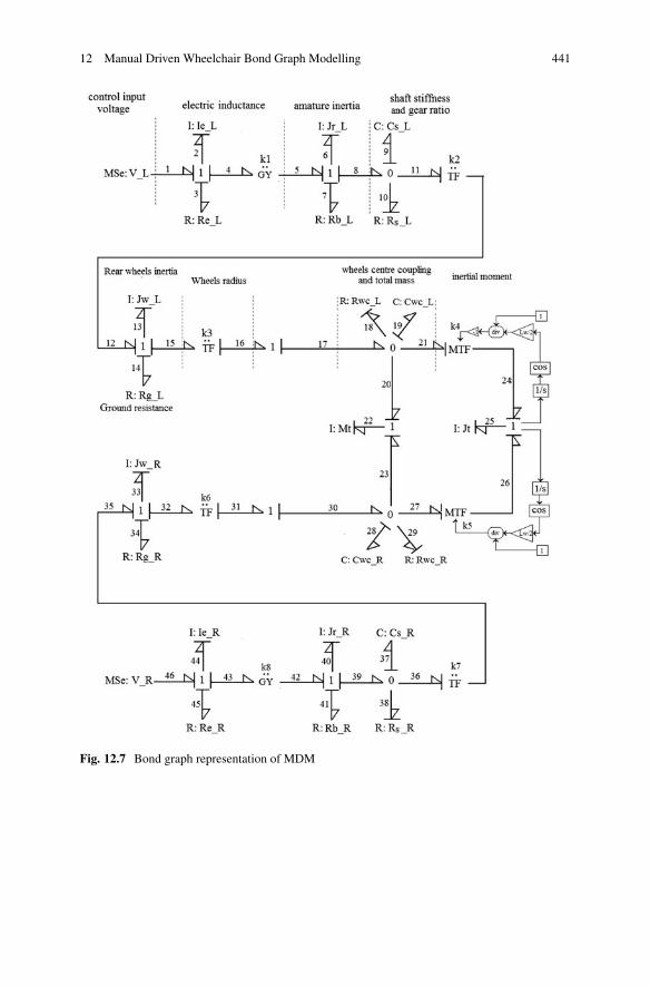
12 Manual Driven Wheelchair Bond Graph Modelling 441
Fig. 12.7 Bond graph representation of MDM
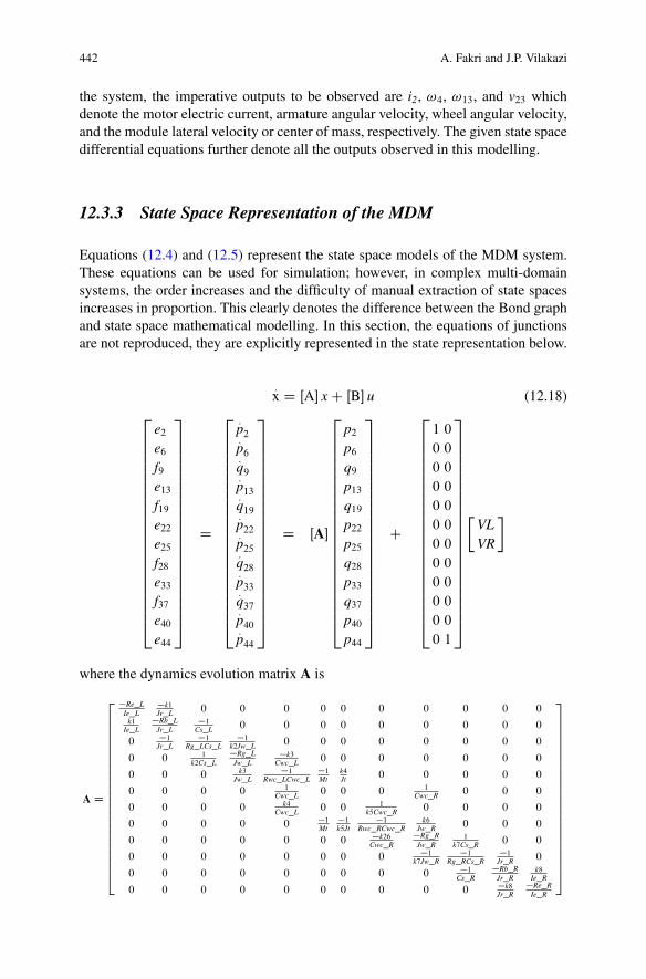
442 A. Fakri and J.P. Vilakazi
the system, the imperative outputs to be observed are i2, !4, !13, and v23 whichdenote the motor electric current, armature angular velocity, wheel angular velocity,and the module lateral velocity or center of mass, respectively. The given state spacedifferential equations further denote all the outputs observed in this modelling.
12.3.3 State Space Representation of the MDM
Equations (12.4) and (12.5) represent the state space models of the MDM system.These equations can be used for simulation; however, in complex multi-domainsystems, the order increases and the difficulty of manual extraction of state spacesincreases in proportion. This clearly denotes the difference between the Bond graphand state space mathematical modelling. In this section, the equations of junctionsare not reproduced, they are explicitly represented in the state representation below.
:x D ŒA� x C ŒB� u (12.18)
2
666666666666666666664
e2e6f9e13f19e22e25f28e33f37e40e44
3
777777777777777777775
D
2
666666666666666666664
:p2:p6:q9:p13:q19:p22:p25:q28:p33:q37:p40:p44
3
777777777777777777775
D ŒA�
2
666666666666666666664
p2p6q9p13q19p22p25q28p33q37p40p44
3
777777777777777777775
C
2
666666666666666666664
1 0
0 0
0 0
0 0
0 0
0 0
0 0
0 0
0 0
0 0
0 0
0 1
3
777777777777777777775
�VLVR
�
where the dynamics evolution matrix A is
A D
2
666666666666666666666664
�Re_LIe_L
�k1Jr_L 0 0 0 0 0 0 0 0 0 0
k1Ie_L
�Rb_LJr_L
�1Cs_L 0 0 0 0 0 0 0 0 0
0 �1Jr_L
�1Rg_LCs_L
�1k2Jw_L 0 0 0 0 0 0 0 0
0 0 1k2Cs_L
�Rg_LJw_L
�k3Cwc_L 0 0 0 0 0 0 0
0 0 0 k3Jw_L
�1Rwc_LCwc_L
�1Mt
k4Jt 0 0 0 0 0
0 0 0 0 1Cwc_L 0 0 0 1
Cwc_R 0 0 0
0 0 0 0 k4Cwc_L 0 0 1
k5Cwc_R 0 0 0 0
0 0 0 0 0 �1Mt
�1k5Jt
�1Rwc_RCwc_R
k6Jw_R 0 0 0
0 0 0 0 0 0 0 �k26Cwc_R
�Rg_RJw_R
1k7Cs_R 0 0
0 0 0 0 0 0 0 0 �1k7Jw_R
�1Rg_RCs_R
�1Jr_R 0
0 0 0 0 0 0 0 0 0 �1Cs_R
�Rb_RJr_R
k8Ie_R
0 0 0 0 0 0 0 0 0 0 �k8Jr_R
�Re_RIe_R
3
777777777777777777777775

12 Manual Driven Wheelchair Bond Graph Modelling 443
The outputs are given by:
y D ŒC� x (12.19)
2
6666666666666664
iL�L
!mL
!wL
VCG
�CG
!wR
!mR
�R
iR
3
7777777777777775
D
2
6666666666666664
i2e6f8f13f22f25f33f39e40i44
3
7777777777777775
D
2
666666666666666664
1Ie_L 0 0 0 0 0 0 0
k1Jr_L 0 0 0 0 0 0 0
0 1Jr_L 0 0 0 0 0 0
0 0 1Jw_L 0 0 0 0 0
0 0 0 1Mt 0 0 0 0
0 0 0 0 1Jt 0 0 0
0 0 0 0 0 1Jw_R 0 0
0 0 0 0 0 0 1Jr_R 0
0 0 0 0 0 0 0 k8Jr_R
0 0 0 0 0 0 0 1Ie_R
3
777777777777777775
2
666666666664
p2p6p13p22p25p33p40p44
3
777777777775
12.3.4 Simulations of the MDM Behavior
The system model is simulated and responses observed during a motion in a spaceof 20 � 10 m2 predetermined trajectory (Fig. 12.8).
The systems were simulated for a period of 45 s with a profile of step inputsignals applied on the electric motor terminals ranging from 0 to 24 V, with themaximum value resulting into a lateral velocity of 1.8 m/s, and eventually brought to
Fig. 12.8 Predetermined trajectory
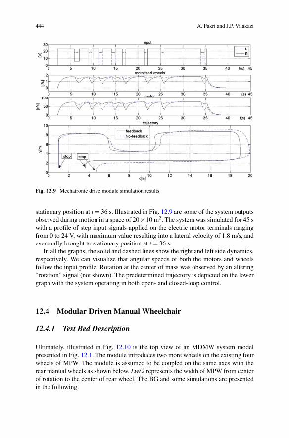
444 A. Fakri and J.P. Vilakazi
Fig. 12.9 Mechatronic drive module simulation results
stationary position at t D 36 s. Illustrated in Fig. 12.9 are some of the system outputsobserved during motion in a space of 20 � 10 m2. The system was simulated for 45 swith a profile of step input signals applied on the electric motor terminals rangingfrom 0 to 24 V, with maximum value resulting into a lateral velocity of 1.8 m/s, andeventually brought to stationary position at t D 36 s.
In all the graphs, the solid and dashed lines show the right and left side dynamics,respectively. We can visualize that angular speeds of both the motors and wheelsfollow the input profile. Rotation at the center of mass was observed by an altering“rotation” signal (not shown). The predetermined trajectory is depicted on the lowergraph with the system operating in both open- and closed-loop control.
12.4 Modular Driven Manual Wheelchair
12.4.1 Test Bed Description
Ultimately, illustrated in Fig. 12.10 is the top view of an MDMW system modelpresented in Fig. 12.1. The module introduces two more wheels on the existing fourwheels of MPW. The module is assumed to be coupled on the same axes with therear manual wheels as shown below. Lw/2 represents the width of MPW from centerof rotation to the center of rear wheel. The BG and some simulations are presentedin the following.
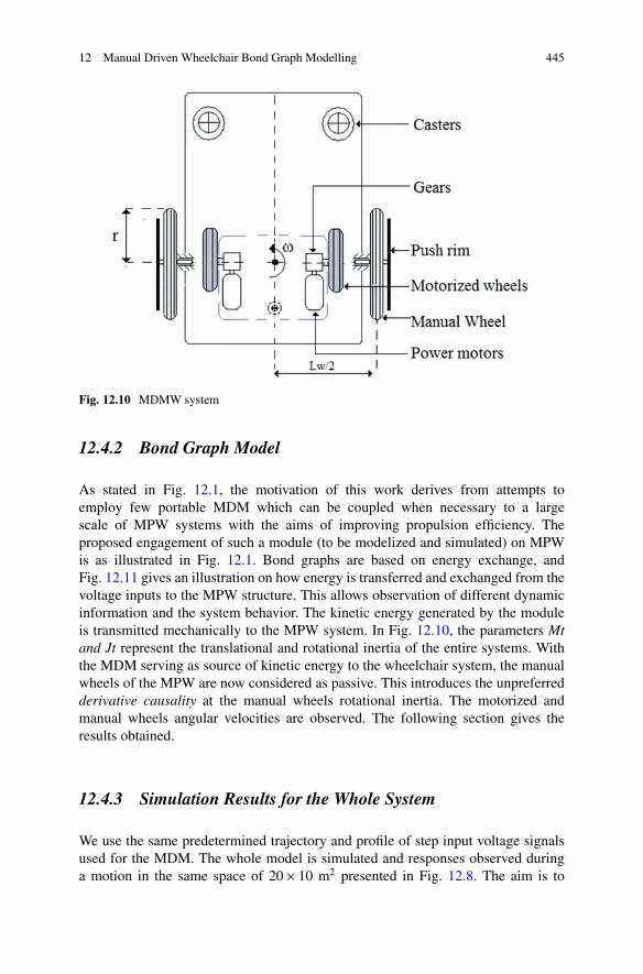
12 Manual Driven Wheelchair Bond Graph Modelling 445
Fig. 12.10 MDMW system
12.4.2 Bond Graph Model
As stated in Fig. 12.1, the motivation of this work derives from attempts toemploy few portable MDM which can be coupled when necessary to a largescale of MPW systems with the aims of improving propulsion efficiency. Theproposed engagement of such a module (to be modelized and simulated) on MPWis as illustrated in Fig. 12.1. Bond graphs are based on energy exchange, andFig. 12.11 gives an illustration on how energy is transferred and exchanged from thevoltage inputs to the MPW structure. This allows observation of different dynamicinformation and the system behavior. The kinetic energy generated by the moduleis transmitted mechanically to the MPW system. In Fig. 12.10, the parameters Mtand Jt represent the translational and rotational inertia of the entire systems. Withthe MDM serving as source of kinetic energy to the wheelchair system, the manualwheels of the MPW are now considered as passive. This introduces the unpreferredderivative causality at the manual wheels rotational inertia. The motorized andmanual wheels angular velocities are observed. The following section gives theresults obtained.
12.4.3 Simulation Results for the Whole System
We use the same predetermined trajectory and profile of step input voltage signalsused for the MDM. The whole model is simulated and responses observed duringa motion in the same space of 20 � 10 m2 presented in Fig. 12.8. The aim is to
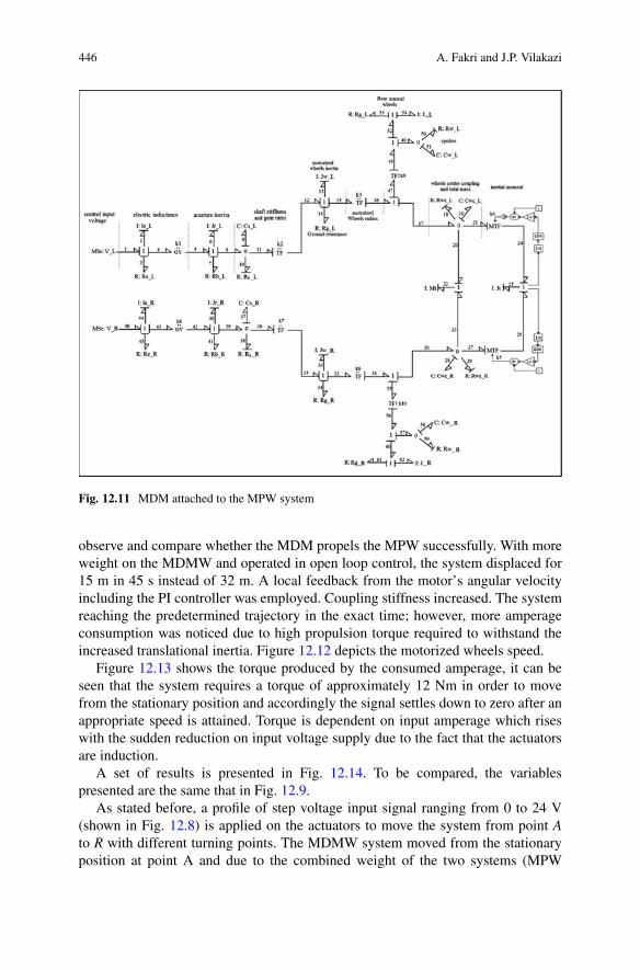
446 A. Fakri and J.P. Vilakazi
Fig. 12.11 MDM attached to the MPW system
observe and compare whether the MDM propels the MPW successfully. With moreweight on the MDMW and operated in open loop control, the system displaced for15 m in 45 s instead of 32 m. A local feedback from the motor’s angular velocityincluding the PI controller was employed. Coupling stiffness increased. The systemreaching the predetermined trajectory in the exact time; however, more amperageconsumption was noticed due to high propulsion torque required to withstand theincreased translational inertia. Figure 12.12 depicts the motorized wheels speed.
Figure 12.13 shows the torque produced by the consumed amperage, it can beseen that the system requires a torque of approximately 12 Nm in order to movefrom the stationary position and accordingly the signal settles down to zero after anappropriate speed is attained. Torque is dependent on input amperage which riseswith the sudden reduction on input voltage supply due to the fact that the actuatorsare induction.
A set of results is presented in Fig. 12.14. To be compared, the variablespresented are the same that in Fig. 12.9.
As stated before, a profile of step voltage input signal ranging from 0 to 24 V(shown in Fig. 12.8) is applied on the actuators to move the system from point Ato R with different turning points. The MDMW system moved from the stationaryposition at point A and due to the combined weight of the two systems (MPW
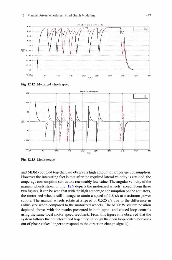
12 Manual Driven Wheelchair Bond Graph Modelling 447
Fig. 12.12 Motorized wheels speed
Fig. 12.13 Motor torque
and MDM) coupled together, we observe a high amount of amperage consumption.However the interesting fact is that after the required lateral velocity is attained, theamperage consumption settles to a reasonably low value. The angular velocity of themanual wheels shown in Fig. 12.9 depicts the motorized wheels’ speed. From thesetwo figures, it can be seen that with the high amperage consumption on the actuators,the motorized wheels still manage to attain a speed of 1.8 r/s at maximum powersupply. The manual wheels rotate at a speed of 0.525 r/s due to the difference inradius size when compared to the motorized wheels. The MDMW system positiondepicted above, with the results presented in both open- and closed-loop controlsusing the same local motor speed feedback. From this figure it is observed that thesystem follows the predetermined trajectory although the open loop control becomesout of phase (takes longer to respond to the direction change signals).
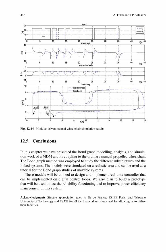
448 A. Fakri and J.P. Vilakazi
Fig. 12.14 Modular driven manual wheelchair simulation results
12.5 Conclusions
In this chapter we have presented the Bond graph modelling, analysis, and simula-tion work of a MDM and its coupling to the ordinary manual propelled wheelchair.The Bond graph method was employed to study the different substructures and thelinked systems. The models were simulated on a realistic area and can be used as atutorial for the Bond graph studies of movable systems.
These models will be utilized to design and implement real-time controller thatcan be implemented on digital control loops. We also plan to build a prototypethat will be used to test the reliability functioning and to improve power efficiencymanagement of this system.
Acknowledgments Sincere appreciation goes to Ile de France, ESIEE Paris, and TshwaneUniversity of Technology and FSATI for all the financial assistance and for allowing us to utilizetheir facilities.
12 Manual Driven Wheelchair Bond Graph Modelling 449
Glossary
BD Block DiagramBG Bond GraphEPPW Electric Power Propelled WheelchairC 1-port Capacitive ElementI 1-port Inductive ElementGY GyratorMSe Modulated Source of EffortMDM Mechatronic Drive ModularMDMW Modular Driven Manual WheelchairMPW Manual Propelled wheelchairMSf Modulated Source of FlowMSe Modulated Source of EffortMTF Modulated TransformerPCG Linear MomentumP� Angular MomentumR 1-port Resistive ElementTF TransformerVCG Center of mass velocity!CG Inertial mass velocity
References
1. Abel, E. N., & Frank, T.G. (1991). The design of an attendant propelled wheelchair. Prostheticand orthotic international, Pubmed (pp. 38–45), Apr 1991.
2. Borutzky, W. (2010). Bond graph methodology, development and analysis of multidisciplinarydynamic system models (1st ed.). Berlin: Springer.
3. Dauphin-Tanguy, G. (2000). Les bond graphs. Paris: Hermes Edition.4. Fakri, A., Rocaries, F., & Carriere, A. (1997). A simple method for the conversion of bond graph
models in presentation by block diagrams. International Conference on Bond graph Modellingand Simulation, ICBGM’97 (pp. 15–19), Phoenix Arizona.
5. Fakri, A., & Vilakazi, J. P. (2010). Modular driven wheelchair bond graph modelling. TheEuropean Modeling & Simulation Symposium, I3M2010 MultiConference, October 2010 Fes,Morocco.
6. Fakri, A., & Vilakazi, J. P. (2014). Wheelchair and electric drive add-on a whole bond graphmodelling. Proceedings of the 2014 11th International Conference on Bond graph Modelingand Simulation (ICBGM’14). SummerSim 2014 Multiconference July 6–10 2014, Monterey,CA, USA. ISBN: 978-1-63266-700-7, Vol. 46 #8, Collection:Simulation Series, 206-210, 222pp. 113.
7. Vilakazi, J. P. (2011). A study of a mechatronic drive module to be coupled on to an ordinarymanual propelled wheelchair. French South African Technical Institute in Electronics (F’SATIE),Tshwane University of Technologie.

450 A. Fakri and J.P. Vilakazi
8. Karnopp, D. C., Margolis, D. L., & Rosenberg, R. C. (2006). System dynamics: A unifiedapproach (4th ed.). New York: Wiley.
9. Wheelchairnet.org (2010). Discussion preparation for manual wheelchair propulsion. MidAtlantic Region: Rehabilitation Engineering Research Centre on Technology Transfer FederalLaboratory Consortium (April 15).

Chapter 13Bond Graph Modelling and Controlof Hyper-Redundant Miniature Robotfor In-Vivo Biopsy
Mihir Kumar Sutar and Pushpraj Mani Pathak
DOF Degrees of freedomPI Proportion-integral controllerCG Centre of gravityPD Proportional derivative controllerEJS Euler junction structure
13.1 Introduction
Endoscopy involves a procedure that uses a specialized tool to view, take biopsysample, and operate on the abdominal cavity of human body when required. Theprocedure allows a surgeon to examine the abdominal cavity to ascertain the cause ofdiscomfort reported by the patient, and for remedial action. It is performed with anendoscope, which is a flexible tube with all attached accessories required for biopsyand viewing. Gastroscopy is a type of endoscopy. It is a symptomatic endoscopicprocedure that examines the gastrointestinal tract. It is considered a minimallyinvasive procedure as it does not require any incision into the body and does notrequire any significant recovery time after the procedure. Conventional endoscopycomplicates the task of the surgeon due to factors like lack of dexterity, poor viewing
M.K. SutarDepartment of Mechanical Engineering, Veer Surendra Sai University of Technology, Burla,Odisha, 768018, Indiae-mail: [email protected]
P.M. Pathak (�)Department of Mechanical and Industrial Engineering, Indian Institute of Technology Roorkee,Roorkee, 247667, Indiae-mail: [email protected]; [email protected]
© Springer International Publishing Switzerland 2017W. Borutzky (ed.), Bond Graphs for Modelling, Control and FaultDiagnosis of Engineering Systems, DOI 10.1007/978-3-319-47434-2_13
451

452 M.K. Sutar and P.M. Pathak
angles, problems in manoeuvring the endoscope inside the abdominal cavity forexploration, and controlling the tip of the flexible endoscope tube to reach at theexact point of interest.
The adoption of in-vivo robots in conjunction with laparoscopic procedureinvolves the insertion of a robot through strategically located incision to place itproperly at the operating location in the abdominal cavity [1]. Laparoscopic in-vivo procedure significantly reduces patient trauma from a long hospital stay andexpensive medical bills as compared to the conventional open surgery. Additionally,it also eliminates the complications associated with surgeon’s tremor during thetraditional procedure. However, these robots pose problems of insertion, retraction,and controlling of the robot.
In order to address the above problems there is a growing awareness tocombine the robot with the endoscope in a procedure that may be called robotizedendoscopy. The main advantage of robotized endoscopy is that it is incision-freeand hence bereft of the difficulties associated with insertion and withdrawal of robotencountered in laparoscopic procedures. However the challenge lies in developing aminiature robot that is small enough to be carried by one of the endoscope channelsand yet has enough manoeuvrability for executing the desired surgical procedures.Research in robotized endoscopy is still in its nascent stage and researchers roundthe globe are working on issues of concern such as compromised dexterity, limitedvisibility for the surgeon when performing the task, fewer degrees of freedom(DOF), and limited manoeuvrability.
The size of the robot should be such that available tool channel in the endoscopecan be used to place the robotized manipulator in it. The endoscope is stationed atthe entrance to the abdominal cavity, the robot comes out and performs its desiredtask of taking biopsy at a particular location by means of an effective inversekinematic solution and then comes back to its home position in the endoscope.
Several robotic systems have been developed over the years to increase thesurgeon’s dexterity by masterly manipulating laparoscopic tools [2] where surgicaldexterity refers to the ability to steer devices such as needles, rigid laparoscopictools, and robotic tools [3]. To counter the problem of limitation on dexterity andto obtain high flexibility and manoeuvrability hyper-redundant robots are preferredover conventional ones. These types of robots are termed so, because their numberof actuatable DOF is much higher than the DOF of their intended workspace [4].Robots akin to snake, tentacles, or elephant trunks are examples of hyper-redundantrobots [3, 5].
The efficiency of robotized surgical manipulator also depends on how it movesinside the abdominal environment in a controlled manner. Conventional endoscopesrely on the expertise of the surgeon to move the forceps tip to the desired locationby rotating the knob in the endoscope. It is a tedious process and the surgeon facesconsiderable difficulty in manoeuvring the endoscope during forceps tip positioningat the location of interest. For the motion of tip of the surgical robot from one desiredposition to another, a proper inverse kinematic analysis is essential. Therefore thereis a progressive need to develop a simple but effective inverse kinematic solution toplace the surgical robot tip at the desired point of interest with minimum error.
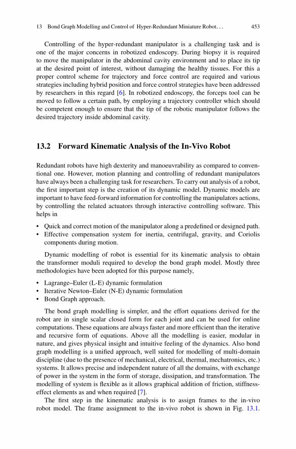
13 Bond Graph Modelling and Control of Hyper-Redundant Miniature Robot. . . 453
Controlling of the hyper-redundant manipulator is a challenging task and isone of the major concerns in robotized endoscopy. During biopsy it is requiredto move the manipulator in the abdominal cavity environment and to place its tipat the desired point of interest, without damaging the healthy tissues. For this aproper control scheme for trajectory and force control are required and variousstrategies including hybrid position and force control strategies have been addressedby researchers in this regard [6]. In robotized endoscopy, the forceps tool can bemoved to follow a certain path, by employing a trajectory controller which shouldbe competent enough to ensure that the tip of the robotic manipulator follows thedesired trajectory inside abdominal cavity.
13.2 Forward Kinematic Analysis of the In-Vivo Robot
Redundant robots have high dexterity and manoeuvrability as compared to conven-tional one. However, motion planning and controlling of redundant manipulatorshave always been a challenging task for researchers. To carry out analysis of a robot,the first important step is the creation of its dynamic model. Dynamic models areimportant to have feed-forward information for controlling the manipulators actions,by controlling the related actuators through interactive controlling software. Thishelps in
• Quick and correct motion of the manipulator along a predefined or designed path.• Effective compensation system for inertia, centrifugal, gravity, and Coriolis
components during motion.
Dynamic modelling of robot is essential for its kinematic analysis to obtainthe transformer moduli required to develop the bond graph model. Mostly threemethodologies have been adopted for this purpose namely,
• Lagrange–Euler (L-E) dynamic formulation• Iterative Newton–Euler (N-E) dynamic formulation• Bond Graph approach.
The bond graph modelling is simpler, and the effort equations derived for therobot are in single scalar closed form for each joint and can be used for onlinecomputations. These equations are always faster and more efficient than the iterativeand recursive form of equations. Above all the modelling is easier, modular innature, and gives physical insight and intuitive feeling of the dynamics. Also bondgraph modelling is a unified approach, well suited for modelling of multi-domaindiscipline (due to the presence of mechanical, electrical, thermal, mechatronics, etc.)systems. It allows precise and independent nature of all the domains, with exchangeof power in the system in the form of storage, dissipation, and transformation. Themodelling of system is flexible as it allows graphical addition of friction, stiffness-effect elements as and when required [7].
The first step in the kinematic analysis is to assign frames to the in-vivorobot model. The frame assignment to the in-vivo robot is shown in Fig. 13.1.
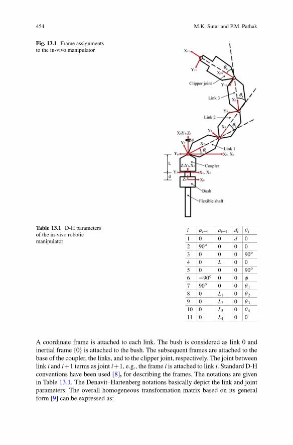
454 M.K. Sutar and P.M. Pathak
Fig. 13.1 Frame assignmentsto the in-vivo manipulator
Table 13.1 D-H parametersof the in-vivo roboticmanipulator
i ˛i�1 ai�1 di � i
1 0 0 d 02 90ı 0 0 03 0 0 0 90ı
4 0 L 0 05 0 0 0 90ı
6 �90ı 0 0 �
7 90ı 0 0 �1
8 0 L1 0 �2
9 0 L2 0 �3
10 0 L3 0 �4
11 0 L4 0 0
A coordinate frame is attached to each link. The bush is considered as link 0 andinertial frame f0g is attached to the bush. The subsequent frames are attached to thebase of the coupler, the links, and to the clipper joint, respectively. The joint betweenlink i and iC1 terms as joint iC1, e.g., the frame i is attached to link i. Standard D-Hconventions have been used [8], for describing the frames. The notations are givenin Table 13.1. The Denavit–Hartenberg notations basically depict the link and jointparameters. The overall homogeneous transformation matrix based on its generalform [9] can be expressed as:
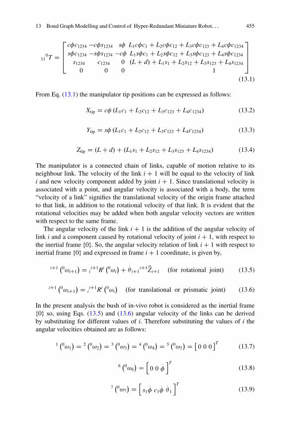
13 Bond Graph Modelling and Control of Hyper-Redundant Miniature Robot. . . 455
110T D
2
664
c�c1234 �c�s1234 s� L1c�c1 C L2c�c12 C L3c�c123 C L4c�c1234s�c1234 �s�s1234 �c� L1s�c1 C L2s�c12 C L3s�c123 C L4s�c1234
s1234 c1234 0 .L C d/C L1s1 C L2s12 C L3s123 C L4s12340 0 0 1
3
775
(13.1)
From Eq. (13.1) the manipulator tip positions can be expressed as follows:
Xtip D c� .L1c1 C L2c12 C L3c123 C L4c1234/ (13.2)
Ytip D s� .L1c1 C L2c12 C L3c123 C L4c1234/ (13.3)
Ztip D .L C d/C .L1s1 C L2s12 C L3s123 C L4s1234/ (13.4)
The manipulator is a connected chain of links, capable of motion relative to itsneighbour link. The velocity of the link i C 1 will be equal to the velocity of linki and new velocity component added by joint i C 1. Since translational velocity isassociated with a point, and angular velocity is associated with a body, the term“velocity of a link” signifies the translational velocity of the origin frame attachedto that link, in addition to the rotational velocity of that link. It is evident that therotational velocities may be added when both angular velocity vectors are writtenwith respect to the same frame.
The angular velocity of the link i C 1 is the addition of the angular velocity oflink i and a component caused by rotational velocity of joint i C 1, with respect tothe inertial frame f0g. So, the angular velocity relation of link i C 1 with respect toinertial frame f0g and expressed in frame i C 1 coordinate, is given by,
iC1 �0!iC1� D i
iC1Ri�0!i�C
:
� iC1iC1bZiC1 .for rotational joint/ (13.5)
iC1 �0!iC1� D i
iC1Ri�0!i�
.for translational or prismatic joint/ (13.6)
In the present analysis the bush of in-vivo robot is considered as the inertial framef0g so, using Eqs. (13.5) and (13.6) angular velocity of the links can be derivedby substituting for different values of i. Therefore substituting the values of i theangular velocities obtained are as follows:
1�0!1
� D 2�0!2
� D 3�0!3
� D 4�0!4
� D 5�0!5
� D �0 0 0
�T(13.7)
6�0!6
� Dh0 0
:
�
iT(13.8)
7�0!7
� Dh
s1:
� c1:
�:
�1
iT(13.9)
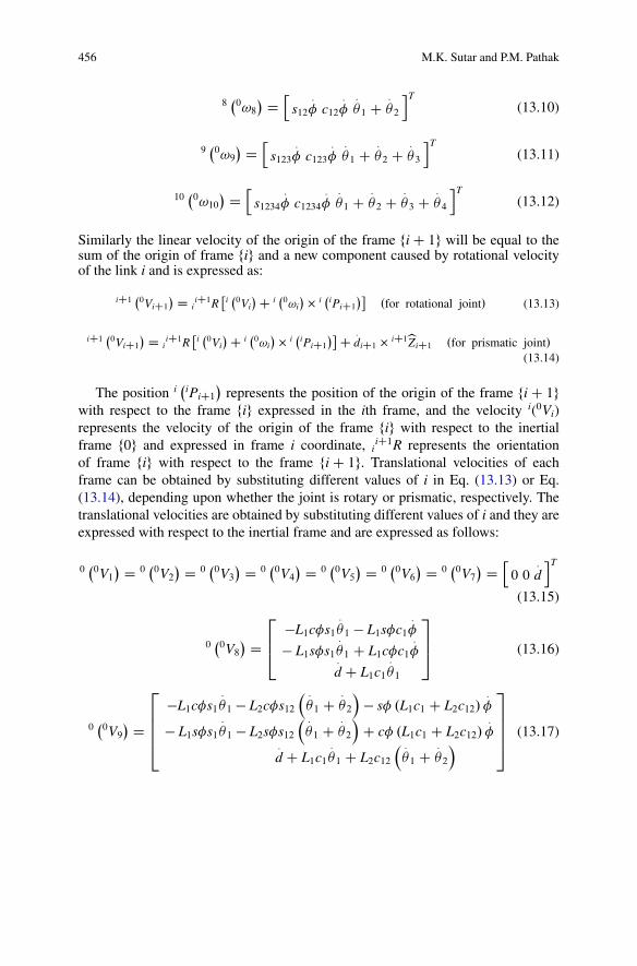
456 M.K. Sutar and P.M. Pathak
8�0!8
� Dh
s12:
� c12:
�:
�1 C:
�2
iT(13.10)
9�0!9
� Dh
s123:
� c123:
�:
�1 C:
�2 C:
�3
iT(13.11)
10�0!10
� Dh
s1234:
� c1234:
�:
�1 C:
�2 C:
�3 C:
�4
iT(13.12)
Similarly the linear velocity of the origin of the frame fi C 1g will be equal to thesum of the origin of frame fig and a new component caused by rotational velocityof the link i and is expressed as:
iC1�0ViC1
� D iiC1R
�i�0Vi
�C i�0!i
�� i�
iPiC1
��.for rotational joint/ (13.13)
iC1�0ViC1
� D iiC1R
�i�0Vi
�C i�0!i
�� i�
iPiC1
��C :
diC1 � iC1bZiC1 .for prismatic joint/(13.14)
The position i�
iPiC1�
represents the position of the origin of the frame fi C 1gwith respect to the frame fig expressed in the ith frame, and the velocity i(0Vi)represents the velocity of the origin of the frame fig with respect to the inertialframe f0g and expressed in frame i coordinate, i
iC1R represents the orientationof frame fig with respect to the frame fi C 1g. Translational velocities of eachframe can be obtained by substituting different values of i in Eq. (13.13) or Eq.(13.14), depending upon whether the joint is rotary or prismatic, respectively. Thetranslational velocities are obtained by substituting different values of i and they areexpressed with respect to the inertial frame and are expressed as follows:
0�0V1
� D 0�0V2
� D 0�0V3
� D 0�0V4
� D 0�0V5
� D 0�0V6
� D 0�0V7
� Dh0 0
:
diT
(13.15)
0�0V8
� D
2
64�L1c�s1
:
�1 � L1s�c1:
�
� L1s�s1:
�1 C L1c�c1:
�:
d C L1c1:
�1
3
75 (13.16)
0�0V9
� D
2
6664
�L1c�s1:
�1 � L2c�s12 :�1 C
:
�2
� s� .L1c1 C L2c12/
:
�
� L1s�s1:
�1 � L2s�s12 :�1 C
:
�2
C c� .L1c1 C L2c12/
:
�:
d C L1c1:
�1 C L2c12 :�1 C
:
�2
3
7775 (13.17)
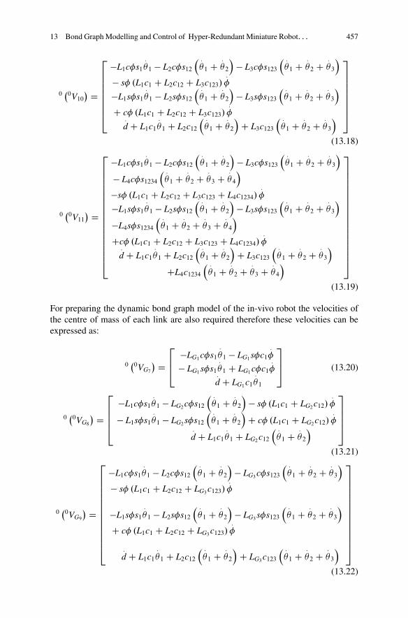
13 Bond Graph Modelling and Control of Hyper-Redundant Miniature Robot. . . 457
0�0V10
� D
2
66666664
�L1c�s1:
�1 � L2c�s12 :�1 C
:
�2
� L3c�s123
:�1 C
:
�2 C:
�3
� s� .L1c1 C L2c12 C L3c123/:
�
�L1s�s1:
�1 � L2s�s12 :�1 C
:
�2
� L3s�s123
:�1 C
:
�2 C:
�3
C c� .L1c1 C L2c12 C L3c123/:
�:
d C L1c1:
�1 C L2c12 :�1 C
:
�2
C L3c123
:�1 C
:
�2 C:
�3
3
77777775
(13.18)
0�0V11
� D
2
66666666666666664
�L1c�s1:
�1 � L2c�s12 :�1 C
:
�2
� L3c�s123
:�1 C
:
�2 C:
�3
� L4c�s1234 :�1 C
:
�2 C:
�3 C:
�4
�s� .L1c1 C L2c12 C L3c123 C L4c1234/:
�
�L1s�s1:
�1 � L2s�s12 :�1 C
:
�2
� L3s�s123
:�1 C
:
�2 C:
�3
�L4s�s1234 :�1 C
:
�2 C:
�3 C:
�4
Cc� .L1c1 C L2c12 C L3c123 C L4c1234/:
�:
d C L1c1:
�1 C L2c12 :�1 C
:
�2
C L3c123
:�1 C
:
�2 C:
�3
CL4c1234 :�1 C
:
�2 C:
�3 C:
�4
3
77777777777777775
(13.19)
For preparing the dynamic bond graph model of the in-vivo robot the velocities ofthe centre of mass of each link are also required therefore these velocities can beexpressed as:
0�0VG7
� D
2
64�LG1c�s1
:
�1 � LG1s�c1:
�
� LG1s�s1:
�1 C LG1c�c1:
�:
d C LG1c1:
�1
3
75 (13.20)
0�0VG8
� D
2
6664
�L1c�s1:
�1 � LG2c�s12 :�1 C
:
�2
� s� .L1c1 C LG2c12/
:
�
� L1s�s1:
�1 � LG2s�s12 :�1 C
:
�2
C c� .L1c1 C LG2c12/
:
�:
d C L1c1:
�1 C LG2c12 :�1 C
:
�2
3
7775
(13.21)
0�0VG9
� D
2
6666666666664
�L1c�s1:
�1 � L2c�s12 :�1 C
:
�2
� LG3c�s123
:�1 C
:
�2 C:
�3
� s� .L1c1 C L2c12 C LG3c123/:
�
�L1s�s1:
�1 � L2s�s12 :�1 C
:
�2
� LG3s�s123
:�1 C
:
�2 C:
�3
C c� .L1c1 C L2c12 C LG3c123/:
�
:
d C L1c1:
�1 C L2c12 :�1 C
:
�2
C LG3c123
:�1 C
:
�2 C:
�3
3
7777777777775
(13.22)
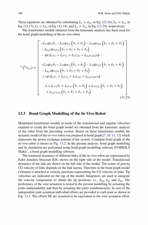
458 M.K. Sutar and P.M. Pathak
These equations are obtained by substituting L1 D LG1 in Eq. (13.16), L2 D LG2 inEq. (13.17), L3 D LG3 in Eq. (13.18), and L4 D LG4 in Eq. (13.19), respectively.
The transformer moduli obtained from the kinematic analysis has been used forthe bond graph modelling of the in-vivo robot.
0�0VG10
� D
2
6666666666666666666664
�L1c�s1:
�1 � L2c�s12 :�1 C
:
�2
� L3c�s123
:�1 C
:
�2 C:
�3
� LG4c�s1234 :�1 C
:
�2 C:
�3 C:
�4
� s� .L1c1 C L2c12 C L3c123 C LG4c1234/:
�
�L1s�s1:
�1 � L2s�s12 :�1 C
:
�2
� L3s�s123
:�1 C
:
�2 C:
�3
� LG4s�s1234 :�1 C
:
�2 C:
�3 C:
�4
C c� .L1c1 C L2c12 C L3c123 C LG4c1234/:
�
:
d C L1c1:
�1 C L2c12 :�1 C
:
�2
C L3c123
:�1 C
:
�2 C:
�3
C LG4c1234 :�1 C
:
�2 C:
�3 C:
�4
3
7777777777777777777775
(13.23)
13.3 Bond Graph Modelling of the In-Vivo Robot
Modulated transformer moduli in terms of the translational and angular velocitiesrequired to create the bond graph model are obtained from the kinematic analysisof the robot from the preceding section. Based on these transformer moduli thedynamic model of the in-vivo robot was prepared in bond graph [7, 10, 11, 12] whichrepresents the power exchange portrait of the system. Complete bond graph of thein-vivo robot is shown in Fig. 13.2. In the present analysis, bond graph modellingand its simulation are performed using bond graph modelling software SYMBOLSShakti
®, a bond graph modelling software.
The rotational dynamics of different links of the in-vivo robot are represented byEuler Junction Structure EJS, shown on the right side of the model. Translationaldynamics of the link are shown on the left side of the model. The centre of gravityCG velocity of links depends on the link inertia. Therefore in the bond graph modelI element is attached at velocity junctions representing the CG velocity of links. Tipvelocities are indicated on the top of the model. Integrators are used to integratethe velocity components to obtain the tip positions, i.e., Xtip, Ytip and Ztip. Theproficiency of the wire actuation is tested in the present modelling by actuating thejoints independently and then by actuating the joints simultaneously. In case of theindependent joint actuation individual efforts are provided to each joint as shown inFig. 13.2. The efforts SE are assumed to be equivalent to the wire actuation effort.
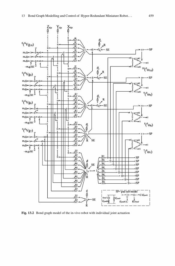
13 Bond Graph Modelling and Control of Hyper-Redundant Miniature Robot. . . 459
Fig. 13.2 Bond graph model of the in-vivo robot with individual joint actuation

460 M.K. Sutar and P.M. Pathak
For rotation of joint a very negligible joint resistance of 0.001 Nm/ (rad/s) is givenand when it is required to lock the joint the joint resistance is set at 10,000 Nm/(rad/s).
13.3.1 Independent Joint Actuation Through Wire Actuation
The initial validity of the bond graph model was tested without wire actuation witha four-scaled model. For the simulation various parameters used are as enlisted inTable 13.2. The initial configuration of the robot is shown in Fig. 13.3. Initially thevalidity of the bond graph was checked without wire actuation. A torque of 2 Nmwas applied on 1st joint and it was rotated while all other joints were locked at zerodegree initial value. As it can be seen a circle of 0.176 m radius (sum of four planarlink lengths) was obtained in X-Y plane, as shown in Fig. 13.4. A torque of 2 Nmwas applied on 1st joint and it was rotated while all other joints were locked at zerodegree initial value.
Tip trajectory obtained is a circle of 0.176 m radius in X-Z plane as plotted inFig. 13.5. Physically this configuration is possible when the manipulator is out ofthe tool channel and is inside the stomach model.
13.3.2 Simultaneous Joint Actuation Through Wire Actuation
For simultaneous joint wire actuation efforts are provided to each joint through thewire actuation as shown in Fig. 13.6. Wire actuation system is integrated in the bondgraph model and shown on the top right-hand side of the figure. Wire flexibility in
Table 13.2 Simulationparameters for in-vivo robotwithout wire actuation
Parameter Value
Link length 0.044 mLink mass 0.001 kgTorque applied 2 NmJoint resistance R1D0.001 Nm/ (rad/s)
Fig. 13.3 Initialconfiguration of the in-vivorobot
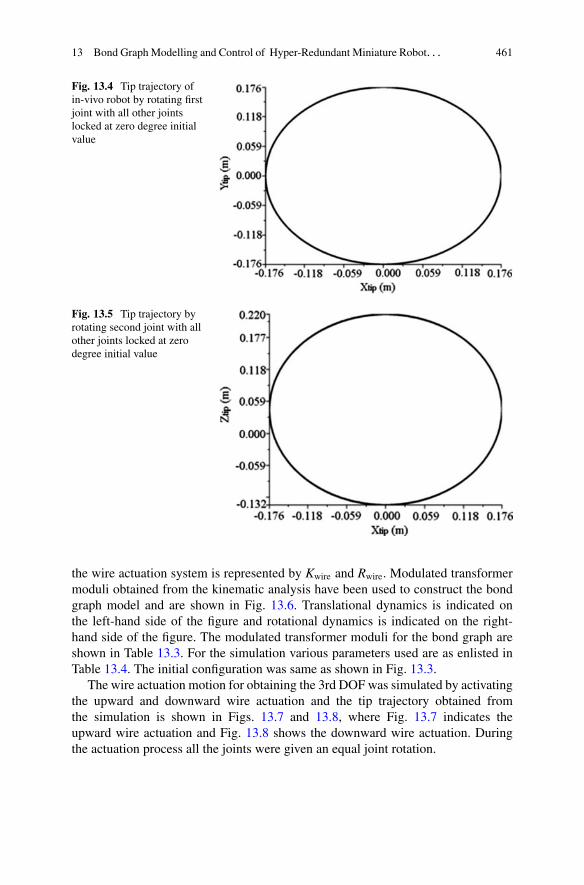
13 Bond Graph Modelling and Control of Hyper-Redundant Miniature Robot. . . 461
Fig. 13.4 Tip trajectory ofin-vivo robot by rotating firstjoint with all other jointslocked at zero degree initialvalue
Fig. 13.5 Tip trajectory byrotating second joint with allother joints locked at zerodegree initial value
the wire actuation system is represented by Kwire and Rwire. Modulated transformermoduli obtained from the kinematic analysis have been used to construct the bondgraph model and are shown in Fig. 13.6. Translational dynamics is indicated onthe left-hand side of the figure and rotational dynamics is indicated on the right-hand side of the figure. The modulated transformer moduli for the bond graph areshown in Table 13.3. For the simulation various parameters used are as enlisted inTable 13.4. The initial configuration was same as shown in Fig. 13.3.
The wire actuation motion for obtaining the 3rd DOF was simulated by activatingthe upward and downward wire actuation and the tip trajectory obtained fromthe simulation is shown in Figs. 13.7 and 13.8, where Fig. 13.7 indicates theupward wire actuation and Fig. 13.8 shows the downward wire actuation. Duringthe actuation process all the joints were given an equal joint rotation.
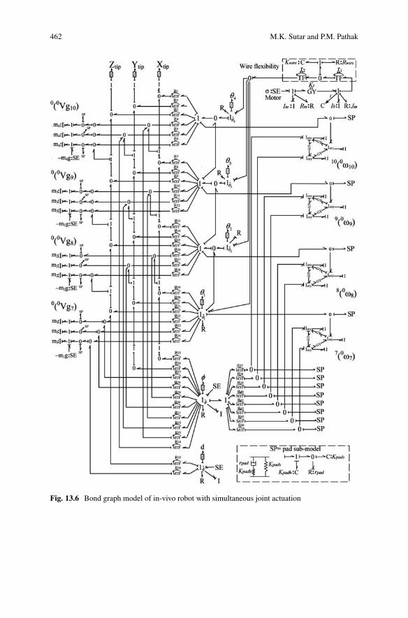
462 M.K. Sutar and P.M. Pathak
Fig. 13.6 Bond graph model of in-vivo robot with simultaneous joint actuation
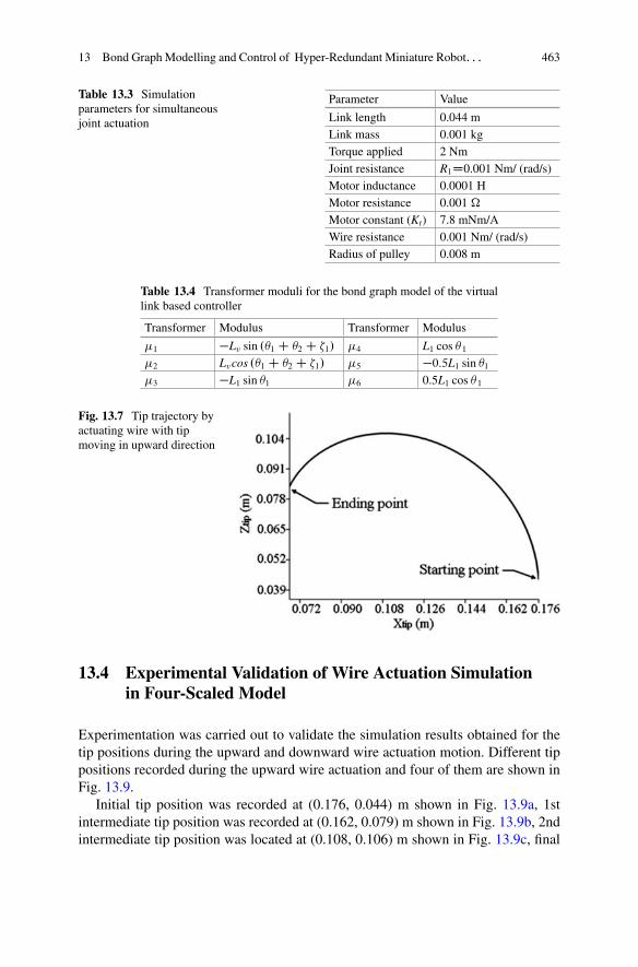
13 Bond Graph Modelling and Control of Hyper-Redundant Miniature Robot. . . 463
Table 13.3 Simulationparameters for simultaneousjoint actuation
Parameter Value
Link length 0.044 mLink mass 0.001 kgTorque applied 2 NmJoint resistance R1D0.001 Nm/ (rad/s)Motor inductance 0.0001 HMotor resistance 0.001 �Motor constant (Kt) 7.8 mNm/AWire resistance 0.001 Nm/ (rad/s)Radius of pulley 0.008 m
Table 13.4 Transformer moduli for the bond graph model of the virtuallink based controller
Transformer Modulus Transformer Modulus
�1 �Lv sin .�1 C �2 C �1/ �4 L1 cos �1
�2 Lvcos .�1 C �2 C �1/ �5 �0:5L1 sin �1�3 �L1 sin �1 �6 0.5L1 cos �1
Fig. 13.7 Tip trajectory byactuating wire with tipmoving in upward direction
13.4 Experimental Validation of Wire Actuation Simulationin Four-Scaled Model
Experimentation was carried out to validate the simulation results obtained for thetip positions during the upward and downward wire actuation motion. Different tippositions recorded during the upward wire actuation and four of them are shown inFig. 13.9.
Initial tip position was recorded at (0.176, 0.044) m shown in Fig. 13.9a, 1stintermediate tip position was recorded at (0.162, 0.079) m shown in Fig. 13.9b, 2ndintermediate tip position was located at (0.108, 0.106) m shown in Fig. 13.9c, final
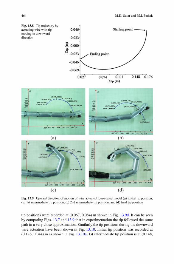
464 M.K. Sutar and P.M. Pathak
Fig. 13.8 Tip trajectory byactuating wire with tipmoving in downwarddirection
Fig. 13.9 Upward direction of motion of wire actuated four-scaled model (a) initial tip position,(b) 1st intermediate tip position, (c) 2nd intermediate tip position, and (d) final tip position
tip positions were recorded at (0.067, 0.084) m shown in Fig. 13.9d. It can be seenby comparing Figs. 13.7 and 13.9 that in experimentation the tip followed the samepath in a very close approximation. Similarly the tip positions during the downwardwire actuation have been shown in Fig. 13.10. Initial tip position was recorded at(0.176, 0.044) m as shown in Fig. 13.10a, 1st intermediate tip position is at (0.148,
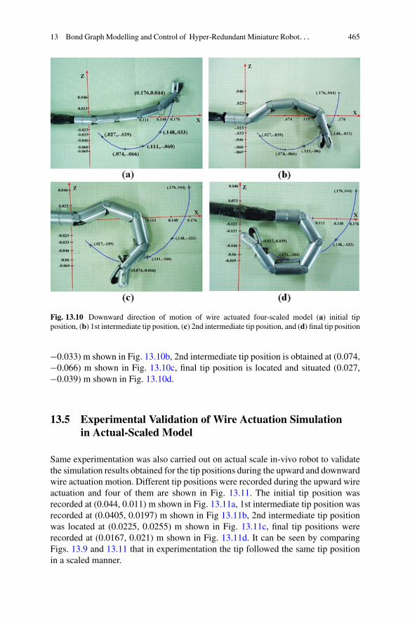
13 Bond Graph Modelling and Control of Hyper-Redundant Miniature Robot. . . 465
Fig. 13.10 Downward direction of motion of wire actuated four-scaled model (a) initial tipposition, (b) 1st intermediate tip position, (c) 2nd intermediate tip position, and (d) final tip position
�0.033) m shown in Fig. 13.10b, 2nd intermediate tip position is obtained at (0.074,�0.066) m shown in Fig. 13.10c, final tip position is located and situated (0.027,�0.039) m shown in Fig. 13.10d.
13.5 Experimental Validation of Wire Actuation Simulationin Actual-Scaled Model
Same experimentation was also carried out on actual scale in-vivo robot to validatethe simulation results obtained for the tip positions during the upward and downwardwire actuation motion. Different tip positions were recorded during the upward wireactuation and four of them are shown in Fig. 13.11. The initial tip position wasrecorded at (0.044, 0.011) m shown in Fig. 13.11a, 1st intermediate tip position wasrecorded at (0.0405, 0.0197) m shown in Fig 13.11b, 2nd intermediate tip positionwas located at (0.0225, 0.0255) m shown in Fig. 13.11c, final tip positions wererecorded at (0.0167, 0.021) m shown in Fig. 13.11d. It can be seen by comparingFigs. 13.9 and 13.11 that in experimentation the tip followed the same tip positionin a scaled manner.
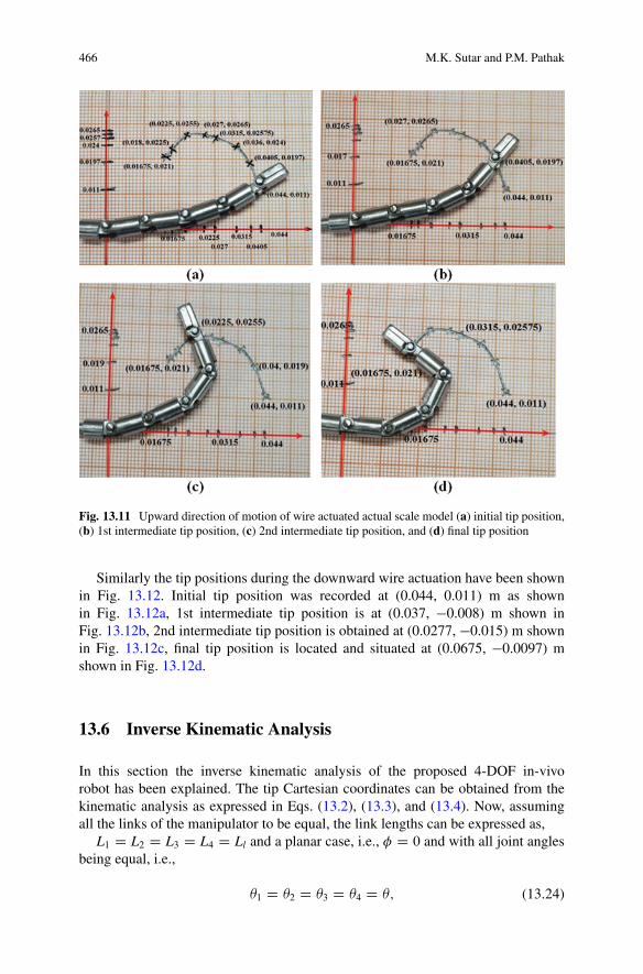
466 M.K. Sutar and P.M. Pathak
Fig. 13.11 Upward direction of motion of wire actuated actual scale model (a) initial tip position,(b) 1st intermediate tip position, (c) 2nd intermediate tip position, and (d) final tip position
Similarly the tip positions during the downward wire actuation have been shownin Fig. 13.12. Initial tip position was recorded at (0.044, 0.011) m as shownin Fig. 13.12a, 1st intermediate tip position is at (0.037, �0.008) m shown inFig. 13.12b, 2nd intermediate tip position is obtained at (0.0277, �0.015) m shownin Fig. 13.12c, final tip position is located and situated at (0.0675, �0.0097) mshown in Fig. 13.12d.
13.6 Inverse Kinematic Analysis
In this section the inverse kinematic analysis of the proposed 4-DOF in-vivorobot has been explained. The tip Cartesian coordinates can be obtained from thekinematic analysis as expressed in Eqs. (13.2), (13.3), and (13.4). Now, assumingall the links of the manipulator to be equal, the link lengths can be expressed as,
L1 D L2 D L3 D L4 D Ll and a planar case, i.e., � D 0 and with all joint anglesbeing equal, i.e.,
�1 D �2 D �3 D �4 D �; (13.24)
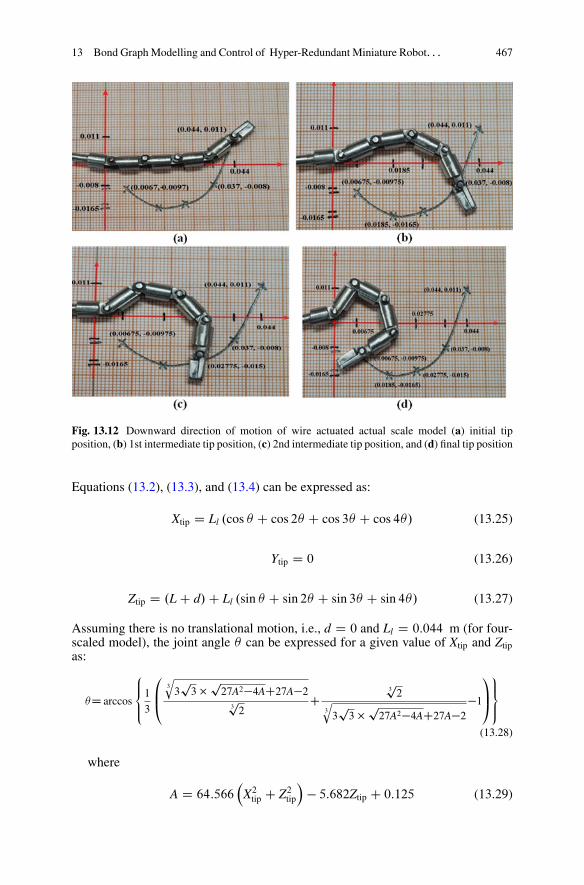
13 Bond Graph Modelling and Control of Hyper-Redundant Miniature Robot. . . 467
Fig. 13.12 Downward direction of motion of wire actuated actual scale model (a) initial tipposition, (b) 1st intermediate tip position, (c) 2nd intermediate tip position, and (d) final tip position
Equations (13.2), (13.3), and (13.4) can be expressed as:
Xtip D Ll .cos � C cos 2� C cos 3� C cos 4�/ (13.25)
Ytip D 0 (13.26)
Ztip D .L C d/C Ll .sin � C sin 2� C sin 3� C sin 4�/ (13.27)
Assuming there is no translational motion, i.e., d D 0 and Ll D 0:044 m (for four-scaled model), the joint angle � can be expressed for a given value of Xtip and Ztipas:
�D arccos
8<
:1
3
0
B@3
q3p3�p27A2�4AC27A�2
3p2
C3p2
3
q3p3�p27A2�4AC27A�2
�11
CA
9>=
>;
(13.28)
where
A D 64:566
X2tip C Z2tip
� 5:682Ztip C 0:125 (13.29)

468 M.K. Sutar and P.M. Pathak
Fig. 13.13 Representation ofwire actuated section ofin-vivo robot arm
Fig. 13.14 Link segmentbetween link 1 and link 2
13.6.1 Determination of Joint Angle in Terms of Wire Length
A relational approach has been established to express joint angle in terms of thelength of outer and inner wire used in actuation. In the analysis it is assumed thatthe wire actuated portion comprising of four articulated links as shown in Fig. 13.13is a perfect arc of a circle.
Now considering a two link segment of the above entire section, i.e., link 1 andlink 2 of joint angle �2 shown in Fig. 13.14, and considering the wire actuationon the two link segment length of outer and inner wire length are as follows,respectively:
l2 D la C lb and;
l1 D lc C ld

13 Bond Graph Modelling and Control of Hyper-Redundant Miniature Robot. . . 469
The relation between the outer and inner wire length can be obtained by consideringthe whole wire actuated portion as shown in Fig. 13.14., and with a known relationla D lc.
The outer wire length is
Lo D 4la C 3lb (13.30)
and the inner wire length is
Lo D 4la C 3lb (13.31)
From Fig. 13.14 the following geometrical relation can be deduced:
sin�2
2D lb � ld
2D(13.32)
where D is the diameter of link. Substituting the values of lb and ld from Eqs. (13.30)and (13.31) in Eq. (13.32), we have
sin�2
2D� Lo�4la
3
� � � Li�4lc3
�
2D(13.33)
Further simplifying the difference in outer and inner wire length can be expressedas:
L0 � Li D 6D sin�
2(13.34)
If wire is wrapped on the same pulley, with direction of wrapping for outer wire tobe opposite to that of inner wire, the length of wire wrapped on pulley is given by,
L0 � Li D rp:�p (13.35)
where rp is the radius of pulley and �p is the pulley rotation. Substituting the valueof Lo � Li from Eq. (13.34) in Eq. (13.35) the pulley rotation can be expressed as:
�p D �6D=rp
�sin .�=2/ (13.36)
Thus for a given Xtip and Ztip one can find � from Eq. (13.28) and for this � , thevalue of pulley rotation �p in terms of tip positions can be obtained. A ProportionalDerivative (PD) controller can be used to take the pulley to desired �p rotation, thusthe robot can be moved to a desired position. To implement the inverse kinematicssolution the motor voltage for a desired pulley rotation corresponding to desired tiplocation can be evaluated as:
V D Kp��p � �a
�C Kv :�p �
:
�a
(13.37)
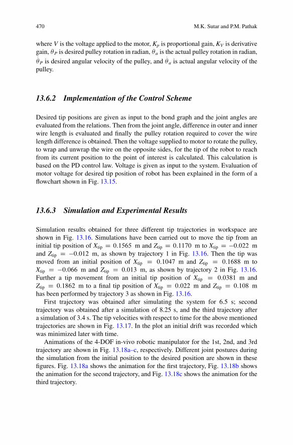
470 M.K. Sutar and P.M. Pathak
where V is the voltage applied to the motor, Kp is proportional gain, KV is derivativegain, �P is desired pulley rotation in radian, �a is the actual pulley rotation in radian,:
�P is desired angular velocity of the pulley, and:
�a is actual angular velocity of thepulley.
13.6.2 Implementation of the Control Scheme
Desired tip positions are given as input to the bond graph and the joint angles areevaluated from the relations. Then from the joint angle, difference in outer and innerwire length is evaluated and finally the pulley rotation required to cover the wirelength difference is obtained. Then the voltage supplied to motor to rotate the pulley,to wrap and unwrap the wire on the opposite sides, for the tip of the robot to reachfrom its current position to the point of interest is calculated. This calculation isbased on the PD control law. Voltage is given as input to the system. Evaluation ofmotor voltage for desired tip position of robot has been explained in the form of aflowchart shown in Fig. 13.15.
13.6.3 Simulation and Experimental Results
Simulation results obtained for three different tip trajectories in workspace areshown in Fig. 13.16. Simulations have been carried out to move the tip from aninitial tip position of Xtip D 0:1565 m and Ztip D 0:1170 m to Xtip D �0:022 mand Ztip D �0:012 m, as shown by trajectory 1 in Fig. 13.16. Then the tip wasmoved from an initial position of Xtip D 0:1047 m and Ztip D 0:1688 m toXtip D �0:066 m and Ztip D 0:013 m, as shown by trajectory 2 in Fig. 13.16.Further a tip movement from an initial tip position of Xtip D 0:0381 m andZtip D 0:1862 m to a final tip position of Xtip D 0:022 m and Ztip D 0:108 mhas been performed by trajectory 3 as shown in Fig. 13.16.
First trajectory was obtained after simulating the system for 6.5 s; secondtrajectory was obtained after a simulation of 8.25 s, and the third trajectory aftera simulation of 3.4 s. The tip velocities with respect to time for the above mentionedtrajectories are shown in Fig. 13.17. In the plot an initial drift was recorded whichwas minimized later with time.
Animations of the 4-DOF in-vivo robotic manipulator for the 1st, 2nd, and 3rdtrajectory are shown in Fig. 13.18a–c, respectively. Different joint postures duringthe simulation from the initial position to the desired position are shown in thesefigures. Fig. 13.18a shows the animation for the first trajectory, Fig. 13.18b showsthe animation for the second trajectory, and Fig. 13.18c shows the animation for thethird trajectory.
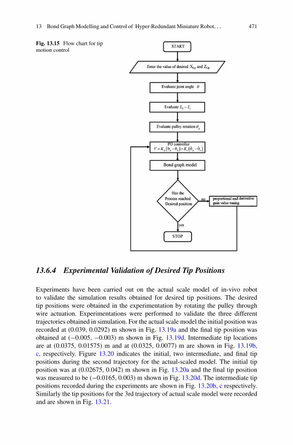
13 Bond Graph Modelling and Control of Hyper-Redundant Miniature Robot. . . 471
Fig. 13.15 Flow chart for tipmotion control
13.6.4 Experimental Validation of Desired Tip Positions
Experiments have been carried out on the actual scale model of in-vivo robotto validate the simulation results obtained for desired tip positions. The desiredtip positions were obtained in the experimentation by rotating the pulley throughwire actuation. Experimentations were performed to validate the three differenttrajectories obtained in simulation. For the actual scale model the initial position wasrecorded at (0.039, 0.0292) m shown in Fig. 13.19a and the final tip position wasobtained at (�0.005, �0.003) m shown in Fig. 13.19d. Intermediate tip locationsare at (0.0375, 0.01575) m and at (0.0325, 0.0077) m are shown in Fig. 13.19b,c, respectively. Figure 13.20 indicates the initial, two intermediate, and final tippositions during the second trajectory for the actual-scaled model. The initial tipposition was at (0.02675, 0.042) m shown in Fig. 13.20a and the final tip positionwas measured to be (�0.0165, 0.003) m shown in Fig. 13.20d. The intermediate tippositions recorded during the experiments are shown in Fig. 13.20b, c respectively.Similarly the tip positions for the 3rd trajectory of actual scale model were recordedand are shown in Fig. 13.21.
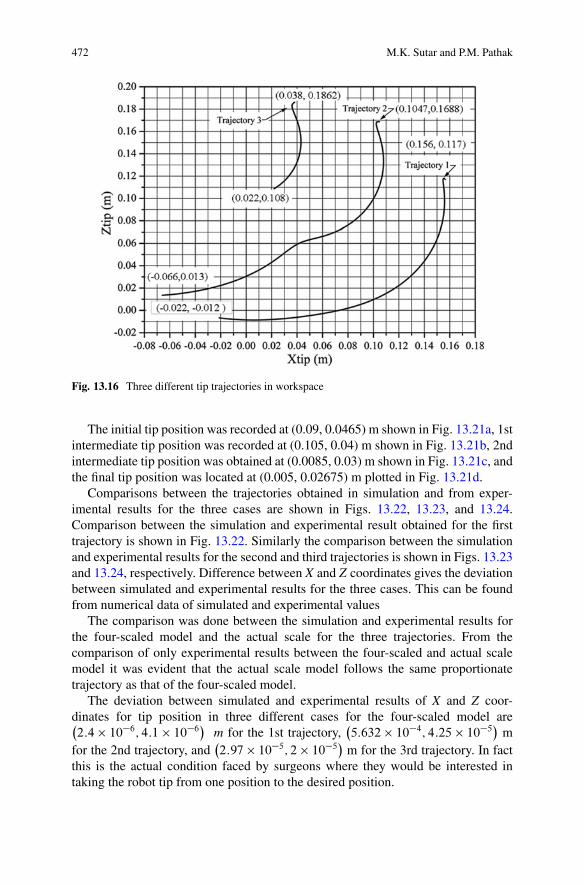
472 M.K. Sutar and P.M. Pathak
Fig. 13.16 Three different tip trajectories in workspace
The initial tip position was recorded at (0.09, 0.0465) m shown in Fig. 13.21a, 1stintermediate tip position was recorded at (0.105, 0.04) m shown in Fig. 13.21b, 2ndintermediate tip position was obtained at (0.0085, 0.03) m shown in Fig. 13.21c, andthe final tip position was located at (0.005, 0.02675) m plotted in Fig. 13.21d.
Comparisons between the trajectories obtained in simulation and from exper-imental results for the three cases are shown in Figs. 13.22, 13.23, and 13.24.Comparison between the simulation and experimental result obtained for the firsttrajectory is shown in Fig. 13.22. Similarly the comparison between the simulationand experimental results for the second and third trajectories is shown in Figs. 13.23and 13.24, respectively. Difference between X and Z coordinates gives the deviationbetween simulated and experimental results for the three cases. This can be foundfrom numerical data of simulated and experimental values
The comparison was done between the simulation and experimental results forthe four-scaled model and the actual scale for the three trajectories. From thecomparison of only experimental results between the four-scaled and actual scalemodel it was evident that the actual scale model follows the same proportionatetrajectory as that of the four-scaled model.
The deviation between simulated and experimental results of X and Z coor-dinates for tip position in three different cases for the four-scaled model are�2:4 � 10�6; 4:1 � 10�6� m for the 1st trajectory,
�5:632 � 10�4; 4:25 � 10�5� m
for the 2nd trajectory, and�2:97 � 10�5; 2 � 10�5� m for the 3rd trajectory. In fact
this is the actual condition faced by surgeons where they would be interested intaking the robot tip from one position to the desired position.

13 Bond Graph Modelling and Control of Hyper-Redundant Miniature Robot. . . 473
Fig. 13.17 Xtip and Ztip trajectory versus time for (a) 1st trajectory, (b) 2nd trajectory, and (c) 3rdtrajectory
13.7 Trajectory Control Analysis of In-Vivo Robot
Controlling hyper-redundant robotic manipulators as in-vivo manipulators is amajor concern for researchers working in this particular field. During biopsy it isrequired to move the manipulator in the abdominal cavity environment and to placeits tip at the desired point of interest. For this a proper trajectory control scheme isrequired.
A trajectory control scheme for a planar hyper-redundant manipulator has beenproposed. The scheme is based on a virtual link based controller. An example ofthree link planar manipulator is considered to illustrate the methodology. The 3-linkplanar manipulator was modelled using bond graph, and a controller, using thevirtual link concept has been formulated. Relations between the real and virtuallinks were established to design the controller and the virtual link based controllerwas used to send effort signals to all the joints of 3-link planar manipulator uponreceiving a corrective signal from PI controller. Different desired trajectory shapeswere used to check the efficiency of the controller. Simulations and animations havebeen performed to test the competence of the controller.
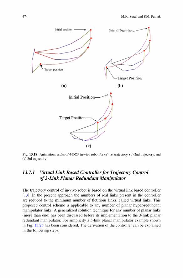
474 M.K. Sutar and P.M. Pathak
Fig. 13.18 Animation results of 4-DOF in-vivo robot for (a) 1st trajectory, (b) 2nd trajectory, and(c) 3rd trajectory
13.7.1 Virtual Link Based Controller for Trajectory Controlof 3-Link Planar Redundant Manipulator
The trajectory control of in-vivo robot is based on the virtual link based controller[13]. In the present approach the numbers of real links present in the controllerare reduced to the minimum number of fictitious links, called virtual links. Thisproposed control scheme is applicable to any number of planar hyper-redundantmanipulator links. A generalized solution technique for any number of planar links(more than one) has been discussed before its implementation to the 3-link planarredundant manipulator. For simplicity a 5-link planar manipulator example shownin Fig. 13.25 has been considered. The derivation of the controller can be explainedin the following steps:
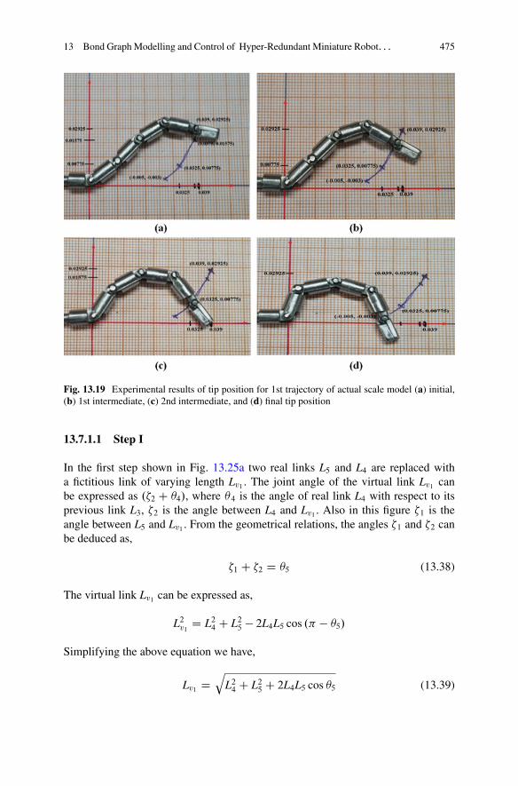
13 Bond Graph Modelling and Control of Hyper-Redundant Miniature Robot. . . 475
Fig. 13.19 Experimental results of tip position for 1st trajectory of actual scale model (a) initial,(b) 1st intermediate, (c) 2nd intermediate, and (d) final tip position
13.7.1.1 Step I
In the first step shown in Fig. 13.25a two real links L5 and L4 are replaced witha fictitious link of varying length Lv1 . The joint angle of the virtual link Lv1 canbe expressed as .�2 C �4/, where �4 is the angle of real link L4 with respect to itsprevious link L3, �2 is the angle between L4 and Lv1 . Also in this figure �1 is theangle between L5 and Lv1 . From the geometrical relations, the angles �1 and �2 canbe deduced as,
�1 C �2 D �5 (13.38)
The virtual link Lv1 can be expressed as,
L2v1 D L24 C L25 � 2L4L5 cos .� � �5/
Simplifying the above equation we have,
Lv1 Dq
L24 C L25 C 2L4L5 cos �5 (13.39)
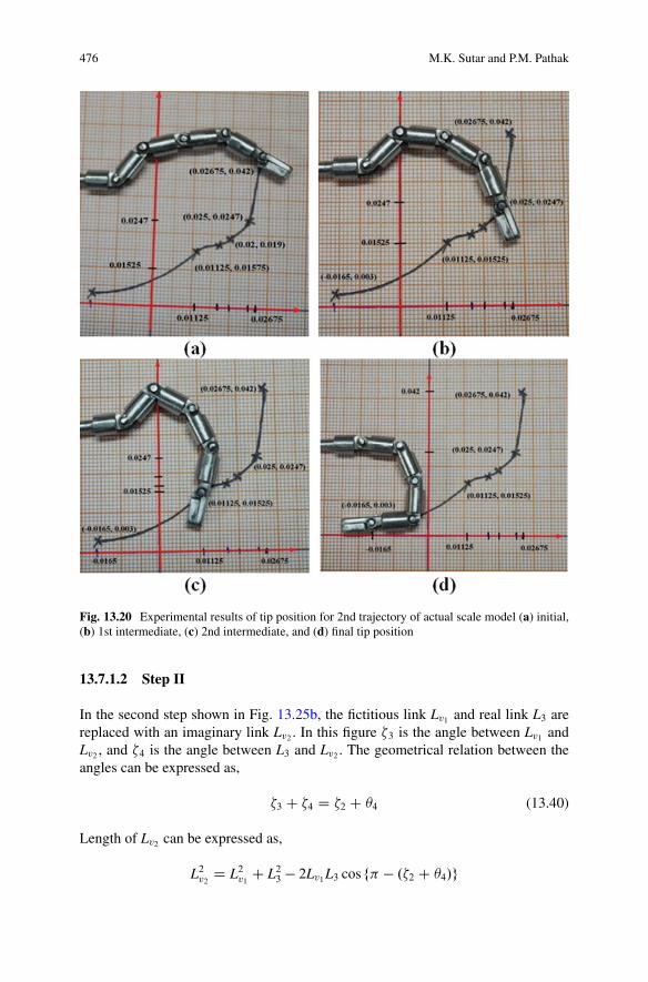
476 M.K. Sutar and P.M. Pathak
Fig. 13.20 Experimental results of tip position for 2nd trajectory of actual scale model (a) initial,(b) 1st intermediate, (c) 2nd intermediate, and (d) final tip position
13.7.1.2 Step II
In the second step shown in Fig. 13.25b, the fictitious link Lv1 and real link L3 arereplaced with an imaginary link Lv2 . In this figure �3 is the angle between Lv1 andLv2 , and �4 is the angle between L3 and Lv2 . The geometrical relation between theangles can be expressed as,
�3 C �4 D �2 C �4 (13.40)
Length of Lv2 can be expressed as,
L2v2 D L2v1 C L23 � 2Lv1L3 cos f� � .�2 C �4/g
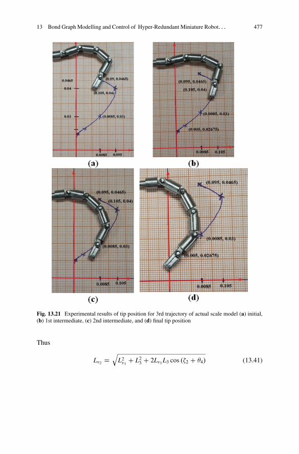
13 Bond Graph Modelling and Control of Hyper-Redundant Miniature Robot. . . 477
Fig. 13.21 Experimental results of tip position for 3rd trajectory of actual scale model (a) initial,(b) 1st intermediate, (c) 2nd intermediate, and (d) final tip position
Thus
Lv2 Dq
L2v1 C L23 C 2Lv1L3 cos .�2 C �4/ (13.41)

478 M.K. Sutar and P.M. Pathak
Fig. 13.22 Comparisonbetween simulation andexperimental result for 1sttrajectory for four-scaledmodel
Fig. 13.23 Comparisonbetween simulation andexperimental result for 2ndtrajectory for four-scaledmodel
13.7.1.3 Step III
In the third step shown in Fig. 13.25c, the fictitious link Lv2 and real link L2 arereplaced with an imaginary link Lv3 . In this figure �5 is the angle between Lv3 andLv2 whereas �6 is the angle between L2 and Lv3 . The geometrical relation betweenthe angles can be expressed as,
�5 C �6 D �4 C �3 (13.42)
The fictitious link length Lv3 can be expressed as,
L2v3 D L2v2 C L22 � 2Lv2L2 cos f� � .�4 C �3/g ;
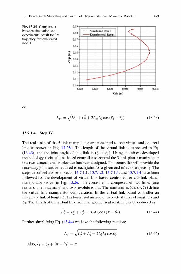
13 Bond Graph Modelling and Control of Hyper-Redundant Miniature Robot. . . 479
Fig. 13.24 Comparisonbetween simulation andexperimental result for 3rdtrajectory for four-scaledmodel
or
Lv3 Dq
L2v2 C L22 C 2Lv2L2 cos .�4 C �3/ (13.43)
13.7.1.4 Step IV
The real links of the 5-link manipulator are converted to one virtual and one reallink, as shown in Fig. 13.25d. The length of the virtual link is expressed in Eq.(13.43), and the joint angle of this link is .�6 C �2/. Using the above developedmethodology a virtual link based controller to control the 3-link planar manipulatorin a two-dimensional workspace has been designed. This controller will provide thenecessary joint torque required to each joint for a given end-effector trajectory. Thesteps described above in Sects. 13.7.1.1, 13.7.1.2, 13.7.1.3, and 13.7.1.4 have beenfollowed for the development of virtual link based controller for a 3-link planarmanipulator shown in Fig. 13.26. The controller is composed of two links (onereal and one imaginary) and two revolute joints. The joint angles (�1, �2, �1) definethe virtual link manipulator configuration. In the virtual link based controller animaginary link of length Lv has been used instead of two actual links of length L2 andL3. The length of the virtual link from the geometrical relation can be deduced as,
L2v D L22 C L23 � 2L2L3 cos .� � �3/ (13.44)
Further simplifying Eq. (13.44) we have the following relation:
Lv Dq
L22 C L23 C 2L2L3 cos �3 (13.45)
Also, �1 C �2 C .� � �3/ D �
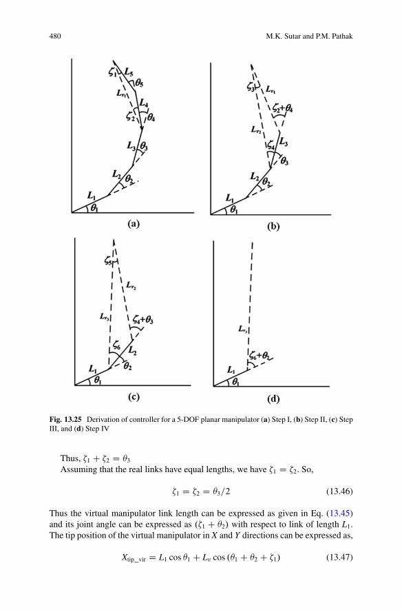
480 M.K. Sutar and P.M. Pathak
Fig. 13.25 Derivation of controller for a 5-DOF planar manipulator (a) Step I, (b) Step II, (c) StepIII, and (d) Step IV
Thus, �1 C �2 D �3Assuming that the real links have equal lengths, we have �1 D �2. So,
�1 D �2 D �3=2 (13.46)
Thus the virtual manipulator link length can be expressed as given in Eq. (13.45)and its joint angle can be expressed as .�1 C �2/ with respect to link of length L1.The tip position of the virtual manipulator in X and Y directions can be expressed as,
Xtip_vir D L1 cos �1 C Lv cos .�1 C �2 C �1/ (13.47)

13 Bond Graph Modelling and Control of Hyper-Redundant Miniature Robot. . . 481
Fig. 13.26 Schematicdiagram of virtual link basedcontroller
Ytip_vir D L1 sin �1 C Lvsin .�1 C �2 C �1/ (13.48)
The corresponding tip velocities can be obtained by differentiating the aboveequations and can be expressed as,
:
Xtip_vir D �L1:
�1 sin �1 � Lv :�1 C
:
�2 C:
�1
sin .�1 C �2 C �1/ (13.49)
:
Y tip_vir D L1:
�1 cos �1 C Lv :�1 C
:
�2 C:
�1
cos .�1 C �2 C �1/ (13.50)
From Eqs. (13.49) and (13.50) different transformer moduli required for developingthe controller based on bond graph for a 3-link planar manipulator can be derivedas shown in Fig. 13.27. The transformer moduli obtained from the above mentionedequations are given in Table 13.4.
These transformer moduli have been used to construct the bond graph modelof the virtual link based controller. The joints of virtual link based controller arerepresented by 1:
�1; 1 :�2
and 1:�1
junction. The difference in the reference and actualvelocity of the manipulator is termed as the error. The error signal is sent to theproportional-integral (PI) controller and it minimizes the error and sends it to thevirtual link based controller. The controller receives the signal from the PI controllerand supplies the required amount of torque to the 3-link planar hyper-redundantmanipulator to obtain the desired tip trajectory. The modulus value at the 1:
�1junction has been taken as 0.5 as per the relation obtained in Eq. (13.46).

482 M.K. Sutar and P.M. Pathak
Fig. 13.27 Bond graph model of virtual link based controller for 3-link planar manipulator
The virtual link based controller is then modelled with dynamic equivalencealong with the plant to simulate different trajectories. The dynamic equivalence isbased on the following three conditions according to [14].
1. The total mass of the real links must be equal to that of the virtual link2. The centre of gravity (CG) of equivalent system must coincide with that of the
virtual link3. Total moment of inertia about an axis through the CG must be equal to that of
the virtual link.
The bond graph model of the dynamically equivalent virtual link based controlleralong with the three link planar manipulator is shown in Fig. 13.28 and the

13 Bond Graph Modelling and Control of Hyper-Redundant Miniature Robot. . . 483
Fig. 13.28 Bond graph model of 3-link planar manipulator
translational dynamics of each link segment in X and Y direction is shown on theleft-hand side of the model. Each link has the CG velocity which depends on thelink inertia. Therefore in the bond graph model I elements are attached at each

484 M.K. Sutar and P.M. Pathak
Table 13.5 D-H parametersof 3-link planar manipulator
i ˛i�1 ai�1 di � i
1 0 0 0 �1
2 0 L1 0 �2
3 0 L2 0 �3
4 0 L3 0 0
Table 13.6 Transformer moduli for the bond graph model of the 3-linkplanar manipulator
Transformer Modulus
�7 �L1 sin �1 � L2 sin .�1 C �2/� 0:5L3 sin .�1 C �2 C �3/�8 �L1 sin �1 � L2 sin .�1 C �2/� L3 sin .�1 C �2 C �3/�9 L1 cos �1 C L2cos .�1 C �2/C L3cos .�1 C �2 C �3/�10 L1 cos �1 C L2cos .�1 C �2/C 0:5L3cos .�1 C �2 C �3/�11 �L1sin�1 � 0:5L2sin .�1 C �2/�12 �L1sin�1 � L2sin .�1 C �2/�13 L1 cos �1 C L2cos .�1 C �2/�14 L1 cos �1 C 0:5L2cos .�1 C �2/�15 �0:5L1 sin �1�16 �L1 sin �1�17 L1 cos �1
�18 0.5L1 cos �1
velocity junction representing the CG velocity of each link. The transformer moduliobtained from the kinematic analysis with the help of the D-H parameters shown inTable 13.5 have been used to draw the bond graph and they are listed in Table 13.6.Soft pads are artificial compliances which have been used in bond graph to avoiddifferential causality.
The tip velocities are indicated on the top of the bond graph model. Integratorsare used to integrate the actual velocity components to obtain the tip positions in Xand Y directions, i.e., Xtip_act and Ytip_act. The reference position of the end-effectortip is denoted by Xtip_ref and Ytip_ref. In Fig. 13.28, J1, J2, and J3 represent the jointinertia, respectively, and the R element on each joint represents the joint resistance.
13.7.2 Simulation and Animation Results
Three types of end-effector trajectories have been considered to validate the controlstrategy. First trajectory is a circle, the second one is a knot-shaped trajectory basedon Lissajous curve [15], and the third one is a cubic polynomial trajectory. Theinitial configuration of the 3-link planar manipulator is shown in Fig. 13.29. Allthe joints were kept at an initial position of 0.698 rad. Parameters used in the
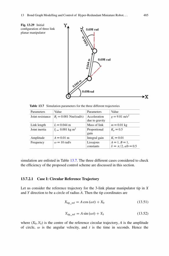
13 Bond Graph Modelling and Control of Hyper-Redundant Miniature Robot. . . 485
Fig. 13.29 Initialconfiguration of three linkplanar manipulator
Table 13.7 Simulation parameters for the three different trajectories
Parameters Value Parameters Value
Joint resistance RjD 0.001 Nm/(rad/s) Accelerationdue to gravity
gD 9.81 m/s2
Link length LD 0.044 m Mass of link mD 0.01 kgJoint inertia Ij D
0.001 kg m2 Proportionalgain
KpD 0.5
Amplitude AD 0.01 m Integral gain KiD 0.01Frequency !D 10 rad/s Lissajous
constantsAD 1, BD 1,ı D �=2, a/bD 0.5
simulation are enlisted in Table 13.7. The three different cases considered to checkthe efficiency of the proposed control scheme are discussed in this section.
13.7.2.1 Case I: Circular Reference Trajectory
Let us consider the reference trajectory for the 3-link planar manipulator tip in Xand Y direction to be a circle of radius A. Then the tip coordinates are
Xtip_ref D A cos .!t/C X0 (13.51)
Ytip_ref D A sin .!t/C Y0 (13.52)
where (X0, Y0) is the centre of the reference circular trajectory, A is the amplitudeof circle, ! is the angular velocity, and t is the time in seconds. Hence the
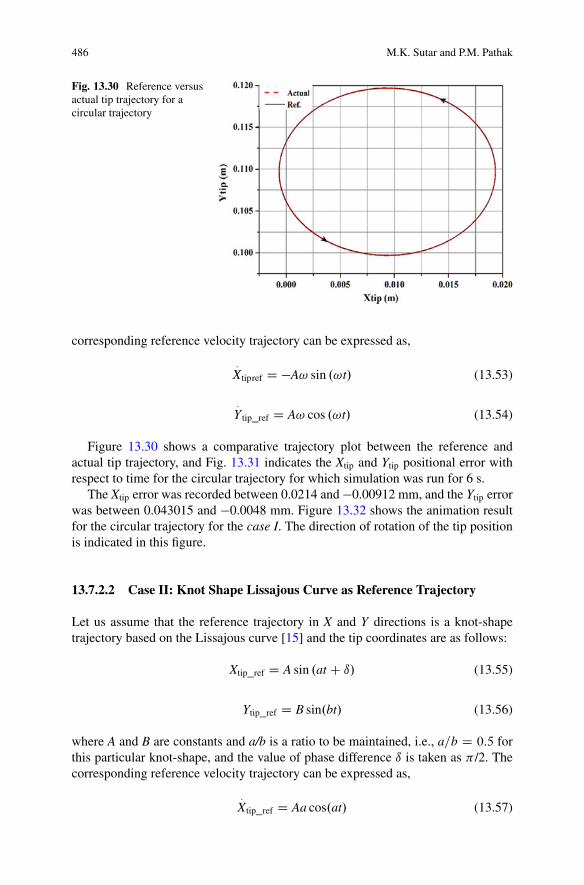
486 M.K. Sutar and P.M. Pathak
Fig. 13.30 Reference versusactual tip trajectory for acircular trajectory
corresponding reference velocity trajectory can be expressed as,
:
Xtipref D �A! sin .!t/ (13.53)
:
Y tip_ref D A! cos .!t/ (13.54)
Figure 13.30 shows a comparative trajectory plot between the reference andactual tip trajectory, and Fig. 13.31 indicates the Xtip and Ytip positional error withrespect to time for the circular trajectory for which simulation was run for 6 s.
The Xtip error was recorded between 0.0214 and �0.00912 mm, and the Ytip errorwas between 0.043015 and �0.0048 mm. Figure 13.32 shows the animation resultfor the circular trajectory for the case I. The direction of rotation of the tip positionis indicated in this figure.
13.7.2.2 Case II: Knot Shape Lissajous Curve as Reference Trajectory
Let us assume that the reference trajectory in X and Y directions is a knot-shapetrajectory based on the Lissajous curve [15] and the tip coordinates are as follows:
Xtip_ref D A sin .at C ı/ (13.55)
Ytip_ref D B sin.bt/ (13.56)
where A and B are constants and a/b is a ratio to be maintained, i.e., a=b D 0:5 forthis particular knot-shape, and the value of phase difference ı is taken as � /2. Thecorresponding reference velocity trajectory can be expressed as,
:
Xtip_ref D Aa cos.at/ (13.57)
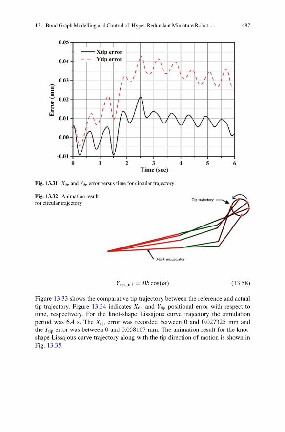
13 Bond Graph Modelling and Control of Hyper-Redundant Miniature Robot. . . 487
Fig. 13.31 Xtip and Ytip error versus time for circular trajectory
Fig. 13.32 Animation resultfor circular trajectory
:
Y tip_ref D Bb cos.bt/ (13.58)
Figure 13.33 shows the comparative tip trajectory between the reference and actualtip trajectory. Figure 13.34 indicates Xtip and Ytip positional error with respect totime, respectively. For the knot-shape Lissajous curve trajectory the simulationperiod was 6.4 s. The Xtip error was recorded between 0 and 0.027325 mm andthe Ytip error was between 0 and 0.058107 mm. The animation result for the knot-shape Lissajous curve trajectory along with the tip direction of motion is shown inFig. 13.35.

488 M.K. Sutar and P.M. Pathak
Fig. 13.33 Reference versus actual tip trajectory for the knot-shape Lissajous curve
Fig. 13.34 Xtip and Ytip error versus time for knot-shape Lissajous curve
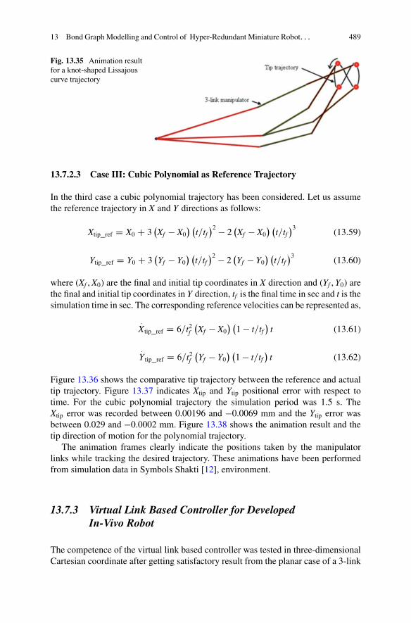
13 Bond Graph Modelling and Control of Hyper-Redundant Miniature Robot. . . 489
Fig. 13.35 Animation resultfor a knot-shaped Lissajouscurve trajectory
13.7.2.3 Case III: Cubic Polynomial as Reference Trajectory
In the third case a cubic polynomial trajectory has been considered. Let us assumethe reference trajectory in X and Y directions as follows:
Xtip_ref D X0 C 3�Xf � X0
� �t=tf
�2 � 2 �Xf � X0� �
t=tf�3
(13.59)
Ytip_ref D Y0 C 3�Yf � Y0
� �t=tf
�2 � 2 �Yf � Y0� �
t=tf�3
(13.60)
where (Xf , X0) are the final and initial tip coordinates in X direction and (Yf , Y0) arethe final and initial tip coordinates in Y direction, tf is the final time in sec and t is thesimulation time in sec. The corresponding reference velocities can be represented as,
:
Xtip_ref D 6=t2f�Xf � X0
� �1 � t=tf
�t (13.61)
:
Y tip_ref D 6=t2f�Yf � Y0
� �1 � t=tf
�t (13.62)
Figure 13.36 shows the comparative tip trajectory between the reference and actualtip trajectory. Figure 13.37 indicates Xtip and Ytip positional error with respect totime. For the cubic polynomial trajectory the simulation period was 1.5 s. TheXtip error was recorded between 0.00196 and �0.0069 mm and the Ytip error wasbetween 0.029 and �0.0002 mm. Figure 13.38 shows the animation result and thetip direction of motion for the polynomial trajectory.
The animation frames clearly indicate the positions taken by the manipulatorlinks while tracking the desired trajectory. These animations have been performedfrom simulation data in Symbols Shakti [12], environment.
13.7.3 Virtual Link Based Controller for DevelopedIn-Vivo Robot
The competence of the virtual link based controller was tested in three-dimensionalCartesian coordinate after getting satisfactory result from the planar case of a 3-link
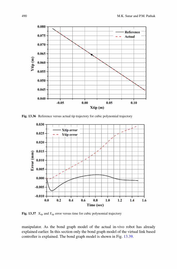
490 M.K. Sutar and P.M. Pathak
Fig. 13.36 Reference versus actual tip trajectory for cubic polynomial trajectory
Fig. 13.37 Xtip and Ytip error versus time for cubic polynomial trajectory
manipulator. As the bond graph model of the actual in-vivo robot has alreadyexplained earlier. In this section only the bond graph model of the virtual link basedcontroller is explained. The bond graph model is shown in Fig. 13.39.
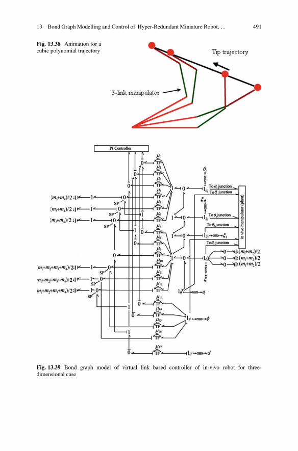
13 Bond Graph Modelling and Control of Hyper-Redundant Miniature Robot. . . 491
Fig. 13.38 Animation for acubic polynomial trajectory
Fig. 13.39 Bond graph model of virtual link based controller of in-vivo robot for three-dimensional case

492 M.K. Sutar and P.M. Pathak
The virtual link lengths of the virtual link based controller used in case ofthree-dimensional trajectory control of in-vivo robot are derived following the samemethodology adopted for the 3-link planar manipulator and can be expressed as:
Lv1 Dq
L21 C L22 C .2L1L2 cos �2/; and
Lv2 Dq
L23 C L24 C .2L3L4 cos �4/
The transformer moduli are obtained using the same methodology that has beenadopted in the planar case and they are enlisted in Table 13.8.
13.7.3.1 Simulation Results
The competence of the developed controller was further tested for three-dimensionalworkspace trajectory for which a cubic polynomial trajectory was chosen. Let usassume the reference trajectory in X and Y directions as follows:
Xtip_ref D X0 C 3�Xf � X0
� �t=tf
�2 � 2 �Xf � X0� �
t=tf�3
(13.63)
Ytip_ref D Y0 C 3�Yf � Y0
� �t=tf
�2 � 2 �Yf � Y0� �
t=tf�3
(13.64)
Table 13.8 Transformer moduli for the bond graph model of virtual link basedcontroller for three-dimensional case
Modulus Expression
�1 �Lv2 cos� sin .�1 C �3 C �1 C �2 C �3/�2 �Lv2 sin� sin .�1 C �3 C �1 C �2 C �3/�3 �Lv2 cos .�1 C �3 C �1 C �2 C �3/�4 �Lv2 cos� sin .�1 C �3 C �1 C �2 C �3/�5 �Lv2 sin� sin .�1 C �3 C �1 C �2 C �3/�6 �Lv2 cos .�1 C �3 C �1 C �2 C �3/�7 �Lv1 cos� sin �1�8 �Lv1 sin� sin �1�9 Lv1 cos �1�10 �Lv1 cos� sin �1�11 �Lv1 sin� sin �1�12 Lv1 cos �1�13 � sin�
˚Lv1 cos .�1 C �1/C Lv2 cos .�1 C �3 C �1 C �2 C �3/
�14 cos�˚Lv1 cos .�1 C �1/C Lv2 cos .�1 C �3 C �1 C �2 C �3/
�15 �Lv1 sin� cos .�1 C �1/�16 Lv1 cos� cos .�1 C �1/

13 Bond Graph Modelling and Control of Hyper-Redundant Miniature Robot. . . 493
Table 13.9 Simulationparameters forthree-dimensional case
Parameters Value
Joint resistance RjD 0.001 Nm/(rad/s)Link length LD 0.011 mAmplitude AD 0.01 mFrequency !D 10 rad/sMass of link mD 0.001 kgAcceleration due to gravity gD 9.81 m/s2
Proportional gain KpD 1000Integral gain KiD 5000Initial position in X coordinate 0.0336 mFinal position in X coordinate 0.03275 mInitial position in Y coordinate 0.02825 mFinal position in Y coordinate 0.02748 mInitial position in Z coordinate 0.01291 mFinal position in Z coordinate 0.02047 m
Ztip_ref D Z0 C 3�Zf � Z0
� �t=tf
�2 � 2 �Zf � Z0� �
t=tf�3
(13.65)
where (Xf , X0) are the final and initial tip coordinates in X direction and (Yf , Y0) arethe final and initial tip coordinates in Y direction, (Zf , Z0) are the final and initial tipcoordinates in Z direction, tf is the final time in sec, and t is the simulation time insec. The corresponding reference velocities can be represented as:
:
Xtip_ref D 6=t2f�Xf � X0
� �1 � t=tf
�t (13.66)
:
Y tip_ref D 6=t2f�Yf � Y0
� �1 � t=tf
�t (13.67)
:
Ztip_ref D 6=t2f�Zf � Z0
� �1 � t=tf
�t (13.68)
The simulation parameters are expressed in Table 13.9.The reference and actual tip trajectory is shown in Fig. 13.40 from which it can
be seen that the robot tip precisely followed the reference path assigned to it fromone known position to another in the three-dimensional Cartesian coordinate.
13.8 Concluding Remarks
In this chapter a forward kinematic analysis of the in-vivo robot manipulator wasperformed. The results obtained from the simulation validate the bond graph model.Further an inverse kinematic solution was found to determine the pulley rotation fordifferent known position of the tip by taking three different trajectories. In fact this is
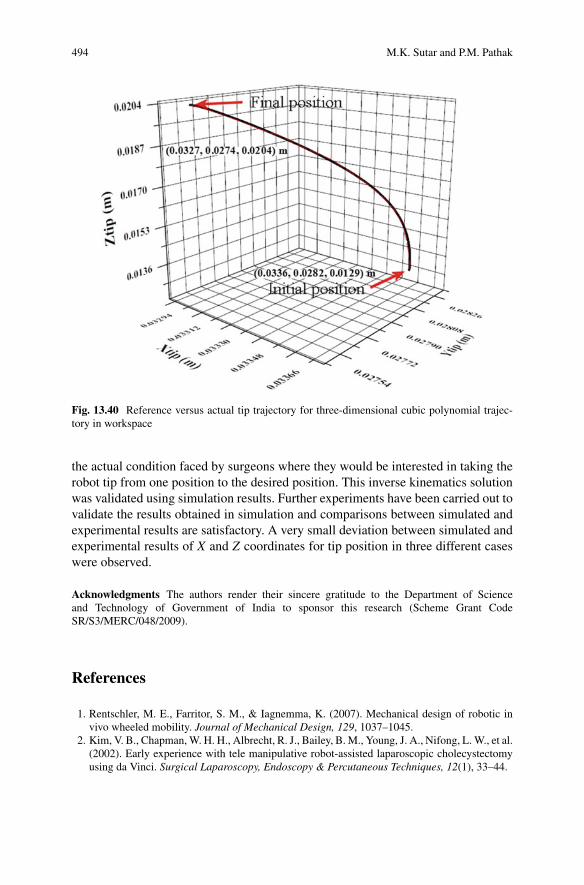
494 M.K. Sutar and P.M. Pathak
Fig. 13.40 Reference versus actual tip trajectory for three-dimensional cubic polynomial trajec-tory in workspace
the actual condition faced by surgeons where they would be interested in taking therobot tip from one position to the desired position. This inverse kinematics solutionwas validated using simulation results. Further experiments have been carried out tovalidate the results obtained in simulation and comparisons between simulated andexperimental results are satisfactory. A very small deviation between simulated andexperimental results of X and Z coordinates for tip position in three different caseswere observed.
Acknowledgments The authors render their sincere gratitude to the Department of Scienceand Technology of Government of India to sponsor this research (Scheme Grant CodeSR/S3/MERC/048/2009).
References
1. Rentschler, M. E., Farritor, S. M., & Iagnemma, K. (2007). Mechanical design of robotic invivo wheeled mobility. Journal of Mechanical Design, 129, 1037–1045.
2. Kim, V. B., Chapman, W. H. H., Albrecht, R. J., Bailey, B. M., Young, J. A., Nifong, L. W., et al.(2002). Early experience with tele manipulative robot-assisted laparoscopic cholecystectomyusing da Vinci. Surgical Laparoscopy, Endoscopy & Percutaneous Techniques, 12(1), 33–44.

13 Bond Graph Modelling and Control of Hyper-Redundant Miniature Robot. . . 495
3. Webster, R. J., III, & Jones, B. A. (2010). Design and kinematic modeling of constantcurvature continuum robots: A review. The International Journal of Robotics Research, 29(13),1661–1683.
4. Wang, J., Li, Y., & Zhao, X. (2010). Inverse kinematics and control of a 7-DOF redundantmanipulator based on the closed-loop algorithm. International Journal of Advanced RoboticSystems, 7(4), 1–9.
5. Chirikjian, J. S., & Burdick, J. W. (1991). Kinematics of hyper-redundant robot locomotionwith application to grasping. Proceedings of the IEEE International Conference on Roboticsand Automation (Vol. 1, pp. 720–725), Sacramento, California, 9–11 April.
6. Raibert, M., & Craig, J. (1981). Hybrid position/force control of manipulators. Transactions ofASME Journal of Dynamic Systems, Measurement and Control, 102(2), 126–133.
7. Merzouki, R., Samantaray, A. K., Pathak, P. M., & Ould Boumama, B. (2013). Intelligentmechatronic systems: Modeling, control and diagnosis. London: Springer.
8. Hartenberg, R. S., & Denavit, J. (1955). A kinematic notation for lower pair mechanisms basedon matrices. Journal of Applied Mechanics, ASME Transactions, 23, 215–221.
9. Craig, J. J. (2005). Introduction to robotics mechanics and control. Upper Saddle, NJ: PearsonPrentice Hall.
10. Borutzky, W. (2010). Bond graph methodology—Development and analysis of multidisci-plinary dynamic system models. London: Springer.
11. Karnopp, D. C., Margolis, D. L., & Rosenberg, R. C. (2012). System dynamics: Modelling andsimulation of mechatronic systems (4th ed.). Hoboken, NJ: Wiley.
12. Mukherjee, A., Karmakar, R., & Samantaray, A. K. (2006). Bond graph in modeling,simulation and fault identification (2nd ed.). New Delhi: I. K. International Publishing HousePvt. Ltd/CRC Press.
13. Sutar, M. K., Pathak, P. M., Sharma, A. K., Mehta, N. K., & Gupta, V. K. (2013). Forwardkinematic analysis of in-vivo robot for stomach biopsy. Journal of Robotic Surgery, 7,281–287.
14. Bevan, T. (2010). The theory of machines. New Delhi: Pearson Education.15. French, A. P. (1971). Vibrations and waves. London: CRC Press.

Chapter 14Bond graph Modeling and Control of CompliantLegged Quadruped Robot
M.M. Gor, P.M. Pathak, A.K. Samantaray, J.M. Yang, and S.W. Kwak
Abbreviations
AVP Angular velocity propagationCG Center of gravityCTF Coordinate transformation blockDOF Degree of freedomEJS Euler Junction StructureLL Leg liftPL Prismatic linkPI Proportion-integral controllerPID Proportional-integral-derivative controller
M.M. GorG H Patel College of Engineering and Technology, Vallabh Vidyanagar, Gujarat, Indiae-mail: [email protected]
P.M. Pathak (�)Indian Institute of Technology Roorkee, Roorkee, Uttarakhand, Indiae-mail: [email protected]; [email protected]
A.K. SamantarayIndian Institute of Technology Kharagpur, Kharagpur, West Bengal, Indiae-mail: [email protected]
J.M. YangKyungpook National University, Daegu, South Koreae-mail: [email protected]
S.W. KwakKeimyung University, Daegu, South Koreae-mail: [email protected]
© Springer International Publishing Switzerland 2017W. Borutzky (ed.), Bond Graphs for Modelling, Control and FaultDiagnosis of Engineering Systems, DOI 10.1007/978-3-319-47434-2_14
497

498 M.M. Gor et al.
RP Revolute-prismaticSL Step lengthTVP Translational velocity propagationZMP Zero moment point
14.1 Historical Survey of Modeling and Controlof Quadruped Robot
Legged robot offers many advantages over wheeled robots including greateradaptability to terrain irregularities and superior off-road mobility [30, 41]. Leggedsystems require only a series of discrete footholds along the pathway for off-roadlocomotion. This property enables legged robots to traverse surfaces inaccessibleto wheeled mobile robots. Compliance in the leg improves locomotion of leggedrobot [40]. Variable compliance in the legs [16] overcomes the size, weight,fragility, and efficiency problem. Basically, legged robots are discrete systemsin which joints of each leg have to operate in particular fashion. So, dynamicsplays an important role in the operation and control of a walking robot. Recently,there has been a noteworthy increase in the use of computational dynamics fordesign, analysis, simulation, and control of various robotic systems. This is due toavailability of various multi-body dynamic analysis tools and faster computationalresources. To this end, various researchers used different dynamic analysis methodsfor multi-body systems, such as the methods based on Lagrangian equation [23],Newton–Euler equation [3, 43], Kane’s equation [2, 5, 33], variational methods [4],and bond graph method [26].
Benani and Giri [6] presented a dynamic model approach of quadruped consid-ering open and/or closed kinematic chain mechanisms. It is based on Newton–Eulerapproach and the explicit formulation of kinematic holonomic constraints for theclosed loop mechanism. Mahapatra and Roy [27] developed a dynamic modelof six legged in CATIA solid modeler, SimDesigner, and ADAMS multi-bodydynamic solver and kinematic and dynamic simulation is performed based on virtualprototyping technology. Krishnan et al. [26] presented a bond graph model ofcompliant legged quadruped robot in a sagittal plane. The sagittal plane dynamicshave been tested through experimental set-up. Soyguder and Ali [39] solved thestance and flight phase dynamic structures in a sequential closed loop for quadrupedand obtained the equation of motion for pronking gait. Shah et al. [36] presented aconcept of kinematic modules for the development of the dynamic model of thefour legged robots where each module is considered as a set of serially connectedlinks. Module-level Decoupled Natural Orthogonal Complement (DeNOC) matriceswere introduced which help to analyze the large number of links as a system witha smaller number of modules. Recursive kinematic relationships were obtainedbetween two adjoining modules. Ganesh and Pathak [17] developed a dynamicmodel of four legged in a sagittal plane by formulating kinetic and potential energy

14 Bond graph Modeling and Control of Compliant Legged Quadruped Robot 499
equation of body and leg. These were used to derive Lagrangian function and thenequation of motion. A locomotion control strategy for quadruped robot has beenpresented in [20]. Dynamic modeling and analysis of quadruped robot through bondgraph technique has been presented in [19].
Many of the quadruped robots developed worldwide are biologically inspired.Process of natural selection governing evolution of species forces animals adapt totheir specific physical features and environment by optimizing their locomotion.Some animals are better at doing certain things in comparison to others. Thus,keeping the required task or operation features in the view, more and morespecialized biologically inspired quadrupeds are being developed now-a-days. Someof them are Baby Elephant [11], BigDog [31], Cheetah-cub [40], HyQ [35],LittleDog [10, 37], and Tekken [14, 25]. Hydraulically actuated Baby Elephant[11] was designed to work as mechanical carrier. It has 12 DOFs and compliantlegs. Multi-body dynamic simulation was used in [11] for its design and theresults were experimentally validated. BigDog [31] was developed with the goalto move in rough terrain without human assistance. It has 20 DOFs and about50 sensors. Four joints of each leg are operated by hydraulic actuator. It uses atwo-stroke internal combustion engine that delivers up to 15 hp power. Electricallyactuated Cheetah-cub [40] was designed for high-speed locomotion. Cheetah-cub’slegs are spring loaded and pantograph mechanism with multiple segments is usedfor shock absorption during running. This robot’s self-stabilizing properties weredemonstrated in hardware model and in simulation carried out in Webots software.HyQ [35] developed at IIT Genova was designed to perform highly dynamic taskslike jumping and running. It has 12 DOFs and both hydraulic and electrical actuationsystems. During running and jumping, generated impact forces were absorbed byhydraulic actuation mounted on hip and knee joints in the flexion/extension plane ofthe leg. The hip abduction/adduction joint was actuated by brushless electric motorwhich provides constant output torque. LittleDog [10, 37] has 12 DOFs and eachjoint is operated by a high-gain servo motor. Sensors mounted on the robot measurebody orientation, joint angles, and ground-foot contact. Sensing, communication,and actuators are controlled by onboard PC-level computer. Tekken [14, 25] is a lightweight (4.3 kg) manually operated power autonomous compliant legged quadrupedrobot. It has 16 DOFs, three joints around pitch axis (ankle, knee, and hip), and onehip joint around yaw axis at each leg. At ETH Zurich, two quadrupeds have beendeveloped having similar structure, size, and morphology, but different concept ofactuation [32]. The first, ALoF, is a classically stiff actuated robot that is controlledkinematically; whereas the second, StarlETH, uses a soft actuation scheme basedon highly compliant series elastic actuators.
In this chapter, three dimensional dynamic model of compliant legged quadrupedrobot using bond graph has been developed. A quadruped robot configuration usedfor analysis is two links legged robot in which upper link is rigid and a lowerlink is compliant. Lower link is considered similar to a prismatic link in which,piston and piston rod is sliding inside the cylinder and movement is restricted bythe spring which generates compliance in the leg. The strategy for locomotioncontrol in joint space as well as workspace is discussed. To validate the same,

500 M.M. Gor et al.
simulation and animation of the trot gait performed by the quadruped is carriedout which is further verified by experiment results. Since trot gait is dynamicallystable gait thus successful validation of model in trot gait ensures the model validityin other gaits also. To prove the versatility of the three dimensional model generateda turning motion of the robot is demonstrated by varying the leg speed in amblegait. Influence of compliance on quadruped locomotion and posture disturbanceis studied. Performance analysis is carried out considering energy efficiency asdeciding criteria. Performance analysis on rigid and compliant legged robots, staticand dynamic gaits, and foot trajectory is carried out. Nomenclature used throughoutthis chapter is listed below.
Nomenclature
fAg Inertial framefBg Robot body frameci, si cos(� i), sin(� i)D Width of a piston of a prismatic linkF ForceFxc, Fyc, Fzc External force acting at the cylinder body fixed x, y, and z axesH Angular momentumI Link number, frame numberIrot Rotor inertiaIxb, Iyb, Izb Moment of inertia of the robot body about x, y, and z axesIxx1, Iyy1, Izz1 Moment of inertia of the upper link of robot leg about x, y, and z axesIxxc, Iyyc, Izzc Moment of inertia of the cylinder part of a prismatic link about x, y, and z axesIxxp, Iyyp, Izzp Moment of inertia of the piston part of a prismatic link about x, y, and z axeskb Contact point stiffness at the piston cylinder of prismatic linkkf Flexibility due to hydraulic pressure inside the cylinder of prismatic linkKgx, Kgy, Kgz Ground contact stiffness in x, y, and z directionKP, KI,KD Proportional, integral, and derivative gain of controllerKpb, Kib, Kdb Proportional, integral, and derivative gain of controller for body forwardlc Contemporary length of prismatic linklcg Distance of cylinder CG from a cylinder end frame of prismatic linkli Length of link i
lp Length of a piston and piston rod of prismatic linklpg Distance of piston CG from a piston end frame of prismatic linkLm Motor inductancemb Mass of the bodymc Mass of cylinder part of the prismatic linkmli Mass of link i
mp Mass of a piston and piston rod of a prismatic linkMxc, Myc, Mzc External moment acting at the cylinder body fixed x, y, and z axesn Gear ratiop Translational momentumABR Transformation from body frame fBg to inertial frame fAg
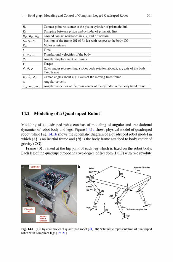
14 Bond graph Modeling and Control of Compliant Legged Quadruped Robot 501
Rb Contact point resistance at the piston cylinder of prismatic linkRf Damping between piston and cylinder of prismatic linkRgx, Rgy, Rgz Ground contact resistance in x, y, and z directionrix, riy, riz Position of the frame f0g of ith leg with respect to the body CGRm Motor resistancet Timevx, vy, vz Translational velocities of the body� i Angular displacement of frame i� Torque , � , � Euler angles representing a robot body rotation about x, y, z axis of the body
fixed frame c, � c, �c, Cardan angles about x, y, z axis of the moving fixed frame! Angular velocity!xc, !yc, !zc Angular velocities of the mass center of the cylinder in the body fixed frame
14.2 Modeling of a Quadruped Robot
Modeling of a quadruped robot consists of modeling of angular and translationaldynamics of robot body and legs. Figure 14.1a shows physical model of quadrupedrobot, while Fig. 14.1b shows the schematic diagram of a quadruped robot model inwhich fAg is an inertial frame and fBg is the body frame attached to body center ofgravity (CG).
Frame f0g is fixed at the hip joint of each leg which is fixed on the robot body.Each leg of the quadruped robot has two degree of freedom (DOF) with two revolute
Fig. 14.1 (a) Physical model of quadruped robot [21]. (b) Schematic representation of quadrupedrobot with compliant legs [19, 21]
502 M.M. Gor et al.
joints per leg. The joint between links i and i C 1 is numbered as i C 1. A coordinateframe fi C 1g is attached to (i C 1) joint. Frame f1g is attached to joint 1 of each leg.Frame f0g is coinciding with frame f1g. Frame f2g is attached to joint f2g, whileframe f3g is attached to leg tip. The rotational inertias are defined about framesfixed at the CG of the link. The CG frame is fixed along the principal directions inthe link or body. The surface on which the robot is walking is assumed as a hardsurface.
14.2.1 Dynamics of a Robot Body
For a given instant, any rigid body has absolute translational velocity �!v and absoluteangular velocity �!! . The translational velocity and angular velocity vectors havebeen resolved into three mutually perpendicular components vx, vy, vz and !x, !y,
!z. The net force�!F acting on the body and the linear momentum �!p can be related
with respect to rotating frame as [24],
�!F D
d�!pdt
!
rel
C �!! � �!p (14.1)
where
d�!pdt
relis the rate of change of momentum relative to the moving frame.
Similarly, the relationship between the net torque �!� acting on the body and the
angular momentum�!h can be written as,
�!� D
d�!h
dt
!
rel
C �!! � �!h (14.2)
Using the right-hand rule for Eqs. (14.1) and (14.2), the component equations canbe written as,
Fx D mb:vx C mb!yvz � mb!zvy (14.3)
Fy D mb:vy C mb!zvx � mb!xvz (14.4)
Fz D mb:vz C mb!xvy � mb!yvx (14.5)
and
�x D Ixx:!x C �
Izz � Iyy�!y!z (14.6)
�y D Iyy:!Y C .Ixx � Izz/ !z!x (14.7)
14 Bond graph Modeling and Control of Compliant Legged Quadruped Robot 503
�z D Izz:!z C �
Iyy � Ixx�!x!y (14.8)
These nonlinear differential equations are known as Newton–Euler‘s equations [28].The cross product terms can be treated as forces in a set of Eqs. (14.3), (14.4), and(14.5) and as torques in a set of Eqs. (14.6), (14.7), and (14.8). The forces andtorques can be added at the respective 1-junctions and using gyrator-ring structuresbond graph is generated as presented in [28]. Generated structure is known as EulerJunction Structures (EJS).
14.2.2 Dynamics of an Upper Link of Leg
Translational velocity of frame f0g of each leg with reference to frame fAg andexpressed in term of frame fAg is given by [12],
A
A�!V 0
D A
A�!
V B
C B
ARh�B
B�!P 0
� B
A�!! B
i(14.9)
where A
A�!V B
represents the translational velocity of body frame fBg with respect
to an inertial frame fAg and expressed in frame fAg; B
A�!! B
represents the angular
velocity of body frame fBg with respect to inertial frame fAg and expressed in frame
fBg; B
B�!P 0
irepresents the position vector of frame f0g of ith leg with respect
to the body CG frame fBg and expressed in frame fBg. It can be expressed asB
B�!P 0
iD �
rix riy riz
�Twhere i denotes legs 1–4. Here r denotes position of frame
f0g with respect to body CG frame. In Eq. (14.9), ABR represent the transformation
from body frame fBg to inertial frame fAg and can be expressed as,
ABR D
0
@c� c� s s� c� � c s� c s� c� C s s�c� s� s s� s� C c c� c s� s� � s c�� s� s c� c c�
1
A (14.10)
where c� is shorthand for cos� , s� for sin� , and so on. �, � and are the Z-Y-XEuler angles. Governing equation for an angular velocity propagation (AVP) of linksof a leg can be given as [12],
iC1 A�!! iC1
DiC1i Ri
A�!! i
C iC1 i�!! iC1
(14.11)
where iC1
A�!! iC1
is the angular velocity of (i C 1) link with respect to inertial
frame fAg and expressed in (i C 1)th frame, i
A�!! i
is the angular velocity of
the ith link with respect to the inertial frame fAg and expressed in ith frame, and
504 M.M. Gor et al.
iC1
i�!! iC1
is the angular velocity of (i C 1) link as observed from ith link and
expressed in (i C 1)th frame. The term can be expressed for link 1 and 2, respectively
as, 10�!! 1
Dh :
�1 0 0
iT, 21�!! 2
Dh :
�2 0 0
iTwhere
:
�1 represents angular
velocity of frame f1g with respect to frame f0g expressed in frame f1g and similarly:
�2 represents the angular velocity of frame f2g with respect to frame f1g expressedin frame f2g.
For translational velocity propagation (TVP), governing equation for the link tipvelocity and link CG velocity are given as,
A
A�!V iC1
D A
A�!
V i
CA
i Rh
i
A�!! i
� i
i�!P iC1i
(14.12)
where A
A�!V iC1
represents the translational velocity of body frame fi C 1g with
respect to an inertial frame fAg and expressed in frame fAg, A
A�!V i
represents
the translational velocity of body frame fig with respect to an inertial frame fAgand expressed in frame fAg, i
i�!P iC1
represents position of frame fi C 1g with
respect to frame fig and expressed in frame fig. Link lengths l1 and l2 are takenalong the principal Y-axis of the links and hence represented in vector form as,0�!P 1 D �
0 0 0�T
, 1�!P 2 D �
0 l1 0�T
, 2�!P 3 D �
0 l2 0�T
Equation (14.12) can be simplified as,
A
A�!V iC1
D A
A�!
V i
CA
i Rh�i
i�!P iC1
�i h
i
A�!!i
i(14.13)
For position of a link CG, i
i�!P Gi
D �
0 lGi 0�T
A
A�!V Gi
D A
A�!
V i
CA
i Rh�i
i�!P Gi
�i h
i
A�!!i
i(14.14)
Equations (14.12), (14.13), and (14.14) represent the TVP of link in each leg of therobot. The CG velocity of links depends on link inertia. In the bond graph model “I”elements (representing mass of a link) are attached at flow junctions. They yield theCG velocities of links. The starting point of the current link is same as the previouslink tip. Hence, the tip velocity of the previous link and the angular velocity of thecurrent link are used to find the tip velocity and the CG velocity of the current link.i
A�!!i
in above equations can be obtained from the AVP for the current link.
The EJS to represent angular dynamics of the link can be constructed similarlyas discussed in Sect. 14.2.1. In case of link, torque is provided in x direction only.
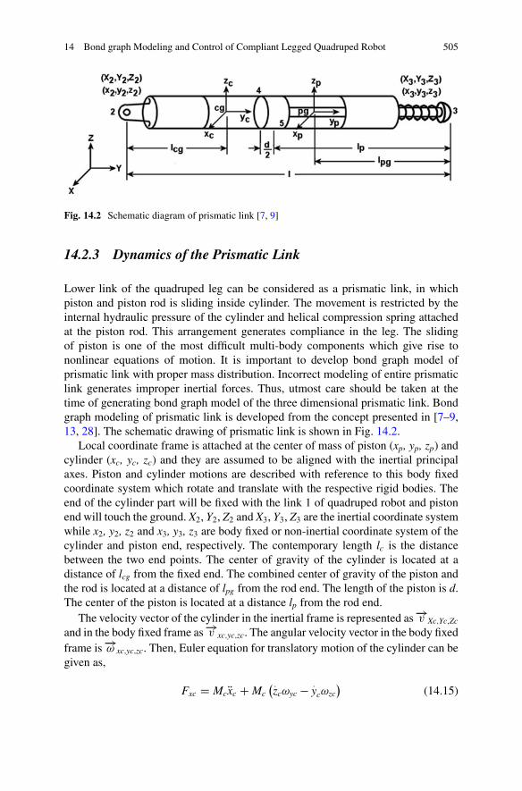
14 Bond graph Modeling and Control of Compliant Legged Quadruped Robot 505
Fig. 14.2 Schematic diagram of prismatic link [7, 9]
14.2.3 Dynamics of the Prismatic Link
Lower link of the quadruped leg can be considered as a prismatic link, in whichpiston and piston rod is sliding inside cylinder. The movement is restricted by theinternal hydraulic pressure of the cylinder and helical compression spring attachedat the piston rod. This arrangement generates compliance in the leg. The slidingof piston is one of the most difficult multi-body components which give rise tononlinear equations of motion. It is important to develop bond graph model ofprismatic link with proper mass distribution. Incorrect modeling of entire prismaticlink generates improper inertial forces. Thus, utmost care should be taken at thetime of generating bond graph model of the three dimensional prismatic link. Bondgraph modeling of prismatic link is developed from the concept presented in [7–9,13, 28]. The schematic drawing of prismatic link is shown in Fig. 14.2.
Local coordinate frame is attached at the center of mass of piston (xp, yp, zp) andcylinder (xc, yc, zc) and they are assumed to be aligned with the inertial principalaxes. Piston and cylinder motions are described with reference to this body fixedcoordinate system which rotate and translate with the respective rigid bodies. Theend of the cylinder part will be fixed with the link 1 of quadruped robot and pistonend will touch the ground. X2, Y2, Z2 and X3, Y3, Z3 are the inertial coordinate systemwhile x2, y2, z2 and x3, y3, z3 are body fixed or non-inertial coordinate system of thecylinder and piston end, respectively. The contemporary length lc is the distancebetween the two end points. The center of gravity of the cylinder is located at adistance of lcg from the fixed end. The combined center of gravity of the piston andthe rod is located at a distance of lpg from the rod end. The length of the piston is d.The center of the piston is located at a distance lp from the rod end.
The velocity vector of the cylinder in the inertial frame is represented as �!v Xc;Yc;Zc
and in the body fixed frame as �!v xc;yc;zc. The angular velocity vector in the body fixedframe is �!! xc;yc;zc. Then, Euler equation for translatory motion of the cylinder can begiven as,
Fxc D Mc Rxc C Mc� :zc!yc � :
yc!zc�
(14.15)
506 M.M. Gor et al.
Fyc D Mc Ryc C Mc� :xc!zc � :
zc!xc�
(14.16)
Fzc D McRzc C Mc� :yc!xc � :
xc!yc�
(14.17)
where Fxc, Fyc, Fzc are external forces acting in body fixed xc, yc, and zc directions,respectively, !xc, !yc, and !zc are angular velocities of the mass center of thecylinder in the body fixed frame.
:xc;
:yc and
:zc are velocities of the mass center in the
body fixed frame, Rxc; Ryc and Rzc are accelerations of the mass center in the body fixedframe. Similarly, Euler equations for rotary motion of the cylinder can be given as,
Mxc D Ixc:!xc � �
Iyc � Izc�!yc!zc (14.18)
Myc D Iyc:!yc � .Izc � Ixc/ !zc!xc (14.19)
Mzc D Izc:!zc � �
Ixc � Iyc�!xc!yc (14.20)
where Ixc, Iyc, and Izc are second moment of inertia about the principal axes, Mxc,Myc, and Mzc are components of resultant moment due to external forces and couplesabout the non-rotating coordinate frame whose axes are momentarily aligned withthe principal axes of the body.
Above Euler equations can be represented by the double gyrator rings where thegyrators are modulated by the angular velocities in the body fixed frame. Similarly,Euler equations can be generated for the piston also and it can be represented by thedouble gyrator rings. Generated bond graph model of above equations are shown inFig. 14.3 in which G1–G12 are the gyrator moduli taken from above equations.
The position of the fixed point in the body fixed frame is x2, y2, z2. The velocityof the cylinder in the body fixed frame is
:x2 D :
xc C z2!yc � y2!zc (14.21):y2 D :
yc C x2!zc � z2!xc (14.22):z2 D :
zc C y2!xc � x2!yc (14.23)
Equations (14.21), (14.22), and (14.23) are body fixed velocities. So, it is necessaryto convert it into the inertial frame by coordinate transformation block (CTF). CTFblock is generated using successive multiplication of rotation matrices as follows:
8<
:
:
X2:
Y2:
Z2
9>=
>;D T�c;�c; c
8<
:
:x2:y2:z2
9=
; (14.24)
where
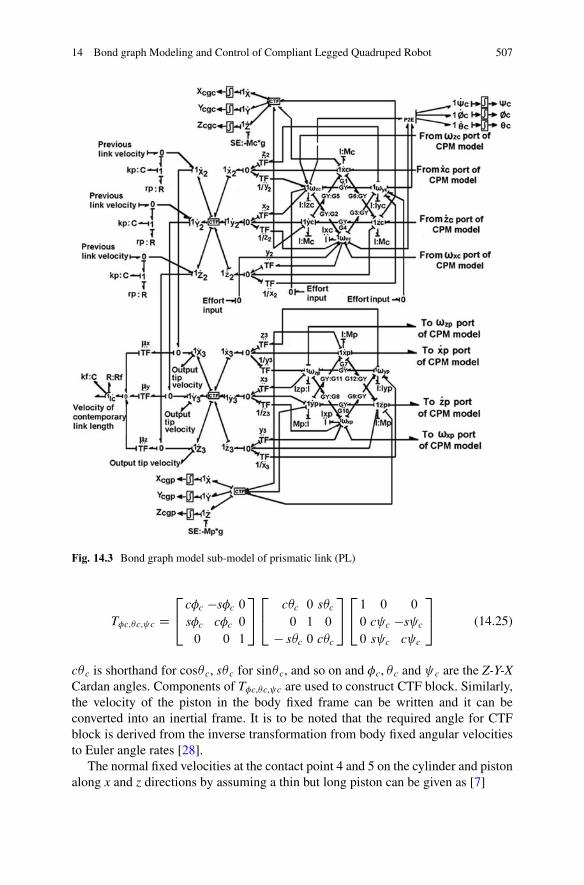
14 Bond graph Modeling and Control of Compliant Legged Quadruped Robot 507
Fig. 14.3 Bond graph model sub-model of prismatic link (PL)
T�c;�c; c D2
4c�c �s�c 0
s�c c�c 0
0 0 1
3
5
2
4c�c 0 s�c
0 1 0
� s�c 0 c�c
3
5
2
41 0 0
0 c c �s c
0 s c c c
3
5 (14.25)
c� c is shorthand for cos� c, s� c for sin� c, and so on and �c, � c and c are the Z-Y-XCardan angles. Components of T�c,�c, c are used to construct CTF block. Similarly,the velocity of the piston in the body fixed frame can be written and it can beconverted into an inertial frame. It is to be noted that the required angle for CTFblock is derived from the inverse transformation from body fixed angular velocitiesto Euler angle rates [28].
The normal fixed velocities at the contact point 4 and 5 on the cylinder and pistonalong x and z directions by assuming a thin but long piston can be given as [7]
508 M.M. Gor et al.
:x4c D :
xc C�
l � lp � lcg � d
2
�!zc (14.26)
:z4c D :
zc C�
l � lp � lcg � d
2
�!xc (14.27)
:x4p D :
xp ��
lp � lpg C d
2
�!zp (14.28)
:z4p D :
zp ��
lp � lpg C d
2
�!xp (14.29)
:x5c D :
xc C�
l � lp � lcg C d
2
�!zc (14.30)
:z5c D :
zc C�
l � lp � lcg C d
2
�!xc (14.31)
:x5p D :
xp ��
lp � lpg � d
2
�!zp (14.32)
:z5p D :
zp ��
lp � lpg � d
2
�!xp (14.33)
where �!! indicates the body fixed angular velocity about the axis indicated insubscript. Subscript c has been used for cylinder while p has been used for thepiston. Above discussed contact point mechanism is model as shown in Fig. 14.4.
The rate of change of contemporary length between two end points of prismaticlink can be expressed as
:
lc D �x
:X02 � :
X03
C �y
:Y02 � :
Y03
C �z
:Z02 � :
Z03
(14.34)
where X0
2, Y0
2, Z0
2 and X0
3, Y0
3, Z0
3 are coordinates of cylinder end and piston end,
respectively, in the inertial frame, �x D .X0
2�X0
3/lc
, �y D .Y0
2�Y0
3/lc
, and �z D .Z0
2�Z0
3/lc
are moduli used to derive the relative sliding velocity between piston and cylinderat “0” junction. Compliance in the link is modeled by “C” and “R” element. Forcontact point mechanics, to compute contact point velocities in body fixed framemoduli ˇ1–ˇ4 and ˇ5–ˇ8 are determined from kinematic analysis of the cylinderand piston, respectively. Through a set of transformer moduli �1–�12 similar to anexpanded form of CTF block, body fixed velocities are transformed into inertialvelocities and then they are implicitly constrained. The relative normal velocitybetween the contact point on the cylinder and the normal velocity at the contact pointon the piston is implicitly constrained by contact stiffness and damping parameters,
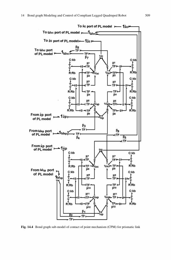
14 Bond graph Modeling and Control of Compliant Legged Quadruped Robot 509
Fig. 14.4 Bond graph sub-model of contact of point mechanism (CPM) for prismatic link
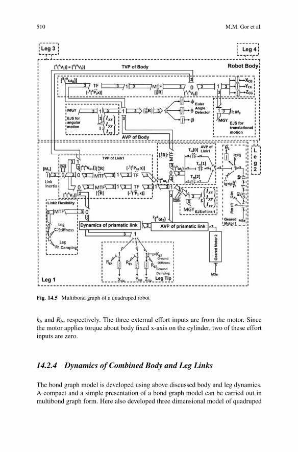
510 M.M. Gor et al.
Fig. 14.5 Multibond graph of a quadruped robot
kb and Rb, respectively. The three external effort inputs are from the motor. Sincethe motor applies torque about body fixed x-axis on the cylinder, two of these effortinputs are zero.
14.2.4 Dynamics of Combined Body and Leg Links
The bond graph model is developed using above discussed body and leg dynamics.A compact and a simple presentation of a bond graph model can be carried out inmultibond graph form. Here also developed three dimensional model of quadruped
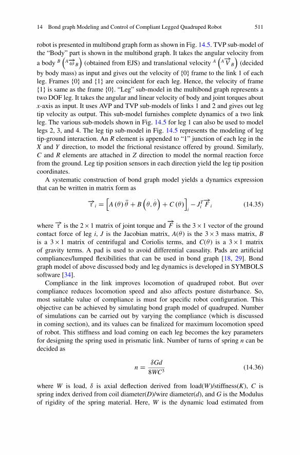
14 Bond graph Modeling and Control of Compliant Legged Quadruped Robot 511
robot is presented in multibond graph form as shown in Fig. 14.5. TVP sub-model ofthe “Body” part is shown in the multibond graph. It takes the angular velocity from
a body B
A�!! B
(obtained from EJS) and translational velocity A
A�!
V B
(decided
by body mass) as input and gives out the velocity of f0g frame to the link 1 of eachleg. Frames f0g and f1g are coincident for each leg. Hence, the velocity of framef1g is same as the frame f0g. “Leg” sub-model in the multibond graph represents atwo DOF leg. It takes the angular and linear velocity of body and joint torques aboutx-axis as input. It uses AVP and TVP sub-models of links 1 and 2 and gives out legtip velocity as output. This sub-model furnishes complete dynamics of a two linkleg. The various sub-models shown in Fig. 14.5 for leg 1 can also be used to modellegs 2, 3, and 4. The leg tip sub-model in Fig. 14.5 represents the modeling of legtip-ground interaction. An R element is appended to “1” junction of each leg in theX and Y direction, to model the frictional resistance offered by ground. Similarly,C and R elements are attached in Z direction to model the normal reaction forcefrom the ground. Leg tip position sensors in each direction yield the leg tip positioncoordinates.
A systematic construction of bond graph model yields a dynamics expressionthat can be written in matrix form as
�!� i DhA .�/ R� C B
�;
:
�
C C .�/i
i� JT
i�!F i (14.35)
where �!� is the 2 � 1 matrix of joint torque and�!F is the 3 � 1 vector of the ground
contact force of leg i, J is the Jacobian matrix, A(� ) is the 3 � 3 mass matrix, Bis a 3 � 1 matrix of centrifugal and Coriolis terms, and C(� ) is a 3 � 1 matrixof gravity terms. A pad is used to avoid differential causality. Pads are artificialcompliances/lumped flexibilities that can be used in bond graph [18, 29]. Bondgraph model of above discussed body and leg dynamics is developed in SYMBOLSsoftware [34].
Compliance in the link improves locomotion of quadruped robot. But overcompliance reduces locomotion speed and also affects posture disturbance. So,most suitable value of compliance is must for specific robot configuration. Thisobjective can be achieved by simulating bond graph model of quadruped. Numberof simulations can be carried out by varying the compliance (which is discussedin coming section), and its values can be finalized for maximum locomotion speedof robot. This stiffness and load coming on each leg becomes the key parametersfor designing the spring used in prismatic link. Number of turns of spring n can bedecided as
n D ıGd
8WC3(14.36)
where W is load, ı is axial deflection derived from load(W)/stiffness(K), C isspring index derived from coil diameter(D)/wire diameter(d), and G is the Modulusof rigidity of the spring material. Here, W is the dynamic load estimated from
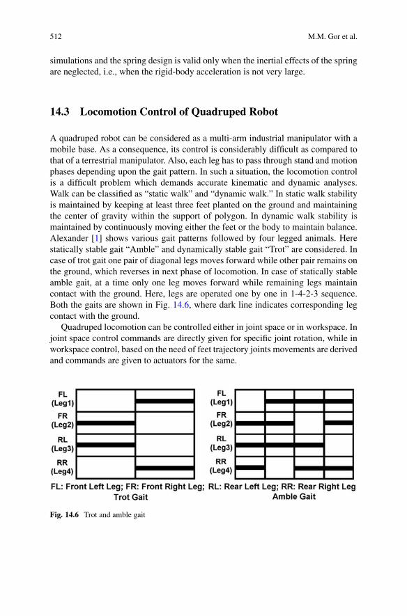
512 M.M. Gor et al.
simulations and the spring design is valid only when the inertial effects of the springare neglected, i.e., when the rigid-body acceleration is not very large.
14.3 Locomotion Control of Quadruped Robot
A quadruped robot can be considered as a multi-arm industrial manipulator with amobile base. As a consequence, its control is considerably difficult as compared tothat of a terrestrial manipulator. Also, each leg has to pass through stand and motionphases depending upon the gait pattern. In such a situation, the locomotion controlis a difficult problem which demands accurate kinematic and dynamic analyses.Walk can be classified as “static walk” and “dynamic walk.” In static walk stabilityis maintained by keeping at least three feet planted on the ground and maintainingthe center of gravity within the support of polygon. In dynamic walk stability ismaintained by continuously moving either the feet or the body to maintain balance.Alexander [1] shows various gait patterns followed by four legged animals. Herestatically stable gait “Amble” and dynamically stable gait “Trot” are considered. Incase of trot gait one pair of diagonal legs moves forward while other pair remains onthe ground, which reverses in next phase of locomotion. In case of statically stableamble gait, at a time only one leg moves forward while remaining legs maintaincontact with the ground. Here, legs are operated one by one in 1-4-2-3 sequence.Both the gaits are shown in Fig. 14.6, where dark line indicates corresponding legcontact with the ground.
Quadruped locomotion can be controlled either in joint space or in workspace. Injoint space control commands are directly given for specific joint rotation, while inworkspace control, based on the need of feet trajectory joints movements are derivedand commands are given to actuators for the same.
Fig. 14.6 Trot and amble gait
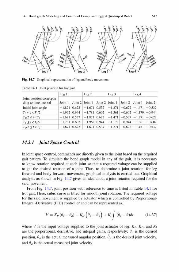
14 Bond graph Modeling and Control of Compliant Legged Quadruped Robot 513
Fig. 14.7 Graphical representation of leg and body movement
Table 14.1 Joint position for trot gait
Leg 1 Leg 2 Leg 3 Leg 4Joint position correspon-ding to time interval Joint 1 Joint 2 Joint 1 Joint 2 Joint 1 Joint 2 Joint 1 Joint 2
Initial joint angle �1.871 0.622 �1.671 0.537 �1.271 �0.622 �1.471 �0.537T0� t < T1/2 �1.962 0.944 �1.781 0.602 �1.361 �0.602 �1.179 �0.944T1/2� t < T1 �1.671 0.537 �1.871 0.622 �1.471 �0.537 �1.271 �0.622T1� t < T2/2 �1.781 0.602 �1.962 0.944 �1.179 �0.944 �1.361 �0.602T2/2� t < T2 �1.871 0.622 �1.671 0.537 �1.271 �0.622 �1.471 �0.537
14.3.1 Joint Space Control
In joint space control, commands are directly given to the joint based on the requiredgait pattern. To simulate the bond graph model in any of the gait, it is necessaryto know rotation required at each joint so that a required voltage can be suppliedto get the desired rotation of a joint. Thus, to determine a joint rotation, for legforward and body forward movement, graphical analysis is carried out. Graphicalanalysis as shown in Fig. 14.7 gives an idea about a joint rotation required for thesaid movement.
From Fig. 14.7, joint position with reference to time is listed in Table 14.1 fortrot gait. Here, cubic curve is fitted for smooth joint rotation. The required voltagefor the said movement is supplied by actuator which is controlled by Proportional-Integral-Derivative (PID) controller and can be represented as,
V D KP .�d � �a/C KD
:�d �
:
�a
C KI
Z.�d � �/dt (14.37)
where V is the input voltage supplied to the joint actuator of leg; KP, KD, and KI
are the proportional, derivative, and integral gains, respectively; �d is the desired
position, �a is the actual measured angular position,:
�d is the desired joint velocity,
and:
�a is the actual measured joint velocity.
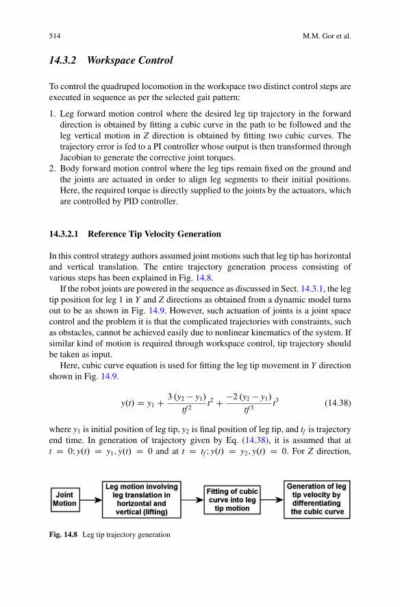
514 M.M. Gor et al.
14.3.2 Workspace Control
To control the quadruped locomotion in the workspace two distinct control steps areexecuted in sequence as per the selected gait pattern:
1. Leg forward motion control where the desired leg tip trajectory in the forwarddirection is obtained by fitting a cubic curve in the path to be followed and theleg vertical motion in Z direction is obtained by fitting two cubic curves. Thetrajectory error is fed to a PI controller whose output is then transformed throughJacobian to generate the corrective joint torques.
2. Body forward motion control where the leg tips remain fixed on the ground andthe joints are actuated in order to align leg segments to their initial positions.Here, the required torque is directly supplied to the joints by the actuators, whichare controlled by PID controller.
14.3.2.1 Reference Tip Velocity Generation
In this control strategy authors assumed joint motions such that leg tip has horizontaland vertical translation. The entire trajectory generation process consisting ofvarious steps has been explained in Fig. 14.8.
If the robot joints are powered in the sequence as discussed in Sect. 14.3.1, the legtip position for leg 1 in Y and Z directions as obtained from a dynamic model turnsout to be as shown in Fig. 14.9. However, such actuation of joints is a joint spacecontrol and the problem it is that the complicated trajectories with constraints, suchas obstacles, cannot be achieved easily due to nonlinear kinematics of the system. Ifsimilar kind of motion is required through workspace control, tip trajectory shouldbe taken as input.
Here, cubic curve equation is used for fitting the leg tip movement in Y directionshown in Fig. 14.9.
y.t/ D y1 C 3 .y2 � y1/
tf 2t2 C �2 .y2 � y1/
tf 3t3 (14.38)
where y1 is initial position of leg tip, y2 is final position of leg tip, and tf is trajectoryend time. In generation of trajectory given by Eq. (14.38), it is assumed that att D 0I y.t/ D y1;
:y.t/ D 0 and at t D tf I y.t/ D y2;
:y.t/ D 0: For Z direction,
Fig. 14.8 Leg tip trajectory generation
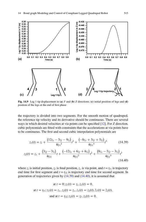
14 Bond graph Modeling and Control of Compliant Legged Quadruped Robot 515
Fig. 14.9 Leg 1 tip displacement in (a) Y and (b) Z directions; (c) initial position of legs and (d)position of the legs at the end of first phase
the trajectory is divided into two segments. For the smooth motion of quadruped,the reference tip velocity and its derivative should be continuous. There are severalways in which desired velocities at via points can be specified [12]. For Z direction,cubic polynomials are fitted with constraints that the accelerations at via points haveto be continuous. The first and second cubic interpolation polynomials are
z1.t/ D zi C�12zv � 3zf � 9zi
�
4tf12t2 C
��8zv C 3zf C 5zi�
4tf13t3 (14.39)
z2.t/ D zv C�3zf � 3zi
�
4tf2t C
��12zv C 6zf C 6zi�
4tf22t2 C
�8zv � 5zf � 3zi
�
4tf23t3
(14.40)
where zi is initial position, zf is final position, zv is via point, and t D tf 1 is trajectoryend time for first segment and t D tf 2 is trajectory end time for second segment. Ingeneration of trajectories given by (14.39) and (14.40), it is assumed that
at t D 0I z1.t/ D zi;:z1.t/ D 0;
at t D tf1I z1.t/ D zv; z2.t/ D zv;:z1.t/ D :
z2.t/; Rz1.t/ D Rz2.t/;and at t D tf2I z2.t/ D zf ;
:z2.t/ D 0:

516 M.M. Gor et al.
:y.t/ D 6 .y2 � y1/
tf 2t C �6 .y2 � y1/
tf 3t2 (14.41)
:z1.t/ D 2
�12zv � 3zf � 9zi
�
4tf12t C 3
��8zv C 3zf C 5zi�
4tf13t2 (14.42)
:z2.t/ D
�3zf � 3zi
�
4tf2C 2
��12zv C 6zf C 6zi�
4tf22t C 3
�8zv � 5zf � 3zi
�
4tf23t2 (14.43)
Use of Eqs. (14.38), (14.39), (14.40), (14.41), (14.42), and (14.43) with requiredgait patterns yields the reference profile for leg as shown in Figs. 14.10 and 14.11.Thus, Fig. 14.9a, b has been faithfully mathematically represented by Fig. 14.10a, b.Similarly, reference profile for remaining legs can also be obtained. These referenceprofiles are used to operate the model in workspace. The velocities are fed in thebond graph model by using SF elements.
Fig. 14.10 Displacement profile through cubic polynomial: (a) displacement in Y, (b) displace-ment in Z directions
Fig. 14.11 Trajectory through cubic polynomial: (a) velocity in Y and (b) velocity in Z directions

14 Bond graph Modeling and Control of Compliant Legged Quadruped Robot 517
14.3.2.2 Proportional Integral Controller
A PI controller is used here to achieve the leg forward movement according to adesired trajectory profile. Here, the joint input torque is controlled by calculating anerror value as the difference between the measured and reference velocities at a legtip. The PI controller gives a control signal gives a control signal
V1 D KPe C KI
Zedt (14.44)
where V1 is the output from the controller when there is an error e which is changingwith time t, KP is the proportionality constant, and KI is the integral constant.
14.3.2.3 Jacobian
Jacobian is a mapping from velocities in joint space to Cartesian space. The inverseproblem, where the joint velocities are to be determined for a given tip velocity,requires the inverse of the Jacobian. For quadruped robot working in workspace,one needs to evaluate the Jacobian for joint control through a controller. Consideringcompliance in the lower links of the leg and velocity propagation, the velocity of the
leg tip A
A�!V 3
represents the translational velocity of frame f3g with respect to the
inertial frame fAg and expressed in frame fAg. A
A�!V 3
can be written as,
A
A�!V 3
D A
A�!
V 2
C 2
ARh�22�!P 3
�i h
2
A�!! 2
iC 2
AR:
d33bZ3 (14.45)
where A
A�!V 2
is the translational velocity of frame f2g with respect to inertial
frame fAg and expressed in frame fAg, A2 R is the rotation matrix which describes f2g
relative to fAg, 22�!P 3
is the position vector of frame f3g with respect to frame
f2g and expressed in frame f2g, and 2
A�!! 2
is the angular velocity of link 2 with
respect to the inertial frame fAg and expressed in frame f2g.Using Eq. (14.45), leg tip velocity of each leg can be derived; the expanded form
of this equation is shown in (14.46).

518 M.M. Gor et al.
:
Xitip:
Yitip:
Zitip
D
2
6666666666666666666666666666666666666666666666666666666666666666666666666666666666666666666664
8ˆˆˆˆˆˆˆˆˆˆˆ<
ˆˆˆˆˆˆˆˆˆˆˆ:
:
XCG C�� s s�c¿s1il1 C c s¿s1il1 C c s�c¿c1il1 C s s¿c1il1
�s s�c¿c1is2il2 C c s¿c1is2il2 � c s�c¿s1is2il2 � s s¿s1is2il2�s s�c¿s1ic2il2 C c s¿s1ic2il2 C c s�c¿c1ic2il2 C s s¿c1ic2il2
� :�1
C �� s s�c¿c1is2il2 C c s¿c1is2il2 � c s�c¿s1is2il2�s s¿s1is2il2 � s s�c¿s1ic2il2 C c s¿s1ic2il2Cc s�c¿c1ic2il2 C s s¿c1ic2il2
� :�2
C �c s�c¿ryi C s s¿ryi � s s�c¿rzi C c s¿rzi � s s�c¿s1il1Cc s¿s1il1 C c s�c¿c1il1 C s s¿c1il1 � s s�c¿c1is2il2 C c s¿c1is2il2�c s�c¿s1is2il2 � s s¿s1is2il2 � s s�c¿s1ic2il2 C c s¿s1ic2il2Cc s�c¿c1ic2il2 C s s¿c1ic2il2
�!x
C �� c s�c¿rxi � s s¿rxi C c�c¿rzi C c�c¿l1s1i
Cc�c¿l2s2ic1i C c�c¿l2c2is1i�!y
C �s s�c¿rxi � c s¿rxi � c�c¿ryi � c�c¿l1c1i
Cc�c¿l2s2is1i � c�c¿l2c2ic1i�!z
C � ..s s�c¿� c s¿/ c1i C .c s�c¿C s s¿/ s1i/ c2i
C .� .s s�c¿� c s¿/ s1i C .c s�c¿� s s¿/ c1i/ s2i�:l2i
9>>>>>>>>>>>>>>>>>>>>>>>>>>>>>>>>=
>>>>>>>>>>>>>>>>>>>>>>>>>>>>>>>>;8ˆˆˆˆˆˆˆˆˆˆˆ<
ˆˆˆˆˆˆˆˆˆˆˆ:
:
YCG C�� s s�s¿s1il1 � c c¿s1il1 C c s�s¿c1il1
�s c¿c1il1 � s s�s¿c1is2il2 � c c¿c1is2il2 � c s�s¿s1is2il2Cs c¿s1is2il2 � s s�s¿s1ic2il2 � c c¿s1ic2il2 C c s�s¿c1ic2il2 � s c¿c1ic2il2
� :�1
C �� s s�s¿c1is2il2 � c c¿c1is2il2 � c s�s¿s1is2il2Cs c¿s1is2il2 � s s�s¿s1ic2il2 � c c¿s1ic2il2Cc s�s¿c1ic2il2 � s c¿c1ic2il2
� :�2
C �c s�s¿ryi � s c¿ryi � s s�s¿rzi � c c¿rzi � s s�s¿s1il1 C c c¿s1il1Cc s�s¿c1il1 � s c¿c1il1 � s s�s¿c1is2il2 � c c¿c1is2il2�c s�s¿s1is2il2 C s c¿s1is2il2 � s s�s¿s1ic2il2 � c c¿s1ic2il2Cc s�s¿c1ic2il2 � s c¿c1ic2il2
�!x
C �� c s�s¿rxi C s c¿rxi C c�s¿rzi C c�s¿l1s1i
Cs2ic1ic�s¿l2 C c2is1ic�s¿l2�!y
C �s s�s¿rxi C c c¿rxi � c�s¿ryi � c�s¿l1c1i
Cs2is1ic�s¿l2 � c2ic1ic�s¿l2�!z
C � ..s s�s¿� c c¿/ c1i C .c s�s¿� s c¿/ s1i/ c2i
C .� .s s�s¿C c c¿/ s1i C .c s�s¿� s c¿/ c1i/ s2i�:l2i
9>>>>>>>>>>>>>>>>>>>>>>>>>>>>>>>>=
>>>>>>>>>>>>>>>>>>>>>>>>>>>>>>>>;8ˆˆˆˆˆ<
ˆˆˆˆˆ:
:
ZCG C�� s c�s1il1 C c c�c1il1 � s c�c1is2il2
�c c�s1is2il1 � s c�s1ic2il2 C c c�c1ic2il2� :�1
C �� s c�c1is2il2 � c c�s1is2il2 � s c�s1ic2il2Cc c�c1ic2il2
� :�2
C �c c�ryi � s c�rzi � s c�s1il1 C c c�c1il1 � s c�c1is2il2�c c�s1is2il2 � s c�s1ic2il2 C c c�c1ic2il2
�!x
C .�c c�rxi � s�rzi � s1is� l1 � s2ic1is� l2 � c2is1is� l2/ !y
C �s�ryi C s c�rxi C c1is� l1 � s2is1is� l2 C c2ic1is� l2�!z
C ..s c�c1i C c c�s1i/ c2i C .�s c�s1i C c c�c1i/ s2i/ i2i
9>>>>>>>>>>>>>>>>=
>>>>>>>>>>>>>>>>;
3
7777777777777777777777777777777777777777777777777777777777777777777777777777777777777777777775
(14.46)
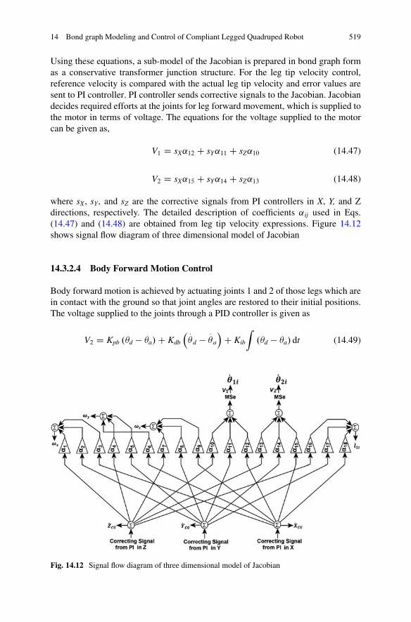
14 Bond graph Modeling and Control of Compliant Legged Quadruped Robot 519
Using these equations, a sub-model of the Jacobian is prepared in bond graph formas a conservative transformer junction structure. For the leg tip velocity control,reference velocity is compared with the actual leg tip velocity and error values aresent to PI controller. PI controller sends corrective signals to the Jacobian. Jacobiandecides required efforts at the joints for leg forward movement, which is supplied tothe motor in terms of voltage. The equations for the voltage supplied to the motorcan be given as,
V1 D sX˛12 C sY˛11 C sZ˛10 (14.47)
V2 D sX˛15 C sY˛14 C sZ˛13 (14.48)
where sX , sY , and sZ are the corrective signals from PI controllers in X, Y, and Zdirections, respectively. The detailed description of coefficients ˛ij used in Eqs.(14.47) and (14.48) are obtained from leg tip velocity expressions. Figure 14.12shows signal flow diagram of three dimensional model of Jacobian
14.3.2.4 Body Forward Motion Control
Body forward motion is achieved by actuating joints 1 and 2 of those legs which arein contact with the ground so that joint angles are restored to their initial positions.The voltage supplied to the joints through a PID controller is given as
V2 D Kpb .�d � �a/C Kdb
:�d �
:
�a
C Kib
Z.�d � �a/ dt (14.49)
Fig. 14.12 Signal flow diagram of three dimensional model of Jacobian

520 M.M. Gor et al.
where V2 is the input voltage supplied to the joint actuator of leg; Kpb, Kdb, and Kib
are the proportional, derivative, and integral gains, respectively; �d is the desired
position, �a is the actual position,:
�d is the desired joint velocity, and:
�a is theactual joint velocity.
14.3.2.5 Combined Control Law
Combined form of the two control laws is entered in bond graph and since both thecontrollers do not work simultaneously for same joint, a switching is used to operatea particular control law. Combined control law can be presented as
V D a1V1 C a2V2 (14.50)
where
a1 D 1 during leg forward motion and 0 during body forward motion, anda2 D 1 during body forward motion and 0 during leg forward motion
14.3.2.6 Three Dimensional Model of Quadruped Robot for WorkspaceControl
Three dimensional model of quadruped robot presented in Sect. 14.2 is modifiedto control in workspace. In this model, joint actuation torque is evaluated as perthe given reference tip trajectory through Jacobian and PI controller. The wordbond graph of quadruped robot control in workspace is shown in Fig. 14.13. Whilemultibond graph presentation of the model is shown in Fig. 14.14.
14.4 Results and Discussions
Above discussed bond graph model can be used for various research aspectspertaining to quadruped robot. Discussed joint space control and workspace controlstrategies are simulated using developed bond graph model, and its results areverified through animation and experimental results. Gait pattern considered forlocomotion control is trot gait. In trot gait, diagonally opposite pairs of legs areactuated together to move forward. This is inspired from the way a horse moves.This two-beat diagonal gait minimizes the shift in body centroid and ensuresgood dynamic stability. Therefore, the quadruped can achieve higher locomotionspeed with this gait. The usefulness of a dynamic model comes when dynamicforces are significant. Therefore, trot gait has been considered in this chapter formodel validation. Influence of compliance is studied on locomotion parameter. Theperformance measure is evaluated based on energy efficiency.

14 Bond graph Modeling and Control of Compliant Legged Quadruped Robot 521
Fig. 14.13 Multibond graph of quadruped robot for locomotion control in workspace
14.4.1 Simulation, Animation, and Experiment Resultsof Locomotion Control in Joint Space
In this section, locomotion control strategy discussed in Sect. 14.3.1 is validatedusing simulation and animation of bond graph dynamic model and also throughexperiment result.

522 M.M. Gor et al.
Fig. 14.14 Word bond graph of quadruped robot control in workspace
14.4.1.1 Simulation Results for Locomotion Control in Joint Space
Bond graph model is simulated for trot gait, for which controlled efforts are suppliedto the actuators, to reach to required joint position as shown in Table 14.1. Inputparameters considered for the simulation are listed in Table 14.2.
Positive Y direction is considered as forward direction. Time duration for eachcycle is 1.7 s. Simulation is carried out for five cycles. Figure 14.15 shows leg tipdisplacement in Y direction, while Fig. 14.16 shows body CG movement in X, Y,and Z directions. It shows robot moves in a forward Y direction. Legs joint rotationsfor the said motion are shown in Fig. 14.17a, b for joint 1 and 2, respectively.Figure 14.18 shows leg tip displacement in Z direction. Similar way, simulationcan be carried out for other gait also.
14.4.1.2 Animation Results for Locomotion Control in Joint Space
Animation of above discussed locomotion strategy of quadruped robot is carried outin SYMBOLS Shakti Animator [34]. The physical characteristics of certain selectedaspects of bond graph model can be directly visualized in this animator, for a better

14 Bond graph Modeling and Control of Compliant Legged Quadruped Robot 523
Table 14.2 Input parameters
Parameters Value
Leg parameters
First link length of leg (l1) 0.225 mMass of first link (Ml1) 1.11 kgMass of cylinder part of the prismatic link (Mc) 0.3 kgMass of piston part of the prismatic link (Mp) 0.2 kgInertia of link 1Ixx1 0.013346 kg m2
Iyy1 0.0073965 kg m2
Izz1 0.011563 kg m2
Inertia of cylinder part of prismatic linkIxxcD Izzc 0.005144 kg m2
Iyyc 0.0000487 kg m2
Inertia of piston and piston rod of prismatic linkIxxpD Izzp 0.00168 kg m2
Iyyp 0.000025 kg m2
Stiffness of spring in compliant link (kf ) 5000 N/mFriction between the piston and cylinder of a prismatic link (Rf ) 274 Ns/mContact point stiffness at the piston cylinder of prismatic link (kb) 108 N/mContact point resistance at the piston and cylinder of prismatic link (Rb) 103 Ns/mLength of piston and piston rod of prismatic link lp 0.1 mDistance of cylinder CG from a cylinder end frame of a prismatic link (lcg) 0.05 mDistance of piston CG from a piston end frame of a prismatic link (lpg) 0.07 mMass of piston and piston rod of the prismatic link (mp) 0.2 kgMass of cylinder part of the prismatic link (mc) 0.3 kgPosition of the cylinder end point with respect to the body fixed frame atthe mass center in meter (x2, y2, z2)
(0.0, �0.05, 0.0)
Position of the piston end point with respect to the body fixed frame at themass center in meter (x3, y3, z3)
(0.0, 0.07, 0.0)
Common parameter
Mass of body (Mb) 6.94 kgInertia of bodyIxb 0.1470 kg m2
Iyb 0.1045 kg m2
Izb 0.2466 kg m2
Ground damping in x, y, z direction (Rgx, Rgy, Rgz) 1000 Ns/mGround stiffness in z direction (Kgz) 106 N/mController parameter
Proportional gain of controller (KP) 100Derivative gain of controller (KD) 80Integral gain of controller (KI) 50Actuator parameter
Motor constant (Km) 0.0276 Nm/AMotor armature resistance (Rm) 0.386 �Motor inductance (Lm) 0.001 HGear ratio (n) 230
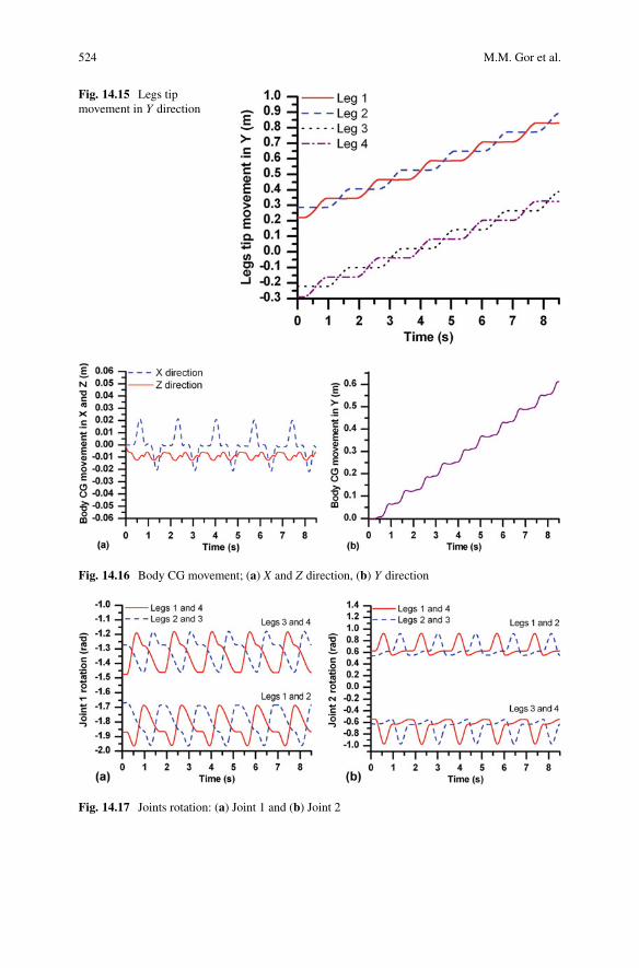
524 M.M. Gor et al.
Fig. 14.15 Legs tipmovement in Y direction
Fig. 14.16 Body CG movement; (a) X and Z direction, (b) Y direction
Fig. 14.17 Joints rotation: (a) Joint 1 and (b) Joint 2
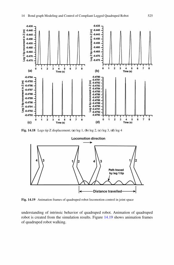
14 Bond graph Modeling and Control of Compliant Legged Quadruped Robot 525
Fig. 14.18 Legs tip Z displacement; (a) leg 1, (b) leg 2, (c) leg 3, (d) leg 4
Fig. 14.19 Animation frames of quadruped robot locomotion control in joint space
understanding of intrinsic behavior of quadruped robot. Animation of quadrupedrobot is created from the simulation results. Figure 14.19 shows animation framesof quadruped robot walking.
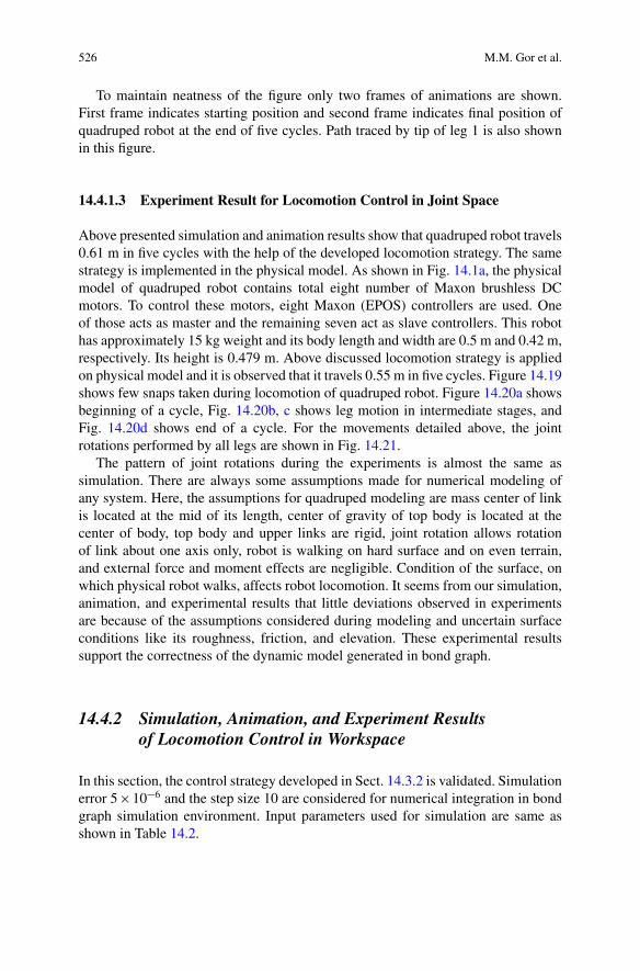
526 M.M. Gor et al.
To maintain neatness of the figure only two frames of animations are shown.First frame indicates starting position and second frame indicates final position ofquadruped robot at the end of five cycles. Path traced by tip of leg 1 is also shownin this figure.
14.4.1.3 Experiment Result for Locomotion Control in Joint Space
Above presented simulation and animation results show that quadruped robot travels0.61 m in five cycles with the help of the developed locomotion strategy. The samestrategy is implemented in the physical model. As shown in Fig. 14.1a, the physicalmodel of quadruped robot contains total eight number of Maxon brushless DCmotors. To control these motors, eight Maxon (EPOS) controllers are used. Oneof those acts as master and the remaining seven act as slave controllers. This robothas approximately 15 kg weight and its body length and width are 0.5 m and 0.42 m,respectively. Its height is 0.479 m. Above discussed locomotion strategy is appliedon physical model and it is observed that it travels 0.55 m in five cycles. Figure 14.19shows few snaps taken during locomotion of quadruped robot. Figure 14.20a showsbeginning of a cycle, Fig. 14.20b, c shows leg motion in intermediate stages, andFig. 14.20d shows end of a cycle. For the movements detailed above, the jointrotations performed by all legs are shown in Fig. 14.21.
The pattern of joint rotations during the experiments is almost the same assimulation. There are always some assumptions made for numerical modeling ofany system. Here, the assumptions for quadruped modeling are mass center of linkis located at the mid of its length, center of gravity of top body is located at thecenter of body, top body and upper links are rigid, joint rotation allows rotationof link about one axis only, robot is walking on hard surface and on even terrain,and external force and moment effects are negligible. Condition of the surface, onwhich physical robot walks, affects robot locomotion. It seems from our simulation,animation, and experimental results that little deviations observed in experimentsare because of the assumptions considered during modeling and uncertain surfaceconditions like its roughness, friction, and elevation. These experimental resultssupport the correctness of the dynamic model generated in bond graph.
14.4.2 Simulation, Animation, and Experiment Resultsof Locomotion Control in Workspace
In this section, the control strategy developed in Sect. 14.3.2 is validated. Simulationerror 5 � 10�6 and the step size 10 are considered for numerical integration in bondgraph simulation environment. Input parameters used for simulation are same asshown in Table 14.2.

14 Bond graph Modeling and Control of Compliant Legged Quadruped Robot 527
Fig. 14.20 Experiment on physical model, (a) initial position, (b) and (c) intermediate positions,(d) end of cycle
14.4.2.1 Simulation and Animation Results for Locomotion Controlin Workspace
This dynamic model is simulated for trot gait. Simulations and animations havebeen carried out for six cycles. In case of trot gait, each cycle takes 1.7 s time.Figure 14.22 shows few animation frames of quadruped motion in trot gait. Tomaintain neatness of the figure only a few animation frames are shown from theentire simulation results. It shows that quadruped locomotion is achieved in theposition Y direction.
Figure 14.23a shows the reference tip displacement (as per the prescribedreference velocity) and the actual tip displacement of legs 1 and 4, while Fig. 14.23bshows those of legs 2 and 3. These results show that the leg tips follow thecorresponding reference trajectories. Error in legs displacement in Y direction of
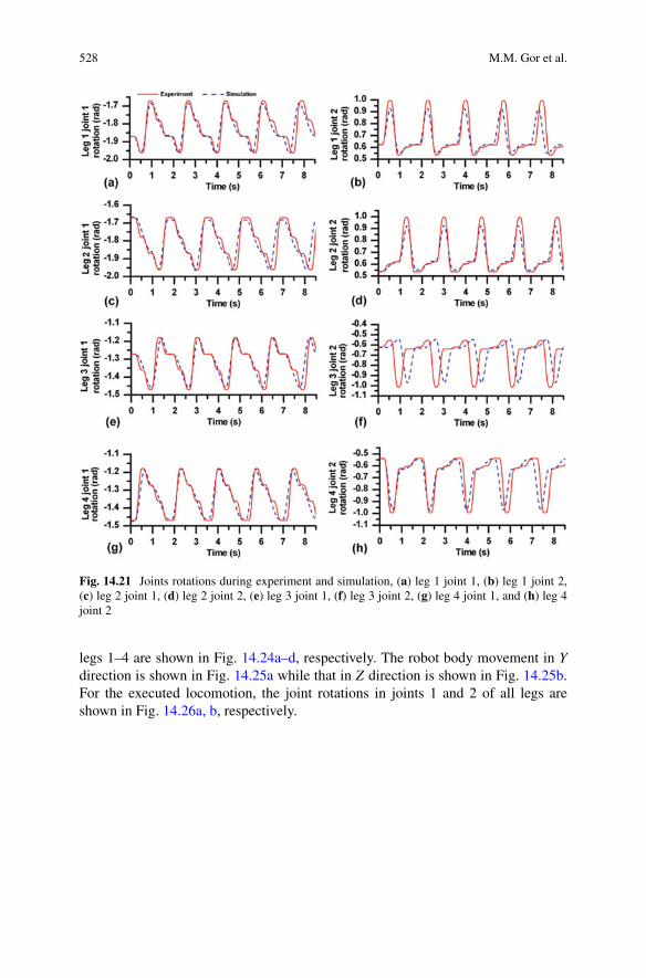
528 M.M. Gor et al.
Fig. 14.21 Joints rotations during experiment and simulation, (a) leg 1 joint 1, (b) leg 1 joint 2,(c) leg 2 joint 1, (d) leg 2 joint 2, (e) leg 3 joint 1, (f) leg 3 joint 2, (g) leg 4 joint 1, and (h) leg 4joint 2
legs 1–4 are shown in Fig. 14.24a–d, respectively. The robot body movement in Ydirection is shown in Fig. 14.25a while that in Z direction is shown in Fig. 14.25b.For the executed locomotion, the joint rotations in joints 1 and 2 of all legs areshown in Fig. 14.26a, b, respectively.

14 Bond graph Modeling and Control of Compliant Legged Quadruped Robot 529
Fig. 14.22 Animation frames of quadruped locomotion control in workspace
Fig. 14.23 Actual and reference leg tip displacements in forward direction for trot gait (a) legs 1and 4, (b) legs 2 and 3
The trot gait in quadruped robot is a dynamic gait where the robot is supportedby either of the diagonally opposite pairs of legs during which the body movesforward. In order to prevent robot falling down, the resultant of gravitational andinertial forces passes through a point on the line joining the tips of the supportinglegs. This ensures dynamic stability. Here, Zero Moment Point (ZMP) introducedin [42] is evaluated to ensure the dynamic stability. By having the ZMP on thediagonal line which connects tips of two legs in contact with the ground, stabilitycan be assured. The ZMP can be calculated as in [44]
Xzmp D
nX
iD1mi� RZi C g
�Xi �
nX
iD1mi RXiZi �
nX
iD1Iiy
R�iy
nX
iD1mi� RZi C g
�(14.51)
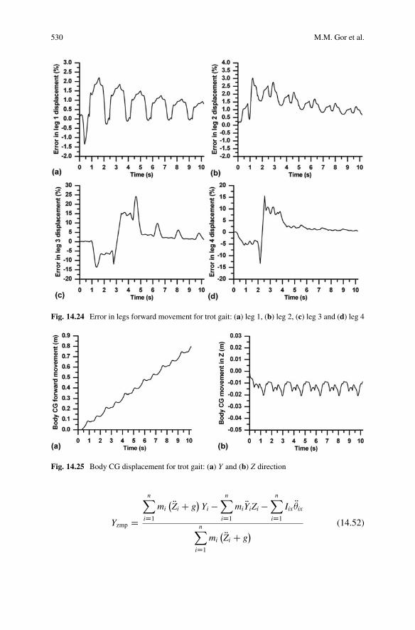
530 M.M. Gor et al.
Fig. 14.24 Error in legs forward movement for trot gait: (a) leg 1, (b) leg 2, (c) leg 3 and (d) leg 4
Fig. 14.25 Body CG displacement for trot gait: (a) Y and (b) Z direction
Yzmp D
nX
iD1mi� RZi C g
�Yi �
nX
iD1mi RYiZi �
nX
iD1Iix
R�ix
nX
iD1mi� RZi C g
�(14.52)

14 Bond graph Modeling and Control of Compliant Legged Quadruped Robot 531
Fig. 14.26 Joints rotation for trot gait: (a) joint 1 and (b) joint 2
Fig. 14.27 ZMP movement for trot gait: (a) X-Y plane for two cycles and (b) in Y direction
where (Xzmp, Yzmp) are coordinates of the ZMP, n is the number of links, i is anenumerator, mi is mass of i-th link, g is gravitational acceleration, Ii is rotary inertiaof i-th link, (Xi, Yi, Zi) are coordinates of the mass center of link i, and R�i is theangular acceleration of link i. Figure 14.27a presents the change in the location ofthe ZMP as the locomotion is executed. For maintaining the clarity of presentation,only the steps followed by the legs during the first two cycles are shown. Duringthe first cycle, legs 2 and 3 are in contact with the ground and the ZMP lies on theline connecting the tips of legs 2 and 3, while during the second cycle, legs 1 and 4are in contact with the ground and the ZMP lies on the line connecting the tips oflegs1 and 4. For six numbers of cycles, the shift of the ZMP in X direction is foundto be in the range �0.020 m to C0.001 m. Figure 14.27b shows the ZMP drift in Ydirection due to robot locomotion.
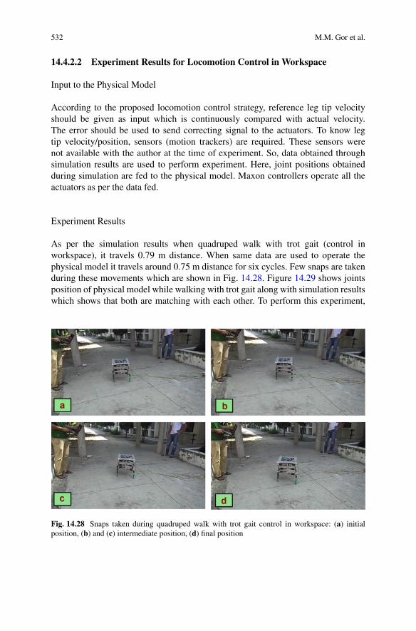
532 M.M. Gor et al.
14.4.2.2 Experiment Results for Locomotion Control in Workspace
Input to the Physical Model
According to the proposed locomotion control strategy, reference leg tip velocityshould be given as input which is continuously compared with actual velocity.The error should be used to send correcting signal to the actuators. To know legtip velocity/position, sensors (motion trackers) are required. These sensors werenot available with the author at the time of experiment. So, data obtained throughsimulation results are used to perform experiment. Here, joint positions obtainedduring simulation are fed to the physical model. Maxon controllers operate all theactuators as per the data fed.
Experiment Results
As per the simulation results when quadruped walk with trot gait (control inworkspace), it travels 0.79 m distance. When same data are used to operate thephysical model it travels around 0.75 m distance for six cycles. Few snaps are takenduring these movements which are shown in Fig. 14.28. Figure 14.29 shows jointsposition of physical model while walking with trot gait along with simulation resultswhich shows that both are matching with each other. To perform this experiment,
Fig. 14.28 Snaps taken during quadruped walk with trot gait control in workspace: (a) initialposition, (b) and (c) intermediate position, (d) final position
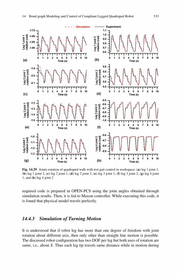
14 Bond graph Modeling and Control of Compliant Legged Quadruped Robot 533
Fig. 14.29 Joints rotation of quadruped walk with trot gait control in workspace: (a) leg 1 joint 1,(b) leg 1 joint 2, (c) leg 2 joint 1, (d) leg 2 joint 2, (e) leg 3 joint 1, (f) leg 3 joint 2, (g) leg 4 joint1, and (h) leg 4 joint 2
required code is prepared in OPEN-PCS using the joint angles obtained throughsimulation results. Then, it is fed to Maxon controller. While executing this code, itis found that physical model travels perfectly.
14.4.3 Simulation of Turning Motion
It is understood that if robot leg has more than one degree of freedom with jointrotation about different axis, then only other than straight line motion is possible.The discussed robot configuration has two DOF per leg but both axes of rotation aresame, i.e., about X. Thus each leg tip travels same distance while in motion during

534 M.M. Gor et al.
Fig. 14.30 Animationframes in top view ofquadruped robot in turningmotion
Table 14.3 Joint position of amble gait for turning motion
Leg 1 Leg 2 Leg 3 Leg 4Joint position correspon-ding to time interval Joint 1 Joint 2 Joint 1 Joint 2 Joint 1 Joint 2 Joint 1 Joint 2
Initial joint angle �1.871 0.622 �1.747 0.586 �1.271 �0.622 �1.395 �0.586To� t < T1/2 �1.979 1.199 �1.781 0.602 �1.323 �0.615 �1.431 �0.564T1/2� t < T1 �1.417 0.265 �1.813 0.613 �1.381 �0.593 �1.471 �0.537T1� t < T2/2 �1.530 0.407 �1.843 0.620 �1.448 �0.554 �1.179 �0.994T2/2� t < T2 �1.618 0.494 �1.871 0.622 �1.523 �0.494 �1.271 �0.622T2� t < T3/2 �1.694 0.554 �1.962 0.944 �1.611 �0.407 �1.299 �0.620T3/2� t < T3 �1.760 0.593 �1.671 0.537 �1.725 �0.265 �1.328 �0.613T3� t < T4/2 �1.819 0.615 �1.710 0.564 �1.162 �1.199 �1.361 �0.602T4/2� t < T5 �1.871 0.622 �1.747 0.586 �1.271 �0.622 �1.395 �0.586
one cycle and robot has straight line motion. If one side of both the leg tips travelssame distance but different from opposite side of leg tips (i.e., legs 1 and 3 tip travelssame distance but they are different from legs 2 and 4 tip travels), then this motiongives a turn instead of moving in straight line. This concept has been demonstratedusing amble gait. Simulation and animation is carried out for 20 cycles. Each cycletakes 0.9 s. Figure 14.30 shows animation frames of quadruped locomotion whichmoves straight for initial five cycles (A) then it takes turn for next ten cycles (B)and finally moves straight for remaining five cycles (C). In this figure path traced byhip joints and body CG are shown. Joint position corresponding to time interval isshown in Table 14.3.
Figure 14.31 shows body CG X motion while Figs. 14.32 and 14.33 show bodyCG Y and Z motions, respectively. Leg tip motion in X and Y directions are shownin Figs. 14.34 and 14.35, respectively. As discussed above, it is necessary to havedifferent joint rotations for this kind of locomotion. Joints 1 and 2 rotations carried
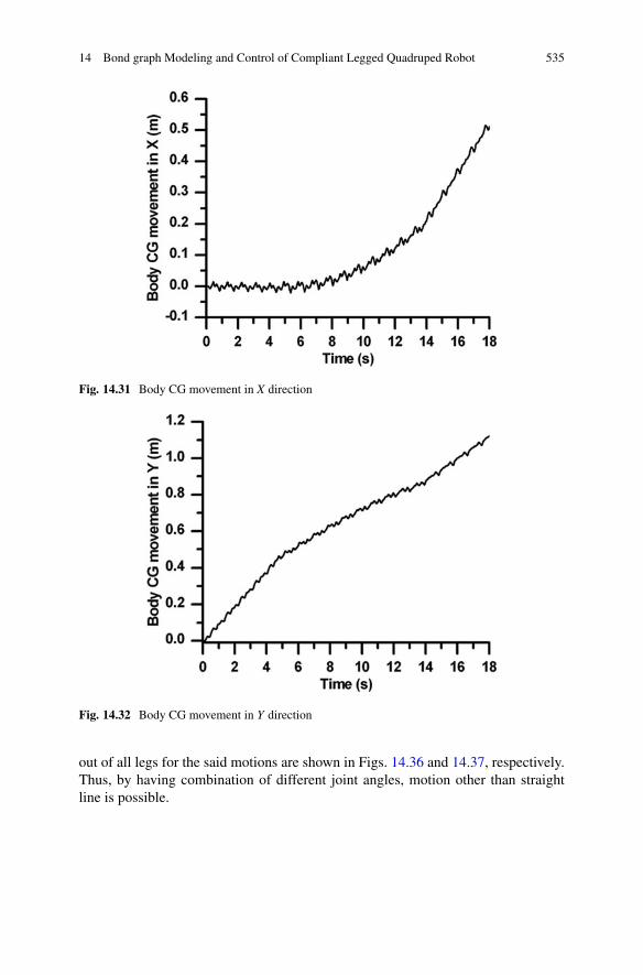
14 Bond graph Modeling and Control of Compliant Legged Quadruped Robot 535
Fig. 14.31 Body CG movement in X direction
Fig. 14.32 Body CG movement in Y direction
out of all legs for the said motions are shown in Figs. 14.36 and 14.37, respectively.Thus, by having combination of different joint angles, motion other than straightline is possible.
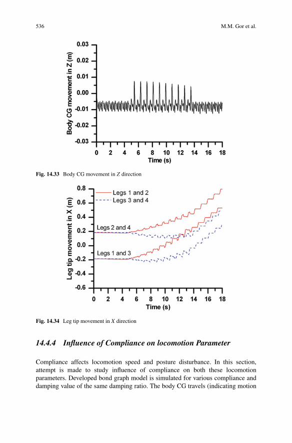
536 M.M. Gor et al.
Fig. 14.33 Body CG movement in Z direction
Fig. 14.34 Leg tip movement in X direction
14.4.4 Influence of Compliance on locomotion Parameter
Compliance affects locomotion speed and posture disturbance. In this section,attempt is made to study influence of compliance on both these locomotionparameters. Developed bond graph model is simulated for various compliance anddamping value of the same damping ratio. The body CG travels (indicating motion

14 Bond graph Modeling and Control of Compliant Legged Quadruped Robot 537
Fig. 14.35 Leg tip movement in Y direction
Fig. 14.36 Joint 1 rotation of legs
of robot in forward direction) and posture disturbance are analyzed. Figure 14.38ashows body CG travels by quadruped robot and Fig. 14.38b shows range of posturedisturbance in roll and pitch during the locomotion.
It is concluded from the results that as the stiffness decreases, the body CGtravel reduces. Body CG travel does not increase noticeably after increasing thestiffness further than about 7000 N/m. It is also seen from the results that the posturedisturbance range at roll and pitch becomes higher at higher stiffness. It is always
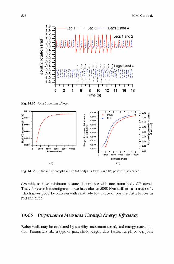
538 M.M. Gor et al.
Fig. 14.37 Joint 2 rotation of legs
Fig. 14.38 Influence of compliance on (a) body CG travels and (b) posture disturbance
desirable to have minimum posture disturbance with maximum body CG travel.Thus, for our robot configuration we have chosen 5000 N/m stiffness as a trade-off,which gives good locomotion with relatively low range of posture disturbances inroll and pitch.
14.4.5 Performance Measures Through Energy Efficiency
Robot walk may be evaluated by stability, maximum speed, and energy consump-tion. Parameters like a type of gait, stride length, duty factor, length of leg, joint

14 Bond graph Modeling and Control of Compliant Legged Quadruped Robot 539
angle, and rotation are deciding the above-mentioned performance criteria. Todiscuss advantage and disadvantage of different designs and control strategies, it isnecessary to evaluate and compare robot performance and abilities with respect tocommon criteria. A common measure to evaluate and compare the energy efficiencyof vehicles is the energy consumption per unit distance. To justify the comparison,mass moved, and velocity obtained should also be considered with the cost oflocomotion. We are comparing here quadruped walk with specific resistance (").The specific resistance [15, 22] is a dimensionless number describing the energyefficiency of a mobile system. The specific resistance is defined as
" D P.v/
mgvD E
mgd(14.53)
where P(v) is the power needed to move the body with velocity v, m is the mass ofthe system, g is the acceleration due to gravity, d is the distance travelled, and E isthe energy spent. Since velocity is not constant in a cycle, energy spent to move unitweight by unit distance is preferred as the performance measure. Sufficient numberof cycles of motion till steady-state is reached should be considered for evaluationof specific resistance. Lower specific resistance implies higher energy efficient.
14.4.5.1 Energy Efficient Structure of Quadruped Robot
In this section, energy efficiency of rigid legged and compliant legged robots areevaluated and compared. Locomotion gait is considered as trot for both the cases.The above developed bond graph model for compliant legged robot was modifiedto generate the model of rigid legged robot. This is done by locking the slidingmotion of the piston within the prismatic link; thereby retaining the same massparameters in both the models. The locking is performed through a high-stiffnessvirtual spring which is called a pad in bond graph terminology. Both rigid leggedand compliant legged models are simulated for same speed which is fixed at 0.42 mdistance travelled in 4.5 s., i.e., with an average locomotion speed of 0.093 m/s. Thesame speed requirement is satisfied by manually tuning the controller parametersand the cycle time durations. Figure 14.39a shows body CG travels by rigid leggedquadruped robot in trot gait. Figure 14.39b shows body CG travels by compliantlegged robot in trot gait. Sensors are placed at the actuators in bond graph models toextract the power consumption data. The specific resistance defined in Eq. (14.53)is evaluated for both these cases considering robot mass as 15 kg and gravitationalacceleration as 9.81 m/s2. It was found that the specific resistance for the compliancelegged model is 0.925 while it is 1.10 for rigid legged model. It is known that smallerthe specific resistance, higher the energy efficiency [15, 22, 38]. So from the aboveresults, smaller specific resistance of compliant legged robot implies that it is energyefficient than rigid legged robot. Leg compliance reduces impact induced bounceand allows for better grip; thereby improving the locomotion efficiency. However,it may be noted that too low or too high-stiffness reduce grip and increase losses
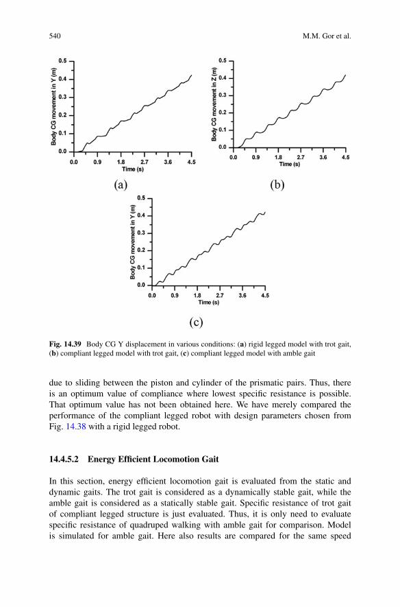
540 M.M. Gor et al.
Fig. 14.39 Body CG Y displacement in various conditions: (a) rigid legged model with trot gait,(b) compliant legged model with trot gait, (c) compliant legged model with amble gait
due to sliding between the piston and cylinder of the prismatic pairs. Thus, thereis an optimum value of compliance where lowest specific resistance is possible.That optimum value has not been obtained here. We have merely compared theperformance of the compliant legged robot with design parameters chosen fromFig. 14.38 with a rigid legged robot.
14.4.5.2 Energy Efficient Locomotion Gait
In this section, energy efficient locomotion gait is evaluated from the static anddynamic gaits. The trot gait is considered as a dynamically stable gait, while theamble gait is considered as a statically stable gait. Specific resistance of trot gaitof compliant legged structure is just evaluated. Thus, it is only need to evaluatespecific resistance of quadruped walking with amble gait for comparison. Modelis simulated for amble gait. Here also results are compared for the same speed

14 Bond graph Modeling and Control of Compliant Legged Quadruped Robot 541
which is obtained by tuning controller parameters and cycle duty times. Body CGdisplacement obtained in Y direction (along the longitudinal axis) for amble gaitis shown in Fig. 14.39c. Results obtained are used to evaluate Eq. (14.53) whichgives the specific resistance of the amble gait as 6.71. From this result it seems thatspecific resistance of the trot gait is smaller. Thus the trot gait is energy efficientthan the amble gait.
14.4.5.3 Energy Efficient Foot Trajectory
Foot trajectory in case of walking robot has two main parameters: leg lift (LL) andstep length (SL), which almost decides the foot trajectory of leg tip. However, theway leg tip reach to LL decides exact curve. Here, numbers of simulations arecarried out to analyze the effect of LL and SL. For this analysis dynamic modelshould be controlled in workspace mode. Assumptions considered for the analysisare robot walks in straight line and on even terrain with trot gait.
First, simulations are carried out for different SL by keeping LL fixed as 0.033 m.Figure 14.40 shows given leg tip motion in Y and Z directions. Specific resistancefor this run is plotted in Fig. 14.41 which indicates that for fixed LL as SL increasesthe specific energy decreases thus walk becomes more and more energy efficient.
Next, simulations are carried out for different LL by keeping SL fixed. Here, twosets of simulations are performed for SL as 0.099 and 0.132 m. Figure 14.42 showsgiven leg tip trajectory while Fig. 14.43 shows specific resistance. In both the casesit is observed that as LL increases specific resistance increases thus walk becomesless energy efficient. At the same time too much low LL also reports less energyefficient as its specific resistance goes high.
Fig. 14.40 Leg tip motion in YZ plane for different step length with same leg lift

542 M.M. Gor et al.
Fig. 14.41 Specific resistance for different step length with same leg lift
Fig. 14.42 Leg tip motion in YZ plane for different foot height with same step length
Thus from all these analysis it can be concluded that for energy efficient walk, SLshould be as high as possible and LL should be low if it walks on even terrain. For0.033 m LL, 0.200 m SL gives most energy efficient walks as its specific resistanceis lowest. However, for different size of robot best combination will be differing.

14 Bond graph Modeling and Control of Compliant Legged Quadruped Robot 543
Fig. 14.43 Specific resistance for different leg lift with same step length
14.5 Conclusions
A three dimensional model of compliant legged quadruped robot using bond graphhas been developed. The legs contain telescopic tubes with axial compliance and themodel considers its detailed dynamics. The developed model is simulated for loco-motion control in joint space as well as in workspace, and the obtained simulationand animation results are compared with the experimental results for validation.The developed model is useful for the various research activities pertaining toquadruped control. Its versatility is demonstrated by performance analysis, whichshows that the compliant legged robot (specific resistance 0.925) is more energyefficient than rigid legged robot (specific resistance 1.10), a dynamically stable trotgait (specific resistance 0.925) is more energy efficient than a statically stable amblegait (specific resistance 6.71), and a foot trajectory consisting of maximum possiblestep length with minimum leg lift gives energy efficient performance. Influence ofcompliance on locomotion parameters is studied and best suitable compliance value,i.e., 5000 N/m for the robot is obtained. Turning motion of the robot is demonstratedby differential leg tip velocity of robot. In future, it is envisaged to use this modelfor workspace control, posture control, and fault accommodation of the quadrupedrobot.
Acknowledgment The work of M. M. Gor, P. M. Pathak, and A. K. Samantaray has been fundedby DST, India under Indo–Korea Joint Research in Science and Technology vide Grant No.INT/Korea/P–13. The work of J.–M. Yang and S. W. Kwak was supported by the Korea government(MEST) vide the National Research Foundation of Korea Grant No. NRF–2011–0027705. M. M.Gor is thankful to G H Patel College of Engineering and Technology, Gujarat, India for allowinghim to carry out research work at IIT Roorkee. Authors are thankful to B.Tech. students Divye,Kamran, Piyush, Param, and Rohan for their assistantship in developing the set-up and conductingthe experiments.
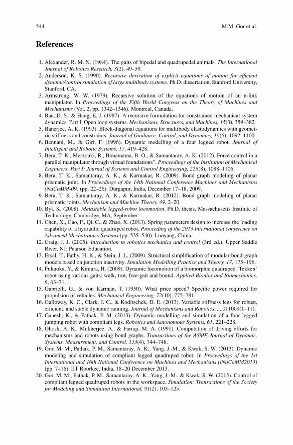
544 M.M. Gor et al.
References
1. Alexander, R. M. N. (1984). The gaits of bipedal and quadrupedal animals. The InternationalJournal of Robotics Research, 3(2), 49–59.
2. Anderson, K. S. (1990). Recursive derivation of explicit equations of motion for efficientdynamic/control simulation of large multibody systems. Ph.D. dissertation, Stanford University,Stanford, CA.
3. Armstrong, W. W. (1979). Recursive solution of the equations of motion of an n-linkmanipulator. In Proceedings of the Fifth World Congress on the Theory of Machines andMechanisms (Vol. 2, pp. 1342–1346). Montreal, Canada.
4. Bae, D. S., & Haug, E. J. (1987). A recursive formulation for constrained mechanical systemdynamics: Part I. Open loop systems. Mechanisms, Structures, and Machines, 15(3), 359–382.
5. Banerjee, A. K. (1993). Block-diagonal equations for multibody elastodynamics with geomet-ric stiffness and constraints. Journal of Guidance, Control, and Dynamics, 16(6), 1092–1100.
6. Bennani, M., & Giri, F. (1996). Dynamic modelling of a four legged robot. Journal ofIntelligent and Robotic Systems, 17, 419–428.
7. Bera, T. K., Merzouki, R., Bouamama, B. O., & Samantaray, A. K. (2012). Force control in aparallel manipulator through virtual foundations”. Proceedings of the Institution of MechanicalEngineers, Part I: Journal of Systems and Control Engineering, 226(8), 1088–1106.
8. Bera, T. K., Samantaray, A. K., & Karmakar, R. (2009). Bond graph modeling of planarprismatic joint. In Proceedings of the 14th National Conference Machines and Mechanisms(NaCoMM-09) (pp. 22–26). Durgapur, India, December 17–18, 2009.
9. Bera, T. K., Samantaray, A. K., & Karmakar, R. (2012). Bond graph modeling of planarprismatic joints. Mechanism and Machine Theory, 49, 2–20.
10. Byl, K. (2008). Metastable legged-robot locomotion. Ph.D. thesis, Massachusetts Institute ofTechnology, Cambridge, MA, September.
11. Chen, X., Gao, F., Qi, C., & Zhao, X. (2013). Spring parameters design to increase the loadingcapability of a hydraulic quadruped robot. Proceeding of the 2013 International conference onAdvanced Mechatronics Systems (pp. 535–540). Luoyang, China.
12. Craig, J. J. (2005). Introduction to robotics mechanics and control (3rd ed.). Upper SaddleRiver, NJ: Pearson Education.
13. Ersal, T., Fathy, H. K., & Stein, J. L. (2009). Structural simplification of modular bond-graphmodels based on junction inactivity. Simulation Modelling Practice and Theory, 17, 175–196.
14. Fukuoka, Y., & Kimura, H. (2009). Dynamic locomotion of a biomorphic quadruped ‘Tekken’robot using various gaits: walk, trot, free-gait and bound. Applied Bionics and Biomechanics,6, 63–71.
15. Gabrielli, G., & von Karman, T. (1950). What price speed? Specific power required forpropulsion of vehicles. Mechanical Engineering, 72(10), 775–781.
16. Galloway, K. C., Clark, J. C., & Koditschek, D. E. (2013). Variable stiffness legs for robust,efficient, and stable dynamic running. Journal of Mechanisms and Robotics, 5, 011009(1–11).
17. Ganesh, K., & Pathak, P. M. (2013). Dynamic modelling and simulation of a four leggedjumping robot with compliant legs. Robotics and Autonomous Systems, 61, 221–228.
18. Ghosh, A. K., Mukherjee, A., & Faruqi, M. A. (1991). Computation of driving efforts formechanisms and robots using bond graphs. Transactions of the ASME Journal of Dynamic,Systems, Measurement, and Control, 113(4), 744–748.
19. Gor, M. M., Pathak, P. M., Samantaray, A. K., Yang, J.-M., & Kwak, S. W. (2013). Dynamicmodeling and simulation of compliant legged quadruped robot. In Proceedings of the 1stInternational and 16th National Conference on Machines and Mechanisms (iNaCoMM2013)(pp. 7–16). IIT Roorkee, India, 18–20 December 2013.
20. Gor, M. M., Pathak, P. M., Samantaray, A. K., Yang, J.-M., & Kwak, S. W. (2015). Control ofcompliant legged quadruped robots in the workspace. Simulation: Transactions of the Societyfor Modeling and Simulation International, 91(2), 103–125.
14 Bond graph Modeling and Control of Compliant Legged Quadruped Robot 545
21. Gor, M. M., Pathak, P. M., Samantaray, A. K., Yang, J.-M., & Kwak, S. W. (2015). Controloriented model-based simulation and experimental studies on a compliant legged quadrupedrobot. Robotics and Autonomous System, 72, 217–234.
22. Gregorio, P., Ahmadi, M., & Buehler, M. (1997). Design, control, and energetics of anelectrically actuated legged robot. IEEE Transactions on Systems, Man and Cybernetics, 27(4),626–634.
23. Hollerbach, J. M. (1980). A recursive Lagrangian formulation of manipulator dynamics and acomparative study of dynamics formulation complexity. IEEE Transactions on Systems, Man,and Cybernetics, 10(11), 730–736.
24. Karnopp, D. C., Margolis, D. L., & Rosenberg, R. C. (2006). System dynamics: Modeling andsimulation of mechatronic systems (4th ed.). New York: Wiley.
25. Kimura, H., & Fukuoka, Y. (2004). Biologically inspired adaptive dynamic walking in outdoorenvironment using a self-contained quadruped robot: ‘Tekken2’. In Proceedings of the 2004IEEE/RSJ International Conference on Intelligent Robots and Systems, 2004, (IROS 2004)(pp. 986–991).
26. Krishnan, V. L., Pathak, P. M., Sardana, L., & Jain, S. C. (2010). Simulation and experimentalstudies on walking robot with flexible legs. In Proceeding of 4th International Conference onIntegrated Modeling and Analysis in Applied Control and Automation (IMAACA 2010), Fes,Morocco (pp. 11–19).
27. Mahapatra, A., & Roy, S. S. (2009). Computer aided dynamic simulation of six legged robot.International Journal of Recent Trends in Engineering, 2(2), 146–151.
28. Merzouki, R., Samantaray, A. K., Pathak, P. M., & OuldBouamama, B. (2013). Intelligentmechatronic systems—Modeling, control and diagnosis. London: Springer.
29. Pathak, P. M., Mukherjee, A., & Dasgupta, A. (2005). Impedance control of space robots usingpassive degrees of freedom in controller domain. Transactions of ASME, Journal of DynamicSystems, Measurement, and Control, 127(4), 564–578.
30. Raibert, M. H. (1986). Legged robots that balance. Cambridge, MA: MIT Press.31. Raibert, M., Blankespoor, K., Nelson, G., & Playter, R. (2008). BigDog, the rough terrain
quadruped robot. Proceedings of the 17th IFAC World Congress, COEX (pp. 10823–10825).South Korea.
32. Remy, C. D., Hutter, M., Hoepflinger, M., Bloesch, M., Gehring, C., & Siegwart, R. (2012).Quadrupedal robots with stiff and compliant actuation. at-Automatisierungstechnik, 60(11),682–691.
33. Rosenthal, D. E. (1990). An order n formulation for robotic systems. Journal of AstronauticalSciences, 38(4), 511–529.
34. Samantaray, A. K., & Mukherjee, A. (2000). User manual of SYMBOLS. Kharagpur: HighTech Consultants, S.T.E.P., Indian Institute of Technology.
35. Semini, C., Tsagarakis, N. G., Guglielmino, E., Focchi, M., Cannella, F., & Caldwell, D.G. (2011). Design of HyQ—A hydraulically and electrically actuated quadruped robot.Proceedings of the Institution of Mechanical Engineers, Part I: Journal of Systems and ControlEngineering, 225(6), 831–849.
36. Shah, S. V., Saha, S. K., & Dutt, J. K. (2012). Modular framework for dynamic modeling andanalyses of legged robots. Mechanism and Machine Theory, 49, 234–255.
37. Shkolnik, A., Levashov, M., Manchester, I. R., & Tedrake, R. (2011). Bounding on roughterrain with the LittleDog robot. The International Journal of Robotics Research, 30, 192–215.
38. Siciliano, B., & Khatib, O. (Eds.). (2008). Springer handbook of robotics. Berlin: Springer.39. Soyguder, S., & Ali, H. (2012). Computer simulation and dynamic modeling of a quadrupedal
pronking gait robot with SLIP model. Computers and Electrical Engineering, 28, 161–174.40. Sprowitz, A., Tuleu, A., Vespignani, M., Ajallooeian, M., Badri, E., & Ijspeert, A. J. (2013).
Towards dynamic trot gait locomotion design control and experiments with cheetah-cub, acompliant quadruped robot. The International Journal of Robotics Research, 32(8), 932–950.
41. Todd, D. J. (1985). Walking machines: An introduction to legged robots. London: Koran Page.42. Vukobratovic, M., & Jurwicic, D. (1969). Contribution to the synthesis of biped gait. IEEE
Transactions on Bio-Medical Engineering, 16, 1–6.

546 M.M. Gor et al.
43. Walker, M. W., & Orin, D. E. (1982). Efficient dynamic computer simulation of roboticmechanisms. Journal of Dynamic Systems, Measurements, and Control, 104, 205–211.
44. Zhang, S., Gao, J., Duan, X., Li, H., Yu, Z., Chen, X., et al. (2013). Trot pattern generationfor quadruped robot based on the ZMP stability margin. ICME International Conference onComplex Medical Engineering (pp. 608–613). Beijing, China, May 25–28, 2013.

Chapter 15Modeling and Control of a Wind Turbine
R. Tapia Sánchez and A. Medina Rios
Abbreviations
DFIG Doubly fed induction generatorMSC Machine side converterNSC Network side converterDC Direct currentCp Power coefficientBEM Blade element momentumDFIM Doubly fed induction motor
15.1 Introduction
Wind turbine is a complex system in which different technical areas are involved.Some publications deal with this topic, e.g., [22, 24, 25]. In [22] a parametricand nonparametric model is proposed using advantage algorithms, only the powercurve is considered. Other contribution [25] reviews recent research of numericalsimulation applied to wind energy and in [24] the modeling of a small-scaledistributed power system containing the power demand, a wind turbine, thephotovoltaic arrays, and the electrical connection is presented. These contributionshighlight the importance of having a reliable model of the wind turbine, in orderto conduct dynamic studies of such system. Nevertheless, the use of differenttechniques previously developed, and the complexity of a wind turbine make
R.T. Sánchez (�) • A.M. RiosDivisión de Estudios de Posgrado, Facultad de Ingeniería Eléctrica, Universidad Michoacanade San Nicolás de Hidalgo, Morelia 58000, Mexicoe-mail: [email protected]
© Springer International Publishing Switzerland 2017W. Borutzky (ed.), Bond Graphs for Modelling, Control and FaultDiagnosis of Engineering Systems, DOI 10.1007/978-3-319-47434-2_15
547

548 R.T. Sánchez and A.M. Rios
possible to visualize even different approaches for their study and analysis. Underthis context, in order to analyze the system in the same reference frame, the bondgraph methodology [3, 19, 37] can represent the whole structure. This methodologypresents some properties that can be applied directly to the model [7].
The bond graph wind turbine model has been addressed in several works, e.g.,[1, 10, 46]. In the first publication, a detailed model of a blade is proposed. Theaerodynamic structural forces are considered, and also real data of a wind turbineare used, in order to calculate the output torque. Besides, it is a general model thatcan be applied to any wind turbine blade. In [46] a six-mass drive train modelis presented. This complete model is formulated and then simplified. The authorsdid not use real parameters of a wind turbine and the aerodynamics forces are notconsidered. In [10], a complete wind turbine based on parameters taken from a realturbine is proposed. The model presents all components of the wind turbine, but theaerodynamics are not considered in detail. The publication is centered on drive traineffects.
The mechanical part of the wind turbine presented in this chapter is taken from[44] which consider the blade model presented in [1].
Nowadays, most of the installed wind turbines have kept the configuration withthe use of a gearbox. Based on this context, a model of the gearbox is used inorder to complete the whole system. In terms of a bond graph methodology, gearshave been modeled for transmission applications [6, 8]. The model used here isbased on the one reported in [21], in which a planetary gears is adopted. Also, in[17] a complete review of graphical tools for modeling gears is given. The authorsconclude that bond graph methodology has major properties, when compared toothers. It is important to mention that gearbox is the most important part of a windturbine, because is at this stage where most of faults occur. It is estimated that awind turbine has around 20 years of life span, but normally the gearbox needs to bereplaced every 5 years [36].
In this chapter a complete bond graph model of a variable-speed wind turbinewith doubly fed induction generator (DFIG) configuration is presented, whichaccounts real data and parameters of a real wind turbine of 750 kW [13]. Thisconfiguration has some important advantages, e.g., the possibility of controllingactive and reactive power, the capability of reducing stresses of the mechanicalstructure, and acoustic noise [5]. Also, losses in the power electronics converter arereduced, as compared to a direct-driver synchronous/induction generator (variable-speed wind turbine with induction generator configuration). This is due to the factthat the converter placed between the grid and the double-fed induction machinerotor handles only a fraction of the turbine rate power [26, 47].
The control of a DFIG has been addressed in several works, e.g., [9, 15, 32, 35].In [9] a sliding mode control is used, and in [35] the power control of a doubly fedinduction machine via output feedback is presented. The behavior of such machinesin large wind farms, along with the general active and reactive power control hasbeen addressed in [15]. A novel simplified model of the DFIG appropriate for bulkpower system studies is presented in [32]. In this chapter, the control law developed

15 Modeling and Control of a Wind Turbine 549
in [45] is taken because this control presents a different structure and the bond graphmodel of the DFIG is used in order to obtain the control law applying the bicausalityconcepts [11].
The outline of this chapter is as follows: the model description is given inSect. 15.2. Then, the wind turbine model is detailed in Sect. 15.3. The DFIG controlis described in Sect. 15.4. The whole system is simulated in Sect. 15.5. The globalconclusions of the chapter are drawn in Sect. 15.6.
15.2 System Description
The wind turbine connected to the electrical network can be represented byFig. 15.1. Every single part (blades, hub, bearings, brake, and hub) of the windturbine scheme is joined by a bond. In most of the elements there is an associatedmechanical power, but the last part (DFIG) transforms this mechanical power intoa three phase electrical power, represented by three bonds. The stator is directlyconnected to the power network, while the rotor is connected through slip rings to apower electronic converter.
Different considerations can be made for the study of this system. Here, ananalysis of the complete model is presented, by considering all the components asshown in Fig. 15.1.
The function of blades is to convert the wind velocity into a torque, transformingthe wind into a force and then into a torque. In Fig. 15.1, the causality of the firstbond shows that torque is provided by the blades.
A large torque is produced by blades, and is transferred to the gearbox, whichtransforms this big torque into a small one, to be applied into generator. A similarsituation is valid for angular velocity, i.e., there is a high speed provided forgenerator, which is transformed by the gearbox into a low speed, presented in therotor turbine (hub).
Fig. 15.1 Wind turbine presented in terms of word bond graph
550 R.T. Sánchez and A.M. Rios
From the generator point of view, a wind turbine has different configurations.Also, the wind turbine can operate with either under fixed-speed or variable-speedmode. This operation depends directly on the generator connection. It means thatfor fixed-speed wind turbines, the generator is directly connected to the powernetwork, since the speed is closely tied to the grid frequency. Besides, for a variable-speed wind turbine, the generator is controlled through power electronics converters,which make possible to control the rotor speed. Therefore, as it was mentionedbefore, a variable-speed wind turbine with doubly fed generator configuration isused (Fig. 15.1).
The main advantage of this configuration is the fact that the power electronicconverter has to handle only a fraction (30 %) of the total power [47]. Therefore, thelosses in the power electronic converter can be reduced.
Two power electronics converters: machine side converter (MSC) and networkside converter (NSC) are used in order to have a DC-link between them, thusallowing the power transfer. With the MSC, it is possible to control the torque orspeed in the DFIG and the power factor at the stator terminals, while with the NSCfunctions the DC-link voltage is kept constant.
In the following sections the model of each elements is presented.
15.3 Model Components
In this section the individual bond graph models for the blades, the gearbox, thedoubly fed induction generator, and the converters are presented.
15.3.1 Blades
As mentioned before, the blade model is taken from [1]. In that publication, theblade structure represents a general model; it means that wind turbines of differentpowers capacity can be simulated by changing the data. The model presented in[1] is divided into three sections; however, it can be divided into more sections.Here this model is recalled, since it represents the blade aerodynamic wind turbine.Nevertheless, the blade is divided into only two sections to allow the improvementof results, in terms of the coefficient of power Cp, as it will be later shown in thissection.
There are problems in system modeling, where lumping of inertia and com-pliance, used in rigid body dynamics, fails to get the essential dynamics of thesystem. Situations like this often arise with systems consisting of long slendermembers, whose flexibility plays an important role in the dynamics of the system.For example, in wind turbine modeling, it will be inadequate to treat the blade as arigid body. These members are essentially distributed system parameters, governedby partial differential equations, and are lumped in space by finite approximation.
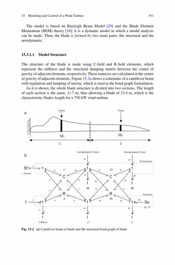
15 Modeling and Control of a Wind Turbine 551
The model is based on Rayleigh Beam Model [29] and the Blade ElementMomentum (BEM) theory [16]; it is a dynamic model in which a modal analysiscan be made. Then, the blade is formed by two main parts: the structural and theaerodynamic.
15.3.1.1 Model Structure
The structure of the blade is made using C-field and R-field elements, whichrepresent the stiffness and the structural damping matrix between the center ofgravity of adjacent elements, respectively. These matrices are calculated at the centerof gravity of adjacent elements. Figure 15.2a shows a schematic of a cantilever beamwith regulation and lumping of inertia, which is used in the bond graph formulation.
As it is shown, the whole blade structure is divided into two sections. The lengthof each section is the same, 11.7 m, thus allowing a blade of 23.4 m, which is thecharacteristic blades length for a 750 kW wind turbine.
Fig. 15.2 (a) Cantilever beam of blade and (b) structural bond graph of blade

552 R.T. Sánchez and A.M. Rios
The bond graph model presented in Fig. 15.2b shows the translation and rotationmotion at the top and bottom of the figure, respectively. Aerodynamic forces foreach section are applied in the translation structure (bonds 12 and 23); this meansthat the effort is imposed.
The stiffness matrix is modeled as a 4–port C–field storing, due to the fourgeneralized displacements shown in Fig. 15.2b. In terms of flexural rigidity (EI)and element length (l), the stiffness matrix is given by Eq. (15.1).
ŒKi� D EI
l3
2
664
12 6l �12 6l6l 4l2 �6l 2l2
� 12 �6l 12 �6l6l 2l2 �6l 4l2
3
775 (15.1)
where E is the Young module of the material, and I the second moment of areaabout the axis of deflection. The structural damping matrix is given by [Ri] D�[Ki],where the � factor represents the coefficient of structural damping.
The boundary condition of the model is represented by the Sf:v_bound and Sesources. The connection between the blade and the hub is assumed to be rigid, i.e.,Sf:v_bound D 0, and the blade has only one degree of freedom Se D 0. Finally, therotating inertia J_whole is the rigid body inertia of the whole blade.
Dynamic equations and also the natural frequencies of the blade can be directlyobtained from the bond graph of Fig. 15.2b. In this case, the main dynamics aroundthe blade structure take into account the parameters (given in Appendix (Table 15.6))for an NACA 4415 blade [48].
Considering Fig. 15.2b the causal loops and causal paths are presented inTable 15.1. The causal loops consider the C and R matrix values, in order tocalculate the frequency. Therefore, each causal loop involved with one I elementand one element of the damping matrix (R) is considered. Besides, there are causalpaths present in the model, between the I-elements and the stiffness matrix, andTable 15.1 shows also the numerical values of these causal paths. It is important tomention that the main frequencies are produced only by the causal loops.
As shown in Table 15.1, the loop involving the translational mass M1 of section 1has small values (bonds 11, 13, 19), compared to the mass M2 (bonds 20, 24). Thisverified that high frequency vibrations are introduced by the last blade sections, and
Table 15.1 Causal loop and causal paths frequencies
Causalloop
2! 4!4! 2
14! 6!6! 14
14! 16!16! 14
25! 18!18! 25
13! 11!11! 13
13! 19!19! 13
24! 20!20! 24
Frequency(rad/s)
120.88 36632.9 54245 76827.7 8.77 12.99 32.22
Causalpath
2! 3 14! 5 13! 10 14! 15 13! 21 25! 17 24! 22
Frequency(rad/s)
690832.9 39685.3 224807.7 39685.33 224807.8 9873.15 482100.3
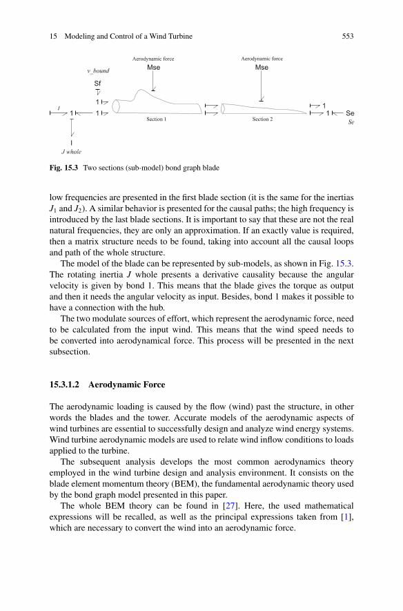
15 Modeling and Control of a Wind Turbine 553
Fig. 15.3 Two sections (sub-model) bond graph blade
low frequencies are presented in the first blade section (it is the same for the inertiasJ1 and J2). A similar behavior is presented for the causal paths; the high frequency isintroduced by the last blade sections. It is important to say that these are not the realnatural frequencies, they are only an approximation. If an exactly value is required,then a matrix structure needs to be found, taking into account all the causal loopsand path of the whole structure.
The model of the blade can be represented by sub-models, as shown in Fig. 15.3.The rotating inertia J whole presents a derivative causality because the angularvelocity is given by bond 1. This means that the blade gives the torque as outputand then it needs the angular velocity as input. Besides, bond 1 makes it possible tohave a connection with the hub.
The two modulate sources of effort, which represent the aerodynamic force, needto be calculated from the input wind. This means that the wind speed needs tobe converted into aerodynamical force. This process will be presented in the nextsubsection.
15.3.1.2 Aerodynamic Force
The aerodynamic loading is caused by the flow (wind) past the structure, in otherwords the blades and the tower. Accurate models of the aerodynamic aspects ofwind turbines are essential to successfully design and analyze wind energy systems.Wind turbine aerodynamic models are used to relate wind inflow conditions to loadsapplied to the turbine.
The subsequent analysis develops the most common aerodynamics theoryemployed in the wind turbine design and analysis environment. It consists on theblade element momentum theory (BEM), the fundamental aerodynamic theory usedby the bond graph model presented in this paper.
The whole BEM theory can be found in [27]. Here, the used mathematicalexpressions will be recalled, as well as the principal expressions taken from [1],which are necessary to convert the wind into an aerodynamic force.
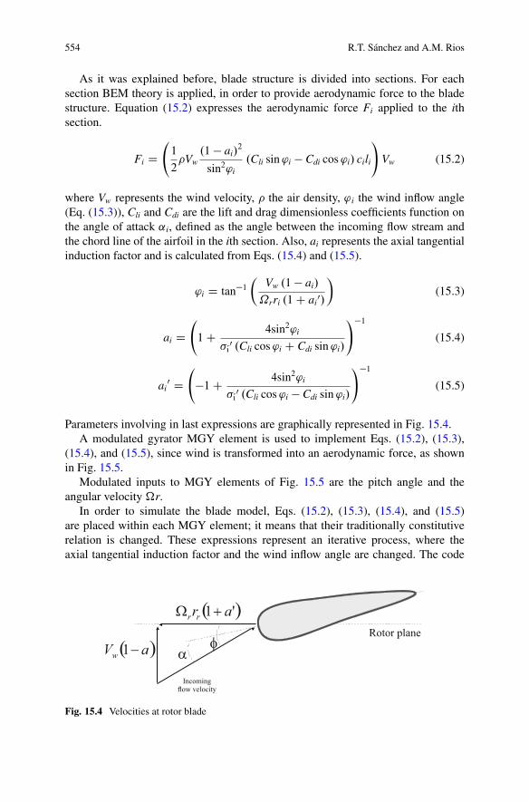
554 R.T. Sánchez and A.M. Rios
As it was explained before, blade structure is divided into sections. For eachsection BEM theory is applied, in order to provide aerodynamic force to the bladestructure. Equation (15.2) expresses the aerodynamic force Fi applied to the ithsection.
Fi D 1
2�Vw
.1 � ai/2
sin2'i.Cli sin'i � Cdi cos'i/ cili
!Vw (15.2)
where Vw represents the wind velocity, � the air density, ' i the wind inflow angle(Eq. (15.3)), Cli and Cdi are the lift and drag dimensionless coefficients function onthe angle of attack ˛i, defined as the angle between the incoming flow stream andthe chord line of the airfoil in the ith section. Also, ai represents the axial tangentialinduction factor and is calculated from Eqs. (15.4) and (15.5).
'i D tan�1�
Vw .1 � ai/
˝rri .1C ai0/
�(15.3)
ai D 1C 4sin2'i
Kı0 .Cli cos'i C Cdi sin'i/
!�1(15.4)
ai0 D
�1C 4sin2'i
Kı0 .Cli cos'i � Cdi sin'i/
!�1(15.5)
Parameters involving in last expressions are graphically represented in Fig. 15.4.A modulated gyrator MGY element is used to implement Eqs. (15.2), (15.3),
(15.4), and (15.5), since wind is transformed into an aerodynamic force, as shownin Fig. 15.5.
Modulated inputs to MGY elements of Fig. 15.5 are the pitch angle and theangular velocity �r.
In order to simulate the blade model, Eqs. (15.2), (15.3), (15.4), and (15.5)are placed within each MGY element; it means that their traditionally constitutiverelation is changed. These expressions represent an iterative process, where theaxial tangential induction factor and the wind inflow angle are changed. The code
Fig. 15.4 Velocities at rotor blade

15 Modeling and Control of a Wind Turbine 555
Fig. 15.5 Representation ofaerodynamic force conversion
Fig. 15.6 Flow diagram code
flow diagram is shown in Fig. 15.6. In order to estimate the initial value of theaxial induction factor, some conditions are assumed at the starting time; then, anestimation of the inflow angle is made. This allows to determinate the accuratecoefficient [4]. After that, the calculation of the axial and tangential inductionfactor is performed and the new value is used for the next cycle. This iterativeprocess is conducted until the tangential induction factor and wind inflow anglehave converged to their final values.
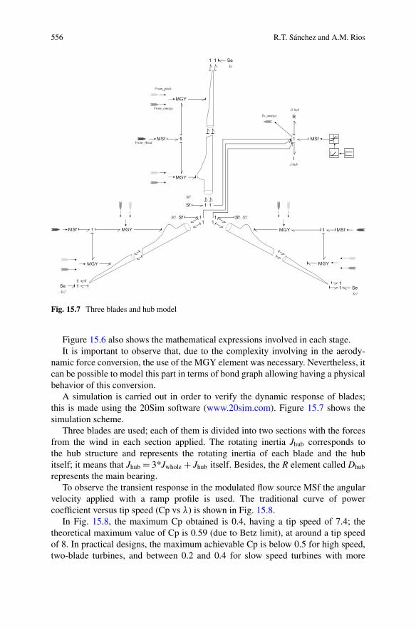
556 R.T. Sánchez and A.M. Rios
Fig. 15.7 Three blades and hub model
Figure 15.6 also shows the mathematical expressions involved in each stage.It is important to observe that, due to the complexity involving in the aerody-
namic force conversion, the use of the MGY element was necessary. Nevertheless, itcan be possible to model this part in terms of bond graph allowing having a physicalbehavior of this conversion.
A simulation is carried out in order to verify the dynamic response of blades;this is made using the 20Sim software (www.20sim.com). Figure 15.7 shows thesimulation scheme.
Three blades are used; each of them is divided into two sections with the forcesfrom the wind in each section applied. The rotating inertia Jhub corresponds tothe hub structure and represents the rotating inertia of each blade and the hubitself; it means that Jhub D 3*Jwhole C Jhub itself. Besides, the R element called Dhub
represents the main bearing.To observe the transient response in the modulated flow source MSf the angular
velocity applied with a ramp profile is used. The traditional curve of powercoefficient versus tip speed (Cp vs ) is shown in Fig. 15.8.
In Fig. 15.8, the maximum Cp obtained is 0.4, having a tip speed of 7.4; thetheoretical maximum value of Cp is 0.59 (due to Betz limit), at around a tip speedof 8. In practical designs, the maximum achievable Cp is below 0.5 for high speed,two-blade turbines, and between 0.2 and 0.4 for slow speed turbines with more
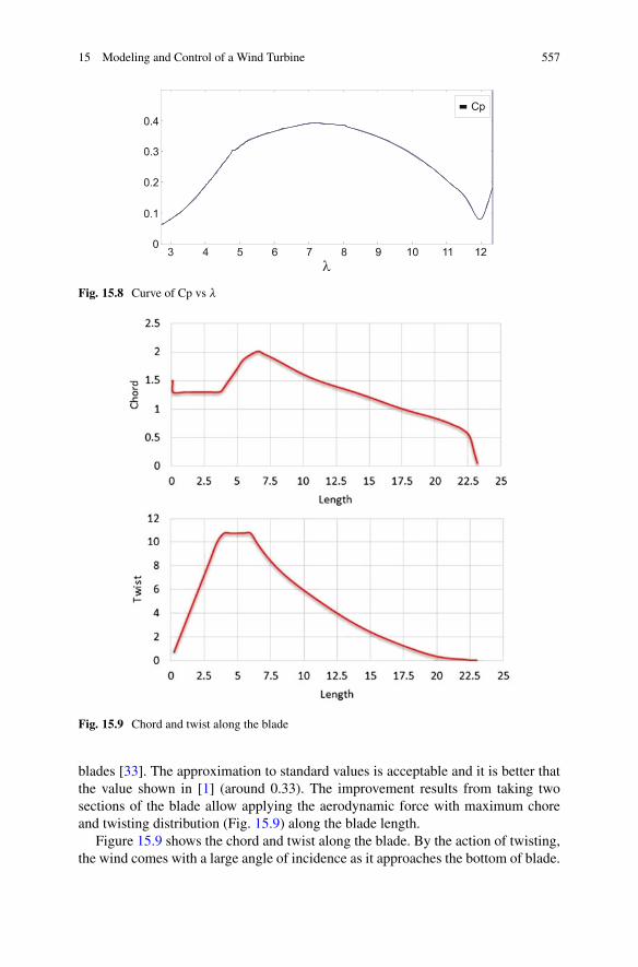
15 Modeling and Control of a Wind Turbine 557
Fig. 15.8 Curve of Cp vs
Fig. 15.9 Chord and twist along the blade
blades [33]. The approximation to standard values is acceptable and it is better thatthe value shown in [1] (around 0.33). The improvement results from taking twosections of the blade allow applying the aerodynamic force with maximum choreand twisting distribution (Fig. 15.9) along the blade length.
Figure 15.9 shows the chord and twist along the blade. By the action of twisting,the wind comes with a large angle of incidence as it approaches the bottom of blade.
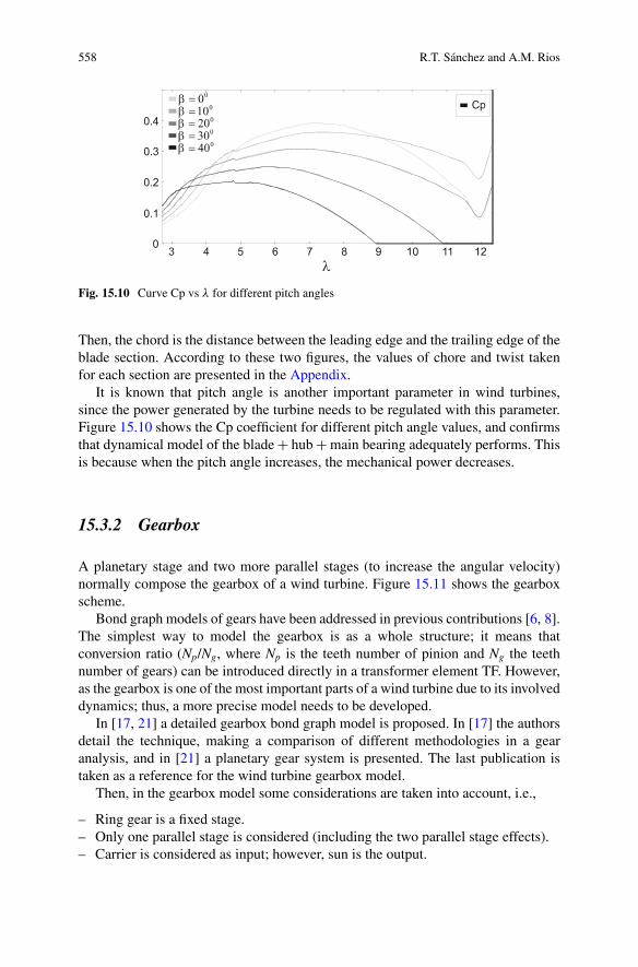
558 R.T. Sánchez and A.M. Rios
Fig. 15.10 Curve Cp vs for different pitch angles
Then, the chord is the distance between the leading edge and the trailing edge of theblade section. According to these two figures, the values of chore and twist takenfor each section are presented in the Appendix.
It is known that pitch angle is another important parameter in wind turbines,since the power generated by the turbine needs to be regulated with this parameter.Figure 15.10 shows the Cp coefficient for different pitch angle values, and confirmsthat dynamical model of the blade C hub C main bearing adequately performs. Thisis because when the pitch angle increases, the mechanical power decreases.
15.3.2 Gearbox
A planetary stage and two more parallel stages (to increase the angular velocity)normally compose the gearbox of a wind turbine. Figure 15.11 shows the gearboxscheme.
Bond graph models of gears have been addressed in previous contributions [6, 8].The simplest way to model the gearbox is as a whole structure; it means thatconversion ratio (Np/Ng, where Np is the teeth number of pinion and Ng the teethnumber of gears) can be introduced directly in a transformer element TF. However,as the gearbox is one of the most important parts of a wind turbine due to its involveddynamics; thus, a more precise model needs to be developed.
In [17, 21] a detailed gearbox bond graph model is proposed. In [17] the authorsdetail the technique, making a comparison of different methodologies in a gearanalysis, and in [21] a planetary gear system is presented. The last publication istaken as a reference for the wind turbine gearbox model.
Then, in the gearbox model some considerations are taken into account, i.e.,
– Ring gear is a fixed stage.– Only one parallel stage is considered (including the two parallel stage effects).– Carrier is considered as input; however, sun is the output.
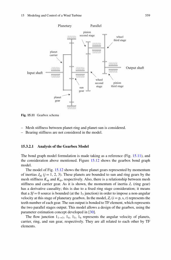
15 Modeling and Control of a Wind Turbine 559
Fig. 15.11 Gearbox schema
– Mesh stiffness between planet-ring and planet-sun is considered.– Bearing stiffness are not considered in the model.
15.3.2.1 Analysis of the Gearbox Model
The bond graph model formulation is made taking as a reference (Fig. 15.11), andthe consideration above mentioned. Figure 15.12 shows the gearbox bond graphmodel.
The model of Fig. 15.12 shows the three planet gears represented by momentumof inertias Jpj (j D 1, 2, 3). These planets are bounded to sun and ring gears by themesh stiffness Ksp and Krp, respectively. Also, there is a relationship between meshstiffness and carrier gear. As it is shown, the momentum of inertia Jr (ring gear)has a derivative causality; this is due to a fixed ring stage consideration; it meansthat a Sf D 0 source is bounded (at the 15 junction) in order to impose a non-angularvelocity at this stage of planetary gearbox. In the model, Zi (i D p, s, r) represents theteeth number of each gear. The sun output is bonded to TF element, which representsthe two parallel stages output. This model allows a design of the gearbox, using theparameter estimation concept developed in [30].
The flow junction 11!3, 14, 15, 16 represents the angular velocity of planets,carrier, ring, and sun gear, respectively. They are all related to each other by TFelements.

560 R.T. Sánchez and A.M. Rios
Fig. 15.12 Gearbox model
Considering the planet 1 (see Fig. 15.12), it is shown that there is a zero junction01, between the transformer TF1, TF2, and TF3, which represents (effort variable)that the planet moves in tangential direction. In this junction, the mesh stiffnessbetween the planet and sun is joined. Transformers TF1:Zs, TF2:1/Zs, and TF3:Zp
allow to obtain the rotating speed of the sun gear, the linear velocity of the planetrevolution around the sun gear, and the planet autorotation. This structure is thesame for the zero junction 02, but considering the relationship between the planet,the ring, and the carrier.
If a more precise model of a gearbox is required, the design can be done as itwas made for the blade model. This means that the gears can be taken as a structure,considering their mass and the translational displacement. Also, bearing stiffnessand torsional support stiffness can be added to the model.
The main dynamics representation can be directly achieved. Opposite to bladestructure, gearbox of Fig. 15.12 does not have causal’s loops, since nonresistiveelements (bearings) are considered. Thus, only a path loop between the inertial gearsand the mesh stiffness can be found. Parameters (see Appendix) for a 750 kW windturbine gearbox are used and have been taken from [13].
15.3.2.2 Gearbox Simulation
One simulation is carried out in order to verify the gearbox model. Table 15.2 showsthe numerical values used for the simulation. Torque and angular velocity for sunand carrier are shown in Fig. 15.13.
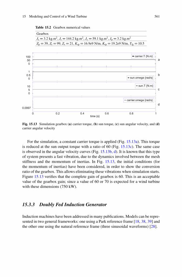
15 Modeling and Control of a Wind Turbine 561
Table 15.2 Gearbox numerical values
GearboxJsD 3.2 kg.m2, JrD 144.2 kg.m2, JcD 59.1 kg.m2, JpD 3.2 kg.m2
ZpD 39, ZrD 99, ZsD 21, KspD 16.9e9 N/m, KrpD 19.2e9 N/m, TfgD 10.5
Fig. 15.13 Simulation gearbox (a) carrier torque, (b) sun torque, (c) sun angular velocity, and (d)carrier angular velocity
For the simulation, a constant carrier torque is applied (Fig. 15.13a). This torqueis reduced at the sun output torque with a ratio of 60 (Fig. 15.13c). The same caseis observed in the angular velocity curves (Fig. 15.13b, d). It is known that this typeof system presents a fast vibration, due to the dynamics involved between the meshstiffness and the momentum of inertias. In Fig. 15.13, the initial conditions (forthe momentum of inertias) have been considered, in order to show the conversionratio of the gearbox. This allows eliminating these vibrations when simulation starts.Figure 15.13 verifies that the complete gain of gearbox is 60. This is an acceptablevalue of the gearbox gain; since a value of 60 or 70 is expected for a wind turbinewith these dimensions (750 kW).
15.3.3 Doubly Fed Induction Generator
Induction machines have been addressed in many publications. Models can be repre-sented in two general frameworks: one using a Park reference frame [18, 38, 39] andthe other one using the natural reference frame (three sinusoidal waveforms) [28].

562 R.T. Sánchez and A.M. Rios
Fig. 15.14 DFIG 2-axis reference frame
15.3.3.1 Park Reference Frame Model
Figure 15.14 shows a bond graph model of the induction machine in the Park 2-axisd-q reference frame [38].
The induction machine model is based on the following assumptions:
– Magnetic hysteresis and magnetic saturation effects are neglected.– The stator winding is sinusoidally distributed along the air-gap.– The stator slots cause no appreciable variation of the rotor inductances with rotor
position.
An arbitrary dq-frame rotating around the homopolar 0-axis to the speed !s ischosen.
The equations that describe the bond graph model of Fig. 15.14 are given by Eq.(15.6).
vd D Rsisd C d'sddt � !s'sq
vq D Rsisq C d'sq
dt C !s'sd
vrd D Rrird C d'rddt � !s'rq C p˝'rq
vrq D Rrirq C d'rq
dt C !s'rd � p˝'rd
�11 D p�'rqird � 'rdirq
�
�11 D Jmd�dt � Tm
(15.6)
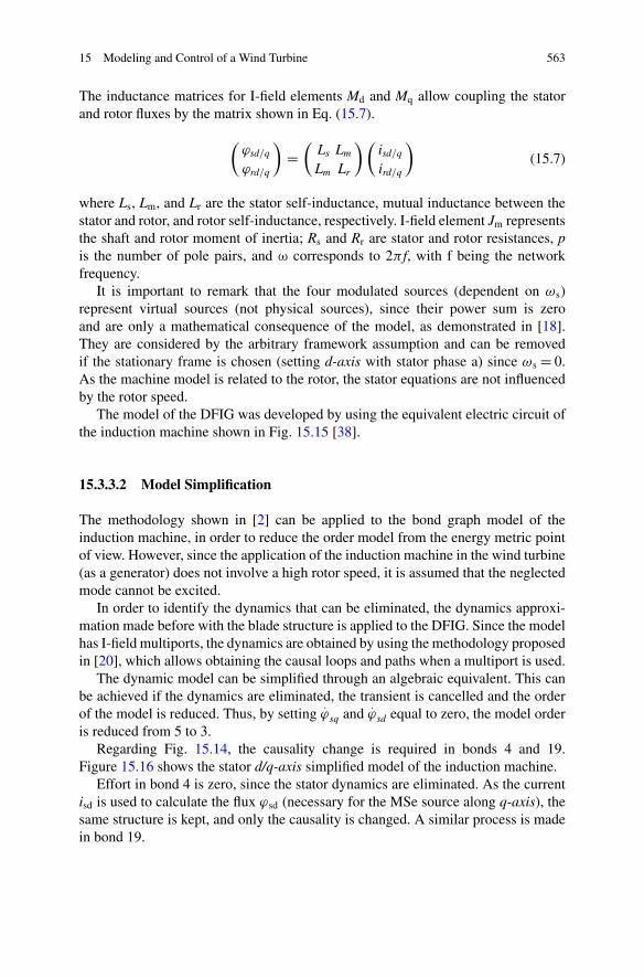
15 Modeling and Control of a Wind Turbine 563
The inductance matrices for I-field elements Md and Mq allow coupling the statorand rotor fluxes by the matrix shown in Eq. (15.7).
�'sd=q
'rd=q
�D�
Ls Lm
Lm Lr
��isd=q
ird=q
�(15.7)
where Ls, Lm, and Lr are the stator self-inductance, mutual inductance between thestator and rotor, and rotor self-inductance, respectively. I-field element Jm representsthe shaft and rotor moment of inertia; Rs and Rr are stator and rotor resistances, pis the number of pole pairs, and ¨ corresponds to 2� f, with f being the networkfrequency.
It is important to remark that the four modulated sources (dependent on !s)represent virtual sources (not physical sources), since their power sum is zeroand are only a mathematical consequence of the model, as demonstrated in [18].They are considered by the arbitrary framework assumption and can be removedif the stationary frame is chosen (setting d-axis with stator phase a) since !s D 0.As the machine model is related to the rotor, the stator equations are not influencedby the rotor speed.
The model of the DFIG was developed by using the equivalent electric circuit ofthe induction machine shown in Fig. 15.15 [38].
15.3.3.2 Model Simplification
The methodology shown in [2] can be applied to the bond graph model of theinduction machine, in order to reduce the order model from the energy metric pointof view. However, since the application of the induction machine in the wind turbine(as a generator) does not involve a high rotor speed, it is assumed that the neglectedmode cannot be excited.
In order to identify the dynamics that can be eliminated, the dynamics approxi-mation made before with the blade structure is applied to the DFIG. Since the modelhas I-field multiports, the dynamics are obtained by using the methodology proposedin [20], which allows obtaining the causal loops and paths when a multiport is used.
The dynamic model can be simplified through an algebraic equivalent. This canbe achieved if the dynamics are eliminated, the transient is cancelled and the orderof the model is reduced. Thus, by setting
:'sq and
:'sd equal to zero, the model order
is reduced from 5 to 3.Regarding Fig. 15.14, the causality change is required in bonds 4 and 19.
Figure 15.16 shows the stator d/q-axis simplified model of the induction machine.Effort in bond 4 is zero, since the stator dynamics are eliminated. As the current
isd is used to calculate the flux 'sd (necessary for the MSe source along q-axis), thesame structure is kept, and only the causality is changed. A similar process is madein bond 19.
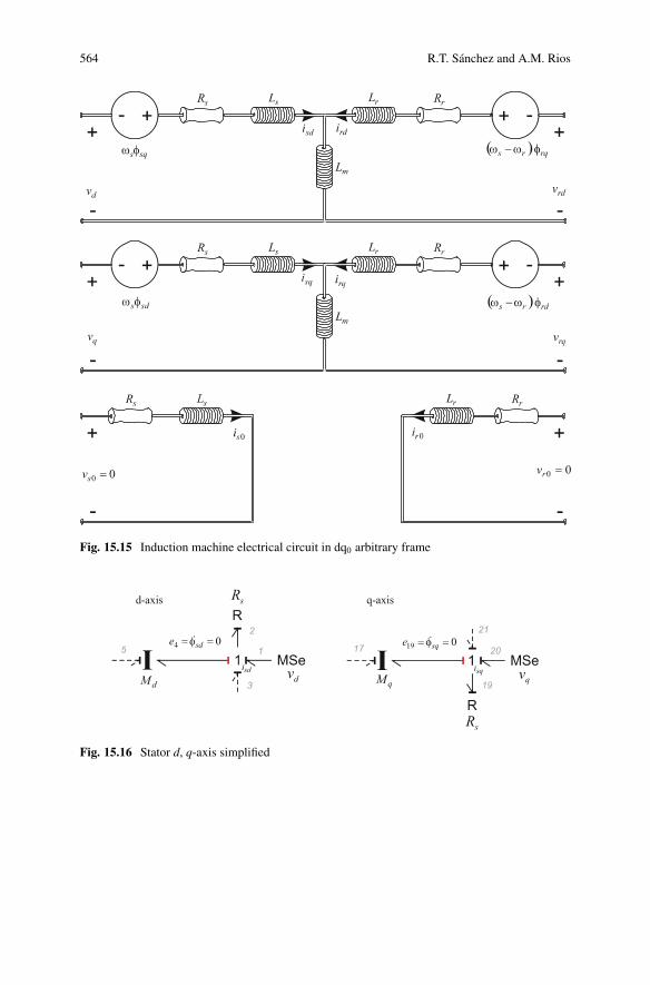
564 R.T. Sánchez and A.M. Rios
Fig. 15.15 Induction machine electrical circuit in dq0 arbitrary frame
Fig. 15.16 Stator d, q-axis simplified

15 Modeling and Control of a Wind Turbine 565
Table 15.3 Doubly fed induction machine parameters
Power 750 kW Stator inductance 2.51 mHPoles numbers 2 Rotor inductance 2.45 mHVoltage 690 V Mutual inductance 2.41 mHStator resistance 0.0022� Inertia 63.89 kg.m2
Rotor resistance 0.0018� Frequency 60 Hz
Causality changes require a modification of (15.7). Matrix expressions in theI-field elements are changed to:
�'sd;q
ird;q
�D
Ls � L2mLr
LmLr
� LmLr
1Lr
!�isd;q
'rd;q
�(15.8)
Causality changes reduce from 5 to 3 the number of independent state variables inthe model. The dynamic equation in the stator part is changed for a static one, andthe effort is set equal to zero in these bonds.
15.3.3.3 DFIG Simulation
In order to compare the behavior of the simplified model (order 3) against thecomplete one (order 5), a simulation is carried out by considering the doubly fedinduction machine as a motor (DFIM). Table 15.3 shows the numerical parametersfor the machine.
The DFIM is started at instant t D 0 s, then at t D 6.5 s the nominal torque isapplied (Tnom D 3978.88 Nm). After that, at t D 8.0 s a voltage reduction of 50 %during 200 ms is applied. Figure 15.17 shows the obtained results.
As observed from Fig. 15.17, the response obtained with both models is inclose agreement. It is important to observe that oscillations are eliminated whenthe simplified model is used. For example, the speed in the complete model (“speedComp,” Fig. 15.17a) oscillates at the instant voltage falls; these are eliminated inthe simplified model (speed Simp). A more pronounced difference between modelsis observed at the machine starting (Fig. 15.17b).
It is important to mention that the simulation of the DFIM is made consideringthe two sources input: one for the stator (vd, vq) and the other for the rotor (vrd, vrq).
If nominal values around the equilibrium point are assumed, pole locationanalysis can be performed. Table 15.4 shows the pole values for the two models. Byusing these values, it is verified again that the change of causality (Fig. 15.16) anddynamics elimination (
:'sq D :
'sd D 0) allow to obtain a model without oscillations.
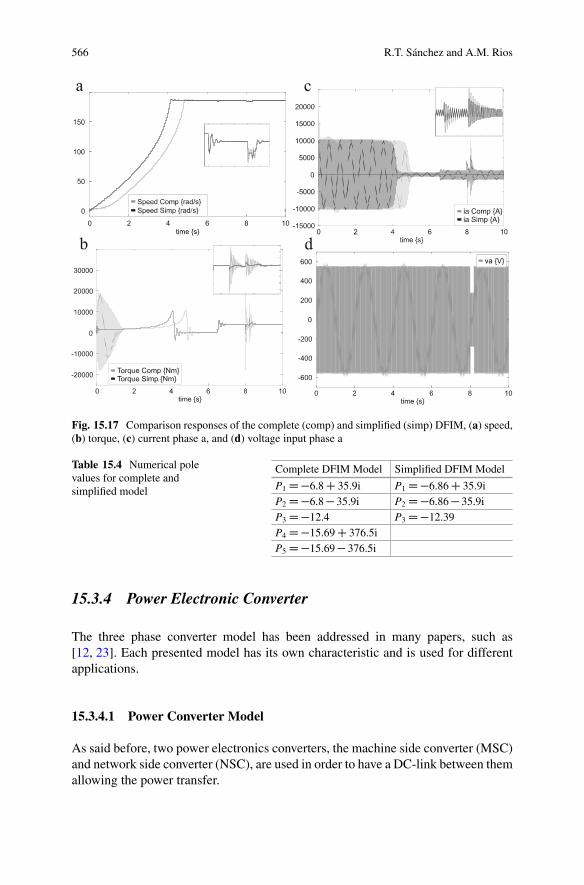
566 R.T. Sánchez and A.M. Rios
Fig. 15.17 Comparison responses of the complete (comp) and simplified (simp) DFIM, (a) speed,(b) torque, (c) current phase a, and (d) voltage input phase a
Table 15.4 Numerical polevalues for complete andsimplified model
Complete DFIM Model Simplified DFIM Model
P1D�6.8C 35.9i P1D�6.86C 35.9iP2D�6.8� 35.9i P2D�6.86� 35.9iP3D�12.4 P3D�12.39P4D�15.69C 376.5iP5D�15.69� 376.5i
15.3.4 Power Electronic Converter
The three phase converter model has been addressed in many papers, such as[12, 23]. Each presented model has its own characteristic and is used for differentapplications.
15.3.4.1 Power Converter Model
As said before, two power electronics converters, the machine side converter (MSC)and network side converter (NSC), are used in order to have a DC-link between themallowing the power transfer.

15 Modeling and Control of a Wind Turbine 567
Fig. 15.18 Network side converter with a three phase LC filter
For the NSC, the model is taken from [42, 43]. This model corresponds to a threephase converter using an LC filter connection. The filter allows to give a voltagesource behavior for the converter, and also to eliminate the harmonic distortionintroduced by the converter. Figure 15.18 shows the NSC used.
The characteristics of the model are the DC-link is considered as a dynamicalelement (Cbus), and the LC filter is composed of three inductances with theirassociated resistances and three Delta connected capacitors.
The causality assignment gives to the power electronic converter associated withthe LC filter a voltage source behavior.
In the next section it will be presented the control law necessary to transfer theactive and reactive power to the network.
15.4 Control of the Doubly Fed Induction Generator
As previously shown, the induction machine is a coupled 5th or 3th order system(depending on the considered model) with four inputs. Actually, the simplificationmade in the previous section allows to intuitively knowing that stator dynamics arenot directly involved in the control law. For that reason, the control inputs which arepresent in the doubly fed induction machine are those of rotor. The last assumptionis commonly made when a generator control law is deduced, but here, the bondgraph model supports this assumption.
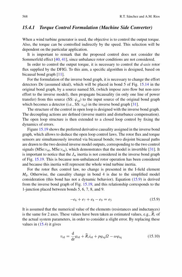
568 R.T. Sánchez and A.M. Rios
15.4.1 Torque Control Formulation (Machine Side Converter)
When a wind turbine generator is used, the objective is to control the output torque.Also, the torque can be controlled indirectly by the speed. This selection will bedependent on the particular application.
It is important to remark that the proposed control does not consider theSommerfeld effect [40, 41], since unbalance rotor conditions are not considered.
In order to control the output torque, it is necessary to control the d-axis rotorflux supplied by the DFIG. To this aim, a specific algorithm is designed, based onbicausal bond graph [11].
For the formulation of the inverse bond graph, it is necessary to change the effortdetectors De (assumed ideal), which will be placed in bond 5 of Fig. 15.14 in theoriginal bond graph, by a source named SS, (which impose zero flow but non-zeroeffort to the inverse model), then propagate bicausality (in only one line of powertransfer) from this source (SS:
:'rd) to the input source of the original bond graph
which becomes a detector (i.e., SS: vrd) in the inverse bond graph [31].The structure of the control in open loop is designed with the inverse bond graph.
The decoupling actions are defined (inverse matrix and disturbance compensation).The open loop structure is then extended to a closed loop control by fixing thedynamics of errors.
Figure 15.19 shows the preferred derivative causality assigned in the inverse bondgraph, which allows to deduce the open loop control laws. The rotor flux and torquesensors are simultaneously inverted via bicausal bonds; two disjoint bicausal pathsare drawn to the two desired inverse model outputs, corresponding to the two controlsignals (MSe:vrd, MSe:vrq), which demonstrates that the model is invertible [31]. Itis important to notice that the Jm inertia is not considered in the inverse bond graphof Fig. 15.19. This is because non-unbalanced rotor operation has been consideredand because this inertia will represent the whole wind turbine inertia.
For the rotor flux control law, no change is presented in the I-field elementMd. Otherwise, the causality change in bond 4 is due to the simplified modelconsideration (this bond has not a dynamic behavior). Equation (15.9) is derivedfrom the inverse bond graph of Fig. 15.19, and this relationship corresponds to the1-junction placed between bonds 5, 6, 7, 8, and 9.
�e6 C e7 C e8 � e9 D e5 (15.9)
It is assumed that the numerical value of the elements (resistances and inductances)is the same for 2 axes. These values have been taken as estimated values, e.g.,bRr ofthe actual system parameters, in order to consider a slight error. By replacing thesevalues in (15.4) it gives
vrd D d
dt'rd CbRrird C p'rq˝ � !'rq (15.10)

15 Modeling and Control of a Wind Turbine 569
Fig. 15.19 Inverse DFIG for calculation of the controls laws
To establish the closed loop control law, the dynamics of the error (" D 'rqref � 'rq)are set in (15.10), as
:" C k1" D 0, where k1 represents the controller to be used.
Expression (15.10) becomes (15.11) as:
vrd D d
dt.'rdref � "/CbRrird C p'rq˝ � !'rq (15.11)
Finally,
vrd D d
dt'rdref C k1 .'rdref � 'rd/CbRrird C p'rq˝ � !'rq (15.12)
For the last expression, the rotor flux 'rq is assumed to be zero. This is justifiedsince 'rq, compared to 'rd has not an important impact on the voltage vrd. Actually,this value is very small compared to the d-axis flux.
Taking the last consideration, (15.12) is represented in the Laplace domain as,
.vrd/.s/ D s.'rdref/.s/ C k1.'rdref � 'rd/.s/ CbRr.ird/.s/ (15.13)
In the same manner as for the determination of the rotor flux control, the torquecontrol law is calculated.

570 R.T. Sánchez and A.M. Rios
Equation (15.14) is derived from the bond graph of Fig. 15.19 as,
e14 � e18 C e15 C e13 � e17 D 0 (15.14)
For (15.14), the effort e17 needs to be calculated from (15.8), by assuming that'rq D R
e17. Making the appropriate substitutions in (15.14), it yields,
vrq DbLrd
dtirq CbRrirq � p'rd˝ C !'rd (15.15)
In (15.15), the current isq of (15.8) has been assumed zero, since the balancedcondition of the Park transformation has been considered. However, the mutualinductance is not present in (15.15).
The voltage vrq and torque relation are not explicitly shown in (15.15). Thus, inorder to relate (15.15) with the torque, another expression is needed.
Two different procedures are visualized, i.e., the first is to replace the speed� forhis equivalent relation with the torque, and the second one is to establish an internalcontrol loop for the irq current, and cascade the torque relationship in the previouslyinternal control loop.
The second solution is chosen, since it provides a control law structure similar tothe traditional vector control [49] applied to this machine.
By using the estimated values and establishing the closed control loop (for irqvariable) as previously described, (15.15) becomes,
vrq DbRrirq � p'rd�C !'rd CbLrd
dtirqref CbLrk2
�irqref � irq
�(15.16)
where k2 represents the controller used for this loop. The other necessary expressionis taken from the original model (Fig. 15.14); specifically, in bond 11 the torque isgiven by,
Te11 D p�'rqird � 'rdirq
�(15.17)
As 'rq D 0, expression (15.17) becomes Te11 D �p'rdirq, and can be expressed asTref D �p'rdirqref. This expression is replaced in (15.16), to obtain the control law(15.18).
�vrq�.s/ DbRr
�irq�.s/ � p'rd�C !'rd CbLrs
�Tref
�p'rd
�
.s/
CbLrk2
�Tref
�p'rd� irq
�
.s/
(15.18)
The controller block diagram (Eqs. (15.13) and (15.17)) is shown in Fig. 15.20. Itis important to notice that the structure of the control law contains a feed-forwardwith a derivative action on the reference signals. The signals are constants, so thatthey can be removed, and by taking into consideration that the wind does not havea sudden change, they are kept in this proposed control law. In addition, the controllaw needs an estimation of 'rd, then the expression (Ls*ird C Lm*isd) [49] is used.

15 Modeling and Control of a Wind Turbine 571
Fig. 15.20 Torque control law schema
15.4.2 Torque Control Simulation
In order to verify control law, a simulation is carried out by considering thatthe DFIG has a primary governor to emulate the torque provided by the turbinemechanical part. Also, as it is considered that the converter has not an importantimpact in the machine behavior, the machine side converter is not used. This allowsto connect the vrd and vrq voltages directly via the MSe sources. Figure 15.21 showsthe simulation scheme.
The stator machine power is regulated by the rotor. In order to simulate the DFIG,a three phase load is connected at machine terminals. Park’s transformation is usedin order to transform from the dq reference frame to the abc framework.
The complete DFIG model is used in the simulation. The results presented herehave been verified against the simplified DFIG model, obtaining the same results;the only difference being that the oscillations due to the fast dynamics are presentin the complete model.
A speed governor is used to maintain the nominal speed in the generator. As theobjective is to test the behavior of the control law; this stage has been representedby using an ideal Governor (PI controller).
Results are shown in Fig. 15.22. Numerical values of Tables 15.3 and 15.5 areused for the simulation. The DFIG is started at instant t D 0 s applying the nominaltorque as reference in the control (Tref D 3978.88 Nm), then at t D 5 s the nominaltorque is reduce to Tref D 2500. This is made in order to observe that the torque inthe machine is also reduced.
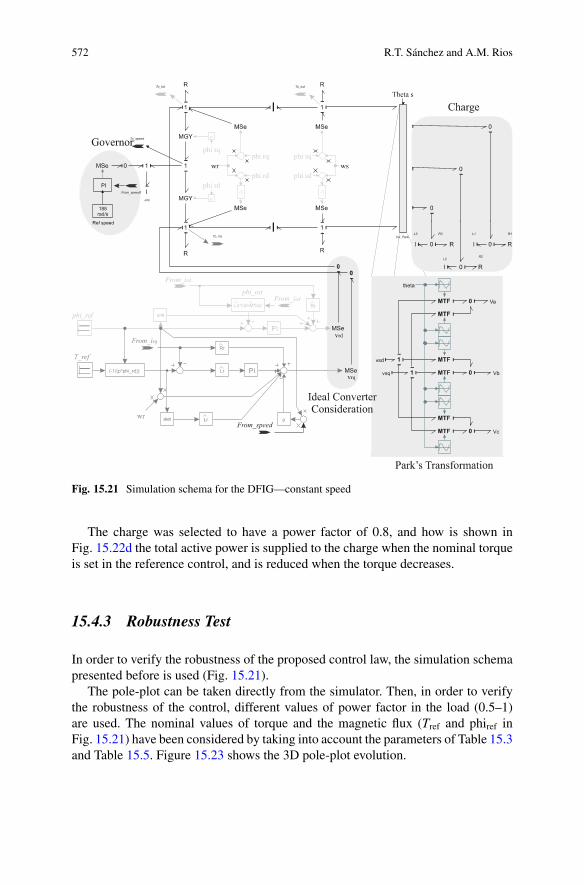
572 R.T. Sánchez and A.M. Rios
Fig. 15.21 Simulation schema for the DFIG—constant speed
The charge was selected to have a power factor of 0.8, and how is shown inFig. 15.22d the total active power is supplied to the charge when the nominal torqueis set in the reference control, and is reduced when the torque decreases.
15.4.3 Robustness Test
In order to verify the robustness of the proposed control law, the simulation schemapresented before is used (Fig. 15.21).
The pole-plot can be taken directly from the simulator. Then, in order to verifythe robustness of the control, different values of power factor in the load (0.5–1)are used. The nominal values of torque and the magnetic flux (Tref and phiref inFig. 15.21) have been considered by taking into account the parameters of Table 15.3and Table 15.5. Figure 15.23 shows the 3D pole-plot evolution.

15 Modeling and Control of a Wind Turbine 573
Fig. 15.22 DFIG responses, (a) Machine speed, (b) torque, (c) reactive power in the charge, and(d) active power in the charge
Table 15.5 Control andcharge numerical values
Control Charge
PI vrd PI vrq
KpD 1000 KpD 150 R1,2,3D 0.5078�KiD 1 m KiD 10 m L1,2,3D 1.01 mH
Poles which have a significant movement correspond to the load poles. Unlikethe generator and control poles, these do not have a significant movement when thepower factor is varied. This shows the robustness of the proposed control in thissystem. It is important to mention that in order to take into account the uncertaintiesdue to parameter estimation the simulation is carried out by assuming a slight errorin the parameters, i.e., 10 % between the model and the controller parameters.
15.4.4 Network Side Converter
As said before, the three phase NSC uses an LC filter in order to impose a voltagebehavior in the converter.
The structure of the converter was presented in Fig. 15.18. Then in this section,the active and reactive power control is presented.
The control law of this converter is also derived from the inverse bond graph(using the bicausality concept); the robustness and accurate performance of the

574 R.T. Sánchez and A.M. Rios
Fig. 15.23 3D pole-plot evolution
proposed control has been demonstrated for voltage regulation [42]. Here, thehighlights of this control are recalled. They are as follows:
• The controller parameters are obtained considering the two loops in cascade, onefor the current in the Lni and another one for the voltage in Cni-elements.
• Only two phase to phase voltages are considered in the control, the third onefixing the voltage reference.
• The current inc is linearly dependent on the two others (ina and inb).• The average behavior of the converter is considered.
The control is composed by three principal stages:
1. DC bus regulation. It is based on a traditional PI (proportional C integral)controller. It provides the active power reference.
2. Active and reactive power regulation. Inspired from the power flow conceptbetween two sources, connected through a line impedance.
3. Voltage and current regulation. A resonant and proportional controller for voltageand current control, respectively.
Figure 15.24 resumes the control stages for the NSC.From Fig. 15.24, the source Vdcref sets the DC-link regulation reference, the ibus
and vbus are necessaries in order to have the total power available in the DC-link.Since this power provides the active power reference. In the right side of Fig. 15.24it can see three I-elements connected in series with their respective R-elements.These elements represent the line impedance, and are necessaries in order to applythe power flow concept.
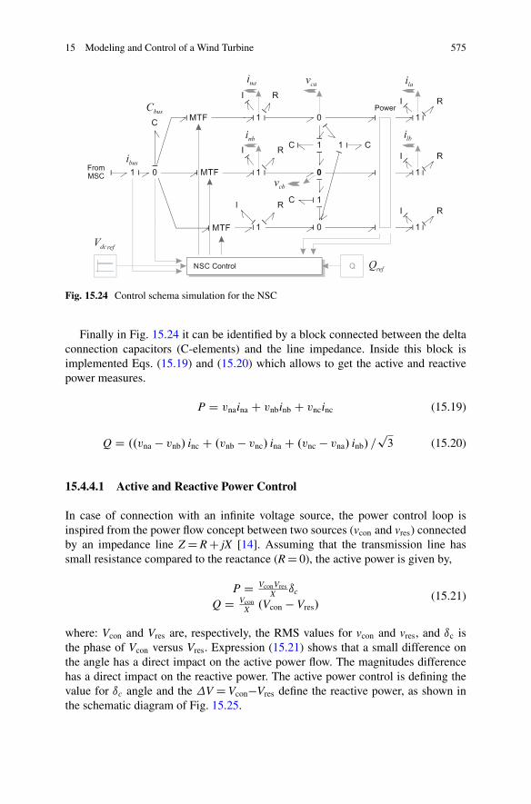
15 Modeling and Control of a Wind Turbine 575
Fig. 15.24 Control schema simulation for the NSC
Finally in Fig. 15.24 it can be identified by a block connected between the deltaconnection capacitors (C-elements) and the line impedance. Inside this block isimplemented Eqs. (15.19) and (15.20) which allows to get the active and reactivepower measures.
P D vnaina C vnbinb C vncinc (15.19)
Q D ..vna � vnb/ inc C .vnb � vnc/ ina C .vnc � vna/ inb/ =p3 (15.20)
15.4.4.1 Active and Reactive Power Control
In case of connection with an infinite voltage source, the power control loop isinspired from the power flow concept between two sources (vcon and vres) connectedby an impedance line Z D R C jX [14]. Assuming that the transmission line hassmall resistance compared to the reactance (R D 0), the active power is given by,
P D VconVresX ıc
Q D VconX .Vcon � Vres/
(15.21)
where: Vcon and Vres are, respectively, the RMS values for vcon and vres, and ıc isthe phase of Vcon versus Vres. Expression (15.21) shows that a small difference onthe angle has a direct impact on the active power flow. The magnitudes differencehas a direct impact on the reactive power. The active power control is defining thevalue for ıc angle and the V D Vcon�Vres define the reactive power, as shown inthe schematic diagram of Fig. 15.25.
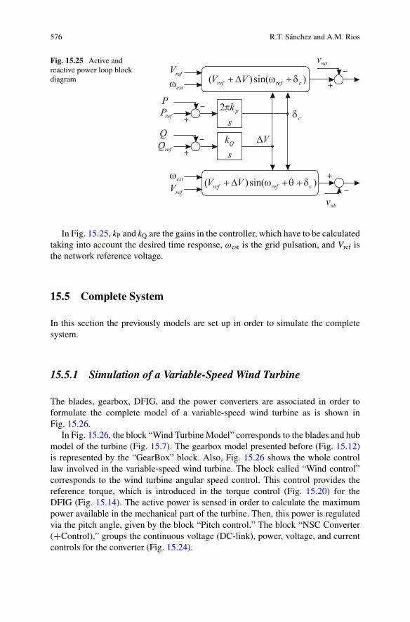
576 R.T. Sánchez and A.M. Rios
Fig. 15.25 Active andreactive power loop blockdiagram
In Fig. 15.25, kP and kQ are the gains in the controller, which have to be calculatedtaking into account the desired time response, !est is the grid pulsation, and Vref isthe network reference voltage.
15.5 Complete System
In this section the previously models are set up in order to simulate the completesystem.
15.5.1 Simulation of a Variable-Speed Wind Turbine
The blades, gearbox, DFIG, and the power converters are associated in order toformulate the complete model of a variable-speed wind turbine as is shown inFig. 15.26.
In Fig. 15.26, the block “Wind Turbine Model” corresponds to the blades and hubmodel of the turbine (Fig. 15.7). The gearbox model presented before (Fig. 15.12)is represented by the “GearBox” block. Also, Fig. 15.26 shows the whole controllaw involved in the variable-speed wind turbine. The block called “Wind control”corresponds to the wind turbine angular speed control. This control provides thereference torque, which is introduced in the torque control (Fig. 15.20) for theDFIG (Fig. 15.14). The active power is sensed in order to calculate the maximumpower available in the mechanical part of the turbine. Then, this power is regulatedvia the pitch angle, given by the block “Pitch control.” The block “NSC Converter(CControl),” groups the continuous voltage (DC-link), power, voltage, and currentcontrols for the converter (Fig. 15.24).
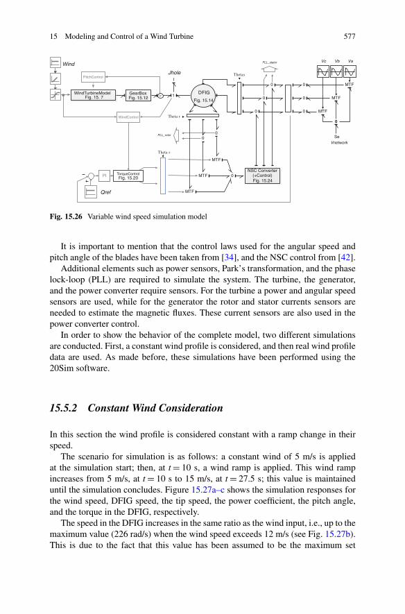
15 Modeling and Control of a Wind Turbine 577
Wind
TorqueControl
Theta s
Theta r
Theta r
Rr
I
Jhole
DFIG
MTF
MTF
MTF
MTF
MTF
MTF
1
Qref
PI
PLL_stator
PLL_rotor
P
SeVnetwork
Va
0
Vb
0
Vc
0
0
0
0
0
0
00
WindControl
PitchControl
GearBoxWindTurbineModelFig. 15. 7 Fig. 15.12 Fig. 15.14
Fig. 15.20
NSC Converter(+Control)Fig. 15.24
Fig. 15.26 Variable wind speed simulation model
It is important to mention that the control laws used for the angular speed andpitch angle of the blades have been taken from [34], and the NSC control from [42].
Additional elements such as power sensors, Park’s transformation, and the phaselock-loop (PLL) are required to simulate the system. The turbine, the generator,and the power converter require sensors. For the turbine a power and angular speedsensors are used, while for the generator the rotor and stator currents sensors areneeded to estimate the magnetic fluxes. These current sensors are also used in thepower converter control.
In order to show the behavior of the complete model, two different simulationsare conducted. First, a constant wind profile is considered, and then real wind profiledata are used. As made before, these simulations have been performed using the20Sim software.
15.5.2 Constant Wind Consideration
In this section the wind profile is considered constant with a ramp change in theirspeed.
The scenario for simulation is as follows: a constant wind of 5 m/s is appliedat the simulation start; then, at t D 10 s, a wind ramp is applied. This wind rampincreases from 5 m/s, at t D 10 s to 15 m/s, at t D 27.5 s; this value is maintaineduntil the simulation concludes. Figure 15.27a–c shows the simulation responses forthe wind speed, DFIG speed, the tip speed, the power coefficient, the pitch angle,and the torque in the DFIG, respectively.
The speed in the DFIG increases in the same ratio as the wind input, i.e., up to themaximum value (226 rad/s) when the wind speed exceeds 12 m/s (see Fig. 15.27b).This is due to the fact that this value has been assumed to be the maximum set

578 R.T. Sánchez and A.M. Rios
Fig. 15.27 Responses for a constant wind profile (a) wind, (b) DFIG speed, (c) , (d) powercoefficient, (e) pitch angle, and (f) DFIG torque
point. The curve called “lambda” corresponds to the tip speed ratio, which presentsits nominal value before the ramp profile starts (Fig. 15.27c). When machine speedincreases to its maximum value, the tip speed decreases from 8 to 5.8. A similarcase is shown for the power coefficient Cp (Fig. 15.27d). Figure 15.27e also showsthe pitch angle applied to the blades, which starts at the instant when the wind speedexceeds 12 m/s. Finally, in Fig. 15.27f the actual torque in the generator is presented.There is a negative torque because the mechanical power is transferred to the powernetwork, and their maximum value is �3315 Nm.
Active power needs to be provided by the wind turbine, and then distributed tothe power network. Nevertheless, as a DFIM is used, the reactive power is present.Figure 15.28 shows the mechanical and electrical power in the wind turbine model.The power of the main shaft and the high speed shaft exactly match (750 kW); the

15 Modeling and Control of a Wind Turbine 579
Fig. 15.28 Power curves for a constant wind profile
Fig. 15.29 Voltage in the DC-link for a constant wind profile
generator active power is closely to these ones (745 kW). This difference is due tothe fact that estimated values for the generator have been calculated. Zero reactivepower (Q) has been set as reference because not reactive power is absorbed by thenetwork.
The regulation of the continuous bus is also an important parameter to take intoconsideration. Figure 15.29 shows the DC-link capacitor voltage, which follows thevoltage reference (1200 V). It is important to mention that an initial condition isused in order to allow the simulation to be performed.
Figure 15.30 shows the three phase stator currents. A 460 V DFIG is used, withcurrents having larger values in order to meet active power demand.
The last simulation results allow the verification of theoretical concepts relatedto the wind turbine dynamic operation.
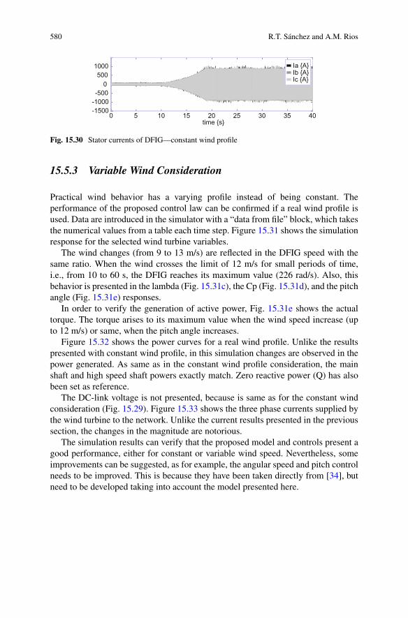
580 R.T. Sánchez and A.M. Rios
Fig. 15.30 Stator currents of DFIG—constant wind profile
15.5.3 Variable Wind Consideration
Practical wind behavior has a varying profile instead of being constant. Theperformance of the proposed control law can be confirmed if a real wind profile isused. Data are introduced in the simulator with a “data from file” block, which takesthe numerical values from a table each time step. Figure 15.31 shows the simulationresponse for the selected wind turbine variables.
The wind changes (from 9 to 13 m/s) are reflected in the DFIG speed with thesame ratio. When the wind crosses the limit of 12 m/s for small periods of time,i.e., from 10 to 60 s, the DFIG reaches its maximum value (226 rad/s). Also, thisbehavior is presented in the lambda (Fig. 15.31c), the Cp (Fig. 15.31d), and the pitchangle (Fig. 15.31e) responses.
In order to verify the generation of active power, Fig. 15.31e shows the actualtorque. The torque arises to its maximum value when the wind speed increase (upto 12 m/s) or same, when the pitch angle increases.
Figure 15.32 shows the power curves for a real wind profile. Unlike the resultspresented with constant wind profile, in this simulation changes are observed in thepower generated. As same as in the constant wind profile consideration, the mainshaft and high speed shaft powers exactly match. Zero reactive power (Q) has alsobeen set as reference.
The DC-link voltage is not presented, because is same as for the constant windconsideration (Fig. 15.29). Figure 15.33 shows the three phase currents supplied bythe wind turbine to the network. Unlike the current results presented in the previoussection, the changes in the magnitude are notorious.
The simulation results can verify that the proposed model and controls present agood performance, either for constant or variable wind speed. Nevertheless, someimprovements can be suggested, as for example, the angular speed and pitch controlneeds to be improved. This is because they have been taken directly from [34], butneed to be developed taking into account the model presented here.

15 Modeling and Control of a Wind Turbine 581
Fig. 15.31 Responses for a real wind profile (a) wind, (b) DFIG speed, (c) , (d) powercoefficient, (e) pitch angle, and (f) DFIG torque
15.6 Conclusions
The complete model of a variable-speed wind turbine has been presented.In order to apply the aerodynamic force, blade structure is considered to be
a flexible body. BEM theory has been used for the wind aerodynamic forceconversion. Values of torque and the coefficient of power in simulations have shownthe validity of this model.
A gearbox model has been presented, where mesh stiffness between planet-sunand ring-planet are considered, and parallel stages are joined in only one stage.Power flows transferred by each stage has been presented in the simulation results.
For the DFIG, the causal loop concept applied to the model allowed to identifythe dynamics (slow and fast) of the model approximation. Then, by choosing the
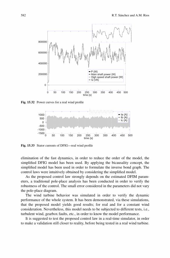
582 R.T. Sánchez and A.M. Rios
Fig. 15.32 Power curves for a real wind profile
Fig. 15.33 Stator currents of DFIG—real wind profile
elimination of the fast dynamics, in order to reduce the order of the model, thesimplified DFIG model has been used. By applying the bicausality concept, thesimplified model has been used in order to formulate the inverse bond graph. Thecontrol laws were intuitively obtained by considering the simplified model.
As the proposed control law strongly depends on the estimated DFIM param-eters, a traditional pole-place analysis has been conducted in order to verify therobustness of the control. The small error considered in the parameters did not varythe pole-place diagram.
The wind turbine behavior was simulated in order to verify the dynamicperformance of the whole system. It has been demonstrated, via these simulations,that the proposed model yields good results; for real and for a constant windconsideration. Nevertheless, this model needs to be subjected to different tests, i.e.,turbulent wind, gearbox faults, etc., in order to know the model performance.
It is suggested to test the proposed control law in a real-time simulator, in orderto make a validation still closer to reality, before being tested in a real wind turbine.
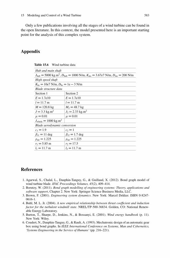
15 Modeling and Control of a Wind Turbine 583
Only a few publications involving all the stages of a wind turbine can be found inthe open literature. In this context, the model presented here is an important startingpoint for the analysis of this complex system.
Appendix
Table 15.6 Wind turbine data
Hub and main shaft
JhubD 5000 kg.m2, DhubD 1000 N/m, KmsD 3.67e7 N/m, DmsD 200 N/mHigh speed shaft
KhsD 10e7 N/m, DhsD 1e� 3 N/mBlade structure data
Section 1 Section 2ED 1.7e10 ED 1.7e10lD 11.7 m lD 11.7 mMD 120.8 kg M2D 48.7 kgJD 3.3 kg.m2 J2D 2.33 kg.m2
�D 0.01 �D 0.01JwholeD 1000 kg.m2
Blade aerodynamic conversion
c1D 1.9 c2D 1ˇt1D 11 deg ˇt2D 1.7 deg�airD 1.225 �airD 1.225r1D 5.85 m r2D 17.5l1D 11.7 m l2D 11.7 m
References
1. Agarwal, S., Chalal, L., Dauphin-Tanguy, G., & Guillaud, X. (2012). Bond graph model ofwind turbine blade. IFAC Proceedings Volumes, 45(2), 409–414.
2. Borutzy, W. (2011). Bond graph modelling of engineering systems: Theory, applications andsoftware support, Chapter 2. New York: Springer Science Business Media, LLC.
3. Brown, F. (2001). Engineering system dynamics. New York: Marcel Dekker. ISBN 0-8247-0616-1.
4. Buhl, M. L. Jr. (2004). A new empirical relationship between thrust coefficient and inductionfactor for the turbulent windmill state. NREL/TP-500-36834. Golden, CO: National Renew-able Energy Laboratory.
5. Burton, T., Sharpe, D., Jenkins, N., & Bossanyi, E. (2001). Wind energy handbook (p. 11).New York: Wiley.
6. Coudert, N., Dauphin-Tanguy, G., & Rault, A. (1993). Mechatronic design of an automatic gearbox using bond graphs. In IEEE International Conference on Systems, Man and Cybernetics,‘Systems Engineering in the Service of Humans’ (pp. 216–221).

584 R.T. Sánchez and A.M. Rios
7. Dauphin-Tanguy, G. (2000). Les bond graphs. Paris: Hermès Science Editor.8. Deur, J., Ivanovic, V., Assadian, F., Kuang, M., Tseng, E. H., & Hrovat, D. (2012). Bond
graph modeling of automotive transmissions and drivelines. Proceedings of the 7th ViennaInternational Conference on Mathematical Modelling (MATHMOD), Vienna, Austria.
9. Etienne-Vidal, P., Pietrzak-David, M., & Bonnet, F. (2008). Mixed control strategy of a doublyfed induction machine. Electrical Engineering (Archiv fur Elektrotechnik), 90(5), 337–346.
10. Gallo, C., Kasuba, R., Pintz, A., & Spring, J. (1986). Design and dynamic simulation of afixed pitch 56 kw wind turbine drive train with a continuously variable transmission. U.S.Department of Energy Conservation and Renewable Energy Wind/Ocean Technology Division,NASA CR-179543.
11. Gawthrop, P. J. (1995). Bicausal bond graph. Proceedings of the International Conference onBond Graph Modeling and Simulation (ICBGM’95) (Vol. 27, pp. 83–88).
12. Gonzáñez-Contreras, M., Rullán-Lara, J. L., Vela-Valdés, L. G., & Claudio, S. A. (2007).Modeling, simulation and fault diagnosis of the three-phase inverter using bond graph. In IEEEInternational Symposium on Industrial Electronics (pp. 130–135).
13. Guo, Y., Keller, J., & Parker, R. G. (2012). Dynamic analysis of wind turbine planetarygears using an extended harmonic balance approach. International Conference on Noise andVibration Engineering, Leuven, Belgium, September 17–19, 2012.
14. Hadi, S. (1999). Power system analysis (pp. 26–28). New York: McGraw-Hill Editions.15. Hansen, A. D., Sorensen, P., Iov, F., & Blaabjerg, F. (2005). Centralized power control of wind
farm with doubly fed induction generators. Renewable Energy, 31(7), 935–951.16. Hansen, M. O. L., Sorensen, J. N., Voutsinas, S., Sorensen, N., & Madsen, H. A. (2006). State
of the art in wind turbine aerodynamics and aeroelasticity. Progress in Aerospace Sciences, 42,285–330.
17. Józef, W., Jerzy, K., & Zawisla, S. (2006). Gears and graphs. Journal of Theoretical andApplied Mechanics, 44(1), 139–162.
18. Karnopp, D. (1991). State functions and bond graph dynamic models for rotary, multi-windingelectrical machines. Journal of the Franklin Institute, 328(1), 45–54.
19. Karnopp, D., Margolis, D., & Rosenberg, R. (1990). System dynamics: A unified approach.New York: Wiley.
20. Kubiak, P. (1996). Analyse symbolique des systèmes physiques modélises par bond graph encomportant des éléments multiports. Thèse Université des Sciences et Technologies de Lille,USTL. Lille France.
21. Luo, Y., & Tan, D. (2011). Dynamics modeling of planetary gear set considering meshingstiffness based on bond graph. Procedia Engineering, 24, 850–855.
22. Lydia, M., Immanuel Selvakumar, A., Suresh Kumar, S., & Edwin Prem Kumar, G. (2013).Advanced algorithms for wind turbine power curve modeling. IEEE Transaction on Sustain-able Energy, 4(3), 827–835.
23. Mezghanni, D., Andoulsi, R., Mami, A., & Dauphin-Tanguy, G. (2007). Bond graph modelingof a photovoltaic system feeding an induction motor-pump. Simulation Modeling Practice andTheory, 15(10), 1224–1238.
24. Mikati, M., Santos, M., & Armenta, C. (2013). Electric grid dependence on the configurationof a small-scale wind and solar power hybrid system. Renewable Energy, 57, 587–593.
25. Miller, A., Chang, B., Issa, R., & Chen, G. (2013). Review of computer-aided numericalsimulation in wind energy. Renewable and Sustainable Energy Reviews, 25, 122–134.
26. Morel, L., Godfroid, H., Mirzaian, A., & Kauffmann, J. (1998). Double-fed induction machine:Converter optimization and field oriented control without position sensor. IEE Proceedings—Electric Power Applications, 145(4), 360–368.
27. Moriarty, P. J., & Hansen, A. C. (2005). AeroDyn theory manual. National Renewable EnergyLaboratory NREL/TP-500-36881.
28. Mukerjee, A., Karmakar, R., & Samantaray, A. K. (1999). Modeling of basic induction motorsand source loading in rotor-motor systems with regenerative force field. Simulation PracticeTheory, 7, 563–576.
29. Mukherjee, A., Karmakar, R., & Samantaray, A. K. (2000). Modelling and simulation ofengineering systems through bond graph. New Delhi: Narosa Publishing House.
15 Modeling and Control of a Wind Turbine 585
30. Ngwomo, R. F., & Scarvarda, S. (1999). Dimensioning problems in system design usingbicausal bond graph. Simulation Practice and Theory, 577–587.
31. Ngwompo, R. F., Scavarda, S., & Thomasset, D. (1996). Inversion of linear time-invariantSISO systems modelled by bond graph. Journal of the Franklin Institute, 333(B)(2), 157–174.
32. Ontiveros, L. J., Mercado, P. E., & Suvire, G. O. (2010). A new model of the doubly-feedinduction generator wind turbine. IEEE/PES Transmission and Distribution Conference andExposition: Latin America.
33. Patel Mukund, R. (2000). Wind and solar power systems. Boca Raton, FL: CRC Press LLC.34. Patiño, C., Tapia, R., Medina, A., & Fuerte, C. (2014). Wind turbine inverse control: A bond
graph approach. IEEE International Autumn Meeting on Power, Electronics and Computing(ROPEC2014) (pp. 1–6). doi:10.1109/ROPEC.2014.7036354.
35. Peresada, S., Tilli, A., & Tonielli, A. (2004). Power control of a doubly fed induction machinevia output feedback. Control Engineering Practice, 12(1), 41–57.
36. Ragheb, A., & Ragheb, M. (2010). Wind turbine gearbox technologies. Proceedings of the 1stInternational Nuclear and Renewable Energy Conference (INREC10), Amman, Jordan, March21–24, 2010.
37. Rosenberg, R. C., & Adry, A. N. (1979). Solvability of bond graph structures with loops. IEEETransactions on Circuits and Systems , CAS-26(2), 130–137.
38. S. Junco. (1999). Real- and complex-power bond graph modeling of the induction motor.Proceedings of the International Conference on Bond Graph Modeling and Simulation(ICBGM’99), San Francisco (Vol. 31, pp. 323–328).
39. Sahm, D. (1979). A two-axis, bond graph model of the dynamics of synchronous electricalmachines. Journal of the Franklin Institute, 308(3), 205–218.
40. Samantaray, A. K., Dasgupta, S. S., & Bhattacharyya, R. (2010). Sommerfeld effect in rota-tionally symmetric planar dynamical systems. International Journal of Engineering Science,48(1), 21–36.
41. Samantaray, A. K., Dasgupta, S. S., & Bhattacharyya, R. (2010). Bond graph modelingof an internally damped non-ideal flexible spinning shaft. Journal of Dynamic Systems,Measurement, and Control, 132(6), 502–509.
42. Sanchez, R., Dauphin-Tanguy, G., Guillaud, X., & Colas, F. (2010). Bond graph based controlof a three-phase inverter with LC filter connection to passive and active loads. SimulationModelling Practice and Theory, 18, 1185–1198.
43. Sanchez, R., Guillaud, X., & Dauphin-Tanguy, G. (2012). Hybrid electrical power systemmodeling and management. Simulation Modelling Practice and Theory, 25, 190–205.
44. Sanchez, R., & Medina, A. (2014). Wind turbine model simulation: A bond graph approach.Simulation Modelling Practice and Theory, 41, 28–45.
45. Tapia, R., & Medina, A. (2015). Doubly-fed wind turbine generator control: A bond graphapproach. Simulation Modelling Practice and Theory, 53, 149–166.
46. Tore, B., & Reza, K. (2011). Wind turbine modeling using the bond graph. IEEE InternationalSymposium on Computer-Aided Control System Design (CACSD) (pp. 1208–1213).
47. Xu, L., & Wei, C. (1995). Torque and reactive power control of a doubly fed induction machineby position sensorless scheme. IEEE Transactions on Industry Application, 31(3), 636–642.
48. Younsy, R., El-Batanony, I., Tritsch, J. B., Naji, H., & Landjerit, B. (2001). Dynamic studyof a wind turbine blade with horizontal axis. European Journal of Mechanics, A. Solids, 20,241–252.
49. Zaimeddine, R., & Undeland, T. (2010). DTC control schemes for induction motor fed bythree-level NPC-VSI using space vector modulation. International Symposium on PowerElectronics, Electrical Drives, Automation and Motion (SPEEDAM 2010), Pisa, Italy, June14–16, 2010.
Chapter 16Bond-Graph Modelling and Causal Analysisof Biomolecular Systems
Peter J. Gawthrop
16.1 Introduction
Bond graphs were introduced by Paynter [32] and their engineering application isdescribed in number of textbooks [15, 21, 25, 44] and a tutorial for control engineers[10]. Bond graphs were first used to model chemical reaction networks by Osteret al. [28] and a detailed account is given by Oster et al. [29]. Subsequent to this, thebond graph approach to chemical reactions has been extended by Cellier [7], Thomaand Mocellin [42] and Greifeneder and Cellier [16]. In 1993, the inventor of bondgraphs, Henry Paynter, said [33]1:
Katchalsky’s breakthroughs in extending bond graphs to biochemistry are very much onmy own mind. I remain convinced that BG models will play an increasingly important rolein the upcoming century, applied to chemistry, electrochemistry and biochemistry, fieldswhose practical consequences will have a significance comparable to that of electronics inthis century. This will occur both in device form, say as chemfets, biochips, etc., as well asin the basic sciences of biology, genetics, etc.
Based on the work of Katchalsky and coworkers [28, 29], and the more recentwork of Gawthrop and Crampin [11, 12] and Gawthrop et al. [13], this chapterpresents an introduction to the bond graph modelling of the biomolecular systemsof living organisms. In particular, the approach is based on the transduction of Gibbsenergy and the corresponding chemical potential/molar flow covariables appropriateto isothermal and isobaric thermodynamic systems [3, 5]. Molecular species arerepresented by non-linear C components and reactions by non-linear two-port
1This was pointed out to me by the Editor of this volume, Wolfgang Borutzky.
P.J. Gawthrop (�)Systems Biology Laboratory, Melbourne School of Engineering, University of Melbourne,Melbourne, VIC 3010, Australiae-mail: [email protected]
© Springer International Publishing Switzerland 2017W. Borutzky (ed.), Bond Graphs for Modelling, Control and FaultDiagnosis of Engineering Systems, DOI 10.1007/978-3-319-47434-2_16
587
588 P.J. Gawthrop
R components. As living systems are neither at thermodynamic equilibrium norclosed, open and non-equilibrium systems are considered and illustrated usingexamples of biomolecular systems. The bond graph representation of biomolecularsystems is complicated by the fact that the R and C components are fundamentallynonlinear; however the bond graph representation of biomolecular systems issimplified by the fact that there are no I or GY components.
In addition to their role in ensuring that models are energetically correct, bondgraphs provide a powerful and natural way of representing and analysing causality.Causality is used in this chapter to examine the properties of the junction structuresof biomolecular systems. Junction structures define the behaviour of the systemsand thus the analysis of junction structures can reveal hidden information about abiomolecular system. Ort and Martens [26] and Perelson [34] give a basic analysisof junction structures and Sueur and Dauphin-Tanguy [38, 39, 40] show how basicsystem properties such as structural controllability can be derived from the bondgraph junction structure by applying both integral and derivative causality.
For the purposes of simulating a biomolecular system, the C components are allin integral causality. As will be seen in this chapter, different causal patterns can beused to probe the fundamental properties of the junction structure. Stoichiometricanalysis of biomolecular systems [18, 22, 30, 31] looks at the null spaces of thestoichiometric matrix to derive fundamental properties of the systems expressedas conserved moieties2 and flux paths. This chapter shows how these results arerelated to the causal properties of the bond graph junction structure and providesnew insights into the dynamics of biomolecular systems.
Section 16.2 introduces bond graph modelling of biomolecular systems andSect. 16.3 describes structural analysis of biomolecular systems using the junctionstructure concept. Section 16.4 gives a bond graph model of a classical biomolecularcycle described by Hill [17] and provides a junction structure based analysis of thesystem. Section 16.5 gives a bond graph model of a simplified model of glycolysis,an important component of the metabolism of living systems. Section 16.6 givessimilar modelling and analysis of a key component of living systems: the phos-phorylation/dephosphorylation reaction system. Section 16.7 contains concludingremarks and suggestions for further work.
16.2 Bond Graph Modelling of Biomolecular Systems
Section 16.2.1 gives some background thermodynamics based on the textbook ofAtkins and de Paula [3]. Following the exposition of Gawthrop and Crampin [11],Sect. 16.2.2 defines the pair of energy covariables used for biomolecular modelling:chemical potential and molar flow rate. Section 16.2.3 looks at the bond graph C
2In this context, a moiety is a part of a molecule; in some reactions, such moieties are conservedacross different molecules.
16 Biomolecular Systems: Modelling and Causal Analysis 589
component which, in this context, corresponds to a chemical species. The effortvariable is chemical potential which is also discussed by Fuchs [9] and Job andHerrmann [19]. Section 16.2.4 looks at the two-port R component (given the specialname Re here) introduced by Oster et al. [29] to model a chemical reaction. A one-port R with associated 1 junction is also used to model reactions as discussedby Karnopp [20]. The corresponding effort variable is affinity, the weighted sumof chemical potentials, and the flow variable is molar flow. As discussed by Osteret al. [28, 29] and Gawthrop and Crampin [11] it is possible to model biomolecularsystems without the use of inertial I or gyrator GY components. Some fundamentalideas related to this point are discussed by Breedveld [6].
The discussion here is restricted to single-compartment systems and a simpleillustrative example is given in Sect. 16.2.5.
16.2.1 Basic Thermodynamics
The following definitions and results are drawn from [3, Sect. F2]; the adjectivesisobaric and isothermal mean constant pressure and temperature respectively.
Molar amount. The number of moles nA of a substance A is the ratio of the numberof entities NA to the Avogadro constant NAvo
nA D NA
NAvomol (16.1)
Mole fraction. In a mixture of substances the mole fraction#A3 of substance A is
the ratio of the molar amount nA of A to the total molar amount of all substancesin the mixture ntotal
#A D nA
ntotal(16.2)
By definition: 0 � #A � 1.Molar concentration. In a mixture of substances the molar concentration ŒA� of
substance A is the ratio of the molar amount nA of A to the total volume Vtotal m3
ŒA� D nA
Vtotalmol m�3 (16.3)
Confusingly, the symbol ŒA� is also used to represent the non-dimensionalquantity
ŒA�
c¿D nA
Vc¿D #Antotal
Vc¿(16.4)
where c¿ is the standard concentration of 1mol dm�3.
3The standard notation would be xA but this clashes with our bond graph notation.
590 P.J. Gawthrop
Molar volume. The molar volume VA of substance A is the volume that it occupiesper mole
VA D Vtotal
nAm3 mol
�1(16.5)
Gibbs energy. The Gibbs energy G J (also called Gibbs free energy or just freeenergy) is defined as in terms of enthalpy H J, temperature T K and entropyS J K�1 as
G D H � TS J (16.6)
Molar enthalpy. The molar enthalpy4 HA of substance A is the enthalpy per mole
HA D H
nAJ mol�1 (16.7)
Partial molar property. A partial molar property of a substance A forming part ofa mixture is the contribution of that (extensive) property to the overall propertyof the mixture. The partial molar property depends not only on the substance butalso on the other substances forming the mixture.
Chemical potential. The partial molar Gibbs energy of substance A is given theevocative title of chemical potential �A
�A D GAm D Gm
nAJ mol�1 (16.8)
where Gm is the Gibbs energy of A within the current mixture. Alternatively, �A
may be defined as @G@nA
where G is the total Gibbs energy of the mixture.5
Entropy exchange. When the enthalpy of an isobaric system changes by�H J, theentropy of the environment Senv J K�1 (assumed to be infinite and at a constanttemperature T) changes by
�Senv D ��H
TJ K�1 (16.9)
Total entropy. If the system is isothermal (temperature T K) and isobaric, the totalentropy change �Stotal is given by
�Stotal D �S � �H
T(16.10)
4Other extensive quantities such as internal energy, entropy, Gibbs energy also have molar versions.5Michael Pan, private communication.
16 Biomolecular Systems: Modelling and Causal Analysis 591
Change in Gibbs energy. For isothermal (temperature T K) and isobaric systems
�G D �H � T�S D �T�Stotal J (16.11)
Chemical potential of substance in an ideal solution. If Henry’s law holds(equivalent to a dilute solution) and substance A is dilute
�A D �?A C RT ln#A J mol�1 (16.12)
where �A is the chemical potential of A, #A is the mole fraction of A (16.2) and�?A is the value of �A when it is pure (#A D 1). Defining xA as the number ofmoles of substance A:
xA D nA mol (16.13)
and xtotal as the total number of moles of all substances in the mixture, Eq. (16.12)becomes
�A D �?A C RT lnxA
xtotalJ mol�1 (16.14)
It is convenient to reformulate Eq. (16.14) as
�A D RT ln KAxA J mol�1 (16.15)
where KA D exp �?ART
xtotalmol�1 (16.16)
16.2.2 Bond Graph Covariables
This chapter considers isothermal isobaric systems. In this context, an appropriatepair of energy covariables for substance A is
Effort. Chemical potential � as expressed in Eq. (16.15) with units of J mol�1.Flow. Molar flow rate v with units of mol s�1.
The product of the effort and flow variables is p D �v with units of J s�1 or W.
16.2.3 The Bond Graph C Component
The C component has one port with flow variable vmol s�1 and associated effortvariables the chemical potential � J mol�1 given by Eq. (16.15). The component
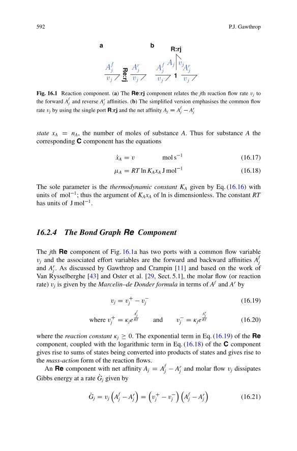
592 P.J. Gawthrop
Re:rjvj vj
ArjAf
a b
j1
R:rj
vj vj
ArjAf
j
Aj vj
Fig. 16.1 Reaction component. (a) The Re:rj component relates the jth reaction flow rate vj to
the forward Afj and reverse Ar
j affinities. (b) The simplified version emphasises the common flow
rate vj by using the single port R:rj and the net affinity Aj D Afj � Ar
j
state xA D nA, the number of moles of substance A. Thus for substance A thecorresponding C component has the equations
PxA D v mol s�1 (16.17)
�A D RT ln KAxA J mol�1 (16.18)
The sole parameter is the thermodynamic constant KA given by Eq. (16.16) withunits of mol�1; thus the argument of KAxA of ln is dimensionless. The constant RThas units of J mol�1.
16.2.4 The Bond Graph Re Component
The jth Re component of Fig. 16.1a has two ports with a common flow variablevj and the associated effort variables are the forward and backward affinities Af
jand Ar
j . As discussed by Gawthrop and Crampin [11] and based on the work ofVan Rysselberghe [43] and Oster et al. [29, Sect. 5.1], the molar flow (or reactionrate) vj is given by the Marcelin–de Donder formula in terms of Af and Ar by
vj D vCj � v�j (16.19)
where vCj D �jeA
fj
RT and v�j D �jeAr
jRT (16.20)
where the reaction constant �j � 0. The exponential term in Eq. (16.19) of the Recomponent, coupled with the logarithmic term in Eq. (16.18) of the C componentgives rise to sums of states being converted into products of states and gives rise tothe mass-action form of the reaction flows.
An Re component with net affinity Aj D Afj � Ar
j and molar flow vj dissipates
Gibbs energy at a rate PGj given by
PGj D vj
Af
j � Arj
DvCj � v�j
Af
j � Arj
(16.21)
16 Biomolecular Systems: Modelling and Causal Analysis 593
Note that when Aj D 0 both vj D 0 and PGj D 0. Thus, to show that Re is dissipative,it is necessary to show that PGj is positive for all vj ¤ 0.
Using Eq. (16.20)
Afj D RT ln
vCj�j
and Arj D RT ln
v�j�j
(16.22)
and so PGj D RTvCj � v�j
lnvCjv�j
(16.23)
Equation (16.23) is given by Qian and Beard [36, Eq. (5)] and Polettini and Esposito[35].
From Eq. (16.20), both vCj and v�j are positive and so it is possible to write
vCj D �v�j where � is positive. Hence Eq. (16.23) can be rewritten as
PGj D RTv�j .� � 1/ ln � (16.24)
There are three possibilities: if � > 1 then both .� � 1/ > 0 and ln � > 0 and so, asv�j > 0, PGj > 0; if � < 1 then both .� � 1/ < 0 and ln � < 0 and so, as v�j > 0,PGj > 0; and, if � D 1, both .� � 1/ D 0 and ln � D 0 and PGj D 0. Hence if vj ¤ 0,PGj > 0 and if vj D 0, PGj D 0.
From Eqs. (16.10) and (16.11), the enthalpy dissipated by the resistor reappearsas external entropy and the remainder of the Gibbs energy (T�S) represents achange of internal entropy. Thus only the enthalpy portion of the Gibbs energy isdissipated as “heat of reaction”—more properly called enthalpy of reaction. Thisphenomenon has been called entropy stripping [41, 42].
The two ports of the reaction component Re of Fig. 16.1a are needed toseparately convey the affinities Af
j and Arj to Eq. (16.19). However, as pointed out
by Karnopp [20], the one port R and 1 junction version of Fig. 16.1b more clearlyshows that the molar flow vj is common to both ports and thus mass is conserved.The R component can be suitably modulated to have the same effect as the Recomponent. The one port version of Fig. 16.1b will be used for the structural analysisof Sect. 16.3.
16.2.5 Example
Figure 16.2a corresponds to a biomolecular system with three species (A, B, C) andthree reactions (r1, r2, r3) given by the chemical formulae
A1�*)� B
2�*)� C3�*)� A (16.25)
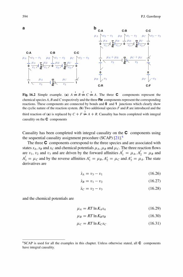
594 P.J. Gawthrop
C:A C:B C:C
Re:
r1
Re:
r2
Re:
r3
0 0 0
11
a b
v1 v1 v2 v2
v3 v3
µA µB µB
µCµA
µC
µA µB µCv3 − v1 v1 − v2 v2 − v3
C:A C:B C:C
C:FC:R
Re:
r1
Re:
r2
Re:
r3
0 0 0
00
11
v1 v1 v2 v2
v3 v3
µA µB µB
µC + µFµA + µR
µC
µA µB µCv3 − v1 v1 − v2 v2 − v3
µR µFv3 −v3
Fig. 16.2 Simple example. (a) A1�*)� B
2�*)� C3�*)� A. The three C components represent the
chemical species A, B and C respectively and the three Re components represent the correspondingreactions. These components are connected by bonds and 0 and 1 junctions which clearly showthe cyclic nature of the reaction system. (b) Two additional species F and R are introduced and the
third reaction of (a) is replaced by C C F3�*)� AC R. Causality has been completed with integral
causality on the C components
Causality has been completed with integral causality on the C components usingthe sequential causality assignment procedure (SCAP) [21].6
The three C components correspond to the three species and are associated withstates xA, xB and xC and chemical potentials �A, �B and �C. The three reaction flowsare v1, v2 and v3 and are driven by the forward affinities Af
1 D �A, Af2 D �B and
Af3 D �C and by the reverse affinities Ar
1 D �B, Ar2 D �C and Ar
3 D �A. The statederivatives are
PxA D v3 � v1 (16.26)
PxB D v1 � v2 (16.27)
PxC D v2 � v3 (16.28)
and the chemical potentials are
�A D RT ln KAxA (16.29)
�B D RT ln KBxB (16.30)
�C D RT ln KCxC (16.31)
6SCAP is used for all the examples in this chapter. Unless otherwise stated, all C componentshave integral causality.
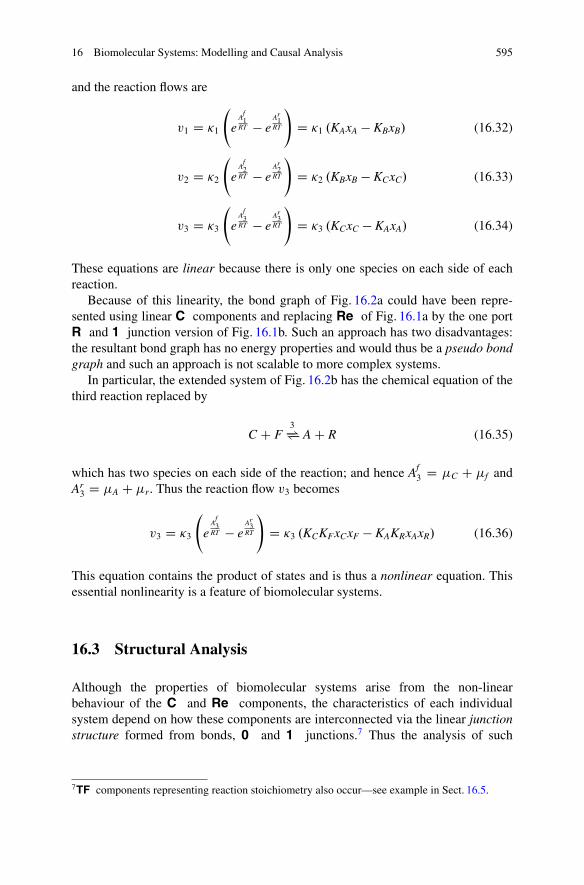
16 Biomolecular Systems: Modelling and Causal Analysis 595
and the reaction flows are
v1 D �1
e
Af1
RT � eAr1
RT
!D �1 .KAxA � KBxB/ (16.32)
v2 D �2
e
Af2
RT � eAr2
RT
!D �2 .KBxB � KCxC/ (16.33)
v3 D �3
e
Af3
RT � eAr3
RT
!D �3 .KCxC � KAxA/ (16.34)
These equations are linear because there is only one species on each side of eachreaction.
Because of this linearity, the bond graph of Fig. 16.2a could have been repre-sented using linear C components and replacing Re of Fig. 16.1a by the one portR and 1 junction version of Fig. 16.1b. Such an approach has two disadvantages:the resultant bond graph has no energy properties and would thus be a pseudo bondgraph and such an approach is not scalable to more complex systems.
In particular, the extended system of Fig. 16.2b has the chemical equation of thethird reaction replaced by
C C F3�*)� A C R (16.35)
which has two species on each side of the reaction; and hence Af3 D �C C �f and
Ar3 D �A C �r. Thus the reaction flow v3 becomes
v3 D �3
e
Af3
RT � eAr3
RT
!D �3 .KCKFxCxF � KAKRxAxR/ (16.36)
This equation contains the product of states and is thus a nonlinear equation. Thisessential nonlinearity is a feature of biomolecular systems.
16.3 Structural Analysis
Although the properties of biomolecular systems arise from the non-linearbehaviour of the C and Re components, the characteristics of each individualsystem depend on how these components are interconnected via the linear junctionstructure formed from bonds, 0 and 1 junctions.7 Thus the analysis of such
7TF components representing reaction stoichiometry also occur—see example in Sect. 16.5.
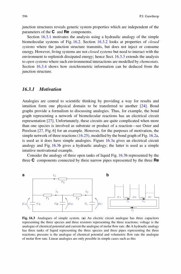
596 P.J. Gawthrop
junction structures reveals generic system properties which are independent of theparameters of the C and Re components.
Section 16.3.1 motivates the analysis using a hydraulic analogy of the simplebiomolecular systems of Fig. 16.2. Section 16.3.2 looks at properties of closedsystems where the junction structure transmits, but does not inject or consumeenergy. However, living systems are not closed systems but need to interact with theenvironment to replenish dissipated energy; hence Sect. 16.3.3 extends the analysisto open systems where such environmental interactions are modelled by chemostats.Section 16.3.4 shows how stoichiometric information can be deduced from thejunction structure.
16.3.1 Motivation
Analogies are central to scientific thinking by providing a way for results andintuition form one physical domain to be transferred to another [24]. Bondgraphs provide a formalism to discussing analogies. Thus, for example, the bondgraph representing a network of biomolecular reactions has an electrical circuitrepresentation [27]. Unfortunately, these circuits are quite complicated when morethan one species is involved as substrate or product of a reaction—see Oster andPerelson [27, Fig. 6] for an example. However, for the purposes of motivation, thesimple network of three reactions (16.25), modelled by the bond graph of Fig. 16.2a,is used as it does have simple analogies. Figure 16.3a gives an electrical circuitanalogy and Fig. 16.3b gives a hydraulic analogy; the latter is used as a simpleintuitive motivational example.
Consider the analogy of three open tanks of liquid Fig. 16.3b represented by thethree C components connected by three narrow pipes represented by the three Re
r1
a b
cAµA cB µB
r2cc µC
i2i1
r3
i3
µA µB µC
v1 v2
v3
Fig. 16.3 Analogues of simple system. (a) An electric circuit analogue has three capacitorsrepresenting the three species and three resistors representing the three reactions; voltage is theanalogue of chemical potential and current the analogue of molar flow rate. (b) A hydraulic analogyhas three tanks of liquid representing the three species and three pipes representing the threereactions; pressure is the analogue of chemical potential and volumetric flow rate the analogueof molar flow rate. Linear analogies are only possible in simple cases such as this

16 Biomolecular Systems: Modelling and Causal Analysis 597
components. �A, �B and �C then represent the pressures associated with the tanksand v1, v2 and v3 the volumetric flow rates though the pipes.
In the linear case, the C components become linear and the Re componentscan be replaced by an R component and 1 junction as in Fig. 16.1 where in the caseof Re:r1 the forward “affinity” or pressure Af
1 D �A and the reverse “affinity” orpressure Ar
1 D �B; the pressure drop across r1 is A1 D Af1 � Ar
1. The followingstatements can be made about this particular system
1. The sum of the volumes of liquid in the three tanks (xtot) is constant
xA.t/C xB.t/C xC.t/ D xtot (16.37)
This is analogous to a conserved moiety in biochemistry.2. As A1 C A2 C A3 D .�A � �B/C .�B � �C/C .�C � �A/ D 0, the sum of the
three pressure drops is zero
A1.t/C A2.t/C A3.t/ D 0 (16.38)
3. In the steady state of this closed system, there is no energy dissipation and so allflows are zero and thus the pressures are equal
�A.1/ D �B.1/ D �C.1/ (16.39)
4. If the third pipe were replaced by a constant-flow pump with flow rate v0, then inthe steady state ( PX D 0)
v1.1/ D v2.1/ D v0 (16.40)
These four statements are illustrated by the simulation of Fig. 16.4. Here all reactionconstants and thermodynamics constants are unity (�1 D �2 D �3 D KA D KB DKC D 1) and the initial states are xA D 3, xB D 2:5 and xC D 0:5.
These four statements are obvious in the context of this simple system, thepurpose of the next section is to show how these statements generalise to arbitrarybiomolecular networks. The fourth statement involves the use of a pump. Thisrequires an external source of energy and thus the resultant system is no longerclosed. Thus the analysis is extended to include open as well as closed systems. Thedesign of biomolecular pumps, and the source of their energy requirement, is key tounderstanding living systems. As will be discussed in Sect. 16.3.3, such pumps canbe modelled using chemostats which are closely related to the bond graph effortsource Se. Such pumps make use of the inherent non-linearity of biomolecularsystems when multiple substrates and products of a reaction are present; in particular
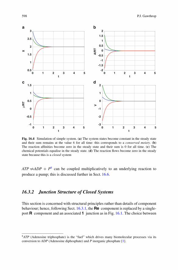
598 P.J. Gawthrop
0.5
1
1.5
2
2.5
3a b
c d
0 1 2 3 4 5
X
t
-2
-1.5
-1
-0.5
0
0.5
1
1.5
2
0 1 2 3 4 5
A/R
T
t
-1
-0.5
0
0.5
1
1.5
0 1 2 3 4 5
μ/R
T
t
-3
-2
-1
0
1
2
0 1 2 3 4 5
V
t
Fig. 16.4 Simulation of simple system. (a) The system states become constant in the steady stateand their sum remains at the value 6 for all time: this corresponds to a conserved moiety. (b)The reaction affinities become zero in the steady state and their sum is 0 for all time. (c) Thechemical potentials equalise in the steady state. (d) The reaction flows become zero in the steadystate because this is a closed system
ATP �*)�ADP C P8 can be coupled multiplicatively to an underlying reaction toproduce a pump; this is discussed further in Sect. 16.6.
16.3.2 Junction Structure of Closed Systems
This section is concerned with structural principles rather than details of componentbehaviour; hence, following Sect. 16.3.1, the Re component is replaced by a single-port R component and an associated 1 junction as in Fig. 16.1. The choice between
8ATP (Adenosine triphosphate) is the “fuel” which drives many biomolecular processes via itsconversion to ADP (Adenosine diphosphate) and P inorganic phosphate [1].
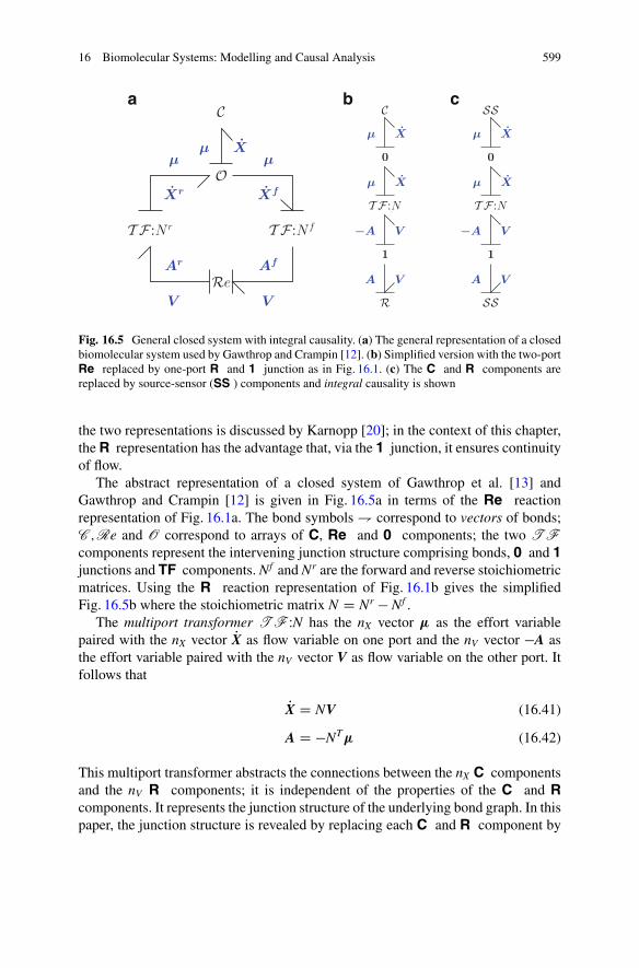
16 Biomolecular Systems: Modelling and Causal Analysis 599
O
µ Xµ
Xf
µ
Xr
T F :Nr T F :Nf
Ca b c
Re
V
Af
V
Ar
0
µ X
T F :N
−A V
µ X
1
R
C
A V
0
µ X
T F :N
−A V
µ X
1
SS
SS
A V
Fig. 16.5 General closed system with integral causality. (a) The general representation of a closedbiomolecular system used by Gawthrop and Crampin [12]. (b) Simplified version with the two-portRe replaced by one-port R and 1 junction as in Fig. 16.1. (c) The C and R components arereplaced by source-sensor (SS ) components and integral causality is shown
the two representations is discussed by Karnopp [20]; in the context of this chapter,the R representation has the advantage that, via the 1 junction, it ensures continuityof flow.
The abstract representation of a closed system of Gawthrop et al. [13] andGawthrop and Crampin [12] is given in Fig. 16.5a in terms of the Re reactionrepresentation of Fig. 16.1a. The bond symbols + correspond to vectors of bonds;C ;Re and O correspond to arrays of C, Re and 0 components; the two T Fcomponents represent the intervening junction structure comprising bonds, 0 and 1junctions and TF components. Nf and Nr are the forward and reverse stoichiometricmatrices. Using the R reaction representation of Fig. 16.1b gives the simplifiedFig. 16.5b where the stoichiometric matrix N D Nr � Nf .
The multiport transformer T F WN has the nX vector � as the effort variablepaired with the nX vector PX as flow variable on one port and the nV vector �A asthe effort variable paired with the nV vector V as flow variable on the other port. Itfollows that
PX D NV (16.41)
A D �NT� (16.42)
This multiport transformer abstracts the connections between the nX C componentsand the nV R components; it is independent of the properties of the C and Rcomponents. It represents the junction structure of the underlying bond graph. In thispaper, the junction structure is revealed by replacing each C and R component by

600 P.J. Gawthrop
a source-sensor SS component [14, 15].9 For example, the bond graph of Fig. 16.2abecomes the junction structure bond graph of Fig. 16.6a. The SS componentshave now preferred causality; in Fig. 16.6a the SS causality has been chosen tocorrespond to the preferred causality of Fig. 16.2a where the C components haveintegral causality (effort output) leading to flow output on each R component.
16.3.2.1 Structure Matrices
With the integral causality shown in Fig. 16.5c the junction structure outputs are thenX C flows (rate of species change, PX mol s�1/ and the nV R efforts (affinities,A J mol�1). and the junction structure inputs are the nX C efforts (chemicalpotentials, �mol s�1) and the nV R flows (molar reaction flows, V mol s�1).Combining the junction structure outputs into the vector Y, and combining thejunction structure inputs into the vector U, Eqs. (16.41) and (16.42) can be rewrittenin a more compact form as
Y D SU (16.43)
where Y D PX
A
!; U D
�
V
!(16.44)
and S D 0nX�nX N�NT 0nV�nV
!(16.45)
The structure matrix S has two notable features:
1. As discussed, for example, by Karnopp et al. [21, Sect. 7.4] the junction structurematrix S is skew symmetric; this arises from the energy transmission propertiesof the multiport transformer.
2. The two block zero elements 0nX�nX and 0nV�nV arise because, in the junctionstructure, the effort and flow variables do not interact: biomolecular systems donot contain gyrators.
16.3.2.2 Derivative Causality
As was noted by Sueur and Dauphin-Tanguy [38, 39], investigating the junctionstructure with C and I components in derivative causality is the key to determiningsystem properties. With this in mind, and noting that the only dynamic componentsare C components, the integral causality leading to S is replaced by maximising the
9The SS component is equivalent to the EN (environment) component introduced by Rosenbergand Andry [37].
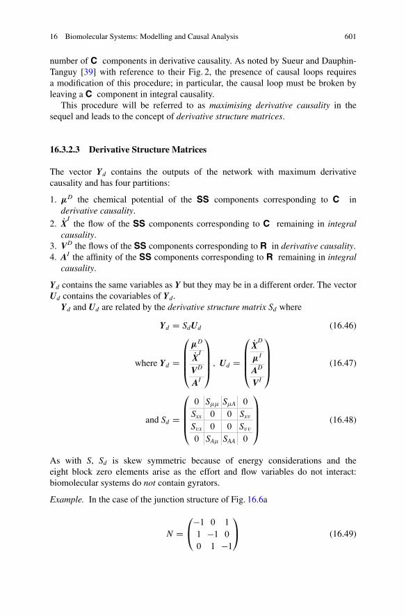
16 Biomolecular Systems: Modelling and Causal Analysis 601
number of C components in derivative causality. As noted by Sueur and Dauphin-Tanguy [39] with reference to their Fig. 2, the presence of causal loops requiresa modification of this procedure; in particular, the causal loop must be broken byleaving a C component in integral causality.
This procedure will be referred to as maximising derivative causality in thesequel and leads to the concept of derivative structure matrices.
16.3.2.3 Derivative Structure Matrices
The vector Yd contains the outputs of the network with maximum derivativecausality and has four partitions:
1. �D the chemical potential of the SS components corresponding to C inderivative causality.
2. PXIthe flow of the SS components corresponding to C remaining in integral
causality.3. VD the flows of the SS components corresponding to R in derivative causality.4. AI the affinity of the SS components corresponding to R remaining in integral
causality.
Yd contains the same variables as Y but they may be in a different order. The vectorUd contains the covariables of Yd.
Yd and Ud are related by the derivative structure matrix Sd where
Yd D SdUd (16.46)
where Yd D
0
BBB@
�D
PXI
VD
AI
1
CCCA ; Ud D
0
BBB@
PXD
�I
AD
VI
1
CCCA (16.47)
and Sd D
0
BBB@
0 S�� S�A 0
Sxx 0 0 Sxv
Svx 0 0 Svv0 SA� SAA 0
1
CCCA (16.48)
As with S, Sd is skew symmetric because of energy considerations and theeight block zero elements arise as the effort and flow variables do not interact:biomolecular systems do not contain gyrators.
Example. In the case of the junction structure of Fig. 16.6a
N D0
@�1 0 1
1 �1 0
0 1 �1
1
A (16.49)
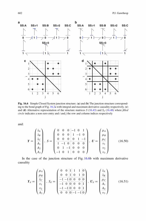
602 P.J. Gawthrop
a b
c d
SS:A SS:B SS:CSS:r1 SS:r2
SS:r3
0 0 0
11 1
1 1
SS:A SS:B SS:CSS:r1 SS:r2
SS:r3
0 0 0
11 1
1 1
1 2 3 4 5 6
1
2
3
4
5
6
j
i
1 2 3 4 5 6
1
2
3
4
5
6
j
i
Fig. 16.6 Simple Closed System junction structure. (a) and (b) The junction structure correspond-ing to the bond graph of Fig. 16.2a with integral and maximum derivative causality respectively. (c)and (d) Alternative representation of the structure matrices S (16.43) and Sd (16.48) where filledcircle indicates a non-zero entry and i and j the row and column indices respectively
and:
Y D
0
BBBBBBB@
PxA
PxB
PxC
A1A2A3
1
CCCCCCCA
; S D
0
BBBBBBB@
0 0 0 �1 0 1
0 0 0 1 �1 0
0 0 0 0 1 �11 �1 0 0 0 0
0 1 �1 0 0 0
�1 0 1 0 0 0
1
CCCCCCCA
; U D
0
BBBBBBB@
�A
�B
�C
v1v2v3
1
CCCCCCCA
(16.50)
In the case of the junction structure of Fig. 16.6b with maximum derivativecausality
Yd D
0
BBBBBBB@
�A
�B
PxC
v1v2
A3
1
CCCCCCCA
; Sd D
0
BBBBBBB@
0 0 1 1 1 0
0 0 1 0 1 0
�1 �1 0 0 0 0
�1 0 0 0 0 1
�1 �1 0 0 0 1
0 0 0 �1 �1 0
1
CCCCCCCA
; Ud D
0
BBBBBBB@
PxA
PxB
�C
A1A2v3
1
CCCCCCCA
(16.51)
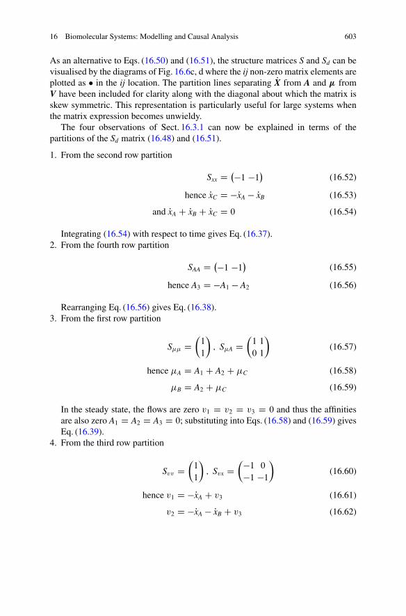
16 Biomolecular Systems: Modelling and Causal Analysis 603
As an alternative to Eqs. (16.50) and (16.51), the structure matrices S and Sd can bevisualised by the diagrams of Fig. 16.6c, d where the ij non-zero matrix elements areplotted as in the ij location. The partition lines separating PX from A and � fromV have been included for clarity along with the diagonal about which the matrix isskew symmetric. This representation is particularly useful for large systems whenthe matrix expression becomes unwieldy.
The four observations of Sect. 16.3.1 can now be explained in terms of thepartitions of the Sd matrix (16.48) and (16.51).
1. From the second row partition
Sxx D ��1 �1� (16.52)
hence PxC D �PxA � PxB (16.53)
and PxA C PxB C PxC D 0 (16.54)
Integrating (16.54) with respect to time gives Eq. (16.37).2. From the fourth row partition
SAA D ��1 �1� (16.55)
hence A3 D �A1 � A2 (16.56)
Rearranging Eq. (16.56) gives Eq. (16.38).3. From the first row partition
S�� D�1
1
�; S�A D
�1 1
0 1
�(16.57)
hence �A D A1 C A2 C �C (16.58)
�B D A2 C �C (16.59)
In the steady state, the flows are zero v1 D v2 D v3 D 0 and thus the affinitiesare also zero A1 D A2 D A3 D 0; substituting into Eqs. (16.58) and (16.59) givesEq. (16.39).
4. From the third row partition
Svv D�1
1
�; Svx D
��1 0
�1 �1�
(16.60)
hence v1 D �PxA C v3 (16.61)
v2 D �PxA � PxB C v3 (16.62)
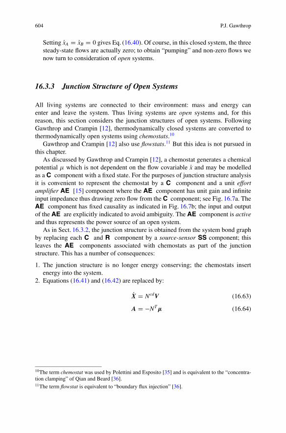
604 P.J. Gawthrop
Setting PxA D PxB D 0 gives Eq. (16.40). Of course, in this closed system, the threesteady-state flows are actually zero; to obtain “pumping” and non-zero flows wenow turn to consideration of open systems.
16.3.3 Junction Structure of Open Systems
All living systems are connected to their environment: mass and energy canenter and leave the system. Thus living systems are open systems and, for thisreason, this section considers the junction structures of open systems. FollowingGawthrop and Crampin [12], thermodynamically closed systems are converted tothermodynamically open systems using chemostats.10
Gawthrop and Crampin [12] also use flowstats.11 But this idea is not pursued inthis chapter.
As discussed by Gawthrop and Crampin [12], a chemostat generates a chemicalpotential � which is not dependent on the flow covariable Px and may be modelledas a C component with a fixed state. For the purposes of junction structure analysisit is convenient to represent the chemostat by a C component and a unit effortamplifier AE [15] component where the AE component has unit gain and infiniteinput impedance thus drawing zero flow from the C component; see Fig. 16.7a. TheAE component has fixed causality as indicated in Fig. 16.7b; the input and outputof the AE are explicitly indicated to avoid ambiguity. The AE component is activeand thus represents the power source of an open system.
As in Sect. 16.3.2, the junction structure is obtained from the system bond graphby replacing each C and R component by a source-sensor SS component; thisleaves the AE components associated with chemostats as part of the junctionstructure. This has a number of consequences:
1. The junction structure is no longer energy conserving; the chemostats insertenergy into the system.
2. Equations (16.41) and (16.42) are replaced by:
PX D NcdV (16.63)
A D �NT� (16.64)
10The term chemostat was used by Polettini and Esposito [35] and is equivalent to the “concentra-tion clamping” of Qian and Beard [36].11The term flowstat is equivalent to “boundary flux injection” [36].

16 Biomolecular Systems: Modelling and Causal Analysis 605
AE
C:c
a b
[in]
[out]
x
0µ
µ
C:A C:B C:C
C:FC:R
iRe:
r1
iRe:
r2
sRe:
r3
EAEA
0 0 0
11
[in]
[out] [out]
[in]
Fig. 16.7 Chemostats. (a) A chemostat is modelled by a C component and a AE effort amplifier;this means that the corresponding chemical potential � is imposed on the rest of the system but thecorresponding flow Px does not effect the C component. (b) The simple example of Fig. 16.2b ismodified with AE components to turn C:F and C:R into chemostats thus creating an open systemfrom a closed system
where Ncd is N with rows corresponding to the chemostats removed[12, Sect. 3.4]. The structure matrix S is no longer of the skew symmetric formof Eq. (16.45) but is rather of the form
S D
0 Ncd
�NT 0
!(16.65)
3. When maximising derivative causality, the possible causal patterns of thejunction structure are constrained by the fixed causality of the AE components.
16.3.3.1 Example (Chemostats)
The closed system of Fig. 16.6 is turned into the open system of Fig. 16.7b wherethe flow v3 is “pumped” by the addition of a forward-driving chemostat C:F and areverse-driving chemostat C:R arranged so that there is no net mass inflow to thesystem. This is the chemostatic version of the chemical equation (16.35) with thebond graph of Fig. 16.2b. Figure 16.8a shows the corresponding junction structurein integral causality and Fig. 16.8b with maximum derivative causality.
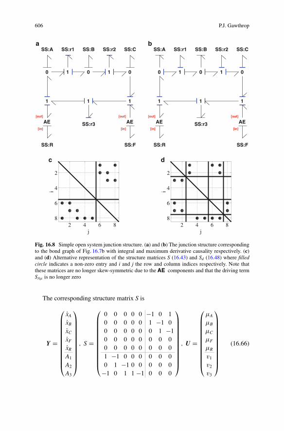
606 P.J. Gawthrop
SS:A SS:B SS:C
SS:FSS:R
a b
c d
SS:r1 SS:r2
SS:r3 EAEA
0 0 0
11
1 1
1
[in]
[out] [out]
[in]
SS:A SS:B SS:C
SS:FSS:R
SS:r1 SS:r2
SS:r3 EAEA
0 0 0
11
1 1
1
[in]
[out] [out]
[in]
2 4 6 8
2
4
6
8
j
i
2 4 6 8
2
4
6
8
j
i
Fig. 16.8 Simple open system junction structure. (a) and (b) The junction structure correspondingto the bond graph of Fig. 16.7b with integral and maximum derivative causality respectively. (c)and (d) Alternative representation of the structure matrices S (16.43) and Sd (16.48) where filledcircle indicates a non-zero entry and i and j the row and column indices respectively. Note thatthese matrices are no longer skew-symmetric due to the AE components and that the driving termSA� is no longer zero
The corresponding structure matrix S is
Y D
0
BBBBBBBBBBB@
PxA
PxB
PxC
PxF
PxR
A1A2A3
1
CCCCCCCCCCCA
; S D
0
BBBBBBBBBBB@
0 0 0 0 0 �1 0 1
0 0 0 0 0 1 �1 0
0 0 0 0 0 0 1 �10 0 0 0 0 0 0 0
0 0 0 0 0 0 0 0
1 �1 0 0 0 0 0 0
0 1 �1 0 0 0 0 0
�1 0 1 1 �1 0 0 0
1
CCCCCCCCCCCA
; U D
0
BBBBBBBBBBB@
�A
�B
�C
�F
�R
v1v2v3
1
CCCCCCCCCCCA
(16.66)
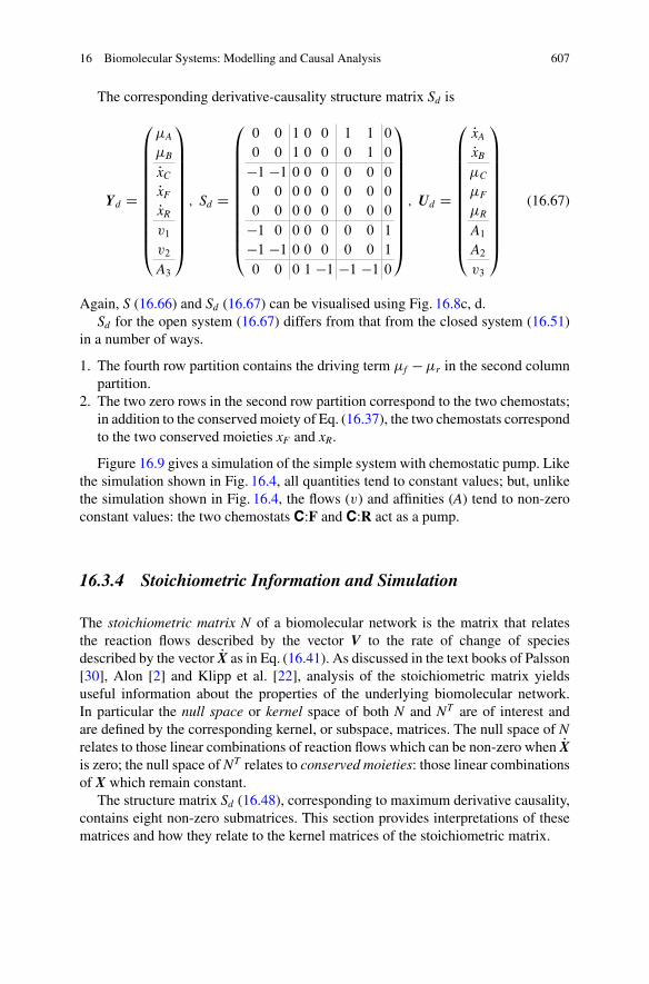
16 Biomolecular Systems: Modelling and Causal Analysis 607
The corresponding derivative-causality structure matrix Sd is
Yd D
0
BBBBBBBBBBB@
�A
�B
PxC
PxF
PxR
v1v2
A3
1
CCCCCCCCCCCA
; Sd D
0
BBBBBBBBBBB@
0 0 1 0 0 1 1 0
0 0 1 0 0 0 1 0
�1 �1 0 0 0 0 0 0
0 0 0 0 0 0 0 0
0 0 0 0 0 0 0 0
�1 0 0 0 0 0 0 1
�1 �1 0 0 0 0 0 1
0 0 0 1 �1 �1 �1 0
1
CCCCCCCCCCCA
; Ud D
0
BBBBBBBBBBB@
PxA
PxB
�C
�F
�R
A1A2v3
1
CCCCCCCCCCCA
(16.67)
Again, S (16.66) and Sd (16.67) can be visualised using Fig. 16.8c, d.Sd for the open system (16.67) differs from that from the closed system (16.51)
in a number of ways.
1. The fourth row partition contains the driving term �f ��r in the second columnpartition.
2. The two zero rows in the second row partition correspond to the two chemostats;in addition to the conserved moiety of Eq. (16.37), the two chemostats correspondto the two conserved moieties xF and xR.
Figure 16.9 gives a simulation of the simple system with chemostatic pump. Likethe simulation shown in Fig. 16.4, all quantities tend to constant values; but, unlikethe simulation shown in Fig. 16.4, the flows (v) and affinities (A) tend to non-zeroconstant values: the two chemostats C:F and C:R act as a pump.
16.3.4 Stoichiometric Information and Simulation
The stoichiometric matrix N of a biomolecular network is the matrix that relatesthe reaction flows described by the vector V to the rate of change of speciesdescribed by the vector PX as in Eq. (16.41). As discussed in the text books of Palsson[30], Alon [2] and Klipp et al. [22], analysis of the stoichiometric matrix yieldsuseful information about the properties of the underlying biomolecular network.In particular the null space or kernel space of both N and NT are of interest andare defined by the corresponding kernel, or subspace, matrices. The null space of Nrelates to those linear combinations of reaction flows which can be non-zero when PXis zero; the null space of NT relates to conserved moieties: those linear combinationsof X which remain constant.
The structure matrix Sd (16.48), corresponding to maximum derivative causality,contains eight non-zero submatrices. This section provides interpretations of thesematrices and how they relate to the kernel matrices of the stoichiometric matrix.
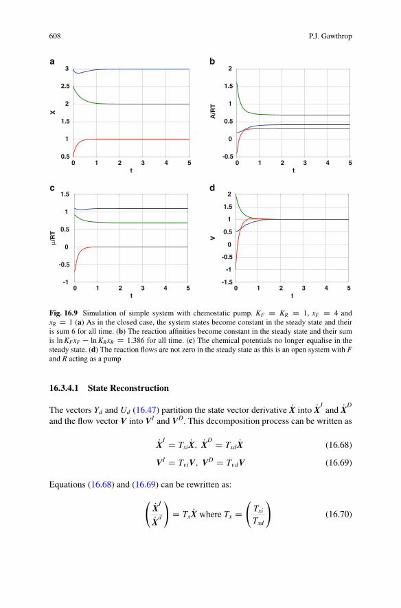
608 P.J. Gawthrop
0.5
1
1.5
2
2.5
3a b
c d
0 1 2 3 4 5
X
t
-0.5
0
0.5
1
1.5
2
0 1 2 3 4 5
A/R
T
t
-1
-0.5
0
0.5
1
1.5
0 1 2 3 4 5
μ/R
T
t
-1.5
-1
-0.5
0
0.5
1
1.5
2
0 1 2 3 4 5
V
t
Fig. 16.9 Simulation of simple system with chemostatic pump. KF D KR D 1, xF D 4 andxR D 1 (a) As in the closed case, the system states become constant in the steady state and theiris sum 6 for all time. (b) The reaction affinities become constant in the steady state and their sumis ln KFxF � ln KRxR D 1:386 for all time. (c) The chemical potentials no longer equalise in thesteady state. (d) The reaction flows are not zero in the steady state as this is an open system with Fand R acting as a pump
16.3.4.1 State Reconstruction
The vectors Yd and Ud (16.47) partition the state vector derivative PX into PXIand PXD
and the flow vector V into VI and VD. This decomposition process can be written as
PXI D Txi PX; PXD D Txd PX (16.68)
VI D TviV; VD D TvdV (16.69)
Equations (16.68) and (16.69) can be rewritten as:
PXI
PXd
!D Tx PX where Tx D
Txi
Txd
!(16.70)
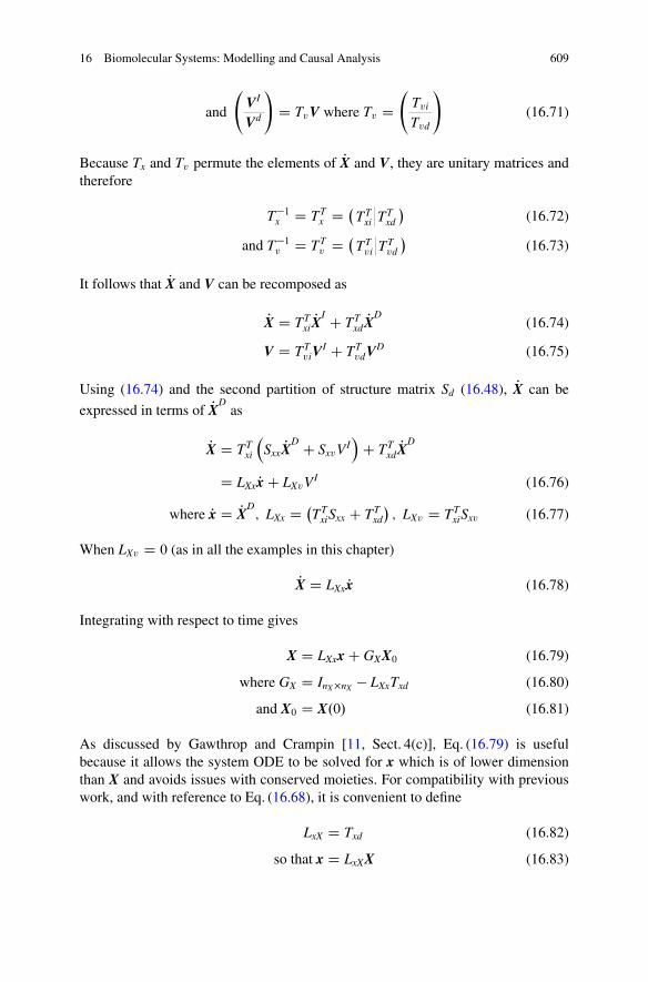
16 Biomolecular Systems: Modelling and Causal Analysis 609
and
VI
Vd
!D TvV where Tv D
Tvi
Tvd
!(16.71)
Because Tx and Tv permute the elements of PX and V, they are unitary matrices andtherefore
T�1x D TTx D �
TTxi TT
xd
�(16.72)
and T�1v D TTv D �
TTvi TT
vd
�(16.73)
It follows that PX and V can be recomposed as
PX D TTxi
PXI C TTxd
PXD(16.74)
V D TTviV
I C TTvdVD (16.75)
Using (16.74) and the second partition of structure matrix Sd (16.48), PX can be
expressed in terms of PXDas
PX D TTxi
Sxx PXD C SxvV
I
C TTxd
PXD
D LXx Px C LXvVI (16.76)
where Px D PXD; LXx D �
TTxiSxx C TT
xd
�; LXv D TT
xiSxv (16.77)
When LXv D 0 (as in all the examples in this chapter)
PX D LXx Px (16.78)
Integrating with respect to time gives
X D LXxx C GXX0 (16.79)
where GX D InX�nX � LXxTxd (16.80)
and X0 D X.0/ (16.81)
As discussed by Gawthrop and Crampin [11, Sect. 4(c)], Eq. (16.79) is usefulbecause it allows the system ODE to be solved for x which is of lower dimensionthan X and avoids issues with conserved moieties. For compatibility with previouswork, and with reference to Eq. (16.68), it is convenient to define
LxX D Txd (16.82)
so that x D LxXX (16.83)
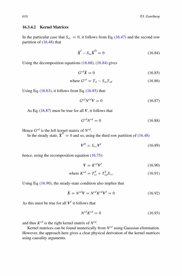
610 P.J. Gawthrop
16.3.4.2 Kernel Matrices
In the particular case that Sxv D 0, it follows from Eq. (16.47) and the second rowpartition of (16.48) that
PXI � Sxx PXD D 0 (16.84)
Using the decomposition equations (16.68), (16.84) gives
Gcd PX D 0 (16.85)
where Gcd D Txi � SxxTxd (16.86)
Using Eq. (16.63), it follows from Eq. (16.85) that:
GcdNcdV D 0 (16.87)
As Eq. (16.87) must be true for all V, it follows that
GcdNcd D 0 (16.88)
Hence Gcd is the left kernel matrix of Ncd.In the steady state, PXD D 0 and so, using the third row partition of (16.48)
VD D SvvVI (16.89)
hence, using the recomposition equation (16.75):
V D KcdVI (16.90)
where Kcd D TTvi C TT
vdSvv (16.91)
Using Eq. (16.90), the steady-state condition also implies that
PX D NcdV D NcdKcdVI D 0 (16.92)
As this must be true for all VI it follows that
NcdKcd D 0 (16.93)
and thus Kcd is the right kernel matrix of Ncd.Kernel matrices can be found numerically from Ncd using Gaussian elimination.
However, the approach here gives a clear physical derivation of the kernel matricesusing causality arguments.
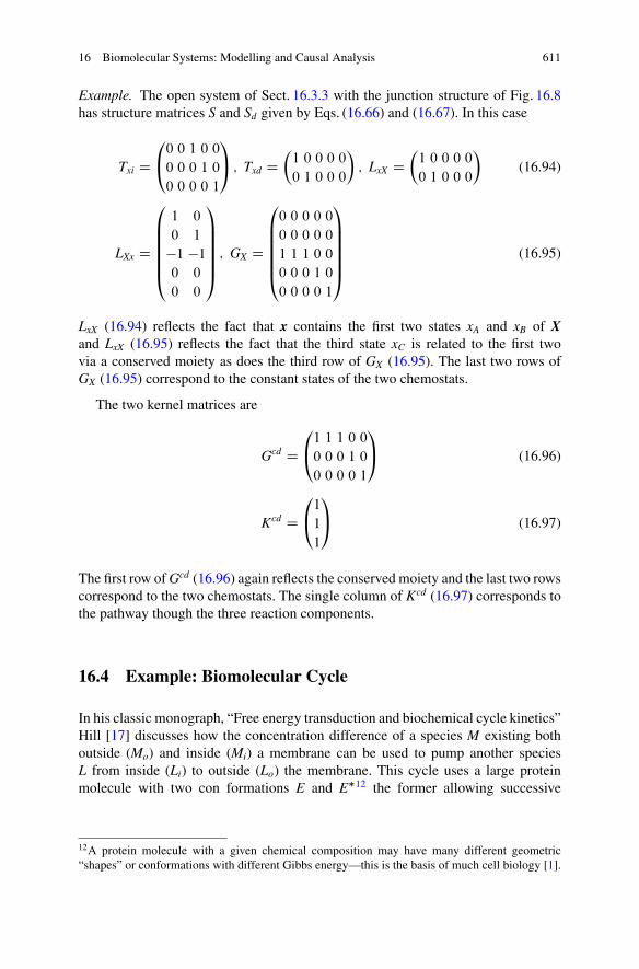
16 Biomolecular Systems: Modelling and Causal Analysis 611
Example. The open system of Sect. 16.3.3 with the junction structure of Fig. 16.8has structure matrices S and Sd given by Eqs. (16.66) and (16.67). In this case
Txi D0
@0 0 1 0 0
0 0 0 1 0
0 0 0 0 1
1
A ; Txd D�1 0 0 0 0
0 1 0 0 0
�; LxX D
�1 0 0 0 0
0 1 0 0 0
�(16.94)
LXx D
0
BBBBB@
1 0
0 1
�1 �10 0
0 0
1
CCCCCA; GX D
0
BBBBB@
0 0 0 0 0
0 0 0 0 0
1 1 1 0 0
0 0 0 1 0
0 0 0 0 1
1
CCCCCA(16.95)
LxX (16.94) reflects the fact that x contains the first two states xA and xB of Xand LxX (16.95) reflects the fact that the third state xC is related to the first twovia a conserved moiety as does the third row of GX (16.95). The last two rows ofGX (16.95) correspond to the constant states of the two chemostats.
The two kernel matrices are
Gcd D0
@1 1 1 0 0
0 0 0 1 0
0 0 0 0 1
1
A (16.96)
Kcd D0
@1
1
1
1
A (16.97)
The first row of Gcd (16.96) again reflects the conserved moiety and the last two rowscorrespond to the two chemostats. The single column of Kcd (16.97) corresponds tothe pathway though the three reaction components.
16.4 Example: Biomolecular Cycle
In his classic monograph, “Free energy transduction and biochemical cycle kinetics”Hill [17] discusses how the concentration difference of a species M existing bothoutside (Mo) and inside (Mi) a membrane can be used to pump another speciesL from inside (Li) to outside (Lo) the membrane. This cycle uses a large proteinmolecule with two con formations E and E�12 the former allowing successive
12A protein molecule with a given chemical composition may have many different geometric“shapes” or conformations with different Gibbs energy—this is the basis of much cell biology [1].

612 P.J. Gawthrop
binding to Mi and Li and the latter to Mo and Lo. This is represented by sevenreactions
Mi C Eem�*)� EM (16.98)
Li C EMlem��*)�� LEM (16.99)
LEMlesm��*)�� LE?M (16.100)
LE?Mesm��*)�� Lo C E?M (16.101)
E?Mes�*)� Mo C E? (16.102)
E?e�*)� E (16.103)
EMslip��*)�� E?M (16.104)
where the last reaction is the so-called slip term. The corresponding bond graphappears in Fig. 16.10a where E? is replaced by Es. The bond graph clearly showsthe cyclic structure of the chemical reactions (16.98)–(16.104) and is topologicallysimilar to the diagram of Hill [17, Fig. 1.2(a)]. As discussed by Hill [17], the fourspecies Mo, Mi, Lo and Li are assumed to have constant concentration: therefore theyare modelled by four chemostats with the corresponding AE components.
The partitions of Y corresponding to Eq. (16.43) are
PX D �PxEM PxLEM PxEs PxEsM PxLEsM PxLi PxLo PxMi PxMo PxE
�T(16.105)
A D �Aem Alem Aes Aesm Aslip Ae Alesm
�T(16.106)
and the partitions of U corresponding to Eq. (16.43) are
� D ��EM �LEM �Es �EsM �LEsM �Li �Lo �Mi �Mo �E
�T(16.107)
V D �vem vlem ves vesm vslip ve vlesm
�T(16.108)
The partitions of Yd corresponding to Eq. (16.47) are
�D D ��EM �LEM �Es �EsM �LEsM
�T(16.109)
PXI D �PxLi PxLo PxMi PxMo PxE
�T(16.110)
VD D �vem vlem ves vesm vslip
�T(16.111)
AI D �Ae Alesm
�T(16.112)
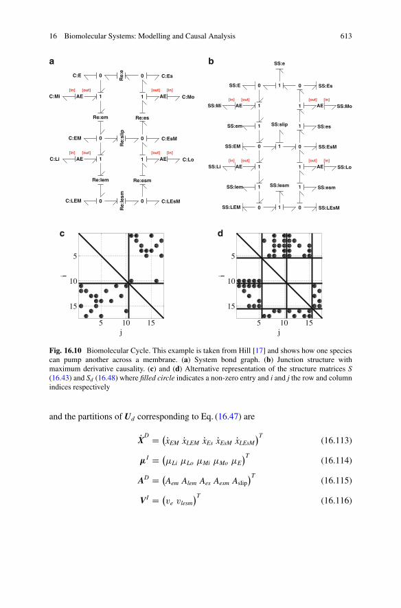
16 Biomolecular Systems: Modelling and Causal Analysis 613
[in] [out]
[in] [out]
[out] [in]
[out] [in]
C:Li C:Lo
C:Mi C:Mo
C:E
C:EM
C:LEM
C:Es
C:EsM
C:LEsM
Re:
eRe:em
Re:lem
Re:es
Re:esm
Re:
lesm
Re:
slip
AE
AE
AE
AE
0
a b
c d
0
0 0
0
0
1
1 1
1[in] [out]
[in] [out]
[out] [in]
[out] [in]
SS:Li SS:Lo
SS:Mi SS:Mo
SS:E
SS:EM
SS:LEM
SS:Es
SS:EsM
SS:LEsM
SS:e
SS:em
SS:lem
SS:es
SS:esmSS:lesm
SS:slip
AE
AE
AE
AE
0
0
0 0
0
0
1
1 1
1
1
1
1
1
1
1
1
5 10 15
5
10
15
j
i
5 10 15
5
10
15
j
i
Fig. 16.10 Biomolecular Cycle. This example is taken from Hill [17] and shows how one speciescan pump another across a membrane. (a) System bond graph. (b) Junction structure withmaximum derivative causality. (c) and (d) Alternative representation of the structure matrices S(16.43) and Sd (16.48) where filled circle indicates a non-zero entry and i and j the row and columnindices respectively
and the partitions of Ud corresponding to Eq. (16.47) are
PXD D �PxEM PxLEM PxEs PxEsM PxLEsM
�T(16.113)
�I D ��Li �Lo �Mi �Mo �E
�T(16.114)
AD D �Aem Alem Aes Aesm Aslip
�T(16.115)
VI D �ve vlesm
�T(16.116)

614 P.J. Gawthrop
The 17 � 17 matrix Sd is summarised in Fig. 16.10d. The relevance of thesubmatrices Sxx, SAA, SA� and Svv are now examined in turn.
1. From the second row partition
Sxx D
0
BBBBB@
0 0 0 0 0
0 0 0 0 0
0 0 0 0 0
0 0 0 0 0
�1 �1 �1 �1 �1
1
CCCCCA(16.117)
the first four rows of Sxx correspond to the four chemostats Li, Lo, Mi and Mo.
PxLi D PxLo D PxMi D PxMo D 0 (16.118)
The fifth row of Sxx corresponds to the conserved moiety
Pxe C Pxem C Pxlem C Pxes C Pxesm C Pxlesm D 0 (16.119)
2. From the fourth row partition
SAA D��1 0 �1 0 �10 �1 0 �1 1
�and SA� D
�0 0 1 �1 01 �1 0 0 0
�(16.120)
the first row of SAA, together with the first row of SA�, corresponds to the sumof the affinities around the upper loop of the biomolecular cycle of Fig. 16.10abeing equal to the weighted sum of the relevant chemostat potentials
Ae C Aem C Aes C Aslip D �Mi � �Mo (16.121)
the second row of SAA, together with the second row of SA�, corresponds to theweighted sum of the affinities around the lower loop of the biomolecular cycle ofFig. 16.10a being equal to the weighted sum of the relevant chemostat potentials
Alesm C Alem C Aesm � Aslip D �li � �lo (16.122)
3. From the third row partition
Svv D
0
BBBBB@
1 0
0 1
1 0
0 1
1 �1
1
CCCCCA(16.123)
In the steady state ( PX D 0). In this case the first four rows of the first columnof Svv correspond to the three steady-state reaction flows in the upper loop beingequal
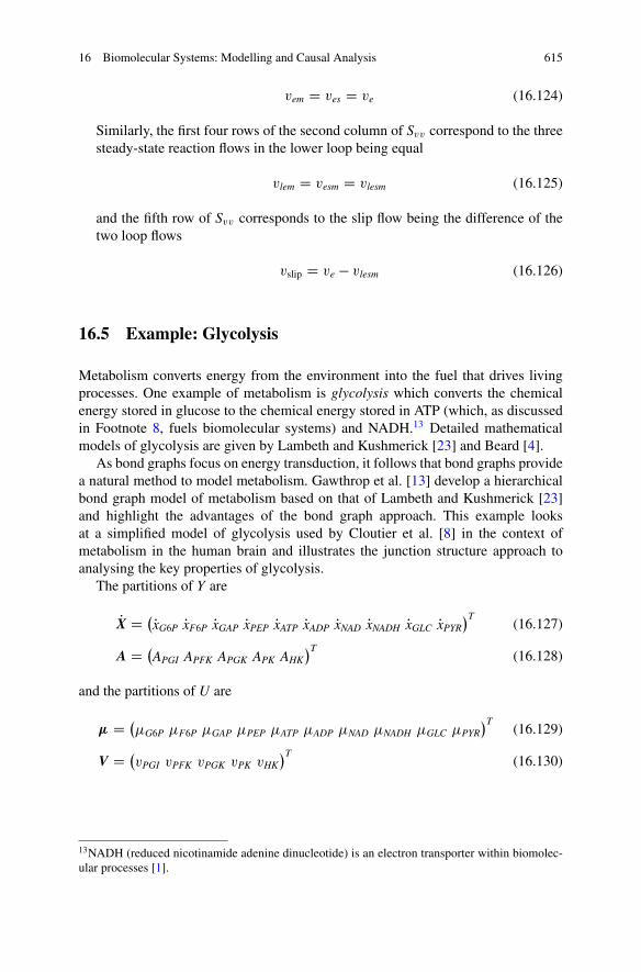
16 Biomolecular Systems: Modelling and Causal Analysis 615
vem D ves D ve (16.124)
Similarly, the first four rows of the second column of Svv correspond to the threesteady-state reaction flows in the lower loop being equal
vlem D vesm D vlesm (16.125)
and the fifth row of Svv corresponds to the slip flow being the difference of thetwo loop flows
vslip D ve � vlesm (16.126)
16.5 Example: Glycolysis
Metabolism converts energy from the environment into the fuel that drives livingprocesses. One example of metabolism is glycolysis which converts the chemicalenergy stored in glucose to the chemical energy stored in ATP (which, as discussedin Footnote 8, fuels biomolecular systems) and NADH.13 Detailed mathematicalmodels of glycolysis are given by Lambeth and Kushmerick [23] and Beard [4].
As bond graphs focus on energy transduction, it follows that bond graphs providea natural method to model metabolism. Gawthrop et al. [13] develop a hierarchicalbond graph model of metabolism based on that of Lambeth and Kushmerick [23]and highlight the advantages of the bond graph approach. This example looksat a simplified model of glycolysis used by Cloutier et al. [8] in the context ofmetabolism in the human brain and illustrates the junction structure approach toanalysing the key properties of glycolysis.
The partitions of Y are
PX D �PxG6P PxF6P PxGAP PxPEP PxATP PxADP PxNAD PxNADH PxGLC PxPYR
�T(16.127)
A D �APGI APFK APGK APK AHK
�T(16.128)
and the partitions of U are
� D ��G6P �F6P �GAP �PEP �ATP �ADP �NAD �NADH �GLC �PYR
�T(16.129)
V D �vPGI vPFK vPGK vPK vHK
�T(16.130)
13NADH (reduced nicotinamide adenine dinucleotide) is an electron transporter within biomolec-ular processes [1].
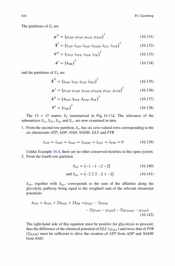
616 P.J. Gawthrop
The partitions of Yd are
�D D ��G6P �F6P �GAP �PEP
�T(16.131)
PXI D �PxATP PxADP PxNAD PxNADH PxGLC PxPYR
�T(16.132)
VD D �vPGI vPFK vPGK vPK
�T(16.133)
AI D �AHK
�T(16.134)
and the partitions of Ud are
PXD D �PxG6P PxF6P PxGAP PxPEP
�T(16.135)
�I D ��ATP �ADP �NAD �NADH �GLC �PYR
�T(16.136)
AD D �APGI APFK APGK APK
�T(16.137)
VI D �vHK
�T(16.138)
The 15 � 15 matrix Sd summarised in Fig. 16.11d. The relevance of thesubmatrices Sxx, SAA, SA� and Svv are now examined in turn.
1. From the second row partition, Sxx has six zero-valued rows corresponding to thesix chemostats ATP, ADP, NAD, NADH, GLY and PYR
PxATP D PxADP D PxNAD D PxNADH D PxGLY D PxPYR D 0 (16.139)
Unlike Example 16.4, there are no other conserved moieties in this open system.2. From the fourth row partition
SAA D ��1 �1 �2 �2� (16.140)
and SA� D ��2 2 2 �2 1 �2� (16.141)
SAA, together with SA�, corresponds to the sum of the affinities along theglycolytic pathway being equal to the weighted sum of the relevant chemostatpotentials
APGI C APFK C 2APGK C 2APK D�GLC � 2�PYR
� 2.�ATP � �ADP/ � 2.�NADH � �NAD/
(16.142)
The right-hand side of this equation must be positive for glycolysis to proceed;thus the difference of the chemical potential of GLC (�GLC) and twice that of PYR(2�PYR) must be sufficient to drive the creation of ATP from ADP and NADHfrom NAD.
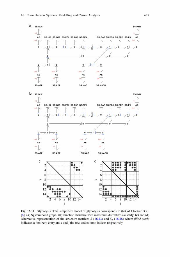
16 Biomolecular Systems: Modelling and Causal Analysis 617
SS:ATP SS:ADP SS:NAD SS:NADH
SS:GLC
SS:G6P SS:F6P SS:GAP SS:PEP
SS:PYR
TF
:t2
SS:HK SS:PGI SS:PFK SS:PGK SS:PKAE
a
b
c d
AE
EAEAEAEA
0 0 0
00
0
0
0 0
0
0000
1 1111
1 1
[out]
[in]
[out]
[in]
[out]
[in]
[out]
[in]
[out]
[in]
[out]
[in]
SS:ATP SS:ADP SS:NAD SS:NADH
SS:GLC
SS:G6P SS:F6P SS:GAP SS:PEP
SS:PYR
TF
:t2
SS:HK SS:PGI SS:PFK SS:PGK SS:PKAE AE
EAEAEAEA
0 0 0
00
0
0
0 0
0
0000
1 1111
1 1
[out]
[in]
[out]
[in]
[out]
[in]
[out]
[in]
[out]
[in]
[out]
[in]
2 4 6 8 10 12 14
2468101214
j
i
2 4 6 8 10 12 14
2468101214
j
i
Fig. 16.11 Glycolysis. This simplified model of glycolysis corresponds to that of Cloutier et al.[8]. (a) System bond graph. (b) Junction structure with maximum derivative causality. (c) and (d)Alternative representation of the structure matrices S (16.43) and Sd (16.48) where filled circleindicates a non-zero entry and i and j the row and column indices respectively
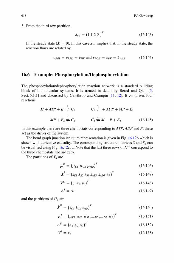
618 P.J. Gawthrop
3. From the third row partition
Svv D �1 1 2 2
�T(16.143)
In the steady state ( PX D 0). In this case Svv implies that, in the steady state, thereaction flows are related by
vPGI D vPFK D vHK and vPGK D vPK D 2vHK (16.144)
16.6 Example: Phosphorylation/Dephosphorylation
The phosphorylation/dephosphorylation reaction network is a standard buildingblock of biomolecular systems. It is treated in detail by Beard and Qian [5,Sect. 5.1.1] and discussed by Gawthrop and Crampin [11, 12]. It comprises fourreactions
M C ATP C E11�*)� C1 C1
2�*)� C ADP C MP C E1
MP C E23�*)� C2 C2
4�*)� M C P C E2 (16.145)
In this example there are three chemostats corresponding to ATP, ADP and P; theseact as the driver of the system.
The bond graph junction structure representation is given in Fig. 16.12b which isshown with derivative causality. The corresponding structure matrices S and Sd canbe visualised using Fig. 16.12c, d. Note that the last three rows of Ncd correspond tothe three chemostats and are zero.
The partitions of Yd are
�D D ��C1 �C2 �MP
�T(16.146)
PXI D �PxE1 PxE2 PxM PxATP PxADP PxP
�T(16.147)
VD D �v1 v2 v3
�T(16.148)
AI D A4 (16.149)
and the partitions of Ud are
PXD D �PxC1 PxC2 PxMP
�T(16.150)
�I D ��E1 �E2 �M �ATP �ADP �P
�T(16.151)
AD D �A1 A2 A3
�T(16.152)
VI D v4 (16.153)
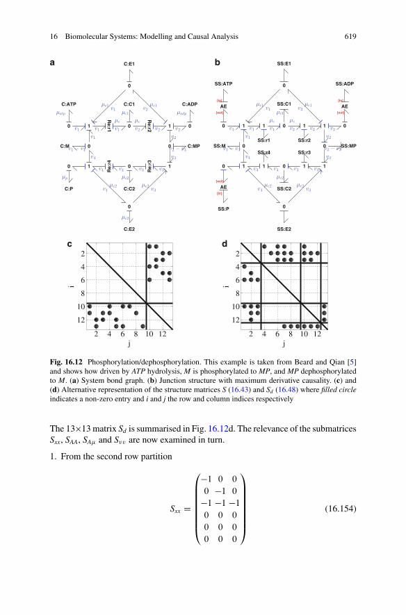
16 Biomolecular Systems: Modelling and Causal Analysis 619
C:E1a b
c d
C:C1
C:E2
C:C2
C:M C:MP
C:ATP C:ADP
C:P
Re:r1
Re:r2
Re:
r3
Re:
r4
0
00 0
0
0
0
0
0
1
11
1
v1 v2
v1 v1 v1 v2 v2
µc µc
µe1
µc1
v2
v3v3v4 v4
v4 v3
µe1
µe2 µe2
µatp µadp
µp
v1 − v4 v2 − v3v4
v1 v2
v3
µc2
µe2
SS:E1
SS:C1
SS:E2
SS:C2
SS:M SS:MP
SS:ATP SS:ADP
SS:P
SS:r1 SS:r2
SS:r3SS:r4
AE
AE
AE
0
00 0
0
0
0
0
0
1
11
11
1 1
1
[in]
[out]
[in]
[in]
[out]
[out]v1 v2
v1 v1 v1 v2 v2
µc µc
µe1
µc1
v2
v3v3v4 v4
v4 v3
µe1
µe2 µe2
v1 − v4 v2 − v3v4
v1 v2
v3
µc2
2 4 6 8 10 12
2
4
6
8
10
12
j
i
2 4 6 8 10 12
2
4
6
8
10
12
j
i
Fig. 16.12 Phosphorylation/dephosphorylation. This example is taken from Beard and Qian [5]and shows how driven by ATP hydrolysis, M is phosphorylated to MP, and MP dephosphorylatedto M. (a) System bond graph. (b) Junction structure with maximum derivative causality. (c) and(d) Alternative representation of the structure matrices S (16.43) and Sd (16.48) where filled circleindicates a non-zero entry and i and j the row and column indices respectively
The 13�13matrix Sd is summarised in Fig. 16.12d. The relevance of the submatricesSxx, SAA, SA� and Svv are now examined in turn.
1. From the second row partition
Sxx D
0
BBBBBBB@
�1 0 0
0 �1 0
�1 �1 �10 0 0
0 0 0
0 0 0
1
CCCCCCCA
(16.154)
620 P.J. Gawthrop
the first and second rows of Sxx correspond to the conserved moieties xe1 Cxc1 D xtot1 and xe2Cxc2 D xtot2. The third row of Sxx corresponds to the conservedmoiety xmp C xc1 C xc2 C xm D xtot. The fourth, fifth and sixth rows of Sxx
correspond to the three constant chemostat states: xATP, xADP and xP.
PxATP D PxADP D PxP D 0 (16.155)
2. From the fourth row partition
SAA D ��1 �1 �1� and SA� D �0 0 0 1 �1 �1� (16.156)
the first row of SAA, together with the first row of SA�, corresponds to the sumof the affinities around the central loop being equal to the weighted sum of thechemostat potentials
A1 C A2 C A3 C A4 D �ATP � �ADP � �P (16.157)
Thus the flow around the loop comprising r1 : : : r4 is driven by the ATP �*)�ADPCP reaction.
3. From the third row partition
Svv D0
@1
1
1
1
A (16.158)
In the steady state ( PX D 0). In this case Svv corresponds to the four reaction flowsbeing equal
v1 D v2 D v3 D v4 (16.159)
16.7 Conclusion
The causal properties of the bond graph junctions structures representing biomolec-ular systems have been examined and shown to provide an alternative approach togenerating the related stoichiometric matrices. As a graphical approach, the bondgraph method gives more intuitive insight than purely numerical approaches.
The bond graph approach uses causality arguments and the sequential causalityassignment procedure (SCAP); the numerical approach uses Gaussian elimination.It follows that the bond graph approach must, in some sense, be equivalent to theGaussian elimination approach; this deserves further investigation.
As discussed in this chapter, it can be more convenient to represent reactionsby a one-port R component and associated 1 junction rather than a two-port Re
16 Biomolecular Systems: Modelling and Causal Analysis 621
component. This raises the question as to whether it is always possible to modelin this way. The key issue here is under what circumstances forward and reversestoichiometric matrices Nf and Nr can be deduced from the stoichiometric matrixN D Nr � Nf .
This chapter focuses on turning closed biomolecular systems into open systemsusing the chemostat (constant chemical potential) concept previously used byPolettini and Esposito [35] and Gawthrop and Crampin [12]. It would be interestingto examine the use of the dual concept of flowstats (constant molar flow) [12] in thecontext of this chapter.
Gawthrop et al. [13] use hierarchical bond graph models to allow large modelsto be built out of submodels and use the notion of a port component to do this. Itwould be interesting to develop a hierarchical version of the methods presented inthis chapter.
Acknowledgements Peter Gawthrop would like to thank the Melbourne School of Engineeringfor its support via a Professorial Fellowship. He would also like to thank Michael Pan and JoeCursons for their close reading of the draft chapter.
References
1. Alberts, B., Johnson, A., Lewis, J., Morgan, D., Raff, M., Roberts, K., et al. (Eds.). (2015).Molecular biology of the cell (6th ed.). Abingdon: Garland Science.
2. Alon, U. (2007). Introduction to systems biology: Design principles of biological networks.Boca Raton: CRC Press.
3. Atkins, P., & de Paula, J. (2011). Physical chemistry for the life sciences (2nd ed.). Oxford:Oxford University Press.
4. Beard, D. A. (2012). Biosimulation: Simulation of living systems. Cambridge: CambridgeUniversity Press. ISBN: 978-0-521-76823-8.
5. Beard, D. A., & Qian, H. (2010). Chemical biophysics: Quantitative analysis of cellularsystems. Cambridge: Cambridge University Press.
6. Breedveld, P. C. (1982). Thermodynamic bond graphs and the problem of ther-mal inertance. Journal of the Franklin Institute, 314(1), 15–40. ISSN: 0016-0032.doi:10.1016/0016-0032(82)90050-3.
7. Cellier, F. E. (1991). Continuous system modelling. New York: Springer.8. Cloutier, M., Bolger, F. B., Lowry J. P., & Wellstead P. (2009). An integrative dynamic model
of brain energy metabolism using in vivo neurochemical measurements. Journal of Computa-tional Neuroscience, 27(3), 391–414. ISSN: 0929-5313. doi:10.1007/s10827-009-0152-8.
9. Fuchs, H. U. (1996). The dynamics of heat. New York: Springer.10. Gawthrop, P. J., & Bevan, G. P. (2007). Bond-graph modeling: A tutorial intro-
duction for control engineers. IEEE Control Systems Magazine, 27(2), 24–45.doi:10.1109/MCS.2007.338279.
11. Gawthrop, P. J., & Crampin, E. J. (2014). Energy-based analysis of biochemical cycles usingbond graphs. Proceedings of the Royal Society A: Mathematical, Physical and EngineeringScience, 470(2171), 1–25. doi:10.1098/rspa.2014.0459. Available at arXiv:1406.2447.
12. Gawthrop, P. J., & Crampin, E. J. (2016). Modular bond-graph modelling and anal-ysis of biomolecular systems. IET Systems Biology, 10, 2016. ISSN: 1751-8849.doi:10.1049/iet-syb.2015.0083. Available at arXiv:1511.06482.

622 P.J. Gawthrop
13. Gawthrop, P. J., Cursons, J., & Crampin, E. J. (2015). Hierarchical bond graph modellingof biochemical networks. Proceedings of the Royal Society A: Mathematical, Physical andEngineering Sciences, 471(2184), 1–23. ISSN: 1364-5021. doi:10.1098/rspa.2015.0642.Available at arXiv:1503.01814.
14. Gawthrop, P. J., & Smith, L. (1992). Causal augmentation of bond graphs with algebraic loops.Journal of the Franklin Institute, 329(2), 291–303. doi:10.1016/0016-0032(92)90035-F.
15. Gawthrop, P. J., & Smith, L. P. S. (1996). Metamodelling: Bond graphs and dynamic systems.Hemel Hempstead: Prentice Hall. ISBN: 0-13-489824-9.
16. Greifeneder, J., & Cellier, F. E. (2012). Modeling chemical reactions using bond graphs. InProceedings ICBGM12, 10th SCS International Conference on Bond Graph Modeling andSimulation, Genoa, Italy (pp. 110–121).
17. Hill, T. L. (1989). Free energy transduction and biochemical cycle kinetics. New York:Springer.
18. Jamshidi, N., & Palsson, B. (2010). Mass action stoichiometric simulation models: Incorporat-ing kinetics and regulation into stoichiometric models. Biophysical Journal, 98(2), 175–185.ISSN: 0006-3495. doi:10.1016/j.bpj.2009.09.064.
19. Job, G., & Herrmann, F. (2006). Chemical potential – A quantity in search of recognition.European Journal of Physics, 27(2), 353–371 (2006). doi:10.1088/0143-0807/27/2/018.
20. Karnopp, D. (1990). Bond graph models for electrochemical energy storage: Electrical,chemical and thermal effects. Journal of the Franklin Institute, 327(6), 983–992. ISSN: 0016-0032. doi:10.1016/0016-0032(90)90073-R.
21. Karnopp, D. C., Margolis, D. L., & Rosenberg, R. C. (2012). System dynamics: Modeling,simulation, and control of mechatronic systems (5th ed.). New York: Wiley. ISBN: 978-0470889084.
22. Klipp, E., Liebermeister, W., Wierling, C., Kowald, A., Lehrach, H., & Herwig, R. (2011).Systems biology. Weinheim: Wiley.
23. Lambeth, M. J., & Kushmerick, M. J. (2002). A computational model for glycogenolysisin skeletal muscle. Annals of Biomedical Engineering, 30(6), 808–827. ISSN: 0090-6964.doi:10.1114/1.1492813.
24. Maxwell, J. C. (1871). Remarks on the mathematical classification of physical quantities.Proceedings London Mathematical Society, 3, 224–233.
25. Mukherjee, A., Karmaker, R., & Samantaray, A. K. (2006). Bond graph in modeling,simulation and fault identification. New Delhi: I.K. International.
26. Ort, J. R., & Martens, H. R. (1973). The properties of bond graph junction structure matrices.Journal of Dynamic Systems, Measurement, and Control, 95, 362–367. ISSN: 0022-0434.doi:10.1115/1.3426736.
27. Oster, G., & Perelson, A. (1974). Chemical reaction networks. IEEE Transactions on Circuitsand Systems, 21(6), 709–721. ISSN: 0098-4094. doi:10.1109/TCS.1974.1083946.
28. Oster, G., Perelson, A., & Katchalsky, A. (1971). Network thermodynamics. Nature, 234,393–399. doi:10.1038/234393a0.
29. Oster, G. F., Perelson, A. S., & Katchalsky, A. (1973). Network thermodynamics:Dynamic modelling of biophysical systems. Quarterly Reviews of Biophysics, 6(01), 1–134doi:10.1017/S0033583500000081.
30. Palsson, B. (2006). Systems biology: Properties of reconstructed networks. Cambridge:Cambridge University Press. ISBN: 0521859034.
31. Palsson, B. (2011). Systems biology: Simulation of dynamic network states. Cambridge:Cambridge University Press.
32. Paynter, H. M. (1961). Analysis and design of engineering systems. Cambridge: MIT Press.33. Paynter, H. M. (1993). Preface. In J. J. Granda & F. E. Cellier (Eds.), Proceedings of the
International Conference On Bond Graph Modeling (ICBGM’93). Simulation Series, La Jolla,CA, USA, January 1993 (Vol. 25). Society for Computer Simulation. ISBN: 1-56555-019-6.
34. Perelson, A. S. (1975). Bond graph junction structures. Journal of Dynamic Systems,Measurement, and Control, 97, 189–195. ISSN: 0022-0434. doi:10.1115/1.3426901.

16 Biomolecular Systems: Modelling and Causal Analysis 623
35. Polettini, M., & Esposito, M. (2014). Irreversible thermodynamics of open chemical networks.I. Emergent cycles and broken conservation laws. The Journal of Chemical Physics, 141(2),024117 doi:10.1063/1.4886396.
36. Qian, H., & Beard, D. A. (2005). Thermodynamics of stoichiometric biochemical networksin living systems far from equilibrium. Biophysical Chemistry, 114(2–3), 213–220. ISSN:0301-4622. doi:10.1016/j.bpc.2004.12.001.
37. Rosenberg, R. C., & Andry, A. N. (1979). Solvability of bond graph junction structureswith loops. IEEE Transactions on Circuits and Systems, 26(2), 130–137. ISSN: 0098-4094.doi:10.1109/TCS.1979.1084615.
38. Sueur, C., & Dauphin-Tanguy, G. (1989). Structural controllability/observability of linearsystems represented by bond graphs. Journal of the Franklin Institute, 326, 869–883.
39. Sueur, C., & Dauphin-Tanguy, G. (1991). Bond-graph approach for structural analysis ofMIMO linear systems. Journal of the Franklin Institute, 328, 55–70.
40. Sueur, C., & Dauphin-Tanguy, G. (1997). Controllability indices for structured systems. LinearAlgebra and its Applications, 250, 275–287.
41. Thoma, J. U., & Atlan, H. (1977). Network thermodynamics with entropy stripping.Journal of the Franklin Institute, 303(4), 319–328. ISSN: 0016-0032. doi:10.1016/0016-0032(77)90114-4.
42. Thoma, J. U., & Mocellin, G. (2006). Simulation with entropy thermodynamics: Understandingmatter and systems with bondgraphs. Heidelberg: Springer. ISBN: 978-3-540-32798-1.
43. Van Rysselberghe, P. (1958). Reaction rates and affinities. The Journal of Chemical Physics,29(3), 640–642. doi:10.1063/1.1744552.
44. Wellstead, P. E. (1979). Introduction to physical system modelling. Academic Press: New York.
Part VSoftware
There are a number of commercial integrated multi-formalism modelling andsimulation software environments available that support bond graph modelling,e.g. 20sim®, Symbols®. Another integrated software environment of which a basicversion is freely available is BondSim. A graphical bond graph user interface tothe sophisticated open source modelling and simulation software OpenModelica isprovided by the freely available BondLib library developed by Cellier.
As bond graphs can be systematically converted into block diagrams alsoprograms such as Matlab®/Simulink® or the open source software Scilab/Xcos canbe used for numerical computation of bond graph models. Furthermore, bond graphpreprocessors such as CAMP-G can derive state space equations automatically froma causal bond graph so that Matlab®/Simulink® can be used to generate transferfunctions in symbolic form or to perform a simulation.
For medium scale bond graphs, equations in the form of a DAE system can bemanually derived in a systematic manner and can be directly formulated either inthe script languages of Matlab® or Scilab or in the modelling language Modelica®.Scilab/Xcos even has a Modelica compiler that supports a subset of the language sothat a submodel formulated in Modelica can be used as a signal block in the blockdiagram interface Xcos.
On computers with a single (multi-core) CPU, the motion of a virtual complexmultibody system (MBS) in 3D space is often visualised for performance reasonsafter the simulation loop has finished. (For rather small class room examples,simulation results can be visualised while the simulation is running.) Data providedby the simulation engine can then be used by a postprocessing software moduleto replay the 3D-motion in real-time or at another speed that may be chosen forreplay. On computers with a multi-core CPU and a graphical co-processor (GPU),one core may compute the dynamic behaviour while a program for the design ofgeometric and kinematic models of multibody systems running on another corecan simultaneously visualise the 3D motion of a MBS by using the GPU. Somelittle delay is caused by the concurrent transfer of results from main memory to thegraphical board.

626 V Software
The last chapter in this book presents an approach that uses the BondSimsoftware environment for the development of a dynamic bond graph model andthe simulation of the dynamic behaviour of a multibody system. Updated values ofdisplacements of joints, i.e. revolute joint angles and prismatic joint displacementsof the MBS are repeatedly sent via interprocess communication to a programBondSimVisual for the design of geometric and kinematic models of multibodysystems that visualises the motion of the MBS by redrawing the virtual 3D scene.BondSim and BondSimVisual have been developed by Professor Damic. Only rathersmall amounts of data are to be exchanged between the two programs so that theoverhead due to the interprocess communication is small. As a result, simulation ofthe dynamic behaviour of an MBS can be performed on one computer while the 3Dmotion of an MBS can be simultaneously visualised on another remote computer(with a GPU).
Chapter 17Multibody System Modeling, Simulation,and 3D Visualization
Vjekoslav Damic and Majda Cohodar
Abbreviations
BDF Backward differentiation formulaDAE Differential-algebraic equationsEJS Euler junction structureMBS Multibody systemMFC Microsoft foundation classRGB Red–green–blueTCP Tool centre pointVTK Visualization Toolkit
17.1 Introduction
There is an extremely large body of literature dealing with the modeling andsimulation of MBS. They mostly deal with kinematics and dynamics of 3Dmechanical objects and systems. To enhance understanding of real behavior of suchsystems more attention was directed to the visualization of their motion in the virtual3D scenes. These are often two separate approaches. Many well-known modelingand simulation software systems, which are quite capable of solving the dynamicalside of the problem, support also the visualization. On other side 3D visualization
V. Damic (�)University of Dubrovnik, Dubrovnik, Croatiae-mail: [email protected]
M. CohodarUniversity of Sarajevo, Sarajevo, Bosnia and Herzegovinae-mail: [email protected]
© Springer International Publishing Switzerland 2017W. Borutzky (ed.), Bond Graphs for Modelling, Control and FaultDiagnosis of Engineering Systems, DOI 10.1007/978-3-319-47434-2_17
627
628 V. Damic and M. Cohodar
tools often support also MBS kinematics. In this chapter the modeling and analysisof MBS systems from two different points of view are analyzed—dynamic andgeometric (visual).
We start with dynamical modeling of MBS based on acausal component modelsbased technique described in more detail in the recent book [3]. It is shown howa model of a complex MBS can be systematically developed. It leads essentiallyto implicit Euler–Lagrange models. It is well known that such models are higherindex DAEs models. However, using bond graphs the corresponding models arevelocity based and thus of a lower index and could be readily solved using availabletechnique [3]. Such models can be systematically developed using BondSim©modeling and simulation environment.
The next topic is geometrical modeling of complex MBS such as robots, or othermechanisms, moving in 3D space. The approach used is based on visualizationpipeline techniques implemented in VTK CCC library of Will Schroeder et al.[12]. The models can be constructed by assembling simple primitive objects suchas cubes, cylinders, and spheres, or the CAD system created geometric objects.The visualization model of the system can be described by a simple script. Thisscript is read by a special designed BondSimVisual© application. It constructs inthe computer memory the corresponding visualization pipeline objects representingthe system in the question. These basically show the corresponding mechanisms asthe static objects in a 3D virtual scene.
In order to interconnect these two models—dynamical bond graph models andgeometrical objects in 3D virtual scene an inter-process communication techniqueis developed. The technique used is based on named pipe technology. It enables thatthe dynamical model during the simulation drive the corresponding visual modelin 3D virtual scene, thus gives to a user 3D view on the problem. In this waythe dynamical and visual model behaves as a complex multi-physics model of theproblem (see, e.g., Damic and Cohodar [2]).
17.2 Motion of Constrained Rigid Bodies in Space
17.2.1 Basic Kinematics
To describe motion of a body in space we use two fundamental coordinate frames(Fig. 17.1)—a base frame Oxyz and a body frame Cx0y0z. There can be a numberof bodies and, hence, a number of body frames that are used for their description.On the other hand, there is a single base (inertial) frame. In robotics it is oftenconvenient to introduce other frames, as well [13]. It is assumed that all frames are3D Cartesian coordinate frames.
We assume that the position of a body frame with respect to the base is defined bya position vector rC of the origin C of the body frame. The point C is the reference
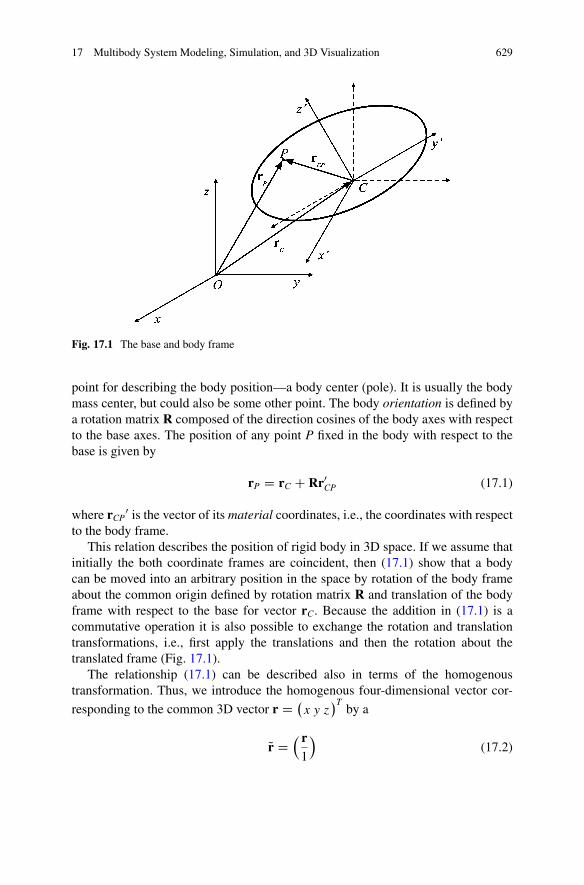
17 Multibody System Modeling, Simulation, and 3D Visualization 629
Fig. 17.1 The base and body frame
point for describing the body position—a body center (pole). It is usually the bodymass center, but could also be some other point. The body orientation is defined bya rotation matrix R composed of the direction cosines of the body axes with respectto the base axes. The position of any point P fixed in the body with respect to thebase is given by
rP D rC C Rr0CP (17.1)
where rCP0 is the vector of its material coordinates, i.e., the coordinates with respect
to the body frame.This relation describes the position of rigid body in 3D space. If we assume that
initially the both coordinate frames are coincident, then (17.1) show that a bodycan be moved into an arbitrary position in the space by rotation of the body frameabout the common origin defined by rotation matrix R and translation of the bodyframe with respect to the base for vector rC. Because the addition in (17.1) is acommutative operation it is also possible to exchange the rotation and translationtransformations, i.e., first apply the translations and then the rotation about thetranslated frame (Fig. 17.1).
The relationship (17.1) can be described also in terms of the homogenoustransformation. Thus, we introduce the homogenous four-dimensional vector cor-
responding to the common 3D vector r D �x y z
�Tby a
Qr D r1
(17.2)

630 V. Damic and M. Cohodar
The fourth component is a scale factor assumed here to be 1. We may introduce amatrix of homogenous transform defined by
T D
R rC
0T 1
!(17.3)
Now (17.1) can be written compactly as
QrP D TQrCP (17.4)
The homogenous transformations of position vectors are often used whendealing with geometric representation of body motion in 3D space (visualization).In dynamics we are more interested in the velocities.
During the motion, the positions of the body center rC and its orientation—represented by matrix R—change with time. The material coordinates of a pointfixed in the body do not change. The velocity of a point P, as seen from the baseframe, can be found by differentiating (17.1) with respect to time, i.e.,
vP D vC C dRdt
r0CP (17.5)
The relative position of a point P with respect to the base frame can be found bymultiplying its body frame coordinates by the rotation matrix R,
rCP D Rr0CP (17.6)
Note that the rotation matrix is an orthogonal matrix, i.e., RTR D RRT D I,where subscript T denotes the transposition operator and I is the identity matrix.Substituting (17.6) into (17.5) yields
vP D vC C dRdt
RTrCP (17.7)
In analogy with vector product notation we may introduce the symbol (Borriet al. [1])
¨� D dRdt
RT (17.8)
Thus, (17.7) can be written as
vP D vC C ¨ � rCP (17.9)
This reminds us of common vector product operation between the vectors. The¨ is really a vector, as can be easily shown.
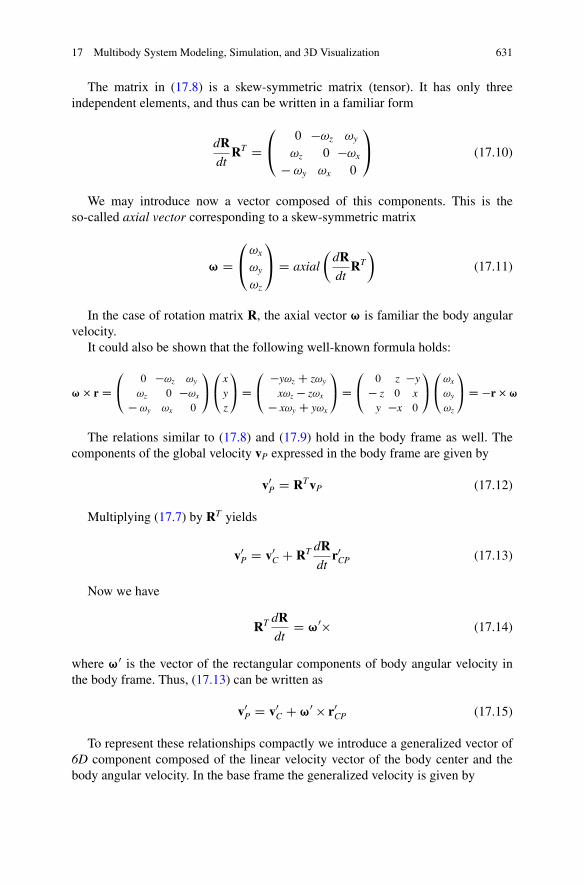
17 Multibody System Modeling, Simulation, and 3D Visualization 631
The matrix in (17.8) is a skew-symmetric matrix (tensor). It has only threeindependent elements, and thus can be written in a familiar form
dRdt
RT D0
@0 �!z !y
!z 0 �!x
� !y !x 0
1
A (17.10)
We may introduce now a vector composed of this components. This is theso-called axial vector corresponding to a skew-symmetric matrix
¨ D0
@!x
!y
!z
1
A D axial
�dRdt
RT
�(17.11)
In the case of rotation matrix R, the axial vector ¨ is familiar the body angularvelocity.
It could also be shown that the following well-known formula holds:
¨� r D0
@0 �!z !y
!z 0 �!x
� !y !x 0
1
A
0
@xyz
1
A D0
@�y!z C z!y
x!z � z!x
� x!y C y!x
1
A D0
@0 z �y� z 0 x
y �x 0
1
A
0
@!x
!y
!z
1
A D �r�¨
The relations similar to (17.8) and (17.9) hold in the body frame as well. Thecomponents of the global velocity vP expressed in the body frame are given by
v0P D RTvP (17.12)
Multiplying (17.7) by RT yields
v0P D v0C C RT dRdt
r0CP (17.13)
Now we have
RT dRdt
D ¨0� (17.14)
where ¨0 is the vector of the rectangular components of body angular velocity inthe body frame. Thus, (17.13) can be written as
v0P D v0C C ¨0 � r0CP (17.15)
To represent these relationships compactly we introduce a generalized vector of6D component composed of the linear velocity vector of the body center and thebody angular velocity. In the base frame the generalized velocity is given by

632 V. Damic and M. Cohodar
fC D�
vC
¨
�(17.16)
and similarly in the body frame as
f0C D�
v0C¨0�
(17.17)
These quantities are denoted by f because, as will be shown later, these are simplythe flows of the bond graph component ports.
In a similar way, a generalized velocity of any other point P fixed in the body canbe represented in the base frame by
fP D�
vP
¨
�(17.18)
and in the body frame as
f0P D�
v0P¨0�
(17.19)
Note that the following holds:
R�¨0 � r0CP
� D ¨ � rCP D �rCP � ¨ D .�rCP � R/¨0
Using (17.15) the corresponding transformation of flows between the body andbase frames can be written compactly as
fP D�
R �rCP � R0 R
�f0C (17.20)
The matrix
C D�
R �rCP � R0 R
�(17.21)
can be termed a representation of the body frame configuration tensor [13]. Hence,(17.20) can be written as
fP D Cf0C (17.22)
The similar relationships hold in the body frame
f0P D C0fC (17.23)
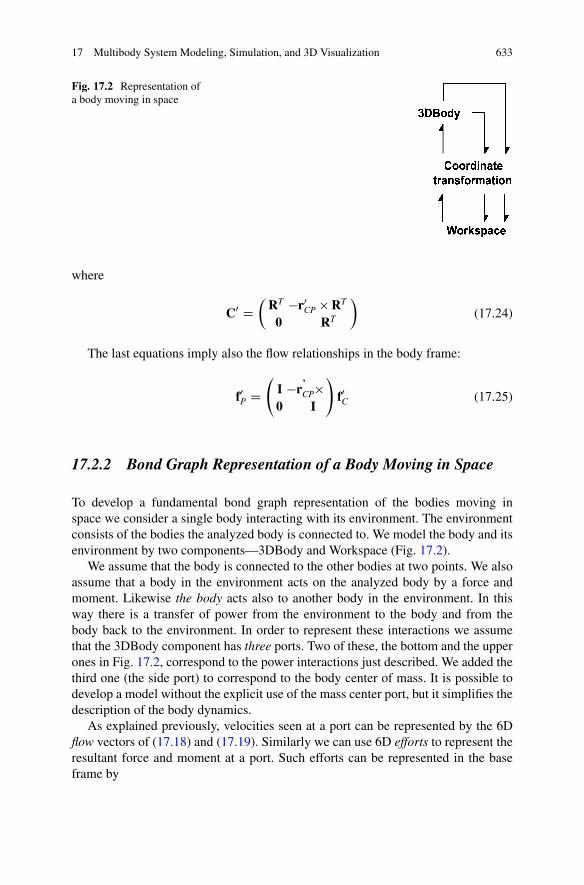
17 Multibody System Modeling, Simulation, and 3D Visualization 633
Fig. 17.2 Representation ofa body moving in space
where
C0 D�
RT �r0CP � RT
0 RT
�(17.24)
The last equations imply also the flow relationships in the body frame:
f0P D
I �r’CP�
0 I
!f0C (17.25)
17.2.2 Bond Graph Representation of a Body Moving in Space
To develop a fundamental bond graph representation of the bodies moving inspace we consider a single body interacting with its environment. The environmentconsists of the bodies the analyzed body is connected to. We model the body and itsenvironment by two components—3DBody and Workspace (Fig. 17.2).
We assume that the body is connected to the other bodies at two points. We alsoassume that a body in the environment acts on the analyzed body by a force andmoment. Likewise the body acts also to another body in the environment. In thisway there is a transfer of power from the environment to the body and from thebody back to the environment. In order to represent these interactions we assumethat the 3DBody component has three ports. Two of these, the bottom and the upperones in Fig. 17.2, correspond to the power interactions just described. We added thethird one (the side port) to correspond to the body center of mass. It is possible todevelop a model without the explicit use of the mass center port, but it simplifies thedescription of the body dynamics.
As explained previously, velocities seen at a port can be represented by the 6Dflow vectors of (17.18) and (17.19). Similarly we can use 6D efforts to represent theresultant force and moment at a port. Such efforts can be represented in the baseframe by
634 V. Damic and M. Cohodar
eP D�
FP
MP
�(17.26)
and, similarly, in the body frame as
e0P D�
F0PM0P
�(17.27)
Here FP and F0
P are 3D representations of the resultant force at connection point Pand MP and M
0
P of the resultant moment.To represent these 6D vector quantities, the ports of the 3DBody and Workspace
components are assumed to consist of two subports. The first one corresponds tothe linear velocity and resultant force, and the other to the body angular velocityand resultant moment. This way the ports can be used to access efforts and flowsat the port by two ordered 6D efforts and flows. At the mass center port, however,as will be seen later, a 3D representation is sufficient. The flow is the mass centervelocity and the effort is the resultant of the forces acting on the body at other ports(interconnection points) and reduced to the mass center. The gravity force (the bodyweight) acting there is not accounted for and is taken into account when dealingwith the body translation dynamics. The reason for this is that body weight can beeasily described in the base frame. However, this is not so in a body frame, becauseit is generally rotated with respect to the first.
We represent effort and flow vectors at body ports as seen in the body, i.e., withrespect to a body fixed frame. Similarly at the workspace ports the correspondingquantities are expressed with respect to the base frame. Transformations betweenthese two representations are given in Fig. 17.2 by the coordinate transformationcomponent. This component transforms effort and flow at a body port to the cor-responding base frame representation and vice versa. The transformation betweenefforts is given by
eP D�
R 00 R
�e0P (17.28)
and similarly for the flows,
fP D�
R 00 R
�f0P (17.29)
where R is the rotation matrix of the body frame with respect to the base.We use Cartesian 3D frames only and, thus, the transformation matrix is
orthogonal. It can be easily shown that the following relationship holds:
f0TPe0P D fTPeP (17.30)
and thus the transformation does not change the power transfer.

17 Multibody System Modeling, Simulation, and 3D Visualization 635
Fig. 17.3 6D transformation: (a) The component representation, (b) The structure
The transformation of the port quantities can be represented by the 6D transformcomponent of Fig. 17.3a. This component transforms the effort-flow pairs of thecorresponding ports, according to (17.28) and (17.29), as shown in Fig. 17.3b.The transformations are represented by the Rot components that describe thetransformation of 3D effort and flow vectors by the rotation matrix R. Thetransformation can be represented using transformer elements TF.
The velocities at a port are related to the velocity of the body mass center by(17.23) and (17.24). To find the relation between forces and moments, we evaluatethe power transfer between the ports. We obtain the following relation:
v0TPF0P C ¨0TM0P D v0TCF0P C ¨0T�r0CP � F0P C M0P
�(17.31)
The last equation, jointly with (17.25), describes the basic velocity and forcerelationships for the rigid bodies. The structure of the 3D Body componentfollowing these relationships is given in Fig. 17.4.
Component 1 is an array of the effort junctions corresponding to the centerof mass velocity. The component Rotation defines the body rotational dynamicdiscussed later. The components 0 represent the array of flow junctions that describethe port velocities relationship given by the first 3D row of (17.25). It gives the linearvelocity at a port as the sum of the velocity of the body mass center and the relativevelocity due to the rotation of the body about the mass center. The joint variable isthe force at the port. The body angular velocity, however, is a property of the bodyand it is directly transferred to the Rotation component.
The LinRot components represent transformations between linear and angularquantities. These transformations are defined by the skew-symmetric tensor opera-tions in (17.25) and (17.31) and can be represented by transformers, as in Fig. 17.5.
Every transformer in Fig. 17.5 corresponds to a nonzero entry of tensor �rCP0�
or its transpose. The flow junctions on the left evaluate the relative velocities atthe left port and the effort junctions on the right give the moment at the right

636 V. Damic and M. Cohodar
Fig. 17.4 The model of 3D body motion
Fig. 17.5 The representation of LinRot transformation
port. The ratios of the transformers are the material coordinates of a body pointcorresponding to the port with respect to the mass center. Thus, they are parametersthat depend on the geometry of the rigid body and don’t change with its motion.
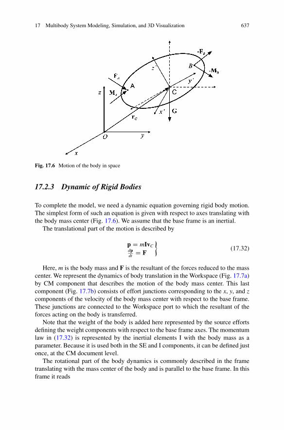
17 Multibody System Modeling, Simulation, and 3D Visualization 637
Fig. 17.6 Motion of the body in space
17.2.3 Dynamic of Rigid Bodies
To complete the model, we need a dynamic equation governing rigid body motion.The simplest form of such an equation is given with respect to axes translating withthe body mass center (Fig. 17.6). We assume that the base frame is an inertial.
The translational part of the motion is described by
p D mIvCdpdt D F
�(17.32)
Here, m is the body mass and F is the resultant of the forces reduced to the masscenter. We represent the dynamics of body translation in the Workspace (Fig. 17.7a)by CM component that describes the motion of the body mass center. This lastcomponent (Fig. 17.7b) consists of effort junctions corresponding to the x, y, and zcomponents of the velocity of the body mass center with respect to the base frame.These junctions are connected to the Workspace port to which the resultant of theforces acting on the body is transferred.
Note that the weight of the body is added here represented by the source effortsdefining the weight components with respect to the base frame axes. The momentumlaw in (17.32) is represented by the inertial elements I with the body mass as aparameter. Because it is used both in the SE and I components, it can be defined justonce, at the CM document level.
The rotational part of the body dynamics is commonly described in the frametranslating with the mass center of the body and is parallel to the base frame. In thisframe it reads
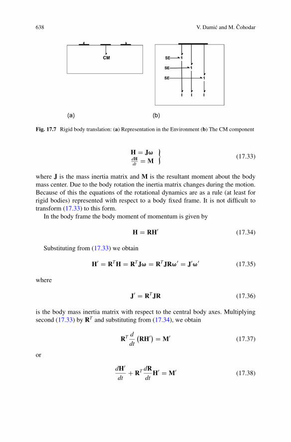
638 V. Damic and M. Cohodar
Fig. 17.7 Rigid body translation: (a) Representation in the Environment (b) The CM component
H D J¨dHdt D M
�(17.33)
where J is the mass inertia matrix and M is the resultant moment about the bodymass center. Due to the body rotation the inertia matrix changes during the motion.Because of this the equations of the rotational dynamics are as a rule (at least forrigid bodies) represented with respect to a body fixed frame. It is not difficult totransform (17.33) to this form.
In the body frame the body moment of momentum is given by
H D RH0 (17.34)
Substituting from (17.33) we obtain
H0 D RTH D RTJ¨ D RTJR¨0 D J0¨0 (17.35)
where
J0 D RTJR (17.36)
is the body mass inertia matrix with respect to the central body axes. Multiplyingsecond (17.33) by RT and substituting from (17.34), we obtain
RT d
dt
�RH0
� D M0 (17.37)
or
dH0
dtC RT dR
dtH0 D M0 (17.38)
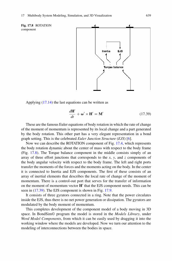
17 Multibody System Modeling, Simulation, and 3D Visualization 639
Fig. 17.8 ROTATIONcomponent
Applying (17.14) the last equations can be written as
dH0
dtC ¨0 � H0 D M0 (17.39)
These are the famous Euler equations of body rotation in which the rate of changeof the moment of momentum is represented by its local change and a part generatedby the body rotation. This other part has a very elegant representation in a bondgraph setting. This is the celebrated Euler Junction Structure (EJS) [6].
Now we can describe the ROTATION component of Fig. 17.4, which representsthe body rotation dynamic about the center of mass with respect to the body frame(Fig. 17.8). The Torque balance component in the middle consists simply of anarray of three effort junctions that corresponds to the x, y, and z components ofthe body angular velocity with respect to the body frame. The left and right portstransfer the moments of the forces and the moments acting on the body. In the centerit is connected to Inertia and EJS components. The first of these consists of anarray of inertial elements that describes the local rate of change of the moment ofmomentum. There is a control-out port that serves for the transfer of informationon the moment of momentum vector H0 that the EJS component needs. This can beseen in (17.39). The EJS component is shown in Fig. 17.9.
It consists of three gyrators connected in a ring. Note that the power circulatesinside the EJS, thus there is no net power generation or dissipation. The gyrators aremodulated by the body moment of momentum.
This completes development of the component model of a body moving in 3Dspace. In BondSim© program the model is stored in the Models Library, underWord Model Components, from which it can be easily used by dragging it into theworking window where the models are developed. Now we turn our attention to themodeling of interconnections between the bodies in space.
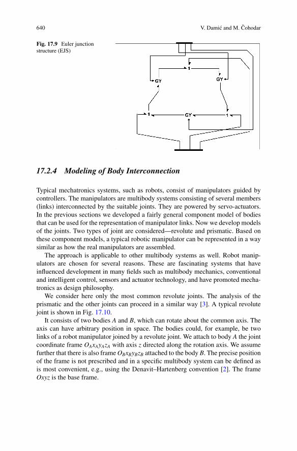
640 V. Damic and M. Cohodar
Fig. 17.9 Euler junctionstructure (EJS)
17.2.4 Modeling of Body Interconnection
Typical mechatronics systems, such as robots, consist of manipulators guided bycontrollers. The manipulators are multibody systems consisting of several members(links) interconnected by the suitable joints. They are powered by servo-actuators.In the previous sections we developed a fairly general component model of bodiesthat can be used for the representation of manipulator links. Now we develop modelsof the joints. Two types of joint are considered—revolute and prismatic. Based onthese component models, a typical robotic manipulator can be represented in a waysimilar as how the real manipulators are assembled.
The approach is applicable to other multibody systems as well. Robot manip-ulators are chosen for several reasons. These are fascinating systems that haveinfluenced development in many fields such as multibody mechanics, conventionaland intelligent control, sensors and actuator technology, and have promoted mecha-tronics as design philosophy.
We consider here only the most common revolute joints. The analysis of theprismatic and the other joints can proceed in a similar way [3]. A typical revolutejoint is shown in Fig. 17.10.
It consists of two bodies A and B, which can rotate about the common axis. Theaxis can have arbitrary position in space. The bodies could, for example, be twolinks of a robot manipulator joined by a revolute joint. We attach to body A the jointcoordinate frame OAxAyAzA with axis z directed along the rotation axis. We assumefurther that there is also frame OBxByBzB attached to the body B. The precise positionof the frame is not prescribed and in a specific multibody system can be defined asis most convenient, e.g., using the Denavit–Hartenberg convention [2]. The frameOxyz is the base frame.

17 Multibody System Modeling, Simulation, and 3D Visualization 641
Fig. 17.10 Revolute joint inspace
Let P be the center point of the revolute joint used as the reference connectionpoint. The joint can be represented as a word model component with two portscorresponding to body A and B. We consider flows and efforts at these portsexpressed in their respective body frames. At A (the power-in) these are
fAP D
�vA
P
¨AA
�(17.40)
and
eAP D
�FA
P
MAP
�(17.41)
Similarly at B (the power-out) we have
fBP D
�vB
P
¨BB
�(17.42)
and
eBP D
�FB
P
MBP
�(17.43)
The linear velocities of bodies A and B at the connection point are common toboth of the bodies. Hence
vAP D RA
BvBP (17.44)
where RAB is the rotation matrix of the body B frame with respect to the body A
frame.
642 V. Damic and M. Cohodar
A similar relation holds for the forces. The linear velocities at the common pointare equal, and the same is true for the power transferred across the joint during itstranslation, i.e.,
�vA
P
�TFA
P D �vB
P
�TFB
P (17.45)
Substituting from (17.44) yields
FBP D RB
AFAP (17.46)
Equations (17.44) and (17.46) describe the relationships between the linear partsof the flow-effort 3D vectors at the joint’s ports. We develop next the relationshipsbetween the angular parts, i.e., the angular velocities and moments.
The rotation matrices of the bodies A and B frames with respect to the base frameare related by composition of the rotations, i.e.,
RB D RARAB (17.47)
Differentiating it with respect to time we get
dRB
dtD dRA
dtRA
B C RAdRA
B
dt(17.48)
From (17.8) and (17.14) we obtain
¨B � RB D RA¨AA � RA
B C RA¨AAB � RA
B (17.49)
where
¨AAB D axial
�dRA
B
dtRB
A
�(17.50)
is the relative angular velocity of body B with respect to body A expressed in bodyA frame. Simplifying (17.49) we get
.RA/T¨B � RA D ¨A
A � C¨AAB� (17.51)
Note that relative velocity of a point in body B with respect to the reference pointP due to rotation of body B expressed in global frame is given by
vPB D ¨B � rPB
The same velocity expressed in the body frame A defined by rotation matrix RA
can be found as
vAPB D .RA/
TvPB D .RA/T¨B � RA.RA/
TrPB D .RA/T¨B � RArA
PB
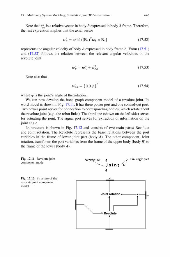
17 Multibody System Modeling, Simulation, and 3D Visualization 643
Note that rAPB
is a relative vector in body B expressed in body A frame. Therefore,the last expression implies that the axial vector
¨AB D axial
�.RA/
T¨B � RA�
(17.52)
represents the angular velocity of body B expressed in body frame A. From (17.51)and (17.52) follows the relation between the relevant angular velocities of therevolute joint
¨AB D ¨A
A C ¨AAB (17.53)
Note also that
¨AAB D �
0 0:'�T
(17.54)
where ® is the joint’s angle of the rotation.We can now develop the bond graph component model of a revolute joint. Its
word model is shown in Fig. 17.11. It has three power port and one control-out port.Two power point serves for connection to corresponding bodies, which rotate aboutthe revolute joint (e.g., the robot links). The third one (shown on the left side) servesfor actuating the joint. The signal port serves for extraction of information on thejoint angle.
Its structure is shown in Fig. 17.12 and consists of two main parts: Revoluteand Joint rotation. The Revolute represents the basic relations between the portvariables in the frame of lower joint part (body A). The other component, Jointrotation, transforms the port variables from the frame of the upper body (body B) tothe frame of the lower (body A).
Fig. 17.11 Revolute jointcomponent model
Fig. 17.12 Structure of therevolute joint componentmodel

644 V. Damic and M. Cohodar
Fig. 17.13 The structure of: Revolute component, Rot subcomponent
The structure of the Revolute component is shown in Fig. 17.13 on the left. Itconsists of two components. The Tr component represents the translational part ofthe joint model and expresses the fact that the joint center point is common to theboth bodies. Thus it consists solely of three effort junctions for the translation in thedirection of xA, yA, and zA axes. This ensures that the joined ends of the bodies movewith the common velocity and that the corresponding forces are equal.
The other component, Rot, whose structure is shown in Fig. 17.13 on the right,represents the relationship between the angular velocities as given by (17.53) and(17.54). The model is very simple and consists of two effort junctions in the xA- andyA-directions in which the angular components are the same for both of the joinedbodies. There is also a flow junction that corresponds to the relative rotation aboutthe zA-axis. The 1-junction on the left in Fig. 17.13 is inserted to extract the jointrelative angular velocity and to obtain the joint rotation angle by integration. It isnot only used in the Joint rotation component, but is also transmitted to the outputport (Fig. 17.12).
An important function of the joint is the rotation transformation between thetwo link frames (Fig. 17.12). This is depicted in Fig. 17.14. The transformationsare applied to the linear effort-flow parts, and separately to the angular. These arerepresented by components RAB. The components represent transformations, asgiven by (17.44) and (17.46) for linear variables. The same transformations hold forthe angular variables.
We do not give here the general structure of the component because it dependson the structure of the kinematic links, which it is a part. Revolute joints play animportant role in the design of robotic manipulators. They offer the simplest wayto change the orientation of the robot links. The component model introduced heregives the main functionality of such joints. They are used later for the building ofmanipulator models.

17 Multibody System Modeling, Simulation, and 3D Visualization 645
Fig. 17.14 Rotationaltransformations by the joint
17.3 Dynamics of an Anthropomorphic Robot Manipulator
In this section we apply modeling approach developed in the previous sections tomodeling the dynamics of anthropomorphic robot manipulators. Many industrialmanipulators are of this type. The first robot with anthropomorphic configurationwas famous PUMA 560 released in 1978. As an example of such robots ABBIRB 1600 was chosen [5]. We concentrated on manipulator in open loop to showtypical dynamic behavior of the robot. The closed model can be easily developed ina similar way as in Damic and Montgomery [3] for PUMA.
17.3.1 Kinematics Structure of ABB IRB 1600
The IRB 1600 is a six degree of freedom manipulator using revolute joints only. Therobot coordinate frames are shown in Fig. 17.15. The links body frames are attachedto the corresponding joint with one of the axes directed along the joint rotation axis.However, it is not required to choose for it the Z-axes, as in Denavit–Hartenbergscheme [9, 13].
The joints and frames are numbered from the base to the robot tip. They aregenerated simply by translations from base X0Y0Z0. Thus, the first link frame X1Y1Z1
in the zero angle pose coincides with the base frame. The second frame can beobtained from the first by translation along X-axis for L2 and along Z-axis for L1.Similarly hold for the third and the fourth joint frame. The rotation axes of the lastthree joints intersect in the common point and are orthogonal. Therefore, the lastthree frames coincide in the zero angle pose. As is well known in anthropomorphicrobot configurations the human-like terms are used for joints and robot links, i.e.,body, upper- and fore-arms, the shoulder, elbow, and wrist.
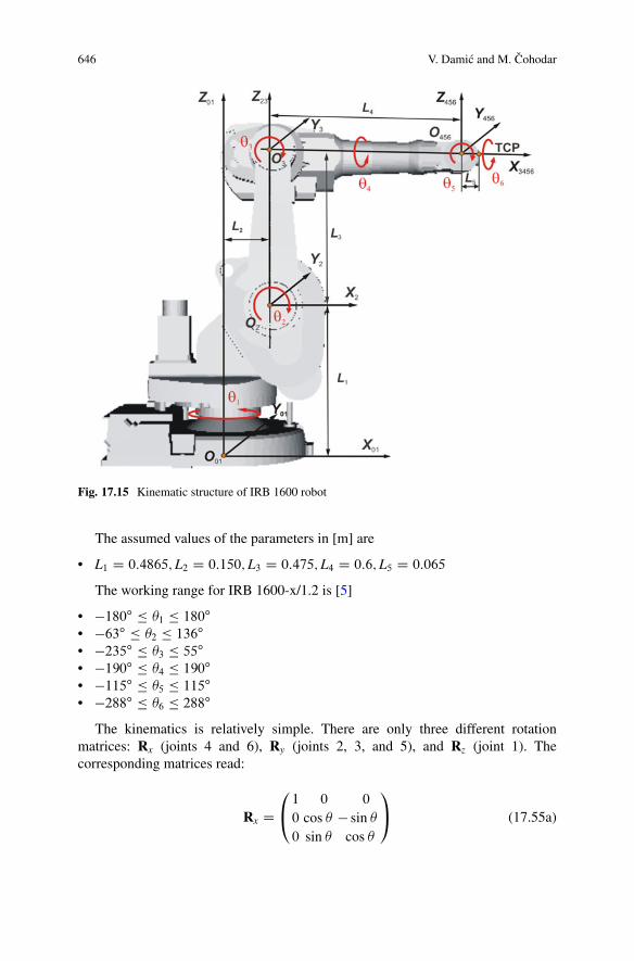
646 V. Damic and M. Cohodar
Fig. 17.15 Kinematic structure of IRB 1600 robot
The assumed values of the parameters in [m] are
• L1 D 0:4865;L2 D 0:150;L3 D 0:475;L4 D 0:6;L5 D 0:065
The working range for IRB 1600-x/1.2 is [5]
• �180ı � �1 � 180ı• �63ı � �2 � 136ı• �235ı � �3 � 55ı• �190ı � �4 � 190ı• �115ı � �5 � 115ı• �288ı � �6 � 288ı
The kinematics is relatively simple. There are only three different rotationmatrices: Rx (joints 4 and 6), Ry (joints 2, 3, and 5), and Rz (joint 1). Thecorresponding matrices read:
Rx D0
@1 0 0
0 cos � � sin �0 sin � cos �
1
A (17.55a)
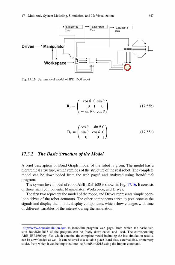
17 Multibody System Modeling, Simulation, and 3D Visualization 647
Fig. 17.16 System level model of IRB 1600 robot
Ry D0
@cos � 0 sin �0 1 0
� sin � 0 cos �
1
A (17.55b)
Rz D0
@cos � � sin � 0sin � cos � 0
0 0 1
1
A (17.55c)
17.3.2 The Basic Structure of the Model
A brief description of Bond Graph model of the robot is given. The model has ahierarchical structure, which reminds of the structure of the real robot. The completemodel can be downloaded from the web page1 and analyzed using BondSim©program.
The system level model of robot ABB IRB1600 is shown in Fig. 17.16. It consistsof three main components: Manipulator, Workspace, and Drives.
The first two represent the model of the robot, and Drives represents simple open-loop drives of the robot actuators. The other components serve to post-process thesignals and display them in the display components, which show changes with timeof different variables of the interest during the simulation.
1http://www.bondsimulation.com is BondSim program web page, from which the basic ver-sion BondSim2015 of the program can be freely downloaded and used. The correspondingABB_IRB1600.ept file, which contains the complete model including the last simulation results,can be downloaded as well. It can be saved to a suitable place (hard disk, external disk, or memorystick), from which it can be imported into the BondSim2015 using the Import command.

648 V. Damic and M. Cohodar
Fig. 17.17 The structure ofthe manipulator model
A special role in this model plays the component in the form of a ring (pipe).It is a component which enables inter-process communication between the robotdynamical model (within BondSim© program) and 3D geometric (visual) model ofthe same robot (within the corresponding BondSimVisual© application). It is reallythe client side of the communication (named) pipe. We will come to this topic later.
Model of the manipulator is shown in Fig. 17.17. It consists of Arm and Wristcomponents. On the left are two bonds, which deliver power to the arm and wristactuators from the left multi-port connector. Similarly the connector on the rightpicks and further distributes the joint angles and angular velocities from thesecomponents.
The arm and wrist are interconnected by bond lines. It is assumed that powerflows from the Workspace (Fig. 17.16) over Arm to Wrist. The wrist with a tool actsto the workspace. Therefore it delivers power to the workspace. However, the wristand arm “feel” these interactions, and there is transfer of power from the Wrist (andtool) over Arm to Workspace. Thus, the model structure in Fig. 17.16 depicts whatreally happens in the robot and thus represents a pretty close physical model of it.
The models of Arm and Wrist are shown in Fig. 17.18. The Link 1 models therobot body, which can rotate about vertical the robot base axis (Fig. 17.15). Joint 2is the shoulder, about which the upper arm (Link 2) can rotate. This arm is furtherconnected by the elbow (Joint 3) to the forearm (Link 3), which carries the wrist.The wrist (Fig. 17.18 on right) represents a spherical joint (see [3] for details). Itconsists of Joint 4–6, and Link 4–6 that house the actuators driving the joints.
Consider the bonds connecting the Joints and Links. The left ones we alreadyhave discussed. More interesting are bonds going down from the last Link 6 to thebase. We remind of the modeling approach we discussed in Sect. 17.2.2, Fig. 17.2.We use three-port component models to represent space body models. Thus, the

17 Multibody System Modeling, Simulation, and 3D Visualization 649
Fig. 17.18 Models of Arm (left) and Wrist (right)
bond coming out of the upper port of Link 6 transfers 3D efforts and flows of therobot wrist (holding a tool) action to the workspace. In addition at it’s center of massthere are the resultant force and its velocity. All these quantities are described in thebody (Joint 6) frame. There are different for an observer in the base. However, wedo not know exact position and orientation of this frame in the base, and thus cannottransform them directly. Instead, we systematically transform these quantities fromthe joint to joint until the base. The same holds for the other links as well, only thatthere are smaller number of the quantities to transform as we approach the base.
Note how the bonds are gradually built. It is important because we needto unpack them later. At every joint to the already transformed quantities weadd the corresponding link center of mass quantities and transform these newquantities further. This looks somewhat complicated, but if we apply this approachsystematically there should be no problem. The similar effects appear in the reality.When we hold a heavy load in our hand, we feel it at every body parts to the foot.
To see these transformations in more detail we open, e.g., Joint 2 component(e.g., by double clicking). The model of Joint 2 on the left is similar to that of

650 V. Damic and M. Cohodar
Fig. 17.19 Structure of Joint 2 model component
Fig. 17.20 Component R21:rotation about Y-axis
Fig. 17.12. There are, however, the additional two top right ports, which transferthe Link 2 center of mass quantities and the quantities from the previous joint,respectively (Fig. 17.18).
The Revolute component, which model the revolute joint, was already discussedin Sect. 17.2.4, Fig. 17.13. The Joint rotation model component is shown inFig. 17.19 on the right. The R21 component describes the transformation cor-responding to rotation about axis Y through the joint angle �2, Fig. 17.15. Thetransformations are governed by matrix (17.55b) and are shown in Fig. 17.20.
We direct at the end our attention to Workspace component in Fig. 17.16. Themodel is shown in Fig. 17.21 left. We may first observe Robot base component. It isa simple component consisting of six source flows, which fix the base to the groundin its initial position, i.e., they imply zero linear and angular velocities of the base.

17 Multibody System Modeling, Simulation, and 3D Visualization 651
Fig. 17.21 The structure of model of the Workspace
The next component CM1 describes the dynamics of the Link1 center of mass.We have discussed it earlier in Sect. 17.2.3 (see Fig. 17.7). To establish the correctconnection to the manipulator (Fig. 17.18) we add also a component called OtherPart 6, indicating that it must contains six other components—the dynamic ofcenters of masses of other five links, and the robot wrist end component representingthe TCP (the tool center point). The structure of the last component Other Part 2 isshown in Fig. 17.21 right. It contains CM6 component describing the dynamicsof the center of the mass of the last link and the TCP component. The lastcomponent consists simply of three 1-junctions connected to the components port.They represent the nodes of TCP velocity components in the basic frame. Free Endcomponent defines the conditions at the robot end. It could be simply zero sourceefforts if the robot end moves freely in the environment. The bond at the right ofTIP extracts its velocity. These signals go out from Other Part 6 in the Fig. 17.21left and are integrated to obtain information on TCP position in the base frame.
One of the strong points in dealing with multibody dynamics as describedabove is a systematical use of compounded ports, i.e., the ports that consistof other subports, these of the others, and so on to the arbitrary depth. Thisenables representing of the complex interaction appearing in the devices of such acomplexity in a straight and readable manner. Otherwise we should deal with forestof the signals. Of course the corresponding mathematical models could be difficultor even impossible to obtain by hand. BondSim© model build algorithm knows howto do it automatically without intervention of the modeler.
17.3.3 Simulation of the Robot Motion
We will now conduct the simulation of developed model of ABB IRB 1600 robot.We consider behavior of the robot in open loop. Thus, we will drive robot by thesource flows, which generates the angular velocities of the joins defined by simplesinusoidal laws
!i D ˛i!0 cos .!0t/ ; .i D 1; : : : ; 6/ (17.56)
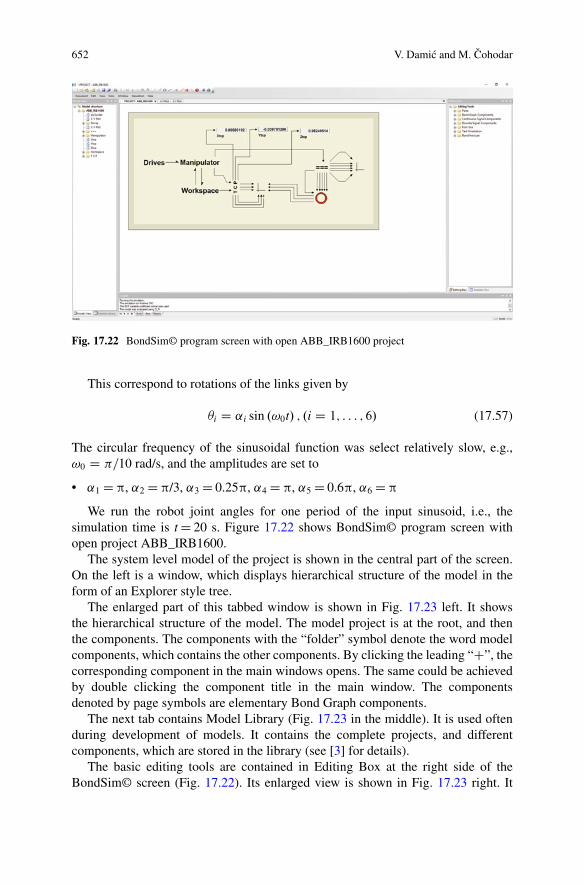
652 V. Damic and M. Cohodar
Fig. 17.22 BondSim© program screen with open ABB_IRB1600 project
This correspond to rotations of the links given by
�i D ˛i sin .!0t/ ; .i D 1; : : : ; 6/ (17.57)
The circular frequency of the sinusoidal function was select relatively slow, e.g.,!0 D �=10 rad/s, and the amplitudes are set to
• ˛1 D , ˛2 D /3, ˛3 D 0.25 , ˛4 D , ˛5 D 0.6 , ˛6 D
We run the robot joint angles for one period of the input sinusoid, i.e., thesimulation time is t D 20 s. Figure 17.22 shows BondSim© program screen withopen project ABB_IRB1600.
The system level model of the project is shown in the central part of the screen.On the left is a window, which displays hierarchical structure of the model in theform of an Explorer style tree.
The enlarged part of this tabbed window is shown in Fig. 17.23 left. It showsthe hierarchical structure of the model. The model project is at the root, and thenthe components. The components with the “folder” symbol denote the word modelcomponents, which contains the other components. By clicking the leading “C”, thecorresponding component in the main windows opens. The same could be achievedby double clicking the component title in the main window. The componentsdenoted by page symbols are elementary Bond Graph components.
The next tab contains Model Library (Fig. 17.23 in the middle). It is used oftenduring development of models. It contains the complete projects, and differentcomponents, which are stored in the library (see [3] for details).
The basic editing tools are contained in Editing Box at the right side of theBondSim© screen (Fig. 17.22). Its enlarged view is shown in Fig. 17.23 right. It

17 Multibody System Modeling, Simulation, and 3D Visualization 653
Fig. 17.23 Enlarged parts of the BondSim© screen
contains several tools for developing Bond Graphs, including the continuous anddiscrete time block diagrams. The development of the models is basically conductedby dragging the tools from Editing box and dropping them into the main windows(refer to [3] for details).
Before starting simulation we need to build the mathematical model of thesystem. This can be done by opening Simulation menu, and choosing Build com-mand. The system starts reading all components the system consists of, checks theconnections, generates the internal variables, and finally generates the mathematicalmodel. The model is generated in symbolic form, which can be recompiled into ahuman readable form for inspection. We will not go in details here. Interested readercan consult [3] for details.
The current model consists of 959 implicit equations, and symbolically generatedJacobian matrix contains 2637 elements. Thus, it is very sparse, with on average lessthan 3 elements per row.
To start simulation, chose Simulation command Run. In the dialog that opens setthe simulation interval to 20 s, the output interval, and maximum step size to 0.05 s.(The output delay interval is not important now.) For all other simulation parametersaccept the default values (the method and error tolerances). Click Restart (if it is notalready set) and select OK. Now simulation starts. System generates the messagesin Output window at the bottom, which inform the user on simulation advance.
During a simulation run the model is repeatedly solved using a BackwardDifferentiation Formula (BDF) type solver. The solver successfully solved themodel as the simulation statistics in Table 17.1 shows.
Figure 17.24 shows the motion of the TCP during the simulation, and Fig. 17.25shows how changes the absolute error in TCP position.
These errors were calculated by comparing the values generating by the simu-lations and values calculated by the direct kinematics in component TCP. Diagramshows that these errors are of order of the simulation error tolerances in Table 17.1.Thus, the accuracy of the simulation is good.
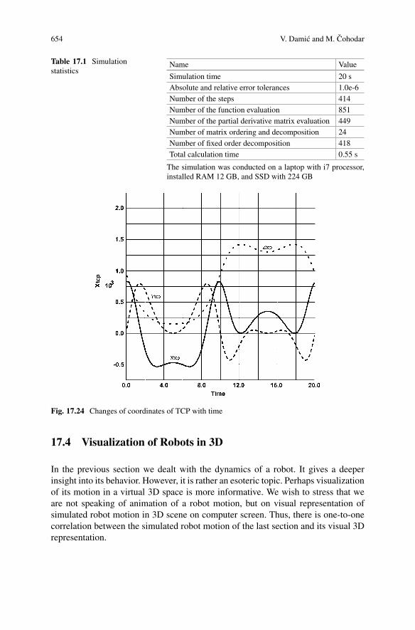
654 V. Damic and M. Cohodar
Table 17.1 Simulationstatistics
Name Value
Simulation time 20 sAbsolute and relative error tolerances 1.0e-6Number of the steps 414Number of the function evaluation 851Number of the partial derivative matrix evaluation 449Number of matrix ordering and decomposition 24Number of fixed order decomposition 418Total calculation time 0.55 s
The simulation was conducted on a laptop with i7 processor,installed RAM 12 GB, and SSD with 224 GB
Fig. 17.24 Changes of coordinates of TCP with time
17.4 Visualization of Robots in 3D
In the previous section we dealt with the dynamics of a robot. It gives a deeperinsight into its behavior. However, it is rather an esoteric topic. Perhaps visualizationof its motion in a virtual 3D space is more informative. We wish to stress that weare not speaking of animation of a robot motion, but on visual representation ofsimulated robot motion in 3D scene on computer screen. Thus, there is one-to-onecorrelation between the simulated robot motion of the last section and its visual 3Drepresentation.
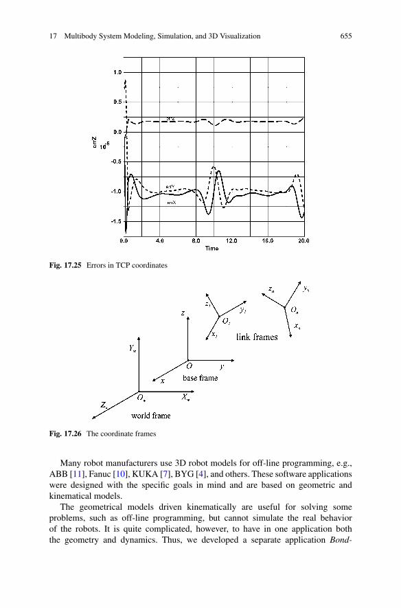
17 Multibody System Modeling, Simulation, and 3D Visualization 655
Fig. 17.25 Errors in TCP coordinates
Fig. 17.26 The coordinate frames
Many robot manufacturers use 3D robot models for off-line programming, e.g.,ABB [11], Fanuc [10], KUKA [7], BYG [4], and others. These software applicationswere designed with the specific goals in mind and are based on geometric andkinematical models.
The geometrical models driven kinematically are useful for solving someproblems, such as off-line programming, but cannot simulate the real behaviorof the robots. It is quite complicated, however, to have in one application boththe geometry and dynamics. Thus, we developed a separate application Bond-
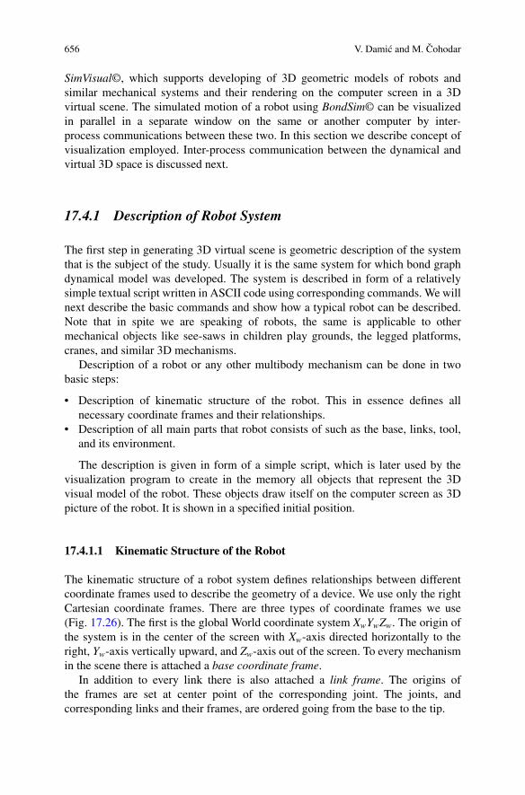
656 V. Damic and M. Cohodar
SimVisual©, which supports developing of 3D geometric models of robots andsimilar mechanical systems and their rendering on the computer screen in a 3Dvirtual scene. The simulated motion of a robot using BondSim© can be visualizedin parallel in a separate window on the same or another computer by inter-process communications between these two. In this section we describe concept ofvisualization employed. Inter-process communication between the dynamical andvirtual 3D space is discussed next.
17.4.1 Description of Robot System
The first step in generating 3D virtual scene is geometric description of the systemthat is the subject of the study. Usually it is the same system for which bond graphdynamical model was developed. The system is described in form of a relativelysimple textual script written in ASCII code using corresponding commands. We willnext describe the basic commands and show how a typical robot can be described.Note that in spite we are speaking of robots, the same is applicable to othermechanical objects like see-saws in children play grounds, the legged platforms,cranes, and similar 3D mechanisms.
Description of a robot or any other multibody mechanism can be done in twobasic steps:
• Description of kinematic structure of the robot. This in essence defines allnecessary coordinate frames and their relationships.
• Description of all main parts that robot consists of such as the base, links, tool,and its environment.
The description is given in form of a simple script, which is later used by thevisualization program to create in the memory all objects that represent the 3Dvisual model of the robot. These objects draw itself on the computer screen as 3Dpicture of the robot. It is shown in a specified initial position.
17.4.1.1 Kinematic Structure of the Robot
The kinematic structure of a robot system defines relationships between differentcoordinate frames used to describe the geometry of a device. We use only the rightCartesian coordinate frames. There are three types of coordinate frames we use(Fig. 17.26). The first is the global World coordinate system XwYwZw. The origin ofthe system is in the center of the screen with Xw-axis directed horizontally to theright, Yw-axis vertically upward, and Zw-axis out of the screen. To every mechanismin the scene there is attached a base coordinate frame.
In addition to every link there is also attached a link frame. The origins ofthe frames are set at center point of the corresponding joint. The joints, andcorresponding links and their frames, are ordered going from the base to the tip.
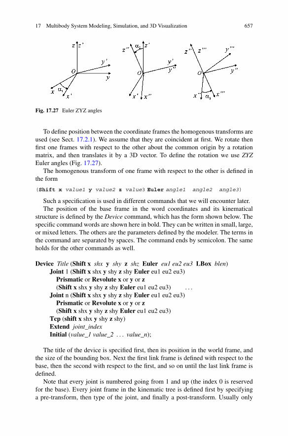
17 Multibody System Modeling, Simulation, and 3D Visualization 657
Fig. 17.27 Euler ZYZ angles
To define position between the coordinate frames the homogenous transforms areused (see Sect. 17.2.1). We assume that they are coincident at first. We rotate thenfirst one frames with respect to the other about the common origin by a rotationmatrix, and then translates it by a 3D vector. To define the rotation we use ZYZEuler angles (Fig. 17.27).
The homogenous transform of one frame with respect to the other is defined inthe form
(Shift x value1 y value2 z value3 Euler angle1 angle2 angle3)
Such a specification is used in different commands that we will encounter later.The position of the base frame in the word coordinates and its kinematical
structure is defined by the Device command, which has the form shown below. Thespecific command words are shown here in bold. They can be written in small, large,or mixed letters. The others are the parameters defined by the modeler. The terms inthe command are separated by spaces. The command ends by semicolon. The sameholds for the other commands as well.
Device Title (Shift x shx y shy z shz Euler eu1 eu2 eu3 LBox blen)Joint 1 (Shift x shx y shy z shy Euler eu1 eu2 eu3)
Prismatic or Revolute x or y or z(Shift x shx y shy z shy Euler eu1 eu2 eu3) : : :
Joint n (Shift x shx y shy z shy Euler eu1 eu2 eu3)Prismatic or Revolute x or y or z(Shift x shx y shy z shy Euler eu1 eu2 eu3)
Tcp (shift x shx y shy z shy)Extend joint_indexInitial (value_1 value_2 : : : value_n);
The title of the device is specified first, then its position in the world frame, andthe size of the bounding box. Next the first link frame is defined with respect to thebase, then the second with respect to the first, and so on until the last link frame isdefined.
Note that every joint is numbered going from 1 and up (the index 0 is reservedfor the base). Every joint frame in the kinematic tree is defined first by specifyinga pre-transform, then type of the joint, and finally a post-transform. Usually only

658 V. Damic and M. Cohodar
pre-transform is enough, but sometimes we need both pre- and post-transforms.It assumes that joints are simple revolute or prismatic. Its rotation or sliding axis isaligned with one of the link coordinate axes.
The Tcp command defines position of the tool central point. The mechanismsoften do not have the simple serial structure, but contains the parallelograms, ormore than one arm. In that case subcommand Extend defines the index of the jointor base where the branching starts.
Finally there are subcommands that define the initial values of the joint variable(angle or displacement). The command defines only the initial position of themechanism. It could be moved manually by a menu command or dynamically byanother application (BondSim©).
17.4.1.2 Geometric Representation of the Robot Parts
The geometric model of the device base or its links can be constructed in twoways—using the primitive forms or 3D CAD generated part files. The predefinedprimitive forms are shown in Fig. 17.28. To define the mechanism structure we usedthe corresponding commands, which are based on corresponding VTK classes [12].
Cylinder
It serves to create a simple body in form of a cylinder (Fig. 17.28a). Its longitudinalaxis is aligned with z axis. The parameters of the command are the dia[meter] of
Fig. 17.28 Primitive forms: (a) Cylinder, (b) Cone, (c) Cube, (d) Sphere, (e) Polyprism, and (f)Module

17 Multibody System Modeling, Simulation, and 3D Visualization 659
its base and its len[gth] (height) in millimeters. The cylinder bases are generatedas regular polygons. The parameter res[olution] defines the number of divisions ofthe base circles. The cylinder center is on z-axis at a half of its height (length). Thesyntax of cylinder command is
Cylinder Title dia cdia res cres len clen;
Cone
A cone is defined in similar way (Fig. 17.28b). The base of the cone is circular withits center at the origin of the coordinates, but can be set to any other point. Similarly,direction vector from the center toward the apex is aligned with z-axis, but can beset to different directions. The other parameters are dia[meter] of the base and itslen[gth]. The circle of the base is generated as a regular polygon whose number ofdivisions is defined by the res[olution] parameter. The syntax of cone command is
Cone Title (Center x value y value z value Direction x valuey value z value) dia cdia res cres len cH;
Cube
It serves to create a simple body whose three orthogonal edges are aligned with x,y, and z axes (Fig. 17.28c). The parameters of the command are the lengths of theedges xLen, yLen, and zLen. The coordinates of the cube center are (0.5 xLen, 0.5yLen, and 0.5 zLen). The syntax of cube command is
Cube Title xLen yLen zLen;
Sphere
It serves to create a simple body with its center in the origin of the coordinates andradius (Fig. 17.28d). It is generated as a polygonal object with a res[olution]. Thesyntax of the sphere command is
Sphere Title radius sR res sres;
Polyprism
This command serves to create a prismatic body, which is generalization of acylinder or cube (Fig. 17.28e). Its base is a closed polygon formed of the straightlines and circular arcs. The syntax of the command is

660 V. Damic and M. Cohodar
Fig. 17.29 Definition of thecoordinates
Fig. 17.30 The arcs of Polyprism: (a) Normal and (b) Large
Polyprism TitleHeight valueCoord1 coord2: : :
coord1 coord2Arc to value1 value2 radius value res valueArc Large to value1 value2 radius value res value: : :
;
The Polyprism base lies in xy coordinate plane and its edges are orthogonal to thebase and parallel to z axis. The command specifies the name of the polyprism andits height. The coordinates of the vertices are defined by its base-plane coordinates(Fig. 17.29).
The arcs are drawn between the point specified by the previous vertex andthe point defined by the x–y coordinates after to subcommands. The first formdefines a (normal) short arc between the end points (Fig. 17.30a), its radius, andthe resolution. The other form is similar but defines a large arc (Fig. 17.30b). Thepositive value of the radius denotes that the arc is drawn in clockwise directionFig. 17.30a. If it is negative it is drawn in the opposite direction.

17 Multibody System Modeling, Simulation, and 3D Visualization 661
Fig. 17.31 Body in form of awedge
Module
This command is used to define a general form of a body (Fig. 17.28f). It defines thename (title) of the body. The Points gives the list of vertices defined by their indicesand the triplets of their x, y, and z coordinates in the local frame. The polygonalsides of the module are defined by Polygons, which consists of the list of indicesof vertices enclosed in parentheses. To illustrate how such a form can be definedconsider a body in form of a wedge in Fig. 17.31.
To define the body by the module command, we define first its name, and anordered list of the coordinates of the vertices (points), and finally the polygons(sides). The vertices are numbered from 0 to 7 and are defined by specifying itscoordinates in the local coordinate frame. The polygonal sides are defined by listingthe indices of their vertices. The corresponding command reads:
Module WedgePoints0 0.0 0.0 0.01 50.0 15.0 0.02 50.0 75.0 0.03 0.0 75.0 0.04 50.0 15.0 15.05 50.0 75.0 15.06 0.0 75.0 20.07 0.0 0.0 20.0Polygons(0 1 2 3)(1 2 5 4)(2 3 6 5)(3 6 7 0)(7 4 1 0)(4 5 6 7);

662 V. Damic and M. Cohodar
Parts
The bodies that make the robot can be generated using the part files generated by aComputer Aided Design (CAD) system such as Catia, Solid Works, ProEngeener,and the others. The robot manufacturers as a rule publish on their web sites the CADfiles of the robot parts in the standard formats. BondSimVisual© supports the stl(stereo-lithography) format. This format is almost exclusively used for visualizationand rapid prototyping. Even if original files are not in stl format but in some otherpublic format, e.g., STEP, DXF, etc., they can be readily converted into it. Such filescan be imported into BondSimVisual© program. To use parts defined in such waythe Part command is used. It simply defines the filename of the imported part file(without extension .stl):
Part Filename;
Set
This command is used to create a complex body consisting of the simpler ones.We assign the name to the new assembly and add to it already defined bodies. Thesecomponent bodies can be translated or rotated with respect to the local frame. This isdescribed by the corresponding transforms enclosed in the parentheses. The syntaxof the command is shown below.
The important application of the Set command is in creation of the device links.Because the links are associated with the joints, the same name is used for the both.In the command the link is defined by devicet_title#joint_index. Due to the fact thatthe link coordinate frame was already defined it is taken as the local frame of theassembly.
Set Title add comp_1 (Shift x shx y shy z shy Euler eu1 eu2 eu3)comp_2 (Shift x shx y shy z shy Euler eu1 eu2 eu3): : : ..comp_n: : :
;
Therefore, the Set commands are commonly used to assign the body assemblesto the joints and thus create the links.
Render
All the previous commands serve to define the structure of the mechanism. TheRender command is really a visualization command. It asks the system to render thecorresponding component and shows it on the screen. Its format is
Render Title color red green blue;

17 Multibody System Modeling, Simulation, and 3D Visualization 663
Table 17.2 Common colorsdefined by RGB values
Color RGB
Black 0 0 0White 1 1 1Red 1 0 0Green 0 1 0Blue 0 0 1Yellow 1 1 0Cyan 0 1 1Magenta 1 0 1Sky blue 0.5 0.5 1.0
The title defines the component which is the target of the command. It can be thebase of the device, specified by its title, the links specified by the device title andits joint index attached by “#” sign (similarly as in Set command), e.g., IRB1600#2.The command also defines the RGB color values of the rendered component byspecifying Red, Green, and Blue values in the range 0.0–1.0. Some common RGBvalues are given in Table 17.2 [12]. Note the “colour” is acceptable as well.
Probe
This command is used to specify a point in the mechanism we are interested in. Itcan be a part of the mechanism, but can be a separate point. The program calculatesits coordinates and outputs it. The syntax is:
Probe Title Frame_in (Shift x shx y shy z shz)Refer Frame_to;
The position of the probe is specified by Shift command (within the brackets)with respect to Frame_in, which can be the mechanism base, or any of the jointcoordinate frames. They are specified as in Set and Render commands. The valuesof probe’s coordinates are calculated with respect to the same or a different frame.It is specified by Refer and Frame_to, which can be World global frame, the robotbase, or some of the joint frames. This command can be useful for visualizationof the robot motion during its simulation. The visualization program returns thecoordinates of the probe, which can be used by the connected (client) program, e.g.,BondSim©.
In order to include the comments in the scripts the text line with leading ‘!’ isused. For more text the command ‘$’ followed with text lines and ended ‘$’ may beused. The comments are skipped when processing the scripts.

664 V. Damic and M. Cohodar
17.5 The Program Script
As application of the commands given above we analyze the script in Box 17.1,which defines the visual model of ABB IRB 1600 robot of Fig. 17.15. Devicecommand defines the kinematical structure of the robot by defining the frames andinitial position of the links. Note the robot title IRB_1600 may be different from theprogram name under which it was developed and stored. It is used locally inside thescript only.
The origin of the base frame coincides with the global frame, but the axes arerotated first for �90ı about global Z-axis (out of the screen), which moves x-axisdownwards, and y-axis to the right. Next it is rotated for �90ı about the new y-axis,which rotates x-axis out of the screen, and z-axis vertically up. This is the positionwe need and thus the third rotation is zero. The last item in the Device command isthe size of the bounding box that defines the extent of the virtual screen. It is usedby the windows system to properly scale the screen and do not rescale it every timethe robot moves.
Next the joint coordinate frames are defined (Fig. 17.15). Starting from the baseframe we have just defined, we assume that the first joint frame in zero angle poseis coincident with it. The joint is the revolute with z rotation axis. The second jointframe we obtain by translating along x-axis for L2 and for L1 along z-axis. It is againa revolute joint with y as the rotation axis. Next we translate upward for L3. Thethird joint is the revolute with y as the rotation axis. We proceed in the same way.Now we translate along x-axis for L4. The fourth joint is revolute about x-axis. Notethe last three joint makes a spherical joint, which rotation axes are orthogonal inzero angles pose. Therefore, we assume that the last two frames coincide with thefourth joint frame. The fifth joint is revolute with y-axis as rotation axis, and the lastjoint is revolute again but about x-axis.
Tcp (tool center point) is displaced by L5 along x-axis. Finally the initial valuesof all joint angles are defined, which are simply equal to zeros.
The next six commands define the robot parts, the robot base, and six links.The Part names represent the filenames under which the stl parts are imported intothe program from the manufacturer web page. This enormously simplifies buildingthe visual model of the robot.
The first Set command attaches the Body0 part to the robot base frame andrenders it in the gray color. Similarly the next Set command attaches the first linkbody to the first joint frame. In this way they define the robot body and its firstlink. The next commands did it with the other links. However, these commandsincorporate the shifts, which we will explain.
The parts supplied by ABB are defined with respect to the base coordinate frame.Therefore to define them with respect to the local joint axes the parts must be firstshifted back to the base frame and then set to the corresponding joint frame. Notealso that all bodies are rendered gray. This follows the recent coloring scheme thatABB Robotics uses.
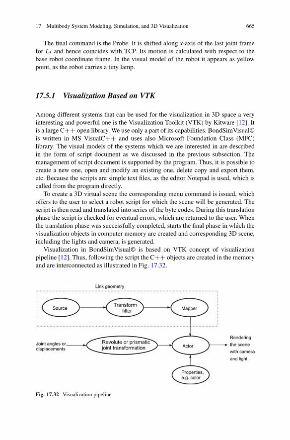
17 Multibody System Modeling, Simulation, and 3D Visualization 665
The final command is the Probe. It is shifted along x-axis of the last joint framefor L5 and hence coincides with TCP. Its motion is calculated with respect to thebase robot coordinate frame. In the visual model of the robot it appears as yellowpoint, as the robot carries a tiny lamp.
17.5.1 Visualization Based on VTK
Among different systems that can be used for the visualization in 3D space a veryinteresting and powerful one is the Visualization Toolkit (VTK) by Kitware [12]. Itis a large CCC open library. We use only a part of its capabilities. BondSimVisual©is written in MS VisualCCC and uses also Microsoft Foundation Class (MFC)library. The visual models of the systems which we are interested in are describedin the form of script document as we discussed in the previous subsection. Themanagement of script document is supported by the program. Thus, it is possible tocreate a new one, open and modify an existing one, delete copy and export them,etc. Because the scripts are simple text files, as the editor Notepad is used, which iscalled from the program directly.
To create a 3D virtual scene the corresponding menu command is issued, whichoffers to the user to select a robot script for which the scene will be generated. Thescript is then read and translated into series of the byte codes. During this translationphase the script is checked for eventual errors, which are returned to the user. Whenthe translation phase was successfully completed, starts the final phase in which thevisualization objects in computer memory are created and corresponding 3D scene,including the lights and camera, is generated.
Visualization in BondSimVisual© is based on VTK concept of visualizationpipeline [12]. Thus, following the script the CCC objects are created in the memoryand are interconnected as illustrated in Fig. 17.32.
Fig. 17.32 Visualization pipeline

666 V. Damic and M. Cohodar
Fig. 17.33 3D scene with ABB IRB1600 robot in the initial pose
The components in the upper part of the figure define the geometry of a link.Typically they use the sources of cubes, cylinders, and others forms, which definethe parts the link is composed of. They are transformed and connected to the mapperobjects, which defines the geometry of the link. It is also possible to use 3D CADmodels of the parts, e.g., in stl format, and using the corresponding reader to readthem into the memory. In the similar manner the base is created.
The outputs of the Mappers are connected to the Actors, which are responsiblefor rendering of the objects. Its properties can be defined, such as color, by Renderscript commands. Its input port is connected to the transform object, which describesrotation or sliding of the link by the revolute or prismatic joints. If the joint’s angleschange, then all connected components are reevaluated and the robot changes itsposition on the screen.
Figure 17.33 shows BondSimVisual© screen showing ABB IRB1600 robotscene. It is shown in the initial zero angles pose.
Program BondSimVisual© is designed to work jointly with another program,which supplies the value of the joint variables, the revolute joint angles, or prismaticjoint displacements. The primary dynamic modeling and simulation program isBondSim©, which supplies these data by the inter-process communication (IPC),Fig. 17.34.
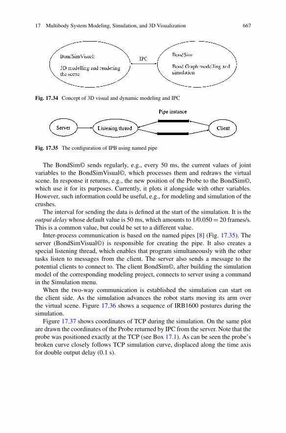
17 Multibody System Modeling, Simulation, and 3D Visualization 667
Fig. 17.34 Concept of 3D visual and dynamic modeling and IPC
Fig. 17.35 The configuration of IPB using named pipe
The BondSim© sends regularly, e.g., every 50 ms, the current values of jointvariables to the BondSimVisual©, which processes them and redraws the virtualscene. In response it returns, e.g., the new position of the Probe to the BondSim©,which use it for its purposes. Currently, it plots it alongside with other variables.However, such information could be useful, e.g., for modeling and simulation of thecrushes.
The interval for sending the data is defined at the start of the simulation. It is theoutput delay whose default value is 50 ms, which amounts to 1/0.050 D 20 frames/s.This is a common value, but could be set to a different value.
Inter-process communication is based on the named pipes [8] (Fig. 17.35). Theserver (BondSimVisual©) is responsible for creating the pipe. It also creates aspecial listening thread, which enables that program simultaneously with the othertasks listen to messages from the client. The server also sends a message to thepotential clients to connect to. The client BondSim©, after building the simulationmodel of the corresponding modeling project, connects to server using a commandin the Simulation menu.
When the two-way communication is established the simulation can start onthe client side. As the simulation advances the robot starts moving its arm overthe virtual scene. Figure 17.36 shows a sequence of IRB1600 postures during thesimulation.
Figure 17.37 shows coordinates of TCP during the simulation. On the same plotare drawn the coordinates of the Probe returned by IPC from the server. Note that theprobe was positioned exactly at the TCP (see Box 17.1). As can be seen the probe’sbroken curve closely follows TCP simulation curve, displaced along the time axisfor double output delay (0.1 s).

668 V. Damic and M. Cohodar
Fig. 17.36 The sequence of motion of ABB IRB1600 robot during the simulation
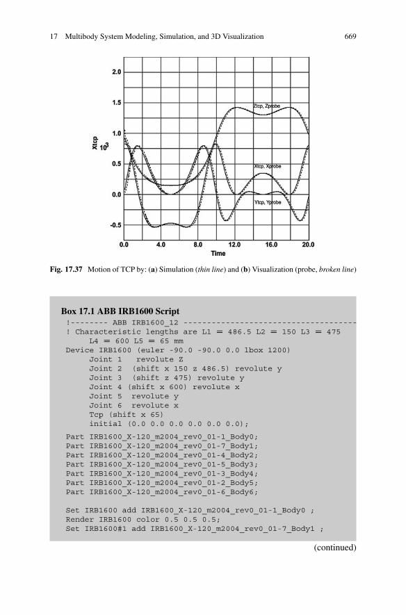
17 Multibody System Modeling, Simulation, and 3D Visualization 669
Fig. 17.37 Motion of TCP by: (a) Simulation (thin line) and (b) Visualization (probe, broken line)
Box 17.1 ABB IRB1600 Script!-------- ABB IRB1600_12 -------------------------------------! Characteristic lengths are L1 D 486.5 L2 D 150 L3 D 475
L4 D 600 L5 D 65 mmDevice IRB1600 (euler -90.0 -90.0 0.0 lbox 1200)
Joint 1 revolute ZJoint 2 (shift x 150 z 486.5) revolute yJoint 3 (shift z 475) revolute yJoint 4 (shift x 600) revolute xJoint 5 revolute yJoint 6 revolute xTcp (shift x 65)initial (0.0 0.0 0.0 0.0 0.0 0.0);
Part IRB1600_X-120_m2004_rev0_01-1_Body0;Part IRB1600_X-120_m2004_rev0_01-7_Body1;Part IRB1600_X-120_m2004_rev0_01-4_Body2;Part IRB1600_X-120_m2004_rev0_01-5_Body3;Part IRB1600_X-120_m2004_rev0_01-3_Body4;Part IRB1600_X-120_m2004_rev0_01-2_Body5;Part IRB1600_X-120_m2004_rev0_01-6_Body6;
Set IRB1600 add IRB1600_X-120_m2004_rev0_01-1_Body0 ;Render IRB1600 color 0.5 0.5 0.5;Set IRB1600#1 add IRB1600_X-120_m2004_rev0_01-7_Body1 ;
(continued)
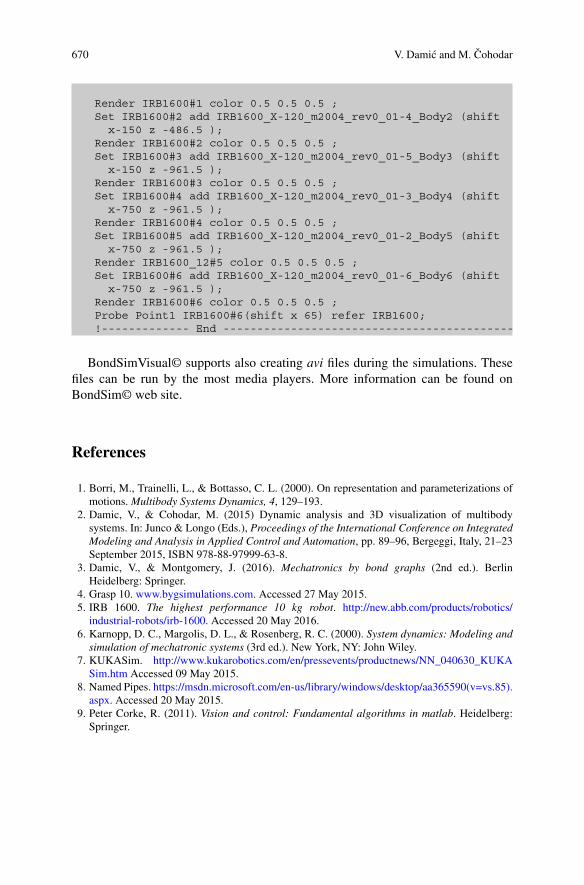
670 V. Damic and M. Cohodar
Render IRB1600#1 color 0.5 0.5 0.5 ;Set IRB1600#2 add IRB1600_X-120_m2004_rev0_01-4_Body2 (shiftx-150 z -486.5 );
Render IRB1600#2 color 0.5 0.5 0.5 ;Set IRB1600#3 add IRB1600_X-120_m2004_rev0_01-5_Body3 (shiftx-150 z -961.5 );
Render IRB1600#3 color 0.5 0.5 0.5 ;Set IRB1600#4 add IRB1600_X-120_m2004_rev0_01-3_Body4 (shiftx-750 z -961.5 );
Render IRB1600#4 color 0.5 0.5 0.5 ;Set IRB1600#5 add IRB1600_X-120_m2004_rev0_01-2_Body5 (shiftx-750 z -961.5 );
Render IRB1600_12#5 color 0.5 0.5 0.5 ;Set IRB1600#6 add IRB1600_X-120_m2004_rev0_01-6_Body6 (shiftx-750 z -961.5 );
Render IRB1600#6 color 0.5 0.5 0.5 ;Probe Point1 IRB1600#6(shift x 65) refer IRB1600;!------------- End -------------------------------------------
BondSimVisual© supports also creating avi files during the simulations. Thesefiles can be run by the most media players. More information can be found onBondSim© web site.
References
1. Borri, M., Trainelli, L., & Bottasso, C. L. (2000). On representation and parameterizations ofmotions. Multibody Systems Dynamics, 4, 129–193.
2. Damic, V., & Cohodar, M. (2015) Dynamic analysis and 3D visualization of multibodysystems. In: Junco & Longo (Eds.), Proceedings of the International Conference on IntegratedModeling and Analysis in Applied Control and Automation, pp. 89–96, Bergeggi, Italy, 21–23September 2015, ISBN 978-88-97999-63-8.
3. Damic, V., & Montgomery, J. (2016). Mechatronics by bond graphs (2nd ed.). BerlinHeidelberg: Springer.
4. Grasp 10. www.bygsimulations.com. Accessed 27 May 2015.5. IRB 1600. The highest performance 10 kg robot. http://new.abb.com/products/robotics/
industrial-robots/irb-1600. Accessed 20 May 2016.6. Karnopp, D. C., Margolis, D. L., & Rosenberg, R. C. (2000). System dynamics: Modeling and
simulation of mechatronic systems (3rd ed.). New York, NY: John Wiley.7. KUKASim. http://www.kukarobotics.com/en/pressevents/productnews/NN_040630_KUKA
Sim.htm Accessed 09 May 2015.8. Named Pipes. https://msdn.microsoft.com/en-us/library/windows/desktop/aa365590(v=vs.85).
aspx. Accessed 20 May 2015.9. Peter Corke, R. (2011). Vision and control: Fundamental algorithms in matlab. Heidelberg:
Springer.

17 Multibody System Modeling, Simulation, and 3D Visualization 671
10. RoboGuide. http://www.fanucamerica.com/products/vision-software/ROBOGUIDE-simulation-software.aspxccessed 09 May 2015.
11. RobotStudio. http://new.abb.com/products/robotics/robotstudio. Accessed 09 May 2015.12. Schroeder, W., Martin, K., & Lorensen, B. (1998). The Visualization Toolkit, Prentice Hall
PTR, Upper Saddle River, New Jersey. The version of the library used is VTK-6.3.0 of1.9.2015.
13. Sciavicco, L., & Siciliano, B. (1996). Modeling and control of robot manipulators. New York,NY: McGraw-Hill.
Appendix ASome Textbooks on Bond Graph Modelling
In the following, some textbooks on bond graph modelling are listed separatelyfrom the references at the end of each chapter for convenience [1–8]. They mayintroduce into the methodology, provide a survey, and serve as a knowledge sourcefor questions regarding details of the bond graph methodology.
References
1. Borutzky, W. (2010). Bond graph methodology – Development and analysis of multidisciplinarydynamic system models. London: Springer. ISBN:978-1-84882-881-0 (print).
2. Brown, F. T. (2001). Engineering system dynamics: A unified graph-centered approach.New York, Basel: Marcel Dekker. ISBN:0-8247-0616-1.
3. Dami , V., & Montgomery, J. (2016). Mechatronics by bond graphs (2nd ed.). Berlin, Heidel-berg: Springer.
4. Gawthrop, P., & Smith, L. (1996). Metamodelling: Bond graphs and dynamic systems. HemelHempstead: Prentice Hall International (UK) Limited. ISBN:0-13-489824-9.
5. Karnopp, D. C., Margolis, D. L., & Rosenberg, R. C. (2012). System dynamics: Modeling,simulation, and control of mechatronic systems (5th ed.). Hoboken, NJ: Wiley.
6. Merzouki, R., Samantaray, A., Pathak, P., & Ould Bouamama, B. (2013). Intelligent mechatronicsystems. Berlin: Springer.
7. Mukherjee, A., Karmakar, R., & Samantaray, A. (2006). Bond graph in modeling, simulationand fault identification. New Delhi, India: I.K. International Publishing House. ISBN: 81-88237-96-5.
8. Samantaray, A., & Ould Bouamama, B. (2008). Model-based process supervision – A bondgraph approach. Advances in industrial control. London: Springer.
© Springer International Publishing Switzerland 2017W. Borutzky (ed.), Bond Graphs for Modelling, Control and FaultDiagnosis of Engineering Systems, DOI 10.1007/978-3-319-47434-2
673
c
Index
AAbrupt parametric fault, 157, 206Active, 47, 87, 88, 102, 103, 109, 119, 126,
139, 141, 170–172, 179, 187, 189,212, 275, 279, 361, 548, 567,572–576, 578–580, 604
Adaptive threshold, 198, 200, 201, 203–204,208, 209, 213, 215, 218, 219, 221,223, 227–229, 240
Affinity, 589, 592–594, 597, 598, 600, 601,603, 607, 608, 614, 616, 620
Analytical redundancy relations (ARRs), 135,139, 141, 156–168, 179–189, 198,200, 201, 208, 212, 220, 229, 234,238–240, 246–250, 260
evaluation, 156
BBehavioural bond graph, 159Biomolecular cycle, 611–615Biomolecular systems, 587–621Bond graph (BG)
behavioural, 135, 159, 179diagnostic, 157–160, 163–165, 167, 179,
180, 185, 187–189, 198, 200, 201modelling, 47–84, 125, 135–137, 141, 146,
157, 188, 231, 431–449, 451–494,587–621
pseudo, 271, 272, 314, 595true, 272, 313, 355
Buck converter, 142, 175, 176, 180,181, 183
CCausality, 1, 2, 16–18, 28, 48, 49, 88, 89, 140,
141, 203, 204, 238, 239, 287, 311,330, 333, 391, 393–396, 435, 438,485, 512, 551, 555, 588
Causality resistance, 89, 90, 106, 111C component, 587, 588, 591–592, 594–597,
599–601, 604, 605CFD. See Computational fluid dynamics
(CFD)Chemical potential, 12, 587–591, 594, 596,
598, 601, 605, 608, 616, 621Chemostats, 596, 597, 604–608, 611, 612, 614,
616, 618, 620, 621Circuit analogy, 596CJ. See Controlled junction (CJ)Closed systems, 596–605, 607Coherence vector, 201, 218–220, 228, 230Complementarity condition, 155Component fault signature, 158, 161, 166Compressible flow, 306, 314–337, 354Computational fluid dynamics (CFD), 272,
311–356Condition based maintenance, 195, 221, 233,
234Conserved moiety(ies), 588, 597, 598, 607,
609, 611, 614, 616, 620Controllability, 108, 115, 121–123, 436, 588Controlled element, 91, 97–100Controlled junction (CJ), 50, 52, 67, 68,
72–73, 83, 89, 91–99, 101–103, 105,106, 111–115, 118, 122–126, 152,201–203, 208, 212
© Springer International Publishing Switzerland 2017W. Borutzky (ed.), Bond Graphs for Modelling, Control and FaultDiagnosis of Engineering Systems, DOI 10.1007/978-3-319-47434-2
675

676 Index
Control properties, 108, 111, 117, 121–125Control reconfiguration, 68, 171Covariables, 271, 385, 587, 588, 591,
601, 604
DDAEs. See Differential algebraic equations
(DAEs)DC motor drive, 127, 142, 175, 176, 180, 181,
186, 426, 438Decision procedure, 201Degradation model, 197–199, 205–207, 209,
221, 222, 229–231, 235, 236,246–254, 261–263
Degradation pattern, 197, 199, 206, 207, 209,221, 223, 229
Derivative causality, 29, 34, 35, 80, 89, 91,100, 102–104, 109, 111, 112, 115,118, 119, 122–125, 140, 203, 204,239, 248, 260, 335, 391, 396,398–400, 415, 445, 553, 559, 568,588, 600–602, 605–607, 613,617–619
Derivative structure matrix(ces), 601–604Descriptor system, 108, 115–117, 121,
126Diagnostic bond graph (DBG), 157–160,
163–165, 167, 179, 180, 185,187–189, 198, 200, 201
Diagnostic hybrid bond graph (DHBG),198–201, 207–210, 212–214, 221,223, 224, 229, 231
Differential algebraic equations (DAEs), 28,38, 39, 45, 66, 84, 88, 140–145,149–155, 173, 174, 177, 180,187–189, 396, 397, 400, 427,628
Discontinuitiesparametric, 90, 91, 97–101structural, 90–97, 111, 119, 120type 1, 110, 111, 119, 120type 2, 111
Discrete event, 47, 64, 142–144, 156, 173,174, 195
Discrete fault, 136, 196, 199, 206, 208Discrete switch states, 142, 143, 149, 154, 156,
157, 163, 165, 189Disturbances, 168–173, 176, 187, 189, 199,
200, 203, 204, 500, 511, 536–538,568
Dynamic causality, 87–130Dynamic Sequential Causality Assignment
Procedure (DSCAP), 95, 96, 101
EEffort amplifier, 605Efforts, 1, 2, 110–18, 21, 23, 24, 33, 34, 36,
40, 41, 43, 44, 51–54, 57, 59, 60,62–64, 67, 68, 70, 73, 76, 78, 81,82, 91–94, 98–100, 102, 105, 116,126, 165, 167, 168, 208, 237, 239,240, 271, 275–278, 281, 283, 285,292, 301, 308, 311–313, 323, 325,330, 333, 335–337, 341, 345, 346,353, 354, 362–364, 390, 392, 397,399–402, 406, 408, 412, 420, 432,435, 453, 458, 460, 473, 510, 519,522, 552, 553, 560, 563, 565, 568,570, 589, 591, 592, 597, 599–601,604, 605, 633–635, 637, 639, 641,644, 649, 651
Enthalpy, 276, 277, 279, 280, 283, 285, 292,312, 590, 593
Entropy, 7, 8, 12–14, 19, 20, 23, 271, 272,276–281, 285, 292, 313–317, 319,321, 322, 325, 329–333, 336–340,342, 345–348, 350–355, 590, 593
stripping, 593Equivalent systems, 224, 482Event, 107, 117, 121, 127, 129, 142–144, 156,
163, 170, 173, 186, 195, 220, 234,238
discrete, 47, 64, 142–144, 156, 173, 174,195
FFailure, 136, 139, 156, 157, 163, 170, 196,
198, 204, 206, 207, 217, 234–237,252, 253, 262, 264, 384
Failure threshold, 136, 198, 204, 206, 207,217, 221, 223, 227, 230, 235
False alarms, 157, 158, 189, 203, 241Fault(s)
accommodation, 139–189, 543additive, 167–168, 170, 171detection, 156–161, 171, 179, 185, 206,
220, 234, 235, 239–241, 247, 254,255, 267
robust, 157, 158, 160diagnosis, 139–189, 198, 200–204, 206,
231, 239hypothesis, 164–167, 181, 196, 214, 218indicators, 141, 143, 147, 156–159, 171,
179isolation, 165, 168, 215, 218–220multiple, 163, 198, 206–210, 214, 215, 219,
220, 228, 231
Index 677
multiplicative, 171parametric, 156, 157, 160, 161, 164–166,
169, 171, 173, 176, 185, 187,195–197, 199, 201, 202, 206, 208,209, 229, 322, 325
progressive parametric, 163, 231scenario, 141, 142, 146, 159, 184–187, 215,
220signature, 158, 161, 165, 166, 201, 219threshold, 198, 204, 206, 207, 217, 221,
223, 227, 230, 235Fault detection and isolation (FDI), 106, 135,
136, 139–141, 157, 163, 171, 179,187, 188, 195–199, 201, 203–205,207, 209, 218
Fault signature matrix (FSM), 136, 158, 159,161, 165, 166, 181, 201–203
Fault tolerant control (FTC), 139, 140, 170,171, 179, 185, 187–189
active, 139, 170, 171, 179, 187, 189passive, 171
Finite element method (FEM), 272, 312, 313,320, 321, 350, 354, 355
Finite modes, 121–123Finite state automaton (FSA), 144, 154, 155Flows, 2, 28, 31, 52, 53, 89, 90, 110, 166, 168,
203, 204, 240, 260, 271, 272, 275,276, 311, 312, 361, 362, 392, 432,433, 504, 519, 553, 554, 587, 588,632
Flowstats, 604, 621Flux paths, 588FSA. See Finite state automaton (FSA)FSM. See Fault signature matrix (FSM)FTC. See Fault tolerant control (FTC)
GGlobal analytical redundancy relation (GARR),
201, 202, 207–209, 212–215, 218,221, 223, 228
Global fault sensitivity signature matrix(GFSSM), 201–203, 208, 209, 213,214, 218–221, 223, 227, 228, 230
Global fault signature matrix (GFSM),201–203, 213, 218, 219
Glycolysis, 588, 615–618Gyrator (GY), 11, 13, 17–20, 23, 101, 224,
277, 300, 330, 392, 395, 398, 432,506, 589, 600, 601, 639
GY component, 588, 589
HHBG. See Hybrid bond graph (HBG)Hierarchical, 145, 189, 383, 615, 621, 647,
652Hybrid
BG (see Bond graph (BG))DAEs, 1, 2, 135, 141, 143, 144, 149–155,
173implicit equation, 104–105junction structure matrix, 101–103, 105model, 2, 3, 87, 88, 106, 117, 135, 136,
140–156, 161, 168, 188, 189system, 2, 47–84, 87, 88, 91, 118, 125, 135,
141–143, 157, 158, 195, 197–215,218, 224, 227, 228
system model, 142, 143, 157, 158Hybrid bond graph (HBG), 87–130, 197,
210–212, 215Hydraulic analogy, 596
II component, 600, 637Implicit model, 108–109, 113Impulse
bond graph, 107, 117-controllability, 121losses, 107, 117–118model, 88, 107, 117, 121modes, 88, 107, 117–123-observability, 123
Incompressible flow, 316, 337–346, 353, 355Input(s), 78, 98, 100–105, 109, 116, 120, 123,
126, 135, 136, 143, 155, 157, 158,164, 169, 170, 172, 174, 179, 182,200, 215, 236, 247, 252, 254, 267,278, 337, 341, 445, 510, 554, 567,600
reconstruction, 141, 171–187, 189Integral causality, 18, 30, 33, 35, 51, 60, 63,
89, 95, 96, 100, 102, 103, 109, 111,114, 115, 118–122, 124–126, 140,157, 175, 258–260, 335, 336, 396,397, 400, 438, 588, 594, 599–601,605
Inverse model, 141, 142, 172, 177, 187–189,568
Inverse simulation, 139–189Isobaric, 587, 589–591Isolability, 201, 247Isothermal, 317, 587, 589–591
678 Index
JJunction structure, 2, 17, 19, 23, 52, 66–80,
89, 91, 100–105, 113, 115, 116,126, 155, 362, 366, 369, 379, 385,391, 392, 458, 503, 519, 588, 596,598–607, 611, 613, 615, 617–619,639, 640
KKatchalsky, A., 587Kernel, 237, 607, 610–611
LLinear complementarity problem (LCP), 156Linear complementarity system (LCS), 155Linear fractional transformation (LFT), 22,
158, 189, 201, 209, 212, 221, 223,234, 238, 239
MMarcelin-de-Donder formula, 592Mass-action, 592Maximising derivative causality, 601, 605MCSM. See Mode change signature matrix
(MCSM)MCSSM. See Mode change sensitivity
signature matrix (MCSSM)Mixed-Boolean state equation, 100–105Mode change sensitivity signature matrix
(MCSSM), 201–203, 208, 213, 214,218–220, 227, 228
Mode change signature matrix (MCSM),201–203, 213, 219
Modelforward, 141, 174, 187–189hybrid, 87, 88, 106, 117, 140–156, 161,
168, 188, 189inverse, 141, 142, 172, 177, 187–189, 568variable structure, 143, 145
Modelica®, 140, 144, 145Modelling uncertainties, 188, 189Mode switching, 55, 65, 97, 98, 143, 173, 174
LTI system, 144, 155–156, 188, 189Monitorability, 201Multiple faults, 163, 198, 206–210, 214, 215,
219, 220, 228, 231Multiport transformer, 17, 18, 21–23, 392, 599,
600
NNull space, 588, 607
OObservability, 115, 121, 123, 124, 436Open, 28, 34, 37, 40, 42, 43, 45, 51, 57,
76, 94, 140, 144, 151, 152, 156,163, 172–178, 180, 184–186, 206,225, 288, 289, 300, 301, 396, 397,432, 444, 446, 447, 452, 498, 533,568, 583, 588, 597, 645, 647, 649,651–653, 665
OpenModelica, 53, 140, 141, 144–147, 149,155, 188
Open systems, 596, 604–608, 611, 616, 621Output equation, 115–117, 362, 369Outputs, 98, 100, 101, 103, 105, 109, 116, 123,
126, 135, 136, 143, 155, 157, 161,164, 165, 169, 170, 175, 179, 182,184, 187, 196, 199, 200, 217, 254,267, 337, 359, 362, 442–444, 568,600, 601, 663, 666
PParameter
degradation, 163, 171, 197–199,204–207, 209, 221, 222, 231,233, 248
estimation, 165, 184, 199, 200, 209, 220,221, 223, 227, 229, 231, 236, 559,573
uncertainty, 203, 204Paynter, H., 275, 276, 311, 587Phosphorylation/dephosphorylation, 618–620Piecewise continuous, 91, 97, 98Port, 2, 5, 6, 11–14, 16–24, 34, 50, 51, 53, 54,
59, 83, 93, 94, 103, 105, 106, 140,144, 145, 149–152, 155, 271, 276,280, 281, 323, 325–330, 333, 341,342, 346, 353, 362, 369, 397, 434,449, 552, 587, 589, 591–593, 595,598, 599, 620, 621, 633–637, 639,643, 644, 648, 649, 651, 666
Power electronic systems, 140–142Prognosis, 135–137, 157, 163, 195–231, 237Progressive fault, 157, 163, 206, 210, 215, 223,
225, 227, 228, 246Pseudo-states, 100, 102–105, 107, 117–120,
125, 126
RR component, 80, 588, 589, 593, 597–600,
604, 620Reaction constant, 592Re component, 592–598
Index 679
Remaining useful life (RUL), 136, 137, 157,163, 195–200, 204–206, 209, 210,215, 221–223, 227–231, 234–238,245, 247, 252–257, 263, 265–267
Residualgenerate, 171, 200sinks, 28, 49, 51, 53, 55, 56, 59, 60, 68, 69,
75, 76, 80–82, 84, 179RUL. See Remaining useful life (RUL)
SSensitivity signature, 199, 202, 208, 214, 218,
219, 231Simulation, 1, 3, 27, 47, 66–84, 87, 139–189,
214–223, 242, 271, 275, 348, 359,381, 383–385, 387–427, 431, 458,498, 547, 597, 627–670
Single fault hypothesis, 164–167, 181, 196,214, 218
Solvability, 14, 87, 89, 96, 121, 174Source-sensor, 599, 600, 604SS component, 600, 601, 604Stability, 48, 108, 121, 124, 139, 171, 399,
421, 436, 512, 520, 529, 538State, 1–3, 29, 47, 66, 87, 137, 140, 196, 233,
272, 275, 311, 359, 384, 400, 432,539, 565, 592
State variable filter, 178, 182Stoichiometric information, 596, 607–611Stoichiometric matrix, 588, 599, 607, 621Structural analysis, 89, 96, 98, 100, 108–125,
427, 588, 593, 595–611Structurally null modes, 125Structural singularity, 145Switch(ing)
bond graphs, 88
model, 49, 76, 80–84, 87, 88, 107, 118non-ideal, 2, 51, 79, 83, 94, 140, 143,
145–147, 150, 151, 153, 175state, 140, 142, 143, 149, 153–157, 163,
165, 189use of non-ideal and ideal switches, 50, 97,
140, 143, 146, 147System model, 7–8, 45, 80, 88, 121, 140–144,
146, 147, 155–158, 163, 165, 168,172, 173, 178, 184, 189, 198, 231,251, 278, 283, 293, 299, 359, 361,395, 443, 550, 627–670
TThermodynamic constant, 592Thermodynamics, 19, 88, 271–273, 275–277,
281, 311, 337, 351, 355, 588–591,597
Thyristorfinite state automaton, 154, 155modelica description, 153, 154
Transfer function, 1, 113–115, 175, 188, 308,390
Two-tank system, 210, 215, 224, 225, 227
UUnknown input observers (UIO), 168–171,
196
VVariable structure models, 88, 143, 145Variable-structure systems, 88Variable topology, 48, 88–90, 109, 117, 126,
130