RC23510 (W0502-005) February 2, 2005Computer Science

IBM Research Report

BlueBot: Asset Tracking via Robotic Location Crawling

Abhishek PatilDepartment of Computer Science and Engineering

Michigan State UniversityEast Lansing, MI 48824

Jonathan Munson, David Wood, Alan ColeIBM Research Division

Thomas J. Watson Research CenterP.O. Box 704

Yorktown Heights, NY 10598

Research DivisionAlmaden - Austin - Beijing - Haifa - India - T. J. Watson - Tokyo - Zurich

LIMITED DISTRIBUTION NOTICE: This report has been submitted for publication outside of IBM and will probably be copyrighted if accepted for publication. It has been issued as a ResearchReport for early dissemination of its contents. In view of the transfer of copyright to the outside publisher, its distribution outside of IBM prior to publication should be limited to peer communications and specificrequests. After outside publication, requests should be filled only by reprints or legally obtained copies of the article (e.g. , payment of royalties). Copies may be requested from IBM T. J. Watson Research Center , P.O. Box 218, Yorktown Heights, NY 10598 USA (email: reports@us.ibm.com). Some reports are available on the internet at http://domino.watson.ibm.com/library/CyberDig.nsf/home .

1

BlueBot: Asset Tracking via Robotic Location Crawling

Abhishek Patil1, Jonathan Munson2, David Wood2 and Alan Cole2 1 Dept of Computer Science and Engineering

Michigan State University East Lansing, MI 48824

patilabh@cse.msu.edu

2 IBM T. J. Watson Research Center 19 Skyline Drive

Hawthorne, NY 10532

{jpmunson, dawood, colea}@us.ibm.com

Abstract: Asset tracking – knowing what you have and where it is located – is essential for the smooth

operation of many enterprises. From manufacturers, distributors, and retailers of consumer goods, to

government departments, enterprises of all kinds are gearing up to use RFID technology to increase the

visibility of goods and assets within their supply chain and on their premises. However, RFID technology

alone lacks the capability to track the location of items once they are moved within a facility. This paper

presents a prototype automatic location sensing system that combines RFID technology and off-the-shelf

Wi-Fi based continuous positioning technology for asset tracking in indoor environments. The system

employs a robot, with an attached RFID reader, which periodically crawls the space, associating items it

detects with its own location determined with the Wi-Fi positioning system. We propose three algorithms

that combine the detected tag’s reading with previous samples to compute its location. Our experiments

have shown that our positioning algorithms can bring a two to three fold improvement on the raw

accuracy provided by the positioning technology.

1 Introduction Consider a typical public library. Each book has its own place in a particular shelf. Usually, readers

like to take several books (from different shelves) and browse through them until they find the right book.

While some readers manage to return the unwanted books to the correct shelf, many of them either leave

the books in some corner of the library or place them back in the wrong location. This latter situation is

hard to detect and can become a librarian’s nightmare. A similar situation exists in many retail stores

where the customers can tryout several items before deciding which one to buy. In most cases, the

customer never returns the tested item to its correct shelf. Some kind of automated tracking mechanism is

required. The problem of asset tracking is not restricted to libraries or small retail stores. Many companies

are realizing the importance of increasing the visibility within their supply chain. Asset tracking –

knowing what you have and where it is located – is essential for the smooth operation of large

manufacturing companies. It also helps big retailers (like Wal-Mart) isolate bottlenecks in their supply

2

chain, reduce overstocking or locate spoiled cargo. Several government and military organizations are

always on the lookout for cheaper (and more efficient) ways to track their assets and equipment.

Automatic location sensing is the key to enabling such tracking applications. One of the most well-

know positioning systems is GPS [16], which relies on satellites to track location. However, due to its

dependence on the satellites, GPS lacks the ability to accurately determine location inside buildings. In

order to achieve location tracking inside buildings, researchers and industry have proposed several

systems, which differ with respect to the technology used, accuracy, coverage, frequency of updates and

the cost of installation and maintenance [22] [2] [25] [4] [14] [6] [20] [23]. Triangulation, scene analysis,

and proximity are the three principal techniques for automatic location-sensing [18]. Steggles and

Cadman [24] provide a good comparison of various RF-tag-based location sensing technologies. Many of

the current location sensing systems are radio based (Wi-Fi - [14] [23] [26] [5] [1], Bluetooth - [3] [1]).

By using base station visibility and signal strength or time of flight, it is possible to locate Wi-Fi devices

with an accuracy of several meters.

In recent years, RFID technology has attracted considerable attention. RFID is emerging as an

important technology that is reshaping supply chain management. RFID not only replaces the old barcode

technology but also provides a greater degree of flexibility in terms of range and access mechanisms. For

example, an RFID scanner can read the encoded information even if the tag is concealed (this might be

for either aesthetic or security reasons). Several companies (like Wal-Mart, Gillette, CVS etc) are

proposing to use RFID for identifying large lots of goods at pallet and carton level. Usually passive tags

are preferred for tagging goods as they are much cheaper, long lived, lightweight and have a smaller foot

print. However since passive tags work without a battery, they have a very small detection range. Current

RFID systems are portal based where tagged items are scanned either when they enter or leave a facility.

This scheme does not provide any information about the exact location of the item once it is moved away

from the portal.

The prototype system described in this paper combines (passive) RFID technology and a Wi-Fi

(802.11b) based continuous location positioning system to provide a periodic asset-locating sweep.

Although, our system uses Wi-Fi based location positioning, it can work with any continuous positioning

technology. The prototype system not only identifies but also provides location information of every

RFID-tagged item in the sweep space. A portable system (e.g. laptop or PDA) running a Wi-Fi client and

connected to an RF reader is mounted on a robot that moves autonomously through the space. As the

robot moves, the RF reader periodically samples which tags are detectable. At each sample time, the

robot’s position is obtained from the positioning system. For each detected tag, given the estimate of the

robot’s current position, knowledge of the reader’s physical detection range, and the robot’s position

3

estimates at previous detections, an algorithm computes an estimate of the tag’s position. In summary, our

experiments with the prototype system show that we are able to estimate positions of tagged entities to

within 1.5m, given an accuracy of the raw positioning system of about 4m. We experimented with

different position estimation algorithms and found that certain algorithms work better than others when

the raw positioning system is capable of giving better accuracy.

The rest of the paper is structured as follows. In Section 2, we survey related work in the area of

location tracking in indoor environments. Section 3 briefly describes RFID technology and its use in our

project. Section 4 explains the Wi-Fi positioning system and our experience with its performance. In

Section 5 we present results of experiments carried out using our prototype system (and our algorithms).

Finally, Section 6 concludes the paper and presents directions for future research.

2 Related Work Researchers and industry have proposed several location-sensing systems, which differ with respect

to technology used, accuracy, coverage, frequency of updates and the cost of installation and

maintenance. Some of these systems suffer from disadvantages that limit their use. For example, infrared

systems [25] have line of sight restriction; ultrasonic systems [2] [4] are accurate but expensive. Recently,

there has been an increase in the number of wireless companies that are seeking newer ways to track

people and things in indoor environment. The rest of this section gives a brief description of several

indoor location sensing technologies and various companies that make use of these technologies for asset

tracking in indoor environment.

Some of the earlier attempts for location sensing used infrared (IR) technology. Active Badge,

developed at Olivetti Research Laboratory (now AT&T Cambridge), used diffuse infrared technology

[25] to realize indoor location positioning. The line-of-sight requirement and short-range signal

transmission are two major limitations that suggest it to be less than effective in practice for indoor

location sensing. More recently, the focus has moved to using radio frequency (RF) signals RF-IR

combination or Ultrasonic. In case of RF, techniques such as Differential Time of Arrival or simple signal

strength measurement at various sensors are employed. RADAR is an RF based system for locating and

tracking users inside buildings [14], using a standard 802.11 network adapter to measure signal strengths

at multiple base stations positioned to provide overlapping coverage in a given area. This system

combines empirical measurements and signal propagation modeling in order to determine user location

thereby enabling location-aware services and applications. WhereNet [13] on the other hand works by

timing signals transmitted from tags to a network of receivers. It uses the same 2.4GHz band as the

802.11 and Bluetooth systems, but it uses a dedicated standard protocol (ANSI 371.1) optimized for low-

4

power spread-spectrum location. AeroScout (formerly BlueSoft) uses 802.11-based time difference of

arrival (TDOA) location solution. It requires the same radio signal to be received at three or more separate

points, timed very accurately (to a few nanoseconds) and processed using the TDOA algorithm to

determine the location. Ekahau [5] Wi-Fi positioning system computes the location of a client device by

applying a probabilistic model to the signal strength measured at the Wi-Fi client device. Unlike

AeroScout (and other TDOA based systems), the indoor environment has to be calibrated so that the

positioning engine get a signal strength map of the room. Ekahau tags (or Wi-Fi devices running Ekahau

client) constantly send their signal strength measure to the positioning engine which keeps track of each

device’s location.

Several other companies like Radianse [9] and Versus [12] use a combination of RF and IR signals to

do location positioning. Their tags emit IF and RF signals containing a unique identifier for each person

or asset being tracked. The use of RF allows coarse-grain positioning (e.g. floor) while the IR signals

provide additional resolution (e.g. room). The Cricket Location Support System [4] and Active Bat

location system [2] are two primary examples that use the ultrasonic technology. Normally, these

systems use an ultrasound time-of-flight measurement technique to provide location information. Most of

them share a significant advantage, which is the overall accuracy. Cricket for example can accurately

delineate 4x4 square-feet regions within a room while Active Bat can locate Bats to within 9cm of their

true position for 95 percent of the measurements. Ultra Wideband (or UWB♣) is a new technology that

has entered the arena of indoor location sensing. Unlike conventional RF systems, UWB systems are

much less affected by multipath distortion. The Ubisense [11] system uses UWB and is based on time of

arrival rather than signal strength and claims to have an accuracy of 6 inches (15 cm) in 3D space at a

confidence level of 95%. The system uses UWB tags (called UbiTags), which are fixed to the items being

tracked.

Discussion The asset tracking technologies mentioned above are mostly geared towards tracking items that

individually have high value (e.g., emergency medical equipment or an important person – a surgeon).

These items require continuous tracking and justify the use of expensive tracking equipment. However, in

many tracking applications (e.g. the library scenario described earlier) the object being tracked is either

too small or too low value to justify the use of a tracking system with high per-item cost. And in fact,

many of these applications do not require continuous tracking. We believe there are many applications

where it is valuable to know the precise location of an asset, yet it is permissible for an asset’s location to

♣ An informative web site on UWB is provided by Multispectral Solutions, Inc [8]

5

be updated on a periodic basis—nightly, for example. Our BlueBot system is targeted towards such

applications.

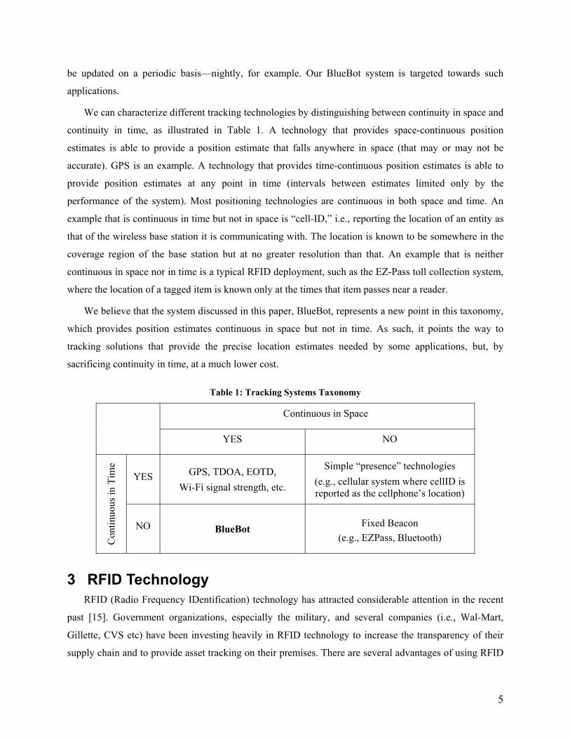
We can characterize different tracking technologies by distinguishing between continuity in space and

continuity in time, as illustrated in Table 1. A technology that provides space-continuous position

estimates is able to provide a position estimate that falls anywhere in space (that may or may not be

accurate). GPS is an example. A technology that provides time-continuous position estimates is able to

provide position estimates at any point in time (intervals between estimates limited only by the

performance of the system). Most positioning technologies are continuous in both space and time. An

example that is continuous in time but not in space is “cell-ID,” i.e., reporting the location of an entity as

that of the wireless base station it is communicating with. The location is known to be somewhere in the

coverage region of the base station but at no greater resolution than that. An example that is neither

continuous in space nor in time is a typical RFID deployment, such as the EZ-Pass toll collection system,

where the location of a tagged item is known only at the times that item passes near a reader.

We believe that the system discussed in this paper, BlueBot, represents a new point in this taxonomy,

which provides position estimates continuous in space but not in time. As such, it points the way to

tracking solutions that provide the precise location estimates needed by some applications, but, by

sacrificing continuity in time, at a much lower cost.

Table 1: Tracking Systems Taxonomy

Continuous in Space

YES NO

YES GPS, TDOA, EOTD, Wi-Fi signal strength, etc.

Simple “presence” technologies (e.g., cellular system where cellID is reported as the cellphone’s location)

Con

tinuo

us in

Tim

e

NO BlueBot Fixed Beacon (e.g., EZPass, Bluetooth)

3 RFID Technology RFID (Radio Frequency IDentification) technology has attracted considerable attention in the recent

past [15]. Government organizations, especially the military, and several companies (i.e., Wal-Mart,

Gillette, CVS etc) have been investing heavily in RFID technology to increase the transparency of their

supply chain and to provide asset tracking on their premises. There are several advantages of using RFID

6

technology – no contact and non-line-of-sight, working under harsh environmental conditions, etc. RFID

systems have a fast response time and in some cases tags can be read in less than a 100 milliseconds. The

other advantages are their promising transmission range and cost-effectiveness. RFID tags can be

concealed for either aesthetic or security reasons and yet be detected by an RFID reader.

RFID tags are categorized as either passive or active. Passive RFID tags usually operate without a

battery and offer a virtually unlimited operational lifetime. They reflect the RF signal transmitted to them

from a reader and add information by modulating the reflected signal. Passive tags are much lighter and

less expensive than active tags. However, ranges of more than 1.5m are not easily achieved using passive

tags. Active tags contain both a radio transceiver and a 2-5 year battery to power the transceiver. Since

there is an onboard radio, active tags have more range than passive tags (30m or more). However, they

are more expensive and have a larger physical footprint compared to passive tags.

4 ft

0.5m

Figure 1: Intermec PCMCIA reader and passive tag. Figure 2: RF characteristic of reader antenna.

In our system, we use the Intermec [7] PCMCIA RFID reader (Figure 1), which operates at a

frequency of 915MHz. The reader can be connected to any device that has a PCMCIA port. In our

experiments, we had the reader connected to a laptop PC, but a smaller device, such as a PDA, or a

custom-built PC, can be used as well for additional portability. The reader is attached to a directional

antenna, which has a very short range (5 feet max). The reader’s antenna is placed facing the ceiling such

that its maximum gain is in the vertical direction. The RF characteristics of the reader would approximate

a vertical cone with its vertex on the reader’s antenna. We observed that tags at a height of 4 feet were

detected with 90% (or higher) probability when the reader was (horizontally) within 0.5m of the tag

(Figure 2). Due to the rectangular base of the reader’s antenna, the RF characteristics had an elliptical

7

shape (with the larger axis along the longer sides of the rectangle). However, we found that the

eccentricity was close to 1. For all our experiments we have considered the reader’s RF characteristics to

be a circle.

4 Wi-Fi Positioning System We use an off-the-shelf Wi-Fi (802.11b) positioning system to track our client system (consisting of

the RFID reader, client machine and the robot - Figure 8). The positioning system computed the location

by using signal strength information (as perceived by the client device being tracked). The positioning

engine advertised an average accuracy of 1m (3.5 ft).

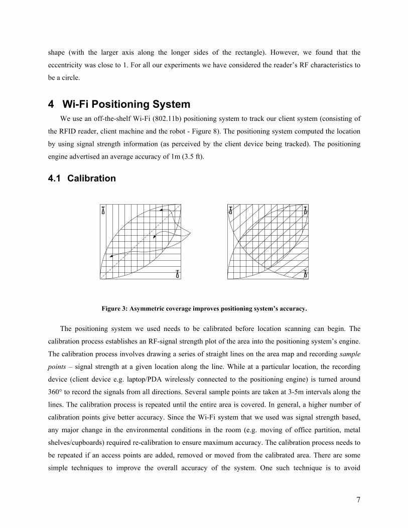
4.1 Calibration

Figure 3: Asymmetric coverage improves positioning system’s accuracy.

The positioning system we used needs to be calibrated before location scanning can begin. The

calibration process establishes an RF-signal strength plot of the area into the positioning system’s engine.

The calibration process involves drawing a series of straight lines on the area map and recording sample

points – signal strength at a given location along the line. While at a particular location, the recording

device (client device e.g. laptop/PDA wirelessly connected to the positioning engine) is turned around

360° to record the signals from all directions. Several sample points are taken at 3-5m intervals along the

lines. The calibration process is repeated until the entire area is covered. In general, a higher number of

calibration points give better accuracy. Since the Wi-Fi system that we used was signal strength based,

any major change in the environmental conditions in the room (e.g. moving of office partition, metal

shelves/cupboards) required re-calibration to ensure maximum accuracy. The calibration process needs to

be repeated if an access points are added, removed or moved from the calibrated area. There are some

simple techniques to improve the overall accuracy of the system. One such technique is to avoid

8

symmetric coverage within a room. For example, using two omnidirectional access points for coverage in

an open room can cause a symmetric RF pattern. As a result, there would be two or more sample points

that would record the same signal strength pattern from the two APs (Figure 3a). Using APs with

directional antennas or having an asymmetric coverage by introducing a third access point (APs at 3

corners of the room - Figure 3b) can solve this problem.

4.2 Positioning Technology Accuracy Analysis Because our tag-position estimation algorithms (described later) use characteristics of the positioning

technology used to position the robot, we carried out two sets of experiments to examine the performance

of our positioning system. The two sets differed in the density of calibration points and the size of the

experiment area.

4.2.1 Case A

Chess Board

1

2

3

4

5

6

7

12

43

48

AP 2

AP 3

1319253137

1824303642

12.5m (500 in)

13.7

5m

(550

in)

Foos

ball

tabl

e

Carpeted Area

AP 1

Room Entrance

Figure 4: Experiment setup (case A)

The experiment area chosen was a large open 12.5m x 13.75m room (Figure 4). The positioning

system was calibrated to work with only the three access points that were installed in the room (during the

calibration process, the positioning engine was programmed to ignore any other access points installed in

9

the building). The calibration points were spaced at a distance of approximately three meters. The three

access points were powered down to run at 15mW. To improve accuracy of the system, we wanted to

have the access point coverage such it gives the steepest signal strength gradient across the room. Our

Cisco 340 access points had four power levels (100mW, 30mW, 15mW and 5mW). Using the positioning

system’s software, we found that 5mW power level didn’t give complete coverage in the room which

resulted in a higher error. We selected 15mW which seemed to give the best gradient.

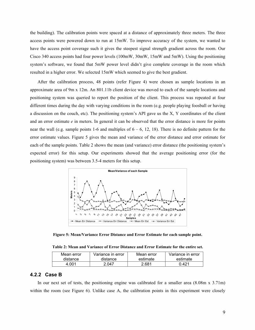
After the calibration process, 48 points (refer Figure 4) were chosen as sample locations in an

approximate area of 9m x 12m. An 801.11b client device was moved to each of the sample locations and

positioning system was queried to report the position of the client. This process was repeated at four

different times during the day with varying conditions in the room (e.g. people playing foosball or having

a discussion on the couch, etc). The positioning system’s API gave us the X, Y coordinates of the client

and an error estimate e in meters. In general it can be observed that the error distance is more for points

near the wall (e.g. sample points 1-6 and multiples of 6 – 6, 12, 18). There is no definite pattern for the

error estimate values. Figure 5 gives the mean and variance of the error distance and error estimate for

each of the sample points. Table 2 shows the mean (and variance) error distance (the positioning system’s

expected error) for this setup. Our experiments showed that the average positioning error (for the

positioning system) was between 3.5-4 meters for this setup.

Mean/Variance of each Sample

0123456789

1 3 5 7 9 11 13 15 17 19 21 23 25 27 29 31 33 35 37 39 41 43 45 47Samples

Met

ers

Mean Err Distance Variance Err Distance Mean Err Est Variance Err Est

Figure 5: Mean/Variance Error Distance and Error Estimate for each sample point.

Table 2: Mean and Variance of Error Distance and Error Estimate for the entire set.

Mean error distance

Variance in error distance

Mean error estimate

Variance in error estimate

4.001 2.047 2.681 0.421

4.2.2 Case B In our next set of tests, the positioning engine was calibrated for a smaller area (8.08m x 3.71m)

within the room (see Figure 6). Unlike case A, the calibration points in this experiment were closely

10

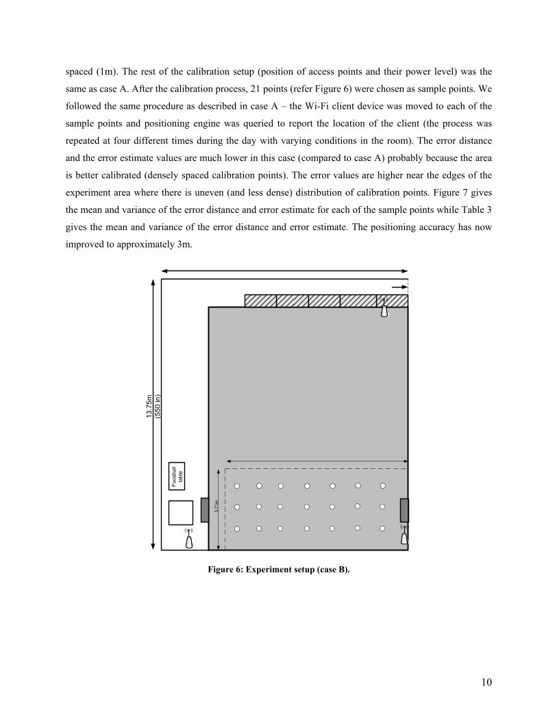
spaced (1m). The rest of the calibration setup (position of access points and their power level) was the

same as case A. After the calibration process, 21 points (refer Figure 6) were chosen as sample points. We

followed the same procedure as described in case A – the Wi-Fi client device was moved to each of the

sample points and positioning engine was queried to report the location of the client (the process was

repeated at four different times during the day with varying conditions in the room). The error distance

and the error estimate values are much lower in this case (compared to case A) probably because the area

is better calibrated (densely spaced calibration points). The error values are higher near the edges of the

experiment area where there is uneven (and less dense) distribution of calibration points. Figure 7 gives

the mean and variance of the error distance and error estimate for each of the sample points while Table 3

gives the mean and variance of the error distance and error estimate. The positioning accuracy has now

improved to approximately 3m.

3.71

m

Foos

ball

tabl

e

13.7

5m

(550

in)

Figure 6: Experiment setup (case B).

11

Mean/Variance of each Sample

0

1

2

3

4

5

6

1 2 3 4 5 6 7 8 9 10 11 12 13 14 15 16 17 18 19 20 21Samples

Met

ers

Mean Err Distance Variance Err Distance Mean Err Est Variance Err Est

Figure 7: Mean/Variance Error Distance and Error Estimate for each sample point.

Table 3: Mean and Variance of Error Distance and Error Estimate for the entire set.

Mean error distance

Variance in error distance

Mean error estimate

Variance in error estimate

2.619 1.386 1.624 0.280

5 The BlueBot System

5.1 BlueBot Setup

Figure 8: BlueBot Setup Figure 9: Samples for a particular tag during robot’s random walk.

Our system uses the Roomba Robotic Floorvac [10] as the robot that moves autonomously in the

sweep space. The Roomba uses intelligent navigation technology to automatically move around the room

without any human direction. The Roomba expects to cover 90% of the room. A server machine running

the positioning engine (PE) tracks our client device (laptop/PDA) that sits on the robot. Figure 8 depicts

the BlueBot setup. The PE is calibrated to work with the access points placed in the corners of the

12

experiment room (case B). The RFID reader is connected to the client device and records all the tags that

it detects as the Roomba moves to different corners of the room. In our experiments, the tagged items

were placed at a height of approximately 4ft from the ground. Whenever the reader detects a tag, the

client machine sends a message containing the tag’s id to the server. The server then notes the current

position of the client and associates it with the detected tag. Our algorithms combine this sample with the

previous samples to refine the position of the tagged item over time. As seen from Figure 9, a tag will be

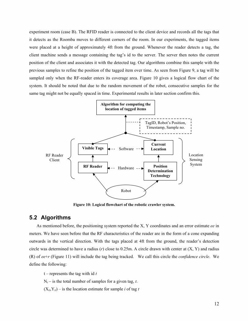
sampled only when the RF-reader enters its coverage area. Figure 10 gives a logical flow chart of the

system. It should be noted that due to the random movement of the robot, consecutive samples for the

same tag might not be equally spaced in time. Experimental results in later section confirm this.

Figure 10: Logical flowchart of the robotic crawler system.

5.2 Algorithms As mentioned before, the positioning system reported the X, Y coordinates and an error estimate ee in

meters. We have seen before that the RF characteristics of the reader are in the form of a cone expanding

outwards in the vertical direction. With the tags placed at 4ft from the ground, the reader’s detection

circle was determined to have a radius (r) close to 0.25m. A circle drawn with center at (X, Y) and radius

(R) of ee+r (Figure 11) will include the tag being tracked. We call this circle the confidence circle. We

define the following:

t – represents the tag with id t

Nt – is the total number of samples for a given tag, t.

(Xti,Yti) – is the location estimate for sample i of tag t

TagID, Robot’s Position, Timestamp, Sample no.

RF Reader Position Determination

Technology

Visible TagsCurrent Location

Algorithm for computing the location of tagged items

Robot

Hardware

SoftwareLocation Sensing System

RF Reader Client

13

eeti – is the error estimate for the positioning report for sample i of tag t

r –is a constant representing the read radius of the RFID reader.

Rti = eeti + r - is the radius of the confidence circle for sample i for tag t. C[(Xti,Yti),Rti] - is the confidence circle for sample i of tag t.

With these in mind, we provide three algorithms to compute the location.

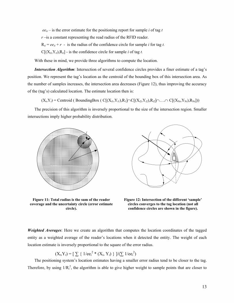
Intersection Algorithm: Intersection of several confidence circles provides a finer estimate of a tag’s

position. We represent the tag’s location as the centroid of the bounding box of this intersection area. As

the number of samples increases, the intersection area decreases (Figure 12), thus improving the accuracy

of the (tag’s) calculated location. The estimate location then is:

(Xt,Yt) = Centroid ( BoundingBox ( C[(Xt1,Yt1),R1]∩C[(Xt2,Yt2),Rt2]∩….∩ C[(XNt,YNt),RNt]))

The precision of this algorithm is inversely proportional to the size of the intersection region. Smaller

intersections imply higher probability distribution.

Figure 11: Total radius is the sum of the reader coverage and the uncertainty circle (error estimate

circle).

Figure 12: Intersection of the different ‘sample’ circles converges to the tag location (not all confidence circles are shown in the figure).

Weighted Averages: Here we create an algorithm that computes the location coordinates of the tagged

entity as a weighted average of the reader’s locations when it detected the entity. The weight of each

location estimate is inversely proportional to the square of the error radius.

(Xt,Yt) = [ ∑ { 1/eei2 * (Xi, Yi) } ]/(∑ 1/eei

2) The positioning system’s location estimates having a smaller error radius tend to be closer to the tag.

Therefore, by using 1/Ri2, the algorithm is able to give higher weight to sample points that are closer to

14

the tag. The accuracy of this algorithm depends more on the estimated position (Xi, Yi) as reported by the

positioning system and also to a large extent on the distribution of samples around the tagged entity. We

assume that with enough samples, this will be averaged out.

Plain Averages: An algorithm that computes the location coordinates of the tagged entity as the statistical

average of the reader’s location when it detected the entity.

(Xt,Yt) = [ ∑ (Xti, Yti) ] / Nt The accuracy of this algorithm is similar to weighted average algorithm. However, since this

algorithm does not take into account the error estimate of the positioning system, the errors in the

estimated location this algorithm will be slightly higher compared to the estimated error for the weighted

average.

Figure 13: Screenshot of our Tag Tracker GUI before convergence (‘X’ marks the actual location of the tags).

Figure 13 shows our tag tracking GUI, which shows the computed positions of detected tags (by the

three algorithms) on a map of the room.

15

5.3 BlueBot Performance We used a large open 12.5m x 13.75m room (Figure 14) to carry out a series of experiments to

examine the performance of our prototype system.

5.3.1 Experiment Set A In the first round of experiments, the positioning engine was calibrated for the entire room as

described in Section 4.2.1. For this setup (as seen in Table 2), the positioning system’s accuracy was

around 4m. The tag placement for this set of experiments is as shown in Figure 14. We recorded the

performance of the three algorithms for this setup for four different runs of the experiment. Figure 15

shows the performance for one such run.

Figure 14: BlueBot setup with non-uniform placement of tags.

16

Error Distance wrt Samples (Tag A)

0

0.5

1

1.5

2

2.5

3

3.5

1 3 5 7 9 11 13 15 17 19 21 23 25 27 29 31 33 35

Sample No.

Met

ers

Plain Weighted Intersection Err Est

a)

Error Distance w.r.t Samples (Tag B)

0

1

2

3

4

5

6

7

1 5 9 13 17 21 25 29 33 37 41 45 49 53 57 61 65

Sample No.

Met

ers

Plain Weighted Intersection Error Estimate

b)

Error Distance wrt Sample (Tag C)

0

0.5

1

1.5

2

2.5

3

3.5

4

4.5

1 6 11 16 21 26 31 36 41 46 51 56 61 66 71 76 81

Sample No.

Met

ers

Plain Weighted Intersection Err Est

c)

Error Distance wrt Samples (Tag D)

0

1

2

3

4

5

6

7

1 6 11 16 21 26 31 36 41 46 51 56 61 66 71 76 81 86

Sample No.

Met

ers

Plain Weighted Intersection Err Est

d)

Figure 15: Error distance convergence w.r.t sample no. for each tag

Distribution of consecutive samples

0

10

20

30

40

50

60

0-30 30-60 60-90 90-120 150-120 180-150 210-180 240-210 270-240 300-270 >=300Time (30 Sec Intervals)

No.

of S

ampl

e (N

orm

aliz

ed)

Exp Run 1 Exp Run 2

Figure 16: Sample distribution w.r.t time for two different experiment runs

It is easy to see that the positioning accuracy of the three algorithms greatly varies between tags. Part

of the reason is due to the large variation in the number of detections for each tag. In our experiments we

started the Roomba from the center of the experiment area. However, we noticed that since it moved in a

random fashion, the number of ‘detection’ samples for each tag is not a uniform distribution. We expect

17

that the averaging effect (from several runs of the experiment) to smooth out the large variation. Figure 16

shows the time distribution between consecutive detections. Since the number of samples per tag per run

is different, the values (per run) have been normalized to be on the same scale.

We define the term error distance as the difference between the estimated location and the actual

location of the tagged item. The three positioning algorithms start with a large error distance and as they

get more samples, they slowly converge to the actual location of the tag. In order to quantify the

performance of our system, we define a convergence point for each tag (in each run of the experiment).

Convergence point can be thought of as the start of the steady state for a tag. Beyond this point, there is

no significant change in the computed coordinates for that tag. For example, the convergence values for

Figure 15 are shown in Table 4. We use convergence values to find the accuracy of our system. Table 5

shows the average time and the average number of samples at which the algorithms converged for each

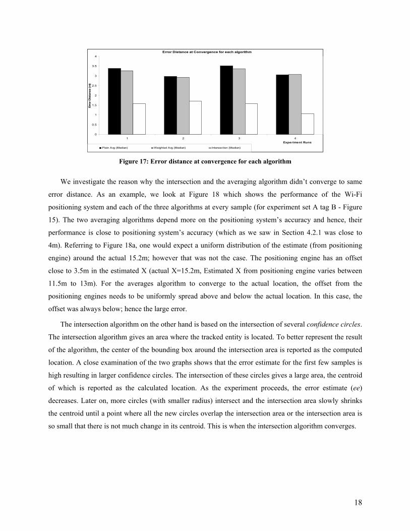
run of the experiment. Table 6 and Figure 17 show the mean and median at convergence for each of the

three algorithms. As we can see from Figure 17, the Intersection algorithm was able to position the tags

with accuracy close to 1.5m. This is almost a three-fold improvement in the accuracy provided by the

positioning system. The two averaging algorithms (plain and weighted), however gave an average error

close to 3.5m.

Table 4: Convergence values for Figure 15

Tag Sample No. Time (sec) Plain (m) Weighted (m) Intersection (m) A 25 1414 1.527 1.510 0.224 B 22 1380 3.478 3.267 1.642 C 19 2430 3.286 3.265 1.4868 D 20 1271 4.5123 4.386 2.583

Table 5: No. of samples and time (sec) at convergence

Run No. No. of samples at Convergence Time at Convergence (sec) Mean Median Std Dev Mean Median Std Dev

1 21.5 21 2.645 1623.75 1397 540.95 2 13.25 14 3.774 1178.25 1169.5 448.973 3 24.25 23 8.845 1706 1553.5 442.621 4 12.75 11.5 6.238 916.75 879 261.515

Average 17.9375 17.375 5.3755 1356.188 1249.75 423.514

Table 6: Error distance at convergence for each algorithm

Run No. Plain Averages Algorithm Weighted Averages Algorithm Intersection Algorithm Mean Median Std Dev Mean Median Std Dev Mean Median Std Dev

1 3.201 3.382 1.239 3.107 3.266 1.188 1.484 1.564 0.969 2 3.120 2.977 1.129 3.088 2.928 1.135 1.735 1.701 0.861 3 3.241 3.513 1.334 3.162 3.360 1.295 1.571 1.587 0.759 4 3.117 3.055 0.793 3.073 3.067 0.745 1.289 1.059 0.576

Average 3.170 3.232 1.124 3.108 3.155 1.091 1.520 1.478 0.791

18

Error Distance at Convergence for each algorithm

0

0.5

1

1.5

2

2.5

3

3.5

4

1 2 3 4Experiment Runs

Erro

r Dis

tanc

e (m

)

Plain Avg (Median) Weighted Avg (Median) Intersection (Median) Figure 17: Error distance at convergence for each algorithm

We investigate the reason why the intersection and the averaging algorithm didn’t converge to same

error distance. As an example, we look at Figure 18 which shows the performance of the Wi-Fi

positioning system and each of the three algorithms at every sample (for experiment set A tag B - Figure

15). The two averaging algorithms depend more on the positioning system’s accuracy and hence, their

performance is close to positioning system’s accuracy (which as we saw in Section 4.2.1 was close to

4m). Referring to Figure 18a, one would expect a uniform distribution of the estimate (from positioning

engine) around the actual 15.2m; however that was not the case. The positioning engine has an offset

close to 3.5m in the estimated X (actual X=15.2m, Estimated X from positioning engine varies between

11.5m to 13m). For the averages algorithm to converge to the actual location, the offset from the

positioning engines needs to be uniformly spread above and below the actual location. In this case, the

offset was always below; hence the large error.

The intersection algorithm on the other hand is based on the intersection of several confidence circles.

The intersection algorithm gives an area where the tracked entity is located. To better represent the result

of the algorithm, the center of the bounding box around the intersection area is reported as the computed

location. A close examination of the two graphs shows that the error estimate for the first few samples is

high resulting in larger confidence circles. The intersection of these circles gives a large area, the centroid

of which is reported as the calculated location. As the experiment proceeds, the error estimate (ee)

decreases. Later on, more circles (with smaller radius) intersect and the intersection area slowly shrinks

the centroid until a point where all the new circles overlap the intersection area or the intersection area is

so small that there is not much change in its centroid. This is when the intersection algorithm converges.

19

Comparison of Actual, Estimated and Algorithm's X

11.5

12

12.5

13

13.5

14

14.5

15

15.5

1 4 7 10 13 16 19 22 25 28 31 34 37 40 43 46 49 52 55 58 61 64Sample No.

Met

ers

1.5

2

2.5

3

3.5

4

4.5

Err E

stim

ate

(m)

ActualX Ekahau Est X PlainX WtdX Intersec ErrEst

a)

Comparison of Actual, Estimated and Algorithm's Y

29

30

31

32

33

34

35

36

1 4 7 10 13 16 19 22 25 28 31 34 37 40 43 46 49 52 55 58 61 64Sample No.

Met

ers

1.5

2

2.5

3

3.5

4

4.5

Err E

stim

ate

(m)

ActualY Ekahau Est Y PlainY WtdY Intersec ErrEst

b)

Figure 18: Comparison of computed/estimated coordinates with the actual coordinates.

5.3.2 Experiment Set B

Figure 19: BlueBot setup with uniform placement of tags.

The calibration setup for our second round of experiments was that of Case B as described in Section

4.2.2. The positioning engine was calibrated to work with the smaller experiment area and the calibration

points were closely spaced. As seen in Section 4.2.2, this setup gave accuracies close to 2.5m (Table 3).

Figure 19 shows the placement of the tags. In this scenario, the positioning technology gave a better

accuracy and had lesser variation in the error estimate. As a result, our averages algorithms performed

better giving us accuracies close to 1m (Figure 23). In most cases, the averages algorithms surpassed the

performance of intersection algorithm by at least 0.5m. Table 7 and Figure 21 shows the computed

location of the tags at the end of an experiment run (same run shown in Figure 20).

20

Error Distance wrt Sample No. (Tag A)

0

1

2

3

4

5

6

71 3 5 7 9 11 13 15 17 19 21 23 25 27 29 31 33 35 37

Sample No.

Err D

ista

nce

(m)

Plain Weighted Intersection Err Est

a)

Error Distance w.r.t Sample No. (Tag B)

0

1

2

3

4

5

6

7

1 4 7 10 13 16 19 22 25 28 31 34 37 40 43 46 49

Sample No.

Err D

ista

nce

(m)

Plain Weighted Intersection Err Est

b)

Error Distance w.r.t Sample No. (Tag C)

0

1

2

3

4

5

6

7

1 4 7 10 13 16 19 22 25 28 31 34 37 40 43 46 49 52 55 58

Sample No.

Err

or D

ista

nce

(m)

Plain Weighted Intersection Err Est

c)

Error Distance wrt Sample No. (Tag D)

0

1

2

3

4

5

6

7

1 4 7 10 13 16 19 22 25 28 31 34 37 40 43 46 49 52 55

Sample No.

Err D

ista

nce

(m)

Plain Weighted Intersection Err Est

d)

Figure 20: Error distance convergence w.r.t to sample no. for each tag

Table 7: Location coordinates of tags as computed by the three algorithms (for Figure 20)

Tag ID Actual (X, Y) Plain Weighted Intersection A (1,2) (1.55, 1.86) (1.43, 1.80) (2.99, 3.02) B (3,2) (2.94, 1.45) (2.86, 1.50) (4.01, 2.47) C (5,2) (4.35, 1.29) (4.80, 1.33) (6.24, 2.35) D (7,2) (4.99, 1.31) (5.32, 1.41) (6.62, 2.22)

Figure 21: Position of tags as computed by the three algorithms (for Figure 20)

21

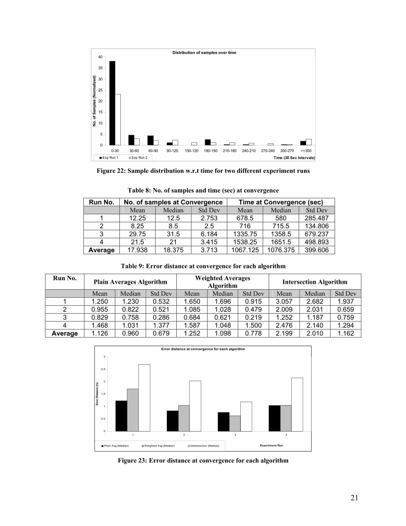
Distribution of samples over time

0

5

10

15

20

25

30

35

40

0-30 30-60 60-90 90-120 150-120 180-150 210-180 240-210 270-240 300-270 >=300

Time (30 Sec Intervals)

No.

of S

ampl

es (N

orm

aliz

ed)

Exp Run 1 Exp Run 2

Figure 22: Sample distribution w.r.t time for two different experiment runs

Table 8: No. of samples and time (sec) at convergence

Run No. No. of samples at Convergence Time at Convergence (sec) Mean Median Std Dev Mean Median Std Dev

1 12.25 12.5 2.753 678.5 580 285.487 2 8.25 8.5 2.5 716 715.5 134.806 3 29.75 31.5 6.184 1335.75 1358.5 679.237 4 21.5 21 3.415 1538.25 1651.5 498.893

Average 17.938 18.375 3.713 1067.125 1076.375 399.606

Table 9: Error distance at convergence for each algorithm

Run No. Plain Averages Algorithm Weighted Averages Algorithm Intersection Algorithm

Mean Median Std Dev Mean Median Std Dev Mean Median Std Dev 1 1.250 1.230 0.532 1.650 1.696 0.915 3.057 2.682 1.937 2 0.955 0.822 0.521 1.085 1.028 0.479 2.009 2.031 0.659 3 0.829 0.758 0.286 0.684 0.621 0.219 1.252 1.187 0.759 4 1.468 1.031 1.377 1.587 1.048 1.500 2.476 2.140 1.294

Average 1.126 0.960 0.679 1.252 1.098 0.778 2.199 2.010 1.162

Error distance at convergence for each algorithm

0

0.5

1

1.5

2

2.5

3

1 2 3 4

Experiment Run

Err

or D

ista

nce

(m)

Plain Avg (Median) Weighted Avg (Median) Interesection (Median)

Figure 23: Error distance at convergence for each algorithm

22

A special note about run 1 in this set: during this run, access point 1 was blocked by a folded ping-

pong table placed in front of it. This change in the environment altered the signal strength map of the

room and hence affected the positioning system’s accuracy. As a result, the three algorithms have a

relatively higher error distance. This illustrates the inability of the (signal strength-based) positioning

system’s to adapt to change in environmental conditions. Some tracking applications may require

recalibration of the room to accommodate the change in the signal strength pattern.

6 Conclusion and Future Research In this paper, we have presented an inexpensive automated indoor asset tracking system called

BlueBot. This prototype system works by making use of any off-the-shelf location positioning system and

passive RFID technology. Beyond simply providing a novel mechanism to track tagged items, our

experiments have shown that our positioning algorithms can bring a three-fold improvement on the raw

accuracy provided by the positioning technology. We also found that the intersection algorithm worked

better than the two averages algorithm when the positioning system was not very accurate. In the case

where the positioning system had high accuracy, the averages algorithm out-performed the intersection

algorithm. We are look at new algorithms that can average out the offset in the raw location reported by

the positioning system.

In our current system, there is a high variation in the amount of time and number of samples required

to converge to a certain level of accuracy. In the future, we are planning to reduce this variation by using

a robot that can be controlled to move in a directed pattern. We have considered employing a feedback

system; so that the direction of the robot is controlled by the RF system. A dual-variable gain antenna

system can be used such that the high gain antenna controls the movement of the robot until its low gain

partner sees the tag being hunted. We noticed that signal strength based Wi-Fi systems are easily affected

by changes in the surroundings. In the future we plan to make use of systems that are immune to

environmental changes (perhaps TDOA based positioning systems) and analyze the performance of our

BlueBot system. Another approach would be to continue to use Wi-Fi signal strength, but add reference

RFID tags through the environment that could be used to remove any positional offsets that might be

present relative to the original calibration. We are also looking at various ways to make 3D positioning

possible.

7 Acknowledgments We thank Sastry Duri and Amaresh Rajasekharan at IBM Watson for their assistance and ideas. We

also thank Intermec for donating a PCMCIA card reader and its software.[17, 19, 21]

23

8 Reference [1] "AeroScout (formally BlueSoft)."http://www.aeroscout.com/ [2] "The Bat Ultrasonic Location System."http://www.uk.research.att.com/bat/ [3] "BlueTags."http://www.bluetags.com/ [4] "The Cricket Indoor Location System."http://nms.lcs.mit.edu/projects/cricket/ [5] "Ekahau Positioning System."http://www.ekahau.com/ [6] "HP Cooltown project."http://www.hpl.hp.com/archive/cooltown/ [7] "Intermec UHF PC Reader."http://www.intermec.com/ [8] "Multispectral Solutions, Inc."http://www.multispectral.com/ [9] "Radianse Indoor Positioning."http://www.radianse.com/ [10] "Roomba Robotic Floorvac."http://www.roombavac.com/ [11] "Ubisense Limited."http://www.ubisense.net/ [12] "Versus Technology."http://www.versustech.com/ [13] "WhereNet location tracking systems."http://www.wherenet.com/ [14] P. Bahl and V. N. Padmanabhan, "RADAR: An In-building RF-based User Location and Tracking

System," IEEE INFOCOM, March, 2000 [15] M. Chiesa, R. Genz, F. Heubler, K. Mingo, C. Noessel, N. Sopieva, D. Slocombe, and J. Tester,

"RFID," Mar, 2002. http://people.interaction-ivrea.it/c.noessel/RFID/RFID_research.pdf (also see /RFID_timeline.pdf) [16] P. Enge and P. Misra, "Special Issue on GPS: The Global positioning System," Proc. of the IEEE,

Jan 1999 [17] A. Haeberlen, E. Flannery, A. Ladd, A. Rudys, D. Wallach, and L. Kavraki, "Practical Robust

Localization over Large-Scale 802.11 Wireless Networks," Mobicom 2004, September, 2004 [18] J. Hightower and G. Borriello, "A Survey and Taxonomy of Location Sensing Systems for

Ubiquitous Computing," University of Washington, Department of Computer Science and Engineering, Seattle, WA, Aug 2001 CSE 01-08-03,

[19] J. Hightower, R. Want, and G. Borriello, "SpotON: An Indoor 3D Location Sensing Technology Based on RF Signal Strength," UW CSE 00-02-02, Feburary, 2000

[20] L. M. Ni, Y. Liu, Y. C. Lau, and A. Patil, "LANDMARC: Indoor Location Sensing Using Active RFID," IEEE PerCom, March, 2003

[21] D. Niculescu and B. Nath, "VOR Base Stations for Indoor 802.11 Positioning," Mobicom 2004, September, 2004

[22] G. Roussos, "Location Sensing Technologies and Application," Nov 2002. http://www.jisc.ac.uk/uploaded_documents/tws_02-08.pdf [23] J. Small, A. Smailagic, and D. Siewiorek, "Determining User Location For Context Aware

Computing Through the Use of a Wireless LAN Infrastructure," Dec 2000 [24] P. Steggles and J. Cadman, "A Comparison of RF Tag Location Products for Real-World

Applications," Ubisense March 2004.http://www.ubisense.net/technology/files/A comparison of RF Tag location products for real world applications - March 2004.pdf

[25] R. Want, A. Hopper, V. Falcao, and J. Gibbons, "The active badge location system," ACM Transactions on Information Systems, Jan. 1992

[26] M. Youssef, A. Agrawala, and A. U. Shankar, "WLAN Location Determination via Clustering and Probability Distributions," IEEE PerCom, March, 2003