Blind Channel Identifiability for Generic Linear Space-Time Block Codes

202 IEEE TRANSACTIONS ON SIGNAL PROCESSING, VOL. 55, NO. 1, JANUARY 2007

Blind Channel Identifiability for Generic LinearSpace-Time Block Codes

Nejib Ammar, Member, IEEE, and Zhi Ding, Fellow, IEEE

Abstract—Linear space-time block codes (STBCs) have proventheir effectiveness in performance improvement of wirelessmultiple-input multiple-output communication systems. Theirsuccessful decoding, however, requires reliable channel knowledgeat the receiver. In this paper, we present a semiblind channelestimation method for linear STBC without the usual code or-thogonality condition. We provide a set of identification conditionsthat are mostly verifiable a priori in terms of code parameters andantenna array configuration. We also present a simple channelestimation algorithm. Finally, we provide simulation results thatillustrate the performance of the proposed scheme.

Index Terms—Blind estimation, channel identifiability, MIMOchannel, space-time codes.

NOMENCLATURE

Transpose operation.

Conjugate transposeoperation.

, Complex conjugation.

, Two-norm, Frobinuis norm,respectively.

th entry of matrix .

identity.

Column space of .

Right null space of .

Trace of .

Vector form of .

Kronecker product of and.

Expected value of a RV .

card Cardinality of finite set.

I. INTRODUCTION

THE rapid popularization of multimedia services and In-ternet-driven applications over wireless links are fueling

the increasing demand for reliable and high-speed communi-

Manuscript received September 13, 2004; accepted February 10, 2006. Thiswork was supported by the National Science Foundation under Grants ECS-0121469, CCF-0515058, CNS-0520126, and DMI-0400155 and by the U.S.Army Research Office under Grant W911NF-05-1-0382. The associate editorcoordinating the review of this manuscript and approving it for publication wasProf. Alex B. Gershman.

The authors are with the Department of Electrical and Computer Engineering,University of California Davis, Davis, CA 95616 USA (e-mail: [email protected]; [email protected]).

Digital Object Identifier 10.1109/TSP.2006.882089

cation solutions. In order to meet this high demand for wirelessservices, we face a number of particularly challenging problemsdue to the limited radio bandwidth and severe channel impair-ment common to wireless systems.

One recently popular and successful technique in wirelesscommunications to combat severe channel fading and dis-tortions is the exploitation of multiple-input multiple-output(MIMO) system diversity that relies on multiple transmit (Tx)and receive (Rx) antennas. Unlike single-input single-output,MIMO systems can potentially offer significant channel ca-pacity improvement and can efficiently combat channel fadingin mobile wireless systems [1]. As a practical mechanism,space-time coding (STC) proves effective in MIMO systems[2], [3]. Between space-time trellis codes (STTCs) [4] andspace-time block codes (STBCs), STBCs are particularlyattractive due to their simpler transceiver structure. They arerelatively easier to encode and often admit lower complexitydecoders.

Since Alamouti first introduced his now well-known code [5],a myriad of linear STBC proposals have emerged. These includethe popular orthogonal codes (O-STBCs) [6], the nonorthogonalSTBCs (NO-STBCs) [7], [8], the quasi-orthogonal codes (QO-STBCs) [9], the diagonal algebraic (DAST) [10], and the dif-ferential space-time codes (DSTCs) [11], to name a few. WhileDSTC can bypass the need for channel information as the dataare differentially encoded and decoded at the cost of a 3 dBsignal-to-noise ratio (SNR) loss, most of the remaining varietyof STCs require the knowledge of the channel at the receiverend in order to recover the transmitted signals.

To assist receivers in estimating an unknown and potentiallyslowly time-varying MIMO channel, traditional approaches re-quire receiver training during which pilot symbols known to thereceiver are either inserted between data packets [12] or super-imposed over information data [13]. A comprehensive study ontraining strategy for STBC MIMO channels can be found in [13]and [14]. Often, the training overhead in terms of rate loss orpower loss can be significant.

We study semiblind and blind methods for bandwidth effi-ciency and power conservation. There are generally two maintypes of (semi)blind methods to recover the channel input. Thefirst type consists of equalizers that aim at restoring the channelinput from the observation data by utilizing filters that com-pensate for the channel effects without directly identifying thechannel. Examples of such methods in the context of STBC in-clude the work of Swindlehurst [15] and [16], who proposed analgorithm that exploits the structure induced by the generalizedspace-time block codes to obtain zero-forcing equalizers of theMIMO channel. Another example is the work of [17], which

1053-587X/$20.00 © 2006 IEEE

AMMAR AND DING: BLIND CHANNEL IDENTIFIABILITY FOR GENERIC LINEAR SPACE-TIME BLOCK CODES 203

features a clairvoyant maximum likelihood (ML) detector. Thesecond type involves the identification of the underlying channelresponse before integrating it in an appropriate equalizer filteror ML sequence estimation metrics. For STBC systems, Ammarand Ding proposed a subspace-based approach to directly esti-mate the channel matrix specific for O-STBC by exploiting theorthogonal designs of STBC to obtain a closed-form channelestimate [18], [19]. This method was later extended to time-re-versal STBC [20]. Another approach that leads to a closed-formchannel estimate in the case of O-STBC was also proposed by[21] and [22].

In this paper, we generalize our blind channel estimation of[18] to cover a much broader class of general linear STBCs.While Swindlehurst’s work was concerned with channel equal-ization, we concentrate in this paper on channel identification.In addition, unlike the work Shahbazpanahi, which tends to em-phasize the novelty of their scheme but fails to provide the iden-tifiability requirements, we derive new channel identificationconditions that are comprehensive and mostly verifiable a prioriaccording to the known STBC parameters and the antenna con-figuration, not to mention that their method is limited to thecase of orthogonal STBC. Furthermore, we characterize andquantify, for channels that are not uniquely identifiable, residualambiguities from using the blind algorithm. We show that, inessence, our blind estimation generates a subspace in which thechannel resides, leading to a vector ambiguity. Naturally, fullchannel equalization often requires the complete removal of anyresidual uncertainty for full effectiveness. To completely resolvethe scalar ambiguity for uniquely identifiable channels or thevector ambiguity for nonunique identifiable channels, we pro-pose a semiblind scheme that integrates blind channel estima-tion with a shorter sequence of training pilots. At this point, wewould like to stress that despite the merit of the blind algorithmand its semiblind extension, a more important contribution ofthis paper lies in the characterization of channel identifiabilityconditions.

II. SYSTEM MODEL

A. Notations

We adopt mostly standard notations in this paper. Uppercaseand bold letters denote matrices, and lower case letters with anarrow atop denote vectors.

B. Channel Model

We consider a wireless link with transmit and receiveantennas. Representing the flat fading channel is ancomplex matrix , whose entry is the channel responsefrom the transmit antenna to the receive antenna. Wemay decompose into the sum between a static componentrepresenting the line of sight and a fading component repre-senting the scattered component. To approximate a (relatively)slow fading channel, we assume a quasi-static fading model,such that the channel remains unchanged over a fixed numberof signaling intervals, before it changes to a new independentrealization [6].

C. Signal Model

For convenience of presentation, we use the following signaldescription. Space-time block coding technique maps a datavector with symbol entries into an ,code matrix , where is the time diversity of the code. Eachcolumn of is a linear mapping of the real part and the imag-inary part of the symbol vector . In other words, each of the

columns in is given by

Here, and form a set of fixed complex valuedmodulation matrices known to both the transmitter and receiver.For quasi-static flat fading channels, a primary performancemeasure of the STBC is the minimum rank of the differenceof any two codeword matrices denoted by [23]. The rateof in symbols per channel use is given by 1 ,where is the size of constellation of the data symbols.

The columns of the code matrix are transmitted inepochs by the Tx antennas. Assuming that the channel isconstant over the epochs and that the reception is corruptedby additive complex white Gaussian noise with power , theoverall received signal is given by

......

(1)

where is the noise vector. If we further let the channel remainconstant over received data symbol vectors , each withcodeword epochs, and collect the received vectors as expressedin (1), we obtain the following receive matrix:

(2)

where we have a channel output signal matrix and a2 data symbol matrix given by

Here the subscripts of and are used to index the block trans-mission of symbols. The noise matrix con-tains the noise vectors.

With these representations, the famous Alamouti code [5]designed for and effectively has

, . Stacking

the received signals from the two epochs results in

noise, where the channel is as-

sumed constant over the two epochs.

III. SUBSPACE CHANNEL IDENTIFICATION

The basic steps in subspace channel estimation are describedin [18]. We will present a set of identification conditions touniquely estimate the channel matrix for general,


linear, and nonorthogonal STBC. We will initially neglect thenoise presence and address its effect later.

The basic algorithm for subspace channel estimation, as de-tailed in [18], can be applied to linear STBC by first extractinga basis for the left null space of without noise. With apersistently exciting data matrix (i.e., with full row rank), weobtain

(3)

The solution of this homogeneous linear equation allows estima-tion of , whose uniqueness depends on both and the codematrix .

A. Uniqueness and Identifiability

Although the subspace channel estimation method is simpleand was first given in [18], the uniqueness and channel identi-fiability conditions differ for different choices of STBC. Here,we study the case of generic linear STBC.

Let be another solution to (3), i.e.,

Clearly lies inside the right null space ofbut does not necessarily span this entire subspace, that is

Therefore, there exists a complex matrix such that

(4)

Note here that is not necessarily of full rank. In fact it admitsfull rank if and only if

.For yet a more explicit relationship between and , (4) is

rearranged as follows:

If has full row rank, then is invertible. With this as-sumption in mind, postmultiplication by leadsto

(5)

The matrix in the last equation,parameterized by , is in fact the channel ambiguity fromchannel estimation based on the linear (blind) equations in(3). It is this ambiguity condition that defines uniqueness inchannel estimation. Substituting back into (4), we obtain the

following requirements on ambiguity matrix in terms of theactual channel matrix and the code parameters :

(6)

Thus, (5), in conjunction with (6), describes the complete set ofsolutions to (3) in terms of the actual channel matrix andan unknown complex square matrix .

We use a well-known Kronecker product property

This property allows us to express the linear equations of (6)as

We can stack all equations vertically to form

(7)

where

...

Similarly, we write (5) as

(8)

where

Thus far, we have expressed all possible solutions to the blindchannel equations (3) in terms of (7) and (8). Clearly,

is always a solution. If is shown to be unique up to ascalar, then the unknown channel is (uniquely) identifiable fromthis estimation approach. Based on this observation, we nowinvestigate the main identification condition.

B. Main Identification Theorem

Our main goal here is to provide a necessary and sufficientchannel identification condition such that is uniquely deter-mined (up to a scalar ambiguity). Before continuing, we would


like to state the following two simple properties about matrixrank that will be needed to establish our results.

1) : If and are two complex matrices having thesame number of rows, then

rank rank rank

(9)

2) [24]: Given two complex matrices and of ap-propriate dimensions, then

rank rank (10)

Back to channel uniqueness, we denote by the channelspace formed by the solution set of the channel equations (7)

and (8) in terms of the unknown vector . With regard to channelidentifiability, we are particularly interested in the rank of .Specifically, the channel is uniquely identifiable up to a com-plex scalar ambiguity (i.e., , ) if and only if

.In order to determine , consider the augmented

channel equation formed by assembling (7) and (8)

(11)

Due to theone-to-onecorrespondencebetween and, where denotes the linear space

formed by the augmented channel vector of (11).The augmented channel space can be described as

(12)

While the first part on the right-hand side of (12) is directly im-plied from (11), the second part further asserts that

means , where has the same dimension as . Infact, we can easily show that if

then , hence satisfying (12). The converse is obvious.Therefore, a straightforward application of the matrix property

in (9) to (12), yields the following expression for the dimen-sion of the channel subspace:

rank

rank

rank (13)

Using the fact that for any two complex matrices and ofappropriate dimensions, we have that

rank rank rank

the right-hand side of (13) can be further simplified, hence re-sulting in

rank

rank

rank rank

rank

rank (14)

We are now in a position to state the following theorem aboutchannel identifiability.

Theorem 1: Suppose that has nontrivial left null space andthat has full row rank. Then, the channel is uniquely identifi-able up to a complex scalar ambiguity if and only if

rank rank

C. Remarks

Theorem 1 provides a necessary and sufficient condition forthe uniqueness of channel estimate using the subspace method.Naturally, the estimation is possible only if is not trivial(zero). In addition, it is assumed that is of full row rank. Awell-designed STBC typically meets this requirement. In fact,by recalling that an STBC may be expressed as

we come to realize that if fails to have full row rank, i.e.,rank , its row rank deficiency rank representsthe number of wasted transmit diversity degrees. In other words,it represents the number of redundant Tx antennas deployed bythe system. Naturally, such a code design would be undesirable.

It should also be noted that in addition to describing thechannel identifiability condition, (14) further quantifies theuncertainties inherent in estimating based on (3). In fact, itdefines the number of linearly independent solutions (channelestimates) for (3). This broader understanding of channel uncer-tainties is of particular importance when the channel cannot beestimated blindly and partial training is needed. The number ofindependent solutions to (3) would potentially shape the trainingstrategies to resolve the ambiguities. We will address this pointlater in discussing a semiblind channel estimation procedure.

From a pragmatic point of view, the identifiability theorem,though necessary and sufficient, has limitations. In particular,without knowing the wireless channel, one would like to definethe class of identifiable channels using only the code informa-tion. Fortunately, most channels under considerations are ofrandom distribution (Rayleigh and Ricean). Most often, the rankof depends almost entirely on the number of transmit andreceive antennas, i.e., rank with probabilityone. This channel richness property will help us to obtain a code-dependent verifiable identification condition from Theorem 1.

IV. CODE VERIFIABLE IDENTIFICATION CONDITIONS

Based on the main result stated in Theorem 1, our goal inthis section is to extract identification conditions that are easyto verify based on code information without involving the un-known channel coefficients.


A. Full Column Rank Channels

We proceed by applying the rank expansion in (10) to (14),which yields the following relationship:

rank rank

(15)

It is to be noted here that the expression above holds, regardlessof the channel rank. One immediate consequence of (15) is thatif has full column rank, then

(From here on subscripts of the zero vector will be dropped.)Consequently, the following statement is true:

If rank then (16)

Thus, we obtain the following corollary.Corollary 1: Let have nontrivial left null space. Suppose

that the channel matrix has full column rank and has fullrow rank. Then, without any (finite alphabet) constraint on thedata symbols, the channel is uniquely identifiable up to a com-plex scalar ambiguity from the channel output signals if andonly if .

The condition of having full column rank allows us to de-couple the effect of channel from the identifiability condition of(15). Thus, the channel identifiability rests solely on the STBC.Under such circumstances, the channel fails to be uniquely iden-tifiable entirely because of a fundamental ambiguity associatedwith the particular STBC design. This inherent ambiguity is ob-viously quantified by .

B. Examples

Consider, for instance, the case of Alamouti code . The rankdifference actually equals four for complex data symbols andtwo for real data symbols. For complex symbols, we notice [15]that, if is any 2 2 invertible complex matrix having the sameform as , then also has the same structure as , i.e.,

if then

In fact, by assuming and , wehave a pair of new symbols for transmission

To see the relevance of this observation on the channel identi-fiability, the received data matrix corresponding to (withoutnoise) can be written as

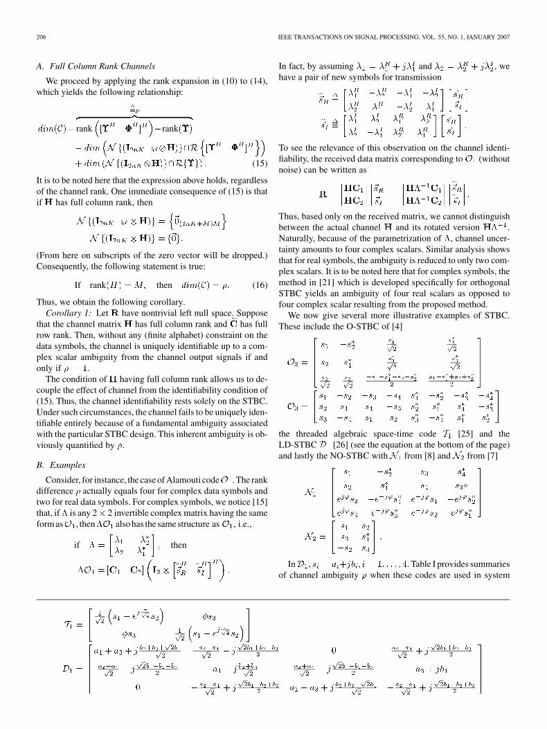
Thus, based only on the received matrix, we cannot distinguishbetween the actual channel and its rotated version .Naturally, because of the parametrization of , channel uncer-tainty amounts to four complex scalars. Similar analysis showsthat for real symbols, the ambiguity is reduced to only two com-plex scalars. It is to be noted here that for complex symbols, themethod in [21] which is developed specifically for orthogonalSTBC yields an ambiguity of four real scalars as opposed tofour complex scalar resulting from the proposed method.

We now give several more illustrative examples of STBC.These include the O-STBC of [4]

the threaded algebraic space-time code [25] and theLD-STBC [26] (see the equation at the bottom of the page)and lastly the NO-STBC with from [8] and from [7]

In , , . Table I provides summariesof channel ambiguity when these codes are used in system


TABLE ISUMMARY OF r AND r FOR DIFFERENT STBCS: COMPLEX SYMBOLS

with Tx antennas rank for complex and realdata signals. We set the parameters and

. The N-STBC is obtained by deleting the fourthrow of (equivalent to disabling the fourth Tx antennas).

C. Column Rank Deficient Channels

We now consider the special case of rank deficient channels.When is column rank deficient, there are two reasons forchannel uncertainties. The first cause has already been identi-fied as the inherent ambiguity from the STBC itself. The secondcause, which is more challenging to quantify, stems from the in-teraction of the STBC parameters with the unknownchannel coefficients. Recall the expression of the channel sub-space dimension from (15), which for convenience is rewrittenhere

Then, the residual term

is associated with the second source.Generally, in order to determine this term, one needs to know. However, because , the more pressing question is

whether or not such a residual term actually exists. In otherwords, we need to determine the circumstances under which wehave equality

(17)

Since we do not know the channel parameters, we will restrictourselves to the case where the dimensions in (17) are equal tozero. That is, we will determine the conditions under which thefollowing system holds true:

(18)

To begin the derivation, first suppose that there exists anonzero . This means that

such that(19)

The relationships in (19) can be reordered as

(20)

in which is the 2 matrix from and ,, are 2 submatrices of such that

. Define the following minimumrank:

rank (21)

which in simple terms means that is the min-imum rank of the nonzero matrix if . Then,the rank of in (20) is bounded by

rank rank (22)

The right-hand side inequality in (22) clearly follows from thefact that lies in the right null space of , which hascolumns. Consequently, if rank , then thereexists no to fulfill (20). In other words

if rank

(23)

Similarly

if rank

then

(24)

Here, is defined analogously to via

rank (25)

where the 2 matrix and thesubmatrices came from .

In light of (15), we combine (23) and (24) to finally deducethat

if rank then

(26)


In Appendix A, we show that if , then. Finally, we can now state the following corollary for rank-

deficient channels.Corollary 2: Suppose that has nontrivial left null space

and has full row rank. If rank , then thechannel is uniquely identifiable from the channel output data upto a complex scalar ambiguity if and only if .

It is clear that Corollary 2 generalizes the identification resultof Corollary 1. Indeed, if has full column rank, it promptlyfulfills the requirement rank as .

One more interesting consequence of Corollary 2 can beobserved for random channels. If , then the minimumnumber of Rx antennas needed to guarantee channel identifia-bility regardless of its coefficients is . To seethis, consider the following tighter upper bound for rankin (22) given by rank rank , where is apositive integer defined by

rank rank

The number of Rx antennas needed to guarantee, irrespective of the channel coefficients,

requires that . Due to the randomness of, has full row rank with probability one, i.e. . Hence

.From a broader perspective, one can generally determine the

minimum number of Rx antennas as a function of andto guarantee the channel ambiguity to be of minimum rank, (i.e.,

. But one first has to be able to calculate thesecrucial ranks. In the following, we will provide a simple proce-dure to evaluate (the extension of this procedure to isstraightforward). The method is based on the following lemma.

Lemma 1: The minimum rank satisfies

cardsubject to

rank rank(27)

where and matrix is formed by verticallyconcatenating the elements of .

Proof: See Appendix B.In order to evaluate , the optimization problem in (27) is

resolved by a rather simple searching algorithm to obtain .We first consider index sets with cardinality 2 1 (i.e.,

is obtained by deleting one , from ).If the rank inequality in (27) is fulfilled, then the search stopsand is reported. If, however, all possible index sets are ex-hausted without success, the cardinality of candidate index set

is reduced by one and the search process starts over. Since, this procedure is carried over until either is

reported or card without success. In thelatter case, . Table I summarizes the values ofand for the STBCs mentioned in the previous sections.

V. CHANNEL ESTIMATION ALGORITHMS

We now describe two proposed algorithms to estimate thechannel matrix. The first algorithm is blind and can be applied

to identifiable channels. However, it will lead to a channel esti-mate with an unknown scalar ambiguity. The second algorithmis semiblind and targets primarily unidentifiable channels butcan also be used with identifiable channels to resolve the scalarambiguity.

A. Blind Algorithm

The blind algorithm we consider here is basically the same asthe one we proposed in [18]. For derivation, we recall the blindequation in (3) and express it in a vector form

(28)

We then conveniently write

...

(29)

By substituting (29) back in (28) and after a simple manipula-tion, we obtain the following relationship:

(30)

Clearly, when is noise-free, the right null space ofwill contain the channel vector . Thus, if the channel is

uniquely identifiable up to a scalar, i.e., , then theactual channel vector must span .

Since in reality we only have access to a noisy , which con-tains additive uncorrelated white Gaussian noise as illustratedby the model in (4), we ought to separate the signal and noisesubspaces as in standard subspace approaches [27], via singularvalue decomposition (SVD). Specifically, the noise subspace of

is spanned by those left singular vectors from SVD that cor-respond to the smallest singular values of .

We propose two ways to calculate . The first way is analyt-ical as illustrated by the following result.

Lemma 2: If rank , where

rank

then rank .Proof: See Appendix C.

Again, can be calculated by the procedure devised for. If, however, the condition in Lemma 2 is not met, i.e., the

number of Rx antennas , we resort to estimatingthrough a simulation-based method. Because the channels we

are dealing with are random with known distribution models,we can simulate the system off-line without noise to obtain anestimate for .

Finally, an estimate of the channel vector is obtainedby the singular value decomposition of in (30). Specifically,


when the unique identifiability condition is satisfied, the rightsingular vector that corresponds to the least singular value of

is collinear to . Hence the channel estimate only has a re-maining scalar ambiguity inherent to the blind algorithm. Itcan be resolved with minimum training, as will be discussedlater when presenting our semiblind estimations algorithm.

B. Semiblind Algorithm

Let us recall the blind channel equations in (30), obtained fora noise-free receive matrix. When the channel is not uniquelyidentifiable, the column rank deficiency of is

. Consequently, if is anorthonormal basis of , then the channel vector in (30) isexpressed as

(31)

where is a 1 complex vector and(hence, ). Therefore,

the channel estimate obtained based simply on has an ambi-guity vector .

In order to completely identify the channel, additionalinformation on is needed to assist the blind algorithm.These additional (linear) equalities may be acquired by partialtraining, where some pilot symbols known to the receiver aresent through the channel. More precisely, for each channelrealization, the transmission undergoes a training phase whichlasts signaling intervals and a regular data transmission phaselasting intervals as discussed earlier. At this point, it isassumed that the block fading lasts a total of symbol in-tervals (a deviation from the assumption we started with, whichassume that the channel is constant over symbol intervals).In addition, it is assumed that the noise characteristics and thetransmission power remain constant during both phases.

The training phase consists in sending an matrixof training symbols over the allocated time slots. The corre-sponding receive signal is an matrix given by

(32)

where is the noise matrix of the training phase. The trainingand data symbols do not necessarily have to originate from thesame symbol constellation. We can, for instance, choose to havethe training symbols coming from a constant envelop constella-tion (APSQ). Additionally, since the receive signal at a partic-ular Rx antenna is a linear superposition of the transmitted sig-nals, is selected to have orthogonal rows. The orthogonalitycriteria for is employed by [12] in a purely training-basedchannel estimation for the same type of channels we are con-cerned with. Their channel estimator achieves the Cramér–Rao(CR) lower bound. It was also shown by [14] that this criterionoptimizes the channel capacity bound.

To integrate the blind and the training equation, we rewrite(32) in vector form

(33)

We then substitute (31) in (33) to obtain

(34)

Notice how, by combining the blind and training equations, theproblem of estimating the channel coefficients is trans-formed into estimating , which has parameters. As-sume that the training symbols are chosen from a constant en-velop constellation; hence , where isthe symbol power. Then, the ML estimate of amounts to

(35)

Substituting back in (31) amounts to the following channelvector estimate:

(36)

In light of (36), the semiblind algorithm implementationbuilds upon the blind algorithm. We first obtain the matrix

by the blind method. We then perform singular value de-composition on and construct from theeigenvectors in that correspond to the least eigen-values. Finally, the channel estimate is obtained by the formulain (36). Notice here that the procedure is equally applicable toidentifiable systems where the blind algorithm retains a scalarambiguity, and to unidentifiable systems as well. One integralpart of the algorithm is the value for . We have furnishedin (14) and (26) the general formula which may require thechannel parameters and a verifiable formula, respectively, for

. In the case where the number of Rx antennas does notcomply with the prerequisite of (26), we can evaluatenumerically based on Monte Carlo simulation of (14).

VI. PERFORMANCE BOUND

In this section, we would like to evaluate the performance ofour semiblind approach to channel estimation. Since the puretraining approaches of [12] coincide with our training phase,and because the method reaches the CR bound, we will use itsmean square error (MSE) as our benchmark.

The training equations in [12] are identical to (32). With, the ML estimate of the channel vector is

given by

(37)

The corresponding estimation error

(38)

is a zero-mean circular symmetric complex Gaussian randomvariable with variance . Hence the unbiased es-


timate in (37) achieves the least variance promised by the CRbound. The MSE amounts to

(39)

In our proposed semiblind channel identification, the overallestimation error is an accumulation of error from the estimationof and error from estimating . Despite the fact that botherrors stem from the noise and finite data length, the overallerror is in fact dominated by the error associated with . Thereason is that is obtained using more data points. In order toobtain a lower bound on the overall estimation error, we assumethat the number of observation windows is large enough (withtending to infinity) and that is obtained error free. It followsthat the estimation error is given by

(40)

which is again Gaussian with zero mean, and covariance equalsto . The mean square error is then given ap-proximately by

(41)

Hence, from (39) and (41), the ratio of MSE (MSER) betweenthe semiblind algorithm and that of the training method is ap-proximately lower bounded by ML.

VII. SIMULATION RESULTS

To demonstrate the efficiency of the proposed MIMO channelestimation scheme, we provide a few simulation examples. Theperformance criterion is the normalized mean square error

NMSE

where is the channel matrix estimate obtained after resolvingthe ambiguities (the final output of the semiblind algorithm),and the symbol error rate (SER) that we expect to achieve byintegrating in a maximum likelihood decoder.

The channel matrix components and of theRicean flat fading channel matrix are generated according tothe following model:

with denoting the Ricean -factor (the ratio of power of theLOS component to the mean power of the NLOS component).Additionally, the pseudostatic component changes to anew independent realization for every signaling in-terval. The expected transmit power at each Tx element is nor-malized to one. The power of the additive white Gaussian noiseis set to 2 SNR per complex dimension. As mentioned ear-lier, the transmit power and noise characteristics for the regular

transmission and the training phase are identical. However, thetraining signals are binary phase-shift keying (BPSK) symbolsregardless of the information data constellation.

Throughout the simulation, we proceed by first processing thereceived signal matrix that corresponds to the informa-tion symbols to obtain with the help of the blind algorithm.At this stage, the parameters and will be determinedas discussed. The Ricean factor is assumed to be unknown.Next, the received data corresponding to the training inputsequence are employed to resolve the channel ambiguities. Inorder to generate the NMSE and the MSER, we average over5000 Monte Carlo (MC) random runs. For the detection perfor-mance, we measure the SER from the ML decoder using theestimate of the current channel realization . The number ofMC runs is set to obtain at least 100 errors for each SNR value.

A. Uniquely Identifiable Channels

1) Example A.1: We consider a wireless system that isequipped with three Tx antennas and utilizes orthogonal STBC

in conjunction with 16-QAM data signals. The number ofRx antennas may vary.

Based on Table I, we see that a Ricean fading channel isuniquely identified for any number of Rx antennas

so long as the receive matrix minus noise has a non-trivial left null space. On the other hand, for any number of Rxantennas , the dimension of such space isgiven by . Hence, we can apply the channel estima-tion procedure for any . In order to resolve the complexscalar ambiguity, we simply chose the following training datamatrix:

(42)

Fig. 1(a) and (b) depicts the NMSE and MSER performancefor two Rx antennas (rank deficient channel matrix) and threeRx antennas (full column rank channel matrix), respectively.The channel is Rayleigh. Different SNR levels and windowlengths are considered. Our semiblind scheme shows a clearadvantage over the purely training scheme. In fact, whenand (which corresponds to a channel coherence time onthe order of 200 symbol intervals), the NMSE corresponding tothe proposed scheme outperforms the training-based scheme byabout 7–8 dB. In order to achieve the same quality of channelestimate by training only, the number of pilot symbols has to beincreased by more than five times as suggested by the MSERplot.

In terms of the SER performance, the improved quality ofchannel estimate translates into a gain of about 2 dB at SER

, as illustrated by Fig. 2(a) and (b). Observe that for, the SER plot is within only 1 dB from the known

channel decoder and could be further reduced by increasing .The gain over the training scheme improves as function of SNRand number of Rx antennas.

In Fig. 3(a) and (b), we depict the SER plots corresponding totwo and three Rx antennas, respectively, when the Riceanis set. We repeat the same experiment in Fig. 4 with .


Fig. 1. NMSE and MSER versus SNR for different window size ` (Rayleighchannel, code O , 16-QAM signals): (a) two Rx antennas and (b) three Rxantennas.

The gap in performance between the training and the semiblindis increased as a function of the Ricean factor.

2) Example A.2: In this second example, we consider awireless link that is similar to the system in Example A.1 butemploys the nonorthogonal code N-STBC together withBPSK data symbols. According to Table II, this code yieldsan identifiable channel when the number of Rx antennas is atleast equal to two. As in the case of , our algorithm cannotfunction when the number of Rx antennas equals one becausethe left null space of the receive matrix (without noise) becomestrivial.

Fig. 5 compares the NMSE curves for different windowlength of the semiblind scheme to that of the training schemewhen , and the training matrix is given in (42). The gainat high SNR for is on the order of 8 dB over the trainingscheme. In Fig. 6(a) and (b), we compare the SER performanceof both schemes for two and three Rx antennas, respectively.

Fig. 2. SER versus SNR; ML decoder uses exact and estimated channels,(Rayleigh channel, code O , 16-QAM signals) (a) Two Rx antennas and(b) three Rx antennas.

There is also a 2 dB gain in favor of the semiblind scheme whenand about 1 dB gain when .

B. Nonidentifiable Channels

1) Example B.1: Consider now a case where the wirelesslink in Example A.1 deploys the orthogonal code togetherwith quaternary PSK (QPSK) data signals. Based on Table I,the noiseless receive matrix has a nontrivial left null space whenthe number of Rx antennas is at least two. However, the code isguaranteed to yield a uniquely identifiable channel if the numberof Rx antennas is at least three.

To see whether or not the channel is uniquely identifiable for, we use simulations. It can be shown that the channel

estimate is not unique with . We employed thetraining matrix of (42) to resolve the uncertainties of the blindchannel estimate. The result are shown in Fig. 7(a) and (b). Ap-proximately, the gain of the semiblind scheme over the training


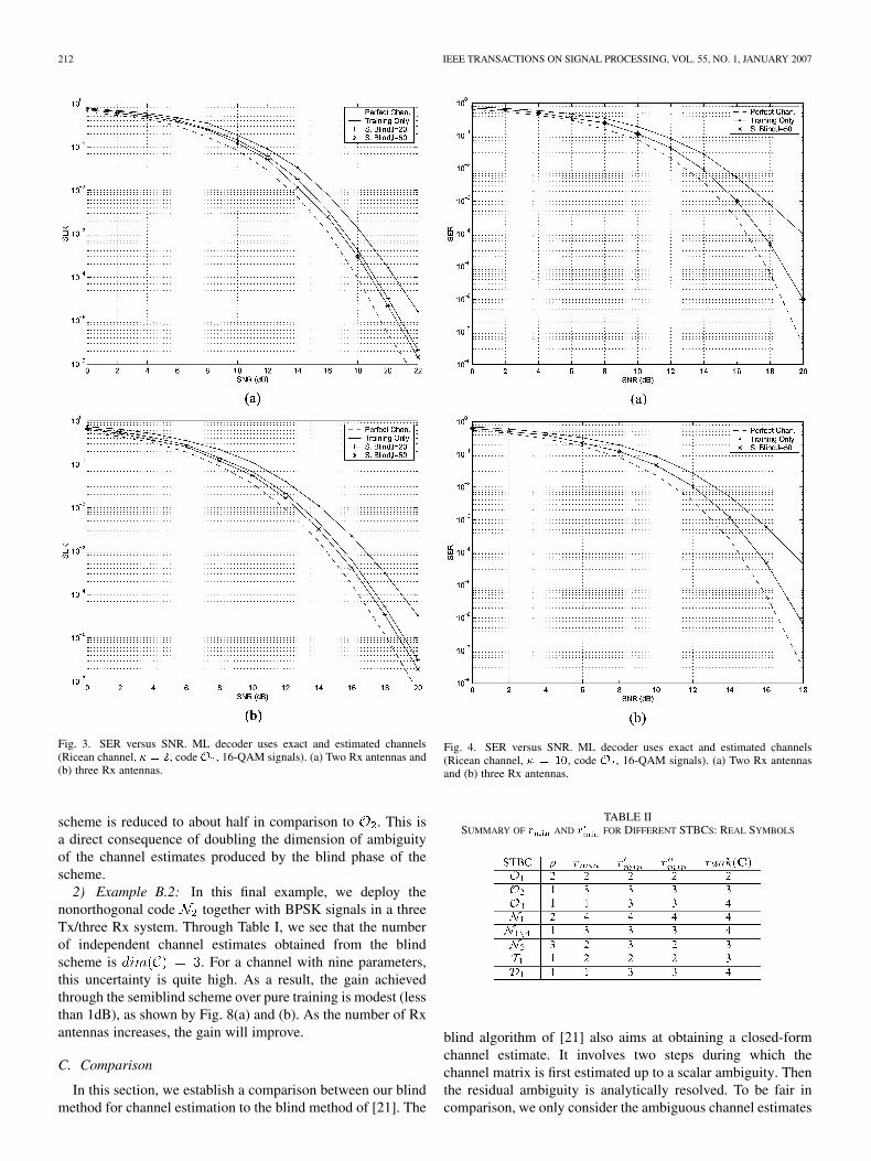
Fig. 3. SER versus SNR. ML decoder uses exact and estimated channels(Ricean channel, � = 2, codeO , 16-QAM signals). (a) Two Rx antennas and(b) three Rx antennas.

scheme is reduced to about half in comparison to . This isa direct consequence of doubling the dimension of ambiguityof the channel estimates produced by the blind phase of thescheme.

2) Example B.2: In this final example, we deploy thenonorthogonal code together with BPSK signals in a threeTx/three Rx system. Through Table I, we see that the numberof independent channel estimates obtained from the blindscheme is . For a channel with nine parameters,this uncertainty is quite high. As a result, the gain achievedthrough the semiblind scheme over pure training is modest (lessthan 1dB), as shown by Fig. 8(a) and (b). As the number of Rxantennas increases, the gain will improve.

C. Comparison

In this section, we establish a comparison between our blindmethod for channel estimation to the blind method of [21]. The

Fig. 4. SER versus SNR. ML decoder uses exact and estimated channels(Ricean channel, � = 10, code O , 16-QAM signals). (a) Two Rx antennasand (b) three Rx antennas.

TABLE IISUMMARY OF r AND r FOR DIFFERENT STBCS: REAL SYMBOLS

blind algorithm of [21] also aims at obtaining a closed-formchannel estimate. It involves two steps during which thechannel matrix is first estimated up to a scalar ambiguity. Thenthe residual ambiguity is analytically resolved. To be fair incomparison, we only consider the ambiguous channel estimates


Fig. 5. NMSE and MSER versus SNR for different window size `, three Txand three Rx Rayleigh channel using code N , BPSK signals.

Fig. 6. SER versus SNR. ML decoder uses exact and estimated channels(Rayleigh channel, code N , BPSK signals). (a) Two Rx antennas and(b) three Rx antennas.

Fig. 7. Channel estimation performance (three Tx and two Rx Rayleighchannel, code O , QPSK signals). (a) NMSE and MSER versus SNR and(b) SER versus SNR.

from both methods and artificially resolve the remaining scalardenoted by by using a linear projection, i.e.,

Fig. 9 depicts the NMSE performance of both methods in thecase of the uniquely identifiable O-STBC for a two Rx an-tenna system using QPSK. The figure reveals a slight advantageof that method for O-STBC. Fig. 10 illustrates the SER perfor-mance of both methods when the window size . No-tice how both methods yield almost identical results especiallyat relatively high SNR values. Moreover, Fig. 11 suggests thatthe slight difference in performance between the two methodsdiminishes as the block size is increased. However, againstnonorthogonal codes such as or 1/4, the method of [21]does not apply because of its necessary requirement of orthog-onal codes.


Fig. 8. Channel estimation performance (three Tx and three Rx Rayleighchannel, code N , BPSK signals). (a) NMSE and MSER versus SNR and(b) SER versus SNR.

Fig. 9. NMSE versus SNR for different window size `, three Tx and two RxRayleigh channel using code O , QPSK signals.

Fig. 10. SER versus SNR, three Tx and two Rx Rayleigh channel using codeO , QPSK signals, ` = 50.

(a) (b)

Fig. 11. SER versus SNR for different window sizes, three Tx and two RxRayleigh channel using codeO , QPSK signals. (a) ` = 30 and (b) ` = 100.

D. Remarks

The simulation examples above served to highlight twoimportant aspects of the proposed semiblind scheme. First,they clearly demonstrate the enhancement in channel esti-mate quality the scheme is capable of achieving over thetraining-based scheme. This enhancement is observed fororthogonal and nonorthogonal STBCs as well. It is particularlysignificant when the STBC leads to a reduced dimension ofresidual channel ambiguities (especially when the channel isidentifiable) and when the number of channel parameters isrelatively high. Naturally it varies also with the length of ob-servation window, SNR, and Ricean factor. The correspondingamelioration in SER performance is quite satisfactory. In fact,we should note here that the ML decoder does not seem to be asvulnerable to the channel mismatch as one might expect. Nev-ertheless, the semiblind scheme proves to make a difference.

The simulation allowed us to closely examine the applicationof the algorithm. The prospect of applying the algorithm ob-viously hinges on the existence of a nontrivial left null space


of the noiseless receive matrix. With the help of the sufficientcondition given in (57), we were in fact able in all presentedcases not only to determine whether or not such a subspace ex-ists but also to evaluate its dimension. This is notably impor-tant, for it allowed us to separate the signal and noise subspaceswithout risking mixing them, a common problem when workingwith subspace-based algorithms. We note, however, that in allcodes we used, the number of Rx antennas needed to utilize thescheme has to be at least two. Additionally, in order to assimi-late the blind and the training phases of the algorithm for non-identifiable channels, the required knowledge about the numberof channel solutions is obtained based on the sufficient condi-tion in (26). This condition was successfully applied in ExampleB.2, but not with Example B.1, leaving us with the numerical al-ternative which may become problematic for unknown channeldistribution/model. Fortunately, as the number of Rx antennasincreases, we can apply (26). In all, the algorithm seems to workbetter with more Rx antennas because the increase in the numberof channel parameters gives it an edge (worthiness) over thetraining-based approach, and also because the parameters re-quired by the algorithm become easier to obtain.

VIII. CONCLUSION

In this paper, we sought to generalize the blind channel es-timation scheme developed earlier for OSTBCs to the broaderclass of linear STBCs. What concerns us mostly in this workis channel identifiability. In principle, the blind technique pro-duces a linear subspace where the unknown channel resides. Byaccounting for its finite dimension, we have obtained a neces-sary and sufficient condition for a unique channel solution up toa complex scalar. The condition is expressed as a function of the(unknown) channel matrix and the STBC parameters. While thepractical aspect of this main identification condition may not beobvious at the first glance, it does in fact pave the way for moreutilitarian results.

For channel matrices with known ranks, such as the case ofRicean and Rayleigh flat fading channels, the main result leadsto sufficient, and easy to verify, identification conditions whichare stated based solely on the STBC information. In fact, theyfeature code-dependent parameters, some of which need to beevaluated by a outlined simple procedure. Moreover, these con-ditions can provide a useful tool not only to check whether or notthe channel solution is unique but also to quantify the numberof independent solutions. By exploiting this knowledge, a semi-blind estimation methodology that integrates the blind schemewith a short training phase is developed to obtain an unequiv-ocal channel solution for blindly identifiable as well as blindlyunidentifiable channels.

APPENDIX A

In this appendix, we would like to show that if , then.

We have already seen that is a solution to (5)and (6), where is a complex scalar. This also means thatverifies (7) and (8), with and , where

. Hence and

. If in addition rank rank (i.e.,), then

(43)

By definition

rank

rank

rank

(44)

In the above, (44) is obtained by splitting the domain of basedon (43). Consider now the second term in (44), which after sim-plification based on the fact that andamounts to

rank

rank

(45)

But is an upper bound of , hence

rank

rank (46)

APPENDIX B

Proof of Lemma 1: Relying on the property (10), the matrixrank on the right-hand side of (21) is expanded as

rank

(47)

Let be a matrix such that . The columns ofsuch a matrix can simply be formed from a basis of . Ifwe substitute for back in (47) and use (9), thenafter simplification, (47) becomes equivalent to

rank rank rank

(48)

Now, let us define the following set of vectors: suchthat , i.e., is formed as the con-catenation of 2 vector blocks, all of which are exceptthe th (counting from top to bottom), which is . Because thevector’s s are orthogonal to one an other, it follows that

rank rank (49)

where is equal to the number of the vector s that do notlie in . Obviously, the value of depends on


the choice of the vector . Substituting (49) back into (48), andrecalling the definition of , we conclude that

(50)

Clearly, the key to obtaining is to determine a vectorthat results in the maximum number of s residing

in . A vector , , means

Hence, an optimum nonzero vector that achieves mustbelong to as many s as possible, but not to all of themas . In mathematical terms, this obser-vation is expressed as

subject to (51)

Since and , the constraintin (51) implies that

rank rank

(52)

As a result, we can rewrite (51) instead as

subject to

rank rank(53)

APPENDIX C

Proof of Lemma 2: By definition

(54)

rank (55)

where (54) follows from the fact that the data are persistentlyexciting while (55) is obtained by applying the rank expansionillustrated in (10). The only unknown in (55) is

. But this is exactly the same problem we encoun-tered earlier when discussing . Hence, in the same spirit,define the following minimum rank:

rank (56)

and apply the same techniques to obtain

if rank

then rank (57)

REFERENCES

[1] L. Zheng and D. Tse, “Diversity and multiplexing: A fundamentaltradeoff in multiple anrenna channels,” IEEE Trans. Inf. Theory, to bepublished.

[2] A. Paulraj and C. B. Papadis, “Space-time processing for wireless com-munications,” IEEE Signal Process. Mag., vol. 14, pp. 49–83, Nov.1997.

[3] D. G. M. S. D.-S. S. P. J. Smith and A. Naguib, “From theory to prac-tice: An overview of MIMO space-time coded wireless systems,” IEEEJ. Sel. Areas Commun, vol. 21, pp. 281–302, Apr. 2003.

[4] V. Tarokh, N. Seshardi, and A. R. Calderbank, “Space-time codes forhigh data rate wireless communication: Performance criteria and codeconstruction,” IEEE Trans. Inf. Theory, vol. 44, pp. 744–765, Mar.1998.

[5] S. M. Alamouti, “A simple transmit diversity technique for wirelesscommunications,” IEEE J. Sel. Areas Commun, vol. 16, pp. 1451–1458,Oct. 1998.

[6] V. Tarokh, H. Jafarkhani, and A. R. Calderbank, “Space-time codesfrom orthogonal designs,” IEEE Trans. Inf. Theory, vol. 45, pp.1456–1467, Jul. 1999.

[7] M. Uysal and C. N. Georghiades, “New space-time block codes forhigh throughput efficiency,” in Proc. IEEE GLOBECOM, 2001, vol. 2,pp. 1103–1107.

[8] A. Boariu and D. M. lonescu, “A class of nonrothogonal rate-one space-time block codes with controlled interference,” IEEE Trans. WirelessCommun., vol. 2, pp. 270–276, Mar. 2003.

[9] H. Jafarkhani, “A quasi-orthogonal space-time block code,” IEEETrans. Commun., vol. 49, pp. 1–4, Jan. 2001.

[10] K. A.-M. M. O. Damen and J.-C. Belfire, “Diagonal algebraic space-time block codes,” IEEE Trans. Inf. Theory, vol. 48, pp. 628–636, Mar.2002.

[11] B. Hughes, “Differential space-time modulation,” IEEE Trans. Inf.Theory, vol. 46, pp. 296–302, Oct. 2000.

[12] V. Tarokh, A. Naguib, N. Seshardi, and A. R. Calderbank, “Space-time codes for high data rate wireless communication: Performancecriteria in thepresence of channel error estimation, mobility and mul-tiple paths,” IEEE Trans. Commun., vol. 47, pp. 199–207, Feb. 1999.

[13] C. Budianu and L. Tong, “Channel estimation for space-time or-thogonal block codes,” IEEE Trans. Signal Process., vol. 50, pp.2515–2528, Oct. 2002.

[14] B. Hassibi and B. M. Hochwald, “High-rate codes that are linear inspace and time,” IEEE Trans. Inf. Theory, vol. 48, pp. 1804–1824, Jul.2002.

[15] A. L. Swindlehurst, “Blind and semi-blind equalization for generalizedspace-time precoding,” in Proc. ICASSP, Orlando, FL, 2002.

[16] A. L. Swindlehurst and G. Leus, “Blind and semi-blind equalizationfor generalized space-time block codes,” IEEE Trans. Signal Process.,vol. 50, pp. 2489–2499, Oct. 2002.

[17] P. Stoica and G. Ganesan, “Space-time block codes: Trained, blind andsemi-blind detection,” in Proc. ICASSP, Orlando, FL, 2002.

[18] N. Ammar and Z. Ding, “On blind channel identifiability underspace-time coded transmission,” in 36th Asilomar Conf. Signals, Syst.Comput., 2002, pp. 664–668.

[19] ——, “Flat fading channel estimation under generic linear space-timeblock coded transmissions,” in Proc. ICC, Paris, France, 2004, pp.2616–2620.

[20] ——, “Frequency selective channel estimation in time-reversed space-time coding,” in Proc. WCNC, 2004, pp. 1838–1843.

[21] S. Shahbazpanahi, A. B. Gershman, and J. H. Matiton, “Closed-formblind decoding of orthogonal space-time block codes,” in Proc.ICASSP, Montreal, PQ, Canada, 2004, pp. 473–476.

[22] ——, “A linear preceding approach to resolve ambiguity of blind de-coding of orthogonal space-time block codes in slowly fading chan-nels,” in Proc. SPAWC, Lisbon, Portugal, 2004.

[23] B. A. Sethuraman, B. S. Rajan, and V. Shashidhar, “Full-diversity,high-rate space-time codes from division algebras,” IEEE Trans. Inf.Theory, vol. 49, pp. 2596–2616, Oct. 2003.

[24] C. R. Rao and M. B. Rao, Matrix Algebra and Its Applications to Sta-tistics and Econometrics, 1st ed. Singapore: World Scientific, 1998.

[25] H. A. Gamal and M. O. Damen, “Universal space-time coding,” IEEETrans. Inf. Theory, vol. 49, pp. 1097–1119, May 2003.

[26] B. Hassibi and B. Hochwald, “High rate codes that are linear in spaceand time,” IEEE Trans. Inf. Theory, vol. 48, pp. 1804–1824, Jul. 2002.

[27] E. Moulines, P. Duhamel, J.-F. Cardoso, and S. Mayrargue, “Subspacemethods for blind identification of multichannel for filters,” IEEETrans. Signal Process., vol. 43, pp. 516–525, Feb. 1995.


Nejib Ammar (M’05) received the B.Sc. andM.Sc. degrees in electrical engineering from BilkentUniversity, Turkey, in 1997 and 2000, respectively,and the Ph.D. degree in electrical and computerengineering from the University of California atDavis in 2005.

Since 2004, he has been an Electrical Engineer inthe area of image and video coding. His research in-terests include signal processing for communicationsand video compression.

Zhi Ding (F’03) received the Ph.D. degree in elec-trical engineering from Cornell University, Ithaca,NY, in 1990.

He has been Professor of electrical of computerengineering at the University of California, Davis,since 2000. From 1990 to 2000, he was a FacultyMember first at Auburn University and later at theUniversity of Iowa. He has held visiting positionswith Australian National University, Hong KongUniversity of Science and Technology, NASA LewisResearch Center, and USAF Wright Laboratory. He

has active collaboration with researchers from Australia, China, Japan, Canada,Taiwan, Korea, Singapore, and Hong Kong. He is also a Visiting Professor withSoutheast University, Nanjing, China.

Dr. Ding has served on the Technical Program Committee of several IEEEworkshops and conferences. He was Associate Editor of IEEE TRANSACTIONS

ON SIGNAL PROCESSING during 1994–1997 and 2001–2004, and Associate Ed-itor of IEEE SIGNAL PROCESSING LETTERS in 2002–2005. He was a memberof the Technical Committees on Statistical Signal and Array Processing and onSignal Processing for Communications (1994–2003). He is Technical ProgramChair of 2006 IEEE Globecom.

Blind Channel Identifiability for Generic Linear Space-Time Block Codes

Documents

Transcript of Blind Channel Identifiability for Generic Linear Space-Time Block Codes