Dow

nloa

ded

By:

[Pin

el, N

.] A

t: 16

:25

3 Ju

ly 2

007

Waves in Random and Complex MediaVol. 17, No. 3, August 2007, 283–303

Bistatic scattering from one-dimensional random roughhomogeneous layers in the high-frequency limit

with shadowing effect

N. PINEL∗, N. DECHAMPS, C. BOURLIER and J. SAILLARD

IREENA, Ecole polytechnique de l’universite de Nantes, La Chantrerie, Rue C. Pauc,BP 50609, 44306 Nantes Cedex 3, France

(Received 15 May 2006; in final form 17 December 2006)

Many fast asymptotic models of electromagnetic scattering from a single rough interface have beendeveloped over the last few years, but only a few have been developed on stacks of rough interfaces. Thespecific case of very rough surfaces, compared to the incident wavelength, has not been treated before,which is the context of this paper. The model starts from the iteration of the Kirchhoff approximationto calculate the fields scattered by a rough layer, and is reduced to the high-frequency limit in orderto rapidly obtain numerical results. The shadowing effect, important under grazing angles, is takeninto account. The model can be applied to any given slope statistics. Then, the model is comparedwith a reference numerical method based on the method of moments, which validates the model inthe high-frequency limit for lossless and lossy inner media.

1. Introduction

Scattering from dielectric homogeneous layers has many applications, like remote sensing ofocean ice, sand cover of arid regions, or oil slicks on the ocean, and also in optics, like opticalstudies of thin films and coated surfaces, and treatment of antireflection coatings. The use offast asymptotic models can be very useful to predict the scattered signal of such systems.

Several models have been developed on rough films where only one surface scatters anincident wave (for example, see [1] and references therein). Only a few asymptotic modelshave been developed on scattering from stacks of rough interfaces, which is the context ofthis paper. The first models on this subject were developed for optical applications, for stacksof slightly rough surfaces compared to the incident wavelength [2–4]. One can also quotethe small perturbation method (SPM) extended to two interfaces [5], also valid for smallroughnesses. However, the mathematical formulation of this method is so complicated thatno numerical result has been presented. Soubret et al. [6] extended the reduced Rayleighequations to the case of two slightly rough interfaces. Fuks et al. [7–9] developed a model forscattering from a slightly rough surface overlying a strongly rough surface compared to theincident electromagnetic wavelength. Bahar et al. have developed the full wave model overmore than 30 years for a rough interface, and extended it to the case of two rough interfaces

∗Corresponding author. E-mail: nicolas.pinel@univ-nantes.fr

Waves in Random and Complex MediaISSN: 1745-5030 (print), 1745-5049 (online) c© 2007 Taylor & Francis

http://www.tandf.co.uk/journalsDOI: 10.1080/17455030701191448

Dow

nloa

ded

By:

[Pin

el, N

.] A

t: 16

:25

3 Ju

ly 2

007

284 N. Pinel et al.

[10]. Simulations have been presented for the monostatic configuration, and for surfaces withrms heights smaller than the wavelength [11]. Using the radiative transfer model, Tjuatjaet al. [12] presented numerical results of the monostatic scattering coefficient from a stackof two rough interfaces separated by an inhomogeneous medium, modeled as a collection ofrandomly distributed spheres. In addition, the scattering from each interface is calculated fromthe asymptotic integral equation method of Fung et al. [13, 14]. Nevertheless, this approachseems to be very difficult to implement numerically, and to demand extensive computingtime.

The objective of this paper is to obtain a simple mathematical expression of the bistaticscattering coefficient in the high-frequency limit (taking the shadowing effect into account),in order to get a fast method for solving the problem of rough homogeneous layers: it is anextension of the classical geometric optics approximation for one rough interface to the caseof several rough interfaces. The starting point of the method is the Kirchhoff approximation(KA) [14–18], applicable to surfaces with large radii of curvature compared to the incidentelectromagnetic wavelength. The model uses the widely used KA in reflection, but also theKA in transmission [14, 17, 18], which allows one to obtain the fields reflected onto andtransmitted through a rough interface. This paper describes the KA applied to a stack of tworough interfaces, in which the KA is iterated for each successive reflection or transmissionon the two rough interfaces. To our knowledge, this is the first time that this problem hasbeen investigated: iterating the KA has only been done for multiple scattering from a singlerough interface [19–21], and only at order two (second-order scattering). It is applied tostrongly rough interfaces to obtain a simple mathematical expression of the bistatic radarcross-section in the high-frequency limit, allowing easy numerical implementation and fastnumerical results. The paper focuses on one-dimensional stationary random rough surfaces,and takes the shadowing effect into account [22, 23].

In the second part of the paper, the expressions of the first- and second-order scattered fieldsare derived with the method of stationary phase (MSP). In the third part, the expressions ofthe radar cross-sections are derived in the high-frequency limit (using the geometric opticsapproximation). Then, numerical results are presented and compared with a benchmark method[24, 25] based on the method of moments to validate the model. A comparison between a roughand a plane lower interface is made, and the case of a lossy inner medium is studied.

2. First- and second-order scattered fields derived with the method of stationary phase

The studied system (see figure 1) is composed of a stack of two rough interfaces (�A forthe upper interface, �B for the lower interface), separated by an intermediate homogeneousmedium �2. The three media �α (α = {1, 2, 3}), with relative permittivity εrα , are supposedto be non-magnetic (relative permeability µrα = 1). kα stands for the wavenumber inside �α

(kα = k0√

εrα , with k0 the wavenumber in the vacuum). Let Ei be the incident field inside themedium �1, of direction ki = (ki , qi )/|k1| = (ki , qi ), and of incidence angle θi . The incidentfield on the upper surface at the point A1 is given by Ei (rA1 ) = E0 exp(i k1ki · rA1 ) (the termexp(−i ωt) is omitted), rA1 = xA1 x + z A1 z, with xA1 and z A1 the abscissa and the elevation ofthe point A1, respectively.

The field transmitted into the intermediate medium �2 along the downward propagationdirection k−,1 (angle θ−,1 with subscript − representing the downward direction) is reflectedonto the lower surface at the point B1 along the upward propagation direction k+,1 (angle θ+,1

with subscript + representing the upward direction), and then reflected onto the upper surfaceat the point A2 and so on. Thus, multiple reflections of the field inside �2 occur, successively

Dow

nloa

ded

By:

[Pin

el, N

.] A

t: 16

:25

3 Ju

ly 2

007

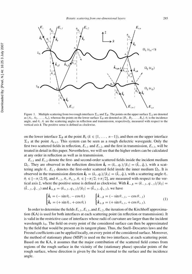
Bistatic scattering from one-dimensional layers 285

Figure 1. Multiple scattering from two rough interfaces �A and �B . The points on the upper surface �A are denotedas {A1, A2, . . . , An}, whereas the points on the lower surface �B are denoted as {B1, B2, . . . , Bn}. θi is the incidenceangle, and θr , θt are the scattering angles in reflection and transmission, respectively, measured with respect to thevertical axis z. The positive sense is defined as clockwise.

on the lower interface �B at the point Bk (k ∈ {1, . . . , n−1}), and then on the upper interface�A at the point Ak+1. This system can be seen as a rough dielectric waveguide. Only thefirst two scattered fields in reflection, Er,1 and Er,2, and the first in transmission, Et,1, will betreated in detail in this paper. Nevertheless, we will see that the higher orders can be calculatedat any order in reflection as well as in transmission.

Er,1 and Er,2 denote the first- and second-order scattered fields inside the incident medium�1. They are observed in the reflection direction kr = (kr , qr )/|k1| = (kr , qr ), with a scat-tering angle θr . Et,1 denotes the first-order scattered field inside the inner medium �3. It isobserved in the transmission direction kt = (kt , qt )/|k3| = (kt , qt ), with a scattering angle θt .θi ∈ [−π/2; 0], and θ−,1, θt , θ+,1, θr ∈ [−π/2; +π/2], are measured with respect to the ver-tical axis z, where the positive sense is defined as clockwise. With k−,1 = (k−,1, q−,1)/|k2| =(k−,1, q−,1) and k+,1 = (k+,1, q+,1)/|k2| = (k+,1, q+,1), we have{

ki = (− sin θi , − cos θi )

kr = (+ sin θr , + cos θr )

{k−,1 = (− sin θ−,1, − cos θ−,1)

k+,1 = (+ sin θ+,1, + cos θ+,1).(1)

In order to determine the fields Er,1, Et,1, and Er,2, the iteration of the Kirchhoff approxima-tion (KA) is used for both interfaces at each scattering point (in reflection or transmission). Itis valid in the restrictive case of interfaces whose radii of curvature are larger than the incidentwavelength λ0. The field on every point of the considered surface can then be approximatedby the field that would be present on its tangent plane. Thus, the Snell–Descartes laws and theFresnel coefficients can be applied locally, on every point of the considered surface. Moreover,the method of stationary phase (MSP) is used on the two interfaces, at each scattering point.Based on the KA, it assumes that the major contribution of the scattered field comes fromregions of the rough surface in the vicinity of the (stationary phase) specular points of therough surface, whose direction is given by the local normal to the surface and the incidenceangle.

Dow

nloa

ded

By:

[Pin

el, N

.] A

t: 16

:25

3 Ju

ly 2

007

286 N. Pinel et al.

In the first subsection, the general principle of the method is exposed from the case of thefirst-order scattered field Er,1. In the second subsection, Et,1 and Er,2 are derived for a roughlower interface, and in the last one they are derived for a plane lower interface.

2.1. General principle of the method

First, the fields scattered in reflection and transmission from the upper interface �A at thepoint A1 are expressed from the classical Kirchhoff–Helmholtz integral equations with theuse of the Kirchhoff approximation [23]. Then, using the Weyl representation of the Greenfunction, one can express the scattered fields at any point of the two media, that is to say �1

for the field scattered in reflection, and �2 for the field scattered in transmission. The scalartwo-dimensional Weyl representation of the Green function G M M ′

α = Gα(rM, rM′ ), for a wavepropagating from a point M to a point M ′ in the medium �α , is defined as

G M M ′α = i

4H (1)

0 (kα‖rM′ − rM‖) = i

4π

∫ +∞

−∞

d kM M ′

qM M ′ei kα kMM′ · rMM′ , (2)

where kM M ′ = kMM′ . x, and qM M ′ = kMM′ . z, with

qM M ′ ={[

1 − k2M M ′

]1/2if ||kMM′ || ≤ 1

i[k2

M M ′ − 1]1/2

if ||kMM′ || > 1,(3)

where rM = xM x + zM z, with xM and zM the abscissa and the elevation of the point M ,respectively. Let us note that the Weyl representation of the Green function is valid for far-field as well as for near-field propagations. The formalism in equation (2), which uses the scalarproduct kMM′ ·rMM′ inside the exponential (similar to the formalism expressed by Bahar et al.[19]) is equivalent to the classical form using absolute values over the heights zM and zM ′ ,|zM ′ − zM | in [26]. When the scattered field is observed in the far-field zone at the point P , thetwo-dimensional scalar Green function can be expressed by the following asymptotic form:

G M Pα i

4

(2

πkαr

)1/2

exp{i[kα(r − ks · rM) − π/4]}, (4)

where r is the distance of P from an arbitrary origin. For our configuration, ks = kr if α = 1,and ks = kt if α = 3.

Then, using the Kirchhoff–Helmholtz integral equation under the Kirchhoff approximationand the asymptotic Green function in equation (4), and adding the surface illumination function(rA1 ), one can express the first-order scattered field Er,1 in the incident medium in the far-fieldzone. Moreover, using the method of stationary phase, the expression can be simplified to

Er,1(rP ) =(

k1

2πr

) 12

exp[i(k1r − π/4)] r12(χ0

ri

)f (ki , kr , n0

ri )

×∫ +L0/2

−L0/2(rA1 ) exp(−ik1kr · rA1 ) Ei (rA1 ) d xA1 (5)

with (rA1 ) = 1 if the point A1 corresponding to rA1 is illuminated, and the rays emanatingfrom both the transmitter and the receiver do not cross the surface; (rA1 ) = 0 otherwise.L0 is the illuminated surface length, f (ki , kr , nri ) = nri . (kr − ki )/2 is obtained from theprojection of the incidence and reflection-scattering vectors onto the local normal to thesurface nri = −γri x + z (defined as being directed upward), with γri its associated slope.r12 is the Fresnel reflection coefficient, with χri the local incidence angle.

Dow

nloa

ded

By:

[Pin

el, N

.] A

t: 16

:25

3 Ju

ly 2

007

Bistatic scattering from one-dimensional layers 287

With the method of stationary phase, in a general way, let k1 represent the incidence unit wavevector inside the medium �α , k2 the reflection unit wave vector inside �α , and nr1 = −γr1 x+zthe local normal to the considered surface (defined as being directed upward), with γr1 itsassociated slope. Then, one can write the projection term as f (k1, k2, nr1) ≡ f (k1, k2, n0

r1) =[1− (k2k1 + q2q1)] / (q2 − q1), and the local incidence angle χr1 ≡ χ0

r1 = −(θ2 −θ1)/2 (θ1, θ2

are oriented angles). The latter is the argument of the Fresnel reflection coefficient rαβ , definedin H and V polarizations as, respectively,

r Hαβ

(χ0

r1

) =√

εrα cos χ0r1 −

√εrβ − εrα sin2 χ0

r1

√εrα cos χ0

r1 +√

εrβ − εrα sin2 χ0r1

, (6)

r Vαβ

(χ0

r1

) = −εrβ cos χ0

r1 − √εrα

√εrβ − εrα sin2 χ0

r1

εrβ cos χ0r1 + √

εrα

√εrβ − εrα sin2 χ0

r1

. (7)

2.2. Derivation of the scattered fields for a rough lower interface

To obtain the higher-order scattered fields (Et,1, Er,2, Et,2, Er,3, etc.), the principle to be used isexactly the same, and one has to iterate this ‘procedure’. For example, to obtain the first-ordertransmitted scattered field Et,1, one first determines the field scattered in transmission fromthe upper interface at the point A1 using the Kirchhoff–Helmholtz integral equation under theKA, and the field at the point B1 using the Weyl representation of the Green function. Then,this procedure is iterated, that is to say the field at the point B1 can be considered as anincident field on the lower interface at B1, and the scattered field in transmission at this pointcan be derived using the Kirchhoff–Helmholtz integral equation under the KA, and then thetransmitted field Et,1 inside �3 in the far-field zone is derived using the asymptotic Greenfunction in equation (2).

Then, the field Et,1, scattered by the rough layer into the lower medium �3 in the far-fieldzone, results from the scattering in transmission through the surface �A at the point A1 intothe medium �2, and the scattering in transmission through the surface �B at the point B1 intothe medium �3. Taking the surfaces illumination functions (rA1 ) and (rB1 ) into accountand using the MSP, it is expressed as

Et,1 = k2

2π

(k3

2πr

) 12

E0ei(k3r−π/4)∫

dk−,1

q−,1dxA1 dxB1 (rA1 )(rB1 )

×t12(χ0

ti

)g12

(ki , k−,1, n0

ti

)t23

(χ0

t−,1

)g23

(k−, 1, kt , n0

t−,1

)×eik1ki ·rA1 eik2k−,1·rA1 B1 e−ik3kt ·rB1 , (8)

where rMM′ = rM′ − rM = (xM ′ − xM )x + (zM ′ − zM )z. In a general way, let k1 represent theincidence unit wave vector inside the medium �α , k3 the transmission unit wave vector insidethe medium �β , and nt1 = −γt1 x + z the local normal to the considered surface (defined asbeing directed upward), with γt1 its associated slope. gαβ(k1, k3, nt1) = nt1 · k3 is obtainedfrom the projection of the incidence and transmission-scattering vectors onto nt1. tαβ is theFresnel transmission coefficient, with χt1 the local incidence angle.

Using the MSP, one can write the projection term as gαβ(k1, k3, nt1) ≡ gαβ(k1, k3, n0t1) =

[kβ − kα (k3k1 + q3q1)]/(kβ q3 − kαq1), and the local incidence angle as cos χt1 ≡ cos χ0t1 =

sign[(−q1 n0t1z

)(kβ q3 − kαq1)] × [kα − kβ(k3k1 + q3q1)] / [k2α + k2

β − 2kαkβ(k3k1 + q3q1)]1/2

,

Dow

nloa

ded

By:

[Pin

el, N

.] A

t: 16

:25

3 Ju

ly 2

007

288 N. Pinel et al.

with n0t1z

the projection of nt1 onto the z axis. χ0t1 is the argument of the Fresnel transmission

coefficient tαβ , defined in H and V polarizations as, respectively,

t Hαβ

(χ0

t1

) = 1 + r Hαβ

(χ0

t1

), (9)

t Vαβ

(χ0

t1

) = [1 − r V

αβ

(χ0

t1

)](εrα/εrβ)1/2. (10)

The computation of Et,1 requires then three-fold integrations. k−,1 ∈] − ∞; +∞[ a priori,but as Et,1 is calculated in the far-field zone, evanescent waves can be neglected (which is con-sistent with the GO approximation). So k−,1 ∈ [−1; +1], leading to k−,1 = − sin θ−,1. Thus,dk−,1/q−,1 can be reduced to dθ−,1, with θ−,1 ∈ [−π/2; +π/2]. xA1 , xB1 ∈ [−L0/2; +L0/2]where L0 is the illuminated surface length.

The field Er,2, scattered by the rough layer into the incident medium �1 in the far-fieldzone, results from the transmission through the surface �A into the medium �2, the reflectiononto the surface �B inside �2, and then the transmission through the surface �A back intothe medium �3. Taking the illumination functions (rA1 ), (rB1 ) and (rA2 ) into account andusing the MSP, it is defined as

Er,2 = −(

k2

2π

)2( k1

2πr

) 12

E0ei(k1r−π/4)∫

dk−,1

q−,1

dk+,1

q+,1dxA1 dxB1 dxA2

×(rA1 )(rB1 )(rA2 ) t12(χ0

ti

)g12

(ki , k−,1, n0

ti

)×r23

(χ0

r−,1

)f(k−,1, k+,1, n0

r−,1

)t21

(χ0

t+,1

)g21

(k+,1, kr , n0

t+,1

)×eik1(ki · rA1 −kr · rA2 ) eik2(k−,1 · rA1 B1 +k+,1 · rB1 A2 ). (11)

The computation of Er,2 requires then five-fold integrations. As Er,2 is calculated in thefar-field zone, evanescent waves can be neglected (which is consistent with the GO approx-imation), so dk−,1, dk+,1 ∈ [−1; +1], leading to k±,1 = ± sin θ±,1. Thus, dk±,1/q±,1 can bereduced to dθ±,1, with θ±,1 ∈ [−π/2; +π/2]. xA1 , xB1 , xA2 ∈ [−L0/2; +L0/2] where L0 isthe illuminated surface length.

Thus, using the same method for the higher orders, that is to say by iterating this ‘procedure’for each scattering in reflection or transmission inside the dielectric waveguide, one can obtainthe expression of any order of transmitted scattered field Et,n and reflected scattered field Er,n

(this is not presented here).

2.3. Derivation of the scattered fields for a plane lower interface

When the lower interface �B , separating the media �2 and �3, is assumed to be plane (it isthen usually denoted as SB), the equations can easily be simplified. Indeed, the problem to besolved is the same as the rough case, except that the scattering (in reflection or transmission)from the lower interface is replaced by a simple reflection or transmission, expressed by thecorresponding Fresnel coefficient. Thus, in equations (8) and (11), there is no integration overxB1 , and we have: (rB1 ) = 1, θ+,1 =−θ−,1, and

√εr3 sin θt = √

εr2 sin θ−,1 (as the lowerinterface is plane). By neglecting the evanescent waves, this leads to, respectively

Et,1 =(

k22

2πk3r

) 12

E0ei(k3r−π/4)∫

dθ−,1dxA1 (rA1 ) δ

[sin θt −

(εr2

εr3

) 12

sin θ−,1

]

× t12(χ0

ti

)g12

(ki , k−,1, n0

ti

)t23(θ−,1) eik1ki · rA1 eik2k−,1 · rA1 B1 e−ik3kt · rB1 , (12)

Dow

nloa

ded

By:

[Pin

el, N

.] A

t: 16

:25

3 Ju

ly 2

007

Bistatic scattering from one-dimensional layers 289

Er,2 = k2

2π

(k1

2πr

) 12

E0ei(k1r−π/4)∫

dθ−,1dxA1 dxA2 (rA1 )(rA2 )δ(θ+,1 + θ−,1)

× t12(χ0

ti

)g12

(ki , k−,1, n0

ti

)r23(θ−,1) t21(χ0

t+,1)g21(k+,1, kr , n0

t+,1

)× eik1(ki · rA1 −kr · rA2 ) eik2(k−,1 · rA1 B1 +k+,1·rB1 A2 ). (13)

Thus, in this particular case of a plane lower interface, only two-fold integrations are requiredfor the calculation of Et,1 (instead of three), and only three for the calculation of Er,2 (insteadof five).

3. Incoherent scattering coefficients in the high-frequency limit

The total scattered field E tots,n (superscript ‘tot’ for total; s ≡ r for the reflection case, and s ≡ t

for the transmission case) for n-th multiple scattering is E tots,n = ∑n

m=1 Es,m . The averagescattered power is expressed as⟨∣∣E tot

s,n

∣∣2⟩2ηα

=n∑

m=1

〈|Es,m |2〉2ηα

+ 1

ηα

e

(⟨n−1∑m=1

Es,m

n∑p=m+1

Es,p∗⟩)

, (14)

with ηα the wave impedance of the considered medium: α ≡ 1 for s ≡ r and α ≡ 2 for s ≡ t .For n = 2, we have E tot

s,2 = Es,1 + Es,2, then 〈|E tots,2|2〉/2ηα = 〈|Es,1|2〉/2ηα +〈|Es,2|2〉/2ηα +

e(〈Es,1 Es,2

∗〉)/ηα , where e(. . .) is the real part operator, (. . .)∗ the complex conju-gate operator, and 〈. . .〉 the ensemble average operator. To distinguish the conjugate Es,n

∗

from the field expression Es,n , the points {Am, Bm} become {A′m, B ′

m}, which means that{xAm , xBm , z Am , zBm } → {xA′

m, xB ′

m, z A′

m, zB ′

m} and {θM M ′ } → {θ ′

M M ′ }. The incoherent power

P tots,n is obtained from P tot

s,n = 〈|E tots,n|2〉/2ηα − |〈E tot

s,n〉|2/2ηα .To calculate the scattering coefficient of the layer in the high-frequency limit, the geometric

optics (GO) approximation (k0σh > 1, with σh being the rms height of the surface) is usedfor both interfaces. It assumes that the scattering intensity contributes for only closely locatedcorrelated points of the surface, M, M ′, compared to the surface correlation length Lc, suchthat the coherent contribution |〈E tot

s,n〉|2/2ηα can be neglected. Moreover, the height differencezM ′ − zM can be expanded as γM (xM ′ − xM ), with γM the surface slope at the point M . Then,one can express the total scattering coefficient σ tot

s,n of a one-dimensional target, defined by[27]

σ tots,n(θi , θs) = r P tot

s,n

L0 cos θi pi, with pi = |Ei |2

2η1, (15)

where r is the distance of the target, and L0 the illuminated surface length (L0 must be greaterthan the surfaces correlation lengths LcA and LcB). In the above equation, for the specificcases n = {1, 2}, we have

P tots,1 = ps,1 and P tot

s,2 = ps,1 + ps,2, with (16){ps,1 = 1

2ηα〈|Es,1|2〉

ps,2 = 12ηα

[〈|Es,2|2〉 + 2 e(〈Es,1 Es,2

∗〉)]. (17)

In this model, the surface shadowing effects in reflection [22] and in transmission [23] aretaken into account. Indeed, for grazing incidence and/or scattering angles, a part of the surfaceis not seen by the emitter and/or the receiver. This phenomenon has to be taken into account

Dow

nloa

ded

By:

[Pin

el, N

.] A

t: 16

:25

3 Ju

ly 2

007

290 N. Pinel et al.

in order not to over-predict the scattering coefficient. The penumbra effect [28], which occursfor grazing angles, is not taken into account in the model. Then, in theory the shadowingfunctions used here are not valid for grazing angles; nevertheless, it was shown that in practicethey are valid if equation (18) of [28] (Bruce) holds. That is to say, for the typical applicationspresented here, the geometric shadowing functions can be applied with good approximationsup to angles of the order of 85◦. Indeed, for the applications presented further (with σs = 0.1and σh ≥ λ/2), the numerical application of equation (18) of [28] (Bruce) gives that the validitydomain of the GO shadowing function is φi > 3◦, that is to say θi < 87◦.

3.1. Scattering coefficients for a rough lower interface

3.1.1. First- and second-order reflection scattering coefficients. The calculation of thefirst-order reflection scattering coefficient σr,1, obtained from the statistical correlation of Er,1,is relatively simple [23, 29, 30]. It is defined by

σr,1 =∣∣r12(χ0

ri )∣∣2

cos θif 2

(ki , kr , n0

ri

) ps(γ 0

ri

)|qr − qi | S11

(θi , θr |γ 0

ri

), (18)

with γ 0ri = −(kr − ki )/(qr − qi ). S11(θi , θr |γ 0

ri ) is the average bistatic reflection shadowingfunction expressed by Bourlier et al. [22]. One can observe that this scattering coefficientdoes not depend on the frequency, is independent of the surface height statistics, and can beapplied for any given slope statistics.

The second-order contribution is given by pr,2 = pr,22 + pr,12, with pr,22 = 〈|Er,2|2〉/2η1

and pr,12 = e(〈Er,1 Er,2

∗〉)/η1. This calculation is much more complicated, as it implies16-fold integrations (12 random variables: six for the heights and six for the slopes, and foursurface variables) for two stationary surfaces (or spatially homogeneous). This number ofintegrations is too high for a numerical implementation. That is why it is necessary to makefurther approximations on the model, in order to get a simple mathematical expression of σr,2.

First, the stationary phase and the geometric optics approximations are used for both inter-faces, at each scattering point. In the high-frequency limit, it is possible to demonstrate that theterm pr,12 = 0 owing to the shadow. Furthermore, to be consistent with the GO approximation,the evanescent waves must be neglected, and it is necessary to suppose that the wavenumberinside the intermediate medium k2 is real. Let us notice that the latter restrictive hypothesisimplies that the model itself cannot handle lossy dielectric media, yet, we will show later thatit is possible to consider it properly. Moreover, the former hypothesis does not mean that thescattering points are in far field from one another. This principle is the same as the one usedfor the double scattering from a single interface: the authors neglect the evanescent waves[20, 21, 31].

Using the same approach as for the double scattering from a single rough interface [20, 21,19], one can divide this problem into coincidental and anti-coincidental cases. The coincidentalcase corresponds to A′

1 close to A1, B ′1 close to B1, and A′

2 close to A2 (compared to thesurface correlation lengths LcA and LcB). This case contributes for all scattering angles. Theanti-coincidental case corresponds to A′

1 close to A2, B ′1 close to B1, and A′

2 close to A1

(compared to the surface correlation lengths LcA and LcB). This case may contribute onlyfor scattering angles in and around the backscattering direction. For the coincidental case, thepoints of successive reflections A1, B1, A2 can be considered as uncorrelated between oneanother, which simplifies the final equation.

By contrast, for the anti-coincidental case, to quantify the backscattering enhancementproperly, one has to take the correlations between the points of successive reflections into ac-count. Then, this complicates the problem to be solved a lot, implying an additional numerical

Dow

nloa

ded

By:

[Pin

el, N

.] A

t: 16

:25

3 Ju

ly 2

007

Bistatic scattering from one-dimensional layers 291

integration by considering Gaussian statistics. After tedious calculations, one obtains for theanti-coincidental contribution σr,2a

σr,2a = k1

2π cos θi2 e

( ∫ + π2

− π2

∫ 0

− π2

dθ−,1dθ ′−,1

t12(χ0

ti

)t∗12

(χ0

ti′)

| (q−,1+q ′−,1)

2 − k1k2

(qi −qr )2 |2

× g12(ki , k−,1, n0

tc1

)g12

(ki , k′

−,1, n0tc2

)r23(θ−,1)r∗

23

(θ ′−,1

)t21

(χ0

t+,1

)t∗21

(χ0

t+,1′)

× g21(k+,1, kr , n0

tc2

)g21

(k′+,1, kr , n0

tc1

)S1221

(ki , k−,1, k′

−,1, kr |γ 0tc1, γ

0tc2

)× e−2ik2(q−,1−q ′

−,1)H∫ xmax

xmindxmc ei(ki +kr −k−,1−k ′

−,1)xmc I1

)(19)

where xmc = xc1 − xc2 with xc1 = (xA1 + xA′2)/2, xc2 = (xA2 + xA′

1)/2, and xmc ∈ [xmin; xmax].

q1 = qi + qr − q−,1 + q ′−,1, q2 = −qi − qr − q−,1 + q ′

−,1, n0tc1 = −γ 0

tc1 x + z with γ 0tc1 =

− (ki −kr )−(k−,1−k ′−,1)

(qi −qr )−(q−,1+q ′−,1) , and n0

tc2 = −γ 0tc2 x + z with γ 0

tc2 = − (ki −kr )+(k−,1−k ′−,1)

(qi −qr )−(q−,1+q ′−,1) . I1 represents the

statistical averaging of eiq1zc1 eiq2zc2 over zc1 and zc2 (also called the characteristic function ofzc1 and zc2). For Gaussian slope statistics, after tedious calculations, one can express I1 as

I1 ≡ I1(xmc) = ps(γ 0

tc1, γ0tc2; xmc

)f(q1, q2, γ

0tc1, γ

0tc2; xmc

), (20)

with

ps(γ 0

tc1, γ0tc2

) = 1

2π

√σ 4

s − W 22

exp

[−

(σ 2

s γ 0tc1

2 + σ 2s γ 0

tc22 + 2W2γ

0tc1γ

0tc2

)2(σ 4

s − W 22

)]

(21)

and

f(q1, q2, γ

0tc1, γ

0tc2

) = ei W1

(σ4s −W 2

2 )[(q1σ

2s −q2W2)γ 0

tc2−(q2σ2s −q1W2)γ 0

tc1]

× e− 1

2(σ4s −W 2

2 )[2q1q2(W0σ

4s +W1W2−W0W 2

2 )−(q21 +q2

2 )W 21 σ 2

s ]

× e− 12 (q2

1 +q22 )σ 2

h , (22)

with W0 the autocorrelation function between zc1 and zc2 (which is a function of the hor-izontal distance xmc), W1 its first derivative, and W2 its second derivative. I1 in (20) is afunction of xmc, as ps and f implicitly depend on xmc through W0, W1, and W2. Whenthe slopes are uncorrelated, W0 = 0, W1 = 0, W2 = 0, leading to the uncorrelated formulaI1 = ps(γ 0

tc1)ps(γ 0tc2) exp[−1/2(q2

1 + q22 )σ 2

h ]. The main difficulty is then to determine or atleast to evaluate the minimum and maximum values of xmc, xmin and xmax, which are randomvariables depending on the heights and the slopes of these points. For typical applicationspresented here (that is to say for slight surface slopes and moderate mean layer thicknessesin the high-frequency limit) the numerical results of σr,2a showed that can be neglected. Thisis in agreement with results from the literature [32, 33], which showed that for the scatteringfrom a rough layer, where the lower interface is plane, this case contributes only when themean layer thickness H satisfies the condition

H >

√εr2√

εr2 − 1RcA, (23)

with RcA the radius of curvature of the upper rough surface. For the simulations presented here,H is much smaller than RcA: this confirms that the anti-coincidental case does not contribute

Dow

nloa

ded

By:

[Pin

el, N

.] A

t: 16

:25

3 Ju

ly 2

007

292 N. Pinel et al.

for the typical applications presented here. Therefore, this case will not be considered furtherfor the sake of simplicity.

Thus, neglecting the anti-coincidental contribution, one can obtain a simple expression ofthe second-order scattering coefficient σr,2, defined by

σr,2 = 1

cos θi

∫ + π2

− π2

∫ + π2

− π2

dθ−,1 dθ+,1

× ∣∣t12(χ0

ti

)g12

(ki , k−,1, n0

ti

)∣∣2 ps(γ 0

t A1

)∣∣q−,1 − k1

k2qi

∣∣ S12(θi , θ−,1|γ 0

t A1

)

× ∣∣r23(χ0

r−,1

)f(k−,1, k+,1, n0

r−,1

)∣∣2 ps(γ 0r B1

)

|q+,1−q−,1| S22(θ−,1, θ+,1|γ 0

r B1

)

× ∣∣t21(χ0

t+,1

)g21

(k+,1, kr , n0

t+,1

)∣∣2 ps(γ 0t A2

)

|qr − k2k1

q+,1|S21

(θ+,1, θr |γ 0

t A2

). (24)

To obtain physical results for grazing angles for the case with shadow, the configurationsof θ+,1 and θr that induce local scattering angles greater than π/2 in absolute values must beomitted. The slopes γ 0

t A1, γ 0

r B1, γ 0

t A2are defined by

γ 0t A1

= −(k2k−,1 − k1ki )/(k2q−,1 − k1qi ), (25)

γ 0r B1

= −(k+,1 − k−,1)/(q+,1 − q−,1), (26)

γ 0t A2

= −(k1kr − k2k+,1)/(k1qr − k2q+,1). (27)

S12(θi , θ−,1|γ 0t A1

), S22(θ−,1, θ+,1|γ 0r B1

), S21(θ+,1, θr |γ 0t A2

) are the bistatic shadowing functions,in transmission from the medium �1 into the medium �2, in reflection inside the medium �2

and onto the medium �3, and in transmission from the medium �2 back into the medium �1,respectively. One can show, for any random process, that [34, 23]:

S12(θi , θ−,1|γ 0

t A1

) = B(1 + �(µi ), 1 + �(µ−,1)), (28)

S21(θ+,1, θr |γ 0

t A2

) = B(1 + �(µ+,1), 1 + �(µr )), (29)

where B is the beta function (also called the Eulerian integral of the first kind), � is thefunction defined by �(µ) = 1/µ

∫ +∞µ

(γ −µ) ps(γ ) dγ , with µ = | cot θ | the absolute slopeof the considered angle.

Thus, the problem can be reduced to only two-fold integrations, which enables a fast nu-merical implementation. One can observe that expression (24) under the geometric opticsapproximation can be applied for any given slope statistics, and is independent of the fre-quency (within the domain of validity of the model). Moreover, assuming that the points ofsuccessive reflections A1, B1 and A2 are uncorrelated, this expression appears as the productof three elementary scattering coefficients of single interfaces, each one corresponding to eachscattering in reflection or transmission inside the rough dielectric waveguide. Indeed, the firstone corresponds to the scattering in transmission from the point A1 of �A into the medium�2, the second one to the scattering in reflection from the point B1 of �B inside �2, and thethird one to the scattering in transmission from the point A2 of �A back into the medium �1.The two-fold integrals account for the energy scattered by the rough surfaces in all scatteringdirections.

Then, under the GO approximation, to obtain the total scattering coefficient σ totr,2, the single

σr,1 and double σr,2 contributions are incoherently added.

Dow

nloa

ded

By:

[Pin

el, N

.] A

t: 16

:25

3 Ju

ly 2

007

Bistatic scattering from one-dimensional layers 293

3.1.2. First-order transmission scattering coefficient. Using exactly the same approachas for σr,1 and σr,2, one can obtain the expression of the first-order transmission scatteringcoefficient σt,1. Thus, σt,1 is defined by

σt,1 =√

εr3

εr1

1

cos θi

∫ + π2

− π2

dθ−,1

× ∣∣t12(χ0

ti

)g12

(ki , k−,1, n0

ti

)∣∣2 ps(γ 0

t A1

)∣∣q−,1− k1

k2qi

∣∣ S12(θi , θ−,1|γ 0

t A1

)

× ∣∣t23(χ0

t−,1

)g23

(k−,1, kt , n0

t−,1

)∣∣2 ps(γ 0t B1

)∣∣qt − k2k3

q−,1

∣∣ S23(θ−,1, θt |γ 0

t B1

), (30)

with γ 0t B1

= −(k3kt − k2k−,1)/(k3qt − k2q−,1), and S23(θ−,1, θt |γ 0t B1

) = B[1 + �(µ−,1), 1 +

�(µt )]. The same concluding remarks on the expression of σt,1 can be made as for σr,2.

3.2. Scattering coefficients for a plane lower interface

For the case of a plane lower interface, the expressions of the scattering coefficients are similar

and much simpler, as the general term∫ + π

2− π

2dθ+,m s Bm

r,23 is replaced by |r23(θ−,m)|2 δ(θ+,m −θ−,m), and the general term s Bm

t,23 is replaced by |t23(θ−,n)|2 δ[sin θt − ( εr2εr3

)12 sin θ−,n].

For m = 1, s B1r,23 = |r23(χ0

r−,1) f (k−,1, k+,1, n0r−,1)|2 ps (γ 0

r B1)

|q+,1−q−,1S22(θ−,1, θ+,1|γ 0

r B1) and s B1

t,23 =|t23(χ0

t−,1) g23(k−,1, kt , n0t−,1)|2 ps (γ 0

t B1)

|qt − k2k3

q−,1|S23(θ−,1, θt |γ 0

t B1). For this simpler case, σr,2 is calcu-

lated with only one numerical integration, allowing us to obtain results quasi-instantaneously.

4. Numerical results

For the simulations, the considered system is a layer of permittivity εr2, with mean layerthickness H = 6λ, overlying a perfectly conducting medium of permittivity εr3 = i∞. Wechoose to take a lower medium as being perfectly conducting, so that the contribution of thesecond-order scattering coefficient σr,2 is the highest. The surface rms height of each interfaceequals half the incident electromagnetic wavelength, σh = λ0/2, and the surface rms slope istaken to be σs = 0.1. This corresponds to the validity domain of the model. The two randomrough surfaces are assumed to be stationary, and we will consider Gaussian slope statisticsfor the simulations. Only the first reflection inside the layer is considered, and its contributionis compared to the scattering from the upper interface. That is to say, one will study thecomparison between the second-order total reflection scattering coefficient σ tot

r,2 = σr,1 + σr,2

and the first-order one σ totr,1 = σr,1. Simulations are presented for θi = 0◦ and θi = −20◦.

Computer simulations for optics applications, with bistatic configuration, are presented tovalidate the model, by comparison with a benchmark numerical method [24, 25] based on themethod of moments. The simulation parameters of this method used for each surface are thesurface length L = 150λ, the number of sampling points of the surface ni = 1500, the numberof realizations of the surface N = 50, and the attenuation parameter of the incident Thorsosbeam g = L/10. A comparison between a rough and a plane lower interfaces is made, andthe case of a lossy inner medium �2 is studied.

Dow

nloa

ded

By:

[Pin

el, N

.] A

t: 16

:25

3 Ju

ly 2

007

294 N. Pinel et al.

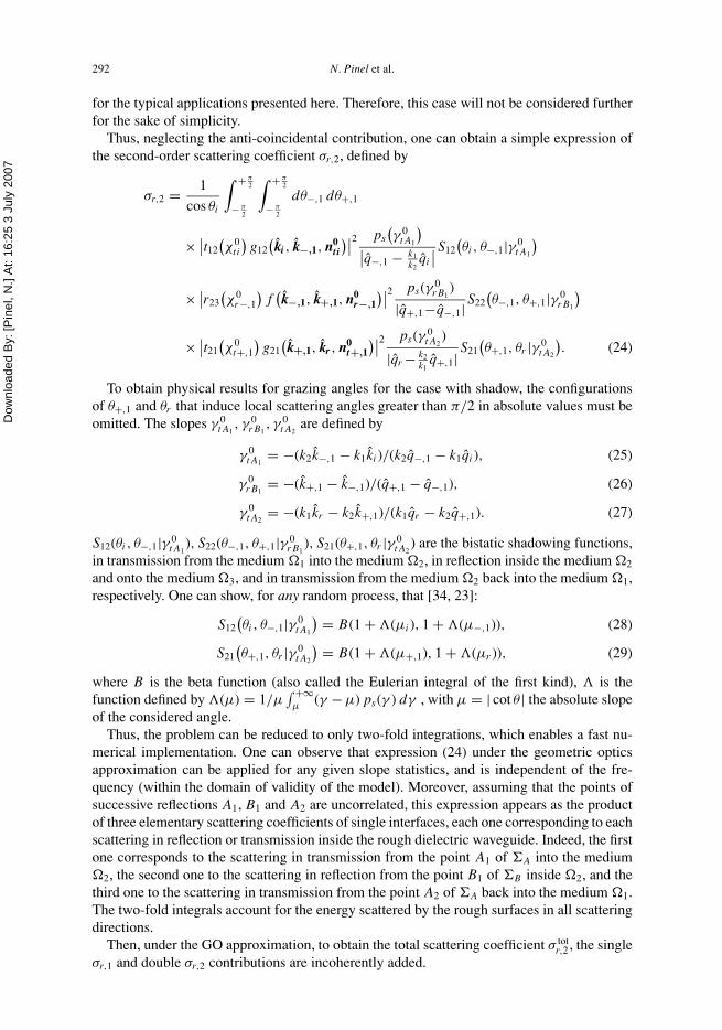
Figure 2. Simulations of the contributions of the first- and second-order scattering coefficients, σr,1 and σr,2 in d B,versus the reflection scattering angle θr (in ◦) for V polarization, for εr2 = 3 and εr3 = i∞, and for θi = 0◦. For thefirst-order contribution, comparison of the model with shadow (circled line) with the reference numerical method(dashdot line). For the second-order contribution, comparison of the model without shadow (full line) and the modelwith shadow (crossed dotted line) with the reference numerical method (dashed line).

5. Model validation by comparison with a benchmark numerical method

To validate the results, an exact reference method is needed. A rigorous way to model thescattering from rough interfaces is done numerically by means of integral methods [30],where the fields and their normal derivative on both interfaces are unknowns. These unknownsare sampled by applying a method of moments [35]; the bulk of the work is then to invert thecorresponding linear system. Nevertheless, for the case of two rough interfaces, this impliesa large number of unknowns. Then, a direct inversion (LU) is inappropriate. Thus, one useshere an original numerical method, the recent Propagation-inside-Layer Expansion (PILE)method [24, 25], in order to deal with this kind of problems on a standard office computer.

The studied model is compared to the PILE method, for θi = {0◦, −20◦}, for the op-tics domain application. The configuration is bistatic, where the scattering angle θr lies in[−90◦; +90◦]. Simulations of the contributions of the first- and second-order bistatic reflec-tion scattering coefficients, σr,1 and σr,2 (that is to say, the total scattering coefficients σ tot

r,1 andσ tot

r,2), are presented for θi = 0◦ in figure 2, and for θi = −20◦ in figure 3.In both figures, for the first-order contribution σr,1, a comparison is made between the model

with shadow, plotted as the circled line, and the PILE method, plotted as the dashdot line. Thenumerical results highlight good agreement of the model with the reference method, in bothV and H polarizations (only the V polarization is represented here), and for both incidenceangles, around the specular direction θr = −θi . The model without shadow is not representedhere as for this configuration, there is no difference with the model with shadow: indeed,for slight slopes and moderate incidence angles, the surface is shadowed only for very highgrazing scattering angles, which have no effect on σr,1 in this case.

For the contribution of the second-order scattering coefficient σr,2 (that is to say the totalsecond-order scattering coefficient σ tot

r,2), a comparison is made between the model, plotted asthe full line for the model without shadow and in crossed dotted line for the model with shadow,

Dow

nloa

ded

By:

[Pin

el, N

.] A

t: 16

:25

3 Ju

ly 2

007

Bistatic scattering from one-dimensional layers 295

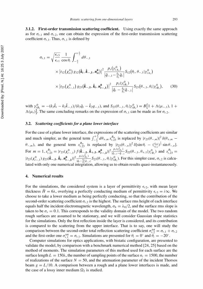
Figure 3. Same simulations as figure 2, but with θi = −20◦.

and the PILE method, plotted as the dashed line. First, one can observe that this contributionis significant, not only in and around the specular direction, but in all reflection scatteringdirections. Indeed, as the permittivity of the inner medium is close to that of the upper medium,the major part of the incident energy is transmitted into the inner medium towards the perfectlyconducting lower interface. Then, all this energy is scattered in reflection towards the upperinterface, which in major part is transmitted back into the incident medium. Thus, the second-order scattering coefficient has a significant contribution to the total scattering coefficient bycomparison with the first-order. Second, the scattered intensity is not concentrated around thespecular direction, contrary to the first-order, but more widely spread around all scatteringangles. Indeed, the second-order scattered power underwent three successive scatterings: twoscatterings in transmission, which are less significant than the scattering in reflection by thelower interface. The numerical results also highlight good agreement of the model with thereference numerical (PILE) method, in both V and H polarizations (only the V polarization isrepresented here), and for both incidence angles. The results confirm that for this configuration,the shadowing effect contributes only for grazing scattering angles (over 75–80◦ here), butis of importance for these angles to get physical numerical results, and consistent with thenumerical method. For both incidence angles, the differences between the studied modeland the PILE method are due to the difficulties in defining the simulation parameters of thefast numerical method, which have a significant influence on the scattering coefficient. Thenumerical method needs a great number of samples of the surface to be accurate, which isvery extensive in computing time and memory space compared to the GO approximation.In addition, the configurations where the scattering coefficient of the GO approximation arehigher than the numerical method cannot be attributed to the multiple scattering on the sameinterface. Indeed, when double scattering phenomena from a single interface occurs, there isan increase in scattering (and not a decrease) since the GO approximation is an incoherentapproach. As a result, a decrease of the scattering coefficient (from the GO approximation tothe numerical method) at low grazing angles cannot be attributed to multiple scattering onthe same interface. Moreover, for typical cases presented here (i.e. surfaces with rms slope

Dow

nloa

ded

By:

[Pin

el, N

.] A

t: 16

:25

3 Ju

ly 2

007

296 N. Pinel et al.

σs = 0.1, bistatic configuration, and θi ≤ 20◦), it is well known [36, 37] that multiple scatteringphenomena can be neglected.

Thus, the model with shadow is in good agreement with the reference numerical method.One can find applications in advanced remote sensing, where the emitter and the receiver arein different places, like for the remote sensing of sand over granite [38], ocean ice [39, 40](when the ice layer can be supposed as homogeneous), and oil slicks on the ocean. One mayalso find applications to optical tomography of biological media [41, 42], as a basic fast modelwhen the media can be supposed as homogeneous.

6. Comparison between a rough and a plane lower interface

This section is devoted to the comparison of the model between the case of a rough lowerinterface and a plane lower interface, and their influence on the contribution of the second-orderscattering coefficient σr,2.

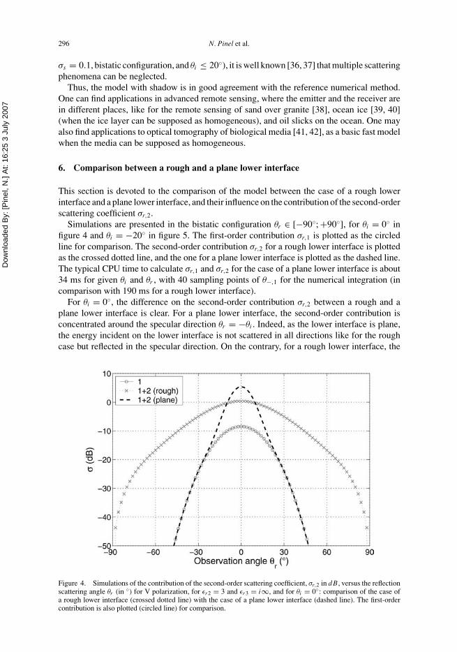
Simulations are presented in the bistatic configuration θr ∈ [−90◦; +90◦], for θi = 0◦ infigure 4 and θi = −20◦ in figure 5. The first-order contribution σr,1 is plotted as the circledline for comparison. The second-order contribution σr,2 for a rough lower interface is plottedas the crossed dotted line, and the one for a plane lower interface is plotted as the dashed line.The typical CPU time to calculate σr,1 and σr,2 for the case of a plane lower interface is about34 ms for given θi and θr , with 40 sampling points of θ−,1 for the numerical integration (incomparison with 190 ms for a rough lower interface).

For θi = 0◦, the difference on the second-order contribution σr,2 between a rough and aplane lower interface is clear. For a plane lower interface, the second-order contribution isconcentrated around the specular direction θr = −θi . Indeed, as the lower interface is plane,the energy incident on the lower interface is not scattered in all directions like for the roughcase but reflected in the specular direction. On the contrary, for a rough lower interface, the

Figure 4. Simulations of the contribution of the second-order scattering coefficient, σr,2 in d B, versus the reflectionscattering angle θr (in ◦) for V polarization, for εr2 = 3 and εr3 = i∞, and for θi = 0◦: comparison of the case ofa rough lower interface (crossed dotted line) with the case of a plane lower interface (dashed line). The first-ordercontribution is also plotted (circled line) for comparison.

Dow

nloa

ded

By:

[Pin

el, N

.] A

t: 16

:25

3 Ju

ly 2

007

Bistatic scattering from one-dimensional layers 297

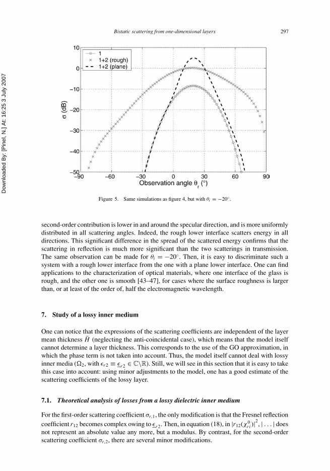
Figure 5. Same simulations as figure 4, but with θi = −20◦.

second-order contribution is lower in and around the specular direction, and is more uniformlydistributed in all scattering angles. Indeed, the rough lower interface scatters energy in alldirections. This significant difference in the spread of the scattered energy confirms that thescattering in reflection is much more significant than the two scatterings in transmission.The same observation can be made for θi = −20◦. Then, it is easy to discriminate such asystem with a rough lower interface from the one with a plane lower interface. One can findapplications to the characterization of optical materials, where one interface of the glass isrough, and the other one is smooth [43–47], for cases where the surface roughness is largerthan, or at least of the order of, half the electromagnetic wavelength.

7. Study of a lossy inner medium

One can notice that the expressions of the scattering coefficients are independent of the layermean thickness H (neglecting the anti-coincidental case), which means that the model itselfcannot determine a layer thickness. This corresponds to the use of the GO approximation, inwhich the phase term is not taken into account. Thus, the model itself cannot deal with lossyinner media (�2, with εr2 ≡ εr2 ∈ C\R). Still, we will see in this section that it is easy to takethis case into account: using minor adjustments to the model, one has a good estimate of thescattering coefficients of the lossy layer.

7.1. Theoretical analysis of losses from a lossy dielectric inner medium

For the first-order scattering coefficient σr,1, the only modification is that the Fresnel reflectioncoefficient r12 becomes complex owing to εr2. Then, in equation (18), in |r12(χ0

ri )|2, | . . . | doesnot represent an absolute value any more, but a modulus. By contrast, for the second-orderscattering coefficient σr,2, there are several minor modifications.

Dow

nloa

ded

By:

[Pin

el, N

.] A

t: 16

:25

3 Ju

ly 2

007

298 N. Pinel et al.

First, there is a problem in defining the physical propagation angles inside the lossy innermedium �2, θ−,1 and θ+,1. Indeed, with lossless media, the latter are usually obtained usingthe refraction and reflection Snell–Descartes laws

√εr2 sin χt = √

εr1 sin χi , (31)

χr = −χi , (32)

with χi the local incidence angle, χt the local transmission angle, and χr the local reflectionangle from the local normal to the considered surface. Then, with the knowledge of the localsurface slope and the incidence angle θi , one can easily obtain θ−,1 with the use of the refractionSnell–Descartes law (31) at the upper interface, and then θ+,1 with the use of the reflectionSnell–Descartes law (32) at the lower interface. The trouble is, with εr2 ≡ εr2 ∈ C, as the termof the right hand-side of equation (31) is real, the product

√εr2 sin χ

tof the left hand-side of

equation (31) must be real, which implies that χt

is complex (as εr2 is complex). However, weneed to determine the physical (with then a real value) local propagation angle χ

physt inside �2

(so as to determine θ−,1 with the knowledge of the local surface slope), which is not simplythe real part of χ

t. It is given by [48, 49]

tan χphyst = sin χi

p, with (33)

p = 1√2

[√(ε′

r2 − sin2 χi )2 + ε′′

r22 + (ε′

r2 − sin2 χi )] 1

2

, (34)

where εr2 = ε′r2 + i ε′′

r2, and p = e(√

εr2 − sin2 χt). Then, this allows one to determine θ−,1,

and then θ+,1 using equation (32) on the lower surface, with the knowledge of the local surfaceslope.

Second, in equation (24), the reflection and transmission Fresnel coefficients become com-plex, and | . . . | represents a modulus, and not an absolute value any more. Let us note thatthe Fresnel reflection coefficient r23(χ0

r−,1), and the Fresnel transmission coefficient t21(χ0t+,1)

use local incidence angles, χ0r−,1 and χ0

t+,1, that are defined with the physical angles θ−,1 andθ+,1, respectively, and the local slope of the surface considered.

Third, with the knowledge of the physical propagation angles θ−,1 and θ+,1 inside �2, themean layer thickness H , and the slope probability density function (PDF) of the two surfaces,one can determine the field path from the point A1 to the point B1, and from the point B1 tothe point A2. Thus, it is possible to determine the propagation loss A of the power inside thelossy inner medium �2 (from A1 to B1, and from B1 to A2).

7.2. Estimation of the losses for numerical implementation

In order to numerically implement the model for the specific case of a lossy inner medium �2

in a fast and easy way, minor changes to the initial model can be made.First, to evaluate the propagation loss A, we will only consider here the simple case of plane

interfaces (indeed, even if the rough case can be calculated, considering only the plane casewill be satisfactory). Then, the propagation loss can easily be evaluated with the knowledgeof θi , θ−,1, and H . Then, this power propagation loss A is evaluated for plane interfaces bythe expression Apl (called the planar power propagation loss) as

A Apl = exp( − 4k0 Hq / cos θ

planet

), with (35)

q = 1√2

[√(ε′

r2 − sin2 θi)2 + ε′′

r22 − (

ε′r2 − sin2 θi

)] 12

, (36)

Dow

nloa

ded

By:

[Pin

el, N

.] A

t: 16

:25

3 Ju

ly 2

007

Bistatic scattering from one-dimensional layers 299

where θplanet is defined by the refraction Snell–Descartes law (31) at the upper inter-

face, for the case of a plane interface where the local incidence angle χi equals θi , and

q = � m(√

εr2 − sin2 χt). Then, the physical local refraction angle χ

physt equals θ−,1 ≡ θ

planet

(as the lower interface is also plane, one also obtains θ+,1 = −θplanet ).

Second, although θ−,1 and θ+,1 can be calculated rigorously, it can be interesting to evaluatethem with few modifications to the initial model. Then, one can use the following approxima-tion: in the refraction Snell–Descartes law (31), instead of using the complex permittivity εr2,one can use either the real part of εr2, ε′

r2, or the real part of the root square of εr2, e(√

εr2).Then, the refraction Snell–Descartes law (31) becomes, respectively√

ε′r2 sin χ

(1)t √

εr1 sin χi , (37)

e(√

εr2) sin χ(2)t √

εr1 sin χi . (38)

In the case of plane interfaces, the local angles χ can be denoted as θ . Here, for the numericalsimulations, it is simpler to use the first approximation of the propagation angle, θ (1)

t θplanet ,

by replacing the complex permittivity εr2 with its real part ε′r2. This approximation is less

precise than the second one, but it is correct for weakly lossy media (more precisely, theprecision depends on the incidence angle, the real part of the permittivity, ε′

r2, and the imaginarypart of the permittivity; in general, even if ε′

r2 tends to 1, for moderate incidence angles andweakly lossy media, the approximation is valid, and it is all the more precise as ε′

r2 increases).For example, for a complex permittivity εr2 = 3 + 0.1i at an incidence angle θi = −20◦,the physical propagation angle is θ

planet = −11.3871◦, the first approximation obtained from

equation (37) is θ(1)t = −11.3888◦, and the second approximation obtained from equation (38)

is θ(2)t = −11.3872◦: both approximations are valid and precise. For εr2 = 3+ i at θi = −20◦,

θplanet = −11.230◦, θ (1)

t = −11.389◦, and θ(2)t = −11.236◦: both approximations are valid, but

only the second one remains precise.For the numerical simulations, the studied system is the same as in the first section, but

with a layer of permittivity εr2 = 3+0.1i . We consider two incidence angles θi = {0◦; −20◦}.Then, the first approximation of the propagation angle, which replaces εr2 = 3 + 0.1i with itsreal part ε′

r2 = 3, can be used. With this approximation, one can obtain that the power prop-agation loss A Apl = 0.046 = −13.4 dB for θi = 0◦, and A Apl = 0.041 = −13.9 dBfor θi = −20◦. The numerical simulations present a comparison of the lossy case (εr2 =3 + 0.1i), with the lossless case (εr2 = 3), and a comparison between the model withshadow, modified in order to take losses into account as described above, and the (refer-ence numerical) PILE method. The simulations of the first-order contribution σr,1 for thelossy case are not plotted here. Indeed, for this configuration of weakly lossy medium,the difference with the lossless case can be ignored, as the modulus of the Fresnel reflec-tion coefficient varies very slightly (the maximum of relative difference does not exceed0.03%!).

Simulations of the contribution ofσr,2 are presented for θi = 0◦ in figure 6, and for θi = −20◦

in figure 7. For the lossy case, the model with shadow is plotted as the dotted line, and thereference method in dashed line. Here, for these simulations, only the propagation loss A needto be considered in the model to quantify the lossy case. The lossless case is also plotted forcomparison, together with the first-order contribution of the model with shadow (the losslesscase, which is practically equal to the lossy case). For both incidence angles, for the twocurves of the model with shadow (taking into account only the propagation loss) and of thereference numerical method, in both cases the difference between the lossy and the losslesscase of the contribution of σr,2 is mainly constant, and is of the order of the planar propagation

Dow

nloa

ded

By:

[Pin

el, N

.] A

t: 16

:25

3 Ju

ly 2

007

300 N. Pinel et al.

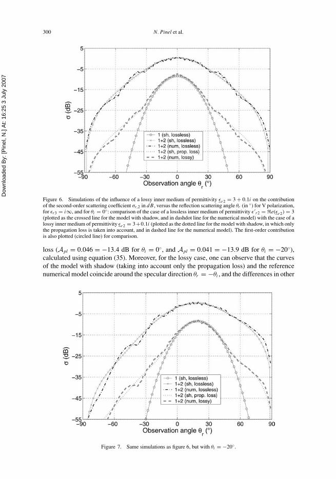
Figure 6. Simulations of the influence of a lossy inner medium of permittivity εr2 = 3 + 0.1i on the contributionof the second-order scattering coefficient σr,2 in d B, versus the reflection scattering angle θr (in ◦) for V polarization,for εr3 = i∞, and for θi = 0◦: comparison of the case of a lossless inner medium of permittivity ε′

r2 = e(εr2) = 3(plotted as the crossed line for the model with shadow, and in dashdot line for the numerical model) with the case of alossy inner medium of permittivity εr2 = 3+0.1i (plotted as the dotted line for the model with shadow, in which onlythe propagation loss is taken into account, and in dashed line for the numerical model). The first-order contributionis also plotted (circled line) for comparison.

loss (Apl = 0.046 = −13.4 dB for θi = 0◦, and Apl = 0.041 = −13.9 dB for θi = −20◦),calculated using equation (35). Moreover, for the lossy case, one can observe that the curvesof the model with shadow (taking into account only the propagation loss) and the referencenumerical model coincide around the specular direction θr = −θi , and the differences in other

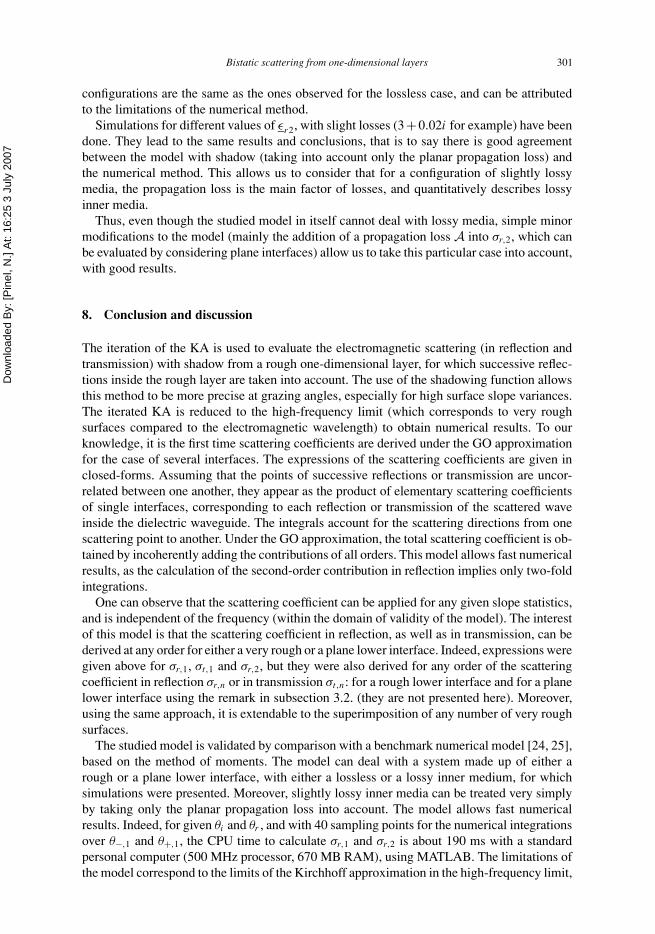
Figure 7. Same simulations as figure 6, but with θi = −20◦.

Dow

nloa

ded

By:

[Pin

el, N

.] A

t: 16

:25

3 Ju

ly 2

007

Bistatic scattering from one-dimensional layers 301

configurations are the same as the ones observed for the lossless case, and can be attributedto the limitations of the numerical method.

Simulations for different values of εr2, with slight losses (3+0.02i for example) have beendone. They lead to the same results and conclusions, that is to say there is good agreementbetween the model with shadow (taking into account only the planar propagation loss) andthe numerical method. This allows us to consider that for a configuration of slightly lossymedia, the propagation loss is the main factor of losses, and quantitatively describes lossyinner media.

Thus, even though the studied model in itself cannot deal with lossy media, simple minormodifications to the model (mainly the addition of a propagation loss A into σr,2, which canbe evaluated by considering plane interfaces) allow us to take this particular case into account,with good results.

8. Conclusion and discussion

The iteration of the KA is used to evaluate the electromagnetic scattering (in reflection andtransmission) with shadow from a rough one-dimensional layer, for which successive reflec-tions inside the rough layer are taken into account. The use of the shadowing function allowsthis method to be more precise at grazing angles, especially for high surface slope variances.The iterated KA is reduced to the high-frequency limit (which corresponds to very roughsurfaces compared to the electromagnetic wavelength) to obtain numerical results. To ourknowledge, it is the first time scattering coefficients are derived under the GO approximationfor the case of several interfaces. The expressions of the scattering coefficients are given inclosed-forms. Assuming that the points of successive reflections or transmission are uncor-related between one another, they appear as the product of elementary scattering coefficientsof single interfaces, corresponding to each reflection or transmission of the scattered waveinside the dielectric waveguide. The integrals account for the scattering directions from onescattering point to another. Under the GO approximation, the total scattering coefficient is ob-tained by incoherently adding the contributions of all orders. This model allows fast numericalresults, as the calculation of the second-order contribution in reflection implies only two-foldintegrations.

One can observe that the scattering coefficient can be applied for any given slope statistics,and is independent of the frequency (within the domain of validity of the model). The interestof this model is that the scattering coefficient in reflection, as well as in transmission, can bederived at any order for either a very rough or a plane lower interface. Indeed, expressions weregiven above for σr,1, σt,1 and σr,2, but they were also derived for any order of the scatteringcoefficient in reflection σr,n or in transmission σt,n: for a rough lower interface and for a planelower interface using the remark in subsection 3.2. (they are not presented here). Moreover,using the same approach, it is extendable to the superimposition of any number of very roughsurfaces.

The studied model is validated by comparison with a benchmark numerical model [24, 25],based on the method of moments. The model can deal with a system made up of either arough or a plane lower interface, with either a lossless or a lossy inner medium, for whichsimulations were presented. Moreover, slightly lossy inner media can be treated very simplyby taking only the planar propagation loss into account. The model allows fast numericalresults. Indeed, for given θi and θr , and with 40 sampling points for the numerical integrationsover θ−,1 and θ+,1, the CPU time to calculate σr,1 and σr,2 is about 190 ms with a standardpersonal computer (500 MHz processor, 670 MB RAM), using MATLAB. The limitations ofthe model correspond to the limits of the Kirchhoff approximation in the high-frequency limit,

Dow

nloa

ded

By:

[Pin

el, N

.] A

t: 16

:25

3 Ju

ly 2

007

302 N. Pinel et al.

that is to say it is not valid for very small grazing angles, and it can only deal with surfaceswith σh >∼ 0.5λ (let us note that the simulations were lead for σh = 0.5λ and allowed us tovalidate the model). With further investigations, it could be interesting to extend the model tothe three-dimensional case to deal with general two-dimensional rough surfaces, using dyadicGreen functions.

References[1] Kaganovskii, Y., Freilikher, V., Kanzieper, E., Nafcha, Y., Rosenbluh, M., and Fuks, I., 1999, Light scattering

from slightly rough dielectric films. Journal of the Optical Society of America A, 16, 331–338.[2] Knittl, Z., 1976, Optics of Thin Films (London: John Wiley).[3] Eastman, J., 1978, Scattering by all-dielectric multilayer band-pass filters and mirrors for lasers. In: G. Hass

and M. H. Francombe (Eds) Physics of Thin Films, Vol. 10, pp. 167–226 (New York: Academic Press).[4] Ohlidal, I. and Navratil, K., 1995, Scattering of light from multilayer with rough boundaries. In: E. Wolf (Ed.)

Progress in Optics, Vol. XXXIV, pp. 248–331 (Amsterdam: Elsevier).[5] Fuks, I. and Voronovich, A., 2000, Wave diffraction by rough interfaces in an arbitrary plane-layered medium.

Waves in Random Media, 10, 253–272.[6] Soubret, A., Berginc, G., and Bourrely, C., 2001, Application of reduced Rayleigh equations to electromagnetic

wave scattering by two-dimensional randomly rough surfaces. Physical Review B, 63, 245411.[7] Fuks, I., 2002, Modeling of scattering by a rough surface of layered media. In: 2002 IEEE International

Geoscience and Remote Sensing Symposium, Toronto, Ontario, Canada, Vol. 2, pp. 1251–1253.[8] Blumberg, D., Freilikher, V., Fuks, I., Kaganovskii, Y., Maradudin, A., and Rosenbluh, M., 2002, Effects of

roughness on the retrorefiection from dielectric layers. Waves in Random Media, 12, 279–292.[9] Gu, Z.-H., Fuks, I., and Ciftan, M., 2004, Grazing angle enhanced backscattering from a dielectric film on a

reflecting metal substrate. Optical Engineering, 43, 559–567.[10] Bahar, E. and Zhang, Y., 1999, Diffuse like and cross-polarized fields scattered from irregular layered structures-

full-wave analysis. IEEE Transactions on Antennas and Propagation, 47, 941–948.[11] Zhang, Y. and Bahar, E., 1999, Mueller matrix elements that characterize scattering from coated random rough

surfaces. IEEE Transactions on Antennas and Propagation, 47, 949–955.[12] Tjuatja, S., Fung, A., and Dawson, M., 1993, An analysis of scattering and emission from sea ice. Remote

Sensing Reviews, 7, 83–106.[13] Fung, A. and Pan, G., 1986, An integral equation method for rough surface scattering. In: Proceedings of

the International Symposium on Multiple Scattering of Waves in Random Media and Random Surfaces,Pennsylvania State University, pp. 701–714.

[14] Fung, A., 1994, Microwave Scattering and Emission Models and Their Applications (Boston: Artech House).[15] Beckmann, P. and Spizzichino, A., 1963, The Scattering of Electromagnetic Waves from Rough Surfaces

(Oxford: Pergamon Press).[16] Ogilvy, J., 1991, Theory of Wave Scattering from Random Surfaces (Bristol: Institute of Physics Publishing).[17] Kong, J. A., 1990, Electromagnetic Wave Theory, 2nd edn (New York: John Wiley).[18] Caron, J. Lafait, J., and Andraud, C., 2002, Scalar Kirchhoff model for light scattering from dielectric random

rough surfaces. Optics Communications, 207, 17–28.[19] Bahar, E. and El-Shenawee, M., 2001, Double-scatter cross sections for two-dimensional random rough surfaces

that exhibit backscatter enhancement. Journal of the Optical Society of America A, 18, 108–116.[20] Ishimaru, A., Le, C., Kuga, Y., Sengers, L., and Chan, T., 1996, Polarimetric scattering theory for high slope

rough surfaces. Progress in Electromagnetic Research, 14, 1–36.[21] Bourlier, C. and Berginc, G., 2004, Multiple scattering in the high-frequency limit with second-order shadowing

function from 2D anisotropic rough dielectric surfaces: I. Theoretical study. Waves in Random Media, 14, 229–252.

[22] Bourlier, C., Berginc, G., and Saillard, J., 2002, Monostatic and bistatic statistical shadowing functions froma one-dimensional stationary randomly rough surface according to the observation length: I. Single scattering.Waves in Random Media, 12, 145–173.

[23] Pinel, N., Bourlier, C., and Saillard, J., 2005, Energy conservation of the scattering from rough surfaces in thehigh-frequency limit. Optics Letters, 30, 2007–2009.

[24] Dechamps, N., 2004, Methodes numeriques appliquees au calcul de la diffusion d’une onde electromagnetiquepar des interfaces naturelles monodimensionnelles. PhD thesis, Universite de Nantes, Nantes, France.

[25] Dechamps, N. de Beaucoudrey, N. Bourlier, C., and Toutain, S., 2006, Fast numerical method for electro-magnetic scattering by rough layered interfaces: Propagation-inside-layer expansion method. Journal of theOptical Society of America A, 23, 359–369.

[26] Tsang, L., Kong, J., Ding, K., and Ao, C., 2000, Scattering of Electromagnetic Waves, Volume I: Theories andApplications (New York: John Wiley).

[27] Tsang, L. and Kong, J., 2001, Scattering of Electromagnetic Waves, Volume III: Advanced Topics (New York:John Wiley).

[28] Bruce, N., 2004, On the validity of the inclusion of geometrical shadowing functions in the multiple-scatterKirchhoff approximation. Waves in Random Media, 14, 1–12.

Dow

nloa

ded

By:

[Pin

el, N

.] A

t: 16

:25

3 Ju

ly 2

007

Bistatic scattering from one-dimensional layers 303

[29] Sancer, M., 1969, Shadow-corrected electromagnetic scattering from a randomly rough surface. IEEE Trans-actions on Antennas and Propagation, AP-17, 577–585.

[30] Tsang, L., Kong, J. A., Ding, K. H., and Ao, C. O., 2001, Scattering of Electromagnetic Waves, Volume II:Numerical Simulations (New York: John Wiley).

[31] Fung, A., Li, Z., and Chen, K., 1992, ‘Backscattering from a randomly rough dielectric surface. IEEE Trans-actions on Geoscience and Remote Sensing, 30, 356–369.

[32] Jakeman, E., 1988, ‘Enhanced backscattering through a deep random phase screen. Journal of the OpticalSociety of America A, 5, 1638–1648.

[33] Lu, J., Maradudin, A., and Michel, T., 1991, Enhanced backscattering from a rough dielectric film on a reflectingsubstrate. Journal of the Optical Society of America B, 8, 311–318.

[34] Pinel, N., Bourlier, C., and Saillard, J., 2005, Radar cross section from a stack of two one-dimensional rough in-terfaces in the high-frequency limit. In: European RADar 2005 Symposium, European Microwave Association,Paris, France.

[35] Harrington, F., 1993, Field Computation by Moment Methods (IEEE Press).[36] Bourlier, C. and Berginc, G., 2004, Multiple scattering in the high-frequency limit with second-order shadowing

function from 2D anisotropic rough dielectric surfaces: II. Comparison with numerical results. Waves in RandomMedia, 14, 253–276.

[37] Lynch, P. and Wagner, R., 1970, Rough-surface scattering: shadowing, multiple scatter, and energy conserva-tion. Journal of Mathematical Physics, 11, 3032–3042.

[38] Saillard, M. and Toso, G., 1997, Electromagnetic scattering from bounded or infinite subsurface bodies. RadioScience, 32, 1347–1360.

[39] Nghiem, S., Kwok, R., Yueh, S., and Drinkwater, M., 1995, Polarimetric signatures of sea ice. 1. Theoreticalmodel. Journal of Geophysical Research, 100, 13665–13679.

[40] Nghiem, S., Kwok, R., Yueh, S., and Drinkwater, M., 1995, Polarimetric signatures of sea ice. 2. Experimentalobservations. Journal of Geophysical Research, 100, 13681–13698.

[41] Lu, J., Hu, X.-H., and Dong, K., 2000, Modeling of the rough-interface effect on a converging light beampropagating in a skin tissue phantom. Applied Optics, 39, 5890–5897.

[42] Ripoll, J., Ntziachristos, V., Culver, J., Pattanayak, D., Yodh, A., and Nieto-Vesperinas, M., 2001, Recovery ofoptical parameters in multiple-layered diffusive media: theory and experiments. Journal of the Optical Societyof America A, 18, 821–830.

[43] Croce, P. and Prod’homme, L., 1980, Contribution of immersion technique to light scattering analysis of veryrough surfaces. Journal of Optics, 11, 319–327.

[44] Croce, P. and Prod’homme, L., 1984, On the conditions for applying light scattering methods to rough surfaceevaluation. Journal of Optics, 15, 95–104.

[45] Yin, Z., Tan, H., and Smith, F., 1996, Determination of the optical constants of diamond films with a roughgrowth surface. Diamond and Related Materials, 5, 1490–1496.

[46] Yin, Z., Akkerman, Z., Yang, B., and Smith, F., 1997, Optical properties and microstructure of CVD diamondfilms. Diamond and Related Materials, 6, 153–158.

[47] Stagg, B. and Charalampopoulos, T., 1991, Surface-roughness effects on the determination of optical propertiesof materials by the reflection method. Applied Optics, 30, 4113–4118.

[48] Combes, P.-F. Micro-ondes – Cours et exercices avec solutions. Tome 1: Lignes, guides et cavites. Dunod,1996.

[49] Roo, R. D. and Tai, C.-T., 2003, Plane wave reflection and refraction involving a finitely conducting medium.IEEE Antennas and Propagation Magazine, 45, 54–61.