BioNavigation: Selecting Optimum Paths

through Biological Resources to Evaluate

Ontological Navigational Queries

Zoe Lacroix1, Kaushal Parekh1, Maria-Esther Vidal2, Marelis Cardenas2, andNatalia Marquez2

1 Arizona State University, Tempe, AZ 85287, USA{zoe.lacroix, kaushal}@asu.edu

www home page: http://bioinformatics.eas.asu.edu2 Universidad Simon Bolıvar, Caracas, Venezuela

{mvidal, mcardenas, nmarquez}@ldc.usb.ve

Abstract. Publicly available biological resources form a complex mazeof highly heterogeneous data sources, interconnected by navigational ca-pabilities and applications. Although it offers scientists multiple valuableoptions, it becomes difficult for them to select the best resources to ob-tain and exploit their data of interest. When expressing a scientific pro-tocol, they struggle with consolidating the best information about thescientific objects being studied and implementing it in terms of queriesagainst biological resources. In this paper we present the BioNavigationsystem that allows scientists to express their queries using an ontologyrepresenting the conceptual level of scientific classes and labeled relation-ships. We developed the ESearch algorithm that generates all possibleevaluation paths for a given ontological query and also ranks them basedon source metadata metrics. BioNavigation thus helps the user visualizethe resources at a higher ontological level, build queries graphically, andprovides valuable guidance on selecting the optimum path through themaze of resources.

1 Introduction

Expressing a scientific protocol, identifying the resources that will be used toimplement each of its steps is a tedious task. To help the scientist in the process,two challenges need to be addressed. First, the scientist needs to express a proto-col at a conceptual level, independently of any resources available to implementit. Only then, the scientist should identify the resources the most suitable to im-plement the protocol. Alas, the scientist often expresses ones protocols mixingits conceptual aim with its implementation. Indeed, there are multiple resources(data sources and applications) where to retrieve information about scientificobjects and analyze them, and scientists cannot know them all. Each of theseresources has its specific data format, data organization, data access, user inter-face, etc. In addition, although many available resources may look similar, theyare different: two similar data sources may offer different coverage, different

levels of curation, different characteristics of the scientific objects they provideinformation about, while two similar applications may generate dramatically dif-ferent outputs. The wealth of biological resources does not benefit completelythe scientists as they typically exploit the few resources they know and trust,avoiding the time consuming process of exploring new resources for each of theirprotocols. Furthermore, the protocols are often driven by the resources known bythe scientists to implement them. Instead of selecting the resources best meet-ing the protocol’s needs, the protocol is expressed so that it can exploit theknown resources. This may affect significantly the quality and completeness ofthe dataset collected by the protocol as different selections of resources in theprotocol evaluation may generate different datasets [1].

Scientific knowledge involves multiple scientific objects and scientific mean-ingful relationships among them. This knowledge may be represented with on-tologies [2] composed of concepts, relations, instances, and axioms. Each conceptrepresents a scientific object (e.g., a gene) that is an abstraction of a set of en-tities within a domain. Relations represent the interactions between conceptsor the properties of a concept. Ontologies aim at modeling scientific informa-tion with respect to the understanding of the scientist. This “scientist-friendly”representation of scientific information has proved useful in the past with sys-tem such as TAMBIS that used an ontology as a user-interface to access andquery multiple integrated databases [3]. In the BioNavigation approach, we aimat exploiting ontologies to provide a scientifically meaningful view of biologicalresources.

In this paper, we present an extension of the BioNavigation system intro-duced in [4]. The system provides scientists with the ability to express scientificqueries at a conceptual level, and returns scientists evaluation paths composedof physical resources to implement the queries. BioNavigation now exploits anontology defining a graph of concept classes and multiple labeled edges. Thequery against the logical graph can be seen as the design of the protocol (e.g.,“retrieve citations related to a genetic disease”), while the evaluation paths re-turned by the BioNavigation system are as many possible implementations of theprotocol (i.e., OMIM1 to PubMed2 using the Entrez PubMed Links). Once thesystem has returned the paths, the scientist may explore the meta-informationrelated to the resources. To better match the scientists needs, the user may selectsemantics that will guide the BioNavigation system in selecting the evaluationpath and return them ordered with respect to the semantics. The three semanticsare maximizing the relevance, maximizing the number of entries, and efficiency.We use three metrics to compute the probability of each path to validate thesemantics.

1 OMIM: Online Mendelian Inheritance in Man http://www.ncbi.nlm.nih.gov/omim2 NCBI PubMed: Literature Database http://www.ncbi.nlm.nih.gov/entrez

2 Physical and Logical Map of Resources

Most data sources typically represent a particular type of scientific class. Forexample, PubMed provides references to published literature, UniProt3 providesinformation about proteins, etc. There can be several data sources for the samescientific class. For example, one can retrieve ‘DNA sequences’ from either NCBINucleotide4 or EMBL5. Data sources also provide links connecting a record toother records in the same data source as well as external data sources in orderto provide comprehensive and complete information about the scientific objectthey represent. Scientists use these links to navigate from one source to anotherand in the process gathering useful information relevant to the scientific ques-tion being studied. Depending on the data source used for obtaining informationabout a given scientific class and the links followed, scientists may retrieve sig-nificantly different information, both in terms of quantity and quality, for thesame scientific query [1]. Thus it is important that the scientist should be ableto identify and explore all possible paths that can be used to evaluate the query.In [5] we described two levels of representation:

1. The Logical Graph in which nodes are scientific classes represented by un-derlying data sources and edges are logical mappings of physical links

2. The Physical Graph which consists of data sources as nodes and the linksbetween them as the edges

This allows the scientists to express their queries at the more general logical levelwhereas the query is evaluated at the physical level using the path that best suitsthe scientist’s needs. Although the graph representation introduced in [5] allowsthe scientists to express their queries at the conceptual level and explore allpossible physical paths that satisfy the query, there are a few limitations to thisrepresentation.

1. The Physical graph did not represent all the resources. It was limited toonly data sources and the navigational capabilities provided by the source.Physical resources also include various applications that the scientists use tomanipulate, analyze, transform, and visualize the data obtained from thesesources. Thus, any path implementing a scientific protocol should also takethese applications into consideration.

2. The logical level graph was used to present a higher level view of the underly-ing resources. In order to allow scientists to formulate meaningful queries, thelogical level needs to represent biological knowledge. The unlabeled edges inthe logical graph fail to do so. Scientific concepts have different types of rela-tionships each having a different biological meaning. A simple edge betweentwo classes does not capture the biological knowledge adequately. What isneeded is an ontological representation of all the classes and their labeledrelationships.

3 UniProt: Universal Protein Resource http://www.ebi.ac.uk/uniprot/4 NCBI Nucleotide http://www.ncbi.nlm.nih.gov/entrez/query.fcgi?db=

Nucleotide5 EMBL: Nucleotide Sequence Database http://www.ebi.ac.uk/embl/

We now provide the formal definitions for the two levels of representation, theontological and the physical, extending significantly, the framework defined in[5]. We also define the mappings that relate the physical resources with conceptsand relationships in the ontology. In section 3.1, we define the query languageto formulate the scientists query and used by the ESearch algorithm to identifypaths in the physical graph. The logical and physical graphs are respectivelydefined in definitions 1 and 2.

Definition 1.

The Logical Graph LG = (VL, E) is a directed graph, where:

– VL is a set of nodes, partitioned into two sets C and A, where, C representslogical classes and A represents logical associations between classes.

– E is a set of directed edges E ⊆ (C × A) ∪ (A × C) that represents rolesplayed by logical classes in the associations.

Definition 2.

The Physical Graph PG = (VP , L) is a directed graph, where:

– VP is a set of nodes, partitioned into three subsets, S, AP and QC, where,• S represents physical data sources.• AP represents applications.• QC represents query capabilities.

– L is a set of directed edges L ⊆ VP ×VP that represents links between sourcesand applications or query capabilities. If a pair (a, b) belongs to L then, a

is a source and b is an application or query capability, or a is an applicationor query capability and b is a source.

Once, the two graphs are defined we introduce φ that maps each logical node tothe set of its physical implementations.

Definition 3.

φ is a one-to-many mapping from VL to 2VP such that it maps (a) a logical classname in C to a set of physical data sources in S and (b) a logical associationin A to a set of applications or query capabilities in 2AP∪QC . Elements in φ(v)represent the physical implementations of a logical node v.

3 The BioNavigation System

We developed the BioNavigation system to allow the scientist to exploit thenumerous available data sources and the links between them [4]. It allows theuser to generate queries graphically and evaluate them with respect to the aboveranking criteria. The main requirement of the interface was to display graphsof sources (nodes) and capabilities (edges) to users in order to interact withand view properties of the sources and capabilities. The BioNavigation interfaceserves two main purposes: browsing and querying.

The browsing mode allows the user to navigate the conceptual and the phys-ical levels of the resources. The user can select any of the nodes representing

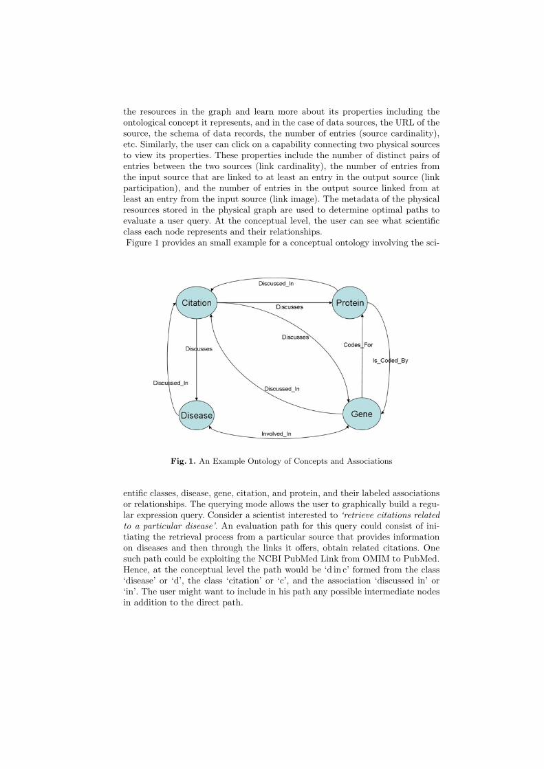
the resources in the graph and learn more about its properties including theontological concept it represents, and in the case of data sources, the URL of thesource, the schema of data records, the number of entries (source cardinality),etc. Similarly, the user can click on a capability connecting two physical sourcesto view its properties. These properties include the number of distinct pairs ofentries between the two sources (link cardinality), the number of entries fromthe input source that are linked to at least an entry in the output source (linkparticipation), and the number of entries in the output source linked from atleast an entry from the input source (link image). The metadata of the physicalresources stored in the physical graph are used to determine optimal paths toevaluate a user query. At the conceptual level, the user can see what scientificclass each node represents and their relationships.Figure 1 provides an small example for a conceptual ontology involving the sci-

Fig. 1. An Example Ontology of Concepts and Associations

entific classes, disease, gene, citation, and protein, and their labeled associationsor relationships. The querying mode allows the user to graphically build a regu-lar expression query. Consider a scientist interested to ‘retrieve citations related

to a particular disease’. An evaluation path for this query could consist of ini-tiating the retrieval process from a particular source that provides informationon diseases and then through the links it offers, obtain related citations. Onesuch path could be exploiting the NCBI PubMed Link from OMIM to PubMed.Hence, at the conceptual level the path would be ‘d in c’ formed from the class‘disease’ or ‘d’, the class ‘citation’ or ‘c’, and the association ‘discussed in’ or‘in’. The user might want to include in his path any possible intermediate nodesin addition to the direct path.

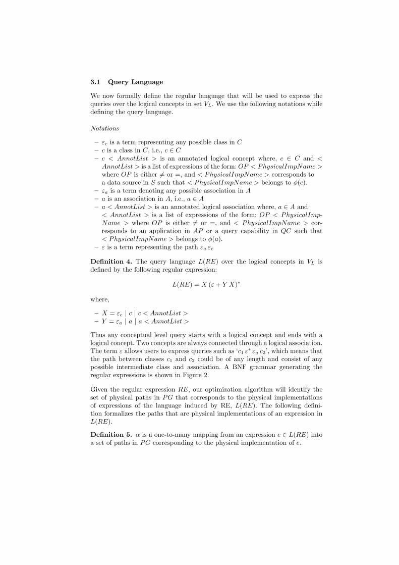
3.1 Query Language

We now formally define the regular language that will be used to express thequeries over the logical concepts in set VL. We use the following notations whiledefining the query language.

Notations

– εc is a term representing any possible class in C

– c is a class in C, i.e., c ∈ C

– c < AnnotList > is an annotated logical concept where, c ∈ C and <

AnnotList > is a list of expressions of the form: OP < PhysicalImpName >

where OP is either 6= or =, and < PhysicalImpName > corresponds toa data source in S such that < PhysicalImpName > belongs to φ(c).

– εa is a term denoting any possible association in A

– a is an association in A, i.e., a ∈ A

– a < AnnotList > is an annotated logical association where, a ∈ A and< AnnotList > is a list of expressions of the form: OP < PhysicalImp-Name > where OP is either 6= or =, and < PhysicalImpName > cor-responds to an application in AP or a query capability in QC such that< PhysicalImpName > belongs to φ(a).

– ε is a term representing the path εa εc

Definition 4. The query language L(RE) over the logical concepts in VL isdefined by the following regular expression:

L(RE) = X (ε + Y X)∗

where,

– X = εc | c | c < AnnotList >

– Y = εa | a | a < AnnotList >

Thus any conceptual level query starts with a logical concept and ends with alogical concept. Two concepts are always connected through a logical association.The term ε allows users to express queries such as ‘c1 ε∗ εa c2’, which means thatthe path between classes c1 and c2 could be of any length and consist of anypossible intermediate class and association. A BNF grammar generating theregular expressions is shown in Figure 2.

Given the regular expression RE, our optimization algorithm will identify theset of physical paths in PG that corresponds to the physical implementationsof expressions of the language induced by RE, L(RE). The following defini-tion formalizes the paths that are physical implementations of an expression inL(RE).

Definition 5. α is a one-to-many mapping from an expression e ∈ L(RE) intoa set of paths in PG corresponding to the physical implementation of e.

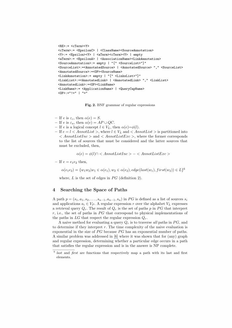
<RE>:= <cTerm><Y>

<cTerm>:= <EpsilonC> | <ClassName><SourceAnnotation>

<Y>:= <Epsilon><Y> | <aTerm><cTerm><Y> | empty

<aTerm>:= <EpsilonA> | <AssociationName><LinkAnnotation>

<SourceAnnotation>:= empty | "[" <SourceList>"]"

<SourceList>:=<AnnotatedSource> | <AnnotatedSource> "," <SourceList>

<AnnotatedSource>:=<OP><SourceName>

<LinkAnnotation>:= empty | "[" <LinksList>"]"

<LinkList>:=<AnnotatedLink> | <AnnotatedLink> "," <LinkList>

<AnnotatedLink>:=<OP><LinkName>

<LinkName>:= <ApplicationName> | <QueryCapName>

<OP>:="!=" | "="

Fig. 2. BNF grammar of regular expressions

– If e is εc, then α(e) = S.– If e is εa, then α(e) = AP ∪ QC.– If e is a logical concept l ∈ VL, then α(e)=φ(l).– If e = l < AnnotList >, where l ∈ VL and < AnnotList > is partitioned into

< AnnotListInc > and < AnnotListExc >, where the former correspondsto the list of sources that must be considered and the latter sources thatmust be excluded, then,

α(e) = φ(l)∩ < AnnotListInc > − < AnnotListExc >

– If e = e1e2 then,

α(e1e2) = {w1w2|w1 ∈ α(e1), w2 ∈ α(e2), edge(last(w1), first(w2)) ∈ L}6

where, L is the set of edges in PG (definition 2).

4 Searching the Space of Paths

A path p = (s1, a1, s2, . . . , sn−1, an−1, sn) in PG is defined as a list of sources si

and applications ai ∈ VP . A regular expression r over the alphabet VL expressesa retrieval query Qr. The result of Qr is the set of paths p in PG that interpretr, i.e., the set of paths in PG that correspond to physical implementations ofthe paths in LG that respect the regular expression Qr.

A naive method for evaluating a query Qr is to traverse all paths in PG, andto determine if they interpret r. The time complexity of the naive evaluation isexponential in the size of PG because PG has an exponential number of paths.A similar problem was addressed in [6] where it was shown that for (any) graphand regular expression, determining whether a particular edge occurs in a paththat satisfies the regular expression and is in the answer is NP complete.

6 last and first are functions that respectively map a path with its last and firstelements.

4.1 Assigning Metrics to Physical Paths

The result of a query Qr is a list of paths that represents the different ways inwhich the user can navigate through the data sources in order to evaluate Qr.It becomes important to assign ranks to these paths so that the user can easilyselect the most suitable one. We use three metrics for ranking the paths:

1. Path Cardinality is the number of instances of paths of the result. For apath of length 1 between two sources S1 and S2, it is the number of pairs(e1, e2) of entries e1 of S1 linked to an entry e2 of S2.

2. Target Object Cardinality is the number of distinct objects retrieved fromthe final data source.

3. Evaluation Cost is the cost of the evaluation plan, which involves both thelocal processing cost and remote network access delays.

These three metrics are meaningful to the scientists as the path cardinality com-putes the probability there exists a path between two sources, the target objectcardinality estimates the number of retrieved entries, whereas the evaluationcost guides the scientists to the selection of an efficient evaluation path. Thethree values for each path are estimated based on the properties of the linksthat exist between the data sources in S using the methods introduced in [5]and [7]. The following definitions describe the mapping from the logical associ-ations between two classes in LG to the links between two data sources in PG

and their properties.The function γ defined in Definition 6 maps a logical association between

two logical classes to the set of its implementations, that is the set of physicallinks that implement it with respect to φ.

Definition 6.

A function γ is a one-to-many mapping from a pair of logical associations in E×E

to pairs of physical links in L × L. If a pair (pl1, pl2) belongs to γ((la1, la2)),then the following holds:

– la1 = (c1, a) and la2 = (a, c2) are logical links, where c1 and c2 are logicalclasses, and a is a logical association between c1 and c2.

– pl1 = (s1, ap) and pl2 = (ap, s2) are physical links where s1 and s2 aresources and ap is an application or a query capability.

– s1 ∈ φ(c1), s2 ∈ φ(c2) and ap ∈ φ(a).

Definition 7.

A function δ is a one-to-many mapping from a pair of edges in E×E to 5-tuplesin L × L × R × R × R. The function δ maps a logical association between twological classes to the set of physical link implementations and the values of themetrics link cardinality, domain participation and image participation. A 5-tuple(pl1, pl2, lc, dp, ip) belongs to δ((la1, la2)), then the following holds:

– la1 = (c1, a) and la2 = (a, c2) are logical links, c1 and c2 are logical classesand, a is a logical association between c1 and c2.

– pl1 = (s1, ap) and pl2 = (ap, s2) are physical links and, s1 and s2 are sourcesand ap is an application or a query capability.

– (pl1, pl2) ∈ γ((la1, la2)).– lc: represents the link cardinality and corresponds to the number of links

from all data objects of source s1 pointing to data objects of s2.– dp: represents the domain participation and corresponds the number of ob-

jects in s1 having at least one outgoing link to an object in s2.– ip: represents the image participation and corresponds to the number of data

objects in s2 that have at least one incoming link from objects in s1.

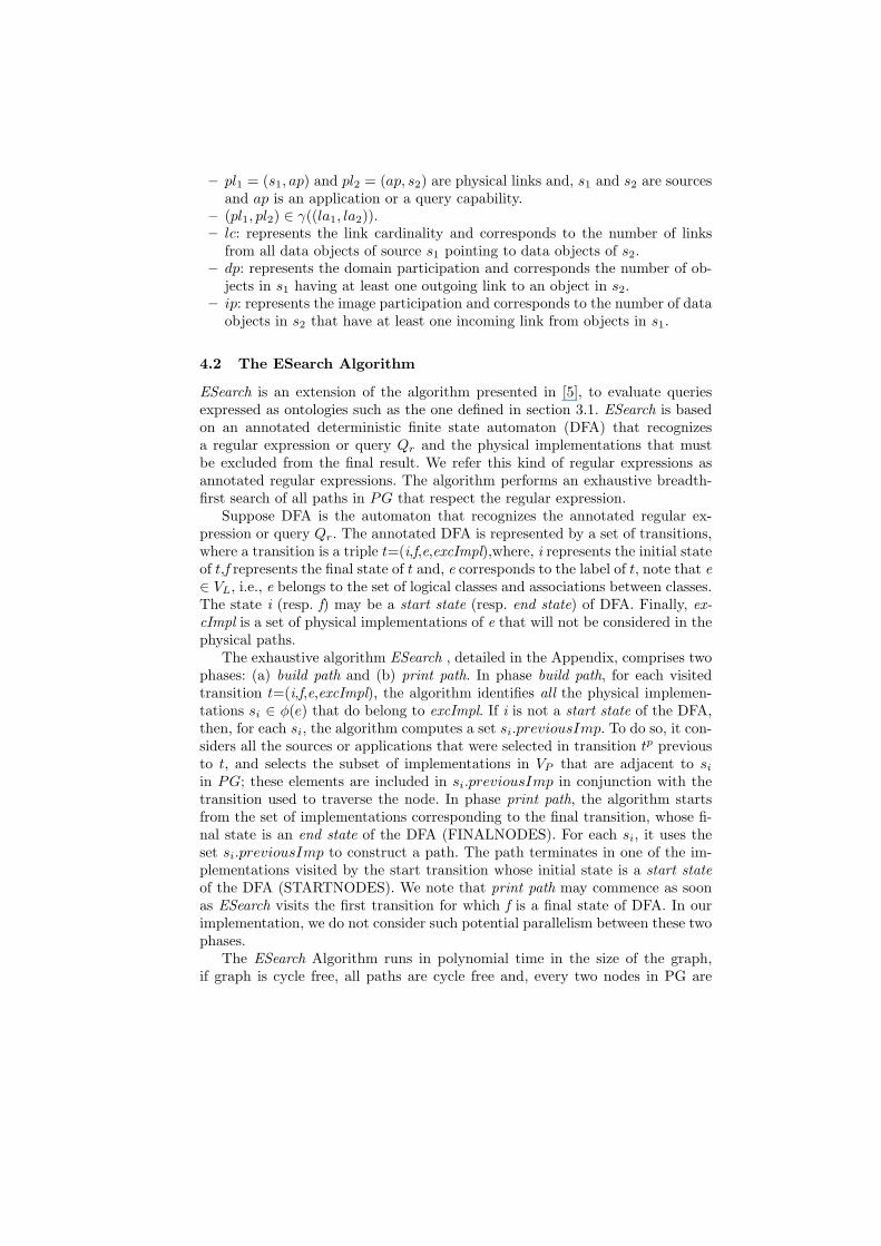
4.2 The ESearch Algorithm

ESearch is an extension of the algorithm presented in [5], to evaluate queriesexpressed as ontologies such as the one defined in section 3.1. ESearch is basedon an annotated deterministic finite state automaton (DFA) that recognizesa regular expression or query Qr and the physical implementations that mustbe excluded from the final result. We refer this kind of regular expressions asannotated regular expressions. The algorithm performs an exhaustive breadth-first search of all paths in PG that respect the regular expression.

Suppose DFA is the automaton that recognizes the annotated regular ex-pression or query Qr. The annotated DFA is represented by a set of transitions,where a transition is a triple t=(i,f,e,excImpl),where, i represents the initial stateof t,f represents the final state of t and, e corresponds to the label of t, note that e

∈ VL, i.e., e belongs to the set of logical classes and associations between classes.The state i (resp. f) may be a start state (resp. end state) of DFA. Finally, ex-

cImpl is a set of physical implementations of e that will not be considered in thephysical paths.

The exhaustive algorithm ESearch , detailed in the Appendix, comprises twophases: (a) build path and (b) print path. In phase build path, for each visitedtransition t=(i,f,e,excImpl), the algorithm identifies all the physical implemen-tations si ∈ φ(e) that do belong to excImpl. If i is not a start state of the DFA,then, for each si, the algorithm computes a set si.previousImp. To do so, it con-siders all the sources or applications that were selected in transition tp previousto t, and selects the subset of implementations in VP that are adjacent to si

in PG; these elements are included in si.previousImp in conjunction with thetransition used to traverse the node. In phase print path, the algorithm startsfrom the set of implementations corresponding to the final transition, whose fi-nal state is an end state of the DFA (FINALNODES). For each si, it uses theset si.previousImp to construct a path. The path terminates in one of the im-plementations visited by the start transition whose initial state is a start state

of the DFA (STARTNODES). We note that print path may commence as soonas ESearch visits the first transition for which f is a final state of DFA. In ourimplementation, we do not consider such potential parallelism between these twophases.

The ESearch Algorithm runs in polynomial time in the size of the graph,if graph is cycle free, all paths are cycle free and, every two nodes in PG are

connected by a unique path. Each node (source) in the graph implements onlyone entity, so a node is visited at most once in each transition (each level ofthe breadth-first search). Similarly, each node is visited at most once in eachiteration of print path. An annotated physical graph is produced during the build

path phase of ESearch. For each transition in the DFA, each implementation si

matching the transition is annotated with implementations in si.previousImp.If d is the maximum number of nodes that can precede a node in the annotatedphysical graph, i.e., the cardinality of previousImp, and b is the maximum lengthof (cycle free) paths satisfying the annotated regular expression, then O(db) isan upper bound for ESearch.

5 Conclusions

BioNavigation can enhance existing mediation approaches by providing scientistswith the ability to browse through available integrated resources and to accesstheir properties. The wildcard ε∗ allows users to identify alternate paths thatmay be exploited to evaluate the queries while the annotations aid specifyingthe resources they may require to be used (or not be used) in the process. TheESearch algorithm designed and implemented for BioNavigation allows efficientsearch in the space of all possible evaluation paths. Moreover three scientificallymeaningful metrics provide scientists the paths that best meet their needs. Inthe future we will combine the BioNavigation system with a system to executethe query on the path selected by the user. BioNavigation will be coupled withthe SemanticBio [8] that allows users to express and execute scientific workflowswith an ontology and Web Services. We will also exploit the system to supportthe exploration and querying of biological pathways.

References

1. Lacroix, Z., Edupuganti, V.: How biological source capabilities may affect the datacollection process. In: Computational Systems Bioinformatics, IEEE Computer So-ciety (2004) 596–597

2. Stevens, R., Goble, C.A., Bechhofer, S.: Ontology-based knowledge representationfor bioinformatics. Briefings in Bioinformatics 1 (2000) 398–416

3. Baker, P.G., Brass, A., Bechhofer, S., Goble, C., Paton, N., Stevens, R.: TAMBIS -transparent access to multiple bioinformatics information sources. In: Sixth Inter-national Conference on Intelligent Systems for Molecular Biology (ISMB), MenlowPark, California, AAAI Press (1998) 25–43

4. Lacroix, Z., Morris, T., Parekh, K., Raschid, L., Vidal, M.E.: Exploiting multiplepaths to express scientific queries. In: 16th International Conference on Scientificand Statistical Database Management (SSDBM), IEEE Computer Society (2004)357–360

5. Lacroix, Z., Raschid, L., Vidal, M.E.: Efficient techniques to explore and rank pathsin life science data sources. [9] 187–202

6. Mendelzon, A.O., Wood, P.T.: Finding regular simple paths in graph databases. InApers, P.M.G., Wiederhold, G., eds.: VLDB, Morgan Kaufmann (1989) 185–193

7. Lacroix, Z., Murthy, H., Naumann, F., Raschid, L.: Links and paths through lifescience data sources. [9] 203–211

8. Lacroix, Z., Menager, H.: Semanticbio: Building conceptual scientific workflows overweb services (2005) Submitted to DILS.

9. Rahm, E., ed.: First International Workshop on Data Integration in the Life Sciences(DILS), Proceedings. Volume 2994 of Lecture Notes in Computer Science, Subseries:Lecture Notes in Bioinformatics., Springer (2004)

APPENDIX: Algorithm ESearch

INPUT:

– DFA: an annotated deterministic finite state automaton for the query.– LG: Logical Graph– PG: Physical Graph.– φ: one-many mapping from logical concepts to sources.

OUTPUT: FINAL: a set of the paths to implement the query.

1. BUILD PATH PHASE:(a) INITIALIZE:

i. Assign Empty to FINAL.ii. Create a set of OPENTransitions of annotated transitions ti. Recall

that each ti is a transition of the annotated DFA and is a 4-tuple(i,f,e,excImpl), where, i is the initial state, f is the final state, e is alogical concept (class or relationship) in LG and, excImpl is a set ofphysical implementations of e that will not be considered.

iii. For each transition ti=(i,f,e,excImpl) in OPENTransitions, add a pair(S,ti) to STARTNODE, where S belongs to φ(e) and does not belongto excImpl.

(b) ANNOTATE:i. While OPENTransitions is not empty

– Remove a transition (i,f,e,excImpl) from OPENTransition.– Create a set LOCALImplementatiosn of sources/applications S

in PG that belongs to φ(e) and does not belong to excImpl.– While LOCALImplementations is not empty

• Remove an element S from LOCALImplementations.• If exists a pair (S′, t′) in OPENImplementations such that,∗ The edge (S′, S) belongs to PG.∗ t′=(i′,i,e′,excImpl′) and t=(i,f,e,excImpl), i.e., t′ is a transi-

tion previous to t in DFA.∗ S does not belong to excImpl.

• Add the pair (S′,t) to S.previousImp.• If f is not a final state in DFA∗ Add the pair (S,t) to OPENImplementation∗ For each transition t′′=(f,k,l,excImpl1) in DFA, Add the pair

(S,t′′) to OPENImplementations. Note that t is a transitionprevious to t′′.

• Else∗ Add the pair (S,t) to FINALTransitions.

2. PRINT PATH PHASE:(a) INITIALIZE:

i. Create a set OPENPATHS of single sub-paths, each one has one pair(S,t), where (S,t) belongs to FINALNODES.

(b) EXPAND:i. While OPENPATHS is not empty

A. Remove a subpath P=(Sj ,tj),...,(Sn,tn) from OPENPATHSB. For each pair (Sj−1,tj−1) in Sj .previousImp that such tj−1 is a

transition previous to tj in DFAC. If the pair (Sj−1,tj−1) belongs to STARTNODE

– Add the path P′=(Sj−1,tj−1),(Sj ,tj),...,(Sn,tn) to TEMPFinalD. Else

– Add P′=(Sj−1,tj−1),(Sj ,tj),...,(Sn,tn) to OPENPATHS(c) PRINT :

– For each path P=(S1,t1),..,(Sn,tn) in TEMPFinal• Add the path P′=S1,...,Sn to FINAL.