Biomass Potential for Heat, Electricity and Vehicle Fuel in ...

Biomass Potential for Heat, Electricity and Vehicle Fuel in Sweden

Volume I

Peter Hagström Faculty of Natural Resources and Agricultural Sciences

Department of Bioenergy Uppsala

Doctoral thesis Swedish University of Agricultural Sciences

Uppsala 2006

Abstract Hagström, P. 2006. Biomass Potential for Heat, Electricity and Vehicle Fuel in Sweden. Doctoral dissertation. The main objective of this thesis was to determine how far a biomass quantity, equal to the potential produced within the Swedish borders, could cover the present energy needs in Sweden with respect to economic and ecological circumstances. Three scenarios were studied where the available biomass was converted to heat, electricity and vehicle fuel. Three different amounts of biomass supply were studied for each scenario: 1) potential biomass amounts derived from forestry, non-forest land, forest industry and community; 2) the same amounts as in Case 1, plus the potential biomass amounts derived from agriculture; 3) the same amounts as in Case 1, plus 50% of the potential pulpwood quantity.

For evaluating the economic and ecological circumstances of using biomass in the Swedish energy system, the scenarios were complemented with energy, cost and emergy analysis.

The scenarios indicated that it may be possible to produce 170.2 PJ (47.3 TWh) per year of electricity from the biomass amounts in Case 2. From the same amount of biomass, the maximum annual production of hydrogen was 241.5 PJ (67.1 TWh) per year or 197.2 PJ (54.8 TWh) per year of methanol.

The energy analysis showed that the ratio of energy output to energy input for large-scale applications ranged from 1.9 at electric power generation by gasification of straw to 40 at district heating generation by combustion of recovered wood. The cost of electricity at gasification ranged from 7.95 to 22.58 €/GJ. The cost of vehicle work generated by using hydrogen produced from forestry biomass in novel fuel cells was economically competitive compared to today’s propulsion systems. However, the cost of vehicle work generated by using methanol produced from forestry biomass in combustion engines was rather higher compared to use of petrol in petrol engines.

The emergy analysis indicated that the only biomass assortment studied with a larger emergy flow from the local environment, in relation to the emergy flow invested from society after conversion, was fuel wood from non-forest land. However, even use of this biomass assortment for production of heat, electricity or vehicle fuels had smaller yields of emergy output in relation to emergy invested from society compared to alternative conversion processes; thus, the net contribution of emergy generated to the economy was smaller compared to these alternative conversion processes. Key words: bioenergy potential, biomass potential, cost analysis, emergy, energy analysis, energy scenarios, systems analysis, thermochemical conversion. Author’s adress: Peter Hagström, Department of Bioenergy, SLU, P.O. Box 7061, SE-750 07 UPPSALA, Sweden. E-mail: [email protected]

Contents Volume I 1. Introduction, 7 Energy use, 9

Premises and dwellings, 9 District heating, 10 Industrial activities, 11

Mining and metal industry, 12 Saw milling industry, 12 Pulp and paper industry, 14

Transport, 14 Energy supply, 16

Biomass, 16 Round wood for residential heating, 17 Logging residues, 17 Charcoal, 17 By-products from saw mills, 17 By-products from pulp mills, 17 Energy crops from agriculture, 18 Peat, 18 Waste, 19

Fossil fuels, 19 Coal and coke, 19 Oil, 19 Natural gas, 20

Electricity, 20 Hydroelectric power, 20 Nuclear power, 20 Wind power, 21 Solar power, 22

Prerequisities for biomass in the future Swedish energy system, 22 Objectives and study design, 23 2. Methods, 27 Description of complex systems, 27 Evaluation methods, 28

Energy scenarios, 30 Energy analysis, 31 Cost analysis, 34 Emergy analysis, 35

Selected systems for the energy, cost and emergy analyses, 39 Data handling, 44 3. Biomass available for energy conversion, 45 Sources and supply systems, 45

Biomass from forestry and fuel wood from non-forest land, 46 Logging residues, 49

Final felling, 49 Thinning, 51

Trees from early thinning, 52 Direct fuel wood cuttings, 52 Fuel wood from industrial wood cuttings, 53 Fuel wood from non-forest land, 53

By-products from forest industries, 53 Agriculture, 56

Willow farming, 56 Reed canary grass, 59 Straw, 60

Municipal waste, 60 Recovered wood, 60

Other potential biomass assortments, 61 4. Selected biomass conversion systems, 65 Small-scale firing, 65 District heating, 67 Combined heat and power generation, 68 Electric power generation, 69 Vehicle fuel production, 71

Hydrogen production, 74 Methanol production, 75

Black liquor gasification, 77 5. Bioenergy in three scenarios, 79 Heat demand and supply in Sweden in 2002, 79

Energy use for heat production to premises and dwellings, 79 Single-family houses, 79 Premises and dwellings excluding single family-houses, 79

Energy use for heat production in industry, 81 District heating, 81

Scenario ‘heat’, 82 Single-family houses, 83 Premises and dwellings excluding single-family houses, 84 Energy use for heat production in industry, 85 District heating, 85 Compilation of biomass amounts required for heat production in scenario

‘heat’, 87 Simulation of the amounts of heat and electricity received, 88

Scenarios electricity and vehicle fuel, 89 Simulations of maximum amounts of electricity and vehicle fuel produced –

Case 1, 91 Simulations of maximum amounts of electricity and vehicle fuel produced –

Case 2, 93

Simulations of maximum amounts of vehicle fuel produced – Case 3, 96 The potential of electricity and vehicle fuel production by black liquor

gasification, 98 Comparison of maximum yields of energy carriers with today’s use, 102 Discussion, 103 6. Energy, cost and emergy analysis, 105 Prerequisites and methods, 105

Energy analysis, 106 Cost analysis, 107 Emergy analysis, 108

Results, 107 Energy analysis, 108 Cost analysis, 115 Emergy analysis, 118 Sensitivity analysis, 122

Discussion, 128 7. Summary and conclusions, 135 Comparisons of used methods and generated results, 135 Policy options, 144 Future work, 145 Conclusions, 145 References, 149 Acknowledgements, 173 Appendices Appendix A: Abbreviations, units, symbols and time concepts, 175 Appendix B: Physical data, 180 Appendix C: Footnotes, 183 Appendix D: Description of the spreadsheet used for the simulations, 203 Appendix E: Brief of other technologies for gasification of biomass, 204 Appendix F: Calculation of sej/SEK index for 2002, 205 Appendix G: Dry matter losses, 213 Appendix H: Embodied energy and solar transformities of machinery

equipment, 217 Volume II Appendix I: Tables A.I-1 through to A.I-17, 225 Appendix J: Data for silviculture, agriculture, machinery and process

equipment, 307

7

1. Introduction

Sweden is the fi fth largest of the European countries (449,964 square kilometres (The Swedish Institute, 2002)). More than half of its land area is covered by forest. Historically, forests have always been a major primary energy source in Sweden, both for heating of dwellings in the rather cold climate and for industrial purposes (Arpi (ed.), 1959).

Other natural resources forming the base for Sweden´s prosperity are rich metal ores and plenty of rivers, in earlier times serving as a transport system as well as a direct power source for fl our-mills and saw mills and also for pumps, bellows and hammers in the mining and metal industry. Nowadays, the rivers have lost their importance in the transport system and serve mainly as the basis for extensive hydroelectric power production (Eklund, 1991).

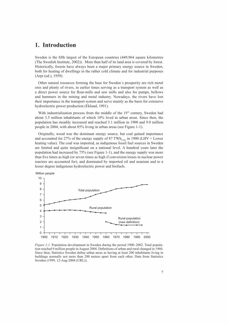
With industrialisation process from the middle of the 19th century, Sweden had about 3.5 million inhabitants of which 10% lived in urban areas. Since then, the population has steadily increased and reached 5.1 million in 1900 and 9.0 million people in 2004, with about 85% living in urban areas (see Figure 1-1).

Originally, wood was the dominant energy source, but coal gained importance and accounted for 27% of the energy supply of 87 TWhLHV in 1900 (LHV = Lower LHV in 1900 (LHV = Lower LHVheating value). The coal was imported, as indigenous fossil fuel sources in Sweden are limited and quite insignifi cant on a national level. A hundred years later the population had increased by 75% (see Figure 1-1), and the energy supply was more than fi ve times as high (or seven times as high if conversion losses in nuclear power reactors are accounted for), and dominated by imported oil and uranium and to a lesser degree indigenous hydroelectric power and biofuels.

Million people

0

6

1900 1920 1950 19701910 196019401930 200019901980

2

4

8

10

Total population

Rural population

Rural population(new definition)

5

1

3

7

9

Figure 1-1. Population development in Sweden during the period 1900–2002. Total popula-tion reached 9 million people in August 2004. Defi nitions of urban and rural changed in 1960. Since then, Statistics Sweden defi ne urban areas as having at least 200 inhabitants living in buildings normally not more than 200 meters apart from each other. Data from Statistics Sweden (1999, 12-Aug-2004 (URL)).

8

Figure 1-2. Energy supply in Sweden during the period 1900–2002. Data on wood fuel 1900-1955 adapted from Arpi ((ed.) 1959); data on other energy supply 1900–1970 adapted from yearly reports by Statistics Sweden; data 1970–2002 from the Swedish Energy Agency (2003a, 2003b). The energy supply is based on lower heating values (LHV).

Biomass(mainly wood)

Hydro power

Coal and coke

Oil

Natural gas

Nuclear power- electricity- wasted heat

TWh/year

700

600

500

400

300

200

100

0

19101900 1920 1930 1940 1950 1960 1970 1980 1990 2000

World War I World War II}

Oil crisis1973

}

Wind power

The development of energy supply from 1900 to 2002 is shown in Figure 1-2, details of the development of bioenergy seperated into different sources are pre-sented in Figure 1-3. Energy supply and use in 2002 are displayed in Figure 1-4,

10

0

20

30

40

100

90

80

70

60

50

TWh/year

1900 1910 1920 1930 1940 1950 1960 1970 1980 1990 2000

World War I World War II

}}

Oil crisis1973

Round woodfor charcoal

Pulp and paper industry- black liquor- other by-products

By-products from saw milling industry

Round wood for residential heating

Other sectors

District heating- municipal refuse- peat- wood fuels- crude tall oil

Biofuels forelectricity production

Figure 1-3. Biomass use for energy in different sectors of the Swedish economy during 1900–2002. Data 1900–1955 from Arpi ((ed.) 1959, Table 43) showing average of fi ve year periods adapted into TWhLHV per year; data 1956–1969 adapted from Statistical Yearbook of Forestry LHV per year; data 1956–1969 adapted from Statistical Yearbook of Forestry LHVpublished annually by the National Board of Forestry; data 1970–2002 from the Swedish Energy Agency (2003a, 2003b).

9

Figure 1-4. Energy supply and fi nal energy use in Sweden in 2002. Adapted from Swedish Energy Agency (2003b). Hh = households, Com = common purposes in the commercial and service sector, A = aviation fuel. The energy supply is based on LHVs.

where the amount of energy supplied is the sum of energy used and conversion and distribution losses.

Comprehensive surveys of Swedish forestry and its historical role have been made by Arpi ((ed.) 1959) and Kardell (2003, 2004), and the role of forestry in Sweden’s development from an agrarian to a highly industrialized modern state has been thor-oughly described. Besides industrial use, an equally important use of wood, though not so well documented, is for household requirements dominated by fuel wood.

Energy useEnergy in Sweden, as in other industrialised countries with a climate similar to Sweden’s, is mainly used for three purposes: (1) heating, lighting and operation of premises and dwellings, (2) industrial processes and (3) transport.

Premises and dwellingsIn 1900, an energy amount of about 25 GJLHV per person (equivalent to about 3.8 LHV per person (equivalent to about 3.8 LHVm3

f of wood (Arpi (ed.), 1959)) or roughly 35–40 percent of the total energy supply f of wood (Arpi (ed.), 1959)) or roughly 35–40 percent of the total energy supply fwas used for heating of premises and dwellings and for cooking. In 2002, the energy amount for the same purposes was 62 GJ per person, or about as much as for indus-trial use (Swedish Energy Agency, 2004b). The difference is due to the larger heated space per person in homes and a substantially larger service sector with stores,

Energy supplied 2002615.8 TWh

6.292,0

Biofuels,peat, etc

98.2

Coal&

coke

28.6

Hydropower

66.7

Nuclearpower

68.8 132.3

Conversion lossesin nuclear power

Crude oil and oil products

198.7

Natural gas,gasworks gas

5.4Electricity

import

Conversion lossesin nuclear power

132.3

Conversionand

distributionlosses

45.936.9

International marinebunkers and use fornon-energy purposes

Petrol Diesel A

2.7

56.0 47.1

3.8 16.57.5

20.9

Final use 2002400.7 TWh

Residential, services,etc

154.7

Transport

94.2

Industry

151.8Heat Hh Com

73.4 41.226.8

11.4 1.9

Electricity

132.1

Coal,coke

16.5 59.0

Biofuels,peat, etc

Oil products

138.6 5.8

Natural gas,gasworks gas

Districtheating

48.7

2.7

56.047.1

16.5 7.520.9

Heat Hh Com

73.441.226.8

11.43.81.9

Petrol Diesel A

91.5

7.4 Heat pumps9.3

91.5

10

offi ces, schools, hospitals and other public buildings (Arpi (ed.), 1959; Swedish Energy Agency, 2004a). Another difference not accounted for is the dissimilarity in energy quality. In 1900, the energy was supplied as fuels; today, energy quality is much higher as one third of the use is supplied as electricity (see Figure 1-4). Some electricty is used for cooling of food, in homes as well as in stores, but also for cool-ing spaces in public buildings with lots of electrical equipment producing more heat than is comfortable (Swedish Energy Agency, 2004a).

As the population increased and moved into more densely built-up areas, wood energy use per person decreased, partly because space heating became more effi -cient, and partly because increasing amounts of imported coal and oil were used for household heating. Therefore, the total demand for wood fuel did not increase with the increasing population but was rather constant in the period 1900 to 1945, with exception of the World Wars, when imports of coal and oil were curtailed and the need had to be covered by indigenous resources (Arpi (ed.), 1959).

After the Second World War, imported oil started to replace other alternatives for space heating. In the beginning of the 1960s, oil was so cheap that it even replaced wood fuel in households in the countryside where people had free access to wood from their own forest. Wood fuel for residential heating decreased from about 35 TWhLHV in 1945 to less than 7 TWhLHV in 1945 to less than 7 TWhLHV LHV/year in the years shortly before the fi rst oil crisis in 1973. After that, the use of round wood for residential heating of small houses increased to about 11 TWhLHV/year (See Figure 1-3). However, over the last three decades biomass has to a large extent replaced oil in the rapidly expanding district heating sector (Swedish Energy Agency, 2004b).

The need for imported oil was considerably reduced with the construction of nuclear power stations between 1972–1985. This resulted in a doubling of electric power generation capacity, with much of the electricity being allocated to the resi-dential and service sector, 73.4 TWh in 2002, of which 22.8 TWh were used for space heating. Another 5 TWh of electricity was used in district heating plants in the same year (Swedish Energy Agency, 2004b).

District heatingThe use of district heating started during the latter half of the 1940s and expanded during the 1950s and 1960s, as a result of the extensive investments in new hous-ing and other buildings built during that period, in conjunction with a substantial need for modernisation or replacement of boilers in the country’s existing building stock. Group heating systems were gradually linked to form larger systems, with a

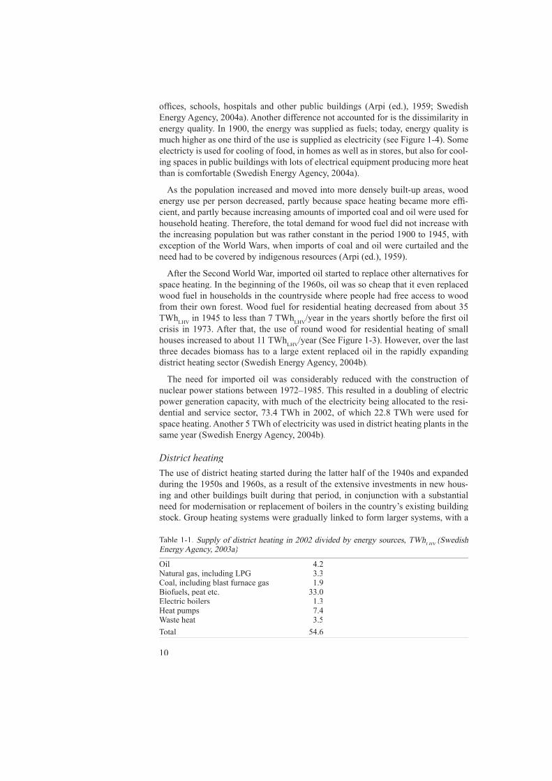
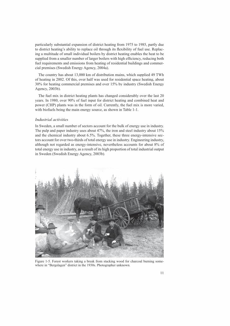
Table 1-1. Supply of district heating in 2002 divided by energy sources, TWhLHV (Swedish Energy Agency, 2003a)

Oil 4.2Natural gas, including LPG 3.3Coal, including blast furnace gas 1.9Biofuels, peat etc. 33.0Electric boilers 1.3Heat pumps 7.4Waste heat 3.5Total 54.6

11

particularly substantial expansion of district heating from 1975 to 1985, partly due to district heating’s ability to replace oil through its fl exibility of fuel use. Replac-ing a multitude of small individual boilers by district heating enables the heat to be supplied from a smaller number of larger boilers with high effi ciency, reducing both fuel requirements and emissions from heating of residential buildings and commer-cial premises (Swedish Energy Agency, 2004a).

The country has about 13,000 km of distribution mains, which supplied 49 TWh of heating in 2002. Of this, over half was used for residential space heating, about 30% for heating commercial premises and over 15% by industry (Swedish Energy Agency, 2003b).

The fuel mix in district heating plants has changed considerably over the last 20 years. In 1980, over 90% of fuel input for district heating and combined heat and power (CHP) plants was in the form of oil. Currently, the fuel mix is more varied, with biofuels being the main energy source, as shown in Table 1-1.

Industrial activitiesIn Sweden, a small number of sectors account for the bulk of energy use in industry. The pulp and paper industry uses about 47%, the iron and steel industry about 15% and the chemical industry about 6.5%. Together, these three energy-intensive sec-tors account for over two-thirds of total energy use in industry. Engineering industry, although not regarded as energy-intensive, nevertheless accounts for about 8% of total energy use in industry, as a result of its high proportion of total industrial output in Sweden (Swedish Energy Agency, 2003b).

Figure 1-5. Forest workers taking a break from stacking wood for charcoal burning some-where in “Bergslagen” district in the 1930s. Photographer unknown.

12

Mining and metal industryBesides agriculture and fi shing, mining and metal production has been an important basis for the Swedish economy since the 15th century. For example, in the 17th cen-tury the Great Copper Mountain of Falun in mid Sweden produced more than half of the world production of copper, enabling Sweden to develop to the most powerful nation in Northern Europe during the period 1560–1720 (Sundberg, 1991). In the mines, large amounts of fuel wood were used to crack the rock by fi re. Even more wood in the form of charcoal was needed in the copper, iron and steel works. Access to wood and charcoal were in most cases the limiting production factors, until the mid 19th century when improved and new technology decreased dependence on charcoal (Arpi (ed.), 1959; Kardell, 2003).

Cracking rock by fi res piled against the walls of the shafts, tunnels and drifts, was slowly replaced from the 1630s by blasting with gunpowder, although wood fi res were still used in some mines into the 19th century when explosives such as dynamite took over (Hult et al., 1989). The Swedish charcoal consumption peaked et al., 1989). The Swedish charcoal consumption peaked et al.in 1885 and decreased slowly up to the 1920s and then more rapidly as the metal manufacturing industry changed to other energy sources (coke and electricity) (Arpi (ed.), 1959). Today, the Swedish mining and metal industry is still an important part of the national economy, but it is totally independent of wood for energy.

Saw milling industryTimber has always been an important raw material for housebuilding and other construction. Earlier, the logs were divided into planks and boards by hand with axes and wedges or by pit-sawing, but saw mills driven by water power were built from the 15th century. These mills had to be located at water falls of a managable size which decided the capacity. The raw material supply was limited to the forests located up-stream and the products were made for a local market as land transport over longer distances with oxen or horses was too expensive. Some export occured, but the products were low quality as they had to be fl oated down the rivers to the coast for further transport by boat. The wood often became contaminated with sand during the river fl oating and had to be washed and dried before it could be sold (Arpi (ed.), 1959; Kardell, 2003).

Steam power was introduced into saw milling in the middle of the 19th century, nullifying the localised dependence on the power source. The saw mills could be placed wherever there was a signifi cant concentration of timber available and could be designed for practically any size of production as the fuel for the steam engines was abundant in the form of sawdust and other residues from the milling process (Arpi (ed.), 1959).

The saw mills for local production, driven by water power or steam, stayed in the inland areas, but production units for export were erected at the mouths of rivers in North and Middle Sweden and in the province of Värmland. The advantages included: potential timber could be supplied from the forests of the whole river valley; timber from other valleys could be rafted along the coast to the saw mill; large amounts of timber could be stored in the water; and the planks and buttons could be loaded directly from the timber-yard onto ships bound for the rapidly grow-ing European market (ibid.).ibid.).ibid.

13

The preconditions for rapid expansion of export were favourable in the middle of the 1800s. The metal works in Middle Sweden had, by tradition, put a claim on a large part of the forests, and in some areas, almost all forest had been used for charcoal production; thus, the forest was relatively young in such areas and larger amounts of old growth timber were not available. However, in North Sweden there were large unexploited forests along the rivers, which offered good transport facili-ties, and sizeable saw mill districts grew up at the river mouths (ibid.). ibid.). ibid.

From 1850 to the turn of the century, the export of sawn wood increased from 0.4 to 5.1 million m3. The expanding saw milling industry was one of the strongest economic forces during the middle of the 1800s when the foundation for the modern industrialized Swedish society was laid (ibid.). ibid.). ibid.

Steam engine technology greatly improved during the latter half of the 19th cen-tury, and older saw mills used all falling sawdust, in addition to other residues in the boilers, which were working with low steam pressure and low effi ciency. As improved technology was introduced, more of the residues could be used for other purposes. Gradually, from the middle of the 1870s the market value of by-products increased in that edgings and slabs, covered by sawdust, were commonly burnt to charcoal for use in the iron and steel industry (ibid.).ibid.).ibid.

In the saw milling process, only about 50% of the raw material is received as planks and boards. The rest is by-products, which is used as fuel in varying degree and different ways at different times. In the 1850s to the 1920s, most of the residues were used as fuel for steam engines at the saw mills and as charcoal for the iron and steel industry. In the 1920s and onwards, the steam engines were replaced by electric motors and the charcoal market was declining as a result of structural and techno-logical changes in the steel industry. However, simultaneously sulphate pulpmills were erected which could use wood chips from the saw mills in their process. In this way, the by-products were still mainly used for energy but in another industrial sector (ibid.).ibid.).ibid.

The sawn products have to be dried. In the past, the boards were piled up in the wood yards and dried naturally by sun and wind; today, drying is performed in kilns fuelled by bark and other wood residues (Kardell, 2004). The by-products not used in the saw mills or pulp mills are often sold to district heating plants or to the expanding wood pellet industry (Swedish Energy Agency, 2004a).

The following example based on Swedish Energy Agency (2003b) and National Board of Forestry (2004) illustrates the present importance of the saw milling indus-try as a user and producer of wood for energy. The round wood consumption of the saw mills in 2002 was 34.3 million m3

fub of which 11.8 million m3fub were transferred

to pulp mills and particle board and fi bre board plants. The production of sawn wood products was 16.1 million m3

f . The difference between wood supply and products f . The difference between wood supply and products fwas (34.3 – 11.8 – 16.1) million m3

fub = 6.4 million m3fub . The bark delivered to the

saw mills with the timber may be estimated at 12% x 34.3 million m3f = 4.1 million f = 4.1 million f

m3f . Hence, the amount of residues available for energy generation was about 10.5 f . Hence, the amount of residues available for energy generation was about 10.5 f

million m3f , theoretically equal to about 23 TWh. Of this, 4.8 TWh were used for f , theoretically equal to about 23 TWh. Of this, 4.8 TWh were used for f

industry. Most of the remainder was probably delivered to district heating plants and other industries as bark is not allowed to be discarded for environmental reasons.

14

Pulp and paper industryTwo chemical methods are generally used for extraction of cellulose, namely the sulphite or the prehydrolysis kraft (sulphate) method. The kraft method is the most common and accounts for approximately 80% of world cellulose production. Kraft pulping involves chemical treatment of wood with caustic soda and disodium sul-phite at high temperature, high pH and high pressure. Lignin in the wood is converted to water-soluble lignosulphonate that comes out of the wood, and is often referred to as kraft black liquor. Some hemicellulose and other secondary metabolites are also removed during this process. The cellulose yield is of the order of 45% and is about 95% pure (hemicellulose being the major contaminant) (Münster, 1998). The black liquor contains potentially valuable inorganic chemicals, which are recovered in a Tomlinson recovery boiler. In this process, the organic components are burnt to generate steam and electricity for the pulping process (Ekbom et al., 2003).et al., 2003).et al.

Mechanical methods are also used for pulp production. Grinding of roundwood by rotating grindstones was introduced in Germany in the 1840s (ForestSweden Webhotel, 2005 (URL)). The pulp produced is called groundwood pulp. In the early 1930s, an engineer, Arne Asplund, invented a new method for refi ning wood chips, namely defi bration of wood chips in disc refi ners (Lindström, 1998). The pulp pro-duced by this method is called refi ner mechanical pulp. The pulp yield may be up to 97% by these methods (Borg, 1989). In the 1970s, the refi ner mechanical pulp proc-ess was further developed. Pretreatment of wood chips with steam was introduced, leading to production of thermomechanical pulp (TMP). Another pulp assortment was also introduced, namely chemi-thermomechanical pulp (CTMP), where the wood chips are impgregnated with sodium sulphite (Na2SO3) (Waluszewski, 1990; Lindström, 1998). The pulp yield is about 90% for TMP and CTMP, but the strength of the paper produced is higher compared to paper produced by groundwood pulp.

A large disadvantage of mechanical pulp is the high consumption of electricity in the manufacturing process. Depending on the quality of paper produced, the use of electricity is between 1800 - 2500 kWh/t for TMP (Lindström, 1998), to be com-pared with the use of electricity at the kraft process, which is about 740 kWh/t90(KAM, 2000). However, the pulp yield is roughly twice as much for mechanical pulp compared to chemical pulp, as mentioned above. Paper produced by the dif-ferent pulp assortments have different properties regarding e.g. strength, opacity, e.g. strength, opacity, e.g.printability and brightness, which lead to a different range of application for the different pulp assortments.

TransportShipping has been important for Sweden since the Viking age. Merchant shipping was further developed during Sweden’s period as a great power in the 17th century. Domestic goods were even transported by shipping along the coasts at this time (The Swedish Transport Council, 1985). Simultaneously, road construction became an important task for the Swedish state authority, and the standard of the Swedish main roads were comparable with road patterns on the Continent of Europe (Ahl-ström, 1985).

Road transport was assessed as not being enough for domestic transport of goods. Thus, many canal construction projects were initiated during the 1780s. The fi rst

15

was Strömsholm’s canal, which opened communication between lake Mälaren and the province of Dalarna. The Göta canal was opened in 1832 and led to a shortened distance for transport between the Baltic sea and the North sea (Ahlström, 1985).

In an international perspective, the constructions of railways started rather late in Sweden. The Swedish Parliament decided in 1853/54 that the main railways, the trunk lines, should be constructed by the Swedish state. The fi rst railways was opened for traffi c in 1856, the trunk lines were completed in South and Central Sweden in the middle of the 1870s and in Northern Sweden in the beginning of the 20th century. Railways were also constructed by private companies for transport of goods, as e.g. agricultural products, iron ore, charcoal, iron and steel (Ahlström, e.g. agricultural products, iron ore, charcoal, iron and steel (Ahlström, e.g.1985).

The breaktrough of industrialism in the 1880s led to an increase in shipping. In 1880, the distribution of domestic transport of goods was 0.4 billion ton kilometre by rail and 0.6 billion ton kilometre via shipping. In 1900, domestic transport of goods was equal for both railway transport and shipping, about 1 billion ton kilome-tre. Since 1900, transport by rail became dominant (The Swedish Transport Council, 1985).

Floating was used on a large scale during the 17th century. The company Stora Kopparberg fl oated building timber used in their mines, and oak-trees were fl oated along Göta Älv and Viskan to be used for shipbuilding. However, the fi rst law for permitting fl oating in Sweden was not introduced until 1766, and the conception “public fl oatway” was introduced in 1880 (Krantz, 1986). At that time, transport via fl oating was 1.0 billion ton kilometre, and the main quantities were used as saw timber (The Swedish Transport Council, 1985; Eklund, 1991).

Motorized forwarding and road transport of roundwood was introduced during the 1920s and at the same time, the establishment of hydroelectric power began to expand. These were two reasons for decreased fl oating (Eklund, 1991). The last river used for fl oating was Klarälven in Värmland, and activity totally stopped in 1991 (National Board of Forestry, 2004).

As railways were considered the most important transport system of the future, road maintenance was neglected at the end of 1880s. However, the use of bicycles increased during the end of the 19th century, resulting in a greater interest in road maintenance. Better roads led to better conditions for the use of cars. The break-through for cars in Sweden arose at the car exhibition in Stockholm in 1903. After that, several Swedish manufacturers, as e.g. Vagnfabriks AB (VABIS) in Södertälje e.g. Vagnfabriks AB (VABIS) in Södertälje e.g.and Maskinfabriks AB Scania in Malmö, began producing both cars and lorries. Volvo produced their fi rst car in 1927 and SAAB began their car production in 1950. The number of cars in Sweden increased from about 50,000 in 1945 to 1.8 million in 1965. By then, Sweden had the largest motor-vehicle density in Europe (Hult et al., 1989). In 2002, the number of cars in Sweden was fully 4 millions (Statistics al., 1989). In 2002, the number of cars in Sweden was fully 4 millions (Statistics al.Sweden, 2005 (URL)).

In 1930, the work required for transporting people by road vehicles was equal to the work required for transporting people by rail. The total work required for transport of people then doubled during the 1930s, from 5 to 10 billion passenger kilometre. During the Second World War, private car traffi c was markedly reduced

16

due to lack of petrol. However, after the war, the number of private cars increased rapidly (The Swedish Transport Council, 1985).

The development of domestic and international aviation in Sweden began in 1936, due to the inauguration of Bromma airport north-west of Stockholm. The Second World War resulted in rapid technological development of both aeroplanes and ground-based equipment, e.g. communication systems, which led to rapid develop-e.g. communication systems, which led to rapid develop-e.g.ment of civil aviation after the war (Hult et al., 1989).et al., 1989).et al.

In 2002, the total work required for domestic transport of people was 128 billion passenger kilometre; 91% was performed via road transport, 7% by rail and fully 2% via aviation. (Swedish Energy Agency, 2003b). The domestic transport work of goods was fully 91 billion ton kilometre in 2003; 41% was performed via road transport, 22% by rail and 37% via shipping (Swedish Energy Agency, 2004a).

The energy use for transport (excluding foreign shipping) was 90.5 TWh in 2002, which corresponds to 23% of the total, fi nal national energy use; 0.5 TWhLHV con-LHV con-LHVsisted of ethanol; 2.9 TWh consisted of electricity; 0.1 TWhLHV consisted of natural LHV consisted of natural LHVgas and light petroleum gas (LPG); and the remainder 87.0 TWhLHV consisted of LHV consisted of LHVdifferent kinds of oil products (petrol, diesel/gas oil, medium/heavy fuel oils and aviation fuels) (Swedish Energy Agency, 2004b).

Energy supplySwedish energy supply is heavily dependent of non-renewable fuels, such as fossil fuels and uranium. In 2002, 1576 PJ (437.7 TWh), or 71.1% of total energy sup-plied in Sweden (being 2217 PJ (615.8 TWh)), came from these sources. The part from renewable energy resources (mainly biofuels and hydropower) was 596 PJ (165.5 TWh), or 26.9% of total energy supplied in Sweden (see Figure 1-4) (Swed-ish Energy Agency, 2003a).

The energy supply mixture has changed markedly during the last three decades. Since 1970, a majority of the fossil fuels has been replaced by nuclear power. The supply of biomass, including peat and waste, has also increased slowly, from 155 PJLHV/year (43 TWhLHV/year) to 354 PJLHV/year (98.2 TWhLHV/year) in 2002. Thus, biomass contributed to 15.9% of total energy supplied in Sweden in 2002. This increasing supply of biomass has mainly replaced fossil fuels (see Figure 1-3) (Swedish Energy Agency, 2003a, 2003b).

BiomassThe term ”biomass” is defi ned as material of biological origin excluding material embedded in geological formations and transformed to fossil. “Biofuel” means fuel produced directly or indirectly from biomass and “bioenergy” denotes energy from biofuels (European Committee for Standardization, 2003).

Biomass is mainly used for heat generation, but some of it, 22.3 PJLHV (6.20 LHV (6.20 LHVTWhLHV) in 2002, is also used for electric power generation in CHP plants and in industrial back-pressure plants. In 2002, approximately 1.8 PJLHV (0.5 TWhLHV (0.5 TWhLHV LHV) of ethanol was also produced from biomass for use as vehicle fuel (Swedish Energy Agency, 2003a).

17

Commercial use of biomass in Sweden is now widespread, both municipally and industrially, as fuel in heating plants and CHP plants. In 2002, 127.8 PJLHV (35.5 LHV (35.5 LHVTWhLHV) was used in municipal district heating plants, whereas 182.9 PJLHV (50.8 LHV (50.8 LHVTWhLHV) was used in industry. 67% (i.e. 122.4 PJi.e. 122.4 PJi.e. LHV (34.0 TWhLHV (34.0 TWhLHV LHV)) of the biomass use in industry consisted of black liquors in the pulp industry (Swedish Energy Agency, 2003a).

Round wood for residential heatingThe supply of round wood was rather high (around 30 TWhLHV.) until the second LHV.) until the second LHVworld war (see Figure 1-3). After the second world war, the supply of round wood decreased until 1965, as round wood for residential heating was replaced by oil fi ring. However, since 1965 the supply of round wood for residential heating has been constant, and is now around 8 TWhLHV (see Figure 1-3).

Logging residuesToday, logging residues are the dominant wood fuel assortment derived from for-estry and that are used for district heating generation in Sweden. The use of this assortment has increased markedly during the two latest decades, and in 2002, the supply was 6.6 TWhLHV

1. As shown in Chapter 3, the potential amounts are much greater than current use.

CharcoalIn 1900, the amount of round wood used for charcoal production in Sweden was approximately 10 TWhLHV (see Figure 1-3). However, this assortment started to LHV (see Figure 1-3). However, this assortment started to LHVdecline after the First World War, and in 1960 it was non-existent.

By-products from saw millsWood chips, sawdust and bark are by-products from saw mills. Bark is mainly used as fuel, both internally at the saw mills and as fuel in district heating plants. Wood chips and sawdust are also used as fuel internally at the saw mills and as fuel in dis-trict heating plants, but are also used as raw material in the pulp and board industry. The total amount of by-products used as fuel internally at the saw mills was 4.9 TWhLHV in 2002 (Swedish Energy Agency, 2004b). The corresponding amount sold LHV in 2002 (Swedish Energy Agency, 2004b). The corresponding amount sold LHVto the pulp and board industry in 2002 was 22.7 TWhLHV

2, and the amount sold as fuel to the district heating sector was 12.8 TWhLHV

3.

By-products from pulp millsThe by-products from pulp mills are mainly bark and black liquor. The bark received is used internally in the pulp mills as fuel for the generation of steam, which is used in pulp and paper processing. The total amount of bark from Swedish pulp mills in 2002 was 6.9 TWhLHV (Swedish Energy Agency, 2004b).LHV (Swedish Energy Agency, 2004b).LHV

Black liquor derives from the wood fi bre extraction step in pulp processing, and consists of dissolved wood organics, mainly lignin, and inorganic chemicals used in this extraction step. After extraction (which is performed in a digester), the black liquor contains 15 – 17% solids. In the next process step, it is evaporated so that the solid content is increased to 70 – 80% (Ekbom et al., 2003).et al., 2003).et al.

18

The black liquor is treated in Tomlinson boilers, in order to recover the inorganic chemicals. These chemicals are then separated in the bottom of the boiler as a smelt bed of molten salts. It is then further dissolved with a weak wash in a tank to form green liquor, which is used in the wood fi bre extraction step. Thus, the inorganic chemicals are recycled in the pulp process (Ekbom et al., 2003).et al., 2003).et al.

The organic components from the wood dissolved in the black liquor are burned in the Tomlinson boiler. The heat released is used for steam production, which is used for providing heat and electric power to the pulp and paper processing. The amount of black liquor deriving from the Swedish pulp mills in 2002 was 34.0 TWhLHV (Swedish Energy Agency, 2004b).LHV (Swedish Energy Agency, 2004b).LHV

Energy crops from agricultureWillow (Salix viminalis L.) is a commonly used species for energy crops in Sweden. The commercial introduction of willow cultivation started in 1991, when Sweden received a new agricultural policy for decreasing overproduction of food.

Interest of cultivation of energy crops on arable land increased at the same time, as biofuels became more competitive when environmental and energy taxes on fossil fuels were considerably increased (Hadders & Olsson, 1996; Rosenqvist et al., 2000). In 2002, the area of cultivated willow was slightly more than 14,600 hec-al., 2000). In 2002, the area of cultivated willow was slightly more than 14,600 hec-al.tare, which corresponds to approximately 0.5% of total arable land in Sweden (The Swedish Board of Agriculture, 2002).

Investigations on using grass as a fuel in Sweden started at the beginning of the 1980s, with reed canary grass (Phalaris arundinacea L.) being the most promis-ing species regarding cultivation and quality (Andersson, 1989; Burvall, 1997). Reed canary grass may be cultivated in throughout Sweden, but harvest yields are estimated to be lower in southern Sweden compared to the northern parts, due to greater biological degradation in southern Sweden (Swedish Business Development Agency, 1994). In 2002, the area of cultivated reed canary grass in Sweden was 650 hectare (Tarighi, 2005).

The topical use of straw as a fuel in Sweden is estimated by Nilsson (1999a) to be about 40,000 metric tons (0.14 TWhLHV) per year. This may be compared with the use of straw in Denmark, where the power plants are obliged to utilize 1.0 million metric tons per year (Zhou et al., 2005). However, the physical potential of using et al., 2005). However, the physical potential of using et al.straw for energy purposes in Sweden is estimated to be much larger than current use. The extent of arable land where straw may be recovered for energy purposes is estimated to be 1.1 million hectare, according to the Swedish Government (1992b). Axenbom et al. (1992) estimate the Swedish potential of straw for energy purposes et al. (1992) estimate the Swedish potential of straw for energy purposes et al.to be 500,000 metric tons (2 TWhLHV) per year.

PeatPeat is a soil type of organic origin, which is formed through biological and chemi-cal processes in wetlands. It consists of plant and animal parts which have been incompletely degraded due to lack of oxygen. The carbon content is slightly more than 50% of dry matter (Ministry of Industry, Employment and Communication, 2002).

19

Sweden’s peat supply is large, as approximately 25% of the land area is covered with peat. The peat land area is estimated to be about 6.5 million ha (the peat layer is thicker than 30 cm). Peat extraction greatly infl uences the environment, as the original biotope is extinguished. However, suitable treatment of the topical area after fi nal extraction may reduce the negative infl uences, and the area can receive new high-quality aspects. Current peat extraction is performed on slightly more than 10,000 ha in Sweden (Ministry of Industry, Employment and Communication, 2002).

The use of peat for energy purposes amounted to 3.9 TWhLHV in 2002, which is the LHV in 2002, which is the LHVhighest amount to date. Approximately 30% of the peat used for energy purposes is imported (Swedish Energy Agency, 2003b).

WasteIn Sweden, waste materials have been used for district heating production since the 1970’s. In 2002, the amount of waste used for district heating production was 5.2 TWhLHV. This amount is expected to increase markedly in the future, due to the pro-LHV. This amount is expected to increase markedly in the future, due to the pro-LHVhibition on landfi ll sorted combustible waste, which was introduced in Sweden in 2002 (Swedish Energy Agency, 2003b).

From 2005, it is prohibited to landfi ll organic waste in Sweden (Swedish Energy Agency, 2003b), which may increase interest in digestion; e.g. organic waste from e.g. organic waste from e.g.the food industry and grocers will increase during the coming years, resulting in a larger potential of biogas production. In 2002, the use of biogas in Sweden was 448 GWhLHV, where 38 GWhLHV, where 38 GWhLHV LHV was used for electric power generation, 325 GWhLHV was used for electric power generation, 325 GWhLHV LHVwas used for heat production and 85 GWhLHV was used as vehicle fuel. The biogas LHV was used as vehicle fuel. The biogas LHVwas mainly produced via digestion of sewage sludge in wastewater treatment plants and via anaerobic degradation of waste at landfi ll stations (Swedish Energy Agency, 2004a).

Fossil fuelsCoal and cokeGlobally, industrialization has been driven by fossil fuels. Sweden is no exception: from the beginning of the 1870s to the beginning of the 1910s the annual import of coal and coke increased from 590,000 metric tons to 4900,000 metric tons (Statistics Sweden, 1925). The supply declined during the World Wars, due to diffi culties in supply by import. In 2002, the use of steam coal was 1520,000 metric tons (Swedish Energy Agency, 2004b).

OilThe import of crude oil increased steadily after the Second World War until the fi rst oil crisis in 1973, from barely 500,000 metric tons in the second half of the 1940s to barely 12 million metric tons in the beginning of the 1970s (Statistics Sweden, 1955, 1975). However, the fi rst oil crisis led to an intensive political debate in Sweden regarding national dependence on imported crude oil. The extension of nuclear power during the 1970s and 1980s (discussed below) led to a decrease in the supply of oil used for power generation (see Figure 1-2). However, increased refi nery capacity in Sweden during the 1970s and 1980s led to a continuously large

20

import of crude oil. In 1985, the import of crude oil was 13.8 million metric tons, whereas the corresponding import was 18.2 million metric tons in 2002 (Swedish Energy Agency, 2004b). During the same period, the Swedish export of refi ned fuels also markedly increased (Hagström & Nilsson, 2004).

Natural gasNatural gas was introduced into Sweden in 1985 and usage increased rapidly until 1992, after which growth continued at a more modest rate. In 2002, imports amounted to 933 million m3, equivalent to 9.3 TWhLHV. Industry, and CHP and district heat-LHV. Industry, and CHP and district heat-LHVing plants, each accounted for about 40% of total use, with domestic consumers accounting for about 15%. A small amount of natural gas is also used as motor fuel (Swedish Energy Agency, 2003b).

ElectricityIn 2002, the Swedish net electric power production was 516 PJ (143.4 TWh) of which 238 PJ (66.0 TWh), or 46.1%, was based on hydroelectric power, and 236 PJ (65.6 TWh), or 45.7% of the production was based on nuclear power. The remain-ing 8.2% of electric power produced was derived from CHP, condensing power, gas turbines, industrial back-pressure power and windpower (Swedish Energy Agency, 2003a).

Hydroelectric powerSweden has more than 100,000 lakes, covering approximately 10% of its area. There are many rivers, of which thirteen have a mean annual fl ow of more than 100 m3/s at the mouth.The fi rst generating stations based on hydro power were established in the 1880s. These stations were usually built where there had previously been directly driven machinery for mills, saws, hammers etc. The stations were small and etc. The stations were small and etcessentially intended to supply power to industries and communities in the immediate vicinity. Hundreds of such small local hydroelectric power stations were constructed during the end of the 19th and the beginning of the 20th century. As the technique of transferring power over longer distances developed at the beginning of the 1900s, it became possible to exploit the large rivers in the south and middle of the country. Development on a larger scale for electric power generation began in the 1910s and reached its peak in 1950–1970 when the production capacity expanded from around 20 to about 65 TWh/year. However, amounts vary greatly according to the weather. In the dry year 1996, the production was down to 52 TWh, but in 2000 and 2001 it was as high as 79 TWh/year.

Most hydroelectric power comes from nine rivers in the northern half of Sweden. Only minor expansions of hydroelectric power capacity are allowed; according to a decision by the Swedish parliament, the four unexploited rivers in the northern part of the country will be saved and untouched of environmental reasons.

Nuclear powerThree months after the atom bombs fell over Hiroshima and Nagasaki in August 1945, the Swedish government started planning for a research and development program for nuclear power with emphasis on civil applications, but also including

21

nuclear weapons. The Swedish peace movement was very strong and politically infl uential with leaders such as Alva Myrdal and Inga Thorsson. After heavy debates in the 1950s and the 1960s whether to continue the development of nuclear weap-ons, this part of the program was abandoned in 1968 (Kaijser, 2001).

Nevertheless, the development of civil nuclear energy continued. The fi rst Swed-ish nuclear reactor was built in Ågesta, just south of Stockholm, and was put into commercial operation in 1964. It was a CHP plant and would deliver 55 MW of heat for district heating and 10 MW of electric power (Kaijser, 2001). This reactor was decommissioned in 1974 due to low profi tability (Hult et al., 1989). A second et al., 1989). A second et al.nuclear reactor was built at Marviken, near the city of Norrköping, during the 1960s. It was constructed as a power plant with a maximum electric power output of 200 MW. However, that plant was never put into operation as a nuclear power plant, as the project was strongly criticized for not meeting the necessary safety require-ments. Instead, it was reconstructed and put into operation as an oil-fi ring power plant (Kaijser, 2001).

The nuclear reactors in Ågesta and Marviken consisted of heavy-water reactors (HWRs). In the early 1960s, it became possible to import enriched uranium from the USA, which made the light water reactors (LWRs) a possible alternative. HWRs were questioned from a commercial point of view by many Swedish power compa-nies, and as a result subsequent nuclear power plants constructed in Sweden con-sisted of LWRs (Kaijser, 2001). The fi rst one was put into operation in Oskarshamn in 1972, and the two last reactors, the eleventh and twelfth, was put into operation in Oskarshamn and Forsmark in 1985.

Much of the electricity generated via nuclear power replaced fossil fuels, which were reduced from about 350 TWh/year in 1972 to about 250 TWh/year in 1985 (see Figure 1-2). However, nuclear power continued to be a controversial issue in the Swedish parliament. The resistance came, and still comes, from environmental-ists in all political parties, who claim that nuclear power production is unsafe with risks for radioactive outlets, and that the plutonium in the residues can be used for production of nuclear weapons or might fall into the hands of terrorists.

Sweden has large deposits of low grade uranium. In the 1970s, there were plans to use the assets, but public opinion and a veto from the local community put an end to ore-mining plans in 1977, and the issue has so far not resurfaced.

The incident at the nuclear reactor on Three Mile Island, Harrisburg, USA in 1979 fuelled the Swedish nuclear power debate. A referendum was held in 1980 result-ing in a political decision to allow operation in the six reactors already built and the next six reactors that were planned, but all nuclear power should then be phased out by the year 2010. The decision has been modifi ed since then, and the date for fi nal shut down is now kept open. The fi rst nuclear reactor, Barsebäck 1, was decommis-sioned in November 1999, and the second, Barsebäck 2, was decommissioned in June 2005.

Wind powerWind power is a renewable energy source which has expanded substantially in Sweden over the last ten years. Despite this, its share of the country’s electricity

22

production is still very modest. At the end of 2002, with 620 wind power plants in operation, it supplied 0.56 TWh, or somewhat less than 0.4% of total electricity production in 2002 (Swedish Energy Agency, 2003b).

Solar powerThe fi rst functional, intentionally constructed photovoltaics device was by C. Fritts in the USA in 1883. He melted selenium into a thin sheet on a metal substrate and pressed a gold-leaf fi lm as the top contact; it was nearly 30 cm2 in area. However, the modern era of photovoltaics started in 1954 when researchers at Bell Labs in the USA accidentally discovered that diodes generated a voltage when the room lights were on. Within a year, they had produced a 6% effi cient silicon solar cell. In the same year and the year after, other research groups in the USA developed solar cells based on other compounds, as e.g. Cue.g. Cue.g. 2S/CdS and GaAs (Hegedus & Luque, 2003).

Solar cells were introduced on to the Swedish market at the end of the 1970s. The fi rst applications were power supply of lighthouses and emergency telephones in the Swedish mountains. In 2002, fully 20,000 non-mains-operated holiday cottages were power supplied by solar cells in Sweden. However, mains-operated solar cell modules for assembly in buildings are now developed both in Sweden and in other countries. The potential for this technology is estimated to be very large (Andersson & Hedström, 2002).

Prerequisities for biomass in the future Swedish energy systemAs a consequence of the fi rst oil crisis in 1973, the interest in energy system studies increased in Sweden. Several studies were initiated, and the fi rst studies focused on issues concerning energy supply. Johansson & Steen (1977) conducted a scenario, where the whole Swedish energy demand would be covered with renewable energy sources in 2015. In this scenario, the biomass supply would be 351 TWhLHV and LHV and LHVcover 62% of the total energy supply. Johansson & Steen concluded that this sce-nario would be realistic, and the costs for replacement of the energy supply systems would not make an assumed doubling of the material welfare impossible.

In a following study by Lönnroth, Johansson & Steen (1979), two national energy systems were compared: 1) energy supply based on nuclear-based heat and power production; 2) energy supply based on renewable energy sources (biomass, solar heat and power, windpower and hydroelectric power). It was concluded that the energy supply system based on renewable energy sources is physically possible, and may also be technically possible if resources are invested for development of this alternative. The costs for the two energy systems were estimated to be roughly equal.

Today, many individuals and organizations are interested in biomass for differ-ent reasons: the forest industry sector needs timber and pulp wood; many politi-cal fractions and groups hope that biomass may replace nuclear fuels in electricity generation; the ratifi cation of the Kyoto protocol may lead to replacement of fossil fuels with biomass for heating purposes and as a raw material for the generation of vehicle fuels in order to mitigate the emission of green house gases; environmental-ists would like to restrict human use of the forest in favour of fl ora and fauna; other

23

groups want to give priority to recreation and eco-tourism before industrial use.

There are mainly two reasons for a continuous exchange of fossil fuels with renewable energy resources. One of the reasons is environmental; the evidences that combustion of fossil fuels cause an increasing temperature in the atmosphere due to the increasing carbon dioxide concentration in the atmosphere have become stronger during the last years (International Panel on Climate Change, 2001). Thus, the Swedish parliament decided to decrease the emissions of greenhouse gases according to the Kyoto protocol and consequent decisions of the European Union (Ministry of Industry, Employment and Communication, 2003). Emissions of carbon dioxide due to combustion of biomass may not lead to a continuously increasing temperature in the atmosphere if the regrowth of biomass is at least equal to the use of biofuels.

The other reason is that supplies of fossil fuels are limited. The output of oil is anticipated to decline about 2008, whereas decrease in natural gas production is esti-mated to begin at about 2030 (The Association for the Study of Peak Oil&Gas, 2004 (URL); Laherrere, 2004). The world reserves of coal are estimated to correspond to about 200 years of production at current rates (Coal Industry Advisory Board, 2004 (URL)).

The Swedish parliament has also decided to phase out nuclear power, as a conse-quence of concerns by the public about the risk of nuclear power such as e.g. acci-e.g. acci-e.g.dents like the one near Harrisburg, USA in 1979 (Ministry of Industry, Employment and Communication, 1995).

Even if there is still a considerable potential to increase production and use of biomass in Sweden, it is obvious that this resource is physically and economically limited. Many of the interested parties are aware of the possibilities and benefi ts in their own business, but are less acquainted with the expectations of others. It is a risk that the potential collective demand greatly exceeds possible supply.

However, there are biomass assortments available for energy conversion purposes, as e.g. logging residues, fuel wood from industrial wood cuttings and by-products e.g. logging residues, fuel wood from industrial wood cuttings and by-products e.g.from forest industry, and there are still possibilities to increase the national supply of biomass in the Swedish energy system, mainly because there are assortments of wood fuels not used for energy purposes (Hektor, Lönner & Parikka, 1995; Parikka, 1997; Lönner et al., 1998), and there is also a physical potential to increase the culti-et al., 1998), and there is also a physical potential to increase the culti-et al.vation of agrofuels (Börjesson et al., 1997). However, one question remains regard-et al., 1997). However, one question remains regard-et al.ing the possibilities for a continuous partial replacement of the fossil fuels and the nuclear power with biomass in the future.

Objectives and study designThe main objective of this study was to determine how far a biomass quantity, equal to the potential produced within the Swedish borders, could cover the present energy needs in Sweden with respect to economic and ecological circumstances. Another aim was to conduct the study in such a way that it can be used as a basis for general judgements about the best use of Swedish biomass resources suitable for energy conversion, as well as an aid for interested parties in their considerations of their own position in the competition for biomass.

24

The fi rst step was to establish which biomass assortments that should be consid-ered within Sweden, and the amounts being potentially available for energy conver-sion with respect to environmental concerns, and those parties interested in biomass and land use for other purposes, e.g. the forest industry sector. Import and export of e.g. the forest industry sector. Import and export of e.g.biomass supplies were not considered.

Three scenarios in which the available biomass was converted to different energy carriers were studied:

• Scenario ‘heat’: biomass covers as much as possible of a heat demand equal to the use of heat in the year 2002. The remaining biomass is converted to electricity or vehicle fuel.

• Scenario ‘electricity’: biomass covers a heat demand equal to the use of heat gen-erated from biomass in 2002. The remaining biomass is converted to electricity.

• Scenario ‘vehicle fuel’: biomass covers a heat demand equal to the use of heat generated from biomass in 2002. The remaining biomass is converted to vehicle fuel (hydrogen or methanol).

Three different amounts of potential biomass supply were studied for the different scenarios (see Figure 1-6):

• Case 1: potential biomass amounts derived from forestry, non-forest land, forest industry and community.

• Case 2: case 1 plus potential biomass amounts derived from agriculture.• Case 3: case 1 plus 50% of potential pulpwood quantity converted to vehicle

fuels. In this case it was hypothesised that industry found it more appropriate to produce hydrogen or methanol rather than pulp and paper from this quantity.

The scenarios included conversion processes based on the newest technology that either are commercially available (e.g. biomass-fi red CHP) or are judged as being e.g. biomass-fi red CHP) or are judged as being e.g.introduced in a near future (integrated gasifi cation combined cycle (IGCC) and vehicle fuel production via gasifi cation). The amounts of different energy sources used for heat production in 2002 were compiled for each scenario and case, and the maximum amounts of energy carriers that could be converted by the remaining amounts of the topical biomass assortments were then calculated.

1

Scenarios ‘Heat’ ‘Electricity’ ‘Vehicle fuel’

Case 1: potential biomass amounts derived from forestry, non-forest land, forest industry and community

X X X

Case 2: Case 1 plus potential biomass amounts derived from agriculture

X X X

Case 3: Case 1 plus 50% of potential pulpwood quantity

– – X

Figure 1-6. The potential amounts of biomass supply studied for the different scenarios.

25

In order to evaluate the economic and ecological circumstances of biomass utiliza-tion in the Swedish energy system and for providing a basis for general judgements about the best use of the Swedish biomass resources suitable for energy conversion, the scenarios were complemented by three other evaluation methods. Energy analy-sis calculated the energy required for handling, pre-treatment and conversion of the biomass assortments studied, and the energy yield at production of each energy car-rier at conversion of the different biomass assortments.

The second method used for analysis of the biomass assortments studied was cost analysis, where the production costs of the energy carriers produced were calcu-lated. The monetary costs of the different operational steps used for the different biomass assortments were also evaluated.

The third method used for analysis of the biomass assortments studied was emergy analysis, where the solar emergy fl ows via the environment and the society at production of the biomass assortments and the energy carriers produced at con-version of the biomass assortments were evaluated. Solar emergy yields and solar transformities of products, emergy yield ratios and emergy investment ratios were also calculated for the different biomass assortments studied and the energy carriers produced.

The methods used are further described in Chapter 2, together with the systems for the energy, cost and emergy analyses. The potential biomass resources and selected methods of harvesting and collecting the different assortments are described in Chapter 3. Selected processes for converting biomass to heat, electricity and vehicle fuels are described in Chapter 4. The scenarios performed are described in Chapter 5. Energy, cost and emergy analysis are covered in Chapter 6 and the results and con-clusions are discussed and compiled in Chapter 7.

27

2. Methods

Description of complex systemsA system is defi ned by Hall & Hagen (1956) as a set of objects together with rela-tionships between the objects and between their attributes. Each object has its own unique characteristics and the characteristic of the system is dependent on the char-acteristics and structure of the objects within the system. Ackoff (1981) declares that a system is a set of two or more elements that satisfi es the following three conditions:- the behaviour of each element has an effect on the behaviour of the whole.- the behaviour of the elements and their effects on the whole are interdependent.- irrespect of how subgroups of the elements are formed, all have an effect on the

behaviour of the whole, but none has an independent effect upon it.

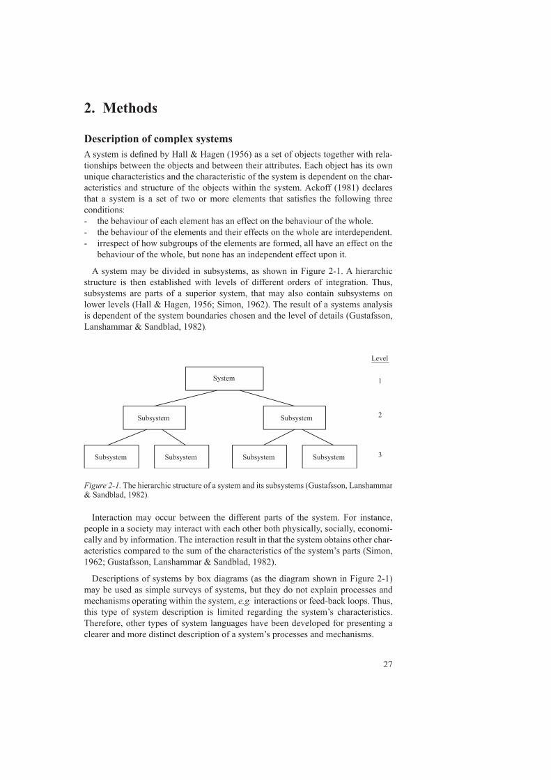
A system may be divided in subsystems, as shown in Figure 2-1. A hierarchic structure is then established with levels of different orders of integration. Thus, subsystems are parts of a superior system, that may also contain subsystems on lower levels (Hall & Hagen, 1956; Simon, 1962). The result of a systems analysis is dependent of the system boundaries chosen and the level of details (Gustafsson, Lanshammar & Sandblad, 1982).

Figure 2-1. The hierarchic structure of a system and its subsystems (Gustafsson, Lanshammar & Sandblad, 1982).

System

Subsystem

Subsystem

Subsystem

Subsystem

Subsystem

Subsystem

Level

1

2

3

Interaction may occur between the different parts of the system. For instance, people in a society may interact with each other both physically, socially, economi-cally and by information. The interaction result in that the system obtains other char-acteristics compared to the sum of the characteristics of the system’s parts (Simon, 1962; Gustafsson, Lanshammar & Sandblad, 1982).

Descriptions of systems by box diagrams (as the diagram shown in Figure 2-1) may be used as simple surveys of systems, but they do not explain processes and mechanisms operating within the system, e.g. interactions or feed-back loops. Thus, this type of system description is limited regarding the system’s characteristics. Therefore, other types of system languages have been developed for presenting a clearer and more distinct description of a system’s processes and mechanisms.

28

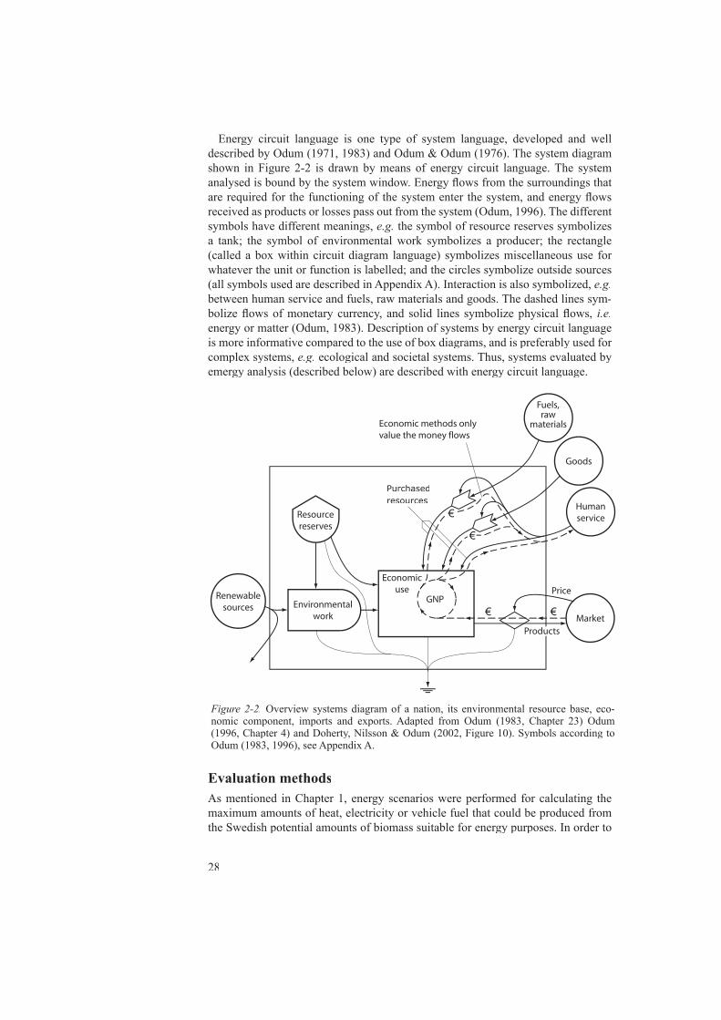
Energy circuit language is one type of system language, developed and well described by Odum (1971, 1983) and Odum & Odum (1976). The system diagram shown in Figure 2-2 is drawn by means of energy circuit language. The system analysed is bound by the system window. Energy fl ows from the surroundings that are required for the functioning of the system enter the system, and energy fl ows received as products or losses pass out from the system (Odum, 1996). The different symbols have different meanings, e.g. the symbol of resource reserves symbolizes a tank; the symbol of environmental work symbolizes a producer; the rectangle (called a box within circuit diagram language) symbolizes miscellaneous use for whatever the unit or function is labelled; and the circles symbolize outside sources (all symbols used are described in Appendix A). Interaction is also symbolized, e.g.between human service and fuels, raw materials and goods. The dashed lines sym-bolize fl ows of monetary currency, and solid lines symbolize physical fl ows, i.e.energy or matter (Odum, 1983). Description of systems by energy circuit language is more informative compared to the use of box diagrams, and is preferably used for complex systems, e.g. ecological and societal systems. Thus, systems evaluated by emergy analysis (described below) are described with energy circuit language.

Evaluation methodsAs mentioned in Chapter 1, energy scenarios were performed for calculating the maximum amounts of heat, electricity or vehicle fuel that could be produced from the Swedish potential amounts of biomass suitable for energy purposes. In order to

Figure 2-2. Overview systems diagram of a nation, its environmental resource base, eco-nomic component, imports and exports. Adapted from Odum (1983, Chapter 23) Odum (1996, Chapter 4) and Doherty, Nilsson & Odum (2002, Figure 10). Symbols according to Odum (1983, 1996), see Appendix A.

��

��

€ €

��

��

��

��

��

��

��

��

��

��

��

��

€

€

Purchasedresources

29

evaluate the economic and ecological circumstances of biomass utilization and for providing a basis for general judgements about the best use of the Swedish biomass resources suitable for energy conversion, these scenarios have to be complemented with other evaluation methods.

The supply and use of energy is a fundamental issue for all systems (e.g. bio-e.g. bio-e.g.logical and societal systems) as energy transformation processes are vital for the system’s continuous functions. As a consequence of rising energy costs during the last decades, the interest in quantifying energy use and the energy effi ciency for dif-ferent processes in industry and society have increased markedly. A main issue in evaluation of the best use of resources for energy purposes is to analyse yields and effi ciencies for handling and conversion of these resources. This is performed by energy analysis. Thus, energy analysis was used inter alia for quantifying the maxi-inter alia for quantifying the maxi-inter aliamum yields of heat, electricity and vehicle fuel in energy units (joule) which could be produced from the potential amounts of the biomass assortments studied.

Economic circumstances are of interest for all societal activities. Economics is the study of how societies with limited, scarce resources decide what gets produced, how, and for whom (Fischer, Dornbusch & Schmalensee, 1988). Here, the cost for production of goods and services is the main task. Cost may be defi ned as a sacrifi ce of resources. There are two major categories of costs: outlay costs and opportunity costs. An outlay cost is a past, present, or future cash outfl ow, while opportunity cost is the return that could be realized from the best foregone alternative use of a resource (Deakin & Maher, 1991). In this thesis, cost analysis was used for calculat-ing the outlay costs for handling and pre-treatment of the different biomass assort-ments and the different energy carriers received at maximum production of heat, electricity or vehicle fuel.

Several methods have been developed for evaluating the environmental impact of societal activities, e.g. life cycle assessment (LCA) (Consoli (ed.), 1993; Hunt e.g. life cycle assessment (LCA) (Consoli (ed.), 1993; Hunt e.g.& Franklin, 1996), ecological footprint (Wackernagel & Rees, 1996) and the sus-tainable process index (SPI) (Narodoslawsky & Krotscheck, 1995; Krotscheck & Narodoslawsky, 1996). LCA is developed for investigation and assessment of the environmental impact of a material, product or service throughout its entire life cycle from raw material acquisition through production, use and disposal (Mattsson, 1999). Ecological footprint measures the area each person requires for his/her annual consumption of goods and services (Wackernagel & Rees, 1996). SPI is defi ned as the ratio of the areas required to provide the raw materials and energy demands and to accommodate by-product fl ows from a process in a sustainable way and the area available to a citizen in a given geographical (from regional to global) context. Thus, low SPI values indicate processes that are competitive under sustainable conditions and environmentally compatible in the long-term view (Narodoslawsky & Krots-check, 1995; Krotscheck & Narodoslawsky, 1996).

In the methods mentioned above, human activities and their impacts on the envi-ronment are the focus. With emergy analysis, systems may be evaluated from a system’s perspective, including natural resources and human activities. The main focus of emergy analysis is the function of the whole system, which may include both natural resources and the human society (Odum, 1996; Brown & Ulgiati, 1999, 2004; Ulgiati & Brown, 2001). Thus, emergy analysis provides a more compre-

30

hensive view of a system than any other method for analysis of the environmental impact caused by human activity.

In emergy analysis, all fl ows in a system can be quantifi ed by one single unit, namely emjoules (discussed further below). Both fl ows of energy and matter are then measured with the same unit. In this thesis, emergy analysis was used for evalu-ating emergy fl ows at maximum production of heat, electricity or vehicle fuel via thermochemical conversion of the potential amounts of the biomass assortments studied.

Any corresponding work, i.e. combination of energy scenarios with energy, cost i.e. combination of energy scenarios with energy, cost i.e.and emergy analysis, is not found to be published for neither Sweden nor any other country. However, studies have been performed where some of these evaluation methods are combined, as e.g. energy and emergy analysis of using straw as fuel in e.g. energy and emergy analysis of using straw as fuel in e.g.district heating plants (Nilsson, 1997). This study, and other studies based on one or some of the evaluation methods used in this thesis, are discussed below after the descriptions of each method.

Energy scenariosHeat demand and supply in Sweden for 2002 was used as a basis for the three sce-narios performed in Chapter 5. Therefore, the Swedish heat demand and supply for this year was surveyed in detail. Data from energy statistics were used for this com-pilation. All sources of heat supply were compiled for each end-use sector, which were divided into single family-houses, premises and dwellings and industry.

The heat demands covered by biomass in the three scenarios were compiled from the survey of heat demand and supply. The biomass amounts required for heat pro-duction in these scenarios were balanced by three cases (stated in Chapter 1). In sce-narios ‘heat’ and ‘electricity’, cases 1 and 2 of biomass supply were simulated, and in scenario ‘vehicle fuel’, cases 1 and 2 of biomass supply were simulated together with case 3 of biomass supply (i.e. 50% of potential pulpwood quantity added to the biomass supply in case 1). The simulations were performed in a spreadsheet (described in Appendix D), where all data concerning available biomass amounts and conversion processes were compiled. The results of the simulations are shown in Figures 5-2 through 5-10.

For the energy balances performed in the scenarios, the fi nal yields of energy carriers produced were calculated through the heating values of the biomass assort-ments used and the effi ciency of the topical conversion processes. However, the energy required in the handling operations of the different energy sources (e.g. fossil fuels, electric power and biomass) was not considered, neither was energy embodied in machinery equipment used in handling operations of the different energy sources considered. This was the main difference between the energy balances and the energy analysis performed, as energy required in both handling and pre-treatment operations and energy embodied in machinery equipment is considered in energy analysis (discussed below). Thus, only the gross yields of energy carriers generated are received by the energy balances performed in the scenarios.

Evaluation of future use of biomass in Sweden by Börjesson et al. (1997) indi-cates that an estimated 450 PJLHV (125 TWhLHV (125 TWhLHV LHV) of biomass is required for replacing

31

all the electric power generated by the Swedish nuclear power plants in 1994 (263 PJ). Furthermore, an estimated 716 PJLHV (199 TWhLHV (199 TWhLHV LHV) of biomass is required for replacing fossil fuels assumed to be replaceable (e.g. coke used in the iron and steel industry was not replaced) and used for heat, electric power generation and transpor-tation in Sweden in 1994 (533 PJLHV in total).LHV in total).LHV

Johansson (1996a) estimates that in 2015, replacement of petrol and diesel oil demand in Sweden by methanol produced via gasifi cation of biomass would require 324 – 468 PJLHV of biomass; this replacement may be covered by Swedish biomass, LHV of biomass; this replacement may be covered by Swedish biomass, LHVif production of methanol is given priority.

Performed scenarios of conversion of potential biomass resources to secondary energy carriers in other countries than Sweden are rare. Lehtilae (2002) has set up scenarios for Finland where the most important general constraint for the future energy system is to reduce greenhouse gases. The results indicate that expansion of the utilization of bioenergy in Finland is one of the key measures for achieving signifi cant reductions in greenhouse gas emissions. However, the most cost-effec-tive ways require introduction of novel technologies, both regarding fuel supply and conversion.

Scenarios for estimation of the biomass potential and the amount of electric power generated from this potential have been performed for Thailand (Sajjakulnukit & Verapong, 2003), the Philippines (Elauria, Castro & Racelis, 2003) and India (Sudha et al., 2003). The potential of electric power generation in Thailand is estimated to et al., 2003). The potential of electric power generation in Thailand is estimated to et al.range from 42 to 384 PJ for the different scenarios; in the Philippines, the corre-sponding potential is estimated to range from 13 to 73 PJ for the different scenarios constructed; and the potential of electric power generation in India is estimated to range from 223 to 1,116 PJ for the different scenarios constructed.

Energy analysisThe fi rst oil crisis in 1973 led to a greater interest in energy required for industrial processes or societal services. Universal methods for quantifying energy required for production of goods and services were then strongly inquired (International Fed-eration of Institutes of Advanced Study, 1974).

A uniform nomenclature and set of conventions for energy analysis were estab-lished in 1974 and 1975 at workshops held by the International Federation of Insti-tutes for Advanced Study (1974, 1975). The aim of this method is to quantify the energy required directly in the primary process, and to quantify the energy required in earlier processes needed for supplying the primary process with equipment and materials. The procedure may be performed through process analysis (Figure 2-3), where energy is traced backwards from the product to the primary sources. Levels 1 and 2 usually account for more than 90% of total energy requirement (Interna-tional Federation of Institutes for Advanced Study, 1974, 1975). However, Pimentel (1992) highlights that only one-third of the energy is required directly for farm pro-duction, and two-thirds is required indirectly 1. Indirect requirement refers to energy required to produce equipment, other goods and services that are consumed on the 1 Energy required in the production of equipment, other goods and services is also called

embodied energy in these goods and services (International Federation of Institutes for Advanced Study, 1975).

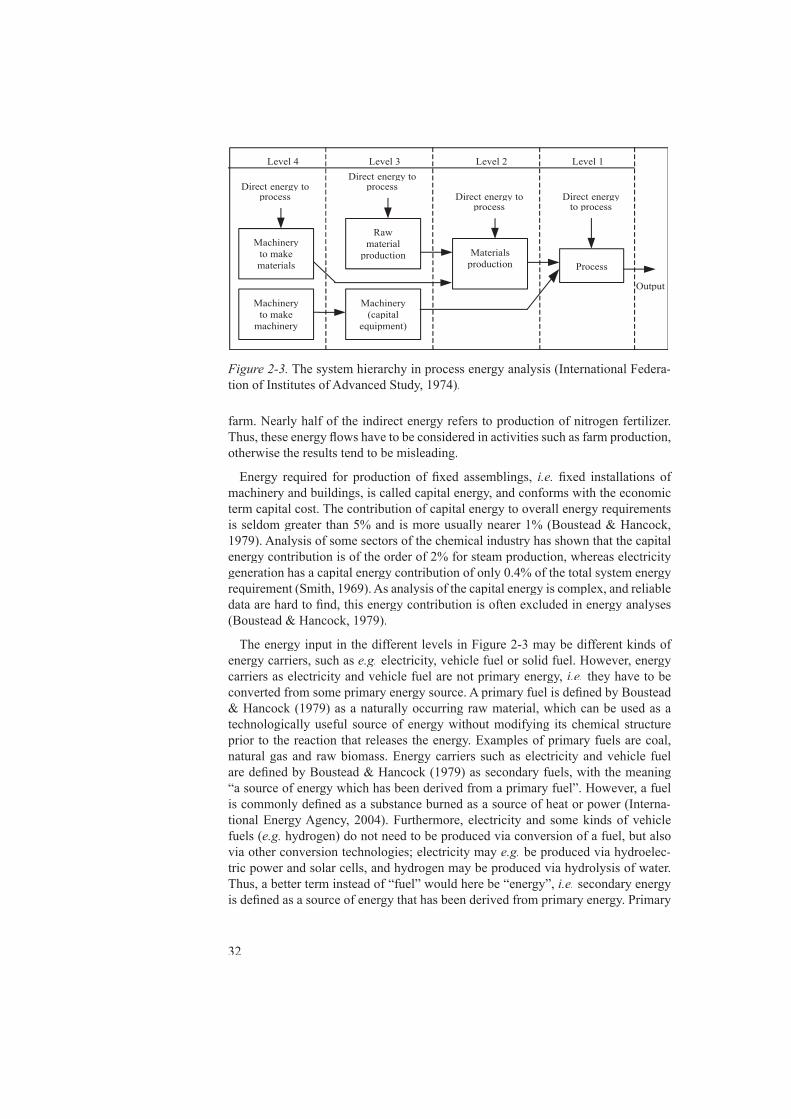
32

farm. Nearly half of the indirect energy refers to production of nitrogen fertilizer. Thus, these energy fl ows have to be considered in activities such as farm production, otherwise the results tend to be misleading.

Energy required for production of fi xed assemblings, i.e. fi xed installations of machinery and buildings, is called capital energy, and conforms with the economic term capital cost. The contribution of capital energy to overall energy requirements is seldom greater than 5% and is more usually nearer 1% (Boustead & Hancock, 1979). Analysis of some sectors of the chemical industry has shown that the capital energy contribution is of the order of 2% for steam production, whereas electricity generation has a capital energy contribution of only 0.4% of the total system energy requirement (Smith, 1969). As analysis of the capital energy is complex, and reliable data are hard to fi nd, this energy contribution is often excluded in energy analyses (Boustead & Hancock, 1979).

The energy input in the different levels in Figure 2-3 may be different kinds of energy carriers, such as e.g. electricity, vehicle fuel or solid fuel. However, energy carriers as electricity and vehicle fuel are not primary energy, i.e. they have to be converted from some primary energy source. A primary fuel is defi ned by Boustead & Hancock (1979) as a naturally occurring raw material, which can be used as a technologically useful source of energy without modifying its chemical structure prior to the reaction that releases the energy. Examples of primary fuels are coal, natural gas and raw biomass. Energy carriers such as electricity and vehicle fuel are defi ned by Boustead & Hancock (1979) as secondary fuels, with the meaning “a source of energy which has been derived from a primary fuel”. However, a fuel is commonly defi ned as a substance burned as a source of heat or power (Interna-tional Energy Agency, 2004). Furthermore, electricity and some kinds of vehicle fuels (e.g. hydrogen) do not need to be produced via conversion of a fuel, but also via other conversion technologies; electricity may e.g. be produced via hydroelec-tric power and solar cells, and hydrogen may be produced via hydrolysis of water. Thus, a better term instead of “fuel” would here be “energy”, i.e. secondary energy is defi ned as a source of energy that has been derived from primary energy. Primary

Figure 2-3. The system hierarchy in process energy analysis (International Federa-tion of Institutes of Advanced Study, 1974).

Level 4 Level 3 Level 2 Level 1

Direct energyto process

Direct energy toprocess

Direct energy toprocessDirect energy to

process

Process

Output

Materialsproduction

Rawmaterial

productionMachinery

to makematerials

Machinery(capital

equipment)

Machineryto make

machinery

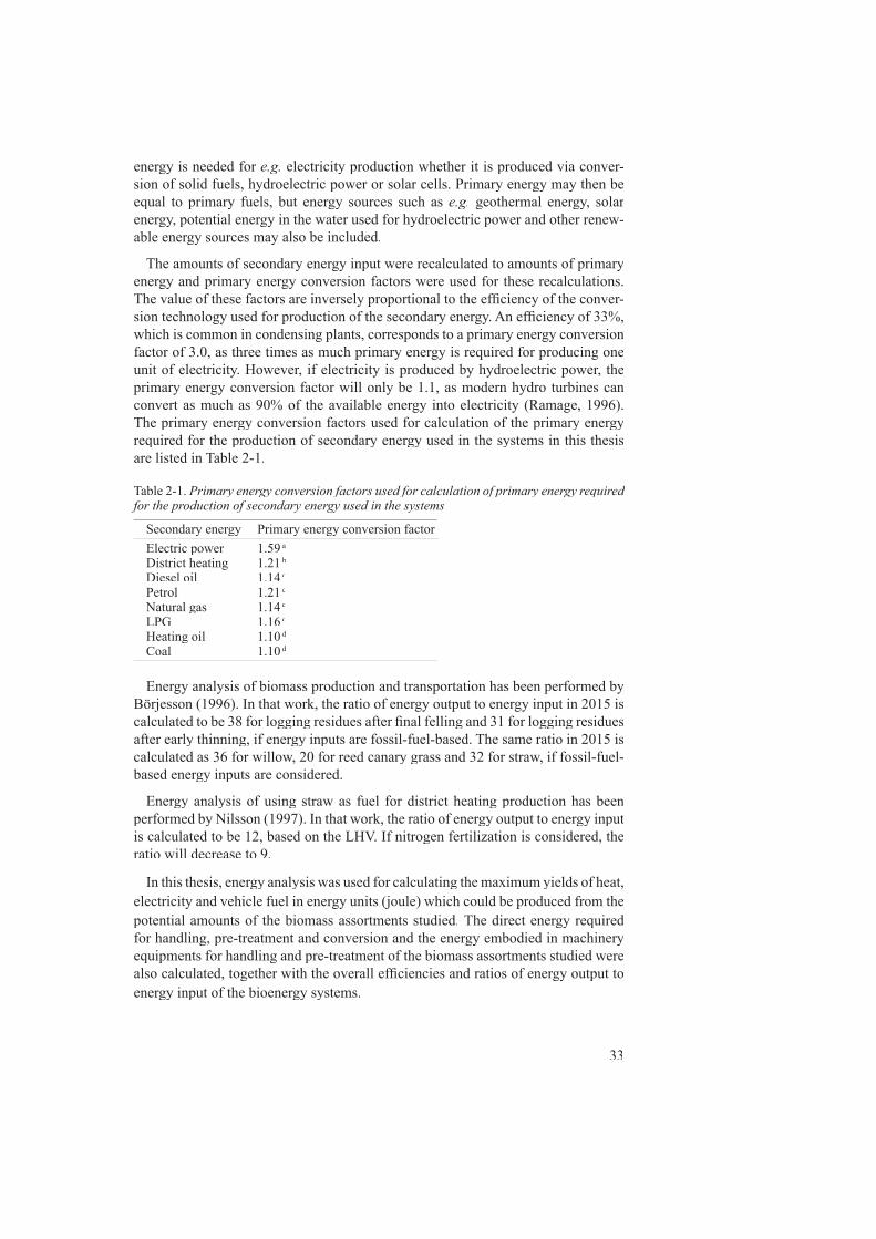
33

energy is needed for e.g. electricity production whether it is produced via conver-sion of solid fuels, hydroelectric power or solar cells. Primary energy may then be equal to primary fuels, but energy sources such as e.g. geothermal energy, solar energy, potential energy in the water used for hydroelectric power and other renew-able energy sources may also be included.

The amounts of secondary energy input were recalculated to amounts of primary energy and primary energy conversion factors were used for these recalculations. The value of these factors are inversely proportional to the effi ciency of the conver-sion technology used for production of the secondary energy. An effi ciency of 33%, which is common in condensing plants, corresponds to a primary energy conversion factor of 3.0, as three times as much primary energy is required for producing one unit of electricity. However, if electricity is produced by hydroelectric power, the primary energy conversion factor will only be 1.1, as modern hydro turbines can convert as much as 90% of the available energy into electricity (Ramage, 1996). The primary energy conversion factors used for calculation of the primary energy required for the production of secondary energy used in the systems in this thesis are listed in Table 2-1.

Table 2-1. Primary energy conversion factors used for calculation of primary energy required for the production of secondary energy used in the systems

Secondary energy Primary energy conversion factor Electric power 1.59 aDistrict heating 1.21 bDiesel oil 1.14 cPetrol 1.21 cNatural gas 1.14 cLPG 1.16 cHeating oil 1.10 dCoal 1.10 d

Energy analysis of biomass production and transportation has been performed by Börjesson (1996). In that work, the ratio of energy output to energy input in 2015 is calculated to be 38 for logging residues after fi nal felling and 31 for logging residues after early thinning, if energy inputs are fossil-fuel-based. The same ratio in 2015 is calculated as 36 for willow, 20 for reed canary grass and 32 for straw, if fossil-fuel-based energy inputs are considered.

Energy analysis of using straw as fuel for district heating production has been performed by Nilsson (1997). In that work, the ratio of energy output to energy input is calculated to be 12, based on the LHV. If nitrogen fertilization is considered, the ratio will decrease to 9.

In this thesis, energy analysis was used for calculating the maximum yields of heat, electricity and vehicle fuel in energy units (joule) which could be produced from the potential amounts of the biomass assortments studied. The direct energy required for handling, pre-treatment and conversion and the energy embodied in machinery equipments for handling and pre-treatment of the biomass assortments studied were also calculated, together with the overall effi ciencies and ratios of energy output to energy input of the bioenergy systems.

34

Cost analysisCost benefi t analysis (CBA) is a common method for decision-making, and was fi rst developed in the 1930s in the USA, when the Federal government had to decide whether to undertake many large, publicly funded irrigation, hydroelectric power and water supply projects in the dry central and western states of USA (Perkins, 1994). Since then, interest in costs other than those of strict business economics has increased markedly. Several works (e.g. Sáez, Linares & Leal, 1998; Miranda & e.g. Sáez, Linares & Leal, 1998; Miranda & e.g.Hale, 2001; El-Kordy et al., 2002) have been performed where external costs (aris-et al., 2002) have been performed where external costs (aris-et al.ing from environmental or societal impact) have been included in economic evalua-tions of different energy systems. Miranda & Hale (2001) estimated the social costs (i.e. the sum of production and external costs) on conversion of refi ned wood fuels in a condensing plant in Sweden to be 558 – 795 SEK/MWhe, of which the external costs are approximately 10% of the social costs.

Cost analysis is not a uniform method; however, the main aim of cost analysis is to evaluate the production costs for any product or process. Carapellucci (2002) has performed a cost analysis, where the cost of electricity (COE) generated by biomass-fi red condensing power processes was calculated as about 22 US$/GJ. However, several other studies have been performed for calculating the production cost of electricity generated by thermochemical conversion of biomass. The COE received at combustion processes have been evaluated by e.g. Sondreal e.g. Sondreal e.g. et al.

(2001) (condensing power), Bärring et al. (2003) (CHP) and Kumar, Cameron & Flynn (2003) (condensing power), and the COE received at gasifi cation of biomass has been evaluated by e.g. Bridgwater (1995) (condensing power), Solantausta, Bridgwater, & Beckman (1996) (both condensing power and CHP), Faaij et al. (1997) (condensing power) and Hoogwijk (2004) (condensing power). The COE received at both combustion or gasifi cation of biomass has been evaluated by e.g. Aleberg, Litzén & Schwartz (1995) (both condensing power and CHP) and Toft (1996) (condensing power). A common feature of most of these studies is that the cost of the biomass used in the conversion process is not calculated due to specifi c conditions regarding silviculture, cultivation, harvesting and further handling of the biomass assortments used. Instead, a standard value of the cost of biomass is used in some studies (Aleberg, Litzén & Schwartz, 1995; Solantausta, Bridgwater, & Beck-man, 1996; Sondreal et al., 2001), the price of the fuel is used as production cost of the fuel in some other studies (Faaij et al., 1997; Bärring et al., 2003) or the fuel cost used is estimated from previous performed work (Bridgwater, 1995). How-ever, there are studies performed where the costs of the cultivation and handling of the biomass prior to conversion are further evaluated; Toft (1996) models systems including transportation of the biomass used for the conversion processes, Kumar, Cameron & Flynn (2003) make a detailed compilation of the costs for the operation steps for producing and handling the biomass prior to the conversion process and Hoogwijk (2004) explores cost-supply curves of energy crops used as fuel over time for different land-use scenarios.

Cost evaluations of vehicle fuel production by conversion of biomass where the cost of the biomass used in the conversion process is calculated due to specifi c conditions regarding silviculture, cultivation, harvesting and further handling of the biomass assortments used are rare. Instead, a standard value of the cost of biomass

35

is used (Bridgwater & Double, 1991; Hamelinck & Faaij, 2002), the cost of biomass is assumed (Larson & Katofsky, 1994; Borgwardt, 1997), prices of biomass are used (Johansson, 1996a) or the cost of biomass is based on previously performed work (Williams et al., 1995; Johansson, 1996b).et al., 1995; Johansson, 1996b).et al.

In this thesis, the annual costs (i.e. the sum of annual investments and variable-costs) were evaluated for each operation in the systems studied. Variable costs included costs for expendables, operating and maintenance costs. Eventual taxes were included, although eventual subsidies were excluded. The production cost of each operation was then calculated for each biomass assortment by dividing the annual cost by the weight of dry matter received.

The production cost for each handling and pre-treatment operation was added to provide the total production cost for each biomass assortment used for energy con-version, and was expressed as the monetary cost in SEK per metric ton of dry matter (SEK/tdm). Secondly, the production costs for each energy carrier (i.e. heat, elec-tricity and vehicle fuel) produced were calculated by dividing the annual costs of the different operations required in the systems by the converted amount of energy carrier. These production costs were expressed as the monetary cost per energy unit (SEK/GJ and €/GJ). All costs were recalculated with the consumer price index to the level of cost corresponding to June 2002. The exchange rate between Swedish crowns (SEK) and euro (€) was 9.119 SEK/€ in June 2002 (Central bank of Sweden, 2005).

The annual investment costs were calculated as fi xed annual instalments. Thus, the investment cost for each part of equipment was distributed over their economic lifetime. The annual investment cost is given by the factor of fi xed annual instal-ments:

where f = the factor of fi xed annual instalments; r = the annual interest rate; n = the r = the annual interest rate; n = the reconomic lifetime [years]. The annual interest rate used for all equipment was 6.0% (further discussed in Chapter 6).

Emergy analysisThe emergy evaluation method was mainly developed by Howard T. Odum, and is described in many of his publications and compiled in his book Environmental Accounting (Odum, 1996). The method has also been further developed by Accounting (Odum, 1996). The method has also been further developed by Accounting e.g.Brown & Ulgiati (1997) for measuring sustainability.

The term “emergy” was introduced by H. T. Odum and D. M. Scienceman, and is defi ned as the available energy of one kind of previously used up directly and indi-rectly to make a service or product. The unit of emergy is emjoule. If the energy fl ow in a system is based on solar energy, the emergy unit is solar emjoule (abbreviated sej) (Odum, 1986, 1988; Scienceman, 1987).

The transformity (i.e. an energy measure of hierarchical position) is defi ned as the

f = r (1+r)n

(1+r)n - 1

36

emergy required to make one joule of a service or product. If solar emergy is used, the unit of transformity is solar emjoule per joule (sej/J). Thus, a product’s solar transformity is its solar emergy divided by its energy content (Odum, 1976, 1988). Considering a system described by the energy circuit langage, such as in Figure 2-3, the transformity increases from left to right in the diagram, as the hierarchy of the system increases from left to right. As a consequence of the second law of thermo-dynamics, some energy is lost as heat in each energy transformation step (Odum, 1996).

All transformities are derived from the total solar emergy fl ow supporting the global processes, called the baseline annual emergy budget, and consists of three independent energy sources that interact to run the processes of the global geobio-sphere: solar insolation, deep earth heat and tidal energy (Odum, 1996). The base-line annual emergy budget was calculated by Doherty, Nilsson & Odum (2002) to be 9.460 x1024 sej/year. The distribution of the baseline annual emergy budget between the three energy sources was 41.6% originating from solar insolation, 43.1% origi-nating from deep earth heat and 15.3% originating from tidal energy.

The prefi x em- has the meaning “embodied energy” or “energy memory” (Sci-enceman, 1987). It is given by the defi nition of the term “emergy” that the emergy amount of a fl ow or product is equal to all the energy (of one kind) previously used up directly and indirectly to produce that fl ow or product. Thus, an amount of emergy is equal to the amount of energy embodied in a fl ow or product, and may also be regarded as the energy memory of that fl ow or product.

By the defi nition of emergy, it is also given that energy differs from emergy, as an energy fl ow is normally defi ned as the direct energy amount released and distributed by some energy conversion process or distributed by an energy distribution system, e.g. district heating or electric power grids. Thus, energy previously required to e.g. district heating or electric power grids. Thus, energy previously required to e.g.form the topical energy fl ow (indirect or embodied energy) is not considered when an energy fl ow is quantifi ed; however, in energy analysis the embodied energy is considered, as discussed above. The distinction between energy and emergy analy-sis is that the system boundaries are different. Emergy fl ows quantifi ed as solar emergy joules (sej) are based on the primary solar energy fl ow, whereas energy analyses exclude primary energy fl ows from the surrounding environment, e.g. the e.g. the e.g.solar insolation. Instead, primary fuels such as fossil fuels or biomass are considered as primary energy in energy analyses (discussed above).

Emergy analysis may be used for the evaluation of the ratio of the emergy fl ow and the fl ow of the monetary value. This may be performed on a regional, national or global level. The received emergy per monetary currency ratio can then be used to estimate the emergy in services, which are quantifi ed in monetary values. Thus, even human work for producing a service or product can be quantifi ed in emergy terms, if the emergy per monetary currency ratio is known (Odum, 1988, 1996). Emergy analysis may then be a complement to evaluation by methods based on standard economic theory, which are insuffi cient as standard economic theory, as monetary values underestimate the signifi cance of natural resources, in particular resources such as wood, peat, coal, oil, natural gas, hydroelectric power and ura-nium (Hall, Cleveland & Kaufmann, 1986; Odum, 1996). The following view is given by Odum (1996, p. 60):

37

“Since money is paid only to people for their contribution, and never to the environment for its contribution, money and market values cannot be used to evaluate the real wealth from the environment. When the resources from the environment are abundant, little work is required from the economy, costs are small, and prices low. However, this is when the net contribution of real wealth to the economy is greatest: this is when everyone has abundant resources and a high standard of living. When the resources are scarce, obtaining costs are higher, supply-and-demand principles cause higher prices, and the market puts a high value on the product. However, this is also when there is little net contribution of the resource to the economy, real wealth is scarce, and standards of living are low. Market values are inverse to real-wealth contributions from the environment and cannot be used to evaluate environmental contributions or environmental impact.”

Hall, Cleveland & Kaufmann (1986, p. 35) addressed the same issue and state that standard economics seems to have missed the important point that:

“...goods and services are derived ultimately from natural resources, which are the real source of material wealth for humans, not the money that represents them in market trans-actions. Unfortunately, many economists appear to have lost sight of this truth and have resorted to manipulating money fl ows as a proxy for the physical fl ows of goods and serv-ices. This approach is not always effective because natural resources obey a different set of laws from monetary fl ows.”

The authors declare that traditional economic policies have been more or less ineffective in combating current economic problems because they ignore the mecha-nisms by which human social and economic processes are constrained by the supply and quality of natural resources (ibid. p. 39-40):

“.. .neoclassical economists consider fuels to be just another input like capital or labour. We disagree. From an energy perspective ... it is evident that energy is the only primary factor of production because it cannot be produced or recycled from any other factor – it must be supplied from outside the human economic system. Labour, capital and technology are intermediate inputs because they depend on a net input of free energy for their production and maintenance. In other words, the availability of free energy is a necessary, but not suf-fi cient, condition for the availability of labour, capital and technology.”

Cleveland (1991, p. 289) writes:

“The neoclassical model of production assumes that capital and labor are primary inputs to production. ... A biophysical model of the economic process assumes that capital and labor are intermediate inputs produced ultimately from the only primary factor of production: low entropy energy and matter”.

Traditional economics has been described as a ‘merry-go-round’ without physical constraints, whereas in reality all productive processes consist of fl ows of energy and matter which are limited in supply (Hall, Cleveland & Kaufmann, 1986, p. 39). Methods attempting to bridge the gap between human economies and nature are now beginning to be developed by scientists from many fi elds. This is not easy as traditional economic models treat nature and environmental processes as “exter-nalities” and therefore almost by defi nition do not fi t the objectives of an integrated study.

Emergy analysis allows studies of the combined macro-economy of humans and nature within the same model, as indicated in Figure 2-2. Energy, both direct and embodied (hence bodied (hence emergy), is the measure quantifying the interactions in the system, as all resource storages and processes can be expressed in energy terms. The concept

38

is based on systems theory and founded in general principles of self-organization and thermodynamics (Odum 1983, 1986, 1988, 1996).

Emergy-based yield and investment ratios are based on the emergy fl ows shown in Figure 2-4. The environmental input (I) is generated from renewable sources and non-renewable storages, and the product or yield (Y) is generated in the economic system by the environmental input (I) and fuels, goods and services (F). The topical ratios are then defi ned as follows:

Emergy yield ratio = Y / FEmergy investment ratio = F / I

Thus, the emergy yield ratio (EYR) is the ratio of the emergy of the output yield divided by the emergy of the inputs (F) to the process that are fed back from outside the system under study. EYR is an indicator of the yield compared to inputs other than local, and gives a measure of the ability of the process to exploit local resources (Brown & Ulgiati, 1997). It is also a measure of the ability of the resource to con-tribute to the economic system by amplifying the investment (Ulgiati & Sciubba, 2003).

The emergy investment ratio (EIR) is the ratio of the emergy (F) fed back from outside the system to the indigenous emergy input (I), and provides an evaluation whether the process is a good user of the emergy invested, in comparison with alter-natives. It is not an independent index, but is linked to the EYR (Brown & Ulgiati, 1997).

Figure 2-4. System diagram with the emergy fl ows used for calculation of the emergy-based yield and investment ratios.

39

Emergy analysis of forest production and thermochemical conversion of biomass from forestry in Sweden has been performed by Doherty (1995) and Doherty, Nils-son & Odum (2002). Doherty (1995) calculates the solar transformity for electric power generated via combustion of wood chips as 96,382 sej/J and for wood powder as 111,490 sej/J. The corresponding values calculated by Doherty, Nilsson & Odum (2002) are 86,306 sej/J and 98,832 sej/J. The EIR for electric power generated via combustion of wood chips is calculated by Doherty (1995) to be 3.48 and for wood powder 4.17. Doherty, Nilsson & Odum (2002) calculate the corresponding values to be 2.91 and 3.64.

Emergy analysis of using straw as fuel for district heating production has been performed by Nilsson (1997). In that work, the solar transformity for the heat gen-erated is calculated to be 10,000 sej/J, whereas the EIR for the heat generated is calculated to be 11.

Selected systems for the energy, cost and emergy analysesA description of the system for utilization and transport of biomass supplies from forestry, non-forest land, agriculture, forest industry (sawmills, plywood industries and pulp mills) and community is shown in Figure 2-5. All steps from planting and cultivation to transport of the biomass to further pre-treatment were included. The different assortments of biomass supplies included in the system were estimated total available resources of: direct fuel wood cuttings; trees from early thinning; log-ging residues from fi nal felling and from thinning; fuel wood from industrial wood cuttings; fuel wood from non-forest land; forest industry by-products (sawdust, wood chips and bark); agrofuels (short rotation forest, energy grass (reed canary grass) and straw); and a lignocellulose-based municipal waste fraction (recovered wood). Organic waste was not included in the analysis, as only lignocellulose-based biomass supplies from the forest, the forest industry, community and agricultural crops cultivated for energy purposes were considered. Conversion of organic waste is also performed by a different conversion technology (anaerobic digestion) than the conversion technologies studied in this work.

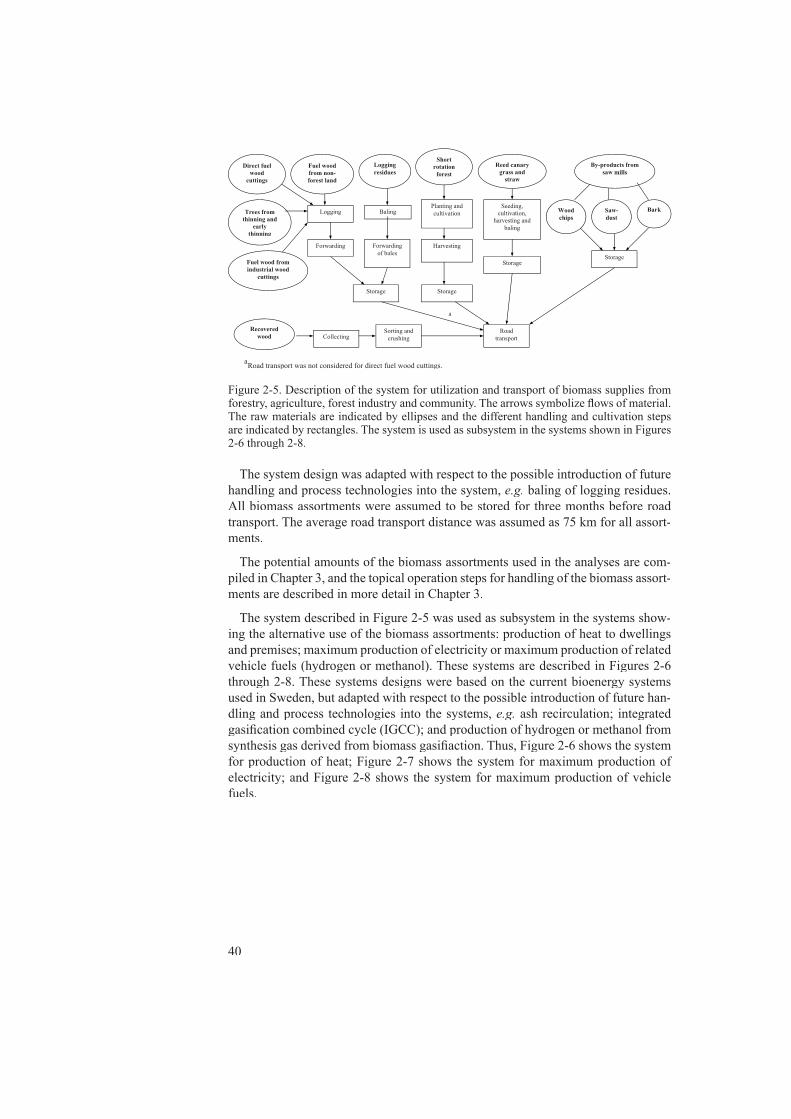
40

The system design was adapted with respect to the possible introduction of future handling and process technologies into the system, e.g. baling of logging residues. All biomass assortments were assumed to be stored for three months before road transport. The average road transport distance was assumed as 75 km for all assort-ments.

The potential amounts of the biomass assortments used in the analyses are com-piled in Chapter 3, and the topical operation steps for handling of the biomass assort-ments are described in more detail in Chapter 3.

The system described in Figure 2-5 was used as subsystem in the systems show-ing the alternative use of the biomass assortments: production of heat to dwellings and premises; maximum production of electricity or maximum production of related vehicle fuels (hydrogen or methanol). These systems are described in Figures 2-6 through 2-8. These systems designs were based on the current bioenergy systems used in Sweden, but adapted with respect to the possible introduction of future han-dling and process technologies into the systems, e.g. ash recirculation; integrated gasifi cation combined cycle (IGCC); and production of hydrogen or methanol from synthesis gas derived from biomass gasifi action. Thus, Figure 2-6 shows the system for production of heat; Figure 2-7 shows the system for maximum production of electricity; and Figure 2-8 shows the system for maximum production of vehicle fuels.

Figure 2-5. Description of the system for utilization and transport of biomass supplies from forestry, agriculture, forest industry and community. The arrows symbolize fl ows of material. The raw materials are indicated by ellipses and the different handling and cultivation steps are indicated by rectangles. The system is used as subsystem in the systems shown in Figures 2-6 through 2-8.

Storage

Baling Logging

Forwarding

Planting and cultivation

Seeding,cultivation,

harvesting and baling

Harvesting

Storage

Storage

By-products from saw mills

Forwarding of bales

Direct fuel wood

cuttings

Logging residues

Short rotation

forest

Reed canary grass and

straw

Woodchips

Saw-dust

Fuel wood from industrial wood

cuttings

Recoveredwood

Road transport

Fuel wood from non-forest land

Storage

Bark

a

Sorting and crushing Collecting

Trees from thinning and

earlythinning

aRoad transport was not considered for direct fuel wood cuttings.

41

Figure 2-6. Description of the system for heat production. The arrows symbolise fl ows of material or energy; the different pre-treatment and conversion steps are indicated by rectan-gles; and the energy carriers produced are indicated by hexagonal shapes. Arrows with solid lines symbolise main fl ows and the arrow with a broken line symbolise a by-fl ow. Utilization and transport of biomass supplies are described in Figure 2-5.

Transport

Small-scale wood firing

Pelletizing

Milling

Drying

Crushing/chipping

b

ElectricityHeating of

houses

Small-scale pellets firing

CombustionGrate firing/CFB

a

Ash recirculation

Utilization and transport of biomass supplies

Recovered wood From forestry From agriculture From saw mills

District heating

a Direct fuel wood cuttings b Combined heat and power

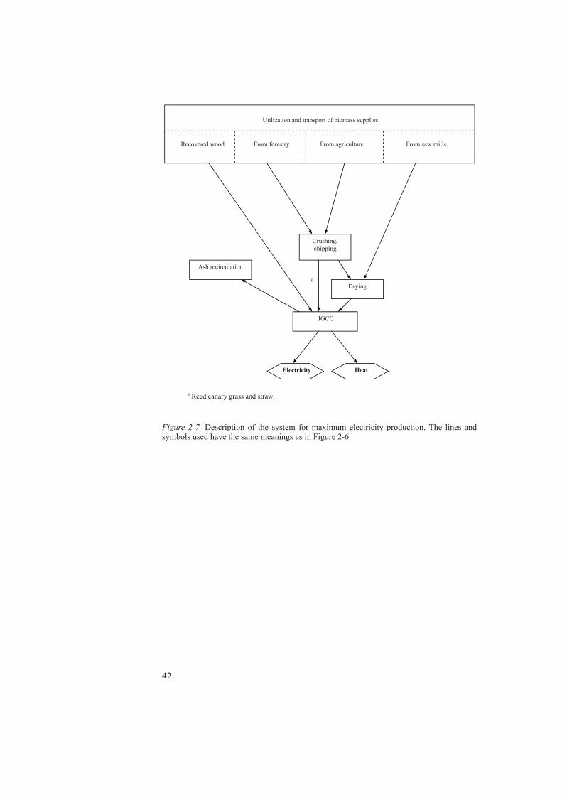
42

Figure 2-7. Description of the system for maximum electricity production. The lines and symbols used have the same meanings as in Figure 2-6.

Drying

Crushing/chipping

Ash recirculation

a



IGCC

Electricity Heat

a Reed canary grass and straw.

43

Figure 2-8. Description of the system for maximum amounts of produced vehicle fuels. The lines and symbols used have the same meanings as in Figures 2-6 and 2-7.

Drying

Crushing/chipping

Ash recirculation



Atmospheric gasification CFB

a

Hydrogen Methanol

a Reed canary grass and straw.

44

District heating is also produced in combined heat and power (CHP) plants. (The Swedish District Heating Association, 1999). Thus, even electricity was produced in the system for heat production (Figure 2-6).

Pellets used for energy conversion are mainly produced of sawdust, but some wood chips and bark are also used. As shown in Figure 2-6, heat is produced as a by-product of the drying of the biomass before pelletizing. A fl ue gas dryer is here used for drying of the biomass to a low moisture content (approximately 10%). A con-siderable part of the heat in the outlet fl ue gas from the dryer may then be recovered by means of fl ue gas condensation and used for example in district heating. Pellets were used both in small-scale and large-scale applications, where the small-scale application consisted of pellet fi ring in a boiler used in single-family houses, and the large-scale application consisted of a pellet boiler used for district heating.

The ashes from all large-scale conversion processes were assumed as being recir-culated. According to Gunnarsson (2004), it was assumed that the recirculation was performed once during a rotation period, namely after thinning.

The conversion processes included in the analyses are further described in Chap-ter 4.

The systems studied were considered as static, as a specifi ed input value to the system gave one specifi ed output value. They were also considered as linear, as the input values were directly proportional to the output values.

As the systems studied included many different process and conversion steps with different condition variables, they were considered as internal. However, as the sys-tems did not include any random elements, they could be considered as determinis-tic. As the systems were considered as both static and deterministic, a spreadsheet was used as a tool for the analyses.

Data handlingThe input data of the scenarios and analyses were based on literature references and personal communications. Swedish energy statistics were used for compilation of the heat demand and supply in Sweden in 2002. The input data on technology performance of the current commercial system, for example energy effi ciencies and energy balances, were based on the best commercially available technology. The choice of input data used is noted in the table footnotes (Appendix C).

Higher heating values (HHVs) of the biomass assortments and other fuels used were primarily used in the calculations in the scenarios and analyses. Lower heating values (LHVs) were used if data for e.g. energy amounts or effi ciencies were based on LHVs. Data from the Swedish energy statistics regarding fuel supply and use are based on LHVs. LHV is noted after the energy unit when an energy amount is based on the LHV. Calculation of the higher heating value, if the lower heating value for a biomass assortment was known, was performed according to Nylinder (1979).

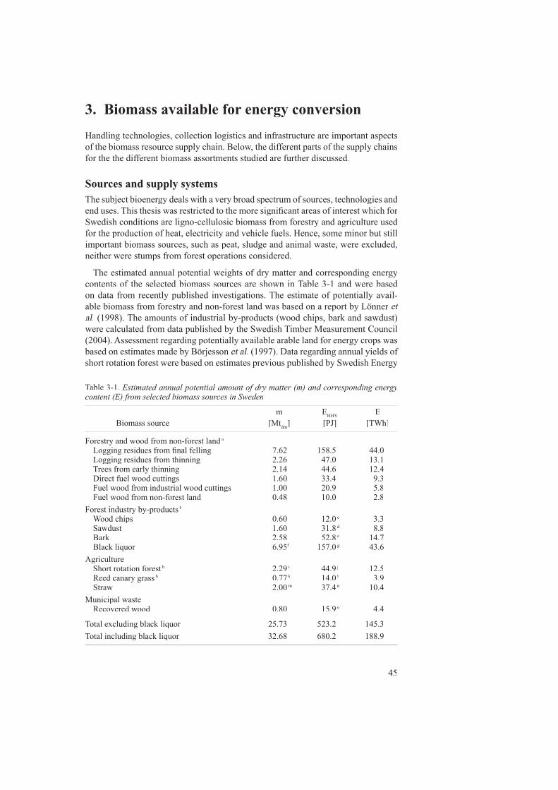
45

3. Biomass available for energy conversionHandling technologies, collection logistics and infrastructure are important aspects of the biomass resource supply chain. Below, the different parts of the supply chains for the the different biomass assortments studied are further discussed.

Sources and supply systems The subject bioenergy deals with a very broad spectrum of sources, technologies and end uses. This thesis was restricted to the more signifi cant areas of interest which for Swedish conditions are ligno-cellulosic biomass from forestry and agriculture used for the production of heat, electricity and vehicle fuels. Hence, some minor but still important biomass sources, such as peat, sludge and animal waste, were excluded,neither were stumps from forest operations considered.

The estimated annual potential weights of dry matter and corresponding energy contents of the selected biomass sources are shown in Table 3-1 and were based on data from recently published investigations. The estimate of potentially avail-able biomass from forestry and non-forest land was based on a report by Lönner etal. (1998). The amounts of industrial by-products (wood chips, bark and sawdust) al. (1998). The amounts of industrial by-products (wood chips, bark and sawdust) al.were calculated from data published by the Swedish Timber Measurement Council (2004). Assessment regarding potentially available arable land for energy crops was based on estimates made by Börjesson et al. (1997). Data regarding annual yields of et al. (1997). Data regarding annual yields of et al.short rotation forest were based on estimates previous published by Swedish Energy

Table 3-1. Estimated annual potential amount of dry matter (m) and corresponding energy content (E) from selected biomass sources in Sweden

m EHHV EHHV EHHV

Biomass source [Mtdm] [PJ] [TWh]

Forestry and wood from non-forest land a Logging residues from fi nal felling 7.62 158.5 44.0 Logging residues from thinning 2.26 47.0 13.1 Trees from early thinning 2.14 44.6 12.4 Direct fuel wood cuttings 1.60 33.4 9.3 Fuel wood from industrial wood cuttings 1.00 20.9 5.8 Fuel wood from non-forest land 0.48 10.0 2.8Forest industry by-products b Wood chips 0.60 12.0 c 3.3 Sawdust 1.60 31.8 d 8.8d 8.8d

Bark 2.58 52.8 e 14.7 Black liquor 6.95f 157.0 f 157.0 f g 43.6Agriculture Short rotation forest h 2.29 i 44.9 j 12.5 Reed canary grass h 0.77 k 14.0 k 14.0 k l 3.9 Straw 2.00 m 37.4 n 10.4Municipal waste Recovered wood 0.80 15.9 o 4.4

Total excluding black liquor 25.73 523.2 145.3Total including black liquor 32.68 680.2 188.9

46

Agency (2003b); annual yields of reed canary grass were based on fi eld experiments performed in Sweden (Olsson et al., 2001); and annual yields of straw were based on et al., 2001); and annual yields of straw were based on et al.estimates made by Börjesson et al. (1997). et al. (1997). et al.

Basic data on selected methods and machines were collected from research reports and interviews with people at research departments, enterprises and organisations in agriculture, forestry and different municipalities.They are compiled in Appendix J.

The total of energy in the biomass assortments was estimated to be 583.9 PJ per year in Case 1; 680.2 PJ in Case 2; and 627.3 PJ in Case 3. The largest contribution was from the forest and forest industry sector (568.0 PJ per year in Cases 1 - 2 and 611.4 PJ per year in Case 3). Agricultural contribution was 96.3 PJ per year and recovered wood from municipal waste was 15.9 PJ per year.

The moisture content before drying was assumed to be 50.0% for all biomass assortments, except for reed canary grass and straw, where the moisture content was assumed to be 15.0%, and recovered wood where the moisture content was assumed to be 10.0%.

Biomass from forestry and fuel wood from non-forest landIn 1992, an analysis known as AVB 92 (AVB is a Swedish acronym for felling calculations) was undertaken as an integral part of the work by the forest policy commission set up by the Swedish government in 1990. The main objective was to analyse and map the possible use and development of Swedish forests during the next 100 years. The results were published by Lundström, Nilsson & Söderberg (1993) and were used in this thesis as a basis for calulations of silvicultural inputs and the amount of by-products from the forest industry sector.

AVB 92 was followed by a project named Forest Impact Analyses 1999 (National Board of Forestry, 2000), initiated by the Swedish National Board of Forestry and conducted in cooperation with the Swedish Environmental Protection Agency, the Swedish Energy Agency, the Swedish National Board for Industrial and Techni-cal Development and the Swedish University of Agricultural Sciences. The results differed little from AVB 92 so the preconditions in this thesis were not changed. A comparison of key data between AVB 92 and SKA 99 is presented in Table 3-2.

The silvicultural program in the calculations of this thesis was based on the areas shown in Table 3-2 and on data for 2002 given by National Board of Forestry (2004). The assumptions and data are shown in Table 3-3.

Parikka (1997) developed a method (called “Biosims”) for calculating the stand level and regional raw material base for woody biomass and wood fuel, taking eco-logical restrictions into consideration. Biomass functions by Marklund (1987, 1988) were inter alia used for these calculations (see Figure 3-1). Lönner inter alia used for these calculations (see Figure 3-1). Lönner inter alia et al. (1998) used this method for assessing the potential wood fuel supply in Sweden by applying the biomass functions of Marklund to the same sample plot data from the National Forest Survey used by AVB 92. Thus, it was estimated that the total annual, poten-tial amount of wood fuels from the forest, together with trees from non-forest land, leaving out by-products from forest industries, would be about 22.6 million metric tons of dry matter on a sustainable basis for the period 1998–2008. The stemwood

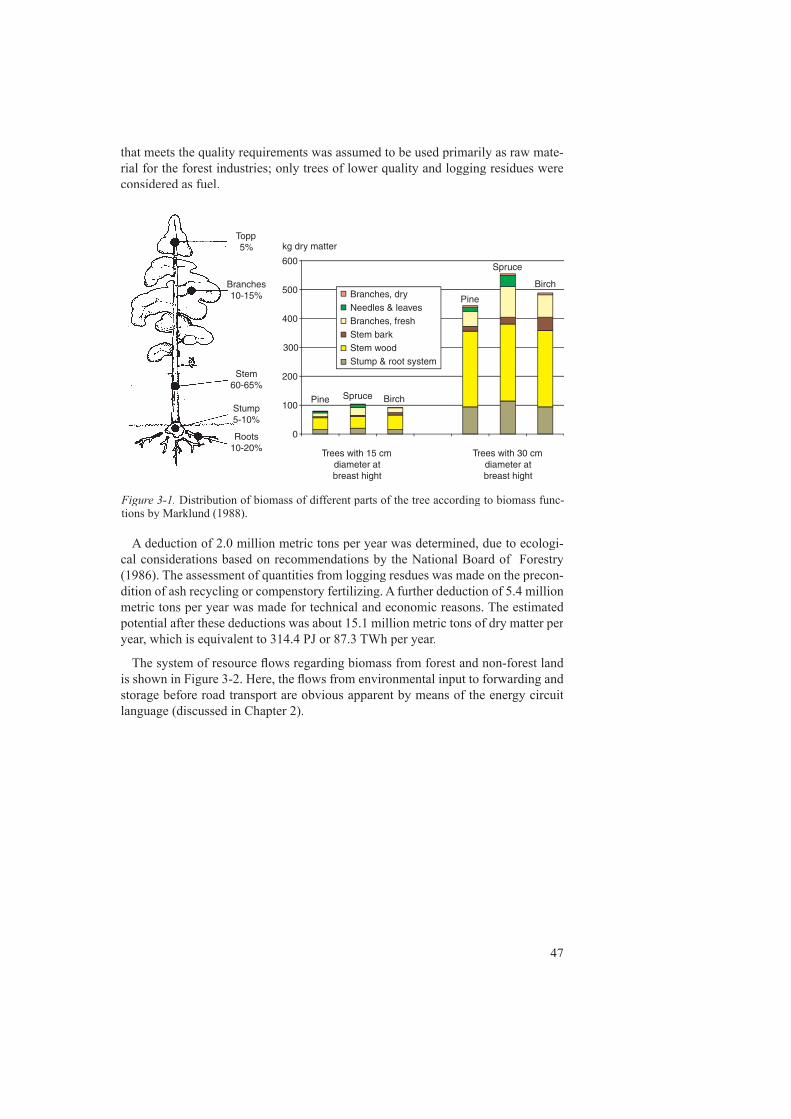
47

that meets the quality requirements was assumed to be used primarily as raw mate-rial for the forest industries; only trees of lower quality and logging residues were considered as fuel.

A deduction of 2.0 million metric tons per year was determined, due to ecologi-cal considerations based on recommendations by the National Board of Forestry (1986). The assessment of quantities from logging resdues was made on the precon-dition of ash recycling or compenstory fertilizing. A further deduction of 5.4 million metric tons per year was made for technical and economic reasons. The estimated potential after these deductions was about 15.1 million metric tons of dry matter per year, which is equivalent to 314.4 PJ or 87.3 TWh per year.

The system of resource fl ows regarding biomass from forest and non-forest land is shown in Figure 3-2. Here, the fl ows from environmental input to forwarding and storage before road transport are obvious apparent by means of the energy circuit language (discussed in Chapter 2).

��

��

��

��

��

��

��

��

��

��

��

��

�

��

��

��

��

��

��

��

Figure 3-1. Distribution of biomass of different parts of the tree according to biomass func-tions by Marklund (1988).

48

Table 3-2. Tree volumes and annual operation areas from AVB 92 used in this thesis com-pared with corresponding tree volumes from SKA 99 (Forest Impact Analyses 1999)

Entire country AVB 92 SKA 99 Period: 1998–2008 2000–2009 Volume Area Volume per ha Volume of treated area [106 m3

sk] [1000 ha] [m3sk /ha] [10sk /ha] [10sk

6 m3sk]

Productive forest land 21,840 Annual increment 105.14 107.57Precommercial thinning 0.989First thinning 10.482 148.3 70.7 9.464Later thinning 16.533 217.6 76.0 17.959Final felling 59.982 222.3 269.8 53.419Total felling of round wood 87.278 81.831

Table 3-3. Assumed annual maintenance inputs in Swedish forestry at maximum sustainable felling

Pesticides a 22.2 t/yearCleaning a 55,000 ha/yearScarifi cation b 195,624 ha/yearPlanting and sawing c 177,840 ha/yearPrecommercial thinning d 222,300 ha/yeard 222,300 ha/yeard

Forest fertilization e 20,000 ha/yearAsh recirculation f 217,600 ha/yearf 217,600 ha/yearf

Forest drainage g 10.5 M(SEK)/yearForest roads h 727.3 M(SEK)/year

Figure 3-2. Systems diagram of forest production and harvesting with an emphasis on wood fuels (logging residues, trees from early thinning and fuel wood cuttings). Symbols according to Odum (1983, 1996), see Appendix A. Heat sink pathways omitted.

Baling/bundling

Forwardingbundles

Loggingresidues

Sun

Rain

Wind

Harvesting and transportBiomass productionEnvironmentalsources

Forest land21.8 million ha

Foreststand1326

[Mtdm /year]

Clearcutting

Forwardingroundtimber

Sawlogs

Pulpwood

Thinning

Earlythinning

Fuelwood

Forwarding

Fuelwoodcuttings

Forwarding

Otherthan productive

forest land

Trees

0.48

2.14

1.60

7.62

2.26

Fuelwood

16.34

1.00

12.92

9.88

4.22

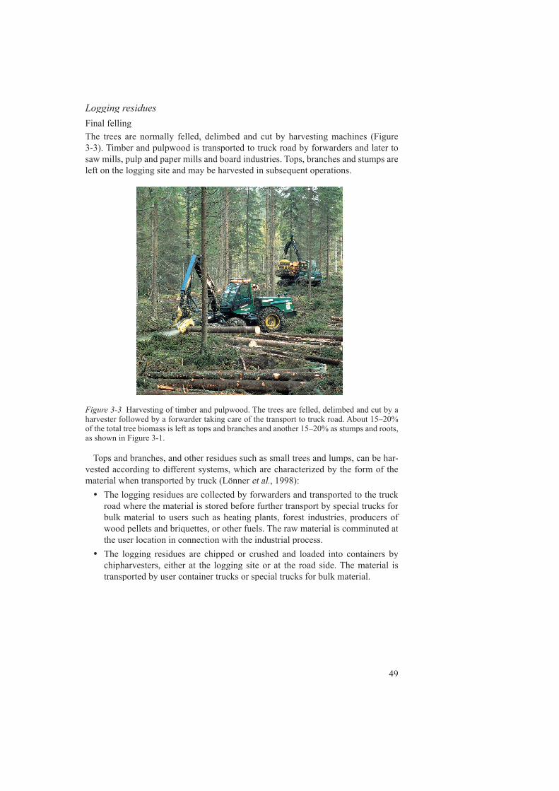
49

Logging residuesFinal fellingThe trees are normally felled, delimbed and cut by harvesting machines (Figure 3-3). Timber and pulpwood is transported to truck road by forwarders and later to saw mills, pulp and paper mills and board industries. Tops, branches and stumps are left on the logging site and may be harvested in subsequent operations.

Tops and branches, and other residues such as small trees and lumps, can be har-vested according to different systems, which are characterized by the form of the material when transported by truck (Lönner et al., 1998): et al., 1998): et al. The logging residues are collected by forwarders and transported to the truck

road where the material is stored before further transport by special trucks for bulk material to users such as heating plants, forest industries, producers of wood pellets and briquettes, or other fuels. The raw material is comminuted at the user location in connection with the industrial process.

The logging residues are chipped or crushed and loaded into containers by chipharvesters, either at the logging site or at the road side. The material is transported by user container trucks or special trucks for bulk material.

Figure 3-3. Harvesting of timber and pulpwood. The trees are felled, delimbed and cut by a harvester followed by a forwarder taking care of the transport to truck road. About 15–20% of the total tree biomass is left as tops and branches and another 15–20% as stumps and roots, as shown in Figure 3-1.

50

The logging residues are compressed and bundled by special machines. The bundles are transported by a standard forwarder to truck road for further trans-port to users with the same kind of trucks used for round wood.

The baling system (Figure 3-4) was choosen in the energy, cost and emergy analy-ses as appeared having a more favourably potential for further development than the system that handles loose material.

The potential quantity of logging residues from fi nal fellings was estimated to be 7.62 Mtdm per year, according to Lönner et al. (1998).et al. (1998).et al.

Fiberpac baling/bunching machine making bales from logging residues.

Forwarder unloading bales at truck road.

Figure 3-4. Collecting, baling and transport of tops and branches after fi nal felling.

51

ThinningThinning or selective cutting is an important forest management tool used to suc-cessively improve the quality and value of the stand at the same time as providing income before fi nal harvest. By removing poor quality trees, the best trees in the stand are given room to grow. It is also a way to salvage trees which would even-tually die naturally. Usually, the forest is thinned 2–3 times before regeneration, depending on the growth conditions.

The same system can be used in both fi nal felling and thinning, although the har-vesting costs are much higher for thinning than in fi nal felling because of lower quantity of material per hectare and slower hand ling as the remaining trees hamper operations.

The potential quantity of logging residues from thinning is estimated as 2.26 Mtdmper year (early thinning excluded), according to Lönner et al. (1998).et al. (1998).et al.

Figure 3-4 continued.

Loading of bales on truck for transport to industry.

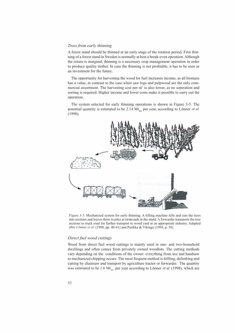
52

Trees from early thinningA forest stand should be thinned at an early stage of the rotation period. First thin-ning of a forest stand in Sweden is normally at best a break-even operation. Although the return is marginal, thinning is a necessary crop management operation in order to produce quality timber. In case the thinning is not profi table, it has to be seen as an investment for the future.

The opportunity for harvesting the wood for fuel increases income, as all biomass has a value, in contrast to the case when saw logs and pulpwood are the only com-mercial assortment. The harvesting cost per m3 is also lower, as no seperation and sorting is required. Higher income and lower costs make it possible to carry out the operation.

The system selected for early thinning operations is shown in Figure 3-5. The potential quantity is estimated to be 2.14 Mtdm per year, according to Lönner et al.(1998).

Direct fuel wood cuttings Wood from direct fuel wood cuttings is mainly used in one- and two-household dwellings and often comes from privately owned woodlots. The cutting methods vary depending on the conditions of the owner: everything from axe and handsaw to mechanized chipping occurs. The most frequent method is fellling, delimbing and cutting by chainsaw and transport by agriculture tractor or forwarder. The quantity was estimated to be 1.6 Mtdm per year according to Lönner et al. (1998), which are et al. (1998), which are et al.

Figure 3-5. Mechanized system for early thinning. A felling machine fells and cuts the trees into sections and leaves them in piles at striproads in the stand. A forwarder transports the tree sections to truck road for further transport to wood yard at an appropriate industry. Adapted after Lönner et al. (1998, pp. 40-41) and Parikka & Vikinge (1994, p. 38).

53

based on statistical data published by Statistics Sweden and the Swedish Energy Agency.

Fuel wood from industrial wood cuttings Round wood of low quality or wood from tree species not usable as industrial raw material are sorted, either in the forest or at the wood yard, and used as fuel. The quantity was estimated at 1.0 Mtdm per year, according to Hektor, Lönner & Parikka (1995).

Fuel wood from non-forest land Trees grow on many kinds of land, e.g. along ditches in farm land, in groves and e.g. along ditches in farm land, in groves and e.g.edges of fi elds and pastures, in power line corridors, in parks, etc. A conservative estimate of the gross amount of cut trees was set to 600,000 tdm per year and the technically available quantity was estimated at 480,000 tdm per year, according to Lönner et al. (1998). The technically available quantity is equavilent to 10.0 PJ per et al. (1998). The technically available quantity is equavilent to 10.0 PJ per et al.year.

By-products from forest industries By-products from forest industries are bark, sawdust, wood chips and black liqour. Bark is a by-product of all industries using round wood, whereas sawdust and wood chips are by-products from saw mills only.

Wood pulp for paper and paper board making may be produced by mechanical or chemical methods (described in Chapter 1). In modern mechanical methods, wood chips are fed between two metal disks in a refi ner. As the disks rotate relative to one another, the action of a series of grooves and bars on their surfaces separate the wood fi bres. The disks are driven by electricity, leading to a large consumption of electricity for this process. Heat developed in the refi ners is recovered and used in other parts of the process. Most of the raw material comes out as a fi nal product.

Chemical methods are used to produce a pulp which is stronger and easier to bleach (whiten) and less likely to loose its brightness over time. However, the result is a much lower yield, usually about 45% (Münster, 1998).

Wood from later thinning and fi nal felling was estimated at 76.52 million m3sk

(see Table 3-2), which corresponded to 72.69 million m3fpb. The distribution of the

raw material to different types of industries was assumed being proportional to the distribution in 2003, which was chosen as a reference year for the use of these assortments in industries.

The amounts of raw material required and products received at saw mills, board industries and pulp mills in 2003 and in the scenarios are compiled in Table 3-4. In 2003, 55.4% (37.7 million m3

fpb ) of the total consumption of roundwood was used in saw mills, whereas 44.0% (29.9 million m3

fpb ) of the total consumption of round-wood was used in pulp mills (Björklund, 2005). The amount of wood chips, sawdust and bark received at saw mills and used for energy purposes was estimated as 66.9 PJ (3.32 Mtdm) per year. Of this amount, 48.6 PJ (2.42 Mtdm) per year was sold to other users, e.g. district heating producers. e.g. district heating producers. e.g.

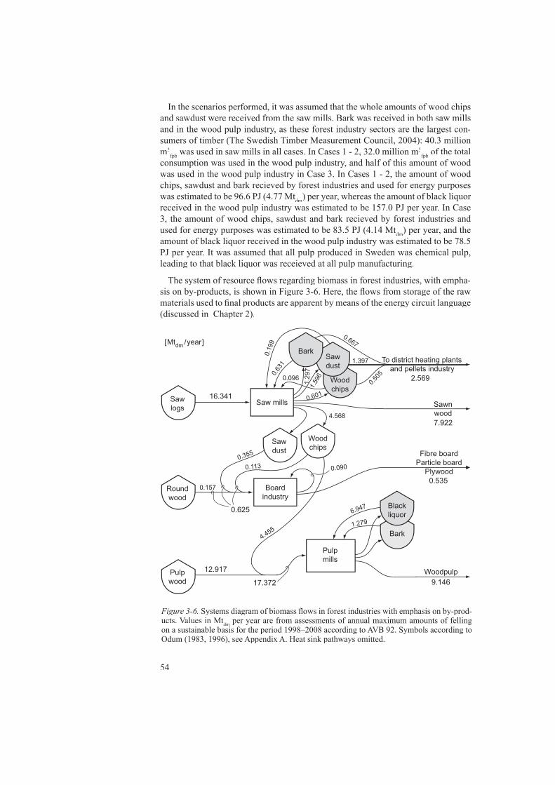
54

In the scenarios performed, it was assumed that the whole amounts of wood chips and sawdust were received from the saw mills. Bark was received in both saw mills and in the wood pulp industry, as these forest industry sectors are the largest con-sumers of timber (The Swedish Timber Measurement Council, 2004): 40.3 million m3

fpb was used in saw mills in all cases. In Cases 1 - 2, 32.0 million m3fpb of the total

consumption was used in the wood pulp industry, and half of this amount of wood was used in the wood pulp industry in Case 3. In Cases 1 - 2, the amount of wood chips, sawdust and bark recieved by forest industries and used for energy purposes was estimated to be 96.6 PJ (4.77 Mtdm) per year, whereas the amount of black liquor received in the wood pulp industry was estimated to be 157.0 PJ per year. In Case 3, the amount of wood chips, sawdust and bark recieved by forest industries and used for energy purposes was estimated to be 83.5 PJ (4.14 Mtdm) per year, and the amount of black liquor received in the wood pulp industry was estimated to be 78.5 PJ per year. It was assumed that all pulp produced in Sweden was chemical pulp, leading to that black liquor was receieved at all pulp manufacturing.

The system of resource fl ows regarding biomass in forest industries, with empha-sis on by-products, is shown in Figure 3-6. Here, the fl ows from storage of the raw materials used to fi nal products are apparent by means of the energy circuit language (discussed in Chapter 2).

Figure 3-6. Systems diagram of biomass fl ows in forest industries with emphasis on by-prod-ucts. Values in Mtdm per year are from assessments of annual maximum amounts of felling on a sustainable basis for the period 1998–2008 according to AVB 92. Symbols according to Odum (1983, 1996), see Appendix A. Heat sink pathways omitted.

Sawlogs

Saw mills Sawnwood

Sawdust

To district heating plantsand pellets industry

Woodchips

Sawdust

Bark

Woodchips

16.341

0.631

0.096

0.667

1.397

0.505

2.569

0.601

1.29

71.596

4.5687.922

[Mtdm /year]

Pulpwood

Bark

Blackliquor

Woodpulp

Pulpmills

12.917

17.372 9.146

6.947

4.455

Roundwood

Boardindustry

0.157

0.355

0.19

9

0.113

0.625

0.535

Fibre boardParticle board

Plywood

1.279

0.090

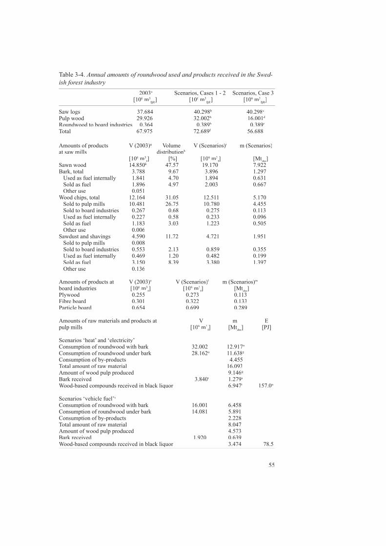
55

Table 3-4. Annual amounts of roundwood used and products received in the Swed-ish forest industry 2003a Scenarios, Cases 1 - 2 Scenarios, Case 3 [106 m3

fpb] [106 m3fpb] [106 m3

fpb]

Saw logs 37.684 40.298b 40.298c

Pulp wood 29.926 32.002b 16.001d

Roundwood to board industries 0.364 0.389b 0.389e

Total 67.975 72.689f 56.688f 56.688f

Amounts of products V (2003)g Volume V (Scenarios)i m (Scenarios)j m (Scenarios)j m (Scenarios)at saw mills distributionh

[106 m3f] [%] [10f] [%] [10f

6 m3f] [Mtf] [Mtf dm]

Sawn wood 14.850k 47.57 19.170 7.922k 47.57 19.170 7.922k

Bark, total 3.788 9.67 3.896 1.297 Used as fuel internally 1.841 4.70 1.894 0.631 Sold as fuel 1.896 4.97 2.003 0.667 Other use 0.051Wood chips, total 12.164 31.05 12.511 5.170 Sold to pulp mills 10.481 26.75 10.780 4.455 Sold to board industries 0.267 0.68 0.275 0.113 Used as fuel internally 0.227 0.58 0.233 0.096 Sold as fuel 1.183 3.03 1.223 0.505 Other use 0.006Sawdust and shavings 4.590 11.72 4.721 1.951 Sold to pulp mills 0.008 Sold to board industries 0.553 2.13 0.859 0.355 Used as fuel internally 0.469 1.20 0.482 0.199 Sold as fuel 3.150 8.39 3.380 1.397 Other use 0.136

Amounts of products at V (2003)a V (Scenarios)l m (Scenarios)m

board industries [106 m3f] [10f] [10f

6 m3f] [Mtf] [Mtf dm]

Plywood 0.255 0.273 0.113Fibre board 0.301 0.322 0.133Particle board 0.654 0.699 0.289

Amounts of raw materials and products at V m Epulp mills [106 m3

f] [Mtf] [Mtf dm] [PJ] Scenarios ‘heat’ and ‘electricity’ Consumption of roundwood with bark 32.002 12.917n

Consumption of roundwood under bark 28.162o 11.638p

Consumption of by-products 4.455Total amount of raw material 16.093Amount of wood pulp produced 9.146q

Bark received 3.840r 1.279r 1.279r s

Wood-based compounds received in black liquor 6.947t 157.0t 157.0t u

Scenarios ‘vehicle fuel’v Consumption of roundwood with bark 16.001 6.458Consumption of roundwood under bark 14.081 5.891Consumption of by-products 2.228 Total amount of raw material 8.047Amount of wood pulp produced 4.573 Bark received 1.920 0.639Wood-based compounds received in black liquor 3.474 78.5

56

AgricultureThere is a large uncertainty about future availability of arable land for energy crop production. Scenarios have been performed by Börjesson et al. (1997), showing that the biomass potential from agriculture may increase to 76 PJ per year (21 TWh per year) around 2015, provided that 15% of the current Swedish arable land is used for cultivation of agrofuels, and energy yields are the same per hectare as today.

In this work, it was assumed that available arable land for energy crops was 400 kha (15% of the total Swedish arable land area), according to Börjesson et al.(1997). The distribution of arable land was calculated to be 275,000 ha for short rotation forest and 125,000 ha for reed canary grass1.The potential of agrofuels was estimated to be 96.3 PJ per year, or 5.06 Mtdm per year.

The system of resource fl ows regarding biomass from agriculture and municipal waste is shown in Figure 3-7. Here, the fl ows from environmental input to societal use are apparent by means of the energy circuit language (discussed in Chapter 2).

Willow farming Short rotation forest is targeted for agricultural lands, both abandoned and marginal, and possibly peat lands in Southern Sweden. Principles of energy forestry include site preparation, planting shoots or cuttings from existing stock and site manage-ment (e.g. fertilization, mechanical and chemical weed control) (Hadders & Olsson, e.g. fertilization, mechanical and chemical weed control) (Hadders & Olsson, e.g.1996). Other species than willow (Salix viminalis L.) suitable for short rotation forest in Sweden are nitrogen fi xing alder (Alnus spp.forest in Sweden are nitrogen fi xing alder (Alnus spp.forest in Sweden are nitrogen fi xing alder ( ) and poplar (Alnus spp.) and poplar (Alnus spp. Populus spp.) and poplar (Populus spp.) and poplar ( ).Populus spp.).Populus spp.

The system studied for cultivation and harvesting of willow is shown in Table 3-5, and is based on experiences and present recommendations for willow cultivation in Sweden. The same arable land was assumed to be used for several rotation periods of willow cultivation, and the rotation period chosen was 22 years, according to the Swedish Energy Agency (2003c). The year before planting (year 22 in the rotation period), couch-grass (Agropyron repens period), couch-grass (Agropyron repens period), couch-grass ( L.) is treated with 4.0 litres/ha Roundup

Bio, according to present recommendations (Jansson, 2004a). The next year, i.e. the fi rst year of the rotation period, the fi eld is harrowed and stones are cleared with a compact wheel loader. Before planting, the fi eld is fi nally rolled once (Rosenqvist, 1997).

The planter commonly used for willow cuttings is a machine called Step. It is pulled by a tractor and is handled by two persons. Shoots with a length of fully 1 meter are stored cold before being cut into cuttings of 20 cm; 14000 cuttings per hectare are planted per hG15 (Sjöström, 2004).

Silky bent-grass and dicotyledonous weeds are treated with 2.0 litres/ha Cougar directly after planting (Jansson, 2004a). Mechanical weed control is then performed with a weed harrow three times during the two fi rst years of the rotation period (Swedish Energy Agency, 2003c). The cultivation is most sensitive to competition from weeds during these years of establishment.

The cuttings are cut with a fi eld chopper during the fi rst winter after planting

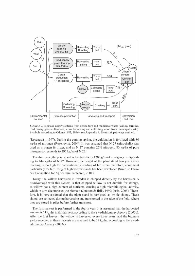
57

(Rosenqvist, 1997). During the coming spring, the cultivation is fertilized with 80 kg/ha of nitrogen (Rosenqvist, 2004). It was assumed that N 27 (nitrochalk) was used as nitrogen fertilizer, and as N 27 contains 27% nitrogen, 80 kg/ha of pure nitrogen corresponds to 296 kg/ha of N 27.

The third year, the plant stand is fertilized with 120 kg/ha of nitrogen, correspond-ing to 444 kg/ha of N 27. However, the height of the plant stand two years after planting is too high for conventional spreading of fertilizers; therefore, equipment particularly for fertilizing of high willow stands has been developed (Swedish Farm-ers’ Foundation for Agricultural Research, 2001).

Today, the willow harvested in Sweden is chipped directly by the harvester. A disadvantage with this system is that chipped willow is not durable for storage, as willow has a high content of nutrients, causing a high microbiological activity, which in turn decomposes the biomass (Jonsson & Jirjis, 1997; Jirjis, 2005). There-fore, it is here assumed that the plant stand is harvested as whole shoots. These shoots are collected during harvesting and transported to the edge of the fi eld, where they are stored in piles before further transport.

The fi rst harvest is performed in the fourth year. It is assumed that the harvested amount is 21 tdm/ha in this harvest, according to the Swedish Energy Agency (2003c). After the fi rst harvest, the willow is harvested every three years, and the biomass yields received at these harvests are assumed to be 27 tdm/ha, according to the Swed-ish Energy Agency (2003c).

�

Rain

Sun

Wind

Recov.wood

Straw

CollectingScreening

Conver-sion

Urbancenters

Assets

Trans-port

Willowfarming

275,000 ha

HarvestingBundling

Trans-port

Trans-port

Cerealproduction

1.1 million haHarvesting Trans-

port

Reed canarygrass farming125,000 ha

HarvestingBaling

Trans-port

Crushing

CollectingBaling

Biomass productionEnvironmentalsources

Conversionand use

Harvesting and transport

[Mt dm /year]

2.29

0.77

5.94

2.00

0.80

Figure 3-7. Biomass supply systems from agriculture and municipal waste (willow farming, Figure 3-7. Biomass supply systems from agriculture and municipal waste (willow farming, Figure 3-7.reed canary grass cultivation, straw harvesting and collecting wood from municipal waste). Symbols according to Odum (1983, 1996), see Appendix A. Heat sink pathways omitted.

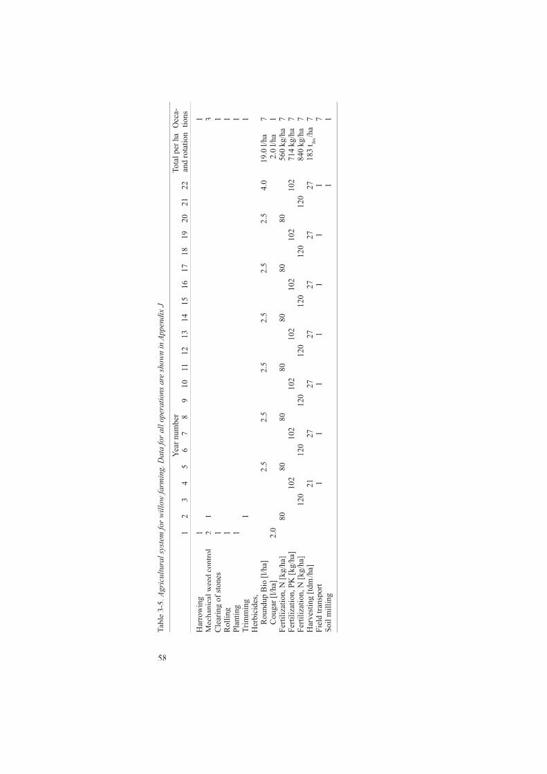
58

Tabl

e 3-

5. A

gric

ultu

ral s

yste

m fo

r will

ow fa

rmin

g. D

ata

for a

ll op

erat

ions

are

show

n in

App

endi

x J

Ye

ar n

umbe

r To

tal p

er h

a O

cca-

Ye

ar n

umbe

r To

tal p

er h

a O

cca-

Ye

ar n

umbe

r

1 2

3 4

5 6

7 8

9 10

11

12

13

14

15

16

17

18

19

20

21

22

an

d ro

tatio

n tio

ns

Har

row

ing

1

1

Mec

hani

cal w

eed

cont

rol

2 1

3

Cle

arin

g of

ston

es

1

1

Rol

ling

1

1

Plan

ting

1

1

Trim

min

g

1

1H

erbi

cide

s,

R

ound

up B

io [l

/ha]

2.

5

2.

5

2.

5

2.

5

2.

5

2.

5

4.0

19.0

l/ha

7

C

ouga

r [l/h

a]

2.0

2.

0 l/h

a 1

Ferti

lizat

ion,

N [k

g/ha

]

80

80

80

80

80

80

80

560

kg/

ha

7Fe

rtiliz

atio

n, P

K [k

g/ha

]

102

102

102

102

102

102

102

714

kg/h

a 7

Ferti

lizat

ion,

N [k

g/ha

]

12

0

12

0

12

0

12

0

12

0

12

0

12

0

840

kg/h

a 7

Har

vest

ing

[tdm

/ha]

21

27

27

27

27

27

27

183

t dm /h

a 7

Fiel

d tra

nspo

rt

1

1

1

1

1

1

1

7

Soil

mill

ing

1

1

59

After each harvest, the fi eld is fertilized with 22 kg/ha of phosphorus and 73 kg/ha of potassium (Rosenqvist, 2004). It was assumed that PK 7-25, containing 7.0% of phosphorus and 24.9% of potassium, was used as fertilizer. Thus, for covering the amounts of these minerals required, the amount of PK 7-25 has to be 320 kg/ha, which corresponds to 22.4 kg/ha of phosphorus and 79.7 kg/ha of potassium.

The fi rst year after each harvest, couch-grass is treated with 2.5 litres/ha Roundup Bio (Jansson, 2004a). The plant stand is also fertilized with 296 kg/ha of N 27 (corresponding to 80 kg/ha of pure nitrogen). The second year after each harvest, the plant stand is fertilized with 444 kg/ha of N 27 (corresponding to 120 kg/ha of nitrogen) with the special equipment for fertilization of high willow stands (Rosen-qvist, 2004).

After the last harvest, the stumps and roots are decomposed through rotary cul-tivation. If this operation is performed in wintertime when there still is frost in the soil, the stumps and roots are decomposed into fi ne particles, so they do not need to be removed in a separate operation (Rosenqvist, 1997).

Reed canary grassAs mentioned in Chapter 1, investigations into using grass as a fuel in Sweden were started in the beginning of the 1980s, and it was shown that reed canary grass (Phalaris arundinacea L.) was the most promising species regarding cultivation and quality aspects. Hadders (1989) pointed out that harvesting in late summer does not guarantee storage and hygienically acceptable quality of the crop. Therefore, a new concept of delayed harvest was introduced based on harvesting in the springtime of the year after sowing (Olsson et al., 1989). The moisture content was then decreased et al., 1989). The moisture content was then decreased et al.to 10-15%, leading to better properties for storage and further handling, e.g. pelletis-e.g. pelletis-e.g.ing, briquetting or powder production without drying (Bondesson, Kraft & Larsson, 1993; Burvall & Segerud, 1993; Burvall & Örberg, 1994).

The system for evaluation of cultivation and harvesting of reed canary grass is shown in Table 3-6. It was selected in accordance with the studies by Olsson et al.(2001). The fi eld is harrowed twice before sowing. Subsequently, rolling is per-formed twice. During the same season, the fi eld is fertilized with 40 kg/ha of nitro-gen, 15 kg/ha of phosphorus and 50 kg/ha of potassium.

The second year the fi eld is fertilized with 100 kg/ha of nitrogen, 15 kg/ha of phosphorus and 80 kg/ha of potassium. The third year and the following seven years, the cultivation is fertilized with 50 kg/ha of nitrogen, 5 kg/ha of phosphorus and 20 kg/ha of potassium.

The fi rst harvest is taken in the third year. The estimate of annual yield was based on fi eld experiments performed in Sweden during the 1990s and was estimated to be 7.5 tdm per hectare (Olsson et al., 2001). The harvested reed canary grass is baled et al., 2001). The harvested reed canary grass is baled et al.in the fi eld and transported to a barn for storage.

The fi eld is harvested nine times before settlement. After the last harvest in the eleventh year of the rotation period, the fi eld is harrowed twice with a disc harrow, followed by regular ploughing.

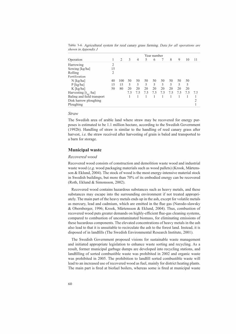
60

StrawThe Swedish area of arable land where straw may be recovered for energy pur-poses is estimated to be 1.1 million hectare, according to the Swedish Government (1992b). Handling of straw is similar to the handling of reed canary grass after harvest, i.e. the straw received after harvesting of grain is baled and transported to i.e. the straw received after harvesting of grain is baled and transported to i.e.a barn for storage.

Municipal wasteRecovered woodRecovered wood consists of construction and demolition waste wood and industrial waste wood (e.g. wood packaging materials such as wood pallets) (Krook, Mårtens-e.g. wood packaging materials such as wood pallets) (Krook, Mårtens-e.g.son & Eklund, 2004). The stock of wood is the most energy-intensive material stock in Swedish buildings, but more than 70% of its embodied energy can be recovered (Roth, Eklund & Simonsson, 2002).

Recovered wood contains hazardous substances such as heavy metals, and these substances may escape into the surrounding environment if not treated appropri-ately. The main part of the heavy metals ends up in the ash, except for volatile metals as mercury, lead and cadmium, which are emitted in the fl ue gas (Narodo-slawsky & Obernberger, 1996; Krook, Mårtensson & Eklund, 2004). Thus, combustion of recovered wood puts greater demands on highly-effi cient fl ue-gas cleaning systems, compared to combustion of uncontaminated biomass, for eliminating emissions of these hazardous components. The elevated concentrations of heavy metals in the ash also lead to that it is unsuitable to recirculate the ash to the forest land. Instead, it is disposed of in landfi lls (The Swedish Environmental Research Institute, 2001).

The Swedish Government proposed visions for sustainable waste management and initiated appropriate legislation to enhance waste sorting and recycling. As a result, former municipal garbage dumps are developed into recycling stations, and landfi lling of sorted combustible waste was prohibited in 2002 and organic waste was prohibited in 2005. The prohibition to landfi ll sorted combustible waste will lead to an increased use of recovered wood as fuel, mainly for district heating plants. The main part is fi red at biofuel boilers, whereas some is fi red at municipal waste

Table 3-6. Agricultural system for reed canary grass farming. Data for all operations are shown in Appendix J

Year numberOperation 1 2 3 4 5 6 7 8 9 10 11Harrowing 2 Sowing [kg/ha] 15 Rolling 2 Fertilization N [kg/ha] 40 100 50 50 50 50 50 50 50 50 P [kg/ha] 15 15 5 5 5 5 5 5 5 5 K [kg/ha] 50 80 20 20 20 20 20 20 20 20 Harvesting [tdm /ha] 7.5 7.5 7.5 7.5 7.5 7.5 7.5 7.5 7.5Baling and fi eld transport 1 1 1 1 1 1 1 1 1Disk harrow ploughing 2Ploughing 1

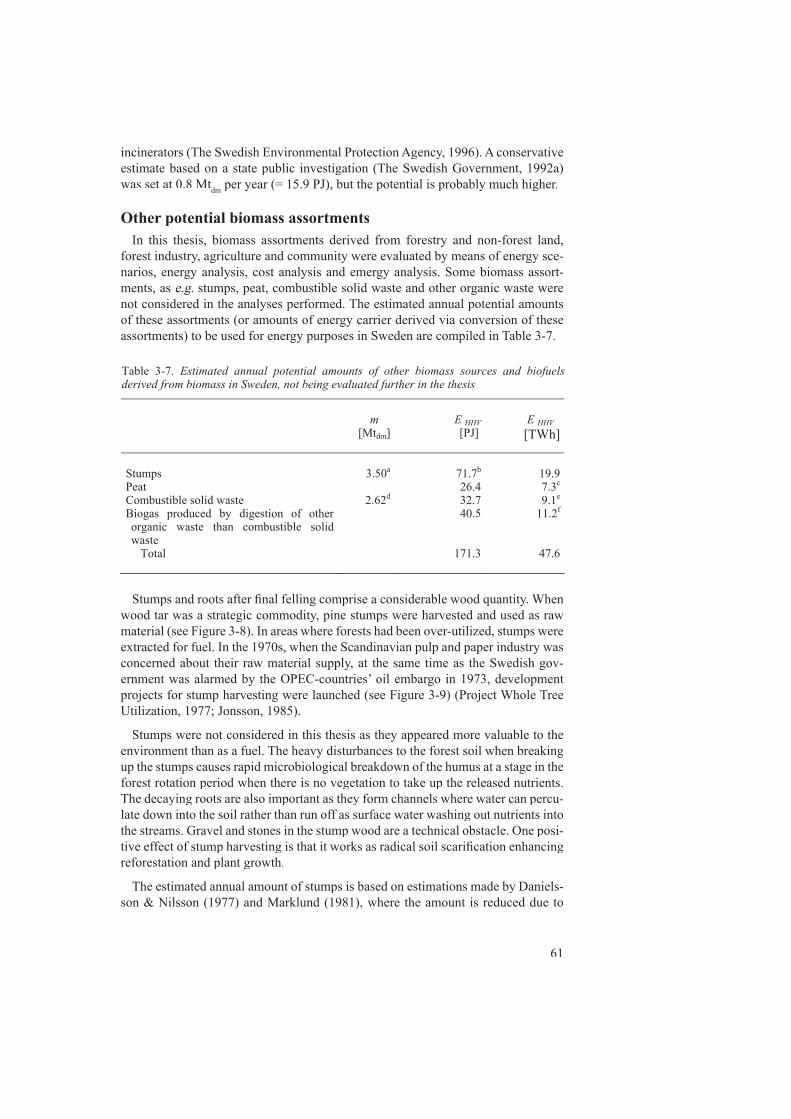
61

incinerators (The Swedish Environmental Protection Agency, 1996). A conservative estimate based on a state public investigation (The Swedish Government, 1992a) was set at 0.8 Mtdm per year (= 15.9 PJ), but the potential is probably much higher.

Other potential biomass assortmentsIn this thesis, biomass assortments derived from forestry and non-forest land,

forest industry, agriculture and community were evaluated by means of energy sce-narios, energy analysis, cost analysis and emergy analysis. Some biomass assort-ments, as e.g. stumps, peat, combustible solid waste and other organic waste were e.g. stumps, peat, combustible solid waste and other organic waste were e.g.not considered in the analyses performed. The estimated annual potential amounts of these assortments (or amounts of energy carrier derived via conversion of these assortments) to be used for energy purposes in Sweden are compiled in Table 3-7.

Stumps and roots after fi nal felling comprise a considerable wood quantity. When wood tar was a strategic commodity, pine stumps were harvested and used as raw material (see Figure 3-8). In areas where forests had been over-utilized, stumps were extracted for fuel. In the 1970s, when the Scandinavian pulp and paper industry was concerned about their raw material supply, at the same time as the Swedish gov-ernment was alarmed by the OPEC-countries’ oil embargo in 1973, development projects for stump harvesting were launched (see Figure 3-9) (Project Whole Tree Utilization, 1977; Jonsson, 1985).

Stumps were not considered in this thesis as they appeared more valuable to the environment than as a fuel. The heavy disturbances to the forest soil when breaking up the stumps causes rapid microbiological breakdown of the humus at a stage in the forest rotation period when there is no vegetation to take up the released nutrients. The decaying roots are also important as they form channels where water can percu-late down into the soil rather than run off as surface water washing out nutrients into the streams. Gravel and stones in the stump wood are a technical obstacle. One posi-tive effect of stump harvesting is that it works as radical soil scarifi cation enhancing reforestation and plant growth.

The estimated annual amount of stumps is based on estimations made by Daniels-son & Nilsson (1977) and Marklund (1981), where the amount is reduced due to

1

Table 3-7. Estimated annual potential amounts of other biomass sources and biofuels derived from biomass in Sweden, not being evaluated further in the thesis

m[Mtdm]

E HHV

[PJ] E HHV

[TWh]

StumpsPeat Combustible solid waste Biogas produced by digestion of other organic waste than combustible solid waste

Total

3.50a

2.62d

71.7b

26.432.740.5

171.3

19.97.3c

9.1e

11.2f

47.6

62

severe terrain, nutrient-poor land, small fi nal-felled areas, small stumps and stumps from broad-leaf trees.

Even if Sweden’s peat supply is large (as mentioned in Chapter 1), the infl uence of the environment at peat extraction decreases the amount of peat that may be extracted annually. The annual growth of peat in Sweden is estimated to be about 18 TWhLHV (The Swedish Peat Research Foundation, 1993), and it is estimated that 6.0 LHV (The Swedish Peat Research Foundation, 1993), and it is estimated that 6.0 LHVTWhLHV (7.3 TWhLHV (7.3 TWhLHV HHV) of peat may be used annually in existing energy conversion plants in Sweden (Ministry of Industry, Employment and Communication, 2002).

Several different estimations of the potential amount of combustible solid waste in Sweden have been published during the last years. Within the Swedish SAME-project (Hovsenius et al., 1999), the amount of solid household waste available for et al., 1999), the amount of solid household waste available for et al.combustion is estimated to decrease to 2 – 3 TWhLHV until 2050, due to increased LHV until 2050, due to increased LHVrecycling of materials. However, Profu (2001a, 2001b) estimates that the amount of combustible solid waste will continuously increase short term: the estimation of the amount of combustible solid waste in Table 3-7 is based on the short-term view of Profu.

The total biogas potential in 2008 is estimated by Nordberg et al. (1998) to be et al. (1998) to be et al.17.4 TWhLHV. However, 7.1 TWhLHV of this amount is derived from straw, which is LHV of this amount is derived from straw, which is LHValready considered in the scenarios and analyses performed in this thesis. Thus, this biogas amount derived from straw was excluded in this compilation of other poten-tial amounts of bioenergy sources. The remaining potential biogas amount is 10.2 TWhLHV (recalculated in Table 3-7 to be 11.2 TWhLHV (recalculated in Table 3-7 to be 11.2 TWhLHV HHV).

The total potential amount of the biomass sources and biofuels derived from bio-mass sources (i.e. biogas) and used for energy purposes in Sweden, and which were not evaluated in the scenarios and analyses performed, was 171.3 PJ (47.6 TWh). However, stump clearing is probably not a realistic biomass potential in the near future in Sweden, as this operation is assessed as being negative for long-term forest production (National Board of Forestry, 9-Aug-2005 (URL)). Thus, the remaining potential amount, excluding stumps, is 99.6 PJ (27.7 TWh). This amount could be compared with the total estimated annual potential amount of biomass sources eval-uated in this thesis (584 PJ in Case 1, 680 PJ in Case 2 and 627 PJ in Case 3). The potential amount of peat, combustible solid waste and biogas produced by digestion of organic waste other than combustible solid waste corresponded to 17% of the total estimated annual potential amount of biomass sources in Case 1, 15% of the total estimated amount of biomass sources in Case 2, and 16% in Case 3. Thus, the amount of other biomass sources and biofuels derived from biomass (biogas) not being evaluated in the scenarios and analyses was considerable compared to the amount of biomass sources evaluated, and should not be ignored when compiling the potential biomass sources and biofuels available.

63

Figure 3-8. Stump harv esting with Björnen No 3. Dalarna, Bjurfors kronopark, July 1918. Photo: Gustaf Lundberg. Picture owner: Swedish University of Agricultural Sciences, the Forestry Library.

Figure 3-9. Stump harvesting with Pallari Stump-arvester in Älvdalen, Sweden, in the 1970s.

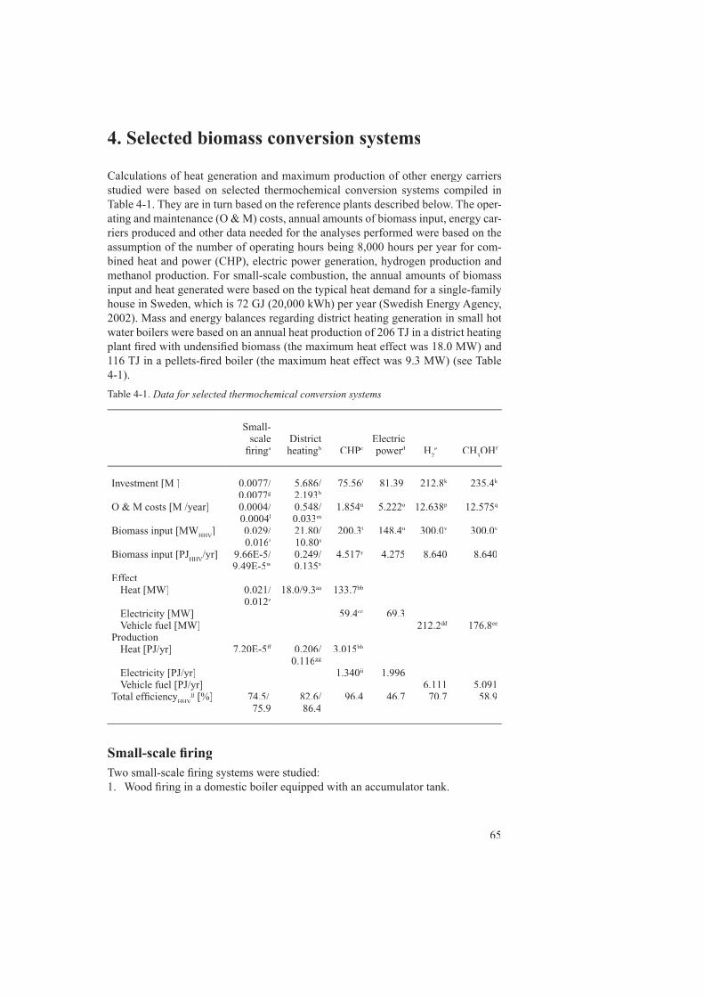
65

4. Selected biomass conversion systems

Calculations of heat generation and maximum production of other energy carriers studied were based on selected thermochemical conversion systems compiled in Table 4-1. They are in turn based on the reference plants described below. The oper-ating and maintenance (O & M) costs, annual amounts of biomass input, energy car-riers produced and other data needed for the analyses performed were based on the assumption of the number of operating hours being 8,000 hours per year for com-bined heat and power (CHP), electric power generation, hydrogen production and methanol production. For small-scale combustion, the annual amounts of biomass input and heat generated were based on the typical heat demand for a single-family house in Sweden, which is 72 GJ (20,000 kWh) per year (Swedish Energy Agency, 2002). Mass and energy balances regarding district heating generation in small hot water boilers were based on an annual heat production of 206 TJ in a district heating plant fi red with undensifi ed biomass (the maximum heat effect was 18.0 MW) and 116 TJ in a pellets-fi red boiler (the maximum heat effect was 9.3 MW) (see Table 4-1).Table 4-1. Data for selected thermochemical conversion systems

Small-scale

fi ringaDistrict heatingb CHPc

Electric powerd H

2e CH

3OHf

Investment [M�]

O & M costs [M�/year]

Biomass input [MWHHV

]

Biomass input [PJHHV

/yr]

EffectHeat [MW]

Electricity [MW]Vehicle fuel [MW]

ProductionHeat [PJ/yr]

Electricity [PJ/yr]Vehicle fuel [PJ/yr]

Total effi ciencyHHV

jj [%]

0.0077/0.0077g

0.0004/0.0004l

0.029/0.016r

9.66E-5/ 9.49E-5w

0.021/0.012z

7.20E-5ff

74.5/75.9

5.686/2.193h

0.548/0.033m

21.80/10.80s

0.249/0.135x

18.0/9.3aa

0.206/0.116gg

82.6/86.4

75.56i

1.854n

200.3t

4.517y

133.7bb

59.4cc

3.015hh

1.340ii

96.4

81.39j81.39j81.39

5.222o

148.4u

4.275

69.3

1.996

46.7

212.8k

12.638p

300.0v

8.640

212.2dd

6.11170.7

235.4k

12.575q

300.0v

8.640

176.8ee

5.09158.9

Small-scale fi ringTwo small-scale fi ring systems were studied:1. Wood fi ring in a domestic boiler equipped with an accumulator tank.

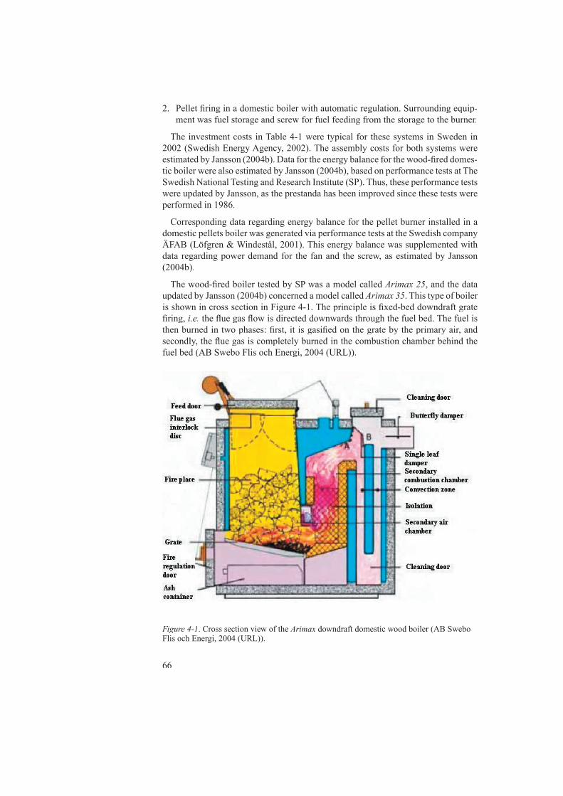
66

2. Pellet fi ring in a domestic boiler with automatic regulation. Surrounding equip-ment was fuel storage and screw for fuel feeding from the storage to the burner.

The investment costs in Table 4-1 were typical for these systems in Sweden in 2002 (Swedish Energy Agency, 2002). The assembly costs for both systems were estimated by Jansson (2004b). Data for the energy balance for the wood-fi red domes-tic boiler were also estimated by Jansson (2004b), based on performance tests at The Swedish National Testing and Research Institute (SP). Thus, these performance tests were updated by Jansson, as the prestanda has been improved since these tests were performed in 1986.

Corresponding data regarding energy balance for the pellet burner installed in a domestic pellets boiler was generated via performance tests at the Swedish company ÄFAB (Löfgren & Windestål, 2001). This energy balance was supplemented with data regarding power demand for the fan and the screw, as estimated by Jansson (2004b).

The wood-fi red boiler tested by SP was a model called Arimax 25, and the data updated by Jansson (2004b) concerned a model called Arimax 35. This type of boiler is shown in cross section in Figure 4-1. The principle is fi xed-bed downdraft grate fi ring, i.e. the fl ue gas fl ow is directed downwards through the fuel bed. The fuel is then burned in two phases: fi rst, it is gasifi ed on the grate by the primary air, and secondly, the fl ue gas is completely burned in the combustion chamber behind the fuel bed (AB Swebo Flis och Energi, 2004 (URL)).

Figure 4-1. Cross section view of the Arimax downdraft domestic wood boiler (AB Swebo Flis och Energi, 2004 (URL)).

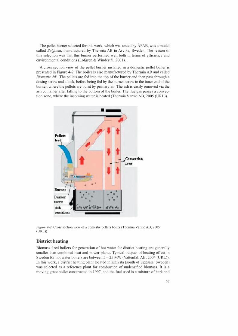
67

The pellet burner selected for this work, which was tested by ÄFAB, was a model called BeQuem, manufactured by Thermia AB in Arvika, Sweden. The reason of this selection was that this burner performed well both in terms of effi ciency and environmental conditions (Löfgren & Windestål, 2001).

A cross section view of the pellet burner installed in a domestic pellet boiler is presented in Figure 4-2. The boiler is also manufactured by Thermia AB and called Biomatic 20+. The pellets are fed into the top of the burner and then pass through a dosing screw and a lock, before being fed by the burner screw to the inner end of the burner, where the pellets are burnt by primary air. The ash is easily removed via the ash container after falling to the bottom of the boiler. The fl ue gas passes a convec-tion zone, where the incoming water is heated (Thermia Värme AB, 2005 (URL)).

Figure 4-2. Cross section view of a domestic pellets boiler (Thermia Värme AB, 2005 (URL)).

District heatingBiomass-fi red boilers for generation of hot water for district heating are generally smaller than combined heat and power plants. Typical outputs of heating effect in Sweden for hot water boilers are between 5 – 25 MW (Vattenfall AB, 2004 (URL)). In this work, a district heating plant located in Knivsta (south of Uppsala, Sweden) was selected as a reference plant for combustion of undensifi ed biomass. It is a moving grate boiler constructed in 1997, and the fuel used is a mixture of bark and

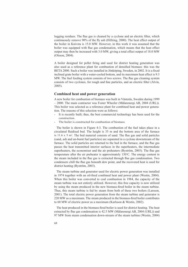
68

logging residues. The fl ue gas is cleaned by a cyclone and an electric fi lter, which continuously remove 90% of the fl y ash (Hillring, 2000). The heat effect output of the boiler in Knivsta is 15.0 MW. However, in this work it was assumed that the boiler was equipped with fl ue gas condensation, which means that the heat effect output may then be increased with 3.0 MW, giving a total effect output of 18.0 MW (Olsson, 2004).

A boiler designed for pellet fi ring and used for district heating generation was also used as a reference plant for combustion of densifi ed biomass: this was the BETA 2000. Such a boiler was installed in Jönköping, Sweden, in 2002. It is a fi xed inclined grate boiler with a water-cooled bottom, and its maximum heat effect is 9.3 MW. The fuel feeding system consists of two screws. The fl ue gas cleaning system consists of two cyclones, for rough and fi ne particles, and an electric fi lter (Alvin, 2005).

Combined heat and power generationA new boiler for combustion of biomass was built in Västerås, Sweden during 1999 – 2000. The main contractor was Foster Wheeler (Mälarenergi AB, 2004 (URL)). This boiler was selected as a reference plant for combined heat and power genera-tion. The reasons of this selection were as follows:- It is recently built; thus, the best commercial technology has been used for the

construction.- The boiler is constructed for combustion of biomass.

The boiler is shown in Figure 4-3. The combustion of the fuel takes place in a circulated fl uidised bed. The height is 35 m and the bottom area of the furnace is 11.6 x 5 m2. The bed material consists of sand. The fl ue gas and solid particles (sand, ash and un-burnt fuel particles) are separated in a cyclone downstream of the furnace. The solid particles are returned to the bed in the furnace, and the fl ue gas passes the heat transmitted interior surfaces in the superheaters, the intermediate superheaters, the economiser and the air preheaters (Byström, 2003). The fl ue gas temperature after the air preheater is approximately 150oC. The energy content in the steam included in the fl ue gas is extracted through fl ue gas condensation. Two condensers chill the fl ue gas beneath dew point, and the recovered heat is used for district heating (Byström, 2003).

The steam turbine and generator used for electric power generation was installed in 1974 together with an oil-fi red combined heat and power plant (Westin, 2004). When this boiler was converted to coal combustion in 1984, the capacity of the steam turbine was not entirely utilized. However, this free capacity is now utilized by using the steam produced in the new biomass-fi red boiler in the steam turbine. Thus, this steam turbine is fed by steam from both of these two boilers (Larsson, 2001). The total electric power generation from the steam turbine and generator is 220 MW as a maximum. The steam produced in the biomass-fi red boiler contributes to 60 MW of electric power as a maximum (Karlsson & Westin, 2002).

The heat produced in the biomass-fi red boiler is used for district heating. The heat extracted by fl ue gas condensation is 42.5 MW (Mälarenergi AB, 2004 (URL)) and 97 MW from steam condensation down-stream of the steam turbine (Westin, 2004)

69

at a maximum. Thus, the total production of heat delivered to the district heating system is 139.5 MW at a maximum. The energy content of the maximum amount of biomass fed into the boiler is 170 MWLHV (Westin, 2004).

Figure 4-3. Västerås’ recently built biomass-fi red boiler (Foster Wheeler, 1998).

Electric power generationGasifi cation of biomass integrated with a combined cycle has a higher effi ciency regarding electric power generation, compared to combustion of biomass in con-ventional boilers with a steam cycle (Bridgwater, 1995; Mitchell et al., 1995; Dorn-burg & Faaij, 2001). Thus, an integrated gasifi cation combined cycle (IGCC) was selected as the technology for maximum electric power generation. However, sev-eral different technologies for gasifi cation of biomass have been developed during the last decades. Some of these are briefl y described in Appendix D.

The fi rst complete IGCC-plant in the World and constructed for gasifi cation of biomass was built in Värnamo, Sweden, during 1991 – 1993 (Sydkraft, 1997). It was built as a demonstration unit, i.e. the purpose of the plant was to test the function of a complete IGCC-plant. The unit was commissioned during 1993 – 1995. After that, a demonstration programme was performed during 1996 – 1999 (Sydkraft, 2000).

70

The main purposes of the demonstration programme were as follows:- Improvements of the technology in this or other future gasifi cation plants.- Test of fuel fl exibility.- Mapping of emissions.- Costs for the technology regarding operation and maintenance, and construction

of new plants.

As this process is well studied due to this demonstration programme, it was selected as a reference plant for maximum electric power generation.

A simplifi ed diagram of the process is shown in Figure 4-4. It is constructed for pressurized gasifi cation; the operating pressure is 18 bar (g). Dried and crushed wood fuel is pressurized in a lock-hopper system and fed by screw feeders into the gasifi er a few meters above the bottom. The gasifi er is a circulating fl uidised bed, consisting of: the reactor unit, a cyclone and cyclone return leg. These parts are refractory lined. The operating temperature of the gasifi er is 950 – 1000oC (Ståhl, Neergaard & Nieminen, 2000).

Figure 4-4. Process diagram of the IGCC demonstration plant in Värnamo, Sweden (Ståhl, Neergaard & Nieminen, 2000).

The fuel is dried, gasifi ed and pyrolized immediately on entering the gasifi er. The gas transports the bed material and the remaining char towards the cyclone, where most of the solids are separated from the gas and are returned to the bottom of the

71

gasifi er through the return leg. The recirculated solids contain some char, which is burned in the bottom zone where air is introduced into the gasifi er. The combustion of the char maintains the required temperature in the gasifi er. After the cyclone, the gas produced is cooled to 350 – 400oC before it fl ows through a hot gas fi lter, where particulate up cleaning occurs. Ash is discharged from the hot gas fi lter, as well as from the bottom of the gasifi er, and is in the meantime cooled and depressurized (ibid.).

The gasifi er is air-blown; thus, about 10% of the air is extracted from the gas tur-bine compressor, further compressed in a booster compressor, and fi nally injected into the bottom of the gasifi er. After burning in the combustion chambers, the cleaned gas expands through the gas turbine, generating 4.2 MW of electric power. The fuel supply system, fuel injectors and the combustors have been redesigned to suit the low calorifi c value gas (5 MJ/nm3). The hot fl ue gas from the gas turbine is ducted to the heat recovery steam generator (HRSG), where the steam generated, along with steam from the gas cooler, is superheated and then supplied to the steam turbine (40 bar, 455oC), generating 1.8 MWof electric power. The plant is equipped with a fl are on the roof of the gasifi cation building, which is used during the start-up procedure and when testing less well known conditions, in order to protect the gas turbine. The energy content of the biomass fed into the gasifi er is 18 MW, and electric power generation is 6 MW and heat generation is 9 MW (ibid.).

Data regarding full-scale plants have been compiled within the demonstration pro-gramme (Sydkraft, 2000). The data for condensing power have been used here for selected conversion system for maximum electric power generation.

Vehicle fuel productionDifferent vehicle fuels can be produced from biomass via thermochemical conver-sion. However, the conversion routes vary, depending on what kind of vehicle fuel is to be produced. Three different thermochemical conversion technologies may be used for vehicle fuels production: gasifi cation, pyrolysis or liquefaction. These tech-nologies may give gasoline and diesel fuel blends, hydrogen, methane, methanol or ethers, depending on what kind of synthesis technology is used downstream of the thermochemical conversion steps (Bridgwater & Double, 1991; Wender, 1996).

Ethanol may be produced via hydrolysis of the cellulosic raw material and fermen-tation of the glucose and xylose sugars received in the hydrolysis step. However, the yield of ethanol is limited because the lignin fraction cannot be fermented to ethanol (Wyman et al., 1993). Estimated effi ciency for cellulosic biomass1 conversion to ethanol are about 50%, but may increase to more than 60% in the future (Lynd, 1996; Chum & Overend, 2001).

1 Cellulosic biomass includes agricultural and forestry feedstocks, municipal solid waste and energy crops (Wyman et al., 1993).

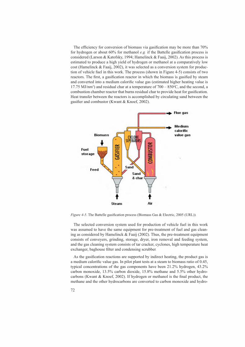
72

The effi ciency for conversion of biomass via gasifi cation may be more than 70% for hydrogen or about 60% for methanol e.g. if the Battelle gasifi cation process is considered (Larson & Katofsky, 1994; Hamelinck & Faaij, 2002). As this process is estimated to produce a high yield of hydrogen or methanol at a comparatively low cost (Hamelinck & Faaij, 2002), it was selected as a conversion system for produc-tion of vehicle fuel in this work. The process (shown in Figure 4-5) consists of two reactors. The fi rst, a gasifi cation reactor in which the biomass is gasifi ed by steam and converted into a medium calorifi c value gas (estimated higher heating value is 17.75 MJ/nm3) and residual char at a temperature of 700 – 850oC, and the second, a combustion chamber reactor that burns residual char to provide heat for gasifi cation. Heat transfer between the reactors is accomplished by circulating sand between the gasifi er and combustor (Kwant & Knoef, 2002).

Figure 4-5. The Battelle gasifi cation process (Biomass Gas & Electric, 2005 (URL)).

The selected conversion system used for production of vehicle fuel in this work was assumed to have the same equipment for pre-treatment of fuel and gas clean-ing as considered by Hamelinck & Faaij (2002). Thus, the pre-treatment equipment consists of conveyers, grinding, storage, dryer, iron removal and feeding system, and the gas cleaning system consists of tar cracker, cyclones, high temperature heat exchanger, baghouse fi lter and condensing scrubber.

As the gasifi cation reactions are supported by indirect heating, the product gas is a medium calorifi c value gas. In pilot plant tests at a steam to biomass ratio of 0.45, typical concentrations of the gas components have been 21.2% hydrogen, 43.2% carbon monoxide, 13.5% carbon dioxide, 15.8% methane and 5.5% other hydro-carbons (Kwant & Knoef, 2002). If hydrogen or methanol is the fi nal product, the methane and the other hydrocarbons are converted to carbon monoxide and hydro-

73

gen by steam reforming. Steam is then added over a nickel catalyst (Hamelinck & Faaij, 2002).

A severe problem with nickel-based catalysts is their tendency to deactivate, due to coke deposition (Coll et al., 2001). An alternative or complement to steam reform-ing is autothermal reforming, which combines partial oxidation in the fi rst part of the reactor with steam reforming in the second part, thereby optimally integrating the heat fl ows. Tijmensen (2000) poses autothermal reforming being the only tech-nology able to prevent coking. The selected conversion system used for production of vehicle fuel in this thesis was assumed to be equipped with only steam reforming for hydrogen production, and equipped with both steam reforming and autothermal reforming for methanol production, according to Hamelinck & Faaij (2002).

After steam reforming and/or autothermal reforming, the H2/CO ratio is increased by the water gas shift reaction, where steam reacts with carbon monoxide to form hydrogen and carbon dioxide (Hamelinck & Faaij, 2002; Tijmensen et al., 2002). Finally, carbon dioxide is removed through Selexol in methanol production, accord-ing to Hamelinck & Faaij (2002).

The size of the boiler infl uences both effi ciency and cost of energy carriers gener-ated (Bridgwater, 1995; Dornburg & Faaij, 2001), which has to be considered when comparing different conversion processes. In this thesis, the biomass input to the gasifi er at vehicle fuel production was assumed as 300.0 MWHHV. The investment HHV. The investment HHVcost depending on the size of the equipment is given by Hamelinck & Faaij (2002):

where: R = a scale factor, unique for each component. The base investment costs and the investment costs calculated for plants with a biomass input of 300.0 MWHHV at HHV at HHVboth hydrogen and methanol production are given in Table 4-2.

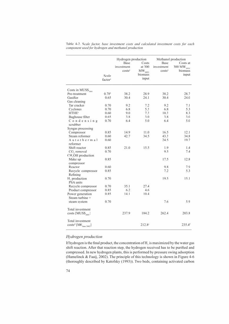
74

Table 4-2. Scale factor, base investment costs and calculated investment costs for each component used for hydrogen and methanol production

Scale factora

Hydrogen production Methanol productionBase

investment costsa

Costs at 300

MWHHV biomass

input

Base investment

costsa

Costs at 300 MWHHV

biomass input

Costs in MUS$2001Pre-treatmentGasifi erGas cleaningTar crackerCyclonesHTHEc

Baghouse fi lterC o n d e n s i n g scrubber

Syngas processingCompressorSteam reformerA u t o t h e r m a l reformerShift reactorCO2 removal

CH3OH productionMake up compressorReactorRecycle compressorRefi ning

H2 productionPSA unitsRecycle compressorProduct compressor

Power generationSteam turbine + steam system

Total investment costs [MUS$2001]

Total investment costsd [M€d [M€d

June 2002]

0.78b

0.65

0.700.700.600.650.70

0.850.600.60

0.850.70

0.85

0.600.85

0.70

0.700.850.85

0.70

38.230.4

9.26.89.03.86.4

14.942.7

21.0

35.16.2

14.1

237.9

28.924.1

7.25.37.33.05.0

11.034.5

15.5

27.44.6

10.4

184.2

212.8e

38.230.4

9.26.8

10.33.86.4

16.543.324.5

1.99.5

17.5

9.87.2

19.5

7.6

262.4

28.724.0

7.15.38.33.05.0

12.134.819.7

1.47.4

12.8

7.95.3

15.1

5.9

203.8

235.4f

Hydrogen productionIf hydrogen is the fi nal product, the concentration of H2 is maximized by the water gas shift reaction. After that reaction step, the hydrogen received has to be purifi ed and compressed. In new hydrogen plants, this is performed by pressure swing adsorption (Hamelinck & Faaij, 2002). The principle of this technology is shown in Figure 4-6 (thoroughly described by Katofsky (1993)). Two beds, containing activated carbon

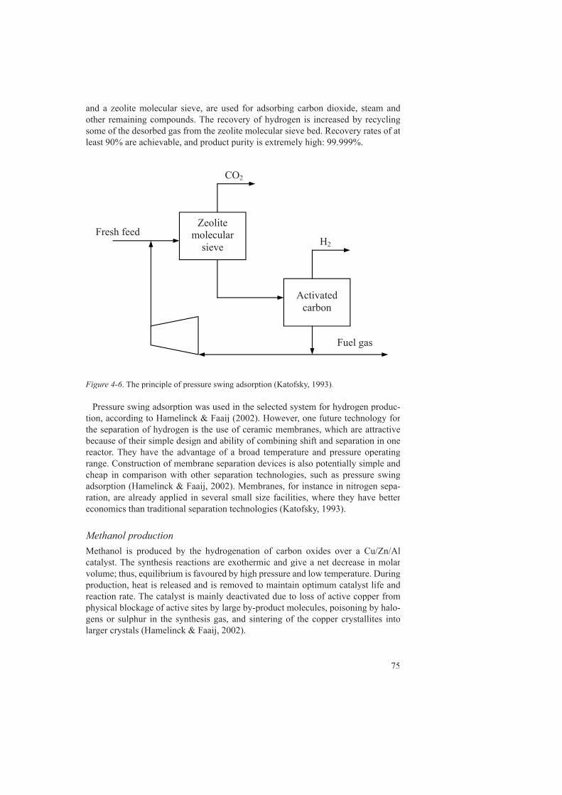
75

and a zeolite molecular sieve, are used for adsorbing carbon dioxide, steam and other remaining compounds. The recovery of hydrogen is increased by recycling some of the desorbed gas from the zeolite molecular sieve bed. Recovery rates of at least 90% are achievable, and product purity is extremely high: 99.999%.

Figure 4-6. The principle of pressure swing adsorption (Katofsky, 1993).

Pressure swing adsorption was used in the selected system for hydrogen produc-tion, according to Hamelinck & Faaij (2002). However, one future technology for the separation of hydrogen is the use of ceramic membranes, which are attractive because of their simple design and ability of combining shift and separation in one reactor. They have the advantage of a broad temperature and pressure operating range. Construction of membrane separation devices is also potentially simple and cheap in comparison with other separation technologies, such as pressure swing adsorption (Hamelinck & Faaij, 2002). Membranes, for instance in nitrogen sepa-ration, are already applied in several small size facilities, where they have better economics than traditional separation technologies (Katofsky, 1993).

Methanol productionMethanol is produced by the hydrogenation of carbon oxides over a Cu/Zn/Al catalyst. The synthesis reactions are exothermic and give a net decrease in molar volume; thus, equilibrium is favoured by high pressure and low temperature. During production, heat is released and is removed to maintain optimum catalyst life and reaction rate. The catalyst is mainly deactivated due to loss of active copper from physical blockage of active sites by large by-product molecules, poisoning by halo-gens or sulphur in the synthesis gas, and sintering of the copper crystallites into larger crystals (Hamelinck & Faaij, 2002).

CO2

Zeolite molecular

sieve

Activatedcarbon

Fuel gas

Fresh feed H2

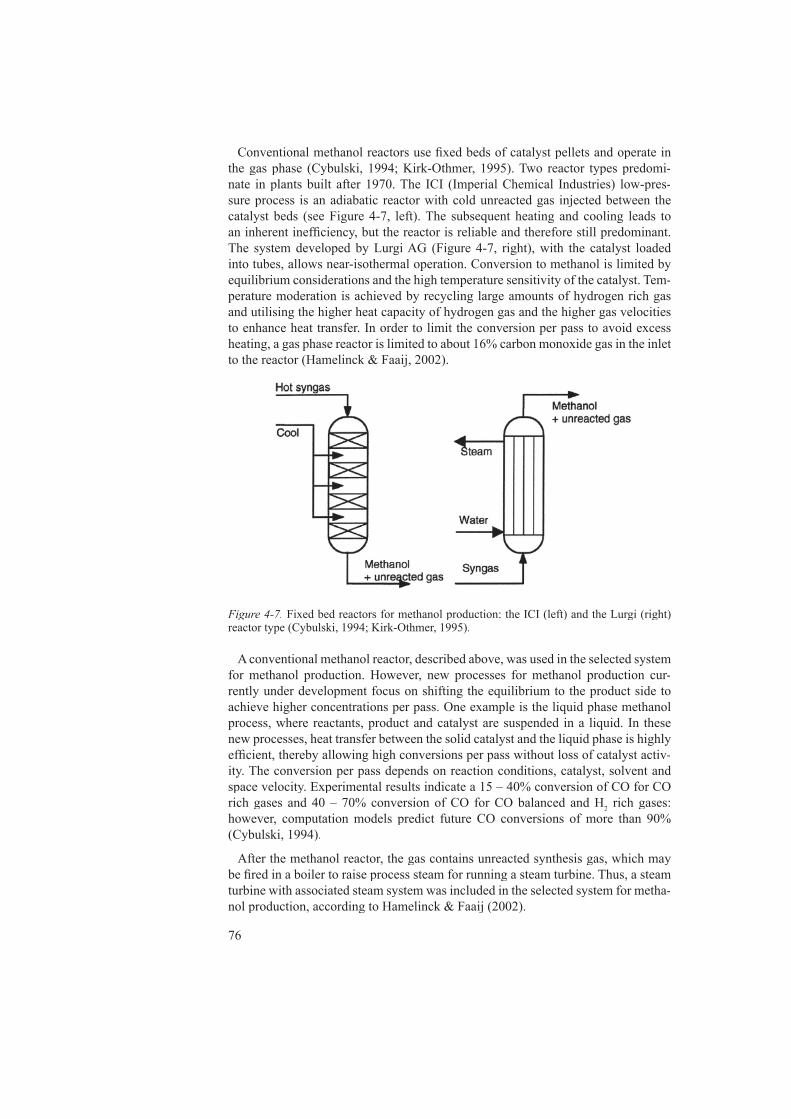
76

Conventional methanol reactors use fi xed beds of catalyst pellets and operate in the gas phase (Cybulski, 1994; Kirk-Othmer, 1995). Two reactor types predomi-nate in plants built after 1970. The ICI (Imperial Chemical Industries) low-pres-sure process is an adiabatic reactor with cold unreacted gas injected between the catalyst beds (see Figure 4-7, left). The subsequent heating and cooling leads to an inherent ineffi ciency, but the reactor is reliable and therefore still predominant. The system developed by Lurgi AG (Figure 4-7, right), with the catalyst loaded into tubes, allows near-isothermal operation. Conversion to methanol is limited by equilibrium considerations and the high temperature sensitivity of the catalyst. Tem-perature moderation is achieved by recycling large amounts of hydrogen rich gas and utilising the higher heat capacity of hydrogen gas and the higher gas velocities to enhance heat transfer. In order to limit the conversion per pass to avoid excess heating, a gas phase reactor is limited to about 16% carbon monoxide gas in the inlet to the reactor (Hamelinck & Faaij, 2002).

Figure 4-7. Fixed bed reactors for methanol production: the ICI (left) and the Lurgi (right) reactor type (Cybulski, 1994; Kirk-Othmer, 1995).

A conventional methanol reactor, described above, was used in the selected system for methanol production. However, new processes for methanol production cur-rently under development focus on shifting the equilibrium to the product side to achieve higher concentrations per pass. One example is the liquid phase methanol process, where reactants, product and catalyst are suspended in a liquid. In these new processes, heat transfer between the solid catalyst and the liquid phase is highly effi cient, thereby allowing high conversions per pass without loss of catalyst activ-ity. The conversion per pass depends on reaction conditions, catalyst, solvent and space velocity. Experimental results indicate a 15 – 40% conversion of CO for CO rich gases and 40 – 70% conversion of CO for CO balanced and H2 rich gases: however, computation models predict future CO conversions of more than 90% (Cybulski, 1994).

After the methanol reactor, the gas contains unreacted synthesis gas, which may be fi red in a boiler to raise process steam for running a steam turbine. Thus, a steam turbine with associated steam system was included in the selected system for metha-nol production, according to Hamelinck & Faaij (2002).

77

Black liquor gasifi cationBlack liquor received in pulp mills is currently recovered in Tomlinson boilers, although technology for gasifying the black liquor is now developed. The synthesis gas produced may then be used for generating electric power in a gas turbine or vehicle fuel production, as described above.

The black liquor gasifi cation process closest to commercial introduction is the process developed by the Swedish company Chemrec AB. This is a pressurised, oxygen-blown entrained-fl ow gasifi cation process at temperatures above the melt-ing point of the inorganic chemicals (Ekbom et al., 2003). The reactor is shown in Figure 4-8. The synthesis gas (syngas) and inorganic smelt are cooled and separated in the quench cooler downstream of the gasifi er. The smelt falls into the quench bath where it dissolves to form green liquor (ibid.).

Figure 4-8. Chemrec’s black liquor gasifi er (Chemrec AB, 2005 (URL)).

The syngas is further cooled in a counter-current condenser after the exit of the gasifi cation reactor. Water vapour in the syngas is then condensed and the heat released is used for steam generation. Hydrogen sulphide is removed in a pressu-rised absorption stage. The resulting gas is a virtually sulphur-free syngas consisting mainly of carbon monoxide, hydrogen and carbon dioxide (Ekbom et al., 2003).

78

In this thesis, the black liquor gasifi cation process was studied within the scenarios for estimating the potential amount of electric power or methanol, produced annu-ally via gasifi cation of the received Swedish black liquor amounts: performance data based on Chemrec’s black liquor gasifi er were used for these estimations (compiled in Table A.J-49). However, energy, cost and emergy analyses were not performed on this process, as not all the necessary data were compiled for these analyses.

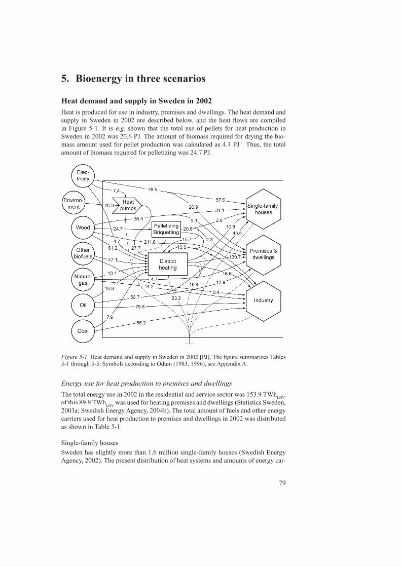
79

5. Bioenergy in three scenarios

Heat demand and supply in Sweden in 2002Heat is produced for use in industry, premises and dwellings. The heat demand and supply in Sweden in 2002 are described below, and the heat fl ows are compiled in Figure 5-1. It is e.g. shown that the total use of pellets for heat production in e.g. shown that the total use of pellets for heat production in e.g.Sweden in 2002 was 20.6 PJ. The amount of biomass required for drying the bio-mass amount used for pellet production was calculated as 4.1 PJ 1. Thus, the total amount of biomass required for pelletizing was 24.7 PJ.

Figure 5-1. Heat demand and supply in Sweden in 2002 [PJ]. The fi gure summarizes Tables 5-1 through 5-5. Symbols according to Odum (1983, 1996), see Appendix A.

Energy use for heat production to premises and dwellingsThe total energy use in 2002 in the residential and service sector was 153.9 TWhLHV, LHV, LHVof this 89.9 TWhLHV was used for heating premises and dwellings (Statistics Sweden, LHV was used for heating premises and dwellings (Statistics Sweden, LHV2003a; Swedish Energy Agency, 2004b). The total amount of fuels and other energy carriers used for heat production to premises and dwellings in 2002 was distributed as shown in Table 5-1.

Single-family housesSweden has slightly more than 1.6 million single-family houses (Swedish Energy Agency, 2002). The present distribution of heat systems and amounts of energy car-

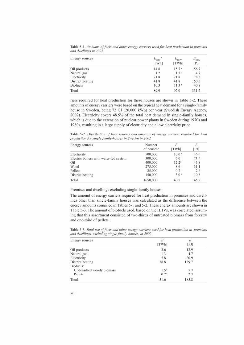
80

Table 5-3. Total use of fuels and other energy carriers used for heat production to premises and dwellings, excluding single family-houses, in 2002

Energy sources E E [TWh] [PJ]

Oil products 3.6 12.9 Natural gas 1.3 4.7Electricity 5.8 20.9District heating 38.8 139.7Biofuels a Undensifi ed woody biomass 1.5 b 5.3 Pellets 0.7 c 2.3Total 51.6 185.8

Table 5-1. Amounts of fuels and other energy carriers used for heat production to premises and dwellings in 2002

Energy sources ELHVELHVE a EHHVEHHVE EHHVEHHVE [TWh] [TWh] [PJ]

Oil products 14.8 15.7 b 56.7Natural gas 1.2 1.3 c 4.7Electricity 21.8 21.8 78.5District heating 41.8 41.8 150.5Biofuels 10.3 11.3 d 40.8Total 89.9 92.0 331.2

riers required for heat production for these houses are shown in Table 5-2. These amounts of energy carriers were based on the typical heat demand for a single-family house in Sweden, being 72 GJ (20,000 kWh) per year (Swedish Energy Agency, 2002). Electricity covers 48.5% of the total heat demand in single-family houses, which is due to the extension of nuclear power plants in Sweden during 1970s and 1980s, resulting in a large supply of electricity and a low electricity price.

Table 5-2. Distribution of heat systems and amounts of energy carriers required for heat production for single family-houses in Sweden in 2002

Energy sources Number E E of houses a [TWh] [PJ]

Electricity 500,000 10.0 b 36.0Electric boilers with water-fed system 300,000 6.0 c 21.6Oil 400,000 12.2d 43.8d 43.8d

Wood 275,000 8.6 e 31.1Pellets 25,000 0.7 f 2.6f 2.6f

District heating 150,000 3.0 g 10.8Total 1650,000 40.5 145.9

Premises and dwellings excluding single-family housesThe amount of energy carriers required for heat production in premises and dwell-ings other than single-family houses was calculated as the difference between the energy amounts compiled in Tables 5-1 and 5-2. These energy amounts are shown in Table 5-3. The amount of biofuels used, based on the HHVs, was correlated, assum-ing that this assortment consisted of two-thirds of untreated biomass from forestry and one-third of pellets.

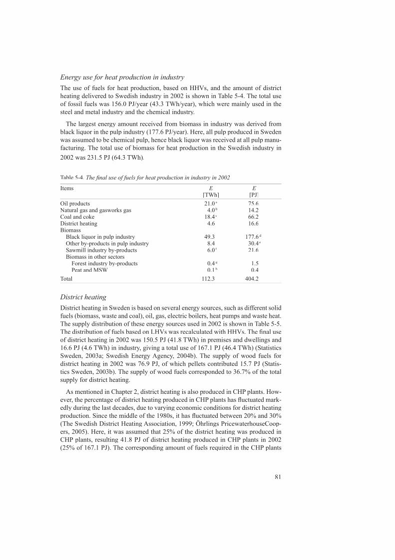
81

Energy use for heat production in industryThe use of fuels for heat production, based on HHVs, and the amount of district heating delivered to Swedish industry in 2002 is shown in Table 5-4. The total use of fossil fuels was 156.0 PJ/year (43.3 TWh/year), which were mainly used in the steel and metal industry and the chemical industry.

The largest energy amount received from biomass in industry was derived from black liquor in the pulp industry (177.6 PJ/year). Here, all pulp produced in Sweden was assumed to be chemical pulp, hence black liquor was received at all pulp manu-facturing. The total use of biomass for heat production in the Swedish industry in 2002 was 231.5 PJ (64.3 TWh).

Table 5-4. The fi nal use of fuels for heat production in industry in 2002

Items E E [TWh] [PJ]

Oil products 21.0 a 75.6Natural gas and gasworks gas 4.0 b 14.2Coal and coke 18.4 c 66.2District heating 4.6 16.6Biomass Black liquor in pulp industry 49.3 177.6 d Other by-products in pulp industry 8.4 30.4 e Sawmill industry by-products 6.0 f 21.6f 21.6f

Biomass in other sectors Forest industry by-products 0.4 g 1.5 Peat and MSW 0.1 h 0.4Total 112.3 404.2

District heatingDistrict heating in Sweden is based on several energy sources, such as different solid fuels (biomass, waste and coal), oil, gas, electric boilers, heat pumps and waste heat. The supply distribution of these energy sources used in 2002 is shown in Table 5-5. The distribution of fuels based on LHVs was recalculated with HHVs. The fi nal use of district heating in 2002 was 150.5 PJ (41.8 TWh) in premises and dwellings and 16.6 PJ (4.6 TWh) in industry, giving a total use of 167.1 PJ (46.4 TWh) (Statistics Sweden, 2003a; Swedish Energy Agency, 2004b). The supply of wood fuels for district heating in 2002 was 76.9 PJ, of which pellets contributed 15.7 PJ (Statis-tics Sweden, 2003b). The supply of wood fuels corresponded to 36.7% of the total supply for district heating.

As mentioned in Chapter 2, district heating is also produced in CHP plants. How-ever, the percentage of district heating produced in CHP plants has fl uctuated mark-edly during the last decades, due to varying economic conditions for district heating production. Since the middle of the 1980s, it has fl uctuated between 20% and 30% (The Swedish District Heating Association, 1999; Öhrlings PricewaterhouseCoop-ers, 2005). Here, it was assumed that 25% of the district heating was produced in CHP plants, resulting 41.8 PJ of district heating produced in CHP plants in 2002 (25% of 167.1 PJ). The corresponding amount of fuels required in the CHP plants

82

Table 5-6. Potential amounts of electricity and fossil fuels to be replaced in premises and dwellings, industry and district heating

Energy sources Premises and dwellings Industry District heating Total [PJ] [PJ] [PJ] [PJ]

Oil products 56.7 75.6 16.8 149.1Natural gas 4.7 14.2 13.1 32.1Coal and coke 66.2 66.2Electricity 78.5 4.7 83.2Total 139.9 156.1 34.6 330.5

Woody biomass 40.8 54.2 77.0 172.0Total 180.7 210.3 111.6 502.5

Table 5-5. Supply of district heating distributed by energy sources and fi nal use in 2002

Energy sources ELVHELVHE EHHVEHHVE EHHVEHHVE [TWh] [TWh] [PJ]

Oil 4.4 a 4.7 b 16.8Natural gas, including light petroleum gas (LPG) 3.3 a 3.6 c 13.1Coal, including blast furnace gas 2.1 a 2.2 d 7.9d 7.9d

Wood fuels Undensifi ed woody biomass 13.9 e 17.0 f 61.2f 61.2f

Pellets and briquettes 4.0 e 4.4 g 15.7Other biofuels 10.7 a 13.1 h 47.1Electric boilers 1.3 a 1.3 4.7Heat pumps 7.7 a 7.7 27.7Waste heat 4.3 a 4.3 15.5Total 51.7 58.3 209.7Conversion losses 6.4 23.2Distribution losses 5.4 a 5.4 19.4Final use 46.4 a 46.4 167.1

was 54.4 PJ 2. The fuel amount required for electric power generation was then 22.9 PJ 3, assuming that the heat effi ciency and conversion losses were equal to the heat effi ciency (66.75%) and conversion losses (3.59%) of the CHP reference plant (see Table A.J-45)). The fuel amount required for electric power generation from wood fuels was 10.9 PJ 4.

Scenario ‘heat’Replacement of electricity and fossil fuels used for heat production with biomass was evaluated for two different amounts of biomass supply, namely Cases 1 and 2 (marked with shaded squares in Figure 5-2). The topical amounts of electricity and fossil fuels being replaced in the different sectors described above are shown in Table 5-6, together with the use of woody biomass for heat production in 2002. The total amount of woody biomass required for replacing electricity and fossil fuels in the different sectors, together with the topical use of woody biomass was 502.5 PJ (139.6 TWh), if differences in conversion losses were not considered. In Table 3-1, it is shown that the total estimated annual potential amount of biomass (Case 2, i.e.biomass from agriculture included) was 523.2 PJ, excluding black liquor. Replace-ment of electricity with biomass for heat production increases conversion losses, leading to that there will not be any considerable excess amount of biomass if all

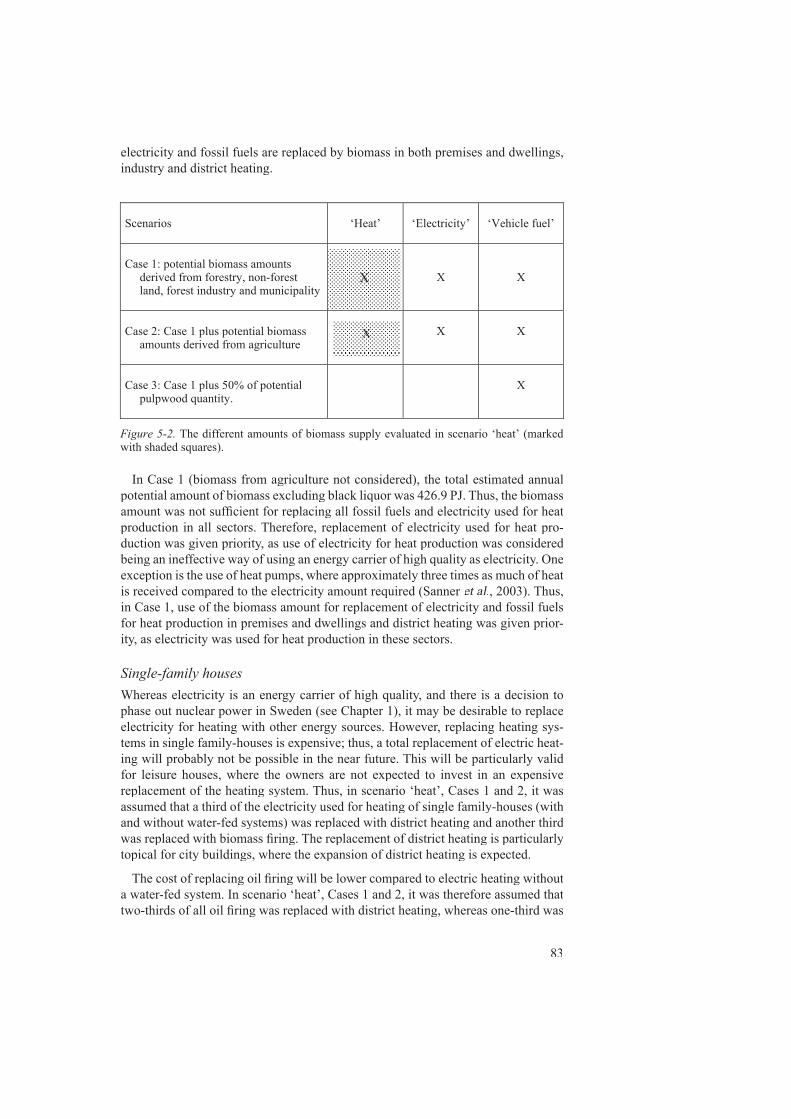
83

electricity and fossil fuels are replaced by biomass in both premises and dwellings, industry and district heating.

In Case 1 (biomass from agriculture not considered), the total estimated annual potential amount of biomass excluding black liquor was 426.9 PJ. Thus, the biomass amount was not suffi cient for replacing all fossil fuels and electricity used for heat production in all sectors. Therefore, replacement of electricity used for heat pro-duction was given priority, as use of electricity for heat production was considered being an ineffective way of using an energy carrier of high quality as electricity. One exception is the use of heat pumps, where approximately three times as much of heat is received compared to the electricity amount required (Sanner et al., 2003). Thus, et al., 2003). Thus, et al.in Case 1, use of the biomass amount for replacement of electricity and fossil fuels for heat production in premises and dwellings and district heating was given prior-ity, as electricity was used for heat production in these sectors.

Single-family housesWhereas electricity is an energy carrier of high quality, and there is a decision to phase out nuclear power in Sweden (see Chapter 1), it may be desirable to replace electricity for heating with other energy sources. However, replacing heating sys-tems in single family-houses is expensive; thus, a total replacement of electric heat-ing will probably not be possible in the near future. This will be particularly valid for leisure houses, where the owners are not expected to invest in an expensive replacement of the heating system. Thus, in scenario ‘heat’, Cases 1 and 2, it was assumed that a third of the electricity used for heating of single family-houses (with and without water-fed systems) was replaced with district heating and another third was replaced with biomass fi ring. The replacement of district heating is particularly topical for city buildings, where the expansion of district heating is expected.

The cost of replacing oil fi ring will be lower compared to electric heating without a water-fed system. In scenario ‘heat’, Cases 1 and 2, it was therefore assumed that two-thirds of all oil fi ring was replaced with district heating, whereas one-third was


Case 1: potential biomass amounts derived from forestry, non-forest land, forest industry and municipality

X

1

X


X

X

X

Case 3: Case 1 plus 50% of potential pulpwood quantity.

X

X

Figure 5-2. The different amounts of biomass supply evaluated in scenario ‘heat’ (marked with shaded squares).

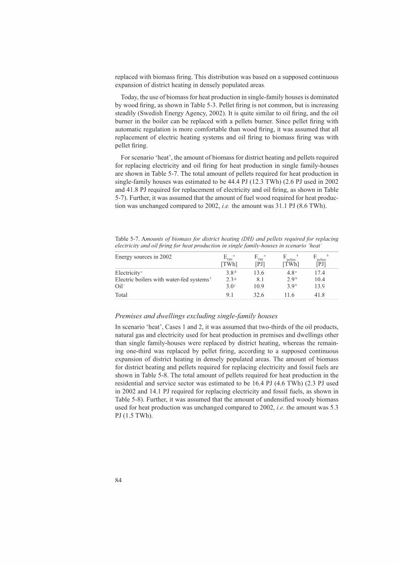
84

replaced with biomass fi ring. This distribution was based on a supposed continuous expansion of district heating in densely populated areas.

Today, the use of biomass for heat production in single-family houses is dominated by wood fi ring, as shown in Table 5-3. Pellet fi ring is not common, but is increasing steadily (Swedish Energy Agency, 2002). It is quite similar to oil fi ring, and the oil burner in the boiler can be replaced with a pellets burner. Since pellet fi ring with automatic regulation is more comfortable than wood fi ring, it was assumed that all replacement of electric heating systems and oil fi ring to biomass fi ring was with pellet fi ring.

For scenario ‘heat’, the amount of biomass for district heating and pellets required for replacing electricity and oil fi ring for heat production in single family-houses are shown in Table 5-7. The total amount of pellets required for heat production in single-family houses was estimated to be 44.4 PJ (12.3 TWh) (2.6 PJ used in 2002 and 41.8 PJ required for replacement of electricity and oil fi ring, as shown in Table 5-7). Further, it was assumed that the amount of fuel wood required for heat produc-tion was unchanged compared to 2002, i.e. the amount was 31.1 PJ (8.6 TWh).

Premises and dwellings excluding single-family housesIn scenario ‘heat’, Cases 1 and 2, it was assumed that two-thirds of the oil products, natural gas and electricity used for heat production in premises and dwellings other than single family-houses were replaced by district heating, whereas the remain-ing one-third was replaced by pellet fi ring, according to a supposed continuous expansion of district heating in densely populated areas. The amount of biomass for district heating and pellets required for replacing electricity and fossil fuels are shown in Table 5-8. The total amount of pellets required for heat production in the residential and service sector was estimated to be 16.4 PJ (4.6 TWh) (2.3 PJ used in 2002 and 14.1 PJ required for replacing electricity and fossil fuels, as shown in Table 5-8). Further, it was assumed that the amount of undensifi ed woody biomass used for heat production was unchanged compared to 2002, i.e. the amount was 5.3 PJ (1.5 TWh).

Table 5-7. Amounts of biomass for district heating (DH) and pellets required for replacing electricity and oil fi ring for heat production in single family-houses in scenario ‘heat’

Energy sources in 2002 EDHa EDH

a Epelletsb Epellets

b

[TWh] [PJ] [TWh] [PJ]

Electricity c 3.8 d 13.6 4.8 d 13.6 4.8 d e 17.4Electric boilers with water-fed systems f 2.3 f 2.3 f g 8.1 2.9 h 10.4Oil i 3.0 j 10.9 3.9 k 13.9k 13.9k

Total 9.1 32.6 11.6 41.8

85

Energy use for heat production in industryAs many industrial processes require fuels with properties similar to fossil fuels (e.g.high heating value and low moisture content) it is diffi cult to replace all fossil fuels with un-dried biomass; however, dried biomass such as pellets or wood powder may be used for heat production in these kind of processes. As mentioned above, the potential amount of biomass in Case 1 (biomass from agriculture not consid-ered) would not suffi ce total replacement of fossil fuels used for heat production in industry, if replacement of electricity and fossil fuels used for heat production in premises and dwellings and for district heating is given priority. However, in Case 2 (biomass from agriculture included), the potential amount of biomass was suffi cient for replacing fossil fuels used for heat production in industry. Thus, in Case 2 it was assumed that two-thirds (in energy units) of the fossil fuels used for heat produc-tion in industry, i.e. 104.0 PJ/year (28.9 TWh/year), were replaced with un-dried biomass, whereas one-third (in energy units) of the fossil fuels was replaced with dried biomass, i.e. 52.0 PJ/year (14.4 TWh/year). Peat and MSW used in industrial sectors other than the pulp and sawmill industry sector were not replaced with other biofuels.

District heatingThe total amount of oil and natural gas (including LPG) used for district heating in 2002 was assumed as being replaced with biomass, referring to the two main rea-sons for a continuous future exchange of fossil fuels with renewable energy sources (discussed in Chapter 1). As oil, natural gas and LPG are mainly used for maximum load, these fuels were replaced with pellets. Coal and blast furnace gas were not replaced with biomass, as blast furnace gas is a by-product of steel plants and a valu-able fuel that may be used e.g. for district heating.e.g. for district heating.e.g.

The use of electric boilers for district heating has decreased markedly since 1990. One reason was the deregulation of the Swedish electricity market in 1996, which led to a faster increase in the price of electricity compared to the consumer price index, especially during recent years (Banks, 2004; Swedish Energy Agency, 2003b, 2004a). Whereas the price of electricity may be expected to increase continuously during the coming years (Hauch, 2003; Lund & Andersen, 2005), the use of electric boilers for district heating are also expected to decrease continuously. Thus, in sce-nario ‘heat’, Cases 1 and 2, it was assumed that all electric boilers used for district heating were replaced with pellet boilers.

The other energy sources, i.e. other biofuels (refuse, tall oil pitch, peat and other

Table 5-8. Amount of district heating (DH) and pellets required for replacement of electricity and fossil fuels for heat production in premises and dwellings other than single family-houses in scenario ‘heat’

Energy sources in 2002 EDHEDHE a EDHEDHE a EpelletsEpelletsE b EpelletsEpelletsE b

[TWh] [PJ] [TWh] [PJ]

Oil c 2.4 d 8.5 1.2 d 8.5 1.2 d e 4.4Natural gas f 0.8 f 0.8 f g 3.0 0.4 h 1.6Electricity i 4.4 j 15.7 2.3 k 8.1k 8.1k

Total 7.6 27.3 3.9 14.1

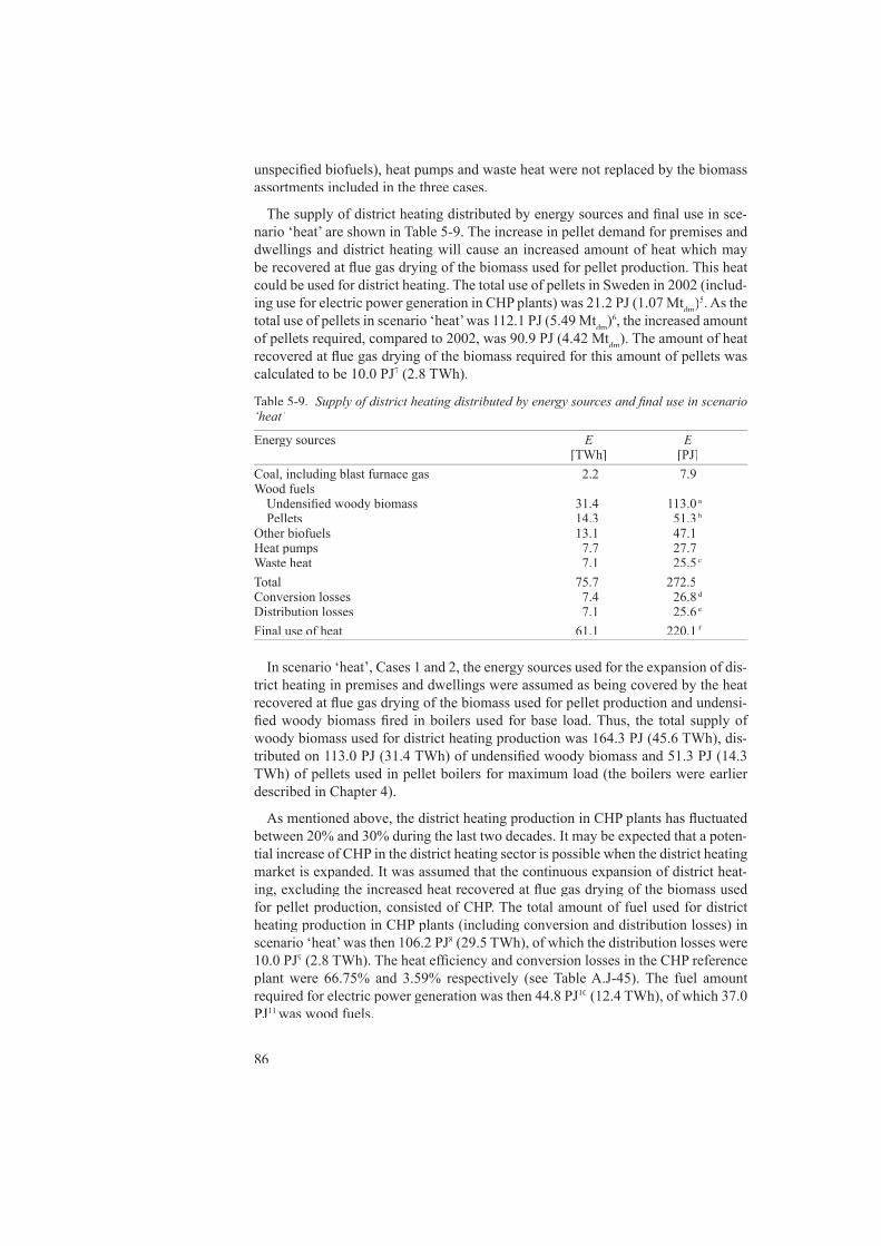
86

Table 5-9. Supply of district heating distributed by energy sources and fi nal use in scenario ‘heat’

Energy sources E E [TWh] [PJ]

Coal, including blast furnace gas 2.2 7.9Wood fuels Undensifi ed woody biomass 31.4 113.0 a Pellets 14.3 51.3 bOther biofuels 13.1 47.1Heat pumps 7.7 27.7Waste heat 7.1 25.5 c

Total 75.7 272.5Conversion losses 7.4 26.8 dDistribution losses 7.1 25.6 e

Final use of heat 61.1 220.1 f

unspecifi ed biofuels), heat pumps and waste heat were not replaced by the biomass assortments included in the three cases.

The supply of district heating distributed by energy sources and fi nal use in sce-nario ‘heat’ are shown in Table 5-9. The increase in pellet demand for premises and dwellings and district heating will cause an increased amount of heat which may be recovered at fl ue gas drying of the biomass used for pellet production. This heat could be used for district heating. The total use of pellets in Sweden in 2002 (includ-ing use for electric power generation in CHP plants) was 21.2 PJ (1.07 Mtdm)5. As the total use of pellets in scenario ‘heat’ was 112.1 PJ (5.49 Mtdm)6, the increased amount of pellets required, compared to 2002, was 90.9 PJ (4.42 Mtdm). The amount of heat recovered at fl ue gas drying of the biomass required for this amount of pellets was calculated to be 10.0 PJ7 (2.8 TWh).

In scenario ‘heat’, Cases 1 and 2, the energy sources used for the expansion of dis-trict heating in premises and dwellings were assumed as being covered by the heat recovered at fl ue gas drying of the biomass used for pellet production and undensi-fi ed woody biomass fi red in boilers used for base load. Thus, the total supply of woody biomass used for district heating production was 164.3 PJ (45.6 TWh), dis-tributed on 113.0 PJ (31.4 TWh) of undensifi ed woody biomass and 51.3 PJ (14.3 TWh) of pellets used in pellet boilers for maximum load (the boilers were earlier described in Chapter 4).

As mentioned above, the district heating production in CHP plants has fl uctuated between 20% and 30% during the last two decades. It may be expected that a poten-tial increase of CHP in the district heating sector is possible when the district heating market is expanded. It was assumed that the continuous expansion of district heat-ing, excluding the increased heat recovered at fl ue gas drying of the biomass used for pellet production, consisted of CHP. The total amount of fuel used for district heating production in CHP plants (including conversion and distribution losses) in scenario ‘heat’ was then 106.2 PJ8 (29.5 TWh), of which the distribution losses were 10.0 PJ9 (2.8 TWh). The heat effi ciency and conversion losses in the CHP reference plant were 66.75% and 3.59% respectively (see Table A.J-45). The fuel amount required for electric power generation was then 44.8 PJ10 (12.4 TWh), of which 37.0 PJ11 was wood fuels.

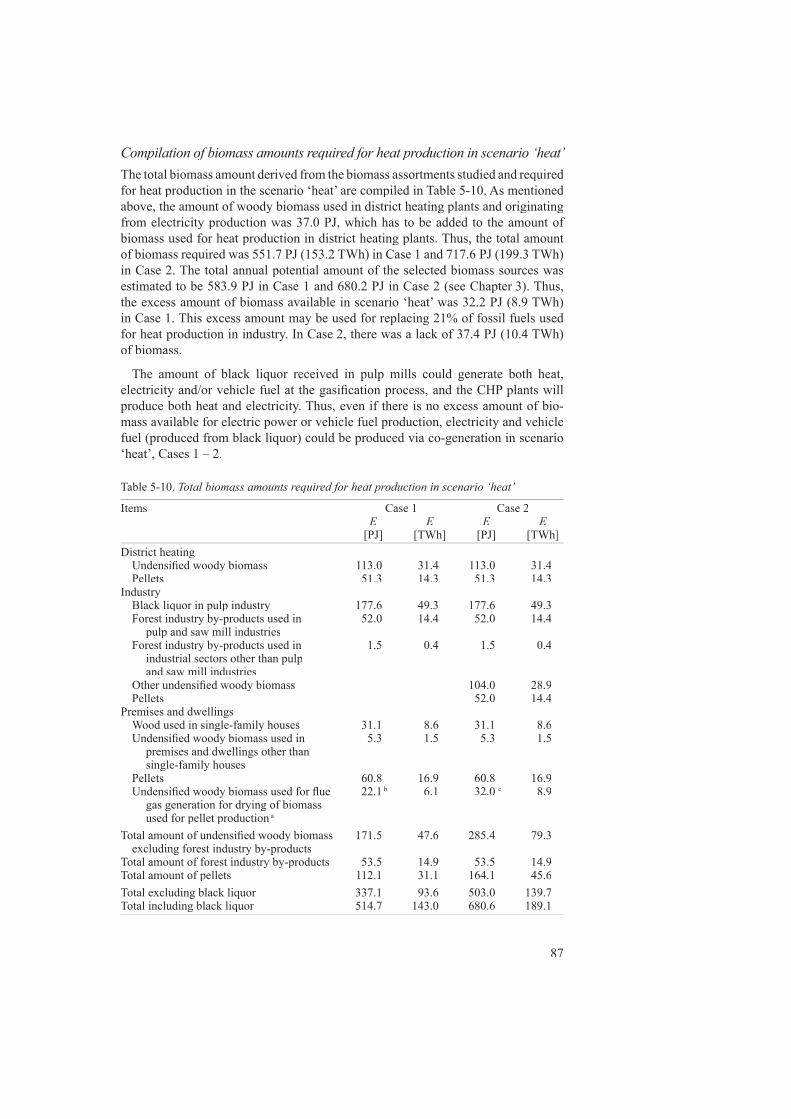
87

Compilation of biomass amounts required for heat production in scenario ‘heat’The total biomass amount derived from the biomass assortments studied and required for heat production in the scenario ‘heat’ are compiled in Table 5-10. As mentioned above, the amount of woody biomass used in district heating plants and originating from electricity production was 37.0 PJ, which has to be added to the amount of biomass used for heat production in district heating plants. Thus, the total amount of biomass required was 551.7 PJ (153.2 TWh) in Case 1 and 717.6 PJ (199.3 TWh) in Case 2. The total annual potential amount of the selected biomass sources was estimated to be 583.9 PJ in Case 1 and 680.2 PJ in Case 2 (see Chapter 3). Thus, the excess amount of biomass available in scenario ‘heat’ was 32.2 PJ (8.9 TWh) in Case 1. This excess amount may be used for replacing 21% of fossil fuels used for heat production in industry. In Case 2, there was a lack of 37.4 PJ (10.4 TWh) of biomass.

The amount of black liquor received in pulp mills could generate both heat, electricity and/or vehicle fuel at the gasifi cation process, and the CHP plants will produce both heat and electricity. Thus, even if there is no excess amount of bio-mass available for electric power or vehicle fuel production, electricity and vehicle fuel (produced from black liquor) could be produced via co-generation in scenario ‘heat’, Cases 1 – 2.

Table 5-10. Total biomass amounts required for heat production in scenario ‘heat’

Items Case 1 Case 2 E E E E [PJ] [TWh] [PJ] [TWh]

District heating Undensifi ed woody biomass 113.0 31.4 113.0 31.4 Pellets 51.3 14.3 51.3 14.3Industry Black liquor in pulp industry 177.6 49.3 177.6 49.3 Forest industry by-products used in 52.0 14.4 52.0 14.4 pulp and saw mill industries Forest industry by-products used in 1.5 0.4 1.5 0.4 industrial sectors other than pulp and saw mill industries Other undensifi ed woody biomass 104.0 28.9 Pellets 52.0 14.4Premises and dwellings Wood used in single-family houses 31.1 8.6 31.1 8.6 Undensifi ed woody biomass used in 5.3 1.5 5.3 1.5 premises and dwellings other than single-family houses Pellets 60.8 16.9 60.8 16.9 Undensifi ed woody biomass used for fl ue 22.1 b 6.1 32.0 c 8.9 gas generation for drying of biomass used for pellet production a

Total amount of undensifi ed woody biomass 171.5 47.6 285.4 79.3 excluding forest industry by-productsTotal amount of forest industry by-products 53.5 14.9 53.5 14.9Total amount of pellets 112.1 31.1 164.1 45.6Total excluding black liquor 337.1 93.6 503.0 139.7Total including black liquor 514.7 143.0 680.6 189.1

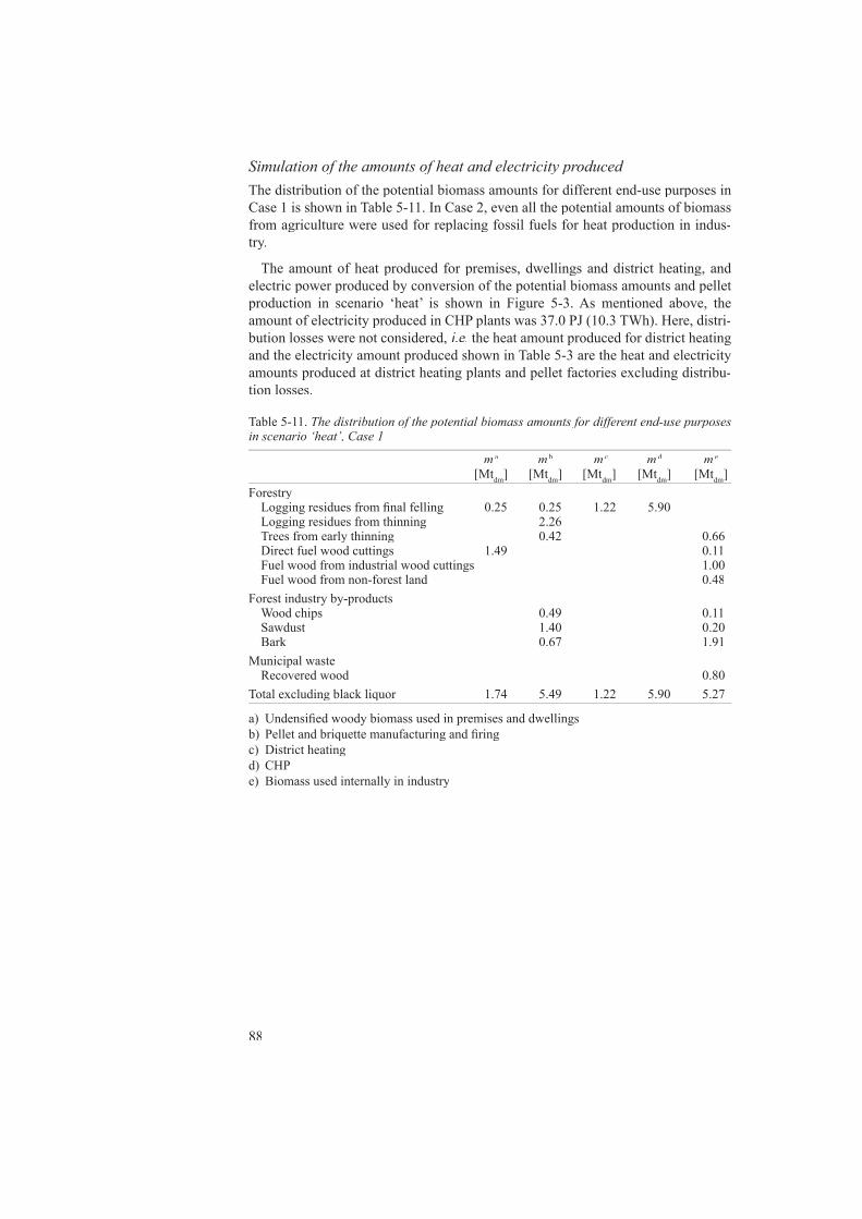
88

Table 5-11. The distribution of the potential biomass amounts for different end-use purposes in scenario ‘heat’, Case 1

m a m b m c m d m e [Mtdm] [Mtdm] [Mtdm] [Mtdm] [Mtdm]

Forestry Logging residues from fi nal felling 0.25 0.25 1.22 5.90 Logging residues from thinning 2.26 Trees from early thinning 0.42 0.66 Direct fuel wood cuttings 1.49 0.11 Fuel wood from industrial wood cuttings 1.00 Fuel wood from non-forest land 0.48Forest industry by-products Wood chips 0.49 0.11 Sawdust 1.40 0.20 Bark 0.67 1.91Municipal waste Recovered wood 0.80Total excluding black liquor 1.74 5.49 1.22 5.90 5.27

a) Undensifi ed woody biomass used in premises and dwellingsb) Pellet and briquette manufacturing and fi ringc) District heatingd) CHPe) Biomass used internally in industry

Simulation of the amounts of heat and electricity producedThe distribution of the potential biomass amounts for different end-use purposes in Case 1 is shown in Table 5-11. In Case 2, even all the potential amounts of biomass from agriculture were used for replacing fossil fuels for heat production in indus-try.

The amount of heat produced for premises, dwellings and district heating, and electric power produced by conversion of the potential biomass amounts and pellet production in scenario ‘heat’ is shown in Figure 5-3. As mentioned above, the amount of electricity produced in CHP plants was 37.0 PJ (10.3 TWh). Here, distri-bution losses were not considered, i.e. the heat amount produced for district heating i.e. the heat amount produced for district heating i.e.and the electricity amount produced shown in Table 5-3 are the heat and electricity amounts produced at district heating plants and pellet factories excluding distribu-tion losses.

89

Scenarios ‘electricity’ and ‘vehicle fuel’The different amounts of biomass supply evaluated in scenarios ‘electricity’ and ‘vehicle fuel’ are marked with shaded squares in Figure 5-4. The total biomass amounts derived from the biomass assortments studied and required for heat produc-tion in scenarios ‘electricity’ and ‘vehicle fuel’ are compiled in Table 5-12. In Cases 1 and 2, these biomass amounts were assumed being equal to the use in 2002. In Case 3, the use of bark for heat production in the pulp industry in scenario ‘vehicle fuel’ was reduced by 50%, and accordingly the amount of pulp wood was reduced by 50%. As mentioned above, the amount of wood fuels used in district heating plants and originating from electric power generation in 2002 was 10.9 PJ, which has to be added to the amount of biomass used for heat production in district heat-ing plants. The total amount of biomass required was then 364.3 PJ (101.2 TWh) in Cases 1 and 2 and 260.3 PJ (72.3 TWh) in Case 3. The total annual potential amount of the selected biomass sources was estimated to be 583.9 PJ in Case 1, 680.2 PJ in Case 2 and 627.3 PJ in Case 3 (see Chapter 3). Thus, the excess amounts of biomass available for production of electricity or vehicle fuels in scenarios ‘electricity’ and ‘vehicle fuel’ were 219.6 PJ (61.0 TWh) in Case 1 and 315.9 PJ (87.8 TWh) in Case 2. The excess amount of biomass available for production of vehicle fuels in sce-nario ‘vehicle fuel’, Case 3, was 367.0 PJ (101.9 TWh).

According to scenario ‘heat’, gasifi cation of black liquor received in pulp mills could generate both heat, electricity and/or vehicle fuel, and the CHP plants will generate both heat and electricity in all Cases studied.

Scenario 'heat'

0

20

40

60

80

100

120

140

160

180

200

220

240

260

280

300

320

Small scale heating District heating Power Vehicle fuel

PJ

Vehicle fuel

Electricity

CHP

District heating

Pellets large

Pellets small

Pellets industry

UndWoBio P&D

Figure 5-3. The amounts of heat produced for premises, dwellings and district heating, and electric power produced by conversion of the potential biomass amounts in scenario ‘heat’. UndWoBio P&D’ in Figures 5-3 and 5-5 – 5-12 means ‘Undensifi ed woody biomass used in premises and dwellings’.

90

Table 5-12. Total biomass amounts required for heat production in the scenarios ‘electricity’ and ‘vehicle fuel’

Items Cases 1 and 2 Case 3 E E E E [PJ] [TWh] [PJ] [TWh]

District heating Undensifi ed woody biomass 61.2 17.0 61.2 17.0 Pellets 15.7 4.4 15.7 4.4Industry Black liquor in pulp industry 177.6 49.3 88.8 24.7 Forest industry by-products used in pulp 52.0 14.4 36.8 a 10.2 and saw mill industries Forest industry by-products used in 1.5 0.4 1.5 0.4 industrial sectors other than pulp and saw mill industriesPremises and dwellings Wood used in single-family houses 31.1 8.6 31.1 8.6 Undensifi ed woody biomass used in 5.3 1.5 5.3 1.5 premises and dwellings other than single-family houses Pellets 4.9 1.4 4.9 1.4Undensifi ed woody biomass used for fl ue gas 4.1 1.1 4.1 1.1 generation for drying of biomass used for pellet productionTotal amount of undensifi ed woody biomass 97.6 27.1 97.6 27.1 excluding forest industry by-productsTotal amount of forest industry by-products 57.6 16.0 42.4 11.7Total amount of pellets 20.6 5.7 20.6 5.7Total excluding black liquor 175.8 48.8 160.6 44.6Total including black liquor 353.4 98.2 249.4 69.3


Case 1: potential biomass amounts derived from forestry, non-forest land, forest industry and community

X

1


X

Case 3: Case 1 plus 50% of potential pulpwood quantity.

X X

X X

X

Figure 5-4. The different amounts of biomass supply evaluated in scenarios ‘electricity’ and ‘vehicle fuel’ (marked with shaded squares).

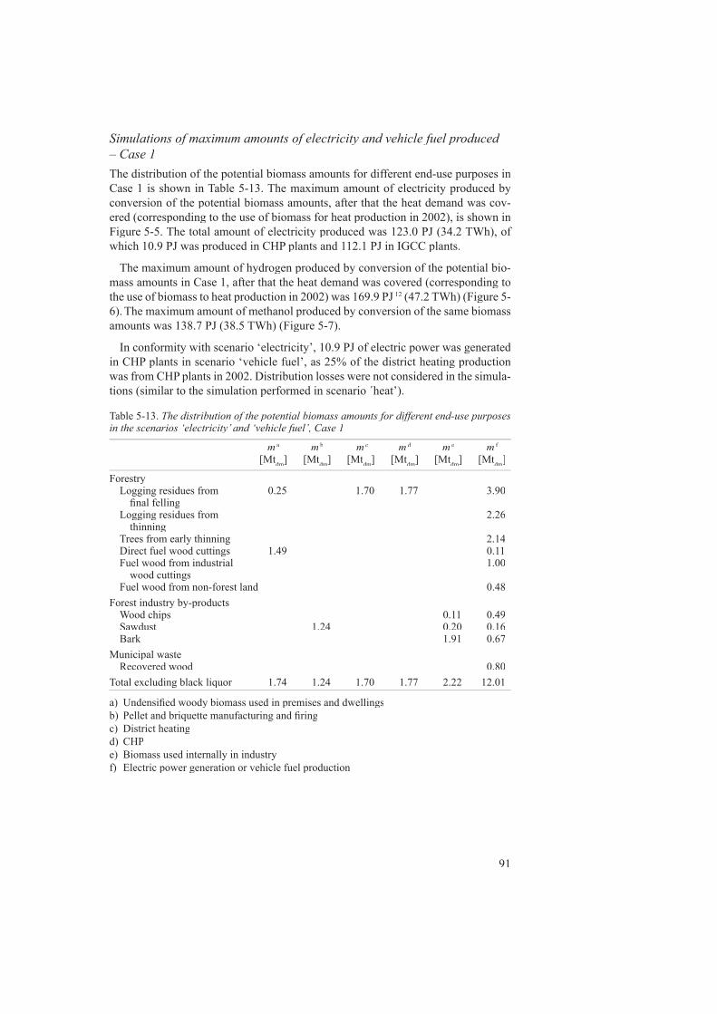
91

Simulations of maximum amounts of electricity and vehicle fuel produced – Case 1The distribution of the potential biomass amounts for different end-use purposes in Case 1 is shown in Table 5-13. The maximum amount of electricity produced by conversion of the potential biomass amounts, after that the heat demand was cov-ered (corresponding to the use of biomass for heat production in 2002), is shown in Figure 5-5. The total amount of electricity produced was 123.0 PJ (34.2 TWh), of which 10.9 PJ was produced in CHP plants and 112.1 PJ in IGCC plants.

The maximum amount of hydrogen produced by conversion of the potential bio-mass amounts in Case 1, after that the heat demand was covered (corresponding to the use of biomass to heat production in 2002) was 169.9 PJ 12 (47.2 TWh) (Figure 5-6). The maximum amount of methanol produced by conversion of the same biomass amounts was 138.7 PJ (38.5 TWh) (Figure 5-7).

In conformity with scenario ‘electricity’, 10.9 PJ of electric power was generated in CHP plants in scenario ‘vehicle fuel’, as 25% of the district heating production was from CHP plants in 2002. Distribution losses were not considered in the simula-tions (similar to the simulation performed in scenario ´heat’).

Table 5-13. The distribution of the potential biomass amounts for different end-use purposes in the scenarios ‘electricity’ and ‘vehicle fuel’, Case 1

m a m b m c m d m e m f [Mtdm] [Mtdm] [Mtdm] [Mtdm] [Mtdm] [Mtdm]

Forestry Logging residues from 0.25 1.70 1.77 3.90 fi nal felling Logging residues from 2.26 thinning Trees from early thinning 2.14 Direct fuel wood cuttings 1.49 0.11 Fuel wood from industrial 1.00 wood cuttings Fuel wood from non-forest land 0.48Forest industry by-products Wood chips 0.11 0.49 Sawdust 1.24 0.20 0.16 Bark 1.91 0.67Municipal waste Recovered wood 0.80Total excluding black liquor 1.74 1.24 1.70 1.77 2.22 12.01

a) Undensifi ed woody biomass used in premises and dwellingsb) Pellet and briquette manufacturing and fi ringc) District heatingd) CHPe) Biomass used internally in industryf) Electric power generation or vehicle fuel production

92

Scenario 'electricity', Case 1

0

20

40

60

80

100

120

140

160

180

200

220

240

260

280

300

320


PJ

Vehicle fuel

Electricity

CHP

District heating

Pellets large

Pellets small

Pellets industry

UndWoBio P&D

Figure 5-5. The amount of heat and electric power produced by conversion of the potential biomass amounts in scenario ‘electricity’, Case 1.

Scenario 'vehicle fuel - hydrogen', Case 1

0

20

40

60

80

100

120

140

160

180

200

220

240

260

280

300

320


PJ

Vehicle fuel

Electricity

CHP

District heating

Pellets large

Pellets small

Pellets industry

UndWoBio P&D

Figure 5-6. The amount of heat, electric power and hydrogen produced by conversion of the potential biomass amounts in scenario ‘vehicle fuel - hydrogen’, Case 1.

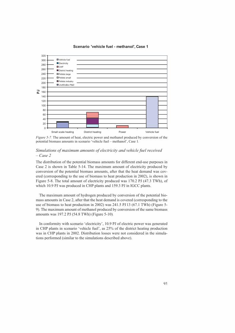
93

Figure 5-7. The amount of heat, electric power and methanol produced by conversion of the potential biomass amounts in scenario ‘vehicle fuel – methanol’, Case 1.

Scenario 'vehicle fuel - methanol', Case 1

0

20

40

60

80

100

120

140

160

180

200

220

240

260

280

300

320


PJ

Vehicle fuel

Electricity

CHP

District heating

Pellets large

Pellets small

Pellets industry

UndWoBio P&D

Simulations of maximum amounts of electricity and vehicle fuel received – Case 2The distribution of the potential biomass amounts for different end-use purposes in Case 2 is shown in Table 5-14. The maximum amount of electricity produced by conversion of the potential biomass amounts, after that the heat demand was cov-ered (corresponding to the use of biomass to heat production in 2002), is shown in Figure 5-8. The total amount of electricity produced was 170.2 PJ (47.3 TWh), of which 10.9 PJ was produced in CHP plants and 159.3 PJ in IGCC plants.

The maximum amount of hydrogen produced by conversion of the potential bio-mass amounts in Case 2, after that the heat demand is covered (corresponding to the use of biomass to heat production in 2002) was 241.5 PJ 13 (67.1 TWh) (Figure 5-9). The maximum amount of methanol produced by conversion of the same biomass amounts was 197.2 PJ (54.8 TWh) (Figure 5-10).

In conformity with scenario ‘electricity’, 10.9 PJ of electric power was generated in CHP plants in scenario ‘vehicle fuel’, as 25% of the district heating production was in CHP plants in 2002. Distribution losses were not considered in the simula-tions performed (similar to the simulations described above).

94

Figure 5-8. The amount of heat and electric power produced by conversion of the potential biomass amounts in scenario ‘electricity’, Case 2.

Table 5-14. The distribution of the potential biomass amounts for different end-use purposes in the scenarios ‘electricity’ and ‘vehicle fuel’, Case 2


Forestry Logging residues from 0.25 1.70 1.77 3.90 fi nal felling Logging residues from 2.26 thinning Trees from early thinning 2.14 Direct fuel wood cuttings 1.49 0.11 Fuel wood from industrial 1.00 wood cuttings Fuel wood from non-forest land 0.48Forest industry by-products Wood chips 0.11 0.49 Sawdust 1.24 0.20 0.16 Bark 1.91 0.67Agriculture Short rotation forest 2.29 Reed canary grass 0.77 Straw 2.00Municipal waste Recovered wood 0.80Total excluding black liquor 1.74 1.24 1.70 1.77 2.22 17.07

a) Undensifi ed woody biomass used in premises and dwellings; b) Pellet and briquette manufacturing and fi ring; c) District heating; d) CHP; e) Biomass used internally in indu-stry; f) Electric power generation or vehicle fuel production

Scenario 'electricity', Case 2

0

20

40

60

80

100

120

140

160

180

200

220

240

260

280

300

320


PJ

Veh fuel

Electricity

H&P

DistrHeat

Pell Large

PellSmall

PellInd

UndWoBio P&D

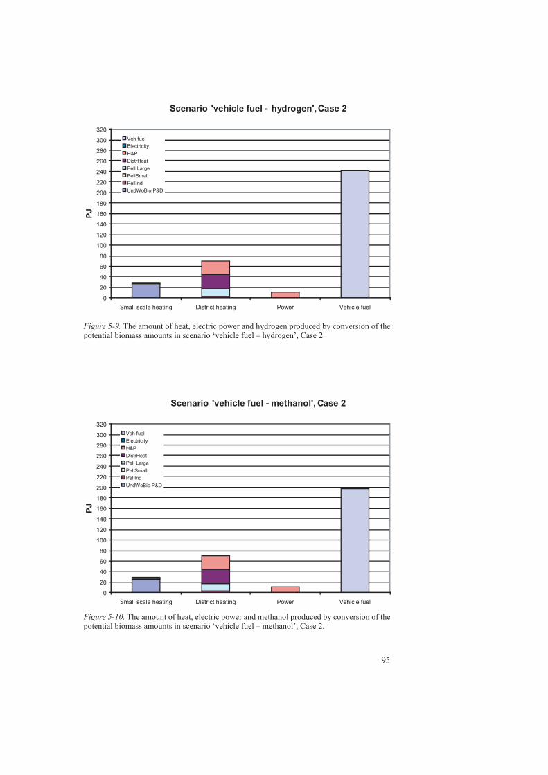
95


Figure 5-9. The amount of heat, electric power and hydrogen produced by conversion of the potential biomass amounts in scenario ‘vehicle fuel – hydrogen’, Case 2.

Scenario 'vehicle fuel - hydrogen',Case 2

0

20

40

60

80

100

120

140

160

180

200

220

240

260

280

300

320


PJ

Veh fuel

Electricity

H&P

DistrHeat

Pell Large

PellSmall

PellInd

UndWoBio P&D


0

20

40

60

80

100

120

140

160

180

200

220

240

260

280

300

320


PJ

Veh fuel

Electricity

H&P

DistrHeat

Pell Large

PellSmall

PellInd

UndWoBio P&D

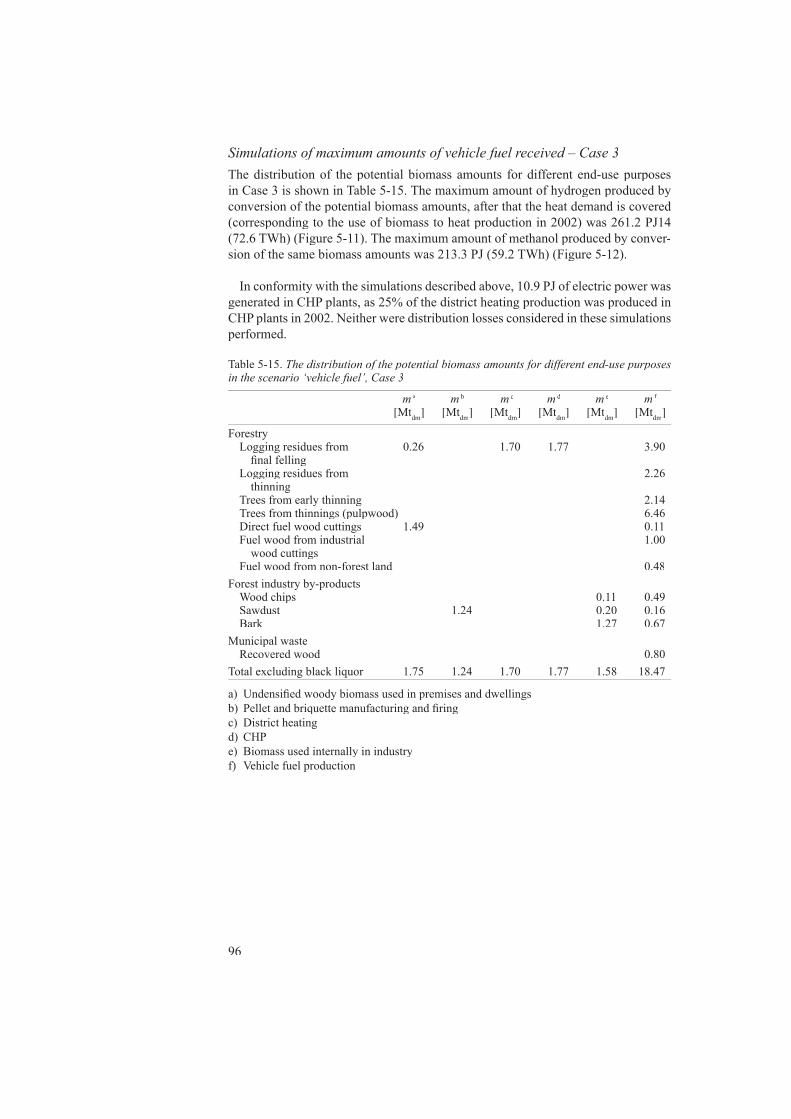
96

Table 5-15. The distribution of the potential biomass amounts for different end-use purposes in the scenario ‘vehicle fuel’, Case 3


Forestry Logging residues from 0.26 1.70 1.77 3.90 fi nal felling Logging residues from 2.26 thinning Trees from early thinning 2.14 Trees from thinnings (pulpwood) 6.46 Direct fuel wood cuttings 1.49 0.11 Fuel wood from industrial 1.00 wood cuttings Fuel wood from non-forest land 0.48Forest industry by-products Wood chips 0.11 0.49 Sawdust 1.24 0.20 0.16 Bark 1.27 0.67Municipal waste Recovered wood 0.80Total excluding black liquor 1.75 1.24 1.70 1.77 1.58 18.47

a) Undensifi ed woody biomass used in premises and dwellingsb) Pellet and briquette manufacturing and fi ringc) District heatingd) CHPe) Biomass used internally in industryf) Vehicle fuel production

Simulations of maximum amounts of vehicle fuel received – Case 3The distribution of the potential biomass amounts for different end-use purposes in Case 3 is shown in Table 5-15. The maximum amount of hydrogen produced by conversion of the potential biomass amounts, after that the heat demand is covered (corresponding to the use of biomass to heat production in 2002) was 261.2 PJ14 (72.6 TWh) (Figure 5-11). The maximum amount of methanol produced by conver-sion of the same biomass amounts was 213.3 PJ (59.2 TWh) (Figure 5-12).

In conformity with the simulations described above, 10.9 PJ of electric power was generated in CHP plants, as 25% of the district heating production was produced in CHP plants in 2002. Neither were distribution losses considered in these simulations performed.

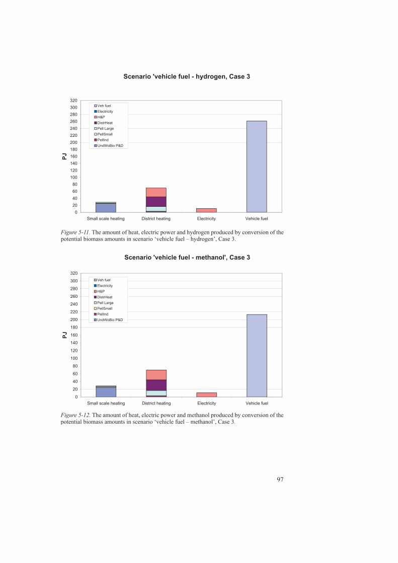
97


Figure 5-11. The amount of heat, electric power and hydrogen produced by conversion of the potential biomass amounts in scenario ‘vehicle fuel – hydrogen’, Case 3.

Scenario 'vehicle fuel - hydrogen, Case 3

020406080

100120140160180200220240260280300320

Small scale heating District heating Electricity Vehicle fuel

PJ

Veh fuelElectricityH&PDistrHeatPell LargePellSmallPellIndUndWoBio P&D


0

20

40

60

80

100

120

140

160

180

200

220

240

260

280

300

320

Small scale heating District heating Electricity Vehicle fuel

PJ

Veh fuelElectricityH&PDistrHeatPell LargePellSmallPellIndUndWoBio P&D

98

The potential of electricity and vehicle fuel production by black liquor gasifi cationBlack liquor is recovered internally in the pulp and paper industry, and the heat and electricity produced in this process is today mainly used internally within this indus-try. However, replacement of conventional recovery boilers with gasifi cation units increases the yield of electricity at recovery of black liquor if a combined cycle is integrated. Alternatively, the product gas received at the gasifi cation process could be used for vehicle fuel production.

The annual excess of electricity and the annual amount of methanol that could be produced from black liquor gasifi cation in Sweden was estimated by means of data regarding the black liquor gasifi cation process developed by Chemrec AB. This process is based on entrained-fl ow gasifi cation of the black liquor at temperatures above the melting point of the inorganic chemicals (Ekbom et al., 2003). The poten-tial excess amounts of electricity and methanol are shown in Table 5-16. As men-tioned in Chapter 3, the estimated potential amount of black liquor is based on the assumption that all pulp produced in Sweden was chemical pulp, leading to that black liquor was received at all pulp manufacturing.

Table 5-16. Potential excess amounts of energy carriers at gasifi cation of black liquor

BLGCC BLGMe

Case 1 and 2a Case 1 and 2a, b Case 3c

Black liquor input [PJ]Additional requirement of biomass [PJ]Excess of main product [PJ]Excess of heat [PJ]

157.0d

39.1f

17.3h

157.0d

59.7e

136.5g

78.529.968.2

The amount of methanol produced implied that 59.7 PJ of biomass has to be added for covering the heat and electricity demand at the pulp mills in Cases 1 and 2, whereas the corresponding amount of biomass in Case 3 was 29.9 PJ (see Table 5-16). This must be considered when summarizing the total yield of methanol from both gasifi cation of black liquor and gasifi cation of the other biomass assortments. Therefore, simulations were performed for calculating the amount of methanol pro-duced by gasifi cation of the other biomass assortments where the total amount of biomass was reduced with 59.7 PJ in Cases 1 and 2, and the corresponding reduc-tion of biomass amount in Case 3 was 29.9 PJ. The distribution of the potential biomass amounts for different end-use purposes in Cases 1-3 are shown in Tables 5-17 through to 5-19.

99

Table 5-17. The distribution of the potential biomass amounts for different end-use purposes in the scenario ‘vehicle fuel’, Case 1, where the total amount of biomass is reduced by 59.7 PJ, corresponding to the amount required additionally for the pulping process

ma

[Mtdm]mb

[Mtdm]mc

[Mtdm] md

[Mtdm] me

[Mtdm] mf

[Mtdm]

ForestryLogging residues from fi nal

fellingLogging residues from

thinningTrees from early thinningDirect fuel wood cuttingsFuel wood from industrial

wood cuttingsFuel wood from non-forest

landForest industry by-productsWood chipsSawdustBark

Municipal waste Recovered wood

Total excluding black liquor

0.25

1.49

1.74

1.24

1.24

1.70

1.70

1.77

1.77

1.59

0.600.362.59

5.14

2.31

2.26

2.14 0.11 1.00

0.48

0.80

9.10


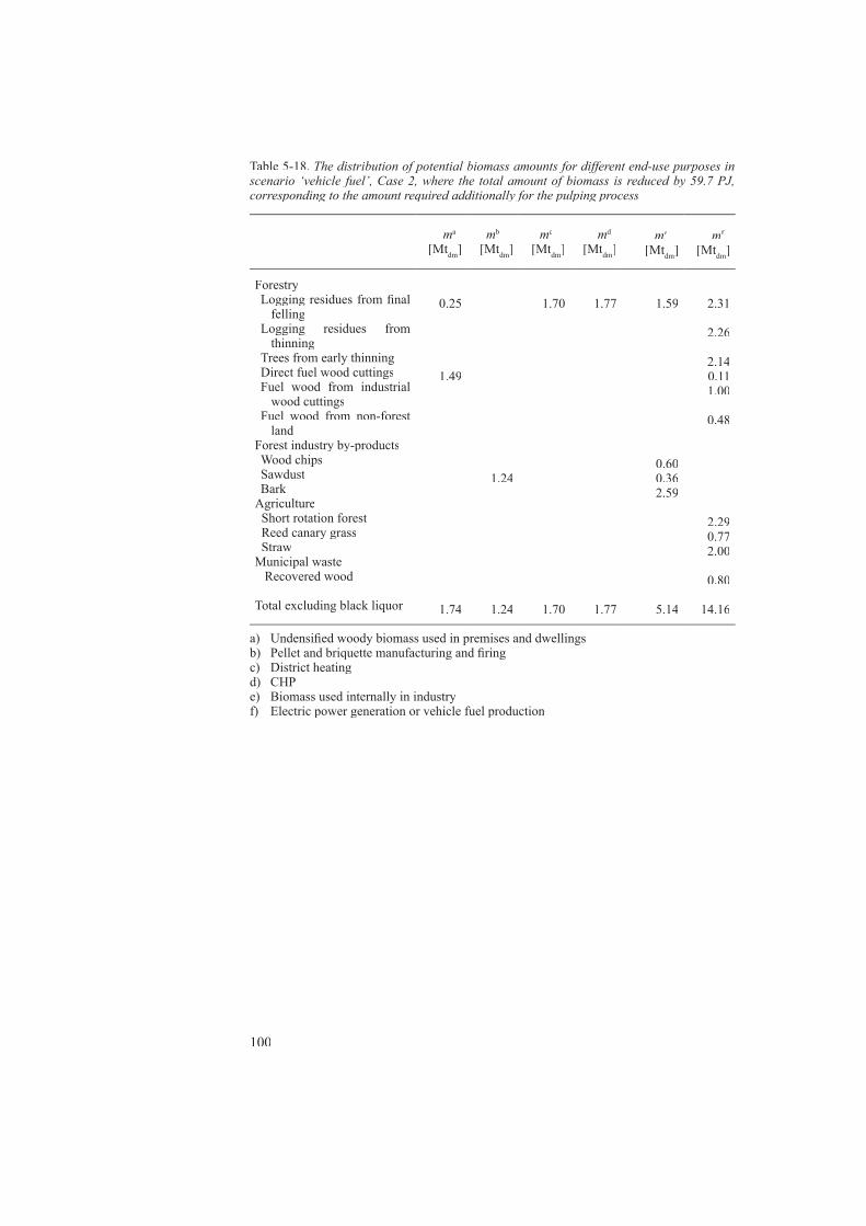
100

Table 5-18. The distribution of potential biomass amounts for different end-use purposes in scenario ‘vehicle fuel’, Case 2, where the total amount of biomass is reduced by 59.7 PJ, corresponding to the amount required additionally for the pulping process

ma

[Mtdm]mb

[Mtdm]mc

[Mtdm] md

[Mtdm] me

[Mtdm] mf

[Mtdm]



thinningTrees from early thinningDirect fuel wood cuttingsFuel wood from industrial



Agriculture Short rotation forest Reed canary grass StrawMunicipal waste Recovered wood


0.25

1.49

1.74

1.24

1.24

1.70

1.70

1.77

1.77

1.59

0.600.362.59

5.14

2.31

2.26

2.14 0.11 1.00

0.48

2.290.772.00

0.80

14.16


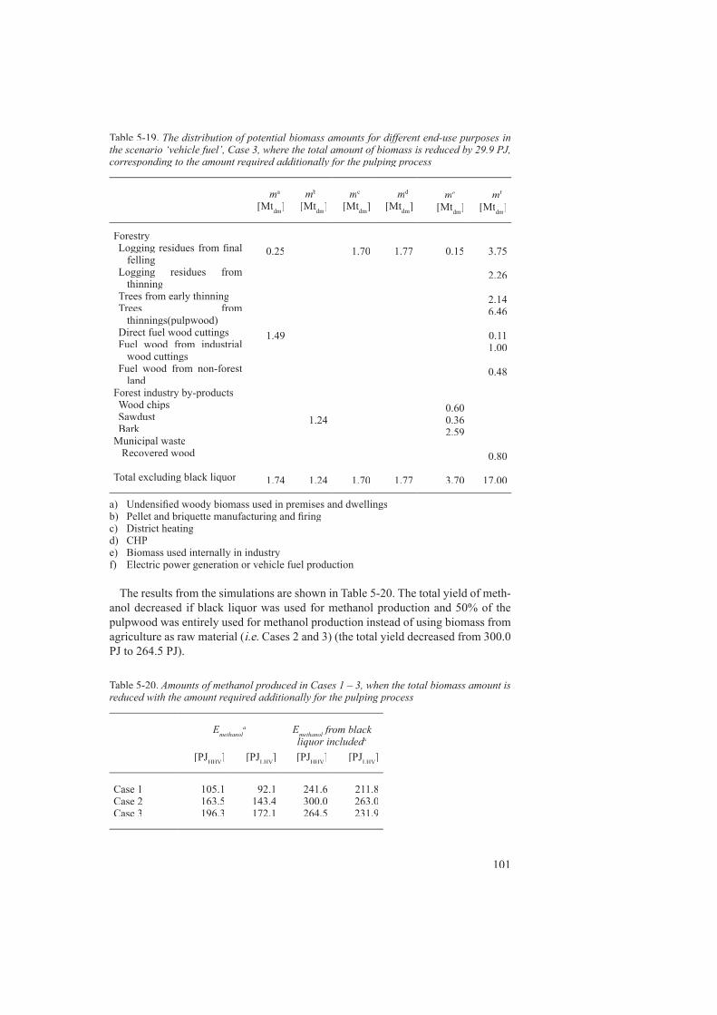
101

Table 5-19. The distribution of potential biomass amounts for different end-use purposes in the scenario ‘vehicle fuel’, Case 3, where the total amount of biomass is reduced by 29.9 PJ, corresponding to the amount required additionally for the pulping process

ma

[Mtdm]mb

[Mtdm]mc

[Mtdm] md

[Mtdm] me

[Mtdm] mf

[Mtdm]



thinningTrees from early thinningTrees from

thinnings(pulpwood)Direct fuel wood cuttingsFuel wood from industrial



Municipal waste Recovered wood


0.25

1.49

1.74

1.24

1.24

1.70

1.70

1.77

1.77

0.15

0.600.362.59

3.70

3.75

2.26

2.146.46

0.11 1.00

0.48

0.80

17.00


The results from the simulations are shown in Table 5-20. The total yield of meth-anol decreased if black liquor was used for methanol production and 50% of the pulpwood was entirely used for methanol production instead of using biomass from agriculture as raw material (i.e. Cases 2 and 3) (the total yield decreased from 300.0 i.e. Cases 2 and 3) (the total yield decreased from 300.0 i.e.PJ to 264.5 PJ).

Table 5-20. Amounts of methanol produced in Cases 1 – 3, when the total biomass amount is reduced with the amount required additionally for the pulping process

EmethanolEmethanolE a

EmethanolEmethanolE from black methanol from black methanolliquor includedaliquor includedaliquor included

[PJHHV] [PJLHV] [PJHHV] [PJLHV]

Case 1Case 2Case 3

105.1163.5196.3

92.1143.4172.1

241.6300.0264.5

211.8263.0231.9

102

Comparison of maximum yields of energy carriers with today’s use

The total use of electricity in Sweden (including distribution losses) was 535.0 PJ in 2002 (Swedish Energy Agency, 2004b). The amount of electricity produced in sce-nario ‘electricity’, Case 1 was 123.0 PJ, and in Case 2 170.2 PJ. Adding the excess amount of electricity produced by black liquor gasifi cation resulted in 162.1 PJ of electricity for Case 1 and 209.3 PJ of electricity and for Case 2. The amounts of elec-tricity produced in Cases 1 and 2 including black liquor gasifi cation corresponded to 30.3% and 39.1% respectively of the total use of electricity in Sweden in 2002. The use of electricity in the Swedish pulp and paper industry in 2002 was approximately 77 PJ (21 TWh) (Swedish Energy Agency, 2003a, 2003b).

In 2002, the total use of petrol was 5.71 million m3 and the total use of diesel oil was 3.91 million m3 (Swedish Energy Agency, 2004b). The energy content of 5.71 million m3 of petrol is 186.1 PJLHV (LHV of petrol is 32.6 MJ/dmLHV (LHV of petrol is 32.6 MJ/dmLHV

3 (Swedish Energy Agency, 2003a)), whereas the energy content of 3.91 million m3 of diesel oil is 140.4 PJLHV (LHV of diesel oil is 35.9 MJ/dmLHV (LHV of diesel oil is 35.9 MJ/dmLHV

3 (Swedish Energy Agency, 2003)). If it is assumed that the mean value of the effi ciency of petrol engines is 14.9% and the corresponding value of diesel engines is 17.6%, based on the LHV (according to Ahlvik & Brandberg (2001)), the mean value of the total vehicle work in petrol and diesel engines in Sweden in 2002 was 27.7 PJ and 24.7 PJ respectively, giving a total amount of annual vehicle work of 52.4 PJ. The effi ciency of hydrogen as fuel in a hybrid fuel cell propulsion system is estimated by Ahlvik & Brandberg (2001) to be 23.5% (based on the LHV), whereas the effi ciency of hydrogen in a conven-tional petrol engine is assumed to be equal to the use of petrol, i.e. 14.9%. Thus, the amount of vehicle work derived from the amount of hydrogen produced in scenario ‘vehicle fuel’, Case 1, will be 21.4 PJ if conventional petrol engines are used or 33.8 PJ if hybrid fuel cell propulsion systems are used in all vehicles.

In Case 2 (biomass from agriculture was also considered), the amount of vehicle work derived from the amount of hydrogen produced was 30.4 PJ if conventional petrol engines were used or 48.0 PJ if hybrid fuel cell propulsion systems were used in all vehicles. The corresponding amounts of vehicle work derived from the amount of hydrogen produced in Case 3 was 32.9 PJ if conventional petrol engines were used or 51.9 PJ if hybrid fuel cell propulsion systems were used in all vehicles. Thus, 99% of the annual total vehicle work in Sweden in 2002 was supplied with hydrogen from the Swedish biomass potential including 50% of the current pulpwood amount but excluding biomass from agriculture, i.e. Case 3 (even if the biomass used for the topical heat demand is taken into account), if new propulsion systems as hybrid fuel cells were used in all vehicles. If the hydrogen was used as substitute for petrol in conventional petrol engines, the hydrogen amount produced by gasifi cation of the biomass supplies in Case 2 would cover the Swedish demand of petrol.

If even black liquor was used for methanol production, the total amount of metha-nol would increase from 138.7 PJ to 241.6 PJ in Case 1; from 197.2 PJ to 300.0 PJ in Case 2 and from 213.3 PJ to 264.5 PJ in Case 3. The additional biomass required for covering the internal heat and electricity demand in the pulp process is then considered. Based on the LHV, the effi ciencies for methanol in conventional petrol engines was 16.2% and 17.6% in diesel engines (Ahlvik & Brandberg, 2001). If

103

these increased amounts of methanol are used as a substitute for petrol in conven-tional petrol engines, they would cover the Swedish demand for petrol, and the excess amount of methanol would be 46.6 PJ in Case 1; 105.0 PJ in Case 2 and 69.5 PJ in Case 3. These amounts of methanol may be used for other purposes, e.g. as a substitute for diesel oil, and any excess amount would replace the same amounts of diesel oil, as the effi ciencies for diesel oil and methanol in diesel engines are estimated to be equal (Ahlvik & Brandberg, 2001). Thus, in Case 1 the amounts of diesel oil replaced correspond to 29.1% of the diesel oil used in Sweden in 2002. In Case 2, the corresponding value for replacing diesel oil used in Sweden in 2002 would be 65.6%, and 43.4% in Case 3. It is evident that the largest amounts of fossil fuels that could be replaced with methanol is in Case 2 (biomass from agriculture taken into account). However, 48.3 PJLHV (13.4 TWhLHV (13.4 TWhLHV LHV) of diesel oil would still be required, even if methanol were produced by gasifi cation of black liquor received in the Swedish pulp mills.

DiscussionIt was concluded in scenario ‘heat’ that the potential amounts of biomass available for energy purposes is not suffi cient for replacing both electricity and fossil fuels used for heating in both premises, dwellings and industry. The lack is greatest in Case 1 (i.e. when biomass from agriculture is excluded). Here, replacement of elec-tricity used for heating is given priority, as use of electricity for heat production is considered being an ineffective way of using a high quality energy carrier as elec-tricity. With the political decision to phase out nuclear power in Sweden, replacing electricity for heating with other sources such as biomass, may be an uncomplicated way of decreasing total electricity demand. However, the use of fossil fuels is also debated, because of the theory that carbon dioxide emissions derived from combus-tion of fossil fuels cause climate changes (International Panel on Climate Change, 2001). The choice of replacing electric power or fossil fuels is therefore not an easy task.

In scenario ‘heat’, Case 2 (biomass from agriculture is also considered), the lack of biomass is only 37.4 PJ (10.4 TWh), if both electricity and fossil fuels used for heating is replaced with biomass (as described above). This lack corresponds to 5.2% of the total requirement of biomass in this scenario and Case.

The estimated amount of black liquor in the scenarios and in 2002 was based on the assumption that all pulp produced in Sweden was chemical pulp, leading to that black liquor was receieved at all pulp manufacturing. In 2002, 26.1% of the pulp produced in Sweden was mechanical pulp, the percentage of half-chemical pulp was 2.9%, the percentage of sulphite pulp was 5.8% and the percentage of sulphate pulp was 65.2% (The Swedish Timber Measurement Council, 2004). If this distribution of different pulp manufacturing processes remains unchanged, the amount of black liquor estimated in the scenarios may be overestimated by roughly 50%. The future development of the pulp market is not further evaluated in this thesis.

The simulations of using black liquor for methanol production show that the total yield of methanol is slightly decreased if 50% of the pulpwood is entirely used for methanol production instead of using biomass from agriculture as raw material (i.e.

104

Cases 2 and 3) (the total yield decreases from 300.0 PJ to 264.5 PJ). However, com-plementary analyses are required for evaluating which case being most favourable if black liquor is used for methanol production, as e.g. cost and/or emergy analyses.

Evaluation of hydrogen production at black liquor gasifi cation was not performed, as reliable data was not found. However, it may be expected that the difference in yields of hydrogen and methanol received by gasifi cation is rather equal at gasifi ca-tion of black liquor and at gasifi cation of solid biomass. Thus, the yield of hydrogen may be somewhat larger than the yield of methanol even at gasifi cation of black liquor.

The result of scenario ‘electricity’, Case 2, is in accordance with the estimation made by Börjesson et al. (1997) concerning the biomass amount required for replac-et al. (1997) concerning the biomass amount required for replac-et al.ing the electric power generated in the Swedish nuclear plants in 1994. As the cur-rent biomass amount used for heat production is considered in scenario ‘electricity’, the amount of electric power generated are smaller compared to the study by Börjes-son et al. (1997)et al. (1997)et al.

The scenario results by Johansson (1996a) concerning the biomass amount required for replacing all petrol and diesel oil with methanol in Sweden in 2015 is roughly in accordance with the result of scenario ‘vehicle fuel - methanol’, Case 3. The difference in the amount of petrol and diesel oil that could be replaced is mainly due to the consideration of biomass amount used for heat production in this latter scenario.

It is diffi cult to compare bioenergy potentials in different countries, as the prereq-uisities may differ in several ways, as e.g. land use pattern, soil fertility and climate. e.g. land use pattern, soil fertility and climate. e.g.Thailand’s area is 51.3 million ha (Sajjakulnukit & Verapong, 2003), to be compared with the area of Sweden, being 45.0 million ha (The Swedish Institute, 2002). How-ever, the forest area and the area of cultivated land in Thailand is 12.8 million ha and 19.9 million ha respectively (Sajjakulnukit & Verapong, 2003); thus, the forest area is quite half of the Swedish forest area, while the area of cultivated land in Thailand is more than seven times the area of cultivated land in Sweden (2.68 million ha in 2002 (The Swedish Board of Agriculture, 2002)). The remaining area in Thailand (18.6 million ha) consists of unclassifi ed lands, grass and idle land. Unclassifi ed lands include e.g. degraded national forest reserves that could be used for forest e.g. degraded national forest reserves that could be used for forest e.g.plantation. It is estimated by Sajjakulnukit & Verapong (2003) that 22.5 million ha of plantations could be used for biomass production in 2010, i.e. roughly the same i.e. roughly the same i.e.area as the forest area in Sweden. The large variation in electric power generation potential estimated by Sajjakulnukit & Verapong (2003) is due to different yields of biomass per ha and different amounts of biomass demand for purposes other than electric power generation. However, the electricity amounts generated in scenario ‘electricity’ is in the range of the electric power generation potential in Thailand in 2010 estimated by Sajjakulnukit & Verapong (2003), as the electricity amounts in scenario ‘electricity’ ranges from 123 to 209 PJ for Cases 1 and 2.

105

6. Energy, cost and emergy analysis The aim of the work presented in this chapter was to evaluate the production of heat, electricity, or vehicle fuel through the production, handling and conversion of biomass received from forestry, non-forest land, forest industry, agricultural land and community (i.e. recovered wood) by energy, cost and emergy analysis. The emergy-based yield and investment ratios, defined by Ulgiati et al. (1995) were used for the emergy analysis, together with calculations of solar emergy and transformity for the production chains based on the biomass assortments studied. Prerequisites and methods Many of the biomass assortments evaluated in this work are nowadays considered as by-products. Logging residues are e.g. received at felling and delimbing of trees, where roundwood is considered as the main product for the production of sawn wood and wood pulp. Normally, the costs of operations connected to a production process are not allocated between the main products and the by-products received, they are all allocated to the main products (Deakin & Maher, 1991).

Allocation of the energy required in a production process between the main products and the by-products received has been an issue within energy analysis since the 1970’s. The International Federation of Institutes for Advanced Study (IFIAS) (1974) discussed several ways of energy allocation. Firstly, all energy requirements are allocated to the output of interest (i.e. the main products). Secondly, all energy requirements are allocated in proportion to financial value or payments. Thirdly, all energy requirements are allocated in proportion to some physical parameter characterising the system, and finally, all energy requirements are allocated in proportion to the marginal energy savings made if the goods or services were not provided. IFIAS recommended that the third method of energy allocation is used whenever possible. The fourth method was not recommended, as it may confuse energy analysis with policy analysis based upon energy analysis.

Recently, international standards for defining, describing, analysing and comparing technical energy systems have been obtainable, namely ISO 13600 – 13602 (International Organization for Standardization, 1997, 1998a, 1998b, 2002). Even in these standards, allocation of the energy required for operations connected to a production process between the main products and the by-products received is an issue. Here, it is recommended that the energy required in the production process be allocated proportionally to the embodied energy amounts in the main products and by-products.

In the future, the interest in renewable energy sources may increase markedly, when the price of energy increases caused by an increased lack of fossil fuels, In such a scenario, the forestry sector and forest industry may consider biomass from forestry and forest industry for energy conversion, e.g. logging residues, sawdust and bark as the main products with economic values equal to roundwood. In this work, all biomass assortments studied were considered as main products, i.e. both the energy required and the costs for all operations were equally allocated on dry

106

matter weight basis between the traditional main products (e.g. roundwood and grain) and the biomass assortments analysed. However, an economic allocation (i.e. allocation due to differences in prices between the main product and by-products) was performed as a sensitivity analysis for straw, for evaluating the differences in costs received at allocation on dry matter weight basis and at economic allocation.

The annual flow of all items in physical, economic and emergy terms were calculated per metric ton of dry matter (tdm). The annual flows of the items for production and handling of biomass from forestry were based on the area of productive forest land used in AVB 92, namely 21.84 million ha (see Chapter 2). The annual flows of the items for production and use of willow; reed canary grass; and straw are based on one hectare of arable land.

Dry matter losses may be significant in some operations for most of the biomass assortments studied, e.g. storage. The estimated dry matter losses used in the analyses are compiled in Appendix G.

The input data of the analyses were based on literature references and personal communication: the choices of input data used are noted in the footnotes to Tables A.I-1 through to A.I-17 and all primary data regarding silviculture, agriculture and machinery equipment are found in Appendix J. The input data for the conversion systems, e.g. energy yields, wear of equipment, capital costs and operating and maintenance (O & M) costs, were based on the reference plants described in Chapter 4: these data are compiled in Tables A.J-42 through to A.J-48. The emergy flows required for the conversion processes were calculated in the same manner as the calculations of the emergy flows required in the previous handling steps, i.e. the emergy flows derived from the internal energy use, wear of equipment, capital costs and costs for human services (O & M costs) were calculated for each conversion process and biomass assortment.

The analyses were performed in spreadsheets and higher heating values of the biomass assortments were used in all calculations. The methods used were described in Chapter 2 and specific details regarding the methods valid for the performed analyses are described below. Energy analysis Level 1 in Figure 2-6 for energy analysis was defined as the conversion processes studied, and level 2 was defined as production and handling of the pre-treated biomass fractions. As the contribution of indirect energy from the production of equipment and other goods and services used in agriculture could not be ignored (see Chapter 2), these items were also considered in both agricultural and forestry operations: the evaluation of embodied energy in machinery is described in Appendix H. Capital energy, i.e. energy required for fixed installations of machinery and buildings, were excluded in the analysis, as this energy contribution to overall energy requirements was small (see Chapter 2).

107

Cost analysis The interest rate used for the calculation of investment costs is dependant on the shares of capital and loan used for the investment, plus, the yield requirement of the capital and the lending rate influence the interest rate (Olsson et al., 1998). Thus, the interest rate used for the calculation of investment costs varies for different situations. In general, the annual interest rate used for the calculation of investment costs for machinery in Sweden is 7% (Swedish University of Agricultural Sciences, 8-Sep-2004 (URL)), whereas, the annual interest rate for calculating investment costs for energy plants in Sweden in general is 5 – 6% (Bärring et al., 2003). Segelod (1989) states that different interest rates lead to different valuations of expected generated capital from the investments. Thus, the annual interest rate used for all equipments was chosen to be 6.0% in this work.

All monetary costs were calculated by means of the Swedish consumer price index and to the level of cost in Sweden in June 2002. Emergy analysis

Transformities (i.e. solar emergy units per unit actual energy, mass or money) for various processes were inter alia taken from Odum (1996) and Doherty, Nilsson & Odum (2002). Transformities for machinery used in forestry and agriculture were estimated by means of the calculated specific embodied energy amounts in machinery (see Appendix H).

The emergy per monetary currency ratio (sej/SEK) for 2002 was calculated by Hagström & Nilsson (2004) and this ratio was used for quantifying human work in emergy terms for that year. The calculation of the Swedish emergy per monetary currency ratio for 2002 is described in Appendix F. Results The main results of the energy, cost and emergy analyses of production and handling of the different biomass assortments received from forestry, forest industry, agriculture and community used for conversion to heat, electricity or vehicle fuel are compiled in Tables 6-1 through to 6-3. All analytical results are shown in Tables A.I-1 through to A.I-17. It is here obvious that the energy and cost analyses are partial compared to the emergy analysis, which considers both energy flows from the environment and society. The energy analysis yields the primary energy required for the different handling steps, the ratio of the final product received to the primary energy input and the ratio of the energy output to the primary energy input. The cost analysis yields the cost for the different handling steps and the cost of the final product received. The emergy analysis yields the emergy flow within the whole system (sej/tdm), the transformity as a value of the hierarchical position (calculated as the solar emergy flow required to produce the received amount of product), the emergy yield ratio (EYR) and the emergy investment ratio (EIR). As mentioned in Chapter 2, the EYR yields information as to whether the process studied may generate a net contribution of emergy to the economy, whereas the EIR yields information whether the process is a good user of the emergy that is invested, in comparison with alternatives.

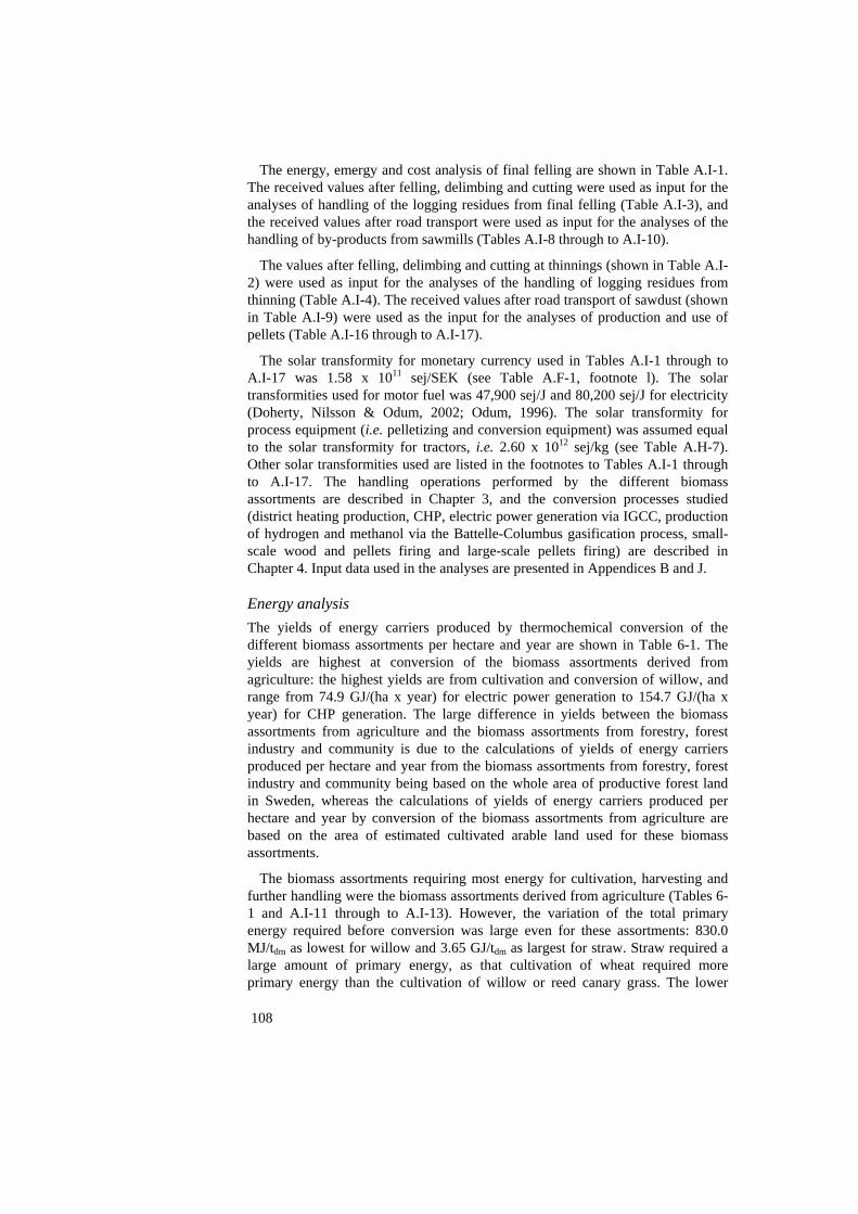
108

The energy, emergy and cost analysis of final felling are shown in Table A.I-1. The received values after felling, delimbing and cutting were used as input for the analyses of handling of the logging residues from final felling (Table A.I-3), and the received values after road transport were used as input for the analyses of the handling of by-products from sawmills (Tables A.I-8 through to A.I-10).

The values after felling, delimbing and cutting at thinnings (shown in Table A.I-2) were used as input for the analyses of the handling of logging residues from thinning (Table A.I-4). The received values after road transport of sawdust (shown in Table A.I-9) were used as the input for the analyses of production and use of pellets (Table A.I-16 through to A.I-17).

The solar transformity for monetary currency used in Tables A.I-1 through to A.I-17 was 1.58 x 1011 sej/SEK (see Table A.F-1, footnote l). The solar transformities used for motor fuel was 47,900 sej/J and 80,200 sej/J for electricity (Doherty, Nilsson & Odum, 2002; Odum, 1996). The solar transformity for process equipment (i.e. pelletizing and conversion equipment) was assumed equal to the solar transformity for tractors, i.e. 2.60 x 1012 sej/kg (see Table A.H-7). Other solar transformities used are listed in the footnotes to Tables A.I-1 through to A.I-17. The handling operations performed by the different biomass assortments are described in Chapter 3, and the conversion processes studied (district heating production, CHP, electric power generation via IGCC, production of hydrogen and methanol via the Battelle-Columbus gasification process, small-scale wood and pellets firing and large-scale pellets firing) are described in Chapter 4. Input data used in the analyses are presented in Appendices B and J. Energy analysis The yields of energy carriers produced by thermochemical conversion of the different biomass assortments per hectare and year are shown in Table 6-1. The yields are highest at conversion of the biomass assortments derived from agriculture: the highest yields are from cultivation and conversion of willow, and range from 74.9 GJ/(ha x year) for electric power generation to 154.7 GJ/(ha x year) for CHP generation. The large difference in yields between the biomass assortments from agriculture and the biomass assortments from forestry, forest industry and community is due to the calculations of yields of energy carriers produced per hectare and year from the biomass assortments from forestry, forest industry and community being based on the whole area of productive forest land in Sweden, whereas the calculations of yields of energy carriers produced per hectare and year by conversion of the biomass assortments from agriculture are based on the area of estimated cultivated arable land used for these biomass assortments.

The biomass assortments requiring most energy for cultivation, harvesting and further handling were the biomass assortments derived from agriculture (Tables 6-1 and A.I-11 through to A.I-13). However, the variation of the total primary energy required before conversion was large even for these assortments: 830.0 MJ/tdm as lowest for willow and 3.65 GJ/tdm as largest for straw. Straw required a large amount of primary energy, as that cultivation of wheat required more primary energy than the cultivation of willow or reed canary grass. The lower

109

yield of straw also led to larger amounts of specific primary energy input for straw handling, compared to the handling of harvested willow and reed canary grass. The dominating item of embodied, primary energy in expendables used in the cultivation of agricultural biomass was the embodied energy in fertilizers, which contributed to 85% of the total embodied, primary energy in expendables for willow cultivation, 93% for reed canary grass cultivation and 59% for cultivation of wheat. Cultivation of wheat required an energy input of 2.23 GJ/tdm of embodied energy and 511 MJ/tdm of diesel oil (Table A.I-13); willow cultivation required 457.7 MJ/tdm of embodied energy and 67.6 MJ/tdm of diesel oil; and reed canary grass cultivation required an 456.0 MJ/tdm of embodied energy and 84.4 MJ/tdm of diesel oil (Tables A.I-11 through to A.I-12).

Another operation requiring much energy for handling the different biomass assortments was road transport. Straw required the largest amount of diesel oil, 229.8 MJ/tdm; other operations requiring much energy were baling (111.4 MJ/tdm of diesel oil) and forwarding of logging residues from thinning (110.9 MJ/tdm of diesel oil) (see Table A.I-4). The difference in energy required for baling and forwarding of logging residues from thinning, compared to baling and forwarding of logging residues from final felling, was due to the lower concentration of logging residues from thinning. The forwarding of trees from early thinning and fuel wood from industrial wood cuttings required 96.3 MJ/tdm of diesel oil, logging of fuel wood from industrial wood cuttings and at thinning required 63.2 MJ/tdm of diesel oil and comminution of reed canary grass and straw required 105.9 MJ/tdm of electricity.

The sum of embodied, primary energy was small compared to the sum of direct primary energy required for all biomass assortments, excluding biomass from agriculture. The sum of embodied, primary energy for these assortments (from forestry, non-forest land, forest industry and community) ranged from 2.7 to 36.7 MJ/tdm compared to the sum of direct primary energy required, which ranged from 111.0 to 900.1 MJ/tdm before conversion. The total primary energy required for these assortments before conversion ranged from 137.6 to 931.8 MJ/tdm, where the smallest amount was required for fuel wood from direct fuel wood cuttings and the largest amount was required for bark.

The primary energy required on conversion (excluding the energy content of the biomass used) ranged from 251.1 to 1602.7 MJ/tdm, where the lowest primary energy amount was required for district heating production and the highest primary energy amount was required for hydrogen production. Hydrogen, methanol and electric power generation required more primary energy (excluding the energy content of the biomass used) at conversion than the total amount of primary energy required for all handling operations before conversion (Tables 6-1 and A.I-2 through to A.I-14). This is due to the conversion process being more complicated than commercial combustion processes. Compressors are e.g. required for syngas processing on hydrogen and methanol production, and for pressurization of the inlet air for gasification of the fuel in the reference IGCC process for electric power generation.

The conversion of the biomass assortments in the CHP plant was the most energy-efficient of the different conversion processes studied (Tables 6-1 and A.I-

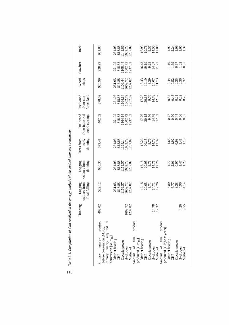
Tabl

e 6-

1. C

ompi

latio

n of

dat

a re

ceiv

ed a

t the

ene

rgy

anal

ysis

of t

he st

udie

d bi

omas

s ass

ortm

ents

Thin

ning

Logg

ing

resi

dues

from

fin

al fe

lling

Logg

ing

resi

dues

from

th

inni

ng

Tree

s fro

m

early

th

inni

ng

Fuel

woo

d fr

om in

dust

rial

woo

d cu

tting

s

Fuel

woo

d fr

om n

on-

fore

st la

nd

Woo

d ch

ips

Saw

dust

Bar

k

Prim

ary

ener

gy

requ

ired

befo

re c

onve

rsio

n [M

J/t dm

] Pr

imar

y en

ergy

re

quire

d at

co

nver

sion

[MJ/

t dm]

Dis

trict

hea

ting

CH

P El

ectri

c po

wer

H

ydro

gen

Met

hano

l A

mou

nt

of

final

pr

oduc

t pr

oduc

ed [G

J/t dm

] D

istri

ct h

eatin

g C

HP

Elec

tric

pow

er

Hyd

roge

n M

etha

nol

Am

ount

of

fin

al

prod

uct

prod

uced

[GJ/

(ha

x ye

ar)]

D

istri

ct h

eatin

g C

HP

Elec

tric

pow

er

Hyd

roge

n M

etha

nol

40

2.02

1602

.72

1237

.82

14.7

812

.32

4.26

3.55

52

2.12

251.

0581

8.88

1158

.57

1602

.72

1237

.82

17.1

820

.05

9.71

14.7

112

.26

5.80

6.77

3.28

4.96

4.14

63

0.35

251.

0581

8.88

1158

.57

1602

.72

1237

.82

17.1

820

.05

9.71

14.7

112

.26

1.72

2.01

0.97

1.47

1.23

37

9.41

25

1.05

81

8.88

11

64.1

4 16

02.7

2 12

37.8

2 17

.26

20.1

5 9.

76

14.7

8 12

.32

1.65

1.

92

0.93

1.

41

1.18

40

2.02

251.

0581

8.88

1164

.14

1602

.72

1237

.82

17.2

620

.15

9.76

14.7

812

.32

0.77

0.90

0.44

0.66

0.55

27

8.62

251.

0581

8.88

1164

.14

1602

.72

1237

.82

17.2

620

.15

9.76

14.7

812

.32

0.37

0.43

0.21

0.32

0.26

92

8.99

251.

0581

8.88

1108

.44

1602

.72

1237

.82

16.4

319

.19

9.29

14.0

711

.73

0.44

0.52

0.25

0.38

0.32

92

8.99

251.

0581

8.88

1108

.44

1602

.72

1237

.82

16.4

319

.19

9.29

14.0

711

.73

1.19

1.39

0.67

1.02

0.85

93

1.83

251.

0581

8.88

1141

.86

1602

.72

1237

.82

16.9

319

.76

9.57

14.5

012

.08

1.92

2.24

1.09

1.65

1.37

110

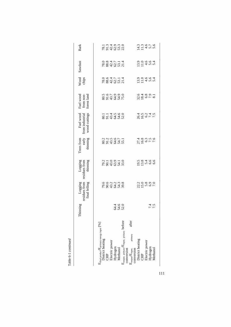
Tabl

e 6-

1 co

ntin

ued

Thin

ning

Logg

ing

resi

dues

from

fin

al fe

lling

Logg

ing

resi

dues

from

th

inni

ng

Tree

s fro

m

early

th

inni

ng

Fuel

woo

d fr

om in

dust

rial

woo

d cu

tting

s

Fuel

woo

d fr

om n

on-

fore

st la

nd

Woo

d ch

ips

Saw

dust

Bar

k

E fin

al p

rodu

ct/E

prim

ary

ener

gy in

put [

%]

Dis

trict

hea

ting

CH

P El

ectri

c po

wer

H

ydro

gen

Met

hano

l E o

utpu

t, pr

imar

y/Ein

put,

prim

ary

befo

re

conv

ersi

on

E out

put/E

inpu

t, pr

imar

y af

ter

conv

ersi

on

Dis

trict

hea

ting

CH

P El

ectri

c po

wer

H

ydro

gen

Met

hano

l

64.4

54.6

52.0 7.4

7.5

79.6

90.6

43.2

64.2

54.3

39.8

22.2

15.0 5.8

6.9

7.0

79.2

90.1

43.0

63.9

54.1

33.0

19.5

13.8 5.4

6.6

6.6

80.2

91.2

43.5

64.6

54.7

55.1

27.4

16.8 6.3

7.5

7.6

80.1

91.1

43.4

64.5

54.6

52.0

26.4

16.5 6.2

7.4

7.5

80.5

91.6

43.7

64.9

54.9

75.0

32.6

18.4 6.8

7.9

8.1

78.0

88.6

42.4

62.7

53.1

21.4

13.9

11.0 4.6

5.6

5.4

78.0

88.8

42.4

62.7

53.1

21.4

13.9

11.0 4.6

5.6

5.4

78.1

91.3

42.4

62.9

53.3

22.0

14.3

11.3 4.6

5.7

5.6

111

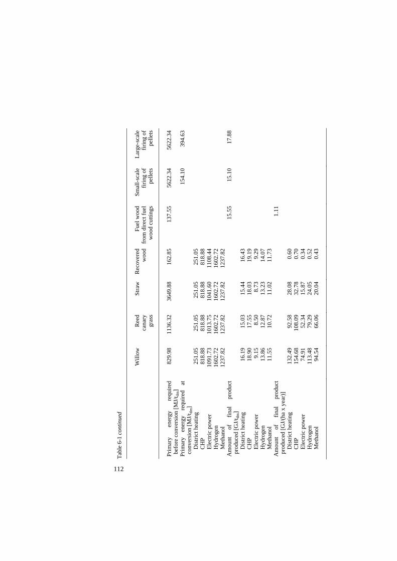
Tabl

e 6-

1 co

ntin

ued

Will

owR

eed

cana

ry

gras

s

Stra

w

Rec

over

ed

woo

d Fu

el w

ood

from

dire

ct fu

el

woo

d cu

tting

s

Smal

l-sca

le

firin

g of

pe

llets

Larg

e-sc

ale

firin

g of

pe

llets

Prim

ary

ener

gy

requ

ired

befo

re c

onve

rsio

n [M

J/t dm

] Pr

imar

y en

ergy

re

quire

d at

co

nver

sion

[MJ/

t dm]

Dis

trict

hea

ting

CH

P El

ectri

c po

wer

H

ydro

gen

Met

hano

l A

mou

nt

of

final

pr

oduc

t pr

oduc

ed [G

J/t dm

] D

istri

ct h

eatin

g C

HP

Elec

tric

pow

er

Hyd

roge

n M

etha

nol

Am

ount

of

fin

al

prod

uct

prod

uced

[GJ/

(ha

x ye

ar)]

D

istri

ct h

eatin

g C

HP

Elec

tric

pow

er

Hyd

roge

n M

etha

nol

82

9.98

251.

0581

8.88

1091

.73

1602

.72

1237

.82

16.1

918

.90

9.15

13.8

611

.55

132.

4915

4.68

74.9

111

3.48

94.5

4

11

36.3

2

251.

0581

8.88

1013

.75

1602

.72

1237

.82

15.0

317

.55

8.50

12.8

710

.72

92

.58

108.

0952

.34

79.2

966

.06

36

49.8

8

251.

0581

8.88

1041

.60

1602

.72

1237

.82

15.4

418

.03

8.73

13.2

311

.02

28

.08

32.7

815

.87

24.0

520

.04

16

2.85

25

1.05

81

8.88

11

08.4

4 16

02.7

2 12

37.8

2 16

.43

19.1

9 9.

29

14.0

7 11

.73

0.

60

0.70

0.

34

0.52

0.

43

13

7.55

15.5

5

1.

11

56

22.3

4

154.

10

15.1

0

56

22.3

4

394.

63

17.8

8

112

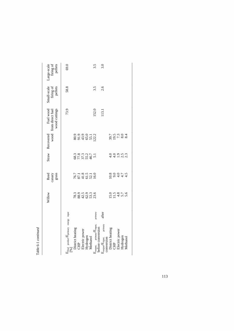
Tabl

e 6-

1 co

ntin

ued

Will

owR

eed

cana

ry

gras

s

Stra

wR

ecov

ered

w

ood

Fu

el w

ood

from

dire

ct fu

el

woo

d cu

tting

s

Smal

l-sca

le

firin

g of

pe

llets

Larg

e-sc

ale

firin

g of

pe

llets

E fin

al

prod

uct/E

prim

ary

ener

gy

inpu

t [%

] Dis

trict

hea

ting

CH

P El

ectri

c po

wer

H

ydro

gen

Met

hano

l E o

utpu

t, pr

imar

y/Ein

put,

prim

ary

befo

re c

onve

rsio

n E o

utpu

t/Ein

put,

prim

ary

afte

r co

nver

sion

D

istri

ct h

eatin

g C

HP

Elec

tric

pow

er

Hyd

roge

n M

etha

nol

78.3

88.9

42.5

62.9

53.3

23.6

15

.011

.5 4.8

5.7

5.6

76.7

87.1

41.8

61.5

52.1

16.0

10

.8 9.0

4.0

4.7

4.5

68.3

77.8

37.3

55.2

46.7 5.1

4.0

4.0

1.9

2.5

2.3

80.9

91.9

43.9

65.0

55.1

122.

2

39

.719

.5 7.3

8.0

8.4

73

.9

152.

0 11

3.1

58.8 3.5

2.6

69.0 3.5

3.0

113

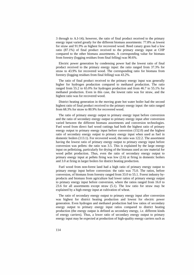
3 through to A.I-14); however, the ratio of final product received to the primary energy input varied greatly for the different biomass assortments: 77.8% as lowest for straw and 91.9% as highest for recovered wood. Reed canary grass had a low ratio (87.1%) of final product received to the primary energy input at CHP compared to the other biomass assortments. A corresponding value for biomass from forestry (logging residues from final felling) was 90.6%.

Electric power generation by condensing power had the lowest ratio of final product received to the primary energy input: the ratio ranged from 37.3% for straw to 43.9% for recovered wood. The corresponding ratio for biomass from forestry (logging residues from final felling) was 43.2%.

The ratio of final product received to the primary energy input was generally higher for hydrogen production compared to methanol production. The ratio ranged from 55.2 to 65.0% for hydrogen production and from 46.7 to 55.1% for methanol production. Even in this case, the lowest ratio was for straw, and the highest ratio was for recovered wood.

District heating generation in the moving grate hot water boiler had the second highest ratio of final product received to the primary energy input: the ratio ranged from 68.3% for straw to 80.9% for recovered wood.

The ratio of primary energy output to primary energy input before conversion and the ratio of secondary energy output to primary energy input after conversion varied between the different biomass assortments and conversion technologies. Fuel wood from direct fuel wood cuttings had both the highest ratio of primary energy output to primary energy input before conversion (152.0) and the highest ratio of secondary energy output to primary energy input when used as fuel in domestic boilers (113.1). For recovered wood, the ratio was 122.2. The assortment having the lowest ratio of primary energy output to primary energy input before conversion was pellets: the ratio was 3.5. This is explained by the large energy input on pelletizing, particularly for drying of the biomass used as raw material for wood pellet production. Thus, even the ratio of secondary energy output to primary energy input at pellets firing was low (2.6) at firing in domestic boilers and 3.0 at firing in larger boilers for district heating production.

Fuel wood from non-forest land had a high ratio of primary energy output to primary energy input before conversion: the ratio was 75.0. The ratios, before conversion, of biomass from forestry ranged from 33.0 to 55.1. Forest industry by-products and biomass from agriculture had lower ratios of primary energy output to primary energy input before conversion, where the ratios ranged from 16.0 to 23.6 for all assortments except straw (5.1). The low ratio for straw may be explained by a high energy input at cultivation of wheat.

The ratio of secondary energy output to primary energy input after conversion was highest for district heating production and lowest for electric power generation. Even hydrogen and methanol production had low ratios of secondary energy output to primary energy input ratios compared to district heating production (the energy output is defined as secondary energy, i.e. different kinds of energy carriers). Thus, a lower ratio of secondary energy output to primary energy input may be expected at production of high-quality energy carriers such as

114

115

electric power and vehicle fuel compared to heat, which is an energy carrier of lower quality. Cost analysis The costs for handling biomass received from forestry and non-forest land are shown in Tables A.I-1 through to A.I-7 and Table A.I-15. The main results of the cost analysis are also compiled in Table 6-2. The total costs before conversion ranged from 308 SEK/tdm for trees from early thinning to 576 SEK/tdm for logging residues from thinning. The most expensive operation was logging of fuel wood from non-forest land (303 SEK/tdm), whereas the cost for the silvicultural operations were lowest (40 SEK/tdm). Thus, the fluctuation in cost for the different operations was wide.

The cost of saw milling was considerable, leading to a large total cost for by-products from sawmills: 1052 to 1054 SEK/tdm before conversion (Tables 6-2 and A.I-8 through to A.I-10). Thus, the total costs for wood chips, sawdust and bark were much higher than the costs for the handling of biomass received from forestry. The large cost of sawdust led to an increased cost of pellets made of sawdust: 1497 SEK/tdm before conversion (Tables 6-2 and A.I-16 through to A.I-17).

The costs for handling willow, reed canary grass and straw are shown in Tables A.I-11 through to A.I-13, Tables A.J-15 through to A.J-17 and compiled in Table 6-2. The total costs before conversion were largest for straw (1255 SEK/tdm) and lowest for willow (505 SEK/tdm). The most expensive field operation for willow farming was fertilization of low plant stands (631 SEK/(ha x year) or 76 SEK/tdm). Other field operations with high costs for willow cultivation were planting (307 SEK/(ha x year) or 37 SEK/tdm), fertilization of high plant stands (357 SEK/(ha x year) or 43 SEK/tdm) and harvesting and field transport (408 SEK/(ha x year) or 49 SEK/tdm). Road transport was the most expensive operation, as the total cost of road transport of willow was 220 SEK/tdm.

The most expensive operation for reed canary grass and straw was baling (1192 SEK/(ha x year) or 194 SEK/tdm for reed canary grass and 1457 SEK/(ha x year) or 194 SEK/tdm for straw). Other expensive operations included: low fertilization of reed canary grass (836 SEK/(ha x year) or 136 SEK/tdm); storage (457 SEK/(ha x year) or 74 SEK/tdm for reed canary grass and 209 SEK/(ha x year) or 48 SEK/tdm for straw); and road transport (145 SEK/tdm for reed canary grass and 159 SEK/tdm for straw). The difference in costs between reed canary grass and straw for the field operations was due to the lower biomass yield per hectare for straw compared to reed canary grass (4.32 tdm/(ha x year) and 6.14 tdm/(ha x year) respectively).

CHP had the lowest costs for producing the energy carriers by the different conversion technologies. The cost of electricity (COE) for CHP generation was lowest for recovered wood (43 SEK/GJ) and highest for straw (108 SEK/GJ). The COE for electric power generation by condensing power in the IGCC plant was similar, but was higher: 72 SEK/GJ for recovered wood and 206 SEK/GJ for straw. The lower costs for electric power at CHP compared to the COE at the

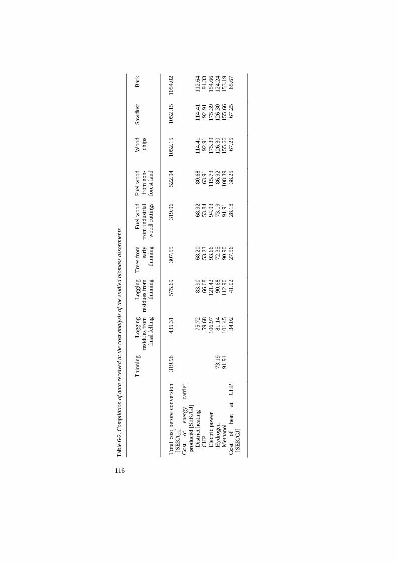
Tabl

e 6-

2. C

ompi

latio

n of

dat

a re

ceiv

ed a

t the

cos

t ana

lysi

s of t

he st

udie

d bi

omas

s ass

ortm

ents

Thin

ning

Logg

ing

resi

dues

from

fin

al fe

lling

Logg

ing

resi

dues

from

th

inni

ng

Tree

s fro

m

early

th

inni

ng

Fuel

woo

d fr

om in

dust

rial

woo

d cu

tting

s

Fuel

woo

d fr

om n

on-

fore

st la

nd

Woo

d ch

ips

Saw

dust

Bar

k

Tota

l co

st b

efor

e co

nver

sion

[S

EK/t d

m]

Cos

t of

en

ergy

ca

rrie

r pr

oduc

ed [S

EK/G

J]

Dis

trict

hea

ting

CH

P El

ectri

c po

wer

H

ydro

gen

Met

hano

l C

ost

of

heat

at

C

HP

[SEK

/GJ]

31

9.96

73.1

991

.91

43

5.31

75.7

259

.68

106.

9781

.14

101.

4534

.02

57

5.69

83.9

066

.68

121.

4290

.68

112.

9041

.02

30

7.55

68

.20

53.2

3 93

.66

72.3

5 90

.90

27.5

6

31

9.96

68.9

253

.84

94.9

373

.19

91.9

128

.18

52

2.94

80.6

863

.91

115.

7386

.92

108.

3938

.25

10

52.1

5

114.

4192

.91

175.

3912

6.30

155.

6667

.25

10

52.1

5

114.

4192

.91

175.

3912

6.30

155.

6667

.25

10

54.0

2

112.

6491

.33

154.

6612

4.24

153.

1965

.67

116

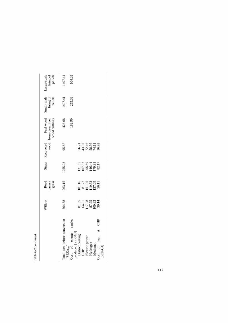
Tabl

e 6-

2 co

ntin

ued

Will

owR

eed

cana

ry

gras

s

Stra

wR

ecov

ered

w

ood

Fu

el w

ood

from

dire

ct fu

el

woo

d cu

tting

s

Smal

l-sca

le

firin

g of

pe

llets

Larg

e-sc

ale

firin

g of

pe

llets

Tota

l co

st b

efor

e co

nver

sion

[S

EK/t d

m]

Cos

t of

en

ergy

ca

rrie

r pr

oduc

ed [S

EK/G

J]

Dis

trict

hea

ting

CH

P El

ectri

c po

wer

H

ydro

gen

Met

hano

l C

ost

of

heat

at

C

HP

[SEK

/GJ]

50

4.58

81.5

564

.81

117.

2887

.95

109.

6239

.14

76

3.15

101.

1681

.77

151.

9511

0.83

137.

0956

.11

12

55.0

8

131.

6510

7.83

205.

8914

6.44

179.

8382

.17

95

.87

56.2

143

.07

72.4

658

.36

74.1

116

.92

42

3.68

182.

90

14

97.4

1

255.

33

14

97.4

1

104.

03

117

118

IGCC condensing power plant was because of the total cost being distributed on both heat and electric power generated at CHP P

1.

The cost of district heating produced in the small moving grate boiler was generally higher than the cost of district heating generated at the CHP plant. This is due to the distribution of the total cost on both electric power and heat at CHP. The larger size of the CHP plant also leads to a lower production cost, as mentioned in Chapter 4.

In the comparison of costs for hydrogen and methanol production and electric power generation (Tables A.I-3 through to A.I-14 (compiled in Table 6-2)), hydrogen production had the lowest cost, whereas electric power generation had the highest cost (one exception was conversion of recovered wood, where the highest cost was for methanol production). However, the size of the IGCC plant for electric power production was approximately half the size of the plants used for hydrogen or methanol production. It was therefore difficult to compare the costs of electric power generation and vehicle fuel production for the different biomass assortments, as boiler size influences both the efficiency and cost for energy carriers generated (see Chapter 4).

The COE on electric power generation was slightly higher than the production cost of methanol for most of the biomass assortments, although, the production cost of hydrogen was lower than both electric power generation and methanol production. The production cost for hydrogen was lowest for recovered wood (58 SEK/GJ) and highest for straw (146 SEK/GJ).

The cost for small-scale heat production is shown in Tables 6-2 and A.I-15 through to A.I-16. It may be seen that the cost of heat generated at wood firing (183 SEK/GJ) was less than the cost of heat generated from pellet firing (255 SEK/GJ).

The cost of heat generated from large-scale pellet firing was much lower than the cost of heat generated from small-scale pellet firing; the cost of heat at large-scale pellet firing was 104 SEK/GJ (see Tables 6-2 and A.I-17). Thus, the larger pellet boiler, which may be used in district heating production, is more cost-effective than smaller pellet boilers used in single family-houses. Emergy analysis The final yields of the energy carriers produced (heat, electric power, hydrogen and methanol) from all biomass assortments revealed that the lowest solar transformity was for district heating production (18,595 – 58,915 sej/J), and the highest solar transformity was for electric power generation in CHP plants (44,842 – 156,816 sej/J) (see Tables 6-3 and A.I-1 through to A.I-17). The high transformity for electric power generation in the CHP plant may be explained by the comparatively low yield of electric power at CHP (varying between 5.40 – 6.08 GJ/tdm for the different biomass assortments). Recovered wood had the lowest transformities and fuel wood from non-forest land had the highest solar transformities. The high transformities for fuel wood from non-forest land is explained by the low yield of fuel wood per hectare, compared to the other biomass assortments.

119

The solar transformities for electric power generation ranged from 33,254 sej/J to 104,635 sej/J, whereas the solar transformities for hydrogen ranged from 25,385 to 72,230 sej/J and from 29,540 to 85,842 sej/J for methanol production. Even with these conversion processes, the lowest solar transformities were received by recovered wood, and the highest were received by fuel wood from non-forest land.

The emergy investment ratio (EIR) was less than one before conversion for most biomass assortments derived directly from forestry and for recovered wood, i.e. the emergy flow fed back from outside the system (fuels, goods and services) were less than the indigenous emergy input (Tables A.I-1 through to A.I-6, A.I-14, A.I-15 and 6-3). One exception was logging residues from thinning, where the EIR was greater than one even after road transport. However, after conversion the EIR of all assortments was greater than one, which meant that the societal emergy flow fed back was greater than the indigenous emergy input.

The EIR of forest industry by-products was larger than one even after saw milling (Tables A.I-8 through A.I-10). The lowest EIR after conversion for these assortments was received for CHP generation (2.83 – 2.88), which means that the emergy flow from society was almost three times greater than the indigenous emergy input. The EIR after the other conversion processes ranged from 3.15 to 3.64, where the lowest EIR was received for district heating generation and the highest EIR was received for hydrogen production.

The EIR for the biomass assortments from agriculture was larger than one even after cultivation: the lowest EIR after cultivation was for reed canary grass (1.75) and the highest was for wheat (5.60). After conversion, the EIR ranged from 5.64 to 11.18, where the lowest EIR was for CHP generation with reed canary grass as the fuel, and the highest was for hydrogen production with straw as a fuel.

The difference in emergy yield ratio (EYR) between the energy carriers received from each biomass assortment was small, whereas the difference in EIR between the energy carriers from each biomass assortment was larger. One exception was fuel wood from non-forest land, where the differences in EYRs received for the different conversion processes were greater than the EIRs received (the EYRs ranged from 3.35 to 4.36 and the EIRs ranged from 0.30 to 0.43). However, the differences in EYRs and EIRs between biomass from agriculture and the other biomass assortments were large; for instance, the EYR for willow was only 1.12 – 1.17 for the different energy carriers produced, whereas the EIR for willow ranged from 5.87 for CHP generation to 8.15 for hydrogen production. The highest EYRs and the lowest EIRs were for the energy carriers received at conversion of fuel wood from non-forest land, with the highest EYR (4.36) and the lowest EIR (0.30) for CHP generation and the lowest EYR (3.35) and the highest EIR (0.43) for hydrogen production. The high EYRs and low EIRs for fuel wood from non-forest land may be explained by the absence of silvicultural input required for this biomass assortment, as opposed to the biomass assortments derived from agriculture, which are highly intensive regarding resource input in cultivation and handling of the biomass in the field. Of all the biomass assortments analysed, only fuel wood from non-forest land had EIRs lower than one after conversion.

The EIR of sawdust was larger than one even after saw milling; and after pelletizing, the EIR was as much as 3.45. The EIR after heat production in the

Tabl

e 6-

3. C

ompi

latio

n of

dat

a re

ceiv

ed a

t the

em

ergy

ana

lysi

s of t

he st

udie

d bi

omas

s ass

ortm

ents

Thin

ning

Logg

ing

resi

dues

from

fin

al fe

lling

Logg

ing

resi

dues

from

th

inni

ng

Tree

s fro

m

early

th

inni

ng

Fuel

woo

d fr

om in

dust

rial

woo

d cu

tting

s

Fuel

woo

d fr

om n

on-

fore

st la

nd

Woo

d ch

ips

Saw

dust

Bar

k

Sola

r tra

nsfo

rmity

be

fore

co

nver

sion

[sej

/J]

Sola

r tra

nsfo

rmity

af

ter

conv

ersi

on [s

ej/J

] D

istri

ct h

eatin

g C

HP

Elec

tric

pow

er

Hyd

roge

n M

etha

nol

EIR

bef

ore

conv

ersi

on

EIR

afte

r con

vers

ion

Dis

trict

hea

ting

CH

P El

ectri

c po

wer

H

ydro

gen

Met

hano

l EY

R b

efor

e co

nver

sion

EY

R a

fter c

onve

rsio

n D

istri

ct h

eatin

g C

HP

Elec

tric

pow

er

Hyd

roge

n M

etha

nol

93

77

26,8

9431

,427

0.57

2.19

2.11

2.74

1.46

1.47

10

,665

21,6

5053

,088

38,7

1628

,742

33,6

380.

79

1.99

1.64

2.03

2.40

2.32

2.26

1.50

1.61

1.49

1.41

1.43

11

,977

23,2

3857

,511

41,5

2630

,597

35,8

641.

23

2.67

2.25

2.71

3.16

3.06

1.94

1.43

1.52

1.43

1.37

1.38

92

34

19,9

13

48,2

25

35,6

51

26,6

92

31,1

84

0.55

1.

76

1.40

1.

79

2.17

2.

08

2.82

1.

57

1.71

1.

56

1.46

1.

48

93

77

20,0

8648

,706

35,9

5726

,894

31,4

270.

57

1.78

1.42

1.82

2.19

2.11

2.74

1.56

1.70

1.55

1.46

1.47

41

,442

58,9

1515

6,81

610

4,63

572

,230

85,8

420.

16

0.36

0.30

0.36

0.43

0.41

7.41

3.80

4.36

3.76

3.35

3.43

18

,812

31,5

4880

,908

56,1

6640

,509

47,6

942.

01

3.16

2.84

3.19

3.58

3.49

1.50

1.32

1.35

1.31

1.28

1.29

18

,755

31,4

7980

,715

56,0

4340

,428

47,5

962.

00

3.15

2.83

3.18

3.57

3.48

1.50

1.32

1.35

1.31

1.28

1.29

18

,458

31,0

9779

,477

52,6

2939

,841

46,9

382.

04

3.23

2.88

3.05

3.64

3.55

1.49

1.31

1.35

1.33

1.27

1.28

120

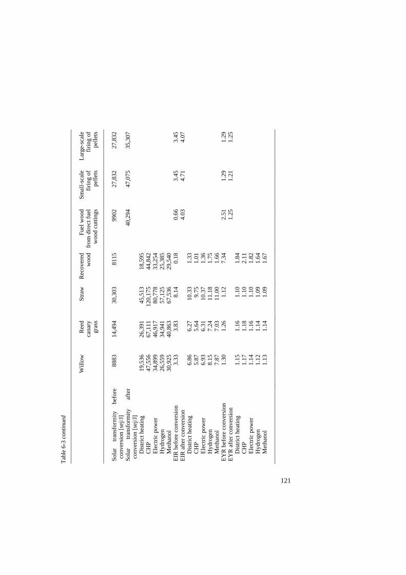
Tabl

e 6-

3 co

ntin

ued

Will

owR

eed

cana

ry

gras

s

Stra

wR

ecov

ered

w

ood

Fu

el w

ood

from

dire

ct fu

el

woo

d cu

tting

s

Smal

l-sca

le

firin

g of

pe

llets

Larg

e-sc

ale

firin

g of

pe

llets

Sola

r tra

nsfo

rmity

be

fore

co

nver

sion

[sej

/J]

Sola

r tra

nsfo

rmity

af

ter

conv

ersi

on [s

ej/J

] D

istri

ct h

eatin

g C

HP

Elec

tric

pow

er

Hyd

roge

n M

etha

nol

EIR

bef

ore

conv

ersi

on

EIR

afte

r con

vers

ion

Dis

trict

hea

ting

CH

P El

ectri

c po

wer

H

ydro

gen

Met

hano

l EY

R b

efor

e co

nver

sion

EY

R a

fter c

onve

rsio

n D

istri

ct h

eatin

g C

HP

Elec

tric

pow

er

Hyd

roge

n M

etha

nol

88

83

19,5

3647

,556

34,8

9926

,559

30,9

253.

33

6.86

5.87

6.93

8.15

7.87

1.30

1.

151.

171.

141.

121.

13

14

,494

26,3

9167

,111

46,9

1734

,941

40,8

633.

83

6.27

5.64

6.31

7.24

7.03

1.26

1.16

1.18

1.16

1.14

1.14

30

,303

45,5

1312

0,17

580

,778

57,1

2567

,536

8.14

10.3

39.

7510

.37

11.1

811

.00

1.12

1.10

1.10

1.10

1.09

1.09

81

15

18,5

9544

,842

33,2

5425

,385

29,5

400.

18

1.33

1.01

1.36

1.75

1.66

7.34

1.84

2.11

1.82

1.64

1.67

99

02

40

,294

0.

66

4.03

2.

51

1.25

27

,832

47,0

75

3.45

4.71

1.29

1.21

27

,832

35,3

07

3.45

4.07

1.29

1.25

121

122

larger pellet boiler was lower (4.07) than the EIR after heat production in the smaller pellet boiler (4.71). Comparison of small-scale pellet firing with small-scale wood firing indicated that the EIR was lower for heat produced at wood firing (4.03). Thus, 4 to almost 5 times of emergy were invested from society compared to the emergy flow invested from the local environment on pellets firing and small-scale wood firing: the EIR ranged from 4.0 to 4.7 for these conversion processes. Sensitivity analysis Road transport required the most direct energy for all biomass assortments before conversion, except forest industry by-products (Tables A.I-1 through to A.I-14). Saw milling required twice the amount of direct energy than road transport (the energy amounts required for wood chips was 300.0 MJ/tdm of electricity and 148.9 MJ/tdm of diesel oil for sawdust). The difference in total primary energy input, total costs and total emergy flows if the road transport distances were doubled, from 75 km to 150 km, for three biomass assortments, logging residues from final felling, sawdust and willow, was evaluated with sensitivity analysis. The doubling of the road transport distance led to that the direct energy required doubled; however, the embodied primary energy only increased by 62% for willow and 76% for logging residues from final felling and sawdust due to the increase in embodied primary energy being inversely proportional to the production per hour during road transport (tdm/hG15). Thus, the hourly production decreased by 62 – 76% at an increase in transport distance from 75 km to 150 km.

Doubling the road transport distance from 75 km to 150 km did not appear to affect the ratio of final product received to the primary energy input as much (Table 6-4). The ratio of final product received to the primary energy input is shown in Table 6-4. It may be seen that the changes of the ratio was rather small. The ratio decreased by 0.9% at conversion of logging residues from final felling and by 0.8% at conversion of sawdust and willow. Thus, a doubling of the road transport distance for the biomass assortments led to small decreases in the total yields of energy carriers.

123

Table 6-4. Changes in the ratio of final product received to the primary energy input when the road transport distance was increased from 75 km to 150 km

District heating

[%]

CHP[%]

Electric power

generation[%]

Hydrogen production

[%]

Methanol production

[%]

Road transport distance = 75 km

Logging residues from final felling

Sawdust Willow Road transport distance = 150 km

Logging residues from final felling

Sawdust Willow

79.6

78.0 78.3

78.9

77.3 77.6

90.6

88.688.9

89.8

87.988.2

43.2

42.442.5

42.8

42.042.2

64.2

62.762.9

63.6

62.362.4

54.3

53.153.3

53.8

52.752.9

The changes in costs for the different energy carriers produced on conversion of

logging residues from final felling, sawdust and willow when the road transport distance was doubled are shown in Table 6-5. The costs for the energy carriers produced on conversion of logging residues from final felling and willow increased by 6 – 8%, and corresponding changes in costs for sawdust were 5 – 6%. Thus, the changes in costs were considerably larger than the change in ratio of final product received to the primary energy input.

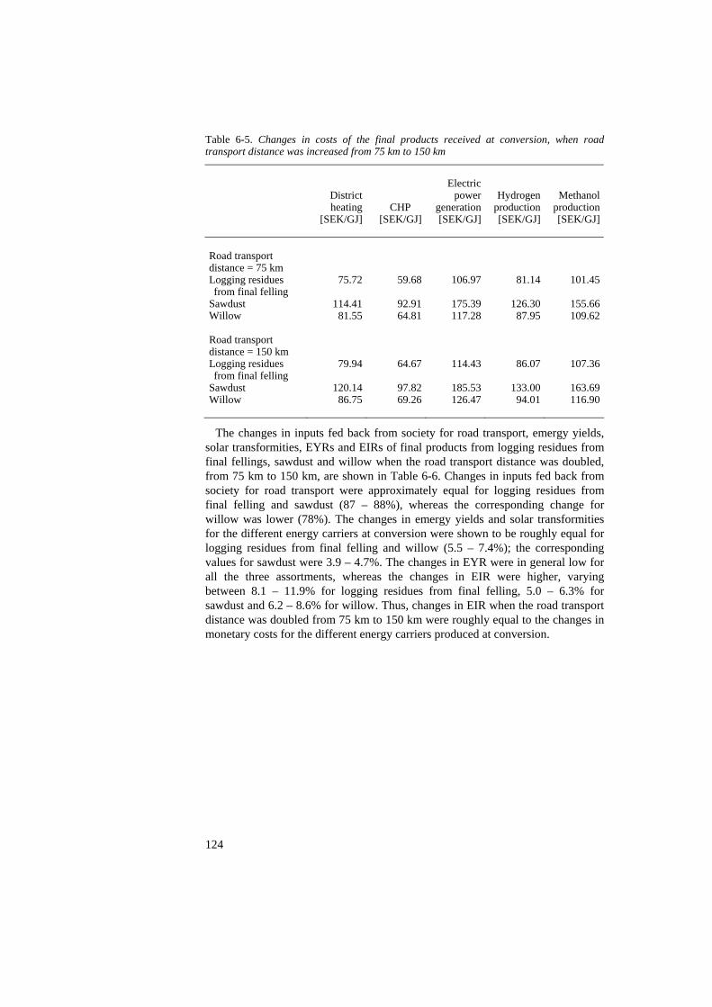
124

Table 6-5. Changes in costs of the final products received at conversion, when road transport distance was increased from 75 km to 150 km

District heating

[SEK/GJ] CHP [SEK/GJ]

Electric power

generation[SEK/GJ]

Hydrogen production [SEK/GJ]

Methanol production[SEK/GJ]

Road transport distance = 75 km Logging residues from final felling

Sawdust Willow Road transport distance = 150 km Logging residues from final felling

Sawdust Willow

75.72

114.4181.55

79.94

120.1486.75

59.68

92.9164.81

64.67

97.8269.26

106.97

175.39117.28

114.43

185.53126.47

81.14

126.30 87.95

86.07

133.00 94.01

101.45

155.66109.62

107.36

163.69116.90

The changes in inputs fed back from society for road transport, emergy yields, solar transformities, EYRs and EIRs of final products from logging residues from final fellings, sawdust and willow when the road transport distance was doubled, from 75 km to 150 km, are shown in Table 6-6. Changes in inputs fed back from society for road transport were approximately equal for logging residues from final felling and sawdust (87 – 88%), whereas the corresponding change for willow was lower (78%). The changes in emergy yields and solar transformities for the different energy carriers at conversion were shown to be roughly equal for logging residues from final felling and willow (5.5 – 7.4%); the corresponding values for sawdust were 3.9 – 4.7%. The changes in EYR were in general low for all the three assortments, whereas the changes in EIR were higher, varying between 8.1 – 11.9% for logging residues from final felling, 5.0 – 6.3% for sawdust and 6.2 – 8.6% for willow. Thus, changes in EIR when the road transport distance was doubled from 75 km to 150 km were roughly equal to the changes in monetary costs for the different energy carriers produced at conversion.

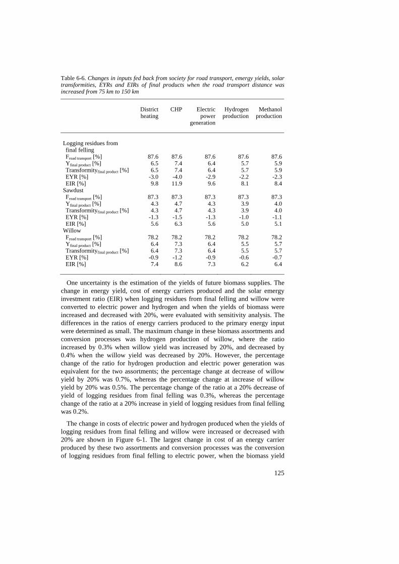
125

Table 6-6. Changes in inputs fed back from society for road transport, emergy yields, solar transformities, EYRs and EIRs of final products when the road transport distance was increased from 75 km to 150 km

District heating

CHP Electric power

generation

Hydrogen production

Methanol production

Logging residues from final felling Froad transport [%] Yfinal product [%] Transformityfinal product [%] EYR [%] EIR [%]

Sawdust Froad transport [%] Yfinal product [%] Transformityfinal product [%] EYR [%] EIR [%]

Willow Froad transport [%] Yfinal product [%] Transformityfinal product [%] EYR [%] EIR [%]

87.6 6.5 6.5

-3.0 9.8

87.3 4.3 4.3

-1.3 5.6

78.2 6.4 6.4

-0.9 7.4

87.67.47.4

-4.011.9

87.34.74.7

-1.56.3

78.27.37.3

-1.28.6

87.66.46.4

-2.99.6

87.34.34.3

-1.35.6

78.26.46.4

-0.97.3

87.65.75.7

-2.28.1

87.33.93.9

-1.05.0

78.25.55.5

-0.66.2

87.65.95.9

-2.38.4

87.34.04.0

-1.15.1

78.25.75.7

-0.76.4

One uncertainty is the estimation of the yields of future biomass supplies. The change in energy yield, cost of energy carriers produced and the solar emergy investment ratio (EIR) when logging residues from final felling and willow were converted to electric power and hydrogen and when the yields of biomass were increased and decreased with 20%, were evaluated with sensitivity analysis. The differences in the ratios of energy carriers produced to the primary energy input were determined as small. The maximum change in these biomass assortments and conversion processes was hydrogen production of willow, where the ratio increased by 0.3% when willow yield was increased by 20%, and decreased by 0.4% when the willow yield was decreased by 20%. However, the percentage change of the ratio for hydrogen production and electric power generation was equivalent for the two assortments; the percentage change at decrease of willow yield by 20% was 0.7%, whereas the percentage change at increase of willow yield by 20% was 0.5%. The percentage change of the ratio at a 20% decrease of yield of logging residues from final felling was 0.3%, whereas the percentage change of the ratio at a 20% increase in yield of logging residues from final felling was 0.2%.

The change in costs of electric power and hydrogen produced when the yields of logging residues from final felling and willow were increased or decreased with 20% are shown in Figure 6-1. The largest change in cost of an energy carrier produced by these two assortments and conversion processes was the conversion of logging residues from final felling to electric power, when the biomass yield

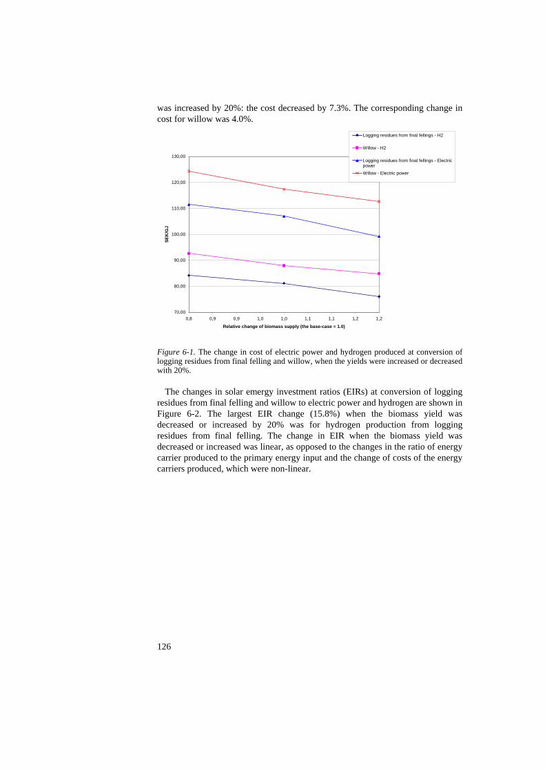
was increased by 20%: the cost decreased by 7.3%. The corresponding change in cost for willow was 4.0%.

70,00

80,00

90,00

100,00

110,00

120,00

130,00

0,8 0,9 0,9 1,0 1,0 1,1 1,1 1,2 1,2

Relative change of biomass supply (the base-case = 1.0)

SEK

/GJ

Logging residues from final fellings - H2

Willow - H2

Logging residues from final fellings - ElectricpowerWillow - Electric power

Figure 6-1. The change in cost of electric power and hydrogen produced at conversion of logging residues from final felling and willow, when the yields were increased or decreased with 20%.

The changes in solar emergy investment ratios (EIRs) at conversion of logging residues from final felling and willow to electric power and hydrogen are shown in Figure 6-2. The largest EIR change (15.8%) when the biomass yield was decreased or increased by 20% was for hydrogen production from logging residues from final felling. The change in EIR when the biomass yield was decreased or increased was linear, as opposed to the changes in the ratio of energy carrier produced to the primary energy input and the change of costs of the energy carriers produced, which were non-linear.

126

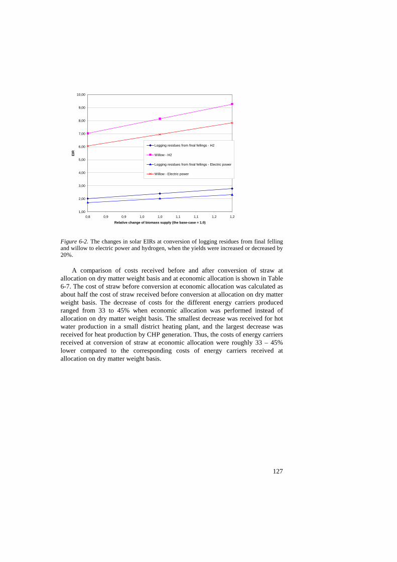
1,00

2,00

3,00

4,00

5,00

6,00

7,00

8,00

9,00

10,00

0,8 0,9 0,9 1,0 1,0 1,1 1,1 1,2 1,2

Relative change of biomass supply (the base-case = 1.0)

EIR

Logging residues from final fellings - H2

Willow - H2

Logging residues from final fellings - Electric power

Willow - Electric power

Figure 6-2. The changes in solar EIRs at conversion of logging residues from final felling and willow to electric power and hydrogen, when the yields were increased or decreased by 20%.

A comparison of costs received before and after conversion of straw at allocation on dry matter weight basis and at economic allocation is shown in Table 6-7. The cost of straw before conversion at economic allocation was calculated as about half the cost of straw received before conversion at allocation on dry matter weight basis. The decrease of costs for the different energy carriers produced ranged from 33 to 45% when economic allocation was performed instead of allocation on dry matter weight basis. The smallest decrease was received for hot water production in a small district heating plant, and the largest decrease was received for heat production by CHP generation. Thus, the costs of energy carriers received at conversion of straw at economic allocation were roughly 33 – 45% lower compared to the corresponding costs of energy carriers received at allocation on dry matter weight basis.

127

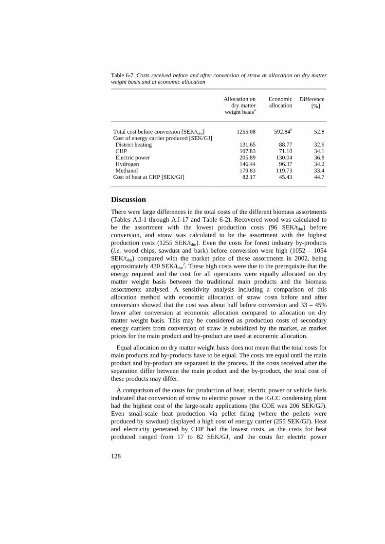
128

Table 6-7. Costs received before and after conversion of straw at allocation on dry matter weight basis and at economic allocation

Allocation on dry matter

weight basisa

Economic allocation

Difference [%]

Total cost before conversion [SEK/tdm] Cost of energy carrier produced [SEK/GJ] District heating CHP Electric power Hydrogen Methanol

Cost of heat at CHP [SEK/GJ]

1255.08

131.65107.83205.89146.44179.8382.17

592.84b

88.77 71.10

130.04 96.37

119.73 45.43

52.8

32.634.136.834.233.444.7

Discussion There were large differences in the total costs of the different biomass assortments (Tables A.I-1 through A.I-17 and Table 6-2). Recovered wood was calculated to be the assortment with the lowest production costs (96 SEK/tdm) before conversion, and straw was calculated to be the assortment with the highest production costs (1255 SEK/tdm). Even the costs for forest industry by-products (i.e. wood chips, sawdust and bark) before conversion were high (1052 – 1054 SEK/tdm) compared with the market price of these assortments in 2002, being approximately 430 SEK/tdm

2. These high costs were due to the prerequisite that the energy required and the cost for all operations were equally allocated on dry matter weight basis between the traditional main products and the biomass assortments analysed. A sensitivity analysis including a comparison of this allocation method with economic allocation of straw costs before and after conversion showed that the cost was about half before conversion and 33 – 45% lower after conversion at economic allocation compared to allocation on dry matter weight basis. This may be considered as production costs of secondary energy carriers from conversion of straw is subsidized by the market, as market prices for the main product and by-product are used at economic allocation.

Equal allocation on dry matter weight basis does not mean that the total costs for main products and by-products have to be equal. The costs are equal until the main product and by-product are separated in the process. If the costs received after the separation differ between the main product and the by-product, the total cost of these products may differ.

A comparison of the costs for production of heat, electric power or vehicle fuels indicated that conversion of straw to electric power in the IGCC condensing plant had the highest cost of the large-scale applications (the COE was 206 SEK/GJ). Even small-scale heat production via pellet firing (where the pellets were produced by sawdust) displayed a high cost of energy carrier (255 SEK/GJ). Heat and electricity generated by CHP had the lowest costs, as the costs for heat produced ranged from 17 to 82 SEK/GJ, and the costs for electric power

129

generation ranged from 43 to 108 SEK/GJ. The lowest costs were for recovered wood and the highest costs were for straw.

A comparison of costs for production of electricity by condensing power in a IGCC plant and production of hydrogen or methanol by gasification determined that electric power generation was more expensive than both hydrogen and methanol production. Hydrogen was the energy carrier with the lowest production cost, with methanol production somewhat higher. One exception was recovered wood, where methanol production was more expensive (74 SEK/GJ) than electric power generation (72 SEK/GJ). Although, it must be remembered that the size of the IGCC plant for electric power generation was approximately half the size of the plant used for hydrogen or methanol production, which in turn influenced both the efficiency and cost for energy carriers generated (see Chapter 4).

Bärring et al. (2003) estimate the topical cost for the production of electricity by 400 MW condensing plants fired with coal (steam cycle) to be 109 SEK/GJ and by natural gas (combined cycle) to be 83 SEK/GJ3. Thus, the calculated cost of electricity (COE) from gasification of logging residues from final felling in an IGCC plant (107 SEK/GJ) is approximately equal to the COE in a coal-fired condensing plant and 29% higher compared to the COE in a condensing plant fired with natural gas. The difference in size of the plants influenced the cost of the energy carrier produced. Thus, if the size of the biomass-fed IGCC plant is increased, compared to the size used as a reference plant in this work, the COE on gasification of biomass derived directly from forestry may be competitive with the COE of both coal-fired and natural gas-fired condensing plants.

The COE calculated by Toft (1996) at conversion of wood chips in an IGCC plant located in Great Britain is 19.63 €/GJ4. Faaij et al. (1997) calculate the COE at conversion of thinnings of poplar in an IGCC plant located in the Netherlands to be about 20.42 €/GJ. These COEs are in the same range as the COE calculated in this thesis at conversion of wood chips and sawdust in an IGCC plant (19.23 €/GJ).

The efficiency of hydrogen as a fuel in a hybrid fuel cell propulsion system is estimated by Ahlvik & Brandberg (2001) to be 23.5%, based on the LHV. The cost per GJ vehicle work when using hydrogen produced by gasification of logging residues from final felling is then 408 SEK/GJvehicle work

5. The average production cost of petrol in 2004 was 2.25 SEK/dm3 (The Swedish Petroleum Institute, 30-Nov-2005 (URL)). The cost per GJ vehicle work for petrol use in a conventional petrol engine may then be calculated by means of the LHV of petrol (32.6 MJ/dm3 (Swedish Energy Agency, 2003a)) and the efficiency (14.9% (Ahlvik & Brandberg, 2001)), being 463 SEK/GJvehicle work

6. Thus, the cost of hydrogen produced by conversion of biomass from forestry and used in novel fuel cell propulsion systems for generating vehicle work does not need to be more expensive than the cost for generating vehicle work with vehicle fuels used in topical propulsion systems.

The cost per GJ vehicle work when using methanol produced by gasification of logging residues from final felling in a conventional petrol engine (the efficiency is 16.2%, based on the LHV (Ahlvik & Brandberg, 2001)) will be 714

130

SEK/GJvehicle work7. The corresponding cost when using methanol with the same

production cost in a conventional diesel engine (the efficiency is 17.6%, based on the LHV (Ahlvik & Brandberg, 2001)) will be 658 SEK/GJvehicle work

8. Thus, the calculated cost per GJ vehicle work when using methanol produced by gasification of logging residues from final felling in a conventional diesel engine will be 42.1% higher compared to the cost per GJ vehicle work for petrol used in a conventional petrol engine. The corresponding difference in cost for vehicle work generated when comparing methanol use in a conventional petrol engine with petrol use in the same type of engine will be 54.2%. Thus, considering only the production costs of the vehicle fuel, the use of methanol, produced by gasification of biomass from forestry, as a fuel in conventional petrol and diesel engines is not economically competitive compared to the use of petrol in conventional petrol engines.

Williams et al. (1995) estimate the cost of hydrogen and methanol produced at conversion of biomass in the Battelle gasification process to be 8.05 €/GJ and 10.36 €/GJ respectively in 19919, and Hamelinck & Faaij (2002) calculate the corresponding costs to be 8.67 €/GJ and 10.17 €/GJ respectively at conversion of biomass available at a price corresponding to American conditions in 200110. These costs are in accordance with the costs calculated in this thesis for hydrogen and methanol produced at conversion of biomass in the Battelle gasification process; e.g. the costs for hydrogen and methanol at conversion of trees from thinning were 8.03 €/GJ and 10.08 €/GJ respectively.

The ratios of primary energy output to primary energy input for logging residues calculated in this thesis are in accordance with the study by Börjesson (1996): in this thesis, the ratios for logging residues from final felling and from thinning were 39.8 and 33.0 respectively. The corresponding values calculated by Börjesson (1996) are 38 and 31 respectively (fossil-fuel-based energy inputs, 2015). However, the ratios of primary energy output to primary energy input for willow, reed canary grass and straw were lower than the corresponding ratios calculated by Börjesson (1996). The difference was greatest for straw, where the ratio of primary energy output to primary energy input was calculated to be 5.1 in this thesis, and 32 by Börjesson (1996). Nilsson (1997) calculates the ratio of primary energy output to primary energy input at district heating production by combustion of straw to be 9 if nitrogen fertilization. The corresponding ratio for district heating production by combustion of straw was 4.0 in this thesis. The lower ratio of primary energy output to primary energy input for straw calculated in this thesis is due to that the energy required for cultivation and harvesting of the grain was considered in the energy analysis of straw in this thesis, while the energy required for these operations were excluded in the energy analyses by Börjesson (1996) and Nilsson (1997).

The energy and cost analyses could be considered as partial analyses of the emergy analysis, as the emergy analysis considers both energy flows from the environment and society. In cost analysis, human work is valued as a monetary currency. In the emergy analysis, the monetary value of human work is transformed to the emergy flow, which corresponds to the monetary value of human work; a sej per monetary currency index is used for this transformation.

131

The sensitivity analysis of doubling road transport distance revealed that changes in EIR approximated to the changes in monetary costs for the different energy carriers produced on conversion. This was due to the cost analysis only considering resource flows derived from the society and did not consider resource flows derived from the environment.

The sensitivity analyses also highlighted that the energy analysis was insensitive to the changes, i.e. a doubling of the road transport distance and an increase or decrease of the biomass yields. Whereas, the cost analysis and emergy analysis displayed significant changes in results: the costs of energy carriers produced decreased by between 4–7% when biomass yield was increased by 20%. However, the EIR increased when the biomass yield was increased; a 20% increase of the biomass yield led to a 13–16% increase in EIR for the biomass assortments and the energy carriers studied in the sensitivity analysis. Thus, the lower cost of energy carrier produced resulted in a larger emergy input from the society as fuels, goods and services in relation to the emergy flow fed from the environment.

A transformity can be viewed as the physical cost in emergy terms for a unit of a service or commodity, expressed in terms of actual energy or mass. As with monetary costs, the transformities change with technological development. For example, the transformity for cutting and transporting a log from the forest to the roadside with a handsaw and draught animals, as the work was done in the beginning of the 20th century, is higher than the transformity for conducting the same operations with a highly mechanized system in 2002. Hagström & Nilsson (2004) describe the relative “standard of living” per capita in monetary terms as increasing three times between 1956 and 2002, whereas the total emergy flow per capita increased only twice during the same period. Thus, on average the transformities in the entire Swedish economy may be 33% lower today, than fifty years ago. The efficiency increase is partly due to technological development but is presumably more dependent on changes in the type of energy used: transformities for fossil fuels and electricity are considerably lower than transformities for draught animal and humans. Transformities, like monetary costs, are also dependent on the scale of the economy.

From the emergy analysis performed in this work, the solar transformities for electric power generation by gasification of biomass from forestry ranged from 35,700 sej/J to 41,500 sej/J. These values may be compared with electric power generation by thermochemical conversion of fossil fuels or conversion of other sources such as wind or potential energy in water (i.e. hydroelectric power). Brown & Ulgiati (2002) calculate the solar transformities for electric power generated in an oil- and a coal-fired power plant to be 187,000 sej/J and 162,000 sej/J respectively, and the solar transformities for wind and hydroelectric power to be 58,900 sej/J and 58,700 sej/J respectively. All the electric power generation facilities evaluated by Brown & Ulgiati (2002) were located in Italy. Thus, the total resources required (i.e. emergy flow) for generating one unit of electric power by gasification of biomass from forestry are less than the alternative processes of electric power generation. The solar transformities for electric power generation by gasification of willow was 34,900 sej/J and 46,900 sej/J for reed canary grass. This means, the use of these biomass assortments as fuel for electric

132

power generation by gasification in an IGCC plant requires less emergy for generating one unit of electric power than wind, hydroelectric power and electric power generation in oil- and coal-fired power plants. This may be due to the use of estimations and non-commercial technologies (IGCC), which reduce the solar transformity, when compared to the use of commercial technology for electric power generation in oil- and coal-fired power plants.

Brown & Ulgiati (2002) also show that the EYRs for electric power generation in an oil- and a coal-fired power plant are 4.21 and 5.48 respectively, and the corresponding values for wind and hydroelectric power are 7.47 and 7.65 respectively. As shown in this thesis, the EYR at electric power generation ranged from 1.43 to 1.56 when biomass from forestry was used as a fuel; the corresponding value for willow was 1.14 and 1.16 for reed canary grass. Thus, the yields of emergy received at electric power generation by gasification of these biomass assortments, in relation to the emergy input as fuels, goods and services, were much less than the ratios of emergy yield received to emergy input as fuels, goods and services in the other processes as evaluated by Brown & Ulgiati (2002).

Brown & Ulgiati (2002) state that processes that yield products with EYRs less than 2 probably do not contribute enough to be considered an energy source; they act more as consumer products or transformation steps than actual energy sources. By that view, the results in this thesis indicate that electric power generation by gasification of biomass from forestry or agriculture may not contribute enough to be considered an energy source; instead, these systems may act as a net consumer of resources.

A similar comparison of hydrogen and methanol produced by gasification of biomass with petroleum-based vehicle fuels indicated that the solar transformities for hydrogen (26,700 – 30,600 sej/J) and methanol (31,200 – 35,900 sej/J) at conversion of biomass from forestry were lower than the solar transformity of petroleum-based vehicle fuels, estimated by Doherty, Nilsson & Odum (2002) to be 47,900 sej/J. However, the EYRs of hydrogen and methanol production produced by gasification of biomass from forestry were 1.37 – 1.46 and 1.38 – 1.48 respectively; the corresponding value for fossil fuels ranges from 3 to 7 (Ulgiati & Sciubba, 2003). Thus, as stated by Brown & Ulgiati (2002), these bioenergy systems may not contribute enough to be considered an energy source, as the EYRs are too low (less than 2). Corresponding values of solar transformities for hydrogen and methanol production by conversion of willow and reed canary grass were in the same range as the conversion of biomass from forestry. However, the EYRs at conversion of willow and reed canary grass to hydrogen (1.12 and 1.14 respectively) and methanol (1.13 and 1.14 respectively) were even lower than the conversion of biomass from forestry to the same energy carriers.

The EYRs for district heating generation were in the same range as the EYRs for electric power generation and vehicle fuel production: the EYR range was 1.43 to 1.57 at conversion of biomass from forestry and 1.10 to 1.16 at conversion of biomass from agriculture. Thus, low EYRs were also received at conversion of these biomass assortments to heat, meaning that the net contribution of emergy to the economy was low when using these biomass assortments for heat production.

133

The corresponding EYR values for small-scale firing were also low: 1.21 for pellet firing and 1.25 for firing of fuel wood.

Handling and conversion of recovered wood had somewhat higher EYRs than biomass from forestry, forest industry and agriculture, and ranged from 1.64 at hydrogen production to 2.11 at CHP production. The highest EYRs from the biomass assortments studied in this thesis were the handling and conversion of fuel wood from non-forest land (e.g. 3.80 at district heating generation and 3.76 at electric power generation). However, the solar transformities for handling and conversion of fuel wood from non-forest land were the highest of the different biomass assortments studied: the solar transformity was e.g. 58,900 sej/J for district heating generation and 104,600 sej/J for electric power generation by gasification. As mentioned above, the corresponding solar transformity values for electric power generated in an oil- and a coal-fired power plant are calculated by Brown & Ulgiati (2002) to be 187,000 sej/J and 162,000 sej/J respectively. Thus, the total emergy flow required for generating one unit of electric power is 35% lower at gasification of fuel wood from non-forest land, compared to electric power generation at a coal-fired power plant, and 44% lower compared to electric power generation at an oil-fired power plant.

As many of the pre-treatment and conversion processes studied here are not currently commercial, there are uncertainties over the results presented. The energy efficiency of these processes may increase when these pre-treatment and conversion processes become commercialized.

Data regarding the conversion processes, such as the total weight and solar transformity of the plants, were assumed, which may also lead to uncertainties over the results of the emergy analysis of the systems where the conversion processes are included. However, the amount of solar emergy derived from mass depreciation of the conversion plants is low compared to other solar emergy flows derived from internal energy use, human services and capital investment. Thus, variations in the total weight and solar transformity of the plants may not lead to any large variation of the total solar emergy flow required for the conversion processes.

Handling of some biomass assortments, e.g. straw, requires large amounts of energy and high costs. Thus, the type of analyses used in this thesis may be useful for identifying the most important items for resource input, such as energy required and human work. Emergy analysis identifies and quantifies the whole resource flow required for manufacturing a product, such as an energy carrier, and is therefore the recommended method for evaluating all resource flows required in systems, as energy and cost analyses only partially identify and quantify resource flows.

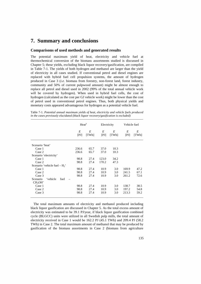
135

7. Summary and conclusions Comparisons of used methods and generated results The potential maximum yield of heat, electricity and vehicle fuel at thermochemical conversion of the biomass assortments studied is discussed in Chapter 5; these yields, excluding black liquor recovery/gasification, are compiled in Table 7-1. The yields of both hydrogen and methanol are larger than the yield of electricity in all cases studied. If conventional petrol and diesel engines are replaced with hybrid fuel cell propulsion systems, the amount of hydrogen produced in Case 3 (i.e. biomass from forestry, non-forest land, forest industry, community and 50% of current pulpwood amount) might be almost enough to replace all petrol and diesel used in 2002 (99% of the total annual vehicle work will be covered by hydrogen). When used in hybrid fuel cells, the cost of hydrogen (calculated as the cost per GJ vehicle work) might be lower than the cost of petrol used in conventional petrol engines. Thus, both physical yields and monetary costs appeared advantageous for hydrogen as a potential vehicle fuel. Table 7-1. Potential annual maximum yields of heat, electricity and vehicle fuels produced in the cases previously elucidated (black liquor recovery/gasification is excluded)

Heata

Electricity

Vehicle fuel

E [PJ]

E [TWh]

E [PJ]

E [TWh]

E [PJ]

E [TWh]

Scenario ‘heat’

Case 1 Case 2

Scenario ‘electricity’ Case 1 Case 2

Scenario ‘vehicle fuel – H2’ Case 1 Case 2 Case 3

Scenario ‘vehicle fuel – CH3OH’

Case 1 Case 2 Case 3

236.6 236.6

98.8 98.8

98.8 98.8 98.8

98.8 98.8 98.8

65.765.7

27.427.4

27.427.427.4

27.427.427.4

37.037.0

123.0170.2

10.910.910.9

10.910.910.9

10.310.3

34.247.3

3.03.03.0

3.03.03.0

169.9241.5261.2

138.7197.2213.3

47.267.172.6

38.554.859.2

The total maximum amounts of electricity and methanol produced including black liquor gasification are discussed in Chapter 5. As the total excess amount of electricity was estimated to be 39.1 PJ/year, if black liquor gasification combined cycle (BLGCC) units were utilized in all Swedish pulp mills, the total amount of electricity received in Case 1 would be 162.2 PJ (45.1 TWh) and 209.4 PJ (58.2 TWh) in Case 2. The total maximum amount of methanol that may be produced by gasification of the biomass assortments in Case 2 (biomass from agriculture

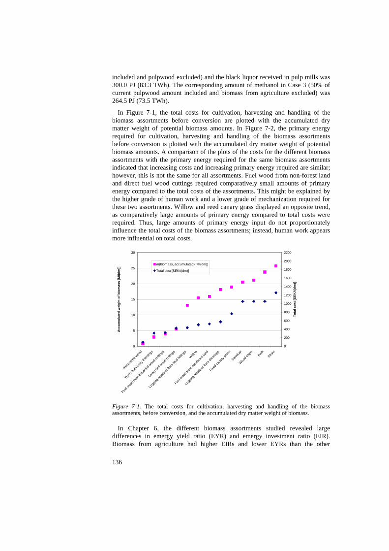
included and pulpwood excluded) and the black liquor received in pulp mills was 300.0 PJ (83.3 TWh). The corresponding amount of methanol in Case 3 (50% of current pulpwood amount included and biomass from agriculture excluded) was 264.5 PJ (73.5 TWh).

In Figure 7-1, the total costs for cultivation, harvesting and handling of the biomass assortments before conversion are plotted with the accumulated dry matter weight of potential biomass amounts. In Figure 7-2, the primary energy required for cultivation, harvesting and handling of the biomass assortments before conversion is plotted with the accumulated dry matter weight of potential biomass amounts. A comparison of the plots of the costs for the different biomass assortments with the primary energy required for the same biomass assortments indicated that increasing costs and increasing primary energy required are similar; however, this is not the same for all assortments. Fuel wood from non-forest land and direct fuel wood cuttings required comparatively small amounts of primary energy compared to the total costs of the assortments. This might be explained by the higher grade of human work and a lower grade of mechanization required for these two assortments. Willow and reed canary grass displayed an opposite trend, as comparatively large amounts of primary energy compared to total costs were required. Thus, large amounts of primary energy input do not proportionately influence the total costs of the biomass assortments; instead, human work appears more influential on total costs.

0

5

10

15

20

25

30

Recov

ered w

ood

Trees f

rom ea

rly th

inning

s

Fuel w

ood f

rom in

dustr

ial w

ood c

utting

s

Direct

fuel w

ood c

utting

s

Logg

ing re

sidue

s from

final

fellin

gs

Willow

Fuel w

ood f

rom no

n-fore

st lan

d

Logg

ing re

sidue

s from

thinn

ings

Reed c

anary

gras

s

Sawdu

st

Woo

d chip

sBark

Straw

Acc

umul

ated

wei

ght o

f bio

mas

s [M

t(dm

)]

0

200

400

600

800

1000

1200

1400

1600

1800

2000

2200

Tota

l cos

t [SE

K/t(

dm)]

m(biomass, accumulated) [Mt(dm)]

Total cost [SEK/t(dm)]

Figure 7-1. The total costs for cultivation, harvesting and handling of the biomass assortments, before conversion, and the accumulated dry matter weight of biomass.

In Chapter 6, the different biomass assortments studied revealed large differences in emergy yield ratio (EYR) and emergy investment ratio (EIR). Biomass from agriculture had higher EIRs and lower EYRs than the other

136

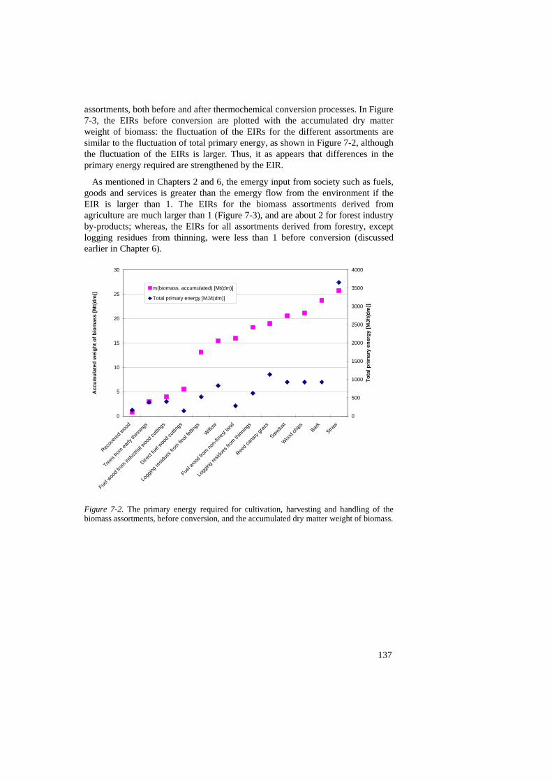
assortments, both before and after thermochemical conversion processes. In Figure 7-3, the EIRs before conversion are plotted with the accumulated dry matter weight of biomass: the fluctuation of the EIRs for the different assortments are similar to the fluctuation of total primary energy, as shown in Figure 7-2, although the fluctuation of the EIRs is larger. Thus, it as appears that differences in the primary energy required are strengthened by the EIR.

As mentioned in Chapters 2 and 6, the emergy input from society such as fuels, goods and services is greater than the emergy flow from the environment if the EIR is larger than 1. The EIRs for the biomass assortments derived from agriculture are much larger than 1 (Figure 7-3), and are about 2 for forest industry by-products; whereas, the EIRs for all assortments derived from forestry, except logging residues from thinning, were less than 1 before conversion (discussed earlier in Chapter 6).

0

5

10

15

20

25

30

Recov

ered w

ood

Trees f

rom ea

rly th

inning

s

Fuel w

ood f

rom in

dustr

ial w

ood c

utting

s

Direct

fuel w

ood c

utting

s

Logg

ing re

sidue

s from

final

fellin

gs

Willow

Fuel w

ood f

rom no

n-fore

st lan

d

Logg

ing re

sidue

s from

thinn

ings

Reed c

anary

gras

s

Sawdu

st

Wood c

hips

BarkStra

w

Acc

umul

ated

wei

ght o

f bio

mas

s [M

t(dm

)]

0

500

1000

1500

2000

2500

3000

3500

4000

Tota

l prim

ary

ener

gy [M

J/t(d

m)]


Total primary energy [MJ/t(dm)]

Figure 7-2. The primary energy required for cultivation, harvesting and handling of the biomass assortments, before conversion, and the accumulated dry matter weight of biomass.

137

0

5

10

15

20

25

30

Recov

ered w

ood

Trees f

rom ea

rly th

inning

s

Fuel w

ood f

rom in

dustr

ial w

ood c

utting

s

Direct

fuel w

ood c

utting

s

Logg

ing re

sidue

s from

final

fellin

gs

Willo

w

Fuel w

ood f

rom no

n-fore

st lan

d

Logg

ing re

sidue

s from

thinn

ings

Reed c

anary

gras

s

Sawdu

st

Wood c

hips

BarkStra

w

Acc

umul

ated

wei

ght o

f bio

mas

s [M

t(dm

)]

0

1

2

3

4

5

6

7

8

9

10

EIR


EIR

Figure 7-3. The EIR of the biomass assortments, before conversion, and the accumulated dry matter weight of biomass.

As the total cost of the biomass assortments before conversion varied (Figure 7-1), the choice of biomass assortments might influence the cost of the energy carriers produced (heat, electricity or vehicle fuel). The costs of the energy carriers produced with the different biomass assortments as fuel/raw material in large-scale applications are shown in Figure 7-4. For the different energy carriers studied, the costs of heat and electric power generated at CHP plants appear to be lowest: COE at CHP ranges from 43 SEK/GJ to 108 SEK/GJ for the different biomass assortments, whereas, COE at IGCC – condensing power ranges from 72 SEK/GJ to 206 SEK/GJ. The corresponding variation of costs for hydrogen production was 58 SEK/GJ to 146 SEK/GJ, and 74 SEK/GJ to 180 SEK/GJ for methanol production.

The cost of the energy carriers produced is largely influenced by the choice of biomass assortments used as fuel. The COE in 400 MW condensing plants fired with coal (steam cycle) is estimated by Bärring et al. (2003) to be 109 SEK/GJ. Figure 7-4 shows that 16.6 Mtdm of the biomass receives a maximum COE of 121 SEK/GJ. The IGCC plant used for the analyses has an electric power output of 69.3 MW (see Chapter 4) so the COE from gasification of these biomass assortments in a larger IGCC plant would be expected to be lower, which is competitive to the COE from large coal-firing condensation plants, as the size of the boiler influences the cost for energy carriers generated (discussed in Chapter 4).

138

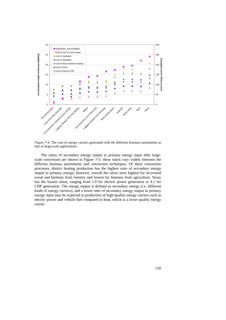
0

5

10

15

20

25

30

Recov

ered w

ood

Trees f

rom ea

rly th

inning

s

Fuel w

ood f

rom in

dustr

ial w

ood c

utting

s

Logg

ing re

sidue

s from

final

fellin

gs

Willow

Fuel w

ood f

rom no

n-fore

st lan

d

Logg

ing re

sidue

s from

thinn

ings

Reed c

anary

gras

s

Sawdu

st

Wood c

hips

BarkStra

w

Acc

umul

ated

wei

ght o

f bio

mas

s [M

t(dm

)]

0

50

100

150

200

250

300

Cos

t of e

nerg

y ca

rrie

rs [S

EK/G

J]

m(biomass, accumulated)

COE at IGCC-Cond. power

Cost of methanol

Cost of hydrogen

Cost of heat at district heating

COE at CHP

Cost of heat at CHP

Figure 7-4. The cost of energy carriers generated with the different biomass assortments as fuel in large-scale applications.

The ratios of secondary energy output to primary energy input after large-scale conversion are shown in Figure 7-5: these ratios vary widely between the different biomass assortments and conversion techniques. Of these conversion processes, district heating production has the highest ratio of secondary energy output to primary energy; however, overall the ratios were highest for recovered wood and biomass from forestry and lowest for biomass from agriculture. Straw has the lowest ratios, ranging from 1.9 for electric power generation to 4.1 for CHP generation. The energy output is defined as secondary energy (i.e. different kinds of energy carriers), and a lower ratio of secondary energy output to primary energy input may be expected at production of high-quality energy carriers such as electric power and vehicle fuel compared to heat, which is a lower quality energy carrier.

139

0

5

10

15

20

25

30

Recov

ered w

ood

Trees f

rom ea

rly th

inning

s

Fuel w

ood f

rom in

dustr

ial w

ood c

utting

s

Logg

ing re

sidue

s from

final

fellin

gs

Willo

w

Fuel w

ood f

rom no

n-fore

st lan

d

Logg

ing re

sidue

s from

thinn

ings

Reed c

anary

gras

s

Sawdu

st

Woo

d chip

sBark

Straw

Acc

umul

ated

wei

ght o

f bio

mas

s [M

T(dm

)]

0

5

10

15

20

25

30

35

40

E(ou

tput

, sec

onda

ry) /

E(in

put,

prim

ary)


IGCC-Cond. power

Methanol

Hydrogen

District heating

CHP

Figure 7-5. The ratios of secondary energy output to primary energy input after large-scale conversion.

The EIRs received after large-scale conversion of the different biomass assortments are shown in Figure 7-6. As the EIR was calculated to be 3.3 for e.g. willow before conversion, 3.3 times as much emergy is invested from fuels, goods and services compared to the indigenous emergy input from the environment. After thermochemical conversion processes, the EIR for willow increased to 6.9 at maximum electricity production, to 8.1 for hydrogen production and 7.9 for methanol production. The biomass assortment receiving the highest EIR was straw: 8.1 before conversion; 10.4 at maximum electricity production; 11.2 at hydrogen production; and 11.0 at methanol production.

140

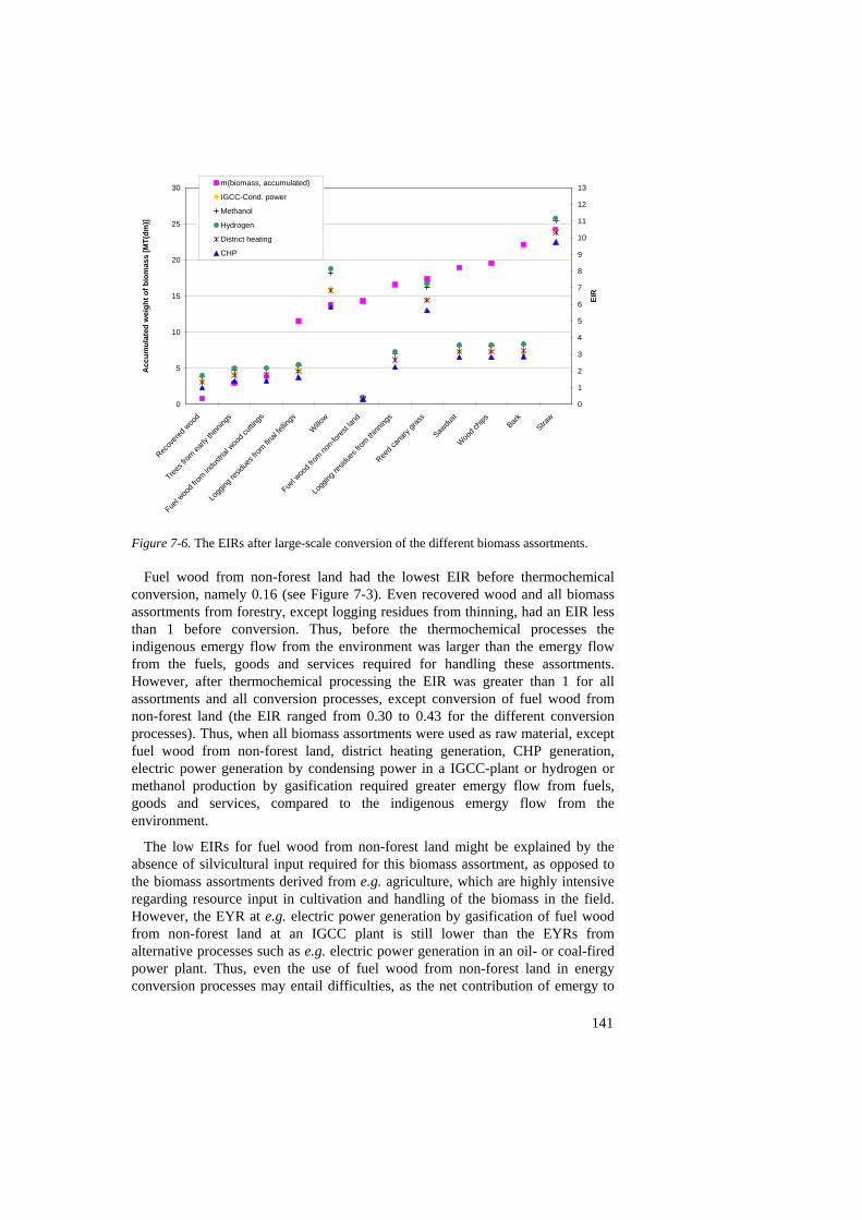
0

5

10

15

20

25

30

Recov

ered w

ood

Trees f

rom ea

rly th

inning

s

Fuel w

ood f

rom in

dustr

ial w

ood c

utting

s

Logg

ing re

sidue

s from

final

fellin

gs

Willo

w

Fuel w

ood f

rom no

n-fore

st lan

d

Logg

ing re

sidue

s from

thinn

ings

Reed c

anary

gras

s

Sawdu

st

Wood c

hips

BarkStra

w

Acc

umul

ated

wei

ght o

f bio

mas

s [M

T(dm

)]

0

1

2

3

4

5

6

7

8

9

10

11

12

13

EIR


IGCC-Cond. power

Methanol

Hydrogen

District heating

CHP

Figure 7-6. The EIRs after large-scale conversion of the different biomass assortments.

Fuel wood from non-forest land had the lowest EIR before thermochemical conversion, namely 0.16 (see Figure 7-3). Even recovered wood and all biomass assortments from forestry, except logging residues from thinning, had an EIR less than 1 before conversion. Thus, before the thermochemical processes the indigenous emergy flow from the environment was larger than the emergy flow from the fuels, goods and services required for handling these assortments. However, after thermochemical processing the EIR was greater than 1 for all assortments and all conversion processes, except conversion of fuel wood from non-forest land (the EIR ranged from 0.30 to 0.43 for the different conversion processes). Thus, when all biomass assortments were used as raw material, except fuel wood from non-forest land, district heating generation, CHP generation, electric power generation by condensing power in a IGCC-plant or hydrogen or methanol production by gasification required greater emergy flow from fuels, goods and services, compared to the indigenous emergy flow from the environment.

The low EIRs for fuel wood from non-forest land might be explained by the absence of silvicultural input required for this biomass assortment, as opposed to the biomass assortments derived from e.g. agriculture, which are highly intensive regarding resource input in cultivation and handling of the biomass in the field. However, the EYR at e.g. electric power generation by gasification of fuel wood from non-forest land at an IGCC plant is still lower than the EYRs from alternative processes such as e.g. electric power generation in an oil- or coal-fired power plant. Thus, even the use of fuel wood from non-forest land in energy conversion processes may entail difficulties, as the net contribution of emergy to

141

142

the economy is lower compared with fossil fuel-based electric power generation processes (discussed in Chapter 6). The EYR at conversion of non-forest-land fuel wood to electric power in an IGCC plant was calculated to be 11% lower than electric power generation in an oil-fired power plant and 31% lower than electric power generation in a coal-fired power plant (comparisons made with data from Brown & Ulgiati (2002)). Ulgiati & Sciubba (2003) state that a lower EYR for a process compared to another leads to difficulties in competing favourably, as the ability of the process to contribute to the economic system by amplifying the investment is less if the EYR is lower.

The reasons for replacing fossil fuels with renewable energy resources were discussed in Chapter 1. Assuming fuel wood from non-forest land is used for electric power or vehicle fuel production, the Swedish potential of this biomass assortment (0.48 Mtdm or 10.0 PJ (see Chapter 3)) is sufficient for generating 4.5 PJ (1.2 TWh) of electricity in IGCC plants, or 6.8 PJ (1.9 TWh) of hydrogen or 5.5 PJ (1.5 TWh) of methanol by gasification. Thus, the maximum contribution of energy carriers produced by conversion of fuel wood from non-forest land in Sweden is small.

The emergy analysis of these biomass energy systems generated results being less advantageous than the results from the energy and cost analyses. The emergy analysis showed that the production of hydrogen or methanol by the technological processes chosen in the systems analysed and from almost all of the biomass assortments were dependant on a larger resource (i.e. emergy) flow from society (i.e. fuels, goods and services) than was received from the environment. Even heat and electric power generation was dependant on a larger emergy flow from the society than was received from the environment, but the EIR was slightly less compared to hydrogen and methanol production. The conversion process obtaining the lowest EIR was CHP generation: the EIR ranged from 0.30 to 9.75 for the different biomass assortments.

There are uncertainties regarding the amounts of selected biomass assortments, as the amounts of these assortments are estimated potential amounts. The assumption that 15% of the total Swedish arable land area is used for cultivation of energy crops is far from the current arable land area used for cultivation of energy crops. In 2002, 15,300 ha of arable land was used for cultivation of willow and reed canary grass, which corresponds to 0.6% of the total arable land area (the total arable land area in Sweden in 2002 was 2680,000 ha) (Tarighi, 2005). An increase in the arable land area used for cultivation of energy crops depends on factors such as the demand of biomass for energy purposes and the energy policy at both national and the European Union level.

As some of the conversion processes studied are non-commercial (IGCC, hydrogen and methanol production via gasification of biomass), there are uncertainties regarding the yields of energy carriers received by these processes. Thus, the estimated biomass potentials and the efficiencies of the conversion processes studied are two main sources of uncertainty in this work.

The holistic view of emergy analysis is presented in Chapter 6, where the production of heat, electricity or vehicle fuel through production, handling and

143

conversion of biomass received from forestry, non-forest land, forest industry, agricultural land and community was analysed. The diagram showing the annual flows of energy and matter and the annual flows of monetary values of a nation (Chapter 2, Figure 2-2) indicates the entirety of emergy analysis, as it includes both physical flows from renewable and non-renewable sources and fuels, goods and services generated in the human economy.

In the energy analysis, the energy flows from renewable sources, e.g. the sun, wind and rain, required for producing natural resources such as biomass and animals, are excluded. Instead, the energy amount stored in these natural resources is considered as primary. Another difference between energy and emergy analysis (and even cost analysis) is that human work in terms of monetary values is not considered, as only the energy flows are regarded in energy analysis. Thus, the system in energy analysis is narrower compared to emergy analysis in several ways.

Another difference between emergy and energy analysis is the use of transformity in emergy analysis. As mentioned in Chapter 2, transformity is defined as the emergy required to make one joule of a service or product. It may also be considered as a measure of the required environmental support (Brown & Ulgiati, 2002), as it quantifies the total resources required to produce one unit of a service or product.

In cost analysis, only monetary values of human work and expendable supplies are considered. These values are decided in the human economic system and are not only linked to the supplies of physical resources, but also dependent on the topical demand of human work and expendable supplies. Thus, cost analysis is poor in evaluating the supplies of physical resources, as the costs are dependent on the topical demands in the human economy.

In emergy analysis, both physical flows of energy and goods are considered, together with the flows of monetary values required in the human economy. Thus, emergy analysis may be regarded as a method composed of the energy and cost analyses. This allows evaluation of the differences in flows arising from natural resources and man-made goods and services by the emergy analysis. The emergy yield and investment ratios (EYR and EIR) used for the evaluation of heat, electricity and vehicle fuel production from the biomass assortments in Chapter 6 are two examples of ratios, used for the evaluation of the relationship between biophysical flows and goods and services from human society. Thus, emergy analysis may generate results regarding e.g. the use of natural resources in the human society that cannot be determined with energy or cost analysis.

The main disadvantage of emergy analysis compared to energy and cost analysis is that the greater complexity leads to the emergy analysis being more time-consuming. Therefore, energy or cost analysis may be preferable, if the results of the analyses are sufficient for the purposes of the topical study. Here, it is considered that the system limits in energy and cost analyses are narrower than in emergy analysis, and there is a lack of results regarding the use of resources (as mentioned above).

144

The results generated in this thesis may be applicable for other countries similar to Sweden regarding land use pattern and climate, such as Finland and Canada. Partial results, such as results considering biomass from agriculture, may also be applicable for countries with larger areas of cultivated land than Sweden but still with a similar climate, as e.g. Ukraine, Denmark and Poland. The results may not be applicable for other countries differing much in climate and land use pattern, such as countries in Southern Asia, Africa and Central America. However, the analysis tool, i.e. the spreadsheets, may be adapted for other countries with different conditions concerning e.g. land use pattern, level of technology, soil conditions and climate.

Policy options The limitations of the methods need to be considered when choosing which methods to use for policy decisions. As cost analysis and energy analysis do not include resource flows from the environment, these methods may not be used if environmental issues have to be considered. Neither is emergy analys a suitable method for evaluating specific environmental impacts, such as climate change, acidification and eutrophication. If such analyses have to be done, LCA is a more suitable method, as it is developed for evaluating specific environmental impacts caused by any product or process.

Emergy analyses have been performed, where the results may be used for policy decisions, and the emergy analyses for different nations have generated results that can be used as a basis for decisions for use of resources, trade and internal investments. A standard procedure for national emergy evaluation has been applied in e.g. Switzerland (Pillet & Odum, 1984), China (Lan, 1992, 1993), Mexico (Brown et al., 1992), Italy (Ulgiati, Odum & Bastianoni, 1994) and Sweden (Lagerberg, Doherty & Nilsson, 1999; Doherty, Nilsson & Odum, 2002; Hagström & Nilsson, 2004).

In regional areas such as watersheds and coastal zones emergy analyses have also generated results used as a basis for policy decisions. Improved means of combining societal development with original environmental contributions of water, sediments and wetlands in the Mississippi River are suggested by Young et al. (1974), Bayley & Walker (1976) and Diamond (1984). Odum (1984) evaluated the coastal zone of Holland, including the giant marine dams constructed to block storm surges.

The results generated by the different analyses performed in this thesis are contradictory due to the different system limits used for the different methods. The broader system limits of emergy analysis means this method is the only one of the three methods used that can be used if resource flows from the environment are taken into account in the analysis: cost analysis and energy analysis may be used if any resource flows from the environment are not considered. Such analyses may be topical e.g. businesslike analyses for enterprises. However, even enterprises cannot neglect the influence on the environment caused by their business activities under the strength of public opinion, especially in the Western World, and may

145

also use methods where the exchange of resource flows with the environment generate results that can be used in making business decisions. Future work The analyses generated results that form the basis for further work. Thermochemical conversion of woody biomass derived from forestry, forest industry, agriculture and community require a larger resource flow from the society than is fed from the environment. One issue is if it is possible to optimize the biomass systems so that a larger resource (i.e. emergy) flow is received from the environment than is required from the society in the form of fuels, goods and services. Thus, the question is if it is possible to develop the biomass systems so that thermochemical conversion of the biomass assortments to heat, electricity, or vehicle fuel becomes societal viable.

Emergy analysis of waste materials or by-products is more complex than emergy analysis of systems receiving only one main product. When waste materials or by-products are received in a system, the emergy flow has to be split between the main products, the by-products and possible waste materials. Some of the biomass assortments analysed in this work use to be considered as by-products or waste material, e.g. logging residues is a by-product and recovered wood is a waste fraction. The question regarding how to split the emergy flow in systems containing by-products and/or waste materials is unclear, and therefore needs to be analysed further.

The use of black liquor for energy conversion was excluded in the energy, cost and emergy analyses, however, as black liquor is a large energy resource in Sweden, the evaluation of black liquor for energy purposes by these methods may prove useful. A more exhaustive evaluation regarding the potential of black liquor as an energy source may also include an estimated distribution of different pulp manufacturing processes in the future.

In this thesis, only thermochemical conversion of different biomass assortments was analysed. Corresponding analyses for other energy sources, such as nuclear power and other renewable energy sources (e.g. solar energy and wind power) are necessary for evaluating which energy systems are societal viable. These kinds of analyses would be advantageous for energy policy decisions aiming to construct and use energy systems being societal viable in the long term. Conclusions • The energy scenarios indicated that it might be physically possible to produce

170.2 PJ (47.3 TWh) per year of electricity by gasification of the Swedish potential biomass amounts derived from forestry, non-forest land, forest industry and agriculture and available for energy conversion. Adding the excess amount of electricity produced by black liquor gasification resulted in an increase of total electricity production to 209.3 PJ (58.1 TWh) per year.

• The maximum amounts of hydrogen and methanol which may be produced by gasification of the potential biomass amounts derived from forestry, non-forest land, forest industry (excluding black liquor) and agriculture and available for

energy conversion are 241.5 PJ/year (67.1 TWh/year for hydrogen) and 197.2 PJ/year (54.8 TWh/year for methanol). If 50% of the current pulpwood amount is considered and biomass from agriculture is excluded, the amounts of hydrogen and methanol will increase to 261.2 PJ/year (72.6 TWh/year) and 213.3 PJ/year (59.2 TWh/year) respectively. If the potential biomass amounts derived from forestry, non-forest land, forest industry and agriculture are used for methanol production, and methanol production by black liquor gasification is considered, the total amount of methanol may increase to 300.0 PJ (83.3 TWh). The maximum amount of hydrogen received could be sufficient to replace the Swedish use of petrol and diesel oil if new vehicle propulsion systems such as hybrid fuels cells are introduced (99% of the total annual vehicle work will be covered by hydrogen). If the methanol produced is used in conventional gasoline and diesel engines, the maximum amount of methanol received (methanol production by black liquor gasification is considered) would not cover current fossil fuels usage in vehicles: the lack would correspond to 48.3 PJLHV (13.4 TWhLHV) of diesel oil.

• The cost of electricity (COE) generated on conversion in IGCC plants varies between 72 SEK/GJ and 206 SEK/GJ for the different biomass assortments, and is largely influenced by the choice of biomass assortments used as fuel. However, 16.6 Mtdm of the biomass potential receives a maximum COE of 121 SEK/GJ, which is competitive to the COE received by coal firing in condensing plants.

• The cost of hydrogen used in novel fuel cell propulsion systems was economically competitive, compared to the cost of generating vehicle work with vehicle fuels currently used in topical propulsion systems. The cost of methanol as a fuel in conventional gasoline and diesel engines was higher, compared to use of gasoline in conventional gasoline engines.

• The emergy analysis indicated that the thermochemical conversion of the biomass assortments to heat, electricity, or vehicle fuel required larger resource flows from society than was received from the environment. One exception was thermochemical conversion of fuel wood from non-forest land to heat, electricity or vehicle fuel, which received a larger resource flow from the environment than was required from the society. This was due to the absence of silvicultural input required for this biomass assortment, leading to a comparatively low total input of fuels, goods and services. However, comparisons with other energy conversion processes such as wind, hydroelectric power and electric power generation in oil- or coal-fired power plants, show that the ratio of emergy received to emergy invested from the society as fuels, goods and services is lower even at thermochemical conversion of fuel wood from non-forest land, compared to these alternative energy conversion processes.

• Emergy analysis of heat, electricity, hydrogen or methanol production by thermochemical conversion of biomass generates results considering resource flows fed from the society and the environment, which are not defined by energy and/or cost analysis. Even if the results of an energy and cost analysis of the same system is compiled and evaluated, there will be a lack of results considering the origin of resource flows required for the generation of products or services. Emergy analysis generates complementary results for the origins of

146

147

the resource flows used, which may be valuable for evaluating the societal and environmental viability of a technological process.

149

References AB Swebo Flis och Energi, Boden, Sweden. http://www.swebo.com (accessed 20-

Jul-2004). Ackoff, R. 1981. Creating the Corporate Future – Plan or Be Planned For. John

Wiley & Sons. New York, U.S.A. AGCO AB, Uppsala, Sweden.

http://www.masseyferguson.com/AGCO/mf/sv/products/Harvesting/CEREA.htm (accessed 4-Oct-2005).

AGCO GmbH, Marktoberdorf, Germany. http://www.fendt.com/index_en.html (accessed 5-Oct-2005).

Ahlström, G. 1985. Infrastructure and communications. Sweden during the 18th and 19th century. [Infrastruktur och kommunikationer. Sverige under 1700- och 1800-talen.] Lunds University, Department of Economic History, Meddelande 40. 1-45. ISSN 0348-680-x (in Swedish).

Ahlvik, P. & Brandberg, Å. 2001. System Effectiveness for Alternative Vehicle Fuels – Different vehicle fuels and propulsion systems/engines in a life cycle perspective 2012. [Systemeffektivitet för alternativa drivmedel – Olika drivmedel och drivsystem/motorer i ett livscykelperspektiv 2012.] The Swedish National Road Administration [Vägverket], Borlänge, Sweden. Publication 2001:39 (in Swedish). 1-61. ISSN 1401-9612.

Ahouissoussi, N. B. C. & Wetzstein, M. E. 1997. A comparative cost analysis of biodiesel, compresed natural gas, methanol, and diesel for transit bus systems. Resource and Energy Economics 20, 1-15.

Aldentun, Y. 2002. Life cycle inventory of forest seedling production – from seed to regeneration site. Journal of Cleaner Production 10, 47-55.

Aleberg, A., Litzén, K.-A. & Schwartz, J. 1995. Costs for some types of power and heat generation plants. [Kostnader för vissa typer av el- och värmeproduktionsanläggningar.] ALSA Kraft Värme Konsult AB, Bromma, Sweden (in Swedish).

Alvarez, H. 1990. Energy technology. Part 1. [Energiteknik. Del 1.] Studentlitteratur. Lund, Sweden (in Swedish).

Alvin, A. 2005. Personal communication. Jönköping Energi AB, Jönköping, Sweden.

Andersson, J. 2004. Personal communication. Norrplant, SCA Skog AB, Sörberge, Sweden.

Andersson, S. 1989. Grass for energy purposes. Species, nitrogen fertilization and harvest time. [Gräs för produktion av energiråvara. Art, kvävegödsling, skördetid.] Seminar: New usage of arable land within the forest counties. Swedish University of Agricultural Sciences, 5-6 December 1989, Umeå, Sweden.

Andersson, S. 2004. Personal communication. Bracke Forest AB, Bräcke, Sweden.

Andersson, M. & Hedström, J. 2002. Solar cells – From sunlight to electricity. [Solceller – Från solljus till elektricitet.] Revised version of Power to the People, Sunlight to electricity using solar cells by M. Green (2000, University of New

150

South Wales Press Ltd, Sidney, Australia). AB Svensk Byggtjänst, Stockholm, Sweden (in Swedish).

Andersson, G. & Nordén, B. 2000. Fiberpac 370 – System study compression logging residues. [Fiberpac 370 - Systemstudie komprimering avverkningsrester.] Skogforsk, Report 448, Uppsala, Sweden. ISSN 1404-305X (in Swedish).

Andresen, N., Björklund, J. & Rydberg, T. 2000. Ecological and conventional pig production - an analysis of resource flows and environmental dependency on farm scale level. In Emergy Analysis to Assess Ecological Sustainability - Strengths and weaknesses. Björklund, J. 2000. PhD-thesis, Agraria 242. Swedish University of Agricultural Sciences, Department of Ecology and Crop Production Science, Uppsala, Sweden.

Arnfeldt, C. 2006. Personal communication. Mälarenergi AB, Västerås, Sweden. Arpi, G (Editor). 1959. The forests of Sweden during 100 years. [Sveriges skogar

under 100 år.] Royal Board of Crown-Lands (Kungliga domänstyrelsen), Stockholm, Sweden. Volumes I and II, 680 pp (in Swedish).

Athanassiadis, D., Lidestav, G. & Nordfjell, T. 2002. Energy use and emissions due to the manufacture of a forwarder. Resources, Conservation and Recycling 34, 149-160.

Axenbom, Å., Kristensen, D. & Praks, O. 1991. Straw as fuel for future power generation – a summary of the present situation. [Halm som bränsle för framtida elproduktion – en sammanfattning av dagsläget.] Vattenfall Utveckling AB, Älvkarleby, Sweden, FUD Report 44. 1-84 (in Swedish).

Axenbom, Å., Johansson, H., Johansson, V., Rosenqvist, H. & Sennblad, G. 1992. Biofuel from earth and forest. Valuation in a market perspective. [Biobränsle från jord och skog. Värdering i ett marknadsperspektiv.] Swedish University of Agricultural Sciences, Uppsala, Sweden. Aktuellt från lantbruksuniversitetet 405/406. Allmänt, 70 pp (in Swedish).

Banks, F. E. 2004. Economic theory and the failure of electricity deregulation in Sweden. Energy and Environment 15, 25-35.

Bayley, S. & Walker, R. 1976. Energy Methodologies for Assessing the Regional Role of Transportation Systems and for Evaluating Environmental Economic Tradeoffs. Final Report to the Florida Department of Transportation Research. University of Florida, Department of Environmental Engineering Sciences, Gainesville, Florida, U.S.A. CFW-76-40. 176 pp.

Berg, S. & Karjalainen, T. 2003. Comparison of greenhouse gas emissions from forest operations in Finland and Sweden. Forestry 76, 271-284.

Berg, S. & Lindholm, E.-L. 2005. Energy use and environmental impacts of forest operations in Sweden. Journal of Cleaner Production 13, 33-42.

Biomass Gas & Electric, LLC, Norcross, Georgia, U.S.A. http://www.biggreenenergy.com/Default.aspx?tabid=2903 (accessed 30-Nov-2005).

Björklund, L. 2005. Personal communication. The Swedish Timber Measurement Council (VMR), Sundsvall, Sweden.

Blomgren, N. 2004. Personal communication. Mälarenergi AB, Västerås, Sweden. Bondesson, J., Kraft, M. & Larsson, B. 1993. Agriculture as supplier of energy –

Energy grass for production of pellets and briquettes. [Lantbruket som energileverantör – Energigräs för pellets- och brikettframställning.] The County

151

Administrative Board of Värmland, Report 1993:5. Karlstad, Sweden (in Swedish).

Borg, O. F. 1989. Paper and wood pulp – a basic book. [Papper och pappersmassa – en grundbok.] The Swedish Forest Industries Federation, Markaryd, Sweden (in Swedish).

Borgwardt, R. H. 1997. Biomass and natural gas as co-feedstocks for production of fuel for fuel-cell vehicles. Biomass and Bioenergy 12, 333-345.

Boustead, I. & Hancock, G. F. 1979. Handbook of Industrial Energy Analysis. 1st edition. Ellis Horwood Limited. Chichester, England. 422 pp.

Bracke Forest AB, Bräcke, Sweden. http://www.brackeforest.se/app/projects/brackeAll/images/M36eng.pdf (accessed 7-Oct-2005).

Bredberg, C.-J. 2004. Personal communication. Holmen Skog AB, Örnsköldsvik, Sweden.

Bridgwater, A. V. 1995. The technical and economic feasibility of biomass gasification for power generation. Fuel 74, 631-653.

Bridgwater, A. V. & Double, J. M. 1991. Production costs of liquid fuels from biomass. Fuel 70, 1209-1224.

Brown, M. T., Green, P., Gonzalez, A. & Venegas, J. 1992. EMERGY Analysis Perspectives, Public Policy Options, and Development Guidelines for the Coastal Zone of Nayarit, Mexico. University of Florida, Center for Wetlands and Water Resources, Gainesville, Florida, U.S.A. Volume 1, 215 pp.; volume 2, 145 pp. and 31 map inserts.

Brown, M. T. & Ulgiati, S. 1997. Emergy-based indices and ratios to evaluate sustainability: monitoring economies and technology toward environmentally sound innovation. Ecological Engineering 9, 51-69.

Brown, M. T. & Ulgiati, S. 1999. Emergy Evaluation of the Biosphere and Natural Capital. Ambio 28, 486-493.

Brown, M. T. & Ulgiati, S. 2002. Emergy evaluations and environmental loading of electricity production systems. Journal of Cleaner Production 10, 321-334.

Brown, M. T. & Ulgiati, S. 2004. Energy quality, emergy, and transformity: H.T. Odum’s contributions to quantifying and understanding systems. Ecological Modelling 178, 201-213.

Brunberg, T. 1992. Logging systems for final felling. [Drivningssystem i slutavverkning.] In The Rationalization Conference, 1992. The Forest Operations Institute of Sweden. Report No. 1. Kista, Sweden (in Swedish).

Brunberg, T. 1997. Basic data for productivity norms for single-grip harvesters in thinning. [Underlag för produktionsnorm för engreppsskördare i gallring.] The Forestry Research Institute of Sweden. Redogörelse no. 8. Uppsala, Sweden. ISSN 1103-4580 (in Swedish with English summary).

Burvall, J. 1997. Reed canary grass as fuel raw material. [Rörflen som bränsleråvara.] Swedish University of Agricultural Sciences, Fakta Teknik, no 1, Uppsala, Sweden (in Swedish).

Burvall, J. 2003. Personal communication. Unit of Biomass Technology and Chemistry, Swedish University of Agricultural Sciences, Umeå, Sweden.

Burvall, J. & Segerud, K. 1993. Powder fuel from reed canary grass. [Pulverbränsle från rörflen.] Stiftelsen Lantbruksforskning, Stockholm, Sweden, Report 5 (in Swedish).

152

Burvall, J. & Örberg, H. 1994. Fuel briquettes from Reed Canary Grass – Technical and economical aspects. [Brikettering av rörflen – Teknik och ekonomi.] Röbäcksdalen meddelar. Swedish University of Agricultural Sciences, Agricultural Research for Northern Sweden, Report 10. Umeå, Sweden (in Swedish).

Byström, I. 2003 and 2004. Personal communication. Mälarenergi AB, Västerås, Sweden.

Bärring, M., Nyström, O., Nilsson, P.-A., Olsson, F., Egard, M. & Jonsson, P. 2003. Electricity from new plants 2003. [El från nya anläggningar 2003.) Elforsk AB, Stockholm, Sweden. Report 03:14. 1-72 (in Swedish).

Börjesson, P. 1996. Energy Analysis of Biomass Production and Transportation. Biomass and Bioenergy 11, 305-318.

Börjesson, P. 2001. Personal communication. Lund University, Department of Technology and Society, Environmental and Energy Systems Studies. Lund, Sweden.

Börjesson, P., Gustavsson, L., Christersson, L. & Linder, S. 1997. Future Production and Utilisation of Biomass in Sweden: Potentials and CO2 Mitigation. Biomass and Bioenergy 13, 399-412.

Carapellucci, R. 2002. Power generation using dedicated woody crops: thermodynamics and economics of integrated plants. Renewable Energy 27, 143-159.

Central bank of Sweden (Sveriges riksbank). 2005. Statistical Yearbook 2004. Norstedt’s printing works, Stockholm, Sweden. ISSN 0348-7342.

Central bank of Sweden (Sveriges riksbank), Stockholm, Sweden. http://www.riksbank.se/upload/Dokument_riksbank/Kat_statistik/mankurs/2004/0407.xls (accessed 26-Aug-2004).

Central bank of Sweden (Sveriges riksbank), Stockholm, Sweden. http://www.riksbank.se/templates/stat.aspx?id=16749 (accessed 27-Jan-2006).

Chemrec AB, Stockholm, Sweden. http://www.chemrec.se (accessed 3-Aug-2005). Chow, S.-Z. & Pickles, K. J. 1971. Thermal softening and degradation of wood

and bark. The Forest Products Research Society Annual Meeting, Pittsburgh, USA.

Chum, H. L. & Overend, R. P. 2001. Biomass and renewable fuels. Fuel Processing Technology 71, 187-195.

Cleveland, C. J. 1991. Natural Resource Scarcity and Economic Growth Revisited: Economic and Biophysical Perspectives. In Ecological Economics: The Science and Management of Sustainability, 289-317. Edited by R. Costanza. Columbia University Press. New York, U.S.A.

Coal Industry Advisory Board. Meeting with IEA Governing Board, Wednesday 10 December 2003. Background Paper. http://library.iea.org/dbtw-wpd/textbase/papers/2003/ciab_demand.pdf (accessed 9-Jul-2004).

Coll, R., Salvadó, J., Farriol, X. & Montané, D. 2001. Steam reforming model compounds of biomass gasification tars: conversion at different operating conditions and tendency towards coke formation. Fuel Processing Technology 74, 19-31.

153

Consoli, F. (editor) 1993. Guidelines for Life-Cycle Assessment: A ‘Code of Practice’. Society of Environmental Toxicology and Chemistry. Brussels/Pensacola.

Consonni, S. & Viganò, F. 2005. Decarbonized hydrogen and electricity from natural gas. International Journal of Hydrogen Energy 30, 701-718.

Cybulski, A. 1994. Liquid phase methanol synthesis: catalysts, mechanism, kinetics, chemical equilibria, vapour-liquid equilibria, and modelling-a review. Catalytic Review of Scientific Engineering 36, 557-615.

Danfors, B. & Nordén, B. 1995. Evaluation of the technology for harvesting and logistics when growing willow for biofuel. [Sammanfattande utvärdering av teknik och logistik vid salixskörd.] Swedish Institute of Agricultural and Environmental Engineering, Uppsala, Sweden, Report 210. ISSN 0346-7597 (in Swedish with English summary).

Danielsson, B.-O. & Nilsson, P. O. 1977. Lucid calculation of the available forest waste amount. [Översiktlig beräkning av tillgänglig mängd skogsavfall.] Project Whole-Tree Utilization, Report 46. Sveriges skogsvårdsförbund, Djursholm, Sweden (in Swedish).

Deakin, E. B. & Maher, M. W. 1991. Cost accounting. 3rd edition. Richard D. Irwin Inc. Homewood, IL, U.S.A. 1059 pp.

Deere & Company, Moline, Illinois, U.S.A. http://www.deere.com/en_US/cfd/forestry/deere_forestry/media/pdfs/harvesters/wheeled/1470D.pdf (accessed 26-Jun-2005).

Deere & Company, Moline, Illinois, U.S.A. http://www.deere.com/en_US/cfd/forestry/deere_forestry/media/pdfs/harvesters/wheeled/1070D.pdf (accessed 27-Jun-2005).

Deere & Company, Moline, Illinois, U.S.A. http://www.deere.com/en_US/cfd/forestry/deere_forestry/media/pdfs/forwarders/1710d.pdf (accessed 28-Jun-2005).

Diamond, C. 1984. Energy Basis for the Regional Organization of the Mississippi River Basin. M. S. Thesis. University of Florida, Environmental Engineering Sciences, Gainesville, Florida, U.S.A. 136 pp.

Doherty, S. J. 1995. Emergy evaluation of and limits to forest production. University of Florida, Gainesville, Florida, U.S.A. Doctoral thesis. 215 pp.

Doherty, S. J., Nilsson, P. O. & Odum, H. T. 2002. Emergy Evaluation of Forest Production and Industries in Sweden. Swedish University of Agricultural Sciences, Department of Bioenergy, Uppsala, Sweden. Report No. 1. ISSN 1651-0720.

Dornburg, V. & Faaij, A. P. C. 2001. Efficiency and economy of wood-fired biomass energy systems in relation to scale regarding heat and power generation using combustion and gasification technologies. Biomass and Bioenergy 21, 91-108.

Edén, P. 2000. Personal communication. Scandiaconsult, Falun, Sweden. Edin, A. & Forsman, M. 2002. Present forwarder productivity compared to

Holmens productivity standard. [Produktivitet vid skotning – En j,förelse av nuläget med Holmens bortsättningsunderlag.] Swedish University of Agricultural Sciences, Section of Forest Technology, Student´s reports 57. 1-39. Umeå, Sweden (in Swedish with English summary).

154

Ekbom, T., Lindblom, M., Berglin, N. & Ahlvik, P. 2003. Technical and Commercial Feasibility Study of Black Liquor Gasification with Methanol/DME Production as Motor Fuels for Automotive Uses - BLGMF. Contract No. 4.1030/Z/01-087/2001. Energy Framework Programme ALTENER, European Union.

Eklund, D. 2004. Personal communication. Bracke Forest, Bräcke, Sweden. Eklund, N. 1991. The changing conditions of log-driving. [Flottningens

förändrade villkor.] Doctorial dissertation. Uppsala University, Department of Economic History, Uppsala, Sweden (in Swedish with English summary).

Elauria, J. C., Castro, M. L. Y. & Racelis, D. A. 2003. Sustainable biomass production for energy in the Philippines. Biomass and Bioenergy 25, 531-540.

Elinder, M. & Falk, C. 1983. Data for working and machines in agriculture. [Arbets- och maskindata inom jordbruket.] Swedish University of Agricultural Sciences, Department of Working Methodology and Technology, Advisory Division/Technology, Uppsala, Sweden. Maskindata 6. ISSN 0280-7440 (in Swedish).

Elinder, M., Almquist, A. & Jirjis, R. 1995. Cold Air ventilated Storage of Salix chips. [Kyllagring av salixflis ventilerad med kall uteluft.] Stiftelsen Lantbruksforskning, Stockholm, Sweden, Report 18. ISSN 1104-6082 (in Swedish).

El-Kordy, M. N., Badr, M. A., Abed, K. A. & Ibrahim, S. M. A. 2002. Economical evaluation of electricity generation considering externalities. Renewable Energy 25, 317-328.

Eriksson, E., Svensson, G., Lövgren, G., Blinge, M., Svingby, M. & Ölund, G. 1995. The environmental impact of transports in a life cycle persoective. [Transporters miljöpåverkan i ett livscykelperspektiv.] The Foundation REFORSK, Malmö, Sweden, FoU 126. 1-129. ISSN 0284-9968 (in Swedish).

European Committee for Standardization. 2003. Solid biofuels – Teminology, definitions and descriptions. CEN/TS 14588. Brussels, Belgium.

Faaij, A., van Ree, R., Waldheim, L., Olsson, E., Oudhuis, A., van Wijk, A., Daey-Ouwens, C. & Turkenburg, W. 1997. Gasification of biomass wastes and residues for electricity production. Biomass and Bioenergy 12, 387-407.

Faaij, A., Meuleman, B. & van Ree, R. 1998. Long term perspectives of biomass integrated gasification with combined cycle technology. The Netherlands Agency for Energy and the Environment (Novem). Utrecht, The Netherlands.

Fischer, S., Dornbusch, R. & Schmalensee, R. 1988. Economics. 2nd edition. McGraw-Hill Book Company. New York, New York State, U.S.A. 813 pp.

Flinkman, M. & Thörnqvist, T. 1986. Storage of bundled unlimbed pulpwood and logging residues. [Lagring av buntade träddelar och hyggesrester.] Swedish University of Agricultural Sciences, Department of Forest Products, Report 180. 1-49. ISSN 0348-4599 (in Swedish with English summary).

Flodén, S. 1994. Costs for handling of dry grass and straw in big bales. [Kostnader för hantering av torrt strå i storbal.] Swedish Institute of Agricultural and Environmental Engineering, Uppsala, Sweden, Report 190. ISSN 0346-7597.

Fluck, R. C. 1985. Energy sequestered in repairs and maintenance of agricultural machinery. TRANSACTIONS of the ASAE 28, 738-744.

Fluck, R. C. & Baird, C. D. 1980. Agricultural Energetics. AVI, Westport, CT, 192 pp.

155

ForestSweden Webhotel. http://www.skogssverige.se/MassaPapper/Faktaom/swe/massaopapptillv/mekmassa.cfm (accessed 18-Aug-2005).

Foster Wheeler. 1998. Fact sheet of CFB boiler producing 59 MWe for MälarEnergi AB, Västerås, Sweden. Foster Wheeler Energi AB, Norrköping, Sweden.

Genfors, W. & Thyr, B. 1976. Basic data for energy-balance evaluations in forestry. [Dataunderlag för energibalansberäkningar inom skogsbruket.] Royal College of Forestry, Department of Operational efficiency, Garpenberg, Sweden, Research Notes 96. 1-65 (in Swedish with English summary).

Geological Survey of Sweden (SGU). 2003. Statistics of the Swedish Mining Industry 2002. [Bergverksstatistik 2002.] Per. publ. 2003:1. Uppsala, Sweden (in Swedish).

Gislerud, O. & Wilhelmsen, G. 1976. Firing of chips and charcoal. [Fyring med flis och trekull.] Norwegian Institute of Forest Research, Division of Forest Technology, Ås, Norway, Report 5 (in Norwegian).

Gullberg, T. 2003. Economic analysis of logging cost for different machine systems in alternative silvicultural methods. [Ekonomisk analys av drivningskostnad för olika maskinsystem vid alternativa skogsbruksmetoder.] Dalarna University, Department of Forestry and Wood Technology, Report 19. 1-33. Garpenberg, Sweden. ISSN 1403-8188 (in Swedish with English summary).

Gullberg, T. 2004. Personal communication. Dalarna University, Department of Forestry and Wood Technology, Garpenberg, Sweden.

Gunnarsson, A. 2004. Personal communication. Dala Skogsvitalisering AB, Falun, Sweden.

Gustafsson, L., Lanshammar, H. & Sandblad, B. 1982. System and model - An introduction to the systems analysis. [System och model – En introduction till systemanalysen.] Studentlitteratur, Lund, Sweden (in Swedish). 275 pp.

Hadders, G. 1989. Harvest, storage and handling of grass for combustion. [Skörd, lagring och hantering av gräs för förbränning.] Swedish Institute of Agricultural Engineering, Uppsala, Sweden, Meddelande 426. 1-59. ISSN 0368-3419 (in Swedish with English summary).

Hadders, G. & Olsson, R. 1996. European Energy Crops Overview – Country Report for Sweden. Swedish Institute of Agricultural Engineering, Uppsala, Sweden, Report 226. ISSN 0346-7597.

Hadders, G., Jonsson, C. & Sundberg, M. 1997. Handling systems for straw in big rectangular bales. [System för hantering av halm i rektangulära storbalar.] Swedish Institute of Agricultural and Environmental Engineering, Uppsala, Sweden, Report 240. ISSN 1401-4963 (in Swedish with English summary).

Hagström, P. & Nilsson, P. O. 2004. Emergy Evaluation of the Swedish Economy since the 1950s. In Proceedings of the Third Biennial Emergy Conference (in press). Ed. by Brown, M. T. University of Florida, Department of Environmental Engineering Sciences, Center for Environmental Policy, Gainesville, Florida, U.S.A.

Hakkila, P. 1978. Harvesting small-sized wood for fuel. [Pienpuun korjuu polttoaineeksi.] Folia Forestalia 342, 1-38 (in Finnish with English summary).

156

Hall, A. D. & Hagen, R. E. 1956. Definition of System. General Systems: the Yearbook of the Society for General Systems Research. Volume I. Ann Arbor, Michigan, U.S.A.

Hall, C. A. S., Cleveland, C. J. & Kaufmann, R. 1986. Energy and Resource Quality. The Ecology of the Economic Process. John Wiley & Sons, Inc. New York, U.S.A. 577 pp.

Hamelinck, C. N. & Faaij, A. P. C. 2002. Future prospects for production of methanol and hydrogen from biomass. Journal of Power Sources 111, 1-22.

Hauch, J. 2003. Electricity trade and CO2 emission reductions in the Nordic countries. Energy Economics 25, 509-526.

Hegedus, S. S. & Luque, A. 2003. Status, Trends, Challenges and the Bright Future of Solar Electricity from Photovoltaics. In Handbook of Photovoltaic Science and Engineering. Edited by Luque, A. & Hegedus, S. S. John Wiley & Sons Ltd. Chichester, Great Britain.

Hektor, B., Lönner, G. & Parikka, M. 1995. Wood fuel potential in Sweden during the 21th century – A task for the Energy Commission. [Trädbränslepotential i Sverige på 2000-talet – Ett uppdrag för Energikommissionen.] Swedish University of Agricultural Sciences, Department of Forest-Industry-Market Studies (SIMS), Uppsala, Sweden. Serien Utredningar 17. 1-44. ISSN 0284-3803 (in Swedish).

Hietanen, L. 2002. MSW source separation and REF production – experiences. In Power production from waste and biomass IV – Advanced concepts and technologies. VTT Symposium 222, Espoo, Finland, 8 – 10 April, 2002. Edited by Sipilä, K. & Rossi, M.

Hillring, B. 2000. The analysis report of plant no. 14. In Co-firing of biomass – evaluation of fuel procurement and handling in selected existing plants and exchange of information (COFIRING) – Part 2. Altener programme AFB-net - Phase V. Ed. by Alakangas, E., VTT Energy, Jyväskylä, Finland.

Hoogwijk, M. M. 2004. On the Global and Regional Potential of Renewable Energy Sources. Utrecht University,Department of Science, Technology and Society, the Netherlands. Doctoral thesis. 256 pp.

Hovsenius, G., Haegermark, H., Larsson, E., Boström, B., Lundborg, A., Gustafsson, B., Wallin, U., Forsgren, A., Froste, H., Hedlund, T., Norén, A. & Staaf, H. 1999. Sustainable energy future? Long-term environmental goals with system solutions for electric power and heat. [Hållbar energiframtid? Långsiktiga miljömål med systemlösningar för el och värme.] Final report from the project Samarbete för ett uthålligt energisystem (SAME). The Swedish Environmental Protection Agency, Stockholm, Sweden. 1-92. ISSN 0282-7298 (in Swedish).

Hult, J., Lindqvist, S., Odelberg, W. & Rydberg, S. 1989. Swedish history of engineering. [Svensk teknikhistoria.] Gidlund, Hedemora, Sweden. 363 pp (in Swedish).

Hunt, R. G. & Franklin, W. E. 1996. LCA – How It Came About. Personal Reflections on the Origin and the Development of LCA in the USA. International Journal of LCA 1, 4-7.

Husqvarna AB, Huskvarna, Sweden. http://utomhus.husqvarna.se (accessed 26-Jun-2005).

157

Huss, M. 2004. Personal communication. Skogens Gödslings AB, Landskrona, Sweden.

International Energy Agency. 2004. Energy Statistics Manual. IEA Publications. Paris, France.

International Federation of Institutes for Advanced Study. 1974. Energy Analysis Workshop on Methodology and Conventions. 25th-30th August 1974, Guldsmedshyttan, Sweden.

International Federation of Institutes for Advanced Study. 1975. Workshop on Energy Analysis and Economics. Report no 9. June 22-27, 1975, Lidingö, Sweden.

International Organization for Standardization. 1997. ISO 13600. Genève, Switzerland.

International Organization for Standardization. 1998a. ISO 13600/Cor 1. Genève, Switzerland.

International Organization for Standardization. 1998b. Technical energy systems – Structure for analysis – Energyware supply and demand sectors. ISO 13601. Genève, Switzerland.

International Organization for Standardization. 2002. Technical energy systems – Methods for analysis – Part 1: General. ISO 13602-1. Genève, Switzerland.

International Panel on Climate Change. 2001. Climate Change 2001: Synthesis Report. Third Assessment Report, 4th volume. Cambridge University Press, Cambridge, United Kingdom.

Jansson, M. 2004a. Personal communication. Agrobränsle AB, Örebro, Sweden. Jansson, M. 2004b. Personal communication. AB Swebo Flis och Energi, Boden,

Sweden. Jirjis, R. 2001. Large-scale storage of sawdust. [Storskalig lagring av sågspån.]

Swedish Energy Agency. Project P 13188-1 (in Swedish with English summary). Jirjis, R. 2005. Effects of particle size and pile height on storage and fuel quality

of comminuted Salix viminalis. Biomass and Bioenergy 28, 193-201. Jirjis, R. & Lehtikangas, P. 1994. Storage of dried bark in ventilated pile. [Lagring

av torkad bark i ventilerad stack.] Swedish University of Agricultural Sciences, Department of Forest Products, Report 243. 1-29. ISSN 0348-4599 (in Swedish with English summary).

Jirjis, R. & Engberg, J. 2001. Effects on storage for refined industrial by-products – bark and fibre sludge. Final report. [Lagringseffekter på förädlade industriella biprodukter - bark och fiberslam. Slutrapport.] Swedish Energy Agency. Project report AVF 01/3 (in Swedish).

Jirjis, R. & Nordén, B. 2001. Quality and aspects of the working environment at storage and handling of logging residue stocks. [Kvalitet och arbetsmiljöaspekter vid lagring och hantering av grotstockar. Slutrapport.] Swedish Energy Agency. Project report TB 01/12 (in Swedish).

Johansson, B. 1996a. Will Swedish biomass be sufficient for future transportation-fuel demands? Energy 21, 1059-1069.

Johansson, B. 1996b. Transportation fuels from Swedish biomass – Environmental and cost aspects. Transportation Research Part D: Transport and Environment 1, 47-62.

Johansson, A., Brandberg, Å. & Roth, A. 1992. Life of fuels: Motor fuels from source to end use. Ecotraffic AB, Stockholm, Sweden.

158

Johansson, T. B. & Steen, P. 1977. Sunny Sweden – an outline to a renewable energy system. [Sol-Sverige – en skiss till ett förnyelsebart energisystem.] The Secretariat for Future Studies. Partial report for the project “Energy and society”. Lund and Stockholm, Sweden. 1-112 (in Swedish).

John Deere International, Schaffhausen, Switzerland. http://www.pontuswidenmaskin.se (accessed 27-Jun-2005).

John Deere International, Schaffhausen, Switzerland. http://www.deere.com/en_GB/forestry/forestry_equipment/downloads/transporting/forwarders/810d_1110d.pdf (accessed 16-Aug-2005).

Jonsson, Y. 1985. Stumpwood Utilization Techniques. [Teknik för tillvaratagande av stubbved.] The Forest Operations Institute of Sweden (Forskningsstiftelsen Skogsarbeten), Spånga, Sweden, Report 3. 1-35. (in Swedish with English summary).

Jonsson, N. & Jirjis, R. 1997. Dry matter losses and microbial activity during storage of Salix chips. [Torrsubstansförsluster och mikrobiell aktivitet vid lagring av salixflis.] Swedish Institute of Agricultural and Environmental Engineering, Uppsala, Sweden, Report 237. ISSN 1401-4963.

Kaijser, A. 2001. From tile stoves to nuclear plants – the history of Swedish energy systems. In Building sustainable energy systems – Swedish experiences. Edited by Silveira, S. AB Svensk Byggtjänst, Stockholm, Sweden and The Swedish Energy Agency, Eskilstuna, Sweden.

KAM. 2000. The Eco-cyclic Pulp Mill. Final report 1996-1999. STFI-Packforsk AB, Stockholm, Sweden. KAM report no. A31.

Kardell, L. 2003. The Swedes and the forest. Part 1: From wood to regular ship. [Svenskarna och skogen. Del 1: Från ved till linjeskepp.] National Board of Forestry, Jönköping, Sweden. 296 pp (in Swedish).

Kardell, L. 2004. The Swedes and the forest. Part 2: From ram lowing to nature conservation. [Svenskarna och skogen. Del 2: Från baggböleri till naturvård.] National Board of Forestry, Jönköping, Sweden. 302 pp (in Swedish).

Karlsson, P. & Westin, J. 2002. Personal communication. Mälarenergi AB, Västerås, Sweden.

Katofsky, R. E. 1993. The Production of Fluid Fuels from Biomass. Princeton University, Center for Energy and Environmental Studies, Princeton, U. S. A.

Kirk-Othmer. 1995. Encyclopedia of Chemical Technology, 4th Edition. Kofman, P. D. & Spinelli, R. 1997. Storage and Handling of Willow from Short

Rotation Coppice. Report from ELSAM project. ISBN 87-986376-2-2. Krantz, O. 1986. Historical national accounts for Sweden: Transports and

communications during 1800 – 1980. [Historiska nationalräkenskaper för Sverige: transporter och kommunikationer 1800 – 1980.] Studentlitteratur, Lund, Sweden. 252 pp (in Swedish).

Krook, J., Mårtensson, A. & Eklund, M. 2004. Metal contamination in recovered waste wood used as energy source in Sweden. Resources, Conservation and Recycling 41, 1-14.

Krotscheck, C. & Narodoslawsky, M. 1996. The Sustainable Process Index – A new dimension in ecological evaluation. Ecological Engineering 6, 241-258.

Kumar, A., Cameron, J. B. & Flynn, P. C. 2003. Biomass power cost and optimum plant size in western Canada. Biomass and Bioenergy 24, 445-464.

159

Kverneland Group Sverige AB, Nyköping, Sweden. http://www.kvernelandgroup.com/images/kvg/images/products/taa/tables/4000%20tech%20spek.jpg (accessed 8-Oct-2004).

Kverneland Group Sverige AB, Nyköping, Sweden. http://www.kvernelandgroup.com/images/kvg/images/products/kve/tables/pb_rb.jpg (accessed 9-Oct-2004).

Kwant, K. W. & Knoef, H. 2002. Status of Gasification in countries participating in the IEA biomass gasification and GasNet acticity September 2002. IEA Bioenergy/GasNet.

Lagerberg, C., Doherty, S. J. & Nilsson, P. O. 1999. Evaluation of the Resource Efficiency and Sustainability of the Swedish Economy Using Emergy-Based Indices. In Lagerberg, C. 1999. Emergy Analysis of the Resource Use in Greenhouse Crop Production and of the Resource Basis of the Swedish Economy. Swedish University of Agricultural Sciences, Acta Universitatis Agriculturae Sueciae, Agraria 191. Alnarp, Sweden.

Laherrere, J. 2004. Future of Natural Gas Supply. Contribution to the 3rd International Workshop on Oil&Gas Depletion. Berlin, Germany, 24-25 May, 2004.

Lan, S. 1992. Emergy analysis of ecological-economic systems. pp. 266-286 in Advances and Trends of Modern Ecology, edited by Jian, G. Beijing, China. 297 pp.

Lan, S. 1993. Chinese translation of Odum, H. T., Odum, E. C., Brown, M. T., Lahart, D., Bersok, C., Sendzimir, J., Scott, G. B., Scienceman, D. & Meith, N. 1988. H. T. Odum: Energy, Environment and Public Policy: A Guide to the Analysis of Systems. Nengliang Huanjing Yu Jingji, Beijing. 232 pp; including an Appendix: EMERGY evaluation of China.

Landbrugets rådgivningscenter. 2002. Handbook in operation planning. [Håndbog til driftsplanlægning.] Århus, Denmark (in Danish).

Larson, E. D. & Katofsky, R. E. 1994. Production of hydrogen and methanol via biomass gasification. In Bridgwater, A. B. Advances in Thermochemical Conversion. Blackie Academic and Professional, London, United Kingdom.

Larson, E., Consonni, S. & Kreutz, T. 1998. Preliminary economics of black liquor gasifier/gas turbine cogeneration at pulp and paper mills. In Proceedings of the 43rd ASME Gas Turbine and Aeroengine Congress, Exposition and Users Symposium. Stockholm, Sweden.

Larsson, K.-A. 2001. A fifth for the combined heat and power plant in Västerås. Energy & Environment, Industry project no 1. [En 5:a för kraftvärmeverket i Västerås. Energi & Miljö, Industriprojekt nr 1.] Mälarenergi AB, Västerås, Sweden (in Swedish).

Lehtilae, A. 2002. Possible energy futures for Finland. In Energy visions 2030 for Finland. Edited by Hirvonen, M., Mattila, R., Viinikainen, L., Tujkanen, S. & Lind, S. VTT Energy, Espoo, Finland. 237 pp.

Lindgren, M., Pettersson, O., Hansson, P.-A. & Norén, O. 2002. Engine load pattern and engine exhaust gas emissions from off-road vehicles and methods to reduce fuel-consumption and engine exhaust gas emissions. [Jordbruks- och anläggningsmaskiners motorbelastning och avgasemissioner – samt metoder att minska bränsleförbrukning och avgasemissioner.] Swedish Institute of

160

Agricultural and Environmental Engineering, Uppsala, Sweden, Report 308 (Series “Agriculture and Industry”). ISSN 1401-4963 (in Swedish).

Lindström, L.-Å. 1998. Milestones in Thermomechanical Pulping. In Mechanical Pulping Scientific Achievements. The Marcus Wallenberg Foundation Symposia Proceedings: 12. Stockholm, Sweden.

Lindström, N. 2005. Personal communication. The Swedish Farmers Supply and Crop Marketing Association (Lantmännen), Enköping, Sweden.

Longwell, J.P, Rubin, E.S. & Wilson, J. 1995. Coal: Energy for the future. Progress in Energy and Combustion Science 21, 269-360.

Lund, H. & Andersen, A. N. 2005. Optimal designs of small CHP plants in a market with fluctuating electricity prices. Energy Conversion and Management 46, 893-904.

Lundborg, A. 1998. A sustainable forest fuel system in Sweden. Biomass and Bioenergy 15, 399-406.

Lundh, N. 2005. Personal communication. The Swedish Farmers Supply and Crop Marketing Association (Lantmännen), Uppsala, Sweden.

Lundström, A., Nilsson, P. & Söderberg, U. 1993. Felling calculations 1992 – results by provinces. [Avverkningsberäkningar 1992 – Länsvisa resultat.] Swedish University of Agricultural Sciences, Department of Forest Survey, Report 56. ISSN 0348-0496. Umeå, Sweden (in Swedish).

Lynd, L. R. 1996. OVERVIEW AND EVALUATION OF FUEL ETHANOL FROM CELLULOSIC BIOMASS: Technology, Economics, the Environment, and Policy. Annual Review of Energy and the Environment 21, 403-465.

Löfgren, B. E. 2004 & 2005. Personal communication. ÄFAB, Lidköping, Sweden.

Löfgren, B. E. & Windestål, B. 2001. Performance test of pellets burners. [Prestandatest av pelletsbrännare.] The Swedish Consumer Agency/ÄFAB, Stockholm/Lidköping, Sweden (in Swedish).

Lönner, G., Danielsson, B.-O., Vikinge, B., Parikka, M., Hektor, B. & Nilsson, P. O. 1998. Availability and cost of wood fuel in 10 years time. [Kostnader och tillgänglighet för trädbränslen på medellång sikt.] Swedish University of Agricultural Sciences, Department of Forest-Industry-Market Studies (SIMS), Uppsala, Sweden. Report 51. 1-116. ISSN 0284-379X (in Swedish with English summary).

Lönnroth, M., Johansson, T. B. & Steen, P. 1979. Sun or uranium – to choose future of energy. [Sol eller uran – att välja energiframtid.] The secretariat for future studies. Final report for the project “Energy and society”. LiberFörlag. Stockholm, Sweden. 240 pp (in Swedish).

Löthstam, J. 2004. Personal communication. DHL, Stockholm, Sweden. Löwegren, G. & Jonsson, L. 1987. Storing of chipped logging residues and

chipped oak stemwood in big piles. [Lagring av flisade hyggesrester och flisad ekstamved i stora stackar.] Swedish University of Agricultural Sciences, Department of Forest Products, Report 191. 1-40. ISSN 0348-4599 (in Swedish with English summary).

Marklund, L.-G. 1981. Forest energy resources in Sweden. Preliminary results on material from the National Forest Survey. [Skogsenergitillgångar i Sverige. Preliminära skattningar grundade på riksskogstaxeringens material.] Swedish

161

University of Agricultural Sciences, Department of Forest Survey, Umeå, Sweden. Report 32. 1-66 (in Swedish).

Marklund, L.-G. 1987. Biomass functions for Norway spruce (Picea abies (L.) Karst.) in Sweden. [Biomassafunktioner för gran i Sverige.] Swedish University of Agricultural Sciences, Department of Forest Survey, Umeå, Sweden. Report 43. 1-127 (in Swedish with English summary).

Marklund, L.-G. 1988. Biomass functions for pine, spruce and birch in Sweden. [Biomassafunktioner för tall, gran och björk i Sverige.] Swedish University of Agricultural Sciences, Department of Forest Survey, Umeå, Sweden. Report 45. 1-73. ISSN 0348-0496 (in Swedish with English summary).

Mattsson, B. 1999. Environmental Life Cycle Assessment (LCA) of Agricultural Food Production. Swedish University of Agricultural Sciences, Acta Universitatis Agriculturae Sueciae, Agraria 187. Alnarp, Sweden.

Ministry of Industry, Employment and Communication (Näringsdepartementet). 1995. Restructuring of the energy system. Final report of the Energy Commission. [Omställning av energisystemet. Slutbetänkande av Energikommissionen.] SOU 1995:139. Stockholm, Sweden (in Swedish).

Ministry of Industry, Employment and Communication (Näringsdepartementet). 2002. Sustainable use of peat. Report of the peat commission. [Uthållig användning av torv. Betänkande från Torvutredningen.] SOU 2002:100. Stockholm, Sweden (in Swedish).

Ministry of Industry, Employment and Communication (Näringsdepartementet). 2003. ERDD – a part of the restructuring of the energy system. Report from the Commission on the Long-Term Energy Policy Programme. [EFUD – en del i omställningen av energisystemet. Betänkande från utredningen om det långsiktiga energipolitiska programmet.] SOU 2003:80. Stockholm, Sweden (in Swedish).

Miranda, M. L. & Hale, B. 2001. Protecting the forest from the trees: the social costs of energy production in Sweden. Energy 26, 869–889.

Mitchell, C. P., Bridgwater, A. V., Stevens, D. J., Toft, A. J. & Watters, M. P. 1995. Technoeconomic assessment of biomass to energy. Biomass and Bioenergy 9, 205-226.

Moheda System AB, Vänersborg, Sweden. http://www.mohedasystem.se/eng/index.htm (accessed 7-Sep-2005).

Monsanto Crop Sciences, Copenhagen, Denmark. http://www.monsanto.dk/roundup/produktfakta.cfm (accessed 18-Nov-2004).

Münster, H. 1998. The ”Miles and May model” improves the mechanical pulping process. In Mechanical Pulping Scientific Achievements. The Marcus Wallenberg Foundation Symposia Proceedings: 12. Stockholm, Sweden.

Mälarenergi AB, Västerås, Sweden. http://www.malarenergi.se/skolor/studiebesok/kvv_biopannan_fakta.aspx (accessed 28-Jun-2004).

Narodoslawsky, M. & Krotscheck, C. 1995. The sustainable process index (SPI): evaluating processes according to environmental compatibility. Journal of Hazardous Materials 41, 383-397.

Narodoslawsky, M. & Obernberger, I. 1996. From waste to raw material – the route from biomass wood ash for cadmium and other heavy metals. J. Hazard Mater, 157-168.

162

National Board of Forestry (Skogsstyrelsen). 1976. Statistical Yearbook of Forestry 1974. [Skogsstatistisk årsbok 1974.] Jönköping, Sweden (in Swedish).

National Board of Forestry (Skogsstyrelsen). 1986. The general guidelines for removal of other tree sections than stem sections on forest land. [Skogsstyrelsens allmänna råd om begränsning vid uttag av träddelar utöver stamvirke på skogsmark.] The Forestry Act, SKSFS 1986:1 (in Swedish).



National Board of Forestry (Skogsstyrelsen). 2000. Forest Impact Analyses 1999 – Possibilities for forest utilization in the 21st century. [Skogliga Konsekvensanalyser 1999 – Skogens möjligheter på 2000-talet.] Jönköping, Sweden. ISSN 1100-0295 (in Swedish).

National Board of Forestry (Skogsstyrelsen). 2002. Fertilization of forest land – effects on forest management, economy, employment and environment. [Skogsmarksgödsling – effecter på skogshushållning, ekonomi, sysselsättning och miljön. Meddelande 6. 1-37. ISSN 1100-0295. Jönköping, Sweden (in Swedish).



National Board of Forestry (Skogsstyrelsen). Jönköping, Sweden. http://www.svo.se/fakta/stat/12bransle/tab11-1.xls (accessed 28-Jun-2005).

National Board of Forestry (Skogsstyrelsen). Jönköping, Sweden. http://www.svo.se/minskog/templates/minskog_vanlig.asp?id=7536 (accessed 9-Aug-2005).

Nilsson, D. 1997. Energy, exergy and emergy analysis of using straw as fuel in district heating plants. Biomass and Bioenergy 13, 63-73.

Nilsson, D. 1999a. Analysis and Simulation of Systems for Delivery of Fuel Straw to District Heating Plants. Swedish University of Agricultural Sciences, Department of Agricultural Engineering, Uppsala, Sweden. Doctoral thesis. 1-54. ISSN 1401-6249.

Nilsson, D. 1999b. SHAM – a simulation model for designing straw fuel delivery systems. Part 2: model applications. Biomass and Bioenergy 16, 39-50.

Nilsson, C. & Ekström, N. 1982. Straw as fuel. Background and systems solutions. [Halm som bränsle. Bakgrund och systemlösningar.] Swedish University of Agricultural Sciences, Department of Farm Buildings, Division of Agricultural Building Technology, Lund, Sweden. Specialmeddelande 114. 1-46. ISSN 0348-0593 (in Swedish).

Nordberg, Å., Lindberg, A., Gruvberger, C., Lilja, T. & Edström, M. 1998. Biogas potential and future plants in Sweden. [Biogaspotential och framtida anläggningar i Sverige.] Swedish Institute of Agricultural and Environmental Engineering, Uppsala, Sweden, Report 17 (series “Kretslopp & avfall”). ISSN 1401-4955 (in Swedish with English summary).

163

Nordén, B & Andersson, G. 1997. Chipping of four forest fuel assortments – Study of BRUKS 1004 CT. [Flisning av fyra skogsbränslesortiment - Studie av BRUKS 1004 CT.] Skogforsk, Uppsala, Sweden (in Swedish).

Nylinder, P. 1972. Wood measurement. [Virkesmätning.] Compendium no 5. Royal College of Forestry, Department of Forest Products, Stockholm, Sweden (in Swedish).

Nylinder, M. 1979. Conversion factors Fuelwood – Oil. [Relationstal Träbränslen – Olja.] University of Agricultural Sciences, Department of Forest Products, Report 110. ISSN 0348-4599 (in Swedish with English summary).

Odum, H. T. 1971. Environment, Power and Society. Wiley-Interscience. New York, U.S.A. 331 pp.

Odum, H. T. 1976. Energy quality and carrying capacity of the earth. Trop. Ecol. 16(1), 1-8.

Odum, H. T. 1983. Systems Ecology – An introduction. Wiley-Interscience. New York, U.S.A. 644 pp.

Odum, H. T. 1984. Energy analysis evaluation of coastal alternatives. Water Science and Technology 16, 717-734.

Odum, H. T. 1986. EMERGY in Ecosystems. pp. 337-369 in Ecosystem Theory and Application, edited by N. Polunin (446 pp). Wiley. New York, U.S.A.

Odum, H. T. 1988. Self-Organization, Transformity, and Information. Science 242, 1132-1139.

Odum, H. T. 1996. Environmental Accounting: Emergy and Environmental Decision Making. John Wiley and Sons. New York, U.S.A. 370 pp.

Odum, H. T. & Arding, J. E. 1991. Emergy analysis of shrimp mariculture in Ecuador. Working paper. University of Rhode Island, Coastal Resources Center, Narrangansett, Rhode Island, U.S.A.

Odum, H. T. & Odum, E. C. 1976, 1980. Energy Basis for Man and Nature. 2nd edition. McGraw-Hill. New York, U.S.A. 297 pp.

Odum, H. T. & Odum, E. C. 1983. Energy analysis overview of nations (366 pp). International Institute for Applied Systems Analysis, Laxenburg, Austria. WP-83-82.

Ogden, J. M., Steinbugler, M. M. & Kreutz, T. G. 1999. A comparison of hydrogen, methanol and gasoline as fuels for fuel cell vehicles: implications for vehicle design and infrastructure development. Journal of Power Sources 79, 143-168.

Olsson, B. 2005. Personal communication. Statistics Sweden, Örebro, Sweden. Olsson, R., Sandström, T., Dahlgren, O. & Andersson, L.-O. 1989. Mixed

combustion of grasses and peat. Environmental and economic advantages. [Sameldning energigräs-torv - miljö och ekonomi.] Statens lantbrukskemiska laboratorium, Report 63. Umeå, Sweden. ISSN 0281-9201 (in Swedish with English summary).

Olsson, R., Rosenqvist, H., Vinterbäck, J., Burvall, J. & Finell, M. 2001. Reed canary grass as Raw Material for Energy and Fibre. A Study of System and Economy. [Rörflen som Energi- och Fiberråvara. En System- och Ekonomistudie.] Swedish University of Agricultural Sciences, Unit of Biomass Technology and Chemistry, Umeå, Sweden. Report 2001:4 (in Swedish).

Olsson, S.-E. 2004. Personal communication. Vattenfall Värme Uppsala AB, Uppsala, Sweden.

164

Olsson, U. E., Karén, M., Ljunggren, S. & Lönnqvist, R. 1998. Calculating for products and investments. [Kalkylering för produkter och investeringar.] 2nd edition. Studentlitteratur. Lund, Sweden (in Swedish). 246 pp.

Parikka, M. 1997. Biosims – A Method for the Estimation of Woody Biomass for Fuel in Sweden. Swedish University of Agricultural Sciences, Acta Universitatis Agriculturae Sueciae, Silvestria 27. Uppsala, Sweden (in Swedish with English summary).

Parikka, M. & Vikinge, B. 1994. Quantities and economy at removal of woody biomass for fuel and industrial purposes from early thinning. [Kvantiteter och ekonomi vid bränsle- och massaveduttag i första gallring.] Swedish University of Agricultural Sciences, Department of Forest-Industry-Market Studies (SIMS), Uppsala, Sweden. Report 37. 1-115. ISSN 0284-379X (in Swedish with English summary).

Perkins, F. C. 1994. Practical Cost Benefit Analysis – Basic Concepts and Applications. MacMillian Education Australia Pty Ltd. ISBN 0 7329 2784 6.

Pillet, G. & Odum, H. T. 1984. Energy externality and the economy of Switzerland. Schweiz Zeitschrift for Volkswirtschaft und Statistik 120(3), 409-435.

Pimentel, D. 1992. Energy Inputs in Production Agriculture. In Energy in World Agriculture, Volume 6: Energy in farm production. Edited by Fluck, R. C. Elsevier. Amsterdam, The Netherlands.

Practical Handbook of Forestry. 1986. [Praktisk skogshandbok.] The Swedish Forestry Association, Djursholm, Sweden. 12th edition (in Swedish).

Profu. 2001a. Capacity for treatment of combustible and organic waste. [Kapacitet för att ta hand om brännbart och organiskt avfall.] Mölndal, Sweden (in Swedish). Available at http://www.profu.se/publ.htm (accessed 9-Aug-2005).

Profu. 2001b. Waste amounts in the future. [Avfallsmängder i framtiden.] Mölndal, Sweden (in Swedish). Available at http://www.profu.se/publ.htm (accessed 9-Aug-2005).

Project Whole-Tree Utilization. 1977. Whole-Tree Utilization in the Pulp Industry. University of Agricultural Sciences, Department of Operational Efficiency, Final Reports. ISSN 0348-1972.

Ramage, J. 1996. Hydroelectricity. In Renewable Energy – Power for a Sustainable Future. Edited by Boyle, G. Oxford University Press, Oxford, Great Britain. 477 pp.

Rasmusson, L. 2004. Personal communication. L. Rasmusson Maskin AB, Munka Ljungby, Sweden.

Rensfelt, E. & Hallgren, A. 1997. Biomass gasification in Sweden. TPS Termiska Processer AB, Nyköping, Sweden, Report 32.

Rensfelt, E., Morris, M. & Waldheim, L. 2003. PROJECT ARBRE, UK – A wood-fuelled combined-cycle demonstration plant. Presented at Biomass-Gasification – The Solution for an Efficient Provision of Electricity and Liquid Fuels, 1-2 October 2003, Leipzig, Germany.

Rockler, T. 2004. Personal communication. Rockler i Vadstena AB, Vadstena, Sweden.

Rosenqvist, H. 1997. Willow growing – Methods of calculation and profitability. [Salixodling – Kalkylmetoder och lönsamhet.] Doctor’s dissertation, Silvestria 24. Swedish University of Agricultural Sciences, Department of Forest-Industry-

165

Market Studies, Uppsala. ISSN 1401-5230. 241 pp (in Swedish with English summary).

Rosenqvist, H. 2004. Personal communication. Billeberga, Sweden. Rosenqvist, H., Roos, A., Ling, E. & Hektor, B. 2000. Willow growers in Sweden.

Biomass and Bioenergy 18, 137-145. Roth, L., Eklund, M. & Simonsson, A. 2002. Assessing the building sector’s

important materials from an energy and material resource perspective. In Proceedings of the International Conference on Sustainable Building. Oslo, Norway, 23 – 24 September.

Rovaniemi, H. 2004. Personal communication. AB KGS Mekaniska, Kiruna, Sweden.

Sáez, R. M., Linares, P. & Leal, J. 1998. Assessment of the externalities of biomass energy, and a comparison of its full costs with coal. Biomass and Bioenergy 14, 469-478.

Sajjakulnukit, B. & Verapong, P. 2003. Sustainable biomass production for energy in Thailand. Biomass and Bioenergy 25, 557-570.

Sanner, B., Karytsas, C., Mendrinos, D. & Rybach, L. 2003. Current status of ground source heat pumps and underground thermal energy storage in Europe. Geothermics 32, 579-588.

Scania, 1998. Scania Environmental Report 1998. Södertälje, Sweden. Scienceman, D. M. 1987. Energy and EMERGY. pp. 257-276 in Environmental

Economics, edited by G. Pillet and T. Murota (308 pp). Roland Leimgruber, Geneva, Switzerland.

Segelod, E. 1989. Cost of Capital, Rate of Interest, Taxes and Inflation. [Kapitalkostnad, kalkylränta, skatt och inflation.] Uppsala University, Department of Business Studies, Uppsala, Sweden, Working paper 1989/8. 1-218. ISSN 0280-1604 (in Swedish).

Sennblad, G. & Gustafson, B. 1975. Data of forestry for planning in combined agriculture and forestry. [Skogsbruksdata för planering I kombinerat jord- och skogsbruk.] Royal College of Agriculture, Stencil set of the adviser division, Economy 43. 1-59. Uppsala, Sweden (in Swedish).

Simon, H. A. 1962. The Architecture of Complexity. From Proceedings of the American Philosophical Society, Vol. 106, No. 6, pp. 467-482.

Sjöström, G. 2004. Personal communication. Agrobränsle AB, Örebro, Sweden. Skogens Gödslings AB, Landskrona, Sweden. http://www.sg-systemet.com/01.pdf

(accessed 12-Oct-2004). Smith, H. 1969. Trans. World Energy Conference, 18, Section E. Solantausta, Y., Bridgwater, T. & Beckman, D. 1996. Electricity production by

advanced biomass power systems. VTT Technical Research Centre of Finland, Espoo, Finland. Research notes 1729. 1-194. ISSN 1235-0605.

Sondreal, E. A., Benson, S. A., Hurley, J. P., Mann, M. D., Pavlish, J. H., Swanson, M. L., Weber, G. F. & Zygarlicke, C. J. 2001. Review of advances in combustion technology and biomass cofiring. Fuel Processing Technology 71, 7-38.

Sonesson, U. 1993. Energy Analysis of Biofuels from Winter wheat, Rape seed and Salix. [Energianalyser av biobränslen från höstvete, raps och salix.] Swedish University of Agricultural Sciences, Department of Agricultural Engineering, Uppsala, Sweden, Report 174. 1-54. ISSN 0283-0086 (in Swedish with English summary).

166

Spiers, H.M. 1962. Technical data on fuel. 6th edition. Wiley. New York, U.S.A. Staland, J. 2004. Personal communication. Skogsåkarna AB, Sandviken, Sweden. Statens Maskinprovningar. 1986. Multiple test of precision choppers in 1985.

[Serieprovning av exakthackar 1985.] Meddelande 3032, Grupp 34. Uppsala, Sweden (in Swedish).

Statistics Sweden (SCB). 1925. Statistical Abstract of Sweden. Twelfth volume 1925. [Statistisk årsbok för Sverige. Tolvte årgången 1925.] Stockholm, Sweden (in Swedish).

Statistics Sweden (SCB). 1955. Statistical Abstract of Sweden 1955. [Statistisk årsbok för Sverige 1955.] Volume 42. Stockholm, Sweden (in Swedish).

Statistics Sweden (SCB). 1959. Statistical Abstract of Sweden 1959. [Statistisk årsbok för Sverige 1959.] Stockholm, Sweden. Vol. 46 (in Swedish).

Statistics Sweden (SCB). 1975. Statistical Abstract of Sweden 1975. [Statistisk årsbok för Sverige 1975.] Volume 62. Stockholm, Sweden (in Swedish).

Statistics Sweden (SCB). 1999. Statistical Yearbook of Sweden 1999. [Statistisk årsbok för Sverige 1999.] Stockholm, Sweden. Vol. 85 (in Swedish).

Statistics Sweden (SCB). 2002. Peat 2001. Production, use, environmental impact. [Torv 2001. Produktion, användning, miljöeffekter.] Sveriges officiella statistik, Statistiska meddelanden, MI 25 SM 0201 (in Swedish with English summary).

Statistics Sweden (SCB). 2003a. Summary of energy statistics for dwellings and non-residential premises for 2000, 2001 and 2002. [Energistatistik för småhus, flerbostadshus och lokaler 2002 – Sammanställning avseende åren 2000, 2001 och 2002.] Sveriges officiella statistik, Statistiska meddelanden, EN 16 SM 0304 (in Swedish with English summary).

Statistics Sweden (SCB). 2003b. Fuels. Deliveries and consumption of fuels during 4th quarter and year 2002. [Bränslen. Leveranser och förbrukning av bränsle fjärde kvartalet 2002 samt året 2002.] Sveriges officiella statistik, Statistiska meddelanden, EN 31 SM 0301 (in Swedish with English summary).

Statistics Sweden (SCB). Sweden’s statistical databases. URL http://www.scb.se; (accessed 14-May-2004).

Statistics Sweden (SCB), Stockholm, Sweden. http://www.ssd.scb.se/databaser/makro/temp/tmp200475112042681PR0101C5.xls (accessed 5-Jul-2004).



Statistics Sweden (SCB), Stockholm, Sweden. http://www.ssd.scb.se/databaser/makro/start.asp (accessed 12-Aug-2004).

Statistics Sweden (SCB), Stockholm, Sweden. http://www.ssd.scb.se/databaser/makro/temp/tmp20041214111358481PR0101C5.xls (accessed 14-Dec-2004).

Statistics Sweden (SCB), Stockholm, Sweden. http://www.scb.se/statistik/TK/TK1001/2004M06/TK1001FORD5.xls (accessed 23-Aug-2005).

167

Ståhl, G., Kempe, G., Nilsson, P., Toet, H. & Holm, S. 2003. Forestry statistics 2003. [Skogsdata 2003.] Official Statistics of Sweden. Swedish University of Aghricultural Sciences, Department of Forest Resource Management and Geomatics, Umeå, Sweden (in Swedish).

Ståhl, K., Neergaard, M. & Nieminen, J. 2000. Värnamo Demonstration Programme-Final Report. 1st World Conference and Exhibition on Biomass for Energy and Industry. Sevilla, Spain, 5-9 June, 2000.

Sudha, P., Somashekhar, H. I., Rao, S. & Ravindranath, N. H. 2003. Sustainable biomass production for energy in India. Biomass and Bioenergy 25, 501-515.

Sundberg, U. 1991. An energy analysis of the production at the Great Copper Mountain of Falun during the mid 17th century. Journal of Forest Engineering 3(1) (supplement).

Swedish Business Development Agency (NUTEK). 1994. Is reed canary grass on the increase? Final report for the framework programme Energy grass. [Våras det för rörflen? Slutrapport från Ramprogram Energigräs.] R 1994:55. ISSN 1102-2574. Stockholm, Sweden (in Swedish).

Swedish database of weeds. http://fm.sjv.se/ogras/FMPro (accessed 22-Oct-2005). Swedish Energy Agency (Statens energimyndighet). 2002. Heat in the house.

[Värme i villan.] ET 17:2002. Eskilstuna, Sweden (in Swedish). Swedish Energy Agency (Statens energimyndighet). 2003a. Facts and figures

2003. Eskilstuna, Sweden. Swedish Energy Agency (Statens energimyndighet). 2003b. The energy condition

in 2003 [Energiläget 2003.] Eskilstuna, Sweden (in Swedish). Swedish Energy Agency (Statens energimyndighet). 2003c. Commission to

evaluate the conditions for continued market introduction of short rotation forest cultivation. [Uppdrag att utvärdera förutsättningarna för fortsatt marknadsintroduktion av energiskogsodling.] Dnr 00-03-462. Eskilstuna, Sweden (in Swedish).

Swedish Energy Agency (Statens energimyndighet). 2004a. The energy condition in 2004 [Energiläget 2004.] Eskilstuna, Sweden (in Swedish).

Swedish Energy Agency (Statens energimyndighet). 2004b. Energy in Sweden: Facts and figures 2004. Eskilstuna, Sweden.

Swedish Energy Agency (Statens energimyndighet). 2005. Prices for biofuels, peat etc. [Prisblad för biobränslen, torv m.m.] No 1. Eskilstuna, Sweden (in Swedish).

Swedish Farmers’ Foundation for Agricultural Research (Stiftelsen Lantbruksforskning). 2001. Short rotation forest – Summary of research results 1996-1998. [Energiskog – Forskningsresultat i sammanfattning 1996-1998.] Stockholm, Sweden (in Swedish).

Swedish University of Agricultural Sciences. 1918. Photo by Gustaf Lundberg. The Forestry Library, Umeå, Sweden.

Swedish University of Agricultural Sciences, Department of Economy, Uppsala, Sweden. http://www.agriwise.org (accessed 8-Sep-2004).

Swedish University of Agricultural Sciences, Department of Economy, Uppsala, Sweden. http://www.agriwise.org/databoken/databok2k5/databok2005htm/index.htm (accessed 29-Dec-2005).

168

Sydkraft. 1997. The Värnamo plant – A demonstration plant for combined heat and power generation from biomass, based on pressurized gasification. Construction and start-up 1991 – 1996. [Värnamoverket – En demonstrationsanläggning för el- och värmeproduktion ur biobränsle, baserad på trycksatt förgasning. Uppförande och driftsättning 1991 – 1996.] Sydkraft, Malmö, Sweden (in Swedish).

Sydkraft. 2000. The Värnamo plant – A demonstration plant for combined heat and power generation from biomass, based on pressurized gasification. The demonstration programme 1996-2000. [Värnamoverket – En demonstrationsanläggning för el- och värmeproduktion ur biobränsle, baserad på trycksatt förgasning. Demonstrationsprogrammet 1996-2000.] Sydkraft, Malmö, Sweden (in Swedish).

Tarighi, M. 2005. Personal communication. Swedish Board of Agriculture, Jönköping, Sweden.

The Association for the Study of Peak Oil&Gas (ASPO). http://www.peakoil.net/uhdsg/Default.htm (accessed 9-Jul-2004).

The International Iron and Steel Institute. 1998. Life cycle inventory data for steel products. International Iron and Steel Institute, Brussels, Belgium.

The National Board of Private Forestry (Kungl. Skogsstyrelsen). 1962. Statistical Yearbook of Forestry 1960. [Skogsstatistisk årsbok 1960.] Stockholm, Sweden (in Swedish).

The Nordic Forest Study Council (NSR). 1978. Forest work study nomenclature. Norwegian Forest Research Institute, Ås, Norway.

Thermia Värme AB, Arvika, Sweden. http://www.thermiapellets.se/docroot/svenska/sidor/biomatic20plus_id287.pdf (accessed 10-Nov-2005).

The Swedish Association of Waste Management (RVF). 1998. Swedish treatment of waste 1998. [Svensk avfallshantering 1998.] Malmö, Sweden (in Swedish).

The Swedish Board of Agriculture (Jordbruksverket). 2002. Use of arable land in the year 2002. [Åkerarealens användning i juni 2002.] Statistiska meddelanden, JO 10 SM 0301. ISSN 1404-5834. Jönköping, Sweden (in Swedish with English summary).

The Swedish Board of Agriculture (Jordbruksverket). 2003. Yearbook of Agricultural Statistics 2003. [Jordbruksstatistisk årsbok 2003.] Jönköping, Sweden. Vol. 39 (in Swedish).

The Swedish Board of Agriculture (Jordbruksverket). 2004. Yearbook of Agricultural Statistics 2004. [Jordbruksstatistisk årsbok 2004.] Jönköping, Sweden. Vol. 40 (in Swedish).

The Swedish District Heating Association (Svenska Fjärrvärmeföreningen). 1999. 50 years with district heating in Sweden. [50 år med fjärrvärme i Sverige.] Stockholm, Sweden (in Swedish).

The Swedish Environmental Protection Agency (Naturvårdsverket). 1996. Mapping of material flows within the building and construction sector. [Kartläggning av materialflöden inom bygg- och anläggningssektorn.] Report 4659. Stockholm, Sweden (in Swedish).

The Swedish Environmental Research Institute (IVL). 2001. Factual study book of environment for fuels. [Miljöfaktabok för bränslen.] Report 172. Stockholm, Sweden (in Swedish).

169

The Swedish Government. 1992a. The Forest Policy at the 21st Century. [Skogspolitiken inför 2000-talet.] Official report, SOU 1992:76. Allmänna förlaget. Stockholm, Sweden (in Swedish).

The Swedish Government. 1992b. Biomass for the future: Final report of the Biofuel Commission. [Biobränsle för framtiden: slutbetänkande av biobränslekommissionen.] Official report, SOU 1992:90-91. Allmänna förlaget. Stockholm, Sweden. ISSN 0375-250X (in Swedish).

The Swedish Institute (Svenska institutet). 2002. Geography of Sweden. Classification: FS 105 g Nc. http://www.sweden.se/upload/Sweden_se/english/factsheets/SI/SI_FS105g_Geography_of_Sweden/fs105g.pdf; (accessed 19-May-2004). Stockholm, Sweden.

The Swedish Peat Research Foundation. 1993. Peat lands and comparable areas. [Torvmarker och jämförande arealer.] Miljökonsekvenser 1. ISSN 1103-5005. Storvreta, Sweden (in Swedish).

The Swedish Petroleum Institute (Svenska Petroleum Institutet), Stockholm, Sweden. http://www.spi.se (accessed 12-May-2004).

The Swedish Petroleum Institute (Svenska Petroleum Institutet), Stockholm, Sweden. (http://www.spi.se/omraknfakt.asp (accessed 9-Oct-2005).

The Swedish Petroleum Institute (Svenska Petroleum Institutet), Stockholm, Sweden. (http://www.spi.se/statistik.asp?art=90 (accessed 30-Nov-2005).

The Swedish Timber Measurement Council (VMR). 2004. The consumption of wood at the forest industry and production of forest products 1999-2003. [Skogsindustrins virkesförbrukning samt produktion av skogsprodukter 1999-2003.] Sundsvall, Sweden (in Swedish).

The Swedish Transport Council (Transportrådet). 1985. Transports in Sweden – An overview. [Transporter i Sverige – En översikt.] Report 1985:4. Solna, Sweden. 1-113. ISSN 0280-1183 (in Swedish).

Tijmensen, M. J. A. 2000. The production of Fischer Tropsch liquids and power through biomass gasification. M. Sc. Thesis. Department of Science, Technology and Society, Utrecht University, Utrecht, The Netherlands.

Tijmensen, M. J. A., Faaij, A. P. C., Hamelinck, C. N. & van Hardeveld, M. R. M. 2002. Exploration of the possibilities for production of Fischer Tropsch liquids and power via biomass gasification. Biomass and Bioenergy 23, 129-152.

Toft, A. J. 1996. A Comparison of Integrated Biomass to Electricity Systems. The University of Aston in Birmingham, Great Britain. Doctoral thesis. 298 pp.

Ulgiati, S., Brown, M. T., Bastianoni, S. & Marchettini, N. 1995. Emergy-based indices and ratios to evaluate the sustainable use of resources. Ecological Engineering 5, 519-531.

Ulgiati, S. & Brown, M. T. 2001. Emergy Accounting of Human-Dominated, Large-Scale Ecosystems. In Thermodynamics and Ecological Modelling, edited by Jørgensen, S. E. Lewis Publishers. Boca Raton, U.S.A. 374 pp.

Ulgiati, S., Odum, H. T. & Bastianoni, S. 1994. EMERGY use, environmental loading and sustainability. An EMERGY Analysis of Italy. Ecological Modelling 73, 215-268.

Ulgiati, S. & Sciubba, E. 2003. Thermodynamic and environmental Assessment of Bioethanol Production from Corn. A Benchmark Case for a Comparison of Different System Evaluation Criteria. In 3rd Biennial International Workshop

170

Advances in Energy Studies – Reconsidering the Importance of Energy, 24 -28 September 2002, Porto Venere, Italy. Editor-in-chief: S. Ulgiati.

Uppenberg, S., Brandel, M., Lindfors, L. G., Marcus, H. O., Wachtmeister, A. & Zetterberg, L. 1999. Environmental facts for fuels. Part 1 & Part 2. [Miljöfaktabok för bränslen. Del 1 & del 2.] IVL Swedish Environmental Research Institute, Stockholm, Sweden, B 1334 A (in Swedish).

Vattenfall AB, Stockholm, Sweden. http://www.vattenfall.se/downloads/produktion/pplants_sverige.pdf (accessed 22-Jun-2004).

Volvo Construction Equipment Corporation, Brussels, Belgium. http://www.volvo.com/constructionequipment/europe/en-gb/products/compactwheelloaders (accessed 12-Sep-2005).

Wackernagel, M. & Rees, W. 1996. Our Ecological Footprint: Reducing Human Impact on the Earth. New Society Publishers. Gabriola Island, B.C. Canada. 160 pp.

Waluszewski, A. 1990. The emergence of a new mechanical pulping technique – a development story. [Framväxten av en ny mekanisk massateknik – en utvecklingshistoria.] Acta Universitatis Upsaliensis, Studia Oeconomiae Negotiorum 31. Uppsala University, Uppsala, Sweden. 243 pp (in Swedish with English summary).

Wender, I. 1996. Reactions of synthesis gas. Fuel Processing Technology 48, 189-297.

Westin, J. 2002 and 2004. Personal communication. Mälarenergi AB, Västerås, Sweden.

Wikar Oy Ab, Kronoby, Finland. http://www.kronos.fi/eng/spro/Kronos%20120.htm (accessed 7-Sep-2005).

Wikar Oy Ab, Kronoby, Finland. http://www.kronos.fi/eng/spro/Kronos%205000.htm (accessed 8-Sep-2005).

Williams, R. H., Larson, E. D., Katofsky, R. E. & Chen, J. 1995. Methanol and hydrogen from biomass for transportation. Energy for Sustainable Development 1, 18-34.

Wimmerstedt, R. 1999. Recent advances in biofuel drying. Chemical Engineering and Processing 38, 441-447.

Wimmerstedt, R. & Linde, B. 1998. Assessment of Technique and Economy of Biofuel Drying. [Analys av det tekniska och ekonomiska läget för torkning av biobränslen.] Värmeforsk, Stockholm, Sweden, Report 637. 1-110. ISSN 0282-3772 (in Swedish).

Wyman, C. E., Bain, R. L., Hinman, N. D. & Stevens, D. J. 1993. Ethanol and methanol from cellulosic biomass. In Johansson, T.B., Kelly, H., Reddy, A. K. N. & Williams, R. H. eds. Renewable Energy: Sources for fuels and electricity. Island Press, Washington, District of Columbia, U.S.A. 1177 pp.

Young, D., Odum, H. T., Day, J. & Butler, T. 1974. Evaluation of regional models for alternatives in management of the Atchafalaya Basin. Report to U. S. Department of the Interior, Bureau of Sport Fisheries and Wildlife. 31 pp.

Zakrisson, M. 2002. A comparison of international pellet production costs. [Internationell jämförelse av produktionskostnader vid pelletstillverkning.] Swedish University of Agricultural Sciences, Department of Forest Management

171

and Products, Examination work 39. Uppsala, Sweden (in Swedish with English summary).

Zhou, H., Jensen, A. D., Glarborg, P., Jensen, P. A. & Kavaliauskas, A. 2005. Numerical modeling of straw combustion in a fixed bed. Fuel 84, 389-403.

Öhrlings PricewaterhouseCoopers. 2005. Judgement of potential for high-effective combined heat and power in Sweden. [Bedömning av potential för högeffektiv kraftvärme i Sverige.] Appendix to SOU 2005:33. Stockholm, Sweden (in Swedish).

Acknowledgements Before I started this work in October 1999, I had never heard about emergy. My first main supervisor, Professor Emeritus Per Olov Nilsson, introduced me in this scientific field, and my conception of systems markedly strengthened. I am very grateful for all fruitful discussions and for all his accomplished work, which has been very valuable for the content of this thesis. As my second main supervisor, Associate Professor Bengt Hillring has been important for the completion of this work. I would like to thank him for his supervision and belief in finishing this thesis. I am also grateful to my third supervisor, Professor Leif Gustafsson, who has contributed with all his knowledge, especially in the field of systems analysis.

The support from my dear girlfriend Johanna has been invaluable during the thesis work. Thank you for your patience and affectionate support! I also want to thank my family and Johanna’s family for all support during these years.

My thanks are due to all colleagues at Department of Bioenergy and former Department of Forest Management and Products. They have all contributed to an inspiring and pleasant working environment. I am also grateful to all people in companies, trade associations and authorities who have contributed with data through personal communication. Finally, I would like to thank Sue Avalon for her rapid and careful review of the English grammar, and Professor Per-Anders Hansson and Associate Professor Jan Erik Mattsson, who have reviewed the scientific content of the thesis.

173

175

Appendix A: Abbreviations, units, symbols and time concepts Abbreviations used AFBG BLGCC BLGMe CFB CHP COE CRL DH DHG dm DME e GF GNP HHV IGCC LHV LPG MC MSW n O & M PFBG RCG MSW

Atmospheric circulating fluidised bed gasification Black liquor gasification combined cycle Black liquor gasification with methanol production Circulating fluidised bed Combined heat and power Cost of electricity Composite residue logs District heating District heating generation Dry matter Dimethyl ether Electric power Grate firing Gross national product Higher heating value Integrated gasification combined cycle Lower heating value Light petroleum gas Moisture content Municipal solid waste Number Operating and maintenance Pressurised circulating fluidised bed gasification Reed canary grass Municipal solid waste

Units huhG15l m3

sk m3

fm3

fpbm3

fubnm3

t tdmt90toe tdm/m3

f

Total working time (see time concepts below) Gross effective time (see time concepts below) Litre (1 dm3) 1 m3 of standing volume (stem volume including bark from stump to tip)

1 m3 of solid volume 1 m3 of solid volume including bark 1 m3 of solid volume excluding bark 1 m3 at T = 273.15 K and P = 100 kPa Metric ton (1 Mg) Metric ton of dry matter Metric ton where the dry matter content is 90%. Metric ton of oil equivalents; 1 toe = 41.868 GJLHV (11.63 MWhLHV)

Basic density

Symbols ρ η € $

Density Efficiency Euro US dollar

176

Energy systems symbols According to Odum (1983, p. 8; 1996, p. 290)

Energy circuit. A pathway whose flow is proportional to the quantity in the storage or source upstream.

Source. Outside source of energy delivering forces according to a program controlled from outside; a forcing function.

Heat sink. Dispersion of potential energy into heat that accompanies all real transformation processes and storages; loss of potential energy from further use by the system.

Tank. A compartment of energy storage within the system storing a quantity as the balance of inflows and outflows; a state variable.

Interaction. Interactive intersection of two pathways coupled to produce an outflow in proportion to a function of both; control action of one flow on another; limiting factor action; work gate.

Consumer. Unit that transforms energy quality, stores it, and feeds it back autocatalytically to improve inflow.

Switching action. A symbol that indicates one or more switching actions.

Producer. Unit that collects and transforms low-quality energy under control interactions of high-quality flows.

Self-limiting energy receiver. A unit that has a self-limiting output when input drives are high because there is a limiting constant quality of material reacting on a circular pathway within.

Box. Miscellaneous symbol used for whatever unit or function is labelled.

Constant-gain amplifier. A unit that delivers an output in proportion to the input I, but changed by a constant factor as long as the energy source S is sufficient.

Transaction. A unit that indicates a sale of goods or services (solid line) in exchange for payment of money (dashed line). Price is shown as an external source.

Price

�

�

177

Time conceptsIn accordance with the agreement on nomenclature of forest work study by The Nordic Forest Study Council (NSR) (1978).

Calendar timeAll available time in a period, e.g. one week = 7 x 24 h = 168 hours.

1. Total working time = utilized time Total time required directly or indirectly to carry out a certain task. The total

working time may be denoted by u (for utilized time), e.g. hu.

1.1. Work place time The time spent in performing a task at a working place.

1.1.1. Gross effective time Effective time is the time required to perform a specified work element that

directly or indirectly changes the work object with regard to its form, posi-tion or state. In practical time studies, some short delays are added to the effective time under the concept gross effective time. If, e.g. the working time is recorded with 15 minutes accuracy, the gross effective time includes the effective time with the addition of delay times shorter than 15 minutes. The gross effective time may be denoted by G with an addition of the maximum delay time that is included, e.g. hG15. Hence, an hour of effective time may be denoted hG0.

1.1.2 Delay time An interruption that interferes with the continuity of a performance.

1.2. Moving time, repair time, travelling time, etc. Some indirect operations necessary for the performance of work at the work

place are recorded separately, e.g. time of moving machinery, equipment and workers from one working place to another (moving time); the time used for preparation of machines, equipment and the conditions of the working place when beginning and after finishing a certain task (change-over time); such time of repair and maintenance which are not a normal procedure in the working place, but have to be carried out at times other than during the normal work place time (repair time); time for daily travel with men and machines to and from the working place (travelling time) .

2. Unutilized time The remaining part of the calendar time which cannot be referred to the total

working time.

178

179

Calendertime

Total workingtime or

Utilized time

Work placetime

Unutilizedtime

Moving time,repair time,

etc.

Delaytime

Grosseffective

time

Effectivetime

Smallinterupt-

ions

Figure 1. The relationship between the different time concepts in forestry work science. Mod-ified from The Nordic Forest Study Council (1978, p. 93).

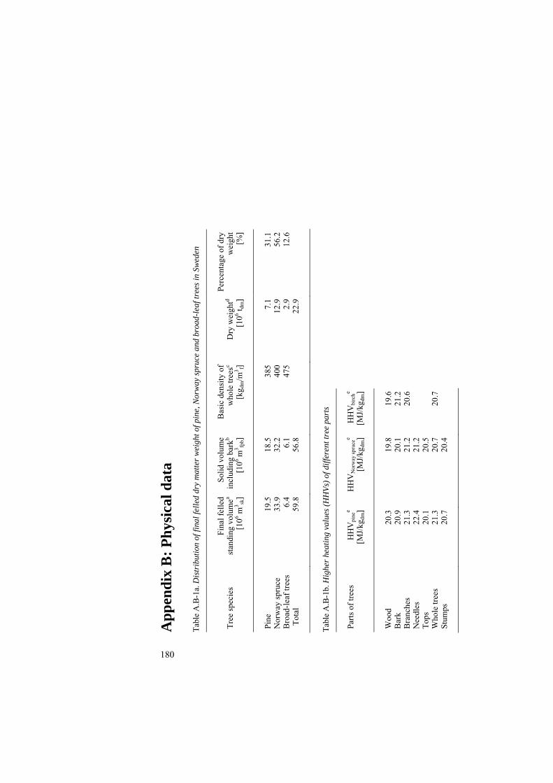
App

endi

x B

: Phy

sica

l dat

a T

able

A.B

-1a.

Dis

trib

utio

n of

fina

l fel

led

dry

mat

ter w

eigh

t of p

ine,

Nor

way

spru

ce a

nd b

road

-leaf

tree

s in

Swed

en

Tre

e sp

ecie

s

Fina

l fel

led

stan

ding

vol

umea

[106 m

3 sk]

Solid

vol

ume

incl

udin

g ba

rkb

[106 m

3 fpb]

Bas

ic d

ensi

ty o

f w

hole

tree

sc [k

g dm

/m3 f]

Dry

wei

ghtd

[106 t d

m]

Perc

enta

ge o

f dr

y w

eigh

t[%

]

Pi

ne

Nor

way

spr

uce

Bro

ad-l

eaf

tree

s T

otal

19.5

33.9 6.4

59.8

18.5

32.2 6.1

56.8

385

400

475

7.1

12.9 2.9

22.9

31.1

56.2

12.6

Tab

le A

.B-1

b. H

ighe

r hea

ting

valu

es (H

HVs

) of d

iffer

ent t

ree

part

s

Part

s of

tree

s

HH

Vpi

nee

[MJ/

kgdm

]H

HV

Nor

way

spr

ucee

[MJ/

kgdm

]H

HV

birc

he

[MJ/

kgdm

]

Woo

d B

ark

Bra

nche

s N

eedl

es

Top

s W

hole

tree

s St

umps

20.3

20.9

21.3

22.4

20.1

21.3

20.7

19.8

20.1

21.2

21.2

20.5

20.7

20.4

19.6

21.2

20.6

20.7

180

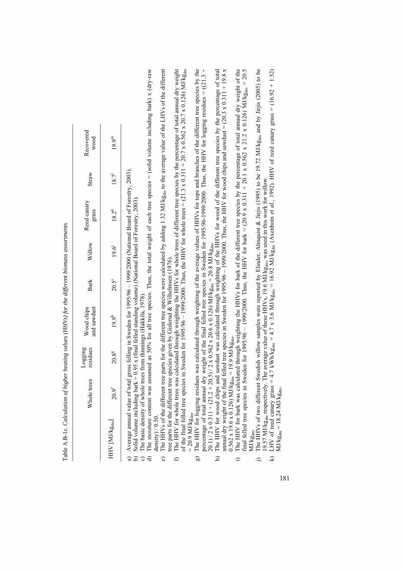
Tab

le A

.B-1

c. C

alcu

latio

n of

hig

her h

eatin

g va

lues

(HH

Vs) f

or th

e di

ffere

nt b

iom

ass a

ssor

tmen

ts

Who

le tr

ees

L

oggi

ng

resi

dues

W

ood

chip

s an

d sa

wdu

st

B

ark

W

illow

R

eed

cana

ry

gras

s

St

raw

R

ecov

ered

w

ood

HH

V [

MJ/

kgdm

]

20

.9f

20

.8g

19

.9h

20

.5i

19

.6j

18

.2k

18

.7l

19

.9m

a)

Ave

rage

ann

ual v

alue

of

tota

l gro

ss f

ellin

g in

Sw

eden

for

199

5/96

– 1

999/

2000

(N

atio

nal B

oard

of

Fore

stry

, 200

3).

b)

Solid

vol

ume

incl

udin

g ba

rk =

0.9

5 x

(fin

al f

elle

d st

andi

ng v

olum

e) (

Nat

iona

l Boa

rd o

f Fo

rest

ry, 2

003)

. c)

T

he b

asic

den

sity

of

who

le tr

ees

from

thin

ning

s (H

akki

la, 1

978)

. d)

T

he m

oist

ure

cont

ent

was

ass

umed

as

50%

for

all

tree

spe

cies

. T

hus,

the

tot

al w

eigh

t of

eac

h tr

ee s

peci

es =

(so

lid v

olum

e in

clud

ing

bark

) x

(dry

-raw

de

nsity

) / 0

.50.

e)

T

he H

HV

s of

the

diff

eren

t tre

e pa

rts

for

the

diff

eren

t tre

e sp

ecie

s w

ere

calc

ulat

ed b

y ad

ding

1.3

2 M

J/kg

dm to

the

aver

age

valu

e of

the

LH

Vs

of th

e di

ffer

ent

tree

par

ts f

or th

e di

ffer

ent t

ree

spec

ies

give

n by

Gis

leru

d &

Wilh

elm

sen

(197

6).

f)

The

HH

V f

or w

hole

tree

s w

as c

alcu

late

d th

roug

h w

eigh

ting

the

HH

Vs

for

who

le tr

ees

of d

iffe

rent

tree

spe

cies

by

the

perc

enta

ge o

f to

tal a

nnua

l dry

wei

ght

of th

e fi

nal f

elle

d tr

ee s

peci

es in

Sw

eden

for

199

5/96

– 1

999/

2000

. Thu

s, th

e H

HV

for

who

le tr

ees

= (

21.3

x 0

.311

+ 2

0.7

x 0.

562

x 20

.7 x

0.1

26)

MJ/

kgdm

=

20.

9 M

J/kg

dm.

g)

The

HH

V f

or l

oggi

ng r

esid

ues

was

cal

cula

ted

thro

ugh

wei

ghtin

g of

the

ave

rage

val

ues

of H

HV

s fo

r to

ps a

nd b

ranc

hes

of t

he d

iffe

rent

tre

e sp

ecie

s by

the

pe

rcen

tage

of

tota

l an

nual

dry

wei

ght

of t

he f

inal

fel

led

tree

spe

cies

in

Swed

en f

or 1

995/

96-1

999/

2000

. T

hus,

the

HH

V f

or l

oggi

ng r

esid

ues

= (

(21.

3 +

20

.1)

/ 2 x

0.3

11 +

(21

.2 +

20.

5) /

2 x

0.56

2 x

20.6

x 0

.126

) M

J/kg

dm =

20.

8 M

J/kg

dm.

h)

The

HH

V f

or w

ood

chip

s an

d sa

wdu

st w

as c

alcu

late

d th

roug

h w

eigh

ting

of t

he H

HV

s fo

r w

ood

of t

he d

iffe

rent

tre

e sp

ecie

s by

the

per

cent

age

of t

otal

an

nual

dry

wei

ght o

f th

e fi

nal f

elle

d tr

ee s

peci

es in

Sw

eden

for

199

5/96

– 1

999/

2000

. Thu

s, th

e H

HV

for

woo

d ch

ips

and

saw

dust

= (

20.3

x 0

.311

+ 1

9.8

x 0.

562

x 19

.6 x

0.1

26)

MJ/

kgdm

= 1

9.9

MJ/

kgdm

. i)

T

he H

HV

for

bar

k w

as c

alcu

late

d th

roug

h w

eigh

ting

the

HH

Vs

for

bark

of

the

diff

eren

t tr

ee s

peci

es b

y th

e pe

rcen

tage

of

tota

l an

nual

dry

wei

ght

of t

he

fina

l fe

lled

tree

spe

cies

in

Swed

en f

or 1

995/

96 –

199

9/20

00.

Thu

s, t

he H

HV

for

bar

k =

(20

.9 x

0.3

11 +

20.

1 x

0.56

2 x

21.2

x 0

.126

) M

J/kg

dm =

20.

5 M

J/kg

dm.

j)

The

HH

Vs

of t

wo

diff

eren

t Sw

edis

h w

illow

sam

ples

wer

e re

port

ed b

y E

linde

r, A

lmqu

ist

& J

irjis

(19

95)

to b

e 19

.72

MJ/

kgdm

and

by

Jirj

is (

2005

) to

be

19.5

7 M

J/kg

dm r

espe

ctiv

ely.

The

ave

rage

val

ue o

f th

ese

HH

Vs,

19.

6 M

J/kg

dm, w

as u

sed

in th

is w

ork

for

will

ow.

k)

LH

V o

f re

ed c

anar

y gr

ass

= 4

.7 k

Wh/

kgdm

= 4

.7 x

3.6

MJ/

kgdm

= 1

6.92

MJ/

kgdm

(A

xenb

om e

t al.,

199

2).

HH

V o

f re

ed c

anar

y gr

ass

= (

16.9

2 +

1.3

2)

MJ/

kgdm

= 1

8.24

MJ/

kgdm

.

181

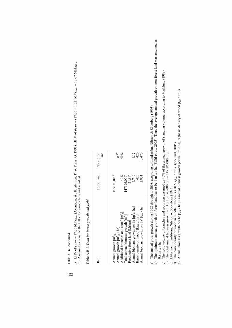
Tab

le A

.B-1

con

tinue

d l)

L

HV

of

stra

w =

17.

35 M

J/kg

dm (

Axe

nbom

, Å.,

Kri

sten

sen,

D. &

Pra

ks, O

. 199

1). H

HV

of

stra

w =

(17

.35

+ 1

.32)

MJ/

kgdm

= 1

8.67

MJ/

kgdm

. m

) A

ssum

ed a

s eq

ual t

o th

e H

HV

for

woo

d ch

ips

and

saw

dust

. T

able

A.B

-2. D

ata

for f

ores

t gro

wth

and

yie

ld

Item

Fo

rest

land

N

on-f

ores

t la

nd

Ann

ual g

row

th [

m3 sk

] A

nnua

l gro

wth

[m

3 sk /

ha]

Add

ition

al b

ranc

hes

and

root

sc [m

3 f] T

otal

ann

ual b

iom

ass

grow

th [

m3 f]

Prod

uctiv

e fo

rest

land

[M

(ha)

] A

nnua

l bio

mas

s gr

owth

per

ha

[m3 f

/ ha]

B

asic

den

sity

of

woo

df [kg

dm /

m3 f]

Ann

ual b

iom

ass

grow

th p

er h

ag [t d

m /

ha]

10

5140

,000

a

40%

1471

96,0

00d

21.8

4e

6.74

042

02.

831

0.

8b

40%

1.12 42

00.

470

a)

T

he a

nnua

l gro

ss g

row

th d

urin

g 19

98 th

roug

h to

200

8, a

ccor

ding

to L

unds

tröm

, Nils

son

& S

öder

berg

(19

93).

b)

T

he m

inim

um a

nnua

l gr

owth

on

fore

st l

and

has

to b

e 1

m3 sk

/ h

a (S

tåhl

et a

l., 2

003)

. Thu

s, t

he a

vera

ge a

nnua

l gr

owth

on

non-

fore

st l

and

was

ass

umed

as

0.8

m3 sk

/ ha

. c)

T

he s

olid

vol

ume

of b

ranc

hes

and

root

s w

as a

ssum

ed a

s 40

% o

f th

e an

nual

gro

wth

of

stan

ding

vol

ume,

acc

ordi

ng to

Mar

klun

d (1

988)

. d)

T

he to

tal a

nnua

l bio

mas

s gr

owth

= 1

.4 x

105

140,

000

m3 f =

147

196,

000

m3 f.

e)

Dat

a fr

om L

unds

tröm

, Nils

son

& S

öder

berg

(19

93).

f)

T

he b

asic

den

sity

of

woo

d in

mid

dle

Swed

en is

420

.5 k

g dm

/ m

3 f (B

jörk

lund

, 200

5).

g)

Ann

ual b

iom

ass

grow

th p

er h

a [t

dm /

ha]

= (

annu

al b

iom

ass

grow

th p

er h

a [m

3 f / h

a])

x (b

asic

den

sity

of

woo

d [t

dm /

m3 f])

182

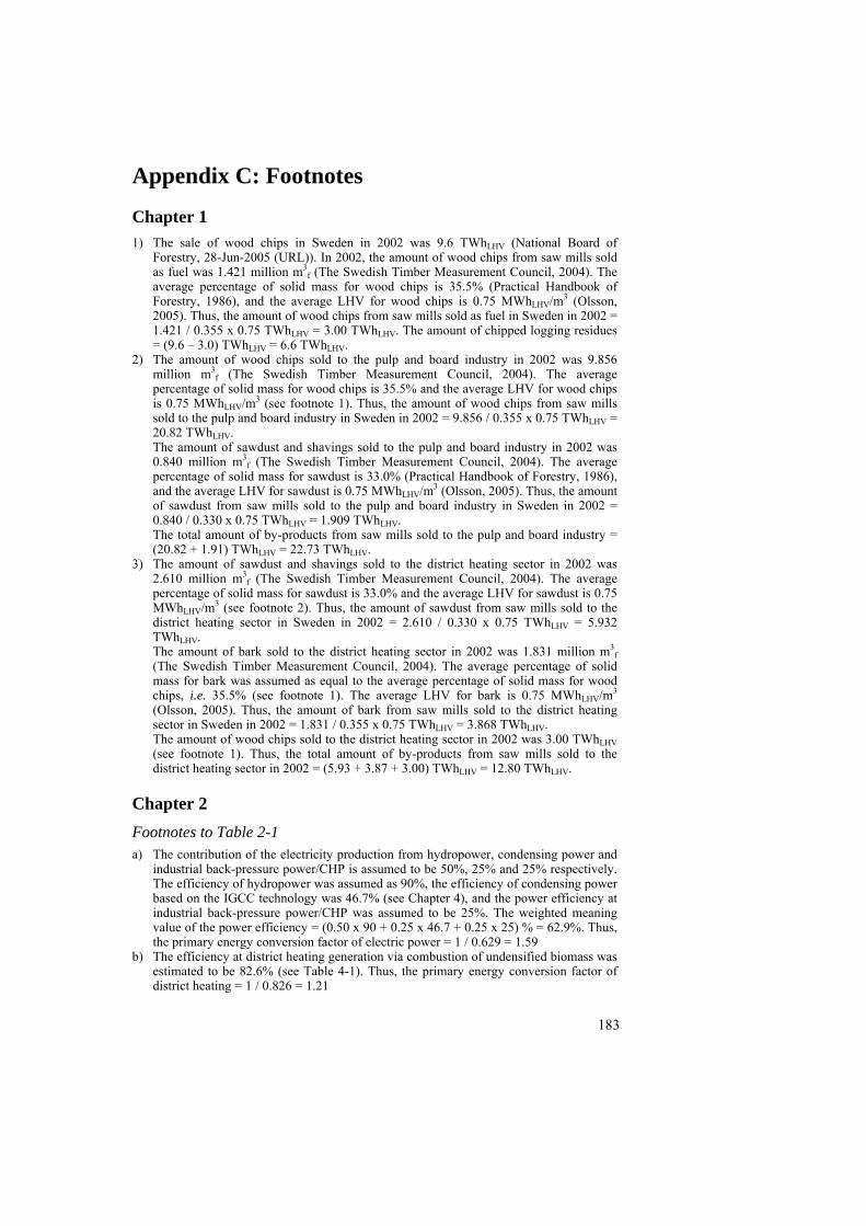
Appendix C: Footnotes Chapter 1 1) The sale of wood chips in Sweden in 2002 was 9.6 TWhLHV (National Board of

Forestry, 28-Jun-2005 (URL)). In 2002, the amount of wood chips from saw mills sold as fuel was 1.421 million m3

f (The Swedish Timber Measurement Council, 2004). The average percentage of solid mass for wood chips is 35.5% (Practical Handbook of Forestry, 1986), and the average LHV for wood chips is 0.75 MWhLHV/m3 (Olsson, 2005). Thus, the amount of wood chips from saw mills sold as fuel in Sweden in 2002 = 1.421 / 0.355 x 0.75 TWhLHV = 3.00 TWhLHV. The amount of chipped logging residues = (9.6 – 3.0) TWhLHV = 6.6 TWhLHV.

2) The amount of wood chips sold to the pulp and board industry in 2002 was 9.856 million m3

f (The Swedish Timber Measurement Council, 2004). The average percentage of solid mass for wood chips is 35.5% and the average LHV for wood chips is 0.75 MWhLHV/m3 (see footnote 1). Thus, the amount of wood chips from saw mills sold to the pulp and board industry in Sweden in 2002 = 9.856 / 0.355 x 0.75 TWhLHV = 20.82 TWhLHV. The amount of sawdust and shavings sold to the pulp and board industry in 2002 was 0.840 million m3

f (The Swedish Timber Measurement Council, 2004). The average percentage of solid mass for sawdust is 33.0% (Practical Handbook of Forestry, 1986), and the average LHV for sawdust is 0.75 MWhLHV/m3 (Olsson, 2005). Thus, the amount of sawdust from saw mills sold to the pulp and board industry in Sweden in 2002 = 0.840 / 0.330 x 0.75 TWhLHV = 1.909 TWhLHV. The total amount of by-products from saw mills sold to the pulp and board industry = (20.82 + 1.91) TWhLHV = 22.73 TWhLHV.

3) The amount of sawdust and shavings sold to the district heating sector in 2002 was 2.610 million m3

f (The Swedish Timber Measurement Council, 2004). The average percentage of solid mass for sawdust is 33.0% and the average LHV for sawdust is 0.75 MWhLHV/m3 (see footnote 2). Thus, the amount of sawdust from saw mills sold to the district heating sector in Sweden in 2002 = 2.610 / 0.330 x 0.75 TWhLHV = 5.932 TWhLHV. The amount of bark sold to the district heating sector in 2002 was 1.831 million m3

f (The Swedish Timber Measurement Council, 2004). The average percentage of solid mass for bark was assumed as equal to the average percentage of solid mass for wood chips, i.e. 35.5% (see footnote 1). The average LHV for bark is 0.75 MWhLHV/m3 (Olsson, 2005). Thus, the amount of bark from saw mills sold to the district heating sector in Sweden in 2002 = 1.831 / 0.355 x 0.75 TWhLHV = 3.868 TWhLHV. The amount of wood chips sold to the district heating sector in 2002 was 3.00 TWhLHV (see footnote 1). Thus, the total amount of by-products from saw mills sold to the district heating sector in 2002 = (5.93 + 3.87 + 3.00) TWhLHV = 12.80 TWhLHV.

Chapter 2 Footnotes to Table 2-1 a) The contribution of the electricity production from hydropower, condensing power and

industrial back-pressure power/CHP is assumed to be 50%, 25% and 25% respectively. The efficiency of hydropower was assumed as 90%, the efficiency of condensing power based on the IGCC technology was 46.7% (see Chapter 4), and the power efficiency at industrial back-pressure power/CHP was assumed to be 25%. The weighted meaning value of the power efficiency = (0.50 x 90 + 0.25 x 46.7 + 0.25 x 25) % = 62.9%. Thus, the primary energy conversion factor of electric power = 1 / 0.629 = 1.59

b) The efficiency at district heating generation via combustion of undensified biomass was estimated to be 82.6% (see Table 4-1). Thus, the primary energy conversion factor of district heating = 1 / 0.826 = 1.21

183

Table 2-1 continued c) Data from Johansson, Brandberg & Roth (1992). d) Assumed values. Chapter 3 1) Future estimated annual yields were 14.25 TWhLHV for short rotation forest and 4.75

TWhLHV reed canary grass (Börjesson et al., 1997). LHVs used for these estimates were 4.5 MWh/tdm for willow and 4.0 MWh/tdm for reed canary grass, and the moisture contents were 50% for willow and 15% for reed canary grass. Estimated annual yields were recalculated to energy amounts based on the HHVs of the two species: Willow: EHHV = 14.25 x (4.5 x 3.6 + 1.32 + 2.45) / 4.5 PJ = 63.29 PJ Reed canary grass: EHHV = 4.75 x (4.0 x 3.6 + 1.32 + 2.45 x (15 / (100 – 15))) / 4.0 PJ = 19.19 PJ The annual energy yields per hectare at present conditions are estimated by Börjesson (1996) to be 180 GJ/ha for willow and 120 GJ/ha for reed canary grass. Thus, an equation system may be defined for calculation of the area used for willow and reed canary grass cultivation respectively:

EWillow x AWillow = 63.29 x 1015 (1) EReed canary grass x AReed canary grass = 19.19 x 1015 (2) AWillow + AReed canary grass = 4.00 x 105 (3) EWillow/EReed canary grass = 3/2 (4)

(3) and (4) in (2) => 4.00 x 105 x AWillow x 2/3 x EWillow = 19.19 x 1015 (5)

(1) in (5) => (4.00 x 105 - AWillow) x 2/3 x 63.29 x 1015/ AWillow = 19.19 x 1015 => (4.00 x 105 - AWillow) x 4.219 x 1016 = AWillow x 19.19 x 1015 => 1.688 x 1022 – 4.219 x 1016 x AWillow = 19.19 x 1015 x AWillow => 6.138 x 106 x AWillow = 1.688 x 1022 => AWillow = 275 x 103 ha

(3) => AReed canary grass = 4.00 x 105 - AWillow => AReed canary grass = 125 x 103 ha

Footnotes to Table 3-1 a) Ecologically and technically available (Lönner et al., 1998). The HHV for logging

residues was calculated to be 20.8 MJ/kgdm, and the HHV for fuel wood and trees from early thinning was calculated to be 20.9 MJ/kgdm (Table A.B-1c).

b) The amount of forest raw materials and by-products in the scenarios were considered as the same percentage distribution as for Swedish forest industries in 2003, according to the statistics published by the Swedish Timber Measurement Council (see Table 3-4).

c) The HHV of wood chips was calculated to be 19.9 MJ/kgdm (Table A.B-1c). EHHV = 0.602 x 106 x 19.9 x 109 J = 11.98 PJ.

d) The HHV of sawdust was calculated to be 19.9 MJ/kgdm (Table A.B-1c). EHHV = 1.596 x 106 x 19.9 x 109 J = 31.76 PJ.

e) HHV of bark was calculated to be 20.5 MJ/kgdm (Table A.B-1c). EHHV = 2.576 x 106 x 20.5 x 109 J = 52.81 PJ.

f) See Table 3-4, footnote q. g) See Table 3-4, footnote r. h) Available land for energy crops was assumed as 15% of the total Swedish arable land

area = 400,000 ha with 275,000 ha for willow farming and 125,000 ha for reed canary grass farming (Börjesson et al., 1997).

i) The yield per a 22-year rotation period was assumed as 183 tdm per hectare (Swedish Energy Agency, 2003c).

j) See Table A.B-1c.

184

Table 3-1 continued k) The yield was based on field experiments performed in Sweden during the 1990s and

was estimated to be 7.5 tdm/(ha x year) in nine years during an 11-year rotation period (Olsson et al., 2001). Average harvest = 9/11 x 7.5 = 6.136 tdm/ha per year.

l) See Table A.B-1c. m) The annual yield on a national level was estimated to be 8 TWhLHV (Börjesson et al.,

1997). LHV of straw with 15% moisture content is 4.0 MWh/tdm (Börjesson, 2001). n) See Table A.B-1c. o) Based on data from Lönner et al. (1998). The HHV was assumed equal to HHVs for

wood chips and sawdust, i.e. 19.9 MJ/kgdm. Footnotes to Table 3-3 a) Data from National Board of Forestry (2004). The conditions were assumed equal to the

conditions in 2002. b) The average annual percentage of the final felled area, regenerated by planting and

prepared with annual scarification during 2001 - 2003 was 88% (National Board of Forestry, 2004). The annual final felled area = 222,300 ha (see Table 3-2). Thus, the area of scarification = 0.88 x 222,300 ha/year = 195,624 ha/year.

c) The percentage of the final felled area regenerated by planting and sowing was estimated to be approximately 80% in 2003 (National Board of Forestry, 2004). The annual final felled area = 222,300 ha (see Table 3-2). Thus, the area regenerated by planting and sowing = 0.80 x 222,300 ha/year = 177,840 ha/year.

d) The annual precommercial thinning area was assumed equal to the annual final felling area, i.e. 222,300 ha/year.

e) The annual average fertilized forest area during 1998 - 2002 was 20,460 ha (National Board of Forestry, 2004). The annual fertilized forest area was assumed as 20,000 ha.

f) Tests performed with ash recirculation are done after thinning (Gunnarsson, 2004). Thus, the annual forest area treated by ash recirculation was assumed equal to the annual thinning area, i.e. 217,600 ha (see Table 3-2).

g) The average cost for new ditches in 1995, 1998, 1999 and 2000 was 7.01 SEK/m and the average annual maintenance costs for the same years were 11.344 MSEK respectively (National Board of Forestry, 2004). The annual length of new ditches was assumed equal to the length of new ditches in 2002, being 75 km (National Board of Forestry, 2004). The average cost for new ditches was assumed as 7.00 SEK/m and the annual maintenance cost was assumed as 10.0 MSEK respectively. Thus, the total annual cost for forest drainage = 75,000 x 7.00 + 10.0 x 106 SEK = 10.525 MSEK.

h) The total annual cost for forest roads was assumed equal to the total cost for forest roads in 2002, being 727.308 MSEK (National Board of Forestry, 2004).

Footnotes to Table 3-4 a) Data from Björklund (2005). b) The distribution of the raw material to different purposes was assumed as proportional

to the distribution in 2003. c) The solid volume of wood used as saw logs was assumed equal to the solid volume of

wood used as saw logs in cases 1 - 2. d) The solid volume of wood used as pulpwood was assumed to be half of the solid

volume of wood used as pulp wood in cases 1 - 2. e) The solid volume of wood used as raw material in board industries was assumed equal

to the solid volume of wood used as raw material in board industries in cases 1 - 2. f) The total volume of wood received at later thinning and final felling, according to AVB

92 = (16.533 + 59.982) x 106 m3sk = 76.515 x 106 m3

sk = 76.515 x 0.95 x 106 m3fpb =

72.689 x 106 m3fpb.

g) Data regarding bark, wood chips, sawdust, and shavings from The Swedish Timber Measurement Council (2004) and Björklund (2005).

h) Based on roundwood consumption with bark.

185

Table 3-4 continued i) The volume distribution of products was assumed as proportional to the volume

distribution of products in 2003. j) The basic density of bark = 333.0 kgdm/m3

f (Björklund, 2005). The average basic density of wood, wood chips, sawdust and shavings was calculated through weighting of the basic density of wood in northern, central and southern Sweden by the roundwood consumption in the three regions. The average basic density of wood in northern Sweden is 403.0 kgdm/m3

f, 420.5 kgdm/m3f in central Sweden and 416.1

kgdm/m3f in southern Sweden, whereas roundwood consumption is 10.28 million m3

fub (northern), 8.11 million m3

fub (central) and 16.73 million m3fub (southern) (Björklund,

2005). Thus, the weighted basic density of wood, wood chips, sawdust and shavings in Sweden = (403.0 x 10.28 + 420.5 x 8.11 + 416.1 x 16.73) / (10.28 + 8.11 + 16.73) kgdm/m3

f = 413.3 kgdm/m3f.

k) The solid volume of wood used at saw mills = 35.392 million m3fub (The Swedish

Timber Measurement Council, 2004). The solid volume of sawn wood = the solid volume of wood consumed - (bark + wood chips + sawdust + shavings). Thus, the solid volume of sawn wood = 35.392 - (3.788 + 12.164 + 4.590) million m3

f = 14.850 million m3

f. l) The difference in volumes of products in the scenarios compared to the volumes of

products in 2003 were assumed to be proportional to the difference in total volume of wood used as raw material in the scenarios, compared to the total volume of wood used as raw material in 2003.

m) The weighted basic density of wood in Sweden = 413.3 kgdm/m3f (see footnote j).

n) The sum of the weight of consumed roundwood under bark and the weight of bark received.

o) The volume of consumed roundwood with bark minus the volume of bark received. p) The average basic density of wood = 413.3 kgdm/m3

f (see footnote i). Thus, the weight of consumed roundwood under bark = 28.162 x 413.3 x 10-3 Mtdm = 11.638 Mtdm.

q) The mass ratio of pulp produced and raw material consumed was assumed proportional to the mass ratio in 2003. The dry matter of pulp produced in 2003 was 10.571 tdm (Björklund, 2005). The solid volume of raw material used for pulp production in 2003 was 45.006 million m3

f. The average basic density of wood = 413.3 kgdm/m3f (see

footnote i). Thus, the dry matter weight of the raw material used in 2003 = 45.006 x 413.3 x 10-3 Mtdm = 18.599 Mtdm. The dry matter of pulp produced in scenarios ‘heat’ and ‘electricity’ = 16.093 x 10.571 / 18.599 Mtdm = 9.146 Mtdm.

r) The bark percentage of the roundwood was assumed as 12.0%. Thus, the solid volume of bark received = 0.12 x 32.002 million m3

fs) The basic density of bark = 333.0 kg

= 3.840 million m3f.

dm/m3f (see footnote i). Thus, the weight of bark

received = 3.840 x 333.0 x 10-3 Mtdm = 1.279 Mtdm. t) Calculated as the difference between the total amount of raw material consumed and the

amount of pulp produced. u) HHV of the wood components in black liquor was assumed as 22.6 MJ/kgdm, based on

the assumption that 42% of the wood is cellulose with 17.6 MJ/kg and the HHV of wood is 20.5 MJ/kg. The cellulose goes into the pulp and the HHV of the remaining wood components in the black liquor is = (20.5 – 0.42 x 17.6) / 0.58 MJ/kgdm = 22.6 MJ/kgdm. Thus, the energy amount of the total black liquor amount received = 6.947 x 22.6 PJ = 157.0 PJ.

v) All volumes, dry matter weights and energy amounts of raw materials and products were half of the amounts in scenarios ‘heat’ and ‘electricity’.

Footnotes to Table 3-7 a) The dry matter weight of stumps per m3

sk final felled roundwood was estimated by Marklund (1981) to be 106 kgdm/m3

sk. The total annual volume of roundwood at final felling during 1998 – 2008 is estimated by Lundström, Nilsson & Söderberg (1993) to be 59.982 million m3

sk. The total dry matter weight of stumps as a function of the final felled volume = 0.106 x 59.982 Mtdm = 6.358 Mtdm. Danielsson & Nilsson (1977)

186

Table 3-7 continued

estimate that 55% of the total stump volume may be available after reduction due to severe terrain, nutrient-poor lands, small final felled areas, small stumps and stumps from broad-leaf trees. Thus, the annual dry matter weight of stumps available after these reductions = 0.55 x 6.358 Mtdm = 3.497 Mtdm.

b) The weighted HHV of stumps from pine and Norway spruce = (20.7 x (0.311 / (1 – 0.126) + 20.4 x (0.562 / (1 – 0.126) MJ/kgdm = 20.5 MJ/kgdm (see Tables A.B-1a and A.B-1b). Estumps available = 3.497 x 20.5 PJ = 71.69 PJ.

c) The potential amount of peat to be used for energy purposes in Sweden is 6.0 TWhLHV (Ministry of Industry, Employment and Communication, 2002). The ratio of HHV and LHV of peat was assumed as equal to the ratio of the HHV and LHV for logging residues with 50% moisture content. HHV for logging residues = 20.8 MJ/kgdm (Table A.B-1c) and LHVlogging residues, MC = 50% = 17.0 MJ/kgdm (see Table 5-4, footnote h). Thus, the corresponding amount of peat based on the HHV = 6.0 x 20.8 / 17.0 TWh = 7.3 TWh.

d) The combustion of waste in waste incineration boilers in 1998 was 2.2 Mt (The Swedish Association of Waste Management, 1998). The lack of incineration capacity in 2002 is estimated by Profu (2001a) to be about 1.3 Mt. Thus, the total potential amount of combustible waste = (2.2 + 1.3) Mt = 3.5 Mt. The moisture content of household waste is 25 – 35% and commercial waste is 10 – 20% (Hietanen, 2002). The average moisture content was assumed as 25%. Thus, the total potential dry matter weight of combustible waste =3.5 x 0.75 Mtdm = 2.62 Mtdm.

e) The use of waste in district heating plants in 1998 was 5.1 TWhLHV (Swedish Energy Agency, 2004b). The energy content of the total potential amount of combustible waste = (2.2 + 1.3) / 2.2 x 5.1 TWhLHV = 8.11 TWhLHV. It was assumed that the ratio of HHV and LHV of the combustible waste was equal to the ratio of the HHV and LHV for wood chips with 25% moisture content. HHV for wood chips = 19.9 MJ/kgdm (Table A.B-1c). LHVwood chips, MC = 25% = 19.9 – 1.32 – 2.45 x 25 / (100 – 25) MJ/kgdm = 17.8 MJ/kgdm. Thus, the corresponding potential amount of combustible waste based on the HHV = 8.11 x 19.9 / 17.8 TWh = 9.07 TWh.

f) The total biogas potential at 2008 is estimated to be 17.37 TWhLHV, where 7.14 TWhLHV is derived from straw (Nordberg et al., 1998). The biogas potential in 2008 excluding straw as a raw material = (17.37 – 7.14) TWhLHV = 10.23 TWhLHV. The ratio of HHV/LHV was assumed as equal to the corresponding ratio for natural gas from Frigg, being 1.0986 (see Table 5-1, footnote c). Thus, the biogas potential for 2008 excluding straw as raw material, based on the HHV = 10.23 x 1.0986 TWh = 11.24 TWh.

Chapter 4 Footnotes to Table 4-1 a) Based on data for firing of wood or pellets in a domestic boiler. Values to the left of the

slash are for wood firing, whereas values to the right of the slash are for pellet firing. b) Based on data for the district heating plant fired with undensified biomass in Knivsta,

Sweden, and the pellet-fired district heating plant in Jönköping, Sweden. Values to the left of the slash are for the boiler fired with undensified biomass, whereas values to the right of the slash are for the pellet boiler.

c) Based on data for the biomass-fired circulated fluidised bed in Västerås, Sweden. d) Based on data for the IGCC demonstration plant in Värnamo, Sweden (Sydkraft, 2000). e) Hydrogen production. The Battelle Columbus gasifier is used for production of

synthesis gas. Based on data from Hamelinck & Faaij (2002). f) Methanol production. The Battelle Columbus gasifier is used for production of

synthesis gas. Based on data from Hamelinck & Faaij (2002). g) The investment cost of a boiler for wood firing and accumulator tank, including

assembling costs was 70,000 SEK in 2002 (Jansson, 2004b; Swedish Energy Agency, 2002). Thus, the investment cost = 70,000 / 9.119 € = 7676 € = 0.0077 M€.

187

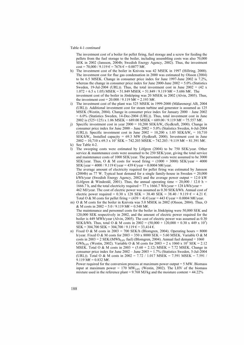
Table 4-1 continued

The investment cost of a boiler for pellet firing, fuel storage and a screw for feeding the pellets from the fuel storage to the boiler, including assembling costs was also 70,000 SEK in 2002 (Jansson, 2004b; Swedish Energy Agency, 2002). Thus, the investment cost = 70,000 / 9.119 € = 7676 € = 0.0077 M€.

h) The investment cost of the boiler in Knivsta was 42 MSEK in 1997 (Hillring, 2000). The investment cost for flue gas condensation in 2000 was estimated by Olsson (2004) to be 6.5 MSEK. Change in consumer price index for June 1997-June 2002 is 7.2%, whereas the change in consumer price index for June 2000-June 2002 = 5.0% (Statistics Sweden, 19-Jul-2004 (URL)). Thus, the total investment cost in June 2002 = (42 x 1.072 + 6.5 x 1.05) MSEK = 51.849 MSEK = 51.849 / 9.119 M€ = 5.686 M€. The investment cost of the boiler in Jönköping was 20 MSEK in 2002 (Alvin, 2005). Thus, the investment cost = 20.000 / 9.119 M€ = 2.193 M€.

i) The investment cost of the plant was 525 MSEK in 1999-2000 (Mälarenergi AB, 2004 (URL)). Additional investment cost for steam turbine and generator is assumed as 125 MSEK (Westin, 2004). Change in consumer price index for January 2000 – June 2002 = 6.0% (Statistics Sweden, 14-Dec-2004 (URL)). Thus, total investment cost in June 2002 is (525+125) x 1.06 MSEK = 689.00 MSEK = 689.00 / 9.119 M€ = 75.557 M€.

j) Specific investment cost in year 2000 = 10,200 SEK/kWe (Sydkraft, 2000). Change in consumer price index for June 2000 – June 2002 = 5.0% (Statistics Sweden, 6-Jul-2004 (URL)). Specific investment cost in June 2002 = 10,200 x 1.05 SEK/kWe = 10,710 SEK/kWe. Installed capacity = 69.3 MW (Sydkraft, 2000). Investment cost in June 2002 = 10,710 x 69.3 x 103 SEK = 742.203 MSEK = 742.203 / 9.119 M€ = 81.391 M€.

k) See Table 4-2. l) The sweeping costs were estimated by Löfgren (2004) to be 750 SEK/year. Other

service & maintenance costs were assumed to be 250 SEK/year, giving the total service and maintenance costs of 1000 SEK/year. The personnel costs were assumed to be 3000 SEK/year. Thus, O & M costs for wood firing = (1000 + 3000) SEK/year = 4000 SEK/year = 4000 / 9.119 €/year = 439 €/year = 0.0004 M€/year. The average amount of electricity required for pellet firing was estimated by Jansson (2004b) as 77 W. Typical heat demand for a single family-house in Sweden = 20,000 kWh/year (Swedish Energy Agency, 2002) and the average power output = 12.0 kW (Löfgren & Windestål, 2001). Thus, the annual operating time = 20,000 / 12.0 h = 1666.7 h, and the total electricity required = 77 x 1666.7 Wh/year = 128 kWh/year = 462 MJ/year. The cost of electric power was assumed as 0.30 SEK/kWh. Annual cost of electric power required = 0.30 x 128 SEK = 38.40 SEK = 38.40 / 9.119 € = 4.21 €. Total O & M costs for pellet firing = (439 + 4) €/year = 443 €/year = 0.0004 M€/year.

m) O & M costs for the boiler in Knivsta was 5.0 MSEK in 2002 (Olsson, 2004). Thus, O & M costs in 2002 = 5.0 / 9.119 M€ = 0.548 M€. The maintenance and personnel costs for the boiler in Jönköping were 50,000 SEK and 120,000 SEK respectively in 2002, and the amount of electric power required for the boiler is 449 MWh/year (Alvin, 2005). The cost of electric power was assumed as 0.30 SEK/kWh. Thus, total O & M costs in 2002 = (50,000 + 120,000 + 0.30 x 449 x 103) SEK = 304,700 SEK = 304,700 / 9.119 € = 33,414 €.

n) Fixed O & M costs in 2003 = 700 SEK/h (Blomgren, 2004). Operating hours = 8000 h/year. Fixed O & M costs for 2003 = 350 x 8000 SEK = 5.60 MSEK. Variable O & M costs in 2003 = 2 SEK/(MWhLHV fuel) (Blomgren, 2004). Annual fuel demand = 1060 GWhLHV (Westin, 2002). Variable O & M costs for 2003 = 2 x 1060 x 103 SEK = 2.12 MSEK. Total O & M costs in 2003 = (5.60 + 2.12) MSEK = 7.72 MSEK. Change in consumer price index for June 2002 – June 2003 = 1.7% (Statistics Sweden, 5-Jul-2004 (URL)). Total O & M costs in 2002 = 7.72 / 1.017 MSEK = 7.591 MSEK = 7.591 / 9.119 M€ = 0.832 M€. Power required for the conversion process at maximum power output = 5 MW. Biomass input at maximum power = 170 MWLHV (Westin, 2002). The LHV of the biomass mixture used in the reference plant = 9.768 MJ/kg and the moisture content = 44.22%

188

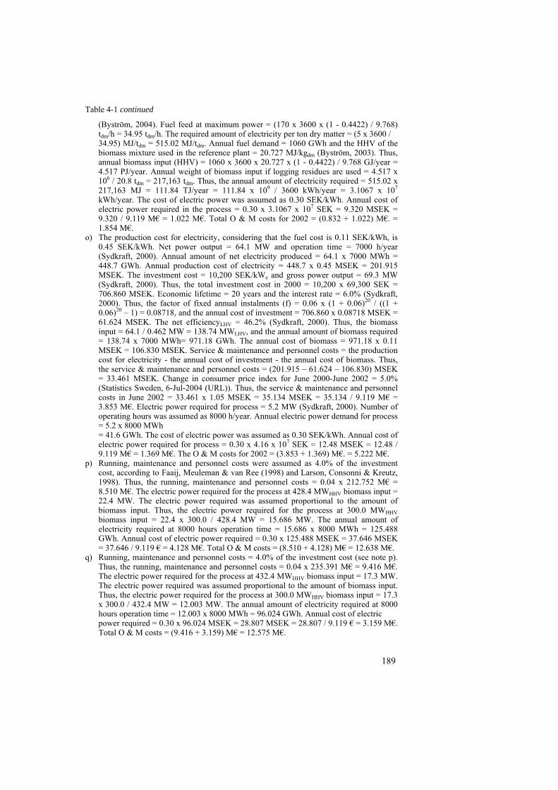
Table 4-1 continued

(Byström, 2004). Fuel feed at maximum power = (170 x 3600 x (1 - 0.4422) / 9.768) tdm/h = 34.95 tdm/h. The required amount of electricity per ton dry matter = (5 x 3600 / 34.95) MJ/tdm = 515.02 MJ/tdm. Annual fuel demand = 1060 GWh and the HHV of the biomass mixture used in the reference plant = 20.727 MJ/kgdm (Byström, 2003). Thus, annual biomass input (HHV) = 1060 x 3600 x 20.727 x (1 - 0.4422) / 9.768 GJ/year = 4.517 PJ/year. Annual weight of biomass input if logging residues are used = 4.517 x 106 / 20.8 tdm = 217,163 tdm. Thus, the annual amount of electricity required = 515.02 x 217,163 MJ = 111.84 TJ/year = 111.84 x 109 / 3600 kWh/year = 3.1067 x 107 kWh/year. The cost of electric power was assumed as 0.30 SEK/kWh. Annual cost of electric power required in the process = 0.30 x 3.1067 x 107 SEK = 9.320 MSEK = 9.320 / 9.119 M€ = 1.022 M€. Total O & M costs for 2002 = (0.832 + 1.022) M€. = 1.854 M€.

o) The production cost for electricity, considering that the fuel cost is 0.11 SEK/kWh, is 0.45 SEK/kWh. Net power output = 64.1 MW and operation time = 7000 h/year (Sydkraft, 2000). Annual amount of net electricity produced = 64.1 x 7000 MWh = 448.7 GWh. Annual production cost of electricity = 448.7 x 0.45 MSEK = 201.915 MSEK. The investment cost = 10,200 SEK/kWe and gross power output = 69.3 MW (Sydkraft, 2000). Thus, the total investment cost in 2000 = 10,200 x 69,300 SEK = 706.860 MSEK. Economic lifetime = 20 years and the interest rate = 6.0% (Sydkraft, 2000). Thus, the factor of fixed annual instalments (f) = 0.06 x (1 + 0.06)20 / ((1 + 0.06)20 – 1) = 0.08718, and the annual cost of investment = 706.860 x 0.08718 MSEK = 61.624 MSEK. The net efficiencyLHV = 46.2% (Sydkraft, 2000). Thus, the biomass input = 64.1 / 0.462 MW = 138.74 MWLHV, and the annual amount of biomass required = 138.74 x 7000 MWh= 971.18 GWh. The annual cost of biomass = 971.18 x 0.11 MSEK = 106.830 MSEK. Service & maintenance and personnel costs = the production cost for electricity - the annual cost of investment - the annual cost of biomass. Thus, the service & maintenance and personnel costs = (201.915 – 61.624 – 106.830) MSEK = 33.461 MSEK. Change in consumer price index for June 2000-June 2002 = 5.0% (Statistics Sweden, 6-Jul-2004 (URL)). Thus, the service & maintenance and personnel costs in June 2002 = 33.461 x 1.05 MSEK = 35.134 MSEK = 35.134 / 9.119 M€ = 3.853 M€. Electric power required for process = 5.2 MW (Sydkraft, 2000). Number of operating hours was assumed as 8000 h/year. Annual electric power demand for process = 5.2 x 8000 MWh = 41.6 GWh. The cost of electric power was assumed as 0.30 SEK/kWh. Annual cost of electric power required for process = 0.30 x 4.16 x 107 SEK = 12.48 MSEK = 12.48 / 9.119 M€ = 1.369 M€. The O & M costs for 2002 = (3.853 + 1.369) M€. = 5.222 M€.

p) Running, maintenance and personnel costs were assumed as 4.0% of the investment cost, according to Faaij, Meuleman & van Ree (1998) and Larson, Consonni & Kreutz, 1998). Thus, the running, maintenance and personnel costs = 0.04 x 212.752 M€ = 8.510 M€. The electric power required for the process at 428.4 MWHHV biomass input = 22.4 MW. The electric power required was assumed proportional to the amount of biomass input. Thus, the electric power required for the process at 300.0 MWHHV biomass input = 22.4 x 300.0 / 428.4 MW = 15.686 MW. The annual amount of electricity required at 8000 hours operation time = 15.686 x 8000 MWh = 125.488 GWh. Annual cost of electric power required = 0.30 x 125.488 MSEK = 37.646 MSEK = 37.646 / 9.119 € = 4.128 M€. Total O & M costs = (8.510 + 4.128) M€ = 12.638 M€.

q) Running, maintenance and personnel costs = 4.0% of the investment cost (see note p). Thus, the running, maintenance and personnel costs = 0.04 x 235.391 M€ = 9.416 M€. The electric power required for the process at 432.4 MWHHV biomass input = 17.3 MW. The electric power required was assumed proportional to the amount of biomass input. Thus, the electric power required for the process at 300.0 MWHHV biomass input = 17.3 x 300.0 / 432.4 MW = 12.003 MW. The annual amount of electricity required at 8000 hours operation time = 12.003 x 8000 MWh = 96.024 GWh. Annual cost of electric power required = 0.30 x 96.024 MSEK = 28.807 MSEK = 28.807 / 9.119 € = 3.159 M€. Total O & M costs = (9.416 + 3.159) M€ = 12.575 M€.

189

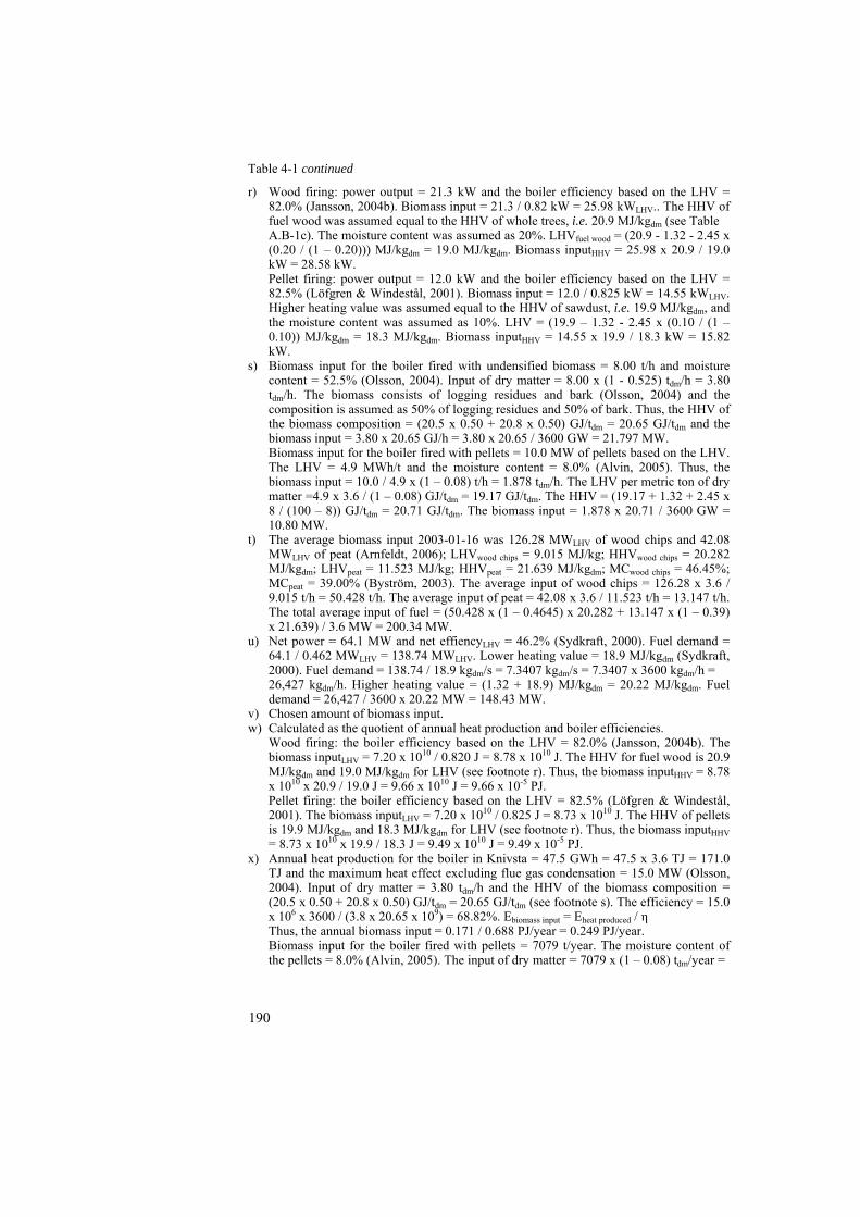
Table 4-1 continued r) Wood firing: power output = 21.3 kW and the boiler efficiency based on the LHV =

82.0% (Jansson, 2004b). Biomass input = 21.3 / 0.82 kW = 25.98 kWLHV.. The HHV of fuel wood was assumed equal to the HHV of whole trees, i.e. 20.9 MJ/kgdm (see Table A.B-1c). The moisture content was assumed as 20%. LHVfuel wood = (20.9 - 1.32 - 2.45 x (0.20 / (1 – 0.20))) MJ/kgdm = 19.0 MJ/kgdm. Biomass inputHHV = 25.98 x 20.9 / 19.0 kW = 28.58 kW. Pellet firing: power output = 12.0 kW and the boiler efficiency based on the LHV = 82.5% (Löfgren & Windestål, 2001). Biomass input = 12.0 / 0.825 kW = 14.55 kWLHV. Higher heating value was assumed equal to the HHV of sawdust, i.e. 19.9 MJ/kgdm, and the moisture content was assumed as 10%. LHV = (19.9 – 1.32 - 2.45 x (0.10 / (1 – 0.10)) MJ/kgdm = 18.3 MJ/kgdm. Biomass inputHHV = 14.55 x 19.9 / 18.3 kW = 15.82 kW.

s) Biomass input for the boiler fired with undensified biomass = 8.00 t/h and moisture content = 52.5% (Olsson, 2004). Input of dry matter = 8.00 x (1 - 0.525) tdm/h = 3.80 tdm/h. The biomass consists of logging residues and bark (Olsson, 2004) and the composition is assumed as 50% of logging residues and 50% of bark. Thus, the HHV of the biomass composition = (20.5 x 0.50 + 20.8 x 0.50) GJ/tdm = 20.65 GJ/tdm and the biomass input = 3.80 x 20.65 GJ/h = 3.80 x 20.65 / 3600 GW = 21.797 MW. Biomass input for the boiler fired with pellets = 10.0 MW of pellets based on the LHV. The LHV = 4.9 MWh/t and the moisture content = 8.0% (Alvin, 2005). Thus, the biomass input = 10.0 / 4.9 x (1 – 0.08) t/h = 1.878 tdm/h. The LHV per metric ton of dry matter =4.9 x 3.6 / (1 – 0.08) GJ/tdm = 19.17 GJ/tdm. The HHV = (19.17 + 1.32 + 2.45 x 8 / (100 – 8)) GJ/tdm = 20.71 GJ/tdm. The biomass input = 1.878 x 20.71 / 3600 GW = 10.80 MW.

t) The average biomass input 2003-01-16 was 126.28 MWLHV of wood chips and 42.08 MWLHV of peat (Arnfeldt, 2006); LHVwood chips = 9.015 MJ/kg; HHVwood chips = 20.282 MJ/kgdm; LHVpeat = 11.523 MJ/kg; HHVpeat = 21.639 MJ/kgdm; MCwood chips = 46.45%; MCpeat = 39.00% (Byström, 2003). The average input of wood chips = 126.28 x 3.6 / 9.015 t/h = 50.428 t/h. The average input of peat = 42.08 x 3.6 / 11.523 t/h = 13.147 t/h. The total average input of fuel = (50.428 x (1 – 0.4645) x 20.282 + 13.147 x (1 – 0.39) x 21.639) / 3.6 MW = 200.34 MW.

u) Net power = 64.1 MW and net effiencyLHV = 46.2% (Sydkraft, 2000). Fuel demand = 64.1 / 0.462 MWLHV = 138.74 MWLHV. Lower heating value = 18.9 MJ/kgdm (Sydkraft, 2000). Fuel demand = 138.74 / 18.9 kgdm/s = 7.3407 kgdm/s = 7.3407 x 3600 kgdm/h = 26,427 kgdm/h. Higher heating value = (1.32 + 18.9) MJ/kgdm = 20.22 MJ/kgdm. Fuel demand = 26,427 / 3600 x 20.22 MW = 148.43 MW.

v) Chosen amount of biomass input. w) Calculated as the quotient of annual heat production and boiler efficiencies.

Wood firing: the boiler efficiency based on the LHV = 82.0% (Jansson, 2004b). The biomass inputLHV = 7.20 x 1010 / 0.820 J = 8.78 x 1010 J. The HHV for fuel wood is 20.9 MJ/kgdm and 19.0 MJ/kgdm for LHV (see footnote r). Thus, the biomass inputHHV = 8.78 x 1010 x 20.9 / 19.0 J = 9.66 x 1010 J = 9.66 x 10-5 PJ. Pellet firing: the boiler efficiency based on the LHV = 82.5% (Löfgren & Windestål, 2001). The biomass inputLHV = 7.20 x 1010 / 0.825 J = 8.73 x 1010 J. The HHV of pellets is 19.9 MJ/kgdm and 18.3 MJ/kgdm for LHV (see footnote r). Thus, the biomass inputHHV = 8.73 x 1010 x 19.9 / 18.3 J = 9.49 x 1010 J = 9.49 x 10-5 PJ.

x) Annual heat production for the boiler in Knivsta = 47.5 GWh = 47.5 x 3.6 TJ = 171.0 TJ and the maximum heat effect excluding flue gas condensation = 15.0 MW (Olsson, 2004). Input of dry matter = 3.80 tdm/h and the HHV of the biomass composition = (20.5 x 0.50 + 20.8 x 0.50) GJ/tdm = 20.65 GJ/tdm (see footnote s). The efficiency = 15.0 x 106 x 3600 / (3.8 x 20.65 x 109) = 68.82%. Ebiomass input = Eheat produced / η Thus, the annual biomass input = 0.171 / 0.688 PJ/year = 0.249 PJ/year. Biomass input for the boiler fired with pellets = 7079 t/year. The moisture content of the pellets = 8.0% (Alvin, 2005). The input of dry matter = 7079 x (1 – 0.08) tdm/year =

190

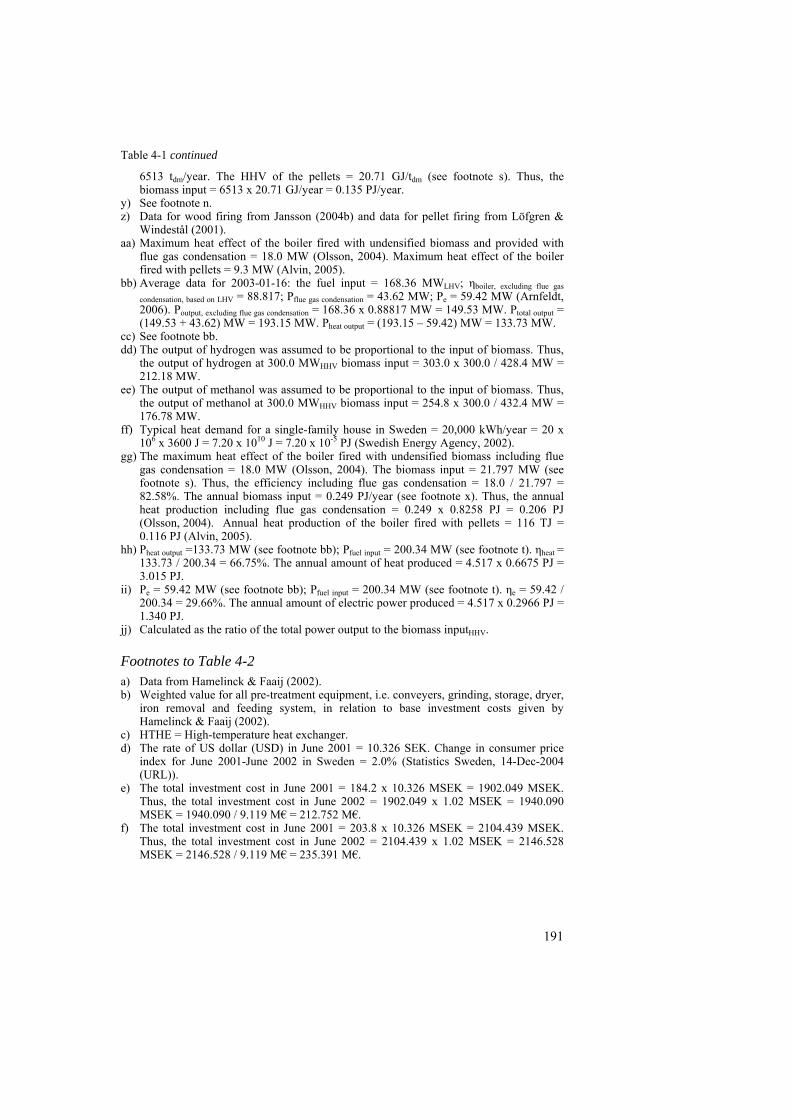
Table 4-1 continued

6513 tdm/year. The HHV of the pellets = 20.71 GJ/tdm (see footnote s). Thus, the biomass input = 6513 x 20.71 GJ/year = 0.135 PJ/year.

y) See footnote n. z) Data for wood firing from Jansson (2004b) and data for pellet firing from Löfgren &

Windestål (2001). aa) Maximum heat effect of the boiler fired with undensified biomass and provided with

flue gas condensation = 18.0 MW (Olsson, 2004). Maximum heat effect of the boiler fired with pellets = 9.3 MW (Alvin, 2005).

bb) Average data for 2003-01-16: the fuel input = 168.36 MWLHV; ηboiler, excluding flue gas

condensation, based on LHV = 88.817; Pflue gas condensation = 43.62 MW; Pe = 59.42 MW (Arnfeldt, 2006). Poutput, excluding flue gas condensation = 168.36 x 0.88817 MW = 149.53 MW. Ptotal output = (149.53 + 43.62) MW = 193.15 MW. Pheat output = (193.15 – 59.42) MW = 133.73 MW.

cc) See footnote bb. dd) The output of hydrogen was assumed to be proportional to the input of biomass. Thus,

the output of hydrogen at 300.0 MWHHV biomass input = 303.0 x 300.0 / 428.4 MW = 212.18 MW.

ee) The output of methanol was assumed to be proportional to the input of biomass. Thus, the output of methanol at 300.0 MWHHV biomass input = 254.8 x 300.0 / 432.4 MW = 176.78 MW.

ff) Typical heat demand for a single-family house in Sweden = 20,000 kWh/year = 20 x 106 x 3600 J = 7.20 x 1010 J = 7.20 x 10-5 PJ (Swedish Energy Agency, 2002).

gg) The maximum heat effect of the boiler fired with undensified biomass including flue gas condensation = 18.0 MW (Olsson, 2004). The biomass input = 21.797 MW (see footnote s). Thus, the efficiency including flue gas condensation = 18.0 / 21.797 = 82.58%. The annual biomass input = 0.249 PJ/year (see footnote x). Thus, the annual heat production including flue gas condensation = 0.249 x 0.8258 PJ = 0.206 PJ (Olsson, 2004). Annual heat production of the boiler fired with pellets = 116 TJ = 0.116 PJ (Alvin, 2005).

hh) Pheat output =133.73 MW (see footnote bb); Pfuel input = 200.34 MW (see footnote t). ηheat = 133.73 / 200.34 = 66.75%. The annual amount of heat produced = 4.517 x 0.6675 PJ = 3.015 PJ.

ii) Pe = 59.42 MW (see footnote bb); Pfuel input = 200.34 MW (see footnote t). ηe = 59.42 / 200.34 = 29.66%. The annual amount of electric power produced = 4.517 x 0.2966 PJ = 1.340 PJ.

jj) Calculated as the ratio of the total power output to the biomass inputHHV. Footnotes to Table 4-2 a) Data from Hamelinck & Faaij (2002). b) Weighted value for all pre-treatment equipment, i.e. conveyers, grinding, storage, dryer,

iron removal and feeding system, in relation to base investment costs given by Hamelinck & Faaij (2002).

c) HTHE = High-temperature heat exchanger. d) The rate of US dollar (USD) in June 2001 = 10.326 SEK. Change in consumer price

index for June 2001-June 2002 in Sweden = 2.0% (Statistics Sweden, 14-Dec-2004 (URL)).

e) The total investment cost in June 2001 = 184.2 x 10.326 MSEK = 1902.049 MSEK. Thus, the total investment cost in June 2002 = 1902.049 x 1.02 MSEK = 1940.090 MSEK = 1940.090 / 9.119 M€ = 212.752 M€.

f) The total investment cost in June 2001 = 203.8 x 10.326 MSEK = 2104.439 MSEK. Thus, the total investment cost in June 2002 = 2104.439 x 1.02 MSEK = 2146.528 MSEK = 2146.528 / 9.119 M€ = 235.391 M€.

191

Chapter 5 1) The efficiency of the furnace used for flue gas production was assumed to be equal to

the efficiency of the district heating plant selected as a reference plant (excluding flue gas condensation) in this work, i.e. 68.8% (see Table A.J-41, footnote j). The same raw material as used for pellet production was assumed as the fuel being used in the furnaces for flue gas generation. HHVsaw dust = 19.9 MJ/kgdm. The amount of biomass to be dried = 20.6 x 1015 / 19.9 x 109 Mtdm = 1.035 Mtdm. The moisture content of the biomass before drying was assumed as 50% and 10% after drying. The amount of moisture to be evaporated = (1.035 / 0.50 – 1.035 / 0.10) Mt = 920 kt. The gross use of heat at flue gas drying is 3.10 MJ/(kg H2O) (Wimmerstedt, 1999). Thus, the dry matter of sawdust required for flue gas drying = [3.10 x 106 x 9.20 x 108 / (0.688 x 19.9 x 106)] kgdm = 2.08 x 108 kgdm = 208 ktdm. Esaw dust required for flue gas drying = 208 x 106 x 19.9 x 106 J = 4.14 PJ.

2) 25% of the final use and the distribution losses were related to CHP. The energy sources in Table 5-5 used in CHP are oil, natural gas, LPG, coal, blast furnace gas, wood fuels and other biofuels. The sum of these energy sources was 161.8 PJ in 2002. The conversion losses were assumed as related to conversion of these energy sources. An energy balance of CHP in 2002 will then be: 161.8 xCHP = 23.2 xCHP + 19.4 x 0.25 + 167.1 x 0.25

xCHP = (19.4 x 0.25 + 167.1 x 0.25) / (161.8 – 23.2) = 0.3364 Thus, 33.6% of the mentioned fuels above were used in CHP plants (based on the HHV), corresponding to 0.336 x 161.8 PJ = 54.4 PJ.

3) The amount of fuel used for district heating production in CHP plants (including conversion and distribution losses) = 54.4 PJ. Etotal amount of fuel including electric power generation = 54.4 / (0.6675 + 0.0359) PJ = 77.34 PJ. Efuel for electric power generation = (77.34 – 54.4) PJ = 22.94 PJ.

4) The percentage of wood fuels used in CHP plants = (61.2 + 15.7) / 161.8 = 47.53%. The amount of wood fuels required for electric power generation in CHP plants = 0.4753 x 22.94 PJ = 10.90 PJ.

5) The total use of pellets for heat production in Sweden in 2002 was 20.6 PJ (see Figure 5-1). The amount of pellets and briquettes used for electric power generation in CHP plants in Sweden in 2002 was 14.0 ktoe = 14.0 x 11.63 GWh = 163 GWh (Statistics Sweden, 2003b). The HHV for pellets made of sawdust with 10% moisture content is 19.9 MJ/kg and 18.3 MJ/kg for LHV (see Table 4-1, footnote r). Thus, the corresponding supply, based on the HHV = 163 x 19.9 / 18.3 GWh = 177 GWh = 177 x 3.6 TJ = 636 TJ. Thus, the total use of pellets in Sweden in 2002 including use for electric power generation in CHP plants = (20.6 + 0.6) PJ = 21.2 PJ. m = E / HHV. Thus, the dry weight of pellets = 21.2 x 10 / 19.9 x 10 kg = 1.07 x 10 kg = 1.07 Mt .

LHV LHV

dm dm

dm15 6

dm9

dm

dm6) The amount of pellets required for heat production in single family-houses in scenario

‘heat’ was calculated as 44.4 PJ. The corresponding amount of pellets required for heat production in premises and dwellings excluding single family-houses in scenario ‘heat’ was calculated as 16.4 PJ. The amount of pellets used for production of district heating was calculated to be 51.3 PJ. Thus, the total use of pellets in scenario ‘heat’ = (44.4 + 16.4 + 51.3) PJ = 112.1 PJ. The raw material used for pellet production was assumed as wood chips, sawdust, bark, logging residues and trees from early thinning. The dry matter amounts were calculated by dividing the energy amounts by the HHVs of the different biomass assortments (shown in Table A.B-1c). Thus, the amounts required and available were as follows:

192

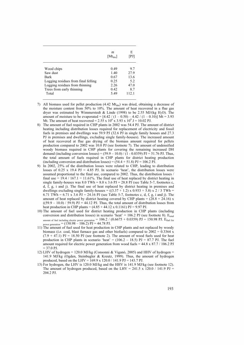
m [Mtdm]

E

[PJ]

Wood chips Saw dust Bark Logging residues from final felling Logging residues from thinning Trees from early thinning Total

0.491.400.67

0.252.260.425.49

9.727.913.65.2

47.08.7

112.1

7) All biomass used for pellet production (4.42 Mtdm) was dried, obtaining a decrease of

the moisture content from 50% to 10%. The amount of heat recovered in a flue gas dryer was estimated by Wimmerstedt & Linde (1998) to be 2.55 MJ/(kg H2O). The amount of moisture to be evaporated = [4.42 / (1 – 0.50) – 4.42 / (1 – 0.10)] Mt = 3.93 Mt. The amount of heat recovered = 2.55 x 106 x 3.93 x 109 J = 10.02 PJ.

8) The amount of fuel required in CHP plants in 2002 was 54.4 PJ. The amount of district heating including distribution losses required for replacement of electricity and fossil fuels in premises and dwellings was 59.9 PJ (32.6 PJ in single family houses and 27.3 PJ in premises and dwellings, excluding single family-houses). The increased amount of heat recovered at flue gas drying of the biomass amount required for pellets production compared to 2002 was 10.0 PJ (see footnote 7). The amount of undensified woody biomass required in CHP plants for covering the remaining increased DH demand (including conversion losses) = (59.9 – 10.0) / (1 - 0.0359) PJ = 51.76 PJ. Thus, the total amount of fuels required in CHP plants for district heating production (including conversion and distribution losses) = (54.4 + 51.8) PJ = 106.2 PJ.

9) In 2002, 25% of the distribution losses were related to CHP, leading to distribution losses of 0.25 x 19.4 PJ = 4.85 PJ. In scenario ‘heat’, the distribution losses were assumed proportional to the final use, compared to 2002. Thus, the distribution losses / final use = 19.4 / 167.1 = 11.61%. The final use of heat replaced by district heating in single family-houses was 8.0 TWh = 8.0 x 3.6 PJ = 28.8 PJ (see Table 5-7, footnotes c, d, f, g, i and j). The final use of heat replaced by district heating in premises and dwellings excluding single family-houses = ((3.37 + 1.2) x 0.933 + 5.8) x 2 / 3 TWh = 6.71 TWh = 6.71 x 3.6 PJ = 24.16 PJ (see Table 5-7, footnotes c, d, f, g, i and j). The amount of heat replaced by district heating covered by CHP plants = (28.8 + 24.16) x ((59.9 – 10.0) / 59.9) PJ = 44.12 PJ. Thus, the total amount of distribution losses from heat production in CHP plants = (4.85 + 44.12 x 0.1161) PJ = 9.97 PJ.

10) The amount of fuel used for district heating production in CHP plants (including conversion and distribution losses) in scenario ‘heat’ = 106.2 PJ (see footnote 8). Etotal amount of fuel including electric power generation = 106.2 / (0.6675 + 0.0359) PJ = 150.98 PJ. Efuel for

power generation = (150.98 – 106.2) PJ = 44.78 PJ. 11) The amount of fuel used for heat production in CHP plants and not replaced by woody

biomass (i.e. coal, blast furnace gas and other biofuels) compared to 2002 = 0.3364 x (7.9 + 47.1) PJ = 18.50 PJ (see footnote 2). The amount of wood fuels used for heat production in CHP plants in scenario ‘heat’ = (106.2 – 18.5) PJ = 87.7 PJ. The fuel amount required for electric power generation from wood fuels = 44.8 x 87.7 / 106.2 PJ = 37.0 PJ.

12) LHV of hydrogen = 120.0 MJ/kg (Consonni & Viganò, 2005) and HHV of hydrogen = 141.9 MJ/kg (Ogden, Steinbugler & Kreutz, 1999). Thus, the amount of hydrogen produced, based on the LHV = 169.9 x 120.0 / 141.9 PJ = 143.7 PJ.

13) For hydrogen, the LHV is 120.0 MJ/kg and the HHV is 141.9 MJ/kg (see footnote 12). The amount of hydrogen produced, based on the LHV = 241.5 x 120.0 / 141.9 PJ = 204.2 PJ.

193

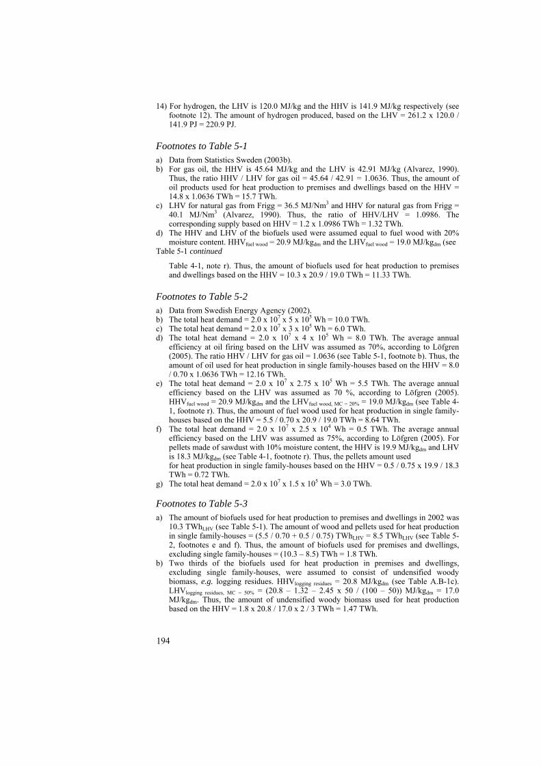
14) For hydrogen, the LHV is 120.0 MJ/kg and the HHV is 141.9 MJ/kg respectively (see footnote 12). The amount of hydrogen produced, based on the LHV = 261.2 x 120.0 / 141.9 PJ = 220.9 PJ.

Footnotes to Table 5-1 a) Data from Statistics Sweden (2003b). b) For gas oil, the HHV is 45.64 MJ/kg and the LHV is 42.91 MJ/kg (Alvarez, 1990).

Thus, the ratio HHV / LHV for gas oil = 45.64 / 42.91 = 1.0636. Thus, the amount of oil products used for heat production to premises and dwellings based on the HHV = 14.8 x 1.0636 TWh = 15.7 TWh.

c) LHV for natural gas from Frigg = 36.5 MJ/Nm3 and HHV for natural gas from Frigg = 40.1 MJ/Nm3 (Alvarez, 1990). Thus, the ratio of HHV/LHV = 1.0986. The corresponding supply based on HHV = 1.2 x 1.0986 TWh = 1.32 TWh.

d) The HHV and LHV of the biofuels used were assumed equal to fuel wood with 20% moisture content. HHVfuel wood = 20.9 MJ/kgdm and the LHVfuel wood = 19.0 MJ/kgdm (see

Table 5-1 continued

Table 4-1, note r). Thus, the amount of biofuels used for heat production to premises and dwellings based on the HHV = 10.3 x 20.9 / 19.0 TWh = 11.33 TWh.

Footnotes to Table 5-2 a) Data from Swedish Energy Agency (2002). b) The total heat demand = 2.0 x 107 x 5 x 105 Wh = 10.0 TWh. c) The total heat demand = 2.0 x 107 x 3 x 105 Wh = 6.0 TWh. d) The total heat demand = 2.0 x 107 x 4 x 105 Wh = 8.0 TWh. The average annual

efficiency at oil firing based on the LHV was assumed as 70%, according to Löfgren (2005). The ratio HHV / LHV for gas oil = 1.0636 (see Table 5-1, footnote b). Thus, the amount of oil used for heat production in single family-houses based on the HHV = 8.0 / 0.70 x 1.0636 TWh = 12.16 TWh.

e) The total heat demand = 2.0 x 107 x 2.75 x 105 Wh = 5.5 TWh. The average annual efficiency based on the LHV was assumed as 70 %, according to Löfgren (2005). HHVfuel wood = 20.9 MJ/kgdm and the LHVfuel wood, MC = 20% = 19.0 MJ/kgdm (see Table 4-1, footnote r). Thus, the amount of fuel wood used for heat production in single family-houses based on the HHV = 5.5 / 0.70 x 20.9 / 19.0 TWh = 8.64 TWh.

f) The total heat demand = 2.0 x 107 x 2.5 x 104 Wh = 0.5 TWh. The average annual efficiency based on the LHV was assumed as 75%, according to Löfgren (2005). For pellets made of sawdust with 10% moisture content, the HHV is 19.9 MJ/kgdm and LHV is 18.3 MJ/kgdm (see Table 4-1, footnote r). Thus, the pellets amount used for heat production in single family-houses based on the HHV = 0.5 / 0.75 x 19.9 / 18.3 TWh = 0.72 TWh.

g

) The total heat demand = 2.0 x 107 x 1.5 x 105 Wh = 3.0 TWh.

Footnotes to Table 5-3 a) The amount of biofuels used for heat production to premises and dwellings in 2002 was

10.3 TWhLHV (see Table 5-1). The amount of wood and pellets used for heat production in single family-houses = (5.5 / 0.70 + 0.5 / 0.75) TWhLHV = 8.5 TWhLHV (see Table 5-2, footnotes e and f). Thus, the amount of biofuels used for premises and dwellings, excluding single family-houses = (10.3 – 8.5) TWh = 1.8 TWh.

b) Two thirds of the biofuels used for heat production in premises and dwellings, excluding single family-houses, were assumed to consist of undensified woody biomass, e.g. logging residues. HHVlogging residues = 20.8 MJ/kgdm (see Table A.B-1c). LHVlogging residues, MC = 50% = (20.8 – 1.32 – 2.45 x 50 / (100 – 50)) MJ/kgdm = 17.0 MJ/kgdm. Thus, the amount of undensified woody biomass used for heat production based on the HHV = 1.8 x 20.8 / 17.0 x 2 / 3 TWh = 1.47 TWh.

194

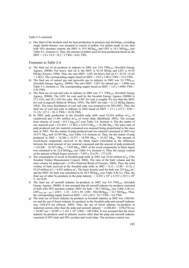
Table 5-3 continued c) One third of the biofuels used for heat production in premises and dwellings, excluding

single family-houses, was assumed to consist of pellets. For pellets made of saw dust with 10% moisture content, the HHV is 19.9 MJ/kgdm and LHV is 18.3 MJ/kgdm (see Table 4-1, footnote r). Thus, the amount of pellets used for heat production based on the HHV = 1.8 x 19.9 / 18.3 / 3 TWh = 0.65 TWh.

Footnotes to Table 5-4 a) The final use of oil products in industry in 2002 was 19.8 TWhLHV (Swedish Energy

Agency, 2004b). For heavy fuel oil 4, the HHV is 43.54 MJ/kg and LHV is 41.03 MJ/kg (Alvarez, 1990). Thus, the ratio HHV / LHV for heavy fuel oil 4 = 43.54 / 41.03 = 1.0612. The corresponding supply based on HHV = 19.8 x 1.0612 TWh = 21.0 TWh.

b) The final use of natural gas and gasworks gas in industry in 2002 was 3.6 TWhLHV (Swedish Energy Agency, 2004b). The ratio HHV / LHV for natural gas = 1.0986 (see Table 5-1, footnote c). The corresponding supply based on HHV = 3.6 x 1.0986 TWh = 3.95 TWh.

c) The final use of coal and coke in industry in 2002 was 17.1 TWhLHV (Swedish Energy Agency, 2004b). The LHV for coal used by the Swedish Energy Agency (2004b) is 27.2 GJ/t, and 28.1 GJ/t for coke. The LHV for coal is roughly 4% less than the HHV for coal (Longwell, Rubin & Wilson, 1995). The HHV for coke = 31.12 MJ/kg (Spiers, 1962). The mass distribution of coal and coke was assumed to be 50%/50%. Thus, the final use of coal and coke in industry in 2002 based on HHV = 17.1 x (27.2 / 0.96 + 31.12) / (27.2 + 28.1) TWh = 18.38 TWh.

d) In 2002, pulp production in the Swedish pulp mills used 32.654 million m3fub of

roundwood and 11.401 million m3fub of wood chips (Björklund, 2005). The average

basic density of wood = 413.3 kgdm/m3f (see Table 3-4, footnote i). The dry matter of

raw material used = (32.654 + 11.401) x 0.4133 Mtdm = 18.206 Mtdm. The mass ratio of pulp produced and raw material consumed was assumed being proportional to the mass ratio in 2003. The dry matter of pulp produced and raw material consumed in 2003 was 10.571 Mtdm and 18.599 Mtdm (see Table 3-4, footnote n). Thus, the dry matter of pulp produced in 2002 = 18.206 x 10.571 / 18.599 Mtdm = 10.347 Mtdm. The amount of wood-based compounds received in the black liquor (calculated as the difference between the total amount of raw material consumed and the amount of pulp produced) = (18.206 – 10.347) Mtdm = 7.859 Mtdm. HHV of the wood components in black liquor was estimated to be 22.6 MJ/kgdm (see Table 3-4, footnote r). Thus, the energy content of the amount of black liquor received = 7.859 x 22.6 PJ = 177.6 PJ.

e) The consumption of wood in Swedish pulp mills in 2002 was 32.65 million m3fub (The

Swedish Timber Measurement Council, 2004). The ratio of the bark volume and the stem volume for pulpwood = 12.0% (National Board of Forestry, 2004). Thus, the solid volume of bark received at the Swedish pulp mills in 2002 = 0.12 / (1.00 – 0.12) x 32.65 million m3

f = 4.452 million m3f. The basic density used for bark was 333 kgdm/m3

f and the HHV for bark was calculated to be 20.5 MJ/kgdm (see Table A.B-1c). Thus, the final use of other by-products in the pulp industry = 4.452 x 106 x 0.333 x 20.5 x 109 J= 30.39 PJ.

f) The final use of sawmill industry by-products in 2002 was 4.9 TWhLHV (Swedish Energy Agency, 2004b). It was assumed that all sawmill industry by-products consisted of bark with 50% moisture content. HHV for bark = 20.5 MJ/kgdm (see Table A.B-1c). LHVbark, MC = 50% = (20.5 – 1.32 – 2.45 x 50 / (100 – 50)) MJ/kgdm = 16.7 MJ/kgdm. Thus, the corresponding supply based on HHV = 4.9 x 20.5 / 16.7 TWh = 6.0 TWh.

g) The total use of forest industry by-products in Swedish industry in 2002 was 1288,461 toe and the use of forest industry by-products in the Swedish pulp and sawmill industry was 1258,474 toe (Olsson, 2005). Thus, the use of forest industry by-products in industrial sectors other than the pulp and sawmill industry = (1288,461 - 1258,474) toe = 29,987 toe = 29,987 x 1.163 x 10-2 GWh = 349 GWh. It was assumed that the forest industry by-products used in industry sectors other than the pulp and sawmill industry consisted of 50% bark and 50% sawdust and wood chips. The moisture content was

195

Table 5-4 continued

assumed as 50%. HHV for bark = 20.5 MJ/kgdm (see Table A.B-1c). LHVbark, MC = 50% = (20.5 – 1.32 – 2.45 x 50 / (100 – 50)) MJ/kgdm = 16.7 MJ/kgdm. HHV for sawdust and wood chips = 19.9 MJ/kgdm (see Table A.B-1c). LHVsaw dust and wood chips, MC = 50% = (19.9 – 1.32 – 2.45 x 50 / (100 – 50)) MJ/kgdm = 16.2 MJ/kgdm. Thus, the corresponding use based on HHV = 349 x (20.5 / 16.7 + 19.9 / 16.2) / 2 GWh = 429 GWh.

h) The total use of peat and municipal solid waste (MSW) in the Swedish industry in 2002 was 8332 toe and the use of peat and MSW in the Swedish pulp and sawmill industry was 46 toe (Olsson, 2005). Thus, the use of peat and MSW in other industry sectors than the pulp and sawmill industry = (8332 – 46) toe = 8286 toe = 8286 x 1.163 x 10-2 GWh = 96.4 GWh. It was assumed that the ratio of HHV and LHV of the peat and MSW used in industrial sectors other than the pulp and sawmill industry was equal to the ratio of the HHV and LHV for logging residues with 50% moisture content. HHV for logging residues = 20.8 MJ/kgdm (see Table A.B-1c) and LHVlogging residues, MC = 50% = 17.0 MJ/kgdm (see note h). Thus, the corresponding use based on the HHV = 96.4 x 20.8 / 17.0 GWh = 118 GWh.

Footnotes to Table 5-5 a) Data from Swedish Energy Agency (2004b). b) The ratio HHV / LHV for heavy fuel oil 4 = 1.0612 (see Table 5-1, footnote a). The

supply based on HHV = 4.4 x 1.0612 TWh = 4.67 TWh. c) The ratio HHV / LHV for natural gas = 1.0986 (see Table 5-1, footnote c). The supply

based on HHV = 3.3 x 1.0986 TWh = 3.63 TWh. d) LHV for coal is roughly 4% less than HHV for coal (Longwell, Rubin & Wilson, 1995).

The supply based on HHV = 2.1 / 0.96 TWh = 2.19 TWh. e) The total amount of wood fuels used for district heating in Sweden in 2002 was 17.9

TWhLHV (Swedish Energy Agency, 2004b). The amount of pellets and briquettes used for district heating in Sweden in 2002 was 346 ktoe = 346 x 1.163 x 10-2 TWhLHV = 4.02 TWhLHV (Statistics Sweden, 2003b). Thus, the amount of undensified wood fuels = (17.9 – 4.0) TWhLHV = 13.9 TWhLHV.

f) All undensified woody biomass used for district heating was assumed to consist of logging residues with 50% moisture content. HHVlogging residues = 20.8 MJ/kgdm (see Table A.B-1c). LHVlogging residues, MC = 50% = (20.8 – 1.32 – 2.45 x 50 / (100 – 50)) MJ/kgdm = 17.03 MJ/kgdm. Thus, the corresponding supply based on HHV = 13.9 x 20.8 / 17.0 TWh = 17.01 TWh.

g) For pellets made of sawdust with 10% moisture content, the HHV is 19.9 MJ/kgdm and LHV is 18.3 MJ/kgdm (see Table 4-1, footnote r). Thus, the corresponding supply based on HHV = 4.02 x 19.9 / 18.3 TWh = 4.37 TWh.

h) Other biofuels include refuse, tall oil pitch, peat and other unspecified biofuels (Swedish Energy Agency, 2004b). The ratio of HHV / LHV for other biofuels was assumed equal to the corresponding ratio for logging residues with 50% moisture content. Thus, the supply based on HHV = 10.7 x 20.8 / 17.0 TWh = 13.09 TWh.

Footnotes to Table 5-7 a) The distribution losses were assumed proportional to the final use compared to 2002.

Thus, the distribution losses / final use = 19.4 / 167.1 = 11.61%. b) The average annual efficiency of the pellet boiler systems was assumed equal to the

efficiency of the pellet boiler system selected as a reference boiler system (see Chapter 4). Thus, the average annual efficiency based on the LHV = 75%, according to Löfgren (2005). For pellets made of sawdust with 10% moisture content, the HHV is 19.9 MJ/kgdm and the LHV is 18.3 MJ/kgdm (see Table 4-1, footnote r).

c) The total heat demand covered by electricity in 2002 was 10.0 TWh (see Table 5-3, footnote b).

196

Table 5-7 continued d) One third of the heat produced by electricity was assumed as being replaced by district

heating. The amount of district heating required for replacement including distribution losses = 10.0 / ((1 – 0.1161) x 3) TWh = 3.77 TWh.

e) One third of the heat produced by electricity was assumed as being replaced by pellet firing. Thus, the pellet amount based on the HHV required for replacement = 10.0 / 0.75 x 19.9 / 18.3 / 3 TWh = 4.83 TWh.

f) The total heat demand covered by electric boilers with water-fed system in 2002 was 6.0 TWh (see Table 5-3, footnote c).

g) One third of the heat produced by electric boilers with water-fed systems in single family-houses in 2002 was assumed as being replaced by district heating. Thus, the DH amount required for replacement including distribution losses = 6.0 / (1 – 0.1161) / 3 TWh = 2.26 TWh.

h) One third of the heat produced by electric boilers with water-fed systems in single family-houses in 2002 was assumed as being replaced by pellet firing. Thus, the pellet amount based on the HHV required for replacement = 6.0 / 0.75 x 19.9 / 18.3 / 3 TWh = 2.90 TWh.

i) The total heat demand covered by oil firing in 2002 was 8.0 TWh (see Table 5-3, footnote d).

j) One third of the heat produced by oil firing in single family-houses in 2002 was assumed as being replaced by district heating. Thus, the DH amount required for replacement including distribution losses = 8.0 / (1 – 0.1161) / 3 TWh = 3.02 TWh.

k) One third of the heat produced by oil firing in single family-houses in 2002 was assumed as being replaced by pellet firing. Thus, the pellet amount based on the HHV required for replacement = 8.0 / 0.75 x 19.9 / 18.3 / 3 TWh = 3.87 TWh.

Footnotes to Table 5-8 a) The distribution losses were assumed proportional to the final use compared to 2002.

Thus, the distribution losses / final use = 19.4 / 167.1 = 11.61%. b) The efficiency of the pellet reference boiler based on the LHV = 93.3% (see Table A.J-

43). For pellets made of sawdust with 10% moisture content the HHV is 19.9 MJ/kgdm and LHV is 18.3 MJ/kgdm (see Table 4-1, footnote r).

c) The total amount of oil products used for heat production to premises and dwellings was 14.8 TWhLHV (see Table 5-1) and the amount of oil used for heat production in single family-houses = 8.0 / 0.70 TWh = 11.43 TWhLHV (see Table 5-2, footnote d). Thus, the amount of oil used for heat production in premises and dwellings other than single family-houses = (14.8 – 11.43) TWhLHV = 3.37 TWhLHV. The efficiency of oil firing in premises and dwellings other than single family-houses based on LHV was assumed equal to the efficiency of the pellet reference boiler, i.e. 93.3%.

d) Two thirds of the heat produced by oil firing was assumed as being replaced by district heating. Thus, the amount of district heating including distribution losses required for replacing the amount of oil = 3.37 x 0.933 / (1 – 0.1161) x 2 / 3 TWh = 2.37 TWh.

e) One third of the heat produced by oil firing was assumed as being replaced by pellet firing. Thus, the amounts of pellets based on the HHV required for replacing the amount of oil = 3.37 x 19.9 / 18.3 / 3 TWh = 1.22 TWh.

f) The total amount of natural gas used for heat production to premises and dwellings was 1.2 TWhLHV (see Table 5-2). The total amount of natural gas was assumed as being used in premises and dwellings other than single family-houses. The efficiency of firing of natural gas in premises and dwellings other than single family-houses was assumed equal to the efficiency of the pellets reference boiler based on the LHV, i.e. 93.3%.

g) Two thirds of the heat produced by natural gas was assumed as being replaced by district heating. Thus, the amount of district heating including distribution losses required for replacing the amount of natural gas = 1.2 x 0.933 / (1 – 0.1161) x 2 / 3 TWh = 0.84 TWh.

197

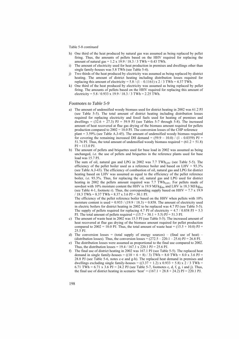
Table 5-8 continued h) One third of the heat produced by natural gas was assumed as being replaced by pellet

firing. Thus, the amounts of pellets based on the HHV required for replacing the amount of natural gas = 1.2 x 19.9 / 18.3 / 3 TWh = 0.43 TWh.

i) The amount of electricity used for heat production in premises and dwellings other than single family-houses was 5.8 TWh (see Table 5-4).

j) Two thirds of the heat produced by electricity was assumed as being replaced by district heating. The amount of district heating including distribution losses required for replacing this amount of electricity = 5.8 / (1 – 0.1161) x 2 / 3 TWh = 4.37 TWh.

k) One third of the heat produced by electricity was assumed as being replaced by pellet firing. The amounts of pellets based on the HHV required for replacing this amount of electricity = 5.8 / 0.933 x 19.9 / 18.3 / 3 TWh = 2.25 TWh.

Footnotes to Table 5-9 a) The amount of undensified woody biomass used for district heating in 2002 was 61.2 PJ

(see Table 5-5). The total amount of district heating including distribution losses required for replacing electricity and fossil fuels used for heating of premises and dwellings = (32.6 + 27.3) PJ = 59.9 PJ (see Tables 5-7 through 5-8). The increased amount of heat recovered at flue gas drying of the biomass amount required for pellets production compared to 2002 = 10.0 PJ. The conversion losses of the CHP reference plant = 3.59% (see Table A.J-45). The amount of undensified woody biomass required for covering the remaining increased DH demand = (59.9 – 10.0) / (1 - 0.0359) PJ = 51.76 PJ. Thus, the total amount of undensified woody biomass required = (61.2 + 51.8) PJ = 113.0 PJ.

b) The amount of pellets and briquettes used for base load in 2002 was assumed as being unchanged, i.e. the use of pellets and briquettes in the reference plants used for base load was 15.7 PJ. The sum of oil, natural gas and LPG in 2002 was 7.7 TWhLHV (see Table 5-5). The efficiency of the pellet boiler used as a reference boiler and based on LHV = 93.3% (see Table A.J-43). The efficiency of combustion of oil, natural gas and LPG for district heating based on LHV was assumed as equal to the efficiency of the pellet reference boiler, i.e. 93.3%. Thus, for replacing the oil, natural gas and LPG used for district heating in 2002 the pellets amount required was 7.7 TWhLHV. For pellets made of sawdust with 10% moisture content the HHV is 19.9 MJ/kgdm and LHV is 18.3 MJ/kgdm (see Table 4-1, footnote r). Thus, the corresponding supply based on HHV = 7.7 x 19.9 / 18.3 TWh = 8.37 TWh = 8.37 x 3.6 PJ = 30.1 PJ. The efficiency of the pellet reference boiler based on the HHV when pellets with 10% moisture content is used = 0.933 / (19.9 / 18.3) = 0.858. The amount of electricity used in electric boilers for district heating in 2002 to be replaced was 4.7 PJ (see Table 5-5). The supply of pellets required for replacing 4.7 PJ of electricity = 4.7 / 0.858 PJ = 5.5 PJ. The total amount of pellets required = (15.7 + 30.1 + 5.5) PJ = 51.3 PJ.

c) The amount of waste heat in 2002 was 15.5 PJ (see Table 5-5). The increased amount of heat recovered at flue gas drying of the biomass amount required for pellet production compared to 2002 = 10.0 PJ. Thus, the total amount of waste heat = (15.5 + 10.0) PJ = 25.5 PJ.

d) The conversion losses = (total supply of energy sources) – (final use of heat) – (distribution losses). Thus, the conversion losses = (272.5 – 220.1 – 25.6) PJ = 26.8 PJ.

e) The distribution losses were assumed as proportional to the final use compared to 2002. Thus, the distribution losses = 19.4 / 167.1 x 220.1 PJ = 25.6 PJ.

f) The final use of district heating in 2002 was 167.1 PJ (see Table 5-5). The replaced heat demand in single family-houses = ((10 + 6 + 8) / 3) TWh = 8.0 TWh = 8.0 x 3.6 PJ = 28.8 PJ (see Table 5-6, notes c-e and g-h). The replaced heat demand in premises and dwellings excluding single family-houses = ((3.37 + 1.2) x 0.933 + 5.8) x 2 / 3 TWh = 6.71 TWh = 6.71 x 3.6 PJ = 24.2 PJ (see Table 5-7, footnotes c, d, f, g, i and j). Thus, the final use of district heating in scenario ‘heat’ = (167.1 + 28.8 + 24.2) PJ = 220.1 PJ.

198

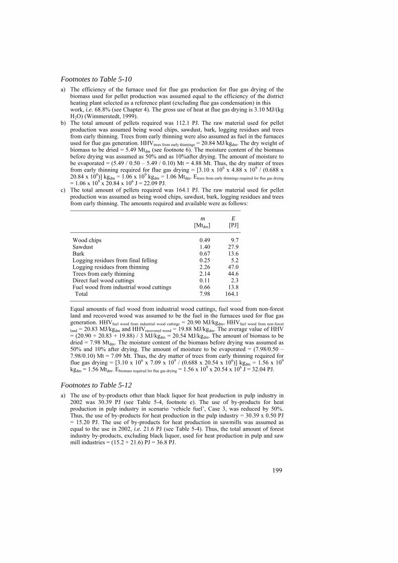
Footnotes to Table 5-10 a) The efficiency of the furnace used for flue gas production for flue gas drying of the

biomass used for pellet production was assumed equal to the efficiency of the district heating plant selected as a reference plant (excluding flue gas condensation) in this

work, i.e. 68.8% (see Chapter 4). The gross use of heat at flue gas drying is 3.10 MJ/(kg H2O) (Wimmerstedt, 1999).

b) The total amount of pellets required was 112.1 PJ. The raw material used for pellet production was assumed being wood chips, sawdust, bark, logging residues and trees from early thinning. Trees from early thinning were also assumed as fuel in the furnaces used for flue gas generation. HHVtrees from early thinnings = 20.84 MJ/kgdm. The dry weight of biomass to be dried = 5.49 Mtdm (see footnote 6). The moisture content of the biomass before drying was assumed as 50% and as 10%after drying. The amount of moisture to be evaporated = (5.49 / 0.50 – 5.49 / 0.10) Mt = 4.88 Mt. Thus, the dry matter of trees from early thinning required for flue gas drying = [3.10 x 106 x 4.88 x 109 / (0.688 x 20.84 x 106)] kgdm = 1.06 x 109 kgdm = 1.06 Mtdm. Etrees from early thinnings required for flue gas drying = 1.06 x 109 x 20.84 x 106 J = 22.09 PJ.

c) The total amount of pellets required was 164.1 PJ. The raw material used for pellet production was assumed as being wood chips, sawdust, bark, logging residues and trees from early thinning. The amounts required and available were as follows:

m

[Mtdm]

E

[PJ]

Wood chips Sawdust Bark Logging residues from final felling Logging residues from thinning Trees from early thinning Direct fuel wood cuttings Fuel wood from industrial wood cuttings Total

0.491.400.67

0.252.262.140.110.667.98

9.7

27.913.65.2

47.044.62.3

13.8164.1

Equal amounts of fuel wood from industrial wood cuttings, fuel wood from non-forest land and recovered wood was assumed to be the fuel in the furnaces used for flue gas generation. HHVfuel wood from industrial wood cuttings = 20.90 MJ/kgdm, HHVfuel wood from non-forest

land = 20.83 MJ/kgdm and HHVrecovered wood = 19.88 MJ/kgdm. The average value of HHV = (20.90 + 20.83 + 19.88) / 3 MJ/kgdm = 20.54 MJ/kgdm. The amount of biomass to be dried = 7.98 Mtdm. The moisture content of the biomass before drying was assumed as 50% and 10% after drying. The amount of moisture to be evaporated = (7.98/0.50 – 7.98/0.10) Mt = 7.09 Mt. Thus, the dry matter of trees from early thinning required for flue gas drying = [3.10 x 106 x 7.09 x 109 / (0.688 x 20.54 x 106)] kgdm = 1.56 x 109 kgdm = 1.56 Mtdm. Ebiomass required for flue gas drying = 1.56 x 109 x 20.54 x 106 J = 32.04 PJ.

Footnotes to Table 5-12 a) The use of by-products other than black liquor for heat production in pulp industry in

2002 was 30.39 PJ (see Table 5-4, footnote e). The use of by-products for heat production in pulp industry in scenario ‘vehicle fuel’, Case 3, was reduced by 50%. Thus, the use of by-products for heat production in the pulp industry = 30.39 x 0.50 PJ = 15.20 PJ. The use of by-products for heat production in sawmills was assumed as equal to the use in 2002, i.e. 21.6 PJ (see Table 5-4). Thus, the total amount of forest industry by-products, excluding black liquor, used for heat production in pulp and saw mill industries = (15.2 + 21.6) PJ = 36.8 PJ.

199

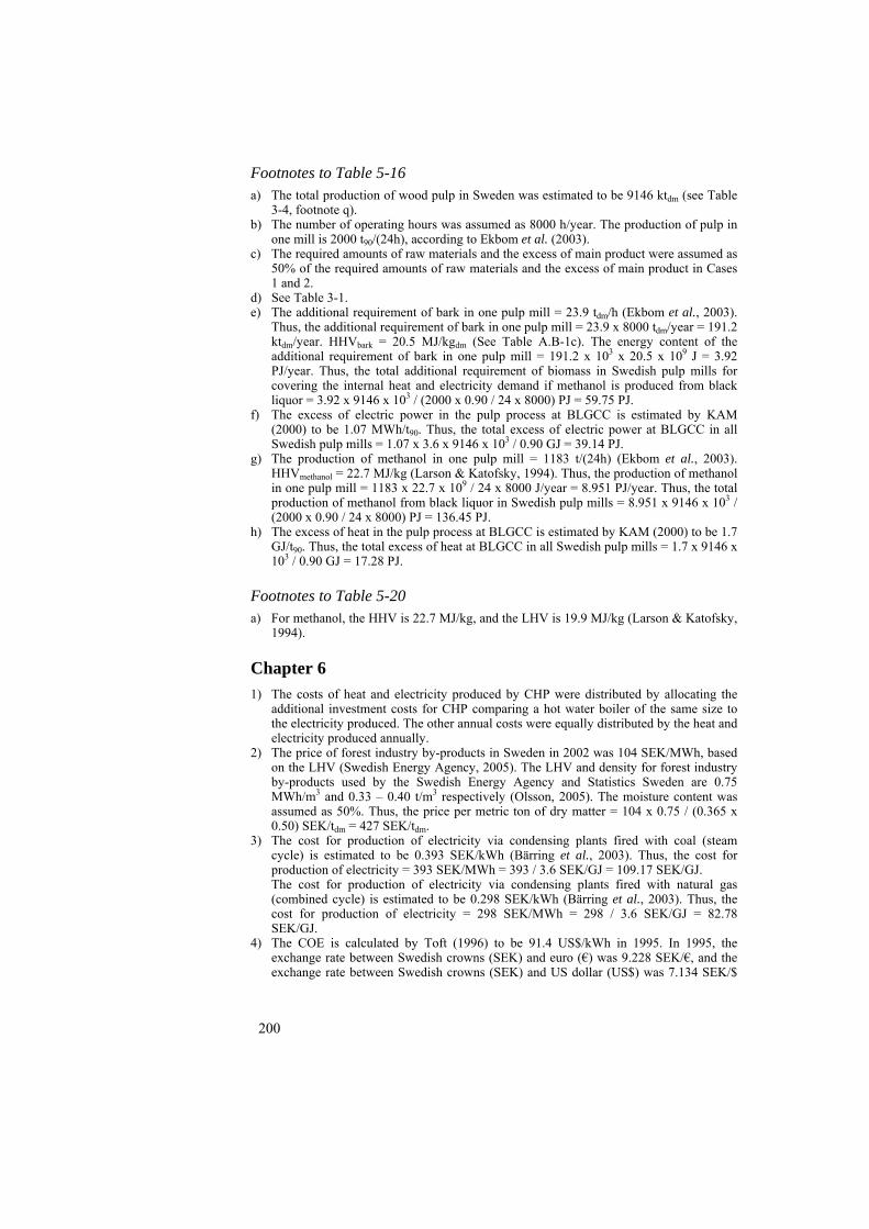
Footnotes to Table 5-16 a) The total production of wood pulp in Sweden was estimated to be 9146 ktdm (see Table

3-4, footnote q). b) The number of operating hours was assumed as 8000 h/year. The production of pulp in

one mill is 2000 t90/(24h), according to Ekbom et al. (2003). c) The required amounts of raw materials and the excess of main product were assumed as

50% of the required amounts of raw materials and the excess of main product in Cases 1 and 2.

d) See Table 3-1. e) The additional requirement of bark in one pulp mill = 23.9 tdm/h (Ekbom et al., 2003).

Thus, the additional requirement of bark in one pulp mill = 23.9 x 8000 tdm/year = 191.2 ktdm/year. HHVbark = 20.5 MJ/kgdm (See Table A.B-1c). The energy content of the additional requirement of bark in one pulp mill = 191.2 x 103 x 20.5 x 109 J = 3.92 PJ/year. Thus, the total additional requirement of biomass in Swedish pulp mills for covering the internal heat and electricity demand if methanol is produced from black liquor = 3.92 x 9146 x 103 / (2000 x 0.90 / 24 x 8000) PJ = 59.75 PJ.

f) The excess of electric power in the pulp process at BLGCC is estimated by KAM (2000) to be 1.07 MWh/t90. Thus, the total excess of electric power at BLGCC in all Swedish pulp mills = 1.07 x 3.6 x 9146 x 103 / 0.90 GJ = 39.14 PJ.

g) The production of methanol in one pulp mill = 1183 t/(24h) (Ekbom et al., 2003). HHVmethanol = 22.7 MJ/kg (Larson & Katofsky, 1994). Thus, the production of methanol in one pulp mill = 1183 x 22.7 x 109 / 24 x 8000 J/year = 8.951 PJ/year. Thus, the total production of methanol from black liquor in Swedish pulp mills = 8.951 x 9146 x 103 / (2000 x 0.90 / 24 x 8000) PJ = 136.45 PJ.

h) The excess of heat in the pulp process at BLGCC is estimated by KAM (2000) to be 1.7 GJ/t90. Thus, the total excess of heat at BLGCC in all Swedish pulp mills = 1.7 x 9146 x 103 / 0.90 GJ = 17.28 PJ.

Footnotes to Table 5-20 a) For methanol, the HHV is 22.7 MJ/kg, and the LHV is 19.9 MJ/kg (Larson & Katofsky,

1994). Chapter 6 1) The costs of heat and electricity produced by CHP were distributed by allocating the

additional investment costs for CHP comparing a hot water boiler of the same size to the electricity produced. The other annual costs were equally distributed by the heat and electricity produced annually.

2) The price of forest industry by-products in Sweden in 2002 was 104 SEK/MWh, based on the LHV (Swedish Energy Agency, 2005). The LHV and density for forest industry by-products used by the Swedish Energy Agency and Statistics Sweden are 0.75 MWh/m3 and 0.33 – 0.40 t/m3 respectively (Olsson, 2005). The moisture content was assumed as 50%. Thus, the price per metric ton of dry matter = 104 x 0.75 / (0.365 x 0.50) SEK/tdm = 427 SEK/tdm.

3) The cost for production of electricity via condensing plants fired with coal (steam cycle) is estimated to be 0.393 SEK/kWh (Bärring et al., 2003). Thus, the cost for production of electricity = 393 SEK/MWh = 393 / 3.6 SEK/GJ = 109.17 SEK/GJ. The cost for production of electricity via condensing plants fired with natural gas (combined cycle) is estimated to be 0.298 SEK/kWh (Bärring et al., 2003). Thus, the cost for production of electricity = 298 SEK/MWh = 298 / 3.6 SEK/GJ = 82.78 SEK/GJ.

4) The COE is calculated by Toft (1996) to be 91.4 US$/kWh in 1995. In 1995, the exchange rate between Swedish crowns (SEK) and euro (€) was 9.228 SEK/€, and the exchange rate between Swedish crowns (SEK) and US dollar (US$) was 7.134 SEK/$

200

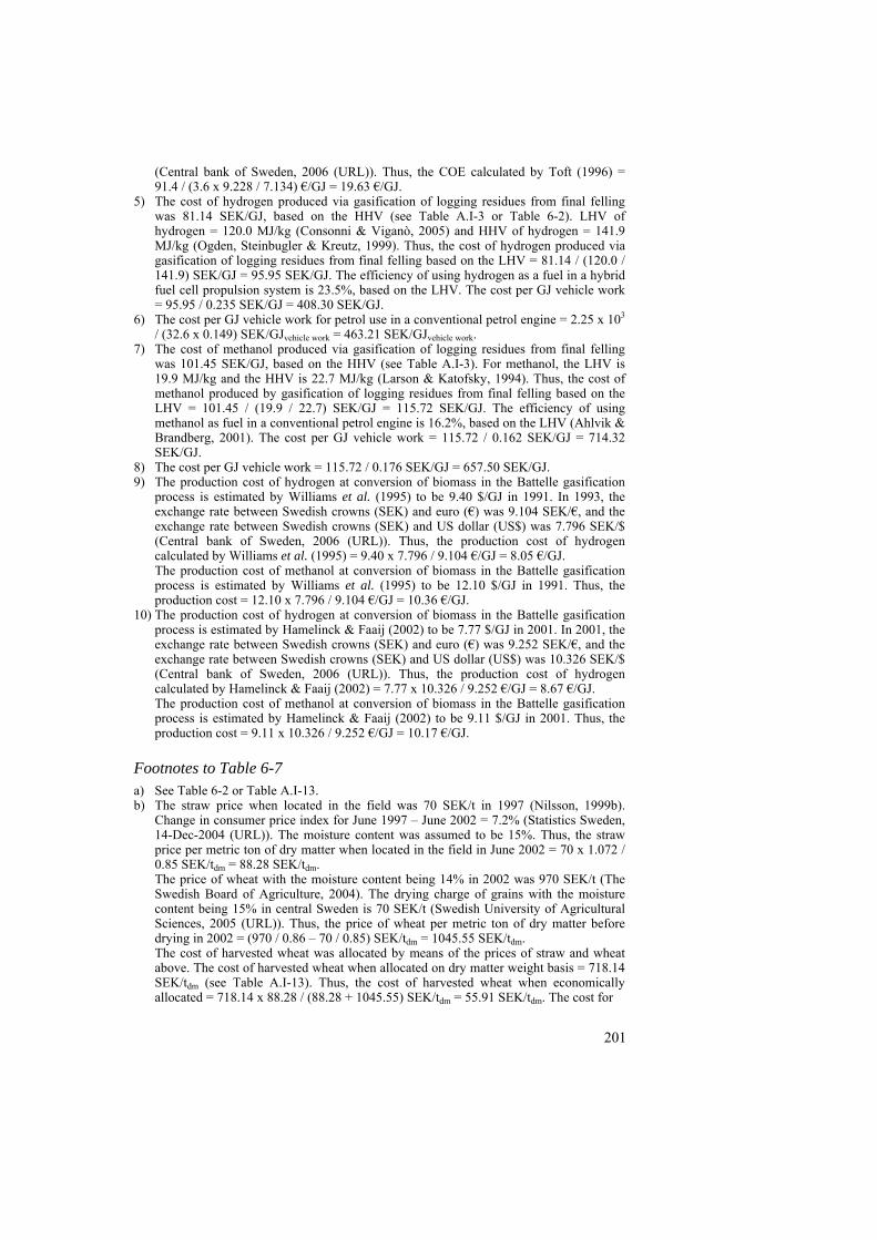
(Central bank of Sweden, 2006 (URL)). Thus, the COE calculated by Toft (1996) = 91.4 / (3.6 x 9.228 / 7.134) €/GJ = 19.63 €/GJ.

5) The cost of hydrogen produced via gasification of logging residues from final felling was 81.14 SEK/GJ, based on the HHV (see Table A.I-3 or Table 6-2). LHV of hydrogen = 120.0 MJ/kg (Consonni & Viganò, 2005) and HHV of hydrogen = 141.9 MJ/kg (Ogden, Steinbugler & Kreutz, 1999). Thus, the cost of hydrogen produced via gasification of logging residues from final felling based on the LHV = 81.14 / (120.0 / 141.9) SEK/GJ = 95.95 SEK/GJ. The efficiency of using hydrogen as a fuel in a hybrid fuel cell propulsion system is 23.5%, based on the LHV. The cost per GJ vehicle work = 95.95 / 0.235 SEK/GJ = 408.30 SEK/GJ.

6) The cost per GJ vehicle work for petrol use in a conventional petrol engine = 2.25 x 103 / (32.6 x 0.149) SEK/GJvehicle work = 463.21 SEK/GJvehicle work.

7) The cost of methanol produced via gasification of logging residues from final felling was 101.45 SEK/GJ, based on the HHV (see Table A.I-3). For methanol, the LHV is 19.9 MJ/kg and the HHV is 22.7 MJ/kg (Larson & Katofsky, 1994). Thus, the cost of methanol produced by gasification of logging residues from final felling based on the LHV = 101.45 / (19.9 / 22.7) SEK/GJ = 115.72 SEK/GJ. The efficiency of using methanol as fuel in a conventional petrol engine is 16.2%, based on the LHV (Ahlvik & Brandberg, 2001). The cost per GJ vehicle work = 115.72 / 0.162 SEK/GJ = 714.32 SEK/GJ.

8) The cost per GJ vehicle work = 115.72 / 0.176 SEK/GJ = 657.50 SEK/GJ. 9) The production cost of hydrogen at conversion of biomass in the Battelle gasification

process is estimated by Williams et al. (1995) to be 9.40 $/GJ in 1991. In 1993, the exchange rate between Swedish crowns (SEK) and euro (€) was 9.104 SEK/€, and the exchange rate between Swedish crowns (SEK) and US dollar (US$) was 7.796 SEK/$ (Central bank of Sweden, 2006 (URL)). Thus, the production cost of hydrogen calculated by Williams et al. (1995) = 9.40 x 7.796 / 9.104 €/GJ = 8.05 €/GJ. The production cost of methanol at conversion of biomass in the Battelle gasification process is estimated by Williams et al. (1995) to be 12.10 $/GJ in 1991. Thus, the production cost = 12.10 x 7.796 / 9.104 €/GJ = 10.36 €/GJ.

10) The production cost of hydrogen at conversion of biomass in the Battelle gasification process is estimated by Hamelinck & Faaij (2002) to be 7.77 $/GJ in 2001. In 2001, the exchange rate between Swedish crowns (SEK) and euro (€) was 9.252 SEK/€, and the exchange rate between Swedish crowns (SEK) and US dollar (US$) was 10.326 SEK/$ (Central bank of Sweden, 2006 (URL)). Thus, the production cost of hydrogen calculated by Hamelinck & Faaij (2002) = 7.77 x 10.326 / 9.252 €/GJ = 8.67 €/GJ. The production cost of methanol at conversion of biomass in the Battelle gasification process is estimated by Hamelinck & Faaij (2002) to be 9.11 $/GJ in 2001. Thus, the production cost = 9.11 x 10.326 / 9.252 €/GJ = 10.17 €/GJ.

Footnotes to Table 6-7 a) See Table 6-2 or Table A.I-13. b) The straw price when located in the field was 70 SEK/t in 1997 (Nilsson, 1999b).

Change in consumer price index for June 1997 – June 2002 = 7.2% (Statistics Sweden, 14-Dec-2004 (URL)). The moisture content was assumed to be 15%. Thus, the straw price per metric ton of dry matter when located in the field in June 2002 = 70 x 1.072 / 0.85 SEK/tdm = 88.28 SEK/tdm. The price of wheat with the moisture content being 14% in 2002 was 970 SEK/t (The Swedish Board of Agriculture, 2004). The drying charge of grains with the moisture content being 15% in central Sweden is 70 SEK/t (Swedish University of Agricultural Sciences, 2005 (URL)). Thus, the price of wheat per metric ton of dry matter before drying in 2002 = (970 / 0.86 – 70 / 0.85) SEK/tdm = 1045.55 SEK/tdm. The cost of harvested wheat was allocated by means of the prices of straw and wheat above. The cost of harvested wheat when allocated on dry matter weight basis = 718.14 SEK/tdm (see Table A.I-13). Thus, the cost of harvested wheat when economically allocated = 718.14 x 88.28 / (88.28 + 1045.55) SEK/tdm = 55.91 SEK/tdm. The cost for

201

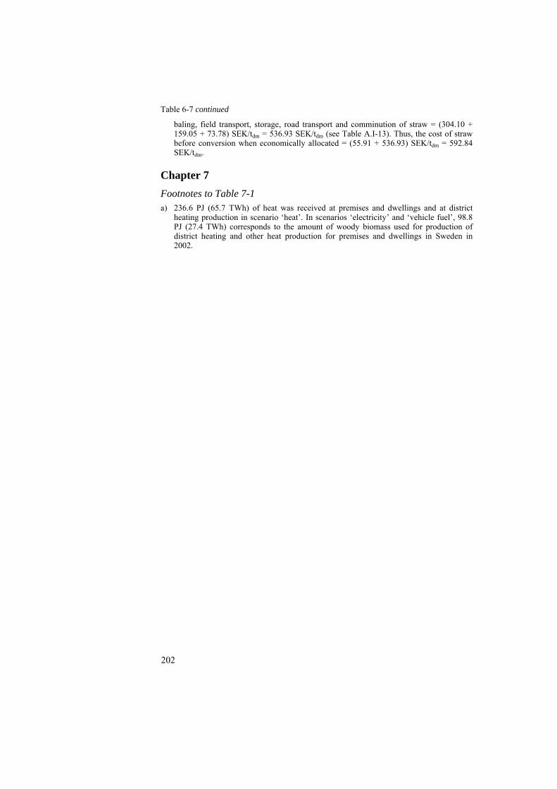
Table 6-7 continued

baling, field transport, storage, road transport and comminution of straw = (304.10 + 159.05 + 73.78) SEK/tdm = 536.93 SEK/tdm (see Table A.I-13). Thus, the cost of straw before conversion when economically allocated = (55.91 + 536.93) SEK/tdm = 592.84 SEK/tdm.

Chapter 7 Footnotes to Table 7-1 a) 236.6 PJ (65.7 TWh) of heat was received at premises and dwellings and at district

heating production in scenario ‘heat’. In scenarios ‘electricity’ and ‘vehicle fuel’, 98.8 PJ (27.4 TWh) corresponds to the amount of woody biomass used for production of district heating and other heat production for premises and dwellings in Sweden in 2002.

202

Appendix D: Description of the spreadsheet used for the simulations The spreadsheet used for the simulations was constructed in Microsoft Excel. The potential amount of the different biomass assortments studied (further discussed in Chapter 3) are first distributed regarding eventual use as raw material for pellet production. The amount of pellets produced is also distributed for use as fuel in domestic pellet boilers and for use as fuel in pellet boilers for district heating generation. Secondly, the remaining amounts of biomass assortments are distributed over the other thermochemical conversion processes to be used for production of heat, electricity or vehicle fuel.

The distribution of the potential biomass assortment is performed in one Excel chart, which is linked to other Excel charts via macro programming. These linked Excel charts include data for the different thermochemical conversion processes (data similar to data in Tables A.J-42 through to A.J-48). Thus, data regarding e.g. efficiencies of the conversion processes are imported from these linked Excel charts. The amount of energy carriers (i.e. heat, electricity or vehicle fuel) received for each biomass assortment are then calculated. These amounts are then summed for each conversion process to achieve the total amount of energy carriers received for each conversion process chosen in the simulation. Finally, block diagrams (as the block diagrams shown in Figures 5-2 through to 5-10) are generated by the macro program.

203

204

Appendix E: Brief of other technologies for gasification of biomass TPS Termiska Processer AB in Studsvik, Sweden has developed an atmospheric process, which has been tested in a pilot plant at Studsvik since 1987. The energy content of the fuel input to that plant is 2 MW. Tests have for instance been performed with a 0.5 MW shaft power turbo-charged eight-cylinder diesel engine running on low calorific gas generated at the pilot plant (Rensfelt & Hallgren, 1997).

A demonstration plant, based on TPS’ gasification technology was completely constructed in early 2001 at Eggborough, North Yorkshire, United Kingdom. It is an IGCC-plant with a total output of 8 MW of electric power (Rensfelt, Morris & Waldheim, 2003). The biomass feed stock is mainly derived from willow and poplar short rotation coppice plantations in the neighbourhood and partly from forestry as residues (Kwant & Knoef, 2002; Rensfelt, Morris & Waldheim 2003). The plant was commissioned during early 2001 – July 2002. During that period, the plant suffered operational delays because of mechanical problems. However, at the end of the commission period, no long term process problems were identified. The gasifier operated smoothly for a total period of more than 1000 hours over ten test periods, each of varying duration. The gas compressor and gas turbine were operated on low calorific value gas for the first time in the beginning of 2002, the gas turbine operating on 70% product gas at 80% load for a number of hours at 3.6 MW (Rensfelt, Morris & Waldheim, 2003).

An IGCC demonstration plant, manufactured by Carbona Inc., Finland, has been constructed in Cascina, Italy. It is a pressurized fluidised bed gasifier with 37 MWth of capacity, and the electric power output will be 16 MW. The plant is expected to be operational during 2004 – 2005 (Kwant & Knoef, 2002).

Several technologies for gasification of biomass have been developed in the USA. A demonstration plant has been built in Burlington, Vermont, based on the low pressure Battelle gasification process (Kwant & Knoef, 2002). This process is described in more detail in Chapter 4. The Gas Technology Institute (GTI) will develop and demonstrate their RENUGAS biomass gasification process at a plant being built in Estill County, Kentucky. The gas generated from the biomass is co-fired with natural gas or coal in steam boilers. Sawdust and other opportunity fuels will be gasified to low calorific value gas. Steam from the boilers will run a conventional steam turbine producing 15 MW of electric power (Kwant & Knoef, 2002).

205

Appendix F: Calculation of sej/SEK index for 2002 Emergy analyses of states and nations have been performed and a specification of such analyses was conducted by Doherty, Nilsson & Odum (2002), where the emergy analysis for Sweden was compared for 1988. This comparison shows that Sweden, like other industrialized countries, is only moderately self-sufficient as only 28% of the solar emergy used came from within its border, and only about 18% of these home sources were renewable: compared with more rural countries, for example Ecuador, where 94% of solar emergy used comes from within its own border (Odum and Arding, 1991). Solar emergy-use per US dollar ratio is much lower for industrialized countries than for rural countries. In the emergy evaluation for Sweden (Doherty, Nilsson & Odum, 2002), this ratio was calculated to be 1.5 x 1012 sej/USD in 1988, whereas the corresponding ratio for Liberia was calculated to be 34.5 x 1012 sej/USD (Odum and Odum, 1983).

The study of Doherty, Nilsson & Odum (2002) was extended by Hagström & Nilsson (2004), by looking at the historical development in Sweden from the 1950s until 2002 as a background to a study on alternatives for the future. Thus, the main purpose of that work was to perform an emergy evaluation for Sweden for five different years during the last fifty years, and for receiving the emergy per monetary currency ratio for these five years. These ratios will then be used in further studies for quantification of human work in emergy terms, as in this thesis regarding 2002. The years selected by Hagström & Nilsson (2004) were: 1956 and 1972, as there is a good data on energy balances in forestry and agriculture for these years (Genfors and Thyr 1976); 1988, which was studied by Doherty, Nilsson & Odum (2002); 1996, investigated by Lagerberg, Doherty & Nilsson (1999); and 2002, the latest year with complete statistics on the Swedish economy. The emergy per monetary currency ratio calculated for 2002 was further used for an emergy evaluation of the production of heat, electricity and vehicle fuels via thermochemical conversion of biomass from forestry and agriculture in this thesis.

The system diagram with the total annual resource flows and the annual flows of monetary values for Sweden is shown in Figure A.F-1. These flows were calculated by first compiling primary input data from national statistics of indigenous production, import and export of goods and services (Geological Survey of Sweden, 2003; http://www.scb.se; 14-May-2004) into a spreadsheet. The emergy value for each item was then calculated by multiplying the quantity or monetary value with their respective transformity. These emergy values were added to calculate the total emergy use and the emergy in import and export of goods and services.

The indigenous resource base of Sweden includes the renewable sources of sunlight, kinetic wind energy, rainfall, stream flow and the energies from a portion of the Baltic Sea, including tides and the surface winds driving waves and currents. Major indigenous production systems are forestry, agriculture, fisheries and hydroelectricity generation. Sweden has an active and rich mineral and metal ore extractive industry. Iron ores, copper, lead, zinc, and other mineral rocks are

annually extracted. These indigenous environmental and meteorological inputs, together with imported and exported goods, fuels and human services were evaluated and compiled by Hagström & Nilsson (2004). These data are summarised and supplemented in Table A.F-1. Based on these evaluations, overview indices of annual emergy-use, origin and economic and demographic relations were calculated (Table A.F-2).

Figure A.F-1. System diagram with the annual resource flows and the annual flows of monetary values for Sweden.

A proper estimate of the emergy/money ratio for other countries has to be done for these kinds of emergy analyses on a national level. This index has to be known as it influences the calculation of the emergy/money index for the country of interest, or what economists call the ”terms of trade” between the countries. In this study, the value given by Doherty, Nilsson & Odum (2002) was used as a starting point, namely 2.0 x 1012 sej/USD for the year 1988. The conversion rate of 6.5 SEK/USD in 1988, which is used in that report, gives 3.08 x 1011 sej/SEK, which was used in this work.

In 2002, the Swedish population was 8.9 million people. The total emergy use, U, was 369.5 x1021 solar emjoules per year. The percentage of service in imported and exported goods in relation to the total emergy use was 88.9%. Total imports were 305.7 x 1021 sej/year and exports were 262.5 x 1021 sej/year. The percentage of indigenous resources of the total economy was 17.3% in emergy terms. Emergy per monetary unit ratio The results of the calculations of the buying power of a monetary unit – the emergy per monetary unit index – are shown in Table A.F-1 (indices P1 and P2). Index P1 was 158 x 109 sej/SEK in 2002.

206

207

As a consequence of economic expansion driven by fossil fuels, the dependence on non-renewable sources has increased considerably during the last decades; in 2002, the renewable part of solar emergy use was only 12.2% (see Table A.F-2, index R/U). Energy The imports of fossil fuels, mainly oil and oil products, increased markedly from the 1950s to the beginning of the 1970s. Later, the nuclear power sector expanded rapidly and imported fossil fuels were largely replaced by electricity. However, in 2002, in emergy terms the total import of fossil fuels (666.6 x 1020 sej) was more than twice the import of uranium (274.6 x 1020 sej).

The import of crude oil is much higher than domestic need (Hagström & Nilsson, 2004). Imports of energy were 999.3 x 1020 sej in 2002, whereas export of energy (mainly refined fuels) was 343.4 x 1020 sej. Investments in refinery capacity during the 1970s and 1980s led to increased flexibility in choice of oil suppliers.

The total energy use (indigenous production plus import minus export) was 851.6 x 1020 sej in 2002. At the same time, the total export of energy was 343.4 x 1020 sej.

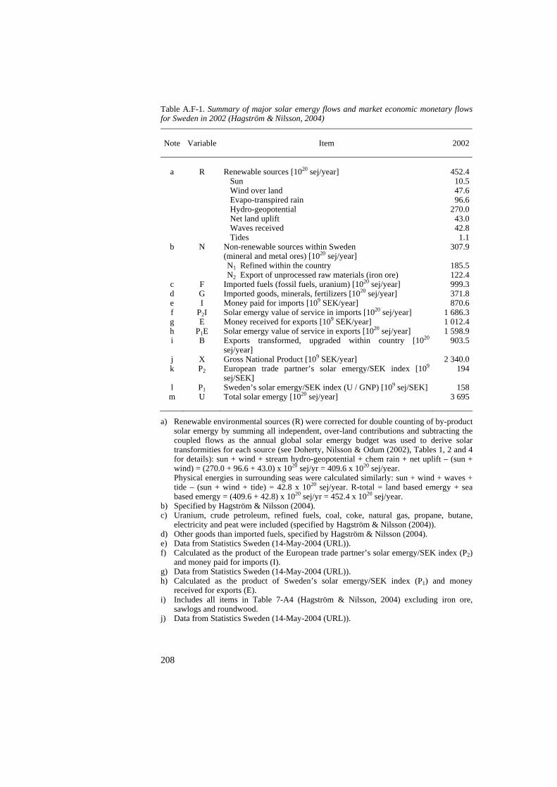
208

Table A.F-1. Summary of major solar emergy flows and market economic monetary flows for Sweden in 2002 (Hagström & Nilsson, 2004) Note

Variable

Item

2002

a

b c d e f g h i j k l m

R

N

F G I

P2I E

P1E B

X P2

P1U

Renewable sources [1020 sej/year] Sun Wind over land Evapo-transpired rain Hydro-geopotential Net land uplift Waves received Tides Non-renewable sources within Sweden (mineral and metal ores) [1020 sej/year] N1 Refined within the country N2 Export of unprocessed raw materials (iron ore)

Imported fuels (fossil fuels, uranium) [1020 sej/year] Imported goods, minerals, fertilizers [1020 sej/year] Money paid for imports [109 SEK/year] Solar emergy value of service in imports [1020 sej/year] Money received for exports [109 SEK/year] Solar emergy value of service in exports [1020 sej/year] Exports transformed, upgraded within country [1020 sej/year] Gross National Product [109 SEK/year] European trade partner’s solar emergy/SEK index [109 sej/SEK] Sweden’s solar emergy/SEK index (U / GNP) [109 sej/SEK] Total solar emergy [1020 sej/year]

452.410.547.696.6

270.043.042.81.1

307.9

185.5122.4999.3371.8870.6

1 686.3 1 012.4 1 598.9

903.5

2 340.0 194

158

3 695

a) Renewable environmental sources (R) were corrected for double counting of by-product

solar emergy by summing all independent, over-land contributions and subtracting the coupled flows as the annual global solar emergy budget was used to derive solar transformities for each source (see Doherty, Nilsson & Odum (2002), Tables 1, 2 and 4 for details): sun + wind + stream hydro-geopotential + chem rain + net uplift – (sun + wind) = (270.0 + 96.6 + 43.0) x 1020 sej/yr = 409.6 x 1020 sej/year. Physical energies in surrounding seas were calculated similarly: sun + wind + waves + tide – (sun + wind + tide) = 42.8 x 1020 sej/year. R-total = land based emergy + sea based emergy = (409.6 + 42.8) x 1020 sej/yr = 452.4 x 1020 sej/year.

b) Specified by Hagström & Nilsson (2004). c) Uranium, crude petroleum, refined fuels, coal, coke, natural gas, propane, butane,

electricity and peat were included (specified by Hagström & Nilsson (2004)). d) Other goods than imported fuels, specified by Hagström & Nilsson (2004). e) Data from Statistics Sweden (14-May-2004 (URL)). f) Calculated as the product of the European trade partner’s solar emergy/SEK index (P2)

and money paid for imports (I). g) Data from Statistics Sweden (14-May-2004 (URL)). h) Calculated as the product of Sweden’s solar emergy/SEK index (P1) and money

received for exports (E). i) Includes all items in Table 7-A4 (Hagström & Nilsson, 2004) excluding iron ore,

sawlogs and roundwood. j) Data from Statistics Sweden (14-May-2004 (URL)).

209

Table A.F-1 continued k) The European trade partner’s solar emergy/USD index was 2.00 x 1012 sej/USD in 1988

(Doherty, Nilsson & Odum, 2002). The conversion rate was 6.5 SEK/USD (ibid.), which gave that the European trade partner’s solar emergy/SEK index (P2) was 308 x 109 sej/SEK. The ratio of the European trade partner’s solar emergy/SEK index (P2) and Sweden’s solar emergy/SEK index (P1) in 2002 was assumed equal in size to 1988. Sweden’s solar emergy/SEK index in 1988 was 251 x 109 sej/SEK (Hagström & Nilsson, 2004). Thus, P2 = 158 x 109 x 308 x 109 / 251 x 109 sej/SEK = 194 x 109 sej/SEK.

l) Calculated as the quotient of the total solar emergy (U) and the gross national product (X).

m) The sum of solar emergy from renewable sources (R), non-renewable sources refined within Sweden (N1), imported fuels (F), imported goods (G) and from service in imports (P2I ).

Table A.F-2. Overview indices of annual solar emergy-use: origin, economic and demographic relations for Sweden in 2002 (Hagström & Nilsson, 2004) Note

Name of index

Derivation

2002

a

b c

d e f g h i j

k l m

n

o

p q r

Flow of imported solar emergy [1020 sej/year] Economic component [1020 sej/year] Total exported solar emergy [1020 sej/year] % Locally renewable (free) Economic/environment ratio Ratio of imports to exports Export to imports Net contribution due to trade (imports minus exports) [1020 sej/year] % of solar emergy-use purchased % of solar emergy-use derived from home sources Solar emergy-use per unit area [109 sej/m2] Population [106 inhabitants] Solar emergy-use per person [1016 sej/person] Renewable carrying capacity at present living standard [106 people] Carrying capacity using local resources [106 people] Fraction electric Fraction fossil fuels Fossil fuel-use per person [1015 sej/person]

F+G+P2I U-R N2+B+P1E R / U (U - R) / R (F+G+P2I) / (N2+B+P1E) (N2+B+P1E) / (F+G+P2I) (F+G+P2I ) - (N2+B+P1E) (F+G+P2I) / U (N1+R) / U U / area U / population (R/U)*(population) [(R+N)/U]*(population) (electricity-use) / U (fuel-use) / U fuel-use / population

3 057.4

3 242.9

2 624.8

12.2 7.17 1.16 0.86432.6

82.7 17.3

899.10

8.941 4.13

1.09

1.84

0.14 0.10 7.45

a) Sum of solar emergy from imported fuels (F), imported goods (G) and from service in

imports (P2I). b) Total solar emergy (U) excluding solar emergy from renewable sources (R). c) Sum of solar emergy from export of unprocessed raw materials (N2), exports

transformed, upgraded within country (B) and from service in exports (P1E). d) The ratio of solar emergy from renewable sources (R) and total solar emergy (U).

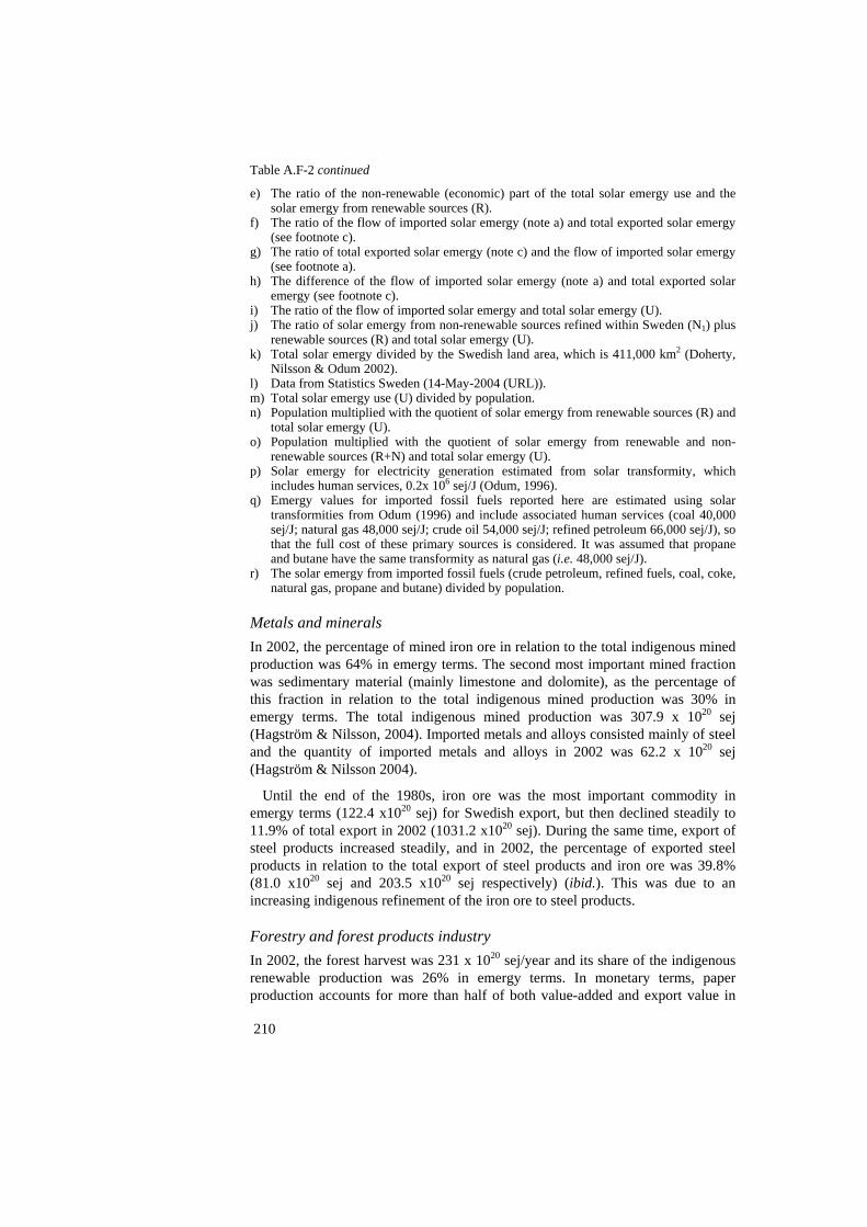
210

Table A.F-2 continued e) The ratio of the non-renewable (economic) part of the total solar emergy use and the

solar emergy from renewable sources (R). f) The ratio of the flow of imported solar emergy (note a) and total exported solar emergy

(see footnote c). g) The ratio of total exported solar emergy (note c) and the flow of imported solar emergy

(see footnote a). h) The difference of the flow of imported solar emergy (note a) and total exported solar

emergy (see footnote c). i) The ratio of the flow of imported solar emergy and total solar emergy (U). j) The ratio of solar emergy from non-renewable sources refined within Sweden (N1) plus

renewable sources (R) and total solar emergy (U). k) Total solar emergy divided by the Swedish land area, which is 411,000 km2 (Doherty,

Nilsson & Odum 2002). l) Data from Statistics Sweden (14-May-2004 (URL)). m) Total solar emergy use (U) divided by population. n) Population multiplied with the quotient of solar emergy from renewable sources (R) and

total solar emergy (U). o) Population multiplied with the quotient of solar emergy from renewable and non-

renewable sources (R+N) and total solar emergy (U). p) Solar emergy for electricity generation estimated from solar transformity, which

includes human services, 0.2x 106 sej/J (Odum, 1996). q) Emergy values for imported fossil fuels reported here are estimated using solar

transformities from Odum (1996) and include associated human services (coal 40,000 sej/J; natural gas 48,000 sej/J; crude oil 54,000 sej/J; refined petroleum 66,000 sej/J), so that the full cost of these primary sources is considered. It was assumed that propane and butane have the same transformity as natural gas (i.e. 48,000 sej/J).

r) The solar emergy from imported fossil fuels (crude petroleum, refined fuels, coal, coke, natural gas, propane and butane) divided by population.

Metals and minerals In 2002, the percentage of mined iron ore in relation to the total indigenous mined production was 64% in emergy terms. The second most important mined fraction was sedimentary material (mainly limestone and dolomite), as the percentage of this fraction in relation to the total indigenous mined production was 30% in emergy terms. The total indigenous mined production was 307.9 x 1020 sej (Hagström & Nilsson, 2004). Imported metals and alloys consisted mainly of steel and the quantity of imported metals and alloys in 2002 was 62.2 x 1020 sej (Hagström & Nilsson 2004).

Until the end of the 1980s, iron ore was the most important commodity in emergy terms (122.4 x1020 sej) for Swedish export, but then declined steadily to 11.9% of total export in 2002 (1031.2 x1020 sej). During the same time, export of steel products increased steadily, and in 2002, the percentage of exported steel products in relation to the total export of steel products and iron ore was 39.8% (81.0 x1020 sej and 203.5 x1020 sej respectively) (ibid.). This was due to an increasing indigenous refinement of the iron ore to steel products. Forestry and forest products industry In 2002, the forest harvest was 231 x 1020 sej/year and its share of the indigenous renewable production was 26% in emergy terms. In monetary terms, paper production accounts for more than half of both value-added and export value in

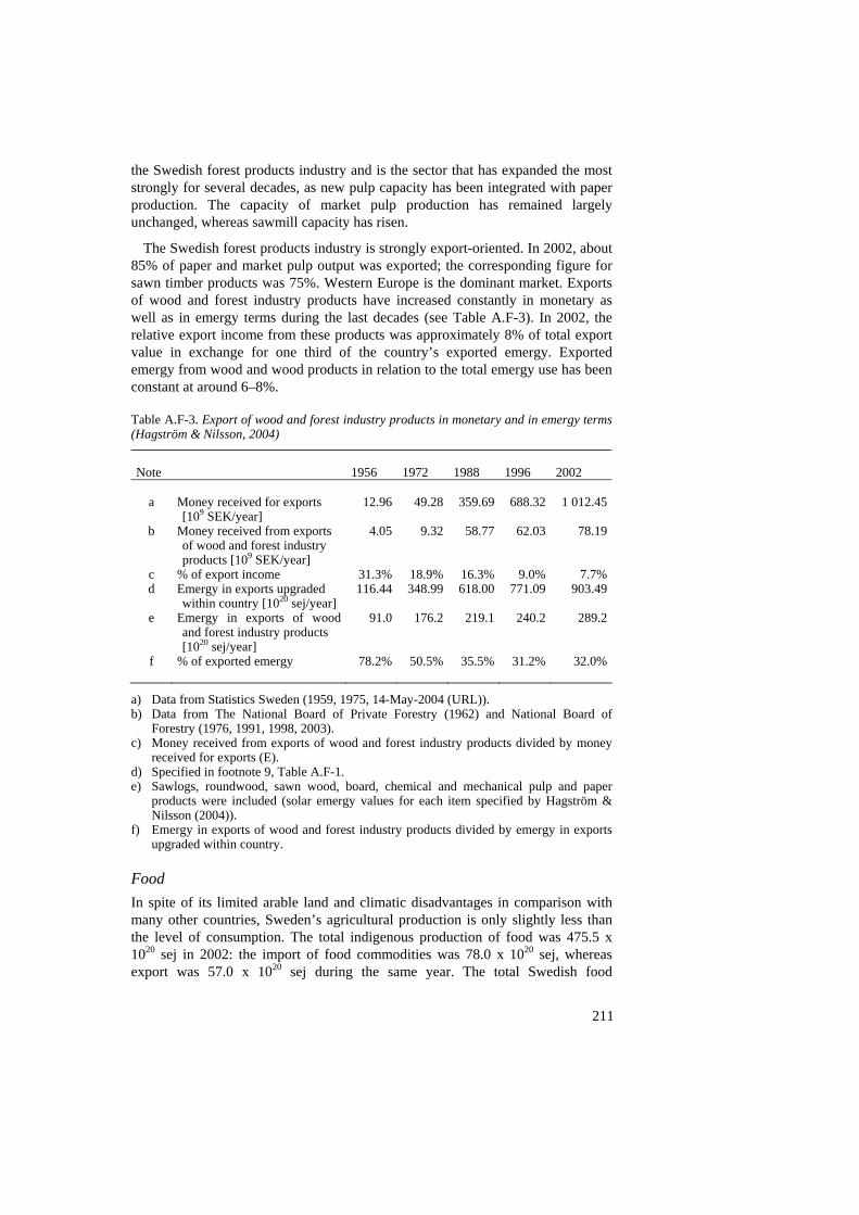
211

the Swedish forest products industry and is the sector that has expanded the most strongly for several decades, as new pulp capacity has been integrated with paper production. The capacity of market pulp production has remained largely unchanged, whereas sawmill capacity has risen.

The Swedish forest products industry is strongly export-oriented. In 2002, about 85% of paper and market pulp output was exported; the corresponding figure for sawn timber products was 75%. Western Europe is the dominant market. Exports of wood and forest industry products have increased constantly in monetary as well as in emergy terms during the last decades (see Table A.F-3). In 2002, the relative export income from these products was approximately 8% of total export value in exchange for one third of the country’s exported emergy. Exported emergy from wood and wood products in relation to the total emergy use has been constant at around 6–8%. Table A.F-3. Export of wood and forest industry products in monetary and in emergy terms (Hagström & Nilsson, 2004) Note

1956

1972

1988

1996

2002

a

b c d e f

Money received for exports [109 SEK/year]

Money received from exports of wood and forest industry products [109 SEK/year]

% of export income Emergy in exports upgraded within country [1020 sej/year]

Emergy in exports of wood and forest industry products [1020 sej/year]

% of exported emergy

12.96

4.05

31.3%116.44

91.0

78.2%

49.28

9.32

18.9%348.99

176.2

50.5%

359.69

58.77

16.3%618.00

219.1

35.5%

688.32

62.03

9.0%771.09

240.2

31.2%

1 012.45

78.19

7.7%903.49

289.2

32.0%

a) Data from Statistics Sweden (1959, 1975, 14-May-2004 (URL)). b) Data from The National Board of Private Forestry (1962) and National Board of

Forestry (1976, 1991, 1998, 2003). c) Money received from exports of wood and forest industry products divided by money

received for exports (E). d) Specified in footnote 9, Table A.F-1. e) Sawlogs, roundwood, sawn wood, board, chemical and mechanical pulp and paper

products were included (solar emergy values for each item specified by Hagström & Nilsson (2004)).

f) Emergy in exports of wood and forest industry products divided by emergy in exports upgraded within country.

Food In spite of its limited arable land and climatic disadvantages in comparison with many other countries, Sweden’s agricultural production is only slightly less than the level of consumption. The total indigenous production of food was 475.5 x 1020 sej in 2002: the import of food commodities was 78.0 x 1020 sej, whereas export was 57.0 x 1020 sej during the same year. The total Swedish food

212

consumption (indigenous production plus import minus export) has been relatively stable during the last decades, around 500 x 1020 sej, with a modest increase mainly reflecting population growth (Hagström & Nilsson, 2004).

In 2002, the nutritional value per person per day was approximately 12.2 kJ. Bread and grain products, meat and edible fats accounted for half of calorie intake in Sweden. Although by weight animal products are the smaller part, in emergy terms, they dominate because of high transformities. The percentage of livestock and dairy in relation to the total indigenous food production (agricultural crops, livestock, dairy products and fish) was 67% in 2002 (ibid.). Machines and vehicles The import and export of vehicles was 25.1 x 1020 sej 40.8 x1020 sej respectively in 2002 and the export of machines was 95.2 x1020 sej. Thus, the export of vehicles and machines was more than five times as large as the import of vehicles in emergy terms (ibid.). Other imports and exports Wool and cotton were important import commodities during the 1950s, as 25.6 x 1020 sej was imported in 1956. In 2002, the import of wool and cotton was 14.5 x 1020 sej (ibid.). Since the 1950s, fertilizer has been an important commodity and in 2002, the import was 17.5 x 1020 sej (ibid.). The import of plastics was 39.0 x 1020 sej in 2002 (ibid.). Commodities specified as other imported goods were animal hides, clothing, cotton fabrics, synthetic fibers, tires, chassis and other car parts. The import of these commodities was 53.6 x 1020 sej in 2002 (ibid.). Commodities specified as other exported goods were ADP machines, ADP parts, telecommunication equipment, televisions and car parts. The export of these commodities was 41.3 x 1020 sej in 2002 (ibid.).

213

Appendix G: Dry matter losses Dry matter losses occur in some handling operations, as e.g. baling and storage. Topical values of dry matter losses at handling of the different biomass assortments are shown in Table A.G-1. The storage time was assumed as three months for all assortments.

The largest dry matter losses received were for storage. However, the dry matter losses at storage varied for the different biomass assortments. It was assumed that there were no dry matter losses at storage of reed canary grass and straw, as the moisture content of these fractions were only 15%, and storage was in a barn (see Chapter 3). Furthermore, it was also assumed that there was no dry matter loss at storage of recovered wood, as the moisture content of this assortment was also low (10%). Recovered wood is also mostly treated by paint or rot-proofing agent, which protected the wood against moisture from the air.

The highest dry matter loss at storage was for bark (3.9% for three months and was due to a high nutrition content in bark, leading to a high microbiological activity and degradation of the biomass (Chow & Pickles, 1971). Even logging residues showed a high value of dry matter loss (3.3% for three months), which also may be due to a high nutrition content of the biomass material (Lundborg, 1998).

Dry matter losses at comminution will occur for all assortments; however, the fine fraction may be utilized as fuel/raw material when the comminution is performed at the conversion plant. Comminution of recovered wood was assumed to take place at a recycling station; therefore, the dry matter losses on comminution of this assortment were assumed not being used as fuel/raw material in the conversion processes studied.

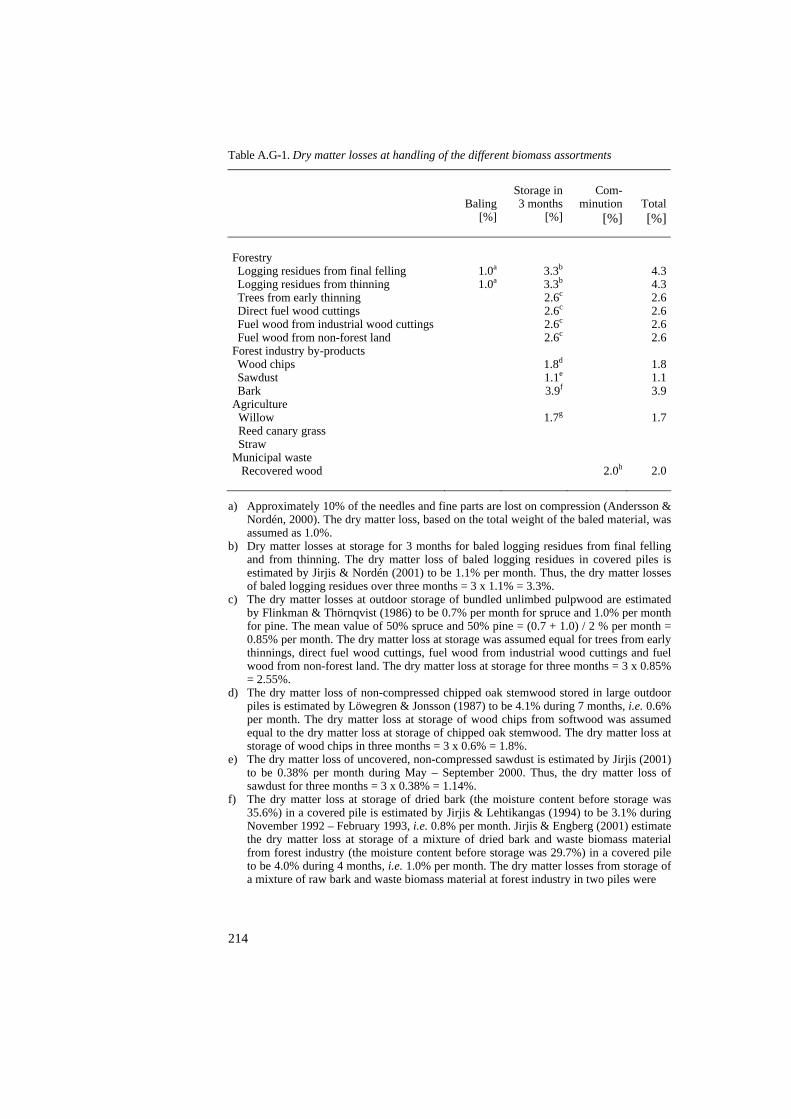
214

Table A.G-1. Dry matter losses at handling of the different biomass assortments

Baling[%]

Storage in 3 months

[%]

Com-

minution [%]

Total[%]

Forestry Logging residues from final felling Logging residues from thinning Trees from early thinning Direct fuel wood cuttings Fuel wood from industrial wood cuttings Fuel wood from non-forest land

Forest industry by-products Wood chips Sawdust Bark

Agriculture Willow Reed canary grass Straw Municipal waste Recovered wood

1.0a

1.0a

3.3b

3.3b

2.6c

2.6c

2.6c

2.6c

1.8d

1.1e

3.9f

1.7g

2.0h

4.34.32.62.62.62.6

1.81.13.9

1.7

2.0

a) Approximately 10% of the needles and fine parts are lost on compression (Andersson &

Nordén, 2000). The dry matter loss, based on the total weight of the baled material, was assumed as 1.0%.

b) Dry matter losses at storage for 3 months for baled logging residues from final felling and from thinning. The dry matter loss of baled logging residues in covered piles is estimated by Jirjis & Nordén (2001) to be 1.1% per month. Thus, the dry matter losses of baled logging residues over three months = 3 x 1.1% = 3.3%.

c) The dry matter losses at outdoor storage of bundled unlimbed pulpwood are estimated by Flinkman & Thörnqvist (1986) to be 0.7% per month for spruce and 1.0% per month for pine. The mean value of 50% spruce and 50% pine = (0.7 + 1.0) / 2 % per month = 0.85% per month. The dry matter loss at storage was assumed equal for trees from early thinnings, direct fuel wood cuttings, fuel wood from industrial wood cuttings and fuel wood from non-forest land. The dry matter loss at storage for three months = 3 x 0.85% = 2.55%.

d) The dry matter loss of non-compressed chipped oak stemwood stored in large outdoor piles is estimated by Löwegren & Jonsson (1987) to be 4.1% during 7 months, i.e. 0.6% per month. The dry matter loss at storage of wood chips from softwood was assumed equal to the dry matter loss at storage of chipped oak stemwood. The dry matter loss at storage of wood chips in three months = 3 x 0.6% = 1.8%.

e) The dry matter loss of uncovered, non-compressed sawdust is estimated by Jirjis (2001) to be 0.38% per month during May – September 2000. Thus, the dry matter loss of sawdust for three months = 3 x 0.38% = 1.14%.

f) The dry matter loss at storage of dried bark (the moisture content before storage was 35.6%) in a covered pile is estimated by Jirjis & Lehtikangas (1994) to be 3.1% during November 1992 – February 1993, i.e. 0.8% per month. Jirjis & Engberg (2001) estimate the dry matter loss at storage of a mixture of dried bark and waste biomass material from forest industry (the moisture content before storage was 29.7%) in a covered pile to be 4.0% during 4 months, i.e. 1.0% per month. The dry matter losses from storage of a mixture of raw bark and waste biomass material at forest industry in two piles were

215

Table A.G-1 continued

estimated by Jirjis & Engberg (2001). In one pile (the moisture content before storage was 66.7%), the dry matter loss was 6.0% during three months, i.e. 2.0% per month, and in the other pile (the moisture content before storage was 64.6%), the dry matter loss was 5.5% during four months, i.e. 1.4% per month. The dry matter loss of bark with 50% moisture content was assumed to be equal to the mean value of the dry matter losses in these measurements, thus the dry matter loss = (0.8 + 1.0 + 2.0 + 1.4) / 4% per month = 1.3% per month. The dry matter loss of bark in three months = 3 x 1.3% = 3.9%.

g) The dry matter losses of covered whole willow stems stored outdoors for five months are estimated by Kofman & Spinelli (1997) to be 2.9%. The average loss of dry matter = 2.9% / 5 = 0.58% per month. The dry matter losses of covered whole willow stems stored outdoors for three months may be estimated to be 3 x 0.58% = 1.74%.

h) Dry matter losses at comminution of recovered wood were assumed equal to the dry matter losses at comminution of baled logging residues, estimated by Nordén & Andersson (1997) to be 2.0%.

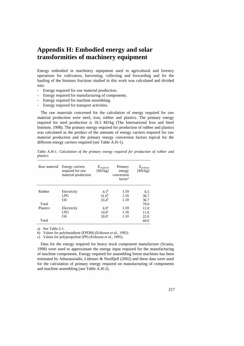
Appendix H: Embodied energy and solar transformities of machinery equipment Energy embodied in machinery equipment used in agricultural and forestry operations for cultivation, harvesting, collecting and forwarding and for the hauling of the biomass fractions studied in this work was calculated and divided into: - Energy required for raw material production. - Energy required for manufacturing of components. - Energy required for machine assembling. - Energy required for transport activities.

The raw materials concerned for the calculation of energy required for raw material production were steel, iron, rubber and plastics. The primary energy required for steel production is 18.3 MJ/kg (The International Iron and Steel Institute, 1998). The primary energy required for production of rubber and plastics was calculated as the product of the amounts of energy carriers required for raw material production and the primary energy conversion factors topical for the different energy carriers required (see Table A.H-1). Table A.H-1. Calculation of the primary energy required for production of rubber and plastics Raw material

Energy carriers required for raw material production

Erequired[MJ/kg]

Primary energy

conversion factora

Eprimary [MJ/kg]

Rubber Total

Plastics Total

Electricity LPG Oil Electricity LPG Oil

4.1b

31.6b

33.4b

6.9c

10.0c

20.0c

1.59 1.16 1.10

1.59 1.16 1.10

6.5

36.7 36.7 79.9 11.0 11.6 22.0 44.6

a) See Table 2-1. b) Values for polybutadiene (EPDM) (Eriksson et al., 1995). c) Values for polypropylene (PP) (Eriksson et al., 1995).

Data for the energy required for heavy truck component manufacture (Scania, 1998) were used to approximate the energy input required for the manufacturing of machine components. Energy required for assembling forest machines has been estimated by Athanassiadis, Lidestav & Nordfjell (2002) and these data were used for the calculation of primary energy required on manufacturing of components and machine assembling (see Table A.H-2).

217

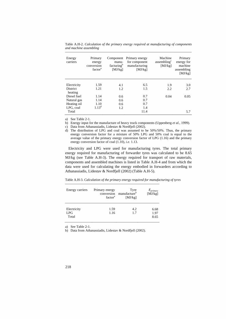
Table A.H-2. Calculation of the primary energy required at manufacturing of components and machine assembling Energy carriers

Primary energy

conversion factora

Component manu-

facturingb [MJ/kg]

Primary energy for component manufacturing

[MJ/kg]

Machine

assemblingc [MJ/kg]

Primary energy for

machine assembling

[MJ/kg]

Electricity District heating

Diesel fuel Natural gas Heating oil LPG, coal Total

1.59 1.21

1.14 1.14 1.10

1.13d

4.1 1.2

0.6 0.6 0.6 1.2

6.5 1.5

0.7 0.7 0.7 1.4

11.4

1.9 2.2

0.04

3.0 2.7

0.05

5.7 a) See Table 2-1. b) Energy input for the manufacture of heavy truck components (Uppenberg et al., 1999). c) Data from Athanassiadis, Lidestav & Nordfjell (2002). d) The distribution of LPG and coal was assumed to be 50%/50%. Thus, the primary

energy conversion factor for a mixture of 50% LPG and 50% coal is equal to the average value of the primary energy conversion factor of LPG (1.16) and the primary energy conversion factor of coal (1.10), i.e. 1.13.

Electricity and LPG were used for manufacturing tyres. The total primary energy required for manufacturing of forwarder tyres was calculated to be 8.65 MJ/kg (see Table A.H-3). The energy required for transport of raw materials, components and assembled machines is listed in Table A.H-4 and from which the data were used for calculating the energy embodied in forwarders according to Athanassiadis, Lidestav & Nordfjell (2002) (Table A.H-5).

Table A.H-3. Calculation of the primary energy required for manufacturing of tyres Energy carriers Primary energy

conversion factora

Tyre manufactureb

[MJ/kg]

Eprimary[MJ/kg]

Electricity LPG Total

1.591.16

4.21.7

6.681.978.65

a) See Table 2-1. b) Data from Athanassiadis, Lidestav & Nordfjell (2002).

218

Table A.H-4. Energy required for transport of raw materials, components and assembled machines, according to Athanassiadis, Lidestav & Nordfjell (2002) Transport activity Eprimary

[MJ/kg]

Raw materials to component manufacturing Components (excluding tyres) to the assembling

plant Tyres to the assembling plant From the assembling plant to the user

0.34a

0.31b

0.75c

0.55d

a) The transport distance was assumed 500 km by truck. b) An average value for the main components used for manufacturing of a forwarder. c) The transport distance was assumed 1100 km by truck. d) The transport distance was assumed 80 km by truck. Table A.H-5. Energy embodied in the manufacture and use of a forwarder Item Eprimary

[MJ/kg]

Raw material production for new equipment Manufacturing of new equipment Transportation and distribution

Total primary energy required for manufacturing of new equipment Raw material production for spare parts Manufacturing of spare parts Transportation and distribution of spare parts

Total primary energy required for manufacturing of spare parts

Total primary energy required for manufacturing and use

26.5a

16.1b

1.3c

43.8

35.5d

14.8e

1.3f

51.7

70.8g

a) The material composition of new equipment is 85% steel, other metals and glass, 12%

rubber and 3% plastics (Athanassiadis, Lidestav & Nordfjell, 2002). The primary energy required for production of other metals and glass was assumed equal to the primary energy required for steel production, i.e. 18.3 MJ/kg. Thus, the primary energy required for raw material production for new equipment = (0.85 x 18.3 + 0.12 x 79.92 + 0.03 x 44.57) MJ/kg = 26.5 MJ/kg.

b) The primary energy required for component manufacturing = 11.4 MJ/kg, and the primary energy required for machine assembling = 5.7 MJ/kg (Table A.I-2). The primary energy required for manufacturing of tyres = 8.65 MJ/kg (Table A.I-3). Thus, the primary energy required for manufacturing of new equipment = (0.85 + 0.03) x (11.4 + 5.7) + 0.12 x 8.65) MJ/kg = 16.1 MJ/kg.

c) Energy required for transport of raw materials, components and assembled machines (Table A.I-4) was weighted by means of the material composition. Thus, energy required for transportation and distribution = (0.34 + (0.85 + 0.03) x 0.31 + 0.12 x 0.75 + 0.55) MJ/kg = 1.3 MJ/kg.

d) The material composition of spare parts is 70% steel, other metals and glass, 26.5% rubber and 3.5% plastics (Athanassiadis, Lidestav & Nordfjell, 2002). The primary energy required for the production of other metals and glass was assumed equal to the

219

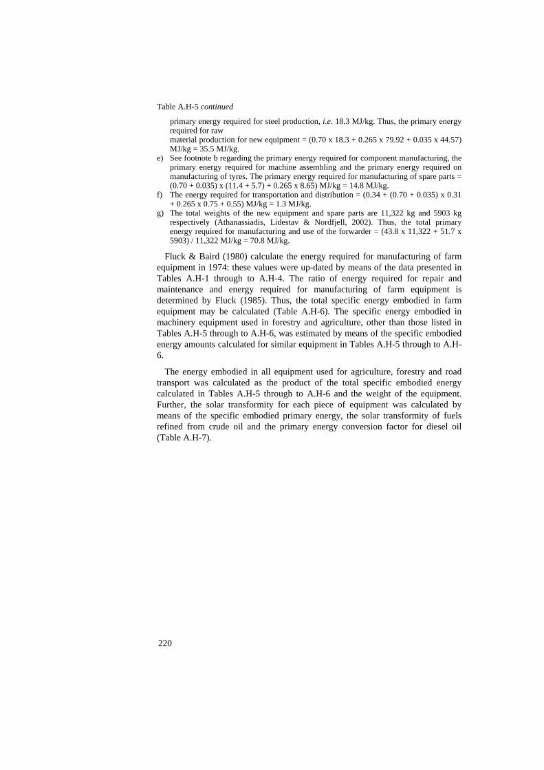
Table A.H-5 continued

primary energy required for steel production, i.e. 18.3 MJ/kg. Thus, the primary energy required for raw material production for new equipment = (0.70 x 18.3 + 0.265 x 79.92 + 0.035 x 44.57) MJ/kg = 35.5 MJ/kg.

e) See footnote b regarding the primary energy required for component manufacturing, the primary energy required for machine assembling and the primary energy required on manufacturing of tyres. The primary energy required for manufacturing of spare parts = (0.70 + 0.035) x (11.4 + 5.7) + 0.265 x 8.65) MJ/kg = 14.8 MJ/kg.

f) The energy required for transportation and distribution = (0.34 + (0.70 + 0.035) x 0.31 + 0.265 x 0.75 + 0.55) MJ/kg = 1.3 MJ/kg.

g) The total weights of the new equipment and spare parts are 11,322 kg and 5903 kg respectively (Athanassiadis, Lidestav & Nordfjell, 2002). Thus, the total primary energy required for manufacturing and use of the forwarder = (43.8 x 11,322 + 51.7 x 5903) / 11,322 MJ/kg = 70.8 MJ/kg.

Fluck & Baird (1980) calculate the energy required for manufacturing of farm equipment in 1974: these values were up-dated by means of the data presented in Tables A.H-1 through to A.H-4. The ratio of energy required for repair and maintenance and energy required for manufacturing of farm equipment is determined by Fluck (1985). Thus, the total specific energy embodied in farm equipment may be calculated (Table A.H-6). The specific energy embodied in machinery equipment used in forestry and agriculture, other than those listed in Tables A.H-5 through to A.H-6, was estimated by means of the specific embodied energy amounts calculated for similar equipment in Tables A.H-5 through to A.H-6.

The energy embodied in all equipment used for agriculture, forestry and road transport was calculated as the product of the total specific embodied energy calculated in Tables A.H-5 through to A.H-6 and the weight of the equipment. Further, the solar transformity for each piece of equipment was calculated by means of the specific embodied primary energy, the solar transformity of fuels refined from crude oil and the primary energy conversion factor for diesel oil (Table A.H-7).

220

Table A.H-7. Embodied energy and solar transformities of all equipment used in forestry, agriculture, road transport and comminution Equipment

Weight[Metric

ton]

Eembodieda

[GJ]

Solar transformityb

[sej/kg]

Forestry Harvester for final fellingc

Harvester for thinningc

Harvester for early thinningc

Forwarder, largeh

Forwarder, mediumh

Forwarder, smallh

Tractor, largel

Tractor, smalll

Soil scarifiero

Spreaderq

CRL machine for logging residuess

CRL machine for trees from early thinningc

Trailer with grapple loaderu

Hanger with grapple loaderu

Power saww

Delimbing-cutting processorw

Agriculture Tractorl

Harrowz

Weed harrowz

Compact wheel loaderbb

Rollerz

Willow planteree

Field chopperu

Fertilizer distributorq

Fertilizer distributor for high willow clumpsq

Sprayerhh

Tipperu

Willow harvesterjj

Rotary cultivatorll

Sowing machinenn

Moweroo

Combineqq

Balerss

Front loadernn

Wagon for big balesu

Discww

Ploughxx

Road transport Roundwood truckbb

Side-tipped truck for chipsbb

Comminution Dumper Crane Drum chipper Scraper

20.0d

14.0f

12.0g

18.0i

16.0j

11.0k

5.0m

2.0n

4.5p

2.0r

6.5t

3.0n

3.5v

1.0n

0.006x

1.5n

7.0y

2.4aa

0.9y

8.0cc

3.5dd

1.1y

1.8ff

0.7gg

0.4y

0.7ii

3.4y

12.2kk

1.4mm

1.5y

1.7pp

11.5rr

7.0tt

0.7uu

3.5vv

2.0n

3.3yy

20.0zz

21.0aaa

12.0bbb

2.0n

4.0n

3.5eee

1,416990.8849.21,2741,133778.4309.6123.8162.762.3

253.9

117.2128.236.60.2358.6

433.487.7

32.9495.4127.944.265.9

21.8

12.5

29.8124.5

525.7

50.660.2

111.2

495.4273.528.1

128.2

68.5149.6

1,238

1,300

2.97E+12e

2.97E+12e

2.97E+12e

2.97E+122.97E+122.97E+122.60E+122.60E+121.52E+121.31E+121.64E+121.64E+121.54E+121.54E+121.64E+121.64E+12

2.60E+121.54E+121.54E+122.60E+121.54E+121.69E+121.54E+121.31E+121.31E+121.79E+121.54E+121.81E+121.52E+121.69E+122.75E+121.81E+121.64E+121.69E+121.54E+121.44E+121.91E+12

2.60E+122.60E+12

2.60E+12ccc

1.52E+12ddd

1.52E+12ddd

1.52E+12ddd

221

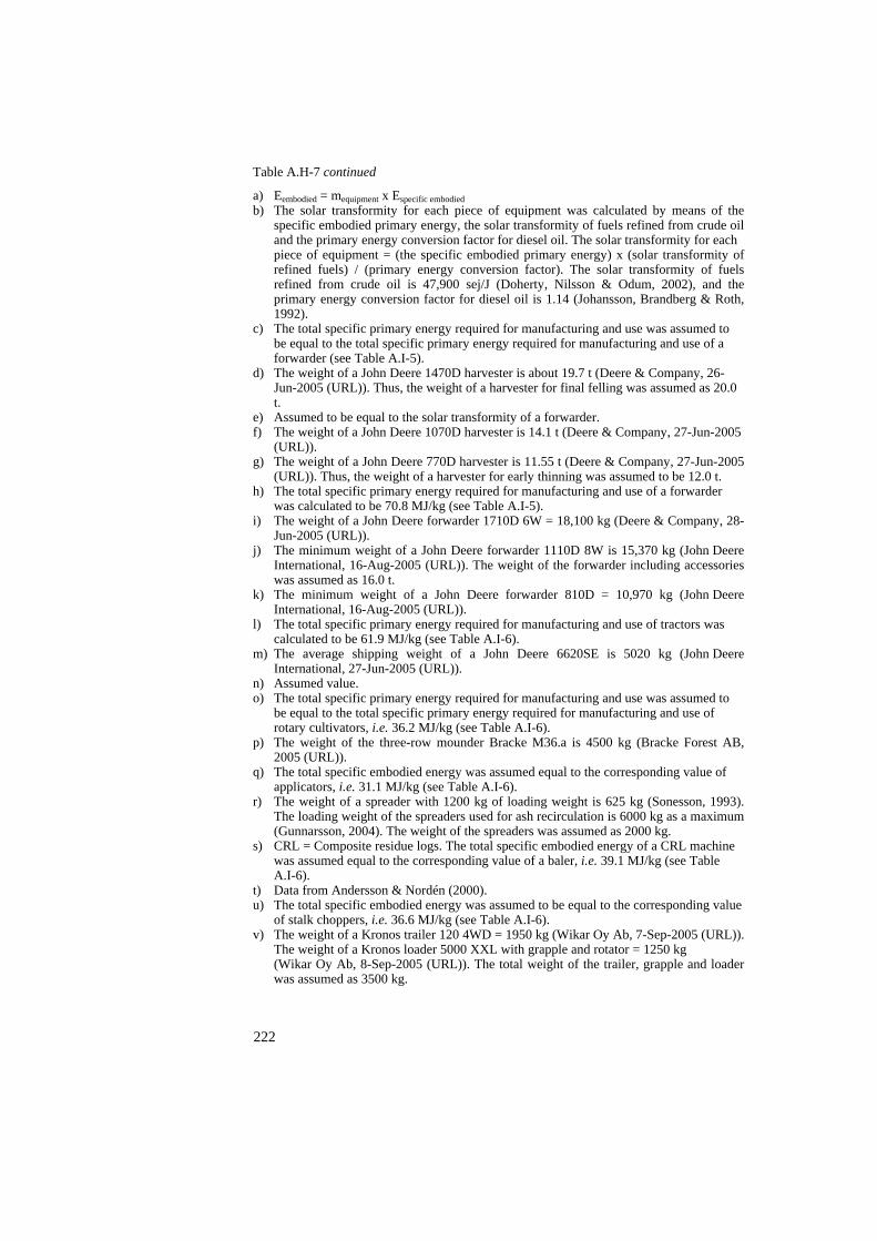
Table A.H-7 continued a) Eembodied = mequipment x Especific embodied b) The solar transformity for each piece of equipment was calculated by means of the

specific embodied primary energy, the solar transformity of fuels refined from crude oil and the primary energy conversion factor for diesel oil. The solar transformity for each piece of equipment = (the specific embodied primary energy) x (solar transformity of refined fuels) / (primary energy conversion factor). The solar transformity of fuels refined from crude oil is 47,900 sej/J (Doherty, Nilsson & Odum, 2002), and the primary energy conversion factor for diesel oil is 1.14 (Johansson, Brandberg & Roth, 1992).

c) The total specific primary energy required for manufacturing and use was assumed to be equal to the total specific primary energy required for manufacturing and use of a forwarder (see Table A.I-5).

d) The weight of a John Deere 1470D harvester is about 19.7 t (Deere & Company, 26-Jun-2005 (URL)). Thus, the weight of a harvester for final felling was assumed as 20.0 t.

e) Assumed to be equal to the solar transformity of a forwarder. f) The weight of a John Deere 1070D harvester is 14.1 t (Deere & Company, 27-Jun-2005

(URL)). g) The weight of a John Deere 770D harvester is 11.55 t (Deere & Company, 27-Jun-2005

(URL)). Thus, the weight of a harvester for early thinning was assumed to be 12.0 t. h) The total specific primary energy required for manufacturing and use of a forwarder

was calculated to be 70.8 MJ/kg (see Table A.I-5). i) The weight of a John Deere forwarder 1710D 6W = 18,100 kg (Deere & Company, 28-

Jun-2005 (URL)). j) The minimum weight of a John Deere forwarder 1110D 8W is 15,370 kg (John Deere

International, 16-Aug-2005 (URL)). The weight of the forwarder including accessories was assumed as 16.0 t.

k) The minimum weight of a John Deere forwarder 810D = 10,970 kg (John Deere International, 16-Aug-2005 (URL)).

l) The total specific primary energy required for manufacturing and use of tractors was calculated to be 61.9 MJ/kg (see Table A.I-6).

m) The average shipping weight of a John Deere 6620SE is 5020 kg (John Deere International, 27-Jun-2005 (URL)).

n) Assumed value. o) The total specific primary energy required for manufacturing and use was assumed to

be equal to the total specific primary energy required for manufacturing and use of rotary cultivators, i.e. 36.2 MJ/kg (see Table A.I-6).

p) The weight of the three-row mounder Bracke M36.a is 4500 kg (Bracke Forest AB, 2005 (URL)).

q) The total specific embodied energy was assumed equal to the corresponding value of applicators, i.e. 31.1 MJ/kg (see Table A.I-6).

r) The weight of a spreader with 1200 kg of loading weight is 625 kg (Sonesson, 1993). The loading weight of the spreaders used for ash recirculation is 6000 kg as a maximum (Gunnarsson, 2004). The weight of the spreaders was assumed as 2000 kg.

s) CRL = Composite residue logs. The total specific embodied energy of a CRL machine was assumed equal to the corresponding value of a baler, i.e. 39.1 MJ/kg (see Table A.I-6).

t) Data from Andersson & Nordén (2000). u) The total specific embodied energy was assumed to be equal to the corresponding value

of stalk choppers, i.e. 36.6 MJ/kg (see Table A.I-6). v) The weight of a Kronos trailer 120 4WD = 1950 kg (Wikar Oy Ab, 7-Sep-2005 (URL)).

The weight of a Kronos loader 5000 XXL with grapple and rotator = 1250 kg (Wikar Oy Ab, 8-Sep-2005 (URL)). The total weight of the trailer, grapple and loader was assumed as 3500 kg.

222

Table A.H-7 continued w) The total specific embodied energy was assumed equal to the corresponding value of

CRL machines, i.e. 39.1 MJ/kg (see footnote s). x) The weights of Husqvarna power saws for professional use vary between 3.8 – 10.4 kg

(Husqvarna AB; 2005 (URL)). The weight of a power saw was assumed as 6.0 kg. y) Data from Sonesson (1993). z) The total specific embodied energy was assumed equal to the corresponding value of

field cultivators, i.e. 36.6 MJ/kg (see Table A.I-6). aa) The weight of a harrow with a width of 9 meter is 3.1 metric ton, and consists of 100%

steel (Sonesson, 1993). Thus, the weight of a harrow with a width being 7 m was assumed to be 7 / 9 x 3.1 t = 2.4 t.

bb) The total specific embodied energy was assumed equal to the corresponding value of tractors, i.e. 61.9 MJ/kg (see Table A.I-6).

cc) The operating weight of a Volvo compact wheel loader L40B is 7900 – 8400 kg (Volvo Construction Equipment Corporation, 2005 (URL)).

dd) Assumed to be equal to the weight of a Väderstad Rollex roller RX 940, operation width = 9.4 m (Sonesson, 1993).

ee) The total specific embodied energy for planters was calculated to be 40.2 MJ/kg (see Table A.I-6).

ff) The weights for different precision choppers vary between 1300 – 2300 kg (Statens Maskinprovningar, 1986). Thus, the weight of a chopper of medium size is about 1800 kg.

gg) The weight of a Bogballe SST 1200 with the loading weight being 1200 kg is 625 kg (Sonesson, 1993). The weight of a fertilizer spreader with the loading weight being 2500 litre was assumed to be 700 kg.

hh) The total specific embodied energy for sprayers was calculated to be 42.6 MJ/kg (see Table A.I-6).

ii) The weight of a sprayer with the operation width being 12 m and loading capacity being 1500 litre = 800 kg (Sonesson, 1993). The weight of a sprayer with the operation width being 12 m and loading capacity being 1000 litre was assumed to be 700 kg.

jj) The total specific embodied energy was assumed to be equal to the corresponding value of combines, i.e. 43.1 MJ/kg (see Table A.I-6).

kk) The weight of a willow harvester, model Empire 2000, is 12.2 t (Danfors & Nordén, 1995).

ll) The total specific embodied energy for rotary cultivators was calculated to be 36.2 MJ/kg (see Table A.I-6).

mm) The weight of a Meri rotary cultivator with the operational width being 2.5 m = 1.36 t (Rovaniemi, 2004).

nn) The total specific embodied energy was assumed equal to the corresponding value of planters, i.e. 40.2 MJ/kg (see Table A.I-6).

oo) The total specific embodied energy for cutterbar mowers was calculated to be 65.4 MJ/kg (see Table A.I-6).

pp) The weight of the mower Taarup 4032C/4032R is 1.7 t (Kverneland Group Sverige AB, 8-Oct-2004 (URL)).

qq) The total specific embodied energy for combines was calculated to be 43.1 MJ/kg (see Table A.I-6).

rr) The weight of the combine Fendt 5220 E (Poutput = 162 kW) without cutting table is 10.1 t (http://www.fendt.com/index_en.html; 4-Oct-2005). The weight of a standard cutting table is about 1.6 t (AGCO AB, 4-Oct-2005 (URL)). Thus, the weight of a combine with 140 kW power output with cutting table was assumed as 11.5 t.

ss) The total specific embodied energy for balers was calculated to be 39.1 MJ/kg (see Table A.I-6).

tt) The weight of the baler Claas Quadrant 1200 is 5500 kg (Sonesson, 1993). As the weight of the bales made by the baler Hesston 4800/4900 is almost twice as high as the weight of the bales made by the baler Claas Quadrant 1200 (Hadders, Jonsson &

223

Table A.H-7 continued

Sundberg, 1997), the weight of the baler Hesston 4800/4900 was assumed to be 7000 kg.

uu) The weight of a front-loader designed for tractors with 32 – 57 kW power output range is 560 kg (Sonesson, 1993). Thus, the weight of a front-loader designed for a tractor with 110 kW power output was assumed as 700 kg.

vv) The weight of the wagon LRMA 12000 designed for big bales is 3.5 t (Rasmusson, 2004).

ww) The total specific embodied energy for discs was calculated to be 34.3 MJ/kg (see Table A.I-6).

xx) The total specific embodied energy for ploughs was calculated to be 45.3 MJ/kg (see Table A.I-6).

yy) Equal to the weight of the plough Kverneland PB/RB (Kverneland Group Sverige AB 9-Oct-2004 (URL)).

zz) Data from Staland (2004). aaa) Data from Löthstam (2004). bbb) The weight of the dumper was assumed equal to the weight of a small harvester. ccc) Assumed equal to the solar transformity of trucks. ddd) Assumed equal to the solar transformity of rotary cultivators. eee) Data from Rockler (2004).

224

Biomass Potential for Heat, Electricity and Vehicle Fuel in ...

Documents

Transcript of Biomass Potential for Heat, Electricity and Vehicle Fuel in ...