1

BIOLOGY 112: Organisms, Evolution, and Ecosystems

LABORATORY MANUAL

FALL 2007

INSTRUCTOR: Dr. Chris Paradise

PRINCIPLES OF BIOLOGY II LABORATORY AND FIELD MANUAL

TABLE OF CONTENTS SECTION PAGE Exercise 1: How to Record and Present Your Data Graphically Using Excel 2

Developed by Chris Paradise

Exercise 2: Evolutionary Mechanisms - The Mating Game & Populus 7 Developed by Patricia Peroni and Chris Paradise

Exercise 3: Variability in Natural Populations 19 Modified from Kephart et al. 2000 (The American Biology Teacher 64:455-463)

Exercise 4: Phylogenetic Analysis 23 Modified from Singer et al. 2001 (The American Biology Teacher 63:518-523)

Exercise 5: Tree Ring Ecology 28 Modified from Rubino & McCarthy 2002 (The American Biology Teacher 64:689-695)

Exercise 6: Plant Defense Bioassay 31 Developed by Mark Stanback

Exercise 7: Factors Affecting Respiration in Goldfish 38 Developed by Michael Dorcas

Exercise 8: Fetal Pig Anatomy 41 Developed by Mark Stanback and Chris Paradise

Appendix A: Laboratory and Field Safety Agreements 66 Appendix B: How to Prepare a Scientific Research Report 70

2

Exercise 1: How to Record and Present Your Data Graphically Using Excel Introduction In this world of high technology and information overload scientists must learn to communicate effectively and efficiently. How can we get our point across to both fellow scientists and nonscientists in a way that is meaningful to both groups? To communicate effectively, scientists must be clear, concise, and consistent. To communicate efficiently scientists must know what data to present in order to emphasize the point they wish to make. Numerical results are useful because they help answer a question or test a hypothesis. Raw data that you collect to test a particular hypothesis must be digested in some way and presented, not as a jumbled mass of field notes and numbers, but as concise and informative tables, diagrams, or graphs. Objective For you to learn and gain perspective on the ways in which raw data may be abstracted and presented in a report, and to prepare sample graphs. Recording Your Data Writing down a number may seem like a simple thing to do, but the numbers that we read from some measuring device are limited in the number of significant digits that we obtain. Every piece of equipment that we use to measure with allows us to ascertain the value in question to a certain degree. For instance, a ruler with centimeters as the smallest gradation can measure to the nearest centimeter. We then estimate the last digit, in this case would to the nearest millimeter. So there is a degree of uncertainty in our estimate of the last digit. Let's say an object is measured and found to be 1.269 meters long. The rightmost digit is in the millimeter position and is our "uncertain" digit. There are four significant digits in this measurement, which gives us a certain amount of confidence as to the precision and accuracy of the measurement, based on the quality of our measuring device. Precision comes into play when you measure the same quantity more than once. How close does your repeated measure come to the original measurement? That is the degree of precision of your instrument. Measuring quantities more than once with the ruler described above, we might expect to get readings that differ by about 1 millimeter. Such a ruler is precise to +1 mm. However, if we had a ruler that measured to a tenth of a millimeter that ruler would have one more significant digit than our first ruler would. It might also be considered more precise. Absorbance of light is measured on a spectrophotometer and while measuring the quantity of light absorbed by a certain solution you want to be sure that the machine is zeroed properly and that you are obtaining the correct reading. So initially, your objective is to check your precision. However, you may discover that your readings are inaccurate because the machine is not zeroed properly. Accuracy is the term used to describe how close any measured value is to the true value. In general, a more precise measurement will also be more accurate, assuming that calibration of the measuring device has been performed properly. Presenting Your Data Numerical results are generally useful because they may help answer a question or test a hypothesis. Your task is to make certain that readers understand why certain data do or do not answer a given question. Usually this requires that the raw data be digested and processed in some way. Presenting data in tabular or graphic form are two methods that scientists use to assist their readers (and themselves) in interpretation of their results. Tables and figures should always be labeled with a table or figure number, such as "Table 1" or "Figure 3." Always refer to the table or

3

figure in the text, either to point out a trend in the data or to discuss the significance of the data. Never put tables or figures into a protocol or write-up without discussing them in the text! Tables are generally used to show the relationships between treatments and controls when it is necessary to present all of the information obtained from an experiment. However, this method can become cumbersome when large data sets are displayed. One way around this is to use graphs, which often demonstrate relationships without burdening the reader with large quantities of numbers. There are advantages and disadvantages to both styles of presentation. Tables are useful when one wants the reader to see the actual numbers. They are also useful to show frequency counts of categorical variables. As previously mentioned, tables can be a disadvantage when one has to present large data sets, because it forces the reader to visualize the relationships among many numbers and the complex interactions between many variables. That's where graphs come in. When a reader looks at a graph, they should be able to quickly grasp the point that is being made. The graph should effectively show a trend (e.g., an increase in the measured variable over time) or a relationship (e.g., the difference between a control and treatments). Graphs generally consist of an independent and a dependent variable. The independent variable is generally displayed on the abscissa (the x-axis) and can be a measured quantity, such as time, or a category, and may be set by the investigator. This variable should be unaffected, or as the name implies, independent, of the variables being studied. The dependent variable, on the other hand, is affected by the independent factor under investigation (or at least one hypothesizes it is prior to experimentation). The dependent variable is graphed against the independent variable so that one can see how the dependent variable changes with changes in the independent variable. There are many different ways to graph data. Line graphs and histograms are probably the most popular and will be the types you will use most frequently. Line graphs show the relationship of a dependent variable to an independent variable when the independent variable is a continuous measurement, such as time (Fig. 1). Histograms, or bar graphs, are the best way to show frequency distributions of categorical variables. The frequency is the number or proportion and is the dependent variable, while the various categories used make up the independent variable. Let's say, for example, that we wanted to test the effects of robin flock size on feeding rates of robins. We have hypothesized that larger flocks of birds will be more successful in terms of number of worms caught by each individual. Below is a portion of the fictional raw data used to construct Table 2 and Figure 1. This table is fairly well organized, which is the key when producing tables and graphs. This table has titles at the head of each column; labels and titles are critical in tables and graphs. Always title your graphs and tables so the reader knows what they are examining, and label axes and rows and columns so that one can quickly see what variables are presented and determine the scale of numbers. However, getting back to our raw data table, a report that simply included these raw data unaltered would be flawed because it is difficult to extract the significant aspects of these results in this form. The first step might be to analyze the field data to determine the number of worms taken per robin for each 30 minutes of hunting time, using the following equation: [(# of worms captured)/(median # of birds in flock)] / [(total observation time (min.))/(30 minutes)]

4

Table A.1. Raw data from experiment on flock size and worm capture rate observations.

Date and Time Number of robins in flock Number of worms taken by entire flock

12 Apr 0705-0740 18-22 16

12 Apr 0800-0830 6-7 2

12 Apr 1530-1635 14-20 18

12 Apr 1610-1630 3-5 1

13 Apr 0730-0845 16-19 15

13 Apr 0750-0845 23-28 31

13 Apr 0815-0925 2 3

This provides us with a standard result that will permit direct comparisons among the various flocks of robins (Table A.2).

Table A.2. The relation between number of robins in a foraging flock and the average foraging success of individuals in flock. Observations made Apr. 12-13 from 0700-0900 & 1500-1700.

Total observation time

(min.)

Number of robins in flock

Median number

Worms taken by flock

Success rate (see equation)

70 2 2 3 0.6

65 3-5 4 1 0.1

25 6-7 6.5 2 0.4

45 14-20 17 18 1.4

20 16-19 17.5 15 1.3

30 18-22 20 16 0.8

55 23-28 25.5 31 0.7

There are still other ways that this material might have been offered to the reader. For example, the data in Table 2 could be used to make a scatter diagram (Figure 1). Diagrams, graphs and charts tend to have a more visual impact than a table, and as a result, they project their meaning more quickly and dramatically. They do so, however, at the expense of some information that might appear in a table. Figure 1 does not allow the reader to determine how long the flocks were watched in order to produce the success rate scores that appear as points on the diagram, whereas Table 2 contains this information. You as a scientist and writer must decide which of several possible ways of presenting data conveys information most advantageously, in relation the question you are asking or hypothesis you are testing.

5

0

0.2

0.4

0.6

0.8

1

1.2

1.4

1.6

0 10 20 30

Median number of robins in flock

Success rate (#/30 minutes)

Figure 1. The correlation between foraging success for worms and number of robins in a flock. Using Excel Provided below are examples of graphs created using Microsoft Excel – there are two of each graph, and one of each is considered high quality, while the other is of poor quality. In each case the legend provides hints and guidelines for how to professionally create graphs, and why the poor quality graphs are of poor quality.

Figure 2a. Tree Size Does Not

Affect Ice Storm Damage

y = -0.0363x + 8.3809

0

2

4

6

8

10

12

14

16

18

20

0 20 40 60 80 100

Tree Diameter (cm)

No. of Branches Broken

Tree Size Does Not Affect Ice Storm Damage

y = -0.0363x + 8.3809

0

5

10

15

20

25

0 30 60 90 120 150

Tree Diameter (cm)

No. of Branches Broken

Figure 2. Both panels depict the same data. However, the figure on the left is of much higher quality than the one on the right. In particular, note in 2a that: 1) the sizes of the fonts are large, easy to read, and of consistent size, 2) the area showing the actual data is maximized, 3) the contrast is high (dark points on a white background), 4) the figure number appears in the title/legend, and 5) the axis labels contain the units of measurement. In the right panel: 1) the fonts are generally smaller and of inconsistent size, 2) the data points are light blue on a gray background (low contrast), 3) the gridlines make it difficult to see the data, 4) there is no figure

6

number, and 5) the scales are not adjusted to maximize the usage of the graph area (there’s a lot of empty space on the right and top).

Figure 3a. Average Damage to Specific Tree

Genera

0

2

4

6

8

10

12

Oaks (6 spp.) Elms (3 spp.) Maples (2

spp.)Genus

Average # of Broken Branches

(+/- 1 s.d.)

Average Damage to Specific Tree

Genera

0

2

4

6

8

10

12

Oaks (6 spp.) Elms (3 spp.) Maples (2 spp.)Genus

Average # of Broken Branches (+/- 1

s.d.)

Oaks (6 spp.)

Elms (3 spp.)

Maples (2 spp.)

Figure 3. Both panels depict the same data. The figure on the left is of higher quality than the one on the right. In particular, note in 3a that: 1) the sizes of the fonts are large, easy to read, and of consistent size, 2) the area showing the actual data is maximized, 3) the contrast is high (dark bars on a white background), 4) the figure number appears in the title/legend, and 5) the axis labels contain the units of measurement. In the right panel: 1) the fonts are generally smaller and of inconsistent size, 2) the data bars are unnecessarily different colors (use different colors for different series of data plotted against the same independent variable), 3) averages are plotted without error bars, 4) there is no figure number, 5) there is an unnecessary and redundant legend, 6) the labels overlap the scales, and 7) the y-axis scale is not adjusted to maximize the usage of the graph area (there’s a lot of empty space at the top).

Assignment

We will generate data from the Mating Game (found in Exercise 2). Your task is to consider ways of presenting these raw data in tabular and graphical fashion to illustrate two major points regarding the data. Use the information above regarding construction of Excel graphs to guide your efforts. Save your work – next week we will complete the construction of a Results section and you will turn it in. Cut and paste the graphs into Word and add proper figure and table legends (see Appendix C). Work in pairs and save the file using the following convention: lastnames_graphs_ex1.doc.

7

Exercise 2: Evolutionary Mechanisms – The Mating Game and Computer Simulations Developed by Drs. Patricia Peroni and Chris Paradise

INTRODUCTION

Evolution can be defined as a change in the genetic composition of a population of organisms that occurs over time. More precisely, evolution is a change that occurs over time in the proportions of organisms in a population that differ genetically in one or more characteristics. Just as the life of an individual organism is dynamic, so is that of a species. In the study of biological evolution we can ask what factors are capable of causing change within a population.

Due to time constraints (thousands of generations may be required for one species to evolve into another) it is difficult to perform evolution experiments on populations in one semester. Our approach will thus be to first investigate these questions using a hypothetical population. We will conduct simulations to determine the factors that can facilitate or inhibit genetic change at one locus within this population. Our hypothetical population will be very simple, and we’ll focus on how different factors affect the genotype and allele frequencies at one locus.

The simulation approach we will use represents a type of theoretical investigation. Why should we use this approach before we conduct experiments with real organisms? Theoretical inquiry serves as a guide for empirical research (i.e., research that involves taking measurements on real organisms). Real systems are complex, and experimental research with these systems is often time consuming and expensive. Theoretical research allows us to ask "what if" questions using very simple systems that we refer to as models. In a general sense, a model should be thought of as formalized working hypothesis. That is, in the context of a computer simulation model, the program itself is written to test a prediction about the mechanisms responsible for a given event (in this case, parameters affecting populations). If the hypothesis is correct, then the program will accurately simulate an event.

The results of such investigations can suggest questions that can be further tested with experiments and the types of results we might expect to obtain from such studies. If the predictions of theoretical investigations and empirical studies are at odds with each other, then we must refine our theoretical models to account for factors omitted from our initial inquiries. The operation of testing a model, and changing it as required, is part of the scientific process. All active areas of research involve this type of interplay between theoretical and empirical research, and our understanding of how the world operates depends upon both types of investigations. BEFORE YOU COME TO LAB

Read the synopsis of the Hardy Weinberg Equilibrium Theory at the end of this lab procedure and begin work on the Evolutionary Mechanisms Problem Set. GAME PLAN 1. As a class we will simulate a very simple population of interbreeding organisms, and we will

then investigate how changes in characteristics of the population and its environment affect the direction and rate of evolution at one particular locus.

2. We will then use a computer program to simulate a similar hypothetical population. The difference between the computer simulations and the ones we conduct by hand is that the software conducts the simulations faster, allows us to specify larger population sizes and longer generation times. The class simulations should familiarize you with the rationale behind the computer simulations and make them less of a "black-box" procedure.

3. Before we conduct each simulation, record your prediction for the simulation's outcome and the rationale you used to make that prediction.

8

CLASS SIMULATIONS Our goal is to simulate a very simple population and look at one very simple genetic

characteristic. In order to accomplish this goal, we will assume that: 1. Each individual in the population reaches reproductive maturity, mates, produces two offspring,

and then dies. 2. Individuals in the population are hermaphrodites (i.e., can function as both mothers and

fathers) but cannot self-fertilize. 3. The genetic trait under consideration is controlled by two alleles, A and a, at one locus. The A

allele is dominant with respect to the a allele. Individuals in the population are homozygous for all other loci.

4. No individuals enter or leave our population (i.e., no immigration or emigration). General Instructions 1. Each new simulation will begin with a population with an initial frequency (p and q) of 0.5 for

alleles A and a, and genotype frequencies of 0.25 for the aa and AA genotypes and 0.50 for the Aa genotype.

2. Each of you will receive two index cards that represent your genotype at the locus of interest (e.g., if you receive two a cards, your genotype is aa). Record this genotype.

3. You will then proceed to mate. Unless instructed otherwise, you should be entirely promiscuous (remember, this is very safe sex - on paper only). Choose anyone else in the class (male or female - remember for our simulation purposes you are all hermaphrodites) and approach them confidently – introduce yourself. They will not refuse to mate. Once you find a mate, flip a coin to determine which allele you will contribute to your first offspring - your mate will do the same. Record the genotype of your offspring. Repeat the process to produce a second offspring for your mate and record it's genotype. By having each couple produce two and only two offspring per generation, we keep the population size constant.

4. Once you and your mate have produced two offspring, wait for me to signal the end of that generation. At the end of the generation, you and your mate will "die", and each of you will assume the genotype of one of your two offspring (e.g., if you produce an AA and an Aa offspring, one of you assumes the AA genotype and the other assumes the Aa genotype). Record your new genotype on your data sheet.

5. When I signal the beginning of a new mating session, you will pick another mate and produce two new offspring using the alleles from your new genotype. Never mate with the same person twice in a row, unless directed to do so.

6. We will complete 5 generations of mating for each simulation. IMPORTANT NOTES

• Mate with only one individual each generation.

• Do not move on to a new generation of mating until I instruct you to do so.

• If you are heterozygous, you sample with replacement when you decide which allele to give to each offspring. This means that if you designate the A allele as heads and the other allele as tails, you could end up donating an A allele to both offspring.

• Remember to record your new genotype in the appropriate place on your data sheet. SIMULATIONS Null Model

If no evolutionary mechanisms influence the locus under consideration, then allele frequencies should remain constant over time and genotype frequencies should eventually match Hardy Weinberg predictions. We’ll calculate allele and genotype frequencies at the beginning of

9

each simulation. If allele and genotype frequencies at the end of each generation deviate from the initial conditions, then we know that some evolutionary mechanism affected the population.

Simulation #1: Small population sizes

In this simulation we will examine the effects of population fragmentation and small population size on evolution. I will randomly split the class into four populations of four individuals each. Remember to clearly mark your data sheet with the name of your population. The individuals in each population will then proceed to mate following the instructions provided above. Record your data in Table 2. NOTE: Mate only with individuals in your population. Simulation #2: Non-random mating

Begin this simulation with the genotype you were assigned at the beginning of simulation #1. Form one large population and examine effects of non-random mating on evolution at our locus. We will again assume that the AA and Aa genotypes have the same phenotype (i.e., A dominant to a). When you pick a mate, try to find one whose phenotype matches yours. Mate only with someone of a different phenotype as a last resort. Otherwise, proceed as you did for simulation #1. Record your genotype for each generation (and the class frequencies) in Table 3. How does this case compare to the first simulation? What happens to p and q? Has evolution occurred?

Table 1. Record your data from simulation 1 here to determine if your class is in Hardy-Weinberg Equilibrium.

Generation Your Genotype

Class Data

A/A A/a a/a p q

Start-P 0.5* 0.5*

F1

F2

F3

F4

F5

Simulation #3: Selection Against Homozygous Recessives We’ll violate another assumption to see how allele frequencies change. Assume there is a genetic disease in our population in which offspring that are homozygous recessive (a/a genotype) do not survive. Individuals who have the a/a genotype are physically debilitated and die at a young age. Individuals of the other two genotypes, A/A and A/a (the homozygous dominant and heterozygous genotypes, respectively) survive equally well. Begin this simulation with the genotype you were assigned at the beginning of simulation #1. We’ll assume that any homozygous recessives (a/a) will survive to mate in this parental generation (however, if you’re a/a to start, you can’t mate with another a/a in generation 1). Mate just like you have been. However, every time you and your partner produce a homozygous recessive child, it dies. Since we want to keep the same population size, continue to mate until you produce two viable offspring. Record your genotype for each generation (and the class frequencies) in Table 4. How does this case compare to the first simulation? What happens to p and q? Has evolution occurred? Are there recessive alleles left in the population?

10

Table 2. Record your data from simulation 1 here to examine genetic drift in small populations.

Generation Your Genotype

Class Data

A/A A/a a/a p q

Start-P

F1

F2

F3

F4

F5

Table 3. Record your data from simulation 2 here to examine non-random mating.

Generation Your Genotype

Class Data

A/A A/a a/a p q

Start-P

F1

F2

F3

F4

F5

Table 4. Record your data from the homozygous recessive simulation (#3).

Generation Your Genotype

Class Data

A/A A/a a/a p q

Start-P

F1

F2

F3

F4

F5

11

COMPUTER SIMULATIONS AND PROBLEMS We can study many evolutionary processes over a longer time period using computer simulations. Computer simulations offer an excellent opportunity to model some of the processes we will discuss in lecture. Computer models can show how selection and genetic drift affect the frequency of alleles over time. The program we are going to use is freeware developed by ecologists at the University of Minnesota. The program is available on all the computers in the computer labs, and is also available from the University of Minn.: http://www.cbs.umn.edu/software/populus.html. Populus contains a set of simulation models that all share a common format, as follows: After a model is chosen from the menu, the program displays (optionally) several screens of background material which introduce the theory and mathematics, and end with basic references. You should see a window listing all of the input parameters; you can change initial defaults to values specified below or of your own choosing. The program sets permissible maxima and minima for each parameter and filters input values accordingly. Usually there are several possible outputs (e.g., allele frequency, p, vs. generation) which can also be selected from the parameter input screen and appear in a separate window. Alternatively, you can view the different outputs in sequence, by clicking on the appropriate button. Context-sensitive help screens are available from the input and output screens of every model. Instructions for Using POPULUS: Population Biology Simulations

• Open Populus by double-clicking the icon. Model Drop-Down Menu (not all shown; ones in bold will be the ones we’ll use):

• Genetic Drift Models: o Genetic Drift o Inbreeding o Population Structure o Drift and Selection

• Selection Models: o Woozleology o Selection on a Diallelic Autosomal Locus o Selection on a Sex-Linked Locus o Selection on a Multi-Allelic Locus o Two Locus Selection o Selection and Mutation

• Quantitative Genetics Models: Brief Synopsis of Assumptions and Questions:

For all simulations and problems below make the following assumptions. Assume that coat color in a certain strain of mice is controlled by one gene with 2 alleles. One allele codes for black coats (A allele), and the other codes for white coats (a allele). In the population you find 3 coat phenotypes: black (AA), gray (heterozygotes – Aa), and white (aa). Now, assume we have a stable population of mice living on an island with no owls. For convenience, let’s assume that there are just as many “A” alleles in the population as “a” alleles (unless otherwise noted), and the population starts out in Hardy-Weinberg equilibrium. Make the following predictions prior to each simulation, either as a group or as a class: 1. Predict whether the observed genotype frequencies in the population will change substantially

as the simulation proceeds (i.e., deviate substantially from those predicted by the Hardy-Weinberg equilibrium theory).

2. What will be the nature of the change you expect (e.g., excess of both homozygotes and a

12

deficiency of heterozygotes)? 3. What will be the ultimate outcome of the situation for the population (e.g., loss of the black

allele from the population)? Simulation A: Here we will assume we have a very large, isolated mouse population with no appreciable mutations in coat color alleles, random mating. When owls find their way to the island, it suddenly becomes somewhat more dangerous to be a white mouse. We want to know how the mouse population evolves in response to this selection pressure. How strong does selection have to be in order for there to be a response to it? 1. Open up Populus and go to the Selection Models. Choose Selection on a Diallelic Autosomal

Locus (by the way, what is a diallelic autosomal locus?). 2. Set plot options to “genotypic frequencies vs. t.” 3. Choose “Fitness” (rather than “Selection”). Fitness is expressed relative to other genotypes.

a. For the fitness of AA, enter 1.0. b. For the fitness of Aa, enter 1.0. c. For the fitness of aa, enter 0.7 (however, if for some inexplicable reason, Populus does not

let you choose the fitness of aa. Heck, it doesn’t even tell you what it chose as the fitness of aa!).

4. For initial conditions, choose one initial frequency and enter 0.5. Set number of generations at 130.

5. Hit “view.” 6. If you select “6 Initial Frequencies” the plot show p vs. t for 6 computer-generated initial

frequencies of the A allele. However, you can’t plot genotypic frequencies vs. time for this selection; if you want to examine genotype frequencies for different initial conditions, you must enter them one at a time (see question f below).

7. Print out copies of the most relevant graphs. 8. Answer the following questions.

a. Identify the lines representing the 3 genotypes. What happens to each one? b. If AA and Aa have equal fitness, why does the frequency of AA go up and the frequency of

Aa go down? c. If aa is bad, why doesn’t that genotype disappear entirely? Why doesn’t the a allele

disappear? In fact, go back to the Plot Options box and check “p vs. t”. This shows how the allele frequency (p = frequency of allele A) changes over time. What do you see?

d. What does this simulation tell us about the relationship between fitness and genotypic frequency?

e. Natural selection is very good at driving deleterious recessives into rarity, but it’s not so good at eliminating them entirely. What does this say about rare genetic diseases?

f. Change the initial frequency of the A allele to 0.1 (leave everything else the same). In other words, we’re assuming that for whatever reason, white mice outnumber dark mice on the island prior to the arrival of owls. So, why does the aa line start so high and drop so fast? Why does Aa increase, then decrease?

g. Plot “p vs. t” for this scenario. What does this tell you about how selection can work? Simulation B: Here we will simulate the same large, isolated population of mice with no appreciable mutation in coat color alleles, random mating, and where individuals with white coats are spotted most frequently by predators, individuals with black coats are the next most frequently spotted, and gray individuals are rarely spotted by predators. 1. In the same model, Selection on a Diallelic Autosomal Locus, set everything up as before,

except that this time, set the fitness of the AA allele at 0.9 (with Aa at 1.0 and aa at 0.7). 2. Questions: What is the equilibrium condition? What are the major differences between this

13

simulation and the previous one? Simulation C: Now, we’ll simulate the same isolated population of mice, but with a small population size. We will assume random mating, no appreciable mutation in coat color alleles, and no differential survival among coat color phenotypes. 1. Open up Populus, then go to the Genetic Drift models. Choose the Monte Carlo tab. Make

sure the default settings read: a. Runtime = 3N generations b. Loci = 6 c. Initial frequency = 0.5 d. Population size = 500

2. Hit view. Each color follows the trajectory through time of the frequency of a particular allele (think of them as six randomly chosen independent loci within the genome). Note that these are neutral alleles (i.e., there is no selection acting on them, and they confer no survival or reproductive advantage relative to other alleles at that locus).

3. Run 18 trials, six with population size of 500, six at N = 50, and six at N = 5. 4. For each trial, record the following information:

a. Trial # b. Population size (N) c. Generations to first fixation (of any allele) d. Color of first to fixation e. Fixation ratio (up/down – i.e., was it fixed or lost from the population?)

5. Answer the following questions in your notebook: a. Within each trial, did each of the 6 loci behave similarly? Why or why not? b. Did each color loci behave similarly across the iterations? Why or why not? c. Were particular colors most likely to be the first to go to fixation? Why or why not? d. Within a given population size, how much did time to first fixation vary? e. How does population size affect time to first fixation? f. If these loci are neutral with respect to selection, why are they changing in frequency over

time? Why are some alleles winners and others losers? g. Many people confuse small population size effects with drift. Genetic drift is one effect of

small population size (see also founder effects and bottleneck effects). One easy way to remember drift is that the colored lines were drifting randomly around on the plot. That random drifting is genetic drift. Note that drift occurs even in large populations, but is more dramatic and consequential in small populations.

h. These simulations show changes in gene frequency over time. Isn’t that the definition of evolution? Were we watching evolution? Explain your answer.

i. What is the probable genetic fate of endangered species? Does a species have to be critically endangered to suffer loss of genetic variation?

j. For a given population, can you precisely predict when loss of genetic variation (fixation) will occur?

Simulation D: Drift vs. Selection - In the real world, drift and selection often operate simultaneously. In fact, drift and selection are probably the two most important agents of evolutionary change. But do they necessarily work hand in hand? Consider again our island mice. With the arrival of owls, the selective regime is against those very common white mice (but note that it’s not lethal to be a white mouse – they do 90% as well as darker mice since they hide well in dense island vegetation…). 1. Go to Genetic Drift Models. Choose Drift and Selection. Alter the default settings to read:

a. N = 500, p = 0.1, Generations = 500

14

b. AA = 1, Aa = 1, aa = .9 2. Before you run the simulation, consider: in the absence of drift, do you expect the a allele to go

extinct in such a population? Explain your answer. 3. Now hit view and see what happens over 500 generations. Hit view 5 more times, each time

seeing what happens. What did happen? Was it the same every time? Why did the A allele go to fixation in this exercise but not in Simulation 1?

4. So … selection is pushing the frequency of the A allele upwards. But unlike what we saw in Simulation 1, it is not a smooth monotonic increase. The increase is jerky. That drifting line IS genetic drift in action.

5. Now change the population size to 50 and hit view. What happens in this smaller population? 6. Hit view 5 more times. Are your results similar to what you saw in the population of 500? 7. When the population size was 500, you undoubtedly saw the frequency of A make its way

upward (jerkily) until it eventually (at least often) became fixed in the population. And it probably did this when the population was at 50, too. But when the population was 50, you probably occasionally saw the frequency of A actually decline and hit zero (that is, a became fixed in the population), EVEN THOUGH “a” WAS BEING SELECTED AGAINST!

8. Were the mice on the island evolving? If so, what mechanism was responsible? 9. What do these results say about the power of selection and drift in small and large

populations?

Assignment

We will generate data from the Mating Game and Populus simulations. Your task is to consider ways of presenting these raw data in tabular and graphical fashion to illustrate two major points regarding the data. Processing of these data is critical, because a report that included just the raw data would be difficult to read and understand. In addition, you will want to practice producing publication quality graphs for future reports and assignments. Use the information above regarding construction of Excel graphs to guide your efforts. Cut and paste the graphs into Word and add proper figure and table legends (see Appendix C). Work in pairs and turn in at the end of class via electronic submission. That is, email the Word document (NOT Excel files) to me. The file should be named using the following convention: lastnames_graphs_ex1.doc

EVOLUTIONARY MECHANISMS PROBLEM SET

Work the following problems before you arrive at lab on 9/5 or 9/6. The first four refer to the population of mice in the computer simulations; some of the rest may challenge you further. 1. Assume that the frequency of the black allele in the population is 0.6, and that the population

meets all of the expectations of the Hardy-Weinberg equilibrium theory. What are the expected genotype frequencies for the coat color locus in this population? Show your work.

2. If the population continues to meet the assumptions of the Hardy- Weinberg Equilibrium theory,

do you expect the allele and genotype frequencies at this locus to change drastically over time? Explain your answer.

3. Now investigate the coat color locus in another large population of this mouse species. In a

sample of 100 mice from this population you find 60 with black coats, 10 with gray coats, and 30 with white coats. Calculate the allele and genotype frequencies in this sample.

4. Is there evidence to suggest that evolutionary mechanisms are operating on the coat color

locus in this population? (This will require you to compare your observed genotype frequencies with those predicted by Hardy Weinberg - show your work) If so, which evolutionary

15

mechanisms would most likely cause such deviations from Hardy-Weinberg expectations? 5. In the plant Phlox the alcohol dehydrogenase (ADH) locus shows two alleles a and b. The

following genotypic frequencies were found in a population; aa = 0.05, ab = 0.35, bb = 0.60. Calculate the allele frequencies.

6. In a sample of minnows from a local stream, three genotypes controlled by 2 alleles (a1 & a2) at

one esterase locus showed the following numbers in the population; a1a1 = 10, a1a2 = 75, and a2a2 = 15. Are these numbers what you would expect if this population were in Hardy-Weinberg equilibrium? If not, is one microevolutionary mechanism more likely to be acting than others, based on the data?

7. What is the frequency of heterozygotes (Aa) in a population in which the frequency of all

dominant phenotypes is 0.25 and the population is in H-W equilibrium? 8. The following frequencies are know from extensive research on a large population of PTC

tasters and Non-Tasters: TT = 251 individuals; Tt = 250 individuals; tt = 334 individuals

a. What are the allele frequencies of T and t? b. What are the expected genotype frequencies? c. What are the phenotype frequencies?

9. Suppose the following data were accumulated for the frequencies of each of three genotypes at

5 separate loci, A through E: AA: 0.36 BB: 0 CC: 1.0 DD: 0.70 EE: 0.25 Aa: 0.48 Bb: 0.03 Cc: 0 Dd: 0.20 Ee: 0.50 Aa: 0.16 bb: 0.97 cc: 0 dd: 0.10 ee: 0.25

a. Which loci are monomorphic? Which loci are polymorphic? b. What are the allele frequencies at each locus? c. Is there evidence that some mechanisms of evolution are acting at some loci but not

others? How can this be? 10. Out of 100 red oaks (Quercus rubra) in a population, the frequency of B allele is 0.45. The

other allele at the locus, a recessive allele (b), was expressed in 20 individuals. Determine: 1) observed and expected genotype frequencies, and 2) whether the pop’n is at H-W Equilibrium.

11. Challenge Question #1: In a population a locus with 3 alleles showed the following genotypic

numbers in a sample; aa=5, ab=12, bb=10, ac=32, bc=35, cc=6. Calculate allele frequencies, and determine the expected genotype frequencies under H-W conditions. Do the genotype frequencies depart from those expected by H-W? What may be going on here if they don't?

12. Challenge Question #1: Can a population with more than 80% heterozgotes for a locus be in

Hardy-Weinberg equilibrium? Less than 10%? Explain. Calculation of Allele and Genotype Frequencies & Hardy-Weinberg Equilibrium Theory

INTRODUCTION

Population geneticists study frequencies of genotypes and alleles within populations. By comparing these frequencies with those predicted by null models that assume no evolutionary mechanisms are acting on populations, they draw conclusions regarding the evolutionary forces in operation. In a constant environment, genes will continue to sort similarly for generations upon

16

generations. The observation of this constancy led two researchers, G. Hardy and W. Weinberg, to express an important relationship in evolution. The Hardy-Weinberg Equilibrium Theory serves as the basic null model for population genetics. If we take all of the alleles of a group of individuals of the same species (that is, a population) we have what is called the gene pool. The frequency, or proportion, of individuals in that population that possess a certain allele is called the allele frequency. Populations can have allele frequencies, but individuals cannot. This obviously makes populations the best hierarchical level to study evolution, as evolution is basically the study of the change in allele frequencies over time. Allele Frequencies

Consider an individual locus and a population of diploid individuals where two different alleles, A and a, can be found at that locus. If your population consists of 100 individuals, then that group possesses 200 alleles for this locus (100 individuals x 2 alleles at that locus per individual). The number of A alleles present in that population expressed as a fraction of all the alleles (A or a) at that locus represents the frequency of the A allele in the population. 1. To calculate allele frequencies for populations of diploid organisms, first multiply the number of

individuals in the population by 2 to obtain the total number of alleles at that locus. 2. Select one of the alleles for your first set of calculations. Let’s first choose the A allele from the

example provided above. a. Individuals homozygous for the A allele will each possess 2 A alleles. Multiply the number

of AA homozygotes by 2 to calculate the number of A alleles. b. Heterozygotes will each possess only one A allele. c. The total number of A alleles in the population = [(the number of Aa heterozygotes) + (2 x

the number of AA homozygotes)] 3. The frequency of the A allele = [(total number of A alleles in the population) / (total number of

alleles in population for that locus)] 4. The frequency of the a allele = (1 - frequency of the A allele) Genotype Frequencies

Consider the same population, locus, and alleles described above. Genotype frequencies represent the abundance of each genotype within a population as a fraction of the population size. In other words, the frequency of the AA genotype represents the fraction of the population homozygous for the A allele. 1. To calculate genotype frequencies for populations of diploid organisms, first determine the

number of individuals with each genotype in the population. In the example above, count the number of individuals with each of the following genotypes: AA, Aa, and aa.

2. To determine the frequency of each genotype, divide the number of individuals with that genotype by the total number of individuals in the population. For example, frequency of AA genotype = # AA individuals / population size.

IMPORTANT NOTE:

Unless you know that a population meets Hardy-Weinberg equilibrium assumptions, you must use the above procedure to calculate genotype frequencies. If you know that a population meets Hardy-Weinberg expectations, then you can calculate genotype frequencies using allele frequencies and the Hardy-Weinberg equations (see below).

Assertions of the Hardy-Weinberg Equilibrium Theory

17

The Hardy-Weinberg Equilibrium Theory refers to loci within populations that experience no evolutionary mechanisms (i.e., selective forces). For such populations the theory asserts that: 1. Allele and genotype frequencies should remain constant from one generation to the next (i.e.,

no evolution has occurred). If, at a certain gene locus, there are only two alleles each will have a frequency such that the frequency of one allele plus the other equals one. Remember, we are discussing the frequency in a population, not in an individual. Formally, we can state the allelic frequency in a population as follows:

p = Frequency of allele A = freq(A) q = Frequency of allele a = freq(a)

and p + q = 1 2. Given a certain set of allele frequencies, genotype frequencies should conform to those

calculated using basic probability. In a one locus/two allele system such as the one described above, the genotype frequencies should be as follows:

a. Frequency of AA genotype = (frequency of A allele)2 b. Frequency of aa genotype = (frequency of a allele)2 c. Frequency of Aa genotype = 2 x (frequency of A allele) x (frequency of a allele)

Within a population, the frequency of the possible combinations of a pair of alleles at one locus is related to the expansion of the binomial (p + q)2. The expansion is

(p + q) x (p + q) = p2 + 2pq + q2 = 1, where

p2 = Frequency of genotype A/A 2pq = Frequency of genotype A/a q2 = Frequency of genotype a/a

3. If the genotype frequencies obtained from a real population do not agree with those predicted by the Hardy-Weinberg Theory, then we know that some evolutionary mechanism or mechanisms must operate on the locus of interest. Knowledge of the theory can help narrow down possible mechanisms. Then we can use experiments to determine which potential mechanism or mechanisms operate on the locus. Thus, the Hardy-Weinberg Equilibrium Theory serves as an important tool for population geneticists.

Assumptions of the Hardy-Weinberg Equilibrium Theory (Evolutionary Mechanisms) The assumptions that populations must meet in order for the H-W assertions to hold are: 1. Large population size (i.e., no genetic drift). Random chance can alter allele frequencies through

mating processes and death within small populations. 2. Random mating, which means that the choice of mates by individuals in the population is

determined by chance, and not influenced by the genotypes of the individuals in question. 3. No difference in the mutation rates between alleles at the same locus. 4. Reproductive isolation from other populations (i.e., no gene flow or migration). 5. No differential survival or reproduction among phenotypes (i.e., no natural selection). Example

Consider a population of 1000 individuals and the locus and alleles described above. Assume that you have no information on the presence or absence of evolutionary mechanism in this population. You find that the population consists of:

• 90 individuals homozygous for the A allele (AA genotype)

18

• 490 individuals homozygous for the a allele (aa genotype)

• 420 heterozygotes (Aa genotype) 1. Calculate the genotype and allele frequencies for this locus. 2. Determine if this population meets Hardy Weinberg Assumptions (in other words determine if

evolutionary mechanisms operate in this population). Calculation of Allele and Genotype Frequencies

Since you do not know if this population meets Hardy Weinberg Assumptions, you must calculate both the allele and genotype frequencies using the raw data. 1. Allele Frequencies:

• The frequency of the A allele will equal: (total number of A alleles in the population) / (total number of alleles in population for locus) = [(90*2) + 420] / (1000*2) = 0.30

• The frequency of the a allele will equal: (1 - 0.30) or (total number of a alleles in the population) / (total number of alleles in population) = [(490*2) + 420] / (1000*2) = 0.70

2. Genotype frequencies:

• Frequency of AA genotype = # AA individuals / population size = 90/1000 = 0.09

• Frequency of Aa genotype = # Aa individuals / population size = 420/1000 = 0.42

• Frequency of aa genotype = # aa individuals / population size = 490/1000 = 0.49 Hardy-Weinberg Predictions

If no evolutionary mechanisms operate on this locus, then the Hardy-Weinberg Equilibrium Theory predicts that the genotype frequencies should be as follows:

• Frequency of AA = (frequency of A allele)2 = (0.3)2 = 0.09

• Frequency of Aa = 2 x (frequency of A allele) x (frequency of a allele) = 2*0.3*0.7 = 0.42

• Frequency of aa = (frequency of a allele)2 = (0.7)2 = 0.49 Conclusion

Since the observed genotype frequencies equal those predicted by the Hardy-Weinberg Equilibrium Theory, we conclude that no evolutionary mechanisms operate on this locus in this population (i.e., the population meets the assumptions of the Hardy Weinberg Theory).

ACKNOWLEDGEMENTS

The mating portion was adapted from one used in the General Biology Program at Duke University and Pennsylvania State University; its origin is attributed to Dr. Paulette Peckol (Smith College). The synopsis of Hardy-Weinberg Equilibrium Theory was written by Dr. Patricia Peroni and the Populus Instructions were written by Drs. Mark Stanback and Chris Paradise.

19

Exercise 3: Variability in Natural Populations Modified from an exercise developed by S.R. Kephart, J. Butler, and A. Foust (Kephart et al.

2000) Introduction

Consider that more than 1.5 million unique species have been identified by taxonomists, and new species are being discovered all the time. In fact, it’s estimated that some 14 million species exist on our planet, so we’ve not even begun to catalog all of Earth’s diversity. We recognize different species on the basis of observable, phenotypic characters that are measured qualitatively or quantitatively. Some observable patterns in species have primarily a genetic basis (e.g., antlers of male deer versus no antlers in females); others depend more on an organism’s exposure to specific environmental conditions (e.g., size of leaves in sun or shade). Thus, the scale of the variability we observe may be ecological, occurring during the life of one individual of a species, or evolutionary, occurring as a result of genetic change over multiple generations. In fact, some phenomena have both a genetic and an environmental basis (e.g., handedness in humans). Deciphering this variability is a formidable challenge, yet from it some very exciting concepts of life on Earth have emerged. Darwin’s observations of variation in small finches, large tortoises, and fossil shells (Fig. 1) in the Galapagos Islands of Ecuador led to one of the most important conceptual advances of the last two centuries.

Populations, or members of the same species living together in a particular area at a

particular time, provide the fundamental unit by which scientists measure genetic change in nature. Populations are a key unit of both ecological and evolutionary organization — i.e., populations of different species interact as larger communities of organisms and with the physical, or abiotic components of ecosystems, and populations evolve in response to these interactions. This lab focuses on measuring and characterizing variability in nature, using populations of shells and leaves as case studies.

Figure 1. Fossilized shells drawn from Darwin’s book (1896) that describes the geological

observations made of South America and its surrounding volcanic islands during his voyage on the H.M.S. Beagle. From Kephart et al. (2002).

The objectives of this exercise are to understand ecological versus evolutionary scales of

variability in natural populations, describe, measure, and statistically evaluate some of the variable characters of organisms, and learn some ways in which biologists study nature. In addition, this exercise will help you improve your ability to develop hypotheses and formulate specific

20

predictions. Finally, we’ll perform a brief exercise that will help you learn the essential elements of constructing a dichotomous key. Reading: Read or review Chapters 23 and 24 in your textbook. Measuring Characters Within Populations: Case Study, Marine Mollusks

On an ultimate, evolutionary scale, Darwin argued that heritable characteristics were selected for or lost in populations based on the differential reproductive success of varied individuals. Over time, the proportion of individuals in a population with a particular trait may change. Evolutionary biologists measure change in many ways. For example we can observe shifts in the morphology (form) or physiology of organisms over time, by using DNA fingerprinting or DNA sequencing, or by examining the enzyme products of an organism’s genetic code. In each case, these data provide characters – features that can be measured qualitatively or quantitatively within a population. On a proximal, ecological scale, geographic and other environmental factors can also influence the form and function of organisms. For example, hair density increases with decreasing winter temperature in most dogs; plants develop larger leaves in the shade. Because polyploidy (multiple sets of chromosomes) also affects the size of organisms in some species, it is sometime difficult to distinguish between ecological or evolutionary causes of variation.

Working in teams of 2 to 3, select one mollusk set (containing two populations of 10-12

mollusk shells each) for your team to measure in the lab, using the following guidelines:

a. Study and observe the variability that is possible in the shells of various species of marine mollusks including aspects of size, shape and form, and coloration (Fig. 2). Record the code or species name for your shell set, then discuss as a team what character your team will define and measure for both populations of 12 shells. In this case, you will measure a variable, quantitative character either as a continuous (e.g., length), or as a discrete variable (e.g., number of spines). The character should vary among individuals, and should not simply be a qualitative feature that is only absent or present in several morphs. Examples include: length of shell, length:width ratio (a shape estimate), and spine density.

b. Summarize your results by calculating the mean (average) and standard error or standard

deviation of the character for each mollusk population. These statistics measure the variability around the mean for the data collected. Construct a database in Excel and then use the formula functions to calculate these values. Be sure to save your file regularly.

c. Visualize your analysis for each character measured by graphing its mean with its standard

error, again, using Excel. Each graph should have a legend labeled with the figure number. Save the file and show it to me on the computer for my feedback. DO NOT print it out and do not send it to me via email. While this work will provide you more practice making graphs and using Excel, the graded portion of this exercise will be a written Materials and Methods section (see below).

d. In class, we will discuss your results and generate plausible hypotheses that might explain

differences in either the means and/or the range of variability you observed for the two populations. We’ll also generate null and other alternative hypotheses. For any hypothesis, if it’s testable, we should be able to formulate a specific prediction that, if tested, would allow us to distinguish between this the null and alternative hypothesis.

21

Figure 2. A small range of the diversity of mollusks you might observe. Variation comes in size,

shape, length-width ratio, presence of spines, and coloration. From Kephart et al. (2002). Measuring Characters Among Populations: Case Study, Leaf Variability Over evolutionary time, discrete populations of the same species may diverge. If they diverge to the point where members of one population are reproductively isolated from members of the other population, then a speciation event has occurred. Members of two closely related species may be difficult to accurately distinguish. Systematists and taxonomists study the variability among species to understand evolutionary processes and to develop phylogenetic histories for groups (taxa) of organisms. We’ll explore that aspect of evolutionary biology next week. By studying characters reflecting the variability of species (Table 1), systematists are able to generate dichotomous keys, which allow others to identify a specimen to a given taxon, such as order, family, genus or species. Dichotomous keys are constructed with paired choices, of which the user selects one. At each junction in the key, another decision is made until an identification of the correct taxon is made (Table 2). 1. In teams, examine the set of leaves collected from trees on campus. You can determine if the

leaf is simple or compound if a small bud or an enlarged junction (node) is present where the leaf joins the true stem. Other common characters of leaves (Fig. 3) include:

a. Leaf arrangement: alternate (leaves attached singly, one per node) versus opposite (leaves attached two to a stem node)

b. Leaf margin: entire (smooth edge); dentate (toothed); or lobed c. Leaf apex: obtuse angle versus acute angle at tip of leaf d. Leaf shape: ovate; linear; cordate (heart-shaped) e. Leaf venation: major veins may be parallel, extend horizontally from center mid-vein

(pinnate), or radiate from the leaf base like fingers from the palm (palmate) Table 1. Sample field characters used to develop a dichotomous key to common plants.

2. Write a dichotomous key to the species of leaves you collected, using the form of Table 2.

There will be tree books and other keys available for reference.

22

Figure 3. Leaf types illustrating variability in leaf arrangement (alternate vs. opposite) as well as differences in leaf type (simple vs. compound), shape, margin type, lobe and venation pattern (see also Table 3). From Kephart et al. (2002). Table 2. Here is a sample dichotomous key to some common shells that illustrates how you might construct a similar key to leaf types. Note that there are two mutually exclusive choices at each junction, leading either to a shell type or a new choice in the key. For each couplet (x and x’) you make a choice and follow to the next couplet until the key dead ends at an organism.

1 Shells bivalved, with two units connected by a hinge 2

1’ Shells made of a single unit, not hinged 3

2 Shells longer than broad, often bluish in color Blue mussel

2’ Shells wider than broad, often white to tan in color Clam

3 Shells conical, with a single hole at the top of the shell Key-hole limpet

3’ Shells coiled, not conical 4

4 Shell coiled inward equally on two sides forming a midline Cowrie

4’ Shell coiled spirally or else unequally on two sides 5

5 Shell coiled in continuous spiral from one opening Snail

5’ Shell coil evident at top; base coiling inward on one side Conch

Assignment

Write a Materials and Methods section for this exercise, including both case studies. The purpose will be to allow the reader to critique or repeat the experiments performed. Address the following questions: What did we do? How did we do it? What organisms did we study and from where did they come? What equipment did we use and how did we measure our variables? How did we analyze the data? How many experimental groups did you have? Do not copy verbatim any instructions from the laboratory manual – this section will be in your own words. This assignment will be due in one week. Each student will turn in their own Materials and Methods section via electronic submission. Email the Word document to me. The file should be named using the following convention: lastname_methods.doc

References Darwin C (1896) Geological Observations on the Volcanic Islands and Parts of South America

Visited During the Voyage of the H.M.S. Beagle. D. Appleton and Co., New York. Kephart SR, Butler J, and Foust A (2000) Variability in natural populations: from mollusks to trees.

The American Biology Teacher 64:455-463.

23

Exercise 4: Methods and Data Used in Phylogenetic Analysis Modified from an exercise developed by F. Singer, J.B. Hagen, and R.R. Sheehy (Singer et

al. 2001) Introduction

A profound implication of Darwin’s Theory of Evolution by Natural Selection is that all life can be traced back to a single ancestor. Reconstructing the one tree of life has not been easy, and it may never be fully resolved, despite advances in analytical techniques. These techniques include comparative methods that are used by biologists who study systematics, the science of organizing Earth’s vast biodiversity. We’ve examined how various evolutionary processes have contributed to the diversity of life on Earth. To examine the extent of this diversity, we need to have some systematic order. That is, we should try to work with groups of organisms and understand their similarities and differences, and determine if there is a pattern to these characteristics that will aid us in establishing the degree of relatedness among organisms. In doing so, we strive to ascertain the evolutionary relationship between two groups, or two species. This is the discipline of phylogenetics, which primarily uses non-experimental techniques to reconstruct evolutionary history. In addition to learning about how phylogeneticists and systematists reconstruct evolutionary history, use of these techniques will give you practice in and improvement of your logical, mathematical, and problem-solving skills.

Reading: To prepare for this laboratory, be sure to read or review Chapter 25 in your textbook.

Every new species discovered is described and identified, and then placed into groups that reflect their relationship to all other known species. Similar organisms are placed in groups called taxa (singlular = taxon). Taxa have a hierarchy that progresses from very broad and encompassing categories to very narrow and specific. Be sure that you understand the concepts of hierarchical classification and the hierarchy itself (kingdom, phylum, class, order, family, genus, and species). See pages 502-503 for an example in your textbook.

Any three taxa hypothetically can be related in three different phylogenetic trees (Fig. 1).

To choose among the alternative hypotheses, we must know something about their shared characteristics, which we assume they inherited from a common ancestor. The more recently derived a shared character is, the more closely related the two species sharing that character are. In many cases, however, phylogeneticists encounter different characters that support different hypotheses (Table 1). It is often difficult to make a rational decision among the hypotheses, but there are techniques and criteria for making such decisions, such as cladistics. Cladistics is a system of classification based on the phylogenetic relationships and evolutionary history of organisms. It categorizes organisms only by their order of branching in an evolutionary tree and not by their morphological similarity.

Figure 1. For taxa A, B, and C, there are three unique hypotheses. With more taxa, the number

of possible hypotheses increases.

Because we assume shared ancestry, all the organisms that phylogeneticists place in a phylum, for instance, share a set of characteristics that define that phylum. Classes within that

24

phylum have additional characteristics that other classes within that phylum lack. Organisms from two different classes within the same phylum may only share unmodified, or ancestral, characters that define the phylum, whereas species within the same class share more recently derived characters.

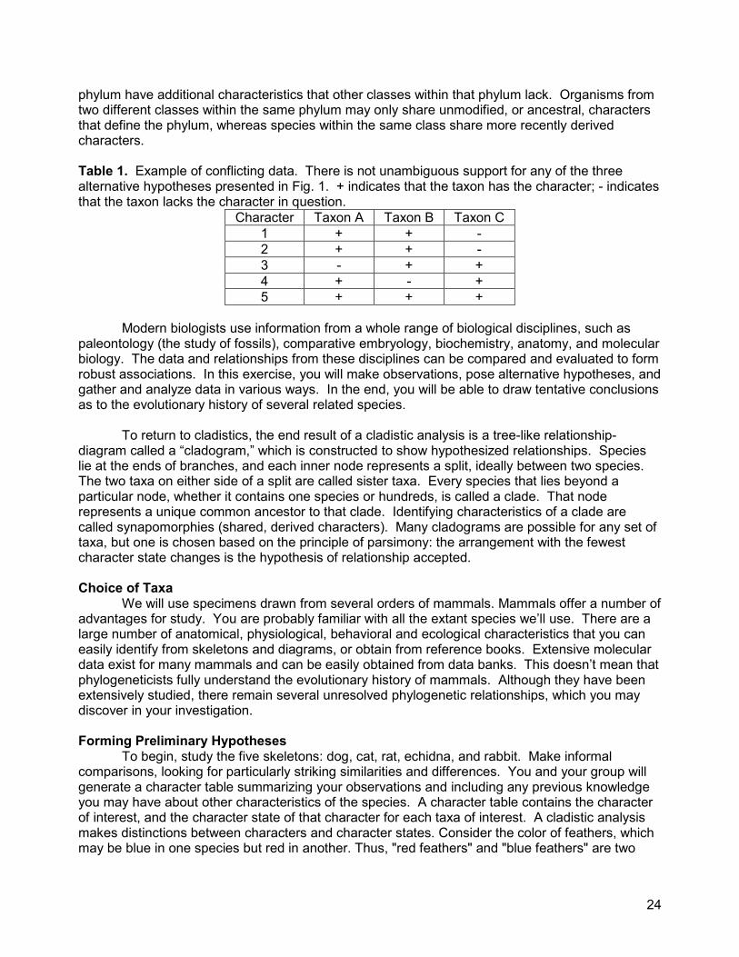
Table 1. Example of conflicting data. There is not unambiguous support for any of the three alternative hypotheses presented in Fig. 1. + indicates that the taxon has the character; - indicates that the taxon lacks the character in question.

Character Taxon A Taxon B Taxon C

1 + + -

2 + + -

3 - + +

4 + - +

5 + + +

Modern biologists use information from a whole range of biological disciplines, such as

paleontology (the study of fossils), comparative embryology, biochemistry, anatomy, and molecular biology. The data and relationships from these disciplines can be compared and evaluated to form robust associations. In this exercise, you will make observations, pose alternative hypotheses, and gather and analyze data in various ways. In the end, you will be able to draw tentative conclusions as to the evolutionary history of several related species.

To return to cladistics, the end result of a cladistic analysis is a tree-like relationship-

diagram called a “cladogram,” which is constructed to show hypothesized relationships. Species lie at the ends of branches, and each inner node represents a split, ideally between two species. The two taxa on either side of a split are called sister taxa. Every species that lies beyond a particular node, whether it contains one species or hundreds, is called a clade. That node represents a unique common ancestor to that clade. Identifying characteristics of a clade are called synapomorphies (shared, derived characters). Many cladograms are possible for any set of taxa, but one is chosen based on the principle of parsimony: the arrangement with the fewest character state changes is the hypothesis of relationship accepted. Choice of Taxa

We will use specimens drawn from several orders of mammals. Mammals offer a number of advantages for study. You are probably familiar with all the extant species we’ll use. There are a large number of anatomical, physiological, behavioral and ecological characteristics that you can easily identify from skeletons and diagrams, or obtain from reference books. Extensive molecular data exist for many mammals and can be easily obtained from data banks. This doesn’t mean that phylogeneticists fully understand the evolutionary history of mammals. Although they have been extensively studied, there remain several unresolved phylogenetic relationships, which you may discover in your investigation. Forming Preliminary Hypotheses

To begin, study the five skeletons: dog, cat, rat, echidna, and rabbit. Make informal comparisons, looking for particularly striking similarities and differences. You and your group will generate a character table summarizing your observations and including any previous knowledge you may have about other characteristics of the species. A character table contains the character of interest, and the character state of that character for each taxa of interest. A cladistic analysis makes distinctions between characters and character states. Consider the color of feathers, which may be blue in one species but red in another. Thus, "red feathers" and "blue feathers" are two

25

character states of the character "feather-color." Develop a phylogenetic tree, or hypothesis, based on your character table. The general

method is to consider taxa that share the most character states in common as sister taxa, and connect them by a node, as in B and C in the leftmost tree in Fig. 1. Then add in the next most closely related taxa from a node further into the past from the first node. Continue this process until all taxa are added into the tree. You may find that the process is not all that straightforward and there may be multiple trees that are plausible, given your data (as in Fig. 1 and Table 1).

Each group will display their best phylogenetic tree and defend it to the class – remember

that a phylogenetic tree is a hypothesis about evolutionary relationships that can be tested by including more characters. The class will debate which characters were useful for discriminating evolutionary relationships and which characters seemed trivial. That is, consider how difficult it would be, genetically and developmentally, for a character to change from character state A to state B. The evolution of the placenta probably required considerable genetic and developmental changes. The independent evolution or loss of such a complex organ in two different lineages is unlikely. On the other hand, evolution of sociality in a nonsocial animal probably requires relatively minor genetic and developmental changes.

Testing Hypotheses with Comparative Anatomy, Physiology, Behavior & Ecology

After the first exercise, you and your partners will have several competing hypotheses to evaluate. As stated above, to test any phylogenetic tree as a hypothesis, we can add more characters and examine how they support or refute any particular branching pattern. Perform a literature and internet search for information on the physiology, behavior, and ecology of each species, and add these characters to your analysis to construct and test phylogenetic trees.

To aid your analysis, examine line drawings of Megazostrodon, which is a presumed

common ancestor of present day mammals (Colbert & Morales 1991). These drawings include several views of the skull and an artist’s reconstruction. Consider Megazostrodon an outgroup of the other species you’re examining. An outgroup is simply a taxa known to be closely related to the taxa in question, but is not categorized with those taxa. Evidence suggests that Megazostrodon diverged from ancestors of the other species (the ingroup) before the ingroup species diverged from each other. The outgroup allows one to determine which traits are shared and ancestral, and which are newly derived by assuming that all the traits the ingroup and outgroup share are ancestral. In this way, the outgroup polarizes the ingroup; we know by comparison with the outgroup that the taxa comprising the ingroup are all more closely related to each other than they are to the outgroup. Another way of looking at it is that Megazostrodon is equally related to each of the ingroup species and that all ingroup species are more closely related to each other than they are to Megazostrodon. Thus, choice of outgroup is important; choosing a group that is too distantly related or that is part of the ingroup could bias our results.

Generate a character table that includes the outgroup, using the characters listed in Table 2

and any others that you and your partners come up with. Consider that some characters may be more useful for discriminating between evolutionary hypotheses. Consider also possible convergence and character reversal. Write a one paragraph essay to defend your preferred hypotheses and justify each node in your tree. Testing Hypotheses with Molecular Data

The use of various kinds of molecular data has become increasingly important in systematics. We will now consider data on a protein molecule, hemoglobin a. This molecule is relatively small, and contains both variable and invariable, or conserved, regions. Analyzing large

26

data sets, such as these molecular data, usually requires a computer, but we’ll begin with a simplified exercise that uses overall hemoglobin a amino acid sequence similarity in the five species of mammals as a single character. Calculate percent similarity for each pair of species by dividing the number of positions where the amino acids are identical by the total number of amino acids. Fill in the similarity matrix (Table 3).

Table 2. Character table for 5 extant and 1 extinct mammal species. Information for Megazotrodon is included.

Character Megazotrodon Opossum Dog Rat Cat Rabbit

Placenta -

Prehensile tail +

Solitary lifestyle ?

Number of teeth 52

Large canines +

Large incisors -

Expanded metatarsals -

Hopping locomotion -

Build an evolutionary tree based on the similarity of hemoglobin a molecules by first

clustering the two most similar species. Use the percent similarity as a scale on the y-axis with the taxa at 100%, and the branches of the first cluster converging at the percent similarity of the two most closely related taxa. Then find the species most similar to the two clustered species. Calculate the mean similarity between this species and the mean of the other two species. If the third species is more similar to the mean of the other two species than it is to any of the remaining species, it is added as a branch to the first cluster (but below the node). If the third species is more similar to one of the remaining species than it is to the mean of the first cluster, then form a new cluster at the appropriate level of similarity. Continue this clustering process until all species have been added to the tree.

After generating a similarity tree for hemoglobin a, we will use a computer program to

determine the shortest phylogenetic tree(s) for the DNA sequence of the 16S subunit of rRNA mitochondrial gene. We will perform this as a class using a program available over the internet. In general, these programs use parsimony methods to select trees that minimize the number of evolutionary steps required to explain the data. Steps are changes in character states. Some programs allow any state to transform directly into another, and consider reverse mutations to be as likely as forward mutations. Initially, all mutations are assumed to have equal weight, so that the development of an amnion is as likely as a neutral nucleotide substitution. Consider how likely it is for a change in any character to be as likely as a change in another. Because several different hypotheses may be supported, choose the two best evolutionary trees based on the unweighted DNA sequence of the mitochondrial gene for the 16S subunit of rRNA. Table 3. Matrix for constructing phylogenetic tree, or cladogram, based on similarities calculated

27

for the hemoglobin a molecule. You only need to fill in above or below the diagonal; we’ll use the bottom. The diagonal represents a species compared to itself.

Dog Cat Rat Opossum Rabbit

Dog 100% X X X X

Cat 100% X X X

Rat 100% X X

Opossum 100% X

Rabbit 100%

Discussion

You and your partners now have several sources of information, including your intuition based on initial observations of skeletal anatomy, a more sophisticated hypothesis based on outgroup analysis of comparative anatomy, physiology, behavior, and ecology, molecular similarity of hemoglobin a, and phylogenetic analysis of rRNA. Each of these sources of information may have supported a different hypothesis.

A couple of cautionary notes are in order as you proceed to analyze trees produced from

different types of characters. First, do not assume that complex characters imply more highly evolved animals. Evolution and natural selection do not work that way. Because we are considering only two molecules with unweighted character states, conclusions based on molecular data are suspect. A particular tree may be most parsimonious, but that does not mean that it reflects evolutionary history. Look for common themes, such that if two species appear to be sister species as determined by a variety of characters, then you should have greater confidence that they are most closely related to each other.

Assignment

Write a Discussion section for this exercise. This is where you tell the reader what you think your findings mean, and why they are important. Present a detailed examination for the few (usually two to three) major points of your study. You can begin with a brief summary of your key results, state why you think these results were found, and compare/contrast your results with those from other studies. You should also point out why the specific research was significant and what general conclusions can be drawn. Which hypothesis was most strongly supported – that is, does the addition of more data or characters increase your confidence in a particular hypothesis? Or is a new hypothesis warranted? Justify your answers. Would it be better to use protein or nucleic acid sequences for these analyses? Why? Should each amino acid be considered an individual character, or should the entire molecule be considered one character? What sources of error and/or bias were present? What new questions come to mind after examining the results? How do your results contribute to an improved understanding of the broad problem you studied? This assignment will be due in one week. Each student will turn in their own Discussion section via electronic submission. Email the Word document to me. The file should be named using the following convention: lastname_discussion.doc

References Singer F, Hagen JB, & Sheehy RR (2001) The comparative method, hypothesis testing and

phylogenetic analysis: An introductory laboratory. The American Biology Teacher 63:518-523.

Colbert EH & Morales M (1991) Evolution of the Vertebrates. John Wiley, New York.

28

Exercise 5: Tree Ring Ecology Modified from an exercise developed by D.L. Rubino and B.C. McCarthy (Rubino &

McCarthy 2002) Introduction

By counting rings on a tree, we can determine the age of the tree and also get a glimpse of the tree’s history. Dendrochronology uses tree rings, dated to their exact year of formation, to analyze temporal and spatial patterns of various processes and phenomena, be they biological, physical, or cultural. In temperate regions, trees deposit one layer of wood every year. In addition to aging of trees, we can examine the amount of growth in any particular year and make inferences regarding the growing conditions. The width of a tree ring in a given year represents the radial-growth response to prevailing environmental conditions. The width of a tree ring can be determined by noting the pattern of earlywood and latewood cells that are produced during secondary or radial growth. During the early part of the growing season, trees often produce large, thinwalled cells, and during the later period of the growing season, they produce smaller, thickerwalled cells. Hence, an annual ring will contain both an earlywood and latewood portion. By measuring the distance from the earlywood boundary of one ring to the earlywood boundary of another ring, the increase in diameter of a tree during a given year can be quantified. Dendrochronologists have used accurately dated and measured tree rings to understand forest community dynamics and past climate conditions, and tree rings have been used to date archeological sites and forest fires. Field Sampling

I will demonstrate the use of increment borers to collect tree cores. We’ll begin by selecting appropriate trees for analysis. Trees with ring-porous wood, which are trees that form rings with very distinct earlywood and latewood, are much easier for novices to date. Typical species to which we’ll have access include species of oaks, elm, ash, black locust, and hickory. However, some of those trees are difficult to core because the wood is so hard. We’ll limit our study to a single species, and it will be a softwood conifer, probably red pine or shortleaf pine. Suitable trees should have a single trunk at breast height and should not have deformities, as these may make coring and dating difficult.

The increment borer includes a handle, bit, and extractor (AKA a core retriever). We’ll pull

a couple of cores just to demonstrate the technique – we have cores in the laboratory for analysis. To obtain a core, insert the bit into the handle and twist it into the tree; the tip of the bit is threaded to pull the hollow bit into the tree. To begin coring, hold the bit just behind the threads and lean into the borer to provide as much body pressure as possible. Slowly turn the bit until the threads have become fully engaged in the tree. After the threads have engaged, step back and turn the handle clockwise. If you hit a rot pocket (you will know immediately because of the ease of turning), back out immediately or else your bit may be incredibly difficult to remove. Continue turning until the borer has slightly gone past the pith. To gauge your depth at any given time, you can hold the extractor up to the side of the tree (it’s the same length as the bit).

When the proper depth has been achieved, turn the handle counter-clockwise one full turn

and insert the extractor into the bit while placing slight up-pressure on the back of the extractor to ensure the leading tip stays under your sample. Insert the extractor to its full length and slowly withdraw the extractor from the bit; you should retrieve an intact core. Remove your borer from the tree as soon as possible to prevent it from being “frozen” in the tree. Immediately place the core into a drinking straw, seal the ends, and mark the straw with the sample ID number. Be sure not to loose any pieces of the core. If the core breaks, maintain the order of the pieces in the straw and store the straws in a protective container while in the field.

29

Laboratory Methods

We will have cores available for analysis. These are cores taken by Dr. Peroni and her students in 2002 to assess a stand of pines on the Davidson College Ecological Preserve. In addition to the cores, we will have on hand sand paper, razor blades, and dissecting microscopes. Even though these cores have been prepared previously, light sanding and wetting will make it easier to view the rings under the microscope. Begin with a coarse grit paper (lower grit number = coarser paper) and use progressively finer grits to attain a smooth surface. Wrap the sandpaper around a wooden block or rubber pencil eraser to facilitate the process. The smoother and cleaner the surface, the easier the rings can be observed.

Tentative dates may now be assigned to each ring by using a dissecting microscope.

Dating begins by counting backwards from the first known year behind the bark, which in our case is 2002. Using a fine pencil, place a single dot on each decadal ring (e.g., 2000, 1990, and so on). For now, these marks are temporary year assignments. Once tentative dates have been assigned, we need to begin crossdating, which is one of the most fundamental and important aspect of tree-ring research. Crossdating compares different cores and matches patterns to assure accurate date assignments. A high confidence in the actual date assigned to each ring will be needed for subsequent analyses and hypothesis testing. Unfortunately, a tree may sometimes have a missing ring or a false ring present. If that happens every ring counted thereafter is off by one year. The key to crossdating is to look for certain years that offer strong signals, such as very thin or very wide rings that we can observe in multiple cores. Once we identify these signal years, we can come to a consensus on what those years are and determine other years based on those signals.

Work in groups to crossdate cores and confirm signal years by consulting with other

groups. Then make sure that cores follow the pattern of large and small rings. After crossdating, be sure to shift any pencil marks to accommodate the cross-validated information. Once this process is finished, assume that exact years are assigned to each ring, and the pencil marks should now be made permanent by using a steel dissecting probe to put pricks in the wood. At this point, estimate the age of the trees for each core that you have been assigned.

Because all of these cores were drawn from trees in the same forest stand, we can

reconstruct a recent history of the forest. We can ask whether all the trees are the same age or whether they began growing at different times, suggesting different possible events that led to the forest as it stands.

In addition, we can use tree rings to reconstruct the past climate. Rings can be measured

to the nearest 0.1 mm using digital calipers. Record the width of each ring and enter it into an Excel spreadsheet along with its year. We can then investigate the relationship between tree-ring widths and climate. Specific questions include asking how climate affects radial growth rate, or is there evidence of severe droughts in this stand? The first step in this process is to remove the growth trend of the tree. A growth trend is a growth pattern observed in a tree over a given time period. By removing the growth trend, we can more accurately relate tree growth to climate. We won’t use actual tree-ring widths for climatic analysis because they do not perform as well as residuals (Rubino & McCarthy 2002).

Use the Analysis ToolPak in Excel to generate the residuals. To do this, use the dates as

the independent variable (x) and the ring widths for the dependent variable (y) in a regression. The residuals are the difference between the observed ring width and the expected ring width from the equation for the line, and those values will be the values used for further analysis.

30

Foresters and ecologists often use annual total growing season precipitation for comparison to residuals of growth ring measurements using correlation analysis. Local climate data will be available from the National Climatic Data Center and National Oceanic and Atmospheric Administration (2001). Prior to using it, produce a graph of residuals vs. year, and inspect the residuals over time to make inferences about years that had large and small residuals, in terms of annual precipitation.

Assignment

Write an Introduction section for this exercise. Here is where you present your argument for why the study was done. It places your work in a broad conceptual context and gives readers enough information to appreciate your objectives. To put your work in a larger context, you will need to review previous publications related to the hypothesis or question. Proceed from the general to the specific, starting with a brief review of current knowledge of the topic and gradually narrowing down to the specific question(s) you have addressed. The Introduction concludes with your specific question, objectives, and/or hypotheses. It is critical that you document (cite) key references in all sections of the paper. Use information from lecture, the manual, the text, sources I provide, and literature you looked up (see Appendix B). This assignment will be due in one week. Each student will turn in their own Introduction section via electronic submission. Email the Word document to me. The file should be named using the following convention: lastname_intro.doc

References National Climatic Data Center & National Oceanic and Atmospheric Administration (2001) CLIMVIS

Information: Selection criteria for displaying period of record. URL: http://www.ncdc.noaa.gov/onlineprod/drought/xmgrg3.html.

Rubino DL & McCarthy BC (2002) Teaching Botany! Ecology & Statistical Principles Through Tree Ring Studies. The American Biology Teacher 64:689-695.

31

Exericise 6: Plant Defenses: Investigating the Differential Allocation of Secondary Compounds

Developed by Dr. Mark Stanback Introduction

The study of plant-animal interactions is an area of great interest in ecology, both from an evolutionary perspective and from a practical standpoint. For instance, the search for pharmaceuticals derived from chemicals found in vanishing plant species, and the use of biological control methods in efforts to improve agricultural productivity are both informed by plant-animal interaction studies. Because an investigation of plant-herbivore interactions uses knowledge and techniques from several sub-disciplines – ecology, biochemistry, evolution, physiology, plant morphology – it provides a model for the integrated nature of research. This lab will investigate the differential allocation of secondary compounds within individual plants as evidenced by a bioassay.

Objectives 1. To appreciate the ever-increasing importance of integrating "field" work with "lab" work in

answering scientific questions. 2. To practice how to state scientific questions and hypotheses and how to evaluate them. 3. To practice techniques such as pipetting, making dilutions, and running a toxicity bioassay. 4. To use search engines to find references from scientific journals. 5. To develop teamwork while working with a group on a scientific investigation. 6. To practice using statistics to answer biological questions. 7. To practice writing a scientific paper. Background

All higher plants contain secondary substances: these are organic chemicals that have no known role in the metabolism of the plants in which they occur. Secondary substances have many different functions; of interest in this exercise is their role as chemical signals. Chemical signals act on different levels in the living world. Substances produced by one tissue that influence another tissue within the same organism are hormones. Those produced by one individual and influencing another individual of the same species are pheromones. Those active between different species are allelochemicals. For the purposes of this investigation, we will assume that the secondary compounds with which we will be working are allelochemicals, although some of these compounds may have evolved to serve a signaling function in the plant.

Allelochemic interactions are a major realm of adaptations that are normally invisible to us.

Tannins, lignins, terpenes, alkaloids (such as caffeine and nicotine), strychnine, curare, and organic cyanides are just a few examples of the chemical arsenal that plants have evolved to defend themselves against herbivores and pathogens. Tannins, for instance, are sequestered in vacuoles in the leaves of oaks and other plants. Once consumed by an animal, they bind with leaf proteins and digestive enzymes in the gut, where they inhibit protein digestion. Thus, tannins considerably slow the growth of caterpillars and other herbivores. Ruffed grouse (Bonasa umbrellus) pay a significant cost to detoxify the coniferyl benzoate found in the flower buds of quaking aspen (Populus tremuloides); in addition, digestive efficiencies of grouse were reduced via dilution of utilizable nutrients by plant secondary metabolites (Guglielmo et al., 1996). Of course, herbivores may counter such toxic effects through adaptations of their own physiology and biochemistry (Tallamy, 1986). Herbivore species that evolve detoxification mechanisms may be able to specialize on plant hosts that are poisonous to most other species.

Plants have evolved some amazing defensive strategies. For example, there is evidence

that plant defenses may be induced by herbivore damage. That is, in response to wounds, toxic

32

compounds may be produced – either in the area of the wound or systematically throughout the entire plant – that reduce subsequent herbivory (Jones et al., 1993). Of particular interest to us will be situations in which individual plants allocate chemical defenses differentially within their own tissues. For example, some plants maintain higher levels of secondary compounds in the high-nitrogen foliage preferred by herbivores (Newman et al., 1997). In the first week of this lab, we will walk around campus and discuss plant animal interactions, both mutualistic (pollination, seed dispersal) and antagonistic (herbivory/defense). After this introduction, you will choose plant species with which to work and develop hypotheses to test. In the second week, we will screen our samples using a “benchtop” bioassay, the brine shrimp bioassay (McGlaughlin, 1991). Brine shrimp (Artemia salina, Fig. 1) larvae have been used for over 30 years in toxicological studies. Researchers use brine shrimp as a pre-screen for plant extracts because they provide a quick, inexpensive, and desirable alternative to testing on larger animals. Brine shrimp bioassays effectively predict pesticide activities and respond to a broad range of chemically and pharmocologically diverse compounds (McGlaughlin, 1991).

Figure 1. Artemia salina, a brine shrimp. From http://biodidac.bio.uottawa.ca.

Bioassays are used for a variety of purposes – in general they allow researchers to screen

for chemicals that show biological activity – that is, that show a biological effect (e.g., effects on survival, growth, or reproduction) on a selected species. For example, botanists and biochemists are currently using bioassays to screen unstudied plants for potentially useful, naturally occurring drugs. The US National Cancer Institute has also launched an intensive effort in “chemical prospecting,” especially in the tropics. This agency alone is screening some 10,000 substances/year for activity against cancer cells, HIV, and other diseases (Wilson, 1989). While it is unlikely that we will discover an unidentified cancer-fighting chemical in the plants investigated, it is important for us to keep in mind that the reason most of those chemicals exist in the first place is the result of coevolution between plants and herbivores. The more we know about “who” makes those chemicals, why they are made, how they are made, and the consequences of allelochemicals to both parties involved, the more we will know about the evolutionary process and about potential practical uses of such chemical evolutionary products for our own benefit.

Week 2 Protocol for Brine Shrimp Assay -- Day 0 1. Divide your group of 4 students into two pairs. One pair will run the assay for one of your

samples (e.g., the ripe fruit = R) and the other pair for the other (e.g., the unripe fruit = U). Each team of 2 will follow all of the procedures below, separately. Use separate data sheets to record results for your 2 samples (e.g., A and B).

33

a. Obtain 10 vials and a small amount of your plant specimen (either R or U) for preparing an extract.

b. Label the vials 1-10 and either R or U (or whatever letters you choose to differentiate your samples).

2. We will run two different kinds of control treatments. The water control (vial #1) will allow us to determine if there are significant effects of the plant chemicals as compared with the "normal" survival of brine shrimp over a 24-hr period. Why is this necessary? Do we expect all brine shrimp placed in seawater in small vials to survive? In addition, vial #2 is a methanol control; it will allow us to gauge the effect of one portion of our protocol (the dissolving of plant material in methanol) independently from the effects of plant material. This is necessary because methanol is likely to be toxic to brine shrimp; if not all the methanol is removed during the evaporation procedure, then an additional variable affecting brine shrimp survival has been introduced. Results from which 2 vials will be compared to test whether or not we have introduced a "methanol effect" in brine shrimp survival? Why then are both control treatments required? a. Mark vial #1 as the water control, vial #2 as the methanol control, vial 3-6 with 100

micrograms/ml and vials 7-10 with 1000 micrograms/ml. These are the two final concentrations of the plant extract you will test.

3. Carefully dry a "mortar" and "pestle" (well plate and test tube). Remove all traces of animal material from your plant specimen and place the plant specimen in the bottom of the well plate. Grind it thoroughly for no less than 5 minutes. Weigh out 40 milligrams (not micrograms or grams) of the plant material on an electronic balance and then transfer the 40 mg sample to a small beaker or vial. Take the sample to the fume hood. The methanol is in the fume hood because it is highly flammable and toxic. It is important to avoid contact with your skin and eyes. Remind yourself of the location of the eyewash stations, just in case. Methanol is being used as a general solvent for the chemicals present in the plant tissue. Carefully add 4 ml of 100% methanol to the plant material. What is the concentration of your extract at this point? Allow the material to dissolve in the methanol for 5 minutes. a. Prepare several airlines for evaporating methanol from samples you will prepare later. You

will want a gentle stream of air coming out of each of the glass pipettes attached to the airlines. Test for "gentleness" by trying the air stream in a beaker of tap water first.

4. Obtain 2 micropipettes for measuring 50 microliters and 500 microliters. Familiarize yourself with the use of the micropipettors by practicing with small aliquots of water.

5. When the 10 mg/ml plant extract has dissolved in the methanol for 5 minutes, add 50 microliters of the mixture to EACH of the 4 vials labeled 3, 4, 5 and 6, and add 500 microliters to EACH of the vials labeled 7, 8, 9, and 10. Do not add any extract to water control tube #1. To methanol control tube #2, add 50 microliters of 100% methanol.

6. Evaporate the methanol from vials 2-10, starting with the vials containing the most methanol. To do this, insert the tip of the glass pipette/airline into the bottom of the vial and gently bubble air through the sample until all liquid vanishes. This should take no longer than 20 minutes for the vials containing the greatest volume. Be ready with the next vial each time an airline is freed up. If you bubble too vigorously and lose some of your extract, you will need to prepare a new vial to replace it -- why?

7. While the first few samples are evaporating, do the math below to see how the values in Table 1 were calculated. Fill in the blanks!

Sample calculation for final concentration for vial #3

: 50 ul x (10 mg plant tissue/ml) = 0.05 ml x (10 mg/ml) = 0.5 mg

0.5 mg of plant material = 0.5 mg x (1000 ug/mg) = 500 ug of plant material

34

Table 1. Calculating the final concentration of plant material in ug/ml for each sample vial.

8. When a sample vial has been evaporated, add 1 ml of plain sea water (2% sea salts) to it. 9. Then add 10 healthy, live brine shrimp to each of the 10 vials (I will demonstrate how to catch

and count them). a. Be sure to add 1-2 ml of plain sea water with them. b. Do not contaminate your vials with dead brine shrimp or eggs, because the assessment of

toxicity is based upon survival as the dependent variable. c. When you think you are finished with each vial, double-check by holding the vial under the

dissecting scope to make sure that it contains no eggs, no dead shrimp, and 10 live shrimp. d. Leave the screw cap off OR placed on the vial loosely -- brine shrimp need oxygen! e. Find an extra vial and mark it at the 5 ml level. Using this vial as a "ruler", carefully add

plain sea water to each of the 10 vials so that each contains a final volume of 5 ml. Make sure that all vials have exactly the same final volume; if you go over the mark, you will need to do that vial over again because the concentration will not be accurate.

10. Record Day 0 information and all of the headings on Table 2. Label the vial rack belonging to your group with your group name, the date, and your lab section (day). I’ll tell you where to store your rack.

Protocol for Brine Shrimp Survival Counts -- Day 1

Return to the lab 24 hours after beginning the cultures to count the shrimp in all 10 vials. Bring this lab handout with you. 1. Count shrimp in each vial, as follows: Pour out your shrimp into watch glasses. Count the

numbers of live and dead shrimp. If your numbers don't add up to 10, recount (don't erase your first numbers). Dead shrimp fall apart quickly -- don't mistake two halves of a body as two dead shrimp. At the least, be sure you have an accurate count of live shrimp. Place live shrimp in the designated tank.

2. Fill in Table 2 completely. 3. Pour out your shrimp vials into the sink, rinse each vial thoroughly, and place the vials and

racks in the designated area. If another lab group is using the room, make sure you don't interfere with their work.

Week 3: Data Analysis and Presentation

The simplest way to analyze our data is by using JMP to do a Fisher Exact test. The Fisher Exact test is a 2 x 2 contingency table. The concept is pretty simple: Each of your columns has only two possibilities: shrimp are either alive or dead, the extract they were in were either tissue A (e.g., leaf) or tissue B (e.g., fruit). That means 4 possibilities (alive in fruit, dead in fruit, alive in leaf, dead in leaf). You can build a nice little 2 x 2 table with A&D on the top and F&L on the sides. The trick to this analysis is that you can’t just plug in your results. Bummer. You actually have to have a row for every single shrimp! But by pasting, it goes really quickly. To make things go even faster, split your group up. Two of you do the following using the LOW concentration data (see example below); the other two do it using the HIGH concentration data. Whoever gets done first can start the control analyses (to increase your statistical power, pool the data from your high and

35

low concentration controls). Remember to save your data sets!

Table 2. Brine shrimp bioassay data sheet.

Group Members ____________________________________________________

Lab Day ______________________________

Tissue type (ripe, unripe, etc) ______________________

Open JMP to a blank spreadsheet. You will use this for your comparison in the LOW concentration treatment. To name the column and set up the parameters, double click on the empty area just above the words “column 1” and between the 2 little boxes. Name the column and set it for character data. Once this is done, go to “add rows” and add 80. Let’s assume you were comparing leaf vs green fruit. So that’s 40 shrimp in the 4 leaf vials and 40 in the 4 fruit vials (as you can see, we’re lumping the data from the 4 replicate vials. There are more complex statistical tests in which you keep them separate and can thus test for the effects of the specific vials, but we’re not going to worry about that).

Go to the first row of the Tissue column. Type in “Leaf”. Then select that cell and copy.

Then select cells 2-40. Hit paste and they should all say Leaf. Now do the same for rows 41-80, except put in the word “Fruit”. Now you’re ready for column 2. Make the data type character and call it “Fate”.

Here’s the tricky part. If you had a total of 30 of your 40 Leaf shrimp (in the low

concentration experiment, of course) alive the next day, type in the word “Alive” in the first cell and paste it in down to row 30. Put the word “Dead” in the cells in rows 31-40. Now do the same alive/dead thing with your data in the Fruit portion of your Fate column. Now go to the Analyze menu, choose fit y by x, assign tissue to “x” and fate to “y” and poof, it will give you your results, both in a figure and as stats.

In the LAP lab, your research hypothesis for the genotype frequency comparison was (for

most of you) “population X is different from population Y.” The null hypothesis was “population X is NOT different from population Y.”

For this lab, you weren’t just predicting that tissue A had a DIFFERENT level of toxicity than tissue B; you had a reason to think that one tissue type might be MORE toxic than the other (and

36

here the null hypothesis is “A is not more than B”). The probability that something is “different” is different than the probability that something is “more.” So your P values for a two-tailed test (looking at both “tails” of the bell-shaped frequency distribution) are different from the P values of a one-tailed test (looking at only one end of the frequency distribution). Moreover, the P value also depends on which you predict is greater. We’ll talk about this more in lab, but the rule of thumb is that if your research hypothesis was supported (look at the JMP graph), you’ll go with the lower of the one-tailed P values (for now, don’t worry about “right” and “left”. If the results were the opposite of what you predicted, you’ll go with the greater of the one-tailed P values. Note that it is easier to get a significant result with a 2-tailed test (a test of difference) than it is with a one-tailed test (a test of directionality). In your lab report, you will report your sample size for each analysis along with the Fisher Exact p-value. You will end up doing 5 different analyses: 1. [Low] Leaf vs. [Low] Fruit 2. [High] Leaf vs. [High] Fruit 3. [Low] Leaf vs. [High] Leaf 4. [Low] Fruit vs. [High] Fruit 5. Water Control vs. Methanol Control

The first two represent your initial research hypothesis (you’re separate analyses of low and high concentrations in case your high concentration is too toxic or your low concentration is not toxic enough). The second two represent an analysis of whether the concentration makes a difference. For these, our hypotheses will be that the higher concentration is more toxic. For your controls, compare the mortality in your pooled water vs. pooled methanol controls. If the mortality in your methanol controls is significantly greater, that would suggest that some of the mortality you observed in your tissue comparisons was due to the toxicity of methanol, not the toxicity of the plant tissue. While this would be problematic, it would not negate your ability to draw some conclusions from your other comparisons. Why not? In addition, there is a simple mathematical correction we can make to account for control mortality. Unless you get a dramatic difference between your water and methanol control, don’t worry about making a figure for it. Just report your results in the text of the Results section.

Make two figures in Excel for your lab report. The first should include the results from #1 &

2 above. The second should include 3 & 4. The Y-axis should represent survivorship or mortality (proportional – that’s decimals). Remember, you’ll want a row labeled as “low” and another as “high” and columns labeled as “leaf” and “fruit”. Fill in the cells with the proportion alive (or dead – but not both – that would be redundant). Your group may work together to make the figures and legends, but the rest of your lab report will be your own work. Because the study of secondary compounds is such an active field, I expect your journal citations to be different from the ones I list below. Table 3. Summary of results.

37

Assignment

Write a full laboratory report for this experiment. Use what you learned writing individual sections and the guidelines in Appendix B to guide your work on each of those sections. Consider the following questions, but do not limit your introduction and discussion to these topics: 1) What is the relationship between the concentration of plant extract and percent shrimp survival (if any) and what is the biological significance of this? 2) Even if the data support your hypothesis, is your hypothesis the ONLY explanation for what you found, or are there still other possibilities? If so, what are they? 3) If producing anti-herbivore chemicals is beneficial to plants, then why don't all plants produce lots of them all the time? The third week of this exercise is devoted entirely to data analysis and preparation of results. I expect all groups to make significant headway in preparation of results. Thus, the final draft of your report is due in two weeks (Oct. 24th or 25th). Each student will turn in their own laboratory report via electronic submission. Email the Word document to me. The file should be named using the following convention: lastname_plantdefense.doc.

References Bruin J, Sabelis MW, & Dicke M (1995) Do plants tap SOS signals from their infested neighbors?

Trends in Ecology and Evolution 10:167-170. Guglielmo CG, Karasov WH, & Jakubas WJ (1996) Nutritional costs of a plant secondary

metabolite explain selective foraging by ruffed grouse. Ecology 77:1103-1115. Jones CG, Hopper RF, Coleman JS, & Krischik VA (1993) Control of systemically induced

herbivore resistance by plant vascular architecture. Oecologia 93:452-456. McGlaughlin JL (1991) Bench-top bioassays for the discovery of bioactive compounds in higher

plants. Brenesia 34:1-14. Newman RM, Kerfoot WC, & Hanscom Z (1997) Watercress allelochemical defends high-nitrogen

foliage against consumption: effects on freshwater invertebrate herbivores. Ecology 77:2312-2323.

Tallamy DW (1986) Behavioral adaptations in insects to plant allelochemicals. In: Molecular aspects of insect-plant associations (Brattsen LB & Ahmad S, eds). Plenum Press, New York, pp. 273-300.

Wilson EO (1989) Threats to biodiversity. Scientific American 261:108-116. This lab investigation was developed for use at Davidson College by Dr. Mark Stanback. It was adapted from: Winnett-Murray K, Hertel L, & Murray KG (1997) Herbivory and anti-herbivory: investigating the

relationship between the toxicity of plant chemical extracts and insect damage to the leaves. In: Tested Studies for Laboratory Teaching (Glase J, ed). Association for Biology Laboratory Education 18: 249-268.

38

Exercise 7: Factors Affecting Respiration in Goldfish Developed by Dr. Michael Dorcas

INTRODUCTION To understand the physiological problems animals face, it is first necessary to understand the abiotic properties of the environment in which they live. This is especially true when trying to understand the problems animals face in gas exchange and how those problems vary with the environments in which they live. Aquatic animals live in environments in which oxygen is found in relatively low concentrations (compared to air, at least). Additionally, the high viscosity and density of water makes it difficult to move the fluid back and forth into respiratory organs like we do with air in our lungs. Consequently, most aquatic animals have special adaptations that help acquire oxygen.

First, most aquatic animals have one-way or flow-through respiratory systems that pump water over their respiratory organs, usually some sort of evagination called a gill. Instead of pumping water into and out of a chamber containing the gills, the animals pump water in one opening and out another, producing a one-way flow of water across the organs. Consequently, the animals don’t expend energy stopping the flow of water and starting it in the opposite direction, which would be much more difficult than performing the same task with air. Second, to increase the concentration gradient of gasses between the blood and water, most aquatic animals have some sort of counter-current exchange system that allows for maximal gas exchange. In this system, the blood flows in the opposite direction as the water, thus maintaining a substantial gradient across the entire gill surface. Finally, because oxygen is often limiting in aquatic environments, the nervous systems of aquatic animals are usually most sensitive to low oxygen levels in their blood, in contrast to terrestrial animals that usually are more sensitive to CO2 levels.

In this laboratory, you will design and conduct an experiment examining a factor or factors

that potentially affect(s) respiration in an aquatic animal, the goldfish (Carassius auratus). General Objective: To develop and conduct original experiments investigating factors affecting

respiration in an aquatic animal. Specific Objectives or Hypotheses: To be determined by you and your partners. We will spend part of the laboratory period the week before this laboratory planning and designing your experiment. MATERIALS AVAILABLE: goldfish acclimated to room temperature air pumps with air stones goldfish acclimated to 10oC pH meter low dissolved oxygen water hydrochloric acid many beakers of different sizes small nets stopwatches magnifying glasses thermometers water at 10oC dechlorinator or dechlorinated water sodium bicarbonate dissolved oxygen meter pipets balance ice (If there is something else you need, ask. We may be able to get it for you). EXPERIMENTAL DESIGN Goldfish have been chosen as subjects for this laboratory because they are small, easily handled, tough, and inexpensive (about 8 cents each) aquatic animal. The primary dependent

39

variable we will measure is respiratory rate, which can be measured easily by carefully observing the fish and counting gill ventilations (using a magnifying glass will help and sometimes it is easier to count mouth openings). However, you can use other dependent variables if desired or if we have the ability. Respiratory rate calculations should be recorded as ventilations/minute.

I will give you some ideas for treatments during our introductory discussion, but I will let you decide on the specific treatments (independent variables) you will examine. You can subject goldfish to different treatments in any number of ways. Some treatments to consider are temperature, exercise, aeration of water, volume of water, pH, recovery time after removal from water, and many other factors. But you can come up with other factors that you think would be of interest. We encourage creativity!! After you decide on the independent variables you would like to examine, write out your hypotheses (research and null). Remember to consider and think about why these factors might affect respiration rates – they may increase stress or the need to metabolize at a higher rate, therefore causing a larger oxygen requirement.

You will then need to plan, in detail, your experimental design. Remember to consider such

factors as sample size needed, number of treatments, and control of extraneous variables. Sample size is important, since the fish are different sizes and ages, and randomly selecting only two for a particular treatment will cause high variance in your estimate of respiration rate. For instance, you might randomly select a stressed fish and a healthy fish, or a large fish and a small fish, and in both scenarios the different individuals will respond differently to the treatment. This is why we always try to have larger sample sizes, at least within the confines of our other constraints, such as total number of fish available and time to perform the experiment. One way to increase sample size without using more total fish is to expose each individual fish to every treatment (with a recovery time period in between each treatment exposure), which is called a repeated-measures experimental design. Using each fish in each treatment or randomly selecting fish within the same size category will both help to reduce error variation, and are considered part of controlling extraneous variables (i.e., you might control for fish size, which will reduce variation caused by size). The number of treatments will be dependent on the question or hypothesis being addressed.

Other considerations you should make before proceeding include such things as how you

will measure respirations. You may count gill operculum openings or mouth openings – both will be measurements of respirations, and one may be easier for you to observe than another, depending on your treatment. You may want to count only for 15 second intervals, instead of a full minute. This decreases your chances of losing count, and allows you to take repeated counts for each individual over a 4 or 5 minute period to calculate an average +/- standard deviation. Also, you should consider dividing up the workload so that there is no bias in treatments caused by individual experimenters. How can you reduce this bias?

Finally, before you begin you also need to decide how you will analyze your data, based on

your experience with various statistical tests (e.g., ANOVA, Regression, Chi-square). Before you begin your experiment, you must run through your hypotheses, proposed design, and proposed analysis with me. Potential independent variables to consider are:

temperature effects of acclimation pH crowding oxygen concentration size

40

Assignment

Prepare a 10 minute oral presentation, with your group, on your experiment. Format it like a laboratory report – that is, incorporate all the components of a full report. Use the guidelines and suggestions below to assist you. The presentations will be due on Nov. 7th and 8th, one week from the data analysis phase. Email a PPT document to me prior to class. The file should be named using the following convention: lastnames_fish.ppt.

Guidelines/Suggestions for Laboratory Symposium Presentation

Prepare your presentation as you would a report, in an organizational sense, with

Introduction, Methods, Results, Discussion, and References. The presentation should run about 10-15 minutes, with all group members participating equally in preparation and presentation. Consider the following points as you prepare your presentation.

1. For each section you might have text to present certain things. However, you want to avoid

large amounts of text. Use bullets with short points, and then discuss those at greater length. 2. You may want to think about adding pictures of your organisms or setups. You can search the

internet for pictures. If you include downloaded pictures, you must include the URL where the picture was obtained, or some other acknowledgement of the source of the picture.

3. Your introduction should address the following questions. What is the general phenomenon under consideration and why is it important? What is your purpose? What is your hypothesis?

4. For methods and materials, avoid long discussion of detailed methods. However, because each group designed their own study, you must go into some detail about your design, how it addresses your hypothesis, and how you analyzed the data.

5. Results should not have much text, but should focus more on high quality figures and tables that are readable by someone at the back of the room and back up the points you make about the data. You may want to include one slide of text with major points, which you describe, and then show with your visual aids. Include averages and standard deviations where appropriate.

6. Figures and tables can be made in Excel, tables can be made in Word, or both can be made in PowerPoint. Anything you make in Excel or Word is easily imported into PowerPoint.

7. Discussion should contain, again, as little text as possible, and emphasize two or three major conclusions regarding your results. Also address why the research is significant and how you might be able to generalize your conclusions to more than just the one species you worked with. Consider the following: do results support research hypotheses, how will your future experiments (that follow up questions from this one) be designed to reduce error or bias, and what new questions arise from this experiment?

8. Presentations often have acknowledgements thanking people that assisted with the project. For instance, Dr. Peroni supplied all the seeds for the LAP lab, and other groups often supplied data for certain populations.

9. Generally, use large fonts and high contrast for ease of viewing by the audience. Apply the principles of preparing professional-quality figures discussed in Exercise 1.

10. Each person in the group should present equal portions of the presentation; you can divide it up by section, or each person can do part of each section.

11. Each person will receive a grade based on the overall presentation, and your individual performance. Grades will be based on: 1) organization and delivery, 2) visual aids (e.g., PowerPoint), 3) ability to convey how your study contributes to the science of biology, 4) ability to focus on 2-3 three major points, 5) ability to stay within the time limit, 6) ability to answer questions at the end, and 7) how well your Discussion addresses the broader significance of the research and relates back to issues raised in the Introduction.

41

Exercise 8: Fetal Pig Anatomy Developed by Dr. Mark Stanback

INTRODUCTION In the following laboratory exercise, you will examine in some detail the external and internal anatomy of a fetal pig (Sus scrofa). As the pig is a mammal, many aspects of its structural and functional organization are identical with those of other mammals, including humans. Thus, a study of the fetal pig is in a very real sense, a study of humans. The fetuses you will use in the following weeks were salvaged from pregnant sows being slaughtered for food. They are not raised specifically for dissection purposes. The fetuses are removed from the sow and embalmed with a preservative, which is injected through the umbilicus. Following this, the arterial and venous systems are injected under pressure with latex, a rubber-like compound. Arteries (red) are injected through the umbilicus; veins (blue) are injected through one of the jugular veins at the base of the throat. With the possible exception of the abdominal cavity, organs rarely appear as they are presented in a diagram. If the purpose of this exercise were simply to have you memorize diagrams (or computer screens), we would do only that and bypass the expense, time, and controversy of dissecting! Dissection is a powerful teaching method, especially for concrete thinkers and visual learners. Only by dissecting can you really appreciate the structural and functional role of the many membranes, mesenteries, and connective tissues that will impede your progress every step of the way. Only by dissecting can you really appreciate the relationship between an organ's texture, location, and function. I do not take the life (or death) of your pig specimen lightly – this is why I demand that you take your dissection seriously and utilize your pig to the fullest extent possible. During these exercises, keep several points in mind. First, be aware that "to dissect" does not mean "to cut up," but rather primarily "to expose to view." Actual cutting should be kept to a minimum. Tissues are picked and teased apart with needle probes, forceps, and blunt probes in order to trace the pathways of blood vessels, nerves, muscles, and other structures. Never cut or move more than is necessary to expose a given part. Second, pay particular attention to the spatial relationships of organs, glands, and other structures as you expose them. Realize that their positions are not random. Third, we encourage you to engage in collaborative discussions with your classmates and compare dissections. Although the structures described below are identified on the accompanying figures, in some cases the figures contain more information than you need to know. Don't panic – this extra information is provided to help you identify what you do need to know. If you wish to explore your pig more thoroughly and identify additional structures (e.g., blood vessels), please do! Each lab group will be provided with a color photograph dissection manual to supplement this handout. By the end of this exercise you should have a very good grasp of the connections between physiological processes and organ structure/function. At the end of each major section, we have produced a set of questions (Think about it). Additionally, there are boldface questions scattered through the text. Make sure you figure out the answers to these questions before moving on. All are fair game for the practical. SAFETY AND HYGIENE 1. Practice safe hygiene when dissecting. Do not place your hands near your mouth or eyes

while handling preserved specimens. Although most of the preservatives in use today are non-

42

toxic to the skin, they may cause minor skin irritations. If the preservative gets on your skin, wash with soap and warm water.

2. If the preservative gets in your eyes, rinse them thoroughly with the safety eyewash. 3. Never splash the preservative in the pig buckets. 4. Wear lab gloves. Small, medium, and large sizes are available. These gloves are expensive--

please don't waste them. 5. Lab gloves and paper towels go in the regular trash. Skin and pieces of pig go into the red

plastic bag at the front of the room (not down the disposal). 6. After bagging your pig and placing it in the mortuary cabinet, rinse your tray and stack it neatly

by the sink. Wipe up your station. MATERIALS fetal pig dissecting tray dissection kit (scissors, scalpel, blunt probe, needle probe, forceps) lab gloves paper towels string OBJECTIVES 1. Perform a whole-body dissection of a vertebrate. 2. Identify the major anatomical features of the vertebrate body in a dissected specimen. 3. Understand the relationship between structure and function in the vertebrate body and relate

concepts covered in lecture to structures found in your pig. 4. Understand mammalian fetal circulation from a mechanical, physiological, and evolutionary

perspective. 5. Apply knowledge and understanding acquired to problems in human physiology. 6. Apply knowledge and understanding acquired to explain organismal adaptive strategies. EXTERNAL FEATURES 1. Determine the anatomical orientation of your specimen.

• *dorsal: toward the back of the body

• *ventral: toward the underside of the body

• *anterior (cranial): toward the head end of the body

• *posterior (caudal): toward the tail end of the body

• lateral: to the side of the body

• median: toward the center of the body

• right and left: the pig's right and left, not yours!

• proximal or basal: closer to the trunk

• distal: farther from the trunk

• superficial: lying closer to the body surface

• deep: lying under or below *The terms anterior and posterior are sometimes used synonymously with ventral and dorsal, respectively, for humans.

2. Note the thin peeling layer of tissue covering the body of your pig. This layer is the epitrichium, a layer of embryonic skin that peels off as hair develops beneath it.

3. Identify the regions of the body (Fig. 1):

• head (cranial) region

• neck (cervical) region

• trunk region (thoracic region)

• tail (caudal) region (abdomoninal region)

43

4. Head: Find the following:

• pinna (auricle): external ear

• external nares (nostrils)

• upper and lower eyelids

• nictitating membrane (third eyelid) 5. Trunk: The terms sometimes used to describe the trunk vary whether one is discussing the

dorsal or ventral surface. The trunk can be described using the terms associated with the vertebral column: thoracic (rib), lumbar (lower back), and sacral (pelvic) vertebrae. Ventrally, the abdominal region dominates the area posterior to the thorax. Note the umbilical cord; it connects the fetus to the placenta of the mother and later becomes the navel. Cut off the very tip (0.5 cm) of the umbilicus to more clearly see the following:

• umbilical arteries: two arteries, carry deoxygenated blood from fetus to placenta

• umbilical vein: a single large vein, carries oxygenated blood from placenta to fetus

• allantoic duct: channels urine to the allantois, an extra-embyronic sac 6. Appendages: Examine the legs of your pig. Find the following:

• On the forelimb find the shoulder, elbow, wrist, and digits.

• On the hindlimb find the hip, knee, ankle, heel, and digits. 7. Determining the sex of your pig:

1. Female: Look for a single urogenital opening just ventral to the anus. A prominent genital papilla projects from the urogenital opening.

2. Male: Look for the scrotum, a sac-like swelling containing the testes and located ventral to the anus. The male urogenital opening is faintly visible just posterior to the umbilicus. Note that males as well as females have multiple nipples = teats = mammary papillae.

Think about it 1. Notice how the number of toes is reduced in your pig. The middle two digits form hooves.

Ungulates (hooved animals) like the pig walk with the weight of the body borne on the tips of the digits (unguligrade locomotion). Cats and dogs use digitigrade locomotion (walking on the balls of their feet). Humans typically use the entire foot for walking (plantigrade locomotion). What form of locomotion do you use when you sprint?

2. Although male mammals have nipples, as a general rule they do not lactate. From an ultimate (why?) rather than a proximate (how?) standpoint, why is male lactation the exception rather than the rule (HINT: there are very few monogamous mammals)?

DIGESTIVE SYSTEM Objectives: 1. Identify and describe the functions of the main organs of the digestive system. 2. Gain an appreciation of the spatial relationships of the many organs and structures that

contribute to the digestion of food and the nourishment of the body's cells. The digestive system of mammals consists of the alimentary canal (mouth, oral cavity, pharynx, esophagus, stomach, small intestine, large intestine, rectum, anus) and other associated structures/organs/glands (salivary glands, gall bladder, liver, pancreas). The cavity behind the teeth and gums is the oral cavity. Note the papillae on the tongue. These provide friction for food handling and contain taste buds. Like all young mammals, fetal pigs have milk teeth (baby teeth) that are later replaced by permanent teeth.

44

Figure 1. External anatomy of the fetal pig. A. Ventral view. B. Lateral view.

C. Posterior view of female. D. Posterior view of male. There are 3 pairs of salivary glands (Fig. 2). Of these, we will view only the mandibular (the parotid is rather diffuse and the sublingual is too difficult to get to). To view the mandibular gland you must remove the skin and muscle tissue from one side of the face (cheek) and neck of your

45

pig. You’ll need to dig through subcutaneous fat, connective tissue, and the parotid salivary gland in order to see it. The mandibular gland is a large, well-defined circular salivary gland just posterior to the masseter. Don’t confuse it with the small oval lymph nodes in the region. Keep an eye out for the facial nerve that runs posteriorly across the masseter. Try to find the parotid duct that carries saliva to the corner of the mouth. This duct can be moved surgically to empty out at the eyes. Until relatively recently, the standard "cure" for dogs whose lacrimal (tear) glands failed to produce the watery component of tears was to move the parotid duct up! The saliva producing glands are:

• Parotid gland: a large dark triangular gland overlying part of the masseter muscle (also note the facial nerve that runs across the dorsal part of the masseter).

• Mandibular gland: under the parotid gland. Not to be confused with the small oval lymph nodes in the region.

• Sublingual gland: long, slender, and difficult to locate (so don't bother). Salivary glands produce prodigious amounts of saliva (>1 l/day in humans). Saliva contains:

• water for moistening food

• mucus (mucin) for lubricating food and binding it into a bolus

• salivary amylase to start the breakdown of starch

• bicarbonate to buffer acidic food in the mouth

• antibacterial agents to kill bacteria in the mouth With scissors, carefully cut through the tissue and bone starting at the corners of the mouth and back toward the ears (keeping the roof of the mouth intact) until the lower jaw can be dropped and the oral (buccal) cavity exposed (Fig. 3). Find the following structures:

• hard palate: has ridges; separates the oral cavity from the nasal cavities

• soft palate: soft because there is no bone underneath (nasopharynx lies above it)

• buccal cavity: from opening of mouth to the base of the tongue

• pharynx: (throat) common passageway for digestive and respiratory system

• esophagus: tube connecting oral cavity to stomach. Swallowing can be initiated voluntarily, but thereafter it is a reflex controlled by a brain region.

• glottis: the opening to the larynx

• epiglottis: the flap that covers the glottis during swallowing

• Eustachian tubes: may be visible on each side of the pharynx. Internal Anatomy of Digestive System As you prepare to open up your pig, remember that most internal organs, including the digestive system, are located in the body cavity, or coelom. A large muscular structure, the diaphragm, divides the mammalian body cavity into the thoracic cavity and the abdominal (peritoneal) cavity. The thoracic cavity is further divided into a pericardial cavity (heart) and two pleural cavities (lungs). Epithelial membranes line these cavities and cover the surface of all organs. Names of the epithelial linings are determined by their location. The word "parietal" refers to the wall of the body, and the word "visceral" in this case refers to organs within those cavities. For example:

• visceral peritoneum: covers organs of the peritoneal cavity

• parietal peritoneum: lines peritoneal cavity

• visceral pericardium: covers surface of heart

46

• parietal pericardium: lines pericardial cavity

• visceral pleura: covers surface of lungs

• parietal pleura: lines pleural cavity Coelomic fluid fills the space between membrane layers. This moisture acts as a lubricant, allowing organs some degree of easy movement. The organs are connected to each other and to the inner body wall by thin sheets of connective tissue called mesenteries, which suspend the organs and provide bridges for blood vessels, nerves, and ducts.

Figures 2, 3, and 4. Salivary glands and neck region (Figure 2), oral cavity (Figure 3),

and incision guide (Figure 4).

47

Use Figure 4 as a guide for making the various incisions. 1. Begin your incision at the small tuft of hair on the upper portion of the throat (1) and continue

the incision posteriorly to approximately 1.5 cm anterior to the umbilicus. You should cut through the muscle layer, but not too deeply or you will damage internal organs.

2. Whether your pig is male or female, make the second incision (2M) as a half circle anterior to

the umbilicus and then proceed with two incisions posteriorly to the region between the hindlimbs. Do not make the 2F incision. If you have a male, be careful not to cut deeply into the scrotum.

3. Deepen incisions 1 and 2 until the body cavity is exposed. Make incisions 3 and 4 to produce

lateral flaps that can be folded back. Pour excess fluid into the waste container and rinse out the body cavity.

4. Just below the lower margin of the rib cage, make a fifth (5) incision laterally in both directions.

This should expose the diaphragm, which separates the thoracic and abdominal cavities. Using your scalpel, free the diaphragm, but do not remove it.

5. Carefully peel back flaps A, B, C, and D and pin them beneath your pig. It may be necessary

to cut through the ventral part of the rib cage (very carefully) with a pair of scissors to separate flaps A and B.

6. Carefully remove any excess latex. 7. To free the umbilicus, cut through the umbilical vein approximately 1 cm from where it enters

the liver. Flap E can now be laid back and pinned. Do not cut off this flap--it contains important organs that we will examine later!!

Examine the neck, thoracic, and abdominal regions of your pig (Fig. 5). First find the thymus gland, which partially covers the anterior portion of the heart and extends along the trachea to the larynx. The thymus plays an important role in the development and maintenance of the immune system – this is where white blood cells mature into antibody-producing T-lymphocytes. Immediately beneath the thymus in the neck is the thyroid gland, a small,solid, reddish, oval mass. The thyroid secretes thyroxine, which in mammals influences the metabolic rate of cells, which in turn influences growth and development. Because iodine is necessary for the production of thyroxine, our salt is often iodized. If synthesis of thyroxine declines (e.g. due to a lack of iodine), the anterior pituitary increases the release of thyroid stimulating hormone (TSH). This may stimulate the proliferation of thyroid cells, but if there is no iodine, thyroxine production will not increase, which causes additional TSH release. The thyroid also produces calcitonin, a hormone that stimulates osteoblasts to lay down bone. The consequence of this activity is a surprisingly rapid decline in blood calcium levels. If blood Ca levels drop too low, or if extra Ca is needed, the parathyroid glands release parathormone. The parathyroid is not a discrete organ in mammals – parathyroid tissue is embedded in the thyroid. Parathormone raises blood Ca levels by activating osteoclasts, by stimulating Ca resorption in the kidney, and by activating vitamin D to enhance absorption of Ca from food. In the neck find the trachea and use it as a landmark to locate the esophagus. Make a small incision in the esophagus in the throat and insert a blunt probe anteriorly; note where it emerges in the oral cavity.

48

Insert the blunt probe through this incision posteriorly toward the stomach (you will need to move the liver to one side to fully expose the stomach). Note that the esophagus penetrates the diaphragm before entering the stomach. Cut open the stomach lengthwise with your scissors. The contents of a fetus's digestive tract is called meconium, composed of a variety of substances including bile stained mucus, amniotic fluid, sloughed epithelial cells, and hair. Clean out the stomach and note the folds (rugae). What role might the rugae play? Many glands that secrete pepsinogen and hydrochloric acid are embedded in the wall of the stomach. Two muscular rings (smooth muscle), the cardiac (closer to the heart) and the pyloric sphincter (adjoining the small intestine), control the movement of food through the stomach. The majority of digestion and absorption takes place in the small intestine. It is composed of the duodenum, the jejunum, and the ileum, the latter two being difficult to distinguish. The duodenum, into which bile and enzymes from the gall bladder and pancreas enter, passes posteriorly and then curves to the left. The coils of the small intestine are held together by mesenteries. A rule of thumb is that the small intestine in both pigs and humans (omnivores) is about five times the length of the body. Note the lymph nodes embedded in the mesenteries. These nodes filter pathogens from the lymph.

Cut a 0.5 cm section of the small intestine, slit it lengthwise, and place it in a clear shallow dish filled with water. Examine it with a dissecting microscope. How does the inner surface appear? Locate the villi, the absorptive projections on the inner surface. A microscopic view of the villi shows microvilli, which further enhance their absorptive capacity (surface area). Villi contain both capillaries and lacteals. What are lacteals and into what system do they empty?

Locate the caecum, a small blind-ended sac found at the juncture of the ilium and the colon (large intestine). This juncture is also the site of the ileocecal valve. Feel for it by rolling the junction between your index finger and thumb. In the pig, the caecum houses bacterial symbionts that help break down cellulose (a major component of plants) – much in the same way that gut protozoans in termites allow the termites to eat wood. Many herbivorous mammals (pigs, horses, rodents, rabbits) use "hindgut fermentation" in the caecum to digest cellulose. One clade of ungulates, the "ruminants" (camels, giraffes, deer, sheep, cattle) use "foregut fermentation". Ruminants have a multi-chambered stomach in which cellulose breakdown takes place. This breakdown is aided by their ability to regurgitate the contents of their fermentation chamber back into their mouth for further mechanical breakdown (i.e., chewing cud). In humans the caecum is known as the appendix and is not used in digestion. Although the human appendix contains some lymphatic tissue, its function is poorly understood and it can be removed without any harmful effects. So why haven't we lost our appendix completely? Recent evidence suggests that the smaller it gets, the more likely it is to get obstructed, inflamed, and infected (appendicitis). Too large an appendix is wasteful, too small is dangerous. Barring a mutation that eliminates it completely, we are stuck with a slightly wasteful, occasionally dangerous tradeoff. Evolution is not about perfection. The colon (large intestine) can be divided into three major regions: ascending, coiled, and descending. The colon runs from the caecum to the rectum. As with the small intestine, examine a small piece of colon under a dissecting scope. How does the internal surface compare with that of the small intestine? The colon functions to absorb water for compaction of the feces. Just past the rectum is the anus, the site of the final muscles of the alimentary canal, the anal sphincter.

49

Figure 5. Views of the internal organs of the fetal pig. A. Neck, thorax, and abdomen, as they appear after just opening, with no disturbance.

B. Close-up of neck region. C. Close-up view of thorax. D. Abdomen, view of intestines.

50

Other Associated Organs The liver, the largest organ in the abdominal cavity, has a multitude of functions, most of which are underappreciated. For example, in the fetus, blood cell production takes place in the liver as well as the bone marrow. In the adult, the liver:

• Synthesizes bile, plasma proteins (prothrombin, fibrinogen, albumin), lipids, and cholesterol.

• Stores vitamins, iron, and glycogen.

• Converts glucose to glycogen, glucose to fat, glycogen to glucose, lactic acid to glycogen, excess amino acids into carbohydrates and fats (producing ammonia in the process), and ammonia (a toxic nitrogenous waste) to urea (a less toxic form).

• Recycles hemoglobin components (and excretes bile pigments).

• Detoxifies chemicals, pollutants, and poisons. The gall bladder, a small, usually greenish sac which lies on the underside of the right central lobe of the liver, stores bile secreted by the liver. Bile from the liver enters the common bile duct via the hepatic duct; bile from the gall bladder enters via the cystic duct. Pick away at the surrounding tissue to find these structures. Bile is composed of bile salts (which emulsify fats (breaks them into small droplets) in the duodenum) and bilirubin, which is a bile pigment. Bilirubin is a byproduct of the breakdown of hemoglobin from old red blood cells, which takes place in the liver and spleen.

Locate the pancreas, an elongate granular mass between the stomach and the small intestine. Actually the pancreas consists of two lobes: one that runs transversely and another than runs longitudinally along the duodenum. The pancreas secretes digestive enzymes and other substances into the small intestine via the pancreatic duct (which you will not be able to see). Remember, the pancreas is an endocrine as well as an exocrine organ. Endocrine glands have no ducts; they secrete their products (hormones) directly into capillaries. Hormones act as chemical signals to mediate other physiological processes. Scattered throughout the exocrine tissue of the pancreas are small islands of endocrine tissue (Islets of Langerhans). Although these islets are too small to see with the naked eye, they are extremely important. They secrete insulin, glucagon, and somatostatin directly into the tiny blood vessels that run through the pancreas. Insulin and glucagon lower and raise blood glucose levels, respectively, and somatostatin regulates levels of both insulin and glucagon.

The spleen is a long, flat, red-brown organ which lies across the stomach. It is not part of

the digestive system and is actually the largest organ of the lymphatic system. It stores and releases red bloods cells into the bloodstream, recycles old red blood cells from circulation, and aids in the development of white blood cells. Despite all of these important functions, your spleen can be removed with few ill effects. What organs pick up the slack? Think about it 1. Saliva contains water (to moisten food), mucus (to lubricate food), salivary amylase (to break

down starch), bicarbonate (to buffer acids in food), and antibacterial agents. Why might these last three components be necessary when the stomach is the next destination anyway?

2. Everyone knows different parts of the tongue are especially sensitive to different tastes. But

why should we devote tongue space to bitterness?

3. In humans, the uvula hangs as a pendant from the posterior end of the soft palate. During swallowing, it lifts upward and closes off the nasopharynx. Why is this important?

51

4. Is diarrhea a defense strategy to rid your body of pathogens or a way for intestinal pathogens

to spread to others (still occurs in less developed countries with no sewage treatment)? 5. In olden days, coal miners often suffered from rickets, a disease characterized by brittle bones.

Miners rarely see the sun, a "source" of vitamin D. What's going on here? 6. Would you expect carnivores to have longer or shorter intestines than herbivores? 7. What happens if the contents of the colon pass too rapidly through the colon? too slowly? 8. What are some possible advantages and disadvantages of foregut and hindgut fermentation?

RESPIRATORY SYSTEM Objectives 1. Identify and describe the function of the main organs and structures in the respiratory system. 2. Describe the movement of air into and out of the lungs. 3. Apply this knowledge to organismal adaptive strategies and problems in human physiology.

The respiratory system is responsible for bringing a fresh supply of oxygen to the blood stream and carrying off excess carbon dioxide. In mammals, air enters the body through the external nares and enters the nasal cavities dorsal to the hard palate. As air passes through these convoluted cavities, it is humidified and warmed to body temperature and dust is caught in the mucus of the membranes that line the cavities. Air moves from here into the nasopharynx, where it passes through the glottis into the larynx. Carefully cut the soft palate longitudinally to examine the nasopharynx of your specimen.

The larynx is a hard-walled chamber composed of cartilaginous tissue. In the course of hominid evolution, the larynx has moved downward (caudally). As a result, human vocalizations tend to come out of the mouth, where the tongue can manipulate them. In chimps, the larynx is higher in the throat, with the result that vocalizations are very nasal (and thus less controllable and understandable). Our descended larynx comes with a price – it makes choking on food far more likely. Interestingly, human babies retain an elevated larynx. It makes baby talk difficult, but it also allows babies to nurse and breathe at the same time.

Slit the larynx longitudinally to expose the vocal cords. The vocal cords are elastic ridges that stretch across the space within the larynx. When air passes over the vocal cords during exhalation, the cords vibrate and produce sound. In adult humans, laryngitis results from viral infection of the vocal cords. They swell and regular speech is difficult to impossible.

Read the following information about the respiratory system. However, do not attempt to identify structures other than the trachea until you have exposed the heart and its major vessels (see Circulatory System further below). The trachea, distinguished by its cartilaginous rings (incomplete on the dorsal side), divides into the two bronchi (singular bronchus), which enter the lungs and divide into bronchioles (don’t try to find the bronchi until you’ve finished examining the heart and its major vessels). Bronchioles terminate in alveoli, where gas exchange takes place. The right lung typically consists of four lobes and the left of two or three. How many does your pig have? The lungs in your fetal pig are small and fairly solid because they have never been

52

inflated. Inflation causes lungs to have a spongy appearance. Note the position of the diaphragm in relation to the lungs. Contraction of the diaphragm enlarges the thoracic cavity and pulls air into the lungs. Remember that only mammals have a true muscular diaphragm; other terrestrial vertebrates use a variety of methods to inflate their lungs. Examine the lungs and note the pleural membranes (one lining the inner surface of the pleural cavity and the other covering the outer surface of the lung). As mentioned earlier, the intrapleural space is filled with fluid. This fluid allows the membranes to slide freely across each other, much like two wet panes of glass (easy to slide, hard to separate), and allows them to maintain contact. This ensures that the lungs will inflate when the thoracic cavity expands as a result of diaphragmatic contraction or expansion of the rib cage. When neonatal mammals inhale for the first time, their lungs inflate. When they then exhale, the lungs don’t deflate all the way. That’s because pulmonary surfactants reduce the surface tension of water (just like soap does – you can float a bottlecap on water until you add a surfactant like soap). In this case the water is in the form of a film that coats each and every alveolus. If it weren’t for these surfactants, the surface tension of this layer would collapse the delicate alveoli – causing the lungs to “collapse” after each breath. This surfactant is produced by the lungs during the last part of pregnancy. Think about it 1. Why does the trachea have cartilaginous rings? 2. Why is it important for air to be moist when it enters the lungs? Many desert mammals have

extremely convoluted nasal cavities. How might these large and complex nasal cavities conserve water during exhalation?

3. When you catch a cold, you get a runny nose. Is snot your body’s way of combating a viral

invader, or is the virus simply using you to reproduce and spread itself? The common cold generally doesn't land you in bed: is this evidence of you're own abilities to "fight" the virus, or is the virus manipulating you to maximize its exposure to uninfected individuals?

4. What is the function of the eustachian tubes? CIRCULATORY SYSTEM Objectives 1. Identify and describe the function of the main organs and structures in the circulatory system. 2. Trace the flow of blood through the pulmonary and systemic circuits. 3. Describe how the circulatory and respiratory systems work together to bring about the

integrated functioning of the body. 4. Understand portal circulation. 5. Understand mammalian fetal circulation from a mechanical, physiological, and evolutionary

perspective.

The circulatory (or cardiovascular) system is responsible for transporting nutrients, gases, hormones, and metabolic wastes to and from individual cells. Actually, the loading and unloading take place in capillaries. Oxygen is added to the blood (and carbon dioxide removed) in the capillaries of the lungs. In the capillaries of the small intestine, nutrients are added to the blood, while in the capillaries of the kidneys the blood is cleansed of various metabolic wastes and excess ions.

53

In mammals, the circulatory system is divided into a pulmonary circuit, which involves blood flow to and from the lungs, and the systemic circuit, which involves blood flow to and from the rest of the body. Your pig has been doubly injected (red for arteries, blue for veins). However, note that in reality, arteries and veins are defined by the direction of blood flow, not by the oxygen content of the blood contained therein. 1. The Heart (Fig. 6) You may remove as much thymus as you need to in order to view the heart. Carefully remove the pericardial sac from the heart. In living animals, the pericardial cavity is filled with fluid that acts as a shock absorber to protect the heart from injury. Identify the coronary artery and coronary vein lying in the diagonal groove between the 2 ventricles. These vessels supply and drain the heart (the heart is a muscle and as such has the same requirements of any other organ). When the coronary artery becomes obstructed, a heart attack may occur. It is the coronary arteries that are "bypassed" in coronary bypass surgery. Note that the atria have external flaps, known as auricles. In an adult mammal (fetal circulation will be discussed below), deoxygenated blood flows into the right atrium from the anterior and posterior vena cavae. It then makes the following circuit: right ventricle, pulmonary trunk, pulmonary artery, lungs, pulmonary vein, left atrium, left ventricle, aortic arch, aorta, and on into the systemic circulation. On the heart model, trace this path and find the above as well as the following structures:

• right atrioventricular valve

• atrioventricular valve

• right semilunar valve (between right ventricle and pulmonary trunk)

• left semilunar valve (between left ventricle and aorta)

• papillary muscles: support chordae tendinae

• chordae tendinae: support AV valves, preventing eversion 2. Major veins of the systemic circulation, anterior to the heart (Fig. 7a) Following the path of deoxygenated blood, find the external jugular vein, which drains the head and neck, and the internal jugular vein, which drains the brain. Note the vagus nerve running between the right common carotid artery and the internal jugular vein (the vagus nerve is responsible for slowing the heart, constricting bronchi, and stimulating the stomach and gallbladder). The jugular veins meet with the subclavian vein to form the brachiocephalic vein. The right and left brachiocephalic veins join to form the anterior (cranial) vena cava. Note, however, that the mass of veins (and arteries) anterior to the heart may not look exactly like what you see in the figure. For example, do the external and internal jugulars join before reaching the brachiocephalic? Does your pig even have a subclavian vein? or do the subscapular (from the shoulder) and axillary (from the arm) veins empty straight into the brachiocephalic vein? How substantial is the brachiocephalic vein? or do the subclavian and jugulars empty straight into the vena cava? Make sure you examine other pigs to appreciate the variability of these vessels. 3. Major arteries of the systemic circulation, anterior to the heart (Fig. 7b) Viewing the major thoracic arteries may require moving (but not removing) some of the thoracic veins (attempt the former before resorting to the latter since you will see them on the lab practical). Like the veins, however, there is a great deal of variation in the branching patterns of the brachiocephalic trunk and the left subclavian artery. The first large vessel that branches from the aortic arch is the brachiocephalic trunk. This artery soon branches into the right subclavian and the common carotid arteries (as well as sending vessels along the inner and outer walls of the

54

rib cage). The subclavian arteries carry blood to the forelimbs, the carotid arteries carry blood to the head. The carotid branches into an internal carotid, which goes to the brain, and the external carotid, which goes to the face. In desert-dwelling ungulates, the internal carotid forms an arterial "capillary" bed (rete) over the nasal passages and then reforms the carotid artery and delivers blood to the brain. Because the nasal passages represent the intersection of hot dry outside air and moist internal body surfaces, a great deal of evaporative cooling takes place there. Instead of expending energy (and water) to cool their entire bodies, these mammals can allow their bodies to heat up to brain-damaging temperatures while their brain's blood stays cool. The second large vessel that branches from the aortic arch is the left subclavian artery. Note how the branching of the arteries is less symmetrical than that of the veins.

Fig. 6. The heart and major arteries and veins.

4. Major arteries of the systemic circulation, posterior to the heart (Figs. 8, 9) Move the internal organs to view the pig’s left kidney area. Pick away the connective tissue to expose the aorta just below the diaphragm and find the coeliac artery. It branches off the aorta to supply the stomach, spleen, and liver. Huh? but the coeliac is so tiny! So the liver, the largest organ in the body, is supplied by a mere branch of a rather small artery! Well, it's more complicated than that. First, the liver also gets blood from the hepatic portal vein (see below). “But that's a vein" you say. And you are correct. But so much blood flows through it ... and the intestines aren't always a super metabolically active organ, so the liver can benefit from it (and it certainly benefits nutrient-wise). The other trick is that despite its size, the liver is not particularly metabolically active. At any given time, only a small proportion of its cells are doing anything. So

55

that, plus the fact that the liver is really weird in having sinusoids rather than proper capillaries, allows it to work as it does.

Figure 7. A. Major veins anterior to the heart.

B. Major arteries of systemic circulation anterior to the heart.

56

Just posterior to the coeliac artery, you will find the cranial (superior) mesenteric artery, which supplies the pancreas and small intestine. Watch out! Make sure you find the crescent-shaped adrenal gland before you go digging for the cranial mesenteric artery. Don’t worry. Your pig has two, so you can look at the adrenal on the right later. Also note the lobe of the pancreas situated just ventral to the cranial mesenteric.

At the kidneys, short renal arteries supply blood to the kidneys. At the caudal end of the abdominal cavity, you can see several branches of the aorta. The external iliac arteries are the main arteries of the hindlimbs. The tiny internal iliac arteries, which supply the rectum and hip, can be found where the aorta branches to form the two umbilical arteries. 5. Major veins of the systemic circulation, posterior to the heart (Figs. 8, 9, 10) In the lower abdominal cavity, find where the external iliac vein and internal iliac vein join to form the common iliac vein. The right and left common iliac veins then join to form the posterior vena cava. Find the renal veins. 6. The hepatic portal system (Figs. 8, 9) In a normal circulatory pathway, blood takes the following path: artery – capillary bed – vein. In a portal system, the blood travels in the following manner: artery – capillary bed – portal vein – capillary bed – vein. Portal systems are found in many different parts of the body and carry blood from the capillaries of one organ to the capillaries of another organ. In the case of the hepatic portal system, nutrient-rich blood from the mesenteric veins flow into a single mesenteric vein, which joins with the lienogastric (gastrosplenic) vein from the spleen and stomach and becomes the hepatic portal vein. This vein now carries blood to the liver, where it breaks into a second capillary bed. Here the products of digestion pass into liver cells. This ensures that the liver has "first shot" at toxins from the diet as well as glucose, amino acids, and lipids. Capillaries in the liver then converge into the hepatic veins, which empty into the caudal vena cava for transport back to the heart. If the intake of toxins (such as alcohol) exceeds the liver's ability to filter them from the blood, the excess enters the general circulation and on to other organs (like the brain).

57

Figure 8. Illustration of hepatic portal system depicting associated veins and organs.

7. Fetal Circulation The amniotic egg is characterized by a yolk sac, a chorion, an allantois, and an amnion, and was one of the keys to the success of the early reptiles (and their descendents – the modern reptiles, birds, and mammals). In a standard amniotic egg (think chicken egg), the yolk sac provides the nutrition for growth, the amnion provides a watery medium to float in, the allantois provides a sac to contain and isolate nitrogenous wastes, and the chorion surrounds all and is the means by which oxygen diffuses in to the embryo. Live birth and placentas have evolved multiple times within the Amniota. This is just a fusion of the chorion and amnion which lies against a highly vascularized uterine wall. Nutrients and oxygen diffuse from maternal capillaries, across these two thin membranes, and into fetal capillaries on the fetal side of the chorion-amnion barrier. Carbon dioxide and nitrogenous wastes diffuse out of fetal capillaries and across into maternal blood. Fetal and maternal blood never mix (this is why mothers and their children can have different blood types). In pigs, nutrients and gases must diffuse across maternal capillary walls, the uterine tissue, the chorion, and finally the fetal capillary walls. In humans (and other primates), the uterine wall and maternal capillaries break down, forming open blood sinuses. Thus in humans, fetal capillaries are separated from sloshing maternal blood by only a thin chorionic layer. Keep in mind that fetal tissues are not as well oxygenated as maternal tissues.

58

Figures 9 and 10. 9. Hepatic portal system. 10A. Fetal and renal circulation. 10B. Posterior circulation.

59

The umbilical vein carries oxygen- and nutrient-rich blood from the fetal side of the placenta to the fetus. However, this relatively well-oxygenated blood mixes with deoxygenated fetal blood before it enters fetal arterial circulation. The first site of mixing is within the liver. The umbilical vein enters the liver and its sinusoids, but as a result of the increasing blood volume as the fetus develops, essentially clears a path through the liver tissue. The resulting channel is known as the ductus venosus. Oxygenated venous blood from the liver (from the hepatic portal system as well as hepatic veins) is mixed in the ductus venosus and continues on to the caudal (posterior) vena cava. Here it mixes with deoxygenated blood from the rest of the body on its way to the heart. Finally, within the right atrium, this blood is once more mixed with deoxygenated blood, this time from the cranial (anterior) vena cava. How do mammalian fetal tissues survive in such a low oxygen environment? The answer lies in their red blood cells. Fetuses have a different kind of hemoglobin than do adult mammals. Fetal hemoglobin has a higher affinity for oxygen than does adult hemoglobin; it is still able to pick up oxygen molecules when environmental oxygen levels are very low (levels at which maternal hemoglobin is shedding oxygen). On the flip side, fetal hemoglobin holds oxygen until tissues are on the verge of oxygen deprivation. In the fetus, the pulmonary circuit is not functional and is therefore bypassed. About half of the blood entering the right atrium flows directly into the left atrium via the foramen ovale (it is not necessary for you to find this small opening, but you can try). From here it moves into the left ventricle, then the aorta, and out into the systemic circulation. The remainder of the blood entering the right atrium flows into the right ventricle and out to the pulmonary trunk. However, instead of flowing on to the pulmonary artery and the lungs, this blood bypasses the pulmonary artery and goes through the ductus arteriosus into the aorta, where it enters systemic circulation. So fetal tissues never have the benefit of contact with highly oxygenated blood. And actually, it’s worse than that. Because maternal blood doesn’t give up all that much oxygen to the placenta. So how do mammalian fetal tissues survive in such a low oxygen environment? The answer lies in their red blood cells. Fetuses have a different kind of hemoglobin than do adult mammals. Fetal hemoglobin has a higher affinity for oxygen than does adult hemoglobin; it is still able to pick up oxygen molecules when environmental oxygen levels are very low (levels at which maternal hemoglobin is shedding oxygen). On the flip side, fetal hemoglobin holds oxygen until tissues are on the verge of oxygen deprivation. In late fetal life, the foramen ovale becomes smaller relative to the rest of the heart and the lumen of the ductus arteriosus narrows, forcing more blood through the pulmonary circuit. At birth, decrease of blood flow through the right atrium and the decreased resistance within the pulmonary circuit has several effects. First, pressure between the two atria equalizes, closing the flaps of the foramen ovale and allowing it to seal itself. Second, the decreased resistance of the pulmonary circuit directs blood in the pulmonary trunk toward the lungs. This causes some of the blood leaving the heart through the aorta (blood that has already been partly aerated by having passed through the lungs) to re-enter the pulmonary artery by the ductus arteriosus and pass through the lungs a second time. Double circulation lasts only a day or so, after which the ductus arteriosus contracts and fills with connective tissue.

So…to review… the most oxygenated blood is in the umbilical vein. It mixes (rather counterintuitively) with the very deoxygenated blood of the posterior vena cava. Thus the posterior vena cava just posterior to the heart is more oxygenated than the anterior vena cava just anterior to the heart. The aorta is thus less oxygenated than the anterior portion of the posterior vena cava! Even more strange, the aorta sends a great deal of rather oxygenated blood straight back to the

60

placenta (via the umbilical arteries). You’d think the fetus would send deoxygenated vena cava blood to the placenta to get oxygen, but nope! It sends oxygenated aorta blood! Remember though, the blood pressure in the vena cava is essentially zero … and that capillary beds work better when there is a blood pressure differential between the arterial and venous sides. The aorta provides that blood pressure. Think about it 1. Why are the larger arteries white rather than red? Why are the large veins nevertheless blue? 2. The dual circulation of mammals is reflected not only in separate pulmonary and systemic

circulatory systems, but also in the four-chambered heart. Fish blood leaves the heart, goes to the gills for oxygenation, and then continues out to the body. How many atria do fish have? How many ventricles?

3. Some salamanders that "breathe" (exchange gases) through their damp skins have lost their

lungs. Do you think their hearts have one or two atria? 4. What might happen if the ductus arteriosus fails to close completely in the days after birth?

The foramen ovale? 5. The condition known as jaundice (yellow skin and eyes) is a result of a build-up of bilirubin and

is usually a sign of liver malfunction. Newborn human infants often go through a period of fetal jaundice in which they turn yellow. This usually reflects not a liver malfunction, but rather the destruction of huge numbers of red blood cells. Why would newborns be cashing in so many red blood cells? In serious cases, neonates are often put under special lights that promote the breakdown of bilirubin. However, recent evidence demonstrates that bilirubin is a potent anti-oxidant. Why would a neonate need so many anti-oxidants?

6. Is the blood within a fetus’s hepatic portal vein nutrient rich? 7. Why are so many alcoholics signed up for liver transplants? UROGENITAL SYSTEM Objectives 1. Identify and describe the function of the excretory system of the fetal pig, noting differences

between the sexes and noting structures shared with the reproductive system. 2. Identify and describe the function of the reproductive systems of male and female fetal pigs and

trace the pathway of sperm and egg from their origin out of the body. Excretory System The bean-shaped kidneys (Fig. 11) perform two functions. First, they continuously remove metabolic wastes from the blood (primarily urea resulting from the metabolism of amino acids in the liver). Second, they monitor and adjust the composition of the blood (particularly water and salts) so that the cells of the body are bathed in a fluid of constant composition. Although the kidneys are situated below the diaphragm, they are actually located outside the peritoneal cavity (dorsal to the parietal peritoneum, the membrane that lines the abdominal cavity). Carefully cut one of the kidneys in half longitudinally (slice it as though you were separating the two halves of a lima bean). Within the kidney, the ureter expands to form a funnel-shaped chamber called the renal pelvis. The dark kidney tissue that you see extending into the renal pelvis is known as medullary tissue (medulla). The outermost portion of the kidney is called the cortex. The cortex contains glomeruli, Bowman’s capsules, proximal convoluted tubules, and distal convoluted tubules. The medulla

61

contains the loops of Henle and the collecting ducts. The medulla is characterized by high solute concentration, so when "pre-urine" flows down the loops of Henle, water flows out of the loops and into the medullary tissue. The net result of this (and a few other processes of the medulla) is that the "urine" becomes increasingly concentrated. In humans, the kidneys filter 1500 liters of blood a day, producing only about 1.5 liters of urine in that time. Near (but usually not actually on) the anterior/medial edge of each kidney lies a narrow band of light colored tissue, the adrenal gland (adrenal means "near or adjacent to the renal [kidney])". The adrenals may be difficult to see, especially in smaller pigs. Despite it's subtle appearance, the adrenal gland is one of the most bizarre and important glands in the body. The cortex is epithelial in origin; the medulla is neural! In fact, the cortex and medulla are not even united in some vertebrates. The outer layer of the adrenal cortex secretes aldosterone, an important hormone for water balance. The middle cortex produces glucocorticoids like cortisol. These “stress hormones” have a variety of effects ranging from carbohydrate balance to immunosuppression. The inner cortex produces androgens, even in females. These androgens are involved in the growth spurt, development of pubic hair during puberty in girls. The adrenal medulla, being of neural origin, produces norepinephrine and epinephrine (aka adrenaline), which are neurotransmitters. When released, these adrenal hormones produce the fight or flight response, mobilize glucose, and increase heart rate.

The renal pelvis of each kidney drains into a coiled tube called the ureter. The ureters lead from the kidney to the urinary bladder, where urine is temporarily stored. Note the unusual shape (elongated) and location (between the umbilical arteries) of the urinary bladder in your fetal pig. In fact it extends into the umbilical cord! Urine produced by the fetus actually bypasses the urethra (the tube that transports urine from the bladder to the outside of the body). If a fetus urinated in an adult manner, the amnionic sac would soon be fouled with toxic nitrogenous wastes (urea is toxic). Instead, urine produced by the fetus proceeds from the bladder through the allantoic duct and to the allantois (a special sac for nitrogenous wastes). But remember that most nitrogenous wastes are transported to the placenta via the umbilical arteries. However, even in reptiles and birds, the allantois takes on a dual function. In addition to storing nitrogenous wastes, it fuses with the chorion to create a vascularized membrane that mediates gas exchange. In mammals, this latter diffusion function takes place in conjunction with the placenta, as does nutritional exhange and waste removal. In both pigs and humans, the allantoic duct collapses at birth and urine flows from the bladder into the urethra.

To follow the urethra to the urogenital opening, you will have to also examine the reproductive system, as they are linked together. Examine the urogenital system in your pig. Then examine a pig of the opposite sex. You are responsible for both male and female anatomy. To examine the urethra and the reproductive structures fully, you will need to carefully cut through the pelvis (pubic bone or pubis) of your pig. Don’t make this cut without consulting me. Make sure you keep your cut slightly to the left or right of the midline to avoid cutting important structures. Female Reproductive System (Fig. 11) In the female, the opening of the urogenital sinus / vaginal vestibule lies directly ventral to the anus. It is bounded laterally by low folds, the labia, which come together ventrally to form a protruding genital papilla. The clitoris, a small body of erectile tissue on the ventral portion of the urogenital sinus, may be visible. The clitoris is homologous (similar in structure and developmental origin) to the male penis. In the male, the tissues of the penis develop around and enclose the urethra, while in the female the urethra opens posteriorly to the clitoris.

62

Figure 11. Kidneys, excretory system, and female reproductive system.

Within the body of the female, the urethra is bound by connective tissue to the vagina. Gently separate this tissue. The vagina and the urethra join together about 1 cm from the exterior body opening to form the urogenital sinus / vaginal vestibule. This structure is not present in adult females--separate external vaginal and urinary openings begin to develop after birth as the urogenital sinus shrinks. How might this occur? Trace the vagina anteriorly to the cervix, a slightly constricted region of tissue which leads to the uterus (did you know that 99% of cervical cancers in humans are due to viral infection?). The cervix acts as a sphincter to separate the vagina from the uterus. It's usually closed. In fact, the female mammalian reproductive system has many safeguards against sexually transmitted

63

disease: an acidic vagina, antibacterial mucus, and lots of white blood cell activity. Why are such safeguards especially important in humans? The uterine body branches anteriorly into two uterine horns (pigs and many other mammals have a bicornate uterus; humans have a simplex uterus). Another feature of uterine horns is the production of litters (incidentally, pigs are the only ungulates that produce litters). Trace the uterine horns to the oviducts, where fertilization normally takes place. These tubes are much smaller than the horns and lie extremely close to the ovaries. The ovaries are the sites of egg production and the source of female sex hormones, estrogen and progesterone. Every egg (actually primary oocyte) that a female pig (or human) will ever produce is already present in the ovary at the time of birth. Male Reproductive System (Fig. 12)

Bear in mind that the testes, the site of sperm and testosterone production, are found in the scrotum in older fetuses, but may remain undescended within the body cavity in younger fetuses. The following instructions/discussion assumes descended testes.

First, make a midline incision into the scrotum. Pull out the two elongated bulbous structures covered with a transparent membrane. This membrane is actually an outpocketing of the abdominal wall. The gubernaculum is the white cord that connects the posterior end of the testes to the scrotum wall. It grows more slowly than the surrounding tissues and thus "pulls" the testes into the scrotum. Cut through the tunica vaginalis to expose a single testis and locate the epididymis, a tightly coiled tube along one side. Sperm produced in the testis mature in the epididymis until ejaculation. Unlike females, male mammals are not born with a lifetime supply of gametes. Sperm are produced only after puberty, but then continue to be produced for the rest of the life of the male. Cells within the testis (but not those that give rise to sperm) are responsible for the production of testosterone. Evidence suggests that sperm may not be recognized as “self” by the immune system and must therefore be protected. Not only is there a blood/testis barrier (just like there is a blood/fetus barrier in females), but also the immunosuppressive characteristics of testosterone are no accident. The testosterone produced within the testes by the interstitial cells that physically surround the spermatogenic cells provide a strong defense. The slender elongated structure that emerges from each testis is the spermatic cord. It goes through the inguinal canal (actually an opening in the abdominal wall connecting the abdominal cavity to the scrotal cavity). It is through this canal that the testes descend. The spermatic cord consists of the vas deferens (plural vasa deferentia), the spermatic nerve, and the spermatic artery and vein. The vasa deferentia are severed in a vasectomy. Expose the full length of the penis and its juncture with the urethra. Make an incision with a scalpel through the muscles in the midventral line between the hindlegs until they lie flat. Carefully remove the muscle tissue and pubic bone on each side until the urethra is exposed. With a blunt probe, tear the connective tissue connecting the urethra to the rectum, which lies dorsal to it. Locate the seminal vesicles on the dorsal surface of the urethra where the two vasa deferens enter. The seminal vesicles are responsible for 60% of the volume of the seminal fluid. They release fructose to provide energy for the swimming sperm and prostaglandins and clotting factors to aid in the mass movement of the ejaculate up the female reproductive tract. Situated between the bases of the seminal vesicles is the prostate gland. This gland produces bicarbonate, an alkaline substance, to neutralize the acidic environment of the vagina. The bulbourethral (Cowper's) glands lie on either side of the juncture of the penis and urethra--their

64

precise function is poorly understood, though they also produce an alkaline solution. The urethra joins the penis just posterior to the Cowper's glands. The retractable penis extends through the tissue of the "flap" that holds the bladder to the urogenital opening. Use your finger to feel the penis within the flap. Carefully pick away the tissue in this area to separate the penis. Think about it 1. Would you expect to find corpa lutea on the ovaries of your pig? Why or why not? 2. Why do most male mammals have testes in an external sac (scrotum)? (Hint: there is some

evidence that men that wear briefs produce fewer viable sperm than men that wear boxers). Why might some mammals pull their testes back into their body in the non-breeding season?

3. The spermatic artery and vein don't just traverse the same canal. They are so closely

associated with one another that they exhibit countercurrent properties – not only do they run side by side through the inguinal canal, they also form a rete by which venous blood is warmed and arterial blood is cooled. Why is this necessary?

4. What is the difference between the ejaculate of a vasectomized man and a man who has not

undergone this procedure? Do vasectomized men continue to produce testosterone, and if so, by what path does it get into the general circulation?

5. Some human males develop an inguinal hernia, a condition in which part of the intestine drops

through the inguinal canal into the scrotum. Pigs and other quadrupeds do not develop inguinal hernias. Why not?

6. Although you may not be able to distinguish it, the thoracic cavity of your pig contains brown

fat. This is a special type of adipose tissue that, when metabolized, produces a great deal of heat (it’s chock full of mitochondria). Birth triggers the metabolism of brown fat in mammalian neonates. Why does a newborn mammal need such a heat source?

7. The rectus abdominus muscle is the main muscle of the abdominal region. Until the early

1980's, women who gave birth via Caesarian section were opened up with a longitudinal cut down the midline of their abdomen. Since then there has been a shift for C-section incisions to cut across the bottom of the belly (i.e. right to left). Cutting a muscle perpendicular to the “grain” is much more damaging to it than a cut along the length of the muscle (“with the grain”). Why is it that obstetricians now cut in this seemingly more damaging direction?

ACKNOWLEDGMENTS

Dr. Mark Stanback developed this dissection exercise. Dr. Chris Paradise enhanced all figures using Fireworks. The following sources were used in the development of the exercise and figures: BIODIDAC. The BIODIDAC Project, A bank of digital resources for teaching biology.

http://biodidac.bio.uottawa.ca. (Figures 1, 2, 3, 5, 10, 11B, and 12C) Dolphin, W.D. (1988) Zoology laboratory manual. Benjamin/Cummings, Menlo Park, CA. McNally, L. Fetal pig handout. Biology 112. Davidson College. Morgan, J.G., Carter, M.E. (1996) Investigating Biology. Benjamin/Cummings, New York. (Figures

6, 7, 8, 9, 11A, 12A, and 12B). Peroni, P. Fetal pig handout. Biology 112. Davidson College. Perry, J.W. & Morton, D. (1989) Laboratory Manual for Starr and Taggart's Biology. Wadsworth,

Belmont, CA. (Figure 4)

65

Figure 12. A. Overall schematic of male urogenital system. B. Close-up of male reproductive

system. C. Photo of male reproductive system. Label parts that I have not labeled.

66

Appendix A: Laboratory and Field Safety Agreements Introduction It is, of course, critical that safety rules are followed because failure to do so could cause injury to you or someone near you. Please be aware that eating and drinking in the laboratory are absolutely prohibited. In addition, if you are coming to laboratory with a drink or food, dispose of your containers and wrappers outside the laboratory. There won’t be many times when we’ll be handling chemicals, but when we do, remember to wear appropriate safety equipment. Also, please wash your hands before leaving class, and sort waste according to type. There will be designated containers for the following: glassware, sharps, and chemicals. Always know what you are handling and how to dispose of it. You have a right to know about the chemicals with which you work – just ask. Whether we’re going in the field or staying in the laboratory, wear appropriate clothing. This means no sandals or open-toed shoes, no cut-offs, or baggy clothes, and no dangling jewelry. In addition, if we’re in the field, it’s best to wear long pants and shirts with sleeves, especially if you’re sensitive to poison ivy or insect bites. Finally, make sure you know where the emergency equipment is and how it works. There are flip charts in the laboratory with simple instructions. Always look out for potential hazards, keep your work area clean and free of clutter, and look out for yourself and your laboratory partners.

Davidson College Department of Biology

Laboratory Use Agreement Please read the following carefully before you sign the forms on page 6. In order to have access to laboratory facilities in Watson Life Science Building or Dana Laboratories, you must agree to the conditions set forth in this agreement. By signing this document, you agree to follow the following rules and accept the risks and responsibilities that accompany use of a scientific laboratory. RULES 1) I will only access rooms and use equipment where I have been granted permission. Access to a room

does not convey unlimited use of the facilities within a room and requires previous training in safety and emergency procedures.

2) I will only access rooms and use equipment for BIOLOGY courses. Within the permitted room, I may only use equipment on which I have been trained by a faculty or staff member and I may only use that equipment for designated assignments. Students may not grant permission or provide training for each other

3) I will only use equipment for which I have prior approval and training by the course instructor. I will follow instructor-approved protocols and safety guidelines.

4) When I am done I will clean the laboratory work area and place all equipment, reagents, trash, etc. in designated areas. This includes collecting "LABORATORY WASTE" in proper designated containers. I will dispose of all solutions properly and I will ask before pouring anything down a drain.

5) I will not eat or drink in the laboratory at any time. Food may not be consumed, stored, or disposed of in any laboratory. Food includes water and gum.

6) I only qualify to ask for laboratory access outside of normally scheduled times if successful completion of my research requires my presence in the laboratory during that additional, privileged, time period. I understand that scheduled classes have priority access to laboratories and equipment.

7) I will plan my lab work so that it will be completed by 1:00 AM. Building access is prohibited 1:00 – 6:00 AM and I understand that I will be removed by security if I am in the lab during these hours. On the rare occasions that my research requires lab access during this restricted time, I will inform my research advisor in advance to ask that s/he apply for an exception through the Vice President for Academic Affairs.

67

8) I will not prop lab doors open for any reason. If working alone in a lab, I will close and lock the door for my safety.

9) I will not perform dangerous experiments or work with hazardous chemicals alone, as per the campus chemical hygiene policy. Under these circumstances, I will make arrangements for a ‘buddy system¹ with two or more people in the same room

10) I will not use the laboratory for other purposes. I understand that laboratories are specialized, technical work areas and as such are NOT available for general student access. Approved uses include course-related work such as: assigned laboratory work, data analysis, or presentation preparation and practice. I understand that access to equipment in the instructors' bench in a teaching lab requires prior, special arrangements with the class instructor.

11) I will use the laboratory printer to print only data analysis and other materials specifically requested by the instructor. Prohibited printing includes:

a. lecture materials b. literature searches, websites or articles even if the items are course related. c. work, papers, or any other materials for other classes.

12) If there is any accident, to a person or to equipment, I will report the incident as soon as possible to the appropriate authority (e.g., security, fire, paramedics, etc.) and to the course instructor. Emergency phones and all exits are well marked.

13) I will not use the adjacent prep room or the equipment within without specific permission. 14) I will not borrow equipment or reagents from other laboratories or research areas without prior

permission from the professor who has principle responsibility for the item/room. I will take responsibility for returning all borrowed items, clean and in good working order, within a predetermined period of time.

RISKS I understand that working in a laboratory may expose me to risks and dangers, including but not limited to the following:

• Chemicals-- including acids, bases, salts, alcohols, corrosives, and fixatives (e.g., formaldehyde, glutaraldehyde). Some chemicals may be neurotoxic, caustic, carcinogenic and/or highly flammable.

• Equipment-- including glassware, sharps (e.g., razor blades and scalpels), high voltage sources, microwaves, and UV light sources.

• Animals-- including snakes, mice, rats and birds

DAVIDSON COLLEGE BIOLOGY DEPARTMENT FIELD ACTIVITY AGREEMENT

ASSUMPTION OF RISK, RELEASE OF LIABILITY AND HOLD HARMLESS AGREEMENT

THIS IS A LEGAL DOCUMENT. READ IT CAREFULLY BEFORE SIGNING. 1. I understand and accept that the Davidson Biology Department activity noted above exposes me to many risks and dangers. Some of the risks, which may be present or occur include, but are not limited to:

• hazards of physical exertion associated with the activity.

• hiking in rugged wilderness terrain, far removed from the comforts and conveniences of civilization, like medical treatment, transportation, and communication.

• trail hazards that make hiking difficult, including steep slopes, rocks and limbs in and over the trail, slippery rocks and footing, and holes and declivities;

• using tools and gear such as, laboratory utensils, kitchen utensils, knives, power tools, trapping devices, marking and measuring devices, and camping equipment;

• chemical hazards associated with trapping, killing and preserving specimens;

• carrying a backpack and other equipment;

• injuries inflicted by animals, insects, reptiles and plants;

• the forces of nature including lightning, weather changes, hypothermia, hyperthermia, sunburn,

68

high winds, blizzards, avalanches and others not named;

• water hazards including swimming, wading, snorkeling, scuba diving, capsized boat;

• traveling in a vehicle not driven by me. 2. I understand and accept that these risks expose me to, but are not limited to, the following consequences: death, serious neck and spinal injuries which may result in complete or partial paralysis, brain damage, serious injury to my musculoskeletal system and serious injury to other aspects of my general health and well being. I also understand that the risks in participating in the field activity include not only the foregoing physical injuries, but also impairment of my future abilities to earn a living, to engage in business, social and recreational activities, and generally to enjoy life. 3. Understanding the risks mentioned above, and understanding that this activity may subject me to rigorous physical exertion, I hereby state that I am physically fit to participate in this activity. 4. In consideration of my being permitted to participate in the field activity, and as a condition of the right to participate in the field activity, i personally assume all risks incident to such activities. I also waive, release and forever discharge Davidson College and any of its employees or agents from all liabilities, losses, damages or costs of any nature that may arise in connection with my travel to or participation in such activities (including rescue activities associated with the programs. I hereby agree not to file suit against Davidson College or any of its employees. I agree to indemnify and hold the college and employees harmless from all liabilities, losses, damages or costs of any nature that may arise in connection with my travel to or participation in such activities, including rescue activities. The terms of this document shall bind me, my heirs and personal representatives.

69

______________Tear this page out, sign, and hand in to your instructor________________

Laboratory and Field Signature Page Class: BIO 112, Organisms, Evolution, and Ecosystems Semester: Fall 2007 Instructor: Dr. Paradise

Davidson College Department of Biology Laboratory Use Agreement

Access to laboratory Bldg(s): Watson Life Sciences Room #: 119 I have completed safety training, understand and accept the stated risks, and agree to the above stated terms of access. I understand that I am responsible for my actions while in the laboratory and that breaking the terms stated above may result in personal penalties and in the entire class having access restricted or revoked. ________________________________________ __________________ Signature Date ________________________________________ Printed name

Davidson College Department of Biology Field Safety Agreement

Date(s) of field activity: Various, during Fall Semester 2007

Prior to signing this document, I have had an adequate opportunity to read and understand it, have had an opportunity to ask questions about it, and any questions I have had have been answered to my satisfaction. I further state that I am ___ years old and competent to sign this document. ________________________________________ __________________ Signature Date ________________________________________ Printed name _________________________________________________________________________ Signature of minor participant’s parent or legal guardian Printed name Date

70

Appendix B: How to Prepare a Scientific Research Report Basic Guidelines for Writing Writing a paper on your observations, experiments, and conclusions is a critical part of a laboratory course. You should set aside whatever notions you may have about “scientific writing” and prepare reports that are composed of straightforward English-language sentences. Remember that the point of the report is to convey a message to the reader as effectively as possible. You have to decide what you want to say, and then translate your mental notions into symbols that will have specific meaning for the reader. In this context, writing sentences that sound right is not merely a matter of aesthetics, but a way of promoting effective communication. Follow the steps below to help organize yourself, and then use the general guidelines for each section to organize your paper (more detailed instructions may follow for particular exercises). 1. Prepare your summary tables and figures. Identify the key points that you wish to make and

structure your paper around them. 2. Use a word-processing program on a computer. Save your outline and report on disk, and save

any early hardcopies you prepare. Be sure to save your work on more than one disk. 3. Prepare an outline. The outline is the design of your paper. The more time you take to construct it

carefully, the more logical your paper will be and the easier it will be to turn the outline into text. 4. Prepare at least two drafts of text. First, prepare a rough draft that can be checked, read aloud,

altered, and rewritten. The second draft may be ready for your instructor. 5. Avoid jargon. Try to state your meaning in a simple and concise manner. Whenever possible,

remove unnecessary words from your sentences. Reading aloud helps identify unnecessary words and awkward phrases. Unnecessarily long sentences are ineffective because they dilute the writer's meaning. Being concise not only conserves paper, but economical sentences drive their messages home forcefully.

6. Use the “spell check” feature of your word processor! Use the “grammar check” too, if you feel inclined. By removing errors, you help the reader focus on your message, rather than by distracting them with your errors. I can tell you that I am easily distracted!

The Form of a Scientific Report Both tradition and common sense support the fundamental structure of scientific report consisting of an introduction, materials and methods, results, discussion, and references cited. In preparing your reports, you may work together in your groups to compare and compute results, but each individual must write their own report. See Exercise 1 to help you decide how to prepare tables and graphs.

1. Title The title identifies the important components of the paper and orients the reader by

specifying the writer’s major findings or perspective. Other scientists will use your title to determine if they want to obtain and read the paper or not. An inaccurate title may waste a reader’s time by suggesting, erroneously, that a paper contains certain information. Organize your title around important words (key words) of the study. Avoid being too vague, but also be concise. 1. Introduction:

The Introduction is where you present your argument for why the study was done. It places your work in a broad conceptual context and gives readers enough information to appreciate your objectives. In a formal scientific paper, the author will usually review previous publications related to the hypothesis or question, in order to put their work in a larger context.

Proceed from the general to the specific, starting with a brief review of current knowledge of the topic and gradually narrowing down to the specific question(s) you have

71

addressed. For example: you could begin with “Interactions among predators and prey are important in structuring communities”, and end with, “Our specific objectives were to evaluate effects of habitat structure in reducing fish effects on snail abundance in a small lake”. The Introduction usually concludes with your specific question, objectives, and/or hypotheses. It is critical that you document (cite) key references in this and all succeeding sections of the paper. Use information from lecture, the manual, the text, and literature you looked up (see below). Proper citation format in the text sections of the paper (including the Introduction, Methods, Results, Discussion) consists of listing the author(s) followed by the date of publication (e.g., Brown and Jones 1998). If there are more than two authors for an article, list the first author followed by “et al.” (e.g., Brown et al. 1999). See our Department’s Plagiarism website at http://www.bio.davidson.edu/dept/plagiarism.html. 2. Methods and Materials:

The purpose of this section is to allow the reader to critique or repeat the experiment performed. This is necessary so that the quality of the data can be evaluated. Usually you would address the following questions: What did we do? How did we do it? Where did we do it? What organisms did we study? What equipment did we use? How did we analyze the data? How did you set up your experiment? How many experimental groups did you have? How did you measure the effect you studied? In a laboratory exercise, however, the methods will be presented in this manual or by the instructor. To repeat them in your report would only be busy work. I will ask you only to describe materials and methods not included above or in another handout. Anything different from methods stated in the manual must be explicitly stated. Ask me if you have questions. 3. Results:

The Results section should summarize important data and statistics graphically and narratively so that interpretations and conclusions you will make in the Discussion section of the paper are supported. Present key findings of the study, the results of experiments and field observation, and/or the data gathered during the project. Here you want to show data, in tables or graphs that relate to your stated hypotheses and questions and make specific points. Each finding should be briefly discussed and perhaps related to other results, although you should save discussion of the truly significant conclusions for the next section. The object here is to describe in a clear and logical way what you discovered.

Whenever we perform experiments with multiple replicates, condense your data into averages and standard deviations across replicates. Do not show all raw data in this section unless I specifically ask you to. Use figures and/or tables to summarize data, number figures and tables in the order they are presented, and cite figures and tables as (Fig. 1) or (Table 1) in the text. For example, treatment means and SEs should be summarized using bar charts (a Figure). Key results from statistical analyses must also be provided (e.g., P- values, t statistics and associated degrees of freedom) in tables or parenthetically in the manuscript text. Additionally, narrative summaries of key results in figures and tables must be provided in the text.

Only results that are important in supporting or refuting hypotheses or in meeting objectives should be reported here. However, you should reveal whether or not null hypotheses presented in the Introduction should or should not be rejected. 4. Discussion:

The Discussion is where you tell the reader what you think your findings mean, and why they are important. Present a detailed examination for the few (usually two to three) major points of your study. You should also point out why the research was significant, what general conclusions can be drawn, and the relation between your findings and basic scientific principles and concepts. Consider the following questions: How do your results support our hypotheses? Or do they? What sources of error and/or bias were present? How would you perform the experiment

72

differently to help eliminate error? What new questions come to mind after examining the results? Compare your results to those of other researchers.

In contrast to the Introduction section, proceed from the specific to the general level in the Discussion. You can begin with a brief summary of your key results, state why you think these results were found, and compare/contrast your results with those from other studies. Last, how do your results contribute to an improved understanding of the broad problem you studied? 5. References: Include complete citations of any works you cite. You need to find and cite at least one reference from the literature relevant to the topic. Primary sources of literature are reports of original findings and ideas. These generally take the form of research papers published in peer-reviewed scientific journals. Book chapters may also be a source of primary literature. Magazines and encyclopedias are poor sources of peer-reviewed or primary literature, and these sources should not be used.

Articles can be located using various literature search databases, including Biological Abstracts. Our library has an excellent selection of indices from which to search. A “keyword” search is an excellent way of locating pertinent literature. Articles not found in the library can be obtained through interlibrary loan. Additionally, many journal articles may be accessed via the Internet; however, these are NOT Internet sources since they appeared first in the peer-reviewed journal. Use the standard format below (find the example that best fits your source). In addition, consult the Department of Biology’s web page on Plagiarism, which provides guidance for when and how to cite within the text and how to format citations (http://www.bio.davidson.edu/dept/plagiarism.html). Journal Articles (pay close attention here and below to my punctuation!): Primary Author's Last Name Initials, Other Author's Last Name Initials (Year) Title of article (only

capitalize first word). Journal Volume Number: Page numbers. McLachlan JA (2001) Environmental signaling: What embryos and evolution teach us about

endocrine disrupting chemicals. Endocrine Reviews 22:319-341. Oberdorster E & Cheek AO (2000) Gender benders at the beach: Endocrine disruption in marine

and estuarine organisms. Environmental Toxicology and Chemistry 20:23-36. Merritt, RW, Dadd, RH, & Walker, ED (1992) Feeding behavior, natural food, and nutritional

relationships of larval mosquitoes. Annual Review of Entomology 37:349-376. Use the following format to cite a journal article retrieved from the WWW: Primary Author's Last Name Initials, Other Author's Last Name Initials (Year) Title of article (only

capitalize first word). Journal Volume Number: Page numbers, <URL>, Accession Date. Citing books and book chapters: Use the following format to cite a whole book: Author Last Name Initials, Other Author's Last Name Initials (Year) Title (capitalize first letter of first

word and all other words except “of” “and” “a” “the”), edition (if not 1st). Publisher, Place, Number of pages.

Newman MC, & Unger MA (2003) Fundamentals of Ecotoxicology, 2nd ed. Lewis Publishers, Inc.

Boca Raton, FL, 458 pages. Carpenter, SR, & Kitchell, JF (1993) The Trophic Cascade in Lakes. Cambridge University Press,

73

London, England. Use this format for citing book chapters: Author Last Name Initials, Other Author's Last Name Initials (Year) Title of chapter. In: Title of

Book, edition (editors). Publisher, Place, Number of pages. Caswell H (1996) Demography meets ecotoxicology: Untangling the population level effects of

toxic substances. In: Ecotoxicology: A Hierarchical Treatment (Newman MC & Jagoe CH, editors). Lewis Publishers, Inc. Boca Raton, FL, 788 pages.

Power, ME, Parker, MS, & Wootton, JT (1995) Disturbance and food chain length in rivers. Pages

286-297 in G. A. Polis and K. O. Winemiller, editors. Food Webs: Integration of Patterns and Dynamics. Chapman and Hall, New York, New York, USA.

Citing web sites:

Most web sites that are not online journals are not peer-reviewed, and so their reliability is highly variable. It is rare to use such non-peer-reviewed web sites as sources for scientific writing. It is up to you to evaluate the reliability of a web site; consider the credentials of the author, the purpose of the web page, the organization for which the page was written, and the date of the last revision, among other things. For on-line sources, provide as much information as you can about the actual author of the material and the title and date. The URL is the last thing to give, not the first. It is the location (like the publisher for a book). Just like with a book, the author (or “Anonymous” if there is no author) goes first. If you cannot find any name or date, use Anonymous as the Author and accession date as the Year. To cite a web site, use the following format: Author Last Name, Initials, Other Author's Last Name, Initials (Date page created or revised) Title

of page (appears at top of IE explorer window). Title of larger work if applicable. <URL>. Accession date.

Anonymous (2002) UC Davis Ecology – Ecotoxicology Home. Graduate Group in Ecology, UC

Davis. http://ecology.ucdavis.edu/ecotox/ecotox_home.htm. 12/21/2003. D. Examples of other sources Proceedings or an Abstract to a Meeting or Conference: Gage M & Paradise CJ (Nov. 2001) Effects of land use on insects in streams north of Charlotte,

NC. Annual Meeting of Sigma Xi, Raleigh, NC. Rith, J (1988) Plant succession on abandoned railways in rural New York State. Proceedings of

the 73rd Annual Meeting of the Ecological Society of America, Davis, CA. Government Documents: EPA (Environmental Protection Agency) (1989) Ecological Assessment of Hazardous Waste Sites,

EPA 600/3-89/013, National Technical Information Service, Springfield, VA, 260 pages. Other: If you use interviews provide the name of the person and date you talked to them. For any other sources not mentioned here, follow above formats as closely as possible, ask me, use common sense, or see the plagiarism website referenced above for guidance.

74

CHECK LIST FOR LABORATORY REPORT TITLE _____ Is the title descriptive, yet concise? INTRODUCTION _____ Did this section begin with a review of current knowledge of the general topic to be studied? _____ Were the questions, hypotheses, and predictions stated clearly and explicitly? _____ Did the reader understand why this question is interesting, and how it advances knowledge? _____ Was a brief, one-sentence description of the experimental approach provided? _____ Were appropriate references cited to support your statements? _____ Were references cited in the proper format? METHODS _____ Were the treatments and controls clearly and sufficiently described? _____ Did the section describe the sampling regime and sample sizes, including how individuals

were assigned to treatments? _____ Were the procedures followed during the experiment cited (e.g., Paradise, 2002) or

explained (e.g., food, photoperiod, randomizing locations)? _____ Did you indicate the dependent variables and how and when variables were measured? _____ Was you write in the past tense and active voice (e.g., “we did this…), and avoid cook book

type instructions? _____ Was information provided regarding the statistical analysis used? RESULTS _____ Were results in the data described in a text section? _____ Is the statistical analysis used to analyze the data identified? _____ Were the values of test statistics, df, and P noted in the text, figures or tables? _____ Were readers referred to tables and figures for descriptive statistics and analyses? _____ Did figures and tables present descriptive statistics rather than all the data collected? _____ Were tables and/or figures used to summarize the important results? _____ Were figures & tables easy to read and interpret, with little extraneous, distracting material? _____ Were figure and table legends present and sufficiently complete? _____ Were figure axes labeled and units of measurement indicated? _____ Did legends or text indicate sample sizes and identify error bars? _____ Did you number figures and tables in order in which they’re cited in text? _____ Did you indicate if null hypotheses were or were not rejected? _____ Did you refrain from interpreting results, comparing your results of other researchers, and

speculating as to why results did or did not support hypotheses, etc.? DISCUSSION _____ Did this section provide a brief summary of key results and your main conclusions? _____ Were key results discussed in light of whether they did or did not support hypotheses? _____ Were appropriate references cited to support your statements? _____ Were the results of this study compared with results of similar investigations? _____ If the results of the current investigation differ from other investigations, were possible

reasons for these differences offered? _____ Were suggestions for future research provided? _____ Were references cited in the proper format? _____ Did you gradually broaden in focus and conclude by addressing the broader significance of

this research project to advancement of science?

75

LITERATURE CITED _____ Did the format used for citations in the text follow the name-year style? _____ Did the Literature Cited section follow the style presented in the Manual? _____ Did this list include only references that were cited in the text of the report? STYLE Organization _____ Were section headings used to identify the parts of the report (e.g., Introduction, Methods) Sentence Structure _____ When read aloud, did sentences flow smoothly, being read without stopping to draw a

breath? _____ Did many sentences contain introductory clauses that provide no useful information? _____ Did you repeat information unnecessarily? _____ Did you use incomplete comparative structures (i.e., if something is stated to be greater,

than it is clear what it is greater than)? _____ Did you make excessive use of passive voice (e.g., “the gel was run…,” rather than “we ran

the gel…”)? Miscellaneous _____ Were "affect" (a verb) and "effect" (a noun) used properly? _____ Is the word "data" treated as a plural noun (e.g., "data were analyzed")? _____ Were Latin names of species underlined or italicized? _____ When a sentence starts with a number, is the number spelled out in words (e.g., "Ten

salamanders were ..." not "10 salamanders were...")? _____ Were page breaks placed so that headings did not appear on the last line of a page? _____ Did you spell-check, proof read, double-space with 2.5 cm margins, and staple your report? _____ When fractions were cited in text, was there a leading 0 before the decimal point (e.g., 0.56,

not .56)? SAMPLE ASSESSMENT SHEET Biology 112: Laboratory Report Grade Title _________ / 2 Introduction Statement of Objectives/Hypotheses _________ / 5 Background/review: why is this interesting/important _________ / 5 Methods: are all variations from lab manual included? _________ / 2 Descriptions of experimental design _________ / 2 Variable descriptions _________ / 2 Results Text description of data _________ / 3 Reference to hypotheses (supported or not) _________ / 3 Proper reference to figures & tables in text, numbered correctly _________ / 2 Proper reference to statistical tests _________ / 3 Figures & tables are support assertions made in text _________ / 3 Figures & tables are displayed well _________ / 3 Discussion Brief summary of key results and main conclusions _________ / 3

Proper interpretation of statistical tests with hypotheses _________ / 3 Integration with biological mechanisms, broad significance, and literature _________ / 4

76

Discussion of error, design improvements & future experiments _________ / 3 References: formatted correctly, cited in text _________ / 4 Overall

Format followed _________ / 3 Writing Style _________ / 2 Grammar & spelling? _________ / 3

Total _________ / 60 (Note: the actual point values may vary, but the proportions will remain about the same)

Sample Laboratory Report #1 Margins should always be 1” (2.54 cm) all around – even if reports are turned in electronically. You could even make margins smaller in order to save paper. If papers are printed out and turned in they are to be double-spaced. The examples presented here are single-spaced to save paper. Your Name goes here Biology xxx Dr. Paradise

Distribution and Dispersion of Wild Flowers in a Field Introduction Plants are amenable to the study of abundance and dispersion of populations. Because they are not mobile, and are relatively easy to identify, herbaceous plants in old fields make excellent subjects for such studies, and we used two such species to estimate density and describe dispersion of their populations. The two herbaceous species we studied were in populations in the fields at the Davidson College Lake Campus. The two species were wild carrot (Genus and species should follow common names - ALWAYS add technical taxonomic information – remember that in different parts of a species range it may have different common names) and the hyssop-leaved thoroughwort (Eupatorium hyssopifolium – here you see the correct taxonomic identification added parenthetically to the common name – also note that this information is italicized and should always be), a showy white member of the aster family. Methods The class divided into pairs or groups of three. One person in each group recorded data, while others located points, identified plants, and recorded numbers of each species in each quadrat. We obtained coordinates for quadrats from a random numbers table (Paradise 2004) – note how the correct citation format is used; (Author Year). We laid a transect in the field and staked out a starting point. We then located a random point in the first grid square in a direction relative to the starting point. We placed the corner of your quadrat sampler at that point. We then recorded the quadrat #, the number of stems of D. carota and the number of stems of E. hyssopifolium (after first use of a taxonomic binomial name it is convention to abbreviate the genus name, but still spell out the species name and remember to italicize!). We then went back to the stake on our transect and moved along the transect 10 m, and repeated the above procedure. We collected data from 10 quadrats in this fashion, as did

77

each other group. Data was (data is plural, so “data were” is the correct tense. You may also find use of the phrase “the data set was” – here referring to one entire data set. However, data refers to multiple data points) pooled by the instructor and made available to us the following week in a spreadsheet. From the pooled data, we calculated the mean densities per m2 (+ 1 standard deviation) (make sure you make use of the superscript/subscript features as appropriate – don’t use m^2 when you can correctly format it using Word) of both plant species.

We compared the distribution of each plant species with a known random distribution, the Poisson distribution. To fit the Poisson distribution to observed data, we used the mean

density, which was our estimate of µ (Insert… Symbol… are the two commands to use to find Greek letters and other symbols), the true mean. We calculated the expected frequency distribution of the numbers of stems/quadrat and compare it to our observed frequency, but we also calculated the Index of Dispersion, I as the observed variance divided by the observed mean (s2/x). The Index is equal to 1 in a random distribution. For aggregated distributions, variance increases relative to the mean, so I>>1. For uniform distributions, variance decreases relative to the mean density, so I<1.

We used a Chi-squared, χ2 (again, note the use of symbols and superscripts), test to compare the observed frequency distribution of # of stems/quadrat with the one predicted for a random dispersion pattern by the Poisson distribution. Results:

The null hypothesis for this study was that populations of both D. carota and E. hyssopifolium would be randomly dispersed throughout the field. The research hypothesis was that the plants were not randomly dispersed, and after brief observation we hypothesized that the plants displayed a clumped distribution – state null and research hypotheses for each statistical test or general hypothesis you test. To test these hypotheses we performed a chi squared test as described above.

The assumption of the Chi squared test is that the plants are randomly dispersed, and the resulting probability value is equal to the probability that the null hypothesis is correct (Lab Manual 12) – this is an INCORRECT format for citation – should be (Paradise 2004) – in the sciences we conventionally use the “author year” system, which means we cite sources in the text using the Author and the year, and we LIST them alphabetically with Authors followed immediately by Years in the Literature Cited section). The results of the Chi squared test and index of dispersion are shown in Table 1 – instead of making the table the focus of your results statements, state the pattern and then cite the table – for instance – Both populations exhibited an aggregated dispersion pattern, as evidenced by the low probability that either exhibited a random distribution and by the large Index of Dispersion values (Table 1). This is a better way to say this, since it states WHAT you found in general terms – the reference to the Table then points the reader to the specific data. Tables and Figures contain evidence (data) that support statements made in the Results. As seen from the P values from the Chi squared tests the null hypothesis for both plants is rejected, proving that in this case the plants are not randomly dispersed (this sentence is REDUNDANT to the earlier statement, and you can never PROVE a hypothesis true or false unless you test EVERY individual in every population, which is practically impossible. Your data SUPPORT one hypothesis or another). The index of dispersion value gives an estimate of the dispersion pattern, and these values greater than

78

one suggest that these plants display a clumped pattern, because it shows that the variance between quadrats is significantly higher than the mean (Paradise 2004). Again, this is redundant to previous statements – don’t overstate the obvious just to pad the report.

Table 1. This table shows the results of the Chi squared and index of dispersion tests. Do not use the phrase “this table shows…” – it’s obvious that this is a table and it’s going to show the reader something. State concisely and clearly what is in the table, and then explain any abbreviations you used. For instance, Index of Dispersion and chi-squared tests of dispersion hypotheses for populations of two plants found in old fields. The standard deviation of the mean is shown in parentheses. Note the magnitudes of the means and standard deviations – Eupatorium has a larger mean density but also has more variation around the mean, leading to the higher Index for Eupatorium than for Daucus.

Null Hypothesis Mean I χχχχ2 df Probability that

null is true Conclusion

The D. carota population is randomly dispersed

0.9 (2.5)

6.7 99.15 5 1.5 x 10-20 Reject null

The E. hyssopifolium population is randomly dispersed

6.9 (8.1)

9.6 266.42 11 5.7 x 10-53 Reject null

A few notes about tables: 1) Never split tables between two pages, UNLESS the table is too big AND you repeat header row at the top of the next page. Similarly, do not separate the legend and the table on separate pages 2) To make your table look more professional, left-justify the left column and center all others vertically AND horizontally. 3) Any numbers shown need to have the proper number of significant digits – generally this number can exceed the number of significant digits in raw measurements by one (which is then an approximation).

A comparison of the actual number of stems to the expected number predicted by a

Poisson distribution is shown in figures 2 and 3. Again, don’t make the figures the subject of your Results – try this instead: A comparison of the observed number of stems per quadrat to the expected number predicted by a Poisson distribution reveals significant departures for both species, with many more quadrats having 0 stems than predicted by a Poisson distribution (Figures 2 and 3). Combined with the results in Table 1, these data further suggest that D. carota and E. hyssopifolium are not randomly distributed.

79

Observed Eupatorium Compared to Poisson Distribution

0

5

10

15

20

25

30

35

40

1 3 5 7 9 11 13 15 17 19 21 23 25 27 29 31 33 35 37 39 41 43 45 47 49

Number of stems

Number of quadrats

poisson expected

observed eupatorium

Figure 1 (this is the legend – the title above should also be labeled Figure 1). This shows (avoid this phrase!) The comparison of the expected numbers predicted by a Poisson distribution to the observed distribution of Eupatorium hyssopifolium. The expected distribution is based on a Poisson distribution with a mean of 6.98 stems/quadrat.

What’s wrong with this figure? First off, the fonts are way too small – I can barely read them. Second, the x-axis starts at 1 when it should start at 0 – you must become proficient with the graphing features of Excel. The x-axis is also labeled incorrectly – the units are “number of stems/quadrat.” The key (which Excel incorrectly calls the legend, by the way) should be simplified to “Expected” and “Observed” – the qualification that the expected is a Poisson expected is unnecessary, and the qualification that the observed is Eupatorium is redundant to title.

80

Figure 2. Observed and Expected Distributions of D. carota in a Davidson

College Lake Campus Field

0

5

10

15

20

25

30

0 1 2 3 4 5 6 7 8 9 10 11 12 13 14 15 16 17 18 19 20 21 22

Number of stems/quadrat

Number of quadrats

Observed

Expected

Figure 2. Comparison of the expected numbers predicted by a Poisson distribution to the observed numbers of stems per quadrat of Daucus carota.

See how much better this figure looks than Figure 1? All the problems mentioned above have been fixed in this figure. Discussion: Our results led us to reject the null hypothesis that these two species were randomly distributed, and supported our research hypothesis that the two plants display clumped, or aggregated, distributions. The lack of fit of the observed distribution, combined with the very large Index of Dispersions for both populations helped support the research hypothesis. (A simple restating of the Results is often a useful device to launch the Discussion – however, don’t be overly redundant to the Results section.) This clumped distribution was observed in both species despite the fact that E. hyssopifolium was about twice as dense as D. carota in this field. It would be interesting to determine why the former has a higher population density than the latter. Dispersal patterns of seeds and/or asexual reproduction of these species probably leads to the clumped distributions (Ricklefs 2001), but why one species has a higher density than the other is unknown. Because we know from our instructor that this field was completely mowed back less than 6 months ago, it is likely that seeds and/or vegetative structures left behind by these plants are responsible for the present distributions (Paradise 2004). It appears that E. hyssopifolium can return to these fields more quickly, possibly due to a large seed bank. This may provide this species with a competitive edge post-disturbance. As succession proceeds, E. hyssopifolium may be replaced by other, longer-lived species. It’s likely, in fact, that

81

both species studied here are extremely early colonists in the successional sequence in temperature deciduous forest biomes (Ricklefs 2001). Based on the dispersal mechanisms and life-history strategies of old field plants, it makes sense that they have clumped, or aggregated, distributions. We suspect that many other species, such as partridge pea (add species name!!!), out in this old field also have clumped distributions, based on our observations. However, the methods we used are scale-dependent, and if we had used quadrats of different size we may have obtained a different distribution pattern. Therefore, it is important to consider quadrat or plot size when designing such studies. We feel that 1 m2 is appropriate for these plants for two reasons: 1) the plants are relatively small and many individual stems are encapsulated in any 1 square meter, and 2) visual inspection of the field led us to hypothesize the clumped distribution. It would be interesting to use the combination of visual inspection of distributions followed by quantitative measurements to further reinforce our visual perception as a means to gauge distribution patterns. It would also be interesting to examine distributions of plants at different stages of the successional sequence, since larger, longer-lived species might be distributed differently, especially as they get older and the long-term effects of competition with neighbors is felt. This Discussion is brief, yet touches on a number of important points, including: 1) mechanisms that cause the observed patterns, 2) broader context of the study – is it generalizeable?, 3) potential sources of error, 4) further questions that arise from the study and which are suggestive of other studies to be done. References: aka Literature Cited. This is NOT a bibliography. Paradise C (2004) Exercise 2: Patterns and processes, density and dispersion. Biology

321 Lab Manual. http://www.bio.davidson.edu/courses/ecology/lab/ex2.pdf Ricklefs R. The Economy of Nature, 5th edition (2001). W.H. Freeman and Company,

New York. This citation is almost correct – the year should follow the author. Also note that the paragraph is formatted using “hanging indents” – a feature that you can find under Paragraph… Special, in the Format drop-down menu. The correct citation should be:

Ricklefs R (2001) The Economy of Nature, 5th edition. W.H. Freeman and Company, New York.