Fuzzy Sets and Systems 157 (2006) 1687–1703www.elsevier.com/locate/fss

Biological taxonomic problem solving using fuzzydecision-making analytical tools

Janice L. Pappas∗

Museum of Zoology, University of Michigan, 1109 Geddes Avenue, Ann Arbor, MI 48109-1079, USA

Received 9 December 2004; received in revised form 19 December 2005; accepted 10 January 2006Available online 20 February 2006

Abstract

Biological taxonomy is at the heart of species identifications. Such identifications are instrumental in biodiversity studies, ecolog-ical assessment, and phylogenetic analysis, among other studies. Fuzzy measures and classification integration was used to analyzeshape groups of the diatom Asterionella using fuzzy Fourier shape coefficients and fuzzy morphometric measures. Based on thisanalysis, six shape groups were determined with specimen membership assignments at or exceeding the crossover point (0.5). Fuzzyaverage overlap values were approximately at or just over the crossover point, indicating similarity in developmental stages. Infurther analysis, spatial and temporal data from specimen samples were used in conjunction with fuzzy membership assignmentvalues. Spatial and temporal variables were ranked and fuzzified based on the mode. The modes were then weighted by degreeof importance as determined by an expert in diatom research. The weighted fuzzy modes for each specimen in each shape groupwere aggregated as a weighted sum. The normalized relative cardinality for each specimen defined the degree of suitability that aspecimen belonged to a shape group, and the expert evaluated the result. While morphological data specifies inheritance (shape)and development (morphometry), spatial and temporal data were proxies for reproductive isolation. These biological principlesconstrained and defined the direction of analysis and defined each shape group as a species to the degree specified by each specimen.This fuzzy decision-making process provided a simple way to aggregate scant available data and a linguistic solution in a taxonomicstudy understandable to a biologist.© 2006 Elsevier B.V. All rights reserved.

Keywords: Asterionella; Biology; Classification integration; Diatoms; Expert systems; Information fusion; Multiple criteria evaluation;Systematics and taxonomy

1. Introduction

In biological classification systems, prior to determining phylogenetic relationships, it is necessary to identify eachorganism as having a sufficient number of differences for comparison purposes to other organisms that are similar ona species or genus level. Being confident of the identity of an organism has important implications for researchers in awide variety of studies. One group of such organisms is the diatoms, and they are used as bioindicators of environmentalconditions such as lake acidification (e.g., [1]), eutrophication [11], hydrologic and climatic change in lakes (e.g., [8]),and in oceans (e.g., [23]). These studies and others are of interest not only to ecologists, but also to those studyingbiodiversity.

∗ Tel.: +1 734 764 0456; fax: +1 734 763 4080.E-mail address: jlpappas@umich.edu (J.L. Pappas).

0165-0114/$ - see front matter © 2006 Elsevier B.V. All rights reserved.doi:10.1016/j.fss.2006.01.002

1688 J.L. Pappas / Fuzzy Sets and Systems 157 (2006) 1687 –1703

One of the more difficult tasks is identification of such organisms that have few distinguishing morphological features.Diatoms have siliceous frustules that fit together like a Petri dish, and they have many shapes and patterns. They rangein size from 3 to 300 �m and are found worldwide. They reproduce sexually, but the meiotic life cycle is unknown forall but a few diatoms [22]. To complicate matters, mitotic division in diatoms results in size diminution and slight shapedistortions occur [16]. Sometimes, the identification of an ontogenetic (developmental) life cycle stage of one diatomis easily mistaken to be a different species. Identification of a given diatom is sometimes difficult and encompassessome degree of uncertainty.

Traditionally, diatom classification has been largely based on frustule morphology. Most often, diatoms are viewed infixed mounts on glass slides using a compound light microscope. Other forms of microscopy have been used to augmentmorphological studies through studies of ultrastructure. Empirical data and measurement constitutes a large portion ofthe evidence gathered when trying to determine the taxonomic status of a given diatom. As a result, a scientific nameof a diatom is a hypothesis to be tested. The species-naming process by a taxonomist occurs with reference to previouswork. Vague or incomplete historical documentation, scant or missing data, and qualitative or descriptive attributesare some of the kinds of information that may be available to the taxonomist. Decision-making necessarily includesuncertainties in relation to the available information at a given time.

At the outset, initial sorting and binning of diatom specimens is largely based on shape. Diatom shape is an inheritedproperty [15,16] and is considered to be a standard starting point in morphological studies. Shape descriptors may bequalitative, but quantitative shape analysis has been used as a tool to determine the range of shape variation in a givenspecies or for comparisons of a taxon with type specimens.

2. Background on Asterionella, shape groups, and taxonomic sorting

What do we know from the historical record of species identification of Asterionella? The record is scant at best[17,20]. If it exists, the biologist usually refers to the type specimen for each named species. In this case, only theneotype of Asterionella formosa exists, was named by Körner [14], and is housed at the Botanical Gardens and Museum,University of Berlin, and the taxon was originally described by Hassall [12]. No photographs exist, and contemporariesof Hassall as well as some 20th century researchers relied on Hassall’s description without examining specimensthemselves. A few early drawings exist of specimen outlines only. Because of the lack of scrutiny of early work and fewsubsequent studies detailing morphology of specimens, researchers in aquatic ecology, limnology, and paleolimnologyassign the neotype’s name to all specimens that resemble Asterionella. However, some researchers have questioned thevalidity of species identifications of Asterionella, including Stoermer and Yang [25] and Stoermer and Ladewski [24].Fuzzy biological taxonomic studies are a recent occurrence [17,21], although fuzzy multivariate analysis has been usedwith regard to morphological variation and ecological gradients [19].

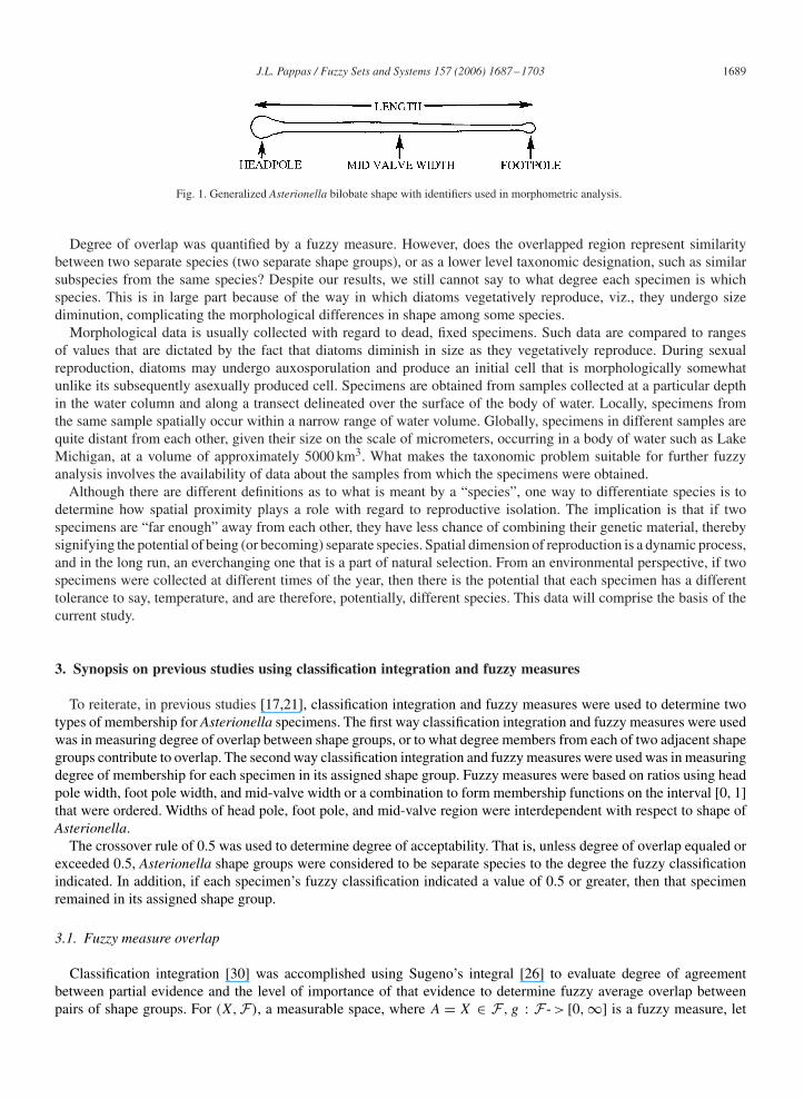
In previous studies [17,21], Fourier shape analysis of specimen outline was used on taxa from the araphid pennatediatom genus Asterionella [18]. This genus has few morphological features, including striae, a labiate process, and asternum without a raphe. All species in this diatom genus have a bilobate shape (Fig. 1). For photographic images ofall the specimens used, see [17].

The multivariate statistical technique, principal components analysis (PCA), was used to ordinate fuzzified Fouriercoefficients defining each Asterionella shape outline. Fuzzification was accomplished by mean-correcting the coef-ficients. From the first PCA of shape variance for each specimen, the resultant shape gradient in fuzzy PCA shapespace was subsectioned into seven groups. Circumscribed specimens were designated as shape groups, and overlap ofadjacent shape groups occurred to some degree. Since diatom shape is largely inherited, each shape group is, to somedegree, an indication of a distinct species. This initial sorting technique is used to reduce some of the arbitrariness intaxonomic decision-making.

A second sorting of specimens within shape groups is then necessary. Sometimes, there is overlap between shapegroups, as there was in this case. Morphometric measures other than shape were used for this next sorting. Mea-surable quantities common to all Asterionella are length, head pole width, mid-valve width, and foot pole width(Fig. 1). (see [17] for more details). Combinations of these measures as ratios can be used as a numerical way todistinguish specimens that look approximately alike. Two fuzzy measures were created using classification integration[26,30]. They were used to determine degree of overlap and degree that specimens belonged to their assigned shapegroup [17].

J.L. Pappas / Fuzzy Sets and Systems 157 (2006) 1687 –1703 1689

Fig. 1. Generalized Asterionella bilobate shape with identifiers used in morphometric analysis.

Degree of overlap was quantified by a fuzzy measure. However, does the overlapped region represent similaritybetween two separate species (two separate shape groups), or as a lower level taxonomic designation, such as similarsubspecies from the same species? Despite our results, we still cannot say to what degree each specimen is whichspecies. This is in large part because of the way in which diatoms vegetatively reproduce, viz., they undergo sizediminution, complicating the morphological differences in shape among some species.

Morphological data is usually collected with regard to dead, fixed specimens. Such data are compared to rangesof values that are dictated by the fact that diatoms diminish in size as they vegetatively reproduce. During sexualreproduction, diatoms may undergo auxosporulation and produce an initial cell that is morphologically somewhatunlike its subsequently asexually produced cell. Specimens are obtained from samples collected at a particular depthin the water column and along a transect delineated over the surface of the body of water. Locally, specimens fromthe same sample spatially occur within a narrow range of water volume. Globally, specimens in different samples arequite distant from each other, given their size on the scale of micrometers, occurring in a body of water such as LakeMichigan, at a volume of approximately 5000 km3. What makes the taxonomic problem suitable for further fuzzyanalysis involves the availability of data about the samples from which the specimens were obtained.

Although there are different definitions as to what is meant by a “species”, one way to differentiate species is todetermine how spatial proximity plays a role with regard to reproductive isolation. The implication is that if twospecimens are “far enough” away from each other, they have less chance of combining their genetic material, therebysignifying the potential of being (or becoming) separate species. Spatial dimension of reproduction is a dynamic process,and in the long run, an everchanging one that is a part of natural selection. From an environmental perspective, if twospecimens were collected at different times of the year, then there is the potential that each specimen has a differenttolerance to say, temperature, and are therefore, potentially, different species. This data will comprise the basis of thecurrent study.

3. Synopsis on previous studies using classification integration and fuzzy measures

To reiterate, in previous studies [17,21], classification integration and fuzzy measures were used to determine twotypes of membership for Asterionella specimens. The first way classification integration and fuzzy measures were usedwas in measuring degree of overlap between shape groups, or to what degree members from each of two adjacent shapegroups contribute to overlap. The second way classification integration and fuzzy measures were used was in measuringdegree of membership for each specimen in its assigned shape group. Fuzzy measures were based on ratios using headpole width, foot pole width, and mid-valve width or a combination to form membership functions on the interval [0, 1]that were ordered. Widths of head pole, foot pole, and mid-valve region were interdependent with respect to shape ofAsterionella.

The crossover rule of 0.5 was used to determine degree of acceptability. That is, unless degree of overlap equaled orexceeded 0.5, Asterionella shape groups were considered to be separate species to the degree the fuzzy classificationindicated. In addition, if each specimen’s fuzzy classification indicated a value of 0.5 or greater, then that specimenremained in its assigned shape group.

3.1. Fuzzy measure overlap

Classification integration [30] was accomplished using Sugeno’s integral [26] to evaluate degree of agreementbetween partial evidence and the level of importance of that evidence to determine fuzzy average overlap betweenpairs of shape groups. For (X, F), a measurable space, where A = X ∈ F, g : F- > [0, ∞] is a fuzzy measure, let

1690 J.L. Pappas / Fuzzy Sets and Systems 157 (2006) 1687 –1703

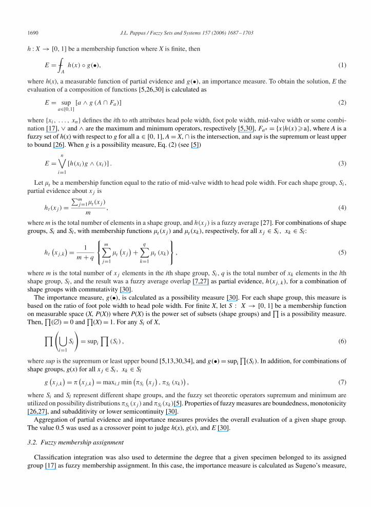
h :X → [0, 1] be a membership function where X is finite, then

E = −∫

A

h(x) ◦ g(•), (1)

where h(x), a measurable function of partial evidence and g(•), an importance measure. To obtain the solution, E theevaluation of a composition of functions [5,26,30] is calculated as

E = supa∈[0,1]

[a ∧ g (A ∩ Fa)] (2)

where {xi, . . . , xn} defines the ith to nth attributes head pole width, foot pole width, mid-valve width or some combi-nation [17], ∨ and ∧ are the maximum and minimum operators, respectively [5,30], Fa� = {x|h(x)�a}, where A is afuzzy set of h(x) with respect to g for all a ∈ [0, 1], A = X, ∩ is the intersection, and sup is the supremum or least upperto bound [26]. When g is a possibility measure, Eq. (2) (see [5])

E =n∨

i=1

[h(xi)g ∧ (xi)] . (3)

Let �t be a membership function equal to the ratio of mid-valve width to head pole width. For each shape group, Si ,partial evidence about xj is

ht (xj ) =∑m

j=1�t (xj )

m, (4)

where m is the total number of elements in a shape group, and h(xj ) is a fuzzy average [27]. For combinations of shapegroups, Si and Sl , with membership functions �t (xj ) and �t (xk), respectively, for all xj ∈ Si, xk ∈ Sl :

ht

(xj,k

)= 1

m + q

⎧⎨⎩

m∑j=1

�t

(xj

)+q∑

k=1

�t (xk)

⎫⎬⎭ , (5)

where m is the total number of xj elements in the ith shape group, Si , q is the total number of xk elements in the lthshape group, Sl , and the result was a fuzzy average overlap [7,27] as partial evidence, h(xj, k), for a combination ofshape groups with commutativity [30].

The importance measure, g(•), is calculated as a possibility measure [30]. For each shape group, this measure isbased on the ratio of foot pole width to head pole width. For finite X, let S : X → [0, 1] be a membership functionon measurable space (X, P(X)) where P(X) is the power set of subsets (shape groups) and

∏is a possibility measure.

Then,∏

(�) = 0 and∏

(X) = 1. For any Si of X,

∏(⋃i=1

Si

)= supi

∏(Si) , (6)

where sup is the supremum or least upper bound [5,13,30,34], and g(•) = supi∏

(Si). In addition, for combinations ofshape groups, g(x) for all xj ∈ Si, xk ∈ Sl

g(xj,k

)= �(xj,k

)= maxi,l min(�Si

(xj

), �Sl (xk)

), (7)

where Si and Sl represent different shape groups, and the fuzzy set theoretic operators supremum and minimum areutilized on possibility distributions �Si

(xj ) and �Sl(xk)[5]. Properties of fuzzy measures are boundedness, monotonicity

[26,27], and subadditivity or lower semicontinuity [30].Aggregation of partial evidence and importance measures provides the overall evaluation of a given shape group.

The value 0.5 was used as a crossover point to judge h(x), g(x), and E [30].

3.2. Fuzzy membership assignment

Classification integration was also used to determine the degree that a given specimen belonged to its assignedgroup [17] as fuzzy membership assignment. In this case, the importance measure is calculated as Sugeno’s measure,

J.L. Pappas / Fuzzy Sets and Systems 157 (2006) 1687 –1703 1691

g�-fuzzy measure. For two attributes for each shape group in which each specimen was considered, two measures werecalculated. One measure, g1, represents ratio of foot pole width to head pole width. The other measure, g2, representsratio of mid-valve width to head pole width.

Sugeno’s measure, g� as �(xi) [30] is

g� (X) = � (X) = 1

�

[n

�i=1

(1 + � · � ({xi})) − 1

](8)

for any � where

� ∈(

− 1

sup �, ∞

)∪ {0} . (9)

If � > 0, then g is a belief measure; if −1 < � < 0, then g is a plausibility measure; if � = 0, then g is a probabilitymeasure [5,30].

As a defining factor for each group, a ratio of normalized mid-valve width to foot pole width represents h(x) foreach specimen. Partial evidence represents the degree of consistency that a particular specimen belongs to a particulargroup. Values equal to one indicate complete consistency that a specimen is assigned to the correct group. Values equalto zero indicated that the specimen did not belong to that group. The crossover point was 0.5. For each specimen, fuzzymembership assignment was 0.5 or greater, and g was calculated to be a plausibility measure.

3.3. Fuzzy morphological taxonomic decision-making

Overlap values were calculated between groups within a region of similar total variance from PCA. Two regionswere defined—one with shape groups I, II and III, and the other one with shape groups IV, V and VI. Generally, butnot exclusively speaking, each region defined two sets of specimens differentiated by geographic location. The firstone (shape groups I, II and III) included most of the specimens from Lakes Superior and Huron, Green Bay and otherareas of northern Lake Michigan. There were a few specimens from central and southern Lake Michigan as well. In thesecond region (shape groups IV, V and VI), most of the specimens were from all of Lake Michigan (excluding GreenBay), but also included a few specimens from Lakes Superior and Huron [17].

Results from fuzzy average overlap calculations were in the range of 0.53–0.60. The degree of overlap suggeststhat paired comparisons of shape groups are as much similar as dissimilar (0.53–0.56), or are slightly more similar toeach other (0.55–0.60). That is, all fuzzy overlap values are similar. This measure somewhat indirectly embodies thedevelopmental stages of this diatom, in that shape of one species at one developmental stage may look like the shape ofanother species at a different developmental stage (overlap). Fuzzy average overlap indicates to what degree specimensfrom adjacent groups are similar and that biological sorting at the species level is not a simple sorting problem [17].

Each specimen’s shape group assignment was calculated to be from 0.49 (one case) to 0.73, with a degree ofplausibility (Sugeno’s measure) from 0.6 to 0.9. A check of each specimen’s plausible fuzzy assignment value atapproximately the crossover point indicates that specimen shape group assignment is correct to some degree [17].

At any point in a taxonomic analysis, an expert in the field can weigh in on outcomes for species designations.Moreover, with additional evidence, a new fuzzy analysis may be useful. This additional evidence must be gleanedfrom available historical sources. Such data includes information about sample collection location and when the samplewas collected. More specifically, data on latitude and longitude of the sample location, time of year when the samplewas collected, and general information about circulation patterns in the bodies of water from which the samples werecollected are available with reference to the diatoms used in fuzzy morphological analyses.

4. Purposes of this study

Previous morphometric studies were useful in finding fuzzy group boundaries and their properties (i.e., fuzzy averageoverlap) and specimen fuzzy membership in groups. The current study focuses on adding new information to what hasalready been done using techniques from fuzzy decision-making, including information fusion, expert systems, andmultiple criteria evaluation. I want to test the fuzzy biological taxonomic shape groups devised with respect to spatialand temporal data and reassess the degree to which specimen assignment in groups is true and also in agreement with

1692 J.L. Pappas / Fuzzy Sets and Systems 157 (2006) 1687 –1703

an expert in diatom research. That is, given the nature of the evidence and the uncertainties therein, I want to determineto what degree that each specimen in its assigned shape group may be called a “species”. Results from this study willprovide a simple, understandable way to decrease arbitrariness in the taxonomic decision making process for biologistsby providing a useful, analytical tool for taxonomists when data is scarce, absent, or indirectly applicable.

5. Methods

Data on sample location as latitude and longitude, long-term circulation patterns in the Great Lakes [2], and the timeof year when specimen samples were collected are used. These data constitute four spatial and/or temporal variables.Latitude and longitude are numerical values relating to the position of sample collection and are local variables. Long-term circulation patterns are a composite of data with regard to time of year and position in the Great Lakes. The premiseof this data is that circulation patterns dictate whether regions of a given lake will incur water mixing, and thereby amore likely chance that specimens would come in close proximity and interbreed. This is a regional or global variable.Time of year is a monthly designation and considered to be a temporal variable on a local scale. The variables latitude,longitude and time of year pertain to samples from which the specimens were collected have definite numerical orcategorical specificity. Long-term circulation patterns represent a composite of many years of data applied to regionsof the Great Lakes and are indirectly applicable to the regions where samples were collected. The data are more generaland are labeled as cyclonic, coastal, annual, or not applicable and are designated as 0, 1, 2, and 3, respectively. Samplelocation and time of year collected are the factors that determine which categorical variable is given to that sample.

Each of these variables is characterized as a quintuple, (x, T, U, J, M), where x is the variable with the name definedas the primary term, T is the set of linguistic values of x as terms, U is the universe of discourse, J is a rule of syntaxfor generating terms of linguistic values of x, and M is a semantic rule indicating meaning of the linguistic values byassigning a fuzzy set to the terms.

5.1. Ranking variables within categories

For each shape group, spatial and temporal data are ranked based on how frequently particular values appear in eachcategory. That is, the mode or relative maximum is used to represent the value that approximately occurs most often.For example, if most of the specimens occur at approximately the same latitude, that value is assigned “most frequent”and ranked as number one. The next most frequently occurring is assigned “more frequent” and ranked as numbertwo. The least frequently occurring is assigned “least frequent” and ranked as number three. If there is more than onerelative maximum within each category (bimodal), the expert decides which relative maximum to use. The premise isthat specimens that occur most closely together and/or at the same time of year are more likely to be the same species.This premise places a biological meaning and constraint on the spatial and temporal data being used as ranked modalvalues. The same process is used with regard to all variables and is the rule of syntax for generating linguistic values, J.For the universe of discourse, U, that is spatial and temporal variables, where x is the primary term, for each variable,the term sets for T are

T (frequent) = {least frequent, more frequent, most frequent} (10)

and are recursively determined as

T 0 = �,

T 1 = least frequent,

T 2 = least frequent, more frequent,

T 3 = least frequent, more frequent, most frequent. (11)

That is,

T i+1 = {frequent} ∪ more T i (12)

J.L. Pappas / Fuzzy Sets and Systems 157 (2006) 1687 –1703 1693

and

more T i = ∪R∈T i

{more R}. (13)

Next, each specimen in each shape group is ranked per variable according to the rankings for the whole group. Thesemantic rule, M(x), is that each variable rank is fuzzified as

v(R) = 1 − R∑R

, (14)

where v(R) is the variable rank of x which defines the membership function �(x) of x, and R is rank of variable with avalue of 1, 2, 3, or 4. Ranking and fuzzification of each variable and each specimen is accomplished in the same wayfor each shape group. This fuzzy ranking acts as a fuzzy restriction on x given the semantic rule, M.

5.2. Weighting of variables between categories

Values from classification integration for each specimen assignment to a shape group are used with the fuzzifiedspatial and temporal data in a new fuzzy attribute matrix. The values for each category must be weighted to representtheir degree of importance in taxonomic decision-making. To determine the weights, the expert identifies the weightsusing linguistic terms. The categories are ranked and a function is applied such that the calculated fuzzy values reflectthe expert’s opinion. The effect is to “weight” the categories with respect to each specimen per shape group.

The primary term is “important”, and linguistic modifiers or hedges used are “very”, “somewhat”, “slightly”, and“not very”. Although morphological data is more important than spatial or temporal data, fuzzy specimen shape groupassignment values, which represent morphological data in this matrix are “not very important” since the linguisticmodifiers refer to spatial and temporal data only. However, morphological data still takes precedence since its fuzzyvalue in the matrix must exceed those for spatial and temporal data (Stoermer, personal communication). The weightingsfor values in this fuzzy matrix as the universe of discourse are determined by the term set

T (important) = {very∗, somewhat∗, slightly∗, not very∗}, (15)

where * represents the primary term. The rule of syntax for generating linguistic hedges is defined as

Very = x2,

Somewhat = 1 − (1 − x2),

Slightly = 1 − (1 − x3),

Not very = √x, (16)

where A = {ai}, i = 1, . . . , n, is the fuzzy set for each row (specimen) of the matrix generated from the semantic rulethat orders the importance of each variable category with respect to the others as �

A(x) : X → {0, 1}, ∀x ∈ X.

The normalized weighted fuzzy modal values, h(x), are calculated as

h(x) = hc(x)

maxai∈Chc(ai)∀x ∈ X, (17)

where hc(x) is an approximate fuzzy histogram (see e.g., [29]) for the cth variable category of all C categories. Thatis, the fuzzy membership values calculated from Eq. (16) as ai are normalized and the result is hc(x) for each categoryfor each specimen.

5.3. Fuzzy weighted attribute matrix and aggregation

Using the normalized weighted fuzzy attribute matrix, aggregation of the information is necessary to determine thedegree to which each specimen belongs to its assigned shape group. The method of aggregation chosen is the weighted(ranking) sum. This aggregation operator is chosen because the categorical variables are independent of each other.Morphological data is biologically based. Latitude, longitude, long-term circulation patterns, and time of year are

1694 J.L. Pappas / Fuzzy Sets and Systems 157 (2006) 1687 –1703

measured independent of one another and on different scales. Linguistic modifier values are based on the mode foreach category per column independent of other categories, and the weighted sum for each row is independent ofother rows.

The rows in the weighted fuzzy attribute matrix are also suitability ratings (or weighted fuzzified rankings) [28]for each specimen with respect to the variable categories for each shape group. A sum of suitability ratings for eachspecimen would represent the total suitability [28] of that specimen in that shape group. Alternatively, the sum of thevalues for each specimen represents a fitness value with respect to that shape group. This fitness value may indicatethe approximate optimum value that the specimen can attain with respect to that shape group.

For each shape group, the approximate optimum is defined as the mode for each category and is the fuzzy setG(x) = {gj }, j = 1, . . . , m. A weighted sum of these values is the threshold against which each specimen is judged.The weighted fuzzy mode threshold or threshold weighted sum is

|G (x)| =m∑

j=1

gj , (18)

where x is the category modal value of latitude, longitude, long-term circulation pattern, and time of year, and by theextension principle [32], the sum is a fuzzy addition.

For each specimen, the weighted sum is the relative cardinality [35] given as

‖A‖ = |A||G| , (19)

where |G| is the threshold weighted sum and |A|=∑x∈X�A(x) is the cardinality of each specimen. The relative cardi-nalities are then normalized, and these values represent the degree that the specimen belongs to the shape group it wasassigned to given combined spatial and temporal factors and fuzzy morphological analytical results. The membershipis defined for the ith specimen in each shape group as

�weighted(xi) ={

1 if xi = xmax,

0.5 < xi < 1 otherwise.(20)

5.4. Expert evaluation

Expert evaluation is crucial in biological taxonomic decision-making. Dr. Eugene F. Stoermer from University ofMichigan is an expert in diatom research and has studied diatoms for over 40 years. The specimens used for this studywere viewed from strewn mounts on microscope slides and were collected from samples from the Great Lakes in the1960s and 1970s and are a part of Dr. Stoermer’s research collection.

There are two types of data available to analyze the taxonomic problem. Initially, morphological analyses are theaccepted way to perform a taxonomic study. This type of analysis takes precedence over spatial and temporal dataanalysis, but does not entirely supercede it (Stoermer, personal communication). Spatial and temporal data are usefulproxies with regard to reproductive isolation. In this study, Dr. Stoermer was consulted and made decisions on therelative importance of morphological vs. spatial and temporal variables (Section 5.2), the relative importance amongspatial and temporal variables (Section 5.2), the modal value for a category when more than one relative maximumexists (Section 5.2), linguistically express the degree of truth about the normalized fuzzy aggregation values for eachspecimen (Section 5.3), and evaluate the final results.

5.5. Fuzzy decision set and linguistic truth-value approximation

Fuzzy weighted membership values for each specimen in each shape group are evaluated with respect to the degreetheir membership is true. Since membership is already true to the degree 0.49 based on morphology alone, re-evaluationwith spatial and temporal data implies that membership values will be ai =[0.5, 1.0] for the ith specimen in each shapegroup. A fuzzy truth set is devised from the membership values interval that is common for all shape groups. A linguisticdecision is generated by devising meaningful labels for the fuzzy truth set, and these labels are determined by linguisticapproximation using a semantic equivalence [32,33]. That is, I want to find a linguistic approximation that is close in

J.L. Pappas / Fuzzy Sets and Systems 157 (2006) 1687 –1703 1695

meaning to the degree that each specimen’s assignment to a shape group is true and the degree of agreement expressedby the expert.

For a fuzzy truth set, �, an equivalent set L is defined by

�L(a) = ��(�B(a)), (21)

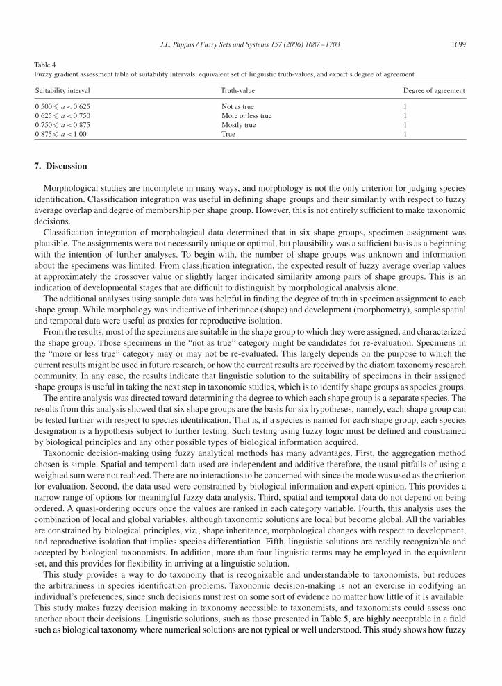
where �B(a) is the degree of agreement of the results by the expert. The equivalent set is inclusively L (Truth) = {true,mostly true, more or less true, not as true}. Additional linguistic terms may be used (e.g., see [3]). A fuzzy gradientassessment table of intervals of suitability of specimen assignment, a, equivalent set of linguistic truth-values, andexpert’s degree of agreement is devised. A linguistic solution is presented of the results.

6. Results

Relative cardinality reflects the situation of each specimen per shape group with respect to what is actually knownabout the specimens biologically and taxonomically. None of the specimens are actually completely excluded orincluded in each shape group. The values are maximized in order of importance. By normalizing the values, a rescalingis useful to indicate the degree to which each specimen belongs to its assigned shape group. The values normalized bythe fuzzy mode exhibit the “typicality” of each specimen in each shape group, and those specimens with values of 1.0characterize each shape group.

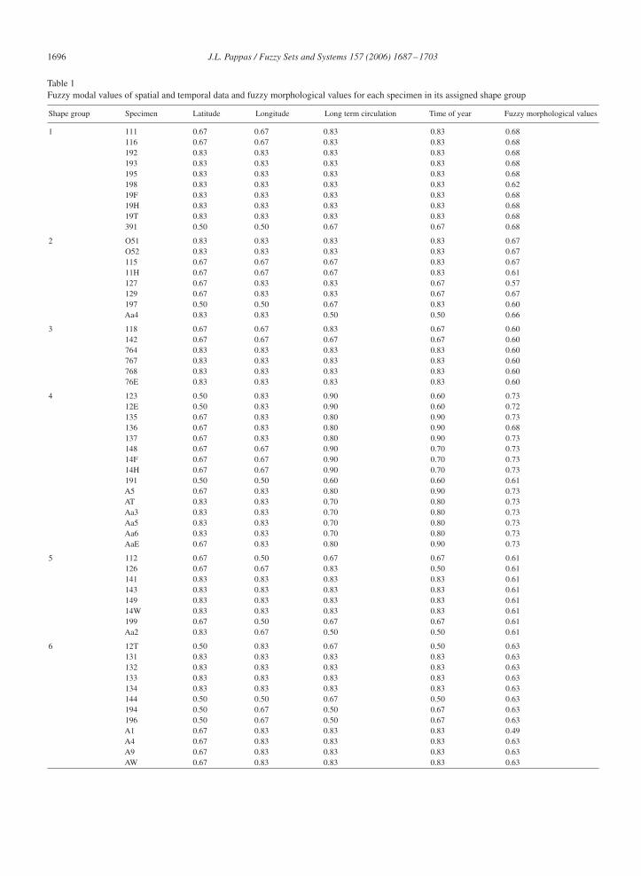
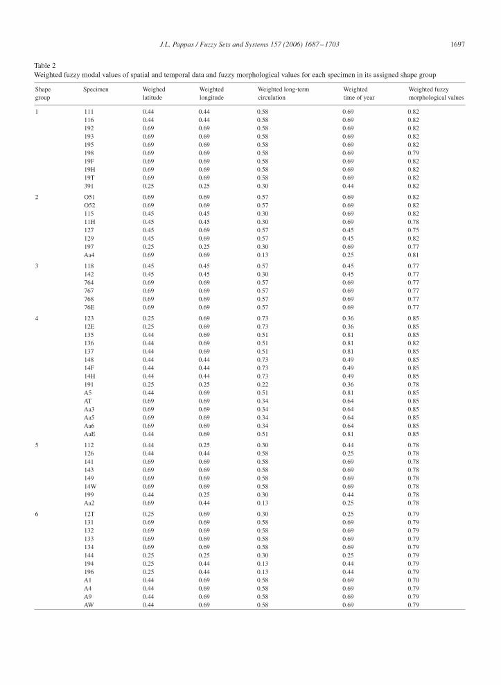
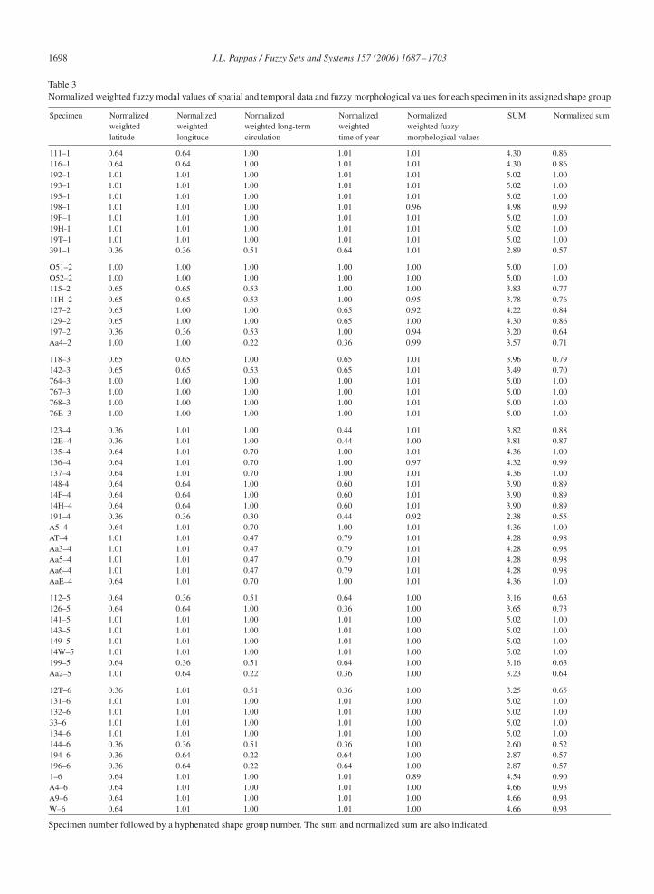
For each shape group, fuzzy matrices were devised of specimen by category values, including spatial, temporal,and morphological values. Fuzzy values based on the mode (as calculated from Eq. (14)) for each of the six shapegroups are presented in Table 1. Weighted fuzzy modal values (as calculated from Eq. (16)) are presented in Table 2.Normalized weighted fuzzy modal values (as calculated from Eq. (17)), their sum (as calculated from Eq. (19)), andthe normalized sum (as calculated from Eq. (20)) are presented in Table 3.

From the fuzzy modal values in each category, there is a widespread departure between the spatial and temporalvalues and the morphological values. From Table 1, fuzzy modes for spatial and temporal variables indicate a differencein importance for each specimen in contrast to fuzzy morphological values. In some cases, fuzzy morphological valuesare identical among all specimens in a given shape group (Table 1—shape groups 1, 3, and 5), whereas spatial andtemporal fuzzy modes are not. An interesting result is that since spatial and temporal variables are independent, latitudeand longitude fuzzy modes are mostly different within shape groups (Table 1—shape groups 2, 4, 5, and 6).

From Table 2, the relative level of importance between spatial and temporal variables is reflected in the weightingapplied. As previously stated, morphological values (local) take precedence over spatial and temporal values (global).Subsequently, the order of importance across spatial and temporal values range from latitude and longitude to time ofyear to long-term circulation pattern.

Normalized weighted modes in Table 3 reflect the relative position each specimen has to every other specimen in eachshape group. Those specimens with a value of 1.0 define their assigned shape groups. The sum, which is normalizedfor each specimen, gives the value of suitability that the specimen has with respect to belonging to its shape group. Avalue of 1.0 for a specimen characterizes the shape group morphologically, spatially, and temporally. Other specimensrelative to those members with a value of approximately 1.0 indicate the degree of suitability that these specimens havein their assigned shape group.

For each shape group, the normalized weighted sum for each specimen was evaluated by the expert, and his judgmentwas rendered as to the degree he agreed with the result. His evaluation was compiled as a solution to be viewed forall shape groups. In this regard, and given the results from Eq. (20), the equivalence set of linguistic approximationswas assigned to four subsets on the interval [0.5, 1.0], and the results of the evaluation are presented in Table 4. Theexpert’s degree of agreement was 1.0 (Stoermer, personal communication).

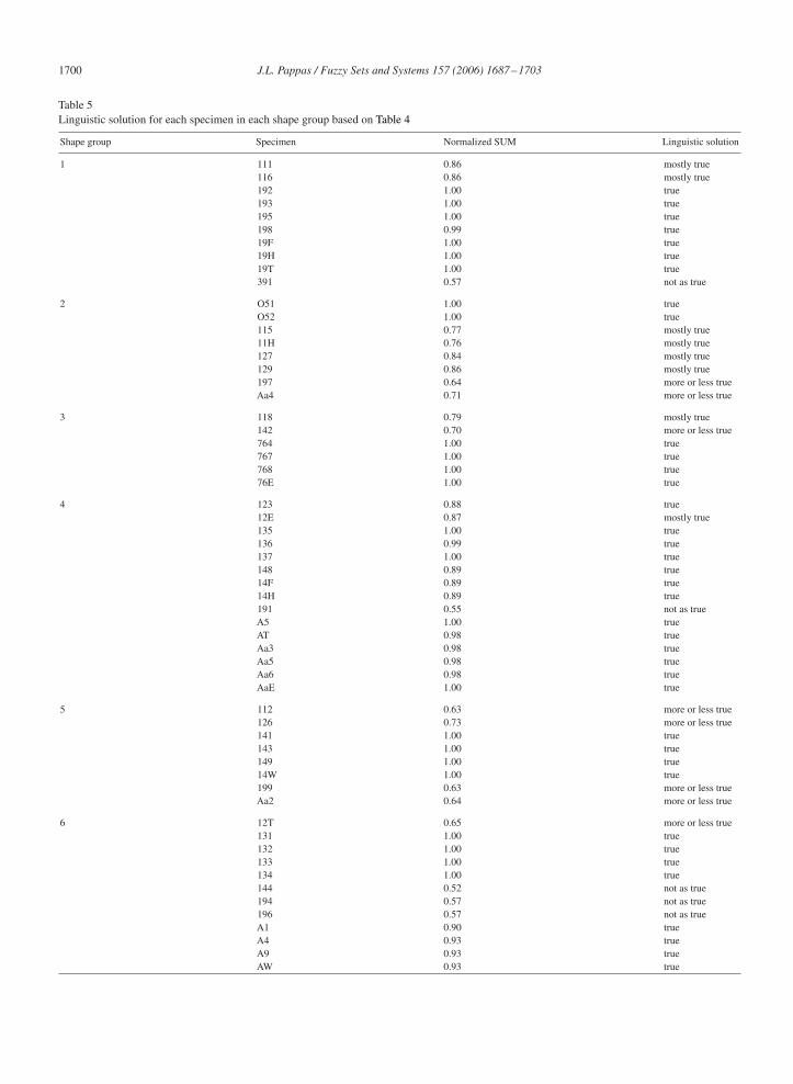
Four suitability intervals were devised, and each interval had a linguistic approximation from the equivalent set. Eachspecimen was then assigned a linguistic approximation based on Table 4. The linguistic solution for all specimens inall shape groups is given in Table 5.

By using 0.75 as a “crossover” point from the interval [0.5, 1.0], most of the shape groups have the majority of theirmembers in the “true” and “mostly true” categories. Shape groups 1, 3, and 4 have all but one member at or greaterthan 0.75. Shape group 2 has two members and shape groups 5 and 6 have four members at less than 0.75.

1696 J.L. Pappas / Fuzzy Sets and Systems 157 (2006) 1687 –1703

Table 1Fuzzy modal values of spatial and temporal data and fuzzy morphological values for each specimen in its assigned shape group

Shape group Specimen Latitude Longitude Long term circulation Time of year Fuzzy morphological values

1 111 0.67 0.67 0.83 0.83 0.68116 0.67 0.67 0.83 0.83 0.68192 0.83 0.83 0.83 0.83 0.68193 0.83 0.83 0.83 0.83 0.68195 0.83 0.83 0.83 0.83 0.68198 0.83 0.83 0.83 0.83 0.6219F 0.83 0.83 0.83 0.83 0.6819H 0.83 0.83 0.83 0.83 0.6819T 0.83 0.83 0.83 0.83 0.68391 0.50 0.50 0.67 0.67 0.68

2 O51 0.83 0.83 0.83 0.83 0.67O52 0.83 0.83 0.83 0.83 0.67115 0.67 0.67 0.67 0.83 0.6711H 0.67 0.67 0.67 0.83 0.61127 0.67 0.83 0.83 0.67 0.57129 0.67 0.83 0.83 0.67 0.67197 0.50 0.50 0.67 0.83 0.60Aa4 0.83 0.83 0.50 0.50 0.66

3 118 0.67 0.67 0.83 0.67 0.60142 0.67 0.67 0.67 0.67 0.60764 0.83 0.83 0.83 0.83 0.60767 0.83 0.83 0.83 0.83 0.60768 0.83 0.83 0.83 0.83 0.6076E 0.83 0.83 0.83 0.83 0.60

4 123 0.50 0.83 0.90 0.60 0.7312E 0.50 0.83 0.90 0.60 0.72135 0.67 0.83 0.80 0.90 0.73136 0.67 0.83 0.80 0.90 0.68137 0.67 0.83 0.80 0.90 0.73148 0.67 0.67 0.90 0.70 0.7314F 0.67 0.67 0.90 0.70 0.7314H 0.67 0.67 0.90 0.70 0.73191 0.50 0.50 0.60 0.60 0.61A5 0.67 0.83 0.80 0.90 0.73AT 0.83 0.83 0.70 0.80 0.73Aa3 0.83 0.83 0.70 0.80 0.73Aa5 0.83 0.83 0.70 0.80 0.73Aa6 0.83 0.83 0.70 0.80 0.73AaE 0.67 0.83 0.80 0.90 0.73

5 112 0.67 0.50 0.67 0.67 0.61126 0.67 0.67 0.83 0.50 0.61141 0.83 0.83 0.83 0.83 0.61143 0.83 0.83 0.83 0.83 0.61149 0.83 0.83 0.83 0.83 0.6114W 0.83 0.83 0.83 0.83 0.61199 0.67 0.50 0.67 0.67 0.61Aa2 0.83 0.67 0.50 0.50 0.61

6 12T 0.50 0.83 0.67 0.50 0.63131 0.83 0.83 0.83 0.83 0.63132 0.83 0.83 0.83 0.83 0.63133 0.83 0.83 0.83 0.83 0.63134 0.83 0.83 0.83 0.83 0.63144 0.50 0.50 0.67 0.50 0.63194 0.50 0.67 0.50 0.67 0.63196 0.50 0.67 0.50 0.67 0.63A1 0.67 0.83 0.83 0.83 0.49A4 0.67 0.83 0.83 0.83 0.63A9 0.67 0.83 0.83 0.83 0.63AW 0.67 0.83 0.83 0.83 0.63

J.L. Pappas / Fuzzy Sets and Systems 157 (2006) 1687 –1703 1697

Table 2Weighted fuzzy modal values of spatial and temporal data and fuzzy morphological values for each specimen in its assigned shape group

Shape Specimen Weighed Weighted Weighted long-term Weighted Weighted fuzzygroup latitude longitude circulation time of year morphological values

1 111 0.44 0.44 0.58 0.69 0.82116 0.44 0.44 0.58 0.69 0.82192 0.69 0.69 0.58 0.69 0.82193 0.69 0.69 0.58 0.69 0.82195 0.69 0.69 0.58 0.69 0.82198 0.69 0.69 0.58 0.69 0.7919F 0.69 0.69 0.58 0.69 0.8219H 0.69 0.69 0.58 0.69 0.8219T 0.69 0.69 0.58 0.69 0.82391 0.25 0.25 0.30 0.44 0.82

2 O51 0.69 0.69 0.57 0.69 0.82O52 0.69 0.69 0.57 0.69 0.82115 0.45 0.45 0.30 0.69 0.8211H 0.45 0.45 0.30 0.69 0.78127 0.45 0.69 0.57 0.45 0.75129 0.45 0.69 0.57 0.45 0.82197 0.25 0.25 0.30 0.69 0.77Aa4 0.69 0.69 0.13 0.25 0.81

3 118 0.45 0.45 0.57 0.45 0.77142 0.45 0.45 0.30 0.45 0.77764 0.69 0.69 0.57 0.69 0.77767 0.69 0.69 0.57 0.69 0.77768 0.69 0.69 0.57 0.69 0.7776E 0.69 0.69 0.57 0.69 0.77

4 123 0.25 0.69 0.73 0.36 0.8512E 0.25 0.69 0.73 0.36 0.85135 0.44 0.69 0.51 0.81 0.85136 0.44 0.69 0.51 0.81 0.82137 0.44 0.69 0.51 0.81 0.85148 0.44 0.44 0.73 0.49 0.8514F 0.44 0.44 0.73 0.49 0.8514H 0.44 0.44 0.73 0.49 0.85191 0.25 0.25 0.22 0.36 0.78A5 0.44 0.69 0.51 0.81 0.85AT 0.69 0.69 0.34 0.64 0.85Aa3 0.69 0.69 0.34 0.64 0.85Aa5 0.69 0.69 0.34 0.64 0.85Aa6 0.69 0.69 0.34 0.64 0.85AaE 0.44 0.69 0.51 0.81 0.85

5 112 0.44 0.25 0.30 0.44 0.78126 0.44 0.44 0.58 0.25 0.78141 0.69 0.69 0.58 0.69 0.78143 0.69 0.69 0.58 0.69 0.78149 0.69 0.69 0.58 0.69 0.7814W 0.69 0.69 0.58 0.69 0.78199 0.44 0.25 0.30 0.44 0.78Aa2 0.69 0.44 0.13 0.25 0.78

6 12T 0.25 0.69 0.30 0.25 0.79131 0.69 0.69 0.58 0.69 0.79132 0.69 0.69 0.58 0.69 0.79133 0.69 0.69 0.58 0.69 0.79134 0.69 0.69 0.58 0.69 0.79144 0.25 0.25 0.30 0.25 0.79194 0.25 0.44 0.13 0.44 0.79196 0.25 0.44 0.13 0.44 0.79A1 0.44 0.69 0.58 0.69 0.70A4 0.44 0.69 0.58 0.69 0.79A9 0.44 0.69 0.58 0.69 0.79AW 0.44 0.69 0.58 0.69 0.79

1698 J.L. Pappas / Fuzzy Sets and Systems 157 (2006) 1687 –1703

Table 3Normalized weighted fuzzy modal values of spatial and temporal data and fuzzy morphological values for each specimen in its assigned shape group

Specimen Normalized Normalized Normalized Normalized Normalized SUM Normalized sumweighted weighted weighted long-term weighted weighted fuzzylatitude longitude circulation time of year morphological values

111–1 0.64 0.64 1.00 1.01 1.01 4.30 0.86116–1 0.64 0.64 1.00 1.01 1.01 4.30 0.86192–1 1.01 1.01 1.00 1.01 1.01 5.02 1.00193–1 1.01 1.01 1.00 1.01 1.01 5.02 1.00195–1 1.01 1.01 1.00 1.01 1.01 5.02 1.00198–1 1.01 1.01 1.00 1.01 0.96 4.98 0.9919F–1 1.01 1.01 1.00 1.01 1.01 5.02 1.0019H-1 1.01 1.01 1.00 1.01 1.01 5.02 1.0019T–1 1.01 1.01 1.00 1.01 1.01 5.02 1.00391–1 0.36 0.36 0.51 0.64 1.01 2.89 0.57

O51–2 1.00 1.00 1.00 1.00 1.00 5.00 1.00O52–2 1.00 1.00 1.00 1.00 1.00 5.00 1.00115–2 0.65 0.65 0.53 1.00 1.00 3.83 0.7711H–2 0.65 0.65 0.53 1.00 0.95 3.78 0.76127–2 0.65 1.00 1.00 0.65 0.92 4.22 0.84129–2 0.65 1.00 1.00 0.65 1.00 4.30 0.86197–2 0.36 0.36 0.53 1.00 0.94 3.20 0.64Aa4–2 1.00 1.00 0.22 0.36 0.99 3.57 0.71

118–3 0.65 0.65 1.00 0.65 1.01 3.96 0.79142–3 0.65 0.65 0.53 0.65 1.01 3.49 0.70764–3 1.00 1.00 1.00 1.00 1.01 5.00 1.00767–3 1.00 1.00 1.00 1.00 1.01 5.00 1.00768–3 1.00 1.00 1.00 1.00 1.01 5.00 1.0076E–3 1.00 1.00 1.00 1.00 1.01 5.00 1.00

123–4 0.36 1.01 1.00 0.44 1.01 3.82 0.8812E–4 0.36 1.01 1.00 0.44 1.00 3.81 0.87135–4 0.64 1.01 0.70 1.00 1.01 4.36 1.00136–4 0.64 1.01 0.70 1.00 0.97 4.32 0.99137–4 0.64 1.01 0.70 1.00 1.01 4.36 1.00148-4 0.64 0.64 1.00 0.60 1.01 3.90 0.8914F–4 0.64 0.64 1.00 0.60 1.01 3.90 0.8914H–4 0.64 0.64 1.00 0.60 1.01 3.90 0.89191–4 0.36 0.36 0.30 0.44 0.92 2.38 0.55A5–4 0.64 1.01 0.70 1.00 1.01 4.36 1.00AT–4 1.01 1.01 0.47 0.79 1.01 4.28 0.98Aa3–4 1.01 1.01 0.47 0.79 1.01 4.28 0.98Aa5–4 1.01 1.01 0.47 0.79 1.01 4.28 0.98Aa6–4 1.01 1.01 0.47 0.79 1.01 4.28 0.98AaE–4 0.64 1.01 0.70 1.00 1.01 4.36 1.00

112–5 0.64 0.36 0.51 0.64 1.00 3.16 0.63126–5 0.64 0.64 1.00 0.36 1.00 3.65 0.73141–5 1.01 1.01 1.00 1.01 1.00 5.02 1.00143–5 1.01 1.01 1.00 1.01 1.00 5.02 1.00149–5 1.01 1.01 1.00 1.01 1.00 5.02 1.0014W–5 1.01 1.01 1.00 1.01 1.00 5.02 1.00199–5 0.64 0.36 0.51 0.64 1.00 3.16 0.63Aa2–5 1.01 0.64 0.22 0.36 1.00 3.23 0.64

12T–6 0.36 1.01 0.51 0.36 1.00 3.25 0.65131–6 1.01 1.01 1.00 1.01 1.00 5.02 1.00132–6 1.01 1.01 1.00 1.01 1.00 5.02 1.0033–6 1.01 1.01 1.00 1.01 1.00 5.02 1.00134–6 1.01 1.01 1.00 1.01 1.00 5.02 1.00144–6 0.36 0.36 0.51 0.36 1.00 2.60 0.52194–6 0.36 0.64 0.22 0.64 1.00 2.87 0.57196–6 0.36 0.64 0.22 0.64 1.00 2.87 0.571–6 0.64 1.01 1.00 1.01 0.89 4.54 0.90A4–6 0.64 1.01 1.00 1.01 1.00 4.66 0.93A9–6 0.64 1.01 1.00 1.01 1.00 4.66 0.93W–6 0.64 1.01 1.00 1.01 1.00 4.66 0.93

Specimen number followed by a hyphenated shape group number. The sum and normalized sum are also indicated.

J.L. Pappas / Fuzzy Sets and Systems 157 (2006) 1687 –1703 1699

Table 4Fuzzy gradient assessment table of suitability intervals, equivalent set of linguistic truth-values, and expert’s degree of agreement

Suitability interval Truth-value Degree of agreement

0.500� a < 0.625 Not as true 10.625� a < 0.750 More or less true 10.750� a < 0.875 Mostly true 10.875� a < 1.00 True 1

7. Discussion

Morphological studies are incomplete in many ways, and morphology is not the only criterion for judging speciesidentification. Classification integration was useful in defining shape groups and their similarity with respect to fuzzyaverage overlap and degree of membership per shape group. However, this is not entirely sufficient to make taxonomicdecisions.

Classification integration of morphological data determined that in six shape groups, specimen assignment wasplausible. The assignments were not necessarily unique or optimal, but plausibility was a sufficient basis as a beginningwith the intention of further analyses. To begin with, the number of shape groups was unknown and informationabout the specimens was limited. From classification integration, the expected result of fuzzy average overlap valuesat approximately the crossover value or slightly larger indicated similarity among pairs of shape groups. This is anindication of developmental stages that are difficult to distinguish by morphological analysis alone.

The additional analyses using sample data was helpful in finding the degree of truth in specimen assignment to eachshape group. While morphology was indicative of inheritance (shape) and development (morphometry), sample spatialand temporal data were useful as proxies for reproductive isolation.

From the results, most of the specimens are suitable in the shape group to which they were assigned, and characterizedthe shape group. Those specimens in the “not as true” category might be candidates for re-evaluation. Specimens inthe “more or less true” category may or may not be re-evaluated. This largely depends on the purpose to which thecurrent results might be used in future research, or how the current results are received by the diatom taxonomy researchcommunity. In any case, the results indicate that linguistic solution to the suitability of specimens in their assignedshape groups is useful in taking the next step in taxonomic studies, which is to identify shape groups as species groups.

The entire analysis was directed toward determining the degree to which each shape group is a separate species. Theresults from this analysis showed that six shape groups are the basis for six hypotheses, namely, each shape group canbe tested further with respect to species identification. That is, if a species is named for each shape group, each speciesdesignation is a hypothesis subject to further testing. Such testing using fuzzy logic must be defined and constrainedby biological principles and any other possible types of biological information acquired.

Taxonomic decision-making using fuzzy analytical methods has many advantages. First, the aggregation methodchosen is simple. Spatial and temporal data used are independent and additive therefore, the usual pitfalls of using aweighted sum were not realized. There are no interactions to be concerned with since the mode was used as the criterionfor evaluation. Second, the data used were constrained by biological information and expert opinion. This provides anarrow range of options for meaningful fuzzy data analysis. Third, spatial and temporal data do not depend on beingordered. A quasi-ordering occurs once the values are ranked in each category variable. Fourth, this analysis uses thecombination of local and global variables, although taxonomic solutions are local but become global. All the variablesare constrained by biological principles, viz., shape inheritance, morphological changes with respect to development,and reproductive isolation that implies species differentiation. Fifth, linguistic solutions are readily recognizable andaccepted by biological taxonomists. In addition, more than four linguistic terms may be employed in the equivalentset, and this provides for flexibility in arriving at a linguistic solution.

This study provides a way to do taxonomy that is recognizable and understandable to taxonomists, but reducesthe arbitrariness in species identification problems. Taxonomic decision-making is not an exercise in codifying anindividual’s preferences, since such decisions must rest on some sort of evidence no matter how little of it is available.This study makes fuzzy decision making in taxonomy accessible to taxonomists, and taxonomists could assess oneanother about their decisions. Linguistic solutions, such as those presented in Table 5, are highly acceptable in a fieldsuch as biological taxonomy where numerical solutions are not typical or well understood. This study shows how fuzzy

1700 J.L. Pappas / Fuzzy Sets and Systems 157 (2006) 1687 –1703

Table 5Linguistic solution for each specimen in each shape group based on Table 4

Shape group Specimen Normalized SUM Linguistic solution

1 111 0.86 mostly true116 0.86 mostly true192 1.00 true193 1.00 true195 1.00 true198 0.99 true19F 1.00 true19H 1.00 true19T 1.00 true391 0.57 not as true

2 O51 1.00 trueO52 1.00 true115 0.77 mostly true11H 0.76 mostly true127 0.84 mostly true129 0.86 mostly true197 0.64 more or less trueAa4 0.71 more or less true

3 118 0.79 mostly true142 0.70 more or less true764 1.00 true767 1.00 true768 1.00 true76E 1.00 true

4 123 0.88 true12E 0.87 mostly true135 1.00 true136 0.99 true137 1.00 true148 0.89 true14F 0.89 true14H 0.89 true191 0.55 not as trueA5 1.00 trueAT 0.98 trueAa3 0.98 trueAa5 0.98 trueAa6 0.98 trueAaE 1.00 true

5 112 0.63 more or less true126 0.73 more or less true141 1.00 true143 1.00 true149 1.00 true14W 1.00 true199 0.63 more or less trueAa2 0.64 more or less true

6 12T 0.65 more or less true131 1.00 true132 1.00 true133 1.00 true134 1.00 true144 0.52 not as true194 0.57 not as true196 0.57 not as trueA1 0.90 trueA4 0.93 trueA9 0.93 trueAW 0.93 true

J.L. Pappas / Fuzzy Sets and Systems 157 (2006) 1687 –1703 1701

logic, approximate reasoning, and information fusion are what actually happen in solving a biological problem, viz.,taxonomy and species identification.

From this study, there are issues that need to be explored further. One problem was how to determine which fuzzymode to use for each category. In this study, consultation with the expert was used. Solving this problem in a moreanalytical way might be accomplished by creating a fuzzy measure to find the minimum distance between the “ideal”for the category and each of the relative maxima. There is still the potential for ties among distance minima. Perhaps aresampling method would be an alternative to use in choosing the relative minimum to use. Alternatively, a resemblancemeasure based on a fuzzy histogram [29] might be devised to compare a specimen with what is “typical” for a givenshape group.

Another issue is that of independence of variables and method of aggregation [6]. In this study, the variables tobe aggregated were independent, and therefore additive. If variables used are not independent, then non-additiveaggregation is warranted. In this regard, the Choquet integral, among others, might be a suitable option [4,9,10]. Thisstudy provided an initial solution to the problem of aggregating spatial and temporal data with morphological data.Although the methods used here do not necessarily provide for a unique solution, given the scant evidence and analysisof specimens relative to each other, the solution is a worthy starting point. In addition, there is the potential that anotherexpert would reassign specimens to different groups, or even weight the spatial and temporal variables differently. Thisstudy is flexible in that amendments can be made to accommodate other types of taxonomic studies, or studies thathave a similar compilation of a variety of inputs. It can be adapted to include more than one expert or more than onedecision-making group. More than one expert may be consulted to contribute to the decision-making process. In thiscase, the process would become more complex, but would be accommodated by some form of fuzzy group decision-making [34]. In essence, the methods used here are simple, adaptable, and understandable to biological taxonomists,especially with the incorporation of linguistic solutions.

It may be that reassigning suboptimal specimens to other shape groups would produce a more optimal solution.By suboptimal I mean those specimens with a value of less than 1.00. Another scenario might be that some of thespecimens with suboptimal assignment do not belong to any of the shape groups. That is, some specimens may belongto a yet-to-be described shape group. A fuzzy permutation program reassigning suboptimal specimens to other shapegroups and re-evaluating results until the more optimal solution is obtained might be useful. The permutation can be ofany type and crosschecked with other permutation methods (e.g., bootstrapping, jackknifing, Monte Carlo permutation).Alternatively, fuzzy decision trees may be used [31].

Perhaps one way to refine results further would be to find relative densities for each shape group with respect to fuzzyoverlap values. If it could be determined which specimens contributed the largest degree to fuzzy average overlap, thenthose particular specimens would be candidates for reassignment and testing, based on a newly devised fuzzy measurefor developmental stage.

Biological taxonomy is not a static enterprise since a scientific name is a hypothesis to be tested, so an optimal orunique solution is not necessarily a realistic expectation. The current results are constrained by biological information,starting with predefined shape groups from an earlier morphological study and incorporating expert opinion in thedecision making process. This provides a sense of validity to the enterprise of biological taxonomy that is not merelyopinion, albeit authoritative opinion.

Taxonomic studies are necessary precursors to phylogenetic analyses and reconstruction of phylogenetic relationsamong taxa. This study has importance for other biological studies, in general, in that a formal way of assessing speciesidentification is a very important indicator of the species concept in biology and how that concept is applied. Anotheradjunct study to this one includes exploring fuzzy position with respect to an organism and climate or habitat qualitysince latitude and longitude are independent variables. This study is only the beginning of possibilities for applicationsof fuzzy logic and decision-making to biological studies.

8. Conclusions

My study was conducted to show that biological taxonomic decision-making may be augmented by the use of fuzzysets and fuzzy decision-making. Information about specimens from the genus Asterionella was scant, and some of thesample data was used as proxies for inferred biological information. Degree of suitability in specimen assignment toshape groups was determined after initial sorting using classification integration of morphometric data. Degree of truth

1702 J.L. Pappas / Fuzzy Sets and Systems 157 (2006) 1687 –1703

in specimen assignment, as given in Table 5, reflects acceptability of the results to an expert in diatom research. That is,the degree to which each specimen is a species was determined using the methodology outlined in my study. Throughoutmy study, biological principles of developmental stage or ontogeny (morphology and morphometrics), reproductiveisolation, and species concepts constrained the analysis to reflect a realistic way to conduct biological taxonomy.Moreover, not only was a numerical result per specimen achieved, but also a linguistic solution was determined thatmakes this study accessible to biologists.

In conducting biological taxonomic studies, researchers will never have all the morphotypes or “species” available forempirical assessment. My study shows that given a limited amount of information and a limited number of specimens,biological taxonomy using fuzzy decision-making can be accomplished to reflect a realistic portrayal of the state ofspecies designations at a given time.

Acknowledgements

I would like to thank Dr. E. F. Stoermer for participating in this study as an expert in diatom research and threeanonymous reviewers for helpful comments on this manuscript.

References

[1] R.W. Battarbee, D.F. Charles, S.S. Dixit, I. Renberg, Diatoms as indicators of surface water acidity, in: E.F. Stoermer, J.P. Smol (Eds.), TheDiatoms: Applications for the Environmental and Earth Sciences, Cambridge University Press, Cambridge, 1999, pp. 85–127.

[2] D. Beletsky, J.H. Saylor, D.J. Schwab, Mean circulation in the Great Lakes, J. Great Lakes Res. 25 (1999) 78–93.[3] R.E. Bellman, L. Zadeh, Local and fuzzy logics, in: J.M. Dunn, G. Epstein (Eds.), Modern Uses of Multiple-Valued Logic, D. Reidel Publishing

Company, Dordrecht, 1977, pp. 105–165.[4] M. Ceberio, F. Modave, An interval-valued, 2-additive Choquet integral for multicriteria decision making, 10th Conf. on Information Processing

and Management of Uncertainty in Knowledge-based Systems (IPMU), July 2004, Perugia, Italy.[5] D. Dubois, H. Prade, Fuzzy Sets and Systems: Theory and Applications, Academic Press, New York, 1980 393 pp.[6] D. Dubois, H. Prade, R. Yager, Merging fuzzy information, in: J.C. Bezdek, D. Dubois, H. Prade (Eds.), Fuzzy Sets in Approximate Reasoning

and Information Systems, Kluwer Academic Publishers, Boston, 1999, pp. 337–401.[7] J.M. Dunn, Indices of partition fuzziness and detection of clusters in large data sets, in: M.M. Gupta, G.N. Saridis, B.R. Gaines (Eds.), Fuzzy

Automata and Decision Process, North-Holland Publishers, Amsterdam, 1977, pp. 271–283.[8] S.C. Fritz, B.F. Cumming, F. Gasse, K.R. Laird, Diatoms as indicators of hydrologic and climatic change in saline lakes, in: E.F. Stoermer, J.P.

Smol (Eds.), The Diatoms: Applications for the Environmental and Earth Sciences, Cambridge University Press, Cambridge, 1999, pp. 41–72.[9] M. Grabisch, C. Labreuche, Fuzzy measures and integrals in mcda, in: J. Figueira, S. Greco, M. Ehrgott (Eds.), Multiple Criteria Decision

Analysis, Kluwer Academic Publishers, Boston, 2004, pp. 1–50.[10] M. Grabisch, M. Roubens, Application of the Choquet integral in multicriteria decision making, in: M. Grabisch, T. Murofiushi, M. Sugeno

(Eds.), Fuzzy Measures and Integrals—Theory and Applications, Physica Verlag, Germany, 2000, pp. 415–434.[11] R.I. Hall, J.P. Smol, Diatoms as indicators of lake eutrophication, in: E.F. Stoermer, J.P. Smol (Eds.), The Diatoms: Applications for the

Environmental and Earth Sciences, Cambridge University Press, Cambridge, 1999, pp. 85–127.[12] A.H. Hassall, Memoir on the organic analysis or microscopic examination of the water supplied to the inhabitants of London and the suburban

districts, The Lancet 1 (1850) 230–235.[13] A. Kandel, Fuzzy Techniques in Pattern Recognition, Wiley, New York, 1982 356 pp.[14] H. Körner, Morphologie und taxonomie der diatomeengattung Asterionella, Nova Hedwigia 20 (1970) 557–724.[15] D.G. Mann, Why didn’t Lund see sex in Asterionella? A discussion of the diatom life cycle in nature, in: F.E. Round (Ed.), Algae and the

Aquatic Environment, Biopress, Bristol, 1988, pp. 384–412.[16] D.G. Mann, The species concept in diatoms, Phycologia 38 (1999) 437–495.[17] J.L. Pappas, Fourier shape analysis and shape group determination by principal component analysis and fuzzy measure theory of Asterionella

Hassall (Heterokontophyta, Bacillariophyceae) from the Great Lakes, Dissertation, University of Michigan, 2000.[18] J.L. Pappas, G.W. Fowler, E.F. Stoermer, Calculating shape descriptors from Fourier analysis: shape analysis of Asterionella (Heterokontophyta,

Bacillariophyceae), Phycologia 40 (2001) 440–456.[19] J.L. Pappas, E.F. Stoermer, Multidimensional analysis of diatom morphologic and morphometric phenotypic variation and relation to niche,

Ecoscience 2 (1995) 357–367.[20] J.L. Pappas, E.F. Stoermer, Asterionella Hassall (Heterokontophyta, Bacillariophyceae): taxonomic history and quantitative methods as an aid

to valve shape differentiation, Diatom 17 (2001) 47–58.[21] J.L. Pappas, E.F. Stoermer, Fourier shape analysis and fuzzy measure shape group differentiation of Great Lakes Asterionella (Heterokontophyta,

Bacillariophyceae), in: A. Economou-Amilli (Ed.), Proc. 16th Internat. Diatom Symp., Amvrosiou Press, Athens, 2001, pp. 485–501.[22] F.E. Round, R.M. Crawford, D.G. Mann, The Diatoms—Biology & Morphology of the Genera, Cambridge University Press, Cambridge, 1990

747 pp.

J.L. Pappas / Fuzzy Sets and Systems 157 (2006) 1687 –1703 1703

[23] C. Sancetta, Diatoms and marine paleoceanography, in: E.F. Stoermer, J.P. Smol (Eds.), The Diatoms: Applications for the Environmental andEarth Sciences, Cambridge University Press, Cambridge, 1999, pp. 374–386.

[24] E.F. Stoermer, T.B. Ladewski, Apparent optimal temperature for the occurrence of some common phytoplankton species in southern LakeMichigan, Great Lakes Research Division Publication 18, University of Michigan, AnnArbor, Mi, 1976 pp. 50.

[25] E.F. Stoermer, J.J. Yang, Plankton diatom assemblages in Lake Michigan, Great Lakes Research Division Special Report No. 47, University ofMichigan, Ann Arbor, Mi, 1969 168pp.

[26] M. Sugeno, Fuzzy measures and fuzzy integrals: a survey, in: M.M. Gupta, G.N. Saridis, B.R. Gaines (Eds.), Fuzzy Automata and DecisionProcesses, North-Holland Publishers, New York, 1977, pp. 89–102.

[27] T. Terano, K. Asai, M. Sugeno, Fuzzy Systems Theory and its Applications, Academic Press, San Diego, 1992 268pp.[28] R.M. Tong, P.P. Bonissone, Linguistic solutions to fuzzy decision problems, in: H.-J. Zimmermann, L.A. Zadeh, B.R. Gaines (Eds.), Fuzzy

Sets and Decision Analysis, North-Holland, Amsterdam, 1984, pp. 323–334.[29] C.Vertan, N. Boujemaa, Embedding fuzzy logic in content based image retrieval, in: 19th Internat. Meeting of NorthAmerican Fuzzy Information

Processing Society, NAFIPS, Atlanta, 2000.[30] Z. Wang, G.J. Klir, Fuzzy Measure Theory, Plenum Press, New York, 1992 354 pp.[31] Y. Yuan, M.J. Shaw, Induction of fuzzy decision trees, Fuzzy Sets and Systems 69 (1995) 125–139.[32] L.A. Zadeh, The concept of a linguistic variable and its application to approximate reasoning, Parts 1, 2, and 3, Inform. Sci. 8 (1975) 199–249,

8 (1975) 301–357, 9 (1975) 43–80.[33] L.A. Zadeh, PRUF—a meaning representation language for natural language, Internat. J. Man–Machine Stud. 10 (1978) 395–460.[34] H.-J. Zimmerman, Fuzzy Sets, Decision Making and Expert Systms, Kluwer Academic Publishers, Boston, 1987 335pp.[35] H.-J. Zimmerman, Fuzzy Set Theory—and its Applications, second revised ed, Kluwer Academic Publishers, Boston, 1991 391pp.