Biodiversity of 52 chicken populations assessed by microsatellite typing of DNA pools

Genet. Sel. Evol. 35 (2003) 533–557 533© INRA, EDP Sciences, 2003DOI: 10.1051/gse:2003038

Original article

Biodiversity of 52 chicken populationsassessed by microsatellite typing

of DNA pools

Jossi HILLELa∗, Martien A.M. GROENENb,Michèle TIXIER-BOICHARDc, Abraham B. KOROLd, Lior DAVIDa,

Valery M. KIRZHNERd, Terry BURKEe, Asili BARRE-DIRIEf,Richard P.M.A. CROOIJMANSb, Kari ELOg, Marcus W. FELDMANh,

Paul J. FREIDLINa, Asko MÄKI-TANILAg, Marian OORTWIJNb,Pippa THOMSONe, Alain VIGNALi, Klaus WIMMERSj,

Steffen WEIGENDf

a Department of Genetics, The Hebrew University of Jerusalem,Faculty of Agriculture, Food and Environmental quality sciences,

Rehovot 76100, Israelb Institute of Animal Sciences, Wageningen Agricultural University,

Wageningen, The Netherlandsc Institut national de la recherche agronomique, Centre de Jouy-en-Josas, France

d Institute of Evolution, University of Haifa, Israele Department of Animal and Plant Sciences, Sheffield University, S10 2TN, UK

f Institute for Animal Science, Federal Agricultural Research Centre,Mariensee, 31535 Neustadt, Germany

g Agricultural Research Centre, Institute of Animal Production,31600 Jokioinen, Finland

h Department of Biological Sciences, Stanford University,Stanford, CA 94305, USA

i Institut national de la recherche agronomique, Centre de Toulouse, Francej Institute of Animal Breeding Science,

Rheinische Friedrich-Wilhelms-Universitat Bonn, Germany

(Received 2 September 2002; accepted 13 March 2003)

∗ Correspondence and reprintsE-mail: [email protected]

534 J. Hillel et al.

Abstract – In a project on the biodiversity of chickens funded by the European Commission(EC), eight laboratories collaborated to assess the genetic variation within and between 52 pop-ulations from a wide range of chicken types. Twenty-two di-nucleotide microsatellite markerswere used to genotype DNA pools of 50 birds from each population. The polymorphism meas-ures for the average, the least polymorphic population (inbred C line) and the most polymorphicpopulation (Gallus gallus spadiceus) were, respectively, as follows: number of alleles per locus,per population: 3.5, 1.3 and 5.2; average gene diversity across markers: 0.47, 0.05 and 0.64; andproportion of polymorphic markers: 0.91, 0.25 and 1.0. These were in good agreement with thebreeding history of the populations. For instance, unselected populations were found to be morepolymorphic than selected breeds such as layers. Thus DNA pools are effective in the preliminaryassessment of genetic variation of populations and markers. Mean genetic distance indicatesthe extent to which a given population shares its genetic diversity with that of the whole testedgene pool and is a useful criterion for conservation of diversity. The distribution of population-specific (private) alleles and the amount of genetic variation shared among populations supportsthe hypothesis that the red jungle fowl is the main progenitor of the domesticated chicken.

genetic distance / polymorphism / red jungle fowl / DNA markers / domesticated chicken

1. INTRODUCTION

It is widely accepted that all populations of domesticated chickens descendfrom a single ancestor, the Red Jungle Fowl (RJF) (Gallus gallus), originatingin Southeast Asia. Although it has been claimed that other wild species ofGallus might have contributed to the domesticated chicken [5], the more widelyaccepted view is that Gallus gallus gallus alone is sufficient to account for thematernal ancestry of the domesticated chicken [14,15]. At the present time,the improved Mediterranean type populations are the most closely relatedto the RJF, which were the first chickens brought into Europe [33]. Muchlater, with the massive use of selection and crossbreeding, local breeds andlines in different parts of Europe were developed, and Asian breeds of theChinese and Malay types were introduced. All of these sources contributedto the modern biodiversity of chicken populations. Inter-crossing, however,may have partly extinguished differences among groups or breeds, with theresult that genetic relationships between chicken populations are not alwaysdefinitive. Furthermore, only some of these sources were used to developthe populations which currently dominate the world’s poultry industry [6,27].Since the start of commercial poultry breeding in the middle of the 20th century,chicken genetic diversity has become partitioned among relatively few highlyspecialized lines. As a consequence, many dual-purpose breeds, resultingfrom centuries of domestication and breeding, are now at the risk of being lost.These breeds may, however, represent a resource of genes for future breedingand research purposes. Therefore, it is necessary to assess the diversity at themolecular level in a wide range of chicken populations, including commerciallines, traditional breeds, experimental lines and the red jungle fowl, in orderto provide recommendations regarding future management or conservation of

Chicken biodiversity assessed by DNA pools 535

these populations. Although decisions on conservation of genetic resourcepopulations should rely upon several sources of information, including specifictraits of interest, molecular markers may serve as an important initial guide [1].In the process of developing strategies to conserve genetic diversity in domesticchickens, it is important to assess quantitatively the genetic uniqueness of agiven population [43], which may be deduced from genetic distances.

Recent advances in molecular technology have provided new opportunities toassess genetic variability at the DNA level. Currently, microsatellites are widelyused since they are numerous, randomly distributed in the genome, highlypolymorphic, and show co-dominant inheritance [20,30]. Many microsatelliteshave recently become available in chickens, and have been mapped in referencepopulations [4,8,9,22]. These markers provide a powerful tool for QTLresearch, and have also been successfully used to study the genetic relationshipbetween and within chicken populations [36,40,41,45,48]. Reliable inform-ation on allele frequencies was obtained from chicken blood or DNA poolsusing minisatellite markers [12,13,24,25], as well as microsatellites [10,31].

This article reports on the results of the AVIANDIV EC-funded researchproject [26,44,47]. The aim of the study was to evaluate the gene-pool of 52chicken populations from a wide range of origins. The results may prove to bevaluable for the future conservation of genetic resources of chickens.

2. MATERIAL AND METHODS

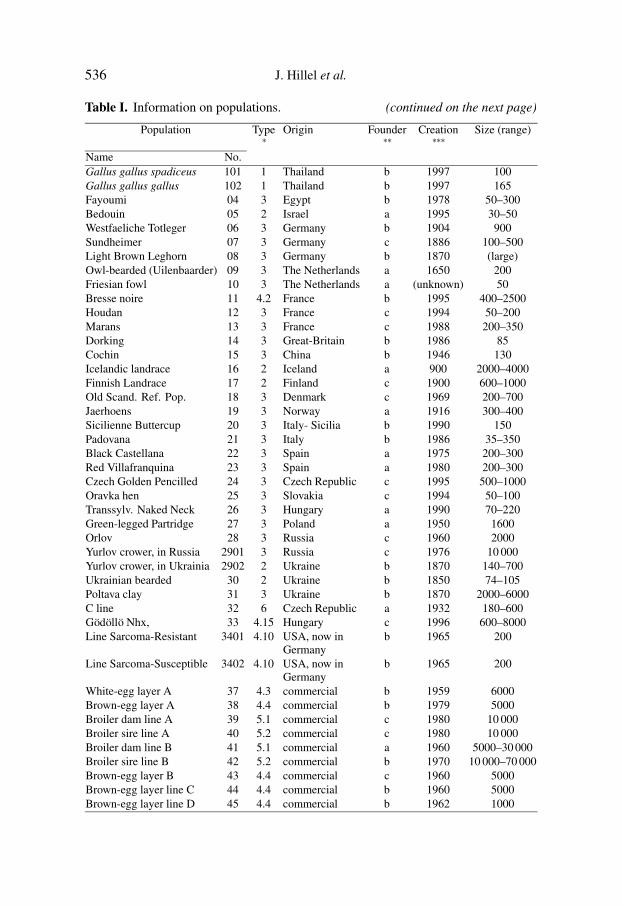
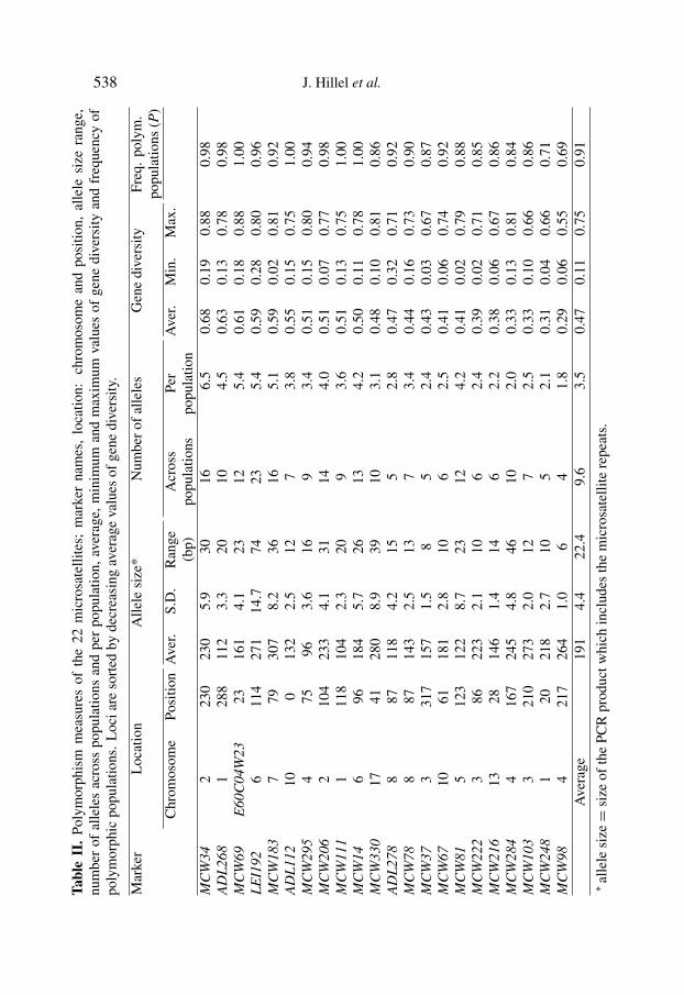
Where possible and relevant, throughout this report, chicken lines, popula-tions, and breeds will be referred to as populations. General information onthese populations is presented in Table I and details were reported by Tixier-Boichard et al. [44]. Information on the markers is given in Table II and a briefdescription of the populations, markers and genotyping is given below.

2.1. Populations and animals

Fifty-two populations were chosen to represent as many European countriesas possible and to cover a wide range of populations differing by selectionhistory and current management. We aimed to sample the same numberof males and females from as many families as possible, for a total of 50chickens per population. Sampled populations were classified a priori intosix types (Tab. I). Type 1 includes two subspecies of the Red Jungle Fowl,Gallus gallus gallus and G. g. spadiceus which were recently caught in the wild.Type 2 represents five domesticated but unselected chicken populations withsubstantial morphological variation. Type 3 represents 23 standardized breeds,where selection has been done, either recently or in the past, on morphologicaltraits according to a phenotypic standard. Type 4 encompasses 13 experimentalor commercial, white- or brown-egg layer lines. Type 5 includes eight lines


Table I. Information on populations. (continued on the next page)

Population Type∗

Origin Founder∗∗

Creation∗∗∗

Size (range)

Name No.Gallus gallus spadiceus 101 1 Thailand b 1997 100Gallus gallus gallus 102 1 Thailand b 1997 165Fayoumi 04 3 Egypt b 1978 50–300Bedouin 05 2 Israel a 1995 30–50Westfaeliche Totleger 06 3 Germany b 1904 900Sundheimer 07 3 Germany c 1886 100–500Light Brown Leghorn 08 3 Germany b 1870 (large)Owl-bearded (Uilenbaarder) 09 3 The Netherlands a 1650 200Friesian fowl 10 3 The Netherlands a (unknown) 50Bresse noire 11 4.2 France b 1995 400–2500Houdan 12 3 France c 1994 50–200Marans 13 3 France c 1988 200–350Dorking 14 3 Great-Britain b 1986 85Cochin 15 3 China b 1946 130Icelandic landrace 16 2 Iceland a 900 2000–4000Finnish Landrace 17 2 Finland c 1900 600–1000Old Scand. Ref. Pop. 18 3 Denmark c 1969 200–700Jaerhoens 19 3 Norway a 1916 300–400Sicilienne Buttercup 20 3 Italy- Sicilia b 1990 150Padovana 21 3 Italy b 1986 35–350Black Castellana 22 3 Spain a 1975 200–300Red Villafranquina 23 3 Spain a 1980 200–300Czech Golden Pencilled 24 3 Czech Republic c 1995 500–1000Oravka hen 25 3 Slovakia c 1994 50–100Transsylv. Naked Neck 26 3 Hungary a 1990 70–220Green-legged Partridge 27 3 Poland a 1950 1600Orlov 28 3 Russia c 1960 2000Yurlov crower, in Russia 2901 3 Russia c 1976 10 000Yurlov crower, in Ukrainia 2902 2 Ukraine b 1870 140–700Ukrainian bearded 30 2 Ukraine b 1850 74–105Poltava clay 31 3 Ukraine b 1870 2000–6000C line 32 6 Czech Republic a 1932 180–600Gödöllö Nhx, 33 4.15 Hungary c 1996 600–8000Line Sarcoma-Resistant 3401 4.10 USA, now in

Germanyb 1965 200

Line Sarcoma-Susceptible 3402 4.10 USA, now inGermany

b 1965 200

White-egg layer A 37 4.3 commercial b 1959 6000Brown-egg layer A 38 4.4 commercial b 1979 5000Broiler dam line A 39 5.1 commercial c 1980 10 000Broiler sire line A 40 5.2 commercial c 1980 10 000Broiler dam line B 41 5.1 commercial a 1960 5000–30 000Broiler sire line B 42 5.2 commercial b 1970 10 000–70 000Brown-egg layer B 43 4.4 commercial c 1960 5000Brown-egg layer line C 44 4.4 commercial b 1960 5000Brown-egg layer line D 45 4.4 commercial b 1962 1000


Table I. Continued.

Population Type∗

Origin Founder∗∗

Creation∗∗∗

Size (range)

Name No.Brown-egg layer line E 46 4.4 commercial b 1955 600Broiler sire line C 47 5.2 commercial a 1974 confidentielBroiler dam line C 48 5.1 commercial a 1974 confidentielBroiler sire line D 49 5.2 commercial a 1992 8000Broiler dam line D 50 5.1 commercial b 1970 5000–20 000Ab line, high 51 4.15 The Netherlands c 1980 75–300Ab line, low 52 4.15 The Netherlands c 1980 75–300Ab line, control 53 4.15 The Netherlands c 1980 110–250∗ type: 1=wild population; 2= domesticated unselected breed; 3= standardized breed selectedon morphology; 4= Layers, selected on quantitative traits; 5= Broilers, selected on quantitativetraits; 6 = inbred line.Detailed information for type 4: 4.10 = experimental White Leghorn; 4.15 = experimentalbrown egg layer; 4.2= commercial white egg layer not White Leghorn; 4.3= commercial WhiteLeghorn; 4.4 = commercial brown-egg layer.Detailed information for type 5: 5.1 = commercial broiler dam line; 5.2 = commercial broilersire line.∗∗ founder: a = small flock; b = one breed; c = a cross between several breeds.∗∗∗ estimate for the Creation Time of the sampled flocks.

of meat type chickens: four broiler dam-lines and four broiler sire-lines. Forlines of types 4 and 5, selection has been applied on a quantitative trait or onan index. Experimental lines included two sets of divergently selected lines.Type 6 is an inbred line.

2.2. Blood and DNA samples

Blood samples of 2–4 mL were collected from the wing vein with SarstedtSyringes containing EDTA as an anti-coagulating agent. In 20 populations,blood samples were collected on the same day and blood cells from individualbirds were obtained from fresh blood by centrifugation and were re-suspendedin an equal volume of PBS/Sucrose (1v/1v). DNA pools from each populationwere used to reduce the amount of genotyping. An aliquot of 50 µL of bloodcells in PBS/Sucrose from each bird in a population was taken to prepare itsblood pool. Individual blood samples and blood pools were frozen at −25 ◦C.High molecular weight DNA was extracted from 80 µL of the blood pool,following several steps of haemolysis, proteinase K incubation, precipitationin dimethyl-formamide/acetone (95v/5v), re-suspension in TE, ethanol precip-itation and final re-suspension in 2 mL TE. For the other 32 populations, a bloodpool could not be made properly, either because the individual blood sampleshad been frozen, or because their quality was not good enough. Consequently,DNA was extracted from individual blood samples and the pooled DNA sample

538 J. Hillel et al.Ta

ble

II.

Poly

mor

phis

mm

easu

res

ofth

e22

mic

rosa

telli

tes;

mar

ker

nam

es,

loca

tion:

chro

mos

ome

and

posi

tion,

alle

lesi

zera

nge,

num

ber

ofal

lele

sac

ross

popu

latio

nsan

dpe

rpo

pula

tion,

aver

age,

min

imum

and

max

imum

valu

esof

gene

dive

rsity

and

freq

uenc

yof

poly

mor

phic

popu

latio

ns.

Loc

iare

sort

edby

decr

easi

ngav

erag

eva

lues

ofge

nedi

vers

ity.

Mar

ker

Loc

atio

nA

llele

size

*N

umbe

rof

alle

les

Gen

edi

vers

ityFr

eq.

poly

m.

popu

latio

ns(P

)C

hrom

osom

ePo

sitio

nA

ver.

S.D

.R

ange

(bp)

Acr

oss

popu

latio

nsPe

rpo

pula

tion

Ave

r.M

in.

Max

.

MC

W34

223

023

05.

930

166.

50.

680.

190.

880.

98A

DL

268

128

811

23.

320

104.

50.

630.

130.

780.

98M

CW

69E

60C

04W

2323

161

4.1

2312

5.4

0.61

0.18

0.88

1.00

LE

I192

611

427

114

.774

235.

40.

590.

280.

800.

96M

CW

183

779

307

8.2

3616

5.1

0.59

0.02

0.81

0.92

AD

L11

210

013

22.

512

73.

80.

550.

150.

751.

00M

CW

295

475

963.

616

93.

40.

510.

150.

800.

94M

CW

206

210

423

34.

131

144.

00.

510.

070.

770.

98M

CW

111

111

810

42.

320

93.

60.

510.

130.

751.

00M

CW

146

9618

45.

726

134.

20.

500.

110.

781.

00M

CW

330

1741

280

8.9

3910

3.1

0.48

0.10

0.81

0.86

AD

L27

88

8711

84.

215

52.

80.

470.

320.

710.

92M

CW

788

8714

32.

513

73.

40.

440.

160.

730.

90M

CW

373

317

157

1.5

85

2.4

0.43

0.03

0.67

0.87

MC

W67

1061

181

2.8

106

2.5

0.41

0.06

0.74

0.92

MC

W81

512

312

28.

723

124.

20.

410.

020.

790.

88M

CW

222

386

223

2.1

106

2.4

0.39

0.02

0.71

0.85

MC

W21

613

2814

61.

414

62.

20.

380.

060.

670.

86M

CW

284

416

724

54.

846

102.

00.

330.

130.

810.

84M

CW

103

321

027

32.

012

72.

50.

330.

100.

660.

86M

CW

248

120

218

2.7

105

2.1

0.31

0.04

0.66

0.71

MC

W98

421

726

41.

06

41.

80.

290.

060.

550.

69A

vera

ge19

14.

422

.49.

63.

50.

470.

110.

750.

91∗ a

llele

size=

size

ofth

ePC

Rpr

oduc

twhi

chin

clud

esth

em

icro

sate

llite

repe

ats.


was prepared by aliquoting equal amounts of individual DNA, as measured byspectrophotometry. Prior to genotyping, the concentration of the DNA poolswas standardized to 100 ng · µL−1 in TE solution. The genotyping of the 52populations was done for 22 microsatellite loci.

2.3. Genotyping at microsatellite loci

A set of 22 (CA)n di-nucleotide microsatellite markers, which are as uni-formly distributed as possible throughout the chicken genome, was testedfor their use in DNA pools. The markers and their genomic position arelisted in Table II. Peak scoring on an ABI sequencer was used to estimatemicrosatellite allele frequencies as detailed in Crooijmans et al. [10]. PCRproducts of different markers were pooled in such a way that each markersignal on the ABI sequencers did not exceed a peak height of about 1000to 1500. Fragment sizes were determined relative to the GENESCAN-350TAMRA with the GENESCAN fragment analysis software (Perkin Elmer,Applied Biosystems Division). Subsequently GENOTYPER software (PerkinElmer, Applied Biosystems Division) was used for automated fragment callingand the generation of an output table containing the fragments for the differentloci and the peak areas for each of these fragments. Finally, these peak areaswere used to calculate the relative fragment frequencies for all peaks of eachlocus. These frequencies were used in this study as the allele frequencies.However, alleles scored from DNA pools using an ABI sequencer, mightbe artefacts and stutter bands rather than real alleles. We assumed that thisdifficulty would be relevant equally to all populations and most markers.

2.4. Gene diversity estimate

Using the calculated allele frequencies Pmi for population m and allele i, genediversity (Hm), namely the expected heterozygosity under Hardy-Weinbergassumptions, is:

Hm = 1−∑

i

P2mi. (1)

An average H was calculated for each locus across populations and for eachpopulation across loci.

2.5. Genetic distance estimates

Three genetic distances based on allele frequencies were used: the Neigenetic distance [34], Cavalli-Sforza chord measure [3] and Reynolds geneticdistance [38]. Additionally, the delta-mu-squared distance [18,19], basedon allele size, was applied. Pairwise distances between each pair of the 52populations (1326 estimates) were calculated for each measure.


2.6. Statistical analyses

Correlation coefficients and rank correlations were estimated using JMP 4.0software [28].

2.7. Calculation of the mutation rate

We used the information on the history of the two Sarcoma lines 3401 and3402 (see Tab. I) and their microsatellites data to estimate the mutation rate ofmicrosatellites in chickens. These lines were divergently selected for resistanceor susceptibility to Rous Sarcoma Viruses (RSV) A and B of 2-to-3 wk oldchickens [23]. The two sub-lines have been kept separately for 25 generations.The two lines had 74 different alleles of which only 46 (62%) were shared. Ateach of the 25 generations, ten sires were selected from each line and mated toapproximately 100 dams. In this process, 220 gametes were involved at eachgeneration and for each line, to produce the next generation. We scored thenumber of microsatellite alleles specific to each of the two lines in comparisonto the other one.

3. RESULTS

Raw data and basic results such as genetic distances between population pairsof the current study, can be obtained from the Poultry Biodiversity database at:http://w3.tzv.fal.de/aviandiv/index.html.

A total of 3760 allele frequencies were obtained. Amongst the 1144 possibletypings (22 markers× 52 populations), 77 (6.7%) were missing due to technicaldifficulties, mainly for three loci: ADL278, MCW14, and MCW330, withmissing data on 27, 15, and 15 populations, respectively. For the remaining 19markers, only 20 (2.0%) genotyping data points were missing.

3.1. Polymorphism of markers

As shown in Table II, all 22 markers were polymorphic in at least 69% of thepopulations, and 91% of the populations were polymorphic. The mean numberof alleles was 9.6 across populations and 3.5 within populations, and averagegene diversity was 0.47. Among the 22 tested markers, the most polymorphicwas MCW34 with 16 alleles across populations and, on average, 6.5 alleles perpopulation. The gene diversity of MCW34 was 0.68 and 98% of the populationswere polymorphic for this marker. At the other extreme, marker MCW98 wasthe least polymorphic, with four alleles across populations, 1.8 alleles perpopulation, and a gene diversity of 0.29; in addition it was polymorphic in 69%of the populations.


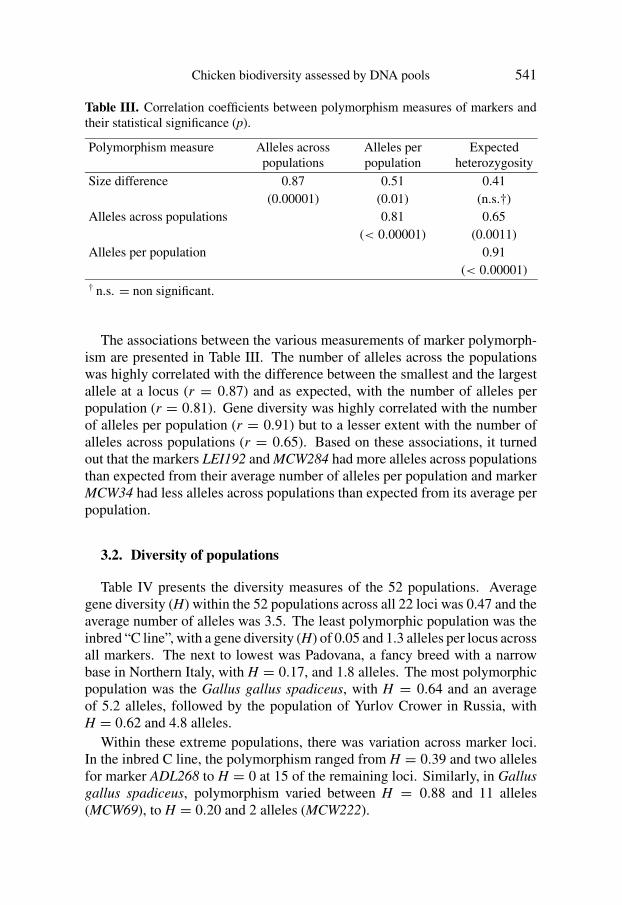
Table III. Correlation coefficients between polymorphism measures of markers andtheir statistical significance (p).

Polymorphism measure Alleles acrosspopulations

Alleles perpopulation

Expectedheterozygosity

Size difference 0.87 0.51 0.41(0.00001) (0.01) (n.s.†)

Alleles across populations 0.81 0.65(< 0.00001) (0.0011)

Alleles per population 0.91(< 0.00001)

† n.s. = non significant.

The associations between the various measurements of marker polymorph-ism are presented in Table III. The number of alleles across the populationswas highly correlated with the difference between the smallest and the largestallele at a locus (r = 0.87) and as expected, with the number of alleles perpopulation (r = 0.81). Gene diversity was highly correlated with the numberof alleles per population (r = 0.91) but to a lesser extent with the number ofalleles across populations (r = 0.65). Based on these associations, it turnedout that the markers LEI192 and MCW284 had more alleles across populationsthan expected from their average number of alleles per population and markerMCW34 had less alleles across populations than expected from its average perpopulation.

3.2. Diversity of populations

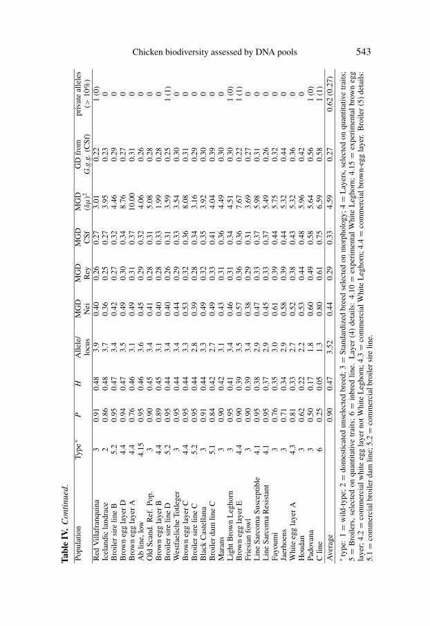
Table IV presents the diversity measures of the 52 populations. Averagegene diversity (H) within the 52 populations across all 22 loci was 0.47 and theaverage number of alleles was 3.5. The least polymorphic population was theinbred “C line”, with a gene diversity (H) of 0.05 and 1.3 alleles per locus acrossall markers. The next to lowest was Padovana, a fancy breed with a narrowbase in Northern Italy, with H = 0.17, and 1.8 alleles. The most polymorphicpopulation was the Gallus gallus spadiceus, with H = 0.64 and an averageof 5.2 alleles, followed by the population of Yurlov Crower in Russia, withH = 0.62 and 4.8 alleles.

Within these extreme populations, there was variation across marker loci.In the inbred C line, the polymorphism ranged from H = 0.39 and two allelesfor marker ADL268 to H = 0 at 15 of the remaining loci. Similarly, in Gallusgallus spadiceus, polymorphism varied between H = 0.88 and 11 alleles(MCW69), to H = 0.20 and 2 alleles (MCW222).

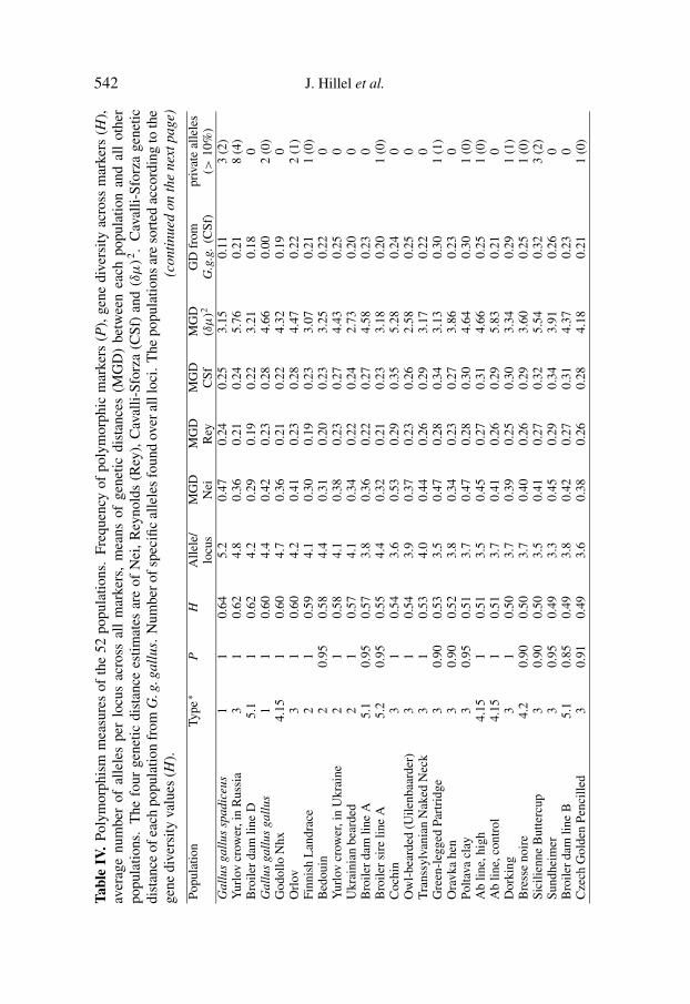
542 J. Hillel et al.Ta

ble

IV.

Poly

mor

phis

mm

easu

res

ofth

e52

popu

latio

ns.

Freq

uenc

yof

poly

mor

phic

mar

kers

(P),

gene

dive

rsity

acro

ssm

arke

rs(H

),av

erag

enu

mbe

rof

alle

les

per

locu

sac

ross

all

mar

kers

,m

eans

ofge

netic

dist

ance

s(M

GD

)be

twee

nea

chpo

pula

tion

and

all

othe

rpo

pula

tions

.T

hefo

urge

netic

dist

ance

estim

ates

are

ofN

ei,

Rey

nold

s(R

ey),

Cav

alli-

Sfor

za(C

Sf)

and(δ

µ)2

.C

aval

li-Sf

orza

gene

ticdi

stan

ceof

each

popu

latio

nfr

omG

.g.g

allu

s.N

umbe

rofs

peci

fical

lele

sfo

und

over

alll

oci.

The

popu

latio

nsar

eso

rted

acco

rdin

gto

the

gene

dive

rsity

valu

es(H

).(c

ontin

ued

onth

ene

xtpa

ge)

Popu

latio

nTy

pe∗

PH

Alle

le/

locu

sM

GD

Nei

MG

DR

eyM

GD

CSf

MG

D(δ

µ)2

GD

from

G.g

.g.

(CSf

)pr

ivat

eal

lele

s(>

10%

)G

allu

sga

llus

spad

iceu

s1

10.

645.

20.

470.

240.

253.

150.

113

(2)

Yur

lov

crow

er,i

nR

ussi

a3

10.

624.

80.

360.

210.

245.

760.

218

(4)

Bro

iler

dam

line

D5.

11

0.62

4.2

0.29

0.19

0.22

3.21

0.18

0G

allu

sga

llus

gallu

s1

10.

604.

40.

420.

230.

284.

660.

002

(0)

God

ollo

Nhx

4.15

10.

604.

70.

360.

210.

224.

320.

190

Orl

ov3

10.

604.

20.

410.

230.

284.

470.

222

(1)

Finn

ish

Lan

drac

e2

10.

594.

10.

300.

190.

233.

070.

211

(0)

Bed

ouin

20.

950.

584.

40.

310.

200.

233.

250.

220

Yur

lov

crow

er,i

nU

krai

ne2

10.

584.

10.

380.

230.

274.

430.

250

Ukr

aini

anbe

arde

d2

10.

574.

10.

340.

220.

242.

730.

200

Bro

iler

dam

line

A5.

10.

950.

573.

80.

360.

220.

274.

580.

230

Bro

iler

sire

line

A5.

20.

950.

554.

40.

320.

210.

233.

180.

201

(0)

Coc

hin

31

0.54

3.6

0.53

0.29

0.35

5.28

0.24

0O

wl-

bear

ded

(Uile

nbaa

rder

)3

10.

543.

90.

370.

230.

262.

580.

250

Tra

nssy

lvan

ian

Nak

edN

eck

31

0.53

4.0

0.44

0.26

0.29

3.17

0.22

0G

reen

-leg

ged

Part

ridg

e3

0.90

0.53

3.5

0.47

0.28

0.34

3.13

0.30

1(1

)O

ravk

ahe

n3

0.90

0.52

3.8

0.34

0.23

0.27

3.86

0.23

0Po

ltava

clay

30.

950.

513.

70.

470.

280.

304.

640.

301

(0)

Ab

line,

high

4.15

10.

513.

50.

450.

270.

314.

660.

251

(0)

Ab

line,

cont

rol

4.15

10.

513.

70.

410.

260.

295.

830.

210

Dor

king

31

0.50

3.7

0.39

0.25

0.30

3.34

0.29

1(1

)B

ress

eno

ire

4.2

0.90

0.50

3.7

0.40

0.26

0.29

3.60

0.25

1(0

)Si

cilie

nne

But

terc

up3

0.90

0.50

3.5

0.41

0.27

0.32

5.54

0.32

3(2

)Su

ndhe

imer

30.

950.

493.

30.

450.

290.

343.

910.

260

Bro

iler

dam

line

B5.

10.

850.

493.

80.

420.

270.

314.

370.

230

Cze

chG

olde

nPe

ncill

ed3

0.91

0.49

3.6

0.38

0.26

0.28

4.18

0.21

1(0

)

Chicken biodiversity assessed by DNA pools 543Ta

ble

IV.

Con

tinue

d.Po

pula

tion

Type∗

PH

Alle

le/

locu

sM

GD

Nei

MG

DR

eyM

GD

CSf

MG

D(δ

µ)2

GD

from

G.g

.g.

(CSf

)pr

ivat

eal

lele

s(>

10%

)R

edV

illaf

ranq

uina

30.

910.

483.

90.

400.

260.

273.

010.

221

(0)

Icel

andi

cla

ndra

ce2

0.86

0.48

3.7

0.36

0.25

0.27

3.95

0.23

0B

roile

rsi

relin

eB

5.2

0.95

0.47

3.4

0.42

0.27

0.32

4.46

0.29

0B

row

neg

gla

yer

D4.

40.

940.

473.

50.

490.

300.

348.

760.

270

Bro

wn

egg

laye

rA

4.4

0.76

0.46

3.1

0.49

0.31

0.37

10.0

00.

310

Ab

line,

low

4.15

0.95

0.46

3.6

0.45

0.29

0.32

4.06

0.26

0O

ldSc

and.

Ref

.Po

p.3

0.90

0.45

3.4

0.41

0.28

0.31

5.08

0.28

0B

row

neg

gla

yer

B4.

40.

890.

453.

10.

400.

280.

331.

990.

280

Bro

iler

sire

line

D5.

20.

950.

443.

40.

400.

260.

313.

590.

251

(1)

Wes

tfae

liche

Totle

ger

30.

950.

443.

40.

440.

290.

333.

540.

300

Bro

wn

egg

laye

rC

4.4

0.95

0.44

3.3

0.53

0.32

0.36

8.08

0.31

0B

roile

rsi

relin

eC

5.2

0.95

0.44

2.8

0.39

0.28

0.34

3.16

0.29

0B

lack

Cas

tella

na3

0.91

0.44

3.3

0.49

0.32

0.35

3.92

0.30

0B

roile

rda

mlin

eC

5.1

0.84

0.42

2.7

0.49

0.33

0.41

4.04

0.39

0M

aran

s3

0.90

0.42

3.1

0.43

0.31

0.36

4.49

0.30

0L

ight

Bro

wn

Leg

horn

30.

950.

413.

40.

460.

310.

344.

510.

301

(0)

Bro

wn

egg

laye

rE

4.4

0.90

0.39

3.5

0.57

0.36

0.36

7.67

0.22

1(1

)Fr

iesi

anfo

wl

30.

900.

393.

40.

380.

290.

313.

690.

270

Lin

eSa

rcom

aSu

scep

tible

4.1

0.95

0.38

2.9

0.47

0.33

0.37

5.98

0.31

0L

ine

Sarc

oma

Res

ista

nt4.

10.

950.

372.

90.

450.

330.

375.

490.

260

Fayo

umi

30.

760.

353.

00.

610.

390.

445.

750.

320

Jaer

hoen

s3

0.71

0.34

2.9

0.58

0.39

0.44

5.32

0.44

0W

hite

egg

laye

rA

4.3

0.81

0.33

2.7

0.52

0.38

0.43

5.32

0.36

0H

ouda

n3

0.62

0.22

2.2

0.53

0.44

0.48

5.96

0.42

0Pa

dova

na3

0.50

0.17

1.8

0.60

0.49

0.58

5.64

0.56

1(0

)C

line

60.

250.

051.

30.

800.

610.

756.

590.

581

(1)

Ave

rage

0.90

0.47

3.52

0.44

0.29

0.33

4.59

0.27

0.62

(0.2

7)∗ t

ype:

1=

wild

-typ

e;2=

dom

estic

ated

unse

lect

edbr

eed;

3=

Stan

dard

ized

bree

dse

lect

edon

mor

phol

ogy;

4=

Lay

ers,

sele

cted

onqu

antit

ativ

etr

aits

;5=

Bro

ilers

,se

lect

edon

quan

titat

ive

trai

ts;

6=

inbr

edlin

e.L

ayer

(4)

deta

ils:

4.10=

expe

rim

enta

lW

hite

Leg

horn

;4.

15=

expe

rim

enta

lbr

own

egg

laye

r;4.

2=

com

mer

cial

whi

teeg

gla

yer

notW

hite

Leg

horn

;4.3=

com

mer

cial

Whi

teL

egho

rn;4

.4=

com

mer

cial

brow

n-eg

gla

yer.

Bro

iler

(5)

deta

ils:

5.1=

com

mer

cial

broi

ler

dam

line;

5.2=

com

mer

cial

broi

ler

sire

line.


In Table IV, the 52 populations are ordered according to decreasing averagegene diversity (H) values across the 22 loci. To examine the stability of the Hvalues, an average H over 22 possible subsets of markers, each eliminating onedifferent marker, was calculated for each population. The average H, based onthe 22 subsets, gave identical order of populations to the original H.

3.3. Population-specific (private) alleles

In total, 213 different alleles were scored across the 52 populations andthe 22 marker loci. Most of these alleles (181) were found in more thanone population. For the 52 populations, the 32 private alleles are indicatedin Table IV. The majority of the populations had either no private alleles(33 populations) or a single one (14 populations) and only one population,the Yurlov crower (in Russia) had eight private alleles. The RJF subspecies:Gallus gallus gallus and Gallus gallus spadiceus with two and three privatealleles respectively are worth mentioning. Taken together, the 50 domesticatedpopulations had 91 alleles which are missing in the two RJF populations. Inturn, RJF had eight private alleles which were absent in the domesticated genepool. Among the 32 private alleles, only 14 had frequencies higher than 10%.

3.4. Mean genetic distances of the 52 populations

Four estimates of genetic distance were calculated between each pair ofpopulations (1326 pairwise distances for each of the four estimates). These arepresented in the Poultry Biodiversity database.

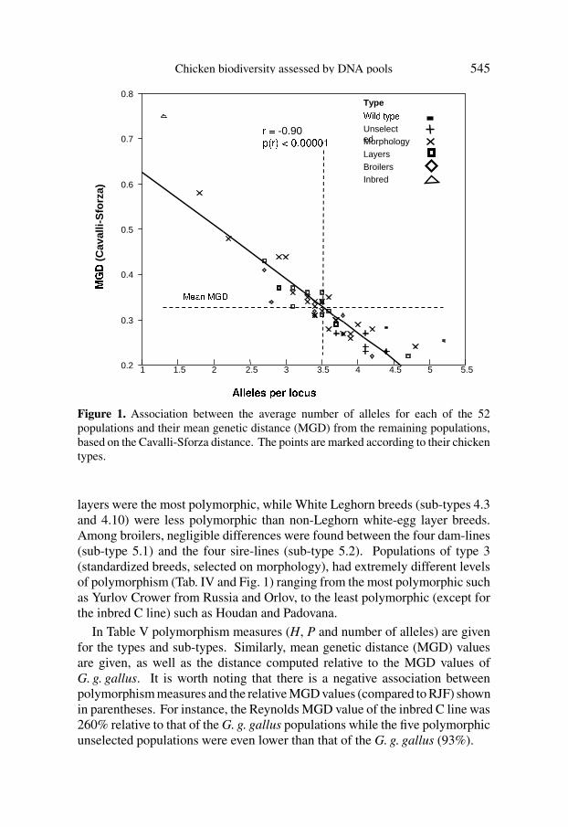
For each of the 52 populations and separately for the four different estimates,we calculated the mean genetic distance (MGD) between a given populationand all other 51 populations (Tab. IV). MGD shows a clear tendency to increaseas polymorphism decreases. This tendency is typical of the MGD estimatesbased on gene frequencies [all except (δµ)2]. For instance, Reynolds MGDvalues ranged between 0.19 for the Broiler dam line D and Finnish Landrace,to 0.61 for the inbred C line. Other MGD had different values according tothe distance used. Figure 1 presents the detailed association between averagenumber of alleles and MGD based on Cavalli-Sforza’s distance.

3.5. Diversity between and within types of populations

Examination of Table V reveals the following: types 1 (wild type) and 2(unselected breeds) were the most polymorphic populations (H = 0.62 and0.56, and number of alleles per locus, na, are 4.8 and 4.1 respectively). Type 6(inbred) was the least polymorphic (H = 0.05 and na = 1.3). On average,layers (type 4; H = 0.45 and na = 3.4) were slightly less polymorphicthan broilers (type 5; H = 0.57 and na = 3.6). Among layers, Brown-egg


0.2

0.3

0.4

0.5

0.6

0.7

0.8

�� (C

aval

li-S

forz

a)

��

�� -0.90��

�� !�" #%$��UnselectedMorphologyLayersBroilersInbred

Type

1 1.5 2 2.5 3 3.5 4 4.5 5 5.5

&(')'+*�')*�,.-�*�/0')1�2�3�,

Figure 1. Association between the average number of alleles for each of the 52populations and their mean genetic distance (MGD) from the remaining populations,based on the Cavalli-Sforza distance. The points are marked according to their chickentypes.

layers were the most polymorphic, while White Leghorn breeds (sub-types 4.3and 4.10) were less polymorphic than non-Leghorn white-egg layer breeds.Among broilers, negligible differences were found between the four dam-lines(sub-type 5.1) and the four sire-lines (sub-type 5.2). Populations of type 3(standardized breeds, selected on morphology), had extremely different levelsof polymorphism (Tab. IV and Fig. 1) ranging from the most polymorphic suchas Yurlov Crower from Russia and Orlov, to the least polymorphic (except forthe inbred C line) such as Houdan and Padovana.

In Table V polymorphism measures (H, P and number of alleles) are givenfor the types and sub-types. Similarly, mean genetic distance (MGD) valuesare given, as well as the distance computed relative to the MGD values ofG. g. gallus. It is worth noting that there is a negative association betweenpolymorphism measures and the relative MGD values (compared to RJF) shownin parentheses. For instance, the Reynolds MGD value of the inbred C line was260% relative to that of the G. g. gallus populations while the five polymorphicunselected populations were even lower than that of the G. g. gallus (93%).


Tabl

eV.

Poly

mor

phis

mm

easu

res

ofpo

pula

tion

cate

gori

esan

dsu

b-ca

tego

ries

.

Cat

egor

ySu

bca

t.N

pops

.P

HA

llele

s/lo

cus∗∗

MG

D-

Nei∗

MG

D-

Rey∗

MG

D-

CSf∗

MG

D-

(δµ)2∗

GD

from

G.g

.g.

(CSf

)

Priv

ate

alle

les

(>10

%)

1-W

ildty

pe2

10.

624.

80.

45(1

00)

0.24

(100

)0.

27(1

00)

3.91

(100

)0.

062.

50(1

)2-

Uns

elec

ted

50.

960.

564.

10.

34(7

6)0.

22(9

3)0.

25(9

4)3.

49(8

9)0.

220.

20(0

)3-

Mor

ph.

Sele

c.23

0.89

0.46

3.5

0.45

(101

)0.

30(1

27)

0.34

(128

)4.

38(1

12)

0.29

0.87

(0.3

9)4-

Lay

ers

130.

920.

453.

40.

46(1

04)

0.30

(128

)0.

34(1

27)

5.83

(149

)0.

270.

23(0

.08)

Exp

er./W

hite

/Leg+

4.1

20.

950.

382.

90.

46(1

03)

0.33

(140

)0.

37(1

40)

5.74

(147

)0.

280

(0)

Exp

er./B

row

n4.

154

0.99

0.52

3.9

0.42

(94)

0.26

(110

)0.

29(1

08)

4.72

(121

)0.

230.

25(0

)C

om./W

hite

/Leg−

4.2

10.

900.

503.

70.

40(9

0)0.

26(1

11)

0.29

(109

)3.

60(9

2)0.

251

(0)

Com

./Whi

te/L

eg+

4.3

10.

810.

332.

70.

52(1

17)

0.38

(162

)0.

43(1

62)

5.32

(136

)0.

360

(0)

Com

./Bro

wn

4.4

50.

890.

443.

30.

50(1

11)

0.31

(134

)0.

35(1

33)

7.30

(187

)0.

280.

20(0

.20)

5-B

roile

rs8

0.93

0.57

3.6

0.39

(87)

0.25

(108

)0.

30(1

14)

3.82

(98)

0.26

0.25

(0.1

25)

Dam

lines

5.1

40.

910.

533.

60.

39(8

8)0.

25(1

07)

0.30

(114

)4.

05(1

04)

0.26

0(0

)Si

relin

es5.

24

0.95

0.80

3.5

0.38

(86)

0.26

(109

)0.

30(1

13)

3.60

(92)

0.26

0.50

(0.2

5)6-

Inbr

ed1

0.25

0.05

1.3

0.80

(180

)0.

61(2

60)

0.75

(283

)6.

59(1

69)

0.58

1(1

)To

tal/a

vera

ge52

0.90

0.47

3.5

0.44

(98)

0.29

(122

)0.

33(1

24)

4.59

(118

)0.

270.

62(0

.27)

P=

freq

uenc

yof

poly

mor

phic

mar

kers

;H=

gene

dive

rsity

acro

ssm

arke

rs;

MG

D=

mea

nge

netic

dist

ance

estim

ates

base

don

Nei

,R

eyno

lds

(Rey

),C

aval

li-Sf

orza

(CSf

)an

d(δ

µ)2

gene

ticdi

stan

ces.∗ t

hem

ean

gene

ticdi

stan

ce(M

GD

)va

lues

,rel

ativ

e(%

)to

that

ofth

eR

edJu

ngle

Fow

lare

give

nin

pare

nthe

ses.∗∗

num

ber

ofal

lele

s,pe

rlo

cus,

per

popu

latio

n.#

gene

ticdi

stan

cefr

omth

eR

edJu

ngle

Fow

lbas

edon

the

Cav

alli-

Sfor

tza

mea

sure

.


Table VI. Correlation coefficients between measurements of Table IV.

MGD Polymorphism

Reynolds Cavalli (δµ)2 P H Alleles/locus

MGD Nei 0.92 0.90 0.56 −0.74 −0.78 −0.71∗∗∗∗ ∗∗∗∗ ∗∗∗∗ ∗∗∗∗ ∗∗∗∗ ∗∗∗∗

Reynolds 0.98 0.47 −0.89 −0.95 −0.88∗∗∗∗ 0.0004 ∗∗∗∗ ∗∗∗∗ ∗∗∗∗

Cavalli 0.45 −0.90 −0.93 −0.90

0.0008 ∗∗∗∗ ∗∗∗∗ ∗∗∗∗

(δµ)2 −0.36 −0.38 −0.36

0.009 0.004 0.008

Polym. P 0.86 0.78∗∗∗∗ ∗∗∗∗

H 0.93∗∗∗∗

∗∗∗∗ = significance at p < 10−5; n.s. = non significant; P = frequency of poly-morphic markers; H = gene diversity across markers; MGD = means of geneticdistances from other populations; Alleles/locus = number of alleles across markers.

3.6. Associations between polymorphism measurementsof populations

Correlations between seven of the measurements in Table IV are recorded inTable VI. Polymorphism estimates were significantly and negatively associatedwith the three MGD values that are based on gene frequencies (see also Fig. 1).MGD based on the (δµ)2 approach was poorly associated with polymorphism.The correlation coefficients between MGD values and gene diversity wereslightly higher than those with the proportion of polymorphic markers (P).The highest association was between gene diversity and MGD values obtainedfrom Reynolds estimates; r = −0.95. The associations between the differentMGD measures were positive and highly significant, except for that basedon (δµ)2.

3.7. Mutation rate of microsatellites

From the DNA pool of the RSV resistant line 3401, we scored 14 privatealleles that were absent in the RSV susceptible line 3402 and for the susceptibleline we scored 14 such alleles. The total number of gametes involved was11 000 (440 gametes × 25 generations). The mutation rate per microsatelliteper locus per generation was: 28/(11 000 gametes× 22 loci) = 1.16× 10−4.


4. DISCUSSION

4.1. Data reliability

In general, the results reported here were in good agreement with what isknown of the history of the populations and with previous scientific reports.For instance, the feral populations and the domesticated unselected populationswere the most polymorphic, while the inbred and the White Leghorn lines werefar less polymorphic. This suggests that use of DNA pools, the chosen markersand the biometrical tools described in this report, provide reliable estimatesfor the population’s biodiversity (see also [10,12,13,24,25,31]). Furthermore,polymorphism estimates obtained from these DNA pools were found to be ingood agreement with those obtained from individually typing a subset of 30birds from 20 populations (unpublished data). For instance, the correlationcoefficient between H values of the current study and observed heterozygotefrequency is r = 0.85 (p = 0.002) and between the number of alleles perlocus is r = 0.91 (p = 0.0002). Data reliability was also supported by thesame order of population H values, based on 22 subsets, with single markerssystematically excluded.

4.2. Diversity of microsatellites and its mutation rate

The wide range of biodiversity in the sampled populations and the high levelof polymorphism of microsatellites were reflected by the finding that eventhe least polymorphic locus, MCW98 was found to be polymorphic in 69%of the populations while four of the 22 markers were polymorphic in all 52populations (Tab. II).

The correlation coefficients between some of the polymorphism measuresare high and very significant (r = 0.81 − 0.91, see the diagonal of Tab. III).On the contrary, allele-size range had lower correlation coefficients with thenumber of alleles per population (na) (r = 0.51, p < 0.01) and with theexpected heterozygote frequency H (r = 0.41, p > 0.05). On closer exam-ination, for three loci, namely LEI92, MCW284 and MCW330, size rangesare larger than expected, based on their na and H values. For LEI192, six ofthe sixteen alleles across populations were present in only a single populationand two alleles in two populations. Excluding these eight alleles, reducedthe range from 74 bp to 46 bp. Similar treatment of the loci MCW284 andMCW330 reduced the number of alleles across populations from eleven to twoand from ten to four, respectively. Similarly, allele size ranges reduced from46 bp to 8 bp for MCW284 and from 39 bp to 30 for MCW330. These canbe interpreted either as population-specific (private) alleles or as signal peaksin the sequencer machine that are not alleles. Discrimination between these is


possible only by analyzing sibships, which is out of the scope of the presentreport.

In studies of human genetic variation, at the continental level there is goodagreement in the ordering by region of gene diversity measures among differentkinds of markers, once ascertainment bias is removed [29,39]. The sameis true for the ordering of genetic distances among populations assessed fordifferent markers [29]. It is reasonable therefore to believe, that the orderingamong chicken breeds of diversity and distances seen here for microsatellitesin DNA pools would not be very different for other genetic marker systems.The microsatellite loci used here were selected to be polymorphic for use ingene mapping. However, Rosenberg et al. [42] obtained diversity and geneticdistance patterns for humans that largely agreed with those of Bowcock et al. [2]even though the former study used microsatellites from a mapping set and thelatter used markers that were not selected. Ascertainment bias is, therefore, notexpected to have had a major effect on the ordering of statistics for our chickendata.

The estimation of the mutation rate using the divergently selected (RSV)lines is based on the assumption that the 22 microsatellite markers are notlinked to genes that are affected by the selection criteria. Weber and Wongfound a mutation rate of 5.6×10−4 for di-nucleotide loci in humans by pedigreeanalysis [46]. Based on 22 di-nucleotide loci, our estimate was about five timeslower, but may underestimate the actual value since it was assumed that noreverse or recurrent mutations occurred. Since this estimate is from a singleset of divergently selected lines, we cannot estimate confidence limits of thisrate. Further analysis of chickens is needed to provide a reliable estimate ofmutation rate.

4.3. Genetic diversity of populations

A gene diversity of 0.48 was obtained from DNA pools in a subset of 20populations. Based on individual typing of the same subset, the frequency ofheterozygotes was 0.47 (unpublished data). These estimates are similar to theaverage H in all 52 populations indicating the good reliability of our estimates.Diversity estimates in this study are lower than the observed frequencies ofheterozygotes reported in other species using microsatellite markers. Forinstance, in human populations the average heterozygote frequency rangesbetween 0.7 and 0.8 [2], in cattle- 0.6 [11], in pigs- 0.68 [21] and in fish-0.86 [16]. Although such comparisons are difficult to interpret, the lowervariability in chickens calls attention to the importance of conserving thechicken gene pool. It is worth mentioning, however, that SNP frequencyin the chicken genome was found to be quite high and significantly higher thanthat found in the human genome (unpublished data).


4.4. Diversity between populations within types

Categorization of populations in this study was done according to the pop-ulations’ history and their breeding purpose, which have affected the geneticdiversity. Indigenous stocks are domesticated but unselected local breeds(type 2) that have persisted in the agricultural societies for decades or evencenturies. Their long history in certain regions might have led to specificadaptation to local environmental conditions and genetic changes due to naturalselection and to some degree due to genetic drift as well. In practice, four outof the five populations of type 2 had relatively high polymorphism, which mayreflect their rather large effective population size and the fact that these stockswere not subjected to intense selection for production.

The group of standardized breeds (type 3) selected for morphological traitscovers a wide range of various breeds kept by fanciers. This type has largevariance in polymorphism levels (Tab. IV) as also reflected in the scatteredpattern of its populations in Figure 1. Based on genetically distinct local popu-lations, pure breeds were developed that differed in many phenotypic traits suchas plumage color, plumage pattern, and comb type. Genetic changes in fancybreeds may occur rather rapidly in these relatively small populations because ofintense selection for exhibition traits, inbreeding, crossbreeding genetic drift,bottleneck and founder effects [17,35,36]. This complexity of histories andbreeding practices may explain the heterogeneity of polymorphism values thatcharacterizes type 3.

Types 4 (layers) and 5 (broilers) of chicken lines, which are selected forquantitative traits, encompass the major commercial poultry industry. Estim-ates for broilers (H = 0.57) were in agreement with a previous report, in whichH = 0.53 was obtained from pooled blood samples [10]. The White Leghornlayer line in our study (sub-type 4.3) was found to have low gene diversity(0.33), slightly higher than the value of 0.27 in the previous report [10]. Amongthe layers this line had the lowest polymorphism.

In the 1940s, poultry breeding began to develop as a business. Pure bredlines were used to develop specialized commercial breeding stocks for tableegg and meat production by applying highly efficient and intense breedingprograms. Industrial egg and meat stocks are bred by large multinationalbreeding companies, and the “end products” are hybrids based mostly on fourhighly selected grandparental lines. In particular during the last decades effortshave been made to limit inbreeding in these grandparental pure bred lines [37].Large flock sizes and limiting inbreeding may be reflected by the degree ofpolymorphism of these types (4 and 5) which is comparable even to thoseof populations that were not subjected to intensive breeding. It should benoted here that the commercial lines in our study are all pure bred lines.Therefore, their level of polymorphism can be considered as a reliable estimatefor the polymorphism of the pure-bred grandparental lines. Differences within


types 4 and 5 might be explained by the different origin of white egg layers,brown egg layers and broilers. White egg layers are chiefly represented byone breed, the Single Comb White Leghorn breed, while the genetic basisfor brown egg layers has been somewhat broader, mainly coming from theRhode Island Red, New Hampshire, Plymouth Rock and Australorp breeds.A similar picture is characteristic of the poultry meat production sector. Thepaternal grandparent lines are mainly derived from the White Cornish breed,while maternal grandparents are heavily based on White Plymouth Rocks. TheCornish was developed in England from Asiatic fighting stocks, and the WhitePlymouth Rock was derived from an American parent breed [6].

The low degree of gene diversity in the inbred C line resulted directly fromthe brother-sister mating scheme used to develop this line and possibly fromgenetic drift due to the limited effective population size.

4.5. Genetic distance measures

The three genetic distance measures which are based on gene frequencieswere in good agreement with the genetic diversity of the examined breeds,indicating that these approaches fit the history of the domesticated chickenswell. However, the (δµ)2 approach that is based on the allele size whichis typical to microsatellites, was different and poorly correlated with othergenetic distances as well as measures of diversity. Probably the history ofthe domesticated chicken does not meet the assumptions behind this approachespecially the constant population size.

4.6. Conceptual aspects of MGD

A domesticated population with a large number of alleles per locus isexpected to represent a large portion of the studied gene pool and thereforeto be genetically close to all other populations. Populations of types 1 and 2are polymorphic and represent the gene pool well and indeed have low valuesof MGD. On the contrary, populations that are relatively monomorphic cannotreflect the whole studied gene pool and therefore will have high MGD values,as evidenced by the inbred C line and a few populations from types 3 and 4.3.Figure 1 shows a negative and clear association between the average numberof alleles per locus and the Cavalli-Sforza MGD values. A similar and tighterassociation is apparent when gene diversity values are examined. The clearassociation discussed above between polymorphism and MGD values suggeststhat the approach of constructing evolutionary trees in domesticated populationsis likely to give a misleading picture of the history. This is particularly truefor rooted trees, which assume a unidirectional evolutionary process. It seemsthat the processes of domestication and breeding have involved more or lesscontinuous and multidirectional gene flow.


Careful examination of Figure 1 reveals that populations with a similarnumber of alleles may have different MGD values. The joint distribution ofthe number of alleles and MGD values can be viewed with a regression linethat will be termed a “trend line”, as in Figure 1. The unselected populations(type 2) are highly polymorphic and located next to or below the trend line,implying that many of their alleles are common to the studied gene pool. Thetwo Gallus gallus subspecies have a large number of alleles per locus but areboth located above the trend line, which implies some proportion of privatealleles. Indeed, five private alleles that are absent in the domesticated chickenwere found to be present in G. g. gallus and six such alleles in G. g. spadiceus.

4.7. The chicken ancestor and the need for conservation

It is assumed that all breeds of the domesticated chicken descend from asingle ancestor, the RJF, which originated in Southeast Asia [5,14,15]. Sincepopulations at the centre of origin should contain the highest diversity (as hasbeen shown for humans and other species [2]), RJF should present a high levelof polymorphism and also hold low values of MGD. The two sub-species ofGallus gallus (RJF) which are represented in this study have high diversityvalues and low MGD values, but not the lowest (Tab. IV and Fig. 1). Theseresults suggest the hypothesis that the Red Jungle Fowl is a major contributor tothe gene pool of the domesticated chicken. The presence of private alleles bothin the RJF and in the domesticated gene pool does not necessarily contradict thishypothesis. These private alleles could result from genetic drift and separateevolution since the onset of domestication. Additionally, private alleles ofthe domesticated breeds may indicate a contribution of other wild species asdebated in Crawford [5]. In studies on the mitochondrial DNA in chickens [14,15], the authors suggest that Gallus gallus gallus could have given rise to thediverse breeds of the domesticated chicken, even though common patterns indomesticated breeds and in G. g. spadiceus and G. g. bankiva are also observed.

With regards to the level of genetic polymorphism and the mean geneticdistance, the Red Jungle Fowl (Gallus gallus) appears to be an importantreservoir of the chicken polymorphism. Nevertheless, during domestication,extensive genetic diversity has accumulated in the chicken, and this diversity isdisplayed by the many breeds and strains differing in their phenotypes whichare the products of many genetic, environmental and management regimes.A complete description of each breed or population would entail ascertainingall genes that contribute to any phenotypic trait. It is very unlikely that suchcomplete knowledge can be achieved in the near future. Therefore, a morepractical alternative is needed. We believe that information from DNA markerstogether with phenotypic performance and population history may providereliable guidelines in choosing populations for practical and for conservationpurposes. However, setting conservation priorities based exclusively on the


diversity of molecular markers might lead to the loss of locally adaptedpopulations [32].

In recent years, breeders of commercial white-egg layers have been con-cerned about reduced genetic variability and future response to selection. Theresults reported in the present article support this concern, particularly forWhite Leghorn breeds. The massive merging of breeding companies in recentyears should call for attention to the need for conservation of genetic variationamong breeds and lines. Appropriate strategies for conservation of populationsis out of the scope of the present report but is an important and controversialissue [7]. Our results emphasize the need to conserve polymorphic populationssuch as Yurlov Crower, the Orlov or the Finnish Landrace for the sake ofglobal variability, and to preserve small populations for their unique geneticfeatures. MGD values can assist in choosing populations most valuable for thepreservation of genetic variation.

ACKNOWLEDGEMENTS

We wish to thank Jean-Luc Coville and Camilo Vilela-Lamego, Inra, Jouy-en-Josas, France, who were involved in the DNA preparation and its distri-bution, and to the following sub-contractors who provided the blood samplesand breed descriptions; without their help this study could not have beenperformed (they are listed alphabetically): Dr. G. Baldane, Padova, Italy; Dr.J. Baumgartner, Research Institute, Ivanka pri Dunaji, Slovakia; Dr. Y. Bond-arenko, Research Institute; Borky, Kharkiv, Alaska; Dr. J.L. Campo, INIA,Madrid, Spain; D. Cassuto, ANAK, Israel; Dr. K. Cywa-Benko, ResearchInstitute, Balice n Cracow, Poland; Dr. E. Eythorsdottir, RALA, Israel; Y.Jego, Hubbard-ISA, France; Dr. J. Kathle, NLH, Norway; Dr. I. Moiseyeva,Research Institute, Gubkin, Moscow, Russia; Dr. G. Pidone, Calatafimi, Italy;Prof. R. Preisinger Lohmann, Germany; M. Protais, Hubbard-ISA, France; P.Rault, SYSAAF, Tours, France; Mrs. V. Roberts, UK; Dr. P. Sorensen, DIAS,Denmark; Dr. I. Szalay, Hungary; Prof. Therdchai Vearasilp, Thailand; Dr.B. Thorp Ross Breeders, Aviagene, UK; Dr. P. Trefil, Biopharmacy Institute,Prague, Czech Republic; F. van Sambeek, Hendrix, Ospel, The Netherlands;Dr.Vilhelmova, Czech Republic; J. Vincent, Cobb, UK; Dr. G. Virag, ResearchInstitute, Godollo, Hungary.

REFERENCES

[1] Barker J.S.F., Bradley D.G., Fries R., Hill W.G., Nei M., Wayne R.K., Anintegrated global protocol to establish the genetic relationships among the breedsof each domestic animal species, Report of a Working Group, Animal Productionand Health Division, FAO, 1993.


[2] Bowcock A.M., Ruiz-Linares A., Tomfohrde J., Minch E., Kidd J.R., Cavalli-Sforza L.L., High-resolution of human evolutionary trees with polymorphicmicrosatellites, Nature 368 (1994) 455–457.

[3] Cavalli-Sforza L.L., Edwards K.J., Phylogenetic analysis: models and estimationprocedures, Am. J. Hum. Genet. 19 (1967) 233–257.

[4] Cheng H.H., Crittenden L.B., Microsatellite markers for genetic mapping in thechicken, Poult. Sci. 73 (1994) 539–546.

[5] Crawford R.D., Domestic fowl, in: Mason I.L. (Ed.), Evolution of domesticatedanimals, Longman, London, 1984, pp. 298–311.

[6] Crawford R.D., Origin and history of poultry species, in: Crawford R.D. (Ed.),Poultry Breeding and Genetics, Elsevier, New York, 1990, pp. 317–329.

[7] Crawford R.D., Christman C.J., Heritage Hatchery Networks in Poultry Con-servation, in: Alderson L., Bodo I. (Eds.), Genetic Conservation of DomesticLivestock, CAB International, Oxon, UK, 1992, pp. 121–122.

[8] Crooijmans R.P.M.A., Van Kampen A.J.A., Van der Poel J.J., Groenen M.A.M.,Highly polymorphic microsatellite markers in poultry, Anim. Genet. 24 (1993)441–443.

[9] Crooijmans R.P.M.A., Van Oers P.A.M., Strijk J.A., Van der Poel J.J., GroenenM.A.M., Preliminary linkage map of the chicken (Gallus domesticus) genomebased on microsatellite markers: 77 new markers mapped, Poult. Sci. 75 (1996)746–754.

[10] Crooijmans R.P.M.A., Groen A.F., Van Kampen A.J.A., Van der Beek S., Van derPoel J.J., Groenen M.A.M., Microsatellite polymorphism in commercial broilerand layer lines estimated using pooled blood samples, Poult. Sci. 75 (1996)904–909.

[11] de Gortari M.J., Freking B.A., Kappes S.M., Leymaster K.A., Crawford A.M.,Stone R.T., Beattie C.W., Extensive genomic conservation of cattle microsatelliteheterozygosity in sheep, Anim. Genet. 28 (1997) 274–290.

[12] Dunnington E.A., Gal O., Plotsky Y., Haberfeld A., Kirk T., Goldberg A., LaviU., Cahaner A., Siegel P.B., Hillel J., DNA fingerprints of chickens selected forhigh and low body weight for 31 generations, Anim. Genet. 21(1990) 221–231.

[13] Dunnington E.A., Stallard L.C., Hillel J., Siegel P.B., Genetic diversity amongcommercial chicken populations estimated from DNA fingerprints, Poult. Sci.73 (1994) 1218–1225.

[14] Fumihito A., Miyake T., Sumi S., Takada M., Ohno S., Kondo N., One subspeciesof the red jungle fowl (Gallus gallus gallus) suffices as the matriarchic ancestorof all domestic breeds, Proc. Natl. Acad. Sci. USA. 91 (1994) 12505–12509.

[15] Fumihito A., Miyake T., Takada M., Shingu R., Endo T., Gojobori T., Kondo N.,Ohno S., Monophyletic origin and unique dispersal patterns of domestic fowls,Proc. Natl. Acad. Sci. USA 93 (1996) 6792–6795.

[16] Garcia de Leon F.J., Dallas J.F., Chatain B., Canonne M., Versini J.J., BonhommeF., Development and use of microsatellite markers in sea bass, Dicentrarchuslabrax (Linnaeus, 1758) (Perciformes: Serrandidae), Mol. Mar. Biol. Biotechnol.4 (1995) 62–68.

[17] Gill J.J.B., Kelly E.P., Genetic variation in rare breeds and the measurementof homozygosity, in: Alderson L., Bodo I. (Eds.), Genetic Conservation ofDomestic Livestock, CAB International, Oxon, UK, 1990, pp. 175–185.


[18] Goldstein D.B., Linares A.R., Cavalli-Sforza L.L., Feldman M.W., An evaluationof genetic distances for use with microsatellite loci, Genetics 139 (1995) 463–471.

[19] Goldstein D.B., Linares A.R., Cavalli-Sforza L.L., Feldman M.W., Geneticabsolute dating based on microsatellites and the origin of modern humans, Proc.Natl. Acad. Sci. USA 92 (1995) 6723–6727.

[20] Groen A.F., Crooijmans R.P.M.A., Van Kampen A.J.A., Van der Beek S., Van derPoel J.J., Groenen M.A.M., Microsatellite polymorphism in commercial broilerand layer lines, in: Proceedings of the 5th World Congress on Genetics Appliedto Livestock Production, Guelph, 7–12 August, 1994, Vol. 21, University ofGuelph, Ontario, pp. 94–97.

[21] Groenen M.A., Ruyter D., Verstege E.J., de Vries M., Van der Poel J.J., Develop-ment and mapping of ten porcine microsatellite markers, Anim. Genet. 26 (1995)115–118.

[22] Groenen M.A.M., Cheng H.H., Bumstead N., Benkel B., Briles E., Burt D.W.,Burke T., Dodgson J., Hillel J., Lamont S., Ponce de Leon F.A., Smith G., SollerM., Takahashi H., Vignal A., Consensus linkage map of the chicken genome,Genome Res. 10 (2000) 137–147.

[23] Hartmann W., von dem Hagen D., Selektion von Leghornlinien auf Resistenzgegen Infektion durch Leukoseviren, Monatshefte Veterinärmedizin 39 (1984)86–89.

[24] Hillel J., Plotzky Y., Gal O., Haberfeld A., Lavi U., Dunnington E.A., SiegelP.B., Jeffreys A.J., Cahaner A., DNA fingerprint in chickens, in: Proceedings ofthe 31st British poultry breeders roundtable, 20–22 September 1989, Reading.

[25] Hillel J., Avner R., Baxter-Jones C., Dunnington E.A., Cahaner A., Siegel P.B.,DNA fingerprints from blood mixes in chickens and turkeys, Anim. Biotechnol.2 (1990) 201–204.

[26] Hillel J., Korol A., Kirzner V., Freidlin P., Weigend S., Barre-Dirie A., GroenenM.A.M., Crooijmans R.P.M.A., Tixier-Boichard M., Vignal A., Wimmers K.,Burke T., Thomson P.A., Maki-Tanila A., Elo K., Zhivotovsky L.A., FeldmanM.W., Biodiversity of Chickens based on DNA pools: first results of the ECfunded project AVIANDIV, in: Proceedings of the Poultry Genetic Symposium,6–8 October 1999, Mariensee, Germany, pp. 22–29.

[27] Hunton P., Industrial breeding and selection, in: Crawford R.D. (Ed.), PoultryBreeding and Genetics, Elsevier, New York, 1990, pp. 1–42.

[28] JMP®, Statistical discovery software (version 4.0). SAS® Institute Inc. NC, USA.[29] Jorde L.B., Watkins W.S., Bamshad M.J., Dixon M.E., Ricker C.E., Seielstad

M.T., Batzer M.A., The distribution of human genetic diversity: A comparisonof mitochondrial, autosomal, and Y-chromosome data, Am. J. Hum. Genet. 66(2000) 979–988.

[30] Kavaca M., Karaca F.G., Patel C., Emara M.G., Preliminary analysis ofmicrosatellite loci in commercial broiler chickens, in: Plant and Animal GenomeVII Conference, 17–21 January, San Diego, 1999, CA, USA.

[31] Khatib H., Darvasi A., Plotski Y., Soller M., Determining relative microsatelliteallele frequencies in pooled DNA samples, PCR Methods and Applications 4(1994) 13–18.


[32] McKay J.K., Bishop J.G., Lin J., Richards J.H., Sala A., Mitchell-Olds T., Localadaptation across a climatic gradient despite small effective population size in therare sapphire rockcress, Proc. R. Soc. Lond. B Biol. Sci. 268 (2001) 1715–1721.

[33] Moiseyeva I.G., Yuguo Z., Nikiforov A.A., Zakharov I.A., Comparative analysisof morphological traits in mediterranean and chinese chicken breeds: the problemof the origin of the domestic chicken, Russian J. Genet. 32 (1996) 1553–1561.

[34] Nei M., Genetic distance between populations, Am. Nat. 106 (1972) 283–292.[35] Obata T., Takeda H., Oishi T., Japanese native livestock breeds, Anim. Genet.

Resour. Inf. (UNEP-FAO) 13 (1994) 13–24.[36] Ponsuksili S., Wimmers K., Schmoll F., Horst P., Schellander K., Comparison

of multilocus DNA fingerprints and microsatellites in an estimate of geneticdistance in chicken, J. Hered. 90 (1999) 656–659.

[37] Preisinger R., Zuchtstrategien für eine nachhaltige Legehennenzucht, LohmannInf. 2 (2000) 3–6.

[38] Reynolds J., Weir B.S., Cockerham C.C., Estimation of the co-ancestry coeffi-cient basis for a short-term genetic-distance, Genetics 105 (1983) 767–779.

[39] Rogers A.R., Jorde L.B., Ascertainment bias in estimates of average heterozy-gosity, Am. J. Hum. Genet. 58 (1996) 1033–1041.

[40] Romanov M.N., Weigend S., Analysis of genetic relationships between variouspopulations of domestic and jungle fowl using microsatellite markers, Poult. Sci.80 (2001) 1057–1063.

[41] Rosenberg N.A., Burke T., Feldman M.W., Freidlin P.J., Groenen A.M., HillelJ., Mäki-Tanila A., Tixier-Boichard M., Vignal A., Wimmers K., Weigend S.,Empirical evaluation of genetic clustering methods using multilocus genotypesfrom twenty chicken breeds, Genetics 159 (2001) 699–713.

[42] Rosenberg N.A., Pritchard J.K., Cann H., Weber J., Kidd K.K., ZhivotovskyL.A., Feldman M.W., Genetic structure of human populations, Science 298(2002) 2381–2385.

[43] Teale A.J., Tan S.G., Tan J.H., Applications of molecular genetic and reproductivetechnologies in the conservation of domestic animal diversity, in: Proceedings ofthe 5th World Congress on Genetics Applied to Livestock Production, Guelph,7–12 August 1994, Vol. 21, University of Guelph, Ontario, pp. 493–500.

[44] Tixier-Boichard M., Coquerelle G., Vilela-Lamego C., Weigend S., Barre-DirrieA., Groenen M., Crooijmans R., Vignal A., Hillel J., Freidlin P., WimmersK., Ponsuksili S., Burke T., Thomson P., Elo K., Maki-Tanila A., Baldane G.,Baumgartner J., Benkova J., Bondarenko Y., Podstreshny A., Campo J., Cywa-Benko K., Jego Y., Knizetova H., Moiseeva I., Protais M., Pidone G., Rault P.,Trefil P., van Sambeek F., Virag G., Hidas A., Contribution of data on history,management and phenotype to the description of the diversity between chickenpopulations sampled within the AVIANDIV project, in: Proceedings of thePoultry Genetic Symposium, 6–8 October 1999, Mariensee, Germany, pp. 15–21.

[45] Vanhala T., Tuiskula-Haavisto M., Elo K., Vilkki J., Maki-Tanila A.S.O., Eval-uation of genetic variability and genetic distances between eight chicken linesusing microsatellite markers, Poult. Sci. 77 (1998) 783–790.

[46] Weber J.L., Wong C., Mutation of human short tandem repeats, Hum. Mol.Genet. 2 (1993) 1123–1128.


[47] Weigend S., Assessment of Biodiversity in poultry with DNA markers, in:Proceedings of the Poultry Genetic Symposium, 6–8 October 1999, Mariensee,Germany, pp. 7–14.

[48] Zhou H., Lamont S.J., Microsatellite markers to estimate genetic differencesamong pedigree-defined inbred chicken lines of commercial and exotic origin,in: Proceedings “From Jay Lush to Genomics”: Visions for Animal Breedingand Genetics, 1999, Iowa, USA, p. 175 (abstract).

To access this journal online:www.edpsciences.org

Biodiversity of 52 chicken populations assessed by microsatellite typing of DNA pools

Documents

Transcript of Biodiversity of 52 chicken populations assessed by microsatellite typing of DNA pools