Ecological Modelling 193 (2006) 182–204

Biochemical modeling of the Nhue River (Hanoi, Vietnam):Practical identifiability analysis and parameters estimation

Duc Trinh Anha, Marie Paule Bonnetb,∗, Georges Vachauda, Chau Van Minhc,Nicolas Prieurd, Loi Vu Duce, Le Lan Anhe

a Laboratoire d’etude des Transferts en Hydrologie et Environnement, UMR 5563, Grenoble, Franceb Laboratoire d’etude des Mecanismes de transfert en geologie, IRD UR 154, Toulouse, France

c INP, NCSTV, Hanoi, Vietnamd French Embassy, Vietnam

e ICH, NCSTV, Hanoi, Vietnam

Received 14 July 2004; received in revised form 2 August 2005; accepted 16 August 2005Available online 25 October 2005

Abstract

Ecological modeling of a complete river system integrates the knowledge of various disciplines. The essential problems areto estimate how many parameters can fit into a context corresponding to a specific site and how to find identifiable parametersubsets given by the experimental layout, while avoiding over-parameterization of the model. It is the aim of this paper to address

y modelre Riverr typicaltes). Thel basis, a

dition, andameters)tion. Theestimation

; Bio-

this question for the parameters of a derivative version of the recently published case study of the river water qualitno. 1 (RWQM1 [Reichert, P., Borchardt, D., Henze, M., Rauch, W., Shanahan, P., Somlyody, L., Vanrolleghem, P., 2001. RiveWater Quality Model no. 1 (RWQM1). II. Biochemical process equations. Water Sci. Technol. 43 (5), 11–30]) of the Nhuand the periphery of Hanoi city (Vietnam). The selection of practically identifiable parameter subsets is discussed foboundary conditions as a function of the experimental layout and of the hydrological regimes (steady and unsteady staresults show that for steady state conditions, the field determination of principal environmental variables on an annuamaximum nine kinetic parameters (among a total of 51 parameters) appear to be identifiable. In an unsteady state conwith only three measured environmental variables, a maximum of three maximum kinetic rates (among a total of 42 parcan be identifiable. The identifiable parameter subsets in both hydrological regimes are subject to parameter estimasuccessful performance of the simulation of the post-estimated parameter model proves the usefulness of parametertechniques employed in this study.© 2005 Elsevier B.V. All rights reserved.

Keywords: RWQM1; Identifiability analysis; Parameter estimation; Collinearity index; Nhue River; Hanoi; Water quality; Urbanizationchemical modeling

∗ Corresponding author.E-mail address: bonnet@lmtg.obs-mip.fr (M.P. Bonnet).

0304-3800/$ – see front matter © 2005 Elsevier B.V. All rights reserved.doi:10.1016/j.ecolmodel.2005.08.029

D. Trinh Anh et al. / Ecological Modelling 193 (2006) 182–204 183

1. Introduction

The integration of knowledge in the form of math-ematical models is useful because of the possibility intesting hypotheses on functional interactions in the sys-tem. Once they are calibrated and validated, models canbe used in predicting future states of the system or itsresponses to assumed or expected changes in drivingconditions. However, prior to any model development,an essential task is the estimation of the number ofparameters that can be calibrated with the available datain order to avoid over-parameterization of the model(Jørgensen, 1999). Indeed, the risk to make parametersnon-identifiable for any single application to a real sys-tem occurs because the trend in requesting to include asmuch knowledge as possible in such integrated modelsmakes them more complex (Beck, 1999).

Since these parameters are generally not universal,site-specific model parameters must be obtained bycalibration to experimental data. It is obviously unre-alistic to estimate all model parameters from a specificdata set (Reichert and Vanrolleghem, 2001). A subsetof parameters should generally be selected to yield awell-calibrated model with the proper data for a givenapplication or purpose of the model to a real system,and then to validate it on a different set of measure-ments. However, this raises questions concerning theselection of the subset of parameters to be adjusted.Important aspects to be considered include:

1 ality

2 ea-

34 m-

t

cti-c or ag youta ns.A phi-c ;R ea unc-t d

method was selected in this study since the first appliesonly for very simple models.

In Vietnam (and more generally in Southeast Asiancountries), the pollution of natural water systems underthe pressure of fast economics growth represents oneof the most important environmental problems. For sci-entists, it is a challenge to understand the processesinvolved in order to develop methods of recovery or atleast protection of the systems with the use of model-ing and, very often, on the basis of limited experimentallayout. It is the goal of this paper to contribute to a solu-tion of this challenge as a representative case study.This analysis will mostly deal with the kinetic parame-ters of the model because their uncertainties are largerthan for stoichiometric parameters.

Among all the existing river models, we decided tobase our modeling study on the RWQM1 model. Thisrecent model includes mathematical formulations ofthe main biochemical processes taking place in rivers,which allows for rigorous computation of mass balanceof chemical elements from elemental composition oforganic matter and stoichiometry of involved biochem-ical conversion processes. In many river water qualitymodels, such as QUAL2E (Brown and Barnwell, 1987)and MIKE11 (DHI, 1992), the impact of sediment is notactively integrated into the model structure as a biolog-ical conversion because these models do not describethe population of bacteria and sessile algae (Rauchet al., 1998). This approach has the disadvantage ofleading to a model in which material cycles are notc bed ben-t ate-r M1a s thed hicha hisi dedt ivers ithA ti-fi

sitea rieflyd ablep ativemi ment

. Prior knowledge on parameter values, universand uncertainty.

. Experimental and initial conditions as well as msurement layout used for data collection.

. Availability and type of measured data.

. Information on the identifiability of model paraeters for this given measurement layout (Reicherand Vanrolleghem, 2001).

Most of the techniques designed to find praally identifiable subsets of model parameters fiven model structure and a given experimental lare based on an investigation of sensitivity functiomong the different possible techniques are graal analyses of sensitivity functions (Holmberg, 1982eichert et al., 1995a), numeric criteria for magnitudnd approximate linear dependence of sensitivity f

ions (Belsley, 1991; Brun et al., 2001). The secon

losed. In RWQM1 the sediment contribution canefined as the mineralization of organic matters by

hic organisms, and this approach leads to closed mial cycles. Contrary to other models, The RWQlso includes strictly chemical processes such aescription of the main acid–base reactions wllows for the computing of proton mass balance. T

s an important feature if in future the model is upgrao describe some of the behavior of metals in the rystem. As explained after, the RWQM1 coupled wQUASIM computational platform is ideal for idenability analysis and parameter estimation.

The paper is structured as follows: First, thend the available measurement data set are bescribed; the technique used for selecting identifiarameter subsets is briefly reviewed and the derivodel of the RWQM1 (Reichert et al., 2001) applied

n this case study is introduced and the measure

184 D. Trinh Anh et al. / Ecological Modelling 193 (2006) 182–204

layouts are selected; the results of identifiability anal-ysis and parameter estimation are presented and dis-cussed. Finally, the key results are summarized andconclusions are drawn.

2. Description of the studied area

The studied area is a river basin constituting twomain rivers, the Nhue and the To Lich Rivers. A mapof this studied area is represented inFig. 1. The To LichRiver stems from the West Lake located in the north-ern part of Hanoi, flows across the city to the southbefore joining the Nhue River in a total distance of14 km length. The domestic and industrial wastewatersof the city are directly discharged into this river with-out any treatment. Therefore, the river is consideredas a principal open air sewer for the city. The NhueRiver, as a branch of the Red River, takes its sourceat Thuy Phuong gate in northwest of Hanoi city. Like

other rivers running in the northern delta of Vietnam,the Nhue River flows south and southeast throughoutits course with few redirections or disruption. At sev-eral points, its course was straightened during Frenchcolonization for irrigation and naval transportation. Inthe south, the Nhue River joins the Chau Giang River atthe Luong Co gate, 72 km from its source. At 20.2 kmfrom its source, the Nhue River collects water massfrom the To Lich’s at the point of Thanh Liet (TL). Themean discharge of the Nhue River is 26 m3/s and it usu-ally receives 5 m3/s untreated wastewater and becomesseverely polluted after the confluence (JICA, 1995).Due to difficulties in data collection, only 41 km of theNhue River, from the Thuy Phuong dam to the DongQuan dam, were considered for this study.

3. Data description for identifiability analysisand parameter estimation

As mentioned byVanrolleghem et al. (1999), mea-suring tactics that support the identification of inte-grated urban wastewater models are huge. Measuringperiods for a few years at measurement sampling inter-vals of tens of seconds are necessary when one triesto cover the range of constant time present in the sys-tem (for example, tens of seconds for oxygen and flowdynamics in treatment plant and sewer, respectively,and months for population dynamics in treatment plantsand rivers). In addition, sewer networks and rivers ared sure-m iverr d bec stew-a an-i etst time.T bases ma-t f ani m.

utiond erchesS s andT or-e gie;h

Fig. 1. Map of the studied area.

istributed as parameter systems requiring meaent at multiple locations. In this case, the Nhue R

eceiving wastewater from the To Lich sewer shoulonsidered as a complicated, integrated urban water system. Its modeling will be identifiable and me

ngful only if sampling tactics and collected data mehe above-mentioned requirements of space andhus this study was started from a very creditableince the data provided for identification and estiion of the model were collected in the framework onterdisciplinary “water quality assessment” progra1

1 “Programme de recherches Franco Vietnamien sur la polles eaux en zone urbaine” between Centre National de Rechcientifiques, CNRS, France and National Center for Scienceechnology of Vietnam, with the support of French Ministry of Fign Affairs and Vietnamese Ministry of Science and Technolottp://www.waterprog-frvn.org.vn.

D. Trinh Anh et al. / Ecological Modelling 193 (2006) 182–204 185

The program was started in January 2001, but a system-atic data collection at fixed places and along the rivercourse to observe spatial and temporal variations ofwater quality was initiated only in January 2002.

Until August 2003, monthly surveying was con-ducted regularly along the Nhue River course at 0 km(N1), 8 km (N2), 15.2 km (N3), 25.2 km (NT1) and33 km (NT2) from its source (Fig. 1). Two other sur-veying locations were selected; the Red River (4 kmupstream the derivative of the Nhue River) and in the ToLich River (800 m upstream the confluence) (TL). Col-lected data were related to hydrology (water velocityand discharge), to physico-chemistry (pH, temperature,conductivity, dissolved oxygen (DO)), trace and majorions, in particular nutrients (nitrogen, phosphorus, sili-cate), organic carbon (BOD, COD, TOC) and finallyto some biological indicators (bacteria biomass andphytoplankton through chlorophylla and other pig-ments). As detailed below, these entire data were usedto perform the identifiable analysis and the parameterestimation of the river water quality model in the steadystate regime.

In addition to monthly field research surveys,three automatic-water quality monitoring stationswere set up upstream and downstream the junctionbetween the To Lich and Nhue Rivers (Fig. 1). Thefirst monitoring station (N3) was located at the CauDen dam, 5 km upstream from the confluence. Thesecond monitoring station (TL) was set up at the ToLich River, 800 m upstream from the confluence. Thel amf ase SA)a A).T tepsv ingu ure,p ),r ea sor,w rvalsv lesi nt omtc sisa eadys veys

and monitoring stations, several surveys and experi-ments at specific times and spaces were conducted toultimately understand environmental situation of thesystem.

4. Model setup

The 41 km river length (from the Thuy Phuongdam to the Dong Quan dam) has been discretized intothree reaches (Fig. 1). The first reach extending fromupstream point (N1) to Cau Den dam (N3) is hydrolog-ically regulated by the Thuy Phuong dam (inflow fromRed River) and the Cau Den dam (Fig. 1). The secondreach is limited by the Cau Den dam and by the conflu-ence Nhue-To Lich Rivers. The last reach extends fromthe confluence point to the Dong Quan dam, down-stream (Fig. 1). The upstream inflow of this third reachis the sum of the outflow of the second reach and of theeffluence from the To Lich River. The lengths of thefirst, second and third reaches are 15.2, 5 and 20.8 km,respectively. Constantly lateral inflow of untreatedwastewater was set up at the first and second reaches asinhabitants increasingly settled along the river banksupstream and the used water is discharged directly tothe river (JICA, 1995). The contents of substance andbiomass organisms set up for lateral inflow were sim-ply taken as the same as the ones for the effluence fromthe To Lich River based on the fact that the two watersources consist mainly of similar untreated domesticw ientu ions(

odela romt co ols:( ndm thed andi latep theh ptuals ffersf reea

or-g itable

ast station (NT1) was located at 5 km downstrerom the confluence. Each monitoring station wquipped with an auto sampler (ISCO 6700, Und a multi parameter probe (Hydrolab 4a, UShe data collected from the probe, at time sarying from some minutes to an hour dependpon the situation, included: water level, temperatH, conductivity, turbidity, dissolved oxygen (DOedox potential (Redox) and NH4 concentration. Thutomatic sampler linked to the multi probe senas used to extract water samples, at a time intearying from an hour to daily, and to store sampn standard conditions (4◦C) before transportatioo laboratories for analysis. Data collected frhese monitoring stations (mainly DO, pH, NH4 andonductivity) were employed for identifiable analynd parameter estimation of the model in an unsttate regime. In addition, besides the monthly sur

astewater. This discretization enables an efficse of the data collected at the monitoring statFig. 1).

The biochemical conceptual scheme of the mnd its dynamic equations are principally derived f

he RWQM1 model (Reichert et al., 2001). The aquatirganisms and materials are sorted into four po1) the inorganic materials including nutrients aajor chemical substances in natural water; (2)ead organic matter pool consisting of degradable

nert organic materials in dissolved and particuhases; (3) the phytoplankton biomass; and (4)eterotrophic and autotrophic bacteria. The concecheme of the model applied to this case study dirom the original RWQM1 conceptual scheme in thspects.

First, instead of counting only the benthic microanisms like sessile algae and bacteria that are su

186 D. Trinh Anh et al. / Ecological Modelling 193 (2006) 182–204

in the typical environment of the Swiss mountainousshallow stream, our model takes into account the sus-pended microorganisms as a major biomass because theNhue water is highly turbid. As light extinction is veryrapid in the water column, no photosynthetic activityis expected at the water column-sediment interface andonly light-independent biochemical conversions aretaken into account. In situ bell-jar experiments wereset up in order to evaluate the sediment contributionto water columns and have shown a strong impact ofbenthic organisms to water columns (Bonnet et al.,2005). These experiments showed that sediment-waterfluxes of dissolved substances were strong, especiallydownstream the confluence between the two rivers. Itwas therefore important to describe these exchanges(both dissolved and particulate fluxes) in the modelbut we needed to cope with data scarcity and did nothave sufficient information about sediment biomass.Therefore, an indirect estimation of sediment biomasshad to be made. It was seen from spatial variation ofsuspended matter that the SS content in the Nhue Riverdecreases continuously downstream. This implies thatthe top sediment layer in the Nhue River is alwaysrenewed by a new deposition of SS. This allowedfor an assumption in a similar organic/inorganicratio in the upper part of the sediment as in thewater column suspended solids. Thus, the biomass ofbacteria and OM contents were estimated and given asfollows:

X

w hero dmc riala ilare teriab

re-s level,w ande ts ouri ssesa

iono , phy-t late

are described as

d(SP)

dt= (De− Er)

P

A(2)

in which Er is the erosion rate from the bottom (g/m2/d),De the deposition rate (g/m2/d), SP (g/m3) the amountof suspended particulate stored in the surface layer,tthe time (d), andP andA are the perimeter (m), and thecross-sectional area (m2), respectively.

The erosion and deposition rates are taken as

Er = R6.7 × 10−5(

u∗Vs

)2

Vs (3)

De = SPbVs = αsSPVs (4)

in which Vs is the effective settling velocity of sus-pended sediment (m/s), also note that Er and De inEqs.(3) and (4)are in g/m2/s and are converted backto g/m2/d by multiplying by 86,400.R is the massratio between considered suspended particulate andinorganic particulate matter (SPM) presented in thewater column, andu* is the friction velocity (m/s).SPb is the concentration of suspended sediment nearthe bottom (g/m3) andαs is a coefficient correlatingSPb with SP and is expressed as below (Ikeda et al.,1992):

αs = Vsh

εz

[1 − exp

(−Vs

εzh)]

s

(5)

i ds eε

ep-t on-s datad er-s

daptt f gasaafi . Int at2

k

org = Sorg

SSPMXSPM (1)

hereX is the concentration of the sediment of eitrganic material (Xorg), or of inorganic suspendeaterial (XSPM) (g/m2); and Sorg and SSPM are the

oncentration in the water column of organic matend inorganic suspended solids, respectively. Simquations are applied for sedimentation of baciomass (Table 1).

The advantage in this simplification is that it repents a spatial change of sediment impact to waterhich intensifies near the pollution point sourcesases up in less impacted water areas. This reflec

n situ observations. All detailed conversion procere indicated inTable 1.

The dynamic equilibrium for deposition and erosf any suspended particulate (SP) such as bacteria

oplankton, organic particulate, or inorganic particu

n which theεz is the vertical diffusivity of suspendeediment (m2/s). The value ofεz is assumed to bz = 0.077u* h (Ikeda and Izumi, 1991).

Secondly, one difference from the original concual scheme RWQM1, the zooplankton is not cidered separately in our system, mainly due toeficiency. Also nitrification is simplified as a convion of NH4 to NO3, not via intermediate NO2.

Finally, some modifications were also made to ao the physical processes such as exchange os a function of water and wind speed (O’Connornd Dobbins, 1958; Wanninkhof, 1992). This modi-cation assisted in the unsteady state simulationhe case of oxygen, the water flow contribution0◦C:

O2 flow = 3.93v0.5

h1.5 (6)

D. Trinh Anh et al. / Ecological Modelling 193 (2006) 182–204 187

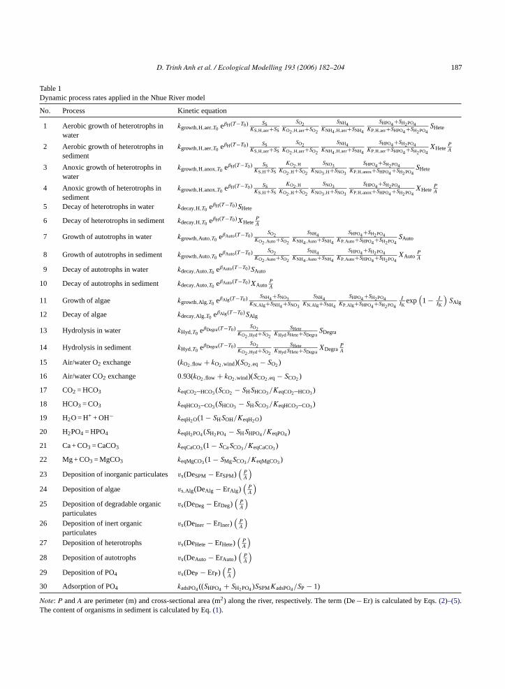
Table 1Dynamic process rates applied in the Nhue River model

No. Process Kinetic equation

1 Aerobic growth of heterotrophs inwater

kgrowth,H,aer,T0 eβH(T−T0) SSKS,H,aer+SS

SO2KO2,H,aer+SO2

SNH4KNH4,H,aer+SNH4

SHPO4+SH2PO4KP,H,aer+SHPO4+SH2PO4

SHete

2 Aerobic growth of heterotrophs insediment

kgrowth,H,aer,T0 eβH(T−T0) SSKS,H,aer+SS

SO2KO2,H,aer+SO2

SNH4KNH4,H,aer+SNH4

SHPO4+SH2PO4KP,H,aer+SHPO4+SH2PO4

XHetePA

3 Anoxic growth of heterotrophs inwater

kgrowth,H,anox,T0 eβH(T−T0) SSKS,H+SS

KO2,H

KO2,H+SO2

SNO3KNO3,H+SNO3

SHPO4+SH2PO4KP,H,anox+SHPO4+SH2PO4

SHete

4 Anoxic growth of heterotrophs insediment

kgrowth,H,anox,T0 eβH(T−T0) SSKS,H+SS

KO2,H

KO2,H+SO2

SNO3KNO3,H+SNO3

SHPO4+SH2PO4KP,H,anox+SHPO4+SH2PO4

XHetePA

5 Decay of heterotrophs in water kdecay,H,T0 eβH(T−T0)SHete

6 Decay of heterotrophs in sediment kdecay,H,T0 eβH(T−T0)XHetePA

7 Growth of autotrophs in water kgrowth,Auto,T0 eβAuto(T−T0) SO2KO2,Auto+SO2

SNH4KNH4,Auto+SNH4

SHPO4+SH2PO4KP,Auto+SHPO4+SH2PO4

SAuto

8 Growth of autotrophs in sediment kgrowth,Auto,T0 eβAuto(T−T0) SO2KO2,Auto+SO2

SNH4KNH4,Auto+SNH4

SHPO4+SH2PO4KP,Auto+SHPO4+SH2PO4

XAutoPA

9 Decay of autotrophs in water kdecay,Auto,T0 eβAuto(T−T0)SAuto

10 Decay of autotrophs in sediment kdecay,Auto,T0 eβAuto(T−T0)XAutoPA

11 Growth of algae kgrowth,Alg,T0 eβAlg (T−T0) SNH4+SNO3KN,Alg+SNH4+SNO3

SNH4KN,Alg+SNH4

SHPO4+SH2PO4KP,Alg+SHPO4+SH2PO4

IIK

exp(

1 − IIK

)SAlg

12 Decay of algae kdecay,Alg,T0 eβAlg (T−T0)SAlg

13 Hydrolysis in water kHyd,T0 eβDegra(T−T0) SO2KO2,Hyd+SO2

SHeteKHydSHete+SDegra

SDegra

14 Hydrolysis in sediment kHyd,T0 eβDegra(T−T0) SO2KO2,Hyd+SO2

SHeteKHydSHete+SDegra

XDegraPA

15 Air/water O2 exchange (kO2,flow + kO2,wind)(SO2,eq − SO2)

16 Air/water CO2 exchange 0.93(kO2,flow + kO2,wind)(SCO2,eq − SCO2)

17 CO2 = HCO3 keqCO2–HCO3(SCO2 − SHSHCO3/KeqCO2–HCO3)

18 HCO3 = CO3 keqHCO3–CO3(SHCO3 − SHSCO3/KeqHCO3–CO3)

19 H2O = H+ + OH− keqH2O(1 − SHSOH/KeqH2O)

20 H2PO4 = HPO4 keqH2PO4(SH2PO4 − SHSHPO4/KeqPO4)

21 Ca + CO3 = CaCO3 keqCaCO3(1 − SCaSCO3/KeqCaCO3)

22 Mg + CO3 = MgCO3 keqMgCO3(1 − SMgSCO3/KeqMgCO3)

23 Deposition of inorganic particulatesvs(DeSPM − ErSPM)(

PA

)24 Deposition of algae vs,Alg(DeAlg − ErAlg)

(PA

)25 Deposition of degradable organic

particulatesvs(DeDeg − ErDeg)

(PA

)26 Deposition of inert organic

particulatesvs(DeIner − ErIner)

(PA

)27 Deposition of heterotrophs vs(DeHete− ErHete)

(PA

)28 Deposition of autotrophs vs(DeAuto − ErAuto)

(PA

)29 Deposition of PO4 vs(DeP − ErP)

(PA

)30 Adsorption of PO4 kadsPO4((SHPO4 + SH2PO4)SSPMKadsPO4/SP − 1)

Note: P andA are perimeter (m) and cross-sectional area (m2) along the river, respectively. The term (De− Er) is calculated by Eqs.(2)–(5).The content of organisms in sediment is calculated by Eq.(1).

188 D. Trinh Anh et al. / Ecological Modelling 193 (2006) 182–204

The wind speed contribution at 20◦C

ko2wind =(

0.24

h

)u2

10K

(Sc

660

)−0.5

(7)

in which kwater is in 1/d; kwind is in 1/d; v the meanwater velocity (m/s);h the mean water depth (m);u10 the wind speed at 10 height (m/s);K = 0.39 (unitless);Sc is the Schmidt number for gas,Sc = 1806.6−120.1T + 3.7818T2 − 0.047608T3.

In the case of carbon dioxide, its exchange rate wasestimated from the exchange rate of reference oxygengas. The conversion coefficient of 0.93 was appliedbased on the difference in diffusivity of the two gases(Holmen and Liss, 1984).

A qualitative stoichiometric matrix illustrating con-cretely all aquatic species and bio-physico-chemicalconversion processes taken into consideration of theNhue River model is represented inTable 2.

5. Parameter identification and parameterestimation with the use of computationalprograms AQUASIM and IDENT

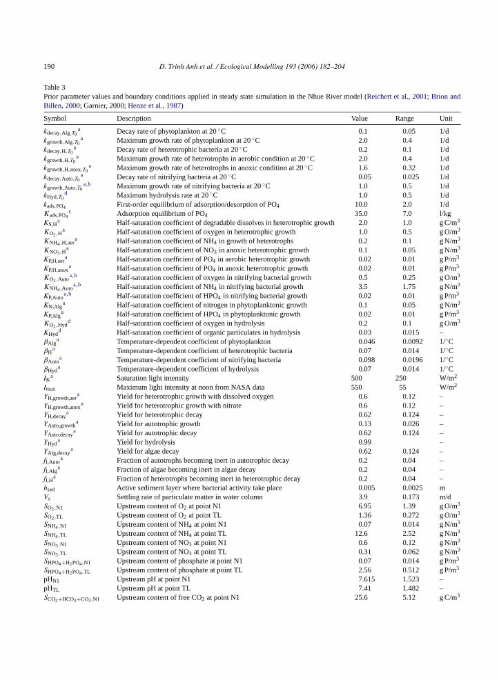
Prior to any simulation, a researcher needs to firstestimate parameter values. These values can be esti-mated based on the literature on the composition oforganic material, on activated sludge models (Henzeet al., 1987), and on existing river water quality mod-els (Reichert et al., 2001; Garnier et al., 2000). Suchv

5p

ss ist

-t tos lb da

m -r

δ

where sij is the sensitivity of the parameterj at theobservationi.

This value is determined by

si,j = ∂η(θj)i∂θj

�θj

sci, i = 1, . . . , n; j = 1, . . . , m

(9)

here ∂η(θj)i/∂θj is the absolute sensitivity function(absolute change of variableη(θj) due to the changeof parameterθj at observationi), �θj is a prior mea-sure of the reasonable range ofθj, and sci is a scalefactor with the same physical dimension as the corre-sponding observation, accounting mainly for differentscales of different output signals.

For instance, if dissolved oxygen (DO) in freshwater ranges around 6 (mg O2/l), the NO3 level is usu-ally less than 1 (mg N/l). The sensitivity comparisonbetween two parameters is obtainable only if they arenormalized, and this is why scale factors of DO andNO3, in mg O2/l and mg N/l, respectively, are intro-duced. Usually, scale factor is selected as the meanvalue of overall experimental observations because itrepresents the highest probability of parameterθj to befound in a normal distribution.

The second condition is addressed by thecollinear-ity index γK, calculated for arbitrary parameter subsetsK (Brun et al., 2001), defined as

γK = 1˜ = 1√

˜(10)

wt inβ

bm of thec iv-iim m-e blefv ofl l.,2

con-s thes een

alues are summarized inTable 3.

.1. Introduction to parameter identification andarameter estimation

The basis of the parameter identification proceo find one (or several) identifiable subset(s).

A parameter subsetK is said to be (potentially) idenifiable if the model output is sufficiently sensitivemall changes of all parameters inK on an individuaasis and if the collinearity index ofK does not exceecritical value (Brun et al., 2001).The first condition is addressed by thesensitivity

easure δmsqrj calculated for every parameterθj, sepa

ately, and defined as

msqrj =

√√√√1

n

n∑i=1

s2ij (8)

min||β||=1||SKβ|| λK

ith SK being ann × k submatrix of S containinghose columns corresponding to the parametersK,

being a vector of coefficients of lengthk, and λk

eing the smallesteigenvalue of STKSK. γK which

easures the degree of near linear dependenceolumns ofSK. The S is normalized/scaled sensitty matrix with S = {sij}, heresij = sij/||sj|| and||sj||s Euclidean norm of thejth column ofS. Although a

aximum value ofγK < 20 usually ensures that paraters included in a particular subset will be identifia

rom the well collected data (Brun et al., 2001), thealue ofγK ≤ 10 is preferable in the study becauseimited available data (Omlin et al., 2001; Brun et a002).

In principal, model parameters represented bytant variables can be estimated by minimizingum of the squares of the weighted deviations betw

D.Trinh

Anh

etal./EcologicalM

odelling193

(2006)182–204

189Table 2Qualitative stoichiometric matrix of the Nhue River model

1,SS

2,SNH4

3,SNO3

4,SHPO4

5,SH2PO4

6,SO2

7,SCO2

8,SHCO3

9,SCO3

10,SH

11,SOH

12,SCa

13,SMg

14,SHete

15,SAuto

16,SAlg

17,SDeg

18,SIner

19,SP

20,SSPM

1 Aerobic growth ofheterotrophs in water

− + − − + + +1

2 Aerobic growth ofheterotrophs in sediment

− + − − + +

3 Anoxic growth ofheterotrophs in water

− − − + − +1

4 Anoxic growth ofheterotrophs in sediment

− − − + −

5 Decay of heterotrophs inwater

+ + − + − −1 + +

6 Decay of heterotrophs insediment

+ + − + −

7 Growth of autotrophs inwater

− + − − − + +1

8 Growth of autotrophs insediment

− + − − − +

9 Decay of autotrophs inwater

+ + − + − −1 + +

10 Decay of autotrophs insediment

+ + − + − + +

11 Growth of algae − − + − − +112 Decay of algae + + − + + −1 + +13 Hydrolysis in water + + + + + + −114 Hydrolysis in sediment + + + + + +15 Air/water O2 exchange +116 Air/water CO2 exchange +117 CO2 = HCO3 −1 +118 HCO3 = CO3 −1 +119 H2O = H+ + OH− +1 +120 H2PO4 = HPO4 +1 −121 Ca + CO3 = CaCO3 −1 −22 Mg + CO3 = MgCO3 −1 −23 Deposition of inorganic

particulates−1

24 Deposition of algae −125 Deposition of degradable

org. particulates−1

26 Deposition of inertorganic particulates

−1

27 Deposition ofheterotrophs

−1

28 Deposition of autotrophs −129 Deposition of PO4 −130 Adsorption of PO4 − − +1

190 D. Trinh Anh et al. / Ecological Modelling 193 (2006) 182–204

Table 3Prior parameter values and boundary conditions applied in steady state simulation in the Nhue River model (Reichert et al., 2001; Brion andBillen, 2000; Garnier, 2000;Henze et al., 1987)

Symbol Description Value Range Unit

kdecay,Alg,T0a Decay rate of phytoplankton at 20◦C 0.1 0.05 1/d

kgrowth,Alg,T0a Maximum growth rate of phytoplankton at 20◦C 2.0 0.4 1/d

kdecay,H,T0a Decay rate of heterotrophic bacteria at 20◦C 0.2 0.1 1/d

kgrowth,H,T0a Maximum growth rate of heterotrophs in aerobic condition at 20◦C 2.0 0.4 1/d

kgrowth,H,anox,T0a Maximum growth rate of heterotrophs in anoxic condition at 20◦C 1.6 0.32 1/d

kdecay,Auto,T0a Decay rate of nitrifying bacteria at 20◦C 0.05 0.025 1/d

kgrowth,Auto,T0a,b Maximum growth rate of nitrifying bacteria at 20◦C 1.0 0.5 1/d

kHyd,T0d Maximum hydrolysis rate at 20◦C 1.0 0.5 1/d

kads,PO4 First-order equilibrium of adsorption/desorption of PO4 10.0 2.0 1/dKads,PO4

c Adsorption equilibrium of PO4 35.0 7.0 l/kgKS,H

a Half-saturation coefficient of degradable dissolves in heterotrophic growth 2.0 1.0 g C/m3

KO2,Ha Half-saturation coefficient of oxygen in heterotrophic growth 1.0 0.5 g O/m3

KNH4,H,aera Half-saturation coefficient of NH4 in growth of heterotrophs 0.2 0.1 g N/m3

KNO3,Ha Half-saturation coefficient of NO3 in anoxic heterotrophic growth 0.1 0.05 g N/m3

KP,H,aera Half-saturation coefficient of PO4 in aerobic heterotrophic growth 0.02 0.01 g P/m3

KP,H,anoxa Half-saturation coefficient of PO4 in anoxic heterotrophic growth 0.02 0.01 g P/m3

KO2,Autoa,b Half-saturation coefficient of oxygen in nitrifying bacterial growth 0.5 0.25 g O/m3

KNH4,Autoa,b Half-saturation coefficient of NH4 in nitrifying bacterial growth 3.5 1.75 g N/m3

KP,Autoa,b Half-saturation coefficient of HPO4 in nitrifying bacterial growth 0.02 0.01 g P/m3

KN,Alga Half-saturation coefficient of nitrogen in phytoplanktonic growth 0.1 0.05 g N/m3

KP,Alga Half-saturation coefficient of HPO4 in phytoplanktonic growth 0.02 0.01 g P/m3

KO2,Hydd Half-saturation coefficient of oxygen in hydrolysis 0.2 0.1 g O/m3

KHydd Half-saturation coefficient of organic particulates in hydrolysis 0.03 0.015 –

βAlga Temperature-dependent coefficient of phytoplankton 0.046 0.0092 1/◦C

βHa Temperature-dependent coefficient of heterotrophic bacteria 0.07 0.014 1/◦C

βAutoa Temperature-dependent coefficient of nitrifying bacteria 0.098 0.0196 1/◦C

βHyda Temperature-dependent coefficient of hydrolysis 0.07 0.014 1/◦C

IKa Saturation light intensity 500 250 W/m2

Imax Maximum light intensity at noon from NASA data 550 55 W/m2

YH,growth,aera Yield for heterotrophic growth with dissolved oxygen 0.6 0.12 –

YH,growth,anoxa Yield for heterotrophic growth with nitrate 0.6 0.12 –

YH,decaya Yield for heterotrophic decay 0.62 0.124 –

YAuto,growtha Yield for autotrophic growth 0.13 0.026 –

YAuto,decaya Yield for autotrophic decay 0.62 0.124 –

YHyda Yield for hydrolysis 0.99 –

YAlg,decaya Yield for algae decay 0.62 0.124 –

fI,Autoa Fraction of autotrophs becoming inert in autotrophic decay 0.2 0.04 –

fI,Alga Fraction of algae becoming inert in algae decay 0.2 0.04 –

fI,Ha Fraction of heterotrophs becoming inert in heterotrophic decay 0.2 0.04 –hsed Active sediment layer where bacterial activity take place 0.005 0.0025 mVs Settling rate of particulate matter in water column 3.9 0.173 m/dSO2,N1 Upstream content of O2 at point N1 6.95 1.39 g O/m3

SO2,TL Upstream content of O2 at point TL 1.36 0.272 g O/m3

SNH4,N1 Upstream content of NH4 at point N1 0.07 0.014 g N/m3

SNH4,TL Upstream content of NH4 at point TL 12.6 2.52 g N/m3

SNO3,N1 Upstream content of NO3 at point N1 0.6 0.12 g N/m3

SNO3,TL Upstream content of NO3 at point TL 0.31 0.062 g N/m3

SHPO4+H2PO4,N1 Upstream content of phosphate at point N1 0.07 0.014 g P/m3

SHPO4+H2PO4,TL Upstream content of phosphate at point TL 2.56 0.512 g P/m3

pHN1 Upstream pH at point N1 7.615 1.523 –pHTL Upstream pH at point TL 7.41 1.482 –SCO2+HCO3+CO3,N1 Upstream content of free CO2 at point N1 25.6 5.12 g C/m3

D. Trinh Anh et al. / Ecological Modelling 193 (2006) 182–204 191

Table 3 (Continued )

Symbol Description Value Range Unit

SCO2+HCO3+CO3,TL Upstream content of free CO2 at point TL 61 12.2 g C/m3

QN1 Upstream discharge at point N1 26.62 5.324 m3/dQTL Upstream discharge at point TL 5.82 1.164 m3/dQLat Lateral inflow in reaches 1 and 2 7.65 1.53 m3/d/mSAlg,N1 Upstream content of phytoplankton at point N1 0.34 0.068 g Alg/m3

SAlg,TL Upstream content of phytoplankton at point TL 2.17 0.434 g Alg/m3

SAuto,N1 Upstream content of autotrophs at point N1 0.0475 0.0075 g Auto/m3

SAuto,TL Upstream content of autotrophs at point TL 0.0522 0.0104 g Auto/m3

SHete,N1 Upstream content of heterotrophs at point N1 0.54 0.086 g Heto/m3

SHete,TL Upstream content of heterotrophs at point TL 3.76 0.752 g Heto/m3

SDeg,N1 Upstream content of degradable organic particulates at point N1 1.77 0.354 g Deg/m3

SDeg,TL Upstream content of degradable organic particulates at point TL 7.72 1.544 g Deg/m3

SIner,N1 Upstream content of inert organic particulates at point N1 1.93 0.386 g Iner/m3

SIner,TL Upstream content of inert organic particulates at point TL 8.42 1.684 g Iner/m3

SI,N1 Upstream content of inert organic dissolves at point N1 2.88 0.576 g I/m3

SI,TL Upstream content of inert organic dissolves at point TL 18.79 3.758 g I/m3

SS,N1 Upstream content of degradable organic dissolves at point N1 2.73 0.546 g S/m3

SS,TL Upstream content of degradable organic dissolves at point TL 6.17 1.234 g S/m3

Note: N1 and TL indicate upstream 1 from the Red River and upstream 2 from To Lich River, respectively. Upstream contents at point TL arealso contents in lateral inflow along the reaches 1 and 2.

a Reichert (2001).b Brion and Billen (2000).c Garnier (2000).d Henze (1987).

measurements and calculated model results (Reichertet al., 1998):

χ2(θ) =n∑

i=1

(ηmeas,i − ηi(θ)

σmeas,i

)2

(11)

whereymeas,i is theith measurement,σmeas,i the stan-dard deviation ofith measurement,ηi(θ) the calculatedvalue of the model variable corresponding to theithmeasurement and evaluated at the time and locationof this measurement,θ = (θ1, θ2, . . ., θm) the modelparameters andn is the number of data points.

Simultaneous comparisons of data for measure-ments corresponding to different variables, compart-ments and zones are possible. Due to the possiblenonlinearity of the model equations and due to thenumerical integration procedure,χ2 must be minimizednumerically.

5.2. Selection of computational platforms

The computational platform AQUASIM (Reichertet al., 1988) was selected for performing the simulation.This software is different from many available general

purpose simulation software that gives their users lit-tle freedom in model formulation and does not usuallysupport model identification and parameter estimation(e.g. Carver et al., 1978; Schiesser, 1991), AQUASIMis very flexible with regard to model formation andprovides methods for sensitivity analysis, parameterestimation and uncertainty analysis in addition to sim-ulation (Reichert, 1995b; Rauch et al., 1998). Theseprominent properties are helpful for construction, cali-bration, and validation of a model applied in a very littleacknowledged environment such as the Nhue River.Moreover, the 1D river model of AQUASIM is suit-able for a dike as well as a long and well-homogenizedriver.

The river section compartment of AQUASIM can beused to describe river hydraulics, advective–dispersivetransport of substances dissolved or suspended in awater column, exchange of substances between thecolumn and the sediment, and transformation pro-cesses of substances in the column or the sedimentin a river section without abrupt hydraulic controls.In the presence of significant hydraulic structures ortributaries, several river sections can be linked advec-tively to model the river reach of interest. The 1D

192 D. Trinh Anh et al. / Ecological Modelling 193 (2006) 182–204

river hydraulics solved by AQUASIM can be describedby a set of two partial differential equations repre-senting a mass and a momentum balance (Reichertet al., 1988). The two most important approximationsto these so-called St. Venant equations are the kine-matic and diffusive wave approximations (Yen, 1979)and are implemented in AQUASIM to describe riverhydraulics. The equations for river hydraulics are cou-pled with advection–diffusion equations to describetransport of substances dissolved or suspended in thewater.

The computer program IDENT (Reichert, 2002,draft version, still complete) special for identifiabil-ity analysis based on sensitivity calculation extractedfrom AQUASIM was selected for process of parameteridentifiability analysis of this model. Briefly, IDENTis a program to calculate quantitative indicators formodel parameter identifiability based on linear sen-sitivity functions, parameter uncertainty ranges andmodel output scaling factors (Brun et al., 2001). Lin-ear sensitivity functions (derivatives of model outputwith respect to model parameters) have to be providedas input to IDENT. It has been successfully appliedfor identifiability analyses of biogeochemical modelsof lakes (Omlin et al., 2001), water quality models ofrivers (Reichert and Vanrolleghem, 2001), and acti-vated sludge sewage treatment plant models (Brunet al., 2002).

The process of parameter estimation was then cal-culated again with the help of the AQUASIM program.I ew lysis,a ed.

6r

6p

cru-c isg rm ble.S useo s ofs

For this case study, data obtained from the monthlysampling surveys conducted over the entire year2002 were used for this simulation and calibration.Boundary conditions were the loadings at the twoupstream points: the derivation from the Red River(upstream 1) and the massive input from the To LichRiver (upstream 2).

However, in order to optimize the constructed modelas well as to resolve some unmeasured boundary con-ditions and physical parameters, prior estimation ofhydrological and physical parameter-conditions weretaken initially. It should be noted that physical andhydrological characters dominate the fate of biochemi-cal processes but cannot be identified and estimated bythe variation of biological parameters. The prior esti-mation work was carried out with a Strickler coefficient(Kst), the settling velocity (Vs), the lateral inflow ofuntreated wastewater along the first two reaches, andthe thickness of sediment layer (hsed), respectively.

Hydrological and topological data were collectedfrom different sources including the 2 years ofsampling and subject to formation of a complete 1Dhydrological model. The roughness coefficient ofthis river (represented as Strickler’s value,Kst) wascalibrated by a water level measured at upstreampositions that gave a fairly low Strickler’s value;Kst = 18.9 m1/3/s. This value corresponds to a surfacebed of slow moving river (Henderson, 1966) and isappropriate to the Nhue River reality.

Lateral inflow discharged by local inhabitantsa t as0 re rveyt pop-u ntlyc estlyr terc aters hasb ;B -m ainp omd se,l al to8 oft ewl on

n conclusion, by using AQUASIM and IDENT, thhole processes of model setup, parameter anand parameter estimation were easily accomplish

. Simulation and calibration in a steady stateegime

.1. Prior estimation of physico-chemicalarameters

Pools of storage products and biomass areial for the dynamic behavior of RWQM1. Itenerally difficult to provide initial conditions foodel components which are not directly measurateady state simulation can be done with thef constant loadings estimated by average valueampling.

long Reach 1 and Reach 2 were initially se.014 m3/s/km (JICA, 1995), but was clearly undestimated as it was based on an old population su

aken in 1963. Since the 1960s, demographic andlation characters of the river basin have significahanged and therefore lateral inflow has been modeevaluated owing to the spatial variation of waonductivity. The evaluation procedure of wastewources characterized by conductivity discrepancyeen discussed in previous publications (EPA, 2000ordalo et al., 2001; Taebi Amir et al., 2004). The estiation is modest because it is very difficult to obtrecise conductivity of untreated wastewater frifferent point sources. In order to simplify the ca

ateral wastewater conductivity is assumedly equ00�S/cm, which is the average conductivity value

he To Lich water in dry weather condition. The nateral inflow calculated from conductivity variati

D. Trinh Anh et al. / Ecological Modelling 193 (2006) 182–204 193

was estimated as 0.091 m3/s/km and used in furthercalculation.

The effective settling rate (Vs) of suspended matters,combined with hydrological conditions is the principalfactor governing the variation of suspended particulatematters concentration in a water column. Based on this,theVs was calibrated and resulted in an estimated set-tling rate of 3.9 m/d that meets the normal range ofalluvial particle settling (Stumm and Morgan, 1996;Minshall et al., 2000; Callieri et al., 1991; Omlin et al.,2001).

Another important but difficult to be determinedparameter is the thickness of sediment layer (hsed)that limits the maximum strength of biological activityin the sediment and the flux of dissolved substancesexchange between water and sediment. Based on ourexperimental results on water-sediment fluxes of dis-solved substances such as DO, NH4, NO3, pH, thick-ness of sediment layer, it was determined that a manualtuning ofhsedwas needed to fit the experimental resultswith the simulation. The work was concentrated to aflux of DO (SOD). It was revealed from the manualtuning of sediment thickness thathsed= 0.005 m witha sediment porosity of 0.98 which fit the experimen-tal results. The simulated and experimental results ofSOD have been compared with other publications intropical-nutrient polluted water systems which showedvery similar results (Alongi et al., 1999; Steeby et al.,2004; Meijer and Avnimelech, 1999).

6

6a

tersn ram-e fore ame-t firstc ntst per-i en-t tedt con-t thatw etere ord-

ing to Reichert and Vanrolleghem (2001), parameteruncertainty can be divided into three classes: (class 1)accurately known parameters, with�θj = 10% (class2) consisted essentially of external and input parame-ters, intermediate with�θj = 20% (class 3) gatheringkinetic rates, and very poorly known parameters, with�θj = 50%, consisted of half-saturation concentrations,specific death and decay rates. Uncertainty in stoichio-metric coefficients was not considered in this analysis.

As a whole, in the steady state simulation, 51 param-eters were selected for sensitivity analysis and param-eter estimation.

6.2.2. Choice of experimental layouts and scalefactors

All the routinely measured variables during themonthly surveys could be included in the experimen-tal layouts. Each variable scale factor was calculatedfrom the monthly data (average value) at the differentmeasurements locations listed inTable 4. Because sus-pended particulate matters and conductivity were ear-lier used to identify settling rate (Vs) and lateral inflowand they do not directly affect biological conversionprocesses, the experimental layout used to estimatethe biochemical conversion kinetics consists of the 8remaining variables (Table 4).

6.2.3. Sensitivity ranking, collinearity index, andsubset selections

The sensitivity of parameters was computed accord-icI hec s areoT rdero ctedt inT

ti-fi exo mongt sug-g lm sed.A call them eters

.2. Sensitivity analysis and parameter selection

.2.1. Selection of parameters for sensitivitynalysis and parameter estimation

The idea in this step is to select the parameeeded to be estimated from the complete set of paters in the model and to assign the uncertaintyach selected parameter. In the first attempt par

ers were grouped into two principal clusters. Theluster includes all physical and chemical coefficiehat were precisely known beforehand, and the exmental parameters that were determined experimally for the studied river. All kinetic parameters relao biological processes, initial concentrations andents of nutrients, organic matters and organismsere potential for sensitivity analysis and paramstimation were placed in the second cluster. Acc

ng to the method described in Section5 using the twoomputer programs: AQUASIM (Reichert, 1998) andDENT (Reichert et al., 2002). The sensitivity of tonsidered parameters and boundary conditionrdered in descending ranking as shown inTable 5.he 29 first ranking parameters with the same of sensitivity magnitude were selected and subje

o a collinearity index calculation (bold lettersable 5).

As indicated in Section5, the next step in the idenability procedure is to compute the collinearity indf each possible subset of parameters chosen a

he 29 top selected parameters. Now, as alreadyested byBrun et al. (2001), for large environmentaodels an additional problem has to be addresmong all the possible subsets fulfilling the criti

evel of γK < 10, many subsets may not containost sensitive parameters or at least the param

194 D. Trinh Anh et al. / Ecological Modelling 193 (2006) 182–204

Table 4Experimental layout and scale factors at the different measurement locations used in the steady state simulation

Variable Unit Scale factors (at different km)

0 km 8 km 15.2 km 25.2 km 33 km

SO2 mg O2/l 6.945 6.020 5.378 3.821 3.777SNH4 mg N/l 0.074 0.364 0.654 2.592 2.285SNO3 mg N/l 0.604 0.618 0.529 0.480 0.557SHPO4+H2PO4 mg P/l 0.072 0.120 0.202 0.628 0.579pH 7.615 7.461 7.392 7.532 7.368SCO2+HCO3+CO3 mg C/l 25.189 26.933 28.667 32.533 31.556SAlg mg Phyto/l 0.338 0.656 0.885 1.021 1.388SDOM mg OM/l 5.62 6.78 8.71 10.84 12.54

involved in the main processes. Looking into the detailsof the biogeochemical function of the model parame-ters can lead to a classification of four types: physicalparameters, stoichiometric parameters, kinetic param-eters and parameters related to input fluxes into theriver (Omlin, 2001). Because of the uncertainty in therate expressions and in the parameter values of the bio-geochemical model, it did not seem to be meaningfulto estimate inflow parameters from river data (inputsto a river are often not measured precisely, but theirestimation from river data would only be meaning-ful if the biogeochemical processes in the river wereknown accurately). Stoichiometric and physical param-eters are usually accurately known or show a smallervariation from one system to another than parameters

of process kinetics. This leads to the general guide-line to estimate primarily kinetic model parameters.We separated the kinetic model parameters into twosmall groups: the biological kinetic process rates andthe half-saturation and yield coefficients. The maxi-mum biological kinetic rates were placed as the mostconcerned.

Since the first selection for sensitivity analysishas already omitted stoichiometric and most physicalparameters, the grouping priority for parameter estima-tion was ordered as following:

1. Biological process rates which are variable and notconfirmed by experiments;

2. half-saturation coefficients and yield coefficients;

Table 5Sensitivity ranking of considered parameters and boundary conditions (N1 and TL indicate the upstream conditions 1 and 2, respectively) insteady state condition

No. Variable δmsqr No. Variable δmsqr No. Variable δmsqr

1 QN1 0.082 18 SI,N1 0.025 35 KO2,Auto 0.00472 kgrowth,Auto,T0 0.051 19 IK 0.023 36 KP,H,aer 0.00453 hsediment 0.047 20 SHete,TL 0.018 37 Imax 0.00444 QLat 0.047 21 YAuto,growth 0.017 38 KP,Auto 0.00285 YH,growth 0.047 22 SI,TL 0.017 39 kdecay,Auto,T0 0.00266 QTL 0.044 23 kgrowth,H,anox,T0 0.015 40 KP,H,anox 0.00237 SAlg,N1 0.044 24 kdecay,Alg,T0 0.014 41 KO2,Hyd 0.00158 kHyd,T0 0.040 25 KN,Alg 0.014 42 KHyd 0.00119 KS,H 0.039 26 KNH4,A,aer 0.011 43 YAlg,decay 0.0010

10 YHyd 0.036 27 SHete,N1 0.010 44 SDegra,TL 0.0004611 kgrowth,Alg,T0 0.035 28 SAuto,N1 0.0092 45 SDegra,N1 0.000271 ,T0

11 y

111 L

2 YH,growth,anox 0.033 29 kdecay,H

3 KNH4,Auto 0.032 30 SS,TL

4 KO2,H 0.031 31 YH,deca

5 kgrowth,H,T0 0.029 32 KP,Alg

6 SAlg,TL 0.028 33 KNO3,H

7 SS,N1 0.026 34 SAuto,T

0.0089 46 fI,H 0.0000860.0077 47 SInert,N1 0.0000650.0063 48 YAuto,decay 0.0000550.0061 49 SInert,TL 0.0000420.0056 50 fI,Alg 0.0000160.0052 51 fI,Auto 0.000001

D. Trinh Anh et al. / Ecological Modelling 193 (2006) 182–204 195

Fig. 2. Collinearity index parameter subsets: subsets are the com-binations of seven maximum kinetic rates (the core subset) with 22other parameters having a similar sensitivity.

3. physical/chemical parameters that are extractedfrom measurements or from publications; and

4. boundary conditions of estimated variables.

Following this method, the first-order prioritygroup of seven biological process rates (kgrowth,Auto,T0,kgrowth,Alg,T0, kgrowth,H,T0, kgrowth,H,anox,T0,kdecay,Alg,T0, kdecay,H,T0 and kHyd,T0) was firstlyselected. The collinearity index of this group wascalculated as 9.15 and satisfied the conditionγK < 10.It is easily recognized that this subset included reactionrates of the most important biological conversions. Inother words, the results prove that the experimentallayout of these eight variables is sufficient in identify-ing this ecological model. This result is not astonishingbecause in the case of RWQM1 the dominant pro-cesses can also be described by five to eight parametersand are identifiable from DO, NH4, NO3 (Reichertand Vanrolleghem, 2001). For this case study, theaddition of other variables, especially of DOM,apparently would increase the size of identifiablesubsets.

Based on this conclusion, these seven parameterswere then set up as thecore for adding other sensibleselected parameters. The parameters of lower priorityorder were then added to combine all possible subsetssatisfying the identifiability criterionγK < 10. Resultsof the collinearity index computation using IDENTprogram (Reichert et al., 2002) are illustrated inFig. 2and shows that the maximum size of the identifiables den-

tifiable subset(s) that contains only kinetic parametersis 9 (7 + 2). There are six identifiable subsets for all con-sidered parameters at size 14 and one subset of 9 kineticparameters that is identifiable with the criterion ofγK < 10 (9.4):kgrowth,Auto,T0,kgrowth,Alg,T0,kgrowth,H,T0,kgrowth,H,anox,T0, kdecay,Alg,T0, kdecay,H,T0 and kHyd,T0,KN,Alg, KNH4,A,aer.

Since there are many sensible parameter subsetsthat meet identifiability criterionγK of 10, parameterestimation for all subsets consumes too much timeand is impracticable. Therefore the choice of whichsubsets among these identifiability subsets subject toparameter estimation required further elimination. Atthis step, we relied again on the priority ranking ofparameters declared above. So in order to shorten thesubset list subject to parameter estimation, the subsetsthat contain any parameter that are not primarilykinetic were eliminated (Omlin et al., 2001). Finally,there was only one subset at the size of 9 (7 + 2)satisfying all criteria. However, because this extendedsubset with two more kinetic parameters (KN,Alg,KNH4,A,aer) does not include parameter of any otherbiological processes compared with the ones ofthe core subset, we decided to perform parameterestimation on both subsets (the core subset and theextended one) in order to compare the advantagebetween the maximum possible subset size selectionand maximum biological process consideration.

6.3. Parameter estimation

ari-a wasp re-m ode( pre-s

ma-t limito emea daryc es isa thed y itsm on-c

thes large

ubsets is 14 (7 + 7) and the maximum size of the i

After the establishment of restricted ranges of vtion for each parameter, an automatic estimationerformed with AQUASIM on the basis of the measuents, which reached convergence in simplex m

Reichert et al., 1998). The estimated results are reented inTable 6.

The first conclusion drawn from parameter estiion is that no parameter value comes close to thef range. It proves that this conceptual model schcquired with monthly average loadings as bounondition together with the preset parameter valupplicable for the Nhue River system. Looking intoetails for each biological process represented baximum kinetic rates and coefficients, further c

lusions were made.Second, by looking at the estimated values of

ubset 1, although most parameters showed

196 D. Trinh Anh et al. / Ecological Modelling 193 (2006) 182–204

Table 6Parameter estimation results in steady state condition (bold formatindicates estimated value is more than 20% different from the priordefined one)

Parameter Unit Range Prior Subset 1 Subset 2

kgrowth,Auto,T0 d−1 0.0–10.0 1.00 1.73 1.63kgrowth,Alg,T0 d−1 0.0–10.0 2.00 2.12 8.87kgrowth,H,T0 d−1 0.0–10.0 2.00 1.34 1.27kgrowth,H,anox,T0 d−1 0.0–10.0 1.60 0.23 0.28kdecay,Alg,T0 d−1 0.0–2.0 0.10 0.06 0.04kdecay,H,T0 d−1 0.0–2.0 0.20 0.06 0.09kHyd,T0 d−1 0.0–5.0 1.00 2.92 3.07KN,Alg g N d−1 0.0–10.0 0.10 2.19KNH4,A,aer g N d−1 0.0–1.0 0.20 0.03

change between prior- and post-estimated values, it isnot astonishing if one looks at the simulated results ofprior parameter estimated model. The intensification ofnitrification, reflected by an increase ofkgrowth,Auto,T0,is matched with a strong reduction of NH4 concen-tration downstream the confluence (Fig. 5) and alsopossibly affected by fairly high NH4 half-saturationcoefficient set up for autotrophic bacteria. The NH4half-saturation coefficient in this model was set as 3.5(mg N/l) and is higher than found in other publications(Flipo et al., 2004; Nuhoglu et al., 2005). The main fac-tor that causes an increase of hydrolysis and decreaseof heterotrophic activities in this study is the strongincrease of dissolved degradable organic matter (whichcontributed to the total increase of DOM) downstream(Table 4). In very favorable conditions of enrichednutrients, the only way to have an increase of DOM isto have a low heterotrophic growth which causes theconsumption of dissolved degradable organic matterand a high hydrolysis process that generates dissolveddegradable organic matter from particulate matter.It is necessary to remind the reader that due to datadeficiency, fractions of degradable and inert organicmatters were not experimentally determined. Insteadthey were roughly estimated from the reports ofServaiset al. (1999). Thus in the future, studies on organicmatter pools and bacterial biomasses should be carriedout.

It is easily understood that the experimental lay-out employed in this calculation which consists ofp urest sionp k-

tonic maximum kinetic rates appeared to be slightlychanged after parameter estimation because the sim-ulated results of phytoplanktonic biomass prior toparameter estimation had already given high similar-ity with the experimental data (Fig. 6).

Since the estimated kinetic growth rates of organ-isms is usually decided by variation of one or severalvariables included in experimental layout (phytoplank-ton biomass for phytoplankton growth, NH4 and DOfor autotrophic bacteria, and DOM for hydrolysis), thedecay rates should be estimated from all participatingvariables that sometimes act as compensation factors ifthe estimated kinetic growth rates do not give a coher-ence between simulated and experimental results. Inthis case study, as the selected conversion processes andkinetic parameters were well selected, the estimateddecay rates did not have to change much for a largecompensation. That is indicated by the fact that theabsolute magnitude of estimated decay rates of phyto-plankton and heterotrophic bacteria changed little fromprior estimated values.

Parameter estimated results of subset 2 showed littledifference from those in subset 1, exceptkgrowth,Alg,T0.The exceptionally high estimatedkgrowth,Alg,T0 is log-ical as there is compensation in the high estimatedKN,Alg when the correlation coefficient between twokinetic parameters is 0.96 (a very high positive corre-lation). This raises a concern that for this case study thecriterion of 10 may still be too high to obtain fast andidentifiable parameter subsets. Thus again the selectiono i-c odel,a

luesb thatp sizep y oft tedea icallys pliedf vail-a mei fors meo ula-t eterso

hytoplankton biomass gives high sensible measo parameters related to phytoplanktonic converrocesses (Table 5). Due to this fact the phytoplan

f the collinearity indexγK is proved as highly dedated and depends on both the complexity of the mnd the quality and quantity of the data.

By comparing the estimated parameter vaetween the two selected subsets, it is concludederforming a parameter estimation of a largearameter subset would probably improve qualit

he model outcome but might lead to unexpecstimated parameter values (kgrowth,Alg,T0, KN,Alg). Solthough the selected parameters have mathematatisfied all setup criteria, parameter estimation apor large size parameter subsets in limited data ability may, ecologically and individually, cause so

rregular results that can be avoided if appliedmaller but a biodiversified subset. The final outcof this small discussion is that in subsequent calc

ions, the model upgraded with estimated paramf subset 1 is used.

D. Trinh Anh et al. / Ecological Modelling 193 (2006) 182–204 197

Fig. 3. Average monthly measured and simulated pHs.

Fig. 4. Average monthly measured and simulated dissolved oxygenconcentration.

6.4. Results of the post-calibration simulation

Results of both prior and post-parameter estimatedmodels are in strong agreement with data as shownin Figs. 3–6for the main variables pH, DO, N NH4,and phytoplankton, respectively. At-test for the depen-dent samples was performed using the statistical com-puter program STATISTICA (Statsoft, 1995). The nullhypothesis was stated that the simulated results were

Fig. 5. Average monthly measured and simulated NH4 concentra-tion.

Fig. 6. Average monthly measured and simulated phytoplanktonbiomass.

significantly different from the experimental data withthep-value < 0.05. Thep-values of the measured dataand simulated results (prior- and post-parameter esti-mations) are summarized inTable 7and support ourresults.

Apart from dissolved oxygen and DOM, spatialtrends of the prominent variables are well reproducedwithin the different river reaches. For dissolved oxy-gen, the model simulates a decrease of DO downstreamwhile experimental results indicated a steady level.We suspect that this is due to submerged grass andalgae attached at the bottom observed downstream theriver, but that are not yet considered in this ecologicalmodel version. The appearance of plants attached tothe bottom in the downstream reach is more probablya consequence of more water column transparency andhigher nutrient contents than in the upstream reach.

In the case of DOM, prior simulated results of esti-mated parameters showed a declining variation whileexperimental results indicated a steady increase in thedownstream reach (thep-value for this test is 0.08and close to 0.05). However, simulated DOM of post-parameter estimated model has shown a significantimprovement (thep-value is 0.21). That improvementis thanks to three times the higher estimated hydrolysisspecific rate.

Since statistical test showed no significant differ-ences among experimental and simulated results inboth prior- and post-parameter estimated models, theconstructed model and its pre-selected kinetic param-e ntals achp tedr were

ters are well suited to describe the environmeituation of the studied river. Looking closely at eair of p-values, apart from the DOM, no simulaesults of the post-parameter estimated model

198 D. Trinh Anh et al. / Ecological Modelling 193 (2006) 182–204

Table 7p-Value oft-test for dependent samples; thep < 0.05 marks the significant difference between simulated and measured results (before and afterparameter estimation) in steady state regime

Variable Prior-estimation Post-estimation Variable Prior-estimation Post-estimation

NO3 0.93 0.12 Algae 0.48 0.43NH4 0.27 0.47 HPO4 + H2PO4 0.39 0.36pH 0.12 0.13 DOM 0.08 0.21DO 0.39 0.32 Ctotal 0.77 0.94

improved compared with the simulated results of theprior parameter estimated model. In order to explainthe reason for no significant difference between theprior- and post-estimation models, theχ2 for each indi-vidual variable was examined to assist in making thisclear. In our model, the prior setup was too coherentfor most variables, so its priorχ2 was low. The onlyhighχ2 (corresponding to low coherence) was seen inthe case of DOM. The process of parameter estimationis automatically tuned for the lowestχ2 of the totalindividualχ2 of all variables. Therefore, while the cal-culation strongly reducedχ2 of DOM to achieve a totallow χ2, the parameter estimation changed slightly theχ2 of other well-fitted variables. Because of this reason,the low denitrification rate was estimated and causedlow similarity in the NO3 (statistical tests gave higherdifferences between experimental and post-parameterestimated simulated results than between experimentaland prior parameter estimated results).

In conclusion, the developed model is well suited forthe description of the water quality within the systemon an annual basis. However, some additional experi-ments are necessary to confirm the estimated values ofheterotrophic growth rate and the fraction of organicmatter pools.

7. Simulation and calibration in an unsteadystate simulation

untf ys-t asp r oft theb esti-m ed top tioni

7.1. Selection of simulation period and thecalculation of loading in the unsteady statesimulation

In transient simulation, boundary conditions varywith time. Based on the fact that continuous mea-surements were taken at N3 (15.2 km from upstreampoint N1) by monitoring stations, we decided to restrictthe studied area from point N3 (15.2 km) to the DongQuan Dam (41 km). Although the modeling area wasrestricted, the principal objective of the simulation ofthe To Lich wastewater impact to the Nhue River wasstill effective. In this calculation monitoring data at N3from 23 to 28 April 2003, were employed as a bound-ary condition, and the monitoring data at NT1 (25.2 kmfrom upstream point) was collected at the same timewere used for model calibration. The period was chosenbecause during that time, water flow was not abruptlyregulated by the dams, water regime changed slightlyand rainfall was very limited. The monitoring stationsworked well, and the monitoring variables were pH,NH4, DO, conductivity, water level, temperature, tur-bidity and redox potential.

For those variables not monitored by the monitor-ing stations, their upstream boundary conditions weresimply taken from simulated results at point N3 of thesteady state calibrated model applied for the entire areastudied. The loading at upstream point N1 of the modelapplied for the whole area and was set up as a dischargeat N1 during this period, multiplied by its 2002 monthlya

rat-i evelr own-s seda them ToL ther the

Unsteady state simulation is important to accoor short-term variation of water quality in the river sem. Thanks to automatic monitoring stations, it wossible to precisely study the transient behavio

he river. First of all, it has to be confirmed thatiochemical model calibrated through parametersation process in steady state simulation was userform sensitivity analysis and parameter estima

n the unsteady state condition.

verage concentration at this point.Discharges at point N3 were derived from the

ng curve established at this point and daily water lecorded at the dam. Water levels recorded at the dtream position (41 km from upstream point) were us the downstream boundary condition. Duringonitoring period, the wastewater inflow from theich River was low because of reconstruction ofegulation dam at point TL. It was estimated that

D. Trinh Anh et al. / Ecological Modelling 193 (2006) 182–204 199

leaked wastewater from the To Lich during this periodwas 0.832 m3/s. An extra calculation was carried out toimprove lateral inflow in reach 1 (QLat). The reason forthe re-estimation ofQLat was that in 2003 new livingquarters and industrial zones were established in theupstream part of the Nhue River basin and the experi-mental surveys have clearly shown the environmentaldeterioration from 2002 to 2003. The same techniquewas used for estimation of these parameters from theexperimental layout consisting of conductivity at N3.The estimated result ofQLat = 0.112 m3/s/km was usedfor next calculation.

7.2. Sensitivity analysis and parameter selection

7.2.1. Choice of experimental layout and scalefactors

In an unsteady state, the use of constant scale factorsis not appropriate because the variable’s concentrationschange due to variation of flowing water and bound-ary conditions. We therefore set up scale factors asseries of average values of measured concentrationsat every 0.2-day interval. Using the 0.2-day intervalsinstead of minutes considerably reduced the work andtime in sensitivity analysis and parameter estimation.It is expected that evaluation of diurnal change is notaffected by this simplification. The monitored data col-lected at point NT1 (at 10 km of 21 km river length)are subject to the scale factor calculation, based onthe measurements of particulate matter, pH, conduc-t ev ne r andc notd

7s

revi-o exw r ofp thes t N1w t N3w etersi havea ongt rity

Fig. 7. Collinearity index parameter subsets. The subsets are com-binations of 2 maximum kinetic rates (the core subset) with 11 otherparameters having a similar sensitivity.

group: kgrowth,H,T0, kgrowth,Alg,T0, and kgrowth,Auto,T0.The collinearity index of this three maximum kineticrate subset was, however, equal to 13.13 and higher thanthe index criterion. The explanation for a high collinear-ity betweenkgrowth,H,T0 andkgrowth,Auto,T0 comes fromthe experimental layout where increase in growth ofheterotrophic and autotrophic bacteria would lead tothe same phenomenon: a decrease of DO, NH4 and pH.If, for instance, NO3 had been included in the experi-mental layout as it was in the steady state computation,the two bacterial growth processes would be less cor-related and their collinearity would have decreased.

Experience from steady state simulation for whichwe found that a collinearity index criterionγK of lessthan 10 seems still high and does not definitively guar-antee good parameter estimation, collinearity indicesof kgrowth,H,T0 having highest sensitivity number witheach remaining maximum kinetic rate were calcu-lated and only subset consisting ofkgrowth,H,T0 andkgrowth,Alg,T0 meets the criterion (its collinearity indexis 3.14) while the index of subsetkgrowth,H,T0 andkgrowth,Auto,T0 is 12.46 (high correlation between twoparameters was found). Following the same tactics asapplied in steady state simulation, the identifiable two-parameter subset was set as the core for adding othersensible parameters and collinearity indices were com-puted for all possible subsets of sensible parameters.Fig. 7represents collinearity indices of all three param-eter subsets. It is easily visible from this figure thatonly the subset made ofk , k andK ep-r enti-fi etso iled

ivity, dissolved oxygen, and NH4. Among these fivariables, only pH, NH4 and DO were included ixperimental layout. Suspended particulate matteonductivity were not included because they doirectly influence biological activities.

.2.2. Sensitivity ranking, collinearity index, andubset selection

Following the same technique as described pusly, the sensitivity ranking and collinearity indere calculated for 42 parameters (the numbearameters was reduced because differently fromteady state condition where upstream loadings aere taken into account, upstream loadings at poinere not considered). Whereas we found 29 param

n the steady state condition, only 13 parameterssensitivity of the same order of magnitude. Am

hem, three parameters are in the primarily prio

growth,H,T0 growth,Alg,T0

O2,Auto consisting of all kinetic parameters and resenting three different biological processes is idable (collinearity index of 4.63). All the other subsf three or more parameter combinations have fa

200 D. Trinh Anh et al. / Ecological Modelling 193 (2006) 182–204

Table 8Parameters estimation of kinetic processes using the general experimental layout in the transient simulation

Parameter Unit Range Prior estimated Subset 1 Subset 2 Subset 3

kgrowth,Auto,T0 d−1 0.0–10.0 1.73 1.50kgrowth,Alg,T0 d−1 0.0–10.0 2.12 0.80 0.57 0.37kgrowth,H,T0 d−1 0.0–10.0 1.34 3.36 3.29 3.39KO2,Auto mg O2 l−1 0.0–10.0 0.50 1.09

to meet the required criteria (e.g. consisting of onlykinetic parameters and represents a maximum numberof biological processes). So this subset and the coresubset were taken to the parameter estimation.

We acknowledged that the criterionγK was not afixed number and can be flexibly modified to adaptto specific application by going back to the subset ofthe three maximum kinetic rates, though its collinear-ity index is higher than 10, it was subject to parameterestimation step. In this circumstance, we hoped thatwith a large number of variable data points, param-eter estimation could be successful for a subset witha high collinearity index. From an ecological pointof view, the estimation of this subset is highly rec-ommended because the subset parameters representthe most important biological processes. Finally, thethree subsets were selected for parameter estimation(Table 8).

7.3. Parameter estimation and post-simulation

As shown inTable 8, parameter estimation for theall three subsets leads to a lower phytoplankton growththan obtained in the steady state condition, to a sim-ilar autotrophic bacteria growth rate, and to a higherheterotrophic growth rate.

From these results some conclusion can be drawnabout the river functioning in transient conditions.However due to the very small size of the subsets, theseconclusion are preliminary and only an extension of thee

thr adys ureso yp it isn duret ulti on-

ducted along the Nhue River in April 2002 and 2003(results not shown). This could suggest that there is aseasonal variation of phytoplankton growth or biomassin the Nhue River. Even if this kind of experimental datais very scarce in Vietnam and in other Southeast Asiacountries, works byLuong et al. (2005)conducted inone Vietnam reservoir, ofTang et al. (2003)related toSouth China Sea, and ofParesys et al. (in press)relatedto some Malaysian water bodies, also report similardips in the form of phytoplanktonic growth.

Our results show that heterotrophic growth rate issignificantly different between transient and steadystate calibrations. Strong biodegradation is indicated bylow DO and high NH4 measured during 6 days of mon-itoring. This strong biodegradation can be explainedas: (1) weather condition change and (2) restrictionof the river section. It is well known that under themonsoon climate of Hanoi area, temperature and irra-diation increase from late March to May. Moreover,rainfall during this period was very limited. These con-ditions are favorable for degradation of organic mate-rial. Moreover, since the data employed for parameterestimation are obtained in the most polluted zone ofthe studied river (from N3 to NT1), the increase ofbacterial activity, represented by a high growth rate ofheterotrophic bacteria, is understandable.

The similarity of estimated kgrowth,H,T0 andkgrowth,Alg,T0 in different subsets proved that with anexperimental layout of three dominant variables and alarge number of experimental points, the selection oft s of1

ateo thatt di-c ateds

, thes ted

xperimental layout could enable it to go further.The new estimation of the phytoplankton grow

ate which is rather low in comparison with our stetate estimation results from especially low measf DO and high measures of NH4 during the studeriod in this part of the river. As a consequence,ot surprising that the parameter estimation proce

ends to limit the photosynthetic activity. This ress in strong agreement with the monthly surveys c

hree-parameter subsets having collinearity indice0 or even higher is rational.

In looking at the estimated maximum kinetic rf autotrophic bacteria in subset 1, we concluded

he change of autotrophic activity is small and inates similarity between measured and prior estimimulated NH4.

Based on the results of the parameter estimationimulation was performed with the newly estima

D. Trinh Anh et al. / Ecological Modelling 193 (2006) 182–204 201

Fig. 8. Measured and simulated dissolved oxygen concentration inunsteady state simulation at point NT1 (only post-estimated resultsof subset 1 are shown).

Fig. 9. Measured and simulated pH in unsteady state simulation atpoint NT1 (only post-estimated results of subset 1 are shown).

parameter model. The simulated results of DO, pHand NH4 are represented inFigs. 8–10, respectively(only simulation of model established with subset 1– kgrowth,Auto,T0, kgrowth,Alg,T0, kgrowth,H,T0 – is repre-sented in these figures).

Fig. 10. Measured and simulated NH4 concentration in unsteadystate simulation at point NT1 (only post-estimated results of subset1 are shown).

Table 9p-Value oft-test for dependent samples; thep < 0.05 marks the signif-icant difference between simulated and measured results (transientcondition)

Variable Prior estimated Subset 1 Subset 2 Subset 3

pH 1.4e−10 8.9e−10 8.9e−10 6.9E−10NH4 0.04 0.28 0.18 1.7E−04DO 1.5e−15 0.37 0.24 0.39

Graphically, one could conclude that the post-parameter estimated simulated results were muchmore coherent with the experimental data than theprior parameter estimated simulated results, though theimprovement in pH was not so strong. While diurnalvariation was well simulated for the NH4 (Fig. 10),diurnal variation was not well simulated for the DO(Fig. 8). Simulated DO peaks and dips were clearlydifferent from the experimental ones. Several attemptswere made to reproduce variation of DO by shifting thedaily maximum irradiation time but was not successfulsince the peaks and dips of DO at NT1 were strangelyobserved at early and very late of the days, respectively(usually in still water DO peak is seen at the noontime). It also should be said that the observation at thispoint NT1 was not the case for the whole river sincepeaks of DO at other points (N3 and TL) were observedaround noon time as predicted. No satisfied answerwas given to explain this strange observation althoughwe were convinced that the DO variation might beaffected by water flow or daily activity change ofinhabitants.

t-Test for dependent samples was conducted toprovide evidence of similarity of the post-estimatedmodel simulation to the experimental records. Thenull hypothesis was the same as previously conducted.The p-values for each pair of comparisons are shownin Table 9. In general, thep-values of the post-estimated comparisons were much higher than theprior-estimated one. In addition, based on statisticalt f allm e itp blesN 2w 1.IDi ted

ests, it was concluded that subset 1 consisting oaximum kinetic rates was the best choice sincroduced better simulated results for both variaH4 and DO. Thep-values obtained for subsetere all lower thanp-values obtained for subset

n the case of subset 3, although thep-value forO was higher than subset 1, thep-value for NH4

ndicated a significant difference between simula

202 D. Trinh Anh et al. / Ecological Modelling 193 (2006) 182–204

and experimental results. Thus, a further conclusionis that in this particular case when data points arenumerous, parameter subsets can be considered asidentifiable as the high collinearity index. The goodestimated results obtained by using the all maximumkinetic rate subsets, on the other hand, proved ourapproach of adding maximum numbers to the max-imum kinetic rate and to the estimated parametersubset.

The lowp-values for pH (Table 9) both before andpost-parameter estimations indicated that the modelhad failed to cope with very large changes of pH fromupstream position N3 (at about 7.8, data not shown) tothe downstream position NT1 (Fig. 9). However, thisconclusion is not negative because pH is a variablethat can be affected by many chemical and physicalfactors, but not biological ones. A positive conclusioncould be made from the change of pH before and afterthe parameter estimation as the process improved thesimulated pH and the model showed a clear decrease inpH downstream. Low pH during this monitoring periodalso was not representative as average monthly pH washigh at this point (Fig. 3). Again, we relied on the activ-ity of inhabitants to explain this special monitoring ofpH.

8. Conclusion

The identifiability analysis technique used int pre-d asetw edb ofn thes tiono nds atedm

d top allyd ear-i d one s. Int dexc ath-e tiono tion

was slightly different from the tactics that selected thefirst sensitivity ranking parameters described in pre-ceding publications (Reichert and Vanrolleghem, 2001;Omlin, 2001).

In the steady state and with the experimental lay-out of eight scale factors, where the only dynamicswas induced by the diurnal variation in light intensity,the measurements of the most important water qualityparameters could lead to the identifiability of a max-imum 14 kinetic parameters. Nevertheless, parameterestimation was successfully performed on two subsetsthat contained a maximum number of biological max-imum kinetic rates.

Measurements of pH, dissolved oxygen, and ammo-nia over 6 days in an unsteady state regime wheredynamics were driven mostly by upstream inflow led tothe identifiability of three kinetic rate parameters. Thesign of especially low phytoplanktonic growth found inunsteady state parameter estimation during April 2003was well fitted to dip phytoplanktonic activity duringthat time of the year in tropical areas as reported inother publications. So by applying this technique, theuser can not only calibrate the ecological model but alsoidentify precisely which individual process has causedenvironmental change.

Especially in this system, where water qual-ity changes significantly between upstream anddownstream reaches, the identifiability analysis andparameter estimation have shown significant increaseof microbiological activities such as organic matterb

v-i ored re-m ismb nges.A ayy iono

inp nsa bero

tao ismb dgef ge-m

his study was easily conducted and showedictive results, even when the experimental datas relatively small. The collinearity index usy Brun et al. (2001)was a sensitive indicatoron-identifiability. However, the technique was notole factor ensuring in good calibration. The selecf varying scale factor(s) in appropriate time apace was another factor in achieving a well-calibrodel.The selection of identifiable subsets subjecte

arameter estimation was not only mathematicependent on parameter important ranking, collin

ty index, and parameter subset size but also basecologically representative and dominant processe

his circumstance, threshold of the collinearity inould be flexibly changed to complement both mmatical and ecological requirements. The selecf maximum kinetic rates for parameter estima

iodegradation.More information could only be gained by impro

ng experimental designs, for instance, under mynamic conditions or with more complex measuents, such as the quantification of microorganiomasses and water sediment material exchalso, microcosmic experiments in the laboratory mield additional information to support the calibratf the constructed model.

The availability of conductivity is very usefulre-estimation of boundary hydrological conditiolthough it does not significantly increase the numf identifiable biologically kinetic parameters.

Despite several difficulties in obtaining dan the hydrological conditions and microorganiomasses, the model was useful in gaining knowle

or prediction purposes and for water quality manaent.

D. Trinh Anh et al. / Ecological Modelling 193 (2006) 182–204 203

Acknowledgements

We thank Prof. Peter Reichert for some expla-nations on the technique described inReichert andVanrolleghem (2001). Gratitude is sent to Prof. JosetteGarnier for highlighting some points in composingthis article. This research was conducted within theframework of the interdisciplinary Franco-Vietnamesewater assessment program funded by the VietnameseAcademy of Science and Technology (VAST, Viet-nam) and Centre National de Recherche Scientifique(CNRS, France).

References

Alongi, D.N., Tirendi, F., Trott, L.A., 1999. Rates and pathways ofbenthic mineralization in extensive shrimp ponds of the Mekongdelta, Vietnam. Aquaculture 175, 269–292.

Beck, M.B., 1999. Coping with ever larger problems, models, anddatabases. Water Sci. Technol. 39 (4), 1–11.

Belsley, D.A., 1991. Conditioning Diagnostics—Collinearity andWeak Data in Regression. Wiley, New York.

Bonnet, M.P., Hostache, R., Trinh Anh, D., Vu Duc, L., Lan Anh, L.,2005. Sediment contribution to oxygen mass balance in a tropicalriver system. Experiment and simple modelling attempt. WaterRes., submitted for publication.

Bordalo, A.A., Nilsumranchit, W., Chalermwat, K., 2001. Waterquality and uses of the Bangpakong River (Thailand). Water Res.35 (15), 3635–3642.

Brion, N., Billen, G., 2000. Wastewater as a source of nitrifyingbacteria in river systems: the case of the river Seine downstreamfrom Paris. Water Res. 34 (12), 3213–3221.

Brown, L.C., Barnwell, T.O., 1987. The Enhanced Stream WaterQuality Models QUAL2E and QUAL2E-UNCAS: Documen-tation and User Manual. Report EPA/600/3-87/007. U.S. EPA,Athens, GA, USA.

Brun, R., Kuhni, M., Siegrist, H., Willi Gujer, W., Reichert, P.,2002. Practical identifiability of ASM2d parameters—systematicselection and tuning of parameter subsets. Water Res. 36,4113–4127.

Brun, R., Reichert, P., Kunsch, H.R., 2001. Practical identifiabilityanalysis of large environmental simulation models. Water Res.37 (4), 1015–1030.

Callieri, C., Bertoni, R., De Marco, C., Contesini, M., 1991. Settlingflux and sinking velocity of seston in Lago di Mergozzo (NorthernItaly) and influence of microbial activity on the decompositionof entrapped organic material. Hydrobiologia 213, 155–165.

DHI, 1992. MIKE11 User Manual. Danish Hydraulic Institute, Den-mark.

EPA, 2000. Nutrient Criteria Technical Guidance Manual, Rivers andStreams. EPA-822-B-00-002.

Flipo, N., Even, S., Poulin, M., Tusseau-Vuillemin, M.H., Ameziane,T., Dauta, A., 2004. Biogeochemical modelling at the river scale:

plankton and periphyton dynamics Grand Morin case study,France. Ecol. Modell. 176, 333–347.

Garnier, J., Billen, G., Palfner, L., 2000. Understanding theoxygen budget and related ecological process in the riverMosel: RIVERSTRAHLER approach. Hydrobiologia 410, 151–166.

Henderson, 1966. Open Channel Flow. The Macmillan Company,Collier-Macmillan Canada Ltd, New York, pp. 96–101.

Henze, M., Grady, C.P.L., Gujer, W., Marais, G.V.R., Matsuo, T.,1987. Activated Sludge Model No. 1. IAWQ, London, ISSN1010-707X.

Holmberg, A., 1982. On the practical identifiability of microbialgrowth models incorporating Michaelis–Menten type nonlinear-ities. Math. Biosci. 62, 23–43.

Holmen, K., Liss, P., 1984. Models for air–water gas transfer: anexperimental investigation. Tellus B 36, 92–100.

Ikeda, S., Izumi, N., 1991. Effect of pile dikes on flow retarda-tion and sediment transport. J. Hydraul. Eng., ASCE 117 (11),1459–1478.

Ikeda, S., Ohta, K., Hasegawa, H., 1992. Effect of bank vegetation offlow and sediment deposition. J. Hydraul. Coast. Environ. Eng.,JSCE 447, 25–34 (in Japanese).

JICA, 1995. The study on Urban Drainage and Wastewater DisposalSystem in Hanoi city, Final report.

Jørgensen, S.E., 1999. State-of-the-art of ecological modelling withemphasis on development of structural dynamic models. Ecol.Model. 120, 75–96.

Luong, V.C., Yang, Yi, Lin, C.K., 2005. Cove culture of marble goby(Oxyeleotris marmorata Bleeker) and carps in Tri An reservoirof Vietnam. Aquaculture 244, 97–107.

Meijer, L.E., Avnimelech, Y., 1999. On the use of micro-electrodesin fish pond sediments. Aquacult. Eng. 21, 71–83.

Minshall, G.W., Thomas, S.A., Newbold, J.D., Monaghan, M.T.,Cushing, C.E., 2000. Physical factors influencing fine organicparticle transport and deposition in streams. J. North Am. Ben-

N od-ocess

O on in

O l ofsis.

P Bar-eval-ro-

teria.

R Som-ing.

R or theity in

R nsti-

thol. Soc. 19 (1), 1–16.uhoglu, A., Keskinler, B., Yildiz, E., 2005. Mathematical m

elling of the activated sludge process—the Erzincan case. PrBiochem. 40, 2467–2473.

’Connor, D.J., Dobbins, W.E., 1958. Mechanisms of reaeratinatural streams. Trans. Am. Soc. Civ. Eng. 123, 641–684.

mlin, M., Brun, R., Reichert, P., 2001. Biogeochemical modeLake Zurich: sensitivity, identifiability and uncertainty analyEcol. Modell. 141, 105–123.

aresys, G., Rigart, C., Rousseau, B., Wong, A.W.M., Fan, F.,bier, J.P., Lavaud, J., in press. Quantitative and qualitativeuation of phytoplankton communities by trichromatic chlophyll fluorescence excitation with special focus on cyanobacWater Res.

auch, W., Henze, M., Koncsos, L., Reichert, P., Shanahan, P.,lyody, L., Vanrolleghem, P., 1998. River water quality modellI. State of the art. Water Sci. Technol. 38 (11), 237–244.

eichert, P., 1995b. Design techniques of a computer program fidentification of processes and the simulation of water qualaquatic systems. Environ. Softw. 10 (3), 199–210.

eichert, P., 1998. AQUASIM 2.0 User Manual. Swiss Federal Itute for Environmental Science and Technology (EAWAG).

204 D. Trinh Anh et al. / Ecological Modelling 193 (2006) 182–204

Reichert, P., 2002. System Identification and Modelling withAQUASIM (PEAK 2002).

Reichert, P., Vanrolleghem, P., 2001. Identifiability and uncertaintyanalysis of the river water quality model no. 1. Water Sci. Tech-nol. 43 (7), 329–338.

Reichert, P., Borchardt, D., Henze, M., Rauch, W., Shanahan, P.,Somlyody, L., Vanrolleghem, P., 2001. River Water QualityModel no. 1 (RWQM1). II. Biochemical process equations. WaterSci. Technol. 43 (5), 11–30.

Reichert, P., von Schulthess, R., Wild, D., 1995a. The use ofAQUASIM for estimating parameters of activated sludge models.Water Sci. Technol. 31 (2), 135–147.

Servais, P., Garnier, J., Demarteau, N., Brion, N., Billen, G., 1999.Supply of organic matter and bacteria to aquatic ecosystemsthrough waste water effluents. Water Res. 33 (16), 3521–3531.

Statsoft (1995). Statistica for Windows. Tulsa, OK, Statsoft. 2325east 13th street.

Steeby, J.A., Hargreaves, J.A., Tucker, C.S., Cathcart, T.P., 2004.Modeling industry-wide sediment oxygen demand and estima-

tion of the contribution of sediment to total respiration in com-mercial channel catfish ponds. Aquacult. Eng. 31, 247–262.

Stumm, W., Morgan, J.J., 1996. Aquatic Chemistry: Chemical Equi-libria and Rates in Natural Waters, 3rd ed. John Wiley andSons/Wiley–Interscience, pp. 818–833.

Taebi Amir, Ronald, L., Droste, 2004. Pollution loads in urban runoffand sanitary wastewater. Sci. Total Environ. 327 (1–3), 175–184.

Tang, D.L., Kawamura, H., Lee, M.A., Dien, T.V., 2003. Seasonaland spatial distribution of chlorophyll-a concentrations and waterconditions in the Gulf of Tonkin, South China Sea. Remote Sens.Environ. 85, 475–483.

Vanrolleghem, P.A., Schilling, W., Rauch, W., Krebs, P., Aalderink,H., 1999. Setting up measuring campaigns for integrated wastew-ater modelling. Water Sci. Technol. 39 (4), 257–268.

Wanninkhof, R., 1992. Relationship between wind speed and gasexchange over ocean. J. Geophys. Res. 97, 7373–7382.

Yen, B., 1979. Unsteady flow mathematical modeling techniques. In:Shen, H. (Ed.), Modeling of Rivers. John Wiley, New York, pp.13-1–13-33.