Analyzing urban green space pattern and eco-network in Hanoi, Vietnam

ORIGINAL PAPER

Analyzing urban green space pattern and eco-networkin Hanoi, Vietnam

Pham Duc Uy Æ Nobukazu Nakagoshi

Received: 24 May 2007 / Revised: 20 August 2007 / Accepted: 7 September 2007 / Published online: 12 October 2007

� International Consortium of Landscape and Ecological Engineering and Springer 2007

Abstract In Hanoi, the capital city of Vietnam, there has

recently been a growing awareness about the roles and

benefits of greening in urbanized areas. As a result, plan-

ners and decision-makers propose a combination of water

bodies and green areas, using cultural as well as historic

values, in a strategic concept for city planning in Hanoi.

This study aims at quantifying the landscape patterns and

ecological processes or clearly linking pattern to process to

identify green space changes and their driving forces, based

on gradient analysis combined with landscape metrics, GIS

support, and FRAGSTATS 3.3, from 1996 to 2003. The

results of gradient analysis taken four directions show that

green spaces have been become more fragmented in this

period, especially in the south and west directions. These

changes could be caused by land use change, economic

growth, population increase, urbanization, and weakness in

planning and managing the urban development. From this

context, graph theory was also applied to find any eco-

networking, by mitigating the fragmentation and enhancing

the green space connectivity, as a biodiversity conservation

strategy for the city. Analyzing the green network based on

graph theory indicates that among six different network

scenarios which were produced from several models

(Traveling Salesman, Paul Revere, Least Cost to User),

network F with 37 links, and gamma (0.07), beta (0.62),

cost ratio (0.606), circuitry (0.098) and connectivity

(0.398) is the best option for ecological restoration in the

Hanoi city. This will be a basis for the 2020 Green Space

Planning in Hanoi.

Keywords Urban green spaces � Gradient analysis �Graph theory � Connectivity � Landscape metrics

Introduction

Urbanization is a vital process and one necessary for

human development; and has been occurring much faster in

developing countries than in developed countries. How-

ever, it also had a negative impact on city dwellers, the

environment, and biodiversity. To reduce these impacts, it

is found that the conservation and development of green

areas are a good solution. Therefore, recently, human

beings over the world are paying attention to the roles and

functions of them more and more. Previous urban green

space studies mention many cases where methods of

landscape ecology are especially suitable for the urban

process.

Gradient analysis originated from vegetation analysis,

and it is found that gradient analysis based on landscape

metrics is useful and effective for studying the urbanization

process (Luck and Wu 2002; Ma et al. 2005; Yu and Ng

2007; Zhu et al. 2006). Kong and Nakagoshi (2006) find

that this method is useful for studying urban green spaces

because the results of gradient analysis show changes in the

spatio-temporal pattern and give light to the driving forces

behind the process as well. Luck and Wu (2002) also show

that quantifying the urbanization gradient is an important

first step to linking pattern with process in urban ecological

studies because they found spatial pattern undoubtedly

affects physical, ecological and socioeconomic processes.

P. D. Uy (&) � N. Nakagoshi

Graduate School for International Development

and Cooperation, Hiroshima University,

1-5-1 Kagamiyama, Higashi-Hiroshima 739-8259, Japan

e-mail: [email protected]

N. Nakagoshi

e-mail: [email protected]

123

Landscape Ecol Eng (2007) 3:143–157

DOI 10.1007/s11355-007-0030-3

How to conserve the pre-urban natural remnants and

create urban green spaces will be the most important task in

any effort to mitigate the potential impacts of urbanization.

Linking gradient analysis with urban dynamics can help

detect such spatially explicit urban green space patterns,

and improve the ability of planners to integrate ecological

considerations in urban planning (Yu and Ng 2007). Also,

applying graph theory, which is a useful tool in researching

landscape connectivity especially ecological network

research (Bunn et al. 2000; Forman and Godron 1986;

Gross and Yellen 1999; Linehan et al. 1995; Rudd et al.

2002; Zhang and Wang 2006), helps to organize green

space networks for ecological restoration in terms of

reducing fragmentation impact and enhancing the connec-

tivity. Because, in graph theory, like island biogeography

theory, gravity model is used to express the interaction of

habitat areas, which shows the greater area and number of

patches, the closer they are, the higher biodiversity and

colonization. Graph theory used here represents through

green nodes, their interactions, and links used to connect

these nodes. The root purpose of graph theory in ecological

restoration is to identify the most optimal network or flow

which satisfies both ‘‘least cost to builder’’ and ‘‘least cost

to user’’ as the best potential network for conserving bio-

diversity, especially in the urban context, where number

and area of green spaces are usually constrained. Moreover,

in biodiversity, landscape connectivity has a special sig-

nificance for seed dispersal and wildlife movement, which

play a decisive role in determining the survival of a

metapopulation. Rudd et al. (2002) have showed that

connectivity analysis in urban green spaces, based on graph

theory presented here, explores the numbers and patterns of

corridors required to connect urban green spaces as part of

an overall biodiversity conservation strategy.

The objectives of this study are to assess spatio-temporal

changes in green spaces, as well as identify their driving

forces; and examine the most effective network for biodi-

versity conservation based on graph theory. In addition,

this study will research how to apply graph theory and

landscape metrics in organizing green spaces and eco-

networking, in order to optimize the benefits of urban green

spaces for biodiversity.

Methods

Data and study area

Study area: Hanoi—the capital of the Socialist Republic of

Vietnam, is the political, economic, cultural, scientific and

technological center of the whole country with latitude

from 20�530 to 21�230 north, and longitude from 105�440 to

106�020 east. Hanoi is an ancient city with nine urban

districts and five rural districts, which has been developing

for almost 1,000 years, viz. since establishment in 1010. It

is located in the center of the Northern Delta with a pop-

ulation of 3,055,300 (2004), and an area of 920.97 km2

(within downtown: 150 km2). The downtown area of Hanoi

city was selected for this study (Fig. 1).

Data sources: the primary data was obtained from

satellite images including those from the 1996 Spot3 BW

taken in September with a resolution of 10 m, band 1; and

2003 Quickbird taken in November with a resolution of

0.7 m, three bands. A 2005 topographic map of 1:25000

was used for geo-referencing. In addition, secondary data

includes that from the 2020 Hanoi Master Plan, from the

Hanoi Department of Planning and Architecture, and other

sources.

Analysis methods

All satellite images were rectified, processed, and geo-

referenced to the Universal Transverse Mercator

(WGS_1984_UTM_Zone_48N) coordinate system, using

the ERDAS image system (Version 8.5, ERDAS,

Atlanta, GA, USA). The geo-referencing process was car-

ried out with the necessary information from labeled

latitude and longitude and distinct ground control points

through field verification with a GPS-model Garmin-12

(Global Positioning System) and then these images were

interpreted manually based on the ArcGIS 9 (Arc/Info,

release version 9.1, ESRI, Redlands, CA, USA) platform.

Fig. 1 Hanoi (left down) and the studied urban area of Hanoi,

Vietnam

144 Landscape Ecol Eng (2007) 3:143–157

123

Because the different resolution of the 1996 and 2003

satellite images caused difficulties in interpretation, we

used not only the ERDAS system to perform a resolution

merge but also the 1992 aerial photos, historical data and

reports combined with field surveys and ground-truthing

taken in August 2006 as referencing sources. This allowed

for referencing, merging and validating of the necessary

data to make them more reliable and accurate. Urban green

spaces in Hanoi were reclassified into seven types includ-

ing real green spaces or evergreen (parks, public green

spaces, roadside green spaces, riverside green spaces,

attached green spaces), and non-real green spaces called

open green spaces (agricultural land and cultivated alluvial

land) using Vietnamese standards and regulations as shown

in Table 1. This allowed vector green maps for 1996 and

2003 to be created, and then converted into raster format

with a pixel size of 10 m · 10 m with the support of Arc/

Map Spatial Analysis (version 9.1, ESRI).

To analyze urban green space pattern change, only

landscape metrics, which is sensitive to landscape change,

was chosen since it includes compositional and configu-

rational metrics including: class area (CA), percent of

landscape (PLAND), patch density (PD), largest patch

index (LPI), landscape shape index (LSI), mean patch size

(MPS), and a weighted mean shape index (AWSI), number

of patches (NP), and mean shape index (MSI) by using the

raster version of FRAFSTATS 3.3 (McGarigal et al. 2002)

(Table 2). Firstly, an analysis of green space change at

class level metrics (CA, PLAND, PD, LPI, LSI, MPS, NP,

AWSI) over the entire area was implemented to capture

synoptic features. Then, to detect the urban green space

gradient change, samples were taken along two transects:

west–east and south–north, cutting across the Hanoi

downtown area. The center area is identified as the ancient

quarter and shown in Fig. 2. The west–east and south–

north transects were composed of eight and seven

2 km · 2 km zones respectively. Landscape level metrics

were computed using an overlapping moving window

across transects with the support of FRAGSTATS 3.3. The

window moved over the whole landscape and calculated

the selected metrics inside the window. As shown by Kong

and Nakagoshi (2006), although this method can cause

over-sampling in the center and under-sampling in the

periphery, it does not affect the final conclusion. Moreover,

it can describe the landscape pattern better; and the moving

window analysis supported by FRAGSTATS combined

with landscape metrics is a suitable approach for such

analysis, Luck and Wu (2002), Yu and Ng (2007), Zhu

et al. (2006).

Network analysis for organizing green space systems,

with the purpose of ecological restoration based on graph

theory, is done in terms of nodes (non-linear elements) and

links (linear elements). Nodes in this study refer to green

patches or habitat areas with an area of more than 10 ha.

Ten hectares was chosen as a hypothetical minimum area

because it can encompass a wider range of species. Hanoi

areas are home of a variety of species such as insects (595

species, 395 genera, 101 families and 13 orders), reptilia

Table 1 Reclassification of urban green spaces

Vietnamese standards/regulations Reclassification Abbreviation Description

Circular Number 20 2005 TCXDVN 362: 2005

Public use plants Park (urban forest [50 ha,

central park \15 ha and

£50 ha, multiple functional

park [10 ha and £15 ha,

small park

Parks P Big area, open to public with natural or

planted vegetation and higher

bio-diversity

Public green space (1–6 ha) Public green spaces PGS Small area, open to public and providing

recreational areas such as flower

gardens, squares, historical sites and

others

Roadside green space

(linear element)

Roadside green spaces RoSP Trees planted beside transportation

routes, creeks, canals to prevent dust,

noise, add beauty and create corridorsRiverside green spaces RiSP

Limited use plants Not applicable Attached green spaces AGS Privately owned trees, planted in schools,

hospitals, factories, temples and other

organizations

Special use plants Not applicable Cultivated alluvial land CAL Outside of river banks, inundation areas,

places sometimes cultivated in the year,

grassland, and aquatic plants

Agricultural land AA Paddy fields, orchards and other

cultivated activities

Landscape Ecol Eng (2007) 3:143–157 145

123

Table 2 Definitions of landscape metrics (adopted from McGarigal et al. 2002)

Landscape metrics Abbreviation Description Units Range

Compositional measures

Class area CA CA equals to the sum of the areas (m2) of all

patches of the corresponding patch type

divided by 10.000 (to convert to hectares).

Hectares CA [ 0, no limits

Number of patches NP Total number of patches in the landscape or the

corresponding patch type (class).

None NP ‡ 1 without limit

Percent of landscape PLAND The proportion of total area occupied by a

particular patch type; a measure of landscape

composition and dominance of patch type.

Percent 0 \ PLAND £ 100

Patch density PD The number of patches per 100 hectares. Number per

100 hectares

[0 without limit

Mean patch size MPS The area occupied by a particular patch type

divided by the number of patches of that type.

Hectares MSP [ 0 without limit

Largest patch index LPI LPI equals the area (m2) of the largest patch of

the corresponding patch type divided by total

landscape area (m2), multiplied by 100 (to

convert to a percentage).

Percent 0 \ LPI £ 100

Configurational measures

Landscape shape index LSI The total length of edge involving the

corresponding class divided by the maximum

length of class edge for a maximally

aggregated class, a measure of class

aggregation or clumpiness.

None LSI ‡ 1 without limit

Mean shape index MSI MSI equals to the sum of the patch perimeter (m)

divided by the square root of patch area (m2)

for each patch of the corresponding patch

type, divided by the number of patches of the

same type or MSI equals to the average shape

index of patches of the corresponding patch type.

None MSI ‡ 1 without limit

Area weighted mean shape index AWMSI AWMSI equals the sum, across all patches of the

corresponding patch type, of each patch

perimeter (m) divided the square root of patch

area (m2), multiplied by the patch area (m2),

divided by total class area or AWMSI equals

to the average shape index of patch of the

corresponding patch type, weighted by each

area.

None AWMSI ‡ 1 without

limit

Fig. 2 The 1996 and 2003

green transects for gradient

analysis


123

(33 species, 12 families, 3 orders), mammalian (38 species,

16 families, 6 orders) etc. Especially, there are many

threatened species (9 reptiles), (3 insects), (7 small mam-

mals) (Yen 2005). Almost all these species have a habitat

area smaller than 10 ha, for example the musk shrew

(Suncus murinus) and tree shrew (Tupaia glis) with habitat

ranges 240–1,200 m2 (0.024–0.12 ha), Chinese ferret-

badger (Melogale moschata) with habitat ranges 4–9 ha

etc. The green patches left were considered as links acting

as corridors or stepping stones. In graph theory and gravity

models for analyzing networks, node weight was calculated

as follows: Na = {X (ha)/S (ha)} · 10 (Linehan et al.

1995). Where: Na = the node weight for the green space,

X = the area of the green space measured in hectares,

S = the minimum area required for the indicator species,

and multiplying by a factor of 10 normalizes the data.

Connectivity analysis is based on the interaction between

pairs of nodes in the gravity model as shown by Linehan

et al. (1995) Gab = {Na · Nb}/Dab2 (km) and Gab = Gba;

where Gab the level of interaction between nodes a and b;

Na the weight of node a; Nb the weight of node b; and Dab is

the distance between the centroid of node a and the cen-

troid of node b. Then, network generation was carried out

based on the concept of ‘‘least cost to user’’ and ‘‘least cost

to builder’’. There are two major groups of network mod-

els: branching and circuit, producing three graphs (Fig. 3).

Branching networks, for example Paul Revere model-the

simplest network, are formed based on connecting all

nodes but visiting once, and there are no extraneous seg-

ments (Linehan et al. 1995; Rudd et al. 2002). Thus, no

circle is created. While circuit models are established based

on the form of closed loops, for instances Traveling

Salesman-the simplest circuit network where each node is

connected only to two other nodes, and Least Cost to User-

the most complex circuit network where all nodes are

connected each other (Linehan et al. 1995; Rudd et al.

2002). Connectivity analysis, which is tested following the

above network models, shows the level of interaction

between each of the green spaces in the study area. Next, it

is necessary to evaluate the circuit network and branching

network approaches. This evaluation is based on gamma,

beta, and cost ratio indices (Forman and Godron 1986;

Linehan et al. 1995; Rudd et al. 2002) where:

Gamma¼ ðnumber of linksÞ=ðmaximum number of linksÞ;Beta¼ ðnumber of linksÞ=ðnumber of nodesÞ;and the

Cost ratio ¼ 1�ðnumber of linksÞ=ðdistance of linksÞ:

To analyze networks here, the formulae of circuitry and

connectivity (Forman and Godron 1986) were also used,

where L and V are links and nodes respectively.

Circuitry: a = L – V + 1/2V – 5 where zero means no

circuitry, and positive values mean more circuitry.

Connectivity: c = L/3(V – 2) in that greater values mean

more connectivity.

Results

Synoptic characteristics of urban green spaces in Hanoi

A study of the synoptic characteristics using landscape

metrics over the entire study area will provide general

information on urban green space patterns in Hanoi. In the

year 1996, there were 357 green patches totalling

8449.6 ha; and in the year 2003, there were 669 green

patches totalling 7139.4 ha. Comparing these two years,

there was a reduction in green space area of 1310.2 ha and

an increase in the number of patches by 312. The reduction

in the whole area: parks, attached green spaces, and agri-

cultural land was 2.2, 3.4, 2.7 and 3.1% per year. The

patches increased at about 12.5% per year. Likewise, the

increase rate of patches for P, PGS, AGS, AA, CAL, RiSP,

RoSP were 14.3, 23.8, 11.6, 11.1, 5.3, 14.3, 20.95%

(Table 3a, i) respectively. The increase in the fragmenta-

tion index, such as in the number of patches (NP) and patch

density (PD), indicates that the landscape was highly

fragmented providing less connectivity, greater isolation

and a higher percentage of edge area in patches. McGarigal

et al. (2002), Luck and Wu (2002) have shown that NP and

PD are two important metrics, which are usually used for

assessing the landscape fragmentation. As expressed in

Table 3a, b, agricultural land (AA), attached green spaces

(AGS) and parks (P) had a reduction of area of 1,170 ha,

247 ha, and 20.5 ha, respectively. This suggests that the

urban sprawl process is occurring strongly in the peri-urban

areas, and the city became more compact. However, public

green spaces (PGS) and roadside green spaces (RoGS)

showed a remarkable increase. PLAND (percent of land) of

real green spaces (parks, public green spaces, riverside

green spaces, roadside green spaces) showed a slight

increase from 18% in 1996 to 19% in 2003. However, non-

real green spaces or open-green spaces (agricultural land)

reduced from 63 to 58% in the period 1996–2003. This

reflects the dominance of this green space type. AA exists

at the periphery of urban areas. Thus, a decrease of its

Paul reserve Traveling salesman Least cost to user

Where Node: and Link:

Fig. 3 Examples of branching and circuit networks


123

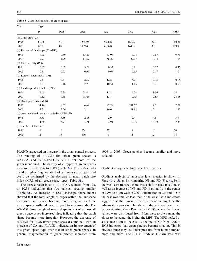
PLAND suggested an increase in the urban sprawl process.

The ranking of PLAND for urban green spaces is

AA[CAL[AGS[RoSP[PGS[P[RiSP for both of the

years mentioned. The density of all types of green spaces

increased from 1996 to 2000 (Table 3c). This index indi-

cated a higher fragmentation of all green space types and

could be confirmed by the decrease in mean patch size

index (MPS) of all green space types (Table 3f).

The largest patch index (LPI) of AA reduced from 12.8

to 10.34 indicating that AA patches became smaller

(Table 3d). An increase in LSI (landscape shape index)

showed that the total length of edges within the landscape

increased, and shape become more irregular as these

green spaces suffered more impact from surrounds. The

AWMSI (area weighted mean shape index) of almost all

green space types increased also, indicating that the patch

shape became more irregular. However, the decrease of

AWMSI for RiGS (river green spaces) combined with an

increase of CA and PLAND indicated an improvement of

this green space type over that of other green spaces. In

general, fragmentation of green patches increased from

1996 to 2003. Green patches became smaller and more

isolated.

Gradient analysis of landscape level metrics

Gradient analysis of landscape level metrics is shown in

Figs. 4a–g, 5a–g. By comparing NP and PD (Fig. 4a, b) in

the west–east transect, there was a shift in peak position, as

well as an increase of NP and PD in going from the center

in 1996 to 4 km west in 2003. Fluctuation in NP and PD in

the east was smaller than that in the west. Both indicators

suggest that the dynamic for this variation might be the

urbanization process. The above judgment was confirmed

by considering Mean Patch Size (MPS), where the lowest

values were distributed from 4 km west to the center, the

closer to the center the higher the MPS. The MPS peaked at

a distance 4 km to the east. A decline of NP from 1996 to

2003 indicated that green patches became smaller. This is

obvious since they are under pressure from human impact

more and more. The LPI in 1996 at 4–2 km west was

Table 3 Class level metrics of green spaces

Year Type

P PGS AGS AA CAL RiSP RoSP

(a) Class area (CA)

1996 86.66 50 1285.95 5326.8 1612.2 27.7 60.31

2003 66.2 89 1039.4 4156.8 1638.2 30 119.8

(b) Percent of landscape (PLAND)

1996 1.03 0.59 15.22 63.04 19.08 0.33 0.71

2003 0.93 1.25 14.57 58.27 22.97 0.34 1.68

(c) Patch density (PD)

1996 0.07 0.07 3.24 0.32 0.1 0.07 0.35

2003 0.51 0.22 6.95 0.67 0.15 0.17 1.04

(d) Largest patch index (LPI)

1996 0.4 0.4 2.57 12.8 8.71 0.13 0.18

2003 0.51 0.46 2.7 10.54 11.15 0.11 0.63

(e) Landscape shape index (LSI)

1996 6.65 6.28 28.4 11.8 6.04 8.36 14

2003 9.12 9.38 38.66 13.7 7.45 9.65 24.65

(f) Mean patch size (MPS)

1996 14.44 8.33 4.69 197.29 201.52 4.6 2.01

2003 5.51 5.56 2.1 86.6 148.92 2 1.62

(g) Area weighted mean shape index (AWMSI)

1996 3.53 3.56 2.85 2.9 2.4 4.5 3.9

2003 4.38 3.77 3.71 2.91 2.95 3.79 7.34

(i) Number of Patches

1996 6 6 274 27 8 6 30

2003 12 16 496 48 11 12 74


123

higher than that of the year 2003 showing that green spaces

at this distance became more fragmented and smaller

except other distances. This may indicate that some green

spaces were preserved as core areas while other green

spaces were reducing in area. Combining this result with

configurational metrics, we can quantify and understand

better the variation in urban green space patterns. As shown

in the Fig. 4e, LSI peaked at a distance around 4 km west

and in the transect center, suggesting that at these distances

the shape of urban green spaces is the most complex. This

seems to reflect different stages in urban development. The

center area is the old quarter and is very compact; the

neighboring areas belong to the government and French

colonial towns; and outside these are new urbanized areas

and urban fringes. However, the Mean Shape Index (MSI)

was stable along the transect and over time. While there

was a big fluctuation of AWMSI in the year 2003, espe-

cially in the center area to 3 km west, it then decreased

slightly on going eastward.

Like the west–east transect, the peak position of NP in

the south–north transect varied from near center (1996) to

4 km south (2003) and then reduced in both directions. The

NP of 2003 was much larger than that of 1996 and its

fluctuation in the south was stronger as well (Fig. 5a).

Together with NP, PD is one of the most important frag-

mentation indices, the PD of 1996 and 2003 peaked at

4 km south and its change in the north was lower than that

during 2003. The LPI for urban green spaces varied

irregularly with multiple peaks. At 4 km south, the varia-

tion of NP and PD was the strongest, but the fluctuation of

0

20

40

60

80

-8 -6 -4 -2 0

Number of Patches (NP) Patch density (PD)

0

30

60

90

120

Mean Patch Size (MPS) (ha)

0

30

60

90

Largest Patch Index (LPI)

0

20

40

60

80

100

Landscape Shape Index (LSI)

0

4

8

12

16

Mean Shape Index (MSI)

0

1

2

3

4

5

Area weighted mean shape index (AWSI)

0

1

2

3

4

5

6

7

Distance to center (km)

19962003

a b

dc

fe

g

West East

642

-8 -6 -4 -2 0 642 -8 -6 -4 -2 0 642

-8 -6 -4 -2 0 642-8 -6 -4 -2 0 642

-8 -6 -4 -2 0 642

-8 -6 -4 -2 0 642

Fig. 4 Gradient changes in

landscape level metrics of

Hanoi urban green spaces, from

west to east in the period

1996–2003


123

LPI and MPS was lowest. For MPS closer to the center,

there was a remarkable decrease comparing 2003–1996,

especially from a distance of 6 km southward. This is

evidence that these green patches here suffered more

pressure from surrounds. A decrease of LSI at 4 km south

suggested that the shape of green patches at this distance

became more complex, while in the center area there was

an improvement. The MSI showed no big changes along

the transect and a slight increase toward the center. Com-

pared to the west–east transect, variation in the MSI of the

south–east transect was bigger. The AWMSI seems to be

similar to the LSI, with the highest values being found at a

distance of 2 km south where the AWMSI then showing a

reduction at 4 km south. This was consistent with an

increase in NP and PD. The AWMSI then slightly

increased again at a distance of 6 km south. However, it

decreased toward the center when comparing 2003 and

1996. In general, the variation in landscape metrics of

urban green spaces in the south was stronger than that of

the north. The peak change was at around 4 km south

indicating that land use change at this distance was

greatest. Moreover one of the more interesting results, in

terms of configurational metrics, was found at the center

where the LSI, MSI and AWMSI for urban green spaces

declined on comparing 2003 and 1996. This revealed an

improvement in green patch shape.

Network analysis

The result of the node interaction (gravity model) of the 33

existing green patches with an area larger than 10 ha

(Table 4) and the common network types (Fig. 3) have

produced six different network scenarios from A to F

(Fig. 6). Specifically, the theory maximum expresses all

nodes connected each other including unfeasible links and

feasible links. Feasible links to connect these nodes are

identified based on the existing land use including corridors

(road green ways, etc.), open spaces, or other small green

spaces, and unfeasible links are virtual links or do not exist

in the reality (business areas, busy highways, etc.) (Linehan

et al. 1995). The network A based on the network model

Number of patches (NP)

0

10

20

30

40

50

60

-8 -6 -4 -2 0 4

Patch Density (PD)

0

50

100

150

200

Largest Patch Index (LPI)

0

25

50

75

100

Mean Patch Size (MPS) (ha)

0

10

20

30

40

50

Landscape Shape Index (LSI)

0

4

8

12

16

Mean Shape Index (MSI)

0

0.5

1

1.5

2

2.5

Area weighted mean shape index (AWSI)

0

2

4

6

Distance to center (km)

19962003

a

dc

fe

g

South North

2-8 -6 -4 -2 0 42

-8 -6 -4 -2 0 42

-8 -6 -4 -2 0 42

-8 -6 -4 -2 0 42

-8 -6 -4 -2 0 42

-8 -6 -4 -2 0 42

bFig 5 Gradient changes in

landscape level metrics of

Hanoi urban green spaces, from

south to north in the period

1996–2003


123

‘‘Least Cost to User’’, namely project max, expresses the

highest connectivity or connects all green spaces with all

feasible links. The network B, based on circle networking,

represents the connection of all largest nodes only. The

network C was built based on the network model ‘‘Paul

Revere’’ or branching network. The Network D was

developed following the network type ‘‘Traveling Sales-

man’’ or circle networking. The network E represents the

connection of the closest green patches as its name

‘‘Minimum Spanning Tree’’. Finally, the network F, based

on the ‘‘Least Cost to User’’, expressed the connection of

selected groups of green patches. The gamma, beta and

cost ratio were used to evaluate each graph model or net-

work scenario (Table 5). In addition to using gamma, beta

and cost ratio scenarios to evaluate networks, the circuitry

(a) and connectivity (c) indices were also used to analyze

network structure. These formulae were adopted by For-

man and Godron (1986), Hagget et al. (1977). In analyzing

networks, these indices are not as sensitive as the other

mentioned indices but they support connectivity analysis

more efficiently and clearly (Table 5).

Discussion

What is the driving force of green space change

in Hanoi?

Analyzing green space patterns over the entire landscape,

and analyzing gradients based on landscape metrics along

two transects, showed that green spaces have changed at

different distances and in different directions, from 1996 to

2003. However, analyzing synoptic characteristics of

landscapes as traditional ways that the averaging of land-

scape metrics over an entire study area may lead to

incorrect interpretation of the causal dynamics in the

region. As shown by Kong and Nakagoshi (2006, p. 12),

‘‘It is difficult to link changes in green space patterns in

local areas accurately with the processes that produced

these changes’’. This difficulty can be solved by using

gradient analysis or the ‘‘moving window’’ method com-

bined with spatially explicit landscape metrics. This

method can provide adequate quantitative information

about the structure and pattern of urban green spaces.

Therefore, a better link between pattern and process, and a

more effective capture of the dynamic changes can result.

Generally, there are two main driving forces causing the

urbanization process: population and economy (Ma et al.

2005). In addition, Luck and Wu (2002) recognize

urbanization as one of the most important driving forces

for land use and land cover change. When studying the

spatio-temporal green space change in Jinan City (China),

Kong and Nakagoshi (2006) found that the driving forces Ta

ble

4N

od

ein

tera

ctio

nb

ased

on

gra

vit

ym

od

el

No

de/

no

de

23

45

67

89

10

11

12

13

14

15

16

17

1.

23

32

0.5

32

80

.62

89

2.2

20

3.1

14

6.5

12

21

36

8.1

10

1.2

49

55

11

0.5

25

21

52

9.8

23

.81

12

.3

2.

00

00

14

08

0.9

80

13

.51

46

9.2

52

0.8

22

2.6

24

08

.41

61

.67

9.5

84

.91

62

.94

48

.52

34

5.3

35

.41

64

.7

3.

00

00

71

91

.31

26

.91

04

.62

11

.51

60

1.9

10

8.2

52

.75

3.6

10

1.3

28

7.9

14

.52

92

2.4

10

1.7

4.

00

00

10

53

99

4.2

18

97

65

60

37

21

68

.21

67

.42

79

.29

33

.94

2.3

84

.76

2.5

27

5.5

5.

00

00

78

.52

1.2

14

1.4

8.7

4.2

4.4

7.9

23

.41

.22

.31

.88

6.

00

00

20

.11

41

.89

4.3

4.5

8.1

24

1.2

2.3

1.8

6.2

7.

00

00

20

71

80

.53

6.2

13

.81

9.3

18

9.6

7.2

14

.51

04

2.1

8.

00

00

11

06

13

24

61

95

4.2

17

35

.31

61

30

36

6.6

73

3.2

42

81

65

1.6

9.

00

00

18

19

.54

69

.89

2.9

21

19

.96

02

.24

0.9

51

.41

81

.8

10

.0

00

08

47

.52

47

54

3.8

21

4.7

29

17

.27

0.2

11

.0

00

05

46

.76

12

.81

2.1

24

.31

5.5

65

.3

12

.0

00

05

29

.81

9.4

33

23

.21

02

.4

13

.0

00

06

09

.71

21

9.3

44

1.6

14

61

.9

14

.0

00

01

16

.71

87

.31

51

15

.0

00

03

19

.19

40

.3

16

.0

00

06

79

.7

17

.0

00

0


123

Ta

ble

4co

nti

nu

ed

No

de/

no

de

18

19

20

21

22

23

24

25

26

27

28

29

30

31

32

33

1.

11

6.9

34

4.2

18

4.2

14

07

.11

71

.51

11

1.4

19

59

.94

30

57

.31

06

6.2

80

6.9

14

85

.99

03

9.6

10

40

.41

07

2.6

13

20

2.

15

1.5

40

0.9

14

2.6

11

92

92

.78

26

.31

56

2.1

30

0.2

39

.37

13

.64

73

.87

83

.93

06

3.6

54

3.7

33

2.9

25

6.3

3.

94

.22

73

.39

0.1

60

9.4

39

.43

33

.26

22

.21

19

.22

2.1

25

0.7

16

4.6

26

78

45

.81

77

.68

6.3

57

.7

4.

24

0.3

60

6.6

22

5.5

11

94

.85

5.7

45

5.2

83

9.8

15

6.3

20

.93

32

20

5.7

33

0.4

93

0.5

22

5.3

97

.96

2.2

5.

7.2

18

6.9

41

.62

.52

1.2

38

.78

.61

16

12

.31

9.2

38

.81

36

.64

.6

6.

7.3

18

.27

38

.82

.51

8.7

38

.36

11

5.7

9.8

27

.54

7.9

10

.95

3.2

7.

34

77

.23

11

53

.66

.94

5.5

64

.31

11

.42

2.1

22

.31

9.7

53

.31

3.4

5.2

3.3

8.

11

31

13

74

55

2.1

27

33

12

2.1

6.5

11

45

19

52

5.8

39

3.8

19

2.5

24

1.2

60

11

61

.85

93

5.2

9.

12

0.6

24

91

04

.34

57

18

.61

24

.71

66

.61

7.7

2.5

34

.31

5.6

25

46

.71

2.9

4.6

2.7

10

.6

3.3

10

7.5

44

.22

03

8.5

57

77

.78

.51

.21

6.2

7.4

9.9

22

.86

.52

.31

.3

11

.6

1.2

11

1.1

44

.72

51

.49

.36

1.1

86

.79

.61

.41

8.3

7.6

11

.32

5.7

7.4

19

71

12

.1

01

.32

05

.48

04

72

.22

6.3

17

71

83

.12

1.3

31

9.6

15

.32

4.9

55

16

.15

.53

13

.7

26

.61

49

0.3

43

8.8

14

79

69

.25

41

.66

71

.97

69

.91

34

.65

3.9

68

.41

29

.43

71

3.1

7.4

14

.1

11

.31

47

.54

8.2

16

6.7

6.5

41

.75

0.4

5.6

0.7

41

1.6

4.4

5.6

8.4

2.8

0.7

20

.4

15

.2

60

.52

84

.71

52

.44

63

15

.61

05

.41

15

.71

31

.72

7.7

10

.61

32

2.7

6.6

1.4

0.8

16

.3

69

42

21

49

.54

30

.16

5.4

97

.21

06

.21

1.6

1.6

25

.47

.81

1.8

15

.96

.21

.20

.7

17

.4

03

8.7

25

16

.71

61

5.7

35

75

.51

09

.87

27

.57

17

.27

3.5

10

.21

69

.66

27

51

07

35

.59

.04

.4

18

.0

00

09

22

9.4

62

23

68

24

.21

75

.31

19

6.4

10

49

10

4.4

13

.52

50

.89

0.3

94

.51

41

.74

8.6

9.5

6

19

.0

00

08

22

72

11

03

54

23

70

03

24

43

23

41

.77

75

.52

78

19

3.6

43

8.3

15

0.4

29

.51

8.5

20

.0

00

02

04

78

.83

58

21

82

.71

69

6.7

14

9.9

19

.53

71

.61

27

.21

42

.61

94

.46

3.4

12

7.8

21

.0

00

01

25

21

75

93

42

81

25

19

50

.32

96

.35

94

2.5

17

08

.73

24

12

27

07

34

.21

25

88

.4

22

.0

00

04

51

3.8

50

15

.52

30

.43

1.7

35

3.2

10

1.6

10

61

34

.94

3.6

7.4

5.3

23

.0

00

04

78

70

.81

77

3.3

25

5.9

65

59

.71

47

5.7

12

77

14

39

.24

52

.27

2.1

52

.8

24

.0

00

01

34

09

21

03

11

06

5.4

24

90

.82

21

1.1

25

30

.38

16

.91

31

.79

5.9

25

.0

00

01

05

52

74

4.5

77

6.2

60

2.4

59

8.3

18

8.4

27

.32

1.5

26

.0

00

01

10

5.2

13

4.5

90

88

27

.33

.83

27

.0

00

06

92

8.7

26

24

.32

02

2.9

60

17

0.4

61

.6

28

.0

00

05

06

9.5

22

11

.55

95

.65

3.3

54

.8

29

.0

00

05

03

5.7

25

44

13

21

04

.9

30

.0

00

01

21

62

54

8.2

20

25

31

.0

00

02

62

.55

7

32

.0

00

01

10

.4

33

.0

00

0

Bec

ause

Gab

=G

ba

soth

atth

ista

ble

issy

mm

etri

cal

and

itis

un

nec

essa

ryto

calc

ula

teb

oth

val

ues

(Lin

ehan

etal

.1

99

5)


123

Fig. 6 The different scenarios

from A to F based on graph

theory

Table 5 Evaluating networks

Name Network model Nodes Links Total distance (km) Gamma raw

adjusted

Beta Cost ratio Circuitry

index

Connectivity

index

Theory max 33 528 Not applicable 1 16 Not applicable Not applicable

A Project max 33 61 149 0.115 1.85 0.60 1 0.457 0.656

B Major nodes 10 10 44 0.019 1 0.73 0.164 0.05 0.107

C Paul Revere 33 32 76.8 0.06 0.97 0.58 0.525 0 0.343

D Traveling salesman 33 33 78.9 0.0625 1 0.58 0.54 0.015 0.352

E Minimum spanning

tree (MST)

33 32 61.5 0.06 0.97 0.48 0.525 0 0.343

F Small circuit group 33 37 99.3 0.07 1.12 0.62 0.606 0.098 0.398


123

are policy affecting the development and management of

urban green spaces, and urbanization. Moreover, the urban

sprawl direction was influenced by green space changes

and vice versa urbanization caused changes in the spatial

pattern of green areas. It is obvious that in different con-

ditions, the driving forces will be different. In Hanoi,

through an analysis of the spatio-temporal change of green

space pattern combined with economic, social data, and

development policy, we found that there were several

reasons for this change. Firstly, the population increase in

the downtown area in the period 1995–2005 was from

1.275 to 2 million with a rate of increase of 4.6%. The rural

population decreased from 52% (1996) to 42.4% (1999),

and the agricultural labor force and non-agricultural labor

force in this period were 32, 68% and 30.2, 69.8%

respectively. This is mainly rural-urban migration because

the birth rate is around 1.3%. Especially, the establishment

of new urban districts including Thanhxuan, Tayho and

Caugiay in this period from rural districts at the south and

west of Hanoi was a main factor, which contributed to an

increase of the urban population (http://www.hanoi.gov.vn

). Moreover, analyzing land-use showed that the rapid

reduction in area of agricultural land (1,200 ha) and

attached green spaces (200 ha), especially in the south and

west as indicated by gradient analysis reflects that the

development of the city not only occurred at the fringes

because of the urban-sprawl process, but also in the city

itself making it more compact in terms of population

density. Another important driving force is the growth of

economy. The year 1995 marked a turning point for

Vietnamese economy in general and Hanoi in particular

when Vietnam and the United States of America normal-

ized the relationship. This led to the first wave of foreign

investment in this period. As a result, the economic growth

of Hanoi city was over 10% per year. The economic

mechanism for industry, services, and agriculture changed

from 38, 58.2 and 3.8% (1996) to 41.5, 55.5 and 3%

(2005). New urbanized areas, roads, business areas and

other infrastructure areas were built to meet the needs of

urbanization, whereby mainly agricultural land (AA) was

converted into built-up areas. One of the most important

driving forces was the lack of suitable planning, and

weakness in controlling and managing the development of

Hanoi. This was evident through the orientation of the

Hanoi Master Plan being mainly westward and northward

(Decision 108/1998/QÐ-TTg 1998), yet our analysis

showed that development mainly occurred in the westward

and southward directions. In other words, the planning

policy for non-west regions in Hanoi up to 2020 prioritizes

development to the north, but not the south (Decision 108/

1998/QÐ-TTg). However, variation in urban green spaces

occurred mainly in the south, not the north, suggesting that

changes in land use in the south have been stronger since

1996. This might result from the urbanization process.

Finally, we could say that policy on the orientation of the

Hanoi development was not strongly effective and well

controlled in that direction. Besides, a plan for developing

urban green spaces in the period 2001–2005 increased from

4 to 5–6 m2 but this analysis has showed that some types of

urban green spaces (public green space, riverside green

space and roadside green space) had a slight increase

around 100 ha while other green spaces (attached green

space, park) decreased around 250 ha. Thus, it is necessary

to inspect and evaluate the effectiveness and efficiency of

this plan.

In brief, the five main reasons leading to changes in

green spaces from 1996 to 2003 were land use change,

economic growth, population increase, urbanization, and

weakness in planning, controlling and managing the urban

development. These changes are reflected in a reduction

not only in area and quality of green spaces, but also that

green patches were more irregularly shaped and unevenly

distributed. Changes in urban green space patterns will

affect ecological processes, leading to a decline in eco-

service quality and in making the city less sustainable. To

improve this circumstance, it is imperative to conserve and

build a green network, which optimizes the benefits of

green spaces as much as possible.

Which network is the best?

Graph theory and the gravity model give us useful methods

in analyzing networks and are especially suitable for

planning eco-networking because they are unbiased or non-

discriminatory methods in determining different levels of

interaction between nodes. Connectivity indices are found

to be useful measures for describing the degree to which

green spaces are connected (Linehan et al. 1995). A good

network is one that satisfies all criteria (gamma, beta and

cost ratio), is appropriate for the site conditions, and takes

into account the feasibility of the network. Habitat con-

nectivity is analyzed by linking high-quality habitat

patches along least-cost paths though this parameterized

cost surface (O’Brien et al. 2006).

Study results showed that networks based on theory max

and project max models (network A) were ideal for con-

servation because they had the greatest consecutiveness (1

for theory max and 0.115 for project max). They also had

the most complicated networks with a beta index of 16 and

1.85 respectively, but their existence is not real and feasi-

ble. As demand for land to develop grows with the

population, cities can usually only afford to preserve a few

large green spaces (Rudd et al. 2002). Network B was built

based on major nodes (ten nodes). These major nodes were

connected to make a single circle. Network B had the


123

http://www.hanoi.gov.vn

lowest raw and adjusted gamma indices with 0.019 and

0.164, which expressed the lowest connectiveness within

the network so that it had the lowest value in maintaining

biodiversity among the six scenarios although the cost ratio

was the greatest at 0.73. If we only considered cost ratio

index, network B would be the best. However, a good eco-

network needs to satisfy all gamma, beta and cost ratio

indices. Therefore, using only one or a few indices could

lead to a misleading network interpretation (Linehan et al.

1995; Rudd et al. 2002). Networks C and E were also not

suitable for building an eco-network because their beta

indices were under 1, indicating that the networks were not

complete circuits and all nodes were not linked together.

These factors act to reduce the accessibility or ease of

movement and dispersal of species between nodes. The

beta index of networks C and E was 0.525, which was

lower than that of networks D (0.54) and F (0.62). For

network E, the cost ratio index was the lowest (0.48). This

means that ‘‘cost to user’’ (wildlife) was highest. The

results of analysis of networks B, C and D were consistent,

with node structure analysis, circuitry, and connectivity

indices of: 0.05; 0; 0 and 0.107; 0.343; and 0343,

respectively.

Networks D and F seem to be more attainable in terms

of this urban context because their network structure (beta

indices of 1 and 1.15, respectively) had enough complexity

to maintain biodiversity in urban areas. Based on assess-

ment using gamma, beta, and cost-to-user criteria, and on

using circuitry and connectivity sub-indices, network F was

the best because it had the greatest raw gamma and

adjusted gamma values. Networks A and B which had

similar or higher such values were excluded because of

lack of feasibility. The beta index of network F was 1.12

with four loops so that its network structure was

Fig. 7 The 2020 Hanoi Master

Plan (sources: Hanoi

Government 2005)


123

complicated and ecologically better than that of network D

(1). The ‘‘cost to user’’ value of network F (0.62) was also

greater than that of network D (0.58), or 4%. However, the

link-use efficiency for network D was 0.42, i.e. higher than

that of F’s at 0.37. Linehan et al. (1995) showed that the

effects of the various links can be systematically tested in

terms of link efficiency, as measured by the amount of

connectivity achieved per unit distance. From this per-

spective, Network F was the best option or best model of

the six network scenarios. Thus, network F needs to be

maintained as the primary greenbelt or inner greenbelt in

Hanoi’s planning in the near future. Network F not only

resists the sprawl process of urbanization but also meets the

requirements of eco-network building and biodiversity.

The next best alternative network was network D. Some

researchers argue that building eco-networks by using

graph theory applied to a similar habitat such as paddy

fields, should be connected with that, i.e. paddy field,

ecology but in fact in this study it is not necessary because

of two reasons. Firstly, there are many species that live in

multiple habitat areas even some species only exist in a

specific habitat, the different habitats are considered as

open spaces acting as corridors or stepping stones for the

survival of species. Moreover, this network is to cover a

variety of species. Secondly, they have potential to develop

into equivalent habitats such as parks, public green spaces

or protected areas.

The results of this analysis give some implications for

the 2020 Urban Green Space Planning in Hanoi (Hanoi

Government 2005). In this plan, Hanoi city will allocate the

per capita 18 m2 for green spaces and sports-fields. In that,

improvements are planned for green spaces, parks, and

flower gardens together with developing green spaces near

big lakes as heart green spaces of city. The creation of

newly planted rows of trees and shrubbery is for ecological

protection of landscapes between the banks of the rivers

(Fig. 7). In addition, at the regional scale, a greenbelt will

be created with a width of 1–4 km for natural and eco-

logical preservation. From the results of this analysis,

almost all green nodes of network F are consistent with the

2020 planned green spaces. However, many of them are

not connected or still isolated. Thus, network F will pro-

vide a basis for enhancing the connectivity of the planned

green spaces by maintaining and creating suitable corri-

dors. This is appropriate with the Vietnamese standard

(TCXDVN 362: 2005), which requires that the city has to

allocate the per capita roadside green space about 1.7–

2 m2. Moreover, in the 2020 Green Space Planning, it

mainly focuses on the roles and functions of parks and

public green spaces but ignores those of small green spaces

such as attached green spaces etc., which also play an

important role in urban green structure. This structure will

create a green network ecologically for the city more

effective than the sum of the individual green spaces.

In conclusion, gradient analysis with the support of

FRAGTATS 3.3 is useful and effective for quantifying

spatial pattern and ecological processes. The results of

this study showed spatial–temporal changes of green

spaces in Hanoi from 1996 to 2003. Green spaces became

smaller and smaller, and more fragmented. This causes

not only the loss of biodiversity but also a reduction in

the quality of ecological services and the quality of life of

urban dwellers in this period. Thus, it is necessary to

build and preserve green spaces. Graph theory has been

proved to be a useful tool in studying the landscape

connectivity, especially in studying ecological networks.

Linehan et al. (1995) stated that graph theory was well

suited to landscape ecology and landscape planning on a

theoretical and scientific basis, and that graph theory

helped systematize greenway planning which in turn,

helped give it additional credence as an important land-

use strategy. Based on the analysis of graph theory, we

have selected one network as the best option for building

an urban ecological network and preserving green spaces

in the greater Hanoi city region. This is a potential net-

work for conserving biodiversity and is fundamental in

planning comprehensive urban green spaces in Hanoi.

Acknowledgments We would like to thank the Hanoi government

offices for offering data on the Hanoi Master Plan; Prof Dr. Xiuzhen

Li, Institute of Applied Ecology, Chinese Academy of Sciences,

Shengyan for giving her valuable suggestions; and many thanks to all

members of the Nakagoshi laboratory for giving their comments and

encouragement and Mr Nick Walker for English checking. This

research was supported by the COE (the twenty-first century Center of

Excellence) programme, and the Social Capacity Development for

Environmental Management and International Cooperation pro-

gramme in Hiroshima University.

References

Bunn AG, Urban DL, Keitt TH (2000) Landscape connectivity: A

conservation application of graph theory. J Environ Manage

59:265–278

Circular No 20/2005/TT-BXD (2005) Instruction on managing plants

in urban areas (in Vietnamese). Ministry of Construction,

Vietnam

Decision 108/1998/QÐ-TTg (1998) Decision of Prime Minister about

the approval on adjustments of Hanoi Master Plan up to 2020 (in

Vietnamese). Hanoi, Vietnam

Forman RTT, Godron M (1986) Landscape ecology. Wiley, New

York

Gross J, Yellen J (1999) Graph theory and its application. CRC,

Florida

Hagget P, Cliff AD, Fry A (1977) Locational analysis in human

geography, 2nd edn. Wiley, New York, p 454

Hanoi Government (2005) The 2020 Hanoi Master Plan. This is

available at http://www.hanoi.gov.vn/hnportal/render.user

LayoutRootNode.uP


123

http://www.hanoi.gov.vn/hnportal/render.userLayoutRootNode.uP

http://www.hanoi.gov.vn/hnportal/render.userLayoutRootNode.uP

Kong F, Nakagoshi N (2006) Spatial and temporal gradient analysis

of urban green spaces in Jinan, China. Landsc Urban Plan

78:147–164

Linehan J, Meir G, John F (1995) Greenway planning: developing a

landscape ecological network approach. Landsc Urban Plan

33:179–193

Luck M, Wu J (2002) A gradient analysis of urban landscape pattern:

a case study from the Phoenix metropolitan region, Arizona,

USA. Landsc Ecol 17:327–339

Ma K, Zhou L, Niu S, Nakagoshi N (2005) Beijing urbanization in the

past 18 years. J Int Dev Cooper Hiroshima Univ 11:87–96

McGarigal K, Ene E, Holmes C (2002) FRAGSTATS (version 3):

FRAGSTATS Metrics. University of Massachusetts-produced

program. Available at the following website: http://www.umass.

edu/landeco/research/fragstats/documents/Metrics/Metrics%20

TOC.htm

O’Brien D, Micheline M, Andrew F, Fortin M-J (2006) Testing the

importance of spatial configuration of winter habitat for wood-

land caribou: an application of graph theory. Biol Conserv

130:70–83

Rudd H, Jamie V, Valentin S (2002) Importance of backyard habitat

in a comprehensive biodiversity conservation strategy: a con-

nectivity analysis of urban green spaces. Restor Ecol 10:368–375

TCXDVN 362: 2005 (2005) Vietnamese construction standard:

Greenery planning for public utilities in urban areas-Design

standards (in Vietnamese)

Yu XJ, Ng CN (2007) Spatial and temporal dynamics of urban sprawl

along two urban-rural transects: a case study of Guangzhou,

China. Landsc Urban Plan 79:69–109

Yen MD (2005) Inventory and evaluation of biodiversity in Hanoi—

Enhancing awareness of community and proposing the solutions

for conservation (in Vietnamese). Summary report, Hanoi

Biological Association

Zhang L, Wang H (2006) Planning an ecological network of Xiamen

Island (China) using landscape metrics and network analysis.

Landsc Urban Plan 78:449–456

Zhu M, Xu J, Jiang N, Li J, Fan Y (2006) Impacts of road corridors on

urban landscape pattern: a gradient analysis with changing grain

size in Shanghai, China. Landsc Ecol 21:723–734


123

http://www.umass.edu/landeco/research/fragstats/documents/Metrics/Metrics%20TOC.htm



Analyzing urban green space pattern and eco-network in Hanoi, Vietnam

Documents

Transcript of Analyzing urban green space pattern and eco-network in Hanoi, Vietnam