Bias correction and Bayesian analysis of aggregate counts in SAGE libraries

METHODOLOGY ARTICLE Open Access

Bias correction and Bayesian analysis ofaggregate counts in SAGE librariesRussell L Zaretzki1*, Michael A Gilchrist2*, William M Briggs3, Artin Armagan4

Abstract

Background: Tag-based techniques, such as SAGE, are commonly used to sample the mRNA pool of anorganism’s transcriptome. Incomplete digestion during the tag formation process may allow for multiple tags to begenerated from a given mRNA transcript. The probability of forming a tag varies with its relative location. As aresult, the observed tag counts represent a biased sample of the actual transcript pool. In SAGE this bias can beavoided by ignoring all but the 3’ most tag but will discard a large fraction of the observed data. Taking this biasinto account should allow more of the available data to be used leading to increased statistical power.

Results: Three new hierarchical models, which directly embed a model for the variation in tag formationprobability, are proposed and their associated Bayesian inference algorithms are developed. These models may beapplied to libraries at both the tag and aggregate level. Simulation experiments and analysis of real data are usedto contrast the accuracy of the various methods. The consequences of tag formation bias are discussed in thecontext of testing differential expression. A description is given as to how these algorithms can be applied in thatcontext.

Conclusions: Several Bayesian inference algorithms that account for tag formation effects are compared with theDPB algorithm providing clear evidence of superior performance. The accuracy of inferences when using aparticular non-informative prior is found to depend on the expression level of a given gene. The multivariatenature of the approach easily allows both univariate and joint tests of differential expression. Calculationsdemonstrate the potential for false positive and negative findings due to variation in tag formation probabilitiesacross samples when testing for differential expression.

BackgroundTag-based transcriptome sequencing libraries consist ofa collection of short sequences of DNA called tags alongwith tabulated counts of the number of times each tag isobserved in a sample. These observed tag counts repre-sent a sample from a much larger pool of mRNA tagsin a tissue or organism. In the past, Serial Analysis ofGene Expression (SAGE) was the most commonly usedtechnology for generating libraries of tag counts. SAGElibraries have been used to address a number of biologi-cal questions including: estimating transcriptome size,and estimating the density of relative expression levels.Most frequently, SAGE was used to assess differential

expression across cells from different tissues or strains,or cells grown under different experimental conditions.Next generation methods such as Digital Gene Expres-sion (DGE) tag profiling [1] now provide a more effi-cient method to generate tag libraries and are growingin popularity. Libraries based on DGE are used toaddress the same questions and provide much largernumbers of tags leading to increased statistical power.However, the close similarities between DGE and SAGE,particularly the use of restriction enzymes, lead bothtechniques to share the same inherent biases.As has been repeatedly noted in both SAGE and DGE

studies e.g. [1-4], the mRNA from a single gene can leadto the production of more than one type of tag within thesame library. Observing multiple tags from a single genecomplicates data analysis and has a number of potentialcauses including alternative mRNA splicing and incom-plete cDNA digestion. Incomplete digestion typically

* Correspondence: [email protected]; [email protected] of Statistics, Operations, and Management Science, TheUniversity of Tennessee, 331 Stokely Management Center, Knoxville, TN,37996, USA2Department of Ecology and Evolutionary Biology, The University ofTennessee, 569 Dabney Hall, Knoxville, TN, 37996, USA

Zaretzki et al. BMC Bioinformatics 2010, 11:72http://www.biomedcentral.com/1471-2105/11/72

© 2010 Zaretzki et al; licensee BioMed Central Ltd. This is an Open Access article distributed under the terms of the Creative CommonsAttribution License (http://creativecommons.org/licenses/by/2.0), which permits unrestricted use, distribution, and reproduction inany medium, provided the original work is properly cited.

mailto:[email protected]

mailto:[email protected]

http://creativecommons.org/licenses/by/2.0

results in a number of different tags being formed fromthe same mRNA transcript. Alternative splicing can leadto multiple mRNA isoforms within a sample. When com-bined with incomplete digestion, each of these isoformsmay give rise to a different tag or group of tags.While it is intuitively sensible to analyze the preva-

lence of an mRNA by aggregating multiple tags derivedfrom it, such tags are often analyzed separately [5]. Atbest, this approach diminishes the statistical power thatis available when testing differences in mRNA abun-dances and reduces the accuracy of inferences based onasymptotic statistical methods (chi-square tests). Moreseriously, such comparisons can result in dramaticbiases leading to erroneous conclusions in testing differ-ential expression due to varying levels of incompletedigestion across libraries.The current work extends an earlier analysis [6] based

on SAGE libraries generated using the yeast Saccharo-myces cerevisiae [7]. Alternative splicing is generally rarein microorganisms such as S. cerevisiae so that the tagmultiplicity observed in these libraries is primarilyattributed to incomplete cDNA digestion. The firstobjective of the current work is to provide a methodol-ogy that allows multiple tags, which arise due to incom-plete digestion, to be combined and used to inferexpression levels of the underlying mRNA transcripts.Aggregation is complicated by the fact that certain tagsare more likely to form than others due to processingmethods [4,6]. Unless the tag formation probabilities areaccounted for, inferences based on aggregate tag countsmay be highly biased.Previously, we have addressed the problem of estima-

tion bias by directly modeling the variation in tag for-mation and deriving bias corrected maximum likelihoodand posterior mode estimators of the composition ofthe mRNA population [6]. However, a number ofassumptions and difficulties limit the application ofthese techniques. We address these in the present study.Three new hierarchical models for SAGE data are intro-duced that directly correct for the bias by embedding amodel of tag formation within the probability distribu-tion describing the data. Corresponding Gibbs samplingalgorithms suitable for model fitting and inference arealso derived. These methods are computationally effi-cient and allow a more general class of prior distribu-tions than earlier analytic approaches. The results arealso applicable for both aggregate and standard tagcounts. We use simulation studies and analysis of pub-licly available data from S. cerevisiae [7] in order to con-trast the accuracy of our sampling methods and analyzethe effects of priors. The approach we present shouldserve as a building block for a more comprehensivemethod that takes into account the effects of bothincomplete digestion and alternative splicing.

A second major objective of the current work is toexplore the general effects of tag formation bias on dif-ferential expression. We carefully demonstrate that, inthe absence of proper adjustments, variation in tag for-mation probability across experiments can lead to bothfalse positive and false negative conclusions regardingthe differential expression of a gene. A brief descriptionof the implementation of proposed algorithms in differ-ential expression analysis is also provided. While theapproaches presented here require more work in proces-sing and preparation than studies that focus on indivi-dual tags, they may offer a significant advantage withrespect to statistical power in studies of differentialexpression.A number of statistical methodologies have been

developed to analyze SAGE libraries. For studies thatfocus on relative expression levels, individual tags areviewed as possible outcomes from a multinomial sam-pling model [7,8]. [9] offered an improvement on this bydirectly applying a Bayesian multinomial-mixtureDirichlet model to the observed vector of tag countswhich improves accuracy in estimation of tag frequency.Marginal analysis may be more useful in studies of tran-scriptome size and was developed by [10] and [11,12].Statistical methods to assess differential expressionacross a number of samples were discussed by [13-16].These analyses typically test the differential expressionof each tag across libraries independently; see [14].

The SAGE MethodologyThe goal of a SAGE experiment [8] is to sample themRNA population within a group of cells. Broadlyspeaking, the SAGE method generates a set of shortsequence-based cDNA tags from the mRNA population.Initially, a pool of mRNA is extracted from a group ofcells. The unstable single stranded mRNA is reversetranscribed into a double stranded DNA copy (cDNA)using a modified primer that allows the cDNA to bebound to a streptavidin bead. Using restriction enzymes,the bead-bound portion of cDNA is cut into small ‘tags’that are concatenated together into longer cDNA mole-cules referred to as concatemers. These concatemers areamplified using PCR and then sequenced. A cleavagemotif of the anchoring enzyme allows the start and stoppoints of tags to be identified within a concatemer. Eachtime a tag from a specific gene is observed in thesequence data, it contributes a count to the library. TheDGE technology follows a similar procedure in the firstseveral steps. However, tags are neither concatenatednor cloned but sequenced immediately.In both technologies the restriction enzymes used to

create the tags cut at very specific sites within thecDNA. For example, the restriction enzyme used by [8]cleaves only at the four nucleotide motif CATG. Thus,


of 15

tags can only be created at specific points within acDNA. Because the site where the cDNA is cut servesas an ‘anchor’ between tags, the restriction enzyme usedis often referred to as the anchoring enzyme (AE). Werefer to the specific points in the cDNA cleaved by theanchoring enzyme as AE sites.While some genes will have no AE sites, many genes

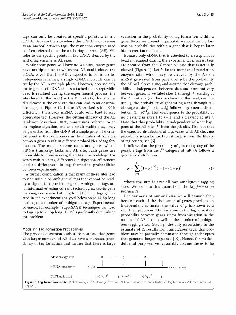
have multiple sites at which the AE could cleave thecDNA. Given that the AE is expected to act in a site-independent manner, a single cDNA molecule can becut by the AE in multiple places. However, because onlythe fragment of cDNA that is attached to a streptavidinbead is retained during the experimental process, thesite closest to the bead (i.e. the 3’ most site) that is actu-ally cleaved is the only site that can lead to an observa-ble tag (see Figure 1). If the AE worked with 100%efficiency, then each mRNA could only lead to oneobservable tag. However, the cutting efficacy of the AEis always less than 100%, sometimes referred to asincomplete digestion, and as a result multiple tags maybe generated from the cDNA of a single gene. The criti-cal point is that differences in the number of AE sitesbetween genes result in different probabilities of tag for-mation. The most extreme cases are genes whosemRNA transcript lacks any AE site. Such genes areimpossible to observe using the SAGE methodology. Forgenes with AE sites, differences in digestion efficiencieslead to differences in tag formation probabilitiesbetween experiments.A further complication is that many of these sites lead

to non-unique or ‘ambiguous’ tags that cannot be read-ily assigned to a particular gene. Ambiguous tags are‘uninformative’ using current technologies; tag-to-genemapping is discussed at length in [17]. The tags gener-ated in the experiment analyzed below were 14 bp longleading to a number of ambiguous tags. Experimentaladvances, for example, ‘SuperSAGE’ techniques can leadto tags up to 26 bp long [18,19] significantly diminishingthis problem.

Modeling Tag Formation ProbabilitiesThe previous discussion leads us to postulate that geneswith larger numbers of AE sites have a increased prob-ability of tag formation and further that there is large

variation in the probability of tag formation within agene. Below we present a quantitative model for tag for-mation probabilities within a gene that is key to laterbias correction methods.Because only cDNA that is attached to a streptavidin

bead is retained during the experimental process, tagsare created from the 3’ most AE site that is actuallycleaved (Figure 1). Let ki be the number of restrictionenzyme sites which may be cleaved by the AE onmRNA generated from gene i, let p be the probabilitythe AE will cleave a site, and assume that cleavage prob-ability is independent between sites and does not varybetween genes. If we label sites 1 through ki starting atthe 3’ most site (i.e. the site closest to the bead; see Fig-ure 1), the probability of generating a tag through AEcleavage at site j Î {1, ..., ki} follows a geometric distri-bution, (1 - p)j-1p. This corresponds to the probability ofno cleaving in sites 1 to j - 1, and a cleaving at site j.Note that this probability is independent of what hap-pens at the AE sites 5’ from the jth site. The fact thatthe expected distribution of tags varies with AE cleavageprobability p can be used to estimate p from the libraryof tag counts; see [6].It follows that the probability of generating any of the

possible tags from the ith category of mRNA follows ageometric distribution

ij

j

kk

p p pi

i

1 1 1

1

1

(1)

where the sum is over all non-ambiguous taggingsites. We refer to this quantity as the tag formationprobability.For purposes of our analysis, we will assume that,

because each of the thousands of genes provides anindependent estimate, the value of p is known to avery high precision. The variation in the tag formationprobability between genes stems from variation in thenumber of AE sites as well as the number of ambigu-ous tagging sites. Given p, the only uncertainty in theestimate of ji results from ambiguous tags; this pro-blem may be partially eliminated through techniquesthat generate longer tags; see [19]. Hence, for metho-dological purposes we reasonably assume the ji to be

Figure 1 Tag formation model. Plot showing cDNA cleavage sites for SAGE with associated probabilities of tag formation. Adopted from [[6],Figure 1].


of 15

known constants (see [6] for a more details on thesecalculations). As a result, the tag pool represents abiased sample of the mRNA population of interestbeing a function of both the known distribution of tagformation probabilities across the genome, and the dis-tribution of these genes within the mRNA populationitself.Traditionally, a gene’s frequency in the tag pool was

assumed to be an unbiased estimate of its frequency inthe mRNA population, the population of interest. Thisequivalence only holds when all genes have the sametag formation probability, a condition that is never met.Consequently, genes with greater than average tag for-mation probabilities will be over-represented whilethose with lower than the average probability will beunder-represented. Equation (1) allows us to accuratelyestimate this sampling bias and correct the inferencesmade from tag libraries.Before the tag counts are considered, we assume that

the data is processed to retain only informative tags, i.e.all ambiguous or orphan tags are removed, as is standardpractice. Let the vector t = (t1, ..., tl) represent the aggre-gated observed tag counts for individual genes. Here l isthe number of genes that contain at least one unambigu-ous AE site and ti is the total number of observed tagsthat can uniquely be attributed to an AE site in gene i.(Note that standard dis-aggregated counts are simply aspecial case of the aggregated counts given above with ji

representing a single element within the summation termin Eq. (1).) It is natural to view this vector as a samplefrom a multinomial distribution with l categories, t~Multi (ttot, θ) where θ = (θ1, ..., θl), θi represents the fre-quency of tags from gene i in the tag pool, and

t ttot ii

l 1is the total count of all observed tags.

Because the variation in tag formation probabilities ji

distorts the abundances of observed tags, it is clear thatθi represents a biased estimate of the true proportion ofmRNA from gene i in the overall pool. Unfortunately,this true proportion of mRNA, denoted mi, is clearly thequantity of interest. [6] relates the biased proportion θi tomi with the following simple expression:

i

mi im j jj

(2)

where ji is the known tag formation probability basedon Eq. (1) and the proportions mi are positive and sumto one. The bias corrected likelihood model is then,

Lt

t t tmi im j jj

tot

l i

t i

m t|, , ,

1 2

(3)

Direct maximization of the likelihood with respect tothe parameters mi is straightforward due to the fact thatthe likelihood function is maximized at the same loca-tion irrespective of the way the model is parameterized.Consider the observed sample proportion i = ti/ttot.The fact that the mi are positive and must sum to onealong with Eq. (2) force the maximum likelihood esti-mates of ˆ { ˆ , ˆ , , ˆ }m m m ml1 2 to satisfy the followingequality,

ˆ

ˆ.

ii mi ii

li

l

1(4)

While computation of the maximum likelihood esti-mates (MLE’s) is relatively straightforward, constructingconfidence intervals for m is difficult. The existence ofthe normalization term ∑jmjjj in the denominator ofthe left hand side of Eq. (4) makes computation of Fish-er’s information matrix taxing, particularly for the largedimensional vectors encountered when working withSAGE data (i.e. l is of the order 103 to 104). In addition,because the number of categories is generally within anorder of magnitude of, or possibly even greater than, thenumber of tags sampled, most categories have eitherzero or only a few observations. These relatively smallcounts call into question inferences such as chi-squaredtests which are based on asymptotic approximations.As an alternative, we consider a Bayesian approach to

the problem. The constraints lead naturally to theassumption of a Dirichlet prior on m,

m ~ , , ,D i

iil

mii

i

lk l

1

1

1

1

where ai is the parameter describing any prior infor-mation we have on the value of mi. Combining thisprior distribution with the likelihood function given inEq. (3) leads to a posterior distribution proportional tothe product

Pr | ( ) .m t

m mi i

i

lt

i it

i

ltot i i

1

1

1

(5)

[6] introduces methods for the direct maximization ofthis quantity and discusses the choice of a prior and itsconsequences on the marginal inferences for individualvalues of mi. However, a number of difficulties severelylimit the range of prior parameters that can be used; i.e.those priors with appreciable weight relative to theobserved sample sizes. Given the bias in the observeddata, the Gibbs sampling based approaches for inferencebased on the posterior of the mRNA proportions


of 15

introduced here are more flexible, and require fewerassumptions than analytic techniques. The methods arealso highly computationally efficient. While the assump-tion of independent cleaving resulted in a geometricmodel, it is important to note that alternative models oftag formation can be substituted into the Bayesian algo-rithms without making any further adjustments to themodel.

Shrinkage Estimation in Multivariate ModelsJoint estimators of the relative proportions of individualtags in SAGE experiments based on posterior meansfrom a conjugate Dirichlet-Multinomial model wereexplored by [9] and have similar properties to the meth-ods proposed here. In the case of flat priors (i.e. ai = 1for all i), they note that while the posterior mean pro-vide improved average accuracy with respect to sums ofsquared errors across all categories, estimates of cate-gories where large counts are observed were shrunkexcessively in order to boost the estimated probabilitiesof cells with few or no counts. Due to the massive num-ber of categories and the extreme imbalance in observedfrequencies (e.g. more than half of the categories havezero counts in our data), the estimates for frequentlyobserved genes tend to consistently underestimate thetrue proportions while the reverse is true of genes withvery low expression proportions. This observation high-lights the main weakness of shrinkage estimators suchas the posterior mean. While they perform better onaverage across categories, they may perform poorly onparticular categories that may be of primary interest. [9]addresses this issue by proposing a mixture of Dirichlet-Multinomial’s but does not discuss the issue of samplingbias. Note that after aggregation, the large reduction inthe number of categories significantly reduces the sideeffects of shrinkage leading to improved inferences.These observations will be useful in analyzing the biascorrected models proposed below.

Results and DiscussionHierarchical Models and Gibbs SamplingThree hierarchical approaches are proposed to modelaggregate tag counts while taking into account the tagformation probability. The Dirichlet-Poisson-Binomialmodel (DPB) extends the method of [10], who modeledtag counts as independent random variables from aPoisson-Gamma mixture to a multivariate setting thatmodels the joint distribution of tags. The Dirichlet-Mul-tinomial-Binomial model (DMB) views the unobservedtrue counts of mRNA in the population as being derivedfrom a multinomial distribution. The missing-datamodel (MD) assumes that if the number of mRNA tran-scripts that were not converted into tags due to incom-plete digestion by the anchoring enzyme, denoted r,

were known then the data could be modeled as a stan-dard Dirichlet-Multinomial model. By proposing a Pois-son distribution for r, posterior inferences can be made.Detailed descriptions for these algorithms are given inthe Methods section. Gibbs samplers based on thesealgorithms all produce posterior samples of m, the vec-tor of relative proportions of each gene in the mRNApopulation. In addition, DPB produces samples repre-senting N, the hypothetical total number of mRNA tran-scripts in the population while MD produces posteriorsamples of r, the number of unconverted transcripts.These quantities may be relevant in studies of the num-ber of unique transcripts.A Dirchlet prior distribution was assumed for the pro-

portion vector m in all three algorithms. Two parametervectors = (a1, ..., al) were tested. The flat prior setsai = 1 for all i while the tub prior sets ai = 1/l. The flatprior effectively assumes that a hypothetical previousexperiment produced 1 tag for each category. As thename suggests, the flat prior represents a uniform den-sity over the parameter space. The tub prior assumesthat the prior information is equivalent to that of a sin-gle tag. The density of this prior takes a bowl or tubshape. The preponderance of mass along the edgesforces the estimates of mi to be small unless significantcounts are observed for that gene.To analyze performance, we applied each algorithm to

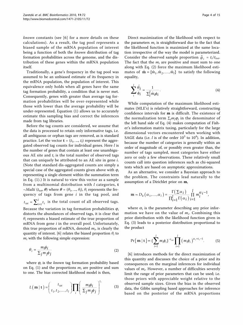
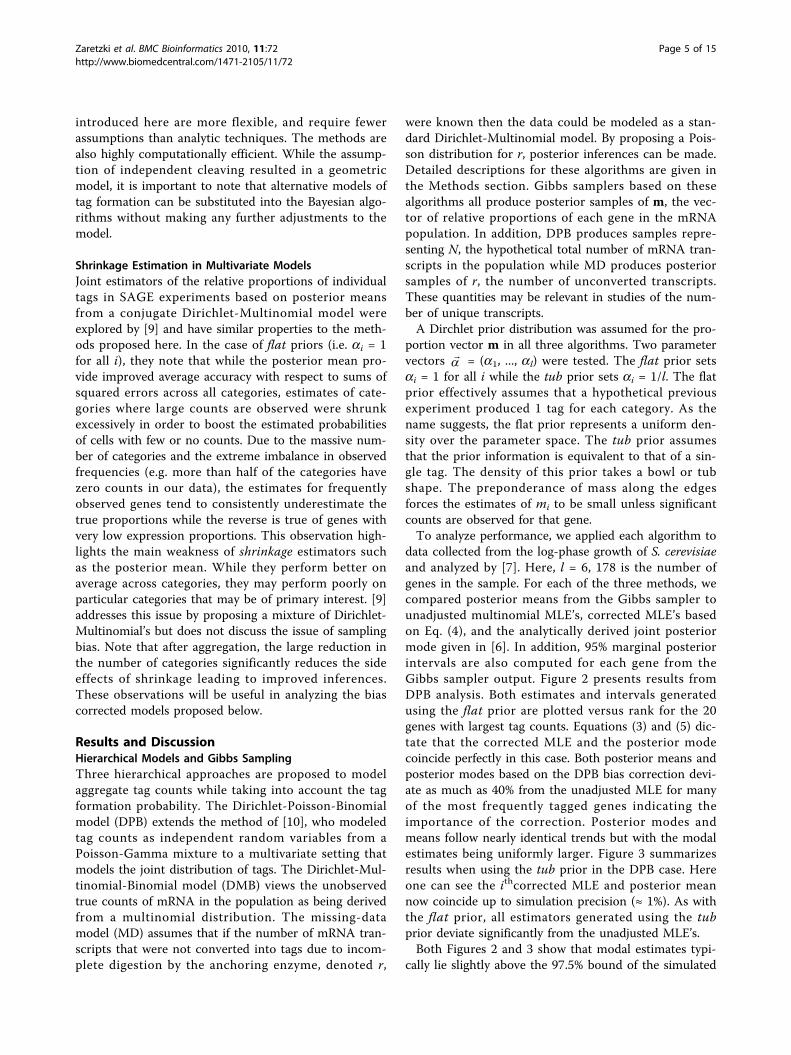
data collected from the log-phase growth of S. cerevisiaeand analyzed by [7]. Here, l = 6, 178 is the number ofgenes in the sample. For each of the three methods, wecompared posterior means from the Gibbs sampler tounadjusted multinomial MLE’s, corrected MLE’s basedon Eq. (4), and the analytically derived joint posteriormode given in [6]. In addition, 95% marginal posteriorintervals are also computed for each gene from theGibbs sampler output. Figure 2 presents results fromDPB analysis. Both estimates and intervals generatedusing the flat prior are plotted versus rank for the 20genes with largest tag counts. Equations (3) and (5) dic-tate that the corrected MLE and the posterior modecoincide perfectly in this case. Both posterior means andposterior modes based on the DPB bias correction devi-ate as much as 40% from the unadjusted MLE for manyof the most frequently tagged genes indicating theimportance of the correction. Posterior modes andmeans follow nearly identical trends but with the modalestimates being uniformly larger. Figure 3 summarizesresults when using the tub prior in the DPB case. Hereone can see the ithcorrected MLE and posterior meannow coincide up to simulation precision (≈ 1%). As withthe flat prior, all estimators generated using the tubprior deviate significantly from the unadjusted MLE’s.Both Figures 2 and 3 show that modal estimates typi-

cally lie slightly above the 97.5% bound of the simulated


of 15

marginal posterior distribution. The reader might won-der why the multivariate mode and mean are so farapart. The explanation lies in the fact that posterior dis-tribution is spread across a a large parameter space con-sisting of many thousands of dimensions. While theposterior distribution has a skewed density with a veryslight slope, it is essentially flat over most of the para-meter space. While the mode is located at the mostlikely point, an extreme point where only a fraction ofthe categories have non-zero tags, the mass spreadacross the rest of the space pulls the mean away fromthis point leading to the observed separation. This issimilar to the effect of skewness in a one dimensionaldistribution which pulls the mean away from the mode.Graphical displays based on the results of the DMB

and MD algorithms had very similar appearances and soare not shown. However, meaningful differences in pos-terior means generated by the methods and across thetwo priors do exist and are discussed in the followingsection.In order to ensure that autocorrelation did not

adversely effect parameter estimates, convergence analy-sis was performed. Posterior samples for the proportionm3, which corresponds to the open reading frameYAL003W, were investigated for all approaches. This

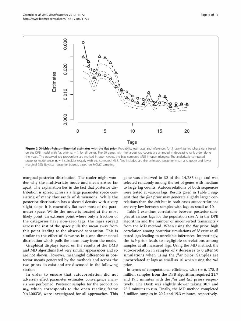
gene was observed in 32 of the 14,285 tags and wasselected randomly among the set of genes with mediumto large tag counts. Autocorrelations of both sequenceswere tested at various lags. Results given in Table 1 sug-gest that the flat prior may generate slightly larger cor-relations than the tub but in both cases autocorrelationsare very low between samples with lags as small as 10.Table 2 examines correlations between posterior sam-

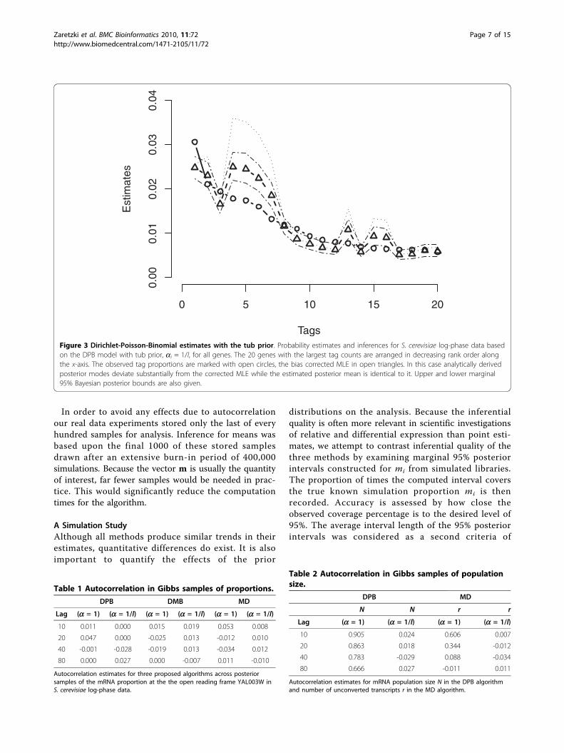
ples at various lags for the population size N in the DPBalgorithm and the number of unconverted transcripts rfrom the MD method. When using the flat prior, highcorrelation among posterior simulations of N exist at alltested lags leading to unreliable inferences. Interestingly,the tub prior leads to negligible correlations amongsamples at all measured lags. Using the MD method, theautocorrelation in samples of r decreases to 0 after 50simulations when using the flat prior. Samples areuncorrelated at lags as small as 10 when using the tubprior.In terms of computational efficiency, with l = 6, 178, 5

million samples from the DPB algorithm required 21.7and 19.3 minutes with the flat and tub priors respec-tively. The DMB was slightly slower taking 30.7 and25.2 minutes to run. Finally, the MD method completed5 million samples in 20.2 and 19.3 minutes, respectively.

Tags

Est

imat

es

0 5 10 15 20

0.00

00.

010

0.02

00.

030

Figure 2 Dirichlet-Poisson-Binomial estimates with the flat prior. Probability estimates and inferences for S. cerevisiae log-phase data basedon the DPB model with flat prior, ai = 1, for all genes. The 20 genes with the largest tag counts are arranged in decreasing rank order alongthe x-axis. The observed tag proportions are marked in open circles, the bias corrected MLE in open triangles. The analytically computedposterior mode when ai = 1 coincides exactly with the corrected MLE. Also included are the estimated posterior mean and upper and lowermarginal 95% Bayesian posterior bounds based on MCMC sampling.


of 15

In order to avoid any effects due to autocorrelationour real data experiments stored only the last of everyhundred samples for analysis. Inference for means wasbased upon the final 1000 of these stored samplesdrawn after an extensive burn-in period of 400,000simulations. Because the vector m is usually the quantityof interest, far fewer samples would be needed in prac-tice. This would significantly reduce the computationtimes for the algorithm.

A Simulation StudyAlthough all methods produce similar trends in theirestimates, quantitative differences do exist. It is alsoimportant to quantify the effects of the prior

distributions on the analysis. Because the inferentialquality is often more relevant in scientific investigationsof relative and differential expression than point esti-mates, we attempt to contrast inferential quality of thethree methods by examining marginal 95% posteriorintervals constructed for mi from simulated libraries.The proportion of times the computed interval coversthe true known simulation proportion mi is thenrecorded. Accuracy is assessed by how close theobserved coverage percentage is to the desired level of95%. The average interval length of the 95% posteriorintervals was considered as a second criteria of

Tags

Est

imat

es

0 5 10 15 20

0.00

0.01

0.02

0.03

0.04

Figure 3 Dirichlet-Poisson-Binomial estimates with the tub prior. Probability estimates and inferences for S. cerevisiae log-phase data basedon the DPB model with tub prior, ai = 1/l, for all genes. The 20 genes with the largest tag counts are arranged in decreasing rank order alongthe x-axis. The observed tag proportions are marked with open circles, the bias corrected MLE in open triangles. In this case analytically derivedposterior modes deviate substantially from the corrected MLE while the estimated posterior mean is identical to it. Upper and lower marginal95% Bayesian posterior bounds are also given.

Table 1 Autocorrelation in Gibbs samples of proportions.

DPB DMB MD

Lag (a = 1) (a = 1/l) (a = 1) (a = 1/l) (a = 1) (a = 1/l)

10 0.011 0.000 0.015 0.019 0.053 0.008

20 0.047 0.000 -0.025 0.013 -0.012 0.010

40 -0.001 -0.028 -0.019 0.013 -0.034 0.012

80 0.000 0.027 0.000 -0.007 0.011 -0.010

Autocorrelation estimates for three proposed algorithms across posteriorsamples of the mRNA proportion at the the open reading frame YAL003W inS. cerevisiae log-phase data.

Table 2 Autocorrelation in Gibbs samples of populationsize.

DPB MD

N N r r

Lag (a = 1) (a = 1/l) (a = 1) (a = 1/l)

10 0.905 0.024 0.606 0.007

20 0.863 0.018 0.344 -0.012

40 0.783 -0.029 0.088 -0.034

80 0.666 0.027 -0.011 0.011

Autocorrelation estimates for mRNA population size N in the DPB algorithmand number of unconverted transcripts r in the MD algorithm.


of 15

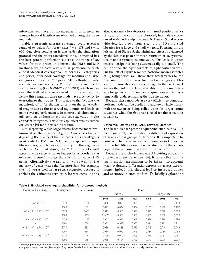
inferential accuracy but no meaningful differences inaverage interval length were observed among the threemethods.Table 3 presents average coverage levels across a

range of mi values for library sizes l = 6, 178 and l = 1,000. One clear conclusion is that under the simulationprotocol and the priors considered, the DPB method hasthe best general performance across the range of mi

values for both priors. In contrast, the DMB and MDmethods, which have very similar performance withalmost identical coverage values across all categoriesand priors, offer poor coverage for medium and largecategories under the flat prior. All methods provideaccurate coverage under the flat prior for the intermedi-ate values of mi (i.e. .0000167 - 0.000912) which repre-sent the bulk of the genes used in our simulations.Below this range, all three methods have a tendency tooverestimate the true mi. This is due to the fact that themagnitude of ai for the flat prior is on the same orderof magnitude as the observed tag counts and leads topoor coverage performance. In contrast, all three meth-ods tend to underestimate the true mi value in theabundant categories. This shrinkage effect was discussedearlier; see [9] for a detailed discussion.Not surprisingly, shrinkage effects become more pro-

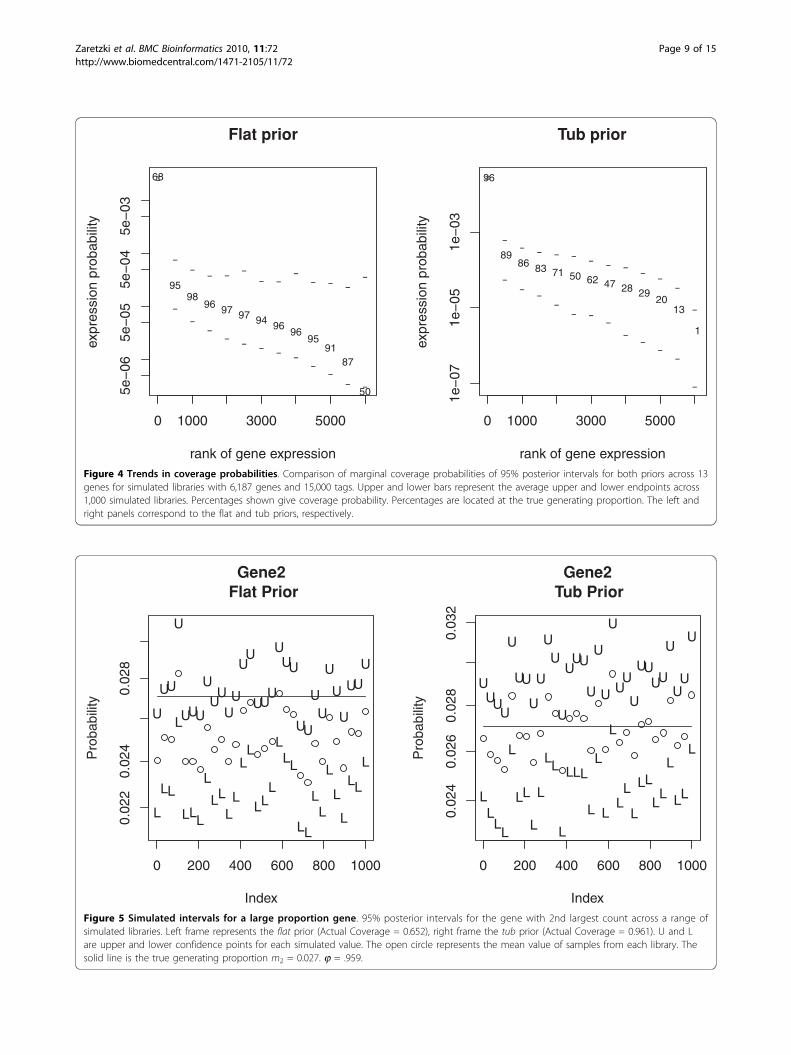
nounced as the number of genes l increases furtherdegrading the quality of the estimates. This shrinkage ismost acute for DMB and MD methods applied to largerlibrary sizes, which perform poorly for the segmentswith the. As noted above, the flat prior works wellacross a wide range of values but performs poorly in theextremes. Figure 4 displays this effect for a subset of 13genes. Alternatively the tub prior works well for themajority of genes where the flat prior fails. For example,the tub works well in large mi categories because itshrinks the estimates very little. Its weakness; it adds

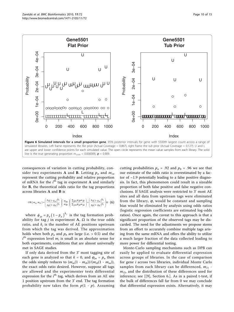
almost no mass to categories with small positive valuesof mi and, if no counts are observed, intervals are pro-duced with both endpoints near 0. Figures 5 and 6 pro-vide detailed views from a sample of 30 simulatedlibraries for a large and small mi gene. Focusing on theleft panel of Figure 5, the shrinkage effect is evidencedby the fact that posterior mean estimates of mi systema-tically underestimate its true value. This leads to upperinterval endpoints being systematically too small. Thetub prior on the right corrects this phenomenon well.On the left of Figure 6 we see posterior mean estimatesof mi being drawn well above their actual values by thereversing of the shrinkage for small mi categories. Thisleads to reasonably accurate coverage. In the right panelwe see that tub prior fails miserably in this case. Inter-vals for genes with 0 counts collapse close to zero sys-tematically underestimating the true mi values.Because these methods are very efficient to compute,

both methods can be applied to analyze a single librarywith the tub prior being relied upon for larger countcategories while the flat prior is used for the remainingcategories.

Differential Expression in SAGE between LibrariesTag based transcriptome sequencing such as SAGE ismost commonly used to identify differential expressionof genes across groups of libraries. It is important topoint out the consequences of differences in tag forma-tion probabilities in such studies along with the advan-tages of the proposed methods in this context.Because the anchoring enzyme AE cutting probability

p is experiment dependent [6], it is sensible for thetag formation mechanism to be taken into accountwhen evaluating differential expression across experi-ments. Indeed, this should lead to increased powerand accuracy in such studies. To briefly explore the

Table 3 Simulated coverage probabilities for proposed methods.

Proportion mi Range Library Size Gene Count Prior

Flat ai = 1 Tub ai = 1/k

DPB DMB MD DPB DMB MD

0 - 1.67 × 10-5 6178 1181 0.800 0.855 0.854 0.104 0.104 0.104

- 1000 25 0.825 0.834 0.834 0.107 0.108 0.107

1.67 × 10-5 - 1.23 × 10-4 6178 3678 0.947 0.975 0.976 0.520 0.520 0.520

- 1000 209 0.9425 0.950 0.950 0.558 0.558 0.558

1.23 × 10-4 - 9.12 × 10-4 6178 1173 0.961 0.951 0.948 0.899 0.898 0.898

- 1000 578 0.952 0.957 0.957 0.911 0.911 0.911

9.12 × 10-4 - 6.74 × 10-3 6178 133 0.939 0.485 0.479 0.945 0.944 0.944

- 1000 165 0.950 0.950 0.945 0.934 0.934 0.934

6.74 × 10-3 - 1.35 × 10-1 6178 13 0.809 0.009 0.005 0.953 0.951 0.951

- 1000 23 0.948 0.794 0.780 0.943 0.939 0.939

Coverage percentages for 95% posterior intervals for MCMC methods. Percentages represent the average number of intervals out of 1000 which covered thetrue proportion mi over the given range of mi values. Standard errors of proportions reported are below 1.5% and typically close to 1%.


of 15

0 1000 3000 5000

5e−

065e

−05

5e−

045e

−03

Flat prior

rank of gene expression

expr

essi

on p

roba

bilit

y

¯

¯¯ ¯ ¯ ¯

¯ ¯¯

¯ ¯ ¯¯

¯

¯¯

¯¯ ¯ ¯ ¯ ¯

¯¯

¯ ¯

68

9598

96 97 97 94 9696

9591

87

50

0 1000 3000 5000

1e−

071e

−05

1e−

03

Tub prior

rank of gene expression

expr

essi

on p

roba

bilit

y

¯

¯ ¯ ¯ ¯ ¯ ¯ ¯ ¯ ¯ ¯¯

¯

¯

¯¯ ¯

¯¯ ¯ ¯

¯ ¯¯

¯

¯

96

89 86 83 71 50 62 47 28 29

20 13

1

Figure 4 Trends in coverage probabilities. Comparison of marginal coverage probabilities of 95% posterior intervals for both priors across 13genes for simulated libraries with 6,187 genes and 15,000 tags. Upper and lower bars represent the average upper and lower endpoints across1,000 simulated libraries. Percentages shown give coverage probability. Percentages are located at the true generating proportion. The left andright panels correspond to the flat and tub priors, respectively.

0 200 400 600 800 1000

0.02

20.

024

0.02

8

Index

Pro

babi

lity

Gene2 Flat Prior

U

UU

U

UUU

U

UU

UU

UU

UUU

UUU

UU

UU

U

U

U

UU

U

L

LL

L

LLL

L

LL

LL

LL

LLL

LLL

LL

LL

L

L

L

LL

L

0 200 400 600 800 1000

0.02

40.

026

0.02

80.

032

Index

Pro

babi

lity

Gene2 Tub Prior

UUU

U

U

UU

U

U

UU

U

UUU

U

U

U

U

UU

U

UUUU

U

UU

U

LLLL

L

LL

L

L

LL

L

LLL

L

L

L

L

LL

L

LL

LL

L

LL

L

Figure 5 Simulated intervals for a large proportion gene. 95% posterior intervals for the gene with 2nd largest count across a range ofsimulated libraries. Left frame represents the flat prior (Actual Coverage = 0.652), right frame the tub prior (Actual Coverage = 0.961). U and Lare upper and lower confidence points for each simulated value. The open circle represents the mean value of samples from each library. Thesolid line is the true generating proportion m2 = 0.027. j = .959.


of 15

consequences of variation in cutting probability, con-sider two experiments A and B. Letting pa and mia

represent the cutting probability and relative proportionof mRNA for the ith tag in experiment A and similarlyfor B, the theoretical odds ratio for the tag proportionsacross libraries A and B is

OR m mpa pa

ki

pb pbki

miamib

jbm jbia ib,

1

1

jj i

jam jaj i

pa paki

pb pbki

1

1 (6)

where ja a ak

p p j 1 is the tag formation prob-ability for tag j in experiment A, Ω is the true oddsratio, and kj is the number of AE positions upstreamfrom which the tag was derived. The approximationholds when both pa and pb are large (i.e. > 0.5) and theith expression level mi is small in an absolute sense forboth experiments, conditions that are almost universallymet in SAGE studies.If only data derived from the 3’ most tagging site of

each gene is analyzed so that k = 0, and jja = pa thenthe odds simply reduces to (mia(1 - mib))/(mib(1 - mia)),the exact odds ratio desired. However, suppose all tagsare allowed and the experimenter tests differentialexpression for the ith tag, which derives from an AE site1 position upstream from the 3’ end. The tag formationprobability now takes the form p(1 - p). Assuming

cutting probabilities pa = .92 and pb = .96 we see thatour estimate of the odds ratio is overestimated by a fac-tor of ~1.9 potentially leading to a false positive diagno-sis. In fact, this phenomenon could result in a sizeableproportion of both false positive and false negative con-clusions. If SAGE analysis were restricted to 3’ most AEsites and all data from upstream tags were eliminatedfrom the library, ji would be constant and samplingbias would be eliminated by analysis using odds ratios(logistic regression coefficients are estimated log-oddsratios). Once again, the caveat to this approach is that asignificant proportion of the observed tags may be dis-carded. The need for the adjustments we propose stemsfrom an effort to accurately combine multiple tags aris-ing from the same mRNA and offers the ability to utilizea much larger fraction of the data collected leading tomore power for differential testing.Monte-Carlo sampling mechanisms such as DPB can

easily be applied to evaluate differential expressionacross groups of libraries. In the case of comparisonfor gene i across two libraries, individual Monte Carlosamples from each library can be differenced, mi1 -mi2, and the distribution of these differences used forinference; see [[9], Section 6.]. As in a paired t-test, ifthe bulk of differences fall far from 0 we may concludethat differential expression exists. Alternatively, it may

0 200 400 600 800 1000

0e+

001e

−04

2e−

043e

−04

4e−

04

Index

Pro

babi

lity

Gene5501 Flat Prior

UUUUUUUUUU

U

UUUUUU

U

UUUUUUU

U

UU

U

U

LLLLLLLLLLLLLLLLLLLLLLLLLLLLLL

0 200 400 600 800 1000

0e+

001e

−04

2e−

043e

−04

Index

Pro

babi

lity

Gene5501 Tub Prior

UUUUU

U

UUUUUUUU

U

U

UUUU

U

UUUUUU

U

UULLLLLLLLLLLLLLLLLLLLLLLLLLLLLL

Figure 6 Simulated intervals for a small proportion gene. 95% posterior intervals for gene with 5500th largest count across a range ofsimulated libraries. Left frame represents the flat prior (Actual Coverage = 0.867), right frame the tub prior (Actual Coverage = 0.127). U and Lare upper and lower confidence points for each simulated value. The open circle represents the mean value samples from each library. The solidline is the true generating proportion m5500 = 0.000009, j = 0.909.


of 15

be more appropriate to form odds ratios based on thesampled quantities and see if the bulk of these are farfrom 1.The Monte-Carlo sampling nature of the algorithms

presented here and their computational efficiency leadsto several advantages over recent methods [14-16]. First,and foremost the ability to use a larger fraction of thedata collected while simultaneously correcting bias iscritical to improving power. In addition, MCMC sam-ples allow both marginal and joint testing for differentialexpression across all genes using a single sampling runfor each library involved. Joint testing of differentialexpression is possible because posterior samples repre-sent the joint posterior distribution of the proportionsm. Importantly, our method requires no asymptoticconditions to be met in order to guarantee the validityof the results.

ConclusionsThis work focuses on a general biasing mechanism thatmay have a significant impact on the interpretation oflibraries generated by SAGE and closely related meth-ods. Beyond drawing attention to the consequences ofincomplete digestion, two main contributions are pre-sented. First, we derive and analyze three Bayesian algo-rithms that provide corrected posterior inference forrelative proportions of genes or tags in the overall popu-lation. Second, through calculations we deduce the con-sequences of tag formation bias on testing of differentialexpression and discuss how the algorithms derived herecan be used to correctly assess differential expression.This work compliments the earlier work in [6] by pro-

viding a flexible and efficient methodology whichextends the range of the prior distributions that areavailable. It also allows researchers access to intervalestimates in order to assess uncertainty in the estimatedquantities.The proposed methods are appropriate when incom-

plete digestion is the main source of multiple tag gen-eration. They may be applied to both tag level dataand to inference at the gene level based on aggregatedcounts. If possible, aggregating tags will provide betterinferences due to larger available counts. Of the threeapproaches, the DPB method provided the most accu-rate confidence intervals over the widest range of rela-tive proportions and we recommend its exclusive use.In addition, the choice of prior also plays an importantrole in the effectiveness of the algorithm. Of the twopriors tested, the flat prior was effective over a widerange of categories but resulted in excessive shrinkagefor the most abundant categories. For a fixed numberof sampled tags, this shrinkage effect becomes moresevere as one increases the number of categories.Hence, aggregating tags provides a second advantage

since it greatly reduces the number of categories usedin an analysis. The proposed tub prior provides littleshrinkage and posterior intervals based on this priorare very accurate for abundant categories. In practice,both priors should be applied and inference should bebased on the samples with the larger average.We note that the sampling algorithms presented are

independent of the model for tag formation probabilityand models other than the geometric model discussedcan easily be substituted. It should also be possible toextend the proposed methods using a mixture metho-dology as suggested by [9].Correction of tag formation bias may play a significant

role in improving power in differential expression stu-dies based on SAGE or related tag libraries. To ensurevalid testing, one must either include bias correction oreliminate non-3’ tag counts from the analysis. Further-more, the ability to effectively test for changes in groupsof genes (gene networks) is now possible due to themultivariate nature of the posterior distribution. Thisadvantage may become significantly more important asmore elaborate studies and techniques are developed inthe future.Due to the overall simplicity of genome architecture,

alternative splicing is generally not a problem whenanalyzing gene expression in S. cerevisiae and othermicroorganisms. However, alternative splicing is wide-spread in most multicellular organisms [1,2] andgreatly complicates transcriptome analysis. While theadjustments we propose do not solve the interpretationproblems caused by alternative splicing, properly iden-tifying multiple tags from common mRNA is a neces-sary first step in doing so. A logical next step wouldbe to expand the tag formation model underlying thiswork by allowing a single gene to produce multiplemRNA isoforms instead of a single type. One approachwould be to extend our model in a manner similar tothe approach developed for analyzing mRNA sequencedata developed by [20].Extending our model in such a way should allow us to

make inferences about the distribution of mRNA iso-forms produced by a gene based on the distribution oftags experimentally observed.Conceptually, the problems caused by alternative

splicing are similar to those caused by tag ambiguitybetween different genes. For example, in the case ofalternative splicing, the challenge is in determining themRNA isoform from which each tag originates. Simi-larly, in the case of ambiguous tags, the challenge is indetermining the gene from which each tag originates.Thus it is plausible that data interpretation problemscaused by both alternative splicing and ambiguous tagscould be overcome by extending our model to includemultiple sources of a single tag.


of 15

MethodsThe DataWe explicitly consider three strategies to simulate fromthe posterior distribution given by Eq. (5). The algo-rithms discussed are tested for inferential accuracy usingsimulated data as well as being applied to a publishedSAGE data set that analyzes a yeast organism S. cerevi-siae [7]. The published data was collected from the log-phase. There are 6,178 genes included in the data. Themaximum tag count was 392 and the minimum waszero. 3,560 of the genes included had observed countsof 0. Gene dependent sampling probabilities range from≈ .3% to 100%. Tag assignments to unique genes andassignment of non-unique tags for this analysis weredescribed in [6].

Computing and SoftwareAll simulations described below were computed usingR-environment (Version 2.6.2) on an 8 core, Intel Xeon2.66 GHz desktop server running Linux Ubuntu 8.04. R-scripts that implement the Gibbs sampling algorithmsdescribed below are provided; see Additional file 1.

The Dirichlet-Poisson-Binomial (DPB) ModelThe DPB approach, inspired by Casella and George[21], assumes a fixed population of mRNA’s of size Nexists within the sampled cells. The total size N is ran-dom across samples and follows a gamma distributionthat is rounded down to the nearest integer. Thechoice of gamma here is convenient due to its role asa conjugate prior to the Poisson distribution. Given N,the relative proportions of the categories of mRNA, mi,are unknown and assumed to follow a Dirichlet distri-bution with prior

= (a1, ..., al). The ai will typically

be identical resulting in objective inference.Because cells contain mRNA transcripts from thou-

sands of different genes, the probability of seeing anyparticular type is low. It is therefore logical to assume,given N and mi, that the actual number of mRNA’s of acertain type gi, i = 1, ... l, extracted from the group ofcells, satisfies a Poisson distribution with mean μ =N·mi. Finally, the restriction enzyme process generates atag count ti for a particular mRNA transcript in a bino-mial fashion based upon the tag formation probabilityji. Hence, the hierarchical data generating mechanismfollows, Ti~Binomial(gi, ji), gi~Poisson(N * mi), m ~Dl

( ), and N ~ceiling(Gamma(g1, g2)). We refer to thismodel as the Dirichlet-Poisson-Binomial (DPB) model.A first weakness of this model is that the sum of all

counts ∑gi may not add up to the total counts N. How-ever, this approach allows us to infer the total popula-tion size N. Together, the elements described above givea joint posterior distribution,

Pr , , | , , ,m g tNg

t

e Nmi Nmi

iit

i

l

ig ti i i

1 2

1

1

iigi

gi

m e NiNi

!

1 12 1

¿From this expression, we can deduce the set of fullconditional distributions,

m g N Gamma g N

g N t Poisson Nm

i i i i

i i i i

| , , , ~ ,

| , , , ~

t

t m

1

NN Gamma gii

l

| , , , ~ ( , )t g m 1 2

1

1

where δ = ( , g1, g2). Gibbs sampling can be imple-

mented by iteratively simulating from each conditionalafter replacing any unknown random quantities in theconditioning set with simulation values from the pre-vious iteration; see [22].The hierarchical model considered here is not identi-

cal to Eq. (3), but depends upon prior parameters (g1,g2) which effect the mode of the posterior distribution.One possibility for choosing values of these parametersis to minimize the distance between the approximateanalytical mode discussed in [6] and the mode of thismodel which can be computed through iterative maxi-mization of the conditionals; see [23,24] for furtherdetails.In our simulations we used a shape parameter g1 =

100 and prior scale g2 = 200. The mean of a gammawith these parameters is 20,000 which is somewhat lar-ger than a natural estimate of the population size, ∑i(ti/ji) = 16438.81. This was chosen intentionally to deter-mine if the posterior would converge to a reasonableestimate of N.

The Dirichlet-Multinomial-Binomial (DMB) ModelThe Dirichlet-Multinomial-Binomial (DMB) approach isarguably more faithful to the sampling mechanisminherent in SAGE than DPB. N, the total number ofmRNA in the sample is assumed to follow a Poissondistribution with mean l. Given this mRNA populationsize, the vector g of counts for each category of mRNAprior to tag formation follows a multinomial distribu-tion,

Pr | , , ~, , ,

, ,g m

N

N

g g gm m m

l

g glg l

1 21 21 2

whose probabilities are the mRNA proportions mi andare assumed to follow a Dirichlet distribution with para-meter vector

. Reminding readers that

= (j1, j2, ...,

jl) is the vector of tag formation probabilities and


of 15

letting δ = (l, g1, g2), the full conditional distributionsare derived to be,

m t g g

g t m t m

| , , , , ~

| , , , , ~ , *

N D

N Multinom N t

l

tot

1

N Gamma gii

k

| , , , , ~ ( , )t g m 2 1

1

1

where m *(1 - ) is an element-wise product with 1

representing a vector of identical dimension to m.Hence, the ith element of the vector is given by mi (1 -ji).This formulation is more natural in the sense that it

restricts the pre-tagging counts to sum to the popula-tion total N. One drawback is that the observed dataprovides no information for posterior inference aboutthe population size N. Iterative maximization for modecalculation is not viable due to the discrete nature ofthe multinomial conditional distribution.

The Missing Data (MD) ModelInstead of re-normalizing the probabilities θi = (miji)/(∑miji) and basing inference on the posterior of Eq. (5),a more straightforward approach uses the concept ofmissing data which is often associated with the EMalgorithm; see [22]. We augment the observed data vec-tor t with an extra category that represents any cDNAthat is not converted to a tag. This count, r, is notobserved, but if a distribution such as the Poisson isproposed, we may consider a Bayesian approach. Giventhe value of r and assuming a Dirichlet prior on theunknown initial proportions m ~Dl(a1, ..., al), theresulting posterior distribution for m is,

Pr | , , ( )m t

r m mi i

i

lr

i it

i

li i

1

1

1

1

This resulting posterior distribution is a Dirichlet dis-tribution with l + 1 categories compared with the l cate-gories in the prior distribution. Exact computation ofthe conditional expectations E(mi|r) is now straightfor-ward. Using the formula for the mean of a Dirichlet dis-tribution

E m r i t i

i r i t iili | , ,t

1

Summing the expectation over mi, which must sum to

one, gives r ti ii

l

i

l i t ii

1 1

which is

intuitively reasonable. Substituting this into the previous

expression eliminates the dependence upon r. Hence,the marginal expectation of mi across values of r is

E m i ti

ii t iii

li | , .t

1

(7)

Gibbs sampling is also available for this problem andextends inference to Bayesian interval estimates. If r~Poisson(μ) then the posterior distribution can be writ-ten,

Pr , | , ( )!

.m tr m me r

ri i

i

lr

i it

i

li i

1

1

1

1

The full conditional distributions are

r Poisson m

r D r t

i i

l

| , , , ~ (( ) )

| , , , , ~ , ,

t m

m t

1

1 1 1

, l lt

In order to apply the Gibbs sampler a value for theprior mean of r, μ must be selected. A logical mean forthe Poisson is ttot ∑imi(1 - ji)/∑imi ji since ∑mi(1 - ji)= 1 - ∑mi ji is the probability that an mRNA is notconverted into a tag. Equation (4) provides a useful esti-mate of ∑mi ji in the case of a flat prior.Like the DPB algorithm above, the missing data algo-

rithm also admits an iterative optimization procedure inorder to compute the posterior mode. The mode of the

Dirichlet conditional given by [22] is mi i = (ti + ai -

1)/(∑i(ai + ti) + r - l) while the mode for the Poisson isthe mean rounded down to the nearest smaller integer.For example, considering a flat prior for m along with aprior mean of μ = 10, 100 for r, the posterior mode ofthe missing data model is nearly identical to the exactanalytical mode given in [6]. It is tempting to invoke theargument used to derive Eq. (7) to obtain the marginalmode.Unfortunately, when ai < 1 and ti = 0 this leads to

estimates outside of the parameter space.

Simulation Study ProtocolSimulation of libraries was based upon the proportionsestimated from the aggregated S. cerevisiae log-phasedata described earlier. First, long and short multino-mial proportion vectors m of lengths l = 6, 178 and 1,000 respectively were constructed. Actual mean esti-mates from the log-phase library were adopted for thecase l = 6, 178 while for l = 1, 000, m was based onrenormalizing the first 1,000 elements of the longercase. The vector of known tag formation probabilities,{j1, ..., jl} was constructed by simulating a theoretical


of 15

number of AE cleaving sites and then using Eq. (1) tocompute individual probabilities ji. The number ofcleaving sites followed a Poisson distribution withmean 2 with 1 count added to each category. Thisensured that each “gene” has at least one cleaving site.The cleavage probability was set at p = .55 based onestimates given in [6].Using the above protocol, for each combination of

library size, l, and prior, 1,000 libraries, tj, each containingn = 15, 000 tags were simulated. For each simulatedlibrary, each of the three proposed algorithms was used togenerate 20,500 posterior sample vectors mjk, k Î 1, ...20,500. Every 20th sample was collected after a burn in per-iod of 500 samples resulting 1,000 Monte Carlo samplesof m for each method. Samples were then used to gener-ate mean, median and 95% marginal posterior intervalsfor each of the l gene categories. Coverage percentagesfor the ith gene category are computed by finding the pro-portion of times that the interval for category i from aparticular method contains the true proportion mi acrossthe 1,000 simulated libraries tj . Figure 4 displays a sampleof coverage percentages across a range of categories forthe DPB method under two different prior values.

Additional file 1: SAGEGibbs.R. File contains a script which implementthe Gibbs Samplers described in the paper. The script is written in the R-environment.Click here for file[ http://www.biomedcentral.com/content/supplementary/1471-2105-11-72-S1.R ]

AcknowledgementsAuthors would like to thank Robert Mee, Naomi Altman, Reviewers andEditors for helpful comments which significantly improved the quality of themanuscript.

Author details1Department of Statistics, Operations, and Management Science, TheUniversity of Tennessee, 331 Stokely Management Center, Knoxville, TN,37996, USA. 2Department of Ecology and Evolutionary Biology, TheUniversity of Tennessee, 569 Dabney Hall, Knoxville, TN, 37996, USA.3Department of Emergency Medicine, Methodist Hospital, Brooklyn, NY, USA.4Department of Statistical Science, Duke University, 217 Old Chemistry Bldg.Durham, NC 27708-0251, USA.

Authors’ contributionsRLZ devised and implemented the algorithms, computed the experimentsand wrote the majority of the manuscript. MAG developed the tagformation model, prepared the real data, wrote parts of the manuscript, andprovided subject matter expertise and computational resources. WMBhelped edit the manuscript and construct graphical displays. AA assisted indevelopment of the algorithms. All authors have read and approved thismanuscript.

Received: 9 July 2009Accepted: 3 February 2010 Published: 3 February 2010

References1. ’t Hoen PAC, Ariyurek Y, Thygesen HH, Vreugdenhil E, Vossen RHAM, de

Menezes RX, Boer JM, van Ommen GJB, den Dunnen JT: Deep sequencing-based expression analysis shows major advances in robustness,resolution and inter-lab portability over five microarray platforms. NucleicAcids Research 2008, 36(21):e141.

2. Pauws E, van Kampen A, Graaf van de S, de Vijlder J, Ris-Stalpers C:Heterogeneity in polyadenylation cleavage sites in mammalian mRNAsequences: implications for SAGE analysis. Nucleic Acids Research 2001,29(8):1690-1694.

3. Boon K, Osorio E, Greenhut S, Schaefer C, Shoemaker J, Polyak K, Morin P,Buetow K, adn S de Souza RS, Riggins G: An anatomy of normal andmalignant gene expression. Proceedings of the National Academy of Science2002, 99(17):11287-11292, [SAGE Genie].

4. Malig R, Varela C, Agosin E, Melo F: Accurate and unambiguous tag-to-gene mapping in serial analysis of gene expression. BMC Bioinformatics2006, 7(487).

5. Romualdi C, Bortoluzzi S, d’Alessi F, Danieli G: IDEG6: a web tool fordetection of differentially expressed genes in multiple tag samplingexperiments. Physiological Genomics 2003, 12:159-162.

6. Gilchrist MA, Qin H, Zaretzki RL: Modeling SAGE tag formation and itseffects on data interpretation within a Bayesian framework. BMCBioinfomatics 2007, 8(403).

7. Velculescu VE, Zhang L, Zhou W, Vogelstein J, Basrai MA, Bassett JDE,Hieter P, Vogelstein B, Kinzler KW: Characterization of the yeasttranscriptome. Cell 1997, 88:243-251.

8. Velculescu VE, Zhang L, Vogelstein B, Kinzler KW: Serial Analysis of GeneExpression. Science 1995, 270(5235):484-487.

9. Morris JS, Baggerly KA, Coombes KR: Bayesian shrinkage estimation of therelative abundance of mRNA transcripts using SAGE. Biometrics 2003,59:476-486.

10. Thygesen HH, Zwinderman AH: Modeling Sage data with a truncatedgamma-Poisson model. BMC Bioinformatics 2006, 7:157.

11. Kuznetsov VA, Knott GD, Bonner RF: General Statistics of StochasticProcess of Gene Expression in Eukaryotic Cells. Genetics 2002,161(3):1321-1332.

12. Kuznetsov VA: Statistical Methods in Serial Analysis of Gene Expression(SAGE). Computational and Statistical Approaches to Genomics New York:Springer VerlagZhang W, Shmulevich I , 2 2006, 163-2008.

13. Baggerly KA, Deng L, Morris JS, Aldaz CM: Differential expression in SAGE:accounting for normal between-library variation. Bioinformatics 2003,19:1477-1483.

14. Baggerly KA, Deng L, Morris JS, Aldaz C: Overdispersed logistic regressionfor SAGE: Modelling multiple groups and covariates. BMC Bioinformatics2004, 5:144.

15. Lu J, Tomfohr JK, Kepler TB: Identifying differential expression in multipleSAGE libraries: an overdispersed log-linear model appraoch. BMCBioinformatics 2005, 6(165).

16. Vencio RZN, Brentani H, Patrao DFC, Pereira CAB: Bayesian modelaccounting for within-class biological variability in Serial Analysis ofGene Expression (SAGE). BMC Bioinformatics 2004, 5(119).

17. Vencio RZN, Brentani H: Statistical Methods in Serial Analysis ofGene Expression(SAGE). Computational and Statistical Approaches toGenomics New York: Springer VerlagZhang W, Shmulevich I , 2 2006,209-233.

18. Matsumura H, Reich S, Ito A, Saitoh H, Kamoun S, Winter P, Kahl G,Reuter M, Kruger DH, Terauchi R: Gene expression analysis of plant host-pathogen interactions by SuperSAGE. Proceedings of the National Academyof Sciences 2003, 100(26):15718-15723http://www.pnas.org/cgi/content/abstract/100/26/15718.

19. Matsumura H, Bin Nasir KH, Yoshida K, Ito A, Kahl G, Kruger DH, Terauchi R:SuperSAGE array: the direct use of 26-base-pair transcript tags inoligonucleotide arrays. Nature Methods 2006, 3:469-474.

20. Jiang H, Wong WH: Statistical inferences for isoform expression in RNA-Seq. Bioinformatics 2009, 25(8):1026-1032.

21. Arnold SF: Gibbs Sampling. Handbook of Statistics New York, NY: Elsevier/North-HollandRao C 1993, 9:599-625.


of 15

http://www.ncbi.nlm.nih.gov/pubmed/18927111?dopt=Abstract



























http://www.pnas.org/cgi/content/abstract/100/26/15718

http://www.pnas.org/cgi/content/abstract/100/26/15718





22. Gelman A, Carlin JB, Stern HS, Rubin DB: Bayesian Data Analysis Texts inStatistical Science, Boca Raton, FL: Chapman & Hall/CRC, 2 2004.

23. Lindley DV, Smith AFM: Bayes Estimates for the Linear Model. Journal ofthe Royal Statistical Society. Series B (Methodological) 1972, 34.

24. Chen MH, Shao QM, Ibrahim JG: Monte Carlo Methods in BayesianComputation New York, NY: Springer Verlag 2000.

doi:10.1186/1471-2105-11-72Cite this article as: Zaretzki et al.: Bias correction and Bayesian analysisof aggregate counts in SAGE libraries. BMC Bioinformatics 2010 11:72.

Submit your next manuscript to BioMed Centraland take full advantage of:

• Convenient online submission

• Thorough peer review

• No space constraints or color figure charges

• Immediate publication on acceptance

• Inclusion in PubMed, CAS, Scopus and Google Scholar

• Research which is freely available for redistribution

Submit your manuscript at www.biomedcentral.com/submit


of 15

Bias correction and Bayesian analysis of aggregate counts in SAGE libraries

Documents

Transcript of Bias correction and Bayesian analysis of aggregate counts in SAGE libraries