Biancacci, Cecilia - University of the Highlands and Islands

UHI Thesis - pdf download summary

Towards a sustainable production of Osmundea pinnatifida:

insight into the cultivation and biochemical composition of the species

Biancacci, Cecilia

DOCTOR OF PHILOSOPHY (AWARDED BY OU/ABERDEEN)

Award date:2019

Awarding institution:University of Aberdeen

Link URL to thesis in UHI Research Database

General rights and useage policyCopyright,IP and moral rights for the publications made accessible in the UHI Research Database are retainedby the author, users must recognise and abide by the legal requirements associated with these rights. This copyhas been supplied on the understanding that it is copyright material and that no quotation from the thesis may bepublished without proper acknowledgement, or without prior permission from the author.

Users may download and print one copy of any thesis from the UHI Research Database for the not-for-profitpurpose of private study or research on the condition that:

1) The full text is not changed in any way2) If citing, a bibliographic link is made to the metadata record on the the UHI Research Database3) You may not further distribute the material or use it for any profit-making activity or commercial gain4) You may freely distribute the URL identifying the publication in the UHI Research DatabaseTake down policyIf you believe that any data within this document represents a breach of copyright, confidence or data protection please contact us [email protected] providing details; we will remove access to the work immediately and investigate your claim.

Download date: 29. May. 2022

https://pure.uhi.ac.uk/en/studentTheses/4ba7ce41-8833-4e41-86df-d0dc22db092b

Towards a sustainable production of Osmundea pinnatifida: insight into the cultivation and biochemical composition of the species

Cecilia Biancacci

A thesis presented for the degree of Doctor of Philosophy at the University of Aberdeen

Academic Partners

The Scottish Association for Marine Science (SAMS)

University of the Highlands and Islands (UHI)

The James Hutton Institute

Under the supervision of Professor Michele S. Stanley, Professor John G. Day and Dr Gordon McDougall

2019

iii

Declaration

I hereby declare that this thesis has been completed solely by Cecilia Biancacci at the Scottish

Association for Marine Science, under the supervision of Professor Michele S. Stanley, Professor

John G. Day and Dr. Gordon McDougall, during the period October 2015- September 2019. The

sources of information are specifically acknowledged. This work has not been submitted for any

previous application for a degree or personal qualification.

Cecilia Biancacci

Date 30/09/2019

iv

Abstract

Towards a sustainable production of Osmundea pinnatifida: insight into the cultivation

and biochemical composition of the species

Cecilia Biancacci

The consumption of wild harvested Osmundea pinnatifida as food in UK, Portugal and Spain has a

long tradition. However, the collection of wild material is time consuming, unsustainable and

limited by seasonality. Cultivation represents the preferred option for future exploitation of this

species. This study aimed at identifying the best rearing system for cultivation and commercial

production of O. pinnatifida. Phylogenetic analyses of populations along the West coast of Scotland

were conducted, to identify the species prior cultivation experiments, but also to explore

population variation within the frame of possible genetic pollution due to introduction of alien

species for farming purpose. The biochemical composition and variation of wild and cultivated

specimens was assessed. Giving for the first time an overview of the seasonality of the biochemical

and metabolomic profile of the species, an understanding of the correlation of biochemistry and

environmental factors, and an insight in how cultivation conditions can manipulate the

composition of the species. This information enhanced the knowledge on the metabolites present

in O. pinnatifida, with significant outcome for further commercial applications (e.g. food,

nutraceutical, pharmaceutical, cosmetic, etc.). Several cultivation methodologies were trialled,

including exploration of reproductive cycle and vegetative cultivation. Particularly, experiments in

flasks, in indoor and outdoor tank systems, PBR and on-sea out-plantation were conducted,

evaluating how cultivation parameters (e.g. light, temperature, nutrient, chemical treatments, supply

of hormones and fertilizer) affect the growth, biochemistry and morphology of the species. The

outcome was the establishment of an indoor tumbling cultivation system for the vegetative

production of O. pinnatifida tetrasporophytes. This pioneering methodology has the potential to be

scaled up and commercially applied, possibly achieving a continuous and tailored supply of the

resource that would be sustainable and independent from seasonality.

v

Acknowledgments

This work would not have been possible without the support, help, guidance and encouragement

that I have received from different people during these 4 years.

I would like to acknowledge the financial support received from IBioIC, MASTS and HIE.

Thank you to my supervisory team, Professor Michele Stanley, Professor John Day and Dr Gordon

McDougall, for their support, guidance, advices, revisions and recommendations, and for making

me a better scientist.

I am grateful for the technical assistance that I have received from Christine Beveridge, Richard

Abell, Sharon Mcneill, Debra Brennan, Alison Mair, Naomi Thomas at SAMS, and William

Allwood and Julie Sungurtas at The James Hutton Institute. Thank you to the Acadian Seaplants

for providing the Acadian Marine Plant Extract Powder (AMPEP) for the experiments presented

in Chapter 8.

To my friends, for have always been there even through miles and miles of distance.

To my family. My sister, for being my person and the best friend that I could have asked for, and

my parents, for having always supported me and for having shown me how to truly live. For their

unconditional love and for everything they have done for me.

To Gianby, for all the laughs, the long walks and talks, the support, the kindness and the love that

you have always shown. For teaching me to always look at the bright side of life and for being my

companion and friend in all the adventures.

vi

Table of Contents Chapter 1 Introduction ............................................................................................................... 1

1.1 Seaweed: a general introduction ................................................................................................... 1

1.2 Seaweed aquaculture ..................................................................................................................... 3

1.2.1 Cultivation methods ................................................................................................................ 6

1.2.2 Epiphytes in cultivated seaweeds ......................................................................................... 10

1.3 Rhodophyta .................................................................................................................................. 11

1.3.1 Introduction .......................................................................................................................... 11

1.3.2 Life cycle and reproduction ................................................................................................... 12

1.3.3 Distribution ........................................................................................................................... 13

1.3.4 Light patterns ........................................................................................................................ 14

1.3.5 Nutrients ............................................................................................................................... 16

1.3.6 Cell wall and storage of reserves in red algae ....................................................................... 17

1.3.7 Economic utilisation of red seaweeds................................................................................... 17

1.4 Scotland ........................................................................................................................................ 19

1.4.1 Scotland and aquaculture ..................................................................................................... 19

1.4.2 Scotland and seaweeds: an ancient tradition ....................................................................... 20

1.4.3 Scotland seaweed chemical industry history ........................................................................ 21

1.4.4 Scotland and commercial harvesting of wild seaweeds ....................................................... 22

1.5 Osmundea pinnatifida (Hudson) Stackhouse, 1809:79 ................................................................ 24

1.6 Project aim ................................................................................................................................... 29

1.6.1 Thesis objectives ................................................................................................................... 31

Chapter 2 Systematics and phylogeny of Osmundea pinnatifida in Scotland: investigation on

molecular biology in the context of the development of a cultivation method for the species . 33

2.1 Introduction ................................................................................................................................. 33

2.1.2 Systematics of Rhodophyceae: the order Ceramiales .......................................................... 34

2.1.3 Systematics of the Laurencia complex .................................................................................. 35

2.1.4 Taxonomy of Rhodophyceae: from morphological structures to DNA-based analyses ....... 37

2.1.5 DNA Barcoding: importance and applications ...................................................................... 38

2.2 Aims .............................................................................................................................................. 40

2.3 Materials and Methods ................................................................................................................ 41

2.3.1 Study area and sample collection ......................................................................................... 41

2.3.2 DNA extraction, PCR amplification, and sequencing ............................................................ 42

2.3.3 Multiple sequence alignments and phylogenetic analyses .................................................. 44

2.4 Results .......................................................................................................................................... 45

2.4.1 DNA extraction, PCR amplification, purification and sequencing ......................................... 45

2.4.2 Phylogenetic analyses ........................................................................................................... 47

vii

2.5 Discussion ..................................................................................................................................... 52

2.6 Conclusions .............................................................................................................................. 56

Chapter 3 Seasonal variation of biochemical composition in Osmundea pinnatifida from the West

coast of Scotland ...................................................................................................................... 58

3.1 The chemical composition of seaweeds ...................................................................................... 58

3.1.2 Red seaweeds: biochemical composition ............................................................................. 59

3.1.2.1 Red seaweeds as functional food: secondary metabolites with antimicrobial,

antioxidant and antiviral activity................................................................................................ 62

3.2 Scope ............................................................................................................................................ 63

3.2.1 Aims ........................................................................................................................................... 63

3.3 Materials and methods ................................................................................................................ 63

3.3.1 Carbohydrate analyses .......................................................................................................... 64

3.3.2 Protein analyses .................................................................................................................... 65

3.3.3 Pigments analyses ................................................................................................................. 66

3.3.4 Moisture content .................................................................................................................. 67

3.3.5 Antioxidant content .............................................................................................................. 67

3.3.6 Total fatty acid analyses ........................................................................................................ 68

3.3.7 Metal analyses ...................................................................................................................... 68

3.3.8 C:N ratio ................................................................................................................................ 69

3.3.9 Dissolved organic carbon and nitrogen (DOCN) and trace metals analyses in water samples

........................................................................................................................................................ 69

3.3.10 Statistical analyses .............................................................................................................. 70

3.4 Results .......................................................................................................................................... 71

3.4.1 Carbohydrate content ........................................................................................................... 71

3.4.2 Protein content ..................................................................................................................... 71

3.4.3 Chlorophyll-a content ........................................................................................................... 72

3.4.4 Carotenoids ........................................................................................................................... 73

3.4.5 Phycobiliproteins ................................................................................................................... 74



3.4.8 Total lipid extracted (TLE) ..................................................................................................... 76

3.4.9 Metal Analyses ...................................................................................................................... 77

3.4.10 C:N ratio .............................................................................................................................. 80

3.4.11 Dissolved organic carbon and nitrogen (DOCN) and trace metals analyses in water

samples .......................................................................................................................................... 81

3.4.12 PCA analysis of seasonal data ............................................................................................. 83

3.5 Discussion ..................................................................................................................................... 86

3.5.1 Carbohydrate content ........................................................................................................... 87

viii

3.5.2 Protein content ..................................................................................................................... 87

3.5.3 Pigment content .................................................................................................................... 88



3.5.6 Total fatty acid content ......................................................................................................... 91

3.5.7 Metals content in seaweed samples ..................................................................................... 91

3.5.8 C:N ratio in seaweed samples ............................................................................................... 93

3.5.9 Metals and DOCN analyses on water samples ...................................................................... 93

3.5.10 PCA Analysis ........................................................................................................................ 94

3.6 Conclusions .................................................................................................................................. 95

Chapter 4 Composition and seasonal variation in the metabolomic profile and flavour of

Osmundea pinnatifida ............................................................................................................... 98

4.1 Introduction ................................................................................................................................. 98

4.2 Aims ............................................................................................................................................ 101

4.3 Materials and methods .............................................................................................................. 101

4.3.1 Solvent extraction ............................................................................................................... 101

4.3.2 Oral extracts: extraction in HEPES buffer of two selected months, November and May .. 101

4.3.3 HILIC-PDA-MS analysis ........................................................................................................ 102

4.4 Results ........................................................................................................................................ 103


4.4.2 Oral extracts: extraction in HEPES buffer of two selected months: November and May .. 118

4.5 Discussion ................................................................................................................................... 125


4.5.1.1 ESI negative polarity ..................................................................................................... 125

4.5.1.2 ESI positive polarity ...................................................................................................... 128

4.5.1.3 Peak abundance variation: regulation trends .............................................................. 130

4.5.1.3.1 Trends for ESI negative polarity ............................................................................ 131

4.5.1.3.2 Trends for ESI positive polarity ............................................................................. 131

4.5.2 Replicating oral conditions .................................................................................................. 131

4.5.2.1 Oral extracts: extraction in HEPES buffer of two selected months, November and May

.................................................................................................................................................. 131

4.6 Conclusions ................................................................................................................................ 133

Chapter 5 Epiphytes control of O. pinnatifida cultures and spores’ production, release and

development in treated specimens ......................................................................................... 136

5.1 Introduction ............................................................................................................................... 136

5.2 Aims ............................................................................................................................................ 139


5.3.1 Chemical removal of epiphytes ........................................................................................... 139

ix

5.3.2 Tidal simulation as epiphytes control ................................................................................. 141

5.3.3 Epiphytes treatment of biomass grown in a tumbling tank system cultivation both indoors

and outdoors ................................................................................................................................ 143

5.3.4 In vitro spores’ production, attachment, germination and growth of juveniles of O.

pinnatifida from epiphytes treated cultures ................................................................................ 146

5.4 Results ........................................................................................................................................ 147

5.4.1 Chemical removal of epiphytes ........................................................................................... 147

5.4.1.1 Petri dish trial ............................................................................................................... 147

5.4.1.2 Flask trial ...................................................................................................................... 148

5.4.1.3 Tank trial ...................................................................................................................... 148

5.4.2 Tidal simulation as epiphytes control ................................................................................. 149

5.4.3 Impact of epiphyte treatment on tumbling cultivation system both indoor and outdoor. 152

5.4.3.1 Winter trial: indoor and outdoor cultivation ............................................................... 152

5.4.3.1.1 Biochemical composition ...................................................................................... 156

5.4.3.2 Summer trial: outdoor experiment .............................................................................. 157

5.4.3.2.1 Biochemical composition ...................................................................................... 161


pinnatifida from epiphytes treated cultures ................................................................................ 161

5.5 Discussion ................................................................................................................................... 166

5.6 Conclusions ................................................................................................................................ 170

Chapter 6 Effects of different media on the growth and biochemical composition of Osmundea

pinnatifida .............................................................................................................................. 172

6.1 Introduction ............................................................................................................................... 172

6.2 Aims ............................................................................................................................................ 174


6.3.1 Effects of three different media types on the growth and biochemical composition of

Osmundea pinnatifida adult cultures .......................................................................................... 174

6.3.2 The impact of different media types on growth and biochemical composition of Osmundea

pinnatifida juvenile plantlets ....................................................................................................... 176

6.3.3 The impact of nitrogen sources and the N:P ratio on Osmundea pinnatifida growth and

biochemical composition ............................................................................................................. 176

6.4 Results ........................................................................................................................................ 177


Osmundea pinnatifida adult cultures .......................................................................................... 177

6.4.1.1 Weight and growth rate of adult cultures grown in three different media ................ 177

6.4.1.2 Effects of three different media types on the biochemical composition of Osmundea

pinnatifida adult cultures ......................................................................................................... 179

6.4.1.2.1 Antioxidant content .............................................................................................. 179

6.4.1.2.2 Carbohydrates and proteins ................................................................................. 179

6.4.1.2.3 Pigments ................................................................................................................ 180

x


pinnatifida juvenile plantlets ....................................................................................................... 181

6.4.2.1 Weight and growth rate of plantlets grown in either F/2 and VS media..................... 181

6.4.2.2 Biochemical composition when two different media types were employed to cultivate

Osmundea pinnatifida juvenile plantlets ................................................................................. 183

6.4.2.2.1 Antioxidant analysis .............................................................................................. 183

6.4.2.2.2 Proteins and carbohydrates analyses ................................................................... 183

6.4.2.2.3 Pigments ................................................................................................................ 184

6.4.3 The impact of nitrogen sources and N:P ratio on Osmundea pinnatifida growth and

biochemical composition ............................................................................................................. 185

6.4.3.1 Weight and growth rate of Osmundea pinnatifida adult cultures grown in different

nitrogen sources ....................................................................................................................... 185

6.4.3.2 Biochemical composition of Osmundea pinnatifida adult cultures grown in different

nitrogen sources ....................................................................................................................... 186

6.4.3.2.1 Protein and carbohydrate content ....................................................................... 186

6.4.3.2.2 Phycobiliproteins................................................................................................... 187

6.5 Discussion ................................................................................................................................... 188

6.6 Conclusions ................................................................................................................................ 192

Chapter 7 Cultivation of Osmundea pinnatifida in the Algem® Photo-bioreactor System ....... 194

7.1. Introduction .............................................................................................................................. 194

7.2 Aims ............................................................................................................................................ 196


7.3.1 Comparison of summer and winter conditions on the vegetative growth of O. pinnatifida

...................................................................................................................................................... 196

7.3.2 Comparison of winter conditions with a daily cycle temperature (DCT) and constant

temperature (CT) on the vegetative growth of O. pinnatifida..................................................... 197

7.3.3 Comparison of autumn and spring conditions on the vegetative growth of O. pinnatifida

...................................................................................................................................................... 198

7.4 Results ........................................................................................................................................ 199


...................................................................................................................................................... 199

7.4.1.1 Antioxidant analyses .................................................................................................... 200

7.4.1.2 Pigment analyses.......................................................................................................... 202

7.4.2 Comparison of winter conditions with a daily cycle temperature (DCT) and a constant

temperature (CT) on the vegetative tissue growth of O. pinnatifida .......................................... 203

7.4.2.1 Pigment analyses.......................................................................................................... 204


...................................................................................................................................................... 206

7.4.3.1 Carbohydrates .............................................................................................................. 208

7.4.3.2 Proteins ........................................................................................................................ 209

xi

7.4.3.3 Pigments ....................................................................................................................... 210

7.4.3.4 Antioxidant analyses .................................................................................................... 211

7.5 Discussion ................................................................................................................................... 212

7.6 Conclusions ................................................................................................................................ 216

Chapter 8 Application of hormones and Acadian Marine Plant Extract Powder (AMPEP) to

cultures of O. pinnatifida and establishment of a tumbling cultivation system for the species218

8.1 Introduction ............................................................................................................................... 218

8.2 Aims ............................................................................................................................................ 220


8.3.1 Multi-well trials ................................................................................................................... 220

8.3.1.1 PGRs applied to cultivation of O. pinnatifida juveniles ................................................ 220

8.3.1.2 AMPEP treatments applied to cultivation of O. pinnatifida juveniles ......................... 221

8.3.2 Flask trials ............................................................................................................................ 222

8.3.2.1 Flask trials applying PGRs to adult O. pinnatifida biomass .......................................... 222

8.3.2.2 Flask trials applying AMPEP treatments to adult O. pinnatifida biomass .................... 222

8.3.3 Tank trial applying AMPEP extract to adult O. pinnatifida biomass ................................... 223

8.4 Results ........................................................................................................................................ 225

8.4.1 Multi-well trials ................................................................................................................... 225

8.4.1.1. PGRs applied to cultivation of O. pinnatifida juveniles ............................................... 225

8.4.1.2 AMPEP treatments applied to cultivation of O. pinnatifida juveniles ......................... 229

8.4.2 Flask trials ............................................................................................................................ 231

8.4.2.1. Flask trials applying PGRs to adult O. pinnatifida biomass ......................................... 231

8.4.2.1.1 Biochemical analyses of O. pinnatifida biomass cultivated applying PGRs .......... 232

8.4.2.2 Flask trials applying AMPEP treatments to adult O. pinnatifida biomass .................... 234

8.4.2.2.1 Biochemical analyses of O. pinnatifida biomass cultivated applying AMPEP

treatments............................................................................................................................ 236

8.4.3 Tank trial applying AMPEP extract to adult O. pinnatifida biomass ................................... 239

8.4.3.1 Biochemical analyses of tank trial applying the AMPEP extract to adult O. pinnatifida

biomass .................................................................................................................................... 243

8.5 Discussion ................................................................................................................................... 246

8.6 Conclusions ................................................................................................................................ 253

Chapter 9 Conclusions and future work .................................................................................. 256

9.1 Conclusions ................................................................................................................................ 256

9.2 Contribution of the work ........................................................................................................... 258

9.3 Practical implications resulting from the findings ..................................................................... 260

9.4 Limitations of the research ........................................................................................................ 261

9.5 Future work ................................................................................................................................ 261

9.6 Recommendations ..................................................................................................................... 263

xii

9.7 Concluding remarks ................................................................................................................... 264

References .............................................................................................................................. 266

Appendices ............................................................................................................................. 309

Appendix A Additional data on Chapter 3 ............................................................................ 309

A.1 Trace metals and DOCN analyses on seaweeds and seawater samples ................................... 309

A.2 Comparison between Multi-assay extraction protocol and Fournier assay for carbohydrates

determination in seasonal samples of O. pinnatifida ...................................................................... 313

A.3 PCA analyses table and abiotic factors used for the correlation analyses in Chapter 3............ 313

Appendix B Accessory data Chapter 4 ................................................................................. 319

Appendix C Additional data on cultivation experiments ...................................................... 321

C.1 Effect of temperature on biomass increase and epiphytes colonization in O. pinnatifida ....... 321

Materials and Methods ................................................................................................................ 321

Results .......................................................................................................................................... 322

C.2 Investigation on the stimulation of spores’ production applying a “heat-shock” in an indoor

tank system for O. pinnatifida ......................................................................................................... 324

Materials and methods ................................................................................................................ 324

Results .......................................................................................................................................... 324

C.3 Effect of light quality on growth rate, pigment content and reproduction in O. pinnatifida

cultures............................................................................................................................................. 326

Material and method ....................................................................................................................... 326

Results .............................................................................................................................................. 327

Discussion ......................................................................................................................................... 330

C.4 Cultivation in flasks of vegetative thalli tied onto nylon ropes ................................................. 331

Results .......................................................................................................................................... 332

Discussion ..................................................................................................................................... 333

C.5 Out-plantation of vegetative material of Osmundea pinnatifida .............................................. 334

xiii

List of figures

Figure 1.1 Women Gathering Seaweed. From: Ukiyo-e woodblock print, about 1810's, Japan, by artist

Katsukawa Shunka II ................................................................................................................................ 2

Figure 1.2 Extensive aquaculture in China, Fujian coast. Photo by George Steinmetz............................... 3 Figure 1.3 Cultivation methodologies; A) suspended long-line; B) bottom line in shallow water; C) tank

(indoor or outdoor); D) IMTA system ...................................................................................................... 9

Figure 1.4 Gracilaria sp. Cycle (modified from Lewmanomont, 1996) ..................................................... 13 Figure 1.5 Absorption spectra of photosynthetically active pigments initially studied for Porphyridium

purpureum. Spectrum of solar radiation is represented as black dotted curve. Modified from Gantt 1975

(Cole and Sheath, 2011) ........................................................................................................................... 15 Figure 1.6 Relationship between growth rate and internal nitrogen content, where “A” represents the

minimum nitrogen content for growth, the slope is the proportion between growth and internal nitrogen

content and “B” the critical value (Hanisak, 1983) .................................................................................. 16 Figure 1.7 A) Schematic view of cell wall in red algae: dark grey cylinders= cellulose microfibrillis; green

line= glucomannan; red line= sulphated glucan; grey twisted line= sulphated xylogalactans; white circle=

known link; grey circle=hypothesized link (modified from Lechat, 1998, in Fleurence and Levine, 2016).

B) Electron micrograph of P. aerugineum: p= pyrenoid; s= starch grains; g=golgi bodies; n= nucleus

(Modified from Gantt, Smithsonian Institution, in Dawes, 1998) ............................................................ 17

Figure 1.8 Scottish crofter 1880 - collecting seaweed on Skye. Photo by George Washington Wilson ..... 20 Figure 1.9 Distribution of Osmundea pinnatifida A) Worldwide (adapted from Guiry and Guiry 2018

records) and B) in UK (Hardy and Guiry, 2003) ...................................................................................... 24

Figure 1.10 Distribution of O. pinnatifida on the shore ............................................................................. 25 Figure 1.11 Samples of O. pinnatifida on the seashore from the same site in A) November, B) March and

C) June ................................................................................................................................................... 25

Figure 1.12 A) O. pinnatifida on a rocky shore (Ganavan beach), B) collected specimens ......................... 26 Figure 1.13 Transverse section of thallus at the stereo microscope; externally are visible dark pigmented

cortical cells and internally multiple layers of light pigmented medullary cells (bar=250µm) ..................... 26 Figure 1.14 Life cycle of O. pinnatifida: (a) male gametophyte (picture from Machín-Sánchez et al., 2012);

(b) female gametophyte; (e) tetrasporophyte; (f): tetraspores (bar=100µm); (g) released spore ............... 27 Figure 1.15 Ultrastructure of O. pinnatifida A) Cystocarp (1000 µm, Zeiss microscope); B)

Tetrasporocystes with visible tetraspores (scale bar=250 µm); C) Tetraspores (optical microscope); D)

Transparent trichoblast on terminal swelled tips of O. pinnatifida samples (optical microscope)

(bar=500µm) ........................................................................................................................................... 28 Figure 1.16 O. pinnatifida A) Germinated spores after release, B) Growing spore after 2 months from

release; C) developing gametophytes; D) developed gametophytes after 6 months from release .............. 28

Figure 1.17 Flow chart of the possible cultivation methodologies for Osmundea pinnatifida ...................... 30

Figure 2.1 Systematic of Rhodophyta with a focus on Osmundea genus ................................................... 34 Figure 2.2 Scheme of the triphasic Polysiphonia-type life history, from “Biology of plants”, 5th edition

(modified from Raven et al., 1992) .......................................................................................................... 35 Figure 2.3 Locations of sampling sites. In yellow Dunstaffnage, where SAMS is situated. Samples are

numbered from 1 to 6 in chronological order .......................................................................................... 41 Figure 2.4 Scheme of primers on the rbcL sequence. The primers are taken from Freshwater and Rueness

(1994) as referred in Table 2.2 ................................................................................................................. 44 Figure 2.5 A) DNA extraction Dundee sample, prepared using DNeasy Plant Mini Kit, 0.8% TBE (0.5x)

gel; B) PCR gel for Easdale sample (on the left) and Ganavan sample (on the right) with the couple of

primers FrbcL-RbcS. 5 µl of Easy Ladder I (BioLine) as reference; C) PCR gel for Easdale and South Uist

samples ................................................................................................................................................... 46 Figure 2.6 A) PCR gel for Jura sample (on the left) and South Uist samples (on the right) with the couple

of primers FrbcL-RbcS. 5 µl of Easy Ladder I (BioLine) as reference B) DNA extraction for Jura sample

with CTAB method ................................................................................................................................. 47

xiv

Figure 2.7 Purification of samples after Amicon kit procedure. L= EasyLadder I; E=Easdale;

D=Dunstaffnage; SU= South Uist; J=Jura .............................................................................................. 47 Figure 2.8 Evolutionary history inferred by using the Maximum Likelihood method based on the Jukes-

Cantor model on MEGA 7 software. Circled in green the samples from this study. The bootstrap

consensus tree inferred from 1000 replicates is taken to represent the evolutionary history of the taxa

analysed. Branches corresponding to partitions reproduced on less than 50% bootstrap replicates are

collapsed. The percentage of replicate tree in which associated taxa clustered together in the bootstrap test

(1000 replicates) are shown next to the branches. Initial tress for the heuristic search were obtained

automatically by applying Neighbor-Join and BioNJ algorithms to a matrix of pairwise distances estimated

using the Maximum Composite Likelihood (MCL) approach, and then selecting the topology with

superior log likelihood value .................................................................................................................... 49 Figure 2.9 Evolutionary history (including the Spanish entry) inferred by using the Maximum Likelihood

method based on the Jukes-Cantor model on MEGA 7 software. Circled in green the samples from this

study ....................................................................................................................................................... 49 Figure 2.10 Neighbour-Joining consensus tree obtained employing Geneious software, Clustal W

alignment, genetic distance method Jukes Cantor, and resample method Bootstrap. Circled in green the

samples here analysed .............................................................................................................................. 50 Figure 2.11 Neighbour-Joining consensus tree obtained employing Geneious software, Clustal W

alignment, genetic distance method Jukes Cantor, and resample method Bootstrap. Circled in red the

outgroup (Centroceras clavulatum, AF259490) (Geneious software) ....................................................... 50 Figure 2.12 Evolutionary history was inferred by using the Maximum Likelihood method based on the

Jukes-Cantor model. In green the samples analysed in this study; in yellow the samples for O. pinnatifida

from NCBI; in red the outgroups (Geneious software) ............................................................................ 51 Figure 3.1 Satellite image of the sampling site, indicated with a star, Dunstaffnage bay (56.4547° N,

5.4374° W) .............................................................................................................................................. 64 Figure 3.2 Variation of carbohydrates content expressed as percentage per dry weight (DW) across the

months in O. pinnatifida samples (n=3; error bar, 1SD of mean) using a Fournier (2001) modified method

................................................................................................................................................................ 71 Figure 3.3 Variation of protein content expressed as percentage per dry weight across the months

(%DW) (n=3; error bar, 1SD of mean) .................................................................................................... 72 Figure 3.4 Variation in colours of seasonal samples of O. pinnatifida from the same sampling site for A)

November, B) February, C) March, D) April, E) May, F) June, G) July, H & I) August ........................ 73 Figure 3.5 Seasonal variation of Chl-a (dark grey) and carotenoids (light grey) in O. pinnatifida samples

expressed as µg/g of dry weight, with the modified method from Torres et al. (2014) (n=3; error bar, 1SD

of mean) .................................................................................................................................................. 73 Figure 3.6 Seasonal variation of PE (dark grey) and PC content (light grey) expressed as mg/g of dry

weight in O. pinnatifida samples (n=3; error bar, 1SD of mean) ................................................................ 74 Figure 3.7 Seasonal variation of full moisture content (FMC) expressed as percentages in O. pinnatifida

samples (n=3; error bar, 1SD of mean) .................................................................................................... 75 Figure 3.8 TPC measurements expressed as µg PGE/mg (phloroglucinol equivalents) of dry weight using

the Folin-Ciocalteau method on seasonal samples (n=3; error bar, 1SD of mean) ................................... 75

Figure 3.9 FRAP assay of monthly collected samples. FRAP results are expressed in µM FeSO₄ eq/mg

dry weight (n=3; error bar, 1SD of mean) ................................................................................................ 76 Figure 3.10 Percentage of total lipid extracted expressed as percentage of dry weight from seasonal

samples of O. pinnatifida. Results are expressed as average of n=3 (Error bar, 1SD of mean).................... 77 Figure 3.11 Variation in metal content expressed as mg/kg of dry weight in seasonal samples of O.

pinnatifida (n=3) ....................................................................................................................................... 80 Figure 3.12 Nitrogen percentage of dry weight (dark grey bars), Carbon percentage of dry weight (light

grey bars) and C:N as molar ratio (dark grey line) of seasonal samples of O. pinnatifida (n=3; error bar, 1

SD of mean) ............................................................................................................................................ 80 Figure 3.13 Comparison of the trends for the DOC (light grey line) (µM) water analyses (June-August

2018) and Al values (dark grey bars) (seaweed samples, June-August 2017) for the same sampling site in

Dunstaffnage beach (n=3; error bar, 1 SD of mean) ................................................................................ 81

xv

Figure 3.14 Comparison of the trends for the TDN (light grey line) (µM) water analyses (June-August

2018) and Al values (dark grey bars) (seaweed samples, June-August 2017) for the same sampling site in

Dunstaffnage beach (n=3; error bar, 1 SD of mean) ................................................................................ 81 Figure 3.15 Correlation between salinity expressed as PSU (light grey line) and aluminium in water

samples expressed as µM (dark grey line) collected from June to August 2018 in Dunstaffnage bay. (n=3;

error bar, 1 SD of mean) ......................................................................................................................... 82 Figure 3.16 Correlation between aluminium in seawater samples (dark grey line) and precipitation data

(light grey bars) (r=0.91, p<0.05). Precipitation data for 2017-2018 are monthly averaged and obtained

from CEDA, Met Office, #918 Dunstaffnage station.............................................................................. 82 Figure 3.17 Screen plot of PCA showing the Eigenvalues and the respective component number. From

the plot trend, it is evident that the majority of data is represented by the first three components, while

from the third there is a change in the inclination of the line and the remaining components account only

for a small percentage of data .................................................................................................................. 84 Figure 3.18 The first and the second PCs were plotted since accounted for more than 75% of variance

together. ANOSIM and SIMPER analyses (PRIMER, v6) identified two groups (b and c) and one

outgroup (a, July) in relation to the similarity between the months in terms of biochemical composition . 85 Figure 3.19 BEST analyses (PRIMER, v6) identified correlation between environmental factors

(maximum temperature, precipitation, hours of light and maximum radiation) and months and importance

of the abiotic factors in influencing the seasonality of the biochemical composition of the species .......... 85 Figure 4.1 Overlay peak graph of MS profiles from August 2016 to January 2017 (Negative Mode, FSD =

7.20E7, Base peak F:FTMS-c ESI Full MS [80-1000]) ........................................................................... 104 Figure 4.2 Overlays peak graph of MS profiles from February to July 2017 (Negative mode, FSD: 9.59E7,

Base peak F:FTMS-c ESI Full MS [80--1000]) ....................................................................................... 105 Figure 4.3 Overlays peak graphs of MS profiles from August 2016 to January 2017 (Positive mode, FSD:

3.20 E8, Base Peak F:FTMS+ c ESI Full MS [80-1000]) ........................................................................ 106 Figure 4.4 Overlays peak graphs of MS profiles from February to July 2017 (Positive mode, FSD: 3.20

E8, Base Peak F:FTMS+ c ESI Full MS [80-1000]) ............................................................................... 107 Figure 4.5 Peak abundance variation over one year time period for putative components that decreased

during the summer months. Putative IDs: 1) Fumarate; 2) 1,4-Thiazane-3-carboxylic acid S-oxide, 3)

Vitamin C), 4) Chilenone A-like (possible isomer with different MS²), 5 & 6) Homocitric acid ............. 110 Figure 4.6 Peak abundance variation over one year time period for putative components that increased

during the summer months. Putative IDs: 1) Vitamin C, 2 to 5) lipid derivatives, 6) Fumarate, 7)

Chilenone B-2H, 8 to 11) Floridoside, 12) Digeneaside, 13) Chilenone A-like (possible isomer with

different MS²), 14) Trans-aconitic acid ................................................................................................... 112 Figure 4.7 Peak abundance variation over a one year time period for putative components that showed

random patterns. Putative IDs 1 & 3) Chilenone B (-2H), 2) Chilenone B, 4) Chilenone A, 5) Trans

aconitic acid .......................................................................................................................................... 113 Figure 4.8 Peak abundance variation over one year time period for putative components that showed

little variation. Putative IDs: 1) TCSO, 2) lipid derivatives ..................................................................... 114 Figure 4.9 Peak abundance variation over one year time period for putative components that showed

down regulation in summer. Putative IDs: 1 & 2) Alkaloids, 3) Amino acid derivatives, 4) valine, 5) 5-

amminopentanol ................................................................................................................................... 115 Figure 4.10 Peak abundance variation over one year time period for putative components that showed up

regulation in summer. Putative IDs: 1) Seryl tyrosine derivatives, 2) Betaine, 3) Porphyra-334, 4)

Shinorine, 5) Amminoheptanoic acid .................................................................................................... 116 Figure 4.11 Peak abundance variation over one year time period for putative components that showed

little changes. Putative IDs: 1) seryl tyrosine derivatives, 2) hydroxy Betaine derivatives, 3) Porphyra-334,

4) Palythine ........................................................................................................................................... 116 Figure 4.12 Peak abundance variation over one year time period for putative components that showed

random changes. Putative IDs: 1) Isodomoic acid, 2) Acetyl carnitine, 3) Hydroxy Betaine derivatives, 4)

Glutamine ............................................................................................................................................. 117 Figure 4.13 Peak abundance variation over one year time period for a putative component that showed

down regulation in autumn. Putative ID: 1) Palythene ........................................................................... 117

xvi

Figure 4.14 A) HEPES buffer extracted samples: in orange “May” and in pink “November”; B) solvent

extract sample ....................................................................................................................................... 119 Figure 4.15 Scanning absorbance spectrum (as absorbance units) of the HEPES extracted sample from

November ............................................................................................................................................. 119

Figure 4.16 Scanning absorbance spectrum of the HEPES extracted sample from May ........................ 120 Figure 4.17 Peak graphs of MS profiles from May oral (black), November oral (red), May (green) and

November (blue) (Positive mode, FSD = 3.90 E8, Base Peak F:FTMS+ c ESI Full MS [80-1000]). Arrow

denotes HEPES peak in oral samples .................................................................................................... 121 Figure 4.18 Peak graphs of MS profiles from May oral (black), November oral (red), May (green) and

November (blue) (Negative mode, FSD = 9.00E7, Base Peak F:FTMS+ c ESI Full MS [80-1000]). Arrow

denotes HEPES peak in oral samples .................................................................................................... 122 Figure 4.19 Main peaks identified in HILIC profiles in negative mode for Solvent and “Oral” extracted

samples (blue= November; light grey= November Oral; orange= May; black= May Oral) (n=3; error bar,

1 SD of mean) ....................................................................................................................................... 123 Figure 4.20 Abundance of main peaks identified in HILIC profiles in positive mode for Solvent and

“Oral” extracted samples (blue= November; light grey= November Oral; orange= May; black= May Oral)

(n=3; error bar, 1 SD of mean) .............................................................................................................. 124 Figure 5.1 The 4 stages of establishment in Osmundea pinnatifida spores (Axio Inverted microscope, Zeiss):

A) cell wall formation; B) polarity; C) germination; D) rhizoid growth and adhesion ............................ 138

Figure 5.2 Schematic view of the microcosm tank from the top ........................................................... 142

Figure 5.3 A) Schematic view of the system from the top; B) Schematic lateral view of the system ...... 143

Figure 5.4 Lateral view of the microcosm and reservoir tanks .............................................................. 143 Figure 5.5 Scheme of the tank tumbling system. Blue circle: air stone; grey block line: aeration pipe;

Green arrow: water inflow; grey cylinder: tambourine filter; blue arrows: circular movement of water due

to the aeration system; orange arrow: outflow system ............................................................................ 144

Figure 5.6 Indoor cultivation system from the front ............................................................................. 145

Figure 5.7 Outdoor cultivation system ................................................................................................. 146 Figure 5.8 QY measurements related to the different treatments utilised for the Petri dish trial measured

at 2 hrs, 7 days and 14 days. (control=green, 0.5% KI= blue, 25% methanol=orange, 1% NaClO= black,

0.25% Kick start=grey, 0.1% NaClO= yellow; n=3; error bar, 1 SD of mean) ....................................... 147 Figure 5.9 QY measurements related to the different treatments for the flask trial measured at 2 hrs, 7

days and 14 days. (control=green, 0.5% KI= blue, 25% methanol=orange, 0.1% NaClO= yellow; n=3;

error bar, 1 SD of mean) ....................................................................................................................... 148 Figure 5.10 QY in relation to exposure time (min) to treatment with 0.5% KI for the tank trial after 2 hrs,

1 and 2 weeks. (10 min incubation= grey, 20 min incubation=blue, 30 min incubation= orange; n=3; error

bar, 1 SD of mean) ................................................................................................................................ 149 Figure 5.11 Comparison of growth data (g, wet weight) between the two trials with different starting

biomass, 110 g (1st trial, dark grey line) and 180 g (2nd trial, light grey line). (n=3; error bar, 1 SD of mean)

.............................................................................................................................................................. 150 Figure 5.12 A) Thalli with new tips and shoots developing from the holdfast; B) Tetrasporophytes with

tetraspores; C) Tetrasporophytes after spores’ release ........................................................................... 150 Figure 5.13 Comparison of absolute growth measurements of first trial (dark grey line) and second trial

(light grey line). (n=3; error bar, 1 SD of mean) ..................................................................................... 151 Figure 5.14 Comparison of SGR measurements of of first trial (dark grey line) and second trial (light grey

line). (n=3; error bar, 1 SD of mean) ..................................................................................................... 151 Figure 5.15 Data collected with HOBO® logger for the indoor tanks from November 2017 to March

2018. Temperature is expressed in °C and Intensity in lum/ft². Temperature (dark grey bars) and Intensity

(light grey line) are plotted on the same reference axis since the values reported for the intensity in the

indoor experiment were particularly low, in set of ten ............................................................................ 152 Figure 5.16 Data collected with HOBO® logger for the outdoor tanks from November 2017 to April

2018. Temperature is expressed in °C (dark grey bars) and Intensity in lum/ft² (light grey line), unit

provided by the logger ........................................................................................................................... 152

xvii

Figure 5.17 Values relative to pH (dark grey bars) and salinity (light grey line) averaged per month for the

tanks outdoor from November 2017 to April 2018 ............................................................................... 153 Figure 5.18 Values relative to pH (dark grey bars) and salinity (light grey line) averaged per month for the

tanks Indoor from November 2017 to March 2018 ............................................................................... 153 Figure 5.19 Growth (expressed in WW) for the indoor (dark grey line) and outdoor (light grey line) tanks

trials from November 2017 to April 2018, every time corresponds to one-month interval. (n=3; error bar,

1 SD of mean) ....................................................................................................................................... 154 Figure 5.20 SGR was measured using the formula from Evans (1972) for every month and expressed as

%day⁻¹ for the Indoor trial (dark grey bars) and Outdoor one (light grey bars) (n=3; error bar, 1 SD of

mean) .................................................................................................................................................... 154 Figure 5.21 QY measured with an AquaPen every month for the cultures in the indoor (dark grey line)

and outdoor (light grey line) systems. (n=3; error bar, 1 SD of mean) .................................................... 155 Figure 5.22 Indoor biomass (A & C) and Outdoor biomass (B &D), after four months (February 2018)

into the cultivation system during the periodic weighing ........................................................................ 155 Figure 5.23 Primary axis: Chl-a (green) and carotenoids (orange) concentration expressed in µg/g for the

cultures in the indoor and outdoor tanks. Secondary axis: PE (red) and PC (blue) concentration (mg/g).

(n=3; error bar, 1 SD of mean) .............................................................................................................. 156 Figure 5.24 Protein (dark grey bars) and carbohydrate (light grey bars) content expressed in percentage

(DW) for samples undergoing Outdoor and Indoor trials. (n=3; error bar, 1 SD of mean) .................... 157 Figure 5.25 Antioxidant compounds measured with FRAP assay in samples undergoing the cultivation in

indoor (dark grey bar) and outdoor (light grey bar) tank trials. (n=3; error bar, 1 SD of mean) .............. 157 Figure 5.26 Growth (WW, g) of cultures in an outdoor tumbling system from April to September 2018.

(n=3; error bar, 1 SD of mean) .............................................................................................................. 158 Figure 5.27 SGR of culture in the outdoor tumbling system from April to September 2018. (n=3; error

bar, 1 SD of mean) ................................................................................................................................ 158 Figure 5.28 QY measurement of cultures in an outdoor tumbling system from April to September 2018.

(n=3; error bar, 1 SD of mean) .............................................................................................................. 159 Figure 5.29 Cultures during the weighing in July 2018 (A &C), wild sample in May 2018 (B) and (D) July

2018 ...................................................................................................................................................... 159 Figure 5.30 Temperature (°C) profile in the tanks in the second outdoor trial as average (blue bars),

maximum (dark grey bars) and minimum (light grey bars) ..................................................................... 160

Figure 5.31 Light profile (lum/ft²) expressed as average in the tanks in the second outdoor trial .......... 160

Figure 5.32 Salinity (light grey bars) and pH (dark grey line) measurements in the second outdoor trial 160 Figure 5.33 A) Multi-well Petri dishes with cut tips from tetrasporophytes; B) Tetraspores are visible

inside the tetrasporophytes on the extremities of the thalli of cultivated samples; empty tetrasporophytes

are visible ahead of the full tetrasporophytes; C) Haploid tetraspores (indicated by the arrows) inside the

diploid tetrasporophytes prior to release; D) Spores released prior attachment in a Petri dish and observed

under a stereo microscope ..................................................................................................................... 162 Figure 5.34 A) Live haploid spore released observed under the Axio stereomicroscope. It is possible to

see the external mucilaginous sheath; B) dead spore after release; note visible deteriorating cell wall and

loss of pigmentation .............................................................................................................................. 162 Figure 5.35 Spores under an Axio stereomicroscope (Zeiss) at different stages of development after the

release: A) Body of germinated spore; B) Rhizoid of germinated spore; C) Rounded spore without rhizoid

apparatus ............................................................................................................................................... 163 Figure 5.36 A) Developed spores after one week into the cultivation system (observed at the Axio

Inverted microscope at 10x); B & C) spores after two weeks into the cultivation system (observed at the

Axio Inverted microscope at 20x and 10x); D) Measurement of a developed spore after one month from

release (Axio Inver microscope); E) Developed juvenile after two months from the release; F) particular

of attachment disc in juvenile after two months in cultivation ............................................................... 164 Figure 5.37 A) Juveniles after two months in tissue flask, B) magnification of juveniles. Each square= 1

mm². ..................................................................................................................................................... 165

xviii

Figure 5.38 A & B) Juveniles after two months of in vitro incubation observed under a stereomicroscope

(Zeiss). C & D) Juveniles after three months of in vitro incubation observed under a stereomicroscope

(Zeiss). Visible ramification and presence of multiple branches as well as other organisms .................... 165

Figure 5.39 6x multi-well with juveniles after 5 months of cultivation .................................................. 166 Figure 6.1 Flasks (6 x 1 l) with adult cultures in the CT room under incubation: 10 °C, 12:12 photoperiod

.............................................................................................................................................................. 174

Figure 6.2 Flasks (6 x 500 ml) with juvenile cultures under incubation: 10 °C, 12 :12 photoperiod ....... 176 Figure 6.3 Different cultures under the different media treatments at the beginning and at the end of the

trial A) F/2, B) F/2 modified and, C) VS at the beginning of the experiment; D) F/2, E)F/2 modified

and, F) VS at the end of the experiment ................................................................................................ 177 Figure 6.4 Weight measurements of cultures (WW) under the three different treatments: F/2 black line,

F/2 modified dark grey line, VS light grey line. (n=3; error bar, 1 SD of mean). .................................... 178 Figure 6.5 Growth rate calculated with the equation for SGR (Evans, 1972). F/2 black line, F/2 modified

dark grey line, VS light grey line. (n=3; error bar, 1 SD of mean) ........................................................... 178 Figure 6.6 FRAP assay for the cultures under the different media. F/2 black bar, F/2 modified dark grey

bar, VS light grey bar. (n=3; error bar, 1 SD of mean) ........................................................................... 179 Figure 6.7 Carbohydrate (dark grey bars) and protein (light grey bars) content expressed as %DW for

cultures undergoing the three different treatments. (n=3; error bar, 1 SD of mean) ............................... 180 Figure 6.8 Chl-a (dark grey bars) and carotenoids (light grey bars) content of the cultures. (n=3; error bar,

1 SD of mean) ....................................................................................................................................... 180 Figure 6.9 PE (dark grey bars) and PC (light grey bars) values for cultures undergoing the three

treatments. (n=3; error bar, 1 SD of mean) ............................................................................................ 181 Figure 6.10 Juveniles cultures under the different treatments after one week A) F2; B) VS, and at the end

of the trial C) F/2 ; D) VS .................................................................................................................... 182 Figure 6.11 Weight measurements (g, WW) for cultures under two different media types: F/2 dark grey

line and VS light grey line. (n=3; error bar, 1 SD of mean) .................................................................... 182 Figure 6.12 SGR (Evans, 1972) of cultures under the different treatments. F/2 dark grey line and VS light

grey line (n=3; error bar, 1 SD of mean) ................................................................................................ 183 Figure 6.13 FRAP assay for the cultures under two media. F/2 dark grey bar and VS light grey bar. (n=3;

error bar, 1 SD of mean) ....................................................................................................................... 183 Figure 6.14 Protein (light grey bars) and carbohydrate (dark grey bars) content expressed in % DW of the

cultures under two different media. (n=3; error bar, 1 SD of mean) ...................................................... 184 Figure 6.15 Pigments content in the cultures under the different treatments. Chlorophyll a =dark grey

bars and carotenoids= light grey bars (n=3; error bar, 1 SD of mean) ................................................... 184 Figure 6.16 PE (dark grey bars) and PC (light grey bars) content (mg/g) for the cultures under different

treatments. (n=3; error bar, 1 SD of mean) ............................................................................................ 185 Figure 6.17 Weight measurements (WW) of cultures under different nitrogen sources: F/2= blue, Urea=

orange, NH4Cl =grey and NH4NO3 =black bars (n=3; error bar, 1 SD of mean) .................................. 185 Figure 6.18 The SGR of cultures undergoing different treatment across the 7 weeks of experiment. F/2=

blue, Urea= orange, NH4Cl =grey and NH4NO3 =black bars (n=3; error bar, 1 SD of mean) ............... 186 Figure 6.19 Carbohydrate (dark grey bars) and protein (light grey bars) content expressed in percentage

(DW) for the cultures under the different treatments applied. (n=3; error bar, 1 SD of mean) ............... 187 Figure 6.20 PE (dark grey bars) and PC (light grey bars) content (mg/g) in samples undergoing different

treatments. (n=3; error bar, 1 SD of mean) ............................................................................................ 187 Figure 7.1 A) Algem®, photobioreactor used for the experiment; B) View of the open temperature

controlled chamber from the top with a 1L conical flask inside; C) Schematic of the PBR system: I=

influent, E = effluent, PP = peristaltic pump, TCC = temperature controlled chamber, MP= micro

processor, TS= Temperature sensor, H= heating system, C=cooling system, V=valve box, CH= chiller,

GMP=Gimbal mixing system. Modified from Whitton, 2006 ............................................................... 195 Figure 7.2 A) Samples under summer conditions, B) samples under winter conditions, after 2 weeks in

the PBR. (bar=1 cm) ............................................................................................................................. 199

xix

Figure 7.3 QY measurements of summer (dark grey bars) vs winter (light grey bars) cultures in the

Algem® unit (n=3; error bar, 1 SD of mean)......................................................................................... 200 Figure 7.4 SGR for cultures undergoing summer (dark grey bars) and winter (light grey bars) conditions

in the PBR (n=3; error bar, 1 SD of mean) ............................................................................................ 200 Figure 7.5 TPC analyses: comparison between field and cultivated samples in relation to summer and

winter conditions (n=3; error bar, 1 SD of mean) .................................................................................. 201 Figure 7.6 FRAP analyses: comparison between field and cultivated samples in relation to summer and

winter conditions (n=3; error bar, 1 SD of mean) .................................................................................. 201 Figure 7.7 Comparison of Chl-a (dark grey bars) and Carotenoids (light grey bars) (µg/g) contents in

biomass grown either in the Algem® for four weeks with wild harvested biomass for summer and winter

conditions, for the same months of references (n=3; error bar, 1 SD of mean) ..................................... 202 Figure 7.8 Comparison of PE (dark grey bars) and PC (light grey bars) (mg/g) contents in biomass grown

in the Algem® for four weeks with wild harvested biomass (n=3; error bar, 1 SD of mean) .................. 203 Figure 7.9 QY average measurements of cultures grown under winter conditions but two different

temperatures, daily cycle temperature (dark grey bars) and constant temperature (light grey bars) (n=3;

error bar, 1 SD of mean) ....................................................................................................................... 204 Figure 7.10 SGR for samples under CT (light grey bars) and DCT (dark grey bars) temperature in the

Algem® PBR (n=3; error bar, 1 SD of mean) ....................................................................................... 204 Figure 7.11 Comparison of Chl-a (dark grey bars) and Carotenoids (light grey bars) (µg/g) contents in O.

pinnatifida between samples cultivated at CT, DCT and wild winter biomass for the same month of

reference (n=3; error bar, 1 SD of mean) .............................................................................................. 205 Figure 7.12 Comparison of PE (dark grey bars) and PC (light grey bars) (mg/g) contents in O. pinnatifida

between samples cultivated at CT, DCT and wild winter biomass for the same month of reference (n=3;

error bar, 1 SD of mean) ....................................................................................................................... 205 Figure 7.13 Cultures cultivated in the Algem® PBR after 3 weeks of cultivation for A) March conditions,

B) September conditions and C) Control (bar=1cm) ............................................................................ 206 Figure 7.14 A comparison of growth, as SGR, for Control (dark grey bars) vs March (light grey bars)

conditions over a 5-weeks period (n=3; error bar, 1 SD of mean) .......................................................... 207 Figure 7.15 A comparison of growth, described as SGR, for Control (dark grey bars) vs September (light

grey bars) conditions over a 5-weeks period (n=3; error bar, 1 SD of mean) .......................................... 207 Figure 7.16 Comparison of weekly growth (SGR) between the two conditions in the Algem, September

(light grey bars) vs March (dark grey bars), over a 5-weeks period (n=3; error bar, 1 SD of mean) ......... 208 Figure 7.17 PAM measurement in reference to the QY of cultures undergoing the two different

treatments and the controls in the Algem set at Spring and Autumn conditions. Control= black, Algem

Spring= light grey and Algem Autumn =dark grey bars (n=3; error bar, 1 SD of mean) ........................ 208 Figure 7.18 Carbohydrate content expressed in percentage of samples undergoing the two different

experiments and the control (n=3; error bar, 1 SD of mean) ................................................................. 209 Figure 7.19 % DW of protein in samples undergoing the two different experiments (including controls

and wild samples for September and March) (n=3; error bar, 1 SD of mean) ........................................ 209 Figure 7.20 Comparison of Chl-a (dark grey bars) and carotenoid (light grey bars) content in samples

under Spring, Autumn and Control conditions in the PBR and wild samples for the same reference

months (n=3; error bar, 1 SD of mean) ................................................................................................. 210 Figure 7.21 Comparison of PE (grey bars) and PC (light grey bars) content in samples under Spring,

Autumn and Control conditions in the PBR and wild samples for the same reference months (n=3; error

bar, 1 SD of mean) ................................................................................................................................ 210 Figure 7.22 FRAP (antioxidant power) of cultures undergoing the two different treatments compared to

the wild samples for the same months (n=3; error bar, 1 SD of mean) .................................................. 211 Figure 7.23 TPC content (antioxidant power) of cultures undergoing the two different treatments

compared to the wild samples for the same months (n=3; error bar, 1 SD of mean) .............................. 212 Figure 8.1 Tumbling system developed for vegetative cultivation of O. pinnatifida tetrasporophytes; A)

Filters and UV system; B) Tanks under 0.5 mg/l treatment and control with 10 l media reservoirs and

dosing pumps for the nutrient supply; C) Tanks under the bathing treatment; D) Frame for supporting

xx

the tank and valve system for aeration and emptying; E) Inflow (yellow pipe) and banjo filter for the

outflow; F) cultures during the weighing ............................................................................................... 224 Figure 8.2 A) Juveniles cultures exposed to 2.5 mg BA at the beginning and B) at the end of the

experiment. Juveniles cultures exposed to IAA:BA 1:5 C) at the beginning and D) at the end of the

experiment. Juveniles cultures exposed to 2.4-D:BA:IAA 5:5:5 E) at the beginning and F) at the end of

the experiment. Each square is 1mm² .................................................................................................... 226 Figure 8.3 Results of the growth (area mm²) for the single hormone treatments applied on juveniles

cultures of O. pinnatifida (n=3; error bar, 1 SD of mean) ........................................................................ 226 Figure 8.4 Results of the growth (area, mm²) of the juveniles cultures under the single hormonal

treatment (light grey line) (2.5 mg/l BA) compared with control (dark grey line) (n=3; error bar, 1 SD of

mean) .................................................................................................................................................... 227 Figure 8.5 Results for the double hormone treatments applied on juveniles’ cultures of O. pinnatifida (n=3;

error bar, 1 SD of mean) ....................................................................................................................... 227 Figure 8.6 Results of the growth (area, mm²) of the juveniles cultures under the double hormonal

treatment (light grey line) (IAA:BA 1:5 mg/l) compared to control (dark grey line) (n=3; error bar, 1 SD

of mean) ................................................................................................................................................ 228 Figure 8.7 Results for the triple hormone treatments applied on juveniles’ cultures of O. pinnatifida (n=3;

error bar, 1 SD of mean) ....................................................................................................................... 228 Figure 8.8 Results of the growth (area mm²) of the juveniles’ cultures under the triple hormonal

treatment (light grey line) (2.4-D:BA:IAA 5:5:5 mg/l) compared to control (dark grey line) (n=3; error bar,

1 SD of mean) ....................................................................................................................................... 229 Figure 8.9 Measurement of the growth (area, mm²) of juveniles under the different AMPEP treatments,

measured with ImageJ®. Control = blue, 3 mg/l = light grey, 0.5 mg/l = dark grey and Bathing (20g/l) =

black bars (n=3; error bar, 1 SD of mean) ............................................................................................. 229

Figure 8.10 SGR (% day⁻¹) of juveniles undergoing different AMPEP treatments. Control= blue, 3 mg/l

= light grey, 0.5 mg/l = dark grey and Bathing (20g/l) = black bars (n=3; error bar, 1 SD of mean) ..... 230 Figure 8.11 Juveniles specimens under AMPEP treatments A) Control; B) Bathing (20 g/l); C) 0.5 mg/l;

D) 3 mg/l. Bar= 1mm .......................................................................................................................... 230

Figure 8.12 Trichoblast in juvenile specimen under AMPEP extract ..................................................... 231 Figure 8.13 Variation of weight (g, WW) across 7 weeks for cultures under different PGRs treatments.

Control: F/2 medium (blue); Single: 2.5 mg BA (orange); Double:IAA:BA (1:5) (grey); Triple: 2.4-

D:BA:IAA (5:5:5) (yellow line) (n=3; error bar, 1 SD of mean) .............................................................. 231

Figure 8.14 SGR (expressed in %day⁻¹, from Evans, 1972) of cultures under different treatments.

Control: F/2 medium (blue); Single: 2.5 mg BA (orange); Double: IAA:BA (1:5) (grey); Triple: 2.4-

D:BA:IAA (5:5:5)(yellow bars) (n=3; error bar, 1 SD of mean) .............................................................. 232 Figure 8.15 Specimens under PGRs treatments in the flask trial at the start A) Control; B) Single

treatment (2.5 mg BA); C) Double treatment (IAA:BA 1:5); D) Triple treatment (2.4D:IAA:BA 5:5:5) and

at the end of the trial E) Control; F) Single treatment; G) Double treatment; H) Triple treatment ....... 232 Figure 8.16 Carbohydrate (dark grey bars) and protein (light grey bars) content expressed in percentage in

cultures undergoing different PGRs hormonal treatments (n=3; error bar, 1 SD of mean) .................... 233 Figure 8.17 Chl-a (dark grey bars) and carotenoids (light grey bars) (µg/g) concentration in samples

undergoing different PGRs hormonal treatments (n=3; error bar, 1 SD of mean) ................................. 233 Figure 8.18 PE (dark grey bars) and PC (light grey bars) (mg/g) concentrations in cultures undergoing

different PGRs hormonal treatments (n=3; error bar, 1 SD of mean) .................................................... 234

Figure 8.19 FRAP assay (µM FeSO₄ eq/mg DW) for cultures undergoing different PGRs hormonal

treatments (n=3; error bar, 1 SD of mean) ............................................................................................ 234 Figure 8.20 SGR measurements of cultures in flask under the different AMPEP treatments. Time is

expressed in weeks (n=3; error bar, 1 SD of mean) ............................................................................... 235 Figure 8.21 Comparison of cultures weight (WW) under the three AMPEP treatments (20 g/l = orange,

0.5 mg/l = grey, 3 mg/l = yellow line) and the Control (F/2) (blue line) (n=3; error bar, 1 SD of mean)

.............................................................................................................................................................. 235

xxi

Figure 8.22 Cultures under the AMPEP treatments A) 0.5 mg/l cultures B) particular of new shoots

from the rhizoids for specimens under 0.5 mg/l; C) Control treatment and; D) Bathing (20 g/l AMPEP

treatment).............................................................................................................................................. 236 Figure 8.23 Particular of new branches (arrow) and callus (circle) formation along the thallus in cultures

under 3 mg/l AMPEP ........................................................................................................................... 236 Figure 8.24 Carbohydrate (dark grey bar) and protein (light grey bars) content expressed in percentage

(DW) of cultures under different AMPEP treatments (n=3; error bar, 1 SD of mean) ........................... 237 Figure 8.25 Chl-a (dark grey bars) and carotenoids (light grey bars) concentration (µg/g) of cultures under

different AMPEP treatments (n=3; error bar, 1 SD of mean) ................................................................ 237 Figure 8.26 PE (dark grey bars) and PC (light grey bars) concentration (mg/g) of cultures under different

AMPEP treatments (n=3; error bar, 1 SD of mean) .............................................................................. 238

Figure 8.27 FRAP analyses (µMFeSO₄eq/mg DW) of cultures under different AMPEP treatments (n=3;

error bar, 1 SD of mean) ....................................................................................................................... 238 Figure 8.28 TPC analyses (µg/mg) of cultures under different AMPEP treatments (n=3; error bar, 1 SD

of mean) ................................................................................................................................................ 239 Figure 8.29 pH (dark grey bars) and salinity (TDS, light grey line) measurements for the tank experiment

applying AMPEP extract ....................................................................................................................... 239 Figure 8.30 Temperature (dark grey bars) and intensity measurements (average light = grey line and

maximum light = dark grey line) recorded with HOBO® loggers in the tanks under the AMPEP

treatments ............................................................................................................................................. 240 Figure 8.31 Weight (WW) of the cultures under the three treatments tested in the tank system after 15

days, 1 month, 45 days, 2 months, 75 days and 3 months (n=3; error bar, 1 SD of mean) ..................... 240 Figure 8.32 Growth rate of the cultures in the tank system applying the AMPEP extract after 15 days,

1month, 45 days, 2 months, 75 days, 3 months (n=3; error bar, 1 SD of mean) ..................................... 241 Figure 8.33 Cultures in the tank system applying the AMPEP extract after 15 days in the cultivation

system. A) 05 mg/l; B) control; C) bathing, circled callus formation; D) control cultures ..................... 241 Figure 8.34 A) cultures after one month (0.5 mg/l AMPEP); B) cultures after two months (bathing in 20

g/l AMPEP); C) new plantlets developed in cultures after 3 months (Control F/2) in the cultivation

system ................................................................................................................................................... 242 Figure 8.35 QY of the cultures under the three different treatments in the tank cultivation system at time

0, after 15 days, 1 month, 45 days, 2 months, 75 days, and 3 months (n=3; error bar, 1 SD of mean) .... 242 Figure 8.36 Content of carbohydrates in samples cultivated in tank after 1 (blue bars), 2 (grey bars) and 3

(orange bars) months of cultivation under AMPEP and control treatments (n=3; error bar, 1 SD of mean)

.............................................................................................................................................................. 243 Figure 8.37 Protein content expressed in percentage of samples after 1 (blue bars), 2 (grey bars) and 3

(orange bars) under AMPEP and control treatments (n=3; error bar, 1 SD of mean) ............................ 244 Figure 8.38 Chl-a and carotenoids content in the three sampling times under AMPEP and control

treatments (n=3; error bar, 1 SD of mean) ............................................................................................ 244 Figure 8.39 PE and PC (mg/g) content for the three sampling times under AMPEP and control

treatments (n=3; error bar, 1 SD of mean) ............................................................................................ 245 Figure 8.40 FRAP assay of samples after 1 (blue bars), 2 (grey bars) and 3 (orange bars) under AMPEP

and control treatments (n=3; error bar, 1 SD of mean) .......................................................................... 246 Figure 9.1 Flow chart that highlights the best methodology to apply for the commercial cultivation and

exploitation of the species ..................................................................................................................... 257 Figure A.1 Metal concentration (expressed in mg/kg DW) in wild (maximum value in blue and minimum

value in red) and cultivated samples (green bars) (n=3; error bar, 1SD of mean) .................................... 309 Figure A.2 Comparison between aluminium, manganese and iron concentration (mg/kg) in wild

(maximum value in blue and minimum value in red) and cultivated samples (green bars) (n=3; error bar,

1SD of mean) ........................................................................................................................................ 310 Figure A.3 Metals assessed in water samples (expressed as µM) in June (blue bars), July (orange bars) and

August (grey bars) (n=3; error bar, 1SD of mean) .................................................................................. 311

xxii

Figure A.4 Metals assessed in water samples (expressed as µg/kg) in June (blue bars), July (orange bars)

and August (grey bars) (n=3; error bar, 1SD of mean) ........................................................................... 312 Figure A.5 Correlation trends for Al (dark grey bar) and Fe (light grey bar) found in water samples (µM)

.............................................................................................................................................................. 312 Figure A.6 Comparison of carbohydrates content expressed in %(DW) with two different methods:

Multi-assay (dark grey bars) (Chen and Vaidyanathan, 2013) and Fournier (light grey bars) (2001) (n=3;

error bar, 1 SD of mean) ....................................................................................................................... 313 Figure A.7 Precipitation data (mm/m) for 2016 (dark grey line) and 2017 (light grey line) in Dunstaffnage

bay, the area of the study for the seasonal sampling (Met-office for the Dunstaffnage n°918 station) .... 314 Figure A.8 Max (dark grey line) and Min (light grey line) temperature for 2016 in Dunstaffnage bay, area

for the study for the seasonal sampling (MET Office, Dunstaffnage station, 2016-2017) ....................... 314 Figure A.9 Max (dark grey line) and Min (light grey line) temperature for 2017 in Dunstaffnage bay, area

for the study for the seasonal sampling (MET Office, Dunstaffnage station, 2016-2017) ....................... 314 Figure A.10 Radiation (W hr/m²) for 2016-2017 in Dunstaffnage bay the area for the seasonal study

(CEDA-Centre for Environmental Data Analyses) ................................................................................ 315 Figure A.11 Radiation (W hr/m²) for 2017-2018 in Dunstaffnage bay the area for the seasonal study

(CEDA-Centre for Environmental Data Analyses) ................................................................................ 315

Figure A.12 Correlation between TPC content (bars) and hours of light (line) (r=0.75) ........................ 316

Figure A.13 Correlation between FRAP (bars) and hours of light (line) (r=0.75) .................................. 316 Figure A.14 Correlation between hours of light (line) and carbohydrate content (bars) (%DW) (r=0.75)

.............................................................................................................................................................. 316

Figure A.15 Correlation between max radiation (line) and carbohydrate content (bars) (r=0.73) ........... 317 Figure A.16 Correlation between temperature (max as dark grey line and min as light grey line) and

carbohydrate content (bars) (r=0.86, max temp; r=0.82, min temp) ....................................................... 317

Figure A.17 Correlation between hours of light (bar) and Chl-a content (line) (r=-0.63) ....................... 317 Figure A.18 Correlation between temperature (max as dark grey line and min as light grey line) and Chl-a

content (bars) (r=-0.71, max temperature; r=-0.75, min temp) ............................................................... 318 Figure B.1 Negative Mode April 2017 comparison of first (black) and second (red) runs (FSD: 7.80E7,

Base Peak F: FTMS-c ESI Full MS [80-1000]) ....................................................................................... 319 Figure B.2 Positive mode April 2017 comparison of first (black) and second (red) runs (FSD: 3.45E8,

Base Peak F: FTMS+c ESI Full MS [80-1000]) ...................................................................................... 319 Figure B.3 Negative mode September 2016 comparison of first (black) and second (red) runs (FSD:

7.60E7, Base Peak F: FTMS-c ESI Full MS [80-1000]) .......................................................................... 319 Figure B.4 Positive mode September 2016 comparison of first (black) and second (red) runs (FSD:

3.50E8, Base Peak F: FTMS+c ESI Full MS [80-1000] .......................................................................... 320 Figure B.5 Negative mode comparison of August 2016 (black) and August 2017 (red) runs (FSD: 7.00E7,

Base Peak F: FTMS-c ESI Full MS [80-1000]) ....................................................................................... 320 Figure B.6 Positive mode comparison of August 2016 (black) and August 2017 (red) runs (NL: 3.40E8,

Base Peak F: FTMS+c ESI Full MS [80-1000]) ...................................................................................... 320

Figure C.1 Flasks under 4 different temperature treatments ................................................................. 321

Figure C.2 KTH medium composition ................................................................................................ 322 Figure C.3 Samples under 4 different treatments: A) 10°C after 7 and B) 28 days; C) 13°C after 7 D) and

28 days; E) 15 °C after 7 F) and 28 days; G) 20°C after 7 H) and 28 days ............................................ 323 Figure C.4 Weight growth of the samples under four treatments in relation to the time (n=3, error bar, 1

SD of mean) .......................................................................................................................................... 323 Figure C.5 Relation between weight increase and time in samples undergoing 3 different treatments:

heater (black), no nutrient (light grey) and control (dark grey bars) (n=3; error bar, 1 SD of mean) ....... 325 Figure C.6 Graph of SGR average for the treatments calculated using the formula from Evans (1972).

Heater black, no nutrient light grey and control dark grey bars (n=3; error bar, 1 SD of mean) ............. 325

Figure C.7 Flasks under culturing conditions ....................................................................................... 327

xxiii

Figure C.8 A) roped slide on the bottom of the flask for spores' collection; B) sample under red light at

the end of the experiment colonized by epiphytes; C) spores released (circled in green) outside the slide

(green light treatment) ........................................................................................................................... 327 Figure C.9 Comparison of the QY (Fv/Fm) between the different wavelengths Blue, green red and

control (grey) bars (n=3; error bar, 1 SD of mean) ................................................................................ 328 Figure C.10 SGR calculated with the formula (Evans, 1972) for Blue, green red and control (grey) bars

(n=3; error bar, 1 SD of mean) .............................................................................................................. 328 Figure C.11 Chl- a (dark grey bars) and Carotenoids content (light grey bars) expressed in µg/g for the

samples under the 4 different light treatments (n=3; error bar, 1 SD of mean) ...................................... 329 Figure C.12 PE (dark grey bars) and PC content (light grey bars) (mg/g) for the samples under different

light treatments (n=3; error bar, 1 SD of mean) ..................................................................................... 329

Figure C.13 Vegetative thalli tied to nylon ropes in A) 1 l flasks and B) 500 ml flasks .......................... 332

Figure C.14 A) 3 x 1 l flasks and B) 3 x 500 ml flasks with tied cultures ............................................... 332 Figure C.15 SGR was calculated with the formula from Evans, (1972) for 1 l cultures (dark grey bars) and

500 ml cultures (light grey bars) (n=3; error bar, 1 SD of mean) ............................................................ 332 Figure C.16 Comparison of growth (SGR) between tied (dark grey line) and untied (light grey line)

cultures (n=3; error bar, 1 SD of mean) ................................................................................................. 333 Figure C.17 A) Bags used for the trials before the out plantation; B) Deployed bags on the farm site

(winter trial) ........................................................................................................................................... 335

Figure C.18 Average temperature (°C) on the farm site relative to the winter and summer trials ........... 336

Figure C.19 Average light (Lux) on the farm site relative to the winter and summer trials..................... 336 Figure C.20 Growth (weight) of winter trial (initial weight as dark grey bars and final weight as light grey

bars) (n=3; error bar, 1 SD of mean) ..................................................................................................... 337 Figure C.21 Moisture content for deployed cultures expressed in percentage (initial FMC as dark grey

bars and final FMC as light grey bars) (n=3; error bar, 1 SD of mean) ................................................... 337

Figure C.22 Carbohydrates (% DW) of outplanted cultures (n=3; error bar, 1 SD of mean) ................ 337 Figure C.23 Chl-a (dark grey bars) and carotenoids (light grey bars) concentration of out planted cultures

(n=3; error bar, 1 SD of mean) .............................................................................................................. 338

Figure C.24 FRAP (µM FeSO₄ eq/mg DW) of out planted cultures (n=3; error bar, 1 SD of mean) .... 338

Figure C.25 Protein content (% DW) of out planted cultures (n=3; error bar, 1 SD of mean) .............. 339 Figure C.26 PE (dark grey bars) and PC (light grey bars) (mg/g) concentration in out planted cultures

(n=3; error bar, 1 SD of mean) .............................................................................................................. 339 Figure C.27 Collected bags (outside-A; inside-B) after 6 months in the out plantation site for the winter

trial ........................................................................................................................................................ 339 Figure C.28 Epibiotic organisms on collected bags including A) tunicates; B) bivalve; C) polychaetes and

D) seaweed ........................................................................................................................................... 340

Figure C.29 Alive recovered material isolated from the bags of the summer trial .................................. 340

xxiv

List of tables

Table 1.1 Table of global aquaculture production of farmed aquatic plants expressed in thousand tonnes,

live weight (modified from FAO, "The state of World Fisheries and Aquaculture”, 2018) ......................... 4 Table 1.2 Production of farmed aquatic plants in the world expressed as thousand tonnes (modified from

FAO, 2018, “The state of world fisheries and aquaculture”. nei intended as “not elsewhere included”) ..... 5 Table 2.1 Number of specific and infraspecific taxa currently recognized/total number of taxa for each

genus of the Laurencia complex (modified from Rousseau et al., 2017) ................................................... 36

Table 2.2 Primers used for the PCR reaction (Modified from: Freshwater and Rueness, 1994) ............... 43 Table 2.3 Identities residues for the samples investigated and the data from NCBI. AF259495 refers to

the entry for L. pinnatifida from France; AF281875 refers to the entry for O. pinnatifida from Ireland ....... 48

Table 2.4 Pairwise distances expressed as p-distances values obtained with MEGA 7 software............... 48

Table 2.5 Percentage of Identity inferred with Geneious® software ....................................................... 48 Table 3.1 Metals recorded in seasonal samples of O. pinnatifida. Values are expressed as mg/kg dry weight

(n=3, error, 1SD of mean) ....................................................................................................................... 79 Table 3.2 The total variance explained by PCA analyses is presented in the table below, including

eigenvalues, together with proportion and cumulative values of variance. PC1 to 10 are the principal

components identified (analyses obtained with PRIMER v6) ................................................................... 83 Table 4.1 Peaks with putative IDs and retention time for the negative ESI mode; in bold under MS² the

most abundant fragments ...................................................................................................................... 108 Table 4.2 Peaks with putative IDs and retention time for the positive ESI mode; in bold under MS² the

most abundant fragments ...................................................................................................................... 109

Table 4.3 Putatively identified components organized by regulation trends (negative ESI mode data) .. 118

Table 4.4 Putatively identified components organized by regulation trends (positive ESI mode data) ... 118

Table 5.1 Epiphytes treatments and exposure time of vegetative thalli in Petri dishes trial .................... 140

Table 5.2 Epiphytes treatments and exposure time of small volume cultures in flasks trial ................... 140

Table 5.3 Epiphytes treatments and exposure time of scale up cultures in tanks trial ............................ 141

Table 5.4 Components of the F/2 medium .......................................................................................... 145

Table 5.5 pH, salinity and temperature measurements of the first trial .................................................. 150

Table 5.6 pH, salinity and temperature measurements of the second trial ............................................. 151 Table 5.7 Biochemical composition with relative concentration of the component analysed for the

outdoor trial (n=3; error 1SD of mean) ................................................................................................. 161 Table 6.1 Media formulation trialled: F/2 recipe (from Andersen 2005), Von Stosch recipe (from

Andersen 2005); F/2 modified. The nitrogen and phosphate sources with the respective concentrations

were taken from the Von Stosch recipe. All the other elements and concentration were kept as normal as

in the original F/2 recipe. ...................................................................................................................... 175 Table 6.2 Composition of treatments applied to cultures where control refers to F/2 medium. The final

molarity of N and P was the same for all the media tested ..................................................................... 177

Table 8.1 Phytohormones found in Rhodophyta (modified from Tarakhovskaya et al., 2007) ............... 219 Table 8.2 Treatments with PGRS and relative concentrations applied on vegetative fragments of O.

pinnatifida. Control only contained F/2 medium ..................................................................................... 221

Table 8.3 AMPEP treatments applied on juveniles cultivated in 6 × multi well .................................... 222 Table 8.4 Treatments with PGRS and relative concentrations applied on cultures of O. pinnatifida. Control

only included F/2 medium .................................................................................................................... 222 Table 8.5 AMPEP treatments applied on a flask trial. Samples under Bathing treatment were left in the

solution for 1hr, then rinsed from the excess of solution and incubated in F/2 medium ........................ 223

Table 8.6 Treatments applied on a tank system .................................................................................... 223 Table A.1 Percent recovery of the certified elements for the certified reference material CRM ERM-

CD200. Cu, Zn, As, Cd and Pb are expressed in mg/kg, error as 1SD ................................................... 311 Table A.2 Data of salinity, pH, DOC and TDN for water samples collected from June to August 2018 in

Dunstaffnage bay .................................................................................................................................. 311

xxv

Table A.3 Correlation between data of metals concentration (Al, V, Mn, Fe, Zn, U) in water samples and

precipitation data obtained from CEDA for Dunstaffnage #918 station from 2017-2018 ..................... 312 Table A.4 Correlation data between metals concentration (Co, Ni, Cu, Cd, Pb) in water samples and

precipitation data obtained from CEDA for Dunstaffnage #918 station from 2017-2018 ..................... 312 Table A.5 Variables and respective principal components for PCA. Values give information about the

correlation between variables and components ...................................................................................... 313

xxvi

List of abbreviations

(18S) 18S ribosomal RNA (2,4 D) 2,4 Dichlorophenoxyacetic acid (28S) 28S ribosomal RNA (4-DG) 4-deoxygadusol (5.8S) 5.8S ribosomal RNA (A.D.) After death (AA) Arachidonic acid (Abs) Absorbance (AHL) Acylated homoserine lactone (Al) Aluminium (ALA) Llpha-linolenic (AMPEP) Ascophyllum Marine Plant Extract Powder (ANOSIM) Analyses of similarities (ANOVA) Analyses of variance (AOAC) Association of Official Analytical Chemists (AOC) Assimilable organic carbon (APC) Allophycocyanins (As) Arsenic (ATP) Adenosine triphosphate

(B₁₂) Cobalamine (BA) 6-Benzylaminopurine (Ba) Barium (BCA) Bicinchoninic acid assay (BDOC) Dissolved organic carbon (BED) Bligh and Dyer Extraction (BEST) Statistical software included in PRIMER-6 (BL) Blue light (bp) Pair base (BSA eq) Bovine Albumin Serine equivalent (C) Carbon (C:N) Carbon: nitrogen ratio (C13-NMR) (C13) Nuclear magnetic resonance (C13-NMR) Carbon-13 Nuclear Magnetic Resonance Spectroscopy (C22:6, n -3, DHA) Docosahexaenoic acid (Ca) Calcium (CB1006R) External primer (Ga Hun Boo, laboratory of Prof. Sung Min Boo) (CB44F) External primer (Ga Hun Boo, laboratory of Prof. Sung Min Boo) (CC) Corps en cerise (CCT) Collision Cell Technology (Cd) Cadmium (CEDA) Centre for environmental data (Chl-a) Chlrophyll-a (CID) Collision-induced dissociation (Co) Cobalt

(CO₂) Carbon dioxide (COB) Cytochrome b (COI) Cytochrome c-oxidase subunit 1 extended fragment (COI-5P) Cytochrome c oxidase I gene (Cox 2-3) Cytochrome oxidase subunit 2-3 intergenic spacer (Cr) Chromium (CRM) Certified Reference Material

xxvii

(Cs) Caesium (CT or CTR) Controlled Temperature room (CT) Constant temperature (CTAB) Cetyltrimethylammonium bromide (Cu) Copper (DA) Domoic Acid (DCT) Daily cycle temperature (DDA) Data dependent analyses (DDA) Data-dependent acquisition (DGDG) digalactosyldiacylglycerol) (DNA) Deoxyribonucleic acid (DOC) Dissolved organic carbon (DOCN) Dissolved organic carbon and nitrogen (DON) Dissolved organic nitrogen (DPPH) α, α-diphenyl-β-picrylhydrazyl free radical scavenging method (DW) Dry weight (EDTA) Ethylenediaminetetraacetic acid (EF2) Elongation factor 2 (EPA) Eicosapentaenoic acid (ESI) Electrospray Ionization (ETR) Electron transport rate (F) Fluorescence yield (F0) Chlorophyll fluorescence yield in dark adapted tissue (FA) Fatty acids (FAO) Food and Agriculture Organization (Fe) Iron (Fm’) maximal chlorophyll fluorescence yield (FMC) Full moisture content (Fq′/Fm′) Operating photosynthetic efficiency of photosystem II (FRAP) Ferric Reducing Antioxidant Power (FSW) filtered seawater (FT) Fourier Transform detector (FTMS) Fourier-transform mass spectrometry (FTS) Fourier Transform spectroscopy (Fv/Fm) quantum efficiency of photochemistry in PSII (FW) Fresh weight (FWHM) Full width at half maximum (GAE/g) Gallic acid equivalent/g (GC) Gas chromatography (GEq) Glucose equivalent (GG) 2-O-α-d-glucopyranosylglycerol (H1-NMR) Proton nuclear magnetic resonance (H1-NMR) Proton nuclear magnetic resonance (HCl) Hydrochloric acid (HClO4) Perchloric acid (HD) High density (HEPES) 4-(2-hydroxyethyl)-1-piperazineethanesulfonic acid (HF) Hydrofluoric acid (HILIC) Hydrophilic interaction chromatography (HIV) Human immunodeficiency virus (HLI) Halogenated Indole Alkaloids (HNO3) Nitric acid (HPLC) High pressure liquid chromatography (HTCO) High temperature oxidation

xxviii

(I) Iodine (IAA) Indole-3-acetic acid (ICP-MS) Quadrupole Inductively Coupled Plasma Mass Spectrometer (ICP-OES) Inductively coupled plasma optical emission spectrometry (ID) Identification (IDT) integrated DNA technologies (IMTA) Integrated Multitrophic Aquaculture (In) Indium (iP-N6) Δ2-isopentenyl)adenine (ITS1-2) Nuclear ribosomal internal transcribed spacer (JECFA) The Joint FAO/WHO Expert Committee on Food Additives (K) Potassium (kDA) Kilodaltons (KI) Potassium iodide (Km) Half-saturation constant (KTH) Kerrison, Twigg, Hughes media (L:D) Light dark photoperiod (LC-MS) Liquid chromatography–mass spectrometry (LD) Low density (LDPE) Low Density Polyethylene (LED) Light Emitting Diode (LN) Natural Logarithm (LNA) Linoleic acids (LTQ-IT) Linear Ion Trap Mass Spectrometer (MAAs) Mycosporine-like amino acids (MCL) Maximum Composite Likelihood (MEGA 7) Molecular Evolutionary Genetics Analysis (Mg) Magnesium (MGDG) Monogalactosyl-diacylglycerol (ML) Maximum likelihood (Mn) Manganese (MS) Mass spectrometry (MS) Mean Square (MUSCLE) Multiple Sequence Alignment (N) Nitrogen (N:P) Nitrogen:Phosphorous ratio

(N₂) Liquid nitrogen (NA) Sodium (NaClO) Sodium hypochlorite (NCBI) National Centre for Biotechnology Information (NDIR) Non-Dispersive infra-Red

(NH₄⁺) Ammonium (Ni) Nickel (NJ) Neighbour joining (nm) Nanometres (NO) Nitric oxide

(NO₃¯) Nitrate (P) Phosphorous (PA) Phoshatidic acid (PAM) Pulse-Amplitude-Modulation (PAR) Photosynthetically active radiation (Pb) Lead (PB) Phosphate buffer (PBR) Photo bioreactor

xxix

(PC) Phosphatidylcholine (PC) Phycocyanin (PCA) Principal Component Analyses (PCR) Polymerase Chain Reaction (PDA) Photodiode Array Detectors (PE) Phosphatidylethanolamine (PE) Phycoerythrin (PEC) Phycoerythrocyanins (PG) Phosphatidylglycerol (PGE) Phoroglucinol equivalent (PGR) Plant growth regulator (PI) Phosphatidylinositol (PL) Phospholipids (PS) Phosphatidylserine (psaA) Photosystem I P700 chlorophyll-a apoprotein A1 (PSI) Photon Systems Instruments (PSII) Photosystem II (PSU) Practical Salinity Unit (ptfe) Politetrafluoroetilene (PUFAs) Polyunsaturated fatty acids (QY) Electron quantum yield (R1) Reagent 1 (Rb) Rubidium (rbcL) Large subunit of ribulose biphosphate carboxylase (RC) Reaction centers (g) Relative centrifugal force (RD) Red light (rDNA) Ribosomal DNA (ROS) Reactive oxygen species (rpm) Revolutions per minute (rRNA) Ribosomal RNA (RT) Retention time (RT) Room temperature (RuBisCo) ribulose-1,5-bisphosphate carboxylase/oxygenase (S) Substrate (SA) Salicylic acid (SAMS) Scottish Association for Marine Science (SD) Standard deviation (SDS) sodium dodecyl sulfate (SGR) Specific growth rate (Si) Silicate (SIMPER) Similarity percentages (Sr) Strontium (SSU) rDNA sequences of the nuclear subunit (TAG) Triacylglycerol (TBE) Tris-Borate-EDTA (TCSO) 1,4-Thiazane-3-carboxylic acid S-oxide (TDN) Total dissolved nitrogen (TDS) Total dissolved salt (TFAs) Total fatty acids (TL) Total lipid (TLE) Total Lipid Extracted (TOC) Total organic a carbon (TPC) Total phenol content

xxx

(TPTZ) 2,4,6-Tris(2-pyridyl)- s-triazine (U) Uranium (UK) United Kingdom (UPW) ultra-pure water (US$ or USD) US dollar (UV) Ultraviolet (UVB) Ultraviolet B (VS or VSE) Von Stosch (W0) Initial weight (WHO) World Health Organization (Wt) Weight at the time (WW) Wet weight (yBP) Years before present (Zn) Zinc

1

Chapter 1 Introduction

1.1 Seaweed: a general introduction

Macroalgae, also commonly called seaweeds, include macroscopic, multicellular marine red, brown

and green algae (Lee, 2008), although all seaweeds, at some stage in their life cycles, are unicellular

in the form of spores, or zygotes, and may be temporarily planktonic (Amsler and Searles, 1980).

Seaweeds are ecologically and economically important, providing essential ecosystem services and

biomass for different applications, such as food, phycocolloids, animal-feeds, soil-additives,

nutraceuticals, chemicals, cosmetics, pharmaceuticals, botanicals and as sources of natural

pigments, bioactive substances, antiviral agents etc. (Chopin, 2007).

They have been used for centuries by humans and some species continued to play large economic

and social roles (Lüning and Pang, 2003). Due to the wide variety of applications, nowadays

seaweeds are intensively cultivated, and account for almost half of the biomass of the world

mariculture production (Chopin, 2007). In 2013, 11.3 million tons of fresh algae were produced

commercially, with a market value of US$ 5.7 billion, although in 2009 the market reached 15

million tonnes of harvested and cultivated macroalgae (FAO, 2013). Farmed seaweed production

now represents 95.6% of the global seaweed supply (Chopin, 2018a). Seaweed production is not

spread uniformly across the world and while many of the properties and potential contributions of

the algae to global issues of sustainability are clear to the scientific community, the common

perception of seaweeds is still not unbiased, particularly in Western countries. Here most algae are

associated with negative concepts, also connected to environmental problems, such as green tides,

or toxic, harmful algal blooms. Even the seaweeds that cast upon the shore as “storm toss” are

considered waste and garbage. In Asian countries, such as China, Japan and Korea, seaweeds are

utilised in traditional Chinese medicines (5000 years ago), and food (4th century in Japan and 6th

century in China, Fig. 1.1) (McHugh, 2003), and are responsible for the majority of the production

(FAO, 2018) (Table 1.1).

2

Except for Iceland, Wales and Ireland, the West (including Europe and North America) has been

somehow slower to adapt to the uses of algae, compared to Asia, Polynesia, South America,

Australia and New Zeeland, and new applications and industries have developed only in the last

few decades. Globally, about 220 species of algae are consumed as food, with six genera (Laminaria,

Undaria, Porphyra, Eucheuma, Kappaphycus and Gracilaria) responsible for 94.8 % of the total seaweed

biomass production (FAO, 2018). The second main application of seaweeds is in the hydrocolloid

industry.

Figure 1.1 Women Gathering Seaweed. From: Ukiyo-e woodblock print, about 1810's, Japan, by artist Katsukawa Shunka II

The most common hydrocolloids manufactured obtained from seaweeds are alginates, agars and

carageenans (Philips and Williams, 2009; Alba and Kontogiorgos, 2017). Research has also been

carried out to evaluate macroalgae as possible alternative protein sources for farmed fish, due to

their high protein content. In the last decades, research has focused on their utilization in

bioremediation of waste waters, in particular from aquaculture systems, due to their ability to

assimilate nutrients such as phosphorous and nitrogen, and to sequester other elements, dangerous

to the ecosystem, for example heavy metals (Davis et al., 2003). Recently they have also been

investigated for their use as biofuel, due to the high biomass productivity, the possibility of utilizing

marginal, infertile land, saltwater, waste-streams as nutrient supply and combustion gas as CO₂

source (Saifullah et al., 2014).

Before being cultivated, seaweeds had been harvested by coastal communities for centuries (Fig.

1.1). Today, harvesting of natural populations of seaweed is primarily for human consumption in

3

South East Asia and for hydrocolloid (phycocolloid) production, supplying algin, agar and

carrageenan in other countries (FAO, 2014).

1.2 Seaweed aquaculture

Figure 1.2 Extensive aquaculture in China, Fujian coast. Photo by George Steinmetz

The term “aquaculture” is defined as the cultivation of marine and freshwater organisms, both

animals and plants. The seaweed industry provides a wide variety of products with an estimated

total annual value of US$ 5.5-6 billion. Food products for human consumption contribute about

US$ 5 billion of this (FAO, 2014).

In terms of price paid by weight, seaweed used for food is the most valuable, particularly in Japan

with Nori (Porphyra sp.) used for Sushi. Furthermore, in the last 15 years, world production of

farmed seaweeds has more than doubled, with expansion particularly significant in Indonesia,

related to the species Kappaphycus alvarezii and Eucheuma spp. (FAO, 2018, Table 1.2), and China

(Fig. 1.2) (e.g. with the development of high-yield strains of major cultivated species). Among Asia’s

major producers, seaweed farming production has declined only in Japan, which was overtaken by

countries such as Indonesia, Philippines and Korea (Table 1.1). However, this fall in domestic

production has been offset by imports from neighbouring countries (FAO, 2018).

4

Table 1.1 Table of global aquaculture production of farmed aquatic plants expressed in thousand tonnes, live weight (modified from FAO, "The state of World Fisheries and Aquaculture”, 2018)

Country 1990 1995 2000 2005 2010 2012 2013 2014 2015 2016

China 1,470 4,162 6,938 9,446 11,092 12,832 13,479 13,241 13,835 14,387

Indonesia 100 102 205 910 3,915 6,515 9,299 10,077 11,269 11,631

Philippines 291 579 707 1,338 1,801 1,751 1,558 1,550 1,566 1,405

Republic of Korea

411 649 374 621 901 1,022 1,131 1,087 1,197 1,351

Democratic People’s

Republic of Korea

… … … 444 444 444 444 489 489 489

Japan 565 569 528 507 432 440 418 374 400 391

Malaysia … … 16 40 208 332 269 245 261 206

Tanzania 8 39 49 77 132 157 117 140 179 119

Madagascar … … … 1 4 1 4 7 15 17

Chile … … … 16 12 4 13 13 12 15

Solomon Islands

… … … 3 7 7 12 12 12 11

Viet Nam … … … 15 18 19 14 14 12 10

Papua New Guinea

0 0 0 0 0 1 3 3 4 4

Kiribati … … … 5 5 8 2 4 4 4

India … … … 1 4 5 5 3 3 3

Others … … … 25 14 16 13 12 16 8

Total 2,845 6,100 8,817 13,450 18,895 23,475 26,780 27,270 29,275 30,050

Beyond Asia, Zanzibar (the United Republic of Tanzania) in East Africa and the Solomon Islands

in the Pacific have experienced strong growth in seaweed farming (mostly Kappaphycus alvarezii) for

export markets (FAO, 2018). In some countries, including India, Timor-Leste, the United Republic

of Tanzania, Madagascar, Fiji, Kiribati and Mozambique, seaweed farming has been recognized as

offering potential for significant production volumes (FAO, 2018). Currently, these countries each

produce from a few hundred to a few thousand tonnes annually (except Mozambique) (FAO,

2018). FAO aquaculture statistics record all farmed aquatic algae under separated species or species

groups, categorized into 13 groups according to their nature and intended uses (FAO, 2018, Table

1.2).

5

Table 1.2 Production of farmed aquatic plants in the world expressed as thousand tonnes (modified from FAO, 2018, “The state of world fisheries and aquaculture”. nei intended as “not elsewhere included”)

Species 2005 2010 2011 2012 2013 2014 2015 2016

Eucheuma spp. 987 3,481 4,616 5,853 8,430 9,034 10,190 10,519

Laminaria japonica 4,371 5,147 5,257 5,682 5,942 7,699 8,027 8,219

Gracilaria spp. 933 1,691 2,171 2,763 3,460 3,751 3,881 4,150

Undaria pinnatifida 2,440 1,537 1,755 2,139 2,079 2,359 2,297 2,070

Kappaphycus alvarezii 1,285 1,888 1,957 1,963 1,726 1,711 1,754 1,527

Porphyra spp. 703 1,072 1,027 1,123 1,139 1,142 1,159 1,353

Seaweeds nei, Algae 1,844 3,126 2,889 2,815 2,864 449 775 1.049

Porphyra tenera 584 564 609 691 722 674 686 710

Euchema denticulatum 172 259 266 288 233 241 274 214

Sargassum fusiforme 86 78 111 112 152 175 189 190

Spirulina spp. 48 97 73 80 82 86 89 89

Brown seaweeds, Phaeophyceae

30 23 28 17 16 19 30 34

Others aquatic plants 20 28 27 28 18 15 14 17

Total 13,503 18,992 20,785 23,555 26,863 27,356 29,365 30,139

The most obvious change in the species composition of world farmed aquatic algae production is

the rapid increase in the dominance of Eucheuma seaweeds (Kappaphycus alvarezii and Eucheuma spp.)

farmed in tropical and subtropical seawater and used for carageenan extraction (Table 1.2). Their

production levels exceeded those of Japanese kelp in 2010 (FAO, 2014). Species classified as

“others” and Gracilaria spp. are mostly produced in China and a large proportion of their

production is used as feed for abalone and sea cucumber culture (Table 1.2). Farmed wakame and

Porphyra spp. seaweeds are almost entirely destined for direct human consumption. In addition,

agar and carrageenan extracted from other seaweed species are also destined for human

consumption in the form of thickening agents such as those used in some beverages (FAO, 2018).

In Europe, cultivation of seaweeds is starting to develop in countries such as France, Ireland,

Norway, Scotland, Ireland, Spain and Portugal. The first commercial cultivation trials in Europe

were initiated in the early 1980s in Brittany with the seaweed Undaria pinnatifida (Wakame) (Werner

et al., 2004). To this followed spreading and diversifying of seaweed cultivation methodologies in

other countries. Seaweed aquaculture has recently been established in North America, where the

seaweed industry is comprised of small wild harvest cottage operations located along the East and

West coasts of United States and few well-established aquaculture companies in Canada. European

6

countries are now starting to focus on establishing cultivation of low-volume high-value seaweeds,

the development of new applications for algae and the identification of specific algal compounds

that can be applied as food supplements, cosmetics, biomedicine and biotechnology. Also, on

environmentally sustainable production systems, such as Integrated multi trophic aquaculture

(IMTA), within a system comprising of finfish, shellfish and/or seaweeds (Ridler et al., 2007).

Furthermore, seaweeds are becoming more widely exploited by the recent trends in lifestyles

towards products that are viewed as natural and healthy. All these aspects can lead to a prosperous

future for advancement in seaweed aquaculture (Netalgae report, 2012).

1.2.1 Cultivation methods

Seaweed production methods are often very similar between countries, but with some variations.

Some seaweeds can be cultivated vegetatively, whilst others can only be cultivated by going through

a reproductive cycle, involving alternation of generations. Some parameters are general and

fundamental for the cultivation of any seaweed and include specific requirements such as salinity

of the water, pH, nutrients, water movement, water temperature and light (FAO, 2003). During

the design of the cultivation system the type of seaweed, together with the season, and the species’

overall requirements must be taken into consideration (FAO, 2003).

Nutrients are important in determining productivity and biomass yield, but they also influence the

abundance of epiphytes. There are three main categories of nutrients: macronutrients (carbon,

nitrogen (N), phosphorous (P), micronutrients (trace elements: e.g. iron, zinc, selenium, copper,

manganese, molybdenum) and vitamins (vitamin B12, thiamine and biotin) (Lobban and Harrison,

1994). In coastal waters, the concentrations of N and P can become limiting for seaweed growth.

They will vary significantly during the year with the highest concentrations in autumn/winter and

the lowest in spring/summer (Lobban and Harrison, 1994).

Wave exposure and tidal currents are particularly important, with some species growing

predominantly in sheltered areas, while others tolerate high exposure to wave action and tidal

currents. Commonly very exposed sites are to be avoided for cultivation systems due to problems

related to the stability of the system and the maintenance of the cultivation site. Water motion is

an essential factor for algal growth and has to be considered in tank cultivation to ensure and

enhance nutrient uptake and algal productivity (Hurd, 2000). Another critical aspect for aquaculture

sites located in bays, estuaries or shallow areas, with restricted water exchanges, could be

fluctuations in salinity, which is a fundamental aspect in algae cultivation, since every species is

adapted to a specific salinity range (Lobban and Harrison, 1994). Furthermore, every species is

adapted to different temperatures and has its optimal range for the maximum growth (Lüning,

7

1990). Elevated temperature, often associated with high irradiances, can be critical for Northern

Europe seaweeds and may lead to bleaching of the thalli. For these species, selected sites should

have temperature ranges of 5-15°C for most of the year (Kerrison et al., 2015). Usually sites for

seaweed aquaculture are collocated in areas with a minimum depth of 5 meters (to guarantee the

right amount of light) and a good water exchange (FAO, 2003). Salinity should range from 33 to

35 PSU, usually resulting in optimal growth, high nutrient loading area should be preferred

(potentially also with nutrient additions, Sun et al., 2008), and density should be considered for the

growth of the cultures (Kerrison et al., 2015).

Vegetative cultivation consists of cutting small pieces from the seaweed; these are taken and placed

in an environment that will sustain their growth. This can either be on land in a tank or in bags at

sea. When they have grown to a suitable size, they are harvested, either by removing the entire

plant or by removing most of it but leaving a small piece that will grow again. When the whole

plant is removed, small pieces are again cut from it and used as seed stock for further cultivation

(Ohno and Critchey, 1993; Santelices, 1999; FAO, 2003). The seedlings that have grown better

than the other are chosen to produce new biomass. Vegetative propagation of some seaweeds,

such as Gracilaria sp. and Ascophyllum sp., has proved to be hugely successful (Ohno and Critchey,

1993; Santelices, 1999; FAO, 2003). However, cultivation involving a reproductive cycle with

alternation of generations is necessary for many seaweeds; for these, new plants cannot be grown

by taking cuttings from mature plants. This is typical for many of the brown seaweeds (e.g.

Laminaria sp.). This kind of cultivation can be divided in two main phases: 1) indoor hatchery phase

and 2) sea-based grow out phase (FAO, 2003). The first phase focuses on the microscopic life

stages of the seaweeds that are seeded, nurtured and grow-out on rafts, nets or ropes. Usually this

phase is carried out in land-based facility were all the parameters of water, temperature, light and

nutrient are carefully kept under control. In the second phase (sea-based grow-out phase) the

seaweed rafts, nets or ropes are moved to coastal waters where the seaweeds grow to maturity.

Different bottlenecks can influence this type of cultivation: the principal difficulty in this kind of

cultivation lies in the management of the transitions from spore to gametophyte to embryonic

sporophyte (FAO, 2003). Current seeding and grow-out methodology in seaweed aquaculture

includes two methods: 1) the Western method, consisting of spraying of gametophytes onto

seaweed collectors from free-living cultures; and the 2) Asian Method, with the direct application

of spore suspension to seaweed collectors (FAO, 2003).

Different cultivation methods have been widely investigated, including suspended long ropes, in

the water between wooden stakes, or tied to ropes on a floating wooden framework (a raft).

Furthermore, netting can be used instead of ropes; seaweeds can be placed on the bottom of a

pond and not fixed in any way. In more open waters, certain type of seaweed can either be forced

8

into the soft sediment on the sea bottom with a fork-like tool or held in place on a sandy bottom

by attaching it to sand-filled plastic tubes. In the off-bottom method, monofilament nylon lines, or

polypropylene ropes are stretched between wooden stakes pounded into the substrate (Fig. 1.3 B).

The floating lines method is suitable in protected areas where water current is weak, or the water

is too deep for fixed lines. Normally the floating construction or raft is used to suspend the seaweed

about 50 cm under the surface (FAO, 2003).

Generally, large-scale farming approaches use low technologies in open water situations. These

techniques were first established in Asia and have then spread rapidly. Typically, in this form of

aquaculture there are basic fixed bottom (Fig. 1.3. B) or hanging (floating) ropes (Fig. 1.3. A).

Extensive seaweed aquaculture is also applied to re-seed previously wild harvested areas in attempt

to re-establish wild populations (e.g. Chile), or it can be applied to the “ranching of seaweeds”,

relatively popular in Japan, where new, coastal constructions (such as artificial islands) are seeded

with selected seaweed (e.g. Sargassum sp.) (Werner et al., 2004). Intensive seaweed aquaculture is

relatively expensive, requires equipment and involves qualified personnel (FAO, 2003). This type

of aquaculture has been applied in South-East Asia, utilising purpose-built ponds, exclusive for

seaweed or integrated with other systems (fish, shrimps, crabs, etc.), or tanks, where the

temperature is controlled and water circulation is required (FAO, 2003). Seaweeds are grown at

high density in these systems (Fig. 1.3. C); thus salinity, oxygen, light and nutrients must be carefully

monitored. However, the cultivation of seaweed in tanks on land is more costly than nearshore

cultivation (Sanderson, 2006; Werner and Dring, 2011). Seaweeds in ponds and/or tanks can also

face contamination from other organism (algae, bacteria, animals, grazers, etc.), affecting the quality

and quantity of biomass cultured. One possible solution is the use of a bioreactor, but this is

considerably more expensive, is appropriate only for the production of high value compounds

from algae, and it is currently mainly used for the growth of microalgae (FAO, 2003; Barahona and

Rorrer 2003).

Often algae are also cultivated as feed for other aquaculture species, such as abalone (Shields and

Lupatsch, 2012) or together with other species in IMTA systems (Neori et al., 2007, 2008;

Redmond et al., 2014) (Fig. 1.3. D). Seaweed are also used as biofilter for high-nutrient waters

derived from fish/mollusc cultivation. This is especially interesting where the cultivation of

seaweeds is not necessarily feasible as the sole form of biomass to be produced (Neori et al., 2007;

Redmond et al., 2014). Furthermore, the use of seaweeds as biofilter can be applied to ecological

studies linked to marine pollution, and they can be used to reduce heavy metals, radioactivity and

chemicals contaminations (Castagna et al., 1985; Conti, 2002).

9

Figure 1.3 Cultivation methodologies; A) suspended long-line; B) bottom line in shallow water; C) tank (indoor or outdoor); D) IMTA system

Another aspect to consider, when cultivating intertidal species, is their capacity to tolerate

desiccation. As the tide rises and falls, intertidal macroalgae must contend with both marine and

terrestrial conditions daily. Such alternations of submergence and emergence brings extremes in

physiological challenges (Lobban and Harrison, 1997; Helmuth and Hofmann, 2001). During high

tide, intertidal algae are underwater and generally experience reduced light levels and cool water

temperatures, while during low tides, intertidal algae may be exposed to increased light stress,

elevated air temperatures, and increased desiccation stress. When the tide returns, intertidal

organisms are rapidly submerged, rehydrated and exposed to cool water temperatures and reduced

light conditions once more. All phases of the tidal cycle affect the physiology and survival of marine

algae. Yet, few studies have tracked changes in algal performance throughout a tidal cycle. Intertidal

seaweeds resist a suite of abiotic stressors associated with submergence and emergence during the

course of a tidal cycle. Differences in the ability of macroalgae to tolerate stressors contribute to

habitat partitioning along the shore. It is well documented that tolerance to acute low tide stress is

higher for seaweeds growing higher on the shore (Bell, 1993; Hunt and Denny, 2008). Some

experiments have focused on the simulation of a tide system for macroalgae cultivation (Jones and

Dent, 1970; Fletcher and Jones, 1975; Pereira and Yarish, 2010; Mactavish and Cohen, 2014). Tidal

simulation systems constructed at a distance from coastal seawater supplies can be expensive,

elaborate, or both. Although a number of tidal simulator studies exist in the literature, there are

limitations linked to location, cost, and space associated with current designs, as well as a paucity

of information regarding relevance to field conditions (Mactavish and Cohen, 2014).

10

1.2.2 Epiphytes in cultivated seaweeds

Biotic interactions involve competition (for a resource, or space); epiphytism and allelopathy;

grazing and symbiosis (Lobban and Harrison, 1994). Epipthism is one of the most serious

problems encountered during cultivation and it can include biofouling of the crop by epiphytic

algae, or animals (Redmond et al., 2014). This may smother, overgrow, or graze the developing

crop, during the hatchery phase, or as the crop develops at sea. Grazing protozoans are important

components of natural aquatic ecosystems, and so are critical to the functioning of the marine food

web (Sherr and Sherr, 2002). In microalgal culture, contamination by protozoans and other

micrograzers can reduce algal abundance and productivity (Moreno-Garrido and Cañavate, 2001)

and so methods to screen for such contamination have been developed. Epiphytes usually

comprise undesirable nuisance algae such as diatoms, Ectocarpus sp. or Ulva sp. These algae compete

for nutrients and represent contaminants in the harvested crop. Many macrophytes are able to

deter epiphytes, either through periodic sloughing of their surface, or by production of antibiotic

chemicals (Gonzales and Goff, 1989b). Terpenoids are the most prevalent feeding deterrents in

tropical seaweeds (Lobban and Harrison, 1994), and they are one of the main compounds present

in the Laurencia complex species (Erickson, 1983; Faulkner, 1986; Bittner et al., 1985; Norte et al.,

1997; Pec et al., 2003).

Epiphytic growth on the cultured seaweed and/or on the pond’s walls can be prevented, their

growth rate slowed down, or they can sometimes be selectively killed off (Kerrison et al., 2016a,

b). Epiphyte control seems to be more easily managed in tank cultivation (Fletcher, 1995) than in

open systems, such as those typically used for large-scale seaweed cultivation (Brawley and Fei,

1987). The control over environmental conditions allowed by tank cultivation systems may be used

strategically to influence competition between maricultured seaweeds and epiphytes. The main

management tools are proper harvesting frequency and water flow (Buschmann et al., 1994),

changes in water level (Neori et al., unpublished), pulse feeding and a high stocking density

(Friedlander et al., 1991). Over-stocking and frequent slight changes in water level are particularly

effective in contrasting epiphyte growth on the pond’s walls. Since epiphytes are generally small,

they are rapidly affected by environmental stresses, a strategy that Asian mariculture operations

take advantage of by periodically raising Porphyra sp. nets out of the water and allowing the biomass

to partially dry (Neori et al., 2004). This kills much of the epiphyte biomass without significantly

harming the macrophytes. Problems with epiphyte infestation can be minimised, however, if total

crop management is implemented properly in the following manner: (1) careful selection of the

farming site with emphasis on water movement and siltation, (2) selection of quality ‘seedlings’

(free from epiphytes) to initiate cultivation, (3) use of the correct stocking density (g/m), (4) proper

culture technique, with frequent inspections of the material, and (5) good post-harvest management

11

(drying and storage) (Andersen, 2005). Many published studies have investigated macroalgal

disinfection. However, their aim has usually been the isolation of axenic laboratory cultures

(McCracken, 1989; Baweja et al., 2009; Reddy et al., 2008). The first steps are usually the selection

of source tissue with few visible epibionts, followed by physical removal of other epibiotic flora

and fauna by brushing, rubbing or using a razor blade (Baweja et al., 2009; Kerrison and Le, 2015).

This is followed by a chemical treatment to eliminate microorganisms such as bacteria, protozoa

and microalgae (Kientz et al., 2012; Baweja et al., 2009). This step should be carefully applied since

macroalgae lack a protective cuticle, and so are highly susceptible to chemical damage to their

tissues (Reddy et al., 2007; Baweja et al., 2009). Many of the methodologies for obtaining axenic

cultures utilise high concentrations and/or exposure times to harsh disinfectants, which can

severely affect the physiology of the host, leading to pigment loss or tissue degradation (Fernandes

et al., 2011). Nevertheless, as long as axenicity is obtained and the host is able to survive and

recover, these are acceptable. Disinfection during macroalgal cultivation has been reported in the

form of salinity or pH manipulation, desiccation and the use of chemicals or physical disruption

such as with a water jet (Hwang et al., 2006a, b; Xie et al., 2013).

Therefore, epithism must be more fully investigated in the context of the development of

cultivation in tank/mariculture system of new species, since it represents an obstacle to the long-

term maintenance of the cultures, growth in biomass, and quality of the harvested product.

1.3 Rhodophyta

1.3.1 Introduction

Red algae or Rhodophyta are a highly diversified group, species occur from polar, to temperate and

tropical waters of the world (Maggs et al., 2007; Robba et al., 2006). They are among the most

ancient organisms on the earth (Yoon et al., 2004, 2006; Robba et al., 2006), representing one of

the major radiations of eukaryotes (Ragan et al., 1994; Robba et al., 2006). Due to their complexity,

they can be present in many different forms and have different representative features. Their

lifecycles are intricate, and they have been valued for their unusual taste, their chemical components

and have been exploited for a long time (Cole and Sheath, 2011). The current number of known

red algal species is much greater than both the greens (ca. 1,100 species) and the brown algae (ca.

1,500 species) taken together (Graham and Wilcox, 2000), covering up to 6,000 species (Guiry and

Guiry, 2014). They can occur on the seashore, forming distinct zones, and in shallow subtidal

marine environment, where they also provide nursery for fishes. Some of the most commonly

recognized species of red algae are also the most commercially important, they can be cultivated

for food (Pereira et al., 2012), or for obtaining products and compounds that are used in a wide

range of industrial processes (Cole and Sheath, 2011).

12

1.3.2 Life cycle and reproduction

The main characteristics of this phylum are the presence of chlorophyll a, unstacked thylacoids in

plastids, plastids containing accessory pigments such as phycoerythirn, phycocyanin and

allophycocyanin, arranged in phycobilisomes, and food reserves stored as floridean starch

(Woelkerling, 1990; Graham and Wilcox, 2000; Graham et al., 2009; Harper and Saunders, 2001a,

b; Maggs et al., 2007). They also lack chloroplast endoplasmic reticulum, have pit connections

between cells of the thallus and they lack flagellated cells in the reproductive phase of their life

cycles (Woelkerling, 1990; Lee, 1999). The absence of motility has been crucial in the development

of a unique complement of reproductive structures to aid sexual reproduction and spore dispersal

(Saunders and Hommersand, 2004; Maggs et al., 2007). Male gametes are present in extracellular

mucilaginous appendages, which adjust their hydrodynamic properties, facilitating sperm

transportation. Furthermore, species-specific cell recognition proteins have been identified in male

gametes, for example, rhodobindin, which allows the attachment of the male gamete to the sessile

female gametes, called carpogonia (Delivopoulos, 2000). The female reproductive morphology

structures of carpogonium, carpogonial branch, and post fertilization development, have been

widely studied (Kylin, 1956). This was a crucial factor in red algal classification before the

introduction of DNA analyses. Red algae can have either heteromorphic or isomorphic life cycles

(Hawkes, 1990), but essentially most of them follow the same tri-phasic pattern: gametophyte,

carposporophyte and tetrasporophyte life phases (Cassano et al., 2009).

The extremely complexed life cycles of red seaweeds include the transition from unicelullarity to

complex multicellular bodies. Multicellular red algae (Rhodophyta) have indeed some of the most

complex life cycles known in living organisms, employing both sexual and asexual reproductions

(Searles, 1980; Guiry, 1987). They can have one, two or three free-living, morphological phases in

their life history and these may be morphologically similar, or different. In the cases of two or three

morphological phases, sexual and/or asexual cycles may be involved (Gabrielson and Garbary,

1986; West and Hommersand, 1981). It is well-known that reproductive processes are controlled

by one or more abiotic factors, including day length, light quality, temperature, and nutrients (Hurd

et al., 2014; García-Jiménez and Robaina, 2015). Likewise, endogenous chemical factors such as

plant growth regulators have been reported to affect reproductive events in some red seaweeds

(García-Jiménez and Robaina, 2015). Still, in the genomic era and given the high throughput

techniques at our disposal, knowledge about the endogenous molecular machinery lags far behind

that of terrestrial plants (García-Jiménez and Robaina, 2015).

13

Figure 1.4 Gracilaria sp. Cycle (modified from Lewmanomont, 1996)

In the red algae, the scheme of sexual reproduction includes the development of a specialized

female filament called the Carpogonial branch. The female gamete (carpogonium) presents a

trichogyne, which is an elongated extension responsible for receiving the male gametes. After

fertilization the zygotic nucleus develops into a diploid phase, called carposporophyte. Carpospores

develop into a second free-living phase called tetrasporophyte, which can be morphologically

similar (isomorphic alternation of generations) or different (heteromorphic alternation of

generations) from the gametophytes. Tetrasporophytic plants produce tetrasporangia by meiosis,

which release tetraspores. When released, each tetraspore will divide into four spores, giving rise

to either a male or a female haploid gametophyte (Fig. 1.4). Vegetative reproduction is also quite

common in red algae and many authors consider thallus fragmentation as the most significant kind

of vegetative reproduction in red algae due to the huge drifting biomass mats observed (Cole and

Sheath, 2011).

1.3.3 Distribution

Red algae are mainly marine, and they are geographically ubiquitous, having been reported in

tropical, temperate and cold-water regions (Cole and Sheath, 2011). They can be found at great

depths, up to 200 m, in the intertidal and in the subtidal, deeper than any other algal class, due to

the presence of their accessory pigments (Lee, 1999). However, red algae are less tolerant of low

salinity gradients compared to the Phaeophyta (Munda, 1977), below a salinity of 20‰ the number

of species decreases dramatically (Larsen and Sand-Jensen, 2006). Different species of red algae

live in the intertidal zone, influenced and controlled by the tidal levels. Algae stranded by the

retreating tides are subjected to aerial conditions until the tide returns and again different species

http://www.google.co.uk/url?sa=i&rct=j&q=&esrc=s&source=images&cd=&cad=rja&uact=8&ved=0ahUKEwjJrJHtjdzNAhXEIcAKHQtUCqYQjRwIBw&url=http://www.fao.org/docrep/field/009/ag152e/AG152E14.htm&bvm=bv.126130881,d.ZGg&psig=AFQjCNG2caTscKXWS2khnjXCs0oLHjkxGg&ust=1467800697716724

14

seem to be differentially susceptible to desiccation stress (Finckh, 1904), and this determines the

upper limits of several species of red algae on the shore (Hruby and Norton, 1979). Some species

of red algae thrive in relatively calm water sites, others in more turbulent localities (Conover, 1968).

Moderate water movement is beneficial, because it carries a supply of nutrients and gases to the

plants, also removing waste products. It is then not surprising that many seaweeds grow faster in

agitated, or flowing cultures than in stationary media (Whitford and Kim, 1966; Munda, 1977;

Hannach and Santelices, 1985; Parker, 1982). Muddy areas are generally inhospitable for red algae

(Norton and Mathieson, 1983) and most red algae inhabit rocky shores (Børgesen, 1908). In the

intertidal zones, red seaweeds must compete for space with ascidians, oysters, or zoanthids and

with fucoid seaweeds (Stephenson and Stephenson, 1972). The most distinctive zone is usually

found close or below the lower limit of barnacles (Stephenson and Stephenson, 1972). In cold

temperate zones, the red algal turf is often a less conspicuous feature of the shore; the most

characteristic species found in these regions are Chondrus crispus, Mastocarpus stellatus, together with

Corallina officinalis, Osmundea pinnatifida and Palmaria palmata (Lewis, 1964). Red algae are a major

source of food for a variety of herbivores, including molluscs (Carefoot, 1967; Dayton, 1971;

Kitting, 1980; Sheperd, 1973; Steneck, 1982) crustaceans (Carefoot, 1973; Nicotri, 1980) sea

urchins (Larson et al., 1980; Lawrence, 1975; Vadas, 1977; Verlaque, 1984) and fish (Horn et al.,

1982, 1985; Lundberg and Lipkin, 1979; Montgomery, 1980). Some red algae seem to encourage

the settlement and metamorphosis of the larvae of a variety of invertebrate grazers (Fretter and

Manly, 1977; Morse and Morse, 1984; Morse et al., 1979; Rumrill and Cameron, 1983; Steneck,

1982) (Cole and Sheath, 1990). The presence of an overlying algal canopy may allow the survival

of an undergrowth of red algae by providing protection from the excessive insolation or desiccation

or by inhibiting the growth of potential rivals (Kastendiek, 1982). The removal of such competitors

often enables red algae to extend the limits of their distribution (Hruby, 1976). This could also

allow the intertidal algae to colonize the lower subtidal zone (Kain, 1975). Growth rates of red

algae are influenced greatly by temperature, particularly in saturating irradiance, which is important

for the regulation of distribution of a number of red algae (Fralick and Mathieson, 1975; Yarish

and Edwards, 1982) triggering also seasonal behaviour (Breeman and ten Hoopen, 1981).

1.3.4 Light patterns

Light is the first fundamental “ingredient” for photosynthetic processes in seaweeds. The principles

of photosynthesis are similar in algae and terrestrial plants. Most of the catalytic proteins involved

in the thylakoid reactions of red algae are homologous with those in all other photosynthetic plants,

but some are analogous (Raven et al., 1990). Three kinds of pigments are directly involved in the

algal photosynthesis and they included chlorophylls, phycobiliproteins, and carotenoids (Meeks,

1974; Goodwin, 1974; Ragan, 1981; Rowan, 1989; Dring, 1990). Chlorophyll a is found in all algae

15

and plants. Seaweeds also have a wide variety of carotenoids. In red algae, the light harvesting

complex consists of phycobiliproteins, especially phycoerythrobilin. Each pigment protein

complex has a characteristic absorption spectrum that will influence the zonation of the seaweed,

making the photosynthetic apparatus of red algae unique in that only chlorophyll a occurs in these

organisms and phycobiliproteins as the major light-harvesting pigments. The phycobiliproteins

present in the red algae, greatly extend the light absorbance capacity by “filling in” where

chlorophyll absorption is low (Cole and Sheath, 2011).

Figure 1.5 Absorption spectra of photosynthetically active pigments initially studied for Porphyridium purpureum. Spectrum of solar radiation is represented as black dotted curve. Modified from Gantt 1975 (Cole and Sheath, 2011)

Phycoerythrin has a double absorption maximum at 545, 563 nm, and a shoulder at 500 nm.

Phycocyanin has a double peak at 550 nm and 617nm. Allophycocianin has a typical absorption

maximum at 650 nm (Mörschel and Rhiel, 1987; Zilinkas and Greenwald, 1986) (Fig. 1.5).

Photoinibition usually occurs at light intensities somewhat higher than light saturation (Kyle and

Ohad, 1986). This phenomenon is well documented in green plants, diatoms and dinoflagellates

(Richardson et al., 1983), but in red algae it appears to be less obvious. Usually much higher light

intensities are tolerated by red algae. However, upon exposure to desiccation conditions photo-

damage has been observed (Hodgson, 1981). A number of carotenoids have also been found in

red algae (Bjørnland et al., 1984), usually with β-carotene as the most common (Dixon, 1973).

http://www.google.co.uk/url?sa=i&rct=j&q=&esrc=s&source=images&cd=&cad=rja&uact=8&ved=0ahUKEwi-lZSbm4LPAhXKwBQKHaEpBuYQjRwIBw&url=http://ssu-oi.wikia.com/wiki/Photosynthetically_Active_Radiation_(PAR)&psig=AFQjCNHSG-wvJL3lS0VDqQIYBGnAKxa__w&ust=1473507959234660

16

1.3.5 Nutrients

Previous studies have demonstrated that C:N and N:P ratios of macroalgae are elevated in low-

level nutrient environments and that this reflects the increasing limitation of net productivity by N,

P, or both (e.g. Lapointe, 1987). C:N:P ratios of macroalgae vary as a function of taxonomic affinity

(Faganeli et al., 1986) and seasonality in nutrient availability (Chapman and Craigie, 1977; Lapointe,

1987). Among the major nutrient for algae, carbon is the most important. It seems that red algae,

along with other seaweeds, use bicarbonate as their source of carbon (Bidwell and McLachlan,

1985; Sand-Jensen and Gordon, 1984), the concentration of which in full salinity seawater rarely

limits photosynthesis (Sand-Jensen and Gordon, 1984), except in intensive cultivation (Bidwell et

al., 1985). Nitrogen is instead usually considered as the nutrient that limits the growth of an alga

(DeBoer and Ryther, 1977). This is valid also for red algae, considering that increased growth is

usually observed after the addition of nitrogen in field experiments (Hanisak, 1983) (Fig. 1.6) and

in laboratory cultures (Morgan and Simpson, 1981a; Neish et al., 1977). Seasonal variation in

nitrogen content of natural population of different red algae, e.g. Chondrus crispus (Asare and Harlin,

1983; Butler, 1936) and Porphyra tenera (Iwasaki and Matsudaira, 1954), may be linked to patterns of

growth and nitrogen availability (Cole and Sheath, 2011). Based on the ratios of nitrogen to

phosphorus concentrations (i.e. Redfield ratios), it has been suggested that phosphorus is most

likely to be the limiting nutrient, for example in coral reef environments (Wheeler and Bjornsater,

1992). Although, studies conducted on Rhodophyceae including on Gracilaria sp. (Lapointe, 1987)

have demonstrated how phosphorous can be just as an important factor, even more than nitrogen,

in winter and summer growth in temperate species.

Figure 1.6 Relationship between growth rate and internal nitrogen content, where “A” represents the minimum nitrogen content for growth, the slope is the proportion between growth and internal nitrogen content and “B” the critical value (Hanisak, 1983)

17

1.3.6 Cell wall and storage of reserves in red algae

With the exception of a few very specialized cases, the cell structure is similar in all the red algae.

Red algal thalli can be interpreted as a group of filaments held together by cell-wall interactions,

mucilage and pit-connections (pseudoparenchyma). Red algal cell walls are composed of cellulose

fibrils (rarely xylan fibrils) and a matrix of hydrocolloids. Cell wall hydrocolloid matrixes in red

algae are formed by sulfated polysaccharides classified in two main groups: agar and carrageenan.

Resulting in the high degree of complexity of cell walls in red algae (Fig. 1.7A). The most important

storage product is a polysaccharide, floridean starch (Kutzing, 1843). Grains of this material are

formed in the cytoplasm, next to the chloroplast envelope (Fig. 1.7 B) (Cole and Sheath, 2011).

Figure 1.7 A) Schematic view of cell wall in red algae: dark grey cylinders= cellulose microfibrillis; green line= glucomannan; red line= sulphated glucan; grey twisted line= sulphated xylogalactans; white circle= known link; grey circle=hypothesized link (modified from Lechat, 1998, in Fleurence and Levine, 2016). B) Electron micrograph of P. aerugineum: p= pyrenoid; s= starch grains; g=golgi bodies; n= nucleus (Modified from Gantt, Smithsonian Institution, in Dawes, 1998)

1.3.7 Economic utilisation of red seaweeds

The first recorded utilisation of seaweed as herb and food in China dates back to the 3rd century

B.C. (Read, 1936). Since then, they have been mainly used as human food and as a raw material for

the extraction of a variety of compounds with a high industrial/commercial importance to relatively

minor resources such as food and food additives in underdeveloped countries (Dixon, 1973).

However, their full agronomic and biotechnological potential has yet to be realized (Cole and

Sheath, 2011). Few studies have considered the application of red seaweed as animal feeds, since

these algae are less employed compared to the brown algae in this sector. Furthermore, the only

reported use as fertilizer is linked to the application of coralline algae as a source of lime (Dixon,

1973). At least 344 species of red algae are considered to be economic valuable (Tseng, 1981), but

to date only species of Porphyra, Gelidiella, Gloiopeltis, Euchema and Gracilaria have been cultivated

with well-established and extensive applications. As already stated, the use of algae in human food

18

has been extensive for centuries in Asian countries (China, Japan, Indo-Malayan region, Hawaii

and Philippines) (Newton, 1951; Chapman, 1970). In the West (Europe and North America) the

two most important species of red algae used as food were initially Palmaria palmata and Porphyra

spp. (usually under different colloquial name such as Dulse or Crannough), in Ireland and Scotland

(Dixon, 1973). In addition to the listed species, there are many other red algae for which there have

been used at a low level, among those Osmundea (Laurencia) pinnatifida was probably the most

common, also called Pepper Dulse and traditionally used as condiment (Dixon, 1973).

The use of red seaweeds as polyelectrolytes, pharmaceutical products, human nutrition,

antimicrobial activity, polysaccharide production, resource management, etc., was recognized and

has been investigated since the eighties (Bird and Benson, 1987). One of the main applications of

red seaweeds is still in the hydrocolloids industry. The first successful extraction of carrageenan

dates back to 1844 (Schmidt, 1844) and since then, seaweed extracts such as alginate, carrageenan

and agar have been widely used in the Western food industry, pharmaceutical and cosmetic sectors

(Nussinovitch, 1997). Agar production (US$ 132 million) is principally from two seaweeds, Gelidium

and Gracilaria, with Gracilaria been cultivated since the 1960-70s, but on a much larger scale since

the 1990s, allowing the expansion of the agar industry (FAO, 2004).

Carrageenan production (US$ 240 million) was originally dependent on wild seaweeds, especially

Chondrus crispus (Irish Moss), a small seaweed growing in cold waters, with a limited resource base.

However, since the early 1970s the industry has expanded rapidly because of the availability of

other carrageenan-containing seaweeds that have been successfully cultivated in warm-water

countries with low labour costs. Today, most of the seaweed used for carrageenan production

comes from cultivation, although there is still some demand for Irish Moss and some other wild

species from South America (FAO, 2003). The introduction of cultivation of species of Eucheuma

sp. in the Philippines during the 1970s provided the carrageenan industry with a much-enhanced

supply of raw material (FAO, 2003). Today most of the raw material comes from the two species

originally cultivated in the Philippines, but their cultivation has now spread to some other warm-

water countries, such as Indonesia and Tanzania (FAO, 2018). Limited quantities of wild Chondrus

sp. are still used; although attempts to cultivate Chondrus sp. in tanks have been successful

biologically, with valuable exploitation as food ingredient, but uneconomic as a raw material for

carrageenan (FAO, 2003; Buschmann et al., 2017). Wild species of Gigartina and Iridaea from Chile

have also been harvested and efforts have been made to find cultivation methods for these (FAO,

2003).

19

1.4 Scotland

Scotland lies on the edge of the European continental shelf, with the Atlantic Ocean to the west

and the North Sea to the east. Warm-water currents, driven along the edge of the shelf by the Gulf

Stream, keep the West coast climate warmer and wetter than that of the east coast. Waters travelling

down from the Arctic keep the north and east cooler. Scotland's coastline is almost 11,800 km

long. Its position at the edge of the continental shelf, the long coastline, its highly variable and

productive sea, and the mixing of warm and cold-water currents combine to make the waters

around Scotland a special place for marine wildlife and habitats, included seaweeds. Water depth

and exposure to wave action and tidal streams together determine which seaweeds and animals that

live on and within the seabed. From exposed vertical walls, plunging to the depths in clear waters

around Scotland's offshore islands to the sheltered kelp fringed shores of the sealochs, Scottish

seas support a wealth of rocky reef habitats (Scot. Gov., 2013).

1.4.1 Scotland and aquaculture

Nearly half of Scotland’s population lives in close proximity to the coast (within 5 km). Scotland’s

coastal economy is made up of a diverse number of sectors with connections to both terrestrial

and marine resources. For coastal communities, marine fisheries and associated industries (fish

processing) are significant, particularly in the northeast. In 2010, the value of landings by Scottish

vessels within the fisheries industry was approximately £428 million and provided direct

employment for 5,218, with Aberdeenshire employing 26% of those. Issues relating to

sustainability, such as previous over-exploitation of some stocks may have contributed to industrial

downsizing, income reduction and fewer job prospects. Coastal communities have been

experiencing a gradual trend towards part-time employment. Consequently, based on the recorded

and projected declines in fishing and fossil fuel related industries (51% drop in tonnes of products

since 2005); the future socioeconomic stability of coastal communities will depend on economic

diversification, such as the development of the aquaculture industry, predominantly on the West

coast. In 2009, the aquaculture industry was estimated to be worth £427m supporting over 1,000

full-time and 1,146 part-time jobs by farmed finfish production and 514 jobs by farmed shellfish.

More recently, provisional figures value the industry around £434m per year. Aquaculture is one

of the fastest growing food production sectors and offers employment in remote and rural

communities (Scot. Gov., 2013).

The main species cultivated in Scotland is Atlantic salmon making it the largest producer in Europe,

and in third place globally with a total production of 179,022 tonnes in 2014 (Scot. Gov., 2013).

Scottish salmon is particularly important to the country’s economy, considering that it is one of the

most significant exports, delivered to more than 50 countries. Rainbow trout, halibut and brown

20

trout are also important. Scottish shellfish production was dominated by farmed blue mussel

production at 7,683 tonnes in 2014. Pacific oyster (3,392.000 shells), native oyster (242,000 shells),

king scallop (48,000 shells) and queen scallop (18,000 shells) were also cultivated in 2014 (Scot.

Gov., 2016). A few small-scale seaweed cultivation sites have been established recently in Scotland

with the product from these seaweed farms which is likely to be used for food for human

consumption, animal feed, nutraceuticals, co-digest for anaerobic digestion plants, and

fertiliser/soil enhancer. This sector is expected to grow along with Integrated Multi-Trophic

Aquaculture. The potential for seaweed farming in Scotland is high; however, at present the

commercial seaweed industry is limited to wild harvesting by a few SMEs, or on a pilot phase

(Capuzzo and McKie, 2016).

1.4.2 Scotland and seaweeds: an ancient tradition

Eating seaweed is generally considered an unusual activity in most of Europe (Guiry and Blunden,

1991), although coastal parts of Scotland and Ireland form exceptions. Scotland had a history of

macroalgal widespread harvesting (Fig. 1.8), which was used as a raw material for the chemical

industry and has a huge potential to cultivate macroalgae.

Figure 1.8 Scottish crofter 1880 - collecting seaweed on Skye. Photo by George Washington Wilson

Seaweeds have traditionally been used in Scotland both as food and for medicinal purposes, which

has led to seaweed being investigated for their natural product content. The first reference about

the use of seaweed in Scotland goes back to 600s AD, in a questionably poem that refers to the

monks of Iona collecting Dulse (Palmaria palmata) from the rocks as food (Ross, 1996). Seaweeds

such as Dulse, especially for coastal crofters, has provided a staple part of the diet throughout the

21

Western coast, where this was eaten with oatmeal in a thick broth, or simply boiled and served with

butter as a separate dish. From the middle of the 1800s, there is some references to the use of

Dulse as medicine, against intestinal parasites. Dulse was also sold along the East coast, together

with Alaria esculenta and Laminaria saccharina. In addition, is long standing the use of species such as

Chondrus crispus, exploited in the Hebrides, primarily to make a jelly-like pudding. A number of

other species have also found their way into the diet of the people of the Highlands and Islands,

including Himanthalia elongata, which has been collected and eaten for centuries. Another main

application of seaweed was as feed for cattle (Pelvetia canaliculata and Ascophyllum nodosum). Farmers

used to employ seaweed as a fertilizer: they were abundant, nutrient-rich and alkaline, they are

particularly suited for use as a fertiliser on Scotland’s generally acidic soils. It is mainly the large,

brown species that have been used. In the past, the seaweeds were taken from winter storm-cast

and dug directly into the soil after a short period of composting. In addition, seaweed has been

used effectively in the Highlands and Islands of Scotland as a traditional medicine for many years

to treat various conditions. Several species have been traditionally used in cooking and to some

extent are still used today (Kenicer et al., 2000). Despite over 30 years of research, the majority of

species found in Scotland have yet to have their chemistry examined and are not well established

in aquaculture. Hence, further analyses and research is necessary to better develop these activities.

There are a wide variety of small, dynamic businesses currently making use of seaweed in Scotland

- mainly producing high value foodstuff and cosmetics. The largest sector using algae apart from

the alginates industry is in agriculture as a fertilizer. Seaweed use in Scotland can be seen to have a

rich history, underpinned by a boom and bust pattern. The industry has never stood still and has

always had to reinvent itself to maintain a modest success. Despite seaweed being used extensively

for their health benefits in the Highlands and Islands for many years, there is relatively little peer-

reviewed literature available on this subject. It is striking that within a region with such a rich

heritage of using natural resources more research has not been carried out.

1.4.3 Scotland seaweed chemical industry history

The Scottish seaweed industry has had three distinct historical phases:

1. The production of kelp for use in the glass and soap industries: from the 17th to the 20th century.

Extraction of soda and potash from Fucus spp., Ascophyllum spp. and Laminaria spp. provided a

ready supply of these chemicals for the British Isles. This allowed independence from the other

main centre of production in Spain. The Western Isles and Orkney archipelago were the main

centres of kelp ash production (Adams, 2016). Soda and potash were important chemicals in the

soap and glass industry and were widely used for linen bleaching. The extraction process involved

22

burning the kelp in large, often stone-lined trenches. Thanks to these applications, the Scottish

soda industry at the end of the 1700 used 400,000 tonnes of harvested seaweeds (Scot. Gov., 2013).

2. The production of kelp as a source of iodine: the Laminarians were first collected for the soda

industry they also contained, but it was not until later that they were used for the manufacture of

iodine. The discovery of iodine has represented a flourishing industry in Scotland, before its decline

after the middle of 1800’s due to the growth of the Chilean producers (Adams, 2016).

3. The use of seaweed as raw material for the alginate industry: at the end of 1800’s alginates were

discovered from Laminaria spp. (Stanford, 1893). Alginates are jelly-like carbohydrates and are used

for their water holding, gelling, emulsifying and stabilising properties. These properties turned out

to be useful in a wide range of applications, in the food industry, cosmetic, medical, paint, and

pharmaceutical industries (Pereira, 2018).

1.4.4 Scotland and commercial harvesting of wild seaweeds

Scotland has an established history of macroalgal harvesting and the potential to cultivate

macroalgae. According to the Scottish government, Scotland's wild seaweed “production” is

currently based on the harvesting and picking of wild seaweed stocks on Orkney, Shetland and the

Western Isles, with only a number of small-scale operations in these areas. This industry is

estimated to make up only a minimum part of the European market. Commercial operations are

undertaken in the Northern and Western Isles, mainly for animal feed supplements and fertilisers

(Capuzzo and McKie, 2016).

Current annual seaweed harvest is approximately 6,000 wet tonnes, with Scottish operators

harvesting a range of wild brown, red and green seaweed stocks, although the main type harvested

is Ascophyllum nodosum, with around 5,000 tonnes of wild plants harvested from intertidal waters in

the Western Isles each year (James, 2010). Smaller quantities of Fucus serratus, and kelp in Orkney

and Shetland are also harvested (Scot. Gov., 2013). “Picking” is a term given to the moderate

removal of smaller species, typically red seaweeds, which live at the top of the shore. Species such

as Mastocarpus stellatus and Chondrus crispus, the Channel Wrack (Pelvetia canaliculata), Dulse (Palmaria

palmata and Dilsea spp.), Pepper Dulse (Osmundea pinnatifida) and laverbread (Porphyra spp.) are also

picked commercially in Scotland. An unknown quantity of cast seaweed is gathered from the shore

in many of Scotland's island communities, for use as a soil conditioner or fertiliser. The Crofters

(Scotland) Act 1993 (as amended) gives crofters access to reasonable use of seaweed under

Common Grazing regulations, although it is understood that this is largely confined to the

gathering of beach-cast Laminaria spp. and other species mixed with it for spreading on machair

land in the Western Isles. As such, little information is available about the extent or size of such

gathering (Scot. Gov., 2013).

23

In Scotland, hand cutting has previously been the most common method of harvesting in the wild,

with tools such as serrated sickles or scythes used from the rocks at low tide. Mechanical harvesting

has also been used in Scottish water where feasible. Mechanized harvesting methods vary, and can

involve mowing seaweed areas with rotating blades, cutting seaweed plants with suction methods,

and dredging of areas with cutters. Modern harvesting vessels have been specifically developed for

these purposes, although harvesting methods vary. The impact of harvesting can differ according

to different considerations: the species harvested and its life cycle, the method adopted, the

proportion of harvested thallus, the level of exposure and the role in the coastal environment and

processes, the presence or absence of grazers and competitors. The method of harvesting will also

affect the regrowth of the seaweed, influencing the ecosystem related to it (Stagnol et al., 2013).

Many species, such as A. nodosum, can regenerate quickly if the frond is not cut back to the rock;

however, the removal of a seaweed in its entirety, or close to the holdfast is unlikely to permit

regrowth of a new individual (Stagnol et al., 2013).

Several studies into the impacts of harvesting techniques and regeneration of seaweeds have

observed changes in the composition of seaweed communities after harvesting (Kelly et al., 2001).

These changes are often temporary until the targeted and harvested species has undergone

sufficient regrowth. Other factors such as the frequency, magnitude and seasonality of harvesting

activities can all influence the ecological impacts of seaweed harvesting operations. The main risk

in expanding wild harvesting in Scotland is likely to be over-harvesting and the use of harvesting

practices that impair the regeneration capability of seaweed communities (i.e. removal of plants at

or close to the holdfast). These can lead to significant changes in the composition of the seaweed

communities (i.e. fewer species or changes in species proportion) and have secondary impacts on

the marine ecosystems that they inhabit (i.e. adverse impacts on biodiversity of marine fauna). By

contrast, a controlled harvesting well-managed could hasten the regeneration of some species and

seaweed communities. Frequent harvesting of the same natural seaweed communities, even if just

a proportion of the plant is harvested, may instead limit effective regrowth and contribute to long-

term loss of habitat in consequence and adversely affect future harvest yields. Other risks associated

with an uncontrolled and frequent harvesting activity are the reduction in the structural diversity

of a marine community, the spreading of non-native species, and a reduction in storm protection

with an increase of coastlines susceptibility. Currently there is no evidence that seaweed harvesting

is already affecting Scotland’s environment; however, all the problems and impacts described above

could become substantial with the future growth of this industry (Scot. Gov., 2016).

The harvest of wild macroalgae, directly or as storm cast material, in the volumes required to

produce regionally or nationally significant quantities of products is unlikely to be environmentally

acceptable or sustainable, now and in the future. It is important to find, establish and promote

24

cultivation activities in order to reduce harvesting impacts and guarantee the production of high-

value and wild-independent products.

1.5 Osmundea pinnatifida (Hudson) Stackhouse, 1809:79

Phylum Rhodophyta

Subphylum Eurhodophytina

Class Florideophyceae

Subclass Rhodymeniophycidae

Order Ceramiales

Family Rhodomelaceae

Genus Osmundea

Species Osmundea pinnatifida (Hudson) Stackhouse, 1809:79

Osmundea pinnatifida is a small red seaweed that has been reported in Europe (Britain, Bulgaria,

Faroe Islands, France, Ireland, Norway, Portugal, Spain) and Atlantic Islands (Canary Islands,

Madeira, Savage Islands); North America (Florida, North Carolina) and South America (Brazil);

Africa (Cape Verde, Ghana, Mauritania, Morocco, São Tomé and Príncipe, Senegal, Western

Sahara) Asia (Cyprus, India, Indonesia, Korea, Oman, Pakistan, Philippines, Taiwan,

Turkey,Yemen) and Australia and New Zeland (Guiry and Guiry, 2018) (Fig. 1.9 A and B).

Figure 1.9 Distribution of Osmundea pinnatifida A) Worldwide (adapted from Guiry and Guiry 2018 records) and B) in UK (Hardy and Guiry, 2003)

This species grows on open rock surfaces, confined to the eulittoral-intertidal zone of sheltered to

exposed coasts (Fig. 1.10), often covering damp slopes, either together or separately from Gelidium

pusillum. O. pinnatifida communities usually occur on shores on which a fucoid canopy is reduced in

25

extent, or even absent. Other turf-forming red seaweeds, such as Corallina officinalis, Mastocarpus

stellatus, Ceramium spp. and Callithamnion hookeri may be present, although O. pinnatifida always

dominates in this habitat, changing its morphology and colour according to the position on the

shore (Fig. 1.11).

Figure 1.10 Distribution of O. pinnatifida on the shore

Figure 1.11 Samples of O. pinnatifida on the seashore from the same site in A) November, B) March and C) June

It can be found all year round but is at its best in December through to May. It forms turf perennate

in June-September, these creeping mats of prostrate axes continue to grow outwards, increasing

the size of the turfs. Erect fronds develop from October onwards, reaching their maximum size in

February-June. According to the description by Maggs and Hommersand (1993), Osmundea (as

Laurencia) pinnatifida thalli forms extensive turfs (Fig. 1.12 A), attached by closely interwoven

stolonous holdfasts. This species presents an erect axis 2-8 cm high; the main axis is compressed,

1-2.5 mm wide and 0.6-0.8 thick. Three layers of dark pigmented cortical cells surround multiple

layers of light pigmented medullary cells (Fig. 1.13). Branches develop irregularly, alternate-

distichously to 4-5 orders, complanate (Fig. 1.12 B). In spite of being a red seaweed, O. pinnatifida

can appear of different colours: from a black or brownish purple to bleached yellow, with apices

greenish-brown in transmitted light. Fronds appear severely bleached and damaged in early

summer, due to the low tide and high temperature/light irradiance (Prathep et al., 2003). The

texture is thick and cartilaginous.

26

Figure 1.12 A) O. pinnatifida on a rocky shore (Ganavan beach), B) collected specimens

Figure 1.13 Transverse section of thallus at the stereo microscope; externally are visible dark pigmented cortical cells and internally multiple layers of light pigmented medullary cells (bar=250µm)

Male and female structures are carried by different plants (Fig. 1.14). These structures occur laterally

on the last order branchlets and consist of urn-shaped male structures and oval female structures

(approx. 1mm) without protruding pores. In tetrasporophytes, the tetrasporangia appear as tiny

dark specks (concentrated around the last order branchlets) (Fig. 1.15 B). Tetrasporangia bearing

tetraspores (Fig. 1.15 C) are borne randomly on cortical cells in the last three orders of branching,

in branchelets that are initially compressed, becoming terete. The mature tetrasporangia size varied

between 75 and 125 µm, and this has also been observed for the samples collected for this study

(pers. comm). Tetrasporangia have been recorded in October and December-June. Female plants

are rare and cystocarps have been noted only in March and June. Fertile female gametophyte

presents cystocarps (Fig. 1.15 A) laterally located, mainly in second-order branches, sessile, slightly

ovoid, with a non-protuberant ostiole. Fertile male branches show pocketshaped spermatangial pits

with apical pores, located at the bifurcations of the ultimate branchlets or laterally in series.

Spermatangial branches are of the filament-type, on the contrary of the Laurencia genus where the

spermatangial branches are of the trichoblast-type (making this one of the key factors in

recognizing and distinguishing the Osmundea genus from Laurencia) terminating in a vescicular,

27

sterile cell. It is assumed that the urn-shaped spermatangial pit with an ostiole-like upper opening

is more protective of the spermatangial trichoblasts/filaments than the open cup-shaped form.

This may have led to the evolutionary loss of the sterile branches in Osmundea clade with urn-shaped

pit structure. Transparent trichoblasts are visible on terminal swelled tips in late May in samples

from the West coast of Scotland (author pers. obs.) (Fig. 1.15 D).

Figure 1.14 Life cycle of O. pinnatifida: (a) male gametophyte (picture from Machín-Sánchez et al., 2012); (b) female gametophyte; (e) tetrasporophyte; (f): tetraspores (bar=100µm); (g) released spore

28

Figure 1.15 Ultrastructure of O. pinnatifida A) Cystocarp (1000 µm, Zeiss microscope); B) Tetrasporocystes with visible tetraspores (scale bar=250 µm); C) Tetraspores (optical microscope); D) Transparent trichoblast on terminal swelled tips of O.pinnatifida samples (optical microscope) (bar=500µm)

Once released the spores (haploid) germinate and generate gametophytes (haploids) (Fig. 1.16 A-

D) that will then merge and fertilize the cystocarp forming the carposporophyte (diploid, develops

on the haploid female thallus). This will then release diploid carpospores that generate new

terasporophytes (diploid).

Figure 1.16 O. pinnatifida A) Germinated spores after release, B) Growing spore after 2 months from release; C) developing gametophytes; D) developed gametophytes after 6 months from release

This species has a strong chemical smell and flavour, due to the peculiar chemical composition of

its biomass. The origin of its peppery flavour is unknown. However, might be hypothesized that it

derives from secondary metabolites abundant in this species (Erickson, 1983; Faulkner, 1986;

29

Bittner et al., 1985). These molecules often have a protective function and deter grazing by molluscs

and fish (Brito et al., 2002). For us, the taste, probably created by these secondary metabolites,

turns this seaweed into a new, surprising high value food ingredient. Furthermore, the peculiar

biochemical profile makes this species a valuable source of antioxidant, antiviral, antibacterial,

antifungal, anti-cancer, and anti-fouling compounds that could be exploited in nutraceutical,

cosmetic and pharmaceutical fields (Flodin et al., 1999; Iliopoulou et al., 2002a, b; Pec et al., 2003).

Currently the production is guaranteed only by wild harvesting, but this is a difficult laborious

work, especially when it is necessary to collect it in large quantities, and great care is needed when

harvesting this seaweed in order not to eradicate the species in any given area, together with other

organisms related to it. Furthermore, wild harvesting is subjected to seasonality variations. Hence,

it is fundamental to develop a sustainable cultivation method for O. pinnatifida production and

supply.

1.6 Project aim

Commercial seaweed production is “booming” with an estimated worldwide annual value of US$

6.4 billion (Cottier-Cook et al., 2016). A rising number of valuable applications for macroalgae is

driving this global seaweed demand. To meet the market needs, establishment of sustainable supply

chains for algal products are required. In Europe, products from seaweeds are breaking new

ground, especially in the gourmet food sector as low-volume high-value raw materials. O. pinnatifida

is currently only collected from the wild and marketed at a high price, dried as a peppery seasoning,

due to its unique taste. It is mainly used in food preparation and a packet (5g dry weight) retails at

approximately £12. There is no universal handbook covering how to establish new cultivation

systems for new species, such as O. pinnatifida, so novel solutions have to be developed (Fig. 1.17),

aimed at reducing the harvesting impact, improving the crop yield and understanding how to

control the cultivation cycle in order to tailor the final product according to the market needs. The

research presented in this thesis focuses on identifying the main parameters to achieve cultivation

initially in the laboratory as well as in outdoor systems. Furthermore, the biochemical composition

of the species will be investigated, taking into account seasonal variations as well as its variation

according to the cultivation parameters applied. This will give an insight into the particular

properties of this species, proving evidence that it is a good candidate for the production of

secondary metabolites that can be further exploited in the nutraceutical and pharmaceutical fields.

30

Figure 1.17 Flow chart of the possible cultivation methodologies for Osmundea pinnatifida

This industrial Ph.D. was a challenging project but represents the chance to translate research from

the academic field into a commercial reality by researchers and industry working together.

31

1.6.1 Thesis objectives

The key objectives of this research were:

To phylogenetically characterize Osmundea pinnatifida specimens’ prior cultivation

experiments as well as investigate the phylogenetic relationships between specimens from

the West coast of Scotland within the context of concerns about genetic pollution due to

the introduction of alien species for farming purposes. (Chapter 2)

To assess the seasonal variation in biochemical composition and metabolomic profile of

Osmundea pinnatifida from one selected site on the West coast of Scotland across one year

and to explore the relation between these and the abiotic factors that might be involved in

regulatory processes of the species. To then apply this knowledge to harvesting,

management, and cultivation of the resource. (Chapters 3 and 4)

To establish chemical and mechanical treatments for epiphyte management in O. pinnatifida

cultures and to explore the feasibility of cultivation of the species through a reproductive

cycle. (Chapter 5)

To investigate different cultivation methodologies and to then identify the best to apply for

commercial cultivation of O. pinnatifida. (Chapters 5, 6, 7 and 8)

To investigate different cultivation media and assess their impact on the growth and

biochemical composition of the species; to then identify the best nutrient supply for the

cultivation of O. pinnatifida. (Chapter 6)

To assess the feasibility of cultivating O. pinnatifida in the Algem® photobioreactor system

targeting the production of antioxidant compounds with interesting commercial

applications. (Chapter 7)

To assess the effects on growth, development and biochemical composition of common

auxins and cytokinins (PGRs) and the fertilizer Acadian Marine Plant Extract Powder

(AMPEP) on O. pinnatifida cultures and to develop a tumbling tank system for scale-up

commercial production of the species. (Chapter 8)

33

Chapter 2 Systematics and phylogeny of Osmundea pinnatifida in

Scotland: investigation on molecular biology in the context of the

development of a cultivation method for the species

2.1 Introduction

Red algae (Rhodophyta) constitute one of the major lineages of eukaryotes, originated ca. 1,500 Ma

(Yoon et al., 2004). They represent a discrete assemblage of marine and freshwater algae, which

can be distinguished from other algal lineages, on the basis of phenotypic characteristics including:

storing carbon as floridan starch; lacking in flagellae; a combination of particular photosynthetic

pigments, having chloroplasts that lack an endoplasmic reticulum, and no aggregated thylakoids

(Woelkerling, 1990; Graham and Wilcox, 2000; Harper and Saunders, 2001a, b; Maggs et al., 2007).

The Rhodophyta have traditionally been placed in a single class, the Rhodophyceae, containing two

subclasses, Bangiophycidae and Florideophycidae (Kraft, 1981; Bold and Wynne, 1985). These two

subclasses contain six and 19 orders, respectively (Woelkerling, 1990; Saunders and Hommersand,

2004). The dichotomy between subclasses Bangiophycidae and Florideophycidae is supported by

nuclear conditions (uninucleate in the Bangiophycidae vs. usually multinucleate in the

Florideophycidae), plastid number, shape and location, as well as, differing patterns of cell division,

presence of pit connection, thallus complexity, sexual reproduction, and from production of

tetrasporangia (Gabrielson and Garbary, 1986; Bold and Wynne, 1985; Ragan et al., 1994; Ragan,

1995). The taxonomic rank to which these groups have been assigned has fluctuated, as molecular

methods have been adopted (Gabrielson et al., 1985; Garbary and Gabrielson, 1990). Currently six

classes are included in the Rhodophyta phylum: Stylonematophyceae, Porphyridiophyceae,

Rhodellophyceae, Compsopogonophyceae, Bangiophyceae, and Florideophyceae (Yoon et al.,

2006). The Florideophyceae, are an assemblage of cosmopolitan red algae, with individual plants

living in marine or freshwater ecosystem, which may be currently categorized in four subclasses on

the basis of molecular and morphological data (Saunders and Hommersand, 2004). Unlike the

Bangiophyceae, the orders within the Florideophycean algae have a strong monophyletic origin

based on a single gene phylogeny and it is postulated that they evolved much later than the

Bangiophyceae (Freshwater et al., 1994; Ragan et al., 1994; Graham and Wilcox, 2000; Harper and

Saunders, 2001a, b; Maggs et al., 2007). Historically, the most widely agreed classification of red

algae was based mainly on female reproductive structures and postfertilization development (Kylin,

1923, 1925, 1932, 1956), which formed the foundation of ordinal taxonomic placement in this

highly diverse class (Maggs et al., 2007).

34

2.1.2 Systematics of Rhodophyceae: the order Ceramiales

Osmundea pinnatifida belongs to the order Ceramiales (Florideophycidae), which according to the

works of Saunders and Hommersand (2004) and Maggs et al. (2007), is the most “advanced” order

in the subclass Rhodymeniophycidae, exhibiting filamentous growth with a generally delicate form.

Shared characteristics among these algae include four-celled carpogonial branches, as well as

auxiliary cells that are lost after fertilization and borne on the supporting cell of the carpogonial

branch (Hommersand and Fredericq, 1990; Lee, 1999). Within this order, there are four families,

Ceramiaceae, Delesseriaceae, Dasyaceae, and Rhodomelaceae (Fig. 2.1).

Figure 2.1 Systematic of Rhodophyta with a focus on Osmundea genus

Ceramiales are characterized by having a triphasic Polysiphonia-type life history (Fig. 2.2), which

consists of a haploid sexual phase, the gametophyte, a diploid phase that develops directly on the

gametophytes, the carposporophyte, and a free living diploid phase, the tetrasporophyte, with

gametophytes and tetrasporophytes which are morphologically similar. Growth is uniaxial; body

plan consisting fundamentally of ecorticate axes or axes corticated by rhizoidal filaments.

Spermatangia formed singly or in clusters of 2-3, either free or separate; spermatia are released

individually, or together in a mucilaginous matrix. The female reproductive structure includes a

35

procarpic apparatus, typically consisting of a fertile periaxial cell, a sterile vegetative filament, a 3-4

celled carpogonial branch terminated by a carpogonium bearing a trichogyne. The tetrasporangia

are terminal, sessile or stipate, solitary or in clusters on determinate lateral filaments or borne on

periaxial or central cells. Tetrasporangi are spherical or subspherical, divided into four tetraspores

(Kylin, 1956; Dixon, 1973; Coomans and Hommersand, 1990; Hommersand and Fredericq, 1990;

Guiry, 1990; Maggs and Hommersand, 1993).

Figure 2.2 Scheme of the triphasic Polysiphonia-type life history, from “Biology of plants”, 5th edition (modified from Raven et al., 1992)

2.1.3 Systematics of the Laurencia complex

The genus Osmundea Stackhouse, is part of the Laurencia complex, which consists of approximately

530 species (Machín-Sánchez et al., 2018), whose ecological distribution is spread along almost all

the world’s temperate and tropical coastlines (McDermid, 1988, 1989). What makes this complex

36

distinct is that all the species included display a polysiphonous construction, with extensive

cortication and apical growth (Kylin, 1956). Over the years, the Laurencia complex has been

restructured, due to the development of molecular methods, which have assisted in species

delineation. Currently, eight related genera constitute the so-called Laurencia complex: Laurencia

sensu stricto Lamouroux; Osmundea Stackhouse; Chondrophycus (Tokida & Saito) Garbary & Harper;

Palisada (Yamada) Nam; Yuzurua (Nam) Martin-Lescanne; Laurenciella Cassano, Gil-Rodríguez,

Sentíes, Díaz-Larrea, M.C. Oliveira & M.T. Fujii; Coronaphycus Metti and, more recently, Olehopapa

Rousseau, Martin-Lescanne & Le Gall (Machín-Sánchez et al., 2018) (Table 2.1). Following these

revisions, each genus in the Laurencia complex has been morphologically and phylogenetically

delineated. With the exception of Lewis et al. (2008) and Sherwood et al. (2010), the molecular

systematics of the Laurencia complex is mainly based on the plastid marker, rbcL. This has been

widely used in the Rhodophyta to answer phylogenetic questions (Freshwater and Rueness, 1994;

Hommersand et al., 1994; Fredericq and Ramirez, 1996; Gurgel and Fredericq, 2004; Abe et al.,

2006; Martin-Lescanne et al., 2010; Cassano et al., 2012).

Table 2.1 Number of specific and infraspecific taxa currently recognized/total number of taxa for each genus of the Laurencia complex (modified from Rousseau et al., 2017)

Genus Authorship and publication Current/total

Chondrophycus (Tokida & Y.Saito) Garbary & J.T.Harper (Garbary & Harper 1998) 17 / 41

Coronaphycus (Metti et al. 2015) 2/2

Laurencia J.V.Lamour., nom. cons. (Lamouroux 1813) 172/421

Laurenciella Cassano, Gil-Rodríguez, Sentíes, Díaz-Larrea, M.C.Oliveira & M.T.Fujii

(Cassano et al. 2012)

1/1

Osmundea Stackh. (Stackhouse 1809) 21/24

Palisada K.W. Nam (2007) 24/29

Yuzurua (K.W. Nam) Martin-Lescanne (Martin-Lescanne et al. 2010) 1/1

Ohelopapa F. Rousseau, Martin-Lescanne, Payri & L. Le Gall 1/1

Laurencia complex 238/519

The genera of the Laurencia complex share typical Rhodomelacean morphology, having apical cells

sunk in apical pits at the apices of branchlets, a central cell row that is recognisable only near the

apical cell and an extensive cortex. In addition to these vegetative features, the procarp-bearing

segments, in the female reproductive structures of each genus, generally have five pericentral cells,

and the spermatangial branch pit is cup-shaped (see Figs 10-20 Nam and Choi, 2001), though it is

37

noteworthy that there are instances of pocket-shaped pits in some species of Osmundea (Martin-

Lescanne et al., 2010).

The Osmundea genus has the most distinctive combination of morphological characters within the

complex. Studies by Nam et al. (1994), Nam and Saito (1995), Garbary and Harper (1998), and

Nam (1999), has defined Osmundea as a monophyletic group, distinct from Laurencia and

Chondrophycus, with its own disjoint distribution. This definitive separation was established on the

basis of the following morphological characters:

1) The number of pericentral cells in vegetative axial filaments;

2) The type of spermatangial development;

3) The origin of tetrasporangia.

On this basis, to date, the genus Osmundea is characterised by the following combination of

characters (Nam et al., 2000):

two pericentral cells in vegetative axial filaments;

spermatangial development of filament-type;

tetrasporangia produced from random epidermal cells.

This genus includes 21 species that occur in the North American Pacific, Brazil, Atlantic Europe,

the Mediterranean Sea, India (Nam et al., 2000; Furnari et al., 2001, 2004), and also in Australia

and Northern Africa (Guiry and Guiry, 2014).

2.1.4 Taxonomy of Rhodophyceae: from morphological structures to DNA-based analyses

Interpretation of life history patterns (Guiry, 1974, 1978; Frederiq and Hommersand, 1989; Maggs

and Pueschel, 1989) and ultrastructural observations (Pueschel and Cole, 1982) have led to a

considerable revision of red algal classification (Saunders and Kraft, 1997). However, the

introduction of molecular tools capable of inferring phylogenetic relationships has had a profound

influence on red algal classification. Molecular techniques have been applied since the 1980s in red

algal taxonomy and they have enabled huge advances in the understanding of species and their

relationships. From the mid 1990’s until the present, the use of molecular DNA in algal taxonomy

and phylogenetic in general has gained popularity (Maggs et al., 2007), and for the red algae the

works of Freshwater et al. (1994), Ragan et al. (1994), Saunders and Hommersand (2004) and Yoon

et al. (2006) provided the foundation of current understanding of the taxonomic relationships of

these algae. Ragan et al. (1994) study on the divergence in nuclear small subunit (SSU) rRNA

sequences pointed out that “(…) rhodophytes are more divergent among themselves than are fungi or green algae

and green plants together.” Red algae display consistently high diversity across a variety of genes

38

including actin and the nuclear and plastid small subunit ribosomal (SSU) genes (Ragan et al., 1994;

Medlin et al., 1997). Molecular studies, revealing their genetic variation, have complemented

understanding of diversity based on their morphology and ultrastructure. The Rhodophyta have

the most gene-rich plastid genomes known, but despite their evolutionary importance, these

genomes are still poorly reported and genomic data from red algae remain scarce. To date, only

one complete nuclear genome and less than a dozen organellar genomes have been characterized

and described (Janouškovec et al., 2013).

At this time, available molecular data for the Osmundea genus is still not comprehensive, with

specimens recorded only from Europe, Brazil and California. This genus has high intraspecific

morphological variation that can lead to a misidentification of the species, as has already been

demonstrated with examples from species on the Atlantic European coasts (Magne, 1989; Maggs

and Hommersand, 1993; Nam et al., 2000) and in the Mediterranean Sea (Serio et al., 2008).

Therefore, molecular analyses represent a fundamental tool, established since the work of Nam et

al. (2000), for the resolution, especially, of the Laurencia complex.

2.1.5 DNA Barcoding: importance and applications

The DNA analyses undertaken in this project focused on DNA barcoding of O. pinnatifida. This

technique, identifying organisms based on comparisons of short, standardized DNA sequences,

(CBOL; http://barcoding.si.edu/), has been championed as a revolutionary system for the

identification and discovery of all the world’s eukaryotic organisms (Hebert et al., 2003a, b;

Saunders and Kucera, 2010). The benefits of employing this approach include the ability to develop

a database of sequences against which unknown biological samples can be compared, thus greatly

increasing the speed at which routine identification can be performed. Across all taxa, DNA

barcoding removes the reliance on morphological characters traditionally used to discriminate

species. This is of particular importance for taxonomic groups that have few phenotypic characters

on which to base identification and for which expert taxonomists are required for even routine

morphological identifications. Seaweeds are notoriously difficult to identify due to simple

morphologies, phenotypic plasticity and convergent evolution (Saunders, 2005). Molecular analyses

are therefore crucial, especially in red algae classification and identification. As described above,

their morphology can be highly variable within and between species, and conspicuous features with

which they can be readily identified are often lacking. In addition, highly convergent morphology

is commonly encountered and often conceals cryptic species that have only come to light from

molecular data. DNA barcoding has proven an effective tool for both the red and brown seaweeds

(Saunders, 2005; Robba et al., 2006; Kucera and Saunders, 2008; Saunders, 2008; McDevit and

Saunders, 2009; Saunders, 2009; Walker et al., 2009; Le Gall and Saunders, 2010) and in analysing

species diversity within the Laurencia complex (Machín-Sanchez et al., 2016).

39

There are several requirements when choosing an appropriate marker for DNA barcoding. First,

the genetic variability of the marker must be adequate for species level resolution. To this end,

species discrimination is considered successful when specimens from a single species cluster

together in a distance analysis (Hebert et al., 2003a) and the largest intraspecific divergence is less

than the smallest interspecific divergence – this difference is termed the “barcoding gap” (Meier et

al., 2008). Second, and equally important, the marker should be universally recoverable across taxa,

meaning there is high PCR and sequencing success, ideally with a near-universal set of PCR

primers. Given current technologies, it is also of benefit for the DNA barcode marker to be short

enough to be sequenced in a single read (<700bp) (Hollingsworth et al., 2009b).

The first bar code sequence to be investigated for red algae was the nuclear ribosomal internal

transcribed spacer (ITS) marker, which has been proved to be useful for species discrimination and

in detecting hybridization, in some cases for population level analyses, and for resolving

relationships amongst closely related taxa (Steane et al., 1991). The SSU, was widely applied in early

studies of red algal phylogenetic (e.g. Bird et al., 1992; Ragan et al., 1994; Saunders and Kraft, 1994),

and is still useful for exploring deeper relationships (e.g. West et al., 2008; Harper and Saunders,

2001b). Freshwater and Bailey (1998) first used the large subunit rRNA (LSU), while Harper and

Saunders (2001a, b) refined the marker by extending the portion of the gene that was amplified. Le

Gall and Saunders (2007) championed the Elongation factor 2 (EF2) as a phylogenetic marker for

red algae in a survey of Florideophyceae and Yoon et al. (2002) devised an amplification strategy

for psaA. Undoubtedly, the widest used marked in Florideophyte phylogenetic and barcoding

studies is the Ribulose-1.5-bisphosphate carboxylase large subunit (rbcL, ~1,350 bp), which was

firstly applied broadly to these algae by Freshwater et al. (1994). Alternative bar codes were

investigated by Saunders (2005) and Robba et al. (2006), proving that Cytochrome c-oxidase

subunit 1 extended fragment, ~1,232 bp (COI) can be used as a barcode marker in red algae, and

subsequent COI based studies have continued to reveal its usefulness for identifying species

(Saunders, 2008, 2009; Yang et al., 2008; Clarkston and Saunders, 2010; Le Gall and Saunders,

2010; Freshwater et al., 2010). Saunders and McDevit (2012) have reviewed the DNA barcode

marker cytochrome c oxidase subunit I (COI-5P) in detail but cautioned that primer advances were

constantly being developed. Cytochrome b (COB, ~940 bp) is a relative “newcomer” to red algal

studies and is amplified with the novel external primers CB44F and CB1006R designed by Ga Hun

Boo et al. (2013) (Saunders and Moore, 2013). Finally, Cytochrome oxidase subunit 2-3 intergenic

spacer (cox 2-3, ~350-400 bp) was first used in red algae by Zuccarello et al. (1999) and has proved

to be a useful tool at the population level (Saunders and Moore, 2013). Although most of these

markers are useful for species level identification, some are not single copy gene or they may be

long, requiring several primer series to obtain a complete sequence. Furthermore, the use of

40

different markers by different laboratories has made it difficult to make comparisons across the

red algae (Saunders, 2005).

Among all the above bar codes, the most frequently employed phylogenetic markers used are the

chloroplast encoded rbcL (1,467 base pair single copy gene that codes for the large subunit of the

ribulose 1,5-bisphosphate carboxylase/ oxygenase enzyme), and the nuclear-encoded ribosomal

cistron encoding 18S, ITS1, 5.8S, ITS2 and the 28S rDNA (e.g. Freshwater et al., 1994; Harper and

Saunders, 2001a, b). Ribosomes are organelles that have the same function (protein synthesis)

throughout the eukaryotes and prokaryotes, and their structure has been highly conserved during

evolution. The 18S and 28S rRNAs are sufficiently large (containing about 2,000 and 5,000

nucleotides, respectively) to allow valid measurement of relationships.

In this study the chloroplast encoded rbcL was chosen because it can provide good resolution of

red algal relationships at the species to genus level (e.g. Freshwater et al., 1994; Bailey and

Freshwater, 1997; de Jong et al., 1998; Muller et al., 1998). It is widely used to generate reliable

phylogenetic hypotheses in red algae at different levels of biological organization (e.g. Gelidiales:

Freshwater et al., 1994; Ceramiales/Delesseriaceae: Lin et al., 2001; Hildenbrandiales: Sherwood

and Sheath, 2003; Gracilariales: Gurgel and Fredericq, 2004; Abe et al., 2006; Martin-Lescanne et

al., 2010, Cassano et al., 2012, 2013), providing a large proportion of sequence data with a high

number of phylogenetically-informative sites, owing to its relatively higher rate of mutation in

comparison to the nuclear small subunit ribosomal marker (SSU) (Bailey and Freshwater, 1998).

The usefulness of this marker has been exemplified in the Laurencia complex where it has been

demonstrated to provide good resolution at both genus and species level (Nam et al., 2000; McIvor

et al., 2002; Abe et al., 2006, Gil-Rodriguez et al., 2009, Martin-Lescanne et al., 2010; Cassano et

al., 2012; Machín-Sanchez et al., 2016).

This chapter focuses on the identification and phylogeny of O. pinnatifida specimens obtained from

the West coast of Scotland. To assess the species identification and phylogenetic relation between

different populations and with other related species a sampling program was conducted along the

West coast of Scotland, including five sites. The delineation of the species based on the plastid-

encoded large subunit of RuBisCO (rbcL) was performed, and relationships among the samples

and other data available from NCBI for related species inferred through a rbcL phylogeny for the

different populations.

2.2 Aims

To develop an extraction protocol for DNA isolation and PCR amplification in O.

pinnatifida from the West coast of Scotland;

41

To identify phylogenetically the species prior cultivation experiments and compare the

analyses with available data on NCBI from previous studies on the species from different

European regions;

To gain a comprehension of the molecular biology of the species from the West coast of

Scotland potentially for further breeding applications;

To explore the population variation of specimens collected along the West coast of

Scotland within the frame of genetic pollution due to introduction of alien species for

farming purpose.

2.3 Materials and Methods

2.3.1 Study area and sample collection

Specimens were collected between October and January of 2015-2016 from sites on the West coast

of Scotland namely: Ganavan (2) (56.4314° N, 5.4747° W), Dunstaffnage (1) (56.4547° N, 5.4374°

W), Easdale (3) (56.2918° N, 5.6582° W), South Uist (4) (57.2642° N, 7.3312° W) and Jura (5)

(55.9042° N, 5.9414° W). In addition, samples were obtained from a site on the East coast of

Scotland in the spring of 2016 (Dundee, site number 6, 56°27'09.2"N 3°03'58.0"W) (Fig. 2.3).

Preliminary species identification was based on morphological characters, following the key

characters defined by Maggs and Hommersand (1993), without undertaking an examination of the

tissue by light microscope.

Figure 2.3 Locations of sampling sites. In yellow Dunstaffnage, where SAMS is situated. Samples are numbered from 1 to 6 in chronological order

42

Samples for molecular analyses were placed in plastic bags on collection and transported to the lab,

where they have been washed with filtered, UV sterilized and tyndalized seawater (33PSU), cleaned

manually, blotted and weighed. The sample from Dundee was also freeze dried by collaborators at

the James Hutton institute prior to dispatch to the Scottish Association for Marine Science (SAMS).

2.3.2 DNA extraction, PCR amplification, and sequencing

DNA was extracted with the DNeasy Plant Mini Kit (Qiagen, Hilden, Germany) following the

instructions of the manufactures. A cetyltrimethylammonium bromide (CTAB) DNA extraction

was also performed, on fresh and freeze-dried material. The steps of the CTAB method used are

described below, with two variations tested. In an initial trial, samples were weighted into 1, 2 and

2.5 g aliquots. In subsequent analyses, 1 g was adopted for all the further studies. Samples were

first ground in liquid nitrogen using a pestle and a mortar followed by grinding the tissue in CTAB

buffer (NaCl 1.4M; Ethylenediaminetetraacetic acid, EDTA 20 mM; Tris-HCl 100 nM; CTAB 2%

W/v). Samples were placed in 50 ml tubes with 20 ml of CTAB buffer, stored at room temperature

for 15 minutes and 100 µl of β-mercaptoethanol added to each sample. Incubated at 55 °C for 1

hour in a heated bath, allowed to cool, then Phenol: Chloroform: Isoamyl (25:24:1) was added (15

ml per sample) and the samples mixed gently 30 times by inverting the tube. They were then

centrifuged at 720 g (2,500 rpm) in a Multifuge X3FR (Thermo Fisher ®) for 10 min. The

supernatant was retained, and the pellet discarded; then 20 ml of Phenol: Chloroform: Isoamyl

(25:24:1) were added, followed by a centrifugation step at 4,200 g (6,000 rpm) for 40 min. The

supernatant was retained and 15 ml of Chloroform: Isoamyl (24:1) added to each sample. The

samples were recentrifuged at 720 g (2,500 rpm) for 10 min and the supernatant retained, 2/3 of

the volume of Isopropanol was added to each sample, mixed and stored at -20°C for 1 hour and

then centrifuged at 7,400 g (8,000 rpm) for 20 min. The isopropanol removed and the pellet washed

with 3 ml of cold ethanol (70%) and centrifuged again at 7,400 g (8,000 rpm) for 5 min. The ethanol

was then removed, and samples left to dry covered overnight or for few hours on the bench (at

room temperature). Finally, they were resuspended in 1 ml TE buffer.

The second approach employed included the addition of 522 µl of Lysis Buffer (Tris HCl 100mM;

NaCl 150 mM; EDTA 10 mM), 28 µl of Sodium dodecyl sulphate (SDS, 10%) and 10 µl of

Proteinase K (20 mg/ml) to each sample after the grinding step. This included an additional

incubation step at 56 °C for 30 minutes. Samples were then treated as described above. DNA

extractions were checked with a Nano spectrophotometer (IMPLEM Nano spectrophotometer)

using a 50 and/or 10 lid factor, in order to verify the quantity and quality of the products. Samples

were also checked on a 0.8 % Tris-borate-EDTA (TBE) agarose gel to verify whether the extraction

43

was successful or not. Subsequent PCR analyses were performed on the samples using a DNA

engine gradient Cycler (Mj Research Ptc-200, GMI).

The My-Taq ᵀᴹPlant-PCR Kit (BioLine®) was also tested on fresh material and DNA extracted

samples. Samples (0.5 mg) in triplicate of fresh tissue were weighted on an analytical balance. The

kit was used following the manufacturer’s instructions: to each sample were added 25 µl of MyTaq

Plant-PCR Mix, 2x, 1 µl of Forward and Reverse primer (FrbcL and RbcS, 20µM) and 23 µl of

water (dH₂O).

The primers used (obtained from IDT) (Table 2.2) were as detailed by Freshwater and Rueness

(1994).

Table 2.2 Primers used for the PCR reaction (Modified from: Freshwater and Rueness, 1994)

Primers Sequences

F -rbcL start: 5' -TGTGTTGTCGACATGTCT AACTCTGTAGAAG-3' (forward amplification primer)

F-577: 5' -GTATATGAAGGTCTAAAAGGTGG-3'

F-753: 5' -GGAAGATATGTATGAAAGAGC-3'

R-rbcS start: 5' -TGTGTTGCGGCCGCCCTTGTGTTAGTCTCAC-3' (reverse amplification primer)

R-1150: 5' -GCATTTGTCCGCAGTGAATACC-3'

R-753: 5' -GCTCTTTCATACATATCTTCC-3'

Initially a gradient PCR (annealing temperature from 37 °C to 55°C) was performed in order to

assess the best temperature for every couple of Primer used: 1a: F-rbcL start- 1b R753; 2a F577-

2b R1150; 3a F753- 3b R-rbcS start (Fig. 2.4). The PCR cycle was readapted from Freshwater and

Rueness (1994) and was as described below: denaturation step at 94 °C for 3 minutes, followed by

40 cycles at 94 °C for 1.5 minutes, annealing temperature at 37.5 °C for Primers F577-R1150; 47.6

°C for Primers FrbcL-R753, and 39.9 °C for Primers F753-RbcS; elongation at 72 °C for 3 minutes

and final elongation at 72 °C for 10 minutes. Subsequently, only one set of primers (1a FrbcL-3b

RbcS) was used to amplify the whole of the rbcL sequence of interested. For these primers, FrbcL-

RbcS, were employed the following parameters: 94°C for 5 minutes, 94°C for 1 minute, annealing

temperature at 42 °C for 30 seconds, 72°C for 2 minutes, repeated for 40 cycles, and a final

elongation step at 72 °C for 10 minutes. This was finally optimized for the following conditions:

94°C for 5 minutes, 94°C for 1 minute, annealing temperature at 50 °C for 30 seconds, 72°C for 2

minutes, repeated for 35 cycles, and a final elongation step at 72 °C for 10 minutes.

44

Figure 2.4 Scheme of primers on the rbcL sequence. The primers are taken from Freshwater and Rueness (1994) as referred in Table 2.2

The PCR products were analysed on a 0.8 % TBE (0.5x) agarose gel at 120 V for 22 minutes and

in order to size the PCR products, 5 µl of Easy Ladder I (Bioline®) was run alongside the PCR

products.

The PCR products were subsequently purified using an Amicon Ultra 30KDa 0.5 kit (Millipore®)

and Wizard SV Gel and PCR Clean-Up System (PROMEGA®, USA), according to the

manufacturer’s instructions. On using the Millipore kit, two extra washing steps with 450 µl of TE

(10 mM Tris-HCl, 1 mM disodium EDTA, pH 8.0) and 450 µl of dH₂O water were performed

according to the manufacture’s suggestions, in order to improve the purification of the samples.

The Wizard SV Gel and PCR Clean-Up System (PROMEGA®, USA) was used in order to cut

bands of interest from the gel, improving the result of the sequencing. A further purification step

using an Amicon Ultra 30KDa 0.5 kit (Millipore®) was also applied.

Purified PCR products were dispatched by post to the DNA Sequencing and Services Medical

Sciences Institute, School of Life Sciences, University of Dundee for sequencing.

2.3.3 Multiple sequence alignments and phylogenetic analyses

The DNA sequences obtained were first trimmed, in order to remove the region of “noise” at the

start and the end of the sequence. The DNA sequence alignments were then constructed using the

multiple alignment on Geneious software (http://www.geneious.com/) and the multiple alignment

on MEGA 7 (http://www.megasoftware.net/) using ClustalW, MUSCLE and Geneious

alignments. Phylogenetic trees have been created with Neighbour joining (NJ) method on

Geneious and Maximum likelihood (ML) method on MEGA 7, using the Jukes-Cantor model for

distance and inferring final bootstrap trees. Phylogenetic trees were performed on 2 datasets: one

including samples investigated in this study originating from Ganavan, Easdale, South Uist, Jura

and Dunstaffnage, plus two from NCBI (AF259495, O. pinnatifida France and AF281875, O.

pinnatifida Ireland), and one for all the sequence data generated plus 45 related species randomly

http://www.geneious.com/

http://www.megasoftware.net/

45

chosen from NCBI, inclusive for the Laurencia complex, following the work of Machín-Sánchez et

al. (2012). The accession numbers AF25940 (Centroceras clavulatum) and AF259491 (Ceramium

brevizonatum) were chosen as outgroups, following the work proposed by Machín-Sánchez et al.

(2012). The evolutionary history was inferred by using the Maximum Likelihood method based on

the Jukes-Cantor model. The bootstrap consensus trees were inferred on MEGA7 from 1000

replicates and taken to represent the evolutionary history of the taxa analysed. Branches

corresponding to partitions reproduced on less than 50% bootstrap replicates were collapsed. The

percentage of replicate tree in which associated taxa clustered together in the bootstrap test (1000

replicates) are shown next to the branches. Initial trees for the heuristic search were obtained

automatically by applying Neighbor-Join and BioNJ algorithms to a matrix of pairwise distances

estimated using the Maximum Composite Likelihood (MCL) approach, and then selecting the

topology with superior log likelihood value. The analyses involved 50 nucleotide sequences. Codon

positions included were 1st+2nd+3d+Noncoding. There were 1,650 positions in the final dataset.

Trees were also built using Geneious, setting as genetic distance method Jukes Cantor, as tree

building method Neighbor-Joining and as resample the bootstrap method. Distances and Identities

between sequences were analysed through matrices on Geneious software both on the 50

sequences data set and on the 5 obtained sequences plus the two datasets more closely related to

them (AF259495, O. pinnatifida France and AF281875, O. pinnatifida Ireland). The intraspecific

sequence divergences within the groups were tested with the pairwise distance tool for the method

“p-distance” (identified as the proportion of nucleotides sites at which two sequences being

compared are different), Kamur and Tamura (2015) on MEGA 7, and using the matrix of distance

on Geneious.

2.4 Results

2.4.1 DNA extraction, PCR amplification, purification and sequencing

The CTAB DNA extraction and DNeasy Plant Mini Kit (Qiagen®, Hilden, Germany) were both

successful in DNA extraction on the samples tested. However, the DNeasy Plant Mini Kit (Qiagen,

Hilden, Germany) was successful only on fresh material (Fig. 2.5 C), while the CTAB method

proved to be effective on both fresh and freeze-dried material, in both the variations applied (Figs

2.5 B and 2.6). The plastid rbcL gene was successfully amplified by all the PCR cycles tested, either

using the primer pairs: FrbcL-R753, F577-R1150, and F753-RbcS, and as one single fragment using

the primer pair F-rbcL-RbcS (Freshwater and Rueness, 1994) with the parameters listed in section

2.3.2. This last primer pair (primer couple FrbCL- RbcS) was chosen for subsequent work, since

the results obtained were the same of the three separate reactions using the entire set of Primers

but the application of just one set of primers made the PCR process quicker and more efficient.

Increasing of the annealing temperature was also successful in reducing the “primer dimer” effect on

46

the reaction and in better bands definition. The reduction of the PCR cycle from 40 to 35 did not

negatively affected the PCR reaction, resulting in positively shortening the cycle’s duration, and the

results obtained from this PCR cycle were satisfactory. Despite DNA being extracted from the

Dundee sample, as confirmed by gel electrophoresis (Fig. 2.5.A), the ratios were not satisfactory

(A260/A280=1.405, A260/A230 =1.040; concentration=52.0 ng/µl-lid factor 10, read at the Nano

spectrophotometer). This suggests a problem with the starting material and the PCR reaction, with

the listed parameters, was not successful for this sample. Multiple trials were conducted but without

any success on this sample, which has then been omitted from this study. The EasyLadder I

(Bioline®) was used as reference in all the PCR runs. This ladder has five regularly spaced bands,

including sizes (bp) 100, 250, 500, 500, 1000, and 2000.

Figure 2.5 A) DNA extraction Dundee sample, prepared using DNeasy Plant Mini Kit, 0.8% TBE (0.5x) gel; B) PCR gel for Easdale sample (on the left) and Ganavan sample (on the right) with the couple of primers FrbcL-RbcS. 5 µl of Easy Ladder I (BioLine) as reference; C) PCR gel for Easdale and South Uist samples

Around 1400 bp section of the rbcL gene were amplified for all the other samples examined, except

for the Jura sample, since the sequence obtained was ~800 bp. Both purification methods were

successful for the tested samples. The Wizard SV Gel and PCR Clean-Up System (PROMEGA,

USA) was applied only if multiple bands were detectable on the gel, in order to excise the band of

interest (Fig. 2.7). The length of the PCR products obtained matched with the ̴1.400 pb reported

for the rbcL gene in O. pinnatifida (Nam et al., 2000; Martin-Lescanne et al., 2010; Cassano et al.,

2012; Machín-Sánchez et al., 2012).

47

Figure 2.6 A) PCR gel for Jura sample (on the left) and South Uist samples (on the right) with the couple of primers FrbcL-RbcS. 5 µl of Easy Ladder I (BioLine) as reference B) DNA extraction for Jura sample with CTAB method

Figure 2.7 Purification of samples after Amicon kit procedure. L= EasyLadder I; E=Easdale; D=Dunstaffnage; SU= South Uist; J=Jura

2.4.2 Phylogenetic analyses

Of the ~1,400 bp included in the rbcL sequences analysed for the 5 samples, the identities’ table

on Geneious software ®, showed the highest value for the Ganavan sample with 1,342 identical

residues, followed by South Uist, Dunstaffnage and Easdale samples respectively and the lowest

for the Jura sample with almost 580 identities for AF259495 sample (O. pinnatifida France). This

was the same for the comparison of identities between samples and the AF281875 sample (O.

pinnatifida Ireland), with the highest value reported for Ganavan (1,342 residues), followed by South

Uist, Dunstaffage and Easdale samples respectively and the lowest for Jura sample (530 identical

48

residues) (Table 2.3). The pairwise distance matrix produced by MEGA7 using the p-distance for

the 5 samples, indicates that the sample from Ganavan has a p-distance value of 0.09 and 0.05 for

AF281875 and AF259495 respectively, followed by Dunstaffnage, Easdale and South Uist samples

(Table 2.4). The sample from Jura had the largest intraspecific sequence divergences among the

samples examined, with values ranging from 0.18 (for AF281875) to 0.35 (for Easdale and

Duntaffnage) (Table 2.4). Percentage of Identities produced by Geneious are reported in Table 2.5

and showed the highest value (in relation to AF259495) among the analysed samples for Ganavan

(94.64), followed by South Uist, Jura and Dunstaffnage, and the lowest for Easdale (71.128).

Table 2.3 Identities residues for the samples investigated and the data from NCBI. AF259495

refers to the entry for L. pinnatifida from France; AF281875 refers to the entry for O. pinnatifida

from Ireland

AF259495

Ganavan AF281875

Easdale South Uist Dunstaffnage Jura

AF259495 1342 1245 990 1130 1049 577

Ganavan 1342 1202 982 1092 1030 530

AF281875 1245 1202 919 1046 994 530

Easdale 990 982 919 977 888 440

South Uist 1130 1092 1046 977 1025 521

Dunstaffnage 1049 1030 994 888 1025 480

Jura 577 530 530 440 521 480

Table 2.4 Pairwise distances expressed as p-distances values obtained with MEGA 7 software

Pairwise distance (MEGA 7) 1 2 3 4 5 6 7

1 O. pinnatifida_France_(AF259495) 0.00 0.01 0.01 0.01 0.01 0.02

2 O. pinnatifida_Ireland(AF281875) 0.00 0.01 0.01 0.01 0.01 0.01

3 South_Uist 0.15 0.09 0.01 0.01 0.01 0.02

4 Dunstaffnage 0.20 0.14 0.25 0.01 0.01 0.02

5 Easdale 0.19 0.16 0.18 0.27 0.01 0.02

6 Ganavan 0.09 0.05 0.16 0.21 0.20 0.02

7 Jura 0.25 0.18 0.31 0.35 0.35 0.29

Table 2.5 Percentage of Identity inferred with Geneious® software

Pairwise distance (Geneious) 1 2 3 4 5 6 7

1 O. pinnatifida_France_(AF259495) 94.64 100 71.128 78.283 73.003 74.838

2 Ganavan 94.64 94.945 70.192 76.236 71.934 69.372

3 O. pinnatifida_Ireland (AF281875) 100 94.945 73.452 83.433 78.693 82.555

4 Easdale 71.128 70.192 73.452 74.491 65.171 57.837

5 South Uist 78.283 76.236 83.433 74.491 69.064 66.624

6 Dunstaffnage 73.003 71.934 78.693 65.171 69.064 62.711

7 Jura 74.838 69.372 82.555 57.837 66.624 62.711

49

Bootstrap consensus trees were generated from both the two data sets of 50 sequences (Fig. 2.12)

and the 7 sequences representing the 5 samples plus two data of O. pinnatifida (AF281875 and

AF259495) that have shown the closest identity to the samples here investigated (Figs 2.8-2.11).

Figure 2.8 Evolutionary history inferred by using the Maximum Likelihood method based on the Jukes-Cantor model on MEGA 7 software. Circled in green the samples from this study. The bootstrap consensus tree inferred from 1000 replicates is taken to represent the evolutionary history of the taxa analysed. Branches corresponding to partitions reproduced on less than 50% bootstrap replicates are collapsed. The percentage of replicate tree in which associated taxa clustered together in the bootstrap test (1000 replicates) are shown next to the branches. Initial tress for the heuristic search were obtained automatically by applying Neighbor-Join and BioNJ algorithms to a matrix of pairwise distances estimated using the Maximum Composite Likelihood (MCL) approach, and then selecting the topology with superior log likelihood value

Figure 2.9 Evolutionary history (including the Spanish entry) inferred by using the Maximum Likelihood method based on the Jukes-Cantor model on MEGA 7 software. Circled in green the samples from this study

50

Figure 2.10 Neighbour-Joining consensus tree obtained employing Geneious software, Clustal W alignment, genetic distance method Jukes Cantor, and resample method Bootstrap. Circled in green the samples here analysed

Figure 2.11 Neighbour-Joining consensus tree obtained employing Geneious software, Clustal W alignment, genetic distance method Jukes Cantor, and resample method Bootstrap. Circled in red the outgroup (Centroceras clavulatum, AF259490) (Geneious software)

51

Figure 2.12 Evolutionary history was inferred by using the Maximum Likelihood method based on the Jukes-Cantor model. In green the samples analysed in this study; in yellow the samples for O. pinnatifida from NCBI; in red the outgroups (Geneious software)

Both the maximum likelihood and NJ trees show the same pattern (Figs 2.9 and 2.10), with the

population from South Uist forming a sister group with the Easdale population, thus they both

form a clade with the Dunstaffnage sample. However, the Jura sample is more closely related to

52

the sequences from France and Ireland than to the other samples of the West of Scotland (Figs

2.8, 2.9, 2.10, and 2.11).

Different alignments (MUSCLE, CLUSTAL W and Geneious) were tested on the 50 sequences

data set and the alignment in Fig. 2.12 ultimately chosen. The trees obtained had some differences,

obviously reflecting the different alignment methods; however, what was important for this study

was that all the O. pinnatifida samples from the West coast of Scotland grouped together with the

other data for O. pinnatifida species obtained from NCBI (Figs 2.8, 2.9, 2.10, and 2.11). This

confirmed that the species being studied is O. pinnatifida and in addition provided an insight into

the relationship between the sampled populations. Furthermore, the values of bootstrap shown on

the nodes of the trees strengthen this observation. Therefore, even if different alignment methods

were tested, the trees here reported were considered the more suitable to represent the dataset here

analysed. They provided a clear and inclusive representation of the relationship inferred among the

Laurencia complex species (Fig. 2.12) and the populations of O. pinnatifida in Scotland (Figs 2.8, 2.9,

2.10, and 2.11).

2.5 Discussion

Methods for major seaweeds cultivation have been developed since the mid-twentieth century

(McHugh, 2003). Nowadays, the seaweed industry is booming, accounting for ~49% of the total

mariculture production (FAO, 2018). Unabated exponential growth of this industry in the last 50

years, has led to a market value of US$ 6.4 billion in 2014, providing jobs, especially in developing

and emerging economies (FAO, 2015). The farming of seaweeds for commercial purposes

undergoes different considerations, amongst which stands out species selection, based on

application as food or other production possibility (e.g. carrageenan, alginate, or biomass for

energy). Strain selection within a species might maximize properties such as growth, disease

resistance, and product quality (Roesijadi et al., 2008). Furthermore, selected strains will allow the

farmers to expand breeding seasons and enhance production (Kim et al., 2017).

The red seaweed represents a species-rich phylum with high commercial value either as food or

industrial products, such as hydrocolloids (Wattier et al., 2000). However, both the genome

characterisation (Stoebe and Kovallik, 1999) and intraspecific genetic biodiversity (Wattier et al.,

1997; Engel et al., 1999) are still poorly explored for many species (Wattier et al., 2000). Therefore,

a comprehension of the molecular biology of a species undergoing farming is fundamental to fully

understand and investigate its diversity and breeding. Additionally, the understanding of seaweed

genetics can potentially lead to engineering applications such as genome-design tools for synthetic

applications and genome-editing methods (Purnick and Weiss, 2009; Lin and Qin, 2014). Seaweed

53

genetic engineering could represent the chance to fill the gap between fundamental and applied

studies in seaweed research (Lin and Qin, 2014).

Most of the preliminary molecular biology studies on red seaweeds have focused on protocols for

DNA isolation and phylogenetic relationship among the species (Wee et al., 1992; Shioda and

Murakmi-Murofusi, 1987; Doyle and Doyle, 1987; Saunders and Bailey, 1997, 1999; Saunders and

Hommersand, 2004). DNA of high quality and quantity is a prerequisite for ensuring the efficacy

of applications, such as polymerase chain reaction (PCR). Since the earlier 2000’s, much of the

work has been focused on trying to improve the existing methods and protocols for the extraction

of genetic material, with the objective of finding a method that could be easily adapted to a range

of different species of seaweed. The application of molecular tools in studies of marine algae has

often been hindered by the difficulties of extracting suitable DNA quantity. This may be due to

polysaccharides, such as sulfated polysaccharides and carboxylic polysaccharides (Bold and Wynne,

1978; Joubert and Fleurence, 2008) in their thallus, high nuclease activity (Wee et al., 1992), and

the presence of secondary metabolites. This may act as an obstacle to DNA isolation, since DNA

often co-purifies with them, thus inhibiting downstream enzymatic reactions such as PCR

(Saunders, 2004). The release of such compounds during cell lysis leads to highly viscous

supernatants, the main source of DNA contamination.

Amongst the published DNA isolation protocols, one of the most widely used is the CTAB

extraction techniques (Doyle and Doyle, 1987). However, different methods have been tested and

applied to O. pinnatifida DNA extraction. In the literature, the most common methods reported are

namely: DNA extraction using DNeasy Plant Mini Kit (Qiagen®), both on silica dried samples

(Machín-Sànchez et al., 2012; Cassano et al., 2012) and fresh material (Nam et al., 2000; Rousseau

et al., 2017); DNeasy Plant Mini Kit (Quiagen®) plus proteinase K (Martin-Lescanne et al., 2010);

CTAB modified method on silica and ethanol treated samples (Abe et al., 2006) or DNA extraction

involving EDTA and SDS (Lewis et al., 2008). All these variants have proved to be successful in

the listed works for O. pinnatifida in obtaining good quality DNA for further analyses. In this study,

the DNeasy Plant Mini Kit (Quiagen) was compared with a modified (CTAB) extraction method

(Doyle and Doyle, 1987) and the My-Taq ᵀᴹPlant-PCR Kit (BioLine®) on both dried and fresh

material.

The Bioline My-Taq ᵀᴹPlant-PCR Kit, has been designed for direct PCR amplification of plant’s

material and has not been yet investigated on red algae. This kit includes a novel buffer system that

replaces the need for complicated extraction or purification steps (including freezing of plant

tissues with liquid nitrogen, mechanical disruption, organic extraction or column DNA

purification). It has the potential of speeding up the process, therefore it has been considered for

54

this study. However, it was not efficient in providing PCR product for O. pinnatifida samples;

therefore, it was not further investigated.

The first two methods, instead, have previously been proved to be effective for DNA extraction

in studies conducted on samples of O. pinnatifida from different geographic regions (Nam et al.,

2000; Martin-Lescanne et al., 2010; Cassano et al., 2012; Machín-Sánchez et al., 2012). Moreover,

in all of the above cited studies, the quantity and the quality of the DNA extracted was sufficient

(applying both methods) for further PCR and purification analyses. (Nam et al., 2000; Machín-

Sánchez et al., 2012; Cassano et al., 2012; Rousseau et al., 2017).

In this chapter, the type of material used for the extraction has made a difference: results were

obtained mainly from a fresh material extraction; the silica gel treatment was not considered in this

study, due to the problematics in using silica gel; with freeze-dried material proving to be the most

difficult for a successful DNA extraction. Even if DNA was extracted from a freeze-dried sample

(Fig. 2.5 A, Dundee sample), the PCR reaction failed. Furthermore, in this study DNeasy Mini

Plant kit (Qiagen®) was successful only on wet biomass from South Uist sample (Fig. 2.5 C). This

sample, compared to the others, was more squashed and brittle, since it was dispatched from the

Outer Hebrides, and this has probably helped in disrupting the tissue and extracting the DNA. The

kit was not successful on freeze dried material. To summarize, for O. pinnatifida from the Scottish

area, a DNA extraction with the CTAB modified method on fresh material appears to be the best

solution for this particular molecular investigation.

As already stated, most of the molecular approaches on O. pinnatifida bar-coding, have been based

on the plastid-encoded rbcL gene (Nam et al., 2000; McIvor et al., 2002; Abe et al., 2006; Fujii et

al., 2009, 2012; Cassano et al., 2009, 2012; Martin-Lescanne et al., 2010), utilising the Primers

proposed by Freshwater and Rueness (1994) (e.g. FrbcLstart-R753, F577-R1150 and F753-RrbcS)

(Fig. 2.4). However, other primers have been previously investigated for the rbcL region (such as

rbcLFC and rbcLRD - Nam et al., 2000) and sometimes different bar-coding investigated (such as

COI-5P – Machín-Sánchez et al., 2016). Since the majority of data available on O. pinnatifida

regarding molecular analyses and bar-coding is based on rbcL gene and the primers proposed by

Freshwater and Rueness (1994), these were chosen for this study. Furthermore, investigations

based on these components have already proved to be resolving at a genus and species level (Nam

et al., 2000; Martin-Lescanne et al., 2010; Machín-Sánchez et al., 2012).

Once obtained, the sequences were blasted on NCBI database for an initial identification of the

species. High level of identity (90-96%) and good E-values (0.00) with the records present in the

NCBI database for the species O. pinnatifida were found. Samples from a range of field sites have

then been phylogenetically analysed together with other species of the Laurencia complex in order

55

to have a more inclusive view of the phylogenetic of the populations investigated in this study

within the Laurencia complex. The Laurencia complex is a monophyletic group, as previously

reported (Garbary and Harper, 1998; Nam et al., 2000) and confirmed by other authors (Martin-

Lescanne et al., 2010; Machín-Sánchez et al., 2012, 2016), that includes eight genera (Rousseau et

al., 2017; Machín-Sánchez et al., 2018). Furthermore, the data obtained confirmed that the genus

Osmundea is distinct from Laurencia. The sequences divergences between the Laurencia complex and

for the genus Osmundea were similar to those reported by other workers (Machín-Sánchez et al.,

2012) and are comparable with intergeneric sequence divergences found in other red algal families

(Hommersand et al., 1994; Lin et al., 2001; McIvor et al., 2002; Martin-Lescanne et al., 2010;

Machín-Sánchez et al., 2012) (Tables 2.3, 2.4, and 2.5).

In this study the sample from South Uist forms a sister group with the Easdale specimen, and they

are grouped together in a clade with the samples from Ganavan, Dunstaffnage, Jura and the entries

from Asturias (North Spain) and the Canary Islands (JF781518, JF781514 and JF781516) (Fig. 2.8).

The Jura sample is closer on a phylogenetic basis to the Spanish, French and Irish samples than to

the other samples collected for this study (Figs 2.8, 2.9, 2.10, and 2.11). This was particularly

interesting, as one might anticipate that populations sampled along the West coast of Scotland

should be more related to each other than with populations from different geographic areas. It

should be noted that the Jura sequences (almost 800 bp) was shorter than those obtained from the

other samples (~1,400 bp); however, this does not compromise the results, since the divergence of

this population was confirmed by statistical analyses (Geneious® and MEGA 7 software, pairwise

distance matrices). Furthermore, sequences deposited in NCBI by other authors for Laurencia

complex species, used for the multiple alignment in this project and other studies, were of

comparable short lengths (Martin-Lescanne et al., 2010; Machín-Sànchez et al., 2012). It should be

noted that this study did not aim to be a comprehensive investigation on the population genetic of

O. pinnatifida in West Scotland.

The results from the phylogenetic methods employed, indicate that the samples collected can be

identify as O. pinnatifida species, that they are grouped in the same clade as the O. pinnatifida

sequences from GenBank (Figs 2.8, 2.9, 2.10 and 2.11), and that is it possible to recognize different

closely related subclades, on the basis of the bar-codes analyses. The samples share common

ancestors and a lower level of divergence (Tables 2.3, 2.4 and 2.5).

This study aimed to provide an overview of the phylogenetic relationships between O. pinnatifida

populations of the West coast of Scotland, in the contest of the development of a breeding system

for the target species. From a cultivation perspective, is important to understand and recognize the

molecular biology of a commercial-exploited species, in order to achieve a successful commercial

production and to prevent possible issues often associated with breeding systems (FAO, 1990).

56

The world-wide expansion in aquaculture has resulted in a significant increase in the number of

species (e.g. aquatic animals and plants), which have been displaced from their native ranges for

the purposes of aquaculture (Welcomme, 1988). These translocations can represent both a positive

improvement to cultivation systems, as well as a negative impact, determining issues such as

introduction of diseases, competition with other species, interbreeding and reduction of genetic

diversity (Rueness, 1989; Turner, 1988; FAO, 1990). Furthermore, molecular knowledge and

subsequent applications to aquaculture systems can be important for a selective breeding of aquatic

organisms (FAO, 1990) or for the application of genetic engineering tools -already investigated for

different seaweeds species (e.g. Chondrus sp., Gelidium sp., Laminaria sp., Euchema sp., etc.) in order

to improve the quality or quantity of the production (FAO, 1990) or to tailor the species for the

production of a specific compound (e.g. phycocolloids and biofuel production; Chen and Taylor,

1978; Saga et al., 1978; Zhang, 1982; Fang et al., 1983b; Patwary and van der Meer, 1992; Lin and

Qin, 2014; Radakovits et al., 2010). The Scottish government published a policy statement (2017)

regarding seaweed cultivation, to support and develop the sustainable economic growth of

aquaculture activities. The Policy 2 cited: “Only species native to the area where seaweed cultivation will take

place should be cultivated, to minimise the risk from non-native species”.

2.6 Conclusions

The best methodology for DNA extraction of O. pinnatifida from the West coast of Scotland

appears to be a CTAB modified method with fresh material. This provided good quality

and quantity of DNA for further analyses;

PCR cycle was improved from previous protocols available in order to maximise the results

and one single couple of PRIMERS was successfully selected from the sets suggested in

previous studies in order to perform the procedure in one set rather than three, as trialled

at the beginning;

According to this study, the problems regarding genetic pollution or genetic loss in

breeding systems for O. pinnatifida appear to be limited, due to the close phylogenetic

relationships between the populations present in Europe (Figs 2.8-2.12); however,

introduction of non-native species should always be avoided;

Selective breeding through strains’ selection and genetic engineering have not been

considered in this contest but should be in order to continue the presented study and

support the future development of O. pinnatifida cultivation.

58

Chapter 3 Seasonal variation of biochemical composition in Osmundea

pinnatifida from the West coast of Scotland

3.1 The chemical composition of seaweeds

Several epidemiological studies have emphasized the health benefits associated with the

consumption of seaweeds (Cassolato et al., 2008; Hold and Kraan, 2011). There is renewed interest

in Europe in the formulation of health-promoting food using macroalgae as one of the ingredients,

such as, addition of Enteromorpha spp., Undaria pinnatifida, Himanthalia elongata, Porphyra umbilicalis,

and Sargassum thunbergii in snack foods, pasta, patties, bakery and meat products (Chun et al., 1999;

López-López et al., 2009). Seaweeds are good sources of protein, carbohydrates, polyunsaturated

fatty acids (PUFAs), amino acids, antioxidants, minerals, dietary fibres and vitamins (Chandini et

al., 2008; Mohamed et al., 2012). The nutritional composition of seaweeds varies within species

(Fujiwara-Arasaki et al., 1984; Nisizawa et al., 1987), geographic area, season, environmental

conditions (Kaehler and Kennish, 1996; Haroon, 2000; Chandini et al., 2008), maturity and gender

(Ito and Hori, 1989; Murakami et al., 2011). Studies on the nutraceutical properties of seaweeds

have been conducted since the 1950’s (Black, 1950b; Paine and Vadas, 1969; Munda, 1977;

Fleurence, 1999; Wong and Cheung, 2000; Rupérez and Saura-Calixto, 2001; McHugh, 2003;

Sanchez-Machado et al., 2004a; Marsham et al., 2007).

In general, seaweeds follow a similar nutrient composition pattern; total concentration of

polysaccharides ranges from 4% to 76% of dry weight (Holdt and Kraan, 2011) the highest levels

are: agar, algins carrageenans and fucoidans. These are all widely used commercially, and can exhibit

biological activities (Mak et al., 2013). The protein content is also variable, and the highest levels

are generally found in green and red seaweeds (1030% of dry weight), in comparison to brown

seaweeds (5-15% of dry weight) (Holdt and Kraan, 2011; Zhou et al., 2015). Phospholipids and

glycolipids are the major classes of lipids found in seaweeds accounting for 1-5% of cell

composition (Chojnacka et al., 2012). Phenolic compounds are another widely reported group of

compounds (Lordan et al., 2011) varying quantitatively and qualitatively for each specimen of red,

brown or green seaweeds (Machu et al., 2015). Carotenoids and phenolic are plant and seaweed

antioxidants that can rapidly neutralize free radicals and retard or decrease the extent of oxidative

deterioration (Rengasamy et al., 2015). This bioactivity has been demonstrated in red algae (Duan

et al., 2006) with the content and profile of phenolic compounds varying with the species. In red

algae for example, one of the main class of phenolic compounds are bromophenols, which have

shown antioxidant activity (Takamatsu et al., 2003). Seaweeds are also recognized as sources rich

in several elements such as Ca, Mg, Na, P and K or trace elements such as Zn, I or Mn. This

elemental richness is related to their capacity to retain inorganic compounds accounting for up to

59

36% of dry matter in some species (Lordan et al., 2011). Furthermore, seaweeds are known to have

a low calorie content, rich in minerals, vitamins, such as thiamine and riboflavin, β-carotene, trace

minerals (Kumar et al., 2008), tocopherols (which may reduce the risk of heart disease, thrombosis

and atherosclerosis, Mishra et al., 1993), steroids and dietary fibres (Lordan et al., 2011). Seaweeds

are of potential interest as added-value foods because they are claimed to contain low cholesterol

content, fight obesity, reduce blood pressure, tackle free radicals and promote healthy digestion

(Plaza et al., 2008). Furthermore, some of them have demonstrated biological properties such as

antibacterial, antiviral, antifungal, and anticoagulant activities (Alghazeer et al., 2013; Chandía and

Matsuhiro, 2008). The Chlorophyceae and the Rhodophyceae, in particular could be seen as

complementary sources of food proteins for human and animal nutrition (Fleurence, 1999; Paiva,

2017).

3.1.2 Red seaweeds: biochemical composition

Because of their substantial diversity and composition, red seaweeds (i.e. Rhodophyta) have

aroused significant interest in the food and the pharmaceutical industry as new nutritional food

sources and bioactive compounds. It is noteworthy that, among seaweeds, red algae contain high

amounts of carbohydrates, proteins and minerals (Rupérez, 2002). Specific functional properties

have been attributed to Rhodophyta proteins/peptides and polysaccharides because of their unique

composition (Cian et al., 2015).

Three main pigments are involved in light harvesting in seaweeds: chlorophylls, phycobiliproteins,

and carotenoids (Meeks, 1974; Ragan, 1981; Rowan, 1989; Dring, 1990). Chlorophyll a is found in

all algae whilst other chlorophylls, such as b and c, are not present in red algae (Lobban and

Harrison, 1997), but chlorophyll d, whose exact function is not well known, has been reported in

some red algae (Lobban and Harrison, 1997). Macroalgae, like higher plants, possess several photo-

protection mechanisms that operate together. An essential part of this mechanism relies on

carotenoids, which play a key role in preventing damage to the photosynthetic apparatus. They act

as light-harvesting pigments and play an essential role by quenching triplet chlorophyll molecules,

by scavenging singlet oxygen and by regulating the rate of thermal energy dissipation (Young,

1991). It has been indicated that the Rhodophyta exhibit a general pattern of carotenoid

composition formed by α and/or β-C and one major xanthophyll, either L or Z (Marquardt and

Hanelt, 2004). Macroalgal pigments can be affected by environmental factors and extreme

conditions, such as salinity, temperature, nutrients, and intense irradiance, which may result in a

high rate of pigment production (Boussiba et al., 1999; Zucchi and Necchi, 2001). Intertidal

macroalgae are exposed to dramatic changing irradiances and complex light patterns governed by

the daily solar cycle, the tidal rhythm and changing cloud cover (Lüning, 1990). Additionally,

nutrient concentrations, salinity, temperature, and hydration are other factors that vary during tides

60

(Benson et al., 1983). For example, when low tides occur at noon on a sunny day, very high

irradiance is frequently associated with photo-inhibition and photo-oxidative damage (Gómez et

al., 2004).

Phycobiliproteins are predominantly light-harvesting pigment-protein complexes found in

cyanobacteria, red algae, some cryptophytes and dinoflagellates (Zhao et al., 2011). They are water-

soluble pigments that form particles on the surfaces of thylakoids called phycobilisome (PBS) that

lie near the chlorophyll a reaction centre of Photosystem II (Glazer, 1989; Sun et al., 2003). They

consist of pigmented phycobilins, whose colours originate mainly from the tetrapyrrole

chromophores, bounded in various combinations to protein complexes. They include

phycoerythrobilin and phycocyanobilin. Generally, four types of phycobiliproteins are

distinguished based on their absorption maxima (Abs max): phycoerythrocyanins (PEC, Abs max

~ 575 nm), phycoerythrins (PE, Abs max ~ 495–575 nm), phycocyanins (PC, Abs max ~ 615–640

nm) and allophycocyanins (APC, Abs max ~ 650–655 nm). In commercial applications, R-

phycoerythrin is commonly used not only for applications in immunology, cell biology and flow

cytometry, as well as a dye in the cosmetics industry and in natural foods. R-phycoerythrin subunits

isolated from red algae can be used as a photosensitizer in photodynamic therapy of carcinoma

cells (Cian et al., 2012). Pigments are also fundamental to depth adaptation. Rhodophyta have the

ability to live at greater depths than other algae groups, with the potential to grow at a depth of up

to 200 m, a capability related to the presence of the accessory pigments (Lee, 2008).

Fibrillary polysaccharides are the most inert and resistant cell wall component in red algae, with

cellulose being the most important (Miller, 1997). The glycoprotein domain is not well understood,

but it consists of glycoproteins that contain “cellulose binding domains” which promote

crosslinking of polysaccharide fibres. Finally, the amorphous matrix consists of sulfated galactans,

polysaccharides, e.g. carrageenans, agarans and galactans where carrageenan and agaran structures

cooccur (DL-hybrid), that contain multiple units of the monosaccharide galactose with sulfate ester

(Jiménez-Escrig et al., 2011). These polysaccharides are also called “phycocolloids” due to their ability

to form aqueous gels (Al-Alawi et al., 2011). Carrageenans are mainly synthesized by red algae of

the Gigartinales order (Gigartina, Chondrus crispus, Eucheuma and Hypnea), although they also appear

in other Rhodophyta species (Campo et al., 2009). Their differences in chemical composition and

configuration are responsible for their interesting properties, which make them useful as gelling,

stabilizing and thickening agents in the food, pharmaceutical and cosmetics industry (Al-Alawi et

al., 2011). Agarans are mainly synthesized by red seaweeds belonging to the Pyropia, Gelidium,

Gracilaria and Pterocladia genera (Souza et al., 2012). These polysaccharides comprise the hot water-

soluble portion of the cell wall and are the main components of marine red algae (Venkatpurwar

et al., 2011).

61

The protein content of red algae, such as Porphyra, Palmaria, Gracilaria, Gelidium and Eucheuma, that

are among the major edible algae, (McLachlan et al., 1972) are at high levels (Galland-Irmouli et

al., 1999), reaching almost 47% w/w of dry matter (Sanchez-Machado et al., 2004a). This is in

contrast with green (926 g protein 100 g¯¹ dry weight) and brown algae (315 g 100 g¯¹ dry weight)

(Fleurence et al., 2012). As an example of the protein content of red algae, the species Pyropia and

Porphyra have a crude content comparable to that of soya (Norziah and Ching, 2000). The

physiological effects of dietary proteins depend on the capacity of the gastrointestinal tract to digest

protein intake. Digestibility of red algal proteins has been found to be moderate when compared

to that of animal proteins. This lower digestibility may be due to a high fibre content of red algae

in general (Cian et al., 2014; Misurcova et al., 2010). Although the structure and biological

properties of algal proteins are still relatively poorly documented, the amino acid composition

corresponding to several species of algae is known (Harnedy and FitzGerald, 2011). Amino acid

levels vary with the season and fluctuations have been linked to a number of variables, including

nutrient supply, which, in turn is related to environmental factors, such as water temperature,

available light, and salinity (Harnedy and FitzGerald, 2011).

Lipid composition of algae can also be affected by environmental factors such as light, nutrients

availability, temperature, etc. (Harwood, 1984; Thompson, 1996). Algal lipids include

phospholipids, glycolipids (glycosylglycerides) and non-polar glycerolipids (neutral lipids)

analogous to higher plants, along with betaine and some other unusual lipids that maybe

characteristic of a particular genus or species (Kumari et al., 2013). Phospholipids (PL) represent

1020% of total lipids in algae (Dembitsky and Rozentsvet, 1990; Dembitsky and Rozentsvet,

1996). The major phospholipids found in algae are phosphatidylglycerol (PG), phosphatidylcholine

(PC), phosphatidylethanolamine (PE), phosphatidylserine (PS), phosphatidylinositol (PI) and

phosphatidic acid (PA) (Kumari et al., 2013), with PC representing >60% of PL in red algae (Illijas

et al., 2009; Jones and Harwood, 1992; Kulikova and Khotimchenko, 2000). Moreover, red algae

contain small amounts of sphingolipids such as cerebrosides and ceramides detected in Chondrus

crispus, Polysiphonia lanosa, Ceratodictyon spongiosum and Halymenia sp. (Bano et al., 1990; Pettitt et al.,

1989). Marine algae also contain long chain C20 and C22 PUFAs such as arachidonic acid (AA),

eicosapentaenoic acid (EPA) and docosahexaenoic acid (C22:6, n -3, DHA). MGDG and DGDG

(monogalactosyl-diacylglycerol and digalactosyldiacylglycerol) in red algae contain AA and EPA

(Kumari et al., 2013). Triacyglycerols (TAGs) are the most prevalent neutral lipid that accumulates

in algae as a storage product and energy reservoir. Algae contain a wide variety of fatty acids and

their oxidized products (oxy-lipins), and sterols of nutritional and chemo-taxonomic importance.

In general, marine macrophytes do not exceed 24.5 % dry weight as lipids, mainly as phospholipids

and glycolipids (Holdt and Kraan, 2011). Of these, the long-chain polyunsaturated fatty acids

(PUFAs) and carotenoids are most noteworthy as functional foods (Holdt and Kraan, 2011).

62

3.1.2.1 Red seaweeds as functional food: secondary metabolites with antimicrobial, antioxidant and

antiviral activity

According to the definition given by FAO, functional foods are all those foods that are similar to

conventional food in appearance, intended to be consumed as part of a normal diet containing

biologically active compounds that offer potential for enhanced health or reduced risk of disease.

For nutraceutical and/or dietary supplements, no agreed definition is found for either and there is

still ambiguity about the regulatory requirements related to nutraceuticals (Shirwaikar and Khan,

2011). Nevertheless, a common aspect is that in all of the products the focus is on improving health

and reducing disease risk through prevention towards improvement of quality of life and well-being

contributing to an increased health and longevity (Shahidi, 2009).

A number of studies have already investigated the capacity of seaweeds to produce secondary

metabolites of antimicrobial value, including: volatile components (phenols, terpenes) (Ozdemir et

al., 2004; König et al., 1999; Awad, 2004; Glombitza et al., 1985; Xu et al., 2003, Karabay-yavasoglu

et al., 2007; Vairappan, 2003); steroids (Awad, 2000); phlorotannins (Nagayama et al., 2002) and

lipids (Ballantine et al., 1987; Freile-Pelegrin and Morales, 2004; Freile-Pelegrin and Robledo, 2013).

Edible seaweeds can contain appreciable amounts of polyphenols (Rodríguez-Bernaldo de Quirós

et al., 2010a, b), which are effective antioxidants and may have particular biological activities e.g.

inhibition of proliferation of cancer cells (Kwon et al., 2007; Yuan et al., 2005), influence in anti-

inflammatory responses (Kim et al., 2009), and influence on responses to diabetes (Lee et al., 2008,

2010a; Nwosu et al., 2011).

Halogenated compounds are produced naturally, mainly by red and brown seaweed. In many cases,

they possess biological activities of pharmacological interest, including antibacterial (Vairappan et

al., 2001a) and anti-tumoral (Fuller et al., 1992) properties. The most notable producers of

halogenated compounds in the marine environment belong to the Laurencia complex (Rhodophyta;

Faulkner, 2001). These compounds may also play multifunctional ecological roles such as acting as

a grazing deterrent (Brito et al., 2002; Flodin et al., 1999; Iliopoulou et al., 2002a, b; Suzuki et al.,

2002). Antioxidant activity has been screened in vitro, revealing that O. pinnatifida is a potential

source of biological active compounds with antioxidant properties (Campos et al., 2019; Silva et

al., 2018; Andrade et al., 2013; Barreto et al., 2012; Jiménez-Escrig, et al., 2012; Paiva et al., 2012;

Rodrigues et al., 2015a, b), although further characterizations are required. The use of natural

antioxidants in food, cosmetic, and therapeutic industry are promising alternative for synthetic

antioxidants with respect to low cost, highly compatible with dietary intake and no harmful effects

to the human body (Lobo et al., 2010). Dietary antioxidants from plants are believed to help prevent

ageing and many degenerative diseases such as cardiovascular diseases and cancers through radical

scavenging activity (Dillard and German, 2000; Wargovich, 2000; Yang et al., 2011). However, the

63

analyses of functional components, such as phenolic compounds, in edible seaweeds is still limited

(Yoshie et al., 2000).

3.2 Scope

A wide variety of seaweeds grows along the Scottish coasts and the red alga investigated here, O.

pinnatifida, is common on rocky shores, in mid to high exposed areas, particularly from October

until June. However, this particular species is perennial with pale-yellow/bleached specimens found

from July to September, after which it starts to recover (pers. obsv.). This variation is thought to

be determined by environmental parameters (e.g. light, temperature, etc.); but no data is available

regarding the link between the biochemical composition and the impact of light/temperature

exposition on the biomass. Furthermore, the few studies conducted on the biochemical

composition of O. pinnatifida in the UK or elsewhere tend to refer only to one particular sample,

without taking into consideration the impact of seasonal variation on the biochemical composition

that may occur in this species and if this variation is directly correlated to a particular abiotic factor

(Paiva et al., 2014; Marsham et al., 2007; Patarra et al., 2011; Rodrigues et al., 2015).

3.2.1 Aims

To investigate, for the first time, the seasonal variation of biochemical composition in O.

pinnatifida from the West coast of Scotland across one year;

To assess the metal content of the species in the view of legislations for human

consumption and intakes of metals with sources of food;

To develop protocols and assays for the biochemical analyses of O. pinnatifida specimens;

To identify the best harvesting season for the species in terms of biochemical composition,

for further cultivation and commercial applications (e.g. targeting interesting components

such as antioxidants);

To link the abiotic parameters (e.g. light and temperature) to the biochemical profile of the

species in order to understand the regulating processes behind the production of certain

compounds.

3.3 Materials and methods

Samples of Osmundea pinnatifida were collected monthly at low tide from Dunstaffnage bay

(56.4547° N, 5.4374° W, Fig. 3.1), a rocky shore environment, over a one-year period starting from

August 2016 until July 2017. Samples were then taken to the lab, cleaned manually from any visible

epiphytes and/or grazers, rinsed with filtered and UV sterilised seawater three times, blotted dried

and wrapped in aluminium foil. They were then plunged into N₂ until completely frozen and stored

64

at -80°C for at least 24 hours. They were then ground milled with a mortar and pestle (<2-3 mm),

the powder flushed with N₂ and then store at -80 °C whilst waiting analysis.

Figure 3.1 Satellite image of the sampling site, indicated with a star, Dunstaffnage bay (56.4547° N, 5.4374° W)

3.3.1 Carbohydrate analyses

A modified phenol-sulphuric acid method derived from that of Fournier (2001), originally

described by Dubois et al. (1956) was applied. Initially, 5 mg of lyophilised biomass were placed

into a 10 ml test-tube with a Teflon-lined screw-cap. To this, 2.5 ml of 1M H₂SO₄ was added and

the lids loosely replaced. The samples were acid-hydrolysed by placing them in an autoclave at

121°C for 15 min (TCR/40/H, Touchclave-R, LTE Scientific, UK). After cooling to RT, the

samples were vortexed (Vortex 3, IKA®) and then 2 ml of hydrolysate was transferred into an

Eppendorf tube. To reduce the likelihood of interference of particulate matter, samples were

centrifuged for 2 minutes at 15,600 g (5414 Microcentrifuge, Eppendorf®) and the supernatant

transferred into a clean Eppendorf tube. Triplicate samples (30 µl) of the hydrolysate (or glucose

stock solutions) were pipetted into a clean reaction tubes and 500 µl of 4% (w/v) phenol solution

added, dispensed using a rapid reagent dispenser. The mixture was then gently swirled and 2.5 ml

of concentrated (>96%) sulphuric acid added directly to the mixture, using a rapid reagent

dispenser. The solution was then lightly vortexed, allowed to cool to RT, and transferred into a

quartz cuvette, using a glass Pasteur pipette, and read spectrophotometrically at 490 nm (OD490).

The concentration of soluble carbohydrate present in hydrolysates was compared against a glucose

standard curve that had a linear equation (y = mx + c, where m is the slope and c is the y-intercept)

and was expressed as a glucose equivalent (GEq), using the equation:

65

𝐺𝐸𝑞 (𝑚𝑔 × 𝐿−1 ) =𝑂𝐷490 − 𝑐

𝑚

Calibration curves were generated by performing the carbohydrate quantification method on

glucose stock solutions ranging from 0-2 mg/ml. Blanks were composed of 30 µl volumes of

dH₂O. The GEq’s were then used to calculate the total soluble carbohydrate content per unit DW

biomass using the formula:

𝐶𝑎𝑟𝑏𝑜ℎ𝑦𝑑𝑟𝑎𝑡𝑒 𝐶𝑜𝑛𝑡𝑒𝑛𝑡 (%𝐷𝑊) = (𝐺𝐸𝑞 × 𝑉

𝑀) × 100

Where GEq is the outcome of the equation of the standard curve, V is the volume of 1M H₂SO₄

added and M the mg (DW) of the sample extracted. Aliquots of samples after the autoclaving step

were stored at -80 °C for possible further HPLC analyses.

3.3.2 Protein analyses

Samples (2 mg) in triplicate, of freeze-dried and ground milled material were weighted in an

analytical balance (0.0001) and put into 2 ml screw Eppendorf tubes. Phosphate Buffer (PB, pH

7.4) in volume of 24.3 µl, 1.8 ml of Reagent 1 (25% methanol in 1N NaOH) and 0.1-0.2 ml of glass

beads (Glass beads, unwashed 425-600 µm, Sigma-Aldrich) were added to the sample. Samples

were then bead-milled in a Tissue Lyser (QIAGEN) at 30 1/s for 30 minutes. They were transferred

into 2 ml capped glass vials and saponified in a block-oven at 100 °C for 30 minutes, left to cool

and vortexed before being transferred into 2 ml Eppendorf and centrifuged at 6,261 g (10,000 rpm)

for 5 minutes. 50 µl in triplicate per each sample were used for the protein assay using a Pierce™

BCA Protein Assay Kit (Thermo Fisher®) to estimate protein content in the samples and to

generate a calibration curve from a known protein standard. Samples, standards and blanks were

prepared as listed: 50 µl of sample or 50 µl of protein standard and 50 µl of R1 were placed in a 2

ml microcentrifuge tube with 1 ml of the reagent mix A+B (Reagent A: sodium carbonate, sodium

bicarbonate, bicinchoninic acid and sodium tartrate in 0.1M sodium hydroxide; Reagent B:

containing 4% cupric sulfate; 50:1 proportion). They were vortexed and put into a water-bath at

37 °C for 30 minutes. Then left to cool down and vortexed again. Samples were transferred and

read in polystyrene cuvettes at 562 nm (IMPLEM nanospectrophotometer). A calibration curve

was generated according to the manufacturer instructions for the BCA kit, using a 2 mg/ml Bovine

serum albumin standard ampule which comes with the kit. Protein (% DW) were calculated using

the formula:

𝑃𝑟𝑜𝑡𝑒𝑖𝑛 𝐶𝑜𝑛𝑡𝑒𝑛𝑡 (%𝐷𝑊) = (𝐵𝑆𝐴𝑞 × 𝑉

𝑀) × 100

66

Where BSAeq is obtained from the equation:

𝐵𝑆𝐴𝑒𝑞 =𝐴𝑏𝑠562𝑛𝑚 − 𝑐

𝑚

V is the volume of R1 added and M the mg (DW) of material extracted. In the second equation c

is the y-intercept and m the slope.

3.3.3 Pigments analyses

Pigments, including chlorophyll-a and carotenoids were determined employing a modified method

proposed originally by Torres et al. (2014). Samples (5 mg) of DW were weighted in triplicate on

an analytical balance (d=0.00001 g) and 1.5 ml of methanol (100%) were added to each sample,

centrifuged at 20,800 g at 4°C for 5 minutes and then read at A750-A666-A453-A416 (IMPLEM

nanospectrophotometer), in polystyrene cuvettes. The same samples were read for carotenoids at

A750- A480- A470-A450. The equations used were readapted by Torres et al. (2014) for red algae.

For Chl-a extracted in Methanol the formula applied was:

𝐶ℎ𝑙𝑎 (µ𝑔 × 𝑚𝑙−1) = 12.61 𝑥 𝐴𝑏𝑠666

for the carotenoids:

𝐶𝑎𝑟𝑜𝑡𝑒𝑛𝑜𝑖𝑑𝑠 (µ𝑔 × 𝑚𝑙−1) = (1000 × 𝐴𝑏𝑠470 − 1.63 × 𝐶ℎ𝑙 − 𝑎)

221

and the obtained values were converted and expressed in µg/g DW.

For the phycobiliproteins assay, phycoerythrin (PE) and phycocyanin (PC) were extracted

following the protocol proposed by Pereira et al. (2012) with modifications. For each sample 50

mg of freeze-dried ground milled material was weighted in triplicate, placed into 15 ml Falcon tubes

and 5 ml of 0.1 M PB pH 6.8 added to the tubes. These were incubated in the dark overnight at 4

°C. The samples were then centrifuged at 11,648 g (10,000 rpm) for 20 minutes. The supernatant

was collected, and absorption measurements were performed at 564, 592 and 455 nm for PE; 592,

618, and 645 nm for PC (IMPLEM nanospectrophotometer).

PC and PE concentration (mg/ml) were calculated according to the following formulae (Beer and

Eshel, 1985):

𝑃𝐸 = [(𝐴564 − 𝐴592) − (𝐴455 − 𝐴592) × 0.20] × 0.12

𝑃𝐶 = [(𝐴618 − 𝐴645) − (𝐴592 − 𝐴645) × 0.51] × 0.15

and then converted and expressed as mg/g DW.

67

3.3.4 Moisture content

Full moisture content (FMC) was estimated in duplicate after freeze drying the samples until all the

water was removed (72 hours) and was calculated by subtracting the dry sample weight (DW) from

the wet weight (WW). Calculation were done using the following formula (Zhang et al., 2010):

𝐹𝑀𝐶 = (𝑊𝑊 − 𝐷𝑊)

𝑊𝑊× 100

3.3.5 Antioxidant content

The antioxidant properties of O. pinnatifida were estimated with a Folin’s method and a Ferric

Reducing Antioxidant Power (FRAP) (Benzie and Strain, 1996) analyses. The preparation of the

samples was the same for both methods: 100 mg ± 5 mg of freeze dried and grounded samples

were weighted in triplicate. Subsequent extraction was done with 1 ml of 50% acetonitrile/UPW

(ultrapure water) containing 0.1% formic acid (w/v). Samples were vortexed thoroughly and

extracted on a blood tube rotator for 30 minutes at a constant speed of 40 rpm, vortexing the

samples every 10 minutes. They were then centrifuged at 16,100 g (13,200 rpm) at 5 °C for 10

minutes. After the extraction, the samples separate into two distinct phases. To ensure full mixing

of the two phases, they were dried in a Speed Vac rotatory evaporator, using the alcohol program

until dry. Dried samples were re-suspended in 600 µl of 20% acetonitrile/UPW vortexed and

placed in an ultrasonic bath for 10-15 minutes, chilled with iced water until fully re-suspended.

They were then centrifuged at 16,100 g (13,200 rpm) for 10 minutes at 5°C.

Total phenol assay was performed applying the Folin-Ciocalteu method. To 10 µl of sample in

duplicate, 240 µl of (UPW) and 250 µl of Folins reagent (Sigma Aldrich®) were added and the

samples were left to stand for 3 minutes. To this 500 µl 13% filtered sodium carbonate (Whatman®

filter paper, pore size 11 µm) was added and the samples were left to stand for one hour at room

temperature. They were read at A750 nm in polystyrene cuvettes (Ultrospec 3100 pro UV/Visible

spectrophotometer). A blank was prepared in parallel with 250 µl of water, 250 µl of Folins reagent

and 500 µl of 13 % filtered sodium carbonate. A standard curve for the phenol assay was prepared

by dissolving 18 mg phloroglucinol in 1.8 ml MeOH (1:10; 10 mg/ml ; 100%); 100 µl of this was

dissolved in 900 µl UPW (1 mg/ml; 10%) and 10 µl dissolved in 990 µl UPW (1%). Standards were

made from dilutions between 0.2 and 8 %. The TPC was calculated from the linear equation of the

standard curve and expressed as µg PGE/mg DW.

A further FRAP assay was performed in order to estimate more accurately the antioxidant power

of O. pinnatifida. The samples were prepared as described above. The reagents used for the reaction

were: 300 mM acetate (Na) buffer, pH 3.6 (3.1 g C₂H₃NaO₂x3H₂O in 16 ml of C₂H₄O₂/l); 10 mM

68

2,4,6-Tri(2-pyridyl)-s-triazine (TPTZ) in 40 mM HCl (0.312 g/100 ml in 0.1% HCl); 20 mM FeCl₃

x 6H₂O in UPW (0.540 g/10 ml). The working solution was made mixing 50 ml of acetate buffer

with 5 ml of TPTZ and 5 ml of ferric ionic solution. The sample was assayed undiluted at 100% as

follows: 100 µl of sample was mixed with 900 µl of the working solution, and a blank made of 100

µl of UPW and 900 µl of the working solution. A standard curve was obtained by using Iron (II)

sulfate between 100-1000 µM. The values obtained from the equation obtained by the calibration

curve were expressed in µM FeSO₄E/mg DW. Samples were read 4 minutes after the addition of

the working solution, at 593 nm (Ultrospec 3100 pro UV/Visible spectrophotometer).

3.3.6 Total fatty acid analyses

Total fatty acids were determined using a Bligh and Dyer (BED) Extraction (Bligh and Dyer, 1959).

Samples (0.3 g) were weighted in triplicate at five decimal places into glass test tubes. During the

procedure, the samples were kept on ice. One ml of 0.88 KI (w/v) in dH₂O was added to each

sample to hydrate the powder. Subsequently, 15 ml of methanol was added to each sample. Samples

were then homogenised for 20 sec using an Ultra Turrax, 7.5 ml of chloroform and 6.75 ml of

0.88% (w/v) KCI in dH₂O were added to each sample, then mixed vigorously before storage at -

20°C for 1 hour. During this time, samples were shaken for ~20 sec every 15 minutes. An additional

7.5 ml of chloroform and 6.75 ml of KCl solution were added to each sample. Samples were placed

at -20°C overnight. The following day samples were centrifuged at 1,200 rpm for 5 minutes (5810R

centrifuge, Eppendorf ®). The upper layer was carefully removed and the remaining sample filtered

into pre-weighted test tube using prewashed chloroform:methanol (2:1) Whatman® no. 1 filters.

Samples were then dried under N-EVP nitrogen evaporator until dried (~2-3 hours). Once dried

they were placed in a vacuum desiccator overnight before being weighed. Total lipid was calculated

using the equation:

𝑇𝑜𝑡𝑎𝑙 𝑙𝑖𝑝𝑖𝑑 = 𝑤𝑒𝑖𝑔ℎ𝑡 𝑜𝑓 𝑣𝑖𝑎𝑙 𝑐𝑜𝑛𝑡𝑎𝑖𝑛𝑖𝑛𝑔 𝑙𝑖𝑝𝑖𝑑 − 𝑤𝑒𝑖𝑔ℎ𝑡 𝑜𝑓 𝑒𝑚𝑝𝑡𝑦 𝑣𝑖𝑎𝑙

The percentage of total fatty acid in the samples was calculated using the equation:

%𝑇𝐿 = 𝑚𝑎𝑠𝑠 𝑜𝑓 𝑙𝑖𝑝𝑖𝑑 (𝑔)

𝑚𝑎𝑠𝑠 𝑜𝑓 𝑠𝑎𝑚𝑝𝑙𝑒 (𝑔)× 100

3.3.7 Metal analyses

The work on metal analyses on seaweed and water samples described in sections 3.3.7, 3.3.8, and

3.3.9, was conducted in conjunction with the technician Richard Abell at SAMS. Metals analyses

were performed on 0.20-0.25 g (DW) ground milled samples weighted in triplicate into acid cleaned

Teflon beakers and acid digested (acids used were high purity analytical grade; SpA grade, ROMIL

Ltd, Convent Drive, Waterbeach, Cambridge, UK). After sample weighing the organic component

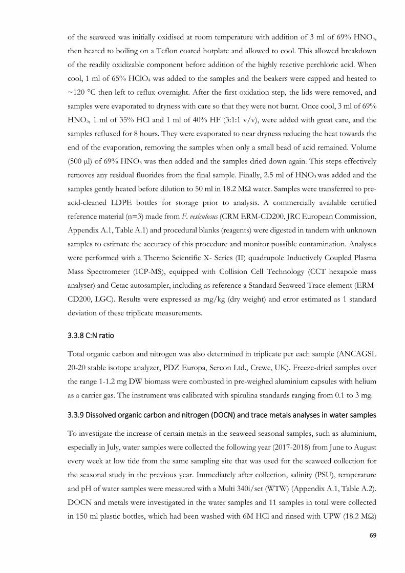
69

of the seaweed was initially oxidised at room temperature with addition of 3 ml of 69% HNO3,

then heated to boiling on a Teflon coated hotplate and allowed to cool. This allowed breakdown

of the readily oxidizable component before addition of the highly reactive perchloric acid. When

cool, 1 ml of 65% HClO4 was added to the samples and the beakers were capped and heated to

~120 °C then left to reflux overnight. After the first oxidation step, the lids were removed, and

samples were evaporated to dryness with care so that they were not burnt. Once cool, 3 ml of 69%

HNO3, 1 ml of 35% HCl and 1 ml of 40% HF (3:1:1 v/v), were added with great care, and the

samples refluxed for 8 hours. They were evaporated to near dryness reducing the heat towards the

end of the evaporation, removing the samples when only a small bead of acid remained. Volume

(500 µl) of 69% HNO3 was then added and the samples dried down again. This steps effectively

removes any residual fluorides from the final sample. Finally, 2.5 ml of HNO3 was added and the

samples gently heated before dilution to 50 ml in 18.2 MΩ water. Samples were transferred to pre-

acid-cleaned LDPE bottles for storage prior to analysis. A commercially available certified

reference material (n=3) made from F. vesiculosus (CRM ERM-CD200, JRC European Commission,

Appendix A.1, Table A.1) and procedural blanks (reagents) were digested in tandem with unknown

samples to estimate the accuracy of this procedure and monitor possible contamination. Analyses

were performed with a Thermo Scientific X- Series (II) quadrupole Inductively Coupled Plasma

Mass Spectrometer (ICP-MS), equipped with Collision Cell Technology (CCT hexapole mass

analyser) and Cetac autosampler, including as reference a Standard Seaweed Trace element (ERM-

CD200, LGC). Results were expressed as mg/kg (dry weight) and error estimated as 1 standard

deviation of these triplicate measurements.

3.3.8 C:N ratio

Total organic carbon and nitrogen was also determined in triplicate per each sample (ANCAGSL

20-20 stable isotope analyzer, PDZ Europa, Sercon Ltd., Crewe, UK). Freeze-dried samples over

the range 1-1.2 mg DW biomass were combusted in pre-weighed aluminium capsules with helium

as a carrier gas. The instrument was calibrated with spirulina standards ranging from 0.1 to 3 mg.

3.3.9 Dissolved organic carbon and nitrogen (DOCN) and trace metals analyses in water samples

To investigate the increase of certain metals in the seaweed seasonal samples, such as aluminium,

especially in July, water samples were collected the following year (2017-2018) from June to August

every week at low tide from the same sampling site that was used for the seaweed collection for

the seasonal study in the previous year. Immediately after collection, salinity (PSU), temperature

and pH of water samples were measured with a Multi 340i/set (WTW) (Appendix A.1, Table A.2).

DOCN and metals were investigated in the water samples and 11 samples in total were collected

in 150 ml plastic bottles, which had been washed with 6M HCl and rinsed with UPW (18.2 MΩ)

70

prior to seawater collection. The bottle was kept in a sampling bag before and after the sampling

and rinsed with UPW (18.2 MΩ) before been brought into the analytical lab for the processing.

The work relative to DOC and DON analyses was conducted in conjunction with the technician

Sharon Mcneill at SAMS. For DOCN, 20 ml of the water samples were filtered through ashed GFF

filters (VWR 513-5242) into a 22 ml borosilicate glass clear 23x85 mm 20-400 screw neck vial

(VWR 548-0679), closed with a chromocol 20-400 mm cap (VWR CRMA20-SC) and injection 20

mm seal silicone, ptfe for 20-SC cap (VWR CRMA20-ST3S) containing 50 µl 85% phosphoric acid.

Samples were than analysed on a Shimadzu TOC-VCPH with Total Nitrogen Module by high

temperature oxidation (HTCO). DOC was analysed on a Total Organic Carbon analyzer

(Shimadzu TOC-VCPH) with Platinum catalyst (0.5% on alumina), carrier gas compressed air (150

ml/min), coupled to an NDIR (Non-Dispersive infra-Red) detector. Total Dissolved Nitrogen

(TDN) was analysed with a nitric oxide Analyser (TNM-1) using high temperature oxidation

converting total nitrogen to nitric oxide (NO) and detection by chemiluminescence. Dissolved

organic nitrogen (DON) was determined by subtraction of total inorganic nitrogen from TDN.

For metal analyses in water samples, samples were filtered through a 0.45 mm polycarbonate filter.

The filtrate was retained in separate acid cleared beakers and acidified using concentrated HCl

(Romil, Cambridge, UK) to give a final concentration of 0.024 M HCl (pH < 2). Indium (In)

internal standard was spiked into the acidified samples prior to analysis to ensure complete recovery

of analytes during analysis. Dissolved metals were analysed using a seaFAST Pico automated pre-

concentration system (Elemental Scientific Instruments Ltd, Warrington, UK). This instrument

loads a 10 ml samples onto a chelation column, removing the seawater matrix prior to elution and

collection of the remaining target metals prior to ICP-MS analysis. A certified reference material

(CRM) NASS6 was processed and analysed in the same manner as unknown samples to estimate

precision and accuracy of the analysis. All metals analysis was performed using a Thermo Scientific

X-Series (II) quadrupole ICP-MS, equipped with a collision cell and Cetac autosampler.

3.3.10 Statistical analyses

Statistical analyses were conducted applying an ANOVA single factor (p<0.05, Minitab 18) with

Tukey’s and Fisher’s post-hoc tests. To understand the relation between months and the

biochemical composition analysed, a PCA (Minitab 18 and PRIMER v6) was performed and the

first two components (considered the most representative) were plotted in an explicative biplot.

Data were standardized as required. BEST, ANOSIM and SIMPER analyses (PRIMER v6) were

performed for correlation with environmental data including temperature (MET Office from

Dunstaffnage station, 2016-2017, Appendix A.3, Figs A.8 and A.9), radiation and hours of light

71

(CEDA-Centre for Environmental Data Analyses, Appendix A.3, Figs A.10 and A.11) and

precipitation data (Met-office for the Dunstaffnage n°918 station, Appendix A.3, Fig. A.7).

3.4 Results

3.4.1 Carbohydrate content

The concentration (% DW) of carbohydrates was determined using the equation obtained from

the calibration curve of standard glucose concentrations (0.25 g/l Glucose stock). Seasonal

variation of carbohydrates in O. pinnatifida samples over a year is reported in Fig. 3.2.

Figure 3.2 Variation of carbohydrates content expressed as percentage per dry weight (DW) across the months in O. pinnatifida samples (n=3; error bar, 1SD of mean) using a Fournier (2001) modified method

There was a statistical difference (p<0.05) between September-May and November -January, also

three main groupings were seen (Sep-May-Aug-Jun-Jul; Apr-Mar-Dec-Oct-Feb; Feb-Nov-Jan)

(Tukey’s comparison, Minitab 18) (Fig. 3.2). The highest values were reported from May to

September and the lowest from October to April.

3.4.2 Protein content

The concentration of protein (%DW) was calculated using the equation obtained from the albumin

standard (2 mg/ml) calibration curve. Absorbance for the samples was corrected with the value

obtained at the same wavelength (562 nm) for the blank (n=3, SD=0.038). Seasonal variation of

protein in O. pinnatifida samples over the 12 months sampling period is reported in the Fig. 3.3.

This follows a different pattern compared to the total carbohydrates, with peaks in September and

December and lower values in the spring and summer months (June: 11.38 %). There was a

statistical difference (p<0.05) between the months, and 4 groupings were identified: Sep-Oct-Nov-

0

5

10

15

20

25

30

35

Car

bo

hyd

rate

co

nte

nt

(% D

W)

Months

72

Dec-Jan, Aug-Apr, Mar, Jul-May-Feb-Jun, which were statistically different from each other

(Tukey’s comparison test).

Figure 3.3 Variation of protein content expressed as percentage per dry weight across the months (%DW) (n=3; error bar, 1SD of mean)

3.4.3 Chlorophyll-a content

Values for chlorophyll-a content with the modified method proposed by Torres et al. (2014) are

reported as µg/g in Fig 3.5. They increased towards the spring period (especially in March) and

started to decrease towards the summer, with lower values for August, compared to the winter

month (such as November, December and January; Fig. 3.5). There was a statistical difference

(p<0.05) between March and August, whilst 4 groups were identified as being similar (Nov-Apr-

Dec-Jan; Dec-Jan-Oct; Jan-Oct-Feb-Sep; Oct-Feb-Sep-June-May-Jul-Aug) with March statistically

separated from the other months. A phenotypical difference in colour of the biomass among the

seasonal samples was also observed (Fig. 3.4).

0

5

10

15

20

25

30

35

Pro

tein

co

nte

nt

(% D

W)

Months

73

Figure 3.4 Variation in colours of seasonal samples of O. pinnatifida from the same sampling site for A) November, B) February, C) March, D) April, E) May, F) June, G) July, H & I) August

Figure 3.5 Seasonal variation of Chl-a (dark grey) and carotenoids (light grey) in O. pinnatifida samples expressed as µg/g of dry weight, with the modified method from Torres et al. (2014) (n=3; error bar, 1SD of mean)

3.4.4 Carotenoids

The modified method proposed by Torres et al. (2014), was effective for extraction of carotenoids

in O. pinnatifida samples and their values for the seasonal samples are reported as µg/g in Fig. 3.5.

The total carotenoid values follow the same pattern as that of the Chl-a measurements (Fig. 3.5).

0

200

400

600

800

1000

1200

1400

1600

1800

2000

Ch

loro

ph

yll a

an

d c

aro

ten

oid

s co

nte

nt

(µg/

g D

W)

Months

74

There were statistical differences (p<0.05) between the months, in particular between March-

April-July. These months showed an increase in the carotenoid content compared to August-

September-October-January-February, which showed a decrease.

3.4.5 Phycobiliproteins

Phycoerythrin (PE) and phycocyanin (PC) were extracted successfully following the protocol

proposed by Pereira et al. (2011) with modification. Statistical analyses, ANOVA (one-way,

p<0.05), identified differences among the samples for PE, especially between the months of

January, December and March. In these months there was an increase in the phycobiliprotein

content, and the samples collected from July, August and May showed a decrease (Tukey’s and

Fisher’s comparison, Minitab 18). The overall trend for the PC and PE pigments was very similar,

with an increase towards December-January and in the spring months (March and April) and a

decrease in the summer months (Fig. 3.6).

Figure 3.6 Seasonal variation of PE (dark grey) and PC content (light grey) expressed as mg/g of dry weight in O. pinnatifida samples (n=3; error bar, 1SD of mean)


The percentage moisture content of O. pinnatifida varies across the months, reaching a maximum

reported value in August and a minimum value in May (Fig 3.7). There were statistical differences

between the months, especially between August, the highest peak for moisture content (88.4 %),

and May and February, which accounted for the lowest values (81.31 and 81.58 respectively)

(p<0.05).

0

0.5

1

1.5

2

2.5

3

3.5

4

PE

and

PC

co

nte

nt

(mg/

g D

W)

Months

75

Figure 3.7 Seasonal variation of full moisture content (FMC) expressed as percentages in O. pinnatifida samples (n=3; error bar, 1SD of mean)


Different dilutions, 1 % dilution and 10 %, for a selected sample were tried in order to estimate

the dilution factor for a more representative reading for TPC and FRAP assays. Neither gave a

strong signal, in relation to the standard curve, as such the samples were analysed undiluted. There

were statistical differences between the samples (p<0.05) especially between June-July-August and

Dec-Feb-Jan, with four groups identified within the one-year sampling period (July-August-June-

March-September; Aug-Mar-June-Sep-Oct; Jun-Mar-Sep-Oct-Nov; Mar-Sep-Oct-Nov-Apr-May-

Dec-Feb-Jan) (Fig 3.8).

Figure 3.8 TPC measurements expressed as µg PGE/mg (phloroglucinol equivalents) of dry weight using the Folin-Ciocalteau method on seasonal samples (n=3; error bar, 1SD of mean)

74

76

78

80

82

84

86

88

90

92

Mo

istu

re c

on

ten

t (%

FM

C)

Months

0

20

40

60

80

100

120

140

160

Tota

l Ph

eno

l Co

nte

nt

(µg/

mg

DW

)

Months

76

The values of the FRAP assay were calculated applying the equation obtained from the Iron (II)

sulfate standard curve (100-1000 µM) and are reported as µM FeSO₄eq/mg DW (FeSO₄Eq stands

for Iron II sulfate equivalents). There was a statistical difference between June-July and the other

months (p<0.05, Tukey’s comparison), while Fisher’s comparison identified 4 groups as statistically

similar. The main difference was reported between July and December. Furthermore, the trend

reported for FRAP analyses is similar to the one for TPC analyses, with the highest values reported

in July and the lowest in December (Fig. 3.9).

Figure 3.9 FRAP assay of monthly collected samples. FRAP results are expressed in µM FeSO₄ eq/mg dry weight (n=3; error bar, 1SD of mean)

3.4.8 Total lipid extracted (TLE)

The highest percentage for total lipid extracted was obtained for December and the lowest value

in July (Fig 3.10). Overall, the percentage of total lipid tends to remain stable across the year. There

was a statistical difference (p<0.05, Tukey’s test, Minitab 18) between the months of December

and July. Generally, the autumn-winter months had the higher concentration of lipid compare to

those of spring and summer.

0

0.5

1

1.5

2

2.5

FRA

P

(µM

FeS

O4

eq

/mg

DW

)

Months

77

Figure 3.10 Percentage of total lipid extracted expressed as percentage of dry weight from seasonal samples of O. pinnatifida. Results are expressed as average of n=3 (Error bar, 1SD of mean)

3.4.9 Metal Analyses

Table (3.1) reports the main metals values expressed in mg/kg (n=3, SD=1) in seasonal samples

of O. pinnatifida. Metal concentrations follow the same pattern across the year, with a general

increase of concentration in February, June, July, October and December, with the peak in

concentrations reached in July (Fig 3.11). There were statistical differences (p<0.05) among the

samples. July differs from September for the Al content, while March and December showed the

highest values for Cr. For Mn concentration, December, February and January differ from the

other months, accounting for the highest values. December, February and July differ from the

other months for Fe content, reporting the highest values; September and August reported the

statistically highest values for Cu concentration. December differs from the other months for the

content of Ni, showing the highest value. November, December, January and February are

statistically higher compared to May and July for Zn content. The highest content for As was

reported in February, which together with June, January and March statistically differ from the

lowest value recorded for July. No statistical differences were reported among the months for Rb.

July shows the highest value for Sr concentration that statistically differs from March. July accounts

for the highest value for Ba concentration, which differs statistically from all the months (excluded

December and June). The highest value for Pb was reported in February and the lowest in

September, with February statistically different from all the other months. Co has the highest

concentration in December, which statistically differs from the other months together with

February. Cd has the statistically highest value in December and the statistically lowest in May. Al

is the most abundant of the metals investigated and ranges from 3245.57 to 526.98. Iron is the

second in abundance and varies from 1147.57 and 316.88. Sr from 458.61 to 100.85; Mn varies

0

0.5

1

1.5

2

2.5

3

3.5

4

4.5

Tota

l lip

id e

xtra

cted

(%

DW

)

Months

78

from 261.54 to 56.16; Zn from 65.96 to 27.89; Ba from 40.76 to 6.68; As from 34.89 to 17.25; Ni

from 13.26 to 5.12; Cu from 8.07 to 1.77; Cr ranges from 4.52 to 1.25; Pb from 3.23 to 0.90; Cd

from 2.57 to 0.66; Co from 0.76 to 0.29; U from 0.44 to 0.18, and Cs from 0.15 to 0.07. Values are

expressed in mg/kg DW (Table 3.1; Fig. 3.11).

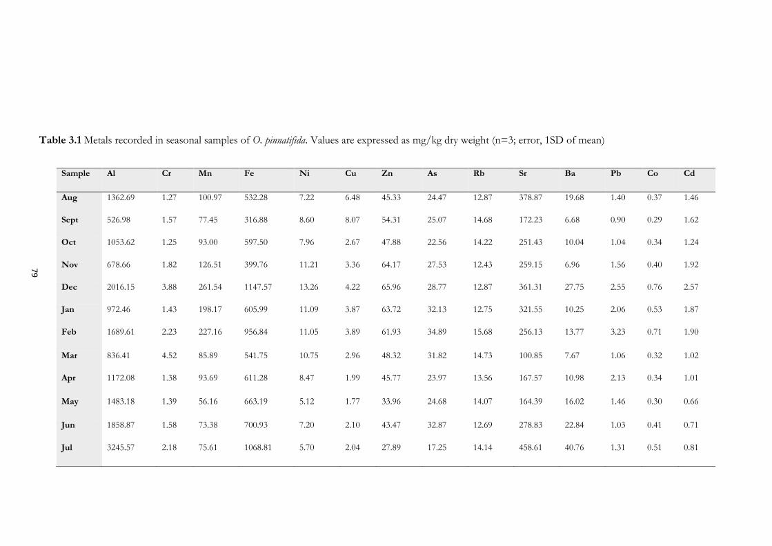
79

Table 3.1 Metals recorded in seasonal samples of O. pinnatifida. Values are expressed as mg/kg dry weight (n=3; error, 1SD of mean)

Sample Al Cr Mn Fe Ni Cu Zn As Rb Sr Ba Pb Co Cd

Aug 1362.69 1.27 100.97 532.28 7.22 6.48 45.33 24.47 12.87 378.87 19.68 1.40 0.37 1.46

Sept 526.98 1.57 77.45 316.88 8.60 8.07 54.31 25.07 14.68 172.23 6.68 0.90 0.29 1.62

Oct 1053.62 1.25 93.00 597.50 7.96 2.67 47.88 22.56 14.22 251.43 10.04 1.04 0.34 1.24

Nov 678.66 1.82 126.51 399.76 11.21 3.36 64.17 27.53 12.43 259.15 6.96 1.56 0.40 1.92

Dec 2016.15 3.88 261.54 1147.57 13.26 4.22 65.96 28.77 12.87 361.31 27.75 2.55 0.76 2.57

Jan 972.46 1.43 198.17 605.99 11.09 3.87 63.72 32.13 12.75 321.55 10.25 2.06 0.53 1.87

Feb 1689.61 2.23 227.16 956.84 11.05 3.89 61.93 34.89 15.68 256.13 13.77 3.23 0.71 1.90

Mar 836.41 4.52 85.89 541.75 10.75 2.96 48.32 31.82 14.73 100.85 7.67 1.06 0.32 1.02

Apr 1172.08 1.38 93.69 611.28 8.47 1.99 45.77 23.97 13.56 167.57 10.98 2.13 0.34 1.01

May 1483.18 1.39 56.16 663.19 5.12 1.77 33.96 24.68 14.07 164.39 16.02 1.46 0.30 0.66

Jun 1858.87 1.58 73.38 700.93 7.20 2.10 43.47 32.87 12.69 278.83 22.84 1.03 0.41 0.71

Jul 3245.57 2.18 75.61 1068.81 5.70 2.04 27.89 17.25 14.14 458.61 40.76 1.31 0.51 0.81

80

Figure 3.11 Variation in metal content expressed as mg/kg of dry weight in seasonal samples of O. pinnatifida (n=3)

3.4.10 C:N ratio

The C:N molar ratio and N and C percentages for the seasonal samples were analysed in triplicate

(Fig. 3.12). The highest value for C content is reported in February while the lowest value is in

September. The highest value for N is reported in December and the lowest in May and September.

The highest C:N ratio was recorded for July and the lowest in March.

Figure 3.12 Nitrogen percentage of dry weight (dark grey bars), Carbon percentage of dry weight (light grey bars) and C:N as molar ratio (dark grey line) of seasonal samples of O. pinnatifida (n=3; error bar, 1 SD of mean)

0

500

1000

1500

2000

2500

3000

3500

4000

4500

5000

5500

Aug Sept Oct Nov Dec Jan Feb Mar Apr May Jun Jul

Met

al c

on

ten

t (m

g/kg

DW

)

Months

Al Cr Mn Fe Ni Cu Zn As Rb Sr Ba Pb Co Cd

0

2

4

6

8

10

12

14

16

18

0

5

10

15

20

25

30

35

40

45

50

C:N

mo

lar

rati

o

Nit

roge

n a

nd

Car

bo

n (

% D

W)

Months

81

3.4.11 Dissolved organic carbon and nitrogen (DOCN) and trace metals analyses in water

samples

There were no statistical differences (ANOVA, p<0.05, Tukey’s test, Minitab 18) reported for the

DOC and TDN values across the months. However, the DOC and TDN analyses follow the same

trend as that of the Al values recorded for the same months the previous year, with a peak in July

(Figs 3.13 and 3.14).

Figure 3.13 Comparison of the trends for the DOC (light grey line) (µM) water analyses (June-August 2018) and Al values (dark grey bars) (seaweed samples, June-August 2017) for the same sampling site in Dunstaffnage beach (n=3; error bar, 1 SD of mean)

Figure 3.14 Comparison of the trends for the TDN (light grey line) (µM) water analyses (June-August 2018) and Al values (dark grey bars) (seaweed samples, June-August 2017) for the same sampling site in Dunstaffnage beach (n=3; error bar, 1 SD of mean)

A positive correlation was reported between Al in seaweed samples and DOC for the seawater

(r=0.99, p<0.05) and Al in seaweed samples and TDN for the seawater (r=0.99, p<0.05).

98

99

100

101

102

103

104

105

106

0

500

1000

1500

2000

2500

3000

3500

4000

Jun July Aug

DO

C in

wat

er s

amp

les

(µM

)

Al c

on

ten

t in

sea

wee

d

(mg/

kg D

W)

Months

0

2

4

6

8

10

12

0

500

1000

1500

2000

2500

3000

3500

4000

Jun July Aug

TDN

in w

ater

sam

ple

s (µ

M)

Al c

on

ten

t in

sea

wee

d

(mg/

kg D

W)

Months

82

Statistical analyses of data on metals content of water samples showed a negative correlation

between aluminium content in water and salinity (r=-0.65, Pearson coefficient p<0.05, Fig. 3.15).

A co-variation of Al and Fe in seawater samples (r=0.99, Pearson coefficient p<0.05) was also

reported (Appendix A.2, Fig. A.5). Furthermore, a positive correlation was observed between Al

content in water samples and precipitation data (r=0.91, p<0.05) (Fig. 3.16) (data from CEDA,

Met office 2017-2018, #918 Station Dunstaffnage, Appendix A.2, Fig. A.7, Tables A.3 and A.4).

Figure 3.15 Correlation between salinity expressed as PSU (light grey line) and aluminium in water samples expressed as µM (dark grey line) collected from June to August 2018 in Dunstaffnage bay. (n=3; error bar, 1 SD of mean)

Figure 3.16 Correlation between aluminium in seawater samples (dark grey line) and precipitation data (light grey bars) (r=0.91, p<0.05). Precipitation data for 2017-2018 are monthly averaged and obtained from CEDA, Met Office, #918 Dunstaffnage station

0

0.2

0.4

0.6

0.8

1

1.2

1.4

1.6

1.8

25

26

27

28

29

30

31

32

33

34

1 2 3 4 5 6 7 8 9

Al i

n w

ater

sam

ple

s (µ

M)

Salin

ity

(PSU

)

Samples

0

0.2

0.4

0.6

0.8

1

1.2

0

20

40

60

80

100

120

140

160

Jun-18 Jul-18 Aug-18

Al i

n s

eaw

taer

sam

ple

s (µ

M)

Pre

cip

itat

ion

(m

m/m

)

Months

83

3.4.12 PCA analysis of seasonal data

The PCA, Eigenvalues, together with proportion and cumulative values are listed in Table 3.2 (see

Appendix A.3, Table A.5 for variables and respective principal components for PCA).

Table 3.2 The total variance explained by PCA analyses is presented in the table below, including eigenvalues, together with proportion and cumulative values of variance. PC1 to 10 are the principal components identified (analyses obtained with PRIMER v6)

PC1 PC2 PC3 PC4 PC5 PC6 PC7 PC8 PC9 PC10

Eigenvalue 5.2138 2.3024 0.8645 0.7731 0.3643 0.2624 0.1118 0.0760 0.0312 0.0005

Proportion 0.521 0.230 0.086 0.077 0.036 0.026 0.011 0.008 0.003 0.000

Cumulative 0.521 0.752 0.838 0.915 0.952 0.978 0.989 0.997 1.000 1.000

Principal component analysis was applied in this study in order to understand the correlation

between the different variables and to explain the general trend recorded from the seasonal

variation of the biochemical composition. Interpretation of the principal components is based on

finding which variables are most strongly correlated with each component. In this case, the first

principle component analyses is a measure of the concentration of PC, PE, FRAP and C:N. PE

and PC have a positive correlation while FRAP and C:N negative, so if the first ones increase the

others will decrease. The second principal component is a measure of the concentration of protein,

carotenoids and lipids. If the protein and lipid increase, the carotenoids will decrease. The third

principal component is a measure of the concentration of TPC, carbohydrates and lipids, all with

negative values of correlation. It means that if one of these value decreases the others will follow

the same trend. The fourth principal component is a measure of the concentration of TPC,

proteins, carbohydrates and carotenoids. If the proteins and TPC values increase, the carbohydrates

and carotenoids decrease. The fifth principal component is a measure of the concentration of TPC,

C:N and carotenoids. If the last two decrease than TPC values increase. However, most of the data

can be represented by the first two components that account for the 75% of variance (Table 3.5,

Fig. 3.17).

Correlation of the environmental parameters and biochemical composition was performed with

data relative to light, temperature and precipitation from MET office and CEDA. (Appendix A.3,

Figs A.7-A.11, precipitation, temperature, and radiation data from 2016 to 2017 for Dunstaffnage

bay). From this, ANOSIM (R=0.758) and SIMPER analyses (Figs 3.18 and 3.19) identified three

main groups. Group “a” only includes July. This differentiates from the other two groups in terms

of the TLE, TPC and C:N values measured. Group “b” includes October, November, December,

January, March and April, differentiates from group “c”, which includes February, May, June,

August and September, in terms of the pigments (Chl-a and carotenoids), moisture and protein

84

contents measured. Group “b” is characterized by the protein, phycobiliproteins, and TLE

contents while group “c” is commonly characterized by the concentration of carbohydrates,

antioxidant and carotenoids. BEST analyses (Fig. 3.18) demonstrated that the two abiotic factors

that express correlations within the monthly samples are the temperature and the hours of light

(No. var=2, Corr. Selections=0.528). Bivariate correlation showed that compounds such as

antioxidants and carbohydrates, are positively correlated with abiotic factors, such as light intensity

and temperature (r for antioxidant compounds and light=0.75; r for antioxidant compounds and

temperature=0.72; r for carbohydrates and light=0.75; r for carbohydrates and temperature=0.86,

see Appendix A.3, Figs A.12-A.18).

Figure 3.17 Screen plot of PCA showing the Eigenvalues and the respective component number. From the plot trend, it is evident that the majority of data is represented by the first three components, while from the third there is a change in the inclination of the line and the remaining components account only for a small percentage of data

85

Figure 3.18 The first and the second PCs were plotted since accounted for more than 75% of variance together. ANOSIM and SIMPER analyses (PRIMER, v6) identified two groups (b and c) and one outgroup (a, July) in relation to the similarity between the months in terms of biochemical composition

Figure 3.19 BEST analyses (PRIMER, v6) identified correlation between environmental factors (maximum temperature, precipitation, hours of light and maximum radiation) and months and importance of the abiotic factors in influencing the seasonality of the biochemical composition of the species

86

3.5 Discussion

According to Chojnacka et al. (2012), there are about ten thousand identified macroalgae species,

yet only about 5% thereof are used as human food, or as animal feed. In Europe, the use of edible

seaweeds for food purposes is largely historic, although this is changing and currently researchers

are studying less-known seaweed species. Not only because of their potential biological properties-

due to specific functional compounds, but mostly for their nutrient profile. They are being

considered as important alternative sources for protein and complex carbohydrates (Ibañez and

Cifuentes, 2013).

From a cultivation perspective, it is important to have a knowledge of the biochemical composition

of a target species and its nutritional profile, in order to exploit it in further applications, such as

food and/or bioactive compound. Nonetheless, investigations are fundamental to improve or

manipulate the nutritional profile in order to fit the market requirements and to exploit new species,

such as O. pinnatifida, as source of biologically active compounds with interests for further

biotechnological applications. While few cultivation trials have been undertaken for O. pinnatifida

(Silva, 2015; Gonçalves, 2018), different studies have been conducted on its nutrient levels,

bioactive properties and biochemical profile (Campos et al., 2019; Rodrigues et al., 2015, 2019;

Paiva et al., 2014; Patarra et al., 2011, 2013; Sabina and Aliya, 2009, 2011; Marsham et al., 2007;

Rizvi and Shameel, 2005). Whilst this study is the second to present the biochemical composition

of O. pinnatifida in UK, the first one was undertaken by Marsham et al. (2007). This study is the

first one to investigate the impact of seasonal variation on the biochemical/chemical composition

of O. pinnatifida, and the first to also consider the relationship this has with abiotic factors.

O. pinnatifida shows variation in its nutrient components across the months, for all the compounds

analysed. Based on previous studies conducted on O. pinnatifida, the following methods were

applied by previous authors for biochemical investigations: nitrogen content was determined by

the Kjeldahal method (Marsham et al., 2007; Denis et al., 2010; Munier et al., 2013; Rodrigues et

al., 2015); total fat content by Soxhlet extraction (AOAC, 2000; Rodrigues et al., 2015) and

Soxtherm method (Marsham et al., 2007) together with the application of GC for fatty acid (FA)

profile (Paiva et al., 2014); total sugar content was calculated by subtracting protein content and fat

content from total organic content (Rodrigues et al., 2015); soluble carbohydrates content has been

determined throughout the phenol-sulphuric acid colourimetric method (Dubois et al., 1956);

polyphenols were extracted and analysed with the Folin-Ciocalteu method (Rodrigues et al., 2015)

and run on a LC-MS system (Nwosu et al., 2011). Elements have been assessed through an acid

digestion and ICP-OES (Rodrigues et al., 2015) or with HPLC (Paiva et al., 2014). Antioxidant

activity (as 2,2-Diphenyl-1-picrylhydrazyl, DPPH*) was determined spectrophotometrically

(Andrade et al., 2013). Amino acids analyses were performed following Barbarino and Lourenco

87

(2005) method, with a modified procedure for derivatisation from Sánchez-Machado et al. (2003),

and an evaluation of amino acids profile on HPLC system (Paiva et al., 2014). However, in this

study a different approach was taken, and a new set of assays for biochemical composition were

tested and compared to those previously employed for O. pinnatifida. This was undertaken in order

to develop and achieve faster, more reliable and efficient methodologies for assessing the chemical

composition of O. pinnatifida.

3.5.1 Carbohydrate content

In Paiva et al. (2014) carbohydrates were measured employing the colorimetric method described

by Dubois et al. (1956) and the value reported (17.59 ± 0.27% of DW) is comparable to that

obtained in this study for the same month (17.09 %, January). Rodrigues et al. (2015) reported a

percentage of total sugar equivalent to 32.4 for O. pinnatifida in Portugal, which is higher compared

to those reported in this study (Fig. 3.2) for the same month (April). The second method applied

(modified from Fournier, 2001) proved to be more efficient in carbohydrates extraction from dry

biomass of O. pinnatifida, compared to the single tube multi-assay extraction (Appendix A.2, Fig.

A.6) (Slocombe et al., 2013). The carbohydrates follow almost a linear trend from January to April,

with an increase in May-June and again in August-September, followed by a decrease in October,

November and December. The highest value obtained was in September (27.78 %) and the lowest

in January (17.09 %). The level of carbohydrates is higher during the spring-summer compared to

the winter and autumn; because the seaweeds accumulate and store this type of resource to use

later in the season when the available nutrients are at lower levels (Lüning and Pang, 2003). The

trends for carbohydrates and protein content look almost inverted, with lower levels of protein

from May to August, when the carbohydrates have increased and is at its highest levels of

concentration (Figs 3.2 and 3.3).

3.5.2 Protein content

The value relative to the percentage of protein are similar to those reported by Rodrigues et al.

(2015), that estimated 21 % for O. pinnatifida sample in April. In Paiva et al. (2014), protein levels

were estimated employing a modified Kjedahl procedure (AOAC, 1990) and the application of a

conversion factor of 6.25, with a value of 20.79 %± 0.12. The same method was applied by Patarra

et al. (2011), with an average value of 20.64 (for January-February) and by Marsham et al. (2007),

that reported a value of 27.3 ± 0.1 % of protein for O. pinnatifida in the UK. These values are similar

to those obtained in this study (Fig. 3.3). Protein content of seaweeds varies not only between

species (Fleurence, 1999), but also between seasonal periods (Mishra et al., 1993). This was

confirmed in this study for O. pinnatifida seasonal samples. As already seen for other red algae

(Galland-Irmouli et al., 1999; Sanchez-Machado et al., 2003; Cian et al., 2015), O. pinnatifida has

88

high level of proteins. Higher values are reported for autumn-winter months (27.41% September

25.13 % December) while the lowest for February (12.04 %) and summer months in general (11.38

% June). The concentration of proteins follows an oscillation along the months but was more

stable compared to the variation in carbohydrate and pigment content (Figs 3.2, 3.3, 3.5 and 3.6).

Most seaweeds contain all the essential amino acids and are a rich source of the acidic residues

aspartic and glutamic acid (Fleurence et al., 2012). However, the composition of the protein was

not estimated in this study, but the data obtained from the metabolomics analyses presented in

Chapter 4, gives some hints as to the major proteins present. Similar variation in protein content,

with an increase in the winter and a decrease in the summer (especially July and August), was

reported for other species of red algae; e.g. G. turuturu (Denis et al., 2010) and P. palmata (Galland-

Irmouli et al., 1999). The same trend was also observed for the phycobiliproteins seasonal samples

of O. pinnatifida, in this study, at least for December and March-April. This is probably related to

the necessity to be able to harvest light in sufficient quantities for photosynthesis to occur during

the winter. As confirmed by other authors (Pereira et al., 2012; Kosovel and Talarico, 1979;

Campbell et al., 1999; Aguilera et al., 2002; Orduña-Rojas et al., 2002) the highest concentration of

protein and phycobiliproteins were observed in the months with the lowest light levels and the

lowest in the months with elevated sunlight levels. This association was confirmed in this study for

O. pinnatifida (Figs 3.3 and 3.6).

3.5.3 Pigment content

Initially for the pigments’ analyses in O. pinnatifida, a single tube multi-assay was considered. This

method was used for measuring the protein content and trialled for carbohydrates, but was

considered unsuitable, because it had been developed for the analyse of green algal biomass (Chen

and Vaidyanathan, 2013). Another method was tested (Torres et al., 2014), which involved

methanol extraction of the pigments from the harvested biomass. The Chl-a and carotenoids were

calculated following the equations in this paper and adapted to red algae (Torres et al., 2014). Within

this chapter, an initial trial was carried out reducing the quantity DW of biomass to be extracted

from 25 mg, as described in the paper, to 5 mg of DW. Between these two values, a range of

selected quantities of DW material were extracted and the results, in term of concentration,

obtained compared. This confirmed that the reduction in biomass extracted gave acceptable set of

results in relation to the quantity of pigments measured. The values obtained were comparable to

those estimated by Torres et al. (2014) (Fig. 3.5). Chl-a concentration changed across the months,

increasing significantly in February-March and then decreasing towards the summer (August). This

is probably related to the light intensity levels and the length of light exposure. The same pattern

was observed for the carotenoid concentration, which means that both pigments act simultaneously

in light harvesting (Chl-a) and protection (carotenoids) (Fig 3.5). Carotenoid contents in

89

macroalgae responds to high radiant energy increasing its concentration for a photo protective

action in preventing photo oxidation (Harker et al., 1999).

For the measurement of phycobiliproteins, the method proposed by Pereira et al. (2012), applied

for Gracilaria sp., was tested for seasonal samples of O. pinnatifida in this study. Only 50 mg of DW

were used for the analyses (rather than 90 mg, as proposed by the protocol). The other steps of the

protocol were kept the same (Pereira et al., 2012). PE and PC in O. pinnatifida followed the same

pattern, with an increase in December-January and March-April, and a decrease towards the

summer. It has been previously reported that high light irradiance can negatively affect

phycobiliprotein pigment concentrations in macroalgae (Aguilera et al., 2002; Zubia et al., 2014).

Another factor that plays a role in the phycobobiliproteins concentration is N limitation, since this

may cause red algae to use their phycobiliproteins as a catabolite, with the consequence of a

reduction in their light-harvesting ability (Lobban and Harrison, 1994) and a “bleaching” effect

(Penniman and Mathieson, 1987). This was confirmed in this study were the concentration of

phycobiliproteins decreases during the summer, this is also the period during which this species

undergoes N limitation, verified by the C:N data (Fig. 3.12). The concentration of PE is higher

than PC, except in August, September and May. A similar pattern, but with lower values were also

obtained for Gracilaria domingensis (Pereira et al., 2012) for PE and PC. The equations applied for

their estimations were those proposed by Beer and Eshel (1985). The results obtained were similar

to those reported for Gracilaria sp., ranging from 0.10 to 0.6 (mg/g) for PC and from 1.5 to 7

(mg/g) for PE (from Pereira et al., 2012) and to those proposed by Beer and Eshel (1985) for

different red algal species (Fig. 3.6). This is one of the most frequently cited phycobilin

quantification techniques (Beer and Eshel, 1985) that utilizes the spectral properties of crude

aqueous extracts to estimate the pigment contents of sample tissues. In particular, pigments were

investigated in this study because O. pinnatifida has a great variability in the colour (Fig. 3.4), linked

to where and when it grows. Since the colour is a fundamental parameter in the commercialization

of different products (e.g. salmon, sea urchin’s gonads, etc.), it is important to see if is it possible

to regulate the phenotype of a species in order to tailor the final product according to the market’s

needs. This might be applicable also to O. pinnatifida; however, it is still not understood if the colour

has any influence on the taste of this particular algal species. The literature reports that macroalgae

regulate their pigment contents, constitution and morphology responding to prolonged exposure

to different light levels (Machalek et al., 1996). Furthermore, when internal N reserves decrease,

seaweed start to lose their dark reddish-brown pigments, turning into a pale-yellow colour and

growth ceases (Ryther et al., 1981). This loss of colour might be correlated to the fact that pigments

are processed as alternative source of protein (Lapointe, 1981; Bird et al., 1982).

90


Moisture content reported in this study is very similar to that estimated by Paiva et al. (2014): for

the sample from Azorean area of January, they reported 90.6 %. Furthermore, Marsham et al.

(2007) reported a similar value of 86.4 ± 3.7 as well as Rodrigues et al. (2015), reporting a

percentage of 88.23 ± 0.01. In this study, the moisture content does not change much across the

months, with statistical differences reported only between August and May-February (Fig. 3.7).


The total phenolic content evaluated through the Folin-Ciocalteu colorimetric method has become

a standard assay in studying phenolic antioxidants. It is a convenient, simple and reproducible assay

(Huang et al., 2005). Seaweed may contain a wide variety of phenolic compounds: from simple (e.g.

phenolic acids) to more complex substances (e.g. phlorotannins) in different quantities. The lack

of an accurate and universal extraction method for phenolic analyses in seaweed is because these

compounds can be combined with other components in the biomass (such as carbohydrates and

proteins). Nevertheless, several solvents (such as methanol, ethanol, acetone and their

combinations) have been widely used for the extraction of phenolic compounds (Dai and Mumper,

2010). As already observed for other chemical compounds, the composition of phenols might also

vary, qualitatively and quantitatively, depending on the habitat, environmental parameters (light,

temperature and salinity), the season, the geographical distribution and the actual species been

investigated (Ibañezet et al., 2012; Rodríguez-Bernaldo et al., 2010a, b). Antioxidant properties

were analysed applying TPC and FRAP assays, without considering the DPPH* measurements,

already reported in previous studies for this species (Silva and Abreu, 2014; Silva et al., 2018). For

TPC, an extraction with 50% Acetonitrile/UPW containing 0.1% formic acid (w/v), followed by

Folin-Ciocalteu method was conducted in this study, while extraction with ethyl acetate plus Folin-

Ciocalteu method was applied by Rodrigues et al. (2015). They reported a TPC of 337± 22 µg/g

DW for O. pinnatifida for April, while in this study the TPC value for that month was 93.69 ± 0.04

µg/mg, with the highest value measured for August and the lowest for January (Fig 3.8). Similar

results were proposed by Campos et al. (2019) that reported a value of 172 mg Gallic acid equivalent

(GAE/100 g DW, TPC) for O. pinnatifida in March. The results obtained from TPC analyses in this

study (Fig 3.8) are higher than those reported by Silva and Abreu (2014) for O. pinnatifida cultivated

in a trial in Portugal (wild samples 87.57 and IMTA-samples 65.89 mg GAE/g). The difference

with previous authors’ work can be attributed to the different extraction methods and reference

standards applied. Furthermore, TPC and FRAP analyses in this study followed the same trend,

confirming the seasonality reported. Generally, the primary function of phenolic compounds in

land plants is as protection against ultraviolet radiation and pathogens (Manach et al., 2004).

Phenolic compounds found in algae also include the phlorotannins found in brown algae and in

91

lower amounts in some red algae (Machu et al., 2015). They are components of cell walls, but they

have also other secondary ecological functions such as radiation protection and reproduction. They

have also been investigated for their potential therapeutic properties (anticancer, antioxidative,

antibacterial, anti-allergic, anti-diabetes, anti-aging, anti-inflammatory and anti-HIV activities) (Li

et al., 2011). Polyphenolic compounds are very common constituents of human diets, there is also

increasing interest from both consumers and food manufacturers linked to these compounds

(Manach et al., 2004). It has been suggested that the phenolic compounds of this species may play

a role in its peculiar taste. A deeper understanding of their concentration and variation could be

applied to the commercial exploitation and tailoring treatments to the cultivation of this species.

But the information present here is relevant for identifying the best harvesting season for this

species and for further commercial exploitation of O. pinnatifida for biotechnological applications.

3.5.6 Total fatty acid content

With respect to the total lipid extracted, it should be noted that the method here applied extracts

all the lipids present in the sample (including pigments, such as carotenoids). The results obtained

were different from those reported by Rodrigues et al. (2015), who published a value of 0.9 for %

total fat (g/100 g dry seaweed) (analyses on gas chromatography) and Paiva et al. (2014), who

reported a lipid % of 7.53 (applying a Soxhlet extraction). However, they are similar to those

recorded by Marsham et al. (2007) that reports a percentage of 4.3 (using a Soxtherm method).

Higher values were reported for the autumn-winter months, while lower ones for the spring-

summer months, with the lowest value reported for July (Fig. 3.10). Similar results have been

obtained for other seaweeds (e.g. Undaria pinnatifida, Laminaria japonica, Fucus serratus, Egregia

menziesii, Condrocanthus canaliculatus and Ulva lobata; Gerasimenko et al., 2011; Kim et al., 1997;

Nelson et al., 2002). Composition of lipids was not analysed in this study.

3.5.7 Metals content in seaweed samples

Seaweeds play an important role in the nutrient dynamics of coastal systems and reflect changes in

water quality efficiently (Wilson, 2002). Contamination of heavy metals in the marine environment

is posing a major problem, which is directly related to anthropogenic actions (Karthick et al., 2012).

Since the species here investigated is used in food applications, it is particularly important to

investigate the metals and minerals content of the biomass. Metals were analysed for O. pinnatifida

in this study and values compared with those obtained by Rodrigues et al. (2015). The accuracy of

the digestion procedure and analyses applied in this study was confirmed by the percent recovery

of the certified elements (Appendix A.1, Table A.1). Furthermore, the step with hydrofluoric acid

was chosen following previous in-house seaweed investigations where residues (possibly silicates)

and sometimes clasts were still clearly visible after the first nitric acid/perchloric acid reflux step

92

and reproducibility of some metals was found to be inconsistent (Abell, pers comm.). These

adjustments confirmed that the methodology was high and sensitive enough to resolve any seasonal

variation within the seaweed samples.

Rodrigues et al. (2015) reported 3.7 for iron, 0.58 for zinc, 0.05 for copper and 0.12 for manganese

(as mg/10g dry weight). Higher results were obtained in this study (for the same month, April),

especially regarding the concentration of iron. Arsenic measured in this study was higher compared

to its concentration estimated in other red algae (e.g. L. papillosa: 1.48 µg/g dry weight; L. johnstonii:

5.65 µg/g dry weight, Sanchéz-Rodrigues et al., 2001) but similar to the results reported for other

species, such as G. pachidermatica (13.8 µg/g dry weight) (Sanchéz-Rodrigues et al., 2001). The other

metals estimated in Sanchéz-Rodrigues et al. (2001) are similar to those estimated in this study

(Table 3.1). Apart from the many positive aspects associated with the consumption of algae, there

are also concerns to consider, especially regarding the concentration of heavy metals. Algae are

known for their capacity of absorbing and accumulating heavy metals (e.g. arsenic, cadmium and

mercury) (Rincon et al., 2005; Brinza et al., 2007). Limits for the consumption of these

contaminants has been determined by the FAO/WHO (2008, 2011a) Expert Committee on Food

Additives (JECFA) with units expressed as µg/kg body weight per week, with the value set for 15

and 7 for arsenic and cadmium respectively. The level of arsenic (mg/kg) in this study range from

34.89 (March) to 17.25 (July), while the Cd value vary from a maximum of 2.57 (December) to 0.66

(May). These results demonstrated that arsenic and cadmium levels are not a major concern for

this species harvested in this geographical region, particularly considering the low amounts of this

seaweed consumed. It should be noted that the toxic potential of heavy metals is also dependent

on their physical state, with the arsenic being the most toxic in its inorganic form. Usually algae

convert most of the inorganic arsenic in arsenosugars and arsenophospholipids (García-Salgado et

al., 2012). Aluminium concentration in all the seasonal samples was higher than any other element

investigated, followed by iron (Table 3.1). However, the critical elements (e.g. As, Pb, Cu, Cd) were

found in moderate/low values, when compared to other seaweed species (such as Laminaria spp.,

S. latissima, A. esculenta, L. obtuse, P. palmata) (Schiener et al., 2015; Mæhre et al., 2016). However, Fe

concentration was particularly high, especially compared with other red algae (such as P. palmata,

Fe 100 mg/kg, Mæhre et al., 2014). High amounts of barium can be normally found in seaweeds

and fish; these minerals are released into aquatic ecosystems by industrial processes and can

accumulate in the organisms. The level of this metal has to be low since high concentration can

have severe and deadly effects on humans and other organisms (Apaydin et al., 2010). In this study,

the level of Ba was generally low, the exception was the month of July. Sr in its elemental form

occurs naturally in many environments and the highest level of Sr in this study was reported for

July. It has been seen that concentrations of chemical elements in seaweeds are generally low in the

warmer months, i.e. the time of the highest algae metabolic activity resulting in dilution of the

93

accumulated metals whereas in the winter with a slowing down of metabolic processes the element

content is higher (Bojanowski, 1973; Hou and Yan, 1998; Villares et al., 2002). However, this was

not completely confirmed in this study, were some metals were observed at their maximum

concentration in the spring-summer months (Fig. 3.11).

3.5.8 C:N ratio in seaweed samples

C:N values between 10 and 15 are typical for macroalgae with normal growth rates (Lobban and

Harrison, 1994). Higher values than this threshold indicate limitation of growth due to nitrogen

deficit while lower values show nitrogen accumulation (Hanisak, 1983). C:N ratio was considered

in this study because since the 1970s it has been used as an index of food quality in seaweed

(McMahon et al., 1974), a low C:N ratios (which mean high N levels) suggests relatively high levels

of protein. A positive correlation between protein and nitrogen content has previously been

reported in brown, red and green seaweeds (Kim et al., 2013; Lapointe and Ryther, 1979;

Robertson-Andersson et al., 2009). However, N and protein content may not be directly related if

the nitrogen is stored in refractory or non-proteinaceous material (McMahon et al., 1974). C:N and

C:P ratios are usually elevated in low nutrient environments, reflecting an increased limitation of

net productivity by N, P or both (Lapointe, 1987). In this study, the highest C:N ratio for O.

pinnatifida was reported for the months from May to August, the maximum values reported was for

July (15.1) and the lowest for March (8.5, Fig. 3.12). However, in general O. pinnatifida never exceeds

C:N ratio of 15, showing a general trend of normal growth rate across the whole year.

3.5.9 Metals and DOCN analyses on water samples

To better understand the high peaks reported in certain months (such as July) for certain metals,

like aluminium, water sampling followed by DOCN and metals analyses were conducted from June

2018 to August 2018 of the following year (2017-2018) and the results compared to the seasonal

seaweed specimens collected in the same area, the previous year, in 2016-2017. Interestingly,

DOCN analyses on water samples showed the same trend reported for the aluminium content in

the seaweed samples, with a peak reported in July. DOCN is an important parameter to consider

when it comes to metal analyses in water. Metals can aggregate with dissolved organic matter in the

water column, such as carbon and nitrogen, through adsorption and flocculation (Dekov et al.,

1998), and to have a complete account of the metals in the water this proportion has to be

considered. Dissolved organic carbon (DOC) present in water is primarily in the form of refractory

(i.e. poorly biodegradable) compounds with some biodegradable dissolved organic carbon (BDOC)

or assimilable organic carbon (AOC). DOC and C:N analyses conducted in this study on the water

samples suggest that there is a higher terrestrial signal of organic matter for the August sample.

C:N ratio <8 are usually from marine sources, while higher ratios (C:N >15) are likely to come

94

from terrestrial sources (Gray and Biddlestone, 1973; Premuzic et al., 1982; Ruttenberg and Goñi,

1997b). Heavy metal pollution originates from natural and anthropogenic sources; the natural

sources include rock weathering and soil erosion, and the anthropogenic sources include domestic

sewage, industrial wastewater, mining wastewater, agricultural fertilizer leachate, and coal burning

(Alvarez-Vazquez et al., 2017; Davis and Birch, 2010; Pan and Wang, 2012; Skordas et al., 2014).

Statistical analyses conducted on seawater and environmental data and evaluation of correlation

with salinity and precipitation data, suggests that the high level of Al and Fe (abundant in terrestrial

derived carbon, Krachler et al., 2010) reported first in the seaweeds samples and then in the water

samples might be related to an inland input (Appendix A.1, Tables A.3 and A.4). Dunstaffnage bay

is surrounded by granitic mountains and is located in close proximity of Loch Etive. Both of which

could supply significant amounts of aluminosilicate particles and cations to the seawater into the

area sampled (Krachler et al., 2010; Muller et al., 2012).

Interestingly, the comparison between wild and cultivated samples (obtained from tank experiment

applying F/2 medium, see Appendix A.1, Figs A.1 and A.2) in regards to certain metals, shows

some differences in particular for Fe, Co, Cu concentration (higher values are reported in the

cultivated sample compared to the wild) and As, Sr, Ba, Al, Mn and U (lower values are reported

in the cultivated sample compared to the field samples). This is probably due to the F/2 medium

used for the cultivation and the source of seawater used for its preparation which comes from

filtered, UV sterilised and tyndalysed seawater pumped from the back beach at SAMS. This can

also be particularly important from a cultivation perspective, since some of the heavy metals

showed statistically lower values in the cultivated samples compared to the wild ones. This

reduction in content of particular metals (As, Ba, Al, Mn and U, Appendix A.1, Figs A.1 and A.2)

during cultivation is interesting for the final product obtained since it can increase the number of

food and nutraceutical applications.

3.5.10 PCA Analysis

The first and the second principal components account for 75% of the variability in the data, while

the cumulative variability for the first three PC is 86 %. Variables were plotted with the first two

components together with the sampled months. Two main groups were observed in the chart and

one outgroup, July. According to the biplot (Figs 3.18 and 3.19) it seems that the summer-early

autumn months are commonly characterized by the concentration of carbohydrates, antioxidant

compounds and C:N ratio. Autumn and early-winter months are instead associated with higher

concentration of protein and lipid. Months of late winter-spring are instead grouped by the values

of pigments, including phycobiliproteins, chlorophyll-a and carotenoids. July emerges as outgroup

from these analyses. This information is useful in understanding which biochemical components

are more characteristic and specific for each month in order to comprehend how the biochemical

95

composition in O. pinnatifida varies, becoming then useful in the application of a harvesting plan

and cultivation trials.

Seaweeds are exposed to seasonal variations of abiotic factors (such as temperature, irradiance,

salinity, etc.) that can influence their metabolic responses, including photosynthesis and growth

rate, as well as levels of their principal constituents (Orduña-Rojas et al., 2002) and their

biochemical composition (Fábregas et al., 1995; Fernandéz-Reiriz et al., 1989). Moreover, the

nutritional properties of seaweeds and their seasonal oscillation are poorly known and normally are

evaluated from the chemical composition (Mabeau and Fleurence, 1993). This study considers

some of the abiotic parameters available for the sampling site in the Dunstaffnage bay, including

hours of light, radiation, temperature and rainfall data. This data was analysed together with the

biochemical components in order to verify if there was any correlation between them and the

variation of the biochemical composition of O. pinnatifida in the West coast of Scotland. The data

considered referred to the period from August 2016 to July 2017, the same time interval of the

biomass sampling.

PCA analyses helped in understanding how the biochemical profile of the species changes across

the seasons. Correlation analyses demonstrated that abiotic factors (such as temperature and

irradiance) can influence the metabolic responses and the biochemical composition of the species,

as already seen for other seaweeds (Orduña-Rojas et al., 2002; Fábregas et al., 1995; Fernandéz-

Reiriz et al., 1989). A positive correlation was found between the hours of light and the production

of antioxidant compounds as well as carbohydrates content (see Appendix A.3, Figs A.12-A.15).

Furthermore, statistical analyses provided a characterization of the months according to their

biochemical profiles, which is fundamental for timing and management of harvesting.

3.6 Conclusions

As already underlined, this study confirms that O. pinnatifida is an important source of

bioactive compounds with beneficial properties such as antioxidant, antiviral, antibacterial

and anticancer. Therefore, the information obtained from this study are fundamental to

gain a better knowledge of how the production of these compounds is regulated by the

environmental factors (such as light and temperature) and how this information can be

used and applied to a cultivation perspective in order to target the final product ensuring a

determined biochemical profile;

Protocols were successfully developed and established for the biochemical analyses of the

species or existing ones were modified and readapted;

The metal content, especially in relation to arsenic and cadmium, does not represent a

threat to human health in the vision of a commercialization of the species as food or

96

nutraceutical products; furthermore, metals’ content can be manipulated in cultivation

systems which can become particularly valuable for commercial production of the biomass

and can reduce the concentration of unwanted metals;

This study helps in identifying a harvesting plan for the species, according to the further

commercial applications of it. This is important if the final scope of the harvested biomass

of this species is, for example, the production of bioactive compounds rather than biomass

to be used in the food industry. In this case, late spring-summer months should be

preferred. On the other hand, if the main aim is instead the exploitation in the food

industry, other parameters such as carbohydrates and protein have also to be taken into

consideration. In regard to carbohydrates, the best harvesting season is summer-early

autumn, while for protein and lipids autumn-early winter. Finally, for pigments the highest

content is reported in spring. Moreover, the information obtained from this study can

become helpful to outline a legislation for collection of the species, considering not only

the abundance but also the quality of the harvested biomass.

This is the first time that the seasonal variation in biochemical composition of O. pinnatifida

across one year has been investigated and also correlated to abiotic data. This information

is paramount in understanding the biochemistry of the species and the application of this

knowledge to cultivation methods (in terms of light and temperature requirements) might

guarantee the continuos supply of a high value tailored and controlled product, exploitable

commercially;

Biochemical analyses confirmed, as already reported by previous authors, that O. pinnatifida

has a good potential for further processing or for direct food and nutraceutical applications

(Rodrigues et al., 2015; Paiva et al., 2014; Patarra et al., 2011, 2013; Sabina and Aliya, 2009,

2011; Marsham et al., 2007; Rizvi and Shameel, 2005).

98

Chapter 4 Composition and seasonal variation in the metabolomic

profile and flavour of Osmundea pinnatifida

4.1 Introduction

Metabolomics has now become a high-resolution biochemical phenotyping tool capable of

advancing our understanding of primary and secondary metabolism. It has made great success in

assessment of responses to environmental stress, biomarker analysis, chemotaxonomy, comparing

mutants and different growth stages, drug discovery, studying global effects of genetic

manipulation, and natural product discovery (Higashi and Saito, 2013; Kim et al., 2011; Muranaka

and Saito, 2013; Putri et al., 2013). Metabolomic analyses provide information on the regulatory

processes and metabolic responses of organisms, and it has recently helped in gaining newer

insights into the biochemical composition and functioning in seaweeds (Gaubert et al., 2019). The

continuing investigation of seaweeds for multiple biochemical, nutraceutical, pharmaceutical

applications, has greatly increased their applications in a wide array of sectors, e.g. food, feed,

fertilizer and hydrocolloids, and new, e.g. cosmetic, nutraceutical, biomaterial, and bioenergy

(Bixler and Porse, 2011; Holdt and Kraan, 2011). These developments have also led to a sudden

rise in seaweed production (FAO, 2010). Metabolomics in seaweeds is still in its infancy compared

to terrestrial plants which have been more widely investigated (Davis and Vasanthi, 2011).

However, some groups of metabolites have been studied for decades in seaweeds including

mycosporine-like amino acids, halogenated compounds (Kundel et al., 2012; La Barre et al., 2010;

Yuan et al., 2009), and lipids and their derivatives (Bouarab et al., 2004; Goulitquer et al., 2012;

Kumari et al., 2013a, b).

Metabolite concentrations in seaweed varies between and within species (Oliveira et al., 2013;

Wright et al., 2000), and can be affected by environmental factors (biotic and abiotic) (Kooke et

al., 2011; Slattery et al., 2014). Metabolite profiling in seaweeds has been carried out for decades

but has been restricted to targeted identification of one group of metabolites (Kumari et al., 2013a,

b; Kundel et al., 2012). There is a lack of information on the global metabolomics response of

seaweeds, especially in relation to changing environment conditions (Greff et al., 2017), with the

majority of present studies that focus on specific families of compounds therefore overlooking

many metabolites likely to play important ecological functions. In 2011, the first high coverage

metabolomics study on red algae was published (Nylund et al., 2011), and it described changes in

metabolites produced by Gracilaria vermiculophylla in relation to defence response. More recently an

attempt has been made to constitute a reference library for seaweed metabolites (Davis and

Vasanthi, 2011).

99

Red seaweeds, compared to green and brown, have proved to produce halogenated metabolites,

especially bromine and iodine derivatives (McConnell and Fenical, 1977; Fenical, 1981; König et

al., 1999a). The orders of Nemaliales, Gigartinales, Ceramiales, Rhodymeniales and Cryptonemiales

have been shown to be engaged in biological halogenations yielding a diverse array of organic

compounds (McConnell and Fenical, 1977). Species of the Laurencia complex (included O.

pinnatifida), have been extensively investigated and are well known source of bioactive halogenated

and non-halogenated secondary metabolites (Masuda et al., 1996; 1997a, b). More than 300

compounds have been isolated and classified in four groups: sesquiterpenoid, diterpenoid,

triterpenoid and C15 bromoethers. Laurencia species have been the most extensively studied for

the composition of these compounds (Vairappan et al., 2001a; Da Gama et al., 2002; Pereira et al.,

2003; Sudatti et al., 2006, 2011; Salgado et al., 2008). In the early 80’s, the structures and absolute

configurations of three halogenated vinyl acetylenes, which are natural products from the red alga

O. pinnatifida, were described (Gonzalez et al., 1982). These first chemical studies were concerned

with assessing the diversity of halogen-based secondary metabolite biosynthesis and structural

proposals were made with spectroscopic C13-NMR and H1-NMR (Gonzalez et al., 1982). Since

the end of the 80s, red algae, included O. pinnatifida, have been recognised as a prolific source of

unusual terpenoid and non-terpenoid C15 metabolites (Erickson, 1983; Faulkner, 1986; Bittner et

al., 1985). In 1988, for example, pinnatazane, a bridged cyclic ether sesquiterpene, was isolated

from O. pinnatifida and structurally characterized with X-ray crystallographic and spectroscopic

techniques (Atta-Ur-Rahman et al., 1988). In 1989, the products E- and Z- dihydrorhodophytin

were isolated in O. pinnatifida extracts (Norte et al., 1989). After the isolation of pinnatifidone (Bano

et al., 1988), pinnatazane (Atta-ur-Rahman et al., 1988) and laurol (Ahmad et al., 1990), pinnatifenol

was isolated in 1991 from O. pinnatifida (Ahmad and Shaiq, 1991). These compounds proved to

have interesting properties, such as the marine polyether triterpenoid dehydrothyrsiferol 298,

originally isolated from O. pinnatifida, which was shown to induce apoptosis in estrogen-dependent

and independent breast cancer cells (Norte et al., 1997; Pec et al., 2003).

Since the late eighties, O. pinnatifida has also been investigated for its antimicrobial activity

(Usmanghani et al., 1984; Bano et al., 1986). A study conducted by Usmanghani, et al. (1984) on

Arabian marine algae, underlined the significant antimicrobial activity played by O. pinnatifida

against microorganisms such as Bacillus subtilis, Bacillus megaterium and Streptococcus viridans. This has

led to new studies in the following years to better understand the chemical composition of its

constituents (Bano et al., 1987). O. pinnatifida, together with other red algae, has also been

investigated for its antileishmanial activities (Sabina and Aliya, 2011), proving that this species

influences the metabolic activity of the investigated parasite, as well as antifungal activity (Silva et

al., 2018). Recent researches focused on the bioactivity (Campos et al., 2019) and chemical,

structural and cytotoxic characterization of the species (Rodrigues et al., 2019).

100

Algae have been part of the human diet for thousands of years (e.g. 14,000 yBP in Chile; Dillehay

et al., 2008; in China, 300 A.D.; in Ireland, 600 A.D.; Newton, 1951; Tseng, 1981; Aaronson, 1986;

Turner, 2003; Gantar and Svircev, 2008; Craigie, 2010). The FAO (2014) reported that 38 % of the

23.8 million t of seaweeds in the 2012 global harvest was eaten by humans in forms recognizable

as seaweeds (e.g. kelps, nori/laver). Overall, there is a trend for increasing nutritional demand for

algal products on a global basis for application in health products and food additives. Nutritional

value is the main quality aspect for food (Picone et al., 2011). Nowadays, molecular nutrition studies

have become an important approach and alternative to the traditional food component analyses

(which focus on protein, carbohydrates, lipids, etc.), offering the possibility to detect/identify

hundreds or thousands of distinct chemical identities in food (Wishart, 2008).

Seasonal samples were collected over a 12-months period (as analysed in Chapter 3) and extracted

with 50% acetonitrile/ultrapure water (UPW) solution (as described in Chapter 3). In addition, an

extraction designed to mimic the conditions in the mouth (artificial saliva) was carried out on dried

biomass of Osmundea pinnatifida for the first time, to mimic what happens in the first phase of the

digestion in the mouth, using an HEPES buffer. This was carried out on winter (November) and

summer (May) samples in order to understand how the taste/flavour varies according to the

harvesting season. The totality of their composition was assessed using HILIC-PDA-MS analyses

in positive and negative MS modes. A wide array of techniques can be applied to obtain data for

metabolomics analyses; however, MS-based and NMR spectroscopic approaches are most popular

and particularly MS-based approaches are the most preferred techniques for metabolite profiling

(Gupta et al., 2014). This was because of their moderate to high sensitivity, high reproducibility

and superior separation potential based on electron ionisation and charge to mass ratio (Gupta et

al., 2014). The hydrophilic interaction chromatography (HILIC) technique is a relatively recent

advance in metabolomics studies, which gives better metabolite coverage than reverse phase

chromatography (Gika et al., 2013). The reference mass spectral library and software packages for

peak assignments for LC-MS data is under progress. A few software tools available publicly for

pre-processing and analysis of LC-MS data include Markerlynx, Mzmine, XCMS and MetAlign.

(Tautenhahn et al., 2012).

Osmundea pinnatifida is a delicious ingredient with a strong smell and flavour, whose origin has not

yet been investigated. However, its flavour may be linked to the secondary metabolites abundant

in this species (Erickson, 1983; Faulkner, 1986; Bittner et al., 1985). It is the taste that makes this

seaweed particularly interesting as a high value food ingredient.

101

4.2 Aims

To characterize, for the first time, the seasonal variation in the metabolomic profile of

Osmundea pinnatifida;

To explore the relationship between taste/flavour and metabolomic profile;

To understand, through the variation of metabolomic profile, the response of the seaweed

to environmental changes;

To identify seasonal patterns, due to identification of chemical classes or fragmentation

groups specific to a particular month or season;

To identify the best harvesting season for the species in terms of nutritional profile and

taste/flavour, for further cultivation and commercial applications.


Samples were collected and pre-treated as described in section 3.3 Material and Method, Chapter

3.

4.3.1 Solvent extraction

Seasonal samples were extracted in triplicate using 50 % acetonitrile/UPW containing 0.1 % formic

acid as already described in Chapter 3 (section 3.3.5). This extraction procedure has been found to

give good coverage of metabolites from plants and previous work on selected seaweeds (Dailey

and Vuong, 2015; Gaubert et al., 2019).

4.3.2 Oral extracts: extraction in HEPES buffer of two selected months, November and May

Two seasonal samples, from November and May, were extracted with HEPES buffer in an attempt

to mimic an artificial saliva digestion to compare the total suite of components extracted using

solvents against those which may be present under conditions in the mouth. These two months

were chosen as representative of winter and summer conditions and because they represent the

moment at which the seaweed reaches the maximum of biomass (November) and the reproductive

season (May), before the biomass decreases and eventually bleaches out in the summer. Samples

of biomass which had been freeze-dried and ground were weighed out in triplicate (100 ± 5 mg).

Subsequent extraction was performed with 1 ml of 100 mM HEPES containing 300 mg CaCl₂ L⁻¹

at pH 6.8. Samples were vortexed for 10 seconds and extracted on a blood rotator at 40 rpm for 5

minutes at room temperature. They were then vortexed and centrifuged at 14,000 rpm for 5

minutes. The supernatant was removed, and the pellet re-extracted with 1.5 ml HEPES solution

for 5 minutes at 40 rpm on a blood rotator. Finally, after centrifugation at 5 minutes at 14,000 rpm,

the supernatants were combined and analysed in the same way as the seasonal samples, as described

102

in the following section. Furthermore, the absorbance spectra of these samples were read from 190

to 700 nm in an UltroSpec spectrometer.

4.3.3 HILIC-PDA-MS analysis

HPLC separations were performed on seasonal and HEPES extracted samples with a Dionex

U3000 UHPLC system coupled with a U3000 PDA and an LTQ-Orbitrap XL MS system

(Thermo-Fisher Ltd. Hemel Hempstead U.K). The MS and PDA systems were tuned and

calibrated according to the manufacturers recommended procedures. The HPLC was operated at

a flow rate of 300 µl/min and the column and guard column (Sequant ZicP HILIC 150 x 4.6mm,

5 µm particle size PN 1.50461.0001, Sequant ZicP HILIC Guard 20 x 2.1mm PN 1.50437.0001,

Merck Ltd.) were maintained at a temperature of 30oC. The solvent system compositions were, A:

20 mM ammonium carbonate prepared in HPLC grade water (J.T. Baker, Scientific Chemical

Supplies Ltd.), and solvent B: HPLC grade acetonitrile (J.T. Baker). Prior to injecting the sample,

the HILIC column and guard column were conditioned with 100% solvent A then 100% solvent

B for a minimum of 40 min at a flow rate of 300 µl/min. A sample injection volume of 20 µl was

employed in partial-loop mode. The gradient programme was as follows: 80-20% B 0-30 min, 20-

5% B 30-30.01 min, hold 5% B 30.01-35 min, 5-80% 35-35.01 mins, hold 80% B 35.01-45 min.

Autosampler syringe and line washes were performed with 80:20 HPLC grade water:acetonitrile

(J.T. Baker.). The HPLC column eluent was first monitored by the U3000 PDA detector where

spectra were collected in wavelength/absorbance mode from 200-600 nm with a filter bandwidth

and wavelength step of 1 nm, the filter rise time was 1 sec, the sample rate was 5 Hz. Additionally

three channel set points were employed, Channel A 280 nm, Channel B 365 nm, Channel C 520

nm, with a bandwidth of 9 nm and a sample rate of 10 Hz. The PDA detector eluate was next

transfered to a Thermo LTQ-Orbitrap XL mass spectrometry system operated under Xcalibur

software (Thermo-Fisher Ltd. UK). Mass spectra were collected with a primary full scan event (m/z

80-1000) at a mass resolution of 30,000 full width at half maximum (FWHM defined at m/z 400)

within the Fourier Transform (FT) detector, and a secondary data-dependent analysis (DDA) MS2

scan for the top3 most intense ions within the LTQ-IT. Helium was applied as a collision gas for

CID at a normalised collision energy of 45%, a trapping window width of 2 (+/- 1) m/z was

applied, an activation time of 30 ms and activation Q of 0.25 were applied, only singly charged ions

were selected for DDA, isotopic ions were also excluded. The preliminary full scan event within

the FT generated 'profile' mode spectral data, where as the LTQ-IT MS2 data were collected in

‘centroid’ mode. A scan speed of 0.1 seconds and 0.4 seconds were apllied in the LTQ-IT and FT-

MS respectively. The Automatic Gain Control was set to 1 x 105 and 1 x 106 for the LTQ-IT and

FT-MS respectively. The following settings were applied to ESI: Spray voltage -3.5 kV (ESI-) and

+4.0 kV (ESI+); Sheath gas 60; Aux gas 30; Capilary voltage -35 V (ESI-) +35 V (ESI+); Tube

103

lens voltage -100 V (ESI-) and +100 V (ESI+); Capilary temperature 280oC; ESI probe temperature

100oC.

The analyses on the 12 samples (n=3) were conducted in two different blocks; hence, two samples

were chosen from the first block of analyses and re-run with the second block of samples. The

peaks and intensity were the same for both runs, proving the robustness of the method applied

and the consistency of the analyses (see Appendix B).

Furthermore, the samples were analysed in a completely randomised order as two independent

analytical blocks respective of ESI positive and ESI negative polarities. For each analytical block,

initially three injections of a mixed sample were performed for LC-MS system conditioning. A

control blank sample was analysed at the start and end of the analytical block.

4.4 Results


Extracted samples were analysed and plotted with Xcalibur software (Thermo Fisher®). This

software only allows comparison of 8 plots, so each set of 12 month samples was divided into two

groups, from August to January and from February to July (Figs 4.1-4.4). Graphs of all samples

were smoothed (level 5) with the software in order to reduce the signal noise. The main peaks

detected for the negative mode are listed in the Table 4.1 and those for the positive mode in Table

4.2.

10

4

Figure 4.1 Overlay peak graph of MS profiles from August 2016 to January 2017 (Negative Mode, FSD = 7.20E7, Base peak F:FTMS-c ESI Full MS [80-1000])

10

5

Figure 4.2 Overlays peak graph of MS profiles from February to July 2017 (Negative mode, FSD: 9.59E7, Base peak F:FTMS-c ESI Full MS [80--1000])

10

6

Figure 4.3 Overlays peak graphs of MS profiles from August 2016 to January 2017 (Positive mode, FSD: 3.20 E8, Base Peak F:FTMS+ c ESI Full MS [80-1000])

10

7

Figure 4.4 Overlays peak graphs of MS profiles from February to July 2017 (Positive mode, FSD: 3.20 E8, Base Peak F:FTMS+ c ESI Full MS [80-1000])

10

8

Table 4.1 Peaks with putative IDs and retention time for the negative ESI mode; in bold under MS² the most abundant fragments

Peak RT m/z [M-H] MS2 Mol. Formula Putative ID

1 4.15

4.15

4.59

291

293

287

211, 203, 193, 169, 97;

275, 205, 195;

197, 189, 129, 114

C15H15O6

C15H17O6

C12H15O8

Unknown – 2H less saturated than chilenone B

Chilenone B (San-Martín et al., 1987)

Methyl furanone derivative (similar MS2 with loss of 98)

2 4.74 195 177, 109, 107, 87, 85 C10H11O4 Chilenone A (San-Martín et al., 1983)

3 5.35-8.00 112.99 95, 87, 69 C4H2O4 Fumarate as 2- ion (ChemSpider ID4573886)

4 5.35-8.00 175 115, 113 C6H7O6 Fumarate + FA/vitamin C (ChemSpider ID10189562)

5 5.35-8.00 305 287, 261, 229, 211, 201, 181,

169

C20H3402 Lipid derivatives – eicosatrienoic acid derivative

6 5.35-8.00 Various

353

351

273

None

C23H4602,

C23H4402,

C16H32O3

Lipid derivatives

methyl-docosanoic acid (Omar et al., 2018)

tricosenoic acid

hydroxy-hexadecanoic acid

7 11.37 162 118 (44), 112 (50), 100 (62), 92

(70), 75 (87)

C5H9O3NS 1, 4-Thiazane-3-carboxylic acid S-oxide (Fumio and Oka, 1963; Kuriyama et al., 1960)

8 12.3 132 71 C₅H₁₁O₃N Amino-oxy pentanoic acid

9 13.11 & 13.57 253 (299 +46) 235, 199, 187, 179, 161, 143,

131, 128, 91

C9H18O8 2-O-α-D-galactopyranosyl glycerol (Floridoside), often present as isomers floridoside

and isofloridoside – main loss is 92 amu = glycerol (Barrow et al., 1995).

10 14.61 97 53 (44) H3PO4 Phosphoric acid (ChemSpider ID979)

11 15.36 267 249, 237, 219, 161, 143, 105, 89,

87

C9H16O9 2-O-α-D-mannpyranosyl glycerol (digeneaside) (Ascencio et al., 2006; Barrow et al.,

1995)

12 15.65 132 115, 114, 88, 71 C₄H₇NO₄ Aspartic acid

13 17.89 205 187, 125 C7H9O7 Homocitric acid (ChemSpider ID26392)

14 18.64 & 19.05 173 129, 111, 85 C6H6O6 Trans-Aconitic acid (MS2 matches MassBank record) (Kurata and Amiya, 1965; Kazuya

and Takashi, 1975).

15 20.15 173 129, 85 C6H6O6 Cis- aconitic acid (different MS2 to trans form) (ChemSpider ID558863)

10

9

Table 4.2 Peaks with putative IDs and retention time for the positive ESI mode; in bold under MS² the most abundant fragments

Peak RT m/z [M-H] MS2 Mol. Formula Putative ID

1 4.40 330 312.7, 295, 277, 215, 197 C15

H23

O7N Amino acid derivative similar to isodomoic acid + 18 (H20) (Zaman et al.,

1997; Maeda et al., 1986,1987)

2 6.83 410 392, 375, 357, 324, 312 C20

H27

O8N Alkaloid (Walter and Buck, 1937)

3 8-10 383 325, 297, 285, 245, 209 C18

H26

O7N

2 Loss of 98 to palythene Possible Seryl tyrosine derivative

4 9-11 285 270, 267, 241, 226, 197 C13

H20

O5N

2 Palythene (mycosporine-like AA)

(Barceló-Villalobos et al., 2017)

5 10.67 204 144, 85, 60 C9H

17O

4N Acetyl carnitine (ChemSpider ID21243783)

6 11.10, 11.86 118 100, 59, 58 C5H

11O

2N Betaine/Valine (Blunden et al., 2010, 1986; Tyihák et al., 1994; Kumar and

Kaladharan, 2007; Černá 2011; Impellizzeri et al., 1977).

7 12.45 134 117, 116, 72, 73, 62, 63 C5H

11O

3N Hydroxy Betaine derivative

8 12.77 116 70 C5H

9O

2N Proline (Hardjani et al., 2017; Mouritsen et al.,2012, 2013; Černá 2011).

9 13.36 347 No MS² C14

H22

O8N

2 Porphyra 334 (mycosporine-like AA) (Hartman et al., 2017; Gracesa et al.,

2018)

10 13.41 146 87, 60 C7H

15O

2N Aminoheptanoic acid (ChemSpider ID198338)

11 13.93 289 274, 230, 186 C12

H20

O6N

2 Mycosporine-like AA (Asterina-330) (Carreto and Carignan, 2011)

12 14.23 333 No MS² C13

H20

O8N

2 Shinorine (mycosporine-like AA) (Cardozo et al., 2006; Carreto and Carignan

2011)

13 14.44 245 230, 227, 209, 186 C10

H16

O5N

2 Palythine (mycosporine-like AA) (Carreto 2011; Hartmann et al., 2017; Carreto

and Carignan, 2011)

14 15.22 147 130, 117 C5H

10O

3N

2 Glutamine (Cole and Sheath, 1990; Dominguez 2013)

15 20.24 104 86, 61, 60 C5H

13ON 5-aminopentanol (ChemSpider ID68156)

110

Peaks that corresponded to putatively identified components were grouped together into five

categories, depending on the trends that those compounds followed across one year of sampling.

The five main trends identified were for compounds with “Levels up in summer”, “Levels down

in summer”, “Random”, “No variation” and “Levels down in autumn”. Results are reported in the

Figs and Tables below. Graphs for each putative compound are reported according to increasing

retention time (RT).

Abundance peak graphs for the trends identified in the ESI negative mode are reported in Figs 4.5-

4.8 (y=abundance, x=months). Particularly representative of “Levels down in summer” were:

Fumarate, 1,4-Thiazane-3-carboxylic acid S-oxide, Vitamin C, Chilenone A (isomer), and

Homocitric acid (Fig. 4.5). The code at the top of the graph indicates m/z then retention time, so

for example, the code 112990_0538N represents a peak at 5.38 mins with m/z 112.990.

Figure 4.5 Peak abundance variation over one year time period for putative components that decreased during the summer months. Putative IDs: 1) Fumarate; 2) 1,4-Thiazane-3-carboxylic acid S-oxide, 3) Vitamin C), 4) Chilenone A-like (possible isomer with different MS²), 5 & 6) Homocitric acid

111

Abundance peak graphs for the putatively identified components that showed “Levels up in

summer” are reported in Fig. 4.6 (y=abundance, x=months). Particularly representative of this

class were lipid derivatives and compounds putatively linked to the osmoregulation of the species

(such as floridoside and digeneaside).

112

Figure 4.6 Peak abundance variation over one year time period for putative components that increased during the summer months. Putative IDs: 1) Vitamin C, 2 to 5) lipid derivatives, 6) Fumarate, 7) Chilenone B-2H, 8 to 11) Floridoside, 12) Digeneaside, 13) Chilenone A-like (possible isomer with different MS²), 14) Trans-aconitic acid

Abundance peak graphs for the putatively identified components that showed “Random”

variations are reported in Fig. 4.7 (y=abundance, x=months).

113

Figure 4.7 Peak abundance variation over a one year time period for putative components that showed random patterns. Putative IDs 1 & 3) Chilenone B (-2H), 2) Chilenone B, 4) Chilenone A, 5) Trans aconitic acid

Abundance peak graphs for the putatively identified components that showed “No changes” are

reported in Fig. 4.8 (y=abundance, x=months).

114

Figure 4.8 Peak abundance variation over one year time period for putative components that showed little variation. Putative IDs: 1) TCSO, 2) lipid derivatives

Abundance peak graphs for the trends identified in the ESI positive mode are reported in Figs 4.9-

4.13 (y=abundance, x=months). Particularly representative of “Levels down in summer”

compounds were valine, amino acid derivatives, and alkaloids.

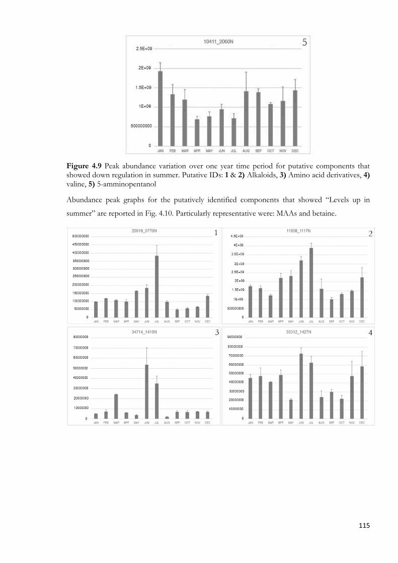
115

Figure 4.9 Peak abundance variation over one year time period for putative components that showed down regulation in summer. Putative IDs: 1 & 2) Alkaloids, 3) Amino acid derivatives, 4) valine, 5) 5-amminopentanol

Abundance peak graphs for the putatively identified components that showed “Levels up in

summer” are reported in Fig. 4.10. Particularly representative were: MAAs and betaine.

116

Figure 4.10 Peak abundance variation over one year time period for putative components that showed up regulation in summer. Putative IDs: 1) Seryl tyrosine derivatives, 2) Betaine, 3) Porphyra-334, 4) Shinorine, 5) Amminoheptanoic acid

Abundance peak graphs for the putatively identified components that showed little or “No

changes” are reported in Fig. 4.11.

Figure 4.11 Peak abundance variation over one year time period for putative components that showed little changes. Putative IDs: 1) seryl tyrosine derivatives, 2) hydroxy Betaine derivatives, 3) Porphyra-334, 4) Palythine

Abundance peak graphs for the putative IDs that showed “Random changes” are reported in Fig.

4.12. Among the “Random” regulated were reported: acetyl carnitine, glutamine, hydroxyl betaine

derivatives and isodomoic acid.

117

Figure 4.12 Peak abundance variation over one year time period for putative components that showed random changes. Putative IDs: 1) Isodomoic acid, 2) Acetyl carnitine, 3) Hydroxy Betaine derivatives, 4) Glutamine

Abundance peak graph for the putatively identified component that showed “Down regulation in

autumn” is reported in Fig. 4.13.

Figure 4.13 Peak abundance variation over one year time period for a putative component that showed down regulation in autumn. Putative ID: 1) Palythene

A summary of the putative IDS with respective m/z, RT and regulation trend for the negative and

positive mode is presented in Tables 4.3 and 4.4 respectively.

118

Table 4.3 Putatively identified components organized by regulation trends (negative ESI mode data)

RT m/z [M-H] Putative ID Trend

5.38 162 1, 4-Thiazane-3-carboxylic acid S-oxide Down summer

14.94 175 Vitamin C/fumarate Down summer

15.20 195 Chilenone A-like Down summer

17.93 and 18.83 205 Homocitric acid Down summer

18.80 173 Trans aconitic acid Down summer

5.54 175 Vitamin C/fumarate Up summer

5.76, 6.40, 7.17,

7.31 and 31.72

273,305,351,353 Lipid derivatives Up summer

10.86 291 Chilenone B (-2H) Up summer

13.06, 13.10 and

13.50

253 2-O-α-D-galactopyranosyl glycerol

(Floridoside)

Up summer

15.32 267 2-O-α-D-mannpyranosyl glycerol

(digeneaside)

Up summer

18.96 195 Chilenone A-like Up summer

20.39 173 Trans aconitic acid Up summer

31.84 287 Methyl furanone derivative Up summer

4.30, 4.33, 4.41 293 Chilenone B Random

4.71 195 Chilenone A Random

18.80 173 Trans aconitic acid Random

11.91 162 TCSO No changes

33.31 305 Lipid derivatives No changes

Table 4.4 Putatively identified components organized by regulation trends (positive ESI mode data)

RT m/z [M-H] Putative ID Trend

20.60 104 5-aminopentanol Down summer

11.82 118.08 Betaine/Valine Down summer

6.33 410.18 Alkaloids Down summer

9.68 285.14 Palythene (MAA) Down autumn

11.17 118.08 Betaine/Valine Up summer

13.38 146.11 Aminoheptanoic acid Up summer

14.27 333.12 Shinorine Up summer

14.10 347.14 Porphyra 334 (MAA) Up summer

10.93 144.02 Acetyl carnitine Random

15.37 147.07 Glutamine Random

4.68 330.15 Amino acid derivatives,

similar to isodomoic

acid+18

Random

13.32 347.14 Porphyra 334 (MAA) Random

14.36 245.11 Palythine (MAA) No changes

12.53 134.08 Hydroxy Betaine derivative No changes

8.41 383.18 Seryl Tyrosine derivatives No changes

4.4.2 Oral extracts: extraction in HEPES buffer of two selected months: November and May

The HEPES extracts of the samples from the different months had clearly different colours (Fig.

4.14 A). The May samples were orange whereas the November samples were pink. Furthermore,

oral extracts differed in colour from the solvent extracts (Fig. 4.14 B).

119

Figure 4.14 A) HEPES buffer extracted samples: in orange “May” and in pink “November”; B)

solvent extract sample

Extracted samples in HEPES, as a proxy for artificial saliva, were read via scanning

spectrophotometric over 380 to 750nm and the main peaks are shown in Figs 4.15 and 4.16.

The absorbance spectra of the extracted samples showed clear differences. The orange colour of

the May samples was due to an increase in absorbance at ~460 nm. This could reflect the presence

of carotenoids, but it is doubtful how well these generally hydrophobic compounds would be

extracted in aqueous HEPES. The pink coloration obvious in the November samples, may be due

to phycobiliproteins, which are also probably present in the May samples (see peaks at around 500-

600 nm). However, carotenoids do not ionise well under ESI conditions and phycobiliproteins

have high molecular weights beyond the detection range of the MS detector at m/z 2000.

Figure 4.15 Scanning absorbance spectrum (as absorbance units) of the HEPES extracted sample from November

0

0.1

0.2

0.3

0.4

0.5

0.6

0.7

0.8

0.9

1

380 430 480 530 580 630 680 730 780

Ab

sorb

ance

(A

U)

nm

120

Figure 4.16 Scanning absorbance spectrum of the HEPES extracted sample from May

Extracted samples were analysed and plotted with Xcalibur software (Thermo Fisher®), and

comparison of peak graphs of MS profiles of oral and wild in positive ESI mode are shown in Fig.

4.17 and for negative ESI mode in Fig. 4.18.

The HILIC profiles of these HEPES extracted samples were compared against the solvent

extracted samples to assess which components were also more likely to be available in the mouth

and contribute to the flavour profile of the seaweed. The HEPES was carried over in the oral

samples and was the major peak in these HILIC runs. The abundance of peaks in both the solvent

and “oral” extracts in positive ESI mode are shown in Fig 4.17 and those for the negative mode in

Fig 4.18.

0

0.1

0.2

0.3

0.4

0.5

0.6

0.7

0.8

0.9

1

375 405 435 465 495 525 555 585 615 645 675 705 735

Ab

sorb

ance

(A

U)

nm

12

1

Figure 4.17 Peak graphs of MS profiles from May oral (black), November oral (red), May (green) and November (blue) (Positive mode, FSD = 3.90 E8, Base Peak

F:FTMS+ c ESI Full MS [80-1000]). Arrow denotes HEPES peak in oral samples

12

2

Figure 4.18 Peak graphs of MS profiles from May oral (black), November oral (red), May (green) and November (blue) (Negative mode, FSD = 9.00E7, Base

Peak F:FTMS+ c ESI Full MS [80-1000]). Arrow denotes HEPES peak in oral samples1

1 Since HEPES peak was off-scale, the scale chosen was the solvent extract (9.00 E7), which allows for a more equal comparison of the data.

123

No peaks were present in the oral extracts that were not present in the total solvent extracts.

Therefore, for simplicity, only the peaks common to the two extractions (already identified in

Tables 4.1 and 4.2 - negative and positive ESI modes respectively) were examined. Those identified

in the negative ESI mode were chilenone B (m/z 291 & 293) and A (m/z 195), fumarate (m/z

112.99, 175), lipid derivatives (m/z 273, 353, 305), TCSO (m/z 162), floridoside (m/z 253),

digeneaside (m/z 267), homocitric acid (m/z 205), and trans and cis aconitic acids (m/z 173) (Fig.

4.19).

Figure 4.19 Main peaks identified in HILIC profiles in negative mode for Solvent and “Oral” extracted samples (blue= November; light grey= November Oral; orange= May; black= May Oral) (n=3; error bar, 1 SD of mean)

Those identified in the positive mode were 5-aminopenthanol (m/z 104), glutamine (m/z 130, 147),

palythine (m/z 245), shinorine (m/z 333), proline (m/z 116), aminoheptanoic acid (m/z 146),

asterina (m/z 289), betaine/valine (m/z 118), hydroxy betaine derivatives (m/z 134), acetyl carnitine

(m/z 144, 204), palythene (m/z 267, 285), porphyra 334 (m/z 347), seryl tyrosine derivative (m/z

285, 383), alkaloids (m/z 312, 410), amino acid derivatives (m/z 312, 330, 277) (Fig. 4.20).

0.00E+00

5.00E+08

1.00E+09

1.50E+09

2.00E+09

2.50E+09

3.00E+09

3.50E+09

4.00E+09

4.50E+09

m/z291

m/z293

m/z195

m/z112

m/z175

m/z273

m/z353

m/z305

m/z162

m/z162

m/z299

m/z253

m/z253

m/z299

m/z267

m/z205

m/z173

m/z205

m/z173

Ab

un

dan

ce

Compound (m/z)

124

Figure 4.20 Abundance of main peaks identified in HILIC profiles in positive mode for Solvent and “Oral” extracted samples (blue= November; light grey= November Oral; orange= May; black= May Oral) (n=3; error bar, 1 SD of mean)

In positive mode, the same compounds were present in both solvent and HEPES extracted

samples, but they varied in abundance. Some compounds did not show differences between the

two sets of samples, such as amino acids derivatives, acetyl carnitine, MAAs, alkaloids, hydroxy

betaine derivative, or proline. Others had higher levels in the solvent extracted samples, e.g.

palythene, palythine, amino acid derivatives, betaine/valine, and seryl tyrosine derivative. A few

components were higher in the HEPES extracted samples including aminoheptanoic acid at m/z

146, alkaloids at m/z 410, and the amino-acid derivative at m/z 330.

However, in negative mode, some compounds that appeared in the solvent samples were not

detected in the “Oral” samples (e.g. chilenone B -2H at m/z 291, fumarate, vitamin C, and lipid

derivatives). Solvent extracted samples had higher abundance of most compounds except for

floridoside (m/z 299), which had higher levels in the HEPES extracts of both May and November

samples. This component was identified as a formate adduct of floridoside (see Table 4.1), but the

main floridoside peak at m/z 253 was higher in the solvent extracts. This difference may be due to

isomers of this compound, one which more readily forms the formate adduct and may be more

extractable in HEPES.

There were differences in peak abundance between the May and November samples, but these

generally showed the same trends in solvent and HEPES extracted samples.

For the HEPES extracted samples in ESI positive mode, statistically higher abundances were

reported in November oral extract for amino heptanoic acid and in May oral extract for seryl

-4E+09

-2E+09

0

2E+09

4E+09

6E+09

8E+09

1E+10

1.2E+10

1.4E+10

1.6E+10

1.8E+10

2E+10

m/z

31

2

m/z

33

0

m/z

27

7

m/z

31

2

m/z

41

0

m/z

41

0

m/z

20

9

m/z

31

2

m/z

38

3

m/z

33

0

m/z

28

5

m/z

28

5

m/z

14

4

m/z

14

4

m/z

11

8

m/z

26

7

m/z

13

4

m/z

11

6

m/z

14

6

m/z

27

7

m/z

28

9

m/z

34

7

m/z

33

3

m/z

24

5

m/z

13

4

m/z

10

4

m/z

10

4

m/z

14

4

Ab

un

dan

ce

Compounds

125

tyrosine derivatives, palythene and asterina (330). For the HEPES extracted samples in ESI

negative mode, statistically higher abundances were reported in November oral extract for

chilenone B, and in May oral sample for lipid derivatives, floridoside and trans aconitic acid (Fig.

4.19).

4.5 Discussion


4.5.1.1 ESI negative polarity

In this study the metabolomic profile of O. pinnatifida across a one-year time period was evaluated

for the first time. Compounds were identified in both negative and positive ESI modes, as reported

in Tables 4.1 and 4.2 respectively. Interestingly, compounds that could be identified in negative

mode mainly included chilenones A & B (and their isomers and isotope), methyl furanone

derivative, lipid derivatives, fumarate, TCSO, carbohydrates (e.g. floridoside and digeneaside) and

aconitic acids (trans and cis). These compounds have been previously reported in other seaweeds

having bioactive properties, e.g. antimicrobial, antiviral, antifungal, anti-grazing and anti-

carcinogenic capabilities (San-Martín et al., 1983; Gianturco et al., 1964; de Nys et al., 1998;

Plouguerné et al., 2010; Tominaga and Oka, 1963; Kuriyama et al., 1960; Omar et al., 2018). More

specifically, Chilenone A was identified by San-Martín et al. (1983) in Laurencia chilensis and is a

dimer of 2-methyl-3(2H)-furanone, which has been reported as one of the volatile constituents of

roasted coffee (Gianturco et al., 1964). San-Martín et al. (1987) isolated Chilenone B from the same

species, which is a trimer of 2-methyl-3(2H)-furanone. Both of the above compounds are natural

sesquiterpenoids (Fraga, 1990, 2012). Methyl furanone derivatives have a role as signal molecules

and they may have anti-carcinogenic, antimicrobial, antiviral, antifungal, and anti-grazing activities

(Slaughter, 1999). In animals, they have a role as attraction signals (Slaughter, 1999), while in plants

and fruits they have been identified as aroma compounds (e.g. in strawberry) (Schieberle and

Hofmann, 1997). The most detailed information available on anti-microbial effects of furanones

in seaweed comes from studies on the Australian subtidal red alga, Delisea pulchra. This seaweed can

prevent the swarming and adhesion of a range of marine bacteria that use an intercellular signal to

change phenotype from free-living to colony through a quorum sensing mechanism. By secreting

halogenated furanones which resemble Acylated homoserine lactone (AHL) (e.g. furanone of the

3-butyl-2-one type) the seaweed prevents colonization by bacteria, interfering with their

intercellular signal (acylated homoserine lactone) (Kjelleberg et al., 1997). The production and

release of these compounds proved also to deter grazing by herbivorous animals (de Nys et al.,

1998; Dworjanyn et al., 1999).

126

Fumarate has previously shown antioxidant activities in seaweeds, and it is commonly present in

many plants and animal, being essential to tissue respiration. It is also prepared industrially and

applied as flavouring additives for beverages, baked food and baked goods (Winter, 2009). It has

been reported previously in Porphyra purpurea (UniProtKB - P80477, SDHB_PORPU).

With respect to Vitamin C, more information is required to confirm its identity in this study, such

as comparison with a standard. The Vitamin C content of algae varies markedly with season, groups

and species. Submerged species are usually richer in vitamin C irrespective of their taxonomical

grouping (Sarojini and Sarma, 1999). Maximum levels of vitamin C are reported for green and

brown algae in summer and for red algae in winter. Vitamin C is thought to affect the health of the

plants as seaweeds that show a more intense and brilliant colour are observed to have higher

content of it (Sarojini and Sarma, 1999). Furthermore, Vitamin C has a key role in the metabolic

reaction of seaweeds, being associated with the morphogenetic, vegetative and reproductive phases

(Anantharaman et al., 2011).

Lipid derivatives were only partially identified in this study with evidence for methyl-docosanoic

acid, eicosatrienoic acid, tricosenoic acid and hydroxy-hexadecanoic acid. Omar et al. (2018)

reported the presence of methyl-docosanoic acid in extracts of the red alga, Laurencia papillosa,

which had anti-microbial activity. Indeed, previous reports have revealed that FA derivatives from

seaweeds have shown strong anti-fouling activity (Bazes et al., 2009; Plouguerné et al., 2010).

Members of the Laurencia genus (Rhodophyta) are prolific producers of terpenoid and non-

terpenoid secondary metabolites that showed antibacterial and antiviral activities (Fujii et al., 2011).

Furthermore, FA derivatives also include carotenoids, that are naturally occurring fat soluble

tetraterpenoids, organic pigments that are found in phototrophic organisms and can have

remarkable biological functions and applications in human health (e.g. β-carotene, astaxanthin and

fucoxanthin) (Maeda et al., 2008; Boominathan and Mahesh, 2015).

One of the more interesting compounds identified in this study was 1,4-thiazane-3-carboxylic acid

S-oxide (TCSO), which has been previously identified in other algae, such as Undaria pinnatifida

(Tominga and Oka, 1963) and Chondria crassicaulis (Tominga and Oka, 1963; Kuriyama et al., 1960).

It is a sulfur-containing amino acid whose natural occurrence in sources other than the red alga

Chondria crassicaulis and Undaria pinnatifida had not previously been reported until now, with this

study. As a cycloallin, it has been reported as organosulfur compound in onion and garlic, reporting

several biological activities (Ichikawa et al., 2006), playing probably a role in the particular taste of

this seaweed.

Aspartate was reported in this study, which has been associated with umami taste, in addition to

glutamate, with less potency and an unknown sensory mechanism (Chandrashekar et al., 2006; Li

127

et al., 2002). Higher levels of glutamate as well as aspartate are associated with more flavourful

seaweeds (e.g. S. japonica, Mouritsen et al., 2012; Mouritsen, 2013).

Floridoside and digeneaside are common low molecular weight carbohydrates biosynthesized

during photosynthesis in marine red seaweeds (Meng et al., 1987). These compounds are thought

to have several functions, such as osmolytes and compatible solutes, with stabilizing effects on

enzymes, membranes and structural macromolecules under hypersaline concentrations (Barrow et

al., 1995). Digeneaside (2-O-α-D-mannopyranosyl glycerol) has been recognized as

chemotaxonomic marker for red algal order Ceramiales (Kirst and Bisson, 1979; Kirst, 1980; Reed,

1990). It was thought that some genera of the Ceramiales (e.g. Laurencia and Osmundea) produced

and accumulated floridoside rather than digeneaside (Barrow et al., 1995). This study suggests the

opposite to what was previously reported for this species (Kremer and Vogl, 1975; Kremer, 1978).

However, this is assuming that these two sugar glycerides ionize to a similar extent, which seems

reasonable.

Floridoside (2-O-glycerol-α-D-galactopyranoside) is a natural glycerol glycoside found in red algae

and is believed to play important roles in carbon storage, transport, assimilation and in the

regulation of osmotic balance (Kirst, 1980; Reed et al., 1980; Ekman et al., 1995). It is a compatible

solute that can be accumulated at high intracellular concentrations without interfering with the

normal functioning of the metabolism (da Costa et al., 1998; Roberts, 2005; Hagemann and Pade,

2015). Its synthesis is enhanced by high osmotic pressure conditions (Kirst and Bisson, 1979; Reed,

1985; Ekman et al., 1995). This glycoside also constitutes the major soluble pool of carbon fixed

by photosynthesis and is a precursor for cell wall polysaccharides in some species (Li et al., 2001,

2002). Apart from its in vivo role as osmolyte, floridoside has been described has having other

interesting properties. Hellio et al. (2004) reported that floridoside is able to inhibit the settlement

of cryptid larvae on the surface of underwater devices, suggesting its application as non-toxic,

natural compound for preventing biofouling, a worldwide problem estimated to cause a loss of

billions of dollars to the marine industry (Callow and Callow, 2002). Moreover, floridoside is a

potential therapeutic agent with the ability to modulate the immune response (Courtois et al., 2008;

Kim et al., 2013) and to promote bone formation (Ryu et al., 2015). The structural similarity with

2-O-α-d-glucopyranosylglycerol (GG), a compatible solute accumulated by cyanobacteria, suggests

that might also be functional in applications as moisturizing agent (Thiem et al., 1997), a non-

cariogenic, low calorie sweetener (Takenaka and Uchiyama, 2000) and a protein stabilizer

(Sawangwan et al., 2010). However, industrial applications for floridoside have not been developed

yet due to limited compound availability (Martínez-García et al., 2016).

The antioxidant capacity of algae is comprised of a variety of constituents such as carotenoids,

tocopherols, flavan-3-ols, phenolic acids, lignans, phlorotannins as well as mycosporine-like amino

128

acids (MAAs; Athukorala et al., 2003, Dunlap et al., 1998, Dunlap and Yamamoto, 1995; Yuan et

al., 2005). Natural compounds produced by seaweeds are usually referred to as secondary

metabolites since they are not involved in the basic biological functions (Cimino et al., 2001). Many

of these secondary metabolites are halogenated (McKey, 1979). Among the different classes of

marine macroalgae, red algae are the major producers of halogenated compounds (Cabrita et al.,

2010). Marine halogenated compounds range from peptides, polyketides, indoles, terpenes,

acetogenins and phenols to volatile halogenated hydrocarbons (Butler et al., 2009). Laurencia and

Osmundea (Rhodomelaceae), are considered two of the most prolific genera in this respect

(Faulkner, 2001; Wright et al., 2003). Trans-Aconitic acid and Cis- aconitic acid are both organic

acid that can become halogenated (e.g. conjugated with bromophenol) already investigated in other

algae (Kurata et al., 1998) and that have been identified in this study proving once again the

relevance of this species for further nutraceutical, pharmaceutical and cosmetic applications.

4.5.1.2 ESI positive polarity

The positive ESI mode mainly identified compounds such as amino acids (e.g. betaine, valine,

proline), amino acid derivatives (isodomoic acid, seryl tyrosine derivative), mycosporine-like amino

acids (palythene, porphyra-334, asterina-330, shironine, palythine), acetyl carnitine and alkaloids

(Table 4.2). Most of these compounds have reported osmoregulation properties and are produced

as compatible osmolytes to regulate adaptation in transient environments (Blunden, 2003;

Hartmann et al., 2017).

Domoic acid (DA) has been previously reported in other algae and originally isolated in Chondria

armata (Zaman et al., 1997). It was then investigated for its insecticidal and anthelmintic activities

(Maeda et al., 1986, 1987). Domoic acid is the most potent activator of the α-kainic receptors in

the central nervous system, which is known to act as a potent agonist to the glutamate receptor,

which conducts Na+ ion channels in the postsynaptic membrane (Debonnel et al., 1989) and can

cause poisoning. However, DA poisoning from red algae is unknown (Higa and Kuniyoshi, 2000).

Together with other FAs such as octanoic acid, nonanoic acid, decanoic acid, dodecanoic acid, and

hexadecanoic acid, the amino-heptanoic acid have been reported as precursors to seafood flavours

and as plant metabolites. But there is no information available for seaweeds (Josephson and

Lindsay, 1986) and this is the first report of their presence in red algae.

Alkaloid derivatives were identified in this study, but not specifically classified. Alkaloids in seaweed

include simple phenylamine (tyramine, hordenine) and catecholamine (dopamine) as well as sulfur-

containing bromoalkaloids, extracted from red algae (Güven et al., 2010). Pharmacologically

activities have been recognized for these compounds including antibacterial (e.g. terrestrial and

some marine bacteria), anticancer, and cytotoxic activities. Within the alkaloids, halogenated Indole

129

Alkaloids (HLI) have only been isolated in marine organisms and algae (mostly red) but not in

terrestrial plants. These alkaloids contain an indole group substituted by bromine and chlorine

atoms that are highly abundant in red algae (e.g. O. pinnatifida, Asparagopsis taxiformis, Euchema sp.,

Gracilaria sp., Chondrus Crispus) (Küpper et al., 2014; Cabrita et al., 2010; Laturnus et al., 2010;

Mithoo-Singh et al., 2017).

The amino acid composition of algae has been often studied, with red seaweeds showing lower

amounts of glutamic and aspartic acids than those recorded from other algae groups (Fleurence,

1999). Essential amino acids can constitute almost 46% of the total amino acid fraction in red algae

(e.g. P. palmata). This study reported essential amino acid such as valine (commonly reported in

seaweed, Tabarsa et al., 2012), showing the potential this seaweed has as a food additive in human

and animal nutrition. Betaine was also identified, and this compound has been studied for its

osmoregulation properties, being an osmolyte and facilitating adaptation to saline and dry

environments (Blunden, 2003). Compounds of this class have been found in many animals, plants,

algae, fungi and bacteria (Blunden and Gorden, 1986), and previously reported in red seaweeds

(e.g. Pyropia yezoensis, Mao et al., 2019).

Proline was identified in this study, which together with histidine, valine and methionine is

associated with a bitter taste (Kato et al., 1989). Proline is known to accumulate in large quantities

in terrestrial plants in response to environmental stresses (Ashraf and Foolad, 2007), and many

plants accumulate proline as a non-toxic and protective osmolyte under saline conditions (Khatkar

and Kuhad, 2000).

One of the main classes of compounds reported in this study are mycosporine-like amino acid.

MAAs are algal secondary metabolites, with absorbance maxima between 310 and 360 nm (Karsten

and Wiencke, 1999; Shick and Dunlap, 2002). More than 30 different MAAs have been identified,

with Rhodophyta accounting for the highest concentration and greatest variety among the different

algal divisions (Karsten et al., 1998; Sinha et al., 1998). MAAs have the ability to absorb UV

radiation due to their structural characteristics and to dissipate its energy without forming ROS

(Sinha et al., 1998; Tao et al., 2008). The induction of MAA synthesis is stimulated by different

light qualities, which cannot be initiated by the same photoreceptor or at least the same

chromophore (Liscum and Briggs, 1995). They have a characteristic cyclo-hexenone or -

hexenimine core, which is conjugated to the nitrogen moiety of an amino acid. This core primary

metabolism is synthesised by the shikimic acid pathway via 3-dehydroquinic acid and 4-

deoxygadusol (4-DG), a known strong antioxidant (Dunlap et al., 1997; Shick and Dunlap, 2002).

They act as UV-radiation protectors in macroalgae (e.g. P. palmata, P. tenera and Devaleraea

ramentacea), corals (e.g. Palythoa tuberculosa), marine species such as sea squirts (Lissoclinum stellatus)

and krill (Euphausia superba) and have potential in photo-protective formulations (Karsten and

130

Wiencke, 1999; Bedoux et al., 2014). They have also antioxidant properties as evidenced in a study

by Dunlap and Yamamoto (1995) for P. palmata and a role as osmoregulators has also been

recognised (Hartmann et al., 2017). The MAAs compounds reported in this study included

palythene, shironine, palythine, asterina 330, and porphyra-334, already reported in other algae

(Barceló-Villalobos et al., 2017; Hartmann et al., 2017; Carreto and Carignan, 2011). These have

potent bioactivities, for example, porphyra-334 exerts antioxidant activity and prevents cellular

damage caused by UV-induced ROS with free radical scavenging capacity (Tao et al., 2008). Several

recent publications have described the immunoregulatory and anti-inflammatory properties of

mycosporine-glycine, shinorine and porphyra-334. Particularly, porphyra-334 and shinorine have

been identified as unique natural products that can provide both a direct antioxidant defence and

stimulate enhanced cytoprotection, making these compounds commercially relevant (Suh et al.,

2014, 2017; Ryu et al., 2015).

Another interesting molecule identified with this study, which can be linked to the taste of the

seaweed and its nutritional profile is acetyl carnitine, a naturally occurring amino acid, previously

reported in brown algae (e.g. Undaria sp.). This can have applications as a diet supplement, for

thyroid control, for treatment of hypertension, and cardiovascular diseases (Jeukendrup and

Randell, 2011; Pereira, 2011). Glutamine is a central amino acid in red seaweed used as nitrogen

source for ammonium assimilation (Cole and Sheath, 1990), which has been investigated for its

relationship with the umami taste in other seaweeds (e.g. Ulva sp. and Gelidium sp., Nagahama et

al., 2009). Identification of this compound and its variation in the seasons can have considerable

relevance in understanding the properties that regulate the taste of O. pinnatifida.

4.5.1.3 Peak abundance variation: regulation trends

The metabolomics analyses conducted in this study took into consideration the variation in the

abundance of the described compounds across a full-year (Figs 4.1-4.4), in order to identify possible

trends and regulation patterns to assess the best harvesting season and link the production of

interesting secondary metabolites with seasonal changes. Secondary metabolites are often

antioxidants, whose production varies as a response of the alga to tissue desiccation or UV-

irradiation (Karsten and Wiencke, 1999). Therefore, it is not surprising that algal levels of

antioxidants (such as carotenoids and tocopherols) tend to be lower during winter and spring

months and higher in summer and autumn (Aguilera et al., 2002, Burritt et al., 2002; Yuan, 2007).

This was confirmed also in this study and by the analyses conducted on the abundance variation

across the seasons for the identified compounds (Tables 4.3 and 4.4).

131

4.5.1.3.1 Trends for ESI negative polarity

The compounds identified in negative ESI mode included osmoregulatory compounds (such as

floridoside) and antioxidant compounds (e.g. lipid derivatives, trans aconitic acid, and chilenone A

& B), which were all statistically higher in the summer months compared to the winter (Figs 4.5-

4.8). Accumulation of these compounds suggests a biological response of the seaweed to high

irradiation, day light length, desiccation, and higher temperatures that characterized the West coast

of Scotland in the summer months, especially for this intertidal species exposed to tides,

temperature, salinity, and light variation. These data confirmed what already seen with the statistical

PCA and BEST analyses in Chapter 3 (Figs 3.18 and 3.19), in terms of relations between

environmental parameters (e.g. irradiation and hours of light) and the biochemical composition of

the species. On the other hand, compounds that were down-regulated in the summer were generally

compounds that could be related to taste and palatability, such as fumarate, vitamin C, chilenone

A-like, and TCSO. This information can give pioneering and useful information on the regulation

of the taste in O. pinnatifida.

4.5.1.3.2 Trends for ESI positive polarity

In positive mode, compounds that may be related to the nutritional qualities and, hypothetically,

flavour, were statistically higher in winter and autumn months compared to spring and summer

months (e.g. valine, alkaloids, amino acid derivatives, and acetyl carnitine, Figs 4.9-4.13). On the

other hand, as already seen for the negative data, compounds that may be linked to stress resistance,

osmoregulation and UV protection were statistically higher in the summer (e.g. betaine and MAAs).

Interestingly, glutamine, identified here as m/z 147 (MS²=130), RT 15.22, and previously linked to

the umami taste in other seaweeds, showed the highest value in June, followed by March and April,

and the lowest in October. The initial hypothesis might be that since the species reaches its

maximum biomass between November and December, when it also shows the darker colour,

higher levels of glutamine would be expected in these months, rather than in June, March and

April. However, the abundance of glutamine is generally high throughout the year, although it

varies between months (Fig. 4.12), and the peculiar taste could be created by a synergetic effect of

different compounds (e.g. acetyl carnitine, TCSO, amino acid derivatives), that mainly show higher

level in late winter months, with glutamine and each other.

4.5.2 Replicating oral conditions

4.5.2.1 Oral extracts: extraction in HEPES buffer of two selected months, November and May

Under conditions that mimic those present in the mouth, the profiles of compounds changed

compared to that of solvent extracted samples. The compounds extracted in HEPES are more

likely to be similar to those released during eating and therefore responsible for the particular

132

flavour of O. pinnatifida. Except certain compounds (e.g. fumarate, vitamin C, and lipid derivatives),

the solvent and HEPES extracted samples generally contained the same main peaks listed in Tables

4.1 and 4.2 As could be expected, almost all components were reduced in abundance compared to

the solvent extraction. (Figs 4.17-4.20).

In negative mode, certain compounds were found only in solvent extracts, chilenone B -2H (m/z

291), fumarate (m/z 112, 175) and the putative lipid derivatives (m/z 273, 353). Some compounds

were higher in solvent extracts such as chilenone A (m/z 195), chilenone B (m/z 293), TCSO (m/z

162), digeneaside (m/z 267) and cis-aconitic acid (m/z 173); others had similar abundance in oral

and solvent extracts, e.g. floridoside (m/z 299) and homocitric acid (m/z 205). Certain components

were higher in oral extracts, such as lipid derivatives (m/z 305 =possibly eicosatrienoic acid in May)

and floridoside (m/z 299, 253 - in May).

In positive mode, differences in abundance of some components were reported between solvent

and oral extracts. The amino-acid derivative (m/z 312, 330), alkaloid derivative (m/z 312), seryl

tyrosine derivative (m/z 383), MAAs (m/z 267, 245), betaine/valine (m/z 118) and 5-

aminopentanol (m/z 104) were higher in the solvent extracts. The alkaloid derivative (m/z 410),

the amino acid derivative (m/z 330), MAAs (m/z 285, 289 for May), and aminoheptanoic acid (m/z

146) were higher in oral extracts. Other components including the amino acid derivative (m/z 277),

seryl tyrosine derivative (m/z 209), acetyl carnitine (m/z 144), hydroxy betaine derivatives (m/z 134,

116) and MAAs (m/z 347, 333) had similar abundances in solvent and oral extracts.

This was the first time that an artificial saliva digestion of dry biomass of O. pinnatifida was

performed to gain a better understanding of the role that certain compounds might have in

influencing and determining the taste of the species. As previously explained, some of the

compounds mentioned above, e.g. seryl tyrosine derivative, aminoheptanoic acid, floridoside, trans

and cis- aconitic acid, acetyl carnitine, TCSO, and fumarate, can have a role in influencing the taste

of O. pinnatifida as well. The fact that the same compounds can be extracted in the aqueous saliva

like HEPES buffer, strengthens the hypothesis previously discussed that these metabolites may

influence the flavour of the species. Furthermore, solvent and oral samples follow same seasonality

patterns, and if a compound is higher in May and lower in November in the solvent samples, this

is reflected also in the oral samples. This further confirms that the metabolomic profile of the

species varies with the season, therefore determining a variation in the taste and flavour of the

species according to the harvesting time.

However, further targeted analyses would need to be performed to confirm the identity and levels

of the key compounds and gain a better understanding of the variation in taste according to the

season. Also, due to time-constraints, this study only focused on major peaks in the HILIC traces

and only discussed the abundance of those components that could be at least putatively identified.

133

However, the MS data was very rich and non-targeted analysis using various data-handling software

techniques (e.g. XCMS data deconvolution and use of multivariate statistics, e.g. McDougall et al.,

2014) could compare the abundance of all peaks across the months and pick out those which

showed similar trends of expression (e.g. “Levels up in summer”), and compare them to those

identified peaks shown above. This non-targeted approach was not possible within this thesis but

could be carried out for future publications. This would provide powerful means for identifying

other, previously unknown, but possibly related compounds that could influence the flavour and

quality of O. pinnatifida.

The method here applied has strengths as well as limitations. While terpenoid, non-terpenoid C15

and halogenated metabolites were previously reported for the species (Erickson, 1983; Faulkner,

1986; Bittner et al., 1985; Atta-Ur-Rahman et al., 1988; Norte et al., 1989; Bano et al., 1988; Ahmad

et al., 1990; Ahmad and Shaiq, 1991), these compounds were not detected in this study. One reason

could be that the extraction applied is not ideal for these molecules, since they might not be

effectively extracted in 50% acetonitrile/UPW solution. Moreover, no special extraction or clean-

up procedures commonly used for pre-selection and detection of certain components were applied

in this study. Therefore, these components may be present but may be swamped out by other more

abundant metabolites. The application of the XCMS non-targeted approach (McDougall et al.,

2014) may help to overcome this and identify more minor components that alter between the

months. In addition, XCMS would assign possible formula including all elements and may help

pick out halogenated compounds previously noted in red seaweeds. However, as this study

compared monthly samples extracted in the same manner, this suggests that these previously

identified compounds do not change across the seasons and are unlikely to contribute to the

seasonal taste profile differences.

4.6 Conclusions

The seasonal variation in the metabolomic profiles of O. pinnatifida was reported for the

first time, providing valuable information regarding seasonal variation in composition as

related to flavour and confirming the importance of harvesting time for the quality of this

commercially valuable product;

The seasonal seaweed samples contained similar metabolites, but they varied in abundance

across the different months of harvest. Seasonal patterns were reported with certain

metabolites increasing over the summer months and others increasing in the autumn and

winter;

134

Particularly, components associated with stress alleviation and resistance were accumulated

during the summer months when the seaweed would be subject to increased levels of

ultraviolet light;

Components (e.g. 1,4-thiazane-3-carboxylic acid S-oxide, glutamine, acetyl carnitine, and

trans- and cis- aconitic acid) were identified that may be related to the particular flavour of

this seaweed;

Selected samples were extracted under replicating conditions in the mouth and compared

to solvent extracts, which confirmed compounds that could be related to the taste and the

seasonality of the flavour of the species, such as seryl tyrosine derivative, aminoheptanoic

acid, floridoside, trans and cis- aconitic acid, acetyl carnitine, TCSO, and fumarate;

A few components were higher in the HEPES extracted compared to the solvent samples

such as alkaloid derivative, amino acid derivative, MAAs, and aminoheptanoic acid. This

suggests that these compounds might play an important role in regulating the flavour of

the seaweed;

Differences in compounds abundance were found between November and May oral

extracts; in particular, higher concentration of alkaloids and aminoheptanoic acid were

recorded in November, suggesting a more intense flavour in this month compared to May;

however, further analyses involving a taste panel should be conducted to gain a better

understanding of flavour variations in the species;

These findings enhanced our understanding of the nutritional features and profile of O.

pinnatifida harvested at different times, of the seasonal pattern associated with the

metabolomic profile, and of the compounds that are present in the species, providing useful

information on the quality assessment of the species;

This study demonstrated that, as already anticipated by previous authors, O. pinnatifida has

a significant potential for further processing in nutraceutical, pharmaceutical and cosmetic

fields or for direct food applications.

136

Chapter 5 Epiphytes control of O. pinnatifida cultures and spores’

production, release and development in treated specimens

5.1 Introduction

Land-based tank system as a sustainable and reliable source of macroalgal biomass production

relies on maintaining vegetative growth with increases in yield and a good quality of the stock

material. These aspects can be heavily affected by epiphytism from other algae, or grazers (Neish

et al., 1977; Lüning and Pang, 2003; Hwang et al., 2006a), and can lead to the spread of diseases

among the cultures or degradation of the biomass (e.g. Ulva spp., Colorni, 1989; Del Campo et al.,

2002). Since the end of 1970s, epiphytic growth has been recognized as one of the greatest issues

for commercial seaweed cultivation (Ryther, 1977) as highlighted by Wheeler et al. (1981) “the control

of epiphytes and the provision of nutrients represented two major problems for macroalgae farmers”.

Seaweed are a flourishing ecosystem for a variety of different organisms. When they are transferred

to the lab for cultivation, they carry with them all the other organisms (e.g. grazers, other seaweeds,

etc.) that they are naturally associated with. Without intervention, contaminating organisms can

multiply, competing with the stock and/or causing deterioration in the quality, potentially leading

to the collapse of the culture (Borowitzka, 2007). The physical removal of contaminating organisms

by washing and hand sorting substantially reduces their impact (Baweja et al., 2009). However, this

is time-consuming and does not eliminate all of the epibionts. In addition, epibionts may be

introduced later in the cultivation cycle during seawater refreshment, by accidental cross-

contamination or by wind- carried spores/eggs in the case of outdoor tanks. Efficient methods for

the removal of such contaminants are essential. In some cases, manipulation of the culture

conditions can prevent or minimise such contamination, such as high stocking densities, low light

and nutrient levels (Lüning and Pang, 2003) or high pH and the release of alleochemicals caused

by the target cultivation species itself (Björk et al., 2004; Gross, 2010). Epiphytes can be controlled

by reducing the input of N in the cultures until the internal seaweed N reaches a critical level

(Harrison and Hurd, 2001). A chemical treatment may also be utilised to kill the contaminant. This

relies on the existence of differential susceptibility, with sensitive contaminants and a resilient

cultivation species (Guillard, 2007). Detergent, sodium hypochlorite (NaClO), reactive iodine,

formaldehyde and organic solvents have been successfully utilised for the disinfection of

macroalgal tissue to create axenic cultures (Shephard, 1970; McCracken, 1989; Baweja et al., 2009).

Other compounds such as acids, peroxides, sodium hydroxide and commercial preparations, for

example Virocid and Kick-start, are used in the aquaculture industry to disinfect equipment and

prevent or treat diseases (Togersen and Håstein, 1995; Barge, pers. comm.). These may also be

useful for decontamination in macroalgal cultures.

137

One of the more efficient way to verify that seaweeds are alive and healthy is by the monitoring of

their photosynthetic activity, using a non-invasive method such as PAM fluorometry. It has been

already applied with success to several macroalgal studies (Kolber and Falkowski, 1993; Enriquez

and Borowitzka, 2010), and is used extensively to assess stress-dependent changes in

photosynthesis of terrestrial plants, micro- and macroalgae as well as cyanobacteria (Schreiber et

al., 1986; Flameling and Kromkamp, 1998; Figueroa et al., 2006). A relative measurement of algal

photosynthetic health is obtained through measurement of the operating photosynthetic efficiency

of photosystem II (Fq′/Fm′). Higher values indicate greater photosynthetic electron flow towards

carbon fixation, while very low values indicate poor health or death (Maxwell and Johnson, 2000;

Cosgrove and Borowitzka, 2010; Kerrison et al., 2016a, b). Thus, fluorometry is a suitable method

to monitor the condition of the algal cell following a chemical treatment, which may disrupt the

delicate balance of cellular processes necessary for photosynthesis (Falkowski and Raven, 2007).

Such measurements have been used previously to assess the suitability of decontamination

treatments on Sargassum spp. (Hwang et al., 2006a, b; Kerrison et al., 2016a, b).

Chemical treatments have been successfully applied for reduction and removal of contaminants

from macroalgae (Guillard, 2007). However, this must be balanced against damaging the biomass

been cultivated (Tamiya, 1955; Richmond, 2004). A previous study by Kerrison et al. (2016a), tested

several chemical treatments on the removal of contaminates from O. pinnatifida in order to identify

the best method for decontamination of epiphytes in tank cultivation. It was not clear whether

consideration was given to the fact that O. pinnatifida is a perennial seaweed. There are three main

disadvantages associated with perennial species and their epiphytes. Firstly, epiphytes and grazers

can easily colonize its thallus and negatively affect the growth and productivity of the plant.

Secondly, once spores/gametes are released from the old thallus, this tends to be cast off from the

plant, in an attempt to remove the colonizing epiphytes. Lastly, the growth rate might be reduced

during the summer even if nutrients are sufficiently present, because the carbohydrates produced

during the photosynthesis have to be stored and used for the winter (Lüning, 1979).

Since O. pinnatifida, in its natural habitat, is exposed to tidal variations, being completely exposed

during low tide, this desiccation aspect was considered important for the cultivation process of this

species. For example, in Japan, farmers have resisted the use of chemicals on seaweed (such as

Nori) and controlled epiphytes and diseases by drying and/or freezing cultivated infected nets

(Ding and Ma, 2005). Depending on the species been cultivated, the epiphytes, especially weed

algae, can be more susceptible to desiccation compared to other species such as Pyropia sp.

(Mumford and Miura, 1988). Methods to prevent/eliminate epiphytes in tank systems are

fundamental to maximise productivity and quality.

138

Another potentially important aspect of seaweed cultivation is obtaining, settling and growth of

algal spores on ropes. Several factors can trigger spore release in algae, including desiccation,

grazing by invertebrates, abrasion and chemicals (Maggs and Callow, 2003). Spores released by red

algae are non-motile and mucilage-coated (Cole and Sheath, 2011). Once released, spores can stick

to the substratum on contact, but their initial adhesion is not always permanent, and they can

detach again (Sawada et al., 1972). Usually, tenacity of adhesion, as already reported for several red

algae, increases with time (Chamberlain, 1976; Chamberlain and Evans, 1973; Charters et al., 1973;

Suto, 1950). In general, rougher substrata enhance the settlement and survival of spores (Harlin

and Lindbergh, 1977; Ogata, 1953). These types of surfaces also protect the spores from

dislodgement by wave action/water currents/ grazer activity (Norton and Mathieson, 1983;

Brawley and Johnson, 1991) as well as desiccation, providing also evaporative cooling processes in

the intertidal region (Gonzales and Goff, 1989b). Seaweeds usually produce enormous numbers of

spores, and this is true also for red algae; however, the great majority of the spores will not survive

long enough to germinate (Maggs and Callow, 2003). Adhesion will comprise of both an initial

(temporary) and primary (permanent) attachment. This latter step is fundamental for colonizing a

new substratum (Maggs and Callow, 2003) and it is likely to depend on the residual mucilage sheath,

a common component of red algal spores (Boney, 1975; Ngan and Price, 1979) together with

adhesive substances such as glycoproteins complexes (Chamberlin and Evans, 1973, 1981-

Ceramium sp.; Pueschel, 1979-Palmaria sp.). After this, “establishment” will occur and comprises of

four stages: cell wall formation, establishment of polarity, germination and primary rhizoid growth

and adhesion (Fig. 5.1 A-D) (Fletcher and Callow, 1992).

Figure 5.1 The 4 stages of establishment in Osmundea pinnatifida spores (Axio Inverted microscope, Zeiss): A) cell wall formation; B) polarity; C) germination; D) rhizoid growth and adhesion

139

A tank system was trialled for indoor and outdoor cultivation of O. pinnatifida in order to assess the

growth of the culture in a tumbling system (in which seaweed are cultured without attachment and

left free to tumble in the tanks due to aeration provided) and the efficiency of a set of the treatments

against epiphytes in such a system. The tumbling system was specifically developed and adapted to

the species. To test the viability of spores obtained from tank cultivated O. pinnatifida

tetrasporophytes that reached this stage during the cultivation trials and after the treatment against

epiphytes, tetraspores were released and allowed to grow. Spores were taken through all the stages

detailed above and allowed to grow to juvenile then through to young plantlets.

5.2 Aims

To establish a protocol for the mechanical and chemical treatment of epiphytes in O.

pinnatifida cultures;

To develop a low-cost tidal simulation system for in tank cultivation of the species;

To apply the chemical treatment for epiphytes control to flasks and tanks culture

experiments for the species;

To assess how stressful the various treatments to be tested were to O. pinnatifida through

the use of PAM fluorometry;

To determine the parameters responsible for the spores’ production and release in cultures

of O. pinnatifida and develop a protocol for spores’ release, collection and isolation;

To determine the development of spores in vitro cultivation;

To identify the parameters responsible for the growth at a juveniles’ stage of O. pinnatifida

spores;

To evaluate the possibility of a cultivation of the species through a reproductive cycle.


5.3.1 Chemical removal of epiphytes

Samples were collected in November 2016 at low tide from Seil (56.29°N -5.63°W), brought to the

laboratory into a Cool-box, washed with FSW and cleaned manually from visible epiphytes and

grazers. The treatments detailed in Table 5.1 were trialled on small fragments of O. pinnatifida thalli

(2-3 cm), over a range of exposure times.

140

Table 5.1 Epiphytes treatments and exposure time of vegetative thalli in Petri dishes trial

Treatments Time (min) Number of

Replicates

0.1 % NaClO 10 3

1 % NaClO 1 3

0.5 % KI 10 3

0.25 % Kickstart 10 3

25 % methanol 3 3

*control - 3

*untreated samples in F/2 medium

The biomass was subjected to the treatments in 6 well plates containing 20 ml of each solution.

After the allotted exposure time, the fragments were transferred into 200-300 ml of filtered, UV-

sterilised and Tyndalised seawater using sterile forceps and rinsed well in order to remove any

excess of the decontamination treatments. They were then transferred into new 30 ml Petri dishes

with 25 ml of F/2 medium and incubated at 9 °C, 12:12 (L:D) and 50 µmol/m²/sec for two weeks.

The initial PAM fluorometry measurements of the samples were taken with an AquaPen-P (PSI)

according to the manufacturer instructions, before the start of the experiment, to ensure that the

biomass was healthy. Samples were checked to verify the impact of the treatments using PAM

fluorometry, after two hours, one week and 14 days. Statistical analyses for all the trials listed in

this and subsequent sections were conducted applying an ANOVA single factor (p<0.05, Minitab

18) with Tukey’s and Fisher’s post-hoc tests.

The three treatments with the best level of recovery of the cultures were selected to treat an

increased amount of biomass, five gr of fresh material, at 250 ml. The treatments are listed in Table

5.2.

Table 5.2 Epiphytes treatments and exposure time of small volume cultures in flasks trial

Treatments Time (min) Number of Replicates

0.1 % NaClO 10 3

0.5 % KI 10 3

25 % methanol 3 3

*control - 3


The biomass was incubated in the treatment for the time listed on a shaking platform (Gyro-

Rocker) at 70 Rev/min. The biomass was then rinsed in 500-600 ml of filtered, UV sterilized and

Tyndalized seawater in order to remove the treatments from the tissue, placed in a new 300 ml

flasks with 250 ml of F/2 medium and incubated at 9 °C, 12:12 (L:D), 50 µmol/m²/sec for two

weeks. The initial PAM fluorometry of the samples were taken with an AquaPen-P (PSI) before

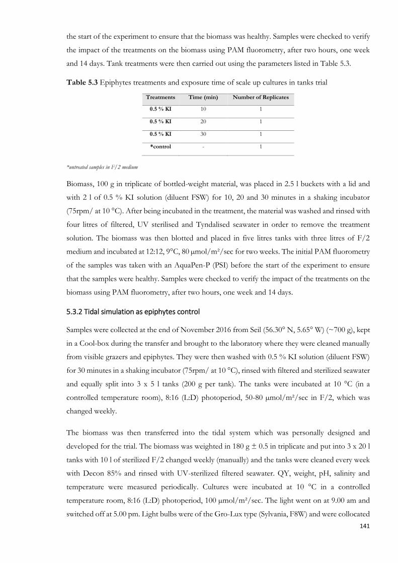
141

the start of the experiment to ensure that the biomass was healthy. Samples were checked to verify

the impact of the treatments on the biomass using PAM fluorometry, after two hours, one week

and 14 days. Tank treatments were then carried out using the parameters listed in Table 5.3.

Table 5.3 Epiphytes treatments and exposure time of scale up cultures in tanks trial

Treatments Time (min) Number of Replicates

0.5 % KI 10 1

0.5 % KI 20 1

0.5 % KI 30 1

*control - 1


Biomass, 100 g in triplicate of bottled-weight material, was placed in 2.5 l buckets with a lid and

with 2 l of 0.5 % KI solution (diluent FSW) for 10, 20 and 30 minutes in a shaking incubator

(75rpm/ at 10 °C). After being incubated in the treatment, the material was washed and rinsed with

four litres of filtered, UV sterilised and Tyndalised seawater in order to remove the treatment

solution. The biomass was then blotted and placed in five litres tanks with three litres of F/2

medium and incubated at 12:12, 9°C, 80 µmol/m²/sec for two weeks. The initial PAM fluorometry

of the samples was taken with an AquaPen-P (PSI) before the start of the experiment to ensure

that the samples were healthy. Samples were checked to verify the impact of the treatments on the

biomass using PAM fluorometry, after two hours, one week and 14 days.

5.3.2 Tidal simulation as epiphytes control

Samples were collected at the end of November 2016 from Seil (56.30° N, 5.65° W) (~700 g), kept

in a Cool-box during the transfer and brought to the laboratory where they were cleaned manually

from visible grazers and epiphytes. They were then washed with 0.5 % KI solution (diluent FSW)

for 30 minutes in a shaking incubator (75rpm/ at 10 °C), rinsed with filtered and sterilized seawater

and equally split into 3 x 5 l tanks (200 g per tank). The tanks were incubated at 10 °C (in a

controlled temperature room), 8:16 (L:D) photoperiod, 50-80 µmol/m²/sec in F/2, which was

changed weekly.

The biomass was then transferred into the tidal system which was personally designed and

developed for the trial. The biomass was weighted in 180 g ± 0.5 in triplicate and put into 3 x 20 l

tanks with 10 l of sterilized F/2 changed weekly (manually) and the tanks were cleaned every week

with Decon 85% and rinsed with UV-sterilized filtered seawater. QY, weight, pH, salinity and

temperature were measured periodically. Cultures were incubated at 10 °C in a controlled

temperature room, 8:16 (L:D) photoperiod, 100 µmol/m²/sec. The light went on at 9.00 am and

switched off at 5.00 pm. Light bulbs were of the Gro-Lux type (Sylvania, F8W) and were collocated

142

on top of the tanks. F/2 was added as medium. The tidal indoor system was organized as follows:

every set of tanks was in triplicate and included two tanks, one working as a microcosm and the

other as reservoir (Figs 5.2-5.4). In every tank, there was a pump (Rule Bilge pump 360 GPH)

which was regulated by a 2 Channel Digital timer. The emptying interval for each pump was 30

seconds. From 6 am to 12 pm (noon) the water was kept in the Reservoir tanks. At 12 pm the

pumps were activated and pumped the water into the Microcosm tanks, where it stayed until 18.00

pm when the pumps were activated again to pump the water back into the Reservoir tanks. The

water was kept in the Reservoir until 12.00 am (midnight) and then pumped again in the Microcosm

tanks until 6.00 am. The seaweed biomass was allowed to float freely in the tanks. A plastic fine

mesh was placed on the bottom of the tank, attached with aquarium suction cups, in order to

maintain the cultures above the level of the water remaining in the tank during the low tide (Figs

5.2 and 5.4). A plastic mesh was also placed in the microcosm tanks to separate the pumps from

the cultures in order to avoid blocking the pumping system due to biomass being sucked into them.

Aeration was provided through either air stones, or aquarium flexible pipes (Figs 5.2-5.4).

The experiment was repeated twice: the first trial went from January to April and the second from

the end of May to the end of June. Two different starting amounts of material were trialled: 180 g

for the first trial and 110 g (blotted weight) for the second, to investigate the effect of biomass

density on the growth.

Figure 5.2 Schematic view of the microcosm tank from the top

143

Figure 5.3 A) Schematic view of the system from the top; B) Schematic lateral view of the system

Figure 5.4 Lateral view of the microcosm and reservoir tanks

5.3.3 Epiphytes treatment of biomass grown in a tumbling tank system cultivation both indoors

and outdoors

Samples were collected at low tide from Seil (56.3000° N, 5.6500° W) in October 2017 and then

again in March 2018 for a second trial, for a total amount of 6 and 4 kg respectively. In both cases,

the collection and treatment of the samples were the same. Samples were kept in Cool-boxes with

wet tissues and brought to the laboratory where they were cleaned manually in order to remove all

the visible epiphytes and grazers. Secondly, samples were washed thoroughly with filtered and UV

sterilised seawater. The biomass was further cleaned with a 0.5 % KI (purchased from Sigma

Aldrich®) solution (made up in filtered and UV sterilised seawater) and left in the solution for 30

minutes with powerful aeration. It was then rinsed three times for 30 minutes in filtered and UV

sterilised seawater. The water in the tank was changed again and samples were left overnight in

filtered and UV sterilised seawater with powerful aeration and with no nutrient added for 48 hours

until the beginning of the experiment.

144

Figure 5.5 Scheme of the tank tumbling system. Blue circle: air stone; grey block line: aeration pipe; Green arrow: water inflow; grey cylinder: tambourine filter; blue arrows: circular movement of water due to the aeration system; orange arrow: outflow system

The cleaned biomass was weighted into 250 g (fresh weight) aliquots, with triplicates per treatment

(3 x indoor and 3 x outdoor) and transferred to 60 l tanks with sand filtered seawater. For both

indoor and outdoor cultivation trials, 3 x 60 l black conical tanks were used. They were placed on

top of 60 l grey buckets. Aeration was provided from the bottom through a central tube inserted

into a pipe and weighed down with a weight and air stone.

The inflow was supported by a pipe connected with taps, pouring directly into each tank. The

outflow consisted of a tambourine meshed filter (in order to avoid the loss of material) (Figs 5.5-

5.7). Water was kept in continuous circulation at a flow rate of 500 ml/min. HOBO® (onset)

loggers for register light intensity and temperature (recording interval 30 mins), were placed in one

tank inside and one outside. Tanks were cleaned twice per month with a solution of 85% Decon,

rinsed with fresh water and successively filtered seawater, and samples were weighted every month

after been spun in a spin salad to measure the fresh weight (Ross et al., 2017). QY of the cultures

was measured with an AquaPen (PSI) in order to assess the physiology of the specimens.

In the indoor system, the light was provided artificially at a photoperiod of 12:12 (L:D). Data

relative to the light intensity (lum/ft²) was plotted as was the temperature (°C). The pH and

conductivity (mS/cm) were measured every 30 minutes with a GHL ProFilux III controller. F/2

was pulse fed through an auto dosing pump (Jebao®, DP-4) releasing 20 ml three times per day of

F/2 medium at the final concentrations (M) listed in Table 5.4. The interval between pulse feeds

was set at 8 hours.

In the outdoor system pH and salinity were monitored every day manually with a Multi 340i/set

(WTW). F/2 nutrients were provided through an Easy Irrigation system (EasyGrowᵀᴹ) at the same

interval and volume as used in the indoor trial. A plastic transparent cover was used on the outside

tanks in order to avoid excessive contamination from rainwater and to keep them clean from leaves,

dust, etc. The canopy did not interfere with the light entering the tanks.

145

The experiment was repeated, but only for the outdoor system, from April to September (2018),

keeping all the parameters and methodology the same. Biochemical analyses of the samples were

conducted at the end of the experiments for all the trials, including pigments, carbohydrates,

protein, and antioxidant compounds (with the methodologies described in Chapter 3) at least on

triplicate samples per tank.

Table 5.4 Components of the F/2 medium

Figure 5.6 Indoor cultivation system from the front

F/2

Component Final concentration (M)

Phosphate stock

NaH₂PO₄.2H₂O 3.62 x 10¯⁵ Nitrate stock

NaNO₃ 8.82 x 10¯⁴ Trace elements

FeCl₃ x 6H₂O 1.17 x 10¯⁵

MnCl₂ x 4H₂O 9.10 x 10¯⁷

NA₂ EDTA 1.17 x 10¯⁵

CuSO₄ x 5H₂O 3.93 x 10¯⁸

ZnSO₄ x 7H₂O 7.65 x 10¯⁸

CoCl₂ x 6H₂O 4.20 x 10¯⁸

Na₂MoO₄ x 2H₂O 2.60 x 10¯⁸ Vitamin stock Thiamine HCl

(Vitamin B₁) 2.96 x 10¯⁷

Biotin (vitamin H) 2.05 x 10¯⁹ Cyanocobalamin

(vitamin B₁₂) 3.69 x 10¯¹0

146

Figure 5.7 Outdoor cultivation system


pinnatifida from epiphytes treated cultures

When tips with visible tetraspores were identified in tank cultivated material, they were cut from

the adult fronds with a sterile blade in a laminar cabinet. The material was rinsed multiple times

with FSW and placed into 12 multi well Petri dishes. The dishes were incubated at 10 °C, 12:12

photoperiod and 20-30 µmol/m²/sec with 2 ml of FSW per well until spores released occurred

(which was normally after two hours; however, the release can continue for up to 48-72 hours).

Multiple release of spores from the same tissue normally occurs. The tissue and spores released

were periodically monitored under an Axio Inverted microscope and a stereo microscope (Zeiss).

Once released, spores, either attached or not, were isolated with a Pasteur pipette in a laminar

cabinet, transferred to six multi-well Petri dishes with FSW and incubated at 12:12. 10°C, 10

µmol/m²/sec for two weeks. The FSW was changed every two days. After the first week of

incubation, F/2 medium (Guillard and Ryther, 1962; Guillard, 1975) was added to the released

spores and this was changed twice per week. After two weeks, germinated spores were transferred

into a tissue culture flasks (75 cm²) with F/2, and incubated at 12:12, 10 °C and 20 µmol/m²/sec.

Medium and the flasks were changed once per week and photographs taken with an Axio Inverted

microscope (Zeiss) to assess the growth of the cultivated juveniles. After two months of cultivation,

juveniles were transferred into 6 multi-well plates (3 juveniles per well with 4 ml of F/2) incubated

under the same conditions as described above with the medium changed every two days. Spores

were cultivated for 5 months and used for further experiments. The number of spores released was

estimated on just a few of the samples from the multi-well plates with a counting cell (Sedgewick®

rafter cell).

147

5.4 Results

5.4.1 Chemical removal of epiphytes

5.4.1.1 Petri dish trial

The 0.25% Kickstart treatment effectively killed the O. pinnatifida cultures. The biomass was pink

in colour and brittle. The QY value observed for this treatment was 0 at every time point measured,

confirming that photosynthesis was not occurring.

Biomass treated with 1% NaClO was slower to recover, when compared to the 0.1% NaClO

treatment. This concentration resulted in a greater recovery and seemed to have less impact on the

biomass. At 1% NaClO an average of 0.08 QY after 2 hours was measured (SD: 0.014), 0.18 (SD:

0.07) after 7 days and 0.15 (SD: 0, 13) after 14 days. With 0.1% NaClO a reported average QY of

0.14 (SD: 0.03) was measured after 2 hours, 0.21 (SD: 0.08) after 7 days and 0.26 (SD: 0.07) after

14 days, demonstrating that photosynthesis was occurring in both sets of treated biomass, but at a

higher rate in the 0.1% NaClO treatment.

Employing 0.5% KI seemed to be the best treatment in terms of recovery with minimal effects on

the biomass of this species. Average QY measurements of 0.26 (SD: 0.07) after 2 hours, 0.28 (SD:

0.03) after 7 days and 0.35 (SD: 0.07) after 14 days were recorded. An ANOVA single factor,

p<0.05, was applied indicating a significant difference between the treatments tested after 2 hours,

7 and 14 days.

All treatments differed significantly from the control after 7 days, while only 0.5% KI and 0.1%

NaClO did not differ from the control after 14 days (Dunnett comparison test, Minitab 18) (Fig.

5.8), demonstrating that these last two treatments were not negatively influencing the cultures.

Figure 5.8 QY measurements related to the different treatments utilised for the Petri dish trial measured at 2 hrs, 7 days and 14 days. (control=green, 0.5% KI= blue, 25% methanol=orange, 1% NaClO= black, 0.25% Kick start=grey, 0.1% NaClO= yellow; n=3; error bar, 1 SD of mean)

0

0.1

0.2

0.3

0.4

0.5

0.6

after 2 hours after 7 days after 14 days

PA

M (

QY)

Time

148

In all the chemical treatments tested, when the biomass was examined periodically under a

stereomicroscope (Zeiss), it was possible to see that grazers (e.g. isopodes) and colonizing

epiphytes (e.g. green and brown seaweeds) were dead/heavily damaged by the treatment.

5.4.1.2 Flask trial

The biomass treated with the 0.1% NaClO solution showed a slow recover of the tissue. This was

supported by the QY average measurements of 0.04 (SD: 0.02) after 2 hours, 0.07 (SD: 0.03) after

7 days and 0.14 (SD: 0.05) after 14 days. The tissue was also green in colour and brittle. Biomass

treated with a 25% methanol solution recovered slowly as supported by the QY measurements:

0.13 after 2 hours (SD: 0.12), 0.11 (SD: 0.03) after 7 days and 0.12 (SD: 0.06) after 14 days. But the

biomass morphology (e.g. texture, colour) seemed to be less affected compare to the 0.1% NaClO

treatment.

When the biomass was treated with 0.5% KI the average QY measured was 0.15 (SD: 0.03) after 2

hours, 0.23 (SD: 0.03) after 7 days and 0.26 (SD: 0.06) after 14 days. The colour and texture of the

samples seemed to have not been affected by the treatment. Grazers were killed by all the

treatments, while epiphytes were reduced visibly. An ANOVA single factor, p<0.05 was applied

demonstrating a significant difference between the treatments tested (MS Between group: 0.037,

MS within groups: 0.002), with 0.5% KI statistically different from the other treatments and this

was taken forward in the tank trial (Fig. 5.9).

Figure 5.9 QY measurements related to the different treatments for the flask trial measured at 2 hrs, 7 days and 14 days. (control=green, 0.5% KI= blue, 25% methanol=orange, 0.1% NaClO= yellow; n=3; error bar, 1 SD of mean)

5.4.1.3 Tank trial

Treatment with 0.5% KI proved to be effective in both the Petri dish and flask trials at controlling

epiphytes (and grazers), leaving the cultures overall healthy, without affecting their colour and

0

0.05

0.1

0.15

0.2

0.25

0.3

0.35

0.4

0.45

after 2 hours after 7 days after 14 days

PA

M (

QY)

Time

149

texture. In order to further optimize this treatment, the biomass was exposed to the 0.5% Kl

solution for 10, 20 and 30 minutes. The results showed that there was a statistical difference

between the 10 and 20 minutes incubation periods and the 30 minutes one after 2 hours (Tukey’s

and Fisher’s tests) (ANOVA, Single factor, p< 0.05). After 7 days there was no statistical difference

between the treatments (ANOVA single factor, p< 0.05, comparison Tukey’s and Fisher’s tests).

The 30 minutes exposure treatment statistically differed from 10 and 20 minutes treatments after

14 days (Fig. 5.10), demonstrating photosynthetically that the biomass recovered quicker from the

longer exposure time treatment. As the experiment proceeded, the cultures continued to grow and

develop tetrasporophytes, were a dark red colour and Ulva spp., Enteromorpha spp., or brown algae

were absent. Demonstrating further that the method tested was effective in removing epiphytes in

long-term tank cultures. This was supported by the PAM measurements (Fig. 5.10).

Figure 5.10 QY in relation to exposure time (min) to treatment with 0.5% KI for the tank trial after 2 hrs, 1 and 2 weeks. (10 min incubation= grey, 20 min incubation=blue, 30 min incubation= orange; n=3; error bar, 1 SD of mean)

5.4.2 Tidal simulation as epiphytes control

Measurements of weight, pH, salinity and temperature were taken every three weeks (Tables 5.5.

and 5.6). The decrease in weight was evident in all the replicates, but it must be emphasized that

the epiphytes were kept under control, and absent in both the tanks and on the cultures. The

biomass also had new shoots developing from the tips and holdfasts (Fig. 5.12 A). Spores were

released from the biomass for the entire cultivation period (Fig. 5.12 B and C). Several methods

were tried to attach the seaweed to the net or a grid (such as plastic clips, aquarium epoxy, cable

ties), however without success, except for tying cultures to nylon ropes (Appendix C.4). A tumbling

cultivation in this study was therefore applied.

0

0.05

0.1

0.15

0.2

0.25

0.3

0.35

0.4

0.45

time 0 after 2 hours after 1 week after 2 weeks

PA

M (

QY)

150

Figure 5.11 Comparison of growth data (g, wet weight) between the two trials with different starting biomass, 110 g (1st trial, dark grey line) and 180 g (2nd trial, light grey line). (n=3; error bar, 1 SD of mean)

Figure 5.12 A) Thalli with new tips and shoots developing from the holdfast; B) Tetrasporophytes with tetraspores; C) Tetrasporophytes after spores’ release

A weight decrease was observed in all the tanks and in both trials (Fig. 5.11). It was noted in the

second trial that the seaweed had new shoots developing from tips and holdfast, epiphytes were

kept under control and spores were produced and released spontaneously from the biomass for

the entire length of the trial. The two trials followed the same pattern (Figs 5.11, 5.13 and 5.14),

even if the initial density and the seasons were different and did not affect the overall growth rates

measured for both (ANOVA, single way, p< 0.05). Measurements of pH, temperature, salinity and

weight were recorded every 8 days (Tables 5.5 and 5.6).

Table 5.5 pH, salinity and temperature measurements of the first trial

Parameters time 0 time 1 time 2 time 3

pH 8 7.8 8 8.04

salinity 35 30.9 32 32.4

temperature 10 13.4 12 11.5

0

20

40

60

80

100

120

140

160

180

200

0 1 2 3

wei

ght

(g W

W)

Months

151

Table 5.6 pH, salinity and temperature measurements of the second trial

Parameters time 0 time 1 time 2 time 3

pH 7.95 8.16 8.03 8.14

salinity 32.4 31.9 31.9 32.2

temperature 14 12.3 12.9 12

Figure 5.13 Comparison of absolute growth measurements of first trial (dark grey line) and second trial (light grey line). (n=3; error bar, 1 SD of mean)

Figure 5.14 Comparison of SGR measurements of of first trial (dark grey line) and second trial (light grey line). (n=3; error bar, 1 SD of mean)

The average growth from the replicates of both trials were different, but this was probably linked

to the different durations of both experiments. Higher values were recorded in the second trial

(Figs 5.11, 5.13 and 5.14). However, an ANOVA (one-way, p<0.05, Minitab 18) indicated there

was no statistical difference between the two trials. This is also clear considering the SGR average

comparison of the two trials (Fig. 5.14).

-100

-80

-60

-40

-20

0

20

0 0.5 1 1.5 2 2.5 3 3.5

Ab

solu

te g

row

th (

%d

ay⁻¹

)

Months

-0.007

-0.006

-0.005

-0.004

-0.003

-0.002

-0.001

0

0.001

0 0.5 1 1.5 2 2.5 3 3.5

SGR

(%

day

¯¹)

Months

152

5.4.3 Impact of epiphyte treatment on tumbling cultivation system both indoor and outdoor

5.4.3.1 Winter trial: indoor and outdoor cultivation

Temperature, light and pH were measured for the indoor and outdoor tanks (Figs 5.15-5.18).

While the light intensity in the indoor experiment was low and constant for all the length of the

trial (Fig. 5.15), light intensity reported for the outdoor trial showed an increase along the

experimental time, according to the seasonal variation (Fig. 5.16).

Figure 5.15 Data collected with HOBO® logger for the indoor tanks from November 2017 to March 2018. Temperature is expressed in °C and Intensity in lum/ft². Temperature (dark grey bars) and Intensity (light grey line) are plotted on the same reference axis since the values reported for the intensity in the indoor experiment were particularly low, in set of ten

Figure 5.16 Data collected with HOBO® logger for the outdoor tanks from November 2017 to April 2018. Temperature is expressed in °C (dark grey bars) and Intensity in lum/ft² (light grey line), unit provided by the logger

Values of pH and salinity for the outdoor experiment followed the same trend, increasing

simultaneously along the trial (Fig. 5.17), while pH and salinity for the indoor experiment followed

0

2

4

6

8

10

12

14

November December January February March

Tem

p (

°C)

and

Lig

ht

Inte

nsi

ty (

lum

/ft²

)

Months

0

50

100

150

200

250

300

350

400

0

2

4

6

8

10

12

November December January February March April

Ligh

t In

ten

sity

(lu

m/f

t²)

Tem

per

atu

re (

°C)

Months

153

an inverted trend, with a decrease in salinity values and an increase in pH towards the end of the

experiment (Fig. 5.18).

Figure 5.17 Values relative to pH (dark grey bars) and salinity (light grey line) averaged per month for the tanks outdoor from November 2017 to April 2018

Figure 5.18 Values relative to pH (dark grey bars) and salinity (light grey line) averaged per month for the tanks Indoor from November 2017 to March 2018

The growth of the cultures indoor started to decline right at the beginning of the experiment, and

the trial was stopped one month before the outdoor trial due to this. However, although the

outdoor tanks showed an initial decrease, they then reached a plateau and started to increase in

weight after March (time 5) (Fig. 5.19). This was also confirmed by the SGR measurements (Fig.

5.20).

27

28

29

30

31

32

33

7.7

7.8

7.9

8

8.1

8.2

8.3

8.4


Salin

ity

(PSU

)

pH

Months

0

10

20

30

40

50

60

7.9

7.95

8

8.05

8.1

8.15

8.2

8.25

8.3

8.35

November December January February March

Co

nd

uct

ivit

y (m

S/cm

)

pH

Months

154

Figure 5.19 Growth (expressed in WW) for the indoor (dark grey line) and outdoor (light grey line) tanks trials from November 2017 to April 2018, every time corresponds to one-month interval. (n=3; error bar, 1 SD of mean)

Figure 5.20 SGR was measured using the formula from Evans (1972) for every month and

expressed as %day⁻¹ for the Indoor trial (dark grey bars) and Outdoor one (light grey bars) (n=3; error bar, 1 SD of mean)

QY measurements fluctuated for the outdoor tanks, reaching a peak between January and February,

while values remain stable and lower for the indoor tanks, due to the difference in the light available

(Figs 5.15 and 5.16). The cultures of the outdoor trial maintained a dark red colour and a thick

texture (Fig. 5.22 B and D), whereas for the indoor tanks the biomass changed colour, turning into

green and becoming brittle (Fig. 5.22 A and C).

0

50

100

150

200

250

300

time 0 time 1 time 2 time 3 time 4 time 5 time 6

wei

ght

(g W

W)

Month

-2

-1.5

-1

-0.5

0

0.5

Time 1 time 2 time 3 time 4 time 5 time 6

Gro

wth

rat

e (%

day

¯¹)

Month

155

Figure 5.21 QY measured with an AquaPen every month for the cultures in the indoor (dark grey line) and outdoor (light grey line) systems. (n=3; error bar, 1 SD of mean)

An ANOVA single factor (Minitab 18) recorded a statistical difference between the QY response

for the tank indoor and outdoor, with the last samples showing a better physiological response

(Fig. 5.21).

Figure 5.22 Indoor biomass (A & C) and Outdoor biomass (B &D), after four months (February

2018) into the cultivation system during the periodic weighing

0

0.05

0.1

0.15

0.2

0.25

0.3

0.35

0.4

0.45

0.5


PA

M (

QY)

Months

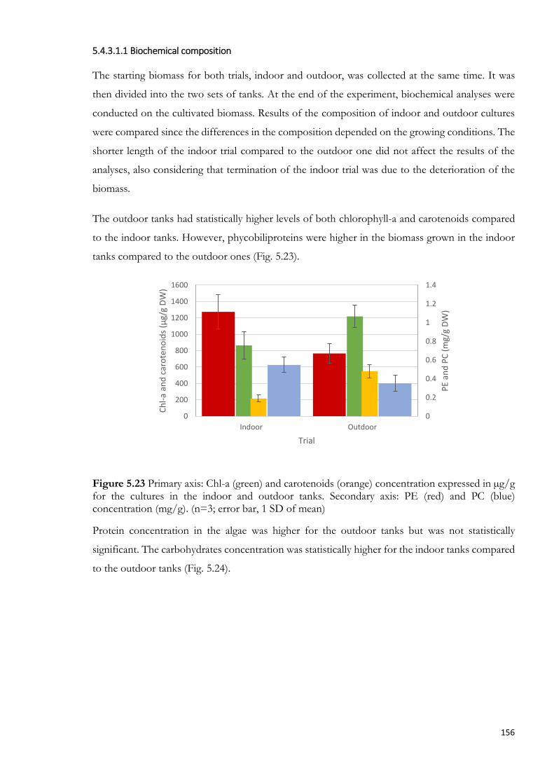
156

5.4.3.1.1 Biochemical composition

The starting biomass for both trials, indoor and outdoor, was collected at the same time. It was

then divided into the two sets of tanks. At the end of the experiment, biochemical analyses were

conducted on the cultivated biomass. Results of the composition of indoor and outdoor cultures

were compared since the differences in the composition depended on the growing conditions. The

shorter length of the indoor trial compared to the outdoor one did not affect the results of the

analyses, also considering that termination of the indoor trial was due to the deterioration of the

biomass.

The outdoor tanks had statistically higher levels of both chlorophyll-a and carotenoids compared

to the indoor tanks. However, phycobiliproteins were higher in the biomass grown in the indoor

tanks compared to the outdoor ones (Fig. 5.23).

Figure 5.23 Primary axis: Chl-a (green) and carotenoids (orange) concentration expressed in µg/g for the cultures in the indoor and outdoor tanks. Secondary axis: PE (red) and PC (blue) concentration (mg/g). (n=3; error bar, 1 SD of mean)

Protein concentration in the algae was higher for the outdoor tanks but was not statistically

significant. The carbohydrates concentration was statistically higher for the indoor tanks compared

to the outdoor tanks (Fig. 5.24).

0

0.2

0.4

0.6

0.8

1

1.2

1.4

0

200

400

600

800

1000

1200

1400

1600

Indoor Outdoor

PE

and

PC

(m

g/g

DW

)

Ch

l-a

and

car

ote

no

ids

(µg/

g D

W)

Trial

157

Figure 5.24 Protein (dark grey bars) and carbohydrate (light grey bars) content expressed in percentage (DW) for samples undergoing Outdoor and Indoor trials. (n=3; error bar, 1 SD of mean)

A statistical difference (p<0.05) was measured for the antioxidant compound concentration for the

outdoor tanks when compared to the indoor ones (Fig. 5.25).

Figure 5.25 Antioxidant compounds measured with FRAP assay in samples undergoing the cultivation in indoor (dark grey bar) and outdoor (light grey bar) tank trials. (n=3; error bar, 1 SD of mean)

5.4.3.2 Summer trial: outdoor experiment

There was an initial increase in growth when the biomass was weighted (from April to June), after

this peak the weight of the culture started to decrease and begun to stabilise again after August

(Fig. 5.26). New shoots and new tips grew on the cultured biomass which also became reproductive

from April to June. This was confirmed also by the SGR measurements (Fig. 5.27).

0

5

10

15

20

25

30

35

40

Outdoor Indoor

Pro

tein

an

d c

arb

oh

ydra

te c

on

ten

t (%

DW

)

Trial

0

0.5

1

1.5

2

2.5

3

3.5

4

Outdoor Indoor

FRA

P

(µM

FeS

O₄

eq/m

g D

W)

Trial

158

Figure 5.26 Growth (WW, g) of cultures in an outdoor tumbling system from April to September 2018. (n=3; error bar, 1 SD of mean)

Figure 5.27 SGR of culture in the outdoor tumbling system from April to September 2018. (n=3; error bar, 1 SD of mean)

QY measurements showed an initial decrease in the recorded values especially in June, followed by

a subsequent increase that reached its maximum in September (Fig. 5.28). The cultures in the

outdoor system underwent the same change in colour that can be seen in the biomass growing in

the wild (Fig. 5.29 B and D). This is directly linked to changes in day length and light intensity.

However, overall the material was healthy and thick in texture, with new growth visible (Fig. 5.29

A and C).

0

50

100

150

200

250

300

350

400

450

April May June July August September

wei

ght

(g W

W)

Month

-1.5

-1

-0.5

0

0.5

1

1.5

SGR 1 SGR 2 SGR 3 SGR 4 SGR 5

Gro

wth

rat

e (%

day

¯¹)

Month

159

Figure 5.28 QY measurement of cultures in an outdoor tumbling system from April to September 2018. (n=3; error bar, 1 SD of mean)

Figure 5.29 Cultures during the weighing in July 2018 (A &C), wild sample in May 2018 (B) and (D) July 2018

Temperature, light, pH and salinity are reported in Figs 5.30-5.32, showing an increase of

temperature especially in June and July (Fig. 5.30), a reduction of light intensity across the

experimental time (Fig. 5.31), an increase of salinity with a peak in August (Fig. 5.32), and a decrease

of pH across the months (Fig. 5.32).

0

0.1

0.2

0.3

0.4

0.5

0.6


PA

M (

QY)

Month

160

Figure 5.30 Temperature (°C) profile in the tanks in the second outdoor trial as average (blue bars), maximum (dark grey bars) and minimum (light grey bars)

Figure 5.31 Light profile (lum/ft²) expressed as average in the tanks in the second outdoor trial

Figure 5.32 Salinity (light grey bars) and pH (dark grey line) measurements in the second outdoor trial

0

5

10

15

20

25


Tem

per

atu

re (

°C)

Months

0

200

400

600

800

1000

1200

1400

1600

1800

2000


Ligh

t In

ten

sity

(lu

m/f

t²)

Months

7.8

7.9

8

8.1

8.2

8.3

8.4

8.5

8.6


31

31.2

31.4

31.6

31.8

32

32.2

32.4

32.6

pH

Months

Salin

ity

(PSU

)

161

5.4.3.2.1 Biochemical composition

Biochemical composition for the outdoor trial is presented in Table 5.7. All analyses were

conducted in triplicate per each tank on the harvested biomass at the end of the trial in September.

For the pigments, there was a statistical difference between tank number 1 and the other two, with

the former having a higher value when compared to the other two.

Table 5.7 Biochemical composition with relative concentration of the component analysed for the outdoor trial (n=3; error 1SD of mean)

Component Content (DW)

Protein 23.82 %

Carbohydrates 23.62 %

Chlorophyll a 2503 µg/g

Carotenoids 1283.6 µg/g

PE 0.68 mg/g

PC 0.25 mg/g

FRAP 1.53 µm FeSO₄/mg


pinnatifida from epiphytes treated cultures

The procedure for spores’ release for the successive isolation and cultivation is showed in Fig. 5.33.

Tips with visible tetraspores were cut (Fig. 5.33 A-C), and release of the spores occurred in the

multiplate (Fig. 5.33 D).

It was estimated that approximately 5,000 to 30,000 spores could be released during multiple release

events from each tip. The high variability of the released numbers and the fact that it was not

possible to obtain an average number of spores released per single plant made the survival

assessment unreliable. However, it was estimated that around 5% of spores survived and reached

the germination phase of the life cycle. The cultures obtained were not axenic.

162

Figure 5.33 A) Multi-well Petri dishes with cut tips from tetrasporophytes; B) Tetraspores are visible inside the tetrasporophytes on the extremities of the thalli of cultivated samples; empty tetrasporophytes are visible ahead of the full tetrasporophytes; C) Haploid tetraspores (indicated by the arrows) inside the diploid tetrasporophytes prior to release; D) Spores released prior attachment in a Petri dish and observed under a stereo microscope

Once released, spores that did survive (Fig. 5.34 A) either attached immediately (within 2 hours) or

remained unattached. In both cases, germination occurred within 24 hours and the attachment was

not fundamental to initiate it (pers. obsv.). Dead spores before germination were also observed

(Fig. 5.34 B).

Figure 5.34 A) Live haploid spore released observed under the Axio stereomicroscope. It is possible to see the external mucilaginous sheath; B) dead spore after release; note visible deteriorating cell wall and loss of pigmentation

163

The spores started to germinate, developing a rudimental rhizoid structure that allowed them to

adhere to the substratum. Their shape changed from rounded to oval and the division in septi of

the body became visible (indicated with A in Fig. 5.35). The basal part of the rudimental rhizoid

appendix quickly developed a swollen extremity, which was the main surface involved in anchoring

the development juvenile (indicated with B in Fig. 5.35). Moreover, even if the spores were released

at the same time, they did not develop at the same rate and while some were already attached and

germinated, others still retained their initial rounded shape or had a shorter developed appendix

(indicated with C in Fig. 5.35).

Figure 5.35 Spores under an Axio stereomicroscope (Zeiss) at different stages of development after the release: A) Body of germinated spore; B) Rhizoid of germinated spore; C) Rounded spore without rhizoid apparatus

After one week, germinated spores developed a long-shaped structure, increased in size and area,

and presented attachment disc (Fig. 5.36 A-F). Considering the different rates at which the spores

of the same age develop, it is difficult to give a general measure of the spores after defined times

in vitro cultivation.

After one month, the juveniles started to elongate and increase the size. The structure of the body

became more complex and the differentiation in cortical and medullar tissue more evident (Fig.

5.36 D). Measurements from the germinated spores were taken, in terms of the body and the

appendix, showing a clear development and enlargement of the spores (Fig. 5.36 D). After two

months of development the juveniles presented a main body, developed a complex structure, with

a cylindrical aspect and a clear distintion between the small rounded cortical cells and the medullary

one (Fig. 5.36 E). Branching was also observed, together with swolled and defined structures

anchoring the juveniles to the surface (Fig. 5.36 F).

164

Figure 5.36 A) Developed spores after one week into the cultivation system (observed at the Axio Inverted microscope at 10x); B & C) spores after two weeks into the cultivation system (observed at the Axio Inverted microscope at 20x and 10x); D) Measurement of a developed spore after one month from release (Axio Inver microscope); E) Developed juvenile after two months from the release; F) particular of attachment disc in juvenile after two months in cultivation

165

Figure 5.37 A) Juveniles after two months in tissue flask, B) magnification of juveniles. Each square= 1 mm².

Most of the juveniles that survived reached approximately 2-3mm after two months of cultivation

(Fig. 5.37 A and B). The proportion between the body and the rhizoid appendices changed, and

individuals generally had a longer cylindrical body of the former. Furthermore, the structure of the

body of the juveniles branched out, developing a structure that was charactheristic of the adult

stage of the life cycle (Fig. 5.38 A-D).

Figure 5.38 A & B) Juveniles after two months of in vitro incubation observed under a stereomicroscope (Zeiss). C & D) Juveniles after three months of in vitro incubation observed under a stereomicroscope (Zeiss). Visible ramification and presence of multiple branches as well as other organisms

After 5 months of in vitro cultivation, the length of the juveniles varied from five to ten mm (Fig.

5.39).

166

.

Figure 5.39 6x multi-well with juveniles after 5 months of cultivation

5.5 Discussion

One of the major challenges in establishing laboratory cultures of seaweed is maintaining them free

of contaminating algae (microalgae and cyanobacteria) and other epiphytes (Redmond et al., 2014).

These organisms tend to grow faster than the seaweed, compete for nutrients and may release

substances that inhibit growth, or are toxic to the alga of interest (Berland et al., 1972). Several

published studies have focused on macroalgal decontamination system; however, they usually aim

to obtain axenic cultures in the laboratory, rather than disinfect cultures used in long-term

cultivation systems (McCracken, 1989; Baweja et al., 2009; Reddy et al., 2008). The physical removal

stage (using razor blade, rubbing, or brushing the seaweeds) to remove epiphytes is followed by

chemical treatments (Baweja et al., 2009; Kientz et al., 2012). These steps can heavily affect

seaweeds that lack a protective cuticle (Reddy et al., 2008; Baweja et al., 2009). The most common

disinfectants utilised for the macroalgal culturing are: sodium hypochlorite (NaClO), reactive iodine

and organic solvents, often followed by an antibiotic mix (Baweja et al., 2009; McCracken, 1989;

Kerrison et al., 2016a, b). In these experiments the most effective treatment for epiphytes removal

on O. pinnatifida cultures was a 0.5% KI solution. This treatment significantly affected epiphytes

and grazers on the cultures, without having an impact on the seaweed. It was able to carry on

growing, showed very little loss in photosynthetic activity, as demonstrated via QY measurements,

plus it was able to develop, produce and release spores. The initial treatment prevented the

formation of epiphytes in the tank system even after months of culturing. The combination of the

chemical treatments and the tidal simulation system, proved to be an effective method in

controlling the growth of epiphytes and in preventing their proliferation in the tank cultivation

system.

167

As an intertidal species, O. pinnatifida must depend on the tides for its biological cycle (e.g.

reproduction and induction of spore release); furthermore, desiccation processes have previously

proved to be efficient in epiphytes control for other species (e.g. Pyropia sp., Ding and Ma, 2005).

Even if the tidal system did not lead to an overall increase in the biomass of the cultures (Fig. 5.11),

it was observed that while the older thalli were degenerating/becoming brittle, new shoots were

developing from the holdfast and from the tips of the branches, as the cultures were beginning to

regenerate. The cultures also produced and released spores for the entire length of the experiment.

Despite the results reported for the absolute and relative growth rates, the cultures were still alive

and growing. In this case it would probably be of more value to evaluate the quality of the culture

biomass rather than the quantity, especially in light of the slow growth rates that O. pinnatifida has

in the wild (pers. obsv.). In seaweeds in general, once the spores are released, the old thallus portion

tends to be slough off from the plant, and resources are used to support the development of new

shoots (Lüning and Pang, 2003). This is probably what happened in the O. pinnatifida tank cultures.

Further evidence to support this was provided in subsequent experiments, were O. pinnatifida

cultures required a long cultivation period to stabilise and eventually demonstrate a measureable

growth in weight.

The development of a tumbling cultivation system for this species provided a more controlled

regime where all the parameters could be monitored. The continuous tumbling of the cultures also

guaranteed a continuous exchange of nutrients, sufficient aeration as well as a uniform distribution

of light. This was the second time that an outdoor tank system for O. pinnatifida has been trialled

and the first time that an indoor system was used (Silva, 2015). The results obtained from this study

differ from those reported by Silva (2015), who conducted short outdoor tank cultivation trials in

Portugual. In the Portuguese study the SGR and productivity were positive for 5 weeks, from

November to December, and this was demonstrated further by an overall increase in the quantity

of biomass obtained. However, they excluded the summer growth experiment that had also been

carried out. Furthemore, cultures in the Portuguese study were supplied with seawater from an

IMTA system (Silva, 2015). Similar results, with fluctuations in SGR in outdoor tanks, were

reported for another Portoguese study (Gonçalves, 2018). For the experiments undertaken within

this chapter, the SGR gave negative values over the complete duration of the winter trials for the

indoor trial, while a positive value was reported at the end of the experiment for the outdoor trial;

on the other hand, positive values were reported for the first two months of the experiment for

the outdoor summer trial. Except the indoor trial, the biomass did not show visible signs of

decomposition. The indoor and outdoor cultivation systems were compared for biomass

production and quality. From this experiment, the outdoor system demonstrated that it was a

promising alternative, from a commercial point of view, and also had lower management costs

associated with it.

168

The indoor experiment was not successfully; this was considered to be due mainly to the type of

tanks used for the experiment. As already showed by previous authors (Lignell and Pedersen, 1987;

Smit et al., 1997), tank colour significantly affects the light field experienced by the algae. The tanks

used in this trial were black conical tanks and their position in the aquarium was away from the

light source (white lights) that were just hanging from the ceiling. Whilst light is fundamental for

seaweed biomass productivity and should always be sufficient to allow photosynthesis (Harrison

and Hurd, 2001). The impact of light limitation was evident from the PAM measurements of the

cultures and the pigments’ analyses. The only exception to this was for PE and PC values, which

were higher in the indoor cultures, probably because they were under stress and accumulating N

in different forms, such as pigments (Lapointe and Duke, 1984; Rico and Fernández, 1996). The

aeration and flow rates were also quite low due to limitations in the supply to the area utilised for

the experiment, whilst adequate water movement is needed to stimulate nutrients exchange and

provide carbon dioxide (Kerrison and Le, 2015). Deficit in the growth of the indoor cultures was

also reflected in accumulation of carbohydrates that are normally used by seaweeds as an energy

source (McCandless, 1981; Stiger et al., 2016).

Similar problems were also noted in the outdoor system, since in the summer water and air supplies

were limited, creating problems. In the winter trial, after four months, the cultures finally started

to stabilize and gain weight, with new shoots developing from the holdfast of the plants. Moreover,

cultures became reproductive around March-April and spontaneously released spores. Epiphytes

were kept under control during the experiment, indicating that the treatment applied previously to

the cultures was effective in their control even in the outdoor system, where the water used was

only filtered through a sand filter. The summer trial was only performed in an outdoor system,

since the conditions available indoor had already proved to be unsuitable. This time the cultures

increased in weight for the first 2-3 months, probably because of increased of light levels (Harrison

and Hurd, 2001) that occurs in Scotland in late spring months (April-May). Few issues caused a

drastic decrease of weight of the cultures, including a low water exchange rate (due to the scarce

water supply and the dependence to the tides variation), an insufficient filtration system that did

not control the inflow of contaminants (e.g. Ectocarpus sp.) and grazers (e.g. polychaetes) that

negatively affected the growth of the cultures (Redmond et al., 2014). The tanks, the filters, as well

as the pipes that supplied water to the tanks were completely infested with Ectocarpus sp., this

proliferated especially once the temperature in the tanks reached their highest levels (18-19°C).

Such high temperatures, negatively affected the cultures (as already showed in a preliminary

experiment, see Appendix C.1), considering that the biomass becomes brittle and eventually dies

off at temperature above 15 °C. Cultures started to stabilize again after August, when the light

intensity, but especially the temperatures, started to decrease. The response of the cultures was also

confirmed by the PAM measurements (Fig. 5.28).

169

The winter and summer trials showed different results in terms of biochemical composition.

Furthermore, variations in the biochemical profiles were previously observed for wild specimens

in relation to the season (Chapter 3), and these differences might be related to the particular

environmental conditions, (Kaehler and Kennish, 1996; Haroon, 2000; Chandini et al., 2008) that

have an effect on the biochemical composition of the seaweeds, especially in the summer trial.

Interestingly, the cultivation system was able to influence the morphology similarly to what

happens in the wild, with cultures showing the same variation in colour already observed in seasonal

samples.

Cultures in the tank systems investigated produced tetraspores, even after treatment against

epiphytes, showing that this chemical treatment does not negatively affect the life cycle of this

species. The reproductive cycle is considered one of the main possibilities for cultivation of a range

of species for seeded line (McHugh, 2003). It offers the advantage of having continuous genetic

recombination that makes future cultures more resistant to diseases, e.g. Ice-ice (Santelices, 1999;

FAO, 2003). But there are limitations with this methodology, such as high mortality rates, slow

growth and the costs associated with cultivation of spores until they reach the juveniles stage, step

that is usually carried out in a hatchery where normally parameters such as pH, salinity, high quality

water, light and temperature are artificially controlled with an associated cost (FAO, 2003). On the

other hand, vegetative production might guarantee a faster increase in biomass, lower production

costs, but this may also be associated with an increased susceptibility to diseases (FAO, 2003). In

the end, it will depend on the market the biomass is being produced for.

In this study, the reproductive cycle and juvenile production was performed in vitro for O.

pinnatifida for the first time from mature tetrasprophytes treated with a 0.5% KI solution cultivated

in a tank system. It was noted that tetrasporophytes could be easily obtained from the adults

cultivated in tanks even outside the natural reproductive period, which is May (Maggs and

Hommersand, 1993, Appendix C.2). Release of spores from the tips was observed once they were

cut from the adult and submerged in filtered seawater. Multiple releases from the same tip

commonly occurred. Spores were released in large numbers and quickly attached and germinated.

For the whole process to be scaled up and commercially applicable there are still several limitations

that need to be overcome. First, it will be necessary to assess the release and survival rates of the

spores, this will give an indication of how much reproductive starting material will be needed at a

commercial level. It will also be important to find an adequate substratum for the attachment of

the spores, which has already been identified as important requirement for a variety of seaweed

spores (Maggs and Callow, 2003; Hurd et al., 2014; Redmond et al., 2014). For this species, it

appears that they are able to attach to several different types of surfaces, including glass and plastic

170

Petri dishes. However, trials on different types of substrata should be conducted in order to solve

the bottleneck in survival rates, as well as the rate of the development.

5.6 Conclusions

Epiphytes and contaminants can be mitigated and controlled in O. pinnatifida cultures

applying a chemical treatment with a 0.5% KI solution and an incubation time of 30

minutes, hence this treatment should always be applied prior cultivation;

The chemical treatment coupled together with the tidal simulation system personally

developed proved to be efficient in controlling and eliminating the presence of epiphytes

on the cultures and cultivation system;

The chemical treatment does not affect the biology of the species and its capacity to

produce and release tetraspores;

Spores production and release for the species investigated is possible; however, several

limitations/problems need to be solved in order to improve the process, such as reduce

the mortality, accelerate the growth rate, control the contaminants and test different

substrata (e.g. shells) for settlement optimization;

Juveniles successfully developed from germinated spores cultivated in vitro reaching the

size of five to 10 mm in five months;

From a commercial prospective, a vegetative cultivation of this species rather than a

reproductive one seems to be more suitable at the moment for exploitability and up-scaling

of O. pinnatifida;

These preliminary tank experiments specifically developed for these trials, permitted to

design and develop a successful indoor tumbling cultivation system for the cultivation of

this species, as described in Chapter 8.

172

Chapter 6 Effects of different media on the growth and biochemical

composition of Osmundea pinnatifida

6.1 Introduction

Flask cultivation of seaweeds is an established methodology allowing for the control of culturing

parameters such as light, temperature and nutrients, in order to manage culture productivity

(Andersen, 2005). Nutrient supply is an important parameter in the management of cultivation

systems (Lignell and Pedersen, 1987), with media being usually composed of three main

components: macronutrients (generally nitrogen and phosphorous), trace elements and vitamins.

For optimal growth, macronutrients are usually required in a ratio of 16N:16Si:1P (Redfield ratio,

1934) (Parsons et al., 1984; Brzezinski, 1985), replicating the ratio found in natural seawater.

However, the N:P for seaweed can vary between 10:1 and 80:1, with an average of 30:1 (Atkinson

and Smith, 1983). Nitrogen is fundamental for the production of amino acids, nucleic acid,

enzymes, nucleoproteins and alkaloids; phosphorous is used by seaweeds in the process of

photosynthesis, respiration, cell division and enlargement, carbohydrates metabolism and has a role

in the transfer/storage of energy (Hopkins and Hüner, 2009). Typically trace metal stock solutions

consist of chloride or sulfate salts of zinc, cobalt, manganese, selenium, nickel, and iron (Andersen,

2005). Usually three vitamins, vitamin B₁₂ (cyanocobalamin), thiamine, and biotin, are added, but

very few algae need all three vitamins (Provasoli and Carlucci, 1974; Provasoli, 1966). The usual

order of vitamin requirements by algae are vitamin B₁₂ > thiamine > biotin.

In this Chapter, three different media types were investigated for the flask cultivation of vegetative

tissue of Osmundea pinnatifida. The aim was to identify the best cultivation medium for this species

in terms of growth and biomass increase, as well as biochemical composition. The commonly used

nutrient medium for indoor cultivation of red seaweeds is von Stosch enrichment medium (VSE)

(Redmond et al., 2014). Several studies have investigated the use of this medium for the cultivation

of different red seaweeds species (Guiry and Cunningham, 1984), including Gigartina sp., as well as

more recent studies; Hypnea cervicornis (Ribeiro et al., 2013), Gracilaria domingensis (J. Agardh; Mendes

et al., 2012); Gracilaria verrucosa (Mensi et al., 2011); Gracilaria sp. (Kim and Yarish, 2014); O.

pinnatifida (Silva, 2015). von Stosch enrichment medium contains nutrients such as nitrate,

phosphate, iron, manganese, EDTA, and vitamins (vitamin B₁₂, thiamine, and biotin). Compared

to other media, its application at commercial scale is limited by its high material and preparation

costs (Kim and Yarish, 2014). In order to confirm the most appropriate cultivation medium, a

comparison was carried out with one of the most widely employed algal medium (F/2) designed

for growing coastal marine algae, in particular diatoms (Guillard and Ryther, 1962; Guillard, 1975),

and a modified version of this medium, where the sources of nitrogen and phosphate were the

173

same (in concentration and type) as that used in VSE medium, while the other elements were kept

the same as F/2. The biochemical composition of the biomass produced from the cultivation in

these three media types was analysed in order to identify any impact on the biochemical profile on

this species. A comparison of media effects on growth and biochemical composition of two

different stages of cultures, adults and juveniles, was carried out again to see if the stage/age of the

cultures might affect the nutrient uptake, as already demonstrated for other seaweeds (Lobban and

Harrison, 1997; Pedersen, 1994).

In addition, the effect of different nitrogen sources on growth and biochemical composition of O.

pinnatifida was also investigated. There is, in general, a lack of available data on the effect that

nutrients, in terms of regimes, type, concentration and N/P, have on seaweed biomass and growth.

This knowledge is fundamental for the management and cultivation of seaweeds (Rueness and

Tananger, 1984). Generally, macroalgal nutrient uptake depends on several factors, such as

environmental N concentration (Harrison and Hurd, 2001) and biological factors, e.g. metabolism,

morphology, tissue type, species, age of the algae and nutritional history (Neori et al., 2004; Lobban

and Harrison, 1997; Pedersen, 1994; Rosenberg and Ramus, 1984), and typically follows a

Michaelis-Menten-type curve (Jimenez del Rio et al., 1996). The growth rate and productivity of

algae is, in part, controlled by the concentration of dissolved inorganic nitrogen (DIN) in the

aqueous medium surrounding the thallus (Chapman and Craigie, 1977; Rosenberg and Ramus,

1982; Lavery and McComb, 1991). The ability of an alga to utilise N for biomass production is

determined by the rate at which DIN can be absorbed and thereafter used in biochemical processes

(Wheeler, 1980; Koch, 1994; Sanford and Crawford, 2000). In seawater, N is available to seaweeds

in three major forms: NO₃, NH₄, and urea (Phillips and Hurd, 2004). It is most likely the key factor

in limiting growth of seaweed, especially those from temperate areas (Lobban and Harrison, 1997).

Generally, N limitation reduces growth, increases phycocolloid content, and decreases

photosynthetic activities (Chopin et al., 1990a). In many macroalgae, growth rates are reduced as

soon as the total N content of the thallus falls below the critical level of approximately 2% (Hanisak,

1983). These studies led to the concept of the “Neish effect”, reduced carrageenan content with

increasing N availability (Neish et al., 1977). However, seaweed can store nitrogen in excess, to

sustain their growth during periods of nutrient limitation/deficiency; this mechanism has important

implications for nutrient management of cultivated seaweeds (Bird et al., 1982; Lapointe, 1985).

The relationship between N, growth, biochemistry (e.g. production of carrageenan) and

photosynthesis is well documented for certain species such as Chondrus crispus (Neish et al., 1977;

Simpson et al., 1978; Chopin et al., 1995). However, there is no information available for O.

pinnatifida, the species been investigated in this thesis. This chapter details experiments carried out

174

in order to understand the impact of different media types and N sources on the growth and

biochemical composition of O. pinnatifida.

6.2 Aims

To identify the best treatment in term of medium composition that would be able to sustain

the growth and the biochemical composition of the species been investigated;

To investigate different nitrogen sources and their impact on cultivated samples in terms

of growth and biochemical composition;

To assess the influence of media composition and stage of development of the cultures

(adults and juveniles) on the biochemical profile of O. pinnatifida.



Osmundea pinnatifida adult cultures

The biomass for this experiment was collected in mid-November 2017 from Seil (56.30° N, 5.65°

W) at low tide. A total of six kg of fresh weight biomass was stored in a Cool-box during transport

to the laboratory, manually cleaned removing all the visible grazers and epiphytes, and rinsed

thoroughly with FSW in order to remove all the remaining debris and epiphytes. Finally, samples

were cleaned with a 0.5% solution of KI (Sigma Aldrich®) in 50 l of filtered and UV sterilised

seawater for 30 minutes. Samples were then rinsed three times for 30 minutes each time in FSW

and left to acclimate at 10 °C, 12:12 (L:D) in filtered and UV sterilised seawater for one week. The

water was changed every day.

Figure 6.1 Flasks (6 x 1 l) with adult cultures in the CT room under incubation: 10 °C, 12:12 photoperiod

175

One-litre flasks with 10 g of wet weight material (dried in a spin salad, as developed by Ross et al.

2017, before weighing) and 0.45 µm Whatman® filters connected to glass Pasteur pipettes for

aeration were used in triplicate for each treatment (Fig. 6.1). Cultures were incubated in a CT room

at 10°C, 12:12 (L:D), 80-100 µmol/m²/sec light intensity. The media treatments are detailed in

Table 6.1. Media were prepared aseptically in filtered, UV sterilized and Tyndalysed natural

seawater. All stock solutions for the different media types were autoclaved prior to use, except for

the vitamin stocks, which were filtered sterilised (0.2 µm), and the iron stock for the VS recipe

(ferrous sulfate was added aseptically to sterile distilled water); both were stored in the fridge until

required. The medium was changed twice per week in a laminar cabinet. Every week the samples

were weighted (after been dried in a spin salad) and the specific growth rate (SGR) was calculated

using the formula (Evans, 1972) where LN is natural logarithm, Wf final weight, Wi initial weight

and t time:

𝑆𝐺𝑅 =(𝐿𝑁(𝑊𝑓) − 𝐿𝑁(𝑊𝑖))𝑥100

𝑡

The experiment was run for 5 weeks in total. Statistical analyses for all the trials listed in this and

subsequent sections were conducted applying an ANOVA single factor (p<0.05, Minitab 18) with

Tukey’s, Fisher’s and Dunnett’s post-hoc tests.

Table 6.1 Media formulation trialled: F/2 recipe (from Andersen 2005), Von Stosch recipe (from Andersen 2005); F/2 modified. The nitrogen and phosphate sources with the respective concentrations were taken from the Von Stosch recipe. All the other elements and concentration were kept as normal as in the original F/2 recipe.

F/2 F/2 modified Von Stosch

Component Final concentration

(M)


(M)


(M)

Phosphate stock Phosphate stock Phosphate stock

NaH₂PO₄x2H₂O 3.62 x 10⁻⁵ Na₂ b-glycerophosphate

2.48 x 10⁻⁴ Na₂ b-glycerophosphate

2.48 x 10⁻⁴

Nitrate stock Nitrate stock Nitrate stock

NaNO₃ 8.82 x 10⁻⁴ NaNO₃ 5.00 x 10⁻³ NaNO₃ 5.00 x 10⁻³

Trace elements Trace elements Trace elements

FeCl₃x6H₂O 1.17 x 10⁻⁵ FeCl₃x6H₂O 1.17 x 10⁻⁵ FeSO₄x7H₂O 1.00 x 10⁻⁵

MnCl₂x4H₂O 9.10 x 10⁻⁷ MnCl₂x4H₂O 9.10 x 10⁻⁷ MnCl₂x4H₂O 1.00 x 10⁻⁴

NA₂ EDTA 1.17 x 10⁻⁵ NA₂ EDTA 1.17 x 10⁻⁵ Na₂EDTAx 2H₂O 1.00 x 10⁻⁴

CuSO₄x5H₂O 3.93 x 10⁻⁸ CuSO₄x5H₂O 3.93 x 10⁻⁸

ZnSO₄x7H₂O 7.65 x 10⁻⁸ ZnSO₄x7H₂O 7.65 x 10⁻⁸

CoCl₂x6H₂O 4.20 x 10⁻⁸ CoCl₂x6H₂O 4.20 x 10⁻⁸

Na₂MoO₄x2H₂O 2.60 x 10⁻⁸ Na₂MoO₄x2H₂O 2.60 x 10⁻⁸

Vitamin stock Vitamin stock Vitamin stock

Thiamine HCl

(Vitamin B₁) 2.96 x 10⁻⁷ Thiamine HCl

(Vitamin B₁) 2.96 x 10⁻⁷ Thiamine HCl

(Vitamin B₁) 5.93 x 10⁻⁶

Biotin (vitamin H) 2.05 x 10⁻⁹ Biotin (vitamin H) 2.05 x 10⁻⁹ Biotin (vitamin H) 4.09 x 10⁻⁹

Cyanocobalamin

(vitamin B₁₂) 3.69 x 10⁻¹⁰ Cyanocobalamin

(vitamin B₁₂) 3.69 x 10⁻¹⁰ Cyanocobalamin

(vitamin B₁₂) 1.48 x 10⁻⁹

176

At the end of the 5 weeks cultivating period, the biomass was harvested and protein, carbohydrates,

antioxidant compounds (FRAP assay) and pigments (including carotenoids, PE and PC and

chlorophyll-a), were analysed in triplicate for each culture with the methodologies already described

in Chapter 3.


pinnatifida juvenile plantlets

The previous experiment (see section 6.3.1) was repeated, but this time on juvenile plantlets of O.

pinnatifida and with only two of the media types, Von Stosch and F/2 (Table 6.1). For this

experiment, 500 ml flasks with 200 ml of medium and 2 g of material (fresh weight after spin-

drying) were used and again the experiment was performed in triplicate for each treatment. All the

other conditions and methodologies used are already described in section 6.3.1.

Figure 6.2 Flasks (6 x 500 ml) with juvenile cultures under incubation: 10 °C, 12 :12 photoperiod

The biochemical composition of the samples was determined as described in Chapter 3 and

included antioxidant compounds (FRAP assay), carbohydrates, protein, and pigments (chlorophyll-

a, carotenoids, PE and PC).

6.3.3 The impact of nitrogen sources and the N:P ratio on Osmundea pinnatifida growth and

biochemical composition

Cultures for this experiment, collected as described in section 6.3.1, were acclimated as follows,

five grams per 12 cultures were incubated for one week in filtered, UV-sterilized and tyndalyzed

seawater with a photoperiod of 12:12 (L:D), white fluorescent light (80-100 µmol/m²/sec) and at

10 °C. The experiment was conducted in triplicate in 500 ml flasks with 5 g WW of biomass and

250 ml of medium changed weekly. F/2 medium was the basic medium type (Table 6.1) with the

nitrogen source varied for the other treatments (Table 6.2):

177

Inorganic Sources: NaNO₃, NH₄Cl, NH₄NO₃

Organic source: NH₂CONH₂ (urea)

Nitrogen was added to the media at a final concentration of 824 µM (Starr and Zeikus 1993).

Phosphate was kept constant (82.4 µM, as normal concentration of F/2). With an N:P ratio of 10:1

(Table 6.2).

Table 6.2 Composition of treatments applied to cultures where control refers to F/2 medium. The final molarity of N and P was the same for all the media tested

Trace elements (ml/l)

Vitamin mix (ml/l)

Phosphate (g/l)

NaH₂PO₄x2H₂O

Nitrogen sources Weight (g/ l)

1 1 5.65 NaNO₃ (control) 75

1 1 5.65 NH₄Cl 40

1 1 5.65 NH₄NO₃ 65.9

1 1 5.65 NH₂CONH₂ 49

Blotted weight, after spin-drying was recorded every week, before the medium was changed.

Relatively daily growth rate was calculated using the formula of Evans (1972) detailed in section

6.3.1. The experiment was run for 7 weeks and the biomass was harvested for protein,

carbohydrates and phycobiliproteins analysis using the methodologies described in Chapter 3.

6.4 Results


Osmundea pinnatifida adult cultures

6.4.1.1 Weight and growth rate of adult cultures grown in three different media

Cultures in this experiment demonstrated positive growth for all of the treatments investigated for

the entire length of the experiment. Samples grew new extremities, as well as developed new shoots

(Fig. 6.3); there was no change in colour, or contamination by epiphytes in the cultures undergoing

all three of the treatments.

Figure 6.3 Different cultures under the different media treatments at the beginning and at the end of the trial A) F/2, B) F/2 modified and, C) VS at the beginning of the experiment; D) F/2, E)F/2 modified and, F) VS at the end of the experiment

178

An ANOVA single factor (p<0.05) indicated a statistical difference in the first two weeks of the

experiment, with the VS treatment giving a statistically higher growth compared to the other two

treatments. However, the trend changed after this, with no statistical difference reported between

the tested treatment and a slightly higher growth reported, at the last time point, for F/2, followed

by VS and lastly F/2 modified (Fig. 6.4).

Figure 6.4 Weight measurements of cultures (WW) under the three different treatments: F/2 black line, F/2 modified dark grey line, VS light grey line. (n=3; error bar, 1 SD of mean).

The relative growth rate shows a decreasing trend, especially in the first two weeks of the

experiment (Fig. 6.5). After that, the relative growth, particularly for VS and F/2 reached a stable

state towards the end of the experiment. All three treatments were able to sustain the growth of O.

pinnatifida vegetative tissue, giving a maximum growth rate in terms of a percentage per week of 1.2

for VS, 0.86 for F/2 and 0.67 for F/2 modified.

Figure 6.5 Growth rate calculated with the equation for SGR (Evans, 1972). F/2 black line, F/2 modified dark grey line, VS light grey line. (n=3; error bar, 1 SD of mean)

9

9.5

10

10.5

11

11.5

12

Time 0 Time 1 Time 2 Time 3 Time 4 Time 5

wei

ght

(g W

W)

Week

0

0.2

0.4

0.6

0.8

1

1.2

1.4

Time (1) Time (2) Time (3) Time (4) Time(5)

Gro

wth

rat

e (%

day

¯¹)

Week

179

6.4.1.2 Effects of three different media types on the biochemical composition of Osmundea pinnatifida

adult cultures

6.4.1.2.1 Antioxidant content

An ANOVA single factor (p<0.05) indicated a statistical difference between VS and the other

treatments, in terms of the antioxidant content (Fisher’s and Tukey’s tests), with F/2 and F/2

modified being statistically different from VS (Fig. 6.6). The highest result was reported for F/2

modified, 5.47 µM/mg FeSO₄, followed by F/2, 4.8 µM/mg FeSO₄ and last VS, 3.40 µM/mg

FeSO₄, demonstrating that the first two media statistically increase the production of antioxidant

compounds in the species.

Figure 6.6 FRAP assay for the cultures under the different media. F/2 black bar, F/2 modified dark grey bar, VS light grey bar. (n=3; error bar, 1 SD of mean)

6.4.1.2.2 Carbohydrates and proteins

An ANOVA single factor (p<0.05) and post hoc tests (Tukey’s and Fisher’s) indicated a statistical

difference in terms of carbohydrate content between VS and F/2 modified, and F/2, with the first

two showing higher values (Fig. 6.7). An ANOVA single factor (p<0.05) and post hoc tests

(Tukey’s and Fisher’s) reported no statistical difference for the protein concentration; however, VS

showed the lowest concentration compared to F/2 (highest value) and F/2 modified. Furthermore,

analyses showed that carbohydrates and protein contents followed inverted trends, while

carbohydrates content increased, the protein content decreased and vice versa (Fig. 6.7).

0

1

2

3

4

5

6

7

VS F/2 F/2 modified

FRA

P

(µM

FeS

O4

eq

/mg

DW

)

Treatment

180

Figure 6.7 Carbohydrate (dark grey bars) and protein (light grey bars) content expressed as %DW for cultures undergoing the three different treatments. (n=3; error bar, 1 SD of mean)

6.4.1.2.3 Pigments

An ANOVA single factor (p<0.05) and post hoc tests (Tukey’s and Fisher’s) indicated a statistical

difference between VS and the other two media tested, with the first one showing the lowest

concentration of Chl-a and the highest value reported for F/2 modified (Fig. 6.8). The same result

was obtained when applying the Dunnet’s test using F/2 as a control. However, no statistical

differences were observed between algae cultivated in F/2 and F/2 modified.

Figure 6.8 Chl-a (dark grey bars) and carotenoids (light grey bars) content of the cultures. (n=3; error bar, 1 SD of mean) A similar situation was recorded for the concentration of carotenoids, where an ANOVA single

factor (p<0.05, Tukey and Fisher’s tests) reported a statistical difference between VS and the other

two treatments, with the first one showing the lowest value and the highest reported for F/2

modified. No statistical difference was reported between F/2 and F/2 modified (Fig. 6.8). For the

0

5

10

15

20

25

VS F/2 F/2 modified

Car

bo

hyd

rate

s an

d p

rote

in c

on

ten

t (%

DW

)

Treatment

0

200

400

600

800

1000

1200

VS F/2 F/2 modified

Ch

loro

ph

yll a

an

d c

aro

ten

oid

s co

nte

nt

(µg/

g D

W)

Treatment

181

PE and PC content, no statistical differences were noted (ANOVA single factor p<0.05, Tukey’s

and Fisher’s tests). For PE the highest value reported was for F/2 modified, followed by VS and

finally F/2. For PC, the highest value was reported for F/2, followed by VS and finally F/2

modified (Fig. 6.9).

Figure 6.9 PE (dark grey bars) and PC (light grey bars) values for cultures undergoing the three treatments. (n=3; error bar, 1 SD of mean)



6.4.2.1 Weight and growth rate of plantlets grown in either F/2 and VS media

From the previous experiment, F/2 and VS were confirmed as more suitable, in sustaining growth

of vegetative tissue of the species being investigated. They were used in subsequent experiments

to investigate their effects on growth and biochemical composition. For juvenile plantlets grown

in both media types (Fig. 6.10), the ANOVA single factor (p<0.05) showed no statistical difference

between the two treatments, in terms of growth (g) for the first 4 weeks, even when growth in F/2

was higher when compared to VS for the 2nd, 3rd and 4th weeks respectively. However, by week 5

there was a statistical difference between the treatments, with F/2 > VS (Fig. 6.11).

0

0.2

0.4

0.6

0.8

1

1.2

1.4

VS F/2 F/2 modified

PE

and

PC

co

nte

nt

(mg/

g D

W)

Treatment

182

Figure 6.10 Juveniles cultures under the different treatments after one week A) F2; B) VS, and at the end of the trial C) F/2 ; D) VS

Figure 6.11 Weight measurements (g, WW) for cultures under two different media types: F/2 dark grey line and VS light grey line. (n=3; error bar, 1 SD of mean)

After an initial decrease, the SGR for F/2 treatment increased, reaching a maximum value at the

beginning of the trial (2.26 % in 7 days) and then increasing again in the 3rd week (0.37 % in 7 days)

and decreasing again after the 4th week. However, with the VS treatment there was a constant

decrease until the 4th week, then an increase in the last week. The maximum value was recorded at

the beginning of the experiment (1.57 % in 7 days), with no statistical differences reported in terms

of the growth rate (Fig. 6.12).

0

0.5

1

1.5

2

2.5

3

3.5

Time 0 Time 1 Time 2 Time 3 Time 4 Time 5

wei

ght

(g W

W)

Week

183

Figure 6.12 SGR (Evans, 1972) of cultures under the different treatments. F/2 dark grey line and VS light grey line (n=3; error bar, 1 SD of mean)

6.4.2.2 Biochemical composition when two different media types were employed to cultivate Osmundea


6.4.2.2.1 Antioxidant analysis

An ANOVA single factor (p<0.05) indicated a statistical difference between F/2 and VS in terms

of antioxidant content (Fisher’s and Tukey’s tests), with F/2 > VS (Fig. 6.13).

Figure 6.13 FRAP assay for the cultures under two media. F/2 dark grey bar and VS light grey bar. (n=3; error bar, 1 SD of mean)

6.4.2.2.2 Proteins and carbohydrates analyses

An ANOVA single factor (p<0.05, Tukey’s and Fisher’s tests) demonstrated that there was no

statistical difference between the two treatments for protein content, with a slightly higher value

for VS compared to F/2 (Fig. 6.14). In the previous experiment, described in Section 6.4.1.2, no

-2

-1

0

1

2

3

4

5

SGR1 SGR2 SGR 3 SGR 4 SGR 5

Gro

wth

rat

e (%

day

¯¹)

Week

0

0.5

1

1.5

2

2.5

3

3.5

4

4.5

VS F/2

FRA

P

(µM

FeS

O4

eq

/mg

DW

)

Treatment

184

statistical difference was observed, but a higher value was reported for F/2 compared to VS. This

difference could be due to the different type, in terms of development, of algal tissue used.

Figure 6.14 Protein (light grey bars) and carbohydrate (dark grey bars) content expressed in % DW

of the cultures under two different media. (n=3; error bar, 1 SD of mean)

An ANOVA single factor (p<0.05, Tukey’s and Fisher’s Tests) indicated a statistical difference

between the treatments for the carbohydrates content, with VS > than F/2 (Fig. 6.14). This was

already estimated in the previous experiment (section 6.4.1.2). Furthermore, in this trial the

percentages reported were higher than those seen for the older thalli tissue.

6.4.2.2.3 Pigments

An ANOVA single factor (p<0.05, Tukey’s and Fisher’s Tests) indicated no statistical difference

in terms of Chl-a and carotenoids content for the cultures under F/2 and VS. However, higher

values were reported for VS (Fig. 6.15), which was different from what was seen in Section 6.4.1.2.3

It was assumed that the difference was probably due to the different typology (in term of

development) of the material investigated.

Figure 6.15 Pigments content in the cultures under the different treatments. Chlorophyll a =dark grey bars and carotenoids= light grey bars (n=3; error bar, 1 SD of mean)

0

5

10

15

20

25

30

35

VS F/2

Pro

tein

an

d c

arb

oh

ydra

tes

con

ten

t (%

DW

)

Treatment

0

100

200

300

400

500

600

700

800

VS F/2

Ch

loro

ph

yll a

an

d c

aro

ten

oid

co

nte

nt

(µg/

g D

W)

Treatment

185

An ANOVA single factor (p<0.05, Tukey’s and Fisher’s tests) demonstrated a statistical difference

between VS and F/2 in terms of PE and PC content, with VS>F/2 (Fig. 6.16). This was already

seen in the previous experiment (see section 6.4.1.2.3) and is in line with what recorded for the

protein content, where the highest concentration was reported for VS.

Figure 6.16 PE (dark grey bars) and PC (light grey bars) content (mg/g) for the cultures under different treatments. (n=3; error bar, 1 SD of mean)

6.4.3 The impact of nitrogen sources and N:P ratio on Osmundea pinnatifida growth and

biochemical composition

6.4.3.1 Weight and growth rate of Osmundea pinnatifida adult cultures grown in different nitrogen

sources

No statistical differences (single factor, p<0.05, Tukey’s, Fisher’s and Dunnett’s-F/2 as control-

tests) were reported for the different treatments in term of weight increase, with the nitrogen

sources used not having a direct effect on the weight increase of O. pinnatifida cultures (Fig. 6.17).

Figure 6.17 Weight measurements (WW) of cultures under different nitrogen sources: F/2= blue, Urea= orange, NH4Cl =grey and NH4NO3 =black bars (n=3; error bar, 1 SD of mean)

0

0.2

0.4

0.6

0.8

1

1.2

1.4

1.6

1.8

2

VS F/2

PE

and

PC

co

nte

nt

(mg/

g D

W)

Treatment

0

1

2

3

4

5

6

7

Time 0 Time 1 Time 2 Time 3 Time 4 Time 5 Time 6 Time 7

wei

ght

(g W

W)

Week

186

Relatively daily growth rate measurements are reported in the Fig. 6.18, with no statistical difference

(single factor, p<0.05, Tukey’s, Fisher’s and Dunnett’s- F/2 as control- tests) reported in terms of

SGR for the different treatments, except for the 6th week were the treatment NH₄Cl was statistically

different from the control (F/2>NH₄Cl). The general pattern in all the cultures was an initial

increase in weight, followed by a slow decrease in the last 2 weeks of the experiment. However,

the NH₄Cl grown biomass decreased in weight in the 3rd week, followed by an increase in the 4th

and again a decrease in the 5th, 6th and 7th weeks. While the F/2 treatment mainly showed a positive

increase in biomass, except in the 2nd and 7th weeks (Fig. 6.18).

Figure 6.18 The SGR of cultures undergoing different treatment across the 7 weeks of experiment. F/2= blue, Urea= orange, NH4Cl =grey and NH4NO3 =black bars (n=3; error bar, 1 SD of mean)

6.4.3.2 Biochemical composition of Osmundea pinnatifida adult cultures grown in different

nitrogen sources

6.4.3.2.1 Protein and carbohydrate content

Statistical analyses (ANOVA, single factor p<0.05, Tukey’s, Fisher’s and Dunnett’s tests) did not

reveal any significant difference in terms of protein content %(DW) in the samples undergoing the

different treatments (Fig. 6.19). However, the highest percentage was reported for the only organic

source supplied (urea) and the lowest for NH₄Cl (14.97 and 13.55 %, respectively). No statistical

differences (p<0.05) were reported in terms of carbohydrates contents in cultures grown in the

different treatments (Fig. 6.19).

-0.6

-0.4

-0.2

0

0.2

0.4

0.6

0.8

1

1.2

1.4

1.6

1.8

2

2.2

Time 1 Time 2 Time 3 Time 4 Time 5 Time 6 Time 7

Gro

wth

rat

e (%

day

⁻¹)

Week

187

Figure 6.19 Carbohydrate (dark grey bars) and protein (light grey bars) content expressed in percentage (DW) for the cultures under the different treatments applied. (n=3; error bar, 1 SD of mean)

6.4.3.2.2 Phycobiliproteins

Phycobiliproteins analyses are shown in Fig. 6.20 expressed in mg/g. ANOVA (single factor

p<0.05, Tukey’s, Fisher’s and Dunnett’s tests) revealed statistical differences for the PE

concentration between the F/2 (control) and the other treatments, with the lowest value reported

for NH₄Cl (0.12 mg/g). Statistical difference in PC content was observed between F/2 (control)

and the other treatments, with the lowest value reported for urea (0.07 mg/g).

Figure 6.20 PE (dark grey bars) and PC (light grey bars) content (mg/g) in samples undergoing different treatments. (n=3; error bar, 1 SD of mean)

0

5

10

15

20

25

30

35

40

F/2 Urea NH₄Cl NH₄NO₃

Car

bo

hyd

rate

s an

d p

rote

in c

on

ten

t (%

DW

)

Treatment

0

0.2

0.4

0.6

0.8

1

1.2

1.4

F/2 Urea NH₄Cl NH₄NO₃

PE

and

PC

co

nte

nt

(mg/

g D

W)

Treatment

188

6.5 Discussion

The impact of different media types on the cultivation of O. pinnatifida has not previously been

reported; previous cultivation studies only used VS medium, effluents from an IMTA system (Silva,

2015) or PES (Gonçalves, 2018). However, every seaweed is different in its requirements and

optimal growing cultivation, and it is a fundamental requirement to identify the best medium for

the cultivation of any selected species. Nutrients and specifically nitrogen source preference can be

determined in macroalgae by species-specific morphology, surface area, shore-line position, the

physiological capability and energetic requirement to uptake and assimilate certain nitrogen forms,

and nutritional or life history stage/age (Phillips and Hurd, 1994; Smit, 2002; Bracken and

Stachowicz, 2006). For example, young tissue has reported to have a higher uptake rates compared

to mature thalli/tissue (Wallentinus, 1984; Thomas et al., 1985; Harrison et al., 1986; Hurd and

Dring, 1990). Furthermore, besides growth rate and nutrient uptake capacity, biochemical

composition is also affected by nutrient regime, as reported by previous authors (Schiener et al.,

2015; Sode et al., 2013; Smit et al., 1997). This aspect can be particularly important for commercially

exploitable species, such as O. pinnatifida. Therefore, the effects of different media and nitrogen

sources on O. pinnatifida growth and biochemical composition were investigated in this Chapter.

In general, all the media tested were capable of sustaining the growth of O. pinnatifida cultures,

resulting in increased biomass and the control of epiphytes growth. The first two trials

demonstrated that there was a statistical difference between the treatments, and even if VS medium

has been considered more suitable for red seaweed cultivation, (Guiry and Cunningham, 1984), for

this particular species, F/2 seems to be more suitable, both for adult and juvenile plantlets. In all

cases, no epiphytes were detected for the entire length of the experiment, demonstrating that the

pre-treatment undertaken prior to cultivation was efficient in keeping the cultures clean. It also

does not affect the growth and development of the seaweeds. The cultures showed two different

patterns of growth: vertically, in elongation, with new tissue developing from the extremities, and

horizontally, with new shoots developing from the holdfast. This type of growth is also observed

in field specimens (Maggs and Hommersand, 1993). In the first trial, F/2 and VS both seemed to

perform better in terms of the growth measured than F/2 modified and as such they were the only

media types taken forward to be re-tested in the second experiment using younger specimens. A

statistical difference (p<0.05) between the two treatments, in term of growth, was confirmed with

the second trial, with F/2 performing better than VS (Fig. 6.11). In addition, adults and juveniles

seemed to have different patterns of growth in terms of weight increase as well as SGR. This

suggests that would be probably more suitable to start a culture in vitro with young material, thus

ensuring exponential growth.

189

These experiments confirmed that the morphology, age and nutritional status of material used

affect the biochemical profile of this species, as has previously been reported for other seaweeds

(Rosenberg and Ramus, 1984; Pedersen, 1994; Neori et al., 2004). In particular, the carbohydrate

concentration seems to follow the same trend for both adult and juvenile plants, with the highest

values reported for VS compared to F/2 in both cases. For the PE and PC, the situation is the

same, with the highest values reported for VS compared to F/2 in both cases. For the protein, Chl-

a and carotenoids content, the juvenile tissue contained the highest levels for all three of these

components in the VS treatment, while in the adult plants tested, the F/2 treatment resulted in the

highest values for the listed components. However, no statistical differences were observed

between F/2 and VS treatments with respect to the protein concentration in both the first and

second trial, as well as for the PE and PC content in the first trial for the different treatments tested.

Whereas, a statistical difference was recorded between the two media types for the Chl-a and

carotenoids contents only in cultivation of adults and for PE and PC content only in cultivation of

juvenile plantlets. These differences were probably due to the diverse age and therefore

typology/development of the material analysed (Lobban and Harrison, 1997; Pedersén, 1994).

Cultures grown in VS and F/2 modified followed the same trend in terms of carbohydrates, protein

and pigments concentration, differentiating from F/2. This might be due to the sources of N and

P employed in the VS and F/2 modified treatment, which differed from those used in the F/2

medium (see Table 6.1). In particular, higher concentrations of carbohydrates were reported for

VS and F/2 modified, compared to F/2, and vice versa for the protein. It has been demonstrated

experimentally that the tissue N content of macroalgal biomass increases with increasing

concentrations of N in the growth medium (Sode et al., 2013). Whilst under nitrogen limitation,

carbohydrates show the opposite trend to that of protein, phycobiliproteins and chlorophyll-a, with

an accumulation of polysaccharides (Smit et al., 1997). This has been reported previously for other

red algae (Chapman and Craigie, 1977; DeBoer et al., 1978; Bird et al., 1982; Rosenberg and Ramus,

1982a; Chopin et al., 1995; Lewis and Hanisak, 1996) and might explain the inverse trend for

carbohydrates and protein contents observed in this study.

Antioxidant analyses (FRAP) both on adults and juveniles showed the same results, with statistically

higher FRAP content of algae in F/2 modified and F/2 compared to VS in the first trial, and in

F/2 compared to VS in the second one. In the first trial, the statistically highest value was reported

for cultures cultivated with F/2 modified, followed by F/2 treatment and then VS. In the second

trial the highest value was observed for F/2 cultivated algae compared to those incubated in VS

medium. While for the juvenile plantlets this could be explained by the lower concentration of N

and P in F/2 compared to VS, as already reported for other seaweeds (Mellouk et al., 2017) and

specifically for red algae, for example Gracilaria spp. and Grateloupia filicina (Lapointe, 1985; Vergara

190

et al., 1995; Lewis and Hanisak, 1996; Athukorala et al., 2003a). For the adults this explanation does

not apply, since F/2 and F/2 modified cultivated algae both had statistically higher values for

antioxidant compounds compared to VS, but F/2 modified shares the same N and P sources and

concentration as VS.

The lower production of antioxidant compounds under VS cultivation in adults and juveniles of

O. pinnatifida was assumed to be mainly due to a shortage of microelements (such as Cu, Zn, SO₄,

etc.), since VS has a simpler trace elements’ composition compared to F/2. Uptake processes of

these metal ions are directly dependent on metabolic processes, and vary with changes in

temperature, light, and age of the seaweed (Sánchez-Rodríguez et al., 2001). As already reported

for other organism such as yeasts (Bhosale, 2004), cyanobacteria (Kobayashi et al., 1992; Tarko et

al., 2012), and plants (Bradáčová et al., 2016), trace elements play a vital role in the production of

antioxidant compounds, acting as enzymatic co-factors in antioxidative stress defence. Trace

elements are generally linked to the composition/functionality of several antioxidant compounds

identified in seaweed, phenols, sulfated polysaccharides, carotenoid pigments, sterols, catechins,

proteins, and vitamins, (Rupérez et al., 2002; Toyosaki and Iwabuchi, 2009). For example,

superoxide dismutases in eukaryotic algae have Mn or Fe, or some combination of Fe, Mn, and

Cu + Zn (Wolfe-Simon et al., 2005). Hence, the richer trace elements composition of F/2, and

consequently F/2 modified, compared to VS, might explain the difference in antioxidant content

of the adult and juvenile cultures grown in the different media types. Considering how important

the production of antioxidant compounds is in this species, particularly with respect to the

possibility of commercial exploitation in pharmaceutical and nutraceutical applications (Rodrigues

et al., 2015, 2016, 2019; Küpper et al., 2014; Silva et al., 2018), there is a clear case for using F/2,

or F/2 modified, instead of VS for the commercial cultivation of O. pinnatifida. As Kim and Yarish

(2014) have stated, economically F/2 medium has the advantage over VS of being cheaper to use,

making the media of choice convenient at a commercial scale.

It has previously been reported that red algae have a preference for NH₄ sources (DeBoer et al.,

1978; Hanisak, 1990; Haglund and Pedersén, 1988; Lobban and Harrison, 1997; Phillips and Hurd,

2004; Smit, 2002). This is probably due to the lower levels of energy required to assimilate this

nutrient (Lobban and Harrison, 1997). While NH₄ uptake often occurs by passive diffusion, nitrate

uptake typically shows saturation kinetics and is an energy-dependent process that can be described

by the Michaelis–Menten equation: 𝑉 =𝑉𝑚𝑎𝑥 (𝑆)

𝐾𝑚+𝑆 (DeBoer, 1981). Nitrogen in the form of urea,

represents an excellent source for certain species such as kelps, but it can reduce the growth of

other seaweeds (DeBoer, 1981; Navarro-Angulo and Robledo, 1999). For some species, for

example Palmaria palmata, there is a preference for N sources dependent on the N-status of the

191

fronds, absorption rate (Hanisak, 1990), with different absorption rates for different sources

directly linked to amino acid production, NH₄ (Lobban and Harrison, 1994), and on nutrient

concentrations (Martínez and Rico, 2004; Corey et al., 2013; Grote, 2016). In this study the

preference for NH₄ sources was not evident, and the growth rate of the species was not affected

either by NH₄ or NO₃. Similar experiments have been conducted on other species of red algae

(Starr and Zeikus, 1993; Navarro and Robledo, 1999) resulting in a comparable set of observations.

No significant difference was found for relative growth rate and biomass increase in this study, or

in a previous study on a different species (Navarro and Robledo, 1999). The growth rate (%day⁻¹)

ranged from 0.03 to 0.43 for F/2; from 0.001 to 0.16 for urea; from 0.05 to 0.20 for NH₄Cl and

from 0.023 to 0.8 for NH₄NO₃, with an evident decrease towards the end of the experiments for

all the treatments investigated.

The results obtained also differ from previous studies on other red seaweed in relation to the

protein content. For example, in G. cornea (Navarro and Robledo, 1999), the highest protein content

was measured when grown on either NH₄Cl or NH₄NO₃ and was lower when cultivated in either

NaNO₃ or urea. Similar results have been reported for P. palmata, with increased protein content

under NH₄ compared to NO₃ (Morgan and Simpson, 1981b; Grote, 2016). Whilst in this case the

opposite situation was true, with urea having the highest value, even if not statistically significant,

followed by NaNO₃ (F/2), NH₄NO₃ and then NH₄Cl. For the carbohydrate analyses there were

no differences between the treatments tested, showing that, according to this study, the source of

nitrogen does not influence their concentration in O. pinnatifida cultures, that might instead depend

on the P available (Hopkins and Hüner, 2009).

Phycobiliproteins represent an important mode of nitrogen storage in red algae (Lapointe, 1981;

Ryther et al., 1981), and have been demonstrated to respond the fastest to nitrogen availability in

the medium (Vergara and Niell, 1993). Furthermore, additions of N normally result in an increase

of N-containing photosynthetic pigments (Dawes, 1995; Vergara et al., 1995). Presumably because

of N limitation, red algae frequently become green during the summer (bleaching), because of

reductions in phycobiliprotein contents relative to chlorophyll-a (Penniman and Mathieson, 1987).

Both PE and PC production were affected by the different nitrogen sources and media types. For

PE, the highest production was obtained with F/2, followed by NH₄NO₃, urea and lastly NH₄Cl.

For PC, the highest content was observed in F/2 cultivated algae, followed by NH₄NO₃, NH₄Cl

and lastly urea. These results differ from those reported for another red species, G. cornea, were the

highest concentration of PE was found with NH₄Cl as the nitrogen source and PC highest with

NH₄NO₃ (Navarro and Robledo, 1999). But for both G. Cornea and O. pinnatifida in cultures

supplied with urea, the phycobiliproteins content was usually lower. This indicates a low affinity of

192

O. pinnatifida to absorb urea, which is an adaptation of certain other intertidal seaweeds linked to

their distribution (Phillips and Hurd, 2004).

6.6 Conclusions

F/2 medium is more appropriate for cultivating O. pinnatifida compared to VS. F/2 was

able to guarantee growth for the duration of the experiment, ensuring a high-quality

product. The algae were thick in texture, dark in colour, with new branches, without

contaminants and with a satisfying biochemical profile, especially in terms of antioxidant

concentration. Furthermore, F/2 is a simpler medium compared to VS and requires a lower

volume of stocks, and is therefore more economical to formulate;

When targeting the production of antioxidant compounds, F/2 modified and F/2 might

be employed instead of VS since these resulted in a statistically higher antioxidant content,

with F/2 modified resulting in the statistically highest content;

Phycobiliproteins and carbohydrates production is increased in cultivation in VS medium

while the antioxidant compounds production seems to be stimulated by F/2 and modified

F/2 media;

The growth rate of the species seems to do not be affected either by the NH₄ or NO₃

sources. On the other hand, the biochemical composition of the cultures is affected by the

treatments applied; in particular, urea treatment seemed to statistically stimulate the

production of protein and NH₄NO₃ the carbohydrates content;

The stage of development of the cultures has an impact on both the growth and the

biochemical composition of the species. Therefore, younger plantlets should be preferred

when starting a cultivation of the species investigated.

194

Chapter 7 Cultivation of Osmundea pinnatifida in the Algem® Photo-

bioreactor System

7.1. Introduction

Cultivation of Osmundea pinnatifida in flasks and/or tanks has yet to be established beyond the lab

scale, with only two significant studies to date having been undertaken (Silva, 2015; Gonçalves,

2018). However, establishment of a methodology for the supply and production of this red seaweed

has great potential considering that it can be exploited either as food, or as a source of biological

active compounds (such as antioxidant, antiviral, antileishmanial, antibacterial and anticancer, Bano

et al., 1986; Silva et al., 2018; Campos et al., 2019 Rodrigues et al., 2019). As already described in

Chapters 3 and 4, this species has been largely investigated for its biochemical composition since

the late eighties (Faulkner, 1986; Bittner et al., 1985; Bano et al., 1988; Norte et al., 1989a).

Secondary metabolites are produced naturally by red seaweeds, acting as grazing deterrents (Brito

et al., 2002; Flodin et al., 1999; Iliopoulou et al., 2002a, b; Suzuki et al., 2002), as well as protectants

against high irradiance and biotic stress in general (Li et al., 2011; Thomas and Kim, 2011). An

insight into how the production of these compounds is regulated in O. pinnatifida would enable the

manipulation of the cultivation conditions in order to stimulate and control their productivity. This

would be an important step forward for the commercial exploitation of this species, considering

that obtaining large amounts of biomass for large volume products is unlikely to be feasible with

such a slow-growing species. Nevertheless, low-volume high-value applications would instead

represent the perfect match for a commercial utilisation of this alga. With this scope in mind, the

Algem® unit, a lab scale photo-bioreactor (PBR) used for microalgae cultivation, has been utilised

in this study to further examine the impact of cultivation parameters on growth and biochemical

profile of the species investigated.

Cultivation systems for algae range from open to closed systems, such as photo-bioreactors, the

latter been used mainly for microalgal cultivation (Holdt et al., 2013). Photo-bioreactors (ranging

from laboratory to industrial scale) have recently attracted interest because they offer a controlled

environment, for conditions such as pH, CO₂, temperature and light, when compared to, for

example, open pond systems (Singh and Sharma, 2012). Photo-bioreactor systems (PBR) have also

been shown to increase the production of biomass as well as control contaminations in microalgae

cultivation (Ugwu et al., 2008). To date, a range of PBR types have been used in production of

various algal products (mainly from microalgae) at a laboratory scale (Ugwu et al., 2008).

Small-scale trials in the photo bioreactor Algem® were previously conducted with microalgae for

comparison of growth and production of modified strains (e.g. P. tricornutum, D’Adamo et al., 2018),

195

cultivation of Cyanobacteria (e.g. Synechocystis sp., Lea-Smith et al., 2013), Dunaliella spp. for

potential commercial production of carotenoids (Xu et al., 2016, 2018), strains of diatoms (Matthijs

et al., 2018), C. reinhardtii strains (Stoffels et al., 2017; Young and Purton, 2018), microalgae for

nutrient removal (Whitton et al., 2018), and Tetraselmis sp. (Pereira et al., 2019). However, this is the

first time that this type of bioreactor has been employed for macroalgae cultivation.

The Algem® consists of two chambers per unit (Fig. 7.1 A), with one conical flask of one liter in

each chamber, which can be linked together. The flasks are closed with hermetic lids with inlets

for filtered gas supply and the chambers can be independently regulated for temperature, light

levels and shaker speed (Fig.7.2 B).

Figure 7.1 A) Algem®, photobioreactor used for the experiment; B) View of the open temperature controlled chamber from the top with a 1L conical flask inside; C) Schematic of the PBR system: I= influent, E = effluent, PP = peristaltic pump, TCC = temperature controlled chamber, MP= micro processor, TS= Temperature sensor, H= heating system, C=cooling system, V=valve box, CH= chiller, GMP=Gimbal mixing system. Modified from Whitton, 2006

Light is provided by LEDs disposed on the bottom of the chamber, blue, red or white, with both

the intensity and light cycle fully controllable. Each chamber is gently rotated by a gimbal mixing

system. A temperature-controlled environment is created in the chamber where temperature is

regulated thanks to a heating and cooling system, and a temperature sensor in each chamber (Fig.

7.1 C). The software controlling the system can also generate geographical modelling of monthly

196

light and temperature profiles according to the coordinates chosen. The system provides data about

the pH and the growth/culture density (expressed as absorbance) of the cultures. It is a flexible

and innovative PBR designed for the cultivation of microalgae species. This chapter describes the

growth of O. pinnatifida in this system using a range of temperature and light profiles relevant to

the conditions for a particular area in Scotland.

7.2 Aims

• To investigate the possibility of cultivating a seaweed in the Algem® system;

• To investigate the capability of the system in guaranteeing a growth of the cultures and

respecting the morphology and biochemical composition of the species investigated;

• To determine the capacity of the system to replicate the environmental conditions of the

set coordinates;

• To investigate the possibility of increasing the production of antioxidant compounds in the

species examined through cultivation in the photo bioreactor system.



Biomass samples were collected in November 2017 at low tide from Seil Island (56.3000° N,

5.6500° W), kept in Cool-boxes during transport and brought to the lab where they were manually

cleaned and treated with a 0.5 % KI solution in FSW, in order to remove epiphytes and grazers, as

described in Chapter 5. They were then acclimated prior to the trials for one week at 10 °C, 12:12

light-dark cycle at 80 µmol/m²/s.

The coordinates selected for the experiment were 56.4547° N, 5.4374° W (referring to the area

used for sampling during this project, Dunstaffnage Bay). Two different conditions were simulated

in the Algem®: one representing winter conditions and the other spring-summer conditions. The

winter conditions replicated the light quality and quantity for December in this area of Scotland,

while the spring-summer condition refers to May. The temperature was set as a stable parameter

at 10 °C. In the summer condition the light (expressed in µmol/m²/s) was as described: maximum

red light was 166, average 68; blue light: 0; maximum white light 1051, average 378; total light:

maximum 1081; average 445, for a total of 17 hours of light, with levels ramping up and down

similar to that observed naturally. Aeration was provided via an aquarium air pump filtered through

Sartorius® air filters (0.2 µm). In the winter conditions the light levels (expressed in µmol/m²/s)

were as follow: maximum red light 30, average 5; blue light: 0; maximum white light: 167, average

31; total light: maximum 197; average 36, for a total of 6.50 hours of light. O. pinnatifida specimens

were blotted dried, five grams was weighed and placed into 1 l flasks with 500 ml of sterilized F/2.

197

Each condition tested was replicated in triplicate samples. During the experiment the pH, light and

growth of the cultures were monitored. QY of the cultures was assessed using an AquaPen-P (PSI),

according to manufacturer instructions, at the beginning of the experiment and weekly. The starting

QY average for the samples was 0.50 (Fv/Fm). The samples were blotted weighed weekly and the

F/2 medium changed weekly. The experiment ran for a total of four weeks. SGR was assessed

using the formula according to Evans (1972) where LN is natural logarithm, Wt weight at final

time, W0 initial weight and t time:

SGR= 𝐿𝑁(𝑊𝑡)−𝐿𝑁(𝑊0)×100

𝑡

Biochemical composition of the cultures (including pigments and antioxidant properties) was

assessed using the methods described in Chapter 3. Statistical analyses were conducted using

Minitab18, performing ANOVA (single factor, p<0.05, with post hoc tests -Tukey’s, Fisher’s and

Dunnett’s).

7.3.2 Comparison of winter conditions with a daily cycle temperature (DCT) and constant

temperature (CT) on the vegetative growth of O. pinnatifida

The experiment was repeated in a second trial using new shoots from material collected in

November 2017 from Seil, as described previously. Temperature was considered in this case and a

comparison was made between a constant temperature (CT) and a daily cycle temperature (DCT)

in order to understand if this parameter played any controlling role in the production of pigments

as well as antioxidant compounds for this species. The month selected for the coordinates and for

the variation of the temperature in relation to the DCT was December (as already considered in

the section 7.3.1). Only one winter condition was tested, with one set of triplicate flasks being

incubated at a constant temperature (10 °C) and the other set of flasks at the environmental

temperature as determined by the Algem® system according to the chosen month and hours

(varying from 0 to 10 °C), which reflected the variation of the seawater temperature, rather than

the air temperature in that specific location. The aim was to determine any significant differences

in weight increase and QY efficiency related to the temperature interval, as well as variation in the

biochemical composition. Five grams was weighed and placed into 1 l flasks with 500 ml of

sterilized F/2. The light levels employed were set to the environmental conditions for December

as described in the previous experiment. The light for both conditions was specifically: maximum

red light 30, average 5; blue light: 0; maximum white light: 167, average 31; total light: maximum

197; average 36; for a total of 6.50 hours of light (expressed in µmol/m²/s). Again, the cultures

were monitored as described in 7.3.1. The experiment ran for a total of four weeks with SGR

assessed using the formula (see section 7.3.1) according to Evans (1972).

198

At the end of the four weeks the biomass was harvested for biochemical analysis, including

chlorophyll-a, carotenoids and phycobiliproteins, using the methods described in Chapter 3.

Statistical analyses were conducted with Minitab 18, performing ANOVA (single factor, p<0.05,

with post hoc tests -Tukey’s, Fisher’s and Dunnett’s).


In this third trial, successive autumn and spring conditions were compared against a control.

Samples were collected and treated as already described in section 7.3.1. For the autumn

experiment, September was chosen as the month of reference whilst for the spring condition

March, on the basis of the results obtained in the seasonal study undertaken (see Chapter 3). The

coordinates set for this experiment were 56.4547° N, 5.4374° W (referring to the area used for

sampling during this project, Dunstaffnage bay). The control was set, for both runs, at 10°C and a

12:12 photoperiod with a constant light intensity set at 100 µmol/m²/sec. The light for the

September trial was maximum red light: 99; average red light 31.37; blue light: 0; maximum white

light: 545, average white light: 177; total light: maximum 644, average 208. The light for March was

maximum red light 90; average red light: 27; blue light: 0; maximum white light: 496; average white

light: 151; total light: maximum 586, average 178 (expressed in µmol/m²/s). Temperature followed

the seasonal profiles for the select area replicated by the model and mostly referred to the sea water

temperature rather than air temperature. Three replicates were set for each condition (either

autumn/spring or control). The biomass, 10 g (WW), was cultivated in 500 ml of F/2; pH and

growth (expressed in absorbance) was monitored during the lifetime of the experiment. The

medium was changed weekly, samples weighted and analysed for QY using an Aqua-Pen. The

length of the experiment was of five weeks for each set of conditions (September vs Control and

March vs Control). SGR was assessed using the formula (see section 7.3.1) according to Evans

(1972).

Biochemical composition of the cultures undergoing the cultivation trials (including pigments, and

antioxidant properties for the first two trials; pigments, antioxidant properties, carbohydrates and

protein for the last trial) was measured using the methodologies already described in Chapter 3.

Statistical analyses were conducted with Minitab 18, performing ANOVA (single factor, p<0.05,

with post hoc tests-Tukey’s, Fisher’s and Dunnett’s).

199

7.4 Results


May and December were chosen for this trial because, from a previous seasonal study (described

in Chapter 3), the field samples related to them showed characteristic profiles clearly diversified in

term of biochemical composition.

Furthermore, even if O. pinnatifida is a perennial species, its abundance as well as quality changes

along the year, reflecting also in its biochemical composition. The two months chosen were selected

to explore the effects of two extreme conditions for this species.

There was no statistical difference observed (p<0.05) in term of increase of weight between the

two sets of conditions (Fig. 7.4). The growth levels from the Algem® system (expressed as

absorbance) varied from 0.003 to 1.82 in the summer condition, whilst for the winter conditions

this was recorded by the system to be -0.48 and 3.80. The average pH was 8.9 for the summer

simulation and 8.52 for the winter. QY was measured weekly and no statistical difference was noted

between the two conditions (Fig. 7.3).

Figure 7.2 A) Samples under summer conditions, B) samples under winter conditions, after 2 weeks in the PBR. (bar=1 cm)

A difference in the colour of the cultures depending on the conditions applied was recorded (Fig.

7.2 A and B). SGR gave a positive value for the summer conditions in the second and third week,

whilst the cultures under winter condition showed a slow decrease in their SGR (Fig. 7.4). Growth

rate (%day⁻¹) varied from -06 to 0.4 in the summer condition and from -0.1 to -0.4 in the winter

condition

200

Figure 7.3 QY measurements of summer (dark grey bars) vs winter (light grey bars) cultures in the Algem® unit (n=3; error bar, 1 SD of mean)

Figure 7.4 SGR for cultures undergoing summer (dark grey bars) and winter (light grey bars)

conditions in the PBR (n=3; error bar, 1 SD of mean)

7.4.1.1 Antioxidant analyses

The results obtained from the TPC assay were higher compared to the TPC conducted on seasonal

samples collected from Dunstaffnage beach (56.4547° N, 5.4374° W), for those months (see

Chapter 3). An average of 156.29 µg/mg (SD= 0.13) was reported for the summer condition and

124.25 µg/mg (SD=0.09) for the winter condition. However, in the wild harvested material the

highest levels for the winter were measured at 92.45 µg/mg (SD=0.05) in December and 127.47

µg/mg (SD=0.007) in July, while in May the figure was 92.73 µg/mg (SD=0.05). ANOVA (single

factor, p<0.05) showed no statistical differences between the summer and winter samples

cultivated in the Algem® unit in relation to antioxidant compounds (Tukey’s and Fisher’s

comparison tests). However, ANOVA (single factor, p<0.05) indicated statistical difference

between the winter sample from the Algem® and wild harvested winter sample, as well as for the

summer samples, with the Algem® samples being significantly higher in values compared to the

field samples (Fig. 7.5).

0

0.05

0.1

0.15

0.2

0.25

0.3

0.35

0.4

0.45

0.5

Time 0 Time 1 Time 2 Time 3 Time 4P

AM

(Q

Y)

Week

-1

-0.8

-0.6

-0.4

-0.2

0

0.2

0.4

0.6

0.8

SGR 1 SGR 2 SGR 3 SGR 4

Gro

wth

rate

(%

day

⁻¹)

Week

201

Figure 7.5 TPC analyses: comparison between field and cultivated samples in relation to summer and winter conditions (n=3; error bar, 1 SD of mean)

The statistical analyses of FRAP values showed a statistical difference between the winter sample

cultivated in the Algem® and the field samples. The same effect was observed in the summer

samples, with the Algem® samples being significantly higher in the levels measured compared to

the wild harvested samples. An average of 4.98 µM/mg (SD=0.11) was measured for the summer

condition and 3.34 µM/mg (SD=0.04) for the winter one in the Algem® units. However, in the

seasonal samples collected from the wild the highest value measured for the summer was for July

with 2.04 µM/mg (SD=0.06) and 0.84 µM/mg (SD=0.10) for February for the winter. While for

the December seasonal sample it was 0.42 µM/mg (SD=0.02) and for May 0.95 µM/mg (SD=0.01)

(Fig. 7.6). Furthermore, a statistical difference was reported also between the summer and winter

samples cultivated in the Algem®, as already reported for the wild samples.

Figure 7.6 FRAP analyses: comparison between field and cultivated samples in relation to summer and winter conditions (n=3; error bar, 1 SD of mean)

0

20

40

60

80

100

120

140

160

180

Summer Algem Summer Wild Winter Algem Winter Wild

Tota

l ph

eno

l co

nte

nt

(µg/

mg

DW

)

Samples

0

1

2

3

4

5

6


FRA

P

(μM

FeSO

₄eq

/mg

DW

)

Samples

202

7.4.1.2 Pigment analyses

An ANOVA (single factor, p<0.05, Tukey’s and Fisher’s comparisons tests) indicated no statistical

difference between the concentration of Chl-a in the samples undergoing the summer condition

and those under winter conditions (Fig 7.7). The wild samples analysed for the seasonal variation

in biochemical composition of O. pinnatifida showed an average (n=3) of 669.6 µg/g for May and

1194.2 (n=3) for December (the months set as reference in the PBR). The values obtained for the

samples under winter conditions in the Algem® are similar to those of the wild sample collected

in December (1097.07 µg/g), while the value for the summer condition are slightly higher than

those for the natural harvested samples (938.6 µg/g). However, no statistical differences were

observed (ANOVA, single factor, p<0.05 Minitab 18) (Fig. 7.7).

Figure 7.7 Comparison of Chl-a (dark grey bars) and Carotenoids (light grey bars) (µg/g) contents in biomass grown either in the Algem® for four weeks with wild harvested biomass for summer and winter conditions, for the same months of references (n=3; error bar, 1 SD of mean)

There was no statistical difference (p<0.05) between the concentration of carotenoids in the

samples grown under the summer condition and those under winter conditions in the Algem®

system. The wild samples analysed for the seasonal variation for carotenoid composition of O.

pinnatifida showed an average (n=3) of 369.3 µg/g for May and 318.6 µg/g (n=3) for December.

No statistical differences were reported among the treatments and the wild samples (p<0.05).

Furthermore, the Algem® cultures showed the same pattern as the seasonal sample in terms of

chlorophyll-a and carotenoids concentration, with a higher concentration of carotenoids during the

summer as compared to the winter (Fig. 7.7).

There was no statistical difference (p<0.05) between the concentration of PE in the samples

incubated under the summer condition and those under winter conditions cultivated in the PBR

(Fig. 7.8). The wild samples analysed for the seasonal variation in biochemical composition of O.

pinnatifida showed an average (n=3) of 0.19 for May and 3.10 for December. A statistical difference

0

200

400

600

800

1000

1200

1400

1600


Ch

loro

ph

yll a

an

d c

aro

ten

oid

co

nte

nt

(µg/

g D

W)

Samples

203

between the winter seasonal sample and the winter and summer Algem® samples was reported

(p<0.05).

Figure 7.8 Comparison of PE (dark grey bars) and PC (light grey bars) (mg/g) contents in biomass grown in the Algem® for four weeks with wild harvested biomass (n=3; error bar, 1 SD of mean)

There was no statistical difference (p<0.05) between the concentration of PC in the samples

incubated under the summer condition and those under winter conditions cultivated in the PBR.

The wild samples analysed for the seasonal variation in biochemical composition of O. pinnatifida

showed an average (n=3) of 0.23 for May and 0.72 for December. A statistical difference between

the winter seasonal sample and the winter and summer Algem samples was observed (p<0.05) (Fig.

7.8) with the seasonal sample having a higher value than the Algem cultivated biomass.

7.4.2 Comparison of winter conditions with a daily cycle temperature (DCT) and a constant

temperature (CT) on the vegetative tissue growth of O. pinnatifida

A minimal increase in the cultures weight or a decrease was recorded and no statistical differences

were noted after 7 days, statistical differences after 14 days, no statistical difference after 21 or after

28 days (p<0.05) (Fig. 7.10). However, new shoots were observed on the specimens and the QY

values increased during the life time of the experiment (Fig. 7.9). However, there were no statistical

differences (p<0.05) observed between the two different conditions, in relation to the temperature,

regarding the QY response (Fig. 7.9). For the second and third weeks, a positive SGR was noted

for both the conditions tested, but with no statistical differences (p<0.05) (Fig. 7.10). Growth rate

(%day⁻¹) varied from -0.02 to 1.6 for DCT conditions, and from -0.14 to 0.30 for the CT

conditions.

0

0.5

1

1.5

2

2.5

3

3.5

4


PE

and

PC

co

nte

nt

(mg/

g D

W)

Samples

204

Figure 7.9 QY average measurements of cultures grown under winter conditions but two different temperatures, daily cycle temperature (dark grey bars) and constant temperature (light grey bars) (n=3; error bar, 1 SD of mean)

Figure 7.10 SGR for samples under CT (light grey bars) and DCT (dark grey bars) temperature in the Algem® PBR (n=3; error bar, 1 SD of mean)

7.4.2.1 Pigment analyses

For the pigment analyses of the second Algem® experiment, there was no statistical difference

(p<0.05) between the concentration of Chl-a in the samples undergoing the DCT condition and

those under CT (Fig. 7.11).

0

0.1

0.2

0.3

0.4

0.5

0.6

Time 0 Time 1 Time 2 Time 3 Time 4

PA

M (

QY)

Week

-2.5

-2

-1.5

-1

-0.5

0

0.5

1

1.5

2

2.5

SGR 1 SGR 2 SGR 3 SGR 4

Gro

wth

rat

e (%

day

¯¹)

Week

205

Figure 7.11 Comparison of Chl-a (dark grey bars) and Carotenoids (light grey bars) (µg/g) contents in O. pinnatifida between samples cultivated at CT, DCT and wild winter biomass for the same month of reference (n=3; error bar, 1 SD of mean)

There was no statistical difference (p<0.05) in the concentration of carotenoids between the

samples collected from the wild in December and those undergoing both treatments (DCT and

CT) in the Algem® (Fig. 7.11).

There was a statistical difference (p<0.05) in the concentration of PE between the samples

collected from the wild in December and those grown in the Algem®, with a higher concentration

observed in samples collected from the wild (Fig. 7.12).

Figure 7.12 Comparison of PE (dark grey bars) and PC (light grey bars) (mg/g) contents in O. pinnatifida between samples cultivated at CT, DCT and wild winter biomass for the same month of reference (n=3; error bar, 1 SD of mean)

There was a statistical difference (p<0.05) in the concentration of PC between the samples

collected from the wild in December and those cultivated under both conditions in the PBR, with

a higher concentration observed in those collected from the wild (Fig. 7.12).

0

200

400

600

800

1000

1200

1400

DCT CT Wild Winter

Ch

loro

ph

yll a

an

d c

aro

ten

oid

s co

nte

nt

(µg/

g D

W)

Conditions

0

0.5

1

1.5

2

2.5

3

3.5

4

DCT CT Wild Winter

PE

and

PC

co

nte

nt

(mg/

g D

W)

Conditions

206


For this experiment, which compared spring with autumn conditions, a control was performed for

each condition. Samples cultivated in the PBR under the three conditions (spring (A), autumn (B)

and control (C)) are showed in Fig. 7.13. Spring and autumn conditions were chosen in order to

fulfil the study of the variation of the biochemical composition across the seasons of the species

investigated. The length of the experiment was extended for a further week in order to understand

if the trend of the growth would have changed or remained constant with the time. The average

pH was reported at 8.4 for the control, 8.25 for the spring simulation and 8.43 for the autumn one.

The maximum growth (absorbance) reported for the spring simulation was 1.32 (average), the

minimum -0.43 and the maximum 2.62; the growth reported for the autumn simulation was 1.74

(average), 0.37 (minimum) and 2.99 (minimum), while those of the control were 1.62 (average),

0.43 (minimum) and 2.56 (maximum).

Figure 7.13 Cultures cultivated in the Algem® PBR after 3 weeks of cultivation for A) March conditions, B) September conditions and C) Control (bar=1cm)

In the spring experiment, a control vs March as the reference month, indicated no statistical

difference (p<0.05) in terms of growth (g) (Fig. 7.14). Furthermore, the cultures looked healthy

and new growth was visible (Fig. 7.13 A).

The SGR was measured weekly for the control and the reference month. It was positive for the

length of the experiment, in contrast to what observed in the previous experiments, which

207

demonstrated no statistical difference between the two conditions. The exception to this was for

the second week of the trial (p<0.05).

No statistical differences were observed in terms of growth (g) between the control and the autumn

reference month, September, (p<0.05). The SGR, except for the first week, was always positive

with no statistical differences between the two conditions investigated (Fig. 7.15). Growth rate

(%day⁻¹) varied from 0.02 to 0.5 in March and from 0.05 to 0.48 in the Control of March.

Figure 7.14 A comparison of growth, as SGR, for Control (dark grey bars) vs March (light grey bars) conditions over a 5-weeks period (n=3; error bar, 1 SD of mean)

Growth rate (%day⁻¹) varied from -0.3 to 0.40 in September and from -0.4 to 0.31 in the Control

of September.

Figure 7.15 A comparison of growth, described as SGR, for Control (dark grey bars) vs September (light grey bars) conditions over a 5-weeks period (n=3; error bar, 1 SD of mean)

When compared, there was no statistical difference in the growth (g) between the reference

months, March and September, (p<0.05) (Fig. 7.16). However, for the PAM assessment there was

a statistical difference between conditions for the two months tested in the first, fourth and fifth

-0.1

0

0.1

0.2

0.3

0.4

0.5

0.6

0.7


Gro

wth

rat

e (%

day

¯¹)

Week

-0.8

-0.6

-0.4

-0.2

0

0.2

0.4

0.6


Gro

wth

rat

e (%

day

¯¹)

Week

208

weeks (September > March) (Fig. 7.17). There was no statistical difference observed between the

controls from the two experiments (p<0.05).

Figure 7.16 Comparison of weekly growth (SGR) between the two conditions in the Algem, September (light grey bars) vs March (dark grey bars), over a 5-weeks period (n=3; error bar, 1 SD of mean)

Figure 7.17 PAM measurement in reference to the QY of cultures undergoing the two different treatments and the controls in the Algem set at Spring and Autumn conditions. Control= black, Algem Spring= light grey and Algem Autumn =dark grey bars (n=3; error bar, 1 SD of mean)

7.4.3.1 Carbohydrates

In these experiments, carbohydrates and proteins were also analysed, together with pigments and

antioxidant compounds. This was performed in order to have a better understanding of the impact

that the PBR has on the biochemical composition of O. pinnatifida. Results for percentage of

carbohydrates are reported in Fig. 7.18 and for the proteins in Fig. 7.19. There was no statistical

difference (p<0.05) in terms of carbohydrates content between September and March, with highest

values reported for September and slightly lower for March. This is similar to what already observed

in the seasonal samples (see Chapter 3). Furthermore, no statistical difference was noted between

-1.2

-1

-0.8

-0.6

-0.4

-0.2

0

0.2

0.4

0.6

0.8

SGR 1 SGR 2 SGR 3 SGR 4 SGR 5G

row

th r

ate

(%d

ay¯¹)

Week

0

0.1

0.2

0.3

0.4

0.5

0.6

week 0 week 1 week 2 week 3 week 4 week 5

PA

M (

QY)

Week

209

the reference months and the control (p<0.05). However, a statistical difference was observed

between the wild samples and the one cultured in the Algem® unit (p<0.05) (Fig. 7.18).

Figure 7.18 Carbohydrate content expressed in percentage of samples undergoing the two different experiments and the control (n=3; error bar, 1 SD of mean)

7.4.3.2 Proteins

No statistical difference in the protein content was observed, with the highest value recorded for

the Control run together with the March condition and the lowest for September (p<0.05). The

results reported for the protein content are similar to those observed for the same months in the

seasonal samples (see Chapter 3). No statistical difference was noted between the reference months

and the control (Fig. 7.19). However, statistical differences between the wild sample of September

and all the other samples was observed (p<0.05) (Fig. 7.19).

Figure 7.19 % DW of protein in samples undergoing the two different experiments (including controls and wild samples for September and March) (n=3; error bar, 1 SD of mean)

0

5

10

15

20

25

30

35

40

Algem Control Algem Spring Algem Autumn Wild Spring Wild Autumn

Car

bo

hyd

rate

s co

nte

nt

(% D

W)

Samples

0

5

10

15

20

25

30

35


Pro

tein

co

nte

nt

(% D

W)

Samples

210

7.4.3.3 Pigments

No statistical difference (p<0.05) was observed between March and September for Chl-a content.

However, a statistical difference was reported for the carotenoids content between the two

references months, with a highest value recorded for September, which is different to what was

observed in the seasonal field samples. A statistical difference (p<0.05) was also observed between

the control and March for the Chl-a content, with the highest value reported for the control (Fig.

7.20).

Figure 7.20 Comparison of Chl-a (dark grey bars) and carotenoid (light grey bars) content in samples under Spring, Autumn and Control conditions in the PBR and wild samples for the same reference months (n=3; error bar, 1 SD of mean)

Figure 7.21 Comparison of PE (grey bars) and PC (light grey bars) content in samples under Spring, Autumn and Control conditions in the PBR and wild samples for the same reference months (n=3; error bar, 1 SD of mean)

No statistical differences were observed among the treatments for the PE content; however, a

statistical difference was noted for the PC content between the two reference months, with the

highest value reported in September, which is different to what was observed in the seasonal field

0

200

400

600

800

1000

1200

1400

1600

1800

2000


Ch

loro

ph

yll a

an

d c

aro

ten

oid

co

nte

nt

(µg/

g D

W)

Samples

0

0.5

1

1.5

2

2.5


PE

and

PC

co

nte

nt

(mg/

g D

W)

Samples

211

samples. A statistical difference was also reported for the PC content between the control and

March, with a highest value reported for the control (p<0.05) (Fig. 7.21).

7.4.3.4 Antioxidant analyses

The highest value for the FRAP assay was observed in September, which, together with March, are

statistically different from the control and the seasonal samples (Fig. 7.22). However, no differences

were noted between September and March samples. This is similar to what already reported for the

seasonal samples (see Chapter 3), and is a similar response observed in the TPC analyses, which

also demonstrated a statistical difference between both the controls and the reference months

(September and March).

Figure 7.22 FRAP (antioxidant power) of cultures undergoing the two different treatments compared to the wild samples for the same months (n=3; error bar, 1 SD of mean)

Furthermore, no statistical differences between the two reference months were recorded for the

TPC content (Fig.7.22). However, both the cultured samples had statistically higher antioxidant

contents compared to the wild samples for the same reference months (p<0.05) (Figs 7.22 and

7.23).

0

1

2

3

4

5

6


FRA

P

(µM

FeS

O₄e

q/m

g D

W)

Samples

212

Figure 7.23 TPC content (antioxidant power) of cultures undergoing the two different treatments compared to the wild samples for the same months (n=3; error bar, 1 SD of mean)

7.5 Discussion

The Algem® system is currently marketed as a PBR for microalgal cultivation with the possibility

to reproduce, in a controlled situation, environmental parameters of a specific area. This represents

the possibility to determine the impact that environmental factors have on both biomass

productivity and biochemical composition. Previous researches on the cultivation of microalgae in

the Algem® have mainly used the system as a controlled environment for cultivation trials, without

focusing on manipulation of biochemical profiles of the species been investigated. Nevertheless,

all the species of microalgae cultivated in this PBR have potential future commercial/

biotechnological applications as source of carotenoids, secondary metabolites, antibacterial or

nutrient removal for waste water treatments (D’Adamo et al., 2018; Lea-Smith et al., 2013; Xu et

al., 2016, 2018; Matthijs et al., 2018; Stoffels et al., 2017; Young and Purton, 2018; Whitton et al.,

2018). Similar to what has been described within this chapter, Pereira et al. (2019) investigated how

the simulation of seasonal conditions might affect the growth of Tetraselmis sp., observing statistical

differences in growth rate of the selected species for the simulated spring season compared to the

autumn in the Algem® PBR.

It is known that some seaweeds properties are dependent or can be influenced by environmental

parameters (Lüning, 1990; Lobban and Harrison, 1994), such as temperature, light regime,

photoperiod, etc., leading to the production of interesting compounds in artificial conditions.

Several studies have focused on the antioxidant properties of species belonging to the Laurencia

complex, including O. pinnatifida, investigating the capacity of the seaweed to produce secondary

metabolites of antimicrobial value. These compounds, which include volatile components, steroids,

phlorotannins, lipids and polyphenols (Vairappan et al., 2001a, b; Vairappan, 2003; Awad, 2000;

Nagayama et al., 2002; Freile-Pelegrin and Morales, 2004; Rodríguez-Bernaldo de Quirós et al.,

0

50

100

150

200

250

300

350


Tota

l ph

eno

l co

nte

nt

(µg/

mg

DW

)

Samples

213

2010a, b), are effective antioxidants and may have interesting biological activities (e.g. inhibition of

proliferation of cancer cells, Kwon et al., 2007; Yuan et al., 2005; influence in anti-inflammatory

responses, Kim et al., 2009; influence on response to diabetes, Lee et al., 2008, 2010). Since the

‘80s, red algae, including O. pinnatifida, have been investigated for the production of terpenoid

compounds, that can have pharmaceutical/nutraceutical applications (Erickson, 1983; Faulkner,

1986; Bittner et al., 1985; Norte et al., 1989a, b, 1997a, b; Bano et al., 1988; Atta-ur-Rahman et al.,

1988; Ahmad et al., 1990; Pec et al., 2003; Brito et al., 2002; Flodin et al., 1999; Iliopoulou et al.,

2002a, b; Suzuki et al., 2002). Increasing the production of antioxidant compounds by manipulating

cultivation conditions is particularly important due to the potential commercial exploitability of

these extracts for cosmetic, pharmaceutical and/or nutraceutical applications. Cultivating O.

pinnatifida in the Algem® bioreactor has demonstrated that this system has the potential to enhance

this type of antioxidant compound production in O. pinnatifida. This was demonstrated in all the

trials conducted within this chapter, especially when compared to biomass collected from the wild

for the same months with similar environmental conditions, light and temperature, as set by the

software operating the PBRs as well with the control. This suggests that the production of these

compounds in this species is influenced not only by the quantity but also by the quality of light that

the cultures receive. For all the experiments run in the Algem®, the concentration of the

antioxidant compounds was not only statistically higher but mostly more than doubled according

to TPC and five time higher for the FRAP analyses in the cultivated samples, when compared to

the wild harvested biomass and set of control conditions in the last trial. This discover is

fundamental for further commercial applications. Ideally, O. pinnatifida could be harvested even in

winter, when antioxidant compounds are lower than in summer (see Chapter 3), and the

concentration of interesting antioxidant compound could be efficiently improved in the PBR

system. Particularly, light and temperature parameters applied in the Summer and Autumn

simulations resulted in the highest antioxidant concentration. This would extremely maximise the

financial value of the species, if we consider that the content of total phenol compounds can go

from 100 mg/g of dry weight powder to 250 mg/g in only four weeks. In this study antioxidant

compound were not specifically identified and results refer to the total phenol content and the

reducing power of the species; however, as seen in Chapter 4, antioxidant compounds play an

important role in determining the flavour of the species. Therefore, increasing their concentration

in controlled cultivation conditions will make more valuable the final tailored product that could

be sold as delicacy at higher price than the wild harvested one to restaurants. Moreover, the final

product could be exploited for applications in the pharmaceutical and nutraceutical sectors.

QY results showed an increase of value during the experimental time, as the species adapted to the

incubation conditions, meaning also that the system is able to simulate the wild conditions in

relation to the selected coordinates. Moreover, the species investigated is able to respond, as it

214

would do under similar conditions in the wild. The change in colour that the cultures underwent,

especially in the summer simulation, is the same as already reported in the wild samples harvested

during the same relevant season.

Pigments analyses demonstrated that Chl-a and carotenoids concentrations do not vary statistically

between the summer and winter conditions set by the Algem® system. However, the samples

cultivated in the bioreactor unit showed the same patterns of pigment production as the wild

biomass samples, with higher concentration of Chl-a in the winter compared to the summer

simulations, and higher concentrations of carotenoid for the summer compared to the winter.

Considering that carotenoid contents in macroalgae responds to high radiant energy increasing its

concentration as they act as photo protector (Harker et al., 1999), it is perhaps not surprising that

this was also true for this study. The phycobiliproteins concentration did not appear to be

influenced by cultivation of the biomass in the Algem® system. However, similar levels were

produced when compared to the seasonal sample, with a slightly higher concentration of PE and

PC in the winter stimulated conditions when compared to the summer, as is seen in the seasonal

samples (see Chapter 3). Variation of the pigments content was also reflected in the change in

colour of the cultures grown under the different conditions (Fig. 7.2).

Previous authors have stated that temperature can strongly influence the cellular chemical

composition, uptake of nutrients, CO₂ and the growth rates of algae (Singh and Singh, 2015).

However, results obtained from the trial undertaken that compared a DCT and CT show that the

temperature seems to do not have an effect on the production of Chl-a and carotenoids. On the

other hand, PE and PC were statistically higher under CT conditions compared to DCT. This could

suggest that the production of such compounds in O. pinnatifida might be affected by the

temperature, as already seen for some cyanobacteria (Takano et al., 1995; Chaneva et al., 2007;

Grossman et al., 1995; Simeunovic et al., 2013; Maurya et al., 2014). Furthermore, the values of PE

and PC in samples cultivated in the PBR were statistically lower compared to those obtained from

the wild samples collected in December. The differences in profile showed by phycobiliproteins in

the PBR could potentially be due to the absence of blue light in the system, since usually, blue and

red light stimulated the accumulation of these pigments (Godínez-Ortega et al., 2008). Blue light

also stimulates nitrogen assimilation and the accumulation of N-compounds such as biliproteins

(Figueroa et al., 1995a, Appendix C.3). Another reason could be N limitation in the cultured

samples (Lobban and Harrison, 1994), or a high light irradiance, which can again negatively affect

phycobiliprotein pigment concentrations in macroalgae (Aguilera et al., 2002; Zubia et al., 2014).

The same situation in terms of phycobiliproteins reduction in comparison to wild samples was

confirmed in the subsequent trial. Phycobiliproteins have gained considerable importance in the

commercial sectors for pharmaceutical applications, in the food industry, immunology, cell biology,

215

flow cytometry, as fluorescent probes and cosmetics colorant (Glazer, 1994; Sekar and

Chandramohan, 2008; Sørensen et al., 2013; López-Cristoffanini et al., 2015). Understanding how

the production of these compounds is regulated in seaweeds, such as O. pinnatifida, by

environmental conditions, has the potential to facilitate the exploitation of a species for these

applications. The measured pigment content in the subsequent run, using September and March

conditions as reference months, resulted in slightly different levels when compared to the wild

biomass samples for the same months. It must also be noted that for these samples there was no

statistical difference between March and September in terms of pigments content measured (see

Chapter 3).

Protein and carbohydrate content analysed in the biomass grown in the last trial showed no

statistical difference between the samples. However, for both March and September, the total

carbohydrate content was statistically different from the values obtained for the seasonal samples,

proving a connection between the exposure to a controlled photoperiod/light intensity and the

production of these compounds. The production of carbohydrates (as already described in Chapter

3) is influenced by the light intensity and quality (Orduña-Rojas et al., 2002; Fábregas et al., 1995;

Fernandéz-Reiriz et al., 1989). This can be explained when considering the role that the

carbohydrates and their immediate derivatives have in relation to photosynthesis in algae (Raven

and Beardall, 2003). Furthermore, protein concentrations increased in the Algem® system at least

for the March conditions, having a statistical difference compared to the seasonal biomass samples

analysed for the same month. This suggests that the bioreactor system is either able to improve or

retain comparable levels of production of carbohydrates and proteins, as observed in the field.

Cultivation of biomass in the PBR has demonstrated, for this particular species, that antioxidant

activity can be controlled and even increased. As already demonstrated in Chapter 3, there is a

correlation between the quality and quantity of light and the production of antioxidant compounds.

Furthermore, as already demonstrated for other species, antioxidant compounds often include

compounds that are used by the seaweeds to protect themselves from light irradiation, photo

oxidation, UVB irradiations, etc. (such as mycosporines, bromo phenols, phycobiliproteins,

carotenoids, phenolic compounds, terpenoids) (Munir et al., 2013). It is then not surprising that

the controlled manipulation of the light parameters under specific cultivation conditions can have

an impact on the production of such compounds in this particular species. This has the potential

to be used to manipulate the culture in order to trigger or target a specific property that is then

commercially exploitable. Antioxidant compounds produced from algae have several health

benefits and they can be utilised in cosmetic, pharmaceutical and nutraceutical markets (Kim and

Yarish, 2010; Haijin et al., 2003; Veena et al., 2007; Parys et al., 2010; Yuan et al., 2005a, b; Ahn et

al., 2007; Hwang et al., 2006; Yabuta et al., 2010; Zhang et al., 2003; Munir et al., 2013). Numerous

216

species of macroalgae and microalgae are also currently referenced in the literature as sources of

bioactive compounds suitable for use as functional food ingredients (Holdt and Kraan, 2011;

Freile-Pelegrin and Robledo, 2013). The global market for antioxidants is constantly growing, with

an estimated value of about USD 63 billion in 2010, which was expected to reach at least USD 90.5

billion by 2013 (Kaur and Das, 2011; Pelegrín and Robledo, 2013).

The feasibility of using this particular PBR for small scale in vitro cultivation for this seaweed has

been demonstrated. This must be considered in terms of the slow growth rate of this species both

in the Algem® and in the wild (pers. obsv.). At a larger scale, cultivation will potentially be difficult.

Nevertheless, this methodology has the potential for a low-volume high-quality production from

an interesting alga, such as O. pinnatifida, as source of natural antioxidants. This can off-set increased

costs of cultivation in a PBR, when taken into consideration with the value of the final product.

7.6 Conclusions

Osmundea pinnatifida can be successfully cultivated in the Algem® unit with an increase of

growth and the production of healthy cultures in terms of physiology and morphology;

The morphology and colour of the samples cultivated in the unit match with that of the

wild harvested samples for the same months of reference;

The comparison of the biochemical profiles of wild and cultivated samples for the same

months demonstrated that the system is either able to maintain the same trend or even

increase the production of certain compounds;

All the trials conducted demonstrated that the system is able to result in a statistically

increased concentration of antioxidant compounds, more than doubling the content

compared to wild harvested material and making the cultivated biomass a valuable, tailored

and high-quality product;

It is possible to use this system to target and improve commercially interesting properties

giving the opportunity for commercial applications not only in the established food

market, where the high quality delicacy can be sold to restaurants instead of the wild

harvested product, but also in nutraceutical and pharmaceutical sectors, giving a promising

possibility of exploiting the increased antioxidant compounds content for low volume-

high-value applications.

218

Chapter 8 Application of hormones and Acadian Marine Plant Extract

Powder (AMPEP) to cultures of O. pinnatifida and establishment of a

tumbling cultivation system for the species

8.1 Introduction

Algal growth is controlled at a variety of different levels, cellular, tissue, and organismal, (Polevoi,

1982; 1986). Coupled to this, macroalgae undergo a series of morphogenic events during their life

cycles. These include germination, branching, reproduction and senescence, which need to be

under some sort of control mechanisms (Stirk et al., 2003). Our knowledge of how the algal

hormonal system impacts on seaweed metabolism and its mechanisms of action, are, at present,

scarce, but they are likely to play an important role in regulating the growth and development of

seaweeds (Bradley, 1991; Evans and Trewavas, 1991). In the 19601970s, an active search for

phytohormones in various algal taxa was performed. During this period, a wide set of compounds

with hormonal activity was discovered in Chlorophyta, Phaeophyta, and Rhodophyta

(Tarakhovskaya et al., 2007). In 1980, all known phytohormones of higher plants were found also

in algae (Niemann and Dorffling, 1980; Bajguz and Czerpak, 1996; Cooke et al., 2002; Ördög et

al., 2004; Tarakhovskaya et al., 2007). Despite their expected importance, only a very limited

number of papers has been published reporting a comprehensive analysis of phytohormone actions

in algae (Wang et al., 2014; Mikami et al., 2016). This might be due to the difficulty in establishing

a robust methodology as well as the possibility that the phytohormones detected are produced by

epiphytic microorganisms (Mori et al., 2017). For red algae, chemical analyses detected endogen

hormones, such as IAA, BA, iP-N6 -(Δ2-isopentenyl) adenine, and SA-salicylic acid, in thalli of the

Bangiophycean algae Pyropia yezoensis, Pyropia haitanensis, and Bangia fuscopurpurea (Mikami et al.,

2015).

The effect of plant growth regulators (PGRs) on cultures of Osmundea pinnatifida has never been

investigated before. However, several studies have analysed the process of plant regeneration in

other red algae such as Gigartinales (Chen and Taylor, 1978; Polne-Fuller and Gibor, 1987; Bradley

and Cheney, 1990; Huang and Fujita, 1996, 1997; Yokoya and Handro, 1996, 1997), underlying

that PGRs play a significant role in the regeneration process (Yokoya et al., 2004). An insight on

the role that hormones have on the growth and development of O. pinnatifida tissue culture is

important. In order to understand the regulatory processes and identify treatments that could

potentially increase the growth rate of this species as well as biomass production. The hormones

tested in this Chapter are amongst the most common for the control of the physiological

development of algae (Table 8.1). They include auxins and cytokinins, specifically Indole-3-acetic

acid (IAA, 3-IAA), 6-Benzylaminopurine (BA) and 2,4 Dichlorophenoxyacetic (2,4-D). The

219

presence of these auxins and cytokinins in algae is well-established (Crouch, 1990; Kiseleva et al.,

2012). Auxins were found in red algae in the 1960-1970s (Schiewer et al., 1967), and they are usually

responsible in terrestrial plants for the induction of elongation growth; differentiation of phloem

elements; apical dominance; tropisms; initiation of root formation; etc. IAA, for example, activates

the plasmalemmal H⁺-ATPase involved in the process of growth by elongation (Polevoi, 1982,

1986). On the other hand, cytokinins regulate the control of cell division; bud and leaf blade

development; senescence retardation (Tarakhovskaya et al., 2007), and are light dependent, playing

a crucial role in photosynthesis (Stirk et al., 2014a).

Table 8.1 Phytohormones found in Rhodophyta (modified from Tarakhovskaya et al., 2007)

Division Phytohormones found References

Rhodophyta IAA (genera Botryocladia, Porphyra) Provasoli and Carlucci, 1974; Sitnik et al., 2003,

Schiewer et al., 1967

Cytokinins (genus Porphyra) Stirk et al., 2003

Jasmonic acid (genus Gelidium) Arnold et al., 2001

Polyamines (genera Cyanidium, Gelidium, Grateloupia) Hamana et al., 1990; Marián et al., 2000;

Sacramento et al., 2004

Rhodomorphin (genus Griffithsia)

Waaland and Watson, 1980; Watson and

Waaland, 1983

This chapter will also investigate the efficiency of Ascophyllum Marine Plant Extract Powder

(AMPEP), extracted from Ascophyllum nodosum, a seaweed-based culture medium, in the

regeneration of O. pinnatifida. This will involve using tissue culture techniques for the production

of vegetative growth and tank cultivation. Several reports have shown the positive effect of this

seaweed extract on land-based crops for growth, yield and quality, pest and disease resistance, and

environmental stress tolerance (Featonby-Smith and van Staden, 1987; Crouch, 1990; Rayorath et

al., 2008a, b). It has been used successfully with agricultural crops and horticulture for the past 30

years (Craigie, 2011). However, the actual mechanisms of action of the AMPEP extract has not yet

been identified (Hurtado and Critchley, 2018). It is a source of naturally occurring major and minor

nutrients, carbohydrates, aminoacids, and plant growth promoting substances, which have proved

to enhance crop health, nutrition and quality. It is also known to contain the following major

macronutrients: total nitrogen (N)=0.81.5%, available phosphoric acid (P₂O₅)=12% and soluble

potash (K₂O)=1722%, these are potentially having an effect on promoting and supporting the

improvements in plant growth reported (Hurtado et al., 2009).

The efficiency of AMPEP extract in improving the daily growth rate and preventing the growth of

epiphytes was demonstrated in previous studies conducted on other red algae, K. alvarezii (Hurtado

et al., 2009; Loureiro et al., 2010; Yunque at al., 2011; Borlongan et al., 2011). Other research has

demonstrated that exogenous application of the commercial A. nodosum extract increased

220

endogenous antioxidant activity in plants, such as increased amounts of nonenzymatic antioxidant

compounds. For example, α-tocopherol, ascorbate, and β-carotene, enhanced activities of

antioxidant enzymes including glutathione reductase and superoxide dismutase, and elevated total

phenolic content (Fan et al., 2010).

Furthermore, the possibility to apply the AMPEP extract to a tank cultivation trial and compare it

with F/2 medium alone was investigated. The design and development of a tumbling indoor

cultivation system for vegetative cultivation of O. pinnatifida tetrasporophytes was undertaken. This

system was again used to compare the effects of AMPEP extract, in comparison with F/2 medium,

on the growth and biochemical composition of cultures.

Plant growth hormones and AMPEP extract were applied separately in every trial on cultures of

Osmundea pinnatifida in order to understand the effect of each compound individually on the species,

therefore not investigating the simultaneous effect of both compounds on O. pinnatifida.

8.2 Aims

To study the effects that some PGRs might have on the growth, development and

biochemical composition of O. pinnatifida (juveniles and adults);

To study the effects that AMPEP might have on the growth, development and biochemical

composition of O. pinnatifida (juveniles and adults);

To identify the best treatment for an eventual further application on a large-scale

cultivation, in order to improve the growth and the biomass production;

To apply the AMPEP extract on juveniles, adult cultures and in a cultivation system for

epiphytes mitigation;

To establish an indoor tumbling tank system for vegetative cultivation of O. pinnatifida.


8.3.1 Multi-well trials

8.3.1.1 PGRs applied to cultivation of O. pinnatifida juveniles

For the PGRs and AMPEP experiments, biomass was harvested from Seil (56.30° N, 5.65° W) in

September 2018. The material was initially incubated at 10-15 °C, 12:12 photoperiod, 50-80

µmol/m²/s and enriched filtered seawater with F/2 prior to experimentation. New growing shoots

were cut from the biomass with a sterile blade under a laminar cabinet in preparation for multi-

well trials.

Every hormone treatment was carried out in triplicate on nine fragments per treatment. The

hormones used were Indole-3-acetic acid (IAA, 3-IAA), 6-Benzylaminopurine (BA) and 2,4

221

Dichlorophenoxyacetic acid (Sigma Aldrich®) in concentrations of 0.5, 2.5 and 5 mg/l as single

hormonal treatment. The hormones were combined for double and triple treatments at 1 and 5

mg/l. All solutions were made up in F/2 medium (Table 8.2). A control was run under the same

conditions, with no hormones added to the F/2 culture media. Samples were incubated at 50-80

µmol/m²/s 9-10°C, 12:12 photoperiod in 6 multi-well dishes for six weeks. The medium was

changed weekly and pictures of the plates were taken at the same time with a Nikon D5500 camera

at a standard distance from the surface, 30 cm, and a 18-55 lens without zoom. A paper grid was

place underneath the plates to act as a reference, and the images were then analysed with ImageJ®

to assess the area increase (expressed in mm²). Averages and sums were calculated, and statistical

analyses were conducted applying ANOVA (single factor, p<0.05; Fisher’s hoc test) with Minitab

18.

Table 8.2 Treatments with PGRS and relative concentrations applied on vegetative fragments of O. pinnatifida. Control only contained F/2 medium

Single Hormone

Conc (mg/l)

Double Hormones

Conc (mg/l)

Triple Hormones

Conc (mg/l)

Control

2,4-D 0.5 IAA:BA 1:1 2.4-D:BA:IAA

1:1:1 F/2 medium, no PGRS

2.5 5:1 5:1:1

5 1:5 5:5:1

IAA 0.5 5:5 1:1:5

2.5 2,4-D:IAA 1:1 1:5:1

5 5:1 1:5:5

BA 0.5 1:5 5:1:5

2.5 5:5 5:5:5

5 2.4-D:BA 1:1 1:1:1

5:1 5:1:1

1:5 5:5:1

5:5 1:1:5

1:5:1

1:5:5

5:1:5

8.3.1.2 AMPEP treatments applied to cultivation of O. pinnatifida juveniles

Cultivated 5 months old juveniles (as described in Chapter 5) were cleaned manually with a brush

prior to setting up the experiment. They were acclimated at 9 °C, 12:12 (L:D), 30 µmol/m²/sec

before the start of the trial. For the AMPEP extract, three different treatments were investigated

plus a control on juveniles cultivated in vitro in 6 multi-well plates: Bathing for one hour in 20 g/l

solution of AMPEP extract; 3 mg/l AMPEP in FSW and 0.5 mg/l AMPEP in FSW. The control

was just F/2 medium (Table 8.3). There were three multi-wells per treatment with three juveniles

per well, in total there were 54 juveniles per treatment. During the Bathing treatment, plates were

kept on a rocking plate (VWR®) at 10 °C in order to guarantee a complete mixing of the juveniles

222

with the solution. During the experiment, medium was replaced twice per week in a laminar cabinet

and the multi-well plate replaced once per week. Four ml of media were placed in each well. Growth

assessment was performed as described in section 8.3.1.1.

Table 8.3 AMPEP treatments applied on juveniles cultivated in 6 × multi well

Multi well trial N° of plantlets Treatment Replicate Duration

3 x 6 multi-well 54 3 mg/l of AMPEP 3x 30 days

3 x 6 multi-well 54 0.5 mg/l of AMPEP 3x 30 days

3 x 6 multi-well 54

Bathing in 20g/l AMPEP solution 3x 30 days

3 x 6 multi-well 54 F/2 (control) 3x 30 days

8.3.2 Flask trials

8.3.2.1 Flask trials applying PGRs to adult O. pinnatifida biomass

Flask trials utilising PGRs are detailed in Table 8.4. The control was F/2 medium only. Five grams

±0.005 of FW material were weighed and placed into 500 ml flasks with 250 ml of FSW plus

hormone or control treatment. The flasks were bubbled with air filtered through 0.45 µm Whatman

filters and incubated at 50-80 µmol/m²/s, 12:12 and 10 °C for seven weeks.

Table 8.4 Treatments with PGRS and relative concentrations applied on cultures of O. pinnatifida. Control only included F/2 medium

Treatment Hormone Concentration (mg/l)

Single Hormone BA 2.5

Double Hormones IAA:BA 1:5

Triple Hormones 2.4-D:BA:IAA 5:5:5

Control No PGRs

Pictures were taken every week using a paper grid as reference. At the end of the seven weeks the

biomass from various treatments was harvested for biochemical analyses including carbohydrates,

protein, pigments and FRAP assays. The assays were conducted according to the methodologies

described in Chapter 3. Statistical analyses were conducted applying ANOVA (single factor,

p<0.05; Fisher’s hoc test) with Minitab 18.

8.3.2.2 Flask trials applying AMPEP treatments to adult O. pinnatifida biomass

For the AMPEP flask trial, three treatments plus a control (Table 8.5) were tested on wild biomass

collected in September 2018 from Seil (56.300° N, 5.650° W), cleaned manually and treated with a

0.5 % KI solution in FSW (as described in Chapter 5). Every treatment was set up in triplicate.

During the Bathing treatment with a 20 g/l AMPEP solution, cultures were kept on a rocking plate

(VWR®) at 10 °C in order to guarantee a complete mixture of the cultures with the solution. The

biomass was weighed and 10 g (WW) were placed into 500 ml flasks with 250 ml media in triplicate.

223

The medium was changed twice per week. Aeration was provided through Whatman® filter (0.45

µm) and cultures incubated at 9°C, 12:12, 80-100 µmol/m²/s for 30 days.

For both trials (application of hormones and AMPEP extract), the biomass weight was recorded

every week after draining it with a spin salad in order to remove the excess of water from the

cultures (Ross et al., 2017), and pictures were taken. Weight (g) of the biomass was recorded and

SGR was assessed weekly applying the following formula (Evans, 1972) where LN is natural

logarithm, Wf final weight, Wi initial weight and t time:

SGR= (𝐿𝑁(𝑊𝑓)−𝐿𝑁(𝑊𝑖)×100

𝑡

Table 8.5 AMPEP treatments applied on a flask trial. Samples under Bathing treatment were left in the solution for 1hr, then rinsed from the excess of solution and incubated in F/2 medium

Flask trial Mass (FW) (g)

Treatment Replicate Duration

500 ml flask 10 3 mg/l AMPEP 3x 30 days

500 ml flask 10 0.5 mg/l AMPEP 3x 30 days

500 ml flask 10 Bathing in 20g/l solution 3x 30 days

500 ml flask 10 F/2 (control) 3x 30 days

8.3.3 Tank trial applying AMPEP extract to adult O. pinnatifida biomass

A seaweed fertilizer, AMPEP extract, was also tested in a tank experiment. Treatments and

concentrations tested are described in Table 8.6.

Table 8.6 Treatments applied on a tank system

Tank trial Mass (FW) (g) Treatment Replicate Duration

60 L tank 200 0.5 mg/l AMPEP

2x 90 days

60 L tank 200 Bathing in 20 g/l solution

2x 90 days

60 L tank 200 F/2 (control) 2x 90 days

Biomass, 3 kg in total, was collected at low tide from Seil (56.300° N, 5.650° W) at the end of

September 2018, placed in Cool boxes with wet tissues and transported to the laboratory. Here it

was manually cleaned in order to remove all visible epiphytes and grazers. The biomass was then

washed thoroughly with filtered UV sterilised seawater and cleaned further in filtered UV sterilised

seawater containing 0.5 % KI solution for 30 minutes with aeration. Finally, it was rinsed three

times, 30 minutes each time, in filtered UV sterilised seawater to remove any residual Kl (as

described in Chapter 5). The water in the tank was changed again, samples were then left overnight

in filtered UV sterilised seawater with powerful aeration and no nutrients. The seawater was

changed the next day and the biomass left in filtered UV sterilized seawater with aeration. Nutrients

were added to the tank after 48 hours. The biomass was acclimated at 10°C, 12:12 light

224

photoperiod, 100 µmol/m²/s, F/2 medium for 28 days before the growth trial. For this, the

biomass was again incubated for 48 hours without nutrients and finally placed into the cultivation

system. Approximately 200 g (±0.05) of biomass (Fig. 8.1 F) was placed into a white 60 l conical

tank with 55 l FSW final volume, there were six tanks in total and the trial lasted three months. The

tanks were supported by metal frames that permitted access to their bottoms where a valve system

for aeration and tank emptying was collocated (Fig. 8.1 D).

Figure 8.1 Tumbling system developed for vegetative cultivation of O. pinnatifida tetrasporophytes; A) Filters and UV system; B) Tanks under 0.5 mg/l treatment and control with 10 l media reservoirs and dosing pumps for the nutrient supply; C) Tanks under the bathing treatment; D) Frame for supporting the tank and valve system for aeration and emptying; E) Inflow (yellow pipe) and banjo filter for the outflow; F) cultures during the weighing

The cultivation system was located in a 10°C CT room (Fig. 8.1 B). Seawater was pumped directly

into the system having first been filtered through a sand filter and then a set of three filters: 100-

20 and 10 µm. A successive 5 µm filter was added for the final month of the experiment. The

water was also UV treated (Fig. 8.1 A). The inflow rate was 1.2 l × min⁻¹, with the seawater in the

tanks being completely replaced every hour. Lights in the CT room were Growth Lux type

225

(Sylvania®) and were kept on 24/7. The maximum radiation reported was almost 3000 lux, the

minimum 80 lux with the average being 1300 lux. HOBO® loggers were placed in two of the six

tanks to measure temperature and light. pH and salinity were measured daily with a pH and TDS

monitor (pH-2771).

Three different treatments (two replicates per treatment) were tested in the system. Two tanks were

kept as controls and were fed with F/2 medium (Guillard and Ryther, 1962). Two tanks were

treated for the entire length of the experiment with 0.5 mg/l AMPEP solution (Fig. 8.1 B). The

cultures in the remaining two tanks were bathed in a 20 g/l solution for 1 hour (in a 60 l tank at

10°C and with aeration) prior to the experiment (Fig. 8.1 C). Then the biomass was placed in the

system and fed with F/2 medium at the same rate as the control tanks. Three electric dosing pumps

(Easy irrigation System, EasyGrow ᵀᴹ) were used to feed the cultures (one for every two tanks),

releasing 180 ml per tank twice per day. The outflow of the tanks constituted of banjo filters (Fig.

8.1 E) and outflow pipes that merged with the main pipe that transported the wastewater to the

water treatment system and finally discharged. Aeration was provided from the bottom of the

system through a 2-3 cm diameter hole and this caused the cultures to tumble. A two-way valve

system allowed the tanks to be emptied directly from the bottom, aeration was switched off when

the tanks were being emptied (Fig. 8.1 D).

Filters were replaced every week and tanks were cleaned every two weeks with a 50% Decon

solution. Cultures were weighted at this time, QY measured and pictures taken. SGR was calculated

applying the formula of Evans (1972) as detailed in section 8.3.2. Every month, excess biomass

was harvested and the new plantlets, which had developed, were placed back into the tanks to

continue growing. The final biomass of the cultures was again taken to the starting biomass weight

of 200 ± 0.05 g. This was done in order to control the density of the cultures and avoid a decrease

in the growth rate due to excessive competition for light and nutrients.

8.4 Results

8.4.1 Multi-well trials

8.4.1.1. PGRs applied to cultivation of O. pinnatifida juveniles

The 2.4-D treatment, at all concentrations tested, was not particularly effective on influencing the

growth of this species. Occasionally the fragments treated with this hormone turned from red to

green in colour. Indicating that the cultures were under some sort of stress. Higher concentrations

of 2.4-D hormone again were unsuitable for this species, the exception being when it was included

in the triple treatment 2.4D:IAA:BA (5:5:5) (Fig. 8.2 E and F). This treatment performed best when

compared to the other treatments.

226

Among the single treatments tested, IAA seemed to initiate elongation of the vegetative tissue in

this species, whilst BA appears to regulate branching (Fig. 8.2 A and B). The combination of IAA

and BA stimulated simultaneously growth via elongation as well as branch development (Fig. 8.2

C and D).

Figure 8.2 A) Juveniles cultures exposed to 2.5 mg BA at the beginning and B) at the end of the experiment. Juveniles cultures exposed to IAA:BA 1:5 C) at the beginning and D) at the end of the experiment. Juveniles cultures exposed to 2.4-D:BA:IAA 5:5:5 E) at the beginning and F) at the end of the experiment. Each square is 1mm²

Figure 8.3 Results of the growth (area mm²) for the single hormone treatments applied on juveniles cultures of O. pinnatifida (n=3; error bar, 1 SD of mean)

0

1

2

3

4

5

6

7

8

9

Control 0.5 mg 2.4-D

2.5 mg 2.4-D

5 mg 2.4-D 0.5 mg IAA 2.5 mg IAA 5 mg IAA 0.5 mg BA 2.5 mg BA 5 mg BA

Are

a (m

m²)

Treatments

Week 1 Week 2 Week 3 Week 4 Week 5 Week 6 Week 7

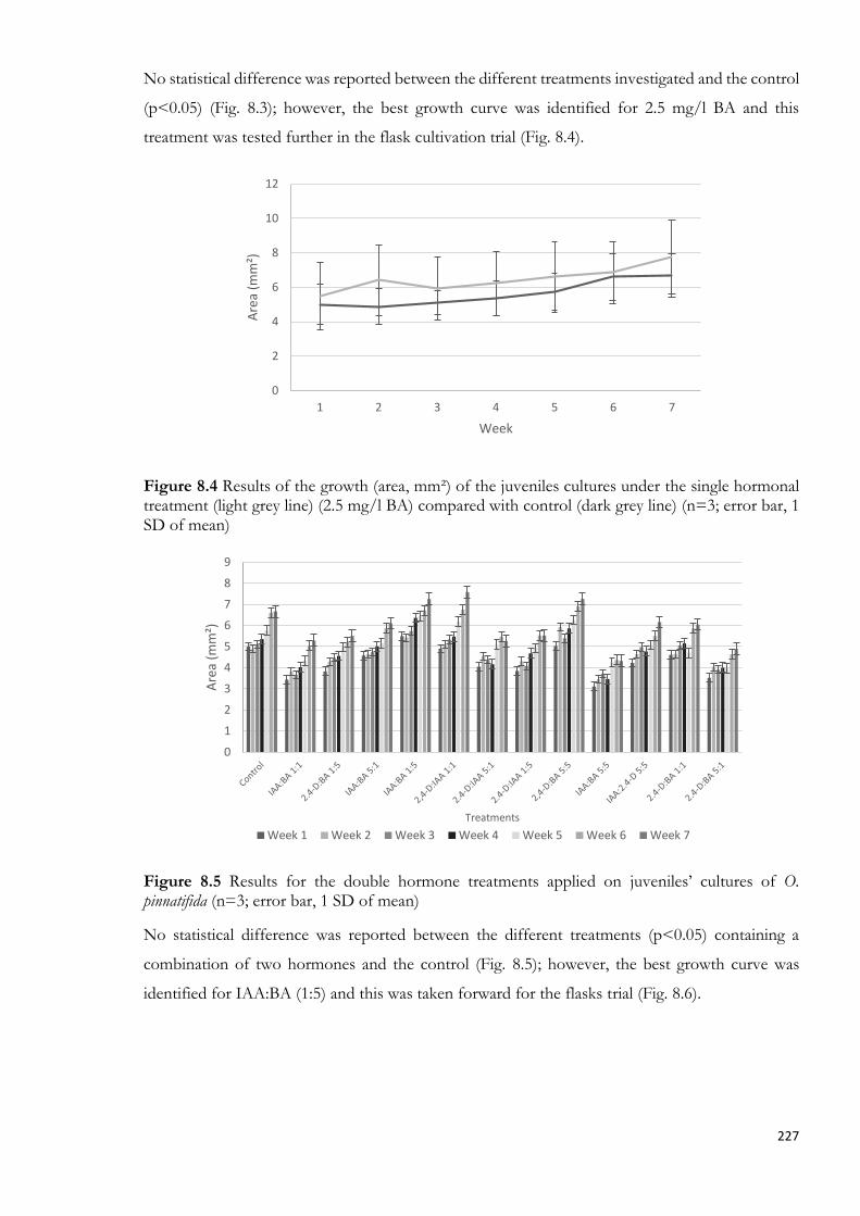
227

No statistical difference was reported between the different treatments investigated and the control

(p<0.05) (Fig. 8.3); however, the best growth curve was identified for 2.5 mg/l BA and this

treatment was tested further in the flask cultivation trial (Fig. 8.4).

Figure 8.4 Results of the growth (area, mm²) of the juveniles cultures under the single hormonal treatment (light grey line) (2.5 mg/l BA) compared with control (dark grey line) (n=3; error bar, 1 SD of mean)

Figure 8.5 Results for the double hormone treatments applied on juveniles’ cultures of O. pinnatifida (n=3; error bar, 1 SD of mean)

No statistical difference was reported between the different treatments (p<0.05) containing a

combination of two hormones and the control (Fig. 8.5); however, the best growth curve was

identified for IAA:BA (1:5) and this was taken forward for the flasks trial (Fig. 8.6).

0

2

4

6

8

10

12

1 2 3 4 5 6 7

Are

a (m

m²)

Week

0

1

2

3

4

5

6

7

8

9

Are

a (m

m²)

Treatments


228

Figure 8.6 Results of the growth (area, mm²) of the juveniles cultures under the double hormonal treatment (light grey line) (IAA:BA 1:5 mg/l) compared to control (dark grey line) (n=3; error bar, 1 SD of mean)

Figure 8.7 Results for the triple hormone treatments applied on juveniles’ cultures of O. pinnatifida (n=3; error bar, 1 SD of mean)

No statistical difference was reported between the different treatments (p<0.05) containing all

three hormones and the control (Fig. 8.7); however, the best growth curve was identified for 2,4-

D:IAA:BA (5:5:5) and this was taken forward for the flasks trial (Fig. 8.8).

0

2

4

6

8

10

12

1 2 3 4 5 6 7

Are

a (m

m²)

Week

0

1

2

3

4

5

6

7

8

Control 2.4-D:BA:IAA1:1:1

2.4-D:BA:IAA5:1:1

2.4-D:BA:IAA5:5:1

2.4-D:BA:IAA1:1:5

2.4-D:BA:IAA1:5:1

2.4-D:BA:IAA1:5:5

2.4-D:BA:IAA5:1:5

2.4-D:BA:IAA5:5:5

Are

a (m

m²)

Treatments


229

Figure 8.8 Results of the growth (area mm²) of the juveniles’ cultures under the triple hormonal treatment (light grey line) (2.4-D:BA:IAA 5:5:5 mg/l) compared to control (dark grey line) (n=3; error bar, 1 SD of mean)

8.4.1.2 AMPEP treatments applied to cultivation of O. pinnatifida juveniles

Results for the growth expressed as mm² and SGR relative to the application of the AMPEP

extracts to juveniles are presented respectively in Figs 8.9 and 8.10. Time is referred to weeks.

Figure 8.9 Measurement of the growth (area, mm²) of juveniles under the different AMPEP treatments, measured with ImageJ®. Control = blue, 3 mg/l = light grey, 0.5 mg/l = dark grey and Bathing (20g/l) = black bars (n=3; error bar, 1 SD of mean)

A statistical difference was reported between the 0.5 mg/l treatment and the other treatments

trialled (ANOVA, p<0.05). The lowest growth was reported for the Bathing (20 g/l) treatment

(Fig. 8.9).

0

2

4

6

8

10

12

1 2 3 4 5 6 7

Are

a (m

m²)

Week

0

0.5

1

1.5

2

2.5

3

3.5

4

Week 0 Week 1 Week 2 Week 3 Week 4

Are

a (m

m²)

Time

230

Figure 8.10 SGR (% day⁻¹) of juveniles undergoing different AMPEP treatments. Control= blue, 3 mg/l = light grey, 0.5 mg/l = dark grey and Bathing (20g/l) = black bars (n=3; error bar, 1 SD of mean)

The highest growth rate was reported for the control (week 1) and for the 0.5 mg of AMPEP

solution (for weeks 2, 3 and 4). The lowest growth rate was observed with the biomass treated with

20 g/l AMPEP solution (Fig. 8.10, week 2) (one-way ANOVA, p<0.05, Fisher’s test). After 30

days, epiphytes were found in reduced numbers in all samples treated with the AMPEP solution

(Fig. 8.11 C and D). While the untreated control showed colonization by epiphytes (Fig. 8.11 A).

This was also true for the biomass bathed in the 20 g/l solution (Fig. 8.11 B). Branching and

trichoblast formation appeared on cultures cultivated under AMPEP extract but not in the control

or in the bathed samples (Figs 8.11 C and D and 8.12).

Figure 8.11 Juveniles specimens under AMPEP treatments A) Control; B) Bathing (20 g/l); C) 0.5 mg/l; D) 3 mg/l. Bar= 1mm

-1

0

1

2

3

4

5

6

7

Week 1 Week 2 Week 3 Week 4

Gro

wth

rat

e (%

day

⁻¹)

Time

231

Figure 8.12 Trichoblast in juvenile specimen under AMPEP extract

8.4.2 Flask trials

8.4.2.1. Flask trials applying PGRs to adult O. pinnatifida biomass

Growth measurements for the hormone flask experiments are reported in Fig. 8.13. All four

treatments displayed a positive growth for the entire length of the experiment. There were no

statistical differences (p<0.05) in terms of weight increase according to the treatment applied. It is

worth noting that the phenotype of the cultures changed during the experiment, especially for the

single treatment, with some of the algal biomass turning green in colour. This phenomenon did

not appear to affect the growth of the specimens.

Figure 8.13 Variation of weight (g, WW) across 7 weeks for cultures under different PGRs treatments. Control: F/2 medium (blue); Single: 2.5 mg BA (orange); Double:IAA:BA (1:5) (grey); Triple: 2.4-D:BA:IAA (5:5:5) (yellow line) (n=3; error bar, 1 SD of mean)

A positive SGR was also seen for all the experiments and for all the treatments tested (Fig. 8.14).

The “double” treatment maintained a statistically higher SGR compare to the control in the 2nd and

3rd weeks, whilst still higher in the 4th and 6th weeks it was not statistically different. The “single”

0

1

2

3

4

5

6

7

8

9

10

Week 0 Week 1 Week 2 Week 3 Week 4 Week 5 Week 6 Week 7

wei

ght

(g W

W)

Time

232

treatment remained significantly lower than the control for the 3rd, 4th and 5th weeks, while it was

significantly higher than the control in the last week (p<0.05). Cultures had multiple branching and

tip elongation under all treatments (Fig. 8.15 E-H) and those grown under the single hormone

treatments changed colour turning green from red (Fig. 8.15 B and F).

Figure 8.14 SGR (expressed in %day⁻¹, from Evans, 1972) of cultures under different treatments. Control: F/2 medium (blue); Single: 2.5 mg BA (orange); Double: IAA:BA (1:5) (grey); Triple: 2.4-D:BA:IAA (5:5:5)(yellow bars) (n=3; error bar, 1 SD of mean)

Figure 8.15 Specimens under PGRs treatments in the flask trial at the start A) Control; B) Single treatment (2.5 mg BA); C) Double treatment (IAA:BA 1:5); D) Triple treatment (2.4D:IAA:BA 5:5:5) and at the end of the trial E) Control; F) Single treatment; G) Double treatment; H) Triple treatment

8.4.2.1.1 Biochemical analyses of O. pinnatifida biomass cultivated applying PGRs

Biochemical analyses relative to carbohydrates and protein content for the flask hormones

experiment are reported in Fig. 8.16. There was a statistical difference in terms of carbohydrates

-0.5

0

0.5

1

1.5

2

2.5

3


Gro

wth

rat

e (%

day

⁻¹)

Time

233

percentage between the single hormonal treatment and the control (p<0.05) (Fig. 8.16). A statistical

difference (p<0.05, Fisher’s hoc test) was reported for the protein concentration between the triple

hormonal treatment and the control. In general, the three hormonal treatments showed higher

percentages of protein compare to the control, which accounted for the lowest rate (Fig. 8.16).

Figure 8.16 Carbohydrate (dark grey bars) and protein (light grey bars) content expressed in percentage in cultures undergoing different PGRs hormonal treatments (n=3; error bar, 1 SD of mean)

Figure 8.17 Chl-a (dark grey bars) and carotenoids (light grey bars) (µg/g) concentration in samples undergoing different PGRs hormonal treatments (n=3; error bar, 1 SD of mean)

A statistical difference (p<0.05) was reported between the double and the triple hormonal

treatments and the control for the concentration of chlorophyll-a. Only the double treatment

showed a statistical difference from the control in term of carotenoids’ concentration (Fig. 8.17).

In general, the three hormonal treatments showed higher concentrations of chlorophyll-a and

carotenoids compare to the control, which accounted for the lowest levels.

0

5

10

15

20

25

30

35

Control Single Double Triple

Car

bo

hyd

rate

s an

d p

rote

in

con

ten

t (%

DW

)

Treatment

0

200

400

600

800

1000

1200


Ch

loro

ph

yll a

an

d c

aro

ten

oid

s co

nte

nt

(µg/

g D

W)

Treatment

234

Figure 8.18 PE (dark grey bars) and PC (light grey bars) (mg/g) concentrations in cultures undergoing different PGRs hormonal treatments (n=3; error bar, 1 SD of mean)

Statistical differences (p<0.05) were identified between the control and the double and triple

hormonal treatment both for the PE and PC concentrations. Only the single treatment showed

lower values compare to the control. Instead, as already seen for the protein concentration, both

double and triple treatments showed higher values compare to the control (Fig. 8.18).

Figure 8.19 FRAP assay (µM FeSO₄ eq/mg DW) for cultures undergoing different PGRs hormonal treatments (n=3; error bar, 1 SD of mean)

No statistical difference was reported in terms of antioxidant content (p<0.05); however, the

three hormonal treatments showed higher values compare to the control (Fig. 8.19).

8.4.2.2 Flask trials applying AMPEP treatments to adult O. pinnatifida biomass

Growth measurements for the application of the AMPEP extract are shown in Fig. 8.20. Time is

referred as weeks.

There was no statistical difference between the treatments tested and the control in term of growth

rate or weight increase (Figs 8.20 and 8.21 respectively). In terms of weight increase, the four

0

0.2

0.4

0.6

0.8

1

1.2

1.4

1.6


PE

and

PC

co

net

n (

mg/

g D

W)

Treatment

0

0.5

1

1.5

2

2.5

3

3.5

4

4.5


FRA

P

(µM

FeS

O₄

eq/m

g D

W)

Treatment

235

treatments performed similarly, with a slightly slower growth for the Bathing (20 g/l) treatment.

This was evident also from the SGR data (Fig. 8.21), where the Bathing treatment was the only one

to show a negative growth rate in the first week of cultivation. The control remained almost stable

for the entire experiment, while for both AMPEP treatments (0.5 and 3 mg/l), there was an

evidence of increased growth in the first week, followed then by a slight decrease and finally the

cultures settled at a constant level (Fig. 8.21).

Figure 8.20 SGR measurements of cultures in flask under the different AMPEP treatments. Time is expressed in weeks (n=3; error bar, 1 SD of mean)

The control performed better than the Bathing treatment even if this was not statistically supported

(Fig. 8.21).

Figure 8.21 Comparison of cultures weight (WW) under the three AMPEP treatments (20 g/l = orange, 0.5 mg/l = grey, 3 mg/l = yellow line) and the Control (F/2) (blue line) (n=3; error bar, 1 SD of mean)

The same trend already reported for Bathing vs control was observed for 0.5 mg/l (AMPEP) vs

control, again with no statistical differences and a reconnection of the two treatments at the last

-0.6

-0.4

-0.2

0

0.2

0.4

0.6

0.8

1

1.2

1.4

Control (F/2) Bathing 20 g/lAMPEP

0.5 mg/l AMPEP 3 mg/l AMPEPGro

wth

rat

e (%

day

¯¹)

TreatmentWeek 1 Week 2 Week 3 Week 4 Week 5

0

2

4

6

8

10

12

14

Week 0 Week 1 Week 2 Week 3 Week 4 Week 5

wei

ght

(g W

W)

Time

236

measurement point. Even for the 3 mg/l (AMPEP) treatment against the control, this last one

performed better, although not statistically (Fig. 8.21).

Samples cultivated under the 0.5 mg/l and 3 mg/l solutions turned green after the first week of the

experiment (Fig. 8.22 A and B). This change in colour was maintained for the length of the trial.

Cultures grown under the control treatment (Fig. 8.22 C) or those bathed in the 20 g/l solution

maintained a dark red colour (Fig. 8.22 D). Branches and ramifications even along the thallus (Fig.

8.23), that are not normally seen in O. pinnatifida grown either in cultivated biomass or in the wild,

as vegetative growth usually appears from the tips and the rhizoid, were present in cultures grown

in 0.5 mg/l and 3 mg/l AMPEP solutions.

Figure 8.22 Cultures under the AMPEP treatments A) 0.5 mg/l cultures B) particular of new shoots from the rhizoids for specimens under 0.5 mg/l; C) Control treatment and; D) Bathing (20 g/l AMPEP treatment)

Figure 8.23 Particular of new branches (arrow) and callus (circle) formation along the thallus in cultures under 3 mg/l AMPEP

8.4.2.2.1 Biochemical analyses of O. pinnatifida biomass cultivated applying AMPEP treatments

Biochemical analyses of O. pinnatifida cultures for carbohydrates and protein content grown with

the addition of AMPEP in flask cultivation system are showed in Fig. 8.24. Statistical differences

(ANOVA, p<0.05) were reported between 0.5, 3 mg/l and the other treatments for the percentage

237

of carbohydrates. The highest result was reported for 0.5 mg/l treatment and the lowest one for

the bathed samples (Fig. 8.24).

Figure 8.24 Carbohydrate (dark grey bar) and protein (light grey bars) content expressed in percentage (DW) of cultures under different AMPEP treatments (n=3; error bar, 1 SD of mean)

A statistical difference (ANOVA, p<0.05) was reported for the percentage of protein content

between the control and bathing treatment and the other two treatments, with the highest levels

reported in the control, followed by Bathing, 0.5 mg/l and finally 3 mg/l treatments (Fig. 8.24).

Statistical differences (ANOVA, p<0.05) were reported, with control and Bathing higher than the

other treatments for the chlorophyll-a and carotenoids content, with the highest levels for Chl-a

reported for the control (1264.78 µg/g), followed by Bathing (1150.45 µg/g), 3 mg/l (480.9 µg/g)

and lastly 0.5 mg/l (444.3 µg/g). For carotenoids the highest levels were reported for control (402

µg/g) followed by Bathing (385 µg/g), 3 mg/l (196 µg/g), and lastly 0.5 mg/l (188 µg/g) (Fig. 8.25).

Figure 8.25 Chl-a (dark grey bars) and carotenoids (light grey bars) concentration (µg/g) of cultures under different AMPEP treatments (n=3; error bar, 1 SD of mean)

0

5

10

15

20

25

30

35


0.5 mg/l AMPEP 3 mg/l AMPEPCar

bo

hyd

rate

s an

d p

rote

in c

on

ten

t (%

DW

)

Treatment

0

200

400

600

800

1000

1200

1400

1600


0.5 mg/l AMPEP 3 mg/l AMPEP

Ch

loro

ph

yll a

an

d c

aro

ten

oid

s co

nte

nt

(µg/

g D

W)

Treatment

238

The same trends were also found for the phycobiliprotein content (Fig. 8.26). The control reported

the highest levels for PE (4 mg/g) and PC (1.2 mg/g), followed by the Bathing treatment (PE 3.2

mg/g; PC 1 mg/g), 3 mg/l (PE 0.36 mg/g; PC 0.3 mg/g) and lastly 0.5 mg/l (PE 0.23mg/g; PC

0.21 mg/g). Furthermore, this difference in pigments content was reflected by the colour of the

cultures.

Figure 8.26 PE (dark grey bars) and PC (light grey bars) concentration (mg/g) of cultures under different AMPEP treatments (n=3; error bar, 1 SD of mean)

Statistical differences (ANOVA, p<0.05) were reported in terms of antioxidant compounds

between the control and the Bathing and the other two treatments, with both FRAP (Fig. 8.27)

and TPC analyses (Fig. 8.28), with highest levels reported for control, followed by Bathing, 0.5

mg/l and finally 3 mg/l treatments.

Figure 8.27 FRAP analyses (µMFeSO₄eq/mg DW) of cultures under different AMPEP treatments (n=3; error bar, 1 SD of mean)

0

0.5

1

1.5

2

2.5

3

3.5

4

4.5

5



PE

and

PC

co

nte

nt

(mg/

g D

W)

Treatment

0

1

2

3

4

5

6

Control (F/2) Bathing 20g/lAMPEP


FRA

P

(µM

FeS

O₄e

q/m

g D

W)

Treatment

239

Figure 8.28 TPC analyses (µg/mg) of cultures under different AMPEP treatments (n=3; error bar, 1 SD of mean)

8.4.3 Tank trial applying AMPEP extract to adult O. pinnatifida biomass

Data relative to pH, salinity, temperature and intensity for the tumbling cultivation system are

reported in Figs 8.29 and 8.30. While the pH increased during the experiment (even if the increase

was not statistically significant) (Fig. 8.29, dark grey bars), the salinity levels initially rose followed

by a decrease in December to then stabilize at around 28 TDS in January and 27 TDS in February

(Fig. 8.29, grey line).

Figure 8.29 pH (dark grey bars) and salinity (TDS, light grey line) measurements for the tank experiment applying AMPEP extract

The temperature slightly decreased during the experiment (Fig. 8.30, dark grey bar) even if this

decrease was not statistically significant. In general, it never surpassed the 12 °C mark and never

fell under 8 °C. The average light intensity was relevantly stable (Fig. 8.30, light grey line) and a

maximum peak was reported only once in January, again this was not statistically significant (Fig.

8.30, grey line).

0

50

100

150

200

250

300

350



Tota

l ph

eno

l co

nte

nt

(µg/

mg

DW

)

Treatment

7.6

7.7

7.8

7.9

8

8.1

8.2

8.3

8.4

8.5

0

5

10

15

20

25

30

35

40

November December January February

pH

TDS

(mg/

l)

Months

240

Figure 8.30 Temperature (dark grey bars) and intensity measurements (average light = grey line and maximum light = dark grey line) recorded with HOBO® loggers in the tanks under the AMPEP treatments

Cultures were weighted every 15 days. Every month the biomass weight was reinstated at the same

level as the start of the experiment. The highest weight (g) for all the treatments was reported at

the end of the second month, with cultures doubling their initial weight, and the highest values

reported for the two AMPEP treatments, but with no statistical differences. A decline of the growth

rate was instead detected in the third month for all the treatment investigated, with cultures still

growing, but at a slower rate. Generally, all the treatments performed equally, with no statistical

difference reported (Fig. 8.31).

Figure 8.31 Weight (WW) of the cultures under the three treatments tested in the tank system after 15 days, 1 month, 45 days, 2 months, 75 days and 3 months (n=3; error bar, 1 SD of mean)

There was no statistical difference between the growth rate and the treatments applied (ANOVA,

p<0.05, Tukey’s test, Minitab18) (Fig. 8.32). All three treatments sustained the growth of the

0

50

100

150

200

250

300

0

2

4

6

8

10

12

14

November December January February

Ligh

t in

ten

sity

(lu

m/f

t²)

Tem

per

atu

re (

°C)

0

50

100

150

200

250

300

350

400

450

500

Control (F/2) Bathing (20 g/l) AMPEP 0.5 mg/l AMPEP

wei

ght

(g W

W)

Treatment

Time 0 15 days Month 1 Time 0 45 days Month 2 Time 0 75 days Month 3

241

cultures with positive SGR. The growth rate of the experiment was measured every 15 days. The

SGR measurements reported for all the treatments an initial decrease, followed by a subsequent

increase and a further decrease in the successive data point, for all three of the months, following

a cycling scheme. The best results were reported for all the treatments in the second month of

cultivation and the worst ones in the third month (Fig. 8.32). There was almost a doubling of the

weight of the biomass every month, with a maximum of almost 5 % day⁻¹ measured in the second

month for the Bathing treatment.

Figure 8.32 Growth rate of the cultures in the tank system applying the AMPEP extract after 15 days, 1month, 45 days, 2 months, 75 days, 3 months (n=3; error bar, 1 SD of mean)

Cultures grew vertically and horizontally (Fig. 8.33 A), developing new tips, new branches (Fig.

8.33 B) and occasionally callus formations (Fig. 8.33 C, black circle) for the entire length of the

experiment.

Figure 8.33 Cultures in the tank system applying the AMPEP extract after 15 days in the cultivation system. A) 05 mg/l; B) control; C) bathing, circled callus formation; D) control cultures

-1

0

1

2

3

4

5

6


Gro

wth

rat

e (%

day

⁻¹)

Treatment

15 days Month 1 45 days Month 2 75 days Month 3

242

Cultures maintained a dark purple colour and a thick texture for the length of the experiment (Figs

8.33 D and 8.34 A-C), with no difference in colour reported between the treatments.

Figure 8.34 A) cultures after one month (0.5 mg/l AMPEP); B) cultures after two months (bathing in 20 g/l AMPEP); C) new plantlets developed in cultures after 3 months (Control F/2) in the cultivation system

Pre-treatment for the prevention of epiphytes, previously described in Chapter 5, proved to be

effective for nearly the entire length of the experiment. Only one single species, Alaria sp.,

contaminated the cultures with its presence being recorded on the last 15 days of the trial.

QY of the cultures was measured every 15 days following the weighing of the cultures. Initially

there was a decrease followed by a constant increase in the PAM response of the cultures until the

second month, to then slightly decrease in the third month, this was not significant statistically (Fig.

8.35). No statistical differences were reported for the PAM measurements between the treatments

tested (p<0.05).

Figure 8.35 QY of the cultures under the three different treatments in the tank cultivation system at time 0, after 15 days, 1 month, 45 days, 2 months, 75 days, and 3 months (n=3; error bar, 1 SD of mean)

0

0.1

0.2

0.3

0.4

0.5

0.6

0.7


PA

M (

QY)

Treatment

Time 0 15 days Month 1 45 days Month 2 75 days Month 3

243

8.4.3.1 Biochemical analyses of tank trial applying the AMPEP extract to adult O. pinnatifida biomass

The biochemical composition of the cultures was analysed every month, for the three treatments

and triplicate samples were taken from each. The percentage (DW) of carbohydrates for the three

treatments (after one, two and three months) is reported in Fig. 8.36. Samples after one month

reported no statistical differences. While samples for the second month reported a statistical

difference between the cultures under the control and those under the 0.5 mg/l treatments, lastly

the results for the third months showed a statistical difference between 0.5 mg/l and Bathing (20

g/l) treatments (ANOVA, p<0.05; Tukey’s post hoc test). For the three sets together, in general

after two months all the treatments showed a statistical decrease of carbohydrates concentration

(Fig. 8.36) and higher results were generally reported for the control treatment.

Figure 8.36 Content of carbohydrates in samples cultivated in tank after 1 (blue bars), 2 (grey bars) and 3 (orange bars) months of cultivation under AMPEP and control treatments (n=3; error bar, 1 SD of mean)

Protein (% DW) content is reported in Fig. 8.37. No statistical differences were reported between

the treatments, or between the three sets of samples, showing a minimum variation of protein

content in the cultures (ANOVA, p<0.05; Tukey’s post hoc test).

0

5

10

15

20

25

30


Car

bo

hyd

rate

co

nte

nt

(% D

W)

Treatment

244

Figure 8.37 Protein content expressed in percentage of samples after 1 (blue bars), 2 (grey bars)

and 3 (orange bars) under AMPEP and control treatments (n=3; error bar, 1 SD of mean)

Pigments contents for chlorophyll-a and carotenoids (µg/g) are reported in Fig. 8.38 and

phycobiliproteins (PE and PC, mg/g) in Fig. 8.39.

Figure 8.38 Chl-a and carotenoids content in the three sampling times under AMPEP and control treatments (n=3; error bar, 1 SD of mean)

There was no statistical difference between the treatments for the first month for Chl-a or

carotenoids content. In the second month there was a statistical difference between Bathing (20

g/l) and the control treatments for the Chl-a content, while both Bathing and 0.5 mg/l treatments

were different from the control for the carotenoids content. For the third month, there was a

statistical difference for 0.5 mg/l and the other treatments (0.5 mg/l> control> bathing). The three

months analysed together showed that the first set of samples was statistically lower than the other

two. A statistical difference was also reported between months two and three (ANOVA, p<0.05,

0

5

10

15

20

25

30

35

40

45


Pro

tein

co

nte

nt

(% D

W)

Treatment

0

500

1000

1500

2000

2500

3000

3500


Ch

loro

ph

yll a

an

d c

aro

ten

oid

sco

nte

nt

(µg/

g D

W)

Treatment

Chl-a Month 1 Chl-a Month 2 Chl-a Month 3 Car Month1 Car Month 2 Car Month 3

245

Tukey’s post hoc test). In general, a statistical increase in pigment content was reported for all the

treatments for all of the experimental period, with the highest concentrations recorded for the 0.5

mg/l treatment at the end of the experiment for both Chl-a and carotenoids.

For the first and the third sets of samples, there was no statistical difference reported between the

treatments for the phycobiliprotein content, while for the second month there was a statistical

difference between Bathing and 0.5 mg/l treatment (PE content) and between the control and 0.5

mg/l treatments (PC). (ANOVA, p<0.05, Tukey’s post hoc test). The statistical analyses between

the three sets of samples for the PE content reported a difference between the sample at month

two for the Bathing treatment and 0.5 mg/l. While for the PC content, only the samples of month

one for the Bathing treatment were statistically different from the samples of month two for the

0.5 mg/l treatment (Fig. 8.39).

Figure 8.39 PE and PC (mg/g) content for the three sampling times under AMPEP and control treatments (n=3; error bar, 1 SD of mean)

Results for antioxidant content obtained from the FRAP assay for the three sampling periods are

reported in Fig. 8.40. Statistical analyses reported no differences among the treatments for the first

set of samples, while a statistical difference between Bathing and the other two treatments

(control>0.5 mg/l> bathing) was reported for month two, and a statistical difference between 0.5

mg/l and the other two treatments (control>bathing>0.5 mg/l) reported for the third month. The

statistical analyses between the three sets, identified in particular a higher concentration of

antioxidant compound in the first month of cultivation for the cultures under Control treatment

(Fig. 8.40).

0

0.2

0.4

0.6

0.8

1

1.2

1.4

1.6

1.8

2


PE

and

PC

co

nte

nt

(mg/

g D

W)

Treatment

PE Month 1 PE Month2 PE Month 3 PC Month 1 PC Month 2 PC Month 3

246

Figure 8.40 FRAP assay of samples after 1 (blue bars), 2 (grey bars) and 3 (orange bars) under AMPEP and control treatments (n=3; error bar, 1 SD of mean)

Comparing the results obtained from the biochemical analyses for the flask and the tank

experiments applying AMPEP extract, PE and PC are statistically higher in the flask experiment

for control and Bathing treatments, while the opposite is true for the 0.5 mg/l treatment. The

carbohydrates concentration was higher in the cultures cultivated in tank compared to those in the

flask experiment, as well as for the protein. The FRAP assay showed statistically higher values in

the flask experiment compared to the tank, while the opposite was seen for the Chl-a and

carotenoids concentration.

8.5 Discussion

The effects of PGRs on tissue cultures of O. pinnatifida were investigated here for the first time.

Considering the analogy with plants, differentiation in some algae might also require the

intervention of specific chemical controllers (Evans and Trewavas, 1991). There is the possibility

that the photoperiodicity and seasonality in the growth behaviour of seaweeds needs to be

controlled by substances, such as PGRs (Lüning and Tom Dieck, 1989). Endogenous PGRs

(auxins, cytokinins, abscisic acid, gibberellins, etc.) have been previously detected in a number of

algae belonging to different evolutionary lineages (Stirk et al., 2014a; Tarakhosvskaya et al., 2007;

Mikani et al., 2015). Jennings (1969) and Dawes (1971) reported stimulation of growth in algae by

auxin and kinetin. Evans (1984) discovered that gibberellins promote cell division in Ulva but acted

as growth inhibitors in other species. Cytokinins were observed to promote the branching in F.

vesiculosus and other algae (Evans and Trewavas, 1991). Besides these studies, knowledge on the

impact these compounds have is still poor, and endogenous concentration of PGRs have only

rarely been measured, making it difficult to establish an appropriate exogenous concentration for

treating algae (Evans and Trewavas, 1991). Addition of exogenous hormones to culture media in

controlled environments could enhance the establishment of seaweed cultures, with subsequent

0

1

2

3

4

5

6


FRA

P (

µM

FeS

O₄/

mg

DW

)

Time

247

development growth of algal biomass. Imelda et al. (1998) suggested that use of exogenous PGRs

could act synergistically with native hormones, further promoting culture growth. Positive

responses to the use of PGRs in some seaweed species have been reported by earlier researchers

(Kaczyna and Megnet, 1993; Hayashi et al., 2008; Yong et al., 2014a; Anuraj et al., 2017).

The impact of phtyoregulators, auxins and cytokinins on the growth of a limited number of red

seaweeds has been previously demonstrated (Jennings, 1971; Fries, 1974; Fries and Iwasaki, 1976).

Treatments with natural or synthetic auxins have been shown to accelerate tissue growth in cultures

and callus development and to have regulatory effects on regeneration processes (Yokoya and

Handro, 1996; García-Jiménez et al., 1998; Yokoya et al., 1999). Other researchers have

demonstrated that auxin controls thallus branching of red and brown macrophytes on the principle

of apical dominance (Yokoya and Handro, 1996; Moss, 1974). Furthermore, Aguirre-Lipperheide

et al. (1995) suggested that red seaweed species responded more to exogenously supplied PGRs

than other seaweeds. Even if numerous authors have hypothesized that the cytokinins are involved

in the regulation of algal growth (Mooney and van Staden, 1986), relatively few studies have been

carried out on the role of cytokinins as endogenous growth regulators, in particular in macroalgae,

and specifically on red seaweeds. Limitations have included complications in controlling the

mechanisms of PGR factors on seaweed growth related to the presence of marine bacteria, known

also to release plant growth promoters (Bradley, 1991), and application of seawater in growth media

and potential disturbance of active compounds contained in the media that could interfere with

the results observed (Pedersén, 1973).

Nonetheless, PGRs were investigated in this thesis to understand their influence on the growth

rate, development and biochemical composition of O. pinnatifida, at a juvenile and adult stage. It

appeared that the hormone 2,4-dichlorophenoxyacetic acid (2,4-D) is not suitable for O. pinnatifida

cultivation if used alone, while in combinations with the other PGRs tested proved to slightly

increase the growth in the triple treatment. This compound is commonly used in herbicides (Stoker

et al., 2010) and its effect, when used alone, on the vegetative tissue of O. pinnatifida was mostly

damaging. The combinations of IAA and BA hormones seemed to be involved in the elongation

of the seaweed and branching, as already seen for other seaweeds (Yokoya and Handro, 1996).

This was particularly visible in the juvenile’s growth. Single hormone treatment in flasks also

affected the colour of the cultures, turning them from red to green in colour. Analyses of the

cultures’ pigments gave further confirmation that this was in fact happening. Usually, this change

in colour is as a result of damage and/or death of the seaweed, caused by the washing out of

phycobiliproteins, which are water soluble. This leaves the remaining Chl-a as the dominant

pigment (van den Hoek et al., 1995; Fleurence and Levine, 2016). This appears to be true also for

this study; however, only the colour of the biomass changed. The overall functionality and

248

physiology of the cultures were unaffected, as shown by PAM analyses. Whilst the treatments with

the hormones did not prove to be particularly effective in increasing the growth rate of this species,

at least for the concentrations and combinations trialled in this study, they had a more visible

impact on the biochemical composition of the cultures. This indicates that they might have some

role in regulating the biochemical pathways and processes of O. pinnatifida. Proteins, pigments, Chl-

a, carotenoids and phycobiliproteins and antioxidants content all increased, showing that the supply

of hormones can affect the biochemical composition of this species, as already seen for other

seaweeds (Han et al., 2018).

The impact of AMPEP extract on the growth of O. pinnatifida was also investigated. The positive

benefits derived from Ascophyllum extracts applied for seaweed cultivation have been previously

recognized and have been reported as been biostimulant/bioeffector (van Oosten et al., 2017).

These include: effects as enhancer or inducer for the direct axis formation and growth, as abiotic

response, (Hurtado et al., 2009, 2012; Yunque et al., 2011; Tibubos et al., 2017), as mitigator to

biotic responses to damaging endophytes (Borlongan et al., 2011; Hurtado et al., 2012; Loureiro et

al., 2012), epiphytes, and epibionts (Loureiro et al., 2009; Marroig et al., 2016), and as stimulant in

in-tank cultivation (Pedra et al., 2017).

The capacity of AMPEP extract to control epiphytes colonisation was confirmed in this study,

especially for juveniles, and particularly for the 0.5 and 3 mg/l treatments. The treated biomass had

much lower levels of epiphyte contamination compared to the untreated O. pinnatifida juveniles.

Cultivation of juveniles under laboratory conditions have been observed to be particularly

susceptible to contaminants during early stages of development (pers. obsv.). The application of

this extract appeared to reduce levels of contamination of the cultures and in controlling epiphytes.

The AMPEP seems to encourage branching of the juveniles as well as the formation of trichoblasts.

These are colourless specialized hair cell types that occur on the surface of many marine and

freshwater members of the Florideophyceae (Oates and Cole, 1994; Delivopoulos, 2002). First

discovered in the Floridae (Rosenvinge, 1911), there are two kinds of trichoblasts that have evolved

within the Rhodomelaceae. One is pigmented and usually persistent, while the second is usually

colourless, deciduous, often present on the vegetative axes (Hommersand, 1963) and are eventually

shed (Garbary and Clarke, 2001). O. pinnatifida trichoblasts belong to this second type

(Hommersand, 1963). Trichoblasts are thought to be related to nutrient uptake (Oates and Cole,

1994) or with reproduction (Falkenberg, 1901; Bold and Wynne, 1985) and protection of

tetraspores (Duckett et al., 1974). Despite their significance and frequent occurrence in most of the

Rhodomelaceae, they remain one of the least investigated structures of the red algae (Delivopoulos,

2002). In this study, production of these hair-like structures seemed to be stimulated by the

AMPEP extract, and they were absent in the control. Their role in this case might be related either

249

to a form of physical protection or to an attempt to maximise nutrients absorption, which is further

supported by the change in the colour of the cultures. The colour of the juveniles was deeply

affected by the extract, changing pigmentation from red to a light green colour. This change in

colour, as already seen in Chapter 6, might be due to a N limitation, since the same effect was not

visible in cultures under F/2 medium, with consequent reductions in phycobiliprotein contents

and a greener colour of the cultivated juveniles (Penniman and Mathieson, 1987). The growth rate

for the 0.5 mg/l treatment performed statistically better than the others (p<0.05), demonstrating

that a lower concentration of this extract is more suitable for this species at this early stage of

development. Previous authors have already reported the highest efficiency of the lower

concentration of the tested extract on cultivation of other species (Hurtado et al., 2012).

The AMPEP extract proved to be an effective control of epiphytes and their proliferation

contamination also in the flask experiment. The colour of the cultures was also affected, as

previously seen in the juveniles, and this observation was confirmed by biochemical analyses. The

levels of pigments measured were statistically lower in cultures grown with the AMPEP extract

compared to the control and the bathing treatments. Trichoblasts were also visible in the adults

cultivated with the extract and developed from the apical extremities of the adults’ branches rather

than from the thallus. In this case, their role could also be in the protection of the tetraspores, as

already seen for other species (Duckett et al., 1974), beside the function of nutrient absorption

(Oates and Cole, 1994). SGR and growth showed that there was no a statistical difference among

the treatments tested in terms of increased biomass. However, it is worth considering the

application of the extract in the early stages of development of this species, when the plantlets are

more susceptible to contaminants and the growth rate is slower, to then substitute it, once they

reach a certain development stage, with a cultivation medium more suitable for adult plants (e.g.

F/2). Especially considering the effect of the extract in enhancing branching and apical elongation

(Hurtado et al., 2009, 2012; Yunque et al., 2011; Tibubos et al., 2017), which will eventually result

in an increased biomass. Biochemical analyses showed that cultures treated with the extract had

statistically higher levels of carbohydrates, probably due the P source applied (Hopkins and Huner,

2009), compared to the control and the Bathing treatments, to which corresponded a lower level

of protein. The inverse trend for carbohydrates and protein content in regard to the nutrient

applied has been reported previously (Smit et al., 1997) and discussed in Chapter 6.

The antioxidant compounds in O. pinnatifida cultures were not statistically increased by the

application of the extract, at least for the concentration trialled. Previous research has demonstrated

that this extract is able to improve the antioxidant activity of some species of red algae (Borlongan

et al., 2011; Tibubos et al., 2017). Instead, the statistically lowest values were reported for cultures

250

under the two different concentrations of the AMPEP extract tested, as already reported for certain

strains of Kappaphycus (Hurtado et al., 2012).

There have been several trials to cultivate different species of red seaweed in land-based tank

systems, such as the cultivation of Gracilaria (Buschmann et al., 1994), Gelidium (Friedlander, 2008),

Chondrus crispus (Bidwell et al., 1985), and Palmaria palmata (Corey et al., 2013; Grote 2016, 2019),

ranging from simple ponds to intensively operated tanks (Buschmann et al., 2017). One of the first

successful commercial-scale pond facilities for a red seaweed operates in the Canadian Maritimes,

to produce Chondrus crispus (Hafting et al., 2015). Commercial on-land pond cultivation has also

been developed in Israel for Gracilaria sp. (Buschmann et al., 2017). Previous attempts of cultivation

in tank of O. pinnatifida were performed in Portugal and included flask trials and small-scale outdoor

trials with some positive results (Silva, 2015; Gonçalves, 2018), as discussed in Chapter 5.

The tank experiment, comparing the AMPEP extract to F/2 medium, proved to be effective in

increasing the biomass of the cultures, which were also dark red in colour and had a thick texture.

This, for the first time, establishes a successful pioneering methodology for the on-land indoor

cultivation of this species. There are further improvements that could be made to make this system

more efficient. For example, the supply of high-quality seawater and the successive treatments used

to treat it, such as filtration, UV treatments, etc., are fundamental for O. pinnatifida cultures, as well

as a continuous flow of water through the system. In this experiment, filters (100-20-10-5 µm) were

changed every week, nonetheless, brown filamentous seaweed, similar to Ectocarpus sp. in

appearance, were found growing in the filter system. Ectocarpus sp. is a common fouling alga (Morris

and Russell, 1974), found mostly as free-floating filaments in intertidal to sublittoral zones of

temperate regions (Baweja et al., 2016). It could easily be pumped in by the water supply system.

As already seen by other authors, the cause and extent of an epiphytic outbreak can depend not

only on the quality of the cultivated strain, but also on abiotic parameters of the site, management

practise and seasonal weather fluctuations (Vairappan et al., 2006). A solution to this would be to

place the main inlet pipe further from the seashore and at a lower depth in the site. This would

reduce the likelihood of pumping in unwanted contaminates as well as overcoming variation in

flow rate due to the tide cycles. Nonetheless, the pre-filtration and UV treatment of the incoming

seawater was mostly effective, and it was only in the last 15 days of the cultivation trial that what

appeared to be Alaria sp. was discovered. This is not a common biofouling organism of other

seaweed species and is also not normally seen in tanks used during cultivation trials, being usually

cultivated on ropes (Arbona and Molla, 2006; Edwards and Watson, 2011). Spores of this species

are release between November and March (Birkett et al., 1998b), which may explain the presence

of Alaria sp. in the system, probably drawn in by the water supply system.

https://nph.onlinelibrary.wiley.com/doi/full/10.1111/j.1469-8137.2007.02304.x#b83

https://nph.onlinelibrary.wiley.com/doi/full/10.1111/j.1469-8137.2007.02304.x#b83

251

Aeration in tumbling cultivation of seaweed cultures is fundamental, as previously reported for

other species, such as Chondrus crispus (L.) Stackh (Neish and Fox, 1971; Neish and Shacklock, 1971;

Neish et al., 1977) Gracilaria, Agardhiella and other genera (DeBoer and Ryther, 1977), in order to

replicate the natural motion of the seawater and provide nutrient exchange. This should be

considered along with supplementing the cultures with CO₂, which was not investigated in this

study. This measure is normally applied to control the pH and the gas exchange of the cultures, as

well as alleviate carbon limitations. This leads to greater biological productivity with an expected

increase in the photosynthetic storage of carbon, consequently stimulating the growth of cultures

(Duarte, 1992; Duarte et al., 2005). In the absence of this, a high flow rate, such as the one adopted

here, will guarantee a continuous exchange of water, aid in gaseous exchange as well as nutrient

and inorganic carbon uptake. Seaweeds obtain the necessary nutrients for growth directly from the

medium in which they are grown in. It is important that the medium is circulated to allow this to

happen and renewed at regular intervals (FAO, 2012). Circulating the water in tanks results in the

movement of the biomass, creating a dynamic light regime that can enhance growth rates (Kübler

and Raven, 1996).

Due to the limited possibility of scaling up related to the facilities available at SAMS, scaling-up of

the production with a transfer of the cultures to bigger volumes was not tested. Instead, cultures

were brought to the original weight after one and two months (since they were doubling their

weight), in order to avoid competition for light, nutrient and an excess of biomass density in the

tanks. Seaweed with a high stocking density are usually self-shading, resulting in reduced

photosynthesis, growth rates, and consequently lower seaweed production rates (Kim et al., 2014,

Corey et al., 2014). Scaling up the cultures to larger volumes could potentially further increase the

biomass production of this seaweed.

The biochemical analyses for the tank experiment involved three sets of sampling, one been taken

every month. This was carried in order to determine if there was any variation in the biochemical

composition of the cultures not only because of the treatments been tested, but also due to the

impact the experimental period might have on growth. For all the treatments there was a general

reduction in their carbohydrate content from month one to month two, followed by an increase in

the final month with the control performing the best. This is potentially linked to the P source

supplied, which as discussed in Chapter 6 influence the carbohydrates content of the species,

compared to the other treatments tested (Hopkins and Huner, 2009). Treatments and length of the

experiment did not affect the protein content which generally remained unaltered, indicating N

was not a limiting factor. There was an increase in the pigment content, and this was supported by

the PAM data. This parameter is normally used to represent the maximum photochemical

efficiency of PSII (Baumann et al., 2009). This increase in content could be due to the quality and

252

quantity of light applied during the experiment. Light characteristics (e.g. spectral quality, quantity,

and duration) are known to have a profound effect on seaweed metabolism and development (Su

et al., 2014). Algal pigment synthesis is also regulated by various photoreceptors that absorb light

at different wavelengths (López-Figueroa and Niell, 1990, 1991). The spectrum of the Gro-Lux

lights used for this experiment includes white light, as well as high levels of blue and red radiation,

which might have influenced the pigment content.

Unlike the flask experiment, the AMPEP treatments tested in the tank system did not affect the

colour of the cultures. Instead, the cultures remained a dark red-purple colour for the entire length

of the experiment. This was evident also from the data for PE and PC concentration. The pulsing

supply of the nutrients, coupled with water motion, reduced N limitation occurring in the cultures

preventing the loss of pigments, such as phycobiliproteins. These pigments are affected by N

availability (Vergara and Niell, 1993; Dawes, 1995; Vergara et al., 1995), and as noted in the flasks,

N limitation lead to the loss of the red colouration of the cultures.

Despite what has already been observed in plants (Craigie, 2011; Khan et al., 2009) and in other

seaweeds (Yunque et al., 2011; Tibubos et al., 2017; Pedra et al., 2017), the AMPEP extract did not

improve the antioxidant content of O. pinnatifida. This was similar to the observations from the

flask experiment. The antioxidant content decreased in all of the treatments tested over the entire

length of the tank experiment. Similar results have been reported for certain colour morphotypes

of Kappaphycus, another red seaweed species. Again, with this species, there was no improvement

in the antioxidant content which decreased during the reported experimental trial (Hurtado et al.,

2012).

The differences in biochemical composition of cultures treated with AMPEP extract at the same

concentration, but cultivated in flask and tanks, could be due to several factors, not just N

limitation. Both experiments had utilised different cultivation conditions. While the temperature

was the same (9-10 °C), the light photoperiod was different (for the flask experiment: 12:12; for

the tank experiment 24/7), as well as the type of lights (white fluorescent light in the flask

experiment and Gro-lux in the tank). In addition, the cultivation systems applied were different.

Medium was static and changed twice per week in the flasks with aeration from the top. In the

tanks there was continuous water exchange and tumbling of the cultures, with aeration provided

from the bottom. Both experiments also used different biomass densities (10 g/l in the flask

experiment, 4.54 g/l in the tank experiment). Resulting differences in profiles are unsurprising since

parameters, such as light, water flow, and nutrient input, impact on the biochemical composition

of seaweeds, as already reported in other species (Dring et al., 1996; Denis et al., 2010; Chow, 2012;

Yang et al., 2015).

253

An interesting effect of the extract on cultures, either juveniles or adults, in flasks or tanks, is the

formation of accessory branches. This has been reported in previous studies for other algae such

as Ascophyllum sp. and Kappaphycus sp. (Rayorath et al., 2008a, b; Borlongan et al., 2011). The

development of new branches was detected not only from the holdfasts, which commonly follows

two patterns of growth, an apical elongation and a lateral ramification, but also from the thallus, as

observed only in the treated samples. The AMPEP extract seems also to promote the formation

of callus tissue, again as previously reported for other species (Hurtado et al., 2009; Yunque et al.,

2011). These effects might be an important consideration for long term cultivation of the

investigated species, since each of these bulges will become a new branch, contributing to increases

in weight and biomass.

Finally, AMPEP extract and the hormones were not tested in combination. Further research could

investigate the combined effects of these two very different sets of compounds. Combining both

has proved to be successful in enhancing growth and increasing the biomass in other species

(Hurtado et al., 2009, 2012; Hurtado and Critchley, 2018; Yunque et al., 2010; Tibubos et al., 2017).

It has been hypothesized that this is probably due to the interaction of the extract with compounds

such as auxin-like, gibberellin-like (Rayorath et al., 2008a, b), cytokinins, precursors of ethylene and

betaine (Mckinnon et al., 2010), which are potentially involved in enhancing plant growth responses

(Crouch, 1990).

8.6 Conclusions

The concentration and combinations of phytohormones tested did not affect the growth

of this species (for both juveniles and adults); however, they did influence developmental

growth;

It is known that phytohormones can be applied in seaweed cultivation for targeting

products such as pigments, fatty acids, and polysaccharides (Han et al., 2018). This was

confirmed in this study, since treated cultures had statistically higher levels of

phycobiliproteins, proteins, Chl-a and carotenoids;

The response of the juveniles and the adults cultivated with the AMPEP extract was

different. A possible further application of the extract could be on the juvenile stages of O.

pinnatifida in order to increase the growth rate, enhance branching, and control the

contamination of epiphytes;

AMPEP extract was able to increase pigments and carbohydrates content in adult O.

pinnatifida biomass;

254

There was no statistical difference in terms of growth and biomass increase in the tank

experiment between the three tank treatments; all were suitable for tank cultivation of this

species;

However, AMPEP extract enhanced the branching of this species, as already determined

for other algae, which will eventually lead to an increase in biomass. Its application as a pre-

treatment for long-term tank cultivation should be considered;

This was the first time that an indoor on-land system at this scale was tested for the

cultivation of this species. It proved to be successful in promoting an increase in biomass,

controlling epiphytes contamination and ensuring an ideal biochemical profile of the

cultures. There are improvements that would need to be applied; however, the proposed

system offers a commercial alternative to wild harvesting, making the production of O.

pinnatifida sustainable and independent from seasonal variation in biomass and quality.

256

Chapter 9 Conclusions and future work

9.1 Conclusions

Seaweed consumption and utilization as a sector continues to grow, with multiple applications for

algae and their extracts. The investigation into the cultivation of new species is expanding with

countries within Europe starting to invest in this form of aquaculture. In order to shorten the

distance between themselves and Asiatic countries, who are the leaders in the production and

consumption of seaweeds, the interest has been towards low volume but high-value species. This

will open the path for the cultivation of those species that are slow growing and “smaller” than the

more well- known kelp species. These are normally harvested in UK, but this is labour intensive,

time consuming, and care must be applied in order not to overharvest a wild population. Little is

available in term of legislation for harvesting of small species, such as O. pinnatifida, in the UK.

Advice centres on mainly cutting the seaweeds, rather than tearing them completely off the solid

substrate they are growing on. This is so part of the algae is left behind for it to regrow, and a

maximum of one third of the species can be taken from a shore in any year, again ensuring a viable

population is left behind (Angus, 2017). Investigating and establishing cultivation methodologies

to produce Pepper Dulse in Scotland, represents a sustainable and profitable alternative to wild

harvesting of this species. This seaweed is known amongst chefs as the “truffle of the sea” and it is a

valuable ingredient already sold by different companies. Furthermore, its particular biochemical

profile, rich in secondary metabolites (e.g. antioxidants) makes it a valuable species that can be

applied in nutraceutical, pharmaceutical and cosmetic fields.

If final applications such as pharmaceutical, nutraceutical, and cosmetic are to be exploited, there

is a need for fundamental knowledge on the regulation and production of compounds of potentially

interest within a chosen species. In this case O. pinnatifida.

With this in mind, the main objectives of this thesis were:

Investigate and identify the parameters that are fundamental for the cultivation of this

species in order to establish a production system both in vitro under laboratory conditions

and in tanks, indoor and outdoor;

Investigate the biochemical composition of this species and how this is regulated. How this

varies in the wild (according to different abiotic factors) and in cultivated specimens

(according to variation and manipulation of the cultivation conditions);

How cultivation conditions can be tailored to improve biomass productivity;

257

Assess the biochemistry and metabolomics profile of the species and its variation according

to the seasons. Moreover, to assess the impact that seasonality potentially has on the overall

taste profile;

Identify phylogenetically the species investigated.

The flowchart (Fig. 9.1), already represented in Chapter 1, presents the two alternative ways

for the cultivation of Osmundea pinnatifida and underlines in blue the preferred methodology.

The research conducted within this thesis identified the vegetative cultivation as the best

methodology for the commercial production and exploitation of the species and the

diagram underlines in blue boxes the steps to apply.

Figure 9.1 Flow chart that highlights the best methodology to apply for the commercial cultivation and exploitation of the species

258

9.2 Contribution of the work

Chapter 2: Several studies have previously focused on the taxonomy and phylogenetic of

O. pinnatifida, changing profoundly its classification (e.g. identifying it as member of the

genus Osmundea rather than Laurencia) (Nam, 1999; Nam et al., 2000). Most of these studies

focused on specimens from Spain and the Canary Islands. This was the first time that

different specimens from the West coast of Scotland were molecularly analysed and

compared to sequence data available for this species on the NCBI database. The best DNA

extraction method was identified, and the PCR cycle optimized. Phylogenetic analyses

confirmed what had already been reported by previous authors, that the Laurencia complex

is a monophyletic group that includes eight genera, (Garbary and Harper, 1998; Nam et al.,

2000; Martin-Lescanne et al., 2010; Machín-Sánchez et al., 2012, 2018), with the genus

Osmundea been distinct from the Laurencia genus. The sequences divergences between the

Laurencia complex and the genus Osmundea sp. were similar to those reported by other

researchers (Machín-Sánchez et al., 2012). It was comparable with intergeneric sequence

divergences found in other red algal families (Hommersand et al., 1994; Lin et al., 2001;

McIvor et al., 2002; Martine Lescanne et al., 2010; Machín-Sánchez et al., 2012). The results

obtained from the phylogenetic methods employed, indicated that the samples collected

can be identify as O. pinnatifida species, that they are grouped in the same clade as the O.

pinnatifida sequences from GenBank, and that is it possible to recognize different closely

related subclades, on the basis of the bar-codes analyses. This information can be further

applied to cultivation of the species, such as optimization of strains and DNA engineering.

Chapter 3: Even if the biochemical composition of wild specimens of O. pinnatifida from

UK has been described previously (Marsham et al., 2007), it is only for one time point in a

year. This was the first time that the biochemical composition of this species was

investigated across a whole year to elucidate the impact that seasonality has on composition.

Different extraction protocols were developed, or existing ones implemented in order to

maximise the results obtained. Analyses showed seasonal patterns and variations for all the

analysed components, which included carbohydrates, proteins, pigments (chlorophyll-a,

carotenoids, PE and PC), lipids, moisture, C:N ratio, DOCN content, antioxidants, and

metals. Statistical analyses gave for the first time an insight into the correlation between

biochemical composition and abiotic factors, highlighting important consequences for the

management of harvesting and commercial exploitation of the species.

Chapter 4: The seasonal variations in the metabolomic profile of this species across one

year has been presented for the first time. Furthermore, the flavour profile of the species

was investigated for the first time, comparing two seasonal samples to assess the effects of

259

seasonality on taste/flavour. This study confirmed that this species has great potential for

further food, nutraceutical and pharmaceutical applications, and gave an insight into

seasonality and regulation of the metabolic profile of O. pinnatifida.

Chapter 5: Epiphytes are one of the major problems in the cultivation systems of seaweed.

They were controlled and mitigated against in O. pinnatifida cultivation with the application

of a chemical treatment. This proved to be efficient, without affecting the physiology and

biology of the species, was coupled to either a tide-simulation system or applied alone. The

treatment for epiphytes mitigation and control proved to be successful in vitro, tanks

(indoor and outdoor) and on sea cultivation trials (Appendix C.5).

Spores production under laboratory conditions was feasible and multiple releases occurred.

It was possible to grow the released spores up to the juveniles’ stage in vitro cultivation.

The process was slow and needs further investigation. Treatments to control the epiphytes

contamination of this early stage were identified (Chapter 8). However, keeping in mind

the flow chart defined in Fig. 9.1, a vegetative cultivation of the species seems to be the

best option at the moment for a commercial exploitation of this seaweed.

Chapter 6: Different media types and nitrogen sources for flask cultivation of O. pinnatifida

have never been tested before. All the media trialled were able to support the growth and

the biochemical requirements of the species been investigated. N sources do not influence

the growth of the cultures but have an impact on the biochemical composition. The

medium that performed the best was F/2, which appeared to be more suitable for the

vegetative cultivation of O. pinnatifida. It was able to support the growth of the culture, to

control the epiphytes contamination, to guarantee a suitable biochemical profile and to be

more economical to be applied, compared to the other types tested. This study led to the

identification of the best nutrient requirements for cultivation in flask and in tank of O.

pinnatifida.

Chapter 7: This chapter explored the possibility to cultivate O. pinnatifida in the Algem®

photobioreactor, with pioneering and successful results. Currently this PBR is only applied

for microalgae cultivation. This study showed that the PBR tested is able to statistically

increase the concentration of antioxidants compounds in the species. Increase in growth

was successful in the system, with neither the physiology nor morphology of O. pinnatifida

negatively affected. This study provided important information for commercial

exploitation of this species, introducing a methodology for cultivation in a PBR, resulting

in an increase in biomass and a tailored biochemical profile. This may have promising

further nutraceutical and pharmaceutical applications, once the cultivated biomass is

processed and analysed.

260

Chapter 8: This was the first time that exogenous hormones and fertilizer were applied to

cultivation in flask and in tank of O. pinnatifida. While the concentration and combination

of hormones trialled in this study did not affect the growth of the cultures, they affected

the development and the biochemical composition. This study showed that the response

of the cultures to the AMPEP extract depends on the stage of development of the biomass.

AMPEP was successful in increasing the growth rate only in juvenile cultures. The extract

helped in controlling and reducing epiphytes in both adult and juvenile cultures, influencing

the biochemical composition of adults. Moreover, the extract was able to increase the

branching of the cultures, which in a long-term cultivation system, might become important

for maximising productivity of the cultures. The extract did not increase the antioxidant

content of the cultures, as reported by previous authors for other seaweeds (Tibubos et al.,

2017; Pedra et al., 2017).

The AMPEP extract was trialled in a tank experiment in comparison with F/2 medium.

For the first time an indoor tumbling tank cultivation system for the vegetative production

of O. pinnatifida tetrasporophytes was established. Cultures were cultivated for three

months, maintaining a positive growth rate for the entire length of the experiment, with

the maximum SGR recorded at almost 5%day⁻¹. PAM response positively increased in the

cultures during the trial. While there was no difference in terms of weight increases between

the treatments tested, they did modify the biochemical composition of the biomass

produced. However, despite what has already been reported by previous authors (Hurtado

et al., 2014), the extract, in the concentrations tested, was not able to increase the

antioxidant content of O. pinnatifida.

The development of this cultivation system might provide a sustainable supply of the

resource, independently from wild harvesting and seasonality. Furthermore, the system is

able to improve the biochemical profile of the species and control epiphytes

contaminations.

9.3 Practical implications resulting from the findings

As already stated by previous authors, O. pinnatifida is a promising species, not only for its explosive

taste that makes it a sought-after seasoning, but also for several nutraceutical and pharmaceutical

applications. Its value as source of antimicrobial, antiviral, antibacterial, antifungal, antifouling and

anticancer compounds has been widely recognised and investigated (Campos et al., 2019; Silva et

al., 2018; Rodrigues et al., 2019, 2016, 2015; Paiva et al., 2014; Küpper et al., 2014; Sabina and Aliya,

2011, 2009; Patarra et al., 2011; Rizvi and Shameel, 2005, 2004, 2003). Knowing how to

trigger/control the production of these compounds might have important consequences for

commercial cultivation of this species and its commercial exploitation. This project investigated

261

and established possible cultivation methodologies for the production of tailored and high-quality

cultures of O. pinnatifida, from flasks, to PBR, to tank trials. Reproductive and vegetative cultivation

were trialled, and a final vegetative indoor tumbling system developed. This could be potentially

scaled up and have further commercial applications, making the production of this species

independent from seasonality and variation in quality/quantity of biomass, tailored and sustainable.

Biochemical analyses of the species, both from the wild as well as cultivated samples, gave

important knowledge on the composition, how it varied seasonally and under cultivation

conditions. The knowledge gained can be applied for both harvesting management (understanding

how the morphology and biochemical profile change seasonally, gaining information on the growth

patterns of the species, and on when it is best to harvest the biomass for further processing) and

cultivation applications. Treatments for control and management of epiphytes in O. pinnatifida

cultures were developed and successfully identified. This aided in the establishment of cultivation

methodologies for this particular species. Metabolomics analyses highlighted unknown and rare

compounds, and their seasonal variations. Thus, providing an insight into patterns and trends of

the biochemical composition of the species according to the season. Information obtained from

these findings are fundamental in improving the knowledge available on the species biology and

ecology, as well as providing pioneering information for the on-land indoor cultivation of O.

pinnatifida, for further commercial applications.

9.4 Limitations of the research

The results obtained from this work are pioneering and meaningful. However, there are some

limitations. These are namely: the difficult in investigating and establishing cultivation

methodologies for a species that, except for its biochemical profile, has been scarcely investigated;

the slow development and growth of this species, observed also in the wild, and the complexity of

the reproductive cycle in order to achieve an efficient production through reproductive

methodologies. Other limitations related mainly to technical issues, such as a lack of experimental

areas or the adaptation of alternative arrangements, in line with what available at the institute, which

proved not ideal for the goals of the project.

9.5 Future work

Further research and development will be necessary in order to strengthen the methodologies

established in this study. This would guarantee success at the scaled-up stage for the commercial

exploitation of O. pinnatifida for food, nutraceutical, and pharmaceutical applications. Aspects,

which merit further research, have been identified on an area basis:

262

Metabolomics analyses for taste investigation: Further analyses should be conducted

again on a seasonal basis and also with cultivated material, involving a tasting panel and

application of the XCMS non-targeted approach (McDougall et al., 2014) in order to

further investigate how the flavour and taste of the species changes and which compounds

are responsible for it;

Minerals composition: Iodine was not considered in this study due to analyses logistics;

however, this element should be evaluated. Especially considering that seaweeds are one

of the best natural sources of iodine and the implication that this mineral has on the health

and diet of the human body (Yeh et al., 2014; Bocanegra et al., 2009). Bromine should be

characterised as well since O. pinnatifida is a known source of active bromine halogens

(Suzuki et al., 2005, Küpper et al., 2014).

Nutrient regime: Results obtained from Chapter 6 identified that nutrients and how they

vary, had an influence on biomass production and biochemistry. In particular, further

investigations should be undertaken in relation to the concentration of P, as well as an

analysis to determinate the absorption rate of nutrients and the impact this has during

cultivation. This would allow a more complete feeding strategy to be determined in terms

of how often media should be changed and renewed for all life stages of O. pinnatifida.

Applications of hormones and AMPEP fertilizer: Different concentrations of

hormones and AMPEP extract, compared to those investigated in this study, should be

tested. A combination of AMPEP and PGRs treatments should be undertaken in order to

further investigate the potential synergistic effects of the fertilizer and hormones on growth

and biomass productivity. Different concentrations of the AMPEP extract should be

evaluated to verify if these might result in an increase of antioxidant compounds in the

cultures as seen in other red algae (Hurtado et al., 2014).

Spores production: Studies should be conducted to further investigate methodologies for

improving spore growth and survival rates. For example, different substrata should be

evaluated as well as decontamination treatments. While smooth surfaces, such as plastic

and glass slides, should be avoided, the focus should be directed towards collectors such as

ropes, or rough substrata e.g. shells and rocks, ideally resembling a barnacle surface, which

is the common habitat of the species and probably linked to the settlement of wild spores

as well.

Indoor cultivation: The tumbling cultivation indoor system developed in this study

proved to be effective and successful for the cultivation of this species. However, in order

to guarantee a commercial application and scale-up of it, some adaptations are necessary,

as detailed in Chapter 8. The water quality should be carefully monitored, followed by an

263

efficient sterilization treatment that should include filters (down to 5µm) and UV

sterilization system in order to keep under control contaminations. Particularly,

temperature, salinity, and pH should be periodically recorded. The supplementation of the

system with CO₂ should be evaluated, considering its importance in biomass increase and

pH control. Scaling up of the system should be achieved in order to avoid nutrient

competition of the cultures and growth decrease, due to high density.

9.6 Recommendations

Although some challenges and some bottle necks still need to be solved, vegetative cultivation of

O. pinnatifida in an indoor tumbling system proved to be a promising methodology with potential

commercial applications and should be preferred to cultivation through reproductive cycle. The

following protocol highlights the steps necessary for a vegetative cultivation system of O. pinnatifida

in Scotland, taking into account all factors investigated in this thesis.

1. Collection of wild material: Wild material should be collected using scissors/knives,

between October and February, at low tides from mid-exposed sites, distant from river

inputs and human activities. Only healthy and free from contaminants cultures should be

chosen in order to reduce possibility of contamination from other organisms and

subsequently maximise the cultivation. Avoid depopulating an area and only if necessary,

remove the holdfast, otherwise leave part of the seaweed behind for it to regrow. Place the

biomass in a Cool-box with wet tissues and bring it to the laboratory for further processing.

2. Cleaning and pre-treatment of the material: Wash the harvested biomass with filtered and

sterilized seawater in order to remove debris and grazers. Carefully clean the biomass

manually from any visible epiphytes and grazers. Rinse again with filtered and sterilized

seawater. Clean the biomass with a 0.5 % KI solution in FSW for three cycles of 30 minutes

each, in a controlled temperature room at 10°C, then rinse with plenty of filtered and

sterilised seawater in order to ensure the KI solution has been removed. Leave overnight

at 10°C in FSW with aeration. Then place the biomass in acclimation tanks, at 12:12

photoperiod, 100 µmol/m²/sec growth lux light, 10 °C, powerful bubbling and with no

nutrients added for at least 48. Acclimation prior to cultivation can last up to 1 month but

nutrients (preferably F/2 medium) must be provided. If this is the case a 48-hour starvation

period prior to cultivation is recommended.

3. Tank tumbling cultivation: Preferably use white conical tanks with aeration provided from

the bottom and light source placed on top of the tank, at a distance of 40-50cm. Place the

tanks (volume can be scaled up as the production increases) in a CTR at 10°C, light

provided by Growth lux light 100µmol/m²/sec and preferably at 18:6 or 24:0 photoperiod.

Density of the cultures should be between 3 and 4 g/l. A continuous flow rate of high

264

quality filtered and sterilized seawater (FSSW) down to 5 µm is necessary. Provide strong

bubbling in order to guarantee a tumbling culture and consider input of CO₂ for pH control

and increased biomass productivity. Supply F/2 nutrient with pulse feeding at least 2-3 per

day, according to the flow rate of the system. Clean the system periodically (weekly or every

10 days). Monitor continuously pH, salinity, light intensity, and temperature. Do not allow

temperature to rise above 15°C in the tanks.

4. Harvesting and processing: Harvest older tissue periodically, leaving in the cultivation

system younger material for further growth. This would facilitate the establishment of a

semi-continuous cultivation system, ensuring continuous stock in the system and avoiding

repeated harvesting of wild populations. Finally, processing the harvested biomass for

either food or extraction of commercially valuable compounds.

9.7 Concluding remarks

Results obtained from this study are pioneering and describe a potential cultivation system for the

sustainable production of Osmundea pinnatifida. This species has a biochemical profile suitable for

human consumption as well as producing other interesting compounds (such as antioxidants) that

could be further exploited and commercially applied. Knowledge gained on the seasonality of O.

pinnatifida and variation in the biochemical profiles according to abiotic parameters, might become

useful for harvesting and cultivation management of this species. The tumbling cultivation system

developed showed promising growth rates, the potential for scaling up and commercial

development of this methodology. Establishment of a successful O. pinnatifida cultivation system

will require collaboration between industrial and research institutes, and even if might appear

challenging and it requires further development, the research presented here is promising, valuable

and commercially relevant.

266

References

Abe, T., Kurihara, A., Kawaguchi, S., Terada, R., and Masuda, M. (2006). Preliminary report on the molecular phylogeny of the Laurencia complex (Rhodomelaceae). Coast. Mar. Sci. 30(1): 209213.

Adams, J. (2016). An overview on seaweed uses in the UK: Past, present and future. Seaweed Resources 36: 16-21.

Aguilera, J., Bischof, K., Karsten, U., Hanelt, D., and Wiencke, C. (2002). Seasonal variation in the ecophysiological patterns in macroalgae from an Artic fjord. II. Pigment accumulation and biochemical defence systems against high light stress. Mar. Biol. 140: 1087-1095.

Aguirre-Lipperheide, M., Estrada-Rodríguez, F.J., and Evans, L.V. (1995). Facts, problems, and needs in seaweed tissue culture: an appraisal. J. Phycol. 31: 67788.

Ahmad, V.U. and Ali, M.S. (1991). Terpenoids from marine red alga Laurencia pinnatifida. Phytochemistry 30: 4172-4174.

Ahmad, V.U., Ali, M.S., and Bano, S. (1990). Marine natural products XII: a new metabolite laurol from the red alga Laurencia pinnatifida. Sci. Pharm. 58: 299-301.

Ahn, G.N., Kim, K.N., Cha, S.H., Song, C.B., Lee, J., Heo, M.S., Yeo, I.K., Lee, N.H., Jee, Y.H., Kim, J.S., Heu, M.S., and Jeon, Y.J. (2007). Antioxidant activities of phlorotannins

purified from Ecklonia cava on free radical scavenging using ESR and H₂O₂- mediated DNA damage. Eur. Food Res. Technol. 226: 71-79.

Al-Alawi, A.A., Al-Marhubi, I.M., Al-Belushi, M.S.M., and Soussi, B. (2011). Characterization of carrageenan extracted from Hypnea bryoides in Oman. Mar. Biotechnol. 13: 893899.

Alba, K. and Kontogiorgos, V. (2017). Seaweed polysaccharides (Agar, Alginate Carrageenan). 10.1016/B978-0-08-100596-5.21587-4.

Alghazeer, R., Whida, F., Abduelrhman, E., Ammoudi, F., and Azwai, S. (2013). Screening of antibacterial activity in marine green, red and brown macroalgae from the Western coast of Libya. Nat. Sci. 5: 714.

Álvarez-Vázquez, M.Á., Prego, R., Caetano, M., De Uña-Álvarez, E., Dovald, M.M., Calvo, S., and Vale, C. (2017). Contributions of trace elements to the sea by small uncontaminated rivers: Effects of a water reservoir and a wastewater treatment plant. Chemosphere 178: 173-186.

Amsler, A.C.D and Searles, R.B. (1980). Vertical distribution of seaweed spores in a water column offshore of North Carolina. J. Phycol. 16 (4): 617-619.

Anantharaman, P., Devi, G.K., Manivannan, K., and Thangavel, B. (2011). Vitamin-C content of some marine macroalgae from Gulf of Mannar marine biosphere reserve, southeast coast of India. Plant Archives. 11: 343-346.

Andersen, R.A. (2005). Phycological Methods: Algal Culturing Techniques. Academic Press, Elsevier Publ. USA, UK. pp. 578.

Andrade, P.B., Barbosa, M., Matos, R.P., Lopes, G., Vinholes, J., Mouga, T., and Valentão, P. (2013). Valuable compounds in macroalgae extracts. Food Chem. 138(2-3): 1819-1828.

Angus, S. (2017). Modern seaweed harvesting and gathering in Scotland: the legal and ecological context. Scott. Geogr. J. 133(2): 1-14.

Anuraj, A., Waman, A., Prakash, C., Dam, Roy, S., Viji, M., Baidya, M., and Chadha, N. (2017). Investigating the effects of exogenous factors on growth, photosynthetic pigments and bud induction in Gracilaria corticata var. cylindrica under in vitro conditions. IJCRAR 6(8): 3235-3246.

AOAC (1990). Official methods of analysis of the Association of Official Analytical Chemists. 15th edition. Washington, DC, Association of Official Analytical Chemists.

267

Apaydin, G., Aylikei, V., Cengiz, E., Saydan, M., Kup, N., and Tirasogu, E. (2010). Analysis of metal contents of seaweed Ulva lactuca from Istambul, Turkey by EDXRF. Turk. J. Fish. Aquat. Sc. 10: 215220.

Arbona, J.F. and Molla, M. (2006). Cultivation of brown seaweed Alaria esculenta. In: Watson, L. (ed.). Aquaculture Explained. Bord Iascaigh Mhara, Dublin. pp. 50.

Armstrong, E., Rogerson, A., and Leftley, J.W. (2000). The abundance of heterotrophic protists associated with intertidal seaweeds. Estuar. Coast Shelf. Sci. 50: 415–424.

Arnold, T.M., Targett, N.M., Tanner, C.E., Hatch, W.I., and Ferrari, K.E. (2001). Evidence for methyl jasmonate-induced phlorotannin production in Fucus vesiculosus (Phaeophyceae) J. Phycol. 37: 1026-1029.

Asare, O. and Harlin, M.M. (1983). Seasonal fluctuations in tissue nitrogen for five species of perennial macroalgae in Long Island Sound. J. Appl. Phycol. 19(2): 254-257.

Ascêncio, S.D., Orsato, A., França, R.A., Duarte, M.E., and Noseda, M.D. (2006). Complete 1H and 13C NMR assignment of digeneaside, a low-molecular-mass carbohydrate produced by red seaweeds. Carbohydr. Res. 341(5): 677-682.

Ashraf, M. and Foolad, M.R. (2007). Roles of glycine, betaine and proline in improving plant abiotic stress resistance. Environ. Exp. Bot. 59(2): 206-216.

Athukorala, Y., Lee, K.W., Song, C.B., Ahn, C.B., Shin, T.S., Cha, Y.J., Shahidi, F., and Jeon, Y.J. (2003a). Potential antioxidant activity of marine red alga Grateloupia filicina extracts. J. Food Lipids 10: 251-265.

Atkinson, M.J and Smith, S.V. (1983). C:N:P ratios of benthic marine. Limnol. Oceanogr. 28 (3): 568-574.

Atta-ur-Rahman, V.U., Ahmad, S., Bano, S.A., Abbas, K.A., Alvi, M.S., Ali, H.S.M., Lu, and Clardy, J. (1988). Pinnatazane, a bridged cyclic ether sesquiterpene from Laurencia pinnatifida. Phytochemistry 27: 3879-3880.

Awad, N.E. (2000). Biologically active steroid from the green algae Ulva lactuca. Phytother. Res. 14: 641-643.

Awad, N.E. (2004). Bioactive brominated diterpenes from the marine red algae Jania rubens (L.) Lamx. Phytother. Res. 18: 275-279.

Bailey, J.C. and Freshwater, D.W. (1997). Molecular systematics of the Gelidiales: inferences from separate and combined analyses of plastid rbcL and nuclear SSU gene sequences. Eur. J. Phycol. 32: 343-52.

Bajguz, A. and Czerpak, R. (1996). Effect of brassinosteroids on growth and proton extrusion in the alga Chlorella vulgaris Beijerinck (Chlorophyceae). J. Plant. Growth Regul. 15: 153-156.

Ballantine, D.L., Gerwick, W.H., Velez, S.M., Alexander, E., and Guevara, P. (1987). Antibiotic activity of lipid-soluble extracts from Caribbean marine algae. Hydrobiologia 151/152: 463-469.

Bano, S., Ahmad, V.U., Perveen, S., Bano, N., Shafiuddin, and Shameel, M. (1987). Marine natural products: II. Chemical constituents of red alga Botryocladia leptopoda. Plant. Med. 53(1): 117-118.

Bano, S., Ali, M.S. and Ahmad, V.U. (1982). Marine natural products: VI. A halogenated chamigrene epoxide from the red alga Laurencia pinnatifida. Planta Med. 53: 508.

Bano, S., Ali, M.S., and Ahmad, V.U. (1988). Marine natural products: VIII. Two minors halogenated sesquiterpenoids from the red alga Laurencia pinnatifida. Sci. Pharm. (Vienna). 56: 125.

Bano, S., Bano, N., Ahmad, V.U., Shameel, M. and Amjad, S. (1986). Marine natural products: 3-formylindole from the red algae Botryocladia leptopoda. J. Nat. Prod. 49(3): 549.

Bano, S., Hayee, A., Ahmad, V.U., Shaikh, W., Usmanghani, K. and Shameel, M. (1988). Marine natural products. Part VII. Steroids from a red alga Asparagopsis sandfordiana. Polish J. Chem. 62: 905-906.

268

Bano, S., Uddin, S., and Ahmed, V.U. (1990). Marine natural products Part XV. An acetylated derivative of a new N-acylsphingosine from red alga Halymenia porphyroides. Planta Med. 56: 233-234.

Barahona, L.F. and Rorrer, G.L. (2003). Isolation of halogenated monoterpenes from bioreactor-cultured microplantlets of the macrophytic red algae Ochtodes secundiramea and Portieria hornemannii J. Nat. Prod. 66: 743-751.

Barbarino, E. and Lourenço, S.O. (2005). An evaluation of methods for extraction and quantification of protein from marine macro- and microalgae. J. Appl. Phycol. 17:447-460.

Barceló-Villalobos, M., Figueroa, F.L., Korbee, N., Álvarez-Gómez, and Abreu, M.H. (2017). Production of mycosporine-like amino acids from Gracilaria vermiculophylla (Rhodophyta) cultured through one year in an Integrated Multi-trophic Aquaculture (IMTA) System. Mar. Biotechnol. 19(3): 246-254.

Barreto, M.C., Mendonça, E., Gouveia V., Anjos, C., Medeiros, J.S., Seca, A.M.L., and Neto, A.I. (2012). Macroalgae from S. Miguel Island as a potential source of antiproliferative and antioxidant products. Arquipel. Life Mar. Sci. 29: 53-58.

Barrow, K.D., Karsten, U., King, R.J., and West, J.A. (1995). Floridoside in the genus Laurencia (Rhodomelaceae, Ceramiales)-A chemosystematic study. Phycologia. 34(4): 279-283.

Barufi, J.B., Figuerosa, F.L., and Plastino, E.M. (2015). Effects of light quality on reproduction, growth and pigment content of Gracilaria birdiae (Rhodophyta: Gracilariales) and pigment content of Gracilaria birdiae. Sci. Mar. 79(1).

Baumann, H.A., Morrison, L., and Stengel, D.B. (2009). Metal accumulation and toxicity measured by PAM-chlorophyll fluorescence in seven species of marine macroalgae. Ecotoxicol. Environ. Saf. 72(4): 1063-1075.

Baweja, P., Sahoo, D., and García-Jiménez, R.R.R. (2009). Seaweed tissue culture as applied to biotechnology: problems, achievements and prospects. Phycol. Res. 57:45-58.

Bazes, A., Silkina, A., Douzenel, P., Fay, F., Kervarec, N., Morin, D., Berge, J., and Bourgougnon, N. (2009). Investigation of the antifouling constituents from the brown alga Sargassum muticum (Yendo) fenshott. J. Appl. Phycol. 21(4): 395-403.

Bedoux, G., Hardouin, K., Marty, C., Taupin, L., Vandanjon, L. and Bourgougnon, N. (2014). Chemical characterization and photoprotective activity measurement of extracts from the red macroalga Solieria chordalis. Bot. Mar. 57: 291301.

Beer, S. and Eshel, A., (1985). Determining phycoerythrin and phycocyanin concentrations in aqueous crude extracts of red algae. Aust. J. Mar. Freshw. Res. 36: 785-92.

Bell, E.C. (1993). Photosynthetic response to temperature and desiccation of the intertidal alga Mastocarpus papillatus. Mar. Biol. 117: 337-346.

Benson, E.E., Rutter, J.C., and Cobb, A.H. (1983). Seasonal variation in frond morphology and chloroplast physiology of the intertidal alga Codium fragile (Suringar) Hariot. New Phytol. 95: 569-580.

Benzie, I.F and Strain, J.J. (1996). The ferric reducing ability of plasma (FRAP) as a measure of “antioxidant power”: the FRAP assay. Anal. Biochem. 239: 70-76.

Berland, B.R., Bonin, D.J., and Maestini, S.T. (1972). Are some bacteria toxic for marine algae? Mar. Bio. 12: 189-193.

Bhattarai, H.D., Ganti, V.S., Paudel, B., Lee, Y.K., Lee, H.K., Hong, Y.K., and Shin, H.W. (2007). Isolation of antifouling compounds from the marine bacterium, Shewanella Oneidensis SCH0402. World J. Microb. Biotechnol. 23: 243-249.

Bhosale, P. (2004). Environmental and cultural stimulants in the production of carotenoids from microorganisms. Appl. Microbiol. Biotechnol. 63: 351-361.

Bidwell, R.G.S. and Mclachlan, J. (1985). Carbon nutrition of seaweeds: Photosynthesis, photorespiration and respiration. J. exp. mar. Biol. Ecol. 86: 15-46.

Bidwell, R.G.S., McLachlan, J., and Lloyd, N.D.H. (1985). Tank cultivation of Irish Moss, Chondrus crispus Stackh. Bot. Mar. 28: 87-97.

269

Biebl, R. (1958). Temperatur und osmotische Resistenz von Meeresalgen der bretonischen Küste. Protoplasma 50: 217-242.

Bird, C.J., Rice, E.L., Murphy, C.A., and Ragan, M.A. (1992). Phylogenetic relationships in the Gracilariales (Rhodophyta) as determined by 18S rDNA sequences. Phycologia 31: 510-522.

Bird, K., Habig, C., and DeBusk, T. (1982). Nitrogen allocation and storage patterns in Gracilaria tikvahiae (Rhodophyta). J. Phycol. 18: 344-348.

Bird, K.T., and Benson, P.H. (1987). Seaweed cultivation for renewable resources. Elsevier, New York, NY. pp. 381.

Birkett, D.A., Maggs, C.A., Dring, M.J., and Boaden, P.J.S. (1998b). Infralittoral reef biotopes with kelp species: an overview of dynamic and sensitivity characteristics for conservation management of marine SACs. Natura 2000 report prepared by Scottish Association of Marine Science (SAMS) for the UK Marine SACs Project., Scottish Association for Marine Science. (UK Marine SACs Project, vol V.).

Bittner, M.L., Silva, M., Paul, V.J., and Fenical, W. (1985). A rearranged chamigrane derivative and its potential biogenetic precursor from a new species of the marine red algal genus Laurencia (Rhodomelaceae). Phytochemistry 24: 987-989.

Bixler, H.J. and Porse, H. (2011). A decade of change in the seaweed hydrocolloids industry. J. Appl. Phycol. 23: 321335.

Björk, M., Axelsson, L., and Beer, S. (2004). Why is Ulva intestinalis the only macroalga inhabiting isolated rockpools along the Swedish Atlantic coast? Mar. Ecol. Prog. Ser. 284: 109-116.

Bjørnland, T., Pennington, F., Haxo, F.T., and Liaaen-Jensen, S. (1984). Carotenoids of Chrysophyceae and Dinophyceae- “Coc. Min. Haltenbanken” and Gymnodinium breve (Florida red tide) 7th Int. IUPAC Symp. on Carotenoids, pp. 26

Black, W.A.P. (1950b). The seasonal variation in weight and chemical composition of the common British Laminariaceae. J. Mar. Biol. Assoc. U.K. 29: 45-72.

Bligh, E.L.G and Dyer, W.J.A. (1959). A rapid method of Total Lipid Extraction and purification. C. J. Biochem. and Physiol. 37(8): 911-917.

Blunden, G. and Gorden, S.M. (1986). Betaines and their sulphonio analogues in marine algae. In: Round, F.E. and Chapman, D.J. (eds.). Progress in Phycological Research, Vol. 4. Biopress, Bristol. pp. 39-80.

Bojanowski, R. (1973). The occurrence of major and minor chemical elements in the more common Baltic seaweed. Oceanologia 2: 81-152.

Bold, H.C. and Wynne, M.J. (1985). Introduction to the Algae. Structure and Reproduction. Englewood Cliffs. New Jersey, Prentice-Hall, xvi. pp. 720.

Boney, A.D. (1975). Mucilage sheaths of spores of red algae. J. Mar. Biol. Ass. U.K. 55: 511518.

Boo, G.H., Park, J.K. and Boo, S.M. (2013). Gelidiophycus (Rhodophyta: Gelidiales): a new genus of marine algae from East Asia. Taxon 62: 1105-1116.

Boominathan, M. and Mahesh, A. (2015). Seaweed carotenoids for cancer therapeutics. In: Kim, S.K. (ed.). Handbook of Anticancer Drugs from Marine Origin. Springer International Publishing, Switzerland.

Børgesen, F. (1908). Botany of the Faeröes. The algae-vegetation of the Faeröese coasts, with remarks on the phytogeography. Nordisk Forl. Copenhagen 3: 683-834.

Borlongan, I.A.G., Tibubos, K.R., Yunque, D.A.T., Hurtado, A.Q., and Critchley, A.T. (2011). Impact of AMPEP on the growth and occurrence of epiphytic Neosiphonia infestation on two varieties of commercially cultivated Kappaphycus alvarezii grown at different depths in the Philippines. J. Appl. Phycol. 23(3): 615-621.

Borowitzka, M.A. (2007). Culturing microalgae in outdoor ponds. In: Andersen, R.A. (ed.). Algal culturing techniques. Elsevier Academic Press, London. pp. 205218.

270

Bouarab, K., Adas, F., Gaquerel, E., Kloareg, B., Salaün, J.P., and Potin, P. (2004). The innate immunity of a marine red alga involves oxylipins from both the eicosanoid and octadecanoid pathways. Plant Physiol. 135: 1838-1848.

Boussiba, S., Bing, W., Yuan, J.P., Zarka, A., and Chen, F. (1999). Changes in pigments profile in the green alga Haeamtococcus pluvialis exposed to environmental stresses. Biotechnol. Lett. 21: 601-604.

Bracken, M.E. and Stachowicz, J.J. (2006). Seaweed diversity enhances nitrogen uptake via complementary use of nitrate and ammonium. Ecol. 87: 2397-2403.

Bradáčová, K., Weber, N.F., Moradtalab, N., Asim, M., Imran, M., Weinmann, M., and Neumann, G. (2016). Micronutrients (Zn/Mn), seaweed extracts, and plant growthpromoting bacteria as coldstress protectants in maize. Chem. Biol. Technol. Agric. 3: 19.

Bradley, P.M. (1991). Plant hormones do have a role in con-trolling growth and development of algae. J. Phycol. 27: 317-321.

Bradley, P.M. and Cheney, D.P. (1990). Some effects of plant growth regulators on tissue cultures of the marine red alga Agardhiella subulata (Gigartinales, Rhodophyta). Hydrobiologia 204/205: 353–60.

Brawley, S.H. and Adey, W.H. (1981). Micrograzers may affect macro-algal density. Nature (London). 292: 177.

Brawley, S.H. and Fei, X.G. (1987). Studies of mesoherbivory in aquaria and in an unbarricaded mariculture farm on the Chinese coast. J. Phycol. 23 (4): 614-623.

Brawley, S.H., and Johnson, L.E. (1991). Survival of fucoid embryos in the intertidal zone depends upon developmental stage and microhabitat. J. Phycol.27: 179-186.

Breeman, A.M. and ten Hoopen, A. (1981). Ecology and distribution of the subtidal red alga Acrosymphyton purpuriferum (J. Ag.) Sjøst. (Rhodophyceae, Cryptonemiales). Aquatic. Bot. 11: 143-166.

Brinza, L., Dring, M.J. and Gavrilescu, M. (2007). Marine micro- and macroalgal species as biosorbents for heavy metals. Environ. Eng. Manage J. 6: 237-251.

Brito, I., Cueto, M., Dorta, E., and Darias, J. (2002). Bromocyclocanol, a halogenated sesquiterpene with a novel carbon skeleton from the red alga Laurencia obtusa. Tetra. Lett. 43: 2551-2553.

Browne, K.L. (2001). Mariculture of the edible red alga Palmaria palmata. PhD thesis, Queen's University of Belfast, UK. pp. 186.

Brzezinski, M.A. (1985). The Si:C:N ratio of marine diatoms. Interspecific variability and the effect of some environmental variables. J. Phycol. 21: 347-357.

Burritt, D.J., Larkindale, J., and Hurd, C.L. (2002). Antioxidant metabolism in the intertidal red seaweed Stictosiphonia arbuscula following desiccation. Planta 215 (5): 829-838.

Buschmann, A.H., Carolina Camus, Infante, J., Neori, A., Israel, Á., Hernández-González, M.C., Pereda, S.V., Gomez-Pinchetti, J.L., Golberg, A., Tadmor-Shalev, N., and Critchley, A.T. (2017). Seaweed production: overview of the global state of exploitation, farming and emerging research activity. Eu. J. Phycol. 52(4): 391-406.

Buschmann, A.H., Mora, O., Gómez, P., Böttger, M., Buitano, S., Retamales, C., Vergara, P., and Gutierrez, A. (1994). Gracilaria chilensis outdoor tank cultivation in Chile: use of land-based salmon culture effluents. Aquacult. Eng. 13: 283-300.

Butler, E.C., Dong, Y., Liang, X., Kuder, T., Philp, R.P., and Krumholz (2009). Abiotic reductive dechlorination of tetrachloroethylene and trichloroethylene in anaerobic environments. Final report for the Strategic Environmental Research and Development program, University of Oklahoma.

Cabrita, M.T, Vale, C. and Rauter, A.P. (2010). Halogenated compounds from marine algae. Mar. Drugs. 8(8): 2301-2317.

Callow, M.E. and Callow, J.A. (2002). Marine biofouling: a sticky problem. Biologist 49: 15.

271

Campbell, S.J., Bité, J.S., and Burridge, T.R. (1999). Seasonal patterns in the photosynthetic capacity, tissue pigment and nutrient content of developmental stages of Undaria pinnatifida (Phaeophyta: Laminariales) in Port Phillip Bay, South- Eastern Australia. Bot. Mar. 42: 231-241.

Campo, V.L., Kawano, D.F., da Silva, D.B., and Carvalho, I. (2009). Carrageenans: Biological properties, chemical modifications and structural analysis-A review. Carbohydr. Polym. 77: 167-180.

Campos, A.M., Matos, J., Afonso, C., Gomes, R., Bandarra, N.M., and Cardoso, C. (2019). Azorean macroalgae (Petalonia binghamiae, Halopteris scoparia and Osmundea pinnatifida) bioprospection: a study of fatty acid profiles and bioactivity. Int. J. Food Sci. Technol. 54: 880-890.

Capuzzo, E. and McKie, T. (2016). Seaweed in the UK and abroadstatus, products, limitations, gaps and Cefas role. Cefas, contract report FC002I.

Cardozo, K.H.M., Carvalho, V.M., Pinto, E., and Colepicolo, P. (2006). Fragmentation of mycosporine-like amino acids by hydrogen/deuterium exchange and electrospray ionisation tandem mass spectrometry. Rapid Commun. Mass. Sp. 20: 253-258.

Cardozo, K.H.M., Vessecchi, R., Carvalho, V.M., Pinto, E., Gates, P.J., Colepicolo, P., Galembeck, S.E., and Lopes, N.P. (2008). A theoretical and mass spectrometry study of the fragmentation of mycosporine-like amino acids. Int. J. Mass. Sp. 273: 11-19.

Carreto, J. and Carignan, M. (2011). Mycosporine-like amino acids: relevant secondary metabolites. chemical and ecological aspects. Mar. Drugs 9(3): 387-446.

Cassano, V., Díaz-Larrea, J., Sentíes, A., Oliveira, M.C., Gil-Rodríguez, M.C., and Fujii, M.T. (2009). Evidence for the conspecificity of Palisada Papillosa with P. Perforata (Ceramiales, Rhodophyta) from the Western and Eastern Atlantic Ocean on the basis of morphological and molecular analyses. Phycologia 48(2): 86-100.

Cassano, V., Manchín-Sánchez, M., Neto, A. I., Oliveira, M.C., Senties, A., Díaz-Larrea, J., and Fujii, M.T. (2013). A DNA barcode approach of the Laurencia Complex (Ceramiales, Rhodophyta) in the tropical and subtropical Atlantic Ocean. Phycologia 52(4): 16.

Cassano, V., Oliveira, M.C., Gil-Rodríguez, M.C., Sentíes, A., Díaz-Larrea, J., and Fujii, M.T. (2012). Molecular support for the establishment of the new genus Laurenciella within the Laurencia complex (Ceramiales, Rhodophyta). Bot. Mar. 55(4): 349-357.

Cassolato, J.E.F., Noseda, M.D., Pujol, C.A., Pellizzari, F.M., Damonte, E.B., and Duarte, M.E.R. (2008). Chemical structure and antiviral activity of the sulfated heterorhamnan isolated from the green seaweed Gayralia oxysperma. Carbohydr. Res. 343: 3085-3095.

Castagna, A., Sinatra, F., Castagna, A.G., Stoli, S., and Zafarana, S. (1985). Trace element evaluations in marine organisms. Mar. Pollut. Bull. 16: 416-419.

Centre for Environmental Data Analysis (CEDA). Met office data relative to the years 2016-2017 and 2017-2018, #918 Station Dunstaffnage, for precipitation and radiation.

Chamberlain, A.H.L. (1976). Algal settlement and secretion of adhesive materials. In: Proceedings of the 3rd international biodegradation symposium. Sharpley, J.M. and Kaplan, A.M. (eds.). Applied Science Publ, London. pp. 417-432.

Chamberlain, A.H.L. and Evans, L.V. (1973). Aspects of spore production in the red alga Ceramium. Protoplasma 76: 139-159.

Chandía, N.P., and Matsuhiro, B. (2008). Characterization of a fucoidan from Lessonia vadosa (Phaeophyta) and its anticoagulant and elicitor properties. Int. J. Biol. Macromol. 42: 235-240.

Chandini, S.K., Ganesan, P., Suresh, P.V., and Bhaskar, N. (2008). Seaweeds as source of nutritionally beneficial compounds: a review. J. Food Sci. Technol. 45:1-13.

Chandrashekar, J., Hoon, M., Ryba, J.P.N., and Zuker, S.C. (2006). The receptors and cells for mammalian taste. Nature 444(7117): 288-294.

Chaneva, G., Furnadzhieva, S., Minkova, K., and Lukavsky, J. (2007). Effect of light and temperature on the cyanobacterium Arthronema africanum- a prospective phycobiliprotein-producing strain. J. Appl. Phycol. 19: 537-544.

272

Chapman, A.R.O. and Craigie, J.S. (1977). Seasonal growth in Laminaria longicruris: Relations with dissolved inorganic nutrients and internal reserves of nitrogen. Mar. Biol. 40: 197-205.

Chapman, V.J. (1970). Seaweeds and their uses. Methuen and Co. Ltd., the Camelot Press Ltd., London, UK. pp. 304.

Charnofsky, K., Towlll, L.R., and Sommerfield, M.R. (1982). Light requirements for monospore germination in Bangia atropurpurea (Rhodophyta). J. Phycol. 18: 417-422.

Charters, A.C., Neushul, M., and Coon, D. (1973). The effect of water motion on alga spore adhesion. Limnol. Oceanogr. 18: 884-896.

Chaudhury, M.K. and Daniel, S. (2006). Settlement behaviour of swimming algal spores on gradient surfaces. Biointerphases. 1(1):18-21.

Chen, L.C.M. and Taylor, A.R.A. (1978). Medullary tissue culture of the red alga Chondrus crispus. Can. J. Bot. 56: 883-886.

Chen, Y. and Vaidyanathan, S. (2012). A simple, reproducible and sensitive spectrophotometric method to estimate microalgal lipids. Anal. Chim. Acta 724: 67-72.

Chen, Y. and Vaidyanathan, S. (2013). Simultaneous assay of pigments, carbohydrates, proteins and lipids in microalgae. Anal. Chim. Acta Elsevier B.V. 776: 31-40.

Cheney, D. (1990). Genetic improvement of seaweeds through protoplasts fusion. In: Yarish, C., Penniman, C., and Van Patten, P. (eds.). Economically important marine plants of the Atlantic: their biology and cultivation. Univ. Conn Sea Grant Program, Storrs. Pp. 1525.

Choi, H.G, Kraft, G.T, Kim, H.S, Guiry, M.D, and Saunders, G.W. (2008). Phylogenetic relationships among lineages of the Ceramiaceae (Ceramiales, Rhodophyta) based on nuclear small subunit rDNA sequence data. J. Phycol. 44: 1033-1048.

Chojnacka, K., Saeid, A., Witkowska, Z., and Tuhy, L. (2012). Biologically active compounds in seaweed extracts - the prospects for the application. Open Conf. Proc. J. 3 (Suppl 1M4): 20-28.

Chopin, T. (2007). Closing remarks of the new president of the international seaweed association. Proceedings of the 19th International Seaweed Symposium, 26-31 March, Kobe, Japan. pp. 1-2.

Chopin, T. (2018a). Seaweed aquaculture–From the global, mostly Asian, picture to the opportunities and constraints of the Canadian scene. Bull. Aquacult. Assoc. Canada 1: 38.

Chopin, T., Gallant, T., and Davison, I. (1995). Phosphorus and nitrogen Nutrition in Chondrus Crispus (Rhodophyta): effects on total phosphorus and nitrogen content, carrageenan production, and photosynthetic pigments and metabolism. J. Phycol. 31(2): 283-293.

Chopin, T., Hanisak, M.D., Koehn, F.E., Mollion, J., and Moreau, S. (1990a). Studies on carrageenans and effects of seawater phosphorus concentration on carrageenan content and growth of Agardhiella subulata (C. Agardh) Kraft and Wynne (Rhodophyceae, Solieriaceae). J. Appl. Phycol. 23-16.

Chow, F. (2012). Nitrate Assimilation: the role of in vitro nitrate reductase assay as nutritional predictor. In: Applied Photosynthesis, Najafpour, M.M. (ed.). Chapter 5, InTech Publication, USA. ISBN-13: 978-953-51-0061-4. pp. 105-118.

Chun, S.S., Park, J.R., Park, J.C., Suh, J.S., and Ahn, C.B. (1999). Quality characteristics of hamburger patties added with seaweed powder. J. Korean Soc. Food Sci. Nutr. 28:140-144.

Cian, R.E., Drago, S.R., Medina, F.S., and Martínez-Augustin, O. (2015). Proteins and carbohydrates from red seaweeds: evidence for beneficial effects on gut function and microbiota. Mar. Drugs 13: 5358-5383.

Cian, R.E., Fajardo, M.A., Alaiz, M., Vioque, J., Gonzalez, R.J., and Drago, S.R. (2014). Chemical composition, nutritional and antioxidant properties of the red edible seaweed Porphyra columbina. Int. J. Food Sci. Nutr. 65: 299-305.

273

Cian, R.E., Lopez-Posadas, R., Drago, S.R., Sánchez de Medina, F., and Martinez-Augustin, O. (2012). Immunomodulatory properties of the protein fraction from Phorphyra columbina. J. Agric. Food Chem. 60: 8146-8154.

Cimino, G. and Ghiselin, M.T. (2001). Marine natural products chemistry as an evolutionary narrative. In: McClintock, J.B. and Baker, B.J. (eds.). Marine Chemical Ecology. CRC Press, Boca Raton, FL, USA. Pp. 115154.

Clarkston, B.E. and Saunders, G.W. (2010). A comparison of two DNA barcode markers for species discrimination in the red algal family Kallymeniaceae (Gigartinales, Florideophyceae), with a description of Euthora timburtonii sp. nov. Botany 88: 119-131.

Cole, K.M and Sheath, R.G. (2011). Biology of the Red algae (end edition). Cambridge University Press, Cambridge, New York, Port Chester, Melbourne, Sydney. pp. 517.

Cole, K.M. (1982). Rhodophycean pit plugs: an ultrastructural survey with taxonomic implications. Amer. J. Bot. 69: 703-720.

Colorni, A. (1989). Perforation disease affecting Ulva sp. cultured in Israel on the Red Sea. Dis. Aquat.Org. 7: 71-73.

Conover, J. (1968). The importance of natural diffusion gradients and transport of substances related to benthic marine plant metabolism. Bot. Mar. 11: 1-9.

Conti, M.E. (2002). SEAM (ed.). Il monitoraggio biologico della qualitá ambientale. Rome, pp. 181.

Cooke, T.J., Poli, D., Sztein, A.E., and Cohen, J.D. (2002). Evolutionary patterns in auxin action. Plant. Mol. Biol. 49: 319-338.

Coomans, R.J. and Hommersand, M.H. (1990). Vegetative growth and organization. In: Cole, K.M. and Sheath, R.G. (eds). Biology of the red algae. Univ Press, Cambridge.

Corey, P., Kim, J.K., Duston, J., and Garbary, D.J. (2014). Growth and nutrient uptake by Palmaria palmata (Palmariales, Rhodophyta) integrated with Atlantic halibut recirculating aquaculture. Algae 29: 35-45.

Corey, P., Kim, J.K., Duston, J., Garbary, D.J., and Prithiviraj, B. (2013). Bioremediation potential of Palmaria palmata and Chondrus crispus (Basin Head): effect of nitrate and ammonium ratio as nitrogen source on nutrient removal. J. Appl. Phycol. 25: 1349-1358.

Cosgrove, J. and Borowitzka, M.A. (2010). Chlorophyll fluorescence terminology: an introduction. In: Suggett, D.J., Prášil, O., and Borowitzka, M.A. (eds.). Chlorophyll a fluorescence in aquatic sciences: methods and applications. Springer, Dordrecht. pp. 117.

Cottier-Cook, E.J., Nagabhatla, N., Badis, Y., Campbell, M., Chopin, T., Day, W., Fang, J., He, P., Chad, H., Gwang Hoon, K., Yuanzi, H., Zengjie, J., Gert, K., Li, X., Feng, L., Liu, H., Liu, Y., Lu, Q., Luo, Q., and Gachon, C. (2016). Safeguarding the future of the global seaweed aquaculture industry. United Nations University. pp. 1-12.

Courtois, A., Simon-Colin Boisset, C., Berthou, C., Deslandes, E., Guézennec, J., and Bordron, A. (2008). Floridoside extracted from the red alga Mastocarpus stellatus is a potent activator of the classical complement pathway. Mar. Drugs. 6: 407-17.

Craigie, J.S. (2011). Seaweed extract stimuli in plant science and agriculture. J. Appl. Phycol. 23: 371-393.

Crouch, I.J. (1990). The effect of seaweed concentrate on plant growth. PhD Thesis. University of Natal, South Africa. pp. 251.

D’Adamo, S., Schiano di Visconte, G., Lowe, G., Szaub-Newton, J., Beacham, T., Landels, A., Allen, J.M., Spicer, A., and Matthijs, M. (2018). Engineering the unicellular alga Phaeodactylum tricornutum for high-value plant triterpenoid production. Plant Biotechnol. J. 1-13.

da Costa, M.S., Santos, H., and Galinski, E.A. (1998). An overview of the role and diversity of compatible solutes in Bacteria and Archaea. In: Antranikian, G. (ed.). Biotechnology of extremophiles. Springer, 1st ed. Berlin. pp. 117153.

Da Gama, B.A.P., Pereira, R.C., Carvalho, A.G.V., Coutinho, R., and Yoneshigue-Valentin, Y. (2002). The effects of seaweed secondary metabolites on biofouling. Biofouling. 18: 13-20.

274

Dai, J. and Mumper, R. J. (2010). Plant phenolics: extraction, analysis and their antioxidant and anticancer properties. Molecules, 15(10): 7313-7352.

Dailey, A. and Vuong, Q.V. (2015). Effect of extraction solvents on recovery of bioactive compounds and antioxidant properties from macadamia (Macadamia tetraphylla) skin waste. J. Food Sci. Technol. 1(1).

Davis, B. and Birch, G. (2010). Comparison of heavy metal loads in stormwater runoff from major and minor urban roads using pollutant yield rating curves. Env. Pollut. 158(8): 2541-2545.

Davis, G.D.J., and Vasanthi, A.H.R (2011). Seaweed metabolite database (SWMD): A database of natural compounds from marine algae. Bioinformation 5(8): 361-364.

Davis, T.A., Volesky B., and Mucci, A. (2003). A review of the biochemistry of heavy metal biosorption by brown algae. Water Res. 37 (18): 4311-30.

Dawes, C.J. (1971) Indole-3-acetic acid in the green algae coenocyte Caulerpa prolifera (Chlorophyceae, Siphonales). Phycologia 10: 375379.

Dawes, C.J. (1998). Marine botany. John Wiley and Sons, Inc., New York, pp. 496.

Dawes, C.J. (1995). The effect of nutrient and photon fluence on the photosynthetic responses of red and pigmented cultivars of Eucheuma denticulatum. Bot. Mar. 38: 323-327.

de Jong, Y.S.D.M., Van Der Wurff, A.W.G., Stam, W.T., and Olsen, J.L. (1998). Studies on Dasyaceae. Towards a phylogeny of the Dasyaceae (Ceramiales, Rhodophyta), based on comparative rbcL gene sequences and morphology. Eur. J. Phycol. 33: 187-201.

de Nys R., Dworjanyn S.A., and Steinberg, P.D. (1998). A new method for determining surface concentrations of marine natural products on seaweeds. Mar. Ecol. Progress Ser. 162: 79-87.

DeBoer, J.A. (1981). Nutrients. In: Lobban, C.S. and Wynne, M.J. (eds.). The Biology of Seaweeds. Blackwell Scientific, Oxford. pp. 356-391.

DeBoer, J.A. and Ryther, J.H. (1977). Potential yields from a waste-recycling algal mariculture system. In Krauss, R. (ed.). The marine plant biomass of the Pacific North-West coast. Corvallis: Oregon State Univeristy Press. pp. 231-49.

DeBoer, J.A., Guigli, H.J., Israel, T.L., and D’Elia, C.F. (1978). Nutritional studies of two red algae. I. Growth rate as a function of nitrogen source and concentration. J. Phycol. 14: 261-266.

Debonnel, G., Beauchesne, L., and de Montigny, C. (1989). Domoic acid, the alleged "mussel toxin," might produce its neurotoxic effect through kainate receptor activation: an electrophysiological study in the dorsal hippocampus. Can. J. Physiol. Pharmacol. 67(1): 29-33.

Dekov, K.M., Araújo, F., Van Grieken, R., and Subramanian, V. (1998). Chemical composition of sediments and suspended matter from the Cauvery and Brahmaputra rivers (India). Sci. Total Environ. 212: 89-105.

Del Campo, E., García-Reina, G., and Correa, J.A. (2002). Degradative disease in Ulva rigida (Chlorophyceae) associated with Acrochaete geniculate (Chlorophyceae). J. Phycol. 34: 160-166.

Delivopoulos, S. (2000). Ultrastructure of spermatiogenesis in the red alga Osmundea spectabilis var. spectabilis (Rhodomelaceae, Ceramiales, Rhodophyta). Phycologia 39(6): 517-526.

Delivopoulos, S. (2002). Ultrastructure of trichoblasts in the red alga Osmunde spectabilis var. spectabilis (Rhodomelaceae, Ceramiales). Eur. J. Phycol. 37(3): 329-338.

Dembitsky, V.M. (1996). Betaine ether linked glycerolipids–chemistry and biology. Prog. Lipid Res. 35: 1-51.

Dembitsky, V.M. and Rozentsvet, O.A (1990). Phospholipid composition of some marine red algae. Phytochemistry 29: 3149-3152.

275

Denis, C., Morançais, M., Li, M., Deniaud, E., Gaudin, P., Wielgosz-Collin, G., Barnathan, G., Jaouen, P., and Fleurence, J. (2010). Study of the chemical composition of edible red macroalgae Grateloupia turuturu from Brittany (France). Food Chem. 119(3): 913-917.

Dillard, C.J. and German, J.B. (2000). Phytochemicals: nutraceuticals and human health. J. Sci. Food Agric. 80: 1744-1756.

Ding, H.Y. and Ma, J.H. (2005). Simultaneous infection by red rot and chytrid diseases in Porphyra yezoensis Ueda. J. Appl. Phycol.17: 51-56.

Dixon, P.S. (1973). Biology of the Rhodophyta. Hafner Press, New York. pp. 285.

Doyle, J.J. and Doyle, J.L. (1987). A rapid DNA isolation procedure for small quantities of fresh leaf tissue. Phytochem. Bull. 19: 11-15.

Dring, M.J. (1988). Photocontrol of development in algae. Ann. Rev. Plant Physiol. Plant Mol. Biol. 39: 157-174.

Dring, M.J. (1990). Light harvesting and pigment composition in marine phytoplankton and macroalgae. In: Herring, P.J., Campbell, A.K., Whitfield, M., and Maddock, L. (eds.). Light and life in the sea. Cambridge University Press, Cambridge. pp. 89-103.

Dring, M.J., Wagner, A., Boeskov, J., and Lüning, K. (1996). Sensitivity of intertidal and subtidal red algae to UVA and UVB radiation, as monitored by chlorophyll fluorescence measurements: influence of collection depth and season, and length of irradiation. Eur. J. Phycol. 31(4): 293-302.

Duan, X.J., Zhang, X.M., Li, X.M., and Wang, B.G. (2006) Evaluation of antioxidant property of extract and fractions obtained from a red alga, Polysiphonia urceolata. Food Chem. 95: 37-43.

Duarte, C.M., Middelburg, J., and Caraco, N. (2005). Major role of marine vegetation on the oceanic carbon cycle. Biogeosciences 2: 1-8.

Dubois, M., Gilles, K.A., Hamilton, J.K., Rebers, P.A. and Smith, F. (1956). Colorimetric method for determination of sugars and related substances. Anal. Chem. 28(3): 350-356.

Duckett, J.G., Buchanan, J.S., Peel, M.C., and Martin, M.T. (1974). An ultrastructural study of pit connections and percurrent proliferations in the red alga, Nemalion helminthoides (Vell. in With.) Batt. New Phytol. 73: 497-507.

Dunlap, W.C. and Yamamoto, Y. (1995). Small-molecule antioxidants in marine organisms: antioxidant activity of mycosporine-glycine. Comp. Biochem. Physiol. 112(B): 105-14.

Dworjanyn, S.A., De Nys, R., and Steinberg, P.D. (1999). Localisation and surface quantification of secondary metabolites in the red alga Delisea pulchra. Mar. Biol. 133: 727-736.

Edwards, M. and Watson, L. (2011). Cultivating Laminaria digitata. In: Watson, L. (ed.). Aquaculture explained no. 26. Bord Iascaigh Mhara, Dublin. pp. 72.

Ekman, P., Yu, S., and Pedersén, M. (1995). Effects of altered salinity, darkness and algal nutrient status on floridoside and starch content, α-galactosidase activity and agar yield of cultivated Gracilaria sordida. Br. Phycol. J. 26: 123-31.

Engel, C.R., Wattier, R., Destombe, C., and Valero, M. (1999). Performance of non-motile male gametes in the sea: analysis of paternity and fertilization success in a natural population of a red seaweed, Gracilaria gracilis. Proc. R. Soc. Lond. B. Biol. Sci. 266:1879-1886.

Enriquez, S. and Borowitzka, M.A. (2010). The use of the fluorescence signal in studies of seagrasses and macroalgae. In: Suggett, D.J., Borowitzka, M.A., and Prášil, O. (eds.). Chlorophyll a fluorescence in aquatic sciences: methods and applications. Springer, Dordrecht. pp. 187-208.

Erickson, K.L. (1983). Constituents of Laurencia. In: Scheuer, P.J. (ed.). Marine Natural Products: chemical and biological perspectives. Vol. 5. Academic Press, New York, NY, USA. pp. 131257.

Evans, G.C. (1972). The quantitative analysis of plant growth. Studies in ecology. Blackwell, Oxford, 1: 1-734.

Evans, L.V. and Trewavas, A.J. (1991). Is algal development controlled by plant growth substances? J. Phycol. 27: 322-326.

276

Evans, M.L. (1984). Function of hormones at the cellular level of organisation. In: Scott, T.K., (ed.). Encyclopedia of plant Physiology, Springer-Verlag, Berlin. pp. 23-80.

Fábregas, J., Patiño, M., Arredondo-Vega, B.O., Tobar, J.L., and Otero, A. (1995). Renewal rate and nutrient concentration as tools to modify productivity and biochemical composition of cyclostat cultures of the marine microalga Dunaliella tertiolecta. Appl. Microbiol. Biotechnol. 44: 287-292.

Faganeli, J., Vukovič, A., Saleh, F.I., and Pezdič, J. (1986). C:N:P ratios and stable carbon and hydrogen isotopes in the benthic marine algae, Ulva rigida C.Ag. and Fucusvirsoides J.Ag. J. Exp. Mar. Biol. Ecol. 102 (2-3): 153-166.

Falkowski, P.G. and LaRoche, J. (1991). Acclimation to spectral irradiance in algae. J. Phycol. 27: 8-14.

Falkowski, P.G. and Raven, J.A. (2007). Aquatic photosynthesis. Princeton University Press, NJ. pp. 488.

Fan, D., Hodges, D.M., Zhang, J., Kirby, C.W., Ji, X., Locke, S.J., Critchley, A.T., and Prithiviraj, B. (2010). Commercial extract of the brown seaweed Ascophyllum nodosum enhances phenolic antioxidant content of spinach (Spinacia oleracea L.) which protects Caenorhabditis elegans against oxidative and thermal stress. Food Chem. 124: 195-202.

Fang, T.C., Cui, J.J., Ou, Y.L., Dai, J.X., Wang, M.L., Liu, Q.S., and Yang, Q.M. (1983b). Breeding of the new variety “Danhai No. 1” of Laminaria japonica by using a female haploid clone of the kelp. J. Shandong Coll. Oceanol. 13(4): 63-70.

FAO, (1990). Fishery statistics: Catches and landings. Rome, Italy. pp. 502.

FAO, (2003). A guide to the seaweed industry. FAO, Fisheries technical paper, 441. Rome, Italy. pp. 118.

FAO, (2012). The State of the World Fisheries and Aquaculture. FAO Fisheries Department, Rome, Italy. pp. 230.

FAO, (2014). The state of World Fisheries and Aquaculture. Rome, Italy. pp. 243.

FAO, (2015). The State of World Fisheries and Aquaculture 2016. Rome, Italy. pp. 200.

FAO, (2018). The state of World Fisheries and Aquaculture. Rome, Italy. pp. 227.

Faulkner, D. J. (1986). Marine natural products. Nat. Prod. Rep. 3:1-33.

Faulkner, D. J. (2001). Marine natural products. Nat. Prod. Rep. 18: 1-49.

Featonby-Smith, B.C. and van Staden, J. (1987) Effects of seaweed concentrate on grain yield in barley. S. Afr. J. Bot. 53: 125-128.

Fenical, W. (1981). Natural halogenated organics. In: Duursma, E.K. and Dawson, R. (eds). Marine organic chemistry: evolution, composition, interactions, and chemistry of organic matter in seawater. Elsevier Scientific Pub, Amsterdam; New York. pp. 375-393.

Fernandes, D.R.P., Yokoya, N.S., and Yoneshigue-Valentin, Y. (2011). Protocol for seaweed decontamination to isolate unialgal cultures. Rev. Bras. Farm. 21: 313-316.

Figueroa, F.L., Aguilera, J., and Niell, F.X. (1995a). Red and blue light regulation of growth and photosynthetic metabolism in Porphyra umbilicalis (Bangiales, Rhodophyta). Eur. J. Phycol. 30: 11-18.

Figueroa, F.L., Santos, R., Conde-Álvarez, R., Mata, L., Pinchetti, J.L.G., Huovinen, P., Schuenhoff, A., and Silva, J. (2006). The use of chlorophyll fluorescence for monitoring photosynthetic condition of two tank-cultivated red macroalgae using fishpond effluents. Bot. Mar. 49: 275-282.

Flameling, I. and Kromkamp, J. (1998). Light dependence of quantum yields for PSII charge separation and oxygen evolution in eucaryotic algae. Limnol. Oceanogr. 43: 284-297.

Fletcher, A. and Jones, W.E. (1975). A simple tide simulator for maintenance of marine (intertidal) algal and lichen cultures. Br. Phycol. J. 10(3): 263-264.

Fletcher, R.L. (1995). Epiphytism and fouling in Gracilaria cultivation: An overview. J. Appl. Phycol. 7: 325-333.

Fletcher, R.L. and Callow, M.E. (1992). The settlement, attachment and establishment of marine algal spores. Br. Phycol. J. 27: 303-329.

277

Fleurence, J. (1999). Seaweed proteins: biochemical, nutritional aspects and potential uses. Trends Food Sci. Technol. 10: 25-28.

Fleurence, J. and Levine, I. (eds.). (2016). Seaweed in Health and Disease Prevention. Elsevier, London. pp. 443.

Fleurence, J., Morançais, M., Dumay, J., Decottignies, P., Turpin, V., Munier, M., García-Bueno, N., and Jaouen, P. (2012). What are the prospects for using seaweed in human nutrition and for marine animals raised through aquaculture? Trends Food Sci. Technol. 27(1): 57-61.

Flodin, C., Helidoniotis, F., and Whitfield, F.B. (1999). Seasonal variation in bromophenol content and bromoperoidase activity in Ulva lactuca. Photochem. 51: 135-138.

Fournier, E. (2001). Colorimetric quantification of carbohydrates. Curr. Protoc. Food Analyt. Chem. 0(1) 1: E1.1.1-E1.1.8.

Fraga, B.M. (2012). Natural sesquiterpenoids. Nat. Prod. Rep. 29: 1334-1366.

Fralick, R.A. and Mathieson, A.C. (1975). Physiological ecology of four Polysiphonia species (Rhodophyta, Ceramiales). Mar. Biol. 29: 29-36.

Fredericq, S. and Ramírez, M.E. (1996). Systematic studies of the Phyllophoraceae (Gigartinales, Rhodophyta) based on rbcL sequence analysis. Hydrobiol. 326/327: 137-143.

Freile-Pelegrin, Y. and Morales, J.L. (2004). Antibacterial activity in marine algae from the coast of Yucatan, Mexico. Bot. Mar. 47: 140-146.

Freile-Pelegrin, Y. and Robledo, D. (2013). Bioactive Phenolic Compounds from Algae,

In: Hernández‐Ledesma, B. and Herrero, M. (eds.). Bioactive Compounds from Marine Foods: Plant and Animal Sources. Wiley-Blackwell. pp. 464.

Freshwater, D. and Rueness, J. (1994). Phylogenetic relationships of some European Gelidium (Gelidiales, Rhodophyta) species, based on rbcL nucleotide sequence analysis. Phycologia 33(3): 187-194.

Freshwater, D.W. and Bailey, J.C. (1998). A multigene phylogeny of the Gelidiales including nuclear large subunit rRNA sequence data. J. Appl. Phycol. 10: 229-236.

Freshwater, D.W., Fredericq, S., Butler, B.S., Hommersand, M.H., and Chase, M.W. (1994). A gene phylogeny of the red algae (Rhodophyta) based on plastid rbcL. Proc. Natl. Acad. Sci. U.S.A. 91(15): 7281-7285.

Freshwater, D.W., Tudor, K., O’Shaughnessy, K., and Wysor, B. (2010). DNA barcoding in the red algal order Gelidiales: comparison of COI with rbcL and verification of the “barcoding gap.” Cryptogamie Algol. 31(4): 435-449.

Friedlander, M. (2008). Advances in cultivation of Gelidiales. J. Appl. Phycol. 20: 451-456.

Fries, L. (1974). Growth stimulation of axenic red algae by simple phenolic compounds. J. Exp. Mar. Biol. Ecol. 15: 1-9.

Fries, L. and Iwasaki, H. (1976). p-Hydroxyphenylacetic acid and other phenolic compounds as growth stimulators of the red alga Porphyra tenera. PI. Sci. Lett. 6: 299-307.

Fujii, M.T., Cassano, V., Senties, A., Diaz-Larrea, J., Machín-Sánchez, M. and Gil- Rodriguez, M.C. (2012). Comparative analysis of the corps en cerise in several species of Laurencia (Ceramiales, Rhodophyta) from the Atlantic Ocean. Braz. J. Phycol. 22(4): 795-804.

Fujii, M.T., Cassano, V., Stein, E.M., and Carvalho, L.R. (2011). Overview of the taxonomy and of the major secondary metabolites and their biological activities related to human health of the Laurencia complex (Ceramiales, Rhodophyta) from Brazil. Braz. J. Phycol. 21(2): 268-282.

Fujii, M.T., Diaz-Larrea, J., Gil-Rodriguez, M.C., Machín-Sánchez, M., Cassano, V., and Senties, A. (2009). Morphology and molecular phylogeny of the genus Osmundea (ceramiales, rhodophyta) from Canary archipelago, eastern Atlantic. Phycologia 48(4).

Fujiwara-Arasaki, T., Mino, N., and Kuroda, M. (1984). The protein value in human nutrition of edible marine algae in Japan. Hydrobiologia 116/117: 513-516.

Fuller, R.W., Cardellina, J.H., Kato, Y., Brinen, L.S., Clardy, J., Snader, K.M., and Boyd, M.R. (1992). A pentahalogenated monoterpene from the red alga Portieria hornemannii

278

produces a novel cytoxicity profile against a diverse panel of human tumour cell lines. J. Med. Chem. 35: 3007-3011.

Furnari, G., Cormaci, M., and Serio, D. (2001). The Laurencia complex (Rhodophyta, Rhodomelaceae) in the Mediterranean Sea: an overview. Cryptogamie, Algol. 22(4): 331-373.

Furnari, G., Serio, D., and Cormaci, M. (2004). Revision of Laurencia pedicularioides (Ceramiales, Rhodophyta). Taxon 53(2): 453-60.

Gabrielson, P.W. and Garbary, D.J. (1986). Systematics of red algae (Rhodophyta). CRC Critical Reviews in Plant Sciences 3: 325-366.

Gabrielson, P.W., Garbary, D.J., and Scagel, R.F. (1985). The nature of the ancestral red alga: inferences from a cladistic analysis. BioSystems 18: 335-346.

Galland-Irmouli, A.V., Fleurence, J., Lamghari, R., Lucon, M., Rouxel, C., Barbaroux, O., Bronowicki, J.P., Villaume, C., and Gueant, J.L. (1999). Nutritional value of proteins from edible seaweed Palmaria palmata (dulse). J. Nutr. Biochem. 10: 353-359.

Garbary, D.J. and Clarke, B. (2001). Apoptosis in trichoblast development in Polysiphonia harveyi (Rhodophyta). Phycol. 40: 324-329.

Garbary, D.J. and Gabrielson, P.W. (1990). Taxonomy and evolution. In: Cole, K.M. and Sheath, R.G. (eds.). Biology of the red algae. Cambridge University Press, Cambridge, UK. pp. 477-498.

Garbary, D.J. and Harper, J.T. (1998). A phylogenetic analysis of the Laurencia complex (Rhodomelaceae) of the red algae. Cryptogamie Algol. 19: 185-200.

García-Jiménez, P. and Robaina, R.R. (2015). On reproduction in red algae: further research needed at the molecular level. Front. Plant. Sci. 6: 93.

García-Jiménez, P., Rodrigo, M., and Robaina, R.R. (1998). Influence of plant growth regulators, polyamines and glycerol interaction on growth and morphogenesis of carposporelings of Grateloupia doryphora cultured in vitro. J. Appl. Phycol. 10: 95-100.

García-Salgado, S., Raber, G., Raml, R., Magnes, C., and Francesconi, K.A. (2012). Arsenosugar phospholipids and arsenic hydrocarbons in two species of brown macroalgae. Environ. Chem. 9(1): 63.

García-Salgado, S., Raber, G., Raml, R., Magnes, C., and Francesconi, K. (2012). Arsenosugar phospholipids and arsenic hydrocarbons in two species of brown macroalgae. Env. Chem. 9(1): 63.

Gaubert, J., Payri, C.E., Vieira, C., Solanki, H., and Thomas, O.P. (2019). High metabolic variation for seaweeds in response to environmental changes: a case study of the brown algae Lobophora in coral reefs. Sci. Rep. 9(1): 993.

Gerasimenko, N.I., Chaikina, E.L., Busarova, N.G., and Anisimov, M.M. (2010). Antimicrobic and hemolytic activity of low molecular metabolites of brown seaweed Laminaria cichorioides (Miyabe). Appl. Biochem. Microbiol. 46: 426-430.

Gianturco, M.A., Giammarino, A.S., Friedel, P., and Flanagan, V. (1964). The volatile constituents of coffee-IV. Tetrahedron 20(12): 2951-2961.

Gika, H.G., Theodoridis, G.A., Plumb, R.S., and Wilson, I.D. (2013). Current practice of liquid chromatography-mass spectrometry in metabolomics and metabonomics. J. Pharm. Biom. Anal. 87: 12-25.

Gil-Rodriguez, M.C., Sentìes, A., Díaz-Larrea, J., Cassano, V., and Fujii, M.T. (2009). Laurencia marilzae SP. Nov. (ceramiales, rhodophyta) from the Canary Islands, Spain, based on morphological and molecular evidence. J. Phycol. 45(1): 264-271.

Glazer, A.N. (1989). Light guides. Directional energy transfer in a photosynthetic antenna. J. Biol. Chem. 264: 14.

Glombitza, K.W., and Gerstberger, G. (1985). Phlorotannins with dibenzodioxin structural elements from the brown alga Eisenia arborea. Phyrochemurry 24: 543-551.

Godínez-Ortega, J.L., Snoeijs, P., Robledo, D., Freile-Pelegrín, Y., and Pedersén, M. (2008). Growth and pigment composition in the red alga Halymenia floresii cultured under different light qualities. J. Appl. Phycol. 20: 253-260.

279

Gómez, I., Figueroa, F.L., Ulloa, N., Morales, V., Lovengreen, C., Huovinen, P., and Hess, S. (2004). Patterns of photosynthesis in 18 species of intertidal macroalgae from southern Chile. Mar. Ecol. Prog. Ser. 270:103-116.

Gonçalves, M.S. (2018). Cultivation of Osmundea pinnatifida and Codium tomentosum, native seaweed species with commercial potential. Master Thesis, University of Porto. pp. 71.

Gonzales, M.A. and Goff, L.J. (1989b). The red algal epiphytes Microcladia coulteri and M. californica (Rhodophyceae, Ceramiaceae). II. Basiphyte specificity. J. Phycol. 25: 558-67.

González, A.G., Darias, V., and Estévez, E. (1982). Chemotherapeutic activity of polyhalogenated terpenes from Spanish algae. Planta Med. 44: 44-46.

Goulitquer, S., Potin, P., and Tonon, T. (2012). Mass spectrometry-based metabolomics to elucidate functions in marine organisms and ecosystems. Mar. Drugs 10: 849-880.

Graham, L.E. and Wilcox, L.W. (2000) Algae. Prentice Hall Incorporated, Upper Saddle River, New Jersey.

Graham, L.E., Graham, J.M and Wilcox, L.W. (2009). Algae. Benjamin Cummings (Pearson), San Francisco, CA. pp. 616.

Gray, K.R. and Biddlestone, A.J. (1973). Composting - process parameters. The Chem. Eng. 71-76.

Greff, S., Zubia, M., Payri, C., Thomas, O.P., and Perez, T. (2017). Chemogeography of the red macroalgae Asparagopsis: metabolomics, bioactivity, and relation to invasiveness. Metabol. 13: 1-13.

Gross, E.M. (2010). Allelopathy of aquatic autotrophs. Crit. Rev. Plant. Sci. 22: 313-339.

Grossman, A., Bhaya, D., Apt, K., and Kohoe, D. (1995). Light harvesting complexes in oxygenic photosynthesis: diversity, control and evolution. Annu. Rev. Genet. 29: 231-288.

Grote, B. (2016). Bioremediation of aquaculture wastewater: evaluating the prospects of the red alga Palmaria palmata (Rhodophyta) for nitrogen uptake. J. Appl. Phycol. 28: 3075-3082.

Grote, B. (2019). Recent developments in aquaculture of Palmaria palmata (Linnaeus) (Weber and Mohr 1805): cultivation and uses. Rev. Aquac. 11: 25-41.

Grzymski, J., Johnsen, G., and Sakshug, E. (1997). The significance of intracellular self-shading on the bio-optical properties of brown, red and green macroalgae. J. Phycol. 33: 408-414.

Guaratini, T., Cardozo, K.H.M., Pinto, E., and Colepicolo, P. (2009). Comparison of diode array and electrochemical detection in the C30 reverse phase HPLC analysis of algae carotenoids. J. Brazil. Chem. Soc. 9: 1609-1616.

Guillard, R.R.L. (1975). Culture of phytoplankton for feeding marine invertebrates. In: Smith, W.L. and Chanley, M.H (eds.) Culture of marine invertebrate animals. Plenum Press, New York, USA. pp. 29-60.

Guillard, R.R.L. (2007). Purification methods for microalgae. In: Andersen, R.A. (ed.). Algal culturing techniques. Elsevier Academic Press, London. pp. 117-132.

Guillard, R.R.L. and Ryther, J.H. (1962). Studies of marine planktonic diatoms. I. Cyclotella nana Hustedt and Detonula confervacea Cleve. Can. J. Microbiol. 8: 229-239.

Guiry, M. and Cunningham, E. (1984). Photoperiodic and temperature responses in the reproduction of the north eastern Atlantic Gigartina acicularis (Rhodophyta: Gigartinales). Phycologia 23: 357-367.

Guiry, M.D. (1974). A preliminary consideration of the taxonomic position of Palmaria palmata (Linnaeus) Stackhouse: Rhodymenia Palmata (Linnaeus) Greville. J. Mar. Biol. Assoc. U.K. 54: 509-528.

Guiry, M.D. (1978). The importance of sporangia in the classification of the Florideophycidae. In Irvine, D.E.G. and Price, J.H. (eds.). Modern approaches to the taxonomy of red and brown algae. Academic Press, London. pp. 111144.

Guiry, M.D. (1987). The evolution of the life history types in the Rhodophyta: an appraisal. Cryptogamie Algol. 8:1-12.

280

Guiry, M.D. (1990). Sporangia and spores. In: Cole, K.M. and Sheath, R.G. (eds.). Biology of the red algae. Univ Press, Cambridge. pp. 347-376.

Guiry, M.D. and Blunden, G. (1991). Seaweed resources in Europe. Uses and Potential. Wiley, Chichester. pp. 432.

Guiry, M.D. and Guiry, G.M. (2014). AlgaeBase. Worldwide electronic publication. National University of Ireland, Galway. http://www.algaebase.org

Guiry, M.D. and Guiry, G.M. (2018). AlgaeBase. Worldwide electronic publication. National University of Ireland, Galway. http://www.algaebase.org

Gupta, V., Thakur, R., Baghel, R., Reddy, C.R.K., and Jha, B. (2014). Seaweed Metabolomics: A New Facet of Functional Genomics. Adv. Bot. Res. 71:31-52.

Gurgel, C.F.D., and Fredericq, S. (2004). Systematics of the Gracilariaceae (Gracilariales, Rhodophyta): a critical assessment based on rbcL sequence analyses. J. Phycol. 40: 139-159.

Güven, K.C., Percot, A., and Sezik, E. (2010). Alkaloids in marine algae. Mar. Drugs 8: 269-284.

Häder, D.P. and Figueroa, F.L. (1997). Photo ecophysiology of macroalgae. Photochem. Photobiol. 66: 1-14.

Häder, D.P., Lebert, M., Sinha, R.P., Barbieri, E.S., and Helbling, E.W. (2002). Role of protective and repair mechanisms in the inhibition of photosynthesis in marine macroalgae. Photoch. Photobio Sci. 1: 809-814.

Hagemann, M. and Pade, N. (2015). Heterosides-compatible solutes occurring in prokaryotic and eukaryotic phototrophs. Plant Biol. 17: 927-34.

Haglund, K. and Pedersén, M. (1988). Spray cultivation of seaweeds in recirculating brackish water. Aquaculture 72: 181-189.

Haijin, M., Xiaolu, J., and Huashi, G. (2003). A k-carrageenan derived oligosaccharide prepared by enzymatic degradation containing anti-tumour activity. J. Appl. Phycol. 15: 297-303.

Hamana, K., Matsuzaki, S., Niitsu, M., Samejima, K., and Nagashima, H. (1990). Polyamines in unicellular thermoacidophilic red alga Cyanidium caldarium. Phytochemistry 29: 377-380.

Han, X., Zeng, H., Bartocci, P., Fantozzi, F., and Yan, Y. (2018). Phytohormones and effects on growth and metabolites of microalgae: a review. Fermentation 4(2): 25.

Hanelt, D., Huppertz, K., and Nultsch, W. (1993). Daily course of photosynthesis and photoinhibition in marine macroalgae investigated in the laboratory and field. Mar. Ecol. Prog. Ser. 97: 31-37.

Hanisak, M.D. (1983). The nitrogen relationships of marine macroalgae. In: Carpenter, E.J. and Capone, D.G. (eds.) Nitrogen in marine environment, Academic Press, NY. pp. 699-730.

Hannach, G. and Santelices, B. (1985). Ecological differences between the isomorphic reproductive phases of two species of Iridaea (Rhodophyta: Gigartinales). Mar. Ecol. Prog. Ser. 22: 291-303.

Hardy, F.G. and Guiry, M.D. (2003). A checklist and atlas of the seaweeds of Britain and Ireland. Published by Bri. Phycol. Soc. pp. 30.

Harker M., Berkaloff, C., Lemoine, Y., Britton, G., Young, A.J., Duval, J.C., Rmiki, N.E., and Rousseau, B. (1999). Effects of high light and desiccation on the operation of the xanthophyll cycle in two marine brown algae. Eur. J. Phycol. 34: 35-42.

Harlin, M.M., and Lindbergh, J.M. (1977). Selection of substrata by seaweeds: optimal surface relief. Mar. Bio. 40: 33-40.

Harnedy, P.A. and FitzGerald, R.J. (2011). Bioactive proteins, peptides, and amino acids from macroalgae. J. Phycol. 47: 218-32.

Haroon, A.M. (2000). The biochemical composition of Enteromorpha spp. from the Gulf of Gdańsk coast on the southern Baltic Sea. Oceanologia 42 (1): 19-28.

http://www.algaebase.org/

281

Harper, J.T. and Saunders, G.W. (2001a) Molecular systematics of the Florideophyceae (Rhodophyta) using nuclear large and small subunit rDNA sequence data. J. Phycol. 37: 1073-1082.

Harper, J.T. and Saunders, G.W. (2001b). The application of sequences of the ribosomal cistron to the systematics and classification of the Rhodophyta. Cah. Biol. Mar. 42: 25-38.

Harrison, P.J. and Hurd, C.L. (2001). Nutrient physiology of seaweeds: application of concepts to aquaculture. Cah. Biol. Mar. 42: 71-82.

Harrison, P.J., Druehl, L.D., Lloyd, K.E., and Thompson, P.A. (1986). Nitrogen uptake kinetics in three year-classes of Laminaria groenlandica (Laminariales: Phaeophyta). Mar. Biol. 93: 29-35.

Hartmann, A., Murauer A., and Ganzera M. (2017). Quantitative analysis of mycosporine-like amino acids in marine algae by capillary electrophoresis with diode-array detection. J. Pharm. Biomed. Anal. 10 (138): 153-157.

Harwood, J. (1984). Effect of the environment on the acyl lipids of algae and higher plants. In: Siegenthahler, P.A. and Eichenberger, W. (eds.) (2001). Structure, function and metabolism of plant lipids. Elsevier, Amsterdam. pp. 543550.

Hawkes, M.W. (1990). Reproductive strategies. In: Cole, K.M. and Sheath, R.G. (eds.). Biology of the Red Algae. Cambridge University Press. pp. 455-476.

Hebert, P.D.N., Cywinska, A., Ball, S.L., and DeWaard, J.R. (2003a). Biological identifications through DNA barcodes. Proc. R. Soc. Lond. B. Biol. Sci. 270(1512): 313-321.

Hebert, P.D.N., Ratnasingham, S., and de Waard, J.R. (2003b). Barcoding animal life: cytochrome c oxidase subunit 1 divergences among closely related species. Proc. R. Soc. B Biol. Sci. 270 (Suppl.1): S96-S99.

Hellio, C., Simon-Colin, C., Clare, A., and Deslandes, E. (2004). Isethonic acid and floridoside isolated from the red alga Grateloupia turuturu inhibit settlement of Balanus Amphitrite crypid larvae. Biofouling 20: 139-45.

Helmuth, B. and Hofmann, G.E. (2001). Microhabitats, thermal heterogeneity and patterns of physiological stress in the rocky intertidal zone. Biol. Bull. 201: 374-384.

Higa, T. and Kuniyoshi, M. (2000). Toxins associated with medicinal and edible seaweeds. J. Toxicol. Toxin Rev. 19(2): 119-137.

Hodgson, L.M. (1981). Photosynthesis of the red alga gastroclonium coulteri (rhodophyta) in response to changes in temperature, light intensity, and desiccation. J. Phycol. 17(1): 37-42.

Holdt, S.L. and Kraan, S. (2011). Bioactive compounds in seaweeds: Functional food applications and legislation. J. Appl. Phycol. 23: 543-597.

Holdt, S.L., Christensen, L., and Iversen, J.J.L. (2013). A novel closed system bubble column photobioreactor for detailed characterisation of micro- and macroalgal growth. J. Appl. Phycol. 26: 825-835.

Hollingsworth, P.M., Forrest, L.L., Spouge, J.L., Hajibabaei, M., Ratnasingham, S., Van Der Bank, M., Little, D.P. (2009b). A DNA barcode for land plants. Proc. Natl. Acad. Sci. U.S.A. 106: 12794-12797.

Hommersand, M.H. (1963). The morphology and classification of some Ceramiaceae and Rhodomelaceae. Univ. Calif. Publ. Bot. 35: 165-366.

Hommersand, M.H. and Fredericq, S. (1990). Sexual reproduction and Cystocarp development. In: Biology of the red algae. Cole, K.M and Sheath, R.G. (eds.). Cambridge University Press. pp. 305-45.

Hommersand, M.H., Fredericq, S. and Freshwater, D.W. (1994). Phylogenetic systematics and biogeography of the Gigartinaceae (Gigartinales, Rhodophyta) based on sequence analysis of rbcL. Bot. Mar. 37:193-203.

Hopkins, W.G. and Hüner, N.P.A. (2009). Introduction to plant physiology. 4th ed. John Wiley and Sons, Inc., Hoboken, NJ. pp. 523.

282

Hou, X. and Yan, X. (1998). Study on the concentration and seasonal variation of inorganic elements in 35 species of marine algae. Sci. Total Environ. 222: 141156.

Hruby, T. (1976). Observations of algal zonation resulting from competition. Estuarine and Coast Mar. Sei 4: 231-233.

Hruby, T. and Norton, T.A. (1979). Algal colonization on rocky shores in the Firth of Clyde. J. Ecol. 67: 65-77.

Huang, W. and Fujita, Y. (1997). Callus induction and thallus regeneration of the red alga Meristotheca papulosa (Rhodophyta, Gigartinales). Bot. Mar. 40: 55-61.

Huang, Z., Ito, K., Morita, I., Yokota, K., Fukushi, K., Timerbaev, A.R., Watanabe, S., and Hirokawa, T. (2005). Sensitive monitoring of iodine species in seawater using capillary electrophoresis: vertical profiles of dissolved iodine in the Pacific Ocean. J. Environ. Monit. 7: 804-808.

Hunt, L.J.H. and Denny, M.W. (2008). Desiccation protection and disruption: a trade-off for an intertidal marine alga. J. Phycol. 44(5): 1164-1170.

Hurd, C.L. (2000). Water motion, marine macroalgal physiology and production. J. Phycol. 36: 453-472.

Hurd, C.L. and Dring, M.J. (1990). Phosphate uptake by intertidal algae in relation to zonation and season. Mar. Biol. 107: 281-289.

Hurd, C.L., Harrison, P.J., Bischof, K., and Lobban, C.S. (2014). Seaweed Ecology and Physiology, 2nd ed. Cambridge: Cambridge University Press. pp. 536.

Hurtado, A. and Critchley, A. (2018). A review of multiple biostimulant and bioeffector benefits of AMPEP, an extract of the brown alga Ascophyllum nodosum, as applied to the enhanced cultivation and micropropagation of the commercially important red algal carrageenophyte Kappaphycus alvarezii and its selected cultivars. J. Appl. Phycol. 30(5): 2859-2873.

Hurtado, A.Q., Joe, M., Sanares, R. C., Fan, D., Prithiviraj, B., and Critchley, A. T. (2012). Investigation of the application of Acadian Marine Plant Extract Powder (AMPEP) to enhance the growth, phenolic content, free radical scavenging, and iron chelating activities of Kappaphycus Doty (Solieriaceae, Gigartinales, Rhodophyta). J. Appl. Phycol. 24(3): 601-611.

Hurtado, A.Q., Yunque, D.A., Tibubos, K., and Critchley, A.T. (2009). Use of Acadian marine plant extract powder from Ascophyllum nodosum in tissue culture of Kappaphycus varieties. J. Appl. Phycol. 21: 633-639.

Hwang, E.K., Ha, D.S., Baek, J.M., Wee, M.Y., and Park, C.S. (2006a). Effects of pH and salinity on the cultivated brown alga Sargassum fulvellum and associated animals. Algae 21: 317-321.

Hwang, E.K., Park, C.S., and Baek, J.M. (2006b). Artificial seed production and cultivation of the edible brown alga Sargassum fulvellum (Turner) C. Agardh: developing a new species for seaweed cultivation in Korea. J. Appl. Phycol. 18: 251-257.

Hwang, H., Chen, T., Nines, R.G., Shin, H.C., and Stoner, G.D. (2006). Photo chemoprevention of UVB-induced skin car-cinogenesis in SKH-1 mice by brown algae polyphenols. Int. J. Cancer 119: 2742-2749.

Ibañez, E. and Cifuentes, A. (2013). Benefits of using algae as natural sources of functional ingredients. J. Sci. Food. Agric. 93: 703-709.

Ibañez, E., Herrero, M., Mendiola, J.A., and Castro-Puyana, M. (2012). Extraction and characterization of bioactive compounds with health benefits from marine resources: macro and micro algae, cyanobacteria, and invertebrates. In: Hayes, M. (ed.). Marine bioactive compounds: sources, characterization and applications. Springer US, Boston, MA. pp. 5598.

Ichikawa, M., Mizuno, I., Yoshida, J., Ide, N., Ushijima, M., Kodera, Y., Hayama, M., and Ono, K. (2006). Pharmacokinetics of cycloalliin, an organosulfur compound found in garlic and onion, in rat. J. Agric. Food. Chem. 27; 54 (26): 9811-9819.

283

Iliopoulou, D., Roussis, V., Pannecouque, C., De Clercq, E., and Vagias, C. (2002a). Halogenated sesquiterpenes from the red alga Laurencia obtusa. Tetrahedron 58: 6749-6755.

Iliopoulou, D., Vagias, C., Harvala, C., and Roussis, V. (2002b). C15 Acetogenins from the red alga Laurencia obtuse. Phytochemistry 59: 111-116.

Illijas, M.I., Indy, J.R., Yasui, H., and Itabashi, Y. (2009). Lipid class and fatty acid composition of a little-known and rarely collected alga Exophyllum wentii Weber-van Bosse from Bali Island, Indonesia. J. Oleo Sci. 58: 103-110.

Imelda, J., and Chennubhotla, V.S.K. (1998). Gibberellic acid and 2,4-D as growth regulators in laboratory culture of seaweeds. Indian J. Mar. Sci. 28: 66-69.

Ito, K. and Hori, K. (1989). Seaweed: chemical composition and potential food uses. Food Rev. Int. 5(1): 101-144.

James, M.A. (2010). A review of initiatives and related R&D being undertaken in the UK and internationally regarding the use of macroalgae as a basis for biofuel production and other non-food uses relevant to Scotland. Report commissioned by the Marine Scotland, pp. 79.

Janouškovec, J., Liu, S.L., Martone, P.T., Carré, W., Leblanc, C., Collén, J., and Keeling, P.J. (2013). Evolution of red algal plastid genomes: ancient architectures, introns, horizontal gene transfer, and taxonomic utility of plastid markers. PLoS ONE 8, e59001.

Jennings, R.C. (1969). Cytokinins as endogenous plant growth regulators in the algae Ecklonia and Hypnea. Aust. J. Biol. Sci. 22: 621-627.

Jennings, R.C. (1971). Studies on the regulation of algal growth by gibberellin. Aust. J. Biol. Sci. 24: 1115-1124.

Jeukendrup, A.E. and Randell, R. (2011). Fat burners: nutrition supplements that increase fat metabolism. Obesity Rev. 12(10): 841-851.

Jimenez del Rio, M., Ramazanov, Z., and Garcia-Reina, G. (1996). Ulva rigida (Ulvales, Chlorophyta) tank culture as biofilters for dissolved inorganic nitrogen from fishpond effluents. Fifteenth International Seaweed Symposium, Springer. pp. 6166.

Jiménez-Escrig, A., Gómez- Ordóñez, E., and Rupérez, P. (2011). Seaweed as a source of novel nutraceutical: sulfated polysaccharides and peptides. Adv. Food Nutr. Res. 64 (64): 325-337.

Jiménez-Escrig, A., Gómez-Ordóñez, E., and Rupérez, P. (2012). Brown and red seaweeds as potential sources of antioxidant nutraceuticals. J. Appl. Phycol. 24(5): 1123-1132.

Jones, L.A. and Harwood, J.L. (1992). Lipid composition of the brown algae Fucus versiculosus and Ascophyllum nodosum. Phytochemistry 31: 3397-3403.

Jones, W.E. and Dent, S. (1970). Culture of marine algae using a recirculating seawater system. Helgoländer wiss. Meeresunters 20: 70-78.

Josephson, D.B. and Lindsay, R.C. (1986). Enzymic Generation of Volatile Aroma Compounds from Fresh Fish. In: Thomas, H.P and Rodney, C. (eds.). Biogeneration of aromas. American Chemical Society, Washington DC. pp. 201-219.

Joubert, Y. and Fleurence, J. (2008). Simultaneous extraction of proteins and DNA by an enzymatic treatment of the cell wall of Palmaria palmata (Rhodophyta). J. Appl. Phycol. 20: 55-61.

Kaehler, S. and Kennish, R. (1996). Summer and winter comparisons in the nutritional value of marine macroalgae from Hong Kong. Bot. Mar. 39 (1-6):11-17.

Kain, J.M. (1975) Algal recolonization of some cleared subtidal areas, The J. Ecol. 63: 739-765.

Karabay-Yavasoglu, N.U., Sukatar, A., Ozdemir, G., and Horzum, Z. (2007). Antimicrobial activity of volatile components and various extracts of the red alga Jania rubens. Phytother. Res. 21: 153-156.

Karsten, U. and Wiencke, C. (1999). Factors controlling the formation of UV-absorbing mycosporine-like amino acids in the marine red alga Palmaria palmata from Spitsbergen (Norway). J. Plant. Physiol. 155: 407-415.

284

Karsten, U., Sawall, T., and Wiencke, C. (1998). A survey of the distribution of UV-absorbing substances in tropical macroalgae. Phycol. Res. 46: 271-279.

Karthick, P., Sankar, R.S., Kaviarasan, T., and Mohanraju R. (2012). Ecological implications of trace metals in seaweeds: bio-indication potential for metal contamination in Wandoor, South Andaman Island. Egypt. J. Aquat. Res. 38: 227-231.

Kastendiek, J. (1982). Factors determining the distribution of the sea pansy, Renilla kollikeri, in a subtidal sand-bottom habitat. Oecologia 52: 340-347.

Kato, H., Rhue, M.R., and Nishimura T., (1989). Role of free amino acids and peptides in food taste. In: Teranishi, R., Buttery, R.G., and Shadidi, F. (eds.). Flavor Chemistry Trends and developments. American Chemical Society, Washington DC. pp. 158-175.

Kaur, S. and Das, M. (2011). Functional foods: an overview. Food Sci. Biotechnol. 20: 861-875.

Kelly, L., Collier, L., Costello, M.J., Diver, M., McGarvey, S., Kraan, S., Morrisey, J., and Guiry, M.D. (2001). Impact assessment of hand and mechanical harvesting of Ascophyllum nodosum on regeneration and biodiversity. Mar. Res. Ser. 19: 1-51.

Kenicer, G., Bridgewater, S., and Milliken, W. (2000). The ebb and flow of Scottish seaweed use. Bot. J. Scot. 52(2): 119-148.

Kennington, K. (2015). The plankton ecology of SEA7 (Scottish West Coast). SAHFOS Report. Plymouth, UK.

Kerrison, P.D. and Le, H.N. (2015). Environmental factors on egg liberation and germling production of Sargassum muticum. J. Appl. Phycol. 28: 481-489.

Kerrison, P.D., Le, H.N., and Hughes, A.D. (2016a). Hatchery decontamination of Sargassum muticum juveniles and adults using a combination of sodium hypochlorite and potassium iodide. J. Appl. Phycol. 28: 1169-1180.

Kerrison, P.D., Le, H.N., Twigg, G.C., Smallman, D.R., MacPhee, R., Houston, F.A.B., and Hughes, A.D. (2016b). Decontamination treatments to eliminate problem biota from macroalgal tank cultures of Osmundea pinnatifida, Palmaria palmata and Ulva lactuca. J. Appl. Phycol. 28(6): 3423-3434.

Kerrison, P.D., Stanley, M.S., Edwards, M.D., Black, K.D., and Hughes, A.D. (2015). The cultivation of European kelp for bioenergy: Site and species selection. Biomass and Bioenerg. 80: 229-242.

Khan, W., Rayirath, U.P., Subramanian, S., Jithesh, M.N., Rayorath, P., Hodges, D.M., Critchley, A.T., Craigie, J.S., Norrie, P., and Prithiviraj, B. (2009). Seaweed extracts as biostimulants of plant growth and development. J. Plant Growth Regul. 28: 386-399.

Khatkar, D. and Kuhad, M.S. (2000). Short-term salinity induced changes in two wheat cultivars at different growth stages. Biol. Plant. 43 (4): 629-632.

Kientz, B., Thabard, M., Cragg, S., Pope, J., and Hellio, C. (2012). A new method for removing microflora from macroalgal surfaces: an important step for natural product discovery. Bot. Mar. 54: 457-469.

Kim, A.R., Shin, T.S., Lee, M.S., Park, J.Y., Park, K.E., Yoon, N.Y., Kim, J.S., Choi, J.S., Jang, B.C., Byun, D.S., Park, N.K., and Kim, H.R. (2009). Isolation and identification of phlorotannins from Ecklonia stolonifera with antioxidant and anti-inflammatory properties. J. Agric. Food. Chem. 57: 3483-3489.

Kim, J.H., Hudson, J.B., Huang, A.M., Bannister, K., Jin, H., Choi, T.J., Towers, G.H.N., Hong, Y.K., and DeWreede, R.E. (1997). Biological activities of seaweed extracts from British Columbia, Canada and Korea. I. Antiviral activity. Can. J. Bot. 75: 1656-1660.

Kim, J.K. and Yarish C. (2014). Development of a sustainable land based Gracilaria cultivation system. Algae 29(3): 217-225.

Kim, J.K. and Yarish, C. (2010). Antioxidant properties of tidal pool microalgae, Halochlorococcum porphyrae and Oltamannsiellopsis unicellularis from Jeju Island, Korea. Algae 25 (1): 45-56.

Kim, J.K., Yarish, C., Hwang, E.K., Park, M., and Kim, Y. (2017). Seaweed aquaculture: cultivation technologies, challenges and its ecosystem services. Algae 32 (1): 1-13.

285

Kim, T.W., Lee, K., Lee, C.K., Jeong, H.D., Suh, Y.S., Lim, W.A., Kim, K.Y., and Jeong, H.J. (2013). Interannual nutrient dynamics in Korean coastal waters. Harmful Algae 30: 15-27.

Kirst, G.O. (1980). Low mw carbohydrates and ions in Rhodophyceae: quantitative measurement of floridoside and digeneaside. Phytochemistry 19: 1107-1110.

Kirst, G.O. and Bisson, M.A. (1979). Regulation of turgor pressure in marine algae: ions and low molecular weight organic compounds. Aust. J. Plant Physiol. 6: 539-556.

Kiseleva, А.А., Tarakhovskaya, E.R., and Shyshova, M.F. (2012). Biosynthesis of phytohormones in algae. Fiziol. Rast. 59(5): 643-659.

Kjelleberg, S., Steinberg, P., Givskov, M., Gram, L., Manefield, M., and de Nys, R. (1997). Do marine natural products interfere with prokaryotic AHL regulatory systems? Aquat. Microb. Ecol. 13: 85-93.

Kobayashi, M., van de Meent, E.J., Ohoka, H., Inoue, K., Itoh, S., Amesz, J., and Watanabe, T. (1992). Pigment composition of heliobacteria and green sulphur bacteria. In: Murata, N. (ed.). Research in Photosynthesis. Kluwer Academic Publishers, Dordrecht. pp. 393-396.

Kolber, Z. and Falkowski, P.G. (1993). Use of active fluorescence to estimate phytoplankton photosynthesis in situ. Limnol. Oceanogr. 38: 1646-1665.

König, G.M., Wright, A.D., and de Nys, R. (1999a). Halogenated monoterpenes from Plocamium costatumand their biological activity. J. Nat. Prod. 62: 383-385.

Kosovel, V. and Talarico, L. (1979). Seasonal variation of phorosynthetic pigments in Gracilaria verrucosa (Huds.) Papenfuss (Florideophyceae-Gigartinales). Boll. Soc. Adriat. Sci. 63: 5-15.

Krachler, R., Krachler, R. F., von der Kammer, F., Süphandag, A., Jirsa, F., Ayromlou, S., Hofman, T., and Keppler, B.K. (2010). Relevance of peat-draining rivers for the riverine input of dissolved iron into the ocean. Sci. Total Environ. 408(11): 2402-2408.

Kraft, G.T. (1981). Rhodophyta: morphology and classification (chap. I). In: Lobban, C.S. and Wynne, M.J. (eds.). Biology of Seaweeds: Botanical Monograph, v. 17, pp. 6-51.

Krause, G.H. and Weis, E. (1991). Chlorophyll fluorescence and photosynthesis: the basics. Annu. Rev. Plant Physiol. Plant Mol. Biol. 42: 313-349.

Kremer, B.P. (1978). Patterns of photo assimilatory products in Pacific Rhodophyceae. Ca. J. Bot. 56: 1655-1659.

Kübler, J. and Raven, J. (1996). Inorganic carbon acquisition by red seaweeds grown under dynamic light regimes. Hydrobiologia. 326-327(1):401-406.

Kucera, H. and Saunders, G.W. (2008). Assigning morphological variants of Fucus (Fucales, Phaeophyceae) in Canadian waters to recognized species using DNA barcoding. Botany 86: 1065-1079.

Kulikova, I.V. and Khotimchenko, S.V. (2000). Lipids of different thallus regions of the brown alga Sargassum miyabei from the Sea of Japan. Russ. J. Mar. Biol. 26(1): 54-57.

Kumar, C.S., Raju, D., Sarada, V.L. and Rengasamy, R. (2008). Seaweed extracts control the leaf spot disease of the medicinal plant Gymnema sylvestre. Indian J. Sci. Technol. 1: 93-94.

Kumari, P., Bijo, A.J., Mantri, V.A., Reddy, C.R.K., and Jha, B. (2013b). Fatty acid profiling of tropical marine macroalgae: an analysis from chemotaxonomic and nutritional perspectives. Phytochemistry. 86: 44-56.

Kumari, P., Kumar, M., Reddy, C.R.K., and Jha, B. (2013a). Algal lipids, fatty acids and sterols, In: Dominguez, H. (ed.). Functional ingredients from algae for foods and nutraceuticals. Woodhead Publishing Ltd, Oxford, Cambridge, Philadelphia, New Delhi. pp. 87-132.

Kundel, M., Thorenz, U.R., Petersen, J.H., Huang, R.J., Bings, N.H., and Hoffmann, T. (2012). Application of mass spectrometric techniques for the trace analysis of short-lived iodine-containing volatiles emitted by seaweed. Anal. Bioanal. Chem. 402: 3345-3357.

286

Küpper, F.C., Leblanc, C., Meyer-Klaucke, W., Potin, P., and Feiters, M.C. (2014). Different speciation for bromine in brown and red algae, revealed by in vivo x-ray absorption spectroscopic studies. J. Phycol. 50 (4): 652-664.

Kurata, K., Taniguchi, K., Agatsuma, Y., and Suzuki, M. (1998). Diterpenoid feeding-deterrents from Laurencia saitoi. Phytochemistry 47: 363-369.

Kuriyama, M., Tagagi, M., and Murata, K. (1960). Ninhydrin reactive substances in marine algae. Bull. Fac. Fisheries Hokkaido Univ. 11: 58-63.

Kursar, T.A., Van Der Meer, J., and Alberte, R.S. (1983b). Light-harvesting system of the red alga Gracilaria tikvahiae. II. Phycobilissome characteristics of pigment mutants. Plant Physiol. 73: 361-369.

Kwon, H.J., Bae, S.Y., Kim, K.H., Han, C.H., Cho, S.H., Nam, S.W., Choi, Y.H., and Kim, B.W. (2007). Induction of apoptosis in HeLa cells by ethanolic extract of Corallina pilulifera. Food Chem. 104: 196-201.

Kyle, D.J. and Ohad, I. (1986). The mechanism of photoinhibition in higher plants and green algae. In: Staehelin, L.A. and Arntzen, C.J. (eds.). Encyclopedia of Plant Physiology, new series. Springer-Verlag, Berlin. pp. 468-476.

Kylin, H. (1917). Ua ber die Keimung der Florideensporen. Ark. Bot. 14: 1-25.

Kylin, H. (1923). Studien über die Entwicklungsgeschichte der Florideen. Kongl. Sven. Sk. Vetenskapsakad. Handl. 63: 1-139.

Kylin, H. (1925). The marine red algae in the vicinity of the biological station at Friday Harbor, Wash.Lunds Univ. Årrskr. N.F. Avd. 2, 21(9): 1-87.

Kylin, H. (1932). Die Florideenordnung Gigartinales. Acta Univ. Å Lund. 28(8): 1-88, Plates 1-28.

Kylin, H. (1956). Die Gattungen der Rhodophyceen. C.W.K. Gleerups, Lund, Sweden pp. xvq673.

La Barre, S., Potin, P., Leblanc, C., and Delage, L. (2010). The halogenated metabolism of brown algae (Phaeophyta), its biological importance and its environmental significance. Mar. Drugs 8: 988-1010.

Lapointe, B. (1981). The effects of light and nitrogen on growth, pigment content, and biochemical composition of Gracilaria foliifera v. agustissima (Giagartinales, Rhodophyta). J. Phycol. 17: 90-95.

Lapointe, B.E and Ryther, J.H. (1979). The effects of nitrogen and seawater flow rate on the growth and biochemical composition of Gracilaria foliifera var. angustissima in mass outdoor cultures. Bot. Mar. 22(8): 529-538.

Lapointe, B.E. (1985). Strategies for pulsed nutrient supply to Gracialria cultures in the Florida Keys: interactions between concentration and frequency of nutrient pulse. J. Exp. Mar. Biol. Ecol. 93 :211-22.

Lapointe, B.E. (1987). Phosphorus and nitrogen limited photosynthesis and growth of Gracilaria tikvahiae (Rhodophyceae) in the Florida Keys: an experimental field study. Mar. Biol. 93: 561568.

Lapointe, B.E. and Duke, C.S. (1984). Biochemical strategies for growth of Gracilaria tikvahiae (Rhodophyta) in relation to light intensity and nitrogen availability. J. Phycol. 20: 488-495.

Larsen, A. and Sand-Jensen, K. (2006). Salt tolerance and distribution of estuarine benthic macroalgae in the Kattegat- Baltic Sea area. Phycologia 45:13-23.

Laturnus, F., Svensson, T., and Wiencke, C. (2010). Release of reactive organichalogens by the brown macroalga Saccharina latissima after exposure to ultraviolet radiation. Polar Res. 29: 379-384.

Lavery, P.S. and McComb, A.J. (1991). The nutritional ecophysiology of Chaetomorpha linum and Ulva rigida in the Peel Inlet, Western Australia. Bot. Mar. 34: 251-260.

Le Gall, L. and Saunders, G.W. (2007). A nuclear phylogeny of the Florideophyceae (Rhodophyta) inferred from combined EF2, small subunit and large subunit ribosomal

287

DNA: Establishing the new red algal subclass Corallinophycidae. Mol. Phylogenetics Evol. 43: 1118-1130.

Le Gall, L. and Saunders, G.W. (2010). DNA barcoding is a powerful tool to uncover algal diversity: a case study of the Phyllophoraceae (Gigartinales, Rhodophyta) in the Canadian flora. J. Phycol. 46(2): 374-389.

Lea-Smith, D.J., Ross, N., Zori, M., Bendall, D.S., Dennis, J.S., Scott, S.A., Smith, A.G., and Howe, C.J. (2013). Thylakoid Terminal Oxidases Are Essential for the Cyanobacterium Synechocystis sp. PCC 6803 to Survive Rapidly Changing Light Intensities. Plant Physiol. 162: 485-495.

Lee, H.J., Kim, H.C., Vitek, L., and Nam, C.M. (2010a). Algae consumption and risk of type 2 diabetes: Korean National Health and Nutrition Examination Survey in 2005. J. Nutr. Sci. Vitaminol .56: 13-18.

Lee, R.E. (1999). Phycology, 3rd ed. Cambridge University Press, Cambridge, UK. pp. 614.

Lee, R.E. (2008). Phycology, 4th. Cambridge University Press. New York, NY. pp. 561.

Lee, S.H., Han, J.S., Heo, S.J., Hwang, J.Y., and Jeon, Y.J. (2010a). Protective effects of dieckol isolated form Ecklonia cava against high glucose-induced oxidative stress in human umbilical endothelial cells. Toxicol. In Vitro 24: 375-381.

Lee, S.H., Li, Y., Karadeniz, F., Kim, M.M., and Kim, S.K. (2008). α-Glucosidase and α- amylase inhibitory activities of phloroglucinol derivatives from edible marine brown alga, Ecklonia cava. J. Sci. Food. Agric. 89: 1552-1558.

Lewis, R.J. and Hanisak, D. (1996). Effects of phosphate and nitrate supply on productivity, agar content and physical properties of agar of Gracilaria strain G-16S. J. Appl. Phycol. 8(1): 41-49.

Lewis, S., Gacesa, P., Gil-Rodriguez, M.C., Valdès, F., and Frias, I. (2008). Molecular systematics of the genera Laurencia, Osmundea and Palisada (Rhodophyta) form the Canary Islands-Analysis of rDNA and RUBISCO spacer sequences. An. Jardin Bot. Madrid 65(1): 91-109.

Lewmanomont, K.S.D and Srimanobhas, V. (1996). Seagrasses of Thailand. In: Kuo, J.R.C. P., Walker, D.I., and Kirkman, H. (eds.). Seagrasses Biology: Proceedings of an international workshop, Rottnest Island, Western Australia. pp. 21-26.

Li, X., Staszewski, L., Xu, H., Durick, K., Zoller, M. and Adler, E. (2002). Human receptors for sweet and umami taste. Proc. Natl. Acad. Sci. USA. 99(7): 4692-4696.

Li, Y.X., Wijesekara, I., Li, Y., and Kim, S.K. (2011). Phlorotannins as bioactive agents from brown algae. Pro. Biochem. 46: 2219-2224.

Lignell, A. and Pedersén, M.F. (1987). Nutrient supply is an important operating parameter in the management of seaweed cultivation systems. Hydrobiologia 151/152: 431-441.

Lignell, A. and Pedersén, M.F. (2007). Effects of pH and inorganic carbon concentration on growth of Gracilaria secundata. Bri. Phycol. J. 24(1): 83-89.

Lin, H. and Qin, S. (2014). Tipping points in seaweed genetic engineering: scaling up opportunities in the next decade. Mar. Drugs 12: 3025-3045.

Lin, S.M., Frederiq, S., and Hommersand, M. (2001). Systematics of the Delesseriaceae (Ceramiales, Rhodophyta) based on the large subunit rDNA and rbcL sequences, including the Phycodryoideae, sub fam. Nov. J Phycol. 37: 881-899.

Liscum, E. and Briggs, W.R. (1995). Mutations in the NPH1 locus of Arabidopsis disrupt the perception of photo-tropic stimuli. Plant Cell. 7: 473-485.

Lobban, C.S. and Harrison, P.J. (1994). Seaweed Ecology and Physiology. Cambridge University Press, pp. 562.

Lobban, C.S. and Harrison, P.J. (1997). Seaweed ecology and physiology. Biologia Plantarum 40 (1): 90-90.

Lobo, V., Patil, A., Phatak, A., and Chandra, N. (2010). Free radicals, antioxidants and functional foods: impact on human health. Pharmacogn. Rev. 4: 118-126.

288

López-Cristoffanini, C., Zapata, J., Gaillard, F., Potin, P., Correa, J.A., and Contreras-Porcia, L. (2015). Identification of proteins involved in desiccation tolerance in the red seaweed Pyropia orbicularis (Rhodophyta, Bangiales). Proteomics 15: 3954-3968.

López-Figueroa, F. and Niell, F.X. (1991). Photocontrol of chlorophyll and biliprotein synthesis in seaweeds: possible photoreceptors and ecological considerations. Sci. Mar. 55: 519-527.

López-Figueroa, F. and Niell, F. X. (1990). Effects of light quality on chlorophyll and biliprotein accumulation in seaweeds. Mar. Biol. 104(2): 321-327.

López-López, I., Cofrades, S., and Jiménez-Colmenero, F. (2009). Low fat frankfurters enriched with n-3 PUFA and edible seaweed: effects of olive oil and chilled storage on physicochemical, sensory and microbial characteristics. Meat Sci. 83: 148-154.

Lordan, S., Ross, R.P., and Stanton, C. (2011). Marine bioactives and functional food ingredients: potential to reduce incidence of chronic diseases. Mar. Drugs 9: 1056-1100.

Loureiro, R.R., Reis, R.P., and Critchley, A.T. (2009). In vitro cultivation of three Kappaphycus alvarezii (Rhodphyta, Areschougiaceae) variants (green, red and brown) exposed to a commercial extract of the brown alga Ascophyllum nodosum (Fucaceae, Ochro-phyta). J. Appl. Phycol. 22: 101-104.

Lüning, K. (1979). Growth strategies of three Laminaria species (Phaeophyceae) inhabiting different depth zones in the sublittoral region of Helgoland (North Sea). Mar. Ecol. Progr. Ser. 1: 195-207.

Lüning, K. (1980). Critical levels of light and temperature regulating the gametogenesis of three Laminaria species (Phaeophyceae). J. Phycol. 16: 1-15.

Lüning, K. (1990). Seaweeds: their environment, biogeography, and ecophysiology. John Wiley and Sons. USA, NY. pp. 527.

Lüning, K. (1992). Day and night kinetics of growth rate in green, brown and red seaweeds. J. Phycol. 28: 794-803.

Lüning, K. and Diek, T. (1989). Environmental triggers in algal seasonality. Bot. Mar. 32(5): 389-397.

Lüning, K. and Dring, M.J. (1985). Action spectra and spectral quantum yield of photosynthesis in marine macroalgae with thin and thick thalli. Mar. Biol. 87:119-129.

Lüning, K. and Pang, S. (2003). Mass cultivation of seaweeds: current aspects and approaches. J. Appl. Phycol. 15: 115-119.

Mabeau, S. and Fleurence, J. (1993) Seaweed in food products: biochemical and nutritional aspects. Trends Food Sci. Technol. 4: 103-107.

Machalek, K.M., Davison, I.R., and Falkowski, P.G. (1996). Thermal and photoacclimation of photosynthesis in the brown alga, Laminaria saccharina. Plant Cell. Environ. 19: 1005-1016.

Machín-Sánchez, M., Diaz-Larrea, J., Fujii, M.T., Senties, A., Cassano, V., and Gil-Rodriguez, M.C. (2012). Morphological and molecular evidences within Osmundea (Ceramiales, Rhodophyta) from the Canary Islands, Eastern Atlantic Ocean. Afr. J. Mar. Sci. 34(1): 27-42.

Machín-Sánchez, M., Gil-Rodríguez, M.C., and Haroun, R. (2018). Phylogeography of the red algal Laurencia complex in the Macaronesia Region and nearby coastal areas: recent advances and future perspectives. Diversity 10:10.

Machín-Sánchez, M., Rousseau, F., Le Gall, L., Cassano, V., Neto, A.I., Senties, A., Fujii, M.T., and Gil-Rodriguez, M.C. (2016). Species diversity of the genus Osmundea (Ceramiales, Rhodophyta) in the Macaronesian region. J. Phycol. 52(4): 664-681.

Machu, L., Misurcova, L., Ambrozova, J.V., Orsavova, J., Mlcek, J., Sochor, J., and Jurikova, T. (2015). Phenolic content and antioxidant capacity in alga food product. Molecules 20: 1118-1133.

MacTavish, M.R. and Cohen, R.A. (2014). A simple, inexpensive, and field-relevant microcosm tidal simulator for use in marsh macrophyte studies. Appl. Plant Sci. 2(11): apps.1400058.

289

Maeda, H., Tsukui, T., Sashima, T., Hosokawa, M., and Miyashita, K. (2008). Seaweed carotenoid, fucoxanthin, as a multi-functional nutrient. Asia Pac. J. Clin. Nutr. 17(1): 196-199.

Mæhre, H.K, Edvinsen, G.K., Eilerten, K.E., and Elvevoll, E.O. (2016). Heat treatment increases the protein bioaccessibility in the red seaweed dulse (palmaria palmata), but not in the brown seaweed winged kelp (alaria esculenta). J. Appl. Phycol. 28(1): 581-590.

Mæhre, H.K., Malde, M.K., Eilertsen, K.E., and Elvevoll, E.O. (2014). Characterization of protein, lipid and mineral contents in common Norwegian seaweeds and evaluation of their potential as food and feed. J. Sci. Food Agric. 94: 3281-3290.

Maggs, C.A. and Pueschel, C.M. (1989). Morphology and development of Ahnfeltia plicata (Rhodophyta): proposal of Ahnfeltiales ord. nov. J. Phycol. 25: 333-351.

Maggs, C.A. and Callow, M.E. (2003). Algal Spores, Encyclopedia of life sciences. (Nature Publishing Group). pp. 1-6.

Maggs, C.A. and Hommersand, M.H. (1993). Seaweeds of the British Isles. Volume 1. Rhodophyta. Part 3A. Ceramiales. London xv: Natural History Museum Publications. pp. 1-444.

Maggs, M.A., Verbruggen, H., and De Clerck. (2007). Molecular systematics of red algae: building future structures of firm foundations. In: Brodie, J. and Lewis, J. (eds.). Unravelling the algae: the past, present and future of algal systematics. CRC Press, Boca Raton, London and New York. pp. 103-121.

Magne, F. (1989). Classification et phylogénie des Rhodophycées. Cryptogam. Algol. 10: 101-115.

Mak, W., Hamid, N., Liu, T., Lu, J., and White, W.L. (2013). Fucoidan from New Zealand Undaria pinnatifida: Monthly variations and determination of antioxidant activities. Carbohydr. Polym. 95: 606-614.

Manach, C., Scalbert, A., Morand, C., Remesy, C., and Jimenez, L. (2004) Polyphenols: food sources and bioavailability. Am. J. Clin. Nutr. 79: 727-747.

Mantri, A.V., Eswaran, K., Shanmugam, M., Ganesan, M., Veeragurunathan, V., Thiruppathi, S., Reddy, C.R.K., and Seth, A. (2017). An appraisal on commercial farming of Kappaphycs alvarezii in India: success in diversification of livelihood and prospects. J. Appl. Phycol. 29: 335-357.

Mao, Y., Chen, N., Cao, M., Chen, R., Guan, X., and Wang, D. (2019). Functional characterization and evolutionary analysis of glycine-betaine biosynthesis pathway in red seaweed Pyropia yezoensis. Mar. Drugs 17(1): 70.

Marquardt, J. and Hanelt, D. (2004). Carotenoid composition of Delesseria lancifolia and other marine red algae from polar and temperate habitats. Eur. J. Phycol. 39: 285-292.

Marroig, R.G., Loureiro, R.R., and Reis, P.R. (2016). The effect of Ascophyllum nodosum (Ochrophyta) extract powder on the epibiosis of Kappaphycus alvarezii (Rhodophyta) commercially cultivated on floating rafts. J. Appl. Phycol. 28: 2471-2477.

Marsham, S., Scott, G.W., and Tobin, M.L. (2007). Comparison of nutritive chemistry of a range of temperate seaweeds. Food Chem. 100(4): 1331-1336.

Martínez, B. and Rico, J.M. (2004). Inorganic nitrogen and phosphorous uptake kinetics in Palmaria palmata and Chondrus crispus (Rhodophyta). J. Phycol. 40 :642-650.

Martínez, B., Viejo, R.M., Rico, J.M., Rødde, R.H., Faes, V.A., Oliveros, J., and Álvarez, D. (2006). Open sea cultivation of Palmaria palmata (Rhodophyta) on the northern Spanish coast. Aquaculture 254: 376-387.

Martínez-García, M., Stuart, M.C.A., and van der Maarel, M.J.E.C. (2016). Characterization of the highly branched glycogen from the thermoacidophilic red microalgae Galdieria sulphuraria and comparison with other glycogens. Int. J. Biol. Macromolec. 89: 12-18.

Martin-Lescanne, J., Rousseau, F., De Reviers, B., Payri, C., Couloux, A., Cruaud, C., and Le Gall, L. (2010). Phylogenetic analyses of the Laurencia complex (Rhodomelaceae, Ceramiales) support recognition of five genera: Chondrophycus, Laurencia, Osmundea, Palisada and Yuzurua stat. nov. Eur. J. Phycol. 45(1): 51-61.

290

Masuda, M., Abe, T., Suzuki, T., and Suzuki, M. (1996). Morphological and chemotaxonomic studies on Laurencia composita and L. okamurae (Ceramiales, Rhodophyta). Phycologia 35(6): 550-562.

Masuda, M., Kawaguchi, S., and Phang, S.M. (1997a). Taxonomic notes on Laurencia similis and L. Papillosa (Ceramiales, Rhodophyta) from the Western pacific. Bot. Mar. 40: 229-239.

Masuda, M., Kawaguchi, S., Takahashi, Y., Matsuo, Y., and Suzuki M. (1997b). A taxonomic study of the genus Laurencia (Ceramiales, Rhodophyta) from Vietnam. I. Laurencia caduciramulosa Masuda et Kawaguchi, sp. nov. Cryptogamie, Algol. 18: 1-10.

Matthijs, M., Fabris, M., Obata, T., Foubert, I., Franco-Zorrilla, J.M., Solano, R., Fernie, A.R., Vyverman, W., and Goossens, A. (2018). The transcription factor bZIP14 regulates the TCA cycle in the diatom Phaeodactylum tricornutum. EMBO J. 36(11): 1559-1576.

Maurya, R., Ghosh, T., Paliwal, C., Shrivastav, A., Chokshi, K., Pancha, I., Ghosh, A., and Mishra, S. (2014). Biosorption of methylene blue by de-oiled algal biomass: equilibrium, kinetics and artificial neural network modelling. PLoS ONE 9: e109545.

Maxwell, K. and Johnson, G.N. (2000). Chlorophyll fluorescence-a practical guide. J. Exp. Bot. 51: 659-668.

McConnell, O. and Fenical, W. (1977). Halogen chemistry of the red alga Asparagopsis. Phytochemistry 16(3): 367-374.

McCracken, I.R. (1989). Purifying algal cultures-a review of chemical methods. Proc. N.S. Inst. Sci. 38: 145-168.

McDermid, K.J. (1988). Laurencia from the Hawaiian Islands. In: Abbott, I.A. (ed.). Taxonomy of economic seaweeds. California Sea Grant Publication No. T-CSGCP-018, University of California, La Jolla, California. Vol.2, pp. 231-247.

McDermid, K.J. (1989). Laurencia crustiformans sp. nov. (Ceramiales, Rhodophyta) from the Hawaiian Islands. Phycologia 28: 352-359.

McDevit, D.C. and Saunders, G.W. (2009). On the utility of DNA barcoding for species differentiation among brown macroalgae (Phaeophyceae) including a novel extraction protocol. Phycol. Res. 57(2): 131-141.

McDougall, G.J., Shpiro, F., Dobson, P., Smith, P., Blake, A., and Stewart, D. (2005). Different polyphenolic components of soft fruits inhibit alpha-amylase and alpha-glucosidase. J. Agric. Food Chem. 53: 2760-2766.

McHugh, D.J. (2003). A Guide to the Seaweed Industry. FAO Fisheries Technical Paper 441, Rome, 105 p.

McIvor, L., Maggs, C.A., Provan, J., and Stanhope, M.J. (2002). rbcL sequences reveal multiple cryptic introductions of the Japanese red alga Polysiphonia harveyi. Mol. Ecol. 10: 911-919.

McKey, D. (1979). The distribution of secondary compounds within plants. In: Rosenthal, G.A. and Janzen, J.H. (eds.). Herbivores: their interactions with secondary plant metabolites. Academic Press, New York, NY. pp. 55-133.

Mckinnon, S.L., Hiltz, D., Ugarte, R., and Craft, C.A. (2010). Improved methods of analysis for betaines in Ascophyllum nodosum and its commercial seaweed extracts. J. Appl. Phycol. 22: 489-494.

McLachlan, J.L., Craigie, J.S., Chen, L.C.M, and Ogata, E. (1972). Porphyra linearis Grev. An edible species from Nova Scotia. Proc. Int. Seaweed Symp. 7: 473-476.

McMahon, R.F., Hunter, R.D., and Russell-Hunter, W.D. (1974). Variation in aufwuchs at six freshwater habitats in terms of carbon biomass and of carbon:nitrogen ratio. Hydrobiol. 45: 391-404.

Medlin, L.K., Kooistra, W.H.C.F., Potter, D., Saunders, G.W., and Andersen, R.A. (1997). Phylogenetic relationships of the ‘golden algae’ (haptophytes, heterokont chromophytes) and their plastids. Plant. Syst. and Evol. (Supplement) 11: 187-219.

Meeks, J.C. (1974). Chlorophylls. In: Stewart, W.D.P. (ed.). Algal physiology and biochemistry, Bot. Monographs. Oxford. 10:161-175.

291

Meier, R., Zhang, G., and Ali, F. (2008). The use of mean instead of smallest interspecific distances exaggerates the size of the “Barcoding Gap” and leads to misidentification. Syst. Biol. 57: 809-813.

Mellouk, Z., Benammar, I., Krouf, D., Goudjil, M., Okbi, M., and Malaisse, W. (2017). Antioxidant properties of the red alga Asparagopsis taxiformis collected on the North West Algerian coast. Exp. Ther. Med. 13(6): 3281-3290.

Mendes, L.F., Vale, L.A.S., Martins, A.P., Yokoya, N.S., Soriano, E.M., and Colepicolo, P. (2012). Influence of temperature, light and nutrients on the growth rates of the macroalga Gracilaria domingensisin. J. Appl. Phycol. 24: 1419-1426.

Meng, J., Rosell, K.G., and Srivastava, L.M. (1987). Chemical characterization of floridosides from Porphyra perforata. Carbohydr. Res. 61: 171-180.

Mensi, F., Ksouri, J., Seale, E.G., and Romdhane, M.S. (2011). Modeling laboratory culture of Gracilaria verrucosa (Hudson) Papenfuss according to nutrients concentrations and salinities levels. Bull. Inst. Natn. Scien. Tech. Mer de Salammbô, Vol. 38

Metti, Y., Millar, A. J. K., and Steinberg, P. (2015). A new molecular phylogeny of the Laurencia complex (Rhodophyta, Rhodomelaceae) and a review of key morphological characters result in a new genus, Coronaphycus, and a description of C. novus. J. Phycol. 51: 929-942.

Mikami, K., Mori, I., Matsuura, T., Ikeda, Y., Kojima, M., Sakakibara, H., and Hirayama, T. (2015). Comprehensive quantification and genome survey reveal the presence of novel phytohormone action modes in red seaweeds. J. Appl. Phycol. 28(4): 2539-2548.

Miller, I.J. (1997). The chemotaxonomic significance of the water-soluble red algal polysaccharides. Recent Res. Dev. Phytochemistry 1: 531-565.

Mishra, V.K., Temelli, F., Ooraikul, B., Shacklock, P.F., and Craigie, J.S. (1993). Lipids of the red alga, Palmaria palmata. Bot. Mar. 36: 169-174.

Misurcova, L., Kracmar, S., Klejdus, B., and Vacek, J. (2010). Nitrogen content, dietary fiber, and digestibility in algal food products. Czech J. Food Sci. 28: 27-35.

Mithoo-Singh, P.K., Keng, F.S.L., Phang, S.M., Elvidge, E.C.L., Sturges, W.T., Malin, G., and Rahman, N.A. (2017). Halocarbon emissions by selected tropical seaweeds: species-specific and compound specific responses under changing pH. PeerJ5:e2918; DOI 10.7717/peerj.2918.

Mohamed, S., Hashim, S.N., and Rahman, H.A. (2012). Seaweeds: a sustainable functional food for complementary and alternative therapy. Trends Food Sci. Technol. 23: 83-96.

Monro, K. and Poore, A.G.B. (2005). Light quantity and quality induce shade-avoiding plasticity in a marine macroalgae. J. Evolution Biol. 18: 426-435.

Mooney, P.A. and van Staden, J. (1986). Algae and cytokinins. J. Plant Physiol. 123: 1-21.

Moreno-Garrido, I. and Cañavate J.P. (2001). Assessing chemical compounds for controlling predator ciliates in outdoor mass cultures of the green algae Dunaliella salina. Aquac. Eng. 24 (2): 107-114.

Morgan, K.C. and Simpson, F.J. (1981a). Cultivation of Palmaria (Rhodymenia) palmata: effect of high concentrations of nitrate and ammonium on growth and nitrogen uptake. Aquat. Bot. 11: 167-171.

Morgan, K.C. and Simpson, F.J. (1981b). The cultivation of Palmaria palmata: effect of light intensity and temperature on growth and chemical composition. Bot. Mar. 24: 547-552.

Mori, I.C., Ikeda, Y., Matsuura, T., Hirayama, T. and Mikami, K. (2017). Phytohormones in red seaweeds: a technical review of methods for analysis and a consideration of genomic data. Bot. Mar. 60: 153-170.

Morris, O.P. and Russel, G. (1974). Interspecific differences in responses to copper by natural 6 populations of Ectocarpus. Br. Phycol. J. 9: 269-272.

Mörschel, E. and Rhiel, E. (1987). Phycobilisomes and thylakoids: the light-harvesting system of cyanobacteria and red algae. In: Harris, J.R. and Horne, R.W. (eds.). Membranous Structures. Academic Press, London. pp. 210-54.

292

Mouritsen, O.G, Williams, L., Bjerregaard, R., and Duelund, L. (2012). Seaweeds for umami flavour in the New Nordic Cuisine. Flavour 1:4.

Mouritsen, O.G. (2013). Seaweeds. Edible, available, and sustainable. The University of Chicago Press Books. pp. 304.

Muller, F.L.L. and Tankéré-Muller, S.P.C. (2012). Seasonal variations in surface water chemistry at disturbed and pristine peatland sites in the Flow Country of northern Scotland. Sci. Total Environ. 43: 351-362.

Muller, K.M., Sheath, R.G., Vis, M.L., Crease, T.J., and Cole, K.M. (1998). Biogeography and systematics of Bangia (Bangiales, Rhodophyta) based on the Rubisco spacer, rbcL gene and 18S rRNA gene sequences and morphometric analyses. I. North America. Phycologia 37: 195-207.

Mumford, T.F. Jr. and Miura, A. (1988). Porphyra as food: cultivation and economics. In: Lembi, C.A. and Waaland, J.R. (eds.). Algae and human affairs. Cambridge University Press, Cambridge. pp. 91-93.

Munda, I.M. (1977). Differences in amino acid composition of estuarine and marine fucoids. Aquat. Bot. 3: 273-280.

Munier, M., Dumay, J., Morançais, M., Jaouen, P., and Fleurence, J. (2013). Variation in the biochemical composition of the edible seaweed Grateloupia turuturu Yamada harvested from two sampling sites on the Brittany coast (France): the influence of storage method on the extraction of the seaweed pigment r- phycoerythrin. J. Chem. Article ID 568548. pp. 8.

Munir, N., Sharif, N., Naz, S., and Mazoor, F. (2013). Algae: a potent antioxidant source. SJMR 1(3): 22-31.

Murakami, K., Yamaguchi, Y., Noda, K., Fujii, T., Shinohara, N., Ushirokawa, T., Sugawa-Katayama, Y., and Katayama, M. (2011). Seasonal variation in the chemical composition of a marine brown alga, Sargassum horneri (Turner) C. Agardh. J. Food Compos. Anal. 24: 231-236.

Nagahama, T., Fujimoto, K., Takami, S., Kinugawa, A., and Narusuye, K. (2009). Effective amino acid composition of seaweeds inducing food preference behaviours in Aplysia kurodai. Neurosci. Res. 64: 243-250.

Nagayama, K., Iwamura, Y., Shibata, T., Hirayama, I., and Nakamura, T. (2002). Bactericidal activity of phlorotannins from the brown alga Ecklonia kurome. J. Antimicrob. Chemother. 50: 889-893.

Nam, K.W. (1999). Morphology of Chondrophycus undulata and C. parvipapillata and its implications for the taxonomy of the Laurencia (Ceramiales, Rhodophyta) complex. Eur. J. Phycol. 34: 455-468.

Nam, K.W. and Choi, H.G. (2001). Morphology of Laurencia clavata and L. elata (Ceramiales, Rhodophyta) in relation to generic circumscription in the Laurencia complex. Eur. J. Phycol 36: 285-294.

Nam, K.W. and Saito, Y. (1995). Vegetative and reproductive anatomy of some Laurencia (Ceramiales, Rhodophyta) species with a description of L. maris-rubri sp. nov. from the Red Sea. Phycologia 34(2): 157-165.

Nam, K.W., Maggs, C.A., and Garbary, D.J. (1994). Resurrection of the genus Osmundea with an emendation of the generic delineation of Laurencia (Ceramiales, Rhodophyta). Phycologia 33(5): 384-395.

Nam, K.W., Maggs, C.A., McIvor, L. and Stanhope, M.J. (2000b). Taxonomy and Phylogeny of Osmundea (Rhodomelaceae, Rhodophyta) in Atlantic Europe. Phycologia 36: 759-772.

Nam, K.W., Maggs, C.A., Mcivor, L., Stanhope, M.J., and Lamouroux, H. (2000). Taxonomy and Phylogeny of Osmundea (Rhodomelaceae, Rhodophyta). J. Phycol. 36: 759-772.

Navarro-Angulo, L. and Robledo, D. (1999). Effects of nitrogen source, N:P ratio and N-pulse concentration and frequency on the growth of Gracilaria cornea (Gracilariales, Rhodophyta) in culture. Hydrobiol. 398-399: 315-320.

293

Neish, A.C., Shacklock, P.F., Fox, C.H. and Simpson, F.J. (1977). The cultivation of Chondrus crispus. Factors affecting growth under greenhouse conditions. Can. J. Bot. 55: 2263-2271.

Nelson, M.M., Phleger, C.F., and Nichols, P.D. (2002). Seasonal lipid composition in macroalgae of the North eastern Pacific Ocean. Bot. Mar. 45: 58-65.

Neori, A. (2008). Essential role of seaweed cultivation in integrated multi-trophic aquaculture farms for global expansion of mariculture: an analysis. J. Appl. Phycol. 20: 567-570.

Neori, A., Chopin, T., Troell, M., Buschmann, A.H., Kraemer, G.P., Halling, C., Shpigel, M. and Yarish, C. (2004). Integrated aquaculture: rationale, evolution and state of the art emphasizing seaweed biofiltration in modern mariculture. Aquac. 231: 361-391.

Neori, A., Krom, M.D, and Rijn, J.V. (2007). Biogeochemical processes in intensive zero-effluent marine fish culture with recirculating aerobic and anaerobic bio filters. J. Exp. Mar. Biol. Ecol. 349: 235-247.

Netalgae (www.netalgae.eu) (2012). Seaweed industry in Europe, Report.

Ngan, Y. and Price, I R. (1979). Systematic significance of spore size in the Florideophyceae (Rhodophyta). Br. Phycol. J. 14: 285-303.

Niemann, D.I. and Dorffling, K. (1980). Growth inhibitors and growth promoters in Enteromorpha compressa (Chlorophyta). J. Phycol. 16: 383-389.

Nisizawa, K., Noda, H., Kikuchi, R., and Watanabe, T. (1987). The main seaweed foods in Japan. Hydrobiologia 151152(1): 5-29.

Norte, M., Fernández, J.J, and Runao, J.Z. (1989b). Three new bromo ethers from the red alga Laurencia obtuse. Tetrahedron 45: 5987-5994.

Norte, M., Fernández, J.J., and Souto, M. (1997b). New polyehter squalene derivatives from Laurencia. Tetrahedron 53: 4649-4654.

Norte, M., Fernández, J.J., Cataldo, F., and González, G. (1989a). E-dihydrorhodophytin, a C15 acetogenin from the red alga Laurencia pinnatifida. Phytochemistry 28: 647-649.

Norte, M., Fernández, J.J., Souto, M.L., Gavín, J.A., and García-Grávalos, M.D. (1997a). Thyrsenols A and B, two unusual polyether squalene derivatives. Tetrahedron 53(9): 3173-3178.

Norton, T.A. and Mathieson, A.C. (1983). The biology of unattached seaweeds. Prog. Phycol. Res. 2: 333-386.

Norziah, M.H. and Ching, C.Y. (2000). Nutritional composition of edible seaweed Gracilaria raggi-an edible species of nori from Nova Scotia. Food Chem. 68: 69-76.

Nussinovitch, A. (1997). Hydrocolloid applications: gum technology in the food and other industries. Blackie Academic and Professional, New York, NY. pp. 354.

Nwosu, F., Morris, J., Lund, V.A., Stewart, D., Ross, H.A., and Mcdougall, G.J. (2011). Anti-proliferative and potential anti-diabetic effects of phenolic-rich extracts from edible marine algae. Food Chem. 126(3): 1006-1012.

Nylund, G.M., Weinberger, F., Rempt, M., and Pohnert, G. (2011). Metabolomic assessment of induced and activated chemical defence in the invasive red alga Gracilaria vermiculophylla. PLoS ONE 6: e29359.

Oates, B.R. and Cole, K. (1994). Comparative studies on hair cells of two agarophyte red algae, Gelidium vagum (Gelidiales, Rhodophyta) and Gracilaria pacifica (Gracilariales, Rhodophyta). Phycologia 33: 420-433.

Ogata, E. (1953). Some experiments on the settling of spores of red algae Bull. Soc. Plant Ecol. 3 (3): 128-134.

Ohno, M. and Critchley, A. T. (1993). Seaweed cultivation and marine ranching. Kanagawa International Fisheries Training Center, Japan International Cooperation Agency (JICA). Kanagawa, Japan, pp. 151.

Oliveira, A.S., Sudatti, D.B., Fujii, M.T., Rodrigues, S.V., and Pereira, R.C. (2013). Inter- and intrapopulation variation in the defensive chemistry of the red seaweed Laurencia dendroidea (Ceramiales, Rhodophyta). Phycologia: 52: 130-136.

http://www.netalgae.eu/

294

Omar, H., Al-Judaibiand, A., and El-Gendy, A. (2018). Antimicrobial, antioxidant, anticancer activity and phytochemical analysis of the red alga, Laurencia papillosa. Int. J. pharmacol. 14 (4): 572-583.

Ördög, V., Stirk, W.A., van Staden, J., Novak, O., and Strnad, M. (2004). Endogenous cytokinins in three genera of microalgae from the Chlorophyta. J. Phycol. 40: 88-95.

Orduña-Rojas, J., Robledo, D., and Dawes, C.J. (2002). Studies on the tropical agarophyte Gracilaria cornea J. Agardh (Rhodophyta, Gracilariales) from Yucatán, Mexico. I. Seasonal physiological and biochemical responses. Bot. Mar. 45: 453-458.

Ozdemir, G., Karabay, N.U., Dalay, M.C., and Pazarbasi, B. (2004). Antibacterial activity of volatile component and various extracts of Spirulina platensis. Phytother. Res. 18: 754-757.

Paine, R.T. and Vadas, R.L. (1969). Calorific values of benthic marine algae and their postulated relation to invertebrate food preference. Mar. Biol. 4: 79-86.

Paiva, L., Lima, E., Neto, A.I., Marcone, M. and Baptista, J. (2017). Nutritional and functional bioactivity value of selected Azorean macroalgae: Ulva compressa, Ulva rigida, Gelidium microdon, and Pterocladiella capillacea. J. Food Sci. 82(7): 1757-1764.

Paiva, L., Lima, E., Patarra, R.F., Neto, A.I., and Baptista, J. (2014). Edible Azorean macroalgae as source of rich nutrients with impact on human health. Food Chem. 164: 128-135.

Paiva, L.S., Patarra, R.F., Neto, A.I., Lima, E.M.C., and Baptista, J.A.B. (2012). Antioxidant activity of macroalgae from the Azores. Arquipelago. Life Mar. Sci. 29: 1-6.

Pan, K. and Wang, W.X. (2012). Trace metal contamination in estuarine and coastal environments in China. Sci. Total Environ. 421: 3-16.

Papenfuss, G.F. (1947). Generic names of algae proposed for conservation. I. Madrono 9(1): 8-17.

Parker, H.S. (1982). Effects of simulated current on the growth rate and nitrogen metabolism of Gracilaria tikvahiae (Rhodophyta). Mar. Biol. 69: 137-145.

Parsons, T.R., Maita, Y. and Lalli, C.M. (1984). A manual of chemical and biological methods for seawater analysis. Pergamon Press, Oxford. pp. 173.

Parys, S., Kehraus, S., Krick, A., Glombitza, K.W., Carmeli, S., Klimo, K., Gerhäuser, C. and König, G.M. (2010). In vitro chemopreventive potential of fucophlorethols from the brown alga Fucus vesiculosus L. by antioxidant activity and inhibition of selected cytochrome P450 enzymes. Phytochemistry 71: 221-229.

Patarra, R.F., Leite, J., Pereira, R., Baptista, J., and Neto, A.I. (2013). Fatty acid composition of selected macrophytes. Nat. Prod. Res. 27(7): 665-669.

Patarra, R.F., Paiva, L., Neto, A.I., Lima, E., and Baptista, J. (2011). Nutritional value of selected macroalgae. J. Appl. Phycol. 23: 205-208.

Patwary, M.U. and van der Meer, J.P. (1992). Genetics and breeding of cultivated seaweeds. Korean J. Phycol. 7: 281-318.

Pec, M.K., Aguirre, A., Moser-Their, K., Fernandez, J.J., Souto, M.L., Dota, J., Diaz-Gonzalez F., and Villar J. (2003). Induction of apoptosis in estrogen dependent and independent breast cancer cells by the marine terpenoid dehydrothyrsiferol. Biochem. Pharmacol. 65: 1451-1461.

Pedersén, M.F. (1973). Identification of a cytokinin, 6-(3 methyl-2-butenylamino) purine, in seawater and the effect of cytokinins on brown algae. Physiol. Plant 28: 101-105.

Pedersén, M.F. (1994). Transient ammonium uptake in the macroalga Ulva-lactuca (Chlorophyta)-nature, regulation, and the consequences for choice of measuring technique. J. Phycol. 30: 980-986.

Pedra, A.G.L.M., Ramlov, F., Maraschin, M., and Hayashi, L. (2017). Cultivation of the red seaweed Kappaphycus alvarezii with effluents from shrimp cultivation and brown seaweed extract: effects on growth and secondary metabolism. Aquacult. 479: 297-303.

295

Penniman, C.A. and Mathieson, A.C. (1987). Variation in chemical composition of Gracilaria tikuahiae McLachlan (Gigartinales, Rhodophyta) in the Great Bay Estuary, New Hampshire. Eot. Mar. 30: 525-34.

Pereira, D.C. Trigueiro, T.G., Colepicolo, P., and Marinho-Soriano, E. (2012). Seasonal changes in the pigment composition of natural population of Gracilaria domingensis (Gracilariales, Rhodophyta). Rev. Bras. Farmacogn. 22(4): 874-880.

Pereira, H., Páramo, J., Silva, J., Marques, A., Barros, A., and Maurício, D. (2018). Scale-up and large-scale production of Tetraselmis sp. CTP4 (Chlorophyta) for CO2 mitigation: from an agar plate to 100-m3 industrial photobioreactors. Sci. Rep. 8(1): 5112.

Pereira, H., Silva, J., Santos, T., Gangadhar, K.N., Raposo, A., Nunes, C., Coimbra, M.A., Gouvela, L., Barreira, L., and Varela, J. (2019). Nutritional potential and toxicological evaluation of Tetraselmis sp. CTP4 microalgal biomass produced in industrial photobioreactors. Molecules 24(17): 3192

Pereira, L. (2011). A review of the nutrient composition of selected edible seaweeds. In: Pomin, V.H (ed.). Seaweed: ecology, nutrient composition and medicinal uses. Nova Scotia Publishers, Inc. pp. 15-47.

Pereira, L. (2018). Biological and therapeutic properties of the seaweed polysaccharides. Int. Biol. Rev. 2(2):1-50.

Pereira, R. and Yarish, C. (2008). Mass production of marine macroalgae. In: Jørgensen, S.E. and Fath, B.D. (eds.). Encyclopedia of ecology, vol 3, Ecological engineering. Elsevier, Oxford. Pp. 2236-2247.

Pereira, R. and Yarish, C. (2010). The role of Porphyrain sustainable culture systems: physiology andapplications. In: Israel, A. and Einav, R. (eds.). Seaweeds and their role in a globally changingenvironment. Springer, Heidelberg. pp. 339-354.

Pereira, R., Yarish, C., and Critchley, A. (2012). Seaweed aquaculture for human foods, land based. In: Costa-Pierce, B.A. (ed.). Ocean farming and sustainable aquaculture science and technology. Encyclopedia of sustainability science and technology. Springer, New York. pp. 9109-9128.

Pettit, T.R., Johnes, A.L., and Harwood, J.L. (1989). Lipid of the red algae, Chondrus and Polysiphonia lanosa. Phytochemistry 28: 399-405.

Philips, G.O. and Williams, P.A. (eds.) (2009). Handbook of Hydrocolloids. Woodhead Publishing. pp. 948.

Phillips, J.C. and Hurd, C.L. (2004). Kinetics of nitrate, ammonium, and urea uptake by four intertidal seaweeds from New Zealand. J. Phycol. 40: 534-545.

Picone, G., Engelsen, S.B., Savorani, F., Testi, S., Badiani, A., and Capozzi, F. (2011). Metabolomics as a powerful tool for molecular quality assessment of the fish Sparus aurata. Nutrients 3: 212-227.

Plaza, M., Cifuentes, A., and Ibáñez, E. (2008). In the search of new functional food ingredients from algae. Trends Food Sci. Tech. 19: 31-39.

Plouguerné, E., Georgantea, P., Ioannou, E., Vagias, C., Roussis, V., Hellio, C., Kraffe, E., and Stiger-Pouvreau, V. (2010). Anti-microfouling activity of lipidic metabolites from the invasive brown alga Sargassum muticum (Yendo) Fensholt. Mar. Biotechnol. 12(1): 52-61.

Polevoi, V.V. (1982). Fitogormony (Phytohormones), Leningrad: Leningr. Gos. Univ.

Polevoi, V.V. (1986). Rol’ auksina v sistemakh regulyatsii u ras- tenii (The Role of Auxin in Regulatory Systems of Plants), Leningrad: Nauka.

Polne-Fuller, M. and Gibor, A. (1987). Calluses and callus-like growth in seaweeds: induction and culture. Hydrobiologia 151/152: 131-138.

Prathep, A., Marrs, R.H., and Norton, T.A. (2003). Spatial and temporal variations in sediment accumulation in an algal turf and their impact on associated fauna. Mar. Biol. 142 (2): 381-390.

Premuzic, E.T., Benkovitz, C.M., Gaffney, J.S., Walsh, J.J. (1982). The nature and distribution of organic matter in the surface sediments of world oceans and seas. Org. Geochem. 4: 63-77.

296

Provasoli, L. (1966). Culture and collections of algae. In: Watanabe, A. and Hattori, A. (eds.). Media and prospects for the cultivation. Jap. Soc. Plant Physiol., Tokyo. pp. 63-75.

Provasoli, L. and Carlucci, A.F. (1974). Vitamins and growth regulators. In: Stewart, W.D.P. (ed.). Algal physiology and biochemistry. Berkeley, Los Angeles. pp. 741-787.

Pueschel, C.M. (1979). Ultrastructure of tetrasporogenesis in Palmaria palmata (Rhodophyta). J. Phycol. 15(4): 409-424.

Pueschel, C.M. and Cole, K.M. (1982). Rhodophycean pit plugs an ultrastructural survey with taxonomic implications. Amer. J. Bot. 69: 703-720.

Purnick, P.E.M. and Weiss, R. (2009). The second wave of synthetic biology: From modules to systems. Nat. Rev. Mol. Cell Biol. 10: 410-422.

Radakovits, R., Jinkerson, R.E., Darzins, A., and Posewitz, M.S. (2010). Genetic engineering of algae for enhanced biofuel production. Eukaryot. Cell 9: 486-501.

Ragan, M.A. (1981). Chemical constituents of seaweeds. In: Lobban, C.S. and Wynne, M. J (eds.). The biology of Seaweeds. Blackwell Scientific, Oxford. pp. 589-626.

Ragan, M.A. and Gutell, R.R. (1995). Are red algae plants? Bot. J. Linean. Soc. 118: 81-105.

Ragan, M.A. Bird C.J., Riceo, E.L., Gutell, R.R., Murphy, C.A., and Singh, R.K. (1994). A molecular phylogeny of the marine red algae (Rhodophyta) based on the nuclear small-subunit ribosomal-RNA gene. Proc. Natl. Acad. Sci. USA 91: 7276-7280.

Ragan, M.A., Bird, C.J., Rice, E.L., Gutell, R.R., Murphy, C.A., and Singh, R.K. (1994). A molecular phylogeny of the marine red algae (Rhodophyta) based on the nuclear small subunit rRNA gene. Proc. Natl. Acad. Sci. USA. 91(15): 7276-80.

Raven, J.A. and Beardall, J. (2003). Carbohydrate Metabolism and Respiration in Algae. In: Larkum, A.W.D., Douglas, S.E., and Raven, J.A. (eds.). Photosynthesis in Algae. Advances in photosynthesis and respiration. Springer, Dordrecht. vol 14.

Raven, J.A., Johnston, A.M., and Macfarlene, J.J. (1990). Carbon metabolism. In: Cole, K.M., and Sheath, R.G. (eds.). Biology of red algae. Cambridge University Press, Cambridge. pp. 171-202.

Raven, P.H., Evert, R.F., and Eichhorn, S.E. (1992). Biology of plants, 5th Edition. Worth Publishers, New York. pp. 791.

Rayorath, P., Khan, W., Palanisamy, R., MacKinnon, S.L., Stefanova, R., Hankins, S.D., Critchley, A.T., and Prithiviraj, B. (2008b). Extracts of the brown seaweed Ascophyllum nodosum induce gibberellic acid (GA3)-independent amylase activity in barley. J. Plant Growth Regul. 27: 370-379.

Rayorath, P., Mundaya, J.N., Farid, A., Wajahatullah, K., Ravishankar, P., Hankins, S.D., Critchley, A.T., and Balakrishnan, P. (2008a). Rapid bioassays to evaluate the plant growth promoting activity of Ascophyllum nodosum (L.) Le Jol. Using a model plant, Arabidopsis thaliana (L) Heynh. J. Appl. Phycol. 20: 423-429.

Read, B.E. (1936). Chinese medicinal plants from the Pen Ts’ao Kang Mu A.D. 1596, 3rd ed. Peking Nat. Hist. Bull. pp. 300.

Reddy, C.R.K., Jha, B., Fujita, Y., and Ohno, M. (2008). Seaweed micropropagation techniques and their potentials: an overview. J. Appl. Phycol. 20: 609-617.

Redmond, S., Kim, J.K., Yarish, C., Pietrak, M., and Bricknell, I. (2014). Culture of Sargassum in Korea: techniques and potential for culture in the U.S. Marine Sea Grant College program, Orono, Maine. pp. 13.

Reed, R.H. (1990). Solute accumulation and osmotic adjustement. In: Cole, K.M and Sheath, R.G. (eds.). Biology of the red algae. Cambridge University Press, Cambridge. pp. 147-170.

Rengasamy, K.R.R., Kulkarni, M.G., Stirk, W.A., and Van Staden, J. (2015). Eckol- a new plant growth stimulant from the brown seaweed Ecklonia maxima J. Appl. Phycol. 27: 581-587.

Ribeiro, A.L.N.L., Tesima, K.E., Souza, J.M.C., and Yokoya, N.S. (2013). Effects of nitrogen and phosphorus availabilities on growth, pigment and protein contents in Hypnea cervicornis J. Agardh (Gigartinales, Rhodophyta). J. Appl. Phycol. 25: 1151-1157.

297

Richardson, K., Beardall, J., and Raven, J.A. (1983). Adaptation of unicellular algae to irradiance: An analysis of strategies. New Phytol. 93(2): 157-191.

Richmond, A. (2004). Biological principles of mass cultivation. In: Richmond, A. (ed.). Handbook of microalgal culture. Biotechnology and applied phycology. Blackwell Science Ltd, Cornwall. pp. 125-177.

Rico, J.M. and Fernándes, C. (1996). Seasonal nitrogen metabolism in an intertidal population of Gelidium latifolium (Gelidiaceae, Rhodophyta). Eur. J. Phycol. 31: 149-155.

Ridler, N., Wowchuk, M., Robinson, B., Barrington, K., Chopin, T., Robinson, S., Page, F., Reid, G., Szemerda, M., Sewuster, J., and Boyne-Travis, S. (2007). Integrated multi-trophic aquaculture (IMTA): a potential strategic choice for farmers. Aquacul. Econ. Manage. 11(1): 99-110.

Rincon, J., Gonzalez, F., Ballester, A., Blazquez, M.L. and Munoz, J.A. (2005). Biosorption of heavy metals by chemically activated alga Fucus vesiculosus. J. Chem. Technol. Biotechnol. 80: 1403-1407.

Rizvi, M.A. and Shameel, M. (2005). Pharmaceutical biology of seaweeds from the Karachi coast of Pakistan. Pharmaceut. Biol. 43(2): 97-107.

Robba, L., Russell, S., and Barker, G.L. (2006). Assessing the Use of the Mitochondrial Cox 1 Marker for use in DNA barcoding of red algae (Rhodophyta). Am. J. Bot. 93(8): 1101-1108.

Roberts, M.F. (2005). Organic compatible solutes of halotolerant and halophilic microorganisms. Saline Syst. 1: 1-30.

Robertson-Andersson, D., Wilson, D., Bolton, J., Anderson, R., and Maneveldt, G. (2009). Rapid assessment of tissue nitrogen in cultivated Gracilaria gracilis (Rhodophyta) and Ulva lactuca (Chlorophyta). Afr. J. Aquat. Sci. 34: 169-172.

Rodrigues, D., Costa-Pinto, A.R., Sousa, S., Vasconcelos, M.W., Pintado, M.M., Pereira, L., Rocha-Santos, T.A.P., da Costa, J.P., Silva, A.M.S., Duarte, A.C., Gomes, A.M.P., and Freitas, A.C. (2019). Sargassum muticum and Osmundea pinnatifida Enzymatic Extracts: Chemical, Structural, and Cytotoxic Characterization. Mar. Drugs 17 (209): 1-15.

Rodrigues, D., Freitas, A.C., Pereira, L., Rocha-Santos, T.A., Vasconcelos, M.W., Roriz, M., Rodríguez-Alcalá, L.M., Gomes, A.M., and Duarte, A.C. (2015a). Chemical composition of red, brown and green macroalgae from Buarcos bay in Central West Coast of Portugal. Food Chem. 183: 197-207.

Rodrigues, D., Sousa, S., Silva, A., Amorim, M., Pereira, L., Rocha-Santos, T.A.P., and Freitas, A.C. (2015b). Impact of enzyme- and ultrasound-assisted extraction methods on biological properties of red, brown, and green seaweeds from the central West coast of Portugal. J. Agric. Food Chem. 63(12): 3177-3188.

Rodrigues, D., Walton, G., Sousa, S., RochaSantos, T.A.P., Duarte, A.C., Freitas, A.C., and Gomes, A.M.P. (2016). In vitro fermentation and prebiotic potential of selected extracts from seaweeds and mushrooms. Lwt Food Sci. Technol. 73: 131-139.

Rodríguez-Bernaldo de Quirós A., Frecha, F.S., Vidal, P.A., and López, H.J. (2010b). Antioxidants compounds in edible brown seaweeds. Eur. Food Res. Technol. 231(3): 495-498.

Rodríguez-Bernaldo de Quirós, A., Lage-Yusty, M.A., and López-Hernández, J. (2010a). Determination of phenolic compounds in macroalgae for human consumption. Food Chem. 121(2): 634-638.

Roesijadi, G., Copping, A.E., and Huesemann, M.H. (2008). Techno-economic feasibility analysis of offshore seaweed farming for bioenergy and biobased products. Independent research and development report, IR Number: PNWD-3931.

Rosell, K.G. and Srivastava L.M. (1987). Fatty acids as antimicrobial substances in brown algae. Hydrobiologia 151: 471-475.

Rosenberg, G. and Ramus, J. (1984). Uptake of inorganic nitrogen and seaweed surface-area-volume ratios. Aquat. Bot. 19: 65-72.

298

Ross, M.E., Stanley, M.S., Day, J.G., and Semião, A.J.C. (2017). A comparison of methods for the non-destructive fresh weight determination of filamentous algae for growth rate analysis and dry weight estimation, J. Appl. Phycol. 1-12.

Ross, W.A. (1996). A little book of Celtic verse. Belfast: The Appletree Press.

Rousseau, F., Gey, D., Kurihara, A., Maggs, C.A., Martin-Lescanne, J., Payri, C., de Reviers B., Sherwood, A.R. and Le Gall, L. (2017). Molecular phylogenies support taxonomic revision of three species of Laurencia (Rhodomelaceae, Rhodophyta), with the description of a new genus. Eur. J. Taxon. 269: 1-19.

Rowan, K.S. (1989). Photosynthetic pigments of algae, Cambridge University Press, UK. pp. 334.

Rüdiger, W. and López-Figueroa, F. (1992). Photoreceptors in algae. Ann. Rev. Photochem. Photobiol. 55: 949-954.

Rueness, J. (1989). Sargassum muticum and other introduced Japanese macroalgae: biological pollution of European coasts. Mar. Poll. Bull. 20:173-176.

Rueness, J. and Tananger, T. (1984). Growth in culture of four red algae from Norway with potential for mariculture. Hydrobiologia 116-117(1): 303-307.

Rupérez, P. (2002). Mineral content of edible marine seaweeds. Food Chem. 79: 23-26.

Rupérez, P., Ahrazem, O., and Leal, J.A. (2002). Potential antioxidant capacity of sulfated polysaccharides from edible marine brown seaweed Fucus vesiculosus. J. Agric. Food Chem. 50: 840-845.

Rupérez, P., and Saura-Calixto, F. (2001). Dietary fibre and physicochemical properties of edible Spanish seaweeds. Eur. Food Res. Technol. 212: 349-354.

Ruttenberg, K.C. and Goñi, M. (1997b). Phosphorus distribution, C:N:P ratios, and δ¹³Coc in arctic, temperate, and tropical coastal sediments: tools for characterizing bulk sedimentary organic matter Article. Mar. Geol. 139(1).

Ryther, J.H. (1977). Preliminary results with a pilot-plan waste recycling-marine aquaculture system. In: D'Itri, F.M. (ed.). Wastewater Renovation and Reuse. Maral Dekker Inc, New York. pp. 89-132.

Ryther, J.H., Corwin, N., DeBusk, T.A., and Williams, L.D (1981). Nitrogen uptake and storage by the red alga Gracilaria tikvahiae (McLachlan, 1979). Aquaculture 26: 107-115.

Ryu, B.M., Li, Y.X., Kang, K.H., Kim, S.K., and Kim, D.G. (2015). Floridoside from Laurencia undulata promotes osteogenic differentiation in murine bone marrow mesenchymal cells. J. Funct. Foods. 19: 505-11.

Ryu, J., Kwon, M.J., and Nam, T.J. (2015). Nrf2 and NF-kB signalling pathways contribute toporphyra-334-mediated inhibition of UVA-induced inflammation in skin fibroblasts. Mar. Drugs 13: 4721-4732.

Sabina, H. and Aliya, R. (2009). Seaweed as a new source of flavone, scutellarein 4 '-methyl ether. Pak. J. Bot. 41(4): 1927-1930.

Sabina, H., and Aliya, R. (2011). Bioactive assessment of selected marine red algae against leishmania major and chemical constituents of Osmundea Pinnatifida. Pak. J. Bot. 43(6): 3053-3056.

Sacramento, A.T., García-Jiménez, P., Alcázar, R., Tiburcio, A.F., and Robaina, R.R. (2004). Influence of Polyamines on the Sporulation of Grateloupia (Halymeniaceae, Rhodophyta). J. Phycol. 40: 887-894.

Saga, N., Uchida, T., and Sakai, Y. (1978). Clone Laminaria from a single isolated cell Bull. Jap. Soc. Scient. Fish. 44: 87.

Saifullah, A.Z.A., Karim, Md. A., and Ahmad-Yazid, A. (2014). Microalgae: An Alternative Source of Renewable Energy. AJER 3(3): 330-338.

Salgado, L.T., Viana, N.B., Andrade, L.R., Leal, R.N., Da Gama, B.A.P., Attias M., Pereira, R.C., and Amado Filho, G.M. (2008). Intra-cellular storage, transport and exocytosis of halogenated compounds in marine red alga Laurencia obtusa. J. Struct. Biol. 162: 345-355.

San Martin, A., Rovirosa, J., Muñoz, O., Chen, M.H.M., Guneratne, R.D., and Clardy, J. (1983). The isolation and structure determination of chilenone A, a putative dimer of 2-

299

methyl-3(2H)-furanone from the marine alga Laurencia chilensis. Tetrahedron Lett. 24 (38): 4063-4066.

Sánchez-Machado, D.I., López-Cervantes, J., López-Hernández J., and Paseiro-Losada, P. (2004a). Fatty acids, total lipid, protein and ash contents of processed edible seaweeds. Food Chem. 85 (3): 439-444.

Sánchez-Machado, D.I., López-Cervantes, J., López-Hernández, J., Paseiro-Losada, P., and Simal-Lozano, J. (2003). High-performance liquid chromatographic analysis of amino acids in edible seaweeds after derivatization with phenyl isothiocyanate. Chromatographia 58: 159-163.

Sánchez-Rodríguez, I., Huerta-Díaz, M.A., Choumiline, E., Holguíın-Quiñones, O., and Zertuche-González, J.A. (2001). Elemental concentrations in different species of seaweeds from Loreto Bay, Baja California Sur, Mexico: implications for the geochemical control of metals in algal tissue. Env. Pollut. 114: 146-160.

Sanderson, J.C. (2006). Reducing the environmental impacts of sea-cage fish farming through cultivation of seaweed. PhD Thesis. Open University, Scottish Association for Marine Sciences, Oban. pp. 339.

Sand-Jensen, K. and Gordon, D.M. (1984). Differential ability of marine and freshwater

macrophytes to utilize HCO₃ and CO₂. Mar. Biol. 80: 247253.

Sanford, L.P. and Crawford, S.M. (2000). Mass transfer versus kinetic control across solid-water boundaries. Limnol. Oceanogr. 45: 1180-1186.

Santelices, B. (1999). A conceptual framework for marine agronomy. Hydrobiol. 398/399: 15-23.

Sarojini, Y. and Sarma, N.S. (1999). Vitamin C content of some macroalgae of Visakhapatnam, east coast of India. Ind. J. Mar. Sci. 28: 408-412.

Saunders, G.W. (2004). Gel purification of red algal genomic DNA: an inexpensive and rapid method for isolation of polymerase chain reaction-friendly DNA. J. Phycol. 29(2): 251-254.

Saunders, G.W. (2005). Applying DNA barcoding to red macroalgae: a preliminary appraisal holds promise for future applications. Philos. Trans. R. Soc. Lond. B. Biol. Sci. 360 (1462): 1879-1888.

Saunders, G.W. (2008). A DNA barcode examination of the red algal family Dumontiaceae in Canadian waters reveals substantial cryptic species diversity. I. The foliose Dilsea–Neodilsea complex and Weeksia. Botany 86(7): 773-789.

Saunders, G.W. (2009). Routine DNA barcoding of Canadian Gracilariales (Rhodophyta) reveals the invasive species Gracilaria vermiculophylla in British Columbia. Mol. Ecol. Resour. 9: 140-150.

Saunders, G.W. and Bailey, J.C., (1999). Molecular systematic analyses indicate that the enigmatic Apophlaea is a member of the Hildenbrandiales (Rhodophyta, Florideophycidae) J. Phycol. 35: 171-175.

Saunders, G.W. and Hommersand, M.H. (2004). Assessing red algal supraordinal diversity and taxonomy in the context of contemporary systematic data. Am. J. Bot. 91: 1494-1507.

Saunders, G.W. and Kraft, G.T. (1997). A molecular perspective on red algal evolution: focus on the Florideophycidae. Plant Syst. Evol. 11 (Supplement): 115-138.

Saunders, G.W. and Kucera, H. (2010). An evaluation of rbcL, tufA, UPA, LSU and ITS as DNA barcode markers for the marine green macroalgae. Cryptogamie Algol. 31(4): 487-528.

Saunders, G.W. and Mcdevit, D.C. (2012). Methods for DNA barcoding photosynthetic protists emphasizing the macroalgae and diatoms. Methods Mol. Biol. 858: 207-222.

Saunders, G.W. and Moore, T. (2013). Refinements for the amplification and sequencing of red algal DNA barcode and RedToL phylogenetic markers: a summary of current primers, profiles and strategies. Algae 28(1): 31-43.

Sawada T., Koga S., and Uchiyama, S. (1972). Some observations on carpospores adherence in Polysiphonia japonica Harvey. Sci. Bull. Fac. Agr. Kyushu Univ. 26: 223-226.

300

Sawangwan, T., Goedl, C., and Nidetzky, B. (2010). Glycosylglycerol and glucosylglycerate as enzyme stabilizers. Biotechnol. J. 5: 187-191.

Schieberle, P. and Hofmann, T. (1997). Evaluation of the character impact odorants in fresh strawberry juice by quantitative measurements and sensory studies on model mixtures. J. Agr. Food Chem.45: 227-232.

Schiener, P., Black, K.D., Stanley, M.S., and Green, D.H. (2015). The seasonal variation in the chemical composition of the kelp species Laminaria digitata, Laminaria hyperborea, Saccharina latissima and Alaria esculenta, J. Appl. Phycol. 27: 363-373.

Schiewer, V. (1967). Auxinvorkommen und Auxinstoffwechsel bei Mehrzelligen Ostseealgen: 1. Zum Vorkommen von Indol-3-Essigsäure. Planta 74: 313-323.

Schmidt, C. (1844). Ueber Pflanzenschleim und Bassorin. Justus Liebigs Annalen der Chemie 51(1): 29-62.

Schreiber, U., Schliwa, U., and Bilger, W. (1986). Continuous recording of photo-chemical and non-photochemical chlorophyll fluorescence quenching with a new type of modulation fluorometer. Photosynth. Res. 10: 51-62.

Serio, D., Petrocelli, A., Cormaci, M., Cecere, E., and Furnari, G. (2008). First record of Osmundea oederi (Gunnerus) G. Furnari comb. nov. (Rhodomelaceae, Rhodophyta) from the Mediterranean Sea. Cryptogamie, Algol. 29: 119-127.

Shahidi, F. (2009). Nutraceuticals and functional foods: Whole versus processed foods. Trends Food Sci. Technol. 20: 376-387.

Shephard, D.C. (1970). Axenic culture of Acetabularia in a synthetic medium. In: Prescott, D.M. (ed.). Methods in cell physiology. Academic Press, New York. Vol 4., pp. 46-69.

Sherr, E.B. and Sherr, B.F. (2002). Significance of predation by protists in aquatic microbial foodwebs. Antonie Van Leeuwenhoek 81: 293-308.

Sherwood, A.A. and Sheath, R.G. (2003). Systematics of the Hilden-brandiales (Rhodophyta): gene sequence and morphometric analyses of global collections. J. Phycol. 39: 409-422.

Sherwood, A.R., Sauvage, T., Kurihara, A., Conklin, K.Y., and Presting, G.G. (2010). A comparative analysis of COI, LSU and UPA marker data for the Hawaiian florideophyte Rhodophyta: implications for DNA barcoding of red algae Cryptogamie, Algol. 31(4): 451.

Shick, J.M. and Dunlap, W.C. (2002). Mycosporine-like amino acids and related Gadusols: biosynthesis, accumulation, and UV-protective functions in aquatic organisms. Annu. Rev. Physiol. 64: 223-262.

Shields, R. and Lupatsch, I. (2012). Algae for aquaculture and animal feeds. In: Posten, C. and Walter, C. (eds.). Microalgal biotechnology: integration and economy. Walter de Gruyter, Berlin, Germany. pp. 79-96.

Shioda, M. and Murakmi-Murofusi, K. (1987). Selective inhibition of DNA polymerase by polysaccharide purified from slime of Physarum polycephalum. Biochem. Biophys. Re. Commun. 146: 5279-5280.

Shirwaikar, A.P.V. and Khan, S. (2011). The changing face of nutraceuticals-An overview. Int. J. Pharm. Life Sci. 2: 925-932.

Silva, P. and Abreu, M.H. (2014). Cultivation trials in land based IMTA conditions of macroalgae with pharmacological potential: Osmundea pinnatifida, Codium tomentosum and Bifurcaria bifurcata. Aquaculture Europe 2014. pp. 1-3.

Silva, P., Fernandes, C., Barros, L., Ferreira, I.C.F.R., Pereira, L., and Gonçalves, T. (2018). The antifungal activity of extracts of Osmundea pinnatifida, an edible seaweed, indicates its usage as a safe environmental fungicide or as a food additive preventing post-harvest fungal food contamination. Food Func. 9 (12): 6188-6196.

Silva, P.J.F. (2015). Screening of biotechnological potential of Osmundea pinnatifida: cultivation trials and biological activities. Master Thesis. University of Coimbra. pp. 92.

Simeunovic, J., Beslin, K., Svircev, Z., Kovac, D., and Babic, O. (2013). Impact of nitrogen and drought on phycobiliprotein content in terrestrial cyanobacterial strains. J. Appl. Phycol. 25(2): 597-607.

301

Simpson, F.J., Shacklock, P.F., Robson, D., and Neish, A.C. (1978). Factors affecting cultivation of Chondrus crispus (Florideophyceae). Proc. Seaweed Spp. 9: 509-513.

Singh, R.N. and Sharma, S. (2012). Development of suitable photobioreactor for algae productionA review. Renew Sust. Energ. Rev. 16: 2347-53.

Singh, S.P. and Singh, P. (2015). Effect of temperature and light on the growth of algae species: a review. Renew. Sust. Energ. Rev. 50: 431-444.

Sinha, R.P, Klisch, M., Grniger, A., and Häder, D.P. (1998). Ultraviolet absorbing/screening substances in cyanobacteria, phytoplankton and macroalgae, J. Photochem. Photobiol. B: Biol. 47: 83-94.

Sitnik, K.M, Musatenko, L.I., Vasyuk, V.A., Vedenicheva, N.P., Generalova, V.M., Martin, G.G., and Nesterova, A.N. (2003). Gormonal’nii kompleks roslin i gribiv (Hormonal complex in plants and fungi), Kiiv: Akademperiodika.

Skordas, K., Kelepertzis, E., Kosmidis, D., Panagiota, P., and Vafidis, D. (2014). Assessment of nutrients and heavy metals in the surface sediments of the artificially lake water reservoir Karla, Thessaly, Greece. Environ. Earth Sci. 73(8).

Slattery, M. and Lesser, M.P. (2014). Allelopathy in the tropical alga Lobophora variegate (phaeophyceae): mechanistic basis for a phase shift on mesophotic coral reef? J. Phycol. 505: 493-505.

Slaughter, C.J. (1999). The naturally occurring furanones: formation and function from pheromone to food. Biol. Rev. Camb. Philos. Soc. 74(3): 259-76.

Slocombe, S.P., Ross, M., Thomas, N., McNeill, S., and Stanley, M.S. (2013). A rapid and general method for measurement of protein in micro-algal biomass. Bioresour. Technol. 129: 51-57.

Smit, A.J. (2002). Nitrogen uptake by Gracilaria gracilis (Rhodophyta): adaptations to a temporally variable nitrogen environment, Bot. Mar. 45: 196-209.

Smit, A.J., Robertson, B.L. and du Preez, D.R. (1997). Influence of ammonium-N pulse concentrations and frequency, tank condition and nitrogen starvation on growth rate and biochemical composition of Gracilaria gracilis. J. Appl. Phycol. 8: 473-481.

Sode, S., Bruhn, A., Balsby, T.J., Larsen, M.M., Gotfredsen, A. and Rasmussen, M.B. (2013). Bioremediation of reject water from anaerobically digested wastewater sludge with macroalgae (Ulva lactuca, Chlorophyta). Bioresour. Technol. 146: 426-435.

Sørensen, L., Hantke, A., and Eriksen, N.T. (2013). Purification of the photosynthetic pigment C-phycocyanin from heterotrophic Galdieria sulphuraria. J. Sci. Food Agric. 93(12): 2933-2938

Souza, B.W.S., Cerqueira, M.A, Bourbon, A.I., Pinheiro, A.C., Martins, J.T, Teixeira, J.A., Coimbra, M.A., and Vicente, A.A. (2012). Chemical characterization and antioxidant activity of sulfated polysaccharide from the red seaweed Gracilaria birdiae. Food Hydrocoll. 27(2): 287-292.

Stagnol, D., Renaud, M. and Davoult, D. (2013). Effects of commercial harvesting of intertidal macroalgae on ecosystem biodiversity and functioning. Estuar. Coast Shelf Sci. 130: 99-110.

Starr, R.C. and Zeikus, J.A. (1993). UTEX–the culture collection of algae at the University of Texas at Austin. The list of cultures. J. Phycol. 29: 1-106.

Steane, D.A, McClure, B.A., Clarke, A.E, and Kraft, G.T (1991). Amplification of the polymorphic 5.8S rRNA gene from selected Australian gigartinalean species (Rhodophyta) by polymerase chain reaction. J. Phycol. 27: 758-62.

Stegenga, H., Bolton, J.J., and Anderson, R.J. (1997). Seaweeds of the South African West Coast. Creda Press, Cape Town. pp. 655.

Stiger, V., Bourgougnon, N., and Deslandes, E. (2016). Carbohydrates from seaweeds. In: Fleurence, J. and Levine, I. (eds.). Seaweed in health and disease prevention. Academic Press, USA. pp. 223-274.

Stirk, W.A., Bálint, P., Tarkowská D., Novák, O., Maróti, G., Ljung, K., Turečková, V., Strnad, M., Ördög, V., and van Staden, J. (2014a). Effect of light on growth and

302

endogenous hormones in Chlorella minutissima (Trebouxiophyceae). Plant Physiol. Biochem. 79: 66-76.

Stirk, W.A., Novák, O., Strnad, M. and Van Staden, J. (2003). Cytokinins in macroalgae. Plant Growth Regul. 41: 13-24.

Stoebe, B. and Kovallik, K.V. (1999). Gene-cluster analysis in chloroplast genomics. TIG 15: 344-347.

Stoffels, L., Taunt, H.N., Charalambous, B., and Purton, S. (2017). Synthesis of bacteriophage lytic proteins against Streptococcus pneumoniae in the chloroplast of Chlamydomonas reinhardtii. Plant Biotechnol. J. 15(9): 1130-1140.

Stoker, T.E. and Kavlock, R.J. (2010). Pesticides as endocrine-disrupting chemicals. In: Robert, K.(ed.). Hayes Handbook of Pesticide Toxicology (3rd Edition). Academic press, Orlando, FL. pp. 551-569.

Su, N., Wu, Q., Shen, Z., Xia, K., and Cui, J. (2014). Effects of light quality on the chloroplastic ultrastructure and photosynthetic characteristics of cucumber seedlings. Plant Growth Regul. 73(3): 227-235.

Sudatti, D.B., Fujii, M.T., Rodrigues, S.V., Turra, A., and Pereira, R.C (2011). Effect of abiotic factors on growth and chemical defense content in Laurencia dendroidea J. Agardh (Ceramiales, Rhodophyta) cultivated clones. Mar. Biol. 158: 1439-1446.

Sudatti, D.B., Rodrigues, S.V., and Pereira, R.C. (2006). Quantitative GC-ECD analysis of halogenated metabolites: determination of elatol on surface and within-thallus of Laurencia obtusa. J. Chem. Ecol. 32: 835-843.

Suh, S.S., Hwang, J., Park, M., Seo, H.H., Kim, H.S., Lee, J.H., Moh, S.H., and Lee, T.K. (2014). Anti-inflammation activities of mycosporine-like amino acids (MAAs) in response to UV radiation suggest potential anti-skin aging activity. Mar. Drugs 12(10): 5174-5187.

Suh, S.S., Oh, S.K., Lee, S.G., Kim, I.C, and Kim, S. (2017). Porphyra-334, a mycosporine-like amino acid, attenuates UV-induced apoptosis in HaCaT cells. Acta Pharm. 27; 67(2):257-264.

Sun, L., Wang, S.M., Chen, L.X., and Gong, X.Q. (2003). Promising Fluorescent Probes from Phycobiliproteins. IEEE J. Select. Quantum Electron 9: 177-188.

Sun, S., Wang, F., Li, C. L., Qin, S., Zhou, M. J., Ding, L.P., Pang, S., Duan, D., Wang, G., Yin, B., Yu, R., Jiang, P., Liu, Z., Zhang, G.T., Fei, X., and Zhou, M. (2008). Emerging challenges: massive green algal blooms in the yellow sea. Nat. Proc. hdl:10101/npre.2008.2266.1.

Suto, S. (1950). Studies on shedding, swimming and fixing of the spores of seaweeds. Bull. Jpn. Soc. Sci. Fish. 16: 1-9.

Suzuki, M., Kawamoto, T., Vairappan, C.S., Ishii, T., Abe, T., and Masuda, M. (2005). Halogenated metabolites from Japanese Laurencia spp. Phytochemistry 66(23): 2787-2793.

Suzuki, M., Yamada, H., and Kurata, K. (2002). Dictyterpenoids A and B, two novel diterpenoids with feeding-deterrent activity from the brown alga Dictyota okamurae. J. Nat. Prod. 65: 121-125.

Tabarsa, M., Rezaei, M., Ramezanpour, Z., and Waaland, J.R. (2012). Chemical compositions of the marine algae Gracilaria Salicornia (Rhodophyta) and Ulva lactuca (Chlorophyta) as potential food source. J. Sci. Food Agric. 92: 2500-2506.

Takamatsu, S., Hodges, T.W., Rajbhandari, I., Gerwick, W.H., Hamann, M.T., and Nagle, D.G. (2003). Marine natural products as novel antioxidant prototypes. J. Nat. Prod. 66: 605-608.

Takano, R., Hayashi, K., Hara, S., and Hirase, S. (1995). Funoran from the red seaweed, Gloiopeltis complanata: polysaccharides with sulfated agarose structure and its precursor structure. Carbohydr. Polym. 27: 305-311.

Takenaka, F. and Uchiyama, H. (2000). Synthesis of α-glucosylglycerol by α-glucosidase and some of its characteristics. Biosci Biotech Biochem. 64: 1321-1326.

303

Tamiya, H. (1955). Growing Chlorella for food and feed. In: Proc. World Symposium on Applied Solar Energy. Phoenix, Arizona, Stanford Research, Menlo Park, California. pp. 231.

Tao, C., Sugawara, T., Maeda, S., Wang, X. and Hirata, T. (2008). Antioxidative activities of a mycosporine-like amino acid, porphyra-334. Fish. Sci. 74: 1166-1172.

Tarakhovskaya, E.R., Maslov, Y.I., and Shishova, M.F. (2007). Phytohormonesin algae. Russ. J. Plant Physiol. 54(2): 163-170.

Tarko, T., Duda-Chodak, A., and Kobus, M. (2012). Influence of growth medium composition on synthesis of bioactive compounds and antioxidant properties of selected strains of Arthrospira cyanobacteria. Czech J. Food Sci. 30: 258-26.

Tautenhahn, R., Patti, G.J., Rinehart, D., and Siuzdak, G. (2012). XCMS Online: a web-based platform to process untargeted metabolimc data. Anal. Chem. 84(11): 5035-5039.

The Scottish Government (2013). Environmental Assessment (Scotland) Act 2005. Seaweed Policy Statement Consultation Document. Environmental report.

The Scottish Government (2016). Scotland’s aquaculture. Topic Sheet No. 106 V2.

Thiem, J., Scheel, O., and Schneider, G. (1997). Cosmetic preparations with an effective amount of glycosylglycerides as skin moisturizers. EP 0 770378, Germany.

Thomas, N.V. and Kim, S.K. (2011). Potential pharmacological applications of polyphenolic derivatives from marine brown algae. Environ. Toxicol. Pharm. 32: 325-335.

Thomas, T.E., Harrison, P.J., and Taylor, E.B. (1985). Nitrogen uptake and growth of the germlings and mature thalli of Fucus distichus. Mar. Biol. 84: 267-274.

Thompson Jr.G.A. (1996). Lipids and membrane function in green algae. Biochim. Biophys. Acta 1302: 17-45.

Tibubos, K.R., Hurtado, A.Q, and Critchley, A.T. (2017). Direct formation of axes in new plantlets of Kappaphycus alvarezii (Doty) Doty, as influenced by the use of AMPEP K+, spindle inhibitors, and plant growth hormones. J. Appl. Phycol. 29(5): 2345-2349.

Togersen, Y. and Håstein, T. (1995). Disinfection in aquaculture. Scientific and technical review of the Office International des Epizooties 14: 419-434.

Tominaga, F. and Oka, K. (1963). On the isolation and identification of 1,4-Thiazane-3-Carboxylic Acid S-Oxide from the Brown Alga Undaria pinnatifida. J. Biochem. 54(3):222-224.

Torres, P.B., Chow, F., Furlan, C.M., Mandelli, F., Mercadante, A., and Dos Santos, D.Y.A.C. (2014). Standardization of a protocol to extract and analyze chlorophyll a and carotenoids in Gracilaria tenuistipitata Var. Liui. Zhang and Xia (Rhodophyta). Braz. J. Oceanogr. 62(1): 57-63.

Toyosaki, T. and Iwabuchi, M. (2009). New antioxidant protein in seaweed (Porphyra yezoenis Ueda.). Int. J. Food Sci. Nutr. 60: 46-56.

Tsekos, I., Niell, F.X., Aguilera, J., Figueroa, F.L., and Delivopoulos S.G. (2002). Ultrastructure of the thallus stage of Porphyra leucosticta (Rhodophyta) grown in red, blue and green light. Phycol. Res. 50: 251-264.

Tseng, C.K. (1981). Marine Phycoculture in China. Proc. Int. Seaweed Symp. 10: 123-152.

Turner, G.E. (ed.) (1988). Codes of practice and manual of procedures for consideration of introductions and transfers of marine and freshwater organisms. FAO, EIFAC/CECPI Occas. Pap. 23: 44.

Ugwu, C.U., Aoyagi, H., and Uchiyama, H. (2008). Photobioreactors for mass cultivation of algae. Bioresour. Technol. 99: 4021-4028.

Usmanghani, K., Shameel, M., Khan, K., and Mahmood, Z.A. (1984). Antibacterial and antifungal activities of marine algae from Karachi seashore of Pakistan. Fitotrap. 55: 73-77.

Vairappan, C.S (2003). Potent antibacterial activity of halogenated metabolites from Malaysian red algae, Laurencia majuscule (Rhodomelaceae, Ceramiales). Biomolecular. Eng. 20: 255-259.

304

Vairappan, C.S, Suzuki, M., Motomura, T., and Ichimura, T. (2001b). Pathogenic bacteria associated with lesions and thallus bleaching symptoms in the Japanese kelp Laminaria religiosa Miyabe (Laminariales, Phaeophyceae). Hydrobiologia 445: 183-191.

Vairappan, C.S. (2006). Seasonal occurrences of epiphytic algae on the commercially cultivated red alga Kappaphycus alvarezii (Solieriaceae, Gigartinales, Rhodophyta). J. Appl. Phycol. 18: 611-617.

Vairappan, C.S., Suzuki, M., Abe, T., and Masuda, M. (2001a). Antibacterial halogenated metabolites from the Malaysian Laurencia species. Phytochemistry 58: 291-297.

van den Hoek, C., Mann, D.G., and Jahns, H.M. (1995). Algae. An Introduction to Phycology. Cambridge University Press, Cambridge. pp. 623.

van Oosten, M.J., Pepe, O., De Pascale, S., Silletti, S., and Maggio, A. (2017). The role of biostimulants and bioeffectors as alleviators of abiotic stress in crop plants. Chem. Biol. Technol. Agric. 4: 5.

Veena, C.K., Josephine, A., Preetha, S.P., and Varalakshmi, P. (2007). Beneficial role of sulfated polysaccharides from edible seaweed Fucus vesicuolosus in experimental hyperoxaluria. Food Chem. 100: 1552-1559.

Venkatpurwar, V., Shiras A., and Pokharkar V. (2011). Porphyran capped gold nanoparticles as a novel carrier for delivery of anticancer drug: in vitro cytotoxicity study. Int. J. Pharm. 409: 314-320.

Vergara, J.J. and Niell, F.X. (1993). Effects of nitrate availability and irradiance on internal nitrogen constituents in Corallina elongata (Rhodophyta). J. Phycol. 29: 285-293.

Vergara, J.J., Bird, K.T., and Niell, F.X. (1995). Nitrogen assimilation following NH⁴+ pulses in the red alga Gracilariopsis lemaneiformis: effect on C metabolism. Mar. Ecol. Progr. Ser. 122: 253-263.

Villares, R., Puente, X., and Carballeira, A. (2002). Seasonal variation and background levels of heavy metals in two green seaweeds. Environ. Pollut. 119: 79-90.

Waaland, S.D. and Watson, B.A. (1980). Isolation of a cell-fusion hormone from Griffithsia pacifica Kylin, a red alga. Planta 149: 493-497.

Walker, R.H., Brodie, J., Russell, S., Irvine, L.M., and Orfanidis, S. (2009). Biodiversity of coralline algae in the Northeast Atlantic including Corallina caespitose sp. nov. (Corallinoideae, Rhodophyta). J. Phycol. 45(1): 287-297.

Wallentinus, I. (1984). Comparisons of nutrient uptake rates for Baltic macroalgae with different thallus morphologies. Mar. Biol. 80: 215-225.

Wang, C., Lei, A., Zhou, K., Hu, Z., Hao, W., and Yang, J. (2014). Growth and nitrogen uptake characteristics reveal outbreak mechanism of the opportunistic macroalga Gracilaria tenuistipitata. PLoS ONE 9(10): e108980.

Wargovich, M.J. (2000). Anticancer properties of fruits and vegetables. HortScience 35 (4): 573-575.

Watson, B.A. and Waaland, S.D. (1983). Partial purification and characterization of a glycoprotein cell fusion hormone from Griffithsia pacifica, a red alga. Plant Physiol. 71: 327-332.

Wattier, R., Dallas, J.F., Destombe, C., Saumitou-Laprade, P., and Valero, M. (1997). Single-locus microsatellites in Gracilariales (Rhodophyta): high level of genetic variability within Gracilaria gracilis and conservation in related species. J. Phycol. 33: 868-880.

Wattier, R., Prodöhl, P., and Maggs, C. (2000). DNA isolation protocol for red seaweed (Rhodophyta). Plant Mol. Biol. Rep. 18(3): 275-281.

Welcomme, R.L. (ed.) (1988). International introductions of inland aquatic species (Vol. 294). Food and agriculture organization of the united nations (FAO). Rome, Italy. pp. 318.

Werner, A. and Dring, M.J. (2011). Cultivating Palmaria palmata. ‘Aquaculture Explained’ Series No. 27 Bord Iascaigh Mhara (BIM), Dublin.

Werner, A., Clarke, D., and Kraan, S. (2004). Strategic review of the feasibility of seaweed aquaculture in Ireland. Report, edited by Irish seaweed Centre, Martin Ryana Institute, National Univeristy of Irlenad (Galway).

305

West, J.A. and Hommersand, M.H. (1981). Rhodophyta: life histories. In: Lobban, C.S. and Wynne, M.J. (eds.). The biology of seaweeds. Blackwell Scientific, Oxford, UK. pp. 133-193.

West, J.A., Scott, J.L., West, K.A., Karsten, U., Clayden, S.L., and Saunders, G.W. (2008). Rhodachlya madagascarensis gen. et sp. nov.: a distinct acrochaetioid represents a new order and family (Rhodachlyales ord. nov., Rhodachlyaceae fam. nov.) of the Florideophyceae (Rhodophyta). Phycologia 47: 203-212.

Wheeler, P.A. and Bjornsater, B.R. (1992). Seasonal fluctuations in tissue nitrogen, phosphorus, and N:P for five macroalgal species common to the Pacific North-West Coast. J. Phycol. 28: 1-6.

Wheeler, W.N., Neushul, M., and Harger, B.W.W. (1981). Development of a coastal marine farm and its associated problems. In: Levring, T. (ed.). Proceedings of the tenth International Seaweed Symposium, Walter de Gruyter, Berlin. pp. 631-636.

Whitford, L.A. and Kim, C.S. (1966). The effect of light and water movement on some species of marine algae. Revue Algol. 3: 251-254.

Whitton, R. (2016). Algae Reactors for Wastewater Treatment. EngD Thesis, pp. 197.

Whitton, R., Santinelli, M., Pidou, M., Ometto, F., Henderson, R., Roddick, F., Jarvis, P., Villa, R., and Jefferson, B. (2018). Tertiary nutrient removal from wastewater by immobilised microalgae: impact of wastewater nutrient characteristics and hydraulic

retention time (HRT). H₂Open J. 1(1): 12-25.

WHO, (2008). Population nutrient intake goals for preventing diet-related chronic diseases. Recommendations for preventing dental diseases. In: World Health Organization. Diet, nutrition and the prevention of chronic diseases. Report of a joint WHO/FAO expert consulta. WHO Technical Report Series), 916. pp. 160.

WHO, (2011a). Evaluation of certain contaminants in food: seventy- second report of the Joint FAO/WHO Expert Committee on Food Additives. WHO, Geneva. Technical Report Series No. 959. pp. 115.

Wilson, S. (2002). Nutritional value of detritus and algae in blenny territories on the Great Barrier Reef. J. Exp. Mar. Biol. Ecol. 271: 155-169.

Winter, R. (2009). A consumer’s dictionary of food additives, 7th edition. Three River Press, New York (USA), pp. 595.

Wishart, D.S. (2008). Metabolomics: application to food science and nutrition research. Trends Food Sci. Tech. 19: 482-493.

Woelkerling, W.J. (1990). An introduction. In: Cole, K.M. and Sheath, R.G. (eds.). Biology of the Red Algae. Cambridge Univ. Press, New York. pp. 1-6.

Wolfe-Simon, F., Grzebyk, D., Schofield, O., and Falkowski, P. (2005). The role and evolution of superoxide dismutases in Algae. J. Phycol. 41(3): 453-465.

Wong, K.H. and Cheung, P.C.K. (2000). Nutritional evaluation of some subtropical red and green seaweeds. Part I. Proximate composition, amino acid profiles and some physicochemical properties. Food Chem. 71(4): 475-482.

Wright, J.T., De Nys, R., and Steinberg, P.D. (2000). Geographic variation in halogenated furanones from the red alga Delisea pulchra and associated herbivores and epiphytes. Mar. Ecol. Prog. Ser. 207: 227-241.

Xie, E.Y., Liu, D.C., Jia, C., Chen, X., and Li, Y.B. (2013). Artificial seed production and cultivation of the edible brown alga Sargassum naozhouense Tseng et Lu. J. Appl. Phycol. 25: 513-522.

Xu, N., Fan, X., Yan, X., Li, X., Niu, R., and Tseng, C.K. (2003). Antibacterial bromophenols from the marine red algae Rhodomela confervoides. Phytochemistry 62: 1221-1226.

Xu, Y., Ibrahim, I.M., and Harve, P.J. (2016). The influence of photoperiod and light intensity on the growth and photosynthesis of Dunaliella salina(chlorophyta) CCAP 19/30. Plant Physiol. Biochem. 106: 305-315.

306

Xu, Y., Ibrahim, I.M., Wosu, I.C., Ben-Amotz, A., and Harvey, P.J. (2018). Potential of New Isolates of Dunaliella Salina for Natural β-Carotene Production. Biology 7(1): 1-14.

Yabuta, Y., Fujimura, H., Kwak, C.S., Enomoto, T., and Watanabe, F. (2010). Antioxidant activity of the phycoeryth-robilin compound formed from a dried Korean purple laver (Porphyra sp.) during in vitro digestion. Food Sci. Technol. Res. 16: 347-351.

Yang, E.C., Kim, M.S., Paul, J.L., Geraldino, P.J.L., Sahoo, D., Shin, J.M, and Boo, S.M. (2008). Mitochondrial cox1 and plastid rbcL genes of Gracilaria vermiculophylla (Gracilariaceae, Rhodophyta). J. Appl. Phycol. 20: 161-168.

Yang, H., Xu, Z., Fan, M., Gupta, R., Slimane, R.H., Bland, A.E., and Wright, I. (2008). Progress in carbon dioxide separation and capture: A review. J. Env. Sci. 20: 14-27.

Yang, Y., Chai, Z., Wang, Q., Chen, W., He, Z., and Jiang, S. (2015). Cultivation of seaweed Gracilaria in Chinese coastal waters and its contribution to environmental improvements. Algal Res. 9: 236-244.

Yang, Y., Chan, S.W., Hu, M., Walden, R., and Tomlinson, B. (2011). Effects of Some Common Food Constituents on Cardiovascular Disease. ISRN Cardiology, 397136.

Yarish, C. and Edwards, P. (1982). A field and cultural investigation of the horizontal and seasonal distribution of estuarine red algae of New Jersey. Phycologia 21 :112-124.

Yeh, T.S., Hung, N.H., and Lin, T.C. (2014). Analysis of iodine content in seaweed by GC-ECD and estimation of iodine intake. JFDA 22(2): 189-196.

Yokoya, N.S. and Handro, W. (1996). Effects of auxins and cytokinins on tissue culture of Grateloupia dichotoma (Gigartinales, Rhodophyta). Hydrobiologia 326/327: 393-400.

Yokoya, N.S. and Handro, W. (1997). Thallus regeneration and growth induced by plant growth regulators and light intensity Grateloupia dichotoma (Rhodophyta). In: Kitamura, T. (ed.). Proceedings of I.T.I.T., AIST/MITI and NEDO, Takamatsu, Japan. pp. 83-86.

Yokoya, N.S., West, J.A., and Luchi, A.E. (2004). Effects of plant growth regulators on callus formation, growth and regeneration in axenic culture of Gracilaria tenuistipitata and Gracilaria perplexa (Gracilariales, Rhodophyta). Phycol. Res. 52: 244-254.

Yong, W.T.L., Ting, S.H., Yong, Y.S., Thien, V.Y., Wong, S.H., Chin, W.L., Rodrigues, K.F., and Anton, A. (2014a). Optimization of culture conditions for the direct regeneration of Kappaphycus alvarezii (Rhodophyta, Solieriaceae). J. Appl. Phycol. 26: 1597-1606.

Yoon, H.S., Hackett, J.D., and Bhattacharya, D. (2002b). A single origin of the peridinin- and fucoxanthin-containing plastids in dinoflagellates through tertiary endosymbiosis. Proc. Natl. Acad. Sci. U.S.A. 99:11724-11729.

Yoon, H.S., Hackett, J.D., Ciniglia, C., Pinto, G., and Bhattacharya, D. (2004). A molecular timeline for the origin of photosynthetic eukaryotes. Mol. Biol. Evol. 21: 809-818.

Yoon, H.S., Müller, K.M., Sheath, R.G., Ott, F.D., and Bhattacharya, D. (2006) Defining the major lineages of red algae (Rhodophyta). J. Phycol. 42: 482-492.

Yoshie, Y., Wang, W., Petillo, D., and Suzuki, T. (2000). Distribution of catechins in Japanese seaweeds. Fisheries Sci. 66: 998-1000.

Young, A. (1991). Control of the light-harvesting function of chloroplast membranes by aggregation of the LHCII chlorophyll-protein complex. FEBS Lett. 292: 1-4.

Young, D.N., Howard, B.M., and Fenical, W. (1980). Subcellular localization of brominated secondary metabolites in the red alga Laurencia snyderae. J. Phycol. 16: 182-185.

Young, R., and Purton, S. (2018). CITRIC: cold-inducible translational read-through in the chloroplast of Chlamydomonas reinhardtii using a novel temperature-sensitive transfer RNA. Microb. Cell Fact 17: 1-12.

Yuan, Y.V. (2007). Antioxidants from edible seaweeds. ACS Symp. Ser. 956: 268-301

Yuan, Y.V., Bone, D.E., and Carrington, M.F. (2005a). Antioxidant activity of dulse (Palmaria palmata) extract evaluated in vitro. Food Chem. 91: 485-494.

Yuan, Y.V., Carrington, M.F., and Walsh, NA. (2005b). Extracts from dulse (Palmaria palmata) are effective antioxidants and inhibitors of cell proliferation in vitro. Food Chem. Toxicol. 43: 1073-1081.

307

Yuan, Y.V., Westcott, N.D., Hu, C., and Kitts, D.D. (2009). Mycosporine- like amino acid composition of the edible red alga Palmaria palmata (dulse) harvested from the West and East coasts of Grand Manan Island, New Brunswick. Food Chem. 112: 321-328.

Yunque, D.A., Tibubos, K.R., Hurtado, A.Q., and Critchley, A.T. (2011). Optimization of culture conditions for tissue culture production of young plantlets of carrageenophyte Kappaphycus. J. Appl. Phycol. 23: 433-438.

Zaman, L., Arakawa, O., Shimosu, A., Onoue, Y., Nishi, S., Shida, Y., and Noguchi, T. (1997). Two new isomers of domoic acid from a red alga, Chondria armata. Toxicon 35: 205-212.

Zertuche González, J.A., García Lepe, G., Pacheco Ruiz, I., Gendrop, V., and Guzmán, J.M. (2001). Open water Chondrus crispus Stackhouse cultivation. J. Appl. Phycol. 13: 249-253.

Zhang, D. (1982). Study on protoplasts preparation, culture and fusion of somatic cells from two species of green algae Ulva linza and Monostroma angicava Kjellm. J. Shandong College of Oceanol. 13: 57-65.

Zhang, Q., Li, N., Zhou, G., Lu, X., Xu, Z., and Li, Z. (2003). In vivo antioxidant activity of polysaccharide fraction from Porphyra haitanesis (Rhodophyta) in aging mice. Pharmacol. Res. 48:151-155.

Zhao, K.H., Porra, R.J., and Scheer, H. (2011). Phycobiliproteins, In: Roy, S., Llewellyn, C.A., Egeland, E.S., and Johnson, G. (eds.). Phytoplankton pigments: characterization, chemotaxonomy and applications in oceanography. Cambridge Univ. Press, Cambridge. pp. 375-411.

Zhou, A.Y., Robertson, J., Hamid, N., Ma, Q., and Lu, J. (2015). Changes in total nitrogen and amino acid composition of New Zealand Undaria pinnatifida with growth, location and plant parts. Food Chem. 186: 319-325.

Zubia, M., Yolanda, F.P., and Robledo, D. (2014). Photosynthesis, pigment composition and antioxidant defences in the red alga Gracilariopsis tenuifrons (Gracilariales, Rhodophyta) under environmental stress. J. Appl. Phycol. 26(5): 2001-2010.

Zuccarello, G.C., Burger, G., West, J.A., and King, R.J. (1999). A mitochondrial marker for red algal interspecific relationships. Mol. Ecol. 8: 1443-1447.

Zuccarello, G.C., Sandercock, B., and West, J.A. (2002). Diversity within red algal species: variation in world-wide samples of Spyridia filamentosa (Ceramiaceae) and Murrayella periclados (Rhodomelaceae) using DNA markers and breeding studies. Eu. J. Phycol. 37: 403-17.

Zucchi, M.R. and Necchi, O. (2001). Effects of temperature, irradiance and photoperiod on growth and pigment content in some freshwater red algae in culture. Phycol. Res. 49: 103-114.

309

Appendices

Appendix A Additional data on Chapter 3

A.1 Trace metals and DOCN analyses on seaweeds and seawater samples

a) Comparison of metal analyses of cultivated and wild samples

Metals and minerals analyses were conducted (as already described in Chapter 3) on cultivated

samples kept in a tank system with F/2 medium. Results showed that the concentration of certain

metals that could represent a threat to human consumption, was significantly lowered by the

cultivation conditions. This was particularly true for Al, As, Ba and Cd, while other metals, such as

Fe, are incremented with the cultivation (Fig. A.1). This is important because, even if there is no a

concern in terms of metals content for the consumption of the species (as already underlined in

Chapter 3), knowing that it is possible to control and particularly reduce/increase the concentration

of certain metals in a cultivation system can turn particularly useful for a commercial exploitation

of the species as food and nutraceutical product.

The results of the cultivated samples were compared with the highest and lowest value obtained

from the seasonal samples. Results are showed in Figs A.1 and A.2.

Figure A.1 Metal concentration (expressed in mg/kg DW) in wild (maximum value in blue and minimum value in red) and cultivated samples (green bars) (n=3; error bar, 1SD of mean)

For every month, was taken the highest and lowest value regarding the metals analysed and

compared with the average obtained from n=3 cultivated samples (indicated in green in Figs A.1

and A.2).

-20.00

0.00

20.00

40.00

60.00

80.00

100.00

Co Ni Cu Zn As Cd Cs Ba Pb U Li B Be

Met

als

con

cen

trat

ion

(mg/

kg D

W)

Metals

310

Figure A.2 Comparison between aluminium, manganese and iron concentration (mg/kg) in wild (maximum value in blue and minimum value in red) and cultivated samples (green bars) (n=3; error bar, 1SD of mean)

ANOVA single factor (p< 0.05) (Minitab 18, Tukey’s test comparison) was performed on the data

showing statistical differences between the highest values and the lowest values obtained for

cultivated samples for Al, Mn, Fe, Co, Ni, Zn, As, Cd, Cs, Ba and Pb (Figs A.1 and A.2). The

highest level reported for As in wild samples was statistically different from the value reported for

the cultivated samples, which was lower than the lowest value reported in the wild. Ba and Zn were

statistically lowered in the cultivated samples (Fig. A.1). Al content statistically lowered in cultivated

samples, in comparison with the highest value reported (Fig. A.2). While Fe content was increased

in the cultivation system (Fig. A.2). No statistical difference was reported for Li, Be, and B. For

Cu, the cultivated sample statistically differed from the lowest seasonal value (Fig. A.1). While for

the Uranium concentration, all the three values statically differ between each other (Fig. A.1).

b) Reference material for metals’ analyses in seaweed seasonal samples

The percent recovery of the certified elements expressed as:

%𝑟𝑒𝑐𝑜𝑣𝑒𝑟𝑦 =𝑎𝑛𝑎𝑙𝑦𝑡𝑒 𝑐𝑜𝑛𝑐𝑒𝑛𝑡𝑟𝑎𝑡𝑖𝑜𝑛 𝑚𝑒𝑎𝑠𝑢𝑟𝑒𝑑

𝑐𝑒𝑟𝑡𝑖𝑓𝑖𝑒𝑑 𝑎𝑛𝑎𝑙𝑦𝑡𝑒 𝑐𝑜𝑛𝑐𝑒𝑛𝑡𝑟𝑎𝑡𝑖𝑜𝑛× 100

is shown in Table A.1. For Cu, Zn, As and Cd the deviation is <10% from the certified value and

<18% for Pb at the lowest sub mg/kg concentration. The low concentration of Pb in the sample

may account for the poorer recovery. These results suggest that the accuracy of the digestion and

analysis was high and sensitive enough to resolve any seasonal variation within the seaweed

samples.

0.00300.00600.00900.00

1200.001500.001800.002100.002400.002700.003000.003300.003600.003900.004200.004500.00

Al Mn Fe

Met

als

con

cen

trat

ion

(m

g/kg

)

Metals

311

Table A.1 Percent recovery of the certified elements for the certified reference material CRM ERM-CD200. Cu, Zn, As, Cd and Pb are expressed in mg/kg, error as 1SD

c) DOC and TDN and Metals analyses on water samples

The Table (A.2) reports the data (expressed in µM) for the salinity, pH, DOC and TDN recorded

in seawater samples and discussed in Chapter 3, collected from June to August 2018 in

Dunstaffnage bay. Concentration of metals in water samples are reported in Figs A.3 and A.4. Fig.

A.5 represents the correlation between Al and Fe content in water samples. Correlations between

the various metals are reported in Tables A.3 and A.4.

Table A.2 Data of salinity, pH, DOC and TDN for water samples collected from June to August 2018 in Dunstaffnage bay

Date sal (PSU)

pH Dissolved organic carbon (DOC) (µM)

Total dissolved nitrogen (TDN) (µM)

01/06/2018 31.25 8.53 104.13 8.45

13/06/2018 31.6 8.6 102.19 9.77

18/06/2018 31.5 8.5 98.27 7.52

28/06/2018 30.7 8.43 104.72 8.86

03/07/2018 29.9 8.38 117.24 13.96

12/07/2018 29.9 8.33 108.67 8.08

17/07/2018 31.1 8.36 102.80 9.90

26/07/2018 33 8.51 87.99 8.41

01/08/2018 32 8.44 90.63 7.48

10/08/2018 28.9 8.47 120.98 8.69

15/08/2018 30 8.4 92.29 8.27

Figure A.3 Metals assessed in water samples (expressed as µM) in June (blue bars), July (orange bars) and August (grey bars) (n=3; error bar, 1SD of mean)

0

2

4

6

8

10

12

14

Al V Mn Fe Zn U

Met

als

con

cen

trat

ion

(µ

M)

Metals

Sample Cu error Zn error As error Cd error Pb error

CRM ERM-CD200 1.8 0.3 24.2 3.1 60.2 16.4 0.9 0.2 0.4 0.1

Certified Values 1.7 0.2 25.3 1.7 55.0 4.0 1.0 0.1 0.5 0.1

Recovery (%) 104.0 95.6 109.4 90.0 82.3

312

Figure A.4 Metals assessed in water samples (expressed as µg/kg) in June (blue bars), July (orange bars) and August (grey bars) (n=3; error bar, 1SD of mean)

Figure A.5 Correlation trends for Al (dark grey bar) and Fe (light grey bar) found in water samples (µM)

Table A.3 Correlation between data of metals concentration (Al, V, Mn, Fe, Zn, U) in water samples and precipitation data obtained from CEDA for Dunstaffnage #918 station from 2017-2018

Al V Mn Fe Zn U Precipitation

Al 1

V -0.86664 1

Mn -0.99824 0.894724 1

Fe 0.990063 -0.78786 -0.97997 1

Zn 0.917468 -0.99359 -0.93946 0.852411 1

U 0.968354 -0.71468 -0.95183 0.993828 0.789147 1

precipitation 0.865985 -1 -0.89414 0.78706 0.993446 0.713771 1

Table A.4 Correlation data between metals concentration (Co, Ni, Cu, Cd, Pb) in water samples and precipitation data obtained from CEDA for Dunstaffnage #918 station from 2017-2018

0

0.05

0.1

0.15

0.2

0.25

0.3

0.35

0.4

Co Ni Cu Cd PbM

etal

s co

nce

ntr

atio

n (

µM

)

Metals

0

0.5

1

1.5

2

2.5

June July August

Al a

nd

Fe

(µM

)

Months

Co Ni Cu Cd Pb precipitation

Co 1

Ni -0.60098 1

Cu 0.876508 -0.142 1

Cd 0.967868 -0.78265 0.727295 1

Pb 0.805435 -0.01033 0.991281 0.630519 1

precipitation -0.92302 0.247198 -0.99425 -0.79661 -0.97147 1

313

A.2 Comparison between Multi-assay extraction protocol and Fournier assay for carbohydrates

determination in seasonal samples of O. pinnatifida

A single tube method for a multi-assay biochemical analyses, already applied on microalgae

(Slocombe et al., 2013; Chen and Vaidyanathan, 2012, 2013), was tested and compared with the

Fournier method (2001) for carbohydrates extraction. Content of carbohydrates extracted with the

two methods is shown in Fig. A.6.

Figure A.6 Comparison of carbohydrates content expressed in %(DW) with two different methods: Multi-assay (dark grey bars) (Chen and Vaidyanathan, 2013) and Fournier (light grey bars) (2001) (n=3; error bar, 1 SD of mean)

The single tube assay was not efficient in extracting carbohydrates from freeze dried samples of O.

pinnatifida, resulting in a statistically lower content compare to the values obtained applying the

method proposed by Fournier (2001) which was applied for carbohydrates analyses in this thesis.

A.3 PCA analyses table and abiotic factors used for the correlation analyses in Chapter 3

Table A.5 Variables and respective principal components for PCA. Values give information about the correlation between variables and components

Variable PC1 PC2 PC3 PC4 PC5

Carbohydrates -0.267 0.292 -0.455 -0.422 0.268

Proteins 0.225 0.439 -0.241 0.459 -0.386

Chl-a 0.349 -0.299 -0.321 -0.018 0.149

Carotenoids 0.126 -0.510 -0.376 -0.409 -0.400

PE 0.367 -0.220 0.119 0.248 -0.075

PC 0.369 -0.225 -0.197 0.244 0.328

Lipid 0.274 0.403 -0.447 -0.097 -0.231

TPC -0.320 -0.127 -0.450 0.467 0.429

FRAP -0.375 -0.265 -0.138 0.165 -0.270

CN -0.389 -0.157 -0.125 0.262 -0.418

0

5

10

15

20

25

30

35

Car

bo

hyd

rate

s co

nte

nt

(% D

W)

314

Environmental data included in the PCA analyses described in Chapter 3 are shown in Figs A7-

A11 and include precipitation data for 2016-2017 (Fig. A.7), temperature (Fig. A.8, 2016; Fig. A.9,

2017), and radiation (Fig. A.10, 2016-2017; Fig. A.11, 2017-2018).

Figure A.7 Precipitation data (mm/m) for 2016 (dark grey line) and 2017 (light grey line) in Dunstaffnage bay, the area of the study for the seasonal sampling (Met-office for the Dunstaffnage n°918 station)

Figure A.8 Max (dark grey line) and Min (light grey line) temperature for 2016 in Dunstaffnage bay, area for the study for the seasonal sampling (MET Office, Dunstaffnage station, 2016-2017)

Figure A.9 Max (dark grey line) and Min (light grey line) temperature for 2017 in Dunstaffnage bay, area for the study for the seasonal sampling (MET Office, Dunstaffnage station, 2016-2017)

00.05

0.10.15

0.20.25

0.30.35

0.40.45

0.5

pre

cip

itat

ion

(m

m/m

)

Months

02468

101214161820

Jan Feb Mar Apr May Jun Jul Aug Sep Oct Nov Dec

Tem

per

atu

re (

°C)

Months

02468

101214161820


Tem

per

atu

re (

°C)

Months

315

Figure A.10 Radiation (W hr/m²) for 2016-2017 in Dunstaffnage bay the area for the seasonal study (CEDA-Centre for Environmental Data Analyses)

Figure A.11 Radiation (W hr/m²) for 2017-2018 in Dunstaffnage bay the area for the seasonal study (CEDA-Centre for Environmental Data Analyses)

Bivariate correlation was conducted between antioxidants, carbohydrates, proteins, pigments and

the abiotic factors, and the most representative results are reported in Figs A.12-A.18.

0

500

1000

1500

2000

2500

00

:00

01

:00

02

:00

03

:00

04

:00

05

:00

06

:00

07

:00

08

:00

09

:00

10

:00

11

:00

12

:00

13

:00

14

:00

15

:00

16

:00

17

:00

18

:00

19

:00

20

:00

21

:00

22

:00

23

:00

Rad

iati

on

(W

hr/

m²)

HoursJanuary February March April May June

July August September October November December

0

200

400

600

800

1000

1200

1400

1600

1800

2000

00

:00

,

01

:00

,

02

:00

,

03

:00

,

04

:00

,

05

:00

,

06

:00

,

07

:00

,

08

:00

,

09

:00

,

10

:00

,

11

:00

,

12

:00

,

13

:00

,

14

:00

,

15

:00

,

16

:00

,

17

:00

,

18

:00

,

19

:00

,

20

:00

,

21

:00

,

22

:00

,

23

:00

,

Rad

iati

on

(W

hr/

m²)

Hours

January February March April May June

July August September October November December

316

Figure A.12 Correlation between TPC content (bars) and hours of light (line) (r=0.75)

Figure A.13 Correlation between FRAP (bars) and hours of light (line) (r=0.75)

Figure A.14 Correlation between hours of light (line) and carbohydrate content (bars) (%DW) (r=0.75)

0

20

40

60

80

100

120

140

160

0

5

10

15

20

25

TPC

(µ

g/m

g D

W)

hrs

of

ligh

t

Months

0

5

10

15

20

25

0

0.5

1

1.5

2

2.5

Hrs

of

ligh

t

FRA

P

(µM

FeSO

₄/m

g D

W)

Months

0

5

10

15

20

25


0

5

10

15

20

25

30

35

Car

bo

hyd

rate

s co

nte

nt

(% D

W)

Months

Hrs

of

Ligh

t

317

Figure A.15 Correlation between max radiation (line) and carbohydrate content (bars) (r=0.73)

Figure A.16 Correlation between temperature (max as dark grey line and min as light grey line) and carbohydrate content (bars) (r=0.86, max temp; r=0.82, min temp)

Figure A.17 Correlation between hours of light (bar) and Chl-a content (line) (r=-0.63)

0

5

10

15

20

25

30

35

0

500

1000

1500

2000

2500


Car

bo

hyd

rate

s co

nte

nt

(%D

W)

Rad

iati

on

(W

hr/

m²)

Months

0

5

10

15

20

25

30

35

0

5

10

15

20

25

Aug Sep Oct Nov Dec Jan Feb Mar Apr May Jun Jul

Tem

per

atu

re (

°C)

Car

bo

hyd

rate

s co

nte

nt

(% D

W)

Months

0

200

400

600

800

1000

1200

1400

1600

1800

2000

0

5

10

15

20

25

Ch

l-a

con

ten

t (µ

g/g

DW

)

Hrs

of

ligh

t

Months

318

Figure A.18 Correlation between temperature (max as dark grey line and min as light grey line) and Chl-a content (bars) (r=-0.71, max temperature; r=-0.75, min temp)

0

200

400

600

800

1000

1200

1400

1600

1800

2000

0

5

10

15

20

25

Ch

l-a

(µg/

g D

W)

Tem

per

atu

re (

°C)

Months

319

Appendix B Accessory data Chapter 4

The analyses on the 12 samples (in three replicates) were conducted in two different blocks, two

samples were chosen from the first run and re-run the second time together with the remaining

block of samples. Results for the comparison of the same month analysed in two different runs for

the positive and negative modes are reported in Figs B.1-B.4. The peaks were the same for both

runs, proving the robustness of the method applied and the consistency of the analyses.

Figure B.1 Negative Mode April 2017 comparison of first (black) and second (red) runs (FSD: 7.80E7, Base Peak F: FTMS-c ESI Full MS [80-1000])

Figure B.2 Positive mode April 2017 comparison of first (black) and second (red) runs (FSD: 3.45E8, Base Peak F: FTMS+c ESI Full MS [80-1000])

Figure B.3 Negative mode September 2016 comparison of first (black) and second (red) runs (FSD: 7.60E7, Base Peak F: FTMS-c ESI Full MS [80-1000])

RT: 2.19 - 23.07 SM: 5B

4 6 8 10 12 14 16 18 20 22

Time (min)

0

5

10

15

20

25

30

35

40

45

50

55

60

65

70

75

80

85

90

95

100

Relat

ive Ab

unda

nce

NL:7.80E7

Base Peak F: FTMS - c ESI Full ms [80.00-1000.00] MS 008_a1_neg

NL:7.80E7

Base Peak F: FTMS - p ESI Full ms [80.00-1000.00] MS ap1

RT: 2.19 - 23.07 SM: 5B

4 6 8 10 12 14 16 18 20 22

Time (min)

0

5

10

15

20

25

30

35

40

45

50

55

60

65

70

75

80

85

90

95

100

Relat

ive Ab

unda

nce

NL:3.45E8

Base Peak F: FTMS + c ESI Full ms [80.00-1000.00] MS 008_a1_pos

NL:3.45E8

Base Peak F: FTMS + p ESI Full ms [80.00-1000.00] MS ap1

RT: 2.19 - 23.07 SM: 5B

4 6 8 10 12 14 16 18 20 22

Time (min)

0

5

10

15

20

25

30

35

40

45

50

55

60

65

70

75

80

85

90

95

100

Relat

ive Ab

unda

nce

NL:7.60E7

Base Peak F: FTMS - c ESI Full ms [80.00-1000.00] MS 003_s1_neg

NL:7.60E7

Base Peak F: FTMS - p ESI Full ms [80.00-1000.00] MS sep1

320

Figure B.4 Positive mode September 2016 comparison of first (black) and second (red) runs (FSD: 3.50E8, Base Peak F: FTMS+c ESI Full MS [80-1000]

The set of analysed samples included a sampling period from August 2016 to July 2017. To verify

if there was a difference between the same months in different years, the sample from August 2016

was compared with the sample from August 2017 and results for the positive and negative modes

are reported in Figs B.5 and B.6. The same peaks were reported in both samples.

Figure B.5 Negative mode comparison of August 2016 (black) and August 2017 (red) runs (FSD: 7.00E7, Base Peak F: FTMS-c ESI Full MS [80-1000])

Figure B.6 Positive mode comparison of August 2016 (black) and August 2017 (red) runs (NL: 3.40E8, Base Peak F: FTMS+c ESI Full MS [80-1000])

RT: 2.19 - 23.07 SM: 5B

4 6 8 10 12 14 16 18 20 22

Time (min)

0

5

10

15

20

25

30

35

40

45

50

55

60

65

70

75

80

85

90

95

100

Relat

ive Ab

unda

nce

NL:3.50E8

Base Peak F: FTMS + c ESI Full ms [80.00-1000.00] MS 003_s1_pos

NL:3.50E8

Base Peak F: FTMS + p ESI Full ms [80.00-1000.00] MS sep1

RT: 2.19 - 23.07 SM: 5B

4 6 8 10 12 14 16 18 20 22

Time (min)

0

5

10

15

20

25

30

35

40

45

50

55

60

65

70

75

80

85

90

95

100

Relat

ive Ab

unda

nce

NL:7.00E7

Base Peak F: FTMS - c ESI Full ms [80.00-1000.00] MS 004_AG1_Neg

NL:7.00E7

Base Peak F: FTMS - p ESI Full ms [80.00-1000.00] MS aug1

RT: 2.19 - 23.07 SM: 5B

4 6 8 10 12 14 16 18 20 22

Time (min)

0

5

10

15

20

25

30

35

40

45

50

55

60

65

70

75

80

85

90

95

100

Relat

ive Ab

unda

nce

NL:3.40E8

Base Peak F: FTMS + c ESI Full ms [80.00-1000.00] MS 004_ag1_pos

NL:3.40E8

Base Peak F: FTMS + p ESI Full ms [80.00-1000.00] MS aug1

321

Appendix C Additional data on cultivation experiments

C.1 Effect of temperature on biomass increase and epiphytes colonization in O. pinnatifida

The aim of this preliminary trial was to assess the best temperature for an increase in biomass and

resistance to epiphytes in O. pinnatifida cultures.

Materials and Methods

Samples were collected from Ganavan Beach (56°26'21.0"N, 5°28'15.8"W) and Dunstaffnage

beach (56°27'07.2"N, 5°26'44.6"W) on rocky mid-sheltered shores, after morphological

identification following the key characters given by Maggs and Hommersand (1993). Samples were

transported to the lab, manually cleaned to remove visible epiphytes and grazers, thereafter, washed

with seawater. The seawater for the experiment was collected from the Algal Culture room, SAMS

facility, filtered (100 µm-25 µm-0.45 µm) and sterilized with UV and then tyndalized at 75 °C for

20 min for three days consecutively. After that, KTH medium (Fig. C.2) was added in a laminar

flow cabinet. Flasks were replaced with sterilized ones during the medium change. Air was filtered

through 0.45 µm (Whatman® filter) into 500 ml flasks and 0.30 g of WW specimens placed in each

flask with KTH medium. The flasks were divided in four different conditions in a controlled

temperature rooms, for a total of 3 flasks for each condition: 13 °C, 10 °C, 15 °C and 20 °C (Fig.

C.1). The photoperiod was 16:8 (L:D) of white light with an intensity of 50-100 µmol/m²/sec. The

length of the experiment was of 4 weeks. The medium was changed weekly, and the weighing of

the samples conducted at this point.

Figure C.1 Flasks under 4 different temperature treatments

322

Figure C.2 KTH medium composition

Results

At the end of the experiment, the 10 °C temperature seemed the most suitable for epiphytes control

and growth increase (Fig. C.3 A and B). Under the 15 °C condition, different green filamentous

epiphytes (e.g. Enteromorpha sp.) were present in the cultures and started to affect the tissue texture

(Fig. C.3 E and F). The 20 °C treatment is unsuitable for a long-term maintenance of the cultures;

after 4 weeks, it was impossible to detect the weight of the specimens since the tissue was almost

completely disrupted, brittle and colonized by green epiphytes (Fig. C.3 G and H). The best

treatment seemed to be the 10 °C, and this temperature was chosen for further experiments;

however, no statistical differences (p<0.05, Minitab 18) were recorded in terms of weight increase

among the treatments investigated, except for the 20 °C treatment (Fig. C.4).

323

Figure C.3 Samples under 4 different treatments: A) 10°C after 7 and B) 28 days; C) 13°C after 7 D) and 28 days; E) 15 °C after 7 F) and 28 days; G) 20°C after 7 H) and 28 days

Figure C.4 Weight growth of the samples under four treatments in relation to the time (n=3, error bar, 1 SD of mean)

Discussion

Four different temperatures were tested in order to assess the adaptation and resistance of the

species. The results showed that O. pinnatifida specimens from Scotland are susceptible to

temperature above 15°C. Cultures at 20°C were negatively affected, decreasing their weight and

being easily colonized by epiphytes. At the end of the experiment, the material under this condition

was heavily damaged and measurements of the weight were impossible. Epiphytes colonization

was higher also in specimens under 15°C, compared to those under 10 and 13 °C. The best

treatment, in term of morphology (Fig. C.3) and weight increase (Fig. C.4) appears to be the 10 °C

condition. Even if the species has been recorded worldwide, it must undergo phenotypical

-0.1

0

0.1

0.2

0.3

0.4

0.5

0.6

weight (0) weight (1) weight (2) weight(3) weight(4)

Wei

ght

(g W

W)

Week

10-13 °C 10° C 15 °C 20 °C

324

adaptations, according to the geographical distribution and temperature where it grows.

Furthermore, must be considered that different strains can be adapted to different conditions, as

already seen for other species (e.g. Palmaria palmata, Manríquez-Hernàndez et al., 2016). From this

study emerged that tolerance to increase of temperature above 13 °C is very low in O. pinnatifida

specimens from the West coast of Scotland.

C.2 Investigation on the stimulation of spores’ production applying a “heat-shock” in an

indoor tank system for O. pinnatifida

Three different treatments were tested in order to investigate potential regulation factors for spore

production in O. pinnatifida cultures in an indoor tank system.

Materials and methods

The Algal Culture Room used for the trials is a controlled temperature room with an average

temperature of 13 °C, monitored with a digital thermometer during the period of one month. The

material for the experiment was collected manually from Easdale Island, North-West Scotland

(56°17'25.5"N 5°39'30.2"W) on a rocky shore during low tide in February 2016. A total amount of

almost 2 kg (FW) was collected. The experimental set-up consisted of 9 Plexiglas, rectangular tanks

of 5 l. They were pre-washed with a 50% DECON solution in water and rinsed to remove any

residual DECON. Before the start of the experiment, the biomass was manually cleaned from

visible epiphytes and grazers and then washed with 0.5ml/l of Sodium Hypochlorite 5% for 2

minutes and then rinsed with FSW for 10 minutes. The biomass was then acclimated for 15 days

at 13°C in FSW and vigorous aeration before the start of the experiment.

The seawater for the experiment was filtered (100 µm-25 µm-0.45 µm) and sterilized with UV and

then tyndalized at 75 ° C for 75 min for 3 days consecutively. Biomass (50 g, FW) was placed in

each tank. Three different treatments in triplicate were tested: “control” (nutrient added. KTH),

“no nutrient added”, and “heat shock” in nutrient added. For this treatment, an aquarium heater

was set for each tank at 20 °C for 3 days, then the heaters were turned off and removed from the

tanks, leaving the temperature to cool down again. The photoperiod chosen for the experiment

was 16:8 (L:D) with white light at an intensity of 80-100 µmol/m²/sec. The aeration system

consisted of 2 tubes for each tank, sunk to the bottom thanks to aquarium stones. The trial run for

4 weeks. Weekly change of the Medium (KTH) and weighing of cultures was performed. Samples

were examined under a SteREO Discovery V8 stereomicroscope (Zeiss) periodically to assess

formation of tetrasporocystes and spores release.

Results

The best growth rate was reported for the “Control” treatment. Cultures under the “no nutrient”

treatment showed a thick texture and mature tetrasporocystes. However, the colour changed

325

turning into green. The treatment using the “heat shock” was not effective in terms of induction

of the sporulation. Cultures under this treatment showed the lowest growth rate (Fig. C.5).

Moreover, the heat shock itself resulted in an increase in epiphytes from Enteromorpha sp..

Figure C.5 Relation between weight increase and time in samples undergoing 3 different treatments: heater (black), no nutrient (light grey) and control (dark grey bars) (n=3; error bar, 1 SD of mean)

Figure C.6 Graph of SGR average for the treatments calculated using the formula from Evans (1972). Heater black, no nutrient light grey and control dark grey bars (n=3; error bar, 1 SD of mean)

No differences in tetrasporocystes formation and sporulation were detected among the treatments

tested, neither a triggering factor (except the cultivation itself) identified. Tetrasporocystes

appeared in cultures under all the treatments after 7 days into the cultivation system. Spores were

naturally released from biomass under the three treatments after two weeks into the cultivation

system. After three weeks most of the tetrasporocystes of biomass under the three treatments were

empty, or with few spores inside. Since the first week of experiment, new plantlets were growing

in all the tanks especially from the holdfast of the plants. Epiphytes were visible especially in the

samples treated with the “heat-shock”.

0

10

20

30

40

50

60

0 1 2 3 4

Wei

ght

(g W

W)

Week

-2

-1.5

-1

-0.5

0

0.5

1

1 2 3 4

Gro

wth

rat

e (%

day

¯¹)

Time (week)

Heater No nutrient Control

326

Conclusions

A “heat-shock” is not effective in stimulating the formation of tetrasporocystes in O.

pinnatifida, which seems to occur once the biomass is put into cultivation systems, even

outside the normal reproductive season (which is May);

Sodium hypochlorite at the tested concentration (5%) and exposure time (2 minutes) is not

efficient in controlling epiphytes in O. pinnatifida cultures;

Absence of nutrient does not statistically reduce the growth rate of the species investigated,

can reduce the contamination of epiphytes, but results in a green colour of the cultures,

probably due to the degradation of pigments (e.g. phycobiliproteins) under N limitation

(Penniman and Mathieson, 1987; Rico and Fernandez, 1996; Harrison and Hurd, 2001). It

may be applied as pre-treatment or alternated to nutrient supply in cultivation systems for

epiphytes management.

C.3 Effect of light quality on growth rate, pigment content and reproduction in O. pinnatifida

cultures

Material and method

Four different wavelengths –red, green, blue and white fluorescent- were tested during this trial.

The light intensity at the source was 150 µmol/m²/sec for the blue and white light, 200

µmol/m²/sec for the red and the green. The flasks for each treatment were placed at the same light

intensity (80 µmol/m²/sec). A tray was placed under the flasks undergoing the same treatment to

avoid the influence of the other lights placed below or above it (Fig. C.7). Flasks (500 ml) containing

five grams of blotted material and 500 ml of autoclaved F/2 were used in triplicate for each

treatment. Aeration was provided throughout air filters (0.45 µm) and sterilized glass pipettes. QY

was assessed using an AquaPen-P (PSI) at the beginning of the experiment and weekly. The starting

QY average for the samples was 0.52 (Fv/Fm) (n=3) (Fig. C.9). The photoperiod was 12:12 (L:D)

and the trial was carried on in a controlled temperature room at an average temperature of 10°C.

The experiment run for 8 weeks. Weight, QY measurements and spore production/release were

assessed weekly (Fig. C.8). Pigment analyses were performed upon completion of the experimental

period. Pigments (including Chl-a, carotenoids, Pe and PC) were analysed as already described in

Chapter 3.

327

Figure C.7 Flasks under culturing conditions

Results

Spores appeared after one week in cultures under all the four treatments, with no difference in

timing. Spores were released spontaneously after one week from appearance in the

tetrasporocystes, without difference between the treatments (Fig. C.8 A-C).

Figure C.8 A) roped slide on the bottom of the flask for spores' collection; B) sample under red light at the end of the experiment colonized by epiphytes; C) spores released (circled in green) outside the slide (green light treatment)

A B C

328

Statistical difference (p<0.05) were reported between the treatments in term of PAM response

between green and red light in the second week, and between blue and white and red and green in

the fourth week, with the first two showing the highest results and the last two the lowest ones.

No differences were reported for the other weeks of experiment (Fig. C.9).

Figure C.9 Comparison of the QY (Fv/Fm) between the different wavelengths Blue, green red and control (grey) bars (n=3; error bar, 1 SD of mean)

The statistical analyses performed for the SGR (Fig. C.10), according to the various lights, shows

that there is a statistical difference between the red and white light treatment (p <0.05, Fisher’s

Test, Minitab 18).

Figure C.10 SGR calculated with the formula (Evans, 1972) for Blue, green red and control (grey) bars (n=3; error bar, 1 SD of mean)

0

0.1

0.2

0.3

0.4

0.5

0.6

time 0 time 1 time 2 time 3 time 4 time 5 time 6 time 7

PA

M (

QY)

Week

0

0.2

0.4

0.6

0.8

1

1.2

1.4

SGR (1) SGR (2) SGR(3) SGR(4) SGR(5) SGR(6)

Gro

wth

rat

e (%

day

¯¹)

Week

329

Figure C.11 Chl- a (dark grey bars) and Carotenoids content (light grey bars) expressed in µg/g for the samples under the 4 different light treatments (n=3; error bar, 1 SD of mean)

For the Chl-α analyses, the Tukey’s and Fisher’s tests showed significant differences in

concentration between the samples under the blue and white (control) lights, red and white and

green and white (Fig. C.11). The highest value (p<0.05) was reported for the samples undergoing

the treatment with the green light (1730.5 µg/g). For the carotenoids, the Tukey’s and Fisher’s tests

(p<0.05) showed significant differences in content between the samples under the blue and white

(control) light, red and white and green and white. The highest value was reported for the samples

undergoing the treatment with the red light (627.6 µg/g) (Fig. C.11).

Figure C.12 PE (dark grey bars) and PC content (light grey bars) (mg/g) for the samples under different light treatments (n=3; error bar, 1 SD of mean)

Statistical analyses showed no differences (p<0.05) in the PC concentration for the samples

undergoing the different treatments. The highest value was reported for the control (white

fluorescent light). Statistical analyses showed no differences in the PE concentration for the

0

200

400

600

800

1000

1200

1400

1600

1800

2000

Blue Red Green Control

Ch

l-a

and

car

ote

no

id c

on

ten

t (µ

g/g

DW

)

Light treatment

0

0.2

0.4

0.6

0.8

1

1.2

1.4

1.6

1.8

2

Blue Red Green Control

PE

and

PC

co

nte

nt

(mg/

g D

W)

Light Treatment

330

samples undergoing the different treatments with the highest value reported for the green light

treatment (Fig. C.12).

Discussion

Light is the primary energy source for algae. These organisms can adapt to the light (photo

acclimation) and avoid the excess of it (photo protection) (Falkowski and La Roche, 1991). As

other intertidal macroalgae (Lüning, 1990; Häder et al., 2002), O. pinnatifida is exposed to changing

irradiances and complex light patterns (Gómez et al., 2004). Protection against the harmful effects

of super excitation due to saturating light intensity is a fundamental survival mechanism of

seaweeds in the intertidal zone (Häder et al., 2002; Cardozo et al., 2006, 2008; Guaratini et al.,

2009). While during low photon flux conditions the algae have to harvest maximum light.

Alterations in red algae pigment content may be related to the size and number of chromophores,

as well as the number, structure or size of phycobilisomes, which are modified to optimize light

absorption (Kursar et al., 1983b; López-Figueroa and Niell, 1990, 1991). Furthermore, the synthesis

of chlorophyll and biliprotein can be regulated by phytochrome (red/far-red light) and blue light

photoreceptors (López-Figueroa and Niell, 1991). In this experiment, Chl-α and carotenoids

production was stimulated by the light quality (green, red and blue), compared to the control state

(Fig. C.12). Particularly, the Chl-a production seems to be stimulated by the green light while the

carotenoids production increases under the red light. Barufi et al. (2015) reported for Gracilaria

birdiae an increase in Chl-α production related to green and blue lights, which is similar (for the

green light) to what was estimated in this experiment (Fig. C.12). An increase in phycobiliprotein

and chlorophyll-a (Chl a) content was observed in Chondrus crispus cultivated under blue, red, and

green light in comparison with white light controls (Franklin et al., 2001). The accessory pigment

synthesis on the other hand, was stimulated only for PE production by Green light (Fig. C.13),

while the PC production was not affected by the different treatments. This is in contrast with a

study conducted on G. birdiae (Barufi et al., 2015), that showed an increase in accessory pigments

due to the different treatments, especially under the blue light. The same observation was shown

in Porphyra leucosticta (Tsekos et al., 2002). Usually, blue and red light stimulated the accumulation

of phycobiliproteins (Godínez-Ortega et al., 2008). Blue light also stimulated nitrogen assimilation

and the accumulation of such N-compounds as biliproteins (Figueroa et al., 1995a). In this

experiment, the red-light treatment showed the highest increase in weight, followed by the green

light, the blue and, as last, the control (white fluorescent) (Fig. C.11). However, must be underlined

that especially the samples undergoing the cultivation in Red light were heavily affected by

epiphytes (Fig. C.9 B). Nevertheless, the statistical difference in weight increase remained even

after the manual cleaning of the samples and the re-weighing of them. PAM response was not

deeply affected by the wavelength applied, showing in general a stable response of the cultures, and

331

only a slight decrease in the last two weeks of the experiment, which was not statistical relevant.

Light can also control metabolic, growth and reproductive processes (Rüdiger and Figueroa, 1992;

Dring, 1988; Lüning, 1992; Monro and Poore, 2005) such as spores’ germination, as already seen

in other red algae (e.g. Bangia atropurpurea, Charnofsky et al., 1982) and gamete formation in brown

algae, such as Laminaria (Lüning, 1980). Moreover, according to the action spectra for

photosynthesis in red algae, photosynthetic activity is lower under blue light than under red, owing

to the low efficiency of electron transport in photosystem II under blue light because most

chlorophyll (about 85%) in red algae is located in photosystem I. Therefore, the absence of blue

spectra could stimulate the investment of light energy for reproduction instead of photosynthesis

and stimulate the development of tetrasporophytes of some red algae, such as G. birdiae (Lüning

and Dring, 1985; Grzymski et al., 1997). In this study, however, tetrasporangium differentiation

occurred simultaneously in all the cultures under the four different treatments one week after the

beginning of the experiment. Neither spermatangial conceptacles nor cystocarps were observed.

The light quality seems to not influence reproduction and spore release in O. pinnatifida. Depending

which one is the final target of the cultivation of the species, these results are important in

understanding how the quality and quantity of pigments of O. pinnatifida can be effectively

manipulated with the manipulation of the wavelength.

C.4 Cultivation in flasks of vegetative thalli tied onto nylon ropes


Material was harvested from Easdale, Seil (56°17'25.5"N 5°39'30.2"W) in November 2017, cleaned

and treated as described in Chapter 5, and placed into cultivation after acclimation in tank at 10 °C,

12:12 (L:D), with filtered and UV sterilized seawater. The experiment was done in triplicate. Two

different volumes were used, 1 l and 500 ml flasks, with 1 l and 500 ml of F/2 respectively.

Vegetative thalli were manually attached onto cleaned and dried (50% Decon solution in UPW)

nylon ropes hanging into the flasks. Two different starting biomasses were chosen, 5 g for 500 ml

volume (Figs C.13 A and C.14 B) and 10 g for the 1 l volume (Figs C.13 B and C.14 A). Medium

was changed twice per week and cultures blotted weighed every week, after been drained in a spin-

salad; cultures were spun until no more water was released from the material. Weight of the rope

was subtracted from the total wet weight of the culture. Cultures were incubated at 10 °C, 12:12

(L:D) photoperiod, 80 µmol/m²/sec. Aeration was provided through 0.45 µm (Whatman® filter).

332

Figure C.13 Vegetative thalli tied to nylon ropes in A) 1 l flasks and B) 500 ml flasks

Figure C.14 A) 3 x 1 l flasks and B) 3 x 500 ml flasks with tied cultures

Results

Cultures, in both 1 l and 500 ml flasks, grew for all the length of the experiment. They did not

detach from the rope and the holdfast of some of the plant started to attach to the nylon rope

toward the end of the experiment (pers. obsv.). No macroscopic epiphytes were detected on the

cultures. Regarding the SGR, the highest rate was reported by the 500 ml flasks (Fig. C.15),

especially after the second week from the start of the experiment. However, no statistical difference

(ANOVA, single factor, p<0.05, Minitab 18) was reported for the SGR between the 500 ml and 1

l flasks (Fig. C.15). This indicates that the density (at least for the values here tested) does not have

an influence on the growth rate of the species.

Figure C.15 SGR was calculated with the formula from Evans, (1972) for 1 l cultures (dark grey bars) and 500 ml cultures (light grey bars) (n=3; error bar, 1 SD of mean)

0

0.5

1

1.5

2

2.5

3

3.5

4

4.5

5

1 2 3 4

Gro

wth

rat

e (%

day

¯¹)

Week

333

Furthermore, the SGR of free-floating cultures from a previous experiment was compared with

those of tied cultures, with the same volume, media and incubation condition. No statistical

difference (p<0.05) was reported among the two treatments, with slightly higher value reported for

the free-floating cultures (Fig. C.16).

Figure C.16 Comparison of growth (SGR) between tied (dark grey line) and untied (light grey line) cultures (n=3; error bar, 1 SD of mean)

Discussion

Line rope farming is an established technique for seaweed cultivation that was pioneered in China

in the 1950s, for the cultivation of brown seaweeds. The methodology has been than broaden and

applied to other genera such as Gracilaria sp.. Ropes can be made of nylon or polypropylene and

the seaweeds can be either insert in the rope, untwisting it, or they can be tied with strings (FAO,

2012). This system is applied for the vegetative propagation of plants as well for the growth of

sporophytes on sea (FAO, 2012). It was here experimented in vitro for the vegetative cultivation

of O. pinnatifida. From this study emerged that O. pinnatifida can grow in both tumbling cultures and

attached to a substratum, following a different trend compare to free-floating cultures in the growth

curve. Since this species normally grows on the seashore, attached to rock and barnacles’ surfaces,

its attachment was considered important in this study from a cultivation prospective, and it is not

surprising that it might have influence on the growth rate and pattern of the cultures. Towards the

end of this trial, some plants started to attach to the rope with their holdfast, and new branches

were evident since from the first week of culturing. New tissue developed both from tips and from

the holdfast. The quality of the cultures was not negatively affected by the methodology, showing

no epiphytes growing on the surface neither in the flasks. However, this methodology is time

consuming and laborious, and might be difficult to apply on a large scale. Every attempt conducted

in this project aimed at attaching the material onto a tough surface failed; however, this should be

further investigated as potentially important for the growth and increase of biomass of the species.

Indeed, the growth increase reported with this study ranged from 1.90% day⁻¹ to 3.92 for 1 l flasks,

-1

-0.5

0

0.5

1

1.5

2

2.5

3

3.5

4

4.5

0 1 2 3

Gro

wth

rat

e (

%d

ay¯¹

)

Week

334

and from 1.66 % day⁻¹ to 2.95 for 500 ml flasks, which is among the highest reported for this

species in this project.

C.5 Out-plantation of vegetative material of Osmundea pinnatifida

Scope

Cultivation of seaweed in open water is an established technique for several species (FAO, 2012).

Here was trialled the possibility to cultivate O. pinnatifida in mesh bags on a seaweed farming site,

testing different depths and densities. This has been already trialled for other red algae (e.g.

Palmaria) with some positive results (Browne, 2001; Martinez et al., 2006). One of the main

problems of this methodology is the contamination that derives by biofouling organisms, such as

other algae and invertebrates, that normally colonise an object that is immersed in the sea for a

certain length of time (Armstrong et al., 2000). The activity of biofouling organisms can affect the

growth and survival rate of the cultures (Sanderson, 2006). They can also interfere with the

physiology of the seaweed (e.g. reducing photosynthetic rate, Sanderson, 2006). This section

investigated the possibility of growing O. pinnatifida inside mesh bags in the sea, trialling a low-cost

system with the potential of creating biomass quickly, with minimum effort.


Samples were collected from Easdale, Seil (56°17'25.5"N 5°39'30.2"W) in the mid of November

2017. They were kept in a Cool-box and brought to the lab where they were left into a 60 l tank

with FSW, at 10 °C and 12:12 (L:D) photoperiod. They were successively cleaned with a 0.5 % KI

as described in Chapter 5. 12 x 20 cm tubular plastic nets, 5-6 cm diameter and 3-4 mm mesh size

were prepared with the material (Fig. C.17A). Two depths were chosen for the experiment: 30 cm

and 1 m from the surface. Two densities were chosen for the experiment: 15 g/20 cm and 60 g/20

cm.

The colour of the meshes was not chosen in accordance to the treatment. Of the six bags at 15g/20,

three bags were deployed at 30 cm from the surface and 3 at 1m from the surface. Of the six bags

at 60 g/20 cm (Fig. C.17 A), three bags were deployed at 30 cm in depth and 3 at 1 m. Bags were

disposed randomly relatively to the density at the target depth, along a 3 m rope in length at

intervals of ~50 cm. They were cable tied to a horizontal rope of 0.5 cm of thickness.

The site chosen for the experiment is the largest experimental seaweed farm in the UK and is used

for upscaling studies as it approaches a size that could be commercially viable. The location is

56.49N, 5.47W in the Lynn of Lorne off the island of Lismore. It is composed of a single 100 x

100 m grid system for growing of seaweed. The depth range is 15-25 m and the site is very exposed

335

to south-westerly winds from the Atlantic with a mean current speed of 0.1 m/s at 5 m below the

surface.

Two out plantation trials were tested with the described conditions, one from November 2017 to

April 2018 (Fig. C.17 B) and one from April 2018 to September 2018.

Figure C.17 A) Bags used for the trials before the out plantation; B) Deployed bags on the farm site (winter trial)

Temperature, light intensity, pH and salinity are monitored in the site of deployment. Here are

reported only the data relative to the temperature and light (Figs C.18 and C.19).

Biochemical analyses were carried on specimens including moisture, pigments, carbohydrates,

protein and antioxidant compounds following the methodologies already described in Chapter 3.

Analyses were done only for samples from the first trial because, unfortunately, the material

collected from the second trial was not analyseable.

Results

Average temperature and light (lux) for the farm site relative to the two trials are reported in Figs

C.19 and C.20. Evident is the oscillation of the recorded parameters according to the season, with

a decrease of temperature in the winter (6-8 °C, Fig. C.18) and an increase in the light intensity

from May to July (Fig. C.19).

336

Figure C.18 Average temperature (°C) on the farm site relative to the winter and summer trials

Figure C.19 Average light (Lux) on the farm site relative to the winter and summer trials

a) Winter trial

Deployed bags, 12/12, were collected after the end of the trial and they were intact. Both the low-

density bags (LD) (at either 30cm and 1 m of depth) showed an increase in weight (0.16 % day⁻¹),

whilst those with a higher density (HD) (at either 30cm and 1 m of depth) a slight decrease (-0.06

%day⁻¹) (Fig. C.20). Epiphytes were present attached outside of the meshes, but they did not

contaminate the cultures in the bags (Fig. C.27 A and B). The ones at low density showed a better

texture and colour, due to the fact that were less packed and more equally distributed in the bag

compared to the HD ones (Fig. C.20). Moisture content was estimated as already described in

Chapter 3. No differences in term of moisture content were found between the two densities as

well as the two depths tested (Fig. C.21).

0

2

4

6

8

10

12

14

16

18.8.16 26.11.16 6.3.17 14.6.17 22.9.17 31.12.17 10.4.18 19.7.18 27.10.18 4.2.19

Tem

per

atu

re (

°C)

Date

0

2000

4000

6000

8000

10000

12000

18.8.16 26.11.16 6.3.17 14.6.17 22.9.17 31.12.17 10.4.18 19.7.18 27.10.18 4.2.19

Ligh

t In

ten

sity

(Lu

x)

Date

337

Figure C.20 Growth (weight) of winter trial (initial weight as dark grey bars and final weight as light grey bars) (n=3; error bar, 1 SD of mean)

Figure C.21 Moisture content for deployed cultures expressed in percentage (initial FMC as dark grey bars and final FMC as light grey bars) (n=3; error bar, 1 SD of mean)

Biochemical composition

For carbohydrates content, only the culture at 30 cm and high density were statistically different

from the other (p<0.05) (Fig. C.22) while for chlorophyll-a and carotenoids no statistic differences

were reported (Fig. C.23) as well as for FRAP content (Fig. C.24).

Figure C.22 Carbohydrates (% DW) of outplanted cultures (n=3; error bar, 1 SD of mean)

0

10

20

30

40

50

60

70

80

30 cm depth LD 30 cm depth HD 1m LD 1m HD

wei

ght

(g W

W)

Treatment

82

83

84

85

86

87

88

89

90

91

30 cm depth LD 30 cm depth HD 1m LD 1m HD

Mo

istu

re c

on

ten

t (%

FM

C)

Treatment

0

5

10

15

20

25

30

35

40

30 cm Lowdensity

30 cm Highdensity

1 m low density 1m high density

Car

bo

hyd

rate

co

nte

nt

(% D

W)

Treatment

338

Figure C.23 Chl-a (dark grey bars) and carotenoids (light grey bars) concentration of out planted cultures (n=3; error bar, 1 SD of mean)

Figure C.24 FRAP (µM FeSO₄ eq/mg DW) of out planted cultures (n=3; error bar, 1 SD of mean)

For protein, a Fisher’s test (p<0.05) reported a statistical difference between cultures at 1 m and

low density and the other (Fig. C.25), whilst for PE content the cultures at 30 cm and low density

were statistically different from the other (p<0.05) (Fig. C.26). No statistical differences were

reported instead for PC (Fig. C.26).

0

200

400

600

800

1000

1200

30 cm low density 30 cm high density 1 m low density 1 m high density

Ch

l-a

and

car

ote

no

id c

on

ten

t (µ

g/g

DW

)

Treatment

0

0.5

1

1.5

2

2.5

3

3.5

30 cm Lowdensity

30 cm highdensity

1 m low density 1 m high density

FRA

P

(µM

FeS

O₄

eq/m

g D

W)

Treatment

339

Figure C.25 Protein content (% DW) of out planted cultures (n=3; error bar, 1 SD of mean)

Figure C.26 PE (dark grey bars) and PC (light grey bars) (mg/g) concentration in out planted cultures (n=3; error bar, 1 SD of mean)

Figure C.27 Collected bags (outside-A; inside-B) after 6 months in the out plantation site for the winter trial

b) Summer trial

Of the deployed bags, 11/12, were recovered. Unfortunately, the bags were completely covered

inside and outside of several epibiontic organisms including bryozoans, snails, bivalves (e.g.

0

5

10

15

20

25

30

30 cm low density 30 cm highdensity


Pro

tein

co

nte

nt

(% D

W)

Treatment

0

0.1

0.2

0.3

0.4

0.5

0.6

0.7

0.8

0.9

30 cm low density 30 cm highdensity


Ph

yco

bili

pro

tein

co

nte

nt

(mg/

g D

W)

Treatment

340

mussels, and scallops), worms (e.g. polychaetes), crustacean (isopodes, amphipodes, etc.), other

seaweed (Ulva spp, Palmaria spp, etc.) and tunicates (Fig. C.28 A-D). Few new plantlets were

however visible and free from epiphytes (Fig. C.29), but the majority of the cultures went

grazed/lost. Therefore, no biochemical analyses neither growth estimation were performed on

these samples.

Figure C.28 Epibiotic organisms on collected bags including A) tunicates; B) bivalve; C) polychaetes and D) seaweed

Figure C.29 Alive recovered material isolated from the bags of the summer trial

Discussion

This was the first time that an out plantation in mesh bags of Osmundea pinnatifida in the open sea

was trialled. Normally, red seaweed used for the production of carrageenans are cultivated on lines

off-bottom or long-lines as well as tube netting, these methodologies apply to species such as

Euchema spp, Gracilaria spp and Kappaphycus spp (FAO, 2012). These species have usually a high

growth rate and are grown vegetatively (FAO, 2012). They are tied to the lines and harvested up

to 8 times per year (e.g. E. cottonii, FAO 2012), proving that these methodologies are successful for

mariculture of these red algae species. The system applied in this study did not include a tie-tie

341

technique of the single plants to the rope. This because Osmundea pinnatifida individuals are small

and thin, difficult to tie to a rope, in order to be sure that the material will remain in place, (also

considering the exposure of the site selected for the experimentation). Therefore, wild specimens,

collected and cleaned as described in Chapter 5, were placed into plastic meshed and hung vertically

from one of the ropes of the seaweed farm grid in place. The size of the meshes was big enough

to guarantee an exchange of nutrient and water, as well as oxygen and light, but to preserve the

cultures from passing through it. This was done following the type of tube netting normally used

for Gracilaria edulis, a technique that permits to this species to grow throughout the net and being

harvested (Mantri et al., 2017). The same pattern of growth was also seen for O. pinnatifida in this

trial, however with a slower growth compared to Gracilaria species (Mantri et al., 2017).

Furthermore, this methodology was applied with success also to other species of red algae, such as

P. palmata (Martínez et al., 2006; Browne, 2001) and Chondrus crispus (Zertuche-González et al.,

2001). While the cultures at LD were evenly distributed in the bag, those at HD resulted more

pressed, and especially the individuals in the middle of the bag were affected by this and showed a

greener colour, probably due to a limitation of light/nutrient diffusion. This is probably also one

of the reasons why an increase in weight was recorded for the LD cultures but not for the HD

ones, with indeed a slight decrease of biomass probably due to the density. Regarding the epiphyte’s

coverage, must be acknowledge that there were no epiphytes directly on the cultures tissue in both

the trials conducted. This proves that the treatment applied prior to the out plantation is effective

in keeping epiphytes under control even in an environment such as the open sea, where

contaminations can be multiple and severe. However, the cultures from the summer trial suffered

of the activity of different epibiotic and grazers, which means that the treatment was not efficient

in controlling the effect of those animals on the cultures. The site chosen for this trial, Port

A’Bhuiltin, is an established seaweed farm used for Saccharina latissima and Alaria esculenta cultivation

and biofouling species were already present and recorded on these species as well. High levels of

biofouling in the summer months normally occur because irradiance, day length and temperatures

are high, determining an increase in phytoplankton density, which provides a food source for

invertebrates (Kennington, 2015). Nonetheless, the few individuals recovered from the summer

trial still alive in the bags were clearly new young juveniles, of a dark colour and thick texture, sign

of a partial recover and regrowth of the cultures (Fig. C.29).

The depth and density at which the cultures were kept do not seem to have influence on the

biochemical composition of the species. It could be said that the optimal seasonal for out plantation

of O. pinnatifida in this investigated site goes from November to late April. After that, the

environmental conditions of the site together with the high impact of the biofouling and grazers

make the cultivation of this species impossible, due to the loss of biomass and the contaminations

determined by all the epibiotic organisms already described. Must be also underlined that even in

342

the wild the highest biomass and best conditions of the species are achieved between October and

April-May. Furthermore, it could be that the length here chosen for the trial was too long and that

shorter cultivation periods are necessary. However, this would unlikely match with the slow growth

rate of the species that, even in nature, requires long time for growing (pers. obsv.). Further studies

are also necessary to determine the appropriate stocking density, which could affect differently the

growth rate of the species and its increase in biomass. As expected, the growth rate tents to decrease

with increasing number of fronds per bags, probably due to a reduction of nutrient supply, light

irradiance (self-shading phenomenon) and reduced turbulence (Browne, 2001; Martínez et al.,

2006- P. palmata; Zertuche-González et al., 2001- Chondrus crispus). Furthermore, the bags applied

for these trials appear to be suitable for the purpose, they resisted throughout the winter and

summer, without torn out or breaking. Results from these trials suggests that cultivation on sea is

feasible for O. pinnatifida in the West coast of Scotland, however, should be limited to a certain

period and further research is necessary.

Biancacci, Cecilia - University of the Highlands and Islands

Documents

Transcript of Biancacci, Cecilia - University of the Highlands and Islands