Beyond the Edge of Feasibility:

Analysis of Bottlenecks

Mohammad Reza Bonyadi, Zbigniew Michalewicz, and Markus Wagner

Optimisation and LogisticsThe University of Adelaide, Australiahttp://cs.adelaide.edu.au/~optlog/

Abstract. The productivity of real-world systems is often limited byso-called bottlenecks. Hence, usually companies are not only interestedin finding the best ways to schedule their current resources so that theirbenefits are maximized (optimization), but, in order to increase the pro-ductivity, they also conduct some analysis to find bottlenecks in theirsystem and eliminate them in the most efficient way (e.g., with the lowestinvestment). We show that the current frequently used analysis (basedon average shadow price) for identifying bottlenecks has some limita-tions: (1) it is limited to linear constraints, (2) it does not consider allpotential sources for bottlenecks in a system, and (3) it does not provideadequate tools for decision makers to find the best way of investment toeliminate bottlenecks and maximize the profit they can gain. We proposea more comprehensive definition of bottlenecks that covers these limita-tions. Based on this new definition, we propose a multi-objective modelfor the benefit and investment. The solution for this model provides thebest way of investment in resources to achieve maximum profit. As theproposed model is multi-objective and non-linear, it opens an importantopportunity for the application of evolutionary algorithms, which cansubsequently have a significant impact on the decision making processof companies.

Keywords: Constraints, bottlenecks, what-if analysis, feasibility.

1 Introduction

Usually real-world optimization problems contain constraints in their formu-lation. The definition of constraints in management sciences is “anything thatlimits a system from achieving higher performance versus its goal” [5]. In general,a constrained optimization problem (COP) is defined as:

find x ∈ S s.t. z = max{f(x)} subject to (1)

gi(x) ≤ 0, for i = 1 to q

hi(x) = 0, for i = q + 1 to m

where f , gi, and hi are real-valued functions on the search space S, q is thenumber of inequalities, m − q is the number of equalities, and s.t. is the shortform of “such that” [2, 12]. Hereafter, the term COP refers to this formulation.

G. Dick et al. (Eds.): SEAL 2014, LNCS 8886, pp. 431–442, 2014.c© Springer International Publishing Switzerland 2014

432 M.R. Bonyadi, Z. Michalewicz, and M. Wagner

It is believed that the optimal solution of most real-world optimization prob-lems is found on the edge of a feasible area of the search space of the problem [15].This belief is not limited to computer science, but it is also found in operationalresearch (linear programming, LP) [3] and management sciences (theory of con-straints) [11, 14] articles. The reason behind this belief is that, in real-worldoptimization problems, constraints usually represent limitations of availabilityof resources. As it is usually beneficial to utilize the resources as much as pos-sible to achieve a high-quality solution (in terms of the objective value, f), it isexpected that the optimal solution is a point where a subset of these resources isused as much as possible, i.e., gi(x

∗) = 0 for some i and a particular high-qualityx∗ in the general formulation of COPs [1]. Thus, the best feasible point is usu-ally located where the value of these constraints achieve their maximum values(0 in the general formulation). The constraints whose values are maximized atthe optimum point are called active constraints. The constraints that are activeat the optimum solution can be thought of as bottlenecks that constrain theachievement of a better objective value [11, 13].

Decision makers in industries usually use some tools, known as decision sup-port systems (DSS) [8], as a guidance for their decisions in different areas of theirsystems. Probably the most important areas that decision makers need guidancefrom DSS are: (1) optimizing schedules of resources to gain more benefit (ac-complished by an optimizer in DSS), (2) identifying bottlenecks (accomplishedby analyzing constraints in DSS), and (3) determining the best ways for futureinvestments to improve their profits (accomplished by an analysis for removingbottlenecks1, known as what-if analysis in DSS). Such support tools are morereadily available than one might initially think: for example, the widespreaddesktop application Microsoft Excel provides these via an add-in.2

Identification of bottlenecks and the best way of investment is at least as valu-able as the optimization in many real-world problems from an industrial pointof view because: “An hour lost at a bottleneck is an hour lost for the entiresystem. An hour saved at a non-bottleneck is a mirage” [6]. Industries are notonly after finding the best schedules of their resources (optimizing the objectivefunction), but they are also after understanding the tradeoffs between variouspossible investments and potential benefits. During the past 30 years, evolution-ary computation methodologies (e.g., evolutionary algorithms) have providedappropriate tools for optimization. However, the last two areas (identifying bot-tlenecks and removing them) that are needed in DSSs seem to have remaineduntouched by evolutionary computation methodologies while it has been an ac-tive research area in management and operations research.

In this article, we review some existing studies on identifying and remov-ing bottlenecks. We investigate the most frequently used bottlenecks removinganalysis (the so-called average shadow price [3]) and identify its limitations.

1 The term removing a bottleneck refers to the investment in the resources related tothat bottleneck to prevent those resources from constraining the problem solver toachieve better objective values.

2 http://tinyurl.com/msexceldss, last accessed 29th March 2014.

Beyond the Edge of Feasibility: Analysis of Bottlenecks 433

We argue that the root of these limitations can be found in the interpretation ofconstraints and the definition of bottlenecks. In particular, the previous studieshave assumed only linear constraints and they have related bottlenecks only toone specific property of resources (usually the availability of resources). Further,they have not provided appropriate tools to guide decision makers in findingthe best ways of investments in their system so that their profits are maximizedby removing the bottlenecks. We propose a more comprehensive definition forbottlenecks that not only leads us to design a more comprehensive model fordetermining the best investment in the system, but also addresses all mentionedlimitations. Because the new model is multi-objective and may lead to the for-mulation of non-linear objective functions/constraints, evolutionary algorithmshave a good potential to be successful on this proposed model. In fact, by ap-plying multi-objective evolutionary algorithms to the proposed model, the foundsolutions represent points that optimize the objective function and the way ofinvestment with different budgets at the same time.

This article is structured as follows. We explain the relevant concepts inSection 2. In Section 3, we highlight limitations of a well-known bottleneck def-inition. In Section 4, we present our model of bottlenecks that addresses theselimitations. In Section 5 we present two first evolutionary approaches that con-sider investments in order to remove bottlenecks. We conclude the paper inSection 6, where we also provide directions for future research.

2 Background

In this section, we provide background information on linear programming, theconcept of shadow price, and bottlenecks in general. Let us begin with linearprogramming. A Linear Programming (LP) problem is a special case of COP(as defined in eq. 1), where f(x) and gi(x) are linear functions:

find x such that z = max{cTx} subject to Ax ≤ b (2)

where A is a m × d dimensional matrix known as coefficients matrix, m is thenumber of constraints, d is the number of dimensions, c is a d-dimensional vector,b is a m-dimensional vector known as Right Hand Side (RHS), x ∈ R

d, andx ≥ 0. The shadow price (SP) for the ith constraint of this problem is the valueof z when bi is increased by one unit. This in fact refers to the best achievablesolution if the RHS of the ith constraint was larger, i.e., that more resourceswere available [10].

The concept of SP in Integer Linear Programming (ILP) is different from theone in LP [13]. The definition for ILP is similar to the definition of LP, exceptthat x ∈ Z

d. In ILP, the concept of Average Shadow Price (ASP) was introducedin [9]. Let us define the perturbation function zi(w) as follows:

find x s.t. zi(w) = max{cTx} subject to aix ≤ bi + w, akx ≤ bk, ∀k �= i (3)

where ai is the ith row of the matrix A and x ≥ 0. Then, the ASP for the ith

constraint is defined by ASPi = supw>0{(zi(w) − zi(0))/w}. ASPi represents

434 M.R. Bonyadi, Z. Michalewicz, and M. Wagner

that if adding one unit of the resource i costs p and p < ASPi, then it isbeneficial (the total profit is increased) to buy w units of this resource. Thisinformation is very valuable for the decision maker as it is helpful for removingbottlenecks. Although the value of ASPi refers to “buying” new resources, it ispossible to similarly define a selling shadow price [9]. The concept of ASP wasextended in a way that a set of resources were considered [4] rather than onlyone resource at a time. Note, however, that this set is predefined by the userand then the analysis is conducted [4]. There, it was also shown that ASP canbe used in mixed integer LP (MILP) problems.

Now, let us take a step back from the definition of ASP in the context ofILP, and let us see how it fits into a bigger picture of resources and bottlenecks.As we mentioned earlier, constraints usually model availability of resources andlimit the optimizers to achieve the best possible solution which maximizes (min-imizes) the objective function [10, 11, 14]. Although finding the best solutionwith the current resources is valuable for decision makers, it is also valuable toexplore opportunities to improve solutions by adding more resources (e.g., pur-chasing new equipment) [9]. In fact, industries are after the most efficient way ofinvestment (removing the bottlenecks) so that their profit is improved the most.

Let us assume that the decision maker has the option of providing someadditional resource of type i at a price p. It is clearly valuable if the problemsolver can determine if adding a unit of this resource can be beneficial in termsof improving the best achievable objective value. It is, however, not necessarilythe case that adding a new resource of the type i improves the best achievableobjective value. As an example, consider there are some trucks that load productsinto some trains for transportation. It might be the case that adding a new traindoes not provide any opportunity for gaining extra benefit because the currentnumber of trucks is too low and they can not fill the trains in time. In this case,we can say that the number of trucks is a bottleneck. Although it is easy todefine bottleneck intuitively, it is not trivial to define this term in general.

There are a few different definitions for bottlenecks [13]. A definition for bot-tlenecks was proposed in [13] which was claimed to be the most comprehensivedefinition: “a set of constraints with positive average shadow price”. In fact, theaverage shadow price in a linear and integer linear program can be consideredas a measure for bottlenecks in a system [11].

3 Limitations of the Existing Bottleneck Definition

Although ASP can be useful in determining the bottlenecks in a system, it hassome limitations when it comes to removing bottlenecks. In this section, wediscuss some limitations of removing bottlenecks based on ASP.

Obviously, the concept of ASP has been only defined for LP and MILP, but notfor problems with non-linear objective functions and constraints. Thus, using theconcept of ASP prevents us from analyzing bottlenecks in a non-linear system.

Beyond the Edge of Feasibility: Analysis of Bottlenecks 435

Let us consider the following simple problem3 (the problem is extremely simpleand it has been only given as an example to clarify limitations of the previousdefinitions): in a mine operation, there are 19 trucks and two trains. Trucks areused to fill trains with some products and trains are used to transport productsto a destination. The rate of the operation for each truck is 100 tonnes per hour(tph) and the capacity of each train is 2,000 tonnes. What is the maximumtonnage that can be loaded to the trains in one hour? The ILP model for thisproblem is given in eq. 4:

find x and y s.t. z = max{2000y} subject to (4)

g1 : 2000y− 100x ≤ 0, g2 : x ≤ 19, g3 : y ≤ 2

where x ≥ 0 is the number of trucks and y ≥ 0 is the number of loaded trains(y can be a floating point value which refers to partially loaded trains). Theconstraint g1 limits the amount of products loaded by the trucks into the trains(trucks can not overload the trains). The solution is obviously y = 0.95 andx = 19 with objective value 1,900. ASPs for the constraints are as follows:

– ASP for g1 is 1: by adding one unit to the first constraint (2000y− 100x ≤ 0becomes 2000y− 100x ≤ 1) the objective value increases by 1,

– ASP for g2 is 100: by adding 1 unit to the second constraint (x ≤ 19 becomesx ≤ 20) the objective value increases by 100,

– ASP for g3 is 0: by adding 1 unit to the third constraint (y ≤ 2 becomesy ≤ 3) the objective value does not increase.

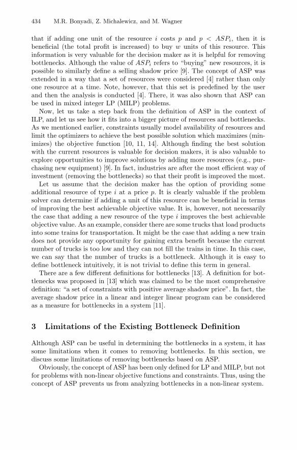
Accordingly, the first and second constraints are bottlenecks as their corre-sponding ASPs are positive. Thus, it would be beneficial if investments are con-centrated on adding one unit to the first or second constraint to improve theobjective value. Adding one unit to the first constraint is meaningless from thepractical point of view. In fact, adding one unit to RHS of the constraint g1means that the amount of products that is loaded into the trains can exceed thetrains’ capacities by one ton, which is not justifiable. In the above example, thereis another option for the decision maker to achieve a better solution: if it is pos-sible to improve the operation rate of the trucks to 101 tph, the best achievablesolution is improved to 1,919 tonnes. Thus, it is clear that the bottleneck mightbe a specification of a resource (the operation rate of trucks in our example) thatis expressed by a value in the coefficients matrix and not necessarily RHS. Thecommonly used ASP, which only gives information about the impact of changingRHS in a constraint, cannot formulate such bottlenecks.

Figure 1 illustrates this limitation. The value of ASP represents only the effectsof changing the value of RHS of the constraints (Figure 1, left) on the objectivevalue while it does not give any information about the effects the values in thecoefficients matrix might have on the objective value (constraint g1 in Figure 1,

3 We have made several such industry-inspired stories and benchmarks available:http://cs.adelaide.edu.au/~optlog/research/bottleneck-stories.htm

436 M.R. Bonyadi, Z. Michalewicz, and M. Wagner

Fig. 1. x and y are number of trucks and number of trains respectively, gray gradient:indication of objective value (the lighter the better), shaded area: feasible area, g1, g2, g3are constraints, the white point is the best feasible point

right). However, as we showed in our example, it is possible to change the valuesin the coefficient matrix in order to achieve better solutions.

The value of ASP does not provide any information about the best strategyof selecting bottlenecks to remove. In fact, it only provides information aboutthe benefit of elevating the RHS in each constraint or a given set of constraintsand does not say anything about the order of significance of the bottlenecks. Itremains the task of the decision maker to compare different scenarios by selectingdifferent subset of constraints (also known as what-if analysis4). Of course onecan analyze all possible subsets of constraints to find which subset is the mostbeneficial one to invest on. However, this strategy potentially leads to solvinganother hard problem, that is a subset selection. From a managerial point ofview, it is important to answer the following question: is adding one unit to thefirst constraint (if possible) better than adding one unit to the second constraint(purchase a new truck)? Note that in real-world problems, there might be manyresources and constraints, and a manual analysis of different scenarios might beprohibitively time consuming. Thus, a smart strategy is needed to find the bestset of to-be-removed bottlenecks in order to gain maximum profit with lowestinvestment. In summary, the limitations of identifying bottlenecks using ASPare:

Limitation 1. ASP is only applicable if objective and constraints are linear.Limitation 2. ASP does not evaluate changes in the coefficients matrix (the

matrix A) and it is only limited to RHS.Limitation 3. ASP does not provide information about the strategy for invest-

ment in resources, and the decision maker has to manually conduct analysesto find the best investment strategy.

4 In the operational research community, there are related terms such as sensitiveanalysis and post-optimality [7].

Beyond the Edge of Feasibility: Analysis of Bottlenecks 437

4 A New Model for Bottleneck

In this section a new definition for bottleneck and a new model for removing bot-tlenecks (investment) is proposed that addresses limitations listed in Section 3.

Each constraint gi in a real-world optimization problem usually models notonly the availability of resources, but also other specifications of resources suchas rates and capacities. Each of these specifications is encoded in a coefficient inthe constraints. Accordingly, we propose a new definition for bottleneck:

Definition 1. A bottleneck is a modifiable specification of resources that bychanging its value, the best achievable performance of the system is improved.

Note that this definition is a generalization of the definition of bottleneckin [13]: “a set of constraints with positive average shadow price is defined asa bottleneck”. In fact, the definition in [13] concentrated on RHS only (it isjust about the average shadow price) and it considers a bottleneck as a set ofconstraints, while our definition is based on any modifiable coefficient in theconstraints (from capacity, to rates, or availability) and it introduces each spec-ification of resources as a potential bottleneck. As an example, based on ourdefinition, the operational rate of trucks can be a bottleneck, while according tothe definition in [13], this is not possible 5 (see Limitation 2 in Section 3). Ofcourse the set of all modifiable specifications need to be provided by the user.

According to the proposed bottlenecks definition, in order to invest on a partof a system to achieve maximum improvement of the objective of that system,not only RHS of all constraints should be assessed, but also all modifiable spec-ifications in constraints need to be processed (e.g., tuning up trucks rather thanbuying new trucks) for potential changes. Hence, it is clear that the earliermethodologies based on ASP were not able to process all opportunities for re-moving bottlenecks and investments to maximize improvement in the objectivefunction (see Limitation 3 in Section 3).

We propose a new model to address the limitations of ASP for removingbottlenecks and finding the best way of investment. We define the vector liwhich contains all modifiable specifications in the constraint gi. For any COP inthe form of eq. 1, we define a Bottleneck COP (BCOP) as follows:

find x and l s.t. z =

{max(f(x, l))

min(B(l))subject to gi(x, li) ≤ 0 for all i (5)

where l is a vector (l might contain continuous or discrete values) which containsli for all i and B(l) is a function that calculates the cost of modified specificationsof resources coded in the vector l. Note that in the linear case, li = {ai, bi}where ai is the ith row of the matrix A in eq. 2. If we consider li = {bi} and

5 One can argue that the operational rate is another constraint that can be modeledby a new variable (g4 : v = 100 in eq. 4). However, if this constraint is added to thedefinition of the problem then constraint g1 becomes non-linear (g1 : 2000y−vx ≤ 0)which then is not suitable for ASP.

438 M.R. Bonyadi, Z. Michalewicz, and M. Wagner

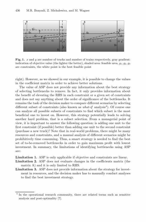
Fig. 2. The impact of an investment (B) on the achievable objective value f (max-imization is the goal): positive/negative investments (reduction of resources) usuallyresults in an increase/decrease in the best achievable objective value

gi(x) = aix− bi (linear constraints) then eq.5 can express ASPi. Figure 2 showsthat, if all pieces of equipment are sold, the best achievable objective value iszero (f = 0) because nothing can be produced anymore (this is called “objectivebreak” point in the figure), that is the same as the selling shadow price [9]. The“cost cross” point shows the point where the best objective value is achievedwith the current specification of resources (B = 0). The point “bottleneck free”is the point where the optimum solution of the search space is inside the feasibleregion. From a practical point of view, in this situation, no matter how thedecision maker invests, the profit is not improved any more. Note also thatsometimes the amount of investment up to some value might not change thebest achievable objective value. As an example, any investment from B1 to B2

does not result in any improvement in the objective value.Let us assume that the associated solution to the point (f1, B1) is x

′ and l′.This solution can be interpreted as if the decision maker invests B1, the bestway to spend this budget is to change the specifications values to l′ (which costsB1) and the best achievable objective value in this case is f1. Note that:

– a BCOP can be formulated for linear and non-linear systems,– any modifiable specification of resources can be formulated in a BCOP in

the vector l and the values for this vector are examined by the solver,– solutions for a BCOP contain best investment strategies for various budgets.

Any multi-objective optimization algorithm can be applied to solve a BCOP.Also, as the specifications can be coefficients in the constraints, the constraintsbecome non-linear, which makes the problem non-linear so that linear program-ming methodologies are not useful in solving this problem.

Let use assume that, in the example from Section 3, the decision maker canbudget $500,000 to improve the maximum loaded products per hours into thetrains. Also, the specifications that can be altered in the system are:

– the operation rate of the trucks can be increased up to 120 (i.e., l1 ={100, 101, ..., 120}) for $100 per tph per truck,

– the capacity of trains can be increased to 2100, with the step size 20 (i.e.,l2 = {2000, 2020, 2040, 2060, ..., 2100} tonnes) for $200 per ton per train,

Beyond the Edge of Feasibility: Analysis of Bottlenecks 439

0 100 200 300 400 5001500

2000

2500

3000

3500

4000

4500

5000

Cost function (B)

Obj

ectiv

e fu

nctio

n (f

)

Shadow price (only RHS)BCOP with exhaustive search

Fig. 3. Impact of an investment on the achievable objective value

– the number of trucks can be increased up to 40 (i.e. l3 = {19, 20, ..., 40}),each truck costs $15,000,

– the number of trains can be increased up to 5 (i.e l4 = {2, 3, 4, 5}), each traincosts $100,000.

The BCOP for this example is written as:

find x and l such that z =

⎧⎪⎨⎪⎩max{l2y}min{0.1l3(l1 − 100) + 0.2l4(l2 − 2000)+

15(l3 − 19) + 100(l4 − 2)}(6)

subject to l2y − l1x ≤ 0, x ≤ l3, y ≤ l4

Note that B(l) = 0 for l = {100, 2000, 19, 2} (the current specification ofthe resources). We can solve this problem by using two methods: changing thevalue of RHS according to the ASP in eq. 4, or performing an exhaustive searchalgorithm that solves BCOP in eq. 6. Note that only practically possible wereadded to the list of solutions. Figure 3 shows the results.

It is clear that when BCOP is used more opportunities for investment areexamined, which can potentially result in higher benefits with smaller invest-ments. As an example, with $135,000 investment, a solution with f = 2950 isfound by solving BCOP with l = {118, 2000, 25, 2}. However, the best solutionfound based on the shadow price for $135,000 investment was only f = 2800 withl = {100, 2000, 28, 2}. According to the solution of BCOP, if the decision makeris going to invest $135,000, the best way of investment (leading to maximumimprovement in the objective function) is to buy 6 new trucks ($6× 15000) andupgrade all trucks to carry 118 tph (18 tph tune up, which costs $18×100×25),which all together costs $135,000. However, by using the shadow price calcula-tions, the decision maker needs to buy 9 new trucks ($9×15000), which improvesthe objective value to 2800. It is clear that better objective values can be achievedby investing the same amount if we use BCOP.

5 An Evolutionary Algorithm for BCOP

In this section we propose two methods to solve BCOPs based on a multi-objective genetic algorithm. As the first algorithm, we use a basic algorithm

440 M.R. Bonyadi, Z. Michalewicz, and M. Wagner

0 200 400 6001000

2000

3000

4000

5000

Cost function (B)

Obj

ecti

ve f

unct

ion

(f)

Exhaustive Search (BCOP)ILP (ASP)GALP (BCOP)GA (BCOP)

0 5 10 15

x 104

3.5

4

4.5

5

5.5

6x 10

5

Cost function (B)

Obj

ecti

ve f

unct

ion

(f)

Exhaustive Search (BCOP)ILP (ASP)GALP (BCOP)GA (BCOP)

(a) (b)

Fig. 4. Impact of an investment on the achievable objective value (a) train loading and(b) tomato farm

with tournament selection, one point crossover (pc = 0.9, set via some trials),and uniform random mutation (pm = 0.3, set via some trials). Each individualcontains the vector l and all decision variables x. We call this first approach GA.

To handle multiple objectives, we use the following simple approach. Twosolutions x0 and x1 are compared based on G(x) =

∑mi=1 max(g(x), 0), which

is known as constraint violation value. If G(x0) = G(x1) or G(x0) ≤ 0 andG(x1) ≤ 0, then we use the dominance relation in multi-dimensional spaces(if both are equal or non-dominating select one randomly, otherwise select thedominating one). Otherwise, we select the solution that is better in terms ofconstraint violation value (preferring smaller constraint violation values).

The second multi-objective algorithm GALP is based on GA. Here, the in-dividuals contain only the vector l, and linear programming is used to find thebest vector x for each generated l.

We applied both methods to the problem defined in eq. 6 with 100 individualsfor 100 iterations (all non-dominating solutions found are reported in Fig. 4(a)).It is clear that both evolutionary methods have found good approximations ofthe Pareto front (computed by exhaustive search). It is also clear that (1) theperformance of the GALP is slightly better than that of GA, and (2) our basicapproaches outperform the established ASP based approach.

This means that both our approaches can be used to better plan the bestinvestment for industries. In the following, let us consider a second example,this time from agriculture, to illustrate that our formulation is straight-forwardand that it can support the decision making processes in the real-world.

Second Scenario: Agricultural Allocation.3 A farmer owns 1,000 acres of more orless homogeneous farmland. His options are to breed cattle, or to grow wheat,corn, or tomatoes. Annually, 12,000 hours of labor are available. For simplicity,we will assume here that these can be used at any time during the year, i.e.,through hiring casual labor during seasons of high need, e.g., for harvesting.

Beyond the Edge of Feasibility: Analysis of Bottlenecks 441

In the following, we list information regarding the profit, yield, and laborneeds for the four economic activities:

– cattle: $1,600/head profit, 0.25 heads/acre yield, 40 h/head annual labor– wheat: $5/bushel profit, 50 bushels/acre yield, 10 h/acre annual labor– corn: $6/bushel profit, 80 bushels/acre yield, 12 h/acre annual labor– tomatoes: 50 cent/lb profit, 1,000 lbs/acre yield, 25 h/acre annual labor

It is required that at least 20% of the farmland that is cultivated in the processis used for the purpose of cattle breeding, at most 30% of the available farmlandcan be used for growing tomatoes, and the ratio between the amount of farmlandassigned to growing wheat and that left uncultivated should not exceed 2 to 1.

Now (and this is the challenging bit), the farmer can make certain investmentsthat can possibly increase the overall profit per year: (1) additional acres offarmland can be rented at $200 per year, (2) additional labor can be hired at$20 per hour, (3) a tomato packing machine can be rented for $5,000 per year,which reduces 25 h/acre to 20 h/acres, (4) a “tomato grower’s licence” can bebought for $10,000 per year, which increases the max ratio from 30% to 35%,and (5) the value 0.25 heads/acre can be improved up to 0.7 heads/acres for$10,000 (0.25 needs $0, 0.7 needs $10,000, and anything in between is linear).

The question now is: should the farmer invest, and if so, how? In Figure 4(b)we show the results of the different approaches.6 Just as in the previous trainloading example, our evolutionary approach GALP that makes use of the BCOPformulation clearly outperform the approach based on average shadow price. Theresults of GALP are close to those of found by an exhaustive search. Note thatthe approach based on average shadow price is not able to assess all cases forinvestment, which makes GALP more appropriate to find best investment plan.Note that in this example the methods were run for 1000 iterations.

6 Conclusions and Directions

In this paper we proposed a new definition for bottlenecks and a new modelto guide decision makers to make the most profitable investment. We did thisin order to narrow the gap between what is being considered in academia andindustry. Our definition for bottlenecks and model for investment overcomesseveral of the drawbacks of the model that is based on average shadow prices:

1. It can work with non-linear constraints and objectives.2. It offers changes to the coefficient matrix.3. It can provide a guide towards optimal investments.

This more general model can form the basis for more comprehensive analyticaltools as well as improved optimization algorithms. In particular for the latterapplication, we conjecture that nature-inspired approaches are adequate, due tothe multi-objective formulation of the problem and its non-linearity.

6 The construction of the BCOP formulation is straight-forward, and we omit it dueto space constraints. It is available on the above-mentioned website of our stories.

442 M.R. Bonyadi, Z. Michalewicz, and M. Wagner

Bottlenecks are ubiquitous and companies make significant efforts to eliminatethem to the best extent possible. To the best of our knowledge, however, thereseems to be very little published research on approaches to identify bottlenecks—research on optimal investment strategies in the presence of bottlenecks seems tobe even non-existent. In the future, we will push this research further, in order toimprove decision support systems.We will design nature-inspired single-objectiveand multi-objective algorithms with the goal to support decision makers to makethe best possible investments in their constrained systems.

References

[1] M. R. Bonyadi and Z. Michalewicz. On the edge of feasibility: a case study of theparticle swarm optimizer. In CEC, pp. 3059–3066. IEEE, 2014.

[2] M. R. Bonyadi, X. Li, and Z. Michalewicz. A hybrid particle swarm with veloc-ity mutation for constraint optimization problems. In Genetic and EvolutionaryComputation Conference (GECCO), pp. 1–8. ACM, 2013.

[3] A. Charnes and W. W. Cooper. Management models and industrial applicationsof linear programming, Vol. 1. John Wiley and Sons, 1961.

[4] A. Crema. Average shadow price in a mixed integer linear programming problem.European Journal of Operational Research, 85:625–635, 1995.

[5] E. M. Goldratt. Theory of constraints. Nrth. River Cro.-on-Hud., NY, 1990.[6] E. M. Goldratt and J. Cox. The goal: a process of ongoing improvement. Gower,

1993.[7] P. A. Jensen and J. F. Bard. Operations research models and methods. John Wiley

& Sons Incorporated, 2003.[8] P. G. W. Keen. Value analysis: Justifying decision support systems. Management

Information Systems Research Center Quarterly, 5:1–15, 1981.[9] S. Kim and S.-c. Cho. A shadow price in integer programming for management

decision. Europ. Journal of Operational Research, 37:328–335, 1988.[10] T. C. Koopmans. Concepts of optimality and their uses. The American Economic

Review, pp. 261–274, 1977.[11] R. Luebbe and B. Finch. Theory of constraints and linear programming: a com-

parison. Int. Journal of Production Research, 30:1471–1478, 1992.[12] Z. Michalewicz and M. Schoenauer. Evolutionary algorithms for constrained pa-

rameter optimization problems. Evolutionary Computation, 4:1–32, 1996.[13] S. Mukherjee and A. Chatterjee. Unified concept of bottleneck. IIMA Working

Papers WP2006-05-01, Indian Institute of Management Ahmedabad, Researchand Publication Department.

[14] S. Rahman. Theory of constraints: A review of the philosophy and applications.Int. Jour. of Oper. and Prod. Manag., 18:336–355, 1998.

[15] M. Schoenauer and Z. Michalewicz. Evolutionary computation at the edge offeasibility. In Parallel Problem Solving from Nature (PPSN), Vol. 1141 of LNCS,pp. 245–254. Springer, 1996.