Beyond Engel s Law - Pursuing an Engelian Approach to Welfare A Cross Country Analysis

JENA ECONOMIC RESEARCH PAPERS

# 2012 – 028

Beyond Engel´s Law – Pursuing an Engelian Approach to Welfare

A Cross Country Analysis

by

Wolfhard Kaus

www.jenecon.de

ISSN 1864-7057

The JENA ECONOMIC RESEARCH PAPERS is a joint publication of the Friedrich

Schiller University and the Max Planck Institute of Economics, Jena, Germany.

For editorial correspondence please contact [email protected].

Impressum: Friedrich Schiller University Jena Max Planck Institute of Economics

Carl-Zeiss-Str. 3 Kahlaische Str. 10

D-07743 Jena D-07745 Jena www.uni-jena.de www.econ.mpg.de

© by the author.

Beyond Engel’s Law - Pursuing an Engelian

Approach to Welfare

A Cross Country Analysis∗

Wolfhard Kaus‡

Abstract

Engel’s law is known to be extraordinarily consistent across time and space. Ac-cordingly, it has been widely used to determine poverty. However, also among thepoorest, a certain amount of non food spending is necessary. To substantiate thedistinction between necessities and luxuries, already Ernst Engel (1895) approacheda behaviorally founded comprehensive assessment of structural changes in consumerexpenditures.

To build upon Engel’s legacy and to complement the scare empirical literature, abehavioral approach is applied. It is conjectured that differences in satiation patternsof universally shared needs translate, on the aggregate level, into different shapes ofEngel curves and thus also into different income elasticities of demand.

Utilizing a nonparametric regression technique, it is explored whether and whichexpenditure categories change systematically with rising income. In line with thetheoretical expectations, a number of empirical regularities in consumer expenditurepatterns can be identified that go well beyond Engel’s law.

Keywords: Engel’s law, income elasticity of demand, necessities, luxuries, differential sa-tiation

JEL classification: D12

∗For helpful discussions and valuable comments I would like to thank Elisabeth Bublitz, Stephan Bruns,Leonhard Lades, Alessio Moneta, Ulrich Witt and the participants of a Jena Economic Research Workshop.The usual disclaimer applies.

‡Max Planck Institute of Economics, Evolutionary Economics Group, Kahlaische Straße 10, 07745 Jena,Germany, [email protected].

1

Jena Economic Research Papers 2012 - 028

1 Introduction

Since the work of Ernst Engel it is a well established fact that the expenditure sharededicated to food consumption decreases as income rises. Using a sample of only 199 Bel-gian family budgets, Ernst Engel (1857, 1895) inferred the observed negative relationshipbetween the expenditure share on food and income to be an economic law. Despite themeager data base available to Engel at this time, this relationship turned out to hold truein most countries and points in time (Houthakker, 1957; Seale and Regmi, 2006; Lewbel,2008).

The extraordinary consistency across time and space and the predictive character ofthe relationship led to the use of Engel’s law to determine absolute household poverty(see, e.g., Musgrove, 1985) and to define poverty lines (see, e.g., Lanjouw and Lanjouw,2001, and other references therein). More recently, Engel’s law is even used to correct pur-chasing power parities (Almas, 2012). Although Engel’s law is an essential nonmonetarydeterminant when distinguishing between poverty and wealth, it covers only one decreas-ing fraction of consumer expenditure as income rises. In contrast, empirical evidence onsystematic changes in other consumer expenditure categories is hardly used. A system-atic assessment of structural changes in consumer expenditure categories as income risesshould, however, allow for a more complete and multidimensional assessment of wealth.

In fact, final per capita poverty lines usually consist of a food poverty line covering an“adequate” energy intake and a certain amount of non food spending that is considerednecessary (Lanjouw and Lanjouw, 2001). While the former can be derived by the humanbody’s need for calories, the latter is usually derived by scaling up the former by a certainfactor. Determining necessary non food spending reflects the insight that even at very lowlevels of income some items other than food are essential. The arbitrariness of the choiceof the scalar (Deaton, 1997), however, mirrors a still missing comprehension of why andwhich consumption items are necessities and which are not. As a result, the size of thescalar needs to be chosen ad-hoc. Both theoretical conjectures and empirical evidence onother systematic changes in the composition of consumer expenditures remain scarce. Inthis paper it is argued that the current state of the art suffers from a missing behavioralfoundation for the distinction between necessities and luxuries.

The lack of such an assessment is even more remarkable as Ernst Engel already pursueda much more encompassing approach. In fact, his approach to consumption expenditureswas never intended to focus solely on the budget share for food. Engel’s original workwas indeed an inquiry into the structural changes of consumption patterns with risingincome, aiming at determining a measure of household welfare (Chai and Moneta, 2010).Therefore, he started out by categorizing expenditure items according to the underlying“wants” they satisfy. In a second step, he assessed the importance of these wants fromthe empirically derived expenditure patterns. In this sense, Engel was not only the first toempirically assess the distinction between “necessities” and “luxuries” (instead of subjec-tively assuming) but also the first to attempt a behavioral explanation for this taxonomy.

Building upon Engel’s legacy requires to better found the assumption about the classi-fication of needs by enriching it with current scientific knowledge on the nature of consumerneeds and how they are satisfied. Therefore, this paper offers a motivational approach toconsumer behavior, which allows to formulate expectations about structural changes of ex-penditure shares as income rises. The theory distinguishes between innate needs on the onehand and both wants and cognitively constructed motives that are acquired in culturallycontingent ways on the other hand (Witt, 2001). To the extent to which consumption isdriven by innate needs, it can be expected that the common genetic basis induces patternsof behavior that are universally shared by humans. This means that consumer expendi-ture patterns should change inter-personally and inter-culturally similarly with income.

2


Engel’s law for expenditures on food – for which a fairly rapidly satiable innate need canbe identified – is a case in point. For other expenditure categories, the theory identifiesother innate needs as driving forces and, corresponding to their differing satiation features,predicts different shapes for the respective Engel curves. The corresponding consumptioncategories can be qualified accordingly as either necessities or luxuries.

In order to assess the evidence for the suggested human universals, the paper presentsan empirical analysis of observable changes in consumption patterns across countries andtime. Using the United Nations National Account Statistics, a data set that contains indi-vidual consumption expenditure by households in 12 categories for more than 50 countriesover up to 50 years is specified. The data at hand allows to

a) explicitly describe the overall changes in consumption patterns with rising incomein real terms (cross-country Engel curves),

b) assess the consistency of the identified changes in consumption patterns relative tothe well known Engel’s law.

Our findings broadly confirm the conjecture that the shape of Engel curves (inclusiveof, but extending beyond, Engel’s law) represent human universals. The study contributesto the literature on income and wealth by a structural assessment of general changes inbudget shares across countries that helps to broaden our understanding of the behavioralfoundations of the necessity – luxury taxonomy. In doing so, it broadens the scope for amore encompassing and multidimensional consumption based assessment of wealth.

The paper is structured as follows. Section 2 outlines the theoretical framework. Insection 3 the creation of a comparable income dimension is described. The empiricalresults on cross-country Engel curves are shown in section 4. The last section concludes.

2 What determines the shape of Engel curves?

This section applies a behavioral approach to consumption to connect differences in satia-tion patterns between innate needs with systematic changes in consumption expenditureswhen income rises. It is conjectured that, at the level of aggregate expenditure data, thesedifferences translate into different income elasticities of demand for groups of goods andservices that are likely to be consumed to serve those needs. This way, it should be ableto explain a good deal of the differences in the shapes of Engel curves of the underlyinggoods and services.

2.1 Engel curves and the income elasticity of demand

The general connection between the shape of an Engel curve and the income elasticity ofthe respective good can easily be illustrated. If an Engel curve for good i is expressed interms of the expenditures qi spent on i depending on the households’ income y, the slopeof the fitted relationship ∂qi/∂y can indirectly be used to derive i′s income elasticity ofdemand. As a good’s income elasticity is defined by the relative change in qi (∆qi/qi)divided by the relative change in y (∆y/y), it can be estimated by regressing logged qi onlogged y (Lewbel, 2008).

Using expenditure shares (wi = qi/y), instead of the expenditures spent on i, allowsmore directly an inference of the income elasticity of demand from the curve’s slope. Areformulation of the basic equation, to be derived in section 4.2, shows that downwardsloping Engel curves indicate income elasticities smaller than 1 (“necessities”), while up-ward sloping Engel curves yield income elasticities above 1 (“luxuries”). Although Engelcurves usually show considerable nonlinearities (Lewbel, 2008), budget share Engel curves

3


allow to readily observe the income elasticity of demand for the underlying group of goodsand services.

2.2 A motivational approach to consumer behavior

Engel’s approach to consumption never solely focused on food expenditures. In fact,Engel’s original contribution was meant to determine and measure household welfare (Chaiand Moneta, 2010). He started out by categorizing expenditure items according to theunderlying “wants” they satisfy. The importance of these wants was subsequently assessedby the empirically derived expenditure patterns. Engel’s work thus essentially focusedon a behavioral foundation of the necessity – luxury taxonomy. In a revised version ofhis original contribution, Engel (1895, p.8) made even more explicit that the motivationof human action, and thus also consumption behavior, is rooted in the satisfaction ofuniversally shared needs (Chai and Moneta, 2010).

To build upon Engel’s legacy, it is necessary to better found the classification of needsby enriching it with current scientific knowledge on the nature of consumer needs andhow they are satisfied. However, motivational underpinnings of economic behavior ingeneral and consumer behavior in particular are rarely addressed in economics. Amongthe existing works, two different explanatory approaches can be identified (Witt, 2010a).While in the utilitarian hedonic approach (Kahneman et al., 1997) the explanation refersto the motives of seeking pleasure and avoiding pain, nonhedonistic variants instead focuson the motivating power that deprived needs and wants have for consumption activities(see, e.g., Menger, 1871; Duesenberry, 1949; Georgescu-Roegen, 1954; Ironmonger, 1972).1

This paper closely connects to the latter approach. A behavioral – need based –interpretation of the consumption motivation is offered (Witt, 2001, 2010b) to explainthe theoretically scarcely substantiated shape of Engel curves. The theory postulates anintimate relationship between human biological and cultural evolution in the sense thatcultural development is based upon as well as constrained by innate behavioral dispositionsand cognitive learning abilities, which have emerged during human phylogeny. Hence, thetheory focuses on the explanation of long-run economic change from a biological andpsychological perspective (Witt, 2008).

The theory of the learning consumer (Witt, 2001, 2010b) emphasizes the role of humanneeds as ultimate motives of consumption behavior. The theory distinguishes betweengenetically determined – innate – needs and both culture and socialization specific acquiredwants that result from processes of conditioning learning (classical, operant, and social-cognitive). The theory holds that the attempt to relieve or reduce of deprivation of thelimited number of innate needs, consequently an increase in satiation level of these needs,is one major motivation to consume. Deprivation is thus seen to intrinsically motivateconsumers to act which creates a rewarding experience.

Needs are the contingencies under which deprivation occurs. Although needs can bemanifold, in this context only the subset of universally shared “basic” needs is relevant.Among these are that for sleep, for something to drink, for something to eat, for maintain-ing body temperature, for physical activity, for status recognition, or for sensory arousal(Witt, 2011).

An important characteristic of these needs is that their satisfaction by an action effectsa primary reinforcement in the sense of instrumental or operant conditioning (Hull, 1943;Herrnstein, 1990; Staddon and Cerutti, 2003). This means that, unless the motivation toact is modified by insetting cognitive reflection, the likelihood that a particular activity

1In behavioral and human sciences, research on motivational theories continued and extended to focuson biological and evolutionary roots of behavior (Wilson, 1975; Caplan, 1978), which draws attention tointer-personal commonalities that can be conjectured to be relevant also for consumer behavior.

4


is chosen over another one depends on its relative contribution to reducing deprivation.Under reinforcement learning, the frequency distribution over actions converges to a statesatisfying the so called “matching law” (Herrnstein, 1997).

Among the universally shared needs, a further distinction relates to the satiating char-acteristics they show (Witt, 2010b, 2011). On the one hand, there are basic needs whichfollow homeostatic features, i.e., deprivation can be reduced relatively easily up to the tem-porary satiation point once rising income allows to sufficiently increase the correspondingconsumption expenditures per period of time. The motivation to consume is, then, tem-porarily reduced or removed. Satisfaction of these needs depends mainly on the intrinsicvalue of the corresponding goods and services. Examples are the homeostatic needs un-derlying eating, drinking, sleeping, and maintenance of body temperature. On the otherhand, there are also basic needs where homeostatic features are absent and where it istherefore difficult, if not impossible, to reduce the average deprivation to zero. Typically,these are needs whose satiation level is defined in relative terms, like the need for arousaland for social recognition.

Despite inter-personal sources of variance, which can be expected due to individualcognitive and conditioning learning processes, it can be conjectured that shared innateneeds exert some systematic effects on behavior that are visible at the level of the popu-lation means, i.e., at the level of aggregate consumer expenditures. As needs differ withrespect to the amount of spending that is necessary to reach satiation, this difference canbe expected to become relevant with rising real income (Witt, 2010b, 2011). Being ableto spend more, consumers should be able to approach the satiation level of some needsfaster than the satiation level of other needs. Their consumption motivation is not equallyupheld and their spending should thus not expand equally. Differences for the incomeelasticity of demand for the products that serve the different needs should express thisdifferential satiation effect.

Taken together, the behavioral approach to consumption suggests connecting the differ-ences in satiation patterns between innate needs with systematic changes in consumptionexpenditures when income rises. It is conjectured that, at the level of aggregate expen-diture data, these differences translate into different income elasticities of demand forproducts or groups of goods and services that are likely to be consumed to serve thoseneeds. The behavioral approach to consumption should thus be able to explain a gooddeal of the differences in the shapes of Engel curves and thus in the income elasticities ofthe underlying goods and services.

2.3 Applying the theoretical framework

Before hypotheses on the shape of Engel curves can be derived, some attention should begiven to the empirical framework. As this paper, on the one hand, aims at inquiring intothe generality of Engel curves across countries and, on the other hand, attempts to explainthe difference in shapes by universally shared human dispositions, it is necessary to departfrom the usual Engel curve framework that plots cross sectional expenditure survey datain one region at a particular point in time on corresponding income or total expendituredata.

In order to derive a more general picture, it is rather desirable to use an empiri-cal framework that allows exploring changes in consumption patterns within and acrosscountries with different levels of income over time. Applying such a framework, how-ever, necessarily entails some flaws. First, it is obvious that an increase in the number ofcountries and observations across time will challenge the comparability of the expenditureitems. Finding comparable expenditure categories is a natural task that will irrevocablylead to a higher level of aggregation. Dealing with various countries over a range of time

5


moreover involves converting the relevant variables into a common denominator.2

2.3.1 The expenditure categories

The expenditure categories used in this paper are drawn from the United Nations NationalAccounts Statistics. Since 1956, the United Nations have annually published the NationalAccounts Statistics: Main Aggregates and Detailed Tables.3 The series superseded tenissues of the Statistics of National Income and Expenditure. For the purpose of thisanalysis, Table III.2, i.e., Individual consumption expenditures, is used.

Data availability is restricted to member countries of the United Nations and someother countries or areas which report to the United Nations. However, only after joiningthe United Nations, all members are required to report such statistics based on commonstandards. The sample used in this paper can be found in Table A2 in the appendix. Itis restricted to data that complies with the System of National Accounts 1993 standards(SNA 93).4 To the best of the author’s knowledge, this is the most valuable source thatallows an exploration of structural changes of consumption patterns as income rises in along term cross-country framework.5

As mentioned before, the long term cross-country framework is necessarily accompa-nied by aggregation of the expenditure categories. In fact, this is the case with the nationalaccount statistic data. A big advantage, however, is that the twelve categories (cf. TableA1) are consistently defined for all observations. The data is categorized according to theUN Statistics Division’s Classification of Individual Consumption According to Purpose(COICOP).

2.3.2 Connecting innate needs and expenditure categories

When connecting differences in satiation patterns of innate needs with systematic changesin consumption expenditures as income rises, two conceptual problems have to be men-tioned first. The one is the problem of determining what expenditures serve what need sothat the predicted satiation features of the needs can be translated into predictions aboutchanging consumption expenditure. The second is the aggregation problem. The reactionsto increasing satiation explained at the individual consumer level have to be aggregatedto the level of aggregate consumption expenditure data, at which structural changes inboth consumption and market shares are usually recorded (Witt, 2010a).

The second problem is of a more general nature and lies in micro-founded theories ofconsumption. The present approach provides a natural solution with the assumption ofinnate, need-based consumption motives and the corresponding satiation patterns. Sincethese individual features are shared with the usual genetic variance in human populations,an aggregate level – of the human population – is already implied.

The first problem of associating goods and services with particular needs is more criticalas products usually have several characteristics and the different characteristics can appealto different needs at the same time. Accordingly, the consumption of a particular goodcan be motivated in multiple ways. If so, it is more difficult, but not impossible, to merge

2For a discussion, please see section 3.3The data is freely available from the National Accounts Official Country Data account of the United

Nations.4Data which is only available according to SNA 68 standards is omitted from the analysis to maintain

a comparable frame of analysis.5Especially among the currently less affluent countries, there is hardly any, let alone long term, data

available. A valuable exception is India, where consumer expenditure surveys have been collected for morethan 60 years by now.

6


the differing satiation patterns into a compound prediction for the satiation dynamics thatoccur with rising income.

As already mentioned above, a certain set of needs could be identified of which somebelong to rather physiological needs that follow homeostatic satiation features and arerelatively easy to satiate, while other needs are rather psychological needs that showdynamic nonhomeostatic satiation features which are less easily, if at all, satiable.

Hypotheses on easily satiable needs

In the case of physiological needs, the homeostatic features imply that the motivation fortaking actions decreases the closer to the satiation level of the need the consumer gets. Themotivation to expand consumption further is then reduced or vanishes such that consump-tion stagnates, if nothing else happens. As consumption expenditures grow with risingdisposable income, satiability of needs results in a saturated demand for correspondinggoods.

A very plausible example for an easily satiable need is food consumption. Satiation inthis case depends on the satiating characteristics of the items consumed such as caloric orcaffeine content. Demand is thus naturally constrained by an upper quantity bound thatis the absorbing capacity of the human body. On the aggregate level, this effect shouldallow a decrease of the proportion spent on food with rising income (Witt, 2011).

Another example is the expenditure category of clothing . The underlying innateneed that is satisfied by the use of clothing and footwear is the maintenance of body tem-perature. As everybody can only wear a limited number of items at a time, the purelyfunctional demand for clothing should be easily saturated once rising disposable incomeallows this. However, this category is also a prime example for one of the conceptuallimitations alluded to above, namely that different characteristics of a particular goodcan appeal to different needs at the same time. Consumption of clothing and footwearis, of course, not only motivated by the desire to maintain body temperature. The pres-ence of other, more cognitively mediated motivations, such as group affiliation or statusrecognition, cannot be denied.

In a time series analysis of the U.S., Frenzel Baudisch (2006) shows that the demandfor footwear mainly followed basic functional uses up to the beginning of the 1970s. In fact,the expenditure share on footwear was steadily decreasing and thus a “necessity” up to thistime. Frenzel Baudisch (2006) is able to show that the subsequent increase in the expen-diture share for footwear, albeit relatively small at the aggregate level, was driven by theproducer’s reaction to the saturated demand for footwear. Producers increasingly releasedfunctionally differentiated product innovations and added new characteristics (cognitiv-elly mediated motives) to their products to escape functional satiation. These supply sidestrategies also gave rise to social comparison and group dynamics that led to a decouplingof the item’s consumption and the initial purely instrumental use (maintenance of bodytemperature).

Despite the fact that multiple motivations to consume items in the clothing categorymight prevail, the example is suitable to illustrate that, the satisfaction of the universallyshared needs for maintaining body temperature and the avoidance of bodily harm can stillbe expected to explain the main structural pattern in the budget share Engel curve beforepurely functional satiation occurs, i.e., supply side driven reactions to escape saturatedmarkets set in. It is therefore suggested that, as long as income is low to moderate, thebudget share Engel curve for clothing should be downward sloping.

7


Hypotheses on hardly satiable needs

In the case of psychological needs that lack homeostatic features, the motivation to expandconsumption, once increasing income allows it, is not easily withheld and, thus, will notlead to a stagnating demand. Therefore, the budget share on expenditure categories thatcan be related to satisfying such needs are expected to increase once the satisfaction ofeasily satiable needs and increases of income allow for this.

An illustrative example is the need for sensory and cognitive arousal (Witt, 2011). Asalready argued by Scitovsky (1981), satisfaction can hardly be achieved, as the arousaldrawn from what is currently consumed is subject to a stupefaction effect. Satiabil-ity is thus endogenously changing, such that ever stronger stimuli are needed to upholdarousal. Although related expenditures grow, the average deprivation level is hardly de-creasing. The insatiability of the need for sensory and cognitive arousal should empiricallybe reflected at least in the various expenditures related to entertainment (e.g., electronicequipment, ballet, art, theater, sporting events, and the like) and media services. Anothervivid expenditure category motivated by the need for arousal is recreational traveling(Chai, 2011). As these items broadly match the expenditure categories recreation &

culture and restaurants & hotels, it is conjectured that upward sloping Engel curvescan be expected.

In the case of status recognition, insatiability results from the relative nature of thiskind of expenditures. Certain consumption items that are suitable to signal status allowthe distinction of oneself from others. However, the strength of this signal diminishes ifrising income allows individuals from lower income groups to purchase similar items. Torestore the status quo ante, more intense status signals are required. However, additionalexpenditures are repeatedly neutralized by expenditures of others such that deprivation ofstatus can, if at all, only be avoided by continuously rising expenditures (Witt, 2011). Theinstability of status races that leads to rising expenditures on status goods has repeatedlybeen illustrated by Hirsch (1978), Frank (2011), and many others.

In a recent study, Charles et al. (2009) determine which goods are signaling better eco-nomic circumstances, “. . . are readily observable in anonymous social interactions, and [...]portable across those interactions” (ibid p. 426). Accordingly, a basket of goods, includingspending on apparel, accessories, such as watches and jewelry, personal care, and vehicleshave been identified. When abstracting from the requirement of portability, expenditureson housing additionally qualify (Charles et al., 2009; Frank, 1999). Among the consump-tion categories in the COICOP system, these items can be found in transport , housing& utilities, furnishings & household equipment , and miscellaneous goods &

services (see Table A1). However, in the case of transport and miscellaneous goods &

services, more than these goods can be found in the respective categories which cannoteasily be connected to the need for status recognition. It can, therefore, only tentativelybe concluded that upward sloping Engel curves should be expected in these categories.

Budget categories without need based hypotheses

When inspecting the expenditure categories in Table A1, a further limitation needs tobe taken into account. The allocation of consumption expenditures is not generally amatter of consumer sovereignty. Institutional settings are likely to interfere for a numberof reasons, such as regulated prices in the form of lower or upper price boundaries, taxes,tariffs, or the like. Among the aggregate COICOP categories, health and education

expenditures appear to be the most outstanding examples. Cross-country expenditurepatters in these categories are thus likely to show much less consistency. Accordingly,hypotheses on structural changes in expenditures as income rises are missing.

8


In the case of communication , network externalities are likely to prohibit a con-sistent pattern in cross-country Engel curves. Individual consumption expenditures oncommunication very much depends on the provision of information and telecommunica-tion networks, which likely differs between countries.

Lastly, in the case of alcohol & tobacco, cognitively constructed motives to con-sume are likely to dominate. Such “aquired wants” (Witt, 2001) are socially constructedand culturally contingent. Accordingly, cross-country Engel curves are likely to show someheterogeneity. However, the fact that the literal consumption of these goods follows home-ostatic satiation features and is limited by physiological bounds might hint to a downwardsloping tendency of the cross-country Engel curve.

3 Constructing a comparable income dimension

The empirical setting of the paper requires transforming the variables of interest suchthat comparisons across countries and time are permitted. In the case of the expenditurecategories, this can easily be facilitated by transforming the expenditures, given in currentvalues and local currency, into expenditure shares. Expenditure shares are created bysumming the nominal expenditure values and dividing the expenditures of each of thecategories by the composite. Without any further adjustments, the shares are alreadycomparable.

To make the income variable comparable across countries and time, several treatmentshave to be undertaken. First of all, GDP per capita is calculated using population data.Second, using annual exchange rates, the national currency values are transformed intocurrent U.S. $. Third, current nominal income per capita in U.S. $ is transformed intoreal income per capita. Therefore, price changes within countries are accounted for byutilizing implicit price deflator data for each country. Eventually, the resulting incomevariable, constant U.S. $ at 2005 prices, is comparable across time and countries.

Although a common currency is created and national inflation is controlled for, theincome variable still has a natural limitation. Comparing expenditure shares across astandardized income variable implicitly assumes that one 2005 U.S. $ allows one to buyapproximately the same in country x and y. That would imply that the law of oneprice holds across space for all kinds of expenditure items. Price levels, however, areconsistently found to be higher in more affluent countries. The systematic difference isusually hypothesized to stem from productivity differences in the tradable sector thatinduce prices in the non-tradable sector, for which similar productivity across countries isassumed, to be biased (Harrod, 1933; Balassa, 1964; Samuelson, 1964). A conversion ofincome measures at market prices (exchange rate) does therefore not accurately representthe true income differentials.

As the law of one price is unlikely to apply to internationally non-tradable goods, thesegoods can be purchased at markedly lower prices in less affluent countries. Such systematicdifferences thus underestimate the purchasing power in less affluent countries. Accountingfor the regional prices of non-tradable goods within a standardized consumption basketconsequently adjusts for “real” purchasing power. Purchasing power parity conversionrates thus help to alleviate this kind of bias.

The conversion of nominal GDP at current prices in national currency YNC,t into acommon currency at constant prices that is comparable over time and space YPPP,2005,i.e., Geary-Khamis international dollar (I$), can be conducted as follows:

YPPP,2005(I$) =YNC,2005

PPPt

(

NCI$

) =

YNC,t

IPD2005

PPPt

(

NCI$

) ,

9


where PPPt

(

NCI$

)

denotes the implicit purchasing power parity conversion rate thatallows the comparison of a similar consumption basket at regional prices and IPD2005

denotes the implicit price deflator referring to a fixed base year (2005) to account fornational inflation rates.

Recent research on purchasing power adjustment however shows that purchasing powerparities are biased as well. Drawing upon micro data from a number of countries, Almas(2012) utilizes Engel curves for food to assess the magnitude of this bias which turns outto be systematic. The results indicate the income of poorer countries to be overestimated.Consequently, PPP adjusted income seems to be over-adjusted.

The degree of purchasing power adjustment can be relevant for the graphical assess-ment of Engel curves in subsection 4.1. While observations of low income countries tendto move right after purchasing power adjustments are applied, observations of high in-come countries move to the left. The shape of the Engel curve can thus be expected tochange as well. As the results presented by Almas (2012) indicate that PPP adjustedincome is over-adjusted, the “true” income adjustment should lie between real income atconstant prices (constant U.S. $ at 2005 prices) and PPP adjusted income at constantprices (Geary-Khamis international dollar, i.e., I$). Therefore, the charts depicted in thefollowing sections plot expenditure share observations on real GDP (maroon circles) andPPP adjusted real GDP (gray triangles). The resulting nonparametrically derived curvesin Figures 1 are color coded as well: real GDP (red dashed line) and PPP adjusted realGDP (black solid line).

To construct a comparable income per capita indicator, annual information on grossdomestic product, population, deflator indices, and exchange rates are drawn from theUnited Nations National Accounts and Main Aggregates database. Data on purchasingpower adjusted GDP per capita at constant 2005 prices, i.e., Geary-Khamis internationaldollar (I$), is drawn from the most recent version of the Penn World Tables (Heston et al.,2011).

4 Beyond Engel’s law

A natural limitation of the approach chosen in this paper is the trade off between breathof the study in terms of the number of countries and years covered and the level of ag-gregation of the expenditure categories. Therefore, it is not surprising that not all thetwelve internationally standardized consumption categories can easily be matched withtheir underlying universally shared needs (see subsection 2.3). However, the hypothesesput forward already imply that from a behavioral consumption approach perspective thereare good reasons to presuppose the existence of more than one robust empirical regularity(“Engel’s law”) in the analysis of demand patterns. To validate the hypotheses and to ex-plore the remaining expenditure patterns, a graphical & nonparametric assessment is usedand the consistency of the overall cross-country Engel curves for each expenditure categoryis evaluated. Moreover, country level functional forms of Engel curves are estimated toassess the consistency of the overall Engel curve shape at the country level.

4.1 Assessing the shape of cross-country Engel curves

This subsection aims at contributing an empirical account of systematic changes in con-sumption patterns across countries as income rises. While it is a well established stylizedfact that the expenditure share dedicated to food consumption decreases as income rises(Engel’s law), evidence on other systematical changes in the composition of expenditureshares remains scarce.

10


The chosen empirical framework allows looking at changes in expenditure patternsfrom a different perspective. Deviating from the standard approach of considering a par-ticular population at a certain point in time, it allows for more conclusive insights aboutwhether observable changes in expenditure shares can be generalized across a range ofcountries.6 Utilizing a nonparametric regression technique, it is explored whether expen-diture categories, inclusive of, but extending beyond, food, change systematically withrising income. Applying this method moreover allows to verify the hypotheses outlined insubsection 2.3.

To properly assess the shape of cross-country Engel curves, a nonparametric approachis used. In contrast to parametric approaches that require an a priori assumption aboutthe functional form, nonparametric approaches allow the data themselves to reveal theactual shape of the estimate (Engel and Kneip, 1996). Various nonparametric regressiontechniques have been developed in recent years.

An early but still very appealing nonparametric regression approach is local linearregression. The idea of local linear regression is to fit straight lines locally to the datawhereby only a limited number of neighboring observations, determined by the bandwidth,are used which are weighted with decreasing weights the further away the observations are(Bowman and Azzalini, 1997). The locally fitted lines are then used to predict a smoothedvalue ysi for each local regression at covariate point xi. The smoothed curve, thus resultsfrom repeated separate local linear regressions for every covariate point.

Local linear regression is used in this paper for its appealing simplicity. Moreover,the technique is, under certain conditions, equivalent to the well known Nadaraya-Watsonkernel estimator (Nadaraya, 1964; Watson, 1964) but behaves superior at the edges of thecovariate space as it employs a variable bandwidth reflecting the density of the observationsthrough a nearest neighbor distance (Hart, 1997).7

Locally weighted scatterplot smoothing (LOWESS, Cleveland, 1979) is a local lin-ear estimator that uses the tricube kernel function to easily evaluate adequately smoothweights for neighboring observations. The smoothing parameter can straightforwardly beinterpreted as the share of the sample that enters the local regression with positive weights(Bowman and Azzalini, 1997).

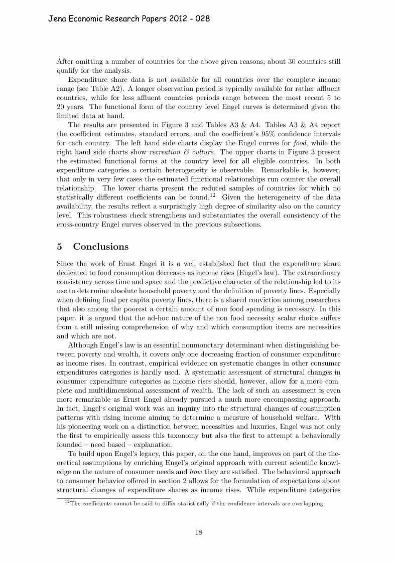
Figures 1 & 2 show Engel curves for all 12 expenditure categories derived via locallyweighted scatterplot smoothing. All charts use the sample described in Table A2. Para-metric as well as nonparametric regression methods are susceptible to outliers. Bothfigures therefore draw on a slightly reduced sample.8

Regarding the potential income adjustment problem outlined in section 3, it can befound that the shapes of the local linear regression estimates for real GDP and PPPadjusted real GDP are not too different. The curve for PPP adjusted real GDP is usuallysmoother than in the case of real GDP. Differences result mostly at the upper tail of theincome distribution. However, the curves are used to indicate an either positive or negativeslope in the overall sample of the data. Therefore, it can be concluded that the qualitativerelationship between the expenditure share category and income remains unchanged in allcases.9

6Using national account statistics it is, however, only possible to show changes in the consumptionpatterns of a mean consumer in each country as income rises.

7The Nadaraya-Watson kernel estimator also solves a locally weighted least squares problem but useslocal mean values instead of predicted values for imputing the smoothed values. Moreover, the Nadaraya-Watson kernel estimator uses a constant weighting function.

8The empirical setting implies the data to be clustered countrywise. Omitting outliers to ensure a lessvolatile course of the curve is thus more controversial than in a cross sectional setting. For a discussion onthe outlier treatment please see appendix A.1.

9All estimations in the following subsections use PPP adjusted real GDP.

11


Figure 1: Changes in expenditure shares with rising income – need based.1

.2.3

.4.5

.6E

xpS

1

0 20000 40000 60000 80000GDP_ppp_cap_2005 / rGDP_cap_2005

Food on GDP_ppp Food on real GDPGDP_ppp (lowess) real GDP (lowess)

0.0

5.1

.15

Exp

S3


Clothing on GDP_ppp Clothing on real GDPGDP_ppp (lowess) real GDP (lowess)

.05

.1.1

5.2

.25

.3E

xpS

4


Housing on GDP_ppp Housing on real GDPGDP_ppp (lowess) real GDP (lowess)

.02

.04

.06

.08

.1.1

2E

xpS

5


Furniture on GDP_ppp Furniture on real GDPGDP_ppp (lowess) real GDP (lowess)

.05

.1.1

5.2

.25

Exp

S7


Transport on GDP_ppp Transport on real GDPGDP_ppp (lowess) real GDP (lowess)

0.0

5.1

.15

Exp

S9


Recreation on GDP_ppp Recreation on real GDPGDP_ppp (lowess) real GDP (lowess)

0.0

5.1

.15

Exp

S11


Restaurants on GDP_ppp Restaurants on real GDPGDP_ppp (lowess) real GDP (lowess)

0.0

5.1

.15

.2E

xpS

12


Miscellaneous on GDP_ppp Miscellaneous on rGDPGDP_ppp (lowess) real GDP (lowess)

Notes: The charts plot the locally weighted smoothing scatterplots of the respective expenditure shareon real GDP (red dashed line) as well as on PPP adjusted real GDP (black solid line). The smoothingparameter is 0.7.

Overall, the charts depicted in Figure 1 suggest that there are much more regularitiesin cross-country consumption patterns than Engel’s law. The tremendous consistency

12


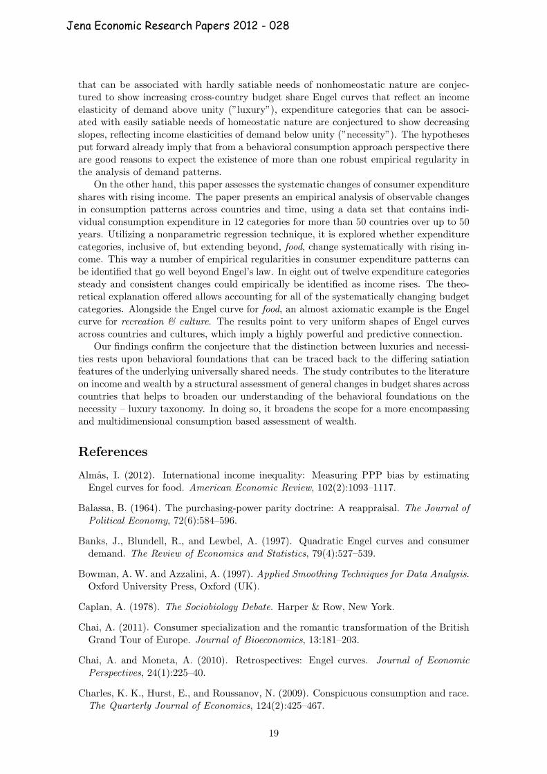
Figure 2: Changes in expenditure shares with rising income – remaining0

.2.4

.6fo

od −

alc

ohol

& ta

bacc

o

0 10000 20000 30000 40000 50000rGDP_cap_2005

0.2

.4.6

food

− h

ealth

0 10000 20000 30000 40000 50000rGDP_cap_2005

0.2

.4.6

food

− c

omm

unic

atio

n

0 10000 20000 30000 40000 50000rGDP_cap_2005

0.2

.4.6

food

− e

duca

tion

0 10000 20000 30000 40000 50000rGDP_cap_2005

Notes: The charts plot the locally weighted smoothing scatterplots of the respective expenditure sharerelative to expenditures on food on PPP adjusted real GDP (black solid line). The smoothing parameteris 0.7.

in the changing expenditure shares as income rises is unlikely to be the result of purechance. In fact, it calls for a rigorous theoretical foundation. As outlined in section 2,the behavioral interpretation of the consumption motivation offers such an explanation byconnecting differences in satiation patterns between innate needs with systematic changesin consumption expenditures as income rises.

The charts depicted in Figure 1 have been conjectured to relate to universally sharedhuman contingencies. The Engel curves of the remaining expenditure categories are shownin Figure 2. Although the slopes are most probably different from zero, compared to thechanges in Engel’s law their magnitude is negligible. In contrast to the charts depicted inFigure 2, all expenditure categories in Figure 1 show systematic changes as income rises.

Among the changes observable in Figure 1, the steadily and exponentially decreasingshape of the Engel curve for food is a unique pattern. Although the expenditure share forclothing is decreasing too, the slope is much less steep and rather linear. The downwardsloping relationship of the Engel curves indicates the underlying expenditure categoriesto be necessities. This is in line with the hypotheses in section 2.3 that relate the instru-mental use of the expenditure categories food and clothing to easily satiable basic needsof homeostatic nature.

The most pervasive pattern characterizing half of the categories, i.e., housing & util-

ities, furnishings & household equipment, transport, recreation & culture, restaurants &

hotels, and miscellaneous goods & services, is a positive relationship which increases at asteadily decreasing rate. In some cases, the curve seems to reach an upper ceiling. How-ever, at the high end of the income distribution, the slope of the curves is determinedonly by a small number of countries. Kinks in the curves in this range should therefore

13


not distract from the overall pattern. The positive slope of the Engel curves indicates theunderlying expenditure categories to be luxuries. This result complies favorably with thehypotheses in section 2.3 which relate these expenditure categories with hardly satiablebasic needs of nonhomeostatic nature.

Overall, the visible inspection of Figures 1 & 2 shows that beyond Engel’s law a numberof consistent relationships between expenditure categories and income exist. In eight outof the twelve COICOP expenditure categories defined by the United Nations statisticsdivision, steady and consistent changes could empirically be identified as income rises.The theoretical explanation offered allows accounting for all of the systematically changingbudget categories. Given the above described limitations of the theoretical approachand the widespread reluctance of the economic literature to explain structural changesin expenditure patterns, this is already a lot. To back the descriptive findings in thissubsection, the consistency of each of the detected expenditure share – income relationshipsis assessed in the following subsection.

4.2 Estimating cross-country income elasticities

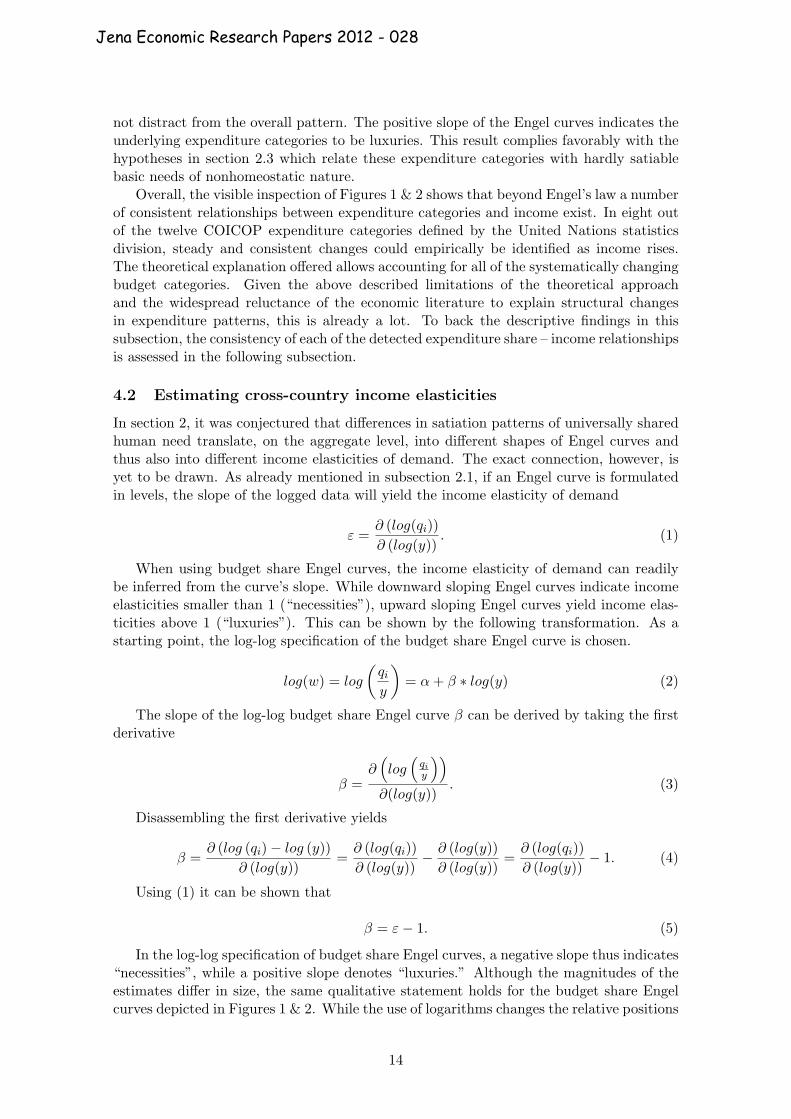
In section 2, it was conjectured that differences in satiation patterns of universally sharedhuman need translate, on the aggregate level, into different shapes of Engel curves andthus also into different income elasticities of demand. The exact connection, however, isyet to be drawn. As already mentioned in subsection 2.1, if an Engel curve is formulatedin levels, the slope of the logged data will yield the income elasticity of demand

ε =∂ (log(qi))

∂ (log(y)). (1)

When using budget share Engel curves, the income elasticity of demand can readilybe inferred from the curve’s slope. While downward sloping Engel curves indicate incomeelasticities smaller than 1 (“necessities”), upward sloping Engel curves yield income elas-ticities above 1 (“luxuries”). This can be shown by the following transformation. As astarting point, the log-log specification of the budget share Engel curve is chosen.

log(w) = log

(

qiy

)

= α+ β ∗ log(y) (2)

The slope of the log-log budget share Engel curve β can be derived by taking the firstderivative

β =∂(

log(

qiy

))

∂(log(y)). (3)

Disassembling the first derivative yields

β =∂ (log (qi)− log (y))

∂ (log(y))=

∂ (log(qi))

∂ (log(y))−

∂ (log(y))

∂ (log(y))=

∂ (log(qi))

∂ (log(y))− 1. (4)

Using (1) it can be shown that

β = ε− 1. (5)

In the log-log specification of budget share Engel curves, a negative slope thus indicates“necessities”, while a positive slope denotes “luxuries.” Although the magnitudes of theestimates differ in size, the same qualitative statement holds for the budget share Engelcurves depicted in Figures 1 & 2. While the use of logarithms changes the relative positions

14


of the observations (which stretches differences between observations in the lower rangeand wraps in the higher range), it does not change the sequence of the observations. Usingthe log-log specification will thus not turn a positive into a negative relationship and viceversa.

To assess the consistency of the cross-country budget share Engel curves, income elas-ticities of demand are estimated using the log-log specification. Figures A4 & A5 plot thetransformed data. For each expenditure category, the raw data and a fitted linear lineis displayed. In line with the above argument, the direction of the fitted lines complieswith the qualitative results of Figure 1. Moreover, it can be observed that the logarithmictransformation sufficiently reduces the nonlinearities of the budget share Engel curves suchthat a parametric linear fit seems to be appropriate in most cases.

Table 1: Cross-country income elasticities of demand

Expenditure category ε R2 R2i /R

2food

Food 0.49 0.80 1Recreation & culture 1.55 0.72 0.90Miscellaneous goods & services 1.40 0.40 0.50Housing & utilities 1.23 0.37 0.46Restaurants & hotels 1.33 0.25 0.31Furnishings & household equipment 1.18 0.23 0.29Transport 1.14 0.22 0.28Education 0.67 0.10 0.13Health 1.18 0.05 0.06Communication 1.17 0.05 0.06Clothing 0.92 0.03 0.04Alcohol & tobacco 0.94 0.01 0.01

Notes: The income elasticities of demand are estimated using equations(2) and (5). All estimations use the full sample described in Table A2.

A convenient and well known measure of consistency of a parametric linear fit tothe data is the coefficient of determination, R2. As the ordinary least squares estimatorminimizes the sum of squared residuals (unexplained variance) the R2 that measures theshare of variation in the dependent variable explained by the variation in the covariate (1-unexplained/total sample variance) is a straightforward measure to assess the predictivequality and thus the consistency of the model.

Table 1 reports the cross-country income elasticities of demand for all twelve COICOPexpenditure categories. Alongside the coefficient of determination, the third column re-ports the model fit relative to the R2 for food. It is readily apparent from Figure 1 that theclear and clean pattern obtained from the Engel curve for food is outstanding comparedto the remaining categories. The pin sharp pattern of the Engel curve for food thus lendsitself to act as a benchmark for judging the relative consistency of the remaining patterns.The lines are ordered by decreasing model fit.

Unsurprisingly, the well known Engel’s law relationship turned out to exhibit the high-est values in terms of the chosen consistency measure. Likewise expectedly, the categoriesthat do not show systematic changes in expenditure shares as income rises, i.e., alcohol& tobacco, health, communication, and education, score low in terms of predictability, i.e.,income can hardly be used to predict the expenditure shares in these categories.

Alongside the expenditure share for food, the six expenditures categories that showsystematically increasing budget shares score relatively high in terms of consistency. Most

15


remarkably is the case of the expenditure share – income relationship for recreation &

culture that is almost as strict as the famous relationship discovered by Ernst Engel(R2

i /R2food = 0.90). Among the remaining five increasing Engel curve relationships, the

relative consistency measure ranges between 0.5 and about 0.3. Bearing in mind thatthe expenditure shares are related to only one explanatory variable, i.e., PPP adjustedreal income, these values are in fact remarkable. Among the expenditure categories thatcould be related to universally shares human contingencies in subsection 2.3, only clothing

displays very low R2 values. An inspection of the data (see Figures 1 & A4) indicatesthat the data consists of two parallel downward sloping clusters. Accounting for thisparticularity would yield a more consistent and stronger negative relationship.

Overall, the results presented in this subsection support the findings of the visualinspection of cross-country Engel curves in the former subsection. In all cases the estima-tion of cross-country income elasticities of demand conform with the identified structuralchanges in the corresponding Engel curves. While expenditure categories that can be re-lated to hardly satiable needs show increasing slopes and income elasticities above unity,expenditure categories related to easily satiable needs show decreasing Engel curve slopesand income elasticities below unity. Except for clothing, the consistency of these relation-ships is remarkably high.

4.3 How similar are the underlying country level Engel curves?

The previous subsections evaluated the shape and the consistency of the cross-countryEngel curves. It could be shown that beyond Engels law a number of theoretically foundedempirical regularities exist. Almost axiomatic examples are the budget share – incomerelationship for food and recreation & culture. The results point to very uniform shapes ofEngel curves across countries and cultures, which imply a highly powerful and predictiveconnection.

Alongside the more general results presented above, a country level perspective isoffered in this subsection, too. While the former analysis draws upon the pooled sampleof observations to obtain a general impression of the respective relationships, the countrylevel was neglected. The observed strictness and consistency in the general patterns might,however, consist of a number of countrywise clustered data points that have somewhatdifferent functional forms at the country level. The utmost degree of consistency wouldrequire to show that the uniform cross-country Engel curve pattern results from uniformEngel curves at the country level.

Therefore the functional form of the Engel curves at the country level is comparedwith the overall shape of the cross-country Engel curves for the two strictest expenditureshare - income relationships, i.e., food and recreation & culture. More precisely, it is testedwhether the coefficients of the parametrically described country level Engel curves matchthe coefficients of the overall functional relationship. As both cross-country Engel curvesfollow some kind of a logarithmic functional relationship, the following nonlinear leastsquares regression is estimated:

wi = α+ β ∗ log(y) + ε. (6)

The nonlinear least squares regression a priori presumes a logarithmic functional formand estimates the coefficients α and a coefficient β that indicates the curvature of thelogarithmic fit.10

10Nonlinear least squares is an optimization technique that determines values of the coefficients whichminimize the sum of squared residuals through iterative processes.

16


Figure 3: Changes in expenditure shares with rising income−

.50

.51

Exp

S1

0 10000 20000 30000 40000 50000GDP_ppp_cap_2005

−.1

0.1

.2.3

Exp

S9

0 10000 20000 30000 40000 50000GDP_ppp_cap_2005

0.2

.4.6

.8E

xpS

1

0 10000 20000 30000 40000 50000GDP_ppp_cap_2005

−.0

50

.05

.1.1

5E

xpS

9

0 10000 20000 30000 40000 50000GDP_ppp_cap_2005

Notes: The left hand side charts display the Engel curves for food while the right hand side charts showrecreation & culture. The upper charts present the fitted functional forms at the country level for alleligible countries using equation (6). The lower charts present the reduced samples of countries for whichno statistically different coefficients can be found. The bold face solid black lines depict the locally weightedsmoothing scatterplots of the respective expenditure share on PPP adjusted real GDP. The bold face solidmaroon lines depict the functional fit of the overall sample using equation (6).

Equation (6) is first applied to the overall sample to estimate benchmark coefficients.The practicality of the benchmark is assessed by two criteria. Firstly, the fitted valuesof the nonlinear regression are compared to the locally weighted smoothing scatterplotapplied in subsection 4.1. Secondly, the coefficient of determination, R2, of the nonlinearestimations should be sufficiently high. Regarding the first criteria, Figure 3 shows that thesmoothed and the fitted lines overlap favorably. Moreover, the R2 of the nonlinear leastsquares regressions for food and recreation & culture exceed 0.80 and 0.65 respectively.Both benchmark criteria are thus met reasonably.11

To sensibly estimate a nonlinear fit on the country level, some restrictions on the dataare required. The country level data should, on the one hand, consist of ,say, more thanat least 10 data points and lie, on the other hand, in the nonlinear part of the cross-country Engel curve. Countries for which only observations in the flat high income rangeare available, like Luxembourg or Switzerland, are thus not eligible. Likewise, countriesfor which observations are only available in the vertical lower income space cannot beused as well. Tables A3 and A4 report the eligible sample and the estimated results.

11Of course also other, more complex, functional forms could be presumed. Applying, for example,an exponential fit of the form wi = α + β1 ∗ β

y2+ ε provides an even better approximation of the locally

weighted smoothing scatterplots. The R2 improves by 0.01. To maintain the simplicity of the illustrativeexercise, the simpler model (equation (6)) is chosen where only two instead of three coefficients have to becompared. Results for the more complex model are available upon request from the author.

17


After omitting a number of countries for the above given reasons, about 30 countries stillqualify for the analysis.

Expenditure share data is not available for all countries over the complete incomerange (see Table A2). A longer observation period is typically available for rather affluentcountries, while for less affluent countries periods range between the most recent 5 to20 years. The functional form of the country level Engel curves is determined given thelimited data at hand.

The results are presented in Figure 3 and Tables A3 & A4. Tables A3 & A4 reportthe coefficient estimates, standard errors, and the coefficient’s 95% confidence intervalsfor each country. The left hand side charts display the Engel curves for food, while theright hand side charts show recreation & culture. The upper charts in Figure 3 presentthe estimated functional forms at the country level for all eligible countries. In bothexpenditure categories a certain heterogeneity is observable. Remarkable is, however,that only in very few cases the estimated functional relationships run counter the overallrelationship. The lower charts present the reduced samples of countries for which nostatistically different coefficients can be found.12 Given the heterogeneity of the dataavailability, the results reflect a surprisingly high degree of similarity also on the countrylevel. This robustness check strengthens and substantiates the overall consistency of thecross-country Engel curves observed in the previous subsections.

5 Conclusions

Since the work of Ernst Engel it is a well established fact that the expenditure sharededicated to food consumption decreases as income rises (Engel’s law). The extraordinaryconsistency across time and space and the predictive character of the relationship led to itsuse to determine absolute household poverty and the definition of poverty lines. Especiallywhen defining final per capita poverty lines, there is a shared conviction among researchersthat also among the poorest a certain amount of non food spending is necessary. In thispaper, it is argued that the ad-hoc nature of the non food necessity scalar choice suffersfrom a still missing comprehension of why and which consumption items are necessitiesand which are not.

Although Engel’s law is an essential nonmonetary determinant when distinguishing be-tween poverty and wealth, it covers only one decreasing fraction of consumer expenditureas income rises. In contrast, empirical evidence on systematic changes in other consumerexpenditures categories is hardly used. A systematic assessment of structural changes inconsumer expenditure categories as income rises should, however, allow for a more com-plete and multidimensional assessment of wealth. The lack of such an assessment is evenmore remarkable as Ernst Engel already pursued a much more encompassing approach.In fact, Engel’s original work was an inquiry into the structural changes of consumptionpatterns with rising income aiming to determine a measure of household welfare. Withhis pioneering work on a distinction between necessities and luxuries, Engel was not onlythe first to empirically assess this taxonomy but also the first to attempt a behaviorallyfounded – need based – explanation.

To build upon Engel’s legacy, this paper, on the one hand, improves on part of the the-oretical assumptions by enriching Engel’s original approach with current scientific knowl-edge on the nature of consumer needs and how they are satisfied. The behavioral approachto consumer behavior offered in section 2 allows for the formulation of expectations aboutstructural changes of expenditure shares as income rises. While expenditure categories

12The coefficients cannot be said to differ statistically if the confidence intervals are overlapping.

18


that can be associated with hardly satiable needs of nonhomeostatic nature are conjec-tured to show increasing cross-country budget share Engel curves that reflect an incomeelasticity of demand above unity (”luxury”), expenditure categories that can be associ-ated with easily satiable needs of homeostatic nature are conjectured to show decreasingslopes, reflecting income elasticities of demand below unity (”necessity”). The hypothesesput forward already imply that from a behavioral consumption approach perspective thereare good reasons to expect the existence of more than one robust empirical regularity inthe analysis of demand patterns.

On the other hand, this paper assesses the systematic changes of consumer expenditureshares with rising income. The paper presents an empirical analysis of observable changesin consumption patterns across countries and time, using a data set that contains indi-vidual consumption expenditure in 12 categories for more than 50 countries over up to 50years. Utilizing a nonparametric regression technique, it is explored whether expenditurecategories, inclusive of, but extending beyond, food, change systematically with rising in-come. This way a number of empirical regularities in consumer expenditure patterns canbe identified that go well beyond Engel’s law. In eight out of twelve expenditure categoriessteady and consistent changes could empirically be identified as income rises. The theo-retical explanation offered allows accounting for all of the systematically changing budgetcategories. Alongside the Engel curve for food, an almost axiomatic example is the Engelcurve for recreation & culture. The results point to very uniform shapes of Engel curvesacross countries and cultures, which imply a highly powerful and predictive connection.

Our findings confirm the conjecture that the distinction between luxuries and necessi-ties rests upon behavioral foundations that can be traced back to the differing satiationfeatures of the underlying universally shared needs. The study contributes to the literatureon income and wealth by a structural assessment of general changes in budget shares acrosscountries that helps to broaden our understanding of the behavioral foundations on thenecessity – luxury taxonomy. In doing so, it broadens the scope for a more encompassingand multidimensional consumption based assessment of wealth.

References

Almas, I. (2012). International income inequality: Measuring PPP bias by estimatingEngel curves for food. American Economic Review, 102(2):1093–1117.

Balassa, B. (1964). The purchasing-power parity doctrine: A reappraisal. The Journal of

Political Economy, 72(6):584–596.

Banks, J., Blundell, R., and Lewbel, A. (1997). Quadratic Engel curves and consumerdemand. The Review of Economics and Statistics, 79(4):527–539.

Bowman, A. W. and Azzalini, A. (1997). Applied Smoothing Techniques for Data Analysis.Oxford University Press, Oxford (UK).

Caplan, A. (1978). The Sociobiology Debate. Harper & Row, New York.

Chai, A. (2011). Consumer specialization and the romantic transformation of the BritishGrand Tour of Europe. Journal of Bioeconomics, 13:181–203.

Chai, A. and Moneta, A. (2010). Retrospectives: Engel curves. Journal of Economic

Perspectives, 24(1):225–40.

Charles, K. K., Hurst, E., and Roussanov, N. (2009). Conspicuous consumption and race.The Quarterly Journal of Economics, 124(2):425–467.

19


Cleveland, W. S. (1979). Robust locally weighted regression and smoothing scatterplots.Journal of the American Statistical Association, 74(368):829–836.

Deaton, A. (1997). The analysis of household surveys: A microeconometric approach to

development policy. Johns Hopkins University Press. The World Bank.

Duesenberry, J. S. (1949). Income, Saving and the Theory of Consumer Behavior. HarvardUniversity Press, Cambridge (MA).

Engel, E. (1857). Die Produktions- und Consumptions Verhaltnisse des Konigreichs Sach-sen. Zeitschrift des Statistischen Bureaus des Koniglich Sachsischen Ministeriums des

Inneren, 8 and 9. Reprinted in the Appendix of Engel (1895).

Engel, E. (1895). Die Lebenskosten belgischer Arbeiterfamilien fruher und jetzt. Bulletinde l’Institut International de Statistique, 9:1–124.

Engel, J. and Kneip, A. (1996). Recent approaches to estimating Engel curves. Journal

of Economics, 63:187–212.

Frank, R. H. (1999). Luxury fever. Money and happiness in an ara of excess. PrincetonUniversity Press.

Frank, R. H. (2011). The Darwin Economy. Princeton University Press, Princeton (NJ).

Frenzel Baudisch, A. (2006). Continuous market growth beyond functional satiation.Time-series analyses of U.S. footwear consumption, 1955-2002. Papers on Economicsand Evolution 2006-03, Max Planck Institute of Economics, Evolutionary EconomicsGroup.

Georgescu-Roegen, N. (1954). Choice, expectations and measurability. The Quarterly

Journal of Economics, 68(4):503–534.

Harrod, R. F. (1933). International Economics. Cambridge University Press, London.

Hart, Jeffrey, D. (1997). Nonparametric Smoothing and Lack-of-Fit Tests. Springer Verlag,New York.

Herrnstein, R. J. (1990). Behavior, reinforcement and utility. Psychological Science,1(4):217–224.

Herrnstein, R. J. (1997). The Matching Law. Harvard University Press, Cambridge (MA).

Heston, A., Summers, R., and Aten, B. (2011). Penn World Table 7.0. Center for Interna-tional Comparisons of Production, Income and Prices at the University of Pennsylvania.

Hirsch, F. (1978). Social limits to growth. Harvard University Press, Cambridge (MA).

Houthakker, H. S. (1957). An international comparison of household expenditure patterns,commemorating the centenary of Engel’s law. Econometrica, 25(4):532–551.

Hull, C. L. (1943). Principles of Behavior. Appleton-Century-Crofts, New York.

Ironmonger, D. S. (1972). New Commodities and Consumer Behavior. Cambridge Uni-versity Press, Cambridge (MA).

Kahneman, D., Wakker, P. P., and Sarin, R. (1997). Back to Bentham? Explorations ofexperienced utility. The Quarterly Journal of Economics, 112(2):375–405.

20


Lanjouw, O. J. and Lanjouw, P. (2001). How to compare apples and oranges: Povertymeasurement based on different definitions of consumption. Review of Income and

Wealth, 47(1):25–42.

Lewbel, A. (2008). Engel curve. In Durlauf, S. N. and Blume, L. E., editors, The New

Palgrave Dictionary of Economics. Palgrave Macmillan, Basingstoke.

Menger, C. (1871). The Principles of Economics. Free Press (1950), Glenco (IL).

Musgrove, P. (1985). Food needs and absolute poverty in urban South America. Review

of Income and Wealth, 31(1):63–83.

Nadaraya, E. A. (1964). On estimating regression. Theory of Probability and its Applica-

tions, 10:186–190.

Samuelson, P. A. (1964). Theoretical notes on trade problems. The Review of Economics

and Statistics, 46(2):145–154.

Scitovsky, T. (1981). The desire for excitement in modern society. Kyklos, 34(1):3–13.

Seale, J. L. and Regmi, A. (2006). Modelling international consumption patterns. Reviewof Income and Wealth, 52(4):603–624.

Staddon, J. E. R. and Cerutti, D. T. (2003). Operant conditioning. Annual Review of

Psychology, 54:115–144.

Watson, G. S. (1964). Smooth regression analysis. Sankhya: The Indian Journal of

Statistics, Series A, 26(4):359–372.

Wilson, E. O. (1975). Sociobiology: The New Synthesis. Harvard University Press, Cam-bridge (MA).

Witt, U. (2001). Learning to consume - a theory of wants and the growth of demand.Journal of Evolutionary Economics, 11(1):23–36.

Witt, U. (2008). What is specific about evolutionary economics? Journal of Evolutionary

Economics, 18(5):547–575.

Witt, U. (2010a). Product characteristics, innovations and the evolution of consumption. Abehavioral approach. mimeo. Paper prepared for the conference on “Technical Change:History, Economics and Policy” in honor of G.N. Tunzelmann, SPRU, March 2010.

Witt, U. (2010b). Symbolic consumption and the social construction of product charac-teristics. Structural Change and Economic Dynamics, 21(1):17–25.

Witt, U. (2011). The dynamics of consumer behavior and the transition to sustainableconsumption patterns. Environmental Innovation and Societal Transitions, 1(1):109–114.

21


A Appendix

A.1 Outlier treatment

In a cross sectional setting, it is usually convenient to cut expenditures on the category ofinterest as well as the income variable at a specific boundary. As a cutoff point, the meanplus three standard deviations is a commonly used rule of thumb (see, e.g., Banks et al.,1997). This kind of standard procedure however does not fit in with the data structure inthis paper.

The empirical setting applied in this paper combines annual country level data formore than 50 countries. Pooling the data of various years implies obtaining a cloudof data points for each country. Depending on the number of years for which data isavailable, the respective data cloud varies in size. Combining the data of various countriesthen results in more or less overlapping countrywise clusters. Outliers thus usually don’ttake the form of displaced single points but separate clusters.

Being interested in assessing and describing structural changes in consumption patternsas income rises, the particularities in a certain country should not determine the overallshape of the estimated Engel curve. An outlying cluster of observations should accordinglybe eliminated. Figures A1 to A3 present the applied outlier treatment.

The left hand side charts plot the locally weighted smoothing scatterplots without anyoutlier treatment. In some cases, the estimated local linear regression curve thus showsunrepresentative shifts. The right hand side charts in Figures A1 to A3 additionally markoutliers with ellipses and/or green color. For comparison, the locally weighted smoothingscatterplots are estimated without the outlying observations. Moreover, another locallinear regression curve, which applies the standard procedure of cutting off observationsabove the mean plus three standard deviations, is added.

Without any outlier treatment, the estimated nonparametric curves would yield un-representative shifts particularly in the higher income range. Most remarkable examplesare the expenditure categories alcohol & tobacco, health, and recreation & culture. A com-parison of both outlier treatments yields remarkable differences too. At least for alcohol &tobacco and furnishings & household equipment the data cloud for Luxembourg lies abovethe overall pattern. Applying the standard outlier procedure omits only a part of the datacloud. The estimated local linear regression curve thus remains affected. The comparisonof the left with the right hand side charts in Figures A1 to A3 shows the need for anoutlier treatment that accounts for the countrywise clustered structure of the data.

Overall, it can be summarized that especially Luxembourg, the country with the high-est income, causes changes in the slope of the locally weighted smoothing scatterplots.Other readily visible outliers are much less disturbing. In fact, only in one case (health)the shape of the estimated curves is affected by countries other than Luxembourg. Al-though the outlier treatment proposed here may appear arbitrary at the first glance, itcan be concluded that it reasonably fits the structure of the data.

22


Figure A1: Changes in expenditure shares with rising income - Outlier correction.1

.2.3

.4.5

.6E

xpS

1


Food on GDP_ppp Food on real GDPGDP_ppp (lowess) real GDP (lowess)

.1.2

.3.4

.5.6

Exp

S1


Food on GDP_ppp Food on real GDPGDP_ppp (lowess) real GDP (lowess)GDP_ppp (lowess<mean+3sd) mean+3sd cut offLuxembourg (GDP_ppp) Luxembourg (rGDP)

0.0

5.1

.15

Exp

S2


Alc/Tob on GDP_ppp Alc/Tob on real GDPGDP_ppp (lowess) real GDP (lowess)

0.0

5.1

.15

Exp

S2

0 20000 40000 60000 80000 100000GDP_ppp_cap_2005 / rGDP_cap_2005

Alc/Tob on GDP_ppp Alc/Tob on real GDPGDP_ppp (lowess) real GDP (lowess)GDP_ppp (lowess<mean+3sd) Luxembourgmean+3sd cut off

0.0

5.1

.15

Exp

S3


Clothing on GDP_ppp Clothing on real GDPGDP_ppp (lowess) real GDP (lowess)

0.0

5.1

.15

Exp

S3


Clothing on GDP_ppp Clothing on real GDPGDP_ppp (lowess) real GDP (lowess)GDP_ppp (lowess<mean+3sd) mean+3sd cut offLuxembourg (GDP_ppp) Luxembourg (rGDP)

.05

.1.1

5.2

.25

.3E

xpS

4


Housing on GDP_ppp Housing on real GDPGDP_ppp (lowess) real GDP (lowess)

0.1

.2.3

.4E

xpS

4


Housing on GDP_ppp Housing on real GDPGDP_ppp (lowess) real GDP (lowess)GDP_ppp (lowess<mean+3sd) mean+3sd cut offLuxembourg (GDP_ppp) Luxembourg (real GDP)

Notes: The left hand side charts plot the locally weighted smoothing scatterplots of the respective expendi-ture share on real GDP (red dashed line) as well as on PPP adjusted real GDP (black solid line). The righthand side charts additionally mark the identified outliers with ellipses and/or green color. For comparisonthe locally weighted smoothing scatterplots are run without the outlying observations. Moreover anotherlocal linear regression curve for PPP adjusted real GDP is added that applies the standard procedure ofcutting off observations above the mean plus three standard deviations (brown solid line). In all cases thesmoothing parameter is 0.7.

23


Figure A2: Changes in expenditure shares with rising income - Outlier correction.0

2.0

4.0

6.0

8.1

.12

Exp

S5


Furniture on GDP_ppp Furniture on real GDPGDP_ppp (lowess) real GDP (lowess)

.02

.04

.06

.08

.1.1

2E

xpS

5


Furniture on GDP_ppp Furniture on real GDPGDP_ppp (lowess) real GDP (lowess)GDP_ppp (lowess<mean+3sd) mean+3sd cut offLuxembourg

0.0

5.1

.15

.2E

xpS

6


Health on GDP_ppp Health on real GDPGDP_ppp (lowess) real GDP (lowess)

0.0

5.1

.15

.2E

xpS

6


Health on GDP_ppp Health on real GDPGDP_ppp (lowess) real GDP (lowess)GDP_ppp (lowess<mean+3sd) mean+3sd cut offUnited States; Switzerland Luxembourg

.05

.1.1

5.2

.25

Exp

S7


Transport on GDP_ppp Transport on real GDPGDP_ppp (lowess) real GDP (lowess)

.05

.1.1

5.2

.25

Exp

S7


Transport on GDP_ppp Transport on real GDPGDP_ppp (lowess) real GDP (lowess)GDP_ppp (lowess<mean+3sd) mean+3sd cut offLuxembourg (GDP_ppp) Luxembourg (real GDP)

0.0

2.0

4.0

6.0

8E

xpS

8


Communication on GDP_ppp Communication on rGDPGDP_ppp (lowess) real GDP (lowess)

0.0

2.0

4.0

6.0

8E

xpS

8


Communication on GDP_ppp Communication on rGDPGDP_ppp (lowess) real GDP (lowess)GDP_ppp (lowess<mean+3sd) mean+3sd cut offLuxembourg


24


Figure A3: Changes in expenditure shares with rising income - Outlier correction0

.05

.1.1

5E

xpS

9


Recreation on GDP_ppp Recreation on real GDPGDP_ppp (lowess) real GDP (lowess)

0.0

5.1

.15

.2E

xpS

9


Recreation on GDP_ppp Recreation on rGDPGDP_ppp (lowess) real GDP (lowess)GDP_ppp (lowess<mean+3sd) mean+3sd cut offLuxembourg (GDP_ppp) Luxembourg (rGDP)

0.0

2.0

4.0

6.0

8.1

Exp

S10


Education on GDP_ppp Education on real GDPGDP_ppp (lowess) real GDP (lowess)

0.0

2.0

4.0

6.0

8.1

Exp

S10


Education on GDP_ppp Education on real GDPGDP_ppp (lowess) real GDP (lowess)GDP_ppp (lowess<mean+3sd) mean+3sd cut offLuxembourg (GDP_ppp) Luxembourg (rGDP)

0.0

5.1

.15

.2E

xpS

11


Restaurants on GDP_ppp Restaurants on real GDPGDP_ppp (lowess) real GDP (lowess)

0.0

5.1

.15

.2E

xpS

11


Restaurants on GDP_ppp Restaurants on rGDPGDP_ppp (lowess) real GDP (lowess)GDP_ppp (lowess<mean+3sd) mean+3sd cut offGreece, Ireland, Malta, Spain Luxembourg

0.0

5.1

.15

.2.2

5E

xpS

12


Miscellaneous on GDP_ppp Miscellaneous on rGDPGDP_ppp (lowess) real GDP (lowess)

0.0

5.1

.15

.2.2

5E

xpS

12


Miscellaneous on GDP_ppp Miscellaneous on rGDPGDP_ppp (lowess) real GDP (lowess)GDP_ppp (lowess<mean+3sd) mean+3sd cut offLuxembourg Brit. Virgin Islands.


25


A.2 Figures & tables

Table A1: COICOP expenditure categoriesExpenditure category Description

1 Food All kinds of food and nonalcoholic beverages consumed at home2 Alcohol & tobacco Spirits, wine, beer, tobacco, narcotics3 Clothing Clothing & footwear incl. related services (cleaning, repair, hire)4 Housing & utilities Rentals, maintenance & repair of dwelling, electricity, water, sew-

erage, gas, other fuels (incl. heat energy)5 Furnishings & household

equipmentFurniture & furnishings, carpets, household appliances, glass- &tableware, routine maintenance of dwelling, related services

6 Health Pharmaceutical & therapeutical products/equipment, outpatientservices (medical & dental), hospital services

7 Transport Purchase of vehicles, fuels, maintenance, services by air, rail, road,waterways

8 Communication Postal services, telephone/fax services & equipment9 Recreation & culture Recreation equipment & services, cultural services, package holidays10 Education Expenses on primary, secondary, tertiary, and other education11 Restaurants & hotels Expenses on catering, restaurants, cafes, canteens, accommodation

services12 Miscellaneous goods &

servicesPersonal care, prostitution, personal effects (incl. jewelry), socialprotection, insurances (incl. live, dwelling, health, transport), fi-nancial services, other services

Notes: The expenditure categories are defined according to the UN Statistics Division’s Classification

of Individual Consumption According to Purpose (COICOP).

Table A2: Availability of data by countries

# Country first year last year N

1 Australia 1959 2007 492 Belarus 1994 2007 143 Botswana 1994 2001 84 British Virgin Islands 1995 1999 55 Bulgaria 1995 2006 126 Cameroon 1996 2004 97 Canada 1970 2007 388 Hong Kong, ChinaJ 1966 2004 239 Macao, ChinaJ 1993 2007 1510 Colombia 1994 2005 1211 Croatia 1999 2006 812 Czech Republic 1992 2007 1613 Denmark 1966 2007 4214 Dominican Republic 1991 1996 615 Estonia 1994 2007 1416 Finland 1975 2007 3317 France 1959 2008 5018 Germany 1991 2007 1719 Greece 1960 2004 4520 Guatemala 2001 2006 621 Honduras 2000 2005 622 Hungary 1995 2008 1423 Iceland 1990 2006 1724 India 1999 2007 925 IranD 1992 2007 1626 Ireland 1990 2007 1827 Israel 1995 2007 1328 Italy 1970 2007 3829 Japan 1980 2007 28

26


Table A2 – continued from previous page

# Country first year last year N

30 KenyaD 1996 2007 1231 Korea, Rep. 1970 2007 3832 Kyrgyzstan 2000 2005 633 Latvia 1995 2007 1334 Lithuania 1995 2007 1335 Luxembourg 1985 2007 2336 Malaysia 2000 2007 837 Malta 1996 2007 1238 Mexico 1988 2004 1739 Mongolia 1997 2007 1140 NamibiaD 2000 2007 841 Netherlands 1987 2007 2142 Netherlands AntillesF 1997 2006 1043 New ZealandD 1987 2007 2144 Nicaragua 1994 2005 1245 NigerF 2003 2008 646 Norway 1980 2006 2747 Papua New GuineaD 1992 2003 1248 Poland 1995 2007 1349 Serbia 2002 2007 650 Sierra LeoneF 2001 2007 751 Singapore 1996 2008 1352 Slovakia 1993 2007 1553 Slovenia 1995 2007 1354 Solomon Islands 2003 2007 555 South AfricaJ 1946 2008 6356 Spain 1995 2007 1357 Sri Lanka 1998 2007 1058 Sweden 1993 2007 1559 Switzerland 1990 2006 1760 Yugoslavia, former (Macedonia) 1996 2007 1261 Ukraine 2001 2007 762 United Kingdom 1970 2007 3663 United States 1970 2007 3864 YemenD 1996 2007 12

Notes: Countries indicated with D are dropped from the analysis due to missings

in more than two expenditure share categories. Countries indicated with F are

dropped from the analysis as they reported no changes in any expenditure share

over the sample period. Countries indicated with J are dropped from the analysis

due to huge – implausible – jumps in expenditure shares at a certain point in time.

27


Table A3: Country level nonlinear least squares estimates of the Engel curve for foodCountry Coef. Std. Err. 95% Conf. Intervalall α 1.35 0.02 1.32 1.38

β 0.12 0.00 0.11 0.12Belarus α 1.75 0.30 1.10 2.40

β 0.14 0.03 0.07 0.22Canada α 1.26 0.06 1.15 1.37

β 0.11 0.01 0.10 0.12Denmark α 1.41 0.03 1.36 1.46

β 0.12 0.00 0.12 0.13France α 1.29 0.01 1.26 1.32

β 0.11 0.00 0.11 0.11Germany α 1.19 0.12 0.92 1.45

β 0.10 0.01 0.08 0.13Hungary α 1.44 0.12 1.18 1.70

β 0.13 0.01 0.10 0.16Ireland α 1.32 0.06 1.19 1.45

β 0.12 0.01 0.10 0.13Israel α 1.61 0.64 0.20 3.02

β 0.14 0.06 0.01 0.28Lithuania α 1.85 0.23 1.35 2.34

β 0.17 0.02 0.11 0.22Poland α 1.56 0.16 1.22 1.90

β 0.14 0.02 0.11 0.18Slovakia α 1.54 0.26 0.98 2.10

β 0.14 0.03 0.08 0.20Spain α 1.19 0.11 0.94 1.44

β 0.10 0.01 0.08 0.13United States α 1.18 0.04 1.09 1.26

β 0.10 0.00 0.10 0.11Australia α 0.82 0.03 0.76 0.89

β 0.07 0.00 0.06 0.08Bulgaria α 2.47 0.31 1.78 3.17

β 0.25 0.04 0.17 0.33Czech Republic α 2.83 0.53 1.69 3.96

β 0.27 0.05 0.15 0.39Estonia α 1.87 0.16 1.51 2.23

β 0.17 0.02 0.14 0.21Finland α 1.91 0.12 1.66 2.15

β 0.17 0.01 0.15 0.20Greece α 2.00 0.12 1.75 2.25

β 0.18 0.01 0.16 0.21Iceland α 1.84 0.12 1.59 2.08

β 0.16 0.01 0.14 0.19Italy α 2.79 0.04 2.70 2.87

β 0.26 0.00 0.25 0.27Japan α 1.74 0.06 1.63 1.86

β 0.15 0.01 0.14 0.17Korea, Rep. α 1.53 0.04 1.45 1.60

β 0.14 0.00 0.13 0.15Latvia α 1.93 0.18 1.53 2.33

β 0.18 0.02 0.14 0.23Netherlands α 1.04 0.03 0.97 1.10

β 0.09 0.00 0.08 0.09Norway α 1.13 0.04 1.06 1.20

β 0.09 0.00 0.08 0.10Singapore α 0.13 0.05 0.02 0.24

β 0.00 0.00 -0.01 0.02Sweden α 0.66 0.11 0.43 0.89

β 0.05 0.01 0.03 0.07United Kingdom α 1.88 0.07 1.74 2.02

β 0.17 0.01 0.16 0.19Notes: The table reports the coefficients, standard errors andthe coefficient’s 95% confidence intervals of countrywise estima-tions using equation (6).

28


Table A4: Country level nonlinear least squares estimates of the Engel curve for recreation& culture

Country Coef. Std. Err. 95% Conf. Intervalall α -0.22 0.01 -0.23 -0.20

β 0.03 0.00 0.03 0.03Australia α -0.15 0.02 -0.19 -0.12

β 0.03 0.00 0.02 0.03Belarus α -0.23 0.03 -0.30 -0.15

β 0.03 0.00 0.02 0.04Czech Republic α -0.19 0.09 -0.38 -0.01

β 0.03 0.01 0.01 0.05Denmark α -0.26 0.02 -0.31 -0.22

β 0.04 0.00 0.03 0.04Estonia α -0.29 0.06 -0.42 -0.16

β 0.04 0.01 0.02 0.05Finland α -0.14 0.02 -0.19 -0.10

β 0.03 0.00 0.02 0.03Korea, Rep. α -0.19 0.02 -0.23 -0.15

β 0.03 0.00 0.02 0.03Latvia α -0.29 0.07 -0.44 -0.15

β 0.04 0.01 0.02 0.06Lithuania α -0.27 0.09 -0.47 -0.07

β 0.04 0.01 0.01 0.06Slovakia α -0.05 0.05 -0.17 0.06

β 0.01 0.01 0.01 0.03Spain α -0.11 0.06 -0.24 0.02

β 0.02 0.01 0.01 0.03Sweden α -0.27 0.10 -0.49 -0.05

β 0.04 0.01 0.02 0.06United States α -0.29 0.02 -0.32 -0.25

β 0.04 0.00 0.03 0.04Bulgaria α -0.37 0.06 -0.50 -0.24

β 0.05 0.01 0.03 0.06Canada α -0.38 0.03 -0.44 -0.33

β 0.05 0.00 0.04 0.05France α -0.06 0.01 -0.08 -0.04

β 0.01 0.00 0.01 0.02Germany α -0.04 0.10 -0.25 0.18

β 0.01 0.01 -0.01 0.03Greece α -0.01 0.01 -0.04 0.01

β 0.01 0.00 0.00 0.01Hungary α 0.10 0.03 0.03 0.17

β -0.00 0.00 -0.01 0.00Iceland α 0.09 0.14 -0.20 0.38

β 0.00 0.01 -0.02 0.03Ireland α 0.22 0.02 0.17 0.26

β -0.01 0.00 -0.02 -0.01Israel α 0.18 0.16 -0.17 0.52

β -0.01 0.02 -0.05 0.02Italy α -0.07 0.02 -0.11 -0.03

β 0.01 0.00 0.01 0.02Japan α -0.51 0.09 -0.70 -0.33

β 0.06 0.01 0.04 0.078Netherlands α 0.33 0.05 0.23 0.42

β -0.02 0.00 -0.03 -0.01Norway α -0.64 0.03 -0.70 -0.58

β 0.07 0.00 0.07 0.08Poland α 0.31 0.09 0.12 0.50

β -0.02 0.01 -0.04 -0.01Singapore α 0.60 0.12 0.35 0.86

β -0.05 0.01 -0.07 -0.02United Kingdom α -0.36 0.02 -0.39 -0.32

β 0.05 0.00 0.04 0.05Notes: The table reports the coefficients and 95% confidenceintervals of countrywise estimations of equation (6).

29


Figure A4: Changes in log expenditure shares with rising log income

−2.

5−

2−

1.5

−1

−.5

log(

Exp

S_f

ood)

7 8 9 10 11log(GDP_ppp_cap_2005)

−4.

5−

4−

3.5

−3

−2.

5−

2lo

g(E

xpS

_alc

ohol

_tob

acco

)

7 8 9 10 11log(GDP_ppp_cap_2005)

−4

−3.

5−

3−

2.5

−2

log(

Exp

S_c

loth

ing)

7 8 9 10 11log(GDP_ppp_cap_2005)

−3

−2.

5−

2−

1.5

−1

log(

Exp

S_h

ousi

ng_u

tiliti

es)

7 8 9 10 11log(GDP_ppp_cap_2005)

−4

−3.

5−

3−

2.5

−2

log(

Exp

S_f

urni

shin

gs)

7 8 9 10 11log(GDP_ppp_cap_2005)

−8

−6

−4

−2

log(

Exp

S_h

ealth

)

7 8 9 10 11log(GDP_ppp_cap_2005)

Notes: The charts display scatterplots for log expenditure shares on log income (PPP adjusted real GDPper capita). A linear fitted regression line is added respectively.

30


Figure A5: Changes in log expenditure shares with rising log income - continued

−3

−2.

5−

2−

1.5

log(

Exp

S_t

rans

port

)

7 8 9 10 11log(GDP_ppp_cap_2005)

−6

−5

−4

−3

−2

log(

Exp

S_c

omm

unic

atio

n)

7 8 9 10 11log(GDP_ppp_cap_2005)

−5

−4

−3

−2

−1

log(

Exp

S_r

ecre

atio

n_cu

lture

)

7 8 9 10 11log(GDP_ppp_cap_2005)

−7

−6

−5

−4

−3

−2

log(

Exp

S_e

duca

tion)

7 8 9 10 11log(GDP_ppp_cap_2005)

−6

−5

−4

−3

−2

log(

Exp

S_r

esta

uran

ts_h

otel

s)

7 8 9 10 11log(GDP_ppp_cap_2005)

−6

−5

−4

−3

−2

log(

Exp

S_m

isce

llane

ous)

7 8 9 10 11log(GDP_ppp_cap_2005)

Notes: The charts display scatterplots for log expenditure shares on log income (PPP adjusted real GDPper capita). A linear fitted regression line is added respectively.

31


Beyond Engel s Law - Pursuing an Engelian Approach to Welfare A Cross Country Analysis

Documents

Transcript of Beyond Engel s Law - Pursuing an Engelian Approach to Welfare A Cross Country Analysis