Beta functions of (3+1)-dimensional projectable Hořava gravity

Beta functions of (3 + 1)-dimensional projectable Horava gravity

Andrei O. Barvinsky ,1 Alexander V. Kurov ,1 and Sergey M. Sibiryakov 2,3,4

1Theory Department, Lebedev Physics Institute, Leninsky Prospect 53, Moscow 119991, Russia2Department of Physics & Astronomy, McMaster University, Hamilton, Ontario, L8S 4M1, Canada

3Perimeter Institute for Theoretical Physics, Waterloo, Ontario, N2L 2Y5, Canada4Institute for Nuclear Research of the Russian Academy of Sciences,60th October Anniversary Prospect, 7a, 117312 Moscow, Russia

(Received 9 November 2021; accepted 6 December 2021; published 7 February 2022)

We derive the full set of beta functions for the marginal essential couplings of projectable Horava gravityin (3þ 1)-dimensional spacetime. To this end we compute the divergent part of the one-loop effectiveaction in static background with an arbitrary spatial metric. The computation is done in several steps:reduction of the problem to three dimensions, extraction of an operator square root from the spatial part ofthe fluctuation operator, and evaluation of its trace using the method of universal functional traces. Thisprovides us with the renormalization of couplings in the potential part of the action which we combine withthe results for the kinetic part obtained previously. The calculation uses symbolic computer algebra and isperformed in four different gauges yielding identical results for the essential beta functions. We additionallycheck the calculation by evaluating the effective action on a special background with spherical spatial slicesusing an alternative method of spectral summation. We conclude with a preliminary discussion of theproperties of the beta functions and the resulting renormalization group flow, identifying several candidateasymptotically free fixed points.

DOI: 10.1103/PhysRevD.105.044009

I. INTRODUCTION AND SUMMARY

A. State of the art

Horava gravity (HG) has been suggested [1] as anapproach to quantum gravity within the framework ofrenormalizable quantum field theory (see [2–6] forreviews). The key idea is borrowed from condensed matterphysics and uses the notion of anisotropic (Lifshitz) scalingof time and space coordinates,1

t ↦ b−dt; xi ↦ b−1xi; ð1:1Þwhere d is the number of spatial dimensions and b is apositive scaling parameter. A theory whose bare (tree-level)action does not contain any irrelevant operators under thisscaling is power-counting renormalizable, implying that ithas fair chances to be perturbatively renormalizable in thestrict sense; i.e., all divergences generated within pertur-bation theory can be absorbed into redefinition of thecouplings in the action.

For any space dimension d bigger than 1, time andspace in (1.1) scale differently. Clearly, a theory of gravityformulated in this setting cannot be Lorentz invariant norcompletely diffeomorphism invariant. The special role oftime restricts possible symmetries to foliation preservingdiffeomorphisms (FDiff) which leave the constant-timeslices invariant,

t ↦ t0ðtÞ; xi ↦ x0iðt;xÞ; ð1:2Þ

where t0ðtÞ is a monotonic function. In other words, weare left with time reparametrizations and time-dependentspatial diffeomorphisms.To formulate the action of HG, the metric is expanded

into time and space components as in the Arnowitt-Deser-Misner (ADM) decomposition,

ds2 ¼ N2dt2 − γijðdxi þ NidtÞðdxj þ NjdtÞ: ð1:3Þ

The lapse N, the shift Ni, and the spatial metric γijtransform in the usual way under FDiff,

N ↦ Ndtdt0

; Ni ↦

�Nj ∂x0i

∂xj −∂x0i∂t

�dtdt0

;

γij ↦ γkl∂xk∂x0i

∂xl∂x0j : ð1:4Þ

1Throughout the paper we use Latin indices to denote thespatial directions, i ¼ 1;…; d.

Published by the American Physical Society under the terms ofthe Creative Commons Attribution 4.0 International license.Further distribution of this work must maintain attribution tothe author(s) and the published article’s title, journal citation,and DOI. Funded by SCOAP3.

PHYSICAL REVIEW D 105, 044009 (2022)

2470-0010=2022=105(4)=044009(41) 044009-1 Published by the American Physical Society

https://orcid.org/0000-0003-4127-5759

https://orcid.org/0000-0002-6222-1138

https://orcid.org/0000-0001-9972-8875

https://crossmark.crossref.org/dialog/?doi=10.1103/PhysRevD.105.044009&domain=pdf&date_stamp=2022-02-07

https://doi.org/10.1103/PhysRevD.105.044009




https://creativecommons.org/licenses/by/4.0/

https://creativecommons.org/licenses/by/4.0/

They are assigned the following dimensions under thescaling (1.1)2:

½N� ¼ ½γij� ¼ 0; ½Ni� ¼ d − 1: ð1:5Þ

The Lagrangian is then built out of all local FDiff-invariantoperators that can be constructed from these fields and havedimension less than or equal to 2d. The latter bound comesfrom the scaling dimension of the spacetime integrationmeasure ½dtddx� ¼ −2d and ensures that the terms in theaction corresponding to relevant (½O� < 2d) and marginal(½O� ¼ 2d) operators have nonpositive dimensions. This isa hallmark of power-counting renormalizability and is anecessary, but in general not sufficient, prerequisite of thetrue perturbative renormalizability.The precise form of the action and its physical content

depends on the assumption about the form of the lapsefunction N. In the nonprojectable version of HG N isassumed to be a full-fledged dynamical field that hasdependence on both space and time coordinates. In thiscase the Lagrangian can depend on the spatial gradients ofN through the FDiff-covariant vector ai ¼ ∂i lnN [7], andthe number of independent operators in the Lagrangian isvery large [order Oð100Þ] [8]. The action simplifies at lowenergies where it reduces to general relativity (GR) plus asector describing the dynamics of the preferred foliation[4,9]. The latter sector is stable and, by appropriatelychoosing the couplings, its interactions with gravity andvisible matter can be suppressed. In other words, despitethe absence of Lorentz invariance or general covariance asfundamental principles in HG, it can reproduce the knownphenomenology of GR at the scales at which it has beentested [10]. While the parameter space of the theory hasbeen strongly constrained by the exquisite tests of Lorentzinvariance in the matter sector [11] and in gravity [12], itstill remains phenomenologically viable [13].However, the question about renormalizability of the

nonprojectable HG remains open. Although its Lagrangianis power-counting renormalizable, the dynamical lapsecomponent of the metric induces an instantaneous inter-action [4,14] which can potentially lead to nonlocaldivergences [15]. Whether such divergences actually occuror not is presently unknown.In this paper we focus on a different version of HG called

projectable whose quantum properties are better under-stood. In projectable HG the lapse N is restricted to be afunction of time only, N ¼ NðtÞ. This assumption iscompatible with the FDiff transformations (1.4). Further,by using the time reparametrization, N can be set to anygiven constant value, say N ¼ 1. In this way lapse iscompletely eliminated from the model. The action reads [1]

S ¼ 1

2G

Zdt ddx

ffiffiffiγp ðKijKij − λK2 − VÞ; ð1:6Þ

where

Kij ¼1

2ð_γij −∇iNj −∇jNiÞ ð1:7Þ

is the extrinsic curvature of the foliation and K ≡ Kijγij is

its trace. Here the dot denotes the time derivative and ∇i isthe covariant derivative associated with the spatial metricγij;G and λ are dimensionless couplings. The potential partV does not involve time derivatives and is constructed outof the curvature tensor corresponding to γij. Its formdepends on the number of spatial dimensions. In d ¼ 3it reads [16]

V ¼ 2Λ − ηRþ μ1R2 þ μ2RijRij þ ν1R3 þ ν2RRijRij

þ ν3RijR

jkR

ki þ ν4∇iR∇iRþ ν5∇iRjk∇iRjk; ð1:8Þ

where we have used that in three dimensions the Riemanntensor is expressed in terms of Ricci Rij. This expressionincludes all relevant and marginal terms that cannot bereduced to each other upon integration by parts and the useof Bianchi identities. It contains nine couplings Λ; η; μ1; μ2,and νa; a ¼ 1;…; 5.The spectrum of perturbations propagated by this action

contains a transverse-traceless (tt) graviton and an addi-tional scalar mode. Both modes have positive kinetic termsas long as G is positive and λ is either less than 1=3 orgreater than 1,

λ < 1=3 or λ > 1; ð1:9Þ

implying that the theory admits unitary quantization. Theirdispersion relations around a flat background3 are [4,15]

ω2tt ¼ ηk2 þ μ2k4 þ ν5k6; ð1:10aÞ

ω2s ¼

1 − λ

1 − 3λð−ηk2 þ ð8μ1 þ 3μ2Þk4Þ þ νsk6; ð1:10bÞ

where k is the spatial momentum and we have defined

νs ≡ ð1 − λÞð8ν4 þ 3ν5Þ1 − 3λ

: ð1:11Þ

These dispersion relations are problematic at low energieswhere they are dominated by the k2-terms. Due to thenegative sign in front of this term, either the scalar mode orthe graviton behaves as a tachyon at low energies, implying

2We say that a field Φ has dimension [Φ] if it transforms under(1.1) as Φ ↦ b½Φ�Φ.

3By this we mean the configuration Ni ¼ 0, γij ¼ δij. It is asolution of equations following from (1.6) and (1.8) provided thecosmological constant Λ is set to zero.

BARVINSKY, KUROV, and SIBIRYAKOV PHYS. REV. D 105, 044009 (2022)

044009-2

that flat space is not a stable vacuum of the model. Attemptsto suppress the instability by choosing λ close to 1 lead tothe loss of perturbative control [4,9,17] (see, however,[2,18,19] for suggestions to restore the control by rearrang-ing the perturbation theory). Alternatively, the instabilitycan be eliminated by tuning η ¼ 0 or by expanding arounda curved vacuum. In both cases the theory does not appearto reproduce GR in the low-energy limit, as there is noregime where the dispersion relation of the tt-gravitonwould have the relativistic form ω2

tt ∝ k2. This low-energyproblem does not affect the ultraviolet (UV) behavior of themodel: At high momenta both dispersion relations (1.10)are perfectly regular, as long as ν5, νs > 0.Projectable HG has been proven to be perturbatively

renormalizable [15,20] in any number of spacetime dimen-sions. Furthermore, for d ¼ 2 its renormalization group(RG) flow was computed and shown to possess an asymp-totically free UV fixed point, implying that the theory is UVcomplete [21]. Also in d ¼ 2 Ref. [22] computed therenormalization of the cosmological constant.Partial results about the RG flow of projectable HG in

d ¼ 3 were obtained in Ref. [23]. The UV behavior of thetheory is parametrized by seven couplings in front of themarginal operators in (1.6) and (1.8): G, λ, νa, a ¼ 1;…; 5.However, not all these couplings have physical meaning,which is reflected in the dependence of their β-functions onthe choice of gauge used in the loop calculations. There arein total six essential couplings which enter into the on-shelleffective action and whose β-functions are thus gaugeinvariant. These can be chosen as follows [23]4:

G¼ Gffiffiffiffiffiν5p ; λ; us¼

ffiffiffiffiffiνsν5

r; va¼

νaν5; a¼1;2;3; ð1:12Þ

where νs is defined in (1.11). The one-loop β-functionof λ depends only on the first three of these couplings andreads [23]

βλ ¼G

120π2ð1− λÞð1þ usÞus× ½27ð1− λÞ2 þ 3usð11− 3λÞð1− λÞ − 2u2sð1− 3λÞ2�:

ð1:13Þ

The gauge-dependent β-function of G (not G) was alsocomputed for several gauge choices, and the results aresummarized in the Appendix A 1.The purpose of this work is to provide β-functions of the

remaining couplings in the list (1.12).

B. Outline of the method and main results

The calculation in [23] was done using a combination ofthe background field approach followed by diagrammaticexpansion around a special background. The latter waschosen to have flat spatial metric, γij ¼ δij, and arbitraryshift vector Ni. This allowed us to avoid the complicatedvertices originating from the potential part of the actionand profit from the relatively simple structure of thekinetic term, which for this background choice reducesto a linear combination of two quadratic invariants ð∂iNjÞ2and ð∂iNiÞ2. Computing the one-loop effective action inthis background we were able to extract the β-functionsof G and λ.However, application of this method to the renormaliza-

tion of the couplings νa, a ¼ 1;…; 5 is infeasible. It wouldrequire evaluation of a huge number of Feynman diagramswith two and tree background metric insertions in theexternal legs. Instead, we use the powerful tools basedon the Schwinger-DeWitt [24–29] or the Gilkey-Seeley[30–32] heat kernel method. They provide an effectiveresummation of the field perturbation series and allow oneto obtain the UV divergences not as an expansion in powersof field perturbations, but as full nonlinear counterterms—local nonlinear functionals of the generic background field.The pioneering application of this method in quantumEinstein theory [33] proved to be very efficient and nowunderlies the majority of results on renormalization of(super)gravitational models. The basic tool of this methodis the heat equation kernel whose proper-time expansioncoefficients—the so-called HAMIDEW [34] or Gilkey-Seeley coefficients—carry full information about UVdivergences and can be systematically calculated.Despite powerful calculational advantages of the heat

kernel method, its application to HG encounters twomajor difficulties. This method is most efficient forcovariant operators in which all spacetime derivativesform covariant d’Alembertians or spatial Laplacians andare treated on equal footing. The existence of preferredtime foliation obviously violates this property. Severalapproaches have been put forward to circumvent thisproblem and extend the heat kernel method to Lifshitz-type theories [35–39]. However, applications to HGmodels are marred by an extra difficulty—nonminimaloperators arising in these models have higher-orderderivative terms which are not exhausted by powersof the spacetime d’Alembertian □≡ gμν∇μ∇ν or spatialLaplacian Δ≡ γij∇i∇j. The principal symbol term ofthese operators is nondiagonal in derivatives whoseindices are contracted with the tensor field indices. Tocircumvent this difficulty we use the technique of theso-called universal functional traces (UFT) applicable tothis class of higher-derivative nonminimal operators.Originally this method was developed for spacetime

covariant operators in [27,28] (see also [40]). Universal

4The coupling us is related to the coupling α used in [23] asα ¼ u2s .

BETA FUNCTIONS OF (3þ 1)-DIMENSIONAL PROJECTABLE … PHYS. REV. D 105, 044009 (2022)

044009-3

functional traces are the coincidence limits of the kernels ofnonlocal (pseudodifferential) operators of the form

∇μ1 � � �∇μm

1

□n δðx; yÞ

��y¼x

; ð1:14Þ

which are defined in curved spacetime with a genericmetric gμν and with the covariant d’Alembertian operator□acting on a generic set of fields φ ¼ φAðxÞ (the hat symboldenotes the matrix structure of the operator kernel in thevector space of φ, 1φ ¼ δABφ

B, etc.). For appropriate valuesof parameters m and n these coincidence limits are UVdivergent and contain all the information about one-loopUV divergences of the theory.The latter property can easily be demonstrated on the

example, say, of the higher-derivative theory with theinverse propagator □N þ Pð∇Þ, where Pð∇Þ is its lower-derivative part. By expanding the one-loop functionaldeterminant Tr lnð□N þ Pð∇ÞÞ ¼ NTr ln□þ Tr lnð1þPð∇Þ=□NÞ in powers of the nonlocal term Pð∇Þ=□N

and commuting to the left the powers of Pð∇Þ and tothe right the inverse powers of □, one finds that the resultwill be given by the infinite series of terms (1.14)multiplied by tensors of ever growing dimensionality.Only a finite number of these terms will be UV divergent,so that the overall one-loop divergent part will be known,provided one can calculate divergent parts of separateuniversal functional traces (1.14). One can easily andsystematically do this by the Schwinger-DeWitt heat kerneltechnique, just as it can be done for the first term NTr ln□of the expansion. This calculation is equally possible forany spacetime dimension and, moreover, can be extendedto noninteger values of n in (1.14). As shown in [27], asimilar technique applies to nonminimal operators.This method admits the generalization to Lorentz vio-

lating Lifshitz theories with regular propagators (the classof HG models in which the proof of their perturbativerenormalizability holds [15])—see, for instance, [41].Fortunately, however, this generalization is not reallyneeded in our case. Due to the properties of the projectableHG, the renormalization of its potential term can be donevia a special three-dimensional reduction, upon which theone-loop effective action is represented as the trace of thesquare root of a certain sixth order operator fully covariantin the three-dimensional space. The operator is nonmini-mal, and bringing its square root to the form suitable for theapplication of the UFT technique presents a major compu-tational challenge. We overcome it by the use of symboliccomputer algebra. As a result, we obtain the one-loopeffective action as a sum of UFTs (1.14) with half-integer nthat are fully covariant in the three-dimensional space and,therefore, fully manageable by the technique of [27].The divergent part of the one-loop background effective

action provides us with the renormalized coupling con-stants νa, a ¼ 1;…; 5, and allows us to determine the

β-functions of G and the other four essential couplingscollectively denoted by χ ¼ ðus; v1; v2; v3; Þ. The corre-sponding expressions have the form

βG ¼G2

26880π2ð1 − λÞ2ð1 − 3λÞ2ð1þ usÞ3u3s

×X7n¼0

unsPGn ½λ; v1; v2; v3�; ð1:15aÞ

βχ ¼ AχG

26880π2ð1 − λÞ3ð1 − 3λÞ3ð1þ usÞ3u5s

×X9n¼0

unsPχn½λ; v1; v2; v3�; ð1:15bÞ

where the prefactor coefficients Aχ ¼ ðAus; Av1 ; Av2 ; Av3Þequal

Aus ¼usð1−λÞ; Av1¼1; Av2 ¼Av3¼2: ð1:16Þ

Note that the coupling G factorizes and its powers enterthe β-functions only as overall coefficients. The functionsPG

n ½λ; v1; v2; v3� and Pχn½λ; v1; v2; v3� are polynomials in λ

and va, a ¼ 1; 2; 3, with integer coefficients. PGn , Pus

n ,and Pva

n are, respectively, of fourth, fifth, and sixth orderin λ. The maximum overall power of the couplings va istwo for PG

n, fPusn and three for Pva

n . Explicit expressionsfor these polynomials are lengthy and are collected inAppendix A 2.Equations (1.15), (1.16), and (A4)–(A8) represent the

main results of this paper. Together with the β-function of λ,Eq. (1.13), they compose the full set of β-functions foressential coupling constants of projectable HG in d ¼ 3.The files containing the β-functions in the Mathematica[42] format are available as Supplemental Material [43].In the rest of the paper we describe in detail our

calculation and various checks, to which we subject ourresults. In Sec. II we discuss the gauge-fixing procedureand the choice of the background and get the generalexpression for the one-loop effective action. In Sec. III weperform the reduction to three dimensions, reformulate theproblem as an extraction of an operator square root, anddescribe an algorithm to perform this extraction. In Sec. IVwe review the UFT technique and classify the UFTsrequired for our calculation. In Sec. V we extract theβ-functions of the essential couplings and discuss theirgauge invariance. In Sec. VI we perform an independentcheck of our results by computing the one-loop effectiveaction on a sphere with a different method based on spectraldecomposition. In Sec. VII we discuss our results and makeseveral preliminary observations about the structure ofthe β-functions and the corresponding RG flow. Somelengthy formulas and technical details are relegated to theAppendixes.


044009-4

II. GAUGE FIXING AND ONE-LOOPEFFECTIVE ACTION

A. The choice of the background and backgroundcovariant gauge fixing

We focus on the part of the action consisting of themarginal operators with respect to the scaling (1.1). Theyform a closed set under renormalization and determine theUV behavior of the theory. From now on we switch tothe imaginary “Euclidean” time τ ¼ it. In this “signature”the tree-level action reads

S ¼ 1

2G

Zdτ d3x

ffiffiffiγp ðKijKij − λK2 þ ν1R3 þ ν2RRijRij

þ ν3RijR

jkR

ki þ ν4∇iR∇iRþ ν5∇iRjk∇iRjkÞ: ð2:1Þ

Renormalization of the theory implies the calculationof the UV divergent part of the effective action, whichhas the same covariant structure as the classical tree-levelaction (2.1) provided one works in the class of the so-called background covariant gauges [25] which werediscussed in the context of HG in [15,20,23]. For therenormalization of the potential part of the action it is,therefore, sufficient to consider the metric background onwhich all its five tensor structures are nonvanishing andcan be distinctly separated. This is the spacetime metricwith a generic static three-dimensional part gijðxÞ andvanishing shift functions Ni ¼ 0. Static nature of gij andzero shift functions lead to the zero kinetic term of (2.1)whose contribution is not needed for the renormalizationof couplings ν1;…; ν5.

5

Thus we perform the split of the full set of fields intothis background and quantum fluctuations hijðτ;xÞ andniðτ;xÞ,

γijðτ;xÞ ¼ gijðxÞ þ hijðτ;xÞ; Niðτ;xÞ ¼ 0þ niðτ;xÞ;ð2:2Þ

retain the relevant quadratic part of the full action on thisbackground, and take the resulting Gaussian path integralover the fluctuations. We begin this procedure by consid-ering first a special gauge-breaking part of the action whichpreserves the gauge invariance of the counterterms and iscompatible with the anisotropic scaling (1.1) [15,20].The gauge-fixing action is chosen as

Sgf ¼σ

2G

Zdτ d3x

ffiffiffigp

FiOijFj; ð2:3Þ

which is the quadratic form in the gauge-condition func-tions Fi with the kernelOij, both parametrically dependingon the background fields in the way that this action isinvariant under the simultaneous diffeomorphisms ofboth the full field (2.2) and the metric background—theso-called background gauge transformations. Notice thatunder these background diffeomorphisms the quantumfields ni and hij transform as a vector and a rank-twotensor, respectively. For a static gij and vanishing back-ground shifts the gauge conditions and the gauge-fixingmatrix take the form

Fi ¼ _ni þ 1

2σO−1

ij ð∇khjk − λ∇jhÞ; ð2:4aÞ

Oij ¼ ðgijΔ2 þ ξ∇iΔ∇jÞ−1: ð2:4bÞ

Here and below the covariant derivatives are definedusing the background metric gij. The gauge functions Fi

are local linear combinations of quantum fields hij and ni

with operator coefficients. The gauge-fixing matrix Oij isthe nonlocal Green’s function of the covariant fourth-orderdifferential operator O−1

ij ¼ gijΔ2 þ ξ∇iΔ∇j. This non-locality can be resolved by integrating in an auxiliary fieldand does not spoil the locality of counterterms [15]. Underbackground gauge transformations Fi and Oij transform,respectively, as the vector and the second rank tensor, sothat the gauge-breaking action (2.3) is indeed invariant andprovides explicit gauge invariance of quantum counter-terms [20].6 Further, this gauge fixing leads to a homo-geneous falloff of all field propagators in UV and ensuresthat all counterterms are compatible with the naive power-counting arguments [15].The gauge conditions (2.4) are parametrized by two

constants ξ and σ. The gauge-breaking action (2.3) readsexplicitly

Sgf ¼1

2G

Zdτ d3x

ffiffiffigp �

σ _niOij _nj þ _nið∇jhij − λ∇ihÞ

þ 1

4σ∇khikO−1

ij ∇lhjl −λ

2σ∇ihO−1

ij ∇khjk

þ λ2

4σ∇ihO−1

ij ∇jh

�: ð2:5Þ

The distinguished nature of this two-parameter family isthat the cross terms between ni and hij in Sgf completelycancel the analogous terms in the kinetic part of theclassical action at the quadratic order,

5This is a strategy opposite to that of [23], where therenormalization of the kinetic term with its couplings G and λwas performed on a three-dimensional flat space backgroundwith nontrivial NiðxÞ treated by perturbations in external lines ofFeynman diagrams.

6Strictly speaking, for Fi to be a vector under backgroundtransformations _ni should be replaced by the covariant timederivative Dτni ¼ _ni − Nk∂kni þ ∂kNink, where Ni is the back-ground shift function [15], but on our background Ni ¼ 0.


044009-5

Skin ¼1

2G

Zdτ d3x

ffiffiffiγp ðKijKij − λK2Þ

¼ 1

2G

Zdτ d3x

ffiffiffigp �

−1

4hijhij þ

λ

4hh

− _nið∇jhij − λ∇ihÞ −1

2niΔni −

�1

2− λ

�ni∇i∇jnj

−1

2niRijnj

�þ � � � ; ð2:6Þ

where dots mean higher-order terms of the expansion. Inthis expression we have integrated by parts in both spaceand time and used the staticity of the background 3-metric,_gij ¼ 0. The cancellation of the cross terms between ni andhij implies that the shift and metric sectors can be treatedseparately.

B. Shift and ghost parts of the action

From the sum of the kinetic action (2.6) and the gauge-breaking term (2.5) we obtain the quadratic in ni part of thegauge-fixed action,

Sn ¼1

2G

Zdτ d3x

ffiffiffigp

ni�−σOij∂2

τ þ λ∇i∇j

−1

2∇j∇i −

1

2gijΔ

�nj

¼ σ

2G

Zdτ d3x

ffiffiffigp

niOij½−δjk∂2τ þ Bj

kð∇Þ�nk; ð2:7Þ

where the differential operator Bijð∇Þ in spatial derivatives

reads

Bijð∇Þ ¼ −

1

2σδijΔ3 −

1

2σΔ2∇j∇i −

ξ

2σ∇iΔ∇k∇j∇k

−ξ

2σ∇iΔ∇jΔþ

λ

σΔ2∇i∇j þ

λξ

σ∇iΔ2∇j: ð2:8Þ

It is quite remarkable that the chosen two-parameterfamily of gauge conditions on a static background providesanother very useful property—modulo the multiplicationby the gauge-fixing matrix the corresponding Faddeev-Popov ghost operator coincides with the operator in theshift action (2.7). Indeed, the action of the ghost fields ci

and cj reads

Sgh ¼ −1

G

Zdτ d3x

ffiffiffigp

ciðsFiÞ; ð2:9Þ

where sFi is the Becchi-Rouet-Stora-Tyutin (BRST) trans-form of the gauge conditions. This is computed using theBRST transformations of the quantum fields hij and ni

which coincide with the infinitesimal diffeomorphisms of

the full fields γij and Ni with the gauge parameter replacedby the Grassmann ghost ci,

shij ¼ ∇icj þ∇jci þ hik∇jck þ hjk∇ick þ ck∇khij;

ci ¼ gijcj; ð2:10aÞ

sni ¼ _ci − nj∇jci þ cj∇jni: ð2:10bÞ

After the substitution of (2.10) into (2.9), the ghostaction in the quadratic order of all quantum fields takes thefollowing form (bearing in mind zero background values ofghosts):

Sgh ¼1

G

Zdτ d3x

ffiffiffigp

cið−δij∂2τ þ Bi

jð∇ÞÞcj; ð2:11Þ

where the operator Bij exactly coincides with that of (2.7).

This property is an artifact of the special choice of thegauge-fixing action and the static nature of the metricbackground, and it significantly simplifies further calcu-lations, because the contributions of ghosts and shiftfunctions are expressed through the functional determinantof one and the same operator.

C. Metric part of the action

The kinetic part for the metric perturbations has the form

−ffiffiffigp2G

hAGAB∂2τhB; ð2:12Þ

where we introduced a collective notation for the indices ofa symmetric rank-2 tensor, hA ≡ hij. The DeWitt metric inthe space of such tensors and its inverse read

Gij;kl ¼ 1

8ðgikgjl þ gilgjkÞ − λ

4gijgkl;

G−1ij;kl ¼ 2ðgikgjl þ gilgjkÞ þ

4λ

1 − 3λgijgkl: ð2:13Þ

The part of the quadratic action with space derivatives ofthe metric is too lengthy (contains hundred of terms) to bewritten explicitly. We have obtained it using the tensorcomputer algebra package xAct [44–47] for Mathematica[42]. Schematically, it has the form

Lpot;hh þ Lgf;hh ¼ffiffiffigp2G

hADABhB; ð2:14Þ

whereDAB is a purely three-dimensional differential operatorof sixth order. Note that in the indices A and B it is not anoperator, but rather a quadratic form. In flat background(2.14) reduces to terms with exactly six derivatives [23],


044009-6

Lpot;hh þ Lgf;hh ¼1

2G

�−ν54hijΔ3hij þ

�ν52−

1

4σ

�hikΔ2∂i∂jhjk þ

�−ν4 −

ν52−

ξ

4σ

�hijΔ∂i∂j∂k∂lhkl

þ�2ν4 þ

ν52þ λð1þ ξÞ

2σ

�hΔ2∂k∂lhkl þ

�−ν4 −

ν54−λ2ð1þ ξÞ

4σ

�hΔ3h

�: ð2:15Þ

D. Total one-loop action

The one-loop effective action is given by the Gaussian path integral

exp ð−Γ1−loopÞ ¼ffiffiffiffiffiffiffiffiffiffiffiffiffiffiffiDetOij

q Z½dhAdnidcidcj� expð−Sð2Þ½hA; ni; ci; cj�Þ; ð2:16Þ

where the quadratic part of the full action consists of three contributions—metric, shift vector, and ghost ones,

Sð2Þ½hA; ni; ci; cj� ¼1

G

Zdτ d3x

ffiffiffigp �

1

2hAð−GAB∂2

τ þ DABÞhB þ1

2σniOikð−δkj∂2

τ þ BkjÞnj þ cið−δij∂2

τ þ BijÞcj

�: ð2:17Þ

The normalization factorffiffiffiffiffiffiffiffiffiffiffiffiffiffiffiDetOij

pcomes from the smearing of the gauge-fixing conditions with a Gaussian weight which

leads to the gauge-breaking term (2.3) [15]. The result of the integration

exp ð−Γ1−loopÞ ¼ffiffiffiffiffiffiffiffiffiffiffiffiffiffiffiDetOij

q Det ð−δij∂2τ þ Bi

jÞffiffiffiffiffiffiffiffiffiffiffiffiffiffiffiffiffiffiffiffiffiffiffiffiffiffiffiffiffiffiffiffiffiffiffiffiffiffiffiffiffiDetð−GAB∂2

τ þ DABÞp ffiffiffiffiffiffiffiffiffiffiffiffiffiffiffiffiffiffiffiffiffiffiffiffiffiffiffiffiffiffiffiffiffiffiffiffiffiffiffiffiffiffiffiffiffiffi

Det ½Oikð−δkj∂2τ þ Bk

jÞ�q ð2:18Þ

immediately shows that the contribution of the operator Oij cancels out, while the shift and ghost parts reduce to thecontribution of a single functional determinant. Factoring out and disregarding the ultralocal determinant of the DeWittmetric,7 we write the effective action as the sum of two parts,

Γ1−loop ¼ 1

2Tr lnð−δAB∂2

τ þ DABÞ −

1

2Tr ln ð−δij∂2

τ þ BijÞ; ð2:19Þ

where

DAB ¼ ðG−1ÞACDCB ð2:20Þ

is now an operator in the condensed indices A and B. We presently turn to the computation of the functional traces enteringin (2.19).

III. 3D REDUCTION: ONE-LOOP EFFECTIVE ACTION AS THE TRACEOF AN OPERATOR SQUARE ROOT

We begin by using the proper-time representation for the trace of the logarithm of an operator

Tr ln F ¼ −Z

∞

0

ds6s6

Tr e−s6ð−∂2τþFÞ; ð3:1Þ

where F is eitherDAB or Bi

j. The subscript of the parameter s6 emphasizes its scaling dimension, ½s6� ¼ −6, which providesthat the exponent is dimensionless (recall that the dimension of the operator −∂2

τ þ F is 6). Thus, we obtain the expressionfor the metric tensor part of the effective action,

7Which is actually canceled by the local measureffiffiffiffiffiffiffiffiffiffiffiffiffiffiffiffiffiffiffiffiffiffiffiffiffiffiffiffiffiDetGABδðx; x0Þ

parising in the Lagrangian path integral after the transition from the

canonical one [48].


044009-7

Γ1−loopmetric ¼ −

1

2

Z∞

0

ds6s6

Tr e−s6ð−δAB∂2τþDABÞ

¼ −1

2

Zdτd3x

Zds6s6

tr e−s6ð−δAB∂2τþDABÞδðτ − τ0Þδðx − x0Þjτ¼τ0;x¼x0 ; ð3:2Þ

where the operator acts on the first arguments of the δ-functions before taking the coincidence limit and “tr” stands for thesimple trace over matrix indices A ¼ ðijÞ. For a static (τ-independent) background it can be transformed by the followingchain of relations:

Γ1−loopmetric ¼ −

1

2

Zdτ d3x

Zds6s6

tr e−s6ð−δAB∂2τþDABÞZ

dω2π

eiωðτ−τ0Þδðx − x0Þ��τ−τ0;x¼x0

¼ −1

2

Zdτ d3x

Zds6s6

Zdω2π

e−s6ω2

tr e−s6DABδðx − x0Þjx¼x0

¼ −1

4ffiffiffiπp

Zdτ d3x

Zds6s3=26

tr e−s6DABδðx − x0Þjx¼x0

¼ −Γð−1=2Þ4

ffiffiffiπp

Zdτ d3x tr

ffiffiffiffiffiffiffiffiffiDA

B

qδðx − x0Þjx¼x0

¼ 1

2

Zdτ Tr3

ffiffiffiffiffiffiffiffiffiDA

B

q: ð3:3Þ

Note that Tr3 in the final formula is the functional tracein the three-dimensional sense (contrary to the four-dimensional one Tr≡ Tr4). Thus, we conclude that thecalculation of the one-loop effective action boils down tothe calculation of the functional trace of the square rootof DA

B, which we denote by QDAB ≡ ffiffiffiffiffiffiffiffiffi

DAB

p. This is a

purely three-dimensional problem. An analogous pro-cedure can be carried out for the vector part of the trace.

Introducing the notation QBij ≡

ffiffiffiffiffiffiffiBi

j

qthe full one-loop

action can be expressed as

Γ1−loop ¼ 1

2

Zdτ½Tr3QD

AB − Tr3QB

ij�: ð3:4Þ

Let us outline the strategy for evaluation of the aboveoperator traces. By commuting the covariant derivativescontracted with each other to the right and collapsing theminto powers of the Laplacian the local operators F ¼ ðD;BÞcan be brought into the following schematic form:

F ¼X6a¼0

RðaÞX

6≥2k≥aαa;k∇1 � � �∇2k−að−ΔÞ3−k: ð3:5Þ

Here RðaÞ are background field tensors built of thecurvature and its derivatives of the following dimension-ality in units of inverse length:

RðaÞ ¼ O

�1

la

�: ð3:6Þ

We will refer to them as “coefficient functions.” On theother hand, αa;k are dimensionless scalar coefficientsdepending on the couplings λ, ν1;…; ν5. Overall powersof derivatives and Laplacians are related to the dimension-ality of the coefficient functions to maintain the totaldimensionality of F which is six.The square root of such operators can be obtained by the

perturbation theory in powers of the background curvatureand the derivatives of this curvature, that is again in powersof 1=l. However, in contrast to F this is not a finite lengthpolynomial, but rather a nonlocal pseudodifferential oper-ator given by an infinite series in RðaÞ,

ffiffiffiFp¼

X∞a¼0

RðaÞXKa

k≥a=2αa;k∇1 � � �∇2k−a

1

ð−ΔÞk−3=2 ; ð3:7Þ

with some other coefficients αa;k obtained from αa;k above.At each dimensionality a the powers of derivatives arebounded from above by some finite number 2Ka − a.Indeed, the number of free tensor indices Kfree of theoperator is fixed by the nature of the space it acts on:Kfree ¼ 2 for

ffiffiffiffiBp

and Kfree ¼ 4 forffiffiffiffiDp

. All the indices ofthe derivatives that are not contracted with each other, minusthe number of free indices, must be contracted with theindices of RðaÞ. The latter is bounded by a. Thus, we have

2k − a ≤ Kfree þ a: ð3:8Þ

Altogether this means that the UV divergent part of (3.4)follows from the calculation of UFTs of the form


044009-8

Zd3xRðaÞðxÞ∇1 � � �∇2k−a

1

ð−ΔÞk−3=2 δðx;x0Þjx¼x0 : ð3:9Þ

Since the divergences of HG have at maximum thedimensionality a ¼ 6, only a finite number of such traceswill be needed. This method splits the problem into twosteps—calculation of the operator square root (3.7) and theevaluation of UFTs (3.9)—which makes it computationallyefficient.The first step is the perturbative calculation of the square

root (3.7). This calculation is based on the fact that in thelowest order approximation of the expansion in curvaturethe covariant derivatives commute. Thus, the procedurereduces to the extraction of the square root from a c-numbermatrix—the principal symbol of the operator, obtained byreplacing the covariant derivatives with c-number momentaand neglecting all terms proportional to curvature. Goingback in the resulting matrix from these momenta tocovariant derivatives one gets the operator Qð0Þ. By denot-ing all curvature corrections in

ffiffiffiFp

as X,ffiffiffiFp¼ Qð0Þ þX; ð3:10Þ

one obtains the equation for this correction term

Qð0ÞXþXQð0Þ ¼ F − ðQð0ÞÞ2 −X2: ð3:11Þ

This nonlinear equation can be solved by iterations becauseits right-hand side (RHS) is at least linear in curvature.Indeed, the difference F − ðQð0ÞÞ2 ∝ R is nonzero entirelydue to the commutation of covariant derivatives, propor-tional to the Riemann tensor R. At each stage of thisiteration procedure one has to go from the operator X toits c-number symbol. Then one finds this symbol from thematrix equation (3.11) in which the right-hand side isknown with a needed accuracy from the previous iterationstages. This is the so-called Sylvester equation, and itssolution will be constructed below. In the meantime wefocus on the square root of the principal symbol of F .

A. Square root of the principal symboland four gauge choices

1. Tensor sector

From Eq. (2.15) we read off the quadratic form Dmn;kl inflat space. Replacing the derivatives with the momenta,∂i ↦ ipi, and contracting with the inverse DeWitt metricG−1ij;mn, we obtain the principal symbol of the operator D,

DðpÞijkl ¼ p6

�ν52ðδki δlj þ δliδ

kjÞ þ

4ν4ð1 − λÞ þ ν51 − 3λ

δijδkl þ

�−ν52þ 1

4σ

�ðδki pjpl þ δlipjpk þ δkj pipl þ δljpipkÞ

þ�−4ν4ð1 − λÞ − ν5

1 − 3λ

�δijpkpl þ

�−4ν4 − ν5 −

λð1þ ξÞσ

�pipjδ

kl þ�4ν4 þ 2ν5 þ

ξ

σ

�pipjpkpl

�; ð3:12Þ

where p ¼ p=p is the unit vector along the momentum. This is a 6 × 6 matrix acting in the space of symmetric tensors hkl.To extract its square root, we need to find its eigenvalues and eigenvectors. We do it by decomposing hkl into a transverse-traceless, vector, and scalar parts. Namely, we write

hkl ¼ TðrÞeðrÞkl þ VðrÞ

1ffiffiffi2p ðeðrÞk pl þ pke

ðrÞl Þ þ ϕ

1ffiffiffi2p ðδkl − pkplÞ þ ψpkpl; ð3:13Þ

where eðrÞk , r ¼ 1; 2 form the basis of unit vectors orthogonal to p, eðrÞkl , r ¼ 1; 2 are the two transverse traceless polarization

tensors, and TðrÞ, VðrÞ, ϕ, and ψ are coefficients. It is straightforward to see that eðrÞkl are eigenvectors of (3.12) with the

eigenvalue κT ¼ ν5p6, whereas the vector polarizations ðeðrÞk pl þ pkeðrÞl Þ=

ffiffiffi2p

are eigenvectors with the eigenvalueκV ¼ p6=2σ. The projectors on the corresponding subspaces are

PðTÞklij ≡ Xr¼1;2

eðrÞij eðrÞkl

¼1

2ðδki δljþδliδ

kjÞ−

1

2δijδ

kl−1

2ðδki pjplþδlipjpkþδkj piplþδljpipkÞþ1

2ðδijpkplþ pipjδ

klÞþ1

2pipjpkpl; ð3:14aÞ

PðVÞklij ≡ Xr¼1;2

1

2ðeðrÞi pj þ pie

ðrÞj ÞðeðrÞkpl þ pkeðrÞlÞ

¼ 1

2ðδki pjpl þ δlipjpk þ δkj pipl þ δljpipkÞ − 2pipjpkpl: ð3:14bÞ


044009-9

In the scalar sector the situation is more subtle. Here we have two eigenvalues that in general are not degenerate. To seethis we act with DðpÞ on the scalar part of (3.13) and find

DðpÞijklhkljscalar ¼ p6

�ϕ

νsffiffiffi2p ðδij − pipjÞ þ

�ϕ

ffiffiffi2p

λ

�νs

1 − λ−1þ ξ

σ

�þ ψð1 − λÞð1þ ξÞ

σ

�pipj

�; ð3:15Þ

where νs is defined by Eq. (1.11). Thus, in the two-dimensional subspace of vectors ϒ ¼ ðϕ;ψÞT the operatorDðpÞ acts as a matrix

p6

� νs 0ffiffiffi2p

λð νs1−λ −

1þξσ Þ ð1−λÞð1þξÞ

σ

�: ð3:16Þ

The corresponding eigenvalues and eigenvectors are

κS1 ¼ νsp6; ϒS1 ¼�

1ffiffi2p

λ1−λ

�; ð3:17aÞ

κS2 ¼ð1 − λÞð1þ ξÞ

σp6; ϒS2 ¼

�0

1

�: ð3:17bÞ

It is convenient to construct the operators PðS1Þ and PðS2Þprojecting on the vectors ϒS1 and ϒS2, respectively. This isdone using the linear forms conjugate to these vectors

ϒ†1 ¼ ð 1 0 Þ; ϒ†

2 ¼�−

ffiffi2p

λ1−λ 1

; ð3:18Þ

that have the property ϒ†rϒq ¼ δrq, r, q ¼ 1; 2. Then

PðS1Þ ¼ ϒS1 ⊗ ϒ†S1; PðS2Þ ¼ ϒS2 ⊗ ϒ†

S2: ð3:19Þ

Restoring the spatial indices we have

Pð1Þklij ¼ 1

2

�δij −

1 − 3λ

1 − λpipj

�ðδkl − pkplÞ;

Pð2Þklij ¼ pipj

�−

λ

1 − λδkl þ 1

1 − λpkpl

�: ð3:20Þ

It is now straightforward to verify that the principalsymbol (3.12) decomposes into the sum of projectors,

DðpÞijkl ¼ ν5p6PðTÞklij þ p6

2σPðVÞklij þ νsp6PðS1Þklij

þ ð1 − λÞð1þ ξÞσ

p6PðS2Þklij : ð3:21Þ

Then its square root is obtained by taking the square rootsof the coefficients,

QDðpÞ ¼ffiffiffiffiffiν5p

p3Xα

uαPðαÞ; α ¼ T; V; S1; S2; ð3:22Þ

where

uT ¼ 1; uV ¼1ffiffiffiffiffiffiffiffiffiffi2σν5p ; uS1 ¼ us;

uS2 ¼ffiffiffiffiffiffiffiffiffiffiffiffiffiffiffiffiffiffiffiffiffiffiffiffiffiffiffiffið1 − λÞð1þ ξÞ

σν5

s; ð3:23Þ

and us is defined in (1.12). Expanding the projectors, wefinally arrive at

QDðpÞijkl ¼ffiffiffiffiffiν5p

p3

�1

2ðδki δlj þ δliδ

kjÞ þ

us − 1

2δijδ

kl þ uV − 1

2ðδki pjpl þ δlipjpk þ δkj pipl þ δljpipkÞ

−us − 1

2δijpkpl −

�us2

1 − 3λ

1 − λ−1

2þ λuS21 − λ

�pipjδ

kl þ�1

2− 2uV þ

us2

1 − 3λ

1 − λþ uS21 − λ

�pipjpkpl

�: ð3:24Þ

This principal symbol plays the central role in theperturbative calculation of the operator square root QD.For a general choice of the gauge parameters σ and ξ thiscalculation is prohibitively complex. Thus we restrict tofour gauge choices that simplify expression (3.24).Gauge (a) First, we consider a choice where the

eigenvalues of the gauge modes coincide with those ofthe physical modes. Namely, we take

uV¼1; uS2¼us⇔σ¼ 1

2ν5; ξ¼ νs

2ν5ð1−λÞ−1: ð3:25Þ

This yields


p3

�1


kjÞ þ

us − 1

2δijδ

kl

−us − 1

2δijpkpl −

us − 1

2pipjδ

kl

þ 3

2ðus − 1Þpipjpkpl

�: ð3:26Þ

Importantly, this choice overlaps with the gauges con-sidered in Ref. [23] (see also Appendix A 1) which allows


044009-10

us to use the results of this paper for the (gauge-dependent)β-function of the coupling G in this gauge.Gauge (b) The second choice is similar, but now

uV ¼ uS2 ¼ 1 ⇔ σ ¼ 1

2ν5; ξ ¼ −

1 − 2λ

2ð1 − λÞ ; ð3:27Þ

and we obtain


p3

�1


kjÞ þ

us − 1

2δijδ

kl

−us − 1

2δijpkpl −

1 − 3λ

2ð1 − λÞ ðus − 1Þpipjδkl

þ 1 − 3λ

2ð1 − λÞ ðus − 1Þpipjpkpl

�: ð3:28Þ

This also overlaps with the choices considered in [23].Gauge (c) Two other choices are adjusted to remove the

term with four vectors p in (3.24) which is challengingfrom the computational viewpoint.8 The most simplifyingchoice is

uV ¼ 1; uS2 ¼3ð1 − λÞ

2−ð1 − 3λÞus

2⇔ σ ¼ 1

2ν5;

ξ ¼ ð3ð1 − λÞ − ð1 − 3λÞusÞ28ð1 − λÞ − 1: ð3:29Þ

The principal symbol becomes


p3

�1


kjÞ þ

us − 1

2δijδ

kl

−us − 1

2δijpkpl −

1 − 3λ

2ðus − 1Þpipjδ

kl

�:

ð3:30Þ

A drawback of this choice is that it differs from thegauges studied in [23]. Therefore, in this gauge we cannotcompute the running of the essential coupling G [seeEq. (1.12)] which requires the knowledge of the β-functionfor G. Nevertheless, we can still compute the running of usand va, a ¼ 1, 2, 3.Gauge (d) To remedy the above drawback of gauge (c)

we also consider

uV ¼ uS2 ¼1 − λþ ð1 − 3λÞus

2ð1 − 2λÞ ⟺

σ ¼ 2ð1 − 2λÞ2ν5ð1 − λþ ð1 − 3λÞusÞ2

; ξ ¼ −1 − 2λ

2ð1 − λÞ : ð3:31Þ

Here the principal symbol takes the form


p3

�1


kjÞ þ

us − 1

2δijδ

kl −us − 1

2δijpkpl −

ð1 − 3λÞðus − 1Þ2ð1 − 2λÞ pipjδ

kl

þ ð1 − 3λÞðus − 1Þ4ð1 − 2λÞ ðδki pjpl þ δlipjpk þ δkj pipl þ δljpipkÞ

�: ð3:32Þ

This gauge again overlaps with the gauges used in [23].Comparison of the results obtained in four different

gauges (a)–(d) provides a strong check of our calculation.

2. Vector sector

We now repeat the analysis for the vector operator Bgiven by the expression (2.8). Its principal symbol reads

BijðpÞ ¼ p6

�1

2σδij þ

1 − 2λþ 2ξð1 − λÞ2σ

pipj

�: ð3:33Þ

This can easily be written in terms of the transverse andlongitudinal projectors,

BijðpÞ ¼

p6

2σPðVTÞij þ

ð1 − λÞð1þ ξÞσ

p6PðVLÞij; ð3:34Þ

where

PðVTÞij ¼ δij − pipj; PðVLÞij ¼ pipj: ð3:35Þ

Then the square root reads

QBðpÞ ¼ ffiffiffiffiffiν5p

p3Xα

uαPðαÞ; α ¼ VT; VL;

uVT ¼ uV; uVL ¼ uS2: ð3:36Þ

B. Canonical form of the pseudodifferential operators

The next step in the procedure outlined at the beginningof this section [see Eqs. (3.10) and (3.11)] consists of therecovery of the pseudo-differential operator Qð0Þ from itssymbol QðpÞ. The result of this procedure is the canonicalform which we formulate as follows:

8When transformed back to configuration space, the fourmomenta become four covariant derivatives that must be com-muted through the other operators in the course of the perturba-tive procedure, see below.


044009-11

(1) All (fractional) powers of p2 are replaced bycovariant Laplacians − Δ and put to the right.

(2) Other occurrences of momenta are replaced bycovariant derivatives, pi ↦ −i∇i. The covariantderivatives whose indices are contracted with thetensor indices of the metric fluctuations or the shiftvector are placed to the right.

As an example consider Qð0ÞD in the gauge (a). The aboveprescription gives

Qð0ÞklDij ¼ffiffiffiffiffiν5p ��

1


kjÞ þ

us − 1

2gijgkl

�ð−ΔÞ3=2

þ us − 1

2gij∇k∇lð−ΔÞ1=2

þ us − 1

2gkl∇i∇jð−ΔÞ1=2

þ 3ðus − 1Þ2

∇i∇j∇k∇lð−ΔÞ−1=2�: ð3:37Þ

Note that the result of the action of this operator on a

symmetric metric fluctuation Qð0ÞklDij hkl is automaticallysymmetric in the indices ði; jÞ. In other words, this operatoracts in the space of symmetric tensors, as it should.Similarly for the vector operator, its zeroth-order part ina generic ðσ; ξÞ-gauge takes the form

Qð0ÞiBj ¼ffiffiffiffiffiν5p ½uVδijð−ΔÞ3=2 þ ðuV − uS2Þ∇i∇jð−ΔÞ1=2�:

ð3:38Þ

In a more general case of the curvature dependent part Xof the square root operator the number of derivatives ishigher and more ordering ambiguities arise. Thus, wesupplement this prescription by one more rule:(3) The derivatives not covered by rules 1 and 2 are

ordered by using the “SortCovDs” command of thexAct package [44].

C. Solution of the Sylvester equation

Perturbation theory for the square root operator Qimplies solving the equation (3.11) for its curvature partX. At each stage of the corresponding iteration procedurewe will encounter the matrix equation of the followingform:

QðpÞXðpÞ þXðpÞQðpÞ ¼ Y ðpÞ: ð3:39Þ

Here QðpÞ is the c-number symbol of Qð0Þ, the matrixY ðpÞ, which is the symbol of the operator Y ≡ F −ðQð0ÞÞ2 −X2 in the right-hand side of Eq. (3.11), isassumed to be known, and we need to find XðpÞ. Allmatrices depend on the three-dimensional wave number p.Equation (3.39) is a special case of the Sylvester matrix

equation, and its solution can be found with the generalmethod of Ref. [49]. In the case at hand, however, it iseasier to obtain the solution using the representationof QðpÞ in terms of the projectors (3.22) and (3.35).The solution reads

XðpÞ ¼ 1ffiffiffiffiffiν5p

p3

Xα;β

1

uα þ uβPðαÞY ðpÞPðβÞ; ð3:40Þ

where the sum is taken over α; β ¼ T; V; S1; S2 (tensorsector) or α; β ¼ VT; VL (vector sector). The proof goes bya direct substitution:

QðpÞXðpÞ ¼Xα;β

uαuα þ uβ

PðαÞY ðpÞPðβÞ;

XðpÞQðpÞ ¼Xα;β

uβuα þ uβ

PðαÞY ðpÞPðβÞ: ð3:41Þ

Here we have used the orthogonality of the projectorsPðαÞPðβÞ ¼ δαβPðαÞ. Summing up the two expressions weobtain

QðpÞXðpÞ þXðpÞQðpÞ ¼Xα;β

PðαÞY ðpÞPðβÞ

¼�X

α

PðαÞ�Y ðpÞ

�Xβ

PðβÞ�

¼ Y ðpÞ; ð3:42Þ

where in the last equality we used the completeness of theprojector basis. In what follows we will denote the linearmap from the RHS of the Sylvester equation to its solutionby “Syl,” so that we will write

XðpÞ ¼ Syl½Y ðpÞ�: ð3:43Þ

D. Perturbative scheme

As discussed in the beginning of this section, to find theone-loop renormalization of the action we need to constructan operator Q whose square coincides with the operatorF ¼ ðD;BÞ entering the quadratic action for the fluctua-tions. We perform this construction perturbatively in thepowers of the background curvature and its derivatives.Namely, we write

Q ¼ Qð0Þ þQð2Þ þQð3Þ þQð4Þ þQð5Þ þQð6Þ þ � � � ;ð3:44Þ

where the index in the brackets represents the order of theoperator in powers of the inverse length scale character-izing the background curvature. Here the operator Qð0Þ isgiven by (3.37) or (3.38), and it does not contain anybackground curvature. The operator Qð2Þ is linear in


044009-12

curvature, and this is counted as second order, since thecurvature contains two derivatives of the metric. Theoperator Qð3Þ contains first derivatives of the curvature(three derivatives of the metric), and so on. Dots stand forhigher-order terms that do not contribute into the divergentpart of the action.Substitution of this expansion into the defining relation

Q2 ¼ F ð3:45Þ

produces at each order an equation of the form,

Qð0ÞQðaÞ þQðaÞQð0Þ ¼ Y ðaÞ; ð3:46Þ

with the RHS

Y ðaÞ ¼ F −X

b; c < abþ c ≤ a

QðbÞQðcÞ: ð3:47Þ

The operator Y ðaÞ contains terms of order a and higher.Then QðaÞ is constructed by the following algorithm:(1) Pick up the part of Y ðaÞ which is exactly of order a;

let us denote it by Y ðaÞa .(2) Replace the covariant derivatives acting on the

metric fluctuations in Y ðaÞa by the wave vector,

∇i ↦ ipi. This gives the c-matrix symbol Y ðaÞa ðpÞ.(3) Solve the corresponding Sylvester equation and

define a matrix

QðaÞðpÞ ¼ Syl½Y ðaÞa ðpÞ�: ð3:48Þ

(4) Replace the wave vectors in QðaÞðpÞ back by thecovariant derivatives, ordering them in a canonicalway (see Sec. III B). For tensor operators, symme-

trize QðaÞklij in the indices ðijÞ and ðklÞ.(5) Construct the combination Qð0ÞQðaÞ þQðaÞQð0Þ and

bring it to the canonical form. By construction, this

combination coincides with Y ðaÞa , up to terms oforder higher than a. Subtract it from Y ðaÞ to define anew operator Zðaþ1Þ.

(6) Construct other products QðbÞQðcÞ with b; c < a,bþ c ¼ aþ 1, bring them to the canonical form,and subtract from Zðaþ1Þ. This determines Y ðaþ1Þ,according to Eq. (3.47).

In this way we arrive at an iterative procedure for aconsecutive determination of QðaÞ. According to (3.47)the right-hand side of (3.46) at different steps is given by

Y ð2Þ ¼ F − ðQð0ÞÞ2; ð3:49aÞ

Y ð3Þ ¼ Y ð2Þ −Qð0ÞQð2Þ −Qð2ÞQð0Þ; ð3:49bÞ

Y ð4Þ ¼ Y ð3Þ −Qð0ÞQð3Þ −Qð3ÞQð0Þ − ðQð2ÞÞ2; ð3:49cÞ

Y ð5Þ ¼ Y ð4Þ −Qð0ÞQð4Þ −Qð4ÞQð0Þ −Qð2ÞQð3Þ −Qð3ÞQð2Þ;

ð3:49dÞ

Y ð6Þ ¼ Y ð5Þ −Qð0ÞQð5Þ −Qð5ÞQð0Þ −Qð2ÞQð4Þ

−Qð4ÞQð2Þ − ðQð3ÞÞ2: ð3:49eÞ

We have automated the algorithm described above usingthe Mathematica [42] package xAct [44].A few comments are in order. First, the coefficient

functions of the fifth order operator Qð5Þ contain either athird derivative of curvature or a product of curvature withits first derivative. None of these combinations can give riseto a divergent counterterm in the one-loop action. Indeed,the renormalizability of the theory implies that the counter-terms have the same structure as the terms in the bare actionwhich have order 6 in our power counting (see [15,20]). Toproduce a sixth order contribution the coefficients of Qð5Þwould have to be multiplied by a covariant object con-structed from the metric using a single derivative. But suchobjects do not exist. Thus, we conclude that Qð5Þ does notcontribute into the beta functions and can be dropped.Then one can verify that the fifth order contributions canconsistently be omitted in all Y ðaÞ at all stages of thecalculation. In particular, instead of solving consecutivelyforQð5Þ and then forQð6Þ using the Y operators (3.49d) and(3.49e), we can directly construct Qð6Þ in a single step bysolving Eq. (3.46) with the RHS

Y ð6Þ ¼Y ð4Þ−Qð0ÞQð4Þ−Qð4ÞQð0Þ−Qð2ÞQð3Þ

−Qð3ÞQð2Þ−Qð2ÞQð4Þ−Qð4ÞQð2Þ−ðQð3ÞÞ2: ð3:50Þ

Second, the most time-consuming part of the calculationare steps 5 and 6, which involve bringing various operatorsto the canonical form. In detail, this canonicalizationproceeds as follows (for concreteness, we focus on themetric sector):

(i) All (fractional) powers of the Laplacian acting on themetric fluctuations are commuted through the co-efficient functions and covariant derivatives to theright and collapsed to a single fractional Laplacian.The commutation is performed using the formula

½Aα; B� ¼X∞n¼1

Cnα½A; ½A;…; ½A|fflfflfflfflfflfflfflffl{zfflfflfflfflfflfflfflffl}

n

; B�� Aα−n; ð3:51Þ

valid for arbitrary operators A and B. Here

Cnα ¼

αðα − 1Þ � � � ðα − nþ 1Þn!

ð3:52Þ


044009-13

are the binomial coefficients. This formula is provedin Appendix B.

(ii) Next, we bring to the right all covariant derivativescontracted with the metric fluctuations. For example,an expression ∇k∇ � � �∇ð−ΔÞαhkl after bringing itto the canonical form will read

∇ � � �∇∇kð−ΔÞαhkl þ � � � ;

where dots stand for the terms with curvature thathave been generated as the result of commutation.

(iii) The remaining derivatives (including possible deriv-atives acting on the curvature) are ordered using the“SortCovDs” command of the xAct package.

(iv) The Riemann tensors appearing from the commu-tations are replaced by their expressions in terms ofthe Ricci tensor and the scalar curvature. This stepmay generate additional Laplacians or contractionsof derivatives with the metric fluctuations, so theordering procedure is repeated iteratively until itconverges.

When performing the commutation of fractional powersof Laplacian the formula (3.51) is truncated at the orderrelevant for a given step of the calculation. A singlecommutator of the Laplacian with a covariant derivativeis proportional to curvature; thus it has second order in ourcounting. Every further commutator increases the order atleast by one. In addition, it can be shown that the lowest-order coefficient function in the nested commutator

½Δ; ½Δ;…; ½Δ|fflfflfflfflfflfflfflfflffl{zfflfflfflfflfflfflfflfflffl}n

;∇�� ð3:53Þ

is a total derivative. Hence, it will not contribute into theeffective action, unless it gets multiplied by another back-ground tensor. The latter has at least dimension two, whichfurther limits the number of nested commutators we needto consider at a given order. A straightforward analysis ofpossible cases tells us that in the commutator of thefractional Laplacian with a covariant derivative we needto go up to

(i) n ¼ 4 in the computation of ðQð0ÞÞ2,(ii) n ¼ 3 in the computation of Qð0ÞQð2Þ and Qð2ÞQð0Þ,(iii) n ¼ 2 in Qð0ÞQð3Þ and Qð3ÞQð0Þ,(iv) n ¼ 1 in Qð0ÞQð4Þ, Qð4ÞQð0Þ, and ðQð2ÞÞ2,(v) in the fifth order operators Qð2ÞQð3Þ, Qð3ÞQð2Þ and

sixth order operators Qð2ÞQð4Þ, Qð4ÞQð2Þ, ðQð3ÞÞ2 allderivatives can be treated as commutative.

Similarly, every commutator of the Laplacian with acoefficient function made of curvature increases the order atleast by one, the lowest order term in

½Δ; ½Δ;…; ½Δ|fflfflfflfflfflfflfflfflffl{zfflfflfflfflfflfflfflfflffl}n

;RðaÞ�� ð3:54Þ

again being a total derivative. By considering possiblecases we conclude that when commuting the fractionalLaplacian with the coefficient functions we need to retainup to

(i) 3 nested commutators in Qð0ÞQð2Þ,(ii) 2 nested commutators in Qð0ÞQð3Þ and ðQð2ÞÞ2,(iii) one commutator in Qð2ÞQð3Þ, Qð3ÞQð2Þ,(iv) in Qð0ÞQð4Þ and Qð4ÞQð2Þ, Qð2ÞQð4Þ, ðQð3ÞÞ2 the

commutator between fractional Laplacians and thecoefficient functions can be omitted altogether.

The iterative algorithm of this section provides us withthe square-root operator in the form (3.7) suitable forfurther processing with the technique of universal func-tional traces. We now describe this technique and draw thelist of the required UFTs.

IV. UNIVERSAL FUNCTIONAL TRACES

A. Schwinger-DeWitt technique and the methodof universal functional traces

The calculation of UFTs of the form (1.14) arising in(3.7) can be done by means of the heat kernel method andthe Schwinger-DeWitt technique of the proper-time expan-sion on generic curved spacetime. The heat kernel methodallows one to write down in (3.7) the integral representationfor a generic power of the Laplacian,

∇ � � �∇ 1

ð−ΔÞα δðx; yÞjdivy¼x

¼ 1

ΓðαÞ∇ � � �∇Z

∞

0

dssα−1esΔδðx; yÞjdivy¼x; ð4:1Þ

in terms of the kernel of the heat equation Kðsjx; yÞ ¼esΔδðx; yÞ with the “Hamiltonian” −Δ. Here Δ ¼ gij∇i∇j

is a covariant Laplacian acting on an arbitrary set of tensorfields ϕAðxÞ labeled by the index A, the hat denoting amatrix in their vector space, 1 ¼ δAB, and the matrix natureof the delta function δðx; yÞ≡ 1 × δðx; yÞ. Note that, incontrast to Eq. (3.1), the dimension of the proper-timeparameter in this formula is ½s� ¼ −2 to match the dimen-sionality of the Laplacian.Expansion of Kðsjx; yÞ at small values of the proper time

allows one to isolate in the coincidence limit y ¼ x theintegrals diverging at the lower boundary s ¼ 0, whichcomprise UV divergences of the universal functional traces(1.14).9 This expansion, in its turn, is based on theSchwinger-DeWitt technique [25,27]. In the most general

9For large positive α the operators can suffer from infrared (IR)divergences associated with the upper integration limit for s, butas we will be interested in UV divergences, which are clearlyseparated at one-loop order from the IR ones, we will disregardthis issue.


044009-14

setting this expansion is explicitly known for a minimalsecond-order operator of the form

Fð∇Þ ¼ □þ P −1

6R; □ ¼ gμν∇μ∇ν; ð4:2Þ

“minimal” meaning that its second order derivatives form acovariant d’Alembertian determined with respect to thespacetime metric gμν. The operator acts in the representa-tion space of ϕAðxÞ in d-dimensional spacetime withcoordinates xμ, μ ¼ 1;…; d and is characterized by theset of “curvatures” ℜ ¼ ðP; bRμν; RλρμνÞ—the potential termP≡ PA

B (the term −R1=6 is singled out from it forconvenience), fiber bundle curvature bRμν ≡ RA

Bμν—commutator of covariant derivatives acting on the vectorϕB or a matrix X ≡ XB

C—and the Riemann tensor,

½∇μ;∇ν�Vλ ¼ RλρμνVρ; ½∇μ;∇ν�ϕ ¼ bRμνϕ;

½∇μ;∇ν�X ¼ ½bRμν; X�: ð4:3Þ

The heat kernel Kðsjx; yÞ ¼ esFð∇Þδðx; yÞ for the oper-ator (4.2) has a small (or early) time asymptotic expansionat s → 0,

Kðsjx; yÞ ¼ D1=2ðx; yÞð4πsÞd=2 g1=2ðyÞe−σðx;yÞ

2s

X∞n¼0

snanðx; yÞ; ð4:4Þ

where σðx; yÞ is the Synge world function—one-half of thesquare of geodetic distance between points x and y, and

Dðx; yÞ ¼ g−1=2ðxÞ�� det ∂2σðx; yÞ

∂xμ∂yν��g−1=2ðyÞ ð4:5Þ

is the (dedensitized) Pauli–Van Vleck–Morette determinantbuilt of σðx; yÞ. Both δðx; yÞ and Kðsjx; yÞ are definedabove as zero weight tensor densities with respect to x andtensor densities of weight one with respect to y, whichexplains the factor g1=2ðyÞ in (4.4). The two-point matrixquantities anðx; yÞ bear the name of HAMIDEW [34] orGilkey-Seely coefficients praising the efforts of mathema-ticians and physicists in heat kernel theory [25,30] (seereview of physics implications of this theory in [27,31,32]).The substitution of expansion (4.4) in (4.1) expresses the

UFTs in terms of the coincidence limits

∇μ1 � � �∇μkσðx; yÞjy¼x; ∇μ1 � � �∇μkD1=2ðx; yÞjy¼x;

∇μ1 � � �∇μk anðx; yÞjy¼x: ð4:6Þ

Their remarkable property is that they are local functions ofthe curvatures and their covariant derivatives. These func-tions can be systematically calculated from the equation forthe world function gμν∇μσ∇νσ ¼ 2σ and the recursive

equations for anðx; yÞ, which follow from the heat equationfor Kðsjx; yÞ. For obvious dimensional reasons the generalstructure of these coincidence limits is the sum of variouscovariant monomials of curvatures and their covariantderivatives of relevant powers defined by k and n. Sinceσðx; yÞ and D1=2ðx; yÞ are determined solely by the space-time metric, the first two sets in (4.6) are given by the sumsof monomials of the form

∇1…∇pσðx; yÞjy¼x ∝∇ � � �∇zfflfflffl}|fflfflffl{k

R � � �Rzfflfflffl}|fflfflffl{m

; 2mþ k¼ p− 2;

ð4:7Þ

∇1…∇pD1=2ðx; yÞjy¼x ∝∇ � � �∇zfflfflffl}|fflfflffl{k

R � � �Rzfflfflffl}|fflfflffl{m

; 2mþ k¼ p;

ð4:8Þ

in terms of purely metric curvatures R (we suppress thetensor indices for clarity), whereas the third set involvesall the “curvatures” ℜ ¼ ðP; bRμν; RμναβÞ pertinent to theoperator (4.2)

∇1 � � �∇panðx; yÞjy¼x ∝ ∇ � � �∇zfflfflffl}|fflfflffl{k

ℜ � � �ℜzfflfflffl}|fflfflffl{m

;

2mþ k ¼ pþ 2n: ð4:9Þ

In Appendix C 1 we briefly describe the recursive pro-cedure of calculating all these coincidence limits.By adjusting the general technique to our three-

dimensional case, d ¼ 3, μ ↦ i ¼ 1, 2, 3, with the operatorF ¼ Δ (P ¼ 1

6R1) acting for the metric sector in the space

of symmetric covariant tensors hkl (1 ¼ δijkl) and in the

space of vectors nj and cj (1 ¼ δij) for the shift and ghostsectors, respectively, we obtain

∇i1 � � �∇ip

1

ð−ΔÞNþ1=2 δðx; yÞ��y¼x

¼ 1

ΓðN þ 1=2Þ1

8π3=2

Z∞

0

dssN−2∇i1 � � �∇ip

×

�D1=2ðx; yÞe−σðx;yÞ

2s

X∞n¼0

snanðx; yÞ�y¼x

: ð4:10Þ

Here we have used that the UFTs needed for our calculationcontain half-integer powers of the Laplacian, as impliedby Eq. (3.7). These UFTs have UV divergences of degreep − 2N þ 2 (recall that the delta function is threedimensional), which correspond to the proper-time inte-grals diverging at s ¼ 0. In view of the growing power of sin this expansion, only the few first terms will contribute tothe UV divergences, which makes the method highlyefficient. Among the divergences we will be interested


044009-15

only in the logarithmic ones of the formR∞0 ds=s—the

divergent coefficients of the counterterms of dimensionalitysix, which determine the beta functions of the theory.

B. Types of universal functional traces

Here we consider the types of universal functional tracesarising in the trace of the operatorQ regarding their numberof derivatives and the powers of the Laplacian acted uponby these derivatives. We focus first on the tensor sector. Asstated in Sec. III, the curvature expansion of QD in thecanonical form (3.7) reads

QDijkl ¼

�Xa;p

RðaÞαa;p∇1 � � �∇p1

ð−ΔÞNþ1=2�ij

kl; ð4:11Þ

where in each term we redefined the overall negative half-integer power of the Laplacian as N þ 1=2 and the numberof derivatives as p. Recall that RðaÞ are the backgroundfield tensors built of the curvature and its derivatives of thedimensionality a in units of inverse length [see Eq. (3.6)].For a ¼ 2 this tensor is just the Ricci curvatureRð2Þ ¼ Rij,for a ¼ 3 it is Rð3Þ ¼ ∇kRij, etc. Obviously, at any a the

tensor quantity has at maximum a indices, RðaÞ ¼ Ri1��irðaÞ ,

r ≤ a. Also, as mentioned in Sec. III, the parameter Nis not independent but follows from the overall dimension-ality of the operator QD which is three, so thataþ p − 2N − 1 ¼ 3 or

2N ¼ aþ p − 4; ð4:12Þwhence it follows, in particular, that aþ p is always even[denoted by 2k in (3.7)]. Thus,

TrQD ¼Z

d3xXa;p

tr�RðaÞαa;p∇1 � � �

×∇p1

ð−ΔÞNþ1=2 δijklðx; yÞjy¼x

�; ð4:13Þ

where tr is the trace which is taken over the multi-indices ijand kl after the action of every nonlocal operator on thetensor delta function has been enforced.Another important point, also mentioned in Sec. III, is

that for every a there is an upper bound on the number ofderivatives p in these functional traces. Indeed, their pindices can be contracted at maximum with r indices ofRðaÞ and four indices of δijklðx; yÞ.10 Therefore p ≤ rþ 4,and in view of r ≤ a the upper bound on p is

p ≤ aþ 4; ð4:14Þ

which coincides with (3.8) for Kfree ¼ 4. From (4.12) thisleads to the upper bound on N,

N ≤ a: ð4:15Þ

In (4.13) every UFT with p derivatives, which isconjugated to the background field tensor RðaÞ of dimen-sionality a,

TðaÞp ≡∇1 � ��∇p1

ð−ΔÞNþ1=2δijklðx;yÞjy¼x; N¼aþp

2−2;

ð4:16Þ

is divergent when its degree of divergence ΩðTðaÞp Þ ¼p − 2N þ 2 ¼ 6 − a is positive, or a ≤ 6. This, of course,corresponds to the logarithmically divergent countertermsof dimensionality six. Therefore, the set of logarithmicallydivergent terms in (4.13) is given by

a ¼ 0; 2; 3; 4; 6; ð4:17Þ

where the contributions of a ¼ 1 and a ¼ 5 are absentbecause there are no background field tensors of dimen-sionality one. Thus we have the following five sets ofuniversal functional traces which contribute to logarithmicdivergences:

1. Traces with a = 0, p ≤ 4, p-even, N + 12 =

p− 32

ð−ΔÞ3=2δðx; yÞjy¼x; ∇i1∇i2ð−ΔÞ1=2δðx; yÞjy¼x;

∇i1∇i2∇i3∇i4

1ð−ΔÞ1=2 δðx; yÞjy¼x: ð4:18Þ

These are the most complicated ones, because they requirethe knowledge of coincidence limits up to ∇8σðx; yÞjy¼x,∇6D1=2ðx;yÞjy¼x, ∇6a0ðx; yÞjy¼x, ∇4a1ðx; yÞjy¼x,∇2a2ðx; yÞjy¼x, and a3ðx; xÞ.


p− 12

ð−ΔÞ1=2δðx; yÞjy¼x; ∇2 1ð−ΔÞ1=2 δðx; yÞjy¼x;

∇4 1ð−ΔÞ3=2 δðx; yÞjy¼x; ∇6 1

ð−ΔÞ5=2 δðx; yÞjy¼x: ð4:19Þ

Here and in what follows we omit for brevity the indicesof derivatives.

10If some of these rþ 4 indices are contracted with each other,then the possible number of derivatives is smaller because theirindices cannot be contracted with anything else but those of thederivatives themselves. These contractions, however, do notcount because they just shift the power N of the Laplacian.


044009-16

3. Traces with a = 3, p ≤ 7, p-odd, N + 12 =

p2

∇ 1ð−ΔÞ1=2 δðx; yÞjy¼x; ∇3 1

ð−ΔÞ3=2 δðx; yÞjy¼x;

∇5 1ð−ΔÞ5=2 δðx; yÞjy¼x; ∇7 1



p+ 12

1ð−ΔÞ1=2 δðx; yÞjy¼x; ∇2 1

ð−ΔÞ3=2 δðx; yÞjy¼x;

∇4 1ð−ΔÞ5=2 δðx; yÞjy¼x;

∇6 1ð−ΔÞ7=2 δðx; yÞjy¼x; ∇8 1



p+ 32

1ð−ΔÞ3=2δðx;yÞjy¼x; ∇2 1

ð−ΔÞ5=2δðx;yÞjy¼x;

∇4 1ð−ΔÞ7=2δðx;yÞjy¼x ∇6 1

ð−ΔÞ9=2δðx;yÞjy¼x;

∇8 1ð−ΔÞ11=2δðx;yÞjy¼x; ∇10 1

ð−ΔÞ13=2δðx;yÞjy¼x: ð4:22Þ

In this fifth group the number of derivatives is high, butthese traces are the simplest ones because they can becalculated in flat space and reduce to symmetrized productsof the metric tensor.The classification of the UFTs in the vector sector

proceeds similarly. The only difference is the modificationof the bounds (4.14) and (4.15) due to the different numberof free indices of QB

ij. We now have

p ≤ aþ 2; N ≤ aþ 1; ð4:23Þ

which removes the last entry at each order in the list ofpossible structures (4.18)–(4.22).We have computed the divergences of all the needed

tensor and vector UFTs using symbolic computer algebra[44]. The code is available at [50]. The full expressionsare very long, so we do not write them explicitly. InAppendix C 2 we present the most laborious traces witha ¼ 0 and a ¼ 2. Some relations between the tensor,vector, and scalar functional traces, which can be obtainedby integration by parts, are discussed in Appendix C 3.These relations can be used as a powerful check of theexplicit results for their divergences.

V. BETA FUNCTIONS

In the last step of our calculation we combine theoperator square root extracted with the procedure describedin Sec. III D with the results for UFTs enumerated inSec. IV B to obtain the divergent part of the one-loopeffective action. Namely, we use Eq. (3.4), in which wesubstitute Eq. (4.13) (and a similar equation for TrQB).Upon collecting similar terms, integration by parts, and theuse of Bianchi identities, the divergence takes the form

Γ1−loopjdiv¼ lnL2

Zdτd3x

ffiffiffigp ðCν1R

3þCν2RRijRij

þCν3RijR

jkR

ki þCν4∇iR∇iRþCν5∇iRjk∇iRjkÞ:

ð5:1Þ

Only the potential part of the action has logarithmicdivergences on our static background. The coefficients Cνa ,which are functions of the couplings λ, ν1;…; ν5, representthe key result of the calculation.The UV divergent factor lnL2 is related to the integral

over the proper-time parameter,

lnL2 ¼Z

ds2s2

: ð5:2Þ

This integral comes from the heat-kernel representationof the powers of spatial Laplacian, Eq. (4.1). Hence, thedimension of the proper time here is ½s2� ¼ −2, which wehighlighted by the subscript.11 This means that the diver-gent logarithm is related to the momentum renormalizationscale k� as

lnL2 ≃ ln

�Λ2UV

k2�

�; ð5:3Þ

where ΛUV is a UV cutoff.We are now ready to compute the β-functions of the

couplings νa, a ¼ 1;…; 5. Comparing Eqs. (2.1) and (5.1),we read off the renormalized combinations of the couplingconstants �

νa2G

�ren¼ νa

2Gþ Cνa lnL

2; ð5:4Þ

whence

βνa ≡dνa;rendlnk�

¼−4GCνaþνaβGG; a¼1;2;…;5: ð5:5Þ

11This is an important difference from the diagrammaticcalculation of [23] which used the proper-time representationfor the full field propagators in (3þ 1)-dimensional spacetime,and hence the proper-time dimension was −6.


044009-17

Therefore, the potential term β-functions are expressed viaconstants Cνa and the β-function of G,

βG ≡ dGren

d ln k�; ð5:6Þ

which was previously obtained in [23] (see alsoAppendix A 1).Neither βG nor βνa is gauge invariant. It is well-known

that a change of gauge adds to the background effectiveaction a linear combination of the equations of motion[51,52]. Such a contribution vanishes on-shell, but not forour off-shell background. This leads to gauge dependenceof the one-loop effective action and the renormalizedcouplings. As shown in Ref. [23], this dependence amountsto a one-parameter family of transformations which, for aninfinitesimal change of gauge, have the form

G ↦ G − 2G2ϵ; νa ↦ νa − 4Gνaϵ; ð5:7Þ

where ϵ is an infinitesimal parameter.We can now construct combinations that are invariant

under these transformations and whose β-functions, there-fore, must be gauge invariant. In this way we arrive at theset of essential couplings (1.12). Their running is easilyobtained from βνa , βG, and βλ [see Eq. (1.13)]:

βG ¼ G�βGG

−1

2

βν5ν5

�; ð5:8aÞ

βva ¼1

ν5

�βνa − νa

βν5ν5

�; a ¼ 1; 2; 3; ð5:8bÞ

βus ¼usβλ

ð1 − λÞð1 − 3λÞ þ4ð1 − λÞβv4ð1 − 3λÞus

; ð5:8cÞ

where v4 ¼ ν4=ν5 and its β-function is defined in the sameway as in (5.8b) at a ¼ 4. This leads us to our main results,Eqs. (1.15), (1.16), and (A4)–(A8).We have calculated βG in three different gauges a;b; c

and βus , βva , a ¼ 1; 2; 3 in four gauges a;b; c;d fromSec. III A. We have found identical results. All steps of thecalculation were performed by two independent codes—one for gauges a;b and one for gauges c;d. Notice thatthough the final results agree, the intermediate expressionsdiffer significantly in different gauges. In particular, thecoupling-dependent coefficients in the square-root operatorQD (which contains a few thousands of distinct tensorstructures) are dramatically different in gauges a;b andc;d. In general, they are rational functions with thedenominator being a product of combinations ðuα þ uβÞ,where uα, α ¼ T; V; S1; S2, are the eigenvalues of theprincipal symbolQDðpÞ defined in Eq. (3.23). This followsfrom the formula for the solution of the Sylvester equa-tion (3.40) used at each iteration of the perturbative

procedure to construct QD. In the gauges a;b the eigen-values corresponding to the gauge modes coincide withthose of the physical modes, so that in the denominator ofthe coefficients we get only the powers of us and ð1þ usÞ.On the other hand, in gauges c and d the gauge eigenvaluesare different and we obtain multiple extra factors uV ,ð1þ uVÞ, uS2, ð1þ uS2Þ, etc. All these extra factors cancelin the essential β-functions, which provide a very powerfulcheck of the correctness and consistency of our result.Finally, let us make the following comment. Once the

gauge invariance of the essential β-functions has beenexplicitly checked, we can invert the logic and derive thecoefficients Cνa in the one-loop effective action for arbi-trary values of the gauge parameters σ and ξ. Indeed,the gauge invariance of the β-functions for the ratiosva ¼ νa=ν5, a ¼ 1; 2; 3; 4, implies that gauge-dependentparts of the coefficients Cνa in the one-loop effective actionare proportional to the couplings νa themselves with acommon proportionality factor,

Cgaugeνa ¼ νaΞðλ; fνg; σ; ξÞ; a ¼ 1;…; 5: ð5:9Þ

Adding to this the invariance of the β-function for theessential coupling G, one derives the gauge-dependent partsof the β-functions for G and νa,

βgaugeG ¼ −4G2Ξ; βgaugeνa ¼ −8GνaΞ: ð5:10Þ

The function Ξ can be fixed by a calculation of the effectiveaction on a simple special background that can be carriedout in a general ðσ; ξÞ-gauge. This task is performed in thenext section and yields a remarkably simple result [seeEq. (6.35)]. In the Supplemental Material [43] we providea Mathematica file with the coefficients Cνa in arbitraryðσ; ξÞ-gauge, obtained by adding the gauge-dependentpiece (5.9) to our explicit results in gauges a;b; c;d.

VI. ADDITIONAL CHECK: EFFECTIVEACTION ON R1 × S3

The complexity of our calculation for the full set of betafunctions imposes the necessity of its efficient verification.It is based on the UFT method of [27–29] which, despite itspower, is not commonly used in the literature and thereforerequires detailed validation and caution. While the gaugeindependence of the essential β-functions discussed abovealready provides a strong argument in favor of the validityof our approach, we perform one more check using analternative calculational scheme. Namely, we compute thedivergence of the one-loop effective action of projectableHG on a static background with spherical spatial slicesusing spectral decomposition for the differential operatorsD and B entering the potential part of the action. The tracesof their square roots are found by means of spectralsummation, for which we use two different regulariza-tions—the dimensional and the ζ-functional one. Due to the


044009-18

simplicity of the background, this calculation can be carriedout in an arbitrary ðσ; ξÞ-gauge introduced in Sec. II A.As a by-product, it fixes the function Ξ from Eq. (5.9), andhence allows us to completely determine the dependence ofthe coefficients Cνa in Eq. (5.1) on the gauge choice. Asanother by-product, we derive the logarithmic dependenceof the renormalized partition function of HG on R1 × S3 onthe radius of the sphere.Consider a static spacetime with spherical three-

dimensional slices of inverse square radius κ. We have

Rij ¼ 2κgij; R ¼ 6κ: ð6:1Þ

On this background, the general expression (5.1) for thedivergent part of the effective action reduces to

Γ1−loopjdivR1×S3

¼ lnL2X3a¼1

Cνa

ZdτIa; ð6:2Þ

where Ia are the following three nonvanishing invariants:

I1 ¼Z

d3xffiffiffigp

R3jS3 ¼ 9 × 48π2κ3=2; ð6:3aÞ

I2 ¼Z

d3xffiffiffigp

RRijRijjS3 ¼ 3 × 48π2κ3=2; ð6:3bÞ

I3 ¼Z

d3xffiffiffigp

RijR

jkR

ki jS3 ¼ 48π2κ3=2: ð6:3cÞ

Therefore, an independent calculation of this divergentpart of Γ1−loop on R1 × S3 provides a check of the linearcombination 9Cν1 þ 3Cν2 þ Cν3 . Notice that this combina-tion is gauge-dependent, so the comparison between thegeneral result and the calculation on the sphere must beperformed in the same gauge.

A. Tensor and vector operators on S3

Our starting point is the formula (3.4) for the one-loopeffective action. On the homogeneous space—a sphereS3—the tensor and vector operators can be explicitlydiagonalized, and the functional traces of their squareroots can be represented as spectral sums of square rootsof their eigenvalues. Then the UV divergences can beobtained under appropriate (dimensional or ζ-functional)regularization of these spectral sums.Diagonalization of the tensor operator takes place in the

complete orthonormal basis of tensor harmonics HAðnÞij

which we present, for the sake of dimensional regulariza-tion, on the d-dimensional sphere Sd. Here A ¼ t; v; s1; s2is the helicity index running over tensor, vector, and twoscalar polarizations contained in the metric, whereas (n)enumerates all other quantum numbers at the level n. In thebasis of these harmonics,

hijðxÞ ¼XA;ðnÞ

hAðnÞHAðnÞij ðxÞ; ð6:4Þ

the operator D, takes the following block-diagonal form:

DjS3 ¼

26664Dt 0 0 0

0 Dv 0 0

0 0 A11 A12

0 0 A21 A22

37775≡ diag½Dt;Dv;Ds�: ð6:5Þ

The harmonics which provide this property can in their turnbe expressed in terms of complete and orthonormal sets

of transverse-traceless tensor hTTðnÞij ðxÞ, transverse vector

ξðnÞi ðxÞ, and scalar ϕðnÞðxÞ eigenfunctions of the covariantLaplacian Δ ¼ gij∇i∇j (see Appendix D for details),

HtðnÞij ðxÞ ¼ hTTðnÞij ðxÞ; n ≥ 2; ð6:6aÞ

HvðnÞij ðxÞ ¼ 2∇ði 1ffiffiffiffiffiffiffiffiffiffiffiffiffiffiffiffiffiffiffiffiffiffiffiffi

2ð−Δ − 1d RÞ

q ξðnÞjÞ ðxÞ; n ≥ 2; ð6:6bÞ

Hs1ðnÞij ðxÞ¼

�∇i∇j−

1

dgijΔ

�1ffiffiffiffiffiffiffiffiffiffiffiffiffiffiffiffiffiffiffiffiffiffiffiffiffiffiffiffiffiffiffiffiffiffiffiffiffiffi

d−1d ð−ΔÞ2−1

dRð−ΔÞq ϕðnÞðxÞ;

n≥2; ð6:6cÞ

Hs2ðnÞij ðxÞ ¼ 1ffiffiffi

dp gijϕðnÞðxÞ; n ≥ 0: ð6:6dÞ

We will denote their relevant eigenvalues as Δtn, Δv

n,and Δs

n and write their orthonormality conditions inthe form

ΔhTTðnÞij ðxÞ ¼ Δtnh

TTðnÞij ðxÞ;Z

ddxffiffiffigp

hTTðnÞij ðxÞhijTTðmÞðxÞ ¼ δðnÞðmÞ; ð6:7aÞ

ΔξðnÞi ðxÞ ¼ ΔvnξðnÞi ðxÞ;

Zddx

ffiffiffigp

ξðnÞi ðxÞξiðmÞðxÞ ¼ δðnÞðmÞ;

ð6:7bÞ

ΔϕðnÞðxÞ¼ΔsnϕðnÞðxÞ;

Zddx

ffiffiffigp

ϕðnÞðxÞϕðmÞðxÞ¼ δðnÞðmÞ:

ð6:7cÞ

Integer quantum numbers (n) enumerating these eigen-functions are of course different for tensor, vector, andscalar modes, but we will not introduce for them differentnotations, for in what follows wewill need for each (n) onlythe eigenvalue Δn and its degeneracy Dn—the dimension-ality of eigenvalue subspace. In generic dimension d, which


044009-19

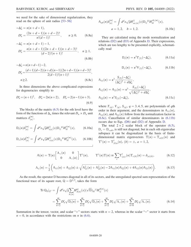
we need for the sake of dimensional regularization, theyread on the sphere of unit radius [53–56]

−Δsn ¼ nðnþ d − 1Þ;

Dsn ¼ð2nþ d − 1Þðnþ d − 2Þ!

n!ðd − 1Þ! ; n ≥ 0; ð6:8aÞ

−Δvn ¼ nðnþ d − 1Þ − 1;

Dvn ¼

nðnþ d − 1Þð2nþ d − 1Þðnþ d − 3Þ!ðd − 2Þ!ðnþ 1Þ! ; n ≥ 1;

ð6:8bÞ−Δt

n¼nðnþd−1Þ−2;

Dtn¼ðdþ1Þðd−2ÞðnþdÞðn−1Þð2nþd−1Þðnþd−3Þ!

2ðd−1Þ!ðnþ1Þ! ;

n≥2: ð6:8cÞIn three dimensions the above complicated expressions

for degeneracies simplify to

Dsn¼ðnþ1Þ2; Dv

n¼2nðnþ2Þ; Dtn¼2ðn−1Þðnþ3Þ:

ð6:9ÞThe blocks of the matrix (6.5) for the nth level have the

form of the functions of Δn times the relevantDn ×Dn unit

matrices δðmÞðnÞ ,

DtðnÞδðmÞðnÞ ¼Z

ddxffiffiffigp

HijtðnÞðxÞDij

klHtðmÞkl ðxÞ; ð6:10aÞ

DvðnÞδðmÞðnÞ ¼Z

ddxffiffiffigp

HijvðnÞðxÞDij

klHvðmÞkl ðxÞ; ð6:10bÞ

AabðnÞδðmÞðnÞ ¼Z

ddxffiffiffigp

Hijsa;ðnÞðxÞDij

klHsb;ðmÞkl ðxÞ;

a ¼ 1; 2; b ¼ 1; 2: ð6:10cÞ

They are calculated using the mode normalization andrelations (D2) and (D3) of Appendix D. Their expressions,which are too lengthy to be presented explicitly, schemati-cally read

DtðnÞ ¼ κ3Tð3Þð−ΔtnÞ; ð6:11aÞ

DvðnÞ ¼ κ3Vð3Þð−ΔvnÞ; ð6:11bÞ

A11ðnÞ ¼ κ3Sð5Þð−Δs

nÞðΔs

nÞ2 þ dΔsn;

A12ðnÞ ¼ A21ðnÞ ¼ κ3Sð4Þð−Δs

nÞffiffiffiffiffiffiffiffiffiffiffiffiffiffiffiffiffiffiffiffiffiffiffiffiffiffiðΔs

nÞ2 þ dΔsn

p ;

A22ðnÞ ¼ κ3Sð3Þð−ΔsnÞ; ð6:11cÞ

where TðqÞ, VðqÞ, SðqÞ, q ¼ 3; 4; 5, are polynomials of qthorder in their argument, and the denominators in A11ðnÞ,A12ðnÞ, and A21ðnÞ follow from the normalization factor in(6.6c). Cancellation of similar denominators in (6.11b)occurs due to Eqs. (D6) and (D2) of Appendix D.The total 2 × 2 scalar block of the operator (6.5),

Ds ¼ Ds;ab, is still not diagonal, but in each nth eigenvaluesubspace it can be diagonalized in the basis of finite-dimensional matrix eigenvectors ϒðnÞ ¼ ϒaðbÞðnÞ and

ϒ†ðnÞ ¼ ϒ†ðbÞaðnÞ, ðbÞ ¼ �, a ¼ 1; 2,

AðnÞ ¼ ϒðnÞ�ΛþðnÞ 0

0 Λ−ðnÞ

�ϒ†ðnÞ; ϒ†ðnÞϒðnÞ≡X

c

ϒ†ðaÞcðnÞϒcðbÞðnÞ ¼ δðaÞðbÞ; ð6:12Þ

Λ�ðnÞ ¼1

2

�A11ðnÞ þ A22ðnÞ �

ffiffiffiffiffiffiffiffiffiffiffiffiffiffiffiffiffiffiffiffiffiffiffiffiffiffiffiffiffiffiffiffiffiffiffiffiffiffiffiffiffiffiffiffiffiffiffiffiffiffiffiffiffiffiffiffiffiffiffiffiffiffiffiffiffiffiffiffiffiffiffiffiffiffiffiffiffiffiffiffiffiffiffiffiffiffiffiffiffiffiffiffiffiffiffiffiffiffiffiffiffiffiffiA2

11ðnÞ þ A222ðnÞ − 2A11ðnÞA22ðnÞ þ 4A12ðnÞA21ðnÞ

q �: ð6:13Þ

As the result, the operator D becomes diagonal in all of its sectors, and the unregulated spectral sum representation of thefunctional trace of its square root, Q ¼ D1=2, takes the form

TrQDjS3 ¼Z

ddxffiffiffigp X

A;ðnÞHkl

AðnÞðxÞðffiffiffiffiDpÞklijHAðnÞ

ij ðxÞ

¼X∞n¼2

Dtn

ffiffiffiffiffiffiffiffiffiffiffiffiDtðnÞ

pþX∞n¼2

Dvn

ffiffiffiffiffiffiffiffiffiffiffiffiDvðnÞ

pþX∞n¼2

Dsn

ffiffiffiffiffiffiffiffiffiffiffiffiffiΛþðnÞ

pþX∞n¼0

Dsn

ffiffiffiffiffiffiffiffiffiffiffiffiffiΛ−ðnÞ

p: ð6:14Þ

Summation in the tensor, vector, and scalar “þ” sectors starts with n ¼ 2, whereas in the scalar “−” sector it starts fromn ¼ 0, in accordance with the restrictions on n in (6.6).


044009-20

The calculation of TrQB on S3 in the ghost and shift sectors proceeds along the same lines, except that we can, in view ofthe simplicity of these sectors, explicitly present the expressions for the corresponding operators. In particular, the operatorB defined by Eq. (2.8), when converted to the canonical form, reads on S3 as

BijjS3 ¼

1

2σ½δijð−ΔÞ3 þ ð1 − 2ð1 − λÞð1þ ξÞÞ∇i∇jð−ΔÞ2 − 2κδijð−ΔÞ2 − 4ð1 − 2λÞξκ∇i∇jð−ΔÞ þ 8λξκ2∇i∇j�: ð6:15Þ

In the basis of transverse and longitudinal vector modes,

cjðxÞ ¼XðnÞ

cTðnÞξjðnÞðxÞ þ

XðnÞ

cLðnÞ∇j 1ffiffiffiffiffiffiffi−Δp ϕðnÞðxÞ; ð6:16Þ

where ξjðnÞ ≡ gjiξðnÞi and ϕðnÞ are orthonormal sets of transverse vector and scalar Laplacian eigenfunctions (6.7b) and (6.7c)

introduced above, this operator similar to (6.5) becomes diagonal B ¼ diag½BT;BL�. Here, as it follows from (6.15),

BT ¼κ3

2σ½ð−Δv

nÞ3 − 2ð−ΔvnÞ2�δðnÞðmÞ ≡ BTðnÞδðnÞðmÞ; ð6:17aÞ

BL ¼κ3

2σ½2ð1 − λÞð1þ ξÞð−Δs

nÞ3 − 4ðξ − 2λþ 3Þð−ΔsnÞ2 þ 8ð3 − λÞð−Δs

nÞ − 16�≡ BLðnÞδðnÞðmÞ; ð6:17bÞ

and

TrQBjS3 ¼X∞n¼1

Dvn

ffiffiffiffiffiffiffiffiffiffiffiffiBvðnÞ

pþX∞n¼1

Dsn

ffiffiffiffiffiffiffiffiffiffiffiffiBsðnÞ

p: ð6:18Þ

The vector modes sum starts with n ¼ 1 because Dv0 ¼ 0, whereas the scalar modes sum begins with n ¼ 1 because the

expansion (6.16) does not include the zero mode of the scalar Laplacian.

B. Dimensional and ζ-functional regularization of spectral sums

Regularization and extraction of divergences by dimensional regularization consists in the extension of these sums tospace dimensionality d ¼ 3 − ε with ε → 0. In the ζ-functional regularization the square root power of the operatorF ¼ ðD;BÞ is analytically continued to 1=2 − ε0.

TrffiffiffiFpjζ−reg: ¼ Tr F

12−ε0 ; ð6:19Þ

which is provided by the replacement of all square roots in the above formula (6.14) by this power while keeping d ¼ 3.We identify

ε0 ¼ ε=6; ð6:20Þ

as implied by the dimensionality of the operator.12 One can show then that the resulting divergent parts of the trace—thepole terms in ε—coincide in both regularizations. Below we demonstrate this on the example of the tensor sector.For the dimensionality d ¼ 3 − ε the multiplicity of the nth eigenvalue in the transverse-traceless tensor sector has for

large n ≫ 1 the following form:

Dtn ¼ðdþ 1Þðd − 2Þðnþ dÞðn − 1Þð2nþ d − 1Þðnþ d − 3Þ!

2ðd − 1Þ!ðnþ 1Þ! ¼ 2n2−ε�1þ 2

n−

3

n2þOðεÞ

�; ð6:21Þ

where we used that

12Indeed, in both dimensional and ζ-regularizations one has to introduce a dimensionful parameter k� to keep the dimension of theoperator trace equal to three. Equating the powers of this parameter in the two cases, we obtain the relation (6.20).


044009-21

Γðnþ 1 − εÞΓðnþ 1Þ ¼ n−εð1þOðεÞÞ; n → ∞: ð6:22Þ

This yields

TrffiffiffiffiffiDt

pjdim :reg: ¼ κ3=2

X∞n¼2

DtnfTð3Þðnðnþ d − 1Þ − 2Þg1=2 ¼

X∞n¼2

n5−εGt

�1

n; ε

�: ð6:23Þ

Here we have explicitly disentangled the fractional power of the growing factor n5−ε as the coefficient of the functionGtð1n ; εÞ which is regular at n → ∞,

Gt

�1

n; ε

�¼ 2κ3=2

�1þ 2

n−

3

n2

��1

n6Tð3Þðn2 þ 2n − 2Þ

�1=2þOðεÞ ð6:24Þ

[remember that Tð3Þðn2 þ 2n − 2Þ is six order polynomial in n].The divergent pole in ε of this series can be extracted using the Abel-Plana formula which expresses a discrete seriesPn fðnÞ in terms of the sum of the integral along the real axes of n and the integral of fðzÞ on the imaginary axis,

X∞n¼0

fðnÞ ¼Z

∞

0

dzfðzÞ þ 1

2fð0Þ þ i

Z∞

0

dzfðizÞ − fð−izÞexpð2πzÞ − 1

: ð6:25Þ

With fðnÞ ¼ ðnþ 2Þ5−εGtð1=ðnþ 2Þ; εÞ the latter integral is convergent being exponentially damped at infinity, while thedivergence of the integral over the real axes at n → ∞ can be isolated by changing the integration variable, nþ 2 ¼ 1=y,and integrating the needed number of times by parts. In the domain of convergence ε > 6 integration by parts does not giveextra terms at y ¼ 0, so that the analytic continuation to ε ¼ 0 yields UV divergences as a pole term

TrffiffiffiffiffiDt

pjdivdim :reg: ¼

Z∞

2

dnn5−εGt

�1

n; ε

�jdiv ¼

Z1=2

0

dyy7−ε

Gtðy; εÞjdiv

¼ 1

ε − 6

1

ε − 5� � � 1

ε − 1

1

ε

Z1=2

0

dyyεd6Gtðy; εÞ

dy6jdiv ¼ 1

6!ε

d6Gtðy; 0Þdy6

jy¼0: ð6:26Þ

This result agrees with the zeta-function regularization. Indeed, we have

TrffiffiffiffiffiDt

pjζ−reg: ¼ κ3=2−ε

X∞n¼2

2ðn − 1Þðnþ 3ÞfTð3Þðnðnþ 2Þ − 2Þg12−ε6 ¼

X∞n¼2

n5−εFt

�1

n; ε

�; ð6:27Þ

where Ftð1n ; εÞ is a function different from Gtð1n ; εÞ, but coinciding with it at ε ¼ 0, Ftð1n ; 0Þ ¼ Gtð1n ; 0Þ. Then, byexpanding this function in Taylor series in 1=n, one acquires a series of Riemannian zeta functions

TrffiffiffiffiffiDt

pjdivζ−reg: ¼

X∞n¼2

n5−εX∞m¼0

1

m!FðmÞt ð0; εÞ

1

nmjdiv

¼X∞m¼0

1

m!FðmÞt ð0; εÞζRðmþ ε − 5Þjdiv ¼ 1

6!ε

d6Ftðy; 0Þdy6

jy¼0; ð6:28Þ

which coincides with (6.26). Here we used the fact that Riemann zeta-function ζRðzÞ has a simple pole only at z ¼ 1 withunit residue.Analogous to the formula (6.23) we regularize the vector and scalar traces

TrffiffiffiffiffiffiDv

p¼

X∞n¼2

n5−εGv

�1

n; ε

�; Tr

ffiffiffiffiffiffiDs

p¼

X∞n¼2

n5−εGþ

�1

n; ε

�þX∞n¼0

n5−εG−

�1

n; ε

�: ð6:29Þ

Then the total divergence reads


044009-22

TrQjdivS3 ¼1

6!ε

d6

dy6½Gtðy; 0Þ þGvðy; 0Þ þ Gþðy; 0Þ þG−ðy; 0Þ�jy¼0: ð6:30Þ

Full expressions for functions Gtðy; 0Þ, Gvðy; 0Þ, G�ðy; 0Þ can be obtained for an arbitrary gauge in the two-parameterfamily of Sec. II A, but are too lengthy to be presented here. TheMathematica code to calculate them can be found at [50].The same procedure applies to the regularization of the trace of the vector operator square roots. The simplicity of this

sector allows us to present the final result,

TrQBjdivS3¼ κ3=2

ε

ffiffiffiffiffiν5p �

−4uV −ð3 − λÞ2ð1þ λÞuS2

16ð1 − λÞ3 þ ð5 − 6λþ 5λ2Þu2V2ð1 − λÞuS2

þ 4ð1 − λÞð5 − 3λÞu4Vu3S2

−32ð1 − λÞ3u6V

u5S2

�; ð6:31Þ

where uV and uS2 have been defined in Eq. (3.23). Combining this result with the tensor contribution, we finally find thedivergent part of the one-loop effective action on the static spacetime with spherical 3-space in an arbitrary ðσ; ξÞ-gauge,

Γ1−loopjdivR1×S3

¼Z

dτκ3=2

εPðλ; us; v1; v2; v3; σ; ξÞ; ð6:32aÞ

Pðλ; us; v1; v2; v3; σ; ξÞ ¼ffiffiffiffiffiν5p

32ð1 − λÞ3ð1 − 3λÞ3u5sfð1 − λÞ6ð144v1 þ 50v2 þ 18v3 − 1Þ3

þ 2u2sð1 − λÞ4ð1 − 3λÞð144v1 þ 50v2 þ 18v3 − 1Þ½72v1ðλþ 1Þþ 2v2ð17λþ 8Þ þ 18v3λ − 5λþ 4�þ 4u4sð1 − λÞ2ð1 − 3λÞ2½72v1ð16λ2 − 9λ − 3Þ þ 2v2ð200λ2 − 120λ − 33Þþ 6v3ð24λ2 − 16λ − 3Þ − 8λ2 þ 12λ − 3�þ 6u5sð1 − λÞ3ð1 − 3λÞ3½12ðv2 þ v3Þðv2ð6v2 þ 25Þ þ 3v3ð4v2 þ 3Þ þ 6v23Þþ 432v1ð2v2 þ 2v3 þ 3Þ þ 430v2 þ 142v3 − 11� þ 8u6sð1 − 3λÞ3λð4λ2 − 8λþ 3Þg

þ 3ν5ð9v1 þ 3v2 þ v3Þ�4

ffiffiffiffiffi2σp

þ 1

ð1 − λÞffiffiffiffiffiffiffiffiffiffiffiffiffiffiffiffiffiffiffiffiffiffiffiffiffiffiffiffi

σ

ð1 − λÞð1þ ξÞr �

: ð6:32bÞ

Note that the R1 × S3 background for a generic radiusκ−1=2 of the 3-sphere is not a solution of equations ofmotion, so that this divergent part of the effective action isoff-shell and, therefore, is gauge dependent. Equations ofmotion on static R1 × S3 imply that the derivative of theaction with respect to κ should vanish and hold only at flatspace geometry, κ ¼ 0, of infinitely large 3-sphere. Thegauge dependence is described by the last term in (6.32b)and is remarkably simple.In comparing this expression to our previous results, we

need the relation between 1=ε and the divergent logarithmlnL2, Eq. (5.2). In dimensional regularization the latter isregularized as Z

ds2s2

↦ kε�

Zds2

sð1−ε=2Þ2

≃2

ε; ð6:33Þ

where k� is a parameter with units of momentum to keepthe expression dimensionless (cf. footnote 12). This giveslnL2 ¼ 2=ε. Comparing with Eqs. (6.2) and (6.3), we find

96π2κ3=2ð9Cν1þ3Cν2þCν3Þ¼ κ3=2Pðλ;us;v1;v2;v3;σ;ξÞ:ð6:34Þ

We have checked that this equality is indeed satisfied in thefour gauges a, b, c, d. This accomplishes the verification ofour results on the static homogeneous spacetime.As a corollary we obtain the expression for the function

Ξ introduced in Eq. (5.9) which parametrizes the gaugedependence of the divergent coefficients in the effectiveaction,

Ξ ¼ 1

32π2

�4

ffiffiffiffiffi2σp

þ 1

ð1 − λÞffiffiffiffiffiffiffiffiffiffiffiffiffiffiffiffiffiffiffiffiffiffiffiffiffiffiffiffi

σ

ð1 − λÞð1þ ξÞr �

: ð6:35Þ

Its knowledge allows us to generalize our expressions forCνa , a ¼ 1;…; 5, to arbitrary ðσ; ξÞ-gauge. The result iscontained in the form of the Mathematica file in theSupplemental Material [43].


044009-23

The final remark here is that the knowledge of thelogarithmic divergences (6.32) allows one to extract thelogarithmic dependence of the finite part of the effectiveaction on the radius if the sphere κ−1=2. This is easily seenwithin the ζ-functional regularization in which the overallscale of operators F ¼ ðD;BÞ ∝ κ3 is raised to the frac-tional power in (6.19) and gives

1

εκ32−ε2 ¼ κ

32

�1

ε−1

2ln

κ

k2�

�; ð6:36Þ

where k� is a normalization scale of the ζ-functionregularization. This leads to the expression for the fulleffective action as a function of κ,

Γ1−loopjR1×S3

¼Z

dτ

�κ3=2

ε−κ3=2

2ln

κ

k2�

�Pðλ; us; v1; v2; v3; σ; ξÞ

þZ

dτκ3=2Qðλ; us; v1; v2; v3; σ; ξÞ; ð6:37Þ

where the logarithmic term plays the role of the Coleman-Weinberg effective potential on the metric backgroundof size κ−1=2. In contrast to the logarithmic contribution,the second term is not controlled by the UV divergentcoefficient and, contrary to the case of single-chargemodels, cannot be absorbed into the redefinition of thenormalization k�, because it carries a nontrivial dependenceon multiple couplings.

VII. DISCUSSION

In this paper we have obtained the full set of one-loopβ-functions for marginal essential coupling constants inprojectable HG. The results underwent a number of verypowerful checks that confirm gauge independence of thesebeta functions in a wide set of gauge conditions—thecornerstone of the physically invariant content of quantumgauge theories. These checks also provide a very deepverification and show high efficiency of the method ofuniversal functional traces which replaces within the back-ground field approach the standard Feynman diagrammatictechnique. This method implicitly performs the summationof a humongous number of Feynman graphs and leads to afinal result hardly achievable by standard momentum spacemethods in flat spacetime. As a by-product of our calcu-lation we derived an expression for the divergence of theone-loop effective action of HG on static background in atwo-parameter family of gauges.The complexity of the expressions (1.15) for the

β-functions with the polynomials Pχn collected in

Eqs. (A4)–(A8) is high, and we postpone a comprehensiveanalysis of the resulting RG flow for the future. At thispoint, we content ourselves with a few preliminaryobservations.

Clearly, the β-functions (1.15) are in general singular atλ → 1=3, λ → 1, or us → 0.13 This is not surprising, sincethe two first limits correspond to the boundaries of theunitarity domain (1.9), whereas in the last limit thedispersion relation of the scalar mode becomes degenerate[see Eq. (1.10b)]. Remarkably, however, for a specialchoice of the values

fv�g∶v1 ¼ 1=2; v2 ¼ −5=2; v3 ¼ 3 ð7:1Þ

the limit us → 0 of the β-functions (1.15) becomes regularfor any λ in the unitary domain:

βva jfv�g;us→0 ¼ 0; a ¼ 1; 2; 3; ð7:2aÞ

βus jfv�g;us→0 ¼1893λ2 − 6720λþ 4576

6720π2ð1 − λÞð1 − 3λÞ G; ð7:2bÞ

βGjfv�g;us→0 ¼ −159

80π2G2: ð7:2cÞ

The point fv�g; us → 0 is special since it corresponds tothe version of HG, in which the potential term is a square ofthe Cotton tensor Cij,

S ¼ 1

2G

Zdτ d3x

ffiffiffiγp ðKijKij − λK2 þ ν5CijCijÞ

¼ 2

G

Zdτ d3x

ffiffiffiγp ðKij þ ffiffiffiffiffi

ν5p

CijÞGij;klðKkl þ ffiffiffiffiffiν5p

CklÞ;

ð7:3Þ

Cij ¼ εikl∇k

�Rjl −

1

4Rδjl

�¼ εklði∇kR

jÞl ; ð7:4Þ

where εikl ¼ ϵikl=ffiffiffigp

, ϵ123 ¼ 1. In the second equality in(7.3) we used the tracelessness of the Cotton tensor andintegration by parts.This version of HG was originally suggested in [1] and

its quantum properties were studied in [57]. It is known asHG with detailed balance and is interesting because theCotton tensor can be rewritten as a variational derivative ofthe three-dimensional gravitational Chern-Simons theory,

Cij ¼ −1ffiffiffigp δWCS½g�

δgijðxÞ; ð7:5Þ

WCS½g� ¼1

2

Zd3xϵijk

�Γmil∂jΓl

km þ2

3ΓnilΓl

jmΓmkn

�; ð7:6Þ

defined in terms of the metric Christoffel symbol as afunctional of gij. Further, there exists a deformation of the

13We do not consider the singularity at us ¼ −1, because us isassumed to be positive by construction [see Eq. (1.12)].


044009-24

action (7.3) by relevant operators which preserves thedetailed balance structure and is related to the topologicalmassive gravity [58–60]. The detailed balance relationbetween d and (dþ 1)-dimensional theories appears inthe context of stochastic quantization [61,62] and estab-lishes a nontrivial connection between the renormalizationproperties of the two theories [63]. In our case this suggestsan intriguing connection between the (3þ 1)-dimensionalprojectable HG and the three-dimensional gravitationalChern-Simons/topological massive gravity [57].It is important to emphasize, however, that the pointfv�g; us → 0 is not a fully regular point of the RG flowin HG, because the β-function (1.13) of the remainingessential coupling λ diverges in this limit,

βλjfv�g;us→0 ∼9

40π21 − λ

usG: ð7:7Þ

Thus, the physical significance of the result (7.2) is unclearat the moment. It will be interesting to understand if theinclusion of fermionic degrees of freedom appearing inthe stochastic quantization framework [57] can change thepicture.An important question is the existence and nature of

fixed points of the RG flow. As already observed, thedependence of the β-functions on the coupling G factorizes.This coupling determines the overall strength of inter-actions in HG and must be small for the validity of theperturbative expansion. Its UV behavior determineswhether the model is asymptotically free (G → 0) or hasa Landau pole (G → ∞). On the other hand, the rest of thecouplings λ, us, va are ratios of the coefficients in the actionand need not be small. The search for fixed points of the RGflow thus splits into two steps. One first identifies the fixedpoints of the flow in the subspace of the couplings λ, us, vaby solving the system,

βλ=G ¼ 0; ð7:8aÞ

βχ=G ¼ 0; χ ¼ us; v1; v2; v3: ð7:8bÞ

In the full parameter space, these solutions correspond toflow lines along the G-direction. One then evaluates βG at agiven solution, whose sign determines whether the flowline goes to a Gaussian fixed point or a Landau pole.

Omitting the denominators in the expressions (1.13) and(1.15b), the system (7.8) becomes a system of five poly-nomial equations for five unknowns λ, us, va, a ¼ 1; 2; 3.We have studied it numerically with the following results:

(i) We have found no solutions in the right part ofthe unitary domain, λ > 1. In this respect (3þ 1)-dimensional HG appears to be different from its(2þ 1)-dimensional counterpart, which possessesan asymptotically free fixed point at λ ¼ 15=14 [21].

(ii) In the left part of the unitary domain, λ < 1=3, wefound four solutions summarized in Table I. Allthese fixed points turn out to be asymptotically free.Note that the two last points correspond to verylarge values of v1 and their validity requires furtherinvestigation. As discussed in [23], the fixed pointsat λ < 1=3 are UV repulsive along the λ-direction.We indicate this in the last column of Table I. We donot know if these fixed points are attractive or notalong the other directions.

It is worth stressing that the results above should be takenwith a grain of salt. Currently we do not have a firm proofof the absence of fixed points at λ > 1, nor do we claim thatthe list of fixed points at λ < 1=3 in Table I is exhaustive.It was conjectured in [64] that the UV fixed points of HG

can lie at infinite λ and that the limit λ → ∞ is well-defined.We find that all β-functions (1.15) are finite at λ → ∞,whereas βλ is proportional to λ,14

βλ ¼ −3ð3 − 2usÞ40π2us

λG; λ → ∞: ð7:9Þ

This behavior is compatible with the conjecture of [64].Notice that the point λ ¼ ∞ is UVattractive (repulsive) forus > 3=2 (us < 3=2). To identify fixed points of the RGflow at λ ¼ ∞, we looked for solutions of the system

βχ=Gjλ¼∞ ¼ 0; χ ¼ us; v1; v2; v3: ð7:10Þ

We have found eight solutions listed in Table II. Threeamong them are UV attractive along the λ-direction andcorrespond to asymptotically free fixed points. Clearly, the

TABLE I. Solutions of the system (7.8). The sixth column gives the value of the β-function for G at the respectivesolution and the seventh column indicates whether it corresponds to an asymptotically free fixed point. The eighthcolumn tells if the fixed point is UV attractive along the λ-direction.

λ us v1 v2 v3 βG=G2 Asymptotically free? UV attractive along λ?

0.1787 60.57 −928.4 −6.206 −1.711 −0.1416 Yes No0.2773 390.6 −19.88 −12.45 2.341 −0.2180 Yes No0.3288 54533 3.798 × 108 −48.66 4.736 −0.8484 Yes No0.3289 57317 −4.125 × 108 −49.17 4.734 −0.8784 Yes No

14The directionality of the limit is not important: the resultingexpressions for the β-functions are the same at λ ¼ �∞.


044009-25

structure of the RG flow around these points deservesfurther investigation. More generally, this strongly moti-vates a detailed study of the λ → ∞ limit of HG. It is worthmentioning that a similar limit naturally arises in con-nection with nonrelativistic gravity to Perelman-Ricciflows [65].Let us stress again that presently we do not know if

Table II is exhaustive. We plan to return to a systematicclassification of fixed points of HG and its RG flow in ourfuture work.

ACKNOWLEDGMENTS

We thank Diego Blas, Mario Herrero-Valea, BenjaminKnorr, Vladimir Nechitailo, and Christian Steinwachs forinvaluable discussions. The work was partially supportedby the Russian Foundation for Basic Research GrantNo. 20-02-00297. The work of A. B. and A. K. is supported

by the Foundation for Theoretical Physics Development“Basis.” The work of S. S. is supported by the NaturalSciences and Engineering Research Council (NSERC) ofCanada. The research at Perimeter Institute is supported inpart by the Government of Canada through the Departmentof Innovation, Science and Economic Development Canadaand by the Province of Ontario through the Ministry ofColleges and Universities.

APPENDIX A: EXPLICIT EXPRESSIONS

1. Beta-function of G

The coupling G of HG is not essential; i.e., it is notdefined using the on-shell quantities. Hence its β-functiondepends on the gauge choice. Reference [23] obtained thisβ-function for the (3þ 1)-dimensional projectable model ina subset of the two-parameter family of regular gaugesdescribed in Sec. II A. The results are as follows:

(i) σ-arbitrary, ξ ¼ − 1−2λ2ð1−λÞ

βG ¼ ffiffiffiffiffiν5p G2

40π2ð1 − λÞð1 − 3λÞð1þ usÞus½−27þ 74λ − 57λ2 − usð5ð1 − 3λÞð5 − 4λÞ

ffiffiffiffiffiffiffiffiffiffi2σν5

pþ 53 − 142λþ 99λ2Þ

− u2sð1 − 3λÞð5ð5 − 4λÞffiffiffiffiffiffiffiffiffiffi2σν5

pþ 18 − 14λÞ�; ðA1Þ

(ii) σ ¼ 12ν5, ξ ¼ νs

2ν5ð1−λÞ − 1

βG ¼ −ffiffiffiffiffiν5p G2

40π2ð1 − λÞð1 − 3λÞð1þ usÞus½32 − 89λþ 57λ2 þ 3usð26 − 79λþ 53λ2Þ þ 2u2sð19 − 74λþ 51λ2Þ�;

ðA2Þ

(iii) σ ¼ 12νs, ξ ¼ ν5

2νsð1−λÞ − 1

βG ¼ −ffiffiffiffiffiν5p G2

40π2ð1 − λÞð1 − 3λÞð1þ usÞus½47 − 154λþ 117λ2 þ 3usð26 − 79λþ 53λ2Þ þ u2sð23 − 83λþ 42λ2Þ�:

ðA3Þ

TABLE II. Solutions of the system (7.10) corresponding to fixed points of Horava gravity at λ ¼ ∞. The fourthcolumn lists the value of the β-function for the coupling G at each solution, whose sign determines whether the flowis asymptotically free or runs into strong coupling, as indicated in the fifth column. The last column tells if the pointis UV attractive along the λ-direction in the space of all couplings.

us v1 v2 v3 βG=G2 Asymptotically free? UV attractive along λ?

0.01950 0.4994 −2.498 2.999 −0.2004 Yes No0.04180 −0.01237 −0.4204 1.321 −1.144 Yes No0.05530 −0.2266 0.4136 0.7177 −1.079 Yes No12.28 −215.1 −6.007 −2.210 −0.1267 Yes Yes21.60 −17.22 −11.43 1.855 −0.1936 Yes Yes440.4 −13566 −2.467 2.967 0.05822 No Yes571.9 −9.401 13.50 −18.25 −0.07454 Yes Yes950.6 −61.35 11.86 3.064 0.4237 No Yes


044009-26

This set of gauges overlaps with the gauges used in the present work. Thus, the gauge (ii) coincides with the gauge (a),Eq. (3.25), whereas the gauge (i) reduces to the gauges (b) and (d) for the appropriate choices of σ [see Eqs. (3.27) and(3.31)]. The expressions (A1) and (A2) are used in Sec. V to derive the β-function of the essential coupling G.

2. Polynomials in the β-functions of essential couplings

In this Appendix we collect the expressions for the polynomials appearing in Eqs. (1.15). For the β-function of thecoupling G the polynomials read,

PG0 ¼ ð1 − λÞ4ð1809v23 þ 832v22 þ 16v2ð159v3 − 217Þ − 4494v3 þ 2401Þ; ðA4aÞ

PG1 ¼ 3PG

0 ; ðA4bÞ

PG2 ¼ −ð1 − λÞ2½3ð15779λ2 − 20362λþ 3967Þ þ 64v22ð81λ2 − 82λþ 1Þþ 27v23ð279λ2 − 238λ − 41Þ − 6v3ð8823λ2 − 10620λþ 1561Þþ 16v2ðv3ð675λ2 − 582λ − 93Þ − 2307λ2 þ 2732λ − 365Þ�; ðA4cÞ

PG3 ¼ ð1 − λÞ2½27v23ð961λ2 − 1434λþ 401Þ þ 64v22ð1717λ2 − 2298λþ 581Þþ 16v2ð19409λ2 − 26004λþ 6415þ 3v3ð2741λ2 − 3690λþ 949ÞÞþ 6v3ð39331λ2 − 58728λþ 14873Þ − 345977λ2 þ 276750λ − 52741�; ðA4dÞ

PG4 ¼ 2ð1 − 3λÞf138545λ3 − 328263λ2 − 5888ð1 − λÞ3v22

− ð1 − λÞ2½16v2ð3119λþ 840v3ð1 − λÞ − 2396Þ− 3v3ð9v3ð353λ − 299Þ − 5012λþ 8210Þ� þ 239597λ − 49947g; ðA4eÞ

PG5 ¼ 2ð1 − 3λÞf159709λ3 − 378471λ2 þ ð1 − λÞ2½16v2ð1243λ − 412Þ

− 3v3ð243v3ð1 − 3λÞ − 13280λþ 4366Þ� þ 273933λ − 55375g; ðA4fÞ

PG6 ¼ −6ð1 − 3λÞ2ð8465λ2 − 16310λþ 3ð1 − λÞ2v3ð254þ 27v3Þ þ 7811Þ; ðA4gÞ

PG7 ¼ 4ð1 − 3λÞ2ð48λ2 − 38λþ 7Þ: ðA4hÞ

Polynomials in the β-function of us are the following:

Pus0 ¼ −3ð1 − λÞ5½537600v21 þ 78992v22 þ 14205v23 þ 2688v1ð154v2 þ 67v3 − 16Þþ 16v2ð4236v3 − 959Þ − 5838v3 þ 329�; ðA5aÞ

Pus1 ¼ 3Pus

0 ; ðA5bÞ

Pus2 ¼ −2ð1 − λÞ3½2419200v21ð1 − λÞ2 þ 8v22ð42645λ2 − 86482λþ 43837Þþ v23ð58698 − 106947λþ 48249λ2Þ þ 4032v1ð462v2ð1 − λÞ2 þ 201v3ð1 − λÞ2 þ 30λ2 − 44λ − 10Þþ 8v2ð6252λ2 − 9188λ − 1468Þ þ 8v2v3ð34335λ2 − 71196λþ 36861Þþ v3ð20556λ2 − 30792λ − 3696Þ þ 4533λ2 − 3881λþ 1448�; ðA5cÞ

Pus3 ¼ −2ð1 − λÞ3½806400v21ð1 − λÞ2 þ 8v22ð20709λ2 − 32026λþ 14957Þ þ v23ð61686λ2

− 52875λþ 20241Þ þ 4032v1ð98þ 154v2ð1 − λÞ2 þ 67v3ð1 − λÞ2 þ 218λ2 − 388λÞþ 8v2ð3v3ð7833λ2 − 9656λþ 4231Þ þ 4ð8658λ2 − 16817λþ 4324ÞÞþ v3ð81594λ2 − 189660λþ 50262Þ − 2970λ2 − 1529þ 6235λ�; ðA5dÞ


044009-27

Pus4 ¼ ð1 − λÞð1 − 3λÞ½32v22ð1 − λÞ2ð4081λ − 1191Þ þ v23ð133083λ3 − 303453λ2 þ 207657λ − 37287Þþ 48384v1ð1 − λÞ2ð13λ − 19Þ − 16v2ð1 − λÞð7873λ2 − 25922λþ 18109

þ 3v3ð5419λ2 − 6970λþ 1551ÞÞ − v3ð31938λ3 þ 15042λ2 − 127314λþ 80334Þþ 10415λ3 þ 11815λ2 − 30239λþ 10017�; ðA5eÞ

Pus5 ¼ ð1 − λÞð1 − 3λÞ½32v22ð1 − λÞ2ð661λ − 203Þ þ v23ð104787λ3 − 240381λ2 þ 168345λ − 32751Þþ 16128v1ð1 − λÞ2ð13λ − 19Þ þ 16v2ð1 − λÞð12761λ2 − 14690λþ 69

− 3v3ð2677λ2 − 3534λþ 857ÞÞ − v3ð178962λ3 − 468990λ2 þ 347070λ − 57042Þþ 379967λ3 − 512385λ2 þ 126609λþ 1081�; ðA5fÞ

Pus6 ¼ −4ð1 − 3λÞ2½6584v22ð1 − λÞ3 − 27v23ð1 − λÞ2ð311λ − 284Þ þ 24v2ð1 − λÞ2ð405λ − 584

þ 581v3ð1 − λÞÞ − 3v3ð1 − λÞ2ð2507λþ 2452Þ − 92671λ3 þ 205653λ2 − 130039λþ 17539�; ðA5gÞ

Pus7 ¼ −2ð1 − 3λÞ2½ð1 − λÞ2ð729v23ð1 − 3λÞ − 16v2ð3133λ − 1042Þ − 6v3ð11680λ − 3863ÞÞ

− 212947λ3 þ 494301λ2 − 341005λþ 61647�; ðA5hÞ

Pus8 ¼ −2ð1 − 3λÞ3ðð1 − λÞ2ð243v23 þ 3360v2 þ 5646v3Þ þ 31443λ2 − 61026λþ 29033Þ; ðA5iÞ

Pus9 ¼ 4ð1 − 3λÞ3ð48λ2 − 38λþ 7Þ: ðA5jÞ

Polynomials in the β-function of v1 are the following:

Pv10 ¼ −ð1 − λÞ6½11612160v31 þ 472088v32 þ 241920v21ð50v2 þ 18v3 − 1Þþ 12v22ð40758v3 − 427Þ þ 1008v1ð4124v22 þ 4v2ð726v3 − 23Þ þ 6v3ð81v3 þ 4Þ − 31Þþ 78v2ð6v3ð345v3 þ 28Þ − 119Þ þ 18v3ð3v3ð318v3 þ 77Þ − 119Þ − 385�; ðA6aÞ

Pv11 ¼ 3Pv1

0 ; ðA6bÞ

Pv12 ¼ −ð1 − λÞ4f34836480v31ð1 − λÞ2 þ 24v32ð54595λ2 − 112134λþ 57539Þþ 108v33ð213λ2 − 602λþ 389Þ þ 161280v21½225v2ð1 − λÞ2 þ 81v3ð1 − λÞ2 − 6λ2 þ 8λ − 4�þ 4v22½6v3ð52401λ2 − 110626λþ 58225Þ − 72285λ2 þ 86204λ − 22411�− 36v23ð1947λ2 − 2236λþ 375Þ þ 2v1½32v22ð190749λ2 − 384238λþ 193489Þ− 224v2ð2613λ2 − 3196λþ 1051Þ þ 528v2v3ð7935λ2 − 16124λþ 8189Þþ 243v23ð2703λ2 − 5620λþ 2917Þ − 42v3ð8535λ2 − 9652λþ 1885Þ þ 7ð22587λ2 − 26516λþ 3353Þ�þ 2v2½18v23ð9687λ2 − 21886λþ 12199Þ − 24v3ð6447λ2 − 7402λþ 1387Þ þ 52401λ2 − 62686λþ 8885�þ 18v3ð1245λ2 − 1506λþ 205Þ þ 14805λ2 − 18928λþ 4151g; ðA6cÞ


044009-28

Pv13 ¼ −ð1 − λÞ4f11612160v31ð1 − λÞ2 þ 8v32ð19267λ2 − 65030λþ 45763Þ

− 324v33ð211λ2 − 246λþ 35Þ þ 483840v21½25v2ð1 − λÞ2 þ 9v3ð1 − λÞ2 − 2λ2�− 12v22½6v3ð1943λ2 þ 1938λ − 3881Þ þ 68869λ2 − 79372λþ 18995�− 108v23ð2255λ2 − 2852λþ 683Þ þ 6v1½32v22ð17541λ2 − 37822λþ 20281Þ− 224v2ð2061λ2 − 2092λþ 499Þ þ 528v2v3ð543λ2 − 1340λþ 797Þþ 243v23ð15λ2 − 244λþ 229Þ − 42v3ð9303λ2 − 11188λþ 2653Þþ 7ð28539λ2 − 38420λþ 9305Þ� − 6v2½18v23ð2273λ2 − 2034λ − 239Þþ 24v3ð7175λ2 − 8858λþ 2115Þ − 64777λ2 þ 87438λ − 21261�þ 18v3ð4687λ2 − 6422λþ 1567Þ þ 7ð6785λ2 − 8992λþ 2219Þg; ðA6dÞ

Pv14 ¼ −2ð1 − λÞ2ð1 − 3λÞf1024v32ð1 − λÞ2ð45λ − 38Þ þ 1728v33ð1 − λÞ2ð7λ − 6Þþ 120960v21ð1 − λÞ2ðλþ 1Þ − 4v22ð1 − λÞ½384ð59λ2 − 109λþ 50Þv3þ 29133λ2 − 55225λþ 25452� − 9v23ð877λ3 þ 871λ2 − 4213λþ 2465Þþ v1½64v22ð1 − λÞ2ð1263λ − 1343Þ − 16v2ð1 − λÞð3v3ð2463λ2 − 5182λþ 2719Þþ 33534λ2 − 52670λþ 19076Þ þ 3ð9v23ð1 − λÞ2ð1513λ − 1833Þþ 2v3ð82239λ3 − 226251λ2 þ 205549λ − 61537Þ − 64219λ3 þ 203973λ2

− 210641λþ 71335Þ� þ 4v2½144v23ð1 − λÞ2ð101λ − 86Þ þ 12v3ð1961λ3 − 6699λ2

þ 7435λ − 2697Þ þ 8085λ3 − 7434λ2 − 9300λþ 8755� þ 6v3ð4487λ3− 9281λ2 þ 4807λþ 7Þ þ 55452λ3 − 123853λ2 þ 81624λ − 13195g; ðA6eÞ

Pv15 ¼ −2ð1 − λÞ2ð1 − 3λÞf168v32ð51λ3 − 149λ2 þ 125λ − 27Þ − 108v33ð9λ3 þ 9λ2

− 25λþ 7Þ − 4v22ð1 − λÞ½18v3ð117λ2 − 366λþ 109Þ − 284λ2 − 7265λþ 5425�þ 40320v21ð1 − λÞ2ðλþ 1Þ − 9v23ð3467λ3 − 8839λ2 þ 6237λ − 865Þþ v1½64v22ð1 − λÞ2ð1717λ − 581Þ − 16v2ð1 − λÞð3v3ð2741λ2 − 3690λþ 949Þþ 25940λ2 − 40662λþ 12022Þ þ 27v23ð961λ3 − 2395λ2 þ 1835λ − 401Þþ 6v3ð52267λ3 − 148963λ2 þ 129881λ − 33185Þ − 288353λ3 þ 542255λ2

− 333355λþ 83485� − 2v2½162v23ð3λ3 þ 35λ2 − 51λþ 13Þ þ 24v3ð1265λ3− 2191λ2 þ 691λþ 235Þ þ 30971λ3 − 40323λ2 þ 13167λ − 4451� − 12v3ð6551λ3− 11593λ2 þ 6124λ − 1112Þ þ 109519λ3 − 252396λ2 þ 177357λ − 34396g; ðA6fÞ

Pv16 ¼ 2ð1 − 3λÞ2f56v32ð1 − λÞ3ð103λ − 13Þ þ 108v33ð1 − λÞ3ð41λ − 11Þþ 4v22ð1 − λÞ3ð2315λþ 54ð89λ − 19Þv3 þ 807Þ − 36v23ð1 − λÞ3ð657λ − 239Þ− 2v1ð1 − λÞ½5888v22ð1 − λÞ3 þ 16v2ð1 − λÞ2ð840v3ð1 − λÞ þ 284λ − 1451Þ− 27v23ð1 − λÞ2ð353λ − 299Þ − 6v3ð1 − λÞ2ð5054λþ 1585Þ − 146609λ3

þ 330783λ2 − 220781λþ 36675� − 2v2ð1 − λÞ2½54v23ð169λ2 − 212λþ 43Þþ 96v3ðλ2 þ 29λ − 30Þ þ 49685λ2 − 66892λþ 16249� − 6v3ð1 − λÞ2ð7601λ2− 11994λþ 4203Þ − 15115λ4 þ 38758λ3 − 23950λ2 − 8038λþ 8337g; ðA6gÞ


044009-29

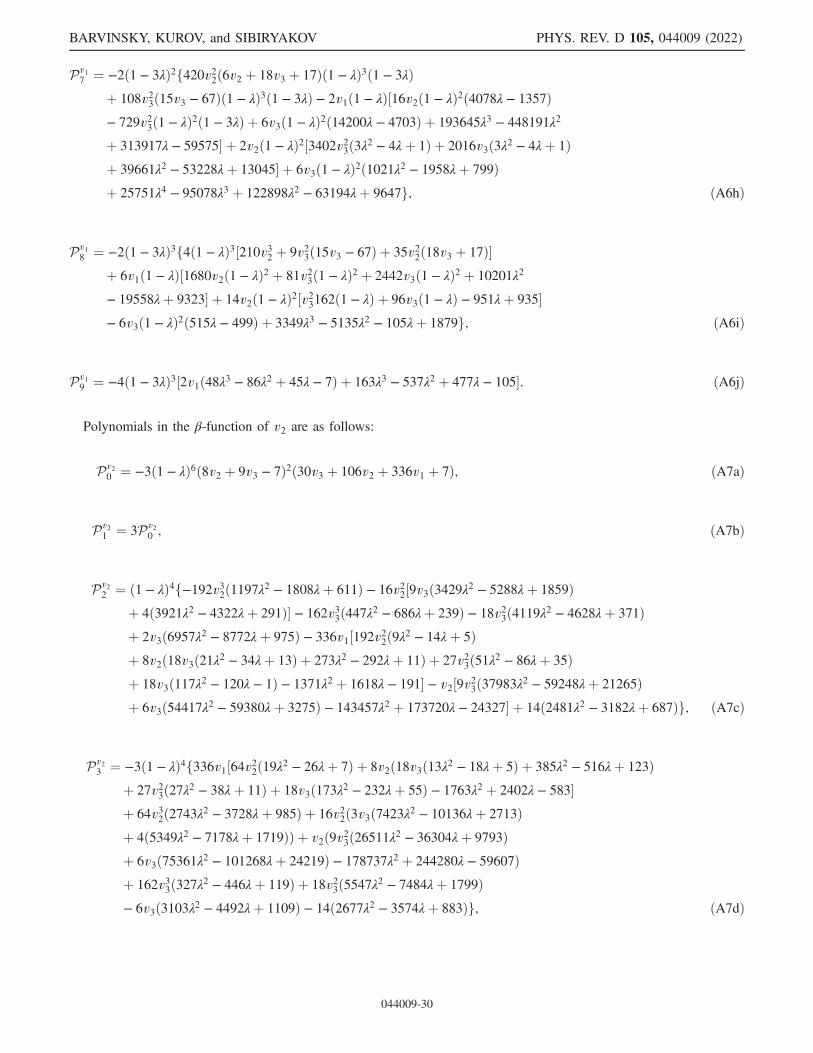
Pv17 ¼ −2ð1 − 3λÞ2f420v22ð6v2 þ 18v3 þ 17Þð1 − λÞ3ð1 − 3λÞþ 108v23ð15v3 − 67Þð1 − λÞ3ð1 − 3λÞ − 2v1ð1 − λÞ½16v2ð1 − λÞ2ð4078λ − 1357Þ− 729v23ð1 − λÞ2ð1 − 3λÞ þ 6v3ð1 − λÞ2ð14200λ − 4703Þ þ 193645λ3 − 448191λ2

þ 313917λ − 59575� þ 2v2ð1 − λÞ2½3402v23ð3λ2 − 4λþ 1Þ þ 2016v3ð3λ2 − 4λþ 1Þþ 39661λ2 − 53228λþ 13045� þ 6v3ð1 − λÞ2ð1021λ2 − 1958λþ 799Þþ 25751λ4 − 95078λ3 þ 122898λ2 − 63194λþ 9647g; ðA6hÞ

Pv18 ¼ −2ð1 − 3λÞ3f4ð1 − λÞ3½210v32 þ 9v23ð15v3 − 67Þ þ 35v22ð18v3 þ 17Þ�þ 6v1ð1 − λÞ½1680v2ð1 − λÞ2 þ 81v23ð1 − λÞ2 þ 2442v3ð1 − λÞ2 þ 10201λ2

− 19558λþ 9323� þ 14v2ð1 − λÞ2½v23162ð1 − λÞ þ 96v3ð1 − λÞ − 951λþ 935�− 6v3ð1 − λÞ2ð515λ − 499Þ þ 3349λ3 − 5135λ2 − 105λþ 1879g; ðA6iÞ

Pv19 ¼ −4ð1 − 3λÞ3½2v1ð48λ3 − 86λ2 þ 45λ − 7Þ þ 163λ3 − 537λ2 þ 477λ − 105�: ðA6jÞ

Polynomials in the β-function of v2 are as follows:

Pv20 ¼ −3ð1 − λÞ6ð8v2 þ 9v3 − 7Þ2ð30v3 þ 106v2 þ 336v1 þ 7Þ; ðA7aÞ

Pv21 ¼ 3Pv2

0 ; ðA7bÞ

Pv22 ¼ ð1 − λÞ4f−192v32ð1197λ2 − 1808λþ 611Þ − 16v22½9v3ð3429λ2 − 5288λþ 1859Þþ 4ð3921λ2 − 4322λþ 291Þ� − 162v33ð447λ2 − 686λþ 239Þ − 18v23ð4119λ2 − 4628λþ 371Þþ 2v3ð6957λ2 − 8772λþ 975Þ − 336v1½192v22ð9λ2 − 14λþ 5Þþ 8v2ð18v3ð21λ2 − 34λþ 13Þ þ 273λ2 − 292λþ 11Þ þ 27v23ð51λ2 − 86λþ 35Þþ 18v3ð117λ2 − 120λ − 1Þ − 1371λ2 þ 1618λ − 191� − v2½9v23ð37983λ2 − 59248λþ 21265Þþ 6v3ð54417λ2 − 59380λþ 3275Þ − 143457λ2 þ 173720λ − 24327� þ 14ð2481λ2 − 3182λþ 687Þg; ðA7cÞ

Pv23 ¼ −3ð1 − λÞ4f336v1½64v22ð19λ2 − 26λþ 7Þ þ 8v2ð18v3ð13λ2 − 18λþ 5Þ þ 385λ2 − 516λþ 123Þþ 27v23ð27λ2 − 38λþ 11Þ þ 18v3ð173λ2 − 232λþ 55Þ − 1763λ2 þ 2402λ − 583�þ 64v32ð2743λ2 − 3728λþ 985Þ þ 16v22ð3v3ð7423λ2 − 10136λþ 2713Þþ 4ð5349λ2 − 7178λþ 1719ÞÞ þ v2ð9v23ð26511λ2 − 36304λþ 9793Þþ 6v3ð75361λ2 − 101268λþ 24219Þ − 178737λ2 þ 244280λ − 59607Þþ 162v33ð327λ2 − 446λþ 119Þ þ 18v23ð5547λ2 − 7484λþ 1799Þ− 6v3ð3103λ2 − 4492λþ 1109Þ − 14ð2677λ2 − 3574λþ 883Þg; ðA7dÞ


044009-30

Pv24 ¼ ð1 − λÞ2ð1 − 3λÞf64v32ð1 − λÞ2ð2369λ − 1953Þ þ 1728v33ð1 − λÞ2ð21λ − 20Þ

− 16ð1 − λÞv22½3v3ð6145λ2 − 11298λþ 5153Þ þ 2ð5124λ2 − 14591λþ 9193Þ�− 9v23ð16909λ3 − 30841λ2 þ 11563λþ 2369Þ þ 1344v1½−192v22ð1 − λÞ3þ 6ð1 − λÞ2v2ð149λ − 48v3ð1 − λÞ − 137Þ − 108v23ð1 − λÞ3þ 9v3ð1 − λÞ2ð98λ − 93Þ − 372λ3 þ 1225λ2 − 1317λþ 462�þ v2½9v23ð1 − λÞ2ð20741λ − 17925Þ − 6v3ð7139λ3 þ 39053λ2 − 97327λþ 51135Þþ 293769λ3 − 562239λ2 þ 237523λþ 29971� þ 6v3ð29825λ3 − 68713λ2 þ 46923λ − 8099Þþ 245651λ3 − 551007λ2 þ 363249λ − 57837g; ðA7eÞ

Pv25 ¼ ð1 − λÞ2ð1 − 3λÞf64v32ðλ − 1Þ2ð329 − 961λÞ þ 324v33ð39λ3 − 73λ2 þ 41λ − 7Þ

− 16v22ðλ − 1Þ½3v3ð1085λ2 − 1482λþ 397Þ þ 22990λ2 − 27850λþ 3776�− 27v23ð7625λ3 − 19677λ2 þ 14703λ − 2651Þ þ 1344v1½2v2ð1 − λÞ2ð181λ − 137Þþ 9v3ð1 − λÞ2ð38λ − 31Þ þ 140λ3 − 53λ2 − 215λþ 122� þ v2½27v23ð683λ3 − 1273λ2 þ 681λ − 91Þ− 6v3ð102523λ3 − 238935λ2 þ 159777λ − 23365Þ þ 193117λ3 − 427691λ2 þ 258807λ − 27161�− 6v3ð31359λ3 − 58643λ2 þ 33565λ − 6089Þ þ 499453λ3 − 1131897λ2 þ 782671λ − 150059g; ðA7fÞ

Pv26 ¼ −2ð1 − 3λÞ2f8576ðλ − 1Þ4v32 − 54v33ð1 − λÞ3ð85λ − 31Þ − 18v23ð1 − λÞ3ð3397λ − 1203Þþ 16v22ð1 − λÞ3ð1116v3ð1 − λÞ þ 634λ − 709Þ þ 2016v1ðλ − 1Þ2ð35λ2 − 48λþ 12Þ− v2ð1 − λÞ½9v23ð1 − λÞ2ð1669λ − 1255Þ þ 6v3ð1 − λÞ2ð8860λ − 1737Þþ 14503λ3 − 16053λ2 − 9653λþ 11135� − 6v3ð1 − λÞ2ð2180λ2 − 7623λþ 5187Þ− 29405λ4 þ 75256λ3 − 46026λ2 − 16152λþ 16351g; ðA7gÞ

Pv27 ¼ −2ð1 − 3λÞ2f16v22ð1 − λÞ3ð727 − 2188λÞ þ 1458v33ð1 − λÞ3ð1 − 3λÞþ 19602v23ð1 − λÞ3ð1 − 3λÞ þ 672v1ð1 − λÞ2ð35λ2 − 48λþ 12Þþ v2ð1 − λÞ½1863v23ð1 − λÞ2ð1 − 3λÞ − 78v3ð1 − λÞ2ð1102λ − 365Þ − 111931λ3

þ 255965λ2 − 176459λþ 32629� þ 6v3ð1 − λÞ2ð14814λ2 − 18371λþ 3829Þ− 47811λ4 þ 180304λ3 − 236654λ2 þ 123472λ − 19239g; ðA7hÞ

Pv28 ¼ −2ð1 − 3λÞ3f6ð280v22 þ 9v23ð9v3 þ 121ÞÞð1 − λÞ3 − 6v3ð1 − λÞ2ð707λ − 715Þþ v2ð1 − λÞ½621v23ð1 − λÞ2 þ 7410v3ð1 − λÞ2 þ 10597λ2 − 18998λþ 8299�− 9739λ3 þ 18073λ2 − 6487λ − 1883g; ðA7iÞ

Pv29 ¼ −2ð1 − 3λÞ3½2v2ð48λ3 − 86λ2 þ 45λ − 7Þ − 295λ3 þ 1253λ2 − 1271λþ 301�: ðA7jÞ

Polynomials in the β-function of v3 are as follows:

Pv30 ¼ −4ð1 − λÞ6ð8v2 þ 9v3 − 7Þ3; ðA8aÞ

Pv31 ¼ 3Pv3

0 ; ðA8bÞ

Pv32 ¼ −ð1 − λÞ4ð8v2 þ 9v3 − 7Þf768v22ð1 − λÞð5λ − 1Þ þ 3v23ð1 − λÞð741λ − 31Þþ 8v2ðv3ð1 − λÞð687λ − 85Þ − 306λ2 þ 496λ − 206Þ þ v3ð651λ2 − 76λ − 719Þ− 5286λ2 þ 6824λ − 1426g; ðA8cÞ


044009-31

Pv33 ¼ −ð1 − λÞ4ð8v2 þ 9v3 − 7Þf256v22ð1 − λÞð53λ − 17Þ þ 9v23ð1 − λÞð1029λ − 319Þþ 8v2ð3v3ð1 − λÞð879λ − 277Þ − 470λ2 þ 592λ − 170Þþ 3v3ð1995λ2 − 2764λþ 625Þ − 17426λ2 þ 23608λ − 5846g; ðA8dÞ

Pv34 ¼ −ð1 − λÞ2ð1 − 3λÞf−64v22ð1 − λÞ½384v2ð1 − λÞ2 þ v3ð495λ2 − 1358λþ 863Þ

− 6ð697λ2 − 942λþ 261Þ� þ 16v2½3v23ð1 − λÞ2ð63λ − 895Þþ v3ð1 − λÞð38823λ2 − 53248λþ 15061Þ þ 31674λ3 − 76106λ2 þ 57078λ − 12630�− 27v33ð1 − λÞ2ð279λþ 425Þ − 12v23ð24879λ3 − 59880λ2 þ 45529λ − 10528Þþ 3v3ð87697λ3 − 220167λ2 þ 178243λ − 45677Þ þ 240090λ3 − 542894λ2 þ 357966λ − 55386g; ðA8eÞ

Pv35 ¼ −ð1 − λÞ2ð1 − 3λÞf−64v22ð1 − λÞ½v3ð1069λ2 − 1434λþ 365Þ − 6026λ2 þ 7932λ − 2002�þ 16v2½3v23ð1 − λÞ2ð1445λ − 517Þ − v3ð38317λ3 − 88093λ2 þ 62567λ − 12791Þþ 2ð2335λ3 − 9175λ2 þ 9161λ − 2297Þ� þ 27v33ð169λ3 − 499λ2 þ 451λ − 121Þ− 12v23ð15961λ3 − 36412λ2 þ 26015λ − 5564Þ − v3ð216917λ3 − 386819λ2 þ 188983λ − 19945Þþ 2ð264149λ3 − 575591λ2 þ 382375λ − 71269Þg; ðA8fÞ

Pv36 ¼ 2ð1 − 3λÞ2fð1 − λÞ3½3v23ð45v3ð73λ − 67Þ − 2ð6835λ − 5644ÞÞ − 256v22ð32v3 − 75Þð1 − λÞ�

− 16v2ð1 − λÞ2½1056v23ð1 − λÞ2 − v3ð3911λ2 − 7243λþ 3332Þ þ 6ð213λ2 − 457λþ 226Þ�− v3ð4877λ4 − 40820λ3 þ 91880λ2 − 80876λþ 24939Þ− 4ð3330λ4 − 7283λ3 þ 1162λ2 þ 6195λ − 3396Þg; ðA8gÞ

Pv37 ¼ −2ð1 − 3λÞ2f3v23ð1 − λÞ3½135v3ð1 − 3λÞ − 14ð289λ − 92Þ�þ 16v2ð1 − λÞ2½v3ð1 − λÞð412 − 1243λÞ − 5542λ2 þ 7230λ − 1788�þ v3ð1 − λÞð93119λ3 − 211785λ2 þ 147207λ − 28337Þþ 4ð4889λ4 − 22219λ3 þ 32834λ2 − 18597λþ 3117Þg; ðA8hÞ

Pv38 ¼ −6ð1 − 3λÞ3f3v23ð15v3 − 88Þð1 − λÞ3 − v3ð1289λ3 − 3119λ2 þ 2337λ − 507Þþ 4ð1297λ3 − 2877λ2 þ 1858λ − 282Þg; ðA8iÞ

Pv39 ¼ −4ð1 − 3λÞ3½v3ð48λ3 − 86λ2 þ 45λ − 7Þ − 151λ3 þ 257λ2 − 135λþ 21�: ðA8jÞ

APPENDIX B: COMMUTATOR OF AN OPERATOR IN A FRACTIONAL POWER

Here we derive the asymptotic series (3.51) for the commutator of an operator in a fractional power. The derivation startswith the representation

Aα ¼ 1

Γð−αÞZ

∞

0

dss−α−1e−sA: ðB1Þ

Next, for XðsÞ≡ ½e−sA; B� we have an equation,

dXds¼ −AX − ½A;B�e−sA; ðB2Þ

with initial condition Xð0Þ ¼ 0. It is straightforward to verify that the solution has the form


044009-32

XðsÞ ¼ −Z

s

0

ds1e−ðs−s1ÞA½A;B�e−s1A: ðB3Þ

Using Eqs. (B1) and (B3) we obtain

½Aα; B� ¼ −1Γð−αÞ

Z∞

0

dss−α−1Z

s

0

ds1e−ðs−s1ÞA½A;B�e−s1A

¼ −1Γð−αÞ

Z∞

0

dss−α−1�s½A;B�e−sA þ

Zs

0

ds1½e−ðs−s1ÞA; ½A;B��e−s1A�

¼ −Γð−αþ 1ÞΓð−αÞ ½A;B�A

α−1 −1

Γð−αÞZ

∞

0

dss−α−1Z

s

0

ds1½e−ðs−s1ÞA; ½A;B��e−s1A: ðB4Þ

In the last term we can again use the formula (B3) that will generate the second term in the expansion (3.51). Proceeding byinduction we obtain the representation

½Aα; B� ¼XNn¼1

Cnα½A; ½A;…½A|fflfflfflfflfflfflffl{zfflfflfflfflfflfflffl}

n

; B�…�Aα−n þ ð−1ÞN

Γð−αÞZ

∞

0

dss−α−1Z

s

0

ds1sN−11

ðN − 1Þ! ½e−ðs−s1ÞA; ½A; ½A;…½A|fflfflfflfflfflfflffl{zfflfflfflfflfflfflffl}

N

; B�…�e−s1A; ðB5Þ

which is valid for arbitrary N. This yields the formula (3.51).

APPENDIX C: MORE ON UNIVERSALFUNCTIONAL TRACES

1. Coincidence limits of the heat kernel coefficients

The heat kernel Kðsjx; yÞ ¼ esFð∇Þδðx; yÞ for the oper-ator (4.2) satisfies the initial value problem for its heatequation

∂sKðsjx; yÞ ¼ Fð∇ÞKðsjx; yÞ; ðC1aÞ

Kð0jx; yÞ ¼ δðx; yÞ: ðC1bÞ

The expansion (4.4) when substituted into Eq. (C1a)leads to the sequence of equations for the HAMIDEWcoefficients anðx; yÞ,

σμ∇μa0 ¼ 0; ðC2aÞ

ðnþ 1Þanþ1 þ σμ∇μanþ1

¼ D−1=2□ðD1=2anÞ þ�P −

1

6R1

�an; n ≥ 0; ðC2bÞ

where σμ ¼ ∇μσðx; yÞ is the vector at the point x tangentialto the geodetic curve connecting x and y. In deriving theserecurrence equations we took into account that in the lowesttwo orders of the s-expansion the heat equation is satisfiedin virtue of the equation for the Synge world functionσðx; yÞ,

σ ¼ 1

2∇μσ∇μσ; ðC3aÞ

and its corollary, the equation for the Van Vleck–Morettedeterminant (4.5)

D−1∇μðDσμÞ ¼ d: ðC3bÞ

These equations in their turn should be amended by theinitial conditions in the coordinate spacetime,

σjy¼x ¼ 0; ∇μσjy¼x ¼ 0; a0jy¼x ¼ 1; ðC4Þ

the latter following from the initial condition (C1b).By consecutively differentiating Eqs. (C2) and (C3) and

taking their coincidence limits one can systematically derivein the closed form the expressions for the needed coinci-dence limits (4.6). The result of these calculations whichbasically reduce to the commutator algebra of covariantderivatives (4.3) begins with the following list [27]15:

σjy¼x ¼ 0; ∇μ∇νσjy¼x ¼ gμν;

∇μ∇ν∇ασjy¼x ¼ 0; ∇μ∇ν∇α∇βσjy¼x ¼ −2

3RμðανβÞ;

ðC5aÞ

∇λ∇μ∇ν∇α∇βσjy¼x¼ −

1

2ð∇λRðαμβÞν þ∇μRðανβÞλ þ∇νRðαλβÞμÞ; ðC5bÞ

15The first and last indices in round brackets are symmetrizedwith the factor 1=2.


044009-33

D1=2jy¼x¼1; ∇μD1=2jy¼x¼0; ∇μ∇νD1=2jy¼x¼1

6Rμν;

ðC5cÞ

∇μ∇ν∇αD1=2jy¼x¼1

12ð∇μRναþ∇νRαμþ∇αRμνÞ; ðC5dÞ

and

a0jy¼x ¼ 1; ∇μa0jy¼x ¼ 0; ∇μ∇νa0jy¼x ¼1

2bRμν;

∇μ∇ν∇αa0jy¼x ¼2

3∇ðμbRνÞα; ðC6aÞ

a1jy¼x ¼ P; ∇μa1jy¼x ¼1

2∇μP −

1

6∇νbRνμ; ðC6bÞ

∇μ∇νa1jy¼x ¼1

180ð2RαβRαμβν þ 2RαβλμRαβλ

ν − 4RμαRαν

þ 3□Rμν −∇μ∇νRÞ1 −1

6bRαðμbRνÞ

α

þ 1

6∇ðμ∇αbRνÞα þ

1

2PbRμν þ

1

3½bRμν; P�

þ 1

3∇μ∇νP; ðC6cÞ

a2jy¼x ¼1

180ðRαβγδRαβγδ − RμνRμν þ□RÞ1

þ 1

12bRμν

bRμν þ 1

2P2 þ 1

6□P: ðC6dÞ

Higher-order coincidence limits, which we need up to∇8σjy¼x, ∇6D1=2jy¼x, ∇6a0jy¼x, ∇4a1jy¼x, ∇2a2jy¼x, anda3jy¼x, take pages, so we do not present them here.To obtain the needed list of traces (4.18)–(4.22), we

apply this method in three spatial dimensions d ¼ 3, μ ↦i ¼ 1; 2; 3 using the symbolic tensor algebra package xAct[44] for Mathematica [42]. For the tensor sector of the

theory we have 1¼δijkl≡δkðiδ

ljÞ, ðRmnÞijkl ¼ −2δðkði R

lÞjÞmn,

whereas for the vector sector 1 ¼ δij, ðRmnÞij ¼ Rijmn.

2. Divergences of tensor and vector traces

To evaluate the one-loop effective action of HG, wecompute the UFTs in the vector and tensor sectors usingthe method described in Sec. IVA. We keep only thelogarithmically divergent part proportional to the infiniteintegral over the proper-time parameter,

lnL2 ≡Z

dss: ðC7Þ

The UFTs are classified in Sec. IV B by the dimensionalitya of the coefficient function that they multiply in the action;the dimension of the UFT itself is then 6 − a. Within eachgroup we order the UFTs by the number of derivativesacting on the powers of Laplacian.Let us start with the simplest traces of zero dimension

(a ¼ 6). Their divergences cannot depend on curvature andare expressed purely in terms of the metric. They have theuniversal form

∇i1 � � �∇i2N−2

1

ð−ΔÞNþ1=2 δðx; yÞjdivy¼x

¼ lnL2

4π2ð−1ÞN−1

ð2N − 1Þ!!ffiffiffigp

gðN−1Þi1��i2N−2

1; ðC8Þ

which is valid for both the tensor and the vector sectors.

Here gðN−1Þi1��i2N−2

is the completely symmetric tensor built ofthe metric by the recurrence relations

gð1Þij ¼ gij; gð2Þijkl ¼ gijgkl þ gikgjl þ gilgjk; ðC9aÞ

gðNÞi1…i2N¼

X2Nk¼2

gi1ikgðN−1Þi2…ik−1ikþ1…i2N

: ðC9bÞ

For other traces the full expressions are very lengthybecause of the large number of free indices that they carryin general. To reduce the length, we can contract the indicesin various combinations which appear in the effectiveaction. Still, for the traces with a ¼ 4 and 3 (linear incurvature and in derivatives of curvature, respectively) thenumber of possible contractions is too high to be listedexplicitly. On the other hand, these traces are obtained by astraightforward algebra from the lower heat-kernel coef-ficients listed in (C5) and (C6). Thus, we focus below onthe most laborious traces with a ¼ 2 and a ¼ 0, whichare quadratic and cubic in curvature. Full expressions foruncontracted UFTs for all a ¼ 0; 2; 3; 4; 6 can be obtainedwith the Mathematica code available at [50].

a. Traces with a = 2, quadratic in curvature

These UFTs enter the divergent part of the action withthe coefficient functions linear in curvature (to form thelogarithmic divergences of the overall cubic power in thecurvature), so that they represent local quantities quadraticin the curvature and having two free indices.Tensor traces can have an even number of derivatives

running from zero to six. For the trace without derivativesthere are three possibilities of index contractions:


044009-34

gijð−ΔÞ1=2δijklðx; yÞjdivy¼x ¼ −lnL2

16π2ffiffiffigp

gkl1

30

�1

2RmnRmn þ

1

4R2 þ ΔR

�; ðC10aÞ

gklð−ΔÞ1=2δijklðx; yÞjdivy¼x ¼ −lnL2

16π2ffiffiffigp

gij1

30

�1

2RmnRmn þ

1

4R2 þ ΔR

�; ðC10bÞ

δikð−ΔÞ1=2δijklðx; yÞjdivy¼x ¼ −1

16π2lnL2 ×

ffiffiffigp �

−43

60δljR

mnRmn þ7

12RmjRml −

7

12RRl

j þ7

20δljR

2 þ 1

15δljΔR

�: ðC10cÞ

For the two-derivative case there are nine contractions,

δmnkl∇i∇j

1

ð−ΔÞ1=2 δklmnðx; yÞjdivy¼x

¼ lnL2

8π2ffiffiffigp �

19

15RikRk

j −41

60gijRmnRmn −

19

15RRij þ

1

2gijR2 þ 3

10∇i∇jRþ

1

10ΔRij −

1

10gijΔR

�; ðC11aÞ

gmngkl∇i∇j1


¼ 1

8π2lnL2 ffiffiffi

gp �

−1

5RikRk

j þ3

40gijRmnRmn þ 1

5RRij −

1

16gijR2 þ 3

20∇i∇jRþ

1

20ΔRij −

1

20gijΔR

�; ðC11bÞ

gmn∇i∇k 1


¼ 1

8π2lnL2 ffiffiffi

gp �

−1

15RikRjk þ

1

40δijRmnRmn þ 1

15RRi

j −1

48δijR

2 þ 1

20∇i∇jRþ

1

60ΔRi

j −1

60δijΔR

�; ðC11cÞ

δln∇i∇k 1

ð−ΔÞ1=2 δkljnðx; yÞjdivy¼x

¼ 1

8π2lnL2 ffiffiffi

gp �

149

120RikR

kj −8

15gijRmnRmn −

119

120RRij þ 13

48gijR2 þ 37

120∇i∇jR −

7

40ΔRij −

1

30gijΔR

�; ðC11dÞ

gkl∇i∇m1

ð−ΔÞ1=2 δklmjðx; yÞjdivy¼x

¼ 1

8π2lnL2 ffiffiffi

gp �

−1

15RikRj

k þ1

40gijRmnRmn þ 1

15RRij −

1

48gijR2 þ 1

20∇i∇jRþ 1

60ΔRij −

1

60gijΔR

�; ðC11eÞ

δln∇i∇m1

ð−ΔÞ1=2 δjlmnðx; yÞjdivy¼x

¼ 1

8π2lnL2 ffiffiffi

gp �

−1

120RikRjk −

7

60δijRmnRmn þ 1

20RRi

j þ1

16δijR

2 −13

120∇i∇jRþ

29

120ΔRi

j −1

30δijΔR

�; ðC11fÞ

∇k∇l 1

ð−ΔÞ1=2 δklijðx; yÞjdivy¼x

¼ 1

8π2lnL2 ffiffiffi

gp �

14

15RikR

kj −37

120gijRmnRmn−

13

30RRij þ 7

48gijR2 þ 13

60∇i∇jR −

3

20ΔRij −

1

60gijΔR

�; ðC11gÞ

∇m∇k 1

ð−ΔÞ1=2 δklmnðx; yÞjdivy¼x ¼

1

8π2lnL2 ffiffiffi

gp �

11

120RklRkn −

3

20δnl RmnRmn −

13

60RRn

l þ1

80δnl R

2 þ 1

40∇l∇nRþ 1

120ΔRn

l

�;

ðC11hÞ


044009-35

∇m∇n1

ð−ΔÞ1=2 δijmnðx; yÞjdivy¼x

¼ 1

8π2lnL2 ffiffiffi

gp �

−1

15Rki Rjk þ

1

40gijRmnRmn þ 1

15RRij −

1

48gijR2 −

7

60∇i∇jRþ

11

60ΔRij −

1

60gijΔR

�: ðC11iÞ

For the four-derivative trace there are five ways to contract indices:

gmn∇i∇j∇k∇l 1


¼ 1

4π2lnL2 ffiffiffi

gp �

1

30RikRk

j −1

80gijRmnRmn −

1

30RRij þ

1

96gijR2 −

1

40∇i∇jR −

1

120ΔRij þ

1

120gijΔR

�; ðC12aÞ

δmn∇i∇j∇k∇l 1

ð−ΔÞ3=2 δlmknðx; yÞjdivy¼x

¼ 1

4π2lnL2 ffiffiffi

gp �

−247

120RikRk

j þ179

240gijRmnRmn þ 41

60RRij −

19

96gijR2 −

13

10∇i∇jR −

1

60ΔRij þ

1

60gijΔR

�; ðC12bÞ

gmn∇i∇j∇k∇l1

ð−ΔÞ3=2 δmnklðx; yÞjdivy¼x

¼ 1

4π2lnL2 ffiffiffi

gp �

1

30RikRk

j −1

80gijRmnRmn −

1

30RRij þ

1

96gijR2 −

1

40∇i∇jR −

1

120ΔRij þ

1

120gijΔR

�; ðC12cÞ

∇i∇m∇k∇l 1

ð−ΔÞ3=2 δklmjðx; yÞjdivy¼x

¼ 1

4π2lnL2 ffiffiffi

gp �

−77

40RikRj

k þ307

240gijRmnRmn þ 113

60RRij −

55

96gijR2 −

17

30∇i∇jRþ 1

30ΔRij þ 1

120gijΔR

�; ðC12dÞ

∇i∇k∇l∇m 1

ð−ΔÞ3=2 δmjklðx; yÞjdivy¼x

¼ 1

4π2lnL2 ffiffiffi

gp �

−17

40RikRk

j −13

240gijRmnRmn −

9

20RRij þ

3

32gijR2 −

29

60∇i∇jR −

1

20ΔRij þ

1

120gijΔR

�: ðC12eÞ

There is only one way to contract indices for the trace with six derivatives:

∇i∇j∇k∇l∇m∇n 1

ð−ΔÞ3=2 δmnklðx; yÞjdivy¼x

¼ 1

6π2lnL2 ffiffiffi

gp �

57

10RikRk

j −457

160gijRmnRmn −

49

20RRij þ

47

64gijR2 þ 283

80∇i∇jRþ

1

80ΔRij þ

19

80gijΔR

�: ðC13Þ

Vector traces In these groups there is one trace without derivatives:

ð−ΔÞ1=2δjiðx; yÞjdivy¼x ¼ −lnL2

16π2ffiffiffigp �

−3

20δijR

klRkl þ1

6RikRkj −

1

6RijRþ

11

120δijR

2 þ 1

30δijΔR

�; ðC14Þ

three traces with two derivatives:

δlk∇i∇j1

ð−ΔÞ1=2 δklðx; yÞjdivy¼x

¼ lnL2

8π2ffiffiffigp �

2

15RikRk

j −11

120gijRklRkl −

2

15RRij þ

1

16gijR2 þ 3

20∇i∇jRþ

1

20ΔRij −

1

20gijΔR

�; ðC15aÞ


044009-36

∇i∇k1

ð−ΔÞ1=2 δjkðx;yÞjdivy¼x ¼

lnL2

8π2ffiffiffigp �

7

20RikRk

j −17

120gijRklRkl −

4

15RRijþ

1

16gijR2þ 2

15∇i∇jR−

1

15ΔRij −

1

60gijΔR

�;

ðC15bÞ

∇i∇j 1

ð−ΔÞ1=2 δjkðx; yÞjdivy¼x ¼

lnL2

8π2ffiffiffigp �

−3

20RijRjkþ 1

40δki RjlRjlþ 3

20RRk

i −1

48δki R

2 −1

30∇i∇kRþ 1

10ΔRk

i −1

60δkiΔR

�;

ðC15cÞ

and a single trace with four derivatives:

∇i∇j∇l∇k1

ð−ΔÞ3=2 δklðx; yÞjdivy¼x

¼ lnL2

4π2ffiffiffigp �

−11

20RikRk

j þ47

240gijRklRkl þ 2

15RRij −

1

32gijR2 −

21

40∇i∇jR −

1

120ΔRij þ

1

120gijΔR

�: ðC16Þ

b. Traces with a= 0, cubic in curvature

These traces have dimension six and thus enter the divergent part of the action without extra curvature coefficients.Hence, for our purposes, it is sufficient to calculate them with all indices contracted and integrated over the whole three-dimensional space. In the integrals we freely integrate by parts in order to convert them to the sum of basic curvatureinvariants of Eq. (2.1).Tensor traces can have no derivatives, two derivatives, or four derivatives. There are two possible index contractions in

the traces without derivatives, which are expressed directly in terms of the coincidence limit of the third Schwinger-DeWittcoefficient a3ijklðx; xÞ,Z

d3xδklijð−ΔÞ3=2δijklðx; yÞjdivy¼x ¼3 lnL2

32π2

Zd3x

ffiffiffigp

δklija3ijklðx; xÞ

¼ 3 lnL2

32π2

Zd3x

ffiffiffigp �

31

45RijR

jkR

ki −

233

210RijRijRþ 673

2520R3 þ 5

84RΔR −

67

420RijΔRij

�;

ðC17aÞZd3xgklgijð−ΔÞ3=2δijklðx; yÞjdivy¼x ¼

3 lnL2

32π2

Zd3x

ffiffiffigp

gklgija3ijklðx; xÞ

¼ 3 lnL2

32π2

Zd3x

ffiffiffigp �

−1

60RijR

jkR

ki þ

1

35RijRijR −

3

560R3 þ 1

112RΔRþ 1

280RijΔRij

�:

ðC17bÞ

The traces with two derivatives admit three possible contractions of indices,Zd3xgij∇k∇lð−ΔÞ1=2δklijðx;yÞjdivy¼x¼

Zd3xgkl∇i∇jð−ΔÞ1=2δijklðx;yÞjdivy¼x

¼−lnL2

16π2

Zd3x

ffiffiffigp �

−1

120RijR

jkR

ki þ

1

70RijRijR−

3

1120R3þ 1

224RΔRþ 1

560RijΔRij

�;

ðC18aÞ

Zd3xδjl∇k∇ið−ΔÞ1=2δijklðx;yÞjdivy¼x ¼−

lnL2

16π2

Zd3x

ffiffiffigp �

−23

80RijR

jkR

ki þ

753

1120RijRijR−

22

105R3−

1

84RΔR−

61

560RijΔRij

�:

ðC18bÞ


044009-37

The trace with four derivatives admits only one type of index contractions and readsZd3x∇k∇l∇i∇j 1

ð−ΔÞ1=2 δijklðx; yÞjdivy¼x

¼ lnL2

8π2

Zd3x

ffiffiffigp �

−211

240RijR

jkR

ki þ

2987

1680RijRijR −

703

2240R3 þ 31

1344RΔRþ 141

1120RijΔRij

�: ðC19Þ

Vector traces: There are two traces in this group,Zd3xδjið−ΔÞ3=2δijðx; yÞjdivy¼x ¼

3 lnL2

32π2

Zd3x

ffiffiffigp �

23

180RijR

jkR

ki −

43

210RijRijRþ 253

5040R3 þ 29

1680RΔR −

5

168RijΔRij

�;

ðC20aÞ

Zd3x∇j∇ið−ΔÞ1=2δijðx; yÞjdivy¼x ¼ −

lnL2

16π2

Zd3x

ffiffiffigp �

1

20RijR

ikR

ki −

67

1680RijRijR −

3

1120R3 −

9

1120RΔR −

13

560RijΔRij

�:

ðC20bÞ

3. Relations between universal functional traces ofdifferent tensor ranks

Tensor traces with a ¼ 0, p ≤ 4, N þ 1=2 ¼ ðp − 3Þ=2listed in Eqs. (C17)–(C19) are the most complicated ones,because they require the knowledge of ∇8σðx; yÞjy¼x,∇6D1=2ðx; yÞjy¼x, ∇6a0ðx; yÞjy¼x, ∇4a1ðx; yÞjy¼x,∇2a2ðx; yÞjy¼x, and a3ðx; xÞ. When used in the calculationof the effective action, the indices of derivatives in them arenecessarily contracted with indices of the tensor deltafunction. Such traces can be simplified to the case oflower tensor rank—to vector and scalar ones.Consider first the four-derivative trace. Since this trace is

already cubic in curvature, it is not multiplied by anydimensionful quantity and enters as an integral (C19). Weuse the general formula valid for an arbitrary kernelGðx; yÞ,

∇xkGðx; yÞjy¼x þ∇y

kGðx; yÞjy¼x ¼ ∇xkGðx; xÞ; ðC21Þ

and denote

Gðx; yÞ∇k ≡∇ykGðx; yÞ; Gðx; yÞ∇k∇l

≡∇yl∇y

kGðx; yÞ:ðC22Þ

Note the order of derivatives is important and gets reversedwith this notation. Neglecting the total-derivative terms,we obtain

Zd3x∇k∇l∇i∇j 1

ð−ΔÞ1=2 δijklðx; yÞjy¼x

¼Z

d3x∇i∇j 1

ð−ΔÞ1=2 δijklðx; yÞ∇k∇l

jy¼x: ðC23Þ

By the definition of the tensor delta function we have

δijklðx; yÞ∇k∇l

¼ ∇i∇jδscalarðx; yÞ; ðC24Þ

becauseRd3yδijklðx; yÞ∇k∇l

φðyÞ≡ R

d3yδijklðx; yÞ×∇k∇lφðyÞ ¼ ∇i∇jφðxÞ for any scalar test function φðxÞ,and δscalarðx; yÞ means the scalar delta function which is ascalar with respect to the argument x and the scalar densitywith respect to the second argument y. Thus (C23) can berewritten as

Zd3x∇k∇l∇i∇j 1

ð−ΔÞ1=2 δijklðx; yÞjy¼x

¼Z

d3x

�ð∇i∇jÞ2

1

ð−ΔscalarÞ1=2þ∇i∇j½ð−ΔÞ−1=2;∇i∇j�

�δscalarðx; yÞjy¼x

¼Z

d3xðð−ΔÞ3=2 þ∇iRij∇jð−ΔÞ−1=2 þ∇i∇j½ð−ΔÞ−1=2;∇i∇j�Þδscalarðx; yÞjy¼x: ðC25Þ


044009-38

The commutator in the last term can be calculated usingEq. (3.51). We have used this identity as a check of thesymbolic computation result and verified that an indepen-dent evaluation of the left-hand side (purely tensorial)coincides with the scalar type functional trace on the right-hand side.The two-derivative traces contain three possible index

contractions. Two of them, Eq. (C18a), trivially reduce tothe purely scalar case,Z

d3xgij∇k∇lð−ΔÞ1=2δijklðx; yÞjy¼x

¼Z

d3x∇k∇lð−ΔÞ1=2gklδscalarðx; yÞjy¼x

¼ −Z

d3xð−ΔÞ3=2δscalarðx; yÞjy¼x: ðC26Þ

For the third trace (C18b) we haveZd3xδik∇l∇jð−ΔÞ1=2δijklðx; yÞjy¼x

¼ −Z

d3xδik∇jð−ΔÞ1=2δijklðx; yÞ∇ljy¼x

¼Z

d3xδik∇jð−ΔÞ1=2∇ðiδjÞkðx; yÞjy¼x; ðC27Þ

where we took into account that δijklðx; yÞ∇l ¼

−∇ðiδjÞkðx; yÞ from the definition of the vector deltafunction16 δjkðx; yÞ. Commuting the Laplacian to the right,we arrive atZ

d3xδik∇jð−ΔÞ1=2∇ðiδjÞkðx; yÞjy¼x¼ 1

2

Zd3xð∇j∇kð−ΔÞ1=2δjkðx; yÞ − δikð−ΔÞ3=2δikðx; yÞ

þ∇j½ð−ΔÞ1=2;∇k�δjkðx; yÞþ δik∇j½ð−ΔÞ1=2;∇j�δikðx; yÞÞjy¼x: ðC28Þ

The first term can be further reduced to scalar traces, butwe do not do it here. This relation has also been used as acheck by independent calculation of the left- and right-hand sides.

APPENDIX D: METRIC DECOMPOSITIONON A SPHERE Sd

Orthonormalbasisof harmonics (6.6) on thed-dimensional

sphere, HAðnÞij , is motivated by the tensor decomposition

into the transverse-traceless tensor, the vector and scalar parts

hij ¼ hTTij þ∇iξj þ∇jξi þ�∇i∇j −

1

dgijΔ

�Eþ 1

dgijϕ;

ðD1aÞ

gijhTTij ¼ 0; ∇ihTTij ¼ 0; ∇iξi ¼ 0; ðD1bÞ

inwhich their ingredientshTTij ðxÞ, ξiðxÞ,EðxÞ, andϕðxÞ are intheir turn expanded in the complete basis of irreducible tensor,vector, andscalar eigenmodesof thecovariantLaplacian (6.7).The square-root normalization factors of the latter easilyfollowfromthe relationswhicharevalid forgeneric transversevectors ξi, ζi and scalars Φ, Ψ on Sd,

4

Zddx

ffiffiffigp ∇ðiξjÞ∇ðiζjÞ ¼ 2

Zddx

ffiffiffigp

ξi

�−Δ −

1

dR

�ζi;

ðD2ÞZddx

ffiffiffigp �

∇i∇j −1

dgijΔ

�ΦðxÞ

�∇i∇j −

1

dgijΔ

�ΨðxÞ

¼Z

ddxffiffiffigp

ΦðxÞ�d − 1

dΔ2 þ 1

dRΔ

�ΨðxÞ: ðD3Þ

This provides orthonormality and completeness relations

for HAðmÞij ðxÞ,Z

ddxffiffiffigp

HAðmÞij ðxÞHij

BðnÞðxÞ ¼ δðmÞðnÞ δAB; ðD4Þ

XA;ðnÞ

HAðnÞij ðxÞHkl

AðnÞðyÞ ¼1ffiffiffigp δij

klðx; yÞ: ðD5Þ

On Sd the operator Dijkl is composed only of covariant

derivatives and covariantly conserved metric. In the cal-culation of the matrix elements (6.10) all covariant deriv-atives, including those in the definition of the sphericalharmonics (6.6), can be grouped into powers of theLaplacian Δ. Then the replacement of Δ by its eigenvaluestells us that the matrix elements in each sector are functionsof the eigenvalues of the Laplacian in this sector. This leadsto Eqs. (6.11).Clearly, in the tensor sector the function DtðnÞ is

polynomial in the Laplacian eigenvalues and has cubicorder, according to the dimensionality of D. In the vectorand scalar sectors this need not be the case a priori, becauseof the normalization factors in (6.6b) and (6.6c) with theinverse powers of the Laplacian. In the vector sector,however, the normalization factors cancel, due to theidentity

Dijkl∇ðkξlÞ ¼ ∇ðiDvξjÞ; ðD6Þ

valid for any transverse vector ξi. Equation (D6) is just thestatement that D transforms a vector polarization of themetric into a vector polarization.

16Note that unlike in the rest of the text, δjkðx; yÞ here acts onvectors with lower indices.


044009-39

[1] P. Horava, Quantum gravity at a Lifshitz point, Phys. Rev. D79, 084008 (2009).

[2] S. Mukohyama, Horava-Lifshitz cosmology: A review,Classical Quantum Gravity 27, 223101 (2010).

[3] T. P. Sotiriou, Horava-Lifshitz gravity: A status report,J. Phys. Conf. Ser. 283, 012034 (2011).

[4] D. Blas, O. Pujolas, and S. Sibiryakov, Models of non-relativistic quantum gravity: The good, the bad and thehealthy, J. High Energy Phys. 04 (2011) 018.

[5] A. Wang, Horava gravity at a Lifshitz point: A progressreport, Int. J. Mod. Phys. D 26, 1730014 (2017).

[6] D. Blas, Horava gravity: Motivation and status, J. Phys.Conf. Ser. 952, 012002 (2018).

[7] D. Blas, O. Pujolas, and S. Sibiryakov, Consistent Extensionof Horava Gravity, Phys. Rev. Lett. 104, 181302 (2010).

[8] I. Kimpton and A. Padilla, Matter in Horava-Lifshitzgravity, J. High Energy Phys. 04 (2013) 133.

[9] D. Blas, O. Pujolas, and S. Sibiryakov, On the extra modeand inconsistency of Horava gravity, J. High Energy Phys.10 (2009) 029.

[10] D. Blas and E. Lim, Phenomenology of theories of gravitywithout Lorentz invariance: The preferred frame case, Int. J.Mod. Phys. D 23, 1443009 (2014).

[11] S. Liberati, Tests of Lorentz invariance: A 2013 update,Classical Quantum Gravity 30, 133001 (2013).

[12] B. P. Abbott et al. (LIGO Scientific, Virgo, Fermi-GBM,INTEGRAL Collaborations), Gravitational waves andgamma-rays from a binary neutron star merger: GW170817and GRB 170817A, Astrophys. J. 848, L13 (2017).

[13] A. E. Gümrükçüoğlu, M. Saravani, and T. P. Sotiriou,Horava gravity after GW170817, Phys. Rev. D 97 (2018)024032.

[14] D. Blas and S. Sibiryakov, Horava gravity versus thermo-dynamics: The black hole case, Phys. Rev. D 84, 124043(2011).

[15] A. O. Barvinsky, D. Blas, M. Herrero-Valea, S. M.Sibiryakov, and C. F. Steinwachs, Renormalization ofHorava gravity, Phys. Rev. D 93, 064022 (2016).

[16] T. P. Sotiriou, M. Visser, and S. Weinfurtner, Phenomeno-logically Viable Lorentz-Violating Quantum Gravity, Phys.Rev. Lett. 102, 251601 (2009).

[17] K. Koyama and F. Arroja, Pathological behaviour of thescalar graviton in Horava-Lifshitz gravity, J. High EnergyPhys. 03 (2010) 061.

[18] K. Izumi and S. Mukohyama, Nonlinear superhorizonperturbations in Horava-Lifshitz gravity, Phys. Rev. D 84,064025 (2011).

[19] A. E. Gumrukcuoglu, S. Mukohyama, and A. Wang, Generalrelativity limit of Horava-Lifshitz gravity with a scalar field ingradient expansion, Phys. Rev. D 85, 064042 (2012).

[20] A. O.Barvinsky,D.Blas,M.Herrero-Valea, S.M. Sibiryakov,andC. F. Steinwachs,Renormalization of gauge theories in thebackground-field approach, J. High Energy Phys. 07 (2018)035.

[21] A. O.Barvinsky,D.Blas,M.Herrero-Valea, S.M. Sibiryakov,and C. F. Steinwachs, Horava Gravity is Asymptotically Freein 2þ 1 Dimensions, Phys. Rev. Lett. 119, 211301 (2017).

[22] T. Griffin, K. T. Grosvenor, C. M. Melby-Thompson, and Z.Yan, Quantization of Horava gravity in 2þ 1 dimensions, J.High Energy Phys. 06 (2017) 004.

[23] A. O. Barvinsky, M. Herrero-Valea, and S. M. Sibiryakov,Towards the renormalization group flow of Horava gravityin (3þ 1) dimensions, Phys. Rev. D 100, 026012 (2019).

[24] J. S. Schwinger, On gauge invariance and vacuum polari-zation, Phys. Rev. 82, 664 (1951).

[25] B. S. DeWitt, Dynamical Theory of Groups and Fields(Gordon and Breach, New York, 1965).

[26] B. S. DeWitt, The Global Approach to Quantum FieldTheory Vol. 1,2 (Oxford University Press, New York,2003).

[27] A. O. Barvinsky and G. A. Vilkovisky, The generalizedSchwinger-Dewitt technique in gauge theories and quantumgravity, Phys. Rep. 119, 1 (1985).

[28] A. O. Barvinsky and G. A. Vilkovisky, The effective actionin quantum field theory: Two-loop approximation, inQuantum Field Theory and Quantum Statistics edited byI. Batalin, C. J. Isham, and G. A. Vilkovisky (Hilger, Bristol,1987), Vol. 1, p. 245.

[29] A. Barvinsky, Heat kernel expansion in the background fieldformalism, Scholarpedia 10, 31644 (2015).

[30] P. B. Gilkey, Invariance Theory, the Heat Equation andthe Atiyah-Singer Index Theorem (Publish or Perish,Wilmington, DE, USA, 1984).

[31] I. G. Avramidi, Heat Kernel and Quantum Gravity(Springer, New York, 2000), Vol. 64.

[32] D. V. Vassilevich, Heat kernel expansion: User’s manual,Phys. Rep. 388, 279 (2003).

[33] G. ’t Hooft and M. J. G. Veltman, One loop divergenciesin the theory of gravitation, Ann. Inst. H. Poincare Phys.Theor. A 20, 69 (1974).

[34] G.W. Gibbons, Quantum field theory in curved space-time,in General Relativity: An Einstein Centenary Survey, editedby S. W. Hawking and W. Israel (Cambridge UniversityPress, Cambridge, 1979), pp. 639–679.

[35] D. Nesterov and S. N. Solodukhin, Gravitational effectiveaction and entanglement entropy in UV modified theorieswith and without Lorentzsymmetry, Nucl. Phys. B842, 141(2011).

[36] G. D’Odorico, F. Saueressig, and M. Schutten, AsymptoticFreedom in Horava-Lifshitz Gravity, Phys. Rev. Lett. 113,171101 (2014).

[37] G. D’Odorico, J.-W. Goossens, and F. Saueressig, Covariantcomputation of effective actions in Hoava-Lifshitz gravity,J. High Energy Phys. 10 (2015) 126.

[38] A. O. Barvinsky, D. Blas, M. Herrero-Valea, D. V. Nesterov,G. Perez-Nadal, and C. F. Steinwachs, Heat kernel methodsfor Lifshitz theories, J. High Energy Phys. 06 (2017) 063.

[39] K. T. Grosvenor, C. Melby-Thompson, and Z. Yan, Newheat kernel method in Lifshitz theories, J. High EnergyPhys. 04 (2021) 178.

[40] I. Jack and H. Osborn, Background field calculations incurved space-time. 1. General formalism and application toscalar fields, Nucl. Phys. B234, 331 (1984).

[41] K. Groh, F. Saueressig, and O. Zanusso, Off-diagonal heat-kernel expansion and its application to fields with differ-ential constraints, arXiv:1112.4856.

[42] Wolfram Research, Inc., Mathematica, Version 12.2.[43] See Supplemental Material at http://link.aps.org/

supplemental/10.1103/PhysRevD.105.044009 for the filesof calculations of β-functions in the Mathematica format.


044009-40



https://doi.org/10.1088/0264-9381/27/22/223101

https://doi.org/10.1088/1742-6596/283/1/012034

https://doi.org/10.1007/JHEP04(2011)018

https://doi.org/10.1142/S0218271817300142

https://doi.org/10.1088/1742-6596/952/1/012002

https://doi.org/10.1088/1742-6596/952/1/012002

https://doi.org/10.1103/PhysRevLett.104.181302


https://doi.org/10.1088/1126-6708/2009/10/029

https://doi.org/10.1088/1126-6708/2009/10/029

https://doi.org/10.1142/S0218271814430093

https://doi.org/10.1142/S0218271814430093

https://doi.org/10.1088/0264-9381/30/13/133001

https://doi.org/10.3847/2041-8213/aa920c



















https://doi.org/10.1103/PhysRev.82.664

https://doi.org/10.1016/0370-1573(85)90148-6

https://doi.org/10.4249/scholarpedia.31644

https://doi.org/10.1016/j.physrep.2003.09.002

https://doi.org/10.1016/j.nuclphysb.2010.08.006

https://doi.org/10.1016/j.nuclphysb.2010.08.006







https://doi.org/10.1016/0550-3213(84)90067-1

https://arXiv.org/abs/1112.4856

http://link.aps.org/supplemental/10.1103/PhysRevD.105.044009







[44] J. M. Martin-Garcia, xAct: Efficient tensor computer alge-bra for the Wolfram Language, http://www.xact.es/.

[45] J. M. Martin-Garcia, xPerm: Fast index canonicalization fortensor computer algebra, Comput. Phys. Commun. 179, 597(2008).

[46] D. Brizuela, J. M. Martin-Garcia, and G. A. M. Marugan,xPert: Computer algebra for metric perturbation theory,Gen. Relativ. Gravit. 41, 2415 (2009).

[47] T. Nutma, xTras: A field-theory inspired xAct package formathematica, Comput. Phys. Commun. 185, 1719 (2014).

[48] M. Henneaux and C. Teitelboim, Quantization of GaugeSystems (Princeton University Press, Princeton, NJ, 1992).

[49] Q. Hu and D. Cheng, The polynomial solution to thesylvester matrix equation, Appl. Math. Lett. 19, 859 (2006).

[50] A. Kurov, https://github.com/AleksandrKurov/Horava-gravity.

[51] B. S. DeWitt, Quantum theory of gravity. 2. The manifestlycovariant theory, Phys. Rev. 162, 1195 (1967).

[52] R. E. Kallosh, The renormalization in non-Abelian gaugetheories, Nucl. Phys. B78, 293 (1974).

[53] G.W. Gibbons and M. J. Perry, Quantizing gravitationalinstantons, Nucl. Phys. B146, 90 (1978).

[54] S. M. Christensen and M. J. Duff, Quantizing gravity with acosmological constant, Nucl. Phys. B170, 480 (1980).

[55] E. S. Fradkin and A. A. Tseytlin, One loop effectivepotential in gauged O(4) supergravity, Nucl. Phys. B234,472 (1984).

[56] Y. Kluth and D. F. Litim, Heat kernel coefficients on thesphere in any dimension, Eur. Phys. J. C 80, 269 (2020).

[57] D. Orlando and S. Reffert, On the renormalizability ofHorava-Lifshitz-type gravities, Classical Quantum Gravity26, 155021 (2009).

[58] S. Deser, R. Jackiw, and S. Templeton, Three-DimensionalMassive Gauge Theories, Phys. Rev. Lett. 48, 975 (1982).

[59] S. Deser, R. Jackiw, and S. Templeton, Topologicallymassive gauge theories, Ann. Phys. (N.Y.) 140, 372 (1982).

[60] S. Deser and Z. Yang, Is topologically massive gravityrenormalizable?, Classical Quantum Gravity 7, 1603 (1990).

[61] G. Parisi and Y.-S. Wu, Perturbation theory without gaugefixing, Sci. Sin. 24, 483 (1981).

[62] P. H. Damgaard and H. Huffel, Stochastic quantization,Phys. Rep. 152, 227 (1987).

[63] J. Zinn-Justin, Renormalization and stochastic quantization,Nucl. Phys. B275, 135 (1986).

[64] A. E. Gumrukcuoglu and S. Mukohyama, Horava-Lifshitzgravity with λ → ∞, Phys. Rev. D 83, 124033 (2011).

[65] A. Frenkel, P. Horava, and S. Randall, Perelman’s Ricciflow in topological quantum gravity, arXiv:2011.11914.


044009-41

http://www.xact.es/

http://www.xact.es/

http://www.xact.es/

https://doi.org/10.1016/j.cpc.2008.05.009


https://doi.org/10.1007/s10714-009-0773-2


https://doi.org/10.1016/j.aml.2005.09.005

https://github.com/AleksandrKurov/Horava-gravity



https://doi.org/10.1103/PhysRev.162.1195

https://doi.org/10.1016/0550-3213(74)90284-3

https://doi.org/10.1016/0550-3213(78)90434-0

https://doi.org/10.1016/0550-3213(80)90423-X

https://doi.org/10.1016/0550-3213(84)90074-9

https://doi.org/10.1016/0550-3213(84)90074-9

https://doi.org/10.1140/epjc/s10052-020-7784-2

https://doi.org/10.1088/0264-9381/26/15/155021

https://doi.org/10.1088/0264-9381/26/15/155021


https://doi.org/10.1016/0003-4916(82)90164-6

https://doi.org/10.1088/0264-9381/7/9/012

https://doi.org/10.1016/0370-1573(87)90144-X

https://doi.org/10.1016/0550-3213(86)90592-4


https://arXiv.org/abs/2011.11914

Beta functions of (3+1)-dimensional projectable Hořava gravity

Documents

Transcript of Beta functions of (3+1)-dimensional projectable Hořava gravity