Behavior Specification of Product Lines via Feature Models and UML Statecharts with Variabilities

Carlos Luna

Universidad ORT, Uruguay luna@ort.edu.uy

Ariel Gonzalez Universidad Nacional de Río IV, Argentina

agonzalez@dc.exa.unrc.edu.ar

Abstract

The study of variability in software development

has become increasingly important in recent years. The research areas in which this is involved range from software specialization to product lines. A common mechanism to represent the variability in a product line is by means of feature models. However, the relationship between these models and UML design models is not straightforward. The contribution of this work is the proposal of an extension of UML statecharts, which consists of introducing variability in their main components, so that the behavior of product lines can be specified. This is accomplished via the use of feature models, in order to describe the common and variant components, in such a way that, starting from different feature configurations, concrete state machines corresponding to different products of a line can be obtained. 1. Introduction

A product line (PL), also called system family, is a set of software systems sharing a common, managed set of features that satisfy the specific needs of a particular market segment or mission and that are developed from a common set of core assets in a prescribed way [1,2].

To develop a system family as opposed to developing a set of isolated systems has important advantages. One of these is the possibility of building a kernel that includes common features, from which desired products can be easily built as extensions. By adding distinguishing characteristics (variability) to such a kernel, different products can be obtained. For example, today we observe in the market a significant number of different types of mobile phones (MPs) that share a core of basic features and differ in other more specific characteristics [3]: availability of a

digital camera, internet access, mp3 player, among others.

The essential goal of the PL approach is the systematic reuse of core assets for building related products. It is possible to apply these concepts from requirements to code, with the advantages that this implies. In order to develop and model the common and alternative parts of related products, appropriate methods and notations should be used. The UML language [4] provides a graphical notation and has become the standard for modeling different aspects of software systems. Statecharts and interaction diagrams are part of the set of tools that UML provide so that the system behavior can be specified, which are specially suitable for the software design phase. Statecharts are used to specify the behavior of the instances of a class (intra-component behavior), and therefore constitute an appropriate mechanism for describing the behavior of certain problems by means of a graphical representation. These diagrams are compact, expressive and provide the capacity for modeling both simple and complex reactive systems. The graphical representation of the problems produces understandable specifications, which are easy to maintain and extend. In the latest version of UML 2.0, the statecharts do not offer operators and/or sublanguages for specifying system family.

In this paper we propose an extension of UML statecharts for modeling PLs. We use feature models so that both common and variant functionality of a system family can be described [5], and we incorporate variability in the essential components of the statecharts, in such a way that, starting from different configurations of a feature model, concrete statecharts corresponding to different products of a PL can be generated.

The rest of the paper is organized as follows. In section 2 and 3 we briefly introduce statecharts and feature models, respectively. Section 4 presents an extension of statecharts with variant elements, which together with the use of feature models allows specifying PLs. In section 5 we detail the

International Conference of the Chilean Computer Science Society

1522-4902/08 $25.00 © 2008 IEEE

DOI 10.1109/SCCC.2008.19

32

mechanisms for obtaining products of a PL from distinct configurations of a feature model. Related works are discussed in section 6 and finally, we conclude and discuss possible further works in section 7.

We exemplify the proposed work by developing part of a case study based on mobile phone technology. A preliminary version of this paper was presented in CLEI’07 [6], and an extended version of this work is the technical report [7]. 2. Statecharts

UML StateCharts (SCs) constitute a well-known specification language for modeling the dynamic system behavior. SCs were introduced by D. Harel [8] and later incorporated in different versions of the UML with some variations. In this section, we present the main concepts and definitions of SCs based on [9]. For additional details, the reader is referred to [7,9].

SCs consist essentially of states and transitions between states. The main feature of SCs is that states can be refined, defining in this way a state hierarchy. A state decomposition can be sequential or parallel. In the first case, a state is decomposed into an automata (Or-state). The second case is supported by a complex statechart composed of several active sub-statecharts (And-state), running simultaneously. In figure 1, Or-state s0 is the highest state in the hierarchy, which is composed of four states, namely: s1, s2, s3 and s8. On the other hand, state s3 is composed of the parallel combination of s4 and s7. A SC configuration represents the state of the system at a given instant in time [9], which is characterized by the set of active states.

Figure 1. Graphical representation of a SC Formally, and following the definitions in [9], let

S, TR, Π and A (Π ⊆ A) be countable sets of state names, transition names, events and actions of a SC, respectively. Also, let us define s∈ S as either a basic term of the form s = [n] (Simple-state), as a term Or of the form s = [n, (s1 ,..., sk), l, T] (Or-state), or as a term And of the form s = [n, (s1 ,..., sk)] (And-state), where name(s) = n is the name of the state s. Here

s1,..., sk are the subterms (substates) of s, also denoted by sub_state(s) = (s1 ,..., sk). Likewise, initial(s) = s1 is the initial state of s, T ⊆ TR is the set of internal transitions of s, and l the active state index of s.

SC transitions are directed. A transition is represented as a tuple t = (ť, so, e, c, α, sd, ht), where name(t) = ť is the transition name, source(t) = so and target(t) = sd are called source and target of t, respectively, ev(t) = e the trigger event, cond(t) = c the trigger condition, and acc(t) = β is the sequence of actions that are carried out when a transition is triggered. In addition, hist(t) = ht is the history type of the target state of t [7]. The graphical notation used in the transitions is t : e,c/β, while the remaining components of the transition can be deduced from the graph.

3. Feature models

Feature Models (FMs) are used to describe

properties or functionalities of a domain. A functionality is a distinctive characteristic of a product or object, and depending of the context it may refer to, it is a requirement or component inside an architecture, and even code pieces, among others. FMs allow us to describe both commonalities and differences of all products of a PL and to establish relationships between common and variant features of the line.

There are multiple notations for describing FMs, such as those described in [5, 10]. In this work we will use the proposal of Czarnecki [5], since it is simple, clear, and expressive. Figure 2 describes a FM in the domain of mobile phone technology using the notation proposed by Czarnecki.

A FM can be described graphically through a tree structure, where the nodes and arcs represent functionalities and relations among these, respectively. Four types of fundamental relations exist between features: mandatory, optional, alternative, and disjunct. The first two relate a parent feature to exactly one child feature, whereas the remaining two relate a parent feature to one or more children features. A mandatory feature indicates that the child feature in this relation is always present, whenever its parent feature is present. For example, all the MPs have a display and a phone directory. The child feature in an optional relation may or may not be present in a product when its parent feature is present. For example, some MPs can have a digital camera, while others may not. A child feature in an alternative relation may be present in a product if its parent feature is included. In this case, only one

33

feature of the set of children is present. For example, if a MP has wireless connection, it should be either infrared or bluetooh technology, but not both. Finally, the child feature in an or–relation may be present in a product if its parent feature is included, but at least one feature of the set of children should be present. For example, a MP can have direct or/and by substring search in the phone directory. In the tree representation, each type of relation has its own notation, as show in Figure 2.

A tree structure instance is a FM configuration (FMConf) that describes the model and that respects the semantics of their relations. That is, a FM allows one to identify common and variant features between products of a PL, while a FM configuration characterizes the functionalities of a specific product. For example, according to figure 2, a basic MP could correspond to a configuration that has only a display and a phone directory, the latter with both direct and “by substrings” search provided. From configurations that include different optional features, more sophisticated MPs can be obtained. For instance, some incorporate a digital camera of, let us say, 1Mpixel.

The functionalities which are present in all the configurations of a FM, i.e., present in all the products of the PL that characterize the FM, constituting the kernel model. For example, MP, Display and Phone Directory are the constituents of the FM kernel of figure 2. Formally, the previously explained concepts of FMs are defined as follows:

Definition 1. A FM is defined as a tree structure represented by a tuple (Funcs, f0, Mand, Opt, Alt, Or-rel), where Funcs is a set of functionalities of a domain (nodes of the tree), f0∈Funcs is the root functionality of the tree and, Mand, Opt, Alt, Or-rel ⊆ Funcs x (℘(Funcs)-{∅}) the mandatory, optional, alternative and disjunct relations of the model, respectively. If (f, sf)∈Mand ∪ Opt then #sf = 1.

Definition 2. A FM configuration corresponding to a FM (Funcs, f0, Mand, Opt, Alt, Or-rel) is a tree (F, R) where F is the set of nodes and R the set of edges; F ⊆ Funcs and R ⊆ {(f,sf)∈F×(℘(F) - {∅}) / ∃ sf'∈℘(Funcs) : sf⊆sf' ∧ (f, sf') ∈ Mand ∪ Opt ∪ Alt ∪ Or-rel}. Moreover, the following conditions must be fulfilled by (F, R): (1) f0∈F; (2) for every (f, sf)∈Mand: if f∈F then (f, sf)∈R; (3) if (f, sf)∈Alt ∧ f∈F then ∃! sf'∈℘(F): sf'⊆sf ∧ (f, sf')∈R ∧ #sf'=1; (4) if (f, sf)∈Or-rel ∧ f∈F then ∃! sf’∈℘(F): sf'⊆sf ∧ (f, sf')∈R ∧ #sf'≥1.

Definition 3. The kernel N of a FM (Funcs, f0, Mand, Opt, Alt, Or-rel) is the set of functionalities

inductively characterized by the following rules: (1) f0∈N; (2) if f1∈N ∧ (f1, {f2})∈Mand then f2∈N.

Figure 2. FM of MPs

4. SCs with variabilities

In this section we extend the SCs with optional or

variant elements and later on we establish the binding between these elements with functionalities of a FM, in order to model the behavior of a PL. We will call our proposed extended machines StateCharts* (SCs*).

4.1. Graphical representation of a SC*

The representation of the optional elements that

extend the system kernel in a SC* are depicted in figure 3. We use dashed lines to graphically denote both optional states as well as transitions.

Figure 3. Optional state and Optional

transition 4.2. Abstract syntax of a SC*

Following the formalization of SCs given in section 2, let S*, ΤR*, Π*, A* be set of states, transitions, events and actions of a SC*, respectively. Now the terms that define a state have an additional component sop ∈ {optional, non_optional} that we will call StateType(s), which indicates whether the state s is optional or not. Similarly, we add component top ∈ {optional, non_optional} to the transitions, and we denote it by TransType(t). We also define the following sets of SC*s optional elements: SOp ⊆ S*, TOp ⊆ TR* and VarElem = SOp∪TOp.

We will refer to states directly by their names, when these are unique for every state in all the SC*;

34

Figure 4. SC* of MPs

otherwise, we will use the dot (.) as separator between state and substate names. A transition name is built from the trigger event name followed by source and target state names, respectively.

4.3. Case study: MPs

Observing the example of the MP, the SC* of

figure 4 specifies the behavior of a subset of the functionalities of the FM described in section 3. We considered here a family of MPs which share some functionalities, such as, for example, the capacity of reproducing monophonic sounds and vibration, or to register contacts in the phone directory. Optionally, we could incorporate into the kernel of functionalities the capacity to make calls by means of quick-marked, to write text messages, to administer multimedia contents, and combinations of these, such as messages with multimedia content (images, polyphonic sounds and videos).

The MP under consideration consists of the following keys: digits (TDigit), lateral (TRight and

TLeft) and vertical (TUp and TDown) displacements, messages (TMessage), to start a call (TCall) and to finish a call (TEnd). For the sake of clarity, the event that is generated by the selection of any one of these keys in the diagram is assumed to be represented by its name. Due to space restrictions, the behavior of some states have not been described in detail.

We have selected the functionalities for the example as an attempt, on one hand, to include the different types of SC elements that can be considered optional and, on the other hand, to reflect the different forms of binding functionalities of the MP. For example, polyphonic sound is an optional functionality that is involved in different areas of the MP behavior. In particular, the existence of polyphonic sounds influences the navigation when the style of the ringer in the incoming calls is being selected. On the other hand, the MessagesAdm functionality, as shown in figure 5, is very complex involving states of type Or as well as of type And. In this last case we can see that, from the state MainDisplay and via the trigger of the event TMessage one of two possible states, depending of

35

the condition [in MessageState…], is reached, where MessageState is a parallel state to Main.

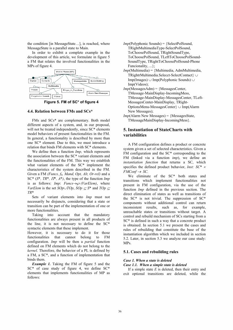
In order to exhibit a complete example in the development of this article, we formulate in figure 5 a FM that relates the involved functionalities in the MPs of figure 4.

Figure 5. FM of SC* of figure 4

4.4. Relation between FMs and SCs*

FMs and SCs* are complementary. Both model

different aspects of a system, and, in our proposal, will not be treated independently, since SC* elements model behaviors of present functionalities in the FM. In general, a functionality is described by more than one SC* element. Due to this, we must introduce a relation that binds FM elements with SC* elements.

We define then a function Imp, which represents the association between the SC* variant elements and the functionalities of the FM. This way we establish what variant elements of the SC* implement the characteristics of the system described in the FM. Given a FM (Funcs, f0, Mand, Opt, Alt, Or-rel) and a SC* (S*, ΤR*, Π*, A*), the type of the function Imp is as follows: Imp: Funcs→℘(VarElem), where VarElem is the set SOp∪TOp, SOp ⊆ S* and TOp ⊆ TR*

Sets of variant elements into Imp must not necessarily be disjuncts, considering that a state or transition can be part of the implementation of one or more functionalities.

Taking into account that the mandatory functionalities are always present in all products of the line, it is not necessary to define the SC* syntactic elements that these implement. However, it is necessary to do it for those functionalities that cannot belong to FM configuration. Imp will be then a partial function defined on FM elements which do not belong to the kernel. Therefore, the behavior of a PL is defined by a FM, a SC*, and a function of implementation that binds them.

Example 1. Taking the FM of figure 5 and the SC* of case study of figure 4, we define SC* elements that implements functionalities of MP as follows:

Imp(Polyphonic Sounds) = {SelectPolSound, TRightMultimediaType-SelectPolSound, ToChoosePolSound, TRightSoundType, ToChoosePolSound, TLeftToChoosePolSound-SoundType, TRightToChoosePolSound-Phone Funcionality, ...};

Imp(Multimedia) = {Multimedia, AdmMultimedia, TRightrMultimedia.Selecct-SelectContact} ∪ Imp(Images) ∪ Imp(Polyphonic Sounds) ∪ Imp(Videos);

Imp(MessagesAdm) = {MessagesCenter, TMessage-MainDisplay-IncomingMess, TMessage-MainDisplay-MessagesCenter, TLeft-MessagesCenter-MainDisplay, TRight-OptionsMenu-MessagesCenter} ∪ Imp(Alarm New Messages);

Imp(Alarm New Messages) = {MessagesState, TMessageMainDisplay-IncomingMess}.

5. Instantiation of StateCharts with variabilities

A FM configuration defines a product or concrete

system given a set of selected characteristics. Given a FM configuration and the SC* corresponding to the FM (linked via a function imp), we define an instantiation function that returns a SC, which specifies the defined product behavior, Inst: SC* × FMConf → SC.

We eliminate of the SC* both states and transitions which implement functionalities not present in FM configuration, via the use of the function Imp defined in the previous section. The direct elimination of states as well as transitions of the SC* is not trivial. The suppression of SC* components without additional control can return inconsistent results, such as, for example, unreachable states or transitions without target. A control and rebuild mechanism of SCs starting from a SC* is defined in such a way that a concrete product is obtained. In section 5.1 we present the cases and rules of rebuilding that constitute the base of the instantiation algorithm which we included in section 5.2. Later, in section 5.3 we analyze our case study: MPs. 5.1. Cases and rebuilding rules Case 1. When a state is deleted Case 1.1. When a simple state is deleted

If a simple state E is deleted, then their entry and exit optional transitions are deleted, while the

36

mandatory transitions are composed using the following rebuilding method.

Let E∈SOp be the state to eliminate, A1,…, An predecessor states of E (i.e., states from which there are non-optional transitions with target E (tAE_1,…, tAE_n)), and S1 ,…, Sm successor states of E (i.e., target states of non-optional transitions with source E (tES_1,…, tES_m)), according to the example of figure 6. When the variant state E is deleted, all entry and exit transitions linked to E are deleted. Simultaneously, new transitions are generated by the composition of the non-optional entry transitions (tAE_1,…, tAE_n) with the non-optional exit transitions (tES_1,…, tES_m).

Figure 6. Generalized SC* of case 1

The composition of two transitions t1 = (t1, so1, e1, c1, α1, sd1, ht1, non_optional) and t2 = (t2, so2, e2, c2, α2, sd2, ht2, non_optional) define a new transition as follows: comp(t1, t2) = (t12, so1, e1:: e2, c1∧c2, α1:: a2, sd2, ht2, non_optional), where :: is the sequential composition of events and actions, and ∧ the conjunction of conditions. Both operations must be associative in order to make the instantiation algorithm deterministic.

Let sc = (S*, ΤR*,Π *, A*) be SC*, we define the set of entry and exit non-optional transitions pairs of a state E of sc as follows:Te_s(E) = {(te, ts)∈TR*×TR* | target(te)=E ∧ source(ts)=E ∧ TransType (te)= TransType (ts)=non_optional}.

The result of eliminating an optional Or-state E of sc corresponds to the SC* following: Delete_simple_state (E, (S*, ΤR*)) =

(S* - {E}, TR* ∪ { comp(te,ts) | (te, ts)∈Te_s(E) } - { t∈TR* |

t∈Domain(Te_s(E)) ∨ t∈Range(Te_s(E)) } - { t∈TR* | TransType(t)=optional ∧ (source(t)=E ∨ target(t)=E ) })

In figure 7, we show the result of the application of this rule on the SC* of figure 6.

Figure 7. Resulting SC* after the deletion of the optional state of figure 6

Case 1.2. When an Or-state is deleted If an Or-state E is deleted, then their entry and exit

optional transitions are deleted, while the mandatory transitions are composed using the following rebuilding method. The proposal consists in applying the previous transition composition method of case 1.1 on E, considering certain conditions and affectations to SC*. Let sc* = (S*, ΤR*) be a SC*, we define the set of all the entry and exit non-optional transition pairs of a Or-state E of sc* as follows: Te_s(E) ={ (te, ts)∈TR*×TR* | target(te) ∈

substates(E) ∧ source(ts)∈substates(E) ∧ TransType(te)=TransType(ts)=non_optiona}

where substates(E) is the set of substates of E. We establish that each entry transition to E is

composed with one exit transition if the source state of the exit transition is reached from the target state of the entry transition. We define Reachable(E, A) as the set of reachable substates of E from the substate A. In figure 8, we show a situation where the elimination of the state E produces the composition of the transitions e3 with e6, since B∈Reachable(E, A) is satisfied. As opposed to this, the transitions e7 and e2 would not have to be composed, since C∉Reachable(E, B) is satisfied.

We define TCompe_s(E) = { (te, ts) ∈ Te_s(E) | source(ts)∈Reachable(E, target(te)) } as the set of transition pairs that must be composed by means of case 1.1, previous modification of these transitions as is indicated as follows. For each entry transition te∈Domain(TCompe_s(E)) its target state is now E, i.e., target(te)=E. Also, for each exit transition ts∈Range(TCompe_s(E)), source(ts)=E. The result of eliminating the optional Or-state E of sc* corresponds to the SC* following: Delete_Or_state (E, (S*, ΤR*)) =

(S* - ({E}∪substates(E)), TR* ∪ { comp(changes_target(te, E),

changes_source(ts ,E)) | (te,ts)∈TCompe_s(E) } - { t∈TR* | source(t) ∈ ({E}∪ substates(E)) ∨ target(t) ∈ ({E}∪ substates(E)) })

The function changes_target(t,E) changes the target of transition t, such that target(t)=E. Likewise, changes_source(t, E) changes the source of transition t, such that source(t)=E.

Figure 8. Deletion of an optional Or-state

37

(a) (b) (c)

Figure 9. Deletion of the optional Or-state E of figure 8

Example 2. Considering the SC* of figure 8, TCompe_s(E) = {(e3, e2), (e3, e6), (e7, e6)}. In figure 9(a) we show how the entry transitions e3 and e7, and the exit transitions e2 and e6, are modified. Later, the internal components as well as entry and exit transitions are eliminated, as shown in figure 9(b). Finally, transition pairs of TCompe_s(e) are composed such as the case 1.1 indicates. The final result of the elimination of the state E is observed in figure 9(c).

Case 1.3. When an And-state is deleted If an optional And-state E is deleted, then their

entry and exit optional transitions are deleted, while the mandatory transitions are composed using a rebuilding method similar to case 1.2. Two possible relations of dependency or synchronization between parallel states exist. One of them refers to the occurrence of an event that produces the trigger of two or more transitions belonging to each one of the parallel substates. The second corresponds to using conditions of type “in E” (see case 3). The latter forces to redefine the concept of reachability, since it is not valid to apply the previous definition of reachability independently from each one of the orthogonal states.

Let E be an And-state with n orthogonal states. We define now Reachable(E , (E1, E2 ,…, En )) as the set of n-tuples of reachable states from (E1, E2 ,…, En). In this way, maintaining the definition of Te_s(e) of the previous case and redefining TCompe_s(E), it is possible to solve the method of transition elimination and composition (Delete_And_state) in an analogous form to case 1.2. TCompe_s (E) = { (te, ts) ∈ Te_s(E) | (∃ n-tuple_init, n-tuple_end ∈ (S* × S* × ... × S*)n | n-tuple_end∈Reachable(E, n-tuple_init) ∧ (∃i, j 1≤i, j≤n | n-tuple_end[i] = source(ts) ∧ n-tuple_init[j] = target(te) ∧ cond(ts) )) }, being n the amount of orthogonal states in E.

Figure 10. Delete of an optional Or-state.

Example 3. Considering the SC* of figure 10, the steps that are carried out when the state E is deleted, are observed in figures 11(a)-(c). Note in figure 11(b) that the condition [in C] in the transition e8 is eliminated (see case 3).

Case 2. Consequences of the elimination of a state

Some situations can appear as a consequence of applying the described cases previously, which must be considered in order to reestablish the SC*. These situations are analyzed in the following cases.

Case 2.1. When an initial state is deleted If an initial state of a state E is eliminated, we

distinguished two cases (for the details, see [7]): 1) if the successor of the initial state of E belongs to the substates of E and is unique, it becomes the new initial substate; and 2) if more than one successor of the initial state of E exists that is also a substate, then the new initial state will be the second state of the list of the substates of E.

Case 2.2. When some substate in a parallel decomposition is deleted

It is possible to establish as a trigger condition of a transition restrictions “in E”, which indicate that the trigger will be executed whenever the state E belongs to the current configuration of the statechart. These restrictions are applied only to parallel states. The conditions of transitions in a parallel decomposition of type “in E” are deleted when the state E is eliminated via some FM configuration [7].

Case 2.3. When all the substates are deleted If all the substates of a superstate E disappear,

then E also disappears, applying the case 1. The substates can disappear by being involved in implementations of different functionalities.

Case 3. When a transition is deleted If a transition t disappears it does not produce

alterations in a SC*, except when some state, or possibly a complete subarea, of SC* is unreachable from the initial state of the system. In this last case, the unreachable area should be eliminated, applying in each situation, i.e. for each component, the previously considered cases.

38

(a) (b) (c)

Figure 11.Deletion of E in figure 10

5.2. Instantiation Algorithm Given a FM and its configuration, we will name

NSF to the set of non-selected functionalities of the model as a consequence of the configuration. For the FM fm = (Funcs, f0, Mand, Opt, Alt, Or-rel) and a configuration conffm = (F, R) of fm, NSF = Funcs - F. We define also the set of non-selected components (NSC) by the configuration conffm of SC* sc, which will not be part of resulting SC, as follows: NSC(conffm, sc) = { x∈VarElem | ∃ fi ∈ NSF: x∈Imp(fi) ∧ ¬∃ fi' ∈ F: fi'≠ fi ∧ x∈Imp(fi') }, with VarElem e Imp defined for sc according to section 4.4. This is, the states and transitions that do not implement selected functionalities by a configuration will be excluded from the behavior of resulting SC. The instantiation process of a SC* sc = (S*, ΤR*) is defined by the algorithm Inst: SC* × FMConf → SC, on the basis of the cases and rules presented in the previous section.

The function ConvOpt(sc) converts the optional

elements of sc in non_optional (this is, in SC elements); VarElemType(x) returns the variant element type of x: simple_state, or_state, and_state, or transition; the function SubComponents(x, sc) returns the set of both substates and internal transitions of the state x of sc; Unreachable

Components(x, sc) returns the set of both unreachable states and transitions of sc after the elimination of the state x; and, Delete_transition implements the case 3 of section 5.1.

5.3. Instantiations of the Case study: MPs

The FM of figure 5 can be configured to

characterize different MPs, according to the specification of the case study of section 4.3. Next, we present a configuration of a MP of figure 5 and we proceed towards obtaining the corresponding SC (the MP wanted), according to the algorithm Inst defined in section 5.2.

A MP, with neither the support for the management of polyphonic sounds nor the capacity of alerting the user when new messages enter in the incoming mailbox, is defined by the configuration conffm = (F, R) of the FM of figure 5, where:

F = {MP, Display, Quick-Marking, Videos, Contacts, MessagesAdm, Multimedia, Images, Ringer_in_ functions}, and

R = {(MP, {Multimedia}), (MP, {MessagesAdm}), (MP, {Quick-Marking}), (MP, {Display}), (MP, {Contacts}), (MP, {Ringer_in_functions}), (Multimedia, {Images}), (Multimedia, {Videos})}.

Taking the previous configuration and the function Imp described in example 1 of section 4.4, the sets NSF and NSC(conffm, sc) are defined as follows:

NSF = {Polyphonic Sounds, AlamrNewMessages}, and NSC(conffm, sc) = {SelectPolSound, TRightMultimedia,

Type-SelectPolSound, ToChoosePolSound, TRightSound Type-ToChoosePolSound, TLeftToChoosePolSound-Sound Type, MessagesState, TRightToChoosePolSound-Phone Funcionality, TMessage-MainDisplay-Incoming Mess}.

In [7] we show a detailed step by step execution of the algorithm Inst, which was omitted here due to space restrictions, on the SC* of figure 4 and the configuration conffm defined previously. The resulting SC is given in figure 12. 6. Related works

A variety of existing approaches propose the

incorporation of variabilities in software systems and in particular on PLs. One of these is the one designed

39

Figure 12. SC for a MP without polyphonic sounds and without alert of new messages

by Jacobson [11], whose weaknesses have been analyzed by several authors, for example in [12].

Most recent solutions attempt to modify or to extend the used models. Different authors have proposed to represent explicitly the variation points by adding annotations or by changing the bases of Use Case Diagrams. For example, Von der Maßen [13] proposes the use of a graphical notation with new relations. John and Muthig [14] suggest the application of use case templates, although they do not distinguish between optional, alternative or obligatory variants. However, Halman and Pohl [15] sustain the modification of use case models for representing graphically variation points. In [12] the authors propose to make use of UML 2 package merge, based on [16], as a tool for the variability

representation and configuration in PLs.With respect to structural models, either UML mechanisms are used directly, as in the mentioned case of Jacobson, or are written in explicit form using stereotypes. The works of Gomaa [2] and Clauß [17] are examples of this latter approach. Czarnecki proposes in [18] and [19] to annotate within UML diagrams, conditions of presence expressed, for example, by means of color codes, in such a way that, each optional characteristic is reflected in one or several parts of a diagram. This representation technique could be applied solely to class diagrams.

An alternative approach to this paper is developed in parallel by other members of the research project in which subsumes this work. In [20] the authors, in a formal framework, define functions that associate

40

SCs (not components of SCs, as in our case) to functionalities of a FM, and analyze forms of combination between different SCs which specify possible variants of a PL. Whereas under our method the behavior of a product in a PL is obtained basically by a selection process, in [20] the focus is oriented towards a process of SC combinations. 7. Conclusions and further works

Most of the techniques of Model Driven Development make use of UML. In particular, the SCs of UML constitutes a mechanism for specifying systems behavior by means of a graphical representation. In this work, we presented an extension of UML SCs by incorporating variability in their essential components to specify PLs. We use FMs to describe he common and variant functionalities, in such a way that, starting from different FM configurations and via an algorithm based on rules, concrete SCs corresponding to different PLs can be obtained. We develop partial examples of a case study based on mobile phone technology, whose full version is not included in this article due to space restrictions. For more information, the reader is referred to [7].

Given the fact that UML and SCs have become very successful languages for analysis and design in the very short run, we are confident that the results of this work can be successfully applied to the real problems of the software industry. It is a timely contribution to an authentic and actual problem.

As part of our plans for future work, we are interested in an extension of SCs which allows us to completely cover the UML 2.0 SCs and analyze variabilities, not only the ones considered in this paper, but in all of their components. Also, we will make an attempt to provide a formal semantics for the extension. This semantics is an essential preliminary step towards both the automatic code generation and the validation of complex software systems. Finally, we will try to compare formally both proposed methods by members of the investigation project in which this work is subsumed, in order to complement and enrich both lines of research.

8. References [1] P. Clements, L. Northrop. Software Product Lines: Practices and Patterns. SEI Series in SE, Addison-Wesley, 2002. [2] H. Gomaa. Designing Software Product Lines with UML: From Use Cases to Pattern-based Software

Architectures. The Addison-Wesley Object Technology Series, 2004. [3] Christian Del Rosso, Evaluation and Assessment in Software Engineering. In Proc. of EASE’06, British Computer Society, Keele, UK, 2006. [4] Object Management Group: OMG Unified Modeling Language Specification Version 2.0, 2004. [5] K. Czarnecki, U. Eisenecker. Generative Programming: Methods, Techniques, and Applications. Addison-Wesley, 2000. [6] N. Szasz, C. Luna, and A. González. Hacia una formalización de líıneas de productos mediante máquinas de estados con variabilidades. In Proc. of XXXIII Conferencia Latinoamericana de Informática, CLEI’07, 2007. [7] C. Luna, A. Gonzalez. Especificación del comportamiento de líneas de productos mediante modelos de funcionalidades y máquinas de estados con variablilidades. TR 06/07, ORT University, 2007. [8] D. Harel. Statecharts: A visual formalism for complex systems. Science of Computer Programming, 8: 231-274,1987. [9] M. von der Beeck. A structured operational semantics for UML-statecharts. Springer, 2002. [10] K. Kang, J. Lee, P. Donohoe. Feature–Oriented Product Line Engineering. IEEE Software, 19(4):58–65, 2002. [11] I. Jacobson et al. Software Reuse. Architecture, Process and Organization for Business Success. Addison-Wesley, 1997. [12] M. Laguna et al. Gestión de la Variabilidad en Líneas de Productos. In Proc. of CLEI’07, Costa Rica, 2007. [13] T. von der Maßen, H. Lichter. Modeling Variability by UML Use Case Diagrams. In Proc. of the International Workshop on Requirements Engineering for Product Lines (REPL’02), 2002. [14] I. John, D. Muthig. Tailoring Use Cases for Product Line Modeling. In Proc. of the International Workshop on Requirements Engineering for Product Lines (REPL’02), 2002. [15] G. Halmans, K. Pohl. Communicating the Variability of a Software-Product Family to Customers. Journal of Software and Systems Modeling 2 (1): 15-36, 2003. [16] A. Zito, Z. Diskin, J. Dingel. Package merge in UML 2: Practice vs. theory?. In O. Nierstrasz, J. Whittle, D. Harel, and G. Reggio, editors, MoDELS/UML’06, 2006. [17] M. Clauß. Generic modeling using Uml extensions for variability. In Workshop on Domain Specific Visual Languages at OOPSLA’01, 2001. [18] K. Czarnecki, M. Antkiewicz. Mapping Features to models: a template approach based on superimposed variants. In Proc. GPCE’05, LNCS 3676, Springer, pp. 422-437, 2005. [19] Czarnecki, K., K. Pietroszek. Verifying Feature-Based Model Templates Against Well-Formedness OCL Constraints. In Proc. of ACM SIGSOFT/SIGPLAN GPCE'06, ACM Press, 2006. [20] N. Szasz, P. Vilanova. Statecharts and Variabilities. In Proc. of Second International Workshop on Variability Modelling of Software-intensive Systems, Germany, 2008.

41