ARTICLE IN PRESS

www.elsevier.com/locate/simpat

Simulation Modelling Practice and Theory xxx (2005) xxx–xxx

Performance evaluation based onsystem modeling using Statecharts extensions

Carlos Renato Lisboa Frances a,*, Edvar da Luz Oliveira a,Joao Crisostomo Weyl Albuquerque Costa a,

Marcos Jose Santana b, Regina Helena Carlucci Santana b,Sarita Mazzini Bruschi b,

Nandamudi Lankalapalli Vijaykumar c,Solon Venancio de Carvalho c

a Programa de Pos-Graduacao em Engenharia Eletrica—PPGEE, Universidade Federal do Para—UFPA,

66075-110 Belem, PA, Brazilb Instituto de Ciencias de Matematica e de Computacao—ICMC, Universidade de Sao Paulo—USP,

13560-970 Sao Carlos, SP, Brazilc Laboratorio Associado de Computacao e Matematica Aplicada—LAC, Instituto Nacional de Pesquisas

Espaciais—INPE, 12227-010 Sao Josedos Campos, SP, Brazil

Received 26 March 2003; received in revised form 15 December 2004; accepted 2 February 2005

Abstract

This paper presents two extensions for Statecharts: the Stochastic Statecharts, which use

the original statecharts notation with a minor modification in the formal semantics and the

Queuing Statecharts, which do not follow the pure Statecharts notation, but a join between

Statecharts and queuing network representations. Some basic elements of Statecharts are rede-

fined such as events and conditions, besides some concepts referring to the dynamic system

behavior. The specification approaches show the basic behavior of a generic queuing system

1569-190X/$ - see front matter � 2005 Elsevier B.V. All rights reserved.

doi:10.1016/j.simpat.2005.02.001

* Corresponding author.

E-mail addresses: rfrances@ufpa.br (C.R.L. Frances), edvar@ufpa.br (E. da Luz Oliveira),

jweyl@ufpa.br (Joao Crisostomo Weyl Albuquerque Costa), mjs@icmc.usp.br (M.J. Santana),

rcs@icmc.usp.br (R.H.C. Santana), sarita@icmc.usp.br (S.M. Bruschi), vijay@lac.inpe.br (N.L. Vijayku-

mar), solon@lac.inpe.br (S.V. de Carvalho).

2 C.R.L. Frances et al. / Simulation Modelling Practice and Theory xxx (2005) xxx–xxx

ARTICLE IN PRESS

by means of templates and standard events. It is presented the PerformCharts, a new simula-

tion environment based on Statecharts specification, which allows model solution using either

Markov chains or the Network Simulator (NS).

� 2005 Elsevier B.V. All rights reserved.

Keywords: Performance evaluation; Statecharts; Queuing systems; Markov chains; Systems modeling

1. Introduction

There are many different reasons to look carefully at performance evaluation of

systems in general. Normally, decision-makers have to investigate when their systemswill saturate in order to find the best way to avoid or at least to delay its occurrence.

Depending on the system this can be based on the knowledge of very experienced

system managers, but a better option is always to look for a systematic performance

evaluation of the system. Performance evaluation can be realized following several

techniques broadly grouped into measuring and modeling techniques. Usually, mea-

surements, benchmarking and prototyping fall into the category of measuring; these

techniques are very useful when investigating existing systems, i.e. systems that have

already been built, providing accurate information for their performance evaluationand analysis. Modeling is also used for providing performance evaluation and anal-

ysis and can be applied to both existing and under-project systems. A modeling pro-

cess usually starts with a high-level specification (either graphical or non-graphical)

and ends up with the presentation of performance measurements. These perfor-

mance measurements come from the solution of the model and this can be produced

by means of both analytical and simulation solutions. An Analytical approach asso-

ciates the system specification to a mathematical model such as Markov chains or

queuing theory. On the other hand, a Simulation approach takes to the constructionof a computer program that reproduces the system behavior, according to the model

specification. Fig. 1 shows the phases defined for the modeling process.

Models of actual systems are generally complex as they involve parallelism, syn-

chronization and interdependence of subsystems. They are normally named reactive

systems as they are based on the occurrence of events according to external or

Specification of Model PN , QN , SC , SD ...

p , λ , t . ..Parameters of Model

MC , QT, SimulationSolution of Model

Text Files, Graphics ... Presentation of Performance Results

PN (Petri nets), QN (Queuing Networks), SC (Statecharts), SD (State-transition Diagrams) p (Probabilities), λ (Rates), t (Time)MC (Markov chains), QT (QueuingTheory).

Fig. 1. Phases of a modeling process.

C.R.L. Frances et al. / Simulation Modelling Practice and Theory xxx (2005) xxx–xxx 3

ARTICLE IN PRESS

internal stimuli. However, the main concern is how to describe the behavior of reac-

tive systems in a clear and realistic way and at the same time maintaining a rigorous

formal basis that can be computationally handled [15]. In order to model these sys-

tems, concepts of parallelism, resource sharing, synchronization, interdependence,

hierarchy and randomness (random interferences) are considered.State-transition diagrams are a natural choice as they represent a system by means

of states and transitions between states based on events. Unfortunately, these dia-

grams cannot cope up with the complexity of most of the systems. The parallelism

of actions increases exponentially with the number of concurrent subsystems consid-

ered. A detailed representation of a given system may not be able to clearly give an

idea of the number of states in the model. In real applications, models may contain

hundreds of thousands of states where ideas of concurrency and interdependency

among the components of the system are difficult to be handled. Thus, there is a needfor high-level model specification tools allowing mathematical models being auto-

matically generated. Some existing higher-level techniques (for the purpose of this

paper) generally associated to stochastic processes are Queuing networks [24] and

Stochastic Petri nets [32]. The premise is that these techniques must be capable of

representing the complexity of a system graphically.

This paper approaches the problem of performance models and finding a model

solution in a straightforward way, maintaining the formal base of statecharts to-

gether with the easy-look of queuing network diagrams and issuing solutions bymeans of both Markov chains and simulation. A modeling/simulation tool is also

proposed and described. The model technique used is general and can be adopted

for modeling systems in many real-world application fields. The tool built can easily

being ported to different computing platforms because it was fully developed in

JAVA [9].

2. Systems specification techniques

This paper gives a brief description of some of the modeling techniques used for

systems modeling in order to give an idea of the way systems can be described at the

specification level. The principal idea is to discuss the association between a clear

graphical specification and a viable solution method, improving the modeling pro-

cess. Originally, Statecharts have been developed for providing behavior analysis

only. However, this work presents a new approach for performance evaluation based

on Statecharts specification, using both analytical and simulation solutions. Finally,an example involving process scheduling in a computer network is explored to see

the advantages and disadvantages of each of these techniques in order to determine

the performance measurements.

2.1. Queuing network specification

In some applications there are situations in which queues are formed. These situ-

ations can be represented by three basic elements: arrivals, service mechanism and

4 C.R.L. Frances et al. / Simulation Modelling Practice and Theory xxx (2005) xxx–xxx

ARTICLE IN PRESS

service discipline. These situations may get complicated in the sense that the output

of one service center (queue + server) can be used to form the input to another one or

outputs from more than one service center may be combined to form the input to

another one. These situations are commonly found in industrial productions where

unfinished products have to undergo through some processes before being availableto the consumer. Such applications are generally modeled by a technique based on

queuing theory known as queuing networks [7,24].

If applications can be merely described by means of queues and server, then the

graphic representation of Queuing Networks may be adequate. However, if the

description of a system needs more complex details, then other specification tools

(such as Petri nets, Statecharts) may be more appropriate.

Several applications make use of queuing networks such as manufacturing sys-

tems, computer networking and telecommunication and broadcasting [10]. As a mat-ter of fact, only since mid-1970s, they have been widely used in representing Flexible

Manufacturing Systems [14]. They are convenient in specifying a model during the

preliminary design. However, complex systems, due to their nature of being reactive,

have a powerful relationship with event occurrences, which are responsible for

changes among states. In these cases, it is strongly recommended to use techniques

that have some additional characteristics, for instance: events and their effect (broad-

casting), hierarchy and refinement of states, concurrence/parallelism among compo-

nents; these features, essential in modeling modern complex systems, cansignificantly enhance the representation of the system behavior.

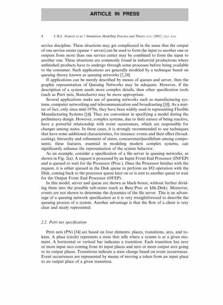
As an example, consider a specification of a file server in queuing networks, as

shown in Fig. 2(a). A request is processed by an Input Front End Processor (INFEP)

and is queued to wait for the Processor (Proc.). Once the Processor finishes with the

request, it is either queued in the Disk queue to perform an I/O operation with the

Disk, coming back to the processor queue later on or is sent to another queue to wait

for the Output Front End Processor (OFEP).

In this model, server and queue are shown as black-boxes, without further divid-ing them into the possible sub-states (such as Busy.Proc or Idle.Disk). Moreover,

events are not shown to determine the dynamics of the file server. This is an advan-

tage of a queuing network specification as it is very straightforward to describe the

queuing process of a system. Another advantage is that the flow of a client is very

clear and nicely represented.

2.2. Petri net specification

Petri nets (PN) [34] are based on four elements: places, transitions, arcs, and to-

kens. A place (circle) represents a state that tells where a system is at a given mo-

ment. A horizontal or vertical bar indicates a transition. Each transition has zero

or more input arcs coming from its input places and zero or more output arcs going

to its output places. Transitions indicate a state change based on event occurrences.

Event occurrences are represented by means of moving a token from an input place

to an output place of a given transition.

Network

Proc.Queue

Proc.Busy

Proc.Free

T1

T2

T3 T4

T5

T6

Disc.Queue

Disc.BusyDisc.Free

INFEP.Free

INFEP.Busy

OFEP.Busy

OFEP.Free

OFEP.Queue

T7

T8T9

(a)

(b)

Fig. 2. (a) Queuing network representation of a file server. (b) Petri net representation of a file server.

C.R.L. Frances et al. / Simulation Modelling Practice and Theory xxx (2005) xxx–xxx 5

ARTICLE IN PRESS

Fig. 2(b) presents the same file server of Fig. 2(a) modeled by Petri nets. In thefigure, the servers INFEP (In Front-End Processor), OFEP (Out Front-End Proces-

sor), Proc (Processor) and Disk are further refined into ‘‘Busy’’ and ‘‘Free’’ sub-

states. Other dependencies such as ‘‘a client can occupy a server only if it is free’’,

or ‘‘for each end of service of a client the respective server is released by moving

the token to Server.Free’’, can also be observed.

The Petri net specification is very popular and several varieties of systems have

taken advantage of this tool to represent them. However, Petri nets can become

unintelligible as the model increases. According to Jensen [23], ‘‘the practical use

6 C.R.L. Frances et al. / Simulation Modelling Practice and Theory xxx (2005) xxx–xxx

ARTICLE IN PRESS

of PN to describe real-world systems has clearly demonstrated a need for more pow-

erful net types, to describe complex systems in a manageable way’’. A more compact

representation has been achieved by equipping each token with an attached data

value—called the token color. The data value may be of arbitrarily complex type

(such as a record structure of some programming languages). By following this idea,there are some extensions to minimize the impact originated by model growth. Some

of the main extensions are Hierarchical and Colored Petri nets [23], which present a

notation very different from the original PN representation (called Place-Transition

PN). Moreover, original Petri nets do not have any mechanism of grouping (super-

state) to create some mode of hierarchy among states that compose a given compo-

nent of the system.

Originally, PNs were not designed to provide performance evaluation (as Queuing

Networks), but Molloy [32] showed the possible association in each transition in aPN with an exponentially distributed random variable that expresses the delay of en-

abling the firing of a transition. PNs with this feature are known as Stochastic Petri

Nets (SPN). Molloy showed that, due to the memoryless property of the exponential

distribution of firing delays, SPNs are isomorphic to continuous-time Markov

chains.

Chiola [8], presented an extension to SPNs known as Generalized Stochastic Petri

Nets (GSPN). GSPNs are obtained by allowing transitions to belong to two different

classes: immediate transitions and timed transitions. The first fires in zero time once itis enabled; the former fires at a random, exponentially distributed, enabling time.

2.3. Statecharts specification

Statecharts are graphic-oriented and are capable of specifying reactive systems.

They have been originally developed to represent and simulate real time systems

[15]. Moreover, Statecharts come with a strong formalism [16] and their visual ap-

peal is very tempting leading to considering them as very potential to represent reac-tive systems. They are an extension of state-transition diagrams with notions of

hierarchy (depth), orthogonality (representation of parallel activities) and interde-

pendence (broadcast-communication). The basic elements of Statecharts to represent

a system are: state, event, condition, action, transition, expression, variable and

label. Details of each element definition as well as their main features are described

in [15–18].

States are used to describe a certain aspect of a given system. As an example, take

a machine that is responsible for processing a job. The machine is idle until an arrivalof a job takes place. The initial idle stage of the machine may be denoted as a ‘‘Wait-

ing’’ state waiting for a job in order to start the processing. Another state would be

‘‘Processing’’ once a job is fed to be processed it is the machine responsibility to re-

spond it for the processing appropriately. The machine may fail while processing a

job. In this case a new state ‘‘Failure’’ would represent the fact.

Event is a very important element to observe the model of a given system. It is

considered as an interference to the system in the sense that the present system

behavior as a whole is changed to another behavior due to an event occurrence.

C.R.L. Frances et al. / Simulation Modelling Practice and Theory xxx (2005) xxx–xxx 7

ARTICLE IN PRESS

From the above example of the machine, the arrival of a job is an event. The system

remains in the ‘‘Waiting’’ state until a job is fed, changing the system state from

‘‘Waiting’’ to ‘‘Processing’’, in which the job is processed. The end of service may

be considered as another event to denote that the processing is done and that the sys-

tem should return to ‘‘Waiting’’. In case the machine fails during processing, theevent failure takes the system to ‘‘Failure’’ state and returning to ‘‘Waiting’’ through

the event end of correction of the failure.

Optionally, an event may be attached to a condition also known as a guarding

condition. The Statecharts, in this case, enable the event even though it is supposed

to be fired only when the condition is satisfied.

Parallelism is used to influence other orthogonal components in the system. This

is done by providing the action entity. Action may be a change of an expression, a

change of a variable or even events that are fired in other orthogonal components.This is associated to the event meaning that once the event is fired, the system state

is changed and the given action is executed so that the system state is continued to be

changed. Statecharts provide some special events such as true(condition), false(condi-

tion), entered(X) and exited(X) (these special conditions are abbreviated in the State-

charts formalism as tr(condition), fs(condition), en(X) and ex(X) respectively) to cope

up with the internal logic of the modeled system. The first two are respectively true

and false if the condition is evaluated to be true and false. The last two are related to

a state X in which the event en(X) is stimulated if state X is entered whereas the eventex(X) is stimulated whenever there is an exit from state X. These four special events

are considered as immediate events, which means that they are the first to be auto-

matically reacted in any given system.

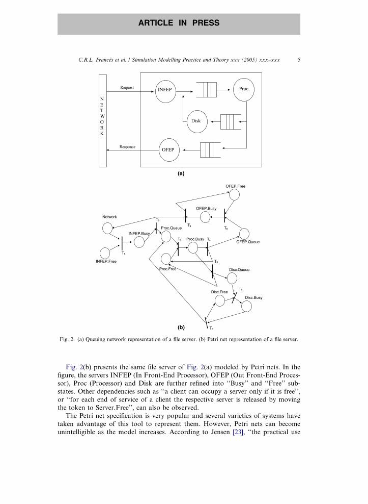
Transition is the physical representation to denote a change of a state within a sys-

tem (transitions are represented by arrows). A label is provided on the arrows to

indicate the events that change the state of a system behavior. For the example of

the machine, there would be an arrow from ‘‘Waiting’’ (W) state to ‘‘Processing’’

(T) state. The label of the arrow could be the event arrival of a job (a) indicating thata transition from ‘‘Waiting’’ state to ‘‘Processing’’ state has occurred when the event

has been fired (Fig. 3). The full syntax of a label along a transition is: ev[c]/a, where

the event ev is fired if the condition c is satisfied and when this ev is fired a change of

system state has occurred. Then the action a is executed by changing again the sys-

tem state (in other components). Fig. 3 also shows other events to indicate end of ser-

vice (s), failure (f) as well as end of correction (c).

F

Ts

a

c

W

f

Fig. 3. States, events and transitions.

8 C.R.L. Frances et al. / Simulation Modelling Practice and Theory xxx (2005) xxx–xxx

ARTICLE IN PRESS

In Statecharts, a state may contain sub-states. This is very useful in models for

performance evaluation when events trigger the same transition from different states.

Instead of representing a physical transition leaving from each state, just an arrow

leaving from the father state (also known as a super-state) is sufficient. In this case,

the number of transitions in the diagram is reduced, simplifying the representation ofthe model.

Fig. 4(a) shows a state-transition diagram representation of a machine that exe-

cutes two types of jobs. The possible states for the machine are: idle (W), working

on job of type 1 (T1), working on job of type 2 (T2) and failure (F). The transitions

can be fired by one of the following events: arrival of a job of type 1 (a1) or type 2

(a2), end of job of type 1 (s1) or type 2 (s2), machine failure (f) and end of repair (c).

It is assumed that a job is executed only if the machine is idle and when the idle ma-

chine is not subject to failures.In Fig. 4(b), the W, T1 and T2 are clustered in state A (Available). The state A is

said to be a macro-state or a super-state of type XOR. The semantics of A is inter-

preted, as whenever this state is active, one and only one of its sub-states is active.

The event f takes the machine from ‘‘available’’ state to ‘‘failure’’ state F. In order

to represent the fact that the machine is not subject to failures when idle, the condi-

tion [not in(W)] is added to the transition label from A to F. To be more precise the

condition must be correctly written as [not in(A.W)]—(indicating state W within the

macro-state A)—to avoid ambiguity whenever state names are repeated. However,this is not necessary here because the figure shows no ambiguity in the names,

making the syntax to be formalized as [not in (W)]. This notation—macro-state.-

sub-state—has been adopted for the proposed work (only when necessary) as no

satisfactory notation for avoiding ambiguity has been found in the literature.

In general it is necessary that some state must be a default or initial state in order

to denote a starting point whenever a system is to be observed for its dynamics. In

Statecharts terminology it is natural to use ‘‘a system is entered’’ meaning that a

F

T1

s1

f

s2

T2

a1 a2

c

W

f

F

T1

s1 s2

T2

a1 a2

c

W

f[not in(W)]

A

F

T1

s1 s2

T2

a1 a2

c

W

f[not in(W)]

A

(a) (b) (c)

Fig. 4. Example of hierarchy.

C.R.L. Frances et al. / Simulation Modelling Practice and Theory xxx (2005) xxx–xxx 9

ARTICLE IN PRESS

macro state is switched on or active. In order to represent an initial state, Statecharts

provide the concept of entry by default. In Fig. 4(c), the bent arrow pointing to the

state W means that this state is the initial entry point within state A. When the sys-

tem enters in A one of its sub-states must be active; in this case W is activated due to

entry by default. In this figure when the A macro-state is active, as mentioned earlier,only one of its sub-states is active. In Statecharts the active states of a given system

are referred to as configuration. Therefore, one can say that the initial configuration

of the macro-state A is W.

Statecharts have been referenced in literature on its theoretical aspects and as

specification tool in many application domains. Without depleting the subject, some

of the applications mentioned in the literature are presented as follow:

In the aspects related to its semantics and syntax, for example:

M. Mendler and G. Luettgen [30]: ‘‘Axiomatizing an algebra of step reactions

for synchronous languages’’.

M. Mendler and G. Luettgen [31]: Statecharts: from visual syntax to model-

theoretic semantics’’.

Gerald Luttgen, Michael von der Beeck and Rance Cleaveland [27]: ‘‘A com-

positional approach to statecharts semantics’’.

In the aspects of application/tools, for example:

Elena Troubitsyna [35]: ‘‘Developing fault tolerant software using Statecharts

and FMEA’’.

D. Latella and M. Massink [26]: ‘‘On mobility extensions of UML Statecharts;

a pragmatic approach’’.

M.C.F. de Oliveira, M.A.S. Turine, P.C. Masiero [33]: ‘‘A Statechart-based

model for hypermedia applications’’.P. Herrmann, H. Krumm, O. Drogehorn, W. Geisselhardt [19]: ‘‘Framework

and tool support for formal verification of high speed transfer protocol

designs’’.

However, despite the use of Statecharts in many domains, it is not used in perfor-

mance evaluation, despite the series of advantages that the Statecharts specification

could bring to the study of the systems performance. This is the main motivation of

this work.

2.4. Statecharts semantics: steps, configurations and micro-configurations

The base for the Statecharts semantics is a sequence of instants of time {ri} i P 0,

that corresponds to the rate of execution of the system. In [16], a set of intervals of

times exists defined by I = (ri,ri+1), where each Dr (ri+1 � ri) represents the elapsed

time for determined step i. The system will react at each end of interval ri ! ri+1,

presenting a new configuration of states.An external stimulus, in ri+1, is a triple (P,h,n), where P is a set of external prim-

itive events that occur in Ii, h is the set of external primitive conditions whose values

10 C.R.L. Frances et al. / Simulation Modelling Practice and Theory xxx (2005) xxx–xxx

ARTICLE IN PRESS

are true in (ri,ri+1), and n is a function determined by the external environment,thus, for a variable v, n(v) = x if the value of v is x in (ri,ri+1). A configuration of

a system associated with the instant ri+1 is a tuple (X,P,h,n), where X is the maxi-mum configuration of states of the root state, and (P,h,n) is an external stimulusassociated to ri+1.A reaction of the system is a pair (,P*), where is the set of transitions called step,

and P* is a set of atomic events generated by . Informally, a step is a set of transi-

tions that can be enabled and are induced by external stimulus. It is important to

stand out that all the constant transitions in a step are gone off simultaneously.

Another definition of a step is viewed as a sequence of micro-steps, which generates

intermediate configurations (micro-configurations), where each micro-step is con-

tained in . In order to clarify the idea of a micro-step, a basic file server [11] will be

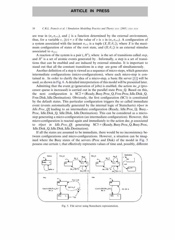
used, as shown in Fig. 6. A detailed interpretation of this model will be presented later.Admitting that the event jg (generation of jobs) is enabled, the action inc_p (pro-

cessor queue is increased) is carried out in the parallel state Proc_Q. Based on this,

the next configuration is SC2 = (Ready,Busy.Proc_Q,Free.Proc, Idle.Disk_Q,

Free.Disk, Idle.Destination). Obviously, the first configuration (SC1) is constituted

by the default states. This particular configuration triggers the so called immediate

event (events automatically generated by the internal logic of Statecharts) tr[not in

Idle.Proc_Q] leading to an intermediate configuration (Ready, Idle.Proc_Q, Busy.-

Proc, Idle.Disk_Q, Idle.Disk, Idle.Destination). This can be considered as a micro-step generating a micro-configuration (an intermediate configuration). However, this

micro-configuration is reacted again and immediately to the action dec_p associated

to tr[not in Idle.Proc_Q] generating SC3 = (Ready,Busy.Proc_Q,Busy.Proc,

Idle.Disk_Q,Idle.Disk, Idle.Destination).

If all the states are assumed to be immediate, there would be no inconsistency be-

tween configurations and micro-configurations. However, a situation can be imag-

ined where the Busy states of the servers (Proc and Disk) of the model in Fig. 5

possess one certain si that effectively represents values of time and, possibly, different

Fig. 5. File server using Statecharts representation.

C.R.L. Frances et al. / Simulation Modelling Practice and Theory xxx (2005) xxx–xxx 11

ARTICLE IN PRESS

values, which are interpreted as an average of one determined probability distribu-

tion (assumed here as exponential). It can still be imagined that, for the example,

ssource > sbusy.proc ^ ssource > sbusy.disc. Thus, in hypothetical values, ssource = 5 u.t.,sbusy.proc = 3 u.t. and sbusy.disk = 4 u.t.In these circumstances, SC1 would still contain default states, SC2 would be

(Ready, Busy.Proc_Q, Idle.Proc, Idle.Disk_Q, Idle.Disk, Idle.Destination) after

the event jg and the action inc_p and SC3 would continue being (Ready,

Idle.Proc_Q, Busy.Proc, Idle.Disk_Q, Idle.Disk, Idle.Destination). However, SC4

would already generate a structural conflict that would be responsible for going

off the micro-steps that compose SC4. If the transition that contains eos is enabled,

then the system will be able to reach two possible SC4 configurations: (1) if proba-

bility p is admitted, then SC4 will be (Ready, Idle.Proc_Q, Idle.Proc, Busy.Disk_Q,

Idle.Disk, Idle.Destination); (2) if the probability 1 � p is admitted, then SC4 will be(Ready, Idle.Proc_Q, Idle.Proc, Idle.Disk_Q, Idle.Disk, Out_FS). Moreover, if the

qualified transition contains the event jg, then configuration SC4 will be (Ready,

Busy.Proc_Q, Busy.Proc, Idle.Disk_Q, Idle.Disk, Idle.Destination).

One way to maintain consistency for successor configurations is the adoption of a

timeline and timers in each state that has an associated delay. Thus, the choice would

be conditional to the least elapsed time (associated to a state) to qualify for an imme-

diate transition.

3. Stochastic Statecharts—A new proposition for syntax, semantics and templates

In this section, a formal semantics to Statecharts is presented by adapting some

points of the original Statecharts semantics and syntax proposed in [16]. In order

to allow the construction of a generic specification, which can be solved by means

of both analytical and simulation solutions, some standard templates have been pro-

posed to describe queuing systems.

3.1. Syntax modifications

Two main modifications have been added to the original specification: states with

exponentially distributed delays and inclusion of probabilities. The first adaptation

considers delays as random variables (interarrival time and service time). Thus, a

state with delay can be a source that generates clients yielding an exponential distri-

bution or a certain server that grants a service to customers according to an exponen-tial distribution. Fig. 6(a) shows the graphic notations for delay and immediate

states.

The second adaptation refers to the need of associating a probabilistic value

for each possible path followed by a client. This situation forces the customer to

choose among various possibilities. The selection through probabilities is repre-

sented by means of a circle with the letter P inside. Fig. 6(b) presents a probabilistic

situation.

Fig. 6. Syntax adaptations: (a) state with delay and immediate and (b) selection for probability.

12 C.R.L. Frances et al. / Simulation Modelling Practice and Theory xxx (2005) xxx–xxx

ARTICLE IN PRESS

Formally, the probabilistic condition is defined as:

(a) $P = {p1,p2, . . .,pn}, where P is the set of probabilities associated to the eventsand pi is a point within the probability space defined by P ) pi 2 P, with

i = 1,2, . . .,n;(b) 0 6 pi 6 1, "i = 1,2, . . .,n;(c)

Pni¼1pi ¼ 1;

(d) It is assumed that pi 2 C (C is the set of conditions defined by Harel [16]).

By extension, if c 2 C and pi 2 C, then ev(c) and ev(pi) are events associated to a

condition c and event conditioned to a probability pi, respectively. In order to distin-

guish the difference between a probabilistic condition and a regular condition, the

notation ev{pi} is used in place of ev(c), as proposed and implemented in [36].

3.2. Redefinition of steps and configurations for Stochastic Statecharts

This section introduces the idea of time in steps and configurations (dynamics) of

Statecharts. As defined by Harel [16], a system is non-deterministic in a given State-

charts configuration (SC) if it has two possible reactions ð� 1;P�1Þ and ð� 2;P�

2Þ, suchthat P�

1 6¼ P�2 or � 15 � 2.

Thus, in the Stochastic Statecharts, a configuration and a step have an interpre-tation if all its states are considered immediate and another interpretation if states

are associated with delays. An extension of the original definitions is required to

reach the temporal features of the statecharts:

Definition 1. A state is considered delayed when a variable si exists, determining

when evaluated:

(i) The mean time between arrivals of customers, when a state is a generating

source of these customers (Source). It is assumed that the inter-arrival times

are exponentially distributed;

(ii) The mean service time to attend the customers, when a state is a server (in

its Busy state). It is assumed that the service times are exponentiallydistributed.

C.R.L. Frances et al. / Simulation Modelling Practice and Theory xxx (2005) xxx–xxx 13

ARTICLE IN PRESS

Definition 2. A state is considered immediate when its delay is considered zero

(si = 0).

Definition 3. The time (ri+1) of the next reachable configuration SC = (X,P,h,n)obeys the following algorithms:

(i) The variable evaluated in n is si where si is the delay associated with a state si,

with i = 1, . . .,n;(ii) min(si) is the function that indicates the least delay time in a configuration SCj,

with j = 1, . . .,n;(iii) The time spent in each step is sj = sj�1 + min(si), with j = 1, . . .,n. The time sj is

equal to the final time of a configuration SCi or to the initial time of a config-

uration SCi+1;

(iv) If j = 1, first step, then sj = min(si), therefore sj�1 = 0;(v) si.rest = {si} � min(si), "si 5 min(si), where si.rest is the remainder of delay time

of a state that it surpasses for the next step;

(vi) stotal ¼Pn

j¼1s� j;(vii) "{si} � {min(si)}, si := si.rest, to end of each step;

(viii) If si = min(si), then si.rest = 0 and si in the following step starts with value 0.

Definition 4. A selection for probability takes the system to different reactions

ð� 1;P�1Þ; ð� 2;P�

2Þ; . . . ; ð� n;P�nÞ, such that P�

1 6¼ P�2 6¼ 6¼ P�

n or � 15 � 25 5 � n.

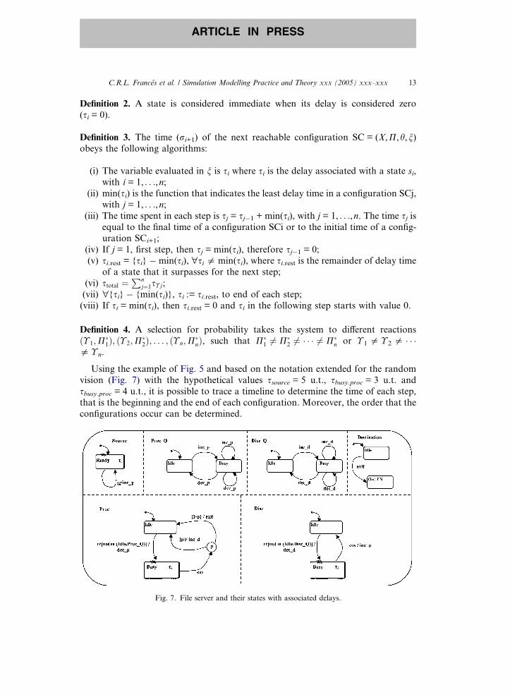
Using the example of Fig. 5 and based on the notation extended for the random

vision (Fig. 7) with the hypothetical values ssource = 5 u.t., sbusy.proc = 3 u.t. andsbusy.proc = 4 u.t., it is possible to trace a timeline to determine the time of each step,that is the beginning and the end of each configuration. Moreover, the order that the

configurations occur can be determined.

Fig. 7. File server and their states with associated delays.

14 C.R.L. Frances et al. / Simulation Modelling Practice and Theory xxx (2005) xxx–xxx

ARTICLE IN PRESS

SC1 is the initial configuration, i.e., it presents the entry to the system in the

Source state (a state with delay of 5 u.t.), and other initial states of other parallel

components. SC2 is the successor configuration and it is a function of the first

one, in relation to the time. If Source state is active, the system waits for 5 u.t. until

the first customer is generated (event jg). After 5 u.t. step 1 is completed with the exe-cution of the action inc_p (in Proc_Q), taking to Busy.Proc_Q. Now, SC3 qualifies

for an immediate transition through event tr[not in(Idle.Proc_Q)], reaching

Busy.Proc and simultaneously reaching Ready (in Source) through jg. The step time

and the next configuration will be determined by previously described functions

(according to the stochastic vision), in the following way (being s1 = ssource, s2 =sbusy.proc, s3 = sbusy.Disk):

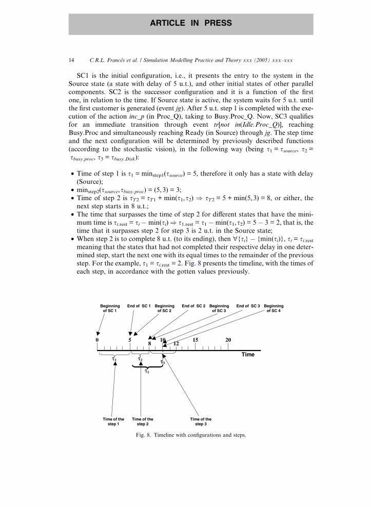
• Time of step 1 is s1 = minstep1(ssource) = 5, therefore it only has a state with delay(Source);

• minstep2(ssource,sbusy.proc) = (5,3) = 3;• Time of step 2 is s�2 = s�1 + min(s1,s2) ) s�2 = 5 + min(5,3) = 8, or either, thenext step starts in 8 u.t.;

• The time that surpasses the time of step 2 for different states that have the mini-mum time is si.rest = si � min(si)) s1.rest = s1 � min(s1,s2) = 5 � 3 = 2, that is, thetime that it surpasses step 2 for step 3 is 2 u.t. in the Source state;

• When step 2 is to complete 8 u.t. (to its ending), then "{si} � {min(si)}, si = si.restmeaning that the states that had not completed their respective delay in one deter-

mined step, start the next one with its equal times to the remainder of the previous

step. For the example, s1 = si.rest = 2. Fig. 8 presents the timeline, with the times ofeach step, in accordance with the gotten values previously.

Time

Time of thestep 1

0 5 10 15 20

Beginningof SC 1

End of SC 1

8

τ1

Beginningof SC 2

τ2

Time of thestep 2

End of SC 2

τ1

12

τ3

Time of thestep 3

Beginningof SC 3

End of SC 3 Beginningof SC 4

Fig. 8. Timeline with configurations and steps.

C.R.L. Frances et al. / Simulation Modelling Practice and Theory xxx (2005) xxx–xxx 15

ARTICLE IN PRESS

The temporal values for SC3 are calculated in the following way:

• minstep2(ssource,sbusy.Disk] = (2,4) = 2;

• Time of step 3 is s�3 = s�2 + min(s1,s3) ) s�3 = 8 + min(2,4) = 10, that is, thenext step starts in 10 u.t.

The time that surpasses time of step 3 for different states that have the minimum

time is si.rest = {si} � min(si) ) s3.rest = s3 � min(s1,s3) = 4 � 2 = 2, that is, the timethat it surpasses of step 3 for step 4 is of 2 u.t. in the Busy.Disk state. To proceed

admitting the previous premises, some considerations must be established. First, it

is important to clarify where it finds the random character of the specification and

the admitted functions. The randomness is intrinsic to the distributions of generation

and attendance to the customer, therefore these distributions generate the rhythms ofarrivals and of service (variables that serve of input for the solution of the system).

The defined functions as premises warrant that the events keep the order expected

for a generic system of queues, what does not harm in any way the random

approach.

There is a general solution that is applicable to most kinds of systems, called Mar-

kov chains. Due to its importance, in the next section it is presented an algorithm for

generating Markov chains from a Statecharts specification.

4. Construction of Markov chain from a Statecharts specification—the general solution

A Markov Chain—more precisely, within the scope of this work, a Continuous-

Time Markov Chain—consisting of transition rates among states is the input to the

available numerical methods [5] to determine the steady-state probabilities.

It has been already seen that a one-to-one correspondence can be made between a

Continuous-Time Markov Chain and a state-transition diagram. Therefore, theproblem of constructing the Markov model will be solved if the model represented

in the high-level specification tool Statecharts generates the state-transition diagram

corresponding to the specified model. As can be seen, it is possible to produce the

transition matrix by using the state-transition diagram and with this matrix the stea-

dy-state probabilities are determined, building the basis to calculate the performance

measurements.

Once the model is specified in a Statecharts representation, the enabled events

must be stimulated so that new configurations are yielded. Internal events are gener-ated by Statecharts semantics and considered as immediate events in the sense they

are immediately stimulated when the model reaches a configuration where they are

active. Events can also be triggered by actions associated to transitions and the ac-

tions are stimulated as soon as the transition is fired. External events are not gener-

ated by the Statecharts semantics and therefore describing the dynamics of the

modeled system behavior must stimulate them. In order to make the association

of Statecharts model with a Markov chain possible, the only type of external events

that can be considered are stochastic events. These events are those that the time

16 C.R.L. Frances et al. / Simulation Modelling Practice and Theory xxx (2005) xxx–xxx

ARTICLE IN PRESS

between their activation and their occurrence follows a stochastic distribution. In

particular, for Continuous-Time Markov Chains, this distribution has to be

exponential.

Once the model is specified using the Statecharts representation, the first step is

taking the initial configuration provided by entries by default. In other words allthe initial States of each orthogonal component are taken. A reaction, that is a stim-

ulation of events to yield a new configuration, is first done by stimulating the imme-

diate events such as true(condition) and false(condition). This reaction results in a

new configuration. If there are actions associated with these immediate events, these

are fired yielding new configuration. This process of reacting to immediate events

continuously takes place until a configuration is obtained in which no more imme-

diate events are active. Then a list of stochastic events is obtained based on the re-

sulted configuration. New configurations are generated reacting to each stochasticevent of the list. Actions are executed if they are associated with these stochastic

events. These new configurations are checked against any active immediate events.

This process goes on until all the configurations have been expanded. The result

of all this process is a list of a structure that contains a source configuration, stochas-

tic event (along with its rate) stimulated and the target configuration. With this infor-

mation a transition matrix is constructed and the steady-state probabilities can be

evaluated.

The research work described here is concentrated on studying this problem anddeveloping a prototype of the mentioned framework. Restrictions (not taking into

consideration all the entities of the Statecharts) have been made to tailor the tool

to be used for the proposed objective of the framework. These restrictions will be

mentioned in the next section that describes the implementation of the tool in details.

However, it is felt that for applications in performance evaluation these restrictions

do not hinder in any way the specification of a reactive system.

The configurations have to be organized in such a way that a transition matrix

consisting of transition rates can be easily generated, i.e., the rows and columns ofthe matrix are configurations and the elements correspond to transition rates from

a source configuration to a destination configuration. This will be the input for

the existing library to calculate the steady-state probability vector and consequently

the performance measurements of interest.

In order to understand the complete functioning of the process from the specifi-

cation until the generation of the transition matrix, an example will be shown. Con-

sider a system with three parallel components that correspond to two machinery

equipments and a supervisor to repair any failure in the equipment. The componentsE1 and E2 denote the equipment whereas the component Supervisor is responsible

for repairing the equipment when they fail and a priority is provided to repair E1

whenever both equipments are down. The list of stochastic events includes a1, r1,

f1, s1 a2, r2, f2 and s2. Internal events are tr[in(B1)], tr[in(B2) ^ �in(B1)]. Actionsc1 and c2 are fired once the events s1 and s2 are also considered as internal events.

This model is shown in Fig. 9.

When the specification is complete, a first reaction is performed by checking and

stimulating the internal events that may be enabled from the initial configuration.

System

P2

B2

r2

a2

f2

c2

W

WS

tr[in(B2) ]∧ in(B1)

E2

Supervisor

W2P1

B1

r1

a1

f1

c1

WW1

E1

C1

s2/c2

tr[in(B1)]

C2

s1/c1

Fig. 9. Statecharts representation of an equipment with a repairer.

C.R.L. Frances et al. / Simulation Modelling Practice and Theory xxx (2005) xxx–xxx 17

ARTICLE IN PRESS

For example, internal events such as tr[in(X)], where X is a State, are reacted if the

initial configuration of the system has an active State X. In the case of the example

presented in Fig. 9, no internal events are active for the initial configuration. There-

fore, taking the initial configuration (W1, W2, WS) the enabled events are the sto-

chastic events a1 and a2. These events will be stimulated to yield the new

configurations.

When the system is in the initial configuration and a1 is activated, the next con-

figuration is (P1, W2, WS). Suppose that during the process of stimulating the eventsa configuration is (B1, B2, WS). In this case, the active events are the immediate

events provided by tr[in(B1)] and tr[(in(B2) ^ �in(B1)]. As mentioned earlier, theseare the events that have to be checked and enabled before the stochastic events,

i.e. even though there are enabled stochastic events, the immediate events (true(con-

dition) and false(condition)) are the events that have to be stimulated.

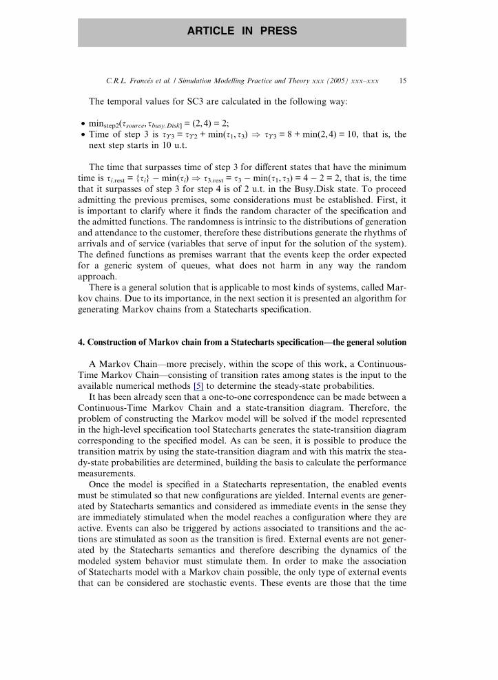
The state-transition diagram is shown in Fig. 10, consisting of stochastic events

that follow exponential distributions. The states and arcs with events following expo-

nential distributions compose a Markov chain, which can be handled with numericalmethods, producing steady-state probabilities that, in turn, are the basis for calculat-

ing the performance measurements.

Fig. 10 is a Markov model and, therefore, a one-to-one correspondence with a

transition matrix can be associated. By organizing the rates among the configura-

tions obtained in the figure, a transition matrix is formed. This transition matrix,

consisting of the transition rates, considering a software tool built in an object-ori-

ented approach, PerformCharts, which to be described in Section 7.

In many situations it is desirable to evaluate systems, which have the presence ofqueues in their main resources, i.e., queuing systems. In order to represent queuing

systems there is a general agreement to use certain standards to describe states and

W1,P2,WS

P1,P2,WS

f1

a2

W1,W2,WS

r1

B1,B2,C2

a1f2

W1,B2,C2

f2

r1

a1

s2

P1,B2,C2

s2

f2

r2

B1,B2,C1

a2

a1

f1

B1,W2,C1

f1

P1,W2,WS

r2

a2

s1

B1,P2,C1

s1

s2s1

r1 r2

Fig. 10. State-transition diagram of Fig. 9.

18 C.R.L. Frances et al. / Simulation Modelling Practice and Theory xxx (2005) xxx–xxx

ARTICLE IN PRESS

events. This is exactly the objective of the following section in which some templates

are provided to represent features of queuing systems (states and standard events), inorder to apply while specifying a given model in Statecharts.

4.1. Templates and standard events for queuing systems

This section presents a set of four templates and its event-standard for specifica-

tion of queuing systems. In the context of this work, a template is a set of states (pos-

sibly unitary) that defines a basic functioning of a given system component. The idea

is that, except for some parameters such as time spent, to attend a job in a server,templates can be applicable to certain components with as minimum modifications

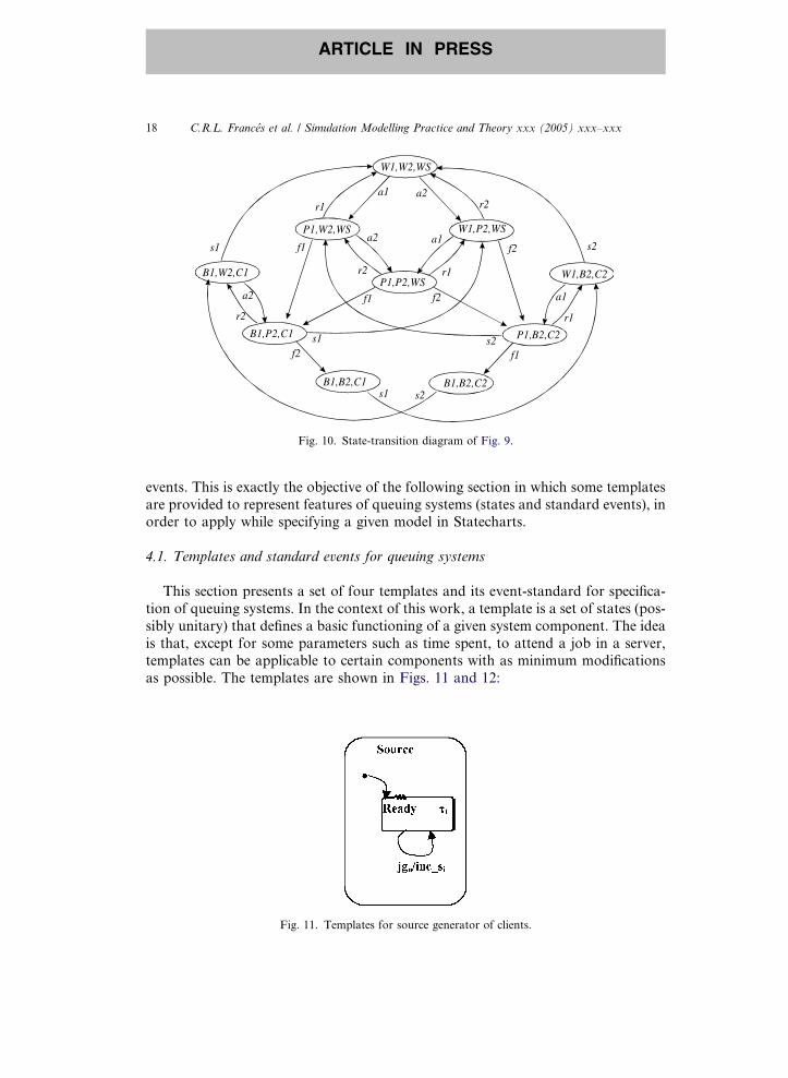
as possible. The templates are shown in Figs. 11 and 12:

Fig. 11. Templates for source generator of clients.

Fig. 12. Templates: (a) for Server Queue, (b) for Server and (c) for Destination.

C.R.L. Frances et al. / Simulation Modelling Practice and Theory xxx (2005) xxx–xxx 19

ARTICLE IN PRESS

In the template shown in Fig. 11, there is no immediate generation of the first cus-tomer; therefore the default state is already a state with delay that, when reached,

must spend si associated to it. In Fig. 11, the event jg (job generation) is responsiblefor generating a customer and the action inc_s adds the client generated in the server

queue.

A template for a server queue is suggested when it contains two sub-states: Idle

and Busy. A queue, by default, is empty (Idle) and every time a customer is gener-

ated, the queue size is increased thus leading the system to Busy state. Continuous

occurrences of the event inc_s keep the queue in Busy. On the other hand, continuousoccurrences of dec_s decrease the queue size until the unitary limit-value (Q = 1),

from which the queue moves to Idle state, indicating the absence of customers. It

is worth mentioning that a decrease in the queue size corresponds to the fact that

the customer is being served. Representation of a template for a server queue is

shown in Fig. 12(a).

A template for representing servers with two sub-states had been created. The two

sub-states are: Idle and Busy, with the same semantics of the previous template.

However, here the Busy state is associated with a delay of si with a mean value ofa probability distribution. If there is a customer in the queue, the event tr[not

in(Idle.Serveri_Q)] is executed qualifying its transition and the queue is decreased.

Once the customer is served, eos is triggered probabilistically. The probability con-

nector leads the customer either to the system exit or to another service. In the latter

case the server queue size is increased (inc_si+1). Fig. 12(b) shows a template for

servers.

Fig. 12(c) shows a template for representing a destination with two sub-states

(Idle and Out_System). This state represents the idea of waiting for some reply (Idle)or a reply is received so that a customer may leave the system (Out_System).

In order to standardize some essential events for performance evaluation, Table 1

provides standard names used for these events along with their semantics. However,

other events may also be added.

5. Queuing Statecharts

In Statecharts, there is an inherent difficulty for representing the linear path a cus-

tomer passes through in a queuing system. Queuing networks cover this feature very

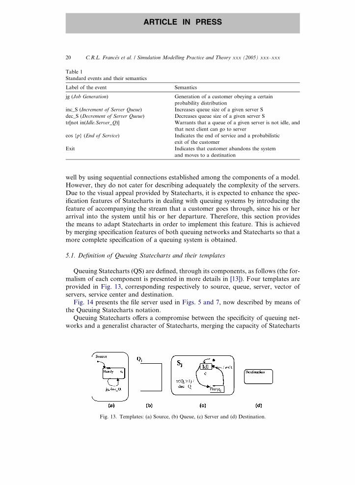
Table 1

Standard events and their semantics

Label of the event Semantics

jg (Job Generation) Generation of a customer obeying a certain

probability distribution

inc_S (Increment of Server Queue) Increases queue size of a given server S

dec_S (Decrement of Server Queue) Decreases queue size of a given server S

tr[not in(Idle.Server_Q)] Warrants that a queue of a given server is not idle, and

that next client can go to server

eos {p} (End of Service) Indicates the end of service and a probabilistic

exit of the customer

Exit Indicates that customer abandons the system

and moves to a destination

20 C.R.L. Frances et al. / Simulation Modelling Practice and Theory xxx (2005) xxx–xxx

ARTICLE IN PRESS

well by using sequential connections established among the components of a model.

However, they do not cater for describing adequately the complexity of the servers.

Due to the visual appeal provided by Statecharts, it is expected to enhance the spec-

ification features of Statecharts in dealing with queuing systems by introducing the

feature of accompanying the stream that a customer goes through, since his or her

arrival into the system until his or her departure. Therefore, this section provides

the means to adapt Statecharts in order to implement this feature. This is achieved

by merging specification features of both queuing networks and Statecharts so that amore complete specification of a queuing system is obtained.

5.1. Definition of Queuing Statecharts and their templates

Queuing Statecharts (QS) are defined, through its components, as follows (the for-

malism of each component is presented in more details in [13]). Four templates are

provided in Fig. 13, corresponding respectively to source, queue, server, vector of

servers, service center and destination.Fig. 14 presents the file server used in Figs. 5 and 7, now described by means of

the Queuing Statecharts notation.

Queuing Statecharts offers a compromise between the specificity of queuing net-

works and a generalist character of Statecharts, merging the capacity of Statecharts

Fig. 13. Templates: (a) Source, (b) Queue, (c) Server and (d) Destination.

Fig. 14. File server in Queuing Statecharts representation.

C.R.L. Frances et al. / Simulation Modelling Practice and Theory xxx (2005) xxx–xxx 21

ARTICLE IN PRESS

for showing different levels of abstraction with the linear path of clients, which com-

prises an elegant feature of queuing diagrams.

6. Solutions for Statecharts models

The aim of this section is at emphasizing the generic character of the proposed

specification, which had been elaborated to provide a certain independence of theadopted solution. In Section 4 it was presented the general solution based on Con-

tinuous-Time Markov Chains. In this section other solutions for queuing systems

modeled by the statecharts are discussed.

With the objective of applying both solutions to the specifications proposed in this

paper, an association between these specifications and Jackson solutions, as well as

an event-based simulation is explored. The model of a file server (already presented

in this paper), now parameterized with arrival and service hypothetical rates, is used

as a testbed.

6.1. Analytical solution

The analytical solution assumes that the modeled system is in equilibrium. In this

context, equilibrium also implies that the system is steady, that is, with q < 1, whereq represents the utilization and is defined as q ¼ k

cl. It is directly proportional to the

arrival rate (k) and inversely proportional to the factor (cl, where c is the number ofservers, and l is the service rate). If q < 1 is true then k < cl, i.e., the arrival rate inthe system must be less than the capacity of this system to serve customers. The cases

studied in this paper admit that the system reaches the equilibrium.

Relationships between the analytical solution and configuration of queuing net-

works (open or closed) are mentioned in [22,1,2]. In the context of this paper, Jack-

son networks for open models are used.

22 C.R.L. Frances et al. / Simulation Modelling Practice and Theory xxx (2005) xxx–xxx

ARTICLE IN PRESS

6.1.1. Jackson networks

In this section, it is presented a possible solution using the Statecharts templates

set. It is suggested an algorithm to solve a Statecharts specification by means of Jack-

son networks [21], which define some types of queuing networks assuming a model

with M nodes, satisfying the following conditions:

• Each node consists of ci identical exponential servers, each one with mean servicerate li, where i = 1,2, . . .,M.

• Customers arrive at node i from the outside of the model in a Poisson standard

(exponential) with mean arrival rate ki (the customers can also arrive at node i

through other nodes of the model), for i = 1,2, . . .,M.• If served in node i, a customer leaves immediately to node j, where j = 1,2, . . .,M,with probability pij; or the customer leaves the model with probability1�

PMj¼1pij.

Models that satisfy these conditions are called Jackson networks. For each node i

of a Jackson network, the mean arrival rate (or mean entrance rate) for the node, Ki,

is given by [1]:

Ki ¼ ki þXMj¼1

pji Kj:

6.1.2. Jackson solution for Queuing Statecharts

The model of the file server presented in Section 6.1 will be used as an example. It

is feasible to apply Jackson solution to this situation as the model is open (with feed-

back from center 2 to center 1), and this is shown in Fig. 12. The model also obeysthe restrictions presented in the Jackson theorem (Section 6.1.1]. The choice for the

Queuing Statecharts notation take into consideration the fact that Jackson networks

are based on the service centers (transitions among them), and these centers are

explicitly defined in Queuing Statecharts.

In the Stochastic Statecharts, the service centers are not explicitly defined. How-

ever, it is possible to match the states server and queue in a service center superstate.

To associate the events of the specification with the variable of the equations used

in the solution of Jackson some considerations are assumed. Thus, the following pre-mises are adopted, some of them also present in the traditional queuing systems:

• pji is the probability of moving from state j to state i, where i, j = 1,2, . . .,M. Ifi = j, then it has a probability of remaining in the current state.

• In the specification of Queuing Statecharts, pji is always associated with the occur-rence of the event inc_Qk, with k = 1,2, . . .,M, being the event inc_Qk produced

either for an external source or another service center. K also specifies the next

center to be visited.• The input rates (K) are always consequence of increment events of the Qk variable

(k = 1,2, . . .,M).

C.R.L. Frances et al. / Simulation Modelling Practice and Theory xxx (2005) xxx–xxx 23

ARTICLE IN PRESS

Parameters considered for the example of Fig. 12 are extracted from [11], adopt-

ing the following values: s1 = 0.083, s2 = 0.04, s3 = 0.05, p = 0.6.Considering exponentially distributed arrivals and services and applying Jackson

method to the example:

K1 ¼ k þ qK1 ¼k

1� q¼ 12

0:6¼ 20;

K2 ¼ 0:4 20 ¼ 8:

With the input rate values K1 and K2, utilization for each center can be calculated:

q1 ¼ Kili

q1 ¼ 2025¼ 0:80;

q2 ¼ 820¼ 0:40:

�

The idea of adopting Jackson solution is justified due to the fact that the model is

open, consisting of a feedback in one of the servers. Moreover, this model obeys the

restrictions imposed by Jackson theorem. However, any another method that con-

templates those restrictions could have been employed in this case. An example is

the study presented in [12], in which the performance evaluation is carried out using

Continuous-Time Markov Chains, as suggested in [36].

The Jackson solution is sufficiently applicable in the real situations as they usuallyhave external generation of customers as shown in the previous example. However,

there are some situations where customers are internal and do not move to an exter-

nal destination. For these cases, an extension to the method of Jackson, called

BCMP was proposed [1].

6.2. Simulation solution

The solution through simulation is an attractive alternative when compared to theanalytical one. Although it is an approximation, it tries to reproduce the behavior of

the real system and from this reproduction an interpretation of the statistics obtained

during the execution of the program is carried out.

In this work, simulation solution is provided by using a functional extension of

the C programming language. As the events and states proposed in this paper for

a Statecharts specification are general purpose for queuing systems, other functional

extensions or simulation environments (being event-oriented) can be straightfor-

wardly adopted.The process that constitutes the simulation is composed of some phases that in-

clude the construction of the model using a specification technique and the transla-

tion of the model into a simulation program.

After establishing the system model and the input data, the model must be trans-

lated to a form suitable to be manipulated by a computer. Simulation software is

widely available to carry out this part, varying from functional extensions of conven-

tional programming languages to specific simulation languages or packages.

24 C.R.L. Frances et al. / Simulation Modelling Practice and Theory xxx (2005) xxx–xxx

ARTICLE IN PRESS

In the context of this paper, an extension of the C programming language (smpl)

is considered [28], but any other kind of event-based simulation language can be eas-

ily used.

6.2.1. smpl simulation solution applied to statecharts

smpl has been proposed as an event-based simulation language (actually a func-

tional extension of the C programming language, easily ported to different computer

platforms). Therefore, it has a direct correlation with the template events of State-

charts that describe the basic functioning of a queuing system. This correlation is

synthesized in Table 2, where the standard templates of events are associated to

the functions in smpl. The correlation between Statecharts events and smpl functions

is also shown in Fig. 15, in which each event of templates (and consequently of a

queuing system) has a one to one correspondence with the smpl functions.The semantics of the Statecharts sequence of Fig. 15 begins with the generation of

customers (jg) as an exponential distribution with mean inter-arrival time s1 (ex-pntl(Ta1)). Each generation of a new customer (inc_S) causes another service request

(request(Server_n,Customer,pri)), that will have to be conditioned into the string of

the requested server. If the server is free, it is taken by the customer (tr[not in

(Idle.Proc_Q)]) and the service rate follows an exponential distribution with mean

inter-arrival time s2 or s3 (for Proc and Disc, respectively). At the end of service,event eos (function release(Servern,Customer)), the customer takes a probabilisticpath (also admitting the path with probability 1).

It is important to observe that there are functions that do not have direct relation-

ship with the described template events for Statecharts. However, these functions

must take place into the structure of an smpl implementation. Such a fact occurs,

for example, with the functions that have the parameter ev, i.e. those functions that

are related to the occurrence of an event (such as schedule()). In order to execute

these functions, it is necessary that a previous call has been placed to the function

cause(ev,Customer), which is responsible for firing an event, that must be removedfrom the stack of events. Similarly, there are events that are represented in templates,

which have the specific objective to make the specification clearer, but they do not

have a direct correlation with an smpl function.

From the association described in Table 2 and Fig. 15 and admitting the same

input parameters used in the analytical solution, the following values are obtained,

Table 2

Correlation between Statecharts events and smpl functions

Standard-events of the Statecharts specification smpl functions

jg schedule(ev, expntl(Ta1), Customer)

inc_s request(Servern, Customer, pri)

tr[not in(Free.Server1_Q)]/dec_s schedule(ev, expntl(Ts1), Customer)

eos release(Servern, Customer)

{p} with a value of 60% and {1 � p} with a value of 40% k = random(i, j);

if ((6001 <= k) && (k<= 10000))

schedule(ev, te, Customer)

Fig. 15. Correlation between smpl functions and Statecharts events for file server.

C.R.L. Frances et al. / Simulation Modelling Practice and Theory xxx (2005) xxx–xxx 25

ARTICLE IN PRESS

considering eight executions, a confidence interval of 95% and exponential distribu-

tions for inter-arrival and service times.

For s1 = 0.0833 (inter-arrival time of customers); s2 = 0.04 (service time of Proces-sor); s1 = 0.05 (service time of Disc); te = 10,000,000 (time of simulation). ProcessorUtilization (U1) = 0.800; Disc Utilization (U2) = 0.400.

7. PerformCharts: An environment for performance evaluation based on Statecharts

specification

PerformCharts is a new environment for providing performance evaluation from

a Statecharts specification that is, at moment, in its final stage of implementation.This new environment can solve a Statecharts model by both simulation and Contin-

uous-Time Markov Chains. Simulation is based on use of the Network Simulator

(ns), which is a well-known simulation tool to study several kinds of networks

[37]. PerformCharts generates from a Statecharts template a correspondent script

TCL (Tool Command Language) [20] that can be understood by the NS tool.

Association between an NS node and a Statecharts template is not easy, since in

NS the queue of each resource is not in a node but inside the input link of each node.

Thus queue and server were split into different components for becoming adequateto the NS semantics.

Fig. 16 shows the use-case diagram for PerformCharts by means of their actors,

according to UML notation [25,4], each one presenting its own view. In the diagram,

the use-cases are grouped according to the main functionalities of the system: inter-

face for users (in which it is built the Statecharts specification), consistency analyzer

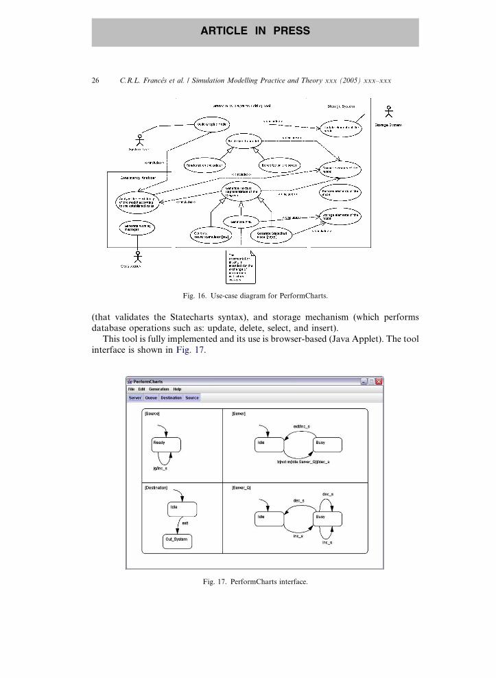
Fig. 16. Use-case diagram for PerformCharts.

26 C.R.L. Frances et al. / Simulation Modelling Practice and Theory xxx (2005) xxx–xxx

ARTICLE IN PRESS

(that validates the Statecharts syntax), and storage mechanism (which performs

database operations such as: update, delete, select, and insert).

This tool is fully implemented and its use is browser-based (Java Applet). The tool

interface is shown in Fig. 17.

Fig. 17. PerformCharts interface.

C.R.L. Frances et al. / Simulation Modelling Practice and Theory xxx (2005) xxx–xxx 27

ARTICLE IN PRESS

The PerformCharts is a highly portable tool mainly because it was built in Java

and generates its output as a XML file. This output file is used both to generate

an input for both a CTMC and an NS simulation script. The CMTC solution is pro-

vided by a software developed in C++ [36] that understands the XML specification.

For NS, an input simulation script is generated from the XML specification.

8. Modeling of the scheduling of processes in a distributed environment—A case study

This section presents a case study, involving distributed programming and its

mechanisms used for scheduling processes, that comprises an area where modeling

techniques can provide an attractive aid. More specifically, the experiment carried

out involves the allocation of processes of a certain application onto distributed pro-cessing elements, using a message-passing environment for communication and syn-

chronization and its respective methods of scheduling.

An experiment carried out empirically serves as the basis for the initial modeling

parameterization and based on this parameterization, it surpasses the situation for

future behaviors, taking into consideration better mechanisms to perform the distri-

bution of the processes. Typical situations of distributed programming and schedul-

ing of processes constitute interesting cases of study, due to the inherent complexity

of the problem.In the following sections, the features of a real environment are presented, in

which experiments were made to obtain the required input values for the modeling.

This environment uses a software to distribute the processes of the application onto

a network of computers. Estimates are made from the real data revealing interesting

features of the system modeled.

The experiment carried out consists of distributing an application to some pro-

cessing elements spread over a local computer network. A study of process schedul-

ing has its efficiency conditioned to the degree of ‘‘intelligence’’ used by thescheduling algorithm. If the scheduling has a criterion of balance when carrying

out the distribution, it is reasonable to expect a better exploitation of the system fea-

tures. Thus, the target of this experiment is to compare the behavior of the system

when using a simple round-robin mechanism (such as the standard scheduling in

PVM [6]) and the behavior of the same system when adopting a mechanism that car-

ries out some type of balancing (the processing rate of each machine is adopted as a

criterion for this case).

8.1. Model specification

The environment considered for the experiment is composed of five servers. The

first one (the PVM server) is responsible for the activation of the processes in the

other servers named lasdix, lasdpc08, lasdpc10 and lasdpc11.

Aiming at a comparison study, three model specifications are presented adopting

Stochastic Statecharts, Queuing Statecharts and Petri Nets as shown in Figs. 18–20.

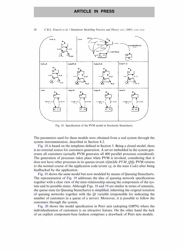
Fig. 18. Specification of the PVM model in Stochastic Statecharts.

28 C.R.L. Frances et al. / Simulation Modelling Practice and Theory xxx (2005) xxx–xxx

ARTICLE IN PRESS

The parameters used for these models were obtained from a real system through the

system instrumentation, described in Section 8.2.

Fig. 18 is based on the templates defined in Section 5. Being a closed model, there

is no external source for customers generation. A server embedded in the system gen-erates all customers (actually PVM generates all 400 parallel processes considered).

The generation of processes takes place when PVM is invoked, considering that it

does not have other processes in its queues (event tr[in(Idle.PVM_Q)]); PVM returns

to the normal course of the application code (event cg, in the state Code) after being

feedbacked by the application.

Fig. 18 shows the same model but now modeled by means of Queuing Statecharts.

The representation of Fig. 19 addresses the idea of queuing network specifications

together with a clear view of the inter-relationship among the components of the sys-tem and its possible states. Although Figs. 18 and 19 are similar in terms of semantic,

the queue state (in Queuing Statecharts) is simplified, inheriting the original notation

of queuing networks together with the Qi variable (responsible for indicating the

number of customers in a queue of a server). Moreover, it is possible to follow the

customers through the system.

Fig. 20 shows the model specification in Petri nets (adopting GSPN) where the

individualization of customers is an attractive feature. On the other hand the lack

of an explicit component-base fashion comprises a drawback of Petri nets models.

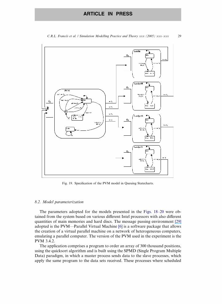
Fig. 19. Specification of the PVM model in Queuing Statecharts.

C.R.L. Frances et al. / Simulation Modelling Practice and Theory xxx (2005) xxx–xxx 29

ARTICLE IN PRESS

8.2. Model parameterization

The parameters adopted for the models presented in the Figs. 18–20 were ob-

tained from the system based on various different Intel processors with also different

quantities of main memories and hard discs. The message passing environment [29]adopted is the PVM—Parallel Virtual Machine [6] is a software package that allows

the creation of a virtual parallel machine on a network of heterogeneous computers,

emulating a parallel computer. The version of the PVM used in the experiment is the

PVM 3.4.2.

The application comprises a program to order an array of 300 thousand positions,

using the quicksort algorithm and is built using the SPMD (Single Program Multiple

Data) paradigm, in which a master process sends data to the slave processes, which

apply the same program to the data sets received. These processes where scheduled

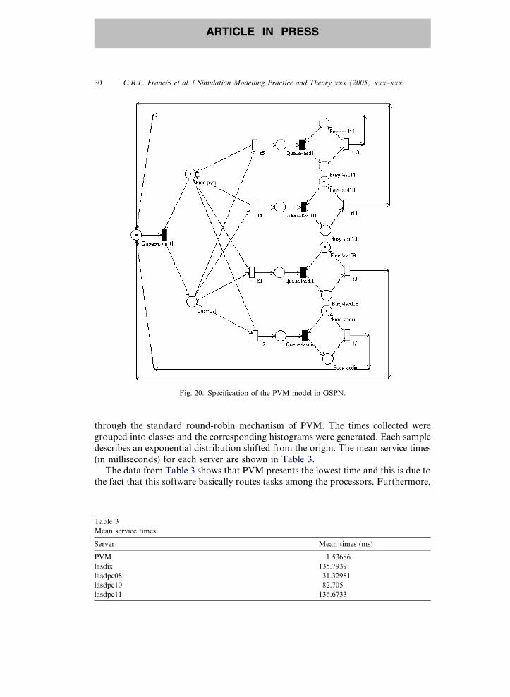
Fig. 20. Specification of the PVM model in GSPN.

30 C.R.L. Frances et al. / Simulation Modelling Practice and Theory xxx (2005) xxx–xxx

ARTICLE IN PRESS

through the standard round-robin mechanism of PVM. The times collected were

grouped into classes and the corresponding histograms were generated. Each sample

describes an exponential distribution shifted from the origin. The mean service times

(in milliseconds) for each server are shown in Table 3.The data from Table 3 shows that PVM presents the lowest time and this is due to

the fact that this software basically routes tasks among the processors. Furthermore,

Table 3

Mean service times

Server Mean times (ms)

PVM 1.53686

lasdix 135.7939

lasdpc08 31.32981

lasdpc10 82.705

lasdpc11 136.6733

C.R.L. Frances et al. / Simulation Modelling Practice and Theory xxx (2005) xxx–xxx 31

ARTICLE IN PRESS

processing time values are directly related to the computational power of the proces-

sors, which is reasonable to be expected.

For this first experiment, all the machines were considered in the same way and

the probability that the PVM chooses each one is the same (25%).

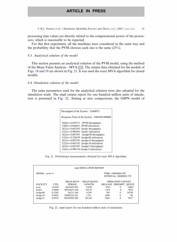
8.3. Analytical solution of the model

This section presents an analytical solution of the PVM model, using the method

of the Mean Value Analysis—MVA [22]. The output data obtained for the models of

Figs. 18 and 19 are shown in Fig. 21. It was used the exact MVA algorithm for closed

models.

8.4. Simulation solution of the model

The same parameters used for the analytical solution were also adopted for the

simulation study. The smpl output report for one hundred million units of simula-

tion is presented in Fig. 22. Aiming at new comparisons, the GSPN model of

Throughput of the System : 0.000073

Response Time of the System: 5484996.000000

X[0]=> 0.029171 (PVM throughput) U[0]=> 0.044831 (PVM utilization) X[1]=> 0.007293 (lasdix throughput) U[1]=> 0.990303 (lasdix utilization) X[2]=> 0.007293 (lasdpc08 throughput) U[2]=> 0.228479 (lasdpc08 utilization) X[3]=> 0.007293 (lasdpc10 throughput) U[3]=> 0.603142 (lasdpc10 utilization) X[4]=> 0.007293 (lasdpc11throughput) U[4]=> 0.996716 (lasdpc11utilization)

Fig. 21. Performance measurements obtained for exact MVA algorithm.

smpl SIMULATION REPORT

MODEL: pvm-v1 TIME: 100000005.087INTERVAL: 90000002.370

MEAN BUSY MEAN QUEUE OPERATION COUNTS FACILITY UTIL. PERIOD LENGTH RELEASE PREEMPT QUEUE pvm 0.0447 4024445.994 0.050 3943 0 14863 lasdix 0.9880 88916674.168 105.91 1764 0 9625 lasdpc08 0.2285 26231.198 0.295 784 0 18750 lasdpc10 0.6010 54085524.253 1.50 1098 0 96 lasdpc11 0.9939 89449585.289 292.40 1864 0 5977

Fig. 22. smpl report for one hundred million units of simulation.

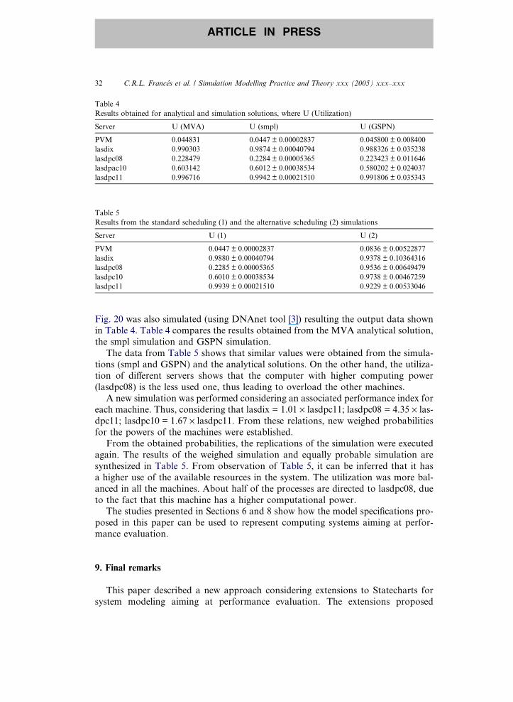
Table 4

Results obtained for analytical and simulation solutions, where U (Utilization)

Server U (MVA) U (smpl) U (GSPN)

PVM 0.044831 0.0447 ± 0.00002837 0.045800 ± 0.008400

lasdix 0.990303 0.9874 ± 0.00040794 0.988326 ± 0.035238

lasdpc08 0.228479 0.2284 ± 0.00005365 0.223423 ± 0.011646

lasdpac10 0.603142 0.6012 ± 0.00038534 0.580202 ± 0.024037

lasdpc11 0.996716 0.9942 ± 0.00021510 0.991806 ± 0.035343

Table 5

Results from the standard scheduling (1) and the alternative scheduling (2) simulations

Server U (1) U (2)

PVM 0.0447 ± 0.00002837 0.0836 ± 0.00522877

lasdix 0.9880 ± 0.00040794 0.9378 ± 0.10364316

lasdpc08 0.2285 ± 0.00005365 0.9536 ± 0.00649479

lasdpc10 0.6010 ± 0.00038534 0.9738 ± 0.00467259

lasdpc11 0.9939 ± 0.00021510 0.9229 ± 0.00533046

32 C.R.L. Frances et al. / Simulation Modelling Practice and Theory xxx (2005) xxx–xxx

ARTICLE IN PRESS

Fig. 20 was also simulated (using DNAnet tool [3]) resulting the output data shown

in Table 4. Table 4 compares the results obtained from the MVA analytical solution,

the smpl simulation and GSPN simulation.

The data from Table 5 shows that similar values were obtained from the simula-

tions (smpl and GSPN) and the analytical solutions. On the other hand, the utiliza-

tion of different servers shows that the computer with higher computing power

(lasdpc08) is the less used one, thus leading to overload the other machines.

A new simulation was performed considering an associated performance index foreach machine. Thus, considering that lasdix = 1.01 · lasdpc11; lasdpc08 = 4.35 · las-dpc11; lasdpc10 = 1.67 · lasdpc11. From these relations, new weighed probabilities

for the powers of the machines were established.

From the obtained probabilities, the replications of the simulation were executed

again. The results of the weighed simulation and equally probable simulation are

synthesized in Table 5. From observation of Table 5, it can be inferred that it has

a higher use of the available resources in the system. The utilization was more bal-

anced in all the machines. About half of the processes are directed to lasdpc08, dueto the fact that this machine has a higher computational power.

The studies presented in Sections 6 and 8 show how the model specifications pro-

posed in this paper can be used to represent computing systems aiming at perfor-

mance evaluation.

9. Final remarks

This paper described a new approach considering extensions to Statecharts for

system modeling aiming at performance evaluation. The extensions proposed

C.R.L. Frances et al. / Simulation Modelling Practice and Theory xxx (2005) xxx–xxx 33

ARTICLE IN PRESS

comprise the Stochastic Statecharts and the Queuing Statecharts. Stochastic State-

charts follow very closely the specifications proposed by 15] for the standard state-

charts, while Queuing Statecharts proposes a new approach to represent queuing

system by merging features of statecharts with the graphical representation of queu-

ing theory. The steps and configurations of the statecharts are redefined according toa stochastic view. The idea of time in steps and configurations are introduced for the

Stochastic Statecharts. An extension of the original definitions is presented to reach

the Queuing Statecharts.

All developments described in this paper were performed in such a way that al-

lows the application of both analytical and simulation techniques to solve the mod-

els. In the former solution, it is presented an algorithm for generating a Markov

chain from a Statecharts specification. This approach comprises the most general

solution and therefore it is not only target on solving queuing systems.In order to demonstrate the usefulness of the approaches proposed, two case stud-

ies where presented which considered an actual file server system (used as a testbed)

and a distributed application running on a PVM-based virtual computing

environment.

The experiments performed show that the application of the approaches proposed

is attractive and potentially improves the set of modeling strategies available for

many research and application areas involved with system performance evaluation.

At the moment, it is being implemented an environment for providing performanceevaluation based on Statecharts specification named PerformCharts. This tool can

solve a Statcharts both by CTMC and the Network Simulator (a well-known simu-

lator that has several users).

Furthermore, the approaches discussed in this paper extend statecharts creating

an alternative modeling technique that deals with concurrency, parallelism, hierar-

chy and simultaneous use of resources in a clearer and better way when compared

to the use of the traditional queuing theory. The merging of statecharts and queuing

graphical representation, summarized in the Queuing Statecharts contributes with agood graphical modeling strategy that can be easily used applying both analytical

and simulation techniques as shown through the case studied.

The techniques described in this paper are general and can easily be applied to

many different application fields. The PerformChart tool was developed in JAVA

and can easily being ported to many different computing platforms. All the software

used for solving the case studies, in both analytical and simulation solutions are writ-

ten in standard C language and therefore can be also easily executed in different com-

puting platforms. The authors will be gladded in providing the codes for interestedusers.

Acknowledgements

The authors would like to thanks the Brazilian Foundations FAPESP, CAPES

and CNPq for the support provided for the research described in this paper.

34 C.R.L. Frances et al. / Simulation Modelling Practice and Theory xxx (2005) xxx–xxx

ARTICLE IN PRESS

References

[1] A.O. Allen, Probability Statistic and Queuing Theory—with Computer Applications, Academic Press,

San Diego, 1990.

[2] A.O. Allen, Introduction to Computer Performance Analysis with Mathematica, Academic Press, San

Diego, 1994.

[3] A. Attieh, M.C. Brady, W.J. Knottenbelt, Kritzinger, Functional and temporal analysis of concurrent

systems. Available from: <http://www.cs.uct.ac.za/~william/DNAnet.html> (May 1995).

[4] H. Baumeister, D. Latella, M. Massink, M. Wirsing, Mobile UML Statecharts with localities,

Published as Technical Report 2003-TR-37, Consiglio Nazionale delle Ricerche, Istituto di Scienza e

Tecnologie dell�Informazione �A. Faedo�, 2003.[5] G. Bolch, S. Greiner, H. Meer, K. Trivedi, Queueing Networks and Markov Chains—modeling and

Performance Evaluation with Computer Science Applications, John Wiley & Sons, Inc., 1998.

[6] A. Beguelin, PVM: Parallel Virtual Machine—A User�s Guide and Tutorial for Networked ParallelComputing, The MIT Press, 1994.

[7] B. Bunday, An Introduction to Queuing Theory, Arnold, 1996.

[8] G. Chiola, M.A. Marsan, G. Conte, Generalized stochastic Petri nets: a definition at the net level and

its implications, IEEE Transactions on Software Engineering 19 (2) (1993) 89–106.

[9] H.M. Deitel, Java How to Program, fourth ed., Bookman, 2002.

[10] N.M. van Dijk, Queuing Networks and Product Forms: a Systems Approach, John Wiley & Sons, 1993.

[11] C.R.L. Frances, N.L. Vijaykumar, R.H.C. Santana, M.J. Santana, S.V. Carvalho, V. Abdurahiman,

The use of analytical and simulation solutions with Statecharts for performance evaluation: a case

study of a file server model, in: 2nd IEEE Latin–American Test Workshop—LATW2001, Cancun,

2001, Digest of Paper, Cancun, LATW, 2001, pp. 136–144.

[12] C.R.L. Frances, M.J. Santana, R.H.C. Santana, N.L. Vijaykumar, V.C. Solon, Performance

evaluation based on Statecharts specification using Markov chains and smpl simulation: a case study

of a distributed environment with a file server, in: Eurosim 2001 Congress, GA Delft, The

Netherlands, 2001.

[13] C.R.L. Frances, Statecharts Estocasticos e Queuing Statecharts: Novas Abordagens para Avaliacao

de Desempenho Baseadas em Especificacao Statecharts, Ph.D. Thesis, ICMC-USP, Brazil, 2001.

[14] S.B. Gershwin, Manufacturing Systems Engineering, Prentice-Hall, Inc., 1994.

[15] D. Harel, Statecharts: a visual formalism for complex systems, Science of Computer Programming 8

(1987) 231–274.

[16] D. Harel, A. Pnueli, J. Schmidt, R. Sherman, On formal semantics of Statecharts, in: IEEE

Symposium on Logic in Computer Science, Ithaca, USA, 1987.

[17] D. Harel, A. Namaad, The STATEMATE semantics of Statecharts, ACM Transactions on Software

Engineering 5 (4) (1996) 293–333.

[18] D. Harel, M. Politi, Modeling Reactive Systems with Statecharts S.l., McGraw-Hill Trade, 1998.

[19] P. Herrmann, H. Krumm, O. Drogehorn, W. Geisselhardt, Framework and tool support for formal

verification of high speed transfer protocol designsTelecommunication Systems, vol. 20, Kluwer

Academic Publisher, 2002, pp. 3–4, 291–310.

[20] J. Hobbs, B.B. Welch, Practical Programming in Tcl and Tk, Prentice Hall, 2003.

[21] J.R. Jackson, Networks of waiting lines, Operations Research 5 (4) (1957) 518–521.

[22] R. Jain, The Art of Computer Systems Performance Analysis—techniques for Experimental Design,

Measurement, Simulation and Modeling S.l., John Wiley & Sons, Inc., 1991.

[23] K. JensenColoured Petri Nets: Basic Concepts, Analysis Methods and Practical Use, vol. 1, Springer-

Verlag, New York, 1992.

[24] L. Kleinrock, Queuing systemsComputer Applications, vol. 2, John Wiley & Sons, 1976.

[25] C. Larman, Applying UML and Patterns—an Introduction to Object-oriented Analysis and Design,

Prentice Hall, 2004.

[26] D. Latella, M. Massink, On mobility extensions of UML Statecharts; a pragmatic approach, in:

Formal Methods for Open Object-Based Distributed Systems, LNCS 2884, 6th IFIP WG 6.1

International Conference, FMOODS 2003, Paris, November 2003.

C.R.L. Frances et al. / Simulation Modelling Practice and Theory xxx (2005) xxx–xxx 35

ARTICLE IN PRESS

[27] G. Luttgen, M.v.d. Beeck, R. Cleaveland, A compositional approach to statecharts semantics, in: 8th

ACM SIGSOFT International Symposium on Foundations of Software Engineering, ACM Press,

2000.

[28] M.H. MacDougall, Simulating Computing Systems Techniques and Tools, MIT Press, Massachu-

setts, 1987.

[29] O.A.A. Mcbryan, Overview of message passing environments, Parallel Computing 20 (1994) 417–444.

[30] M. Mendler, G. Luettgen, Axiomatizing an algebra of step reactions for synchronous languages, in:

13th International Conference on Concurrency Theory (CONCUR 2002)Lecture Notes in Computer

Science, vol. 2421, Springer-Verlag, 2002, pp. 386–401.

[31] M. Mendler, G. Luettgen, Statecharts: from visual syntax to model-theoretic semantics, in: Workshop

on Integrating Diagrammatic and Formal Specification Techniques (IDFST 2001), 2001, pp. 615–621.

[32] M.K. Molloy, Performance evaluation using stochastic Petri nets, IEEE Transactions on Computers

C-31 (9) (1982) 913–917.

[33] M.C.F. Oliveira, M.A.S. Turine, P.C.A Masiero, Statechart-based model for hypermedia applica-

tions, ACM Transactions on Information Systems 19 (1) (2001) 28–52.

[34] J.L. Peterson, Petri Nets: an Introduction, Prentice Hall, Inc., 1981.

[35] E. Troubitsyna, Developing fault tolerant software using statecharts and FMEA, in: Proceedings of

the International Conference on Computer Science, Software Engineering, Information Technology,

e-Business, and applications, (CSITeA� 03), Brazil, 2003.[36] N.L. Vijaykumar, Statecharts: their use in specifying and dealing with performance models, Ph.D.

Thesis, ITA, Sao Josedos Campos, Brazil, 1999.

[37] VINT, Project; Network Simulator 2.1b9a. Available from: <http://www.isi.edu/nsnam/ns/> (March

2003).