Bearingless AC Homopolar Machine Design and Control for ...
210
Bearingless AC Homopolar Machine Design and Control for Distributed Flywheel Energy Storage A DISSERTATION SUBMITTED TO THE FACULTY OF THE GRADUATE SCHOOL OF THE UNIVERSITY OF MINNESOTA BY Eric Loren Severson IN PARTIAL FULFILLMENT OF THE REQUIREMENTS FOR THE DEGREE OF DOCTOR OF PHILOSOPHY Advisor: Ned Mohan, Co-advisor: Robert Nilssen June, 2015
-
Upload
khangminh22 -
Category
Documents
-
view
1 -
download
0
Transcript of Bearingless AC Homopolar Machine Design and Control for ...

Bearingless AC Homopolar Machine Design and Control
for Distributed Flywheel Energy Storage
A DISSERTATION
SUBMITTED TO THE FACULTY OF THE GRADUATE SCHOOL
OF THE UNIVERSITY OF MINNESOTA
BY
Eric Loren Severson
IN PARTIAL FULFILLMENT OF THE REQUIREMENTS
FOR THE DEGREE OF
DOCTOR OF PHILOSOPHY
Advisor: Ned Mohan,
Co-advisor: Robert Nilssen
June, 2015

c© Eric Loren Severson 2015
ALL RIGHTS RESERVED

Acknowledgements
This dissertation has spanned nearly six years, the same number research trips to NTNU
in Trondheim, Norway totaling nearly one year, and countless individuals who have gone
out of their way to support me. I have been fortunate to be part of a large and active
research group at the University of Minnesota and to have been embraced by an even
larger research department at NTNU.
I am especially thankful to my advisor, Ned Mohan, who has taught me that the
most important thing a person can do is to show respect for others. Professor Mohan’s
rare combination of mischief, humility, passion for mentoring students, and laissez-faire
attitude has molded me as a researcher and encouraged this project to grow wildly
beyond my initial goals. I have received an incredible amount of support from my co-
advisor, Robert Nilssen, in the form of creative ideas and directions for the project,
lessons on winding design, and creating a welcoming research environment at NTNU.
I would also like to acknowledge the support of the graduate students and staff with
whom I have had the pleasure of working with at both the University of Minnesota and
NTNU–especially Tore Undeland, for his help initiating my collaboration with NTNU
and serving as my host advisor on the first research trip; Dominik Hager, for all of his
effort, time, and creativity in constructing the protoype machines; NTNU’s Service Lab
for their logistical and technical support of my experimental setups; Saurabh Tewari, for
the many hours he has spent reading my paper drafts, providing technical guidance, and
sharing an occasional beer; Kristin Bjerke, for her enthusiastic support of my work and
providing my wife and me with an adoptive Norwegian family; Apurva, Ashish, Astrid,
Fritz, Gysler, Kartik, Kaushik, Maggi, Nathalie, Nathan, Rohit, Ruben, Santhosh,
Santiago, Shanker, Srikant, Sverre, Vince, Visweshwar, Zhang, and the numerous other
friends I have made along the way who have made this all worthwhile.
i

I would like to acknowledge Karsten Moholt AS, and especially Linn Moholt, for
installing windings on the prototype machines; Infolytica Corp and Chad Ghalamzan
for providing me with finite element analysis tools and support; my father, Verne Sev-
erson, and John Hardy Jr. from Forward Pay Systems, Inc. for assistance with the
power electronic drive fabrication; the Norwegian Centre for International Cooperation
in Education (SIU) for providing funding to start my collaboration with NTNU; the Of-
fice of Naval Research (ONR) for providing financial support; and the National Science
Foundation, the Department of Defense, and the University of Minnesota for providing
me with six years of fellowship funding in the form of the GRFP, NDSEG Fellowship,
and the Doctoral Dissertation Fellowship. I would also like to thank my dissertation
committee for their careful review of my work.
Finally, I would like to thank Marie Vera for adding urgency to complete my PhD.
ii

Dedication
To Ann Marie Severson
iii

Abstract
The increasing ownership of electric vehicles, in-home solar and wind generation, and
wider penetration of renewable energies onto the power grid has created a need for
grid-based energy storage to provide energy-neutral services. These services include
frequency regulation, which requires short response-times, high power ramping capabil-
ities, and several charge cycles over the course of one day; and diurnal load-/generation-
following services to offset the inherent mismatch between renewable generation and the
power grid’s load profile, which requires low self-discharge so that a reasonable efficiency
is obtained over a 24 hour storage interval. To realize the maximum benefits of energy
storage, the technology should be modular and have minimum geographic constraints,
so that it is easily scalable according to local demands. Furthermore, the technology
must be economically viable to participate in the energy markets.
There is currently no storage technology that is able to simultaneously meet all
of these needs. This dissertation focuses on developing a new energy storage device
based on flywheel technology to meet these needs. It is shown that the bearingless
ac homopolar machine can be used to overcome key obstacles in flywheel technology,
namely: unacceptable self-discharge and overall system cost and complexity.
Bearingless machines combine the functionality of a magnetic bearing and a mo-
tor/generator into a single electromechanical device. Design of these machines is par-
ticularly challenging due to cross-coupling effects and trade-offs between motor and
magnetic bearing capabilities. The bearingless ac homopolar machine adds to these
design challenges due to its 3D flux paths requiring computationally expensive 3D finite
element analysis. At the time this dissertation was started, bearingless ac homopolar
machines were a highly immature technology. This dissertation advances the state-
of-the-art of these machines through research contributions in the areas of magnetic
modeling, winding design, control, and power-electronic drive implementation. While
these contributions are oriented towards facilitating more optimal flywheel designs, they
will also be useful in applying the bearingless ac homopolar machine in other applica-
tions. Example designs are considered through finite element analysis and experimental
iv

validation is provided from a proof-of-concept prototype that has been designed and
constructed as a part of this dissertation.
v

Contents
Acknowledgements i
Dedication iii
Abstract iv
List of Tables xi
List of Figures xiii
1 Introduction 1
1.1 Distribution grid-based energy storage . . . . . . . . . . . . . . . . . . . 1
1.1.1 Motivation . . . . . . . . . . . . . . . . . . . . . . . . . . . . . . 1
1.1.2 Requirements of an energy storage device . . . . . . . . . . . . . 2
1.1.3 Overview of energy storage technologies . . . . . . . . . . . . . . 3
1.2 Flywheel systems . . . . . . . . . . . . . . . . . . . . . . . . . . . . . . . 4
1.2.1 Overview of conventional flywheel systems . . . . . . . . . . . . . 4
1.2.2 Flywheel materials . . . . . . . . . . . . . . . . . . . . . . . . . . 5
1.2.3 Commercial products . . . . . . . . . . . . . . . . . . . . . . . . 7
1.2.4 Problems with current technology . . . . . . . . . . . . . . . . . 9
1.2.5 Relevant flywheel research projects . . . . . . . . . . . . . . . . . 10
1.3 Proposed flywheel system . . . . . . . . . . . . . . . . . . . . . . . . . . 11
1.4 Research contributions . . . . . . . . . . . . . . . . . . . . . . . . . . . . 12
1.5 Dissertation outline . . . . . . . . . . . . . . . . . . . . . . . . . . . . . . 13
vi
2 Model of the Bearingless AC Homopolar Motor 14
2.1 Introduction . . . . . . . . . . . . . . . . . . . . . . . . . . . . . . . . . . 14
2.2 Description of bearingless ac homopolar motor . . . . . . . . . . . . . . 17
2.2.1 Torque production . . . . . . . . . . . . . . . . . . . . . . . . . . 17
2.2.2 Suspension force production . . . . . . . . . . . . . . . . . . . . . 17
2.3 Analysis of torque production . . . . . . . . . . . . . . . . . . . . . . . . 19
2.3.1 Sinusoidal airgap profile . . . . . . . . . . . . . . . . . . . . . . . 23
2.3.2 Square airgap profile . . . . . . . . . . . . . . . . . . . . . . . . . 25
2.4 Suspension winding configurations . . . . . . . . . . . . . . . . . . . . . 27
2.4.1 MMF calculations . . . . . . . . . . . . . . . . . . . . . . . . . . 27
2.4.2 Flux linkage calculations . . . . . . . . . . . . . . . . . . . . . . . 28
2.5 Complete machine inductance matrices . . . . . . . . . . . . . . . . . . . 29
2.5.1 Sinusoidal airgap profile . . . . . . . . . . . . . . . . . . . . . . . 31
2.5.2 Square airgap profile . . . . . . . . . . . . . . . . . . . . . . . . . 31
2.6 Analysis of suspension force production . . . . . . . . . . . . . . . . . . 31
2.6.1 Sinusoidal airgap profile . . . . . . . . . . . . . . . . . . . . . . . 32
2.6.2 Square airgap profile . . . . . . . . . . . . . . . . . . . . . . . . . 33
2.7 Analysis of interference torque . . . . . . . . . . . . . . . . . . . . . . . 33
3 Outer-Rotor AC Homopolar Motors for Flywheel Energy Storage 34
3.1 Introduction . . . . . . . . . . . . . . . . . . . . . . . . . . . . . . . . . . 34
3.2 Outer-rotor ac homopolar motor . . . . . . . . . . . . . . . . . . . . . . 36
3.3 Comparison to the PM motor . . . . . . . . . . . . . . . . . . . . . . . . 37
3.3.1 Torque density . . . . . . . . . . . . . . . . . . . . . . . . . . . . 37
3.3.2 Motor losses . . . . . . . . . . . . . . . . . . . . . . . . . . . . . . 38
3.4 Machine sizing equations for flywheel energy storage . . . . . . . . . . . 39
3.4.1 Flywheel sizing . . . . . . . . . . . . . . . . . . . . . . . . . . . . 39
3.4.2 AC homopolar motor sizing . . . . . . . . . . . . . . . . . . . . . 40
3.5 Example design . . . . . . . . . . . . . . . . . . . . . . . . . . . . . . . . 43
3.6 Conclusion . . . . . . . . . . . . . . . . . . . . . . . . . . . . . . . . . . 45
4 Magnetic Equivalent Circuit Modeling of the AC Homopolar Motor 47
4.1 Introduction . . . . . . . . . . . . . . . . . . . . . . . . . . . . . . . . . . 48
vii

4.2 Background . . . . . . . . . . . . . . . . . . . . . . . . . . . . . . . . . . 49
4.3 Overview of the MEC model . . . . . . . . . . . . . . . . . . . . . . . . 50
4.4 Flux tube definitions . . . . . . . . . . . . . . . . . . . . . . . . . . . . . 54
4.4.1 Stator flux tubes . . . . . . . . . . . . . . . . . . . . . . . . . . . 54
4.4.2 Rotor flux tubes . . . . . . . . . . . . . . . . . . . . . . . . . . . 55
4.4.3 Airgap flux tubes and rotor motion . . . . . . . . . . . . . . . . . 56
4.4.4 Axial flux tubes . . . . . . . . . . . . . . . . . . . . . . . . . . . 59
4.5 Results . . . . . . . . . . . . . . . . . . . . . . . . . . . . . . . . . . . . . 60
4.6 Conclusion . . . . . . . . . . . . . . . . . . . . . . . . . . . . . . . . . . 66
5 Rigid Body Rotor Model Under Variable Excitation 68
5.1 Introduction . . . . . . . . . . . . . . . . . . . . . . . . . . . . . . . . . . 68
5.2 Rigid body model . . . . . . . . . . . . . . . . . . . . . . . . . . . . . . . 69
5.3 Machine design . . . . . . . . . . . . . . . . . . . . . . . . . . . . . . . . 72
5.4 Finite element analysis . . . . . . . . . . . . . . . . . . . . . . . . . . . . 72
5.5 Force ripple and interference . . . . . . . . . . . . . . . . . . . . . . . . 73
5.6 Dependence on field excitation . . . . . . . . . . . . . . . . . . . . . . . 74
5.7 Discussion . . . . . . . . . . . . . . . . . . . . . . . . . . . . . . . . . . . 74
5.8 Conclusion . . . . . . . . . . . . . . . . . . . . . . . . . . . . . . . . . . 77
6 Dual Purpose No Voltage Winding Design for Bearingless Motors 79
6.1 Introduction . . . . . . . . . . . . . . . . . . . . . . . . . . . . . . . . . . 80
6.2 Dual purpose no voltage windings . . . . . . . . . . . . . . . . . . . . . . 82
6.3 Winding design theory and properties . . . . . . . . . . . . . . . . . . . 86
6.3.1 Phasor star diagram . . . . . . . . . . . . . . . . . . . . . . . . . 86
6.3.2 Key terminology . . . . . . . . . . . . . . . . . . . . . . . . . . . 87
6.3.3 Winding layout techniques . . . . . . . . . . . . . . . . . . . . . 88
6.3.4 Relevant bearingless motor and DPNV winding properties . . . . 88
6.4 Winding design requirements . . . . . . . . . . . . . . . . . . . . . . . . 89
6.4.1 Symmetry requirements . . . . . . . . . . . . . . . . . . . . . . . 89
6.4.2 No voltage requirements . . . . . . . . . . . . . . . . . . . . . . . 90
6.4.3 Non-Zero suspension winding distribution factor . . . . . . . . . 91
6.4.4 Layout requirements . . . . . . . . . . . . . . . . . . . . . . . . . 95
viii

6.5 Winding design procedure . . . . . . . . . . . . . . . . . . . . . . . . . . 95
6.5.1 Table of permissible windings . . . . . . . . . . . . . . . . . . . . 95
6.5.2 Select coil span . . . . . . . . . . . . . . . . . . . . . . . . . . . . 97
6.5.3 Design each winding in the table . . . . . . . . . . . . . . . . . . 97
6.5.4 Design selection . . . . . . . . . . . . . . . . . . . . . . . . . . . . 98
6.6 Validation of DPNV winding design . . . . . . . . . . . . . . . . . . . . 99
6.6.1 Survey of various DPNV designs . . . . . . . . . . . . . . . . . . 99
6.6.2 Detailed study of Q = 12, p = 4, ps = 5 DPNV winding . . . . . 103
6.6.3 Comparison to conventional bearingless windings . . . . . . . . . 104
6.7 Conclusion . . . . . . . . . . . . . . . . . . . . . . . . . . . . . . . . . . 108
6.8 Fractional-slot winding theory . . . . . . . . . . . . . . . . . . . . . . . . 110
6.8.1 Key terms . . . . . . . . . . . . . . . . . . . . . . . . . . . . . . . 110
6.8.2 Useful relations . . . . . . . . . . . . . . . . . . . . . . . . . . . . 110
7 Dual Purpose No Voltage Drives for Bearingless Motors 112
7.1 Introduction . . . . . . . . . . . . . . . . . . . . . . . . . . . . . . . . . . 112
7.2 Bearingless motor operation . . . . . . . . . . . . . . . . . . . . . . . . . 113
7.2.1 p± 1 bearingless motors . . . . . . . . . . . . . . . . . . . . . . . 113
7.2.2 p = 1 bearingless motors . . . . . . . . . . . . . . . . . . . . . . . 114
7.3 DPNV winding operation . . . . . . . . . . . . . . . . . . . . . . . . . . 115
7.4 Power electronic implementation . . . . . . . . . . . . . . . . . . . . . . 119
7.4.1 Parallel configuration . . . . . . . . . . . . . . . . . . . . . . . . 121
7.4.2 Bridge configuration . . . . . . . . . . . . . . . . . . . . . . . . . 122
7.5 Control considerations . . . . . . . . . . . . . . . . . . . . . . . . . . . . 123
7.6 Simulation results . . . . . . . . . . . . . . . . . . . . . . . . . . . . . . 126
7.7 Conclusion . . . . . . . . . . . . . . . . . . . . . . . . . . . . . . . . . . 127
8 Bearingless Prototype Design and Experimental Results 130
8.1 Introduction . . . . . . . . . . . . . . . . . . . . . . . . . . . . . . . . . . 130
8.2 Axial PM bearing design . . . . . . . . . . . . . . . . . . . . . . . . . . . 131
8.2.1 Design . . . . . . . . . . . . . . . . . . . . . . . . . . . . . . . . . 133
8.2.2 Review of bearing characterization techniques . . . . . . . . . . . 134
8.2.3 Measurement technique used . . . . . . . . . . . . . . . . . . . . 137
ix
8.2.4 Results . . . . . . . . . . . . . . . . . . . . . . . . . . . . . . . . 139
8.3 Bearingless winding design . . . . . . . . . . . . . . . . . . . . . . . . . . 143
8.3.1 DPNV winding design . . . . . . . . . . . . . . . . . . . . . . . . 144
8.3.2 FEA study of the DPNV winding design . . . . . . . . . . . . . . 148
8.3.3 Comparison to conventional bearingless winding . . . . . . . . . 152
8.4 Control design and implementation . . . . . . . . . . . . . . . . . . . . . 155
8.4.1 Control overview . . . . . . . . . . . . . . . . . . . . . . . . . . . 156
8.4.2 PI current controller design . . . . . . . . . . . . . . . . . . . . . 160
8.4.3 PID position controller design . . . . . . . . . . . . . . . . . . . . 161
8.4.4 Hardware implementation . . . . . . . . . . . . . . . . . . . . . . 164
8.5 Results . . . . . . . . . . . . . . . . . . . . . . . . . . . . . . . . . . . . . 168
8.5.1 No load . . . . . . . . . . . . . . . . . . . . . . . . . . . . . . . . 168
8.5.2 Full bearingless operation . . . . . . . . . . . . . . . . . . . . . . 169
9 Conclusion and Future Work 176
9.1 Conclusion . . . . . . . . . . . . . . . . . . . . . . . . . . . . . . . . . . 176
9.2 Future work . . . . . . . . . . . . . . . . . . . . . . . . . . . . . . . . . . 177
References 179
x
List of Tables
1.1 Typical chemical battery properties . . . . . . . . . . . . . . . . . . . . . 4
1.2 Comparison of flywheel materials . . . . . . . . . . . . . . . . . . . . . . 6
1.3 Example flywheel dimensions . . . . . . . . . . . . . . . . . . . . . . . . 7
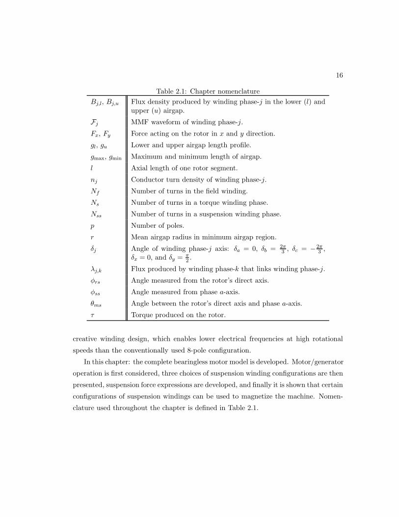
2.1 Chapter nomenclature . . . . . . . . . . . . . . . . . . . . . . . . . . . . 16
3.1 Example flywheel design parameters . . . . . . . . . . . . . . . . . . . . 43
4.1 Permeance calculations for rotor airgap . . . . . . . . . . . . . . . . . . 58
4.2 AC homopolar prototype parameters . . . . . . . . . . . . . . . . . . . . 61
5.1 Machine design parameters . . . . . . . . . . . . . . . . . . . . . . . . . 73
6.1 Chapter nomenclature . . . . . . . . . . . . . . . . . . . . . . . . . . . . 83
6.2 DPNV winding symmetry requirements . . . . . . . . . . . . . . . . . . 89
6.3 DPNV winding no-voltage requirements . . . . . . . . . . . . . . . . . . 90
6.4 DPNV winding suspension winding factor requirements . . . . . . . . . 90
6.5 Example winding design table . . . . . . . . . . . . . . . . . . . . . . . . 100
6.6 Model parameters for designs in Table 6.5 . . . . . . . . . . . . . . . . . 101
6.7 Examples of separate suspension windings . . . . . . . . . . . . . . . . . 109
6.8 Relevant fractional-slot winding information . . . . . . . . . . . . . . . . 111
7.1 Comparison of power electronic implementations . . . . . . . . . . . . . 120
8.1 Magnetic bearing design . . . . . . . . . . . . . . . . . . . . . . . . . . . 134
8.2 Stiffness results . . . . . . . . . . . . . . . . . . . . . . . . . . . . . . . . 140
8.3 Example design suspension winding factors . . . . . . . . . . . . . . . . 147
8.4 Harmonics leading to force ripple . . . . . . . . . . . . . . . . . . . . . . 147
8.5 Bearingless prototype machine parameters . . . . . . . . . . . . . . . . . 150
8.6 FEA results for winding suspension force characteristics . . . . . . . . . 151
8.7 Winding factors for example separate suspension winding . . . . . . . . 155
xi
8.8 Machine parameters used for controller design . . . . . . . . . . . . . . . 166
8.9 Control design and hardware parameters . . . . . . . . . . . . . . . . . . 167
8.10 Final reference values for the rotor’s magnetic center . . . . . . . . . . . 168
xii
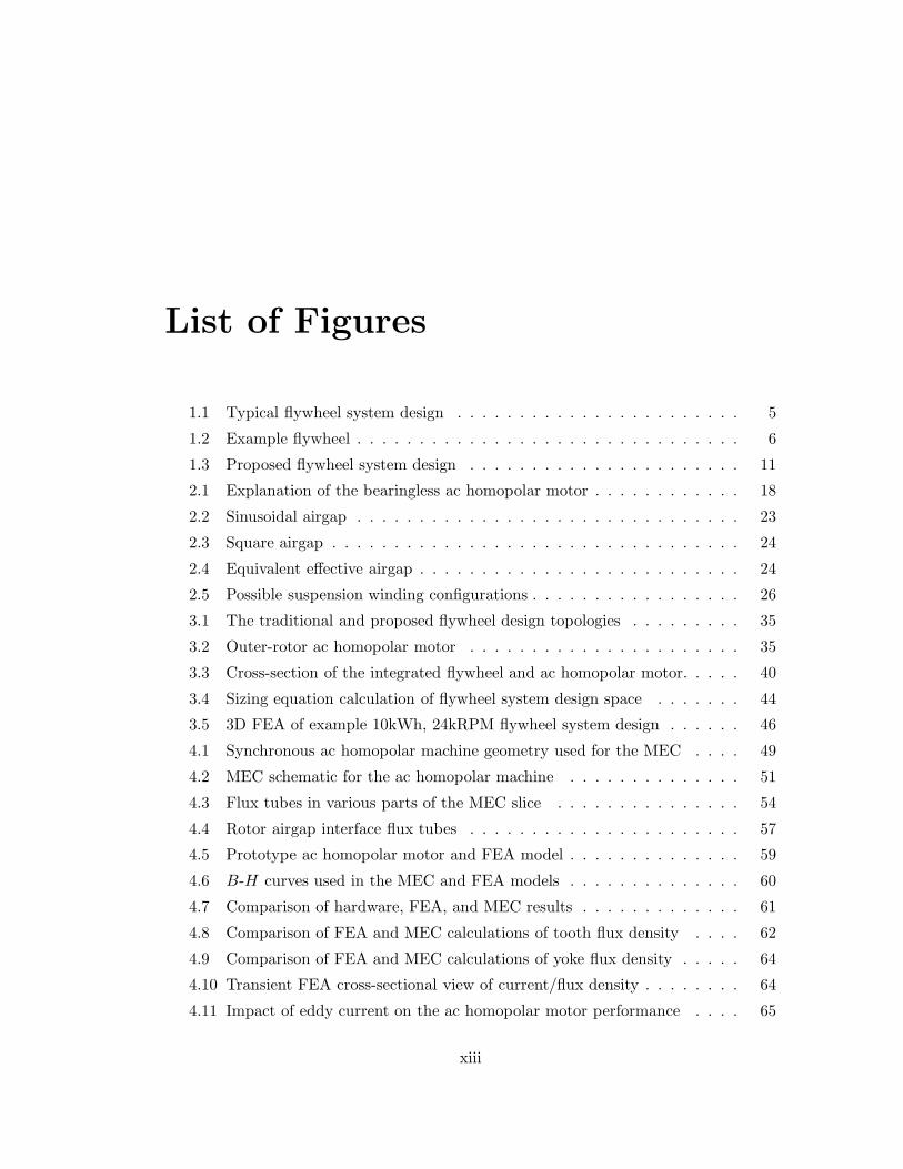
List of Figures
1.1 Typical flywheel system design . . . . . . . . . . . . . . . . . . . . . . . 5
1.2 Example flywheel . . . . . . . . . . . . . . . . . . . . . . . . . . . . . . . 6
1.3 Proposed flywheel system design . . . . . . . . . . . . . . . . . . . . . . 11
2.1 Explanation of the bearingless ac homopolar motor . . . . . . . . . . . . 18
2.2 Sinusoidal airgap . . . . . . . . . . . . . . . . . . . . . . . . . . . . . . . 23
2.3 Square airgap . . . . . . . . . . . . . . . . . . . . . . . . . . . . . . . . . 24
2.4 Equivalent effective airgap . . . . . . . . . . . . . . . . . . . . . . . . . . 24
2.5 Possible suspension winding configurations . . . . . . . . . . . . . . . . . 26
3.1 The traditional and proposed flywheel design topologies . . . . . . . . . 35
3.2 Outer-rotor ac homopolar motor . . . . . . . . . . . . . . . . . . . . . . 35
3.3 Cross-section of the integrated flywheel and ac homopolar motor. . . . . 40
3.4 Sizing equation calculation of flywheel system design space . . . . . . . 44
3.5 3D FEA of example 10kWh, 24kRPM flywheel system design . . . . . . 46
4.1 Synchronous ac homopolar machine geometry used for the MEC . . . . 49
4.2 MEC schematic for the ac homopolar machine . . . . . . . . . . . . . . 51
4.3 Flux tubes in various parts of the MEC slice . . . . . . . . . . . . . . . 54
4.4 Rotor airgap interface flux tubes . . . . . . . . . . . . . . . . . . . . . . 57
4.5 Prototype ac homopolar motor and FEA model . . . . . . . . . . . . . . 59
4.6 B-H curves used in the MEC and FEA models . . . . . . . . . . . . . . 60
4.7 Comparison of hardware, FEA, and MEC results . . . . . . . . . . . . . 61
4.8 Comparison of FEA and MEC calculations of tooth flux density . . . . 62
4.9 Comparison of FEA and MEC calculations of yoke flux density . . . . . 64
4.10 Transient FEA cross-sectional view of current/flux density . . . . . . . . 64
4.11 Impact of eddy current on the ac homopolar motor performance . . . . 65
xiii
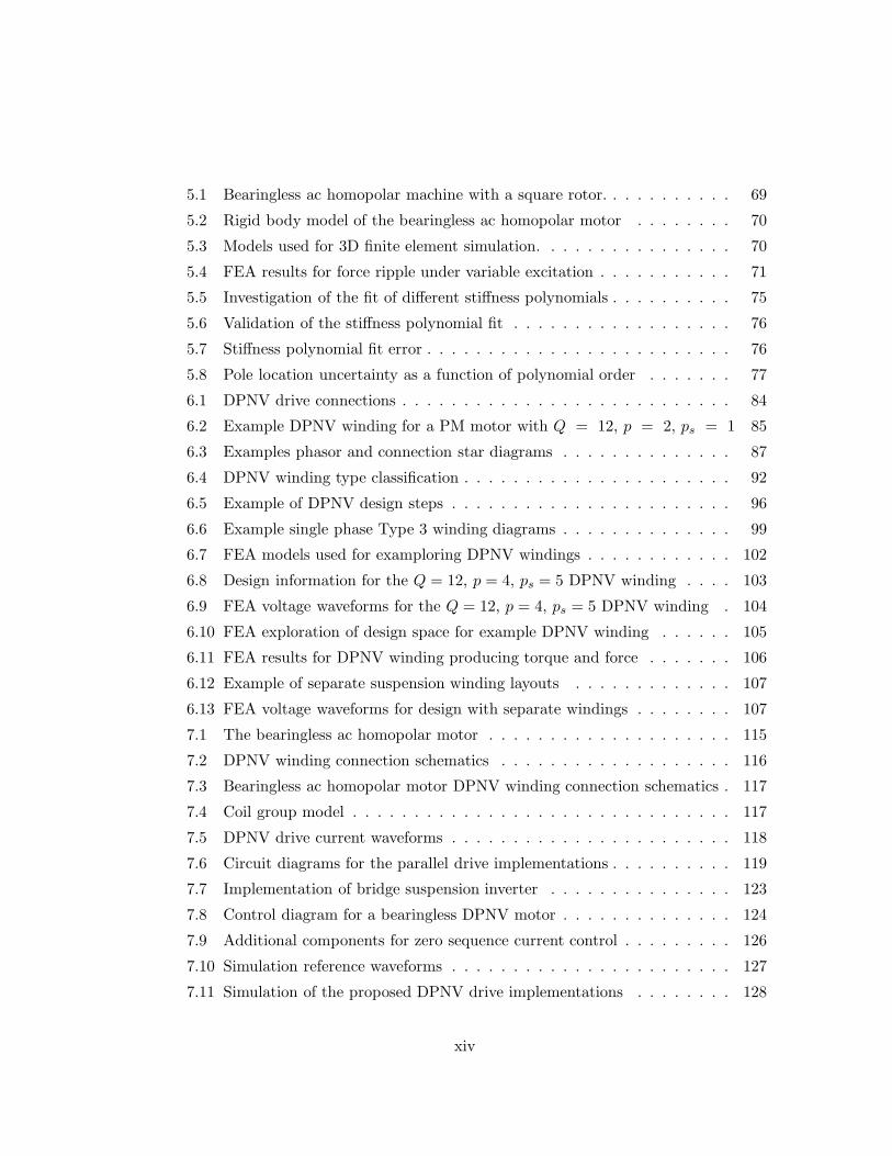
5.1 Bearingless ac homopolar machine with a square rotor. . . . . . . . . . . 69
5.2 Rigid body model of the bearingless ac homopolar motor . . . . . . . . 70
5.3 Models used for 3D finite element simulation. . . . . . . . . . . . . . . . 70
5.4 FEA results for force ripple under variable excitation . . . . . . . . . . . 71
5.5 Investigation of the fit of different stiffness polynomials . . . . . . . . . . 75
5.6 Validation of the stiffness polynomial fit . . . . . . . . . . . . . . . . . . 76
5.7 Stiffness polynomial fit error . . . . . . . . . . . . . . . . . . . . . . . . . 76
5.8 Pole location uncertainty as a function of polynomial order . . . . . . . 77
6.1 DPNV drive connections . . . . . . . . . . . . . . . . . . . . . . . . . . . 84
6.2 Example DPNV winding for a PM motor with Q = 12, p = 2, ps = 1 85
6.3 Examples phasor and connection star diagrams . . . . . . . . . . . . . . 87
6.4 DPNV winding type classification . . . . . . . . . . . . . . . . . . . . . . 92
6.5 Example of DPNV design steps . . . . . . . . . . . . . . . . . . . . . . . 96
6.6 Example single phase Type 3 winding diagrams . . . . . . . . . . . . . . 99
6.7 FEA models used for examploring DPNV windings . . . . . . . . . . . . 102
6.8 Design information for the Q = 12, p = 4, ps = 5 DPNV winding . . . . 103
6.9 FEA voltage waveforms for the Q = 12, p = 4, ps = 5 DPNV winding . 104
6.10 FEA exploration of design space for example DPNV winding . . . . . . 105
6.11 FEA results for DPNV winding producing torque and force . . . . . . . 106
6.12 Example of separate suspension winding layouts . . . . . . . . . . . . . 107
6.13 FEA voltage waveforms for design with separate windings . . . . . . . . 107
7.1 The bearingless ac homopolar motor . . . . . . . . . . . . . . . . . . . . 115
7.2 DPNV winding connection schematics . . . . . . . . . . . . . . . . . . . 116
7.3 Bearingless ac homopolar motor DPNV winding connection schematics . 117
7.4 Coil group model . . . . . . . . . . . . . . . . . . . . . . . . . . . . . . . 117
7.5 DPNV drive current waveforms . . . . . . . . . . . . . . . . . . . . . . . 118
7.6 Circuit diagrams for the parallel drive implementations . . . . . . . . . . 119
7.7 Implementation of bridge suspension inverter . . . . . . . . . . . . . . . 123
7.8 Control diagram for a bearingless DPNV motor . . . . . . . . . . . . . . 124
7.9 Additional components for zero sequence current control . . . . . . . . . 126
7.10 Simulation reference waveforms . . . . . . . . . . . . . . . . . . . . . . . 127
7.11 Simulation of the proposed DPNV drive implementations . . . . . . . . 128
xiv
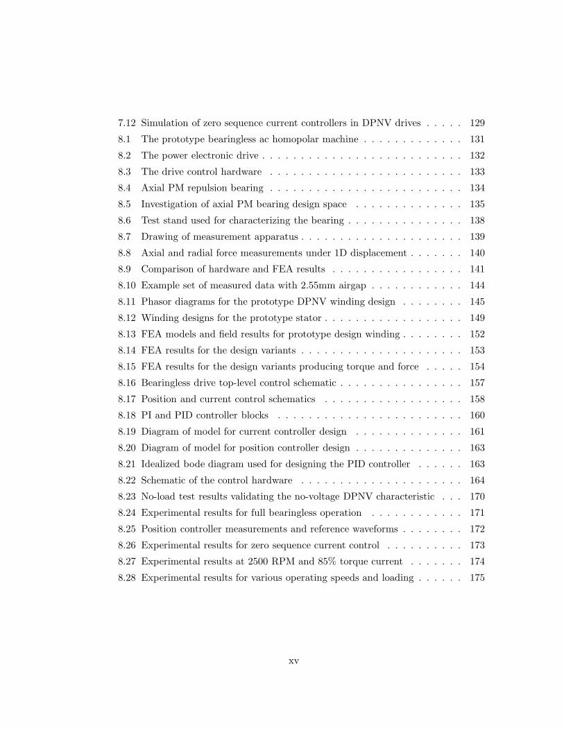
7.12 Simulation of zero sequence current controllers in DPNV drives . . . . . 129
8.1 The prototype bearingless ac homopolar machine . . . . . . . . . . . . . 131
8.2 The power electronic drive . . . . . . . . . . . . . . . . . . . . . . . . . . 132
8.3 The drive control hardware . . . . . . . . . . . . . . . . . . . . . . . . . 133
8.4 Axial PM repulsion bearing . . . . . . . . . . . . . . . . . . . . . . . . . 134
8.5 Investigation of axial PM bearing design space . . . . . . . . . . . . . . 135
8.6 Test stand used for characterizing the bearing . . . . . . . . . . . . . . . 138
8.7 Drawing of measurement apparatus . . . . . . . . . . . . . . . . . . . . . 139
8.8 Axial and radial force measurements under 1D displacement . . . . . . . 140
8.9 Comparison of hardware and FEA results . . . . . . . . . . . . . . . . . 141
8.10 Example set of measured data with 2.55mm airgap . . . . . . . . . . . . 144
8.11 Phasor diagrams for the prototype DPNV winding design . . . . . . . . 145
8.12 Winding designs for the prototype stator . . . . . . . . . . . . . . . . . . 149
8.13 FEA models and field results for prototype design winding . . . . . . . . 152
8.14 FEA results for the design variants . . . . . . . . . . . . . . . . . . . . . 153
8.15 FEA results for the design variants producing torque and force . . . . . 154
8.16 Bearingless drive top-level control schematic . . . . . . . . . . . . . . . . 157
8.17 Position and current control schematics . . . . . . . . . . . . . . . . . . 158
8.18 PI and PID controller blocks . . . . . . . . . . . . . . . . . . . . . . . . 160
8.19 Diagram of model for current controller design . . . . . . . . . . . . . . 161
8.20 Diagram of model for position controller design . . . . . . . . . . . . . . 163
8.21 Idealized bode diagram used for designing the PID controller . . . . . . 163
8.22 Schematic of the control hardware . . . . . . . . . . . . . . . . . . . . . 164
8.23 No-load test results validating the no-voltage DPNV characteristic . . . 170
8.24 Experimental results for full bearingless operation . . . . . . . . . . . . 171
8.25 Position controller measurements and reference waveforms . . . . . . . . 172
8.26 Experimental results for zero sequence current control . . . . . . . . . . 173
8.27 Experimental results at 2500 RPM and 85% torque current . . . . . . . 174
8.28 Experimental results for various operating speeds and loading . . . . . . 175
xv
Chapter 1
Introduction
1.1 Distribution grid-based energy storage
1.1.1 Motivation
Recently, the electric power grid has seen an increase in wind and solar generation
as well as increasingly volatile loads from electric vehicles (EVs). The integration of
available renewable generation is mandatory and has the effect of displacing a market’s
highest cost generators. These generators often have the fastest response time and the
highest ramp rates and are therefore typically those best-suited for providing frequency
regulation and load following services to the power grid [1]. Renewable generation is
typically unable to provide regulation and its variability can actually increase the need
for regulation. This means that one result of adding renewable generation to a market
is a reduction in the market’s regulation capacity which, combined with sudden changes
in distribution grid load due to EV charging, decreases the reliability of the power grid.
Additionally, there is a diurnal generation cycle present in the renewable technology that
does not match the power grid’s diurnal load cycle, causing more volatile energy prices.
At current levels of renewable generation, the threats posed by these problems have been
shown to be manageable. However, with initiatives to significantly increase renewable
penetration, such as the Department of Energy’s “20% wind by 2030,” and the continued
integration of renewable vehicles, these issues will need to be addressed. Both frequency
regulation and diurnal load following services are energy neutral and, because generators
1

2
must deliver a net positive amount of energy to the grid, it is suggested in [1–7] that
energy storage devices be used to provide these services.
To maximize the benefits of energy storage, this dissertation proposes locating stor-
age modules on the distribution grid, near points of congestion. This would allow the
grid operator to direct bulk energy to points of anticipated load when it is most optimal
to do so, i.e. so as to increase transmission efficiency or avoid curtailing renewable gener-
ation when load is lacking (diurnal load following). These devices could simultaneously
provide frequency regulation services in response to local grid conditions to increase
the grid stability. Moreover, locating energy storage near points of load would enable
the grid infrastructure (transformers and transmission lines) to operate closer to the
average load, enabling utilities to avoid costly upgrades due to large peak loads, such
as those associated with electric vehicles. A similar use-case was considered in [7], for
flywheel systems providing load-following and smoothing services at various locations
on the distribution grid.
1.1.2 Requirements of an energy storage device
The requirements of implementing distribution-grid energy storage that is able to simul-
taneously provide frequency regulation and diurnal load-following services are numerous
and diverse. Frequency regulation has energy transfer time requirements on the order
of seconds to several minutes and is typically energy neutral on a time scale of a half-
hour [2, 3]. Energy storage devices that provide frequency regulation must have a long
cycle-lifetime, high power ratings, short response times, and fast ramp rates. To un-
derstand how extreme the cycle-lifetime requirements are, consider data published by
Beacon Power which indicates that their frequency regulation facility in New York ex-
periences 2500 - 5000 charge cycles per year [8]. Finally, because frequency regulation
is power-intensive, the energy storage device must have a reasonable cost per installed
kW.
Diurnal load following services have energy transfer times on the order of several
hours and are energy neutral over a period of 24 hours [7]. This means that energy
storage devices must have a low self-discharge rate so that a meaningful amount of
energy can be stored for a 24 hour period. Furthermore, load-following services are
energy-intensive, which requires storage devices to have both a reasonable energy density
3
and cost per kWh stored.
Suitable distribution-grid energy storage must have a modular form factor so that
it is easily installed regardless of geographic location or population density and easily
scalable based on the local grid requirements. Since it will be installed in small quantities
that are staggered throughout the grid, it must be low maintenance.
In summary, the key requirements of an energy storage device for this application
are: long cycle-lifetime, low self-discharge rate, modular form factor, and reasonable
cost and size per kW as well as per kWh.
1.1.3 Overview of energy storage technologies
Storage technologies that are typically considered for grid applications include pumped
hydro, compressed air, thermal, ultracapacitors, chemical batteries, and flywheel tech-
nology. Many published studies have evaluated these different storage technologies for
use on grid. For example, [2–6,9,10] which suggest that conventional storage technology
is inadequate to meet the needs summarized in Section 1.1.2:
• Pumped hydro and compressed air: these technologies have been economically
developed in large, centralized installations where they achieve round-trip effi-
ciencies on the order of 60-80%, but are limited by geographic restrictions and
environmental concerns.
• Small scale compressed air and thermal: these technologies suffer from low round-
trip efficiencies.
• Ultracapacitors: this technology is regarded as having a cost per kWh that is too
high and an energy density that is too low for the bulk storage required for diurnal
load following.
• Various types of chemical batteries: these technologies are generally regarded
favorably for diurnal storage applications, but contain hazardous chemicals and
suffer from low cycle-lifetimes which limit their use for frequency regulation. Ta-
ble 1.1 shows a comparison of several different chemical batteries. Alternative
technologies, such as sodium-sulfur and flow batteries, have much longer cycle-
lifetimes, but require large installations, making them non-modular and therefore
4
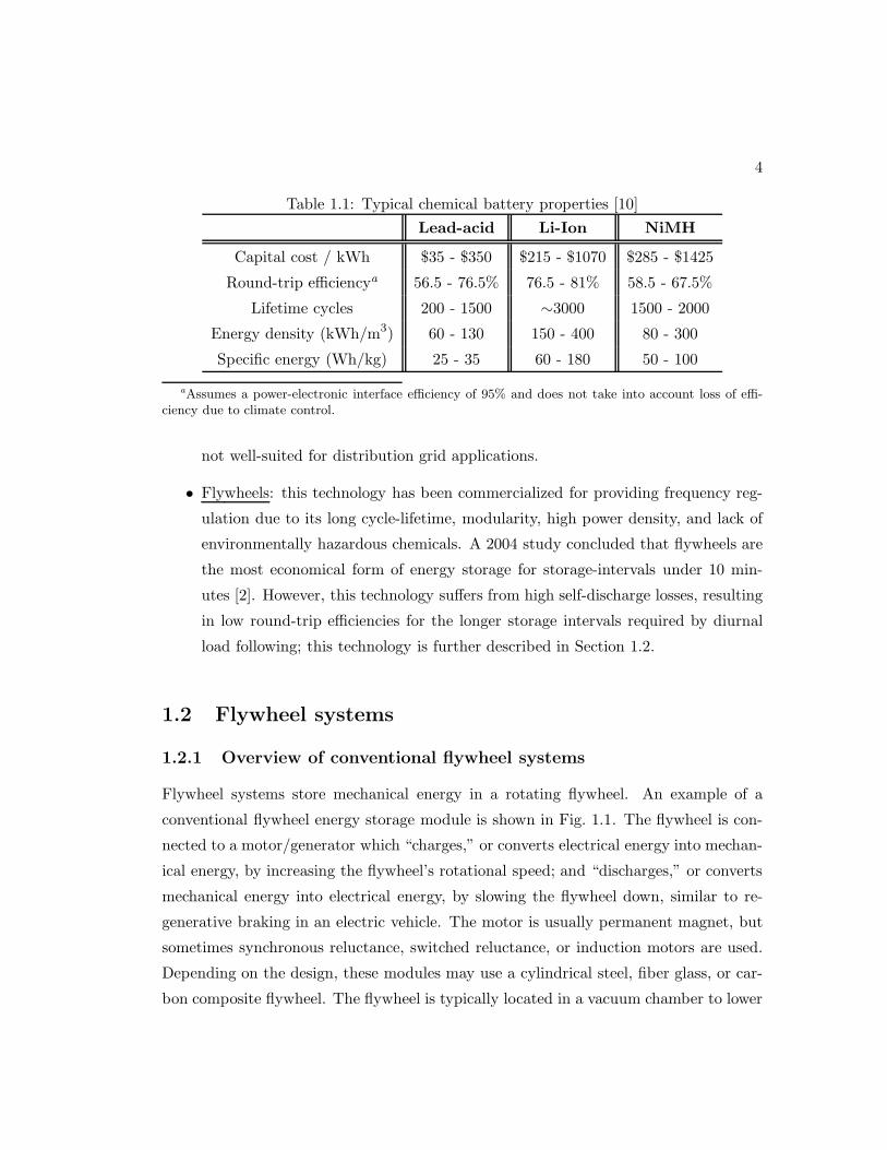
Table 1.1: Typical chemical battery properties [10]
Lead-acid Li-Ion NiMH
Capital cost / kWh $35 - $350 $215 - $1070 $285 - $1425
Round-trip efficiencya 56.5 - 76.5% 76.5 - 81% 58.5 - 67.5%
Lifetime cycles 200 - 1500 ∼3000 1500 - 2000
Energy density (kWh/m3) 60 - 130 150 - 400 80 - 300
Specific energy (Wh/kg) 25 - 35 60 - 180 50 - 100
aAssumes a power-electronic interface efficiency of 95% and does not take into account loss of effi-ciency due to climate control.
not well-suited for distribution grid applications.
• Flywheels: this technology has been commercialized for providing frequency reg-
ulation due to its long cycle-lifetime, modularity, high power density, and lack of
environmentally hazardous chemicals. A 2004 study concluded that flywheels are
the most economical form of energy storage for storage-intervals under 10 min-
utes [2]. However, this technology suffers from high self-discharge losses, resulting
in low round-trip efficiencies for the longer storage intervals required by diurnal
load following; this technology is further described in Section 1.2.
1.2 Flywheel systems
1.2.1 Overview of conventional flywheel systems
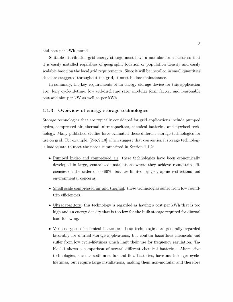
Flywheel systems store mechanical energy in a rotating flywheel. An example of a
conventional flywheel energy storage module is shown in Fig. 1.1. The flywheel is con-
nected to a motor/generator which “charges,” or converts electrical energy into mechan-
ical energy, by increasing the flywheel’s rotational speed; and “discharges,” or converts
mechanical energy into electrical energy, by slowing the flywheel down, similar to re-
generative braking in an electric vehicle. The motor is usually permanent magnet, but
sometimes synchronous reluctance, switched reluctance, or induction motors are used.
Depending on the design, these modules may use a cylindrical steel, fiber glass, or car-
bon composite flywheel. The flywheel is typically located in a vacuum chamber to lower
5
Bearing system
PM Motor
Containment andvacuum housing
Composite flywheel
Bearing system
Figure 1.1: Typical flywheel system design
wind-resistance losses and suspended via active magnetic bearings to reduce drag and
reliability concerns. To achieve optimal energy density and form factor, high rotational
speeds are typically required (10 kRPM – 100 kRPM). For high-speed units, a contain-
ment structure is required to prevent flywheel shards from escaping the module and
causing damage or harm in the event of a flywheel failure.
1.2.2 Flywheel materials
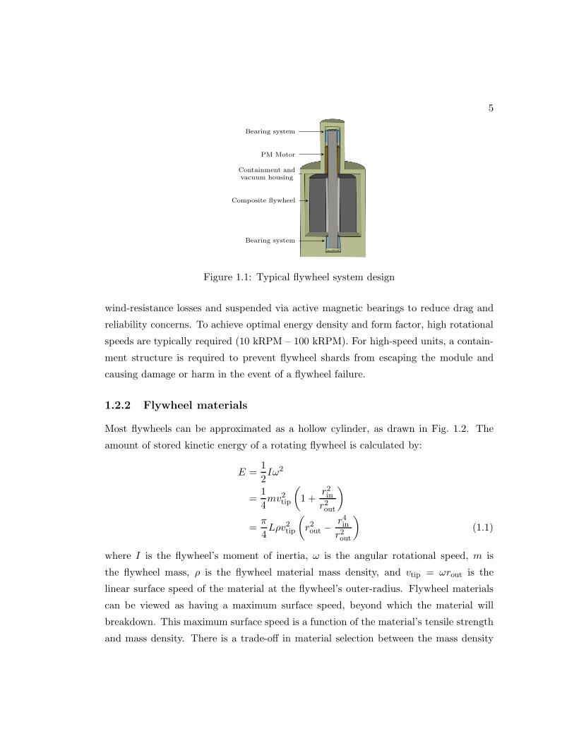
Most flywheels can be approximated as a hollow cylinder, as drawn in Fig. 1.2. The
amount of stored kinetic energy of a rotating flywheel is calculated by:
E =1
2Iω2
=1
4mv2tip
(
1 +r2inr2out
)
=π
4Lρv2tip
(
r2out −r4inr2out
)
(1.1)
where I is the flywheel’s moment of inertia, ω is the angular rotational speed, m is
the flywheel mass, ρ is the flywheel material mass density, and vtip = ωrout is the
linear surface speed of the material at the flywheel’s outer-radius. Flywheel materials
can be viewed as having a maximum surface speed, beyond which the material will
breakdown. This maximum surface speed is a function of the material’s tensile strength
and mass density. There is a trade-off in material selection between the mass density
6
rinrout
L
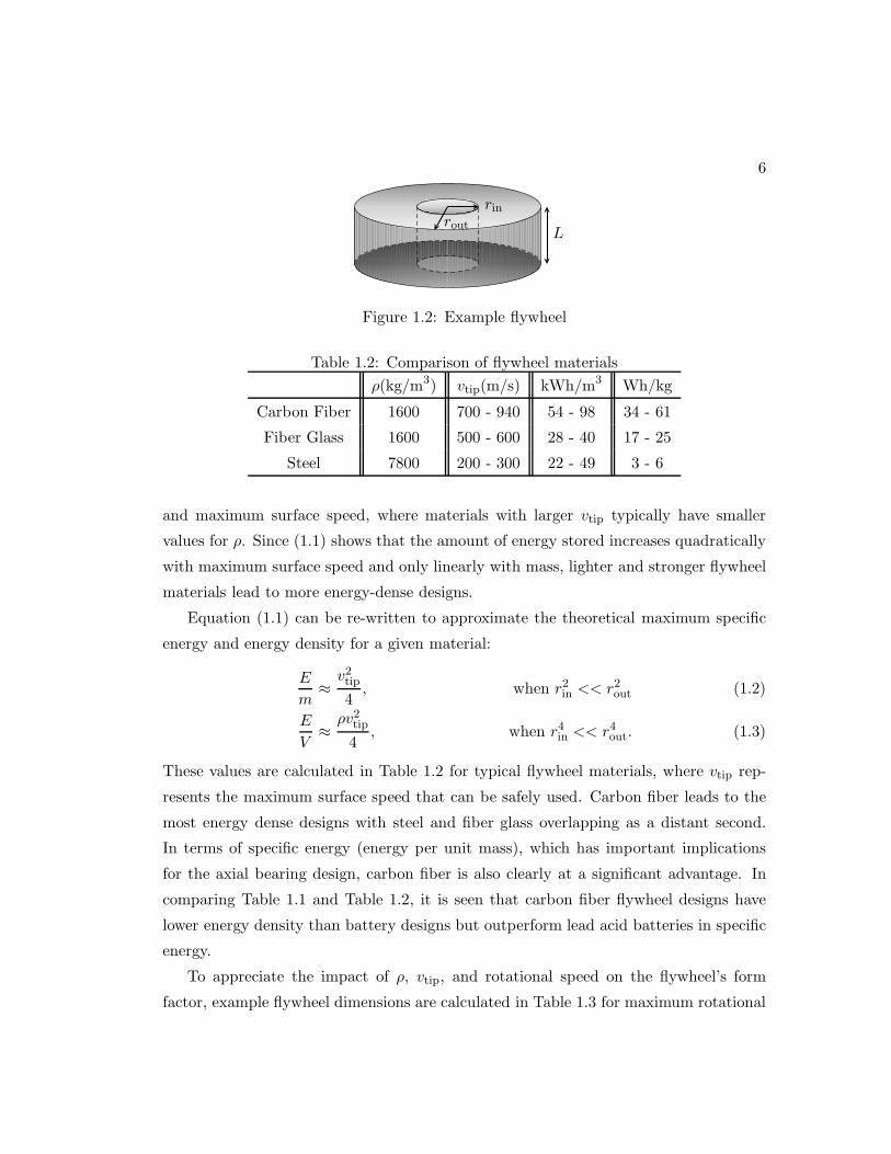
Figure 1.2: Example flywheel
Table 1.2: Comparison of flywheel materials
ρ(kg/m3) vtip(m/s) kWh/m3 Wh/kg
Carbon Fiber 1600 700 - 940 54 - 98 34 - 61
Fiber Glass 1600 500 - 600 28 - 40 17 - 25
Steel 7800 200 - 300 22 - 49 3 - 6
and maximum surface speed, where materials with larger vtip typically have smaller
values for ρ. Since (1.1) shows that the amount of energy stored increases quadratically
with maximum surface speed and only linearly with mass, lighter and stronger flywheel
materials lead to more energy-dense designs.
Equation (1.1) can be re-written to approximate the theoretical maximum specific
energy and energy density for a given material:
E
m≈v2tip4, when r2in << r2out (1.2)
E
V≈ρv2tip4
, when r4in << r4out. (1.3)
These values are calculated in Table 1.2 for typical flywheel materials, where vtip rep-
resents the maximum surface speed that can be safely used. Carbon fiber leads to the
most energy dense designs with steel and fiber glass overlapping as a distant second.
In terms of specific energy (energy per unit mass), which has important implications
for the axial bearing design, carbon fiber is also clearly at a significant advantage. In
comparing Table 1.1 and Table 1.2, it is seen that carbon fiber flywheel designs have
lower energy density than battery designs but outperform lead acid batteries in specific
energy.
To appreciate the impact of ρ, vtip, and rotational speed on the flywheel’s form
factor, example flywheel dimensions are calculated in Table 1.3 for maximum rotational
7
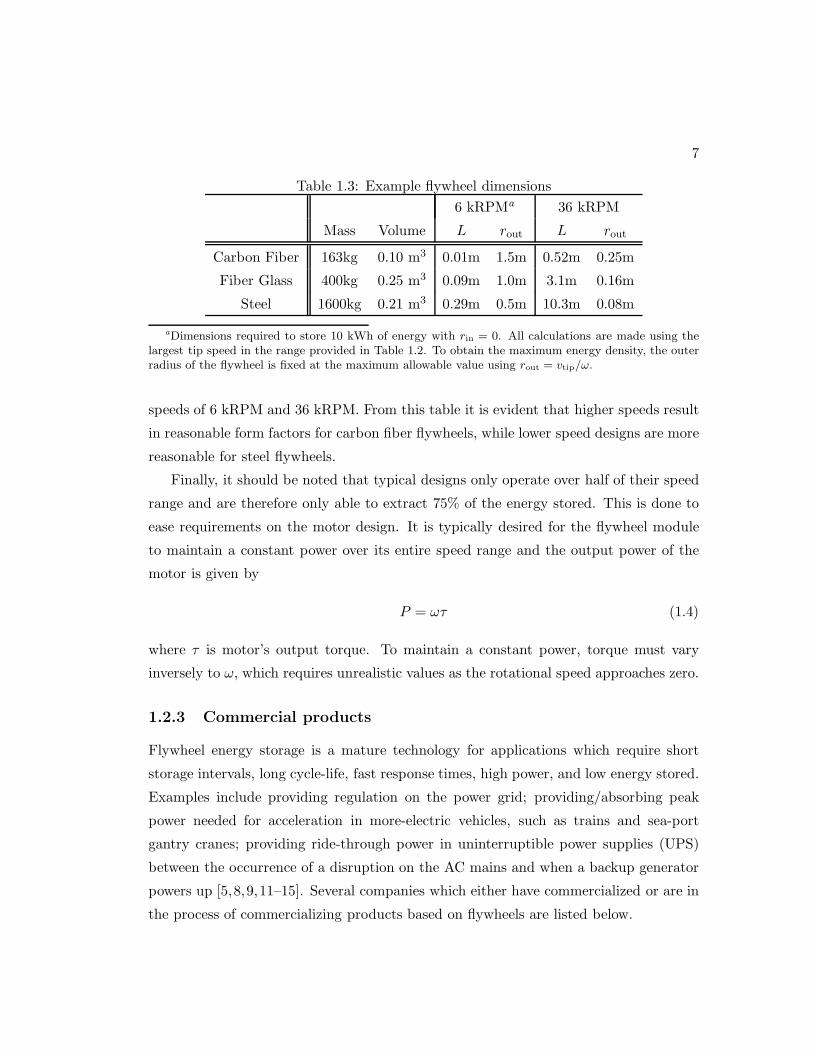
Table 1.3: Example flywheel dimensions
6 kRPMa 36 kRPM
Mass Volume L rout L rout
Carbon Fiber 163kg 0.10 m3 0.01m 1.5m 0.52m 0.25m
Fiber Glass 400kg 0.25 m3 0.09m 1.0m 3.1m 0.16m
Steel 1600kg 0.21 m3 0.29m 0.5m 10.3m 0.08m
aDimensions required to store 10 kWh of energy with rin = 0. All calculations are made using thelargest tip speed in the range provided in Table 1.2. To obtain the maximum energy density, the outerradius of the flywheel is fixed at the maximum allowable value using rout = vtip/ω.
speeds of 6 kRPM and 36 kRPM. From this table it is evident that higher speeds result
in reasonable form factors for carbon fiber flywheels, while lower speed designs are more
reasonable for steel flywheels.
Finally, it should be noted that typical designs only operate over half of their speed
range and are therefore only able to extract 75% of the energy stored. This is done to
ease requirements on the motor design. It is typically desired for the flywheel module
to maintain a constant power over its entire speed range and the output power of the
motor is given by
P = ωτ (1.4)
where τ is motor’s output torque. To maintain a constant power, torque must vary
inversely to ω, which requires unrealistic values as the rotational speed approaches zero.
1.2.3 Commercial products
Flywheel energy storage is a mature technology for applications which require short
storage intervals, long cycle-life, fast response times, high power, and low energy stored.
Examples include providing regulation on the power grid; providing/absorbing peak
power needed for acceleration in more-electric vehicles, such as trains and sea-port
gantry cranes; providing ride-through power in uninterruptible power supplies (UPS)
between the occurrence of a disruption on the AC mains and when a backup generator
powers up [5,8,9,11–15]. Several companies which either have commercialized or are in
the process of commercializing products based on flywheels are listed below.
8
• Beacon Power LLC has constructed two flywheel facilities to provide large-scale
frequency regulation services on the order of 20 MW through flywheel modules
connected in an array [12]. The modules use a carbon-fiber flywheel operating at
up to 16,000 RPM, weigh 1130 kg, utilize a 100 kW permanent magnet motor,
store 25 kWh, and have a typical round-trip efficiency of 84% for the short storage
intervals required by frequency regulation.
• PowerThru (formerly Pentadyne Power Corporation) and Active Power, Inc. have
developed UPS systems that utilize flywheel energy storage. PowerThru’s design
utilizes a 190 kW, 4-pole synchronous reluctance motor/generator operating at
52,000 RPM and a carbon composite flywheel that stores approximately 750 Wh.
Each unit weighs approximately 590 kg and has a volume of 960 liters. The self-
discharge losses are 250 W, which means that a unit will dissipate its stored energy
after idling for only a few hours [13].
• VYCON, Inc. has commercialized flywheel energy storage units for use in sea
port cranes. Their modules operate inside a vacuum chamber and utilize a 150
kW permanent magnet motor with a maximum speed of 36,000 RPM, a steel
flywheel that stores 1.27 kWh, active magnetic bearings, and weigh 320 kg [14].
The required energy storage time is on the order of minutes.
• Rotonix USA, Inc. has commercialized flywheel devices for several different ap-
plications. Their modules have a 1.1MW power rating, use a carbon compoite
flywheel that stores 12 kWh, have self-discharge losses of 500 W, weigh 2700 kg,
and use magnetic bearings [16]. Unlike other companies, this flywheel system uses
an outer-rotor motor design to increase the energy density, but no information is
available on the type of motor used. At this self-discharge rate, the flywheel will
dissipate its stored energy over the course of one day.
• Amber Kinetics, Inc. focuses on low-cost flywheel products for custom applica-
tions, which have included power smoothing and uninterruptible power supplies.
They have ongoing projects with the Blue Planet Research in Hawaii and San
Diego Gas and Electric in California. Their systems use steel flywheels but no
other design information is available [17].

9
1.2.4 Problems with current technology
Flywheel technology has already been shown to be feasible for providing frequency
regulation, but is currently not usable for providing diurnal load following services due
to its high self-discharge rate while idling, with the best flywheel designs completely
self-discharging over a period of one day. Secondary concerns with flywheel modules are
the overall cost and manufacturing complexity.
The sources of self-discharge losses include bearing loss, frictional windage loss due
to the high rotational speed, and magnetic losses associated with the motor and, in some
designs, magnetic bearings. Bearing losses can be minimized through use of magnetic
bearings with optimized magnetic circuit design to minimize flux variability [18] or by
implementing high-temperature superconducting bearings [19] at the expense of cost
and complexity. For most designs, frictional windage losses can be reduced to nearly
negligible levels by using a vacuum of less than 1 mTorr [20]. Magnetic losses associated
with the motor remain a key concern and are one of the primary areas the proposed
use of the ac homopolar motor addresses. Motors that use permanent magnets will
inherently have losses while they are freewheeling due to hysteresis and induced eddy
currents from the rotating magnetic fields. Traditional machines without permanent
magnets have other complications:
• Induction and switched reluctance motors have increased rotor heating which lim-
its the energy transfer time of the flywheel module before the motor/generator
must idle to prevent overheating, a consequence of the rotor being levitated on
magnetic bearings and operating in a vacuum where the only mechanism for heat
exchange is radiation.
• Wound-rotor and doubly-fed motors require brushes that are not usable for high-
speed operation.
• Synchronous reluctance motors require a high Ld/Lq ratio which leads to a rotor
structure that is not mechanically robust for high-speed operation.
10
1.2.5 Relevant flywheel research projects
There are many recent and ongoing research projects in flywheel technology, for example:
[19–45]. To increase the energy density, integrating the flywheel into the motor has been
proposed to various extents [22,24,25]. The traditional topology, depicted in Fig. 1.1, is
at one extreme of this spectrum, where the flywheel is mounted on a shaft at a separate
axial location from the motor. At the other extreme, designs where the motor’s rotor
is the flywheel have been considered [27] as well as designs where an outer-rotor motor
is used and the flywheel is mounted directly on the motor’s rotor, as described later in
Fig. 1.3a.
Efforts to reduce self-discharge losses have taken several different approaches. Projects
focused on improving permanent magnet motors have included investigations into Hal-
bach configurations and core-less stators [35, 37], which resulted in reduced power and
energy density, as well as an investigation into a design with a removable stator that was
retracted from the rotor during idling times [42], which has the negative consequences
of reducing the system’s energy density, increasing the response time, and increasing
the overall system cost and complexity. Other efforts have focused on magnetic bearing
losses and have looked at optimizing active and hybrid magnetic bearings [38,39] as well
as using superconducting bearings [19,21,25].
There are numerous examples of recent investigations into the use of bearingless mo-
tors for flywheel energy storage, including [30,43–45]. Bearingless designs combine the
functionality of magnetic bearing and a motor into a single device and as such are theo-
retically able to reduce the overall flywheel system size, amount of raw materials needed,
and the manufacturing complexity. All types of traditional motors can be redesigned as
bearingless motors with varying consequences to the overall machine performance. One
significant drawback of conventional bearingless motors is that they utilize a separate
set of windings to produce magnetic bearing forces which must share the same slot
space as the torque windings. This creates a trade-off between the magnetic bearing
and motor capabilities and is an issue that is explored in this dissertation.

11
Outer-rotor bearingless
ac homopolar motor
Containment and
vacuum housing
Composite flywheel
(a) Proposed flywheel system design
Steel stator shaft
Rotor laminations
Steel rotor sleeve
Stationaryfield winding
Magnetizingflux path
Stator laminations
(b) Bearingless ac homopolar motor
Figure 1.3: Proposed flywheel system design
1.3 Proposed flywheel system
This dissertation proposes the flywheel module topology depicted in Fig. 1.3. The
proposed design has the following key features:
• AC homopolar motor to eliminate motor losses while idling. The ac homopolar
motor is completely stator-side current excited. This means that during times of
idling, the magnetization can be removed by turning all current off, and therefore
self-discharge losses from the motor can be eliminated. The ac homopolar motor
avoids the previously mentioned pitfalls of traditional motors which either suffer
from rotor loss, the required use of brushes, or non-robust rotor structure. Fur-
thermore, because the machine uses current excitation, the excitation level can be
varied based on the flywheel system’s current rotational speed to reduce losses in
the power electronic motor drive during times of energy transfer.
• Integrated design topology to increase the energy and power density of the flywheel
system. The motor is implemented in an outer-rotor fashion where the rotor forms
the inner backing for a carbon composite flywheel. Since, as is shown by (1.1),
most of the flywheel’s energy is stored near the flywheel’s outer-radius, hollowing
the flywheel out does not result in a sizable reduction in the amount of energy
stored; instead, this dramatically increases the flywheel system’s overall energy
density as the flywheel and the motor are now able to occupy the same volume.
12
• Bearingless motor to reduce the system size, cost, and manufacturing complexity.
By using a bearingless version of the ac homopolar motor, the need for separate
radial magnetic bearings is eliminated. This reduces the amount of raw materials
required and, because active magnetic bearings are complex electromechanical
devices with their own stator windings, reduces the required manufacturing effort.
Note that an axial thrust bearing is still required to support the flywheel’s weight.
However, this can be implemented with a very simple permanent magnet passive
bearing design.
1.4 Research contributions
The results of this project have resulted in the following papers either published or
submitted for publication: [46–55]. The individual contributions can be summarized as:
• exploring the application of bearingless ac homopolar machines to flywheel energy
storage;
• developing magnetic eqivalent circuit (MEC) models of the ac homopolar machine
that are suitable for use in the design process; these models can be solved in a
fraction of a second as opposed to transient 3D finite element models which have
a solve time on the order of days;
• developing a design procedure and constraints for dual purpose no voltage (DPNV)
windings; these windings allows the same stator coils to be used for both radial
force and torque production and thereby increase the machine’s torque density;
the results of this contribution as well as the next item apply generally to all types
of radial flux bearingless machines;
• proposing and evaluating different power-electronic drive implementations for DPNV
windings;
• designing a prototype bearingless ac homopolar motor and presenting experimen-
tal validation of the above contributions; because relatively little literature exists
on the bearingless ac homopolar machine, the publication of experimental data is
particularly valuable to the bearingless machines community.

13
1.5 Dissertation outline
• Chapter 2 introduces the bearingless ac homopolar machine and derives its oper-
ating principles from a drives perspective.
• Chapter 3 explores the application of the ac homopolar machine for flywheel en-
ergy storage. A macroscopic design sizing approach is investigated and compared
against results from 3D FEA.
• Chapter 4 develops and validates a MEC of the ac homopolar machine that is
suitable for design optimization.
• Chapter 5 presents the rigid body rotor model for the suspension of the bearingless
ac homopolar machine and investigates the impact of variable excitation on the
model.
• Chapter 6 derives the necessary conditions to realize DPNV windings, proposes
a design procedure, and explores several example bearingless motor designs using
DPNV windings.
• Chapter 7 proposes and evaluates implementations of power-electronic drives for
DPNV-wound motors.
• Chapter 8 describes the prototype design of the bearingless ac homopolar machine,
including the power electronic drive and controllers, and presents experimental
results.
• Chapter 9 presents the dissertation conclusions and proposes future work.

Chapter 2
Model of the Bearingless AC
Homopolar Motor
This chapter investigates the bearingless ac homopolar motor from a drives perspective.
Idealized machine quantities are assumed, such as sinusoidally distributed windings and
infinite iron permeability. The point of the chapter is to describe how the motor and
magnetic bearing functionality work and derive simple inductances matrices as well as
torque and force expressions that will be used later when developing a drive for the
machine. Note that while the overall goal of the dissertation is to develop an outer-
rotor bearingless motor for flywheel energy storage, in this chapter (as well as in several
other chapters) an inner-rotor motor is considered. Since the same results and theory
apply to both the inner- and outer-rotor variants, this is done to be consistent with the
hardware prototype that was developed (described in Chapter 8).1
2.1 Introduction
Classical bearingless motors require that a suspension winding produce a revolving p±2-
pole flux density to disrupt the otherwise symmetric, revolving p-pole magnetic field in
the motor’s airgap [56, 57]. This requires high-bandwidth angular-position sensors and
an ac suspension current to produce a constant force. Alternatively, the bearingless
1 Portions of the material in this chapter have also been published in [52] and submitted for publi-cation in [48].
14
15
consequent-pole motor has been developed which utilizes a 2-pole suspension winding
with a dc current to produce a constant radial force for a p ≥ 8-pole motor [56, 58].
However, this motor has permanent magnets on its rotor, making it not applicable
to superconducting applications; less desirable for variable-speed applications, such as
flywheel energy storage, where a controllable excitation is desired; and difficult to im-
plement in high-speed applications where securing the magnets to the rotor becomes a
challenge. For such applications, the bearingless ac homopolar motor is best suited.
Like the bearingless consequent-pole motor, a p ≥ 8-pole bearingless ac homopolar
motor is able to produce a constant radial suspension force with a dc current. Un-
like the consequent-pole motor, the homopolar motor is magnetized through a dc field
winding secured to the stator, allowing for variable excitation. Since the field wind-
ing is stationary, no brushes are required and, in the case of a superconducting coil,
coolant does not need to be pumped into the rotor. The rotor’s structure is therefore
very simple and conducive to high-speed operation. One important drawback of the
ac homopolar motor is that its theoretical torque density is roughly one-half that of a
classical synchronous motor. The motor’s torque density can be somewhat improved
in the case of a superconducting machine where the field winding is able to provide
a very large excitation [59]. It is shown in Chapter 3 that when losses are normalized
when comparing this machine to other synchronous machines, the discrepancy in torque
density disappears.
There have been several papers considering the ac homopolar motor, but little lit-
erature on the bearingless ac homopolar motor [56, 60–62]. The ac homopolar motor
has attracted recent attention as a high speed machine, a superconducting machine,
an alternator operated with a rectifier for capacitor charge power supplies, and in the
dissertation’s application of flywheel energy storage [27, 51, 63–69]. In flywheel energy
storage, the ac homopolar machine has been considered in both outer and inner rotor
configurations [27,51,69] with varying degrees of rotor/flyweel integration. It was shown
in [27] that a solid steel rotor can be used, which in this case also served as the flywheel,
while still achieving acceptable losses. As a bearingless motor, existing literature has
focused on the suspension force capability [56,60–62], neglecting the complete bearing-
less machine model and only considering a single rotor geometry. In [62], it was shown
that acceptable suspension performance can be achieved for 6-pole configurations via
16
Table 2.1: Chapter nomenclature
Bj,l, Bj,u Flux density produced by winding phase-j in the lower (l) andupper (u) airgap.
Fj MMF waveform of winding phase-j.
Fx, Fy Force acting on the rotor in x and y direction.
gl, gu Lower and upper airgap length profile.
gmax, gmin Maximum and minimum length of airgap.
l Axial length of one rotor segment.
nj Conductor turn density of winding phase-j.
Nf Number of turns in the field winding.
Ns Number of turns in a torque winding phase.
Nss Number of turns in a suspension winding phase.
p Number of poles.
r Mean airgap radius in minimum airgap region.
δj Angle of winding phase-j axis: δa = 0, δb = 2π3 , δc = −2π
3 ,δx = 0, and δy =
π2 .
λj,k Flux produced by winding phase-k that links winding phase-j.
φrs Angle measured from the rotor’s direct axis.
φss Angle measured from phase a-axis.
θms Angle between the rotor’s direct axis and phase a-axis.
τ Torque produced on the rotor.
creative winding design, which enables lower electrical frequencies at high rotational
speeds than the conventionally used 8-pole configuration.
In this chapter: the complete bearingless motor model is developed. Motor/generator
operation is first considered, three choices of suspension winding configurations are then
presented, suspension force expressions are developed, and finally it is shown that certain
configurations of suspension windings can be used to magnetize the machine. Nomen-
clature used throughout the chapter is defined in Table 2.1.
17
2.2 Description of bearingless ac homopolar motor
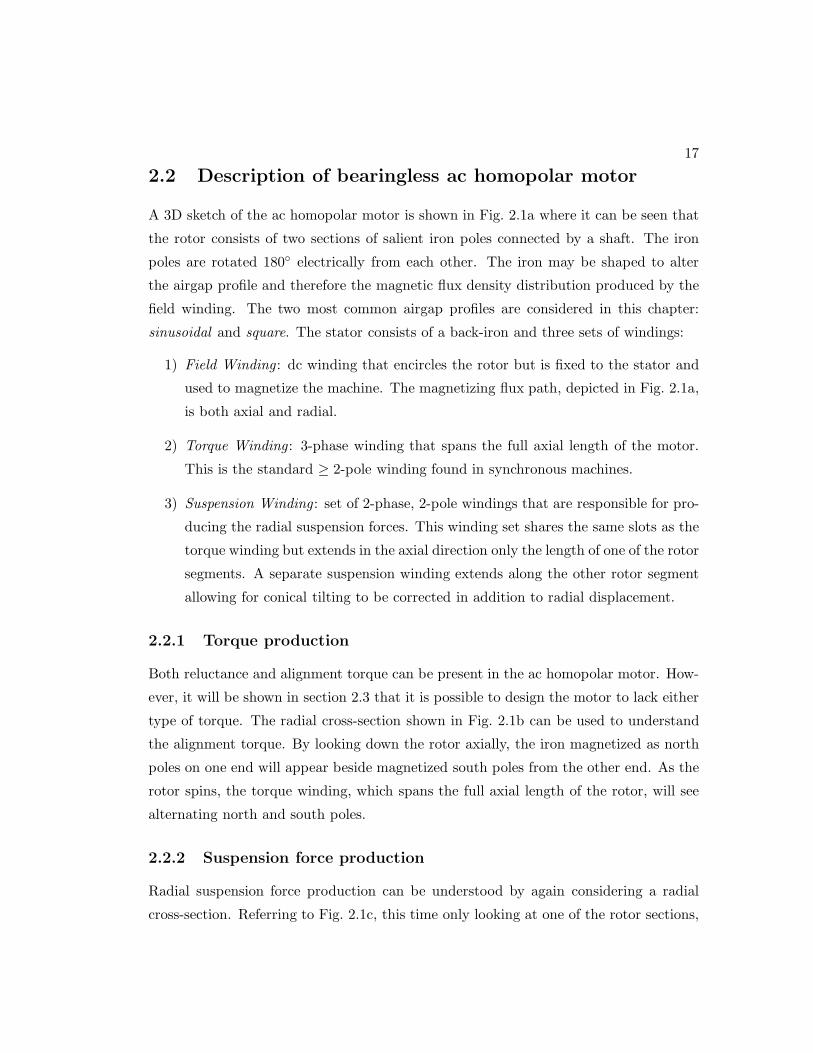
A 3D sketch of the ac homopolar motor is shown in Fig. 2.1a where it can be seen that
the rotor consists of two sections of salient iron poles connected by a shaft. The iron
poles are rotated 180 electrically from each other. The iron may be shaped to alter
the airgap profile and therefore the magnetic flux density distribution produced by the
field winding. The two most common airgap profiles are considered in this chapter:
sinusoidal and square. The stator consists of a back-iron and three sets of windings:
1) Field Winding : dc winding that encircles the rotor but is fixed to the stator and
used to magnetize the machine. The magnetizing flux path, depicted in Fig. 2.1a,
is both axial and radial.
2) Torque Winding : 3-phase winding that spans the full axial length of the motor.
This is the standard ≥ 2-pole winding found in synchronous machines.
3) Suspension Winding : set of 2-phase, 2-pole windings that are responsible for pro-
ducing the radial suspension forces. This winding set shares the same slots as the
torque winding but extends in the axial direction only the length of one of the rotor
segments. A separate suspension winding extends along the other rotor segment
allowing for conical tilting to be corrected in addition to radial displacement.
2.2.1 Torque production
Both reluctance and alignment torque can be present in the ac homopolar motor. How-
ever, it will be shown in section 2.3 that it is possible to design the motor to lack either
type of torque. The radial cross-section shown in Fig. 2.1b can be used to understand
the alignment torque. By looking down the rotor axially, the iron magnetized as north
poles on one end will appear beside magnetized south poles from the other end. As the
rotor spins, the torque winding, which spans the full axial length of the rotor, will see
alternating north and south poles.
2.2.2 Suspension force production
Radial suspension force production can be understood by again considering a radial
cross-section. Referring to Fig. 2.1c, this time only looking at one of the rotor sections,
18
Magnetizing flux path
Rotor laminationsStator laminationsField winding
Stator sleeve
(a)
N
S
N
SN
S
N
S
d-axis
θms φss
φrs
q-axis
a
c
b
(b)
x
y
(c)
Figure 2.1: Bearingless ac homopolar motor: (a) full motor with square airgap profile,(b) magnetized cross-section depicting the notation for angles and phase axes, (c) cross-section depicting flux paths for suspension windings given a positive terminal current;blue lines correspond to the x-phase winding, brown lines correspond to the y-phasewinding, and the black lines are the magnetization flux.
19
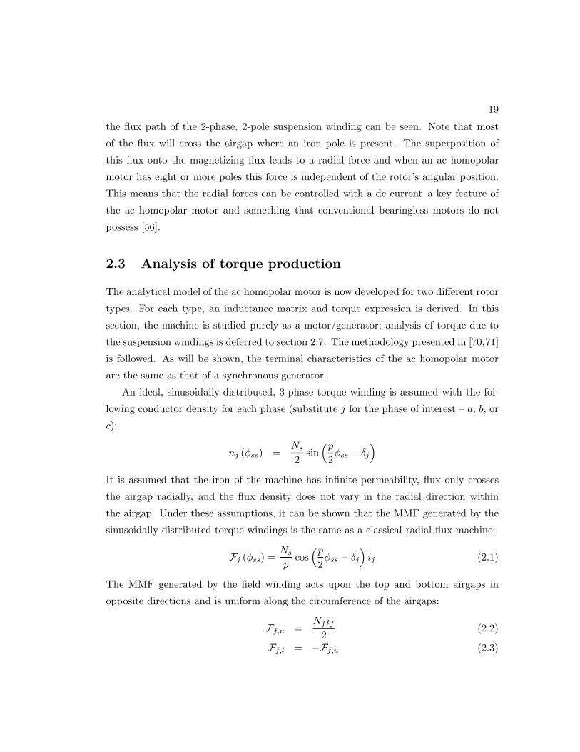
the flux path of the 2-phase, 2-pole suspension winding can be seen. Note that most
of the flux will cross the airgap where an iron pole is present. The superposition of
this flux onto the magnetizing flux leads to a radial force and when an ac homopolar
motor has eight or more poles this force is independent of the rotor’s angular position.
This means that the radial forces can be controlled with a dc current–a key feature of
the ac homopolar motor and something that conventional bearingless motors do not
possess [56].
2.3 Analysis of torque production
The analytical model of the ac homopolar motor is now developed for two different rotor
types. For each type, an inductance matrix and torque expression is derived. In this
section, the machine is studied purely as a motor/generator; analysis of torque due to
the suspension windings is deferred to section 2.7. The methodology presented in [70,71]
is followed. As will be shown, the terminal characteristics of the ac homopolar motor
are the same as that of a synchronous generator.
An ideal, sinusoidally-distributed, 3-phase torque winding is assumed with the fol-
lowing conductor density for each phase (substitute j for the phase of interest – a, b, or
c):
nj (φss) =Ns
2sin(p
2φss − δj
)
It is assumed that the iron of the machine has infinite permeability, flux only crosses
the airgap radially, and the flux density does not vary in the radial direction within
the airgap. Under these assumptions, it can be shown that the MMF generated by the
sinusoidally distributed torque windings is the same as a classical radial flux machine:
Fj (φss) =Ns
pcos(p
2φss − δj
)
ij (2.1)
The MMF generated by the field winding acts upon the top and bottom airgaps in
opposite directions and is uniform along the circumference of the airgaps:
Ff,u =Nf if2
(2.2)
Ff,l = −Ff,u (2.3)
20
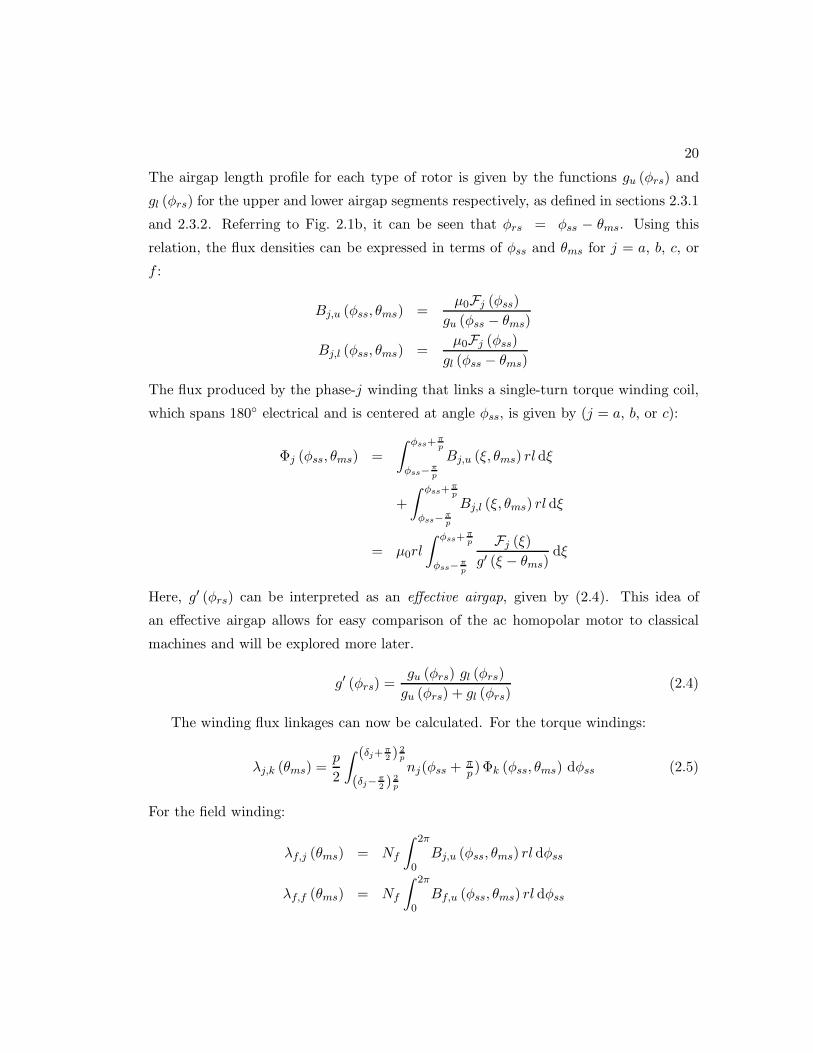
The airgap length profile for each type of rotor is given by the functions gu (φrs) and
gl (φrs) for the upper and lower airgap segments respectively, as defined in sections 2.3.1
and 2.3.2. Referring to Fig. 2.1b, it can be seen that φrs = φss − θms. Using this
relation, the flux densities can be expressed in terms of φss and θms for j = a, b, c, or
f :
Bj,u (φss, θms) =µ0Fj (φss)
gu (φss − θms)
Bj,l (φss, θms) =µ0Fj (φss)
gl (φss − θms)
The flux produced by the phase-j winding that links a single-turn torque winding coil,
which spans 180 electrical and is centered at angle φss, is given by (j = a, b, or c):
Φj (φss, θms) =
∫ φss+πp
φss−πp
Bj,u (ξ, θms) rl dξ
+
∫ φss+πp
φss−πp
Bj,l (ξ, θms) rl dξ
= µ0rl
∫ φss+πp
φss−πp
Fj (ξ)g′ (ξ − θms)
dξ
Here, g′ (φrs) can be interpreted as an effective airgap, given by (2.4). This idea of
an effective airgap allows for easy comparison of the ac homopolar motor to classical
machines and will be explored more later.
g′ (φrs) =gu (φrs) gl (φrs)
gu (φrs) + gl (φrs)(2.4)
The winding flux linkages can now be calculated. For the torque windings:
λj,k (θms) =p
2
∫ (δj+π2 )
2p
(δj−π2 )
2p
nj(φss +πp )Φk (φss, θms) dφss (2.5)
For the field winding:
λf,j (θms) = Nf
∫ 2π
0Bj,u (φss, θms) rl dφss
λf,f (θms) = Nf
∫ 2π
0Bf,u (φss, θms) rl dφss

21
When the airgap functions gu (φrs) and gl (φrs) are defined, the inductance matrix can
be constructed. For the cases considered in this chapter, the inductance matrix takes
the following form:
λa
λb
λc
λf
=
La,a La,b La,c La,f
La,b Lb,b Lb,c Lb,f
La,c Lb,c Lc,c Lc,f
La,f Lb,f Lc,f Lf,f
ia
ib
ic
if
(2.6)
for the phase windings, where j and k = a, b, or c :
Lj,j = Lls + L0 + Lg cos (pθms + δj)
Lj,k = −1
2L0 + Lg cos (pθms − δj − δk)
for the inductance terms involving the field winding, where j = a, b, or c :
Lj,f = Lf0 cos(p
2θms − δj
)
Lf,f = Llf + Lf
Here, Lg, L0, Lf0, and Lf depend on the rotor shape and will be calculated later; Lls and
Llf are leakage inductance terms and are not practical to calculate in this derivation.
To remove the dependence on rotor position and thereby simplify the equations, the
system can be cast into an equivalent d-q form. The transformation as presented in [72]
is used with the d-winding axis aligned with the rotor as shown in Fig. 2.1b, and the
d and q windings each having√
32Ns turns. Following the procedure outlined in [71],
(2.6) can be partitioned as:
λabc = [Labc] iabc+ [Lmf ] if (2.7)
λf = [Lmf ]T iabc+ Lf,f if (2.8)
which can then be transformed into
λdq = [T ] [Labc] [T ]−1 idq+ [T ] [Lmf ] if
λf = [Lmf ]T [T ]−1 idq+ Lf,f if

22
using the following transformation matrix (θm = p2θms):
T =√
23
cos θm cos(
θm − 2π3
)
cos(
θm + 2π3
)
− sin θm − sin(
θm − 2π3
)
− sin(
θm + 2π3
)
1 1 1
The resulting system is shown below. Note that the zero-sequence terms have been
discarded.
λd
λq
=
[
Ld 0
0 Lq
]
id
iq
+
[
L′mf
0
]
if
λf =[
L′mf 0
]
id
iq
+ Lf,f if
where:
Ld = Lls +3
2(L0 + Lg)
Lq = Lls +3
2(L0 − Lg)
L′mf =
√
32Lf0
This gives the following torque expression:
τ =p
2(λdiq − λqid) (2.9)
=p
2iq(
[Ld − Lq] id + L′mf if
)
=p
2iq
(
3Lgid +√
32Lf0 if
)
(2.10)
The first term in (2.10) corresponds to reluctance torque and can be derived by consid-
ering a classical machine with an effective airgap as defined by (2.4). The second term
corresponds to alignment torque and does not fit into the effective airgap paradigm.
Therefore the torque production of the ac homopolar motor can be viewed as the su-
perposition of two torque producing motors: a synchronous reluctance motor and a
cylindrical synchronous motor.
The torque expressions developed for each rotor structure can be compared against
torque expressions derived in textbooks such as [70] for synchronous reluctance and
23
(a)
φrs [rad]
0 0.5π π
gu
gmax
gmin
(b)
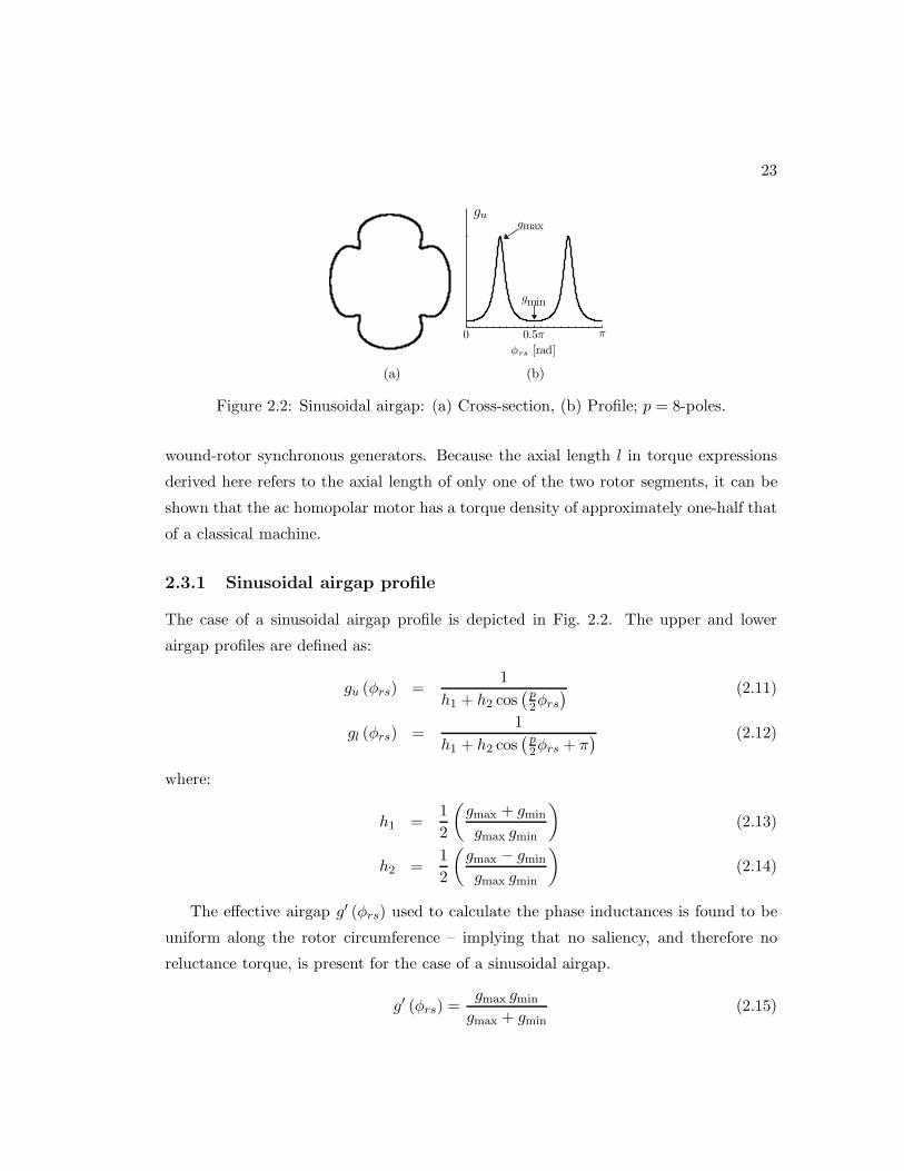
Figure 2.2: Sinusoidal airgap: (a) Cross-section, (b) Profile; p = 8-poles.
wound-rotor synchronous generators. Because the axial length l in torque expressions
derived here refers to the axial length of only one of the two rotor segments, it can be
shown that the ac homopolar motor has a torque density of approximately one-half that
of a classical machine.
2.3.1 Sinusoidal airgap profile
The case of a sinusoidal airgap profile is depicted in Fig. 2.2. The upper and lower
airgap profiles are defined as:
gu (φrs) =1
h1 + h2 cos(p2φrs
) (2.11)
gl (φrs) =1
h1 + h2 cos(p2φrs + π
) (2.12)
where:
h1 =1
2
(
gmax + gmin
gmax gmin
)
(2.13)
h2 =1
2
(
gmax − gmin
gmax gmin
)
(2.14)
The effective airgap g′ (φrs) used to calculate the phase inductances is found to be
uniform along the rotor circumference – implying that no saliency, and therefore no
reluctance torque, is present for the case of a sinusoidal airgap.
g′ (φrs) =gmax gmin
gmax + gmin(2.15)
24
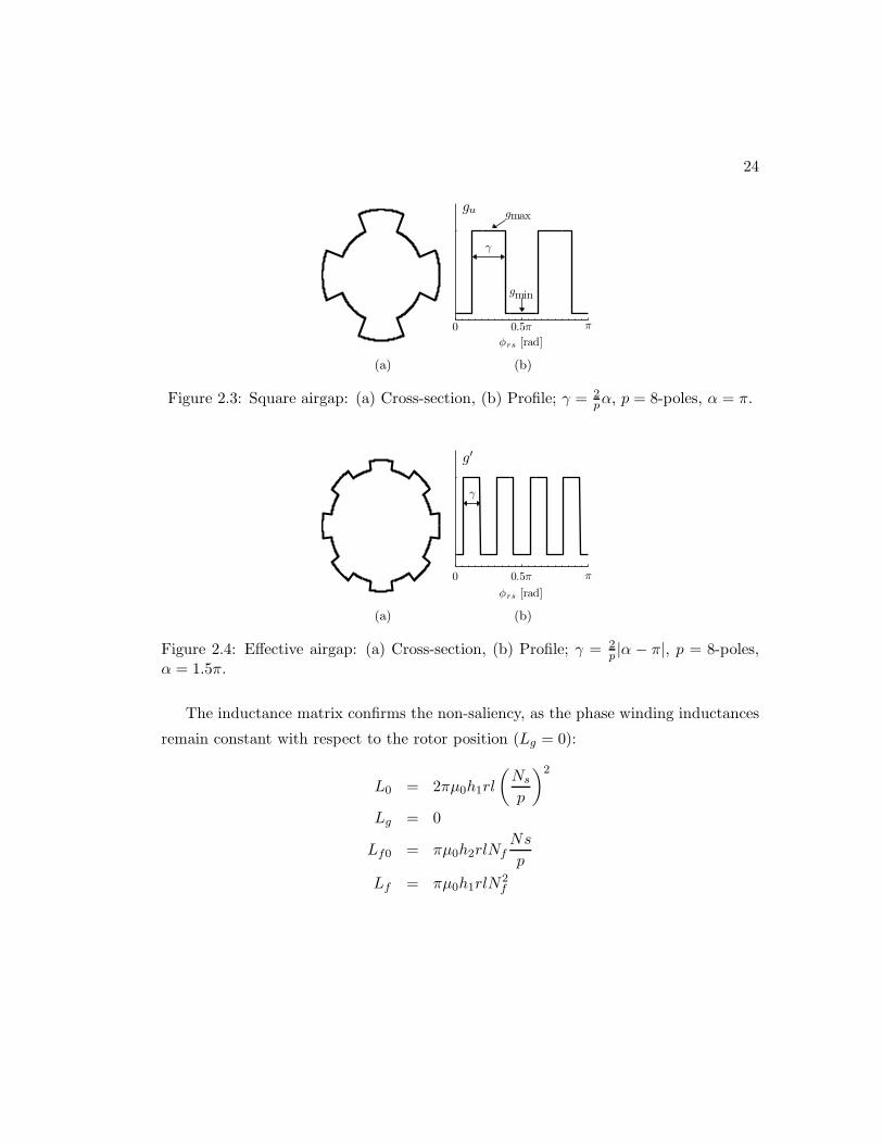
(a)
φrs [rad]
0 0.5π π
γ
gu gmax
gmin
(b)
Figure 2.3: Square airgap: (a) Cross-section, (b) Profile; γ = 2pα, p = 8-poles, α = π.
(a)
φrs [rad]
0 0.5π π
γ
g′
(b)
Figure 2.4: Effective airgap: (a) Cross-section, (b) Profile; γ = 2p |α − π|, p = 8-poles,
α = 1.5π.
The inductance matrix confirms the non-saliency, as the phase winding inductances
remain constant with respect to the rotor position (Lg = 0):
L0 = 2πµ0h1rl
(
Ns
p
)2
Lg = 0
Lf0 = πµ0h2rlNfNs
p
Lf = πµ0h1rlN2f

25
2.3.2 Square airgap profile
The case of a square airgap profile is depicted in Fig. 2.3 and is specified in terms of a
variable duty-cycle square wave:
gu (φrs) =1
h1 + h2 SQα
(p2φrs
) (2.16)
gl (φrs) =1
h1 + h2 SQα
(p2φrs + π
) (2.17)
where h1 is defined by (2.13) and h2 by (2.14). SQα (θ) can be expressed as a Fourier
series:
SQβ (θ) = 1− β
π− 4
π
∞∑
n=1
1
nsin
nβ
2cos (nθ + nπ)
The effective airgap defined in (2.4) to calculate the phase inductances is given
below:
g′ (φrs) =1
g1 + g2 SQ2|α−π|(pφrs)(2.18)
where g1 and g2 depend on the value of α:
g1 =
kg (3gmax + gmin) if α ≤ π,
kg (3gmin + gmax) if α ≥ π.
g2 =
kg (gmin − gmax) if α ≤ π,
kg (gmax − gmin) if α ≥ π.
and kg = (2gmax gmin)−1.
The terms of the inductance matrix are evaluated as:
L0 = 2µ0rl (πh1 + h2 [π − α])
(
Ns
p
)2
Lg = −2µ0h2rl
(
Ns
p
)2
sinα
Lf0 = 4µ0h2rlNf
(
Ns
p
)
sinα
2
Lf = µ0rl (πh1 + h2 [π − α])N2f
Notice that when α = π, (2.18) reduces to (2.15), Lg becomes 0, and the reluctance
torque term in (2.10) vanishes. Therefore, α = π corresponds to a non-salient rotor
26
φc
(a)
φc
(b)
φc
(c)
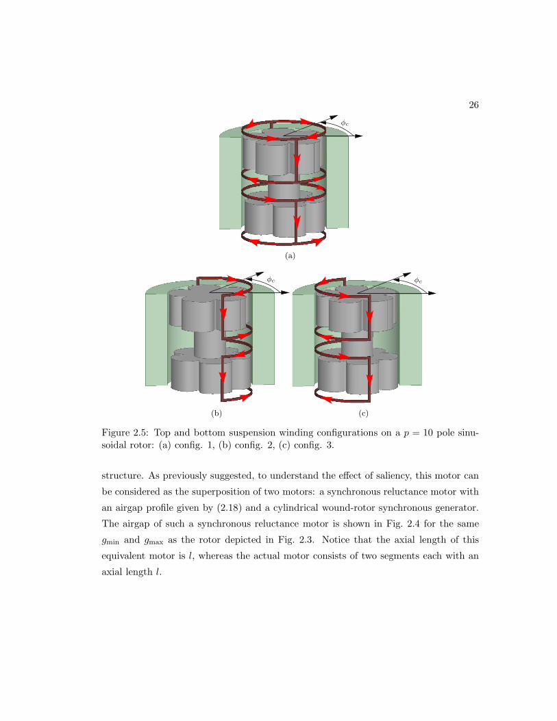
Figure 2.5: Top and bottom suspension winding configurations on a p = 10 pole sinu-soidal rotor: (a) config. 1, (b) config. 2, (c) config. 3.
structure. As previously suggested, to understand the effect of saliency, this motor can
be considered as the superposition of two motors: a synchronous reluctance motor with
an airgap profile given by (2.18) and a cylindrical wound-rotor synchronous generator.
The airgap of such a synchronous reluctance motor is shown in Fig. 2.4 for the same
gmin and gmax as the rotor depicted in Fig. 2.3. Notice that the axial length of this
equivalent motor is l, whereas the actual motor consists of two segments each with an
axial length l.

27
2.4 Suspension winding configurations
Unlike the torque winding, the choice of end-turn configuration of each phase of the
suspension winding has implications for the machine operation. The reason for this is
that one of the end-turn sections is located in the middle of the axial length of the
rotor, similar to the field winding, allowing for a circulating flux to flow axially from the
bottom of the rotor to the top, cross the airgap radially, and return axially from the top
of the stator to the bottom. The three choices of end-turn configuration are depicted
for a single turn in Fig. (2.5). Note that configuration 1 corresponds to a double layer,
full-pitch winding.
2.4.1 MMF calculations
The curl and divergence of the magnetic field can be imposed to solve for the MMF
generated by a current flowing through N -turns of the suspension winding centered at
an angle φc and spanning the ψ rotor section (ψ = u for the upper rotor section, ψ = l
for the lower rotor section):
fp,h,ψ (φc, φss, θms) =NI
2
[ghψ (φc, θms)
gav+ Ph
+ SQπ (φc − φss)]
(2.19)
fs,h,ψ (φc, φss, θms) =NI
2
[
ghψ (φc, θms)
gav+ Sh
]
(2.20)
where the subscript p indicates that the MMF is acting on the rotor section that the
suspension winding spans (specified by ψ), the subscript s indicates that the MMF is
acting on the other rotor section, the subscript h denotes the style of the suspension
winding (1, 2, or 3) as labeled in Fig. 2.5, it is assumed that gl (φrs) = gu(
φrs +2pπ)
,
and:
ghψ (φc, θms) =
∫ φc+3π2
φc+π2
1
gψ (φss − θms)dφss
gav =
∫ 2π
0
1
gu (φss − θms)dφss
=
∫ 2π
0
1
gl (φss − θms)dφss
28
Ph =
−12 if h = 1,
0 if h = 2,
−1 if h = 3.
Sh =
−12 if h = 1,
−1 if h = 2,
0 if h = 3.
Similar to the torque winding, the number of conductors at an angular location φss
of phase-j of the suspension winding spanning rotor section ψ, is defined by:
njψ (φss) =Nss
2sin (φss − δj)
The resultant MMF produced by this phase winding is obtained from superimposing
the MMF generated by the conductors located at each angle where N is replaced by
njψ(
φc +π2
)
and I is replaced by the phase winding current ijψ. Since njψ (φss) is
a continuous function, this is done in the form of an integral. Each of the two rotor
structures considered in this chapter yield the same resultant MMFs:
Fp,j,h,ψ (φss) =∫ δj+
π2
δj−π2fp,h,ψ (φc, φss, θms) dφc
=Nss
2
[
−Kh
2+ cos (φss − δj)
]
ijψ (2.21)
Fs,j,h,ψ (φss) =∫ δj+
π2
δj−π2fs,h,ψ (φc, φss, θms) dφc
=Kh
2
Nss
2ijψ (2.22)
where the subscript j indicates the phase winding, the remaining subscripts are as
defined for (2.19) and (2.20), and
Kh =
0 if h = 1,
−1 if h = 2,
1 if h = 3.
(2.23)
2.4.2 Flux linkage calculations
The flux linkage calculations also vary based on the style of suspension winding config-
uration. Taking note of Fig. 2.5, the flux linking a single turn centered at angle φss for
29
each configuration is given below.
Φ1,ψ (φss, θms) =1
2[Φ2,ψ (φss, θms) + Φ3,ψ (φss, θms)]
Φ2,ψ (φss, θms) =
∫ φss+π2
φss−π2
Bψ (ξ, θms) rl dξ
Φ3,ψ (φss, θms) = −∫ φss+
3π2
φss+π2
Bψ (ξ, θms) rl dξ
where Bψ is the flux density in the airgap of the rotor section specified by ψ. These
expressions can then be used to obtain the flux linkage for a phase-j suspension winding
of configuration h:
λh,j,ψ (θms) =
∫ δj+π2
δj−π2
njψ(φss +π2 )Φh,ψ(φss, θms)dφss (2.24)
2.5 Complete machine inductance matrices
The inductance matrices related to the suspension winding are now calculated for each
rotor structure to complete the inductance matrix model of the motor. These matrices
include the self inductance of the suspension winding, the mutual inductances between
the torque and suspension windings, and the mutual inductances between the field and
suspension windings. To calculate these, (2.24) is evaluated when the magnetic field in
the airgap is produced by each of the various windings and the result is divided by the
current flowing in that winding. The system inductance matrices can be partitioned as
shown below:
λabc = [Labc] iabc+ [Lmf ] if + [Lmtxy,u] ixyu
+ [Lmtxy,l] ixyl (2.25)
λxyu = [Lmtxy,u]T iabc+ [Lmfxy,u] if
+ [Lsxy,u] ixyu+ [Lmxy,l] ixyl (2.26)
λxyl = [Lmtxy,l]T iabc+ [Lmfxy,l] if
+ [Lsxy,l] ixyl+ [Lmxy,u] ixyu (2.27)
λf = [Lmf ]T iabc+ [Lmfxy,u]
T ixyu
+ [Lmfxy,l]T ixy,l+ Lf,f if (2.28)
30
where [Labc], [Lmf ], and Lf,f were previously calculated in (2.6). For the two rotor
structures considered in this chapter the remaining matrices take the following general
forms:
[Lmtxy,ψ] =
La,x,ψ La,y,ψ
Lb,x,ψ Lb,y,ψ
Lc,x,ψ Lc,y,ψ
Lj,k,ψ = KhkψLts,ψ cos(p2θms − δj
)
[Lmfxy,ψ] = Lsf,ψ
[
Kxψ
Kyψ
]
[Lsxy,ψ] = Lss
1 +K2hxψ
KhxψKhyψ
KhyψKhxψ 1 +K2hyψ
[Lmxy,u] = −Lss[
KhxuKhxl KhxuKhyl
KhyuKhxl KhyuKhyl
]
[Lmxy,l] = [Lmxy,u]T
where Kh is defined by (2.23) and hkψ is the suspension winding configuration of phase
k spanning rotor section ψ.
In certain situations it is desirable to have two different end-turn configurations for
the same suspension phase. For example, if the upper x-phase and y-phase windings each
consisted of two separate windings with different configurations and the corresponding
terminal currents ixu1, iyu1, ixu2, iyu2, the following mutual inductance matrix must be
defined:
λxy,u1 = ...+ [Lsxy,hu,12] ixy,u2
[Lsxy,hu,12] = Lss
[
1 +Khxu1Khxu2 Khxu1Khyu2
Khyu1Khxu2 1 +Khyu1Khyu2
]
[Lsxy,hu,21] = [Lsxy,hu,12]T
31
2.5.1 Sinusoidal airgap profile
For the sinusoidally-shaped rotor airgap profile previously defined in (2.11), the induc-
tance constants become:
Lts,u = −πµ0h2rlNs
p
Nss
2
Lts,l = −Lts,u
Lsf,u = 2πµ0h1rlNf
2
Nss
2
Lsf,l = −Lsf,u
Lss = πµ0h1rl
(
Nss
2
)2
2.5.2 Square airgap profile
For the square-shaped rotor airgap profile previously defined in (2.16), the inductance
constants become:
Lts,u = −4µ0h2rlNs
p
Nss
2sin α
2
Lts,l = −Lts,u
Lsf,u = 2µ0rlNf
2
Nss
2(πh1 + h2 [π − α])
Lsf,l = −Lsf,u
Lss = µ0rl
(
Nss
2
)2
(πh1 + h2 [π − α])
2.6 Analysis of suspension force production
Expressions for suspension forces produced by the bearingless ac homopolar motor are
now developed for the two rotor structures and three suspension winding configurations.
Radial forces acting upon the rotor can be calculated from the Maxwell Stress Tensor:
Fx,ψ =
∫ 2π
0
1
2µ0Bg,ψ (φss)
2 lr cosφss dφss (2.29)
Fy,ψ =
∫ 2π
0
1
2µ0Bg,ψ (φss)
2 lr sinφss dφss (2.30)
32
where Bg,ψ (φss) is the net or resultant flux density in the airgap of the ψ rotor section.
For both airgap profiles considered, it is found that as long as the bearingless ac
homopolar motor has p ≥ 8-poles, θms does not appear in the resulting suspension force
expressions, meaning that the suspension forces are independent of the rotor’s angular
position. When that is not the case, the bearingless ac homopolar motor lacks one of
its primary features and therefore becomes difficult to justify as a bearingless motor.
For this reason force expressions are only evaluated for the p ≥ 8 case.
Evaluating (2.29) and (2.30) when the rotor is centered gives the following form for
the force expressions:
Fk,u =(
ks
[
Nf2 if +
Nss4 C (ixy,ul)
]
+ kd id
)
iku (2.31)
Fk,l = −(
ks
[
Nf2 if +
Nss4 C (ixy,ul)
]
+ kd id
)
ikl (2.32)
C (ixy,ul) = Khxlixl +Khyliyl −Khxuixu −Khyuiyu
where the subscript k indicates the direction of the force as well as the phase of the
suspension winding, the constants ks and kd are dependent upon the rotor structure,
Kh is defined by (2.23), and additional terms can be added to C (ixy,ul) if a phase of
a suspension winding contains multiple configurations. It should be noted that if all
suspension windings are of configuration 1, then C (ixy,ul) = 0.
2.6.1 Sinusoidal airgap profile
For the sinusoidally shaped rotor structure defined by (2.11) and (2.12), the force con-
stants become:
ks = πµ0Nss
2rl(
h21 +12h
22
)
kd =√
32 πµ0
Ns
p
Nss
2rlh1h2
33
2.6.2 Square airgap profile
For the square rotor structure defined by (2.16) and (2.17), the force constants become:
ks = µ0Nss
2rl[
π(
h21 + h22)
+ 2h1h2 (π − α)]
kd = 2√6µ0
Ns
p
Nss
2rlh1h2 sin
α2
2.7 Analysis of interference torque
Here, the analysis of section 2.3 is extended to include the effects of current in the sus-
pension winding on the machine’s torque. Analogous to section 2.6 revealing that the
torque windings contribute to the suspension forces, this section shows that the suspen-
sion windings interfere with torque production. In most cases, this is not desirable, as
any transients in the suspension winding current would then need to be compensated
for by the torque controller. However in certain cases, such as when the rotor is hor-
izontally oriented, a constant force may be desired and hence the torque interference
from the suspension winding can be designed such that it is desirable.
Transforming the torque windings into the d-q representation described in section
2.3 results in the following expressions for d and q flux linkages:
λd
λq
=
[
Ld 0
0 Lq
]
id
iq
+
[
L′ts,xu L′
ts,yu
0 0
]
ixu
iyu
+
[
L′ts,xl L′
ts,yl
0 0
]
ixl
iyl
+
[
L′mf
0
]
if
where L′ts,hkψ
=√
3/2KhkψLts. Using (2.9), an additional torque term appears in (2.10):
τi =p
2iq[
L′ts,xuixu + L′
ts,yuiyu + L′ts,xlixl + L′
ts,yliyl]
It is important to note here that since K1 = 0, suspension winding configuration 1 will
result in no interference torque.
Chapter 3
Outer-Rotor AC Homopolar
Motors for Flywheel Energy
Storage
This chapter investigates the bearingless ac homopolar machine as a motor (no bear-
ingless capability) for use in flywheel energy storage as an alternative to the permenant
magnet (PM) motor. The primary objectives of using the ac homopolar motor is to
decrease the flywheel system’s idling losses, increase energy density, and decrease cost.
Motor sizing equations, a comparison to the typically-used permanent magnet motor,
and 3D finite element analysis of an example design are presented. It is shown that for
high-performance flywheel designs, the ac homopolar motor can have a torque density
comparable to that of a permanent magnet motor.1
3.1 Introduction
As described in Chapter 1, the traditional flywheel system design topology, which is non-
integrated, is depicted in Fig. 3.1a. This dissertation proposes a fully integrated design
based around an outer-rotor bearingless ac homopolar motor, depicted in Fig. 3.1b.
Since most of the flywheel’s energy is stored near its outer radius, removing the inner
1 Portions of the material in this chapter have also been published in [51].
34
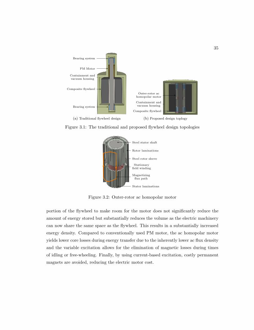
35
Bearing system
PM Motor
Containment andvacuum housing
Composite flywheel
Bearing system
(a) Traditional flywheel design
Outer-rotor achomopolar motor
Containment andvacuum housing
Composite flywheel
(b) Proposed design toplogy
Figure 3.1: The traditional and proposed flywheel design topologies
Steel stator shaft
Rotor laminations
Steel rotor sleeve
Stationary
field winding
Magnetizing
flux path
Stator laminations
Figure 3.2: Outer-rotor ac homopolar motor
portion of the flywheel to make room for the motor does not significantly reduce the
amount of energy stored but substantially reduces the volume as the electric machinery
can now share the same space as the flywheel. This results in a substantially increased
energy density. Compared to conventionally used PM motor, the ac homopolar motor
yields lower core losses during energy transfer due to the inherently lower ac flux density
and the variable excitation allows for the elimination of magnetic losses during times
of idling or free-wheeling. Finally, by using current-based excitation, costly permanent
magnets are avoided, reducing the electric motor cost.

36
3.2 Outer-rotor ac homopolar motor
The outer-rotor ac homopolar motor is shown in Fig. 3.2. It features variable excitation
due to a field winding which is fixed to the stator. This means that no brushes or
slip rings are required. This motor has been widely considered in the literature as an
inner-rotor motor for use in superconducting and high-speed applications due to its
current-based excitation and robust rotor structure, and as a high frequency generator
due to its parallel arrangement of poles requiring no additional ampere-turns of field
winding for an increased number of poles [27,59,65,73–75].
The magnetizing flux path, depicted in Fig. 1c, is both radial and axial. The har-
monics of the magnetizing flux density in the airgap can be controlled by the rotor
shape, with the most common rotor shapes having an airgap length profile of a square
wave and an inverted sine wave. Since the stator and rotor laminations have low mag-
netic permeability in the axial direction, a solid steel stator shaft and rotor sleeve are
used to provide an axial flux path. The difference between the stator lamination inner
diameter and outer diameter must be large enough to allow the flux to evenly distribute
itself before reaching the stator shaft, or eddy currents may be induced in the steel.
Several designs, such as [27,65], have successfully used a solid rotor and, in some cases,
a slot-less stator.
The machine only uses half of its magnetic circuit at any location, meaning that
magnetizing flux density is always north-facing in one of the two stator/rotor sections
and always south-facing in the other stator/rotor section. In this chapter, the two
stator/rotor sections are referred to as the “top” section and the “bottom” section. The
homopolar and fundamental magnetizing airgap flux density in the top and bottom
rotor/stator segments can be described by (3.1). Using only one-half of the magnetic
circuit at any location decreases both the torque density and the core losses significantly
as compared to a traditional radial flux machine. This is considered in more detail later
in the chapter.
Bf,top (α) = Bf1 cos pα+Bf0
Bf,bot (α) = Bf1 cos pα−Bf0 (3.1)
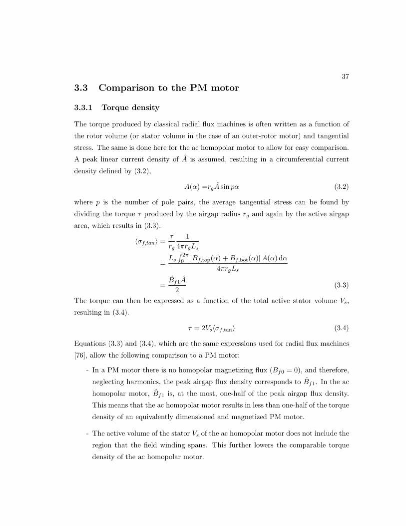
37
3.3 Comparison to the PM motor
3.3.1 Torque density
The torque produced by classical radial flux machines is often written as a function of
the rotor volume (or stator volume in the case of an outer-rotor motor) and tangential
stress. The same is done here for the ac homopolar motor to allow for easy comparison.
A peak linear current density of A is assumed, resulting in a circumferential current
density defined by (3.2),
A(α) =rgA sin pα (3.2)
where p is the number of pole pairs, the average tangential stress can be found by
dividing the torque τ produced by the airgap radius rg and again by the active airgap
area, which results in (3.3).
〈σf,tan〉 =τ
rg
1
4πrgLs
=Ls∫ 2π0 [Bf,top(α) +Bf,bot(α)]A(α) dα
4πrgLs
=Bf1A
2(3.3)
The torque can then be expressed as a function of the total active stator volume Vs,
resulting in (3.4).
τ = 2Vs〈σf,tan〉 (3.4)
Equations (3.3) and (3.4), which are the same expressions used for radial flux machines
[76], allow the following comparison to a PM motor:
- In a PM motor there is no homopolar magnetizing flux (Bf0 = 0), and therefore,
neglecting harmonics, the peak airgap flux density corresponds to Bf1. In the ac
homopolar motor, Bf1 is, at the most, one-half of the peak airgap flux density.
This means that the ac homopolar motor results in less than one-half of the torque
density of an equivalently dimensioned and magnetized PM motor.
- The active volume of the stator Vs of the ac homopolar motor does not include the
region that the field winding spans. This further lowers the comparable torque
density of the ac homopolar motor.
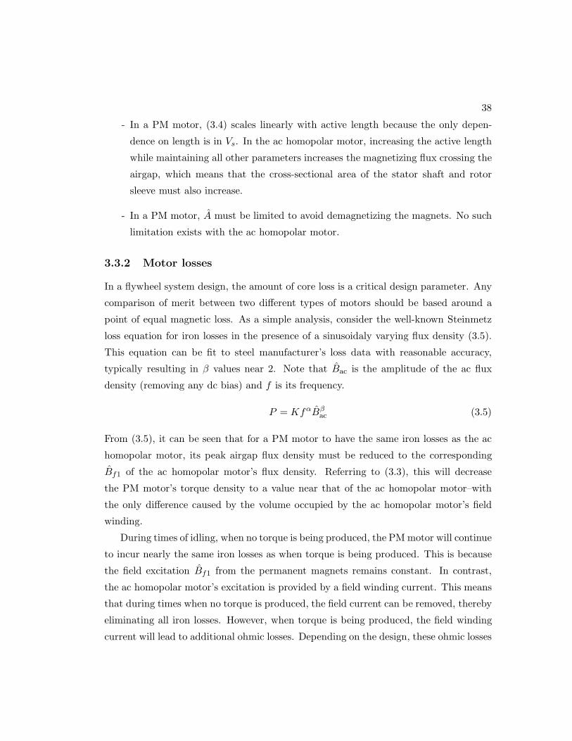
38
- In a PM motor, (3.4) scales linearly with active length because the only depen-
dence on length is in Vs. In the ac homopolar motor, increasing the active length
while maintaining all other parameters increases the magnetizing flux crossing the
airgap, which means that the cross-sectional area of the stator shaft and rotor
sleeve must also increase.
- In a PM motor, A must be limited to avoid demagnetizing the magnets. No such
limitation exists with the ac homopolar motor.
3.3.2 Motor losses
In a flywheel system design, the amount of core loss is a critical design parameter. Any
comparison of merit between two different types of motors should be based around a
point of equal magnetic loss. As a simple analysis, consider the well-known Steinmetz
loss equation for iron losses in the presence of a sinusoidaly varying flux density (3.5).
This equation can be fit to steel manufacturer’s loss data with reasonable accuracy,
typically resulting in β values near 2. Note that Bac is the amplitude of the ac flux
density (removing any dc bias) and f is its frequency.
P = KfαBβac (3.5)
From (3.5), it can be seen that for a PM motor to have the same iron losses as the ac
homopolar motor, its peak airgap flux density must be reduced to the corresponding
Bf1 of the ac homopolar motor’s flux density. Referring to (3.3), this will decrease
the PM motor’s torque density to a value near that of the ac homopolar motor–with
the only difference caused by the volume occupied by the ac homopolar motor’s field
winding.
During times of idling, when no torque is being produced, the PMmotor will continue
to incur nearly the same iron losses as when torque is being produced. This is because
the field excitation Bf1 from the permanent magnets remains constant. In contrast,
the ac homopolar motor’s excitation is provided by a field winding current. This means
that during times when no torque is produced, the field current can be removed, thereby
eliminating all iron losses. However, when torque is being produced, the field winding
current will lead to additional ohmic losses. Depending on the design, these ohmic losses

39
may be compensated for by being able to adjust the excitation to the most efficient
point–i.e. decreasing the excitation with increasing rotor speed.
3.4 Machine sizing equations for flywheel energy storage
The integrated flywheel and rotor can be viewed as two concentric hollow rotating
cylinders where the inner hollow cylinder is the ac homopolar rotor and the outer hollow
cylinder is the flywheel. The ac homopolar rotor can be dimensioned according the
motor design requirements with a maximum tip speed vsl,tip limiting the outer-diameter
of the rotor sleeve. The flywheel dimensions are determined by the required storage
capacity, rotational speed, and outer diameter of the homopolar rotor.
Simplistic design equations follow, with relevant dimensions labeled in Fig. 3.3.
These equations use the stored energy and parameters based around losses as inputs
and provide the module dimensions and power rating as outputs. This approach is
appropriate for the application of long-term flywheel energy storage, where the storage
capacity and power losses are more important than the power rating. These equations
neglect leakage flux, of which this machine caries a considerable amount, and assume an
infinetly permeable back-iron. An approximation of the machine size and design trade-
off’s can be obtained from these equations; however, a more precise design requires 3D
FE modeling.
3.4.1 Flywheel sizing
The total amount of energy stored in the flywheel is approximated as that stored in a
hollow rotating cylinder, E = 12Iω
2 . To obtain the maximum energy density, the outer
diameter is chosen to be the maximum that the flywheel’s material can support (3.6)
and the length is scaled to achieve the required storage capacity (3.7), where vf,tip is
the flywheel material’s maximum surface speed, ρf is the material’s mass density, and
rsl,out is the outer radius of the rotor sleeve.
rf,out = vf,tip/ω (3.6)
Lf =4E
πρfv2f,tip
(
r2f,out −r4sl,outr2f,out
) (3.7)
40
rf,out
rgrsl,out
rsl,in
trs
tss
gmax
gmin
Figure 3.3: Cross-section of the integrated flywheel and ac homopolar motor.
The energy E in (3.7) must be increased if the module doesn’t use the full speed range.
Typical designs operate over half of their speed range as a compromise between usable
energy and the torque requirement to provide constant power regardless of the state of
charge.
3.4.2 AC homopolar motor sizing
The two stator/rotor segments of the ac homopolar motor can be dimensioned using
(3.4) combined with a constraint based around the maximum tip speed of the rotor sleeve
material and a constraint based around the magnetizing flux path: the magnetizing flux
crossing the airgap is limited by the amount that the stator shaft and rotor sleeve can
support. For mechanical and magnetic reasons, the following fixed lengths are assumed:
- trs between the rotor lamination notch and sleeve,
- tss between the stator teeth and the shaft,
- gmin minimum airgap length.
In addition to this, it is assumed that Bf1 and A of (3.3) and maximum flux densities
of the airgap Bmax, stator shaft Bsh, and rotor sleeve Bsl are chosen based on loss
and material saturation considerations. With these design choices, combined with the
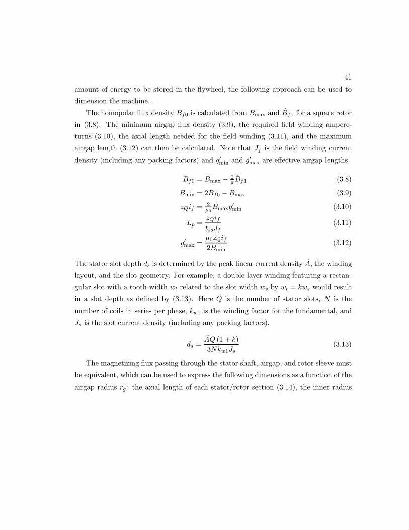
41
amount of energy to be stored in the flywheel, the following approach can be used to
dimension the machine.
The homopolar flux density Bf0 is calculated from Bmax and Bf1 for a square rotor
in (3.8). The minimum airgap flux density (3.9), the required field winding ampere-
turns (3.10), the axial length needed for the field winding (3.11), and the maximum
airgap length (3.12) can then be calculated. Note that Jf is the field winding current
density (including any packing factors) and g′min and g′max are effective airgap lengths.
Bf0 = Bmax − 2π Bf1 (3.8)
Bmin = 2Bf0 −Bmax (3.9)
zQif = 2µ0Bmaxg
′min (3.10)
Lp =zQiftssJf
(3.11)
g′max =µ0zQif2Bmin
(3.12)
The stator slot depth ds is determined by the peak linear current density A, the winding
layout, and the slot geometry. For example, a double layer winding featuring a rectan-
gular slot with a tooth width wt related to the slot width ws by wt = kws would result
in a slot depth as defined by (3.13). Here Q is the number of stator slots, N is the
number of coils in series per phase, kw1 is the winding factor for the fundamental, and
Js is the slot current density (including any packing factors).
ds =AQ (1 + k)
3Nkw1Js(3.13)
The magnetizing flux passing through the stator shaft, airgap, and rotor sleeve must
be equivalent, which can be used to express the following dimensions as a function of the
airgap radius rg: the axial length of each stator/rotor section (3.14), the inner radius
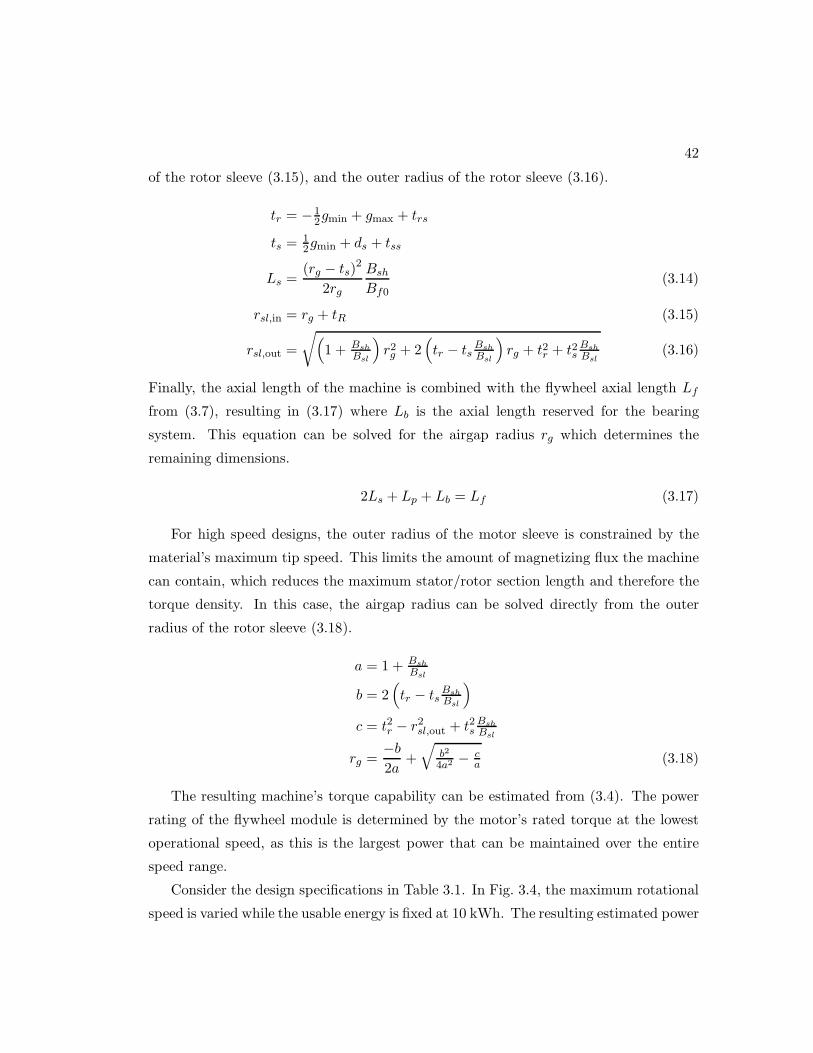
42
of the rotor sleeve (3.15), and the outer radius of the rotor sleeve (3.16).
tr = −12gmin + gmax + trs
ts =12gmin + ds + tss
Ls =(rg − ts)
2
2rg
BshBf0
(3.14)
rsl,in = rg + tR (3.15)
rsl,out =
√
(
1 + BshBsl
)
r2g + 2(
tr − tsBshBsl
)
rg + t2r + t2sBshBsl
(3.16)
Finally, the axial length of the machine is combined with the flywheel axial length Lf
from (3.7), resulting in (3.17) where Lb is the axial length reserved for the bearing
system. This equation can be solved for the airgap radius rg which determines the
remaining dimensions.
2Ls + Lp + Lb = Lf (3.17)
For high speed designs, the outer radius of the motor sleeve is constrained by the
material’s maximum tip speed. This limits the amount of magnetizing flux the machine
can contain, which reduces the maximum stator/rotor section length and therefore the
torque density. In this case, the airgap radius can be solved directly from the outer
radius of the rotor sleeve (3.18).
a = 1 + BshBsl
b = 2(
tr − tsBshBsl
)
c = t2r − r2sl,out + t2sBshBsl
rg =−b2a
+
√
b2
4a2− c
a (3.18)
The resulting machine’s torque capability can be estimated from (3.4). The power
rating of the flywheel module is determined by the motor’s rated torque at the lowest
operational speed, as this is the largest power that can be maintained over the entire
speed range.
Consider the design specifications in Table 3.1. In Fig. 3.4, the maximum rotational
speed is varied while the usable energy is fixed at 10 kWh. The resulting estimated power
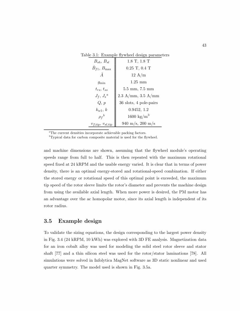
43
Table 3.1: Example flywheel design parameters
Bsh, Bsl 1.8 T, 1.8 T
Bf1, Bmax 0.25 T, 0.4 T
A 12 A/m
gmin 1.25 mm
trs, tss 5.5 mm, 7.5 mm
Jf , Jsa 2.3 A/mm, 3.5 A/mm
Q, p 36 slots, 4 pole-pairs
kw1, k 0.9452, 1.2
ρfb 1600 kg/m3
vf,tip, vsl,tip 940 m/s, 200 m/s
aThe current densities incorporate achievable packing factors.bTypical data for carbon composite material is used for the flywheel.
and machine dimensions are shown, assuming that the flywheel module’s operating
speeds range from full to half. This is then repeated with the maximum rotational
speed fixed at 24 kRPM and the usable energy varied. It is clear that in terms of power
density, there is an optimal energy-stored and rotational-speed combination. If either
the stored energy or rotational speed of this optimal point is exceeded, the maximum
tip speed of the rotor sleeve limits the rotor’s diameter and prevents the machine design
from using the available axial length. When more power is desired, the PM motor has
an advantage over the ac homopolar motor, since its axial length is independent of its
rotor radius.
3.5 Example design
To validate the sizing equations, the design corresponding to the largest power density
in Fig. 3.4 (24 kRPM, 10 kWh) was explored with 3D FE analysis. Magnetization data
for an iron cobalt alloy was used for modeling the solid steel rotor sleeve and stator
shaft [77] and a thin silicon steel was used for the rotor/stator laminations [78]. All
simulations were solved in Infolytica MagNet software as 3D static nonlinear and used
quarter symmetry. The model used is shown in Fig. 3.5a.
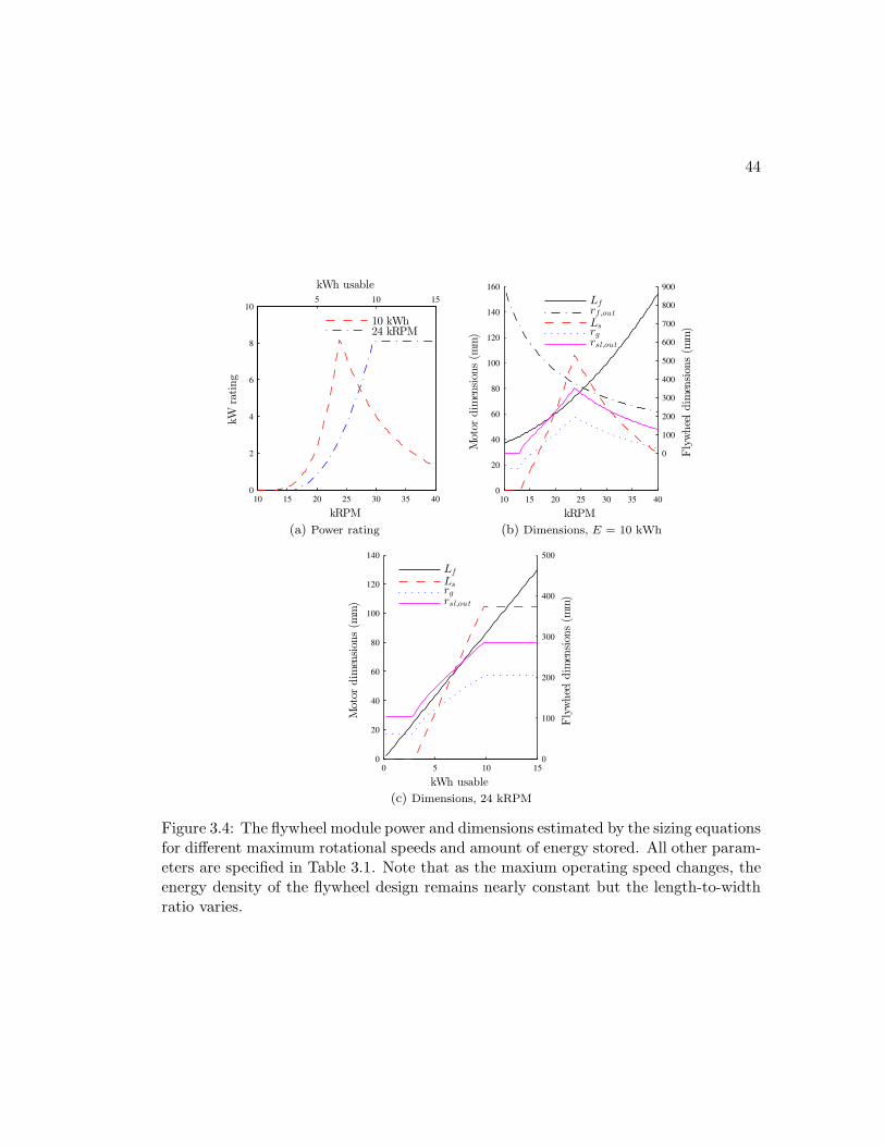
44
5 10 15
kWh usable
10 15 20 25 30 35 400
2
4
6
8
10
kRPM
kWrating
10 kWh24 kRPM
(a) Power rating
10 15 20 25 30 35 40
0
100
200
300
400
500
600
700
800
900
kRPM
Flywheeldim
ension
s(m
m)
0
20
40
60
80
100
120
140
160
Motor
dim
ension
s(m
m)
Lfrf,outLsrgrsl,out
(b) Dimensions, E = 10 kWh
0 5 10 150
100
200
300
400
500
kWh usable
Flywheeldim
ension
s(m
m)
0
20
40
60
80
100
120
140
Motor
dim
ension
s(m
m)
Lf
Lsrgrsl,out
(c) Dimensions, 24 kRPM
Figure 3.4: The flywheel module power and dimensions estimated by the sizing equationsfor different maximum rotational speeds and amount of energy stored. All other param-eters are specified in Table 3.1. Note that as the maxium operating speed changes, theenergy density of the flywheel design remains nearly constant but the length-to-widthratio varies.

45
FE results under full-load and no-load are shown in Fig. 3.5. The excitation current
had to be increased by 30% from that calculated by the sizing equations to obtain the
required airgap flux density and the torque estimated by the sizing equations was ap-
proximately 1.2 Nm greater than that obtained through the FE results. This illustrates
the inaccuracies of the sizing equations and the need for 3D FE analysis when designing
the ac homopolar motor. In a future work, 3D transient nonlinear modeling will be
conducted to analyze losses in the laminations and solid steel and to determine values
for tss and trs.
3.6 Conclusion
The outer-rotor ac homopolar motor has been investigated for use in flywheel energy
storage technology. It was shown that for low power designs, where magnetic losses
are a key design parameter, the ac homopolar motor has a similar torque density to
the typically-used PM motor. The PM motor has magnetic losses while idling but the
ac homopolar motor does not. For these reasons, it is concluded that this motor is a
promising machine for developing a flywheel system with long storage intervals.

46
(a) FE Model
0 20 40 60 800
1
2
3
4
5
6
550 ampere-turns field excitationAverage torque of 3.2 Nm
1100 ampere-turns field excitationAverage torque of 5.2 Nm
Nm
degrees
(b) Torque waveform
(c) No load (d) Full load
0 20 40 60 80−0.6
−0.4
−0.2
0
0.2
0.4
0.6
tesla
degrees
Top airgap
Bottom airgap
(e) No load airgap flux density
0 20 40 60 80−0.6
−0.4
−0.2
0
0.2
0.4
0.6
tesla
degrees
Top airgap
Bottom airgap
(f) Full load airgap flux density
Figure 3.5: Results from 3D FE analysis of a 10kWh, 24 kRPM design; the full fieldexcitation of 1100 ampere-turns is to be used at half-speed while 550 ampere-turns offield excitation is to be used at full-speed; (b), (c), (e), and (f) correspond to full fieldexcitation and are evaluated at an axial location in the middle of each stator/rotorsection.

Chapter 4
Magnetic Equivalent Circuit
Modeling of the AC Homopolar
Motor
This chapter develops a magnetic equivalent circuit model suitable to the design and
optimization of the synchronous ac homopolar motor. This machine features both axial
and radial magnetizing flux paths, which requires finite element analysis to be conducted
in 3D. The computation time associated with 3D finite element modeling is highly
prohibitive in the design process. The magnetic equivalent circuit model developed in
this chapter is shown to be a viable alternative for calculating several design performance
parameters and has a computation time which is orders of magnitude less than that of
3D finite element analysis. Results obtained from the developed model are shown to
be in good agreement with finite element and experimental results for varying levels of
saturation.1
1 Portions of the material in this chapter have been submitted for publication in [48].
47
48
4.1 Introduction
The complex geometry and flux paths of the ac homopolar machine make the machine
particularly difficult to design. The magnetizing flux flows in all three directions, re-
quiring that finite element (FE) models be constructed in 3D. The computation time to
evaluate 3D FE models is significant, making them impractical for use in optimizing the
machine’s design. Obtaining a less computationally expensive model of this machine for
use in the design process has been the focus of several recent papers [31,79–82]. These
papers have used techniques including magnetic equivalent circuits (MEC), analytic
modeling, and a 2D equivalent FE model and either fail to accurately model saturation,
exhibit poor agreement with 3D FE results, are highly specific to a certain design’s
unique geometry, or take too long to solve. To the author’s knowledge, there is not
yet a sufficiently accurate model of the ac homopolar machine which is computationally
efficient enough to be used in a design optimization.
The main contribution of this chapter is to develop a model of the ac homopolar
machine which is both sufficiently accurate and has a short enough solve-time that
it can be used in the design process. This model is based on MEC theory and is
constructed in a manner which allows the designer to easily select a desired trade-off
between accuracy and solve time. Simple, 1D flux tubes are used within a 3D magnetic
circuit that includes both leakage flux paths and the effects of saturation. The geometry
and path of each flux tube is presented. Symmetry is exploited based on the number
of machine pole pairs and additional axial symmetry is used for evaluating the machine
under no-load conditions. A mesh-based solution is used, as opposed to the conventional
nodal-based solution, because it has been shown in [83, 84] that this solution exhibits
better non-linear convergence and therefore reduces the computation time when portions
of the model are saturated. Finally, both 3D FE and experimental results are used to
validate the developed model. In Section 4.2, background information and literature on
ac homopolar machine and MEC are presented; in Section 4.3, an overview of the MEC
model as applied to the ac homopolar machine is presented; in Section 4.4, the geometry
of each flux tube is defined; and in Section 4.5, results obtained from the MEC model
are compared against FE and experimental results.

49
Stationary
Stator laminationsStator sleeve
Rotor laminations
Magnetizing flux path
field winding
Figure 4.1: Synchronous ac homopolar machine geometry used for the MEC
4.2 Background
A diagram of the ac homopolar machine, as considered in this chapter, is shown in
Fig. 4.1. As drawn here, the machine has two laminated rotor segments mounted on
a magnetic shaft. A stationary field winding is mounted on the stator which encircles
the rotor and causes a homopolar magnetizing flux to flow axially along the rotor shaft,
radially through the rotor and stator laminations, and axially along a steel stator sleeve.
The stator laminations can either be continuous, as drawn in Fig. 4.1, or they can be
constructed as two separate stacks sandwiching the field winding.
Recent literature has proposed using MECs with 1D flux tubes in the design of
various synchronous PM, induction, and wound-rotor machines as an alternative to 2D
FE models [85–89]. It has been shown that this is an effective tool in population-based
design processes, where the number of candidate designs can easily exceed 106 and
even 2D FE models are too computationally expensive [85, 90]. The MEC model is
usually solved using a nodal approach, similar to what is done in various electric circuit
solvers; as previously mentioned, it has been shown in [83,84] that this solution approach
can lead to convergence problems. In [91] an approach to model nonlinear magnetic
materials was presented that guarantees convergence properties for mesh-based MEC
solutions. While the convergence problems are eliminated with a mesh-based solution, a
new problem arises due to the number of airgap flux tubes changing with rotor rotation
(setting a flux tube permeance to zero results in an infinite reluctance); possible solutions
to this include either using a fixed airgap mesh or the shaping algorithm defined in [84].
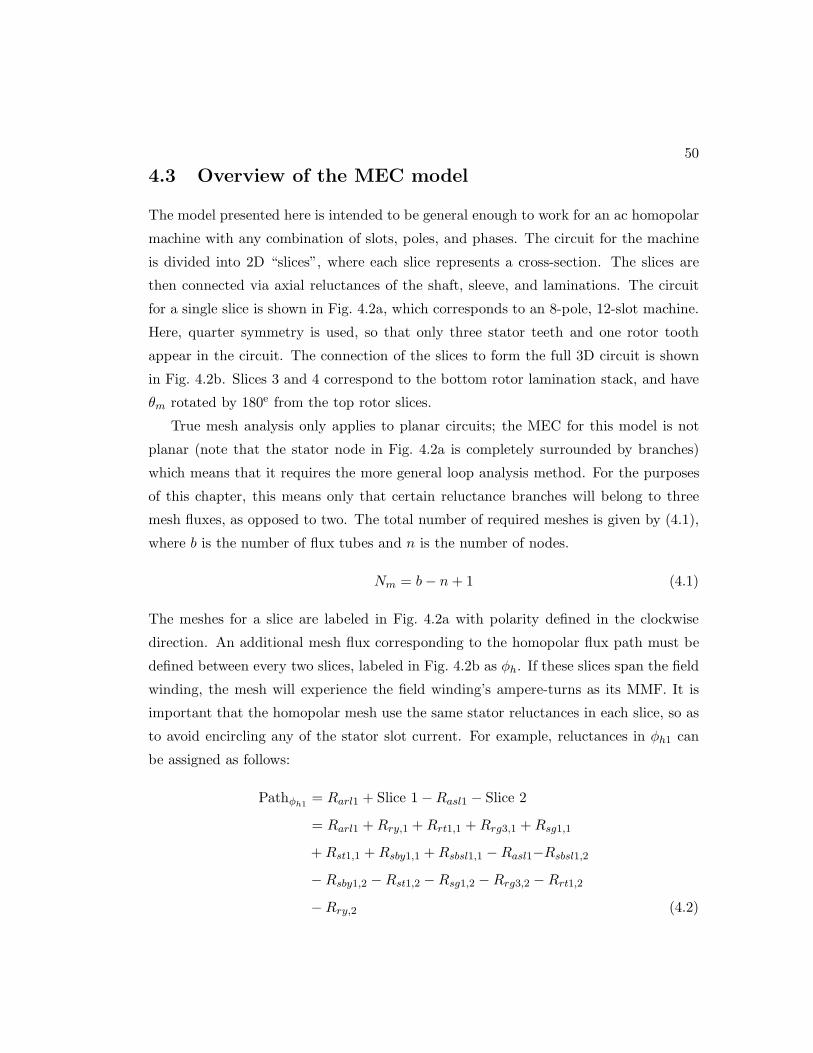
50
4.3 Overview of the MEC model
The model presented here is intended to be general enough to work for an ac homopolar
machine with any combination of slots, poles, and phases. The circuit for the machine
is divided into 2D “slices”, where each slice represents a cross-section. The slices are
then connected via axial reluctances of the shaft, sleeve, and laminations. The circuit
for a single slice is shown in Fig. 4.2a, which corresponds to an 8-pole, 12-slot machine.
Here, quarter symmetry is used, so that only three stator teeth and one rotor tooth
appear in the circuit. The connection of the slices to form the full 3D circuit is shown
in Fig. 4.2b. Slices 3 and 4 correspond to the bottom rotor lamination stack, and have
θm rotated by 180e from the top rotor slices.
True mesh analysis only applies to planar circuits; the MEC for this model is not
planar (note that the stator node in Fig. 4.2a is completely surrounded by branches)
which means that it requires the more general loop analysis method. For the purposes
of this chapter, this means only that certain reluctance branches will belong to three
mesh fluxes, as opposed to two. The total number of required meshes is given by (4.1),
where b is the number of flux tubes and n is the number of nodes.
Nm = b− n+ 1 (4.1)
The meshes for a slice are labeled in Fig. 4.2a with polarity defined in the clockwise
direction. An additional mesh flux corresponding to the homopolar flux path must be
defined between every two slices, labeled in Fig. 4.2b as φh. If these slices span the field
winding, the mesh will experience the field winding’s ampere-turns as its MMF. It is
important that the homopolar mesh use the same stator reluctances in each slice, so as
to avoid encircling any of the stator slot current. For example, reluctances in φh1 can
be assigned as follows:
Pathφh1 = Rarl1 + Slice 1−Rasl1 − Slice 2
= Rarl1 +Rry,1 +Rrt1,1 +Rrg3,1 +Rsg1,1
+Rst1,1 +Rsby1,1 +Rsbsl1,1 −Rasl1−Rsbsl1,2−Rsby1,2 −Rst1,2 −Rsg1,2 −Rrg3,2 −Rrt1,2
−Rry,2 (4.2)

51
Rsy1 Rsy2
Rsg1
Rtt1 Rtt2
Rsby1
Rsbsl1
Rscy1
Rscsl1
Rtf1
Rsf1
φst1
φslkg1
φgt1
φsy1 φsy2
Rst1
Rfg1 Rfg2
φgm1 φgm2
Rsy3 Rsy4
Rsg2
Rtt3Rsf2 Rtt4
Rtf2
Rsby2
Rsbsl2
Rscy2
Rscsl2
nss
φst2
φslkg2
φgt2
φsy3 φsy4
Rst2
Rfg3 Rfg4
φgm3 φgm4
Rsy5 Rsy6
Rsg3
Rtt5Rsf3 Rtt6
Rtf3
Rsby3
Rsbsl3
Rscy3
Rscsl3
φst3
φslkg3
φgt3
φsy5 φsy6
Rst3
Rfg5 Rfg6
φgm5 φgm6
Rscy1
Rscsl1
Rrs2
Rrg1Rrg2 Rrg3
Rrg4 Rrg5Rrg6 Rrg7
Rrg8 Rrg9Rrg10 Rrg11
Rrg12
φgb1 φgb2 φgb3 φgb4 φgb5
Rrtt1 Rrtt2 Rrtt3
φrt1 φrt2 φrt3
nrs
Rry
Rrt1 Rrt4Rrt2 Rrt3
Rrs1
θm
(a) MEC for a single slice
Rshf
Rshl3
Rshl4 Rarl4
Rarl3
Rshl2
Rshl1 Rarl1
Rarl2
Slice 1
Slice 2
Slice 3
Slice 4
Rasl1
Raslf
Rsl1
Rslf
Rsl2Rasl2
nrs,1
nrs,2
nrs,3
nrs,4
nss,1
nss,2
nss,3
nss,4
φshl1
φshl2
φshl3
φshl4
φsll1
φsll2
φsll3
φh1
φh2
φhf
Shaft Rotor laminations Stator laminations Sleeve
(b) Axial connection of the slices
Figure 4.2: MEC for an eight pole, 12 slot ac homopolar machine using quarter sym-metry
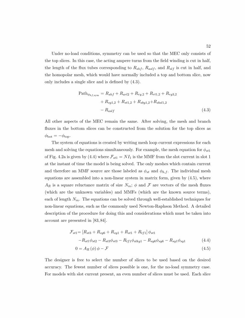
52
Under no-load conditions, symmetry can be used so that the MEC only consists of
the top slices. In this case, the acting ampere turns from the field winding is cut in half,
the length of the flux tubes corresponding to Rshf , Raslf , and Rslf is cut in half, and
the homopolar mesh, which would have normally included a top and bottom slice, now
only includes a single slice and is defined by (4.3).
Pathφhf,sym = Rshf +Rarl2 +Rry,2 +Rrt1,2 +Rrg3,2
+Rsg1,2 +Rst1,2 +Rsby1,2+Rsbsl1,2
−Raslf (4.3)
All other aspects of the MEC remain the same. After solving, the mesh and branch
fluxes in the bottom slices can be constructed from the solution for the top slices as
φbot = −φtop.The system of equations is created by writing mesh loop current expressions for each
mesh and solving the equations simultaneously. For example, the mesh equation for φst1
of Fig. 4.2a is given by (4.4) where Fst1 = NI1 is the MMF from the slot current in slot 1
at the instant of time the model is being solved. The only meshes which contain current
and therefore an MMF source are those labeled as φst and φh,f . The individual mesh
equations are assembled into a non-linear system in matrix form, given by (4.5), where
AR is a square reluctance matrix of size Nm; φ and F are vectors of the mesh fluxes
(which are the unknown variables) and MMFs (which are the known source terms),
each of length Nm. The equations can be solved through well-established techniques for
non-linear equations, such as the commonly used Newton-Raphson Method. A detailed
description of the procedure for doing this and considerations which must be taken into
account are presented in [83,84].
Fst1= [Rst3 +Rsy6 +Rsy1 +Rst1 +Rtf1]φst1
−Rst1φst2 −Rst3φst3 −Rtf1φslkg1 −Rsy6φsy6 −Rsy1φsy1 (4.4)
0 = AR (φ)φ−F (4.5)
The designer is free to select the number of slices to be used based on the desired
accuracy. The fewest number of slices possible is one, for the no-load symmetry case.
For models with slot current present, an even number of slices must be used. Each slice

53
contains 10Q− 1 meshes, where Q is the number of stator slots in each slice’s problem
space (i.e. Q = 3 in Fig. 4.2a). Since the system of equations consists of as many
equations as there are meshes, increasing the number of slices increases the required
solve time.
Once the system of equations has been solved, the mesh fluxes are used to calculate
the flux flowing through each flux tube of the MEC. The flux densities in various points
of the machine can be calculated by dividing the flux flowing through a flux tube of
interest by its cross-sectional area. This information can then be used to calculate
magnetic losses. The flux linkage for each stator coil is calculated as the sum of the flux
linking the coil in each slice, which [85] shows is the sum of the φst meshes that encircle
a given coil. The model can be solved for different values of θm to construct a Fourier
Series of the phase flux linkage, which can then be differentiated to obtain the phase
back-EMF (4.7).
λu (θm) = λ0 +∞∑
v=1
λu,v sin (vθm + φv) (4.6)
Vu (t) =dλudt
=dθmdt
∞∑
v=1
vλu,v cos (vθm + φv) (4.7)
Torque can be calculated from the field energy in the airgap permeances [92]. When
the machine winding does not contain subharmonics, enabling symmetry to be used
to model a single pole-pair, the torque can be calculated from (4.8), where Na is the
number of Rrg flux tubes over all slices, θm is in electric radians, and p is the number
of pole-pairs, and Prg,i is the permeance of the specified flux tube. Only airgap flux
tubes corresponding to Rrg are considered in the torque expression because, as described
later in Section 4.4.3, these are the only flux tubes which have permeance values that
depend on rotor position. The partial derivative of these permeances can be calculated
analytically and expressions are provided in Section 4.4.3.
T (θm) =p
2
Na∑
i=1
F2rg,i
∂Prg,i∂θm
(4.8)
54
Stator sleeve
Rst
Rsby
Rsbsl
Rscy
Rscsl
Rsy
Rtf
Rtt
Rsf
Wsy
dst
Wst
b1Tps Wps
(a) Stator lamination and slot region
Shaft
RryRrt
Rrtt
Rrs
Lri
L′ri Lro
αrt
Shlr
(b) Rotor lamination and slot re-gion
Rsg Rfg
Wst
g2
(c) Stator airgap
Figure 4.3: Flux tubes in various parts of the MEC slice
4.4 Flux tube definitions
The shape of each of the flux tubes is now considered. While the flux tubes are defined
with regards to the particular geometry this machine drawn in Fig. 4.1, they can easily
be modified to account for different pole and tooth shapes.
4.4.1 Stator flux tubes
The stator lamination and slot flux tubes are defined in Fig. 4.3a where the nodes
connecting the reluctances are labeled as black dots. The flux tubes are largely the same
as what is described in [85], with two exceptions: first, pole shoes and their associated
fringing fluxes are modeled (Rtt and Rsf ); second, radial flux tubes are added to the
stator yoke and sleeve (Rsby, Rsbsl, Rscy, Rscsl) for the homopolar flux.
Whenever the path length varies in a flux tube, such as in Rsy and Rtf , the mean
path length is used. The length of the stator tooth flux tube Rst is assumed to extend
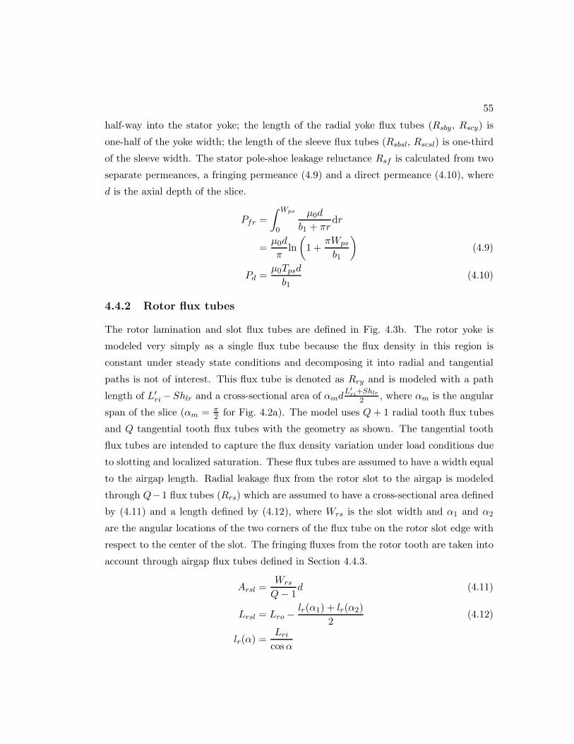
55
half-way into the stator yoke; the length of the radial yoke flux tubes (Rsby, Rscy) is
one-half of the yoke width; the length of the sleeve flux tubes (Rsbsl, Rscsl) is one-third
of the sleeve width. The stator pole-shoe leakage reluctance Rsf is calculated from two
separate permeances, a fringing permeance (4.9) and a direct permeance (4.10), where
d is the axial depth of the slice.
Pfr =
∫ Wps
0
µ0d
b1 + πrdr
=µ0d
πln
(
1 +πWps
b1
)
(4.9)
Pd =µ0Tpsd
b1(4.10)
4.4.2 Rotor flux tubes
The rotor lamination and slot flux tubes are defined in Fig. 4.3b. The rotor yoke is
modeled very simply as a single flux tube because the flux density in this region is
constant under steady state conditions and decomposing it into radial and tangential
paths is not of interest. This flux tube is denoted as Rry and is modeled with a path
length of L′ri−Shlr and a cross-sectional area of αmd
L′ri+Shlr
2 , where αm is the angular
span of the slice (αm = π2 for Fig. 4.2a). The model uses Q+ 1 radial tooth flux tubes
and Q tangential tooth flux tubes with the geometry as shown. The tangential tooth
flux tubes are intended to capture the flux density variation under load conditions due
to slotting and localized saturation. These flux tubes are assumed to have a width equal
to the airgap length. Radial leakage flux from the rotor slot to the airgap is modeled
through Q−1 flux tubes (Rrs) which are assumed to have a cross-sectional area defined
by (4.11) and a length defined by (4.12), where Wrs is the slot width and α1 and α2
are the angular locations of the two corners of the flux tube on the rotor slot edge with
respect to the center of the slot. The fringing fluxes from the rotor tooth are taken into
account through airgap flux tubes defined in Section 4.4.3.
Arsl =Wrs
Q− 1d (4.11)
Lrsl = Lro −lr(α1) + lr(α2)
2(4.12)
lr(α) =Lricosα

56
4.4.3 Airgap flux tubes and rotor motion
To avoid the previously described issues pertaining to rotation, a uniform number of
airgap flux tubes are used (regardless of the rotor position) which are connected to
evenly spaced nodes in the center of the airgap, shown in Fig. 4.2a. The airgap nodes
are centered in equal width regions which connect to stator flux tubes on the top and
rotor flux tubes on the bottom. The number of airgap nodes is equal to twice the
number of stator teeth so that the fringing fluxes from the stator pole shoes have a well
defined path. The location of these airgap nodes does not change with rotor position,
meaning that the flux tubes on the stator side of the rotor need only be calculated once.
The geometry for the stator airgap flux tubes is shown in Fig. 4.3c; the reluctance value
for Rsg is given by (4.13) and Rfg is calculated through two parallel permeances defined
in (4.14) and (4.15).
Rsg =g/2
µ0Wstd(4.13)
Rfg = (Pfr + Pd)−1
Pfr =
∫ Tps
0
µ0d
g/2 + π2 r
dr
=2µ0d
πln
(
1 +πTpsg
)
(4.14)
Pd =µ0dWps
g/2(4.15)
On the rotor side, an equal number of nodes are placed on the rotor at the interface
to the airgap which are also assumed to reside in equal width regions. Based on the
rotor’s rotation (the value of θm), each rotor interface node is connected to the nearest
two stationary airgap nodes via flux tubes. The permeance of the flux tubes is based on
the overlap of the airgap and rotor interface regions. When the rotor node resides on
an edge of the rotor tooth, fringing permeances are defined. Three cases which must be
considered when calculating the permeances are depicted in Fig. 4.4. Note that cases
2 and 3 are depicted for when the rotor node is on the right edge of the rotor tooth;
similar drawings can be made for when the rotor node is on the left edge. Calculations
are now presented for the rotor airgap interface permeances and their derivatives, which
are needed for use in the torque expression (4.8).
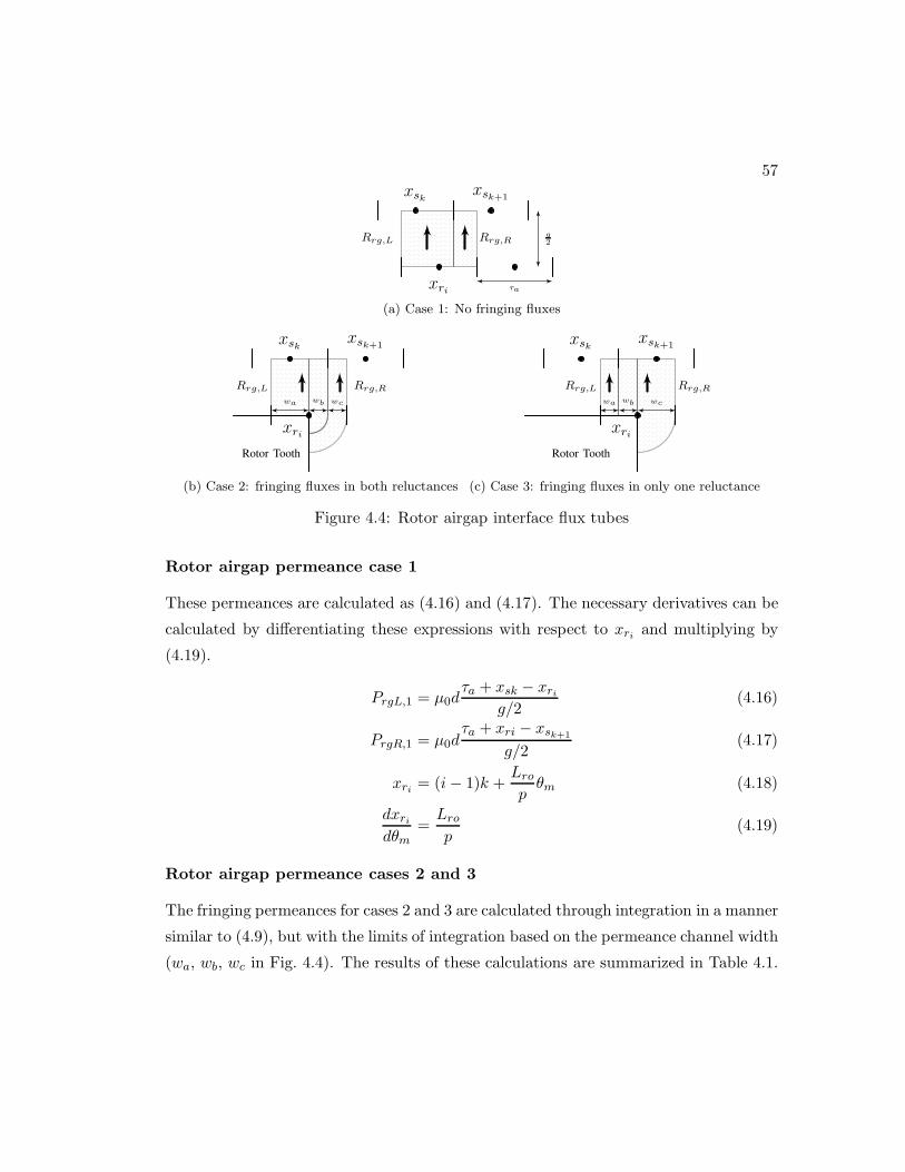
57
xsk xsk+1
xri
Rrg,L Rrg,R
τa
g2
(a) Case 1: No fringing fluxes
xsk xsk+1
Rotor Tooth
xri
Rrg,L Rrg,Rwa wb wc
(b) Case 2: fringing fluxes in both reluctances
xsk xsk+1
Rotor Tooth
xri
Rrg,L Rrg,Rwa wb wc
(c) Case 3: fringing fluxes in only one reluctance
Figure 4.4: Rotor airgap interface flux tubes
Rotor airgap permeance case 1
These permeances are calculated as (4.16) and (4.17). The necessary derivatives can be
calculated by differentiating these expressions with respect to xri and multiplying by
(4.19).
PrgL,1 = µ0dτa + xsk − xri
g/2(4.16)
PrgR,1 = µ0dτa + xri − xsk+1
g/2(4.17)
xri = (i− 1)k +Lropθm (4.18)
dxridθm
=Lrop
(4.19)
Rotor airgap permeance cases 2 and 3
The fringing permeances for cases 2 and 3 are calculated through integration in a manner
similar to (4.9), but with the limits of integration based on the permeance channel width
(wa, wb, wc in Fig. 4.4). The results of these calculations are summarized in Table 4.1.
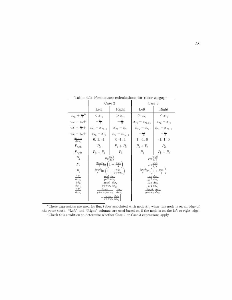
58
Table 4.1: Permeance calculations for rotor airgapa
Case 2 Case 3
Left Right Left Right
xsk +τa2b < xri > xri ≥ xri ≤ xri
wa = τa+ − τa2 − τa
2 xri − xsk+1xsk − xri
wb =τa2 + xri − xsk+1
xsk − xri xsk − xri xri − xsk+1
wc = τa+ xsk − xri xri − xsk+1− τa
2 − τa2
dwabcdxri
0, 1, -1 0 -1, 1 1, -1, 0 -1, 1, 0
PrgL Pc Pa + Pb Pb + Pc Pa
PrgR Pa + Pb Pc Pa Pb + Pc
Pa µ0wadg/2 µ0
wadg/2
Pb2µ0dπ ln
(
1 + πwbg
)
µ0wbdg/2
Pc2µ0dπ ln
(
1 + πwcg+πwb
)
2µ0dπ ln
(
1 + πwcg
)
∂Pa∂xri
µ0dg/2
dwadxri
µ0dg/2
dwadxri
∂Pb∂xri
2µ0dg+πwb
dwbdxri
µ0dg/2
dwbdxri
∂Pc∂xri
2µ0dg+πwb+πwc
[
dwcdxri
2µ0dg+πwc
dwcdxri
− πwcg+πwb
dwbdxri
]
aThese expressions are used for flux tubes associated with node xri when this node is on an edge ofthe rotor tooth. “Left” and “Right” columns are used based on if the node is on the left or right edge.
bCheck this condition to determine whether Case 2 or Case 3 expressions apply

59
(a) Test stand
(b) Rotor laminations (c) Modified stator (d) FEA Model
Figure 4.5: (a) AC homopolar machine (right) connected to a dc motor (left) with anencoder (far left) and torque transducer (center) in the test stand; (b) the rotor lami-nations; (c) the modified stator with field winding installed; (d) the quarter-symmetry3D FEA model used.
4.4.4 Axial flux tubes
The axial flux tubes that connect pairs of slices, shown in Fig. 4.2b, are assumed to
have a length equal to the sum of half of each slice’s thickness. The flux tubes for the
shaft and sleeve (Rshl, Rshf , Rsl, Rslf ) are cylindrical shapes and the dimensions are
easily determined. The axial stator lamination flux tubes (Rasl, Raslf ) are in the shape
of cylinder spanning the stator yoke (from the back of the stator slots to the start of
the stator sleeve). The axial rotor lamination flux tubes (Rshl) are assumed to have a
cross-sectional area equal to the entire rotor lamination cross-section.
The flux flowing through the axial lamination flux tubes encounters a large re-
luctance because it is flowing against the stacking direction and was initially ignored.
However, in designs were the rotor shaft and stator sleeve are near saturating, significant
homopolar flux flows axially in the laminated regions and is important to the machine’s
performance.

60
H (A/m) ×104
0 2 4 6 8 10
B(Tesla)
0
0.5
1
1.5
2
M19
M19 Axial
Solid Rotor Steel
Figure 4.6: B-H curves used in the MEC and FEA models. The dotted points representthe data and the solid line is the fit. The M19 axial entry is the data used for axiallamination flux tubes.
4.5 Results
An ac homopolar machine has been constructed by modifying the stator of a commer-
cially available induction machine. Pictures of the prototype can be seen in Fig. 4.5 and
the machine parameters are described in Table 4.2. The MEC has been used to model
this machine under various load and no load conditions. Quarter symmetry is used, so
that the MEC consists of 9 slots and all no-load models make use of axial symmetry.
The results are validated against FEA simulations conducted using Infolytica’s Mag-
Net software. The laminated steel was modeled using data provided in MagNet and a
generic solid steel material model was used for the rotor shaft and stator sleeve. In the
FEA models, the laminations are modeled as anistropic, with a reduced permeability in
the axial direction based on the stacking factor. The BH curves used for FEA were fit
to the anhysteretic permeability model presented in [91], shown in Fig. 4.6, for use in
the MEC model.
Results from a no-load test and the measured torque profile are shown in Fig. 4.7.
The MEC model was solved several times with differing numbers of slices to observe the
trade-off between computational accuracy and effort. A single solve consistently required
less than one second for up to 8 slices, while a single static solve of the 3D FEA model
required approximately 2 minutes. Fig. 4.7a depicts the effect that the number of slices
had on calculating the no load phase voltage for varying levels of saturation. There is
a noticeable improvement when using 2 slices instead of 1 slice; much less improvement
is observed when using 5 slices instead of 2 slices. The calculated voltage waveform

61
Field current (amps)0 0.2 0.4 0.6 0.8 1
PhaseVoltage
(V)
0
20
40
60
80
100
Hardware
FEA
MEC: 1 Slice
MEC: 2 Slices
MEC: 5 Slices
(a) Phase voltage magnitude
Time (seconds)0 0.005 0.01 0.015 0.02
Voltage
-100
-50
0
50
100
Hardware
FEA
MEC
(b) Phase voltage waveform
Torque angle (degrees)0 50 100 150
Torque(N
m)
0
2
4
6
8
10
FEA
MEC
(c) Torque characteristic
Figure 4.7: Comparison of: (a) the fundamental component of the no load phase voltageat various field excitations; (b) the no load phase voltage waveform; (c) the torqueprofile. In (c), each line corresponds to a different field current: starting at 0.3A andincreasing by 0.3A. All FEA was conducted on static models.
Table 4.2: AC homopolar prototype parameters
Field winding 2760 turns
Rated field winding current 0.57 A
Rated phase current 3.2 A (RMS)
Airgap min / max length 1 / 16.5 mm
Airgap radius 52 mm
Rated speed 750 RPM
Number of poles / slots 8 / 36
Coil span 4 slots
Laminations 24 Gauge M19

62
degrees0 20 40 60 80
Rad
ialfluxdensity
(Tesla)
0
0.5
1
1.5
2
FEA
MEC
(a) No load
degrees0 20 40 60 80
Rad
ialfluxdensity
(Tesla)
0
0.5
1
1.5
2
FEA
MEC
(b) Rated load
Axial length (mm)-50 0 50
Rad
ialfluxdensity
(Tesla)
-0.5
0
0.5
1
1.5
FEA
MEC
(c) No load
Axial length (mm)-50 0 50
Rad
ialfluxdensity
(Tesla)
-0.5
0
0.5
1
1.5
FEA
MEC
(d) Rated load
Figure 4.8: Radial flux density in the stator teeth under rated field excitation andeither no-load or rated load with a torque angle of 90: (a), (b) in each tooth at anaxial location matching the middle of the top rotor lamination stack, tooth 1 is at 10;(c), (d) in tooth 1, each MEC data point is from a separate slice.
63
is shown in Fig. 4.7b where it is apparent that the MEC does a poor job of handling
harmonic content. The torque angle profile calculations from both the FEA and MEC
models are shown in Fig. 4.7c for a wide range of saturation levels. The MEC clearly
exhibits good agreement with the FEA results. The MEC also accurately calculated
the flux density in various locations of the machine. A comparison of calculations with
static FEA for the stator teeth, yoke, and sleeve is shown in Fig. 4.8 and 4.9.
The machine performance is also affected by transient effects due to eddy currents
in the solid steel of the rotor shaft and stator sleeve. Under steady-state operation, the
rotor flux rotates at the same speed as the shaft and therefore induces no current in
the shaft; however, the stator sleeve will experience a rotating flux and therefore eddy
currents. These eddy currents present a greater reluctance to time varying flux, resulting
in the following effects that are not modeled in the MEC or static FEA: 1) the homopolar
flux will more evenly distribute itself in the stator yoke before entering the sleeve; 2)
the armature reaction flux will be more constrained to the stator yoke. An example
of the eddy currents and resulting field is depicted in Fig 4.10. Transient FE models
were used to explore these effects and were constructed by setting the conductivity of
the solid steel regions to 6.3 × 10⁶ S/m (a typical value for low carbon steels), placing
layers of 3rd order elements sized at one skin depth on the inner bore of the stator
sleeve (“Eddy current region” in Fig. 4.10), and solving for 1.5 electrical periods (to
allow initial “turn-on” transients to decay). Depending on the operating conditions,
each model required 20 - 30 hours to solve. For the example design, transient models
operated from 750RPM to 45,000 RPM yielded no significant differences from the static
results presented in Fig. 4.7-4.9.
The calculated sleeve eddy current losses vary as a function of rotational speed and
are shown in Fig. 4.11a. While the models that are under load exhibit more sleeve
loss due to the armature reaction field, the sleeve losses remain insignificant compared
to both the design’s rated power and the iron losses in the laminated yoke. Next,
the yoke thickness wsy was decreased from 11.9mm to cause saturation in the yoke
and force additional time varying flux into the sleeve, see Fig. 4.11b. Reducing the
yoke thickness increases the tangential field (Fig. 4.11c), which is time varying, causing
significant increases in the yoke iron losses before any observable increase in sleeve losses.
Fig. 4.11c shows that the transient model always calculates the largest peak tangential
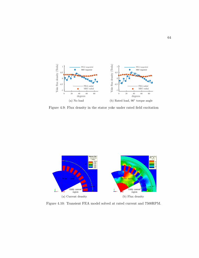
64
degrees0 20 40 60 80
Yokefluxdensity
(Tesla)
-1
-0.5
0
0.5
1 FEA tangential
MEC tangential
FEA radial
MEC radial
(a) No load
degrees0 20 40 60 80
Yokefluxdensity
(Tesla)
-1
-0.5
0
0.5
1 FEA tangential
MEC tangential
FEA radial
MEC radial
(b) Rated load, 90 torque angle
Figure 4.9: Flux density in the stator yoke under rated field excitation
Eddy current
region
Stator sleeve
(a) Current density
Eddy current
region
Stator sleeve
(b) Flux density
Figure 4.10: Transient FEA model solved at rated current and 7500RPM.

65
kRPM0 10 20 30 40
Sleeveeddycurrentlosses
(W)
0
0.1
0.2
0.3
0.4
0.5
No load
Rated load
(a) Impact of rotational speed
Yoke thickness (mm)4 6 8 10 12
Sleeveeddycurrentlosses
(W)
0
2
4
6
8
10
12
No load 7.5kRPM
Rated load 7.5kRPM
No load 30kRPM
Rated load 30kRPM
(b) Impact of yoke thickness
Yoke thickness (mm)4 6 8 10 12
Tan
.yoke
fluxdensity
(Tesla)
0
0.5
1
1.5
Static Load FEA
Trans. load FEA
Load MEC
Static no load FEA
Trans. no load FEA
No load MEC
(c) Peak tangential yoke flux density
Time (seconds)0 0.02 0.04 0.06 0.08 0.1
Field
current(amperes)
0
0.2
0.4
0.6
0.8
1
Transient FEA
Static FEA
MEC
(d) Transient field current
Figure 4.11: Comparison of (a), (b) calculated eddy current losses in the stator sleeve;(c) maximum tangential field in the stator yoke (averaged over one slot-tooth pitch),transient results: 30 kRPM; (d) calculated field current when a 200V dc supply issuddenly applied to the field winding.

66
field in the yoke, which is an expected consequence of the sleeve eddy currents. The
static FEA and MEC models exhibit the same trends as the transient model and all
three models are in good agreement for the more reasonable values of yoke thickness.
This trend agreement combined with flywheel designs being highly sensitive to losses
and lamination losses varying with small changes in yoke thickness mean that a design
optimization utilizing the MEC would move away from the unreasonably thin yokes
where Fig. 4.11c shows the static models to be inaccurate.
Finally, since the flux path of the field winding is through the solid steel regions,
changes in the field winding current will induce eddy currents in both the stator sleeve
and the rotor shaft. The machine is operated with a dc field current, meaning that this
will only have an effect when the field winding is turned on or off–i.e. when the flywheel
unit is transitioning into or out of idling mode. The current response to applying
200V for 100ms is shown in Fig. 4.11d. The static FEA and MEC models are used
to calculate this current by transforming V = RI + LI + IL into a difference equation
using a backwards-difference approximation. The eddy currents cause the flux paths in
the transient model to initially have a greater reluctance, reducing the inductance and
allowing current to build up more rapidly. When the current exceeds 500mA, the flux
paths in the static FEA and MEC models start to saturate, causing them to experience
less inductance than the transient model and an accelerated increase in current. While
this current response is the most notable discrepancy between the static and transient
models, it is not typically an important design parameter of flywheel systems and can
most likely be ignored in a design optimization.
4.6 Conclusion
AC homopolar machines have unique features which could be leveraged to design a
long-term, low self-discharge flywheel energy storage module. However, a significant
challenge in designing and optimizing the ac homopolar machine is the computation
time required by 3D FEA models. This chapter has developed a general MEC model
which can be solved in a fraction of the time required by 3D FEA models and has been
shown to exhibit sufficient accuracy in key performance parameters, including: torque,
no load voltage magnitude, and flux density (enabling loss calculations). It was shown

67
that inacuracies due to static assumptions either do not matter for flywheel designs or
only occur in unsuitable designs. The author envisions this MEC model being used in
the design optimization process of ac homopolar machines, with a transient 3D FEA
reserved for final design validation.
Chapter 5
Rigid Body Rotor Model Under
Variable Excitation
One of the primary reasons that this dissertation is proposing the use of the bearingless
ac homopolar motor for flywheel energy storage is the ease at which the machine can be
operated under reduced excitation to minimize idling losses. This chapter investigates
the impact of the excitation level on the magnetic bearing capabilities of the machine.1
5.1 Introduction
A complication arises in the radial force production when operating the bearingless ac
homopolar motor under various excitation levels. The magnetic bearing position stiff-
ness, which determines the unstable pole locations of the magnetic suspension system,
and the bearing current stiffness are dependent upon the field excitation level. This
means that a suspension controller proven to be stable for one level of field excitation
may be unstable or perform unsatisfactorily for another level of field excitation. Since
variable field excitation is an important ability of a bearingless ac homopolar machine
applied to flywheel energy storage systems, it is necessary to have a suspension force
model that can account for different excitation levels. The bearingless ac homopolar
motor has been considered in [52,56,60,62], none of which analyze this dependency. In
1 Portions of the material in this chapter have also been published in [50].
68
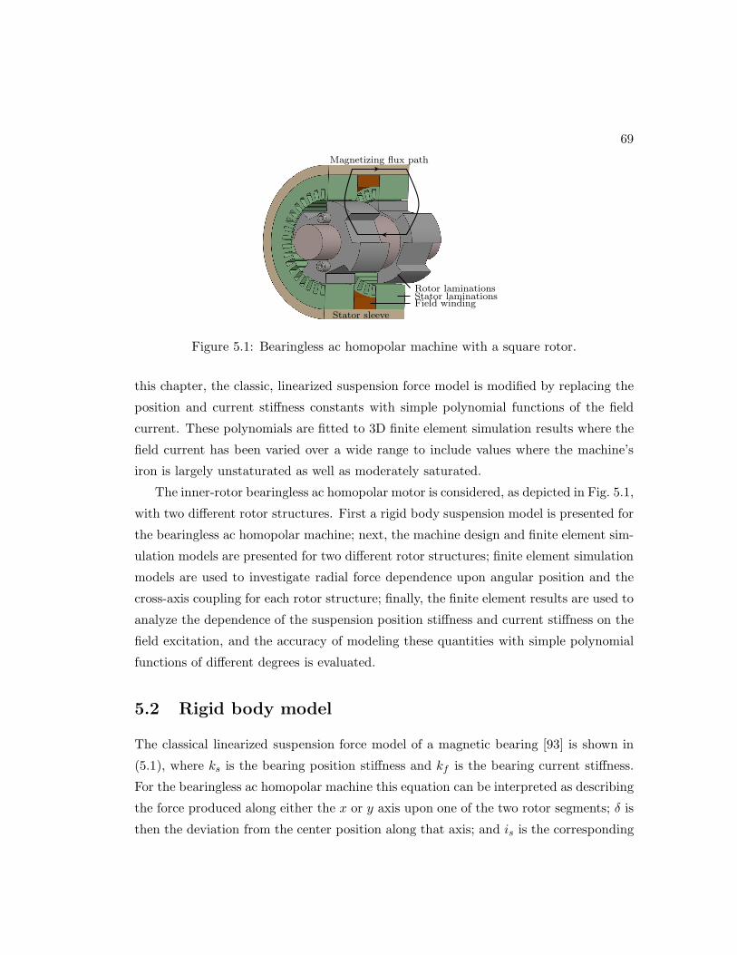
69
Magnetizing flux path
Rotor laminationsStator laminationsField winding
Stator sleeve
Figure 5.1: Bearingless ac homopolar machine with a square rotor.
this chapter, the classic, linearized suspension force model is modified by replacing the
position and current stiffness constants with simple polynomial functions of the field
current. These polynomials are fitted to 3D finite element simulation results where the
field current has been varied over a wide range to include values where the machine’s
iron is largely unstaturated as well as moderately saturated.
The inner-rotor bearingless ac homopolar motor is considered, as depicted in Fig. 5.1,
with two different rotor structures. First a rigid body suspension model is presented for
the bearingless ac homopolar machine; next, the machine design and finite element sim-
ulation models are presented for two different rotor structures; finite element simulation
models are used to investigate radial force dependence upon angular position and the
cross-axis coupling for each rotor structure; finally, the finite element results are used to
analyze the dependence of the suspension position stiffness and current stiffness on the
field excitation, and the accuracy of modeling these quantities with simple polynomial
functions of different degrees is evaluated.
5.2 Rigid body model
The classical linearized suspension force model of a magnetic bearing [93] is shown in
(5.1), where ks is the bearing position stiffness and kf is the bearing current stiffness.
For the bearingless ac homopolar machine this equation can be interpreted as describing
the force produced along either the x or y axis upon one of the two rotor segments; δ is
then the deviation from the center position along that axis; and is is the corresponding
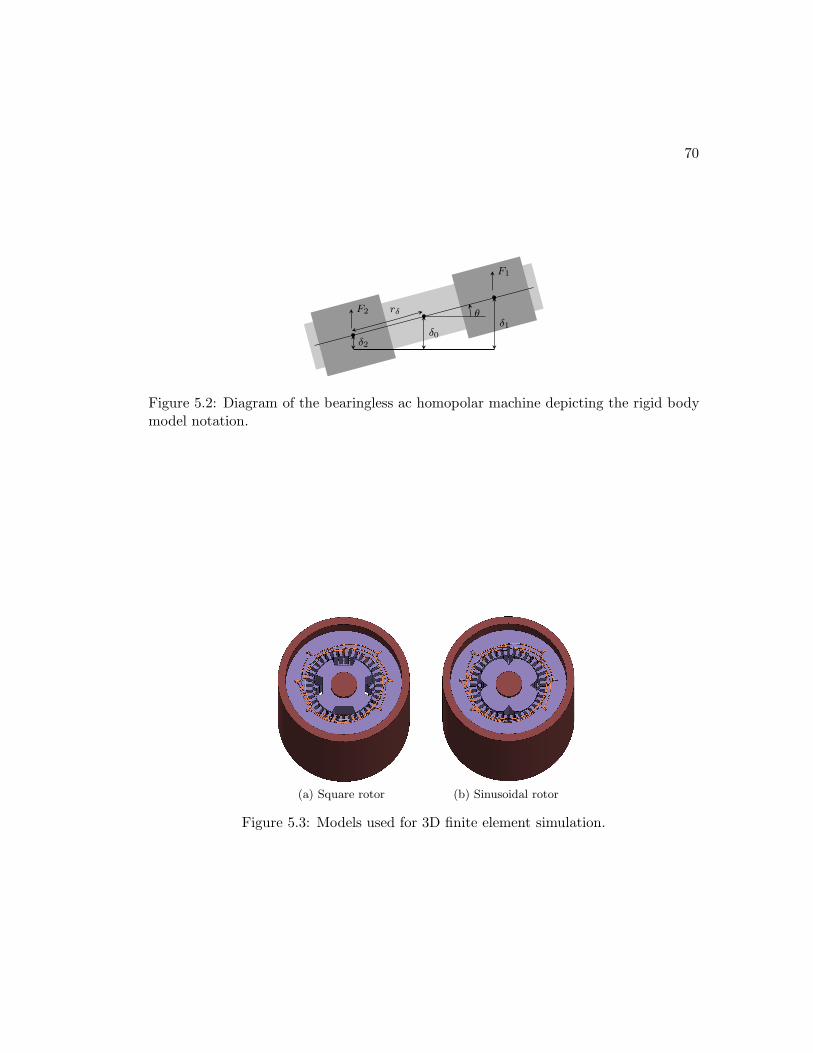
70
rδ θ
F1
F2
δ1
δ2δ0
Figure 5.2: Diagram of the bearingless ac homopolar machine depicting the rigid bodymodel notation.
(a) Square rotor (b) Sinusoidal rotor
Figure 5.3: Models used for 3D finite element simulation.
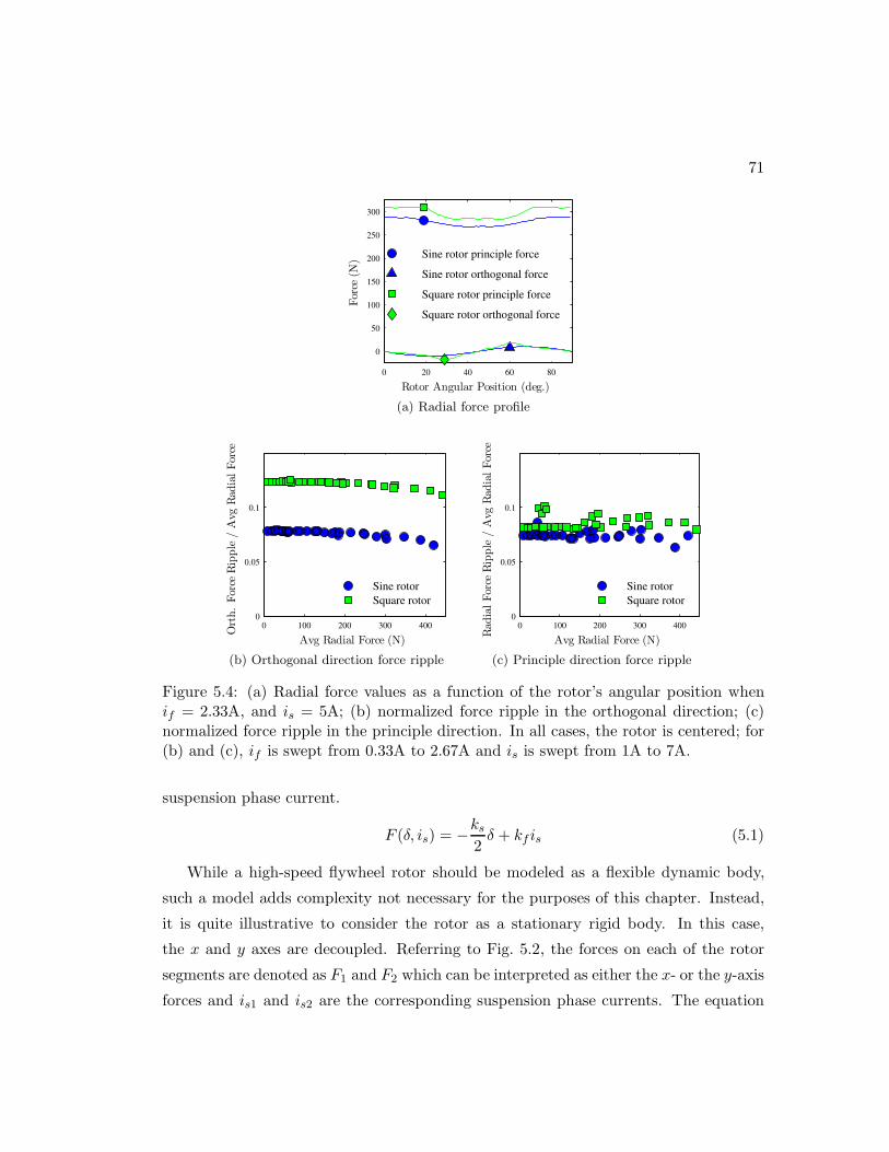
71
0 20 40 60 80
0
50
100
150
200
250
300
Rotor Angular Position (deg.)
Force
(N)
Sine rotor principle force
Sine rotor orthogonal force
Square rotor principle force
Square rotor orthogonal force
(a) Radial force profile
0 100 200 300 4000
0.05
0.1
Avg Radial Force (N)
Orth.Force
Ripple/Avg
Rad
ialForce
Sine rotor
Square rotor
(b) Orthogonal direction force ripple
0 100 200 300 4000
0.05
0.1
Avg Radial Force (N)
Rad
ialForce
Ripple/Avg
Rad
ialForce
Sine rotor
Square rotor
(c) Principle direction force ripple
Figure 5.4: (a) Radial force values as a function of the rotor’s angular position whenif = 2.33A, and is = 5A; (b) normalized force ripple in the orthogonal direction; (c)normalized force ripple in the principle direction. In all cases, the rotor is centered; for(b) and (c), if is swept from 0.33A to 2.67A and is is swept from 1A to 7A.
suspension phase current.
F (δ, is) = −ks2δ + kf is (5.1)
While a high-speed flywheel rotor should be modeled as a flexible dynamic body,
such a model adds complexity not necessary for the purposes of this chapter. Instead,
it is quite illustrative to consider the rotor as a stationary rigid body. In this case,
the x and y axes are decoupled. Referring to Fig. 5.2, the forces on each of the rotor
segments are denoted as F1 and F2 which can be interpreted as either the x- or the y-axis
forces and is1 and is2 are the corresponding suspension phase currents. The equation

72
of motion can be applied and the results linearized to derive the following state-space
representation with two states, δ0 and θ [93]:
δ0
δ0
θ
θ
=
0 1 0 0
−ksm 0 0 0
0 0 0 1
0 0 − r2δksI 0
δ0
δ0
θ
θ
+
0 0kfm
kfm
0 0rδkfI − rδkf
I
is1
is2
(5.2)
where m is the mass of the shaft, I is the moment of inertia of the shaft about the
magnetic bearing axis (either the x- or y-axis). The characteristic polynomial2 has
unstable poles located at
√
|ks|m and
√
r2δ |ks|I . The suspension controller must stabilize
these poles in order to levitate the rotor.
5.3 Machine design
This chapter considers two different designs with the same stator but different rotors.
Each rotor structure has the same minimum and maximum airgap length and in both
cases backup bearings prevent the rotor from being displaced more than 1mm. The
remaining machine design parameters are summarized in Table 5.1.
5.4 Finite element analysis
Infolytica’s MagNet software was used for finite element modeling. Since the flux paths
are both axial and radial, the analysis must be done in 3D. In addition to this, the
suspension winding end-turns needed to be fully modeled as they reside between the
two stator stacks. All results were taken with only the field winding and a single
suspension winding phase excited (i.e. the x-direction phase) under static analysis. The
rotor’s angular position, the rotor’s lateral displacement, the field winding’s excitation,
2 Note that for magnetic bearings ks is always negative
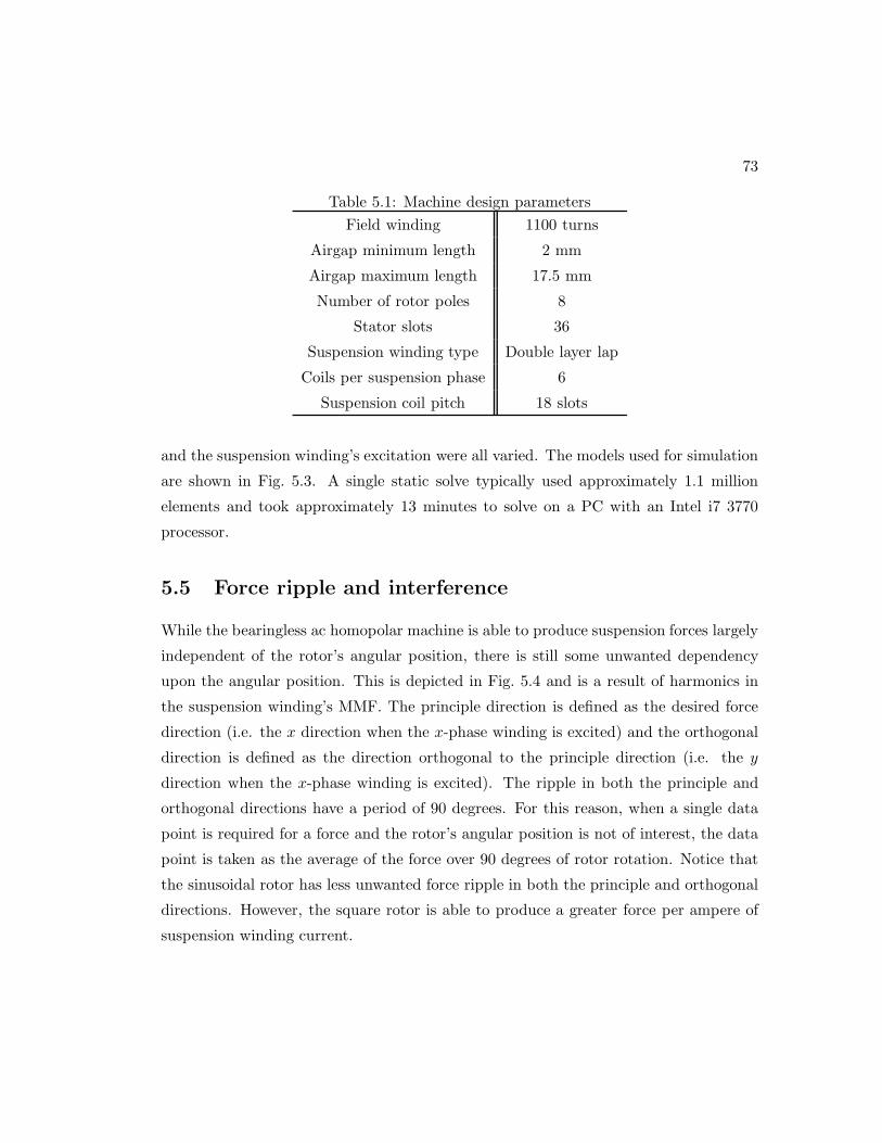
73
Table 5.1: Machine design parameters
Field winding 1100 turns
Airgap minimum length 2 mm
Airgap maximum length 17.5 mm
Number of rotor poles 8
Stator slots 36
Suspension winding type Double layer lap
Coils per suspension phase 6
Suspension coil pitch 18 slots
and the suspension winding’s excitation were all varied. The models used for simulation
are shown in Fig. 5.3. A single static solve typically used approximately 1.1 million
elements and took approximately 13 minutes to solve on a PC with an Intel i7 3770
processor.
5.5 Force ripple and interference
While the bearingless ac homopolar machine is able to produce suspension forces largely
independent of the rotor’s angular position, there is still some unwanted dependency
upon the angular position. This is depicted in Fig. 5.4 and is a result of harmonics in
the suspension winding’s MMF. The principle direction is defined as the desired force
direction (i.e. the x direction when the x-phase winding is excited) and the orthogonal
direction is defined as the direction orthogonal to the principle direction (i.e. the y
direction when the x-phase winding is excited). The ripple in both the principle and
orthogonal directions have a period of 90 degrees. For this reason, when a single data
point is required for a force and the rotor’s angular position is not of interest, the data
point is taken as the average of the force over 90 degrees of rotor rotation. Notice that
the sinusoidal rotor has less unwanted force ripple in both the principle and orthogonal
directions. However, the square rotor is able to produce a greater force per ampere of
suspension winding current.
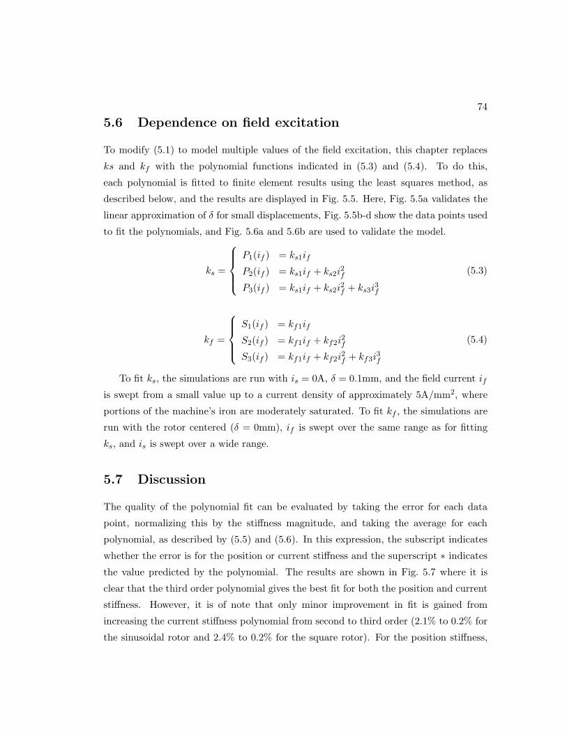
74
5.6 Dependence on field excitation
To modify (5.1) to model multiple values of the field excitation, this chapter replaces
ks and kf with the polynomial functions indicated in (5.3) and (5.4). To do this,
each polynomial is fitted to finite element results using the least squares method, as
described below, and the results are displayed in Fig. 5.5. Here, Fig. 5.5a validates the
linear approximation of δ for small displacements, Fig. 5.5b-d show the data points used
to fit the polynomials, and Fig. 5.6a and 5.6b are used to validate the model.
ks =
P1(if ) = ks1if
P2(if ) = ks1if + ks2i2f
P3(if ) = ks1if + ks2i2f + ks3i
3f
(5.3)
kf =
S1(if ) = kf1if
S2(if ) = kf1if + kf2i2f
S3(if ) = kf1if + kf2i2f + kf3i
3f
(5.4)
To fit ks, the simulations are run with is = 0A, δ = 0.1mm, and the field current if
is swept from a small value up to a current density of approximately 5A/mm2, where
portions of the machine’s iron are moderately saturated. To fit kf , the simulations are
run with the rotor centered (δ = 0mm), if is swept over the same range as for fitting
ks, and is is swept over a wide range.
5.7 Discussion
The quality of the polynomial fit can be evaluated by taking the error for each data
point, normalizing this by the stiffness magnitude, and taking the average for each
polynomial, as described by (5.5) and (5.6). In this expression, the subscript indicates
whether the error is for the position or current stiffness and the superscript ∗ indicates
the value predicted by the polynomial. The results are shown in Fig. 5.7 where it is
clear that the third order polynomial gives the best fit for both the position and current
stiffness. However, it is of note that only minor improvement in fit is gained from
increasing the current stiffness polynomial from second to third order (2.1% to 0.2% for
the sinusoidal rotor and 2.4% to 0.2% for the square rotor). For the position stiffness,
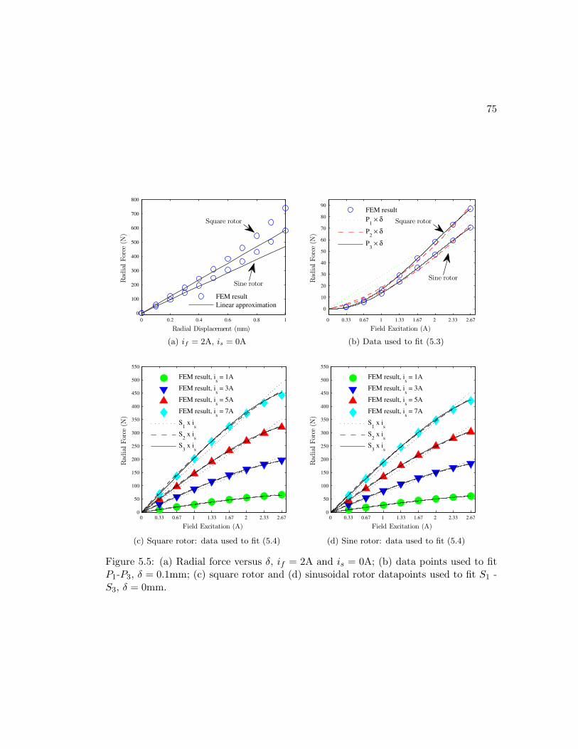
75
0 0.2 0.4 0.6 0.8 1
0
100
200
300
400
500
600
700
800
Radial Displacement (mm)
Rad
ialForce
(N)
FEM result
Linear approximation
Square rotor
Sine rotor
(a) if = 2A, is = 0A
0 0.33 0.67 1 1.33 1.67 2 2.33 2.67
0
10
20
30
40
50
60
70
80
90
Field Excitation (A)
Rad
ialForce
(N)
FEM result
P1 × δ
P2 × δ
P3 × δ
Square rotor
Sine rotor
(b) Data used to fit (5.3)
0 0.33 0.67 1 1.33 1.67 2 2.33 2.670
50
100
150
200
250
300
350
400
450
500
550
Field Excitation (A)
Rad
ialForce
(N)
FEM result, i
s = 1A
FEM result, is = 3A
FEM result, is = 5A
FEM result, is = 7A
S1 x i
s
S2 x i
s
S3 x i
s
(c) Square rotor: data used to fit (5.4)
0 0.33 0.67 1 1.33 1.67 2 2.33 2.670
50
100
150
200
250
300
350
400
450
500
550
Field Excitation (A)
Rad
ialForce
(N)
FEM result, i
s = 1A
FEM result, is = 3A
FEM result, is = 5A
FEM result, is = 7A
S1 x i
s
S2 x i
s
S3 x i
s
(d) Sine rotor: data used to fit (5.4)
Figure 5.5: (a) Radial force versus δ, if = 2A and is = 0A; (b) data points used to fitP1-P3, δ = 0.1mm; (c) square rotor and (d) sinusoidal rotor datapoints used to fit S1 -S3, δ = 0mm.
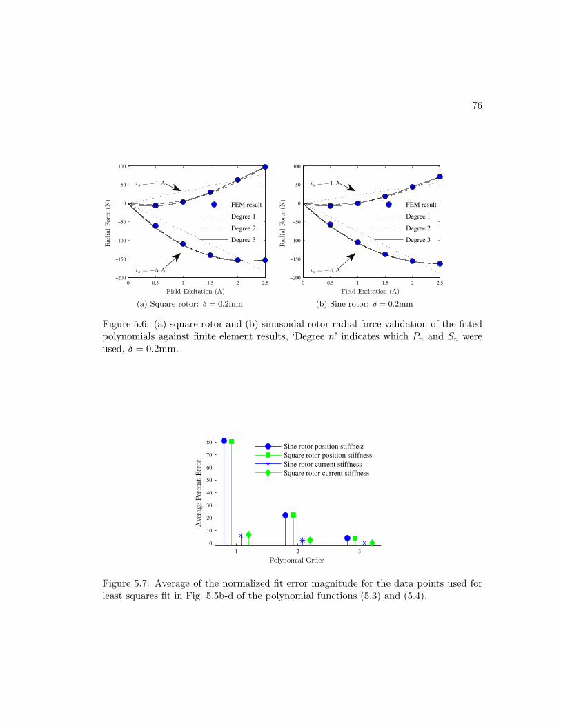
76
0 0.5 1 1.5 2 2.5−200
−150
−100
−50
0
50
100
Field Excitation (A)
Rad
ialForce
(N)
FEM result
Degree 1
Degree 2
Degree 3
is = −1 A
is = −5 A
(a) Square rotor: δ = 0.2mm
0 0.5 1 1.5 2 2.5−200
−150
−100
−50
0
50
100
Field Excitation (A)
Rad
ialForce
(N)
FEM result
Degree 1
Degree 2
Degree 3
is = −1 A
is = −5 A
(b) Sine rotor: δ = 0.2mm
Figure 5.6: (a) square rotor and (b) sinusoidal rotor radial force validation of the fittedpolynomials against finite element results, ‘Degree n’ indicates which Pn and Sn wereused, δ = 0.2mm.
1 2 3
0
10
20
30
40
50
60
70
80
Polynomial Order
Average
PercentError
Sine rotor position stiffness
Square rotor position stiffness
Sine rotor current stiffness
Square rotor current stiffness
Figure 5.7: Average of the normalized fit error magnitude for the data points used forleast squares fit in Fig. 5.5b-d of the polynomial functions (5.3) and (5.4).

77
1 2 3
−60
−50
−40
−30
−20
−10
0
10
20
30
40
Polynomial Order
PercentUncertainty
inPoleLocation
Sine rotor
Square rotor
Figure 5.8: Uncertainty in suspension pole locations due to error in the position stiffnesspolynomial approximation.
this improvement is significant (22.1% to 4.0% for the sinusoidal rotor and 22.3% to
3.9% for the square rotor).
ǫs =
⟨ |k∗s − ks||ks|
⟩
(5.5)
ǫf =
⟨
∣
∣
∣k∗f − kf
∣
∣
∣
|kf |
⟩
(5.6)
As shown in Section 5.2, the unstable poles’ locations vary by the square root of the
position stiffness. If the uncertainty in the position stiffness is taken as ǫs from (5.5),
then the uncertainty in the predicted pole locations can be defined as (5.7). The results
are depicted in Fig. 5.8, where it can be seen that the third order polynomial gives a
very accurate estimation for the pole locations.
ǫp =P ∗ − P
P
=√1± ǫs − 1 (5.7)
5.8 Conclusion
The classic, linearized magnetic bearing force equation has been revised to model the
bearingless ac homopolar machine’s suspension force under various excitation values. It
has been found that the revised model accurately reflects the finite element simulations
78
when the current stiffness is modeled with a second or third order polynomial function of
the field current and the suspension stiffness is modeled with a third order polynomial
function of the field current. All simulations and analysis have been conducted on
a practical design of the bearingless ac homopolar machine which is currently being
constructed.
The model presented in this chapter allows a control designer to accurately predict
the field excitation’s impact on the unstable suspension pole locations. The ability to
do this is crucial to utilizing the bearingless ac homopolar machine in flywheel energy
storage technology.
Chapter 6
Dual Purpose No Voltage
Winding Design for Bearingless
Motors
This chapter develops a winding design approach to create a single motor winding which
is able to produce both radial force and torque. This approach can be used to design new
bearingless motors as well as to transform conventional motor designs into bearingless
motors by simply modifying the winding end-connections. The resulting winding has
two sets of terminal connections: one for torque and one for suspension. The suspension
terminals experience no motional-EMF when the rotor is centered, which means that
the suspension drive can have a low voltage rating and that rotor vibrations can be
passively dampened by simply short-circuiting the suspension terminals. Bearingless
motors that use these so-called “dual purpose no voltage windings” can be designed to
have higher torque density and lower losses associated with the magnetic suspension op-
eration than traditional bearingless motors which utilize separate torque and suspension
windings. It will be shown that many popular winding designs, including fractional-slot
and concentrated windings, can be realized as dual purpose no voltage windings. The
proposed approach applies to traditional p ± 1 pole-pair bearingless motors as well as
the bearingless consequent-pole and ac homopolar motors.1
1 Portions of the material in this chapter have been submitted for publication in [46].
79

80
6.1 Introduction
Traditional bearingless motors are created by adding a p± 1 pole-pair suspension wind-
ing to a p pole-pair motor. Both windings are fed with currents at the synchronous
frequency and the suspension current phase angle determines the force direction. This
has been widely developed for both synchronous motors, such as permanent magnet and
synchronous reluctance, and asynchronous motors [94–97]. More recently, the bearing-
less consequent pole [98] and ac homopolar motors [60], which this dissertation is pri-
marily interested in, have been proposed which use a 2-pole suspension winding. These
motors have decoupled magnetic bearing and torque functionality, enabling them to use
a dc suspension current to produce a constant direction force regardless of the rotor’s
rotation as long as the rotor has at least 8-poles.
All of the aforementioned bearingless motors rely on separate torque and suspension
windings which share the same slots. This creates a trade-off in slot space allocation
that translates to a trade-off between radial force capability and torque density: whether
the device is a “good” magnetic bearing or a “good” motor. The slot space must be
allocated to the suspension winding based on the maximum force required. Many imple-
mentations of bearingless motors, such as those with vertical shafts, require relatively
small suspension forces during normal operation and large forces during certain events,
i.e. when accelerating through a critical speed. During normal operation, such machines
effectively waste slot space which could otherwise carry torque current. Furthermore,
to create radial forces, the suspension winding carries current to cancel torque winding
current in certain slots, causing increased copper loss [99,100]. For these reasons, there
has been recent interest in combining the suspension and torque winding into a single
winding [47,99–111]. Such a winding is referred to as a “dual purpose” winding in this
chapter. Efforts to create dual purpose windings have included:
1. various types of “split-windings” [100–104, 106–108], where the stator winding is
divided into several separate windings located adjacent to one another so that the
phase currents in each winding can be varied to adjust the airgap flux density at
different locations;
2. a “middle-point-current-injection” design [110], where suspension currents are in-
jected into certain coils in an otherwise-standard torque winding;

81
3. “no-voltage” designs based around a bridge [99, 105, 109] or a parallel winding
structure [111]; the phrase “no-voltage” refers to the fact that the suspension
terminals experience no motional-EMF when the rotor is centered.
In cases 1) and 2), the drive must overcome a motional-EMF to inject a suspen-
sion current. This requires a higher drive voltage to achieve satisfactory response times
which can lead to significant increases in the inverter cost and losses [110, 111]. On
the other hand, the terminal characteristics of the no-voltage winding approaches (case
3) are similar to that of the traditional separate winding approach in that the suspen-
sion terminals see no motional-EMF. This also means that the suspension terminals
can be short-circuited to passively provide corrective forces when the rotor is rotating
eccentrically [105], which can be an inexpensive way to dampen rotor vibrations in
conventional machines with mechanical bearings. For these reasons, the case 3 wind-
ings, referred to as dual purpose no voltage (DPNV) windings, are seen to be at a
significant advantage to the other types of dual purpose windings. DPNV technology
is still relatively immature, with existing papers describing only specific example bear-
ingless designs [99,105,109,111], all of which utilize integral-slot windings. These days,
fractional-slot windings are often preferred over integral-slot windings because they can
reduce torque ripple, manufacturing cost, and end-turn length. In [47], fractional-slot
DPNV windings are explored, but the results only apply to bearingless consequent-pole
and ac homopolar motors. There is not currently any design method or analysis of the
acceptable combination of slots, poles, and phases to construct DPNV windings for a
general machine.
This chapter overcomes the above shortcomings by deriving DPNV winding re-
quirements and proposing a design procedure applicable to a general machine. Other
notable contributions include presenting examples of many popular winding designs,
including concentrated windings, where the end-connections have been modified to con-
struct DPNV windings; and investigating performance differences of example bearingless
motors utilizing conventional and DPNV winding designs. Because the required end-
connection modifications come at virtually no penalty in terms of machine performance
or cost, the results of this chapter will be useful to bearingless motor designers looking
for complete magnetic levitation as well as designers of conventional motors looking to
suppress rotor vibrations while still utilizing mechanical bearings.

82
In this chapter, Section 6.2 introduces the DPNV winding concept; Section 6.3
describes the chapter’s use of the phasor star and defines terminology necessary for
understanding the derivations; Section 6.4 derives the DPNV winding requirements;
Section 6.5 proposes and describes a DPNV winding design procedure; Section 6.6 uses
FEA results to validate the DPNV winding concept–example bearingless motor designs
are explored and compared using both DPNV windings and conventional bearingless
windings; Section 6.8 summarizes relevant fractional slot winding theory. Nomenclature
used throughout the chapter is defined in Table 6.1.
6.2 Dual purpose no voltage windings
As described in the introduction, bearingless radial-flux motors can be classified into two
categories as follows: ps = p± 1 (bearingless versions of traditional motors) and ps = 1
(bearingless consequent-pole and ac homopolar motors); the operating principles for
each can be found in Chapters 7 and 14 of [56] and are briefly described in Section 7.2.
The stator winding for any category of a bearingless motor is responsible for generating
two airgap flux densities: a p pole-pair field for torque production and a ps pole-pair field
for suspension force production. While conventional bearingless motors use separate
windings (and therefore separate coils) for creating each field, the DPNV windings
described in this chapter use a single winding (the same coils) for creating both fields.
The defining features of a DPNV winding can be summarized as: 1) using the same
coils to construct a p pole-pair torque MMF and a ps pole-pair suspension MMF; 2)
having suspension terminals which connect to the same coils as the torque terminals, but
with half of the coils’ direction reversed so that these terminals experience no motional-
EMF. Two different styles of drive connection have been proposed to interface with a
DPNV winding. The first is the bridge configuration, shown in Fig. 6.1a. This was
proposed in [109] with further development in [99, 105]. It features coils connected in
a manner resembling a wheatstone bridge and uses isolated single-phase inverters to
inject currents into the suspension terminals. The second is the parallel configuration,
proposed in [111] and shown in Fig. 6.1b. Here, the suspension winding terminals appear
as a virtual “neutral” for the motor winding, meaning that the suspension inverter must
also carry half of the motor current, and non-isolated multi-phase inverters are used to
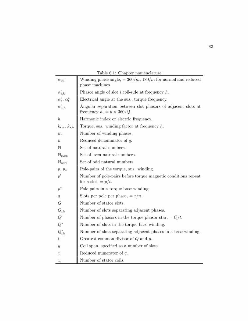
83
Table 6.1: Chapter nomenclature
αph Winding phase angle, = 360/m, 180/m for normal and reducedphase machines.
αei,h Phasor angle of slot i coil-side at frequency h.
αes, α
et Electrical angle at the sus., torque frequency.
αeu,h Angular separation between slot phasors of adjacent slots at
frequency h, = h× 360/Q.
h Harmonic index or electric frequency.
kt,h, ks,h Torque, sus. winding factor at frequency h.
m Number of winding phases.
n Reduced denominator of q.
N Set of natural numbers.
Neven Set of even natural numbers.
Nodd Set of odd natural numbers.
p, ps Pole-pairs of the torque, sus. winding.
p′ Number of pole-pairs before torque magnetic conditions repeatfor a slot, = p/t.
p∗ Pole-pairs in a torque base winding.
q Slots per pole per phase, = z/n.
Q Number of stator slots.
Qph Number of slots separating adjacent phases.
Q′ Number of phasors in the torque phasor star, = Q/t.
Q∗ Number of slots in the torque base winding.
Q∗ph Number of slots separating adjacent phases in a base winding.
t Greatest common divisor of Q and p.
y Coil span, specified as a number of slots.
z Reduced numerator of q.
zc Number of stator coils.
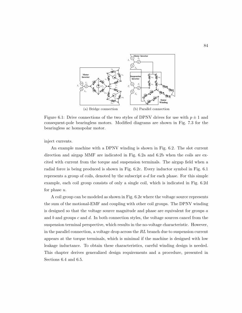
84
Iu
MotorInverter
uaud
ucub
I ′ut n
vc
vb
va
vd
I ′vt
Ivwc
wb
wa
wd
I′wt
Iw
(a) Bridge connection
IuMotor Inverter
Iv
Iw
ua
uc
ub
ud
n
vb
vd
va
vc
wb
wd
wa
wc
StatorWinding
I ′u
SuspensionInverter
I ′v
I ′w
(b) Parallel connection
Figure 6.1: Drive connections of the two styles of DPNV drives for use with p± 1 andconsequent-pole bearingless motors. Modified diagrams are shown in Fig. 7.3 for thebearingless ac homopolar motor.
inject currents.
An example machine with a DPNV winding is shown in Fig. 6.2. The slot current
direction and airgap MMF are indicated in Fig. 6.2a and 6.2b when the coils are ex-
cited with current from the torque and suspension terminals. The airgap field when a
radial force is being produced is shown in Fig. 6.2c. Every inductor symbol in Fig. 6.1
represents a group of coils, denoted by the subscript a-d for each phase. For this simple
example, each coil group consists of only a single coil, which is indicated in Fig. 6.2d
for phase u.
A coil group can be modeled as shown in Fig. 6.2e where the voltage source represents
the sum of the motional-EMF and coupling with other coil groups. The DPNV winding
is designed so that the voltage source magnitude and phase are equivalent for groups a
and b and groups c and d. In both connection styles, the voltage sources cancel from the
suspension terminal perspective, which results in the no-voltage characteristic. However,
in the parallel connection, a voltage drop across theRL branch due to suspension current
appears at the torque terminals, which is minimal if the machine is designed with low
leakage inductance. To obtain these characteristics, careful winding design is needed.
This chapter derives generalized design requirements and a procedure, presented in
Sections 6.4 and 6.5.
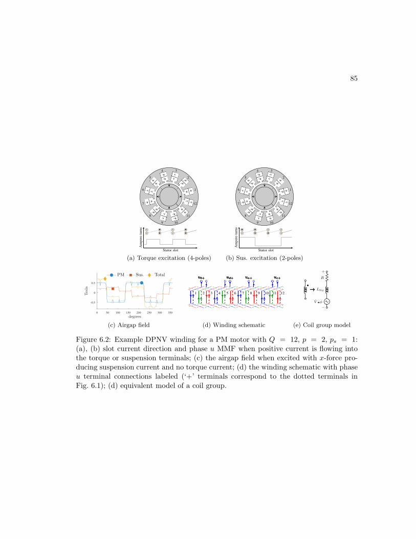
85
u u 1
-w-w
2v
v3
-u
-u4
ww
5
-v-v6
uu7
-w-w
8v
v
9
-u
-u
10
ww
11
-v -v 12
Am
per
e-tu
rns
Stator slot
•×
ו
•×
ו
(a) Torque excitation (4-poles)
-u u 1
ww
2v
-v3
-u
-u4
-ww
5
vv6
u-u7
-w-w
8-v
v
9
u
u
10
w-w
11
-v -v 12
Am
per
e-tu
rns
Stator slot
•×
ו
ו
•×
(b) Sus. excitation (2-poles)
degrees0 50 100 150 200 250 300 350
Tesla
-0.5
0
0.5
PM Sus. Total
(c) Airgap field
1
ua+ub+ uc+ud+
4
ua+ub+ uc+ud+
7
ua+ub+ uc+ud+
10
ua+ub+ uc+ud+
3 6 9 122 5 8 11
(d) Winding schematic
V 6 φ
Llkg
R
+
−
(e) Coil group model
Figure 6.2: Example DPNV winding for a PM motor with Q = 12, p = 2, ps = 1:(a), (b) slot current direction and phase u MMF when positive current is flowing intothe torque or suspension terminals; (c) the airgap field when excited with x-force pro-ducing suspension current and no torque current; (d) the winding schematic with phaseu terminal connections labeled (‘+’ terminals correspond to the dotted terminals inFig. 6.1); (d) equivalent model of a coil group.
86
6.3 Winding design theory and properties
This chapter relies heavily on fractional-slot winding design theory and a summary of
the relevant details and terminology can be found in Section 6.8. This section describes
how the chapter utilizes various concepts of this theory as well as important properties
of bearingless motors.
6.3.1 Phasor star diagram
The phasor star, or star of slots, is a diagram that indicates the phasor of a particular
harmonic of EMF that would be induced in each coil-side if the airgap contained a ro-
tating sinusoidal radial flux density at that harmonic frequency. An example is shown in
Fig. 6.3. The individual phasors of the star are termed “slot phasors” and are numbered
to indicate the slot where the coil-side is located. Separate phasor star diagrams are
constructed for each frequency of interest. For the fundamental frequency, there will be
t phasors at each angular location and therefore t levels to the phasor star. The winding
factor for a particular harmonic can be calculated from that hamonic’s phasor star by
(6.1), for a phase consisting of N coil sides. The electrical frequency is the frequency
of the harmonic of interest (for the fundamental frequency, h = p). Coils are made up
of two coils-sides: one connected in a positive direction and one connected in a reverse
direction. When coils are placed in the final winding, individual coils may be connected
in reverse. For coil-sides connected in reverse, αei,h is rotated by 180e when used in (6.1).
The phasor star is always drawn without regard to the connection direction.
kh = abs
(
1
N
N∑
i=1
ejαei,h
)
(6.1)
To simplify the case of a double-layer winding, all coils are assumed to span the same
number of slots and the returning coil-side is neglected from the phasor star, meaning
that only a single phasor is drawn for each slot. The terms “slot phasor” and “coil
phasor” are used interchangeably when referring to a double layer winding. The only
effect this has on the analysis is that the winding factor calculation of (6.1) is redefined
as being the winding distribution factor (where N is redefined as the number of coils).

87
1
23
4
56
7
89
10
1112
+u
+v
+w
−u
−v
−w
αeu,p
αph1
-2
3
-4
5
-6
7
-8
9
-10
11
-12
u
v
w
1
-4
7
-10
1
2
34
5
6
7
8
9 10
11
12
αeu,ps
1
2
-3 -4
5
6
-7
-8
9 10
-11
-12
αph
1-4-7 10
Torque phasor star Torque connection star Torque phase uconnection star
drawn at h = ps
Sus. phasor star Sus. connection star
Sus. phase uconnection star
drawn at h = p
Figure 6.3: Phasor and connection star diagrams for the winding of Fig. 6.2; the torquephasor star has 60e phase belts drawn. The phasor numbers indicate the coil-side slot,with negative numbers for coil sides connected in reverse.
To calculate the total winding factor, the distribution factor is then multiplied by a
pitch factor.
6.3.2 Key terminology
The torque and suspension frequencies are defined as the fundamental frequencies of
the torque and suspension windings, which is equal to p and ps. A torque or suspen-
sion phasor is a slot phasor drawn at the torque or suspension frequency. The terms
torque phasor, suspension phasor, and slot phasor always indicate a coil-side’s pha-
sor without regard to the connection direction (without the 180e rotation for reverse
connections). The torque and suspension winding factors are calculated assuming that
only the torque or suspension terminals are present. The winding phase angle αph is the
angular separation of winding phases. Torque and suspension phasor stars are phasor
stars drawn at the torque and suspension frequencies. A winding connection star is a
phasor star redrawn to take into account the connection direction of the coil-sides in
the final winding. Torque and suspension connection stars are drawn for the torque or
suspension terminal connections at their fundamental frequency (p or ps, respectively)
unless otherwise indicated. The individual phasors of the connection star are referred
to as connection phasors. These concepts are illustrated in Fig 6.3.
88
6.3.3 Winding layout techniques
Winding layout techniques are used to assign the coil-side direction and to assign the
coils to each phase. The two most common techniques are referred to as the zone
diagram and phasor star approaches. The zone diagram is often used for laying out
single layer windings because it typically results in a more even distribution of coil
groups and therefore more satisfactory harmonic content and end-connection length.
The phasor star approach can be used for both single and double layer windings, but is
most popular for double layer windings. In this approach, phase bands, typically with
an angular width of 180e/m, are drawn on top of the phasor star to assign coils to each
phase. An example of this is shown in Fig. 6.3. More information on both approaches
can be found in Chapter 2 of [76]. Restrictions on these approaches for DPNV windings
are considered in Section 6.4.4.
6.3.4 Relevant bearingless motor and DPNV winding properties
Relevant properties are summarized in the following paragraphs that are used through-
out the chapter.
The radial flux bearingless motors considered have co-prime values of p and ps.
From Fig. 6.1 it is seen that windings used in the bridge configuration must have a
multiple of four coils per phase,
zcm
= 4k. (6.2)
Windings used in the parallel configuration must have a multiple of two coils per phase,
zcm
= 2k. (6.3)
Combining (6.2) and (6.3) with (6.22) - (6.27) of Appendix 6.8, it can be shown that
(6.4) is true for all DPNV windings.
p
n∈ N (6.4)
Fractional slot winding definitions and calculations (i.e. q, t, Q′, classification as
first- or second-grade winding, etc.) are all based on the torque frequency.
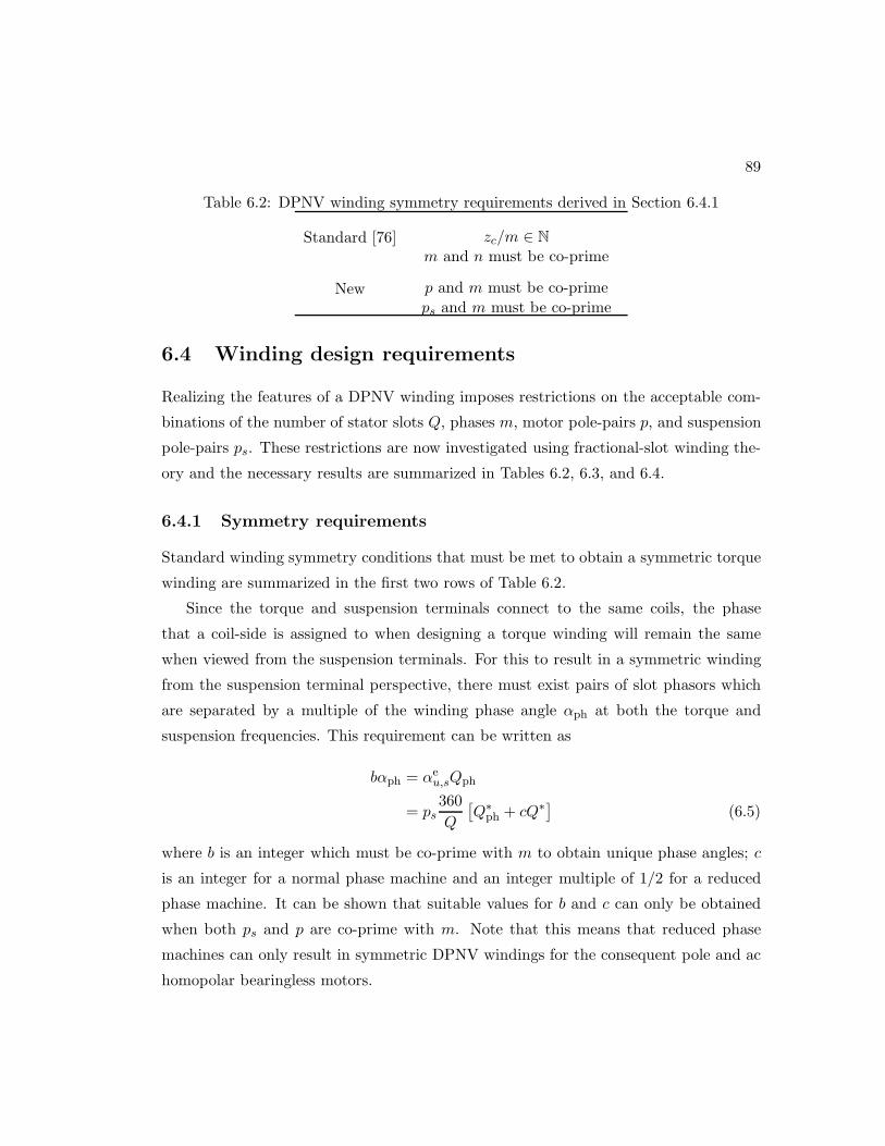
89
Table 6.2: DPNV winding symmetry requirements derived in Section 6.4.1
Standard [76] zc/m ∈ N
m and n must be co-prime
New p and m must be co-prime
ps and m must be co-prime
6.4 Winding design requirements
Realizing the features of a DPNV winding imposes restrictions on the acceptable com-
binations of the number of stator slots Q, phases m, motor pole-pairs p, and suspension
pole-pairs ps. These restrictions are now investigated using fractional-slot winding the-
ory and the necessary results are summarized in Tables 6.2, 6.3, and 6.4.
6.4.1 Symmetry requirements
Standard winding symmetry conditions that must be met to obtain a symmetric torque
winding are summarized in the first two rows of Table 6.2.
Since the torque and suspension terminals connect to the same coils, the phase
that a coil-side is assigned to when designing a torque winding will remain the same
when viewed from the suspension terminals. For this to result in a symmetric winding
from the suspension terminal perspective, there must exist pairs of slot phasors which
are separated by a multiple of the winding phase angle αph at both the torque and
suspension frequencies. This requirement can be written as
bαph = αeu,sQph
= ps360
Q
[
Q∗ph + cQ∗] (6.5)
where b is an integer which must be co-prime with m to obtain unique phase angles; c
is an integer for a normal phase machine and an integer multiple of 1/2 for a reduced
phase machine. It can be shown that suitable values for b and c can only be obtained
when both ps and p are co-prime with m. Note that this means that reduced phase
machines can only result in symmetric DPNV windings for the consequent pole and ac
homopolar bearingless motors.

90
Table 6.3: DPNV winding no-voltage requirements derived in Section 6.4.2
First-grade Second-grade
Layers Single Double Single Double
Parallelconfiguration
Q4m ∈ N
Q2m ∈ N
t4 ∈ N
t2 ∈ N
Bridge
configuration
Q8m ∈ N
Q4m ∈ N
t8 ∈ N
t4 ∈ N
Table 6.4: DPNV winding suspension winding distribution factor requirements derivedin Section 6.4.3
Defining featuresa Requirementb
Type 1 Identical torque,opposing suspension
p ∈ Neven
Type 2 Opposing torque,identical suspension
p ∈ Nodd, ps ∈ Neven
Type 3 All other cases p ∈ Nodd, ps = 1, t > 1
aThe features are given in terms of the phasor behavior, shown in Fig. 6.4.bWindings must also meet the requirements summarized in Tables 6.2 and 6.3.
6.4.2 No voltage requirements
For the DPNV winding to have no motional-EMF present at the suspension terminals,
the suspension winding factors must be zero at the torque frequency and its harmonics.
This is achieved by reversing half of the coils’ direction for connection to the suspension
terminals and can be illustrated through the torque connection star. In this diagram,
there needs to be an even number of phasors present at each angular location so that
half of the phasors can be rotated 180e (by reversing the direction of half of the coils)
to cancel the non-rotated phasors. In order to obtain these phasors in the torque
connection star, necessary limitations on Q, m, and p are now considered. Furthermore,
it is also necessary that the phasors which are to cancel each other belong to different
coils in the same phase; this restricts the winding layout approach and is considered in
Section 6.4.4. Symmetric windings are classified as being either first or second grade
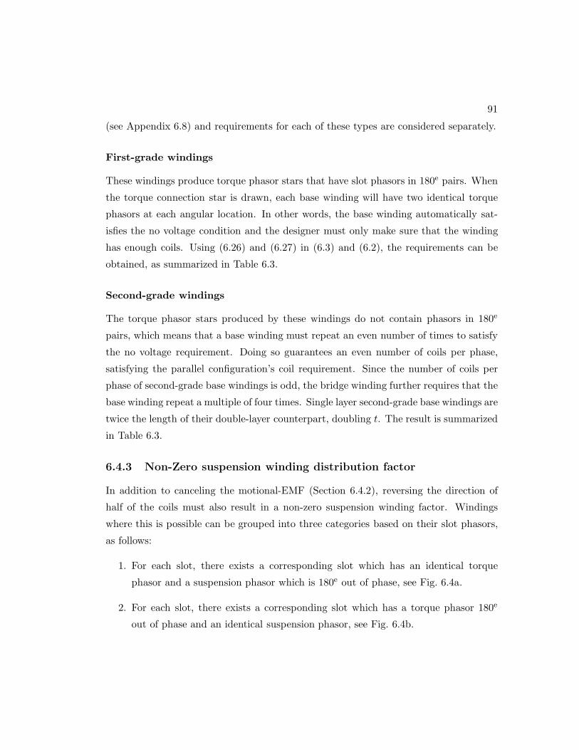
91
(see Appendix 6.8) and requirements for each of these types are considered separately.
First-grade windings
These windings produce torque phasor stars that have slot phasors in 180e pairs. When
the torque connection star is drawn, each base winding will have two identical torque
phasors at each angular location. In other words, the base winding automatically sat-
isfies the no voltage condition and the designer must only make sure that the winding
has enough coils. Using (6.26) and (6.27) in (6.3) and (6.2), the requirements can be
obtained, as summarized in Table 6.3.
Second-grade windings
The torque phasor stars produced by these windings do not contain phasors in 180e
pairs, which means that a base winding must repeat an even number of times to satisfy
the no voltage requirement. Doing so guarantees an even number of coils per phase,
satisfying the parallel configuration’s coil requirement. Since the number of coils per
phase of second-grade base windings is odd, the bridge winding further requires that the
base winding repeat a multiple of four times. Single layer second-grade base windings are
twice the length of their double-layer counterpart, doubling t. The result is summarized
in Table 6.3.
6.4.3 Non-Zero suspension winding distribution factor
In addition to canceling the motional-EMF (Section 6.4.2), reversing the direction of
half of the coils must also result in a non-zero suspension winding factor. Windings
where this is possible can be grouped into three categories based on their slot phasors,
as follows:
1. For each slot, there exists a corresponding slot which has an identical torque
phasor and a suspension phasor which is 180e out of phase, see Fig. 6.4a.
2. For each slot, there exists a corresponding slot which has a torque phasor 180e
out of phase and an identical suspension phasor, see Fig. 6.4b.
92
Torque frequency•
Suspension frequency•
(a) Type 1 slot phasor transformation
Torque frequency•
Suspension frequency•
(b) Type 2 slot phasor transformation
+ + +
Torque frequency•
−−− +
−+
−
+ −Suspension frequency
•
(c) Type 3 slot phasor transformation
Figure 6.4: DPNV winding type classification. Winding phasor star diagrams drawn atthe torque and suspension frequencies to depict the slot phasor behavior that defines (a)Type 1, (b) Type 2, and (c) Type 3 windings. Note that the phasor stars are incompleteand only depict the relevant slot phasors. In (c), the − and + signs are used to keeptrack of the transformation of the two groups of slot phasors.
3. The slot phasors do not meet Type 1 or Type 2 conditions but the winding can
still be configured to produce a non-zero suspension MMF, see Fig. 6.4c.
Requirements of each of these types of windings is summarized in Table 6.4 and
derived below.
Type 1
Two slot phasors displaced by a specific multiple of 360e at the torque frequency must
be displaced by an odd multiple of 180e at the suspension frequency,
ks × 180 = psp h1 × 360 (6.6)
where h1 is the integer number of pole-pairs between the identical torque phasors that
allows an integer ks and must be less than p; ks represents the number of suspension
poles between the 180e suspension phasors and is therefore an odd integer less than 2ps.
Since psh1 is an integer, p must be restricted to (6.7). Equation (6.6) can be solved for

93
h1 (6.8).
p
2∈ N (6.7)
h1 =ksps
p
2(6.8)
Since p and ps are co-prime, ks = ps and therefore h1 = p/2. This means that a slot
must exist every h1 pole-pairs, requiring
h1p∗
∈ N. (6.9)
Using the values of p∗ from Table 6.8, it can be shown that any first-grade and double-
layer second-grade winding requires
t
2∈ N (6.10)
while any second-grade single-layer winding requires
t
4∈ N. (6.11)
It can be seen from (6.23) and (6.10) that any first-grade winding satisfying (6.7) will be
a Type 1 winding. Any second-grade winding satisfying the requirements of Table 6.3
will satisfy (6.10) or (6.11) and, it can be seen from (6.25), will satisfy (6.7) and therefore
be a Type 1 winding. In summary, any winding that meets the no-voltage requirements
and has an even number of pole-pairs will be a Type 1 winding.
Type 2
Two slot phasors displaced by a specific odd multiple of 180e at the torque frequency
must be separated by a multiple of 360e at the suspension frequency,
k′s × 360 = psp h2 × 180 (6.12)
where k′s is the number of pole-pairs between the identical suspension phasors and must
be less than ps; h2 is the number of poles separating the torque phasors and must be
an odd integer less than 2p. This can be re-written as
h2 =2k′spsp. (6.13)
94
Since p and ps are co-prime and h2 is odd, it is required that:
p ∈ Nodd (6.14)
ps ∈ Neven (6.15)
which results in k′s = ps/2 and h2 = p. In addition to this, the torque phasor star needs
to have 180e torque phasor pairs present, which means the winding must be a first-grade
winding. In fact, first-grade windings are the only windings that can meet both (6.14)
and the no-voltage conditions of Table 6.3; this can be seen from (6.4) and Table 6.8,
which indicate that a second grade no voltage winding will have t ∈ Neven, which is not
possible when (6.14) is true.
In summary, any no-voltage winding that satisfies (6.14) and (6.15) will be a Type
2 no-voltage winding.
Type 3
The remaining windings have
p ∈ Nodd (6.16)
ps ∈ Nodd (6.17)
which corresponds to the case of a bearingless consequent pole or ac homopolar motor
when p ∈ Nodd. These are first-grade windings and will therefore have t ∈ Nodd due to
(6.16), torque phasors separated by 180e, and may have torque phasors separated by
360e if t > 1. Slots which have torque phasors separated by multiples of 180e, will have
suspension phasors separated by
αes =
1ph
′ × 180 (6.18)
where h′ is the number of poles between all torque phasors displaced by multiples of
180e. Since 180e phasors occur every p′ poles, h′ will take on values of all integer
multiples of p′ less than 2p. The resulting suspension angles will be
αes = k′
180
t, k′ = 1, ..., 2t − 1. (6.19)
Therefore, to have a non-zero suspension winding factor after half of the phasors have
been rotated 180e, it is required that
t > 1. (6.20)
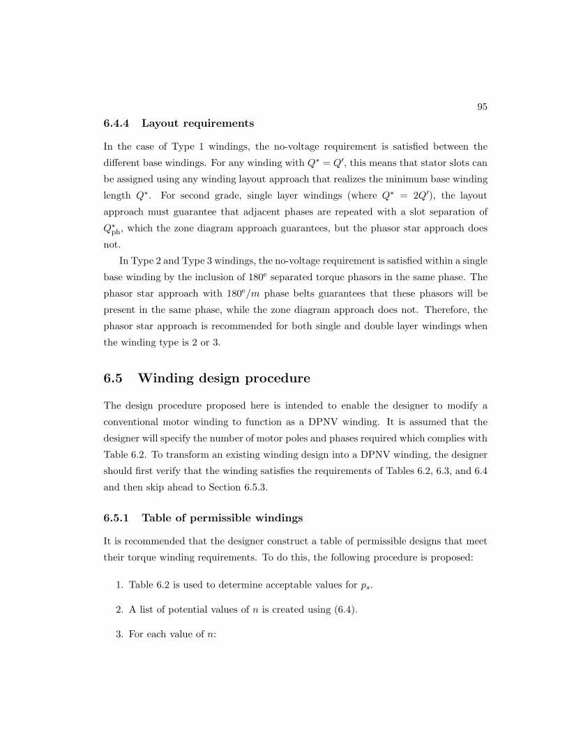
95
6.4.4 Layout requirements
In the case of Type 1 windings, the no-voltage requirement is satisfied between the
different base windings. For any winding with Q∗ = Q′, this means that stator slots can
be assigned using any winding layout approach that realizes the minimum base winding
length Q∗. For second grade, single layer windings (where Q∗ = 2Q′), the layout
approach must guarantee that adjacent phases are repeated with a slot separation of
Q∗ph, which the zone diagram approach guarantees, but the phasor star approach does
not.
In Type 2 and Type 3 windings, the no-voltage requirement is satisfied within a single
base winding by the inclusion of 180e separated torque phasors in the same phase. The
phasor star approach with 180e/m phase belts guarantees that these phasors will be
present in the same phase, while the zone diagram approach does not. Therefore, the
phasor star approach is recommended for both single and double layer windings when
the winding type is 2 or 3.
6.5 Winding design procedure
The design procedure proposed here is intended to enable the designer to modify a
conventional motor winding to function as a DPNV winding. It is assumed that the
designer will specify the number of motor poles and phases required which complies with
Table 6.2. To transform an existing winding design into a DPNV winding, the designer
should first verify that the winding satisfies the requirements of Tables 6.2, 6.3, and 6.4
and then skip ahead to Section 6.5.3.
6.5.1 Table of permissible windings
It is recommended that the designer construct a table of permissible designs that meet
their torque winding requirements. To do this, the following procedure is proposed:
1. Table 6.2 is used to determine acceptable values for ps.
2. A list of potential values of n is created using (6.4).
3. For each value of n:

96
1
2
3
4
5
6
7
8
9
10
11
12
13
14
15
16
17
18
+u
+v
+w
−u
−v
−w
Torque phasor star
17
1319
2
814
20
3
9
15
21
4 10
16 22
5
1117
23
6
12
18
24
+u
+v
+w
−u
−v
−w
1) Layout torque
winding
1
-14
12
-10
5
-3
Torque phase u conn.
star drawn for h = ps
180e band
used
alternate
180e band
1
-47
-10
13
-1619
-22
2) Determine which coils
to reverse for sus. winding
-1012
-14ua
1-3
5ub
Torque phasors for
the coil groups
7 -10
ua
1 -4
ub
13 -16
uc
19 -22
ud
3) Assign coils to
coil groups
Typ
e1
Q=24
,p
=4
,ps
=5
Bri
dge
or
par
alle
lco
nfi
g.
Typ
e2
Q=18
,p
=5
,ps
=4
Par
alle
lco
nfi
g.
1
ua+ ua−ub+ ub− uc+ uc− ud+ ud−
4
ua+ ua−ub+ ub− uc+ uc− ud+ ud−
7
ua+ ua−ub+ ub− uc+ uc− ud+ ud−
10
ua+ ua−ub+ ub− uc+ uc− ud+ ud−
13
ua+ ua−ub+ ub− uc+ uc− ud+ ud−
16
ua+ ua−ub+ ub− uc+ uc− ud+ ud−
19
ua+ ua−ub+ ub− uc+ uc− ud+ ud−
22
ua+ ua−ub+ ub− uc+ uc− ud+ ud−
3 6 9 12 15 18 21 242 5 8 11 14 17 20 23
1
ua+ ua−ub+ ub−
3
ua+ ua−ub+ ub−
5
ua+ ua−ub+ ub−
10
ua+ ua−ub+ ub−
12
ua+ ua−ub+ ub−
14
ua+ ua−ub+ ub−
4 6 8 13 15 172 7 9 11 16 18
Resulting winding layouts
Figure 6.5: The design steps of Section 6.5.3 applied to two example DPNV windingentries in Table 6.5.
(a) the winding grade is determined from Table 6.8;
(b) t is calculated using (6.23) or (6.25);
(c) for a second-grade winding, t is checked against Table 6.3; for a Type 3
winding, t is checked against Table 6.4. Any values of n which fail are
removed.
4. Permissible values of z are determined by requiring that z and n are co-prime.
5. Acceptable values of Q are found using (6.22) and (6.24). For first grade windings,
Q is checked against Table 6.3.
97
6. The results are compiled into a table with rows for each Q value; i.e. see Table 6.5,
discussed later.
6.5.2 Select coil span
The effect of coil span should be carefully considered. When all coils have the same
span, the pitch factor is (6.21)
kp,h = sin(hαy2) (6.21)
where αy is the angular pitch of each coil [76]. Maximizing the coil pitch factor for
the torque frequency may result in a low value at the suspension frequency and an
unacceptably low suspension force rating. This is especially true when the relative
difference in the two frequencies is very large, i.e. when p is small or when ps = 1. The
pitch factor may also be used to prevent harmonics that would otherwise create force
ripple. The design in Section 6.5.3 is significantly constrained and will often result in
large suspension winding distribution factors for h 6= ps which can be suppressed by
kp,h.
6.5.3 Design each winding in the table
For each entry in the design table generated in Section 6.5.1, the designer should perform
the following steps.
First, the layout should be conducted for the torque winding. Section 6.4.4 should
be used to select a layout approach.
Second, the torque connection star of a single phase should be drawn at the suspen-
sion frequency and half of the connection phasors should be selected to rotate 180e (the
coils to reverse for connection to the suspension terminals) in a way that 1) cancels all
phasors at the torque frequency and 2) results in a non-zero suspension winding distri-
bution factor. The approach to doing this is described below for each of the winding
types defined in Table 6.4.
Finally, the designer must assign the coils to coil groups a-d, depicted in Fig. 6.1.
Groups a and c should only contain coils which have been reversed for connection to the
suspension terminals. Furthermore, the vector sum of the torque connection phasors of

98
groups a and b must be equivalent and groups c and d must be equivalent. For parallel
drive connections, groups c and d need not exist.
Type 1 and Type 2
The results of Section 6.4.3 indicate that any 180e band of connection phasors (from each
phase of the torque connection star drawn at the suspension frequency) can be selected
for rotation. The angular separation of the connection phasors is not guaranteed to be
uniform, meaning that in some cases selecting one 180e band over another will result in
more optimal suspension winding distribution factors. An example of the design steps
applied to these types of windings is shown in Fig. 6.5.
Type 3
The results of Section 6.4.3 indicate that unlike Type 1 and 2 windings, an arbitrary 180e
band of torque connection phasors cannot be used for rotation. From (6.19) and noting
that t ∈ Nodd, it can be shown that the resulting torque connection star (drawn at the
suspension frequency) will consist of 2t phasors at t equally spaced angular locations,
as shown in Fig. 6.6a. From this star, acceptable combinations of torque connection
phasors can be identified and rotated to cancel the motional-EMF and create a non-zero
suspension winding factor. If the torque phase connection star contains phasor groups
rotated αet 6= 180e, each of these phasor groups will result in additional suspension
phasor groups as shown in Fig. 6.6b. Type 3 windings use suspension current in an
especially inefficient manner, as the MMFs of some coils end up canceling each other.
6.5.4 Design selection
The designer must now select the final winding to use. To do this, it is recommended to
add performance metrics as columns in the table generated in Section 6.5.1. Common
metrics have been added to Table 6.5. These include the ratio of ks,ps to kt,p, which
predicts how effectively the machine uses current to produce radial forces, and results
obtained via FEA: the rated average force along an axis (i.e. 〈Fx〉 for an x-axis force),the normalized maximum deviation from the average of the force waveform along the
principle axis (i.e. ∆Fx/〈Fx〉), and the normalized maximum value in the force waveform
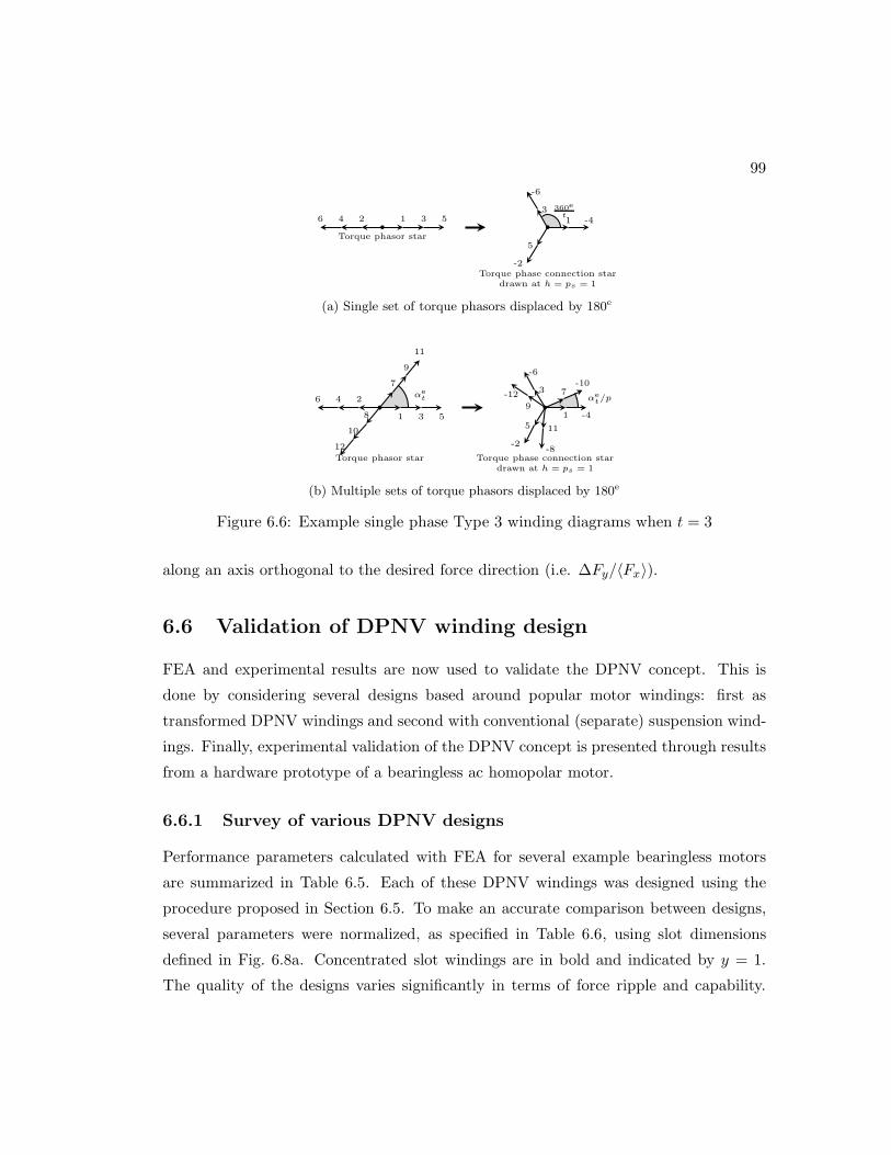
99
1 3 5
Torque phasor star•
246 1
-2
3
-4
5
-6
360e
t
Torque phase connection stardrawn at h = ps = 1
•
(a) Single set of torque phasors displaced by 180e
1 3 5
Torque phasor star
•246
7
9
11
•8
10
12
αet
1
-2
3
-4
5
-6
Torque phase connection stardrawn at h = ps = 1
•
7
-8
9
-10
11
-12 αet/p
(b) Multiple sets of torque phasors displaced by 180e
Figure 6.6: Example single phase Type 3 winding diagrams when t = 3
along an axis orthogonal to the desired force direction (i.e. ∆Fy/〈Fx〉).
6.6 Validation of DPNV winding design
FEA and experimental results are now used to validate the DPNV concept. This is
done by considering several designs based around popular motor windings: first as
transformed DPNV windings and second with conventional (separate) suspension wind-
ings. Finally, experimental validation of the DPNV concept is presented through results
from a hardware prototype of a bearingless ac homopolar motor.
6.6.1 Survey of various DPNV designs
Performance parameters calculated with FEA for several example bearingless motors
are summarized in Table 6.5. Each of these DPNV windings was designed using the
procedure proposed in Section 6.5. To make an accurate comparison between designs,
several parameters were normalized, as specified in Table 6.6, using slot dimensions
defined in Fig. 6.8a. Concentrated slot windings are in bold and indicated by y = 1.
The quality of the designs varies significantly in terms of force ripple and capability.
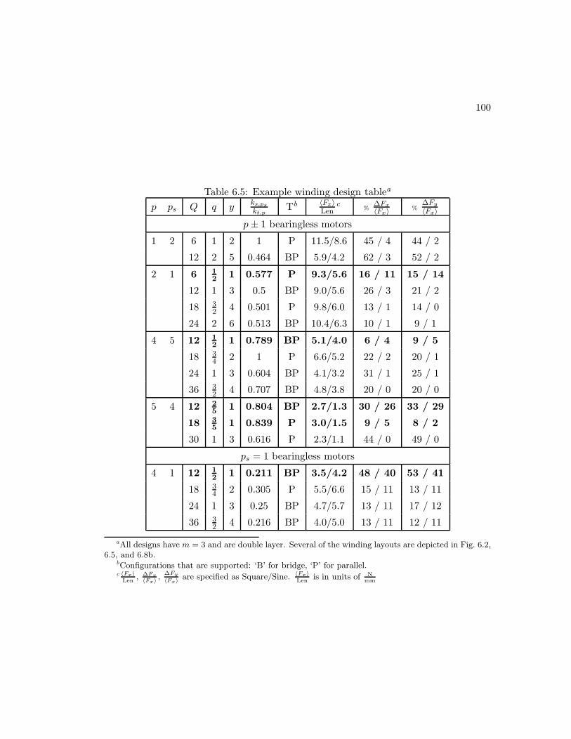
100
Table 6.5: Example winding design tablea
p ps Q q yks,pskt,p
Tb 〈Fx〉Len
c%
∆Fx〈Fx〉 %
∆Fy〈Fx〉
p± 1 bearingless motors
1 2 6 1 2 1 P 11.5/8.6 45 / 4 44 / 2
12 2 5 0.464 BP 5.9/4.2 62 / 3 52 / 2
2 1 6 12
1 0.577 P 9.3/5.6 16 / 11 15 / 14
12 1 3 0.5 BP 9.0/5.6 26 / 3 21 / 2
18 32 4 0.501 P 9.8/6.0 13 / 1 14 / 0
24 2 6 0.513 BP 10.4/6.3 10 / 1 9 / 1
4 5 12 12
1 0.789 BP 5.1/4.0 6 / 4 9 / 5
18 34 2 1 P 6.6/5.2 22 / 2 20 / 1
24 1 3 0.604 BP 4.1/3.2 31 / 1 25 / 1
36 32 4 0.707 BP 4.8/3.8 20 / 0 20 / 0
5 4 12 25
1 0.804 BP 2.7/1.3 30 / 26 33 / 29
18 35
1 0.839 P 3.0/1.5 9 / 5 8 / 2
30 1 3 0.616 P 2.3/1.1 44 / 0 49 / 0
ps = 1 bearingless motors
4 1 12 12
1 0.211 BP 3.5/4.2 48 / 40 53 / 41
18 34 2 0.305 P 5.5/6.6 15 / 11 13 / 11
24 1 3 0.25 BP 4.7/5.7 13 / 11 17 / 12
36 32 4 0.216 BP 4.0/5.0 13 / 11 12 / 11
aAll designs have m = 3 and are double layer. Several of the winding layouts are depicted in Fig. 6.2,6.5, and 6.8b.
bConfigurations that are supported: ‘B’ for bridge, ‘P’ for parallel.c 〈Fx〉
Len, ∆Fx
〈Fx〉,
∆Fy
〈Fx〉are specified as Square/Sine. 〈Fx〉
Lenis in units of N
mm
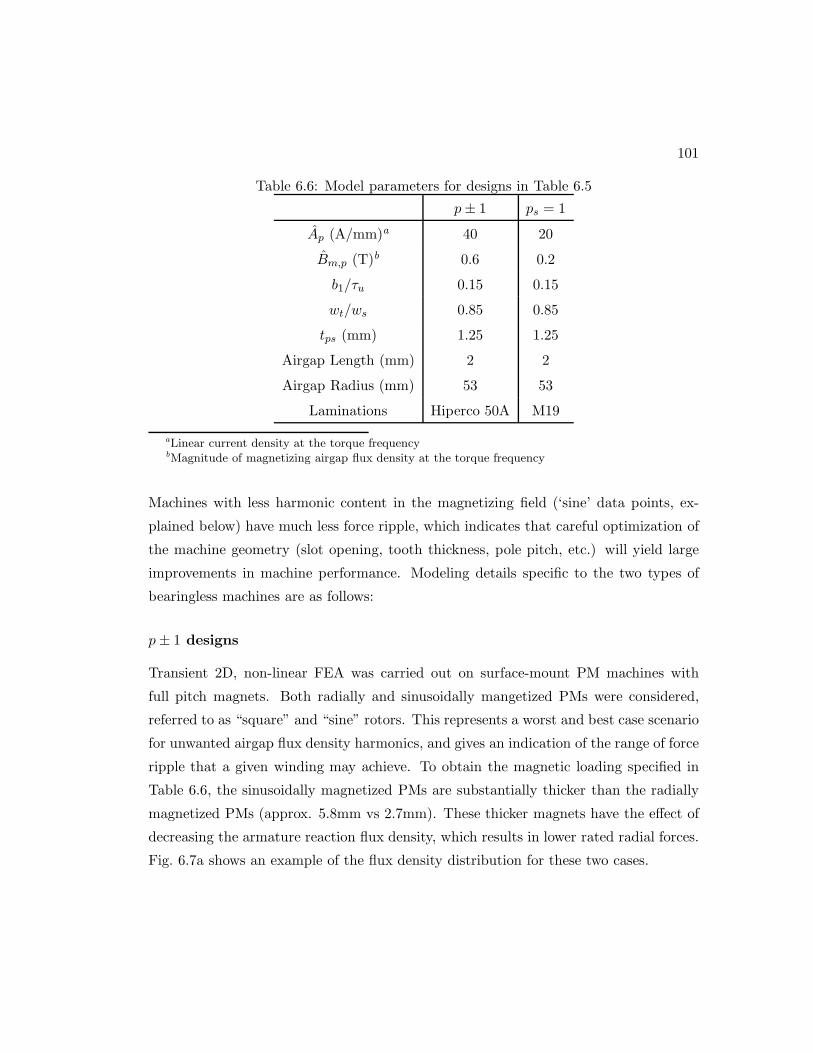
101
Table 6.6: Model parameters for designs in Table 6.5
p± 1 ps = 1
Ap (A/mm)a 40 20
Bm,p (T)b 0.6 0.2
b1/τu 0.15 0.15
wt/ws 0.85 0.85
tps (mm) 1.25 1.25
Airgap Length (mm) 2 2
Airgap Radius (mm) 53 53
Laminations Hiperco 50A M19
aLinear current density at the torque frequencybMagnitude of magnetizing airgap flux density at the torque frequency
Machines with less harmonic content in the magnetizing field (‘sine’ data points, ex-
plained below) have much less force ripple, which indicates that careful optimization of
the machine geometry (slot opening, tooth thickness, pole pitch, etc.) will yield large
improvements in machine performance. Modeling details specific to the two types of
bearingless machines are as follows:
p± 1 designs
Transient 2D, non-linear FEA was carried out on surface-mount PM machines with
full pitch magnets. Both radially and sinusoidally mangetized PMs were considered,
referred to as “square” and “sine” rotors. This represents a worst and best case scenario
for unwanted airgap flux density harmonics, and gives an indication of the range of force
ripple that a given winding may achieve. To obtain the magnetic loading specified in
Table 6.6, the sinusoidally magnetized PMs are substantially thicker than the radially
magnetized PMs (approx. 5.8mm vs 2.7mm). These thicker magnets have the effect of
decreasing the armature reaction flux density, which results in lower rated radial forces.
Fig. 6.7a shows an example of the flux density distribution for these two cases.

102
(a) Q = 12, p = 4, ps = 5 flux density while producing x force
(b) 3D FE models for Q = 12 ac homopolar winding design
Figure 6.7: FEA models. The left-most images correspond to “square” rotors and theright-most to “sine” rotors.
ps = 1 designs
Static 3D non-linear FEA was carried out on ac homopolar machines where the rotor’s
angular position was swept. Only 8 pole designs were considered as this is the most
common implementation. Two rotor structures were used to change the harmonic con-
tent of the magnetizing flux density: a “square” rotor (square airgap length profile)
and a “sine” rotor (inverted sinusoidal airgap length profile), see Fig. 6.7b. The airgap
has the same minimum length (specified in Table 6.6), which requires a greater field
excitation to be used with a sine rotor to obtain the same Bm,p value. This resulted in
the sine rotor having a greater circulating homopolar flux and therefore a greater force
capability. However, note that from a motor design perspective, the sine rotors are at a
disadvantage because the machine has to carry greater flux to achieve the same torque
as the square rotors.

103
tps
b1
τu
wtws
(a) Stator slot dimensions
1
2
3
4
5
6
7
8
9
10
11
12
+u
+v
+w
−u
−v
−w
1
ua+ub+ uc+ud+
4
ua+ub+ uc+ud+
7
ua+ub+ uc+ud+
10
ua+ub+ uc+ud+
2 5 8 113 6 9 12
Torque phasor star Winding layout
(b) Winding design
0.4 0.6 0.8 1 1.2 1.4
Tesla
0
0.5
1
1.5
2
Rated x-force
Rated torque No load
wt/ws
(c) Maximum flux density at tooth center
Figure 6.8: Design information for the Q = 12, p = 4, ps = 5 entry in Table 6.5.
6.6.2 Detailed study of Q = 12, p = 4, ps = 5 DPNV winding
The square rotor design from Table 6.5 is now studied in more detail. The winding
layout is shown in Fig. 6.8b and terminal voltage waveforms are shown in Fig. 6.9. As
expected, the suspension terminals do not experience any voltage due to the rotor’s
rotation or the torque terminal current; under rated suspension current, a suspension
terminal voltage appears due to the RL branch of each coil group (Fig. 6.2e). The
parallel configuration’s torque terminals see a voltage due to these same RL branches
(described at the end of Section 6.2) which may need to be accounted for in the motor
drive if the designer is unable to sufficiently reduce it.
Next, the impact of the slot opening and tooth thickness was considered for three
operating conditions: 1) no stator currents; 2) rated torque, no suspension current; and
3) rated suspension, no torque current. The ratio of the tooth thickness to slot width was
swept to obtain designs with varying degrees of tooth staturation, as shown in Fig. 6.8c.
In all resulting designs, the suspension terminals never exhibit any voltage for cases 1
and 2. For case 3, the peak suspension terminal voltage of the parallel configuration is
plotted as a function of slot opening and tooth thickness on the left side of Fig. 6.10.
This voltage exhibits a large dependence on the slot opening, but less dependence on
the tooth thickness, indicating that tooth-tip leakage inductance is the primary cause.
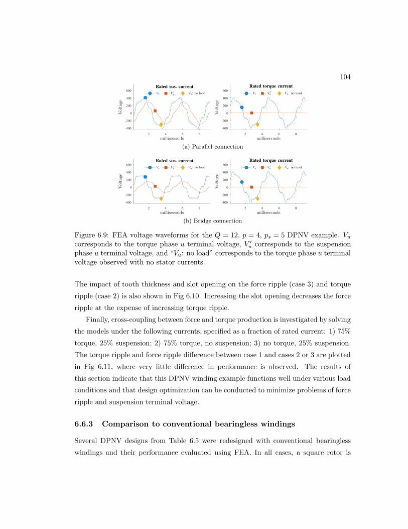
104
milliseconds2 4 6 8
Voltage
-400
-200
0
200
400
600Vu V ′
u Vu: no load
milliseconds2 4 6 8
Voltage
-400
-200
0
200
400
600Vu V ′
u Vu: no load
Rated sus. current Rated torque current
(a) Parallel connection
milliseconds2 4 6 8
Voltage
-400
-200
0
200
400
600Vu V ′
u Vu: no load
milliseconds2 4 6 8
Voltage
-400
-200
0
200
400
600Vu V ′
u Vu: no load
Rated sus. current Rated torque current
(b) Bridge connection
Figure 6.9: FEA voltage waveforms for the Q = 12, p = 4, ps = 5 DPNV example. Vucorresponds to the torque phase u terminal voltage, V ′
u corresponds to the suspensionphase u terminal voltage, and “Vu: no load” corresponds to the torque phase u terminalvoltage observed with no stator currents.
The impact of tooth thickness and slot opening on the force ripple (case 3) and torque
ripple (case 2) is also shown in Fig 6.10. Increasing the slot opening decreases the force
ripple at the expense of increasing torque ripple.
Finally, cross-coupling between force and torque production is investigated by solving
the models under the following currents, specified as a fraction of rated current: 1) 75%
torque, 25% suspension; 2) 75% torque, no suspension; 3) no torque, 25% suspension.
The torque ripple and force ripple difference between case 1 and cases 2 or 3 are plotted
in Fig 6.11, where very little difference in performance is observed. The results of
this section indicate that this DPNV winding example functions well under various load
conditions and that design optimization can be conducted to minimize problems of force
ripple and suspension terminal voltage.
6.6.3 Comparison to conventional bearingless windings
Several DPNV designs from Table 6.5 were redesigned with conventional bearingless
windings and their performance evaluated using FEA. In all cases, a square rotor is
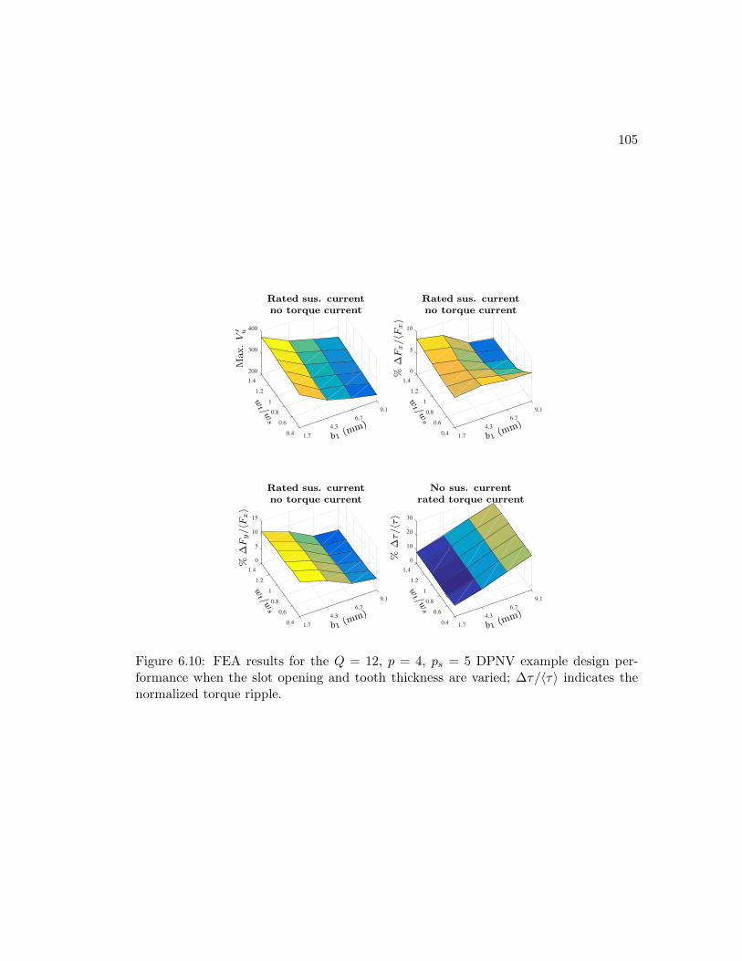
105
9.1
6.7
4.3
1.70.4
0.6
0.8
1
1.2
200
300
400
1.4
Max.V
′ u
wt /w
s
b1 (mm)
Rated sus. current
no torque current
9.1
6.7
4.3
1.70.4
0.6
0.8
1
1.2
0
5
10
1.4
%∆Fx/〈Fx〉
wt /w
s
b1 (mm)
Rated sus. current
no torque current
9.1
6.7
4.3
1.70.4
0.6
0.8
1
1.2
15
5
0
10
1.4
%∆Fy/〈Fx〉
wt /w
s
b1 (mm)
Rated sus. current
no torque current
9.1
6.7
4.3
1.70.4
0.6
0.8
1
1.2
10
30
20
0
1.4
%∆τ/〈τ〉
wt /w
s
b1 (mm)
No sus. current
rated torque current
Figure 6.10: FEA results for the Q = 12, p = 4, ps = 5 DPNV example design per-formance when the slot opening and tooth thickness are varied; ∆τ/〈τ〉 indicates thenormalized torque ripple.

106
9.1
6.7
4.3
1.70.4
0.6
0.8
1
1.2
-2
2
0
4
1.4
%∆
Fx,τ−
∆Fx
〈Fx,τ〉
wt /w
s
b1 (mm)
9.1
6.7
4.3
1.70.4
0.6
0.8
1
1.2
0.5
-0.5
0
1
1.4
%∆
τx−
∆τ
〈τx〉
wt /w
s
b1 (mm)
Figure 6.11: FEA results evaluating the machine performance during simultaneous forceand torque production. Fx,τ is the x radial force produced with simultaneous torqueand τx is the torque produced with simultaneous x force.
used, the double layer winding of the DPNV design becomes the torque winding, and a
new suspension winding is added to the same slots. The resulting designs have three or
four winding layers depending on whether a single or double layer suspension winding is
used, whereas the DPNV windings had only two layers. To enable a direct comparison,
the new designs have the same dimensions with the exception that 75% of the slot space
is now permenantly allocated to the suspension windings, reducing the torque winding
turns and therefore the machines’ rated torque to 75% of the value of the DPNV designs.
The results from this study are presented in Table 6.7. Concentrated-slot designs are
again indicated in bold. The difference in force ripple between conventional or DPNV
windings for a design largely varies on a per-design basis, with each winding approach
outperforming the other in certain designs. Many designs with conventional windings
feature higher ks,ps/kt,p ratios, indicating that they would have higher suspension force
capabilities if the entire slot space could be allocated to the suspension winding. How-
ever, this is not possible since the machine must also be able to produce the required
torque. In the Q = 6, p = 2 example, the double layer suspension winding is actually
identical to the DPNV design (from the suspension terminal perspective).
The winding layouts for the Q = 12, p = 4, ps = 5 design are shown in Fig. 6.12 and
voltage waveforms are shown in Fig. 6.13. These results can be compared to the DPNV
waveforms for the same design in Fig. 6.9. Since the number of turns of the torque
winding is reduced from the DPNV winding, the torque terminal voltage magnitude
is also reduced. The single layer suspension winding has non-zero winding factors at
multiples of the torque frequency, and therefore its suspension terminals experience a
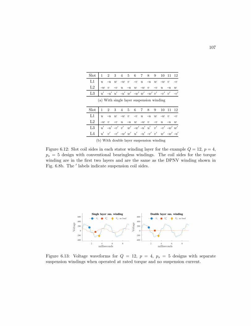
107
Slot 1 2 3 4 5 6 7 8 9 10 11 12
L1 u -u w -w v -v u -u w -w v -v
L2 -w v -v u -u w -w v -v u -u w
L3 u′ -u′ u′ -u′ w′ -w′ w′ -w′ v′ -v′ v′ -v′
(a) With single layer suspension winding
Slot 1 2 3 4 5 6 7 8 9 10 11 12
L1 u -u w -w v -v u -u w -w v -v
L2 -w v -v u -u w -w v -v u -u w
L3 u′ -u′ -v′ v′ w′ -w′ -u′ u′ v′ -v′ -w′ w′
L4 u′ v′ -v′ -w′ w′ u′ -u′ -v′ v′ w′ -w′ -u′
(b) With double layer suspension winding
Figure 6.12: Slot coil sides in each stator winding layer for the example Q = 12, p = 4,ps = 5 design with conventional bearingless windings. The coil sides for the torquewinding are in the first two layers and are the same as the DPNV winding shown inFig. 6.8b. The ′ labels indicate suspension coil sides.
milliseconds2 4 6 8
Voltage
-400
-200
0
200
400
600Vu V ′
u Vu: no load
milliseconds2 4 6 8
Voltage
-400
-200
0
200
400
600Vu V ′
u Vu: no load
Single layer sus. winding Double layer sus. winding
Figure 6.13: Voltage waveforms for Q = 12, p = 4, ps = 5 designs with separatesuspension windings when operated at rated torque and no suspension current.

108
motional-EMF (unlike the DPNV winding).
The conclusion of whether a DPNV winding is advantageous over a conventional
winding must be made on a per-design basis. The primary benefits of a DPNV winding
can be summarized as: 1) allowing the drive to dynamically allocate the fraction of the
slot current used for torque or suspension forces and therefore enabling greater maximum
torque or suspension forces; 2) reducing the number of winding layers to what is needed
by the torque winding–this reduces manufacturing complexity and increases the winding
packing factor; 3) potentially reducing copper losses–this has been shown in [99,100] to
be true for specific example designs. However, certain combinations of slots, poles, and
phases do not work for DPNV designs and other combinations may yield unacceptably
high force ripple or low force rating. Furthermore, in designs with constant radial
forces, there is less value in being able to dynamically allocate slot current between the
suspension and torque operation. The DPNV winding approach is most advantageous
in designs with one or more of the following criteria: 1) the suspension forces are
intermittent or variable, 2) the resulting DPNV suspension performance is similar or
equivalent to what would be obtained with a conventional bearingless winding (i.e. the
Q = 6, p = 2 entry in Table 6.7), 3) mechanical bearings are used and the suspension
forces will provide vibration suppression.
6.7 Conclusion
DPNV windings use the same coils to produce both torque and radial suspension forces
and thereby offer a solution to a major obstacle in the wider adaptation of bearingless
motor technology: low torque density. This chapter significantly advances the state-of-
the-art of DPNV winding technology by deriving the design requirements and proposing
a generalized design approach which can also be used to transform existing motor designs
into bearingless motors by simply modifying the end connections. Such modification
comes at no extra machine cost, requires no redesign effort, and can be used to passively
provide corrective forces with no additional drive circuitry.
Fractional-slot winding theory has been used to explore the DPNV winding concept
and an FEA study was conducted to validate several example designs and contrast the
resulting performance with conventional bearingless windings. It was shown that the

109
Table 6.7: Examples of separate suspension windingsa
p ps Q q ybks,pskt,p
Lc 〈Fx〉Len %
∆Fx〈Fx〉 %
∆Fy〈Fx〉
p± 1 bearingless motors
1 2 6 12 1 1 1 2.6 53 54
6 12 1 1 2 2.8 44 45
2 1 6 1 3 1.155 1 5.1 16 14
6 1 1 0.577 2 2.7 15 15
18 3 9 1.015 1 5.1 4 4
4 5 12 25
1 0.966 1 1.6 10 6
12 25
1 1.077 2 1.8 5 4
36 65 - 0.997 1 1.7 3 3
36 65 3 0.977 2 1.7 1 1
5 4 12 12
1 0.928 1 0.8 27 23
12 12
1 0.928 2 0.8 29 28
18 34
- 1.286 1 1.2 8 9
18 34
1 0.839 2 0.8 12 10
4 1 36 32 18 0.991 1 4.7 3 3
aAll of the information in this table pertains to the suspension winding; the torque windings are thesame as those in Table 6.5.
b- is used for single layer windings which have coils with varying pitchcNumber of layers of the suspension winding.
110
benefits of DPNV windings vary on a per-design basis, with applications with intermit-
tent force requirements seeing the greatest benefit. Finally, experimental validation is
presented via a prototype machine in Chapter 8.
6.8 Fractional-slot winding theory
Relevant fractional slot winding information is provided in Table 6.8 and several stan-
dard terms are defined below. More detailed information can be found in textbooks
such as [76].
6.8.1 Key terms
Base winding
smallest independent section of a winding. Symmetric windings consist repeated base
windings.
First grade and second grade windings
defined based on the properties in Table 6.8. All symmetric windings can be classified
as either first or second grade (integral-slot windings are considered first-grade since
n = 1).
Normal phase machine
machine with m ∈ Nodd.
Reduced phase machine
machine with m ∈ Neven.
6.8.2 Useful relations
For the purposes of this chapter, it is useful to note that if a designer picks n,m, t, and
z they will arrive at the number of poles and slots given by (6.22) and (6.23) for first

111
Table 6.8: Relevant fractional-slot winding information [76]
First-grade Second grade
Q′
m Even Odd
t pn
2pn
n Odd Even
180 phasors?a Yes No
Single layer Double layer
Q∗ Q′ 2Q′ Q′
p∗ p′ 2p′ p′
awhether the phasor star contains phasors in 180e pairs
grade windings
Q = 2mtz (6.22)
p = nt (6.23)
and (6.24) and (6.25) for second grade windings.
Q = mtz (6.24)
p =nt
2(6.25)
In single layer windings, the number of coils is
zc =Q
2(6.26)
and in double layer windings, the number of coils is
zc = Q. (6.27)

Chapter 7
Dual Purpose No Voltage Drives
for Bearingless Motors
This chapter investigates the power electronic implementation of drives for bearingless
motors with DPNV windings. The results are valid for conventional p±1 pole-pair bear-
ingless motors (i.e. bearingless permanent magnet and induction motors) and p = 1
bearingless motors (bearingless ac homopolar and consequent-pole motors). The advan-
tages and disadvantages of each configuration are explored in terms of control complexity
and required hardware; potential paths for circulating currents are identified along with
mitigation strategies.1
7.1 Introduction
Literature on DPNV bearingless windings has focused on winding design and proof-of-
concept prototypes. To date, there has been no detailed analysis on the use of power
electronics to implement these drives. The primary contribution of this chapter is
to investigate practical aspects of implementing bridge and parallel configurations of
DPNV drives using two-level, three-phase and single-phase inverters. In this chapter,
Section 7.2 provides an overview of the operation of the different types of bearingless mo-
tors considered; Section 7.3 introduces DPNV windings and the operation of bearingless
1 Portions of the material in this chapter have also been published in [49].
112
113
motors with these windings; Section 7.4 proposes power electronic drive implementa-
tions for the two DPNV configurations and compares the hardware requirements with
the conventional bearingless drive; Section 7.5 presents relevant considerations for con-
troller design, including strategies for suppressing circulating currents; Section 7.6 uses
simulation results to demonstrate the proposed control strategies and power electronic
implementations; and experimental results to validate the parallel and bridge winding
drive implementations for a bearingless ac homopolar motor are presented in Chapter 8.
7.2 Bearingless motor operation
Radial flux bearingless motors produce radial suspension forces by creating an unsym-
metrical flux density in the airgap. The forces can be calculated via the Maxwell Stress
Tensor, which for the idealized case of radial fields that do not vary with motor’s axial
length, can be written as (7.1),
Fx =lr
2µ0
∫ 2π
0Br (α)
2 cosα dα
Fy =lr
2µ0
∫ 2π
0Br (α)
2 sinα dα (7.1)
where l is the motor’s active axial length, r is the airgap radius, and Br is the cumulative
radial flux density in the airgap at angular location α. From this expression, it can be
shown that to create a radial force, the airgap flux density must contain components
which differ in harmonic index by one. Force expressions and suspension operation are
now summarized for the two types of radial flux bearingless motors. More detailed
information can be found in [56]. Note that idealized current waveforms for force and
torque production are presented later, in Section 7.3.
7.2.1 p± 1 bearingless motors
Conventional radial flux motors, i.e. permanent magnet (PM) or induction motors, have
a radial airgap flux density given by (7.2), assuming that harmonics are neglected.
BF (α) = BF cos (−pα+ φF ) (7.2)
Here, p represents the number of pole-pairs of the motor and φF indicates the angular
location of the magnetic field at an instant of time. The magnetic field is composed of
114
a magnetizing field (for example, produced by PM’s or a rotor winding) and armature
reaction field. To transform this type of motor into a bearingless motor, a suspension
winding with either p+ 1 or p− 1 pole-pairs is added to the stator to produce a radial
flux density which differs in harmonic index by one (7.3). This flux denisty is produced
by balanced sinusoidal suspension currents (7.4).
Bs (α) = Bs cos (− [p± 1]α+ φs) (7.3)
i′u = Is cos (φs)
i′v = Is cos(
φs − 2π3
)
i′w = Is cos(
φs +2π3
)
(7.4)
These currents can be transformed into an equivalent two-phase system using the well-
known DQ transformation. If this is done with respect to the angle φF , convenient
constant expressions for the radial force result (7.5), where ix and iy are the two-phase
DQ currents from the transformation.
Fx = kf ix
Fy = kf iy (7.5)
Typically, a suspension controller specifies required values of Fx and Fy, which are then
used to determine the phase currents via an inverse DQ transformation (7.6). Noting
that φF increases at the speed of the armature winding frequency, it can be seen that
to produce a constant force, the suspension currents will have the same frequency as
the armature currents.
i′u
i′vi′w
=
√
2/3
kf
cosφF − sinφF
cos(
φF − 2π3
)
− sin(
φF − 2π3
)
cos(
φF + 2π3
)
− sin(
φF + 2π3
)
Fx
Fy
(7.6)
7.2.2 p = 1 bearingless motors
This class includes the ac homopolar and consequent-pole bearingless motors. These
motors can be viewed as having a constant radial airgap flux density component which
does not vary with the angular position (7.7).
BF0 (α) = BF0 (7.7)
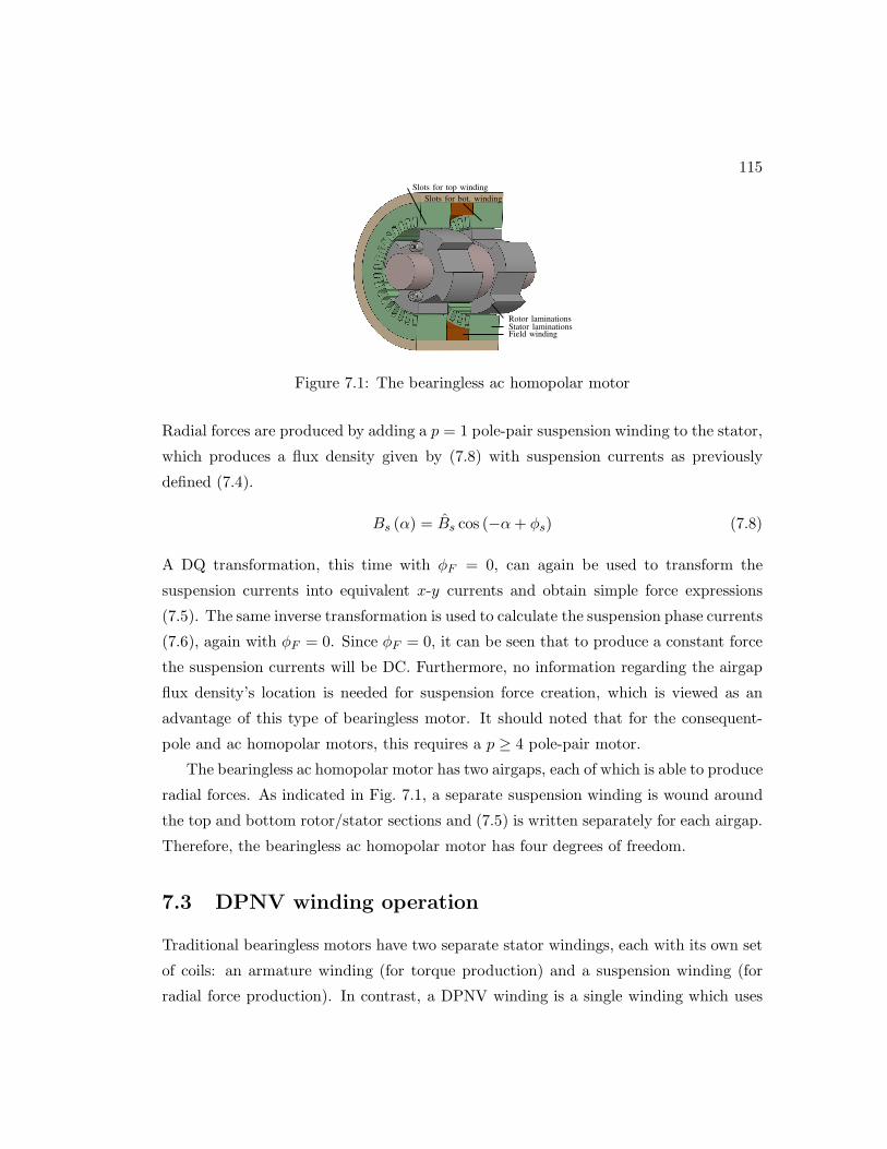
115Slots for top winding
Slots for bot. winding
Rotor laminationsStator laminationsField winding
Figure 7.1: The bearingless ac homopolar motor
Radial forces are produced by adding a p = 1 pole-pair suspension winding to the stator,
which produces a flux density given by (7.8) with suspension currents as previously
defined (7.4).
Bs (α) = Bs cos (−α+ φs) (7.8)
A DQ transformation, this time with φF = 0, can again be used to transform the
suspension currents into equivalent x-y currents and obtain simple force expressions
(7.5). The same inverse transformation is used to calculate the suspension phase currents
(7.6), again with φF = 0. Since φF = 0, it can be seen that to produce a constant force
the suspension currents will be DC. Furthermore, no information regarding the airgap
flux density’s location is needed for suspension force creation, which is viewed as an
advantage of this type of bearingless motor. It should noted that for the consequent-
pole and ac homopolar motors, this requires a p ≥ 4 pole-pair motor.
The bearingless ac homopolar motor has two airgaps, each of which is able to produce
radial forces. As indicated in Fig. 7.1, a separate suspension winding is wound around
the top and bottom rotor/stator sections and (7.5) is written separately for each airgap.
Therefore, the bearingless ac homopolar motor has four degrees of freedom.
7.3 DPNV winding operation
Traditional bearingless motors have two separate stator windings, each with its own set
of coils: an armature winding (for torque production) and a suspension winding (for
radial force production). In contrast, a DPNV winding is a single winding which uses
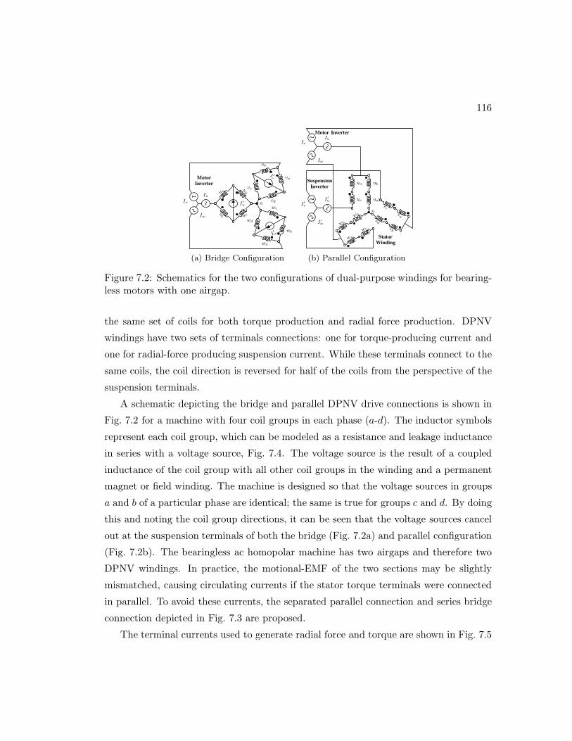
116
Iu
MotorInverter
uaud
ucub
I ′u n
vc
vb
va
vd
I ′v
Ivwc
wb
wa
wd
I′w
Iw
(a) Bridge Configuration
IuMotor Inverter
Iv
Iw
ua
uc
ub
ud
n
vb
vd
va
vc
wb
wd
wa
wc
StatorWinding
I ′u
SuspensionInverter
I ′v
I ′w
(b) Parallel Configuration
Figure 7.2: Schematics for the two configurations of dual-purpose windings for bearing-less motors with one airgap.
the same set of coils for both torque production and radial force production. DPNV
windings have two sets of terminals connections: one for torque-producing current and
one for radial-force producing suspension current. While these terminals connect to the
same coils, the coil direction is reversed for half of the coils from the perspective of the
suspension terminals.
A schematic depicting the bridge and parallel DPNV drive connections is shown in
Fig. 7.2 for a machine with four coil groups in each phase (a-d). The inductor symbols
represent each coil group, which can be modeled as a resistance and leakage inductance
in series with a voltage source, Fig. 7.4. The voltage source is the result of a coupled
inductance of the coil group with all other coil groups in the winding and a permanent
magnet or field winding. The machine is designed so that the voltage sources in groups
a and b of a particular phase are identical; the same is true for groups c and d. By doing
this and noting the coil group directions, it can be seen that the voltage sources cancel
out at the suspension terminals of both the bridge (Fig. 7.2a) and parallel configuration
(Fig. 7.2b). The bearingless ac homopolar machine has two airgaps and therefore two
DPNV windings. In practice, the motional-EMF of the two sections may be slightly
mismatched, causing circulating currents if the stator torque terminals were connected
in parallel. To avoid these currents, the separated parallel connection and series bridge
connection depicted in Fig. 7.3 are proposed.
The terminal currents used to generate radial force and torque are shown in Fig. 7.5

117
Iu
ua
uduc
u b
I ′ut vc
v bva
vdI ′vt
Iv
Motor Inverter
wc
w bwa
wdI ′wt
Iw
Top Stator Winding
Bot Stator Winding
ua
uduc
u b
I ′ub
n
vc
v bva
vdI ′vb w
c
w bwa
wdI ′wb
(a) Bridge Configuration
IuTop Motor Inverter
Iv
Iw
ua
uc
ub
ud
nt
vb
vd
va
vc
wb
wd
wa
wc
Top StatorWinding
I ′ut
TopSuspension
Inverter
I ′vt
I ′wt
IuBot. Motor Inverter
Iv
Iw
ua
uc
ub
ud
nb
vb
vd
va
vc
wb
wd
wa
wc
Bot. StatorWinding
I ′ub
Bot.Suspension
Inverter
I ′vb
I ′wb
(b) Parallel Configuration
Figure 7.3: Schematics of the two DPNV configurations applied to the bearingless achomopolar motor.
V 6 φ
Llkg
R
Figure 7.4: Coil group model
for the two types of bearingless motors connected in both parallel and bridge configu-
rations. In the parallel configuration, the suspension current terminals carry half of the
torque terminal current in addition to the required force-producing suspension current.
This is in contrast to the bridge suspension terminals, which only carries force-producing
current. The parallel configuration has a series connection to all of the coils, whereas the
bridge configuration has a parallel current path to the coils, meaning that the parallel
suspension terminals only carry half the force-producing current of the bridge suspen-
sion terminals. Differences in required current waveforms between the two types of
bearingless motors are also readily apparent, matching the discussion in Section 7.2.
Note that the shape of the terminal currents in the bridge configuration is the same
as the terminal currents for a conventional bearingless winding, which has separate
armature and suspension windings.
The current of each coil group is a superposition of the suspension and torque ter-
minal currents. Based on the amount of suspension current required, the drive must
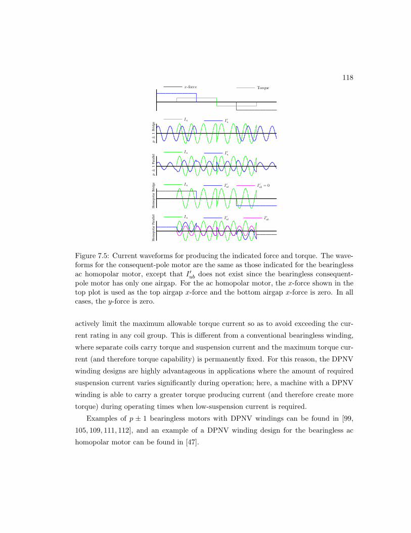
118
x-force
Torque
Iu
I ′u
Iu
I ′u
Iu
I ′ut
I ′ub = 0
Iu
I ′ut
I ′ub
p±
1B
rid
ge
p±
1P
aral
lel
Ho
mo
po
lar
Bri
dg
eH
om
op
ola
rP
aral
lel
Figure 7.5: Current waveforms for producing the indicated force and torque. The wave-forms for the consequent-pole motor are the same as those indicated for the bearinglessac homopolar motor, except that I ′ub does not exist since the bearingless consequent-pole motor has only one airgap. For the ac homopolar motor, the x-force shown in thetop plot is used as the top airgap x-force and the bottom airgap x-force is zero. In allcases, the y-force is zero.
actively limit the maximum allowable torque current so as to avoid exceeding the cur-
rent rating in any coil group. This is different from a conventional bearingless winding,
where separate coils carry torque and suspension current and the maximum torque cur-
rent (and therefore torque capability) is permanently fixed. For this reason, the DPNV
winding designs are highly advantageous in applications where the amount of required
suspension current varies significantly during operation; here, a machine with a DPNV
winding is able to carry a greater torque producing current (and therefore create more
torque) during operating times when low-suspension current is required.
Examples of p ± 1 bearingless motors with DPNV windings can be found in [99,
105, 109, 111, 112], and an example of a DPNV winding design for the bearingless ac
homopolar motor can be found in [47].
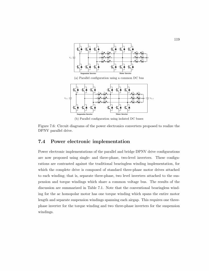
119
Vdc
uc ua
vc va
wc wa
ub ud
vb vd
wb wdn
Suspension Inverter Motor Inverter
(a) Parallel configuration using a common DC bus
Vdc,1 Vdc,2
uc ua
vc va
wc wa
ub ud
vb vd
wb wdn
Suspension Inverter Motor Inverter
(b) Parallel configuration using isolated DC buses
Figure 7.6: Circuit diagrams of the power electronics converters proposed to realize theDPNV parallel drive.
7.4 Power electronic implementation
Power electronic implementations of the parallel and bridge DPNV drive configurations
are now proposed using single- and three-phase, two-level inverters. These configu-
rations are contrasted against the traditional bearingless winding implementation, for
which the complete drive is composed of standard three-phase motor drives attached
to each winding; that is, separate three-phase, two level inverters attached to the sus-
pension and torque windings which share a common voltage bus. The results of the
discussion are summarized in Table 7.1. Note that the conventional bearingless wind-
ing for the ac homopolar motor has one torque winding which spans the entire motor
length and separate suspension windings spanning each airgap. This requires one three-
phase inverter for the torque winding and two three-phase inverters for the suspension
windings.
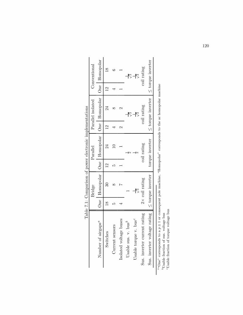
120
Tab
le7.1:
Com
parison
ofpow
erelectron
icim
plementation
s
Bridge
Parallel
Parallelisolated
Con
vention
al
Number
ofairgap
saOne
Hom
opolar
One
Hom
opolar
One
Hom
opolar
One
Hom
opolar
Switches
1830
1224
1224
1218
Currentsensors
58
510
48
46
Isolated
voltagebuses
47
11
22
11
Usable
sus.
v.busb
11 2
1 √3
1 √3
Usable
torquev.busc
1 √3
1 21 √3
1 √3
Sus.
inverter
currentrating
2×coilrating
coilrating
coilrating
coilrating
Sus.
inverter
voltagerating
≤torqueinverter
torqueinverter
≤torqueinverter
≤torqueinverter
a“One”
correspondsto
ap±
1orconsequen
tpole
mach
ine,
“Homopolar”
correspondsto
theachomopolarmach
ine
bUsable
fractionofsus.
voltagebus
cUsable
fractionoftorquevoltagebus

121
7.4.1 Parallel configuration
The parallel DPNV drive can be implemented using three-phase, two-level inverters
sharing a common voltage bus, as shown in Fig. 7.6a. For the bearingless consequent-
pole and p ± 1 pole-pair motors, this requires 12 switches. For the bearingless ac
homopolar motor, two sets of these inverter pairs are required, one for the top airgap
and one for the bottom airgap, requiring 24 switches. Care must be taken to avoid
circulating currents between the two inverters in each set. There are two primary
factors that can lead to significant circulating currents:
1) instantaneous mismatch between the applied common mode voltages at the ter-
minals of each inverter;
2) unbalanced phase impedances or the unexpected presence of a small voltage at
the suspension terminals.
Item 1) prevents the use of modulation schemes that apply different common mode
voltage when averaged over a switching period, such as the widely used Conventional
Space Vector Pulse Width Modulation (CSVPWM) which allows output phase voltages
as large as Vdc√3[113]. The Sine Triangle Comparator PWM method can be used, as it
applies a constant common mode voltage, but this limits the output phase voltage toVdc2 [113]. Since slight asymmetries in the phase impedance are inevitable and slight
variations from the “no voltage” property of the suspension winding may arise, item 2)
requires that five current sensors be used for each set of inverters so that circulating
currents can be detected and actively removed.
Alternatively, the two inverters of each set can be operated from isolated dc buses to
eliminate all concern of circulating currents, shown in Fig. 7.6b. In this configuration,
CSVPWM can be used and only four current sensors are required for each two inverter
set (two current sensors for each three-phase inverter). The suspension inverter voltage
bus can now have a different value than the torque inverter bus. This is a useful feature
because the “no voltage” property of the suspension terminals means that the suspension
inverter can utilize a lower voltage bus than the torque inverter in most designs; using
a lower bus voltage (for the same output current) results in lower suspension inverter
losses and enables the suspension inverter to use less expensive switches that have
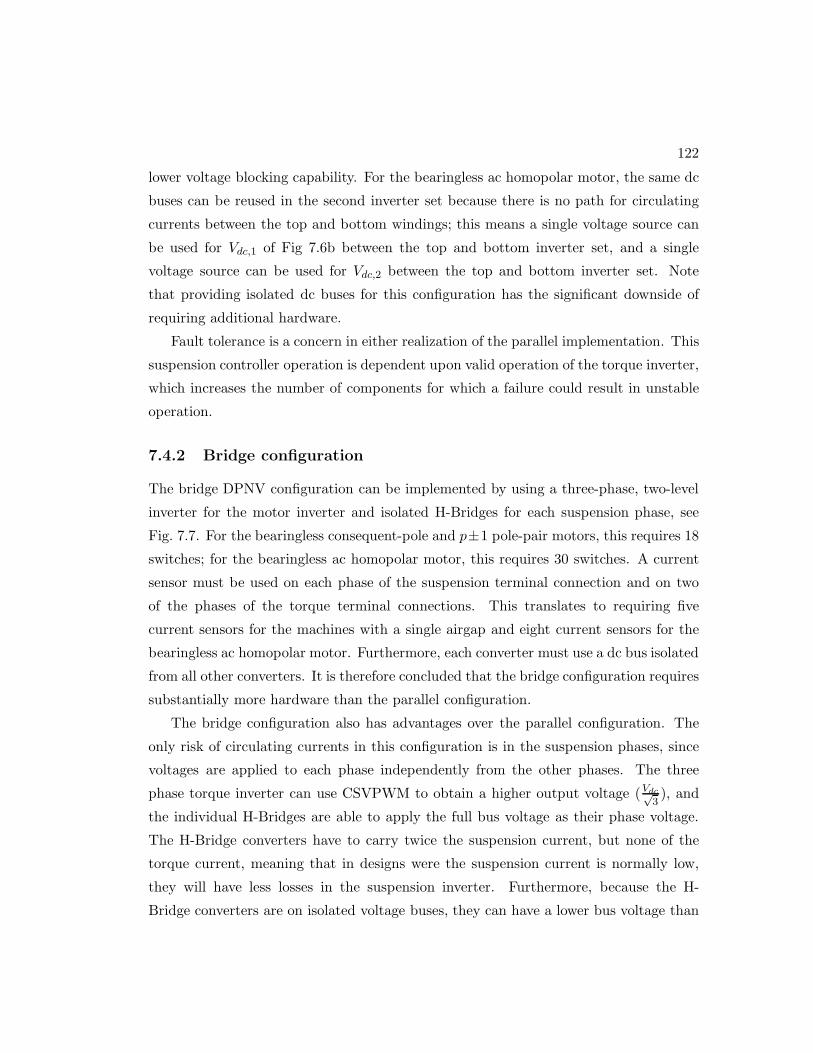
122
lower voltage blocking capability. For the bearingless ac homopolar motor, the same dc
buses can be reused in the second inverter set because there is no path for circulating
currents between the top and bottom windings; this means a single voltage source can
be used for Vdc,1 of Fig 7.6b between the top and bottom inverter set, and a single
voltage source can be used for Vdc,2 between the top and bottom inverter set. Note
that providing isolated dc buses for this configuration has the significant downside of
requiring additional hardware.
Fault tolerance is a concern in either realization of the parallel implementation. This
suspension controller operation is dependent upon valid operation of the torque inverter,
which increases the number of components for which a failure could result in unstable
operation.
7.4.2 Bridge configuration
The bridge DPNV configuration can be implemented by using a three-phase, two-level
inverter for the motor inverter and isolated H-Bridges for each suspension phase, see
Fig. 7.7. For the bearingless consequent-pole and p±1 pole-pair motors, this requires 18
switches; for the bearingless ac homopolar motor, this requires 30 switches. A current
sensor must be used on each phase of the suspension terminal connection and on two
of the phases of the torque terminal connections. This translates to requiring five
current sensors for the machines with a single airgap and eight current sensors for the
bearingless ac homopolar motor. Furthermore, each converter must use a dc bus isolated
from all other converters. It is therefore concluded that the bridge configuration requires
substantially more hardware than the parallel configuration.
The bridge configuration also has advantages over the parallel configuration. The
only risk of circulating currents in this configuration is in the suspension phases, since
voltages are applied to each phase independently from the other phases. The three
phase torque inverter can use CSVPWM to obtain a higher output voltage (Vdc√3), and
the individual H-Bridges are able to apply the full bus voltage as their phase voltage.
The H-Bridge converters have to carry twice the suspension current, but none of the
torque current, meaning that in designs were the suspension current is normally low,
they will have less losses in the suspension inverter. Furthermore, because the H-
Bridge converters are on isolated voltage buses, they can have a lower bus voltage than

123
Vdc
+
−
−
+
H-Bridge
Figure 7.7: Implementation of bridge suspension inverter
the torque inverter; this has the same advantages that were described for the isolated
implementation of the parallel drive.
In terms of fault redundancy, the bridge configuration is also at an advantage. Since
the torque inverter is completely isolated from the suspension inverter, a failure in the
torque inverter circuit or current sensor, would not impact the suspension operation.
Furthermore, utilizing isolated voltage buses for each of the H-Bridges provides more
redundancy, since a shorted-inverter would only disrupt a single suspension phase and
it is possible to provide x− y forces with two of the three phases.
7.5 Control considerations
The typical control system for a bearingless motor drive is illustrated in Fig. 7.8a.
This same implementation can be used for a bridge configured bearingless drive. In
the parallel configuration, the suspension terminals carry half of the torque current,
which must be added to the suspension current references; this is shown in Fig. 7.8b.
The blocks labeled as “PI-based motor/suspension current controller” correspond to the
vector control approach taken in motor drives [72]. The operation of the blocks labeled
as “Deterimine kf and φf” and “Determine suspension currents” correspond to the
discussion in Section 7.2, primarily (7.5); in the case of a p = 1 bearingless motor, kf is
a constant and φf = 0 which significantly simplifies these blocks. The blocks labeled as
“Convert UVW to DQ0” and “Convert DQ0 to UVW” correspond to DQ and inverse-
DQ transformations, respectively. The “PWM” blocks represent the interface to the
power electronics and the type of pulse width modulation used, which was described in
Section 7.4. For the bridge configuration suspension terminals, this corresponds to the
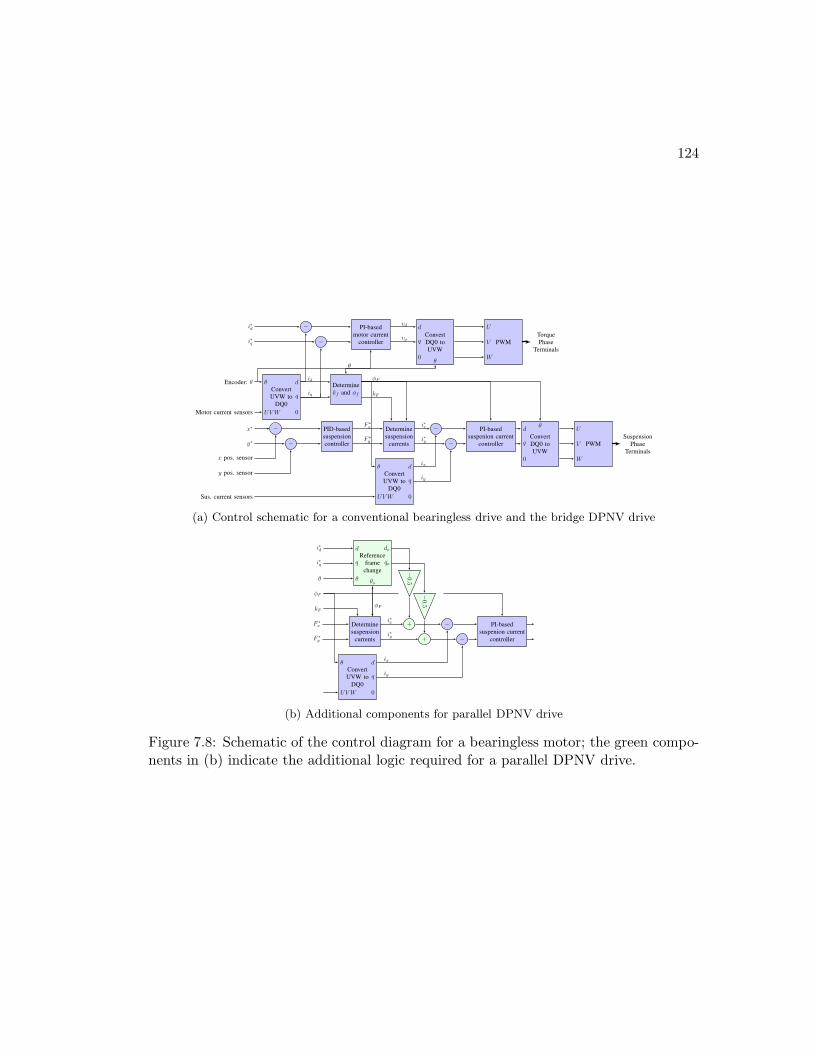
124
−
−
PI-based
motor current
controller
Convert
DQ0 to
UVW
d
q
0θ
PWM
U
V
W
−
−
PID-based
suspension
controller
Determine
suspension
currents
−
−
PI-based
suspenion current
controller
Convert
DQ0 to
UVW
d
q
0
θ
PWM
U
V
W
Convert
UVW to
DQ0
θ
UVW
d
q
0
x pos. sensor
y pos. sensor Convert
UVW to
DQ0
θ
UVW
d
q
0
Determine
kf and φf
i∗d
i∗q
vd
vqTorque
Phase
Terminals
kF
φF
x∗
y∗
F ∗x
F ∗y
i∗x
i∗ySuspension
Phase
Terminals
Encoder: θ
Motor current sensors
id
iq
θ
ix
iy
Sus. current sensors
(a) Control schematic for a conventional bearingless drive and the bridge DPNV drive
Determine
suspension
currents
Reference
frame
change
d
q
θ θo
do
qo
+
+
−0.5
−0.5
−
−
PI-based
suspenion current
controller
Convert
UVW to
DQ0
θ
UVW
d
q
0
i∗x
i∗y
φF
ix
iy
i∗d
i∗q
θ
φF
kF
F ∗x
F ∗y
(b) Additional components for parallel DPNV drive
Figure 7.8: Schematic of the control diagram for a bearingless motor; the green compo-nents in (b) indicate the additional logic required for a parallel DPNV drive.
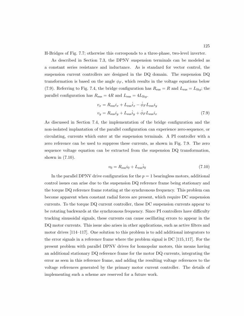
125
H-Bridges of Fig. 7.7; otherwise this corresponds to a three-phase, two-level inverter.
As described in Section 7.3, the DPNV suspension terminals can be modeled as
a constant series resistance and inductance. As is standard for vector control, the
suspension current controllers are designed in the DQ domain. The suspension DQ
transformation is based on the angle φF , which results in the voltage equations below
(7.9). Referring to Fig. 7.4, the bridge configuration has Rsus = R and Lsus = Llkg; the
parallel configuration has Rsus = 4R and Lsus = 4Llkg.
vx = Rsusix + Lsusix − φFLsusiy
vy = Rsusiy + Lsusiy + φFLsusix (7.9)
As discussed in Section 7.4, the implementation of the bridge configuration and the
non-isolated implantation of the parallel configuration can experience zero-sequence, or
circulating, currents which enter at the suspension terminals. A PI controller with a
zero reference can be used to suppress these currents, as shown in Fig. 7.9. The zero
sequence voltage equation can be extracted from the suspension DQ transformation,
shown in (7.10).
v0 = Rsusi0 + Lsusi0 (7.10)
In the parallel DPNV drive configuration for the p = 1 bearingless motors, additional
control issues can arise due to the suspension DQ reference frame being stationary and
the torque DQ reference frame rotating at the synchronous frequency. This problem can
become apparent when constant radial forces are present, which require DC suspension
currents. To the torque DQ current controller, these DC suspension currents appear to
be rotating backwards at the synchronous frequency. Since PI controllers have difficulty
tracking sinusoidal signals, these currents can cause oscillating errors to appear in the
DQ motor currents. This issue also arises in other applications, such as active filters and
motor drives [114–117]. One solution to this problem is to add additional integrators to
the error signals in a reference frame where the problem signal is DC [115,117]. For the
present problem with parallel DPNV drives for homopolar motors, this means having
an additional stationary DQ reference frame for the motor DQ currents, integrating the
error as seen in this reference frame, and adding the resulting voltage references to the
voltage references generated by the primary motor current controller. The details of
implementing such a scheme are reserved for a future work.
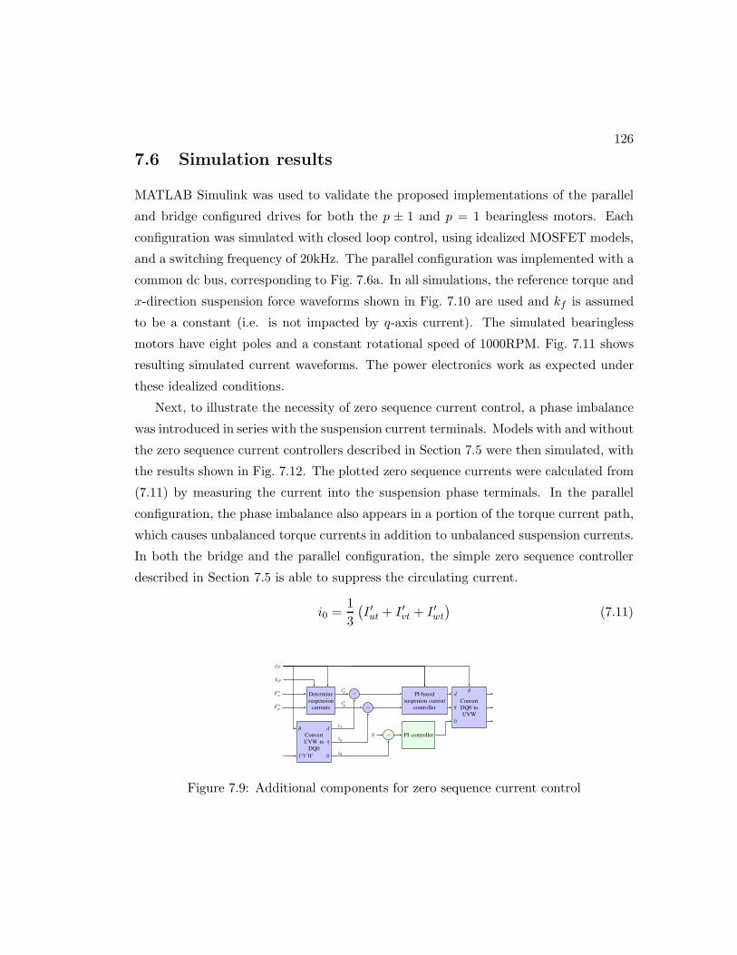
126
7.6 Simulation results
MATLAB Simulink was used to validate the proposed implementations of the parallel
and bridge configured drives for both the p ± 1 and p = 1 bearingless motors. Each
configuration was simulated with closed loop control, using idealized MOSFET models,
and a switching frequency of 20kHz. The parallel configuration was implemented with a
common dc bus, corresponding to Fig. 7.6a. In all simulations, the reference torque and
x-direction suspension force waveforms shown in Fig. 7.10 are used and kf is assumed
to be a constant (i.e. is not impacted by q-axis current). The simulated bearingless
motors have eight poles and a constant rotational speed of 1000RPM. Fig. 7.11 shows
resulting simulated current waveforms. The power electronics work as expected under
these idealized conditions.
Next, to illustrate the necessity of zero sequence current control, a phase imbalance
was introduced in series with the suspension current terminals. Models with and without
the zero sequence current controllers described in Section 7.5 were then simulated, with
the results shown in Fig. 7.12. The plotted zero sequence currents were calculated from
(7.11) by measuring the current into the suspension phase terminals. In the parallel
configuration, the phase imbalance also appears in a portion of the torque current path,
which causes unbalanced torque currents in addition to unbalanced suspension currents.
In both the bridge and the parallel configuration, the simple zero sequence controller
described in Section 7.5 is able to suppress the circulating current.
i0 =1
3
(
I ′ut + I ′vt + I ′wt)
(7.11)
Determine
suspension
currents
−
−
− PI controller
PI-based
suspenion current
controller
Convert
DQ0 to
UVW
d
q
0
θ
Convert
UVW to
DQ0
θ
UVW
d
q
0
i∗x
i∗y
ix
iy
i0
φF
kF
F ∗x
F ∗y
0
Figure 7.9: Additional components for zero sequence current control

127
0 0.025 0.05 0.075 0.1 0.125 0.15
0
seconds
x-force
Torque
Figure 7.10: Simulation reference waveforms
7.7 Conclusion
This chapter investigated the power electronics used to implement drives for machines
with DPNV windings. A comparison between the hardware requirements of the parallel
and bridge DPNV drives and the conventional bearingless drive was presented as well
as simulation results. Hardware results are presented later, in Chapter 8.
It was shown in the chapter that there are advantages and disadvantages to each of
the DPNV drive configurations. The parallel configuration requires the least hardware
components, but has less fault tolerance and more complex control requirements due
to potential interactions between the torque and suspension inverters. Neither config-
uration can be realized in as few components as a standard bearingless motor drive,
meaning that the DPNV drives will have a higher cost. This must be weighed against
the potential increase in bearingless machine performance when deciding whether to
design a bearingless motor with a DPNV winding.
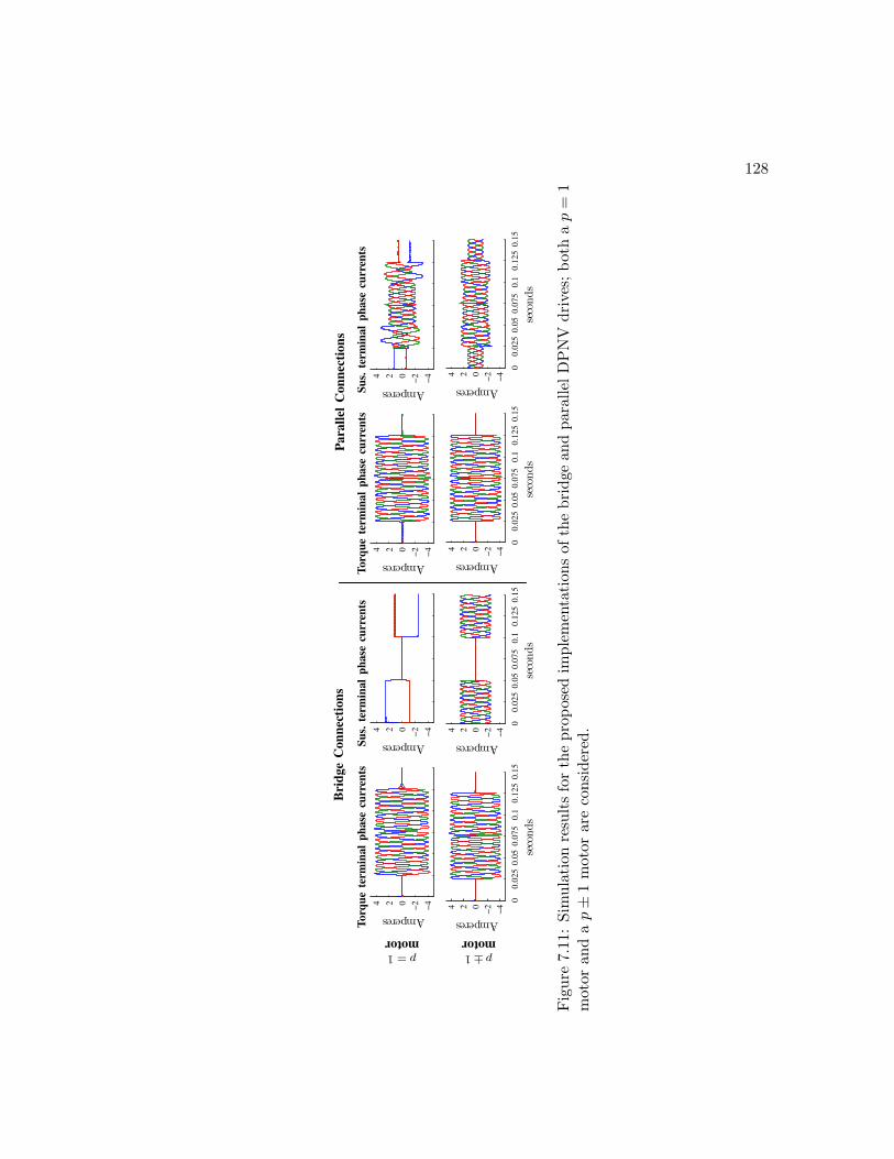
128
−4
−2024
Amperes
−4
−2024
Amperes
−4
−2024
Amperes
−4
−2024
Amperes
00.0
25
0.0
50.0
75
0.1
0.1
25
0.1
5
−4
−2024
Amperes
seconds
00.0
25
0.0
50.0
75
0.1
0.1
25
0.1
5
−4
−2024
Amperes
seconds
00.0
25
0.0
50.0
75
0.1
0.1
25
0.1
5
−4
−2024
Amperes
seconds
00.0
25
0.0
50.0
75
0.1
0.1
25
0.1
5
−4
−2024
Amperes
seconds
Torq
ue
term
inal
ph
ase
curr
ents
Su
s.te
rmin
al
ph
ase
curr
ents
Torq
ue
term
inal
ph
ase
curr
ents
Su
s.te
rmin
al
ph
ase
curr
ents
p=1motor
p±1motor
Bri
dge
Con
nec
tion
sP
ara
llel
Con
nec
tion
s
Figure
7.11:Sim
ulation
resultsfortheproposed
implementation
sof
thebridge
andparallelDPNV
drives;bothap=
1motor
andap±
1motor
areconsidered
.
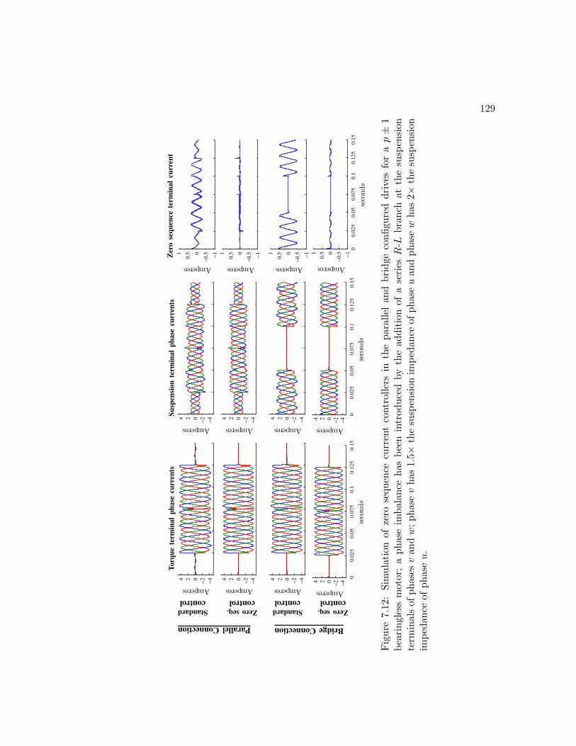
129
−4
−2024
Amperes
−4
−2024
Amperes
−4
−2024
Amperes
−4
−2024
Amperes
−1
−0.50
0.51
Amperes
−1
−0.50
0.51
Amperes
−4
−2024
Amperes
00.0
25
0.0
50.0
75
0.1
0.1
25
0.1
5
−4
−2024
Amperes
seconds
−4
−2024
Amperes
00.0
25
0.0
50.0
75
0.1
0.1
25
0.1
5
−4
−2024
Amperes
seconds
−1
−0.50
0.51
Amperes
00.0
25
0.0
50.0
75
0.1
0.1
25
0.1
5−
1
−0.50
0.51
Amperes
seconds
Torq
ue
term
inal
ph
ase
curr
ents
Su
spen
sion
term
inal
ph
ase
curr
ents
Zer
ose
qu
ence
term
inal
curr
ent
Standard
controlZeroseq.
controlStandard
controlZeroseq.
control
ParallelConnection BridgeConnection
Figure
7.12:Sim
ulation
ofzero
sequen
cecu
rrentcontrollers
intheparallelan
dbridge
configu
reddrivesforap±
1bearinglessmotor;aphaseim
balan
cehas
beenintroducedbythead
ditionof
aseriesR-L
branch
atthesuspen
sion
term
inalsof
phasesvan
dw;phasevhas
1.5×
thesuspen
sion
imped
ance
ofphaseuan
dphasew
has
2×thesuspen
sion
imped
ance
ofphaseu.
Chapter 8
Bearingless Prototype Design and
Experimental Results
8.1 Introduction
The design of various components of the prototype bearingless ac homopolar machine
and the drive system used to operate it are now described. Experimental results are pre-
sented in this chapter to characterize the machine and validate the concepts developed
in previous chapters.
The final prototype machine is shown in Fig. 8.1, the power electronics are shown
in Fig. 8.2, and the control hardware is shown in Fig. 8.3. The power electronic invert-
ers use silicon carbide (SiC) MOSFETs so that they can operate at a high switching
frequency. This enables faster control operation and bandwidth and ultimately better
machine performance than would be possible with the switching frequencies achievable
with IGBTs. The design and characterization of the individual half-bridge circuits that
are connected to make up these inverters has been published in [118].
Despite the dissertation’s interest in developing an outer-rotor bearingless ac ho-
mopolar motor for flywheel energy storage, an inner-rotor topology has been used. This
was done for ease of testing, as inner-rotor machines are standard and existing products
were more easily purchased to construct the test stand. The concepts developed in this
dissertation apply to both the inner- and outer-rotor topologies and the purpose of this
prototype is to simply validate these concepts. The ac homopolar machine geometry is
130
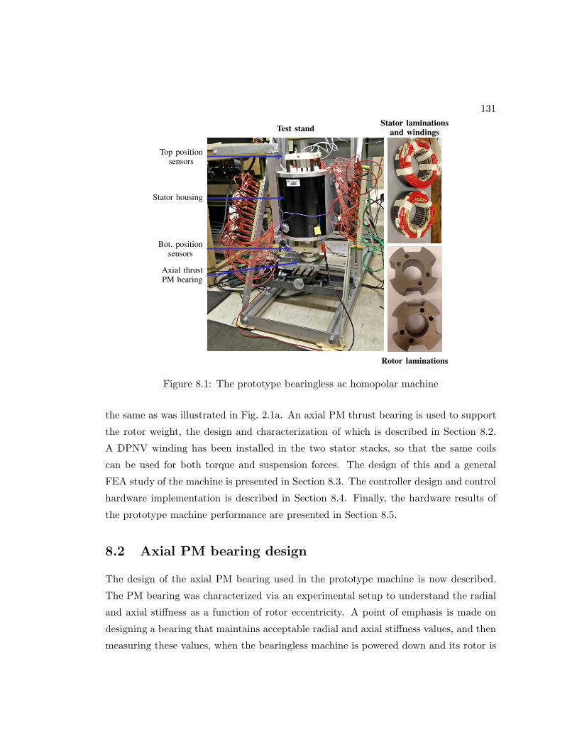
131
Top positionsensors
Stator housing
Bot. positionsensors
Axial thrustPM bearing
Test standStator laminations
and windings
Rotor laminations
Figure 8.1: The prototype bearingless ac homopolar machine
the same as was illustrated in Fig. 2.1a. An axial PM thrust bearing is used to support
the rotor weight, the design and characterization of which is described in Section 8.2.
A DPNV winding has been installed in the two stator stacks, so that the same coils
can be used for both torque and suspension forces. The design of this and a general
FEA study of the machine is presented in Section 8.3. The controller design and control
hardware implementation is described in Section 8.4. Finally, the hardware results of
the prototype machine performance are presented in Section 8.5.
8.2 Axial PM bearing design
The design of the axial PM bearing used in the prototype machine is now described.
The PM bearing was characterized via an experimental setup to understand the radial
and axial stiffness as a function of rotor eccentricity. A point of emphasis is made on
designing a bearing that maintains acceptable radial and axial stiffness values, and then
measuring these values, when the bearingless machine is powered down and its rotor is

132
Current measurementcircuit boards
Common modechokes
Power electronicinverters
(a) Power electronics cabinet
(b) SiC-based Inverter
Figure 8.2: The power electronic drive

133
ZedBoard
Data businterface
Custom FPGAcircuit board
ADC connections tocur. and pos. sensors
PWM connections
Figure 8.3: The drive control hardware
highly eccentric. A literature review of bearing characterization techniques is presented
along with a description of the characterization procedure used and the characterization
results.1
8.2.1 Design
The axial bearing design is based around a simple repulsive ring bearing, as depicted in
Fig. 8.4. The design was conducted using FEA, with the design goals of minimizing the
radial unstabilizing forces and changes in the axial forces when the rotor is fully eccentric
(resting upon its touchdown bearings) and minimizing the design cost by reducing the
magnet volume. The bearing stator consists of an axially magnetized ring magnet glued
to an aluminum yoke; the rotor consists of an axially magnetized ring magnet glued to
an aluminum sleeve which is secured to the bottom of the bearingless motor’s rotor
shaft.
The bearing design space is explored through 2D and 3D FE simulations in Fig. 8.5.
The rotor weight, desired airgap, and magnet material properties are design constants
1 Portions of this material have also been published in [53].
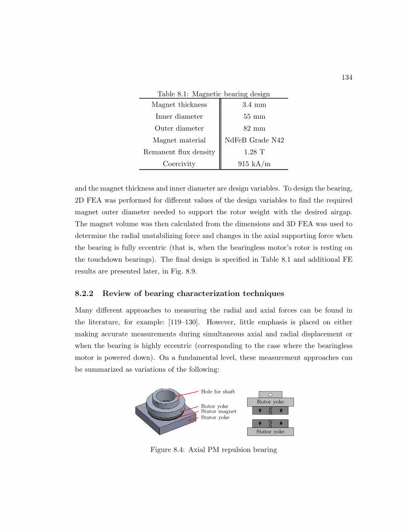
134
Table 8.1: Magnetic bearing design
Magnet thickness 3.4 mm
Inner diameter 55 mm
Outer diameter 82 mm
Magnet material NdFeB Grade N42
Remanent flux density 1.28 T
Coercivity 915 kA/m
and the magnet thickness and inner diameter are design variables. To design the bearing,
2D FEA was performed for different values of the design variables to find the required
magnet outer diameter needed to support the rotor weight with the desired airgap.
The magnet volume was then calculated from the dimensions and 3D FEA was used to
determine the radial unstabilizing force and changes in the axial supporting force when
the bearing is fully eccentric (that is, when the bearingless motor’s rotor is resting on
the touchdown bearings). The final design is specified in Table 8.1 and additional FE
results are presented later, in Fig. 8.9.
8.2.2 Review of bearing characterization techniques
Many different approaches to measuring the radial and axial forces can be found in
the literature, for example: [119–130]. However, little emphasis is placed on either
making accurate measurements during simultaneous axial and radial displacement or
when the bearing is highly eccentric (corresponding to the case where the bearingless
motor is powered down). On a fundamental level, these measurement approaches can
be summarized as variations of the following:
Hole for shaft
Rotor yokeStator magnetStator yoke
SN
SN
Stator yoke
Rotor yoke
Figure 8.4: Axial PM repulsion bearing
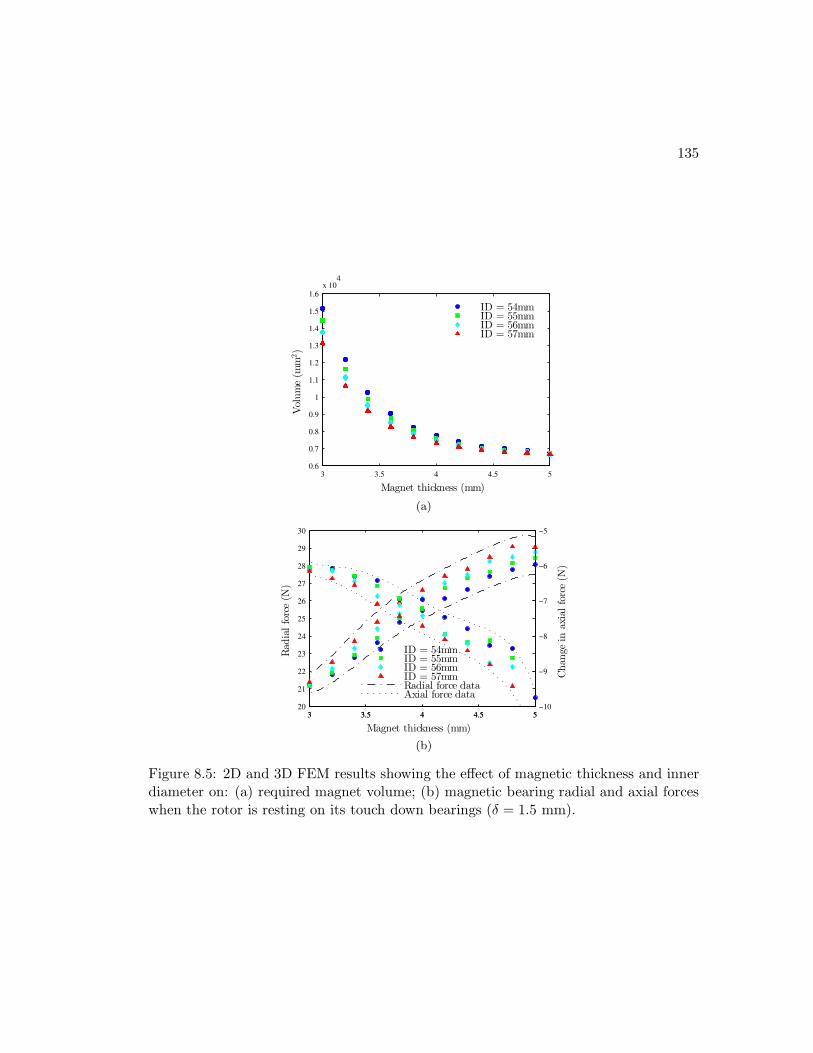
135
3 3.5 4 4.5 50.6
0.7
0.8
0.9
1
1.1
1.2
1.3
1.4
1.5
1.6x 10
4
Magnet thickness (mm)
Volume(m
m2)
ID = 54mmID = 55mmID = 56mmID = 57mm
(a)
3 3.5 4 4.5 520
21
22
23
24
25
26
27
28
29
30
Magnet thickness (mm)
Rad
ialforce(N
)
3 3.5 4 4.5 5−10
−9
−8
−7
−6
−5
Chan
gein
axialforce(N
)
ID = 54mmID = 55mmID = 56mmID = 57mmRadial force dataAxial force data
(b)
Figure 8.5: 2D and 3D FEM results showing the effect of magnetic thickness and innerdiameter on: (a) required magnet volume; (b) magnetic bearing radial and axial forceswhen the rotor is resting on its touch down bearings (δ = 1.5 mm).
136
• the rotor and stator are somehow mechanically displaced from each other and a
device (such as a load cell) is used to measure the force along that direction for
various displacements [119–121,125,128–130];
• a known force (i.e. a weight) is applied to the rotor along an axis and the dis-
placement is measured for various forces; this will only work in cases where the
magnetic bearing is stable in the displacement direction [119,123,125,130].
There are also several different approaches to measuring the radial/axial stiffness, most
of which can be summarized as variations of the following:
• extract the stiffness from the force data by fitting a linear regression line to the data
as a function of displacement for small displacements [119,120,122,125,128,130];
• excite the rotor with an impact hammer and observe the rotor’s frequency response
[122,129].
A common variation on the above techniques is used in [122] for measuring radial
stiffness (axial stiffness is measured via the impact hammer test). Here, a consequent-
pole bearingless motor is considered with a PM axial bearing. To measure the radial
stiffness, the bearingless motor suspension force characteristic is first measured: kf of
the linearized magnetic bearing force model (8.1) is calculated by using the magnetic
bearing controller to keep the rotor centered (fixing δ = 0 mm), applying a radial force
to the rotor, and measuring the required suspension current, is.
F (δ, is) = −ksδ + kf is (8.1)
Next, the controller is used to displace the rotor radially to a small value of δ. When
the rotor is in equilibrium, F (δ, is) = 0 and the radial stiffness is measured: ks = kf is/δ
with and without the PM bearing connected. While this is a very low-cost approach,
there are two potential problems that must be carefully addressed on a per-device basis
to ensure accurate results:
• the force model of (8.1) is typically only a linear approximation of the radial
force’s dependence on displacement; it is therefore only accurate for sufficiently
small values of δ and it doesn’t account for axial displacement;
137
• as is noted in [58], the radial suspension force of the bearingless motor can vary
to a limited extent as a function of the rotor’s angular position, so if the rotor
were to rotate between the time that the suspension force was characterized and
the stiffness was measured, inaccurate results would be obtained.
Another variation is used in [130]. Here, the machine’s rotor is displaced to several
small values of δ by the controller. For each value, radial forces are applied to the
rotor and the suspension current is measured while the controller keeps the displace-
ment fixed. The bearing stiffness is approximated by dividing the difference in applied
force for a given suspension current at two different displacements by the difference
in displacement. Again, this suffers from the same potential inaccuracies as mentioned
before. However, it is found that the method is sufficiently accurate for the device being
considered in [130] under very small displacements.
Neither of the aforementioned variations are likely to provide acceptable radial stiff-
ness measurements for large displacements in either the radial or axial direction and
therefore are unlikely to accurately characterize the PM bearing when the bearingless
machine is powered down and the rotor is fully displaced. In [120], a force measurement
procedure is described which should be capable of accurately measuring radial/axial
forces as a function of both radial and axial displacement. Here, the stator is connected
to a load cell capable of measuring forces in three dimensions. An automated 3D x-y-z
cross-table is used to move the stator and rotor with respect to each other. While radial
and axial force results are only reported for displacements along their respective axes,
it appears that this setup could be used to accurately measure forces along both axes.
However, such equipment was not available and is considerably more expensive than
the equipment required for the measurement which was used.
8.2.3 Measurement technique used
To characterize the PM bearing, the test stand depicted in Fig. 8.6 and Fig. 8.7 was
built. The rotor is fixed radially but is free to move axially. This is accomplished by
mounting two brass sliding bearings on the housing of the bearingless motor. The PM
bearing stator is restricted axially and movements in the radial direction are controlled
by a manual x-y cross-table. The connection to the cross-table is through single-axis

138
CrosspieceBearing statorBearing rotor
Bearingless motor
Dial indicator
(a) Full test stand
Brass slide
x load cell
Axial load cell
Cross-table
(b) Measurement apparatus
Ball transfer units
(c) Test stand bottom
Figure 8.6: Photographs of (a) the full test stand; (b) the measurement apparatus; and(c) the bottom of the test stand with the PM bearing and radial load cells removed.
load cells. An “x” and a “y” load cell are each connected to a side of the bearing stator
through universal joint linkages. The universal joint linkages are used instead of bolts
to decrease any cross-talk between the sensors, as they only support forces along their
axes. The PM bearing stator rests axially against eight ball transfer units which have
been installed in the crosspiece and are shown in Fig. 8.6c. The ball transfer units
prevent friction between the bearing stator and the crosspiece that could interfere with
radial force measurement. The radial force sensors are also mounted to this crosspiece
and the entire apparatus is centered on top of another single-axis load cell for axial force
measurements.
The rotor can be displaced axially by placing weights upon it (see the basket on

139
Crosspiece
Bearing stator
Universal joint linkagex load cell
Axial load cell
Cross-table
Figure 8.7: Drawing of measurement apparatus
the top of Fig. 8.6a) while the stator can be displaced radially by adjusting the x-y
cross-table. Since the brass sliding bearings have some axial friction, the value of the
weights added to the top of the rotor are ignored and instead the axial load cell is used
to measure the axial force that the bearing provides. The rotor’s axial displacement is
measured via a dial indicator while the x-y cross-table is able to accurately position the
stator to within 0.025 mm.
All measurements are taken with the bearingless homopolar machine completely
powered down.
8.2.4 Results
Radial and axial force measurements are shown in Fig. 8.8 and 8.9. The airgap between
the PM bearing and stator was measured at being 2.55 mm nominally, which, as can be
seen in Fig. 8.8a, matches the FE simulations. The radial and axial stiffness values about
the nominal positions were calculated from linear regression lines fit to the data and
shown in Fig. 8.8a and 8.8b. These stiffness values are given in Table 8.2. Note that the
measured radial stiffness value is approximately 4% greater than the FEA calculation
and the measured axial stiffness is approximately 3% greater than the FEA calculation.
Earnshaw’s theorem predicts that for an axially symmetric magnetic bearing without
iron, the axial stiffness should be twice the radial stiffness [131, 132]. The FE results
satisfy this exactly and the small discrepancy in the measured results can be explained
by measurement uncertainty, as discussed later.
The radial and axial force measurements as a function of both radial and axial
displacement are shown in Fig. 8.9a and 8.9b. The range of radial displacement is

140
0 0.5 1 1.5 2120
140
160
180
200
220
240
Axial displacement (mm)
Axial
force(N
)
Measurement
Measurement stiffness regression line
2D FEM result
FEM stiffness regression line
(a) Axial stiffness
0 0.5 1 1.5
0
5
10
15
20
25
Radial displacement (mm)
Rad
ialforce(N
)
Measurement
Measurement stiffness regression line
3D FEM result
FEM stiffness regression line
(b) Radial stiffness
Figure 8.8: Axial and radial force measurements under 1D displacement: (a) Axialforce measurements when the rotor is centered; (b) radial force measurements when theairgap is at its nominal value.
Table 8.2: Stiffness results
Parametera Measured FEM Result
Radial Stiffness (N/mm) 16.8 16.2
Axial Stiffness (N/mm) 33.3 32.4
aAll stiffness values are reported about the nominal position and are taken as the slope of theregression lines shown in Fig. 8.9

141
−1.5−1
−0.50
0.51
1.5
0
0.25
0.5
0.75
1
0
10
20
30
40
Radial di
splacemen
t (mm)
Axial displacement (mm)
Rad
ialforcemagnitude(N
)
(a) Radial force measurements
−1.5−1
−0.50
0.51
1.5
0
0.25
0.5
0.75
1
120
125
130
135
140
145
150
155
Radial di
splacemen
t (mm)
Axial displacement (mm)Axial
force(N
)
(b) Axial force measurements
−1.5−1
−0.50
0.51
1.5
0
0.25
0.5
0.75
1
0
10
20
30
40
Radial dis
placement
(mm)
Axial displacement (mm)
Rad
ialforcemagnitude(N
)
(c) Radial force FEM results
−1.5−1
−0.50
0.51
1.5
0
0.25
0.5
0.75
1
120
125
130
135
140
145
150
155
Radial di
splacemen
t (mm)
Axial displacement (mm)
Axial
force(N
)
(d) Axial force FEM results
Figure 8.9: Comparison of hardware and FEA results: (a) radial force measurementsunder both axial and radial displacement; (b) axial force measurements under both axialand radial displacement; (c) 3D FEM results for radial forces and (d) 3D FEM resultsfor axial forces under the same displacements as in a) and b); note that positive valuesof axial displacement indicate a smaller airgap.

142
selected to be -1.5 mm to 1.5 mm to include the displacement when the bearingless
ac homopolar machine is powered down and the shaft is resting upon the touchdown
bearings. Fig. 8.9c and 8.9d show FEA results for the same displacements.
Repeatability
To assess the repeatability of the radial force measurements, the radial force data shown
in Fig. 8.8b was collected eight times for each radial offset. The standard deviation in
measurement data at each radial displacement is calculated. The average of these values
is 0.4 N and all standard deviations are within 0.1 N of this. For radial displacements
greater than 0.5 mm, the average standard deviation was 2.1% of the average force
measured.
Assessing the repeatability of the axial force measurements is more challenging.
Since the brass slides exert a frictional force on the rotor shaft, both the axial displace-
ment and axial force differed between measurements for the same weight being placed
upon the shaft. Therefore, it is not possible to compare force variation for the same
axial displacement. Instead, it was observed from FEA that a quadratic polynomial
accurately fit the axial force dependence upon axial displacement. The measured data
shown in Fig. 8.8a were fit to a quadratic polynomial using the least squares method and
the force difference between each measured data point and the value predicted by the
polynomial was calculated and normalized by the value predicted by the polynomial.
The average of the normalized error magnitudes is 0.9%.
The repeatability for both radial and axial forces are considered to be very good
and any significant measurement error should be due to a systemic bias.
Systemic errors
There were two primary sources for systemic bias error observed in the measurements.
The first is that the airgap between the PM bearing and stator was not completely
parallel. It was measured at being 2.55 mm nominally and, despite efforts to mount
the two surfaces perfectly parallel, there was a deviation of approximately 0.05 mm
measured. Finite element simulations results showed that this could lead to a maximum
difference in force measurements of 0.9 N over all values of axial and radial displacements
tested, which was deemed acceptable. The finite element simulations predicted that for
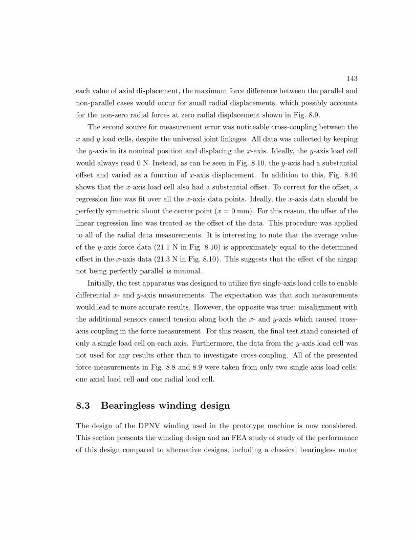
143
each value of axial displacement, the maximum force difference between the parallel and
non-parallel cases would occur for small radial displacements, which possibly accounts
for the non-zero radial forces at zero radial displacement shown in Fig. 8.9.
The second source for measurement error was noticeable cross-coupling between the
x and y load cells, despite the universal joint linkages. All data was collected by keeping
the y-axis in its nominal position and displacing the x-axis. Ideally, the y-axis load cell
would always read 0 N. Instead, as can be seen in Fig. 8.10, the y-axis had a substantial
offset and varied as a function of x-axis displacement. In addition to this, Fig. 8.10
shows that the x-axis load cell also had a substantial offset. To correct for the offset, a
regression line was fit over all the x-axis data points. Ideally, the x-axis data should be
perfectly symmetric about the center point (x = 0 mm). For this reason, the offset of the
linear regression line was treated as the offset of the data. This procedure was applied
to all of the radial data measurements. It is interesting to note that the average value
of the y-axis force data (21.1 N in Fig. 8.10) is approximately equal to the determined
offset in the x-axis data (21.3 N in Fig. 8.10). This suggests that the effect of the airgap
not being perfectly parallel is minimal.
Initially, the test apparatus was designed to utilize five single-axis load cells to enable
differential x- and y-axis measurements. The expectation was that such measurements
would lead to more accurate results. However, the opposite was true: misalignment with
the additional sensors caused tension along both the x- and y-axis which caused cross-
axis coupling in the force measurement. For this reason, the final test stand consisted of
only a single load cell on each axis. Furthermore, the data from the y-axis load cell was
not used for any results other than to investigate cross-coupling. All of the presented
force measurements in Fig. 8.8 and 8.9 were taken from only two single-axis load cells:
one axial load cell and one radial load cell.
8.3 Bearingless winding design
The design of the DPNV winding used in the prototype machine is now considered.
This section presents the winding design and an FEA study of study of the performance
of this design compared to alternative designs, including a classical bearingless motor
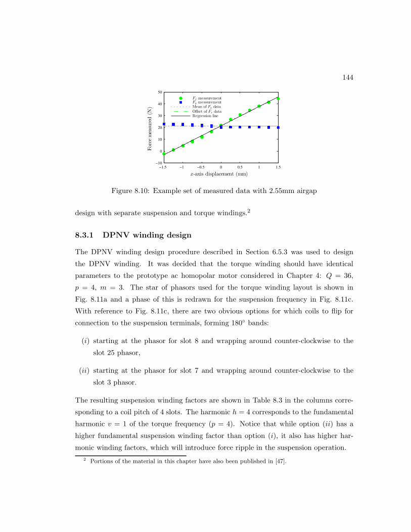
144
−1.5 −1 −0.5 0 0.5 1 1.5−10
0
10
20
30
40
50
x-axis displacement (mm)
Force
measured(N
)
Fx measurementFy measurementMean of Fy dataOffset of Fx dataRegression line
Figure 8.10: Example set of measured data with 2.55mm airgap
design with separate suspension and torque windings.2
8.3.1 DPNV winding design
The DPNV winding design procedure described in Section 6.5.3 was used to design
the DPNV winding. It was decided that the torque winding should have identical
parameters to the prototype ac homopolar motor considered in Chapter 4: Q = 36,
p = 4, m = 3. The star of phasors used for the torque winding layout is shown in
Fig. 8.11a and a phase of this is redrawn for the suspension frequency in Fig. 8.11c.
With reference to Fig. 8.11c, there are two obvious options for which coils to flip for
connection to the suspension terminals, forming 180 bands:
(i) starting at the phasor for slot 8 and wrapping around counter-clockwise to the
slot 25 phasor,
(ii) starting at the phasor for slot 7 and wrapping around counter-clockwise to the
slot 3 phasor.
The resulting suspension winding factors are shown in Table 8.3 in the columns corre-
sponding to a coil pitch of 4 slots. The harmonic h = 4 corresponds to the fundamental
harmonic v = 1 of the torque frequency (p = 4). Notice that while option (ii) has a
higher fundamental suspension winding factor than option (i), it also has higher har-
monic winding factors, which will introduce force ripple in the suspension operation.
2 Portions of the material in this chapter have also been published in [47].

145
+u
-w
+v
-u
+w
-v
7
8
910
11
12
13
14
15
16
17
1819
20
21
22
23
24
25
26
27
28
29
30
31 32
33
34
35
36
1
2
3
4 5
6
(a) Torque phasor star
-12-21
-30-3
7 16
25 34
81726
35
(b) Torque phase uconn. star
7
26
-12
34
35
-21
8
-30
16
17
-3
25
(c) Torque phase u conn.star drawn for h = ps
7
26
-12
34
35
-21
8
-30
16
17
-3
25
(d) Torque phase u conn.star drawn for h = 5
Figure 8.11: Phasor diagrams for the example Q = 36, p = 4, m = 3 design; (a) torquewinding layout using 60 phase belts; (b) phase u at the torque frequency; (c) phase u atthe suspension frequency; (d) phase u at the 5th harmonic of the suspension frequency;dashed phasors correspond to coils whose direction is reversed when connected to thesuspension terminals
146
To understand the importance of suspension winding factors on force ripple, refer
back to the radial force calculations in Chapter 2. In summary, the Maxwell Stress Ten-
sor is used to calculate radial forces which result from the interaction of the suspension
field and the magnetizing field:
gu (α, θ) =1
h1+h2f(p[α−θ])) (8.2)
gl (α, θ) =1
h1+h2f(p[α−θ]+π)) (8.3)
Bψ (α, θ) = µ0Fψ
gψ (α, θ)(8.4)
where the subscript ψ is set to u or l to indicate the top or bottom airgap and Frepresents an MMF. The airgap flux density will contain the harmonics of each MMF
as well as plus or minus the harmonics contained in the effective airgap length function
f (φ) of (8.2). The interaction between the first 11 suspension MMF harmonics and the
magnetizing and torque flux density harmonics is summarized in Table 8.4 for the simple
case where the effective airgap length function is given by f (φ) = cosφ. The interacting
harmonic index of the magnetizing or torque flux density is written as “(v = ..)” where
v indicates the harmonic of the torque frequency. Harmonics are crossed out which do
not exist in this configuration (for example, triplen harmonics, since the phase currents
sum to zero, and even suspension harmonics). The first row of the table is the only row
that corresponds to a radial force which does not vary with rotor position: the existence
of any other row is undesirable. It can be concluded that the most important winding
factor to minimize for force ripple is h = 5 since it is the only harmonic to interact
with main components of both the magnetizing and the torque armature reaction flux
density. This harmonic is particularly difficult to deal with because it is near the p = 4
torque frequency, meaning that the pitching factor at h = 5 is relatively large. For
a fixed coil pitch, the only way to minimize this suspension winding factor is by the
winding distribution factor; that is, by selecting the coil direction in design step 2 in
a way that minimizes this harmonic. The results can be visualized in a phasor star
diagram drawn at this frequency, see Fig. 8.11d.
Table 8.3 shows that the suspension winding factors have low values, meaning that
current is used inefficiently. This is largely the result of the coil pitch, which was
selected for the torque winding design and is therefore extremely short at the suspension
frequency. Increasing the coil pitch will result in better suspension winding factor.

147
Table 8.3: Example design suspension winding factors
4 slot coil pitch 5 slot coil pitch
h winding i winding ii winding i winding ii
1 0.204 0.225 0.252 0.278
3 0.000 0.289 0.000 0.322
5 0.204 0.305 0.170 0.253
7 0.204 0.371 0.027 0.050
9 0.000 0.000 0.500 0.373
11 0.204 0.126 0.316 0.196
Table 8.4: Harmonics leading to force ripple
Sus. MMF Harmonic Interacting Torque Flux Density Harmonic
h h h− 4 h+ 4
1 v = 0 v = 1 v = 1
2 - - -
3 - - -
4 - - -
5 v = 1 v = 0 v = 2
6 - - -
7 v = 2 v = 1 v = 3
8 - - -
9 - - -
10 - - -
11 v = 3 v = 2 v = 4
148
However, this must be done with caution, as it may lead to an inferior torque winding
in terms of winding factor, conduction losses, and end-effects. In this particular example
with q = 3/2, a full pitch coil would be y = mq = 4.5 slots. This is typically rounded
down to 4 slots to obtain shorter coils. However, if this were rounded up to 5 slots, the
suspension winding factors would be improved considerably while the torque winding
factors would remain the same, as shown in Table 8.3.
The winding design option (i) with a 4-slot pitch was built for the prototype ma-
chine. The layout schematic and MMF diagrams are depicted in Fig. 8.12 alongside an
example of an alternate, conventional bearingless winding design which is considered
in Section 8.3.3. The prototype machine uses separate, identical windings on top and
bottom stator stacks that sandwich the field winding to provide 4-axis control of the
rotor’s position. The remaining machine parameters of the constructed prototype are
specified in Table 8.5.
8.3.2 FEA study of the DPNV winding design
FEA has been conducted on the prototype design for two different DPNV windings, the
4 and 5 slot coil pitch variants of winding i in Table 8.3 (the layout for the former case,
which was used in the prototype machine, is depicted in Fig. 8.12b). Two different rotor
structures representing lower and upper bounds on the harmonic content of the effective
airgap length have been considered: one with an inverted sinusoidal airgap length and
one with a square airgap length, where f (φ) of (8.2) is cosφ and SQ (φ) respectively.
This winding design can be interfaced to either the bridge or parallel style of drive. All
simulations have been solved on static, non-linear 3D models using Infolytica’s MagNet
software, shown in Fig. 8.13a. The machine parameters and ratings are summarized in
Table 8.5. The B-H curves used for the laminations and the solid steel are the same as
what was previously depicted in Fig. 4.6.
First, the rated coil current is used to create an x-directed suspension force in the top
rotor/stator section while no torque current is used. The resulting force and terminal
current waveforms are shown in Fig. 8.14a. In the parallel configuration the suspension
terminal has a series connection to all coil groups, whereas in the bridge configuration
there are two parallel branches; therefore, to obtain the rated coil current, the bridge
configuration’s suspension terminals carry twice the current of the parallel configuration.

149
Slot
12
34
56
78
910
11
12
13
14
15
16
17
18
19
20
21
22
23
24
25
26
27
28
29
30
31
32
33
34
35
36
Top
vv
-uw
w-v
uu
-wv
v-u
ww
-vu
u-w
vv
-uw
w-v
uu
-wv
v-u
ww
-vu
u-w
Mid
v-u
-uw
-v-v
u-w
-wv
-u-u
w-v
-vu
-w-w
v-u
-uw
-v-v
u-w
-wv
-u-u
w-v
-vu
-w-w
Bot
v sv s
v sv s
v sv s
-us-us-us-us-us-uswswswswswsws-vs-vs-vs-vs-vs-vsusus
usus
usus
-ws-ws-ws-ws-ws-ws
(a)Conven
tionalwindinglayout(w
ithseparate
torqueandsusp
ensionwindings)
fortheex
ample
design
Slot
12
34
56
78
910
11
12
13
14
15
16
17
18
19
20
21
22
23
24
25
26
27
28
29
30
31
32
33
34
35
36
Top
vv
-uw
w-v
uu
-wv
v-u
ww
-vu
u-w
vv
-uw
w-v
uu
-wv
v-u
ww
-vu
u-w
Bot
v-u
-uw
-v-v
u-w
-wv
-u-u
w-v
-vu
-w-w
v-u
-uw
-v-v
u-w
-wv
-u-u
w-v
-vu
-w-w
(b)DPNV
windinglayoutusedin
theprototypemach
ine
Ampere-turns
Sta
tor
slo
t
ו
•×
•×
ו
•×
•×
ו
•×
•×
ו
•×
•×
(c)DPNV
phase
uex
citedfrom
torqueterm
inal
Ampere-turns
Sta
tor
slo
t
•×
•×
ו
ו
ו
ו
ו
ו
•×
•×
•×
•×
(d)DPNV
phase
uex
citedfrom
sus.
term
inal
Ampere-turns
Sta
tor
slo
t
ו
ו
ו
ו
ו
ו
(e)Phase
useparate
sus.
winding
3
ua+
ua−
ub+
ub−
uc+
uc−
ud+
ud−
7
ua+
ua−
ub+
ub−
uc+
uc−
ud+
ud−
8
ua+
ua−
ub+
ub−
uc+
uc−
ud+
ud−
12
ua+
ua−
ub+
ub−
uc+
uc−
ud+
ud−
16
ua+
ua−
ub+
ub−
uc+
uc−
ud+
ud−
17
ua+
ua−
ub+
ub−
uc+
uc−
ud+
ud−
21
ua+
ua−
ub+
ub−
uc+
uc−
ud+
ud−
25
ua+
ua−
ub+
ub−
uc+
uc−
ud+
ud−
26ua+
ua−
ub+
ub−
uc+
uc−
ud+
ud−
30
ua+
ua−
ub+
ub−
uc+
uc−
ud+
ud−
34
ua+
ua−
ub+
ub−
uc+
uc−
ud+
ud−
35
ua+
ua−
ub+
ub−
uc+
uc−
ud+
ud−
12
610
11
15
19
20
24
28
29
33
45
913
14
18
22
23
27
31
32
36
(f)W
indingschem
aticofDPNV
windingusedin
theprototypemach
ine
Figure
8.12:W
indingdesignsfortheprototypestator
which
utilizesa(a)convention
albearinglesswindingdesign
and(b)DPNV
windingdesignthat
was
constructed
intheprototypemachine.
Torqueproductionrequires
an8-pole
magnetic
fieldan
dsuspen
sion
forceproductionrequires
a2-polemagnetic
field.Bothwindings
havethesamelayout
withregardsto
producingthetorqueMMF;theconvention
aldesignhas
aseparatewindingforproducingthesuspen
sion
MMF.

150
Table 8.5: Bearingless prototype machine parameters
Rated Coil Current 2.6 A (RMS)
Rated Torque (Sine Rotor) 2.0 Nm
Rated Torque (Square Rotor) 2.5 Nm
Mean Airgap Radius 53 mm
Min. / Max. Airgap Length 2 mm / 17.5 mm
Stator Segment Active Length 40 mm
Rotor / Stator Lamination Material M19
Rotor Shaft / Stator Sleeve Material Solid Rotor Steel
Field Winding Turns 1000
Field Winding Conductor Diameter 0.8 mm
Turns in Each Armature Coil 27
Armature Conductor Diameter 0.8mm
The quality of a bearingless motor’s magnetic suspension is often analyzed by looking
at the force ripple along each radial axis (x and y) when a force is desired along only
one of the axes. The ripple value is typically normalized by the average force produced
along the desired axis. This information is extracted from Fig. 8.14a and summarized
in the first two rows of Table 8.6. Here, ∆Fx/y is defined as the maximum difference
between the force waveform and the average force produced for that axis. As expected
from the winding factors, the winding design with a coil pitch of y = 5 slots outperforms
the shorter pitched design in terms of both the amount of average radial force produced
and the amount of normalized force ripple.
Next, the flux linkage of the phase u torque and suspension terminals is explored
to identify coupling between the torque and suspension terminals as well as to validate
the “no voltage” characteristic of the suspension terminals. Three operation scenarios
are considered with different terminal currents, as follows: 1) no suspension or torque
current; 2) rated torque current, no suspension current; 3) no torque current, rated
suspension current. The results are plotted in Fig. 8.14b for the square rotor with the
winding coil pitch of y = 4 slots, as this design should exhibit the greatest harmonic
content. The flux linkage is measured by summing each coil group’s flux linkage (a-d),
taking into account the group’s direction with respect to the suspension and torque
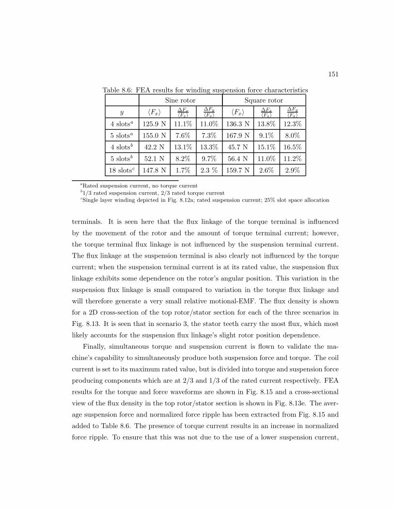
151
Table 8.6: FEA results for winding suspension force characteristics
Sine rotor Square rotor
y 〈Fx〉 ∆Fx〈Fx〉
∆Fy〈Fx〉 〈Fx〉 ∆Fx
〈Fx〉∆Fy〈Fx〉
4 slotsa 125.9 N 11.1% 11.0% 136.3 N 13.8% 12.3%
5 slotsa 155.0 N 7.6% 7.3% 167.9 N 9.1% 8.0%
4 slotsb 42.2 N 13.1% 13.3% 45.7 N 15.1% 16.5%
5 slotsb 52.1 N 8.2% 9.7% 56.4 N 11.0% 11.2%
18 slotsc 147.8 N 1.7% 2.3 % 159.7 N 2.6% 2.9%
aRated suspension current, no torque currentb1/3 rated suspension current, 2/3 rated torque currentcSingle layer winding depicted in Fig. 8.12a; rated suspension current; 25% slot space allocation
terminals. It is seen here that the flux linkage of the torque terminal is influenced
by the movement of the rotor and the amount of torque terminal current; however,
the torque terminal flux linkage is not influenced by the suspension terminal current.
The flux linkage at the suspension terminal is also clearly not influenced by the torque
current; when the suspension terminal current is at its rated value, the suspension flux
linkage exhibits some dependence on the rotor’s angular position. This variation in the
suspension flux linkage is small compared to variation in the torque flux linkage and
will therefore generate a very small relative motional-EMF. The flux density is shown
for a 2D cross-section of the top rotor/stator section for each of the three scenarios in
Fig. 8.13. It is seen that in scenario 3, the stator teeth carry the most flux, which most
likely accounts for the suspension flux linkage’s slight rotor position dependence.
Finally, simultaneous torque and suspension current is flown to validate the ma-
chine’s capability to simultaneously produce both suspension force and torque. The coil
current is set to its maximum rated value, but is divided into torque and suspension force
producing components which are at 2/3 and 1/3 of the rated current respectively. FEA
results for the torque and force waveforms are shown in Fig. 8.15 and a cross-sectional
view of the flux density in the top rotor/stator section is shown in Fig. 8.13e. The aver-
age suspension force and normalized force ripple has been extracted from Fig. 8.15 and
added to Table 8.6. The presence of torque current results in an increase in normalized
force ripple. To ensure that this was not due to the use of a lower suspension current,
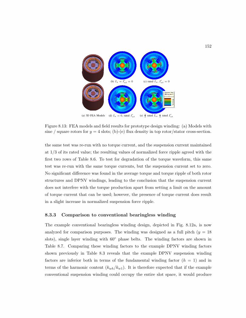
152
(a) 3D FEA Models
(b) Iu = I′ut = 0 (c) rated Iu , I′
ut = 0
(d) Iu = 0, rated I′ut (e) 2
3rated Iu, 1
3rated I′
ut
Figure 8.13: FEA models and field results for prototype design winding: (a) Models withsine / square rotors for y = 4 slots; (b)-(e) flux density in top rotor/stator cross-section.
the same test was re-run with no torque current, and the suspension current maintained
at 1/3 of its rated value; the resulting values of normalized force ripple agreed with the
first two rows of Table 8.6. To test for degradation of the torque waveform, this same
test was re-run with the same torque currents, but the suspension current set to zero.
No significant difference was found in the average torque and torque ripple of both rotor
structures and DPNV windings, leading to the conclusion that the suspension current
does not interfere with the torque production apart from setting a limit on the amount
of torque current that can be used; however, the presence of torque current does result
in a slight increase in normalized suspension force ripple.
8.3.3 Comparison to conventional bearingless winding
The example conventional bearingless winding design, depicted in Fig. 8.12a, is now
analyzed for comparison purposes. The winding was designed as a full pitch (y = 18
slots), single layer winding with 60 phase belts. The winding factors are shown in
Table 8.7. Comparing these winding factors to the example DPNV winding factors
shown previously in Table 8.3 reveals that the example DPNV suspension winding
factors are inferior both in terms of the fundamental winding factor (h = 1) and in
terms of the harmonic content (kwh/kw1). It is therefore expected that if the example
conventional suspension winding could occupy the entire slot space, it would produce

153
−40
0
40
80
120
160
Force
(N)
Sine rotor x-force, y = 4Square rotor x-force, y = 4Sine rotor y-force, y = 4Square rotor y-force, y = 4
Sine rotor x-force, y = 5Square rotor x-force, y = 5Sine rotor y-force, y = 5Square rotor y-force, y = 5
0 50 100 150 200 250 300 3500
2
4
6
Rotor angular position (deg)
Terminal
current(A
)
I ′ut Parallel
I ′ub Parallel
IuI ′ut BridgeI ′ub Bridge
(a) Rated suspension force waveforms when no torque is produced
0 50 100 150 200 250 300 350
−0.1
−0.05
0
0.05
0.1
0.15
Rotor angular position (deg)
FluxLinkage
(Wb-t)
Iu = I ′
ut = 0
rated Iu, I
′ut = 0
Iu = 0, rated I ′
ut
Torque
phase u
Sus.
phase u
(b) Torque and suspension phase terminal flux linkage (y = 4 slots)
Figure 8.14: FEA results for the design variants with y = 4 and y = 5 DPNV wind-ings for the two different rotor shapes shown in Fig. 8.13a. The terminal currents areindicated for both the bridge and parallel drive implementations. Note: in (b) resultsare shown for the y = 4 DPNV winding with a square rotor and waveforms which passthrough the “Torque phase u” circle correspond to the the torque terminal.
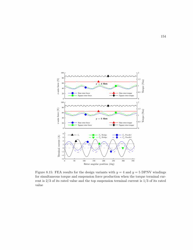
154
0
20
40
60
80
100
x-axisforce(N
)
0
0.5
1
1.5
2
Torqu
e(N
m)
Sine rotor force
Square rotor force
Sine rotor torque
Square rotor torque
0
20
40
60
80
100
x-axisforce(N
)
0
0.5
1
1.5
2
Torqu
e(N
m)
Sine rotor force
Square rotor force
Sine rotor torque
Square rotor torque
0 50 100 150 200 250 300 350−6
−4
−2
0
2
4
6
8
Rotor angular position (deg)
Terminal
current(A
)
Iu
I ′ut Parallel
I ′ub Parallel
I ′ut Bridge
I ′ub Bridge
y = 5 Slots
y = 4 Slots
Figure 8.15: FEA results for the design variants with y = 4 and y = 5 DPNV windingsfor simultaneous torque and suspension force production when the torque terminal cur-rent is 2/3 of its rated value and the top suspension terminal current is 1/3 of its ratedvalue
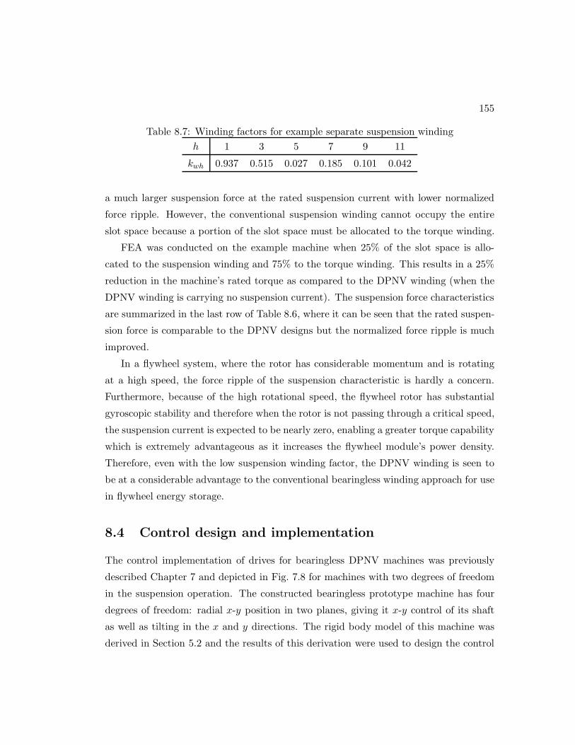
155
Table 8.7: Winding factors for example separate suspension winding
h 1 3 5 7 9 11
kwh 0.937 0.515 0.027 0.185 0.101 0.042
a much larger suspension force at the rated suspension current with lower normalized
force ripple. However, the conventional suspension winding cannot occupy the entire
slot space because a portion of the slot space must be allocated to the torque winding.
FEA was conducted on the example machine when 25% of the slot space is allo-
cated to the suspension winding and 75% to the torque winding. This results in a 25%
reduction in the machine’s rated torque as compared to the DPNV winding (when the
DPNV winding is carrying no suspension current). The suspension force characteristics
are summarized in the last row of Table 8.6, where it can be seen that the rated suspen-
sion force is comparable to the DPNV designs but the normalized force ripple is much
improved.
In a flywheel system, where the rotor has considerable momentum and is rotating
at a high speed, the force ripple of the suspension characteristic is hardly a concern.
Furthermore, because of the high rotational speed, the flywheel rotor has substantial
gyroscopic stability and therefore when the rotor is not passing through a critical speed,
the suspension current is expected to be nearly zero, enabling a greater torque capability
which is extremely advantageous as it increases the flywheel module’s power density.
Therefore, even with the low suspension winding factor, the DPNV winding is seen to
be at a considerable advantage to the conventional bearingless winding approach for use
in flywheel energy storage.
8.4 Control design and implementation
The control implementation of drives for bearingless DPNV machines was previously
described Chapter 7 and depicted in Fig. 7.8 for machines with two degrees of freedom
in the suspension operation. The constructed bearingless prototype machine has four
degrees of freedom: radial x-y position in two planes, giving it x-y control of its shaft
as well as tilting in the x and y directions. The rigid body model of this machine was
derived in Section 5.2 and the results of this derivation were used to design the control

156
logic for the prototype drive, which is now described. An overview of the control logic
is presented; the PI and PID controller designs are investigated; and finally, details of
the hardware implementation are summarized.
8.4.1 Control overview
To provide four-axis control, the previously presented control diagram of Fig. 7.8 is
replaced by Fig. 8.16. This control is based on the rigid body model depicted in Fig. 5.2,
where the rotor position in the x and y axes are decoupled. Detailed diagrams of the
position and current controllers are depicted in Fig. 8.17 and the PI and PID in Fig. 8.18.
The rigid body model has state variables of δ0 and θ, as labeled in Fig. 5.2 and
expressed in state-space form in (5.2). An independent set of these states exist for
each axis (x and y). Using the transformed inputs defined in (8.5), decoupled transfer
functions can be written for each of these states (8.6) which have the same unstable
poles that were identified in Section 5.2.
Fc1 = kf is1
Fc2 = kf is2
Fsum = Fc1 + Fc2
Fdiff = Fc1 − Fc2 (8.5)
δ0(s)
Fsum(s)=
1/m
s2 − |ks|/mθ(s)
Fdiff(s)=
rδ/I
s2 − r2δ |ks|/I(8.6)
The position PID controllers of Fig. 8.17a are designed to operate on these decoupled
transfer functions. Note that kf , is1, and is2 have the same meaning as defined in Sec-
tion 5.2. The currents is1 and is2 are the equivalent suspension current in a winding
spanning the top or bottom airgap for the given axis (x or y). As was done in Fig. 7.8,
these equivalent currents are calculated by a d-q transformation of the three phase sus-
pension currents, using the angle φf . However, here armature reaction flux is neglected
so φf is a constant value fixed to the x-axis, which in this prototype is set to the phase
u winding axis and assigned to 0 (notice the 0 values being fed into the suspension
current controllers of Fig. 8.16).

157
Position
Controller
1/kf
1/kf
+
+
Current
Controller
θ
UV W
d
q
PWM
U
V
W
Position
Controller
1/kf
1/kf
+
+
Current
Controller
θ
UV W
d
q
PWM
U
V
W
Reference
frame
change
d
q
θ θo
do
qo
−0.5
−0.5
Current
Controller
θ
UV W
d
q
PWM
U
V
W
Current
Controller
θ
UV W
d
q
PWM
U
V
W
top x pos. sensor
bot. x pos. sensor
top x∗
bot. x∗
top sus. current sensors
top F ∗x
bot F ∗x
top i∗x
top i∗y
0
Top Sus.
Phase Terminals
top y pos. sensor
bot. y pos. sensor
top y∗
bot. y∗
bot. sus. current sensors
top F ∗y
bot F ∗y
bot i∗x
bot i∗y
0
Bot. Sus.
Phase Terminals
0
Encoder: θ
i∗d
i∗q
top torque current sensors
Top Torque
Phase Terminals
bot. torque current sensors
Bot. Torque
Phase Terminals
Figure 8.16: Bearingless drive top-level control schematic. The blocks labeled as “Po-sition Controller” and “Current Controller” are depicted in detail in Fig. 8.17. Thecurrent controllers for torque current control do not implement zero sequence control.The green elements are only required for the parallel DPNV drive configuration.
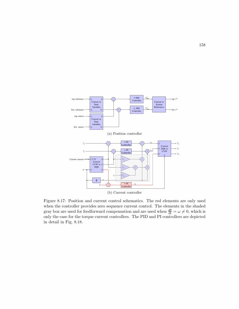
158
Convert to
State
Variables
δ1
δ2
θ
δ0
Convert to
State
Variables
δ1
δ2
θ
δ0
−
−
θ PID
Controller
δ0 PID
Controller
Convert to
System
References
top reference
bot. reference
top sensor
bot. sensor
F ∗diff
F ∗sum
top F ∗
bot F ∗
(a) Position controller
Convert
UVW to
DQ0
θ
UV W d
q
0
ddt
−
−
d PI
Controller
q PI
Controller
−
+
Convert
DQ0 to
UVW
d
q
0θ
Lq
Ld
L′mf
×
+ ×
− 0 PI
Controller
i∗d
i∗q
Current sensors
θ
vd
vq
ω
if
0v0
Vu
Vv
Vw
(b) Current controller
Figure 8.17: Position and current control schematics. The red elements are only usedwhen the controller provides zero sequence current control. The elements in the shadedgray box are used for feedforward compensation and are used when dθ
dt = ω 6= 0, which isonly the case for the torque current controllers. The PID and PI controllers are depictedin detail in Fig. 8.18.

159
In Fig. 8.17a, the θ and δ0 state variables are calculated from top and bottom rotor
position values by the block labeled “Convert to State Variables” by (8.7), using the
notation indicated in Fig. 5.2. To speed up the control loop, these equations have been
linearized using the small angle approximation that sin θ ≈ θ. If the position sensors
are located at a distance other than rδ from the axial center of the shaft, this distance
is substituted in place of rδ in (8.7) when calculating the measured rotor position.
θ =1
2rδ(δ1 − δ2)
δ0 =1
2(δ1 + δ2) (8.7)
Similarly, the reference values of Fsum and Fdiff that the position controllers generate
must be converted back to reference top and bottom forces. This is done by the block
labeled as “Convert to System References” in Fig. 8.17a using (8.8).
Fc1 =Fsum + Fdiff
2
Fc2 =Fsum − Fdiff
2(8.8)
In Fig. 8.16, the reference force values are divided by kf to calculate the corresponding
suspension current references and then fed into the appropriate top or bottom suspension
current controller.
Similar to Fig. 7.8, the extra current control logic required for the parallel DPNV
drive configuration is indicated by green shaded blocks. The logic required for zero se-
quence current control is drawn in red in Fig. 8.17b. As was the case in Chapter 7, these
controllers are only present in the suspension current controllers. The computation done
in the “Reference frame change” block is given by (8.9). In Fig. 8.17b, the computation
done in the “Convert UVW to DQ0” block is given by (8.10) and the “Convert DQ0
to UVW” block performs the inverse of this. When the current controller is being used
for suspension currents, d and q quantities are replaced by x and y quantities.
d0 = d cos (θ − θ0)− q sin (θ − θ0)
q0 = d sin (θ − θ0) + q cos (θ − θ0) (8.9)

160
kp
kis
+error output
(a) PI controller
kp
kis
skd1
s/ωp+1
+error output
(b) PID controller
Figure 8.18: PI and PID controller blocks.
d
q
0
=√
2/3
cos θ cos (θ − 2π/3) cos (θ + 2π/3)
− sin θ − sin (θ − 2π/3) − sin (θ + 2π/3)
1 1 1
U
V
W
(8.10)
8.4.2 PI current controller design
For both the torque and suspension current controllers, the winding model looks like
an R-L load. The resistance is simply the phase resistance and the inductances are
the transformed d-q (or x-y) quantities. The machine was designed so that Ld ≈ Lq
and Lx ≈ Ly, which means that the d and q PI controllers are identical within a single
current controller block. Because of the orientation of the winding coils within a coil
group leading to the no-voltage suspension condition, the values of Lx and Ly are simply
equal to the phase leakage inductance. The zero sequence R-L plant, and therefore PI
controller, is identical to the suspension plant (and PI controller).
The closed loop transfer function used for the current controller design is depicted
in Fig. 8.19 where C(s) is the controller, G(s) is the plant, and L corresponds to the
d-q or x-y quantity. The loop gain is given by (8.11).
IL(s) = C(s)×G(s)
=kp
(
s+ kikp
)
Ls(
s+ RL
) (8.11)
The controller gains (8.12) were chosen to achieve a desired controller bandwidth ωc
and to cancel the plant’s open-loop pole. This was done to achieve a first-order closed
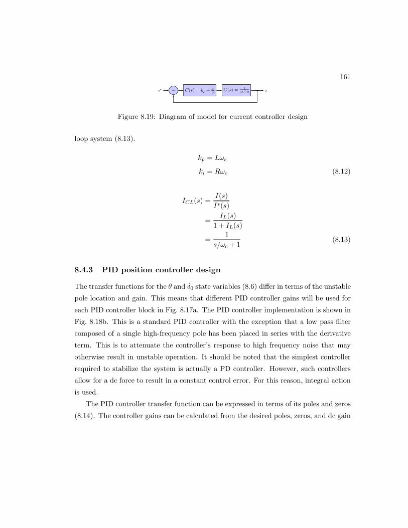
161
− C(s) = kp +kis
G(s) = 1sL+Ri∗ i
Figure 8.19: Diagram of model for current controller design
loop system (8.13).
kp = Lωc
ki = Rωc (8.12)
ICL(s) =I(s)
I∗(s)
=IL(s)
1 + IL(s)
=1
s/ωc + 1(8.13)
8.4.3 PID position controller design
The transfer functions for the θ and δ0 state variables (8.6) differ in terms of the unstable
pole location and gain. This means that different PID controller gains will be used for
each PID controller block in Fig. 8.17a. The PID controller implementation is shown in
Fig. 8.18b. This is a standard PID controller with the exception that a low pass filter
composed of a single high-frequency pole has been placed in series with the derivative
term. This is to attenuate the controller’s response to high frequency noise that may
otherwise result in unstable operation. It should be noted that the simplest controller
required to stabilize the system is actually a PD controller. However, such controllers
allow for a dc force to result in a constant control error. For this reason, integral action
is used.
The PID controller transfer function can be expressed in terms of its poles and zeros
(8.14). The controller gains can be calculated from the desired poles, zeros, and dc gain

162
kdc (8.15).
C(s) = kp + ki1
s+ kd
s
s/ωp + 1
=(kp/ωp + kd)s
2 + (kp + ki/ωp)s+ kis (s/ωp + 1)
= kdc(s/ωz1 + 1) (s/ωz2 + 1)
s (s/ωp + 1)(8.14)
kp = kdc
(
ωz1 + ωz2ωz1ωz2
− 1
ωp
)
ki = kdc
kd = kdc
(
1
ωz1ωz2− ωz1 + ωz2ωz1ωz2ωp
+1
ω2p
)
(8.15)
To generalize the design procedure, a generic plant transfer function is defined here
(8.16), where kG and ωx are replaced with the actual values of either transfer function
defined in (8.6).
G(s) =ω2xkG
s2 − ω2x
=kG
(s/ωx + 1) (s/ωx − 1)(8.16)
The closed loop model used for the PID controller design is depicted in Fig. 8.20,
where ICL(s) corresponds to the inner current control loop. The frequency design
method is used, with the primary objective of stabilizing the system. Approximated,
idealized bode plots of the various model transfer functions are shown in Fig. 8.21 where
it is seen that G(s) has a constant phase angle of −180. To stabilize the system, the
open-loop phase angle must be greater than −180 at the cross-over frequency (the
frequency at which the loop gain is at unity magnitude). To do this, the first zero of
(8.14) must be located far below the cross-over frequency to boost the phase angle and
prevent premature attenuation of the loop gain due to the poles of G(s). The location
of the second zero is chosen to further boost the phase angle to obtain a desired phase
margin at the cross-over frequency. The dc gain kdc of C(s) is used to set the cross-over
frequency. Finally, the pole in series with the PID controller’s derivative term is set to
a value far greater than the cross-over frequency.
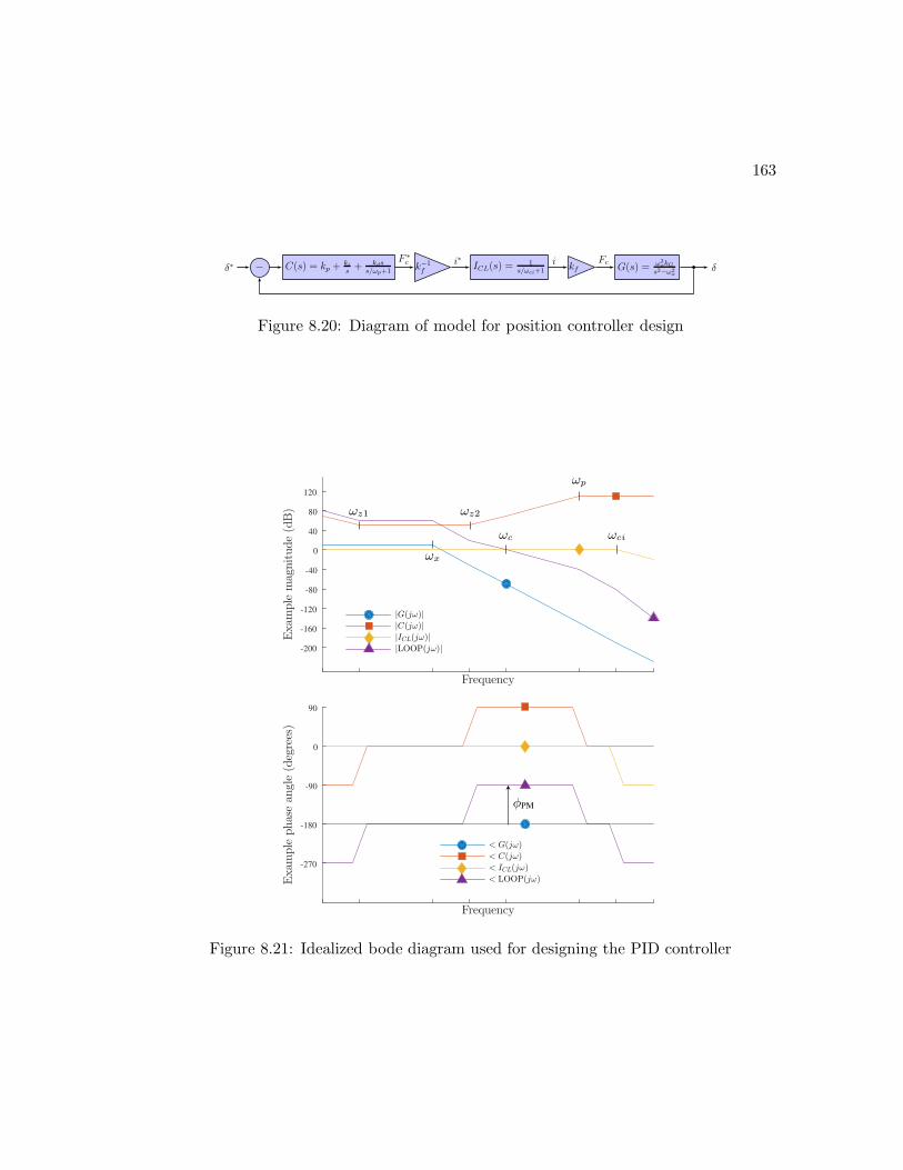
163
− C(s) = kp +kis+ kds
s/ωp+1 k−1f
ICL(s) =1
s/ωci+1 kf G(s) = ω2xkG
s2−ω2x
δ∗F ∗c i∗ i Fc
δ
Figure 8.20: Diagram of model for position controller design
Frequency
Exam
ple
magnitude(dB)
-200
-160
-120
-80
-40
0
40
80
120
|G(jω)|
|C(jω)|
|ICL(jω)|
|LOOP(jω)|
Frequency
Exam
ple
phasean
gle(degrees)
-270
-180
-90
0
90
< G(jω)
< C(jω)
< ICL(jω)
< LOOP(jω)
φPM
ωc
ωz1 ωz2
ωp
ωci
ωx
Figure 8.21: Idealized bode diagram used for designing the PID controller

164
ZedBoard FPGA
ADCs
Pos. sensor LPF
Cur. sensor LPF
PWM output drivers
Pos. sensors
Cur. sensors
Inverter
transistor
gates
Custom FPGA circuit board
Figure 8.22: Schematic of the control hardware. The actual hardware is shown inFig. 8.3.
The primary design input parameters are the desire phase margin φPM and the
cross-over frequency ωc, which have a strong effect on the suspension performance. The
controller gains were calculated from these parameters by (8.17). The expressions for
ωz1 and ωp were chosen based on what worked well in practice. As will be discussed later,
it is suspected that a detailed controller tuning effort may yield significant improvement
in suspension performance.
ωz1 = ωc/100
ωp = 4ωc
ωz2 =ωc
tan(
φPM + 90 + arctan ωcωci
− arctan ωcωz1
+ arctan ωcωp
)
kdc =1
∣
∣
∣C(jωc)
∣
∣
kdc=1
∣
∣
∣|ICL(jωc)| |G(jωc)|
(8.17)
8.4.4 Hardware implementation
A diagram of the control hardware is shown in Fig. 8.22. The main control logic has been
written in C code and runs bare-metal on the DSP portion of a Xilinx Zynq SoC. The
DSP board is interfaced to a custom FPGA circuit board developed in the UMN Power
Electronic’s Research Laboratory via a high speed data bus. This custom FPGA circuit
board contains analog to digital converters (ADCs) to interface to the eddy current
position sensors used for rotor position feedback and the hall-effect current sensors used
to measure the phase current. Low pass, first order filters are placed in front of the
ADCs to prevent aliasing. These filters are implemented with simple R-C circuits.
The FPGA circuit board also contains the PWM output drivers which are used to
165
send transistor gate pulses to the power electronic inverters. The power electronic in-
verter circuit topologies used were described in Chapter 7. The DSP writes duty ratio
values for each 2-level half-bridge inverter circuit to the FPGA. The FPGA then gener-
ates PWM signals from these duty ratio values via a triangle comparator. The FPGA
synchronizes its sampling of the ADCs to the positive and negative peaks of triangle
comparator to minimize switching noise. This means that the ADCs are sampled at
twice the inverter’s switching frequency. The FPGA then uses first-order, low pass dig-
ital filters to remove frequency components that would be aliased by the DSP’s digital
control loops’ sample rate. The filtered ADC values are stored in FPGA registers from
which the DSP reads new values at every iteration of its digital control loops.
The machine parameters used for the controller design are given in Table 8.8 and
the controller parameters and hardware information are provided in Table 8.9.
There was no encoder used in the final prototype testing. Instead, a stationary
value of θ from Fig. 8.16 was selected and a torque current was flown to align the
rotor. Then, increasing values of ω were used until the desired ω value was obtained.
If ω was increased too rapidly or reached too great of a value, the machine would lose
synchronism and the rotor would spin down. While the lack of an encoder made it
impossible to flow true q or d axis current and limited the maximum rotational speed,
it was advantageous to the suspension performance results because it meant that the
rotor had no contact with, and therefore experienced no forces from, the stator. Future
work is planned to mount an encoder onto the rotor in a way that provides minimal
interference from the stator and will allow test results to be taken at higher rotational
speeds.
When the rotor is centered in the airgap, the suspension system is at an unstable
equilibrium and therefore a well-tuned suspension control system should require very
little current. However, despite efforts to precisely align the axial PM bearing and the
eddy current position sensors, zero position references for the top and bottom x/y rotor
position (top x∗, bot. x∗, top y∗, bot. y∗) required significant suspension current to
maintain the rotor’s position. To remedy this, the magnetic center of the system was
found by “tuning” the values of the position references. This was done with an iterative
process, as follows:
1) rotate the rotor in 10 increments (corresponding to the cogging locations for a

166
Table 8.8: Machine parameters used for controller design
Bridge Parallel
Suspension Ra 1.1Ω 3.0Ω
Lx, Ly, L0b 0.41 mH 4.50 mH
Torque Rc 0.8Ω
Ld, Lqd 3.80 mH
L′mf 5.60 mH
kf (if )e 11.4if + 0.8i2f − 0.52i3f 22.8if + 1.6i2f +−1.05i3f
ks(if )(
35.9if − 246.2i2f + 41i3f
)
× 103
m 12 kg
I 0.105 kg-m2
rδ 48.5 mm
rsensef 191 mm
aAll sus. resistance values were measured using an LCR meter at the inverter terminals.bAll sus. inductance values were measured using an LCR meter at a frequency near the current
controller’s bandwidth at the inverter terminals.cDC measurement using a multimeterdAll torque inductance values were calculated using 3D FEA.ekf and ks are specified as polynomials of the field current as was done in Chapter 5. The polynomial
parameters were calculated using 3D FEA models of the constructed prototype in the same manner asin Chapter 5.
fThe axial distance from the position sensor to the center of the shaft. This replaces rδ whencalculating the state variables from position sensor readings in (8.7)

167
Table 8.9: Control design and hardware parametersa
φPM 50 for δ0, 60 for θ
Position controller ωc 2π × 75Hz
Current controller ωc 2π× 1.25kHz for sus., 1kHz for torque
R-C filter bandwidthb 2π× 3.6kHz for pos., 16kHz for cur. sensors
Digital filter bandwidthc 2π× 400Hz for pos., 9kHz for cur. sensors
Digital control frequencyd 20kHz
Inverter switching frequency 100kHz
DSP Xilinx Zynq-7000 AP SoC XC7Z020-CLG484
on the Avnet ZedBoard 7020
FPGA Xilinx Spartan 3E XC3S500E
on a custom PCB
Position sensors Kaman DIT5200-20N
aSeveral different values of phase margin, filter bandwidth, and controller bandwidth were used.The data presented in this table are the final values which were found to yield the most satisfactoryperformance.
bThis is the bandwidth of the first-order, low pass filter used on the FPGA circuit board to preventADC sampling aliasing.
cThis is the bandwidth of the first-order, low pass digital filter that the FPGA uses on sampled ADCvalues to prevent digital control aliasing.
dThe frequency, or inverse of the sampling rate, at which the digital control loops were run.

168
Table 8.10: Final reference values for the rotor’s magnetic center
top x∗ 0.251 mm
top y∗ −0.053 mm
bot. x∗ 0.089 mm
bot. y∗ −0.140 mm
36 slot stator) and average the required x and y top and bottom currents over an
entire revolution;
2) change each position reference in a manner to decrease the magnitude of the
averaged x and y top and bottom currents;
3) repeat steps 1) and 2) until satisfactory stationary suspension currents are ob-
tained.
This process had to be repeated every time any modification was made to the test
stand which disrupted the magnetic center. Final reference values used are shown in
Table 8.10.
8.5 Results
Results from the hardware prototype of the bearingless machine are now presented.
The DPNV winding was tested in both a parallel and a bridge configuration with and
without zero sequence current controllers for various speeds and armature torque current
values.3
8.5.1 No load
First, the machine was operated with mechanical bearings to measure the no-load ter-
minal voltage characteristic. A dc power supply was used to provide rated current to
the field winding. An electric drill was coupled to the rotor and used to rotate the rotor
at 1000RPM. The results of this are shown in Fig. 8.23 for the armature coil groups
3 Portions of the material in this chapter have also been published or submitted for publicationin [46,47,49].

169
connected in both parallel and bridge configurations. From these results, it is clear the
suspension winding experiences no significant motional-EMF.
8.5.2 Full bearingless operation
Experimental results are now presented for the parallel and bridge under full bearingless
motor operation at a rotational speed of 1000RPM while 1.5A RMS of current is flowing
in the motor phases. In an effort to illustrate the torque inverter’s impact on the
suspension terminal currents, only the torque inverter for the top DPNV winding is
connected in both configurations.
In the bridge configuration, 20V buses were used for the suspension inverters and a
40V bus was used for the torque inverter. The terminal currents are shown in Fig. 8.24b
along with the orbital x-y positions in Fig. 8.24a. An ac suspension current with a fre-
quency equal to the rotational speed is clearly visible. This is because the rotor does not
remain perfectly centered over a single revolution, causing the suspension controller to
generate restorative forces with a period of one revolution. Terminal current waveforms
for the parallel DPNV drive are shown in Fig. 8.24c. This drive is implemented with a
single voltage bus of 40V, matching Fig. 7.6a.
The suspension controller’s measured shaft displacement input and force references
were logged and are displayed in Fig. 8.25. This data shows that the machine is utilizing
approximately 18% of its rated suspension force, meaning that approximately 82% of
the slot space can be devoted to torque production. As the rotor speed increases, gyro-
scopic stabilization increases which decreases the amount of required suspension force,
giving the machine a higher torque capability. This dynamic torque capability com-
pares favorably to the example of a conventional bearingless winding design considered
in Section 8.3.3 where the torque slot space was permanently fixed at 75%.
The bridge and parallel configured drives were both operated with and without the
zero sequence current controller described in Fig. 7.9 of Section 7.5. The zero sequence
currents are calculated from (7.11) and the results are shown in Fig. 8.26. For the bridge
configuration, it can be seen in Fig. 8.26a that there was very little zero sequence current
present without the controller, and therefore little improvement was obtained with the
zero sequence controller. However, the results for the parallel configuration without
the zero sequence controller had significant circulating currents and highly distorted
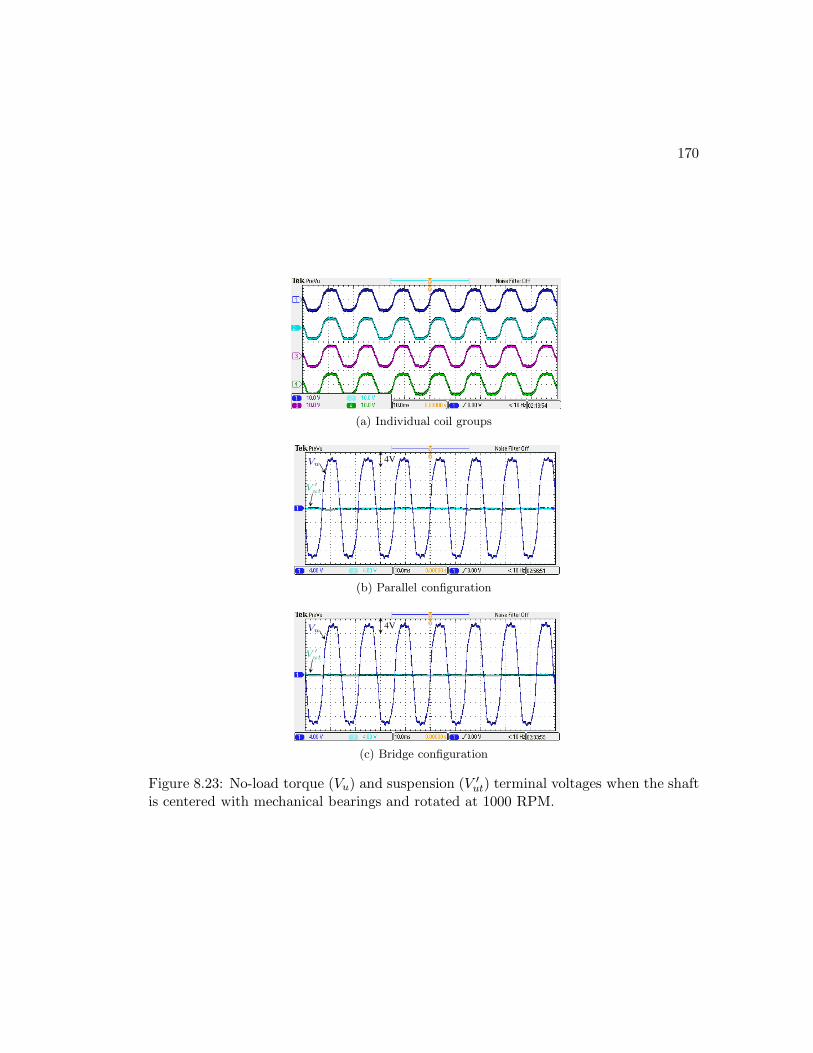
170
(a) Individual coil groups
4VVu
V ′ut
(b) Parallel configuration
4VVu
V ′ut
(c) Bridge configuration
Figure 8.23: No-load torque (Vu) and suspension (V ′ut) terminal voltages when the shaft
is centered with mechanical bearings and rotated at 1000 RPM.
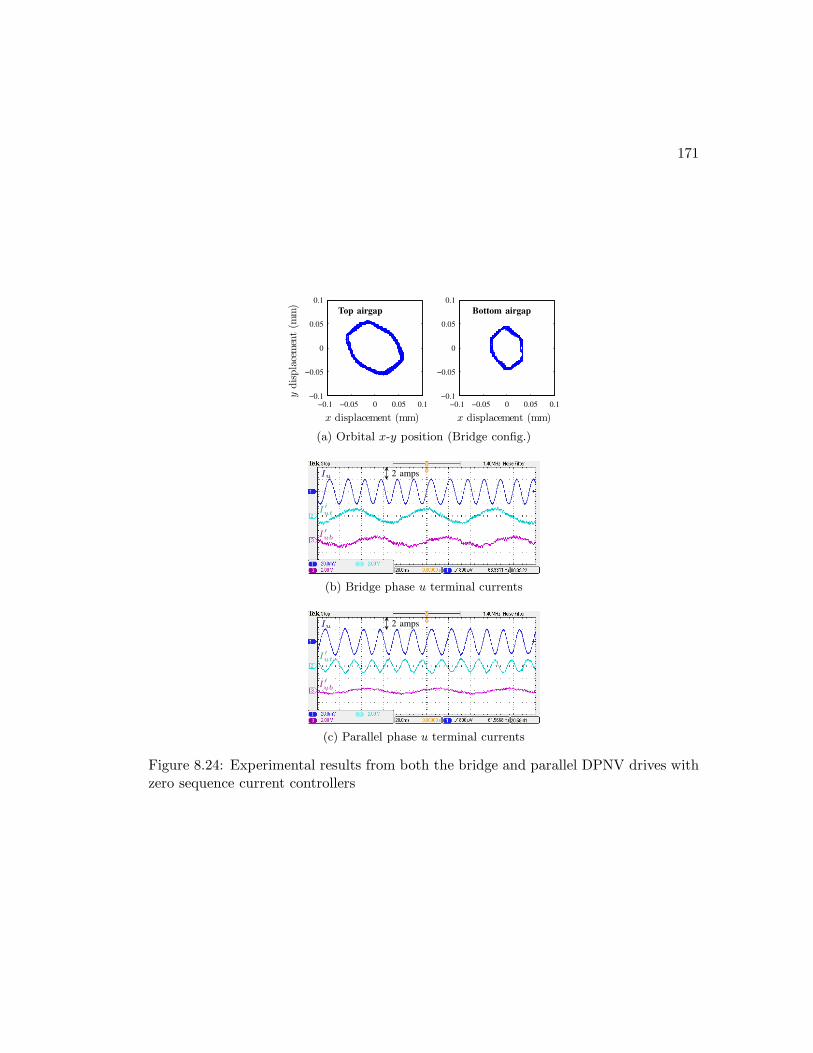
171
−0.1 −0.05 0 0.05 0.1−0.1
−0.05
0
0.05
0.1
ydisplacement(m
m)
x displacement (mm)
−0.1 −0.05 0 0.05 0.1−0.1
−0.05
0
0.05
0.1ydisplacement(m
m)
x displacement (mm)
Top airgap Bottom airgap
(a) Orbital x-y position (Bridge config.)
2 ampsIu
I′ut
I′ub
(b) Bridge phase u terminal currents
2 ampsIu
I′ut
I′ub
(c) Parallel phase u terminal currents
Figure 8.24: Experimental results from both the bridge and parallel DPNV drives withzero sequence current controllers

172
−0.05
0
0.05
0.1
Displacement(m
m)
Top ∆x
Top ∆y
0 0.05 0.1 0.15 0.2
−25
0
25
50
Time (s)
Force
reference
(N)
Top x-force
Top y-force
(a) Top displacement and force reference
−0.05
0
0.05
0.1
Displacement(m
m)
Bot. ∆x
Bot. ∆y
0 0.05 0.1 0.15 0.2
−25
0
25
50
Time (s)
Force
reference
(N)
Bot. x-force
Bot. y-force
(b) Bottom displacement and force reference
Figure 8.25: Position controller measurements and reference waveforms for the bridgeconfiguration. The data were collected from the DSP-based controller: the controller’smeasured x and y displacements and generated x and y corrective forces were loggedfor 200ms.
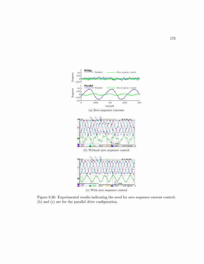
173
0 0.005 0.01 0.015 0.02−0.5
−0.25
0
0.25
0.5
seconds
Amperes
Standard
Zero sequence control
0 0.005 0.01 0.015 0.02−0.5
−0.25
0
0.25
0.5
seconds
Amperes
Standard
Zero sequence control
Bridge
Parallel
(a) Zero sequence currents
1 amp
IuIvIw
I′ut
(b) Without zero sequence control
1 amp
IuIvIw
I′ut
(c) With zero sequence control
Figure 8.26: Experimental results indicating the need for zero sequence current control;(b) and (c) are for the parallel drive configuration.
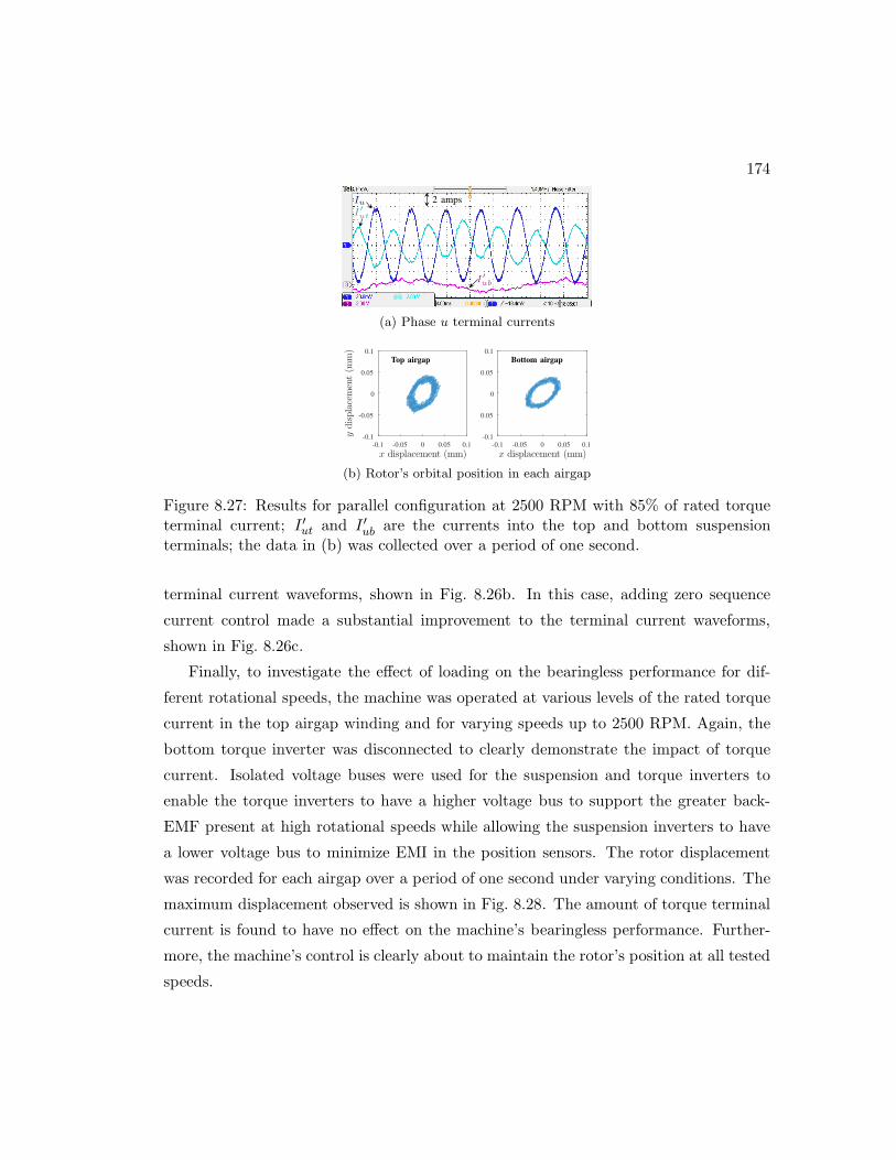
174
2 ampsIuI′ut
I′ub
(a) Phase u terminal currents
x displacement (mm)-0.1 -0.05 0 0.05 0.1
ydisplacement(m
m)
-0.1
-0.05
0
0.05
0.1
x displacement (mm)-0.1 -0.05 0 0.05 0.1
ydisplacement(m
m)
-0.1
-0.05
0
0.05
0.1
Top airgap Bottom airgap
(b) Rotor’s orbital position in each airgap
Figure 8.27: Results for parallel configuration at 2500 RPM with 85% of rated torqueterminal current; I ′ut and I ′ub are the currents into the top and bottom suspensionterminals; the data in (b) was collected over a period of one second.
terminal current waveforms, shown in Fig. 8.26b. In this case, adding zero sequence
current control made a substantial improvement to the terminal current waveforms,
shown in Fig. 8.26c.
Finally, to investigate the effect of loading on the bearingless performance for dif-
ferent rotational speeds, the machine was operated at various levels of the rated torque
current in the top airgap winding and for varying speeds up to 2500 RPM. Again, the
bottom torque inverter was disconnected to clearly demonstrate the impact of torque
current. Isolated voltage buses were used for the suspension and torque inverters to
enable the torque inverters to have a higher voltage bus to support the greater back-
EMF present at high rotational speeds while allowing the suspension inverters to have
a lower voltage bus to minimize EMI in the position sensors. The rotor displacement
was recorded for each airgap over a period of one second under varying conditions. The
maximum displacement observed is shown in Fig. 8.28. The amount of torque terminal
current is found to have no effect on the machine’s bearingless performance. Further-
more, the machine’s control is clearly about to maintain the rotor’s position at all tested
speeds.
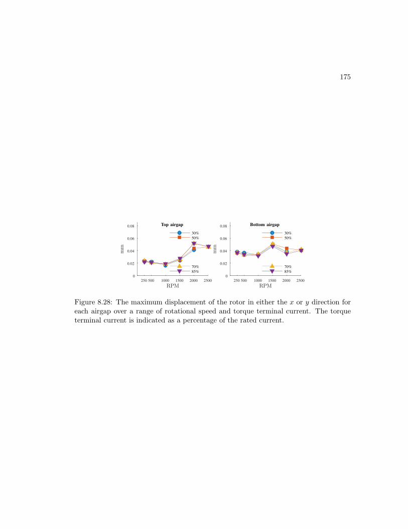
175
RPM250 500 1000 1500 2000 2500
mm
0
0.02
0.04
0.06
0.08
30%
50%
70%
85%
RPM250 500 1000 1500 2000 2500
mm
0
0.02
0.04
0.06
0.08
30%
50%
70%
85%
Top airgap Bottom airgap
Figure 8.28: The maximum displacement of the rotor in either the x or y direction foreach airgap over a range of rotational speed and torque terminal current. The torqueterminal current is indicated as a percentage of the rated current.

Chapter 9
Conclusion and Future Work
9.1 Conclusion
The primary conclusion of this dissertation is that energy storage devices based on
flywheel technology have the potential to simultaneously provide both frequency regu-
lation and load following services to the power grid in a modular form factor that can be
installed locally on a per-need basis. However, to develop such a device, key obstacles
in flywheel technology must be resolved. The most important of which is the high rate
of self-discharge that flywheel systems experience when idling due to magnetic losses in
the permanent magnet motor/generator. This dissertation has re-envisioned the design
of flywheel energy storage devices to be based around the bearingless ac homopolar
machine. It has shown that the field excitation of this machine can be easily removed
when idling to eliminate the magnetic losses that cause self-discharge. Furthermore,
the dissertation has shown that designs based around the ac homopolar machine al-
low for several secondary benefits to flywheel systems, including reduced overall system
complexity and cost due to the elimination of separate radial magnetic bearings.
At the onset of this disseration, the bearingless ac homopolar machine was an imma-
ture technology with very few examples of prototype machines available in the literature.
This dissertation has advanced the state-of-the-art of this technology as both a bear-
ingless machine and as a motor through contributions in magnetic modeling, winding
design, control, and presenting experimental validation of these aforementioned con-
tributions. All of this has laid the ground work and justification for future design
176
177
optimization of this machine.
Finally, this dissertation has also made significant contributions to the broader field
of bearingless machine design through its derivation of dual purpose no voltage winding
design rules, a design procedure, and drive implementations. By using the same coils for
both torque and radial force production, these windings will increase the torque density
of future bearingless machine designs and reduce the cost of bearingless machines to
values closer to what is required of non-bearingless machines. In effect, this technology
will lower the threshold of need that is required to consider a bearingless design, resulting
in more optimal electromechanical devices.
9.2 Future work
Several future projects are suggested to continue the development of flywheel energy
storage based around the bearingless ac homopolar machine as well as to continue the
development of dual purpose no voltage bearingless windings.
• The experimental validation of the prototype has placed no emphasis on optimal
control. It is suggested that future work experimentally measure the machine’s
suspension transfer functions and thoroughly explore the performance improve-
ments that can be achieved by control tuning or alternative control implementa-
tions. Furthermore, the experimental prototype did not make use of an encoder
and because of this the maximum achievable rotational speed was limited to 2500
RPM. Next steps should involve either mounting an encoder on the prototype or
exploring sensorless techniques (see the next item) to increase the rotational speed.
Note that higher speeds may require more advanced control design to handle the
changing suspension pole locations due to gyroscopic effects.
• An exploration of sensorless and self-sensing control techniques for both the rotor’s
angular position and the rotor’s linear position is suggested. The eddy current
linear position sensors used for feedback were expensive and, if they are required in
final flywheel system designs, would constitute a significant portion of the mod-
ule’s cost. While angular position detection can be implemented with low-cost
equipment, it adds manufacturing complexity/cost and overall system reliability

178
concerns. For these reasons, a fully position-sensorless flywheel system would have
considerable advantages.
• Now that computationally efficient magnetic models have been developed and once
sensorless techniques are developed and validated in the bearingless ac homopolar
prototype, the logical next step is to consider the design optimization of an outer-
rotor prototype. Of particular interest is the achievable cost/kWh, cost/kW, and
suspension power needed to maintain levitation while the machine is idling. The
suspension power will act as a source of self-discharge, which must be carefully
considered in the design optimization. Also of interest in the design optimization
is the mechanical design integrating the flywheel and the machine’s rotor. The
loading from the rotor teeth at high speeds and the PM axial bearing on the
flywheel will need to be taken into account. When carbon composite flywheels are
used, careful consideration must be given to the machine’s operating temperature
to prevent weakening and catastrophic flywheel failure.
• Apart from flywheel energy storage, future work can be conducted to continue
the development of bearingless machines with dual purpose no voltage windings.
One aspect of these windings which has not been explored in this dissertation
is their ability to passively provide corrective forces when the rotor is eccentric.
Designs that generate these forces can use standard motor windings (that have
modified end-connections) and must only have their suspension terminal connec-
tions short-circuited. The generated forces could potentially be used to dampen
rotor vibrations in conventional machine designs and, because this comes at nearly
no additional cost, could have a huge impact on large-scale machines where reli-
ability is especially important. Future work focusing in this area should explore
requirements on winding factors and rotational speeds to develop significant forces
in the presence of eccentricity.

References
[1] Brendan J Kirby. Frequency regulation basics and trends. United States. Depart-
ment of Energy, 2005.
[2] J.P. Barton and D.G. Infield. Energy storage and its use with intermittent renew-
able energy. Energy Conversion, IEEE Transactions on, 19(2):441–448, 2004.
[3] A. Oudalov, T. Buehler, and D. Chartouni. Utility scale applications of energy
storage. In Energy 2030 Conference, 2008. ENERGY 2008. IEEE, pages 1–7,
2008.
[4] H. Ibrahim, A. Ilinca, and J. Perron. Energy storage systems characteristics and
comparisons. Renewable and Sustainable Energy Reviews, 12(5):1221 –1250, 2008.
[5] Ioannis Hadjipaschalis, Andreas Poullikkas, and Venizelos Efthimiou. Overview
of current and future energy storage technologies for electric power applications.
Renewable and Sustainable Energy Reviews, 13(6):1513–1522, 2009.
[6] Paul Denholm, Erik Ela, Brendan Kirby, and Michael Milligan. The role of energy
storage with renewable electricity generation. 2010.
[7] C.S. Hearn, M.C. Lewis, S.B. Pratap, R.E. Hebner, F.M. Uriarte, Dongmei Chen,
and R.G. Longoria. Utilization of optimal control law to size grid-level flywheel
energy storage. Sustainable Energy, IEEE Transactions on, 4(3):611–618, 2013.
[8] M.L. Lazarewicz and T.M. Ryan. Integration of flywheel-based energy storage
for frequency regulation in deregulated markets. In Power and Energy Society
General Meeting, 2010 IEEE, pages 1–6, 2010.
179
180
[9] V.A. Boicea. Energy storage technologies: The past and the present. Proceedings
of the IEEE, 102(11):1777–1794, Nov 2014.
[10] Gauthier Delille and Bruno Francois. A review of some technical and economic
features of energy storage technologies for distribution system integration. Eco-
logical engineering and environment protection, 1:40–49, 2008.
[11] P. Fairley. Flywheels get their spin back [news]. Spectrum, IEEE, 52(1):18–18,
January 2015.
[12] Beacon Power. [online]. http://www.beaconpower.com/. Accessed: 2015-05-13.
[13] PowerThru. Clean flywheel energy storage systems [online].
http://www.power-thru.com/. Accessed: 2015-05-13.
[14] M.M. Flynn, P. McMullen, and O. Solis. Saving energy using flywheels. Industry
Applications Magazine, IEEE, 14(6):69–76, November 2008.
[15] M. Lafoz Pastor, L. Garcia-Tabares Rodriguez, and C. Vazquez Velez. Flywheels
store to save: Improving railway efficiency with energy storage. Electrification
Magazine, IEEE, 1(2):13–20, Dec 2013.
[16] Rotonix. [online]. http://rotonix.com/. Accessed: 2015-05-13.
[17] Amber Kinetics. [online]. http://www.amberkinetics.com/. Accessed: 2015-05-
13.
[18] M.A. Pichot and M.D. Driga. Loss reduction strategies in design of magnetic
bearing actuators for vehicle applications. Magnetics, IEEE Transactions on,
41(1):492–496, Jan 2005.
[19] M. Strasik, P.E. Johnson, A.C. Day, J. Mittleider, M.D. Higgins, J. Edwards, J.R.
Schindler, K.E. McCrary, C.R. McIver, D. Carlson, J.F. Gonder, and J.R. Hull.
Design, fabrication, and test of a 5-kwh/100-kw flywheel energy storage utilizing
a high-temperature superconducting bearing. Applied Superconductivity, IEEE
Transactions on, 17(2):2133–2137, June 2007.
181
[20] M. Flynn. A Methodology for Evaluating and Reducing Rotor Losses, Heating,
and Operational Limitations of High-Speed Flywheel Batteries. PhD thesis, The
University of Texas at Austin, Austin, TX, 2003.
[21] H.J. Bornemann, A. Tonoli, T. Ritter, C. Urban, O. Zaitsev, K. Weber, and
H. Rietschel. Engineering prototype of a superconducting flywheel for long term
energy storage. Applied Superconductivity, IEEE Transactions on, 5(2):618–621,
June 1995.
[22] P.P. Acarnley, B.C. Mecrow, J.S. Burdess, J. N. Fawcett, P.G. Dickinson, and
J. G. Kelly. An integrated flywheel/machine energy store for road vehicles. In
New Topologies for Permanent Magnet Machines (Digest No: 1997/090), IEE
Colloquium on, pages 9/1–9/6, 1997.
[23] M. A. Pichot, J.P. Kajs, B. R. Murphy, A. Ouroua, B. Rech, R.J. Hayes, J.H. Beno,
G.D. Buckner, and A.B. Palazzolo. Active magnetic bearings for energy storage
systems for combat vehicles. Magnetics, IEEE Transactions on, 37(1):318–323,
2001.
[24] RJ Hayes, JP Kajs, RC Thompson, and JH Beno. Design and testing of a flywheel
battery for a transit bus. SAE transactions, 108(6; PART 2):2199–2207, 2000.
[25] Clay Stephen Hearn. Design methodologies for advanced flywheel energy storage.
PhD thesis, The University of Texas at Austin, Austin, TX, 2013.
[26] H. Hofmann. High-speed synchronous reluctance machine for flywheel applications.
PhD thesis, The University of California at Berkley, Berkley, CA, 1998.
[27] Perry Tsao, M. Senesky, and S.R. Sanders. An integrated flywheel energy stor-
age system with homopolar inductor motor/generator and high-frequency drive.
Industry Applications, IEEE Transactions on, 39(6):1710 – 1725, nov.-dec. 2003.
[28] T. Ichihara, K. Matsunaga, M. Kita, Izumi Hirabayashi, M. Isono, M. Hirose,
K. Yoshii, K. Kurihara, O. Saito, S. Saito, M. Murakami, H. Takabayashi, M. Nat-
sumeda, and N. Koshizuka. Application of superconducting magnetic bearings to
a 10 kwh-class flywheel energy storage system. Applied Superconductivity, IEEE
Transactions on, 15(2):2245–2248, June 2005.

182
[29] F.N. Werfel, U. Floegel-Delor, T. Riedel, R. Rothfeld, D. Wippich, B. Goebel,
G. Reiner, and N. Wehlau. A compact hts 5 kwh/250 kw flywheel energy storage
system. Applied Superconductivity, IEEE Transactions on, 17(2):2138–2141, June
2007.
[30] Peter Kascak. Fully Levitated Rotor Magnetically Suspended By Two Pole-Pair
Seperated Conical Motors. PhD thesis, Case Western University, Cleveland, OH,
2010.
[31] Qian Wang, Chengjun Liu, Jibin Zou, Xinghe Fu, and Juan Zhang. Numerical
analysis and design optimization of a homopolar inductor machine used for fly-
wheel energy storage. Plasma Science, IEEE Transactions on, 41(5):1290–1294,
May 2013.
[32] Trong Duy Nguyen, G. Foo, King-Jet Tseng, and D.M. Vilathgamuwa. Modeling
and sensorless direct torque and flux control of a dual-airgap axial flux permanent-
magnet machine with field-weakening operation. Mechatronics, IEEE/ASME
Transactions on, 19(2):412–422, April 2014.
[33] Todd Andrew Begalke. Synchronous Reluctance Drive for Flywheel Batteries. PhD
thesis, University of Minnesota, 2006. Major: Electrical engineering., 2006.
[34] Maria Ines Lopes Marques. Design and Control of an Electrical Machine for
Flywheel Energy-Storage System. PhD thesis, MA thesis, IST, Lisbon, Portugal,
2008.
[35] J. Santiago, J.G. Oliveira, J. Lundin, A. Larsson, and H. Bernhoff. Losses in axial-
flux permanent-magnet coreless flywheel energy storage systems. In Electrical
Machines, 2008. ICEM 2008. 18th International Conference on, pages 1–5, Sept
2008.
[36] Jae-Do Park, C. Kalev, and H.F. Hofmann. Control of high-speed solid-rotor
synchronous reluctance motor/generator for flywheel-based uninterruptible power
supplies. Industrial Electronics, IEEE Transactions on, 55(8):3038–3046, Aug
2008.

183
[37] Seok-Myeong Jang, Ji-Hoon Park, Dae-Joon You, and Sang-Ho Choi. Analysis
on operational power and eddy current losses for applying coreless double-sided
permanent magnet synchronous motor/generator to high-power flywheel energy
storage system. Journal of Applied Physics, 105(7):07F116–07F116–3, Apr 2009.
[38] L. Bakay, M. Dubois, P. Viarouge, and J. Ruel. Losses in an optimized 8-pole
radial amb for long term flywheel energy storage. In Electrical Machines and
Systems, 2009. ICEMS 2009. International Conference on, pages 1 –6, nov. 2009.
[39] L. Bakay, M. Dubois, P. Viarouge, and J. Ruel. Losses in hybrid and active mag-
netic bearings applied to long term flywheel energy storage. In Power Electronics,
Machines and Drives (PEMD 2010), 5th IET International Conference on, pages
1–6, April 2010.
[40] G. Cimuca, S. Breban, M.M. Radulescu, C. Saudemont, and B. Robyns. De-
sign and control strategies of an induction-machine-based flywheel energy storage
system associated to a variable-speed wind generator. Energy Conversion, IEEE
Transactions on, 25(2):526–534, June 2010.
[41] Johan Abrahamsson. Kinetic Energy Storage and Magnetic Bearings: for Vehic-
ular Applications. PhD thesis, Uppsala University, Uppsala, SE, 2014.
[42] M. Garcia-Gracia, M.A. Cova, M.T. Villen, and A. Uson. Novel modular and
retractable permanent magnet motor/generator for flywheel applications with re-
duced iron losses in stand-by mode. Renewable Power Generation, IET, 8(5):551–
557, July 2014.
[43] K. Asami, A. Chiba, M. Azizur Rahman, T. Hoshino, and A. Nakajima. Stiffness
analysis of a magnetically suspended bearingless motor with permanent magnet
passive positioning. Magnetics, IEEE Transactions on, 41(10):3820–3822, Oct
2005.
[44] M. Ooshima, S. Kitazawa, A. Chiba, T. Fukao, and D.G. Dorrell. Design and
analyses of a coreless-stator-type bearingless motor/generator for clean energy
generation and storage systems. Magnetics, IEEE Transactions on, 42(10):3461–
3463, Oct 2006.
184
[45] M.N. Recheis, B. Schweighofer, P. Fulmek, and H. Wegleiter. Selection of mag-
netic materials for bearingless high-speed mobile flywheel energy storage systems.
Magnetics, IEEE Transactions on, 50(4):1–4, April 2014.
[46] E. Severson, R. Nilssen, T. Undeland, and N. Mohan. Dual purpose no voltage
winding design for bearingless motors. Industrial Electronics, IEEE Transactions
on, PP(99):1–1, Under Review.
[47] E. Severson, R. Nilssen, T. Undeland, and N. Mohan. Dual purpose no voltage
winding design for the bearingless ac homopolar and consequent pole motors.
Industry Applications, IEEE Transactions on, PP(99):1–1, 2015.
[48] E. Severson, R. Nilssen, T. Undeland, and N. Mohan. Magnetic equivalent cir-
cuit modeling of the ac homopolar machine for flywheel energy storage. Energy
Conversion, IEEE Transactions on, PP(99):1–1, 2015.
[49] Eric Severson, Srikant Gandikota, and Ned Mohan. Practical implementation of
dual purpose no voltage drives for bearingless motors. In Applied Power Elec-
tronics Conference and Exposition (APEC), 2015 IEEE, pages 819–826, March
2015.
[50] E. Severson, R. Nilssen, T. Undeland, and N. Mohan. Suspension force model for
bearingless ac homopolar machines designed for flywheel energy storage. In GCC
Conference and Exhibition (GCC), 2013 7th IEEE, pages 274–279, Nov 2013.
[51] E Severson, R Nilssen, T Undeland, and N Mohan. Outer-rotor ac homopolar
motors for flywheel energy storage. In Power Electronics, Machines and Drives
(PEMD 2014), 7th IET International Conference on, pages 1–6, April 2014.
[52] E. Severson, R. Nilssen, T. Undeland, and N. Mohan. Analysis of the bearingless
ac homopolar motor. In International Conference on Electrical Machines (ICEM),
2012., pages 568 – 574, Sep. 2012.
[53] E. Severson, A. Rokke, R. Nilssen, T. Undeland, and N. Mohan. Design and
measurement of a passive thrust magnetic bearing for a bearingless motor. In In-
dustrial Electronics Society, IECON 2013 - 39th Annual Conference of the IEEE,
pages 2720–2725, Nov 2013.
185
[54] E. Severson, R. Nilssen, T. Undeland, and N. Mohan. Experimental results and
3d finite element analysis of the ac homopolar motor. Presented at MMM/IEEE
Intermag, 2013.
[55] E. Severson, R. Nilssen, T. Undeland, and N. Mohan. Dual purpose no voltage
winding design for the bearingless ac homopolar and consequent pole motors.
In Power Electronics Conference (IPEC-Hiroshima 2014 - ECCE-ASIA), 2014
International, pages 1412–1419, May 2014.
[56] A. Chiba, T. Fukao, O. Ichikawa, M. Oshima, M. Takemoto, and D.G. Dorrell.
Magnetic Bearings and Bearingless Drives. Newnes, 2005.
[57] Wenshao Bu, Shenghua Huang, Shanming Wan, and Wensheng Liu. General
analytical models of inductance matrices of four-pole bearingless motors with two-
pole controlling windings. Magnetics, IEEE Transactions on, 45(9):3316 –3321,
sept. 2009.
[58] J. Amemiya, A. Chiba, D.G. Dorrell, and T. Fukao. Basic characteristics of
a consequent-pole-type bearingless motor. Magnetics, IEEE Transactions on,
41(1):82 – 89, jan. 2005.
[59] Swarn S. Kalsi. Applications of High Temperature Superconductors to Electric
Power Equipment. Wiley-IEEE Press, 2011.
[60] O. Ichikawa, A. Chiba, and T. Fukao. Inherently decoupled magnetic suspension
in homopolar-type bearingless motors. Industry Applications, IEEE Transactions
on, 37(6):1668 –1674, nov/dec 2001.
[61] H. Hara, M. Takemoto, Y. Tanaka, A. Chiba, and T. Fukao. Reduction effect
of suspension input power using rotor eccentricity in a bearingless motor. In
Electrical Machines and Systems, 2008. ICEMS 2008. International Conference
on, pages 2968 –2973, oct. 2008.
[62] J. Asama, R. Natsume, H. Fukuhara, T. Oiwa, and A. Chiba. Optimal suspen-
sion winding configuration in a homo-polar bearingless motor. Magnetics, IEEE
Transactions on, 48(11):2973 –2976, Nov. 2012.

186
[63] H. Devred, M. Martinez, and J. Huonic. 150 kva, 56000 rpm, turbo engine in-
tegrated homopolar electrical generator. In Electric Machines and Drives, 1999.
International Conference IEMD ’99, pages 749–751, May 1999.
[64] K. Sivasubramaniam, E.T. Laskaris, M.R. Shah, J.W. Bray, and N.R. Garrigan.
High-temperature superconducting homopolar inductor alternator for marine ap-
plications. Applied Superconductivity, IEEE Transactions on, 18(1):1–6, March
2008.
[65] K. Sivasubramaniam, T. Zhang, M. Lokhandwalla, E.T. Laskaris, J.W. Bray,
B. Gerstler, M.R. Shah, and J.P. Alexander. Development of a high speed hts
generator for airborne applications. Applied Superconductivity, IEEE Transactions
on, 19(3):1656 –1661, June 2009.
[66] H.M. Cheshmehbeigi and E. Afjei. Design optimization of a homopolar salient-
pole brushless dc machine: Analysis, simulation, and experimental tests. Energy
Conversion, IEEE Transactions on, 28(2):289–297, June 2013.
[67] Zhang’ao Ren, Kexun Yu, Qingming Xin, and Yuan Pan. Performance of homopo-
lar inductor alternator with diode-bridge rectifier and capacitive load. Industrial
Electronics, IEEE Transactions on, 60(11):4891–4902, Nov 2013.
[68] Xin Qingming, Yu Kexun, You Qilin, and Yuan Man. Repetition pulse charging
characteristics for homopolar inductor alternator with rectified capacitive load.
IEEJ Transactions on Electrical and Electronic Engineering, 10(1):44–49, 2015.
[69] Christopher W Gabrys. Inductor alternator flywheel system, September 21 2004.
US Patent 6,794,776.
[70] Paul C. Krause, Oleg Wasynczuk, and Scott D. Sudhoff. Analysis of Electric
Machinery and Drive Systems (2nd Edition). Wiley-IEEE Press, 2002.
[71] P. Tsao. An Integrated Flywheel Energy Storage System with a Homopolar Inductor
Motor/Generator and High-Frequency Drive. PhD thesis, University of California,
Berkley, Berkley, CA, 2003.

187
[72] Ned Mohan. Advanced Electric Drives: Analysis, Control and Modeling Using
Simulink. Mnpere, 2001.
[73] X. Fu, M. Lin, H. Yu, L. Hao, D. Xu, P. Jin, and J. Zou. Calculation and analysis
of iron loss in homopolar inductor alternator. Magnetics, IEEE Transactions on,
48(11):3466 –3469, nov. 2012.
[74] Zhang ao Ren, Kexun Yu, Zhenxiu Lou, and Caiyong Ye. Investigation of a
novel pulse ccps utilizing inertial energy storage of homopolar inductor alternator.
Plasma Science, IEEE Transactions on, 39(1):310 –315, jan. 2011.
[75] N. Levin, S. Orlova, V. Pugachov, and L. Ribickis. Optimization of the magnetic
circuit of the homopolar inductor machine with non-overlapping concentrated
windings. In Power Electronics and Motion Control Conference (EPE/PEMC),
2010 14th International, pages T4–77 –T4–81, sept. 2010.
[76] Juha Pyrhonen, Tapani Jokinen, and Valeria Hrabovcova. Design of Rotating
Electrical Machines. Wiley, 2009.
[77] Hiperco 27 alloy data sheet.
[78] Arnon 5 data sheet.
[79] Zhenxiu Lou, Yigang He, Yuan Cheng, Caiyong Ye, and Kexun Yu. Analytical
calculation of d- and q-axis synchronous reactances of homopolar inductor alter-
nator. In Electromagnetic Launch Technology (EML), 2014 17th International
Symposium on, pages 1–8, July 2014.
[80] S.I. Deaconu, M. Topor, L. Tutelea, G.N. Popa, and C. Abrudean. Mathematical
model of a reactive homopolar synchronous machine with stator excitation. In
Power Electronics and Applications, 2009. EPE ’09. 13th European Conference
on, pages 1–9, Sept 2009.
[81] C. Belalahy, I. Rasoanarivo, and F. M Sargos. Using 3d reluctance network for
design a three phase synchronous homopolar machine. In Industrial Electronics,
2008. IECON 2008. 34th Annual Conference of IEEE, pages 2067–2072, Nov 2008.
188
[82] B. Nedjar, S. Hlioui, L. Vido, Y. Amara, and M. Gabsi. Hybrid excitation syn-
chronous machine modeling using magnetic equivalent circuits. In Electrical Ma-
chines and Systems (ICEMS), 2011 International Conference on, pages 1–6, Aug
2011.
[83] H.W. Derbas, J.M. Williams, A.C. Koenig, and S.D. Pekarek. A comparison of
nodal- and mesh-based magnetic equivalent circuit models. Energy Conversion,
IEEE Transactions on, 24(2):388–396, June 2009.
[84] M.L. Bash, J.M. Williams, and S.D. Pekarek. Incorporating motion in mesh-
based magnetic equivalent circuits. Energy Conversion, IEEE Transactions on,
25(2):329–338, June 2010.
[85] M.L. Bash and S.D. Pekarek. Modeling of salient-pole wound-rotor synchronous
machines for population-based design. Energy Conversion, IEEE Transactions
on, 26(2):381–392, June 2011.
[86] H. Gorginpour, H. Oraee, and R.A. McMahon. A novel modeling approach for
design studies of brushless doubly fed induction generator based on magnetic
equivalent circuit. Energy Conversion, IEEE Transactions on, 28(4):902–912,
Dec 2013.
[87] Min-Fu Hsieh and You-Chiuan Hsu. A generalized magnetic circuit modeling
approach for design of surface permanent-magnet machines. Industrial Electronics,
IEEE Transactions on, 59(2):779–792, Feb 2012.
[88] A.R. Tariq, C.E. Nino-Baron, and E.G. Strangas. Iron and magnet losses and
torque calculation of interior permanent magnet synchronous machines using mag-
netic equivalent circuit. Magnetics, IEEE Transactions on, 46(12):4073–4080, Dec
2010.
[89] T. Hosoi, K. Shima, and T. Fukami. Magnetic circuit analysis of permanent-
magnet-assisted salient-pole synchronous machines under steady states. Industry
Applications, IEEE Transactions on, 48(3):895–902, May 2012.
189
[90] M.L. Bash and S. Pekarek. Analysis and validation of a population-based design
of a wound-rotor synchronous machine. Energy Conversion, IEEE Transactions
on, 27(3):603–614, Sept 2012.
[91] G.M. Shane and S.D. Sudhoff. Refinements in anhysteretic characterization and
permeability modeling. Magnetics, IEEE Transactions on, 46(11):3834–3843, Nov
2010.
[92] Vlado Ostovic. Dynamics of Saturated Electric Machines. Springer, 1989.
[93] Gerhard Schweitzer and Eric H Maslen. Magnetic bearings: theory, design, and
application to rotating machinery. Springer, 2009.
[94] A. Chiba, T. Deido, T. Fukao, and M.A. Rahman. An analysis of bearingless ac
motors. Energy Conversion, IEEE Transactions on, 9(1):61–68, Mar 1994.
[95] Xiaodong Sun, Long Chen, and Zebin Yang. Overview of bearingless permanent-
magnet synchronous motors. Industrial Electronics, IEEE Transactions on,
60(12):5528–5538, Dec 2013.
[96] X Sun, C Chen, and Z Yang. Overview of bearingless induction motors. Mathe-
matical Problems in Engineering, 2014, 2014.
[97] H. Wang, J. Bao, B. Xue, and J. Liu. Control of suspending force in novel perma-
nent magnet biased bearingless switched reluctance motor. Industrial Electronics,
IEEE Transactions on, PP(99):1–1, 2015.
[98] Tomohiro Takenaga, Yutaka Kubota, Akira Chiba, and Tadashi Fukao. A principle
and winding design of consequent-pole bearingless motors. JSME International
Journal Series C, 46(2):363–369, 2003.
[99] W. K S Khoo. Bridge configured winding for polyphase self-bearing machines.
Magnetics, IEEE Transactions on, 41(4):1289–1295, 2005.
[100] Klaus Raggl, Thomas Nussbaumer, and Johann W Kolar. Comparison of sepa-
rated and combined winding concepts for bearingless centrifugal pumps. J. Power
Electron, 9(2):243–258, 2009.
190
[101] T. Reichert, T. Nussbaumer, and J.W. Kolar. Bearingless 300-w pmsm for biore-
actor mixing. Industrial Electronics, IEEE Transactions on, 59(3):1376–1388,
March 2012.
[102] W. Gruber, T. Nussbaumer, H. Grabner, and W. Amrhein. Wide air gap and
large-scale bearingless segment motor with six stator elements. Magnetics, IEEE
Transactions on, 46(6):2438–2441, June 2010.
[103] D. Steinert, T. Nussbaumer, and J.W. Kolar. Slotless bearingless disk drive for
high-speed and high-purity applications. Industrial Electronics, IEEE Transac-
tions on, 61(11):5974–5986, Nov 2014.
[104] P. Kascak, R. Jansen, T. Dever, A. Nagorny, and K. Loparo. Levitation perfor-
mance of two opposed permanent magnet pole-pair separated conical bearingless
motors. In Energy Conversion Congress and Exposition (ECCE), IEEE, pages
1649–1656, 2011.
[105] W. K S Khoo, K. Kalita, and S.D. Garvey. Practical implementation of the
bridge configured winding for producing controllable transverse forces in electrical
machines. Magnetics, IEEE Transactions on, 47(6):1712–1718, 2011.
[106] Jin Huang, Bingnan Li, Haibo Jiang, and Min Kang. Analysis and control of
multiphase permanent-magnet bearingless motor with a single set of half-coiled
winding. Industrial Electronics, IEEE Transactions on, 61(7):3137–3145, July
2014.
[107] E.F. Rodriguez and J.A. Santisteban. An improved control system for a split
winding bearingless induction motor. Industrial Electronics, IEEE Transactions
on, 58(8):3401–3408, Aug 2011.
[108] R. L A Ribeiro, F. E F Castro, A.O. Salazar, and A.L. Maitelli. A suitable
current control strategy for split-phase bearingless three-phase induction machine.
In Power Electronics Specialists Conference, 2005. PESC ’05. IEEE 36th, pages
701–706, June 2005.

191
[109] SWK Khoo, RL Fittro, and SD Garvey. An ac self-bearing rotating machine with
a single set of windings. In Power Electronics, Machines and Drives. International
Conference on, pages 292–297. IET, 2002.
[110] A. Chiba, K. Sotome, Y. Iiyama, and M. Azizur Rahman. A novel middle-point-
current-injection-type bearingless pm synchronous motor for vibration suppres-
sion. Industry Applications, IEEE Transactions on, 47(4):1700–1706, 2011.
[111] R. Oishi, S. Horima, H. Sugimoto, and A. Chiba. A novel parallel motor winding
structure for bearingless motors. Magnetics, IEEE Transactions on, 49(5):2287–
2290, 2013.
[112] A Chiba, S. Horima, and H. Sugimoto. A principle and test results of a novel
bearingless motor with motor parallel winding structure. In Energy Conversion
Congress and Exposition (ECCE), 2013 IEEE, pages 2474–2479, Sept 2013.
[113] D. Grahame Holmes and Thomas A. Lipo. Pulse Width Modulation for Power
Converters: Principles and Practice. Wiley-IEEE Press, 2003.
[114] Yashan Hu, Zi-Qiang Zhu, and Kan Liu. Current control for dual three-phase
permanent magnet synchronous motors accounting for current unbalance and
harmonics. Emerging and Selected Topics in Power Electronics, IEEE Journal
of, 2(2):272–284, June 2014.
[115] Xiaoming Yuan, W. Merk, H. Stemmler, and J. Allmeling. Stationary-frame gen-
eralized integrators for current control of active power filters with zero steady-state
error for current harmonics of concern under unbalanced and distorted operating
conditions. Industry Applications, IEEE Transactions on, 38(2):523–532, Mar
2002.
[116] Jing Wang, D.D. Konikkara, and A. Monti. A generalized approach for harmonics
and unbalanced current compensation through inverter interfaced distributed gen-
erator. In Power Electronics for Distributed Generation Systems (PEDG), 2014
IEEE 5th International Symposium on, pages 1–8, June 2014.
[117] Ping Hsu and M. Behnke. A three-phase synchronous frame controller for un-
balanced load [invertor operation]. In Power Electronics Specialists Conference,
192
1998. PESC 98 Record. 29th Annual IEEE, volume 2, pages 1369–1374 vol.2, May
1998.
[118] L. Ravi, E.L. Severson, S. Tewari, and N. Mohan. Circuit-level characterization
and loss modeling of sic-based power electronic converters. In Industrial Electron-
ics Society, IECON 2014 - 40th Annual Conference of the IEEE, pages 1291–1297,
Oct 2014.
[119] P. Karutz, T. Nussbaumer, W. Gruber, and J.W. Kolar. Novel magnetically
levitated two-level motor. Mechatronics, IEEE/ASME Transactions on, 13(6):658
–668, dec. 2008.
[120] W. Gruber, H. Grabner, S. Silber, and W. Amrhein. Design of a brushless per-
manent magnet synchronous drive with a merely passively suspended rotor. In
Power Electronics, Electrical Drives, Automation and Motion (SPEEDAM), In-
ternational Symposium on, pages 597–602, 2012.
[121] H. Grabner, W. Amrhein, S. Silber, and W. Gruber. Nonlinear feedback control
of a bearingless brushless dc motor. Mechatronics, IEEE/ASME Transactions on,
15(1):40–47, Feb.
[122] J. Asama, T. Asami, T. Imakawa, A. Chiba, A. Nakajima, and M.A. Rahman.
Effects of permanent-magnet passive magnetic bearing on a two-axis actively reg-
ulated low-speed bearingless motor. Energy Conversion, IEEE Transactions on,
26(1):46 –54, march 2011.
[123] Fengxiang Wang and Longya Xu. Calculation and measurement of radial and
axial forces for a bearingless pmdc motor. In Industry Applications Conference,
2000. Conference Record of the 2000 IEEE, volume 1, pages 249–252 vol.1.
[124] B. Warberger, R. Kaelin, T. Nussbaumer, and J.W. Kolar. 50- /2500-w bearing-
less motor for high-purity pharmaceutical mixing. Industrial Electronics, IEEE
Transactions on, 59(5):2236–2247, 2012.
[125] M. Siebert, B. Ebihara, R. Jansen, R.L. Fusaro, A. Kascak, and A. Kenny. A
passive magnetic bearing flywheel. In Proceedings of the Intersociety Energy Con-
version Engineering Conference, pages 125–132, Feb. 2002.
193
[126] T. Ohji, S.C. Mukhopadhyay, M. Iwahara, and S. Yamada. Permanent magnet
bearings for horizontal- and vertical-shaft machines: A comparative study. Journal
of Applied Physics, 85(8):4648–4650, Apr 1999.
[127] R. De Andrade Jr., G.G. Sotelo, A.C. Ferreira, L.G.B. Rolim, J.L. Da Silva Neto,
R.M. Stephan, W.I. Suemitsu, and R. Nicolsky. Flywheel energy storage sys-
tem description and tests. IEEE Transactions on Applied Superconductivity,
17(2):2154–2157, 2007.
[128] G.G. Sotelo, R. De Andrade Jr., and A.C. Ferreira. Magnetic bearing sets for a
flywheel system. IEEE Transactions on Applied Superconductivity, 17(2):2150–
2153, 2007.
[129] R.M. Stephan, R. De Andrade Jr., G.C. Dos Santos, M.A. Neves, and R. Nicolsky.
Levitation force and stability of superconducting linear bearings using ndfeb and
ferrite magnets. Physica C: Superconductivity and its Applications, 386:490–494,
2003.
[130] M. Autila, E. Lantto, and A. Arkkio. Determination of forces and linearized pa-
rameters of radial active magnetic bearings by finite element technique. Magnetics,
IEEE Transactions on, 34(3):684–694, May 1998.
[131] Samuel Earnshaw. On the nature of the molecular forces which regulate the
constitution of the luminiferous ether. Trans. Camb. Phil. Soc, 7:97–112, 1842.
[132] J. Delamare, E. Rulliere, and J.P. Yonnet. Classification and synthesis of perma-
nent magnet bearing configurations. IEEE Transactions on Magnetics, 31(6 pt
2):4190–4192, 1995.