Beam parameters of a Mobius ring

V. Ziemann, FREIA, Uppsala University

January 5, 2022

Abstract

We describe a racetrack-shaped ring in which the cross-plane couplingcan be continuously varied between an uncoupled configuration to aMobius configuration, where the transverse planes change role afterone turn. Tunes, emittances, and other beam parameters that dependon the emission of synchrotron radiation are calculated as a functionof the coupling.

1 Introduction

In order to explore a new algorithm [1] to calculate the radiation integrals [2]we designed an accelerator lattice for a storage ring in which the transversecoupling can be continuously varied; all the way from the uncoupled lattice toa Mobius configuration [3] and even beyond. Then we calculate the radiationintegrals for this strongly coupled lattice and derive beam parameters suchas the emittances.

All MATLAB scripts used to design this ring are available from [4]. Thesoftware is based on [5] but is adapted to handle coupling and dispersioneffects simultaneously. In order to keep the design conceptually simple, weuse thin-lens quadrupoles, both for the upright and the skew quadrupolesand base our design on the 90o FODO cell, shown on the left-hand side inFigure 1. This cell has a length of 2L = 10 m, where L = 5 m is the lengthof the drift space between the quadrupoles, which have a focal length ofL/√

2, giving the phase-advance of 90 degrees per cell in both planes. Thebeta functions assume their maximum and minimum value of 17.7 and 2.9 m,respectively. The value in the middle of the straight section is 3L/2 = 7.5 m.

1

arX

iv:2

201.

0108

3v1

[ph

ysic

s.ac

c-ph

] 4

Jan

202

2

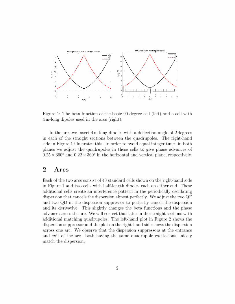
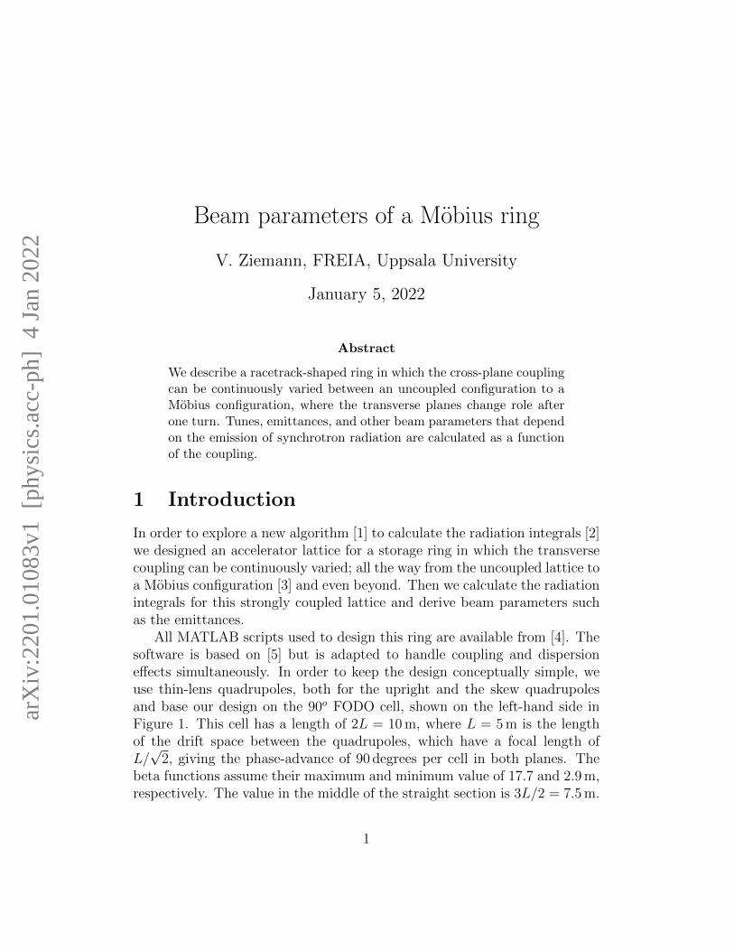
Figure 1: The beta function of the basic 90-degree cell (left) and a cell with4 m-long dipoles used in the arcs (right).

In the arcs we insert 4 m long dipoles with a deflection angle of 2 degreesin each of the straight sections between the quadrupoles. The right-handside in Figure 1 illustrates this. In order to avoid equal integer tunes in bothplanes we adjust the quadrupoles in these cells to give phase advances of0.25× 360o and 0.22× 360o in the horizontal and vertical plane, respectively.

2 Arcs

Each of the two arcs consist of 43 standard cells shown on the right-hand sidein Figure 1 and two cells with half-length dipoles each on either end. Theseadditional cells create an interference pattern in the periodically oscillatingdispersion that cancels the dispersion almost perfectly. We adjust the two QFand two QD in the dispersion suppressor to perfectly cancel the dispersionand its derivative. This slightly changes the beta functions and the phaseadvance across the arc. We will correct that later in the straight sections withadditional matching quadrupoles. The left-hand plot in Figure 2 shows thedispersion suppressor and the plot on the right-hand side shows the dispersionacross one arc. We observe that the dispersion suppressors at the entranceand exit of the arc—both having the same quadrupole excitations—nicelymatch the dispersion.

2

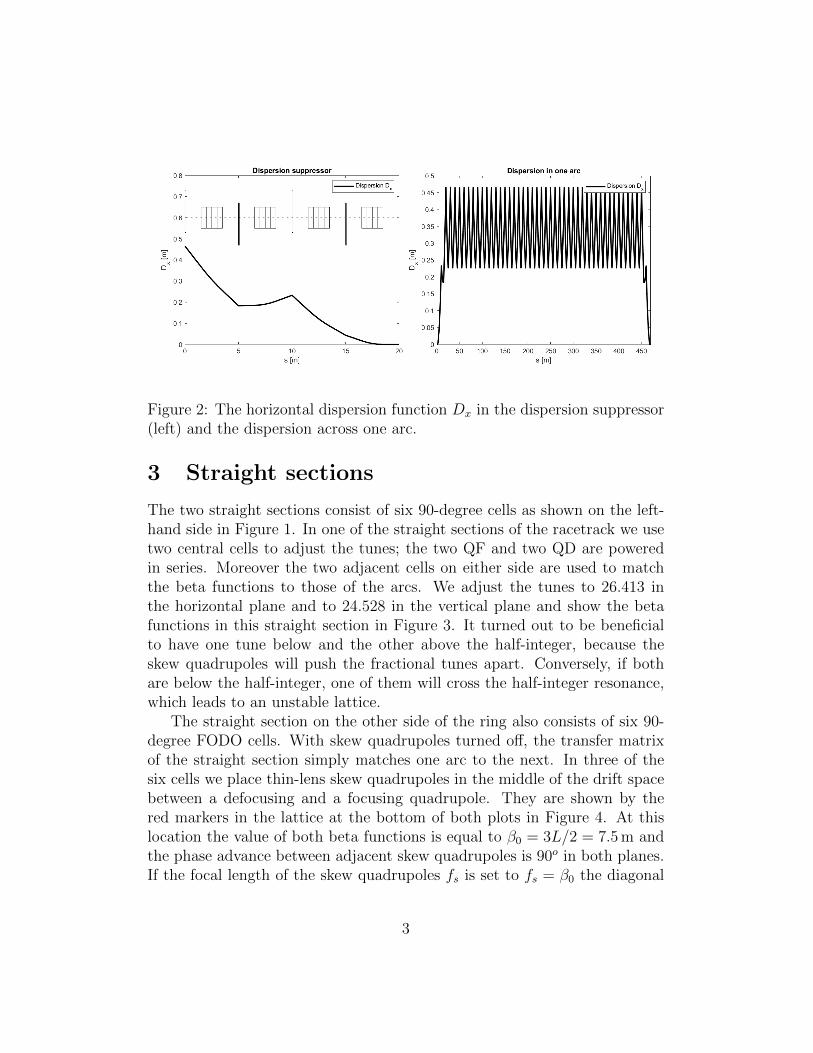
Figure 2: The horizontal dispersion function Dx in the dispersion suppressor(left) and the dispersion across one arc.

3 Straight sections

The two straight sections consist of six 90-degree cells as shown on the left-hand side in Figure 1. In one of the straight sections of the racetrack we usetwo central cells to adjust the tunes; the two QF and two QD are poweredin series. Moreover the two adjacent cells on either side are used to matchthe beta functions to those of the arcs. We adjust the tunes to 26.413 inthe horizontal plane and to 24.528 in the vertical plane and show the betafunctions in this straight section in Figure 3. It turned out to be beneficialto have one tune below and the other above the half-integer, because theskew quadrupoles will push the fractional tunes apart. Conversely, if bothare below the half-integer, one of them will cross the half-integer resonance,which leads to an unstable lattice.

The straight section on the other side of the ring also consists of six 90-degree FODO cells. With skew quadrupoles turned off, the transfer matrixof the straight section simply matches one arc to the next. In three of thesix cells we place thin-lens skew quadrupoles in the middle of the drift spacebetween a defocusing and a focusing quadrupole. They are shown by thered markers in the lattice at the bottom of both plots in Figure 4. At thislocation the value of both beta functions is equal to β0 = 3L/2 = 7.5 m andthe phase advance between adjacent skew quadrupoles is 90o in both planes.If the focal length of the skew quadrupoles fs is set to fs = β0 the diagonal

3

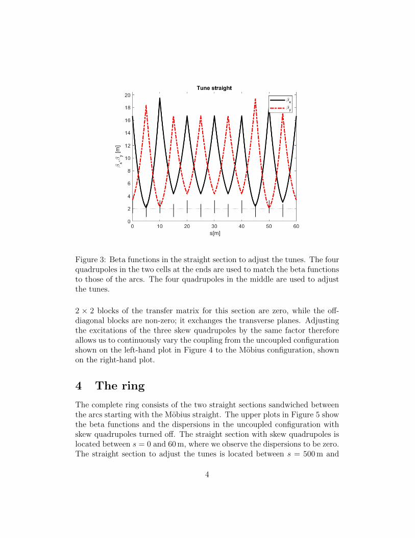
Figure 3: Beta functions in the straight section to adjust the tunes. The fourquadrupoles in the two cells at the ends are used to match the beta functionsto those of the arcs. The four quadrupoles in the middle are used to adjustthe tunes.

2 × 2 blocks of the transfer matrix for this section are zero, while the off-diagonal blocks are non-zero; it exchanges the transverse planes. Adjustingthe excitations of the three skew quadrupoles by the same factor thereforeallows us to continuously vary the coupling from the uncoupled configurationshown on the left-hand plot in Figure 4 to the Mobius configuration, shownon the right-hand plot.

4 The ring

The complete ring consists of the two straight sections sandwiched betweenthe arcs starting with the Mobius straight. The upper plots in Figure 5 showthe beta functions and the dispersions in the uncoupled configuration withskew quadrupoles turned off. The straight section with skew quadrupoles islocated between s = 0 and 60 m, where we observe the dispersions to be zero.The straight section to adjust the tunes is located between s = 500 m and

4

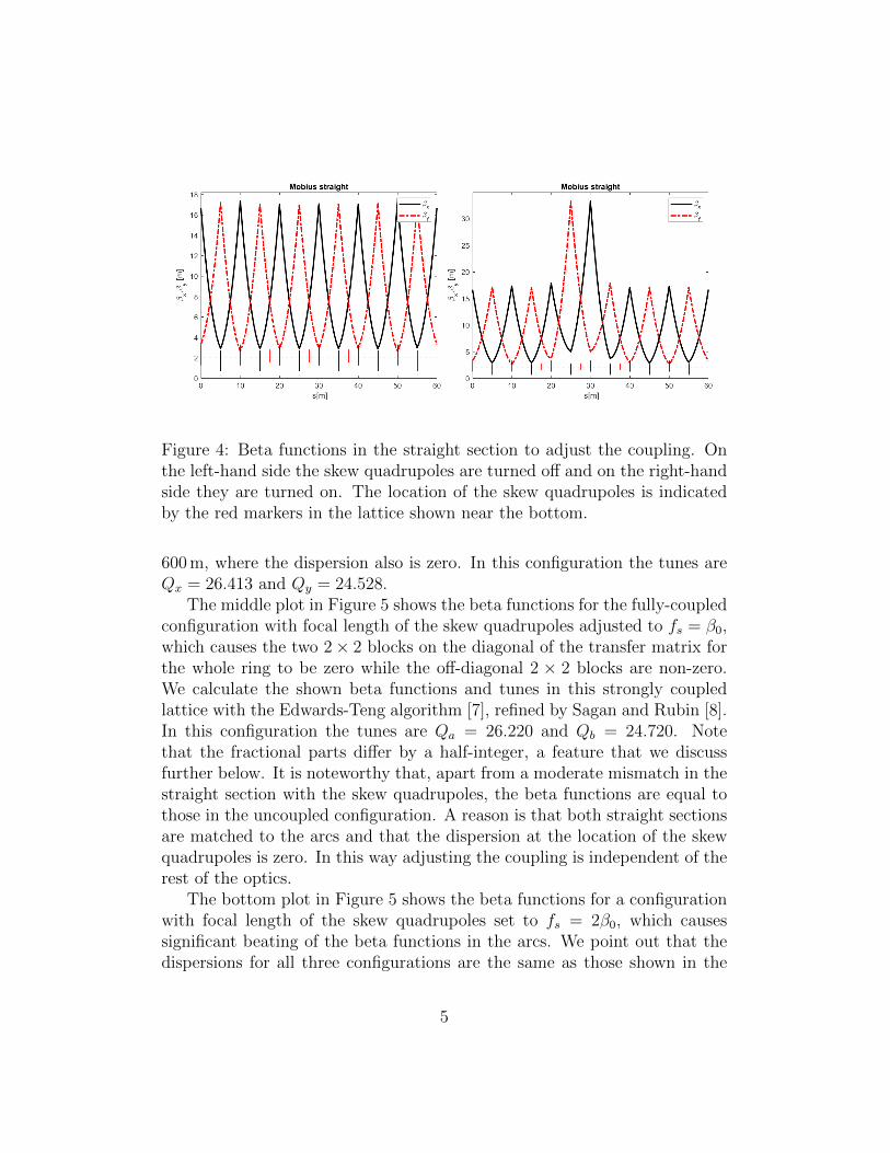
Figure 4: Beta functions in the straight section to adjust the coupling. Onthe left-hand side the skew quadrupoles are turned off and on the right-handside they are turned on. The location of the skew quadrupoles is indicatedby the red markers in the lattice shown near the bottom.

600 m, where the dispersion also is zero. In this configuration the tunes areQx = 26.413 and Qy = 24.528.

The middle plot in Figure 5 shows the beta functions for the fully-coupledconfiguration with focal length of the skew quadrupoles adjusted to fs = β0,which causes the two 2× 2 blocks on the diagonal of the transfer matrix forthe whole ring to be zero while the off-diagonal 2 × 2 blocks are non-zero.We calculate the shown beta functions and tunes in this strongly coupledlattice with the Edwards-Teng algorithm [7], refined by Sagan and Rubin [8].In this configuration the tunes are Qa = 26.220 and Qb = 24.720. Notethat the fractional parts differ by a half-integer, a feature that we discussfurther below. It is noteworthy that, apart from a moderate mismatch in thestraight section with the skew quadrupoles, the beta functions are equal tothose in the uncoupled configuration. A reason is that both straight sectionsare matched to the arcs and that the dispersion at the location of the skewquadrupoles is zero. In this way adjusting the coupling is independent of therest of the optics.

The bottom plot in Figure 5 shows the beta functions for a configurationwith focal length of the skew quadrupoles set to fs = 2β0, which causessignificant beating of the beta functions in the arcs. We point out that thedispersions for all three configurations are the same as those shown in the

5

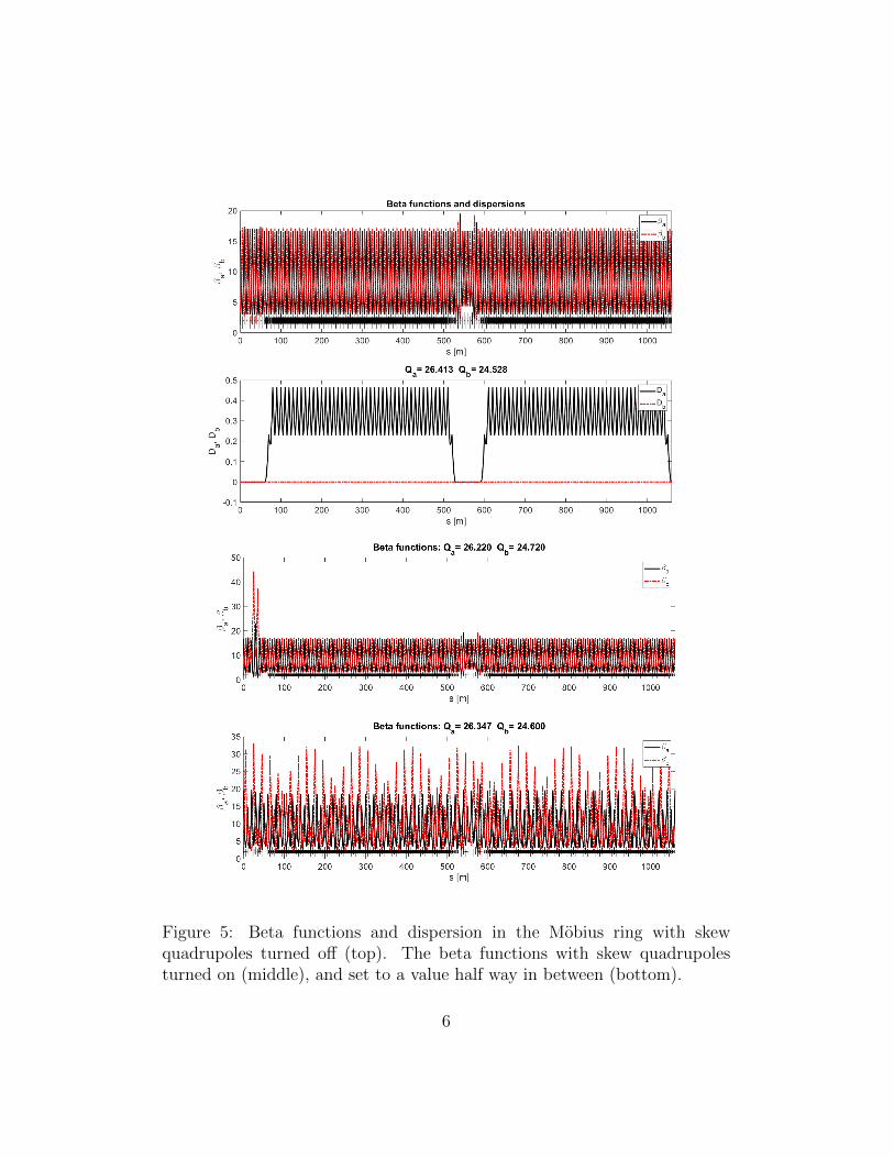
Figure 5: Beta functions and dispersion in the Mobius ring with skewquadrupoles turned off (top). The beta functions with skew quadrupolesturned on (middle), and set to a value half way in between (bottom).

6

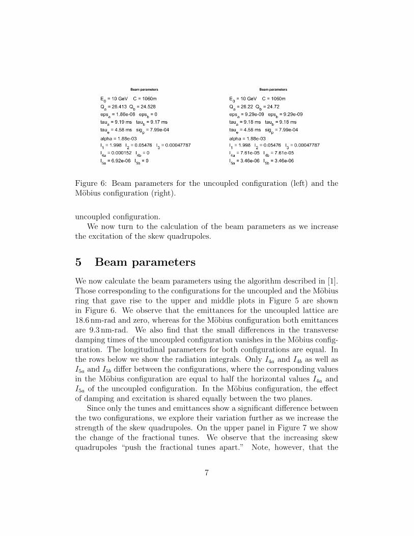
Figure 6: Beam parameters for the uncoupled configuration (left) and theMobius configuration (right).

uncoupled configuration.We now turn to the calculation of the beam parameters as we increase

the excitation of the skew quadrupoles.

5 Beam parameters

We now calculate the beam parameters using the algorithm described in [1].Those corresponding to the configurations for the uncoupled and the Mobiusring that gave rise to the upper and middle plots in Figure 5 are shownin Figure 6. We observe that the emittances for the uncoupled lattice are18.6 nm-rad and zero, whereas for the Mobius configuration both emittancesare 9.3 nm-rad. We also find that the small differences in the transversedamping times of the uncoupled configuration vanishes in the Mobius config-uration. The longitudinal parameters for both configurations are equal. Inthe rows below we show the radiation integrals. Only I4a and I4b as well asI5a and I5b differ between the configurations, where the corresponding valuesin the Mobius configuration are equal to half the horizontal values I4a andI5a of the uncoupled configuration. In the Mobius configuration, the effectof damping and excitation is shared equally between the two planes.

Since only the tunes and emittances show a significant difference betweenthe two configurations, we explore their variation further as we increase thestrength of the skew quadrupoles. On the upper panel in Figure 7 we showthe change of the fractional tunes. We observe that the increasing skewquadrupoles “push the fractional tunes apart.” Note, however, that the

7

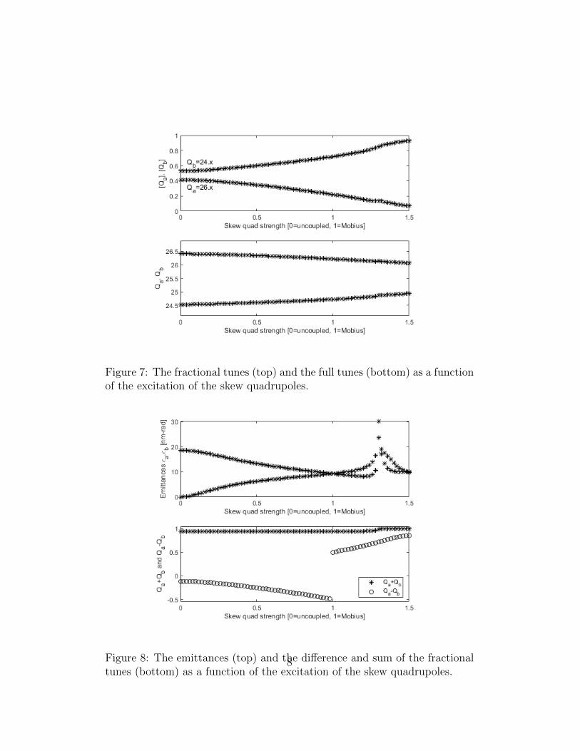
Figure 7: The fractional tunes (top) and the full tunes (bottom) as a functionof the excitation of the skew quadrupoles.

Figure 8: The emittances (top) and the difference and sum of the fractionaltunes (bottom) as a function of the excitation of the skew quadrupoles.

8

upper branch corresponds to the “vertical” tune Qb and the lower branchto the “horizontal” tune Qa. The lower panel also shows both tunes butincluding their integral part.

The upper panel in Figure 8 shows the emittances as a function of theexcitation of the skew quadrupoles. We see that initially εa is non-zero andεb is zero, but as the coupling increases their values get closer and becomeequal in the Mobius configuration. This is accompanied by the difference ofthe fractional tunes approaching a half-integer. This is apparent from thecircles on the lower panel, which show Qa−Qb. If we increase the excitationbeyond the Mobius configuration both emittances increase dramatically. Theplot on the lower panel provides an explanation; the sum of the tunes Qa +Qb becomes an integer and the system crosses a sum resonance shown bythe asterisks in the lower panel from Figure 8. And on a sum resonance,the emittances can become arbitrarily large, because only their difference isbounded [9, 10].

6 Conclusions

In order to explore the ability of the new method to calculate synchrotronradiation integrals [1] to handle highly-coupled systems we designed a ring,based on 90-degree FODO cells, which can be continuously tuned from anuncoupled to a Mobius configuration. The method works well and allow usto calculate all beam parameters that depend on the synchrotron radiationintegrals. In particular, the damping times only show a small dependence onthe coupling whereas the emittances, which differ greatly in the uncoupledconfiguration, become equal in the Mobius configuration. If we increase thecoupling beyond the Mobius configuration, the system encounters a sumresonance, where both emittances grow significantly, consistent with [9, 10].

Having the emittances and momentum spread available, we can calculatethe self-consistent equilibrium beam sizes in all three dimensions, even forhighly-coupled lattices.

Apart from serving as a test ground for the new method to calculatesynchrotron radiation integrals, the Mobius ring might become useful to ex-plore the effect of coupling on orbit correction, non-linear effects, and thebeam-beam interaction.

9

References

[1] V. Ziemann, A. Streun, Equilibrium parameters in coupled storage ringlattices and practical applications, in preparation.

[2] Richard H. Helm, Martin J. Lee, P. L. Morton, and M. Sands, Evaluationof synchrotron radiation integrals, IEEE Trans. Nucl. Sci. 20 (1973) 900.

[3] R. Talman, A proposed Mobius accelerator, Physical Review Letters 74(1995) 1590.

[4] Software used to design the Mobius ring is available from https://

github.com/volkziem/MobiusRing.

[5] V. Ziemann, Hands-On Accelerator Physics Using MATLAB, CRCPress, Boca Raton, 2019.

[6] M. Aiba, M. Ehrlichman, A. Streun, Round beam operation in electronstorage rings and generalization of Mobius accelerator, Proceedings ofIPAC 2015 in Richmond VA, USA, (2015) 1716.

[7] D. Edwards, L. Teng, Parameterization of linear coupled motion in pe-riodic systems, IEEE Trans. Nucl. Sci. 20 (1973) 885.

[8] D. Sagan and D. Rubin, Linear analysis of coupled lattices, Phys.Rev. ST Accel. Beams, 2:074001, 1999. [Phys. Rev. ST Accel.Beams3,059901(2000)].

[9] Section 1.3.1 in H. Wiedemann, Particle Accelerator Physics II, 2nd ed.,Springer Verlag, Heidelberg, 2003.

[10] Section 2.1.3 in A. Chao, M. Tigner, Handbook of Accelerator Physicsand Engineering, World Scientific, Singapore, 1999.

10