Bayesian Learning of Occupancy Grids - Colorado State ...

This article has been accepted for inclusion in a future issue of this journal. Content is final as presented, with the exception of pagination.

IEEE TRANSACTIONS ON INTELLIGENT TRANSPORTATION SYSTEMS 1

Bayesian Learning of Occupancy GridsChristopher Robbiano , Member, IEEE, Edwin K. P. Chong , Fellow, IEEE,

Mahmood R. Azimi-Sadjadi, Life Member, IEEE, Louis L. Scharf , Life Fellow, IEEE,and Ali Pezeshki, Member, IEEE

Abstract— Occupancy grids encode for hot spots on a map thatis represented by a two dimensional grid of disjoint cells. Theproblem is to recursively update the probability that each cell inthe grid is occupied, based on a sequence of sensor measurementsfrom a moving platform. In this paper, we provide a newBayesian framework for generating these probabilities that doesnot assume statistical independence between the occupancy stateof grid cells. This approach is made analytically tractable throughthe use of binary asymmetric channel models that capture theerrors associated with observing the occupancy state of a gridcell. Binary-valued measurement vectors are the thresholdedoutput of a sensor in a radar, sonar, or other sensory system.We compare the performance of the proposed framework tothat of the classical formulation for occupancy grids. The resultsshow that the proposed framework identifies occupancy gridswith lower false alarm and miss detection rates, and requiresfewer observations of the surrounding area, to generate anaccurate estimate of occupancy probabilities when compared toconventional formulations.

Index Terms— Occupancy grids, Bayesian estimation, sonar,robotic mapping.

I. INTRODUCTION

THE process of generating a map of occupied cells froma set of sequential observations has many applications,

e.g., in target localization and path planning. Both of theseapplications can be considered part of the active perceptionproblem, in which a sequence of actions is chosen thatmaximizes the amount of information attained through thoseactions [1]. An example of an active perception problemis considered in this paper, involving an ego-vehicle in theform of an autonomous underwater vehicle (AUV) whichnavigates through previously unexplored areas, taking a seriesof sequential measurements, while simultaneously performinginference for the purpose of efficiently detecting and locatingunderwater targets.

One of the commonly used approaches for this activeperception problem is occupancy grid estimation. This process,

Manuscript received November 13, 2019; revised March 30, 2020 andJuly 9, 2020; accepted August 13, 2020. This work was supported bythe Office of Naval Research (ONR) under Contract N00014-18-1-2805.The Associate Editor for this article was Z. Duric. (Corresponding author:Christopher Robbiano.)

Christopher Robbiano, Edwin K. P. Chong, Mahmood R. Azimi-Sadjadi,and Ali Pezeshki are with the Electrical and Computer EngineeringDepartment, Colorado State University, Fort Collins, CO 80524 USA(e-mail: [email protected]; [email protected]; [email protected]; [email protected]).

Louis L. Scharf is with the Mathematics and Statistics Depart-ments, Colorado State University, Fort Collins, CO 80521 USA (e-mail:[email protected]).

Digital Object Identifier 10.1109/TITS.2020.3019813

which involves estimating the occupancy map given a set ofobservations, was originally introduced by Elfes and Moravecin the mid 1980s [2]. Several subsequent papers explored alter-native methods for performing sensor fusion for distributingsensor measurements over the occupancy grids [3], and forcombining multiple occupancy grids [4], [5] from multipleindependent sensors into a single grid. These methods makethe assumption that the occupancy states of the grid cells arestatistically independent by modeling the problem as a MarkovRandom Field [2], [4], [5]. This allows for the factorizationof the joint occupancy distribution on the occupancy map intothe product of occupancy distributions of individual grid cells.

Thrun [6] provided a new occupancy grid formulation,using forward sensor models, that accounts for statisticaldependence between the occupancy state of grid cells. Themethod assumes that the sensor provides range measurementsfrom within an observation cone, and that the single rangemeasurement comes from only a single source within thecone. This measurement is assumed to be produced by eithera true positive (detection of object), a false positive (falsealarm), a true negative (no object in range), or a falsenegative (missed detection). Each of these possible eventsis modeled with a distribution from the exponential family,and the process of identifying the occupancy grid becomesa most-likely-model selection process through the use of anexpectation-maximization (EM) algorithm [6].

The recent work in [7], [8] used real antenna radiationpatterns to better inform occupancy grid estimation and henceprovide more realistic maps. In [9], [10], the authors model thedependence between grid cells using Gaussian processes. Theuse of Bayesian Occupancy Filters (BOF) [11] for generatingoccupancy grids, assuming statistical independence betweenthe grid cells, has been studied in [12]–[14].

The methods for occupancy grid estimation typically makethe assumption that a sensor produces a range measurement,i.e., reporting the range of the closest detected object inthe sensors’ field of view (FoV). However, in our activeperception problem, a sensory system on a moving platformtakes observations at all possible ranges within its beam length,producing a vector-valued measurement. Classical occupancygrid estimation does not deal with this situation. Additionally,the classical methods treat the occupancy state of each gridcell as being statistically independent. In a typical occupancygrid type problem, the area of a grid cell is much smallerthan the area which an object occupies, leading to objectswithin the interrogation field typically occupying multiple gridcells. Consequently, the occupancy state of a grid cell is

1524-9050 © 2020 IEEE. Personal use is permitted, but republication/redistribution requires IEEE permission.See https://www.ieee.org/publications/rights/index.html for more information.

Authorized licensed use limited to: COLORADO STATE UNIVERSITY. Downloaded on September 13,2021 at 20:52:22 UTC from IEEE Xplore. Restrictions apply.

https://orcid.org/0000-0003-2758-5435

https://orcid.org/0000-0002-7622-4815

https://orcid.org/0000-0003-1764-9335


2 IEEE TRANSACTIONS ON INTELLIGENT TRANSPORTATION SYSTEMS

inherently correlated with its neighboring cells, and thus theoccupancy state of the grid cells should be jointly consid-ered when performing occupancy grid estimation. These twodepartures from the classical methods motivated us to developa new occupancy grid estimation method to circumvent theseproblems.

To this end, we present a framework for solving thejoint and marginal distributions of grid cell occupancy states,while accounting for the statistical dependence between theoccupancy states of grid cells, given vector-valued sensormeasurements. We then present a method for solving thisproblem with a sensor model that exploits a network of binaryasymmetric channels (BACs). This BAC network sensor modelcan be used to represent any real sensor, with examples givenfor an ideal ranging sensor, a sonar system, and a distributednetwork of pressure sensors.

The main contributions of this paper are as follows. UsingBACs, we build a sensor model for the interaction betweenthe occupancy state of each grid cell and each sensor mea-surement. This sensor model provides a tractable methodfor considering the statistical dependence between grid celloccupancy states. The use of BACs provides a method ofmodeling any physical sensor by considering its statisticalperformance (probability of false alarm and probability ofdetection), and does not rely on a presumed distribution forsensor measurements. We also show that the original formula-tion of Elfes [2], [4], which assumed statistical independencebetween each grid cell occupancy state, can be considered aspecial case of the methods proposed here.

The remainder of this paper is organized as follows.In Section II, we first define the occupancy grid estima-tion process and establish notation. Section III develops theBayesian update equation for computing the posterior prob-ability that a particular grid cell is occupied. Three differentmethods are proposed, a general formulation and two specialcases. Experimental results for each case are presented inSection IV for: a toy problem for the purpose of comparingthe three proposed methods and two using simulated sonardata. Concluding remarks are given in Section V.

II. TERMINOLOGIES & NOTATIONS

Lowercase italic x is used for scalars, vectors and matri-ces are represented by lowercase bold italic symbols x anduppercase bold italic symbols X , respectively.

The environment under consideration is assumed to bepartitioned into grid cells (or simply cells) ci at coordinates(xi , yi , zi ), i = 1, 2, . . . , B . To each grid cell, an indicatorvariable bi ∈ {0, 1} is attached with bi = 1 indicating thatgrid cell ci is occupied by a scatterer of radiation, and bi = 0indicating that grid cell ci is empty. An occupied grid cellmay be called a hot spot. These indicators may be organizedin any convenient manner. Here, we arrange them into a vectorb = [b1, b2, . . . , bB] ∈ {0, 1}B . It is common to call the set ofindicators, organized in any manner, a map. A map capturesthe occupancy state of the grid cells.

The problem is then to estimate, for each β ∈ {0, 1}B ,the conditional probability that b = β, given a sequence

of measurement vectors J S = �j1, j2, . . . , j s , . . . , j S

�.

The subscript S indicates the current sensing time, while1 ≤ s ≤ S indicates a time index at which measurements aretaken. Each j s ∈ {0, 1}K is a binary vector (e.g., thresholdeddetection statistics) and β ∈ {0, 1}B is a specific map withinthe set of all possible maps with B elements. We denotethis probability as pb|J (b|J S) and return our estimates as themarginal posterior probabilities pb|J (br = 1|J S), where br isthe r th indicator random variable in b. Importantly, it is theset of marginal posterior probabilities {pb|J (br = 1|J S)}B

r=1that is returned by our algorithm. This set of probabilitiescan be organized in any order, and we choose to arrangethem into a vector p = [pb|J (b1 = 1|J S), pb|J (b2 =1|J S), . . . , pb|J (bB = 1|J S)] ∈ [0, 1]B . These marginalposterior probabilities can be produced for any 1-, 2-, or 3-dimensional grid depending on the problem.

There are some inconsistencies in the related literature as tothe precise definition of an occupancy grid or occupancy gridmap [4]–[6], [12]–[16], and whether it is a map, as defined pre-viously, or the set of marginal posterior probabilities. For thisreason, we will refer to b as cellular occupancies, and the setof corresponding posterior probabilities as cellular posteriorprobabilities. It is common to illustrate, or plot, both cellularoccupancies and cellular posterior probabilities to provide avisual representation for comparison. Here, we reserve theoccupancy grid name for both cellular occupancies and cellularposterior probabilities when they are illustrated, or plotted,in some way.

The following is a summary of the notation used in thedevelopment of our occupancy grid estimation framework.

• B : The number of grid cells in a map.• b : A random vector taking values in {0, 1}B representing

cellular occupancies.• b̃ ∈ {0, 1}B : The virtual cellular occupancies after the

occupancy state of each grid cell has been passed througha binary asymmetric channel (BAC).

• p = [pb|J (b1 = 1|J S), . . . , pb|J (bB = 1|J S)] ∈ [0, 1]B

: The vector of cellular posterior probabilities.• B : Set of all possible cellular occupancies b. |B| = 2B .• B(r, β) = {b|br = β} : Set of all cellular occupancies

with br = β, β ∈ {0, 1}.• S : Current/latest time index.• s : Time index with 1 ≤ s ≤ S.• j s ∈ {0, 1}K : Binary-valued measurement vector of

dimension K taken from the output of a sensory systemat time s.

• J S = �j1, . . . , j S

�: Collection of binary-valued mea-

surement vectors up to time S.At each time s a measurement vector j s , comprising

binary values (e.g., thresholded detection statistics) js,k, k =1, . . . , K , is taken, where K is the maximum number ofsamples recorded by the sensor. The index k encodes forsome position (xk, yk, zk) within the environment. During thecollection of each measurement, the sensor is effectively ina fixed position in its trajectory path, and the sensor has aFoV of the grid cells. The sequence of these measurementvectors forms the matrix J S = �

j1, . . . , j s, . . . , j S�

withcolumns that are all the past and present binary measurement



ROBBIANO et al.: BAYESIAN LEARNING OF OCCUPANCY GRIDS 3

vectors. Note that here we consider a sensor in its mostgeneral form to be a probabilistic map that takes as inputthe object we are measuring (in our case, the cellular occu-pancies) and gives as output a random variable (the mea-surement j s ). Each sensor is characterized by the conditionaldistribution of the output given the input. Real-world sensorysystems can be described with this definition as presented inSection IV-D.

The goal is to develop a sequential Bayesian frameworkfor updating the posterior probability of the occupancy ofeach grid cell ci with associated indicator random variable bi ,given the sequence of measurements in J S . That is, we wishto update the cellular posterior probabilities after each timestep.

III. OCCUPANCY GRID ESTIMATION-FORMULATION

To produce the estimate of the vector of cellular posteriorprobabilities p, most of the existing methods [2], [4], [5], [7],[12] factor the joint distribution of the cellular occupanciesas pb(b) = �

i pb(bi ). Similarly, when conditioned on thecollection of measurement vectors in J S , the joint distributionis assumed to be factored as pb|J (b|J S) = �

i pb|J (bi |J S)which implies that the elements in the cellular occupanciesare conditionally independent. As pointed out before, thesesimplifying assumptions limit the applicability of such meth-ods in many practical situations. The general formulation (GF)presented in this section is intended to lift these restrictiveassumptions.

Throughout the development of this formulation, we assumethat the sensor position at each time is reasonably accu-rate, i.e., the odometry errors are small enough to ignore.This is a valid assumption for sensory system deployed onmany autonomous platforms, where a low velocity and smallmeasurement error from the odometry sensors satisfies theego-motion estimation for the vehicle.

A. Model for Grid Cell and Measurement Interactions

The sensor model presented in this section provides a wayto probabilistically solve the data association problem of deter-mining which grid cells are occupied given the measurements.A network of binary asymmetric channels (BACs) [17] areused to model the relationship between grid cell occupancystates and measurements. The BAC outputs, the so-calledvirtual occupancies, are latent variables, and are merely usedto model the measurements.

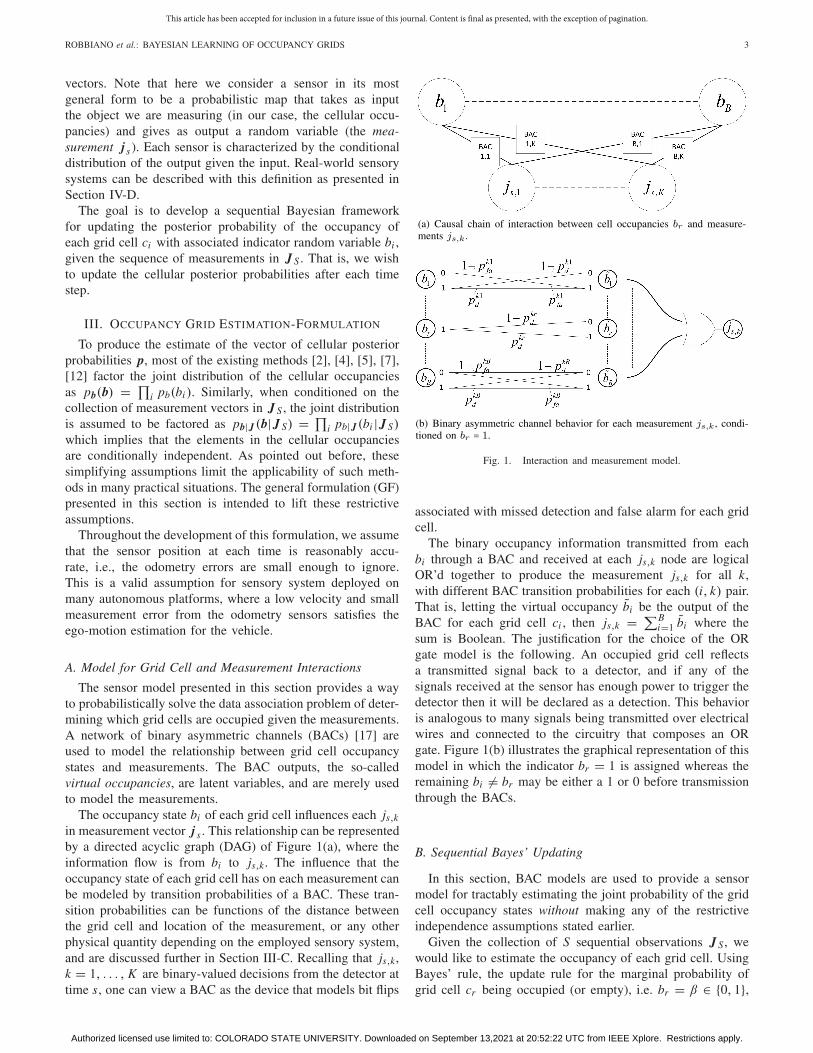
The occupancy state bi of each grid cell influences each js,kin measurement vector j s . This relationship can be representedby a directed acyclic graph (DAG) of Figure 1(a), where theinformation flow is from bi to js,k. The influence that theoccupancy state of each grid cell has on each measurement canbe modeled by transition probabilities of a BAC. These tran-sition probabilities can be functions of the distance betweenthe grid cell and location of the measurement, or any otherphysical quantity depending on the employed sensory system,and are discussed further in Section III-C. Recalling that js,k,k = 1, . . . , K are binary-valued decisions from the detector attime s, one can view a BAC as the device that models bit flips

Fig. 1. Interaction and measurement model.

associated with missed detection and false alarm for each gridcell.

The binary occupancy information transmitted from eachbi through a BAC and received at each js,k node are logicalOR’d together to produce the measurement js,k for all k,with different BAC transition probabilities for each (i, k) pair.That is, letting the virtual occupancy b̃i be the output of theBAC for each grid cell ci , then js,k = �B

i=1 b̃i where thesum is Boolean. The justification for the choice of the ORgate model is the following. An occupied grid cell reflectsa transmitted signal back to a detector, and if any of thesignals received at the sensor has enough power to trigger thedetector then it will be declared as a detection. This behavioris analogous to many signals being transmitted over electricalwires and connected to the circuitry that composes an ORgate. Figure 1(b) illustrates the graphical representation of thismodel in which the indicator br = 1 is assigned whereas theremaining bi �= br may be either a 1 or 0 before transmissionthrough the BACs.

B. Sequential Bayes’ Updating

In this section, BAC models are used to provide a sensormodel for tractably estimating the joint probability of the gridcell occupancy states without making any of the restrictiveindependence assumptions stated earlier.

Given the collection of S sequential observations J S , wewould like to estimate the occupancy of each grid cell. UsingBayes’ rule, the update rule for the marginal probability ofgrid cell cr being occupied (or empty), i.e. br = β ∈ {0, 1},




given the entire set of measurements J S , is given as

pb|J (br = 1|J S)

= pb,J (br = 1, J S)

pJ (J S)= pb,J (br = 1, j S, J S−1)

pJ ( j S, J S−1)

=��

b∈B(r,1) pb,J (b, j S, J S−1)�

pJ ( j S, J S−1)

=��

b∈B(r,1) p j |b( j S |b, J S−1)pb|J (b|J S−1)�

p j |J ( j S |J S−1)

= η�

b∈B(r,1)

p j |b( j S |b)pb|J (b|J S−1), (1)

where η is a normalization term such that pb|J (br = 1|J S)+pb|J (br = 0|J S) = 1. The second to last line comes fromthe conditional independence of measurements. The secondterm on the right hand side of the last line, pb|J (b|J S−1),is the posterior probability from the previous time step S − 1.Likewise, the posterior probability pb|J (b|J S) can be writtenusing the same sensor model used in (1):

pb|J (b|J S) = pb,J ( j S, b, J S−1)

pJ ( j S, J S−1)

= μp j |b( j S |b)pb|J (b|J S−1), (2)

where μ is a normalization term such that�

β∈Bpb|J (b =

β|J S) = 1. For any value of S, plugging (2) into (1) andexpanding (2) shows the explicit dependence on all historicalmeasurement information for the occupancy state update.

Given the map or occupancy state b, the measurements{ js,k}K

k=1 in j s are indeed conditionally independent. Thus,we can write

p j |b( j s |b) =

k

p j |b( js,k|b). (3)

Note that this is different than the commonly used assumptionthat the elements in the cellular occupancies are conditionallyindependent, i.e., pb|J (b|J S) = �

i pb|J (bi |J S).To better describe the term p j |b( js,k|b) in (3), and specif-

ically p j |b( js,k = 0|b), let b̃ = {b̃i}Bi=1 be the collection of

BAC outputs (cf. Section III-A) which are the latent variablesthat capture the influence of grid cell ci on each measurementjs,k. More specifically, each js,k is a Boolean function ofvirtual occupancies, i.e., js,k = �B

i=1 b̃i . Thus, we can write

p j |b( js,k = 0|b) = pb̃|b(b̃i = 0 ∀i |b) : OR gate assumption

=

i

pb̃|b(b̃i = 0|bi)

=

i

p00ki (1 − bi )+ p01

ki bi , (4)

where pb̃|b(b̃i = 0|bi ) is implicitly parameterized by k, i.e., theindex of the measurement. For each pair (k, i) of measurementindex k and grid cell ci , we define pki

d and pkifa to be the

probability of detection and false alarm, respectively. Then,we have

p00ki = pb̃|b(b̃i = 0|bi = 0) = 1 − pki

fa ,

p01ki = pb̃|b(b̃i = 0|bi = 1) = 1 − pki

d ,

where p00ki models the probability that bi = 0 is transmitted

through the BAC and received correctly as b̃i = 0; whilep01

ki models the probability that bi = 0 is transmitted throughthe BAC and received incorrectly as b̃i = 1. The otherprobabilities p11

ki = pkid and p10

ki = pkifa are similarly defined.

Plugging all these into (1) and (2) gives the followingclosed-form expressions that can be used for computing theBayesian updates:pb|J (br = 1|J S)

= η�

b∈B(r,1)

p j |b( j S|b)pb|J (b|J S−1)

∝�

b∈B(r,1)

k

i

�p00

ki (1 − bi )+ p01ki bi

�(1 − jS,k)

+ 1 − (p00

ki (1 − bi )+ p01ki bi )

�jS,k

�pb|J (b|J S−1), (5)

and,

pb|J (b|J S)

= μ

k

i

�p00

ki (1 − bi)+ p01ki bi

�(1 − jS,k)

+ 1 − (p00

ki (1 − bi )+ p01ki bi)

�jS,k

�pb|J (b|J S−1). (6)

This is what we refer to as the general formulation (GF)of the occupancy grid problem. The formulation in [4], whichassumes independence between occupancy states of grid cells,can be viewed as a special case of this formulation. To seethis let us consider the case when the set B(r, 1) containsonly a single element, indicating that only one grid cell isbeing processed at a time. The sum over B(r, 1) and theproduct over i in (5) vanish. The product over k would also berestricted to the indices k ∈ κ = {κ, κ + 1, . . . , κ + K �}, withκ ≥ 0 and κ + K � ≤ K , that coincide with the neighborhoodaround grid cell cr . Thus, (5) in this case reduces to

pb|J (br = 1|J S) = ηk∈κ

�p01

ki (1 − jS,k)+ 1 − p01

ki

�jS,k

× pb|J (br = 1|J S−1), (7)

which is equivalent to the formulation in [4] derived using ourBAC model.

C. Choices of Transition Probabilities

The choice of appropriate transition probabilities foreach BAC can be made using two different categories ofapproaches. The first category involves using heuristic factorswhere the designer imparts a belief into the choice of thetransition probabilities. Such factors exploit distance-basedor any other plausible measure. For example, a similar ideawas adopted in the formulations presented in [7], [8] wherereal-world receiver antenna gain patterns were used as a wayto choose the values of p10

ki and p11ki for different grid cells.

The second category of methods uses statistical estimationmethods to learn the transition probabilities given a collectionof training data. The success of these methods depends on theenvironments in which the senors are operating and amountof data used to estimate the transition probabilities. For exam-ple, if the environments are consistent from experiment to




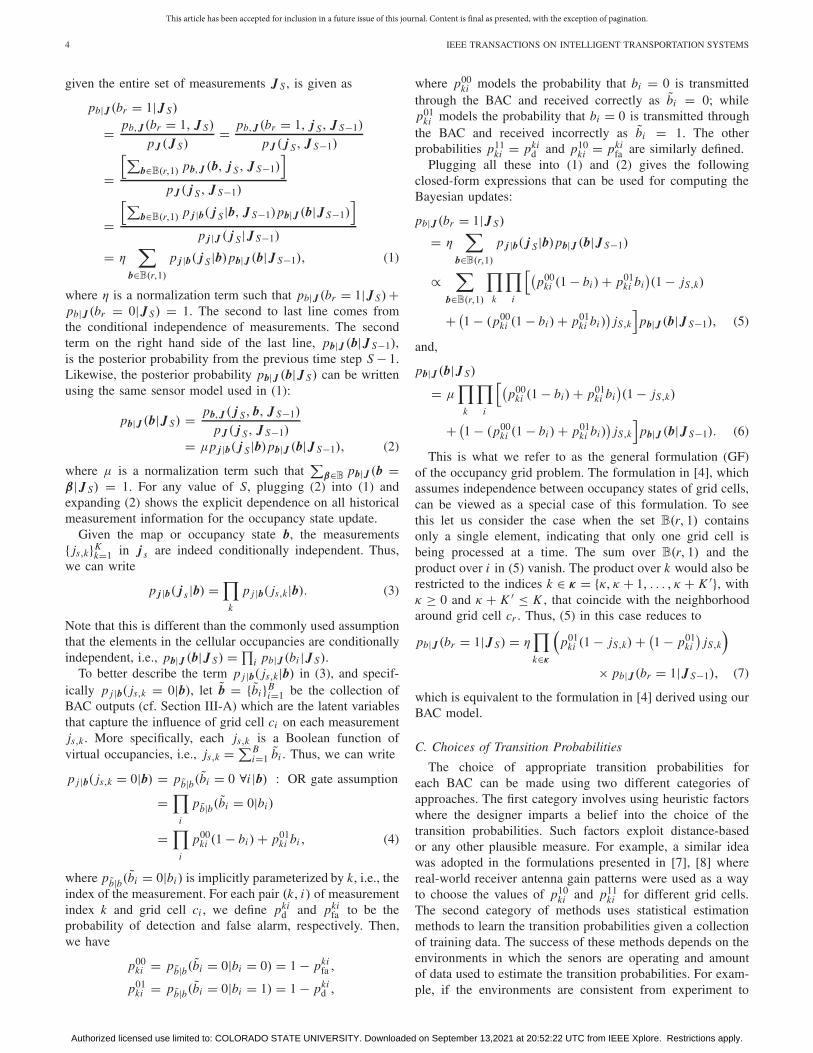
Fig. 2. Occupancy probability profile for an ideal sensor.

experiment, and we have sufficient data, then convergence ofthe transition probability estimates can be expected. However,if the sensor takes measurements in a different environmentfor each experiment, then the training data may not containsufficient information for proper estimation of the transitionprobabilities.

We must point out that the occupancy probability profile(OPP) [4] for almost any sensor model may be representedat any time S using the proposed BAC model throughproper selection of the transition probabilities. As an example,we show how to model the OPP for the ideal sensor, whichreturns a scalar value representing the closest distance at whicha reflection from an object was seen. The ideal sensor OPP[4], illustrated in Figure 2, can be modeled using the BACmodel through appropriate choice of transition probabilities.This OPP modeling is performed with the use of (7). Letη� = ηpb|J (br = 1|J S−1). Then, (7) becomes pb|J (br =1|J S) = η� �

k∈κ (p01ki (1 − jS,k)+ (1 − p01

ki ) jS,k).Let the index k of jS,k be related to the range from the

sensor, placing jS,k ∈ j S in ascending order by range fromthe sensor (i.e., jS,k further away from the sensor have alarger k). Also, let p01

ki be a function of jS,k and k. Denoteby r a scalar range measurement from the ideal sensor, andassociate r = r0 with the smallest index k such that jS,k = 1.Figure 2 illustrates these details along with the OPP for theideal sensor. The scalar range measurement can be convertedto its associated vector of length K by assigning 0s at allindices of the vector, then placing a 1 at the index k encodingfor the distance closest to r = r0.

Indicator di = −1 implies that grid cell ci with occupancystate variable bi is closer than r0 − ε units from the sensor,di = 0 indicate that it is r0 ± ε units from the sensor, anddi = 1 otherwise. The ranges associated with di are annotatedon Figure 2. The following set of rules can be applied tochoose p01

ki such that pb|J (bi = 1|J S) matches the OPP forthe ideal sensor, where |κ | is the cardinality of the set κ , andI(k) = �

k∈κ 1 − jS,k is the indicator function that counts thenumber of jS,k ∈ j S that are 0:

p01ki =

⎧⎪⎪⎪⎪⎪⎨⎪⎪⎪⎪⎪⎩

0 di = −1

1 − jS,k

η�

1I(k)

di = 0

0.5

η�

1|κ |

di = 1

∀k ∈ κ.

D. Special Cases for Cone-Like Sensor Models

Here, we present two special cases for sensors that can bemodeled with a cone-like radiation pattern (e.g., radar, sonar,

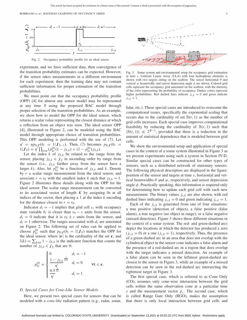
Fig. 3. Sonar system and environmental setup for occupancy grid estimationat time s. Uniform Linear Array (ULA) with four hydrophone elements isshown with two targets sitting on the seafloor. The sensor horizontal θ andvertical ψ beamwidth, and sensor depression angle φ are shown. Colored gridcells represent the occupancy grid annotated on the seafloor, with the intensityof the color representing the probability of occupancy. Darker colors representhigher probabilities. Red dashed lines indicate js,k = 0 and green indicatejs,k = 1.

lidar, etc.). These special cases are introduced to overcome thecomputational issues, specifically the exponential scaling thatoccurs due to the cardinality of set B(r, 1) as the number ofgrid cells increases. Each special case improves computationalfeasibility by reducing the cardinality of B(r, 1) such that|B(r, 1)| 2B−1, provided that there is a reduction in theamount of statistical dependence that is modeled between gridcells.

We show the environmental setup and application of specialcases in the context of a sonar system illustrated in Figure 3 aswe present experiments using such a system in Section IV-D.Similar special cases can be constructed for other types ofsensors, such as a distributed network of stationary sensors.The following physical descriptors are displayed in the figure:position of the sensor and targets at time s, horizontal and ver-tical beamwidths θ and ψ , respectively, and sensor depressionangle φ. Practically speaking, this information is required onlyfor determining how to update each grid cell with each newmeasurement. The binary values js,k are also shown, with reddashed lines indicating js,k = 0 and green indicating js,k = 1.

Each of the js,k is generated from one of four situations:a true positive (detection of object), a false positive (falsealarm), a true negative (no object in range), or a false negative(missed detection). Figure 3 shows these different situations inthe context of a sonar system. The red- and green-dashed arcsdepict the locations at which the detector has produced a zero( js,k = 0) or a one ( js,k = 1), respectively. Thus, the presenceof a green-dashed arc in an area that does not overlap with thecylindrical object in the sensor cone indicates a false alarm andthe presence of a red-dashed arc in a region that does overlapwith the target indicates a missed detection. An example ofa false alarm can be seen in the leftmost green-dashed arcclosest to the sensor in Figure 3, while an example of a misseddetection can be seen in the red-dashed arc intersecting therightmost target in Figure 3.

The first special case, which is referred to as Cone Only(CO), assumes only cone-wise interaction between the gridcells within the same observation cone at a particular times and the measurement vector j s . The second case, whichis called Range Gate Only (RGO), makes the assumptionthat there is only local interaction between grid cells and




Fig. 4. Physical interpretation of CO and RGO cell-measurement interactions.The set bI is depicted in blue, while the set bO is depicted in grey for bothcases.

measurements, restricted to within a particular range gate.Note that we refer to a range gate as that comprising multiplerange intervals where each range interval is a constant distancefrom the sensor. A graphical interpretation of these specialcases is illustrated in Figure 4, which helps to provide somephysical intuition of each special case.

Case 1 (Cone Only): Here, we assume that the interactionbetween the measurement vector j s and the grid cells that lieoutside the observation cone at time s is negligible, and henceboth the probability of detection p11

ki and false alarm p10ki are

0 for grid cells ci outside of the observation cone.To formally describe this, let us partition the grid indices

{1, 2, . . . , B} into two parts, I and O, such that I �O ={1, 2, . . . , B} and I �O = ∅. The set I captures the indicesof grid cells that fall within the sensor cone, while the set Ocaptures the indices of the grid cells that fall outside of thesensor cone.

The indicator variables composing a particular vector b ofcellular occupancies can then be partitioned into two disjointsets, the set bI = {bi |i ∈ I} for grid cells inside the sensorcone and the set bO = {bo|o ∈ O} for grid cells outside suchthat b = bI

�bO. Evaluating (4) for this case gives

p j |b( js,k = 0|b) =

o

pb̃|b(b̃o = 0|bo)

i

pb̃|b(b̃i = 0|bi )

= (1)

i

pb̃|b(b̃i = 0|bi )

= p j |b( js,k = 0|bI), (8)

because the conditional probability of receiving a 0 throughthe BAC for each b̃o is 1. By making this assumption,the cardinality of B(r, 1) is reduced to |B(r, 1)| = 2B−1−|I| 2B−1. Although this provides faster computational time whilemaintaining the statistical dependence between all grid cellswithin the sensor cone, it has the side effect of ignoringinformation imparted by neighboring occupied cells if, forexample, an obstacle occupies the inside and outside of thesensor cone.

Case 2 (Range Gate Only): This special case accountsfor only the interaction between measurements and grid cellswithin a specific range gate in the observation cone. A visu-alization of a range gate can be seen in the blue band of grid

cells in the observation cone in Figure 4(b). Similar to CO,this case also ignores information imparted by neighboringgrid cells if an obstacle occupies the inside and outside of aparticular range gate. A potential way to help mitigate this isto allow for overlapping range gates.

In a similar manner as was done for CO, let b = bI�

bO,but for this special case bI is the set of grid cells within arange gate of an observation cone as in shown in Figure 4(b).Although (8) can still be used for this case, a restriction isput on j s such that the delay at which the kth measurementis taken must coincide with the selected ranges, i.e., onlythe js,k falling within the range gate are considered. In thisway, we calculate the posterior distributions of grid celloccupancies in each range gate separately. This further reducesthe cardinality of B(r, 1) when compared to the first specialcase.

Remarks: The implementation of the proposed methods isexpected to use the most general form that is tractable for theproblem. For a small number of total grid cells, GF can beapplied without much overhead. As the total number of gridcells increases, the cardinality of B(r, 1) increases and thusso does the computation time for the marginalization in (1).For implementation purposes, the choice between GF, CO, andRGO should be driven by the desire to keep the cardinality ofB(r, 1) at a reasonable level that allows for a tractable amountof computation time for the system.

Consider segmenting the observation cone into manysmaller disjoint cones and then using RGO to update thecellular posterior probabilities. It is not hard to imagine that inthe limit of splitting the observation cone into smaller conesand applying RGO to small range gates, the updating of gridcells would happen independently from one another. In otherwords, there would only be a single grid cell being updatedat any particular time.

These simplifications produce the same Bayesian updaterule, presented in (7), that one would obtain by assumingindependence between the occupancy state of grid cells,and independence between measurement errors. In this case,the computational complexity would no longer scale expo-nentially in B , at the expense of possible degradation in theperformance.

IV. EXPERIMENTAL RESULTS

In this section, we present experimental results for GFdefined in (5), as well as those for CO and RGO specialcases. Two types of experiments were conducted with anincreasing number of grid cells per experiment. The first typeof experiment is considered as a toy experiment, where asmall number of grid cells compose the entire map. This typeof experiment is necessary for comparison between GF, CO,and RGO, as there is a limit to the number of grid cells GFcan be tractably applied to because of the exponential scalingof the cardinality of B(r, 1). The second type of experimentuses simulated sonar data, and emulates the detection andlocalization component of our active perception problem.

In all experiments, we assume there is an array of sensorstaking observations of the map containing no moving targets.




Using the first set of experiments we show that GF providesthe best overall performance, and that each special caseprovides performance that is related to the number of gridcells that are updated concurrently. The sensor array producesmeasurements that are thresholded detection statistics in theform of binary-valued vectors. The detector’s threshold waschosen to produce a desired false alarm probability pfa andhence a probability of detection pd.

In all experiments, the BAC transition probabilities p00ki and

p01ki were modeled as p00

ki = (1 − pd)/(1 + dist(bi , js,k))α

and p01ki = (1 − pfa)/(1 + dist(bi , js,k))α , where dist(bi , js,k)

represents the Euclidean distance between the location ofgrid cell ci and that at which sample js,k was taken, andα ≥ 1. This particular modeling is used to emulate degradeddetection performance due to attenuation in the signal strengthas a function of distance due to losses from the transmissionmedium, i.e., salty water for the sonar experiments.

A. Metrics Used for Performance Comparison

To evaluate the performance of various methods, two dif-ferent metrics are used. For both metrics, we consider the truecellular occupancy and the cellular posterior probabilities tobe occupancy grids to facilitate direct comparison. To makethe following notation a bit more compact, we write pi asthe probability mass function for the i th element from thecellular posterior probability occupancy grid p, βi is the i thelement from the ground truth occupancy grid β, and pβi isthe probability mass function of βi .

1) Similarity between the cellular posterior probability occu-pancy grid p to that of the true occupancy grid β: ρ =�β, p�/||β||2|| p||2, where �·, ·� is an inner product. Clearly,0 ≤ ρ ≤ 1, and ρ = 1 when each cellular posteriorprobability in p is driven to either 0 or 1 and p = β.

2) Sum of the Jensen-Shannon distance (SJSD) DJS(pβi ||pi)[18] over all i grid cells in an occupancy grid:

SJSD = 1

2

�i

DJS(pβi ||pi)

=�

i

DKL(pβi ||Mi )+ DKL(pi ||Mi )

= −�

i

1

2

� �x∈X

pβi (x) log� Mi (x)

pβi (x)

+�x∈X

pi(x) log� Mi (x)

pi(x)

�,

where Mi (x) = 12 ×

pi(x) + pβi (x)�, and DKL(·, ·)

is the Kullback-Leibler (KL) divergence [18]. TheJensen-Shannon distance is used in favor of the KL diver-gence as it is symmetric, positive, and always finite. Themaximum value of SJSD is log(2)×B , with smaller valuesindicating that β and p are similar and SJSD =0 whenβ = p.

B. Comparison With Other Methods

We must note that a direct comparison to the traditionaloccupancy grid frameworks of [4], [5] is not appropriate.

This is due to the fact that those methods assume that thesensor produces a single range measurement (identifies the firstpeak in the return above a predetermined threshold) for eachobservation and fit a heuristic model for sharing these rangemeasurements over the observed grid cells at each time step.Additionally, a direct comparison with Thrun’s method [6] thatdoes not make the statistical independence of grid cell assump-tion is not possible, as the method also relies on single rangemeasurements in its formulation. Therefore, we benchmarkthe performance of the proposed methods against two similarmethods, both of which follow the traditional occupancy gridmapping algorithm. That is, they use a Bayesian update [19]for each grid cell assuming independence between the gridcells, and independence between measurements. The firstmethod uses our sensor model and will henceforth be referredto as the independence method (IM). The second method usesthe conventional occupancy grid sensor model [5], [6] andis adapted to allow for binary-valued vector measurements.We call the second method the conventional method (CM)throughout the remained of the paper.

The method for performing the Bayesian update on a 2-dimensional map, using IM, for experiments that use a coneshaped observation model is summarized as follows:

1) Find the global position of each grid cell observed withinthe observation cone at time s.

2) Determine the centerline of the cone, and project theposition of each observed grid cell onto the centerline.

3) Associate each measurement js,k with its distance alongthe centerline. Identify the set of all projected grid cellswhere projections equal this centerline distance.

4) Update the probability of each grid cell cr , at location(xr , yr ), being occupied given the set of measurementson that grid cell, { js,k}κ+K �

k=κ , using (7).Similarly, the Bayesian update on a 2-dimensional map

using CM follows steps 1)-3) from above, and uses thesensor model proposed in [5], [6] to perform the update.The built-in occupancy grid estimation tools available in thenavigation toolbox of Matlab R2019b were used to performthe probabilistic integration for CM.

C. Experiments With Toy Problem

The first set of experiments involves a toy problem thatis sufficiently small such that all three proposed methodscan be applied and compared. The toy environment used a2-dimensional map comprising 16 grid cells with an equal dis-tance of 0.5 units between the centers of individual grid cells.Each grid cell had a total of 9 different measurements sampleduniformly throughout the area it covers. The measurementvector j s comprises 144 measurements j s = [ js,1, . . . , js,144],9 samples for each of the 16 cells, taken at equal distancecovering the same overall area as the grid cells.

This experiment can be thought of as modeling multipleapplication scenarios. One scenario entails using a traditionalego-vehicle that is observing an area and estimating thelocations of occupied grid cells using transmit-receive sens-ing. Alternatively, we can consider a scenario that involvesusing a distributed network of stationary sensors to capture




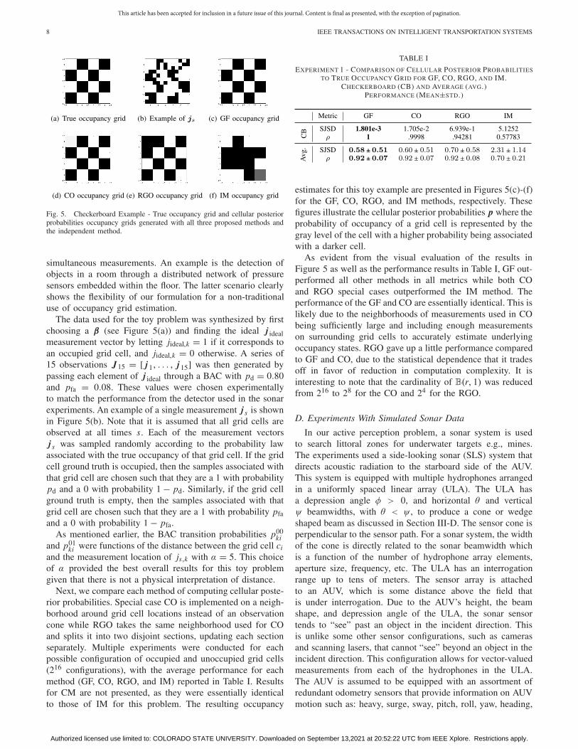
Fig. 5. Checkerboard Example - True occupancy grid and cellular posteriorprobabilities occupancy grids generated with all three proposed methods andthe independent method.

simultaneous measurements. An example is the detection ofobjects in a room through a distributed network of pressuresensors embedded within the floor. The latter scenario clearlyshows the flexibility of our formulation for a non-traditionaluse of occupancy grid estimation.

The data used for the toy problem was synthesized by firstchoosing a β (see Figure 5(a)) and finding the ideal j idealmeasurement vector by letting jideal,k = 1 if it corresponds toan occupied grid cell, and jideal,k = 0 otherwise. A series of15 observations J15 = [ j1, . . . , j15] was then generated bypassing each element of j ideal through a BAC with pd = 0.80and pfa = 0.08. These values were chosen experimentallyto match the performance from the detector used in the sonarexperiments. An example of a single measurement j s is shownin Figure 5(b). Note that it is assumed that all grid cells areobserved at all times s. Each of the measurement vectorsj s was sampled randomly according to the probability lawassociated with the true occupancy of that grid cell. If the gridcell ground truth is occupied, then the samples associated withthat grid cell are chosen such that they are a 1 with probabilitypd and a 0 with probability 1 − pd. Similarly, if the grid cellground truth is empty, then the samples associated with thatgrid cell are chosen such that they are a 1 with probability pfaand a 0 with probability 1 − pfa.

As mentioned earlier, the BAC transition probabilities p00ki

and p01ki were functions of the distance between the grid cell ci

and the measurement location of js,k with α = 5. This choiceof α provided the best overall results for this toy problemgiven that there is not a physical interpretation of distance.

Next, we compare each method of computing cellular poste-rior probabilities. Special case CO is implemented on a neigh-borhood around grid cell locations instead of an observationcone while RGO takes the same neighborhood used for COand splits it into two disjoint sections, updating each sectionseparately. Multiple experiments were conducted for eachpossible configuration of occupied and unoccupied grid cells(216 configurations), with the average performance for eachmethod (GF, CO, RGO, and IM) reported in Table I. Resultsfor CM are not presented, as they were essentially identicalto those of IM for this problem. The resulting occupancy

TABLE I

EXPERIMENT 1 - COMPARISON OF CELLULAR POSTERIOR PROBABILITIESTO TRUE OCCUPANCY GRID FOR GF, CO, RGO, AND IM.

CHECKERBOARD (CB) AND AVERAGE (AVG.)PERFORMANCE (MEAN±STD.)

estimates for this toy example are presented in Figures 5(c)-(f)for the GF, CO, RGO, and IM methods, respectively. Thesefigures illustrate the cellular posterior probabilities p where theprobability of occupancy of a grid cell is represented by thegray level of the cell with a higher probability being associatedwith a darker cell.

As evident from the visual evaluation of the results inFigure 5 as well as the performance results in Table I, GF out-performed all other methods in all metrics while both COand RGO special cases outperformed the IM method. Theperformance of the GF and CO are essentially identical. This islikely due to the neighborhoods of measurements used in CObeing sufficiently large and including enough measurementson surrounding grid cells to accurately estimate underlyingoccupancy states. RGO gave up a little performance comparedto GF and CO, due to the statistical dependence that it tradesoff in favor of reduction in computation complexity. It isinteresting to note that the cardinality of B(r, 1) was reducedfrom 216 to 28 for the CO and 24 for the RGO.

D. Experiments With Simulated Sonar Data

In our active perception problem, a sonar system is usedto search littoral zones for underwater targets e.g., mines.The experiments used a side-looking sonar (SLS) system thatdirects acoustic radiation to the starboard side of the AUV.This system is equipped with multiple hydrophones arrangedin a uniformly spaced linear array (ULA). The ULA hasa depression angle φ > 0, and horizontal θ and verticalψ beamwidths, with θ < ψ , to produce a cone or wedgeshaped beam as discussed in Section III-D. The sensor cone isperpendicular to the sensor path. For a sonar system, the widthof the cone is directly related to the sonar beamwidth whichis a function of the number of hydrophone array elements,aperture size, frequency, etc. The ULA has an interrogationrange up to tens of meters. The sensor array is attachedto an AUV, which is some distance above the field thatis under interrogation. Due to the AUV’s height, the beamshape, and depression angle of the ULA, the sonar sensortends to “see” past an object in the incident direction. Thisis unlike some other sensor configurations, such as camerasand scanning lasers, that cannot “see” beyond an object in theincident direction. This configuration allows for vector-valuedmeasurements from each of the hydrophones in the ULA.The AUV is assumed to be equipped with an assortment ofredundant odometry sensors that provide information on AUVmotion such as: heavy, surge, sway, pitch, roll, yaw, heading,




depth, altitude, velocity and acceleration. A low velocity andsmall measurement error from the odometry sensors satisfiesthe ego-motion estimation for the AUV.

The simulated sonar data used in this experiment weregenerated by the Personal Computer Shallow Water AcousticToolset (PC SWAT) simulation tool [20] developed at theNaval Surface Warfare Center, Panama City (NSWC PCD).PC SWAT is the cutting-edge, physics-based sonar simulatorthat models high frequency broadband scattering from thetarget by a combination of the Kirchhoff approximation andthe geometric theory of diffraction. Propagation of sound intoa marine sediment with ripples is described by an applicationof Snell’s law and second order perturbation theory in termsof Bragg scattering [20]. PC SWAT has been used to pro-duce simulations providing exemplar template measurementsthat match real data generated by real shallow water sonarsystems [21].

The sensor data generated by PC SWAT for the ULAelements at ping s were fed through an adaptive coher-ence estimator (ACE) detector [22]–[24] to produce a singlebeamformed measurement vector. This beamformed vector isthresholded at a predetermined value to produce a desired pfaand pd. The thresholded detection statistics (see Figure 6(a))are then used to produce single binary-valued measurementvectors j s .

For the following experiments, the path of the AUV, andplacement of the targets are illustrated in Figure 6(b) and 8(b).The targets are marked by a transparent green cylindricalshape, showing the size and orientation of each target. In someof the images, the black grid cells occlude the green rectangles(e.g., in the ground truth images). The true occupancy gridsin Figure 6(b) and 8(b) were generated by setting βi = 1 forany grid cell that contained any significant part of a target,and a 0 otherwise. The path of the AUV follows the green-to-black gradient line. The last position of the AUV is markedin a black triangle, with the AUV traveling from the dark endof the line to the triangle. After the sonar returns at each pingwere received, an update to the cellular posterior probabilitiestakes place.

Two experiments are conducted here. The first experimentuses a short range, narrow beamwidth and coarse spatial grid-ding, which allows CO and RGO to be used while the secondexperiment uses a longer range, wider beamwidth and a finerspatial gridding, which allows only RGO to be used. Detailsabout each experiment will be presented in their respectivesections.

1) Experiment 1 - Short, Skinny Beam: In this experimentthe AUV is at 10 meters above the seafloor with two cylindricalobjects located 5 meters above the sandy seafloor (i.e. in thewater-column) in the sonar interrogation area. The targetswere both 2 meters long along the major axis with a radiusof 0.25 meters. The AUV uses a single sonar projectorand an 11-hydrophone ULA with 3◦ horizontal beamwidth.Hydrophone elements were separated by a half-wavelength ofthe carrier frequency, with the geometry required to achievethe desired beamwidth being designed by PC SWAT. Thetransmit waveform was a linearly frequency modulated (LFM)chirp with center frequency fc = 80 kHz, bandwidth

Fig. 6. Experiment 1 - (a) The series of measurement vectors js ,s = 1, . . . , 200. (b) The true occupancy grid. (c), (d), (e), (f) The occupancygrids generated by CO, RGO, IM, and CM, all with 0.25 × 0.25 meter gridcells. Green rectangles represent the true size, position, and rotation of thetargets. Grey-scale value of pixels represent the computed posterior occupancyprobability given the measurements.

BW = 20 kHz, and sampling frequency fs = 60 kHz. A totalof 200 pings were collected along the shown curved path,spaced at 0.01 meters apart. The output for all 200 pings formsJ200 = [ j1, . . . , j200]. Only CO, RGO and IM were used forthis experiment owing to the very large size of B(r, 1) for thisproblem.

The choice of transition probabilities plays a significantrole in the performance of each method. The BAC transitionprobabilities p00

ki and p01ki used for CO were chosen according

to the model given earlier with α = 2. However, for RGOthese probabilities were p00

ki = (1 − pd)/(1 + 0.96)2 andp01

ki = (1 − pfa)/(1 + 0.96)2, i.e., did not change as a functionof distance. This constant scaling across all cells in a rangegate provided better estimates for RGO.

The occupancy grids generated by the CO, RGO, and IMare illustrated in Figures 6(c), 6(d), and 6(e), respectively. Sixrange gates were used for RGO. We can see that both COand RGO visually perform in a similar manner, surroundingthe true occupied grid cells with areas of high probabilityof occupancy while providing an area of low probability ofoccupancy between the two targets. IM and CM, on the otherhand, could not resolve the two closely spaced targets andhence merged them together. When compared to CO, they had




TABLE II

EXPERIMENT 1 - COMPARISON OF CELLULAR POSTERIOR PROBABILITIESOCCUPANCY GRIDS TO TRUE OCCUPANCY FOR CO,

RGO, IM, AND CM

Fig. 7. Probability of error as a function of threshold γ for different methods.

more grid cells that are in an uncertain state with their posterioroccupancy probabilities remaining within a small range around0.5, instead of being close to 0 or 1.

The performance for each of the methods was also evaluatedusing the SJSD and ρ measures and the results are presentedin Table II. As can be seen from these results, RGO slightlyoutperformed CO. This is, in part, attributed to a smallernumber of hot spots on the upper target in Figure 6(c), whichis likely due to the larger mismatch in the collection oftransition probabilities for CO resulting from poorly modelingthe statistical dependence between grid cell occupancy states.Both IM and CM were outperformed by CO and RGO as theyproduced more false alarms, even though they had a greaternumber of hits on each target.

It is possible to generate an estimate of the underlyingoccupancy by applying a threshold 0 ≤ γ ≤ 1 to the cellularposterior probabilities in order to produce a binary detectionmap that facilitates further analysis by human operator orautonomous navigation systems. An appropriate value for thethreshold γ can be chosen, e.g., to minimize the probabilityof error. Figure 7(a) shows the probability of error as afunction of the threshold γ for CO, RGO, IM, and CM.The results presented in Table II are echoed in Figure 7(a),as RGO provides a lower probability of error for all thresholds,followed by CO, and finally IM and CM.

This result, along with the results from the previous toyexperiment, suggest that using RGO provides similar perfor-mance to those of both GF and CO while outperforming theIM method. Moreover, RGO involves fewer computations thanCO. Compared to IM, RGO incurs only a minor increase incomputation time while providing considerably better occu-pancy grid estimation results. All methods outperform CM.

2) Experiment 2 - Long, Wider Beam: In many ways, thisexperiment is similar to Experiment 1 in Section IV-D, withsome exceptions discussed here. The AUV is 10 meters abovethe seafloor. Four cylindrical objects are partially buried and/orproud on the sandy seafloor. The horizontal beamwidth is 10◦.

Fig. 8. Experiment 2 - (a) The series of measurement vectors js ,s = 1, . . . , 200. (b) The true occupancy grid. (c), (d), (e) The occupancygrids generated by RGO, IM, and CM, all with 0.2 × 0.2 meter gridcells. Green rectangles represent the true size, position, and rotation of thetargets. Grey-scale value of pixels represent the computed posterior occupancyprobability given the measurements.

A total of 300 pings were collected along a curved path, spacedat 0.1 meters apart between pings. The cardinality of B(r, 1) isgreater than 2100 for an observation cone. Thus, this precludesthe use of CO, as the computation time for a single pingbecomes unreasonable. Therefore, only RGO and IM wereused for this experiment.

The occupancy grids generated by the RGO, and IM areillustrated in Figures 8(c) and 8(d), respectively. One hundredand thirty two overlapping range gates were used for RGO.The BAC transition probabilities used for RGO are the sameas those in Experiment 1.

From Figure 8(c), it is seen that RGO clearly identifiedthe four separate targets by correctly separating them whilegenerating hot spots over the majority of each target. It doesthis without producing too many false alarms. The IM alsoidentifies the four targets, but produced many false alarmsthat join the four targets together. It produced the correcttarget shapes, but offset the hot spots slightly when com-pared to the actual target locations. Unlike RGO and IMmethods, the results of CM method shown in Figure 8(e) areunacceptable as it greatly overestimated the cellular posteriorprobabilities surrounding the targets.




TABLE III

EXPERIMENT 2 - COMPARISON OF CELLULAR POSTERIOR PROBABILITIESOCCUPANCY GRIDS TO TRUE OCCUPANCY GRID

FOR RGO, IM, AND CM

The values for SJSD and ρ are recorded in Table III, whereRGO can be seen to outperform IM. The value for ρ is similarbetween the two methods, which is to be expected as both ofthe occupancy grids are similar to the truth.

As with Experiment 1, the probability of error as a functionof the threshold γ was computed and illustrated in Figure 8(c).As can be seen, the probability of error for RGO is lower thanthat of IM and CM for every choice of the threshold. Thisindicates that the addition of some complexity to the jointdistribution model in the form of inter-cell statistical depen-dence, albeit small in the case of RGO, gives considerableimprovements over IM.

V. CONCLUDING REMARKS

In this paper we have presented a new formulation foroccupancy grid estimation that accounts for the statisticaldependence between grid cell occupancy states and allows forvector valued measurements. This contrasts with the classicalmethods in [2], [4] that consider the occupancy states of gridcells to be statistically independent, as well as the work in [6]that considers statistical dependence but only allows for scalarmeasurements through the use of correspondence variables.

We have shown that the independence method can beviewed as a special case of our formulation. The experimentalresults reveal that our formulations outperform the indepen-dence method which in turn outperforms the conventionalmethod. The proposed method offers much better resolutionof small gaps between closely positioned objects, whereasthe independent method groups them together. Although itis intractable to use the general formulation for real-worldapplications, modeling some correlation effects between theoccupancy state of grid cells, as offered by CO and RGOmethods, indeed provides good approximation to the generalform while offering significantly reduced computational time.

ACKNOWLEDGMENT

The authors would like to specially thank Denton Woodsand Gary Sammelmann at Naval Surface Warfare CenterPanama City (NSWC PCD) for providing the Personal Com-puter Shallow Water Acoustic Toolset (PC SWAT) simulatorand their support throughout this research.

REFERENCES

[1] R. Bajcsy, “Active perception,” Proc. IEEE, vol. 76, no. 8, pp. 966–1005,Aug. 1988.

[2] H. Moravec and A. Elfes, “High resolution maps from wide angle sonar,”in Proc. IEEE Int. Conf. Robot. Autom., Mar. 1985, pp. 116–121.

[3] H. P. Moravec, “Sensor fusion in certainty grids for mobile robots,”in Sensor Devices and Systems for Robotics. New York, NY, USA:Springer, 1989, pp. 253–276.

[4] A. Elfes, “Using occupancy grids for mobile robot perception andnavigation,” Computer, vol. 22, no. 6, pp. 46–57, Jun. 1989.

[5] A. Elfes et al., “Occupancy grids: A stochastic spatial representation foractive robot perception,” in Proc. 6th conf. Uncertainty AI, vol. 2929,1990, p. 6.

[6] S. Thrun, “Learning occupancy grid maps with forward sensor models,”Auto. Robots, vol. 15, no. 2, pp. 111–127, Sep. 2003.

[7] B. Clarke, S. Worrall, G. Brooker, and E. Nebot, “Sensor modelling forradar-based occupancy mapping,” in Proc. IEEE/RSJ Int. Conf. Intell.Robots Syst., Oct. 2012, pp. 3047–3054.

[8] A. Guerra, F. Guidi, J. DallrAra, and D. Dardari, “Occupancy gridmapping for personal radar applications,” in Proc. IEEE Stat. SignalProcess. Workshop (SSP), Jun. 2018, pp. 766–770.

[9] S. Bai, J. Wang, F. Chen, and B. Englot, “Information-theoretic explo-ration with Bayesian optimization,” in Proc. IEEE/RSJ Int. Conf. Intell.Robots Syst. (IROS), Oct. 2016, pp. 1816–1822.

[10] S. T. O’Callaghan and F. T. Ramos, “Gaussian process occupancy maps,”Int. J. Robot. Res., vol. 31, no. 1, pp. 42–62, Jan. 2012.

[11] M. Saval-Calvo, L. Medina-Valdés, J. Castillo-Secilla, S. Cuenca-Asensi,A. Martínez-Álvarez, and J. Villagrá, “A review of the Bayesian occu-pancy filter,” Sensors, vol. 17, no. 2, p. 344, Feb. 2017.

[12] T. Gindele, S. Brechtel, J. Schroder, and R. Dillmann, “Bayesian occu-pancy grid filter for dynamic environments using prior map knowledge,”in Proc. IEEE Intell. Vehicles Symp., Jun. 2009, pp. 669–676.

[13] C. Coué, C. Pradalier, C. Laugier, T. Fraichard, and P. Bessière,“Bayesian occupancy filtering for multitarget tracking: An automotiveapplication,” Int. J. Robot. Res., vol. 25, no. 1, pp. 19–30, Jan. 2006.

[14] A. Negre, L. Rummelhard, and C. Laugier, “Hybrid sampling Bayesianoccupancy filter,” in Proc. IEEE Intell. Vehicles Symp., Jun. 2014,pp. 1307–1312.

[15] K. Konolige, “Improved occupancy grids for map building,” Auto.Robots, vol. 4, no. 4, pp. 351–367, Oct. 1997, doi: 10.1023/A:1008806422571.

[16] V. Dhiman, A. Kundu, F. Dellaert, and J. J. Corso, “Modern MAPinference methods for accurate and fast occupancy grid mapping onhigher order factor graphs,” in Proc. IEEE Int. Conf. Robot. Autom.(ICRA), May 2014, pp. 2037–2044.

[17] T. M. Cover and J. A. Thomas, Elements of Information Theory.Hoboken, NJ, USA: Wiley, 2012.

[18] J. Lin, “Divergence measures based on the Shannon entropy,” IEEETrans. Inf. Theory, vol. 37, no. 1, pp. 145–151, Jan. 1991.

[19] R. R. Murphy, Introduction to AI Robotics. Cambridge, MA, USA: MIT,2019.

[20] G. S. Sammelmann, “Propagation and scattering in very shallow water,”in Proc. MTS/IEEE Oceans Conf., vol. 1, Nov. 2001, pp. 337–344.

[21] R. Lim, “Data and processing tools for sonar classification of underwaterUXO,” Strategic Environ. Res. Develop. Program (SERDP), Alexandria,VA, USA, Tech. Rep. SERDP MR-2230, 2015.

[22] L. L. Scharf and L. T. McWhorter, “Adaptive matched subspace detectorsand adaptive coherence estimators,” in Proc. Conf. Rec. 13th AsilomarConf. Signals, Syst. Comput., Nov. 1996, pp. 1114–1117.

[23] S. Kraut, L. L. Scharf, and L. T. McWhorter, “Adaptive subspacedetectors,” IEEE Trans. Signal Process., vol. 49, no. 1, pp. 1–16,Jan. 2001.

[24] S. Kraut, L. L. Scharf, and R. W. Butler, “The adaptive coherence esti-mator: A uniformly most-powerful-invariant adaptive detection statistic,”IEEE Trans. Signal Process., vol. 53, no. 2, pp. 427–438, Feb. 2005.

Christopher Robbiano (Member, IEEE) receivedthe B.S. degree in physics and the B.S. and M.S.degrees in electrical engineering from ColoradoState University, in 2011 and 2017, respectively,where he is currently pursuing the Ph.D. degree,performing research in the areas of interactive sens-ing for sonar systems. He also works as a SystemsEngineer with Ball Aerospace. His research interestsinclude machine learning, autonomous systems, andstatistical signal processing.


http://dx.doi.org/10.1023/A:1008806422571

http://dx.doi.org/10.1023/A:1008806422571



Edwin K. P. Chong (Fellow, IEEE) received theB.E. degree (Hons.) from The University of Ade-laide, SA, Australia, in 1987, and the M.A. andPh.D. degrees from Princeton University in 1989 and1991, respectively, where he held an IBM Fel-lowship. He joined the School of Electrical andComputer Engineering, Purdue University, in 1991,where he was named as a University Faculty Scholarin 1999. Since August 2001, he has been a Professorof electrical and computer engineering and of math-ematics with Colorado State University. He coau-

thored the best-selling book "An Introduction to Optimization" (Wiley-Interscience, 2013). He was the President of the IEEE Control Systems Societyin 2017.

Mahmood R. Azimi-Sadjadi (Life Member, IEEE)received the M.S. and Ph.D. degrees in electri-cal engineering, with specialization in digital sig-nal/image processing, from the Imperial Collegeof Science and Technology, University of London,U.K., in 1978 and 1982, respectively.

He is currently a Full Professor with the Electricaland Computer Engineering Department, ColoradoState University (CSU), where he is also servingas the Director of the Digital Signal/Image Labo-ratory. His main areas of interests include statistical

signal and image processing, machine learning and adaptive systems, targetdetection, classification and tracking, sensor array processing, and distributedsensor networks.

Dr. Azimi-Sadjadi served as an Associate Editor for the IEEE TRANSAC-TIONS ON SIGNAL PROCESSING and the IEEE TRANSACTIONS ON NEURALNETWORKS.

Louis L. Scharf (Life Fellow, IEEE) is currentlya Research Professor in mathematics and an Emer-itus Professor in electrical and computer engineer-ing with Colorado State University, Fort Collins,CO, USA. He has coauthored the books “Statisti-cal Signal Processing: Detection, Estimation, andTime Series Analysis” (Addison-Wesley, 1991) and“Statistical Signal Processing of Complex-ValuedData: The Theory of Improper and NoncircularSignals” (Cambridge University Press, 2010), with P.J. Schreier. His research interests include statistical

signal processing and machine learning, as it applies to adaptive arrayprocessing for radar, sonar, and communication; modal analysis for electricpower monitoring; and image processing for classification. He has receivedseveral awards for his professional service and his contributions to statisticalsignal processing, including the Technical Achievement and Society Awardsfrom the IEEE Signal Processing Society (SPS), the Donald W. Tufts Awardfor Underwater Acoustic Signal Processing, the Diamond Award from theUniversity of Washington, and the 2016 IEEE Jack S. Kilby Medal for SignalProcessing.

Ali Pezeshki (Member, IEEE) received the B.Sc.and M.Sc. degrees in electrical engineering fromUniversity of Tehran, Tehran, Iran, in 1999 and2001, respectively, and the Ph.D. degree in electricalengineering from Colorado State University in 2004.In 2005, he was a Post-Doctoral Research Asso-ciate with the Electrical and Computer EngineeringDepartment, Colorado State University. From Jan-uary 2006 to August 2008, he was a Post-DoctoralResearch Associate with the Program in Applied andComputational Mathematics at Princeton University.

In August 2008, he joined the faculty of Colorado State University, wherehe is currently a Professor with the Department of Electrical and ComputerEngineering, and the Department of Mathematics. His research interestsinclude statistical signal processing, machine learning, optimization, codingtheory, geometry, applied harmonic analysis, and bioimaging. He served onthe editorial board of IEEE ACCESS from 2012 to 2018.


Bayesian Learning of Occupancy Grids - Colorado State ...

Documents

Transcript of Bayesian Learning of Occupancy Grids - Colorado State ...