BARIUM CLOUDS—MEASUREMENTS ~ tgirin - Defense ...
101
~~~~ — ~ LEVE1 ~ DNA ~ ELECTRON DENSITY STRUCTURE IN BARIUM CLOUDS—MEASUREMENTS ~ AND INTERPRETATION Utah State University P. O. Box 1357 Logan , Uta h 8 4 322 Februa r y 1978 LU _.J Final Report for Period 1 ~ June 1976—28 Februar y 1 9 78 LL- C-, CONTRACT No. DNA 001 —76-C-0278 A PPROVED FOR PUBLIC RELEASE; DIST RIBUTION UNLIMITED. THIS WORK SPONSORED BY THE DEFENSE NUCLEAR AGENCY UNDER RDT&E RMSS CODE B322077462 125AAXHX6334 1 H2590D. DDC Prepared for (‘ 7ffl ~ E ~~ EflflflEfl Director ~~ ~ OCT 17 1918 DEFENSE NUCLEAR AGENCY U1tt t ~ tgirin ~ U Washingto n, D. C. 20305 B ~~ F S - - - ~ - -. - _1- . ~~ —L
-
Upload
khangminh22 -
Category
Documents
-
view
1 -
download
0
Transcript of BARIUM CLOUDS—MEASUREMENTS ~ tgirin - Defense ...

~~~~
—
~ LEVE1~ DNA
~ ELECTRON DENSITY STRUCTURE INBARIUM CLOUDS—MEASUREMENTS
~ AND INTERPRETATION
Utah State UniversityP.O. Box 1357Logan , Uta h 84322
Februa ry 1978
LU_.J Final Report for Period 1 ~June 1976—28 Februar y 1978LL-
C-,CONTRACT No. DNA 001 —76-C-0278
A PPROVED FOR PUBLIC RELEASE;DIST RIBUTION UNLIMITED.
THIS WORK SPONSORED BY THE DEFENSE NUCLEAR AGENCYUNDER RDT&E RMSS CODE B322077462 125AAXHX6334 1 H2590D.
D D CPrepared for (‘ 7ffl~E~~EflflflEfl
Director ~~ ~
OCT 17 1918
DEFENSE NUCLEAR AGENCY U1tt t~tgirin~UWashington, D. C. 20305 B
~~
F S- - -~ - -. - _1- .
~~—L

_ _ _ _ _ _ _ _ _ _
~~~~~~
—
Destroy this report when it is no l ongerneeded . Do not return to sender .PLEAS E N OTIFY THE DEFENSE NUC LEAR AGENCY ,ATTN : TISI , WASHINGTON , D.C. 20305, IFYOUR ADDRE SS IS INCORRECT , IF YOU WISH TOBE DELETED FROM THE DISTRIBUTION LIST , ORIF THE ADDRESSEE IS NO LONGER EMP LOYED BYYOUR ORGANIZA TION .
0 N 4
—z
0

r
~7T~ / ~ ( / =I -d
F N C I , A S S I F I E D ISE C U B I T ’ , C L A S SIE IC A T I O N L E T H IS PAGE rIh..r, ~~~~~~
REPORT DOCUMENTATION PAGEI R E P O R T N U M B E R 2 G O V T ACCESSION NO . 3 RE C I P I I N T S C A T A L O G N U M B E R
DNA 456 1F ~A T I T L E ~~~~ S ,b r l , t r I
-— 5... ..P~ ~~~~ ~~~~ 0 ,-~~,,ruu t O V E R ED
~LECTR 0N~~~EN SITY~~~TRUC TU R E I N BARIU M cLOUDS_ Jo’ ~~~~ ~~~ ~~
.lI1‘IEA’~Lk I ’tI \~~S \\ I ) I N T E R P R L F A I I O N —
~~~~~~~~ ~~~~~~~~ ~~~~ M E E E R
2 AU 1~~~~E~~~,,.—— -- ‘ ( , ‘ M R U B’
K. D. Bakt~r . 1.. C.. Howlett / N. o&sbat~dj, DNA 0O1—76—c-Ø27’~~J. C. t lw i,’k ~, C. D.,All~~~~j
— •—-— — — —
“I. C ./Keli ev. t~~~ ii r,.v‘I J r ’ A F , O N N~~MF A N D A D D R E S S U . , U A F , r I I I~~1 N T U~~ 3 I (‘1 T ASK
/ A R L A L, * 0,., D L ’ N ’ M i I PSUtah S t a t e U n i v e r s i t yP .C. Box 1357 , ‘ ) T S u b t ~~sk!I~~~~~~~~~h 3 3 _ 4 ILDLi ,Ifl t tab So 3. _______
~~~~~~~~~~~~~~~~~~~~~~~~~~~ ~~~~~~~~~~~ I~ ~~~~~~~~~~~~~~~~~~~~~~~~~~~~~~~~
Director I I ’ Fe hsjj —1~~78D e f e n s e N u c l e a r L\ ’UL ’V
~s’as hington , D . C . 20305 ________
100 ______________________
‘14 o - , ‘ ‘ o ‘,~, A N N A M E 8 A c F 4 E ~~~’ ; , ! , U , r , . ’ , ! r ~~~~ ‘, F r !! r ’,1 III,, ’ IS ~ I U R IT T C L A L S ‘I ‘ ‘ j ’
U N ( ’ l . A S S I F I i~~ /~~ / ~ /_~~c,, i ) I , L A S ’ L I , A ’ ?~~’~~~~~~~ ANGHALLLE~~.
C U I I L F
I~ ,TE4 I~~ ,J T I O N S~~A~~E M E N T of r h , .
A pi’ rL ’v E ’ L~ b r puhi Ic rcle:Iiic ; d is t r i but i on fin] imi ted.
.5 I 1 I’ll.”.’ ’ Ir. ’r~
8 LI~~~’ — ~.
This ,~‘ ‘ r k sponsored by t he Def ense Nuclear ~\gencv u n d e r RDT&E RNSS Code1132207 7~ h2 12 ~A .\X } !Xh 1 1 ’ .! 112 ~‘~I) I ) .
F r *~~~U’ ’ ’ ,, ‘ ,,,.,,. , ,,, ,,‘,~~r ’.,’ . I.’ ,f ’,,’ .’ ’ ,,’, ,,, ’,J ,d,’,, ’ , I r b, ‘ ‘I . ’ . I ’. ’,
M e.I S I , r U m e n t s in ICi r jun C l,u S
R o c k e t b r r n e Nt ’ . is urements 01 Lle, t ron D e n s i t yF i t et ro n !)ens i tv in F a r i um Clouds
A U . U A 1 ‘C r, Fin,,.. ‘,,, ,r~~ . ~~~~ If r o, ..~ ,,,r, o’. ,f, r, U(, ~~ I I’ ’ . o,,’., F r
S i x j ns trune l ltc d r o c k e t s were used to probe three separate ion clouds thatresu l ted i ron F—region barium re lease ’ ; , and measure elect ron dens i tv s t r u c t u r ewithin the clouds. Two probes wer e launched into eac h ol the three ion clouds ,and each p r ob e showed considerabl e enhancement in F—region electron densityover the Ilriiia l ID,~~ ‘round lE v e ls. In i~ ui L~,Iversa ls the electron d e n s i tyexceeded ~,J0 0
cm with a max iniI, ’i of ~xlO cn~_ ‘Ir served in one c a s e . ~~~~~~~ . ,‘
Ii ‘-
DD ~~~~~~~~~
1473 E D I T I O N OF N O’ . IS OS SOLI l ’N ( ’ I , \ SS IFIEDSE I I JR I Y “IC A T L ~~~ ~~~ ‘, r A , . E II’ ,. Dz’ ’. fli.i . 1
7~ Ub ~s

UNCLASSIF1 EDS E C U R I T Y C L A S S I F I C A T I O N OF T H I S PAGE(W), w 0.1. Ent.,edI
‘~ 20. ABSTRACT (Continued)
Two showed dramatic struCture in the electron density profiles associated withpassage throug h striated portions of the cloud. These structures had spatialex ten t as measured by the rocket probes norma l to the terrestrial magneticfield of hundreds of meters with the density changing by factors of from about2 to 10 as the probes passed into and out of the structure. The change ofdensity on some of the features had particularly fast drop off , cor respond ingto less than 20 meters travel normal to the magnetic field.
T
NTIS W4jteDDC BGff ~~~~~~~~~
~j JUNANNOIJNCr~JUSTI CAT ION ,
8Y
UNCLA S SI F I EDSFI C IJRITY C L A S S I F I C A T I O N OF ‘IB IS PA GEI 13’Ii.’n D,,te F,,I,r ..dI
_ _ _ _ _ A

______________________ -
TABLE OF CONTENTS
List of illustrations 3List of Tables 6
1. INTRODUCTION 7
2. PAYLOADS -CONFIGURATION AND INSTRUMENTATION 11
DC Probe 14
Plasma Frequency Probe 16
3. STRESS PROBE FIRING SUMMARY AND GEOMETRY 19
4. D~’~ A REDUCTION 28Data Reduction Overview 28
Engineering Unit/Trajectory Merge Routines 28
Spectral Analysis of Electron Density Variations 31
5. ELECTRON DENSITY RESULTS 34
Rocket ST7 (J7.3l—l (Dianne, R+15 m m ) 34
Rocket ST707.51—2 (Dianne, R+34 m m ) 6
Rocket ST707.51—3 (Esther , R+28 m m ) 36
Rocket ST707.5l—4 (Esther, R+46 mlii) 39
Rocket ST7O7.51—5 (Fern, R+42 m m ) 48
Rocket ST707.51—6 (Fern, R+80 m m ) 48
6. SPECTRAL ANALYSIS OF THE ELECTRON DENSITY VARIATIONS . . . . 52
Short Wavelength Characteristics 53Rocket ST707.5l.4 53Rocket ST707.51—5 55
Long Wavelength Characteristics 69
7. COMPARISON BETWEEN ThEORY AND OBSERVATION OF BARIUM CLOUDSTRUCTURE 71Location of Large Scale Striations 71
Comparison with Linear and Nonlinear Theory 73
Short Wavelength Irregularities
771
— -~~~~
TABLE OF CONTENT S (cont . )
8. APPLICATIONS ASPECTS OF Till: STRIATION OBSERVAT IONS TOA R T I F I C I A L AND NATIJRAL IONOSPHERIC DISTRUBANCES 81
A pp.l icat ion to S c i n ti . l l at ions 81
Relevance to the Naturally Disturbed Ionosphere—E quatoriaiSpread F 84
9. S1J~ ’1ARY AND FUTURE EXPERIMENTAL DIRECTIONS 91
10. REFERENCES 9 3
2

LIST OF ILLUSTRATIONS
Figure No. Page No.1.1 A scenario of rocket launches for a typical barmu n
event during project STRESS 9
2 . 1 STRESS electron density probe pre—launch confi guration 12
2.2 STRESS payload confi guration 13
2.3 Block diagram o f DC prob e 15
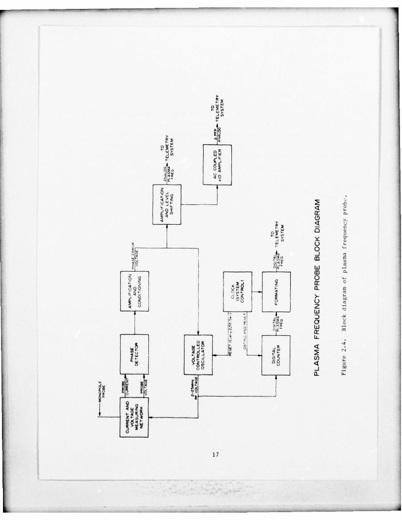
2.4 Block diagram of Plasma Frequency Probe 17
3.1 I l lustration of barium event Dianne and the flight ofprobe ST7 07.5 1—l 22
3.2 Illustration of barium event Dianne and the f li ght ofprobe ST 7 0 7. S l—2 23
3.3 Illus tration of barium event Esther and the f l i ght ofprobe ST 7 0 7 . 5 1 —3 24
3.4 I l lus t ra t ion of barium event Esther and the flight ofprobe ST707 .5 l—4 25
3.5 Il lustration of barium event Fern and the flight ofprobe ST 707 . 5 l—5 26
4.1 Pro jec t STRESS data flow 29
5.1 Electron density profile , probe ST707.51—l 35
5.2 Electron density profile , probe ST707.Sl—2
5.3 Electron density profile , probe ST7O7.5l—3 38
5.4 Ion cloud geometry (Esther) and fligh t ofprobe ST707.5l—3 40
5.5 Electron density profile , probe ST707.51—4 41
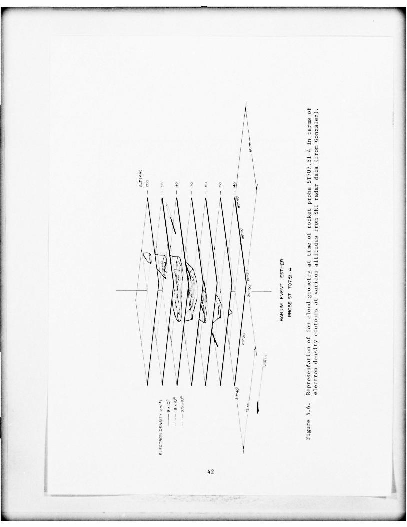
5.6 Ion cloud geometry (Esther) and fli ght ofprobe S1707.51—4 42
3
_ _ _ _ _ _ ~~~~~~~~~~~~~~~~~~~~~~~~~~~~~~~~~~~~~~~~~~~~~~~~~~~~~ ~~~~~~~~~~~~~~~~~ - ‘ ~~—~~~~~~~~~~~~-- - -
~~~~ ‘~~~~~ ‘ ‘ ~~~~--
LIST OF ILLUSTRATIONS (cont . )
Figure No. Page No.
5.7 Electron density striations as measurod by probe ST707 .51—4 43
5.8 Magnification of electron density striat ions as measuredby probe ST707.51—4 45
5.9 Magnification of electron density striations as measuredby probe ST707.Sl—4 46
5.10 Electron density profile , probe ST707.5l—5 49
5.11 Electron density striations as measured by probe ST707.5l—5 50
6.1 Amplitude di stributions of electron density variat ions (AN/N)vs. frequency (Hz) and wavelength (m), ST707.51—4 , 147.7 km 57
6.2 i/N vs. Hz and m , ST7 07 .51—4 , 151.6 km 57
6.3 ~N/ N vs. Hz and m, ST7O 7 .5 1—4 , 155.3 kin 58
6.4 ‘.N/N vs. Hz and m, ST707 .5 l—4 , 158.9 km 58
6.5 N/N vs. Hz and m, ST707 .5 l— 4 , 162.3 km 59
6.6 N/N vs. Hz and m, ST707 .5 1— 4 , 165.6 km 59
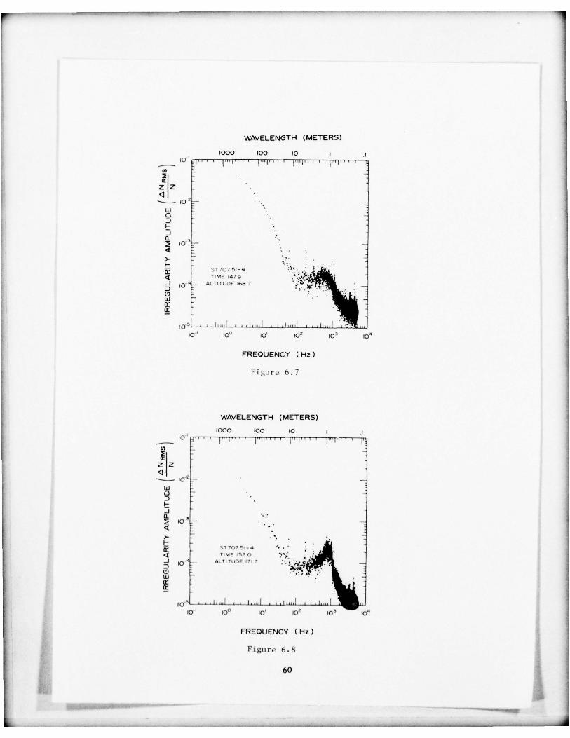
6.7 AN /N vs. Hz and m, ST707 .5 1— 4 , 168. 7 km 60
6.8 ‘N/N vs. Hz and m , ST707.51—4, 171.7 km 60
6.9 N/N vs. Hz and m , ST707.51—4 , 174.5 km 61
6.10 N/N vs. Hz and m , ST707.51—4 , 177.2 km 61
6.11 N/N vs. Hz and m, ST707.51—4 , 179.7 km
6.12 :N/N vs. Hz and m , ST707.5l—4 , 182.0 km 62
6.13 ‘N/N vs. Hz and m , ST707.51—4 , 184.3 km 63
6.14 AN/N vs. Hz and m , ST707.5l—4 , 186.3 km 63
6.15 AN/N vs. Hz and m, ST707.5l— 5, 145.0 km 64
6.16 N / N vs. Hz and m, ST707.51- 5, 150.6 km 64
4

-
LIST OF ILLUSTRATIONS (cont.)
F ig u r e No Page No.
6.17 ‘N / N vs. Hz and in , ST707.51—5 , 156.0 km 65
6.18 ‘N/N vs. Hz and in , ST70 7.5 l—5 , 161.3 km 65
6.19 ‘N/N vs. Hz and in, ST 707 .5 1—5 , 166.4 km 66
6.20 ‘N/N vs. Hz and in, ST70 7 .5 1—5, 180.9 km 66
6. 21 N/N vs. Hz and m, ST 707 .5 1—5 , 189.8 km 67
6 .22 ‘N/N vs. liz and m, ST 707. 5 l— 5 , 202.0 km 67
6.23 N/N vs. Hz and in, ST 707 .S l—5 , 209.4 km 68
6 .24 Power spectral density of AN/N irregularities ,probe ST 707 .5 1—4 , in reg ion of str iat ions 70
6.2 5 Power spectral density of AN/ N irregularities,probe ST707.51—S, in region of striat ions 70
7.1 Cross section of ion cloud and ST707.5l—4 trajector .showing predicted direction of inst ability
7.2 Illustration of development of striations
7.3 Detrended data showing electron density variations inregion of striations from ST7O7.5l—5 78
7.4 Power spectrum of figure 7.3 and a spectrum of equatorialspread—F 79
8.1 Electron density variations about a mean va lue plus plotsgenerated by arbitrary phase angle to Fourier analyzedelectron density variations 83
8.2 Electron density variations measured in equatorial spread—Fcondition from Natal , Braz il 85
8.3 Examples of occurrence of spread—F compared with F—regionvertical drift velocities over Jicamarca , Per u 87
8.4 Plot_ of linear growth rates for Rayleigh Taylor instabilityand E S B Instab i l ity for maximum solar condit ions . * .
895

LIST OF TABLES
‘ lab le No ~~~~~~~~1.1 Veh icle launch summary — p ro j ec t STRESS 10
2 . 1 P r o j e c t STRESS probe t e l e m e t r y assi gnments 12
3.1 Summary of probe rocket flight c h a r a c t e ’ r i s t i c s 20
3.2 Summary ot STRESS probe fli ghts 21
4. 1 Tra l cc o cv cee f f i c i t’nts 30
5. 1 Summary of fe.’it t ir e s of e l e c t ron density striations(ST707.5l—4) 4 7
5.2 Summary ef STRESS probe results 51
6
A” ~~~~~~~~~~~~~~~~~~~ - - -.

_ _ _ _ _ _ _ _ _ _ _ _ _ _ _ _ _ _ _ _ _ _ _ _ _ -~~--
1. INTRODUCTION
A program of measurements to investi gate radio wave propagation
through ionospheric regions perturbed by the presence of ionized ,
barium—vapor clouds , was undertaken during the period extending from
December , 1976 through mid—March , 1977. These investi gations have been
termed the STRESS (Satel l i te Transmission E f fec ts Simulations) Program.
The primary objt ’tive of the program was to define and correlate the
effects on radio wave propagation with observed characteristics of the
ionized barium regions through whi ch the radio waves were propagated.
Fundamental t o these studies wer e hi gh spatial reso lu t ion measurements
of ionospheric electron densit y struc ture within the ionized barium
regions and particularly within the striated portions of the clouds.
These investi gations were the object ive of the rocket probe measurements
program rep ort- ed herein.
The desired measurements were achieved b y r e l e is i n n barium vapor
from rockets upon attaining altitud es of approximat ely 1~~5 km. The t iming
of the releases was such that the region was sunl ii. . Subsequent Iv , as
t h e barium—vapor was ionized and developed stri , i t ions , additional rocket—
b o r n e payloads , equipped with inst rtlmen tat ion to make t’ i ne—sca le neasure—
nents of e l e c t r o n d e n s i t y , wer e launched in an ,‘ifor t to penetrate the
s t r i a ted port ion of ~he ionized c louds. ih~’’~ ’ pr hes p rovided pro f i l e s
ot electron de ns i ty and ii’’~’ — ~ , i1~’ s t r ~iet urk’ ( I m) m t ~‘ r n ,il to t h e c l o u d s
is the p ay l o ad s t t’ ,iv~’rsed t - , - -~~i ’ n and ~ ‘.a ‘r~~,i I to the clouds
throughout the remainde r of the I lights.
The invest igations wer e conduct ed rem Eglin A i r For~-e Base , Florida.Twelve rockets wer e used in tlit’ program. ~ix of t l i e ’~’ were two—stage ,Honest .Joh n— hi ydac vehicles equ ipped I o r A~ kg chem ical (barium) releasesat predetermined a l t i tudes . S ix addi t ional vehic les , two—e t age Nike—Hydacs ,were instrumented w i t h e lec t ro n d e n s i t y probes and VHF t ransmi t te rs .
Ground—based and a ire r a f t borne inst rtimen ta t ion provided cove rage re la ted
to vehicle and c i oud t r ack ing and rad io wave ~ r op ag a t ion e f f e c t s
7
~
_ _ _ _ _ _ _ _ _ _
_ _ _ _ - ‘ _
~~~~~~~~~~~~~~~~~~~~~~ ‘
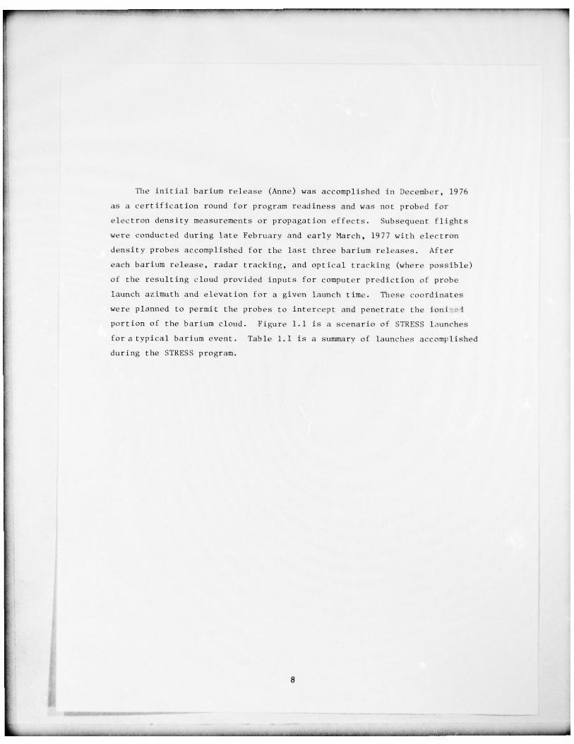
The initial barium release (Anne) was accomp lished in December , 1976
is a cer t i f i ca t ion round for program readiness and was not probed for
e l e c t r o n density measurements or propagation e f f e c t s . Subsequent flights
were conducted during late February and early March , 1977 with e lec t ron
density probes accomplished for t he last three barium releases. A f t e r
each barium release , radar tracking , and opt ical tracking (where possible)
of the resulting cloud provided inputs for computer prediction of probe
launch azimuth and elevation for a given launch t ime . These coordinates
were planned to permit the probes to intercept and penetrate the lon i c’ lportion of the barium cloud . Figure 1.1 is a scenario of STRESS launches
for a typ ical barium event. Table 1.1 is a summary of launches accomplished
during the STRESS program.
8
_ _ ___ -~~~~~~--- ~~~- -_—-- .—-_ .‘-~~ ---- - — -‘—— - _ _ ~~~~~~~~~~~~~~~~~~~~

-J
h ~~~~~
,
~~~~~~~~
I
I
I-.
0
4 ~~~ -, r-
S
9
_ _ _ ______ -.---~~~- .- - ‘ - _ ‘ _ _ _ _ -

TABLE 1.1
VEHICLE LAUNCH SU~ff’1ARY - PROJECT STRESS
—
Event LaunchVehicle Name Experiment Date/Time Remarks
ST61O. 31—1 Anne Barium 1 Dec 76 CertificationRelease 2308:37(GMT)
ST71O.3l—2 Betty Barium 26 Feb 77 Not ProbedRelease 2349:33(GMT)
ST71O.31—3 Carolyn Barium 2 Mar 77 Not ProbedRelease 2351 :00(GMT)
ST7IO.31—4 Dianne Barium 7 Mar 77 Probed at Release +15 mmRelease 2358:0O(GMT) by ST707.5l—l
Probed R(Rclease) +33 mmby 5T7 0 7 . 5 l—2
S’f707. 5 1—I f)ianiie Probe 8 Mar 77 Dianne early probe00l4:05(GMT) R + 15 m m .
5 T7 O 7 .5 1—2 Dianne Probe 8 Mar 77 Dianne late probe0032:04(GMT) R + 33 m m .
ST7 IO.3 1—5 Esther Barium 13 Mar 77 Probed at R + 28 mmRelease 2258:0O( cMT) by ST707 . 5 l— 3
Probed at R + 46 mmby ST7 0 7.5 l—4
ST7 07 . 5 1 — 3 Esther Probe 13 Mar 77 Esther ear ly probe2327:O0( G MT) R + 28 mm
ST707. l— 4 Esther Probe 13 Mar 77 Esther la te probe23 44:50(GMT) R + 46 mm
ST 7IO. 3 1— t Fern Barium 14 Mar 77 Probed at R + 41 mmRelease 2243:OO (GMT) by ST707.51—S
Probed at R + 80 mmby ST 707.51—6
ST707 . 51—5 Fern Probe 14 Mar 77 Fern early probe2325:2O (GMT) R + 41 mm
S T 7 0 7 . 5 l— 6 Fern Probe 15 Mar 77 Fern l a t e probe0003:l0(C’MT) R + 80 mm
10
.---
~
--
~
‘_ -

2. PAYi~OA1)S — CONE ICIIRATi ON ANt) I NSTRIIMEN I’AT I ON
A l 1 ot the s ix pay loads I or proli Ing t he barium ion clouds wo re
I dent I cal , and a ll were propell ed by two—st age Ni ke— llvdae motors . The
pro— launch vehic I e coit figuration is shown in Figure 2. 1 . As ~an he
noted f r o m Ft gore 1 . 1 , the pay loads consisted 01’ four sepa rat e se c t i otis
The na in pay load (inc I ud lug t lie nosesp ike) , an Amp lit’ tide Modulated ,
P—hand propagat ion experiment , to tenet rv and beacon , and a sect ion I or
hal last to ach ieve desired ve h ic le pt’ rtormance and pay load stabil itv
Thu . ma in payload , i l lustrated in Ft gure 1~ 2, conta ined two e lec t ton
dons it v measti r ing Inst rumont s , .i p la sma frequency probe , and a h)C probe.
Each of these’ probes U t ii I zed a port ion ol the I—rn long, 6. 35—cm d jane t et ’
iiosesp ike as the ii’ sons og element in coot act vi t Ii t i to i t itiosphier f t ~“l
;lsma
The P~~Y load spit i ax i s svmme t rv and freedom I ron pay load doors and mechaii i sms
prod uced a 11 [gu t un it that was s imp he , rugged , and caused m i n i m a l el Iec t s
I’ rem wakes or sp in modu I at ion iii the oh a toed data.
I n add it I on to t lie i ns t ritmoj i at ion t’o r m&’asu romeo t of ionosp h e r ic
e lee troll dens It v , each j iav load inc I ude.’d a lie l i t . lux RA!’1 SC magnet Ic a s p e c t
setiso r mounted across the rocket ‘s ma _i or ax is to provide a measure o
roc ket sp ill and to give Some ’ lndl cat ion of vehicle at t i t title and st i t iii tA C— band radar t ransponder was j o e l tided t o prov ide a si gna l for so l i d
radar tracking , and .in S—hand t elemet rv svs t em , operat lug at a link Ire—(juenc ot 2151. 5 Mh1~ pro v ldcd for dat 1 ransuil ss ion to the ground St at Ion.
Tab he 2 . 1 det i i I.s the te l onie t ry [RI C channels and ass i gnments. To ta l
p a y loa d we ight I or t he probes was lit) lbs . w i t hi t h e ma iii p.t ~ load w e t ghlngIn a t 70 ihis .
11
_ _ _ _ _ _ -~~~~~~~~~.---~~~~-- -—— -

RAYLO~AD HYDAC MOTOR NIKE MOTOR
— MAIN ~~~~~~~~~ k—VHF MODULE
PAYLOAD
Fi gure 2.1. STRESS electron densi ty probe pre—launch conf igura t ion .
TABLE 2.1
PROJECT STRESS PROBE TELEMETRY ASSIGNMENTS
tRIG IRIGChannel Assignment Channel Assi gnment
21 DC Probe x10 17 DC Probe x lOO
20 DC Probe xl 16 PFP Digital
19 APFP 15 DC Probe x l000
18 PFP Analog 13 Magnetometer
12

___ -.-——DC PROBE SENSING
INSULATOR ~ ELEMENT
PLASMA FREQUENCY PROBEMONOPOLE
INSULATORS GUARD ELECTRODE
PLASMA FREQUENCY PROBEELECTRONICS
INSULATORS ~ GUARD ELECTRODE
MAGNETOMETER
-—--DC PROBE ELECTRONICS
—28V BATTERIESBEACON ANTENNA - — ~~~
— -CONTROL BOX
— BEACON TRANSMITTER
-S-BAND TRANSMITTERa vcs • s
S-BAND ANTENNA - -
~~ - -BA LLAST
~~— — VHF MODULE
Fi gure 1.2. S ‘k’FSS p.iv l oad con i g ti ra t Lou .
13

DC Probe
The DC probe operates on the principle that the electron flow to
a small, positively charged electrode immersed in the ionospheric
plasma is d i rec t l y related to the electron densmty of the p lasma .
Figure 4 is a conceptual block digram of the DC probes used in the
STRESS program. As its sensing electrode in contact with the ionospheric
plasma , the DC probe uses the foremost segment of the payload nose spike
(see Figure 2.2) with dimensions as noted in Figure 2.3.
The operation of the DC probe is exceptionally simple and is illus-
trated in Figure 2.3. The current collected by the 63 cm ’ p robe electrode
(the forward 4.76 cm of the payload nose spike) which is biased at +3 V
with respect to the rest of the payload , is fed to the electronics
system preamplifier at B. With a finite sensing electrode current caused
by electron flow from the p lasma to the electrode , the voltages at C and
D are not equal , and the differential stage amplifies the difference
giving an output which is proportional to the sensing electrode current
flow. The output from the dm fferentia l amplifier is fed to four ampli-
fiers having gains of xl , xl0, x lOO , and xl000 with the four outputs
going to the payload tele’netry section.
The DC probes used in the STRESS program were designed to be capable
of measuring fine—scale spatial variations of electron density. This
high spatial resolution capability is determined by the dimension of the
probe electrode , the payload velocity, and the electrical bandwidth of
the telemetry system. For these applications the telemetry system
bandwidth and the payload velocity through the ion cloud of approximately
1 km/sec limits the DC probe spatial resolution to the order of 30 cm.
The DC probe current cannot be related independently to electron
with high absolute accuracy but will give reliable relative values . This
does not present a serious draw—back here since the relative changes
are the important values and over a limited altitude range the
electron density will be proportional to the probe current. By cross
comparison to other measurements such as an rf probe or an lonosonde the
DC probe can be calibrated in absolute numbers . This is the manner in
which we utilize this probe.
14

cn a:I-.. I-D (Li
I- w
0-i 0j 2~~ ~~~~ j_ Q.. ;Q. ~~Q_
_
I
_
I
~
I
- -p
~3.
15
_ _ _ _ _ _ _ _ _ _ _ _ _— --—-------— ~~- ‘-~--- .------— — -.-- .--— ‘—‘---- -‘ “- —‘ ‘~~ .-~~-‘

Plasma Frequency Probe
The plasma frequency probe (PFP) utilizes the well established
relationships between plasma frequency, electron density, and the
reactance of a probe immersed in the plasma to provide a measurement
of electron density (Rak~a’, ~~ a!., 1969). In the version of the PFP
flown in the STRESS program a phase—locked loop is used to track the
frequency that produces zero phase angle between rf current and voltage
being fed to the sensing antenna . This frequency of resonance is
closely related to the electron plasma frequency, in kHz
f = ~~~~~~~~~
= 80.6 X lO 6Ne(cm’3 )N
4 2
In the absence of a magnetic field the resonance occurs at this
electron plasma frequency . The e f fec t of the magnetic field is to
shift the resonance slightly higher in frequency to the upper hybrid
frequency
2 eBf = f + f , where fH N B B
The phased—locked version of the PFP which is shown in the block
diagram in Figure 2. 4 utilizes the forward half of the 1—rn long noseas its antenna . The system is desi gned to sense the zero phase condi t ion
of the antenna impedance at the hybrid resonant frequency and to cause
a phase —locked loop to fo rce the rf oscillator to track the frequency
producing the zero phase angle condition. The frequency of the oscil-
lator is d igitally counted for 1 msec and forms the data for a digital
plasma frequency readout. Additionally, the voltage controlling the
loop oscillator is monitored to provide an analog measurement of plasma
frequency and loop operation. The digita l output provides excelle nt
accuracy in the measurement of e lectron density at samples with about
a meter spatial dimension separated in sp ace by the distance the pay load
16
I
‘ . “ - ‘ — —~~~~~~~~~~~~~~~~~~ -- ‘ - - -‘ -- .
- . —~~~
.- — - -- ~~~~~~~~ -
l~~u,
I—
_J u, Iw II’-
r~ o I~ I-
I I_ _ _
o~J~~ 5.
_________ _________ _________
W
_ _ _
L~~~~~~~~~~~~~~~H [1
a
_ _ _
~~~~~~~~~~~~~~~~~~~~~~~
~~
17
_ _ _ _ _ _ _ _ _ _ _ _ _ _ _ _ _ - - - - —--

_
travels in a 16—ms sample period (25 m). In order to provide higherspatial resolution measurem ents , a continuous analog chan nel and ac —coupled x 10 amplified channel (APFP) were provided that responded downto about 1 meter scale size fluctuations. The range of electron densi-ties covered by the plasma frequency probe is from about l0~ to7 x l0
6cm 3 .
18

3. STRESS PROBE FIRING SU1~4ARY AND GEOMETRY
The electron density probe rockets were flown in pairs into rho last
three barium clouds as briefly summarized earlier in Table 1.1 and elabo—
rated on in Table 3.1 which includes a listing of parameters relevent to
the description of each flight.
Probe encounters with the barium clouds are described in Table 3.2
where entries under “probe residence in the Ba cloud” were determined
from significant electron density enhancements over background as deter-
mined from the in—situ probe results. The age of the cloud is given in
minutes after release for the maximum observed electron density on each
probe flight.
To assist in visualizing the probe/cloud encounter and penetration ,
Figures 3.1 through 3.5 are conceptual drawings whici- include the geo-
graphic coordinates of the launches , the vehicle ground track and trajec—
tory , coordinates of the barium release , and subsequent development of
the barium cloud. Probe entry point into the cloud , point of maximum
electron density, and exit po int (all from electron density res~t1ts) are
marked by Jots along the rocket trajectory . Rocket apogee is noted in
each figure as is the track of the barium cloud vs. ne.
The flight of rocket ST707.51—6 is omitted from these conceptual
drawings as the cloud track on this probe was doubtful , and the electron
density measurements were of limited usefulness as noted later in this
report (section 5).
In viewing the electron density results presented in section 5 of
this report , it is important to consider the veloci ty of each probe as
it moves through the ion cloud region . Since the ion cloud s t ruc tu re
wi ll be aligned along magnetic fie ld lines , perhaps the most important
velocity will be that normal to the magnetic f ield. To aid in viewing
the data the pertinent rocket velocities for each probe fligh t are
summarized in Table 3.3 for the region of the maximum measured electron
density in each case . V~ is the total rocket velocity having vertical
and horizontal components of Vv and VE, respectively . V11
and V are
the veloci ty of the rocket para llel to and perpendicular to the
ter rest r ial magnetic f ield.
19

--- -—-——~
- — —- - - -- - -- ----- ---- --~~~-- - - -
00
-
11) ~Q ~ ~~ C 1 Lñx u ~~co~~~~m0.
~0. 4~ -.
0-4s c u
~ •,o r- c’~ ,C
~ c’~” m ~~ ~~ C’I
U, 4.2C..) a-~I- 0. F—. F--. F--. .o r-. I--.-- -4
0
H0
4.2o 00 a 00 ‘b ~0 ‘C ‘C (‘-I 0’
.~~ E ~ -.~ ~o —sH
-~ ~4 ~0 ~~ 4 ~-4 -~ ‘-4 ~~4N
0-4
4,, ,-~£4.
C-c-~ H 0)
Cc ~~ —‘ -4 — -4 0) -.~ .-1~c E ~ c ’C ~~‘
4,~ ‘CH c) ~0 .~ C—J C~-i ,-i c4 ..-~ ~—io
Cc0)0
0. 0)0)
£4. 0 0’ 0~’ (~4o o .~4 —~ 0 C’-I 0’ -~ C~-J00 ‘-V’ NJ (N NJ NJ (N
g
O H (-i H H H HU, U, (/) U, U) U)
Cc Cc4.2 Z Cc Ccz ~~~~~~z zW ~ (-‘ H ~> 4-4 -4 U) U) Cc
~ u~
20
-- --- - -— -- - ----.--— --- —— —— -- - - - - — - - -

_ _ _ _
~00)0.0 Cl)
64.4 ~~ 00 0 ) 0
~ -4o Cl) 0) 4.2 ~~~~~~~5 ...4 0 a -.4 0) —0) .)~t 0 -4 ~~~~00 S£4 .,.4 4.2 £4 .,.4 5 C) p
0 (0 4.2 0) 4.2 0.~~4.4 £4 ~ Cl) ( 0 0 ) 4.4S ~o 0 0.0) 0) 0. 0 0
£4. 0. 0 (1) ~0 C )0 0 0 0. 0) 14..
0) 0 0.—4 00 0) 4.J a ~~~ 0 . 4 00 ~ a0) .~-4 0 > £ 4 . ,~4 0 0 )0 £4 .
~.4 Q) •~ 4.4 ~ 4 00
4.4 4.2 0 0. 0 5-o a - o a I 0 ~~~4..a ~ ~ ~ ~0 0 0 £4 -4 0 0 00~~—l ~~~~, 4 4.2 0) - . 4 0 0 ) 0o i~-~ c~ U) ~~ 0 —’ 0) C)
0 0 0 0 0 00 0 ..4 ..4 .~.4 .
~_4 .,4 -4
o E E 0 0 0 0-40 L/) -~ U) ‘C (N 0
F- 1 (N ~~ -~ 0)
C-hH0-4
a — — —-. —~ — —‘(.4.. ...4 C-) 4/)
~~ C ‘/) (N C0) -~ ‘C ‘C ‘C 1/) 0)
Cc 0) 5 ~~ ~.4 ,...4 ~..4 —
C) I I I I I0 0 ~C + C ‘C C’) C (N F’)
NJ ~ 0) 0 (N L/) (N 1’) 0’ 0)0. 0 0 4J .-4 .-.4 —4 —4
C’) .,.4 ,-~4 S...? S.’ ‘~~ ‘.. ‘ “~~ ‘U) (00Cc U) 0)
CcF0~~~~ 0)< H 0) 1/) C’) (N .-4 ~5) ‘CH C/) El N. 0) 0’ 0) 0 0
0 .S~ I ~~~ r-~ 4 ~ 4 NJ (N£4. £4 I I I I I I0 0. 4.2 -.4 0) 0 1/1 -4 (N
-.4 61) N- ‘0 61) 4,) —

BARIUM RELEASE DIANEPROBE ST 70751- i
NORTH~~~~~~~~~~~~~~~~~~~~~~~~~~~~~~~~~~~ -
EAST80 KM~~~ ~~~ -
~~~~~~~~~~~~~~~~~~~~~~~~~~~~ Y>~~~~~~~~~~~~~APOGEE~ ELEAs~ ‘~~~~~~~~~~~ ‘ ‘~~~~‘ - - - 213 KM
/
\2~~~~~~~~~~~~~~~~ ~~~~~~3Q03Q~ -‘: .A~~~~\~ -
~~~~-~~.:~~~~~~‘
• ‘\-~A-•-
~~~’~~ ~~~~~~~~~~~~~~~SITE “A — 15 \ ~ 85°- . ‘
30° ‘ ~~~~~~~~~~~~~ \
~ 86°
290 /870
Fi gure 3.1. I1l j .~ r - p ~~~
‘
~r - t t - k .~~ ‘. ~1— t P ’o ’ r::. &‘i~~i ,c
H v i h i k- i zedC- ) - I k t - -
- -
t H ~). l~ ‘ r1j ‘- C l : - ‘ . Hoeket et~~~~ t p t C O ~~ C l ( ’ U l , - - ‘ j ~’fl ~~~1 C ~~I e>~~t ~~~ ( C I-‘1 ‘ • t’ - TI i f ’ h ‘ . ‘- ~!( - - ) ~ ~ - : t i - i t ~~~~
- P -~~ C 1 - i i~~~ ,~~ ~
22
_ --~~~~~~~~~~

BARIUM RELEASE DIANEPROBE ST 707.51-2
NORTH EASy180
- J~~~~~~~~~ / 9
~~~~~~~~~~~~~~ ri i/APOGEE203 KM
\ \t~~~’~j/ / /
SITE
~V \\/\ ~~~~~ JY /30° \,\ ~~
\x~~ ‘\ N ~~~~~~ I\ \ ~ ~~\ I’~ \~\L7/ 86°
290 87°
Fi gure 3.2. T I i P I tr ’~t t p fl ~f prohr’ rP -/ k e t - . 51— ’ tr~~~o ’ C r - . flel~~i~~r‘ C TI t P p~~’ Even ~- t fin 1, - t ic-wt ~ u i ~n 1~ ‘ C . } t h e visible i ~‘n i edloud r’icuk HOI CIH i t , R~ 5 , 1O. 1S.~~~I minu f~~~. Rocket entry
‘ C it Tl~~fl Hin ~~ 11( 1 , C l I X t P1I ~ ~~( P i C I C . and ‘x i t p e it it ( l’r- ’rret deII~~i ty re i i j t e ) p r ’ i n d t p Ited by Ihe 3 dol~ i~~
t hi’ t_ r i ,f 0 ’ t p Pry
23

‘1
BARIUM RELEASE ESTHERPROBE ST 707.51-3
APOGEE
NORTH - ~~~~ .~ 5
2~95KM
180 KM / / 1 - -
.10 ‘~20
RELEASE / - ~~~~~~~~~~~~~~~~~~
/p
/-
- .
- •‘__5_.4; -
~:i-SITE A-15 ~, ç30°30
~(‘ “ ;i~ FP>
~ 85°‘~~~~~~~-< .)
~~~~~~~~.
30° ~~~~~~ 6
290 870
Fi gure 3 .3 . Iliuiitrit ,i t i ‘ t ’ probe roo kc ’t - i~T7O7 .5l— r-p ,~~’ eC -r’ .po i n t , of EverI t- Es t her h uhc t d , r i i ‘- i l l t he rodarni~~~ Pj ( j t r - i - - k l ( ) i f l t , i t it , Ri I C . 20. ~~ m in u t n ~~. R O ’ k( ’t. -n t rypoint m t the C l o i i p l . ~~~~~~~~~~~ ir id e x i C po int ( frome lert run lenoit,y reitults ) ire m d i ‘toted i v the 3 let ~~i 1 p ~i i 1~,t I c t r i~~ec to r v
24
- . .- - - - --~~~~~~—-~~- ---~~~

~ - . ~~
-~~~~~~~
-
BARIUM RELEASE ESTHERPROBE ST 707.51-4
7Th~~~~
-.NORTH
~~~~~~~~~~~~~~ -~~~~~~~~~~~~~~~~~~~~~~ 28 ~~~~ +4~ EAST180 KM ~~~~ N j ~~.?~~~~2 0J jy t-.~
-~- —5-,’
RELEASE— - - - -- I’
. .~~
- —
-.
\\ /7~t~\ \/ )~~~~~~~~~ A~
’ ..b~~~~~~~1 1 /3oo3o~~~~~~~~~~~~~<~1~~~~~cJk/ /;ç ‘~�k\~~L~~ /850SITE A — 1 5 ’ — --‘
~~90 870
F i ~~ i r , ’ ~~. -‘i . I l l ru C j ‘n - ‘ t ’ ~ ’~ - - n
~‘,
~T7 ~7. — -~ t t ’ n,H ’ - C ery . P t (‘ni t ’. . ‘ - - .~~‘ I t I t r u t ‘ v u C 1’ ; t - i i ’r i , - I i - wii to b ib’ m~ 1 he rnd;i re l - i - I - i’ • - ’~~~~T-~~~~, TT R~ lfl . .~Q . :~~~. .~~~~- i i f i u t e~~. R ’ e k ’ t t ’C i t I ”~’
in t o t he ~‘ l ’ - i i - I , l i X ~~~ l C ~~~ ~~~~~t - i n I e x i t t ’~’ r u i t ( t ’rp o t• ‘l e~’ t ‘n 1 ‘ni -. i t :- ‘ r ’ i i I ) ‘ i c ’ nd i i ‘ 1 ,‘,‘ H i ’ 1 ‘i ‘ l i p ’
25
- ---S -- ‘- 5 -. ‘- -‘- 5: - - - - - - --

-~~~~~~-~~~~~-- - ------ ‘— --
BARIUM RELEASE FERN /~~~POGEEPROBE ST 70751-5 / 249.2 KM
NORTH ~-t.- .42 / ~~
- - EAST180 KM - —~~ ‘ ‘i -
+~~~~~ \* 4 ~
,:r- -
- 5
RELEASE -
~~~~1 ~~~~~‘
L-
! /<‘, ‘ ‘c’ \ ‘ ‘~- “
30° 30’ ~ ~‘ / ~
- ‘ 85°
/ “ ‘- 5”~~~~~ .” -
SITE A — 1 5 ” ~~~~ . “
‘~ ‘s’
30° ~~ .
-
86°\
290 87°
Figure 3 . 5 . IJiu;ut r” p t i p ’ti ‘1 ’ n r H - n r, e’ hoC ~‘t” -’~r , ’ i~~t l,r ri~~e - t ‘r .point , of l-:v ‘ i i t F ’ eru j , u ;tiown TiT~u j ~-~~’ iT}j the radar
r’’ p - ’k ~oI f i t , ’ nt , R÷lO. p~ ut : i n u ’ r’ ,~ . “p ’ ’~~’t e nt r y t 0 t n tt. l)(~
p~i, ~p p 1 , ~~~ rum ‘~~ Ii C - rorid e x i t t p e i f i t , ( t ’ ri ‘ I L e~ k r - - i il i i i t i r’ ’ . uults ) t i c ’ I t i t i c a t ep i by tIt ’ ~ -I~’ t -i i- — ni ’ l ie
C , r ’ p ’ ’ - ‘ 6 - ry .
26
— - __ __ . _~_ 5_,_ _ _ _ _ ___ _ --

0 . . . ..)~ C C C 0 0 0
Cl) ‘ ‘ 0’ 0) 0 0) (1)C C 0) ‘0 0’
- > 0 . . . .~~ -~ C ‘-.4 0 0
“It
>>!
~i,,, I ,—4 Li) 6/) ,—‘ N- —o i-4 5-— ‘tI’ (N (“4 F’) 4,) ‘~~> 5 . . .u,- ~i ,- — ,-.4 - -4 —
H4.2 . . .
0)0 0 -‘~~ - I (N N’ ,..4 C)0 0 0 ‘C CC N- N- N . ‘C4.2 0 ~~ ~~ ~.4 -.4 ,-2 _4 ~—4
...4 (N I”) ‘,-~ r~ ‘C0 I I I I I I
Z ~~~ -4 — — -4
~ri ,i) n ~~~ Li~C
4.4 . . .0) N- N. N- I’- N- N-
0 0 0 0 0 0C) N. N- N- N- N- N-0 H H H H I-. HCl) (/) U, U) U, U,
27
:~

4. DATA REDUCTION
Data Reduction Overview
Fi gure 4.1 depicts the flow of da ta through the sequence of routines
developed to produce the final STRESS data products. The raw data for
each probe , stored on magnetic tape , consisted of a CMT time tag and
associated digital counts. Individual processing routines were developed
for each of the STRESS probes and these routines converted the raw counts
to engineering units , computed vehicle altitude associated with each
measurement and created the engineering u n i t / t r a j e c t o r y data base used
as input to various plot , list , and analysis routines. The plot/list
routines provided the capability of displaying time and altitude profiles
of the engineering unit data for the entire data set or for se lec ted
periods of interest. A descri ption of the mathematics involved in the
reduction routines is included in a succeeding section .
Engineering Un!t/Tra~ectory Merge Routines
Individual routines were tailored for each of the STRESS probes
(PFP analog, PFP digital and DC probe). Each routine computed vehicle
altitude based on a quadratic fit to the raw trajectory data. A least
square polynomial routine was used in deriving the trajectory coefficients.
Table 4.1 summarizes the coeff icients for each of the vehicles.
For the PFP analog and the DC probe data , the digital counts con-
tained on the raw data tape were converted to voltage using conversion
factors received with each magnetic tape. The data on the PFP Digital
raw data tapes represented direct measurements of frequency.
DC probe routines converted the voltage values (v) to current (I)
using the linear conversion expressions . The probe currents were converted
to electron densities by multiplication by the appropriate constant over
each altitude range as determined by comparison with the plasma frequency
probe and lonosonde data.
28
*

“~~~~~~~~~ - -- - - -
RAWDATATAPE
ENGINEERINGUNIT/ TRAJ
ROUTINE
E NGUNITDATABASE
(PLOT/LIST ANALYSISROUTi N~~~
J
ROUTINES
) [ ,~j LIST PLOT
Fi gure 4 .1 . Projec t STRESS data f low.
29
_

‘~
- ‘~
-~
--
For the PFP Analog data , voltage (v) was converted to frequency (f)
by means of linear calibrations. Frequency for both the PFP Analog and
PFP digita l data was converted to electron density(M0)using the expression
Nc = 1.24 x 1O ” [ f~ — (1.5)2] cm 3
w here I’ is the measured frequency in t~fl1z.
TABLE 4.1
TRAJECTORY COEFFICI l-:N’F ~
j r /I i i - t erv Eqii;it ion ALT at -,
+ ht + c(t t ine in seconds a f t e r launch)
Vehicle a h c
ST707.51—1 — .0046 2 .18059 — 4 4 . 0 7 1 4ST7 0 7 .51 —2 — .0045 2.0799 — 3 6 . 7 98S T 7 0 7 . S 1 — 3 — .0045 2 . 157 —36 .896ST707.51—4 — .0045 2.0633 —37.102
ST707.51—5 — .0045 2.296 —41.853ST707.51-o — .0045 2.1605 —36 .6054
-
30
_ _ _ _ _ _ _ _ _ _ _ _ _ _ - -

r ~~~~~~~~~~~~~~~~~~~~~~~~~~~~~~~~~~~~~~~~~~~~~~~~~~~~
-
Spectral Analysis of Electron Density Variations
A computer program was developed to analyze the variations in the
current (Al/I) or density (AN/N) as a function of time by power spectral
density analysis techniques. Negative or zero values (density) indicated
a reset pulse of the PFP was being read . The program did not accept
data values up to 19 points before or 299 points a f t e r a reset pulse.
The program linearly interpolates or extrapolates to fill in the gaps
in the data created by the reset pulse.
The program analyzes NPOIN + 1 (NPOIN is the number of input data
points usually 8192) decimated data points at a time . Each point is
found by averaging (decimating) LDEC (input data usually 1 or 5) input
points. The program averages the results to form LNN (input data usually
1 or 5) consecutive samples of I (or N) where the last value of one
sample is the first value of the next sample.
The program analyzes NPOIN + 1 points as follows . The data is de—
trended by fitting a least squares polynomial of degree NORDER (input
data) to all the input data (not including any interpolated or extra—
polated values). Form the values
— I(t)[or N(t)]( t ) -
y ( t )
where 1(t) is the value of I and y ( t ) is the value of the pol yn omial
both at time t . Now calculate
— 1 ,. — 2E = ~ - - t f ( t ) — f ( t ) ]
where t he sum is over the NPOIN + 1 data values and N equals NPOIN + 1— number of interpolated or extrapolated data values and
~~(t ) = - j~
----,~
-—~
Ef ( t ) .
31
L
-

--- . - ‘~~ -- -~~—----- -- -~~~~~~~“- _ _
Form
g(t) = f ( t + At ) - ~f(t) (a input data , usually 1)
where At is the equal time spacing of the data. Form
h(w) =
where
j =J- iW = 0 , ± WR~ ± 2
~ R’ ~ ~~R’ ~~‘ ~~
where=
8192*At ‘
h(w) is found by using a Fast Fourier Transform on ~ g(t).
Form g 1 (ia) = g(ia)~~2 and smooth the resultant “whitened ” power
spectral density through Hamming to form g2 (t). Thus
g w ~~) =
= 0.23(~ 1 [(~ — l)WR] + g 1[(~ + l)WR]) + 0.54 g 1 (~~L L ~~)
for 9, = 2 , 3 , . . . , 4095
g2 (4095 - ‘ R~ = g 1
(4095 WR)
g2 (4096 - R~ g 1 (4096
~~~
Find
2Ef 4096 ~~~ g
2~~~~~’~~~~~ ) 4 ” (~i — ~ cos(’~-~~-~)] + c~
?sin 2(~~~~~~)
Renormalize g2 to form normalized answers g 3
,\ t Eg 3 (u) = ‘— -p— g2 (-i)
g . 1 (w) is the whitened powe r spectral density
~~~~~~~~~~~~~~~~~~~~~ _:i_~~~

and
=
~~~~~~~ El - a c os( ~~~~ 6) ] + a2sin2(~~~~
6)
is the final power spectral density.
The frequency is often transformed to a wavenumber reading by dividing
4’~R
by an appropriate velocity constant (FIXTXS). For short—wavelength
calculations FIXTXS = ~ ~~V x BI where V is the rocket velocity (found
from a model) and B is the magnetic field (found from a model). The sum
is over all non—extrapolated or interpolated data values. Similarly , f o r
long—wavelen gth calculations let w = B x U and then formin g a unit y
we have FIXTXS = y j . Here U is a vector pointing from the center
of the cloud in the direction of — (E x B) based on model of cloud develop-
ment (see section 7 and particularly Eqn. 7.4)
- - E x B p
Two types of plots have been provided : the f i rst is a plot of the
irregularity amplitude distribution (square—root of Power [g~ (f)] versus
f requency (f f-)) and the second is Power tg~ (wave—number)] * FIXTXS
versus wavenumber. Both of these plots are on a log 1 0 versus log 10 scale.
33
5 — ’ - - - -- -~~—-- ~~~~- -- - -- -~~~~~~~~~~~ - - ‘ -- - ‘~~~~~-__-
~~~~~~ ---~~~~~~- -
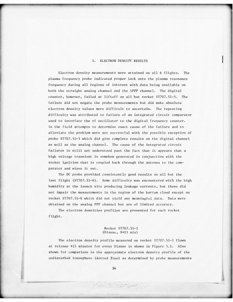
5. ELECTRON DENSITY RESULTS
Electron density measurements were attained on all 6 flights. The
plasma frequency probe indicated proper lock onto the plasma resonance
frequency during all regions of interest with data being available on
both the straight analog channel and the APFP channel. The digital
counter , however , failed at l i f to f f on all but rocket ST707 .51— 5 . The p
failure did not negate the probe measurements but did make absolute
electron density values more difficult to ascertain . The repeating
difficulty was attributed to failure of an integrated circuit comparator
used to interface the rf oscillator to the digital frequency counter.
In the field at tem pts to determine exact cause of the failure and to
alleviate the problem were not successful with the possible exception of
probe ST70 7.5 1—5 which did give complete results on the digital channel
as well as the analog channel. The cause of the integrated circuit
failures is still not understood past the fact that it appears that a
high voltage transient is somehow generated in conjunction with the
rocket ignition that is coupled back through the antenna to the com-
parator and wipes it out.
The DC probe provided consistently good results on all but the
last flight (ST707.51—6). Some difficulty was encountered with the hi gh
humidity at the launch site producing leakage currents , but these did
not impair the measurements in the region of the barium cloud except on
rocket ST 707.5 l — 6 which did not yield any meaning ful data. Data were
obtained on the analog PFP channel but are of limited accuracy.
The electron densities profiles are presented for each rocket
flight.
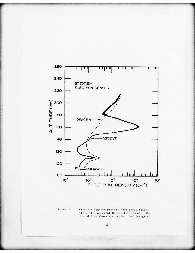
Rocket ST 707.5 1—1(Dianne , R+15 m m )
The electron density p r ot il e measured on rocket ST707.51—1 flown
a t release +15 mInutes for event Dianne is shown in Figure 5.1. Also
sho w n fo r comparison is the a ppr ex ima t e electron density profile of the
undisturbed ionosphere (dotted ~ine) as determined by probe measurements
34
-_ _ -~~~~~
260 1 1 1 1 1 1 1 I I I I 1 1 1 I J I ~~~
240 — —
ST707. 5l—IELECTRON DENSITY
220 — —
/E 2 0 0 — / —
//
a lso — —
DESCENT ~~ /
tj l6O — / —
4~~~~~~~~~~~~~~~~~~~~~~~ A ENT
I I I I III!! I I I I IIIII I I I 111111 I I I 11111i05 106
ELECTRON DENSITY (cn~3)
Fi glirl - ~ . I. LI ‘c t ron dens i t v profile from probe flightST707 .S 1—l on even t Dianne (R+l 5 mm ). Thedashed line show s the undisturbed F—region.
35
—-——
~
-—
~
—- ‘ ---
~
5- -_- - --
~
- —- - - ~-- --~~~~ - --- - -~~~ -- -

-~~~ ~~~~- - - -5- - - - - —- --~~~
above and below the cloud region and measurements on rocket descent. A
check was also made by comparing the F—region density with the ground
based ionosonde value . it is obvious that the rock e t probe t raversed
the region of enhanced electron density associated with the barium ion
cloud over the altitude range from about 150 to 180 km. The peak electron
density of the barium cloud layer of 1.4 x 106cm 3 found at 162 km is
about a factor of 100 larger than the clectron density at that altitude
in the undisturbed ionosphere . The layer is relativel y smooth and
devoid of large scale structure that would be expected if cloud stria—
tions had been penetrated. The layer has a width at half amplitude of
10 km in vertical extent which would correspond to a movement of the
rocke t probe of 6 km across the terrestrial magnetic field.
Rocket ST707.5l—2(Dianne , R+34 m m )
Rocke t probe ST707.51—2 was flown in event Dianne about 19 minutes
after ST707.5l-- 1 and just penetrated the edge of the ion cloud as can be
seen in the profile presented in Figure 5.2. The peak densit y found
was the same as the earlier probe (1.4 x 106cm 3) hut the penetration
was at the higher altitude of 182 km. The sharp feature at 182 km has
an electron density about 2 orders of magnitude over the ambient density
and is imbedded in a broader region of enhanced density more of the shape
of the profile found on ST707.5l—l , but with less density and at a higher
altitude. The apparent higher altitude of the layer is due to the late
penetration of the cloud since the rocket flew to the north of the cloud
(see section 3, Figure 3.2). The sharp finger rises above the broader
region by about an order of magnitude . The finger has a width (half
amplitude) of about 1.5 to 2 kilometers in extent either vertically or
normal to B.
Rocket ST707.51—3(Esther 1(4-28 m m )
The electron density profile measured on probe rocket ST707.51—3
which penetrated the barium cloud Esther at about 28 minutes after release
is shown in Figure 5.3. The profile is smooth , showing no large scale
36
‘— ---__ --5 - - -- -. —5-- - ’ --- —_ - - -- - - - ---~ -- - . - --—“--- _-5 5----- 4

- — - ‘
260 I 1 1 1 1 1 1 1 i 1 1 1 1 1 1 1 I 1 1 1 1 1 1 1 I I I I
240 — —
ST707. 51-2
220 — ELECTRON DENSITY
—
E 200 — —
a iso — DESCENT ø../
~~~~~~~~~~~~~~~~~~~~~~~~~ —
( . ~~~~~~I60 — if —
~ ASCENT
140 — —
120 — —
—
100 — —
so I I 1 111111 I I I 11111 1 i i i I 1111 1 I I I I 1111
I0~ IO~ IO~ (06 I0~ELECTRON DENSITY(crñ3)
F I .L IIre 5.2. El ec t 1~~/fl density profile from probe f l ightST707 .I1— 2 on event Dianne p.K+ 14 mill). Thedashed line shows the undisturbed F—region.
37
-_---_--_5- _-- --~~~-- ‘ - ---- - - --5---

~ - --~~~~- -~~~~~ _ _ _ _ _ _ _ _
260 I~~
i (((
~
I ( 1 1 ( 1 1 1 1 I I I (( 9 I 1 I I l l
240 — —
ST707. 51—3ELECTRON DENSITY
220 — —
—//
w /O ieo — I —
D ESCENT —*’-l
/
/ ASCENT
$ 4 0 — —
120 — — — __ —
—
I ‘~1’.J — —
so I I I 111111 I I I 111111 1 I I h u l l I I I Ill i l
IO3 I0~ IO~ 106
ELECTRON DENSITY (cth3)
Fi gure 5. 1. Electron density pro file from probe fli ghtST707.51—3 on event Esther (R+28 mm ). Thedashed line shows the undisturbed F—region .
_

_ _ _ —5- 5- - - - - --_ -------5--—- - -—-~~
---
St rue t ores of evidence of cloud st r iat ions. (Tu e sharp peaks in the
reg I On /1 re sporadi c F— I avers not ~issoc i a ted w i t h t he bar i tim re lease. )The I ~i~ ’t ’ r / l 55O ~ i / I t ed wit ii t lie ion cloud has a peak elect ron de ns i ty of
7 x I0’cm 3 at 177 km with a width (half amp li tude) of 24 km. At t u e
peak of t. he I aver t h e dens i t v is enhanced over the ~imb lent (det erm i ned h~’
rocket descent) of nearly an order of magn it ude. For compa ri son wi th
th e ion cloud form~it i o n , the rocke t t rzi ~ ec t or\ ’ is superimposed upon
tile elect ron dens it v coot ours mt-asu red by lie ground—based radar in
Figure 5.4 (cour t esv SRI , V i c t o r Gonzalez) .
Rocket ST70 7. 51-4(Esther R+46 mitt )
The second probe rocket (ST707. 5 1— 4 ) f lown in to the bar ion cloud
Es titer at release plus 46 minuteS penetrated the ion cloud and produced
an e l e c t r o n dens it v pro 1 i 1 - , Fi gure 5. 5 , t hat showed large sea Ic st r iic—
tures in t h e 163— I 78 km reg ion inhedded i-i a genera l layer s imi la r o the
l ayer probed by rocket ST707. 5 1—3 (Fl gure 5. L~) . The observed layer has
moved down f rom t he t-a r 1 ier 1 77 km he i gu t to being cent ered at about
170 km. The peak value of e l e c t ron dens i ty at 173 km of 5 x lOb cm 3
s hows an enhancemen ol about two orders magnitude over the norma l
ionos phere
The ent ry of t he rocket probe into the s t r i a t e d cloud region is
cons is tent W i ti i the c 100(1 geome t ry as determined f rom e lec t run dens i ty
cont ours lurn ished by SRr f rom tile ground—based radar returns ( c o u r t e s y
V i c t or :~~~ za I e z) (due to the amb ient Ii gii t leVel , no opt i c/ I l images
of c loud and s t r ia t ions were possible). Figure 5.6 shows tills c loud
g -onet ry , tile rocket t r aj e c t o r y and the reg ion of expected st r iat ions
from a s imp le bar i urn cloud model (see Sc-c t ion 7) . An expand~-d versi on
of t he electron d e n s i ty s t r u c t u r e as the probe p e n e t r a t e d tile s t r i a t e d
reg i on i s shown in t u e time plot of F i gll re 5. 7. This plot shows the
e l e c t r o n den s i t v f rom T+ l40 to T+160 sec of probe rocket fli ght time .
This include s i ll o t the s t r i a t ions penet ra ted by ti le probe in tile
alt it u de reg ion between 163 and 178 km. For discu ssion , the striation
f i n g e r s have he&’ti numbered . Tile features have v a ry i n g widths (half
amp l 1 t uck ) f rom 0. 17 sec ( f e a t u r e 9) to 2 . 4 5 sec on f ea tu re 7. Note
how some of t he f i n g e r s , n o t a b l y 3 and 6, have very fast
39
_ _ _
_ _ _ _ _

_ - 5 - -- —- - -
¶ O s
I C ai — N
1 0
I \
I \~~~~
~ ; :
~~ 1k~ ~
-
“I I / I \ / \~. II / i
I I \ ,
/ a:~~~~~ $i
— —H 1 i
~~
_ - -
~,
C u2~~ -~-~I I a : a . ~-r
~. -
I
I
‘-
~ - \
.5 -
I ~ -5 - --’
I c c0 I-5
~ \ I -~oz H
t~.
SiUi
40
_ _ _
A
_ _ _ _ _ - - - -- - .5 - - ---~~~~~—-— -— -~~~~~~- -- - - - - 5 . 5 ’ --

- ‘5- 5-~~~~~~~~~~~ 5- 5- ‘ - -
260 I u h h h h h l I I h I h h I 9 I I 1 1 1 1 1 1 1 I I 1 1 1 1 1 1
240 — —
ST7O7.51-4ELECTRON DENSITY
220 — —
E 200 - -
O iso — / ~~~ —
/DESCENT —~J
’
~5 I6O — / —
ASCENT140 — —
20 —
=
—
(00 — —
so I I I I I I I I[ i i i ~~~ 1 1 I 11111 1 1 1 1 11111IO~ IO 5 106 iO~
ELECTRON DENS t TY (cr~3)
Fi gure 5 . 5 . E lec t ron d e n s i ty p ro f i l e from probe flightST707.5I—4 on event Esther (R+46 mm ). Thedashed line shows undisturbed F—reg ion .
41
_ _ _ _ _ _ _ _ _ - - - - - - - - - -----5-- - - - - -_ - -5 - 5 - —
_ _ _ _ _ - - ~~~~~~~~~~~~~~~~~~~~~~~~~~~~~~~~~~~~~~~~~~~~~~~ -~~~
/~- N
- 1~~ 5I —
0
CI i - -
I — - -S
-
-
“~ -~~ 0 C ~
I II— i—
- II I I 0 t h
I -~~I Ic c
/ I
I /
‘_i ~ 0 -
- --~ - 5-- Ui
L UJ C/) ~I x ,
/ \ \
~
I I\I I c c
- — - -.5 — -- I

5- 5-
ST 707.51-4 DC PROBE5- _ _ _ _
- 6 85~~ .4tv~t13
—~ ~~~~~~~ v~ I
2 1 / -~~>- - I 4
-
- 4i—.— A, 1
- I I -
-0 ~~~~~~~~~~~~~ ~~~~~~~~~~~~~~~~~z
HI—o -wLjJ
— - — ~~~~~~ 4 - - - — - — 4 - - - - ~~ —— +-~~~~~~~~- ~~4 0 - 0 6 14 2 . 5 0 : 4 5 - 0 0 t 4 ” .SO 150 00 52.50 155-CO ~ /.5C U-C OOr r~
F i gure ~.7. Region of e lect ron densi ty s t r iat ions measuredfrom T+140 to 160 seconds (163—178 km) on probefli ght ST707.51—4 (Esther 1(4-46 nm ). Thedensit y s t n a t ions arc numbered to aid discussion.
43
- -
S
- - ‘ - - --- --- - ‘- .. - . - -

5- - -— -~~~~-------- - --
fall t imes (about 20 milliseconds). Figures 5.8 and 5.9 show a further
magnification of portions of the striated region to facilitate a better
visualization of the structure shapes.
Relating the observed variations to spatial feature geometry is not
simple since the observations represent a single path cut through the
spatial structure . The observations of the striation features (fingers)
are summarized in Table 5.1. As a first attemp t to relate the observa—
t ions to spatial structure , the dimensions of the features across mag—
netic field lines is g iven bu utilizing the component of the rocket velocity
perpendicular to the terrestrial magnetic field (800 m/sec). The total
rocket velocity at this time is about 1310 rn/sec so all dimensions would
be about a factor of 1.6 larger as measured by actual rocket probe cut
through the structures along the fli ght path. If the velocity normal to
the V — E x B/Br direction (345 m/sec) (see discussion of section 7)
were used , the features would be 40Z of those given in the table.
The peak densit y (feature 7) of 4.7 x 106cm 3 is a factor of 6 larger
than the valley ~o11owing it. The density falls after the last structure
(feature 10) from a value of 2.5 x 101 cm 3 over an order of magnitude
in about ‘30 m travel normal to B.
- .~~ ~~~~~~~~~~~~~~~~~~~~ - _~~~~~~~~~~

---5---- -- -5- -~~~~-- - -5’-~~~~~ - - -—5- -
5- - - - —~~
—-—~ ¶ I
L)C.)
(f WD) AJJSN3G NO~~L~ 313
45
- 5 ’ - ____ _ _ _ _ _ _ _ _

5-5-
¶ -
~~~
-__
- :
)~~~
C
.~~
I i ~ .— ‘ 0
CD O QI 01 —4a~’~
U
~~~
‘—F .5-. 0-1~~0N-1—(1w) 1-
L ~ - L ~_ ~~~
_ ~~~~~~~~~
—
44)Q Q
(~~~W3) AiISN~~~ NOW. Z~B1J
- -‘
46
-
- -—-- — ‘ - -— -5 - —- --—

-.
~~~~~~~~~~~~~~~~~~~~~~~~~~~~~ — -
CO
~C ‘0 CO C —xt C ‘0 i-C i-cCO CO NJ CO Cs U 5 -.
m ~l’ Cs0)0)
—S-4‘—I
CO
Cs Cs Cs -4 C Cs Ifl C--I N. CsI 0) U -~~ ‘C C — —‘ C C~ l — C C0)
xiS) 0 0 0 C C C C C C C
CO
sO NJ ‘0 i-C ~~ NJ CO ~~~~ N- 0’ 0’ -~~ C C — CO —CU) C ‘C Cs — C-1 .-4 C-i-4
0)0)
CI,.1-,
-— I 0) r— -r C— r-i CO CO c-i — CO0 c-i CO c- 1 — —~ C-~ C-i — C0)
(hI C C C C C C C C C
-~ C CO C -~ Cs C ‘0 i-C -~C--i CO Cs CO N- ~c c’- c-i CO(I, ~ti dEl ‘C C-i C-i IN ci- -r — dES
07 I
—‘ C —. IUi H It~) LEI
• C-i xii ‘C) C CO Sn C’) N. C-iCO H r-. U ‘0 -.0 CO -r -r c-i —r ‘C — C—<~ (hO 0)H N- c/I o 0 0 0 0 0 Cs C C C
0 (/10110
I i-C Sri — CO -r r— CO s-ElCl) ‘~s 0 srI -.0 ‘0 CO i-C’ CC’ CO CC’ C-i CC’
‘-‘~ t..C C C C C - -
~~ C C C C-4 >50)
—4r.’ (~I >aU
C-i- CO CS N. Cs -~ Ui N- N. N. sf1.)~
Z CO 0 — NJ — C-i C-i -~ C-i —. Ii4)
U0) -.0 C CO sO — ‘0 0’ —C/I
— CS S/i i-C CO C’ C N. Os0) -r —r —r -r -r -~ sri dPI sri (hiCO E — — ~ —
0)0UiCO4)
- NJ dEl ‘C N- CO 0’ 0-4
47

p.- ~~~~~~~~~~~~~~~~~~~~~~~~~~~~~~~~~~~~~~~~~~~~~~~~~~~~~~~~~~~~~~~~~~~~~~
Rocket ST707.51—5(Fern , R+42 m m )
Probe ST707.51—5 penetrated barium cloud Fern at 42 minutes after
release giving the electron density profile of Figure 5.10. The probe
entered the enhanced region due to the cloud at 130 km indicating the
effects of the cloud extended well down into the E—region. The enhanced
region extended on the high side to over 200 km. The main electron
density layer showed a broad peak of 1.3 x lO6 cm O at about 150 km andshowed a relatively smooth profile up to about 170 km when s t ructures
appeared giving evidence of passing through a striated region of the
cloud . This region of striations persists until the electron density
appears to return to the normal F—region values at about 210 km.
The region of striations are shown in the time plot of Figure 5.11
to allow a bet ter visualization of the structure of the str iat ions. An
ana lysis of the spatial structure of this region is given in section 7.
Rocket ST707.5l—6(Fern R+80 n m )
No profiles are presented for probe ST 707 .5 1—6 since the electrondensity measurements were of limited usefulness. The enhanced region
of electron density associated with the ion cloud was observed and ex-
tended over a large altitude range from about 112 to over 200 km.
Table 5.2 is a summary of the STRESS probe results.
48
_____
A.5 - _ _
-

1
260 t J ~1I I ~ I I I liii ! 1 I 1( 11111
I I I I ’’’’240 — —
ST 707.51—5ELECTRON DENSITY
220 — —
E 200 — / —
DESCENT—’7”Ui0 180 — —
I!:5 160 —
I!
—
140 — I —
120 — ,‘~~~~~~~ ASCENT
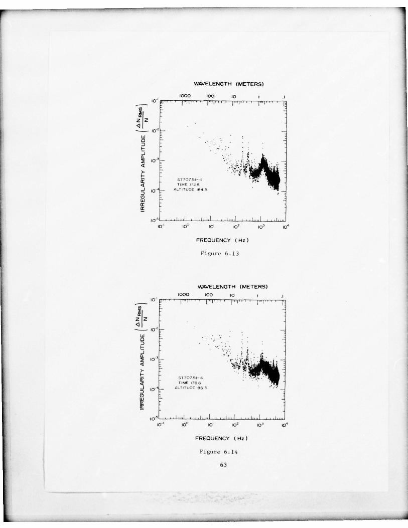
100 — —
80 i i i l ii t i l I 11 1 111 1 i i lii ii
106 I0~
ELECTRON DENSITY (cr,~3)
5.10. Electron density profi le from probe f lightST 70 7 . 5 1—5 on event Ft -r n (R+4 2 mm ). Thedashed line show s the undis turbed F—region.
49
IL

— - 5 - —--- - - —-- -- - ‘- -~~~~~ —~~~
-
r
I LI I I I IIi~ 0
ç~~J~~ ,kitSNJa NO~ J DJ1J
50
L - . _ _ - _~~~~~~~~~~~~~~~~~~~~~~~~~~~~~~-- --
~~~~- -—

~~~~- —
~~~~~~~~~~~~-
~~~~~~~~~~~~~~~~~~~
-—------
Cal
0 C C’) C-’ NI0 CC’ ‘C -r s/i NJci ‘-4 .--4 .- ,.-44)
(IS)
r- -~ r~N) NJ C-- C-i —i-C CO C- N- N.
05 -4 . 4 -4 -I ~~~ %~d ~~~ ‘~~aV
L51
, 0
—r —r N.
-~ ~~ d ~
‘ I0
-‘U)>5 1-.
CO ~— -~~~~~~0 I))C -~ C (4 ) .~~~-~ >(N CO U) .U) IN 0
C Cc C(hi 0 ES ~~~~~~ 0 CC/I 0 -4 ,- . ‘4) CS Ui 0
I C 0 — 0 4-’ I - ICs-I C U) .4U) .~~l 0 0 C C (sI,
cc CO C 4- — ~C )~. C-i C-- 4)
-I I- H Is IJ 0 4- <C C U O~~~4 o 4 4 - C OH (/1 - -~ C’ ‘ “ 4. 0 C l C ‘- 4-s- I 0 C ‘- ‘ 0 C’ - LU > - C 0I C-C C ‘— o o o o o c i
C ~~~— ‘ H I C .—’ C .—s - .- t ~~4. 0 C- I 4- ~-‘ I— 0 .54) C) LU C C
I 0 0 0 C U i ECO H - >, - --S C’ 4 - 4 - U )H I C C C C C S ~4
I I — — - -‘ ‘C 0 0) C I) —4 0H > 0 C I) 4 - ) ) 0~~O~~—’ C O O
- C Ui c) 0 Ui Ui NIc/I C Ui U ) 0 -~ U ) 0 C U i C C .C 0 1 I
C 0 0 0 4 — - ~ C-C C-CIN- - 0 0 Li 0 C Li .C Ui 4- --4 1-. ~ -4
C 0 C O 0 0 0 C~~ - 4 s ~i .-—, C —4I/I (IS) C (/1 4— -4 4-) CS) U) I/I —~ —‘
0IU- Z
-~ CS C-i -r x i i i-CI I I I I I
4 - 0 ) ~—4 -4 -4 ‘-4 —4S/i SC-S 5’S) h Sri Sn
C-)0 - -
CO - -
a 1 — — — —-. r-0 0 0 0 0 0U i I~~ 0 .,.4 .,.4 .,4 .,.4 .,.4a a a a a a4) ¶0 0) 0) 4- 4-
4- ¶1) 1) C dEl C -r 4) CO 4) i-C c—i oCs-I 0 .-—’ C — Cc - i .0~~N .0 -r c — r O C O
..-.~ i~ - ‘ S ) -4~ 10+ J J + ~~~~ 4 - +)•J 4 - ~~~~~~~ ~~4 C O U ) O’~ U I C O 4 ) C O‘-U
- ~~ i--U (i-I ‘— Cs.) Ui 4-~
51
- -~~ - -_ - - -— -- -~~~~~~~~~~~~~~~~~~~~~~~~~~~~~~~~~~~~~~~~~~~~~~~~~~~~~~~~~~~~~~~~~~~~~~~~~~~~~~~~~~~~~~~~~~~~~~~~~~~~~~~~~~~~~~~~~~~~~~~~~~~~~~~~~~~~~~~~~~~~~~~~~~~~~

-- ‘ -
SPECTRA L ANALYSIS OF THE ELECTRON DENSITY VARIATIONS
Ills’ conc entrat ion in this s e c t i o n is on the examination and compari-
son u t the s p e c t r a l analysis of the variations of the electron densit y
results which were presented as hei ght profiles in the previous sect ion .These data art ’ presented in two subsections : Short Wavelength Charac—t s - r i s t i cs (less than 50 meters) and Long Wavelength Characteristi cs
(greater than 50 meters). The DC probe results from xl gain range( I R I C channel 20) , which had suff icient bandwidth to allow 10 KHz di giti-
zation ( fo r the Short Wavelength Studies) , were util ized. First , for the
Short Wavelength Characteristh-s , Fourier transforms of the detrended
electron density data were obtained every 0.8192 sec. The-i- - were spec-
trally smoothed by averag ing each successive 5 spectra ,and these resulting
spectra are presented in this ~o s -c t i on . The irregularit y amplitude (~cN/ N)
spectra are shown in the frequency (time) domain in order to ident i f- .’ non—
atmospheric induced characteristics (e.g. rocket spin e f f e c t s ; a 60 liz
ground station pick up). Spatial scales are added to ti le f i gures . when
appropriate , which are obtained by utilizing the rocket velocity perpen-
dicular to the rnagnctic field (of course , another rocket vt’l ocitv e.g.
that parallel to the magnetic f ield, could have been used.) Spec t ra
are shown in detail for the two rockets that penetrated the striated
barium clouds — rockets ST707.51—4 and ST707.51—5 . A few spectra from
rocket ST707.5l—3 which preceded rocket ST707.5l—4 through the same
bariun~ cloud (Esther) but with no evidence of striations at that t ime
are shown for comparison purposes. With respect to the Long Wavelength
Characteristics , preliminary calculations have shown that only the rockets
that penetrated the striated barium regions exhibit spectral distributions
that Increase in amplitude at these wavelengths (and only in the striated
regions). For rocke t ST707.51—4 (Esther), the striated region is from
140 to 160 sec rocket flight time , corresponding to rocket altitude from
165 to 178 km. For rocket 5T707.51—5 (Fern), the striated region is
from 120 to 160 sec rocket fli ght time , corresponding to rocket altitude
169 to 210 km. These long wavelength data are discussed briefly since
the next section (7) discusses the results in detail.
52

-
I
Short Wavelength Characteristics
Rocke t ST707. 51— 4
This rocket entered the barium cloud (Esther) at 125 sec (150 km),
entered the striated reg ion at 140 sec (165 kin), departed this region at
160 Sec (178 kin) and was out of the cloud into the normal atmosphere
at 180 sec (188 kin). The firs t series of spectra examine tile characteristics
of the unstriated barium cloud from the time of rocket penetration to the
striated region (125—140 s&’r) using tile spectral smoothed results (average
of 5 spectr .t , t o t a l i n te rva l about 4.1 see). The spec tra prior to
125 set- all look alike and are the same as those obtained after ~he rocket
h ays-s h is- barium cloud . This spectrum is shown in frequency because it
ident I f i e s so - le .t rly t ile e f f e c t of the spin of the rocke t on the e lectron
dens i tv measurements (fundamental l It 6.0 Hz plus up pe r harm oni cs ) and a
ground s t a t ion p ickup su per imposed on t he da t a (60 Hz p l u s odd ha rmon ic s
most visibl e ). These lsot l i can he , of course , eliminat ed by filtering but
Irs- useful in the fo l l ow ing d iscuss ions as re fe rence p o i n t s s ince not
s ’fl lV ~s t i le i r r e g u l a r i t y s t r u c t u r e of the electron densit y changing (AN),
hu t ils o the electron dens i ty (N) . The next spectrum (Figure 6.2) at 128.24
see (from now on only the end time of the samp le interval will be i dentified)
when the ro -ket is w i t h i n t lis - unst r i a ted b a r i um cloud shows d i s t inct
changes f rom the previous one. First , with exception of the interval
f r o m about 700 Hz to l0~ Hz , the whole spectrum has moved down in level as
expected due to (lit’ increased eles - t r o n dens i t y (N) in this in te rva l . However ,
not expec ted is the i n - r s - a s e in ampl i tude in t h e i n t e r v a l 700 to l0~ Hz
(lower scale) wh ich corresponds t o sca le s i z e s of appr ox im att -lv 1 .1 t o 0.8
m e t e r s ;as me~lSUred across the terrestrial magnet i c f i e l d (u pper s c a l e ) .
the rocke t veloc it v perpendic ular to tile magnetic field is al )o ut 760 rn/st-c
in this t ime i n t e r v a l . ‘I lit- next f i gure (Fi gur e 6 . 3 ) at 132. l ’ s s e t - , shows
a d i s t m e t Increas e ;lt about 1 . 1 met c r5 (b y about a f ac to r s f two) compared
to t li - p rev tons figure . ScsI e a ls~ I he re I at i vs his -i ght s of the peaks in
hot Ii figures compared to the ‘‘300 Hz ret erenes- sp ike ” as well - is rd -It lye
to th e Consta n t lowest level at the h ighest f t s -q i t-n ics/lowest wavelength
53

~-- ‘ -.
both of which indicate the growt h of tits ’ peak. More subtle is t h e
incre.Ise in power in the wave leng ths f rom about 10 meters to 1.5 meters .
The nex t two figures (Figure 6.4 at 136.4 sec and Fi gure 6.5 at 140.5 -i5
show this increase in the interva l 10 to 1.5 meters more distinctly as
well as the’ disappearance of tile peak and the increase in t his- electron
density (N). Note throughout Fi gures 6.1—6.5 , the lower frequencies
(wave-lengths greater than 10 meters) have not (-hanged and that at wave-
lengths less than about 0.35 meters the leve l is constant. The Concen-
tration in this section is an examination and comparison of t he data at
the short wavelengths but it will be pointed out , when appropria te , the
changes occurring a t the longer wavelengths (SO to 500 meters) since in
this section (compared to the next — Lon g Wavelength C h a r a c t e r i s t i c s )
shorter t ime (and spatial) intervals are examined .
The next series of spectra , Figures 6.6—6.10 cover the striated
region of tlis’ cloud , from 140.5 to 161 st-c; 5 spectra (each averaging
5 spectra) each in the t ime in terva l of 4.1 sec (St’t - Fi gure 5. 7 of the
previous section which shows the striat ed region in the electron density
profile). The first spec t rum , Fi gure 6.6, covers the time interval
140.5 to 144.6 see , the beg inning of the time when the rocket enters
the striated region throug h the first two “fingers ” (peaks in Ne ).
Compared to the previous spectra , iimnediatelv a p p a r e n t i s t h e increase
in irregularity amplitude at the hi gher wavelengths (from about 10 to
800 meters). The Long Wavelength Characteristics in the next section
show this increase over the whole striated region , not just , as in this
case, at the beginning. This spectrum does confirm , however , that the
longer wavelengths are only increased in irregularity amplitude or
power in the striated region as compared to the unstriated barium cloud .S
(Figure 6.10 the last spectrum in the striated region compared to Fi gure 6.11
the first spectrum back in the barium cloud shows this also.) The next
few spectra are all pretty maci) the same as Figure 6.6 except that Fi gure 6.7
shows a steeper slope than the other l ower altitude spectra at the higher
wavelengths (- -10 meters) and Fi gure 6.8 shows a higher slope at the Very
short wave lengths (<1 meter ) as well as a d is t inc t increase in irregularity
amplitude between 1.6 and 0.8 meters. Fi gure 6.7 covers the interva l
54

~- - - .-~~~~- - ‘ - - - -~~~ -- -~~~~
where the rocket goes through the most “fingers” (finger Nos. 5 & 6) which
have the sharpest slopes (see Figures 5.7 and 5.8 of the last section
showing the striated region in detail). Figure 6.8 covers the interval
where the electron density has its highest value (finger no. 7) and for
a relatively longer period (again see Figures 5.7 and 5.8). It is also
interesting to note that Figure 6.9 which only covers one “finger ” (finger
no. 8) is very similar to the others which cover two or more.
The next series of spectra Figures 6.11—6.14 cover the t ime interval
161 to 177.4 sec when the rocket is back in the unstriated barium cloud
until the rocke t leaves the cloud . First , Figure 6.11 compared with
Figure 6.10 shows (1) the decrease in irregularity amplitude in the longer
wavelengths (‘~-50 meters) to a slope like that before entering the striated
structure (2) a decrease in the region 10 meters to about 1 meter (3) an
increase and peaking at about 1 meter and (4) the lowest wavelength
spectra about the same . Figure 6.12 continues this trend with the peak
first decreasing in amplitude towards the longer wavelengthside giving
the appearance of a shift of the peak to shorter wavelengths. Figure 6.13
continues to show th e decrease out to the longer wavelengths until by
Figure 6.14 (the last spectrum in the barium cloud) the spectrum looks
like Figure 6.1. Note also how Figures 6.11 & 6.12 compare to Fi gure 6.3
and Figure 6.13 compares to Figure 6.2. In other word s the phenomenology
before entering the striated reg ion looks the same as that after leaving
the striated region.
Rocket ST707.5l—5
The electron density results from rocket ST707.5l—5 (Fern) are
obviously different from rocket ST707.Sl—4 as shown in the previous section ,
but what about the short wave irregularities amplitude characteristics?
The discussion will be in two parts (I) the unstriated barium cloud from
90 to 120 sec (128 to 169 kin) and (2) the striated region 120 to 160 sec
(1.69 to 210 km). The spectra up until barium cloud entrance are pretty
much the same and look like the spectra in the undisturbed atmosphere
above 218 km — and like the spectra from rocket ST707.5l—4 outside the
barium cloud . The first distin ct change is shown in Figure 6.15 for the
55

time interval 99.6 to 103.7 sec. A sharp peak is formed at 1260 Hz on
the frequency scale which is 0.25 meter in wavelength (rocket velocity
perpendicular to the magnetic field at this time 300 meters/sec). Note
that for rocket ST707.51—4 (Figure 6.2) the peak occurred at 1 meter
and also different is the fact that the frequency of the peak was near
750 Hz with the rocket velocity perpendicular to the magnetic field 760
meters/sec. The next series of figures until rocket entrance into the
striated region Figures 6 16—6.19 show the growth in power in the region
from about 10 meters to about 0.2 meters .
The spectra in the striated region of the cloud from 120 to 136.5
sec (157 km to about 175 km) are all about the same and Figure 6.20
is representative of the irregularity amplitude spectrum for this region .
This spectrum compared with one from rocket ST707.51—4 in the striated
region, e.g. Figure 6.7 shows similarity for the short wavelengths.
From 136.5 sec to departure from the barium cloud near 160 sec (210 km)
there is a general decrease in irregularity amplitude in the spectra as
shown In three representative spectra; Figure 6.21 (140.6 sec—l 91 km),
Figure 6.22 (153 sec—203 kin) and Figure 6.23 (161 sec—2l0 km). The latter
figure is representative of the spectra obtained up to rocket apogee of
250 km. Note that rocket ST707.51—4 came out of the striated region
abruptly into the background barium cloud whereas rocket ST707.51—5 went
from a gradually decreasing striated region (and of course not nearly
as striated as ST707.51—4) into the normal ionosphere.
In Figures 6.1—6.23 amplitude distribution of electron density
irregularities (AN/N) versus frequency (lower scale) and spatial dimen-
sion (upper scale) derived from the rocket velocity perpendicular to the
terrestrial magnetic field. The spectral distributions were derived by
taking a fast fourier transform (FFT) of the detrended A N / N results di gi-
tized at a 10 kHz rate over about 0.8 seconds and then averag ing over 5
spectra for a total t ime of abou t 4 seconds for each plot. The rocket
probe number and time and altitude of the end of the 4—second period of
the spectra are sh~~n on each figure.
56

_ _ _ _ - - ---~~~ -- -
WAVELENGTH (METERS)1Q00 00 tO I
Jo_ S
U) - - .
‘I ‘ - - - -
-: -
- Yl’ , ~-h -
-
— -
‘, T ’ O7~~~ - 4
4 T IME 2 3 3
- ‘ — ALTITUDE 4 ‘7 —
0Ui
a:so 5 I I I
0 1 10° Id 102 01 io~
FREQUENCY (Hz )
Figure 6.1
WAVELENGTH (METERS)1Q00 100 10 I
0 — - — j~’’U,
z z - - . . I
~~__ ____ 10~ — - .
,
I0~
l i
~~~~~~~~~~~~~~~~~~~
ST,O~~5l-4
4 T I M E S2~~4AL ITIJDE 151 6
C,Ui -
a:
I s i , , , ! ., .L,,,I , ,I,,,, J0 ’ 0° Id 01
FREQUENCY (Hz )
Fi gure 6.2
57
~~~ - - -—- - -~~~~~~~~~~ - - - _ . ---~~~~~— - ~

WAVELENGTH (METERS)1000 100 10 I
10~ ~~ ‘ I ’ ’ ! ’ ’ ’ I t ’U, -
zz -
2 -—
.. . —
- --- - . - i ‘ - -
D - . . : -
F .•~~~ -
-~~-~ - :~~~~~~- . i.
~ IO~ ~
- - . - : ,
-
TIME 1 315J
~~~~ — ALTITUDE - i ~~ 3 —
C,Liia:a:
i - I i ! _ i ~~ IJ o_ I 100 101 102 ~ 3
FREQUENCY ( H z )
Fi gure 6.3
WAVELENGTH (METERS)
1000 tOO tO I0 ‘‘ ‘ t ’ ’ ’ J ’ ’ ’ ~~‘ t ’ - ’ j~’~i ’ ’ ’ I ’’ I ’ ’ ’
U) -
z z -
“1~~~~~~~~~ I0~ — - —
D - - -‘
I0~~ -
to ’ — A L T I T U D E 58-~ ~~~~~~~ —
C,Ui -
a:a:I ~~~~~
10 ’ 10° 101 IO~ Id4
FREQUENCY (Hz )
Fi giirs- 6.4
~±E

WAVELENGTH (METERS)000 100 tO
~ Jz
0 r,~~ ‘ ~
‘ ‘ ‘ f - ’ — — ~~~~ l ’ ~
’ ’ ’
— Jo’ — —
-
D . -
0. -
~ 0 — -
~~ME ~‘ ~
AL~~ TUDE
i~~ I ~~~~~~~I0 ’ 100 10
1 10
2 to3 to4
FREQUENCY (Hz )
Figi irs - h . 7
WAVELENGTH (METERS)1000 too to t
Jo _ I I~~~~~ ~
‘ ‘ ‘ i~~
’ ’ ’ I I ’ ’ ‘ ‘ I I ” ’ ’ ’ ’ ’cit - -
z z2
-
— 10- - —
I- -
- - .
~ IO~~ — . ..4 - -
‘. . -
to — AIJ ITuDE 656
- ,J,,,! b I , ,i,,to-I o° io 102
~~
FREQUENCY (Hz )
Figtt re 6 .6
59
- - -
WAVELENGTH (METERS)
000 00 10 I
2
‘ ‘ ‘ ‘ ‘ I ” ’
,
-~ I I ’ ’ ’ ’ I i ’ ‘ ‘ V ’
— ‘.•
—
3F - -
0. -,
~ i0~~— - -
4 ~~_ I
I0~ 00 0’ 102 01
FREQUENCY (Hz)
Fi 1:,irs- h . 7
WAVELENGTH (METERS)000 100 10
1’ - I ’ ’ ’ ’ ’ ’ ‘ ‘ i ’ ’ ’ I I ’ ’U, -
z z -
- —
Ui --
3FJ0 . , ,~ Jo -- . . .4
F~~~~ ‘~~~‘~~~‘- ‘~ - . - : - -4 7 M L 520 “s. •
~~ :~~~ :
TUOE
I1O ’ 100 10 1 102 ~~~
FREQUENCY ( Hz )
Fi gure 6.8
60
~~~--~~~~~~~~~~~~~~~~~~ -- - ---- - - - - - ----

_ _ _ - - - -~~~- . - ~~~ -~~~~~~~~ --~~~~~ -~~~~~~~~~-
WAVELENGTH (METERS)1000 00 10 I
I I ’ ’ ’ I 1 l ~~~1 1 I ’ ’ ’ ’ ’
U, -
z z_~__~_~ ~ -2 — —
3 - -I— -
0. - . -
~ I 0 - - -,. - - -
- —
- :.~~~~‘
5770751-4 ‘C
4 TIME E-S- .- : ‘ ‘
~~
— ALTITUDE
I
—
Jo-I 100 0 ~ 2 ~~3 ~~~
FREQUENCY (Hz)
Figure 6.9
WAVELENGTH (METERS)000 tOO 10 I
Jo I _ ’ _ ’ l ’ ’ ’~~
_ _ - ’ _ ’ ’ ~ -
I - I I I ’Ut -
z z -
‘I -
~~~~~~~~ I0~ — - —
Lii -a -
3j - -
0. - -
I :i__
A CflTUOE 1772
I0 ’ 100 101 102 0° I0~
FREQUENCY ( Hz )
Fig u re 6 .10
61
_ _I
~
~~~~~~~~~~~~~~~

-- --- -- - - - _---- -- - _ - - —_--~~~ ------- —-__ - _-
WAVELENGTH (METERS)
I 1000 100 toto -
~~~~~~~~~~~~~~~~~~~~ I t ’ ’ V 1 ’ ’ ’ 1” “ ‘ ‘ I
U) -
z z~~~ IO~ . —
-
-
-
ST 707 51-4 ~~~~~~~~~~~~~~~~~~~ ~~
‘
- .:
-
4 TIM E SO4 3 -
~~
ULTITU D E I ’97
- i~~I , , - i ~~- - I
‘
0 ’ 0° tO 02 01
FREQUENCY (Hz )
Fi gur e 6 . 1 1
WAVELENGTH (METERS)1000 100 tO I .1
I ’’ ’ ’’ I’’ I ’ ’ ’ ’ I ’ ’ i ’ ’ ’ I’’’ ’ ’ IU) -
z z -
2— to- - . -
- . . .
-3 --. -F - - -
~~~~~. - - -
~ IO~ — ~~
- A --
577075 1-4 -.
-‘~ . -.4 TIME 684 -
I0~ — ALTITUDE ‘82 0
‘ - “:
tcrsL , _ i . ~ . I , . i _ _ , , I ~~~~~ I i . , ItO ’ 10° 10 1 102 01 Io~
FREQUENCY (Hz )
F i gure 6.12
62
____________________ —-
WAVELENGTH (METERS)
1Q00 100 tO II ’’ ’ ’’ ‘— ‘ ‘ ‘ i ’’ ’ ’ I ’ ’ ’ I ’ ’l
_I
_r~ ~~~~~~~~
0 2
3 . -
F - -
- - -0.. -° ~ - .‘
~ to — — - .- - - i : ~~~~~~~ : - - —
~~~~~~~~~~~~~~~~~~~~~
ST70751- 4
4 TIME I~~~~5
— ALTITUDE 184 3 ,.
—
C,Ui -
a:a:
- i.~ I -~~~~- - I i , ,10 ’ 0° 10 102 0° JO~
FREQUENCY (Hz)
Fi gure 6. 13
WAVELENGTH (METERS)
- I 1000 100 tOJO ‘ ‘ ‘ ‘ ‘ I ’ ’ I I ’ ’ !‘“ r ’ ’ ’ I”I’ ’’
iO_2 — - . —
3 - - - . -
F
I0~~~
-
S17075I-4
-
4 TIME 76 €S
—‘ to- — A LT I T U DE ISG ’ - ., .- .
—
Ui -a:a:
I0~’ i~ , ,i. I i , I to-I 10° 10 102 J0~ ~~
FREQUENCY (Hz )
Figure ( ‘ . 14
63
_ ~~~~- - _ -- - —~~~~~~~~~ ——- _ --— ~~~~~~~~~~~~—--
~~~~~~- - - -—- —---
~~-- -

- - — -~~~~ -- —~~~--
~~~ - -- ----
WAVELENGTH (METERS)- S
000 00 J O I10 I l’ ’ ’ I ’ ’ I ’ ’ ’ I ’ ’ ’ J ’ 1 _ I _ _ I
0, -a:z z‘I
.________
Lii -a -
3F
~~ J0 - - -4 .
.
F - . -STTOT 5I-5 -
- - - - - - :
-
~~
ALTITUOE 4~~~
I i I~~~~~~~~~~~~~~~ i1IO~ JQO Jo to2 Jo3 J0~
FREQUENCY ( H z )
Figure 6. 1,
WAVELENGTH (METERS)000 00 Jo I
0 — I ’ ’ ’ ’ ’ ’ I ’ ’ ’ I ’ ’ ’ ’ ’ V ’ ’ ’ ’ I’~ra:z z -
J0 2 — —
3F0. - - - -
~ I0~ - - - - -4
>- . - . .F -
- -— ST707 51 - ’ - - - : - - - - -
-
l IM E 069 - ~~~~~~~~~
I O~ ~~~~~~~~~ ~~~~~~ 5 ~~~~~~~~~~ ~~~ ___ L ~~~~to- I 100 101 102 01 to4
FREQUENCY ( H z )
Fi g u t - ,- 6.16
64
- _ -- - -_ - - -------- - --- ~~~--- --- ----- —-—— -- -—-~~--—-~~~~~m-~~~---------- . —-~~~~~-- - -_

- - -~~~ ~~~~~~~~~~~~ - -_
WAVELENGTH (METERS)1000 00 JO
tO I~~’ ’ I’’’ ’’’ ‘‘ I ’ ’ I’
(0a:z z
io 2 — —
U - - -a - -3I- . -I0. - -
~ to- — --.
. -4
-
--
--
~~~~-
>- .~~ . -I— - -. ,5T7075I-5
4 TIME 1 1 1 .0 :- — - - ‘ : -
1: 5L
A LTIT U
~~
1560
I i
J o_ I 00 0 02 io 3 to4
FREQUENCY (Hz )
Figure b. 17
WAVELENGTH (METERS)
1000 100 10J0 r ‘‘
~~~‘ ‘ ‘ ‘‘ I’’’ ‘‘‘i’ ‘ ‘ 1 ’ ’ ’ ’ I I
U, -
a:z z -
—— to-’ --U - - -
a -3I--I0. . . . -
~ JO-’ — -
4 - -
->. I- ..-
ST 7 0 7 5 1 - ’ -
~~, — -
~ r TIME 11 5. 1 :::‘ - ‘.~~~~ ‘ - - -~ - -
~ o~~— ALT ITUDE I6j 3 ‘: ~-~~ :
- - _ —
- ~~~~~~~
- - .-‘ i _
a:a:
o’ ~- I , - ‘ I~~~~~Il~~,
0 ’ to° to 102 to ’
FREQUENCy ( Hz )
1- igure 6.18
65
~~- -- - - - -- - -~~~~~~ -- _ --- _ _ _ _

WAVELENGTH (METERS)1000 tOO 10 I
JO - ~~ ‘~~~ ‘ ‘ ‘ ‘ I t l l I’’’ i ’ ’ , I
U, -
a: -z z -
2 — - -
—
3 - .
I-I - -
0. ~, - -
- - -
~~~~I o — .
4 -
.
->- -F - ~~~~~~~~~~~~~~~~ -
T I _ P -
____
I io — ALTITUDE 66 4 -
‘ - ‘ -—
I —3 . - - - I-C, - - - - - -U — .;- -a:a:
J 0~ ~~~ _ i I 5 _ i _ _ _ I _ . i , I I Jo-I 0° Id 102 to’ to4
FREQUENCY (Hz )
Figiir~ 6.19
WAVELENGTH (METERS)1000 00 JO
0 . ‘ I ’ ’ ’ ’ I ” ’ ’ I ’ I”
— tO 2 —
=3F - .
I0. , -~~~~~~~t 0- .
-4 - - -- -
-
~~~~~~~~~~~~~~~~~~~~~~~~~~~ST7O7SI-5 ~
~~~;:-4 TIME -‘ - 5
. - ‘ ‘ . ..- ,
~~~
— ALTITUD E S
I I ! i
10 ’ tO0 101 JO2 to 3 to4
FREQUENCY (Hz )
Fi gure 6.20
66
- - - - - - - ---- --- -- -_-- - ---‘--- — - --_ _ —---—- - - --.~—-- ‘---------- .~~--——‘----——---~~~~~ --——-__-*--_
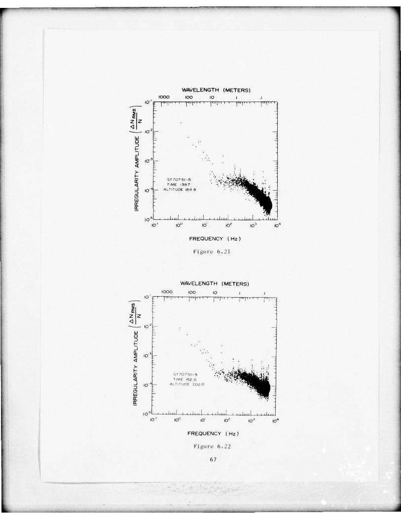
___________________
WAVELENGTH (METERS)1000 100 tO
I - , - ‘ ‘ 1 _ l I t I’” ~‘‘‘ l’’’
— —U - -a -
- -3 - -I—I - -
-0. , - - - -
-
~~~ t o — - -- -
4 - -
F - -
- ‘. - ~.
—
TIME 1397 --
: -
-
~,: -
~: :~~
— A L T I T U D E 189
I01 00 0 to~ ~~~ to4
FREQUENCY (Hz)
Ft gl t c 6. 2 1
WAVELENGTH (METERS)
- 000 00 to
JO - ‘ ‘ ‘ ‘ ‘ I ’’’’ I ’ ’ J ’ ’ I’’ ‘ ‘ ‘ ‘ I I ’U,
a: -
z z -I
lo _ _ -
U -a - -
3I—I -
-0. , - - - - -
~ 0 - _ -4 _
>. _- —- : - ,
I—- ~- ‘ - c ’ 5 - S ~~~~~~~~~~~~~~ -
JO - .51 - - II’[ 0 0 - ‘
~‘
F—3 ~,r_ —
(:1 -—
a:
- - ~ ~~~~~~~~~~~~~~ _ _ t _ _ _ _ [
JO ’ tO’ tO tO’ 10’
FREQUENCY (Hz )
Figtt rc h. 22
67
____ ________________ --- _---—--_- - -- _

r -_-- ----- - -
~~~
-- —-—.--- --
~~
- —_ - - ---— —--_--
~~~~~
WAVELENGTH (METERS)
000 tOO JOtO i --- ~
, ‘ ‘~~~~~
“‘~~
‘ ‘ ‘ —TrI’l— lI I I ’ ’ ’ ’ ’U, -
a:2 2
2 -
—J o- - —
3FI -0. , - - .
~~~~ t O — - - - - - -
-
‘I -- -. . - -
- J - -
—~~
_~wA~~~
_~~
~ 101— ALTIT UDr 209 4 .•~ ~~~~~~~~~~~
—C, . .
~~~~-
4 -U - - ‘i s-
a: - -
a:
~~~ ~~~~~~~~ - -- ~ ‘ - - -~~~-~~~~~~~~~~~~~~~~~~~~ _ ~~~Ito ’ Jo0 10 01 to4
FREQUENCY (Hz )
F i g s t r - 6.23
68
_ _ _ _ _ -~ --_ ~~~~ - — -

Long Wavelength Characteristics
The power spectrum shown in Fi gure 6.24 was obtained over the t ime
interval from 140 to 153 sec of rocket ST707.5l—4 (Eother) utilizing the
DC probe xl data. These data were decimated by averaging together 16points and detrended by fitting to a polynomial of degree 3. Note the
uniform slope between .2and 50Hz. Fi gure 6.25 shows tile power spectrum
for rocket ST707 . 5 l—5 (Fern) in the s t r iated region. The data were
decimated by averag ing together 80 points and detrended by fitting to a
polynomial of degree 3. These resu l ts are very similar to Fi gure 6.24
with the slope not quite as steep however. The implications of the
Long Wavelength Spectra are d iscussed in the next sections.
69
- --~~~~~~- - -— -~~~~~~~~~~~~ -~~~~~~ ~~~~~~~~~~~~ ---

p.—- —‘-—--- -
~~~~~~~~~~~~~~~~~~~~~~~~~~~~~~~~~~~~~~~~~~~~~~~~~~~~~~~~~~~~~~~~~~~~~~~~~~~~~~~~~~~~~~~~~~~~~~~~~~~~~~~~~~~~~~~~~~~~~~~~~~~~~~~~~~~~~~~~~~~~~~~~~~~~~
___________________________________ .~~I ~~- — . - - —, __ 4.1 U 4-I“-4 0
-‘.— I_
~
4-J O S . .
- - -~~~~~~~~
- -- _ - -: - - - 0 — S.
- --. -
~~ Q~~~~ ~~~~~~~~~~~~~~~~~~~~~
- -~~~~~‘ : - — 1.-~~~~~~~ C5 . ,~,3 4-~~~~5) N~~(2
- .-~~~~- - - - - - 0 u .
~~ooU 0 > r — ,, ,-~ a:
— - - -
~‘005 — l-~- . _0
_ -
- - ~- s- 0 ,—4 ,—4 S. 0- 0-
4 —— 0LT~
- - - - - I --
c-’J- -~ ~- .., - ~~~~~ 4,-fl
S 55 4 5- , • 2 92 2 Q ’Q 2 g o Q 2 0 2 ’0
I.
ZH (N~~~V lN V ) ~3M0d A1I~ V1flO3~~ I
-. - r
~~ ii’ - r~” ~ ‘r” - I~T- I ~‘~‘E:.’ - ~-‘ ~.)- - - . ~•4- - - - .-
~~~ 0— -‘ W/.. - - 0-
~~~~~~~~ ~~~~
‘ •:•~~~
- _i-._ —
7-_ O _ .~ 0.“ - - - ~- ‘ 0 4.4 .4- _i~ .--~_ - - - —
- ,5J - - -
- > 0 S.-~~~~
: - UZ l~1 .-4 1 55
— ..- - - - - — U• . 3- - - -
~~~~ S~~~~~0 • 0~-~~5)
- ~~~~~~ U- - — -° I a: C) ~~~r—~~~
I LL- -~~~~ I-- “I- -i I t.1
- I
0~- _
- 10
5 55 4 5~ . S 1’ 2 52 2 Q Q 2 2 c ’
~~~~~~2 ’Q 2
I ZH ( N ~S~~~~~~ ) ~~ MOd A±IèJV1flD3è~efl U
70
~~~~~~~-~~~~~~~~~~~~ - - —_ - - - - - - — — — - - —~~~~
— —

r --——— - - —.-——---- .-------- --_-_--
7. COMPARISON BETWEEN THEORY AND OBSERVATION OF BARIUM CLOUD STRUCTURE
1. Location Of Large Scale Striations
In this section we r e l a t e the dat a to the predictions of linear and
nonlinear theory for the structures which develop in large barium clouds.
The basic phenomena can he understood in relation to equation 7. 1 which
relates the velocit y V~ of a barium cloud perpendicular to the Earth ’s
magnetic f i e ld ~ to the ambient electr ic field E and the neutral wind
Vn (Haerendc l et al - , 1967)
- - * ~~~~=
2 ExR — (~~:1) ~~ (1)
2 B
where
= inte~~rate d cloud conductivi tv + inte~~rated back~~ ound conductiv ity
- integrated background conduct iv i ty
I&- have dropued a te rm of order \I /~, , the collision frequency of ions
In in -divided by their gyro frequency , which is valid at the altitude of t iJe
*clouds studied . in the case of a small cloud A 1. and the cloud moves
with the ~erpend icular velocity ~x B /B 2. For a large cloud , A can be-
come s ic~n if icant iv large r thin 1 , which is the case of interest here.
Consider f i r s t t h e case that V 0. Then in the center of the cloud , then
t o t a l electr ic h eld is smaller than either the ambient field or the
f ie l d in the surrounding cloud (an effect ver i f i ed wi th e l e c t r i c field
measu rements during the Secede program by Schutz et al. , 1974). Those
parts of the cloud in t h e direct ion of the background Exfl move away from
the center , the “leading edges” while those at tile opposite side catch—up
to the central portion . The number density following a fluid element
changes according to the convective derivative
= + ~~~~~ (2)
At long t imes after release no new barium ions are forming in the main
part of the cloud and recombination is slow , so ~n/~ t=O . Thus the only
changes in density occur where ~~~~~~~~~ In the backside V is parallel
to -n so the density Increases and in the frontside th e y are opposite*so the density decreases. The leading edges become tenious (A ‘1) and
approaches t~Je ExB velocit y of the ambient medium while tile backside
71

becomes more dense and forms a steep gradient in density. It is this
gradien t in e l e c t r o n dens i ty which is unstable to striation development.
lo determine the sector of instability, one can t hus draw a vector from
the cloud center in the direc t ion of — (ExB).
In the mid—latitude ionosphere one can seldom ignore t i le neutra l
wind term . However , if one t ransform s to a re ference frame movin g with
velocity V (the direction of tile wind velocity in the plane perpendicular
to B , then the neutral wind is ~ero and we can use the derivation outlined
above with the electri c field in tile new frame given by the t ransformation
(Jackson , 1960)
i~,
= [ + ~~~~ x~ (3)0
where E and V are measured In the Earth’ s fixed frame . Note tha t B isn
—unchanged in such a transformation if V ‘- ‘-c. The unstable sector is
again in the — (E’x B ) / B 2 direction . We relate our measurements to
Earth fixed quantit ies so we must substitute 7.3 into this expression :
= - (~ x~ ) x~ /B~ = V -ExB/B
2 (4)B B2 n
Thus to determine the unstable region we can construct this vector if we
know V and E. Unfortunate ly , viewing conditiot i a during the experiment
were such that optical measurements of the wind from the neutral cloud
and of E from the “leading edge” of the barium were not possible. We
can thus only show consistency with the theory , but not detailed com-
parison . Optical observations of these quantities plus the striations
made in tile Secede series (Davis et al. , 1974) were able to show detailed
agreement and we can have confidence that our interpre tation is valid.
If we know the velocity of the cloud , V~ , and the neutral wind , we
s-an still determine the direction of the striated region without know-
ledge of the ambient electric field or \ * as follows . In tile neutra l
wind frame from equation 7.1 we know that the cloud velocity Vj is g ive n
by
= ~~~ )~ ‘ xi~Ii3 2 (5)± A + i
thus the sector of striation is in the direction —V ’ which can be
determined without knowledge of \*~ To construct —V ’ , we t irst determine
‘~

- - -
~~~ -~~~~~
in the Earth fixed frame . In the neutral wind frame then
V ’ V1 —V . Thus the direction of striations should be V —V . Ini _ _ n n- I-the cases of interest (Esther and Fern) when striations were observed ,
was obtained from radar measurements , but we must appeal to models
for the neutral wind ve1ocity .
Esther: Probe 51—3 detected a very strong density enhancement ,
but no striations. Since we do not have a neutral wind measurement
due to the earls’ cloud deployment in sunlit conditions , we can only
estimate the wind velocity from measurements and models constructed
for Millstone h ill (42.6°N ; 71.5°W) as reported by Roble et al. (1977).
For winter season at the local time of interest the neutral wind at
release altitude is given as 94 m/s, 32° north of east. The ion cloud
velocity was determined from radar measurements (Gonzales , personal
communication , 1977). The resulting vector Vn_YL was 38° north ofgeomagnetic east , while probe 51—3 passed through the south east portion
of the cloud.
Probe 51—4 , however , passed through the cloud much closer to the
predicted reg ion of instabi l i ty. The radar map at 185 km is reproduced
in Fi gure 7.1 along with the rocket position and its d i-ec t ion of
t r a v e l . Tile posit ion when s t r i a ted plasma was observed is indicated
as is the (V —V1 ) direction.
Fern : Only one probe functioned during the Fern event and it also
d e t e c t e d strong striations. Detailed radar measurements are not
available , hut vector V —V constructed as defined above was in the samen
qt t adrant of tile cloud which the rocket penet ra ted . S t r i a t i on s were
observed for a longer t ime since the rocket t r a j e c t o r y was s teepe r and
hence more c losely aligned wi t i l the cloud axis.
We t hus conclude that the regior. of occ urr~~nce o f the large scale
structures is consistent with the CxB ii sta hl l lty as a causative
mechanism.
2. Comparison With I~inear and Nonlinear Theory
Before comparing the resu l ts wit i l nonlinear theor y and computer
simulations , it is instructive to see why tile striations develop -it all.
In Fi gure 7.2, the steep “backside” density gradient discussed earlier
Is dep icted along with a sinusoidal perturbation . The p icture is drawn
73
~~~~~-- - -- - - -~~~~~~~~- - -~~~~~~~~-- -- m— - - ---- - -~~~~~-- -- - -- ---_---

r
BARIIJM EVENT ESTHERPROBE ST 707.51-4
00
\ PRED ICTED D I RECTIONOF UNSTABLE EDGE
270° ~~~~~~~~~~~~ 900
- - ROCKET POSITION \WHEN STR I AT I ONSBEGAN (hrt64km )
ROCKET TRA JECTORYIN HOR I ZONTAL PLANE
1800
Figure 7.1. Cross section of ion cloud (from V. Gonzalez)
and rocket trajectory for probe ST707.51 4showing entrance of probe In striated regionand p red i c ted d i r e c t i o n of development of
i n s t a b i l i ty .
74

—~ - -- - - - ----- - - - - - -—---- -_---- - - . - ---—— ------ - - - - - ------—_----- - - __—- - - - - --- - --_ - - - - - -- -
I w l - .
~~~~~~~
IL
(~~~iw ------
~~~~
--
~LLJ~~~~~~ - -
~~~- -+1 - -~~
—~---/ ------- -
- - -- --+1 ~~~ - -
+/
C55
‘-I W—-
— - C’-~IC -~
- N.
w(‘Si — - -C C -
75

in t i le t rame of t h~ neutra l wind so there is only au electric field , wh ich
is pointed to t iJe right , B is out of the paper , and ExB downward . The
Pederst - n current f lowin g in the cloud pi les — up pos i t ive and negat ive char ge
as indica ted until t h e low density reg ion (not cross—hatched) has a large
eno ugh e lec t n c field E+E1 to make tiJe current continuous across t h e bound—arv . T u e high density reg ion will adjust charge to have a sma l l e r elec-
t r i c field E—E 1 and will again be such tha t t h e current is con t inuo us .
These changes are in accordance w ith tile cons e rva t i on o f charge equa t ion
— —~~I~ t (6)
which says that charge will build —up in a way to keep -I divergence f ree .
The result ing per turbat ion e lec t r i c fields and —E1 are oriented
in such a way that the low density reg ion will E1xB drift into the cloud
and ti le hi gh density reg ion will — E1xB dr i f t the opposite dir ection . The
resulting perturbation is larger and hence will intercept even more
charge and then grow larger still , an instability .
the linear growth rate has been derived by several workers (Simon ,
1963; Linson and Workman , 1970) and tested in a computer simulation by
Zabrusky et al. (1973) very successfu l ly . As discussed below , the
growtil rate , ~, is a function of wavelength but is usually normalized
to y= E ’/BL s1 where L is the density gradient in tile cloud and E’ is
the magnitude of E+V xB. For E’/B equal to 100 rn/s and L of 4 km ,n
1 =2 .SxlO seconds. The earliest striation measurements made in tills0
rocke t se r ies were at t+42 minutes. Thus time was available for more
than 50 c—folds (0~t) of any initial perturbations. Thus the clouds
were clearly Into the fully nonlinear regime and comparison with linear
theory relevant only to the question of where the striations first should
develop , and not their final amplitude nor their distribution of ampli
tude with respect to wave length (spectrum) . In fact , it is very clear
that linear theory is deceiving in this regard since it predicts that
the shor tes t wavelengths gro w the fastest (Linson and Workman , 1970)
whereas the observations show that the final state has more intensity
at tile longest wavelengths.
The non l inear computer simulation of late t ime striation develop-
ment performed by Scannapieco et al. (1976) seems most applicable to
the data. In fact. the results are In excellent agreement w it i l the
76
- ~~~~~~~~~~~~~~~~~~~~~~~~~ ~~~~~~~~~~~

_ _ _ _ _ _ _ _- - -- -~~~~~~~~~~~~~~~ - _ _
data. We concentrate on the Fern data here due to the longer t ime
interva l and hence the larger number of observed structures. ln order
to best compare the results to theor’ , we have detrended the data by
fitting a third order polynomial to the tine interva l t+1lO seconds
to t+l65.5 seconds and dividing each data point by the value of the
curve at that point. This yields s curve of relative density with near
zero mean value which is plotted in Figure 7.3. The distance scale was
determined by projecting the rocke t veloci t y onto the direction
(V -V )xB. this is in t ile dire ction of the most unstable wave vectorsn
in t ile l inear theory and corresponds to tile x direction in the paper by
Scannap ieco et :Jl. (1976). The projected velocity was 179 rn/s. The
s t ria t ions appear to have dominant power in the 1—5 km range and dis—
play very steep gradients.
The power spectrum of this data set has been determined by a
Fast Fourier I ransform and the result plotted in Figure 7.4. A power
law is indic ated with index 1~~3 tO .2 . As in all probe data this
corresponds to a one—dimensiona l power law since an implicit integra l
is made by tile detector as it t~~ss~ s across a two—dimensional structure.
Scannapieco e t al. have numericall y calculated one—dimensiona l spec t ra
for late time stri Jtions in the ~ direction and found an index be tween
2 and 3 for wavelengths between 0.6 and ~~ km.
We thus conclude that the observations are in excellent agreenent
wi th the nonlinear theory for Ex~ instability (k heN~’cc n 0.5 and 10 km l)
3. Short Wavelength Irregularities
The peaks in the spectra at high frequencies (short \) plotted
earlier are remarkabl e since t he y appear in t u e otherwise undisturbed
bari um p lasma . Sin ce a Langmuir probe measures a scalar qttan tit \- and
Sin ce there is no clear theoretical explanation for these waves , we
cannot even be sure of thìe correct mapping between frequencY and wave—
number space. For any ele ct rosI at 1s~ mode below the lower hybrid
resonanco , however , we expec t phase ye hoc it ies - tile acoust ic speed
which is comparable to the rocket v e l o c i ty . Thus the frequency spectra
must corr s-spsi nd to wavelengths between 0.1—10 meters . Such waves could
hive q u i t e serious eff ec ts upon backscatte r radars looking through the
disturbed medi Jiru if the wave vector were parallel or anti-paralle l to
77
- _ _ _ _ _
— __--~~- - - —~~~~~ ----------- -- - - -~~~~-~~~ - - - -_ ----_ ----- - - - - -- -

— ——- -- ---—- -~----- - ----- -- --
~~- .---- - - -
~~~~~.---- -~~~------~~~~~~
- -
I .h~ I‘4-i
-
L
- o~~
- -
a
c c0 1-s
- (
)
- a
U.)
—
- - (I) > 1 1~
- —s - —o
~~~~~~ a-
~~~-
-
~~~~~~~~~~~~~— 0
- - Lii
J O-
-
- -
— - — a. ‘ - 4 5 5+
~0 055~~~~J 4.J~~~~~ — J O
a
‘
a -~ 0
~4 —- -
—
(U/Us ) NOLLVIeJVA AJJSN3O BALLV 1J~
78
-
~~~~~~~~~~~~~~~~~~~~~~~~~~~~~~~~~~~~~~~~~~~~~~~~~~~~~~~~~~~~~~~~~~~~~~~~ . - -

- - - - — - ~~~~~~~~~~~~~~~~~~~~~~~~~~~~~~~~
I I I j I I T 1 I I
10 -
• LATE TIME Ba STRIATIONS (FERN)
~~ - x EQUATORIAL SPREAD F —
-
J
-
‘ii0~(I)
-~ -Ui JO —
0a--
a’ - -
JQ O - I I I I I I , i I I I I L I i
100 0 02 JO~
WAVE NUMBER , K M ’
Figure 7.4. Power spectrum of the data of Figure 7.3 (Fern ,ST707.51—5) determined by a Fast Fourier Trans-f o r m (FFT). Also shown is a spectrum from a rocketflown into an equatorial spread F condition((‘ - - n~~~ -zn ! K~?Z ?c,, 1977)
79
~
- _ _ _ - - - -~~~~~~~~~~~~~ --- --- - --~~~~~~~~~~~ ----- ~~~~~~~~ ~~~-~~~~~~~-- - -- -~~~~

- -,—--- — - - - --- ----- -~~~~~~~~~
-- - --- ~~~
-- --- , - -
radar look direction .
Similar band—limited electrostatic noise has been reported by
Kelley et al. (1974); Timerin and Kellev (1977); and Kintner et al.
(1976) in the earliest stages of very small barium releases. In the
latter case there was also an electric field detector which showed that
the waves were polarized parallel to the magnetic field direct ion .
Ti lis suggests an ion acoustic mode and not tile flute—like mode polarized
perpend icu1a r to B which are charac ter is t i c of tile ExB , Raylei gh—Tay lor
and drift wave instabilities.
Counter—streaming of the cloud ions ,bar ium,and til e ambient ions has
been su~ g iste d as a mechanism for generating ion acoust ic waves . Even
In the late l ime case studied here , there will be count er--t reaming
because of pressure gradients and the gravitational field. In the
polar wind it is thought that the amhinolar electric field due to oxygen
plasma expansion accelerates the light hydrogen ions. An estimate for
t h e oxygen velocity due to a barium plasma induced e l e c t r i c f ie ld is
M gv = Ba ( 7 )0 ~4 V .
At 200 km , 1 7 sec 1 and V 12 rn/s . This velocit y is too low to generate
ion acoust ic waves in a two—stream process.
80
- —~~~~~~~~~~~ --.- — - - - -- - ---

~—~~ ---- —
~~~. APPLICATIONS ASPECTS OF THE STRIATION OBSERVATIONS TO ARTIFICIAL
AND NATURA L IONOS PH ER IC Dl S TU R B ANC E S
1. App lication to Scin ti ilatio ns
In the preceeding section , it was shown that the experimental
and theoretical basis for the understanding of striations in large
ionospheric plasma clouds is on a very firm basis. The physical phenomena
ire understood as are the detailed time evolution of the irregularities.
Furthe r progress in understanding the propagation of radiowaves through
such striated media depends upon proper application of the physical
description to scintillation theory . The purpose oh’ this section is
to review the recent history of such s intillat ion calculations and to
point out a possible mis—interpretation of the present results and the
need for a new type of scintillation calculation .
Original models of scintillation effects assumed that the irregular
medium could he characterized by some dominant scale size a , with larger
and smaller scales of little importance. In such a case the irregulari-
ties could be modeled by a Gaussian distribution about a and the weak
scattering , thin diffracting screen equations easily integrated to yield
pred ic t i ons of tile sc int i l lat ion e f f e c t at large distances from the
screen. Rtlfemlcil (1975) realized that the magnetic field must play an
essential role and suggested that , i f indeed Gaussian , ionospheric
irregularities should at least be anisotrop ic. He also introduced
approximate calculations of scintillation effects due to non—Gaussian
distribution s of irregularities , namely, the isotropic and anisotrop ic
power laws . Interest in the latter type of calculation has been high
since (1) many natural phenomena result in power law forms for turbulent
processes and (2) many in situ ionosp heric rocket and satellite probes
have indicated power law distributions of irregularities (Dyson et al.
1974; Sagalyn et al., 1976; I<ellcv et al., 1976; Morse et al., 1977).
These experiments have uniformly reported a power law spectrum
varying as k~~ . Costa and Kellev (1977) have carried out matheniaticall\
rigorous cairulat ions for the ani sotrop ic power law spectra with arhi-
trary index and introduced a third , hybrid model , which is Gaussian
along B and a power l u ~’ in the p lane perpendicular to ~~ . The hybrid
mode l was meant to model flute—like processes in which the plasma
— ~~~~~ w~~ .’th*.. — - - - - . a ... . - - - - -- — - - - ——-~~~~~~~
— - _____________
—- --—— .- __ __ —_i~~~~~~~~ ~—--——- -- -- --- — - - -~~~~~~~~~~~~~~~~~~—-- - —-—--- - --—--—--S

- -
distribution along B is due to production , d i f f u si on , and recouhina t ion
processes (such as i:i barium striations) whereas tile perpendicular
st ruc ture is due to the instability process.
The f a c t that so nuch work has been done on power law calculations— 7
seems to imply that propagation through k irregularities is well
understood. Tue problem is that tile ambi g ious k 4 spectrum nay not be
due to turbulence—like irregularities a t all , but to the steep edges
which deve lop upon the longest scale size structures. To draw an
analogy , our present interpretation of tile data is that the late time
striat ions are more siiJih:l r to breaking water waves than to tile turbu-
lent eddies in a rushing mountain stream.
The difference between these two descri ptions is illustrated in
Figure 8 . 1. In the upper plot the detri-’ided data from probe 5 1 - 5 is
plot ted as done previous lv in Figure 7 .3. The time ser ies of d a t a was
then Fourier analyzed and one -omp l ex amp l i t ude and phase dot i-rmi ned
for each of the disc rete f requencies. Then an a r b i t r a ry phase angle
was added to each of th ese complex numbers us ing a table of random num-
bers and the data was transformed back into the tine domain and plotted
in the Figure. Tile upper p lot corresponds to no change in the phase
ang le and hence it returns to the orig ina l d a t a sample. File two other
data sets are from (h i l t i-rent random sets of phase angle. Since the
pilase angle does not a f f e c t the power spectrum , which is tile absolute
value of each of tile u -omp hi -x numbers re fer r -d t o above • t ile power
spectrum of these three data streams is absolute ly ident ica l and , in
fact , has ui ready been p lot ted in Figure 7. -~~. We contend thc two
lower p lo ts are phys ica l ly d f le rent from the true d a t u and conform
to t he concept of a “power law” i r regu lar i ty s p e c t r u m as ‘use d in
sc in t i l l a t ion ca lc u la t io ns. the real data does not . Ihe reason that
a random phase factor accomp lishes this lransformatio :~ is t h i t
ut ~-o p~-nc~ structures require a cer t a in coherence in the p h ase of the
Fourier components to produce the sharp edg -s. In turublence this
coherence does not exist.
This type of analy sis was first used by Costa and Kelley (1973),
after a st~g~ &st ion by h).T. Parley , to analyze naturall y occurring
equator ial spread F whi dl , is discussed be low , is a rema rkably sin! lar
82

—
Ba CLOUD FERN PROBE ST 7O75I-5
06 _ _ _ _ _ _ _ _ _ _ _ _ _ _ _ _ _
~~~~ ________________
~~ ..~:
P/II~~
\ I ~~
~~~~
‘
~‘~-:
FLIGHT TIME MINUS 110 SECONDS
Fi gure 8.1. Electron density variations ( N/N) abou t themean va lu&- . The upper plot Is the dot a fromprobe S T 7 0 7 . S l — 5 shown in Figure 7 . 3 whi le thebo t tom two p lots are generated from addingarbit rary phase angle to t he Fourier analyzedresu l t s of the upper data.
83
L ~~~~~~~~~~~~~~ - - - -— -- ~~~~~~~~~~~ -.- —~~- -

phenom enon to late time barium cloud striation. it thus seems clear
t hat new models of scintillation phenomena using realistic irregularity
models are required both for propagation through the natural and ar t i—
t i cia i l y disturbed ionospheric medium .
2. Relevance To The Naturally Disturbed Ionosphere—E quatorial Spread F
Extensive rocket , satellite , and radio wave probing of the equator--
ial ionosphere is currently underway in an effort to understand the nat—
um r all v occurring phenomena called equatorial spread F. Various types
of “spread F” occur worldwide and are casued by quite different processes .
The equatorial type is one of the most interesting since it occurs far
from regions such as the auroral zone where extraterrestrial effects
conn licate tile theory , since it is readily accessible to experimental
study, and since it causes quite remarkable intense scintillation prob-
lems extending even into tile Gigahertz frequency range . A rev iew of
the s ta tus of equatorial scintillation and spread F theory, circa
sunnie r l~~76, has been published by Basu and Kellev (1977) with an update
t o be presented at the IES symposium in January 1978 by the same authors.
Tile connection between late time striation of barium cloud s and
equ a to r i a l spread F is clearly indicated in Figure 8 .2 where we
plot probe data obtained on a NASA rocket flight from Nata l , Brazil.
ili e rocket proim s d e t e c t e d intense irregu]arit ies on the bottomside of
the equatorial F reg ion (Costa and Kelley, 1978). Tile structures are
very similar in appearance to the barium cloud data. In addition, both
sets have similar mower spectra as shown in Figure 7.-i where the two
spectra are plotted . Time spri-ad F spectral index was — 2 . i 4 ± .15.
These data were obtained be low the peak in electron density which
occJlrs at a relativel y hi~’h altitude near the magnetic equator (-400 kin).
This is the region where the disturbances org inate and are first detected
by ionosondes and backscatter radars. A remarkable feature of equatorial
spread F, howeve r , is that the structure is not confined to the bottom—
side hut burrows through into the dense topside region where the~- have
been detected as “holes” or “plumes ” by sate l l i tes (~icC1ure et al.
1077), rocket (Kelley et al., 1976), and radar (Woodman and La Hoz ,
1976) techn iques. The high plasma dens i ty in this topside reg ion coup led
with the large layer thickness accessible to the irregularity formation
84
-J
~~~~~~~~~~~~~~~~~~~~~~~~~~~~~~~~~~~~~~~~~~~~~~~~~~

- - - - -~~~~~~~~~~~~ - -~~
I “
~
-
~~
‘
z— _ w o
g
F L~~=~t~~~ L~~~~~~~~~~~~~ o~~ a
()~~~~~
NOLLVI~JVA AJJSN3O 3ALLV13~I
-.
--
~~
---— - ~~~~~
---~~-- - -~~‘ - - - - - —. --------— --- ----—- - — - -“-- ---- - - --— ~-~-_ _ _

process accounts for the intense VHF and Gigahertz scintillations.
IndIcations of this upwelling process have encouraged several
workers to investigate the collisional gravitational Rayleigh—Tay lor
instabili ty due to the encourag ing geometry on the bottomside of the
equatorial F pea k , name ly , g anti—parallel to ~‘n and both perpendicular
to B. Tills conditions is linearly unstable to the growth of f lu te mode
waves. It g is para llel t o n , on the topside for example , the waves
are linearly damped in a process almost identical in form to the back—
side ins tabilit y of barium clouds (just replace ExB by g in Fi gure 7 . 2
and J= upE by J=nmgxB/B . I nder til is model there is an interchange of
hi gh density flux t ubes downward and low density regions upwards. As
pointed out ear l ie r , linear t heory cannot be t rus ted in describing
final states and nonlinear e f f e c t s become very important. As a finite
plasma h ole pushes up into the topside (see tile computer simulation by
Scannap ieco and Ossakow , 19 76), the concept of a growth rate becomes
meaning less and it is more aporopriate to discuss the terminal velocity
of such structures (Ott , 1977). Note that on the topside the gxB
current continues to f l o w , unlike Pedersen currents which require
collisions, and hence can still supply charge to the edges of the
bubbles. Thus charge causes the internal e lect r ic field to grow .
Thu s it seems that on the topside a gravitationall y driven process
is ulec essarv. ‘Iuuis succe- -s o f gravit at i o uu a h thu-or i es Oil the tops ide ,
however , should not preclude other possibi l i t ies at low altitudes. We
contend lucre that the same ~~~ instabi l i ty process which causes late
time striation in barium clouds contributes to the hottomside instabil-
ity lust a f t e r sunset and for a c lass o f equatorial spread F which
occurs during geoma gni-tica llv active periods. At other times tile
gravi tation al process c o n t i n u e s t o operate and will cause growth of
irregularities initiated in the ExB process.
The geophysical conditions under which the ExB instability should
enhance tile growth rate o. bottom side equatorial spread F are those
when thert- is a strong uplift of the F region plasma . The key t imes
alluded to above are both i l lustrated in Figure 8.3 reproduced from
Fe~ er et al. (197 7) . In this graph the vert ical d r i f t velocit y of the
F region ionosphere over Jicamarca Peru is plotted along with an
86
--~~ --- -~~~~~~~~~~~~~~~~ -~ -. -— .4

_
rn/s 12-13 Aug. (968 -‘k’—— Sp. F
4C F-REGION VERTICAL DRIFT
-6 0 - 1 + 1+ 2~ 1+ I- 1+ O~ I- -
L I I I ~~~~ i l l I ( t i l t 1 ( 1 1 1
- 08-09 Aug. (972
3-~ 2 ~ l2Di L4~~~ 1 I
57 i
13- 14 Sep. 972
~7 7 ~ ?
f: ”T”~Ti l i i l i i l i i I i l I I l I 1 l I i i i
60 31 Oct. -01 Nov. (972
-
_ _ _ _ _
_ _ _ _
=v~’_ _
_ _ _ _ _ _ _
_
-60 -~3 6 i ~~ i I~~~ i ~~ ~6 ~~ i 6 ~~ i~08 (2 6 20 00 04 08
LOCAL TIMEFIgure 8.3. Examples of occurrence of spread—F compared
with F—reg ion vertical drift velocities over.Jicamarca , Peru (from ~~~~~~ n et ui. , 1977).
87

- -—---~~~~ -- - -~~--
~~~~~~~~~~~~~~~~~ -—- -—--~~~~
—--——-—------
indication of times when equatorial spread F occurred (cross--hatched
areas) on several days. The pattern of vertical drift on 12—13
Augus t 1968 is typical of tile equatorial region . During the day
the ionosphere drifts upward slowly . Near sunset there is often an
enhanced upward velocity, seen this day at 1830 LT which is followed
by a reversal to downward drift which lasts all night. Farley et al.
(1970) have pointed out that initiation of equatorial spread F often
is corre lated with this uplift in plasma.
We argue here that this electric field and i ts enhancement near
sunset plays an important role in tile initiation of equatorial spread
F. Before pursuing this further , we must point out that it is not just
the increased electric field which controls the onset of equatorial
spread F. When tile sun sets on the E region recombination rap idl y
destroys the conductivity of that layer. This allows the build—up
of the F layer perturbation electric fields E1
shown in Figure 7. 2
Dur ine thc daytime such fie lds would be shorted out by the “conducti ng
end plates ”, to use the vernacular of laboratory plasma physics.
Reconibination also eats away at the bottomside of the F layer to
create a steep vertically directed gradient on the hottomside. These
three factors then p lay a role in the ExB instabilit y of the enuatorial
F layer; tile absence of all E reg ion , the steep vertical gradient , and
the eastward electric field.
In order to compare the re lat ive importance of the collisional
Ravlei-~h— lav lot instability with tile ExB ins tab i l i ty we have p lotted
t he linear growth ra tes of these t ’~— - o p roce sses in Figure 6 . -~ for
the same condit ions using the r e s u l t s of Hudson and Kennel (1975) for
the forme r and Linson and Workman (1970) for the l a t t e r . In making
hese p lots , we have chosen sunspot maximum conditions (Johnson , 1960) ,
a verti cal drift veloc ity of 20 m/s (see Fi g u r e 8 .3 ) , and a gradient
sca le length of 20 km which has been measured during equator ia l spread F
cond i t i ons (Kellev et al.. 1976). We see tha t in the a l t i tude range
less than 380 km t ile )X8 linear growth rate y exceeds t ile Rayleigh—
Taylor growth ra te . This result is somewhat misleading since the ExB
growth rate decreases w i th increasing wavelength. h owever , the rocket
data ind icates that the cha rac te r i s t i c wavelength of hottomside
88
— - -- -- - -~~~~~
————~~~~~
--- --—--—,- - -—

1!N
\\\\\\\
F— I-
~.c c ~.,~ z~~-~—>-_~~~~ C
—I ~~~~~~~~~
—J U)— ~-.
LU -I, I—. ~~~~ ‘-‘ ~~
-~~~~~~~~~~ I— ~-~~~ C- ~~~~~~~~~~~~
F-. zorim
• -
C— ~
-
I)I-.
I I I II I I IO 0 0 0 0o o 0 0 0w It) ifl N
(vg >l ) 3~ fl1LL1V
89
-
~
-
~
—
~
- -~~~~~ - - - -- ~~~~-- - - - - - -- ---- -—— . . -~~~~~~

___ - _ _ _ _ _ _ _ _ _ _ _ _ _ _ _ _ _ _ _ _ _
structures is ~5 km which for L=20 km , corresponds to kL=8~r . The
Linson—Work man growth rate at this value of kL isO.75~ which exceeds
RT for h-- 350 kin .
The re—initiation of equatoria l spread F late in the evening on
the other three nights plotted in Figure 8 . 3, may also be exp lained
by this process since an anomalous reversal of the vertica l drift from
negative to posi tive preceeded this increase in irregularities. The
particular change in equatorial electric field on August 8—9 , 1972
was correlated with a sharp increase in the auroral zone electric
field
The relevance of the presen t late time barium cloud striation
results to equatorial spread F is (- lear. As we have already pointed
out the spectra and space domain si gnatures of the two phenomen ’ are
almost indistinguishable . The form of th’ linear growth rate is
identical during t imes when the ExE instability dominates tIle natural
process. Even if tile Rayleigh—Tay lor mode is the more important linear
process (during very slow or zero upward drifts) it seems likely that
the final nonlinear state will he identical , since the Ex B gr ow th ra te
decreases at long wavelength hut still noni inear lv evolves into la rse
sca le irregularities. The Rayle igh—Tay lor mode ~Lrow t h r i t e peaks at
the lowest wavenumber and hence should he at least as i - t f e c t i ve as the
ExB instabilit y in produc ing large scale irregularities.
It should he noted that Scannap ieco et al. (1976) have pointed
out the similarity between equatorial spread F bubbles and the dep le ted
regions of late time barium st r ia t ions. The la t ter propagate t~n :ird
the front of the barium cloud s i n c e t h e - v have a larger ExB d r i f t than
the central portion which is loading down the flux tubes. The effect
should be even more pronounced than the simulation shown (see Figure 5
of Scannapieco et al., 1976), since in a one—dimensional cloud simula—
t ion the dense central portion cannot polarize and must continue to
FxB drift with the ambient velocity.
90
~~~~~~~~~~~~~~ -

— - -.•--------- - - - - ----— -.—-—-—---_---———--—--- -_—-—---—-—-----—-—- I
9. SL~~ 1AL\’ AND FUTURE EXPERl~lENTAL DI KEC Ilu ~ S
Summary— We have measured late time striiitions in barium clouds and
found their development to be- in excel lent agreement wi th the computer
codes developed b~- tile group at ~RL. For example , they predicted the
wa venumber powe r law index to be in t h e range —2 t o —3 w lui cli compares
favorably to the observed index of —2.16.
— A i h:i~ e analysis of tile data ind icates tilat rod -1 ing the st ruc --
tures w i t h an •inisotrop ic powe r law , as typical ly done in ex i s t i ng
scint illation calculations, may not proper ly take into account t h e
physical structure of the irregulari ties. Ihe powe r law results
frotu nonlinear steepening of t h e large sca le St rue tures and not, plasma
tur bulence.
— Ihe resu l t s are remarkably similar to t h e bot toms ide ins tab i l i t y
in natura lly occurring equator ial spread F. T uu ls implies tha t the non—
I inesur deveiopinen t. of the tw o phenomena - u re iden t 1 ca l . We also suggest
t hat the Lxii ins tab i l i ty at t us es is more important than collisional
Rayleigh Tay lor p r o c e s s in i i - tons ide eq u u ton al spread I .
— •-\ bandl imi ted short s~~ve leiugt h in s t ab i l i ty o pe ra te - s in t ie
por t ion of tile c loud undisturbed by the striat ion process. :co viable
t heory has been identif ied I or Liii s p rocess . Depending upon the
d i rec t i o n of the wave vec to rs , su ch i r regular i t ies may hav e st rong
effect s upon Vdi- and UHF radars propagating throug h such a med inn.
Future Experimental Directions
It can safe- i ~ be said that t h e major process afFectin g large p l asma
c loud dcvc I upri - it in t u e mid — lat i tude ion~ sp hue F e ~ 5 well understood
s-n re- t i cal ly and t u i t t hue i Iueo r ies h ave Is-e n c liecked in dot a i I by
experiment. Development of such a cloud ut high la t i tudes may he
si gn i fi cant ly modified , ho w e ver.
~ne majo r d i f fe rence of i ruportance is t h e l urg e ambient el e ctric
f i e ld at hig h Lut iludes. Flue linear growth rate- will • 01 course , be’
higher by a t u t o r of ten (for E=50 mv/n W ilic ll is not atyp i c a l ) . This
may j (us t ( Ic- cr c - u - t h e t j une for fill non l inear deve iopme -nt . It seems
likely . tinuuig hi , t - it modest -impi itude- st rue- I ures will peel o f f t ile
91
- -- -~~~~~ ----rn— --- -- -—-—
~

coge ’s of t h e backside- and f low in t h e ExB d i rec t ion . Since this ambient,
los is e u s t ~~ ’e s t this will le ud to an elongated curtain ot irregularit ies
St re t clul uu g across tile sky upstream from t h e - c loud .
Oti te r processes at hui gIl lat ituides i-ia v e f f e c t t he cloud d e V i l Op a c u t
Vet oc i Cv shear i cia ta h Li it lo~ ma piav a role , as may feedback from
e- uuLI Fce -d co ld plasm u dens Civ onto pa r t i cle p rec ipita t ron oul tile same
t j e ld lines , ash t h e xis t ailce - of ambient irregiulari ties .
As Ill the mid—lat m d c SL u ess expe r hun t-nt a c l- - t a i l e d ccunt rol ied
ix per i rs i t t at hi gh Lit itudes may y ield important insi ghts into t h e
processe s wul cil crcatC- t h e i r regular i t ies in the natural di -turbed
• F reg ion at ii g latitude.
92
- - - - ---- ~~~ • -~~~~~~~ --

-- ---
~~~~~~~~~~
-
~
- -
~
-
~~~~~~~~~~~~~~~~~~~~~~
10. REFERENCES
Baker , K.D. ~.F. Pound , and J.C. Ulwick , Digital plasma frequency probe
for fin. ~i’a1e ionospheric measurements , Sr7~ ?l ?o~ ket Insty’wnentation
~~~~~~~~~~ ed. by K.—I. Maeda , p. 49, North—Holland Publishing Co.,Amsterdam , 1969.
Basu , S., and M.C. Kelley, Review of equatorial scintillation phenomenain light of recent developments in the theory and measurements ofequatorial irregularities , to appear in J. A tmos. Tc?’r. Phys., 1977.
Costa, E., and M.C. Kelley, Evidence for and development of a 2—steptheory for equatorial spread F., J. Geop hys . Res., submitted , 1977.
Costa, E., and M.C. Kelley, Ionospheric scintillation calculations basedon in situ irregularity spectra , in press , ~~~~ ~~~~~~ 1977.
Davis, T.N., G.J. Romick, E.M. Wescott , R.A. Jeffries , D.M. Kerr , andH.M. Peek, Observations of the development of striations in largebarium ion clouds , Pla~1et ~ ‘f., 22 , 67 , 1974.
Dyson, P.L., J.P. McClure, and W.B. Hanson , In situ measurements of thespectral characteristics of F region ionospheric irregularities ,.~~. ibo ~ h i s., Res. , 79, 1497 , 1974.
Fa rley, D.T., B.B. Balsley, R.F. Woodman, and J.P. McClu re , Equa to r ia lspread F: Implications of VHF radar observations , J . G~’ 1 ~’~~. Res .,/5 , 7199 , 1970 .
Fejer, B.C. D.T. Farley, B.B. Balsley , and R.F. Woodman , Radar studiesof anomalous velocity reversals in the equatorial ionosphere,J. k oh~~ . Roe., 81 , 4621 , 1976.
Haerendel , C., R. Lust, and E. Rieger , Motion of artificial ion cloudsin the upper atmosphere , [~~ v i~~~ Sp~wc Sci., 1.5, 1, 1967.
Hudson , M.K., and C.F. Kennel, Linear theory of spread F., J. ~~p h~io.Pee., ~/ , 4581, 1975.
Jackson , J.D., Classic~il El ti~~’f~d nay’i.’cs , John Wiley and Sons , New York,NY, 380 , 1960.
Kelley, M.C., C.A. Pedersen , U.V. Fahieson, D. Jones, and D. Kohn, Activeexperiments stimulating waves and particle precipitation with smallionospheric barium releases, ~J . Geophys. Res., 79, 2859, 1974.
Kelley , M.C., G.A. Haerendel, B.B. Baisley, and F.S. Mozer, Evidence fora Rayleigh—Taylor type instability and upwelling of depleted densityregions during equatorial spread F., Geophys. Roe. T~c’tts., 3, 448,1976.
93
_

Kintner , P.M., M.C. Kelley , C. Holmgren , and U.V . Fahieson , Plasmawaveresults from Trigger , Seattle IAGA/IAMA P Program 83, 1977.
Linson , L.M., and J.B. Workman , Formation on striations in ionosphericplasma clouds , ~~~. ~~~~~ ~~~~~~~ / t , 3211, 1970.
McClure , J.P., W.G. Hanson , and J.H. Hoffman , Plasma bubbles and irregu-lar i t ies in the equatorial ionosphere , ~1. ~~~~~~~~~~~~~~~~~ 83, 2650 ,1977.
Morse, F.A ., B.C. Edgar , H.C. Koons , C.J. Rice , W.J. Heikkila , J.H. Hoffman ,B.A. Tinsely, J.D. Winningham , A.B. Christensen , R.F. Woodman ,J. Pomalaza , and N.R. Teixeira , - ‘/
~~ - ~~, Aerospace Corp.,El Segundo , CA , 1976.
Ott , E., Theory of Rayleigh—Taylor bubbles in the equatorial ionosphere ,submitted to ~~~. ~~~~~~~~~~~~~~~~~~~~~~~~~~~ , 1977.
Rufenach , C.L., Ionospheric scintillation by a random phase screen ;Spectral approach , E~~i .. ’ ‘ ‘
•., 10 , 155 , 1975.
Sagalyn, R.C., M. Smiddy, and M. Ahmed , High latitude irregularities inthe topside ionosphere based on ISIS I thermal probe data , -~~. ,‘ ‘ t u i ~~.
~~~~ 4252, 1974.
Scannapleco , A.J ., and S.L. Ossakow, Nonlinear equatorial spread F.,~~~~~~~~~~~~~~~~~~~~~ 3, 451 , 1976.
Scannapieco, A .J., S.L. Ossakow, S.R. Goldman , and J.M. Pierre , Plasmacloud striation spectra , ~~~. ~ ‘~~~. ‘ . , /1 , 937 , 1976.
Schutz, S., G.J. Adams, and F.S. Mozer , Probe electric field measurementsnear a mid—latitude ionospheric barium release, ~
‘. ~~~~~~ ~~~~~~~~~~ ~~~,
66 34, 1973.
Simon, A., Instability of a partially ionized plasma in crossed electricand magnetic f ie lds , i’h ;j ~~ . P 1 a I i : ~ , ~~~, 382 , 1963.
Timerin , H., and M.C. Kelley , Rocket borne wave measurements in the day—side auroral oval, submitted to - . l~ iO. ~~~~~~ , 1977.
Woodman , R.f., and C. La Hoz, Radar observations of F region equatorialirregularities , 1• ‘ h ~oi. Pee., 81, 5447, 1976.
Zabusky , M.H., J.H. Doies III , and F.w. Perkins , Deformation and stria-tion of plasma clouds in the ionosphere , 2, Numberical simulationof a nonlinear two—dimensional model , .1. (h~ ’p uio. ~~~ , 78, 711,1973.
-
A

DISTRIBUTION LIST
iii ’ lF rFN4, ’ lWj ’ART i4ENT OF TUE ARMY (C’~~ m u d )
5’; itt m t t o t in ’ A. ’ iv of Dv t n lIM It Adv a us ’ cd l,’c I.. U t, \ t o m i. ’ r , , , ’r ~~v h u n t s v i l l e O f f I ’.’
\f’i ’N : ‘‘s.’,’ i , t i v e A , . n i ’ , t , e , t A F t ’ S : A T C—T . ‘I . U~~’j’it
~. ‘. u i . T evh.n le , ,1 i n , ‘F h I , , r r v D i u m o n d L d ’ ’r , , t5: ‘— n A i l AIIM : i t - i 1 1 1 ) — N t
S F 1 5 : UEI .hID — MI’ • F . Witue n Iti ’.. 51: ’ , i i . ’ i t n ’ I . . h ’ r oj . - 5 , ’ f l ’ v S F15 oi• :i . i iD — i ’l . ‘I. W~~In e r
i r I s : \ ‘E~I n N : 4! ’ ’ ‘ .5. 5.-n v l’ ’r , l , i i A - i . - n ’ .- & Te. I,. C E r .
A f t ’ S : 1’. i ’ r n ~1, ’vi i t i n ii :: n t - t v ( ‘e u , t t r
S N .‘~l.’ I: .1 ‘5’ .‘. V ‘4 . ,‘s.’ i’:v A i t ’ I .‘ Comm..n Icu t Ions A 1nn ’ ’ V‘ .1. ’ A ” ’ : ’ . K . ( ‘ r , i w t , ’r , h Si rS : Do.’um en t C . n t r,’l
lie ? ‘ l iM e ‘“ilflL,flj, ’,,t to,i s S : . ’,, v U .S. Ar my ( 5 : 1 01 A v i t i t m ’ , A m.. ! s - s i n A l l v i iI I I ’S: I ’ d ’ I I ’! . ‘ , E , , : ‘ ‘ ~~~ ‘u r u A V I S : A T A A — A Ai l l S : i’ . ’ ! .’ 1( 1 1 K
‘‘ ‘2, D i i I I I i’ , \Ai ’N ( NI’ lU ill!’ N A S AS ‘d.. S K . R ost ro,,
i i ’ . ’ ’ ! N w., I Rese , .r eh‘ i ’ ’ , , ’ S ’ .- i’n’,,t 1 i i ,’ .- i t - i ’ ,51’TN : ( ‘ I . ’ ‘. 1 !
. 1 ” l t ’ ? ‘ ‘ i i S t I ‘ii
S I N IC N i ’ ,, I ((I .~~ tAIr s 1’ ’! . ’ 501 I
‘di, h e i r S ’ v,i ,I ‘~ \ N,is ’ ,i I I t i t m l ! vi ny . ’ Sn ppo r t CI r
S r I ’ S : ~(“1 1’ AIIM: ‘ 4 1 1 1 ’ I . ’ . ‘Ir. D u b b t n‘I’ ‘ 4 f ’S ’ f ,
-.~~ ‘ s’ \f ~~’4: III!, N u t ! 0, u . n f ’ s t ,’ms l ’ ,’, ,t . ’rA I ”FN: (‘ ‘dv 2200
F i e l d I , i’’.ri ,111 i . I i , ’ I , ’ , t v , ’ Ni l, ’ s t y As ’ ,’ii , ’ s5: 1 1 ’! 5 N,i~’ , t t R, ’s, ’,,r,’i, t, . ,I’ ,’ r , , t , ’ri’
ATT N “ot t 5600 . K . Slu Idt n t , ’, ’ , i . ’ Nus’le..r N.’u p ’iis A v t t . .’i AIIM: Code 54 (11
.5 I ‘5 Poeume,i t (‘on t ro I A I’ ‘N i ’ ~!. 7! 27 • C . , ?.’ liii sonI I I’S : (‘ ‘dv 7 ? i i I l ~ I. C o f t ’ .’s’
f i t (I I, let of ., I
s r i ’s: , I— I . Ic4~ ,A’A rs’,, I , , . , t I..,, O f f i c e ‘I o i l Su r f i . e We;tpo fl i t l S ’, l t e t ’ATTN : l ’ ,iv I ’ l l
i~~l n t ‘~ t ‘ 0 , r , . ! ‘ ! . n t t l n g ‘:,iff\ r I ’ ’ 4 : . i i . Tw — 1 N , : i i ’ ‘4 p , I i ’. S ’s t emc s 5 , 1 s ’ ( t v
AIIM : i~~,i. ’ 52l i v er m or e I t i v i s i , . E lm! . ! l ’,,vii’ .v,it I DNAI,,,s~r,’i,i’ ,’ l i v er m or e I , , t ’ ’ r , . t , ’,’ v St ‘ l i l t ’ ~~i’ ’,t i r i s I’ t , ’ , ’ , t ( i t ! I , ’ ,’
A l t ’S : Ft’I’Rl . , \ F F N : N ’4 t ’ —~~I - , I.SVVN : s~s(’— ,’7$: . F. I4iri!’,’,’ ( i
M u I:,,,, I 5t ’ ’ i. r I t s ’ ,Sv, ’,s’vSri’S S i .’ • .1 . SkI! Imun t l ! ’ F A R rM! ’N’i’ i l l ’ TI ! ! A I R FORCEvr ’ rN t
Al’ 0.’,’(’hvsl: ’s ly, l’ i ’r ,tt , ’ rv . AFSCN A t ’ ,) 5, ’h ymi l ( S U A P I ’ l S I T S : (irK—I . 7. l’I ,.’ick
.511’S : I ’ S . Document . . i ’l l t i e r M I’S : 1’!!!) . .1. M u l I ~~tiAi’i’N ~l’ ’I • R,’s. ’,iy,’h
l it,!, r Sec r I.. ‘v ~ 1 tit le,, Me I’ r R,c I,. & Fni~rc . ATIN : I’!!!’ • .1 . Au ron it5115: ‘4: r,. t , ’ i’,h’ -ni l A r., ,‘ As ’ s? , ‘ms (OS ) AIIM : PHI? . 1 • BitcH,,,
IAI.”il ’ i ’ ’, Sv ’ i t . n i F,,;~ l i t , ’ , ’ r l t t , ~ Or g . A!’ Weup .in s i ., .b , ’r , O o r s • AFSCA r TS : R. ( ‘ r . ,w l ,’ r ,( AIIM : DVI . I.. W1ttw ~ r
ATTN : DVI . ‘1. F ’ vIII ’S Ii “IFS t 11 TI!!’ ARMY ATTN : Sill.
ATTN : DII ’. .1. lIsrnmI ’ . A . Army Cnmm—F.lec . i” , . gr c . 1 1 1 : 1 il • A g v .
AIIM: ElIrn-rEn. :. I ui.’
1
~~~~~~~~~~~~~~~~~~~~~~~~~~~~ ,~~~~~~~~~~ :

DEPARI~~ NI OF THE A I R FORCE ( C o n t i n u e d ) DEPARTMENT OF DEFENSE CONTRACTORS (Con E inu, ’d)
Air Force Tec hnical Appi icat ions Center Berke l ey Research ,Ssit’.ts ’ l o t u s , I n s ’ .ATIN: IN AIIM: 2 . Work ma:i
A i r Force Avionics Laborats’rv . AFSC Bum 1mg Co.AIIM : AAD , A. Johns on ATFN : D. Murray
AIIM: C.. K e i s t e rFt ’r s ’ign Iechnst l igv D i v i s i o n . AFSC
AIIM : N I CD Library Cb (ar les St..rk Draper Lab oratory . inc .AIIN : 2 . Ci ln, s ,re
Rome Air Development I’cnter . 5151 ’ AIIN: D. CoyAIIM: Documents Llbr,.rv/ISLD
Computer Sc ience s C r ; , .S jiosre and 51155 lIe System s llrgar,i zation ,’MN AIIM: J. SpoorAir For c e Systems Co.tm,and AIIM: C. Nail
AIIM : MNNL , Lt Col KennedyCorns’! 1 ‘Il ivers it v
Spas’ s’ and M iss lie Systems Organio,it iou/SE Department of EIe,’tr ical EngineeringAir Force Systems U,sv’,m,ind AIIM : D. t’orlev , Jr .
AIIM: SEA , 5, ClavinElect rospits ’s’ Av st e r n s • Inc .
Sps~’e and M i s s i l e Systems Organizat is,n/YA AIIM : P. Phi 11( 1isSit’ Force Systems Conmiand
AI TN : VAT . L. Bl,,ckwelder “A !,. Its ’ .SITS : ,l . M,.rsl,al I
St rateg ie A ir Comm,,nd A i I M : I ’ , F r e t t i eATT N : NE TSI TS ’. Al ’I.’AT F . B. lan.’ r i,,’n,’r al Electric Co.,STTN : XP FS . B. Steph;in ,ST’rN : F. Reibs ’ r t
DEP ARIMES T OF t ” N E R I 5 I c i i . ’ r i I E l , ’ . ’l r lv (Is . — TIM!’’’( t i t t e r for Advanced Studies
(.,,wrencc Livermc’re l.ub .,r,,l,’, v A I l S : DASIA ,’SITS: Bssc . ( I ’m . (or Technical SnI’ i’rnnat i i , ATTN . (4 .
Dept. i,ihr,,ryGeneral Ress ’ , i r c h l ’. ’r p .
‘it Al ms ’s Scien tit is’ L,)y’r ,, t , ’rv Saul, Barbara Divi sion-ST’rN : Doc . Con , for R .Je I’feric,; ATTN~: . l . I: ,’.rh~ riiti ,AIIM : Doc . Con, for 2. Wo lco tt ATIS: J. ls,’ , , lr.SITS: Doc. Con. “or I . Z in n
(A,’s’1it,vs fc~ l Inst ituteSandia I, ,,h’r,,t,’ ries l’n i v e r s i t v of AI,,ska
AIIM: Di , : ’ . Con. for 14. Brown AIIM : Is ’chn ic,G l ibraryAIIM : Doc . Con. b r I) . Dahlgren,S’i’TN: Due . (Ion. l’ si r I , W r i v h t I:n (v e r s l t v of I l l i t t o i sA F ’T N : Dc’c . lAm . t . i r I , ‘I,,rt ii, IicI’ , ,rt me nt of F’les ’ t r i .’ ,il Enci ,o’c
AIIM : K. Ye!,OIlIER ::i)vI’RNMENT A f: I ’Ns ’IES—
1,1st II,, I.’ I .‘r fle f,’,,se Ana l D’ ”’’Central I n t e l l ig e n c e A ’ - ,’ I v .STTN : E . Ba,u’r
AIIM : RD /SI . Km. ‘G :s s . 11g. Bld g..f or OSI/PSTD In t . ‘r l i , i t ( s ’n ,i i Tm I . I. Tel e r , ‘h
AlU M : Ic, ’ I i n , , ’ ,,I i,ilir.,ryI t u t e f , ’r Tel ci :,mmun ic at i o n s Sc ien, ’ s’s
N t i t,,, 1 Telecommun h i lt i, ,rt s & I n f o . As(rr , l i t .S~ TN: 14. S’ t la u t A I I M : S. G o l d m an
NA SA Johns Hop k in s (‘ m l s i r s i t v(5 .1:1 r i S p,u ’e Fl ight I ’,’nt , ’ r Applied Physic s L ,,Ii,’r ,it .‘rv
AIIM : -\ I ” 4 - ” . P. Corri gan ATrN : I. P,itemraAIIM : Do cument 1.1 t’r , ’r I nt
t? F:r ARt ’MENT OF DEFENSE CONTRACTORS ATTN ’ .!.
Ae r , i s ; i ,- t , ’ , ’ i’ ,’ i r , K;im;,n Sc iences i ’ ’,
ATTN : N. ‘4!.’i ’kw eII ATTN : I . ‘I, ’ - , s : I m ’ tAIlS: S M!’ -’ for P14WSF15 : I . Cnr ter Li nk a hit (‘ ‘rI’ .ATIN: I. C.,, rf unk,’ I ATTN: t las ’,’ l’s
96
L ~~~~~~~~~~~~~~~~~~~~~~~~~~~~~~~~~~~~~~~~~~~~~~~~~~~~~~~~~~~~~~~~~~~~~~~~~~~~~~~~~~~~~~~~~~~~~~~~~~~~~~~~~~~~~~~~~~~~~~~~~~~~~~~~~~~ ~~~~~~~~~~~~~~~~~~~~~~~~~~~~~~~~ ‘~~~~~~~~~~~~~ ‘

DEPART 5~~NT OF DEFENSE CONTRACTORS (Continued) DEPARTMENT OF DEFENSE CONTRACTORS ( C o n t i n . . ed )
U n i v e r s I t y of Lowe l l Research Founda t ion Raytheon Co.ATTN : K. Bib I ATIN: B. Adams
MIT Linc oln I,aboratinrv Science App l i c a t ions . Inc .,SITN : D. Tow le AIIM: 0. Hamlin
AIIM: D Sac hsMcDonnell Douglas Corp. ATTN I, . Linson
AT TN : Techni:’ ,,l l ib rary Se rv IcesSRI International
M i s s i o n R e s e a r c h Corp. ATTN : D. McDaniels.5115: R. Bog.iscb, ATTN: 14. ChesnutAIIM : F. Fajen AI IM: C. RinosSITN: D. Sappenfield AIIM: 5’. (‘.onzale sSlIM: K . Hendr ick ATTN : R . l.eadabr andAIlS : K . K il b ATIN : R. Hake , Jr.
Mitr e Corp. Technology International Corp.AIIM : 14. Sen AIIM : 14. Boquist
‘l i t r e Corp. Ut ah Sl it , ’ I” i v e rsi tyAIIM: V . Hall AIIM: K. Rak erAIIM: V. Foster .V I’TN: J. (, ‘ t w j s ’k
AIIM : N . Reli cs’R&D A ssociates AIIM : L. Hew lett
AIlS : V . Karzas 5115: ii . A lIredAIIM: R. Lele v ier sSTIN’. D. D,’lorevAIIM: B. Gabba rd ATIN : N . Cr o ssb ard
Rand Corp.AIIM : C. Cra mAIIM : F . Bedro’c lan
____ _ _ _ _ _ _ _ _ _ _ .‘ .______ L~~~~~~~~~~~~~~~~~~~~~~~~~~~~~~~~~~~ ,‘.s. ,sin.aaM~,,(l ’ , .,.,..,.__ —‘ — 0’~’~ , - ,s, - .,s u ’ 5’— ‘.——‘~ -“~—“— ‘ ‘ -
k— - ~~~~~~~~~~~~~~~~~~~~~~~~~~~~~~~~~~~~~~~~~~~~~~~~~~~~~~~~~~~~~~~~~~~~~~~~~~~~~~~~~~~~~~~ ~~~~~~~~~~~~~~~~~~~~~~~~