Back from the future

Back from the future

Andrea Masini — Luca Viganò —Marco Volpe

Dipartimento di InformaticaUniversità degli Studi di VeronaStrada le Grazie, 1537134 Verona (Italy)

[email protected]@[email protected]

ABSTRACT. Until is a notoriously difficult temporal operator as it is both existential and universalat the same time: AUB holds at the current time instant w iff either B holds at w or thereexists a time instant w? in the future at which B holds and such that A holds in all the timeinstants between the current one and w?. This “ambivalent” nature poses a significant challengewhen attempting to give deduction rules for until. In this paper, in contrast, we make explicitthis duality of until by introducing a new temporal operator ∇ that allows us to formalize the“history” of until, i.e., the “internal” universal quantification over the time instants betweenthe current one and w?. This approach provides the basis for formalizing deduction systemsfor temporal logics endowed with the until operator. For concreteness, we give here a labelednatural deduction system N(LTL∇) for a linear-time logic LTL∇ endowed with the new historyoperator. We show that LTL∇ is equivalent to the linear temporal logic LTL with until, whichfollows by formalizing back and forth translations between the two logics. We also define anindirect translation from LTL∇ into LTL via temporal logics with past operators; such a resultprovides an upper bound to the problem of satisfiability for LTL∇ formulas.

KEYWORDS: Temporal logic, Until, LTL, Labeled Deduction, Natural Deduction.

1. Introduction

Until is a notoriously difficult temporal operator. This is because of its “ambiva-lent” nature of being an operator that is both existential and universal at the same time:AUB holds at the current time instant (sometimes “world” or “state” is used in place

of “time instant”) w iff either B holds at w or there exists a time instant w? in the futureat which B holds and such that A holds in all the time instants between the current oneand w?. The words in emphasis highlight the dual existential and universal nature of U,which poses a significant challenge when attempting to give deduction rules for until,so that deduction systems for temporal logics either deliberately exclude until fromthe set of operators considered or devise clever ways to formalize reasoning about un-til. And even if one manages to give rules, these often come at the price of additionaldifficulties for, or even the impossibility of, proving useful metatheoretic properties,such as normalization or the subformula property. (This is even more so in the caseof Hilbert-style axiomatizations, which provide axioms for until, but are not easilyusable for proof construction.) See, for instance, (Basin et al., 2009; Bolotov et al.,2007; Fisher et al., 2005; Goré, 1999; Gough, 1989; Schwendimann, 1998), wheretechniques for formalizing suitable inference rules include introducing additional in-formation (such as the use of a Skolem function f (AUB) to name the time instantwhere B begins to hold), or exploiting the standard recursive unfolding of until

AUB ≡ B ∨ (A ∧ ?(AUB)) (1)

which says that AUB iff either B holds or A holds and in the successor time instant (asexpressed by the next operator ?) we have again AUB.

In this paper, in contrast, we make explicit the duality of until by introducing a newtemporal operator ∇ that allows us to formalize the “history” of until, i.e., the fact thatwhen we have AUB the formula A holds in all the time instants between the currentone and the one where B holds.1 We express this “historic” universal quantification bymeans of ∇ with respect to the following intuitive translation:

AUB ≡ B ∨?(?B ∧ ∇A) (2)

That is: AUB iff either B holds or there exists a time instant w? in the future (asexpressed by the sometime in the future operator ?) such that– B holds in the successor time instant, and– A holds in all the time instants between the current one and w? (included).

The latter conjunct is precisely what the history operator ∇ expresses.2 This is betterseen when introducing labeling: since ∇ actually quantifies over the time instants in aninterval (delimited by the current instant and the one where the B of the until holds),we adopt a labeling discipline that is slightly different from the more customary oneof labeled deduction.

1. In other, more informal, words, we can go forth in time to the point where B holds and thenassert that A holds in all the time instants we encounter when coming “back from the future” tothe current instant (hence the title of the paper).2. This is in contrast to the unfolding (1). The decoupling of U that we achieve with ∇ isprecisely what allows us to give well-behaved (in a sense made clearer below) natural deductionrules.

2

The framework of labeled deduction has been successfully employed for severalnon-classical, and in particular modal and temporal, logics, e.g., (Gabbay, 1996a;Simpson, 1994; Viganò, 2000), since labeling provides a clean and effective way ofdealing with modalities and gives rise to deduction systems with good proof-theoreticalproperties. The basic idea is that labels allow one to explicitly encode additional infor-mation, of a semantic or proof-theoretical nature, that is otherwise implicit in the logicone wants to capture. So, for instance, instead of a formula A, one can consider thelabeled formula b : A, which intuitively means that A holds at the time instant denotedby b within the underlying Kripke semantics. One can also use labels to specify howtime instants are related, e.g., the relational formula b ? c states that the time instantc is accessible from b.

Considering labels that consist of a single time instant is not enough for ∇, as theoperator is explicitly designed to speak about intervals of time instants (namely, theintervals constituting the history of the corresponding until, if indeed ∇ results fromthe translation of an U). We thus consider labels that may also consist of pairs of timeinstants, so that we can write, e.g., b1b3 : ∇A to express, intuitively, that A holds in theinterval between time instants b1 and b3. This allows us to give the natural deductionelimination rule

b1b3 : ∇A b1 ? b2 b2 ? b3b2 : A

∇E

that says that if ∇A holds at the pair b1b3 and if b2 is in-between b1 and b3, as expressedby the relational formulas with the accessibility relation ?, then we can conclude thatA holds at b2.

Dually, we can introduce ∇A at the pair b1b3 whenever from the assumptions b1 ?b2 and b2 ? b3 for a fresh b2 we can infer b2 : A, i.e.,3

[b1 ? b2] [b2 ? b3]....b2 : A

b1b3 : ∇A ∇I

The adoption of time instant sequences for labels has thus allowed us to give rulesfor ∇ that are well-behaved in the spirit of natural deduction (Prawitz, 1965): thereis precisely one introduction and one elimination rule for ∇, as well as for the otherconnectives and temporal operators (⊃, ?, and ?). This paves the way to a proof-theoretical analysis of the resulting natural deduction systems, e.g., to show proof nor-malization and other useful meta-theoretical results, which we are tackling in currentwork.

Moreover, the rules ∇I and ∇E provide a clean-cut way of reasoning about until,according to the translation (2), provided that we also give rules for ? and ?. These

3. The side condition that b2 is fresh means that b2 is different from b1 and b3, and does notoccur in any assumption on which b2 : A depends other than the discarded assumptions b1 ? b2and b2 ? b3.

3

operators have a local nature, in the sense that they speak not about intervals but aboutsingle time instants. Still, we can easily give natural deduction rules for them bygeneralizing the more standard “single-time instant” rules (e.g., (Basin et al., 2009;Bolotov et al., 2007; Goré, 1999; Masini et al., 2009; Simpson, 1994; Viganò, 2000;Viganò & Volpe, 2008)) using our labeling with sequences of time instants. As we willdiscuss in more detail below, if we collapse the sequences of time instants to consideronly the final time instant in the sequence, then these rules reduce to the standard ones.For instance, for the always in the future operator ? (the dual of ?) and ?, with thecorresponding successor relation ?, we can give the elimination rules

(b)b1 : ?A b1 ? b2b1b2 : A

?E and(b)b1 : ?A b1 ? b2

b1b2 : A?E

where the use of the parentheses denotes that the rules can be applied both when themajor premise is labeled by a single time-instant and when it is labeled by a pair.The rule ?E says that if ?A holds at time instant b1 (or at the pair bb1) and b2 is ?-accessible from b1 (i.e., b1 ? b2), then we can conclude that A holds at b1b2. Therule ?E is justified similarly (via ?). The corresponding introduction rules are givenin Section 5.1, together with rules for ⊥ and the connective ⊃, as well as a rule forinduction on the underlying linear ordering. As we will see, we also need rules ex-pressing the properties of the relations ? and ?. Moreover, the fact that we consideralso pairs of time instants as labels requires us to consider some structural rules toexpress properties of such pairs (with respect to formulas).

This approach thus provides the basis for formalizing deduction systems for tem-poral logics endowed with the until operator. For concreteness, we give here a soundand (in a certain sense, to be explained below) complete labeled natural deductionsystem for a linear-time logic endowed with the new history operator ∇. We call thislogic LTL∇ and the corresponding natural deduction system N(LTL∇). Such a systemcan be used to capture reasoning in LTL and in fact we show that LTL∇ is equivalentto the linear temporal logic LTL with until, which follows by formalizing back andforth translations between the two logics. We also define an indirect translation fromLTL∇ into LTL via the logics NLTL of (Laroussinie et al., 2002) and LTL with pastoperators; such a result also provides an upper bound to the problem of satisfiabilityfor LTL∇ formulas.

Although we have considered concretely LTL, our approach is not specific to itand we could proceed similarly to what we do here to give labeled natural deduc-tion systems for other temporal logics endowed with the new history operator ∇,e.g. branching-time logics. As a consequence of the generality of the approach andof the equivalence between logics with until and logics with ∇, we have that the newoperator may be applied for the specification of interesting and useful temporal prop-erties of systems and programs. The analysis of concrete applications is left for futurework.

Organization of the paper. We proceed as follows. In Section 2, we briefly recallthe syntax and semantics of LTL, and give an Hilbert-style axiomatization for it. In

4

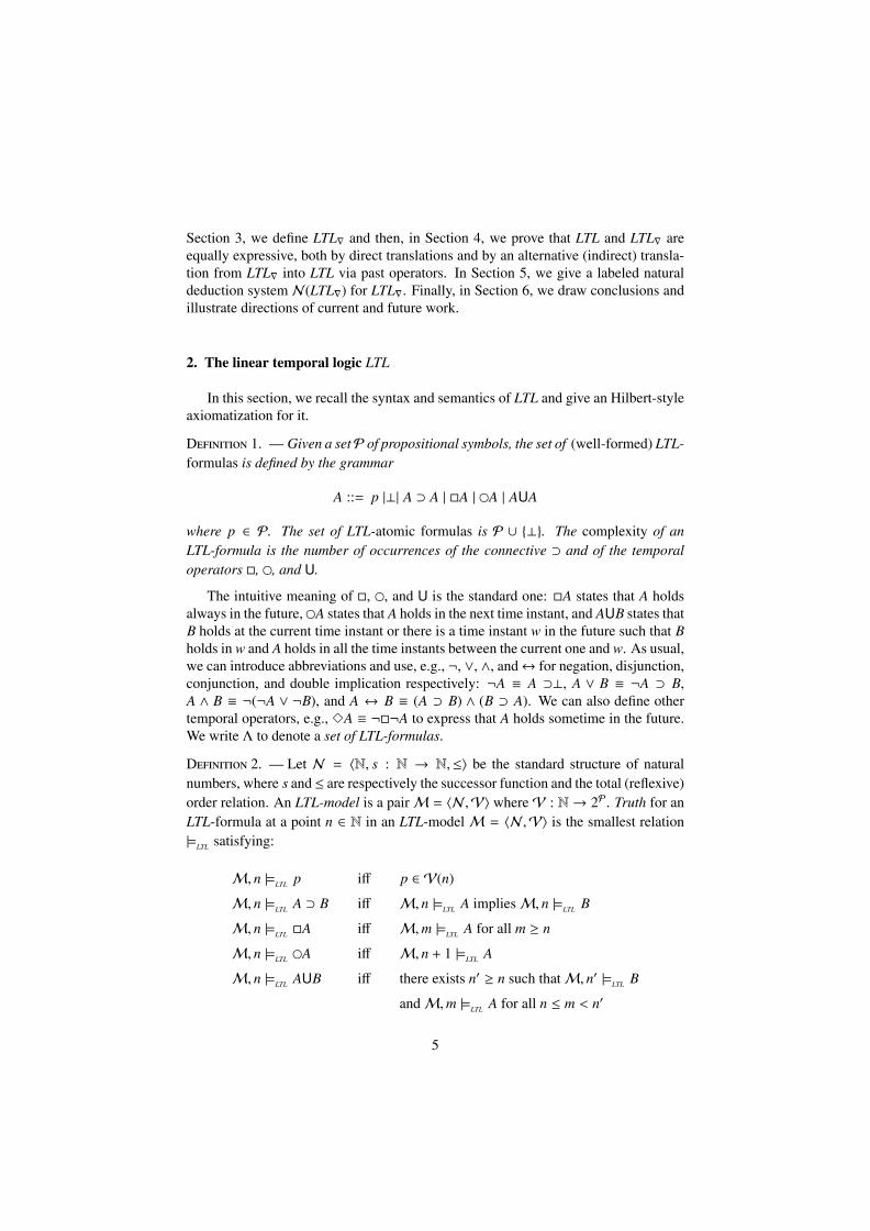
Section 3, we define LTL∇ and then, in Section 4, we prove that LTL and LTL∇ areequally expressive, both by direct translations and by an alternative (indirect) transla-tion from LTL∇ into LTL via past operators. In Section 5, we give a labeled naturaldeduction system N(LTL∇) for LTL∇. Finally, in Section 6, we draw conclusions andillustrate directions of current and future work.

2. The linear temporal logic LTL

In this section, we recall the syntax and semantics of LTL and give an Hilbert-styleaxiomatization for it.

Definition 1. — Given a setP of propositional symbols, the set of (well-formed) LTL-formulas is defined by the grammar

A ::= p |⊥| A ⊃ A | ?A | ?A | AUA

where p ∈ P. The set of LTL-atomic formulas is P ∪ {⊥}. The complexity of anLTL-formula is the number of occurrences of the connective ⊃ and of the temporaloperators ?, ?, and U.

The intuitive meaning of ?, ?, and U is the standard one: ?A states that A holdsalways in the future, ?A states that A holds in the next time instant, and AUB states thatB holds at the current time instant or there is a time instant w in the future such that Bholds in w and A holds in all the time instants between the current one and w. As usual,we can introduce abbreviations and use, e.g., ¬, ∨, ∧, and↔ for negation, disjunction,conjunction, and double implication respectively: ¬A ≡ A ⊃⊥, A ∨ B ≡ ¬A ⊃ B,A ∧ B ≡ ¬(¬A ∨ ¬B), and A ↔ B ≡ (A ⊃ B) ∧ (B ⊃ A). We can also define othertemporal operators, e.g., ?A ≡ ¬?¬A to express that A holds sometime in the future.We write Λ to denote a set of LTL-formulas.

Definition 2. — Let N = ?N, s : N → N,≤? be the standard structure of naturalnumbers, where s and ≤ are respectively the successor function and the total (reflexive)order relation. An LTL-model is a pairM = ?N ,V? whereV : N → 2P. Truth for anLTL-formula at a point n ∈ N in an LTL-modelM = ?N ,V? is the smallest relation|=LTL satisfying:

M, n |=LTL p iff p ∈ V(n)M, n |=LTL A ⊃ B iff M, n |=LTL A impliesM, n |=LTL B

M, n |=LTL ?A iff M,m |=LTL A for all m ≥ n

M, n |=LTL ?A iff M, n + 1 |=LTL A

M, n |=LTL AUB iff there exists n? ≥ n such thatM, n? |=LTL B

andM,m |=LTL A for all n ≤ m < n?

5

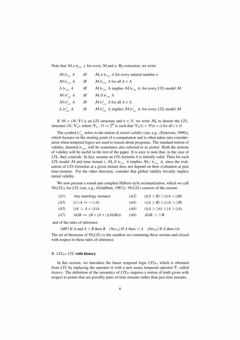
Note thatM, n ?LTL ⊥ for everyM and n. By extension, we write:

M |=LTL A iff M, n |=LTL A for every natural number n

M |=LTL Λ iff M |=LTL A for all A ∈ ΛΛ |=LTL A iff M |=LTL Λ impliesM |=LTL A, for every LTL-modelMM |=i

LTLA iff M, 0 |=LTL A

M |=iLTLΛ iff M |=i

LTLA for all A ∈ Λ

Λ |=iLTL

A iff M |=iLTLΛ impliesM |=i

LTLA, for every LTL-modelM

IfM = (N ,V) is an LTL-structure and n ∈ N, we writeMn to denote the LTL-structure (N ,Vn), whereVn : N ?→ 2P is such thatVn(i) = V(n + i) for all i ∈ N.The symbol |=i

LTLrefers to the notion of initial validity (see, e.g., (Emerson, 1990)),

which focuses on the starting point of a computation and is often taken into consider-ation when temporal logics are used to reason about programs. The standard notion ofvalidity, denoted |=LTL , will be sometimes also referred to as global. Both the notionsof validity will be useful in the rest of the paper. It is easy to note that, in the case ofLTL, they coincide. In fact, assume an LTL-formula A is initially valid. Then for eachLTL-model M and time instant i, Mi, 0 |=LTL A implies M, i |=LTL A, since the eval-uation of LTL-formulas at a given instant does not depend on their evaluation at pasttime-instants. For the other direction, consider that global validity trivially impliesinitial validity.

We now present a sound and complete Hilbert-style axiomatization, which we callH(LTL), for LTL (see, e.g., (Goldblatt, 1987)). H(LTL) consists of the axioms

(A1) Any tautology instance (A2) ?(A ⊃ B) ⊃ (?A ⊃ ?B)

(A3) (?¬A↔ ¬ ? A) (A4) ?(A ⊃ B) ⊃ (?A ⊃ ?B)

(A5) ?A ⊃ A ∧ ??A (A6) ?(A ⊃ ?A) ⊃ (A ⊃ ?A)(A7) AUB ↔ (B ∨ (A ∧ ?(AUB))) (A8) AUB ⊃ ?B

and of the rules of inference

(MP) If A and A ⊃ B then B (NecX) If A then ? A (NecG) If A then ?AThe set of theorems ofH(LTL) is the smallest set containing these axioms and closedwith respect to these rules of inference.

3. LTL∇: LTL with history

In this section, we introduce the linear temporal logic LTL∇, which is obtainedfrom LTL by replacing the operator U with a new unary temporal operator ∇, calledhistory. The definition of the semantics of LTL∇ requires a notion of truth given withrespect to points that are possibly pairs of time instants rather than just time instants.

6

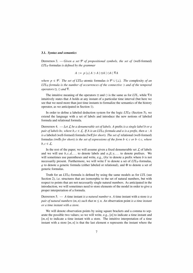
3.1. Syntax and semantics

Definition 3. — Given a set P of propositional symbols, the set of (well-formed)LTL∇-formulas is defined by the grammar

A ::= p |⊥| A ⊃ A | ?A | ?A | ∇A

where p ∈ P. The set of LTL∇-atomic formulas is P ∪ {⊥}. The complexity of anLTL∇-formula is the number of occurrences of the connective ⊃ and of the temporaloperators ?, ? and ∇.

The intuitive meaning of the operators ? and ? is the same as for LTL, while ∇Aintuitively states that A holds at any instant of a particular time interval (but here wesee that we need more than just time instants to formalize the semantics of the historyoperator, as we anticipated in Section 1).

In order to define a labeled deduction system for the logic LTL∇ (Section 5), weextend the language with a set of labels and introduce the new notions of labeledformula and relational formula.

Definition 4. — Let L be a denumerable set of labels. A prefix is a single label b or apair of labels bc, where b, c ∈ L. If A is an LTL∇-formula and α is a prefix, then α : Ais a labeled (well-formed) formula (lwff for short). The set of relational (well-formed)formulas (rwffs for short) is the set of expressions of the form b ? c or b ? c, whereb, c ∈ L.

In the rest of the paper, we will assume given a fixed denumerable set L of labelsand we will use b, c, d, . . . to denote labels and α, β, γ, . . . to denote prefixes. Wewill sometimes use parentheses and write, e.g., (b)c to denote a prefix where b is notnecessarily present. Furthermore, we will write Γ to denote a set of LTL∇-formulas,ϕ to denote a generic formula (either labeled or relational), and Φ to denote a set ofgeneric formulas.

Truth for an LTL∇-formula is defined by using the same models as for LTL (seeSection 2), i.e. structures that are isomorphic to the set of natural numbers, but withrespect to points that are not necessarily single natural numbers. As anticipated in theintroduction, we will sometimes need to store elements of the model in order to give aproper interpretation of a formula.

Definition 5. — A time instant is a natural number n. A time instant with a store is apair of natural numbers (m, n) such that m ≤ n. An observation point is a time instantor a time instant with a store.

We will denote observation points by using square brackets and a comma to sep-arate the possible two values; so we will write, e.g., [n] to indicate a time instant and[m, n] to indicate a time instant with a store. The intuitive interpretation of a timeinstant with a store [m, n] is that the last element n represents the instant where the

7

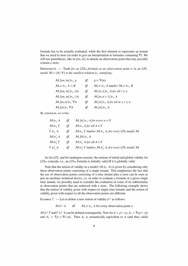
formula has to be actually evaluated, while the first element m represents an instantthat we need to store (in order to give an interpretation to formulas containing ∇). Wewill use parentheses, like in [(m, )n], to denote an observation point that may possiblycontain a store.

Definition 6. — Truth for an LTL∇-formula at an observation point σ in an LTL-modelM = (N ,V) is the smallest relation |=∇ satisfying:

M, [(m, )n] |=∇ p iff p ∈ V(n)M, σ |=∇ A ⊃ B iff M, σ |=∇ A impliesM, σ |=∇ B

M, [(m, )n] |=∇ ?A iff M, [n, i] |=∇ A for all i ≥ n

M, [(m, )n] |=∇ ?A iff M, [n, n + 1] |=∇ A

M, [m, n] |=∇ ∇A iff M, [i] |=∇ A for all m ≤ i ≤ n

M, [n] |=∇ ∇A iff M, [n] |=∇ A

By extension, we write:

M |=∇ A iff M, [n] |=∇ A for every n ∈ NM |=∇ Γ iff M |=∇ A for all A ∈ ΓΓ |=∇ A iff M |=∇ Γ impliesM |=∇ A, for every LTL-modelMM |=i

∇ A iff M, [0] |=∇ A

M |=i∇ Γ iff M |=i

∇ A for all A ∈ ΓΓ |=i

∇ A iff M |=i∇ Γ impliesM |=i

∇ A, for every LTL-modelM

As for LTL, and for analogous reasons, the notions of initial and global validity forLTL∇ coincide, i.e., an LTL∇-formula is initially valid iff it is globally valid.

Note that the notion of validity in a model (M |=∇ A) is given by considering onlythose observation points consisting of a single instant. This emphasizes the fact thatthe use of observation points consisting of a time instant plus a store can be seen asjust an auxiliary technical device, i.e. in order to evaluate a formula at a given singletime instant, we possibly need to consider the evaluation of some of its subformulasat observation points that are endowed with a store. The following example showsthat the notion of validity given with respect to single time instants and the notion ofvalidity given with respect to all the observation points are different.

Example 7. — Let us define a new notion of validity |=∇ as follows:M |=∇ A iff M, σ |=∇ A for every observation point σ

M |=∇ Γ and Γ |=∇ A can be defined consequently. Now let A = p∨¬p, A1 = ∇(p∨¬p)and A2 = ∇p ∨ ∇(¬p). Then A1 is semantically equivalent to A (and thus valid)

8

according to both the notions of validity, while A2 is semantically equivalent to A (andthus valid) only according to the notion of validity |=∇ . In fact, we have |=∇ A2 iff |=∇ por |=∇ ¬p and thus A2 is not valid according to |=∇ . ?Now we introduce the notion of interpretation of labels and prefixes and define, in

terms of it, the notion of truth for labeled and relational formulas.

Definition 8. — Given an LTL-model M and a set L of labels, an interpretationI : L → N is a function mapping each label to a natural number. Let Pref be theset of prefixes defined on L and Σ the set of observation points onM. We define theextension I+ : Pref → Σ of I as follows:

I+(n) = [I(n)];I+(n1 n2) = [I(n1),I(n2)].

Given an LTL-modelM, a set L of labels and an interpretation I on them, truth for ageneric formula ϕ in a pair (M,I) is the smallest relation |=∇ satisfying:

M,I |=∇ b ? c iff I(b) ≤ I(c)M,I |=∇ b ? c iff I(c) = I(b) + 1M,I |=∇ α : A iff M,I+(α) |=∇ A

Note thatM, σ ?∇ ⊥ andM,I ?∇ α : ⊥ for everyM, σ and I.Given a set Φ of generic formulas and a generic formula ϕ:

M,I |=∇ Φ iff M,I |=∇ ϕ for all ϕ ∈ ΦΦ |=∇ ϕ iff M,I |=∇ Φ impliesM,I |=∇ ϕ for allM and I

4. The equivalence of LTL and LTL∇

We introduced a variant of LTL based on replacing the operator U with the operator∇. In this section, we study the relation between LTL and LTL∇ and prove that the twologics are indeed equally expressive. Such a proof is given by defining a translationfrom LTL into LTL∇ and an inverse one from LTL∇ into LTL. In the case of the LTL∇ →LTL direction, we propose two solutions: the first one consists in translating LTL∇formulas directly into the language of LTL and thus shows in a constructive way therelation between the two logics; the second one uses a simpler translation into thelogic NLTL (Laroussinie et al., 2002), from which we also obtain an upper bound forthe satisfiability problem in LTL∇.

It is useful to recall some notions concerning the compared expressivity of logics(see, e.g., (Emerson, 1990; Laroussinie & Schnoebelen, 1995)). The following defini-tions are given with respect to generic logics defined over the class of LTL-structures.We use the symbol |= to denote the notion of truth in such logics.

9

Definition 9. — We say that two formulas A and B are (globally) equivalent, writtenA ≡ B, iff for all LTL-structuresM and for all n, we haveM, n |= A iffM, n |= B.We say that two formulas A and B are initially equivalent, written A ≡i B, iff for allLTL-structuresM, we haveM, 0 |= A iffM, 0 |= B.

We remark that, with a slight abuse of notation, Definition 9 can be applied toLTL∇-formulas as well: just readM, n andM, 0 asM, [n] andM, [0], respectively.Definition 10. — Let L1 and L2 be two logics defined over LTL-structures. We saythat L2 is (globally) at least as expressive as L1, written L1 ≤ L2, iff for any formula A1in the language of L1 there is a formula A2 in the language of L2 such that A1 ≡ A2.We say that L2 is initially at least as expressive as L1, written L1 ≤i L2, iff for anyformula A1 in the language of L1 there is a formula A2 in the language of L2 such thatA1 ≡i A2. We say that L1 and L2 are (globally) equally expressive, written L1 ≡ L2, iffL1 ≤ L2 and L2 ≤ L1. Finally, we say that L1 and L2 are initially equally expressive,written L1 ≡i L2, iff L1 ≤i L2 and L2 ≤i L1.

4.1. A translation from LTL into LTL∇

We proceed as follows: first, we define a translation (·)∗ from LTL into LTL∇. Then,in Lemma 12, we show that if an LTL∇-formula corresponds to the translation of someLTL-formula, then it can be interpreted “locally”, i.e., its truth value with respect toan observation point depends only on the last element and not on the store. Finally,in Lemma 14 and Theorem 16, we use this result to prove that the translation fullypreserves the semantics of the formulas.

Definition 11. — We define the translation (·)∗ from the language of LTL into thelanguage of LTL∇ inductively as follows:

(p)∗ = p , for p atomic (⊥)∗ = ⊥(A ⊃ B)∗ = (A)∗ ⊃ (B)∗ (?A)∗ = ? (A)∗

(?A)∗ = ? (A)∗ (AUB)∗ = (B)∗ ∨ (? (?(B)∗ ∧ ∇(A)∗ ))

We extend (·)∗ to sets of formulas in the obvious way: Λ∗ = {(A)∗ | A ∈ Λ}.In the following, when not confusing, we will sometimes omit parentheses and

write, e.g., A∗ instead of (A)∗.

Lemma 12. — LetM be an LTL-model, [(m, )n] an observation point and A an LTL-formula. ThenM, [(m, )n] |=∇ A∗ iffM, [(i, )n] |=∇ A∗ for every natural number i.

Proof. — By induction on the complexity of A. The base case is when A = p orA =⊥ and is trivial. There is one inductive step case for each connective and temporaloperator.

10

A = B ⊃ C. Then the translation of A is A∗ = B∗ ⊃ C∗. By Definition 6, we ob-tainM, [(m, )n] |=∇ B∗ ⊃ C∗ iffM, [(m, )n] |=∇ B∗ implies M, [(m, )n] |=∇ C∗.By the induction hypothesis, we see that this holds iff M, [(i, )n] |=∇ B∗ im-pliesM, [(i, )n] |=∇ C∗ for every natural number i and thus, by Definition 6, iffM, [(i, )n] |=∇ B∗ ⊃ C∗ for every natural number i.

A = ?B. Then A∗ = ?B∗. In this case, we do not even use the induction hypothesis.Just observe that, by Definition 6, the possible value of m is not involved in theevaluation of the formula. Thus we have M, [(m, )n] |=∇ ?B∗ iff for all l s.t.l ≥ n, M, [n, l] |=∇ B∗ iffM, [(i, )n] |=∇ ?B∗ for every natural number i.

A = ?B. This case is very similar to the previous one and we omit it.

A = BUC. Then A∗ = C∗ ∨ (?(?C∗ ∧∇B∗)). By Definition 6, we haveM, [(m, )n] |=∇A∗ iff (M, [(m, )n] |=∇ C∗ orM, [(m, )n] |=∇ ?(?C∗∧∇B∗)) iff (M, [(m, )n] |=∇ C∗

or there exists l ≥ n s.t. (M, [n, l] |=∇ ?C∗∧∇B∗)) iff (M, [(m, )n] |=∇ C∗ or thereexists l ≥ n s.t. (M, [n, l] |=∇ ?C∗ andM, [n, l] |=∇ ∇B∗)) iff (M, [(m, )n] |=∇ C∗

or there exists l ≥ n s.t. (M, [l, l + 1] |=∇ C∗ and for all l?, n ≤ l? ≤ l impliesM, [l?] |=∇ B∗)) iff (by the induction hypothesis) for every natural number i,we have (M, [(i, )n] |=∇ C∗ or there exists l ≥ n s.t. (M, [l, l + 1] |=∇ C∗ andfor all l?, n ≤ l? ≤ l implies M, [l?] |=∇ B∗)) iff (by Definition 6) M, [(i, )n]|=∇ C∗ ∨ (?(?C∗ ∧ ∇B∗)) for every natural number i.

?

Corollary 13. — LetM be an LTL-model, [(m, )n] an observation point, and A anLTL-formula. ThenM, [(m, )n] |=∇ A∗ iffM, [n] |=∇ A∗.

Proof. — Immediate, by Lemma 12. ?

Lemma 14. — LetM be an LTL-model, n a natural number, and A an LTL-formula.ThenM, n |=LTL A iffM, [n] |=∇ A∗.

Proof. — By induction on the complexity of A. The base case is when A = p orA =⊥ and is trivial. There is an inductive step case for each connective and temporaloperator.

A = B ⊃ C. Then A∗ = B∗ ⊃ C∗. We have M, n |=LTL B ⊃ C iff (by Definition 2)M, n |=LTL B impliesM, n |=LTL C iff (by the induction hypothesis)M, [n] |=∇ B∗

impliesM, [n] |=∇ C∗ iff (by Definition 6)M, [n] |=∇ B∗ ⊃ C∗.

A = ?B. Then A∗ = ?B∗. We haveM, n |=LTL ?B iff (by Definition 2) for all m ≥ n,M,m |=LTL B iff (by the induction hypothesis) for allm ≥ n,M, [m] |=∇ B∗ iff (byLemma 12) for all m ≥ n,M, [n,m] |=∇ B∗ iff (by Definition 6)M, [n] |=∇ ?B∗.

11


A = BUC. Then A∗ = C∗ ∨ (?(?C∗ ∧ ∇B∗)). We haveM, n |=LTL A iff (by Definition2) there exists m ≥ n s.t. M,m |=LTL C and for all n?, n ≤ n? < m impliesM, n? |=LTL B iff M, n |=LTL C or ( there exists m > n s.t. M,m |=LTL C andfor all n?, n ≤ n? < m impliesM, n? |=LTL B) iff (by the induction hypothesis)M, [n] |=∇ C∗ or ( there existsm > n s.t.M, [m] |=∇ C∗ and for all n?, n ≤ n? < mimpliesM, [n?] |=∇ B∗) iff (by simple rewriting)M, [n] |=∇ C∗ or ( there existsl ≥ n s.t. M, [l + 1] |=∇ C∗ and for all n?, n ≤ n? ≤ l impliesM, [n?] |=∇ B∗) iff(by Lemma 12)M, [n] |=∇ C∗ or ( there exists l ≥ n s.t. M, [l, l + 1] |=∇ C∗ andfor all n?, n ≤ n? ≤ l impliesM, [n?] |=∇ B∗) iff (by Definition 6)M, [n] |=∇ C∗

or ( there exists l ≥ n s.t.M, [n, l] |=∇ ?C∗∧∇B∗) iff (by Definition 6)M, [n] |=∇C∗ ∨ ?(?C∗ ∧ ∇B∗).

?

Corollary 15. — LTL∇ is at least as expressive as LTL.


Theorem 16. — Let Λ be a set of LTL-formulas and A an LTL-formula. Then Λ |=LTL

A iff Λ∗ |=∇ A∗.

Proof. — By Definition 2, Λ |=LTL A iff for every LTL-modelM, (M |=LTL Λ impliesM |=LTL A) iff for all M, (for all B in Λ, for all n, M, n |=LTL B implies for all n,M, n |=LTL A) iff (by Lemma 14) for allM, (for all B in Λ, for all n, M, [n] |=∇ B∗

implies for all n,M, [n] |=∇ A∗) iff (by Lemma 12) for allM, (for all B in Λ, for allσ,M, σ |=∇ B∗ implies for all σ,M, σ |=∇ A∗) iff (by Definition 6) for allM, (for allB in Λ,M |=∇ B∗ impliesM |=∇ A∗) iff for allM, (M |=∇ Λ∗ impliesM |=∇ A∗) iffΛ∗ |=∇ A∗. ?

4.2. A translation from LTL∇ into LTL

Defining a translation from LTL∇ into LTL is a much trickier task. Typically, trans-lations are defined recursively: we have a case for each possible main connective of aformula and in all of these cases the translation is given in terms of the translation ofits subformulas. A similar recursive definition, when translating LTL∇ into LTL, needsto take into account some subtleties.

Clearly, the interesting case in the translation is the one concerning formulas thatcontain the operator ∇. Furthermore, by observing the semantics of LTL∇ (Section3.1), one can conclude (we will prove it formally below) that: (i) when ∇ is in thescope of another ∇, it can be ignored, e.g., ∇∇A ≡ ∇A; and (ii) when ∇ is not inthe scope of any temporal operator, it does not alter the evaluation of the formula,

12

e.g., ∇A ≡ A. Thus the crucial case is when ∇ is in the scope of a different temporaloperator: ? or ? (or ?, if we consider it explicitly).4

We have seen that, in order to define the semantics of LTL∇, we need to considerpairs of instants, such that one instant (the second one) is where the evaluation actuallytakes place and the other (the first one) is a kind of pointer to some other instant in theflow of time. By reading Definition 6, we deduce that this pointer is in fact only neededto evaluate a restricted class of LTL∇-formulas. Namely, we can divide LTL∇-formulasinto two classes:

– the class of history-independent formulas, whose evaluation only depends onthe last element of an observation point;– the class of history-dependent formulas, whose evaluation depends also on the

first element (the pointer, or the store) of an observation point.

By observing the semantics of LTL∇, one can easily check that the history-dependentformulas are indeed those where the ∇ operator is not in the scope of any different tem-poral operator. As an example, we have that the formula ?∇p is history-independent,but its subformula ∇p is history-dependent.

All these arguments lead to the intuition that the translation of a formula of theform ?A or ?A should depend on the nature of the subformula A. If the formula A ishistory-independent, then we can give for it a simple recursive definition, otherwisewe need to consider a translation that mimics in some way the action of the pointer. Inthis second case, considering a (disjunctive) normal form for LTL∇-formulas will helpdefine the translation.

In the following paragraphs, we formalize all these ideas and prove that the result-ing translation preserves the truth values of formulas.

4.2.1. An alternative grammar for LTL∇-formulas

Here we give an alternative grammar for LTL∇-formulas with the intent of mak-ing the separation between history-independent and history-dependent formulas clear.Since it allows for a simpler presentation of the translation, we give the grammar byconsidering ¬, ∧, ∨, ? and ? as primitive connectives. ⊥, ⊃ and ? can be defined interms of these in the standard way.

Definition 17. — Given a set P of propositional symbols, the set of (well-formed)LTL∇-formulas is defined by the grammar

A ::= γ | δ

γ ::= p | γ ∧ γ | γ ∨ γ | ¬γ | ?γ | ?γ | ?δ | ?δ

4. Indeed, even the case of a ∇ in the scope of an ? could be simplified by splitting it into twoelementary subcases, e.g., ?∇A ≡ A ∧ ?A. Thus, in conclusion, the case of a ∇ in the scope ofa ? (or of a ?) is the one that really matters.

13

δ ::= ∇A | ¬δ | A ∧ δ | δ ∧ A | A ∨ δ | δ ∨ A

where p ∈ P. We call (LTL∇) history-independent formulas the formulas belonging tothe syntactic category γ and (LTL∇) history-dependent formulas the formulas belong-ing to the syntactic category δ.

Lemma 18. — The language of LTL∇-formulas and the language of LTL∇-formulascoincide.

Proof. — We have to show that: (i) each LTL∇-formula is also an LTL∇-formula; and,vice versa, (ii) each LTL∇-formula is also an LTL∇-formula. The proof follows easilyby structural induction in both directions. ?

Because of Lemma 18, from now on, for simplicity, we will speak of LTL∇-formulas also when referring to formulas originating from the grammar in Definition17.

4.2.2. A normal form for LTL∇-formulas

Considering a normal form for LTL∇-formulas will help define the translation. Thefirst step consists in eliminating some redundant occurrences of ∇: intuitively, thoseoccurrences falling directly into the scope of another ∇. Some proper terminologyneeds to be introduced.

Definition 19. — Let A be an LTL∇-formula of the form ?A? (or ?A?, or ∇A?) and letus denote with h that occurrence of ? (or of ?, or of ∇, respectively). Then for eachoccurrence h? of a temporal operator in A?, we say that h? is in the temporal scope ofh.

Given an LTL∇-formula A, we say that an occurrence h of a temporal operator inA is in the strict temporal scope of an occurrence h? of a temporal operator in A iff: (i)h is in the temporal scope of h?; and (ii) for each occurrence h?? of a temporal operatorin A, either h is not in the temporal scope of h?? or h? is in the temporal scope of h??.

We also say that an occurrence of a ∇ in an LTL∇-formula A is redundant if it is inthe strict temporal scope of another occurrence of ∇.

Example 20. — Consider the formula ??(∇p ∧ q). The occurrence of ∇ (not redun-dant) is in the temporal scope of the occurrences of both ? and ?, and in the stricttemporal scope of the occurrence of ?.

In ?∇(∇p ∧ q), the second occurrence of ∇ is in the strict temporal scope of thefirst one and thus it is redundant. ?Lemma 21. — Let A be an LTL∇-formula and B be the formula obtained by removingall the redundant occurrences of the operator ∇. Then A and B are semanticallyequivalent.

14

Proof. — By observing the semantics given in Definition 6, we can first note that theevaluation of a formula of the form ∇A at an observation point that is a single timeinstant (without a store) corresponds to the evaluation of the formula A at the samepoint. Now observe that if an occurrence of ∇ is in the strict temporal scope of anotheroccurrence of ∇, then its evaluation is performed in an observation point that consistsof a single time instant. This implies that the removal of the inner-most ∇ does notalter the evaluation. ?

In order to get a normal form, we require, in addition to the removal of redundantoccurrences of ∇, that each history-dependent subformula is written in a particularform. The following definition, lemma and example clarify and formalize the form ofnormal LTL∇-formulas.

Definition 22. — Given an LTL∇-formula A, we say that δ is a history-dependentsubformula of A iff δ is a subformula of A and is a history-dependent formula.

Definition 23. — A δ-disjunctive normal form clause (δ-DNF clause, for short) isan LTL∇-formula consisting in a conjunction of formulas that are either (i) history-independent formulas or (ii) history-dependent formulas of the form ∇γ or ¬∇γ forsome history-independent formula γ.

An LTL∇-formula A is in δ-disjunctive normal form (in δ-DNF, for short) if: (i) Adoes not contain any redundant occurrence of a ∇; and (ii) for each history-dependentsubformula δ of A, δ is the disjunction of δ-DNF clauses.

Lemma 24. — For every LTL∇-formula A, there exists an equivalent LTL∇-formulaA? such that A? is in δ-DNF.

Proof. — We prove the statement by describing a procedure for transforming a genericLTL∇-formula A into an LTL∇-formula A? that is in δ-DNF.

First, we remove all the occurrences of the operator ∇ that are in the strict temporalscope of another occurrence of ∇. Lemma 21 ensures that after this process we havean equivalent formula.

Then we observe that, once we have removed the redundant occurrences of ∇,given a subformula δ of A, the process of reducing δ to a disjunction of conjunctions(as required by Definition 23) is equivalent to the process of reducing a formula ofpropositional classical logic into the standard disjunctive normal form (see, e.g., (vanDalen, 1980)), where we consider as literals: (i) history-independent formulas; and(ii) history-dependent formulas of the form ∇γ or ¬∇γ for some history-independentformula γ.

Thus, in order to transform an LTL∇-formula without redundant occurrences of ∇into a formula in δ-DNF, we can iteratively apply the following procedure, correspond-

15

ing (mutatis mutandis) to the one defined for producing a disjunctive normal form, toeach history dependent subformula of A, starting from the inner-most one:

1) we iteratively apply the so-called double negation and De Morgan’s laws (see(van Dalen, 1980)) in order to get a formula where we have only single negations andthey occur just before the atoms (where we consider history-independent formulas orhistory-dependent formulas of the form ∇γ as atoms);2) we iteratively apply distributivity laws in order to get a disjunction of conjunc-

tions.

The proof that the resulting formula is equivalent to the original one is a trivial adapta-tion (again, mutatis mutandis) of the proof (van Dalen, 1980) given for transformationsinto the standard disjunctive normal form in the case of propositional classical logic.

?

Example 25. — Let us consider the LTL∇-formula A = p1 ∧ ¬?(?∇p2 ∧ ¬(p3 ∨∇?∇(p4 ∨ p5))). First, we eliminate the redundant occurrences of ∇ and obtain A1 =p1 ∧ ¬?(?∇p2 ∧ ¬(p3 ∨ ∇?(p4 ∨ p5))). Then we consider the history-dependentsubformulas of A?. The inner-most ones are ∇p2 and ∇?(p4 ∨ p5), which are alreadyin normal form. Then we consider ¬(p3 ∧ ∇?(p4 ∨ p5)), to which we can apply DeMorgan laws and obtain A2 = p1 ∧ ¬?(?∇p2 ∧ (¬p3 ∨ ¬∇?(p4 ∨ p5))). Finally, byapplying distributivity laws to ?∇p2 ∧ (¬p3 ∨ ¬∇?(p4 ∨ p5)), we get A3 = p1 ∧¬?((?∇p2 ∧ ¬p3) ∨ (?∇p2 ∧ ¬∇?(p4 ∨ p5))), which is in δ-DNF. ?

4.2.3. The translation (·)#

Since Lemma 24 holds, we can, with no loss of generality, restrict the attention toLTL∇-formulas that are in δ-DNF and define the translation (·)# from LTL∇ into LTLin terms of this class of formulas. We also remark, as it will be useful in defining thetranslation and in proving some statements, that given an LTL∇-formula A in δ-DNF,every subformula of A of the form ∇B is such that B is history-independent. Such afact is a direct consequence of the absence of redundant occurrences of ∇ in a formulain δ-DNF form.

Definition 26. — We define the translation (·)# from the language of LTL∇-formulasin δ-DNF form into the language of LTL inductively as follows. (Note that, as in Defi-nition 17, we use A, γ and δ (possibly subscripted) to denote a generic LTL∇-formula,a history-independent formula, and a history-dependent formula, respectively.)

16

(p)# = p , for p atomic (A1 ∧ A2)# = (A1)# ∧ (A2)#(A1 ∨ A2)# = (A1)# ∨ (A2)# (¬A)# = ¬ (A)#(?γ)# = ? (γ)# (?γ)# = ? (γ)#(∇A)# = (A)# (?δ)# = (C1)? ∨ . . . ∨ (Cn)?

(?δ)# = (C1)? ∨ . . . ∨ (Cn)?

where δ = C1 ∨ . . . ∨ Cn for C1, . . . ,Cn δ-DNF clauses and (·)? and (·)? are auxiliarytranslations defined from the set of δ-DNF clauses into the set of LTL-formulas asspecified below.

Let C be a δ-DNF clause. Since the order of the elements of a conjunction doesnot alter its evaluation, we can always write it as:

C ≡ (γ1 ∧ . . . ∧ γn) ∧ (∇γ?1 ∧ . . . ∧ ∇γ?m) ∧ (¬∇γ??1 ∧ . . . ∧ ¬∇γ??l ) .Furthermore, let γ = γ1 ∧ . . . ∧ γn and γ∇ = γ

?1 ∧ . . . ∧ γ?m. For greater convenience,

we also define another version of the operator until on LTL-formulas:

AUB ≡ (A ∧ B) ∨ ((A ∧ ?A)U B) ,

where the idea is that now A holds also in the instant where B holds.

Then we define (·)? and (·)? as follows:

(C)? = ?(γ)# ∧ (γ∇ )# ∧ ?(γ∇ )# ∧ (¬(γ??1 )# ∨ ¬ ? (γ??1 )#) ∧ . . . ∧ (¬(γ??l )# ∨ ¬ ? (γ??l )#)

(C)? = ?(γ)# ∧ ((γ∇ )# U (γ)#) ∧ ¬((γ??1 )# U (γ)#) ∧ . . . ∧ ¬((γ??l )# U (γ)#)

We extend (·)# to sets of formulas in the obvious way: Γ# = {(A)# | A ∈ Γ}.In the following, when not confusing, we will sometimes omit parentheses and

write, e.g., A#, C? and C? instead of (A)#, (C)? and (C)?, respectively.

4.2.4. Properties of the translation

We show that the translation (·)# preserves the truth values of formulas. In theproofs of the following lemmas, γ, γ1, γ2, . . . will denote history-independent formu-las, δ, δ1, δ2, . . . history-dependent formulas and A, A1, A2, . . . generic LTL∇-formulas.

Lemma 27. — LetM be an LTL-model, m, n ∈ N, and γ a history-independent for-mula. ThenM, [(m, )n] |=∇ γ iff M, [(m?, )n] |=∇ γ , for all m? ∈ N.Proof. — The proof is by induction on the complexity of the formula γ. The base caseis when γ = p and is trivial. There is one inductive step case for each other formationcase coming from the recursive definition of the grammar in Definition 17.

17

γ = γ1 ∧ γ2. By Definition 6, we haveM, [(m, )n] |=∇ γ1 ∧ γ2 iff M, [(m, )n] |=∇ γ1and M, [(m, )n] |=∇ γ2. By the induction hypothesis, this holds iff M, [(m?, )n]|=∇ γ1 and M, [(m?, )n] |=∇ γ2 for every natural number m?, and thus, by Defi-nition 6, iffM, [(m?, )n] |=∇ γ1 ∧ γ2 for every natural number m?.

γ = γ1 ∨ γ2. By Definition 6, we haveM, [(m, )n] |=∇ γ1 ∨ γ2 iff M, [(m, )n] |=∇ γ1or M, [(m, )n] |=∇ γ2. By the induction hypothesis, this holds iff M, [(m?, )n] |=∇γ1 or M, [(m?, )n] |=∇ γ2 for every natural number m?, and thus, by Definition6, iffM, [(m?, )n] |=∇ γ1 ∨ γ2 for every natural number m?.

γ = ¬γ1. By Definition 6, we haveM, [(m, )n] |=∇ ¬γ1 iff M, [(m, )n] ?∇ γ1. By theinduction hypothesis, this holds iff M, [(m?, )n] ?∇ γ1 for every natural numberm?, and thus, by Definition 6, iffM, [(m?, )n] |=∇ ¬γ1 for every natural numberm?.

γ = ?A. We treat at the same time the cases where A is a history-independent and A isa history-dependent formula, and we do not need to use the induction hypothe-sis. By Definition 6, we haveM, [(m, )n] |=∇ ?A iff M, [n, n+1] |=∇ A . Again,by Definition 6, this holds iffM, [(m?, )n] |=∇ ?A for every natural number m?.

γ = ?A. Again, we do not use the induction hypothesis. By Definition 6, we haveM, [(m, )n] |=∇ ?A iff there exists i ≥ n such that M, [n, i] |=∇ A . ByDefinition 6, this holds iffM, [(m?, )n] |=∇ ?A for every natural number m?.

?

Lemma 28. — Let M be an LTL-model, n ∈ N and A an LTL∇-formula. ThenM, [n] |=∇ A iff M, n |=LTL A#.

Proof. — The proof is by structural induction on A.

A = p. By Definition 26, A# = p. We have M, [n] |=∇ p iff (by Definition 6) p ∈V(n) iff (by Definition 2) M, n |=LTL p.

A = A1 ∧ A2. By Definition 26, A# = A#1 ∧ A#2. We haveM, [n] |=∇ A1 ∧ A2 iff (byDefinition 6) M, [n] |=∇ A1 andM, [n] |=∇ A2 iff (by the induction hypothesis)M, n |=LTL A#1 andM, n |=LTL A#2 iff (by Definition 2) M, n |=LTL A#1 ∧ A#2.

A = A1 ∨ A2. By Definition 26, A# = A#1 ∨ A#2. We haveM, [n] |=∇ A1 ∨ A2 iff (byDefinition 6) M, [n] |=∇ A1 orM, [n] |=∇ A2 iff (by the induction hypothesis)M, n |=LTL A#1 orM, n |=LTL A#2 iff (by Definition 2) M, n |=LTL A#1 ∨ A#2.

A = ¬A1. By Definition 26, A# = ¬(A#1). We haveM, [n] |=∇ ¬A1 iff (by Definition 6)M, [n] ?∇ A1 iff (by the induction hypothesis) M, n ?LTL A#1 iff (by Definition2) M, n |=LTL ¬(A#1).

18

A = ?γ. By Definition 26, A# = ?(γ#). We haveM, [n] |=∇ ?γ iff (by Definition 6)M, [n, n + 1] |=∇ γ iff (by Lemma 28) M, [n + 1] |=∇ γ iff (by the inductionhypothesis) M, n + 1 |=LTL γ

# iff (by Definition 2) M, n |=LTL ?(γ#).

A = ?γ. By Definition 26, A# = ?(γ#). We haveM, [n] |=∇ ?γ iff (by Definition 6)there exists i ≥ n such thatM, [n, i] |=∇ γ iff (by Lemma 28) there exists i ≥ nsuch thatM, [i] |=∇ γ iff (by the induction hypothesis) there exists i ≥ n suchthatM, i |=LTL γ

# iff (by Definition 2) M, n |=LTL ?(γ#).A = ?δ. By Definition 26, A# = (C1)? ∨ . . . ∨ (Cm)?, where δ = C1 ∨ . . . ∨ Cm and

C1, . . . ,Cm are δ-DNF clauses. For 1 ≤ i ≤ m, we can write Ci = γ1 ∧ . . . ∧γki∧ (∇γ?

1∧ . . .∧∇γ?

ji)∧ (¬∇γ??

1∧ . . .∧¬∇γ??

li). For convenience, we also define

γ∧i = γ1 ∧ . . . ∧ γkiand γ∇i

= γ?1∧ . . . ∧ γ?

ji.

First, we prove that, for 1 ≤ i ≤ m, M, [n, n + 1] |=∇ Ci iff M, n |=LTL (Ci)?.We have: M, [n, n + 1] |=∇ Ci iff (by Definition 6) M, [n, n + 1] |=∇ γh forall h s.t. 1 ≤ h ≤ ki and M, [n, n + 1] |=∇ ∇γ?h for all h s.t. 1 ≤ h ≤ ji andM, [n, n+ 1] |=∇ ¬∇γ??h for all h s.t. 1 ≤ h ≤ li iff (by Lemma 27) M, [n+ 1] |=∇γh for all h s.t. 1 ≤ h ≤ ki and M, [n, n + 1] |=∇ ∇γ?h for all h s.t. 1 ≤ h ≤ jiand M, [n, n + 1] |=∇ ¬∇γ??h for all h s.t. 1 ≤ h ≤ li iff (by Definition 6)M, [n+1] |=∇ γh for all h s.t. 1 ≤ h ≤ ki and (M, [n] |=∇ γ?h andM, [n+1] |=∇ γ?h )for all h s.t. 1 ≤ h ≤ ji and (M, [n] ?∇ γ??h orM, [n + 1] ?∇ γ??h ) for all h s.t.1 ≤ h ≤ li iff (by the induction hypothesis) M, n + 1 |=LTL γ

#hfor all h s.t.

1 ≤ h ≤ ki and (M, n |=LTL γ?#handM, n + 1 |=LTL γ

?#h) for all h s.t. 1 ≤ h ≤ ji

and (M, n ?LTL γ??#hor M, n + 1 ?LTL γ

??#h) for all h s.t. 1 ≤ h ≤ li iff (by

Definition 2) M, n + 1 |=LTL γ#1∧ . . . ∧ γ#

kiand (M, n |=LTL γ

?#1∧ . . . ∧ γ?#

jiand

M, n + 1 |=LTL γ?#1∧ . . . ∧ γ?#

ji) and (M, n ?LTL γ

??#horM, n ?LTL ?(γ

??#h)) for all h

s.t. 1 ≤ h ≤ li iff (by Definition 26) M, n + 1 |=LTL (γ∧i )# and (M, n |=LTL (γ∇i

)#

andM, n + 1 |=LTL (γ∇i)#) and (M, n ?LTL γ

??#horM, n ?LTL ?(γ

??#h)) for all h s.t.

1 ≤ h ≤ li iff (by Definition 2) M, n |=LTL ?(γ∧i )# and M, n |=LTL (γ∇i

)# andM, n |=LTL ?((γ∇i

)#) and (M, n |=LTL ¬(γ??#h) orM, n |=LTL ¬ ? (γ??#h

)) for all h s.t.1 ≤ h ≤ li iff M, n |=LTL (Ci)? .

Now we use this result to prove the main statement. Namely we have:M, [n] |=∇?δ iff (by Definition 6) M, [n, n+1] |=∇ δ iff (by Definition 6) M, [n, n+1] |=∇C1 or . . . orM, [n, n + 1] |=∇ Cm iff (by the result above) M, n |=LTL (C1)

? or. . . orM, n |=LTL (Cm)? iff (by Definition 2) M, n |=LTL (C1)

? ∨ . . . ∨ (Cm)? iffM, n |=LTL A# .

A = ?δ. By Definition 26, A# = (C1)? ∨ . . . ∨ (Cm)?, where δ = C1 ∨ . . . ∨ Cm andC1, . . . ,Cm are δ-DNF clauses. For 1 ≤ i ≤ m, we can write Ci = γ1 ∧ . . .∧ γki

∧(∇γ?

1∧ . . . ∧ ∇γ?

ji) ∧ (¬∇γ??

1∧ . . . ∧ ¬∇γ??

li). For convenience, we also define, as

above, γ∧i = γ1 ∧ . . . ∧ γkiand γ∇i

= γ?1∧ . . . ∧ γ?

ji.

19

First, we prove that, for 1 ≤ i ≤ m, there exists n? ≥ n such that M, [n, n?] |=∇ Ci

iffM, n |=LTL (Ci)?. In fact, we have: there exists n? ≥ n such thatM, [n, n?] |=∇Ci iff (by Definition 6) there exists n? ≥ n such thatM, [n, n?] |=∇ γh for all hs.t. 1 ≤ h ≤ ki and M, [n, n?] |=∇ ∇γ?h for all h s.t. 1 ≤ h ≤ ji and M, [n, n?] |=∇¬∇γ??

hfor all h s.t. 1 ≤ h ≤ li iff (by Lemma 27) there exists n? ≥ n such that

M, [n?] |=∇ γh for all h s.t. 1 ≤ h ≤ ki and M, [n, n?] |=∇ ∇γ?h for all h s.t.1 ≤ h ≤ ji and M, [n, n?] |=∇ ¬∇γ??h for all h s.t. 1 ≤ h ≤ li iff (by Definition6) there exists n? ≥ n such that M, [n?] |=∇ γh for all h s.t. 1 ≤ h ≤ ki and(M, [n??] |=∇ γ?h for all n?? s.t. n ≤ n?? ≤ n? and for all h s.t. 1 ≤ h ≤ ji) and (forall h s.t. 1 ≤ h ≤ li there exists n?? s.t. n ≤ n?? ≤ n? for whichM, [n??] ?∇ γ??h )iff (by the induction hypothesis) there exists n? ≥ n such thatM, n? |=LTL γ

#hfor

all h s.t. 1 ≤ h ≤ ki and (M, n?? |=LTL γ?#hfor all n?? s.t. n ≤ n?? ≤ n? and

for all h s.t. 1 ≤ h ≤ ji) and (for all h s.t. 1 ≤ h ≤ li there exists n?? s.t.n ≤ n?? ≤ n? for whichM, n?? ?LTL γ

??#h) iff (by Definition 2) there exists n? ≥ n

such that (M, n? |=LTL γ#1∧ . . . ∧ γ#

ki) and (M, n?? |=LTL γ

?#1∧ . . . ∧ γ?#

jifor all n??

s.t. n ≤ n?? ≤ n?) and (for all h s.t. 1 ≤ h ≤ li there exists n?? s.t. n ≤ n?? ≤ n?

for which M, n?? ?LTL γ??#h) iff (by Definition 26) there exists n? ≥ n such that

(M, n? |=LTL (γ∧i )#) and (M, n?? |=LTL (γ∇i

)# for all n?? s.t. n ≤ n?? ≤ n?) and (forall h s.t. 1 ≤ h ≤ li there exists n?? s.t. n ≤ n?? ≤ n? for whichM, n?? ?LTL γ

??#h) iff

(by Definition 2) M, n |=LTL ?(γ∧i )# andM, n |=LTL ((γ∇i)#U(γ∧i )

#) and for all hs.t. 1 ≤ h ≤ li , M, n |=LTL ¬((γ??h )#U(γ∧i )#) iff M, n |=LTL (Ci)? .Now we use this result to prove the main statement. Namely we have:M, [n] |=∇?δ iff (by Definition 6) there exists n? ≥ n such thatM, [n, n?] |=∇ δ iff (by Defi-nition 6) there exists n? ≥ n such thatM, [n, n?] |=∇ C1 or . . . orM, [n, n?] |=∇ Cm

iff (by the result above) M, n |=LTL (C1)? or . . . orM, n |=LTL (Cm)? iff (by Def-

inition 2) M, n |=LTL (C1)? ∨ . . . ∨ (Cm)? iff M, n |=LTL A# .

?

Corollary 29. — LTL is at least as expressive as LTL∇.


Proposition 30. — Let M be an LTL-model and γ a history-independent formula.ThenM |=∇ γ iff M |=LTL γ

#.

Proof. — By Definition 6,M |=∇ γ iffM, [n] |=∇ γ for all n ∈ N iff (by Lemma 28)M, n |=LTL γ

# for all n ∈ N iff (by Definition 2)M |=LTL γ#. ?

Proposition 31. — LetM be an LTL-model and δ a history-dependent formula. ThenM |=∇ δ iff M |=LTL δ

#.

Proof. — By Definition 6,M |=∇ δ iffM, [n] |=∇ δ for all n ∈ N iff (by Lemma 28)M, n |=LTL δ

# for all n ∈ N iff (by Definition 2)M |=LTL δ#. ?

20

Theorem 32. — Let Γ be a set of LTL∇-formulas and A an LTL∇-formula. ThenΓ |=∇ A iff Γ# |=LTL A#.

Proof. — We have Γ |=∇ A iff (by Definition 6) for every LTL-modelM, (M |=∇ ΓimpliesM |=∇ A) iff (by Definition 6) for every LTL-modelM, ((M |=∇ B for everyLTL∇-formula B ∈ Γ) implies M |=∇ A) iff (by Propositions 30 and 31) for everyLTL-modelM, ((M |=LTL B# for every LTL∇-formula B ∈ Γ) implies M |=LTL A#) iff(by Definition 2) Γ# |=LTL A#. ?

Theorem 33. — LTL and LTL∇ are equally expressive.

Proof. — It follows trivially from Corollaries 15 and 29. ?

4.3. A translation from LTL∇ into NLTL

In this section, we propose an alternative (indirect) translation from LTL∇ intoLTL, which is obtained by exploiting some known results on temporal logics with pastoperators.

4.3.1. NLTL: syntax and semantics

We introduce the syntax and the semantics of the logic NLTL (Laroussinie et al.,2002). The language is obtained by enriching the language of PLTL, i.e. LTL withpast operators, with a further unary operator now N, which intuitively allows one to“forget” the past.

Definition 34. — Given a set P of propositional symbols, the set of (well-formed)NLTL-formulas is defined by the grammar

A ::= p |⊥| A ⊃ A | ?A | ?A | UA | ?A | ?A | SA | NA

where p ∈ P. The set of NLTL-atomic formulas is P ∪ {⊥}. The complexity of anNLTL-formula is the number of occurrences of the connective ⊃ and of the temporaloperators ?, ?, U, ?, ?, S and N.

In the following, we will write Θ to denote a set of NLTL-formulas.

21

Definition 35. — Truth for an NLTL-formula at an observation point σ in an LTL-modelM = (N ,V) is the smallest relation |=N satisfying :

M, n |=N p iff p ∈ V(n)M, n |=N A ⊃ B iff M, n |=N A implies M, n |=N B

M, n |=N ?A iff M, i |=N A for all i ≥ n

M, n |=N ?A iff M, n + 1 |=N A

M, n |=N AUB iff there exists i ≥ n such that

M, i |=N B and M, j |=N A for all n ≤ j < i

M, n |=N ?A iff M, i |=N A for all 0 ≤ i ≤ n

M, n |=N ?A iff n > 0 and M, n − 1 |=N A

M, n |=N ASB iff there exists 0 ≤ i ≤ n such that

M, i |=N B and M, j |=N A for all i < j ≤ n

M, n |=N NA iff Mn, 0 |=N A

By extension, we write:

M |=N A iff M, n |=N A for every n ∈ NM |=N Θ iff M |=N A for all A ∈ ΘΘ |=N A iff M |=N Θ implies M |=N A, for every LTL-modelMM |=i

NA iff M, 0 |=N A

M |=iNΘ iff M |=i

NA for all A ∈ Θ

Θ |=iN

A iff M |=iNΘ impliesM |=i

NA, for every LTL-modelM

Note that in NLTL since and until are definable in terms of the other operators,e.g. AUB ≡ B ∨ N(?(?B ∧ ?A)).The language and the semantics of PLTL can be inferred from Definitions 34 and

35 by just ignoring the clauses concerning the operator N.

4.3.2. The translation (·)NThe semantics of NLTL given above suggests an extremely natural way of trans-

lating LTL∇-formulas into equivalent NLTL-formulas. In particular, by exploiting theoperator N, which allows one to forget the past of the computation we are considering,we can easily mimic the behavior of a ∇ that occurs inside the scope of a differenttemporal operator and write, e.g., N??A for ?∇A.

Definition 36. — We define the translation (·)N from the language of LTL∇ into thelanguage of NLTL inductively as follows:

22

(p)N = p , for p atomic (⊥)N = ⊥(A ⊃ B)N = (A)N ⊃ (B)N (?A)N = N? (A)N

(?A)N = N ? (A)N (∇A)N = ?N(A)N

We extend (·)N to sets of formulas in the obvious way: ΘN = {(A)N | A ∈ Θ}.Parentheses will sometimes be omitted.

Lemma 37. — LetM be an LTL-model, [m, n] an observation point such that m ≤ nand A an LTL∇-formula. ThenM, [m, n] |=∇ A iff Mm, n − m |=N AN.

Proof. — By induction on the complexity of A. The base case is when A = p orA =⊥ and is trivial. There is one inductive step case for each connective and temporaloperator.

A = B ⊃ C. Then the translation of A is AN = BN ⊃ CN. By Definition 6, we obtainM, [m, n] |=∇ BN ⊃ CN iff M, [m, n] |=∇ BN implies M, [m, n] |=∇ CN. Bythe induction hypothesis, we see that this holds iff Mm, n − m |=N BN impliesMm, n − m |=N CN and thus, by Definition 35, iff Mm, n − m |=N BN ⊃ CN.

A = ?B. Then AN = N?BN. By Definition 6, M, [m, n] |=∇ ?B iff M, [n, i] |=∇ B forall i ≥ n iff (by the induction hypothesis) Mn, i − n |=N BN for all i ≥ n iff (byDefinition 35) Mn, 0 |=N ?BN iff (by Definition 35) Mm, n − m |=N N?BN .


A = ∇B. Then AN = ?NBN. By Definition 6, M, [m, n] |=∇ ∇B iff M, [i] |=∇ B for allm ≤ i ≤ n iff M, [i, i] |=∇ B for all m ≤ i ≤ n iff (by the induction hypothesis)Mi, 0 |=N BN for all m ≤ i ≤ n iff (by Definition 35) Mm, l |=N NBN for all0 ≤ l ≤ n − m iff (by Definition 35) Mm, n − m |=N ?NBN .

?

Corollary 38. — Let M be an LTL-model, n a natural number, and A an LTL∇-formula. ThenM, [n] |=∇ A iff Mn, 0 |=N AN.

Proof. — Observe thatM, [n] |=∇ A iffM, [n, n] |=∇ A for each LTL-modelM, LTL∇-formula A and natural number n. Then the thesis is just an instance of the assert ofLemma 37. ?

Theorem 39. — NLTL is initially at least as expressive as LTL∇.

Proof. — By Corollary 38, for every LTL∇-formula A and every LTL-modelM, wehaveM, [0] |=∇ A iffM, 0 |=N AN. ?

23

Theorem 40. — Let Γ be a set of LTL∇-formulas and A an LTL∇-formula. ThenΓ |=i

∇ A iff ΓN |=iN

AN.

Proof. — By Definition 6, Γ |=i∇ A iff for every LTL-model M, M |=i

∇ Γ impliesM |=i

∇ A iff for all M, for all B in Γ, M, [0] |=∇ B implies M, [0] |=∇ A iff (byCorollary 38) for all M, (for all B in Γ, M, 0 |=N BN implies M, 0 |=N AN ) iff (byDefinition 35) for all m, (M |=i

NΓN impliesM |=i

NAN ) iff ΓN |=i

NAN. ?

4.3.3. From LTL∇ to LTL via NLTL.

The translation (·)N from LTL∇ into NLTL can be used as an alternative way ofmoving from LTL∇ to LTL. In fact, in (Laroussinie et al., 2002) (see also (Laroussinie& Schnoebelen, 1995)), a translation from NLTL into PLTL is proposed, showingthat NLTL is globally as expressive as PLTL. Furthermore, we know from Gabbay’sseparation theorem (Gabbay et al., 1980; Gabbay, 1989) and from Kamp’s theorem(Kamp, 1968) that PLTL and LTL are initially equally expressive. Finally, Theorem40 shows that NLTL is initially at least as expressive as LTL∇. By summing up, wehave:

LTL∇ ≤i NLTL ≡ PLTL ≡i LTL .

In terms of translations, by using Theorem 40 and the results in (Gabbay et al., 1980;Laroussinie et al., 2002), we have:

LTL∇ →i NLTL → PLTL →i LTL ,

where→ denotes a translation that preserves global validity and→i denotes a transla-tion that preserves initial validity.

Thus, apparently, the translation that we are able to define via NLTL preservesonly initial validity. Indeed, by exploiting the fact that the notions of global and initialvalidity coincide both in the case of LTL∇ and in the case of LTL, we can show thatthe translation we obtain preserves global validity as well.

Lemma 41. — Let A be an LTL∇-formula and B an LTL-formula. Then A ≡i B iffA ≡ B.

Proof. — (⇒) Just observe that, when evaluated with respect to single time-instants(without a store), both LTL and LTL∇-formulas are pure-future formulas, i.e., formulaswhose evaluation in a given time instant does not depend on the evaluation of formulasin any previous time instant. Consequently, for each LTL-model M and each timeinstant n, we have that (i) M, [n] |=∇ A iff Mn, [0] |=∇ A and (ii) M, n |=LTL B iffMn, 0 |=LTL B. Now assume there exist a modelM and a natural number n such thatM, [n] |=∇ A and M, n ?LTL B. This would imply Mn, [0] |=∇ A and Mn, 0 ?LTL B,thus violating initial equivalence. An analogous contradiction arises if we considerthe symmetrical case whenM, [n] ?∇ A andM, n |=LTL B.

(⇐) Global equivalence clearly implies initial equivalence. ?

24

Now we are in a position to prove the same equivalence result as in Theorem 33by using the translation into NLTL.

Theorem 42. — LTL and LTL∇ are equally expressive.

Proof. — By Theorem 40 and the results in (Gabbay et al., 1980; Laroussinie et al.,2002), we have that LTL and LTL∇ are initially equally expressive, i.e. for every LTL∇-formula A there exists an LTL-formula A? such that A and A? are initially equivalentand, vice versa, for every LTL-formula B? there exists an LTL∇-formula B such that Band B? are initially equivalent. By Lemma 41, A and A? are also globally equivalentand the same holds for B and B?. ?

Defining a translation into NLTL is interesting since it provides also a way of stat-ing an upper bound to the complexity of the satisfiability problem for LTL∇. In fact, wecan now reduce it to the analogous problem for NLTL (the cost of the translation pro-cedure does not increase the complexity), which has been shown to be EXPSPACE-complete in (Laroussinie et al., 2002).

5. N(LTL∇): a labeled natural deduction system for LTL∇

In this section, we first define a labeled natural deduction system N(LTL∇) onthe language of LTL∇-formulas. Then, by exploiting the translations (·)∗ and (·)#, weshow how it is possible to use such a system also for reasoning on LTL and discusssoundness and completeness.

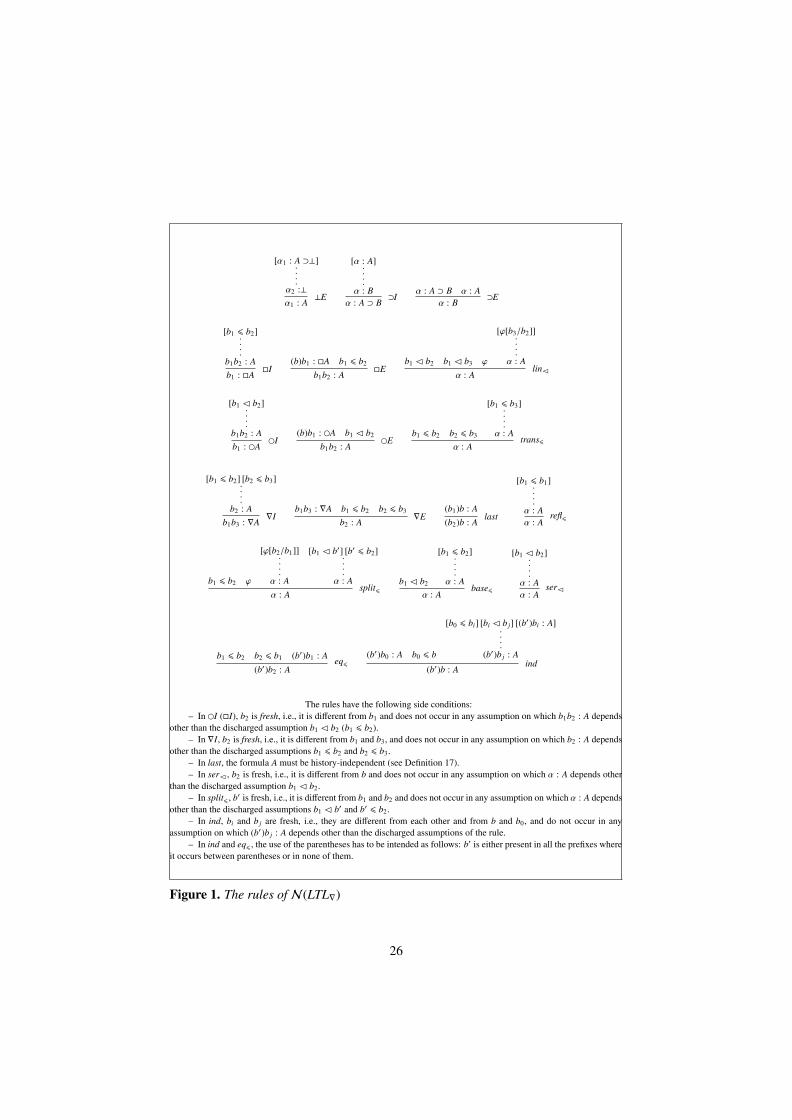
5.1. The rules of N(LTL∇)

The rules of N(LTL∇) are given in Figure 1. In N(LTL∇), we do not make useof a proper relational labeling algebra (as, e.g., in (Viganò, 2000)) containing rulesthat derive rwffs from other rwffs or even lwffs. Since we are mainly interested in thederivation of logical formulas, we rather follow an approach that aims at simplifyingthe system: we use rwffs only as assumptions for the derivation of lwffs (as in Simp-son’s system for intuitionistic modal logic (Simpson, 1994)). Thus, in N(LTL∇) thereare no rules whose conclusion is an rwff.

The rules ⊃I and ⊃E are just the labeled version of the standard (Prawitz, 1965)natural deduction rules for implication introduction and elimination, where the notionof discharged/open assumption is also standard; e.g., [α : A] means that the formulais discharged in ⊃I. The rule ⊥E is a labeled version of reductio ad absurdum, wherewe do not constrain the time instant sequence (α2) in which we derive a contradictionto be the same (α1) as in the assumption.

The rules for the introduction and the elimination of ? and ? share the same struc-ture. Consider, for instance, ? and the corresponding relation ?. The idea underlying

25

[α1 : A ⊃⊥]....α2 :⊥α1 : A

⊥E

[α : A]....α : Bα : A ⊃ B

⊃I α : A ⊃ B α : Aα : B

⊃E

[b1 ? b2]....b1b2 : Ab1 : ?A

?I(b)b1 : ?A b1 ? b2

b1b2 : A?E

b1 ? b2 b1 ? b3 ϕ

[ϕ[b3/b2]]....α : A

α : Alin?

[b1 ? b2]....b1b2 : Ab1 : ?A

?I(b)b1 : ?A b1 ? b2

b1b2 : A?E

b1 ? b2 b2 ? b3

[b1 ? b3]....α : A

α : Atrans?

[b1 ? b2] [b2 ? b3]....b2 : A

b1b3 : ∇A∇I

b1b3 : ∇A b1 ? b2 b2 ? b3b2 : A

∇E(b1)b : A(b2)b : A

last

[b1 ? b1]....α : Aα : A

refl?

b1 ? b2 ϕ

[ϕ[b2/b1]]....α : A

[b1 ? b?] [b? ? b2]....α : A

α : Asplit?

b1 ? b2

[b1 ? b2]....α : A

α : Abase?

[b1 ? b2]....α : Aα : A

ser?

b1 ? b2 b2 ? b1 (b?)b1 : A(b?)b2 : A

eq?(b?)b0 : A b0 ? b

[b0 ? bi] [bi ? b j] [(b?)bi : A]....(b?)b j : A

(b?)b : Aind

The rules have the following side conditions:– In ?I (?I), b2 is fresh, i.e., it is different from b1 and does not occur in any assumption on which b1b2 : A depends

other than the discharged assumption b1 ? b2 (b1 ? b2).– In ∇I, b2 is fresh, i.e., it is different from b1 and b3, and does not occur in any assumption on which b2 : A depends

other than the discharged assumptions b1 ? b2 and b2 ? b3.– In last, the formula A must be history-independent (see Definition 17).– In ser? , b2 is fresh, i.e., it is different from b and does not occur in any assumption on which α : A depends other

than the discharged assumption b1 ? b2.– In split? , b

? is fresh, i.e., it is different from b1 and b2 and does not occur in any assumption on which α : A dependsother than the discharged assumptions b1 ? b? and b? ? b2.

– In ind, bi and b j are fresh, i.e., they are different from each other and from b and b0, and do not occur in anyassumption on which (b?)b j : A depends other than the discharged assumptions of the rule.

– In ind and eq? , the use of the parentheses has to be intended as follows: b? is either present in all the prefixes where

it occurs between parentheses or in none of them.

Figure 1. The rules of N(LTL∇)

26

the introduction rule ?I is that the meaning of b1 : ?A is given by the metalevelimplication b1 ? b2 =⇒ b1b2 : A for an arbitrary b2 ?-accessible from b1 (wherethe arbitrariness of b2 is ensured by the side-condition on the rule). As we remarkedabove, the operators ? and ? have a local nature, in that when we write (b1)b2 : ?A weare stating that ?A holds at time instant b2, which is the last in the observation point.Hence, the elimination rule ?E says that if b2 is ?-accessible from b1 (i.e., b1 ? b2),then we can conclude that A holds for the sequence b1b2. Similar observations holdfor ? and the corresponding relation ?5.

The rule ser? models the fact that every time instant has an immediate successor,while the rule lin? specifies that such a successor must be unique. ser? tells us that ifby assuming b1 ? b2 we can derive α : A, then we can discharge the assumption andconclude that indeed α : A. lin? is slightly more complex: assume that b1 had twodifferent immediate successors b2 and b3 (which we know cannot be) and assume thatthe generic formula ϕ holds; if by substituting b3 for b2 in ϕ we obtain α : A, then wecan discharge the assumption and conclude that indeed α : A.

Similarly, the rules refl? and trans? state the reflexivity and transitivity of ?, whileeq? captures substitution of equals.

6 The rule split? states that if b1 ? b2, then eitherb1 = b2 or b1 < b2. The rule thus works in the style of a disjunction elimination:if by assuming either of the two cases, we can derive a formula α : A, then we candischarge the assumptions and conclude α : A. Since we do not use = and < explicitlyin our syntax, we express such relations in an indirect way: the equality of b1 and b2is expressed by replacing one with the other in a generic formula ϕ, whereas the order< corresponds to the composition of ? and ?.

The rule base? expresses the fact that ? contains ?, while the rule ind models theinduction principle underlying the relation between ? and ?. If (base case) A holdsin (b?)b0 and if (inductive step) by assuming that A holds in (b?)bi for an arbitrarybi ?-accessible from b0, we can derive that A holds also in (b?)b j, where b j is theimmediate successor of bi, then we can conclude that A holds in every (b?)b such thatb is ?-accessible from b0.7

Finally, we have three rules that speak about the history and the observation points:the rules ∇I and ∇E, which we already described in the introduction, and last. Thisrule expresses what we also anticipated in Sections 1 and 4: the standard operators(and connectives) of LTL only speak about single time instants, and thus if a formulaA is history-independent (see Definition 17), then given a lwff (b1)b : A we can safelyreplace the possible store b1 of our observation point by any other time instant b2 andconclude that A holds at (b2)b.

5. In fact, since the immediate successor of each point is unique, we can give a “universal”formulation also for the rules ?I and ?E.6. Recall that in this paper we use rwffs only as assumptions for the derivation of lwffs, so wedo not need a more general rule that concludes ϕ[b2/b1] from ϕ, b1 ? b2 and b2 ? b1.7. The rule is given only in terms of relations between labels, since we restrict the treatment ofoperators in the system to the specific rules for their introduction and elimination.

27

Given the rules in Fig. 1, the notion of derivation is the standard one for naturaldeduction systems (Prawitz, 1965; Troelstra & Schwichtenberg, 2000). We write Φ ?∇α : A to say that there exists a derivation of α : A in the system N(LTL∇) whoseopen assumptions are all contained in the set of formulas Φ. A derivation of α : A inN(LTL∇) where all the assumptions are discharged is a proof of α : A inN(LTL∇) andwe then say that α : A is a theorem of N(LTL∇) (and write ?∇ α : A).As notation, we write

ϕ1 . . . ϕnΠα : A

to denote that Π is a derivation of α : A whose set of assumptions may contain theformulas ϕ1, . . . , ϕn.

5.2. Soundness

In this section, we discuss the soundness of N(LTL∇). First, we show that thesystem is sound with respect to the semantics of LTL∇. Then we extend this resultto LTL and prove that N(LTL∇) is also sound, by means of the translation (·)#, withrespect to the semantics of LTL.

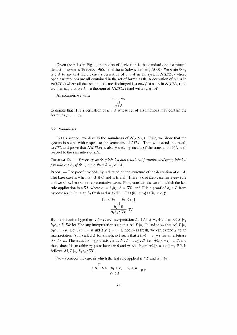
Theorem 43. — For every set Φ of labeled and relational formulas and every labeledformula α : A , if Φ ?∇ α : A then Φ |=∇ α : A.Proof. — The proof proceeds by induction on the structure of the derivation of α : A.The base case is when α : A ∈ Φ and is trivial. There is one step case for every ruleand we show here some representative cases. First, consider the case in which the lastrule application is a ∇I, where α = b1b3, A = ∇B, and Π is a proof of b2 : B fromhypotheses in Φ?, with b2 fresh and with Φ? = Φ ∪ {b1 ? b2} ∪ {b2 ? b3}:

[b1 ? b2] [b2 ? b3]Π

b2 : Bb1b3 : ∇B ∇I

By the induction hypothesis, for every interpretation I, ifM,I |=∇ Φ?, thenM,I |=∇b1b2 : B. We let I be any interpretation such thatM,I |=∇ Φ, and show thatM,I |=∇b1b3 : ∇B. Let I(b1) = n and I(b3) = m. Since b2 is fresh, we can extend I to aninterpretation (still called I for simplicity) such that I(b2) = n + i for an arbitrary0 ≤ i ≤ m. The induction hypothesis yieldsM,I |=∇ b2 : B, i.e.,M, [n + i] |=∇ B, andthus, since i is an arbitrary point between 0 and m, we obtainM, [n, n + m] |=∇ ∇B. ItfollowsM,I |=∇ b1b3 : ∇B.

Now consider the case in which the last rule applied is ∇E and α = b2:

Πb1b3 : ∇A b1 ? b2 b2 ? b3

b2 : A∇E

28

where Π is a proof of b1b3 : ∇A from hypotheses in Φ1, with Φ = Φ1 ∪ {b1 ?b2} ∪ {b2 ? b3} for some set Φ1 of formulas. By applying the induction hypothesis onΠ, we have Φ1 |=∇ b1b3 : ∇A. We proceed by considering a generic LTL-modelMand a generic interpretation I on it such thatM,I |=∇ Φ and showing that this entailsM,I |=∇ b2 : A. Since Φ1 ⊂ Φ, we deduce M,I |=∇ Φ1 and, from the inductionhypothesis,M,I |=∇ b1b3 : ∇A. FurthermoreM,I |=∇ Φ entailsM,I |=∇ b1 ? b2andM,I |=∇ b2 ? b3. Then, by Definition 6, we obtainM,I |=∇ b2 : A.

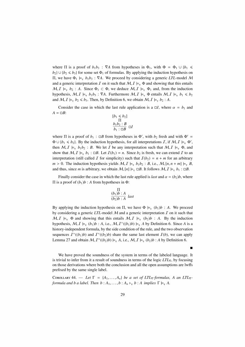
Consider the case in which the last rule application is a ?I, where α = b1 andA = ?B:

[b1 ? b2]Π

b1b2 : Bb1 : ?B ?I

where Π is a proof of b1 : ?B from hypotheses in Φ?, with b2 fresh and with Φ? =Φ ∪ {b1 ? b2}. By the induction hypothesis, for all interpretations I, ifM,I |=∇ Φ?,then M,I |=∇ b1b2 : B. We let I be any interpretation such that M,I |=∇ Φ, andshow thatM,I |=∇ b1 : ?B. Let I(b1) = n. Since b2 is fresh, we can extend I to aninterpretation (still called I for simplicity) such that I(b2) = n + m for an arbitrarym > 0. The induction hypothesis yieldsM,I |=∇ b1b2 : B, i.e.,M, [n, n + m] |=∇ B,and thus, since m is arbitrary, we obtainM, [n] |=∇ ?B. It followsM,I |=∇ b1 : ?B.

Finally consider the case in which the last rule applied is last and α = (b2)b, whereΠ is a proof of (b1)b : A from hypotheses in Φ:

Π(b1)b : A(b2)b : A

last

By applying the induction hypothesis on Π, we have Φ |=∇ (b1)b : A. We proceedby considering a generic LTL-modelM and a generic interpretation I on it such thatM,I |=∇ Φ and showing that this entails M,I |=∇ (b2)b : A. By the inductionhypothesis,M,I |=∇ (b1)b : A, i.e.,M,I+((b1)b) |=∇ A by Definition 6. Since A is ahistory-independent formula, by the side condition of the rule, and the two observationsequences I+((b1)b) and I+((b2)b) share the same last element I(b), we can applyLemma 27 and obtainM,I+((b2)b) |=∇ A, i.e.,M,I |=∇ (b2)b : A by Definition 6.

?

We have proved the soundness of the system in terms of the labeled language. Itis trivial to infer from it a result of soundness in terms of the logic LTL∇, by focusingon those derivations where both the conclusion and all the open assumptions are lwffsprefixed by the same single label.

Corollary 44. — Let Γ = {A1, . . . , An} be a set of LTL∇-formulas, A an LTL∇-formula and b a label. Then b : A1, . . . , b : An ?∇ b : A implies Γ |=∇ A.

29

Proof. — By Theorem 43, b : A1, . . . , b : An ?∇ b : A implies b : A1, . . . , b : An |=∇b : A. By Definition 8, b : A1, . . . , b : An |=∇ b : A implies Γ |=∇ A. ?

Now, by exploiting the translation (·)# defined in Section 4.2, we extend this resultto a form of soundness with respect to LTL.

Theorem 45. — Let Γ = {A1, . . . , An} be a set of LTL∇-formulas, A an LTL∇-formulaand b a label. Then b : A1, . . . , b : An ?∇ b : A implies Γ# |=LTL A#.

Proof. — By Corollary 44, b : A1, . . . , b : An ?∇ b : A implies Γ |=∇ A. By Theorem32, Γ |=∇ A implies Γ# |=LTL A#. ?

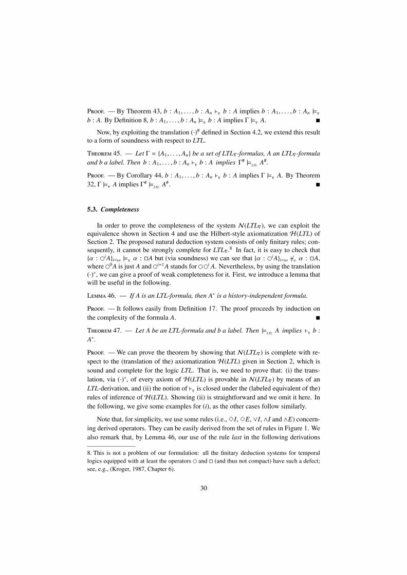
5.3. Completeness

In order to prove the completeness of the system N(LTL∇), we can exploit theequivalence shown in Section 4 and use the Hilbert-style axiomatization H(LTL) ofSection 2. The proposed natural deduction system consists of only finitary rules; con-sequently, it cannot be strongly complete for LTL∇.8 In fact, it is easy to check that{α : ?iA}i<ω |=∇ α : ?A but (via soundness) we can see that {α : ?iA}i<ω ??∇ α : ?A,where ?0A is just A and ?i+1A stands for ??i A. Nevertheless, by using the translation(·)∗, we can give a proof of weak completeness for it. First, we introduce a lemma thatwill be useful in the following.

Lemma 46. — If A is an LTL-formula, then A∗ is a history-independent formula.

Proof. — It follows easily from Definition 17. The proof proceeds by induction onthe complexity of the formula A. ?

Theorem 47. — Let A be an LTL-formula and b a label. Then |=LTL A implies ?∇ b :A∗.

Proof. — We can prove the theorem by showing that N(LTL∇) is complete with re-spect to the (translation of the) axiomatization H(LTL) given in Section 2, which issound and complete for the logic LTL. That is, we need to prove that: (i) the trans-lation, via (·)∗, of every axiom of H(LTL) is provable in N(LTL∇) by means of anLTL-derivation, and (ii) the notion of ?∇ is closed under the (labeled equivalent of the)rules of inference of H(LTL). Showing (ii) is straightforward and we omit it here. Inthe following, we give some examples for (i), as the other cases follow similarly.

Note that, for simplicity, we use some rules (i.e.,?I,?E, ∨I, ∧I and ∧E) concern-ing derived operators. They can be easily derived from the set of rules in Figure 1. Wealso remark that, by Lemma 46, our use of the rule last in the following derivations

8. This is not a problem of our formulation: all the finitary deduction systems for temporallogics equipped with at least the operators ? and ? (and thus not compact) have such a defect;see, e.g., (Kroger, 1987, Chapter 6).

30

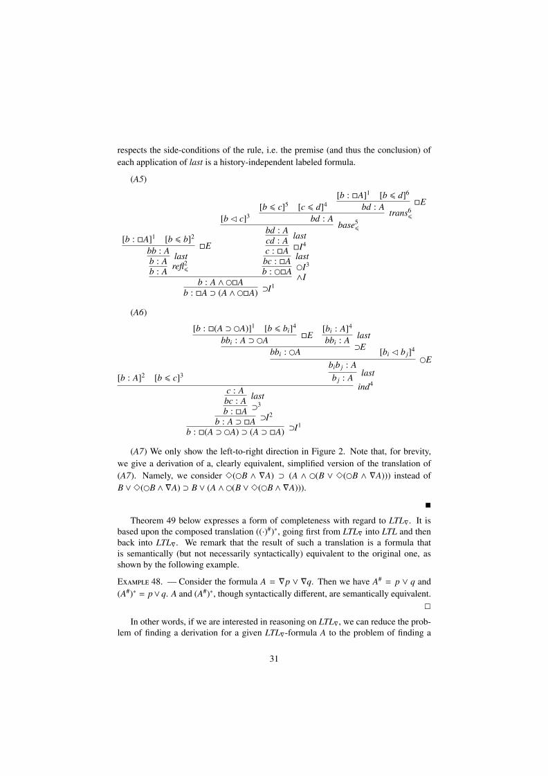
respects the side-conditions of the rule, i.e. the premise (and thus the conclusion) ofeach application of last is a history-independent labeled formula.

(A5)

[b : ?A]1 [b ? b]2

bb : A ?E

b : A last

b : A refl2?

[b ? c]3[b ? c]5 [c ? d]4

[b : ?A]1 [b ? d]6

bd : A ?E

bd : Atrans6?

bd : A base5?cd : A last

c : ?A ?I4

bc : ?A last

b : ??A ?I3

b : A ∧ ??A ∧I

b : ?A ⊃ (A ∧ ??A) ⊃I1

(A6)

[b : A]2 [b ? c]3

[b : ?(A ⊃ ?A)]1 [b ? bi]4

bbi : A ⊃ ?A ?E[bi : A]4

bbi : Alast

bbi : ?A⊃E [bi ? b j]4

bib j : A?E

b j : Alast

c : A ind4

bc : A last

b : ?A ⊃3b : A ⊃ ?A ⊃I2

b : ?(A ⊃ ?A) ⊃ (A ⊃ ?A) ⊃I1

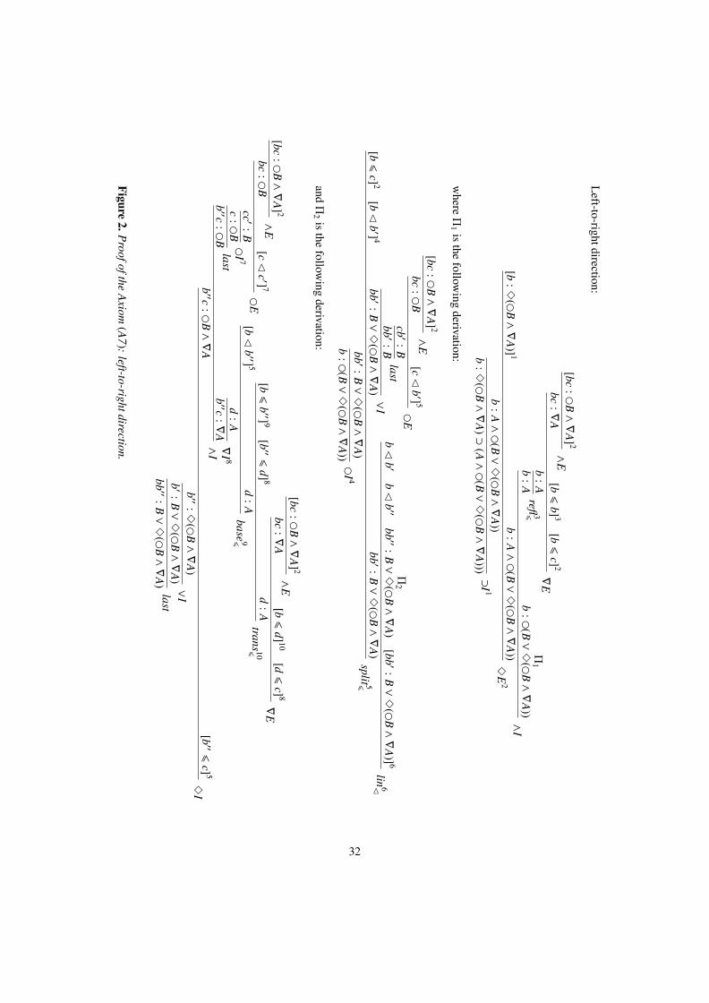
(A7) We only show the left-to-right direction in Figure 2. Note that, for brevity,we give a derivation of a, clearly equivalent, simplified version of the translation of(A7). Namely, we consider ?(?B ∧ ∇A) ⊃ (A ∧ ?(B ∨ ?(?B ∧ ∇A))) instead ofB ∨?(?B ∧ ∇A) ⊃ B ∨ (A ∧ ?(B ∨?(?B ∧ ∇A))).

?

Theorem 49 below expresses a form of completeness with regard to LTL∇. It isbased upon the composed translation ((·)#)∗, going first from LTL∇ into LTL and thenback into LTL∇. We remark that the result of such a translation is a formula thatis semantically (but not necessarily syntactically) equivalent to the original one, asshown by the following example.

Example 48. — Consider the formula A = ∇p ∨ ∇q. Then we have A# = p ∨ q and(A#)∗ = p∨ q. A and (A#)∗, though syntactically different, are semantically equivalent.

?In other words, if we are interested in reasoning on LTL∇, we can reduce the prob-

lem of finding a derivation for a given LTL∇-formula A to the problem of finding a

31

Left-to-rightdirection:

[b:?(?

B∧∇

A)] 1

[bc:?

B∧∇

A] 2

bc:∇

A∧

E[b?

b] 3[b?

c] 2

b:A

∇E

b:A

refl3?

Π1

b:?(B∨?

(?B∧∇

A))

b:A∧

?(B∨?

(?B∧∇

A))

∧I

b:A∧

?(B∨?

(?B∧∇

A))

?E2

b:?(?

B∧∇

A)⊃

(A∧?(B∨?

(?B∧∇

A))) ⊃

I 1

whereΠ1isthe

following

derivation:

[b?

c] 2[b?

b ?] 4

[bc:?

B∧∇

A] 2

bc:?

B∧

E[c?

b ?] 5

cb ?:B?E

bb ?:Blast

bb ?:B∨?(?

B∧∇

A) ∨

Ib?

b ?b?

b ??Π2

bb ??:B∨?(?

B∧∇

A)[bb ?:B∨?

(?B∧∇

A)] 6

bb ?:B∨?(?

B∧∇

A)

lin6?

bb ?:B∨?(?

B∧∇

A)

split 5?

b:?(B∨?

(?B∧∇

A))?I 4

andΠ2isthe

following

derivation:

[bc:?

B∧∇

A] 2

bc:?

B∧

E[c?

c ?] 7

cc ?:B?E

c:?

B?I 7

b ??c:?

Blast

[b?b ??] 5

[b?

b ??] 9[b ???

d] 8

[bc:?

B∧∇

A] 2

bc:∇

A∧

E[b?

d] 10[d?

c] 8

d:A

∇E

d:A

trans 10?

d:A

base9?

b ??c:∇

A∇

I 8

b ??c:?

B∧∇

A∧

I[b ???

c] 5

b ??:?(?

B∧∇

A)

?I

b ?:B∨?(?

B∧∇

A) ∨

I

bb ??:B∨?(?

B∧∇

A)

last

Figure2.P

roofoftheAxiom

(A7):

left-to-rightdirection.

32

derivation for the formula (A#)∗, which is semantically equivalent to A and for whicha derivation in N(LTL∇) exists.

Theorem 49. — Let A be an LTL∇-formula and b a label. Then

|=∇ A ⇒ ?∇ b : (A#)∗ .

Proof. — By Theorem 32, |=∇ A implies |=LTL A#. By Theorem 47, |=LTL A# implies?∇ b : (A#)∗. ?

6. Conclusions and related works

The introduction of the new operator ∇ allowed us to formalize the “history” ofuntil and to give a labeled natural deduction system for LTL∇, a variant of LTL where∇ replaces U. Such a logic has been proved to be as expressive as LTL with until and,by using proper translations, we are able to use the system for reasoning on LTL aswell and to prove results of soundness and completeness for both LTL and LTL with∇. We remark that the “recipe” for dealing with until that we gave here is abstract andgeneral, and thus provides the basis for formalizing deduction systems for temporallogics endowed with U, both linear and branching-time.

While the treatment of U is not easy from a proof-theoretical point of view, thenew operator allows for the definition of well-behaved systems. In this paper, wedid not address normalization matters explicitly. However the well-behaved natureof this approach, where each connective and operator has one introduction and oneelimination rule, paves the way to a proof-theoretical analysis of the resulting naturaldeduction systems, e.g., to show proof normalization and other useful meta-theoreticalproperties. In fact, we believe that the normalization procedures described in (Viganò& Volpe, 2008; Masini et al., 2010b) in the case of labeled natural deduction systemsfor several temporal logics could be easily adapted to deal with ∇ as well. This wouldthen pave the way to an automation of deduction in LTL∇.

With respect to the discussion on the rule last, we believe that the restriction weimposed, i.e., the rule can only be applied to history-independent formulas, is closelyrelated, at least in spirit, to the focus on persistent formulas when combining intuition-istic and classical logic so as to avoid the collapse of the two logics into one, see (delCerro & Herzig, 1996) but also (Caleiro & Ramos, 2007; Gabbay, 1996b). We are,after all, considering here formulas stemming from two classes (if not two logics al-together), and it makes thus sense that they require different labeling (single instantsand pairs of time instants).

Several extensions of temporal logics based on the introduction of new operatorshave been presented in the literature. As shown by the translation in Section 4.3, log-ics with history have some similarities with temporal logics with the operator now N

33

(Laroussinie & Schnoebelen, 1995; Laroussinie et al., 2002). When used in combina-tion with past operators, now allows to “forget” part of the past. In particular, the logicNLTL obtained by adding N to LTL with past operators, is proved (Laroussinie et al.,2002) to be equally expressive to, but more succinct than, LTL with past. With respectto LTL∇, we proved here that NLTL is initially at least as expressive as LTL∇.

Another class of logics extending the expressivity of standard temporal logics isthat of hybrid temporal logics, where the possibility of referring to worlds (instants) ofa model is internalized in the syntax of the logic itself and not just used as a technicaldevice when performing deduction like we did in our system here. Early examplesare in (Prior, 1967; Bull, 1970); more recent works in (Blackburn & Tzakova, 1999;Allen, 1984; Goranko, 2000).

Finally, it is worth observing that several works have considered interval temporallogics, e.g., (Bowman & Thompson, 2003; Cerrito & Mayer, 2000; Goranko et al.,2006; Halpern & Shoham, 1991; Schmitt & Goubault-Larrecq, 1997). While theseworks consider intervals explicitly, we have used them somehow implicitly here, as ameans to formalize the dual nature of until via the operator ∇.

Acknowledgements

This work was partially supported by the PRIN’07 projects “CONCERTO” and“SOFT”. We thank Carlos Caleiro and Stéphane Demri for their useful comments onthe paper (Masini et al., 2010a), which is extended and superseded by this paper.

7. References

Allen, J. F. (1984). Towards a general theory of action and time. Artificial Intelligence, 23(2),123–154.

Basin, D., Caleiro, C., Ramos, J., & Viganò, L. (2009). Labelled tableaux for distributedtemporal logic. Journal of Logic and Computation, 19(6), 1245–1279.

Blackburn, P. & Tzakova, M. (1999). Hybrid languages and temporal logic. Logic Journal ofthe IGPL, 7(1), 27–54.

Bolotov, A., Grigoriev, O., & Shangin, V. (2007). Automated natural deduction for propo-sitional linear-time temporal logic. In V. Goranko & X. Wang (Eds.), Proceedings of the14th International Symposium on Temporal Representation and Reasoning (TIME 2007)(pp. 47–58).: IEEE Computer Society.

Bowman, H. & Thompson, S. J. (2003). A decision procedure and complete axiomatizationof finite interval temporal logic with projection. Journal of Logic and Computation, 13(2),195–239.

Bull, R. A. (1970). An approach to tense logic. Theoria, 36, 282–300.

34

Caleiro, C. & Ramos, J. (2007). Combining classical and intuitionistic implications. In B.Konev & F. Wolter (Eds.), Proceedings of the 6th International Symposium on Frontiersof Combining Systems (FroCoS 2007), volume 4720 of Lecture Notes in Computer Science(pp. 118–132).: Springer.

Cerrito, S. & Mayer, M. C. (2000). Labelled tableaux for propositional linear time logic overfinite frames. In D. Basin, M. D’Agostino, D. M. Gabbay, S. Matthews, & L. Viganò (Eds.),Labelled Deduction (pp. 135–159). Kluwer Academic Publishers.

del Cerro, L. F. & Herzig, A. (1996). Combining classical and intuitionistic logic, or: Intu-itionistic implication as a conditional. In F. Baader & K. U. Schulz (Eds.), Proceedingsof the 1st International Workshop on Frontiers of Combining Systems (FroCoS 1996), vol-ume 3 of Applied Logic Series (pp. 93–102).: Kluwer Academic Publishers.

Emerson, E. A. (1990). Temporal and modal logic. In J. van Leeuwen (Ed.), Handbookof Theoretical Computer Science, Volume B: Formal Models and Semantics (B) (pp. 995–1072). North-Holland - MIT Press.

Fisher, M., Gabbay, D. M., & Vila, L. (2005). Handbook of Temporal Reasoning in ArtificialIntelligence (Foundations of Artificial Intelligence). Elsevier Science Inc.

Gabbay, D. M. (1989). The declarative past and imperative future: Executable temporal logicfor interactive systems. In B. Banieqbal, H. Barringer, & A. Pnueli (Eds.), Proceedingsof Temporal Logic in Specification (TLS 1987), volume 398 of Lecture Notes in ComputerScience (pp. 409–448).: Springer.

Gabbay, D. M. (1996a). Labelled Deductive Systems. Clarendon Press.

Gabbay, D. M. (1996b). An overview of fibred semantics and the combination of logics. In F.Baader & K. U. Schulz (Eds.), Proceedings of the 1st International Workshop on Frontiers ofCombining Systems (FroCoS 1996), volume 3 of Applied Logic Series (pp. 1–55).: KluwerAcademic Publishers.

Gabbay, D. M., Pnueli, A., Shelah, S., & Stavi, J. (1980). On the temporal analysis of fairness.In Proceedings of the 7th ACM SIGPLAN-SIGACT Symposium on Principles of program-ming languages (POPL 1980) (pp. 163–173).: ACM.

Goldblatt, R. I. (1987). Logics of Time and Computation. Stanford CA : Center for the Studyof Language and Information.

Goranko, V. (2000). Temporal logics with reference pointers and computation tree logics.Journal of Applied Non-Classical Logics, 10(3-4), 221–242.

Goranko, V., Montanari, A., Sala, P., & Sciavicco, G. (2006). A general tableau method forpropositional interval temporal logics: Theory and implementation. Journal of AppliedLogic, 4(3), 305–330.

Goré, R. (1999). Tableau methods for modal and temporal logics. In M. D’Agostino, D.Gabbay, R. Hahnle, & J.Posegga (Eds.), Handbook of Tableau Methods (pp. 297–396).Kluwer Academic Publishers.

35

Gough, G. D. (1989). Decision Procedures for Temporal Logic. Technical Reports UMCS-89-10-1, Department of Computer Science, University of Manchester.

Halpern, J. Y. & Shoham, Y. (1991). A propositional modal logic of time intervals. Journal ofthe ACM, 38(4), 935–962.

Kamp, J. A. W. (1968). Tense Logic and the Theory of Linear Order. PhD thesis, Universityof California, Los Angeles.

Kroger, F. (1987). Temporal Logic of Programs. Springer.

Laroussinie, F., Markey, N., & Schnoebelen, P. (2002). Temporal logic with forgettable past.In G. Plotkin (Ed.), Proceedings of the 17th IEEE Symposium on Logic in Computer Science(LICS 2002) (pp. 383–392).: IEEE Computer Society.

Laroussinie, F. & Schnoebelen, P. (1995). A hierarchy of temporal logics with past. Theoreti-cal Computer Science, 148(2), 303–324.

Masini, A., Viganò, L., & Volpe, M. (2009). A labeled natural deduction system for a fragmentof ctl*. In S. N. Artëmov & A. Nerode (Eds.), Proceedings of the International Symposiumon Logical Foundations of Computer Science (LFCS 2009), volume 5407 of Lecture Notesin Computer Science (pp. 338–353).: Springer.

Masini, A., Viganò, L., & Volpe, M. (2010a). A history of until. In T. Bolander & T. Braüner(Eds.), Proceedings of the 6th Workshop on Methods for Modalities (M4M-06), ElectronicNotes in Theoretical Computer Science (pp. 189–204).

Masini, A., Viganò, L., & Volpe, M. (2010b). Labeled natural deduction for a bundled branch-ing temporal logic. Journal of Logic and Computation, doi:10.1093/logcom/exq028.

Prawitz, D. (1965). Natural Deduction: a Proof-Theoretical Study. Number 3 in StockholmStudies in Philosophy. Almqvist and Wiskell.

Prior, A. (1967). Past, Present and Future. Oxford University Press.

Schmitt, P. H. & Goubault-Larrecq, J. (1997). A tableau system for linear-time temporallogic. In E. Brinksma (Ed.), Proceedings of the 3rd International Workshop on Algorithmsfor Construction and Analysis of Systems (TACAS 1997), volume 1217 of Lecture Notes inComputer Science (pp. 130–144).: Springer.

Schwendimann, S. (1998). A new one-pass tableau calculus for pltl. In H. C. M. de Swart(Ed.), Proceedings of the 7th International Conference on Automated Reasoning with Ana-lytic Tableaux and Related Methods (TABLEAUX 1998), volume 1397 of Lecture Notes inComputer Science (pp. 277–292).: Springer.

Simpson, A. K. (1994). The Proof Theory and Semantics of Intuitionistic Modal Logic. PhDthesis, College of Science and Engineering, School of Informatics, University of Edinburgh.

Troelstra, A. S. & Schwichtenberg, H. (2000). Basic Proof Theory. Cambridge UniversityPress.

van Dalen, D. (1980). Logic and Structure. Springer.

36

Viganò, L. (2000). Labelled Non-Classical Logics. Kluwer Academic Publishers.

Viganò, L. & Volpe, M. (2008). Labeled natural deduction systems for a family of tenselogics. In S. Demri & C. S. Jensen (Eds.), Proceedings of the 15th International Symposiumon Temporal Representation and Reasoning (TIME 2008) (pp. 118–126).: IEEE ComputerSociety.

37

Back from the future

Documents

Transcript of Back from the future