Bachelor's Degree Final Project Report - UPCommons
150
Bachelor’s Degree Final Project Aerospace Vehicles Engineering COMPUTATIONAL RESOLUTION OF THE NAVIER-STOKES EQUATIONS FOR LAMINAR AND TURBULENT FLOWS. IMPLEMENTATION OF THE SPALART-ALLMARAS TURBULENCE MODEL. H EAT AND MASS T RANSFER C ENTER (CTTC) Report Friday 3 rd July, 2020 Author: Sergio Guti´ errez S´ anchez Director: Assensi Oliva Llena Co-director: Carles David P´ erez Segarra Call: 2019/2020 QP
-
Upload
khangminh22 -
Category
Documents
-
view
3 -
download
0
Transcript of Bachelor's Degree Final Project Report - UPCommons
Bachelor’s Degree Final ProjectAerospace Vehicles Engineering
COMPUTATIONAL RESOLUTION OF THENAVIER-STOKES EQUATIONS FOR LAMINAR ANDTURBULENT FLOWS. IMPLEMENTATION OF THE
SPALART-ALLMARAS TURBULENCE MODEL.
HEAT AND MASS TRANSFER CENTER (CTTC)
ReportFriday 3rd July, 2020
Author: Sergio Gutierrez Sanchez
Director: Assensi Oliva Llena
Co-director: Carles David Perez Segarra
Call: 2019/2020 QP

Acknowledgements
Me gustarıa agradecer a diversas personas y organismos el apoyo y la ayuda recibidas duranteel desarollo de este proyecto y durante el tiempo de estudio del grado en ingenierıa en vehıculosaeroespaciales.
• Mi agradecimiento al sistema universitario catalan y espanol por la oportunidad de estu-diar esta carrera y por la formacion academica y personal recibida durante este tiempo.
• A mi familia, quienes desde que tengo uso de razon me han motivado y ayudado in-condicionalmente a cumplir mi sueno de llegar a ser ingeniero aeronautico y dedicarmeprofesionalmente a ello sin importar cualquier circunstancia.
• Mi mas sincero agradecimiento tambien para los profesores y doctores Assensi OlivaLlena y Carlos David Perez Segarra por darme la increıble oportunidad de entrar en elCTTC para formarme como ingeniero de CFD. Ası como a todos los miembros del centro,entre ellos el doctor Francesc Xavier Trias Miquel por su inestimable ayuda.
• En especial tambien me gustarıa agradecer a Jesus Ruano, companero del CTTC quedesde el primer dıa me ha ayudado en todo lo que he necesitado y sin el cual este proyecto,desde su base, habrıa sido completamente imposible de desarrollar.
1

Abstract
The present project consists on the computational study and resolution of the Navier-Stokesequations and the physical phenomena involved.
The main objective is the development of C++ programming codes to solve flow’s governingequations using numerical methods. The project comprises the fluid dynamic and thermal studyand analysis of both laminar and turbulent regimes. In addition to that, in case of turbulent flow,there has been selected to implement a RANS turbulence model called Spalart-Allmaras.
The computational codes developed will be used to simulate the study cases LID Driven Cavity,LID Differentially Heated and Square Cylinder for the laminar regime and a supersonic pipe incase of the turbulent part. Additionally, the results obtained will be extensively analysed andverified using scientific publications.

Declaration of honourI declare that,
the work in this Degree Thesis is completely my own work,
no part of this Degree Thesis is taken from other people’s work without giving them credit,
all references have been clearly cited,
I’m authorised to make use of the research group related information I’m providing in thisdocument.
I understand that an infringement of this declaration leaves me subject to the foreseen disci-plinary actions by The Universitat Politecnica de Catalunya - BarcelonaTECH.
Sergio Gutierrez Sanchez Friday 3rd July, 2020
Student name Signature Date
Title of the Thesis:
Study for the computational resolution of conservation equations of mass, momentum and en-ergy. Possible application to different aeronautical and industrial engineering problems: Case50B
1

Contents
List of Figures 4
List of Tables 7
Nomenclature 8
1 Introduction 111.1 Justification . . . . . . . . . . . . . . . . . . . . . . . . . . . . . . . . . . . . 111.2 Scope . . . . . . . . . . . . . . . . . . . . . . . . . . . . . . . . . . . . . . . 121.3 Specifications . . . . . . . . . . . . . . . . . . . . . . . . . . . . . . . . . . . 13
2 What is Fluid Mechanics 152.1 Introduction and history of the field. . . . . . . . . . . . . . . . . . . . . . . . 152.2 Governing equations of fluid mechanics. . . . . . . . . . . . . . . . . . . . . . 16
2.2.1 The material derivative . . . . . . . . . . . . . . . . . . . . . . . . . . 172.2.2 Convection - Diffusion equation. . . . . . . . . . . . . . . . . . . . . . 182.2.3 Mass conservation equation. . . . . . . . . . . . . . . . . . . . . . . . 182.2.4 Momentum conservation equation. . . . . . . . . . . . . . . . . . . . . 192.2.5 Energy conservation equation. . . . . . . . . . . . . . . . . . . . . . . 20
2.3 Non-dimensionalization. . . . . . . . . . . . . . . . . . . . . . . . . . . . . . 222.4 Computational Fluid Dynamics. . . . . . . . . . . . . . . . . . . . . . . . . . 24
3 Laminar regime 273.1 Theoretical framework . . . . . . . . . . . . . . . . . . . . . . . . . . . . . . 27
3.1.1 Hypothesis and simplifications made . . . . . . . . . . . . . . . . . . . 283.1.2 Laminar regime Navier - Stokes equations. . . . . . . . . . . . . . . . 303.1.3 Laminar regime study cases. . . . . . . . . . . . . . . . . . . . . . . . 31
3.2 Numerical framework . . . . . . . . . . . . . . . . . . . . . . . . . . . . . . . 343.2.1 Spatial discretization . . . . . . . . . . . . . . . . . . . . . . . . . . . 353.2.2 Resolution of the equations. . . . . . . . . . . . . . . . . . . . . . . . 463.2.3 Time integration . . . . . . . . . . . . . . . . . . . . . . . . . . . . . . 493.2.4 Discretization of the equations. . . . . . . . . . . . . . . . . . . . . . . 513.2.5 Solver implementation. . . . . . . . . . . . . . . . . . . . . . . . . . . 583.2.6 Simulation algorithm. . . . . . . . . . . . . . . . . . . . . . . . . . . . 61
3.3 LID Driven Cavity . . . . . . . . . . . . . . . . . . . . . . . . . . . . . . . . 653.3.1 Obtained results and verification . . . . . . . . . . . . . . . . . . . . . 65
3.4 LID Differentially Heated . . . . . . . . . . . . . . . . . . . . . . . . . . . . . 743.4.1 Obtained results and verification . . . . . . . . . . . . . . . . . . . . . 75
2
CONTENTS
3.5 Square Cylinder . . . . . . . . . . . . . . . . . . . . . . . . . . . . . . . . . . 833.5.1 Obtained results and verification . . . . . . . . . . . . . . . . . . . . . 84
4 Turbulent Regime. 964.1 Theoretical framework. . . . . . . . . . . . . . . . . . . . . . . . . . . . . . . 96
4.1.1 Hypothesis and simplifications made . . . . . . . . . . . . . . . . . . . 974.1.2 Turbulent regime Navier - Stokes equations. . . . . . . . . . . . . . . . 99
4.2 Turbulence modelling . . . . . . . . . . . . . . . . . . . . . . . . . . . . . . . 1004.2.1 Reynolds Averaged Navier Stokes Equations (RANS). . . . . . . . . . 100
4.3 Symmetry-preserving discretization for compressible flows. . . . . . . . . . . . 1074.4 Problem studied. . . . . . . . . . . . . . . . . . . . . . . . . . . . . . . . . . . 1104.5 Numerical framework. . . . . . . . . . . . . . . . . . . . . . . . . . . . . . . 112
4.5.1 Spatial discretization. . . . . . . . . . . . . . . . . . . . . . . . . . . . 1124.5.2 Modified compressible Navier Stokes equations discretization. . . . . . 1154.5.3 Spalart-Allmaras RANS turbulence model implementation. . . . . . . . 1224.5.4 Time integration. . . . . . . . . . . . . . . . . . . . . . . . . . . . . . 1264.5.5 Simulation algorithm. . . . . . . . . . . . . . . . . . . . . . . . . . . . 127
4.6 Simulation of turbulent compressible pipe flow. . . . . . . . . . . . . . . . . . 1314.6.1 Obtained results and verification . . . . . . . . . . . . . . . . . . . . . 132
5 Environmental impact of the project 1405.1 Documentation and investigation. . . . . . . . . . . . . . . . . . . . . . . . . . 1405.2 Coding and debugging. . . . . . . . . . . . . . . . . . . . . . . . . . . . . . . 1405.3 Verification of the results. . . . . . . . . . . . . . . . . . . . . . . . . . . . . . 1415.4 Project’s memory development. . . . . . . . . . . . . . . . . . . . . . . . . . . 141
6 Conclusions and future work. 1426.1 General conclusions. . . . . . . . . . . . . . . . . . . . . . . . . . . . . . . . 1426.2 Future work. . . . . . . . . . . . . . . . . . . . . . . . . . . . . . . . . . . . . 143
6.2.1 Short term. . . . . . . . . . . . . . . . . . . . . . . . . . . . . . . . . 1446.2.2 Mid term. . . . . . . . . . . . . . . . . . . . . . . . . . . . . . . . . . 144
Bibliography 145
3

List of Figures
2.1 Da Vinci’s sketch of free-surface turbulence behind obstacle. Extracted from [1] 152.2 Historical timeline of fluid mechanics. Extracted from [1] . . . . . . . . . . . . 162.3 CFD simulation of an aircraft. Extracted from [2] . . . . . . . . . . . . . . . . 242.4 CFD simulation of racing car. Extracted from [3] . . . . . . . . . . . . . . . . 242.5 CFD simulation of F1 racing car. Extracted from [4] . . . . . . . . . . . . . . . 252.6 CFD simulation of Space Shuttle. Extracted from [5] . . . . . . . . . . . . . . 252.7 Vertical Kaplan Turbine geometry. Extracted from [6] . . . . . . . . . . . . . . 252.8 Meshing of different components of Kaplan Turbine. Extracted from [6] . . . . 262.9 Analysis and post-processing of the results obtained. Extracted from [6] . . . . 26
3.1 Laminar flow velocities profile through a channel. Extracted from [7] . . . . . . 273.2 LID Driven Cavity case scheme . . . . . . . . . . . . . . . . . . . . . . . . . . 313.3 LID Differentially Heated case scheme . . . . . . . . . . . . . . . . . . . . . . 323.4 Square Cylinder case scheme . . . . . . . . . . . . . . . . . . . . . . . . . . . 333.5 Finite Volume Method representation . . . . . . . . . . . . . . . . . . . . . . . 343.6 FVM discretization basis representation . . . . . . . . . . . . . . . . . . . . . 353.7 Structured Orthogonal Uniform mesh . . . . . . . . . . . . . . . . . . . . . . . 363.8 Structured Orthogonal Non-Uniform mesh . . . . . . . . . . . . . . . . . . . . 363.9 Non orthogonal mesh for airfoil simulation. Extracted from [8] . . . . . . . . . 363.10 Unstructured mesh for airfoil simulation. Extracted from [9] . . . . . . . . . . 373.11 Hybrid mesh. Extracted from [10] . . . . . . . . . . . . . . . . . . . . . . . . 373.12 Structured Orthogonal Uniform Collocated mesh scheme . . . . . . . . . . . . 383.13 Checkerboard case representation . . . . . . . . . . . . . . . . . . . . . . . . . 383.14 Structured Orthogonal Uniform Staggered mesh scheme . . . . . . . . . . . . . 393.15 Pressure (P) mesh . . . . . . . . . . . . . . . . . . . . . . . . . . . . . . . . . 403.16 Vertical velocity (V) mesh . . . . . . . . . . . . . . . . . . . . . . . . . . . . 403.17 Horizontal velocity (U) mesh . . . . . . . . . . . . . . . . . . . . . . . . . . . 403.18 Structured Orthogonal Uniform modified Staggered mesh scheme . . . . . . . 403.19 Hyperbolic tangent function (SF = 1.5) . . . . . . . . . . . . . . . . . . . . . . 423.20 Structured Orthogonal Hyperbolic tangent horizontal distribution mesh (SF = 1.5) 423.21 Cosine function . . . . . . . . . . . . . . . . . . . . . . . . . . . . . . . . . . 433.22 Structured Orthogonal Cosinoidal horizontal distribution mesh . . . . . . . . . 433.23 Sine function . . . . . . . . . . . . . . . . . . . . . . . . . . . . . . . . . . . 443.24 Structured Orthogonal Sinoidal horizontal distribution mesh . . . . . . . . . . 443.25 LID Driven Cavity mesh . . . . . . . . . . . . . . . . . . . . . . . . . . . . . 443.26 LID Differentially Heated mesh . . . . . . . . . . . . . . . . . . . . . . . . . . 453.27 Square Cylinder geometry division . . . . . . . . . . . . . . . . . . . . . . . . 453.28 Square Cylinder mesh distributions used in the simulations . . . . . . . . . . . 46
4

LIST OF FIGURES
3.29 Local meshing around the cylinder in Square cylinder case . . . . . . . . . . . 463.30 Implicit temporal method scheme . . . . . . . . . . . . . . . . . . . . . . . . . 493.31 Explicit temporal method scheme . . . . . . . . . . . . . . . . . . . . . . . . . 503.32 Pressure node P discretization scheme . . . . . . . . . . . . . . . . . . . . . . 523.33 F(u) discretization scheme . . . . . . . . . . . . . . . . . . . . . . . . . . . . 533.34 Convective scheme diagram . . . . . . . . . . . . . . . . . . . . . . . . . . . . 543.35 Poisson’s equation scheme . . . . . . . . . . . . . . . . . . . . . . . . . . . . 593.36 Laminar regime simulation algorithm flow scheme . . . . . . . . . . . . . . . . 623.37 LID Driven Cavity velocity verification scheme . . . . . . . . . . . . . . . . . 663.38 LID Driven Cavity Horizontal Velocity U(y) verification for Reynolds 100 . . . 673.39 LID Driven Cavity Vertical Velocity V(x) verification for Reynolds 100 . . . . 673.40 LID Driven Cavity Horizontal Velocity U(y) verification for Reynolds 7500 . . 683.41 LID Driven Cavity Vertical Velocity V(x) verification for Reynolds 7500 . . . . 683.42 LID Driven Cavity Velocity Magnitude field Reynolds 100 . . . . . . . . . . . 703.43 LID Driven Cavity Velocity Magnitude field Reynolds 7500 . . . . . . . . . . . 703.44 LID Driven Cavity Streamlines field for Reynolds 100 . . . . . . . . . . . . . . 713.45 LID Driven Cavity Streamlines field for Reynolds 7500 . . . . . . . . . . . . . 713.46 LID Driven Cavity Relative Pressure field Reynolds 100 . . . . . . . . . . . . . 723.47 LID Driven Cavity Relative Pressure field Reynolds 7500 . . . . . . . . . . . . 723.48 LID Differentially Heated Temperatures field Rayleigh 1.0E3 . . . . . . . . . . 793.49 LID Differentially Heated Temperatures field Rayleigh 1.0E6 . . . . . . . . . . 793.50 LID Differentially Heated Velocity Magnitude field Rayleigh 1.0E3 . . . . . . 803.51 LID Differentially Heated Velocity Magnitude field Rayleigh 1.0E6 . . . . . . 803.52 LID Differentially Heated Streamlines field Rayleigh 1.0E3 . . . . . . . . . . . 813.53 LID Differentially Heated Streamlines field Rayleigh 1.0E6 . . . . . . . . . . . 813.54 Square Cylinder geometry parameters definition . . . . . . . . . . . . . . . . . 833.55 Square Cylinder Velocity Magnitude field Reynolds 5 . . . . . . . . . . . . . . 853.56 Square Cylinder Velocity Magnitude field Reynolds 200 . . . . . . . . . . . . . 863.57 Square Cylinder Strealines field Reynolds 5 . . . . . . . . . . . . . . . . . . . 863.58 Square Cylinder Streamlines field Reynolds 200 . . . . . . . . . . . . . . . . . 873.59 Square Cylinder Pressure field Reynolds 5 . . . . . . . . . . . . . . . . . . . . 883.60 Square Cylinder Pressure field Reynolds 200 . . . . . . . . . . . . . . . . . . . 883.61 Square Cylinder Reynolds 50 Streamlines field behind the cylinder . . . . . . . 893.62 Recirculation Length results comparison . . . . . . . . . . . . . . . . . . . . . 903.63 Drag coefficient calculation scheme . . . . . . . . . . . . . . . . . . . . . . . 913.64 Drag coefficient calculation scheme . . . . . . . . . . . . . . . . . . . . . . . 913.65 Drag coefficient temporal evolution for Reynolds 200 . . . . . . . . . . . . . . 933.66 Lift coefficient temporal evolution for Reynolds 200 . . . . . . . . . . . . . . . 93
4.1 CFD Simulation of the development of turbulent flow in a jet. Extracted from [11] 964.2 RANS averaging scheme . . . . . . . . . . . . . . . . . . . . . . . . . . . . . 1014.3 Constant velocity profile scheme . . . . . . . . . . . . . . . . . . . . . . . . . 1054.4 Variable velocity profile scheme . . . . . . . . . . . . . . . . . . . . . . . . . 1054.5 Pipe simulation case 3D scheme . . . . . . . . . . . . . . . . . . . . . . . . . 1104.6 Turbulent regime pipe case scheme . . . . . . . . . . . . . . . . . . . . . . . . 1114.7 Tri-dimensional mesh control volume representation . . . . . . . . . . . . . . . 1134.8 Axisymmetric mesh control volume representation . . . . . . . . . . . . . . . 113
5

LIST OF FIGURES
4.9 Spatial discretization of constant radius axisymmetric pipe . . . . . . . . . . . 1144.10 Surfaces’ normal vectors scheme . . . . . . . . . . . . . . . . . . . . . . . . . 1174.11 Turbulent regime simulation algorithm . . . . . . . . . . . . . . . . . . . . . . 1294.12 Flow profile at the wall scheme . . . . . . . . . . . . . . . . . . . . . . . . . . 1334.13 Temperature non-dimensional profiles comparison . . . . . . . . . . . . . . . . 1354.14 Density non-dimensional profiles comparison . . . . . . . . . . . . . . . . . . 1354.15 Turbulent supersonic compressible pipe temperatures field . . . . . . . . . . . 1364.16 Turbulent supersonic compressible pipe Velocity Magnitude field . . . . . . . . 1374.17 Turbulent supersonic compressible pipe non-dimensional Horizontal Velocity
profile at x = 24 m . . . . . . . . . . . . . . . . . . . . . . . . . . . . . . . . . 1384.18 Turbulent supersonic compressible pipe Horizontal Velocity profile at x = 24 m 1384.19 Turbulent supersonic compressible pipe pressure field . . . . . . . . . . . . . . 1394.20 Turbulent supersonic compressible pipe density field . . . . . . . . . . . . . . 139
6

List of Tables
1 Mathematical expressions nomenclature . . . . . . . . . . . . . . . . . . . . . 82 Fluid mechanics nomenclature . . . . . . . . . . . . . . . . . . . . . . . . . . 93 Numerical methods nomenclature . . . . . . . . . . . . . . . . . . . . . . . . 104 Spalart-Allmaras model nomenclature . . . . . . . . . . . . . . . . . . . . . . 10
2.1 Generic Convection - Diffusion equation parameters for Navier - Stokes equa-tions. . . . . . . . . . . . . . . . . . . . . . . . . . . . . . . . . . . . . . . . 18
3.1 Nodal distribution selected for Square Cylinder case . . . . . . . . . . . . . . 463.2 LID Driven Cavity Simulation parameters . . . . . . . . . . . . . . . . . . . . 663.3 LID Driven Cavity main vortex distance from the centre of the cavity . . . . . 693.4 LID Differentially Heated simulation parameters . . . . . . . . . . . . . . . . . 763.5 LID Differentially Heated Rayleigh 1.0E3 Simulation Nusselt results . . . . . 773.6 LID Differentially Heated Rayleigh 1.0E6 Simulation Nusselt results . . . . . 773.7 LID Differentially Heated Rayleigh 1.0E6 Simulation Velocities results . . . . 783.8 LID Differentially Heated Rayleigh 1.0E6 Simulation Velocities results . . . . 783.9 Square Cylinder geometry parameters selected for the simulations . . . . . . . 843.10 Square Cylinder Simulation parameters . . . . . . . . . . . . . . . . . . . . . 853.11 Square Cylinder Drag Coefficient results comparison . . . . . . . . . . . . . . 923.12 Square Cylinder Drag Coefficient variation comparison . . . . . . . . . . . . . 923.13 Square Cylinder Lift Coefficient variation comparison . . . . . . . . . . . . . 933.14 Square Cylinder Strouhal number comparison . . . . . . . . . . . . . . . . . . 95
4.1 Spalart-Allmaras turbulence model constants values. Extracted from [12] . . . 1044.2 Turbulent compressible supersonic pipe simulation parameters . . . . . . . . . 1324.3 Reynolds and Mach numbers obtained comparison . . . . . . . . . . . . . . . 134
7

Nomenclature
Table 1: Mathematical expressions nomenclatureSymbol Definition
DDt Total/material derivative∂
∂x Partial derivative with respect to x∂
∂ t Temporal derivative
∂φ φ Differential
∇· Divergence
∇ Gradient
∇2 Laplacian operator
M:N Frobenius inner product
∑ Summation
n Normal unit vector to the surface∫∫dS Surface integral∫∫∫dV Volumetric integral
8

LIST OF TABLES
Table 2: Fluid mechanics nomenclatureSymbol Definition Units (IS)
u Velocity vector [m/s]
u Velocity horizontal/axial component [m/s]
v Velocity vertical/radial component [m/s]
w Velocity depth/azimuthal component [m/s]
µ Dynamic viscosity [Pa · s]ν Kinematic viscosity [m2/s]
λ/K Conduction heat transfer [W/K ·m]
Cv Heat capacity at constant volume [J/Kg ·K]
Cp Heat capacity at constant pressure [J/Kg ·K]
ρ Density [Kg/m3]
q Heat flux [W/m[2]
T Temperature [K]
P Pressure [Pa]
f Volumetric force [N/Kg]
τ Viscous stress tensor [N/m2]
g Gravity acceleration [m/s2]
h Specific enthalphy [J/Kg]
e Specific energy [J/Kg]
u Specific internal energy [J/Kg]
α Heat diffusivity [m2/s]
β Thermal expansion coefficient [K−1]
c Speed of sound [m/s]
γ Heat capacity ratio -
R Ideal gas constant [J/Kg ·K]
9

LIST OF TABLES
Table 3: Numerical methods nomenclatureSymbol Definition
φ Generic variable
φ n Generic variable at present time step
φ n−1 Generic variable at previous time step
φ n+1 Generic variable at next time step
φ f /φ | f Generic variable value at control’s volume surface
φ ′′ Generic variable fluctuation
φ Density weighted averaged Generic variable
φ Generic variable non-dimensional value
φ Generic variable mean value
φ Generic variable surface normal component
φP/φK Generic variable at present control volume
φnb( f ) Generic variable of neighbour control volume
∆X Distance between two nodes on the meshXi / Yi Spatial coordinate of the node i
NX Total number of nodes in X direction
NY Total number of nodes in Y direction
SF Stretching factor of Hyperbolic Tangent nodal distribution
∆t Time increase between steps
F(φ) Variable φ contribution
δ Convergence criteria
Ω Total volume of the control volume
∆S / A f Area of the control volume f face
ϕ f Surface normal deviation from coordinate system axis
RK Radial coordinate of node K
βTime Temporal integration parameter
dPE Distance between nodes P and East
Table 4: Spalart-Allmaras model nomenclatureSymbol Definition Units (IS)
ν Turbulent kinematic viscosity [m/s2]
d Closest distance to any solid wall [m]
KV K Von-Karman constant -
w Vorticity [Γ/m2]
10

Chapter 1
Introduction
The present project aims to the study and resolution of both laminar and turbulent regimes,therefore, the thesis structure proposed is the following.
First, in the Introduction chapter are presented the justification, scope and specifications to givea better insight of the framework and objectives of the project.
Then, in chapter 2 is presented a brief explanation of the history of Fluid Mechanics, alongsidewith an extensive description of the Navier-Stokes fluid governing equations and the physicalphenomena involved. Additionally, in this chapter are exposed a necessary presentation of theimportance of non-dimensional analysis and a short description of what is Computational FluidDynamics.
In chapter 3 is presented all the work developed for the study of laminar regime flow. First, atheoretical background of the fluid characteristics and physical phenomena involved is exposed.After that, all the numerical methods and techniques applied are extensively explained. Finallythe results obtained for the simulation cases are shown alongside with a deep analysis andverification of them using scientific references.
The turbulent regime study is presented in chapter 4. It comprises a theoretical backgroundof flow’s characteristics and phenomena, alongside with a profoundly explanation of RANSturbulence modelling. In addition, all the numerical methods used in this part of the project arepresented too. Lastly, the results obtained in the simulations and the verification are exposedtoo.
In chapter 5 is presented the study of the environmental impact of the project.
Finally, in chapter 6 are presented the final conclusions of the whole project and the plannedfuture work.
1.1 JustificationComputational Fluid Dynamics is a field of knowledge that has been growing unstoppably sinceseveral decades ago. The enormous increase in computational power has allowed researchersand engineers to develop more complex studies and to expand the areas in which CFD is useful.
11

CHAPTER 1. INTRODUCTION
Nowadays, Computational Fluid Dynamics has spread on most of the engineering industries andhas become a great tool for design, development and optimisation. It allows to carry out manydifferent type of studies for the same design and cuts down all experimentation costs. Everyyear there are new numerical methods and algorithms that improve the previous simulations.However, the biggest aspect to remark of Computational Fluid Dynamics may be its unlimitedpossibilities in the future.
In this project, CFD is used in the study of both laminar and turbulent regimes. In case of thefirst one, it is of vital importance to have a good understanding in the numerical simulationof these kind of flows. They are the basis in which more complex CFD studies support. It isessential a good comprehension and experience in these type of simulations to be able to getinto the turbulent regime area.
Nevertheless, the main justification of this project comes from the turbulent regime part of it.Most of the industrial and scientific applications of CFD are based on turbulent flows. Therefore,a great background in the simulation of these provides with enormous possibilities.
In this project is presented the study and simulation of a turbulent supersonic pipe. This helpsin the understanding of the physical and numerical phenomena involved and provides a greatbasis for the future development of the programming codes. The long-term main objective isthe development of a computational tool to simulate, analyse and optimise rocket nozzles. Thiswould ease enormously the design and development of them. However, due to the extremedifficult of this aim, it is impossible to present that in this report. Nevertheless, the turbulentregime codes already developed are a great basis to continue working for this objective.
Another important aspect of the project is the development of C++ simulation codes instead ofusing already programmed commercial simulation software. It is true that, the use of this kindof tools reduce dramatically the difficulty of the whole project. However, they limit severelythe possibilities in mid and long term since they are only simulation tools. On the other hand,in C++ it is possible to program and do everything the developer may want to. This allows, forinstance of having a tool not only able to simulate turbulent flows in rocket nozzles, but alsoone capable of analyse and optimise them.
In conclusion, although the work presented in this project comprises a global view of fluidmechanics with the study of laminar and turbulent regime, it provides with a great basis forfurther development of computational codes for simulating, analysing and optimising rocketnozzles with endless possibilities.
1.2 ScopeThe scope of this project is divided in two main sections.
Laminar regime.
• Study of the Navier-Stokes equations and the involved physical phenomena for the simu-lation of laminar flows’ behaviour.
• Deduction and application of several hypothesis for the simulation of laminar incompress-ible regime flows.
12

CHAPTER 1. INTRODUCTION
• Numerical spatial discretization of the proposed cases geometries based on Finite VolumeMethod theoretical background and the hypothesis previously assumed.
• Resolution of the Navier-Stokes adapted equations with Fractional Step Method and othernumerical techniques.
• Simulation of the proposed laminar regime cases LID Driven Cavity, LID DifferentiallyHeated and Square Cylinder.
• Verification of the obtained results from the previous simulations based on trustworthysources.
Turbulent regime.
• Study of the physical theoretical phenomena involved in turbulent regime flows.
• Study of the basis of turbulence modelling. Specially emphasising in RANS (ReynoldsAveraged Navier-Stokes equations) turbulence modelling.
• Study of the theoretical basis of the Spalart-Allmaras RANS turbulence model.
• Application of several hypothesis for the simulation of turbulent compressible supersonicflows.
• Numerical spatial discretization of the proposed geometries based on Finite Volume Method.
• Resolution of the adapted Navier-Stokes equations for the simulation of compressiblesupersonic flows.
• Numerical implementation of the Spalart-Allmaras turbulence model.
• Simulation of the proposed turbulent regime study case.
• Verification of the obtained results from the previous simulations with scientific publica-tions.
1.3 SpecificationsThe technical specifications for the development of this project are the following.
Programming specifications.
• No commercial simulation software can be used in any of the study cases.
• All the codes of the project must be developed entirely by the student. No other non-commercial code can be used, except for a matrix inverter C++ library.
• All the codes must be programmed in C++ language and they should be able to work in aLinux Ubuntu environment.
• The programming developed must be object-oriented.
• The codes developed for laminar and turbulent regime must be generic enough to at leastbeing able to simulate all the different study cases proposed for each flow regime respec-tively.
13

CHAPTER 1. INTRODUCTION
Simulation specifications.
• Study cases geometries and equations resolution must be based on Finite Volume Method(FVM).
• Assumed simulation hypothesis of each flow regime must be presented at the beginningof their respective sections.
• For the turbulent regime study there will be necessary the implementation of a RANSturbulence model apart from the resolution of the Navier-Stokes equations.
Post-processing specifications.
• Paraview, Gnuplot and Inkscape free software can be used for post-processing and resultsvisualization tasks.
• Each study case presented must be verified using trustworthy scientific publications.
14
Chapter 2
What is Fluid Mechanics
2.1 Introduction and history of the field.Fluid mechanics, as the name already indicates, consists on the application of the laws of forceand motion to fluids, liquids and plasma. There are two main branches inside of it.
First of them, the Fluid statics or Hydrostatics, which is based on the study of fluids at rest. Theother one, in which this project focuses on, is the Fluid dynamics, related to fluid’s motion.
Along the history, specially in 20th century, Fluid mechanics branch has grown in importanceexponentially. Nowadays there are millions of modern engineering devices that depend partiallyor completely on it. Great inventions wouldn’t exist without all the knowledge behind, all thediscovered phenomena, all the experimentation, etc...
This field of knowledge has been studied from several millennia ago. In the ancient Greek,Archimedes (285-212 BC), formulated the laws of buoyancy, known as Archimedes Principle.
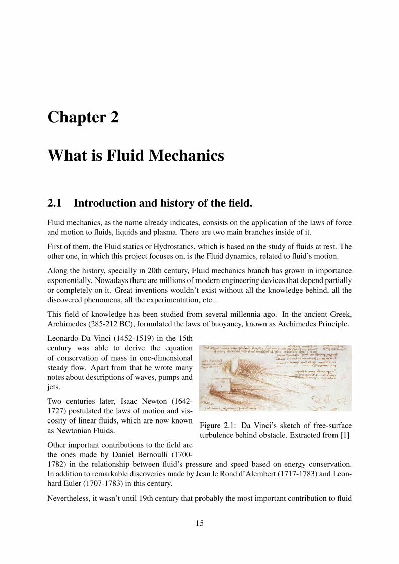
Figure 2.1: Da Vinci’s sketch of free-surfaceturbulence behind obstacle. Extracted from [1]
Leonardo Da Vinci (1452-1519) in the 15thcentury was able to derive the equationof conservation of mass in one-dimensionalsteady flow. Apart from that he wrote manynotes about descriptions of waves, pumps andjets.
Two centuries later, Isaac Newton (1642-1727) postulated the laws of motion and vis-cosity of linear fluids, which are now knownas Newtonian Fluids.
Other important contributions to the field arethe ones made by Daniel Bernoulli (1700-1782) in the relationship between fluid’s pressure and speed based on energy conservation.In addition to remarkable discoveries made by Jean le Rond d’Alembert (1717-1783) and Leon-hard Euler (1707-1783) in this century.
Nevertheless, it wasn’t until 19th century that probably the most important contribution to fluid
15

CHAPTER 2. WHAT IS FLUID MECHANICS
mechanics was made. French engineer Claude-Louis Navier (1785-1836) and Irish mathemati-cian George Gabriel Stokes (1819-1903) succeeded in creating governing equations for realfluid motion. This was an outstanding milestone due to the fact that it was the first time experi-mental and theoretical analysis on the field matched.
These equations are in which today’s fluid dynamics studies are based on. However, mosttheoretical solutions for them remain undiscovered. They often include turbulence, which isstill one of the greatest problems in physics and engineering nowadays.
In the early 20th century, Ludwig Prandtl (1875-1953) came up with the idea of boundary layer.Other contributions to the field were made by Theodore Von Karman (1881–1963) and PaulRichard Blasius (1883–1970).
In this century, due to the difficult challenges that, specially aerodynamics represented, andthe creation of computers, the fluid mechanics shifted from an analytical point of view to anumerical one. This new knowledge branch was called Computational Fluid Dynamics, whichwill be explained in a more detailed way in section 2.4.
Figure 2.2: Historical timeline of fluid mechanics. Extracted from [1]
2.2 Governing equations of fluid mechanics.As it has been exposed, the fluid mechanics theoretical basis rely on the equations presented byClaude-Louis Navier and George Gabriel Stokes. There are two types of approach for them.
16

CHAPTER 2. WHAT IS FLUID MECHANICS
• Lagrangian description.
This is an approach based on the follow-up of the fluid particle and its properties evolutionover time.
In this case, a fluid particle, the tiniest, indivisible, element of fluid is identified by itsinitial position at a time to. Then, Navier-Stokes equations are used to determine its posi-tion inside the study domain at a certain time. Therefore, knowing its location, allows tocalculate other associated characteristics such as velocity, pressure or density.
• Eulerian description.
In contrast to the Lagrangian way, Eulerian approach is based on the monitoring of a fixedpoint in the domain, instead a moving element.
Initially, it is specified the fluid properties (velocity, density, pressure...) in this fixed pointat a chosen time. Then, solving Navier-Stokes equations gives the evolution of mentionedphysical characteristics over time.
This is the most common approach used in fluid mechanics in scientific and industrialstudies. Mainly because, Eulerian way is much more cheaper than Lagrangian in compu-tational costs.
For further information about the physical and mathematical differences between both ap-proaches go to [13].
In this project, Eulerian approach is used in all studies and simulation carried out.
All the following equations are presented in its differential form and from an Eulerian approach.
2.2.1 The material derivativeOne important aspect to understand properly the Navier-Stokes conservation equations is theconcept of Material derivative.
It is defined as follows.
Dφ
Dt=
∂φ
∂ t+∇ · (φu) (2.1)
Expanding the last term of the equation (2.1), it is possible to obtain the following expression.
Dφ
Dt=
∂φ
∂ t+u
∂φ
∂x+ v
∂φ
∂y+w
∂φ
∂ z(2.2)
And, finally, if the velocity variables (u, v and w) also vary with x, y, or z (as in most cases), itcan be obtained the next equation.
Dφ
Dt=
∂φ
∂ t+
∂φu∂x
+∂φv∂y
+∂φw∂ z
(2.3)
17

CHAPTER 2. WHAT IS FLUID MECHANICS
2.2.2 Convection - Diffusion equation.The convection - diffusion equation describes the phenomena in which physical properties of amaterial or fluid are transferred through a system due to convection (advection) and diffusion.
The convection process, also known as advection consists on the transport of physical propertiessuch as temperature or density by the velocity of the particles.
On the other hand, diffusion phenomena comprises the transport of physical properties due tono-null gradients of these ones.
All Navier-Stokes equations can be written based on Convection - Diffusion equation.
Dρφ
Dt= ∇ · (Γφ ∇φ)+Source (2.4)
∂ρφ
∂ t+
∂ρφu∂x
+∂ρφv
∂y+
∂ρφw∂ z
= ∇ · (Γφ ∇φ)+Source (2.5)
Table 2.1: Generic Convection - Diffusion equation parameters for Navier - Stokes equations.Equation φ Γφ Source
Mass Conservation 1 0 0
Momentum Conservation u µ -∇P + ρf
Energy Conservation T λ
Cv-DP
Dt + Φ
As it can be seen, all Navier - Stokes equations are based on the convection or advection anddiffusion phenomena, plus in each case its respective source.
2.2.3 Mass conservation equation.First of them is the Mass conservation equation, also known as the Continuity equation. Itrelates the density and velocity of any material particle during motion.
Dρ
Dt= 0 (2.6)
∂ρ
∂ t+∇ · (ρu) = 0 (2.7)
In a rough way, it can be described as the following statement.
”The rate of increase of mass in a control volume must equal the rate at which mass is flowinginto the volume through its bounding surface per unit of time”
• Density change rate (∂ρ
∂ t ).
It represents the rate at which the density is varying inside the control volume and so itsmass.
18
CHAPTER 2. WHAT IS FLUID MECHANICS
• Flow into the volume (∇ · (ρu)).
It represents the rate at which the mass in flowing in or out the volume through its bound-ing surfaces. It is also known as the convective term of the Mass conservation equation.
This can be expressed in the Cartesian coordinate system as following.
∂ρ
∂ t+
(∂ρu∂x
+∂ρv∂y
+∂ρw∂ z
)= 0 (2.8)
2.2.4 Momentum conservation equation.This equation makes reference to Newton’s second law (the rate of change of any body’s mo-mentum is proportional to the force applied).
The Momentum conservation equation it can be expressed in the following way.
The rate of change of momentum inside a control volume must be equal to the rate at whichmomentum is flowing through its bounding surfaces plus the forces applied on it.
DρuDt
=−∇p+∇ · τ +ρ f (2.9)
∂ρu∂ t
+∇ · (ρuu) =−∇p+∇ · τ +ρ f (2.10)
• Momentum change rate (∂ρu∂ t ).
This term represents the total rate of change of momentum (ρu) inside a control volume.
• Flow into the volume (∇ · (ρuu)).
It represents the rate at which momentum is flowing through the bounding surfaces of thecontrol volume. It is also known as the convective term of the Momentum Conservationequation.
• Pressure gradient (−∇p).
It is the force applied to the control volume surfaces due to a pressure difference betweenits limits. As it can be seen, it is negative. This is due to the fact that the resulting force isalways opposed to it. An increasing gradient in the positive direction results in a negativenet force.
• Viscous stress (∇ · τ).
This term represents the force applied to control volume’s bounding surfaces due to theviscosity of the fluid. This force is generated by the velocities gradients. The higher it is,the higher the shear stress produced and so the forces.
It depends on the physical properties of the fluid. The behaviour may vary significantlyfrom one type of fluid to another. This is the case for instance of viscous and non-viscousfluids.
19

CHAPTER 2. WHAT IS FLUID MECHANICS
• Volumetric force (ρ f ).
This term represents the force applied in the control volume due to a determined grav-itational acceleration or any other non-interaction forces (fundamental forces). In thisproject, only gravity will be set in this term.
The Momentum Conservation equation can be be expressed in the Cartesian coordinate systemas following.
X axis.∂ρu∂ t
+∇ · (ρuu) =−∂ p∂x
+∇ · τ|x +ρgx (2.11)
Y axis.∂ρv∂ t
+∇ · (ρvv) =−∂ p∂y
+∇ · τ|y +ρgy (2.12)
Z axis.∂ρw∂ t
+∇ · (ρww) =−∂ p∂ z
+∇ · τ|z +ρgz (2.13)
2.2.5 Energy conservation equation.The Energy conservation equation is based on the thermodynamics’s law which states that therate of change of energy in a fluid particle must be equal to the energy received by heat andwork transfers.
There are many ways to express this equation depending on the energy variable selected. Spe-cific energy or kinetic energy are other variables this equation can be expressed as a function of.In this case it is presented using the internal specific enthalpy.
DρhDt
=−DPDt−∇q+ τ : ∇u (2.14)
∂ρh∂ t
+∇ · (ρhu) =−DPDt−∇q+ τ : ∇u (2.15)
The energy rate of change of a control volume must be equal to the energy flow through itsbounding surfaces plus the heat transferred and the work applied to the control volume.
To introduce the concept of enthalpy, it is necessary first to present what is the specific energy.
The amount of energy per unit of mass can be expressed as follows.
e = u+12·u2 +g (2.16)
Being u the internal energy per mass of fluid, (12 ·u
2) the kinetic energy per mass of fluid and gthe gravitational potential energy per mass of fluid.
Then, the specific energy and enthalpy can be related in the following way.
h = e+Pρ
(2.17)
20

CHAPTER 2. WHAT IS FLUID MECHANICS
• Energy change rate (∂ρh∂ t ).
It represents the rate of change of energy (ρh) of a control volume.
• Energy flow into the volume (∇ · (ρhu)).
This term comprises the energy flowing through the bounding surfaces of the controlvolume in and out of it.
• Pressure term (−DPDt ).
It represents the rate of energy transfered due to variations of pressure. As it has been ex-posed before, the total energy of a fluid depends on its pressure (equation (2.17)). There-fore, a change on this variable produces a variation of it.
Following the procedure shown in section 2.2.1, this term can be expanded as follows.
DPDt
=∂P∂ t
+∂Pu∂x
+∂Pv∂y
+∂Pw∂ z
(2.18)
• Conduction heat transfer (∇q).
This term represents the heat transfer inside the fluid due to temperature gradients. It isbased on Fourier’s law, which states as following.
qi =−K∂T∂xi
(2.19)
It depends on fluid’s thermal conductivity, K, and is also related to several heat transferphenomena that will be explained in a more detailed way later in this thesis.
• Energy viscous dissipation (τ : ∇u).
It represents the energy transfer due to fluid’s work against viscous forces. As it has beenshown in section 2.2.4, velocity gradients generate viscous stress in the fluid. These createan energy transfer due to dissipation.
The mathematical development of the term can be found in appendix G in Annex docu-ment of this project.
Finally, it is presented the Energy Conservation equation expanded.
∂ρh∂ t
+∇ · (ρhu) =∂P∂ t
+∂Pu∂ t
+∂Pv∂ t
+∂Pw∂ t−∇q+ τ : ∇u (2.20)
For further information about the Fluid Mechanics governing equations go to [14], [15] and[16].
21

CHAPTER 2. WHAT IS FLUID MECHANICS
2.3 Non-dimensionalization.In all physical phenomena there are variables and parameters involved that govern its behaviourand its characteristics. However, it isn’t necessary to know all of them to describe or to quantifythis phenomena. For instance, in order to determine the flow around a cylinder it doesn’t matterif the velocity is 1 m/s or 10 m/s.
What really matters is the relationship between the physical properties involved. This is callednon-dimensionalization.
It consists on removing the physical dimensions from an equation or from a properties relation-ship. Imagine having a problem in which ux represents the horizontal velocity of the flow. Thismagnitude dimensions is m/s, so, fixing a reference velocity Ure f , there can be obtained thedimensionless variable.
UNon−Dim =ux
Ure f
This is a common practice when the problem involves physical phenomena and partial differ-ential equations. In fact, non-dimensionalization isn’t at all necessary to solve or to simulate aproblem. However, it gives a great advantage in terms of experimentation and analysis.
This is the case, for instance, of the simulation of flow inside a pipe. Imagine fixing its non-dimensional variables, for example, a dimensionless diameter. This allows to know the be-haviour of the fluid for the fixed dimensional variables (diameter in this situation), but also forany other dimensional diameter with the same dimensionless value.
The physical or mathematical results are the same if these non-dimensional variables are equalin both cases.
Throughout fluid mechanics history, there have been discovered many physical phenomena in-volved in the behaviour of the fluids. In order to take these into account exploiting the potentialof non-dimensional analysis scientist created different dimensionless numbers to describe andrelate them.
• Reynolds number (Re).
Perhaps, the most famous non-dimensional number in fluid mechanics. Established byOsborne Reynolds (1842 - 1912) in 1883 while studying the flow inside pipes with differ-ent diameters.
It represents the ratio between the inertial forces to viscous forces. As it is explained afterin this thesis, this number is used to differ the flow regime between laminar and turbulent.
Re =ρULre f
µ=
ULre f
ν(2.21)
• Prandtl number (Pr).
Created by the German engineer Ludwig Prandtl (1875 - 1953). It represents the ratiobetween momentum diffusivity to thermal diffusivity.
22

CHAPTER 2. WHAT IS FLUID MECHANICS
Pr =ν
α=
Cpµ
K(2.22)
• Nusselt number (Nu).
Established by Wilhelm Nusselt (1882 - 1957). It is the relationship between the convec-tive and conductive heat transfer at a boundary layer in a fluid.
Nux =∂ (Tw−Tx)
∂y·
Lre f
Tw−T∞
(2.23)
• Rayleigh number (Ra).
Set by the British scientist Lord Rayleigh (1842 - 1919). It is highly related to the Nusseltnumber as it represents the ratio between the convection and conduction heat transfer inthe fluid.
– Natural convection.
Natural convection is characterised by a low heat transfer coefficient. This is becauseof the low fluid motion velocities, since its move occurs by natural means such asbuoyancy [17].
– Forced convection.
In this case the heat transfer increases due to the rise in the velocities. The fluids areforced to move by ceiling fans, pumps, etc... [18].
The frontier between natural and forced convection is determined by the Rayleigh numberalthough this limit may differ from one problem to another. The bigger Rayleigh, thehigher heat transfer.
Ra =ρgβ∆T L3
αµ(2.24)
• Strouhal number (St).
Named after Vincent Strouhal (1850 - 1922). It is a dimensionless number that describesthe oscillating flow mechanisms. In fluid dynamics it is related to vortex shedding (oscil-lating flow that generated vortexes when it goes through an object).
St =f ·Lre f
Ure f(2.25)
• Mach number (Ma).
This non-dimensional number is the rate between the velocity of the fluid and the speed ofsound. It is commonly used in fluid mechanics, especially in aerodynamics. For instance,it is widely accepted the use of Mach number to determine if air flows can be consideredcompressible or not (above 0.3 is compressible).
23

CHAPTER 2. WHAT IS FLUID MECHANICS
Ma =Uc
(2.26)
2.4 Computational Fluid Dynamics.Computational fluid dynamics (CFD) is the application of numerical methods and algorithmsto solve the fluid flow equations. This allows to predict the behaviour of any fluid based on theresolution of the Navier-Stokes equations. These mathematical expressions govern the way afluid flows under any boundary conditions, from water inside a pipe, to planetary atmospheres.
Since no one has ever provided a generic, analytic solution for the Navier - Stokes equations,scientists had to look for alternative ways or determined hypothesis to get reasonable results.This is the case for instance of inviscid fluid studies in the early 20th century.
After World War 2, fluid dynamics problems became a great challenge to scientists and engi-neers to keep solving them analytically, specially aircraft related problems. New inventions anddiscoveries increased significantly the difficulty and the complexity of studies and designs. Thisproved essentially to the development of the numerical methods applied to fluid mechanics andthe so called Computational Fluid Dynamics.
In addition to that, the invention of the computer and the quick and exponential growth of itspower, resulted in a huge expansion of the CFD branch of knowledge.
Apart from that, the main reason of this growth is that today’s industry tendency aims to cutdown all costs as much as possible. When designing a new product or system, it is muchcheaper to simulate and optimise it computationally rather than building a prototype for everydesign modification proposal.
Applying the CFD basis to the design of a system has many advantages over the experimentalway. First of all, it gives an enormous versatility in means of optimisation. For instance, it iseasy to change design parameters without increasing too much the complexity of the problem,in contrast, it would be necessary to build another experimental prototype.
Figure 2.3: CFD simulation of an aircraft. Ex-tracted from [2]
Figure 2.4: CFD simulation of racing car. Ex-tracted from [3]
Secondly, although computers are necessary to carry out a simulation, these allow to developmany of them, which, in the long term, results to be incredibly cheaper than the other way.
24

CHAPTER 2. WHAT IS FLUID MECHANICS
Unfortunately, depending on the complexity of the simulation, it may take a great amount ofcomputation time. However, this time has been continuously reduced over the decades thanks toseveral reasons. First of them, the computational power available has grown exponentially sincethe beginnings of this knowledge branch. In addition, many more efficient solving techniqueshave been implemented.
Nowadays, Computational Fluid Dynamics approaches are widely used in many sectors. Fromaircraft design or automotive industry to biomedical advancements.
Figure 2.5: CFD simulation of F1 racing car.Extracted from [4]
Figure 2.6: CFD simulation of Space Shuttle.Extracted from [5]
Although there are a great amount of different algorithms, methods and techniques applied tothe field, all of them have a common structure.
Figure 2.7: Vertical KaplanTurbine geometry. Extractedfrom [6]
Geometry.
Given a problem, it is necessary to identify its geometry. Defineall its components, specify, if necessary, which hypothesis canbe assumed on each of the studies. Determine which are theconditions of the problem, for instance, the walls temperature,the flow initial speed, etc.
Meshing and resolution.
Then, in order to apply the numerical methods to solve the equa-tions, it is needed to divide this geometry in a determined numberof parts, this is known as spatial discretization. There are sev-eral numerical techniques to make this division, Finite ElementMethod (FEM), Finite Difference Method (FDM) and Final Vol-ume Method (FVM).
All of them are very similar in terms of geometry discretization,with minor variations. However, the major differences comprisethe way how equations are discretized and solved.
25

CHAPTER 2. WHAT IS FLUID MECHANICS
After that, it is necessary to discretize the fluid flow PDE (Partial Differential Equations) andapply them to the created elements of the geometry to solve them.
Figure 2.8: Meshing of different components of Kaplan Turbine. Extracted from [6]
Simulation and post-processing.
Finally, once the simulation has been carried out, it is time for post processing and analysis andvalidation of the obtained results.
Figure 2.9: Analysis and post-processing of the results obtained. Extracted from [6]
26

Chapter 3
Laminar regime
3.1 Theoretical framework
Figure 3.1: Laminar flow velocities profilethrough a channel. Extracted from [7]
In fluid mechanics, laminar flow or laminarregime takes place when a fluid flows in or-derly and parallel layers with no disruptionbetween them. There are no transverse flowor currents. In the case of a channel, all thefluid particles move parallel to its walls, asthere can be seen in figure 3.1.
This situation is mostly characterised bysmall velocities. Since these are relativelylow, the flow is characterised by a high mo-mentum diffusion in comparison to momen-tum convection (advection). This means that,in this kind of flows, it is more likely for phys-ical properties to move through the fluid be-cause of gradients rather than being moved by the flow.
There is virtually no mixing between layers. fluid particles moved on observable paths orstreamlines and it is in this regime when viscosity plays a significant part.
For more information related to the physical phenomena involved in the laminar regime go to[19].
The main parameter that splits a problem between laminar and turbulent regime is the Reynoldsnumber (section 2.3). This parameter quantifies how fast is the flow moving in comparison ofhow viscous it is. At low velocities, Reynolds number is relatively small. Increasing this meansrising the flow rate of the fluid and making it less laminar, less orderly, until turbulent regime isachieved.
From the point of view of Computational Fluid Dynamics, laminar regime is characterisedmainly by the required computational resources. Since the velocities are low, and so otherphenomena like heat transfer doesn’t play a significant part there is no need for a great com-
27

CHAPTER 3. LAMINAR REGIME
putational power. For instance, one aspect that increases enormously the required computingresources are variables’ gradients. In this regime, these are relatively low.
In addition, there can be made several assumptions about the flow to decrease the power needed.In the following section will be presented the hypothesis made for the laminar flow characteris-tics in this project.
3.1.1 Hypothesis and simplifications madeIn this project, there have been made several assumptions that modify the problems slightly andalso cuts down the amount of computational resources necessary to carry out the simulations.
This modifications vary from fluid’s physical properties to equation’s simplifications.
Continuous flow distribution
Although the resolution is numeric instead of analytic, it is assumed that the flow has a bigenough amount of molecules to consider it and its physical properties variation to be continuousin time and space.
Bi-dimensional flow.
This assumption has been made in order to cut down the computational power necessary tocarry out the simulations. The problem, initially three-dimensional has been reduced to a bi-dimensional. The problem geometry has been considered as deep enough in Z dimension toonly take into account flow variations in X-Y plane. This reduces the amount of equations thatmust be solved and so the time and resources needed.
Constant density
In this section of the project, laminar regime, the density of the fluid has been set to be constantin all the spatial and temporal domain. Considering it as incompressible isn’t an assumptionthat may vary a lot the final results in case of not doing it.
If the fluid is a liquid, these suffer tiny density variations in comparison with gases. But also,if this the case, if flow speed is small enough (M < 0.3), the fluid can be considered as incom-pressible. This is the case of laminar regime, characterised by low velocities.
Constant fluid viscosity.
Kinematic and dynamic viscosity vary with fluid’s physical properties such as temperature orpressure. However, these changes not only are almost negligible due to selected flow regime,but also their effects on the overall behaviour and simulation of the fluid don’t play a significantpart.
In addition, this change simplifies slightly the equations to solve and also reduces the necessarycomputing power.
28

CHAPTER 3. LAMINAR REGIME
Newtonian fluid
Depending on the fluid type there can be different modifications in the equations and in fluid’sbehaviour in the simulations. In this case there has been chosen to consider the fluid as Newto-nian. This means that viscous stresses are linearly and directly proportional to the local rate ofchange and deformation of the flow field.
The viscous stresses have the following expression.
τ =−µ · (∇u+∇uT− 23
∇ ·u) (3.1)
In case of incompressible flow, its divergence (∇ ·u) is null in all cases. In addition to that, thehypothesis of constant fluid viscosity mentioned before leads to the following expression of thediffusion term in the Navier-Stokes Momentum Conservation equation.
∇ · τ = µ∇2u (3.2)
Boussinesq approximation.
In order to determine which is the effect that gravity and temperature is going to have on fluid’sbehaviour, it has been selected to use Boussinesq’s theory.
This approximation is only valid when density changes are much smaller than fluid’s density(∆ρ ρ0). Therefore, taking into account that the study cases are incompressible, it can beconsidered as a suitable hypothesis.
g−→ g · (1−β · (T −T0)) (3.3)
This approximation has the same overall effect on the fluid as density changes would have. Thehotter the fluid is (the smaller its density would be) the faster it ascends and the opposite forsmall temperature areas.
For further information about the Boussinesq approximation go to [20] and [21].
Constant thermal conductivity.
As in the previous case, thermal conductivity of a fluid varies with its physical properties, spe-cially temperature. Nevertheless, this change can be assumed without major variations in thefinal results, and it also eases slightly the resolution of the equations.
Constant specific heat coefficient.
Repeatedly, specific heat coefficient of a fluid varies with its physical properties.
However, in order to ease the resolution of Energy conservation equation dramatically, it hasbeen considered as constant. As it can be seen in section 2.2.5, the equation 2.20 has as heatvariables specific enthalpy and temperature.
29
CHAPTER 3. LAMINAR REGIME
So, in order to simplify them into a unique work variable, considering the specific heat coeffi-cient as constant is necessary. If so, enthalpy can be written as follows.
dh =Cp ·dT (3.4)
Negligible energy pressure dissipation.
Although it is part of the Energy conservation equation (2.20), it doesn’t play a significantpart on fluid’s behaviour. Pressure energy dissipation comes due to high rates of change on it.However, in laminar regime these variations are relatively small, and so the energy dissipationdue to them.
Negligible viscous energy dissipation.
Again, this viscous dissipation term is part of the Energy conservation equation. Nevertheless, itis rarely important. It is taken into account only for simulations of high speed flows and narrowcapillaries where viscous heating is not negligible.
In this flow regime, it doesn’t play a big role on the Energy Conservation equation effects, andalso removing it cuts down a lot the computing power and implementation time needed.
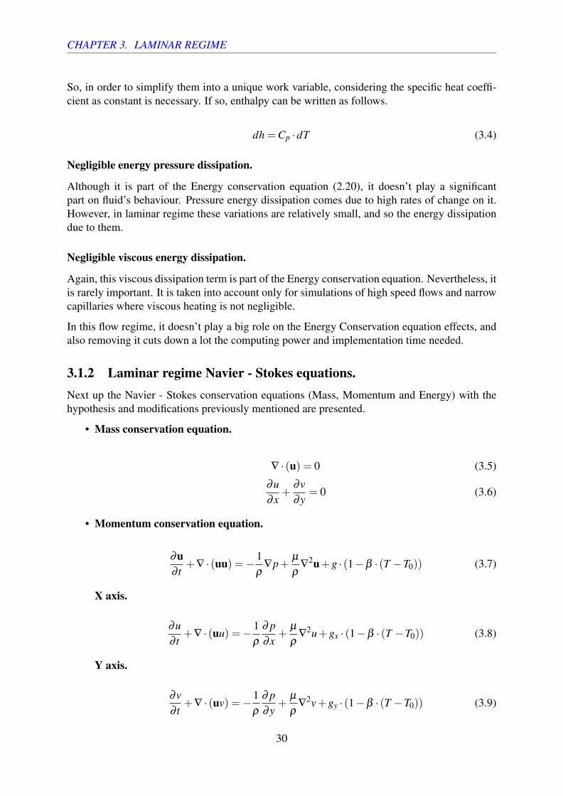
3.1.2 Laminar regime Navier - Stokes equations.Next up the Navier - Stokes conservation equations (Mass, Momentum and Energy) with thehypothesis and modifications previously mentioned are presented.
• Mass conservation equation.
∇ · (u) = 0 (3.5)
∂u∂x
+∂v∂y
= 0 (3.6)
• Momentum conservation equation.
∂u∂ t
+∇ · (uu) =− 1ρ
∇p+µ
ρ∇
2u+g · (1−β · (T −T0)) (3.7)
X axis.
∂u∂ t
+∇ · (uu) =− 1ρ
∂ p∂x
+µ
ρ∇
2u+gx · (1−β · (T −T0)) (3.8)
Y axis.
∂v∂ t
+∇ · (uv) =− 1ρ
∂ p∂y
+µ
ρ∇
2v+gy · (1−β · (T −T0)) (3.9)
30

CHAPTER 3. LAMINAR REGIME
Since the flux has been considered as bi-dimensional in X-Y plane, there is no need forconsidering Z axis equations anymore.
• Energy conservation equation.
∂T∂ t
+∇ · (uT ) =K
ρCp∇
2T (3.10)
These are the equations which will be used on this part of the project.
3.1.3 Laminar regime study cases.To give a better insight of the simulation cases and their particularities, each of them will bepresented in this section before showing obtained results in their respective sections later.
LID Driven Cavity.
The first of the 3 laminar simulated problems is one of the most known cases in CFD field, LIDDriven Cavity.
It consists on a cavity opened only on the upper side, in which a fluid flows parallel to. In orderto give a better insigh of this problem it is its presented the scheme in figure 3.2.
Figure 3.2: LID Driven Cavity case scheme
As it can be seen in the scheme, on the top of the cavity the fluid only has horizontal velocity,while vertical is null. On the rest of the walls, non-slip condition is imposed. This means thatright on them (on its surface) all the velocities (U and V) remains null during all the simulation.
At low Reynolds numbers (high viscosity and low speeds), it is only possible to appreciate thelarge central vortex. However, the bigger the Reynolds is, the more easy to see little vortexes at
31

CHAPTER 3. LAMINAR REGIME
the corners of the cavity. This phenomena will be shown in a more detailed way in LID DrivenCavity results section (section 3.3).
LID Differentially Heated.
The second laminar regime study case is known as LID Differentially Heated or LID-DrivenDifferentially Heated. It consists on an enclosed cavity with the vertical walls at different tem-peratures, while the top and bottom are completely adiabatic (thermally isolated).
This simulation case has two main differences from the other laminar regime problems. First,it is the only one in which Energy Conservation equation must be solved. This process willbe explained later. And secondly, it is the only one in which gravity is considered. Otherwise,since there is no velocity source (like in LID Driven Cavity case), the fluid wouldn’t move nomatter the walls’ temperatures.
In the following figure 3.3 it is presented the problem scheme.
Figure 3.3: LID Differentially Heated case scheme
In the case of figure 3.3, left wall’s temperature (TLe f t) is considered to be higher than the rightone (TRight in the picture). Due to this fact, the fluid, when approaching first one, heats up andascends, while when getting closer to the right wall, loses its heat and goes down. This createsan infinite loop that ends in a steady state.
Again, non-slip condition is imposed on every solid wall, turning all the horizontal and verticalvelocities on them to zero.
32

CHAPTER 3. LAMINAR REGIME
Finally, it is important to mention that, in this case, the main parameter that governs the fluidbehaviour (velocity and viscosity) is the Rayleigh number (see section 2.3). This happens dueto the important role that heat transfer plays in this problem.
Square Cylinder.
Last case of simulation is known as Square Cylinder or Flow past a Square Cylinder. As itsname already indicates, it consists on a square cylinder around which there is fluid flowing.
To have a better insight of the problem, it is presented its scheme in figure 3.4.
Figure 3.4: Square Cylinder case scheme
Again, non-slip condition is imposed on every solid wall (top and bottom walls). On the otherhand, the inlet of the system (the fluid entrance) is characterised by a parabolic horizontal veloc-ity profile. The outlet boundary condition is considered to be null gradients on both horizontaland vertical velocities.
Apart from being the most difficult to implement and the problem that requires the most com-putational resources, it has a special characteristic that differs it from the other two previouslypresented.
The main parameter that governs the flow is Reynolds number, as in LID Driven Cavity case.In this problem, rising this value made small lateral vortexes to be more appreciable, but theyremained in an steady state.
However, in Square Cylinder, increasing Reynolds number above a called Critical Reynoldscauses moving vortexes to appear behind the cylinder. These are known as Von−KarmanVortexes. To have a better understanding of this phenomena, see Square Cylinder results insection 3.5.
33

CHAPTER 3. LAMINAR REGIME
3.2 Numerical frameworkAs it has been previously mentioned, no one has ever been able to give a solution for genericNavier - Stokes equations, only a few times with highly restricted boundary conditions. How-ever, the aim of this project comprises several study requirements and conditions that would beimpossible to fulfil with an analytic approach. Therefore, numerical methods are indispensableto get the desired results.
In this project, Finite Volume Method (FVM) is used. This is a method for discretizing andsolving partial differential equations in algebraic form.
This numerical method has several advantages. First, it is relatively easy to adapt the discretiza-tion to the selected geometry, it has a great flexibility. In addition, it imposes the conservationof the physical properties of the equations and gives a great insight and intuitive idea whilediscretizing them.
It consists on dividing the study domain in a determined number of non-overlapping fixed vol-umes. All of these have a node right on each of their centroids. In figure 3.5 these controlvolumes are presented as cubes (or squares in 2D). However, there are many other geometricalshapes these can be described with, such as tetrahedrons, pyramids, prisms or hexahedrons in3D or in 2D, triangles, circular sections, etc...
ΦCenter
West Face
Front Face
East Face
North Face
South Face
Back Face
Figure 3.5: Finite Volume Method representation
FVM considers that, the value of any physical variable in the volume is its the mean value in allof the volume.
34
CHAPTER 3. LAMINAR REGIME
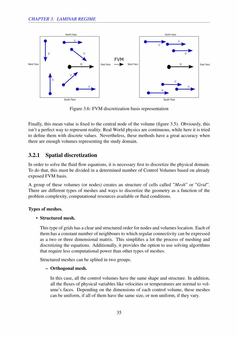
Figure 3.6: FVM discretization basis representation
Finally, this mean value is fixed to the central node of the volume (figure 3.5). Obviously, thisisn’t a perfect way to represent reality. Real World physics are continuous, while here it is triedto define them with discrete values. Nevertheless, these methods have a great accuracy whenthere are enough volumes representing the study domain.
3.2.1 Spatial discretizationIn order to solve the fluid flow equations, it is necessary first to discretize the physical domain.To do that, this must be divided in a determined number of Control Volumes based on alreadyexposed FVM basis.
A group of these volumes (or nodes) creates an structure of cells called ”Mesh” or ”Grid”.There are different types of meshes and ways to discretize the geometry as a function of theproblem complexity, computational resources available or fluid conditions.
Types of meshes.
• Structured mesh.
This type of grids has a clear and structured order for nodes and volumes location. Each ofthem has a constant number of neighbours to which regular connectivity can be expressedas a two or three dimensional matrix. This simplifies a lot the process of meshing anddiscretizing the equations. Additionally, it provides the option to use solving algorithmsthat require less computational power than other types of meshes.
Structured meshes can be splited in two groups.
– Orthogonal mesh.
In this case, all the control volumes have the same shape and structure. In addition,all the fluxes of physical variables like velocities or temperatures are normal to vol-ume’s faces. Depending on the dimensions of each control volume, these meshescan be uniform, if all of them have the same size, or non uniform, if they vary.
35

CHAPTER 3. LAMINAR REGIME
Figure 3.7: Structured Orthogo-nal Uniform mesh
Figure 3.8: Structured Orthogo-nal Non-Uniform mesh
– Non orthogonal mesh.
These types of meshes are used to adapt the control volumes to the geometry bound-aries of the problem. They allow to represent more complex geometries than orthog-onal meshes. However, fluxes through the surfaces are no longer normal to them, sothe implementation difficulty rises.
Figure 3.9: Non orthogonal mesh for airfoil simulation. Extracted from [8]
• Unstructured mesh.
Unlike structured meshes, these don’t have a constant number of neighbours around them.This allows to discretize a great range of different and complex geometries in addition tosetting many different and useful options to the grid. However, the difficulty of meshingand equation’s solving process increases dramatically in front of a structured grid.
36

CHAPTER 3. LAMINAR REGIME
Figure 3.10: Unstructured mesh for airfoil simulation. Extracted from [9]
• Hybrid mesh.
This type of mesh contains portions of structured and unstructured meshes. Regular andeasy parts of the geometry are discretized using structured grids, while more complexones (or where it is more useful) use an unstructured mesh.
Figure 3.11: Hybrid mesh. Extracted from [10]
Apart from that, there are many meshing techniques beyond initial discretization. This is casefor instance of adaptive meshes refinement, moving or rotating grids, etc..
In this project, structured orthogonal uniform and non-uniform meshes are used. Since selectedgeometries for the simulations are fixed and not highly complex, there is no need for imple-menting non-orthogonal or unstructured meshers.
Additionally, it is necessary to select one last characteristic of the grid. If it is going to be aCollocated Mesh or a Staggered Mesh.
37

CHAPTER 3. LAMINAR REGIME
In bi-dimensional, incompressible and cartesian-based CFD problems there are 3 main variablesto which a mesh has to be created. Pressure and horizontal and vertical velocity, P, U and Vrespectively. In what comes to the temperature variable, this share mesh with the pressure.
Depending on the type of grid (Collocated or Staggered) there will be necessary to have 1 or 3spatial grids.
• Collocated mesh.
In this case, a node is located at the centroid of each control volume (as usual in FVM).All of aforementioned variables (P, U and V) of the control volume, have to be spatiallyset on this node. Only 1 mesh is necessary to discretize the domain.
Figure 3.12: Structured Orthogonal Uniform Collocated mesh scheme
Although this may seem an easy and suitable way to discretize the domain for CFD be-giners, it has a great disadvantage.
While solving velocities’ field in Navier-Stokes equations, pressure must be obviouslytaken into account. However, this kind of discretization decouples the velocities and thepressure of each node. This numerical phenomena is known as Checkerboard.
To give a better insigth, it is presented the next problem. Imagine this is the pressure fieldof an arbitrary case (figure 3.13). It is necessary to determine the velocity U2. To do that,pressure gradient of the node N2 must be determined among other parameters.
Figure 3.13: Checkerboard case representation
However, the pressure of this node N2 (5 Pa) isn’t used to calculate it. In collocatedmeshes West and East neighbours’ pressure are used.
38

CHAPTER 3. LAMINAR REGIME
∂P∂x
=50 Pa−50 Pa
∆X= 0
The pressure and the velocities decouple. This generates numerical instabilities and os-cillations of the results.
There are techniques to avoid this problem using a Collocated mesh. Nevertheless, in thisproject there has been chosen to use Staggered meshes for the laminar regime part.
• Staggered mesh.
Unlike previous case, choosing a staggered mesh means creating 3 different grids. Onefor pressure, P, one for horizontal velocity, U, and last one, for vertical velocity, V.
Pressure mesh remains equally in location to the previous Collocated mesh. However, Uand V nodes are placed exactly at the surfaces of pressure’s control volumes. Horizontalvelocity located at the vertical walls (West and East) and vertical velocity at horizontalwalls (South and North) (figure 3.5).
Next up it is presented an structured orthogonal uniform staggered mesh (figure 3.14).
Figure 3.14: Structured Orthogonal Uniform Staggered mesh scheme
In this case, there is no Checkerboard-related problem. When calculating horizontal orvertical velocities (U or V respectively), there isn’t a pressure node right on the samelocation. This allows to compute pressure gradients without the issue of decoupling.
In addition, this mesh configuration ease the implementation of the discretized equationsin case of using FVM (as it has been done).
Having 3 different meshes each of them with a variable rises the implementation difficultyand the risk of making programming errors that may give wrong results. Nevertheless,this type of mesh gives great stability and avoid problems like mentioned Checkerboard.
39

CHAPTER 3. LAMINAR REGIME
As shown in figures 3.15, 3.16 and 3.17, the combination of these 3 meshes creates thegrid on figure 3.14.
Figure 3.15: Pressure (P)mesh
Figure 3.16: Vertical velocity(V) mesh
Figure 3.17: Horizontal veloc-ity (U) mesh
Modifications for the Staggered mesh.
Additionally, although it is not considered part of the staggered mesh, it is necessary to locatenodes right on the solid walls.
As it can be seen in figure 3.14, there are horizontal velocity (U) nodes on the vertical wallsand so V nodes in horizontal ones. However, to be able to impose boundary conditions to thesimulation, it is also needed to locate U nodes on the horizontal walls and V ones in the verticals.
In conclusion, the final staggered mesh have the following shape (figure 3.18).
Figure 3.18: Structured Orthogonal Uniform modified Staggered mesh scheme
Meshing of the study cases.
Once all types of different meshes and grid characteristics have been presented, there will beexposed the chosen discretization options for each of the problem cases.
40

CHAPTER 3. LAMINAR REGIME
To solve correctly a CFD problem getting accurate results it is essential to choose the adequatemeshing options. Is the grid going to be structured, unstructured, uniform... In this case, as ithas been previously mentioned, all the meshes developed are structured and orthogonal.
First, it is so important to remark that, since CFD is based on discrete solutions of a continuousphysical world, it is impossible to achieve a 100% accuracy. However, the higher the number ofdiscrete points, the more precise results can be obtained.
Other important factor that affects dramatically the meshes is the problem’s physical conditions.It isn’t the same to simulate the flow around an aircraft travelling at 300 km/h than do it for an800 km/h velocity. Reynolds number is higher, speeds and pressures gradient are much bigger,etc...
This kind of different conditions in the problems is what makes them to require one type ofmesh or other. In this project, there will be different mesh requirements for each case of studyand even in the same problem, for different Reynolds or Rayleigh numbers.
The higher this non-dimensional values, the higher the number of nodes on the domain required.Especially where the gradients are higher. This is the case of solid walls.
As it has been mentioned, all solid walls in all the problems have been set with the non-slipcondition (velocities drop to zero on the surface). However, these are not null close to them.Therefore, velocity gradients are huge in this area when compared to the middle of the geometry.
This is the main reason why when increasing parameters like Reynolds or Rayleigh numbers itis necessary to locate many control volumes (nodes) near each wall. This is known as ”MeshDensi f ication”.
All meshes of the laminar regime part of the project are bi-dimensional. This means that theyhave a certain number of nodes in the horizontal direction and in the vertical (NX and NY re-spectively).
In order to locate them, there are several mathematical expressions that are commonly used.Next up are presented the ones implemented for these cases.
• Regular distribution.
As its name already indicates, this type of distribution places the nodes in a way all ofthem are equally separated from its neighbours. All the control volumes have the samesize and dimensions.
∆X =XTOTAL
NX∆Y =
YTOTAL
NY(3.11)
This type of distribution leads to an orthogonal uniform mesh (figure 3.7).
• Hyperbolic tangent distribution.
This is one of the most used types of nodes distribution in CFD problems. As it has beensaid, one crucial aspect of the meshing process is the densification near the walls. Thistype of distribution covers this need. It can be observed in figure 3.20 the clear change innode’s density near the edges.
41

CHAPTER 3. LAMINAR REGIME
This distribution not only locates enough nodes automatically near the walls, but also itreduces the total amount of these needed, cutting down the computational power and timerequired.
In addition, the grade of densification can be controlled by modiying one parameter. Thisis the Stretching Factor or Densi f ication Factor (SF in equation (3.12)). The higher itis, the more nodes are located near the walls.
xi =L2·
[tanh(SF ·
(2·i−NXNX
))
tanh(SF)+1
](3.12)
Figure 3.19: Hyperbolic tangentfunction (SF = 1.5)
Figure 3.20: Structured Orthogo-nal Hyperbolic tangent horizontaldistribution mesh (SF = 1.5)
It must be mentioned that this node’s type of location (as it is shown in figure 3.20) isn’tfixed. It can be modified just to take one half of the distribution and increasing the densityonly in one of the edges. Or, as it has been aforementioned, locating much more or lessnodes on the walls.
• Cosine distribution.
Although this type of distribution may seem the same as half hyperbolic tangent, theydiffer in one crucial aspect. Unfortunately, cosinoidal distribution can’t modify nodaldensity near the walls (this is only possible by changing the total number of nodes in thedirection).
However, despite it is a bit hard to observe in figure 3.22, for the same number of nodesin the horizontal direction, cosinoidal distribution places the first node much closer to thewall than hyperbolic tangent one.
This is really important for CFD simulations. As it has been mentioned, it is crucial tohave enough nodes near the walls where large gradients take place. But, it is even moreimportant the distance between the wall and the closest node. If this isn’t small enough,the simulation may give wrong or nonsense results.
42
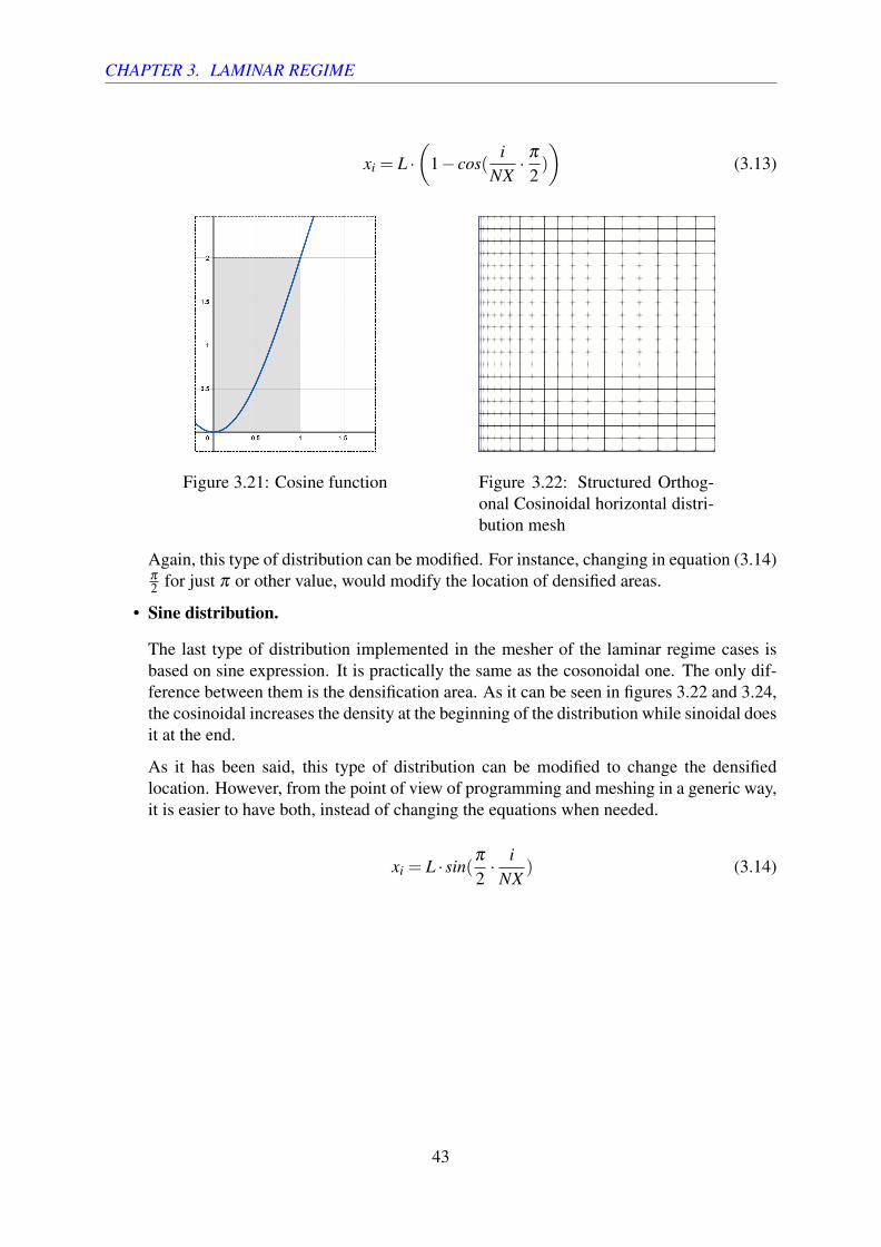
CHAPTER 3. LAMINAR REGIME
xi = L ·(
1− cos(i
NX· π
2)
)(3.13)
Figure 3.21: Cosine function Figure 3.22: Structured Orthog-onal Cosinoidal horizontal distri-bution mesh
Again, this type of distribution can be modified. For instance, changing in equation (3.14)π
2 for just π or other value, would modify the location of densified areas.
• Sine distribution.
The last type of distribution implemented in the mesher of the laminar regime cases isbased on sine expression. It is practically the same as the cosonoidal one. The only dif-ference between them is the densification area. As it can be seen in figures 3.22 and 3.24,the cosinoidal increases the density at the beginning of the distribution while sinoidal doesit at the end.
As it has been said, this type of distribution can be modified to change the densifiedlocation. However, from the point of view of programming and meshing in a generic way,it is easier to have both, instead of changing the equations when needed.
xi = L · sin(π
2· i
NX) (3.14)
43

CHAPTER 3. LAMINAR REGIME
Figure 3.23: Sine function Figure 3.24: Structured Orthog-onal Sinoidal horizontal distribu-tion mesh
All of these nodal distributions types have been implemented to the code’s mesher. However,not all of them have been used in the same problem case. Next up will be presented which arethe nodal configurations that have been chosen to carry out the simulations.
LID Driven Cavity meshing.
In the first study case, LID Driven Cavity, while the Reynolds number of the simulation wasn’thigher than 400 approximately, the mesh distributions used were both regular, resulting in aUniform grid.
However, once this value was surpassed, there was decided to used a hyperbolic tangent distri-bution on the horizontal direction, and cosinoidal at the vertical. With them , it was possible todensify near the 3 walls of the cavity, while setting in the upper part enough nodes to have anacceptable resolution.
Figure 3.25: LID Driven Cavity mesh
LID Differentially Heated meshing.
44

CHAPTER 3. LAMINAR REGIME
For the second study case, LID Differentially Heated, the meshing selected is very similar tothe previous problem.
The firsts simulations, with a relatively low Rayleigh number were done with a regular Uniformmesh. Once this parameter was above 1E4 approximately, horizontal and vertical directions’distributions were changed to hyperbolic tangent, since this time there also a solid wall at thetop of the geometry.
This final mesh is presented in figure 3.26.
Figure 3.26: LID Differentially Heated mesh
Square Cylinder meshing.
Last case, Square Cylinder, is for sure the most complex problem for meshing in the laminarregime presented cases. This is because the geometry domain (figure 3.4) is divided into 9different areas (figure 3.27).
Figure 3.27: Square Cylinder geometry division
Each of these zones have to have a different nodal distribution in order to reduce the computa-tional power required but always having a good resolution and acceptable results
To do that, one of the crucial aspects was the meshing around the cylinder, and also the upperand lower walls. It is the critical part of the geometry. If there weren’t enough nodes close to it,the simulation would not be possible to carry out or would give nonsense results.
In table 3.1 are presented the distributions selected for the simulations.
45

CHAPTER 3. LAMINAR REGIME
Table 3.1: Nodal distribution selected for Square Cylinder caseZone X distribution Y distribution
1 Senoidal/Hyperbolic Hyperbolic
2 Regular Hyperbolic
3 Cosinoidal Hyperbolic
4 Senoidal/Hyperbolic Regular
5 Cosinoidal Regular
6 Senoidal/Hyperbolic Hyperbolic
7 Regular Hyperbolic
8 Cosinoidal Hyperbolic
9 Regular Regular
It is so important to choose the correct distributions on the right areas not just because of allaforementioned about nodal densification, resolution, etc. All the 9 different meshes must matchwith their neighbours, if not, the codes couldn’t even be executable due to meshing nonsenses.
Next up is shown in figure 3.28 the global grid with mentioned nodal distributions for SquareCylinder case.
Figure 3.28: Square Cylinder mesh distributions used in the simulations
Additionally is presented a detailed view of the mesh in the cylinder area (figure 3.29).
Figure 3.29: Local meshing around the cylinder in Square cylinder case
3.2.2 Resolution of the equations.Once all the meshes are correctly and fully developed, it is necessary to choose a solving methodfor the incompressible Navier-Stokes equations.
46
CHAPTER 3. LAMINAR REGIME
Fractional Step Method.
To solve the fluid-flow equations, Fractional Step Method (FSM) is selected ([22] and [23]).It is one of the most commonly implemented methods to solve incompressible Navier-Stokesequations. It has several advantages over other numerical techniques.
First, it is easier to program than other ones. It stands out for its simplicity. In addition, itprovides a better computational performance than other solving methods.
It is used to solve the Mass and Momentum Conservation equations. In case of the Energy one,it isn’t necessary the application of this method but only a time integration technique.
Next up will be presented all the FSM algorithm and explained in a detailed way.
First of all, it is necessary to have the equations that are going to be solved. These are theones presented in section 3.1.2 (they are already simplified with all hypothesis assumed, section3.1.1).
Mass and Momentum Conservation equations resolution.
Since this is the resolution of an incompressible fluid problem, it is only necessary to deter-mine pressure (p) and horizontal and vertical velocities (U and V respectively) from these twoequations, (3.5) and (3.7).
The first step consist on splitting the Momentum equation (3.7) in three different terms.
∂u∂ t
= F(u)+S(p) (3.15)
Where:
F(u) =−∇ · (uu)+µ
ρ∇
2u+g · (1−β · (T −T0)) (3.16)
S(p) =− 1ρ
∇p (3.17)
On the other side of the equation, it is necessary to write the velocity change rate in terms oftime steps.
∂u∂ t
=un+1−un
∆t(3.18)
Reorganising equation (3.15) with this last modification of equation (3.18) the following ex-pression can be obtained.
un+1 = un +∆t ·F(u)+∆t ·S(pn+1) (3.19)
Then, a Predictor velocity (u∗) must be defined. It is an approximate solution for the momentumequation.
u∗ = un +∆t ·F(u) (3.20)
47

CHAPTER 3. LAMINAR REGIME
Combining last expression with equations (3.17) and (3.19), the following can be obtained.
un+1 = u∗− ∆tρ
∇pn+1 (3.21)
Here comes the crucial part of the Fractional Step Method. Applying Divergence operator atboth sides of equation 3.21 leads to the next expression.
∇ ·un+1 = ∇ ·u∗− ∆tρ
∇ · (∇pn+1) (3.22)
Now, taking into account incompressible Mass Conservation equation (3.5), left term of expres-sion (3.22) can be removed. Therefore the following can be obtained.
1∆t·∇ ·u∗ = 1
ρ∇
2 pn+1 (3.23)
This expression is known as Poisson’s pressure equation. Since the predictor velocity can’tsatisfy the incompressibility hypothesis at the next time step, Poisson’s equation determines theminimum perturbation on the flow that makes predictor to be incompressible [22].
From equation 3.23, it is possible to compute the pressure of the next time step (n+1). Once ithas been calculated, U and V velocities can be calculated.
In order to do that, it is only needed to decompose equation (3.21) in Cartesian axis.
Horizontal velocity (u):
un+1 = u∗− ∆tρ
∆pn+1
∆x(3.24)
Vertical velocity (v):
vn+1 = v∗− ∆tρ
∆pn+1
∆y(3.25)
Energy Conservation equation resolution.
Unlike previous Mass and Momentum equations, for Energy one there is no need for applyingFSM to solve it.
In this case, only it is necessary to reorganise the equation’s terms to develop a temporal inte-gration (this last step will be explained in a more detailed way in section 3.2.3).
On the basis of equation (3.10), it is only needed to write it in the following way.
∂T∂ t
= F(T ) (3.26)
48
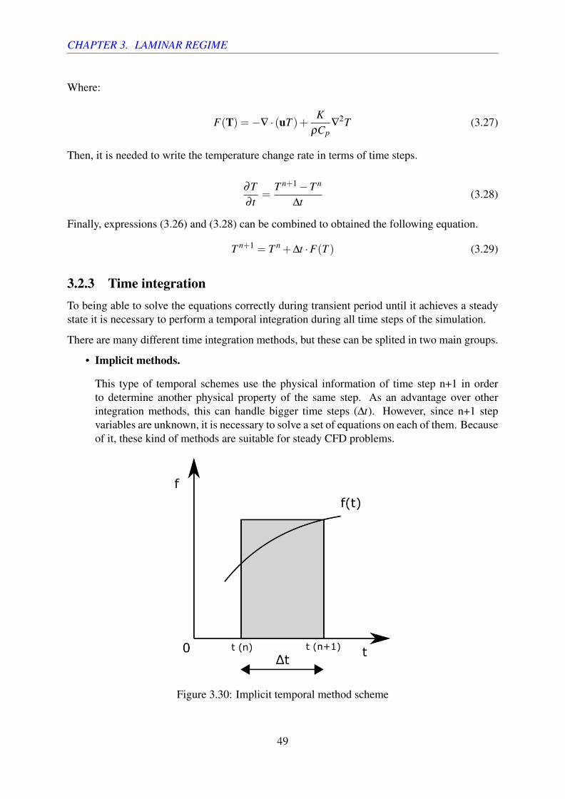
CHAPTER 3. LAMINAR REGIME
Where:
F(T) =−∇ · (uT )+K
ρCp∇
2T (3.27)
Then, it is needed to write the temperature change rate in terms of time steps.
∂T∂ t
=T n+1−T n
∆t(3.28)
Finally, expressions (3.26) and (3.28) can be combined to obtained the following equation.
T n+1 = T n +∆t ·F(T ) (3.29)
3.2.3 Time integrationTo being able to solve the equations correctly during transient period until it achieves a steadystate it is necessary to perform a temporal integration during all time steps of the simulation.
There are many different time integration methods, but these can be splited in two main groups.
• Implicit methods.
This type of temporal schemes use the physical information of time step n+1 in orderto determine another physical property of the same step. As an advantage over otherintegration methods, this can handle bigger time steps (∆t). However, since n+1 stepvariables are unknown, it is necessary to solve a set of equations on each of them. Becauseof it, these kind of methods are suitable for steady CFD problems.
Figure 3.30: Implicit temporal method scheme
49

CHAPTER 3. LAMINAR REGIME
• Explicit methods.
Unlike implicit methods, explicit schemes use the physical data information of present (n)or previous time steps (n-1, n-2, ...) to compute next’s step one (n+1). On the one hand,these type of methods are computationally lighter. They do not require to solve a coupledsystem of equations. However, time steps’ length (∆t) are relatively smaller than in caseof implicit schemes. Nevertheless, these methods are commonly used for transient statesimulations.
Figure 3.31: Explicit temporal method scheme
In this project, it has been selected to do temporal integration with an explicit scheme, more pre-cisely, a second-order Adams-Bashforth scheme. Its basis consists on determining the propertyvalue of next time step by using present and former time steps information.
As it can be observed in section 3.2.2, in many of the final equations appears the term F(u), F(v)or F(T).
These are the terms in which Adams-Bashforth method is applied. They are computed byevaluating them on the present and former time steps and assigning each a certain coefficient.
F(u) =32·F(un)− 1
2·F(un−1) (3.30)
Applying this to equations (3.20) and (3.29) leads to the following expressions respectively.
u∗ = un +∆t ·[
32·F(un)− 1
2·F(un−1)
](3.31)
T n+1 = T n +∆t ·[
32·F(T n)− 1
2·F(T n−1)
](3.32)
There is still something in temporal integration process that hasn’t been determined yet. Tosolve all exposed equations, as these has been presented, it is necessary to compute the timesteps value (∆t). This is a crucial part of the simulation. If the time step is too small, the
50

CHAPTER 3. LAMINAR REGIME
execution of the code may last days until the flow achieves an steady state. However, if it is toolarge, the simulation may diverge and stop.
Courant–Friedrichs–Lewy condition.
To determine the correct value, Courant–Friedrichs–Lewy (CFL) condition is used. This isn’tan exact solution for the calculation of time steps value. However, it is an approximation easy toimplement which gives relatively good stability to the simulations. Unfortunately, the demon-stration of ∆t calculation without this method uses advanced mathematics which are far awayfrom project’s scope. More information about this can be found in [24].
CFL condition is based on the following expressions.
∆tc = min(
0.35∆x|u|
, 0.35∆y|v|
)(3.33)
∆td = min(
0.20ρ∆x2
µ, 0.20
ρ∆y2
µ
)(3.34)
∆tdh = min(
0.20ρCp∆x2
K, 0.20
ρCp∆y2
K
)(3.35)
Every time step, it is necessary to compute the minimum of these 3 equations and look for thesmallest one.
∆t = min(∆tc,∆td,∆tdh) (3.36)
Each of these expressions takes into account different flow phenomena that influences simula-tion’s process. Equation (3.33) is based on flow’s convection. It is clear that time step valuecan’t be higher than the time needed for the flow to travel from one node to its neighbour.The same is applied to expressions (3.34) and (3.35) for diffusion terms of the Momentum andEnergy Conservation equations respectively.
In addition, there are different coefficients on these equations (0.35 in expression (3.33) and0.20 in (3.34) and (3.35)). Since this method is an approximation, these expressions are set withcoefficients smaller than 1 to ensure the stability of the simulations.
Nevertheless, they are not fixed. Along all the simulations carried out, these coefficients havebeen modified depending on the conditions. For instance, it is suitable to change 0.20 for 0.10or 0.05 in time step calculation but on the other side, cut down dramatically the total number ofnodes of the discretization. It is based on looking for an overall improvement of the simulationperformance modifying the different options available.
3.2.4 Discretization of the equations.Once the spatial and temporal discretizations have been exposed, it is necessary to present howare equations in section 3.2.2 going to be adapted to these.
51

CHAPTER 3. LAMINAR REGIME
Next up are exposed all the aforementioned equations to be discretized.
Divergence Theorem.
All the discretizations are based on the application of the Divergence Theorem.
(∇ ·Φ) =1Ω
∫∫∫dV
∇ ·ΦdV =1Ω
∫∫dS
Φ ·dS (3.37)
This theorem is one of the basis of Finite Volume Method. However equation (3.37) is still incontinuous mathematics. It is necessary to transform it to discrete values.
1Ω
∫∫dS
Φ ·dS =1Ω
∑Φ f ·n ·∆S (3.38)
• Poisson’s pressure equation.
1∆t·∇u∗ =
1ρ
∇2 pn+1 (3.39)
Figure 3.32: Pressure node P discretization scheme
First term:
1∆t
∇ · (u∗) =1∆t
1Ω
∫∫∫dV
∇ ·u∗dV =1∆t
1Ω
∫∫dS
u∗dS = ∑u∗f n ·∆S (3.40)
=1∆t
1Ω[u∗e∆Se−u∗w∆Sw + v∗n∆Sn− v∗s ∆Ss]︸ ︷︷ ︸
bp
Next up only the discretization of Predictor’s velocity u∗P will be presented. To see all theother ones go to appendix A in Annex document of this project.
u∗P = uP +∆t[
32·F(un
P)−12·F(un−1
P )
](3.41)
52

CHAPTER 3. LAMINAR REGIME
F(unP) =−∇ · (uP ·uP)+
µ
ρ∇
2uP +g(1−β (TP−T0)) (3.42)
Figure 3.33: F(u) discretization scheme
Discretization of convective term.
∇ · (uu) =1Ω
∫∫∫dV
∇ · (uu) dV =1Ω
∫∫dS
uu dS =1Ω
∑uuf ·n∆S (3.43)
=1Ω[ueue∆Se−uwuw∆Sw +unvn∆Sn−usvs∆Ss]
As it can be seen in figure 3.33, these velocities (ue, uw, vn, ...) of the convective termequation (3.43) are not assigned to any node.
Convective schemes.
Since the mathematical discretization locates these velocity terms at the walls of eachcontrol volume, it is necessary to compute them as accurately as possible. The aim of theconvective or numeric schemes consists on calculating these values.
There are many types of convective schemes. Depending on problem’s characteristicsthere are some that are more suitable or others that may make the simulation to diverge.In addition to that, numeric schemes can be of different orders.
The fact of being a first, second, third, etc.. order convective scheme is related with theaccuracy of the simulation. The higher its order, the faster error decreases with moredensified meshes.
53
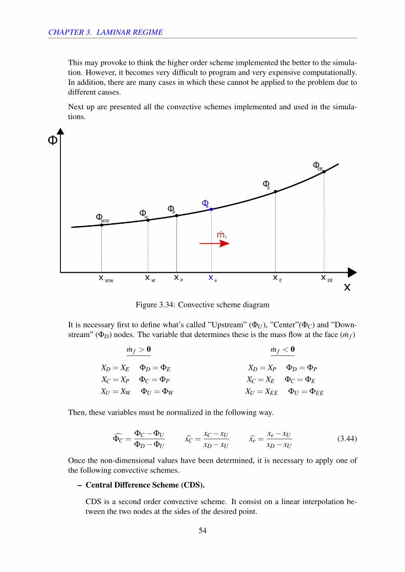
CHAPTER 3. LAMINAR REGIME
This may provoke to think the higher order scheme implemented the better to the simula-tion. However, it becomes very difficult to program and very expensive computationally.In addition, there are many cases in which these cannot be applied to the problem due todifferent causes.
Next up are presented all the convective schemes implemented and used in the simula-tions.
Figure 3.34: Convective scheme diagram
It is necessary first to define what’s called ”Upstream” (ΦU ), ”Center”(ΦC) and ”Down-stream” (ΦD) nodes. The variable that determines these is the mass flow at the face (m f )
m f > 0 m f < 0
XD = XE ΦD = ΦE XD = XP ΦD = ΦP
XC = XP ΦC = ΦP XC = XE ΦC = ΦE
XU = XW ΦU = ΦW XU = XEE ΦU = ΦEE
Then, these variables must be normalized in the following way.
ΦC =ΦC−ΦU
ΦD−ΦUxC =
xC− xU
xD− xUxe =
xe− xU
xD− xU(3.44)
Once the non-dimensional values have been determined, it is necessary to apply one ofthe following convective schemes.
– Central Difference Scheme (CDS).
CDS is a second order convective scheme. It consist on a linear interpolation be-tween the two nodes at the sides of the desired point.
54

CHAPTER 3. LAMINAR REGIME
The mathematical expression to determine this value is the following.
Φe =xe− xC
1− xC+
xe−1xC−1
ΦC (3.45)
– Upwind Difference Scheme (UDS).
This first order convective scheme is mainly characterised by the great stability ithas. However, its accuracy isn’t as good as in case of other schemes. This happensbecause it generates too much diffusivity (numeric diffusivity).
It consists on setting the value to determine at the wall as the value upstream.
For instance, in case of figure 3.34, since the flow’s upstream is xP, ΦP would be theproperty value at the desired point xe.
The mathematical rule of the scheme is presented next up.
Φe = ΦC (3.46)
– Second Order Upwind Difference Scheme (SUDS).
SUDS scheme is based on the same mathematical rule as UDS one. However, as itcan be seen in equation (3.47), it also takes into account points location and so thedifferent characteristics of the mesh on that area.
Its mathematical expression is shown next up.
Φe =xe
xCΦC (3.47)
– Quadratic Upstream Interpolation for Convective Kinematics (QUICK).
This third order convective scheme uses 2 nodes on the upstream and in the down-stream. It has a better accuracy than other lower order schemes. However, one ofthe main problems it has is that, since it is not limited, it may give results that arenot physically possible.
The mathematical equation of the numeric scheme is presented next up.
Φe = xe +xe(xe−1)xC(xC−1)
(ΦC− xC) (3.48)
Finally, to calculate the desired value, it is only needed to dimensionalise it from thechanges done previously.
Φe = ΦU +(ΦD−ΦU) · Φe (3.49)
This process of defining the variables, applying the convective schemes, etc... must bedone for each of the unknown wall velocities of the convective terms. Additionally, it
55

CHAPTER 3. LAMINAR REGIME
needs to be mentioned that, the way to determine these, the selected scheme, can varyhugely the simulation results.
Discretization of viscous stress (Diffusive term).
µ
ρ∇
2u =1Ω
∫∫∫dV
µ
ρ∇ · (∇u) dV =
µ
ρΩ
∫∫dS
∇u dS =µ
ρΩ∑∇un∆S (3.50)
=µ
ρΩ
[uE −uP
∆x∆Se−
uP−uW
∆x∆Sw +
uN−uP
∆y∆Sn−
uP−uS
∆y∆Ss
]
As it can be seen in equation (3.50), the velocity gradients are calculated at control vol-ume’s walls, right in the middle of the two nodes involved.
Discretization of the volumetric force term.
g(1−β (TP−T0)) = gx(1−β (TP−T0)) (3.51)
This term of the equation doesn’t need a special discretization. It is only necessary todiffer between gx (horizontal gravity term, usually 0 m/s) for U, and gy, set to Earth’sgravity value (- 9.81 m/s). In addition to this, it must be mentioned that there is no needfor temperature adaptation to the mesh since it shares the nodes with the pressure.
Combining all the discretizations above exposed leads to the following expression.
F(unP) = − 1
Ω[un
eune∆SE −un
wunw∆SW +un
nvnn∆SN−un
s vns ∆SS] (3.52)
+µ
ρΩ
[un
E −unP
∆x∆Se−
unP−un
W∆x
∆Sw +un
N−unP
∆y∆Sn−
unP−un
S∆y
∆Ss
]+gx(1−β (T n
P −T0))
Second term:
1ρ
∇2 p =
1ρΩ
∫∫∫dV
∇ · (∇p) dV =1
ρΩ
∫∫dS
∇p dS =1
ρΩ∑∇pn∆S (3.53)
=1
ρΩ
[PE −PP
∆x∆Se−
PP−PW
∆x∆Sw +
PN−PP
∆y∆Sn−
PP−PS
∆y∆Ss
]
This discretizated expression is divided into several ”Pressure Coefficients”.
aE =1
ρΩ
∆Se
∆xaW =
1ρΩ
∆Sw
∆xaN =
1ρΩ
∆Sn
∆yaS =
1ρΩ
∆Ss
∆y(3.54)
aP = aE +aW +aN +aS (3.55)
56

CHAPTER 3. LAMINAR REGIME
Finally, discretized first and second term (equations (3.40), (3.54) and (3.55)) of Poisson’spressure equations combined lead to the following expression.
aPPn+1P = aEPn+1
E +aW Pn+1W +aNPn+1
N +aSPn+1S +bP (3.56)
The obtained result of this set of equations previously presented is the pressure field ofthe step (n+1). The resolution is explained in the following section of this thesis (section3.2.5).
• Horizontal velocity equation.
Once the pressure values of the step (n+1) have been determined, it is necessary to calcu-late the velocities and temperature ones.
un+1 = u∗− ∆tρ
∂ pn+1
∂x(3.57)
In this case, u∗ has been already previously computed, so it is only necessary to determinethe second term.
− ∆tρ
∂ pn+1
∂x=−∆t
ρ
Pn+1E −Pn+1
P∆x
(3.58)
un+1P = un
P +∆t[
32·F(un
P)−12·F(un−1
P )
]− ∆t
ρ
Pn+1E −Pn+1
P∆x
(3.59)
• Vertical velocity equation.
The procedure to determine the vertical velocity is the same as in case of horizontal one.The only difference is the pressure nodes used to compute it. Again, v∗ term is alreadycalculated.
vn+1 = v∗− ∆tρ
∂ pn+1
∂y(3.60)
vn+1P = vn
P +∆t[
32·F(vn
P)−12·F(vn−1
P )
]− ∆t
ρ
Pn+1N −Pn+1
P∆y
(3.61)
• Energy Conservation equation.
In case of Energy Conservation equation the discretization is very similar as the one al-ready presented.
T n+1 = T n +∆t ·[
32·F(T n)− 1
2·F(T n−1)
](3.62)
57

CHAPTER 3. LAMINAR REGIME
F(T) =−∇ · (uT )+K
ρCp∇
2T (3.63)
Discretization of the convective term.
As in case of Momentum Conservation equation, convective schemes must be used too.However, this time, velocities at the walls doesn’t need to be determined. The discretiza-tion only require walls’ normal velocities. And, as it can be seen in staggered meshschemes presented (section 3.2.1), velocity grids are located exactly to be normal to pres-sure/temperature control volumes’ walls.
It is only needed to apply explained convective schemes to the calculation of temperaturesat the walls.
∇ · (uT ) =1Ω
∫∫∫dV
∇ · (uT )dV =1Ω
∫∫dS
uT dS =1Ω
∑uTf n∆S (3.64)
=1Ω[ueTe∆Se−uwTw∆Sw +unTn∆Sn−usTs∆Ss]
Discretization of the diffusive term.
As in previous case, the diffusive term of the conservation equation is discretized as fol-lows.
KρCp
∇2T =
1Ω
∫∫∫dV
KρCp
∇ · (∇T )dV =K
ΩρCp
∫∫dS
∇T dS =K
ΩρCp∑∇T ·n∆S (3.65)
=K
ΩρCp
[TE −TP
∆x∆Se−
TP−TW
∆x∆Sw +
TN−TP
∆y∆Sn−
TP−TS
∆y∆Ss
]
Combining these last expressions leads to the following equation.
F(T ) = − 1Ω[ueTe∆Se−uwTw∆Sw +unTn∆Sn−usTs∆Ss] (3.66)
+K
ΩρCp
[TE −TP
∆x∆Se−
TP−TW
∆x∆Sw +
TN−TP
∆y∆Sn−
TP−TS
∆y∆Ss
]
3.2.5 Solver implementation.Since the time integration chosen is explicit, the only algebraic equations set that needs to besolved is Poisson’s equation. This has been already presented and explained in a detailed wayin section 3.2.2 (equation (3.23)).
Its discretization has also been exposed in the previous section. The mathematical expression isthe following.
aPPn+1P = aEPn+1
E +aW Pn+1W +aNPn+1
N +aSPn+1S +bn
P (3.67)
58

CHAPTER 3. LAMINAR REGIME
This equation repeats consistently for every node of the discrete domain. In order to have abetter insight of it, an easy example is presented next up in figure 3.35.
Figure 3.35: Poisson’s equation scheme
All nodes’ Poisson equations combined can be expressed as a set of equations in a matrix in theform AX = B. Imagine the spatial discretization presented in figure 3.35. The discrete domaincreated has a total of 9 nodes. This means there will be 9 different equations like (3.67) thatneed to be solved.
A︷ ︸︸ ︷
aP1 aE1 0 aS1 0 0 0 0 0aW2 aP2 aE2 0 aS2 0 0 0 0
0 aW3 aP3 0 0 aS3 0 0 0aN4 0 0 aP4 aE4 0 aS4 0 00 aN5 0 aW5 aP5 aE4 0 aS5 00 0 aN6 0 aW6 aP6 0 0 aS6
0 0 0 aN7 0 0 aP7 aE7 00 0 0 0 aN8 0 aW8 aP8 aE8
0 0 0 0 aN9 aW9 aP9
·
X︷ ︸︸ ︷
P1
P2
P3
P4
P5
P6
P7
P8
P9
=
B︷ ︸︸ ︷
bP1
bP2
bP3
bP4
bP5
bP6
bP7
bP8
bP9
(3.68)
As it can be seen in the previous set of equations, the main objective to solve the system and todetermine the pressure field (the pressure of each node) is to find the inverse matrix of A.
To do that, there have been implemented and tested, in the code, different linear iterative andnon-iterative solvers. These will be shown next up in a more detailed way.
• Gauss-Seidel.
Gauss-Seidel is an iterative solver. It is based on going through every node on the do-main supposing its pressure value (or the physical variable to be solved). It is able to
59

CHAPTER 3. LAMINAR REGIME
solve every set of equations which matrix is diagonally dominant, symmetric or positive.Unfortunately, it is the slowest solver among all presented.
However, it has en enormous advantage over the rest. This solver method allows to usemore than 1 CPU core to solve the entire problem. This is called High-PerformanceComputing. Using only 1 core with Gauss-Seidel is clearly slower than others, but notusing a hundred or thousands of cores.
The solver iterates on every time step and compares the solution with the former one. Ifthe absolute difference is less or equal than a certain value called Convergence, the systemis known to have achieved an stationary state.
|Φn+1−Φn| ≤ δ (3.69)
• Tri-diagonal matrix algorithm (TDMA).
TDMA is a solver based on the Gaussian elimination. It is designed to solve one-dimensionalsets of equations. However, it can be applied to bi-dimensional ones, as it is in this case.
This method is based on going through every row and every column of the spatial dis-cretization. In every time step it passes through all of them.
As in previous solver, the set of equations that need to be solved is based on matrixsystem presented before. However, since TDMA is a one-dimensional solver, it needs tobe adapted.
When going through the rows.
aPPn+1P = aEPn+1
E +aW Pn+1W +b′P (3.70)
b′p = bp +aNPn+1N +aSPn+1
S (3.71)
And, once it has passed through all the rows, the modification for columns is quite similar.
aPPn+1P = aNPn+1
N +aSPn+1S +b′′P (3.72)
b′′p = bp +aEPn+1E +aW Pn+1
W (3.73)
Once the set of equations have been transformed to a linear system, TDMA solver isapplied.
Pn+1P =
RP ·Pn+1E +QP
aP(3.74)
Where RP and QP have the following expression.
RP =b′P
aP−aEPEQP =
aEQE
aP−aEPE(3.75)
60

CHAPTER 3. LAMINAR REGIME
On every row or column, the method begins the iteration process from last node (NX orNY) to the first one (i = 0, j = 0).
In case of being in these 4 special cases, the equations are modified slightly.
RP =b′PaP
QP = 0 (3.76)
Again, the iterative solver is based on comparing the physical property value calculatedon present time step with the previous one.
|Φn+1−Φn| ≤ δ
If this condition is true for every node of the spatial discretization, again, the simulationhas achieved an stationary state.
In terms of computational time, it needs to be mentioned that, in this project, since onlyone CPU core has been used, it is much more faster than Gauss-Seidel tests. It may requiremore calculations per iteration, but it needs less iterations to achieved desired state, whichin the end, means a significant amount of time saved.
• Matrix inverter.
Last solver method is based on inverting a matrix. As it can be observed in the set of ma-trixes (3.68), the pressure variable can be obtained by inverting A matrix and multiplyingon the other side.
This is just what SuiteSparse C++ library used does. Looking at section 3.2.4, there canbe seen that Pressure Coefficients (aP, aW , aE , aN and aS) are always constant (as the waythey have been discretized). This allows to only need to invert A matrix once in all thesimulation and then using it every time step. This saves an immense amount of time, andmakes this non-iterative method the fastest of the ones presented.
In this case, there is no need for checking if the results obtained for a certain time stepsdiffer so much or not with the previous step ones. The multiplication of inverted and Bmatrix already gives the pressure of all nodes.
Although this method may seem as the most efficient in all cases, it isn’t. Invertingextremely large matrix requires a huge amount of RAM memory. In addition to that, whenusing only one CPU core for the simulation, this is clearly the best option. However, inparallel computation (several CPU cores used at the same time) it becomes really difficultto inverse matrix between different processors.
3.2.6 Simulation algorithm.To give a better insight of the simulation process, next up will be presented the algorithm andits different steps briefly explained.
61

CHAPTER 3. LAMINAR REGIME
Figure 3.36: Laminar regime simulation algorithm flow scheme
62

CHAPTER 3. LAMINAR REGIME
• 1. Data Input.
At the beginning of each simulation, it is necessary to define which problem case is goingto be solved and the characteristics of this, geometry, boundary conditions, Reynolds orRayleigh, etc...
• 2. Mesh creation.
Once the problem and its geometry have been completely defined, the grid needs to becreated, based on the meshing options also entered in the previous step.
• 3. Mesh geometric entities determination.
Selected discretization of the equations makes compulsory to determine several meshparameter like control volumes volume, surfaces value, distance between nodes, etc...
• 4. Previous variables calculation.
In the simulation it is necessary to determine some physical data from the one that hasbeen entered at the first step. This is the case for instance of Cp, whose value depends onPrandtl number selected.
• 5.1. Setting of initial boundary conditions
In the first steps it is necessary to define the boundary conditions the simulation will beginwith.
• 5.2 Initial calculation of pressure coefficients.
As it has been previously explained, pressure coefficients (aP, aW , aE , aN and aS) areconstant, so computationally, it is a better option to determine them before the loop sim-ulation process. In case of using the direct solver (matrix inverter), it is here when theinverted matrix is computed.
• 6.1 Setting of boundary conditions.
At the beginning of each step of the simulation is vital to set correctly all desired boundaryconditions.
• 6.2 Determination of time step value.
As it has been exposed in previous sections, time step value is an essential parameter forthe stability of the simulation and for the discretization of the equations.
• 7. Determination of predictor velocities.
In this step of the simulation it is necessary to determine the predictor velocities to be ableto solve Poisson’s pressure equation.
• 8. Determination of the pressure field.
As explained, to determine the pressure field it is needed to solve Poisson’s pressureequation. To do that, it is necessary to select one of the mentioned solvers for it.
63

CHAPTER 3. LAMINAR REGIME
• 9. Determination of velocities field.
Once the pressure field has been completely calculated, velocities one can be computedaccurately.
• 10. Determination of temperatures field.
In case of selecting LID Differentially Heated problem, in which Energy Conservationequation is solved, it is needed to determine the temperatures field following the processand discretization previously explained.
• 11. Final calculations.
Once all the physical variables fields have been completely determined, it may be neces-sary in some cases to calculate parameters like Nusselt number, aerodynamic coefficients,etc...
• 12.1. Checking of stop criteria.
In every time step it is needed to check if stopping criteria has been achieved or not.
• 12.1. Results keeping for postprocessing.
Depending on the postprocessing study type, it is necessary to save some data or param-eters from the simulation.
• 13. Postprocessing.
Study and analysis of the obtained results during the simulation.
64

CHAPTER 3. LAMINAR REGIME
3.3 LID Driven CavityIn this section are presented the obtained results in the simulation of the case LID Driven Cav-ity. Additionally, it is presented the verification and a detailed explanation of the phenomenainvolved in the studied problem.
The scheme of the case has already been presented in section 3.1.3. It consists on a squarecavity with a parallel flow on its upper part. However, before showing all the obtained results,it is important to explain the influence of the simulation main parameter: the Reynolds number.
This has already been presented in section 2.3. It represents the ratio between the inertial andviscous forces.
Re =ρURe f LRe f
µ
As there can be seen on its mathematical expression, at low Reynolds numbers (high viscosityin front of inertial forces), the viscosity effects dominate the flow behaviour. On the other hand,an increasing Reynolds makes the inertial forces to play a more significant role on the flow.
This physical phenomena will be perfectly observable in the simulation results as the Reynoldsnumber increases.
Since the problem density (ρ), velocity (URe f ) and reference length (LRe f ) are fixed parametersdue to boundary or geometric conditions, the variable modification because of the Reynoldsnumber is the dynamic viscosity (µ).
In addition, there is one important aspect that hasn’t been mentioned yet about Reynolds num-ber. It defines if the flow regime is laminar or turbulent. The limit between both differ from oneproblem to another depending mainly on its characteristics and boundary conditions. In thiscase, frontier between both regimes is approximately Reynolds 10000. All the simulations ofLID Driven Cavity above this value belong to turbulent flow studies. Therefore, since the ap-proach of this case is completely laminar, the maximum Reynolds number simulated has been7500.
Since there have been carried out up to 6 different Reynolds number simulations, there is noneed to present all their results and verification in this report, but only the most significant ofthem. However, the simulations not exposed in this document can be found in appendix B inAnnex document of this project.
3.3.1 Obtained results and verificationFirst of all, it is necessary to present the simulation parameters for each of them carried out(table 3.2).
65

CHAPTER 3. LAMINAR REGIME
Table 3.2: LID Driven Cavity Simulation parametersReynolds 100 7500LRe f [m] 1.0 1.0
ρ [Kg/m3] 1.0 1.0
X Direction Nodes 100 250
Y Direction Nodes 100 180
X Nodal Distribution Regular Hyp. Tang.
Y Nodal Distribution Regular Sine
Hyp. Tan. Stretching - 1.5
Stop Criteria 1,0E-06 1,0E-06
Convective scheme CDS CDS
Verification.
Once a CFD simulation has been completed, one of the most important tasks to do is to verify theobtained results. This step must be done using trustworthy scientific sources. For this project,there has been chosen to compare obtained results with the ones presented in [25].
In this case, the verification has been done by comparing 3 different variables of the results forevery simulation carried out. These are the horizontal velocity along the vertical line of cavity’scentre U(y) (figure 3.37), the vertical velocity along the horizontal line at the centre V(x) (figure3.37), and the distance between the centre of the cavity and the centre of the main flow vortex.
Figure 3.37: LID Driven Cavity velocity verification scheme
Next up are presented the velocities verification for Reynolds 100 and 7500.
66

CHAPTER 3. LAMINAR REGIME
Figure 3.38: LID Driven Cavity Horizontal Velocity U(y) verification for Reynolds 100
Figure 3.39: LID Driven Cavity Vertical Velocity V(x) verification for Reynolds 100
67

CHAPTER 3. LAMINAR REGIME
Figure 3.40: LID Driven Cavity Horizontal Velocity U(y) verification for Reynolds 7500
Figure 3.41: LID Driven Cavity Vertical Velocity V(x) verification for Reynolds 7500
As there can be seen in figures 3.38, 3.39, 3.40 and 3.41, the accuracy of the obtained results incomparison with the scientific source ones is more than acceptable. The nodal density, alongsidewith the numerical scheme chosen for both of the simulations have proven to be a great choice.
Not only they have been able to replicate almost perfectly the results from the scientific publi-cation, but in case of the Reynolds 7500 simulation, the nodal distribution selected has allowedto complete the simulation in a relatively low computational time.
It also needs to be remarked that there are many different factors that make impossible to ob-tained the same mathematically results. The author may have been used a different numerical
68

CHAPTER 3. LAMINAR REGIME
scheme, nodal density or distribution, etc..
However, in what comes of velocities verification, it can be stated that the results for simulationsbetween both Reynolds can be considered acceptable.
Finally, although it isn’t essential to verify the results since velocities are already proven to becorrect, it is also presented in table 3.3 the distance between centre of the cavity and centre ofthe main vortex.
Table 3.3: LID Driven Cavity main vortex distance from the centre of the cavityReynolds Obtained Results (m) Ghia, U. Results (m) Relative Error (%)
100 0,2653 0,2621 1,3430
400 0,1208 0,1188 1,8519
1000 0,0724 0,0699 3,9342
3200 0,0442 0,0497 12,1730
5000 0,0385 0,0371 4,1509
7500 0,0347 0,0343 1,2828
Once again, the obtained results match almost perfectly with the ones from the scientific source.There are 2 or 3 different Reynolds simulations that may not be as accurate as the other ones(Reynolds 1000, 3200 and 5000). This happens because of several facts. First of them, it isn’teasy to find the exact location of the main vortex centre. It is necessary to make several sweepsthough many central control volumes to see which of them has exactly null or almost null speedon both axis. Therefore the results may vary slightly.
In addition to that, this scale of accuracy are severely affected by the simulation parameters onthis project’s codes and author’s ones, alongside the spatial discretization chosen.
However, although every result presented in this verification section has a relative error, in CFDproblems are considered as acceptable up to a 10% or 15% of it. Therefore, all LID DrivenCavity results exposed in this thesis are confirmed to be correct.
Results.
Once the obtained results have been verified and can be considered as correct, they can be deeplyanalysed and explained.
Velocity fields.
In figures 3.42 and 3.43 are presented the velocity fields for Reynolds 100 and 7500. There hasbeen chosen to expose this two values to give a better insight of the flow behaviour dependenceof this parameter. In order to see the whole evolution through the rest of the simulations done,go to appendix B in Annex document.
69

CHAPTER 3. LAMINAR REGIME
Figure 3.42: LID Driven Cavity VelocityMagnitude field Reynolds 100
Figure 3.43: LID Driven Cavity VelocityMagnitude field Reynolds 7500
In what comes to velocity, the changes are pretty clear. In case of Reynolds 100, the viscosityeffects dominate over the inertial forces, avoiding the flow to reach the lower parts of the cavityand reducing dramatically its velocity. This phenomena can be clearly appreciated looking atthe right side of figures 3.42 and 3.43.
In both of them, the upper part velocity remains similar, the boundary condition imposes this.However, when approaching the right wall, it can be observed the severely reduction in flowvelocity at Reynolds 100 in front of Reynolds 7500.
This happens because, the lower the Reynolds is, the higher the dynamic viscosity. This makeslatter effects to play a more significant role on flow’s speed when approaching a solid wall.Therefore, the fluid lost much of its velocity due to viscous effects and doesn’t have enoughspeed to reach the lower parts of the cavity.
On the other hand, having a Reynolds 7500 means to have a much lower dynamic viscosity. Theeffect of this can be observed at the flow field. The fluid doesn’t lose much of its velocity dueto viscous dissipation effects. And so it is capable of not only reaching the lower parts of thecavity, but also approaching the left solid wall and not stopping there, like in the first case onthe right wall.
This phenomena can also be appreciated in figures 3.38, 3.39, 3.40 and 3.41. For instance, incase of the horizontal velocity there can be clearly stated the huge difference on the velocity atthe lower part of the cavity (Y << LRe f ). Both two simulations have non-slip condition at thewall (U = 0). However in Reynolds 7500 case, the flow is able to reach this part with a muchhigher speed. And so this happens similarly for the vertical velocity at the centre line.
This is the perfect example of the definition of the Reynolds number, the ratio between inertialforces and viscosity. The lower it is, the bigger role viscous effects play on the flow, slowing
70

CHAPTER 3. LAMINAR REGIME
it and dissipating most of its kinetic energy. Meanwhile, a higher Reynolds prove to reduceviscous dissipation effects in front of inertial forces, keeping the flow with most of its initialkinetic energy and so its velocity.
Streamlines fields.
Additionally, it is important to present the Streamlines fields for this two simulation cases.
Figure 3.44: LID Driven Cavity Streamlinesfield for Reynolds 100
Figure 3.45: LID Driven Cavity Streamlinesfield for Reynolds 7500
As in the velocity fields case, here there can be seen again the enormous effect Reynolds numberrepresent in flow’s behaviour. There are two important aspects to mention in the streamlinescomparison.
First of them is referred to the main vortex centre location. As can be seen in the verificationsection in table 3.3, the higher the Reynolds number is, the closer the vortex is from the centre ofthe cavity. This phenomena doesn’t have any different explanation but the one aforementioned.A low Reynolds dissipates much more fluid’s kinetic energy, avoiding the flow to reach lowerparts of the cavity, and so the centre of the vortex is closer to the upper part (figure 3.44).Meanwhile, higher Reynolds number makes inertial forces to play a bigger role and the fluidreaches all parts of the cavity getting the vortex closer to the centre (figure 3.45).
The other important aspect is, as it can be observed in figures 3.44 and 3.45, the minor vortexesformation. The higher Reynolds, the higher number of minor vortexes and the bigger these are.
At low Reynolds, not only the fluid arrives to the corners with much less kinetic energy, but alsoit is dominated by the viscous effects, which immediately slow down the fluid avoiding vortexesgeneration.
On the other hand, the reduction of the viscosity role on the flow (higher Reynolds) allows thefluid to achieve corners of the cavity with enough energy to not only generate vortexes, but alsosub-vortexes, like right lower corner in figure 3.45.
71

CHAPTER 3. LAMINAR REGIME
To see the evolution of the vortex generation through different Reynolds number, go to appendixB in Annex document of the project.
Pressure fields.
Finally, in this results section for the LID Driven Cavity, it is presented the relative pressurefields for the simulations of Reynolds 100 and 7500.
Figure 3.46: LID Driven Cavity RelativePressure field Reynolds 100
Figure 3.47: LID Driven Cavity RelativePressure field Reynolds 7500
Before analysing the simulation pressure results, it is important to present Bernouilli’s Principle.
In every fluid there is a inverse proportionality between its velocity and its pressure.
u2
2+gz+
Pρ=Constant (3.77)
The equality shown in expression (3.77) can be applied on every flow. Assuming a constantgravity and height value ”z” (potential energy), if the velocity goes down, the pressure increasesand vice versa, but always keeping the relation in previous equation.
This phenomena can be clearly observed in figures 3.46 and 3.47. At Reynolds 100 (figure 3.46),the velocity modulo drops down at the upper part of the right wall. Then, applying Bernouilli’sPrincipal, the pressure should increase, which is exactly what it does. Meanwhile, as there canbe seen in Reynolds 7500 pressure field (figure 3.47), the pressure rise is much lower than onthe other case (0.8 Pa and 2.9 Pa respectively).
This has no other explanation but the one provided while showing velocity results. Due toincreasing Reynolds, flow’s kinetic energy (speed) are not as dissipated as in Reynolds 100case, so the pressure doesn’t increase as in the first figure.
72

CHAPTER 3. LAMINAR REGIME
In addition, looking at the left corner of the upper part proves the same fact. At low Reynolds,the flow comes from below that part with not so much velocity. Then, when it arrives to it, theinlet flow from the upper part accelerates it dramatically, and so the pressure drops severely.
On the other hand, the higher Reynolds number is, the lower the velocity change is at that partof the cavity, and so the pressure drop due to the flow acceleration.
73

CHAPTER 3. LAMINAR REGIME
3.4 LID Differentially HeatedIn this section the results obtained in the simulations of the LID Differentially Heated caseare presented. Alongside with these, there will also be presented the verification and a deeplyexplanation of the physical phenomena of the problem.
LID Differentially Heated theoretical basis and scheme have already been presented in section3.1.3. It consists on a closed square cavity with 2 adiabatic walls and the other ones withdifferent temperatures.
When the fluid approaches to the heated wall, it heats up and due to buoyancy (Boussinesqapproximation hypothesis, section 3.1.1) goes up until it looses that energy while getting closerto the cold wall. This phenomena is clearly observable in figure 3.3 in section 3.1.3.
There are many different configurations for this case depending on the distribution of the bound-ary conditions. For this project, there has been chosen to set as adiabatic the upper and lowerwalls. And so the left and right ones with a temperature difference between them. Being higherleft side’s one.
However, choosing the same adiabatic configuration and setting right wall’s temperature higherwould give the same numeric results but mirrored physical properties fields. Another option isto make left and right walls adiabatic and the upper one to have a higher temperature than thelower side.
In this 3 mentioned configurations, the system is able to reach a steady state after enough time(if the Rayleigh is still in the laminar regime). Nevertheless, setting as adiabatic walls left andright ones and having a higher temperature the lower part than the upper one, the fluid would becontinuously changing.
In this case, it is impossible to arrive to an steady state. The fluid near the ground heats up andgoes up until it looses too much energy and then falls down. This process is repeated again andagain, and the system is continuously oscillating in what is called as a Periodic state.
However, this study case is far away from this project’s scope for laminar regime. Only the firstcase of the 4 mentioned has been simulated.
LID Differentially Heated problem has two great differences with the other 2 cases developedin laminar regime part of this project.
First of them is related with the equations resolution. It is the only case in which temperatureplays a role. This means that, unlike in the other two, in this problem it is necessary to solvethe Navier-Stokes Energy Conservation equation (apart from the other ones). Its numericaldiscretization for the case can be found in section 3.2.4.
The other main difference is related to non-dimensional numbers. In LID Driven Cavity andSquare Cylinder cases, the parameter controlling flow’s behaviour is the Reynolds number.However, in this problem there are two different variables to do that, Prandtl and Rayleighnumbers.
Their theoretical basis is already explained in section 2.3. Nevertheless, there are some aspectsthat still needs to be define.
74

CHAPTER 3. LAMINAR REGIME
The Rayleigh number definition allows to calculate the dynamics viscosity of the problem (µ).The rest of the variables are already defined by the problem boundary conditions or by itsgeometry.
Ra =ρgβ∆T L3
Re f
αµ
Additionally, in the simulations, it is considered that the fluid inside the cavity is air. Due tothis, Prandtl number has to be set to 0.71 compulsory. It is exactly the relationship that existsbetween its variables for air at ambient temperature.
Pr =Cpµ
K= 0.71
Additionally, the CP is set to 1000.0 J/KgK, to simulate air at ambient conditions.
This parameter setting allows to fix the thermal conductivity (K) to simulate exactly the be-haviour of air in these conditions.
There is no reason for talking about Prandtl number as a frontier between the laminar andturbulent flow regime. This is controlled by the Rayleigh.
For the chosen boundary conditions and geometry, the limit is approximately 1.0E6 for Ra.Above this value, the system is unable to achieve a steady state because of the turbulence gen-erated.
Due to this fact, all simulations shown are below or equal to this limit.
In this report, there are presented the cases of Rayleigh 1E3 and 1E6. These are the lowest andhigher Rayleigh numbers simulated, in order to give a better insight of the variation and changesthis parameter makes on the flow. To see the whole evolution and the rest of the simulationscarried out, go to appendix C in Annex document of this project.
3.4.1 Obtained results and verificationNext up, in table 3.4, are presented the simulation parameters for LID Differentially Heatedcases presented in the report.
75

CHAPTER 3. LAMINAR REGIME
Table 3.4: LID Differentially Heated simulation parametersRayleigh 1.0E3 1.0E6LRe f [m] 1.0 1.0
ρ [Kg/m3] 1.0 1.0
g [m/s2] -9.81 -9.81
TLe f t [K] 1.0 1.0
TRight [K] 0.0 0.0
X Direction Nodes 100 180
Y Direction Nodes 100 180
X Nodal Distribution Regular Hyp. Tang.
Y Nodal Distribution Regular Hyp. Tang.
Hyp. Tan. Stretching - 1.4
Stop Criteria 1.0E-6 1.0E-6
Convective scheme CDS CDS
Verification.
For the verification of the LID Diferentially Heated obtained results, there has been chosen touse as trustworthy scientific source [26]. In the publication, the authors, N.C. Markatos and K.A. Pericleous, use another scientific source as well [27], written by G. de Vahl Davis.
The variables compared in the verification process are the minimum, mean and maximum Nus-selt number on the left wall. And the maximum horizontal and vertical velocities in the centralvertical and horizontal lines respectively. Additionally, the vertical or horizontal coordinate ofthese variables is also verified.
Nusselt number has already been presented in section 2.3. It is a non-dimensional variable thatquantifies the heat transfer from the heated all to the fluid, right in flow’s boundary layer.
NuY =∂T∂x|x=0 ·
Lre f
Tw−T∞
(3.78)
Since there has been selected in the boundary conditions that the heated wall is the left one, allNusselt number calculations have been done at this.
In order to apply previous mathematical expression to the discrete values in the domain, it isnecessary to transform it into the following equation.
NuY =TLe f t−Ti=1
∆Xi=1·
LRe f
TLe f t−TRight(3.79)
As there can be seen in previous expression, in order to compute the temperature gradient at theleft wall, it is necessary to take the value of the first node in the horizontal direction (Ti=1).
76

CHAPTER 3. LAMINAR REGIME
Additionally, to make the resulting number non-dimensional, it is needed to multiply the men-tioned gradient by the second term of the equation (3.79).
Then, the only step after these is to compute the mean Nusselt (Nu) and find the maximum andthe minimum of them and their respective location at the left wall.
These results are presented next up, in tables 3.5 and 3.6, alongside with the results from thechosen scientific source.
Table 3.5: LID Differentially Heated Rayleigh 1.0E3 Simulation Nusselt resultsParameters Obtained Results M. and P. Results Vahl Davis Results
Nu 1.103 1.108 1.118
Numax 1.470 1.496 1.505
Y Coord. (Numax) (m) 0.095 0.083 0.092
Numin 0.699 0.720 0.692
Y Coord. (Numin) (m) 0.995 0.993 1.000
Table 3.6: LID Differentially Heated Rayleigh 1.0E6 Simulation Nusselt resultsParameters Obtained Results M. and P. Results Vahl Davis Results
Nu 8.924 8.754 8.799
Numax 18.321 17,872 17.925
Y Coord. (Numax) (m) 0.035 0.0375 0.0378
Numin 0.973 1.232 0.989
Y Coord. (Numin) (m) 0.995 0.9925 1.000
As there can be clearly observed in tables 3.5 and 3.6, the higher the Rayleigh, the higher theNusselt. Latter depends on the temperature gradient right at the heated wall, where the fluidgets its temperature from.
A higher gradient means more heat transfer between the wall and the fluid. Which is exactlywhat an increase in Rayleigh number represents. It is completely bonded with the total amountof heat that is being transfered from a solid to a fluid.
Both simulations presented are in the laminar convection range. Nevertheless, there can beobserved the severely change in heat transfer between them by just looking at the mean Nusseltsobtained.
In what comes to the accuracy of the results there are several aspects that need to be mentioned.
First of them is that, these Nusselt values depend enormously on the nodal density and resolutionnear the walls. This is why there was chosen to use a Hyperbolic Tangent distribution. And,as there can be seen, obtained results match almost perfectly with the ones from the referenceauthors. Even in some cases being between both of authors’ results, which gives even morecredit to the accuracy.
77
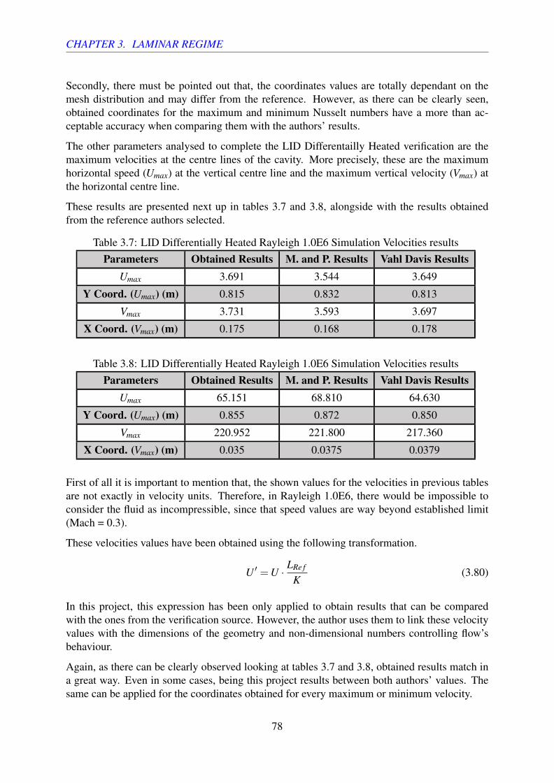
CHAPTER 3. LAMINAR REGIME
Secondly, there must be pointed out that, the coordinates values are totally dependant on themesh distribution and may differ from the reference. However, as there can be clearly seen,obtained coordinates for the maximum and minimum Nusselt numbers have a more than ac-ceptable accuracy when comparing them with the authors’ results.
The other parameters analysed to complete the LID Differentailly Heated verification are themaximum velocities at the centre lines of the cavity. More precisely, these are the maximumhorizontal speed (Umax) at the vertical centre line and the maximum vertical velocity (Vmax) atthe horizontal centre line.
These results are presented next up in tables 3.7 and 3.8, alongside with the results obtainedfrom the reference authors selected.
Table 3.7: LID Differentially Heated Rayleigh 1.0E6 Simulation Velocities resultsParameters Obtained Results M. and P. Results Vahl Davis Results
Umax 3.691 3.544 3.649
Y Coord. (Umax) (m) 0.815 0.832 0.813
Vmax 3.731 3.593 3.697
X Coord. (Vmax) (m) 0.175 0.168 0.178
Table 3.8: LID Differentially Heated Rayleigh 1.0E6 Simulation Velocities resultsParameters Obtained Results M. and P. Results Vahl Davis Results
Umax 65.151 68.810 64.630
Y Coord. (Umax) (m) 0.855 0.872 0.850
Vmax 220.952 221.800 217.360
X Coord. (Vmax) (m) 0.035 0.0375 0.0379
First of all it is important to mention that, the shown values for the velocities in previous tablesare not exactly in velocity units. Therefore, in Rayleigh 1.0E6, there would be impossible toconsider the fluid as incompressible, since that speed values are way beyond established limit(Mach = 0.3).
These velocities values have been obtained using the following transformation.
U ′ =U ·LRe f
K(3.80)
In this project, this expression has been only applied to obtain results that can be comparedwith the ones from the verification source. However, the author uses them to link these velocityvalues with the dimensions of the geometry and non-dimensional numbers controlling flow’sbehaviour.
Again, as there can be clearly observed looking at tables 3.7 and 3.8, obtained results match ina great way. Even in some cases, being this project results between both authors’ values. Thesame can be applied for the coordinates obtained for every maximum or minimum velocity.
78

CHAPTER 3. LAMINAR REGIME
With these and the former Nusselt parameter verification, it can be firmly stated that the obtainedresults for the LID Differentially Heated case simulations can be considered as correct.
Next up will be presented the obtained results of velocity, streamlines and temperature fieldsfor the simulations of Rayleigh 1.0E3 and 1.0E6. These are the lowest and the highest Rayleighsimulated, in order to give a better view of the changes this parameter produces in flow’s be-haviour. To see the flow evolution between these two values, go to appendix C in Annex docu-ment of this project.
Results.
Temperature fields.
In figures 3.48 and 3.49 are presented the temperatures fields obtained in the simulations ofRayleigh 1.0E3 and 1.0E6.
Figure 3.48: LID Differentially Heated Tem-peratures field Rayleigh 1.0E3
Figure 3.49: LID Differentially Heated Tem-peratures field Rayleigh 1.0E6
LID Differentially Heated is the only laminar case of this project in which the temperatures fieldis significantly relevant. Due to the presence of the buoyancy term (Boussinesq approximation),the fluid’s temperature plays a huge role on its behaviour in the flow. That’s why this is the onlycase in which temperatures field is presented.
In what comes to the obtained results for the temperature, there are several aspects that need tobe mention.
First of them, as it was clearly expected, the higher temperatures takes place near the heatedwall. The cold fluid approaches it from the lower part, heats up due to convection and conduc-tion transfer and then it is capable of overcome the gravity effect. When it is located at the top
79

CHAPTER 3. LAMINAR REGIME
of the cavity, it approaches the cold wall, where looses most of its temperature, going back tothe beginning of the loop.
Looking at both images, there can be clearly observed the influence the Rayleigh number hason the flow. In the first case (figure 3.48), the fluid heat transfer takes place at a much slowerrate. It takes the flow on the lower part almost half of the cavity distance to heat up from 20% to80% of left wall’s temperature. Here it can be observed the great impact Rayleigh has on fluidconduction heat transfer.
On the other hand, looking at figure 3.49, it is appreciated an incredible increasing in convectiveand conduction heat transfer. In this case, the fluid is able to heat up in a tiny distance from thewall. As there can be seen, it changes its temperature from about 20% to 80 or 90% of leftwall’s temperature in just a tiny distance near the wall. In addition to that, the flow is able tomaintain this temperature during much more time while approaching the right cold wall.
There is such difference between both conduction heat transfer values that, in the first case(figure 3.48), the flow reaches an steady state more or less with the same temperatures fieldas the walls temperature distribution. Meanwhile, at Rayleigh 1.0E6 (figure 3.49), the flowreaches an steady state in which there are only two thin boundary layers at the walls and a verydifferentiated temperatures areas at the lower and upper part of the cavity.
Velocity fields.
Next up in figures 3.50 and 3.51 are presented the velocity fields obtained in the simulations ofRayleigh 1.0E3 and 1.0E6.
Figure 3.50: LID Differentially Heated Veloc-ity Magnitude field Rayleigh 1.0E3
Figure 3.51: LID Differentially Heated Veloc-ity Magnitude field Rayleigh 1.0E6
The velocity fields for every Rayleigh simulated is a consequence of the previous temperaturesfields.
80

CHAPTER 3. LAMINAR REGIME
In the first case (figure 3.50), the heat transfer doesn’t play a big role in the overall contribu-tion to fluid’s velocity. However, thanks to the buoyancy term, the flow travels the movementdescribed before. When approaching the heated wall, the buoyancy term begins to overcomethe gravity effects. Then, when it reaches the top, due to boundary conditions, goes towards theright wall and looses its heat and so gravity play a bigger role than buoyancy and falls down.
On the other case (figure 3.51), the heat transfer at the left wall takes places at a so tiny distanceand time that the buoyancy term rapidly overcome gravity increasing its speed in the verticaldirection. This allows to the generation of a boundary layer at both walls. In case of right one,it happens when the fluid looses so quickly all its temperature and falls down.
However, there are two areas in the cavity in which although the fluid is in the heated area, itfalls down, and vice versa for the cold one. This happens due to the fast heat transfer that takesplace at that areas. These zones are right in the middle between both temperature regions andso it is constantly heating up and then cooling down.
Streamlines fields.
Finally, in figures 3.52 and 3.53 are presented the Streamlines fields for the Rayleigh 1.0E3 and1.0E6 simulations carried out.
Figure 3.52: LID Differentially HeatedStreamlines field Rayleigh 1.0E3
Figure 3.53: LID Differentially HeatedStreamlines field Rayleigh 1.0E6
In the streamlines fields in figures 3.52 and 3.53 there can be seen what has been already men-tioned in velocities ones.
In the first case (figure 3.52), a huge vortex in the middle of the cavity is observed. This hasbeen generated due to the loop process on the fluid’s travel through the cavity going up anddown at the left and right walls respectively.
However, at Rayleigh 1.0E6 (figure 3.53), the phenomena described for the velocities field can
81

CHAPTER 3. LAMINAR REGIME
be much clearly observed. The fluid’s heat transfer takes place so fast and in a so tiny area thatit is capable of generating little steady vortexes due to this movement.
As there can be noticed, in LID Differentially Heated case the pressure fields obtained in thesimulationshaven’t been presented. Due to the importance of the temperature and heat transferin the problem, there has been chosen not to expose the pressure results. These are consideredto be not enough relevant in flow’s behaviour to add them to the report. Markatos and Pericleousand Vahl Davis don’t even include pressure results to compare with.
As in the other two cases for the laminar regime, the rest of simulations properties fields thathaven’t been shown here can be found in appendix C of Annex Document of this project.
82

CHAPTER 3. LAMINAR REGIME
3.5 Square CylinderIn this section are presented the results obtained in the simulations of flow past a square cylinder.As in the previous LID Driven Cavity and LID Differentially Heated cases, here will also bepresented the verification and explanation of the physical phenomena involving the problem.
The Square Cylinder theoretical background has already been exposed in section 3.1.3. It con-sists on a channel with a parabolic profile inlet in which there is a square cylinder.
As in LID Driven Cavity case, the main parameter that controls the behaviour of the fluid is theReynolds number. However, there are some slightly modifications around this variable in thisproblem.
Re =ρURe f LRe f
µ
In section 3.3, there can be seen for instance that, the reference length for the non-dimensionalnumber (LRe f ) corresponds to the cavity length/height. Nevertheless, in this case, the referenceis the length/height of the interior square, not the channel (figure 3.54).
Moreover, in LID Driven Cavity problem, the reference velocity was pretty clear to be exactlythe inlet speed. However, Square Cylinder boundary conditions imposes a parabolic inlet profile(figure 3.54). This means there are different options as a reference velocity. In this project, therehas been chosen to set as reference velocity the mean value of the inlet.
U =Umax√
2.0
Figure 3.54: Square Cylinder geometry parameters definition
Therefore, the Reynolds number for the Square Cylinder study case can be expressed as follow-ing.
Re =ρUmaxDµ√
2.0(3.81)
83

CHAPTER 3. LAMINAR REGIME
The following geometry parameters (table 3.9) have been selected for all the simulations done.
Table 3.9: Square Cylinder geometry parameters selected for the simulationsParameter Value (m)
D 1.0
M 12.5
L 50.0
H 8.0
Again, as in the LID Driven Cavity problem, the modified parameter depending on the Reynoldsis the dynamics viscosity.
However, the biggest change from that case, or even LID Differentially Heated, to this one hasalready been slightly mentioned while presenting the case in section 3.1.3.
LID Driven Cavity and LID Differentially Heated cases simulations always arrive to an steadystate in which the variables values remain constant. This situation may happen sooner or laterdepending on the simulation condition, Reynolds or Rayleigh numbers, etc...
However, in Square Cylinder problem, once a certain Critical Reynolds number has been ex-ceeded, the system begins to oscillate by generating vortexes behind the cylinder. These arealso known as Von−Karman Vortexes.
Due to these, the system is unable to achieve an steady state. Nevertheless, once the oscillationshave stabilised around a certain value, it is called as ”Periodic State”.
Normally, in a non-oscillatory system, the cylinder would experiment a constant drag horizontalforce because of the flow. But, due to the oscillations, this isn’t a fixed value, it begins to swingaround a certain value. Moreover, a lift oscillating force appears too.
As there has been proven in the simulation, alongside with the scientific sources, the men-tioned Critical Reynolds number is approximate to 70. In this report will be only presented andexplained the results for Reynolds 5 and Reynolds 200 (the lowest and highest Reynolds simu-lations done). In order to see the results from all the other simulation carried out go to appendixD in Annex document of this project.
3.5.1 Obtained results and verificationAs in previous LID Driven Cavity and Differentially Heated cases, main simulation parametersare presented.
84

CHAPTER 3. LAMINAR REGIME
Table 3.10: Square Cylinder Simulation parametersReynolds 5 200ρ [Kg/m3] 1.0 1.0
Umax [m/s] 1.0 1.0
X Direction Nodes 243 450
Y Direction Nodes 178 236
Stop Criteria 1,0E-06 -
Convective scheme QUICK QUICK
In order to give a better insight and an easier explanation of the verification parameters, theseare presented alongside the obtained results for the case.
Verification and results.
Velocity fields.
In figures 3.55 and 3.56 are presented the velocity fields obtained in the simulations of Reynolds5 and 200. These two have been selected in order to ease the understanding of the oscillationphenomena involving the case.
Figure 3.55: Square Cylinder Velocity Magnitude field Reynolds 5
85

CHAPTER 3. LAMINAR REGIME
Figure 3.56: Square Cylinder Velocity Magnitude field Reynolds 200
As there can be seen in figure 3.55, the flow remains in an steady state through all the channel.There are only little perturbations due to the presence of the cylinder. Due to the reduced crosssection, and fluid’s incompressibility, the flow has to increase its velocity in this part. However,as there can be seen in the scale, it is a slightly change in comparison to flow’s cross sectionaverage speed.
On the other hand, in Reynolds 200 simulation, there can be seen perfectly the oscillation phe-nomena described previously. Above Critical Reynolds (70 approximately), the flow begins togenerate Von-Karman Vortexes behind the cylinder due to its presence.
Finally, it must be at least mentioned the boundary layer generated at the upper and lower wallsof the cylinder. This can be observed in a more detailed way in figure 3.56.
As in the case for instance of aerodynamic airfoils, the higher the Reynolds, the larger theboundary layer is, and so in this case.
In addition to the figures exposed, next up are presented the Streamlines fields for the samesimulations to give a deeper view of the results.
Streamlines fields.
In figures 3.57 and 3.58 are presented the Streamlines fields for the simulations of Reynolds 5and 200.
Figure 3.57: Square Cylinder Strealines field Reynolds 5
86

CHAPTER 3. LAMINAR REGIME
Figure 3.58: Square Cylinder Streamlines field Reynolds 200
There are some conclusions related also to the velocity fields that can be extracted from theprevious images.
First, in figure 3.57, there can be seen a steady flow with no mayor perturbations apart from thecylinder. In addition to that, there can be firmly stated that this image is a perfect definition ofwhat a laminar flow is.
As it is already explained at the beginning of section 3.1, laminar regime is characterised byordered and parallel layers of flow with no transverse velocity. This definition can be clearlyextrapolated to figure 3.57.
All its streamlines are perfectly ordered and there is almost no transverse speed apart from theone generated by the presence of the cylinder.
Meanwhile, in Reynolds 200 streamlines field, there can be observed what has already beenmentioned. Due to the presence of the cylinder the flow begins to generate Von-Karman Vor-texes.
Nevertheless, as there can be observed, the farther these are, the more they are dissipated. Itcan only be slightly noticed with the scale. However, in a long enough channel, the vortexesgenerated right behind the cylinder wouldn’t be able to reach the outlet of the channel due to itsdissipation on the flow.
This loss in kinetic energy takes place due to the viscosity of the fluid. Therefore, the higher theReynolds is, the longer it takes to dissipate all the energy of the vortexes.
Pressure fields.
To give a final view of the Square Cylinder results, there are presented the relative pressurefields of the simulations of Reynolds 5 and 200 in figures 3.59 and 3.60 respectively.
87

CHAPTER 3. LAMINAR REGIME
Figure 3.59: Square Cylinder Pressure field Reynolds 5
Figure 3.60: Square Cylinder Pressure field Reynolds 200
As there can be seen in both images 3.59 and 3.60, there is a pressure loss right at the upper andlower sides of the cylinder. The theoretical basis of this phenomena has already been explained.
Due to the presence of the cylinder, the channel cross section reduces. And,since the fluid isconsidered to be incompressible, its velocity must increase.
This acceleration on the fluid makes the relative pressure to decay (Bernouilli’s Principle, equa-tion 3.77). This phenomena doesn’t only happen in laminar regime or in this case. It is widelyand deeply studied problem in fluid mechanics.
However, this pressure loss isn’t constant for every flow condition. As there can be seen infigures 3.59 and 3.60, the lower the Reynolds is, the higher the loss.
Finally, looking at image 3.60, there can be observed the vortexes generated by the pressuredifference inside and outside these. The pressure field perturbation at the outlet of the channelin figure 3.60 takes place due to boundary conditions. However, this doesn’t affect the validityof the results.
Although velocity, streamlines and pressure fields results have been presented and explained in adetailed way, there are several different related parameters or phenomena that will be explainednext up in the verification process. To save space, there has been only chosen to present the
88

CHAPTER 3. LAMINAR REGIME
images obtained from Reynolds 5 and 200 simulations. However, in the verification processthere has been selected to shown the results from every simulation carried out.
This verification data of the obtained results for the simulation case of Square Cylinder havebeen extracted from a trustworthy scientific source [28].
There will be compared up to 5 different variables results obtained. These are the Recircula-tion Length, the drag and lift coefficient mean and oscillation values (only mean drag) and theStrouhal number of the system.
Recirculation Length.
Due to the presence of the square cylinder and the flow around it, there is a low relative pressurearea right behind this one. This makes the flow close to it to go that zone due to the pressuregradient. Therefore, there is an area in which fluid’s velocity is opposite to the main flow.
And it isn’t until a certain distance behind the cylinder that the velocity returns to have thesame direction as the main flow. This distance is known as ”Recirculation length”. In order togive a better insight of this physical phenomena, it is presented in figure 3.61 mentioned areaStreamlines field in Reynolds 50 case.
Figure 3.61: Square Cylinder Reynolds 50 Streamlines field behind the cylinder
As there can be seen in figure 3.61, the flow changes its direction because of the pressure gra-dient due to the presence of the cylinder. Recirculation Length grows as the Reynolds numberdoes due to the fact that it depends enormously on the dominance of the inertial forces overviscosity. However, once the system begins to oscillate, there is no reason to use this parameteras a measure variable because it continuously changes with the oscillations.
Next up in figure 3.62 is presented the comparison of the Recirculation Length results with theones from the mentioned scientific source.
In figure 3.62, there can be seen what has been mentioned before. The higher the Reynoldsis, the higher the Recirculating Length is. A higher Reynolds makes the pressure behind thecylinder to be lower and so it is harder for the deviated flow to come back to its initial direction.
In what comes to the accuracy of the obtained results, the following statement can be made.
Despite the fact that, at higher Reynolds number, there is a slightly difference between bothresults, these can be considered as acceptable. It can be clearly observed, the similar mathemat-
89

CHAPTER 3. LAMINAR REGIME
Figure 3.62: Recirculation Length results comparison
ical tendency on both cases. Moreover, none of the results have a relative error above 10% or15%, so they can be considered as correct from an engineering point of view.
Drag and Lift Coefficients.
As it has been mentioned, due to the presence of the cylinder inside the flow, there is a dragforce on the same direction as the first of these. And, since there is only flow in the horizontaldirection, there is lift coefficient due to forces on the vertical axis.
However, this changes when system begins to oscillate. Drag coefficient begins to swing arounda certain Reynolds dependant value, and lift ceases being null.
In every fluids mechanics or aerodynamics problem, the drag and lift coefficients are computedas follows.
CD =DF
12ρU2LRe f
(3.82)
CL =LF
12ρU2LRe f
(3.83)
As the reader may think, the reference length and velocity must be the same as the ones chosenfor the case simulations.
CD =DF
12ρ(Umax√
2.0)2D
(3.84)
CL =LF
12ρ(Umax√
2.0)2D
(3.85)
90

CHAPTER 3. LAMINAR REGIME
The only unknown parameters are the drag and lift forces, DF and LF respectively.
In order to calculate them, it is necessary to take into account the pressure difference betweenboth sides of the cylinder and the viscous stresses on its surface.
Figure 3.63: Drag coefficient calculationscheme
Figure 3.64: Drag coefficient calculationscheme
Since the obtained pressure and velocity results are discrete, it is necessary to do a sweep onevery control volume at cylinder’s face for each case.
DF = ∑f
[PX1i ·∆SX1−PX2i ·∆SX2 +µ
∂u1i
∂y∆SY 1 +µ
∂u2i
∂y∆SY 2
](3.86)
LF = ∑f
[PY 1i ·∆SY 1−PY 2i ·∆SY 2 +µ
∂v1i
∂x∆SX1 +µ
∂v2i
∂x∆SX2
](3.87)
Once the coefficients calculation processes have been explained, it is presented the obtainedresults for them in the simulations.
First, in table 3.11, it is presented the Drag Coefficient comparison.
91

CHAPTER 3. LAMINAR REGIME
Table 3.11: Square Cylinder Drag Coefficient results comparisonReynolds Mean Drag Results Breuer M. Results Relative Error (%)
1 23.58 24.2 2.56
5 5.62 5.75 2.26
10 3.65 3.60 1,39
20 2.41 2.40 0.42
50 1.64 1.60 2.50
70 1.44 1.43 0.70
100 1.35 1.35 0.00
150 1.29 1.32 2.27
175 1.34 1.33 0.75
200 1.36 1.34 1.50
For Reynolds numbers equal or above 70, the shown Drag Coefficient is its mean value.
As there can be seen in table 3.11, drag coefficient has a strong dependence on the viscouseffects of the flow. At Reynolds 1, it has an huge value in comparison to the rest of simulations.
At this flow regime, the viscosity plays an important role on the drag force calculation, repre-senting a great part of it. However, the higher the Reynolds is, the lower CD. This happens dueto the following reasons.
First, although the pressure difference between the frontal and back face of the cylinder is higheras Reynolds increases, its contribution to the drag represents a little part of the total force. Inaddition to that, as there has been seen, the higher Reynolds, the lower dynamics viscosity.Despite the fact that velocity gradient at the walls are higher as Reynolds increase, µ plays ahuge role on the total drag force due to viscosity stress, and so the global contribution is reduced.
In what comes to the accuracy of the obtained results, there can be clearly seen in table 3.11that they can be firmly considered as acceptable from an engineering point o view. It is almostimpossible to get exactly the same values, there are too many factors like numeric schemechosen, nodal density or distribution or even the resolution method.
In the following tables 3.12 and 3.13, there are presented the drag and lift coefficients oscillationvalue and the comparison with the reference selected.
Table 3.12: Square Cylinder Drag Coefficient variation comparisonReynolds (CDmax−CDmin) Results Breuer M. Results Relative Error (%)
70 0.0011 0.001 10.00
100 0.0091 0.01 9.00
150 0.0274 0.03 8.67
175 0.045 0.040 11.85
200 0.069 0.07 1.43
92

CHAPTER 3. LAMINAR REGIME
Table 3.13: Square Cylinder Lift Coefficient variation comparisonReynolds (CLmax−CLmin) Results Breuer M. Results Relative Error (%)
70 0.230 0.26 11.53
100 0.383 0.391 2.05
150 0.573 0.62 7.58
175 0.87 0.87 0.46
200 1.224 1.20 2.00
Additionally, it is presented the temporal evolution of the drag and lift coefficient respectivelyfor Reynolds 200 simulation.
Figure 3.65: Drag coefficient temporal evolu-tion for Reynolds 200
Figure 3.66: Lift coefficient temporal evolu-tion for Reynolds 200
As there can be seen in figures 3.65 and 3.66, the drag and the lift coefficients begin to varyuntil they arrive to a periodic oscillating state.
Depending on the simulation parameters, specially, Reynolds number, the system may takelonger or not to achieve this state. However, as in case of the steady LID Driven Cavity andDifferentially Heated, the system always arrive to it.
As it was expected, the drag coefficient oscillates around a certain value. However, since thelift coefficient is a secondary effect of the oscillations, its value swings around 0. In case ofcomputing the mean value, it may give something different to 0, but very close to it due tonumerical inaccuracies and not enough resolution.
Additionally, as there can be observed in tables 3.12 and 3.13, the higher Reynolds, the higheroscillation amplitude. This makes sense due to the fact that, as Reynolds increases, so does thesize of the vortexes generated. However, these have different effects on each coefficient.
Looking at table 3.12, there can be clearly stated that these oscillations doesn’t affect so muchto the drag coefficient. This phenomena can be explained by looking at how it is computed.
Observing equation (3.86) and scheme 3.63, there can be seen that the only variation that theoscillations produce consists on the change in the pressure field behind the cylinder. As it hasbeen said, this has a little contribution to the overall coefficient value, so the local temporalvalue of the coefficient is slightly modified.
93

CHAPTER 3. LAMINAR REGIME
On the other side, as there can be seen in table 3.13, the lift coefficient is severely affected bythe oscillations. Again, looking at how it is calculated (equation (3.87) and figure 3.64) therecan be seen that the oscillations modify the velocity profile behind the cylinder and so the forcedue to viscous stresses.
In terms of results accuracy, there are several important things to mention.
First of them is that, these kind of parameters are not easy to calculate or to get the most accuratevalue. As in every simulation, there are many factors that may vary slightly the solution obtainedsuch as numeric scheme selected, total number of nodes, etc..
Nevertheless, although relative errors for the coefficient variations may seem too large in com-parison with other calculated parameters in this project, they can be considered as acceptable.It is true, that some of them, like Reynolds 70 to 150, could be more accurate.
This happens because, when doing that simulations, the total amount of nodes were reducedwithout compromising the validity of the results. A great reduction of them was achieved,however, this affected slightly to the results. The perfect example of this is Reynolds 200simulation. In this case, there were no extreme mesh optimisation to reduce the total nodesnumber. Therefore, great results in every parameter where achieved.
However, none of these results has a relative error above 15%. This means they can be consid-ered as correct from a Computational Fluid Dynamics point of view.
Strouhal number.
Last result to be verified in the Strouhal number. As it is already explained in section 2.3, thisparameter is a non-dimensional number related to the frequency of any system.
St =f ·LRe f
URe f
In this case, it is related to the temporal frequency of the oscillations. As for other non-dimensional numbers in Square Cylinder case, the reference length and velocity are cylinder’sside value and mean inlet speed respectively.
St =f ·D√
2.0U
(3.88)
Next up, in table 3.14 it is presented the comparison for the obtained Strouhal number results inthe simulations.
94

CHAPTER 3. LAMINAR REGIME
Table 3.14: Square Cylinder Strouhal number comparisonReynolds Obtained Results Source Results Relative Error (%)
70 0.128 0.126 1.59
100 0.136 0.138 1.45
150 0,160 0.143 11.88
175 0.144 0.140 2.85
200 0.137 0.134 2.75
Looking at table 3.14, there are some conclusions that can be extracted. First, as there can beseen, the frequency of the oscillations is not severely affected by the Reynolds number variation.It reaches a maximum near Reynolds 150, but then it decays again.
From the accuracy point of view, there can be stated that, apart from Reynolds 150 results, therest have a more than negligible relative error. Moreover, the highest of these are below thementioned 15%. Therefore, all of the obtained results for the Strouhal number are consideredto be correct.
95

Chapter 4
Turbulent Regime.
4.1 Theoretical framework.
Figure 4.1: CFD Simulation of the developmentof turbulent flow in a jet. Extracted from [11]
Almost all fluid flows of our daily life areheavily dominated by turbulence. From theflow around a car, aircraft boundary layers,the air of a room, or even our blood. Mainlyevery flow witnessed every day is turbulent.
This flow regime can be easily described inonly one word, chaos. It is a form of fluidtransport in which velocities fluctuate ran-domly, disrupting the orderly and parallelfluid layers from laminar regime. In this case,transverse flows appear due to the random-ness of the fluid resulting in chaotic velocityfields like the one presented in figure 4.1.
As there can be seen in the image, the flow inlet can be still considered as laminar. However, itgoes through a transition during a small distance and the it becomes turbulent rapidly. There isno fluid pattern or any kind of order. The flow variables are randomly fluctuating.
Turbulent flow are characterised by been heavily irregular, highly unsteady, difficult to predictand chaotic.
In addition to that, turbulence usually occurs at high Reynolds numbers. For instance, in bound-ary layer, the mentioned laminar to turbulent transition takes place at Reynolds 500000 approx-imately.
Other important aspect of turbulent flow is that it is always tri-dimensional and unsteady. How-ever, depending on the equations treatment and problem’s geometry, it can be considered asbi-dimensional. This is going to be crucial for the development of turbulent regime part of thisproject.
From a theoretical point of view, turbulence remains still as one of science biggest problems.Even nowadays, turbulent flows require a great amount of resources and knowledge to be able
96

CHAPTER 4. TURBULENT REGIME.
to study it.
In Computational Fluid Dynamics this doesn’t change. Most of engineering and scientific in-ventions related to fluid mechanics are heavily dependant on turbulent flows. Because of this,there has been a great focus in this area and how to carry out this kind of simulations.
During decades, many different techniques, algorithms or even theories have been developed inorder to be able to predict the behaviour of these flows. Turbulence modelling is a branch ofknowledge that has been developed for almost half century. Nowadays, even with the exponen-tial increase in computational power, there are still many difficulties to do that.
In this project there will be presented the implementation of one of these different turbulencemodelling techniques, RANS (Reynolds Averaged Navier-Stokes).
In addition to that, due to the computational resources available, there are several hypothesisthat must be assumed for the turbulent flow simulation. These are presented next up, in section4.1.1.
4.1.1 Hypothesis and simplifications madeAs in the case of the laminar regime simulations, in this part of the project there are sometheoretical and numerical assumptions. These are presented and described next up in the presentsection.
Continuous flow distribution
As in the laminar regime, continuous flow distribution assumption is one of the basis of thesimulations of turbulent regime flows.
Axisymmetrical flow.
As it is exposed in the laminar regime hypothesis section (section 3.1.1), the flow was consideredto be bi-dimensional.
In this case, the assumption made about this is similar. In the turbulent regime part of theproject, all the simulations have what’s known as axisymmetric geometry.
The easiest case to think about is a pipe. It has a central axis and complete symmetry withrespect to this. So, in order to reduce the computational power required, it has been decidedto remove the azimuthal (angular) flow direction. This can make the fluid to be considered asbi-dimensional in a roughly way.
To learn more about the implementation of this decision, go to section 4.5.1).
Compressible flow
One of the main characteristics of the laminar regime simulations carried out was the fluid’sincompressibility.
However, since one of the main characteristics chosen for the flow is that this is supersonic, it isabsolutely impossible to consider it as incompressible.
97

CHAPTER 4. TURBULENT REGIME.
Usually, in fluid mechanics, the limit to consider a fluid compressible or incompressible rangesnear Mach 0.3. Supersonic flow Mach number is always higher or equal to 1.0. Therefore,considering it as incompressible would be an unacceptable mistake.
Newtonian fluid
As in the laminar regime studies, the simulation fluid is considered to be Newtonian for theturbulent part of the project as well.
Temperature dependant fluid viscosity.
Due to the characteristics of the flow and the simulations to carry out in this part of the project,there has been selected set fluid’s viscosity as temperature dependant.
The fact that flow is compressible and supersonic makes impossible to set a fixed fluid’s vis-cosity. There are huge temperature and pressure changes in the flow that affects severely thisphysical property.
Due to this aspect, there has been chosen to use the Sutherland’s viscosity law. This was pro-posed by the Scottish scientist William Sutherland.
He came with the idea of defining the dynamic viscosity of a fluid depending on its temperatureand certain fluid’s physical properties. There are different mathematical expressions of theviscosity as a function of temperature. For this project, the following one is used.
µ(T )µRe f
=
(T
TRe f
)n
(4.1)
Constant heat capacity ratio.
Since the effects of temperature and pressure changes are almost negligible, heat capacity ratiocan be considered as constant. This parameter is defined as follows.
λ =CP
CV(4.2)
Constant specific heat coefficient.
Due to the decision in the previous hypothesis, the constant volume heat capacity (Cv) can beconsidered as constant.
This makes the code implementation a little bit easier. In this case, it is possible to assume thefollowing.
∂e =Cv ·∂T (4.3)
In addition to that, since the value is fixed, there is no need for spending computational resourceson its calculation.
98

CHAPTER 4. TURBULENT REGIME.
Ideal gas.
It is considered that the simulation gas is ideal. Although this is no 100% accurate, it sim-plifies enormously the numerical implementation. Moreover, many scientific publications ofcompressible flows use the same hypothesis.
This hypothesis allows to compute the pressure using the following mathematical expression.
P = ρ ·R ·T (4.4)
4.1.2 Turbulent regime Navier - Stokes equations.In this section are presented the Navier-Stokes Mass, Momentum and Energy equations withthe hypothesis and assumptions previously mentioned.
• Mass conservation equation.
∂ρ
∂ t+∇ · (ρu) = 0 (4.5)
• Momentum conservation equation.
∂ρu∂ t
+∇ · (ρuu) =−∇p+∇ · τ (4.6)
X axis.
∂ρu∂ t
+∇ · (ρuu) =−∂ p∂x
+∇ · τ|u (4.7)
R axis.
∂ρv∂ t
+∇ · (ρvv) =−∂ p∂ r
+∇ · τ|r (4.8)
Since the flux has been considered as axisymmetric in X-R plane, there is no need forconsidering azimuthal axis equations anymore.
• Energy conservation equation.
∂ρe∂ t
+∇ · (ρue) =−p ·∇u+∇q+ τ : ∇u (4.9)
To see the mathematical development of terms ∇ · τ|u, ∇ · τ|r and τ : ∇u from the axial andradial momentum and energy equations, go to appendix G in Annex document of this project.
99

CHAPTER 4. TURBULENT REGIME.
4.2 Turbulence modellingAs there has been seen in the previous section (section 4.1), turbulence represent an enormouschallenge from a theoretical and numerical point of view. The difficulty of the physical phe-nomena involved is way beyond from the laminar regime.
In addition to that, the computational power required to simulate this flow regime grows expo-nentially as the turbulence increase. The total number of nodes needed for the simulation ofturbulent regime is considered to grow at a rate of Re2.25.
Unfortunately, even today, with the enormous increase in computational power, it is impossibleto do certain turbulent regime studies. Because of this, researchers ad engineers have developedduring decades many ways to modelling turbulence and the phenomena involved.
The most common methods of turbulence modelling are DNS (Direct Numerical Simulation),LES (Large Eddy Simulation) and RANS (Reynolds Averaged Navier-Stokes equations).
First of them, DNS, consists on using the same numerical methods as in laminar regime increas-ing the mesh up to the simulation requirements.
On the one hand, it is the easiest way to simulate turbulence. No modifications for the equationsor the resolution are needed. However, on the other hand, these kind of simulations requirea huge computational power. Nowadays, it is absolutely impossible to carry out these typeof studies in a personal computer. It is necessary an enormous cluster of hundreds or eventhousands of CPUs. And still, it isn’t enough to simulate industrial applications cases.
By comparison, LES (Large Eddy Simulation) doesn’t require the same amount of resourcesas DNS. As the reader may sense from its name, this method consists on the simulation of thelarge scales of the flow and the modelling of the smaller ones. This reduces dramatically thecomputational power required. However, it increases the implementation difficulty.
In this project there has been chosen to apply RANS modelling basis due to the physical char-acteristics of the study case. Next up is presented this turbulence modelling method in a muchmore detailed way.
4.2.1 Reynolds Averaged Navier Stokes Equations (RANS).As its name already indicates, RANS turbulence modelling theory is based on averaging val-ues. Turbulent flow is considered to be fluctuating. Therefore, RANS equations average thesefluctuating variables by splitting them in two terms (equation (4.10)).
100
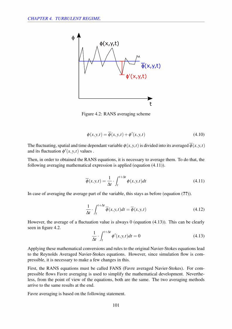
CHAPTER 4. TURBULENT REGIME.
Figure 4.2: RANS averaging scheme
φ(x,y, t) = φ(x,y, t)+φ′(x,y, t) (4.10)
The fluctuating, spatial and time dependant variable φ(x,y, t) is divided into its averaged φ(x,y, t)and its fluctuation φ ′(x,y, t) values .
Then, in order to obtained the RANS equations, it is necessary to average them. To do that, thefollowing averaging mathematical expression is applied (equation (4.11)).
φ(x,y, t) =1∆t·∫ t+∆t
tφ(x,y, t)dt (4.11)
In case of averaging the average part of the variable, this stays as before (equation (??)).
1∆t·∫ t+∆t
tφ(x,y, t)dt = φ(x,y, t) (4.12)
However, the average of a fluctuation value is always 0 (equation (4.13)). This can be clearlyseen in figure 4.2.
1∆t·∫ t+∆t
tφ′(x,y, t)dt = 0 (4.13)
Applying these mathematical conversions and rules to the original Navier-Stokes equations leadto the Reynolds Averaged Navier-Stokes equations. However, since simulation flow is com-pressible, it is necessary to make a few changes in this.
First, the RANS equations must be called FANS (Favre averaged Navier-Stokes). For com-pressible flows Favre averaging is used to simplify the mathematical development. Neverthe-less, from the point of view of the equations, both are the same. The two averaging methodsarrive to the same results at the end.
Favre averaging is based on the following statement.
101

CHAPTER 4. TURBULENT REGIME.
ρφ = ρ · (φ +φ ′′) = ρ · φ +ρ ·φ ′′
ρ · φ = ρφ = ρ ·ρ · φρ
= ρ ·φ
ρ ·φ = ρ · φ +ρ ·φ ′′ = ρ ·φ +ρ ·φ ′′ −→ ρ ·φ ′′ = 0 (4.14)
It is based on density weighted averaging. This eases a lot the mathematical development forcompressible flows.
To give a better insight of Favre averaging method, it is presented the mathematical developmentof Mass Conservation equation next up.
Mass Conservation Equation.
∂ρ
∂ t+∇ · (ρu) = 0 (4.15)
To ease the understanding, each term development is shown.
∂ρ
∂ t=
∂ρ
∂(4.16)
∇ · (ρu) = ∇ · (ρ · (u+u′′)) = ∇ · (ρ · u+*0
ρ ·u′′) = ∇ · (ρ · u) (4.17)
Adding obtained terms lead to the following Reynolds Averaged Navier-Stokes Mass Conser-vation equation (equation (4.18)).
∂ρ
∂ t+∇ · (ρ · u) = 0 (4.18)
As there can be seen, the obtained equation is equal to the initial one. In the implementation, theaveraging is already taken into account in this equation, there is no need to make any changeson it.
However, this doesn’t happen in the Momentum and Energy Conservation equations.
Averaging these leads to the following expressions for each of them respectively (equations(4.19), (4.20) and (4.21)). To see the mathematical development of these equations, go to ap-pendix E in Annex document of this project.
∂ (ρ · u)∂ t
+∇ · (ρuu) =−∂P∂x
+∇ · (τ|x)+∇ · (τ ′′|x−ρu′′u′′)︸ ︷︷ ︸New Terms
(4.19)
102

CHAPTER 4. TURBULENT REGIME.
∂ (ρ · v)∂ t
+∇ · (ρuv) =−∂P∂y
+∇ · (τ|y)+∇ · (τ ′′|y−ρu′′y′′)︸ ︷︷ ︸New Terms
(4.20)
∂ρ e∂ t
+∇ · (ρue) =−p ·∇ · (u)−∇q+ τ : ∇(u)−∇ · (ρu′′e′′)︸ ︷︷ ︸New Term
(4.21)
For further information about Favre averaging go to [29].
As there can be seen, the equations are equal, except for 2 additional terms on each of them.
In order to solve the momentum equation, it is needed to add the effect these terms have on theoverall contributions to the velocities. To do that, they need to be modelled.
The mathematical development of the process is way beyond project’s scope. Therefore, it willbe mentioned only the modification in the simulation code.
Usually, the kinematic or dynamic viscosity of the fluid is computed depending on the Reynoldsnumber, on the temperature, on the fluid properties, etc...
Nevertheless, what is done in RANS modelling to take into account the effects of the new termsof the equations is adding a new turbulent viscosity.
µNew = µ +µt (4.22)
This new viscosity µNew substitutes the former viscosity in the Momentum Conservation equa-tion and for instance, in the time step value calculation. Instead of working with the fluid’s baseviscosity, turbulent one is added.
The question now is, how to compute this new turbulent viscosity. To do that, researchers andengineers have developed turbulence models.
These take the fluid conditions and compute the turbulent viscosity. There are many types ofRANS turbulence models. Linear eddy viscosity models, non-linear eddy viscosity models,Reynolds stress based viscosity models, etc...
However, the most commons RANS models are the one-equation and two-equation models.
For this project, the RANS model selected for the turbulent regime simulations is the Spalart-Allmaras turbulence model, which will be presented next up in a more detailed way.
Spalart-Allmaras turbulence model.
The Spalart-Allmaras model is a RANS one equation model designed specifically for aerospaceapplications.
It was first developed and presented by Phillipe Spalart and S. R Allmaras in 1994 in their paper”A one-equation turbulence model for aerodynamic flows while working at Boeing.
This model solves a transport equation for the kinematic turbulent viscosity (ν), also known as”Spalart-Allmaras variable”.
103

CHAPTER 4. TURBULENT REGIME.
Next up is presented the transport equation proposed by the authors in 1994.
∂ ν
∂ t+∇ · (νu) =Cb1Sν +
1σ[∇((ν + ν) ·∇ν)+Cb2∇ν ·∇ν ]−Cw1 fw
(ν
d
)2
(4.23)
In addition to the transport equation shown before, there are several parameters or variables thatneed to be calculated on every step of the simulation.
µt = ν ·ρ · fv1 (4.24) fv1 =X3
X3 +C3v1
(4.25)
X =ν
ν(4.26) fw = g ·
[1+C6
w3
g6 +C6w3
]1/6
(4.27)
g = r+Cw2 · (r6− r) (4.28) r = min
(ν
S ·K2V K ·d2
,10.0
)(4.29)
S = S+ν
K2V K ·d2 · fv2 (4.30) fv2 = 1.0− X
1.0+X · fv1(4.31)
S =√
2.0 ·ω ·ω (4.32) ω =12·(
∂u∂y− ∂v
∂x
)(4.33)
Cw1 =Cb1
K2V K
+(1.0+Cb2)
σ(4.34)
Next up in table 4.1 are presented the values of all constants needed to solve the model.
Table 4.1: Spalart-Allmaras turbulence model constants values. Extracted from [12]Constant Value
σ 2/3
Cb1 0.1355
Cb2 0.6220
KV K 0.4100
Cw2 0.3000
Cw3 2.0000
Cv1 7.1000
As it has been said, Spalart and Allmaras presented in 1994 the transport equation for the eddyturbulent viscosity, equation (4.23). However, this expression is only valid for incompressible
104

CHAPTER 4. TURBULENT REGIME.
flows. In case of compressible regime studies, it is necessary to modify slightly the equation asfollows.
∂ρν
∂ t+∇ · (ρνu) =Cb1Sρν +
1σ[∇((µ +ρν) ·∇ν)+Cb2∇ν ·∇ν ]−Cw1ρ fw
(ν
d
)2
(4.35)
This is the transport equation for the eddy turbulent viscosity that is going to be implementedfor the simulation.
In order to give a better insight of the turbulence model, next up, each term of the previousequation will be explained in a more detailed way.
• Eddy turbulent viscosity change rate (∂ρν
∂ t ).
As in Mass, Momentum and Energy Conservation equations, this term represents the rateof change of the eddy turbulent viscosity inside the control volume studied.
• Eddy turbulent viscosity flow into the volume (∇ · (ρνu)).
It represents the eddy turbulent viscosity flowing through the bounding surfaces of thechosen control volume in and out of it because of the fluid’s velocity.
• Eddy turbulent viscosity generation term (Cb1Sρν).
This term represents the flow turbulence generation due to velocity gradients (shears) inthe flow field.
Figure 4.3: Constant velocity profilescheme Figure 4.4: Variable velocity profile scheme
Figures 4.3 and 4.4 are presented to give a better understanding of this phenomena.
The viscosity generation of the model depends mainly on this term. And its value reliesdirectly on the velocity gradient, as it can be seen in equations (4.30), (4.32) and (4.33).For instance, in figure 4.3, the turbulent velocity generation would be null, while on the
105

CHAPTER 4. TURBULENT REGIME.
second scheme (figure 4.4), there is a clear and significant velocity gradient on the Ydirection, and so it is taken into account to produce turbulent viscosity.
The term considers speed variations in the horizontal and vertical axis (in case of being3D, it would also do for the other direction) and generates a directly proportional quantityof turbulent viscosity.
• Diffusion of turbulence term ( 1σ[∇((µ +ρν) ·∇ν)+Cb2∇ν ·∇ν ]).
As in many physical variables transport equations, there is a diffusion term which allowsthese properties to spread out from region in which there are high concentrations of themto lower ones. This is the case of the present term.
In addition to what has been mentioned, this expression can be splited in two. The firstterm, 1
σ∇((µ +ρν) ·∇ν) is known as the linear term. Comparing it with other diffusion
terms from other equations such as Momentum Conservation equation (section 2.2.4),there can be seen that both have a common structure.
However, the second term is non-linear, also known as source term. It was added by themodel authors to control and get a more accurate spread of wakes in turbulent regionswhere diffusion dominates in front of other phenomena.
• Destruction of turbulence term (−Cw1ρ fw
(ν
d
)2).
As it can be observed for the ”− ” sign, this term makes the generated viscosity to de-crease.
When approaching walls in the geometry, the turbulence begins to reduce until being nullright at the solid surface. This term represents this decrease. As it can be seen in itsequation, the closer it is from the wall (d), the higher it is and so the reduction in totalviscosity.
Since the release of Spalart-Allmaras turbulence model, it has suffered a lot of changes.
For instance, due to the fact that it was originally conceived for aerospace applications, a verywide field of knowledge, there have been many additions and modifications on its transportequation (adding or changing terms), on the constants of the model, etc..
However, in this project there will be implemented and applied the equations and constantspresented before.
For further information about the Spalart-Allmaras turbulence model and its modifications forcompressible flows go to [30], [31] and [32].
106

CHAPTER 4. TURBULENT REGIME.
4.3 Symmetry-preserving discretization for compressible flows.Although been able to simulate compressible flows gives countless possibilities and studies tobe carried out, it also increases the difficulty enormously.
When simulating these kind of flows, people tend to use dissipative convective schemes (Up-wind scheme for example) to make the simulation more stable [33]. However, this isn’t soaccurate from a mathematical point of view. The convective scheme should not dissipate en-ergy.
Therefore, it is a better option to use kinetic energy preserving schemes. This is the case ofRozema [34].
In the publication, he proposes the idea of a new non-dissipative stable scheme for compressibleflows. The modifications are made to the convective term of each Navier-Stokes equations. Nextup are presented the mathematical development of each of them.
Original Mass Conservation equation.
∂ρ
∂ t+∇ · (ρu) = 0 (4.36)
Original Momentum Conservation equation.
∂ρu∂ t
+∇ · (ρuu) =−∇p+∇ · τ (4.37)
Original Energy Conservation equation.
∂ρe∂ t
+∇ · (ρue) =−p ·∇ ·u+∇q+ τ : ∇u (4.38)
As it can be seen in the previous equations, these are defined by the following variables.
−→g = (ρ, ρu, ρe)
However, the change that Rozema proposes in his paper consists on modifying these variablesinto the following.
−→h = (
√ρ,
√ρu√2,√
ρe)
To maintain the mathematical equality between both ways to write the equations, the authorputs forward the following modification for the convective term.
−∇ · (uφ) =−12
u ·∇φ − 12
∇ · (uφ) (4.39)
−∇ · (uφ) = c(u)φ (4.40)
107

CHAPTER 4. TURBULENT REGIME.
For an structured and collocated mesh, the convective operator has this form. (See [paperRozema] for the complete development).
(c(u)φ)k =12
φk ·1
Ωk∑
fA f uf ·nf−
1Ωk
∑f
A f uf ·nf12(φk +φnb( f )) (4.41)
Operating on the previous equation leads to the following expression for the convective term.
(c(u)φ)k =−1
Ωk∑
f
12
A f uf ·nf φnb( f ) (4.42)
Modified Mass Conservation equation.
First, it is necessary to change the main variable of the equation ρ .
∂ρ
∂ t=
∂ (√
ρ ·√ρ)
∂ t(4.43)
Now, applying the chain rule leads to the following.
∂ (√
ρ ·√ρ)
∂ t=
∂√
ρ
∂ t·√
ρ +√
ρ ·∂√
ρ
∂ t= 2 ·
√ρ ·
∂√
ρ
∂ t(4.44)
Since Mass Conservation equation only has the convective term as part of it, the modified equa-tion states as presented next up.
∂ρ
∂ t= 2 ·
√ρ ·
∂√
ρ
∂ t= 2 ·
√ρk ·
[− 1
Ωk∑
f
12
A f uf ·nf ρnb( f )
](4.45)
Finally, the new Mass Conservation equation states as the following.
∂ρ
∂ t=− 1
Ωk∑
fA f uf ·nf
√ρk√
ρnb( f ) (4.46)
Modified Momentum Conservation equation.
As in the previous case, it is necessary to change the variable and after that, applying the chainrule to the partial derivative.
∂ρu∂ t
=√
2 ·∂ (√
ρ ·√
ρu√2)
∂ t(4.47)
√2 ·
∂ (√
ρ ·√
ρu√2)
∂ t=√
2 ·∂ (√
ρ)
∂ t·√
ρu√2︸ ︷︷ ︸
Term 1
+√
2 ·√
ρ ·∂ (√
ρu√2)
∂ t︸ ︷︷ ︸Term 2
(4.48)
108

CHAPTER 4. TURBULENT REGIME.
Term 1.
√2 ·
∂ (√
ρ)
∂ t·√
ρu√2
=√
2 ·
[− 1
Ωk∑
f
12
A f uf ·nf√
ρnb( f )
]·√
ρkuk√2
(4.49)
= − 1Ωk
∑f
12
A f uf ·nf√
ρnb( f ) ·√
ρkuk
Term 2.
√2 ·√
ρ ·∂ (√
ρu√2)
∂ t=√
2 ·√
ρk ·
[− 1
Ωk∑
f
12
A f uf ·nf
√ρnb( f )unb(f)√
2− ∇p√
2 ·√ρk+
∇ · τ√2 ·√ρk
](4.50)
= − 1Ωk
∑f
12
A f uf ·nf√
ρnb( f ) ·√
ρk ·unb(f)−∇p+∇ · τ
Adding both terms leads to the following Momentum Conservation modified equation.
∂ρu∂ t
=− 1Ωk
∑f
12
A f uf ·nf√
ρnb( f ) ·√
ρk ·12(uk +unb(f))−∇p+∇ · τ (4.51)
Modified Energy Conservation equation.
In case of the Energy equation, the process is similar to the previous ones. First, it is needed tochange the main variable and apply the chain rule to it.
∂ (ρe)∂ t
=∂ (√
ρe ·√ρe)∂ t
(4.52)
∂ (√
ρe√
ρe)∂ t
=∂ (√
ρe)∂ t
·√
ρe+√
ρe ·∂ (√
ρe)∂ t
= 2 ·√
ρe ·∂ (√
ρe)∂ t
(4.53)
∂ (ρe)∂ t
= 2 ·√
ρkek ·
[− 1
Ωk∑
f
12
A f uf ·nf ·√
ρnb( f )enb( f )−p ·∇u
2 ·√ρkek+
τ : ∇u2 ·√ρkek
− ∇q2 ·√ρkek
](4.54)
Finally, the modified Energy Conservation equation has the following expression.
∂ (ρe)∂ t
=− 1Ωk
∑f
A f uf ·nf ·√
ρnb( f )enb( f )√
ρkek− p ·∇u+ τ : ∇u−∇q (4.55)
As it can be seen in all of the equations developed previously, mathematically, the expressionsare the same. However, this modifications ensure a symmetry-preserving discretization. Formore details about this, see [paper Rozema].
109

CHAPTER 4. TURBULENT REGIME.
4.4 Problem studied.In order to give a better insight and ease the understanding of the simulation case and its numer-ical aspects for the turbulent regime study, it is presented next up in this section.
The codes developed for the study of the turbulence regime and the turbulence model methodsare programmed in order to solve axisymmetric geometries.
As the reader may sense from its name, an axisymmetric geometry is the one that has completesymmetry on its central axis. The easiest case of this is a pipe (figure 4.5).
Figure 4.5: Pipe simulation case 3D scheme
The mesher of the codes are capable of creating a grid for endless axisymmetric geometries. Itjust need the mathematical expression of the radius as a function of the axial coordinate.
In this case, there has been selected as simulation case of study a constant radius pipe.
110

CHAPTER 4. TURBULENT REGIME.
Figure 4.6: Turbulent regime pipe case scheme
As there can be seen in the scheme in image 4.6, the solid wall of the pipe has a non-slipcondition for the flow, both axial (U) and radial (V ) velocities are null.
Since the study case is said to be turbulent and supersonic, the inlet must have a velocity higherthan the speed of sound (M > 1.0). The imposed profile profile is constant, as it can be seen infigure 4.6. However, due to the non-slip condition, this quickly disappears into one with moreparabolic tendency.
Although it may seem as a simple study case, it has a lot features and physical phenomenainvolved that is presented and deeply explained in turbulent regime results section (4.6).
111

CHAPTER 4. TURBULENT REGIME.
4.5 Numerical framework.In the present section there will be exposed all the turbulent regime studies numerical imple-mentations. This comprises the spatial discretization of the axisymmetric cases, the modifiedNavier-Stokes compressible equations discretizations alongside the numerical implementationof the Spalart-Allmaras turbulence model and the time integration and resolution processes.
Since there are many aspects and features of turbulent regime numerical framework that arealready present of the laminar one, there are many explanations that will be referred to that partof the thesis.
4.5.1 Spatial discretization.As in every Computational Fluid Dynamics study, one of the crucial aspects is the mesh cre-ation. Like in the laminar regime section, the fundamental basis for the grid development andequation’s resolution is Finite Volume Method. However, there are important and significantdifferences between both meshes design.
The main modification may be the axisymmetricity. All the cases, that this turbulent regimeproject’s codes are designed for, have a symmetric geometry with a central axis, for instance, apipe.
As it is mentioned in the laminar regime part of the thesis, accurate simulation results can alsobe achieved despite using bi-dimensional condition, and so it happens in turbulent flow.
When simulating a case with that axisymmetric geometry, the main variation of the physicalproperties involved takes place at the axial and radial directions. And, when averaging theequations, the mean value of each variable in the azimuthal direction is null. Therefore, itwould be a waste of computational resources and time to simulate flow behaviour in all axial,radial and azimuthal axis.
To avoid this to happen there has been chosen to develop an axisymmetric mesh. Its basis aresimilar to the grid design presented for the laminar regime cases.
However, the fact that the geometry has a mentioned central axis makes it a little bit different interms of volume and surfaces computation.
Next up, in figure 4.7, it is presented the scheme of a control volume in a tri-dimensional meshfor a pipe.
112

CHAPTER 4. TURBULENT REGIME.
Figure 4.7: Tri-dimensional mesh control volume representation
As there can be seen in the representation (figure 4.7), apart from the axial and radial limits,there is an azimuthal division. This, although it is the most accurate way to mesh the geometry,isn’t necessary at all. It increases dramatically the computational power required alongside theprogramming difficulty. Nevertheless, as it has been mentioned, obtained results doesn’t differseverely from an axisymmetric option.
What has been made in this project to avoid this waste of resources is to remove the azimuthalaxis from the meshing (figure 4.8).
Figure 4.8: Axisymmetric mesh control volume representation
As there can be seen in the previous scheme, the geometry meshing is based on circular crowns.
113

CHAPTER 4. TURBULENT REGIME.
Each control volume in figure 4.9 has actually that tri-dimensional shape. The complete geom-etry are formed by all of these placed together in the right positions.
On the one hand, it reduces significantly the amount of resources and eases the programmingdifficulty in terms of equations’ resolution. However, it increases the meshing one. In this case,the surfaces and the volumes must be computed as revolution geometric entities, instead of justoperating with node’s coordinates.
Figure 4.9: Spatial discretization of constant radius axisymmetric pipe
As it has been mentioned before in section 4.3, the chosen grid is an structured orthogonal/non-orthogonal collocated mesh (section 3.2.1 for more information).
This collocated mesh reduces the total number of grids from 3 to 1. It places all the mainphysical properties (density, velocity, pressure...) at the control volume’s centred node.
Since it was already implemented in the laminar regime mesher code, in case of turbulent sim-ulations, there has been chosen to use the same grid spacing type to take advantage of itsstrengths. It is a perfect way to divide the geometry alongside its numerous possibilities ofdifferent mesh distributions (section 3.2.1).
Previously, there has been mentioned the fact that the chosen grid is an structured orthogonal/non-orthogonal mesh. This is another new feature from turbulent regime codes in front of laminarones.
Since one of the aims o this project coding is to make it generic in order to be able to simulateas many cases as possible, there has been added the possibility to create an orthogonal andnon-orthogonal mesh depending on the case needs.
Instead of setting an arbitrary geometry on the codes’ inputs, the program is designed to intro-duce an axial length and a user-defined mathematical expression that gives the local radius asa function of the axial coordinate. This, although it increases a little the coding difficulty, itallows to mesh a lot more different geometries.
Imagine a geometry with a constant radius, in that case, the resultant grid would be orthogonal,all the nodes would have the same shape despite size changes due to nodal distribution. How-ever, if the simulation geometry has a variable radius, there will be some parts of the mesh inwhich certain volumes would have to represent this radius change. In that case, these won’thave the same shape as in constant radius parts of the geometry.
Once this mathematical equation is completed, it is only needed to decide the type of nodaldistribution (section 3.2.1) and the program meshes it completely. This simply addition allowsto simulate countless geometries with no need for a huge readjustment of the codes’ mesher.
114

CHAPTER 4. TURBULENT REGIME.
And, since there can be many different cases with different geometries and nodal spacing needs,it is also necessary to implement again different mathematical distributions for control volumes(regular, hyperbolic tangent, etc..).
For instance, in case of simulating a constant radius pipe, a good choice for the axial and radialnodal distribution could be regular and hyperbolic tangent or sine respectively.
In the first direction there are only a flow inlet and outlet, there is no need for a special nodedistribution due to flow conditions. However, on the radial axis there is a solid wall on theupper part (the pipe wall) with non-slip boundary condition. And, as it was explained in section3.2.1, it is a good choice to place a higher number of nodes near it, and a great way to do that ischoosing of the mentioned nodal distributions.
4.5.2 Modified compressible Navier Stokes equations discretization.In this section is exposed the numerical discretization of the compressible Navier-Stokes mod-ified equations presented before. These have been developed following the basis of Finite Vol-ume Method applied to the spatial discretization shown in section 4.5.1.
Since this is an axisymmetric study, there will be only presented the discretization of the nec-essary expressions to do the simulations [35]. Azimuthal axis equations won’t be exposed orexplained.
Divergence Theorem.
Before presenting all the discretization for the equations, it is necessary to explain one of theimportant mathematical laws these discretizations are based in.
As the reader can observe in sections 4.2.1 and 4.3, to solve the equations it is needed to computemany gradients and divergences. To do that, as its name suggests, Divergence Theorem is goingto be used. However, the fact of working on cylindrical coordinates makes it a little bit differentfrom Cartesian systems.
As it is already explained at the beginning of in section 3.2.4, in FVM, the Divergence or Stokes’theorem states the following.
(∇ ·Φ) =1Ω
∑f
A f Φ f n (4.56)
In a bi-dimensional, regular grid, with Cartesian coordinate system, the operation (∇ ·Φ) repre-sents the sum of the variable derivatives in the both axis.
(∇ ·Φ) =∂Φ
∂x+
∂Φ
∂y(4.57)
This happens because, in mentioned grid system, parallel surfaces are equal (West-East, North-South).
Nevertheless, this isn’t true in a regular grid with cylindrical coordinate system. North surfacehas a higher radius than South one, and so a bigger surface.
115

CHAPTER 4. TURBULENT REGIME.
This fact modifies a little bit previous equation.
(∇ ·Φ) =∂Φ
∂x+
∂Φ
∂ r+
Φ
r(4.58)
The difference between the surfaces makes an additional Φ
r term to appear. However, this termis bonded with the radial gradient.
For instance, to compute the axial gradient of a variable Φ, Divergence theorem can be appliedwithout any changes.
∂Φ
∂x=
1Ω
∑f
A f Φ f nx f (4.59)
Nevertheless, in case of calculating the gradient in the radial direction is where this modificationappears [36].
∂Φ
∂ r=
1Ω[∑
fA f Φ f nr f ]−
Φ
r(4.60)
Before continuing to the discretized equations, it is necessary to mentioned a little feature addedto the turbulent regime codes.
Since one of the objectives of these project is to develop programs able simulate many differentaxisymmetric geometry cases, one of the aims must be to make it as generic as possible. Dueto that decision, the equations’ discretization for the turbulent regime are all implemented witha new feature in terms of surface’s normals calculation, which, at the same time, eases theprogramming difficulty.
The terms nx f and nr f on the previous equations (4.59) and (4.60) are the two components ofthe surfaces normal vectors (n). These are computed as the cosinus and sinus of its angle plusthe angle between face normal and horizontal/vertical axis.
In order to give a better insight of this, it is presented in figure 4.10 a simplified scheme of it.
116

CHAPTER 4. TURBULENT REGIME.
Figure 4.10: Surfaces’ normal vectors scheme
For instance, the normal vector components for the North surface of the scheme are the follow-ing.
n = (nx, ny) = (cos(π
2+ϕn), sin(
π
2+ϕn))
• Discretization of the Mass Conservation equation.
The discretization is the Mass Conservation equation doesn’t represent a great challengein comparison to the others, and so the computational power required for it. However, itis because of solving this, simulating compressible regime that equations change dramat-ically from the ones discretized in the laminar case.
∂ρ
∂ t=− 1
Ωk∑
fA f uf ·nf
√ρk√
ρnb( f )︸ ︷︷ ︸Convective Term (c(u)ρ)k︸ ︷︷ ︸
F(ρ)
Convective term.
117

CHAPTER 4. TURBULENT REGIME.
(c(u)ρ)k = − 1ΩK·
[Aw ·√
ρK ·√
ρW [uw · cos(π +ϕw)+ vw · sin(π +ϕw)] (4.61)
+Ae ·√
ρK ·√
ρE [ue · cos(ϕe)+ ve · sin(ϕe)]
+As ·√
ρK ·√
ρS
[us · cos(
3π
2+ϕs)+ vs · sin(
3π
2+ϕs)
]+An ·
√ρK ·√
ρN
[un · cos(
π
2+ϕn)+ vn · sin(
π
2+ϕn)
]]
• Discretization of the Axial Momentum Conservation equation.
As in the previous case, the discretized equation has already been developed before. How-ever, this time, it has other terms apart from the convective.
∂ρu∂ t
=− 1Ωk
∑f
12
A f uf ·nf√
ρnb( f ) ·√
ρk ·12(uk +unb( f ))︸ ︷︷ ︸
Convective Term (c(u)u)k
− ∂ p∂x︸︷︷︸
Pressure gradient
+ ∇ · τ|u︸ ︷︷ ︸Di f f usive Term︸ ︷︷ ︸
F(u)
Convective term.
(c(u)u)k = − 1ΩK·
[Aw√
ρK√
ρW [uw · cos(π +ϕw)+ vw · sin(π +ϕw)] ·12(uK +uW )(4.62)
+Ae√
ρK√
ρE [ue · cos(ϕe)+ ve · sin(ϕe)] ·12(uK +uE)
+As√
ρK√
ρS
[us · cos(
3π
2+ϕs)+ vs · sin(
3π
2+ϕs)
]· 1
2(uK +uS)
+An√
ρK√
ρN
[un · cos(
π
2+ϕn)+ vn · sin(
π
2+ϕn)
]· 1
2(uK +uN)
]
Pressure gradient.
In this case, the discretized term is the pressure gradient on the axial direction. Therefore,as it has been explained at the beginning of the section, it isn’t necessary to subtract theadditional term due to cylindrical coordinate system.
∂ p∂x
=1
ΩK·
[Aw ·Pw · cos(π +ϕw)+Ae ·Pe · cos(ϕe) (4.63)
+As ·Ps · cos(3π
2+ϕs)+An ·Pn · cos(
π
2+ϕn)
]
118

CHAPTER 4. TURBULENT REGIME.
Viscous stress.
To see the mathematical development of this term of the momentum equation go to ap-pendix G in Annex document of this project. Additionally, the numerical discretizationof all stress term (τ) can be found in appendix H of the same document.
∇ · τ|u =∂τxx
∂x+
∂τxr
∂ r+
τxr
τxr︸ ︷︷ ︸∇·τxr
∇ · τ|u =1
ΩK·
[Aw · [τxx|w · cos(π +ϕw)+ τxr|w · sin(π +ϕw)] (4.64)
+Ae · [τxx|e · cos(ϕe)+ τxr|e · sin(ϕe)]
+As · [τxx|s · cos(3π
2+ϕs)+ τxr|s · sin(
3π
2ϕs)]
+An · [τxx|n · cos(3π
2+ϕn)+ τxr|n · sin(
3π
2ϕn)]
]
• Discretization of the Radial Momentum Conservation equation.
∂ρv∂ t
=− 1Ωk
∑f
12
A f uf ·nf√
ρnb( f ) ·√
ρk ·12(vk + vnb( f ))︸ ︷︷ ︸
Convective Term (c(u)v)k
− ∂ p∂ r︸︷︷︸
Pressure gradient
+ ∇ · τ|r︸ ︷︷ ︸Di f f usive Term︸ ︷︷ ︸
F(v)
(4.65)
Convective term.
(c(u)v)k = − 1ΩK·
[Aw√
ρK√
ρW [uw · cos(π +ϕw)+ vw · sin(π +ϕw)] ·12(vK + vW )(4.66)
+Ae√
ρK√
ρE [ue · cos(ϕe)+ ve · sin(ϕe)] ·12(vK + vE)
+As√
ρK√
ρS
[us · cos(
3π
2+ϕs)+ vs · sin(
3π
2+ϕs)
]· 1
2(vK + vS)
+An√
ρK√
ρN
[un · cos(
π
2+ϕn)+ vn · sin(
π
2+ϕn)
]· 1
2(vK + vN)
]
Pressure gradient.
Here, in this term discretization, there can be seen a perfect example of the application ofthe mentioned modification for the Divergence theorem in cylindrical coordinates.
119

CHAPTER 4. TURBULENT REGIME.
∂ p∂ r
=1
ΩK·
[Aw ·Pw · sin(π +ϕw)+Ae ·Pe · sin(ϕe) (4.67)
+As ·Ps · sin(3π
2+ϕs)+An ·Pn · sin(
π
2+ϕn)
]− PK
RK
Viscous stress.
As in case of the axial momentum conservation, the mathematical development of theviscous stress term can be found in appendix G in Annex document of this project.
∇ · τ|r =∂τrx
∂x+
∂τrr
∂ r+
τrr
τxr︸ ︷︷ ︸∇·τxr
−τθθ
r
∇ · τ|r =1
ΩK·
[Aw · [τrx|w · cos(π +ϕw)+ τrr|w · sin(π +ϕw)] (4.68)
+Ae · [τrx|e · cos(ϕe)+ τrr|e · sin(ϕe)]
+As · [τrx|s · cos(3π
2+ϕs)+ τrr|s · sin(
3π
2ϕs)]
+An · [τrx|n · cos(3π
2+ϕn)+ τrr|n · sin(
3π
2ϕn)]
]− τθθ |K
RK
• Discretization of the Energy Conservation equation.
∂ρe∂ t
=− 1Ωk
∑f
12
A f uf ·nf√
ρnb( f )enb( f )·√
ρkek︸ ︷︷ ︸Convective Term (c(u)e)k
− p∇u︸︷︷︸Pressure dissipation
− ∇q︸︷︷︸T hermal conduction
+ τ : ∇u︸ ︷︷ ︸Viscous dissipation
︸ ︷︷ ︸F(e)
(4.69)
Convective term.
(c(u)e)k = − 1ΩK·
[Aw ·√
ρKeK ·√
ρW eW [uw · cos(π +ϕw)+ vw · sin(π +ϕw)] (4.70)
+Ae ·√
ρKeK ·√
ρEeE [ue · cos(ϕe)+ ve · sin(ϕe)]
+As ·√
ρKeK ·√
ρSeS
[us · cos(
3π
2+ϕs)+ vs · sin(
3π
2+ϕs)
]+An ·
√ρKeK ·
√ρNeN
[un · cos(
π
2+ϕn)+ vn · sin(
π
2+ϕn)
]]
120

CHAPTER 4. TURBULENT REGIME.
Pressure dissipation term.
p · (∇ ·u) = PK ·1
ΩK·
[Aw · [uw · cos(π +ϕw)+ vw · sin(π +ϕw)] (4.71)
+Ae · [ue · cos(ϕe)+ ve · sin(ϕe)]
+As · [us · cos(3π
2+ϕs)+ vs · sin(
3π
2+ϕs)]
+An · [un · cos(π
2+ϕn)+ vn · sin(
π
2+ϕn)]
]
Thermal conduction.
∇ ·q =1
ΩK·
[Aw ·Kw ·
TK−TW
dKW· cos(π +ϕw)+Ae ·Ke ·
TE −TK
dKE· cos(ϕe) (4.72)
+As ·Ks ·TK−TS
dKS· sin(
3π
2+ϕs)+An ·Kn ·
TN−TK
dKN· sin(
π
2+ϕn)
]
Viscous energy dissipation.
The mathematical development of this term of the Energy Conservation equation and thestrain stress terms (τ) numerical discretization are presented in appendixes G and H ofthe Annex document of this project respectively.
τ : ∇u = τrr ·∂v∂ r
+ τrz ·∂v∂x
+ τθθ ·vr+ τzr ·
∂u∂ r
+ τzz ·∂u∂x
121
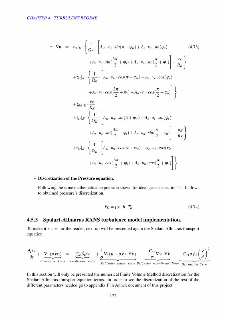
CHAPTER 4. TURBULENT REGIME.
τ : ∇u = τrr|K ·
1
ΩK·
[Aw · vw · sin(π +ϕw)+Ae · ve · sin(ϕe) (4.73)
+As · vs · sin(3π
2+ϕs)+An · vn · sin(
π
2+ϕn)
]− vK
RK
+τrz|K ·
1
ΩK·
[Aw · vw · cos(π +ϕw)+Ae · ve · cos(ϕe)
+As · vs · cos(3π
2+ϕs)+An · vn · cos(
π
2+ϕn)
]+τθθ |K ·
vK
RK
+τzr|K ·
1
ΩK·
[Aw ·uw · sin(π +ϕw)+Ae ·ue · sin(ϕe)
+As ·us · sin(3π
2+ϕs)+An ·un · sin(
π
2+ϕn)
]− uK
RK
+τzz|K ·
1
ΩK·
[Aw ·uw · cos(π +ϕw)+Ae ·ue · cos(ϕe)
+As ·us · cos(3π
2+ϕs)+An ·un · cos(
π
2+ϕn)
]
• Discretization of the Pressure equation.
Following the same mathematical expression shown for ideal gases in section 4.1.1 allowsto obtained pressure’s discretization.
PK = ρK ·R ·TK (4.74)
4.5.3 Spalart-Allmaras RANS turbulence model implementation.To make it easier for the reader, next up will be presented again the Spalart-Allmaras transportequation.
∂ρν
∂ t+ ∇ · (ρνu)︸ ︷︷ ︸
Convective Term
= Cb1Sρν︸ ︷︷ ︸Production Term
+1σ
∇((µ +ρν) ·∇ν)︸ ︷︷ ︸Di f f usive linear Term
+Cb2
σ∇ν ·∇ν︸ ︷︷ ︸
Di f f usive non−linear Term
−Cw1ρ fw
(ν
d
)2
︸ ︷︷ ︸Destruction Term
In this section will only be presented the numerical Finite Volume Method discretization for theSpalart-Allmaras transport equation terms. In order to see the discretization of the rest of thedifferent parameters needed go to appendix F in Annex document of this project.
122

CHAPTER 4. TURBULENT REGIME.
• Discretization of the convective term.
Unlike the modified Mass, Momentum and Energy conservation equations shown in sec-tion 4.3, the discretization of the convective term is equal to the one explained in thelaminar regime part of this thesis (section 3.2.4). The only minor difference betweenthem is that, in first case, the coordinate system was Cartesian, while this time it is cylin-drical. However, this only affects in small aspects like control volume surfaces differencebetween lower and upper limits.
Applying the Finite Volume Method basis and Stokes theorem leads to the followingnumerical expression of the equation.
∇ · (ρνu) =1
ΩK·
[Aw ·ρw · νw · (uw · cos(π +ϕw)+ vw · sin(π +ϕw)) (4.75)
+Ae ·ρe · νe · (ue · cos(ϕe)+ ve · sin(ϕe))
+As ·ρs · νs · (us · cos(3π
2+ϕs)+ vs · sin(
3π
2+ϕs))
+An ·ρn · νn · (un · cos(π
2+ϕn)+ vn · sin(
π
2+ϕn))
]
• Discretization of the production term.
As it can be seen in its equation, production term doesn’t represent a great challenge fromthe point of view of the discretization. There is Nabla operators (∇) such as divergenceor gradient.
The only difficulty may be the computation of extra parameters like S.
Cb1Sρν =Cb1 · SK ·ρK · νK (4.76)
• Discretization of the diffusive linear term.
The discretization of this term is similar to the one exposed for the diffusive term inMomentum and Energy conservation equations in laminar regime (section 3.2.4).
The only minor difference may be again, the switch from Cartesian to cylindrical coordi-nate system in terms of control volume surfaces.
Once again, applying the Finite Volume Method discretization basis and Stokes theoremfor the Divergence operator leads to the following discretized equation.
123

CHAPTER 4. TURBULENT REGIME.
1σ
∇((µ +ρν) ·∇ν) =1
ΩK·
[Aw · (µw +ρwνw) ·
νK− νW
dKW· cos(π +ϕw) (4.77)
+Ae · (µe +ρeνe) ·νE − νK
dKE· cos(ϕe)
+As · (µs +ρsνs) ·νK− νS
dKS· sin(
3π
2+ϕs)
+An · (µn +ρnνn) ·νN− νK
dKN· sin(
π
2+ϕn)
]
• Discretization of the diffusive non-linear term.
This term of the Spalart-Allmaras transport equation has a certain peculiarity. Until now,in order to simplify the equations, every gradient has been expressed as an scalar valuewhich depends only on the two node variables involved.
However, the gradient operator is actually a vector with 1, 2 or 3 components dependingif the study is uni, bi or tri-dimensional.
∇φ =
(∂φ
∂x,
∂φ
∂y,
∂φ
∂ z
)(4.78)
So, mathematically, the operation ∇φ ·∇φ is a scalar product between both vectors. Thisleads to the following result (for bi-dimensional cylindrical coordinates).
∇φ ·∇φ =∂φ
∂x· ∂φ
∂x+
∂φ
∂ r· ∂φ
∂ r=
(∂φ
∂x
)2
+
(∂φ
∂ r
)2
(4.79)
It also needs to be mentioned that, in this case, the gradients are referred to the con-trol volume, not its faces. This means, it is necessary to apply the already explainedDivergence-Gradient mathematical relationship for the radial direction gradients.
124

CHAPTER 4. TURBULENT REGIME.
Cb2
σ∇ν ·∇ν = Cb2 ·
[1
ΩK· [Aw · νw · cos(π +ϕw) (4.80)
+Ae · νe · cos(ϕe)
+As · νs · cos(3π
2+ϕs)
+An · νn · cos(π
2+ϕn)]
]2
+
[1
ΩK· [Aw · νw · sin(π +ϕw)
+Ae · νe · sin(ϕe)
+As · νs · sin(3π
2+ϕs)
+An · νn · sin(π
2+ϕn)]−
νK
RK
]2
• Discretization of the destruction term.
As in the case of the production term, the discretization of the destruction one is verystraight and easy in comparison with other ones like the previous one.
Again, the only aspect to take into account is that is is necessary to compute certainsecondary parameters before calculating this term.
−Cw1ρ fw
(ν
d
)2
=−Cw1 ·ρ · fwK
(νK
dK
)2
(4.81)
Once all this terms have been determined separately, it is necessary to add them all.
F(ν) =−∇ · (ρνu)+Cb1Sρν +1σ[∇((µ +ρν) ·∇ν)+Cb2∇ν ·∇ν ]−Cw1ρ fw
(ν
d
)2
(4.82)
Then, νn+1 is determined as a function of νn, νn−1, F(ν)n−1 and F(ν)n. (Explained in a moredetailed way in the next section).
Now, it is only needed to compute the following parameters.
Xn+1 =νn+1
νn+1 −→ f n+1v1 =
(Xn+1)3
(Xn+1)3 +C3v1
(4.83)
And finally, it is possible to determine the turbulent dynamic viscosity that will be added to thenormal viscosity.
125

CHAPTER 4. TURBULENT REGIME.
µn+1t = ν
n+1 ·ρn+1 · f n+1v1 (4.84)
4.5.4 Time integration.The time integration method used for the turbulent regime study doesn’t differ so much fromthe one of the laminar regime apart from certain changes.
The main similarity between both processes is that, as in the laminar case, in the turbulent studyan explicit time integration method is used (section 3.2.3).
However, this time, instead of using a fixed Adam-Bashforth method, it has been chosen toimplement a slightly change [37].
φn+1 =
2 ·βTime ·φ n− (βTime−0.50) ·φ n−1
βTime +0.50+∆t · [(1+βTime) ·F(φ)n−βTime ·F(φ)n−1]
(4.85)
Thanks to this tiny change in the time integration, it is possible to select the weight that eachtime step may have on the future value of the property.
Next up is presented the time integration expressions for the main physical properties of thesimulation.
Density.
ρn+1 =
2 ·βTime ·ρn− (βTime−0.50) ·ρn−1
βTime +0.50+∆t ·
[(1+βTime) ·F(ρ)n−βTime ·F(ρ)n−1]
(4.86)
Axial velocity.
un+1 =2 ·βTime ·un− (βTime−0.50) ·un−1
βTime +0.50+∆t ·
[(1+βTime) ·
F(u)n
ρn −βTime ·F(u)n−1
ρn−1
](4.87)
Radial velocity.
vn+1 =2 ·βTime · vn− (βTime−0.50) · vn−1
βTime +0.50+∆t ·
[(1+βTime) ·
F(v)n
ρn −βTime ·F(v)n−1
ρn−1
](4.88)
Internal energy.
en+1 =2 ·βTime · en− (βTime−0.50) · en−1
βTime +0.50+∆t ·
[(1+βTime) ·
F(e)n
ρn −βTime ·F(e)n−1
ρn−1
](4.89)
Turbulent viscosity.
νn+1 =
2 ·βTime · νn− (βTime−0.50) · νn−1
βTime +0.50+∆t ·
[(1+βTime) ·
F(ν)n
ρn −βTime ·F(ν)n−1
ρn−1
](4.90)
126

CHAPTER 4. TURBULENT REGIME.
As there can be seen in time integration equations (4.87), (4.88), (4.89) and (4.90), the time stepcontributions F(u), F(v), etc.. are divided by the density.
This is because of the variable on the time change rate on the left side of the equation. In theseexpressions, the overall contributions are referred to the values ρφ , and so this must be takeninto account when operating.
Finally, the other modification on the time integration method for the turbulent regime con-sists on a little addition to the already shown Courant-Friedrichs-Lewy condition (CFL, section3.2.3).
As it is explained there, the ∆t of each simulation step isn’t arbitrary, it is computed following acertain criteria.
This is related with the diffusion of velocity, temperature and the convection (advection) ofvelocity. And it is, this last term, the CFL convection criteria which is slightly changed becauseof compressible flow.
While studying incompressible flow, the mathematical equations make perturbations in the fieldto transport themselves at infinite speed. To give a better insight of this imagine a that at acertain time step a great perturbation takes place at the middle of the flow. Then, right at thenext step, this perturbation effects will be noticed by every control volume of the geometry (itseffects may vary with the distance).
However, one thing that makes compressible flow much harder to simulate is the fact that, aperturbation on the flow moves through this one at sound speed.
Among other aspects, the increasing difficulty in the compressible flow simulations comes dueto the following fact. If the simulation diverges at a certain control volume at present timestep, it won’t be until many time steps in the future that it will be possible to notice that thesimulation has gone wrong. Unfortunately, this makes necessary to repeat the simulation againhaving wasted many computational time worthless.
Turning back to the CFL condition modification, this consists on adding the sound speed to thespread out velocity in the convection term.
∆tc = min(
0.35∆x|u+ c|
, 0.35∆y|v+ c|
)(4.91)
In order to compute the value of the speed of sound, the following expression is used.
c =√
γ ·R ·T (4.92)
4.5.5 Simulation algorithm.Unlike in the laminar regime section, in this case there is no Poisson’s equation that needs anspecial solver. Instead of that, in order to compute the physical fluid properties of the nextstep o the simulation, it is only necessary to apply the time integration process described in theprevious section (section 4.5.4).
127

CHAPTER 4. TURBULENT REGIME.
However, in the turbulent compressible regime it is necessary to solve the Spalart-Allmarasturbulence model and the Mass Conservation equations additionally. Therefore, there are somechanges in the simulation algorithm from the one presented in section 3.2.6.
The complete turbulent regime smiluation algorithm is presented in figure 4.11. Nevertheless,only the non already explained steps are exposed after it.
128

CHAPTER 4. TURBULENT REGIME.
Figure 4.11: Turbulent regime simulation algorithm
129

CHAPTER 4. TURBULENT REGIME.
• 2. Geometry acquisition.
As it has already been explained, one of the aims of the code is to be as generic as possible.It is capable of meshing and simulating many different axisymmetric geometries. Butfirst, it is necessary to obtained the mathematical equation of these.
• 5.2 Initial calculation of physical variables.
At the beginning of each simulation, it is necessary to compute some physical data likeheat capacities, or certain boundary conditions, etc..
• 6.2 Determination of base dynamic viscosity.
At the beginning of each time step, it is important to compute the base dynamic viscosity(due to problem’s boundary conditions), needed to solve the turbulence model.
• 7. Resolution of the Spalart-Allmaras model.
In order to solve the Navier-Stokes equations, kinematic turbulent viscosity from Spalart-Allmaras model must be determined.
• 9. Resolution of Mass Conservation Equation.
It it the first of the 3 Navier-Stokes equations that need to be solved. In order to do that, itis necessary to compute each of its discretized terms (section 4.5.2).
• 10. Resolution of Momentum Conservation Equation.
Again, it is one of the Navier-Stokes discretized equations that need to be solved. To dothat, all its discretized terms must be determined first (section 4.5.2).
• 11. Resolution of Energy Conservation Equation.
Last of the Navier-Stokes equations that is necessary to solve. Again, it is necessary firstto calculate its discretized terms (section 4.5.2).
130

CHAPTER 4. TURBULENT REGIME.
4.6 Simulation of turbulent compressible pipe flow.In this section are presented the obtained results in the simulations of the turbulent supersoniccompressible pipe. As there has already been done in the laminar regime results sections, therewill also be presented the verification and an extensive explanation of the physical phenomenainvolved in the problem.
The turbulent supersonic pipe case has already been briefly presented previously, in section 4.4.As its name already indicates, it consists on a constant radius pipe in which there is a supersonicflow at its inlet.
The trustworthy scientific publication used in the comparisons can be found in [38]. In order tobe able to compare the obtained results with the source mentioned, there has been necessary toadd some features to the case. These are exposed next up.
First of them, and probably, the most significant one is the Reynolds number selection. In caseof the laminar regime LID Driven Cavity and Square Cylinder, this parameter is calculatedor set depending on several variables but not temperature. In turbulent compressible flows,temperature plays a huge role, and it is impossible to define the flow conditions without it.
In the problem case, the solid wall of the pipe is set to have a constant temperature (TWall) in allof its length. This define the speed of sound in all of the geometry.
c =√
γ ·R ·TWall (4.93)
The other two parameters that define the sonic speed γ and R are set to simulate air.
γ = 1.40 R = 286.90 J/Kg ·K (4.94)
Since these have been set as the air characteristics values, so must the Prandtl number of thesimulation. As in the LID Differentially Heated problem, in this case it is set to 0.71.
Reynolds number is defined by fluid’s viscosity too. As there has been exposed in section 4.1.1,in the turbulent regime study the viscosity has been set to be temperature dependant.
The mathematical expression selected from the Sutherland law is the following.
µ(T )µRe f
=
(T
TRe f
)n
(4.95)
For the problem, there has been set the reference values of the equation (4.95) for an ambienttemperature of 25ºC. The data for the reference dynamic viscosity at that temperature can befound in [39]. In addition to that, the reference sets the value of the n as 0.7, and so it is done inthe project.
In what comes to the reference length of the problem, this has been set as the pipe radius.
Once these parameters have been defined, it is possible to calculate or set the Reynolds number.However, in this case there will be used what’s known as bulk Reynolds. This is a Reynolds
131

CHAPTER 4. TURBULENT REGIME.
number based on the averaging of the flow variables. It doesn’t have any relation with theaveraging processes shown in previous sections for RANS turbulence modelling. It is also usedin DNS simulations.
This bulk Reynolds have the following expression.
Rem =ρm ·um ·LRe f
µw(4.96)
It is presented the definition of the Mach number for the problem too.
Mm =um√
γRTWall(4.97)
Once the previously mentioned variables have been calculated, it is possible to define the flowcharacteristics at the inlet by using the equations (4.96) and (4.97).
By setting the mean Mach number at the entrance Mm, it is possible to compute the meanvelocity um there. Then, it is possible to compute the dynamic viscosity at the wall by applyingthe mathematical formula presented before (4.95).
Finally, defining a bulk Reynolds number, the value of the density at the inlet can be imposed.
All the flow variables at the inlet have been completely defined.
4.6.1 Obtained results and verificationFirst of all, as in the laminar regime study cases, it is presented the simulation parameters intable 4.2.
Table 4.2: Turbulent compressible supersonic pipe simulation parametersSimulation DNS RANS
LRe f (m) 1.0 1.0
Pipe Length (m) 25.0 25.0
TWall (K) 298.15 298.15
Rem 3181.0 3181.0
Mm 1.30 1.30
X Direction Nodes 250 120
R Direction Nodes 120 90
X Nodal Distribution Regular Regular
R Nodal Distribution Hyp. Tan Regular
Hyp. Tan. Stretching 1.0 -
Stop Criteria - 1,00E-06
As it is shown in previous table, there have been made 2 different simulations. One solving thealready explained RANS Spalart-Allmaras turbulence model, and the other one by just carrying
132

CHAPTER 4. TURBULENT REGIME.
out a DNS simulation. This allows to compare the results obtained in both of them and see theadvantages and disadvantages of each type of approach.
Verification.
The verification of the turbulent regime study case simulation is based on the comparison ofseveral parameters and flow profiles with the ones present in [38]. In the publication, the authorscarry out a DNS simulation of a turbulent compressible supersonic pipe with a tri-dimensionalapproach.
The parameters of the comparison are the friction Reynolds and Mach numbers.
As the reader may sense from the names, these are related to the friction of the pipe flow withits solid wall.
The viscosity of the fluid alongside with the non-slip condition at the solid wall leads to a non-null friction in this area.
Figure 4.12: Flow profile at the wall scheme
Calculating the velocity gradient right at the wall gives the wall shear stress, which is the baseof the two verification parameters previously mentioned, friction Reynolds and Mach numbers.
τW = µ · ∂u∂ r
(4.98)
Since all the data is discrete, there are several tiny modifications to make to equation (4.98).
The way to compute the velocity gradient is to take the difference between the wall node andthe closest to it. This leads to a linear gradient. In order to avoid this simlification and obtainedmore accurate results, it is possible to develop a wall shear model. However, this is way beyondthe project scope for this section.
Nevertheless, the nodal resolution at the wall is set to be enough accurate to get an acceptableresults of this calculation.
In order to being able to describe with the parameters the flow at the pipe, no discrete individualdata can be taken. The mean value must be computed τW . To obtain this, an spatial integrationof the discrete values must be done.
Then, another variable should be computed based on the previous one, the friction velocity uτ .
133

CHAPTER 4. TURBULENT REGIME.
uτ =
√τW
ρW(4.99)
In this case, it is also necessary to compute the mean value of the density at the wall by doingagain an spatial integration of this variable.
Once the friction velocity has been determined, it is possible to compute the friction Reynoldsand Mach numbers (equations (4.100) and (4.101) respectively).
Reτ =ρW ·uτ ·LRe f
µW(4.100)
Mτ =uτ√
γ ·R ·TWall(4.101)
Next up, in table 4.3, are presented the comparison between the obtained results and the onesfrom the scientific paper of the previous parameters. In addition, it is shown the values of thebulk Reynolds and Mach numbers at the calculation section of the friction parameters.
Table 4.3: Reynolds and Mach numbers obtained comparisonParameter Reτ Mτ Rem Mm
Source DNS 245.000 0.077 3181.000 1.300
Obtained DNS 237.334 0.087 3182.918 1.359
Ob. DNS Relative Error (%) 3.129 12.987 0.060 4.538
Obtained RANS 238.144 0.088 3180.987 1.358
Ob. RANS Relative Error (%) 2.798 14.286 0.001 4.462
There are several aspects to comment about the results presented in table 4.3.
First, it must be mentioned that, in what comes to the friction Reynolds, the results obtained area little lower than the one from the scientific paper. However, the relative error in both cases islower than a 5%, which shows that they can be considered as correct.
On the other hand, the friction Mach numbers have a higher relative error than Reynolds ones.As it has been mentioned, there is a strong dependence of this value from the way to computethe velocity gradient at the wall and the resolution of the mesh close to it. Nevertheless, noneof them has a relative error higher than 15% approximately. They are close to it, but the resultscan still be considered as acceptable from an engineering point of view.
In addition, there must be mentioned that the results from the source and the codes developedare likely to differ in a certain way. In the scientific publication, the authors use many differentand more complex numerical techniques and methods, which, although are aimed to solve thesame equations, the final results may differ from one project to another.
Finally, it is presented the bulk Reynolds and Mach numbers comparison. As it has been said,the inlet conditions are controlled by this same parameters. However, it is always important toverify if the imposed conditions are still present where the additional data is been computed.
134

CHAPTER 4. TURBULENT REGIME.
In other words, the friction parameters depend strongly in the bulk ones. Therefore, it is crucialto verify that where the first ones are been calculated, there are still the flow conditions initiallyimposed.
The other variables used for the verification of the turbulent regime case are the temperaturesand density radial non-dimensionalized profiles of the flow. These are presented in figures 4.13and 4.14 respectively.
Figure 4.13: Temperature non-dimensional profiles comparison
Figure 4.14: Density non-dimensional profiles comparison
In order to be able to compare the temperature and density profiles, the authors present in thepublication the non-dimensionalized values. The reference parameters chosen are the wall’stemperature (TWall) and the density at the same location (ρW ), both previously set or calculated.
T ∗(r) =T (r)TWall
ρ∗(r) =
ρ(r)ρW
(4.102)
135

CHAPTER 4. TURBULENT REGIME.
As there can be seen in both figures, obtained DNS and RANS temperature and density profileshave very similar results. This has been already seen in table 4.3. The friction parameters resultsfor both of these simulations match almost perfectly.
However, looking at figures 4.13 and 4.14, there can be seen that the obtained results are not ex-actly the same as the ones from the scientific publication. As it has been previously mentioned,the authors use different numerical techniques and methods that make the results to differ. Inaddition to the temporal integration of the results, which is completely different and extremelycomplex in comparison with the one done for the DNS in this project. In case of the RANSmodel simulation, it is not needed since it already provides the averaged values.
Nevertheless, it may look like a great difference in both cases. However, when analysing itnumerically, this difference gets smaller in comparison. The average relative error is less than5%. But, in addition to that, it is only needed to look at the enormous similarity between theprofiles tendencies to consider the results obtained as acceptable.
Results
Next up the results obtained for the RANS simulation are presented. As it is specified in thesimulation parameters (table 4.2), the total length of the pipe has been set to 25 m. However,since the relevant part of the study is where there is a fully developed flow, only the last half ofthe pipe is presented.
Temperatures field.
In figure 4.15 is presented the temperatures field obtained in the simulation.
Figure 4.15: Turbulent supersonic compressible pipe temperatures field
As there can be seen in figure 4.15, most of the pipe flow temperature profile is close to 390 to400 K. This can be also found in figure 4.13. The wall’s temperature has been set to 298.15 K(25ºC). Therefore, a 1.30 non-dimensional value of this lead to the present temperatures field.
In addition to that, it is important to mention the huge temperature gradient that takes place nearthe wall. In figure 4.13 this can be seen by the quickly increase in the plot value. But, the bestway to see it is looking at figure 4.15, where there can be seen an enormous change from 298.15K to almost 400 K in less than 20 cm.
Velocities field.
136

CHAPTER 4. TURBULENT REGIME.
In figure 4.16 is presented the non-dimensional velocities field obtained for the simulation ofthe turbulent supersonic compressible pipe.
Figure 4.16: Turbulent supersonic compressible pipe Velocity Magnitude field
There are several aspects to mention about the non-dimensionalized velocities field in figure4.16.
First of them concerns concerns the choice of present the velocity results as a function of Machnumber. While studying or simulating supersonic flow, the velocities reached by the flow areusually too high to work and use them to compare.
Instead of that, it is much more practical and useful to show these results with the Mach number.When presenting the capabilities of a supersonic aircraft, Mach number is used to mention itsvelocity, not m/s or Km/h.
The other important aspect that must be remarked is the cross-sectional velocity profile. As ithas been mentioned before, non-slip condition is imposed at the pipe wall. Therefore, a velocitygradient is generated due to this restriction. However, in this case, the resulting gradient isextremely larger than any shown in the laminar regime section.
To give the reader an idea about its magnitude, in this case are presented the velocity profileand the non-dimensionalized velocity profile of the cross-section of the pipe in figures 4.17 and4.18 respectively.
137

CHAPTER 4. TURBULENT REGIME.
Figure 4.17: Turbulent supersonic compressible pipe non-dimensional Horizontal Velocity pro-file at x = 24 m
Figure 4.18: Turbulent supersonic compressible pipe Horizontal Velocity profile at x = 24 m
As there can be seen in both figures, the velocity gradient at the wall is much higher thananyone shown in the project before. It reaches 100 m/s in just less than 5 cm from the wallapproximately. This is one of the main difficulties when calculating variables at the wall likethe ones presented before, friction Reynolds and Mach numbers. The gradients are so high thata great resolution is needed. Otherwise, nonsense results could be obtained.
In addition to that, there must be mentioned the huge velocities present at the pipe. For instant,the highest one of figure 4.17 is larger than 500 m/s, which is more than 1800 Km/h, twice thecruise speed of a commercial aircraft.
Pressure field.
In figure 4.19 is presented the pressure field for the simulation of the turbulent supersonic com-pressible pipe.
138

CHAPTER 4. TURBULENT REGIME.
Figure 4.19: Turbulent supersonic compressible pipe pressure field
As there can be seen in figure 4.19, there is a tiny pressure drop in the axial direction. However,the flow velocities (shown previously) are so high that this pressure gradient can be consideredas negligible.
In addition to that, looking at image 4.19, there can be observed the almost null change inpressure in the radial direction. This is mainly because the radial velocity is close to zero, andso its gradients.
Density field.
In figure 4.20 is presented density field obtained in the simulation.
Figure 4.20: Turbulent supersonic compressible pipe density field
Looking at figure 4.20 there can be seen the same radial density profile as the one shown pre-viously in the verification. The fluid’s density close to the wall is much higher than near thecentral axis. This happens because of the flow velocities.
Near the wall, flow’s speed is much lower than at the centre due to non-slip condition at thewall. And so the density increases in this area.
139

Chapter 5
Environmental impact of the project
Once every project is almost finished, it is essential to look back and carry out an environmentalstudy of it. Not only to see if it has been a success in this aspect, but to know if it is possible toimprove the results in this area.
Because of that, next up is presented an exhaustive study of the environmental impact of thepresent project. This will be divided into the work tasks exposed in the budget section.
5.1 Documentation and investigation.Most of the information and learning of the theoretical basis of the project have come fromtrustworthy Internet sources and scientific publications. The environmental impact of this partof the project has been smaller in comparison with other tasks.
First, in what comes to energy use during this part, it must be mentioned that most of the timenatural light was used, instead of artificial. Additionally, in order to save energy, the computersused have been off when these weren’t needed.
However, one aspect that clearly can be improved is the paper sheets usage. Due to the enormousamount of information that should be gathered to fulfil project’s requirement, there has beennecessary to buy a pack of these. Unfortunately, these weren’t recycled sheets.
So, the main aspect that should be improved for next projects in this tasks is the usage of leastpossible paper sheets and if possible recycled ones.
5.2 Coding and debugging.This section of the project is probably the one with the highest environmental impact. For thispart, it is necessary at least to use one computer at a time, if not the two available.
Coding takes a lot of time. This kind of Computational Fluid Dynamics projects needs an enor-mous programming effort. The student has to develop every feature of the code. For instance,all of the present project combined have more than 7 thousand lines of coding.
140

CHAPTER 5. ENVIRONMENTAL IMPACT OF THE PROJECT
This is a huge computer power consumption which is quite difficulty to reduce. A lot of pro-gramming experience is necessary. And even with it, there will be needed to add the debuggingtime to the energy usage.
However, there has been tried to minimise this consumption by using only one computer at atime when it was possible. Unfortunately, there were many situations in which this was reallydifficult.
5.3 Verification of the results.This section is probably the one with the smallest environmental impact of the whole project.The flow simulations have been carried out as part of this task. These obviously represent thehighest energy usage per hour of all tasks. The computer were at maximum power. However,these didn’t take as much time as others. The reduction in total hours is quite significant incomparison with any of the rest.
In addition to that, it must be mentioned that one of the aims of every computational codedeveloped is to be as efficient as possible. This, obviously, improve with the coding experience.
5.4 Project’s memory development.Since the project’s memory has been written using an online text service, the only environmentalimpact of this task comprises the power consumption of the computer and the artificial lightused.
First, it must be mentioned again that, when it was possible, only one computer was used at atime, in order to save energy. In addition to that, artificial light consumption was reduced asmuch as possible.
Finally, to be able to cut down even more the impact, there has been decided not to print thememory thesis or any of its attached documents.
In conclusion, there has been obviously several points in which the environmental impact couldbe severely reduced. However, this project has taken a lot of time and power resources, whichare likely to be cut down in future developments with better equipment and much more experi-ence.
141

Chapter 6
Conclusions and future work.
Next up are presented the conclusions extracted from the development of the present project, itsimplications and the future work.
6.1 General conclusions.The main conclusion that can be extracted from an overall view of the whole project is thecomplete fulfilment of its scope. The aim was to study the computational resolution of theNavier-Stokes conservation equations and the application to different cases.
First of all, it is important to mention the difficulty and all the hard work needed for the devel-opment of this kind of studies. It is not only needed to coding and carry out the simulations.It is necessary to find the information about the physical phenomena involved, learn algorithmsand programming techniques, coding and debugging, which takes a lot of time, and validatingthe results using trustworthy scientific sources.
In what comes to the development of the laminar regime scopes of the project there are severalconclusions that can be extracted.
First of them comprises the learning of the physical phenomena and the flow characteristics. Inaddition to that, there must be noticed the success in the computational implementation of theresolution algorithms. As it has been shown, these add an extra difficulty to the project, since itis necessary to develop all of them.
There were many simulation difficulties. It was necessary much code debugging time.
However, that extra time added to the project development has been completely worthy. The re-sults obtained for the laminar regime study cases, LID Driven Cavity, LID Differentially Heatedand Square Cylinder are more than acceptable. As there has been shown, all of these matchgreatly with the referencesc authors selected for the comparison.
Nevertheless, there is one aspect in the laminar regime part of the project that can be clearlyimproved, the code efficiency. These codes were the first ones to be programmed by the studentin the CFD area. Therefore, these can be improved severely in the aspect of efficiency.
142

CHAPTER 6. CONCLUSIONS AND FUTURE WORK.
Additionally, there are many different conclusions to extract from the turbulent regime sectionof the project.
First of them is the enormous increase in difficulty in comparison with the laminar regime. Notonly because turbulent flow has a much more complicated theoretical basis behind, but also dueto the simulation of compressible fluid.
As there has been shown, it is needed to modify the Navier-Stokes equations to avoid gettinginstabilities in the simulations. In addition to that, in order to be able to simulate the proposedcase, there has been needed the implementation of the Spalart-Allmaras turbulence model.
This added even extra difficulties due to the following reasons.
First of them, it was necessary to learn and understand all the theoretical basis of RANS turbu-lence models and the equations averaging.
In addition to that, the numerical implementation of the Spalart-Allmaras model made compul-sory to learn again, the theoretical basis behind, which wasn’t easy at all.
But, furthermore, the addition of the compressible flow hypothesis to the simulations made theimplementation even more complicated. Originally, the model was developed for incompress-ible fluids, as it can be seen in the authors paper from 1994 [30]. Therefore, it is difficult eventoday to find trustworthy information about the compressible form of the model. There areseveral differences in the equations from one application case to another.
However, in spite of all the difficulties previously mentioned, the obtained results for this sectionof the project can be considered as acceptable. It is true that there are some parameters such asthe friction Mach number which have almost a relative error of 15%. Nevertheless, there mustbe taken into account the great difficulty in its calculation due to the flow conditions simulated(supersonic velocities) and the nodal resolution near the wall.
Therefore, for the present project, these results can be considered as highly acceptable. How-ever, they can be improved with more experience in turbulence modelling and CFD simulation.
It is because of all aforementioned that in what comes to the fulfilment of the project scopes,these can be considered as a clear success. Not only there has been developed several complexstudies for each of the flow regimes in CFD. But also, the results obtained can be considered asuccess too.
6.2 Future work.This project has provided a great background in Computational Fluid Dynamics. All the differ-ent theoretical basis learnt, the algorithms implemented and the kind of studies developed givethe student amazing possibilities for further work.
Therefore, it would be a waste of learning time and possibilities to stop at this point. Next upare presented the future lines of research for the project.
143

CHAPTER 6. CONCLUSIONS AND FUTURE WORK.
6.2.1 Short term.Due to the situation brought by the Covid-19 outbreak, the turbulent regime part of the projecthas been severely reduced. Therefore, the first tasks to be developed aim completely to this partof the project. Initially, there were several study cases related to rocket nozzle. However, therehasn’t been possible to complete them all.
Therefore, the first line of research is to be able to simulate these cases and if possible, to addmore geometry simulation features to the codes.
6.2.2 Mid term.For the mid-term lines of research, the aim is to implement others RANS turbulence modelssuch as k−ω or k− ε and compare them with the Spalart-Allmaras. This would give a moreglobal vision of the RANS turbulence modelling and allow to compare the results obtained witheach of them, in order to select which are better for each application.
As there can be seen, the future work is completely related to the computational resolution ofturbulent regime flows and its application to the simulation of rocket nozzles mainly.
The global aim is to create a ”tool” to simulate, analyse and improve the performance of thegeometries of rocket nozzles. It is a huge and far aim for just a graduate student. However, thebackground acquired with this project is a great way to begin the path with.
144
Bibliography
[1] Josip Basic. Turbulent history of fluid mechanics (brief essay). (January), 2016. doi:10.13140/RG.2.1.3487.8485.
[2] Bachelor/Master Thesis in Computational Fluid Dynamics(CFD), . URL https://www.termoflow.com/jobs/detail/
bachelor-master-thesis-in-computational-fluid-dynamics-cfd-1. Re-trieved 25-3-2020.
[3] Computational Fluid Dynamics Software Saves Time, Cuts Costs — 2018-03-07 — Assembly Magazine, . URL https://www.assemblymag.com/articles/
94178-computational-fluid-dynamics-software-saves-time-cuts-costs. Re-trieved 25-3-2020.
[4] Computational Fluid Dynamics Optimisation Based On Formula 1 Meth-ods – Swiss Side, . URL https://www.swissside.com/blogs/news/
computational-fluid-dynamics-optimisation-based-on-formula-1-methods.Retrieved 25-3-2020.
[5] NASA@SC11 Demo: Space Shuttle Aerodynamics and Debris Simulations, . URLhttps://www.nas.nasa.gov/SC11/demos/demo20.html. Retrieved 25-3-2020.
[6] Shahil S Charania, Vishal Soni, Kiran C Patel, Jaymin Desai, and Vishal Chauhan. Eval-uation of Vertical Kaplan Turbine using CFD. Proceedings of the Thirty Ninth Na-tional Conference on Fluid Mechanics and Fluid Power, (December):1–10, 2012. doi:10.13140/2.1.3455.3926.
[7] Characteristics of Laminar Flow & Turbulent Flow — ibidi. URL https://ibidi.com/
content/286-the-different-types-of-flow#laminar. Retrieved 26-3-2020.
[8] Niels N. Sørensen, B. Mendez, A. Munoz, G. Sieros, E. Jost, T. Lutz, G. Papadakis,S. Voutsinas, G. N. Barakos, S. Colonia, D. Baldacchino, C. Baptista, and C. Ferreira.CFD code comparison for 2D airfoil flows. Journal of Physics: Conference Series, 753(8), 2016. ISSN 17426596. doi: 10.1088/1742-6596/753/8/082019.
[9] Hammond Steven; Schreiber Robert. Mapping Unstructured Grid Problems to the Connec-tion Machine. Research Institute for Advanced Computer Science NASA Ames ResearchCenter, 1990. doi: 10.1006/rwos.2001.0118.
[10] S. Arias and A. Montlaur. Numerical study and experimental comparison of two-phaseflow generation in a T-junction. AIAA Journal, 55(5):1565–1574, 2017. ISSN 00011452.doi: 10.2514/1.J055387.
145

BIBLIOGRAPHY
[11] A.D. Elster. Laminar v turbulent - Questions and Answers in MRI, 2018. URL http:
//mriquestions.com/laminar-v-turbulent.html. Retrieved 5-19-2020.
[12] Spalart-Allmaras model – CFD-Wiki, the free CFD reference, . URL https://www.
cfd-online.com/Wiki/Spalart-Allmaras_model. Retrieved 27-4-2020.
[13] Lecture Notes, Fluid Dynamics, and Chiang C Mei. Methods of Describing Fluid Motion.pages 1–3, 2003.
[14] Charles Hirsch. The Basic Equations of Fluid Dynamics. Numerical Computation ofInternal and External Flows, (3):27–64, 2007. doi: 10.1016/b978-075066594-0/50041-2.
[15] Robin Kravets and Cigdem Sengul. Energy conservation. Ad Hoc Networks: Technologiesand Protocols, pages 153–195, 2005. doi: 10.1007/0-387-22690-7\ 6.
[16] Cuneyt Sert. Governing Equations of Fluid Flow and Heat Transfer. ME 582 FiniteElement Analysis in Thermofluids, pages 1–13, 2012.
[17] Richard D. Noble. Natural Convection. AIChEMI Modular Instruction, Series C: Trans-port, 4:20–28, 1983. doi: 10.1017/cbo9780511841606.009.
[18] Forced convection - Energy Education. URL https://energyeducation.ca/
encyclopedia/Forced_convection. Retrieved 22-3-2020.
[19] Laminar Flow Fluid Flow Review - Engineers Edge. URL https://www.
engineersedge.com/fluid_flow/laminar_flow.htm. Retrieved 26-3-2020.
[20] Boussinesq Approximation Definition, . URL https://www.comsol.com/
multiphysics/boussinesq-approximation. Retrieved 26-3-2020.
[21] Boussinesq approximation (buoyancy) - Wikipedia, . URL https://en.wikipedia.
org/wiki/Boussinesq_approximation_(buoyancy). Retrieved 26-3-2020.
[22] CTTC - Universitat Politecnica de Catalunya. Fractional Step Method Staggered Meshes.2014.
[23] CTTC. Introduction to the Fractional Step Method. pages 1–10.
[24] F. X. Trias and O. Lehmkuhl. A self-adaptive strategy for the time integration of navier-stokes equations. Numerical Heat Transfer, Part B: Fundamentals, 60(2):116–134, 8 2011.ISSN 10407790. doi: 10.1080/10407790.2011.594398. URL https://upcommons.upc.
edu/handle/2117/13309.
[25] U. Ghia, K. N. Ghia, and C. T. Shin. High-Re solutions for incompressible flow using theNavier-Stokes equations and a multigrid method. Journal of Computational Physics, 48(3):387–411, 1982. ISSN 10902716. doi: 10.1016/0021-9991(82)90058-4.
[26] N. C. Markatos and K. A. Pericleous. Laminar and turbulent natural convection in anenclosed cavity. International Journal of Heat and Mass Transfer, 27(5):755–772, 1984.ISSN 00179310. doi: 10.1016/0017-9310(84)90145-5.
[27] G. De Vahl Davis. Natural convection of air in a square cavity: A bench mark numericalsolution. International Journal for Numerical Methods in Fluids, 3(3):249–264, 1983.ISSN 10970363. doi: 10.1002/fld.1650030305.
146

BIBLIOGRAPHY
[28] M. Breuer, J. Bernsdorf, T. Zeiser, and F. Durst. Accurate computations of the laminarflow past a square cylinder based on two different methods: Lattice-Boltzmann and finite-volume. International Journal of Heat and Fluid Flow, 21(2):186–196, 2000. ISSN0142727X. doi: 10.1016/S0142-727X(99)00081-8.
[29] Favre averaged Navier-Stokes equations – CFD-Wiki, the free CFD reference.URL https://www.cfd-online.com/Wiki/Favre_averaged_Navier-Stokes_
equations. Retrieved 10-5-2020.
[30] P. R. Spalart and S. R. Allmaras. One-equation turbulence model for aerodynamic flows.Recherche aerospatiale, (1):5–21, 1994. ISSN 00341223. doi: 10.2514/6.1992-439.
[31] Juan Bautista and Pedro Costa. On the Numerical Compressible Flows.
[32] [CFD] The Spalart-Allmaras Turbulence Model - YouTube, . URL https://www.
youtube.com/watch?v=Xivc0EIGFQw. Retrieved 12-5-2020.
[33] Munshoor Ahmed, M. Rehan Saleem, Saqib Zia, and Shamsul Qamar. Central upwindscheme for a compressible two-phase flow model. PLoS ONE, 10(6):e0126273, 6 2015.ISSN 19326203. doi: 10.1371/journal.pone.0126273. URL https://journals.plos.
org/plosone/article?id=10.1371/journal.pone.0126273.
[34] W. Rozema, J. C. Kok, R. W.C.P. Verstappen, and A. E.P. Veldman. A symmetry-preserving discretisation and regularisation model for compressible flow with applicationto turbulent channel flow. Journal of Turbulence, 15(6):386–410, 2014. ISSN 14685248.doi: 10.1080/14685248.2014.910604.
[35] Basic Mathematical Relations. The Conservation Equations of Fluid Dynamics. FluidDynamics, 0(4):1–9, 2011.
[36] Del in cylindrical and spherical coordinates - Wikipedia. URL https:
//en.wikipedia.org/wiki/Del_in_cylindrical_and_spherical_coordinates#
Cylindrical_derivation. Retrieved 4-5-2020.
[37] F. X. Trias, M. Soria, A. Oliva, and C. D. Perez-segarra. Direct numerical simulationsof two- and three-dimensional turbulent natural convection flows in a differentially heatedcavity of aspect ratio 4. Journal of Fluid Mechanics, 586:259–293, 2007. ISSN 00221120.doi: 10.1017/S0022112007006908.
[38] Somnath Ghosh, Holger Foysi, and Rainer Friedrich. Compressible turbulent channel andpipe flow: Similarities and differences. Journal of Fluid Mechanics, 648:155–181, 2010.ISSN 00221120. doi: 10.1017/S0022112009993004.
[39] Air - Dynamic and Kinematic Viscosity. URL https://www.engineeringtoolbox.
com/air-absolute-kinematic-viscosity-d_601.html. Retrieved 14-5-2020.
147