B & V CORP - Records Collections
331
SDMS US EPA REGION V -1 SOME IMAGES WITHIN THIS DOCUMENT MAY BE ILLEGIBLE DUE TO BAD SOURCE DOCUMENTS.
-
Upload
khangminh22 -
Category
Documents
-
view
1 -
download
0
Transcript of B & V CORP - Records Collections
SDMS US EPA REGION V -1
SOME IMAGES WITHIN THISDOCUMENT MAY BE ILLEGIBLE
DUE TO BAD SOURCEDOCUMENTS.

STANDARD REFERENCE COMPARISONS
•foo
oDOM
~l~I T TTTTT~TTT T~r 7 ~TTT~T"T
o o o-A,
"I
SIin-___-..._..__
— Tj i TTTTI i i i i i i T r T i i i i i i i rr f'rr
O O O O Oco <- M- h> noCN CM r-- r\l
s\\,\
h-
YI i T ii i i i i i i i i i i i i i i i fi i i r 11 iO O O O
CM CN
II")
o'•si
in"
o"ro
'OJ
o"
^^(X
o
o o CDO
O-
Ul —
K3O"
OJO"
o
r.
_ L 1 1 1 L
oenO
roOOo
Or
S;Cv
O O O ONJO O
tvjOO
"bi~cn
o
-c.
oe OL e oI I i I I I i___L
'rrYvryYyipTfr
V
oHXHruu6
L009
[0
ho*
\
ii1-09
00 L
—•
^ ^ - - r , -.,.,_,
hog
,u fe-* /T\ r\ f~V~ /"\ /~\ ',(i'dup uu i-
1°^wyniFf
E
r[hop-i-09E_
^-09-7 A/-j^Po d-1 a 'UP

00 "SI B-H.L
——J
i

on

INFORMATIONUA SET CRL LOG No.SAMPLE I.D. FILENAME STATION PERCENT MATRIX10001177 937BH S05D TPH005D MW39G 13.35X soil
SIIMS TPH011MS SBSOJ 15.09X soilS11MSO TPH11MSO SBSOJ 15.09X soilblank1 TPHBLK Na2S04 N/A Na2S04
SAMPLE UT. FINAL VOL.11.45 10TO.87 1010.70 1010.50 10
DILUTION RUN TPH VALUE Mom. Amt.1 05/14 213 ug/kg X Rec.1 05/H 415 221.2 137.87X1 05/K 88 221.2 -9.99X1 05/H 20 U
W001186 V3ZBH S980
932815
05209 SB53G
10001200 93ZB15
S04MSS04MSOblank «2
S97DS98MSS9BMSD
0520505206052011
06240020624Q060624007
SB39ESB39ENa2S04
MV33ESBHSBH
blank «3 0624008 Na2SO4
15.86X soil
9.04X soil9.04X soil
N/A Na2SM
5.91X soil15.10X soil15.10X soil
N/A
10.23 10 05/20 11K

SAMPLE RESULTS FORM
SAMPLE I. D.:
SAMPLE WEIGHT (g)FILENAME:STATION LOCATION:MATRIX:DATE RUN:
D93Q001177
10.30TPHBLKNa2S04Na2S0405/14/93
932B14 blankl
FINAL VOLUME (ml): 10DILUTION FACTOR: 1% MOISTURE: N/AEXTRACTION DATE: 05/11/93
TFH VALUE:(concentration estimatedfrom diesel standard)
20 U mq/kq
SPECIFIC PRODUCTS IDENTIFIED: none
Samples with equivalent chromatograms: N/A
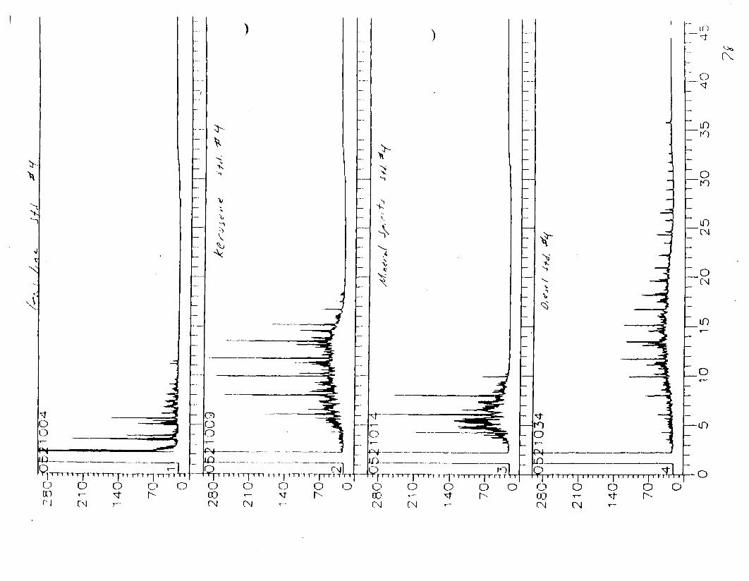
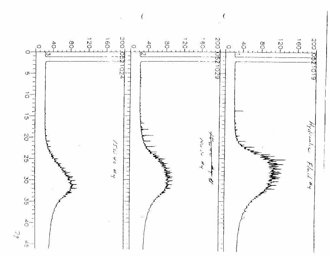
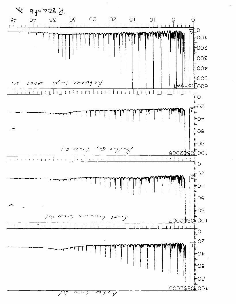
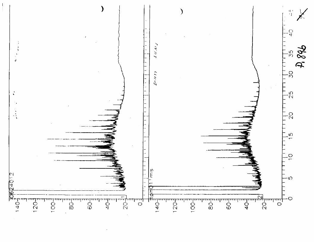
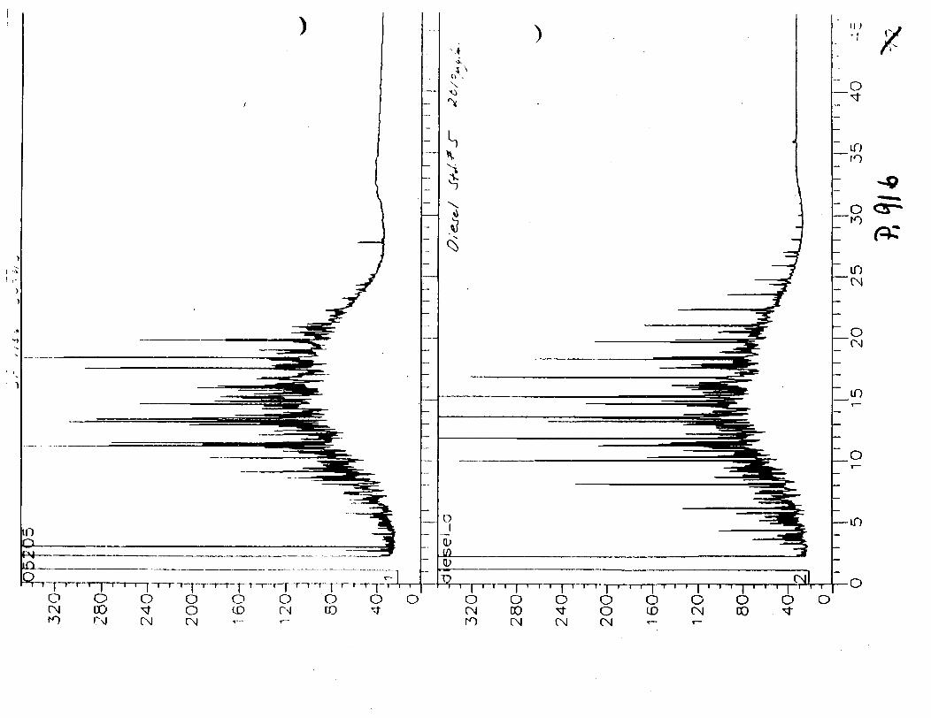
COMMENTS:Copies of the sample chromatogram and a diesel standard chromatogram areattached, as are comparisons with equivalent samples.Diesel standards were used to quantitate the samples for a TPH value as theyhave similar responses.
FLAGS: U Analyte is not present in concentrations at or abovequantitation limit.
J Reported value is estimated.E Analytes concentration in the sample exceeded the calibration
range.D Sample was diluted.

90 ^C62-101 0
72-
63^
54-E
27-
18-E1)
JJLJL
i I i i i | • I I I | ! I ! I
90:trt
72-
h Ik
18-
0 10 15 20 25 30 35 40
P,

SAMPLE RESULTS FORM
SAMPLE I. D.: D93Q001186 932B15 blank *2
SAMPLE WEIGHT (g): 10.00FILENAME: 052011 FINAL VOLUME (ml):STATION LOCATION: Na2S04 DILUTION FACTOR: 1MATRIX: Na2S04 % MOISTURE: N/ADATE RUN: 05/20/93 EXTRACTION DATE: 05/18/93
TPH VALUE: 20 u ma/lca(concentration estimatedfrom diesel standard)
SPECIFIC PRODUCTS IDENTIFIED: none
Samples with equivalent chromatograms: N/A
COMMENTS:Copies of the sample chromatogram and a diesel standard chromatogram areattached, as are comparisons with equivalent samples.Diesel standards were used to quantitate the samples for a TPH value as theyhave similar responses.
FLAGS: U Analyte is not present in concentrations at or abovequantitation limit.
J Reported value is estimated.E Analytes concentration in the sample exceeded the calibration
range.D Sample was diluted.

f
00NJxl
O)CT) M 00
O 03M-J CT> (Ji
c n - c n
(Jl —
MO'
KJ
0
" J
•0 OTJT
o
by
1 1 1 1 1 1 1 1 1 1 1 1 1 1 1 1 1 1 1 1 1 1 1 1 1 1 1 1 1 1 1 1 1 1 1 1 1 1 1 1 1 1 1 1 1 1 1 1 1 1 1 1 ii 11 li 1 1 1 1 1 1 1 1 1
v_V
~Si|"K
O
^i\%^
^V
\J
<c>
»\
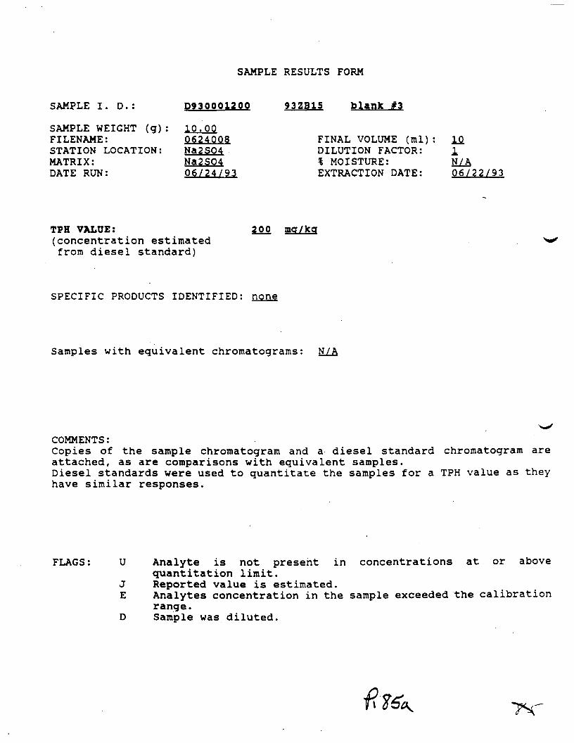
SAMPLE RESULTS FORM
SAMPLE I. D.: D930001200
SAMPLE WEIGHT (g): 10.00FILENAME: 0624008STATION LOCATION: N32SO4MATRIX: N32S04DATE RUN: 06/24/93
93ZB15 blanlc
FINAL VOLUME (ml): ±0DILUTION FACTOR: 1% MOISTURE: N/AEXTRACTION DATE: 06/22/93
TPH VALUE: 200 mq/kcr(concentration estimatedfrom diesel standard)
SPECIFIC PRODUCTS IDENTIFIED: none
Samples with equivalent chromatograms: N/A
COMMENTS:Copies of the sample chromatogram and a diesel standard chromatogram areattached, as are comparisons with equivalent samples.Diesel standards were used to quantitate the samples for a TPH value as theyhave similar responses.
FLAGS: U Analyte is not present in concentrations at or abovequantitation limit.
J Reported value is estimated.E Analytes concentration in the sample exceeded the calibration
range.D Sample was diluted.

enCO
o—
Ui —
0
T) M—-V-/ (i
OJ
£.o
•(Jl
_ i I I I I 11 I i I I i I ll l I 1 I 1 l . l l l II II Ll I I I I I I I I I I I I I I I 1 I I I Ll I I I I II il II il ilU
,L______________________________ Ql
Oo00
Le
VV
oa ID-» o


SAMPLE RESULTS FORM
SAMPLE I. D. :
SAMPLE WEIGHT (g)FILENAME:STATION LOCATION:MATRIX:DATE RUN:
D9300Q1177
10.87TPHQ11MSSB50Jsoil05/14/93
93ZB14 SUMS
FINAL VOLUME (ml)DILUTION FACTOR:% MOISTURE:EXTRACTION DATE:
15.1%05/11/93
TPH VALDE:(concentration estimatedfrom diesel standard)
410 ma /*CT
SPECIFIC PRODUCTS IDENTIFIED: none
Samples with equivalent chromatograms: N/A
COMMENTS:Copies of the sample chromatogram and a diesel standard chromatogram areattached, as are comparisons with equivalent samples.Diesel standards were used to quantitate the samples for a TPH value as theyhave similar responses.
FLAGS: U Analyte is not present in concentrations at or abovequantitation limit.
J Reported value is estimated.E Analytes concentration in the sample exceeded the calibration
range.D Sample was diluted.
o
m j-rm-p I I I | I I i 11 11 11 | i i t i [ i rnrTTTTjTTn [ 11 I I [-rrrrpno o o o o o** CsJ O 00 (D "3
TTTfT-p I I I I II T I
O O
TTtr-Trri
O or\j
OO
OCO
O 0CN
o'
o
in"(N
o"OJ
—m
o

SAMPLE RESULTS FORM
SAMPLE I. D.: D930001177 932B14 811M8D
SAMPLE WEIGHT (g): 10.70FILENAME: TPH11MSD FINAL VOLUME (ml) : .10STATION LOCATION: SB50J DILUTION FACTOR: IMATRIX: soil % MOISTURE: 15.1%DATE RUN: 05/14/93 EXTRACTION DATE: 05/11/93
TPH VALUE: 90 ma/Xa(concentration estimatedfrom diesel standard)
SPECIFIC PRODUCTS IDENTIFIED: none
Samples with equivalent chromatograms: N/A
COMMENTS:Copies of the sample chromatogram and a diesel standard chromatogram areattached, as are comparisons with equivalent samples.Diesel standards were used to quantitate the samples for a TPH value as theyhave similar responses.
FLAGS: U Analyte is not present in concentrations at or abovequantitation limit.
J Reported value is estimated.E Analytes concentration in the sample exceeded the calibration
range.D Sample was diluted.

-> NJ e»-i -t* en en --J Coo o o o o o o o oo-
en—
o
en
o
IvJUi
en
O
UD oo o,aw .
X
S
-» KI Lrj 4^ en 01o o o o o o ollllll Illll 111 I I I II I I 111 I I III 111 II 111 I I ll I II 111 I I 111 111 11 111 II
\:^____ _______
-J GO <O OO O O OLni iluului.LLLu.iiuiiluy.____________. fj

SAMPLE RESULTS FORM
SAMPLE I. D.: D930001186 93ZB1S 804M8
SAMPLE WEIGHT (g): 9.97FILENAME: 05205STATION LOCATION: SB39EMATRIX: soilDATE RUN: 05/20/93
FINAL VOLUME (ml):DILUTION FACTOR: 1% MOISTURE: 9.4%EXTRACTION DATE: 05/18/93
TPH VALUE:(concentration estimatedfrom diesel standard)
2400 ma/Xa
SPECIFIC PRODUCTS IDENTIFIED: none
Samples with equivalent chromatograms: N/A
COMMENTS:Copies of the sample chromatogram and a diesel standard chromatogram areattached, as are comparisons with equivalent samples.Diesel standards were used to quantitate the samples for a TPH value as theyhave similar responses.
FLAGS: U Analyte is not present in concentrations at or abovequantitation limit.
J Reported value is estimated.E Analytes concentration in the sample exceeded the calibration
range.D Sample was diluted.
o o o o oID CN DO
o

SAMPLE RESULTS FORM
SAMPLE I. D.: D930Q01186 932B15 804M8D
SAMPLE WEIGHT (g): 10.23FILENAME: 05206 FINAL VOLUME (ml):STATION LOCATION: SB39E DILUTION FACTOR: 1MATRIX: soil V MOISTURE: 9.0%DATE RUN: 05/20/93 EXTRACTION DATE: 05/18/93
TPH VALDE: 3100(concentration estimatedfrom diesel standard)
SPECIFIC PRODUCTS IDENTIFIED: none
Samples with equivalent chromatograms: N/A
COMMENTS:Copies of the sample chromatogram and a diesel standard chromatogram areattached, as are comparisons with equivalent samples.Diesel standards were used to quantitate the samples for a TPH value as theyhave similar responses.
FLAGS: U Analyte is not present in concentrations at or abovequantitation limit.
J Reported value is estimated.E Analytes concentration in the sample exceeded the calibration
range.D Sample was diluted.

OL £ 0i I i i i i I i i i i
r'^ '••*'; .-•/- "///-/Ji t i i i
• • • i i ; 1 i i i • i i i i i 1 i i i i 1 i i i i i i 1- 1 1 1 1 ! 1
9C1 I ! ! 1
,-C
|
ai
_Z:
-09
-OZl
r09L
i -

SAMPLE RESULTS FORM
SAMPLE I. D.:
SAMPLE WEIGHT (g):FILENAME:STATION LOCATION:MATRIX:DATE RUN:
D930001200
10.610624006SB14soil06/24/93
93ZB1S 89 8MB
FINAL VOLUME (ml): 10DILUTION FACTOR: 1% MOISTURE: 15.1%EXTRACTION DATE: 06/22/93
TPH VALUE:(concentration estimatedfrom diesel standard)
4900 ma/kg
SPECIFIC PRODUCTS IDENTIFIED: none
Samples with equivalent chromatograms: N/A
COMMENTS:Copies of the sample chromatogram and a diesel standard chromatogram areattached, as are comparisons with equivalent samples.Diesel standards were used to quantitate the samples for a TPH value as theyhave similar responses.
FLAGS: U Analyte is not present in concentrations at or abovequantitation limit.
J Reported value is estimated.E Analytes concentration in the sample exceeded the calibration
range.D Sample was diluted.

0

SAMPLE RESULTS FORM
SAMPLE I. D.: D930001200 93ZB1S 898M8D
SAMPLE WEIGHT (g): 10.01FILENAME: 0624007 FINAL VOLUME (ml):STATION LOCATION: SB14 DILUTION FACTOR: iMATRIX: soil . % MOISTURE: 15.1%DATE RUN: 06/24/93 EXTRACTION DATE: 06/22/93
TPH VALUE:(concentration estimatedfrom diesel standard)
SPECIFIC PRODUCTS IDENTIFIED: none
Samples with equivalent chromatograms: N/A
COMMENTS:Copies of the sample chromatogram and a diesel standard chromatogram areattached, as are comparisons with equivalent samples.Diesel standards were used to quantitate the samples for a TPH value as theyhave similar responses.
FLAGS: U Analyte is not present in concentrations at or abovequantitation limit.
J Reported value is estimated.E Analytes concentration in the sample exceeded the calibration
range.D Sample was diluted.

400
10 15 20 25 30 35 40

If?'16

APPENDIX H
VERTICAL SAMPLING ANALYTICAL RESULTS
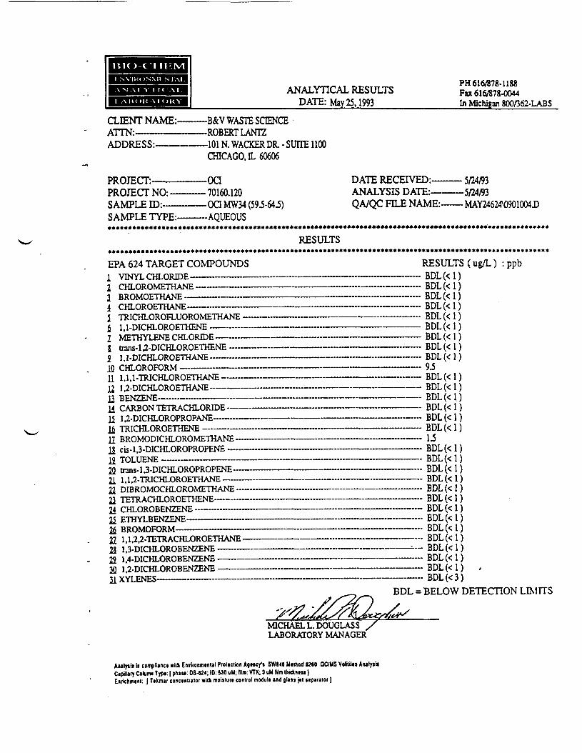
ANALYTICAL RESULTSDATE: May 25,1993
PH 616/878-1188Fax 616/878-0044In Michigan 800/362-LABS
CLIENT NAME:-ATTN:—————ADDRESS:-
-B&V WASTE SCIENCE-ROBERT LANTZ-101N. WACKER DR. - SUITE 1100CHICAGO, IL 60606
PROJECT:——PROJECT NO:-SAMPLE ID:—
-OCI-70160.120- OCI MW34 (59.5-64.5)
DATE RECEIVED:—ANALYSIS DATE:—QA/QC FILE NAME:-
- 5/24/93-5/24/93-MAY24624\)901004D
SAMPLE TYPE:———AQUEOUS„.,«»».»»«»«•.»*»»»»»*»•**«»•»•***»**»***»»**««•******••******»•*•*«*•**•»»»*«•*«•*«««••*•••
RESULTS»»***»»»»»«»*»»*«»**»»»«*»*»**«*•«•»•««»»»•»••••*»*•••••**»»»»»««»»**»»•*»»»«»»»«•»*»»*»«»»**•»•*••••»»•»**EPA 624 TARGET COMPOUNDS1 VINYL CHLORIDE-2 CHLOROMETHANE——————-1 BROMOETHANE-———————-—4 CHLOROETHANE-—————--—3 TRICHLOROFLUOROMETHANE$ 1,1-DICHLOROETHENE -——2 METHYLENE CHLORIDE———•1 mns-U-DICHLOROETHENE ——2 1,1-DICHLOROETHANE -———12 CHLOROFORM11 1.1.1-TRICHLOROETHANE———12 1,2-DICHLOROETHANE"————H BENZENE-—--——»-————--—14 CARBON TETRACHLORIDE-——15 U-DICHLOROPROPANE—-———1$ TRICHLOROETHENE —«——--12 BROMODICHLOROMETHANE —H cis-l,3-DICHLOROPROPENE -——12 TOLUENE ——————-—————2Q trans-l,3-DICHLOROPROPENE»—21 1.1,2-TRICHLOROETHANE ————22 DIBROMOCHLOROMETHANE —-21 TETRACHLOROETHENE——24 CHLOROBENZENE ———-———21 ETHYLBENZENE-2fi BROMOFORM—22 1,1,2,2-TETRACHLOROETHANE-25 1,3-DICHLOROBENZENE ~-22 1,4-DICHLOROBENZENE —2Q 1,2-DICHLOROBENZENE—HXYLENES-
RESULTS (ug/L) : ppb- BDL(<1)- BDL(<1)- BDL(<1)- B D L ( < 1 )- BDL(<1)- BDL(<1)- BDL(<1)- BDL(<1)- BDL (< 1)- 9^
BDL(<1)BDL(<1)BDL(<1)BDL(<1)BDL(<1)BDL(<1)1.5
- BDL(<1)- BDL(<1)- BDL(<1). BDL(<1)- BDL(<1)- B D L ( < 1 )- BDL(<1)
- BDL(<1)- BDL(<1)- BDL(<1)-- BDL(<1)- BDL(<1)-BDL(<1) .- BDL(<3)
BDL = BELOW DETECTION LIMITS
MICHAEL L.DOUGLASSLABORATORY MANAGER
Analytii In complianci with Envilonmtnlll Pioltclion Ajincy'i SWI46 Mitliod 1260 GC/US VolHiln AnalyjijCapnUtY Column Type [ phau: OS-824; ID: WO UU. film: VTX; 3 uM Iditi Ikidiiiisi)Entiehnnnl: | Trtmai eonet»ualo( with moislurt control moduli and glait |<t upaiator |

ANALYTICAL RESULTSDATE: May 25.1993
PH 616/878-1188Fax 616/878-0044In Michigan 800/362-LABS
CLIENT NAME:-ATTN:—————ADDRESS:-
-B&V WASTE SCIENCE-ROBERT LANTZ-101N. WACKER DR. - SUITE 1100
CHICAGO, IL 60606
PROJECT:——PROJECT NO:-SAMPLE ID:—
-OQ-70160.120-OQMW34 (64.5-69.5)
DATE RECEIVED:—ANALYSIS DATE:—QA/QC FILE NAME:-
•5/24/93•5/24/93•MAY24624\1001005D
SAMPLE TYPE:———AQUEOUS••**•*••••••*****••*••********••****»***************•***••*••************•***•«*•****»*********»***********
RESULTS,»»»»»»»»«,»»»»,««•«••»»»»»«»*»»*•»»**»»»**»»•»•»••••***»•»»»**«***»»»***«*«**»»»»»»•••»»»*«•«««»*»»****»«»EPA 624 TARGET COMPOUNDS RESULTS ( ug/L ) : ppbj. virx i i* t.ru.uiuijc ———————————————————————————————————2 CHLOROMETHANE ——————————————————————————————1 BROMOETHANE ————————————————————————————————A fMIT ni>rN7TTTAMT7 ... ,
i TDTr^UT fM>r»17T Tir^OrvMFTHAMT? ... .. .. . ,T,,.... . -r- T... _
6 1 1 rWHT f\Q nFTI-TP WP .............. ............. ..„.....«
2 METHYLENE CHLORIDE ————————————————————— - —————i trans-U-DICHLOROETHENE - ——————— - —— ——..—-- ——————— -2 1 1 TYIPUT /"TOfinTTT AMP ...
it 111 TDTr'tJT f^p r\vrv A MP .. . ......... _ ... .. .............
1? ie^reXTC OETHAN£
H r* APP/*IM TtiTtf A/"*IJT nprnp .„„..«..«. — ..1< 1 *> TMOUT /^DAPT?r^t*AMn . ...T,...^L ......
l/r TDT^HT rt"D rYPTtTFMP . ........... . ..... _
IT DDO\jf/^rMr*UT f%POK^PTTTAMI7 — _ ......._.............
irt TYM TTCVTC . T,,,^-. ........ ....... .......
•>n h^inr i i r\Tr*HT nor^PpnPFMF ......... .. ........Ol 1 1 "> TDTr»HT /^DARTTTAMP -T-T »,,21 1 , 1 ,i- 1 KlCrU-L/KUc 1 rlATic, — — —— .............. —— —— — .... —
*»•» •I^_"l"l> A UT \P f\C TTJCXTC . ....
*»< T?TTTVT t*m>J7PMP .. ..... . ....... .............. ..................
If D T> rMk if f\Cf\O *•£ « .......
*M 1 1 *> T *1UTP APUT r^D r^TTTTT A MTT .. * . ... _-n« ,
10 1 1 T\T/"*UT ^!>^%BT?KrTTrMP . . .. T,.. . . ,,
22 1,4-DICHLOROBENZENE —————— „__«-__ ———— . —————————*YA t ^> TM/^UT f^D^BTTXT"7PWF T.... . ^r -.i.j_
. ——— ..... oul_ \*. i i
BDL(<1)BDL(<1)BDL(<1)BDL(<1)
———— BDL(<1)BDL(<1)BDL(<1)
———— BDL(<1)
BDL(<1)ROT (s 1 ^
- BDL(<1)——— . BDL(<1)
__ •> inni ts i \BDL(<1)BDL f< 1 \DVL* \^ 1 Inni (t i ^
_ __ i nnni f<- 1 ^
-BDL(<1)———— BDL(<1)
BDL(<1)• BDL(<1)
BDL(<1)———— BDL(<1)
.... Bni.f^l^BDL = BELOW DETECTION LIMITS
MICHAEL L.DOUGLASS /LABORATORY MANAGER*^
Anilyiis I* compliJKi wild Enviionmtaltl Prouction A)inc|T> SW646 U.thod ttto GC/US VoUlilti Aulyii*CapIUiy Column Typt: I pKaM: DB-U4; ID: 530 uM; film: VTK; 1 uM 19m IhidnMi |£Btichm««t: | Ttkmar coMtnuatot with Moiatura conUol modult and (Ills )•! atparaloi ]

ANALYTICAL RESULTSDATE: May 25,1993
PH 616/878-1188Fa 616/878-0044In Michigan 800/362-LABS
CLIENT NAME:-ATTN:—————ADDRESS:-
-B&V WASTE SCIENCE-ROBERT LANTZ-101N. WACKER DR. - SUITE 1100CHICAGO, IL 60606
PROJECT:———PROJECT NO:—SAMPLE ID:——SAMPLE TYPE:-************
-OCI-70160.120-OQMW34(69J-74J)-AQUEOUS
DATE RECEIVED:-—ANALYSIS DATE:—QA/QC FILE NAME:-
• 5/24/93•5/24/93•MAY24624M101006D
*****************RESULTS
»»***»»»»»***»**»*»*»*»**»****»**»••***»»*»***»•*•****»»*»**••*•**»*»»**•»»»*»*»******»EPA 624 TARGET COMPOUNDS1 VINYL CHLORIDE -I CHLOROMETHANE •I BROMOETHANE-4 CHLOROETHANE-i TRICHLOROFLUOROMETHANE — - ———ft 1 . 1-DICHLOROETHENE ——— — —— ——
METHYLENE CHLORIDE— — — ——— — -trans-U-DICHLOROETHENE — — - —— —1,1-DICHLOROETHANE ———— —— —— —CHLOROFORM — —— ...._.—— —— —1.1.1-TR1CHLOROETHANE —— — ——— — -1 ,2-DICHLOROETHANE ————————
RESULTS (ug/L) : ppbBDL(<1)BDL(<1)BDL(<1)
I121QJi1211\ 1
14 CARBON TETRACHLORIDE—li 1,2-DICHLOROPROPANE- ——
—- BDL(<1)———— BDL(<1).———... BDL(<1)_———.. BDL (< 1).—..—— BDL (< 1)———— BDL(<1)
H BROMODICHLOROMETHANE—————14 cis-l,3-DICHLOROPROPENE —12 TOLUENE ———-———————2Q lnns-l,3-DICHLOROPROPENE"21 l.U-TRICHLOROETHANE-22 DIBROMOCHLOROMETHANE-21 TETRACHLOROETHENE-24 CHLOROBENZENE •25 ETHYLBENZENE"———————-2fi BROMOFORM————————-——21 1.1,2,2-TETRACHLOROETHANE--25 1.3-D1CHLOROBENZENE-——-22 1,4-DICHLOROBENZENE •22 1,2-DICHLOROBENZENE-21XYLENES-
——.....————. BDL(<1)___———— BDL(<1)
—"—""•""•——...«—-•• DUb \^ 1 f
————————— BDL(<1)
— 1.9—— BDL(<1)——.. BDL(<1).—— BDL(<1)
—- BDL(<1)— BDL(<1)
BDL(<1).——————— BDL(<1)———————— BDL(<1)——.———— BDL(<1)——————— BDL(<1)
— BDL(<1)— BDL(<1)
——— BDL(<1)____. BDL(<3)BDL = BELOW DETECTION LIMITS
MICHAEL L. DOUGLASS /LABORATORY MANAGER
Analytit in complianct with Envlrotimmial Proltction Agncy1! SWH6 Utthod 12(0 GC/HS Vofitilti AulyiilCapilUry Column Typt: | phait: 08-624; ID: 530 uM; Urn: VTK; 3 uU llm Ihiduitu |Eniickmtni: [ Tikmar coftcintiator wilh moislurt control moduli and glati |*l Mparatoi |
ANALYTICAL RESULTSDATE: May 25.1993
PH 616/878-1188Fax 616/878-0044In Michigan 800/362-LABS
CLIENT NAME:-ATTN:—————ADDRESS:-
PROJECT:———PROJECT NO:—SAMPLE ID:——SAMPLE TYPE:-
-B&V WASTE SCIENCE-ROBERT LANTZ-101N. WACKER DR. - SUTIE1100CHICAGO, IL 60606
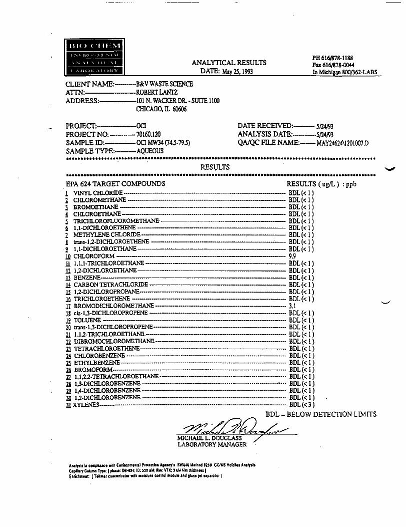
-OQ-70160.120-OCIMW34 (74.5-79 .5)-AQUEOUS
DATE RECEIVED:—ANALYSIS DATE:—QA/QC FILE NAME:-
•5/24/93•5/24/93•MAY24624M201007J.
•*»»•»»»•*•«»«»»»*»*»»•••*»**»»*»«*•«»*•*»«**»«•*»««»*«*••***•»•»»»••»••»*••*»»«»»»»•»»»*»«»•«»*«*»*»»»«»«»RESULTS
»»*»»»•»»»****•»»*»»«»»«»•**»»»«**»»*****»»***»»•»»»»»»***»***»»•«*»•****»•»**»»**«»•»*•*»»••«•••««««••»*•»EPA 624 TARGET COMPOUNDS1 TfTMYT PTTT HPTHP .......... ... . . . . . . ____ .„ ,....,...., A
1 CHLOROMETHANE ———————————————————————————————————1 BROMOETHANE —————————————————————————————————————4f*ui f\Df\rrr\3 AMPi TRICHLOROFLUOROMETHANE ———————————————————————————$ 1.1-DICHLOROETHENE ——————————————————— - ——————— - ——————2 1 nCTT-TVr CXTC ^"UT /^D TT.n
J tnns-U-DICHLOROETHENE - —— — ——— -__——.-_„_ ————————— __2 1 1 TMPHI nROFTTT AMP ................................................................ ....1A PTIT -"IPnPP.PA.'f
1 1 1 1 1 TPTPWT HPOPTHAMF ................ ..^ ...11 1 *> nTPPTT rtPAPTTTAT^TP ....... ..11 TJTTMVPMP x _,,,,... ._.-.................»............._.......... .. . ....
14 PAPRHMTFTRAPHT ORTHP . . r r r T TT r- ............ _ „...._.-------_ir i o nir*MT nRnpROPAMF....... ................... _ .......... JJ...,1^: TOTnrr npnFTMPT^iF ......................................... ,,_,n pT>nMr*r»TPWf npnvfPTHAMP-rT T , . ,,
10 TAT ITPKTPin •.«.«•• 1 ^ TMOITI ^^D^^DD/^DCVTC
11 110 TPTPHT APOFTHANP ..... ..-............»..._ .... ......... .... ......11 mnPOMnPMT nPOMFTTTAMP .............. T. ......11 'I ' l l 1 U APTTf riPnFTKFNP...... .............. ......_... _ . ,.„,,.„,..—..... ......_....._....i^ PHT r\i>f^Pi7Nr7P?\iF ..^. .. . .............^tj ^_l LLf*_j*l*L*L*t*lrl •*_-'-' 1A^ "• —
1^ PTTTVT T*FTST7P>JF _ . ___ . _ . ....... , . .. .. _ _ _ _ _ ...... ^1* nT>rtll4OCrtp\* ...... T T-T..J!
11 1 1 1 *> Tll"n> APHT /^Pr^PTHATsTP
2J 13-DICHLOROBENZENE —————————————————————————————— ^-~22 1.4-DICHLOROBENZENE ————————————————————————————————in 1 *> TMPUf ADrtPPMTT^MP^i WT cxrcc
BDL =
RESULTS (ug/L) : ppbBDL(<1)BDL(<1)BDL(<1)BDL(<1)BDL(<1)BDL(<1)BDL(<1)BDL(<1)BDL(<1)9.9BDL(<1)BDL(<1)BDL(<1)BDL(<1)BDL(<1)BDL(<1)3.1BDL(<1)BDL(<1)BDL(<1)BDL(<1)BDL(<1)BDL(<1)BDL(<1)BDL(<1)BDL(<1)BDL(<1)BDL(<1)BDL(<1)BDL(<1) .BDL(<3)
BELOW DETECTION LIMITS
MICHAEL L. DOUGLASSLABORATORY MANAGER
Aulyiis I* canpliaiKi with Enviranmnlil Prouctioii Ajiney1! SWMI Uilhod 1260 GC/US VolitOti AuhnbCipJUrr Column Typi: | pk*M: DB-«24; ID: 530 uM; (Mm: VTK; 3 uM Urn thidtntu |Enrkhmiot: [ Tiknur co«c»nu»loi »rtb moiilun control moduli trot glut jtl upirtlor |

BIO-CM IF. IVlN V I K < >NMI- . r s r iAI .
\ N Al Y I 1C" A I.
I .AItOK Al € > K Y
ANALYTICAL RESULTSDATE: June 4,1993
PH 616/878-1188Fax 616/878-0044In Michigan 800/362-LABS
CLIENT NAME:-ATTN:—————ADDRESS:-
-B&V WASTE SCENCE-ROBERT LANT2-101 N. WACKER DR. - SUITE 1100CHICAGO, IL 60606
PROJECT:——PROJECT NO:-SAMPLE ID:-
-ORGANIC CHEMICALS, INC.-70160.125»OCIMW35(60'-551)
DATE RECEIVED:—ANALYSIS DATE:—QA/QC FILE NAME:-
- 6/4/93-6/4/93-JUN03624M601010D
SAMPLE TYPE:--——-AQUEOUS»«•«•»»••»»»»*»••»•*••»»»»»*»*»••*»***»*»*»*»****»*********»»*»«•*»•***»«»»»•*•*»**«»*»»
RESULTS
EPA 624 TARGET COMPOUNDS RESULTS ( ug/L ) : ppb
1 PPnXjf/"VCT'UAWTI ._.....
A PTTT r\& kOPTW A MP ...... -.
J TRICHLOROFLUOROMETHANE ————t 11 TMPWT ADOPTTTFMF
2 METHYLENE CHLORIDE- —— — — ——1 trans-U-DICHLOROETHENE —————2 1.1-DICHLOROETHANE —————————»A i^TTT f\T* f\T?f\T* aV *
11 111 TTJTPTTT fi-P ntTTTT i MP ..«_-.
12 U-DICHLOROETHANE — ———— — —
14 CARBON TETRACHLORIDE —— - ————1< 1 0 nifWT f"U>f'"&P13f*PA WP ... __ .......
16 1 KlUrU-UKUt 1 ntrst — — — — - - • • • • — • — ••••JJ BROMODICHLOROMETHANE— —— — -U cis-l,3-DICHLOROPROPENE -— —— — -
22 trans-l,3-DICHLOROPROPENE— — — -
22 DIBROMOCHLOROMETHANE ——— — •
24 LrlLUKUBcIN^ctNl; -- ———————— — "
22 1.U2-TETRACHLOROETHANE- ——— •*>o i i rvir*uT ODr^BCaSTTTMP .. .. —22 1,4-DICHLOROBENZENE- ———————2Q 1,2-DICHLOROBENZENE ——— ——— — .71 YYT PNIP^_ —— ———
_ _____ __________ nni /< 1 1_ _____ _ __ . _ . nni if i \
oni (t i \, ^. ...............,,,...— ........... BRI f< n
. . ,,T . Jt... ^ . . RDT ?< 1 \BDL(<1)
-BDL(<1)BDL(<1)
......................... _ ._...... .... 144,„.,-,-— ................ T nnr fx i ^
__ . _ . __ Dfu is i \. .„. _ TT . _ . _ _ . . .„ .„„. . . , RDT f x l >
. — - - - BDL(<1)^ . . , , , , . ^ . , , - , , , nm << i ^ULJL* \** 1 ^
___ . ____ nni /<• i \1 C
____ _____ _ „ _ nni fx i \
_ __ . „ _ _ _ nni /<• 1 1_ . —— .. __ ___ .. BDL (< 1 )
.. . _ __ __ .. __ _ _ nni (< 1 1„ . _ __ ..... ..... . _ ... .... nni <<• i \
.. _ nni is i >_ . _ _ _ nni if ]\
____ .. . ____ nni if i \...... __ ___ ___ nni if i \......... -._.. ....... ... UM^ \^ If
_ _ . ___ _ __ • BDL (< 1 )_ _ _ nni if 1 1
_ .. P.DT t<\\
BDL = BELOW DETECTION LIMITS
MICHAEL L.DOUGLASSLABORATORY MANAGER
Analpii in complianct wilh Environmental Piottclion Agincy's SWIM Uttnod 1260 GOUS Volititot AnarpbCapillary Column Typt: [ phas*: DB424; 10: S30 uU. lilm: VTK; 1 uM lilm thiduitsi)Enrichmtnl: | Tikmar concintraloi wilh moiilur* control moduli and glait jll iiparalor |

ANALYTICAL RESULTSDATE: June 4.1993 •
PH 616/878-1188Fax 616/878-0044In Michigan 800/362-LABS
CLIENT NAME:—ATTN:——————ADDRESS:——-
PROJECT:————PROJECT NO: —SAMPLE ID:——SAMPLE TYPE:--
-B&V WASTE SCIENCE-ROBERT LANTZ-101N. WACKER DR. - SUITE 1100CHICAGO, IL 60606
-ORGANIC CHEMICALS, INC.-70160.125-OaMW35(65>-601)-AQUEOUS
DATE RECEIVED:—ANALYSIS DATE:—QA/QC FILE NAME:-
6/4/93-6/4/93•JUN03624M501009D
«***•***»*•****RESULTS
»«»•»»*»»»*»»»»»**»•»*»»»*»*»»»«»»•********»***»«***»»******»**»****»*»»»*»»*««»»**»*«»*»»*•*»»••*»*•»•***»EPA 624 TARGET COMPOUNDSI v r w v r r*wr rvprnP ....2 CHLOROMETHANE ———————————————————1 BROMOETHANE ———————————————————A PHT r^nrtPTHAMP ..................... __ .—i TRICHLOROFLUOROMETHANE ———————————f 11 TM/^Uf f\l> C\ IT 1 'ITRMP _.....
2 MPTTTYT PMP PHT nPfHP .--.-..-.-............-.
1 tnuis-U-DICHLOROETHENE ——————— - ————2 1 1 TMPIJT P*I>r\TTTHAMP u........
Irt PUT P*BP*CODM _.»«.«.. .
11 1 *) TMPHT P*T>P<PTTT 4 MP . .................. ..,11 PPM7PMP . ,.T T T - r - T , ................... __ ...^4 P A O Tl nM *1*F'TT> A PTTT P*P TTiP1< 11 TMPHT P*PPiPT?PiPAMP . _». . «
Irfl TDTPTIT f\O f\ PTHPMT?
n PI>P*X/fP«rMPHT PrfPPiXTPTWA'MP u....
if ^-Sr i T TVPtTT npnppnpFMP ................-...—. r ,..1 0 TPiT T TT7XTTT ^ r . , ^ ^7 1 VJlrfUHT'lC *———-•———"«« ——— ••• • .-••". L j ...«.......r r .r _ _ • . ! .
2Q trans-U-DICHLOROPROPENE— -— — —— — — - — —
n TMUDp*x>fpiPMT r*ii?nx>rP"rHAWP — .. ..». .... .«*1 >T •<_"?'» A /^T_IT rtDrtf I'LTCKTC
24 CHLOROBEN2ENE ——— —— ___»__...__».0< CTTJVT DCXT7RMT7 ._......« .......... .
11 1 1 O 0 TCTD APUT PiPHPTHAMP __ ... ... • -, ___ . «-
22 1.4-DICHLOROBENZENE ——— .._.-..———- ——2Q 1 (Z-UiL-rilAJKUDcIN .tlNts — —— - ————— —— ———— —
RESULTS ( ug/L > : ppbBDL(<1)
————————————— . BDL (< 1 )_ _ . _ . _ _ _ . , , , ....... _ nni if i \............................ __... DUls^l)
....... ........ ......... _ .... BDT^n———— . ————————— BDL (< 1 )
r .... - HIM (S 1 \
.... ___ Dn; /<> i \................... ...._.... ... RDT ten
_ _ .. prjT is 1 \.. _ _ ____ _ 1*0.................. r ... __ .„. ... RDT te 1 ^
tmr /^ i AHIM te 1 \
---. ... r. , . PflT /^ 1 S
- - - - ~-BDL(<l).._......_....._.............. „. pni it i \
.... r ..... . i 2imi if i N
___ ___ . -}A 1......... . j.. ^i^j
... r.. t nni ^<r i ^— —— DUL(*.l)____________ _ Bni /<• i •»
..._..... —————— . —— .. BDL(< 1 )
. —————— . —————— BDL(<1)_ _ _ nni if i \
———— . — ————— .... BDL (< 1 )___ _ . _ oni if i \
. _____ ___ _ vn\ if i \.. _____ . _ __ _ nni if i \
. ______ ___ ________ __ Df)T (f\\__ _ DIM If 1 \
.. _______ __ __ _ nni if\\
BDL = BELOW DETECTION LIMITS
MICHAEL L. DOUGLASSLABORATORY MANAGER
Aiulyia In compHlnct wilh EnvironmMUl Prowelios AjinqTi SWI4I Utthod K60 GC/US VolilH»» Amlyt*CipJUry Column T»pr. | ph»»: OB-«2«: 10: SJO uM; ita: VTK;} uM Bra thidnm |Etiiichmttil: | Ttkmii eonctmiiioi with moistun coniiol modult ind gl<» j«t siparaior ]

ANALYTICAL RESULTSDATE: June 4.1993
PH 616/878-1188Fax 616/878-0044In Michigan 800/362-LABS
CLIENT NAME:-ATTN:-ADDRESS:-
-B&V WASTE SCIENCE-ROBERT LANTZ-101N. WACKERDR. - SUITE 1100CHICAGO, IL 60606
PROJECT:——PROJECT NO:-SAMPLE JD:~SAMPLE TYPE:—
-ORGANIC CHEMICALS, INC.-70160.125-OCIMW35 (70-65)-AQUEOUS
DATE RECEIVED:———- 6/3/93ANALYSIS DATE:————6/4/93QA/QC FILE NAME:——- JUN03624M101006D
•»»»»••»»*»*»*»»»»•*••«»»»»***»*«»«•»**»***»»»«*»»••»*»»•«»»»•»***»**»••»»••»**»*«»»*•»»»*»»»•••»»»»**«**»*RESULTS
»»«*»«•»«»«»»«»**»*»»*»»«*••**»«»***«»«»**»»**»*»*»»**«*****«*»«*»***»«*»**«««•»•«**»*»••••»»«»***»»«**»***EPA 624 TARGET COMPOUNDS
VINYL CHLORIDE-CHLOROMETHANE •BROMOETHANE —CHLOROETHANE—
RESULTS (ug/L) : ppb~ BDL(<1)•- BDL(<1)— BDL(<1)
BDL(<1)J TRICHLOROFLUOROMETHANE ————————— — —————————————— - BDL (< 1 )fi 1.1-DICHLOROETHENE ————————————————————— : ————————— - BDL (< 1 )1 METHYLENE CHLORIDE ——————————— • —— —— — - - —————————— - BDL (< 1 )J trans-U-DICHLOROETHENE —————————— : —————— - ————————— • —— BDL (< 1 )2 1,1-DICHLOROETHANE - ———————————— -- ————————————————— -— BDL (< 1 )Ifl CHLOROFORM ———————— ..._....._. ——— ... —— . —————— - —— . ———— . 25.111 1,1,1-TRICHLOROETHANE ————— — —— — —— - ———— -- —— — — -- —————— -— BDL(< 1 )12 U-DICHLOROETHANE ———————— - ——— - ———— — -—- ———— - —— — — BDL(< 1 )13 BENZENE _ ~— _ • ___ • ______ • ________ • _ — _ • _______ — _ •• __ 1.314 CARBON TETRACHLORIDE- —— — — -- —— ——————————. ——— -~— BDL(< 1 )li U-DICHLOROPROPANE—— — — —————————————— —— — —— BDL(< 1 )1$ TRICHLOROETHENE ————— -- ———— ——— - —— ._——————.. — „._._. BDL(< 1 )II BROMODICHLOROMETHANE — — — —— —————————————— —— -. 4.4IS cis-l,3-DICHLOROPROPENE ——— -.._..-—..—————————————— BDL(< 1 )12 TOLUENE ———— ----- -— . ——————— ——————————————————— 4.82Q trans-l,3-DICHLOROPROPENE— —— — ——— — — - — — — - — - —— - ———— — BDL(< 1 )21 1,1,2-TRICHLOROETHANE—————————————————————————— BDL(< 1 )22 DIBROMOCHLOROMETHANE — — - —— —————————————————— 1321 TETRACHLOROETHENE —— --»-» —— — ———————— ———— —— ——._.._„_ BDL(< 1 )24 CHLOROBENZENE - ——— — -— -— — ——— — -—— —— — ----- — — - — BDL (< 1 )2i ETHYLBENZENE- ——— - —— - — - — ——————————————— BDL(< 1 )2fi BROMOFORM ——————— -- ——— — -- — —-————————- ———— - —— - BDL(< 1 )21 l.UJ-TETRACHLOROETHANE— - —————— — — - ——— - —— —— — — - —— -- BDL(< 1)2J 1,3-DICHLOROBENZENE —— - — — ———— ——————————————— BDL(< 1)22 1,4-DICHLOROBENZENE •— ———————— — — — —— — — — — —— - — - BDL(< 1 )2Q 1 ,2-DICHLOROBENZENE —— —— —— ——— — ———— —— — - —————— ——— BDL (< 1 )31 XYLENES ——————————— — — —— ————-——- —— — - —— — -- BDL (< 3 )
BDL = BELOW DETECTION LIMITS
____MICHAEL L. DOUGLASSLABORATORY MANAGER
AMlyiit in complianci «ilh Enviionm«nlil Pfoltction Agincy"! SWI46 Utlhod 1260 GC/MS Volitilei AnalyiitCtpiltoiy Column Typr I ph»»: 08-624; 10: 530uM; film: VTK; 3 uM llmIhkkntM |Enrichmtnl: | Tikmar conctnliator with moitlurt eonuol modult >nd glast j«t Mpinior |

CLIENT NAME:-ATTN:——————ADDRESS:-
ANALYTICAL RESULTSDATE: June 4.1993 .
PH 616/878-1188Fax 616/878-0044In Michigan 800/362-LABS
-B&V WASTE SCIENCE-ROBERT LANTZ-101 N. WACKER DR. - SUITE 1100CHICAGO, IL 60606
PROJECT:——PROJECT NO:-SAMPLE ID:—
-ORGANIC CHEMICALS, INC.-70160.125-OQMW35 (75-70)-AQUEOUS
DATE RECEIVED:——— 6/3/93ANALYSIS DATE:————6/4/93QA7QC FILE NAME:—— JUN03624\1301008D
trans-1,2-DICHLOROETHENE1,1-DICHLOROETHANE -
SAMPLE TYPE:-••»»»•»»»•»»*»»*****»**»•»«*•*»**«»»«*«••«»•»«**»»*«»»»**»»*»»*»*«•»*»•**•«»*»»«»«»»•»****«»»»•*»»»»»»»*»«*
RESULTS»***»»»»*•*»**»«•****»*«*«**•*******«**»•»•»••»***»»***•»****»*»*«**»•»**•***»***»»•****»»**«»»*«»»»««*»»*«EPA 624 TARGET COMPOUNDS1 VINYL CHLORIDE——————-——2 " ' ""•14I£1ii14Jl 1,1,1-TRICHLOROETHANE-12 U-DICHLOROETHANE-Ji BENZENE————————————————————————————————————— BDL(<I)H CARBON TETRACHLORIDE———-————————————-———————————— BDL(<1)li U-DICHLOROPROPANE-————————————————-————————————- BDL(<1)Ifi TRICHLOROETHENE ———————--———————————-———-———-—— BDL(<1)17 cKUA'lvJJ^l^rfU^lM'IxvJlVLC-1 i"l/UNC "——•«"•••••—•••—•••TT... ............... ......... ....-•..»._..... n j
IS cis-l,3-DICHLOROPROPENE -——————-————-——-——————-————— BDL(< 1)10 TAT TTCMC _ ___ _ — ......... ....... . _... .. ....... . „ ...____ .. A (\17 iv/i-wCTtC. ——«••————-————-«————•"••"••"•»•—-— «.••-•-—»•.-•-.——---.«••...—--——-«•......... «t.U
2Q trans-l,3-DICHLOROPROPENE——————.———..._....—..—...._.„.—— BDL(< 1)21 1,1,2-TRICHLOROETHANE—-——-——————-——-—-————--——— BDL(< 1)22 DIBROMOCHLOROMETHANE ——————————--—.———.._......_..——.... 1.4Tl TCTO APWT OPOPTWPMP _ ____._.-™___.._..___.. __.._... _.. _ RT1I 1f\\LJ i ciix/%v,ru^vyc\v/d ru^^c ....... . . ^n-— ..... ....................... 01^1^^ 1 jIA r"vn oponPf\r7T:?\n: __ _ _ _.__.____.....___....___.__ _...._ Rni I* \ \lA wflA.WI^WPd*1** ini^lC — -' -———————— —— - —- — « ..... .......... -———--——— OLfLt \^ 1 )
*< UTUVT ndsT7PMi5 .._. _ __________ -____ .___... __.„ _ nnt If i \^J r I M T r*r-j-*f-r-.1^ r~....... . .. ....-. ..-...... '— ....-..— .... .........w 11...... OL/I^ l>* 1 I
IL RPOMnPTlRM .._ ...____._...__.-...___.__....___..._.__.._..___„____... RHI If \ \L\J OI\WlVIWrW*»i"* ^^ Ui lrf ^X 1 J
.....——.._.....——..——._„........„._.... BDL(< 1)
RESULTS (ug/L) : ppbBDL(<1)BDL(<1)BDL(<1)BDL(<1)BDL(<1)BDL(<1)
— BDL(<1)— BDL(<1)
- BDL(<1).—.. 23.9
— BDL(<1)—-- BDL(<1)
21 1.1.2^-TETRACHLOROETHANE—28 U-DICHLOROBENZENE - — —22 1,4-DICHLOROBENZENE ———— .3fl U-DICHLOROBENZENE — —11 YYT PMPQ _______ „..._ .J I A I l CJ ICO"*""" •*•"•" — -»——
- BDL(< 1).... flDL(< 1 )
BDL(< 1 )
BDL = BELOW DETECTION LIMITS
MICHAEL L. DOUGLASS /LABORATORY MANAGER
Anilysls in compliant wilk E»»ironm«tiUl PioMction Agwcy's SWUe Muhod 1240 GC/MS Volitiltl AnalytiiCapiluy Column Typi: [ ph»J»: OB «24; ID: S30 uU; Mm: VTK: J uM fintliiduita ]Enrichmint: | Tikmat conciitrauir with moislun control moduli and glatt jti wparalor |

t ill VI
ANAliYTICALvRESULTSDATE:-May 10.1393 '
PH6I6/S78-U88Fax 616/8784044In Michigan 800/362-LABS
CLIENT NAME:-ATTN:—————ADDRESS:-
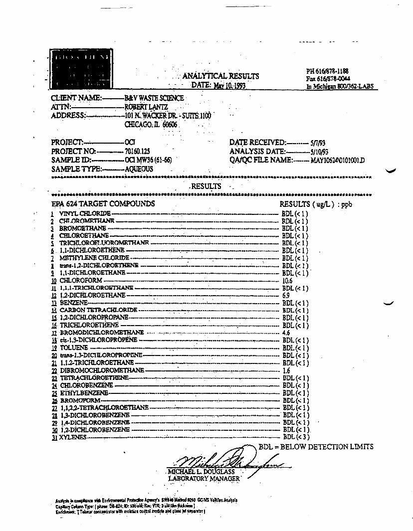
PROJECT:——PROJECT NO:—SAMPLE ID:——SAMPLE TYPE:-
-B&YWASIE-SeENCE-IfiOBERrLANTZ-101N. WACKER Dfc -' SUTII1100..
CHICAGO, IL 60606 - ' '
.oa-7016ai25-OQMW36 (67-72)-AQUEOUS
DATEKECHVED:—ANALYSIS DATE:—QA/QCFILENAME:-
-5/7/93-5/9/93-MAY7562M301003J)
******** »************t**»************4******»»«**»«**********»**»
RESULTS•r* »»»»«•*»«••*»««»*»*»****** A**************************************** **»•*•****»****•**•••*»*•*»••*•**••****
EPA 624 TARGET COMPOUNDSVINYL CHLORIDE-CHLOROMETHANE-
RESULTS(ug/L) :ppb. BDL(<1)- B D L ( < I )
TRICHLOROFLUOROMETHANE ——U-DICHLOROETHENE •——'•——
2 METHYLENE CHLORIDE
2 ' 1,1-DICHLOROETHANE————12 CHLOROFORM ————————U U.l-TRJCHIORORTHANF.——12 l^DICHLORQETHANE————13 -BENZENE—————————'—Id CARBON TRTRACHLORmR——ji U-DICHLOROPR'OPANE-—•-Ifi TRICHLOROETHENE ————-U BROMODICHLOROMETHANE——————.15 cis-l,3-DICHLO.ROPROPENE-———~—12 TOLUENE —--2J> tmns-l.J-DICHLOROPROPENK-21 Kia-TRICHLOROETBANE——2J DmROMOCHLOROMEIHAJ<E-21 TETRACHLOROETHENE-24 CHLOROBENZENE ———25 ETHYLBENZENE————76 BROMOTORM-r———r-r2Z. 1,1 |25-TETRACHLOROETHANE -
22 1,4-plCHLOROBENZENE-2ft U-DICHLOROBENZENE •H XYLENES——-—————•
BDL(<1)BDL(<1)BDI.(<1)BDL(<1)9.9BDL(<1)4.1BDL(<1)
BDL(<1)BDL(<1)3.1BDL(<1)BDL(< 1)BDL(<1)BDL(<1)BDL(<1)BDL(<1)BDL(<1)BDL(<1)BDL(<1)BDL(<1)BDL(<1)BDL(<1)
. BDL(<1)•BDL(<3)
BDL = BELOW Db~l tClION LiMil S>
LABORATORY MANAGER
ti)nc»B»nl: (I'wdw tanciniraior »1« mptourrnmaaiBiodjIf icd gbp Jw
TOTPtL
CLIENT NAME:-ATTK:-ADDRESS:-
ANALYTICAL RESULTS- DATE:M»yia-1993
-B&V WASTE SCIENCE-RCBEkTLANTZ .-ioi K.VACKER'IJR. - SUITE udp'(HCAGO.IL 60606. -
PH 610878-1188Fax616/S78-OOUIn Mfchinn 800/362-LAB5
PROJECT:———PROJECT NO: ~SAMPLE ID:——SAMPLE TYPE:-
-oa• 70160.125•OCIMW36 (61-66)•AQUEOUS
PATE RECEIVED:—— 5/7/WANALYSIS DATE:—.——5/10/93QA/QC FILE NAME:—— MAY1C62M101001D
-RESULTS*«»****«*«**« ***«»***»*»»»*«»»**»««*««»»««««»«»«»»«*«JW»»*« *»«*»»*»»«»•»*»»»»»•»»»*»»»**»*»*»***»»«»*«»»»»
EPA 624 TARGET COMPOUNDS1214I4212121112
VINYL CHLORIDE.
BROMOEIHANE ————————•CHLOROETHANE —————••—•TRICHLC«CMFI.UOROKffiTHANRU-DiCHLOROETHENE.
RESULTS (ug/L) :ppb
- BDL(<1)
BDL(<1)BDL(<1)
1)trars-1 J-DICHLOROETHENE ——1,1-DICHLOROETHANB————-CHLOROFORM ——————--—1,1.1-raiCHLOROffrHANE ———-
'
BENZENE-Ii CARBON TETRACHLORIDE--Ji U-DICHLOROPROPANE-———Ifi TRICHLOROETHENE —JI BROMODICHLOROMETHANEIS c$$.l,3-DICHLOROPRbPENE'.U TOLUENE —2Q ttans-l^-DICHLOROPROPENE-21 1.1J.7RICHLOROETHANE—222221^ ETHYLBENZENE-tt
BDL(<1)
BDL(<1)BDL(<1)BDL(<1)BDL(<1)
BDL(<1)(<1)
22 l.l.J^lEIRACHLOROETHANE-2! 13-DICHLOROBENZENE ———22 M3Q 1,2-DiCHLCROBENZENE.ai'XYLENES-
1.6BDL(<1)BDL(<1)BDL(<1)BDL(<1)BDL(<1)BDL(<1)BDL(<1)BDL(<1)
BDL = BELOW DETECTION LIMITS
Entfcwnwttl PtoMlM AgtncT'i SWI« M«M RCO G&VS V^tiVrt Mtf*wf:*W»4:(>:sa6«*RKnX:JW(*«Ai4ni«J .
Enndinin: ITtUur eoMiitntxwini mcsturi Wetol ee«l« iM (tec W ttpnar]

ANALYTICALRESULTSDATE; May U.
PH6KVS73-1188Fax 614878-OM4In Michigan 800/362-LABS
CLIENT NAME:-ATTN:———:——ADDRESS:--
PROJECT:————PROJECT NO:——SAMPLE ID:———SAMPLE TYPE:—
-B&V WASTE SCIENCE-RORKRTUNTZ-101N. WACKER DR. • SUTIE1100OBCACCYlL 60606-•
—ORGANIC CHEMICAL INC— N/A—OCIMW36 (36-61)—AQUEOUS
DATE RECEIVED:——— 5/11/93ANALYSIS DATE:————5/13/93QA/QC FILE NAME:—— MAY1362M701004D
RESULTS«*»»*»»***«**»*»***»»»»•»»«*«»»*»«»••«»««•*««*«*»«»*»*»»***»»****»»•*•****•«»***•»*•»*»»•»*»»»»»»*«»»•»»**
CHLOROMETHANE -———————-BROMOETHANE ————————CHLOROETHANE —————:———
EPA 624 TARGET COMPOUNDS1 VINYL CHLORIDE-21455111Jfl CHLOROFORM —————————H l.l'.i-TTUCIILOROETIIANE——-12 1.2-DICHLdROETHANE——»«»12 BENZENE—-————————-14 CARBON TETRACHLORIDE——-1£ 1,2-DICHLOROPROPANE—————
RESULTS (ug/L) :ppb-———BDL(<1)
— BDL(<1)— BDL(<1)
BDL(<1)
U-DICHLOROETHENE ——-METHYLENE CHLORIDE ——trans-15-DICHLOROETHENE -1.J.D1CHLOROEIHANE-——--
H BROMODICHLOROMETHANE —————
12 TOLUENE ——-————————-—————22 trans-p-DICHLOROPROPENE—:—-—•11 1,1,2-TRICHLOROETHANE—-———22 PIBROMOCHLOROMETHANE-—».—2i TElKACHLOKOfcTHENE-——————-—21 CHLOROBENZENE ——————-——-25 EIHYLBENZEME—2i
———...._„.. BDL(<1)—»———— BDL(<1)—————... BDL(<I)———-——- BDL(<1)—————~BDL(<1)——————. 10.7———........... BDL(<1)
———————BDL(<1)——————... BDL(<1)"*""*"'"**"'"""""***• DLJ\-t \^ 1 f
———————BDL(<1)BDL(<1)
.—.... BDL(<1)
...——. BDL(<1)——— BDL(<1)
BDL(<1)———— BDL(<1)———- BDL(<I )
BDL(<1).. ...... ._'•
21 l.U^-TETRACHLOROETHANE————-.2J i^-DICHLOROBENZENE—22
21XYLENES-——
__.„._.—————.—— BDL(<1)—————.—.._..——— BDL(<1)———————————.__.. BDL (< 1), _.——.—.——........ BDL (< 1)
BDL(<1)BDL(<1)BDL(<3)
r- ' •f^ffttf!f^^^:MICHAEL;L.-1X5UGLLABORATORY MANAGER
= BELOW DETECTION LIMITS
Aoilpb h CMi bnot who EnyimiiwiUl Pnltdioa Afm^i SWM« MrttottW COVS Vrtiln Anthn*Cj^7CAi«imT)p.-|p^iM:'p8424:1Ch!CniiH:t!lm:yTltJu'VrimCiyin»ul
'Enriehntot: \T«)iinw.t*e»mia«wi*moBt»fi»rtrolinsdrtiasiljlanj«>^«j»f 1

I; l< > (. I H M
ANAOTICAL; RESULTS PH 616/878-1188F»61fl878-00«UIn Michigan aOO/362-LABS
CLIENT NAME:-ATTNsADDRESS:-
PROJECT:——PROJECT NO:-SAMPLE ID:—
-B&y WASTE SCIENCE-ROBERTLANTZ
-101N. WACKER DR. • SUITE 1100CHICAGO, L 60606.
-ORGANIC CHEMICAL INC
SAMPLE TYPE:..- CO MW36 (51-56)-AQUEOUS
DATE RECEIVED:ANALYSIS DATE:
' QA/QC FILE NAME:
5/11/935/13/93
- MAY1352M501002D»•***********•***+
RESULTS*********
EPA 624 TARGET COMPOUNDSi VINYL CHLORIDE————:————2 CHLOROMBTHANE ———————I BROMOETHANE————————4 CHLOROETHANE———————i TR1CHLOROFLUOROMETHANE
1,1-DiCHLOROETHENE --
RESULTS (ug/L) :ppb....... BDL(<1)
--—— BDL(<1)BDL(<1)
METHYLENE CHLORIDE-lnuw-15-DICHLOROETHENE ———————:——1 .l-DICHLOROETHANE -——————————-
Ifl CHLOROFORM ———————————————~11 1.1,1-TRICHLOROETHANE——————————J2 1,2-DICHLOROETHANE——————-————U BENZENE—————........™..-.—_..—-•-..
BDL(<—» BDL(<1)
BDL(<1).__.... 73
._....._.... BDL(<1)4.9
-BDL(<1)U U-DICHLOROPROPANE-——————-Ifi TRICHLOROETHENB ———-————--J7 BROMODICHLOROMETHANE——.-.H cis-U-DICHLOROPROPENE————«1£ TOLUENE ——————————————2J Uans-13-DlCHLpROPROPENE-———-21 l.U-TRICHLOROETHANE22 DIBRbMOCHLOROMETHANE2 •lElKACHLOKOETHENE—~-2i CHLORpBENZENE—————-2i ETHYLBENZENE——2*
...——— BDL(<1)
BDL(<1)BDL(^1)BDL(<1)
_ 1,U^-TETRACHLORaETHANE-2$ U-DICHLOROBENZENE——•-—22 1.4.DICHLOROBENZENE -——-—3Q 1.2-DICHLOROBENZBNE————21XYLENES-—————————————
BDL(<1)BDL«1)BDL(<1)BDL(<1)BDL(<1)BDL(<1)BDL(<1)BDL(<3)
BELOW DETECTION LIMITS
MICHAEL LdbUGL ASSLABORATORY MANAGER
Capibrr CeViiwi Tyr«.< pk«M:OMJ<; O: S» uM; (&«: MX 1 vU Ktai iMdoMsi jf BfkHmtM: 1 T«ki-a/emwirtratcr with moilluft eowol modul* »(ri (teat j»! Mpintor 1

ANALYTICAL RESULTSDATE:Mav24,1993
PH 616/878-1188Fax 616/878-0044In Michigan 800/362-LABS
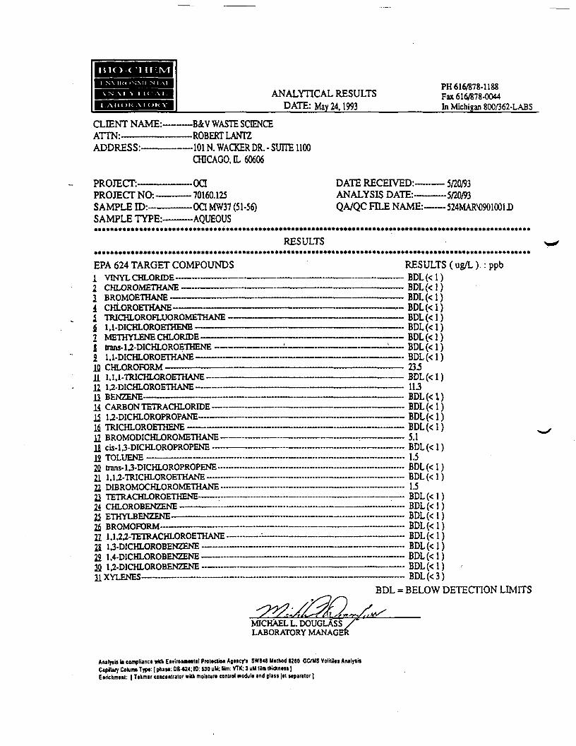
CLIENT NAME:-ATTN:—————ADDRESS:-
PROJECT:——PROJECT NO:-SAMPLE ID:-~SAMPLE TYPE:-———-AQUEOUS
-B4V WASTE SCIENCE-ROBERTLANTZ-101N. WACKER DR. - SUITE 1100
CHICAGO, IL 60606
--OCI-70160.125-OCIMW37(36^1)
DATE RECEIVED:----ANALYSIS DATE:—QA/QC FILE NAME:-
—- 5/20/93——5/20/93— 524MARM201004H
«*»»*«»»»•»»»»»»»»»»*»«*«*«»•*»»•»»**«»»***»*»**»»»«*»»*»»»*»«*••»***»««*»»»RESULTS
*»»»»»*»*»»»»«»•••»»«•»•»»»»****»«»»»*»*»«»««»•*»••••*»••»»»*»«**»»»»*»»»••»***»»»*••»•»***«»«•«»«•••••••«»EPA 624 TARGET COMPOUNDS1 VTWVT r*WT APTT\F . ... ... . .........--..«
2 CHLOROMETHANE ————————————————————2 BROMOETHANE ——————————————————————4 CHLOROETHANE ———————————— - ————————i TRICHLOROFLUOROMETHANE —— - —————————fi 1,1-DICHLOROETHENE ——————————————————1 METHYLENE CHLORIDE ————————————————4 trans-U-DICHLOROETHENE —————————— '• ———J 1,1-DICHLOROETHANE ——————————————————m PTTT OPHFOPM ,. _ ..... .. .... ..... .11 1,1,1-TRICHLOROETHANE ——————— — ———————11 1 t DTPVTT ORnpTHAWF ..,_ ,. ... ... .... .....11 PFISTTPT^JP . , .,T. .....!.. ... .,., ... ... ... ...-L.,J. |E| |M^ l l ^ l . . .................. ................ LJ.......^..|
14 CARBON TETRACHLORmE—-- —— ——— —— — —— ~i< i o TMPHT npnppnpAMP — — .. ... . _ .. _ .
H BROMODICHLOROMETHANE — — —— — — — —— — —11 /•;* i i TVPHT npnPBriPPMP .. _ _ .. __ __
22 trans-U-DICHLOROPROPENE— — — — — — — — — — —
22 D1BROMOCHLOROMETHANE - — — — — ——— ---_-——.
^p c 1111 J-BLJNi-JUNn. --• . .«-•••--••••••••••••••••• .....................
m 1 1 O O TCTP A PUT APAPTUAMP ...
2Sl 1 z-L/lLrll-UKUDClN^txlNii -- -- - —— -*-• -- ——21 A I LcXHco ——— - — — •- —— — — —— —— —— —
RESULTS ( ug/L ) : ppbnni <* 1 \BDL(<1)BDL(<1)BDL(<1)BDL(<1)BDL(<1)BDL(<1)
-BDL(<1)BDL(<1)A1 0——————————————— 47.8BDL(<1)
- - - - 9.0TinT (f \\
, . .. ... . BDT (•£ 1 \.. .... ..... RDT (f 1 \
PHI Is 1 \. _____ . . __ •» 0
. .•„ _ . nni if i \— .. — .... Di.^^ i ;DIM /,. i \
„ _ _ __ _ Bni tf i \. ... _ _ oni (f i \
. 1 1__ ___ _ _ _ nni if i \. __ _ _ __ _ T»n[ if i \
.. ... ,-- BHI If 1 \..... .._..., ...................... BDLf< 1 )
MSLSU V"* * /
. . . . ____ __ DIM If 1 •(
. • - .. Bni if i \__ . .. _ „ •ora if \ \_ _ „ _ _ „ Br\T I* n
__ ___ ... imi /xi^
_ BDL = BELOW DETECTION LIMITS
MICHAEL L.DOUGLASSLABORATORY MANAGER
Analysis in compliance with Enviranrntntal Piouction Agtncy's SWI46 Ullhod 1260 GC/MS Volitilis AnalysisCapillary Column Typt: I phase DB-624- ID: 530 uU. Him: VTK; ] uM lilm Uiidiness |Enrichmtnt: | Ttkmat concentrator with moistun control moduli and glass j«t stparator ]

mo c iHIM
ANALYTICAL RESULTSDATE: May 24,1993
PH 616/878-1188Fax 616/878-0044In Michigan 800/362-LABS
CLIENT NAME:-ATTN:——————
-B&V WASTE SCIENCE-ROBERT LANTZ
ADDRESS:-——————-101N. WACKER DR. - SUITE 1100CHICAGO, IL 60606
PROJECT:-'NCh —
SAMPLE ID:——SAMPLE TYPE:-
-OQ- 70160.125-OCIMW37(4M6)
DATE RECEIVED:—ANALYSIS DATE:——QA/QC FILE NAME:-
• 5/20/93•5/20/93•524MARM101003D
»»•«»»*»»»»*»*»»»**•»»*»*»*•*»************»*»***»*»«»****»*»**»»»•»»•«»«»»»****»»«»»««**»»»»»«*»»•••«««««««RESULTS
»«»«*»«»*»»»«»*»*•»•*»**»*»•«»**»»«»»****»»****•»»••»»»»»»**»**»•*•«»*****»**»»»*»*****»«»•EPA 624 TARGET COMPOUNDSi TTTMVT p«T nPTHF n...... ..
2 r*HT nPf>VfPTTTAWF n, , ,^
a n D C\\ Xf\PTH A WP „
4 ^T¥T ^n rt ^'^ T A X^P
5 TT? Tr*lTT fTO OTTT T Tf^POX/fPTTJ A MP
* 1 1 TMPHT nPOPTTTPTSTP . .... ........................... .......
1 * jL"i'tTVT PMP PHT npiTYP _._1 trans-U-DICHLOROETHENE —————————— :— ————2 1 1 TMr*TTT rVPHPTH AMP — ... ..
Ifl CHLOROFORM ————————————————— —— ————11 1,1,1-TRICHLOROETHANE ————————— - ———— -— ———IT 1 1 F*TPHT OPOPTHAMP ^ ......................._.....................1 1 PPW7PNP. ....... „.,, , . . . . . . . , , , , . ...,..,,. _ _ _ _ _ _ _ _ n .
H PAPnnMTFTP APTTT OPTHP ............... .... . , _..............if i *> ntPWT npnppnpAMP+ t TT> T/"*TTT ^"\o f\\ "I'lTTKTr
n nommnnipwi nunvfCTHAMP ~ ..H cis-U-DICHLOROPROPENE ..——————————————-
2fl trans-l,3-DICHLOROPROPENE— — — — —— — — — — —— — -11 1 1 O TDTPUT r>P APTT-T A MP
22 DIBROMOCHLOROMETHANE ——————————————•>! 'I'L'l'U A PUT nPflFTWPWP — . — .. ...
24 CHLOROBENZENE - — - — ~——— —— — — — — —— .*>< CTTJVT P.PKT7PMP — .^2 h.inii-oiiiN^nr.c,— — • —— —— —— ————— — ———— •
IT 1 1 O "-1 TU'I V APUT OPOPTUAMP
21 U-DICHLOROBENZENE .— —— —— — —— ._......— -._.......•>o i A rwf*ui r>POBWM7T??iJT: . _. ___ . . _____ .in i o.nrrHT nRORFNTPNF .. . — ————— —— ————— .
RESULTS ( ug/L ) : ppbtini (* i ^DflT (s 1 \
. . _ _ _ RDT /x 1 \
.. ——————— ._ BDL(<1)nni f^ i ^
„ _ . _ _ „ nni (f i ___ _ _ nnr i •(
™. . . ' RDI /<• 1 \—— — DI^I^ISI;1.1 i ,...., tJ TinT f <f i ^
ITS
nnr /,- 1 >.... . SS
_ ___ nni /^. i \. ..LI , T,,...... nni {< i ^
PDI ?^ 1 ^„ — — BUL ^ A ___ ___ Df)I /x. 1 \
_____ __ . _ oni (f i \. ___ nni /<• 1 \_ j»r)j /x- 1 \
RDT ^ 1 \1 A
_____ nni fx 1 \___ _ oni if i \, . _ „ BDL ^< 1 ^. __ . nni if i \.......... PHT /** i \_ . _ . BDL (< 1 \
_.. ___ _ _______ DHT ("<• 1 \
_.... ..... —— ..._.... RDT U MjJJJJ^ \^_ j j
DDL = BELOW DETECTION LLMITS
MICHAEL L.'DOUGLASSLABORATORY MANAGER
Analysis ii CMvBanci »it» Etvinanmul PiotKtion Agincy1! SWU6 U.lhod 12(0 CC/US Volililti AnalysisCapillary Cakim* Type [ phau: OB-U4; 10:530 tiM; fOm: VTK; 3 uM 19m Ihidtntss |Enrichnunl: [ Ttkmar conciliator with moitlurt conlrol moduli and glass jil siparalor ]

BIO-C:HEMiI NVIKONMINTAI.
A N A I V I If ' A I
I . A I i O K AI UK YANALYTICAL RESULTS
DATE: May 24.1993
PH 616/878-1188Fax 616/878-0044In Michigan 800/362-LABS
CLIENT NAME:-ATTN:—————ADDRESS:-
—B&V WASTE SCIENCE—ROBERT LANTZ—101 N. WACKER DR. - SUITE 1100
CHICAGO, IL 60606
PROJECT:———PROJECT NO: -SAMPLE ID:——
--OCI-70160.125-OCIMW37 (46-51)
SAMPLE TYPE:———AQUEOUS
DATE RECEIVED:-——ANALYSIS DATE:--—QA/QC FILE NAME:-
- 5/20/93-5/20/93-524MARM001002J)
»**«»«»»«*»»***«»**»»»»••»**»»»******»»***»**»*»*«*»»******»*****•*•*»»»»»*******»»**•«RESULTS
»««»»»»»**»»»»*»»»««*•»**»**••«««»»*»••«»*»»•»***»**»»»»••**•»»»******»*»***«•»**•******»•*•»••*•«««**»»**»EPA 624 TARGET COMPOUNDS1 VINYL CHLORIDE———————
CHLOROMETHANE ————————BROMOETHANE ——————————
RESULTS (ug/L) : ppb: l)
TRICHLOROFLUOROMETHANE -1,1-DICHLOROETHENE —————METHYLENE CHLORIDE————trans-1,2-DICHLOROETHENE1,1-1
Ifl CHLOROFORM •11 1.1.1-TRICHLOROETHANE-12 1,2-DICHLOROETHANE-11 BENZENE-14 CARBON TETRACHLORIDE-
1$ TRICHLOROETHENE -12 BROMODICHLOROMETHANE——-————U cis-l,3-DICHLOROPROPENE ———-———-—^9 TULUtNii ."—•—•«-—————-«—•—-«-———-—-2Q trans-l,3-DICHLOROPROPENE-—————21 1.1.2-TRICHLOROETHANE ——-———————22 D1BROMOCHLOROMETHANE——-———-——21 TETRACHLOROETHENE-——--———-----——
—— BDL(<1)—— BDL(<1)— BDL(<1)— BDL(<1)— BDL(<1)—— BDL(<1)— BDL(<1)
— BDL(<1)— 33.5
—- BDL(<1)— 11.9~-BDL(<U—- BDL(<1)
BDL(<1'.._.... BDL(<1)___ 4g——.. BDL(<1)
-———- BDL(< 1)-———- BDL(< 1)
——-—— BDL(< 1)BUl* ^Vi 1 )BDL(< 1)2S ETHYLBENZENE-™
2$ BROMOFORM-————-———————————-——————-—-—————- BDL(< 1)21 1,1,2,2-TETRACHLOROETHANE-——-————....._.....——————————........... BDL(< 1)28 1,3-DICHLOROBENZENE —————-—————-—~——-———....——__-— BDL(< 1)22 1,4-DICHLOROBENZENE—-—————...__...-——...._.———.__._.—————— BDL(< 1)22 1,2-DICHLOROBENZENE———-.—-—.———-——-——.——._—.—..._.— BDL(< 1)H XYLENES----——-—————.._-.._.-..._....—-...-.————————.._.._.... BDL (< 3)
BDL = BELOW DETECTION LIMITS
MICHAEL L. DOUGLASSLABORATORY MANAGER
Analysis in compliant* with Envlronmtnlal Protlction AgMCfi SWI46 M«lhod 8260 GDUS Volitiltt AnalpiiCapillary Column Typ*: [pnaM: OS-624; 10:530uM; film VTK; 3 uU 19m Ihidmtu |Entictimtnl: | Ttkmar conctnuator wilh moiitun contiol modulo and glau jot Mparator |
ANALYTICAL RESULTSDATE: May 24,1993
PH 616/878-1188Fax 616/878-0044In Michigan 800/362-LABS
CLIENT NAME:-ATTN:—————ADDRESS:———
-B&V WASTE SCIENCE-ROBERT LANTZ
——101N. WACKER DR. - SUITE 1100CHICAGO, IL 60606
PROJECT:———PROJECT NO:—SAMPLE ID:——SAMPLE TYPE:-
-OQ-70160.123-OCIMW37 (51-56)-AQUEOUS
DATE RECEIVED:--ANALYSIS DATE:—QA/QC FILE NAME:-
-5/20/93-5/20/93-524MARW01001D
•••••••A************************************************************************************RESULTS
»•»»**«*»»•**•*»»«•*•***•»»»»•******•»*»««*»*»»•*••••••***»»»»*»»»***»**«*»»**»*»»»»*•»••*•»•»»»»«««»»*****EPA 624 TARGET COMPOUNDS
VINYL CHLORIDE-CHLOROMETHANE -BROMOETHANE-CHLOROETHANE—————————TRICHLOROFLUOROMETHANE —1,1-DICHLOROETHENE ——————METHYLENE CHLORIDE —————trans-U-DICHLOROETHENE —1,1-DICHLOROETHANE-
Ifl CHLOROFORM ——————11 1,1,1-TRICHLOROETHANE-12 U-DICHLOROETHANE——11 BENZENE-_ CARBON TETRACHLORIDE-11 U-DICHLOROPROPANE——Ifi TRICHLOROETHENE •12 BROMODICHLOROMETHANE-U cis-l,3-DICHLOROPROPENE -——12 TOLUENE ———————-——-—2Q trans-U-DICHLOROPROPENE—21 1,1,2-TRICHLOROETHANE——-22 DffiROMOCHLOROMETHANE.———————————————————- 1.521 TETRACHLOROETHENE————-————————————————-————— BDL(< 1)24 CHLOROBENZENE—————...._.——.———..._..„„„„..—._.————..—— BDL(< 1)2i ETHiLBtiruCtpit•• ~--""""••-•—•-——••««-•-•——«
21 1,1,2^-TETRACHLOROETHANE—————-2J U-DICHLOROBENZENE -——..—..—-—
RESULTS (ug/L).: ppb— BDL(<1)
BDL(<1)BDL(<1)BDL(<1)BDL(<1)BDL(<1)BDL(<1)BDL(<1)BDL(<1)125BDL(<1)113BDL(<1)BDL(<1)BDL(<1)BDL(<1)5.1BDL(<1)1.5BDL(<1)BDL(<1)
11
22 1,4-DICHLOROBENZENE22 U-DICHLOROBENZENE11 YVT CMTTC _._ _« „—...JL A 11*EPICO""""•"•'"
BDL(<1)BDL(<1)BDL(<1)BDL(<1)BDL(<1)
—— BDL(<3)BDL = BELOW DETECTION LIMITS
MICHAEL L. DOUGLASSLABORATORY MANAGER
Analysis in eomplUnci wlifc Ewiro«m<nul Piowctioa AgnqTs SW84J Mtlhod 1260 GC/MS VolitOcs AulysitCapilay Column Tjp«: | phaw: OB-624; 10:530 uU: film: VTK; 3 uU 13m Ihicknist ]E«riclimt»l: | Tikmat conctnltalor with molsturt eonuol modult ind glass jtl stparator |

pot *)npou |onuo: unittoui t|ii«A :ulni :nn OtS :OI >
«!«<|«»y »|!>!|OA SriOO 09CT poi|l«n SUMS M3Ui6y utnpiioid |ciutuiuojiAU3 nii» tmtt|duio3 ui tiU|tuy
HHDVNVW AH01VHOSV1ssvionog '
SlIWH MOLLD3LLHQ AVO1H9 = 1Q9SHN3TAXTT
-I'I K(i>)iaa ——d>)iaa ----------d>)iaa -----d>)iaad>)iaa -----n -—-d>)iaa -—d>)iaa --—-d>)iaa —
6'9 "—d>)iaa —d>)iaa —d>)iaa —-Ct>)iaa -----d>)iaa —d>)iaa -—-
qdd:
(i>)iaa —d>)iaa —d>)iaa —d>)iaa —d>)iaa —(t>)iaa -—d>)iaa —d>)iaa -—d>)iaa —-
———— HNazNaaoHOTHDia-ci sz-——aNVHlHOHOTHDVaL31-rn'I Ti——.——————wscHOWcme 5Z
..„._..—HNHZNHaTAHLH JZ
——————HhaHlHOaOTHDVHlHl ft—— HNVRLHNOHOTHDONOyaia Ti—-—— aNVHlHOHOTHDIUL-C' t' I TC———-3NHdOHdOHOTH3ia-£'I-sucfl JJZ.——.._.._.———..._ HNHniOl 5T—-— HNHdOHdOHOTHDId-ETStt 5T
—-————— HNHHlHOHOTHDnLL 9T
————-HOIHOTHDVyjLHlNOaHVD ?T—HN3ZNH8 IT
'I IT———— HNVmHOHOTHDRLL-lTl TT
• WHOdOHOTHD UT— 3NVHLHOa01HDia-I'l 5NHHiaOHOTHDia-n-suEfl f—HarHOTHDaNHlAHiaW I— HNHHiaOHOTHDia-I'l 5
J--HNVH1HOHOTHD F— HNVHLHOWOHa I•HMVH13WOH01HD I-HdraOTHDTANIA T
SONHOdWOD 1HO>TV1 W9 VdH»«*»»«*•««•»*»»«»««**«*»•«»«»****»**»**»*»»•»**•«»***•»«•««»»«»•••*«*«»»«**»***«**•«*»*»***»««»•»»***«»**»»
*«»•«•••»»••«•«•«*««••*•»»*«*««»«»»»»»»•»**»**»***»«*«»*»»»»*»**»**»»****»»»•»•«»****« **»**»*»•««»»«
E6/C2/S :H1VQ SISATVNVH1VQ
90909 H'OOVOIHDooii aims - TKHIXDVA -N ioi
SaVl-
881 1 -8t8/9I9 Hdsnnsara TVDLIAIVNV

UK )-<
A I V I 1C A I. ANALYTICAL RESULTSDATE: May 24.1993
PH 616/878-1188Fax 616/878-0044In Michigan 800/362-LABS
CLIENT NAME:-ATTN:——————ADDRESS:-
PROJECT:———PROJECT NO: —SAMPLE ID:——SAMPLE TYPE:-
-B&V WASTE SCIENCE-ROBERTLANTZ-101N. WACKER DR. - SUITE 1100
CHICAGO, 1L 60606
-oa-70160.120--OCIMW38 (50.5-55.5)-AQUEOUS
DATE RECEIVED:-—ANALYSIS DATE:—QA/QCFILENAME:-
•5/22/93•5/23/93•MAY2262-NM01004D
»».*••***»»*«»*»»*»*•»»*****«**•»***»**»**»*»*«**»«••«•«»*»*»»»«»»**»»»*******»«»»»**•»•»»»*«««»«**»»**»»*»RESULTS
*»»*»»»*»**»««*»»»»»»»**»»»»»»**»*«»»*»**•*»*»*»*•••••»«*•««»»*•*«***»»»»*»«*•»»»•**********»•»»•*•»»*»**»»EPA 624 TARGET COMPOUNDSi VTMVT /^WT f^PTT^P .......... ..... ..................
2 PWT OPn>if4FTRA,MP . ..............
1 PPnX4ATTTHAMP ........._............._............ ...
A /""Tit r^PAPTHAiMP ............................... . ...
i TDTf^HT API^CT TTr\PAMP*THAMP — ..... — ..............f. t i TVf'HT OPOPTTTPMP ... _ ...«......_...... ...................Q iti-^^^ f*L*\jr^j^ L i " J " rL •••••••• ....i '•»• - ..............m.»21 jt-'Tuvn cxrc rf^ur r*o rrvc
1 trans-U-DICHLOROETHENE ————————— - ————— - ———— ———2 1 1 nTPHT n-POFTP AMF ..... ... . ,,r rr „ — r.,.TI ,..,.....,...,IA r*m f\orvpf\o\x .. ........ .......,....^. ^^ ...11 1,1,1-TRICHLOROETHANE ————— —— - ————————————— - ———11 i o r\Tr»uT f\of\^m A KTC - , .... ...... _ ...1 1 DC KP"/UXTC
1J r^APDOKI TTTTP APTTT lOPTHTt ,..................».._......«. . ._H 1 *? T^IPTTT nPOPPOPAMF ..................................... _ . _
n ppov4nr\TPHT npmv/FTTTAMF _ _ _ _ _ _ _ _ _ _ _ _ _ _ _ _ _ _ T _ _ _ _ T . ¥ _ i r i .is *•;* i i r.T^T-TT npnpprvPTTMT: .^ _ _ _ ..... ........... .
2Q tnns-l,3-DICHLOROPROPENE »»-»»--""-"-•»"-»""-»«---«----»»*>l 11O TPTPUT nPHPTUAMT? . ___ ___ ___ .. __ — . ««^i mp.pnMnr'MT r.pr.MPTHAWP __ .... __ — _ _____ ......11 T_L" I'll A OLTI /*M> ^\CTUCVTC
1/1 r'UT -^DtOnCKrTtNTVC ........*.......«
22 1 ,4-DICHLOROBENZENE -— — —— ..—_-— ——————— .——..-—...-in i o T^T-^IJT /\p f>n c KI v i? MTT
RESULTS (ug/L) : ppbBDL(<1)
- BDL(<1)- — BDL(<1)
~- BDL(<1)- -BDL(<1)
- - BDL(<1)........... . BDI (< \ \
— BDL(<1)-BDL(<1)- 316
BDL(<1)BDL(<1)BDL(<1,)
———— BDL(<1)BDL(<1)UTV t^> i \9.4
- - BDL(<1)— . RDT (< 1 \
- -BDL(<1)RDI (f 1 \
._ . . _ 30
. ____ nni If \ \VlXiprf ^X 1 j
____ „ nni /<• i \_____ „ nny (< ] \,. ——— --BDL(<1)—— ._.... BDL(<1)
. _ _ Bnr is i _..„........ BDL(<1)_....„_.„. BDL (<1) ,
fjf)l If T. \
BDL = BELOW DETECTION LIMITS
MICHAEL L.DOUGLASSLABORATORY MANAGER
Analysis In compliaitci «rth EnyiranmmUl Proliclion Agfncy-s SW846 Udhod 1210 GC/US Volililis AnalysisCapllary Column Typ*: | pkass: DB-U4; ID: 530 uU, film: VTK; 3 uU IDra ihidntsi |EnrichrMnt: (T.kmir conctnualo( «iih moiilufi control modul* and (last j«i siparalor ]

[ joititdn i«! ttt)E put »|npoiu iciiun unitioui qim loitnuiiuoi itvivi ] :iuiuiv»>«3| naoipiiii ui(| «n t IxiA:«!»'n« OK :QI >!>-9Q :«"!< I -""l minm *««d«3
f|$X|tuy MIHOOA SHOO 0921 po<|l»n SUMS «^»t«y «0!U«10)d IIIIMUUOJUIIJ nil* •9Ut!|du03 «! uiiituy
HHOVNVW AHQ1VHOSV1ssvionoa n THVHDIW
JJJWI1 NOLL03LLHCI M.O1H3 = 1Q9a>) iua\ [ '/ lUtt\\ "1 1VJQ
d>)iaa — — -•d>)iaa -——d>)iaa - ——v I *) lun(, 1 ?y 1UHV I x/ IvJU
1 ———i >> IQS ——I >; Ida ——
V I "/ 1V1Q
V I >) iQa
I >) Idav i "/ ivia
^ lua\ I '1 1UQ
>J Ida.( T >) 1Q8 —————<ri£ ———v i 'i luav i "^ luad>)iaa ———\\ ') lUav i fi lua\ i "/ iviad>)iaa ——\ i 'i ivia
........... mii"i_r7K-TTTfTf^MfVTTJ'"\TfT-fe*T / 7
«... —— ............. ...... ....... — ...... ...._-. j^d^i-myiiu UU1U t I BC
ahTvlli3OaOTH.jVaJ^.L t £ I
... .. —— ........................ — —— •••••••••••••• "dNdrLLdUaU LrUVcLLaJL 1C
..._..__.......---.-..-.--.---.---...-„-...— .—.-- HNVHIHWOHOTHDOWOaaia U——— —————— ——— —— . ——— —— ... — HNVHidUaU IHwHaJ- 6 L I 1C
.. ——— .........................................._...... ...» —— ......... — dNdll IUX 01Tkn Trt\I T'*^\TrtTTT'*^T^T-C*T -*m 6T
dfxdrLLd.Ua.U irLJlcLL yi....*TkT^/ T^\\T Trt\Ti^TTT*^Ti*T-7* T ^T
HOraOTHJValal NOajTV J
.... —————————————————————————— HNVHlHOHOTHDia-n ZTHhT/HldOaOTHJlJlL 11 I I
............. ———— . ........... . ........... 1 .. MMVH.I X I I H l l IH.)1U 11 0
. . U . H . T . T . . . . . . ^... ___ ._«... — -.— «TT*J/TrSTr^TTJ^ TTM'J' 1 1 tTTJW T
............ ___ .....rT nK.TTnTT^AMI^TTT'MfT-T'T 5aNin.ii'iUQU uuiu 11 y————————————————— HNVHlHWOHOn'UOaOTHDIUL J————————————————————————————— HNVRLHO^OTHD F——————————————————————————————— HNVRLHOWOHa I............ .............. dNVrU-oyVUaU lilwJ t
(l>)lQfl "" ——— ..................... . . . . ......... . auiavj iriij IAI^IL/I i
qdd : ( i/3n ) snnS3^I SONHOdWOD 1HOW1 ^9 VdH***********************************************************************************************************
snnsHHv**********************************************************************************************************F noanov——;HdAX Hidwvs
—:HWVN HTU DG/vb (r 09-r?s) KAAH DO———-:ai mdwvs£6/K/S————:H1VQ SISATVNV OZt'09IOi ———— :ON 1D3TOHd£6/32/5 ————:Q3AIHDH>I 3LLVQ DO———————UDHTOtf d
90909 TI'ODVDDDam stuns - a ^HXDVM -N 101————
SaVl-J9£/008WOO-8Z.8/919 wj88tI-8i8/9I9Hd TVDLLA1VNV

mo ( i u:;vi
CLIENT NAME:-ATTN:—————ADDRESS:-
ANALYTICAL RESULTSDATE: May 24.1993
PH 616/878-1188Fax 616/878-0044In Michigan 800/362-LABS
-B&V WASTE SCIENCE-ROBERT LANTZ--101N. WACKER DR. - SUITE 1100
CHICAGO, L 60606
PROJECT:——PROJECT NO:-SAMPLE ID:—
-OQ-70160.120-OCIMW38(60.5-65.5)
DATE RECEIVED:--ANALYSIS DATE:—QA/QC FILE NAME:
•5/22/93——5/23/93—— MAY22624\)201002J)
SAMPLE TYPE:———AQUEOUS»•»»•»«»»*»*»»•***»**»»*«•••»»**»**••»»*»••«»•»****»*»**•*****•*»»«••»»»*»»*»*•»*•»»***»•»*»»**»»«»••»«»*«»
RESULTS•««»•••»*•*»•»•*»««»«»»«*•****»»»••*«•••»«»«»»»•»»»*»*«********»•••«•«*»*••»»*****»**«»••••»»«««»•»««*»»»•»EPA 624 TARGET COMPOUNDSI TJTMVT PHT nPTHF ....... , i..
I CHLOROMETHANE ————————————————————— - ————1 BROMOETHANE ————————————————————————————4 PUi ^P. ^^liTUA fv^c ....... ii I . . .
i TRICHLOROFLUOROMETHANE —— - — - ———$ 1,1-DICHLOROETHENE ————————————————————————1 METHYLENE CHLORIDE - - - - —————————————J trans-U-DICHLOROETHENE - ————————— : —————————
In rmoBnmB vf ^^11 111 TO TfUT ("IDflL'l HAMF _.... _ .......... _ _ _ ..........................
!•> 1 •> nTPHT r»P AFTTl A NIP ............ .............................
1jl r* APPOM 'I'L'I U APTTT OPTT>F ... .. ........ _ — ....-_..
Tnirm nnnrTT^MFJl BROMODICHLOROMETHANE — —— - — - ——————— - ——————i> <-!r 1 1 Twin nnnpTJAPFMF ..... ^..... ..... .......,.,, ,,.,......,
•\ft »«.«M 1 1 T^T/^UT f\O f*\W f\&C NTC
22 DIBROMOCHLOROMETHANE _.——_..——————— ———11 TCTD A/^UT OO nrn'VTPMF ._.........._...^j r^I_IT ^M>^%OCVFTCKTC _
1< L"TTTVT PT7KT7FMP ... ............_....._....
10 1 1 TMfMJI rtP/^BTTKTTFMP
10 1 A TMPUl APOBUM7FMP ...... .... ..... ..... «... ...
J^ AIJLJCJNCO' — ———---•••"••-•-— ——— — ————— •• —— •"• ——— —...—-.— ———
RESULTS ( ug/L ) : ppb____ „ nnr fa i \
- —————— BDL(<1)BDL(<1)
——————— BDL(<1)BDL(<1)
——————— BDL(<1)——————— BDL(<1)————— •• — BDL(<1)
14.6.. —————— BDL(<1)
^^ ............... RHT (< 1 >——————— BDL(<1)
Bnt ( i \
.„. ... . BDL(<1). — . PflT ?^ 1 \
...... ..,,....,., nnr fx i \_ _ i>nT rv i \
onr /x i \DfjT /^ 1 \
_._. _ _ DfVT (< 1 ^
...... __ ... BDL(<1)_.. ———— -BDL(<1)
•DT\\ (f 1 \
. ._ BDL(<1)..................... nni c<f n
nni t* i \
BDL = BELOW DETECTION LIMITS
MICHAEL L. DOUGLASSLABORATORY MANAGER
An«lr>b I* complUnct with Enviionrainul Pioiiction Ajtncy'i SWI46 U»thod 1260 GC/MS Volitilts AnalysisCipJUry Coluiw Tn»: 1 phiM: OB-624; 10:530 uM; film: VTX; 1 uM llm thiduitsi |
kiMM: | Tikmtr conc»ualor whh moisiun control modult ind glass jti sipaiatoi |

ANALYTICAL RESULTSDATE: May 24.1993
PH 616/878-1188Fax 616/878-0044In Michiaan 800/362-LABS
CLIENT NAME:-ATTN:—————ADDRESS:-
-B&V WASTE SCIENCE-ROBERTLANTZ-101N. WACKER DR. - SUITE 1100CHICAGO, IL 60606
PROJECT:——PROJECT NO:-SAMPLE ID:-
-OQ-70160.125-OCIMW39 (47.5-52.5)-AQUEOUS
DATE RECEIVED:———- 5/20/93ANALYSIS DATE:————5/20/93QA/QC FILE NAME:——- 524MARM601008D
SAMPLE TYPE:—••»»•»•»»»*»«*»»««•»»•••••»»»*»»*•*«»»*»****»»»•»•*•«*•»*»***»«»*»•*•»***»»**»*»**»»•»••»»»•«•»«»*««»«»»»««
RESULTS»«»»»«*»»»»»»»»»»»*»»»******•»*•»»***»»»»*»•»***»**»»»»««*•*»****»***»»••»*••«••*»»»*********«»»»•••••••«•»EPA 624 TARGET COMPOUNDS1 VINYL CHLORIDE-——--—————
CHLOROMETHANEBROMOETHANE ——
RESULTS (ug/L) : ppb- BDL(<1)- BDL(<1)
— BDL(<1)4 CHLOROETHANE
TRICHLOROFLUOROMETHANE •1.1-DICHLOROETHENE —————
2 METHYLENE CHLORIDEJ trans-U-DICHLOROETHENE
1,1-DICHLOROETHANECHLOROFORM
2Ifl11 1,1,1-TRICHLOROETHANE —12 U-DICHLOROETHANE———12 BENZENE———————————-14 CARBON TETRACHLORIDE"
1,2-DICHLOROPROPANE-TRICHLOROETHENE ——
12 BROMODICHLOROMETHANE—————18 cis-l,3-DICHLOROPROPENE ———.-.—.-.12 TOLUENE ————-—————-——•——2Q trans-l,3-DICHLOROPROPENE--——-——21 1.1,2-TRICHLOROETHANE——-————————._.—.——..——-——-——- BDL(< 1)22 DIBROMOCHLOROMETHANE -——————————————————————- 2.121 TETRACHLOROETHENE———————-————————————————— BDL(< 1)24 CHLOROBENZENE ——————————————————————————. BDL (< 1)
——. BDL(<1)—— BDL(<1)—— BDL(<1)—— BDL(<1)
BDL(<1)~ BDL(<1)-- 9.7- BDL(<1)- 12.6- BDL(<1)-- BDL(<1)- BDL(<1)- BDL(<1)
7.1BDL(<1)BDL(<1)BDL(<1)
25 ETHYLBENZENE2fi BROMOFORM
1.1,2,2-TETRACHLOROETHANE-13-DICHLOROBENZENE—— — -1.4-DICHLOROBENZENE —— — -1,2-DICHLOROBENZENE « —— -
2121221Q21XYLENES—————————————
BDL(<1)BDL(<1)BDL(<1)BDL(<1)BDL(<1)BDL(<1)BDL(<3)
BDL = BELOW DETECTION LIMITS
MICHAEL L. DOUGLASS /LABORATORY MANAGER '
complianct with Environminial PioUciion Agincy's SWIM Milhod J260 GC/US Voliiiln AnalyiliCapilary Column Typi: | phaw: DB-R4: ID: 530 uU; lilm: VTK, 3 uU lilm Ikidnm ]Emkhmtnl: | Tlkmar coiKinlialoi with moislun conliol moduli and glass jil siparalor ]

ANALYTICAL RESULTSDATE: May 24.1993
PH 616/878-1188Fax 616/878-OOWIn Michigan 800/362-LABS
CLIENT NAME:-ATTN:————.ADDRESS:-
PROJECT:——PROJECT NO: •SAMPLE ID:—
-B&V WASTE SCIENCE-ROBERT LANTZ-101N. WACKER DR. - SUITE 1100CHICAGO, IL 60606
-OCI-70160.125-OCIMW39 (52.5-57.5)
DATE RECEIVED:—ANALYSIS DATE:—QA/QCFILENAME:-
— 5/20/93—5/20/93— 524MARM501007D
SAMPLE TYPE:———AQUEOUS*»»*»*•»»»»*»»*»**»»«»»*»*»»»*•»«*»»»***»»*»*»»»»»»»•****»*«»*»*»•»»»•*»»»»»»»»»»»»•»*»•»••»«*»*»»«»*«*«»»»
RESULTS•»»*»***»»»»***»«»•»•***»*»»«*****»«»»**««•••»•»»*••••»*»»»•»»**«•*•*»**»**»**»»«**••»•**»»•««««*»»•»»*•••»EPA 624 TARGET COMPOUNDS1 17TXTVT /^TJT I"\DTT*C
2 CHLOROMETHANE —————————————————
4 CHLOROETHANE ——— - ———————— - ————5 TR1CHLOROFLUOROMETHANE —————————fi 1.1-DICHLOROETHENE ———————————————1 METHYLENE CHLORIDE ——————————————1 trans-U-DICHLOROETHENE —————————— -2 1,1-DICHLOROETHANE ———————————————Ifl CHLOROFORM ———————————————— -—-11 1 1 t TDTfHT mj(~»PTTTAWF ....
12 U-DICHLOROETHANE ——————————— - ———
ij r*AppiOw TIUTW APWT oprnp . ...
1< TOlCTTf nPtOFTTTFMP «,.... _ ..................... ..j,.,.
n BPnXjfriTHPWT nPnMFTHANF-- —. —
IS cis-U-DICHLOROPROPENE ————————— - ——10 TT1TTTF1MF _......— i. , , , , . , . , , . , , . , . ,2Q trans- 1 ,3-DICHLOROPROPENE ——01 11O TPTPMT nPnPTHAMF «. __ — ..^
11 TT7TP APT-TT OPOPTTTPMP...«— .. . ...n r*ur lOPiOPTTKrTFMP*5< L."I'UVT TlCM7T3i\rP _. . «..« . ....
IT 1 1 O O TCTPAPWT HPHPTHAMF.- __ ___ ___ .ic t 7 nTPur npiORFisrmsrp ..... . — ...oo i A r»Tr*ur tOPiORPiSrTPMP . .... .... .... . — - ..in 1 O FiT^WT nPOPTFMTFNF — . . ... — — — - —
RESULTS ( ug/L ) : ppb................. _ ... . . PfJT f<f 1 ^......_......_............._. PHT ^<r 1
PHT (<* \—— . ————————— . —— BDL(< 1 )—————————————— BDL(<1)——————————————— BDL(< 1 )——————————————— BDL(< 1 ).. ———————————— ; —— BDL (< 1 )
DTM 1* 1 \
——————————————— 35.1r -, Bni i*\\
—————————————— 93... —————————————— BDL (< 1 )
•DflT If 1 \
nni fc i \___ ___ . .. BT\T /<• 1 \
—— . ————— . ————— BDL (< 1 )BDT (<• 1 \
....... ..... _ _ _ _ nni c^ i , , ,T , T BHT fx \\
„ _ ________ Df)I 1 s \ \
......_.™.._... — . ————— . BDL(< 1 )Df)T ^ 1 \
- . ..-_- . ___ _ P.DT 1 ^__________ __ . _ oni /v- 1 \
.. _ . _ . RHT ^ 1 ^__ __ __ _ . pnr is i \
Tinr /^ i \_ . __ __ nnr /x *i \
___ BDL = BELOW DETECTION LIMITS
MICHAEL L. DOUGLASS ~/LABORATORY MANAGER '
Analjjis In complianct with Envlranmtnul Ptoltction Agtncy1! SWS46 Utihod 12(0 GC/US Volililtl AnalysisCapilaiy Column Typt: I pnast: D6-624; ID: S30 uM; tin: VTK: 3 uM lim ihidtntst |Enrichmtni: [ Ttkmat conctnlialor wilh moislurt conlrol moduli and glass jit siparaioi |
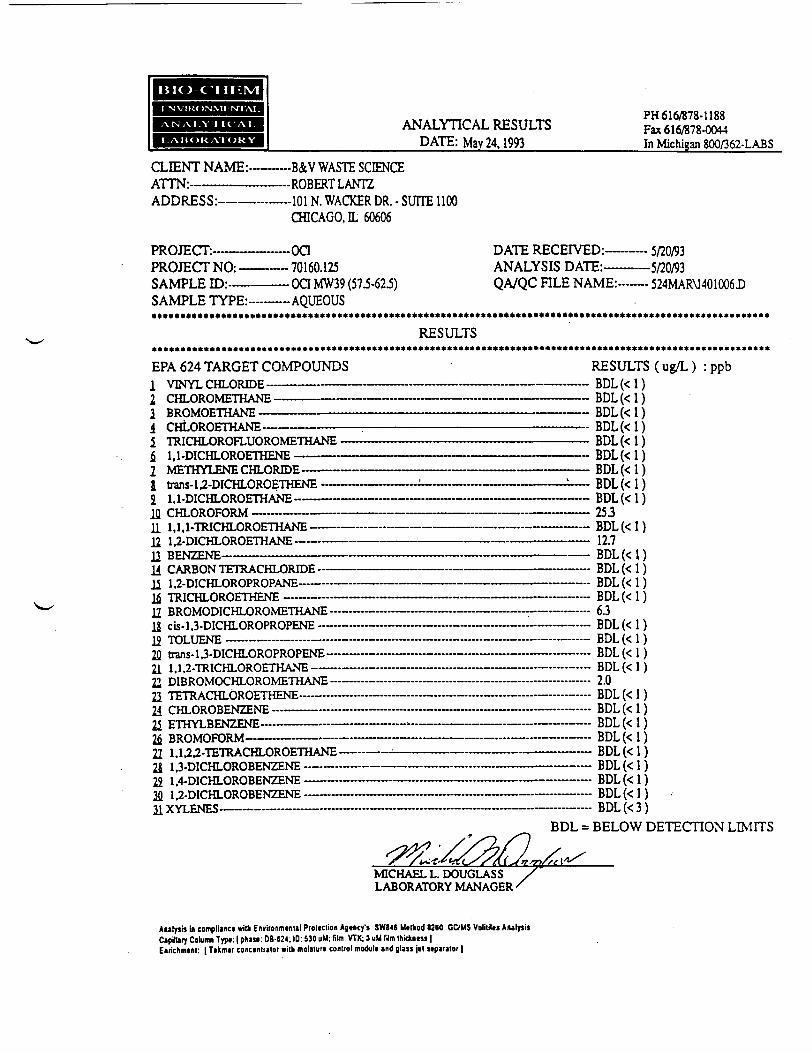
ANALYTICAL RESULTSDATE: May 24.1993
PH 616/878-1188Fax. 616/878-0044In Michigan 800/362-LABS
CLIENT NAME:-—ATTN:———————ADDRESS:————-
PROJECT:———PROJECT NO: —SAMPLE ID:-—SAMPLE TYPE:-———AQUEOUS
—B&V WASTE SCIENCE—-ROBERT LANTZ—101N. WACKER DR. - SUITE 1100
CHICAGO, IL 60606
—OCI—70160.125—OCIMW39 (57.5-62.5)
DATE RECEIVED:———— 5/20/93ANALYSIS DATE:————5/20/93QA/QC FILE NAME:——- 524MARM401006D
»»»••«*«**»«*»••»*«»*»«*****»»*»•*«*»«***»»*»**«•»»****«**»*»***»**«*«**»****•»*»***»**•*«*«««««•«««•«•«•«*RESULTS
»»•«»»»»»«»••»««»•*««»»»»*»«»•»»•»»*»»•*•»«»»»»»»»*«*»»»»*»»****»»••**»*»»«»•»»•*»»*»»*••««»*««««*•«••»•*»*EPA 624 TARGET COMPOUNDS RESULTS (ug/L) : ppb
2 CHLOROMETHANE ——————————— - —————————————————1 BROMOETHANE ——————————————————————————————A ("ur ("rt>nnrtiAVTni TRICHLOROFLUOROMETHANE —————————————————————$ 1.1-DICHLOROETHENE —————————————————————————2 METHYLENE CHLORIDE ——————————————————— - —————1 trans-U-DICHLOROETHENE —————————— : ———————————J 1 1 T\T_*^IJT /^P/^LTU A XTC
in PMT HPOPOPM .................. ...._.._ ....11 111 TPT/"*TTT APAPTTJAWP
11 1 o r*ir*TTT oprvpTTJAWP1 * PPM7T7VJP _ _ _ _ _ .,...rr..r - - - - - - - - - . . , „ . , . . . .
14 CARBON TETRACHLORIDE- ——————————————————— - ————1< 1O TMfllT HPAPPOPAWP
if XPT.TTT APAPTT-TPMP . ............. .... ,.._ . . — .. .............
H BROMODICHLOROMETOANE ————— ™ —— -- —— -» ———— - —— r19 /*;« 1 1 r»TPwr nunppnpPMP .- -- .*.. _.-......_. .... ..«.-...«.«.....
in trnnc 1 7 FiTPUT nPHPPHPPIMP . _ ___ ___ ___ _ — - ...... — ..
2fi BROMOFORM ————————— — — ———— — ———————— ....__.-1T 1 1 1 *> 'ITJ'I V APWT OPOPTTIAMP ....... ......................... ......... ......
19 1 1 TMPUT nPARPMTPMP . ...._..... . . .._ ..
22 1,4-DICHLOROBENZENE —————————————————— — - ——— —3Q 1,2-DICHLOROBENZENE - ———————————— - —— — • ———————JL AILCJNCO ————— - — ,.....— ...... .....—-..» +-+L.
BDL(<1)- BDL(<1)- BDL(<1)
BDL(<1)————— BDL(<1)
BDL(<1)BDL(<1)
:,.,.L,.LL ., . RnT If 1 'I
253————— BDL(<1)• — — 12.7.- -- - RHT ^ 1 >
— — BDL(<1)_ __ _ . nni (s i \. ———— — BDL(<1). ______ (. -i
V.J
. _____ nni It 1 ^
.. .„„„..„ BDL(<1)___ . . tmi (s i
_ — .. RDI r<r 1 ^•) nRDT ^<- 1 1
————— .... BDL(<1)-- BDL(<1).. BDI (f i \DLIL (.V. 1 ;
RDI <t 1 ^Bny /<• i \
. ——— . . BDL(<1)p.ni (s 1 \
. — .... BDL(<3)BDL = BELOW DETECTION LIMITS
MICHAEL L. DOUGLASSLABORATORY MANAGER'
Analyin in compliance wilh Environminial Ptoltclion Agtncy'j SWI46 Mtikod U60 GC/MS Volililts AnalpiiCapiUry Column Typ«: | phau: DB-C24; ID: 530 uM; film. VTK; 3 uU Urn ihickntu)Ei»ichm«ni: [ Tikmat conctnlialof with moisiurt coni/ol modult and glast j«1 iiparator |

CLIENT NAME:-ATTN:-ADDRESS:—-
ANALYTICAL RESULTSDATE: May 24.1993
PH 616/878-1188Fax 616/878-0044In Michigan 800/362-LABS
-B&V WASTE SCIENCE-ROBERT LANTZ-101N. WACKER DR. - SUTIE 1100CHICAGO, IL 60606
PROJECT:PROJECT NO-SAMPLE ID:-SAMPLETYPE:—•********************
-OCI-70160.125-OaMW39-AQUEOUS
DATE RECEIVED:——ANALYSIS DATE:——QA/QC FILE NAME:—
• 5/20/93•5/20/93•524MARM301005D
*********************************************************************************RESULTS
tit********************************************************************************************************EPA 624 TARGET COMPOUNDS1 VTWYT PHT r^DTT»F .- ....—.-..-.—. . ^ ____ .... ... ... ...... _... _
t BT^?;SvcTOiSir
J rHtOTOETOANEi TRICHLOROFLUOROMETHANE ——————————————$ 1,1-DICHLOROETHENE ——————————————————— - ————
1 trans-U-DICHLOROETHENE —————————— ' —————————2 1,1-DICHLOROETHANE ——————————————————————1A ^t_TT f\Of\Cf\O\ t
11 111 1T>IiPWT APOPTT4AMF ...... ..................
12 U-DICHLOROETHANE ————————————————————————
H CARBON TETRACHLORIDE —————————————————————\t 1 T^T^tn iOP kOPP PA l^F n i i i
17 PiTIiOT^TOr^T^HT OHOI^ETTiAI^JE ....•••..... ............
M /-IC 1 i TVPUT npnppnpPMP . _ — . . . . _
22 trans-l,3-DICHLOROPROPENE- —— - ———— - ——— — —— -- —— — -11 1 1 *5 T"DTf"*lJT r^POPTT-IAWF — ...................
Ifl 1 A TYIf^UT iOPOTlt7MVPNrP
11 WT TZMT7C r-*-, T-. .
RESULTS ( ug/L ) : ppbBDL(<1)
- BDL(<1)BDL(<1)
................... BHT (s \\- - BDL(<1)——————— BDL(<1)
BDL(<1)nni is i ^
——————— BDL(<1)12.6BDL(<1)
••• 18 1BDL(<U
——————— BDL(<1)——————— BDL(<1)——————— BDL(<1)— —— ...23
Bni is i 'i————— - Di-'L (< 1 )_ ____ BHT is 1 1ULsLj ^X 1 f
nni Is 1 \_____ _ nni is i \
. 9 8_____ __ nnr is i ^
____ . _ nni (s i __ _ nni (t 1 ^
BT^T t^ 1 ^
_ Dni /£ i \_ _ nni /^- 1 \
tiny ts 1 \— - - BDL (< 1
nnr /<> i \
BDL = BELOW DETECTION LIMITS
MICHAEL L. DOUGLASS ' /LABORATORY MANAGER '
Arulfirs In complunci «iih Exiionminlil Pioltction Agency's SWI46 M«lhod 6J80 GC/MS VolilUts AulytaCjpilUry Cokimn Tfpl: | phau: DB-824.10: S30 uM. lilm: VTK; 3 uM lilm Ihicfcneu ]Entkhmtnl: | T*kmai conctnltalor with moislun control moduli ind glass jll siparator |

CLIENT NAME:-ATTN:—————ADDRESS:-
ANALYTICAL RESULTSDATE: May 24.1993
-B&V WASTE SCIENCE-ROBERTLANTZ--101N. WACKER DR. - SUITE 1100
CHICAGO, IL 60606
PH 616/878-1188Fax 616/878-0044In Michigan 800/362-LABS
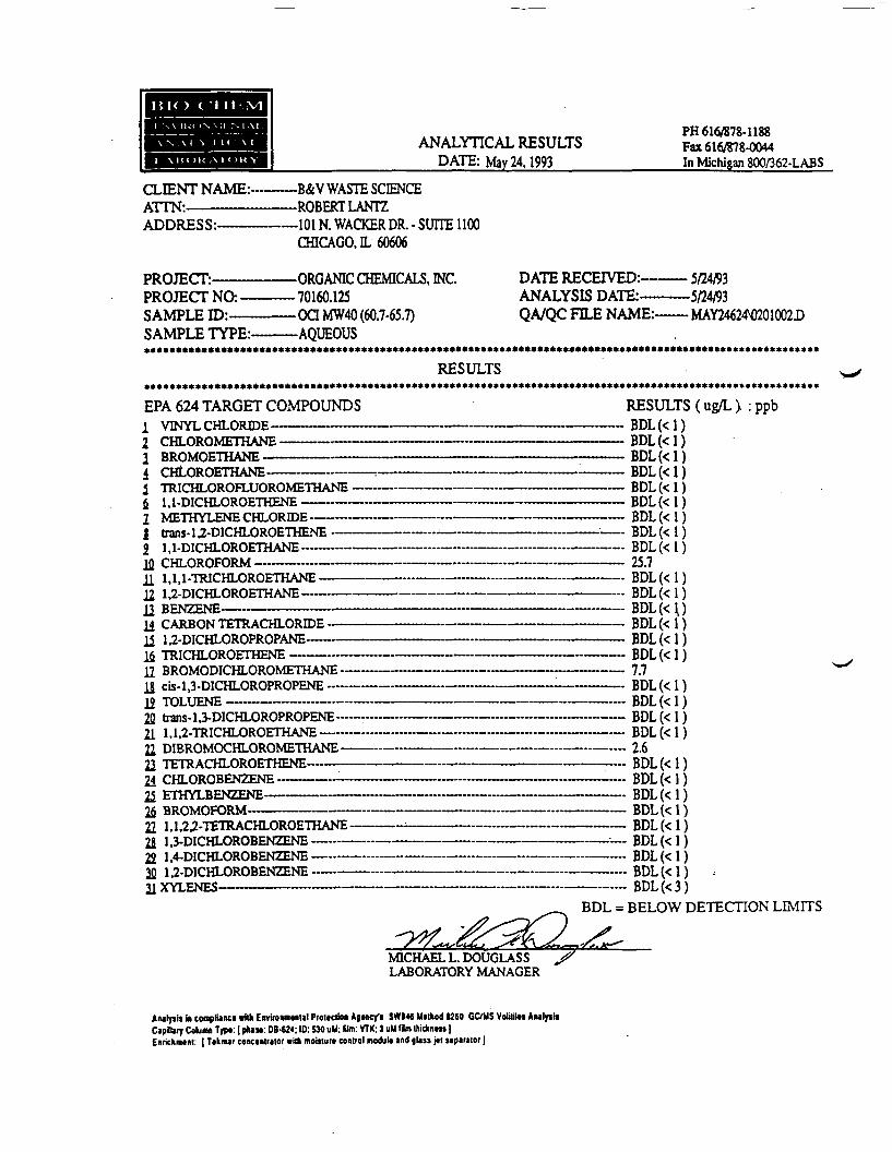
PROJECT:——PROJECT NO:-SAMPLE ID:—
-ORGANIC CHEMICALS, INC.-70160.125-OCIMW40 (55.7-60.7)-AQUEOUS
DATE RECEIVED:--"—— 5/24/93ANALYSIS DATE:———-5/24/93QA/QC FILE NAME:—— MAY24624\)101001D
SAMPLE TYPE:—•»»»»»»•*•»*»»»»»»»»»»•»»••*»»»»»•«•»»••*»»••»»*»*»»*»»•»»»»»»»*»»»»»*»••»••••»•»*»»»»••«»»«•«»«»«»»«»»»»»»
RESULTS*»»»•»*»»»•»••••»»»»»*»»•»»•»•»***»***»*»»•»»»»»*»»••»***»«»»»*«»*•••*»*»»***»«»*••*****«*»****»«•••««»*«*«EPA 624 TARGET COMPOUNDS
VINYL CHLORIDE--CHLOROMETHANE -BROMOETHANE —CHLOROETHANE-
1214I&112Ifl CHLOROFORM ——————11 l.l.l-TRICHLOROETHANE-12 1,2-DICHLOROETHANE —
BENZENE——
TRICHLOROFLUOROMETHANE1,1-DICHLOROETHENE —————METHYLENE CHLORIDE ————tnns-U-DICHLOROETHENE ——1,1-DICHLOROETHANE ————
RESULTS (ug/L) :ppb— BDL(<1)— BDL(<1)~- BDL(<1)— BDL(<1)
14 CARBON TETRACHLORIDE-——11 U-DICHLOROPROPANE-———-1$ TRICHLOROETHENE ——-———12 BROMODICHLOROMETHANE —IS cis-U-DICHLOROPROPENE —-—12 TOLUENE
trans-l,3-DICHLOROPROPENE-21 1 .U-TRICHLOROETHANE ————————22 DIBROMOCHLOROMETHANE — —————21 TETRACHLOROETHENE ————— - —— —24 CHLOROBENZENE ————————————2i ETHYLBENZENE ——————————————2f BROMOFORM-21 1.1,2,2-TETRACHLOROETHANE —— -2J U-DICHLOROBENZENE —2i 1,4-DICHLOROBENZENE —3fl 1,2-DICHLOROBENZENEH XYLENES
BDL(<1)BDL(<1)BDL(<1)BDL(<1)38.6BDL(<1)
----- BDL(<1)----- BDL(<1)—— BDL(<1)~ BDL(<1)----- BDL(<1)—« 11.9----- BDL(<1)----- BDL(<1)—- BDL(<1)----- BDL(<1)__ j 4—-- BDL(<1)—~ BDL(<1)
BDL(<1)BDL(<1)
_.—— BDL(<1)BDL(<1)
•-- BDL(<1)
BDLBDL(<3)
BELOW DETECTION LIMITS
MICHAEL L. DOUGLASSLABORATORY MANAGER
Aulpii in conplianci whh Envitonrntnul Protlction Agincy1! SWI4( Unn»d 1260 CC/MS Volitiltt Aiulpi*Capita)} Caluim Typ«: (phaw: OB-624; 10: S30 uM; film: VTK; 3 uM 19m Ikttntu |Enriehmiit: | Tikmar concinuator with moiuuri control moduli ind (list jit tipintor 1
CLIENT NAME:-ATTN:——————ADDRESS:-
ANALYTICAL RESULTSDATE: May 24.1993
PH 616/878-1188Fax 616/878-0044In Michigan 800/362-LABS
-B&V WASTE SCIENCE-ROBERT LANTZ-101N. WACKER DR. - SUITE 1100CHICAGO, IL 60606
PROJECT:——PROJECT NCh-SAMPLEID:-
-ORGANIC CHEMICALS, INC.-70160.125-CX3MW40 (60.7-65.7)
DATE RECEIVED:—ANALYSIS DATE:—QA/QC FILE NAME:-
•5/24/93•5/24/93•MAY2462<N)201002D
SAMPLE TYPE:———AQUEOUS»*•***»***•***»***•**************************»»*************************»*******************•*»«*******•*>»
RESULTS•••*•***»•*****»*»•****»****************************•**•**************•**********************•*****>*******EPA 624 TARGET COMPOUNDS RESULTS (ug/L) : ppbi viii i i- v,nj_wi\-UJC. • ———— „_„...._.... ——— ..._........ —— ......_....._.... —— ..
2 BROMOETHANE —————————————————————————————— —4 PT4T APAFTWAMP ._ ,...,. . . . .
i TPT/^TJf APAPT TTAPAMPTTTA WP ......... ......... ......... . ,...f, 11 TVPHT APAPTTTFMP . .. ..............................................
I TiJiUTTIVT PMP f*HT APTHP
I ti-inr 1 *> TMPT-TT APAPTTTPWP ...... .. ...... . ........ . ....
H 1,1,1-TRICHLOROETHANE —————— - ——————— ..-..._....._...._..... ——
12 BENZENE —————————————————————————————————————ii PAPROMTPTB APTTT nprnp !.... _ . ..._. . . . . . . . ..., . . . . . . . . + ....li 1 ,2-DICHLOROPROPANE ———————————————— - ——————— — - ——i/r TDTfTTT APAPTOPWP .. . . . i .L l i_L ......... . . . L J - T . T , , . , ........... ....
n -BT*r\\4r\T\ir>m rvar\\jmTUA vrr
H cis-l,3-DICHLOROPROPENE ——————————— - ——————————— ^ ——— -Ifl TAT TTPKIP ... . -j , . . j j L n r . , ....... «...
•>rt tr-inr 1 1 niPHf APAPPAPPMP . ^ _L
21 1,1,2-TRICHLOROETHANE ~—— -«— — _.._———— —— -—— ————TT r\TnPAK'fAOHT APAMPTH A?STP . , , ,..,,.. , - T - - U . L ... x.11 TTTTD APMT APAPTHPMP ^. . T.. . .. ™.
Id PUT APARPW7PNP ............. . .r . . . . . r ...... r L T.... _ .....................1< T7TTTVT P.PKT7PMP ...... ..... .................... ..... . .....
2fi BROMOFORM ———————————— - ———————————— — - ———— -- ——21 l.U^-TETRACHLOROETHANE ————— = —————— - ———— -- — - ——IB 1 1 TWr'VI APAWPMVPMP .. . .. ... . ....
OO 1 A TM/ tlf APAP.PNT7PWP ... ... ...... ...... .....
1rt 1 *> TM^Uf APAPPM7PMP . .. ...... ... .. . .
11 YVT PTSlP*! j-i T. .x. . . .......... . ............ .......... . ..
.._.™ viSl* \^ 1 )
BDL(<1)BDL(<1)
—— BDL(<1)BDL(<1)
—— BDL(<1)BDL(<1)nni if i \nni is i \25.7
—— . BDL(<1)—— - BDL(<1)
—— BDL(<1)—— BDL(<1)
BDL(<1)__ 77—— BDL(<1)
p.ni t< i \___ nni (< i \,. —— . BDL(<1)— .... 2.6
—— BDL(<1)__ oni if i \——— BDL(<1)——— BDL(<1)—-- BDL(<1)——— BDL(<1)
_ nni /<• i \
BDL = BELOW DETECTION LIMITS
MICHAEL L. DOUGLASSLABORATORY MANAGER
AMtyjil» coi ilunct wttli Envuonmtnul Prottctio. AjMCTl SWI46 Ultkod 12(0 GC/US VolMKi AdjlyiiiCipaiaiy Coluow Typ<: [ phiti: 08-62<; 10:530 uU. film: VTX; 3 uU film Ihickniu |EnrichiMnt: [ Tokmar conciDtrator with mooturt control moduli and glass jit sipatator)

BIO-C"! IHIVi
ANALYTICAL RESULTSDATE: June 4.1993
PH 616/878-1188Fax 616/878-0044In Michigan 800/362-LABS
CLIENT NAME:-ATTN:———__ADDRESS:-
-B&V WASTE SCIENCE-ROBERT LANTZ--101N. WACKER DR. - SUITE 1100
CHICAGO, H. 60606
PROJECT:——PROJECT NO: -SAMPLE ID:-
-ORGANIC CHEMICALS, INC.-70160.123-OdMW41(10I51-97.51)
DATE RECEIVED:—ANALYSIS DATE:—QA/QCFILENAME:-
-6/3/93-6/3/93-JUN03624\0801004D
SAMPLE TYPE:————AQUEOUS•*»»*»»»»»***»»»»»•«•«»**»*»••*••»»»*•*•*»*»*»****»*****»»*»»*»»»******»***«•••»••»*»*******»**«*»»»»»**»»»
RESULTS•»»»•«»»«»»*»*»*«•»*****»*»•*»*«***»»****»»*»*»••****«***»»*•»»*****»**•**••»»*»»*«»•*»«•*•»»»»*•*«*»»»»••*EPA 624 TARGET COMPOUNDS1 VINYL CHLORIDE —I CHLOROMETHANE—————1 BROMOETHANE—————————i CHLOROETHANE————————i TRICHLOROFLUOROMETHANEi 1,1-DICHLOROETHENE —————
METHYLENE CHLORIDE————
RESULTS (ug/L) : ppb
trans-U-DICHLOROETHENE —1,1-DICHLOROETHANE-CHLOROFORM ———
1J2112H 1,1,1-TRICHLOROETHANE-12 1,2-DICHLOROETHANE ————11 BENZENE—————————————14 CARBON TETRACHLORIDE ——U U-DICHLOROPROPANE———-1$ TRICHLOROETHENE —————11 BROMODICHLOROMETHANE-U cis-1.3-DICHLOROPROPENE-—12 TOLUENE ————---——-——-2Q irons-1,3-DICHLOROPROPENE—21 1,1.2-TRICHLOROETHANE——22 DIBROMOCHLOROMETHANE-21 TETRACHLOROETHENE———-24 CHLOROBENZENE -——————25 ETHYLBENZENE———————-
BROMOFORM-—————————-
———— BDL(<1)———— BDL(<1)———— BDL(<1)———— BDL(<1)———— BDL(<1)————- BDL(<1)————- BDL(<1)———— BDL(<1)———— BDL(<1)____ 2 8———— BDL(<1)———— BDL(<1)
BDL(<1)BDL(<1)
:1)
2^22 1,1.2^-TETRACHLOROETHANE ———2J 1,3-DICHLOROBENZENE ——————22 1,4-DICHLOROBENZENE ——2Q 1,2-DICHLOROBENZENE —21XYLENES-————.—_.-_-
.———.. BDL(<1)„..__.... BDL(<1),....._.... BDL(<1)„...._.... BDL(<1)„..._...- BDL(<1)..._._.... BDL(<1),„...__.. BDL(<1)._..._.... BDL(<1)""~~'~""~~ *~~~ ijUL* ^^ 1 f
,„._.... BDL(<1)———— BDL(<1).———— BDL(<1).......—— BDL(<1)
—- BDL(<1)....——._.... BDL(<3)
BDL = BELOW DETECTION LIMITS
MICHAEL L. DOUGLASSLABORATORY MANAGER
AMlyili In complilnct with Eiwlronmtntil Prollction Ajtncy. SWI« Muhod 1260 GOMS Voliiilti AnalpisCapilUtr Cokimji Type | phai*: DB-624; 10:530 uM; film: VTK; 1 uM lilm tkidiMU 1tniichm.nl: | Ttkmar cononiulot *iih moislura conlrol modul* and gla» j«i ttpaiaior ]

ANALYTICAL RESULTSDATE: June 4.1993 .
PH 616/878-1188Fax 616/878-0044In Michigan 800/362-LABS
CLIENT NAME:-ATTN:—————ADDRESS:-
PROJECT:———PROJECT NO:-~SAMPLE ID:——SAMPLE TYPE:-
-B&V WASTE SCIENCE-ROBERT LANTZ-101N. WACKER DR. - SUITE 1100CHICAGO, IL 60606
-ORGANIC CHEMICALS, INC.-70160.125-OdMW41(107.51-102.5')-AQUEOUS
DATE RECEIVED:—ANALYSIS DATE:--QA/QCFILENAME:-
-6/3/93-6/3/93-JUN03624\)701003D
*»•*«•****•**«»****«*•**»*»***»»•»•»*•»«****««»»*»••••»**»*»****»»*»«*•*•**»•**«•***«*»«*»•**«»*«*»*»*»»«••RESULTS
»»»***«»»*•»****•••«»•**»**»*»»•»*»*»»*»***»»»»**••»•«»»»»*»»»«»»»*»»»»»»*»*»****»»»»»•«**»••••«•»••»«»•***EPA 624 TARGET COMPOUNDS1 \7TKJYT PTTT nP_T_P - - - - - . ,. .... .....................
2 /^trr npf\K_fF*roA_srF . _1 PPAMr_PTHAWF .. ..... . .. ......................
1 f*\n rtDrtlTTTTAMP
5 XPTPTIT r»POF! TTOPA>i/fFTTTAMF6 11 TWHI APnPTJTPWP ^ . U J J i . j , - - . ,. ,. ,. ...... , , , r r . - - - - T ..
1 METHYLENE CHLORIDE ———————————— - ————————— - —— — — ——— --1 trans-U-DICHLOROETHENE — ————————— : ——————————————— ; ——5 1 i r\Tr«TJT /~n>rttrrtj AVTC1A PUT nPOFHPM .......... _ _ _ _ _it 111 •roirf"»uT _*M»r\TrTti AVTC
12 U-DICHLOROETHANE —————————————————————————————————tl DCKTTCKIC
i A /•» A D n f\K.t "IT." I'll A /^TTT f\O TT%C
H 1 ? DTPHLnROPROPANE ___ -- - -^^1£ TRTPHT HPOPTHFMP ..-.....-....M............ ........ ..... ..........................
J2 BROMODICHLOROMETHANE ————————— - ——— - ———————— - ——————19 ric t T TVPHI ORnPPOPPMF ,T , ^ m . ..1 Q Tf~»T T TWCR -. .. _ _ __ ._.7n trim: 1 1-DIPHLOROPROPENE _____ ___ __ __ _____ __ __ —*__ 1 1 *) TTJTPWT OPnFTHAMP —
22 DIBROMOCHLOROMETHANE —————..... —— .__....__.„.._.__ —— ..__*?1 TTTP APHT npnPTHFNP ,,. , , ..*)A r*HT OPr^RPlSTTPMP ..... ..._..-..,, ....... ... _.......... . ..0< FTTTVT PPNT7FMP . . . . .....
^< PPHMHPHPM ... ... ^..........T AJ .,..!, ... ,L ........ T .......TT
T7 1 t 79 TFTRAPHT ORORTHANP __ . _ _____ __ _________ _Ifl 1 1 HTPWI OPORPNTFMP «... __ . .. __ __ — . _ ....... . _ ..,..— __ . ....tQ 1 A HTPUT OPORPN7FMF .. ____ ..... .... .. __ . .. ....... __ _ .- ___ _ .1A 1 *> TVPWT nPOPPMTFT^JF ........... ............................................ ....,..T,11 YVT CN7T7C .._ ... — -
^--,^-^ BDL =
RESULTS ( ug/L ) : ppbBDL(<1)BDL(<1)BDL(<1)BDL(<1)BDL(<1)BDL(<1)BDL(<1)BDL(<1)BDL(<1)2.3BDL(<1)BDL(<1)BDL(<1)BDL(<I)BDL(<1)BDL(<1)BDL(<1)BDL(<1)BDL(<1)BDL(<1)BDL(<1)BDL(<1)BDL(<1)BDL(<1)BDL(<1)BDL(<1)BDL(<1)BDL(<1)BDL(<1)BDL(<1) •BDL(<3)
BELOW DETECTION LIMITS
MICHAEL L. DOUGLASS LABORATORY MANAGER
Autyin I* cwnpliancl »illi Envuonmmul Ptoltction Agincy'i SWI4I Ulthod 6260 GC/MS VofiUlis AnalyiiiCiplUry Cohim Type [ phiu: 08-824.10:530 uM; Olm: VTK; 3 uH llm Ihidmm ]Enrichmtni: | Tikmit concinttttoi with moislun control moduli ind |l»t fll Mpiriloi)

ANALYTICAL RESULTSDATE: June 4,1993 .
PH 616/878-1188Fax 616/878-0044In Michigan 800/362-LABS
CLIENT NAME:-ATTN:—————ADDRESS:--
-B&V WASTE SCIENCE-ROBERT LANTZ
—101N. WACKERDR. - SUTTE1100CHICAGO, H 60606
PROJECT:-PROJECT NO: —SAMPLE ID:——SAMPLE TYPE:-
-ORGANIC CHEMICALS, INC.-70160.125-OQMW41 (lllS'-KW)-AQUEOUS
DATE RECEIVED:-——- 6/3/93ANALYSIS DATE:——--6/3/93QA/QC HLE NAME:-—- JUN03624W01002.D
••»»»•»•*»»«»•«»**»*»»»»»»»**»**««»»•****»»»»»»••»»»•»»*»»**»»*»»»**•»***»»**»***»»•*»«*»**»•»*»»••»••»•••«RESULTS
«»»*»•*•*»»*»»*»«»»*»•»»***»«»»»•*»»*•******»***»******«»**»»»**»****»**•«***»**•*******»*•»««»•«»»******»*EPA 624 TARGET COMPOUNDS RESULTS (ug/L) : ppb1 VINYL CHLORIDE ——————————————————————————-———- BDL (< 1)2 CHLOROMETHANE——————————————————————————————————— BDL(<1)1 BROMOETHANE —————————————————————————————————- BDL (< 1)1 CHLOROETHANE—————————————————————————————————— BDL(< 1)i TRICHLOROFLUOROMETHANE ————————————————————————— BDL (< 1)
4 fi 1.1-DICHLOROETHENE —————————————————————————————— BDL (< 1)1 METHYLENE CHLORIDE——————————————————————————————BDL(<1)1 trans-U-DICHLOROETHENE ————————————————————————:—— BDL (< 1)2 1,1-DICHLOROETHANE———————'——————————————-————-BDL(<1)
"' in PUT OPnFHDM ______._ ___ ..__. _...._..._. „___._.__..__.__..________._ 1 *)lu v>xUrfWi\vyf^v/*vi*& ....••.—».— ~~« . . 11 .«»._..-«.......>». __.. —_..*—— »» jtff11 1,1,1-TRICHLOROETHANE——————————————————-————————- BDL(<1)12 U-DICHLOROETHANE-—-——————————————————————— BDL (< 1)12 BENZENE—————————————————.—._.--—..—._——————.... BDL (< 1)14 CARBON TETRACHLORIDE—————--————-_———.————————— BDL(< 1)li 1,2-DICHLOROPROPANE--————————--——————.———..———.._... BDL(< 1)1$ TRICHLOROETHENE ———-—————-——————————-————------- BDL(< 1)U BROMODICHLOROMETHANE———-—————-————-———————...._._. BDL(< 1)15 cis-l,3-DICHLOROPROPENE ——--———-——-—.—_—.——————.. BDL (< I)12 TOLUENE ————————————-——————————————————— BDL(< 1)2fl trans-1.3-DICHLOROPROPENE-—-———————._...———————.——.—- BDL(< 1)21 l.U-TRICHLOROETHANE————--—————.-_.-...—.--————-—-——- BDL(< 1)22 DIBROMOCHLOROMETHANE———-----~———-....—.-._.-———-————— BDL(< 1)21 TETRACHLOROETHENE-—————-——-————————....——.——————-—— BDL(<1)24 CHLOROBENZENE ————————————————.....—..,._..———._..——— BDL (< 1)25 E1W.T LUt-T'i^iiINc••—••—«-.•—..•-»—«.»»-^-»-».»..-.—-«•»»•—-—»—.—-.——.——.—-«.-^..-.-••- fjL/L^ ^s 1 )2fi BROMOFORM--———————————--—————.—_-—————-——— BDL(< 1)22 1.1,2,2-TETRACHLOROETHANE-————————-——————-_-——————- BDL(< 1)2S U-DICHLOROBENZENE————-———————-----———-——————— BDL(< 1)22 1.4-DICHLOROBENZENE -————..._.._.__.——..._..———._.„..__..-._.._ BDL(< 1)2JJ 1,2-DICHLOROBENZENE-———-————-——-—--—.....—————-—————-BDL(<1)21XYLENES--————————-———————-—————.._—.—-.._—————- BDL (< 3)
BDL = BELOW DETECTION LIMITS
MICHAEL L. DOUGLASS /LABORATORY MANAGER
Anilpii In complianct wilh EnvironnKnul Prouciion Ajtncy'» SWI46 Miikod (260 CC/MS Volitiln AnalpliCapaiary Column Type [ pha»: OB-(24; 10:530 uM; film: VTX; 3 uU (Dm thIAntsi 1Enrichminl: | Ttkmir concinuator wilh moisturi control modulo ind gla» |tt stpaiator ]

CLIENT NAME:-ATTN:—————ADDRESS:-
ANALYTICAL RESULTSDATE: June 4.1993
PH 616/878-1188Fax 616/878-0044In Michigan 800/362-LABS
—B&V WASTE SCIENCE—ROBERT LANTZ—101N. WACKERDR. - SUITE 1100
CHICAGO, DL 60606
PROJECT:———PROJECT NO:--SAMPLE ID:-—SAMPLE TYPE:———AQUEOUS**«»»•»»*•»»•*•**•*****»»•••**•**•!
—ORGANIC CHEMICALS. INC.— 70160.125
DATE RECEIVED:-----ANALYSIS DATE:——QA/QCFTLENAME:-
-6/3/93-6/4/93-JUN03624M201007J)
•••***»**»»»»*»*•*•»**••»»*»•*»»•••*••»»•*»»»*••»•»»*»«••»»*••••«»*•RESULTS
••»»»*»»»*«»»»»•**»**»»••»«*»»«»»»•«*••**»»«»***»**»»»»»»*»*»«**»»»»»•»•*•«»*»*»»«*•»•«»•»»••*••»»»*»«»**»»EPA 624 TARGET COMPOUNDS RESULTS (ug/L) : ppb1 VINYL CHLORIDE ——————-—————————————-—-—————————— BDL (< 1)2 CHLOROMETHANE —————-—————-————————————————-——— BDL (< 1)2 DpriwnPTHAlMP _ _ ____. _.. _ ..-———-———-—_—.._ ___..__._._._ RTV (* 1 OIXV/IVIV^C 1 CW*C i......... ...— ............. _..... ...........ii ii..« ... DLS1* IV 1 I
1 CHLOROETHANE--—————————————-———————————————— BDL(<1)J TRICHLOROFLUOROMETHANE —-———————————————————————— BDL (< 1)fi 1.1-DICHLOROETHENE ———————————~—————.—,——.._.————— BDL (< 1)2 METHYLENE CHLORIDE-———--———-——————»———-»~————— BDL(< 1)
...* JJULI^ 1 JJ£ 1,i~Ul\^AlL«vi'lxvJC 1 H-AiNc.• ' ™-..™....----—-»-»»--•-••••....___........*•••••_••...••___ JJ^L [^ ^ jin1U
1,1,1* lM^.*^L%J*\x^*JI r^^UNt *"~"~""*~*~*"""'**~*"~"*~""""••"«"•"—•»»»•••••••• —•••-«-"•••••••••• JJ^L Iv 1 I•-•• DUJL* \v 1 1«-- 15UL ^ ^ ^
Ji CARBON TETRACHLORIDE———....._...—......_...——....———....._...——... BDL(< 1)Ji 1,2-DICHLOROPROPANE-————————.._......_............_..„.._....._.„. BDL(< 1)Jj5 TRICHLOROETHENE—-—_—-—..-—.—.--—---_.....———.——....—- BDL(< 1)12 BROMODICHLOROMETHANE——————————————————--—- BDL(< 1)Ji cis-l,3-DICHLOROPROPENE -———————-—————--.:—.._....-—.._.... BDL (< 1)12 TOLUENE ——————————..._....._....__...——.„_„.,.._.....—.—...._.... 2.12Q trans-l,3-DICHLOROPROPENE--————--——---—-——-—-——-——-—- BDL(< 1)21 U.2-TRICHLOROETHANE--——-----..-—---—.-.—....._....._......_....__.. BDL(< 1)22 DIBROMOCHLOROMETHANE-—-——»«————-—_.——.—--———-—-.-- BDL(< 1)21 TETRACHLOROETHENE——-——-——~~—-——--—-———-_—.—...——. BDL(< 1)24 CHLOROBENZENE-———-——»—-.--—-———-.—-——-———......_.... BDL(<1)25 ETHYLBENZENE———--————•——----————.-—-——————-———... BDL(< 1)1A T)nr\\/rr\cf\D\t __ .«_ «..««. ..____________________. _ _ __._._-... PHI fc 1 \^y J3I»WI»lvr^x*VI»l .—•—•••••••-—-----™™ —.--».-—.—....•.••«»_••.».„•..».•———....«—«——™ JL*i/^ ^V 1 f
22 1,U>TETOACHLOROETHANE"——--»———--—..—.—...————- BDL(<1)28 1,3-DICHLOROBENZENE—-——————.———————.———.._......_„.. BDL(< 1)22 1.4-DICHLOROBENZENE-——.—...——.——.————————————— BDL(< 1)22 1,2-DICHLOROBENZENE————————————————————————— BDL(< 1)21XYLENES—————————————————————————————— BDL (< 3)
BDL = BELOW DETECTION LIMITS
MICHAEL L. DOUGLASSLABORATORY MANAGER
Analyiii in conplianci with Enviionminlal Pfoltction Kfncfi SWU6 Mtthod 1260 GC/MS Volitilti AulysiiCapfllary Column Typt: (phas«: OB-624; 10:530 uM, lilm: VTK; 3 uM lilm ihidtntu |Entichnwnl: | Ttkfflar conctnlralor with moinult comiol moduli and glass jtt stparalor |
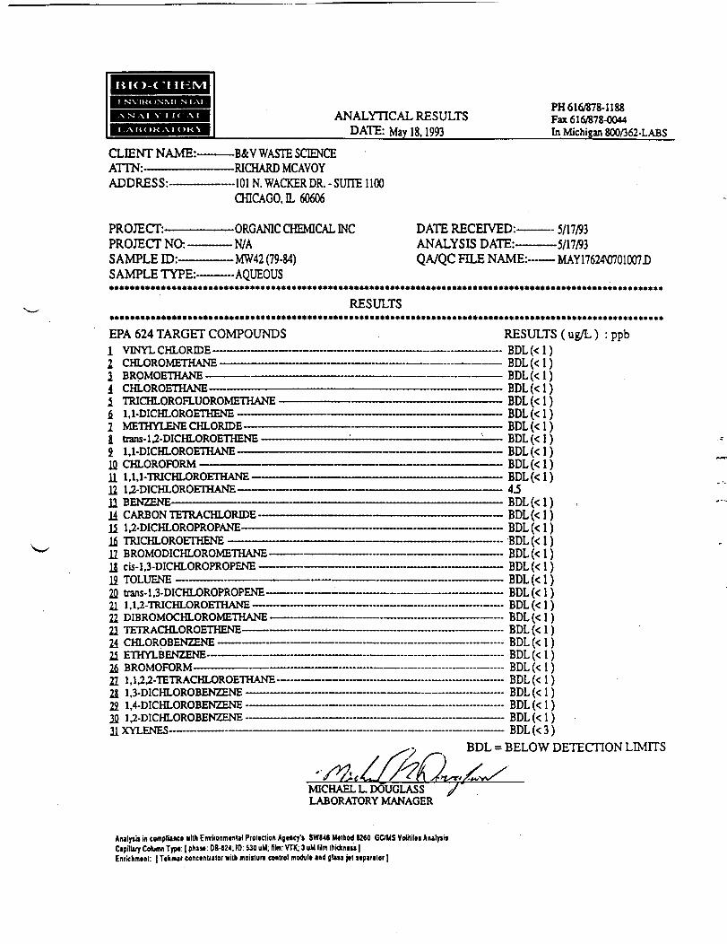
ANALYTICAL RESULTSDATE: May 18.1993
PH 616/878-1188Fax 616/878-0044In Michigan 800/362-LABS
CLIENT NAME:-ATTN:—————ADDRESS:-
-B&V WASTE SCIENCE-RICHARD MCAVOY
—101N. WACKER DR. - SUITE 1100CHICAGO, IL 60606
PROJECT:———PROJECT NO: —SAMPLE ID:——SAMPLE TYPE:-
-ORGANIC CHEMICAL INC-N/A-MW42 (79-84)-AQUEOUS
DATE RECEIVED:—ANALYSIS DATE:—QA/QC FILE NAME:-
- 5/17/93-5/17/93-MAY1762M701007D
•A******************* •«»*»»»•»»»«•»»•*•»»»**•»*»»*»*«»»••»»»*»**•»*«••*»*»»»*»»••«RESULTS
»»»»»»•»••»»»»*»••»••»**«»*»«»«•»»»****»**»*»«•••*•»»*•»«»»»*»»»*»«•»**»»»»***»*»»»»**»»**»»*»*«*»EPA 624 TARGET COMPOUNDS
VINYL CHLORIDE-CHLOROMETHANE-BROMOETHANE —CHLOROETHANE-TRICHLOROFLUOROMETHANE1,1-DICHLOROETHENE —————METHYLENE CHLORIDE ———trans-U-DICHLOROETHENE ——1,1-DICHLOROETHANE ————
Ifl CHLOROFORM ——————11 1,1,1-TRICHLOROETHANE-12 U-DICHLOROETHANE——11 BENZENE-
RESULTS (ug/L ) : ppb- BDL(<1)
BDL(<1)BDL(<1)BDL(<1)BDL(<1)BDL(<1)
- BDL(<1)- BDL(<1)- BDL(<1)- BDL(<1)~ BDL(<1)
CARBON TETRACHLORIDE--U-DICHLOROPROPANE——TRICHLOROETHENE —
BDL(<1)BDL(<1)
12 BROMODICHLOROMETHANE-11 cis-l,3-DICHLOROPROPENE •12 TOLUENE —————-————2Q trans-1.3-DICHLOROPROPENE-21 l.U-TRICHLOROETHANE-22 DIBROMOCHLOROMETHANE —21 TETRACHLOROETHENE————24 CHLOROBENZENE •25 ETHYLBENZENE-2fi BROMOFORM——————————21 1,1,2>TETRACHLOROETHANE-21 1,3-DICHLOROBENZENE ————22 1,4-DICHLOROBENZENE -———1Q U-DICHLOROBENZENE ————H XYLENES——————-——————
BDL(<1)BDL(<1)
____________ DIM If 1 \- vlsLf \^ 1 f—-— " ' ' D1JL« ^v 1 f....——.——. BDL(<1)......——..—. BDL(<1)....—————... BDL(<1)......———--BDL(<1)"**""*"""*"*"***"" DULr ^V 1 J
....——.——.. BDL(<1)_......_........... BDL(<1)_„.._.....—— BDL(<1)———.——.... BDL(<1)„...——.._.... BDL(<1)__ _ ____ tini (<> i \».....»«....„.... mjL* y^, i j_...._....—— BDL(<3)
BDL = BELOW DETECTION LIMITS
L^xMICHAEL L. DOUGLASSLABORATORY MANAGER
AMlytit in complianci wilh Enviionmtntal Pronclion AgMqr's SW848 Mtlbod 8J60 GC/MS VoUlilis AnalytiiCapHlaiy CoKiim Typ«: [ phis*: OB-62*. ID: 530 uU, Him: VTK; 3 uM lilm Ihiduiws ]Enrkhmtni: | Tikmar conctnttaloi wilh moislurt control moduli and glass j*t stparalor ]

ANALYTICAL RESULTSDATE: May 18.1993
PH 616/878-1188Fax 616/878-0044In Michigan 800/362-LABS
CLIENT NAME:-ATTN:—————ADDRESS:-
-B&V WASTE SCIENCE-RICHARD MCAVOY
-101 N. WACKER DR. - SUITE 1100CHICAGO, IL 60606
PROJECT:———PROJECT NO: —SAMPLE ID:——SAMPLE TYPE:-
-ORGANIC CHEMICAL INC-N/A-MW42 (84-89)-AQUEOUS
DATE RECEIVED:—ANALYSIS DATE:—QA/QC FILE NAME:-
- 5/17/93-5/17/93-MAY17624M001010D
••••»»•»»••*»»••«»*»»•»»•••»»»»•»•»»*»*»«**»»•«*«**•«*»*»••*»•»»«•»*»»*»»»»»»»*»•»•»»**»RESULTS
EPA 624 TARGET COMPOUNDS1 VTMVT pwrnpinp.. ^. . , L J I . , . T , .......... .2 CHLOROMETHANE —————— - ———————— -— — ——————3 BROMOETHANE —————————— - ————— ————— —————A /ttrf r\r*rvcm3 A vns
i TD T/"*HT iOD kOPT T Tf"\P nAifPTO A MP
$ 1,1-DICHLOROETHENE ———————————————————————2 \fCTlT\n CKTC /"tJT rtDTT^C
1 trans-U-DICHLOROETHENE2 1,1-DICHLOROETHANE ———————————————————————Jfl CHLOROFORM ——————————————————————————1 1 1 1 1 TPTPHT nPAPTHAWP1*7 1 ? TWHT nP-OFTHANP ....._. ...... K..^,^ ......L. ^Jl BENZENE ———————————————————————————— « ——1.1 C APRON TFTR APHT OPTTlF , ..-. ._ ... ........... .,...., .....1^.^^
it TUTPHT npnPTHPNP r ........ - , - - , - , , . ...
11 cis-l,3-DICHLOROPROPENE — — — - — -———..—————...-in TOLUENE . • • • • • - •—•• • • • • - • • • _ '-- - - — - - - - - - - - - - , , , . ........ , , . . . ......2Q trans-l,3-DICHLOROPROPENE- —— -_—-—......—--—.—.—
22 DIBROMOCHLOROMETHANE .——.—————————...—01 "I'C'TT? APHT f^PkOPTHPP'JP •
t< PTTIVT P.P1M7PMP ..... ..... — .
11 1 1 O O TTITD Ar*UT nPHPTWATMPoo i a nipwr npnnPMTPMP ... . __22 1,4-DlCHLOROBENZENE .——-————-——--———-— ———1A 1 0 TMPHT nPHPPlSTTPMP _ - ___ ___ _ .. — ___ ....11 YVT PMP*J
K***********************4i************»«*
RESULTS ( ug/L ) : ppbDTM (s? 1 \
- - BDL(<1)——————— BDL(<1)
BDL(<1)——————— BDL(<1)——————— BDL(<1)- - BDL(<1)——————— : —— BDL(<1)——————— BDL(<1)——————— BDL(<1)——————— BDL(<1)
6.1——————— BDL(<1)——————— BDL(<1)
nni if i \. __ ... ... BDL (< 1 \UULi \^ I J
nni if i \. __ _____ nni if i \. _ ___ nni if i \
nni is i ^nni if i \
. _ _ nni if i\
._„. ____ RHT (* 1 \__ Dnj ({ 1 \
_ _ nn] /^ i \
. RHT iV 1 ^. __ „ . _ onj (< i \._„. _ _ DIM ({ \\
BDL = BELOW DETECTION LIMITS
MICHAEL L.DOUGLASSLABORATORY MANAGER
Analysis in compliance wild Enviionminlal Prottclion Agency's SWI4( Utlhod 1260 GC/MS Volililts AnalysisCapillary Column Typt: [ phase: DB-S24; ID: 530 uM; film: VTK; 3 uM lilm Ikidintss |Enrichment: [ Ttkmar concentraior with moisture control module and tliss jet separator |

ANALYTICAL RESULTSDATE: May 18,1993
PH 616/878-1188Fax 616/878-0044In Michigan 800/362-LABS
CLIENT NAME:-ATTN:—————ADDRESS:-
——B&V WASTE SCIENCE——RICHARD MCAVOY——101N. WACKER DR. - SUITE 1100
CHICAGO, IL 60606
PROJECT:———PROJECT NO: —SAMPLE ID:——SAMPLE TYPE:-
-ORGANIC CHEMICAL INC-N/A-MW42 (89-94)-AQUEOUS
DATE RECEIVED:—ANALYSIS DATE:-—QA/QC FILE NAME:-
• 5/17/93•5/17/93•MAY17624W)1008D
•»«•*•*•»»»«*«••»**»**»»»•*•*»»**»•**•••*•»•**»»»**• •»*•*»»****»•»«•*•••»•»*»RESULTS
*»*•»*»»»»»•»»*•*»»»*»»*******«»•******»**»**»»»»»***««*«««*****»»*»***»»*•*»»**»**»•»•***EPA 624 TARGET COMPOUNDS
VINYL CHLORIDE-
BROMOETHANE —————————CHLOROETHANE————————TRICHLOROFLUOROMETHANE1,1-DICHLOROETHENE —————METHYLENE CHLORIDE————tans-U-DICHLOROETHENE ——1,1-DICHLOROETHANE————
Ifl CHLOROFORM -11 l.U-TRICHLOROETHANE-12 U-DICHLOROETHANE—13 BENZENE-14 CARBON TETRACHLORIDE.li U-DICHLOROPROPANE——1$ TRICHLOROETHENE12 BROMODICHLOROMETHANE-11 cis-l,3-DICHLOROPROPENE ——12 TOLUENE ————————————2Q trans-U-DICHLOROPROPENE—21 l.U-TRICHLOROETHANE-22 DffiROMOCHLOROMETHANE-21 TETRACHLOROETHENE-24 CHLOROBENZENE ———2i ETHYLBENZENE————2fi BROMOFORM-
RESULTS (ug/L)" : ppb— B D L ( < 1 )— BDL(<1)— BDL(<1)— BDL(<1)— BDL(<1)—- BDL(<1)—~ BDL(<1)~ BDL(<1)—- BDL(<1)~ BDL(<1)—- BDL(<1)— 4.7— BDL(<1)~ BDL(<1)— BDL(<1)— BDL(<1)—- BDL(<1)
BDL(<1)._.... BDL(<1).._... BDL (<1)——. BDL(<1)
—— BDL(<1)——.. BDL(<1)——.. BDL(<1)......... BDL(<1)
BDL(<1)- BDL(<:
21 1.U.2-TETRACHLOROETHANE——————————21 U-DICHLOROBENZENE—————————-————-- _ _ _ v , . ,22 1,4-DICHLOROBENZENE ———————-——»—-—————»—————-————-- BDL(< 1)2Q U-DICHLOROBENZENE ———._...—....._......_...__......—..——._.-—.... BDL (< 1)11 VVT CMT7C _______ _ ____ _ ._....._.--—_ _ „ _.._________.- Rnl (f \ \JI A X I Cl JCO- ........i... r .................. •«. .....................—.. UUL* \^* J J
BDL = BELOW DETECTION LIMITS
MICHAEL L.DOUGLASS ./LABORATORY MANAGER
Analysil In complianc* with Enviionmtntal Ptoltctiofi Agincy's SWI4I Utihod I2>0 GDUS VoliUks AnalylilCipilUrr Cohirm Type: | phasi: DB-K4; 10:530 uU; film: VTK; 3 uU lim Ihldintss |Enrichment: [ Iikmar concintialorwhh moislun control moduli and glass jil uparator |

CLIENT NAME:-ATTN:————ADDRESS:-
ANALYTICAL RESULTSDATE: May 18.1993
PH 616/878-1188Fax 616/878-0044In Michigan 800/362-LABS
-B&V WASTE SCIENCE-RICHARD MCAVOY-101N. WACKER DR. - SUITE 1100
CHICAGO, L 60606
PROJECT:——PROJECT NO:-SAMPLE ID:-
-ORGANIC CHEMICAL INC- N/A-MW42 (94-99)
DATE RECEIVED:—ANALYSIS DATE:—QA/QC FILE NAME:
• 5/17/93•5/18/93•MAY18624X)301003JO
SAMPLE TYPE:————AQUEOUS****************************************************************
RESULTS»»*»«»»»»**»»»»««•»»»»»»«»•«*»*»**»»•»«•••»*•«***»**•*»••••»«•••»**»»*»»»»«»**»*»•»•»*»»***«»••••»«»•«•»«•»EPA 624 TARGET COMPOUNDSi i/TVTVT PTJT PiPTHF .. ..,-,-,. — ..
2 CHLOROMETHANE — ———————————————————————2 TJD f\\ «"iCTU A VIC
J PTTT PiPPrFTTIAMF . . . . . . . . . . _ _ . .
5 TRICHLOROFLUOROMETHANE ————————————————i 1,1-DICHLOROETHENE ———————————————————————1 1 JUTLIVT CXTC OUT /"fcDTTMJ
i trans-U-DICHLOROETHENE —————————— : ————————2 1,1-DICHLOROETHANE ———————————— ———— —————in PWT f\Df\Kf\D\Jt
11 1.1,1-TRJCHLOROETHANE —————————————————————12 U-DICHLOROETHANE- — — — - — - - —11 BENZENE ————— - —— • ——————————————————— - ——IA pAppr>MTU'i w Anrr nprriF.. . — _ _11 U-DICHLOROPROPANE- —————— - —— -—- ———————— -& TRICHLOROETHENE ————————————— — ———————— -12 BROMODICHLOROMETHANE — —— - —— — - ————— - ——— •10 /•;<• 1 1 FUPUT PiPPiPPPiPFNJF . ....
19 TOLUENE TI~~ ~-2Q trans-l,3-DICHLOROPROPENE-~— ----- » —— -— ——— -- ——11 1 1 *> TPTPTTT nPHFTHANF ............22 DIBROMCX:HLOROMETHANE — —— .. ——— ...„-„.„„..*>T TTTTP APTTT PiPPiFTRFMF. ............. ,r , r i , .11 PUT PiPPiPFNJTFVF .__— —— . — - - _ ...«.....«.»">f TTTTTVT T*FM7FMF ,_, . , . ...........
OT 1 1 O "5 TCTPAPU1 PiPHFTHAMF. __ _ «f a 1 •* T\TPHT OPPiPFMTFMF
1A 1 1 TMPHT PiPARFNTTFNF ._..........11 YVT FNTF*J .._....... ___ __ ..... __ __ _., __ __ ___ „,
RESULTS ( ug/L ) : ppb- - BDL(<1)
BDL(<1)BDL(<1)BDL(<1)BDL(<1)BDL(<1)BDL(<1)BDL(<1)
-BDL(<1)- BDL(<1)
———————— BDL(<1). _ _ 39
———————— BDL(<1)———— . ——— BDL(<1).„_.. ______ Bni if i \UlSLj \^* i J... _ .. _ pni i< i \
onr (s i \pni (t i \
..._... —— . —— BDL(<1)_ . _ nny u i \
« Rni (< 1 . .. RDT (t 1 \
____ __ _ nni if \\__ Tint t<> i \
. ._.. .... BDL(<1). P.ni (< 1 VAXU ^ A f
Dm AX i \... .. .. . _ oni (f i \_ _ _ Dni /<• i \..._....._„ ... p,nT.f<:'^^
DL = BELOW DETECTION LIMITS
MICHAEL L.DOUGLASSLABORATORY MANAGER
Analytic In compBanct wilh Emirenmmlal Pioltclion Aginc|f'i SWI46 Mithod U60 CDUS VolililM AulysitCapiUry Column Type | phas*: DB-624; ID: MO uU; Mm: VTK; 3 uU lam ihidtnm ]EnrkhmiKf. | Ttkmit conctnualot with moisture conuol moduli and glau j*t uparator)

ANALYTICAL RESULTSDATE: May 18.1993
PH 616/878-1188Fax 616/878-0044In Michigan 800/362-LABS
CLIENT NAME:-ATTN:——————ADDRESS:-
PROJECT:-PROJECTNO: —SAMPLE ID:——SAMPLE TYPE:-
-B&V WASTE SCIENCE-RICHARD MCAVOY-101N. WACKER DR. - SUITE 1100CHICAGO, IL 60606
-ORGANIC CHEMICAL INC-N/A
--MW43 (60-65) 91-AMK—-AQUEOUS
DATE RECEIVED:-———- 5/17/93ANALYSIS DATE:————5/17/93QA/QC FILE NAME:-— MAY17624W01009D
••A********************************************************************************************************
RESULTS•*»»»•»****»«***»******«•*«•*******»»»»»****»***»«•»****«»••**»«*******»•**»•»•»**»***»*»«*••«««****««*»***EPA 624 TARGET COMPOUNDS1 ^mMVT PUT HPTT^P
1 CHLOROMETHANE1 BROMOETHANE ————————————————————4 ^ur nD>>tmi*vTC
i TRICHLOROFLUOROMETHANEit 1,1-DICHLOROETHENE
I tmna 1 1 TMOTJT f\T>f\C 1'LJL.MT?
2 1,1-DICHLOROETHANE —————————————————Ifl CHLOROFORM ————————————————————11 til 'TOTrf^UT /"M* r\TTTO A VTC
11 1 *> fMPMT lOPnFTTTAMP
i j p A i> B AM TT-TI'D A »r*HT AP TT^P
15 1 ,2-DICHLOROPROPANE ————————————— -—- —1A TUTPHT OPOPTHPNF a.... ......,.....TTT^ .i..... t
12 BROMODICHLOROMETHANE —— - —— - ————————14 cis-l,3-DICHLOROPROPENE - — - ————————————10 TYVTTPMF . _..... . r , , ..................
2fl frans-1 ,3-DICHLOROPROPENE ———————— -- ——— -
01 TFTP APTTT APAFTHFMP _ .........
21 CHLOROBENZENE ——————————————— = ————1< TTTTTV7 PPKT7PMP . .,t
2fi BROMOFORM —————————————————— —— •*)*T 1 1 1 O 'flV'l'W Aif*WT APAPTTTAMP
a » *5 r*Tr^TJT /"\T>/"\uexrTCXTC*>n 1 /I FiTPHT APAPPhTTPMP «.1ft 1 O TMr*tTT APAPPISTTPMP
11 YVT PMP*! — ... .... . ........ .
RESULTS (ug/L) : ppb-BDL(<1)
- -BDL(<1)BDL(<1)BDL(<1)
- - BDL(<1)BDL(<1)BDL(<1)BDL(<1)BDL(<1)BDL(<1)pr\T (-f 1 \3 6
————————————— BDL (< 1 ) .nr\T (f i \
. ___„_„__. ._ . nni U i \*JLfl+ ^X l J___ _ _ _ . nni ?<• i \
... _ ___ ... BDL (< 1 )__________ .. __ BDL (< 1 )_. „ _ nni is i \
TJT^T If 1 \
_ _ nni if 1 ^___ ..... „ . ... nni (< i \
____ .. ... BDL (< 1 )- - - -- BDL(<1)
——— .... „ .. _. BDL(<1)_ BDL (< 1 )
____ nnr (<• i \_ _ Tjni is i \
. Brvr if i \_ .. _ .._. ____ . Bni.f<-i^
BDL = BELOW DETECTION LIMITS
MICHAEL L. DOUGLASSLABORATORY MANAGER
Analysis in compliinci with Envltonmintal Pioliction Agincy1! SWI4* Mithod 8260 GC/US Volililts AnalysisCapJIary Column Typ«: [ phaso: OB-624; 10:530 gM; Sim: VTK; 3 uM lilm Uiidniii)Enlichownl: [ Tiknur concintratoi with noitlura control moduli and glass jit upaiatoi ]

mo c 'i H-:M
ANALYTICAL RESULTSDATE: Mav 24,1993
PH 616/878-1188Fax 616/878-0044In Michigan 800/362-LABS
CLIENT NAME:-ATTN- ___ _ _r\i i n t •—••.• « - • • - — i 1 ....<
ADDRESS:——-—
PROJECT--PROJECT NO: -SAMPLE ID:——SAMPLE TYPE:--
-B&V WASTE SCIENCE-ROBERT LANTZ-101N. WACKER DR. - SUITE 1100CHICAGO, L 60606
-oa-70160.125-BIO-CHEM BLANK WATER-AQUEOUS
DATE RECEIVED:-——— 5/20/93ANALYSIS DATE:————5/20/93QA/QC FILE NAME:—— 524MARW01001D
»«»«»«»*»«*»••»**»•*«»«»****••••••»»»*•»»••*•••***»»****»»»•••»»»**»**»RESULTS
EPA 624 TARGET COMPOUNDS1 VTMVT PHT PiPTTlF „ . . . . r-, ....... n, „ . - , , „ - , - *-.-,,.„-,,*„
2 PUT PiPPrfX/fFTTIAXrP -,
3 BROMOETHANE —————— - —————————————————————————————4 P H t f">Pr»FTHAMF . . . . . . . . . . . . . • - • - - , .
5 TRICHLOROFLUOROMETHANE —— : ——————————— - ————— » ————— —fi 1,1-DICHLOROETHENE —— —— —————————————— -_____ ———————1 METHYLENE CHLORIDE —— ————————— -• ———— —— — . ————————S trans-U-DICHLOROETHENE - —————————— : —————————— - ——— -* ——2 1 1 FiTPHT PiPPiFTTTANP. _ . _ ....................... ... ....... ,Irt PtTT OPOnPiPM" . . . . . ..._.-...._....._..........
tl t 1 1 TPTPITT PiPPiPTTTANF . . . . . . . . . . . . . . . . . . . . . . . . . . . . . . . . . . . . . . . . . . . . . . . . . . . . . .I") 1 *> niPHT OPHPTHAMP __ — . . ___ .. . ___ —— — _ - « .— — -.^^ 1 t4.-J,^i^lllrf\_/I\V^jM A4*J~U 1*^ .......................... j .. .
n pcvr/Lrxrc ,- ,, T _.....M....
M r* Apnoisr TP'i'p APWT oprnP « . ........... ..............1< 1 TMP1TT OP^PPOPAMP . . . _ .................. .......1 3 i,i-L/iv— m-vyr\Wi i\wi^u"& .-.—.....—.....—......-. . . . . ._ . .» .. .............I/- TOTPHT r^P OTTXTTPKTP ^. . ......
n UPHMnniPUT r^POMPTHAMP «. . ... -.-. -- _ .- . ..
M .:c i -j r*TPUT PiPPiPPOPPMP ... ».... .....»..„.1rt TVM TTCKTC . Tr T T.«»», .
22 &ans-l,3-DICHLOROPROPENE««— ._--—___—————— — __.———*)1 1 1 0 TPTPUT HPPiPTHAMP — __ ..... .. .. ...... .............. __ , _ ....«T) nTPPPiViPtPUT PtPPiMPTHAMP — . ... .. __ ___ ., _ ^. _ ..11 'l'L"l't> APUT ^PPiTmTPMP1J PUT PiPPiRPKTTPNJP ..«. .... ______ .... ___ ______ ... ....... ........ _____ .«.. _1< CTTJYT PP?sT7PMn ... ........................... .............................
IX T3 D A\>f rNCtf"*P Vf . . .
11 1 1 O 0 TCTPAPWT PiPPiPTHAMP-..-. _ ___ ... __ ___ __ ........ ... . ..
25 1 ,3-DICHLOROBENZENE ——————————————— —— - —— — —— —— .10 1 A TMPUl ^PPiPPMTPMP .........................
irt i o r»Tpm r\pp<ppN*7PisrF . ... ...... ..... ...... ..
RESULTS ( ug/L ) : ppbBDL(<1)BDL(<1)BDL(<1)BDL(<1)BDL(<1)BDL(<1)BDL(<1)BDL(<1)BDL(<1)BDL(<1)BDL(<1)BDL(<1)BDL(<UBDL(<1)BDL(<1)BDL(<1)BDL(<1)BDL(<1)BDL(<1)BDL(<1)BDL(<1)B D L ( < 1 )BDL(<1)BDL(<1)BDL(<1)BDL(<1)BDL(<1)BDL(<1)BDL(<1)BDL(<1)Tini (<"\\
BDL = BELOW DETECTION LIMITS
MICHAEL L. DOUGLASS ./LABORATORY MANAGER '
AMlylis in complianc* with Enviionmtnul PtoHclion Ajincy'j SWS46 Muhod 1260 GC/MS Volililtl AnalylitCapilU^ Column Typr. | pliau: OB-62*. ID: S30 uH; film: VTK; 3 uU llm ihickntu |Enrichment: | Ttkmai conontiator with moisture control modul* and glass jti separator |
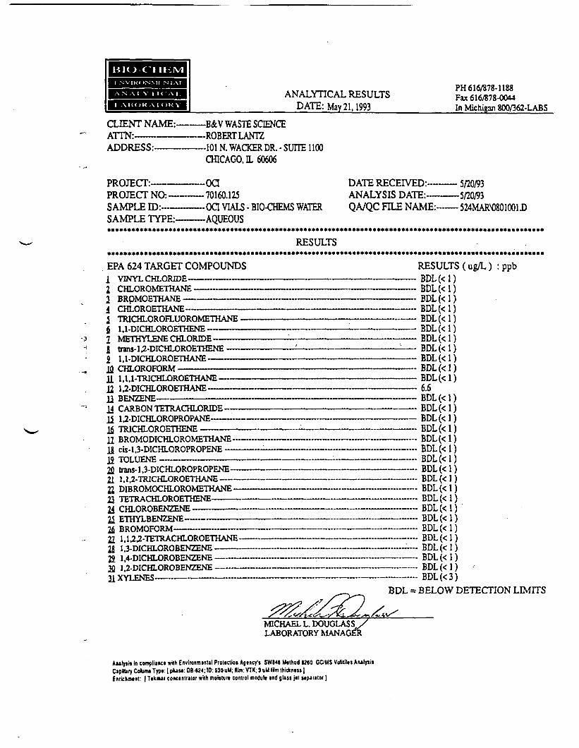
BIO c;i ii1 NVIKf >NMI N lAt.
I .Al tOK A I ( >K V
ANALYTICAL RESULTSDATE: May 21,1993
PH 616/878-1188Fax 616/878-0044In Michigan 800/362-LABS
CLIENT NAME:—-ATTN:———————ADDRESS:-
PROJECT:———PROJECT NO: ~SAMPLE ID:——SAMPLE TYPE:-
-B&V WASTE SCIENCE-ROBERT LANTZ-101 N. WACKER DR. - SUITE 1100
CHICAGO, IL 60606
-OQ-70160.125~OCI VIALS • BIO-CHEMS WATER-AQUEOUS
DATE RECEIVED:—ANALYSIS DATE:—QA/QC FILE NAME:
• 5/20/93•5/20/93•524MARXJ801001D
•«•«»«»****»»»»•***••»**«»*»»•***«»****»**»***»*•«»»«*»*»***»»»•*•»•»»****»«»•»»•*•***««»«••*«»«•««**•*««**RESULTS
»»»**»»«»»»******»»««»»«»•»***»»»»•»»»•»•«»«*»»»**«**»»•••»»»*»»»»»»•»»»»»»»
EPA 624 TARGET COMPOUNDS1 VTNVT PUT PiPTnF . __ ^ ,.„,,.,,
2 CHLOROMETHANE — - -I nnnwnmru AKTTT . . ,. ..... ,,T ....
i CHLOROETHANE —————————————————————— - ————————————— -1 TRICHLOROFLUOROMETHANE ———————————————— : —————— - ——t t 1 TVT/^tJT f\Ty f\ C*f TJCVTC
I fcifCTTTVT TTXTT7 PWT HP TAP
1 trans-U-DICHLOROETHENE —————————— : ——————————————— - ——2 1 1 TVPHT PiPnPTTTAMF , . . , .., ... ... ,.................._.... __ ...T
1Q CHLOROFORM —————————————————————————————————— --11 1 1 - 1 *mir**Tt /*\P^Mr*T*lJAXTC
i^ i A r\T/"»irr r\p rvrro A vrn
14 CARBON TETRACHLORIDE- ———————————————————————————it | *> TMPHT OPr^PPOPAMF . ... . ... ...r. .. ...T ...... . .....irf TPTPTTT nPHPTTTFMF .. .. ,'.L ... .L.... ,_ , , ,.T. j . - rr
11 BROMODICHLOROMETHANE ——————————— - ——————— — - ————— —
1ft TOT TTPMP . _L..T -^ ..T -..rr T ^...-T -L.L - • -j— -- ', -T — . ......................•V\ i .,_ i. 1 1 TMOUT »^T> i*^OO rtPCVTC
11 1 1 1 TPTPHT OPiOPTWAMP . ... ...
22 DIBROMOCHLOROMETHANE ————————— -- —————————— - — — — —
1i< .PUT .T\P.OP.T7>J*7FMF .............. ....._....-.........-......... .......................
*>T 1 1 O O TCTPAPUT OPOPTHAMT? _............._.-.,....-.--..- . M.M^^.n- ............— ....^/ i,itXjjt" i &i^/\wn^vyiw/& A ivu^Cr ¥——....»—..... ............ ..... P ...._..._.— «...—
Ifl 1 A TMPUT P*PP*PPN7T?NI3 . ... .....H..... . ... —.. ... — ..-..-....
Tl YVI FWPS
RESULTS ( ugA- ) : ppbBDL(<1)BDL(<1)BDL(<1)BDL(<1)BDL(<1)BDL(<1)BDL(<1)BDL(<1)BDL(<1)BDL(<1)BDL(<1)6.6BDL(<1)BDL(<1)BDL(<1)BDL(<1)BDL(<1)BDL(<1)BDL(<1)BDL(<1)BDL(<1)BDL(<1)BDL(<1)BDL(<1)BDL(<1)BDL(<1)BDL(<1)BDL(<1)BDL(<1)BDL(<1) •RDI.te'n
BDL = BELOW DETECTION LIMITS
MICHAEL L. DOUGLASSI/LABORATORY MANAGER
Aiulpis in complianci wilh Environmtnla! Proticlraa Agtncfi SW646 Mtthod B260 GDMS Volililtl AulytiiCapilUfy Column TIP*: [ phai*: 08-624; ID: 530 uM; Rim: VTK; 3 uU INm thidmtsi)Enrkhmint: | Ttkmat concinlraior wilh monlura conuol modult and glaii jtl stpatalor ]

APPENDIX I
GEOPHYSICAL INVESTIGATION REPORT

GartnerLee
Professional Services in Environmental Management
11
Geophysical InvestigationOrganic Chemicals Superfund Site
Grandville, MichiganGartnerLee
T Prepared by:
Gartner Lee, Inc.105 Main Street
Niagara Falls, NY, 14303
Prepared for:
B&V Waste Science & Technology Corp.230 West MonroeChicago, IL 60606
Project No. 92-801
April 3,1992
Distribution: Client - 4File - 2
I
• 105 Main StreetNiagara Falls, NY 14303Fax (716) 285-8275
I(716)285-5448
Professional Servicesin EnvironmentalManagement
E
II
Gartner Lee, Inc.
April 2, 1992
Mr. Richard McAvoyB&V Waste Science and Technology Corp.230 West MonroeSuite 2250Chicago, IL 60606
Dear Mr. McAvoy:
Re: Geophysical Investigation. Organic Chemicals SuperfundSite. Grandville. Michigan
1.0 Introduction. Background Information, Purpose and Scope
On March 9th through March 13th, 1992, an electromagnetic (EM) survey wasperformed at the Organic Chemicals Superfund Site in Grandville, Michigan.
The Organic Chemicals, Inc. (OCI) facility is an abandoned chemicalmanufacturing and solvent recovery operation. The OCI facility operatedfrom 1969 to 1991 at this location. The OCI site property was previouslyutilized as a bulk petroleum terminal and crude oil refinery. The area to thenorth and northwest of the OCI facility was mined for sand and gravel. Aftermining operations were completed, the area was backfilled with constructionand demolition debris, foundry sand, and other solid wastes. Areas ofconcrete, metal and re-enforcement bar were noted at surface in thesepreviously mined areas during data collection. A sewer line was also notednorth of the OCI facility. The sewer line appeared to trend east-west asdefined by manholes located approximately 500 feet apart. The sewer lineappeared to mark the southern boundary of landfilling in the areas northwestof the OCI facility.
The geology of the site, as defined by test borings and monitor wells locatedin and around the site, is as follows:
• Near surface sand and gravel layer with lesser amounts of silty sands,clayey sands clayey silts and silts. This unit is believed to becontinuous across the site with varying thicknesses of 4 to 41 feet;

I
i
E
ii
Page3B&V Waste Science and Technology Corp.April 2, 1992
snow covered construction and demolition debris fill, an east-west trending buriedsewer line, fences, buildings and other anthropogenic features, data were only collectedin profile format at this site.
A base line was established that trended approximately S3°W with a Sokkia AutomaticLevel, stadia rod and tape measure. The base line was referenced to existing structuresand the eastern edge of pavement of Sanford Avenue. The base line was designatedLine 1 and each additional profile line was referenced to it. Profile Line 1 through Line6 were staked at 50 foot intervals with alternating colors of red and yellow wire surveyflags (Figure 1).
Survey Line 7 was established at the request of B&V personnel (Figure 1). It wasrequested that data be collected along the eastern property boundary of the adjacent,abandoned Hagar-Busch Facility. Line 7 was established and staked using the EM34-3XL's 20 meter reference cable as a chain. Line 7 was staked at 65.6 foot (20 meter)intervals with red wire survey flags. Line 7 was subsequently tied into the existingreference grid. Individual stations were referenced to the eastern property boundary ofthe Hagar-Busch facility.
Each data point collected on-site was referenced to the survey grid in units of feet. Thecoordinates of each station were translated into true northings and eastings utilizing thesoftware package GEOSOFT. The coordinates were then re-translated by rotating thegrid 30° at station location 0 North, 0 East. The grid translation was performed so thatthe grid could be scaled and matched to an aerial photograph provided by B&V (Figure1). It should be noted that as a result of the coordinate grid translation, the stationvalues labelled on the flags at the site no longer match the grid coordinates of Figure 1.
Upon completion of the geophysical survey, relative elevation data were recorded at100 foot horizontal increments. The relative elevation data were referenced to the topof the sewer manhole located approximately 275 feet south along Line 1.
Relative elevation data is important when interpreting stratigraphy with EM equipmentas changes in elevation may result in changes in observed apparent soil conductivities.Relative elevation data were collected along survey lines that were free of surface ornear surface buried metals. Relative elevation data were not recorded along profileLine 3 and the northern most 275 feet of profile Line 1 due to problems associated withthe presence of fill and near surface metals.

Iffl
1
Ir
ii
Page 4B&V Waste Science and Technology Corp.April 2,1992
2.2 EM34-3XL Survey
A Geonics EM34-3XL Frequency Domain Terrain Conductivity meter was used tocollect apparent conductivity data along the seven profile lines (designated Line 1through Line 7, Figure 1). Data were collected at 25 foot station increments alongprofile Lines 1 through 6, and at 65.6 foot (20 m) increments along Line 7.
The EM34-3XL device is equipped with a transmitter coil and a receiver coil that canbe separated by 10, 20 or 40 meter intercoil spacings. The instruments depth ofinvestigation is dependant upon coil separation and dipole orientation. Data arecollected with the receiver and transmitter coils' dipoles oriented either both verticallyor horizontally.
The EM34-3XL was used to measure the quadrature component of the electromagneticfield at each station. The quadrature component data are a measurement of theapparent ground conductivity in units of milliSiemens per meter (mS/m). Thequadrature component data are representative of changes in the electrical conductivityof pore fluids, the presence of buried metals and fills, soil types, changes in bedrocklithology, and the presence of saturated bedrock fractures and faults.
Data were collected at 10 and 20 meter intercoil spacings and in the horizontal andvertical dipole mode at the OCI site. The approximate depth of investigation for theEM34-3XL is 0.75 times the intercoil spacing when the dipoles are oriented horizontallyand 1.50 times the intercoil spacing when the dipoles are oriented vertically. The depthof investigation for the various dipole orientations and intercoil spacings for datacollected at the OCI site are as follows:
• 10 meter intercoil spacing, horizontal dipole mode: surface to 7.5 meters.
• 10 meter intercoil spacing, vertical dipole mode: near surface to 15 meters.
• 20 meter intercoil spacing, horizontal dipole mode: surface to 15 meters.
• 20 meter intercoil spacing, vertical dipole mode: near surface to 30 meters.
A base station was established on-site that was believed to be free of fill, surface metalor other sources of potential signal interference. The EM34-3XL was calibrated at thebase station twice daily following procedures specified in the operations manual.Readings were periodically taken at previously surveyed stations to check forinstrument drift and malfunction. Readings were automatically stored in a solid state

IPageSB&V Waste Science and Technology Corp.April 2, 1992
data logger and recorded by hand during the survey. The data logger was interfaceddaily to a portable laptop computer and the data were transferred to a floppy disk for
^ subsequent processing and interpretation.
• 2.3 EM31-DL Survey
It was noted during the site reconnaissance that areas of fill were present across the™ site. To better identify these areas of fill and to gain information on the apparent
conductivities of the near surface soils, Gartner Lee mobilized a Geonics EM31-DL.^ Frequency Domain Terrain Conductivity meter to the site. The EM31-DL, which has a
depth of exploration of approximately 12 to 15 feet, was used to supplement the datacollected from the deeper investigating EM34-3XL survey.
A total of 1,995 data points were collected along survey lines 1 through 7 with theEM31-DL and solid state data logger. Quadrature and in-phase data weresimultaneously collected at virtually continuous intervals (approximately every 2 to 3feet) along the survey lines. The quadrature component data, as mentioned above, area measurement of the apparent ground conductivity. Quadrature component data were
R collected in units of mS/m. The EM31-DL also records the in-phase component of theelectromagnetic field measured in units of parts per thousand (ppt). The in-phase
-, component data are susceptible to the presence of electrically conductive materialsp such as metals. All readings with the EM31-DL were taken with the instrument\^ oriented parallel to the direction of travel, in the vertical dipole mode and with the
instrument at waist height.
The EM31-DL was calibrated daily at an established base station following proceduresspecified in the operations manual. Readings were automatically stored in a solid statedata logger during the survey. The data logger was interfaced to a portable computerand the data were transferred to a floppy disk for subsequent processing andinterpretation.
II
2.4 Data Reduction
Both EM34-3XL and EM31-DL data were edited and analyzed utilizing the Geonicssoftware packages DAT34-3/DAT31Q respectively. Additional survey line editing wasthen performed using the software LOTUS 123 and GEOSOFT. Line and stationlocations were then transformed, scaled and plotted as Figure 1 using the softwarepackage GEOSOFT. GEOSOFT was also used to grid, low pass filter and colorcontour the EM34-3XL 20 meter horizontal dipole data as presented in Figure 2. Datawere interpretated and presented as profile plots utilizing the software packageGRAPHER. The EM34-3XL, EM31-DL and the relative elevation data are presented

IPage 6B&V Waste Science and Technology Corp.April 2,1992
as Figures 3 through 16. Observed anomalies are annotated on each figure and a briefdiscussion of our interpretations are presented in Section 3.1.
3.0 Results
ft The purpose of the geophysical investigation was to define areas where the clay layerthins or is absent beneath the site. The near surface sand and gravel soils and the
m limestone bedrock typically produce low apparent conductivity responses with EMequipment. Saturated clays tend to produce relatively high apparent conductivity
"—• responses with EM equipment. Due to this apparent conductivity contrast, areas wherethe clay layer thins or is discontinuous should produce a relatively low apparentconductivity (high apparent resistivity) response. Unfortunately, the presence of fillmaterial, buried metals and/or ground water contamination can make identifying astratigraphic unit such as a clay layer difficult with EM equipment.
3.1 EM34-3XL and EM31-DL Survey Results
The EM34-3XL and EM31-DL surveys revealed five apparent conductivity lows thatf may be associated with a thinning of the clay layer. These observed apparent low* conductivity anomalies were observed along Lines 1,2,4,6 and 7. Due to the fill
material present along the northern portion of Lines 1 and 5, the eastern extent of LineI 4 and the entire length of Line 3, a determination as to the presence or absence of a^^ clay layer could not accurately be made.
The following is a discussion of the observed anomalies noted along each profile line.Observed anomalies are annotated with capital letters for horizontal dipole anomaliesand small case letters for vertical anomalies.
Color Contours of the 20 Meter EM34-3XL Horizontal Site Data f Figure2^
Figure 2 is a color contour representation of the EM34-3XL 20 meter horizontal datafor the site. Shades of green and green-yellow appear to represent backgroundconditions. Shades of dark greens and blue-greens are believed to be representative ofthe thinning clay layer and/or thickening sand lenses. Shades of reds and purples arerepresentative of fill material, buried metallic debris and conductive or contaminatedsoils.I
I An acetate overlay of a site aerial photograph is provided in the back pocket of thereport. This overlay was created to use with Figure 2 to gain a better understanding ofthe anomalies locations relative to monitoring wells and other known structures.

IH
E
II
Page?B&V Waste Science and Technology Corp.April 2,1992
Line 1 (Figure 2. Figures 3 and 4^
Line 1 was located on the west side of the site and trended approximately north-south(Figure 1). Data were collected in a south to north direction. An east-west trendingsewer line was located at line position 175 South. Fill and surface metal was observedalong the northern-most portions of this survey line. The following anomalies wereobserved:
(A,a) Anomaly "A,a" was observed to be a broad smooth apparent conductivity low.^ This anomaly is shown in shades of blue-green in Figure 2. This anomaly was observed
in the EM31-DL data, EM34-3XL horizontal data and to a lesser extent in the EM34-3XL vertical data (Figures 3 and 4). Test boring B-27A, SB-6 and monitor MW-8 werein the vicinity of this anomaly. These drilling logs show the presence of a clay layer at adepth of 12 to 17.5 feet, 12.5 to 16.5 feet and 13 to 18 feet, respectively. The nearsurface layer is described in the log of MW-8 as a silty gravel. It was observed that atwo foot thick sand lens was observed at 7 to 9 feet below grade at MW-8. Bedrock wasconfirmed in boring SB-6 at a depth of 16.5 feet. This anomaly may represent athinning of the clay layer, an increase in the thickness of the sand lens, or both.
' (B,b) Anomaly "B,b" was observed as an extremely "noisy" signal response as a result ofthe presence of fill and buried metals. Anomaly "B" is shown in shades of yellow and
I red (Figure 2). This response was noted between station locations 0 North and -200^ North. It appeared that the presence of an east-west trending sewer marked the
southern boundary of the filled area at this location.
Line 2 (Figure 2. Figures 5 and 6)
Line 2 was an east-west trending survey line located in the western area of the site(Figure 1). Line 2 appeared to be free of surface metal or fill. Buried utilities andabove ground power lines that parallel Sanford Avenue were noted near the westernextent of the survey line. These services appeared to only cause signal interference onthe 20 meter vertical data at the two western most stations. The following anomalieswere observed:
(C) Apparent conductivity values appeared to decrease as the survey line trended west.Anomaly "C" is shown in shades of green and blue-greens (Figure 2). Monitor MW-12was noted in the vicinity of this survey line. Clay was noted at 18.0 to 18.5 feet belowsurface. The boring terminated at 18.5 feet below surface. A sand lense was noted at9.0 to 15.5 feet below surface and a gravel layer was noted at 15.5 to 18 feet belowsurface. Anomaly "C" may be due to the presence of a thinning clay layer or athickening sand and gravel lens or both.
I a
I
EI
1I
PageSB&V Waste Science and Technology Corp.April 2,1992
(c) Anomaly "c" was noted in the 20 meter intercoil spacing vertical dipole data.Overhead power lines and a buried water line were noted along Sanford Avenue.Anomaly "c" was observed as a conductivity high, possibly due to the presence of over-head power lines and buried utilities noted along Sanford Avenue.
Line 3 (Figure 2. Figures 7 and 8)
Line 3 was an east-west trending survey line that was located in an area that waspreviously mined and backfilled (Figure 1). The near surface material appeared tocontain concrete, re-enforcement bar and other debris. Extreme signal interference(signal noise) was observed with the EM equipment at this location. Relative elevationdata were not collected along this line due to the observed signal interference. Thesignal interference was probably due to areas of buried metallic objects or other highlyconductive material within the fill at this location.
(D,d) Anomaly "D,d" was observed as a conductivity high in the horizontal dipoleorientation and as a negative response in the vertical dipole orientation. Anomaly "D"is shown is shades of purple on Figure 2. This anomaly was located along the westernextent of Line 3. Monitors MW-14 and SB-10 were located west and east of thisanomaly respectively. This anomaly is probably due to the presence of surface andburied metallic objects and/or contaminated, highly conductive soils.
(E,e) Anomaly "E,e" was observed as a conductivity high in the horizontal dipoleorientation and as a negative response in the vertical dipole orientation. Anomaly "E"is shown in shades of purple on Figure 2. A truck frame was noted approximated 50feet north of this anomaly and may have contributed to the observed values. Anomaly"E,e" is probably due to the presence of surface metals and large buried metallicobjects, and/or highly conductive contaminated fill material.
(F,f) Anomaly "F,f' was observed as a conductivity high in the horizontal dipoleorientation and as a negative response in the vertical dipole orientation. Anomaly "F" isshown in shades of reds and yellows on Figure 2. This anomaly was observed west ofmonitors SB-8/MW-10. Steel re-enforcement bar was observed at surface near thisanomaly. This anomaly is probably due to surface and buried metallic objects and/orhighly conductive contaminated fill material.

KH
i
ip
iK
Page 9B&V Waste Science and Technology Corp.April 2,1992
Line 4 (Figure 2. Figures 9 and 10)
Line 4 was an east-west trending survey line that was located north of the Hagar-Buschand OCI facilities (Figure 1). It appeared that sand and gravel mining activity may haveoccurred near the center of the survey line. The eastern areas of the survey linecontained hummocky areas and some surface debris was noted. These areas may havereceived fill material.
(G,g) Anomaly "G,g" was observed as a broad conductivity low in the horizontal andvertical dipole data. Anomaly "G" is shown in shades of blue-green on Figure 2. Thisanomaly may be due to the presence of a thinning clay layer or a thickening sand lense.
(H,h) Anomaly "H,h" was observed as a "noisy" conductivity high in the horizontaldipole data and the EM31-DL data. A strong negative response was noted in thevertical dipole data and the EM31-DL data at the eastern extent of the survey line.Anomaly "H" is shown in shades of green-yellows on Figure 2. Monitors MW-5 andMW-6 were noted in the vicinity of these anomalies. Fill was noted at boring MW-6and stained soils with strong hydrocarbon odors were noted on both boring logs. Somesurface debris and surface metals were noted in the vicinity of MW-6. These anomaliesare probably representative of fill material, contaminated soils and ground water,and/or surface and buried metallic objects.
Line 5 (Figure 2. Figures 11 and 12)
Line 5 was a north-south trending survey line located north of the OCI facility (Figure1). A three to four foot rise was noted near the northern extent of the survey line. Aneast west trending sewer line was crossed near station 875 South. It appeared that thenorthern extent of this line may have received fill material.
(I,i) Anomaly "I,i", was observed as "noisy" apparent conductivity highs in thehorizontal and vertical dipole data. Anomaly "I" is shown as shades of yellow andgreen-yellow on Figure 1. The signal interference at this anomaly location probablyrepresents the presence of fill, contaminated soils and/or buried metallic debris.
Line 6 (Figure 2. Figures 13 and 14)
Line 6 was located along an access road in the central area of the site (Figure 1). Line6 trends approximately north-south.

IPage 10B& V Waste Science and Technology Corp.April 2,1992
(J) A conductivity low was observed in the 20 meter horizontal data at this location.This anomaly is represented as shades of green on Figure 2. The drilling logs forMonitors MW-9 and SB-7 indicate that the near surface soils are gravel with some silt.The clay is present at 13.5 to 16.5 and 11.5 to 15.5 feet below surface respectively.Bedrock was confirmed in boring SB-7 at 15.5 feet below surface. A sand lens was notobserved in either boring log. The 10 meter horizontal data and the EM31-DL datawere "noisy" at this location. The "noisy" response suggests that near surface fill may bepresent. This anomaly may be due to the thinning of the clay layer at this location.
^ (j) A "noisy" vertical dipole signal response was observed at this line location. This"noisy" response is probably due to the presence of near surface fill.
Line 7 (Figure 2. Figures 15 and 16)
Line 7 was located along the eastern property boundary within the abandoned Hagar-Busch facility (Figure 1). Fill materials were noted at the northern extent of the surveyline.
K (K,k) Anomaly "K,k" was observed as an apparent conductivity low at the southern endof Line 7 (Figure 1). The anomaly is represented as shades of blue-greens on Figure 2.
P A "noisy" signal response was observed with the EM31-DL at this location whichsuggests the presence of near surface fill. Monitors MW-3 and MW-19 were noted in
\^ the vicinity of the observed anomaly. The drilling log for MW-19 revealed a silty graveldeposit near surface with a sand layer from 10.0 to 17.5 feet below surface. Two siltyclay layers were observed from 21.0 to 23.5 and from 27 to 44 feet below surface. Thedrilling log for MW-3 revealed a near surface silty gravel deposit with a sand lenspresent from 8.0 to 16.5 feet below surface. A silty clay unit was observed from 18.5 to22.0 feet below surface. Anomaly "K,k" may represent an increase in the thickness ofthe sand layer and/or a thinning/deepening of the clay layer.
(L,l) Anomaly "L,l" was observed as an apparent conductivity low at the northernextent of Line 7 (Figure 1). This anomaly is represented as shades of blue-green onFigure 2. An increase in surface elevation was noted at the northern end of the surveyline as a result of the presence of fill. A "noisy" signal response was observed in the
B EM31 and the EM34-3XL vertical dipole data. This anomaly is probably due to the* presence of fill material.
IPage 11B&V Waste Science and Technology Corp.April 2,1992
4.0 Conclusions and Recommendations•
Five anomalies were identified during this investigation that may be related to a• thinning clay layer or the presence of thickening sand lenses. These anomalies are A,i C, G, J and K (Figure 2). As the data were collected profile format, it was difficult to
determine if the anomalies were due to sand lenses or thinning clay layers. It was also• difficult to determine the trend of these anomalies and the extent to which they are
laterally continuous.
Fill materials, buried metals and/or possible contaminated soils/ground waters wereobserved at anomaly locations B, D, E, F, H, I and L (Figure 2). Line 3 and thenorthern extents of Lines 1 and 5 are believed to be located over fill materials (Figure1). Line 3 appeared to contain areas of large, buried metallic objects and/or veryconductive soils. Areas of fill with buried metals appeared to be laterally extensivealong the northern areas of the site.
Signal interference was observed along the northern extent of Lines 1 and 7 due to the| presence of surface metals and fill materials.
_ The following recommendations are provided for your consideration:Ix^ l). Anomalies A, C, G, and J may represent areas of thinning clay layers or
thickening sand lenses. These anomalous areas should be drilled or test pittedto confirm the EM responses.
2). The site should be cleared of dense vegetation and resurveyed with the EMequipment at regular line and station spacings. A color contour map of the EMresults could then be produced in plan view which would allow for a betterunderstanding of the lateral continuity of the clay layer and the sand lenses.
II
3). An EM31-DL survey should be performed over the northern areas of the site todefine the lateral extent of contaminated soils related to landfill ing operations.The EM31-DL survey would also allow for the identification of areas of buriedmetals possibly representative of drums or other waste.
4). From a health and safety perspective, any future monitors or test boringsplanned in or around areas of the site thought to have received fill should bescreened for buried metallic hazards with an EM31-DL.

IPage 12B&V Waste Science and Technology Corp.April 2, 1992
5). Consideration should be given to performing down-hole induction and naturalgamma logging with a Geonics EM39 to gain information concerning the actualconductivities of the stratigraphic layers. This survey would allow the site to bemodelled such that stratigraphic target layer depths could be estimated. Adown-hole induction survey in existing PVC monitors may also provideimportant information on screen locations relative to conductive contaminatedground water.
At this time we would like to thank B&V for involving us in this most interesting study.If there are any questions or comments please feel free to contact our office.
Respectfully submitted,
GARTNER LEE, INC.
EI
Thomas E. Jordan, M.S. David D. Slaine, M.S., C.G.W.P.Hydrogeologist/Geophysicist Principal
Hydrogeologist/Geophysicist
TEJ/DDS:pmk

IHE
fP
II
FIGURES

1000 W 750 W 500 W 250 W 750 I
500 S- —
1000 S
1500 S
500 8
1000 S
'- - 1500 S
1000 W 750 W 500 TT 250 V
Scale 1:3600
<«•*>
FIGURE 1
TM
GEOPHYSICAL SURVEY RESULTSORGANIC CHEMICALS. INC. GRANDVILLE. MI
T ~ ~ "jup SHOWING BH31 AND BM34-3ILI SUSVBY UN1 LOCATIONS
UABCH 1B92 PROJBCT 482801GARTNER LEE. INC. NIAGARA FALLS. NY
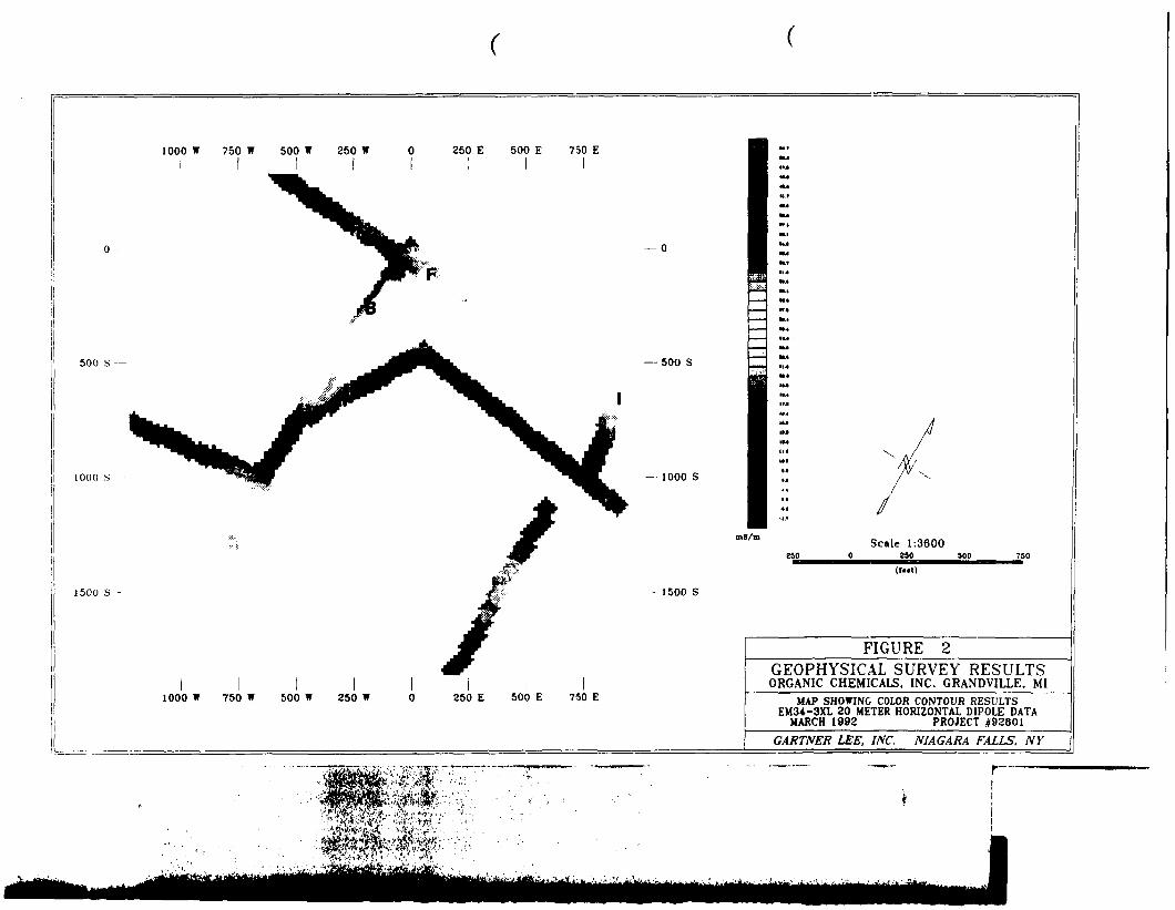
1000 W 750 W 500 W 250 W 0 250 E 500 E 750 E
0 --
500 S —
100(1 hi
1500 S -
250 E 500 E 750 E1000 W 750 W 500 W 250 W
— 500 S
1000 S
- 1500 S
mS/m Scale 1:36000_______250_______100
FIGURE 2GEOPHYSICAL SURVEY RESULTSORGANIC CHEMICALS. INC. GRANDVILLE. MI
MAP SHOWING COLOR CONTOUR RESULTSEM34-3XL 20 METER HORIZONTAL DIPOLE DATA
MARCH 1992 PROJECT 192801GARTNER LEE, INC. NIAGARA FALLS, NY
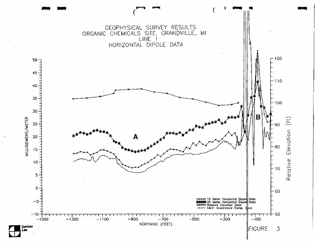
50-
40-
35 -_
30-ceLJ
fc 25 H
en20-
LJtoH 15 H
10-
5~
°~
-5-
— 1 0— i i i i i i i
rGEOPHYSICAL SURVEY RESULTS
ORGANIC CHEMICALS SITE, GRANDVILLE, MlLINE 1
HORIZONTAL DIPOLE DATA
10 Meter Horizontal Dipolt120 Meter Horizontal Dipoli
*«*** Relative Elevation Data—:—— EM31 Quadrature Comp.
-1500 -1300i i r | i i \
-11001 ' I 1 ' I
GartnerLee
-900 -700NORTHING (FEET)
i i i i I-500 -300
DataData
]ta
-120
-110
-100
i I i i i-100
Co
'-4-'
O
LJ
CD>
'-+--_D0)
-60
50
FIGURE 3

GEOPHYSICAL SURVEY RESULTSORGANIC CHEMICALS SITE, GRANDVILLE,
LINE 1VERTICAL DIPOLE DATA
U)UJ
IT)
75-1
65 H
55 H
45 H
35 H
25 H
-5H
-15H
-25H
-35-1500
Gartner
10 Meter Vertical Dipole Data20 Meter Vertical Dipole DataRelative Elevation Data
I I I I I-1300
I I l I l l l I I I I I I I I-1100 -900 -700
NORTHING (FEET)-500
i i I i-300
1 I '-100
-120
-110
MOO
-80
-70
^60
-50
FIGURE 4
co
jDLJ
(U>
-t->_O(U

GEOPHYSICAL SURVEY RESULTSORGANIC CHEMICALS SITE, GRANDVILLE, Ml
LINE 2HORIZONTAL DIPOLE DATA
50-
45 -_
40^
35 -.
30-
LJtZJ 25-
yV)
20-
15H
10-
5-
0-
-5-
-1300
10 Meter Horizontal Oipole DataMeter Horizontal Dipole Data
Relative Elevation DataEM31 Quadrature Comp. Data
-10- i i i i l i i l i i i I i r-1100 -900 700 -500
EASTING (FEET)-300
i I i i r-100
1 I '100
r-120
-110
-100
-90
-80
-70
-60
CO
'-4-1
D
LJ
0)
0)o:
50
jGartner FIGURE

GEOPHYSICAL SURVEY RESULTSORGANIC CHEMICALS SITE, GRANDVILLE, Ml
LINE 2VERTICAL DIPOLE DATA
so
40-
35 ~
30-o:UJtu 25-•2
2 20-UJ
| 15H2
10-
-5-
-10--1300
Gartner
1 I ' '-1100
10 Meter Verticol Dipole Ooto20 Meter Vertical Dipole DataRelative Elevation Data
i-120
-110
-100
-90
-80
-70
-60
-900I I I I I I I | Y\
-700 -500EASTING (FEET)
I ' '-300
i I i i-100
co
'-(-'o
LJ
^0)
50100
FIGURE 6
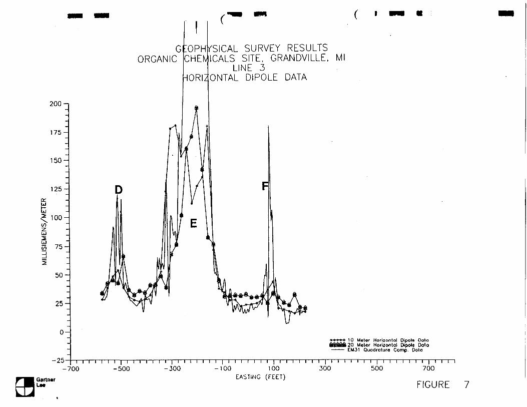
200-1
175-
150-
125-o:LJt
100-
UJ(75 75 H
50-
25-
0-
-25
Ga rtner
G!:OPHORGANIC
— i i i i — r— | — | i-700 -500
HEN/
HORI
I
fSICAL SURVEY RESULTSICALS SITE, GRANDVILLE,
LINE 3ONTAL DIPOLE DATA
10 Meter Horizontal Dipole Data20 Meter Horizontal Dipole DotaEM31 Quadrature Comp. Dota
| i i i i i i i — |— i — T-I — i — i — r— i — r— i — n — r— i — r~i — \~~\ ~ i — i — i — i — i — i — | — i — i — i — i i i — r~| — r~i — n300 -100 100 300 500 700
EASTING (FEET)FIGURE 7

]
GEOPHYSICAL SURVEY RESULTSORGANIC CHEMICALS SITE, GRANDVILLE,
LINE 3VERTICAL DIPOLE DATA
175-
125-
75-
25-Ul
fc
£ -25H
UJ
D -75-j
-125-
-175-
-225-
-275
10 Meter Verticol Dipole Data(3638020 Meter Vertical Oipole Data
Relative Elevation Data
I I I I I I I •[ I I I I I I I | I I I I-700 -500 -300
HGartnerLee
I i | i I I I I I I | I I I I I I I | I I I I I I I | I- 1 00 1 00 300 500
EASTING (FEET)
I I I I i I | i i i i700
FIGURE 8

UJ
50q
45-
40-
35-
30
25-
20-
10-
-5-
-10
I GartnerLe«
I
GEOPHYSICAL SURVEYORGANIC CHEMICALS SITE, GR,
LINE 4HORIZONTAL DIPOLE
^*-———*———*-
RESULTSNDVILLE,
)ATA
T 1 I I
200I I I | I I I I I I I | I
400 600 800EASTING (FEET)
10 Meter Horizontal Dipole Data20 Meter Horizontal Dipole DataRelative Elevation DataEM31 Quadrature Comp. Data
1 I '1000
1 I '1200
r-120
-110
-100
-90
-80
-70
-60
cO
H-1
O
(D
(Da:
•soi i I i i1400
FIGURE 9
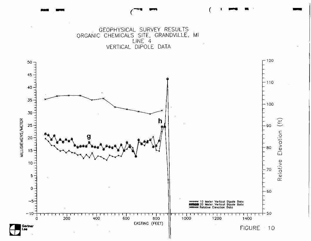
GEOPHYSICAL SURVEY RESULTSORGANIC CHEMICALS SITE, GRANDVILLE, Ml
LINE 4VERTICAL DIPOLE DATA
so-n
45 ~.
40^
35 •:30 •:
25-
CO
5 20 HUJto
15-
10-
-5-
-10-
I GartiwrL*e
1 I ' '200 400 600 800
EASTING (FEET)
10 Meter Verticol Dipole Data20 Meter Vertical Dipole DataRelative Elevation Data
I I I I I I I I1000 1200
i I i i1400
-120
-110
-100
-90coo
K80 g
-70
-60
(D
0)
50
FIGURE 10

GEOPHYSICAL SURVEY RESULTSORGANIC CHEMICALS SITE, GRANDVILLE,
LINE 5HORIZONTAL DIPOLE DATA
so
40
35
30o:
tu
ui 20
15-
10-
-5-
-10-1100
Qartner
10 Meter Horizontal Oipole Data20 Meter Horizontal Dipole DataRelative Elevation DataEM31 Quadrature Comp. Data
r-1?o
h-110
h-100
h90
-900-i-n-| r
-700i I i i i i i i i I i i i i i-500 -300
NORTHING (FEET)
1 I '-100
i i i I i i i i i100
I I I I300
co
'-i—•o>jyLJ
<D>
-*->_O
<Dct:
heo
•50
FIGURE 1 1

GEOPHYSICAL SURVEY RESULTSORGANIC CHEMICALS SITE, GRANDVILLE,
LINE 5VERTICAL DIPOLE DATA
50-
45^
40^
35 -.
30-o:Ld
ti 25 H
20 H.UJ
15~
-5-
-10
10 Meter Vertical Dipole Data20 Meter Vertical Dipole DataRelative Elevation Doto
I I I I I I I I I -1 I I I I I I I I I I I I I I I I I I I I I I I I I I I I I I I-1100 -900 -700 -500 -300 -100
NORTHING (FEET)| Gartner
' ' ' I ' ' '100
1 I l
300
r- 120
h-110
Moo
h-80
h?0
heo
•50
Co
'->->o
(D>
'-*-'_D0)
EIGURE 12
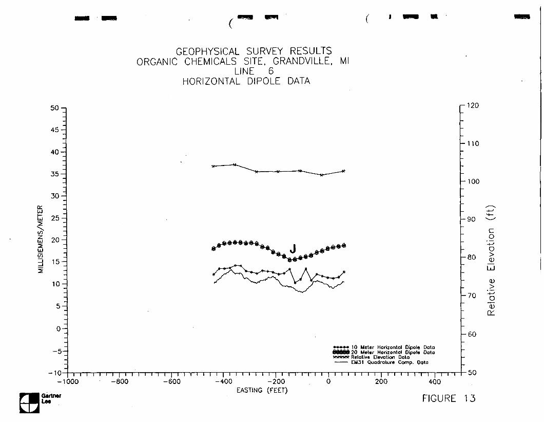
GEOPHYSICAL SURVEY RESULTSORGANIC CHEMICALS SITE, GRANDVILLE, Ml
LINE 6HORIZONTAL DIPOLE DATA
ceUJ
t
MIL
LISI
EMEN
S/I
so q
45 -j
-40^
35-
30 •:
25 -_
20-
15~
10^
5^
°":
-10--1
**~ ^^^^ .. M u.— -*—
^3^*rx V^-^Y^ jy^^
***** 10 Meter Horizontal Dipole DataCOOlOOZO Meter Horizontal Dipole Data***** Relative Elevation Data——— EM31 Quadrature Comp. Data
- I2U
-110
-100
M—-90 "— '
CO
O-80 >
UJ
>-70 '-^
13cr
-60
eni i i i i i i | l l i i i i i | i i l i i l i | i i l l 1 1 l | i l i i l l l | i l l l i i i | i i i l i l i | l i i -^000 -800 -600 -400 -200 0 200 400
EASTING (FEET)1ST" FIGURE 13
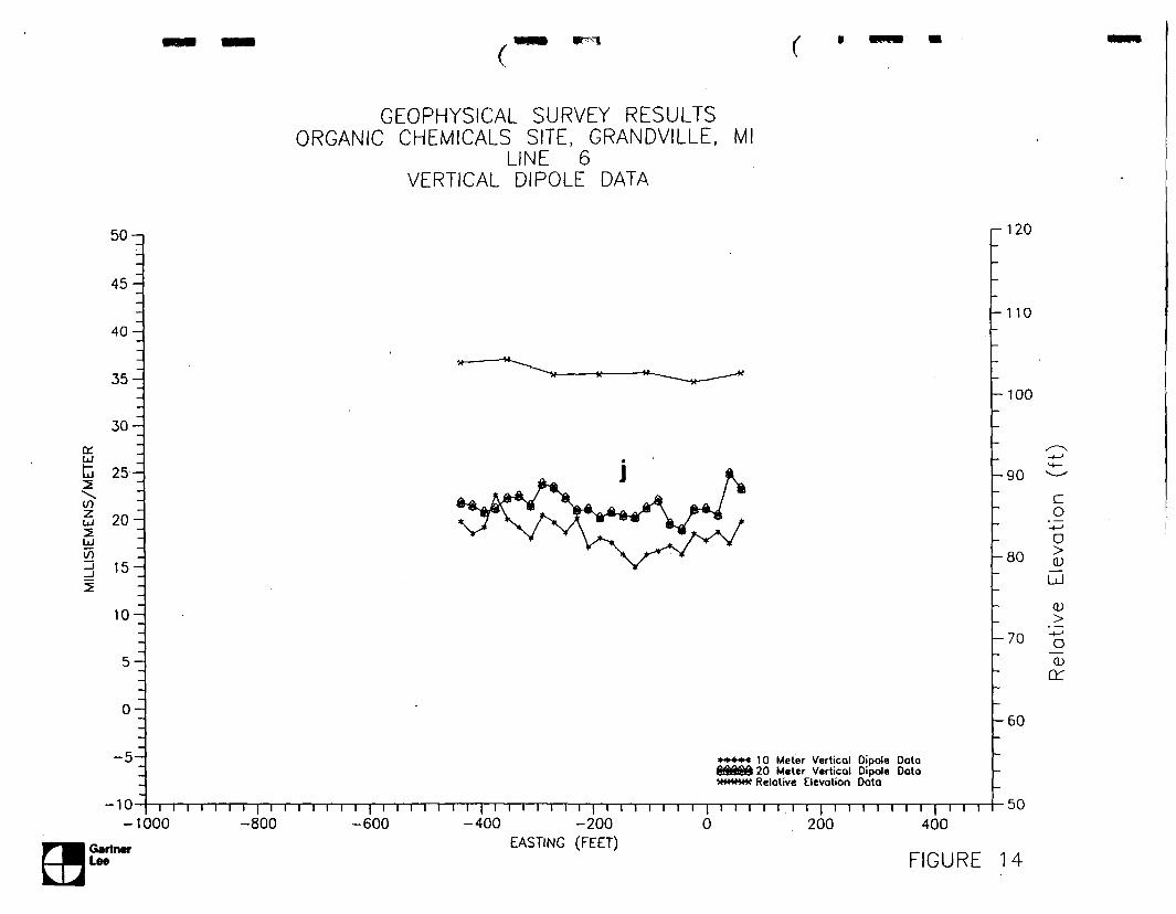
GEOPHYSICAL SURVEY RESULTSORGANIC CHEMICALS SITE, GRANDVILLE, Ml
LINE 6VERTICAL DIPOLE DATA
C£LJsX,zUJ2LJ(f>
32
so q
45 •::
40-
35--
30 •:-25T
_-
20-
1 *S —
10-
5 —
0^
-s-E-10-
-1
** ~~~^~^~~u »w ""~~-~-«— • "~~
1
«. Rf t -A/na a /^iffllS ' iB -gY A . fSf "\ ft-A^j<
\ 7 **v Ax. X '•'*•» V*/ ^^ /v* N/ v Y^, ^vsA/
\i t^^4;»
***** 10 Meter Vertical Dipole Data£$ag&20 Meter Vertical Dipole Data**ww« Relative Elevation Data
- i/u
- 110
-100
s~*._ -* — '
M—
-90 ^^Co"o
-80 ^UJ
QJ
-70 '•§"oo:
-60
-
crvi i I i i I i | I i i i i I i | I I i i i i i | i i i i i i I | i i I i i I i | i i i I i I I | I I I I i i i | i i I *->v000 -800 -600 -400 -200 0 200 400
IGartnar EA 'NG (FEET) _ . _ . . _ _Lee hIGUKL 14

GEOPHYSICAL SURVEY RESULTSORGANIC CHEMICALS SITE, GRANDVILLE, Ml
LINE 7HORIZONTAL DIPOLE DATA
50
45
40-
35 -.
30-o:LJt 25
CO
5 20UJCO
10 Meter Horizontal Dipole Data20 Meter Horizontal Dipole DataRelative Elevation DataEM31 Quadrature Component Data
-110
-100
-90
-80
-70
-60
coo
0)>
0)
EH-10- i i i i i i i | i i i i i i i | i i i ri i i | i i i i i i i | i i i i i i i | i i i i i i i | i i i i i i i | i i i ~ 50
-2000 -1800 -1600 -1400 -1200 -1000 -800 -600NORTHING (FEET)
FIGURE 15Qartner

GEOPHYSICAL SURVEY RESULTSORGANIC CHEMICALS SITE, GRANDVILLE, Ml
LINE 7VERTICAL DIPOLE DATA
so q
45 -_
40^
35 ~
30-
D 25 H2
£i 20-•5.LJ
1 15
2
10-
5-
-5-
-10--2000
Gartner
10 Meter Vertical Dipole Data120 Meter Vertical Dipole Data
******** Relative Elevation Data
i i |^ \\ i i i i I T i i i i i i j i i i i i i i i in i I-1800 -1600 -1400 -1200
NORTHING (FEET)
i r i i i i i I i i i i i i i r
-120
-110
-100
-90
h80
-70
-60
co
LJ
0)a:
•50-1000 -800 -600
FIGURE 16

APPENDIX J
HYDRAULIC CONDUCTIVITY TEST DATA ANDCALCULATIONS

Method of Analysis
Hvorslev equation for unconfined conditions:
2LT0
Hvorslev equation for confined conditions:
2LTa
where: L = length of screen (ft.)R = radius of borehole (ft.)T0 = Basic time lag (min) measured off plot of head vs. timeH = water level at some time t (ft.)H0 = water level at start of test (ft.)r = radius of well (ft.)K = hydraulic conductivity (ft/day)
T0 is determined by plotting H/H0 versus t on semilogarithmic paper. Using standardenglish units in the Hvorslev equation gives the hydraulic conductivity in ft/day. Tochange this value to cm/sec, 3.53xlO"4 is the multiplier.

Hydraulic Conductivity Determined From Slug TestOraanic Chemicals Inc.
WeM.*:MW-llTest Date: February 1994
Run# Radius ofWell
(inches)r
Length ofScreen(inches)
L1 1 1 5 42 | 13 1 1
Radius of i Basic TimeBorehole Lag(inches) (min.)
R T4 : 0.031
54 | 454
0.054 0.033
Hydraulic Hydraulic jConductivity Conductivity]
(ft/day) j (cm/sec)K 1 K i
93 | 3.28E-02 i57.687.3
2.03E-02 i3.08E-02 i
Geometric Mean = 77.6 2.74E-02 i
R u n t f lElapsed Time
0.01330.01660.02000.02330.02660.03000.03330.05000.06660.0833
Run #2Elapsed Time
0.00000.00330.00660.00990.01330.01660.02000.02330.02660.03000.03330.05000.06660.0833
Run #3Elapsed Time
0.01330.01660.02000.02330.02660.03000.03330.05000.06660.08330.1000
Value
0.000.050.130.200.320.14
-0.020.04
-0.01-0.01
Value
0.000.000.02
-0.05-0.18-0.180.01
-0.04-0.10-0.14-0.13-0.05-0.010.00
Value
0.000.030.110.110.110.130.190.040.04
-0.01-0.01
Time
0.01330.01660.02000.02330.02660.03000.03330.05000.06660.0833
Time
0.02000.02330.02660.03000.03330.05000.06660.0833
Time
0.02660.03000.03330.05000.06660.08330.1000
WHO
0.000.160.410.631.000.440.060.130.030.03
BHO
0.070.290.711.000.930.360.070.00
H/HO
0.580.681.000.210.210.050.05

Piezometric Head Ratio vs. TimeField Slug Test MW-11 Run 1 Organic Chemicals Inc. February 1994
0.010.02 0.04 0.06 0.08
Tinie(Min.)0.12 i
Piezometric Head Ratio vs. Time !Field Slug Test MW-11 Run 2. Organic Chemicals Inc. February 1994 ;
0.010.02 0.04 0.06
Time (Min.)0.08 0.1
Piezometric Head Ratio vs. TimeField Slug Test MW-11 Run 3 Organic Chemicals Inc. February 1994
•8 0.1
0.010.02 0.04 0.06
Time (Min.)0.08 0.1
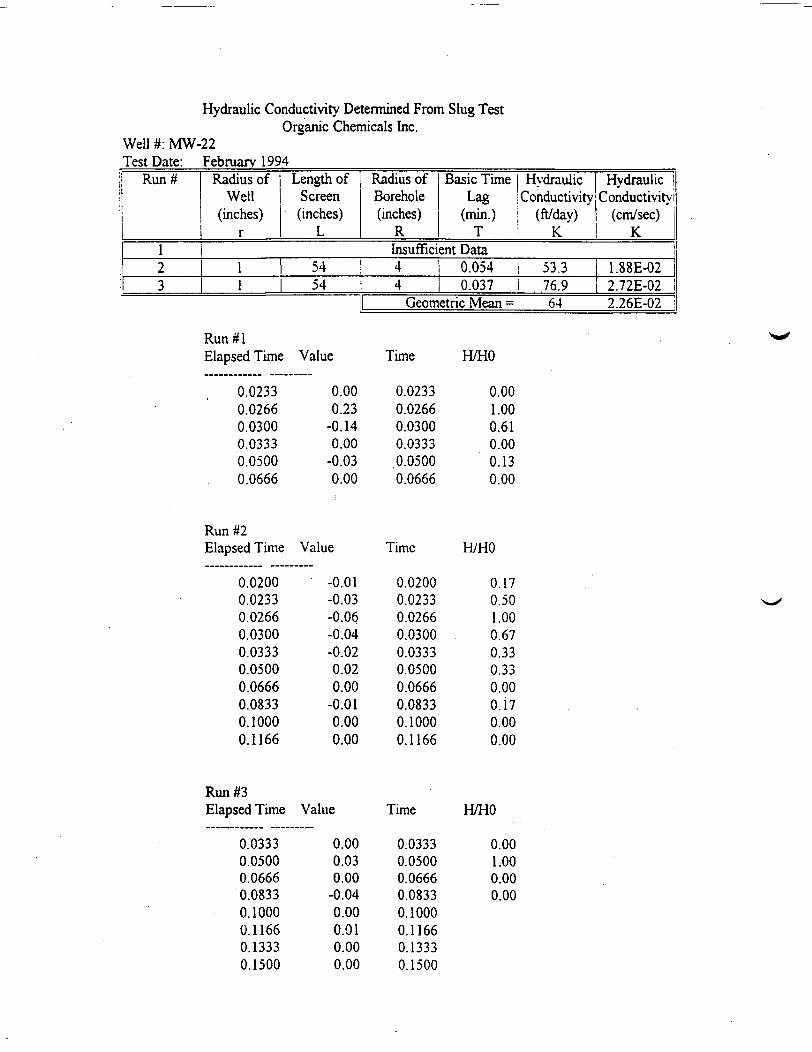
Hydraulic Conductivity Determined From Slug TestOrganic Chemicals Inc.
Well #: MW-22Test Date: February 1994
Run#
123
Radius ofWell
(inches)r
Length ofScreen(inches)
L
Radius ofBorehole(inches)
R
Basic Time I HydraulicLag ; Conductivity
(min.) j (ft/day)T ! K
Hydraulic !Conductivity
(cm/sec)K
Insufficient Data11
5454
44
0.054 53.30.037 76.9
1.88E-022.72E-02
|| Geometric Mean = 64 2.26E-02 ;
Run#lElapsed Time
0.02330.02660.03000.03330.05000.0666
Value
0.000.23
-0.140.00
-0.030.00
Time
0.02330.02660.03000.0333
.0.05000.0666
H/HO
0.001.000.610.000.130.00
Run #2Elapsed Time
0.02000.02330.02660.03000.03330.05000.06660.08330.10000.1166
Value Time
-0.01-0.03-0.06-0.04-0.020.020.00-0.010.000.00
0.02000.02330.02660.03000.03330.05000.06660.08330.10000.1166
H/HO
0.170.501.000.670.330.330.000.170.000.00
Run #3Elapsed Time
0.03330.05000.06660.08330.10000.11660.13330.1500
Value
0.000.030.00
-0.040.000.010.000.00
Time
0.03330.05000.06660.08330.10000.11660.13330.1500
H/HO
0.001.000.000.00
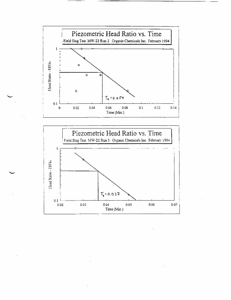
Piezometric Head Ratio vs. TimeField Slug Test MW-22 Run 2 Organic Chemicals Inc. February 1994
I [
"2•J
0.10 0.02 0.04 0.06 0.08
Time (Min.)0.1 0.12 0.14
Piezometric Head Ratio vs. TimeField Slug Test MW-22 Run 3 Organic Chemicals Inc. February 1994
0.02 0.03 0.04 0.05Time (Mn.)
0.06 0.07

Hydraulic Conductivity Damned From Slug TestOnjank Chemicals Inc.
Wen «: .\IW-24Tot Dale Frt
Run*
12
Radius orWe!
Catena)r
Length ofScreen
(inches)L
1 i 541
Radius ofBorehole(inches;
BasKTmKLa,
(mm.)T
4 i 003554 I 4
3 1 1 1 5 4 40.1
0.06
Hydnubc | HydnulK jConjductmyiConductivuyj
(ftVdty) icnvsec)K 1 K 1
32.4 i 1.J5E-02 128.8 > 1.02E-02 •48 • U9E-02 i
Run 41ElaptedTune Value
0026600300003330.0500D0666308330.10000.11660.13330.1500016660.18330.3000021660.23330.25000.26660.28330.30000.31660.33330.4167
0.070.150.230100080.060050.040.03oo:0.02o.o:0.020.010010.010.010010.010010.00000
TlIIK
0.02660.03000.03330050000666008330.1000011660.13330.15000.16660.18330:0000.2166023330.250002666023330.3000OJI66033330.4167
WHO
0.300.631.000430350.260220.170130090.090090090040040040.040040.040.040000.00
Run nElapsed Tune
002660.030000333005000.0666008330.10000.11660.13330.15000 16660.1833020000.21660.2333025000.2666
Value
•004-008•0.01•0.18-0.12-008-0.06-0.05•004-003-0.02•002-0.01-0.01•001•001000
Tune
0.02660.03000.03330.05000.06660.08330.10000.11660.133301500016660.18330200002166023330250002666
0220440.061.000670.440.330.280.220170.110.110.060060060.06000
Run»3Elapsed Time Value
0.00990.01330.01660020000233003660.0300003330.05000.06660.0833010000.11660.13330.15000.166601833020000.2166023330.25000.26660283303000
0.000070030.140.190.270200.160.070.080.060.050040.040.030.030.020.020.020.020010010.01001
Tune
000990013300166002000.023300266003000.03330.05000.06660.08330.10000.11660.13330.15000.16660.18330.20000.21660.23330.25000.26660283303000
H/HO
0000.260300520.701.000.740.590.260300.220.190.150.15O.I IO.I I0.070.070.070.070.040.040040.04

Piezometric Head Ratio vs. Time! Field Slug Test MW-24 Run 1 Organic Chemicals Inc. February 1994
O.OI0.2
Time(Min.)
1
0
s
i °-!
_0
0.01(
Piezometric Head Ratio vs. Timei Field Slug Test MW-24 Run 2 Organic Chemicals Inc. February 1994
! «" V^^
To=0.10
r>^^
) 0.1 0.2 0.3Time (Min.)
1
0
o73
1i-U
0.01(
Piezometric Head Ratio vs. TimeField Slug Test MW-24 Run 3 Organic Chemicals Inc. February' 1994
Ny- 0
)
vs^ O O
>x^ O O O *$• O 3
0.1 0.2 0.3Time (Min.)
To=0.060
0.4 0 5

Hydraulic Conductivity Determined From Slug TestOrganic Chemicals Inc.
Hell f: MM-26Test Date; February 1994
Run t Radius ofHell
(inches)r
1 ! 12 13 1
Length ofScreen(inches)
L545454
Radius ofBorehole(inches)
R44
Basic Time|Hydraulic .Hydraulic]Lag Conductivi Conduct! vi 1
(min.)T
0.0340.03
4 1 0.037
(ft/day) i (cm/sec) iK > K i
84.7 2.99E-0296.1 (3.39E-02 !77.8 '2.75E-02 i
;! Geometric Mean « 85.9 3.03E-02 i
Run #1Elapsed Time
0.00000.00330.00660.00990.01330.0166020002330266030003330500066608331000
0.1166
Valu0.00-0.10-0.11•0.12•0.11•0.17•0.15-0.12-0.10-•0.09-0.07-0.03-0.02-0.01-0.01-0.01
Time0.00000.00330.00660.00990.0133 '0.01660.02000.02330.02650.03000.03330.05000.06660.08330.10000.1166
H/HO0.000.590.650.710.651.000.880.710.590.530.410.180.120.060.060.06
Run #2Elapsed Time
0.00000.00330.00660.00990.01330.01660.02000.02330.02660.03000.03330.05000.06660.0833
Valu0.100.080.090.100.160.130.110.09•0.080.06•0.05•0.02•0.01o.oo-
Time0.00000.00330.00660.00990.01330.01660.02000.02330.02660.03000.03330.05000.06660.0833
H/HO0.630.500.560.631.000.810.690.560.500.380.310.130.060.00
Run 13Elapsed Time
0099013301660200023302660300033305000666
0.0833
Valu0.08•0.160.170.140.110.090.08•0.060.02•0.010.00
Time0.00990.01330.01660.02000.02330.02660.03000.03330.05000.06660.0833
H/HO0.470.941.000.820.650.530.470.350.120.060.00

F
oIX
0
'•5 0-or13<uX
0.0
Piezometric Head Ratio vs. Timeeld Slug Test MW-26 Run 1 Organic Chemicals Inc. February 1994
•- v "SvE *» ^^.
tF
E ___ - _.\
0 0.02 0.04 0.06Time (Win.)
To=0.034 !i
0\
i0.08 0.1
Piezometric Head Ratio vs. TimeField Slug Test MW-26 Run 2 Organic Chemicals Inc. February
0
Xi0ra °-1
(TJ0)X
0.01(
= ^Sc> * o v ^N>
n-
[
-
fs^s^
\^
3 0.02 0.04 0.06Time(Min.)
To=0.030
^0.08
1994
0.1
Piezometric Head Ratio vs. TimeField Slug Test MW-26 Run 3 Organic Chemicals Inc. February 1994
1
oXi
O<0 w' '(£.
•gX
0.01(
^-'V
-
[>v
\^ ®
\^
To=0.037
O ^ O
3 0.02 0.04 0.06 0.08 0.1 0.12 0.14Time (Min.)
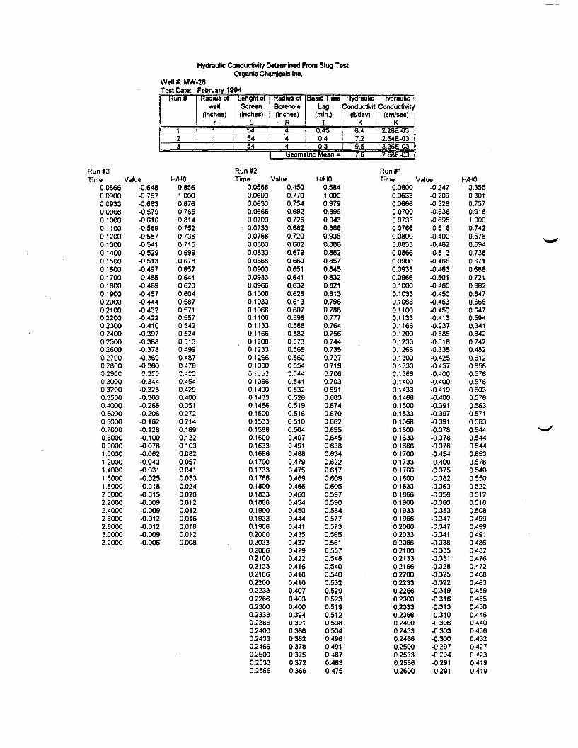
Hydraulic Conductivity Determined From Slug TestOrganic Chemicals Inc.
Well *: MW-28Test Date: February 1994
Run* Radius ofwell
(inches)r
1 I 123
11
Lengnt ofScreen(inches)
L545454
Radius ofBorehole(inches)
• R
Basic Time I HydraulicLag
(min.)T
4 0.4544
0.40.3
Conductivit(tt/day)
K6.47.29.5
Geometric Mean - 7.5
Hydraulic !Conductivity
(cm/sec) 'K ;
2.25^-032.54E-03 I3.36E-03 I2.53E-03 i
Run #3Time
0.08660.09000.09330.09660.10000.11000.12000.13000.14000.15000.16000.17000.18000.19000.20000.21000.22000.23000.24000.25000.26000.27000.2800029CC030000.32000.35000.40000.50000.60000.70000.80000.90001.00001.20001.40001.60001.80002.00002.20002.40002.60002.80003.00003.2000
Value-0.648-0.757-0.663-0.579-0.616-0.569-0.557-0.541-0.529-0.513-0.497-0.485-0.469-0.457-0.444-0.432-0.422-0.410-0.397-0.388-0.378-0.369-0.3600 350
-0.344-0.325-0.303-0.266-0.206-0.162-0.128-0.100-0.078-0.062-0.043-0.031-0.025-0.018-0.015-0.009-0.009-0.012-0.012-0.009•0.006
H/HO0.8561.0000.8760.7650.8140.7520.7360.7150.6990.6780.6570.6410.6200.6040.5870.5710.5570.5420.52405130.4990.4870.476n *****w.S<__
0.4540.4290.4000.3510.2720.2140.1690.1320.1030.0820.0570.0410.0330.0240.0200.0120.0120.0160.0160.0120.008
Run #2Time
0.05660.06000.06330.06660.07000.07330.07660.08000.08330.08660.09000.09330.09660.10000.10330.10660.11000.11330.11660.12000.12330.126601300Z . s - s Z0.13660.14000.14330.14660.15000.15330.15660.16000.16330.16660.17000.17330.17660.18000.18330.18660.19000.19330.19660.20000.20330.20660.21000.21330.21660.22000.22330.22660.23000.23330.23660.24000.24330.24660.2SOO0.25330.2566
Value0.4500.7700.7540.6920.7260.6820.7200.6820.6790.6600.6510.6410.6320.6260.6130.6070.5980.5880.5820.5730.5660.5600.554T.S'M0.5410.5320.5260.5190.5160.5100.5040.4970.4910.4880.4790.4750.4690.4660.4600.4540.4500.4440.4410.4350.4320.4290.4220.4160.4160.4100.4070.4030.4000.3940.3910.3880.3820.3780.3750.3720.366
H/HO0.5841.0000.9790.8990.9430.8860.9350.8860.8820.8570.8450.8320.8210.8130.7960.7880.7770.7640.7560.7440.7350.7270.7190.7060.7030.6910.6830.6740.6700.6620.6550.6450.6380.6340.6220.6170.6090.6050.5970.5900.5840.5770.5730.5650.5610.5570.5480.5400.5400.5320.5290.5230.5190.5120.5080.5040.4960.4910..-.870.4830.475
Run*!Time
0.06000.06330.06660.07000.07330.07660.08000.08330.08660.09000.09330.09660.10000.10330.10660.11000.11330.11660.12000.12330.12660.13000.1333C.I 3660.14000.14330.14660.15000.15330.15660.16000.16330.16660.17000.17330.17660.18000.18330.18660.19000.19330.19660.20000.20330.20660.21000.21330.21660.22000.22330.22660.23000.23330.23660.24000.24330.24660.2500025330.25660.2600
Value-0.247-0.209-0.526-0.638-0.695-0.516-0.400-0.482-0.513-0.466-0.463-0.501-0.460-0.450-0.463-0.450-0.413-0.237-0.585-0.516-0.335-0.425-0.457-O.JCO-0.400-0.419-0.400-0.391-0.397-0.391-0.378-0.378-0.378-0.454-0.400-0.375-0.382-0.363-0.356-0.360-0.353-0.347-0.347-0.341-0.338-0.335-0.331-0.328-0.325-0.322-0.319-0.316-0.313-0.310-0.306-0.303-0.300-0.297-0.294-0.291-0.291
H/HO0.3550.3010.7570.9181.0000.7420.5760.6940.7380.6710.6660.7210.6620.6470.6660.6470.5940.3410.8420.7420.4820.6120.6580.5760.5760.6030.5760.5630.5710.5630.5440.5440.5440.6530.57605400.550052205120.5180.5080.4990.499049104860.4820.4760.47204680.4630.4590.4550.4500.4460.4400.4360.43204270<>230.4190.419

Run»2Time
0.26000.26330.26660.27000.27330.27660.28000.28330.28660.29000.29330.29660.30000.30330.30660.31000.31330.31660.32000.32330.32660.33000.33330.35000.36660.38330.40000.41660.43330.45000.4666.0.48330.50000.51660.53330.55000.56660.58330.60000.61660.63330.65000.66660.68330.70000.71660.73330.75000.76660.78330.80000.81660.83330.85000.86660.88330.90000.91660.93330.95000.96660.98331.00001.20001.40001.60001.80002.00002.20002.40002.60002.80003.0000
Value0.3630.3600.3560.3530.3500.34703440.3410.3380.3350.3310.3280.3280.3250.3220.3190.3160.3130.3130.3100.3060.3030.3000.2880.2750.2630.2500.2410.2310.2220.2120.2030.1940.1870.1780.172C.1650.1560.1500.1440.1400.1340.1280.1220.1150.1120.1060.1030.1000.0930.0900.0870.0810.0810.0750.0720.0680.0650.0650.0620.0590.0590.0530.0280.0150.0120.0030.0030.0000.000
-0.003-0.003-0.003
H/HO0.4710.4680.4620.4580.4550.4510.4470.4430.4390.4350.4300.4260.4260.4220.4180.4140.4100.4060.4060.4030.3970.3940.3900.3740.3570.3420.3250.3130.3000.2880.2750.2640.2520.2430.2310.2230.2140.2030.1950.1870.1820.1740.1660.1580.1490.1450.1380.1340.1300.1210.1170.1130.1050.1050.0970.0940.0880.0840.0840.0810.0770.0770.0690.0360.0190.0160.0040.0040.0000.000
Run*1Time
0.26330.26660.27000.27330.27660.28000.28330.28660.29000.29330.29660.30000.30330.30660.31000.31330.31660.32000.32330.32660.33000.3333035000.36660.38330.40000.41660.43330.45000.46660.48330.50000.51660.53330.55000.56660.58130.60000.61660.63330.65000.66660.68330.70000.71660.73330.75000.76660.78330.80000.81660.83330.85000.86660.88330.90000.91660.93330.95000.96660.98331.00001.20001.40001.60001.80002.00002.20002.40002.60002.80003.0000
Value-0.284-0.284-0.281-0.278-0.275-0.272-0.269-0.269-0.266-0.263-0.259-0.256-0.253-0.250-0.250-0.247-0.244-0.241-0.237-0.237-0.234-0.231-0.219-0.206-0.197-0.187-0.178-0.169-0.159-0.150-0.140-0.131-0.125-0.118-0.112-0.106-0.100-0.093-0.087-0.081-0.075-0.072-0.065-0.062-0056-0.053-0.050-0.046-0.043-0.037-0.034-0.031-0.028-0.025-0.021-0.021-0.015-0.015-0.012-0.009-0.006-0.0060.0180.0340.0400.0430.0500.0500.0530.0530.0560.053
H/HO0.4090.4090.4040.4000.3960.3910.3870.3870.3830.3780.3730.3680.3640.3600.3600.3550.3510.3470.3410.3410.3370.3320.3150.2960.2830.2690.2560.2430.2290.2160.2010.1880.1800.1700.1610.153O.1 ',40.1340.1250.1170.1080.1040.0940.0890.0810.0760.0720.0660.0620.0530.0490.0450.0400.0360.0300.0300.02200220.0170.0130.0090.009
-0.026-0.049-0.058-0.062-0.072-0.072-0.076-0.076-0.081-0.076
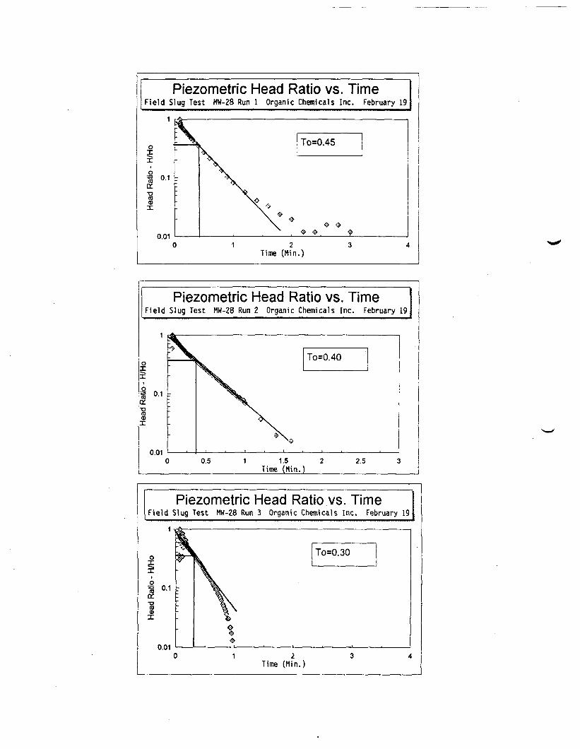
Piezometric Head Ratio vs. TimeField Slug Test MW-28 Run 1 Organic Chemicals Inc. February 19
-
\1 I '
1 :®
0.01 ——— — — — - — ——
>
0 1 2Time (Min
To=0.45
o <&
3 4.)
Piezometric Head Ratio vs. TimeField Slug Test MW-28 Run 2 Organic Chemicals Inc. February 19
0.01
Piezometric Head Ratio vs. TimeField Slug Test MW-28 Run 3 Organic Chemicals Inc. February 19
1 ^
1o
I0"1
10)
0.01c
-VIN%
o) 1 2
Time (Min.)
To=0.30
3 4

Hydraulic Conductivity Determined From Slug TestOrganic Chemicals Inc.
Well #: MW-29Teat Date: February 1994
Run* Radius ofWell
Length ofScreen
(inches) (inches)r L
1 1 5 42 1 54
Radius ofBorehole(inches)
R44
3 1 54 4
Basic TuneLag
(min.)T
0.0740.0470.11
Hydraulic HydraulicConductivity.Conductivity
(ft/day) (crosec)K j_ K
38.961.326.2
1.37E-022.17E-029.24E-03
J Geometric Mean = 39.7 1.40E-02
Run siElapsed Time
0.00000.03000.03330.05000.06660.08330.10000.11660.13330.15000.16660.18330.20000.21660.2333
Run 42Elapsed Time
0.00660 0099U.ul330.01660.02000.02330.02660.03000.03330.05000.06660.08330.10000.11660.13330.15000.16660.18330.20000.2166
Run S3Elapsed Time
0.03330.05000.06660.08330.10000. 1 1660.13330.15000.16660.18330.20000.21660.23330.25000.2666
Value0.000.100.170.150.120.090.070.050.040.030.020.010.01o.'oi0.00
Value-0.03-0.10-0.23-0.19-0.17-0.16-0.14-0.13-0.12-0.08-0.05-0.03-0.02-0.02-0.01-0.01-0.01-0.01-0.010.00
Value0.000.420.140.130.100.080.060.050.040.030.020.010.010.010.00
Time0.00000.03000.03330.05000.06660.08330.10000.11660.13330.15000.16660.18330.20000.21660.2333
Time0.00660.0099O.ui330.01660.02000.02330.02660.03000.03330.05000.06660.08330.10000.11660.13330.15000.16660.18330.20000.2166
Time0.03330.05000.06660.08330.10000.11660.13330.15000.16660.18330.20000.21660.23330.25000.2666
H/HO0.000.591.000.880.710.530.410.290.240.180.120.060.060.060.00
HHO0.130.431.000.830.740.700.610.570.520.350.220.130.090.090.040.040.040.040.040.00
H/HO0.001.000.330.310.240.190.140.120.100.070.050.020.020.020.00

Piezometric Head Ratio vs. TimeI Fiels Slug Test MW-29 Runl Organic Chemicals Inc. February 1994
0.010.05 0.1 0.15
Time (Min.)
1
o1o^3
1
0.01c
Piezometric Head Ratio vs. TimeField Slug Test MW-29 Run 2 Organic Chemicals Inc. February 1994
^X
;» ^\.X^.0.05 0.1 0.15
Time (Min.)
To=0.047
0.2 0.25
1
o
oaa.
-a«
0.01C
-
Piezometric Head Ratio vs. TimeField Slug Test MW-29 Run 3 Organic Chemicals Inc. February 1994
0 "^^^
:\
0.05 0.1 0.15Time (Min.)
To=0.11
*\o o ^
0.2 C.21

Hydraulic Conductivity DeunnaKd From Shit; TotOnjanic Cnoncah! Inc.
Well": MW.JOTea Date: February 1994
Run*
1
Radius orWell
linches)r1
1 '1 1 1
LenimofScreen(inches)
L545454
Radius orBacholelincbes)
R44 '
Basic TuneL«*
(mm.)T
DIM0.175
Hydraulic HydraulicConduct! vtyiCooductivny
(fl/day)K2]
(otvtcc)K
81 IE-0316.4 , 5.79E-OJ
4 i 0.04 71.9 ! 2.54E-02Geomemc Mean - 10 1 .06E-02
Run«iElapsed Time
000990011300164002000.0211Ot>:66OOJ3300500006660.08350.10000116601313015000166601S110.2000021660.23330.250002666028330300001166
Run nElapsed Time
002000.021300:66001000033300500006660.08330 10000 1166013330150001666018330:00002166o:ill0:5000:6660.28110100001166013330.41670.50000 583306667
Run*]Elapsed Time
0.0000003000033300500004660.0813010000.116601111015000166601 S3]0200002166023330.25000.266602S330300001166033330416705000058330.6667075000811]
Value0.000.060.16Oi l0510.410250.160.13O i l
. 0090010.060050.040.040.010.02OOJ0010010010010.00
Value-oos-010•016•023-022-017•019•016-0.14•012- O i l-010•0.09•008-0.07-007•006-006•006-0.05-005-005-005•004-004-004-004
Value0000050150290.170150.13O i l010OOS0070060050050.040.040030030030.030.020020.020010010.010.01
Time000990.0133001660020000233002660.0311005000.06660.08330.100001166013330.150001666018310:000021660.23310.2500026660.28330300003166
Time0.02000.023300:660030000333005000066600833010000.1166013310150001666018330.200002166023130.250002666OJS1301000011660333)041670.50000581106667
Time00000001000.01330.050000666008)30100001166011110.15000.16660.18110.2000021660211]025000266602811030000.116603311041670500005833066670.750008133
WHO0.00O i l0.300.58100Oil0470300.250.210170.15O i l0090.080.080.060.040.040020020020.020.00
RH>0220430.701.000.960.740830.700610520490.4]0190.350300300260260260220220220 2 20.17017017017
two0000170521000590.520.450380340.280240.210.170.170140140 100100100100070.070070.0100]00]00]

i Piezometric Head Ratio vs. Time! Field Slug Test MW-30 Run 1 Organic Chemicals Inc. February 1994
0.010.2
To=0.125
<> O O •:>
0.4 0.6Time(Min.)
0.8
Piezometric Head Ratio vs. TimeField Slug Test MW-30 Run 2 Oraanic Chemicals Inc. Febmarv 1994
To=0.175
0.2 0.4Time (Min.)
0.6 0.8
i Piezometric Head Ratio vs. Timei Field Slug Test MW-30 Run 3 Organic Chemicals Inc. Februan 1994
0.010?
Time (Min.)
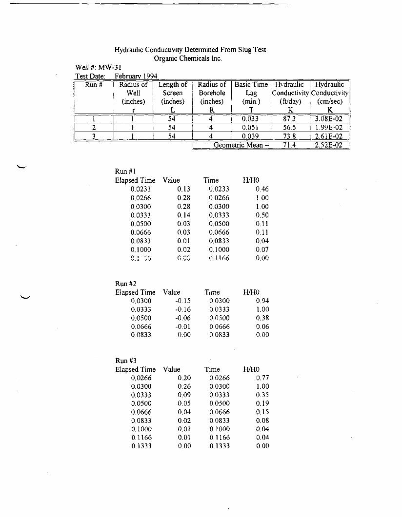
Hydraulic Conductivity Determined From Slug TestOrganic Chemicals Inc.
Well#:MW-31Test Date: February 1994
Run#
123
Radius ofWell
(inches)r
Length ofScreen(inches)
L1 1 541 i 541 1 54
Radius ofBorehole(inches)
R*
4
Basic TimeLag
(min.)T
0.0330.051
4 I 0.039
Hydraulic | HydraulicConductivity Conductivity
(ft/day)K
87.356.573.8
(cm/sec)K
3.08E-021.99E-022.61E-02
Geometric Mean = 71.4 2.52E-02
Run#lElapsed Time Value
0.0233 0.130.02660.03000.03330.05000.06660.08330.1000A 1 ' /" S"W. * V-O
0.280.280.140.030.030.010.02C 00
Time0.02330.02660.03000.03330.05000.06660.08330.1000O.M66
H/HO0.461.001.000.500.110.110.040.070.00
Run #2Elapsed Time Value
0.0300 -0.150.03330.05000.06660.0833
-0.16-0.06-0.010.00
Time0.03000.03330.05000.06660.0833
H/HO0.941.000.380.060.00
Run #3Elapsed Time
0.02660.03000.03330.05000.06660.08330.10000.11660.1333
Value0.200.260.090.050.040.020.010.010.00
Time0.02660.03000.03330.05000.06660.08330.10000.11660.1333
H/HO0.771.000.350.190.150.080.040.040.00

Piezometric Head Ratio vs. TimeField Slug Test MW-31 Run 1 Organic Chemicals Inc. February 1994
0.010.02 0.04 0.06 0.08 0.1
Time (Min.)0.12 0.14
Piezometric Head Ratio vs. TimeField Slug Test MW-31 Run 2 Organic Chemicals Inc. February 1994
- 0.1
0.010.02 0.04 0.06
Time (Min.)0.08 0.1
Piezometric Head Ratio vs. TimeField Slug Test MW-31 Run 3 Organic Chemicals Inc. February 1994
o§
•2 0.1
1
0.010.02 0.04 0.06 0.08
Time (Mill.)_0.1 0.12 0.14

Hydrainc CondlKttvily Deunnuud Fiom Slug TernOtgmic Cliemiclli Inc.
Well «: MW-31Tesl D«r Febrtary 1994
Run* Radius orWell
linchei)r
length orScreen
(inches)L
1 1 ' 54: : i 543 1 I 54
Radios ofBorehole(inches)
Bane TimsKg
(nun.)T
4 44 3.134 36
Gcomctnc Men •
HydrateConductivity
(fl/diy)K
0719092205
HyilnuucConductivity
(cnvsec)K
254E-0432SE-042S2E-04
0809 2.S6E-04
RunaiQapsedTims
0.08330100001166013330.15000 16660.18330:0000216602333025000266603330.300003164033330.41470500005333064670.750003333091671.0000103331 16671 25001 3333141661.500015333166671 75001 3333I »I6>':oooo2.500030000350004000045000500005500060000650007.00007.50003.00003.50009000095000
100000IIOOOO
Vllue0.3)0.210.210200200.200.2)0.3)0.200200.200 190190190190.20O H0.110.170.17.0160.160.160.1S0.1S0 140140.140.140 130.130130.1!0 130.120.120.100.09O.OS0.070060060050040.04OOJ0030.020.020020.02001000
Tinu008330 1000011660.13330 15000.16660 18330.20000.216602333025000266602333030000.316603333041670500005833066670.7500033330.916710000108331.16671.25001 33331.41661 500015833166671 75001 33331 91672.0000250003.00003500040000450005000055000600006.500070000750003.00008.50009000095000
100000120000
am0951.001 000950.950950950.950.950.950.950.900.900900900950360360310310760760."60.710.710.670670670670620620620.570.570.570570480430380330.290.290240190 190.140140100 100100.100.05000
Run»2Elapsed Time
005000.06660.08330.100001166013330.15000 16660 18330.20000.21660.2333025000266602SJ303000031660.3333041670500005*33066670.7500033330.9167loom1.0833I 16671 2500133331416615000153331.66671.7500133331.91672000025000300003500040000450005000055000600006.50007.00007500030000850009000095000
10.000012.0000140000
Vtlue-0.24-0.25-024-024-024-024-023-023-023-0.23•023-o ::•0 22-022-0 22-0.22-o 22.0:1•021•020•020-019•019-0 13•0 13•0.17-0.17,016-016-0.16-015-015-015-014-0.14-0.14-0 13413-012- O i l-0 10-009•0.03'-0.03-0.07JIM-006-006-005-005-005-0.04-004•004-0.03-003
Tune0050000666008330.10000.11660.13330.15000 166601333020000216602333025000266603330300003166033330.416705000058330.66670.7500083330916710000108331 16671.250013333141661.50001 583316667i 'KO13333191672.00002.50003000035000400004500050000550006000065000700007500030000350009000095000
100000120000140000
H/KO0961.000960960%0960.920920.920.920.92OSS0.880380380880330.340840800300.760.760.720.720630680640640.640600600.600.560560560520.520480440400360320.320230.240240240200200200.160 160.160 12012
Run<3Elapsed Time
0.05000.06660.08330.10000.11660133301500016660183302000021660.2333025000.26660.233303000031660 33330416705000053330.66670.75000333309167100001.08331.1667125001 333314166150001 53331.6667i.75001 33331.91672.00002.50003.000035000400004500050000550006.00006.50007.00007500030000850009000095000
10000012.0000140000
Value0150200.200200200.200.190 190 1 90.190.190.190 190190.180180130.130.130.170.170160.160 160 150150150.140 140.140.130.130.130.13C..20.120.120120.100090080030.070.060.060.050050040.040.040.040.030.03003002002
Time005000066600833010000.1166013330.15000 166601333020000.21660.23330.25000:666023330300003166033330.416705000058330666707500033330916710000108331.16671 250013333141661.5000158331.6667l.TStai18333191672.0000250003000035000400004500050000550006.0000650007.00007.50008000085000900009.5000
10.000012.0000140000
K.HO0.751.001.001.00100100
0.950950950950950950950950900900900900900350.350.300300300.750.750.750.700700.70065065065n M
,uU wO0600.600500450400400350300300250.250.3)0200200300 150 150150.100 10

I Piezometric Head Ratio vs. TimeField Slug Test MW-32 Run 1 Organic Chemicals Inc. February 1994J
0.015 10
Time (Min.)
Piezometric Head Ratio vs. TimeField Slug Test MW-32 Run 2 Organic Chemicals Inc. February 1994
1 4
_o
"* ["^oa
S£•aJU
0.1
: \=- $
rV *\ O <>\ ^
\ -5> O -3>N. O^.<>
^ <
t 5Time (Min.)
To=3.13
> -S>0
®
10
*
15
Piezometric Head Ratio vs. TimeField Slug Test MW-32 Run 3 Organic Chemicals Inc. February 1994
•&.•a
1
0.01' 6 8Time (Min.)

Hydnulic Conductivty Determined From Slug TotOrganic Chemicals Inc.
Well « MW-J3Tea D»t February 1994
Run »1Earned Time
103000 03330 0500306660 08335 10000 11*60 13330.1500016660 13330:0000:16602333015000:66603330300003166033330.4167
Vain.-0.14-019-OH-0.14-0.12-009-008-006-0.03-0.04-004-003-002-002-0.02-001-001-001-001-001
0.00
Tune00300003330050000666O.OS330 10000 11*60 13330.15000.16660 IS330:0000:1660:333o:_vx>o:6*«025303000031660.33330.4167
Run*
1:3
Radius ofI Will| I inches)
r1
Length ofScreen
(incha)L
RadiuiofBorehole(inchei)
R54 i 4
i 1 • 54 41 54 4
Bane Timelag
imm.)
HydraulicConductivity
in/day)K
0 125 230 125 23021 13.7
HydrjulK .CorhlucuvKyj
(cnneci iK
J 13E-OJ8 13E-03 .4 J4E-03 1
HHO0"4'..00095
0320260 2 10:i0 16) II0 II0 II005005005005005000
Geometric Mean •
Run<2Darned Time
00500006*600833010000 1166013330.15000 16660 18330:0000:166OIS330:5000:6*603330300003166033330.4167
Value-0.23-0.17-014-0 11-009-0.07-006-0.05-004-003-005-oo:-oo:-oo:-001•001-001-001
0.00
Time0050000666O.OS330.10000 1166013330 15000 16660 1333OMOO0.21660233302500o:«60231305000031560333304167
KHO1000.7406104S0.390300.26o::0.170130130.090.090.090.040.040.040040.00
Run »3Elapied Time
0050070030 100.120 130 1 5o.r0 1J0:0o::0:30:10:70305003:03304;050053OS"0-5
Value-o.:o-0:2-013-0.16-0 14-0.12•0 II•0 10•009-009-008-003-007-007-007-007-0.06-006.006-006-005-005-005
Time0050.070.080 100.120130 150 170 13020o::023025027oa0300320330 4 2050053067075
H>HO0911 000320"30*40550 500450.410 4 10.560360320320320320:70:70.27027023015023

Piezometric Head Ratio vs. Time1 Field Slug Test MW-33 Run I Organic Chemicals Inc. February 1994
1 E —— 5 5- —————————————————————————————————————————- f> ^fe: <>si
— ri°4Ot. j-
1 k— L
iro.oi 1 —————— ' —
0 0.1
>* To=0.125
\<>
N^.. |
, '
0.2 0.3 0.4 0.5Time (Min.)
Piezometric Head Ratio vs. TimeField Slug Test MW-33 Run 2 Organic Chemicals Inc. February 1994
1 0.1 F
-o3
0.010.2 0.3Time (Min.)
0.4 0.5
Piezometric Head Ratio vs. TimeField Slug Test MW-33 Run 3 Organic Chemicals Inc. February 1994
0.10.2 0.4
Time (Min.)0.6 0.8

Hydraulic Conductivity Delermined From Slug TestOrganic Chemicals Inc.
WeD *: MW-34Test Dale: February 1994
Run » Radius ofWell
; (inches)r
1 ' 1
Length otScreen(inches)
L
Radius ofBorehok(inches)
R
Basic TuneLag
(min.)T
HydraulicConductivity
(ft/ dav)K
5 4 1 2 1 7 0 j 0.025
HydraulicConductivity
(cm/sec)K
6.97E-06
Run«Time Value
0.66670.75000.83330.9167.0000.0833.1667.2500.3333.4166.5000.5833.6667.7500.83331.91672.00002.50003.00003.50004.00004.50005.00005.50006.00006.50007.00007.50008.00008.50009.00009.500010.000012.000014.000016.000018.000020.000022.000024.000026.000028.000030.000032.000034.000036.000038.000040.000042.000044.000046.000048.000050.000052.000054.000056.000058.000060.000062.000064.0000
0.550.550.550.550.550.550.550.550.550.550.550.550.550.550.550.550.550.550.550.540.540.540.540.540.540.540.530.530.530.530.530.530.530.520.510.510.500.490.490.480.480.470.470.460.460.450.440.440.430.430.420.420.410.410.400.400.400.390.390.38
H/HO1.001.001.001.001.001.001.001.001.001.001.001.001.001.001.001.001.001.001.000.980.980.980.980.980.980.980.%0.960.960.960.960.%0.%0.950.930.930.910.890.890.870.870.850.850.840.840.820.800.800.780.780.760.760.750.750.730.730.730.710.710.69
Run Dlcon'tTime Value
66.000068.000070.000072.000074.000076.000078.000080.000082.000084.000086.000088.000090.000092.000094.000096.000098.0000100.0000110.0000120.0000130.0000140.0000150.0000160.0000170.00001SO.OOOO190.0000200.0000210.0000220.0000230.0000240.0000250.0000260.0000270.0000280.0000290.0000300.0000310.0000320.0000330.0000340.0000350.0000360.0000370.0000380.0000390.0000400.0000410.0000420.0000430.0000440.0000450.0000460.0000470.0000480.0000490.0000500.0000510.0000520.0000530.0000540.0000550.0000
0.380.370.370.360.360.360.350.350.340.340.340.330.330.320.320.320.310.310.290.270.260.240.230.210.200.190.180.170.160.150.140.130.120.120.110.100.090.090.080.080.070.070.060.060.050.050.050.040.040.040.030.030.030.020.020.020.020.010.010.010.010.010.00
HHO0.690.670.670.650.650.650.640.640.620.620.620.600.600.580.580.580.560.560.530.490.470.440.420.380.360.350.330.310.290.270.250.240.220.220.200.180.160.160.150.150.130.130.110.110.090.090.090.070.070.070.050.050.050.040.040.040.040.020.020.020.020.020.00

Piezometric Head Ratio vs. TimeField Slug Test MW-34 Run 1 Organic Chemicals Inc. February 1994
0.01200 400 600
Time (Min.)

Hydnulk Condnoiviy DtunmiHd From Slug TMOrganic Chamicab Inc.
W«U» MW-36Teal Dele: February 1994
Run*
1
RadmsofWell
(inchee)rI
Length ofScreen
(inche»L
54
RadiuiofBorehole{utchal
R2
Benc TimeLag
lincheelT
375
Hydraulic ! HydraulicConductrvtty (Conductivity
Id/day) (cnvaec)K | K
0.00502 1 1.77E-06
R u n « lTim. Value
011000 11330 116*0.12000.1133012660 13000.1333013660 14000 14 J3014640 15000 15330 15660 1600016330 1666017000173301-66013000 18330 ISM0.19000 19330 19660.2000020330206602100021330216602200022J302266023000233302366024000243302466025000253302566026000263302666027000.2-330.27M0230002333023660 29000293302966030000 303303066031000313303166032000323303266033000 3333035000366603333040000416604333045000466604333050000.5166053330.55000566605833
•5028-5.022-4978-496«-4975-197:-(.972-4.941-4960-1.978-1978-4972-4966-49->8-4985-4.972-497J-1.975-4981-4969-4935-4.J75-497S-4985-4.975-4.978-4981-4975-4978-4981-4931-1581-4988-4981-4935-4983-4985-l?3<-4985-4985-4985-4935-4935-4985-4938-4985-4.985-49S8-4985-4988-4988-4985-4938-4938-4 988-4993-4933-1988-4933-49S8-4988-4981-4991-498»-4988-49S»-J9S8-4991-4991-4.991-4991-4985-4.944-4.941-4953-4.922-4944-4 944-4.913-4.916-4.910-4919-4919
H.HO1001000.990990990990990.980990990990990990990.990.990990990990.990990990990990990.99099099099099099099099099099099099^ c?0990990990990990990990990990990.990.990990990990990990990990990990990990990990.990990990990990990990990990.93093099098098093093093093098093
Run • 1 contTune Value
060000616606333065000666606333O'OOO071660733307500076660-333080000816603333085000.3666039330900009166093330.95000966609833100001 2000140001600018000200002.20002.4000260002800030000320001 4000..;•«..33000
0000200040006000.3000
5.0000520005.400056000580006000062000640006.6000680007.00007200074000760007300080000820003400036000880009000092000940009600098000
10000012000014000016000013000020000022.000024000026000028000030000032.000034.000036.0000380000
-4922-4922-4922-4922-4.922-4922-4922-4.922-4922-4 922-4.922-4922-4.925-1922-4922-4922-4922-4.922-4922-4.922-1922-4922-4 922-4922-4922-4919-4916-4913-4910-4906-4906-4903-4900-4397-4394-4891-4333-. Sw-4881-4881-4373-4875-4872-4872-4369-4366-4363-4363-4359-4359-4856-4353-4.353-4850-4847-4 S44-4344-4341-4341-4837-4837-4334-4334•4311-4331-4323-4825-4825-4822-4.822-4306-4.790-4.778-4762-4747-4.734-4.721-4.706-4690-4.678-4665-4653-4643-4628
H/HO0980.980930980980980980930930930980980980.930980.930980930930930930930.930980930.9809809809309809309309709709709709709"0970970970970970970.970970.970.970970970.970970970.960.960960960960960960960960960960960960960960960%0960950950950940940940940930930930930920.92
Run*lcon1Time Value
40000042.000044000046000048000050000052000054000056000058000060000062000064000066000063.000070.000072.000074.000076000078000030000032.000034000036000033000090000092.0000940000960000930000
1000000120000014000001600000130000020000002200000240 oryx)2600000230.0000300000032000003400000360000033000004000000420000044000004600000430.00005000000520.0000540000056000005SOOOOO600UOOO6200000640.00006600000630000070000007200000740000076000007300000300.00003200000840.0000360.0000330000090000009200000940000096000009300000
10000000120000001400000016000000130000002000000022000000240000002600.0000
-4615-4606-4590-4511-4565-4552-4540-4534-4.521-4509-4493-4434-1474-4462-4452-4443-4430-1413-4403-4396-4336-4374-4365-4355-4343-4333-4321-4311-4302-4.293-4230-4 183-4039-3995-3.907-3320-37353654
-3.572-3491-3416-3.341-3269-3200-3131-3.062-3002-29J4-2874-2311-2.749-2639•2.636-2.580-2.523-2476-2.417-2367-2.314-2.2"0-2220-2173-2.126•2032-2.033-1994-1 953-1913-1.372-1833-1.797-1759-1.722-1687-1650-1.618-1.302-1052-0354-0633-0554-0447-0353-0275
UNO0920.920910910910910900900900900390390890.39039OSJ0330330330.370870.370.870870360860360360360350850330310.790730.760740730710690630660650640620610.600.530.570560.550530520510500.490430.470460450440430.420 4 10410400390330370370360350340340330.320260.210.170 14O i l009007005

Piezometric Head Ratio vs. TimeField Slug Test MW-36 Run 1 Organic Chemicals Inc. February 1994
0.01
ThousandsTime (Min.)

Hydraulic Conductivity Determined From Slug TestOrganic Chemicals Inc.
Well # : MW-40Test Date February 1994 _
Run#
•i
2
Radius ofWell
(inches)r1i
Length ofScreen
(inches)L
5454
Radius ofBorehole(inches)
R22
Basic Time i HydraulicLag Conductivity
(inches) ! (ft/day)T ! K
0.65 | 5.750.6 ! 6.13
HydraulicConductivity
(cm/sec)K I
2.03E-032.16E-03
Geometric Mean = 5.94 2.09E-03 j
Run#lTime
0.10000.10330.10660.11000.11330.11660.12000.12330.12660.13000.13330.13660.14000.14330.14660.15000.15330.15660.16000.16330.16660.17000.17330.17660.18000.18330.18660.19000.19330.19660.2000
Value-3.998-4.111-4.243-3.867-3.908-3.923-3.989-3.810-3.873-3.848-3.807-3.804-3.763-3.729-3.688-3.660-3.638-3.616-3.576-3.566-3.532-3.497-3.491-3.457-3.435-3.397-3.375-3.360-3.334-3.303-3.291
H/HO0.9731.0001.0320.9410.9510.9540.9700.9270.9420.9360.9260.9250.9150.9070.8970.8900.8850.8800.8700.8670.8590.8510.8490.8410.8360.8260.8210.8170.8110.8030.801
Run #2Time
0.08330.08660.09000.09330.09660.10000.10330.10660.11000.11330.11660.12000.12330.12660.13000.13330.13660.14000.14330.14660.15000.15330.15660.16000.16330.16660.17000.17330.17660.18000.1833
Value-3.989-4.261-4.311-4.365-4.299-4.296-4.305-4.296-4.252-4.211-4.167-4.142-4.101-4.092-4.080-4.064-4.036-3.995-3.976-3.945-3.917-3.895-3.854-3.845-3.810-3.801-3.754-3.741-3.716-3.694-3.666
H/HO0.9140.9760.9881.0000.9850.9840.9860.984r» 0740.9650.9550.9490.9400.9370.9350.9310.9250.9150.9110.9040.8970.8920.8830.8810.8730.8710.8600.8570.8510.8460.840

0.20330.20660.21000.21330.21660.22000.22330.22660.23000.23330.23660.24000.24330.24660.25000.25330.25660.26000.26330.26660.27000.27330.27660.28000.28330.28660.29000.29330.29660.30000.30330.30660.31000.31330.31660.32000.32330.32660.33000.33330.35000.36660.38330.40000.41660.4333
-3.259-3.234-3.212-3.184-3.175-3.147-3.122-3.096-3.078-3.050-3.028-3.009-2.987-2.962-2.940-2.918-2.896-2.874-2.855-2.833-2.815-2.793-2.771-2.752-2.733-2.711-2.693-2.674-2.652-2.633-2.614-2.595-2.577-2.558-2.539-2.520-2.502-2.483-2.464-2.448-2.348-2.254-2.167-2.076-1.994-1.910
0.7930.7870.7810.7750.7720.7660.7590.7530.7490.7420.7370.7320.7270.7210.7150.7100.7040.6990.6940.6890.6850.6790.6740.6690.6650.6590.6550.6500.6450.6400.6360.6310.6270.6220.6180.6130.6090.6040.5990.5950.5710.5480.5270.5050.4850.465
0.18660.19000.19330.19660.20000.20330.20660.21000.21330.21660.22000.22330.22660.23000.23330.23660.24000.24330.24660.25000.25330.25660.26000.26330.26660.27000.27330.27660.28000.28330.28660.29000.29330.29660.30000.30330.30660.31000.31330.31660.32000.32330.32660.33000.33330.3500
-3.644-3.610-3.585-3.560-3.544-3.528-3.494-3.472-3.450-3.431-3.409-3.381-3.359-3.337-3.315-3.294-3.272-3.250-3.231-3.209-3.187-3.165-3.146-3.125-3.103-3.084-3.062-3.043-3.021-3.002-2.980-2.962-2.943-2.924-2.905-2.883-2.865-2.846-2.827-2.808-2.789-2.771-2.752-2.733-2.717-2.617
0.8350.8270.8210.8160.8120.8080.8000.7950.7900.7860.7810.7750.7700.7640.7590.7550.7500.7450.7400.7350.7300.7250.721^ -T - /-(I. 1 HJ
0.7110.7070.7010.6970.6920.6880.6830.6790.6740.6700.6660.6600.6560.6520.6480.6430.6390.6350.6300.6260.6220.600
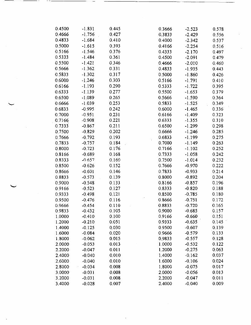
0.45000.46660.48330.50000.51660.53330.55000.56660.58330.60000.61660.63330.65000.66660.68330.70000.71660.73330.75000.76660.78330.80000.81660.83330.85000.86660.88330.90000.91660.93330.95000.96660.98331.00001.20001.40001.60001.80002.00002.20002.40002.60002.80003.00003.20003.4000
-1.831-1.756-1.684-1.615-1.546-1.484-1.421-1.362-1.302-1.246-1.193-1.139-1.089-1.039-0.995-0.951-0.908-0.867-0.829-0.792-0.757-0.723-0.689-0657-0.626-0.601-0.573-0.548-0.523-0.498-0.476-0.454-0.432-0.410-0.210-0.125-0.084-0.062-0.053-0.047-0.040-0.040-0.034-0.031-0.031-0.028
0.4450.4270.4100.3930.3760.3610.3460.3310.3170.3030.2900.2770.2650.2530.2420.2310.2210.2110.2020.1930.1840.1760.1680.1600.1520.1460.1390.1330.1270.1210.1160.1100.1050.1000.0510.0300.0200.0150.0130.0110.0100.0100.0080.0080.0080.007
0.36660.38330.40000.41660.43330.45000.46660.48330.50000.51660.53330.55000.56660.58330.60000.61660.63330.65000.66660.68330.70000.71660.73330.75000.76660.78330.80000.81660.83330.85000.86660.88330.90000.91660.93330.95000.96660.98331.00001.20001.40001.60001.80002.00002.20002.4000
-2.523-2.429-2.342-2.254-2.170-2.091-2.010-1.935-1.860-1.791-1.722-1.653-1.590-1.525-1.465-1.409-1.355-1.299-1.246-1.199-1.149-1.102-1.058-1.014-0.970-0.933-0.892-0.857-0.820-0.785-0.751-0.720-0.685-0.660-0.635-0.607-0.579-0.557-0.532-0.275-0.162-0.106-0.075-0.056-0.047-0.040
0.5780.5560.5370.5160.4970.4790.4600.4430.4260.4100.3950.3790.3640.3490.3360.3230.3100.2980.2850.2750.2630.2520.2420.2320.2220.2140.2040.1960.1880.1800.1720.1650.1570.1510.1450.1390.1330.1280.1220.0630.0370.0240.0170.0130.0110.009
3.60003.80004.00004.20004.40004.60004.80005.00005.20005.40005.60005.80006.00006.20006.40006.60006.80007.00007.20007.40007.60007.80008.00008.20008.40008.60008.80009.00009.20009.40009.60009.800010.000012.000014.0000
-0.025-0.028-0.025-0.022-0.025-0.022-0.022-0.018-0.022-0.022-0.018-0.022-0.022-0.018-0.018-0.018-0.018-0.015-0.018-0.015-0.018-0.015-0.015-O.C15-0.015-0.015-0.015-0.015-0.015-0.012-0.015-0.012-0.012-0.012-0.012
0.0060.0070.0060.0050.0060.0050.0050.0040.0050.0050.0040.0050.0050.0040.0040.0040.0040.0040.0040.0040.0040.0040.0040.0040.0040.0040.0040.0040.0040.0030.0040.0030.0030.0030.003
2.60002.80003.00003.20003.40003.60003.80004.00004.20004.40004.60004.80005.00005.20005.40005.60005.80006.00006.20006.40006.60006.80007.00007.20007.40007.60007.80008.0000
-0.037-0.034-0.034-0.031-0.031-0.028-0.028-0.028-0.025-0.025-0.028-0.028-0.025-0.025-0.025-0.021-0.021-0.021-0.021-0.018-0.018-0.018-0.018-0.018-0.018-0.018-0.018-0.018
0.0080.0080.0080.0070.0070.0060.0060.0060.0060.0060.0060.0060.0060.0060.0060.0050.0050.0050.0050.0040.0040.0040.0040.0040.0040.0040.0040.004

Piezometric Head Ratio vs. TimeField Slug Test MW-40 Run 1 Organic Chemicals Inc. February 1994
0.01
To=0.65I
4 6Time (Min.)
10
Piezometric Head Ratio vs. TimeField Slug Test MW-40 Run 2 Organic Chemicals Inc. February 1994
To=0.60
10 15Time (Min.)

Hydraulic Conductivity Determined From Slug TestOrganic Chemicals Inc.
Well #: MW-41Test Date: February 1994
Run# Radius ofWell
(inches)
12
r11
Length ofScreen
(inches)L
5454
Radius ofBorehole(inches)
R22
i Basic TimeLag
i (mm.)! T! 0.7I 0.65
Geometric Mean =
Hydraulic HydraulicConductivity Conductivity
i (ft/day): j£
i 6.17i 6.65
6.41
(cm/sec)K
2.18E-03 i2.35E-03 !2.26E-03
Run#lTime
0.07330.07660.08000.08330.08660.09000.09330.0966n 10000.10330.10660.11000.11330.11660.12000.12330.12660.13000.13330,13660.14000.14330.14660.15000.15330.15660.16000.16330.16660.17000.1733
Value-4.095-4.164-4.167-4.145-4.127-4.127-3.788-3.826-3.823-3.823-3.826-3.782-3.760-3.757-3.748-3.704-3.676-3.644-3.629-3.607-3.591-3.560-3.529-3.516-3.500-3.472-3.447-3.425-3.400-3.378-3.359
H/HO0.9830.9991.0000.9950.9900.9900.9090.9180.9170.9170.9180.9080.9020.9020.8990.8890.8820.8740.8710.8660.8620.8540.8470.8440.8400.8330.8270.8220.8160.8110.806
Run #2Time
0.07660.08000.08330.08660.09000.09330.09660.10000.10330.10660.11000.11330.11660.12000.12330.12660.13000.13330.13660.14000.14330.14660.15000.15330.15660.16000.16330.16660.17000.17330.1766
Value-4.008-4.155-4.249-4.242-4.221-4.227-4.130-4.152-4.067-3.945-3.911-3.889-3.914-3.907-3.848-3.823-3.782-3.767-3.751-3.729-3.707-3.676-3.648-3.632-3.613-3.579-3.554-3.541-3.516-3.488-3.469
H/HO0.9430.9781.0000.9980.9930.9950.9720.9770.9570.9280.9200.9150.9210.9200.9060.9000.8900.8870.8830.8780.8720.8650.8590.8550.8500.8420.8360.8330.8270.8210.816

0.17660.18000.18330.18660.19000.19330.19660.20000.20330.20660.21000.21330.21660.22000.22330.22660.23000.23330.23660.24000.24330.24660.25000.25330.25660.26000.26330.26660.27000.27330.27660.28000.28330.28660.29000.29330.29660.30000.30330.30660.31000.31330.31660.32000.32330.3266
-3.337-3.319-3.300-3.278-3.256-3.234-3.215-3.193-3.175-3.153-3.134-3.115-3.093-3.074-3.053-3.037-3.018-2.999-2.977-2.959-2.940-2.921-2.902-2.887-2.868-2.849-2.833-2.818-2.799-2.783-2.764-2.749-2.733-2.714 .-2.696-2.680-2.664-2.649-2.630-2.614-2.599-2.583-2.567-2.548-2.536-2.520
0.8010.7960.7920.7870.7810.7760.7720.7660.7620.7570.7520.7480.7420.7380.7330.7290.7240.7200.7140.7100.7060.7010.69606930.6880.6840.6800.6760.6720.6680.6630.6600.6560.6510.6470.6430.6390.6360.6310.6270.6240.6200.6160.6110.6090.605
0.18000.18330.18660.19000.19330.19660.20000.20330.20660.21000.21330.21660.22000.22330.22660.23000.23330.23660.24000.24330.24660.25000.25330.25660.26000.26330.26660.27000.27330.27660.28000.28330.28660.29000.29330.29660.30000.30330.30660.31000.31330.31660.32000.32330.32660.3300
-3.447-3.428-3.406-3.384-3.363-3.341-3.319-3.294-3.275-3.256-3.237-3.215-3.193-3.172-3.153-3.131-3.112-3.090-3.074-3.056-3.037-3.015-2.996-2.977-2.962-2.946-2.924-2.909-2.890-2.871-2.855-2.840-2.824-2.805-2.790-2.771-2.752-2.736-2.718-2.702-2.686-2.667-2.652-2.633-2.617-2.602
0.8110.8070.8020.7960.7910.7860.7810.7750.7710.7660.7620.7570.7510.7470.7420.7370.7320.7270.7230.7190.7150.7100.7050.7010.6970.6930.6880.6850.6800.6760.6720.6680.6650.6600.6570.6520.6480.6440.6400.6360.6320.6280.6240.6200.6160.612

0.33000.33330.35000.36660.38330.40000.41660.43330.45000.46660.48330.50000.51660.53330.55000.56660.58330.60000.61660.63330.65000.66660.68330.70000.71660.73330.75000.76660.78330.80000.81660.83330.85000.86660.88330.90000.91660.93330.95000.96660.98331.00001.20001.40001.60001.8000
-2.505-2.489-2.401-2.320-2.245-2.166-2.094-2.022-1.957-1.891-1.831-1.769-1.712-1.653-1.600-1.546-1.496-1.446-1.399-1.355-1.312-1.268-1.227-1.186-1.149-1.111-1.074-1.039-1.005-0.973-0.945-0.914-0.886-0.857-0.829-0.804-0.779-0.754-0.729-0.704-0.682-0.663-0.410-0.281-0.200-0.140
0.6010.5970.5760.5570.5390.5200.5030.4850.4700.4540.4390.4250.4110.3970.3840.3710.3590.3470.3360.3250.3150.3040.2940.2850.2760.2670.2580.2490.2410.2340.2270.2190.2130.2060.1990.1930.1870.1810.1750.1690.1640.1590.0980.0670.0480.034
0.33330.35000.36660.38330.40000.41660.43330.45000.46660.48330.50000.51660.53330.55000.56660.58330.60000.61660.63330.65000.66660.68330.70000.71660.73330.75000.76660.78330.80000.81660.83330.85000.86660.88330.90000.91660.93330.95000.96660.98331.00001.20001 .40001.60001.80002.0000
-2.586-2.498-2.417-2.336-2.257-2.182-2.107-2.032-1.966-1.903-1.841-1.775-1.719-1.665-1.612-1.559-1.506-1.456-1.409-1.362-1.318-1.274-1.233-1.196-1.155-1.117-1.086-1.052-1.020-0.989-0.955-0.923-0.898-0.870-0.842-0.814-0.789-0.764-0.742-0.710-0.688-0.419-0.294-0.206-0.147-0.112
0.6090.5880.5690.5500.5310.5140.4960.4780.4630.4480.4330.4180.4050.3920.3790.3670.3540.3430.3320.3210.3100.3000.2900.2810.2720.2630.2560.2480.2400.2330.2250.2170.2110.2050.1980.1920.1860.1800.1750.1670.1620.0990.0690.0480.0350.026

2.00002.20002.40002.60002.80003.00003.20003.40003.60003.80004.00004.20004.40004.60004.80005.0000
-0.100-0.068-0.046-0.034-0.021-0.018-0.015-0.012-0.006-0.006-0.003-0.003-0.003-0.0030.0000.000
0.0240.0160.0110.0080.0050.0040.0040.0030.0010.0010.0010.0010.0010.0010.0000.000
2.20002.40002.60002.80003.00003.20003.40003.60003.80004.00004.20004.40004.60004.80005.00005.20005.40005.60005.80006.00006.20006.40006.60006.80007.00007.20007.40007.60007.80008.00008.20008.40008.60008.80009.00009.20009.40009.60009.800010.000012.000014.000016.000018:0000
-0.078-0.056-0.046-0.040-0.025-0.025-0.025-0.021-0.021-0.015-0.012-0.009-0.015-0.012-0.012-0.012-0.003-0.009-0.009-0.006-0.009-0.009-0.009-0.009-0.009-0.003-0.009-0.006-0.006-0.006-0.003-0.003-0.009-0.009-0.006-0.009-0.006-0.006-0.006-0.009-0.006-0.006-0.009-0.009
0.0180.0130.0110.0090.0060.0060.0060.0050.0050.0040.0030.0020.0040.0030.0030.0030.0010.0020.0020.0010.0020.0020.0020.0020.0020.0010.0020.0010.0010.0010.0010.0010.0020.0020.0010.0020.0010.0010.0010.0020.0010.0010.0020.002

Piezometric Head Ratio vs. Timej Field Slug Test MW-41 Run 1 Organic Chemicals Inc. February 1994
0.01
! To=0.70
10Time (Min.)
15 20
Piezometric Head Ratio vs. TimeField Slug Test MW-40 Run 2 Organic Chemicals Inc. Februarv-1994
1•uS 0.001
0.0001
Time (Min.)
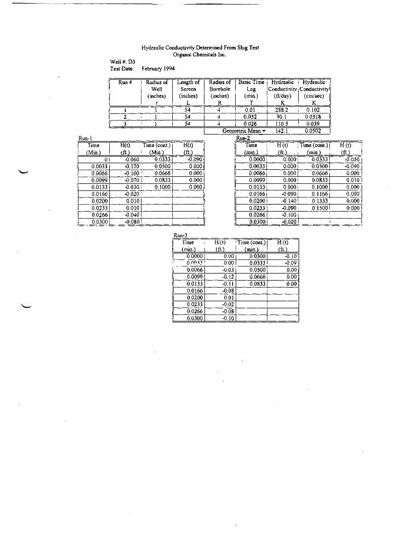
Well #: D3Test Date:
Hydraulic Conductivity Determined From Slug TestOrganic Chemicals Inc.
February 1994
Run-1
Run*
12
Radius ofWell
(inches)
Length ofScreen
(inches)r L11
54
Radius ofBorehole(inches)
R4
Basic TimeLag
(min.)
HvdraulicConductivity
(ft/day)T K
0.0154 | 4 ; 0.032
3 1 I 54 | 4 | 0.026
288.290.1110.5
| Geometric Mean = 142. 1
HydraulicConductivity
(cm/sec)K !
0.102 i0.0318 j0.0390.0502
Run-2Time(Min.)
00.00330.00660.00990.01330.01660.02000.02330.02660.0300
H(t)(ft.)-0.060-0.170
Time (cont.)(Min.)0.03330.0500
-0.1001 0.0666-0.070 1 0.0833-0.030: 0.1000-0.0200.0100.010 i-0.040 1-0.080
H(t) ;(ft.) :-0.090 >o.ooojO.OOOi0.000 1O.OOOi
1 !
Run-3Time(min.)0.0000o oo:<30.00660.00990.01330.01660.02000.02330.02660.0300
H/(0(ft.)
0.000.00-0.03-0.12-0.11-0.080.01-0.02-0.08-0.10
Time (cont.)Imin.)0.03000.03330.05000.06660.0833
H/(t) |(ft.) \
-0.10 i-0.09'0.00 jo.oo|o.oo i
Time{min.)
H(t)(ft.)
Time (cont.)(min.)
0.00001 0.000 1 0.03330.00330.00660.0099
0.0000.000
0.05000.0666
0.000 i 0.08330.0133 1 0.0000.0166 -0.090
0.10000.1166
0.02001 -0.140] 0.13330.02330.0266
-0.090-0.100
0.0300 1 -0.020
0.1500
H(t)(ft.)
-0.050:-0.0900.0000.010'0.000 i0.0000.000 '0.000

o.i
Piezometric Head Ratio vs. TimeField Slug Test D3 Run 1 Organic Chemicals Inc. February 1994
0.01 0.02Time (Min.)
0.03
0.1
Piezometric Head Ratio vs. TimeField Slug Test D3 Rurr 2 Organic Chemicals Inc. February 1994
0.02 0.04Time (Min.)
0.06 0.08
Piezometric Head Ratio vs. TimeField Slug Test D3 Run 3 Organic Chemicals hie. February 1994
oMM
I
OiT3
0.10.005 0.01 0.015 0.01
Time (Min.)0.025
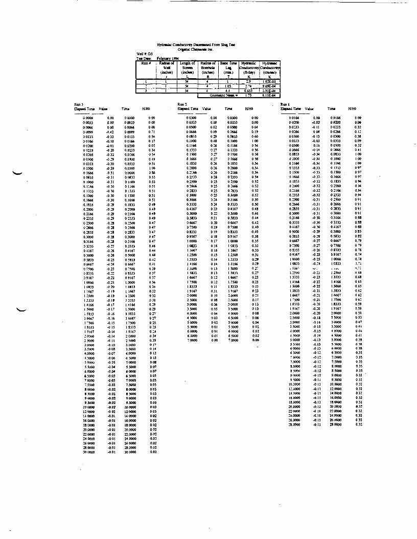
Hydnulk Conductivity Dtunramd From Slug TMOnjBUC Chtmicilt Inc.
Wdl«' DiTen Par. Ftbnarvl»4
Ron'
12 '
Roliui ofWdl
(iocha)r11
3 i 1
Length ofScntn(inch-)
L5454
RidiuiofBcnhoU(incha)
R44
B«BC linnL«l
(mm.)T1
1.0554 1 4 1 44
HydnulicConductivity
«Wiy)K
1»2 T4
0.653
HjdnubcConducnWy
(CIU/MC)K---
I.02E4)969E-042.31E-04
|_ Geomanc Mm - 17] 6] IE-04
Run 3EaepeedTime
00000000330006600099001330.0166002000.023300266003000033)0030000«660.08)30 10000.11660 133)0 150001666O.IS))0.20000216602333025000266602333030000)166033330416705000053330.66670.7500033330.91671.00001.08331.16671.250013333141661500015333166671 "50013)331 91672.000025000JOOOO350004.00004 5000500005500060000650007.00007.500030000J50009000095000
10000012000014000016000018000020.000022.000024.000026000023.0000300000
Vilue
0.000.00000
•0.42-033-010-001-020-032•029-030-059-051-031-031-030-030-O.)0-030-02S-029-0.29429-0.2S•028•0.28-028•0.28-027-026-026-025-024-0.2)-0.22•0.22-021420•0.19•0 19-018417-0.17-0 16•0.16-0 IS-015-0 14-0 14-0 II-0.10-0084.074064054044.044.03-0.0)-0.0)4.014.024.024.024024024.014014014014.01-0014.014.014.01
Time
00000000))0006600099001))001660.02000.02))0.02660.0)0000)))0050000666008))01000011660 13330 15000.16660133)02000021660.23330.250002666028330300003166033)30.416705000058330.666707500OS)))09167100001.08331 16671 25001 3333141661 5000153331.666717500183331 916720000250003000035000400004 5000SOOOO5500060000650007.00007.50008.0000850009000093000
10000011000014000016000018000020000022.000024000026000028.000030.0000
HHO
0000.000000.710.560.170.020340540490511000360.530530510510.510.510490490490490470470470470470.460.440440.420.410390.370370.360340320320)10290290.270270230250240.240.190.170140120 100080.070.070030.050.050.0)00)0030.0)00)0030020020020.020.020.020.020.02002
Run 2ElapMdTimt
00300003330.0500006660.08330.10000 116601333015000166601333020000.21660233302500026660.23330)00003166033330416705000058330666707500033)3091671.0000108331.16671.25001.33331.41661.5000158331666717500183331916720000250003.0000350004.0000450005000055000600006.50007.0000
Value
0.000.000.020.090.290480260270.270.270260260260260.250250230230240240230 220210200.19019018
' 0.170160 16O.IS0 140.140130.1)0120.120 110.110 100030.060.0500400)0020010010.01000
Time
003000.03M005000.06660.08330 10000.1166013330.15000.16660183302000021660233)025000266602333030000316603)3)0416705000053)30.66670.75000.8)3)09167100001083)1 16671.2500133331.4166150001 533)166671750013333191672.00002500030000350004000045000SOOOO55000.60000650007.0000
two0000.000040190601000540.560560.560.540540540340520.520520.520500500430460.440420.40•0.400.380.350.330330)10.290.29OJT0270.230.250.230230.210.170.130 100030060040020.020020.00
0016600200002))002660030000333005000.06640.03330100001166013330 1300016660133)0200002166023))0230002666023))030000.3164033330.4167050000383)0666707500OS)))091671000010833, J56V1.25001.3)))141661500015335166671.75001333319167200002.50003000035000400004500050000550006000065000'00007.5000SOOOO350009000095000
10000012.000014000016000013000020000022.00002400002600003.0000
0004.024 11004413403on4 14-034-0344.J44.334334.33432-0324.)24324.314314.31431-O.JO-O.JO-030-029423•0.274.274264.25425421-V.-
423423422422421-021-0.21-0204.204.204 13416-0154 154.144.134.13413412412-0.12-0.12-0 124.124.114114.114.114.114.114.114.114114.1]411
00166002000023)0026600300003))00500006660.08))0 10000 116601)))013000 1666018)302000021660233302500026660283)030000316603)33041670.500005333066670.75000833309167100001C3331 tv.
1 2300133331416615000153)3166671.75001.83)31.9167100002500030000350004.000045000500005500060000650007.00007.50008.00008.50009000095000
10.000012000014.000016.000013000020.000022.000024.000026000023.0000
0000.060320 120.380090320 4 11001 001000970.970.970940.940.940940.910910910910880880330.350320.790.790760.740.743.71•1.7;0.6S0.630650630620620620590590590.530470440440410330380380350350350350350350320320320320320320320)20)20320.32
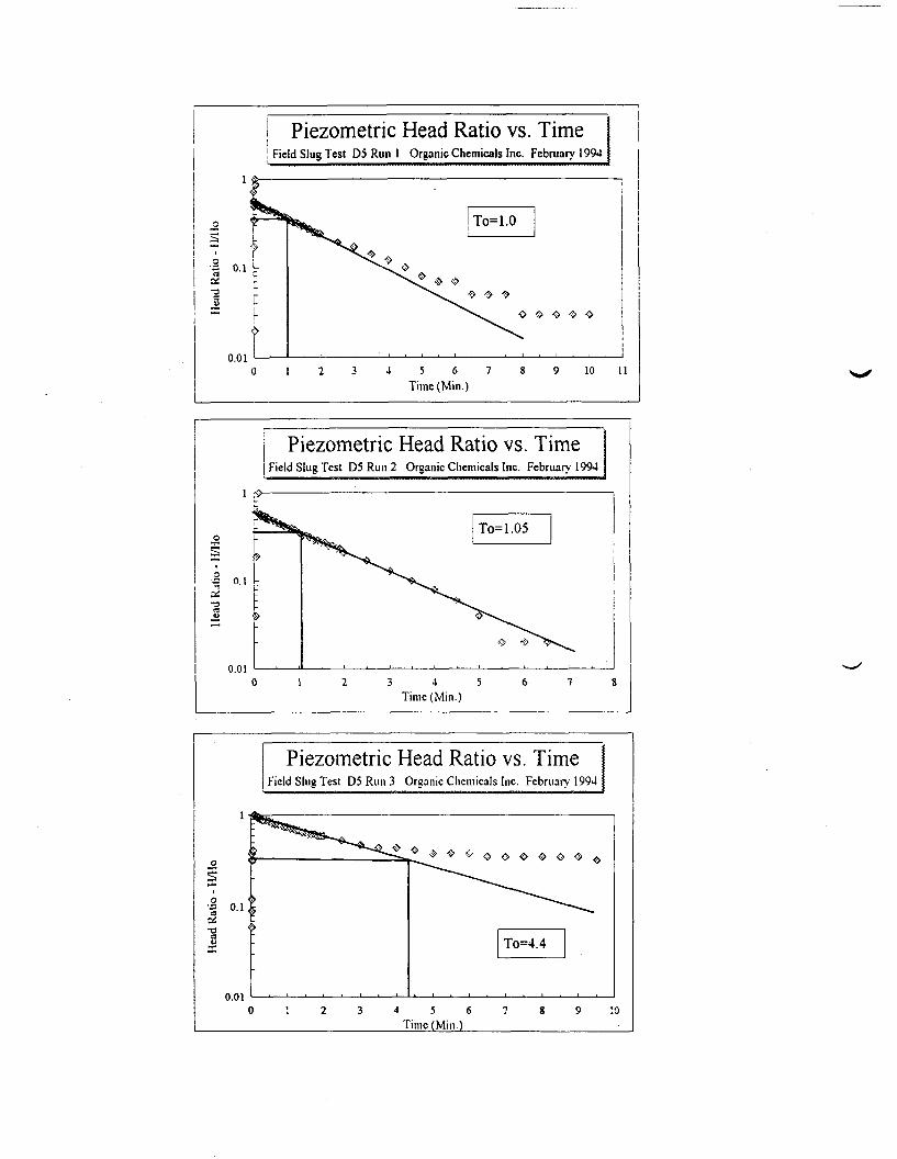
Piezometric Head Ratio vs. Time |i II Field Slug Test D5 Run 1 Organic Chemicals Inc. February 1994 ]
2 3 4 5 6 7 8 9 1 0 1 10.01
0 1
Piezometric Head Ratio vs. TimeField Slug Test D5 Run 2 Organic Chemicals Inc. February 1994
0.012 3 4 5
Time (Min.)6 7
Piezometric Head Ratio vs. TimeField Slug Test D 5 R u u 3 Organic Chemicals Inc. February 1994
0.012 3 4 5 6
__________Time (Min.)8 9 10

APPENDIX K
GROUNDWATER CONTAMINANT ISOPLETH ASSUMPTIONS

APPENDIX K
GROUNDWATER CONTAMINANT ISOPLETH ASSUMPTIONS
The 1989 and 1993 groundwater conditions were represented on Figures 4-1, 4-2, 4-5and 4-6, respectively, using contaminant isopleths. Contaminant isopleths were drawn usingSURFER, Version 4.14, by Golden Software, Inc., Golden, Colorado. The following data-specific assumptions were made to draw the contaminant isopleths:
1) total chlorinated VOCs were contoured in Figures 4-1 and 4-5; total VOCswere contoured in Figures 4-2 and 4-6;
2) VOCs at each well location were assumed to be equal to theaverage of round 1 and 2 data;
3) contours are based solely on data collected from UGS monitoring wells,and;
4) data qualified "j" were assumed to be positive "hits".The following model-specific assumptions were made to draw the contaminant isopleth
contours:1) the kriging data interpolation method was employed;2) a grid density of 50 x 50 was employed;3) topographic contour levels of 10 (figures 4-1 and 4-5 only), 100, 1,000 and
10,000 ug/L were employed, and;4) contour lines were "smoothed".
Additional assumptions were made to the data set in order to create the contaminantisopleth contours. In instances where two UGS wells occured at the same location, thegroundwater concentrations from both wells and both sampling rounds were averaged. Forexample, in the case of the the groundwater concentration used to represent Phase 1 totalVOCs at MW-l/MW-2, (i.e., 41,603 ug/L, see Figure 4-2), the following values wereaveraged: 15,310 ug/L, 44,057 ug/L, 91,900 ug/L, and 15,146 ug/L. Monitoring wells MW-14, MW-15, MW-16, MW-32, and MW-33 were assumed to have been impacted by sourcesother than the OCI site, and therefore were not used to draw contaminant isopleths.
Chloromethane (320 ug/L) detected in MW-25 during phase 2, round 1 sampling wasassumed not to represent true conditions. At MW-25, chloromethane was the onlycontaminant detected in round 1 sampling, and there were no contaminants detected in round2 sampling. Additional information regarding the occurence of chloromethane was discussedin Section 4.2.1.
Volinated chlorinated hydrocarbons were determined by determining the sum of thefollowing compounds: chloroform, chlorobenzene, 1,1-dichloroethene, 1,1-dichloroethane,1,2-dichloroethene (total), 1,2-dichloropropane, methylene chloride, tetrachloroethene,trichloroethene, 1,1,1-trichloroethane, 1,1,2-trichloroethane, vinyl chloride.
Using these assumptions and the input data presented in Tables K-l, K-2, K-3, and K-4, the contaminant isopleths presented in Figures 4-1, 4-2, 4-5, and 4-6, were generated.
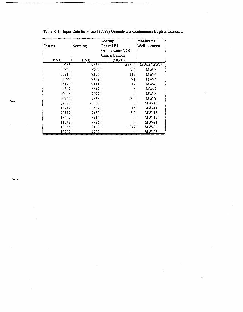
Table K-l. Input Data for Phase I (1989) Groundwater Contaminant Isopletll Contours.
Easting
(feet)119581182011710118991212611302109081095511320122121011212547119411206512252
Northing
(feet)92738909935598129781827290979733
115031051294508915893591979452
AveragePhase I RIGroundwater VOCConcentrations
(UG/L)41603
7.5142911269
3.50
153.5
44
. 2424
MonitoringWell Location
MW-l/MW-2 iMW-3MW-4MW-5 jMW-6MW-7MW-8 ;MW-9
MW-10MW-11 iMW-13MW-17MW-21MW-22MW-23 '

Table K-2. Input Data for Phase II (1993) Groundwater Contaminant Isopleth Contours.
Easting
(feet)11958118201189911302109081095511320101121254711941120651207212398122541170012128122171163811732
Northing
(feet)928689099812827290979733
11503945089158935919799969369945593199775
105051041511116
AveragePhase II RIGroundwater VOCConcentrations
(UG/L)766.5
02702
4.51.5
00.52.5
114.548.5
07.8
1370.513.8
506
MonitoringWell Location
iiMW-l/MW-2
MW-3MW-5MW-7MW-8MW-9MW-10MW-13MW-17MW-21MW-22MW-24MW-25
MW-26/MW-23MW-27/MW-4MW-28/MW-6
MW-29/MW-11MW-30MW-31

Table K-3. Input Data for Phase I (1989) Volatile ChlorinatedOrganic Groundwater Contaminant Isopleth Contours.
Easting
(feet)I 11958
1182011710118991212611302109081095511320122121011212547119411206512252
Northing
(feet)92738909935598129781827290979733
115031051294508915893591979452
AveragePhase I RIGroundwater VOCConcentrations
(UG/L)18667
7.525.5
178.5
69.53.5
012
3.54
4.5212.5
4
MonitoringWell Location i
i
MW-l/MW-2 jMW-3MW-4MW-5 iMW-6MW-7MW-8MW-9
MW-10MW-11MW-13MW-17 IMW-21MW-22 IMW-23

Table K-4. Input Data for Phase II (1993) Volatile ChlorinatedOrganic Groundwater Contaminant Isopleth Contours.
Easting
(feet)11958118201189911302109081095511320101121254711941120651207212398122541170012128122171163811732
Northing
(feet)928689099812827290979733
11503945089158935919799969369945593199775
105051041511116
AveragePhase II RIGroundwater VOCConcentrations
(UG/L)3700.53.5
00.51.51.5
00
0.5205
403
3210300
MonitoringWell Location
MW-l/MW-2MW-3MW-5MW-7MW-8MW-9
MW-10MW-13MW-17MW-21MW-22MW-24MW-25
MW-26/MW-23MW-27/MW-4MW-28/MW-6 iMW-29/MW-11
MW-30MW-31
APPENDIX L
BACKGROUND SOIL CONCENTRATION CALCULATIONS

Background Inorganic Concentrations in Site Soils
PURPOSE:This documentation outlines the procedures for determining background metalsconcentrations of soils found at OCI. All samples were reviewed for qualifying asbackground samples appear in Tables I and II. Table I lists surface soil samples (0-2 ft)by soil type(s). Table II lists subsurface soil samples (>2 ft) also by the soil type(s)found within a 2 ft sampling interval.
CONDITIONS FOR BACKGROUND:In order for a sample to qualify as a background, the sample must meet the followingconditions: TIC levels for volatiles must be less than 100 and for semivolatiles, less than5000.
Qualifying soil samples are then categorized based on their primary constituents. Soiltypes were grouped under one of three categories; gravel, sand/silt, and clay. Thecategories include:
Gravel Sand ClayGravel* Sand. ClaySandy gravel Silty sand Sandy clay*Silty gravel* Clayey sand Silty clay
Silt* Gravelly clay*Clayey siltSilty cinder*
Note: Soil types labeled (*) did not have samples which were qualified as backgroundsbut are to be considered a part of the category under which it appears.
STATISTICAL ANALYSIS:Four samples were selected from each class to satisfy the minimum number of samplesrequired by the MDNR (1) (see attached sheets). A statistical analysis of the metalsconcentrations for each category determined a mean, standard deviation, and coefficientof variance (c.v) for each target metal. The data is provided on Tables III-V. Note thatfor non-detected metals (those not shaded), the reportedconcentrations were divided inhalf.
For metals with a c.v.>0.50, the samples were screened for outliers. For gravel (TableIII), cadmium was found to have c.v.=0.58. However, SS-35 will not be considered anoutlier since all values for cadmium were non-detects. For sand (Table IV), potassiumhas a c.v.=0.59. Rather than labeling SB-46J an outlier, the MDNR guidelinesrecommend that the background concentration for potassium in sand be defaulted to thepotassium concentration in gravel, thereby using a more conservative estimate.
Background concentrations are taken to be the sum of the mean and 3 times the

standard deviation.
References: 1. MDNR, April 1994, "Guidance Document for Verification of SoilRemediation", pp. 5-8.

Table I
S...4.SB-JSASB-)]SB-14SB-25SB- 26SB-JJSB- 36SB-J7SB-38SB-43SB-44SB-4)SB-ItSB-49SB-52SB-55SB- 54SB-5'SB-51SB- 59MW-33
Sa.pl.SB- 15SB-ISSB-60
Sa.pl.SS-JISS-40SS-59SS-61SS-«7SS-6«SS-'5SS-81SS-94SS-97SS-103
Sa.pl.SS-JISS--8SS-85SS-105MW-32MW-35
S.mpl.SS-!3SS-43SS-51SS-J3SS-6J55-66SS-16SS-8TSS-MSS-99S3- 109SB-24MW-29MW-37MW-40
Sa.pl.SS-40SS-91
Sa.pl.SS-93SB-34
literal0-20-20-20-20-20-20-20-20-20-20-20-20-20-20-20-20-20-20-20-20-2
laural0-20-20-2
laural0-20-J0-20-20-20-20-20-20-20-20-2
[•Ural0-20-20-20-20-20-2
l.lerval0-20-20-20-20-20-20-20-20-20-20-20-20-20-20-2
l.ural0-20-2
liural0-20-2
SoilTyptClayey SandClavavauidClayey MildClayey MildClayey ModClayey landClayey MndClayey MndClayey MndClayey MfidClayey MndClayey MndClayey andClayey amdClayey MndClayey MndClayey emdClayey MndClayey MndCliyryaudClayey and
Soil Typ.Clayey nitCUyry nilCUyry nil
Soil Typ.Gravelly nkGravdlynltGravelly nkGnvclly nitOnvelly nilOnvelly nilGravelly nitGravelly nitGravelly nitGnvetty nitGnveUynk
Soil Typ.SuidSandSandSandSandSand
Soil Typ.Sandy nitSandy nilSandy nUSandy nilSandy MlSandy nkSandva*Sandy «HSandy nkSandy nkSandy nkSandy nkSandy.*Sandy a*Sandy nh
SollTyp.sikSik
Soil Typ.Sandy claySandy day
So.ptoSB-30
SanptoSB-13SB-20SB-22MU'-SI
SaaipteSB-27SB-28
SaaipteSB-53
SaaiptoMW-3«AM1ft'-3-AMW-34ASS-32SS-38SS-45SS-74SS-77SS-79SS-95SS-96SS-I2ISB-41MW-24MW-25MW-2SMW-34MW-W
S..p4.SS-106MW-26
SaaiptaM'*-30MW-39
SaaipleSS-44SS-S2SS-6JSS-110
SaaptaSB-11
Suipt.SB- 16
Sa.pl.SB-33SB-54
lalarval0-2
lalcrval0-20-20-20-2
lateral0-20-2
laUral0-2
lateral0-20-20-20-20-20-20-20-20-20-20-20-20-20-20-20-20-20-2
lateral0-20-2
Interval0-20-2
Interval0-20-20-20-2
[atervaJ0-2
[•larval0-2
lateral0-20-2
Soil TypeClayey •andinveUy and
SoMTyp.Clayey nllanveUy MndClayey nit invtlly MadClayey nltgnvelly aindClayey nit gravelly faad
SoMTyp.Sandy clay pivelly MndSandy claygraveUy Mnd
SoUTyp.Silly clay/Mndy gnvd
SoilTyp.SilrySandSdtySandSilrySandSdtvnudSilly MndSilrynuidSdtynndSdtynndSilrvrandSdtyMndSdry andSilrvnuidSUryMndSUrynuidSUty MndSdry MndSilly MndSdry Mnd
Soil TypeSdry gravelSilty grave!
Soil TypeSdt) claySdry clay
S«ilTyp.Sdry cinderSdry cinderSdry cinderSdtyonder
SoilTyp.Silly cl>y<nwd
Soil Typ.Silly clay/day
Soil Typ.Clayey Mnd MndClayey MndfMnd
SaaipteSS-47SS-41SS-50SS-55SS-56SS-6JSS-64SS-69SS-71SS-72SS-7JSS-S2SS-91SS-92SS-102SS-107SS-108ss-n:SS-II3SS-114SS-116SS-117SS-111SS-119SS-120SS-122SS-124SS-125SB-17SB-19SB-21SB-23SB-31SB-32SB-39SB-40SB-41SB-46SB-47SB- SOSB-51MW-27MW-42
Sa.pl.SB-2-ASB-28ASB-39ASB-40ASB-46ASS-27SS-2SSS-29SS-30SS-34SS-33SS-36SS-37SS-42SS-46SS-49SS-S4SS-57SS-58SS-70SS-80ss-uSS-S9SS-MSS-IOOSS-IOISS-104SS-111SS-II5SS-123SB-29MW-31
lalerval0-20-20-20-20-20-20-20-20-20-20-20-20-20-20-20-20-20-20-20-20-20-20-20-20-20-20-20-20-20-20-20-20-20-20-20-20-20-20-20-20-20-20-2
laural0-20-20-20-20-20-20-20-20-20-20-20-20-20-20-20-20-20-20-20-20-20-20-20-20-20-20-20-20-20-20-20-2
SollTyp.Cranny MndOnvelly MndGnvellyMndOnveily MndGnvdly MndGnv.dyMndGravelly .andGravelly MndGnvelry MndGrav.Uy anidGravelly MndGnvellyMndOnveUyMndOnvelly MndOnveUyMndGnvcUy MndOnvelly MndGnveUyMBdOnveDyModGnveOy andOnvelly MndGnveUy andOnvelly MndGnvelry MndOnvedyaandGnvellyMndGnveUy MndGravelly MndGnvellyaandGnvellyMndGnveUy MndGnveUy MndGnveUy eand.Gnvetty aahdGnvellyMndGnvelry MndGnvetty MndOnvelly MndGravely MndOraveflyMndOnveUyMndOravelryMndOnveUytand
Soil Typ.Sandy OnvriSandy GravelSandy OnvdSandy OnvdSandy OnvdSandy OnvdSandy GravelSandy OnvdSandy OnvdSandy OravdSandy OnvdSandy GnvdSandy GravdSandy OnvdSandy OnvdSandy GravelSandy OnvdSandy GravdSandy OnvdSandy OnvdSandy OnvdSandy OnvdSandy travdSandNinvdSandy jnvdSandy (ravdSandy $nvdSandvgnvdSandy travdSandy aravdSandy tnvdSandy nmvd

Table II
SampleSB-UKSB-::FSB-:JJSB-36QSB-44QSB-60SD-2Q
SamptoSB-S6BSB-3"CSB-J8BSB-59CSB-59D
SampleSB-I5BSB-JIMSB-39FSB-401
SampleSB-44M
SampleSB-5"Q
SampleSB-JJHSB-590SB-4 INSB- WOMW-S4PMW-S5NMW.J8GMW-39KMW-420
Sempl.SB-4 IKSB-S3L
SmmfttSB-:.MSB-48T
SampleSB-4:0
SampleSB-53R
literal20-2210-1218-2032-3432-3436-3832-34
Interval2-44-62-44-46-8lateral2-424-2610-1216-U
lalerval24-26
lateral32-J4
Iiltml14-1612-1426-2128-3030-322«-2I12-1420-222»-30
lateral20-22::-24
[alerval16-1138-40
lalervel28-30
lateral34-36
SollTvp.ClayCayClayClay0«yClayCtay
SollTyp.Clayey tandClayry eindClayey andClayey andClayey and
Soil TypaClayey «UClayey nitClayey nitClayey alt
Sail TypaGnvtt
Soil TyptSand Clay
Soil TyptSUty claySiliyclaySilly claySUty claySdiyclaySJiy claySilly clayStltyclaySdiyclay
MITyp*Sdtv>andSiltynnd
Soil TypeSUty clay''claySilty clayclay
SollTyp.Sand nllv clay
Soil TypeSilly rand'nn
SanpkiSB-338SB-56DSB-58CSB-39B
SampleSB-2"D
StmfttSB-I7HSB-28E
Sa.plaSB-41 H
SampleVTW-40E
SampleSB-43 M
SampleSB-1 1CSB-351SB-3TNSB-461SB-46JSB-49CSB-49DSB-52MSB-52PSB-S4BSB-54CSB-540D-2MD-30MW-36K
SampleMW-36S
SampleSB-26HSB-301SB-331
SampleSB-31M
SampleSB- JOE
SampleMW-J3D
lalerval2-46-14-62-4
lateral6-8
lateral14-168-10
laienal14-16
lalenal8-10
lalerval24-26
Interval4-«18-2026-2816-1818-204-6M2)-2630-322-44-66-824-2628-3020-22
laienal36-38
Interval14-16I6-1J16-18
Ulerval24-26
lalerval8-10
lateral6-8
Soil TypeClayey MfioVgravelly tendClaye>- mnd'iravelly nndClayey e«nd envclly midClayey eand gravelly and
SollTyp.Gravelly eaad'clayey nh
Soil 1^Gnvelly land ally clayGravelly eaiHinlty clay
SollTyp.Gravelly md/iiny aand
Soil TypeSandy BiveLfnvclly and
SoilT^Sandy anveUHydav
Soil TypeSandSandSandSandSandSandSandSandSandSandSandSandSandSandSand
Soil TypeSilly rand nlry clay
Soil TypeSandy gravel claySandy gravel'claySandy Bavel clay
S4ITypeSilty clay/oil
Soil TypeSand/anveOy eand
SoilT>TXlSaKiMDdyclav
Sampl.SB-38J
literal18-20
SallTyp.
SampleSB-49B
SampleSB-32L
SampleSB- 138SB-I3HSB-131SB-15ESB-I6HSB-161SB-I7DSB- ISOSB-I8HSB-19ESB-20KSB-2 1CSB-210SB-22BSB-23ESB- 230SB-25CSB-2TCSB-28CSB-340SB-45HSB-4"HSB-50HSB-310SB-S5CSB-!?DSB- 580SB-40OMW-40F
SampleSB- 18kSB- 190SB-I9HSB-38KD-4NMW-40H
SampleSB-45N
SampleSB-36N
SampleSB-IDSB-26DSB-32ESB-33HSB-400SB-43HSB-48M0-4FMW.34HMW-J5KMW-38OMW-39EMW-J9FMW-420
laurvml2-4
lalerval22-24
lateral2-414-1616-188-1014-1616-186-812-1414-168-1020-224-6.12-142-48-1012-144-64-64-66-414-1614-1614-1612-144-66-*6-82S-3010-12
lateral20-226414-1620-2226-2814-16
Interval26-28
lalerval26-28
lalerval18-20648-1014-1612-1414-1624-2610-1214-1620-226-88-1010-1212-14
SollTyp.Clayey (and eand
Soil TypeGravelly day/day
SollTyp.OnvellymndGravelly andGravelly eandGravelly eandGravelly mdGravelly HndGravelly eaadGravelly mndGravelly HndGravelly eandGraveUvaandGravelly HndGravelly andGravelly andGravelly andGravelly eandGravelly HndGravelly randGravelly HndGravelly andGravelly HndGraveBy .andGravelly emdGravelly endGravelly andGnveUyHndGravelly .andGravelly HndGravelly end
Soil TypeGravelly eand>cJayGravelly mnaVdeyGravelly md/dayGravelly end/clayGravelly Hud/clayGravelly rand/day
Soil TypeGravelly and/and
SollTyp.Gravel' eandy clay
Soil TypeSandy Grave)Sandy gravelSandy fjavrtSandy (ravelSandy envelSandy gravelSaady grave*Sandy gravelSandy gravelSandy gravrfSandy gravelSandy grantSndygnvalSandy gravel

Table HI
Soil Type: GravelOCI Sample No.: SS-35 SS-54 SS-101 SS-111 Mean Std Dcv. 3*Std.Dev. Co. Var. HACK.GROUND
AluminumAntimonyArsenicBariumBerylliumCadmiumCalciumChromiumCobaltCopperIronLeadMagnesiumManganeseMercuryNickelPotassiumSeleniumSilverSodiumThalliumVanadiumZincCyanide
31802751.714
011044
5000011.13
916370182
15700175
0055582030.330.3391.30.119.93610275
47602829228
01250125713001063.120212400243122003090065.5560
02450.245
92012518434.60305
3910263
2560115011556400
9 72911.5
9610416
29400237
005552496
02250225152
011513
5240285
3530252.416.70110.11
1160008.92.49.8
649024419800165
005562689
0.2150.215118
0.1112.834.7027
3845.002.662.50
19.780 120.20
73425.0010.08
2.851265
8717.5027.13
19275.00221 50
0.065.68
487.000.250.25
113.330.12
13.5339.45
0.28
587980.120.514.630.010.14
25766.880.840.274.45
2491.488.73
6434.8257.56
0.000.37
178090.050.05
24.790.013.077.500.01
1763.950361.54
13900.020.42
77300.632.530.81
13.347474.44
26.181930445
172.670.011.11
534.280 140.14
74.360.029.21
22.500.04
0 150.040.210230050.710.350.080.090.350290.320.330260.040.070.370.180.180.220050.230.190.05
560903.040
3370.13062
150725.612.63.7
26.016191 9
533385795
394200668
1021 3039039
187.70 1322762.00.32

Table IV
Soil Type: SandOCI Sample No.:
AluminumAntimonyArsenicBariumBerylliumCadmiumCalciumChromiumCobaltCopperIronLeadMagnesiumManganeseMercuryNickelPotassiumSeleniumSilverSodiumThalliumVanadiumZincCyanide
SB-I9A
36601.93226.40.14016
327001273.712
76608.9
13200230
00259.34030.320.4
60.902514.723.30255
SB-46J
57601.75
3.841.8027
0.1654980013.74.7106
103007.1
207002210.0813.413500.360.371260.2813.221
0.27
SB-19D
4650
19
2.532.70.250.18
189008.44
6.989509.1
78101710088.1495
034504167
0.2751430
0.28
MW-36S
2440
205
19
179
03019547500
5.7185.5
516034
202001350.085.14210.370.4351150.2910
11.40.3
Mean
4127.501.902 85
29.700.240.18
37225.0010.133.558.75
8067507.13
15477.5018925
0.078.98
667.250.350.40
117.230.27
12.9821.430.28
Sld. Dev.
1225.180.110.728.740.060.01
12449773.241.072.64
188809229
5328.0938,550.022.98
395.690.020.02
37.860.011.806.670.02
3*Sld.Dev.
3675.540.322.15
26.220.180.03
37349.329.723.227.93
5664.266.86
15984.26115.65
0.078.93
1187.070.060.07
113.570.045.39
20.000.05
Co. Var
0300060.250.290.250060330320.300300.230320.340200.360.330590.050060.320.050 140.310.06
Background
7803.042.22500
55.92042021
74574.321984677
16.6813731.76
139931461 76
304900.14
17.91185432
0410.47
23079032
18.374142033
c

c
Table V
Soil Type: Clay
OCI Sample No.:
AluminumAntimonyArsenicBariumBerylliumCadmiumCalciumChromiumCobaltCopperIronLeadMagnesiumManganeseMercuryNickelPotassiumSeleniumSilverSodiumThalliumVanadiumZincCyanide
SB-500
7300
21
5.1699
038
016
56300
12768134
14100
59
19800
254
003
1S6
1790
0325
0375
172
03
162
306
029
MW-36S
2440
205
1 9
179
03
0195
47500
67
18
55
5160
34
20200
135
008
51
421
037
0435
115
029
10
114
03
SB-.18K
10100
1 9
38
685
039
018
81400
17 3
82
156
16400
76
33200
329
003
197
2080
0365
0405
193
0155
237
379
0275
SB-24H
8190
2
37
632
05
0 19
79600
156
74
14
14300
78
32800
320
008
174
1660
036
0425
204
0285
206
335
0275
Mean
9 1 45.001.953.75
65.850450 19
805000016.45
7.801480
15350.00770
33000.00324.50
0.0618.55
1870.000360.42
198.500.22
22.1535.70
0.28
Std Dcv.
955.000.050052.65006().(K)
900.000.850.400.80
1050.000.10
200.004.500.031 15
210.000.000.015.500.071.552.200.00
3*Std.Dev.
2865.000 150 157.950.17001
2700.002.551.202.40
3150.000.30
600.001350
0.083.45
630.000010.03
16.500204.656.600.00
Co Var.
0.100.030.010.040.120.030010.050050050.070.010.010.010450.060. 1 10.010.020.030.300.070060.00
BACKGROUND
1201000210390
7380061020
83200.001900900
172018500.00
8003360000
33800013
22.00250000
0.37045
21500042
26804230028

MICHIGAN DEPARTMENT OF NATURAL RESOURCES
GUIDANCE DOCUMENT FOR VERIFICATION OF SOIL REMEDIATION
EXECUTIVE SUMMARY
The document provides guidance for sampling soils to verify that soilcontamination has been remediated to Type A or Type B criteria in accordancewith Act 307 P.A. 1982, as amended. This document is not designed to eitherguide investigations to determine whether a release has occurred or the natureand extent of an identified release, nor to guide due diligence by a potentialproperty owner.
Soil sampling and analyses to verify that site remediation is complete canresult in two basic errors.
• Declaring a site clean when it is contaminated
• Declaring a site contaminated when it is clean
A soil sampling plan submitted to the DNR must minimize these errors. Theguidance document presents acceptable methods for verifying soil remediation.It contains guidance on soil sampling protocols and documentation necessary tocharacterize and verify cleanup of contaminated soils. The document providesrecommended procedures for establishing soil background concentrations,sampling grids, chemical constituent evaluations, statistical comparisons,verifying excavation and in-situ and ex-situ remedies, evaluating treatedsoils, and soil characterization. The recommended procedures are notabsolutes. Other methods are available to verify soil remediation. TheDepartment of Natural Resources will evaluate other sampling and statisticalstrategies on a case-by-case basis.
The guidance document is divided into two parts:
Part 1 contains guidance for small site cleanup verification (less than10,890 square feet—<.25 acre). It is a "biased" sampling strategyrecommending soil sampling from areas most likely to contain contamination.
Part 2 contains guidance for soil characterization and cleanup verificationof medium and large sites (greater than 10,890 square feet—>.2S acre).It is a statistical random sampling strategy that minimizes biases insampling.
Both sampling strategies require discrete soil samples. Compositing samplesfor cleanup verification is not accepted without prior DNR approval.
The guidance document contains verification checklists and reporting sections.The reporting sections should be carefully followed in reporting samplingrationale.
Reader's Note: Questions regarding this guidance document should be directedto Department staff you are currently working with for your project or site.
APRIL 94

ATTACHMENTS-DNR GUIDANCE DOCUMENT
VERIFICATION OF SOIL REMEDIATION
attachment attachment page /
1 Guide to Sample Bias . . . . . . . . . . . . . . . . . . . . 21-22
2 Sampling Protocol for CharacterizingWaste/Treatment Levels . . . . . . . . . . . . . . . . . . . 23-36
Strategies for Evaluating TreatedSoils and Waste Materials . . . . . . . . . . . . . . . . . 23
Statistical Sampling Strategies . . . . . . . . . . . . . . 24
Random Numbers Table . . . . . . . . . . . . . . . . . . . . 25
Sampling Grids . . . . . . . . . . . . . . . . . . . . . . . 26
Statistical Evaluation of Waste/Treatment CharacterizationSamplings . . . . . . . . . . . . . . . . . . . . . . . 27-29
Example:Calculation of Confidence Limits & Lamda Calculation . . 30-32
Table: Cumulative t Distribution . . . . . . . . . . . . . 33
Table: Number of Observations for t test of Mean . . . . . 34
Sampling Process Streams . . . . . . . . . . . . . . . . . . 35
Random Time Waste Sampling Example . . . . . . . . . . . . . 36
3 Tolerance Factors (K)[NTIS Document PB-89-151-047, Table 5] . . . . . . . . . . . . . 37
4 Waste Management Division'sClean Closure Certification Checklist . . . . . . . . . . . 38-39

TABLE OF CONTENTS-DNR GUIDANCE DOCUMENTVERIFICATION OF SOIL REMEDIATION
PARS 1—Small Site Soil Cleanup Verification, Introduction ...... 1
Verifying Excavation Remedies . . . . . . . . . . . . . . . . . . 2-4Sample Locations . . . . . . . . . . . . . . . . . . . . . . . . 2Number of Samples ...................... 3-4Number of Sxca.va.tion Floor Samples . . . . . . . . . . . . . . 3Kumher of Excavation Sidevall Samples . . . . . . . . . . . 3-4
Verifying In-Situ and Ex-Situ Soil Remedies . . . . . . . . . . . . 4
Background Soil Samples . . . . . . . . . . . . . . . . . . . . . 5-8Establishing Soil Background . . . . . . . . . . . . . . . . . . 5Statistical Analysis for Establishing Background Concentrations 6-31. Mean Plus 3 Standard Deviation Approach . . . . . . . . . 6-72. Other Statistical Procedures for Establishing Background . . 8Procedures for Nan-Detect Values . . . . . . . . . . . . . . . . 8
Report for Small Site Verification . . . . . . . . . . . . . . . . 9
PART 2—Medium and Large Site Soil Cleanup Verification, Introduction . . 10
Establishing Grid Interval . . . . . . . . . . . . . . . . 11-141. Basic Strategies . . . . . . . . . . . . . . . . . . . . 11-122. Setting the Grid . . . . . . . . . . . . . . . . . . . . . . 123. Variations on Basic Strategy . . . . . . . . . . . . . . 13-14Sampling of Grid . . . . . . . . . . . . . . . . . . . . . . . . 14
Establishing Soil Background . . .............. 14-15
Statistical Analysis for Establishing Background Concentrations 15-181. Meaji Plus 3 Standard Deviation Approach . . . . . . . . 15-172. Tolerance limit . . . . . . . . . . . . . . . . . . . . . . 173. t-tests . . . . . . . . . . . . . . . . . . . . . . . . . . 184. Other Statistical Procedures for Establishing Background . . 18
Procedures for Non-Detect Values . . . . . . . . . . . . . . . . 18
Statistical Evaluation of Data . . . . . . . . . . . . . . . . . 18
Grid Approach to Additional Remediation . . . . . . . . . . . . 19rwo-Oimensional Node Sampling Excavation Grid . . . . . . . 19rwo-Oimensional Suicell Sampling Excavation Grid ...... 19Three-Dimensional Cleanup Verification . . . . . . . . . . 19Batch Sampling z"or £x-Situ Treatment Processes ....... 19
Disposal Options . . . . . . . . . . . . . . . . . . . . . . . . 20
Report for Medium & Large Site Verification . . . . . . . . . . 20
RCRA Clean Closure Certification Checklist . . . . . . . . . . . 20
Cited References . . . . . . . . . . . . . . . . . . . . . . . . . . . . 40

DNR--GUIDANCE DOCUMENT, PART 1
SMALL SITE SOIL CLEANUP VERIFICATION (LESS THAN 10,890 SQUARE FEET)
Part 1 of this document is a guide for a biased sampling strategy to verify thatsoil contamination has been remediated at small sites. Soil sampling andanalyses to verify that a site remediation is complete can result in two basicerrors.
4 Declaring a site clean when it is contaminated
• Declaring a. site contaminated when it is clean
A soil sampling plan submitted to the DNR must minimize these errors. Part 1presents a biased sampling method of verifying soil remediation at small sites.The biased sampling approach specified in this guidance recommends soils samplingfrom areas most likely to still exceed cleanup criteria. The location of thesoil sample points relies on a site specific analysis of the released orcontaminant distribution and the soil types encountered. Th« remediation isverified using a point by point comparison of sample values with the appropriatecleanup criteria. If the cleanup criteria are exceeded at any sampled point, thebiased sampling methodology may require additional remediation at that poi-tuntil the criteria are met. Verification of cleanup utilizing the biasedapproach should generally require fewer samples to demonstrate attainment thanby using the unbiased approach. DNR will evaluate other sampling and statisticalstrategies on a case-by-case basis.
Any biased sampling plan, whether presented in the guidance document or someother geostatistical approach, requires professional judgment. Therefore,documentation and the rationale used to select sample locations is extremelyimportant. The report section (page 9) of this guidance document should becarefully followed.
Compositing samples for verifying soil remediation is not acceptable withoutprior DNR approval. When verifying a soil remediation is 'complete, contaminantconcentrations will be low. Compositing may result in the contaminantconcentrations not being representative of what remains in the soil. Ifconcentrations are low, compositing may dilute the concentrations of acontaminant to below its threshold detection limit. Additionally, if contamina-tion is indicated in a composited sample, the location of the contaminationremains unknown.
Part 1 is divided into foux main sections: Verifying Excavation Remedies,Verifying In-Situ and Ex-Sltu Soil Remedies, Background Soil Samples, andReports. The excavation and in-situ remediations require different strategiesfor verification. Guidance is presented for statistically determining backgroundconcentrations of compounds/contaminants. Guidance for reporting all appropriateinformation is presented to facilitate remediation approval.
. -1-

VERIFYING EXCAVATION REMEDIES
Verifying that contaminated soil is remediated by means of excavation requiressamples from the excavation bottom and sidewalls. Tables and formulas presentedprovide the minimum number of samples necessary to verify cleanup for varioussize excavations. The biased approach specified in this guidance recommends soilsampling from areas most likely to still exceed cleanup criteria. The locationof the sample collection points relies on site specific analysis of the releaseor contaminant distribution and the soil types encountered in the excavation.The minimum number of excavation floor and sidewall samples required todemonstrate verification using a point by point comparison with the cleanupcriteria are specified. If the cleanup criteria are exceeded at any point, thisverification methodology may require additional excavation at that point untilthe criteria are attained.
Sampling and analyzing the locations most likely to have contaminants canminimize the number of samples needed to verify remediation is complete. Sinceprofessional judgment and site specific knowledge are required for selectingsampling locations, the rationale used to select these locations must bedocumented in the verification report.
SAMPLE LOCATIONS
Using a biased sampling approach, samples must be collected where they w4 5 ] -ics*-likely encounter contamination which could exceed the cleanup criteria. Thiswill minimize the number of samples needed to verify a site is remediated. Asampling strategy that uses bias to choose sample locations : is recommended.While it is inappropriate for this guidance document to dictate exact locationsfor sample collection in this strategy, site specific information (e.g., thelocation of leaks in an underground storage tank or its piping) from the remedialinvestigation concerning the release and soil conditions should be used alongwith professional judgment and the general guidance provided here to selectappropriate soil sampling locations.
S2AKPL5: It would be incorrect to sample the north side of an excavation pitas extensively as the south side when the leak was confirmed on the south sideof the tank.
Because a site must be remediated to a certain degree before approval can beconsidered, an analysis of data generated by prior investigation should yieldinformation for the verification analysis. The field personnel present duringremediation should be sufficiently familiar with the conditions on site toimplement an appropriate verification strategy. A soil verification strategyshould incorporate all pertinent biases of a site which may include, but are notlimited to, those listed below.
4 preferential pathways of contaminant migration4 source ar-»asI stained soilsf other site specific "clues" (e.g., fractures in clays)4 changes in soil characteristics (e.g., sand/clay interfaces)4 soil types and characteristics
-1-
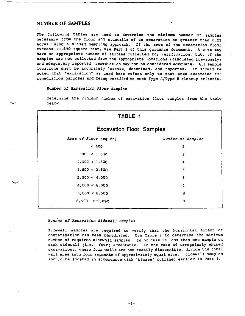
NUMBER OF SAMPLES
The following tables are u»«d to determine the minimum number of samplesnecessary from the floor and sidewalls of an excavation no greater than 0.25acres using a biased sampling approach. If the area of the excavation floorexceeds 10,890 square feet, use Part 2 of this guidance document. A site mayhave an appropriate number of samples collected for verification, but, if thesamples are not collected from the appropriate locations (discussed previously)and adequately reported, remediation may not be considered adequate. All samplelocations must be accurately located, described, and reported. It should benoted that "excavation" as used here refers only to that area excavated forremediation purposes and being verified to meet Type A/Type B cleanup criteria.
Number of Excavation Floor Samples
Determine the minimum number of excavation floor samples from the tablebelow.
TABLE 1
Excavation Floor SamplesArea of floor (aq ft) Number of Samples
< 500 2
^00 < 1,000 3
1,000 < 1,500 4
1,500 < 2,500 5
2,500 < 4,000 6
4,000 < 6,000 7
6,000 < 8,5QO 8
8,500 <10,890 9
of .Excavation Sid«vall Samples
Sidewall samples are required to verify that the horizontal extent ofcontamination has been remediated. Use Table 2 to determine the minimumnumber of required sidewall samples. In no case is less than one sample oneach sidewall (i.e., four) acceptable. In the case of irregularly shapedexcavations, where four walls are not readily discernible, divide the totalwall area into four segments of approximately equal size. Sidewall samplesshould be located in accordance with "biases" outlined earlier in Part 1.
-3-

TABLE 2
Excavation Sidewall SamplesTotal Area of Sidevalls (aq ft) dumber of Samples
< 500 4
500 < 1,000 5
1,000 < 1,500 6
1,500 < 2,000 7
2,000 < 3,000 8
3,000 < 4,000 <5
> 4,000 1 sample per 45 lineal feet of sidewall
VERIFYING IN-SITU AND EX-SITU SOIL REMEDIES
The effectiveness of in-situ soil remedies must be verified by three-dimensionalrandom soil sampling. Refer to Attachment 2 for approved statistical samplingstrategies. Certain ex-situ remedies, such as bio-piles or above-ground vaporextraction, may be amenable to statistical sampling strategies or batch sampling.Any proposed sampling strategy for in-situ or ex-situ remedies should be pre-approved by the DNR.
-4-

BACKGROUND SOIL SAMPLES
ESTABLISHING SOIL BACKGROUND
Establishing soil background, as required by Act 307 PA 1982, as amended,Michigan Environmental Response Act (HERA), can be accomplished by utilizingOperational Memorandum #15 or using the following guidance.
Background should be established for site specific waste constituents, specificchemicals used in various processes, facility operations, or remedial investiga-tion results. Sample analyses may include metals, organic constituents, or othersite specific waste constituents. Analyses should be in accordance with Act 307P.A. 1982, as amended.
Many factors can play a part in the background concentrations of a chemical insoil.
KXAMPLX: The geologic origin (e.g., the parent rock) of glacial drift may havebeen high in copper, lead, or other metals that may be potential contaminants.Additionally, the hydrogeologic situation can alter the quantity of theseelements. Groundwater recharge areas (e.g., highlands) are frequently leachedof metals while groundwater discharge areas (e.g., swamps, floodplain) are therecipients of leached metals. Thus, sites in low areas will usually have higherbackground concentrations than upland areas. Other conditions, such asprecipitation and atmospheric fallout from widely diaper?*"* M'.man and n3tur»iactivities, also affect soil concentrations.
A minimum of four samples must be used to establish "background" in soils. Thiswill help account for natural constituent occurrences and inherent variabilitywithin each distinctive soil horizon. Background samples must be collected inan area which has not been impacted by environmental contamination from the siteand representative of natural background conditions. Based on waste type,contaminant mobility, operation practices, and soil type (sand, silty sand,clay), an estimate of contamination depth should be made and background samplestaken at comparable depths for the particular soil type. Multiple soil horizonsshould have "background" established separately (e.g., minimum of four samplesper each soil unit).
SXAHPLS:
Ground SurfaceBrown medium-coarse SAND
Lt. brown silty fine SAND
Gray silty CLAY w/trace offine-med sand
4 samples
.£:%:.£-;-£V-;fy|=- 4 samples
4 samples
-5-
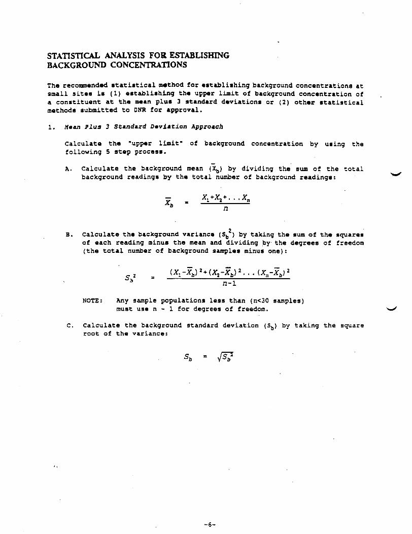
STATISTICAL ANALYSIS FOR ESTABLISHINGBACKGROUND CONCENTRATIONS
The recommended statistical method for establishing background concentrations atsmall sites is (1) establishing the upper limit of background concentration ofa constituent at the mean plus 3 standard deviations or (2) other statisticalmethods submitted to DNR for approval.
1. /fean Plus 3 Standard Deviation Approach
Calculate the "upper limit" of background concentration by using thefollowing 5 step process.
A. Calculate the background mean (Xb) by dividing the sum of the totalbackground readings by the total number of background readings:
n
B. Calculate the background variance (Sfa ) by taking the sum of the squaresof each reading minus the mean and dividing by the degrees of freedom(the total number of background samples minus one):
n-l
NOTE: Any sample populations less than (n<30 samples)must use n-l for degrees of freedom.
C. Calculate the background standard deviation (Sb) by taking the squareroot of the variance:
-6-

D. Th« Coefficient of Variation Test (CV) where
CV = -^**
is used to evaluate data distribution. The background data should generallyhave a CV of less than 0.5 for granular soils, less than 0.75 for cohesivesoils, or an explanation accounting for higher CV values. The maximumrecommended CV is 1.00. if the data distribution exceeds a CV of 1.00, thena thorough evaluation will need to be made to account for this variability(e.g., lab QA/QC, typographical errors, soil classification, samplelocation, data not normally distributed etc.). If the CV exceed* 1.0 andthere is sufficient evidence to suggest a data point does not accuratelyrepresent background conditions or if QA/QC problems exist which invalidatethat data point, the outlier data may be dropped or additional samplescollected and analyzed to ensure a sufficient representative data population(n) is achieved. A high concentration in and of itself is not sufficientjustification to exclude the data point.
Use the Xb + 3*Sb of "background" data as the maximum allowable limit orupper limit. Where 3*Sb equals three times the standard deviation andXb equals the background mean (this statistical method only requires onesample per station). Compare each sample point to the calculatedmaximum allowable limit or upper limit analyzed from background data.
?Tur 2-.-^ samples from a site were analyzed fcr background ccr.can-trations for lead. Concentrations of lead from the sample analyses returnedfrom the lab were 56, 25, 18, and 35 ppb. Now, the investigator wants toexamine the data set to discover whether the 56 ppb sample is an outlier:
Xb mean = 56+25+18+35 = 33 .5
[56 -33. 5] 2 + [25 -33. 5] 2 + [18 -33. 5] 2 + [35-33. 5] 2 = 2 73.67
Sb = (standard deviation) = ^S^ - 16.5
CV = 16 -5 = o .49
Because 0.49 is less than 0.5, no further evaluation of the background dataset is necessary.
Therefore, the background upper limit value for this site is
background upper limit = Xb + (3*5 ) = 33.5 +(3*16.5) =83.0 ppb
If a value is found to be an outlier which is not representative ofbackground conditions, it may be replaced by another sample that is not anoutlier to maintain at least four samples for background determination.
-7-

2. otAer statistic*! procedures /or •stdJblishing background. Refer to astatistical reference book or U.S. E?A's Interim Final Statistical Analysisof Groundwater Monitoring Data at RCRA Facilities (April 1989) and Addendum(July.1992).
PROCEDURES FOR NON-DETECT VALUES
The following provides some guidelines in incorporating non-detectable sampleresults into the procedure to calculate background concentrations.
1. If less than 50% of the background data is below the detection limit (DL),use Jj of the detection limit as the value.
2. If more than 50% of the background data is below the detection limit, useone of the following procedures.
* Alternate "O" and the detection limit (DL) resulting in a net valueof h the detection limit, with a variance.
EXAMPLE: Actual Valu« Substitutt Valut<OL 01<OL 0<OL DL<OL 0
• The Continuity Correction procedure with the t-test, Cohen's method,or other approved methods.
-8-

REPORT FOR SMALL SITE VERIFICATION
Soil cleanup verification reports for small sites must identify the number andlocation of samples and justify the sample location selected (why and how). Theverification report must include the following.
1. MA?(3) and CROSS SECTIONS
Provide a scaled map of the floor and walls of an excavation (the verticaland horizontal area treated for "in-situ" remediations) with samplelocations identified. The cross section should depict the stratigraphy,fractures, soil types, discolorations, unusual characteristics, odor, etc.
SAMPLE LOCATION RATIONALE
A. Background sample locationB. Verification sample locationsC. Sample depthsD. Sample collection proceduresE. Describe biases and rationale used for collecting each sample (e.g.,
clay fractures, discolored soil, location of leak in tank)
3. DATA ANALYSES
A. Analytical parametersB. Analytical methods usedC. Method detection limitsD. Laboratory Quality Assurance/Quality Control
4. STATISTICAL ANALYSES
A. Calculation of background concentrationsB. Coefficient of variance calculationsC. Lab resultsD. Narrative explanation of background concentrations
-9-

DNR-GU1DANCE DOCUMENT, PART 2
iMEDIUM AND LARGE SITE SOIL CLEANUP
VERIFICATION (GREATER THAN 10,890 SQUARE FEET)
Part 2 describes statistical random sampling strategies to verify the remediationof medium and large sites greater than 0.25 acres in size. The strategies employthe use of gridding to facilitate the unbiased selection of sampling points andaccepted statistical tools for evaluating the resultant data. The strategiesprovide a 95% confidence level of determining any hot spot concentrations on asite. It contains guidance on sampling protocol and necessary documentation forclean closures. Part 2 also discusses how to establish grid intervals, setgrids, sample grids, statistically evaluate the data, use grids to guideadditional remedial activities, disposal options, reporting, and a certificationchecklist. It also provides guidance on the sampling of ex-situ remedialprocesses (e.g., thermal desorption).
The term 'clean closure' means that the site has been restored to either Type Aor Type B levels. Type A is defined in Act 307 P.A. 1982, as amended, whichreferences non-detect or background levels. Tvro a is iiefir*»<i in a-:t; 307 P.A.1982, as amended, which references risk-based or background levels. Waste, soil,other environmental media, and/or debris removed should be classified ashazardous or non-hazardous to determine disposal options and handling require-ments (i.e., solid waste under Act 641 P.A. 1978, as amended; hazardous wasteunder Act 64 P.A. 1979, as amended; land ban restrictions under 40 CFR Part 268).
All cleanup verification evaluations must consider the spatial arrangements ofsample values (patterned vs totally random) and the impacts on the present andfuture uses of the site. Because Type 8 cleanups are based on residual risk, thedistribution of that risk, now and in the future, must be determined. Theseprocedures are not absolutes. Other sampling approaches may be developed andsubmitted for DNR approval.
Three of the statistical sampling strategies most commonly used for evaluatingremedial sites and wastes are described in Attachment 2. For further discussionon sampling strategies and sample collection methods, see "Test Methods forEvaluating Solid Waste," SW-846 Volume It: Field Methods, November 1986, ThirdEdition, US EPA.
Compositing samples for verifying soil remediation is not acceptable withoutprior DNR approval. When verifying a soil remediation is complete, contaminantconcentrations will be low. Compositing may result in the contaminantconcentrations not being representative of what remains in the soil. Ifconcentrations are low, compositing may dilute the concentrations cf acontaminant to below its threshold detection limit. Additionally, if contamina-tion is indicated in a composited sample, the location of the contaminationremains unknown.
-10-
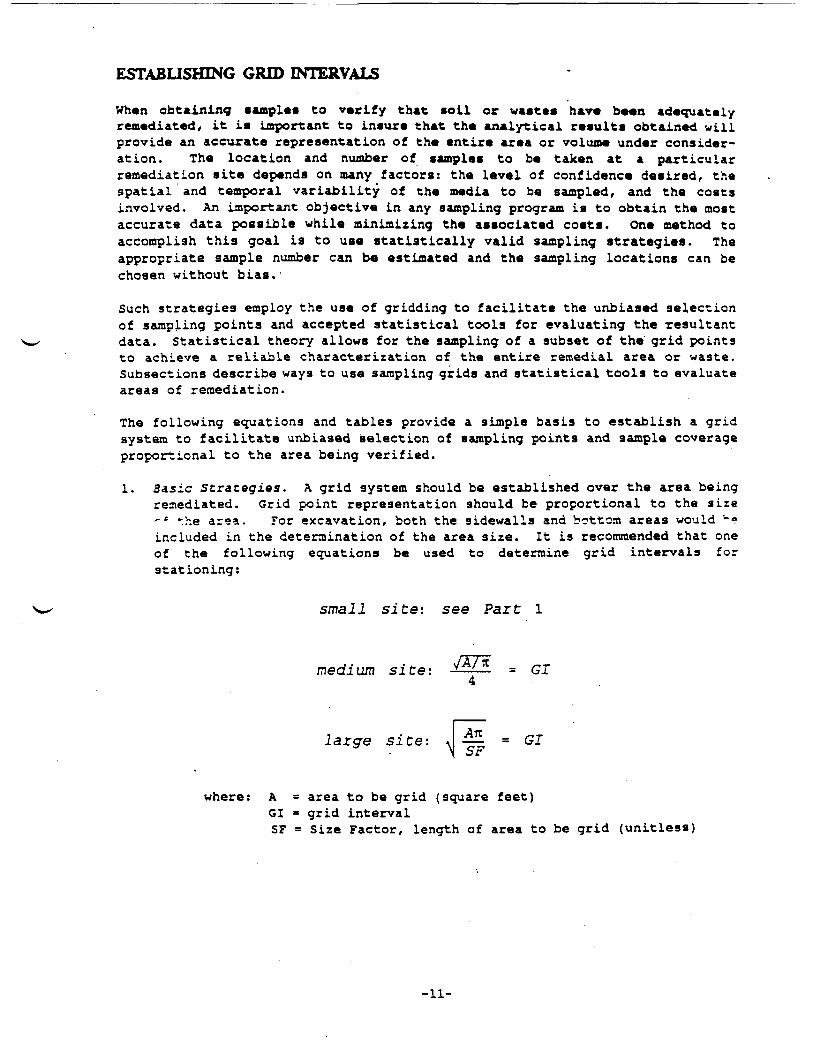
ESTABLISHING GRID INTERVALS
When obtaining samples to verify that soil or wastes haw been adequatelyremediated, it is important to insure that the analytical results obtained willprovide an accurate representation of the entire area or volume under consider-ation. The location and number of samples to be taken at a particularremediation site depends on many factors: the level of confidence desired, thespatial and temporal variability of the media to be sampled, and the costsinvolved. An important objective in any sampling program is to obtain the mostaccurate data possible while minimizing the associated costs. One method toaccomplish this goal is to use statistically valid sampling strategies. Theappropriate sample number can be estimated and the sampling locations can bechosen without bias.
Such strategies employ the use of gridding to facilitate the unbiased selectionof sampling points and accepted statistical tools for evaluating the resultantdata. Statistical theory allows for the sampling of a subset of the grid pointsto achieve a reliable characterization of the entire remedial area or waste.Subsections describe ways to use sampling grids and statistical tools to evaluateareas of remediation.
The following equations and tables provide a simple basis to establish a gridsystem to facilitate unbiased selection of sampling points and sample coverageproportional to the area being verified.
1. Basic Strategies. A grid system should be established over the area beingremediated. Grid point representation should be proportional to the size-* *:he area. For excavation, both the sidewalls and bottom areas would u«?included in the determination of the area size. It is recommended that oneof the following equations be used to determine grid intervals forstationing:
small site: see Part 1
medium site: ^^- = GI
large site: \AnSF
= GI
where: A = area to be grid (square feet)GI » grid intervalSF = Size Factor, length of area to be grid (unitless]
-11-

It appears that there are logical size ranges of site* to which the gridequations apply:
A) small: up to 0.25 acre
B) medium: 0.25 - 3.0 acres
C) large: 3.0 acres and greater
To simplify this application, use the following chart based on anaverage size range of sites (1 acre =» 43,560 square feet). Theapproximate grid ranges are provided as a quick check on numbersgenerated for specific sites using the above formulas.
Sit9 Acreage* Sguare 7eet* ~ Grid .Interval Xaages
up to 0.25 (small) up to 10,890 See Part 1
0.25-3.00 (medium) 10,890-130,680 15-50 feet
3.0 and over (large) 130,680 + 30 feet plus
Site acreage, square footage, is total area of sidewallsand base of excavation.
Setting the Grid. After the grid interval is calculated, it is recommendedthat a scaled grid overlay be made to superimpose on a map of the remediatedarea (this area includes both sidewalls and base). Some specified point(usually the southwest corner) should be designated as the 0,0 coordinate.The grid can then be adjusted to maximize sampling coverage. Some gridadjustment may be necessary for unusually shaped areas. Grid adjustment mayalso be needed to accommodate a minimum of at least one sample from eachsidewall.
-12-

3. Variations on S««ic Strmtmgy.
A. Subgridding. It nay b« warranted to apply grid* with different intervalswithin th« remediated area so that a proportional sampling can befocused on suspect areas (such as sumpe, tank leak areas, etc.).
IZXKPLX:
10'n 20'
* * * ** , ** • * ** . * .* « * »
Area I Sample station, 80' x 200', GI = 20'Area II (subset of I) Sample Station, 30' x 50' GI « 10'
B. Further Randomization. Sites that may have a patterned distribution ofwaste or contamination due to time sequence of filling, productionsequences, or physical, site conditions (i.e., furrows) may require afurther randomization of sampling. In such cases, the following gridcell sampling format may be selected instead of at grid point stations.Each grid cell to be sampled muse oe divided inic r.ine equal sizea-subcells." Next, a random number table is used to select in which ofthe subcells the sample will be taken. The random number table is usedagain to select which subcell for the next cell and so on.
KXAXPLSi
20'
Area = 120' x 200', GI = 20'
In the example above, a, sampling grid has been set up with grid pointstations 20 feet apart using the appropriate formula. Two cells which havebeen selected at random have been divided into nine subcells each. Subcell/4 was chosen randomly irx one cell and subcell #2 in the other cell. Thisprocess is continued for all of the cells selected at random for sampling.Samples are then taken in each randomly chosen subcell.
-13-

C. Thre« dimensional gridding: In-Situ and Bx-Situ Remediation*.
In-aitu and ex-«itu remediation* involving soils and/or wastes with asignificant vertical component should be evaluated in three dimensions(volume evaluation). Examples of such remediations would be in-situ soilvapor extraction or ex-situ bioremediation involving several cubic feet ofsoil and/or waste. A grid is superimposed on the remediation area asdescribed in the previous sections and a vertical component is added at eachnode. The vertical sampling increments would be site specific and requireprior approval from the DNR.
SAMPLING OF GRID
Sampling of grids may include all of the grid stations or a phased subset of thetotal stations. The subset of grid stations is created by assigning coordinatesto all the nodes and randomly selecting nodes using a random number generator ora random number table (refer to Attachment 2). A minimum of 10 samples or- 25%,whichever is larger, of the total grid stations should be sampled and analyzedinitially to allow a large enough data pool for statistical analysis. It isadvisable that extra samples also be taken and kept under proper chain of custodyand storage procedures at the time of initial sampling. If the statisticalanalysis indicates that more samples are needed, an additional sample trip to thefield may have been avoided. A method for calculating the sample sizerequirements is presented in Attachment 2 (Lamda relationship) .
ESTABLISHING SOIL BACKGROUND
Establishing soil background, as required by Act 307 PA 1982, as amended,Michigan Environmental Response Act (HERA), can be accomplished by utilizingOperational Memorandum #15 or using the following guidance.
Background should be established for site specific waste constituents, specificchemicals used in various processes, facility operations, or remedial investiga-tion results. Sample analyses may include metals, organic constituents, or othersite specific waste constituents. Analyses should be in accordance with Act 307P. A. 1982, as amended. .
Many factors can play a part in the background concentrations of a chemical iasoil.
The geologic origin (e.g., the parent rock) of glacial drift may havebeen high in copper, lead, or other metals that may be potential contaminants.Additionally, the hydrogeologic situation can alter the quantity of theseelements. Groundwater recharge areas (e.g., highlands) are frequently leachedof metals while groundwater discharge areas (e.g., swamps, floodplain) are therecipients of leached metals. Thus, sites in low areas will usually have higherbackground concentrations than upland areas. Other conditions, such asprecipitation and atmospheric fallout from widely dispersed human and naturalactivities, also affect soil concentrations.
-14-

A minimum of four samples must be usad to establish "background" in soils. Thiswill help account for natural constituent occurrences and" inherent variabilitywithin each distinctive soil horizon. Background samples must b« collected inan area.which has not been impacted by environmental contamination from the siteand representative of natural background conditions. Based on waste type,contaminant mobility, operation practices, and soil type (sand, silty sand,clay), an estimate of contamination depth should be made and background samplestaken at comparable depths for the particular soil typ«. Multiple soil horizonsshould have "background" established separately (e.g., minimum of four samplesper each soil unit).
SXAMPUt:
Ground SurfaceBrown medium-coarse SAND
Lt. brown silty fine SAND
Gray silty CLAY w/trace offine-med sand
4 samples
SJ?. -i--. '::--y .r . 4 samples
4 samples
STATISTICAL ANALYSIS FOR ESTABLISHINGBACKGROUND CONCENTRATIONS
The recommended statistical method(s) for establishing background concentrationsat medium and large sites are (1) establishing the upper limit of backgroundconcentration of a constituent at the mean plus 3 standard deviations, (2)tolerance limit, (3) t-tests, and (4) other statistical methods submitted to theDNR for approval.
1. Mean Plus 3 Standard Deviation Approach.
Calculate the "upper limit" of background concentration by using thefollowing 5 step process.
A. Calculate the background mean (Xb) by dividing the sum of the totalbackground readings by the total number of background readings:
n
B. Calculate the background variance (Sfe ) by taking the sum of the squaresof each reading minus the mean and dividing by the degrees of freedom(the total number of background samples minus one):
-15-

2 . . . (X-X)0 fl-1
NOTE: Any sample population* less than (n<30 samples)must us* n - 1 for degree* of freedom.
C. Calculate the background standard deviation (S^) by taking th* squareroot of the variance:
S*
D. The Coefficient of Variation Test (CV) where
CV = -=£X»
is used to evaluate data distribution. The background data should generallyhave a CV of less than 0.5 for granular soils, less than 0.75 for cohesivesoils, or an explanation accounting for higher CV values. The maximumrecommended CV is 1.00. If the data distribution exceeds a CV of 1.00, thena thorough evaluation will need to be made to account for this variability;;=.,••, lab QA/QC, typographical errors, soil classification, -i.r>t;' .location, data not normally distributed etc.'). If the CV exceeds 1.0 andthere is sufficient evidence to suggest a data point does not accuratelyrepresent background conditions or if QA/QC problems exist which invalidatethat data point, the outlier data may be dropped or additional samplescollected and analyzed to ensure a sufficient representative data population(n) is achieved. A high concentration in and of itself is not sufficientjustification to exclude the data point.
-16-

B. Ose th« X^ + 3*Sb ot "background" data as th« ma^i^m allowable limit orupp«r limit. Where 3*Sb equals thr«« timee the standard deviation andXjj equals the background owan (this statistical method only requiresone sample per station). Compare each sample point to the calculatedmaximum allowable limit or upper limit analyzed from background data.
B2AMPUE: Four sand samples from a site were analyzed for background concen-trations for lead. Concentrations of lead from the sample analyses returnedfrom the lab were 56, 25, 18, and 35 ppb. Now, the investigator wants toexamine the data set to discover whether the 56 ppb sample is an out liar:
7 m«*n - 56+25+18*35 ,, _X mean = ———————— = 33.5
[56-33. 5] 2+[25-33. 5] 2+[18-33. 5] 2+[35-33. 5] 2 _ ,7Vfi,-——————————————————— - 2 / J . o /
(standard deviation) = ^s = 16.5
CV = -=?-^. =» o .49
Because 0.49 is less than 0.5, no further evaluation of the background dataset is necessary.
Therefore, the background upper limit value for this site is
background upper limit = Xb -|-(3*Sil) = 33.5 +(3*16.5) = 83.0 ppb
If a value is found to be an outlier which is not representative ofbackground conditions, it may be replaced by another sample that is not anoutlier to maintain at least four samples for background determination.
2. Tolerance Limit. This statistical procedure is a fairly sensitive programfor environmental purposes. It minimizes false positive and is simple toperform. A ainiaua background data base of n=8 (optimum n»16) is needed forthis method. Other suggested criteria follow:
A. The Coefficient of Variation Test (CV) to evaluate data distribution.See this Guidance Document, Part 2, Statistical Comparisons, £1.0. (theCoefficient of Variation Test....).
B. Using the mean (Xb) and standard deviation (Sb), construct the one-sidedupper tolerance limit (TL) by taking the mean plus a tolerance coeffi-cient (K) at the 95% probability level for a 95% coverage (for K values,see Attachment 3) times the standard deviation as follows:
TL = Xb + KSb
-17-
3. e-cests. Any t-test should be "approved" by DNR atioj: to use sine* thereare a number of variation*. The Cosset student t-test (1908) or Cochran'sApproximation to the Behren's-Fisher Student's t-test as referenced in the40 CFR Part 264, Appendix IV are recoonended. Note that these statisticalcomparison methods require that two or more discrete samples be taken ateach sampling station.
4. Other statistical procedures for •staWisning background. Refer to astatistical reference book or U.S. EPA's Interim Final Statistical Analysisof Groundwater Monitoring Data at RCRA Facilities (April 1989) and Addendum(July 1992).
PROCEDURES FOR NON-DETECT VALUES
The following provides some guidelines in incorporating non-detectable sampleresults into the procedure to calculate background concentrations.
1. If less than 50% of the background data is below the detection limit (DL),use Jj of the detection limit as the value.
2. If more than 50% of the background data is below the detection limit, useone of the following procedures.
* Alternate "O" and the detection limit (DL) resulting in a net valueof % the detection limit, with a variance.
EXAMPLE: Actual vaiu« auos^tute Vat"*<OL DL<OL 0<OL DL<OL 0
* The Continuity Correction procedure with the t-test, Cohen's method,or other approved methods.
STATISTICAL EVALUATION OF DATA
A detailed description of an acceptable approach for evaluating the datagenerated by statistically based random sampling strategies such as thosedescribed in the foregoing sections is provided in Attachment 2 (page 27). The95% upper confidence limit (UCL) of the mean is calculated for each constituentof concern and compared to the regulatory threshold (RT) (i.e., cleanupcriterion, eg., Type A or B) . If the UCL is less than the RT and an adequatenumber of samples have been collected and spatially evaluated, the remediationis deemed complete. Attachment 2 also provides a step wise procedure fordetermining whether an adequate number of samples have been collected, based onthe analytical data derived from the initial and subsequent rounds of samples.All evaluations must consider the spatial correlation of sample values (e.g.,highest concentrations in the same area), present and future uses of the site,residual risk, and distribution of that risk now and in the future. Otheracceptable methods for UCL and sample size calculations can be found in U.S. ETASW-846, Third Edition, Section 9.1.1.3.
-18-

GRID APPROACH TO ADDITIONAL REMEDIATION
1. Tvo-Dimensional Nod* Stapling Excavation Grid. Verification sampling asdescribed above will at times indicate that remediation is incomplete.Excavation of contaminated areas should be baaed on the established gridsystem interval (as recoamended in this Guidance Document, Part 2). wherea subset of grid points has indicated that the entire area exceeds thecleanup, the nodes adjacent to the sampled nodes that are causing theexceedance should be sampled, and this process repeated until the "Hotspots" requiring removal have been defined. The radius of excavation aroundthe contaminated sample point(s) is equal to the grid interval (Gl-r).Excavation depth is to the deepest point of contamination or to the depthwhere acceptable levels are anticipated. After excavation, the impactedpoint(s) must be resampltd at their new elevations to verify that the areameets the selected cleanup criteria. If continued contamination Ladetected, the excavation format is repeated until a satisfactory result isobtained.
GL = 150A - 11,250GI - 14.9
'i *^ "V v ' SafflPl* Station> x Contaminated Station
TV, / ,'/ : -V-15' r » GI » 15 feet-V ~* ' : -\
Remediation of contaminated soil by excavation will be in accordance withAct 307 P.A. 1982, as amended. The proposed remedial action plan must beapproved by the DNR.
2. Tvo-Dimensional Subcell Sampling Excavation Grid. Use this GuidanceDocument, Part 2. The radius of excavation around a contaminated point mayneed to be adjusted to greater than the GI distance. This adjustment is dueto the variable distances between sampling points.
3. Three-Dimensional Cleanup Verification. If sampling and statisticalanalysis using this Guidance Document indicate that Act 307 cleanup criteriahave not been met, additional 'remediation will be required. The samplingprotocol and strategies described in Attachment 2 and in SW-846, ThirdEdition, Volume II, Part III, Chapter 9, are acceptable. All samplingstrategies, detection levels, and sampling pathways must be in accordancewith Act 307 P.A. 1982, as amended. If any portion of the soil mass inquestion appears to be causing the material to fail, it may be identifiedthrough hot spot sampling and selectively removed. Subsequent sampling mustbe done to confirm that the remaining material meets Act 307 P.A. 1982, asamended.
4. Batch Sampling for ex-situ treatment processes. If ex-situ treatmentprocesses of contaminated soil or waste is used in the remediation, asampling program for the process stream needs to be developed. The basisof this program is to get representative samples over time versus a spatialapproach (Attachment 2, Sampling Process Streams).
-19-

DISPOSAL OPTIONS
Soils remediated to Act 307 P.A. 1982, as amended, standard* (Type A and/orType B) are no longer considered a waste per Act 64 P.A. of 1979, as amended, andRCRA regulations. Disposal of excavated waste, soil, other environmental media,and/or debris must be in accordance with all applicable Federal, State, and localregulations.
REPORT FOR MEDIUM AND LARGE SITES VERIFICATION
Soil cleanup verification reports for medium and large sites must identify thenumber and location of sample* and justify the sample location selected (why andhow). The verification report must include the following.
1. HAP(S) AND CROSS SECTIONSProvide a scaled map of the floor and walls of the excavation (the verticaland horizontal area treated for "in-situ" remediations) with sample grid andsample locations identified. Appropriate cross section should depict thestratigraphy, fractures, soil types, and final depth and elevations of theexcavation.
2. SAMPLE LOCATION RATIONALEa. Properly labelled and easily identified sampling grid stations (map)
including background stationsb. Sample Depths
Sample Collection Proceduresc. Results of all tests to determine clean closure (charts, tables, lab
sheets, field notes, well logs, boring logs)
3. DATA ANALYSESa. Analytical parametersb. Analytical methods usedc. Method detection limitsd. Laboratory Quality Assurance/Quality Control
4. STATISTICAL ANALYSESa. Explanation and calculation of background concentrationsb. Statistical comparisons on sampling results compared to background (this
should include full computations on background and.statistical analysis)c. Lab results
5. Additional information to support closure (e.g, residual risks, spatialcorrelation of sample values, present and future land uses)
RCRA CLEAN CLOSURE CERTIFICATION CHECKLIST
Attachment 4 is a guide that indicates the information that a facility shouldprovide to certify that their activities meet the conditions for a clean closureunder the Act 64/RCPA regulations.
-20-
A T T A C H M E N T 1
GUIDE TO SAMPLE BIAS
Many factors can play a part in the concentrations of contaminants. Thefollowing contains some of the factors impacting chemical concentrations andlocations.
CHEMICAL TRANSFORMATIONSMany organic chemicals may undergo aerobic and anaerobic degradation. Adescription of these processes is beyond the scope of this document. The subjectis approached here, however, to be sure that samplers are aware that thechemical(s) spilled may not b« the only chemical{s) in the soil after a transfor-mation has occurred. These occurrences should be documented in the remedialinvestigation. The full scan of chemicals from the remedial investigationrequiring cleanup should be analyzed when doing a closure. Analyses should bedone for all chemicals that have been identified as breakdown products of thechemicals found on site.
The professional literature contains many articles on this subject (Cline andBrown, 1989; Borden and Bedient, 1987; Wilson and Wilson, 1985). The interestedreader is directed to these articles.
Organic Carbon Content of SoilThe organic carbon content of soils is a key factor in the ability of any soilto adsorb contaminants. For a variety of reasons (Lindsay, 1979), an increasein organic carbon content leads to an increase in the adsorption of severalclasses of chemicals.
Where to sample: Areas of the excavation that appear to have excess organiccarbon (e.g. peat, muck., darker soils) should be preferentially sampled.
Kediua Sajid or Larger GrainsMedium to larger grain size sand has from 20 to 40 percent porosity. Most sandsin Michigan are composed of quartz, limestone, and small amounts of metamorphicrock fragments. These soils have a low capacity for adsorbing metals orhydrophilic (soluble) organic chemicals. Hydrophobic (insoluble) organicchemicals with low molecular weight will adsorb to this soil in small amounts.Hydrophobic chemicals with high molecular weight will adsorb in moderate amounts(Cline & Brown, 1989). Thesej soils have a low capacity to hold contaminants inthe grain interstices due to low capillary action. Contaminants that are heldin these soils adhere to the grains themselves in dry soils and are forced intothe smaller pore spaces in w«t soils (Schwille, 1988).
Where to saaple: Samples should be placed at regular intervals along thebase and sidewalls of the excavation being sure that samples are locatedwhere the source was removed. In these soils, the capillary force is lewenough to ignore its affects in transporting contaminants lateral togravity. Therefore, sidawall samples should be located near the excavationfloor. This is especially true for low surface tension products such asgasoline.
The limestone sand grains can act as a buffer to contaminants that cause pHchanges (e.g., steel mill pickling acids). For these types of contaminants,the sampler should be on the lookout for intra-granular precipitates. Thesecan appear as grain surface staining or make the soil appear clumpy oraggregated. Soils containing precipitates should be sampled.
-21-

ad 512 CThese soils have strong capillary action due to the -small inter-granulardistances. A determination of the fluid surface tension of the spilled productis helpful. High surface tension aids in the ability of a substance to overcomegravity by capillary action. As before, higher molecular weight products can beexpected to adsorb to the grains to a greater degree. This allows a product to"move lateral to gravity and, to a degree, upward from the leak location. Lowsurface tension products, such as TCS (trichloroethene), are more likely to gostraight down than oils in these kinds of soils. However, the hydraulic head(i.e., the amount of product in the original spill) must be substantial to forcea dense non-aqueous phase liquid through a media with a hydraulic conductivityless than 1 x 10 cm/sec (Schwille, 1988).
Where to cample: Interfaces between fine sand layers with larger grainsabove should be sampled. When high surface tension contaminants aresuspected, silt layers should be sampled.
ClaysClay soils are very different from the sands and silts. c^-aY3 possess a netnegative charge. This causes heavy metal cations (e.g., Cr* , Cd* , Pb* ) toadsorb to the clay surface. In fact, this is true for any positive ionizablesubstance. Clays also have a much greater secondary porosity than primary(primary porosity is the space between the soil particles; secondary porosity isthe space between fractures, bedding planes, and soil structures). As a result,spills in clay soils tend to follow preferred pathways, clays will often showsigns of shrinkage cracks or fractures that will allow contaminants to migratein what would otherwise be considered a "tight" soil in a lab analysis ofpermeability. Signs of fracturing include "patterned" mottling. This is wherethe Fe (and also Mn^ wi 1 ' ho oxidizeo to a red, yellow, cr reddish brown coloralong the crack while the matrix remains the reduced blue/gray color (Lindsay,1979).
Where to sample: It is very important to take clay soil samples fromfractures. The fractures are the avenue of travel for contaminants in claysoils. Clay soils may also have sand lenses which should always be sampled.Sand lenses in clays tend to collect fluids. As such, they may harborcontaminants.
BedrockExcavations in bedrock present difficult problems. Unlike clay, some bedrockformations have substantial primary porosity as well as secondary porosity. InMichigan, these are sandstones, conglomerates, and brecciated/coarse grainedlimestones. Examples of bedrock in Michigan with low primary porosity are finegrained limestones, shale, and crystalline metamorphic recks (e.g., gneiss). Ifthe sampler is unaware of the type of bedrock thac is in an excavation, ageologist must be consulted.
Where to sample: Excavations in areas of bedrock with significant primaryporosity must be sampled in both the fractures and the matrix. Bedrockwithout primary porosity should have sampling predominantly in the fracturesas in the clay situation. Weathered zones in bedrock will hold contaminantsbetter than unweathered rones. This is due to the increased number ofadsorption sites available in weathered rock.
-22-

A T T A C H M E N T 2
SAMPLING PROTOCOLFOR CHARACTERIZING WASTE/TREATMENT LEVELS:
STRATEGIES FOR EVALUATING TREATED SOILS AND WASTE MATERIALS
When obtaining samples to characterize a treated soil or waste material, it isimportant to insure that the analytical results obtained will provide an accurateestimation of the nature of the entire area/volume under consideration. Thelocation and number of samples to be taken at a particular site depends on manyfactors: the degree of accuracy desired, the spatial and temporal variability ofthe media to be sampled, and the costs involved. An important objective in anysampling program is to obtain the most accurate data possible while minimizingthe associated costs. One method to accomplish this goal is to use statisticallyvalid sampling strategies. The appropriate sample number can be estimated andthe sampling locations can b« chosen without bias.
Attachment 2 provides information on the methods used to obtain accurate datawhile minimizing the costs. The attachments include a discussion of threestatistical sampling strategies and methods to determine the appropriate gridsize for the area under investigation. If several areas on a site' are underinvesticrtion, it may be advisable to grid them separately. This is especiallytrue 11 information does not exist to indicate that the areas contain similarconstituents or that they were placed at the same time period.
Information is also supplied on the statistical evaluation of the resultantanalytical data. A minimum of 10 samples or 25%, whichever is greater, of thetotal grid stations should be sampled and analyzed initially to allow a largeenough data pool for the statistical analysis. Extra samples should be taken andkept under proper chain of custody and handling procedures at the time of initialsampling. If the statistical analysis indicates that two or three more samplesare needed, an additional trip to the field may not be necessary. This may alsoavoid the need to reestablish the grid pattern at a later date.
For further discussion on sampling strategies and sample collection methods, see"Test Methods for Evaluating Solid Waste," SW-846 Volume II: Field Methods,November 1986, Third Edition, US EPA.
-23-
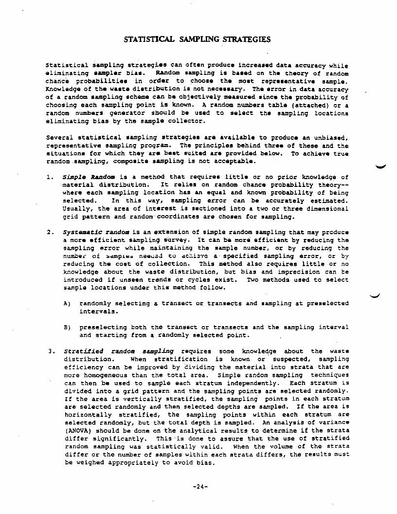
STATISTICAL SAMPLING STRATEGIES
Statistical sampling strategies can often produce increased data accuracy whileeliminating sampler bias. Random sampling is based on the theory of randomchance probabilities in order to choose the most representative sample.Knowledge of the waste distribution is not necessary. The error in data accuracyof a random sampling scheme can be objectively measured since the probability ofchoosing each sampling point is known. A random numbers table (attached) or arandom numbers generator should be used to select the sampling locationseliminating bias by the sample collector.
Several statistical sampling strategies are available to produce an unbiased,representative sampling program. The principles behind three of these and thesituations for which they are best suited are provided below. To achieve truerandom sampling, composite sampling is not acceptable.
1. Simple Random is a method that requires little or no prior knowledge ofmaterial distribution. It relies on random chance probability theory—where each sampling location has an equal and known probability of beingselected. In this way/ sampling error can be accurately estimated.Usually, the area of interest is sectioned into a two or three dimensionalgrid pattern and random coordinates are chosen for sampling.
2. Systematic random is an extension of simple random sampling that may producea more efficient sampling survey. It can be more efficient by reducing thesampling error while maintaining the sample number, or by reducing thenumber of sdmpiea neeusJ to achiave a specified sampling error, or byreducing the cost of collection. This method also requires little or noknowledge about the waste distribution, but bias and imprecision can beintroduced if unseen trends or cycles exist. Two methods used to selectsample locations under this method follow.
A) randomly selecting a transect or transects and sampling at preselectedintervals.
B) preselecting both the transect or transects and the sampling intervaland starting from a randomly selected point.
3. Stratified random sampling requires some knowledge about the wastedistribution. When stratification is known or suspected, samplingefficiency can be improved by dividing the material into strata that aremore homogeneous than the total area. Simple random sampling techniquescan then be used to sample each stratum independently. Each stratum isdivided into a grid pattern and the sampling points are selected randomly.If the area is vertically stratified, the sampling points in each stratumare selected randomly and then selected depths are sampled. If the area ishorizontally stratified, the sampling points within each stratum areselected randomly, but the total depth is sampled. An analysis of variance(ANOVA) should be done on the analytical results to determine if the stratadiffer significantly. This -is done to assure that the use of stratifiedrandom sampling was statistically valid. When the volume of the stratadiffer or the number of samples within each strata differs, the results mustbe weighed appropriately to avoid bias.
-24-
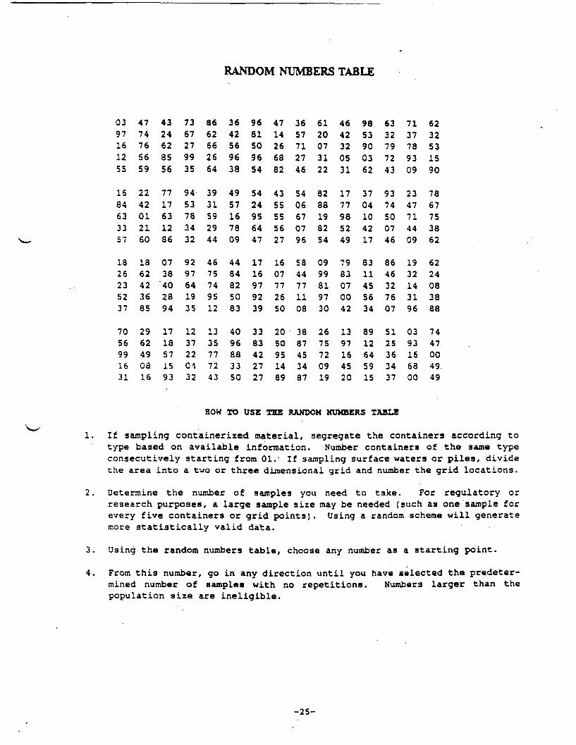
RANDOM NUMBERS TABLE
03 47 43 73 86 36 96 47 36 61 46 98 63 71 6297 74 24 67 62 42 81 14 57 20 42 53 32 37 3216 76 62 27 66 56 50 26 71 07 32 90 79 78 5312 56 85 99 26 96 96 68 27 31 05 03 72 93 1555 59 56 35 64 38 54 82 46 22 31 62 43 09 90
16 22 77 94 39 49 54 43 54 82 17 37 93 23 7884 42 17 53 31 57 24 55 06 88 77 04 74 47 6763 01 63 78 59 16 95 55 67 19 98 10 50 71 7533 21 12 34 29 78 64 56 07 82 52 42 07 44 3857 60 86 32 44 09 47 27 96 54 49 17 46 09 62
18 18 07 92 46 44 17 16 S3 09 79 83 86 19 6226 62 38 97 75 84 16 07 44 99 83 11 46 32 2423 42 '40 64 74 82 97 77 77 81 07 45 32 14 0852 36 28 19 95 50 92 26 11 97 00 56 76 31 3837 85 94 35 12 83 39 SO 08 30 42 34 07 96 88
70 29 17 12 13 40 33 20 38 26 13 89 51 03 7456 62 18 37 35 96 83 50 87 75 97 12 25 93 4799 49 57 22 77 88 42 95 45 72 16 64 36 16 0016 08 15 01 72 33 27 14 34 09 45 59 34 63 49.31 16 93 32 43 50 27 89 87 19 20 15 37 00 49
HOW TO USE THE RANDOM NUMBERS TABLE
1. If sampling containerized material, segregate the containers according totype baaed on available information. Number containers of the same typeconsecutively starting from 01." If sampling surface waters or piles, dividethe area into a two or three dimensional grid and number the grid locations.
2. Determine the number of samples you need to take. For regulatory orresearch purposes, a large sample size may be needed (such as one sample forevery five containers or grid points). Using a random scheme will generatemore statistically valid data.
3. Using the random numbers table, choose any number as a starting point.
4. From this number, go in any direction until you have selected the predeter-mined number of samples with no repetitions. Numbers larger than thepopulation size are ineligible.
-25-

SAMPLING GRIDS
1. A grid system should be established over the specified area (sidewalls andbase). Grid point representation should be proportioned to the size of thearea. It is recommended that one of the following equations be used todetermine grid intervals for stationing.
small site VA/K -GI
medium site * ' =GI
large site AnSF •-GI
where: A » area to be grid (sq. ft.)GI = grid intervalSF - Size Factor, length of area to be grid (unitless)
It appears that there are logical size ranges of sites to which the threeequations apply:
A) small: up to 0.25 acre
B) medium: 0.25 - 3.0 acres, and
C) large: 3.0 acres and greater
To simplify this application, use the following chart based on an averagesize range of sites (1 acre = 43,560 square feet). The approximate gridranges are provided as a quick check on numbers generated for specific sitesusing the above formulas.
Site Acreage* Sguare feet* ~ Grid Interval Ranges
up to 0.25 (small) up to 10,890 -See Part 1
0.25-3.0O (medium) 10,890-130,680 15-50 feet'
3.0 and over (large) 130,680 + 30 feet plus
* Site acreage, square footage, is total area of sidewallsand base of excavation.
After the grid interval is calculated, it is recommended that a scaled gridoverlay be made to superimpose on the area under consideration. Somespecified point (usually the southwest corner) should be designated as the0,0 coordinate. The grid can then be adjusted to maximize samplingcoverage. Some grid adjustment may be necessary for unusually shaped areas.
-26-
STATISTICAL EVALUATIONWASTE/TREATMENT CHARACTERIZATION SAMPLINGS
Following La a step by step description of the approach used to calculateconfidence limits baaed on the analytical data derived from the preliminarysamples.
1. Calculate a preliminary estimate of X
i-ln
where: n = number of measurementsX = variable concentrationXi = individual measurements
2. Calculate a preliminary estimate of the variance (S: ) and the standarddeviation (S). Standard deviation is a function of both sampling variabili-ty and measurement variability.
n-1
3. Calculate the standard error of the mean (Sx) . Standard error is inverselyproportional to the square root of the number of samples (increasing n from4 to 16 reduces Sx by 50%}.
5x=— •
4. Since the concern is only whether the upper limit of a confidence intervalis below or above the regulatory threshold, the lower confidence limit (LCL)need not be considered. The upper confidence limit (UCL) can be calculatedusing the one-tailed (one-sided) t values with n-1 degrees of freedomderived from a table of the Student's t distribution. Where only smallsized statistical samples are involved (n<30), the normal or Gausaiandistribution is not accurate, and the t distribution must be used.
-27-
5. The 95% UCL ia calculated by uaing the following formula and substitutingthe values determined above plus the appropriate t value obtained from thet table.
UCL = 5?+[t0.95(a-l) ]SX
The term in brackets indicates a one-tailed t-test at n-1 degrees offreedom. See the t-distribution table in Attachment 2.
The UCL number resulting from this formula will indicate with a 95% probabilitythat it ia either above or below the regulatory threshold (RT) developed for theconstituent being subjected to the test. If a compound does not have a specifiedRT, then the UCL is compared to whatever concentration is of concern (i.e., aclean up level, action level, etc). Other confidence levels can be used, basedon the specific sampling situation.
If the preliminary data indicate that more samples are needed to make a hazarddetermination, the Lambda (X) relationship should be used. A step by stepapproach to calculating the appropriate sample size follows:
1. The appropriate number of samples to be collected can be estimated by useof the Lambda (X) relationship and then consulting a table of values andtheir corresponding sample size number.
, RT-X
The lower the calculated value, the more samples are required to maintaina certain level of confidence. Also, as X approaches RT, X becomessmaller, and therefore a greater sample size is indicated for a certainlevel of confidence.
2. To obtain the appropriate sample size from the table of values, use thesingle sided value for a to test at the desired significance level (for 5%,a = 0.05).
3. Randomly collect any additional samples that may be needed using the samegrid and random numbers sequence as the first sampling. All field andlaboratory procedures should be kept as consistent as possible to lower theamount of variability in the data.
4. Use all data values to calculate new IT, S, and Sx.
-28-

5. If the new X > RT, then the contaminant is present at an unacceptableconcentration and the study would be complete..
6. If X < RT and X > Sz , calculate C (the criterion fo£ determining if.contamination is present at hazardous concentration). If H * s2 or Ic < S: ,the data must be transformed prior to calculating C.
Using the new data, C is calculated by the formula:
7. Compare the calculated C value to the two-tailed t value for the level ofsignificance desired. The two-tailed t-value is used because both thepossibility that C is > t or that C is < t must be checked.
Use tO.95 and df (degrees of freedom) * n-1.
S. If C > t value, the contaminant is present at unacceptable concentrationsand the study would be over. If C < t value, re-estimate the total numberof additional samples to be collected by.deriving a new X. Use the newlycalculated values of X and S.
3 ~* this new number of samples is not more than 20% creater than the last setcollected, there is little chance that additional samples would decrease Sxand result in the material being considered unacceptable. Therefore, thestudy would be complete.
-29-

EXAMPLE
CALCULATION OF CONFIDENCE LIMITS AND LAMDA CALCULATION
Problem 1: STATISTICAL SAMPLING
A metal plating factory has been discharging process wastewaters into a largenearby swampy area for several years. This swampy area drains into a smallriver. The discharged wastewaters are known to be contaminated with very lowlevels of cadmium and chromium (i.e., the levels in the wastewater are below thefacilities NPDES permit limitations). However, it has been suspected that thesediments in this swampy area may contain high levels of cadmium and chromium.Three preliminary sediment samples were taken with a Ponar dredge and analyzedto determine whether or not these sediments were contaminated with hazardouslevels of these two metals. In 40 CFR 261.24, it states that a waste ishazardous under.the characteristic of EP toxicity if it contains cadmium at alevel > 1.0 mg/£ or chromium at a level > 5.0 mg/£. The analysis of the threepreliminary samples indicated a mean cadmium concentration of 0.37 mg/£ (3samples at 0.25, 0.51, and 0.35 mg/£) and a mean chromium concentration of 4.66mg/£ (3 samples at 4.93, 4.21, and 4.84 mg/£). Based on this analytical data,the cadmium level is well below the regulatory threshold (RT), but the chromiumlevel closely approaches its RT. Because large legal or monetary losses may beincurred if the sediments are declared hazardous, the analytical data must be.;_nd a-;d i hi^h degree of confidence is necessary in any decision made.
QUESTIONS: Given the above scenario, answer the followingquestions and calculate the appropriate answers.
1. Based on the chromium data supplied
Calculate S2, S, Sx
Calculate the 95% UCL
With what degree of confidence can it be stated thatthe chromium concentration does not exceed the RT?
2. If more samples are deemed necessary, determine liow many
Calculate the X value
Calculate the appropriate number of additional samplesusing Ot - 0.05 and {3 = 0.05
-30-

PROBLEM 1 ANSWER SHEET -
Given three samples with chromium concentrations of 4.93, 4.21, and 4.84 mg/l and
X = 4.66 mg/t
(la) Calculate S
i-ln-1
4 . 9 3 2 + 4 . 2 1 2 + 4 . 8 4 2 - ( 4 . 9 3 + 4 . 2 1 + 4 . 8 4 ) 2 / 3
= 0.15
Calculate S
= /OV15 = 0.39
Calculate Sj
( lb) Calculate the 95% UCL
95% UCL = X + [C0.95(n- l ) ]5jf
= 4.66 + (2 .920 ) (0 .23)« 5.33
( 1 C )
90% UCL = X + [ C O . 90 (n-1) jSjf
= 4.66 +• (1.886)(0.23)= 5.09
80% UCL - X + [C0.80(/l-ins s
- 4.66 + (1.061)(0.23)= 4.90
-31-

The preceding two calculations indicate that it can be stated with somewherebetween 80% and 90% confidence that the chromium concentration doee not exceedthe RT. This degree of confidence may not be sufficient to meet the needa of thesampling plan. Therefore, more samples may need to be taken.
2a. Calculate the X value
2b. Calculate the number of additional samples
Using Attachment 2, Numfier of Observations for T Test of Mean, page 34 ofthis Guidance Document, using a single-sided test with Ot«0.05 and 0*0.OS,approximately IS to 17 total samples need to be collected. Therefore, basedon the three preliminary samples that were collected, an additional 13samples need to be taken.
-32-

Cumalative t Distribution
df(n-1)
one-tailedtwo-tailed
12345
678910
1112131415
1617IS19
) 20
2122232425
2627282930
4060120
0.0.
0.0.0.0.0.
0.0.0.0.0.
0.0.0.0.0.
sso100
158142137134132
131130130129129
129128128128128
0.1280.0..128,127
0.1270.127
0,0.127.127
0.1270.1270.127
00000
0000
.127
.127
.127
.127
.127
.126
.126
.126
.126
NOTE:
0.7500.500
1.0000.8160.7650.7410.727
0.7180.7110.7060.7030.700
0.6970.6950.6940.6920.691
0.6900.6890.6880.6880.687
0.6860.6860.6850.6850.684
0.6840.6840.6830.6830.683
0.6810.6790.6770.674
0.0800.600
1.3761.0610.9780.9410.920
0.9060.8960.8890.8830.879
0.8760.8730.8700.8680.866
0.8650.8630.8620.8610.860
0.8590.8580.8580.8570.856
0.8560.8550.8550.8540.854
0.8510.8480.8450.842
For one-tailedFor two-tailed
P0.9000.800
3.0781.8861.6381.5331.476
1.4401.4151.3971.3831.372
1.3631.3561.3501.3451.341
1.3371.3331.3301.3281.325
1.3231.3211.3191.3181.316
1.3151.3141.3131.3111.310
1.3031.2961.2891.282
0.9500.900
6.3142.9202.3532.1322.015
1.9431.8951.8601.8331.812
1.7961.7821.7711.7611.753
1.7461.7401.7341.7291.725
1.7211.7171.7141.7111.708
1.7061.7031.7011.6991.697
1.6841.6711.6581.645
distributionsdistributions
0.0.
12.4.3.2.2.
2.2.2.2.2.
2.2.2.2.2.
2.2.2.2.2.
2.2,2.
975950
706303182776571
447365306262228
201179160145131
120110101C°3086
,080.074,069
2.0642
22222
2. 211
a/2a
.060
.056
.052
.048
.045
.042
.021
.000
.980
.960
-3C
0.9900.980
31.6.4.3.3.
3.2.2.2.2.
2.2.2.2.2.
2.2.2.2 .2.
2.2.
821925541747365
143998896821764
718681650624602
583567552— -»
528
518508
2.5002.2.
2,2222
2222
1-P1-p
.492
.485
.479
.473
.467
.462
.457
.423
.390
.358
.326
0.9950.990
63.6579.9255.8414.6044.032
3.7073.4993.3553.2503.169
3.1063.0553.0122.977
. 2.947
2.9212.8982.878" . Cil2.845
2.8312.8192.8072.7972.787
2.7792.7712.7632.7562.750
2.7042.6602.6172.576
-33-
NUMBER OF OBJiEHVATIC.,'.» FOK X TEST OP MEAN
Level fcr t Test
, . . . = 0.005 = 0.01 „ = 0.025Single-sided a a a_ ?\ . . . = 0.01 = 0.02 - 0.05Double- aided
X0.050.100.150.200.250.300.350.400.450.500.550.600.650.700.750.80
to 0.85t 0.90
0.951.00
1.11.21.31.41.51.61.71.81.92.02.12.22.32 . 42 .53.03.S4 .0
)3= 0.01 0.05 0.1 0.2 0.5
110134 78
125 99 58115 97 77 45
92 77 62 37100 75 63 51 3083 63 53 42 2671 53 45 36 2261 46 39 31 2053 40 34 28 1747 36 30 25 1641 32 27 22 1437 29 24 20 1334 26 22 18 1231 24 20 17 1128 22 19 16 10
24 19 16 14 921 16 14 12 818 15 13 11 816 13 12 10 815 12 11 9 713 11 10 8 612 10 9 8 612 10 9 8 611 9 8 7 610 8 8 7 510 8 7 79 8 7 69 7 7 68 7 7 68 7 6 67 6 6 56 5 56
0.01 0.05 0.1 0.2 0.5
13990
115 63109 &5 47
101 85 66 37110 81 68 53 3090 66 55 43 2575 55 46 36 2163 47 39 31 1855 41 34 27 1647 35 30 24 1442 31 27 21 1337 ; 28 24 19 1233 25 21 17 1129 23 19 16 1027 ; 21 18 14 925 19 16 13 9
21 ; 16 14 12 818 i 14 12 10 716 13 11 9 614 11 10 9 613 10 9 8 61 2 1 0 9 7 511 9 8 710 8 7 710 8 7 6
9 7 7 68 7 6 68 7 6 58 6 67 6 67 6 66 5 55
0.01 0.05 0.1 0.2 0.5
99128 64
119 90 45109 88 67 34
117 84 68 51 2693 67 54 41 2176 54 44 34 1863 45 37 28 1553 38 32 24 1346 33 27 21 1240 29 24 19 1O35 26 21 16 931 22 19 15 928 21 17 13 825 19 16 12 723 17 14 11 721 16 13 10 6
18 13 11 9 615 12 10 8 514 10 9 712 9 8 711 8 7 610 8 7 69 7 6 58 7 68 6 67 6 57 67 66 5665
0.01 0
1?1
101 180 ]655446 jjj39 934 |30 i27 I
" 119 I18 §
>'<:
fc;13 I11109887 !
7 \6665
a - 0- 0 5- 0.1
|0| 0.1 0.2 0.5
12270
139 101 45f| 97 71 32§ 72 52 246 55 40 191 44 33 15I 36 27 13i 30 22 111 26 19 9.£ 22 17 81 19 15 8| 17 13 7f 15 12 6$ 14 11 6I 13 10 51 11 9 51 11 8 5
1 9 7
8 67 67 56
i 6 'i 5
1
T cant i>.\u i;o 95V

SAMPLING PROCESS STREAMS
Although sampling is generally thought to occur on a pile of material or over anarea of treated soil, other schemes are possible. The most common instance iswhen the material is to be sampled at the point of generation. This is thepreferred method, since it is most representative of the material under study.The lack of exposure to elements that might cause chemical degradation and/orleaching will result in material most indicative of actual conditions.
A sampling point along the material conveyor that can be fairly easily and safelyreached should be chosen. It should be in an area where the entire belt can beaccessed for sampling. Under this scenario, a temporal, rather than a spatial,approach needs to be used.
Tine stratum should be established over the course of the process day. Ideally,the entire active time of the line should be included in the sampling scheme.Once tine strata are chosen, the random numbers table can be used to establishsampling times. For a four hour period, a point somewhere on the table would bechosen and every number greater than 0 but less than 240 would be selected untilthe number of'samples for that strata were obtained. The number would relate totime in minutes. This would be added to the starting time for that strata todetermine the time of sampling.
If the time strata chosen are of unequal lengths, the number of samples chosenfrom any one strata should reflect the percentage contribution that strata makesto the time frame as a whole. For example, if for a 24 hour operating time,strata 1 is 4 hours and strata 2 is 3 hours, strata 2 should have twice as manysamples as strata 1.
When the appropriate sampling time arrives, the material from the conveyor beltpoint that had been identified would be removed. This material should be wellmixed and a subsample taken for inclusion in the jar for lab analysis. Anexample of the use of this protocol is attached.
-35-
RANDOM TIME WASTE SAMPLING EXAMPLE
Sampling RandomPoint Minute Time
Stratum #16:00 to 8:00 hours
Stratum #28:00 to 20:00 hours
Stratum #320:00 to 22:00 hours
Stratum #422:00 to 6:00 hours
1234
123456789 .101112
1234
12345678
286299112
11107156173296313398497555600637/Uto
135288108
48113153189227290314474
6:287:027:397:52
8:119:4710:3610:5312:5613:1314:3816:1717 : 1518:0018:3719:<*6
20:1320:5221:2821:48
22:4823:5324:331:091:472:493:145:44
-36-

A i i A *_ tt iVl It,
TOLERANCE FACTORS (K)
TOLERANCE FACTORS (K) FOR ONE-SIDED NORMAL TOLERANCE INTERVALS WITHPROBABILITY LEVEL (CONFIDENCE FACTOR)
T = 0.95 AND COVERAGE P a 93%
345678910111213141516171819202122232425303540455055606570
7.6555.1454.2023.7073.3993.1883.0312.9112.8152.7362.6702.6142.5662.5232.4862.4532.4232.3962.3712.3502.3292.3092.2922.2202.1662.1262.0922.0652.0362.0172.0001.986
75100125150175200225250275300325350375400425450475500525550375600625650675700725750775800825850875900925950975
1,000
1.9721.9241.8911.8681.8501.8361.8241.8141.8061.7991.7921.7871.7821.7771.7731.7691.7661.7631.7601.7571.7:41.7521.7501.7481.7461.7441.7421.7401.7391.7370.7361.7341.7331.7321.7311.7291.7281.727
SOURCE: FOR SAMPLE SIZES < 50: Lieberman, Gerald F. 1958. "Tables for One-sidedStatistical Tolerance Limits." Industrial Quality Control. Vol. XIV,No. 10.
FOR SAMPLE SIZES > 50: K values were calculated from large sampleapproximation.
NTIS Document P3-89-151-047
-37-
A T T A C H M E N T 4
WASTE MANAGEMENT DIVISION'S
CLEAN CLOSURE CERTIFICATION CHECKLIST
This checklist was developed to review RCRA clean closures. Due to directreference to 40 CFR, Part 264, Subpart G, by Act 64, Rule 613; Act 64 closuresshould also be evaluated by this checklist.
Documentation supporting the owners /operators and the independent registeredprofessional engineer's certification can be requested under 40 CFR, 264.115 and265.115 (as of October 29, 1986). The owner/operator must submit at least fourcopies of certification documentation.
The checklist identifies items recommended to properly evaluate a closurecertification. These items are not "absolutes." Other information orsubstitutions may be provided which technically justify and certify a "cleanclosure. *
This checklist can be used for land disposal, storage, and treatment facilities.Several of the items would not be required for storage and/or treatmentfacilities where testing was minimal. Items 1 through 5 would be required forall closures. Items 6 through 11 would be optional for storage and/or treatmentfacilities, dependent on extent of testing required. Land disposal facilities
all ite.tis listed.
1. Manifests (or some type of manifest/waste removal summary) of where and hewmuch waste was shipped.
2. Certification statement is needed by the owner/operator AND an independentregistered engineer. All independent registered professional engineercertificates must have an original stamp on at least one copy.
3. Summary of decontamination procedures (pressure wash, Steam clean, etc.) andhow the resultant waste water was disposed.
4. Summary analysis (include conditions of haul roads, .time table, soil andgroundwater results, weather conditions, runoff controls, equipmentdecontamination, etc.).
5. Results of all tests used to determine clean closure (charts, tables, labsheets) .
6. Statistical comparisons on sampling results compared to cleanup criteria(this should include full computations on background and statistical analy-sis).
7. Sampling and analysis procedures (specify references).
8. Final depth and elevations of excavations of wastes and soils.
-38-
9. Properly labelled and easily identified sampling locations and grid stations(map) including background stations.
10. Groundwater data (and statistical evaluation) used to determine ifgroundwater degradation has occurred (usually four sets of replicateanalysis compared to sampling event after closure activities). Monitor wellconstruction details and sampling and analysis procedures may be requiredif documentation is not in the file.
11. Summary of final restoration of excavated area...information on fill material used and/or future land use outline. If cleanclosure cannotr -be achieved (e.g., contaminated soils to water table andgroundwater results show contamination}. This summary item should be usedto address the need for any post closure program and/or corrective action.
12. A copy of all field notes pertaining to these closure activities.
13. A copy of the approved closure plan and letter of closure plan approval.
-39-

CITED REFERENCES
Borden, R.C., Bedient, ?.3., In-Situ Measurement of Adsorption and Biotransfor-mation at a Hazardous Waste Site, Water Resources Bulletin. 23 (4), pp. 629-636, 1987 f
Cline, P.V., Brown S., Site Specific Evaluation of Contaminant Fate: TestApplications and Limitations, Suoerfund '89. Hazardous Materials ControlResearch Institute, Silver Springs, MB, 1989
Davis, J.C., Statistics and Data Analysis in Geology. 2nd ed., John Wiley andSons, New York, 1986
Gilbert, R.O., Statistical Methods for Environmental Pollution Monitoring. VanNostrand, New York, 1987
Lindsay, W.L., Chemical Ecruilibria In Soils. John Wiley and Sons, New York, 1979
Schwille, F., Dense Non-Aaueous Phase Liquids In Porous and Fractured Media-Model Experiments, Lewis Publishers, 3oca Raton, LA, 1988
USEPA, Office of Policy, Planning, a-nd Evaluation, Methods for Evaluating theAttainment of Cleanup Standards, Volume 1; Soils and Solid Media. EPA230/02-89-042, Washington D.C., 1989
USEPA, Office of Solid Waste Management Division, Tfesr Methods for EvaluatingSolid Waste, SW-846 Volume II: Field Methods, US EPA, November 1986, ThirdEdition
USEPA, Office of Solid Waste Management Division, Statistical Analysis ofGroundwater Monitoring Data at RCRA Facilities. Interim final Guidance, EPA,Washington D.C., April 1989.
USEPA, Office of Solid Waste Management Division, Statistical Analysis ofGroundwater Monitoring data at RCRA Facilities, Addendum to Interim FinalGuidance, EPA, Washington D.C., June 1992.
Wilson, J.T., Wilson B.H., Biotransformation of Trichloroethylene in Soil,Applied Environmental Mierobioloov, 49:242-243, 1985
WMD, DNR, Draft Guidance, How clean is Clean. May 1988
ASTM STP-540, Sampling Standards and Homogeneity^ Kennedy/Woodruff, BaltimoreMD, 1973
ASTM STP-845, Statistics in the Environmental Sciences, Gentz/Londoneditors, Baltimore MD, 1986
Underwood, E.E., Quantitative Stereologv. A^dison-Wesley, Pea.ling Massachu-setts, 1970
-40-

APPENDIX M
USAGE CONE PENETROMETERSTUDY

MISCELLANEOUS PAPER GL-92-38 £/./
USE OF THE SITE CHARACTERIZATIONAND ANALYSIS PENETROMETER SYSTEM
AT GRANDVILLE, MICHIGANSUPERFUND SITE
by
Michael K. Sharp, Raju KalaGeotechnical Laboratory
and
Jeff Powell
Instrumentation Services Division
DEPARTMENT OF THE ARMYWaterways Experiment Station, Corps of Engineers
3909 Halls Ferry Road, Vicksburg, Mississippi 39180-6199
MAR 29
December 1992Final Report
Approved For Public Release; Distribution Is Unlimited
Prepared for US Environmental Protection Agency, Region VChicago, Illinois 60604
andUS Army Toxic and Hazardous Materials Agency
Aberdeen Proving Ground, Maryland 21010-5401

When this report is no longer needed return it tothe originator.
The findings in this report are not to be construed as anofficial Department of the Army position unless so
designated by other authorized documents.
The contents of this report are not to be used foradvertising, publication, or promotional purposes.Citation of trade names does not constitute anofficial endorsement or approval of the use of such
commercial products.
I
I

I
I
I
f
REPORT DOCUMENTATION PAGEForm ApprovedOMB No. 0704-0188
PUOIK rtponino aurotn 'O' thn coii«iion of information n ntimjtM 10 KWtq* i nour ov rtioont. including tfi« urn* lor rtvKwinq instructions, wwcninq tinting diu Murcn.utntnnq ind mtMitwnino, tht d*u nudid. «nd comaKting *nd rmtwmq tM collection ol in«orm*non. S*nd coaimtmi rcaardin? thn burden «tim«tt or «<y otner np*ct ol tlwtcollection ot information, including wqgmtiont tor reducing inn ou/dtn to i«»tnington *eMau*rten S«rvKtt. Oiracroratt 'or inlomwtien Oecritiom <nd Rteom, U15 jcrlcnon
.,. suitt I JO*. Arlington, vi JJJ02-*JOJ *nd to tn* Office ol M*««q«mt«t and (udqvt. »ie«rwork taduction froi«<T (0 704-01M). Wnhington. DC 20MJ
1. AGENCY USE ONLY (i.««v* blink) 2. REPORT DATEDecember 1992
3. REPORT TYPE AND DATES COVEREDFinal report_________
4. TITLE AND SUBTITLEUse of Site Characterization and Analysis PenetrometerSystem at Grandville, Michigan, Superfund Site
6. AUTHOR(S)
Michael K. Sharp, Raju Kala, Jeff Powell
PERFORMING ORGANIZATION NAME(S) AND ADDRESSES)
See reverse.
9. SPONSORING/MONITORING AGENCY NAME<S) AND ADORESS(ES)
See reverse.
5. FUNDING NUMBERS
8. PERFORMING ORGANIZATIONREPORT NUMBER
Miscellaneous PaperGL-92-38
10. SPONSORING/MONITORINGAGENCY REPORT NUMBER
1. SUPPLEMENTARY NOTES
This report is available from the National Technical Information Service,5285 Port Royal Road, Springfield, VA 22161.
2». DISTRIBUTION / AVAILABILITY STATEMENT
Approved for public release; distribution is unlimited
12b. DISTRIBUTION CODE
3. ABSTRACT (Mtximum 200 won*)
This report documents the results of an investigation at the OrganicChemical, Inc. site in Grandville, Michigan. This site is on the NationalPriority List for cleanup, and is being overseen by the Environmental ProtectionAgency, Chicago, Region V office. The site was investigated utilizing the SiteCharacterization and Analysis Penetrometer System, with a fiber optic fluorime-ter sensor. This sensor allows the detection of hydrocarbon contaminants in chesubsurface. A total of fifty pushes were completed at the site to an averagedepth of approximately 15 ft, covering approximately 80 acres. A hydrocarboncontaminant plume was located at the site extending from the OCI facility in anortherly direction. This matches the flow of the groundwater in the area as icmoves toward the Grand River. The plume was successfully bounded on the North,South, and Vest sides. The plume boundary on the East side could not beestablished due to property constraints. The concentrations of contaminants incertain areas of the site exceeded 5000 ppm.
4. SUBJECT TERMS
Cone PenetrometerFiber optic fluorescence
Geophysics
7. SECURITY CLASSIFICATIONOF REPORT
UNCLASSIFIEDNSN 7540-01-280-5500
18. SECURITY CLASSIFICATIONOF THIS PAGE
UNCLASSIFIED
19. SECURITY CLASSIFICATIONOF ABSTRACT
15. NUMBER OF PAGES_______9916. PRICE CODE
20. LIMITATION OF ABSTRACT
Standard Form 298 (ReverncrioM by ANSI Std Z31-H298-102
2-89)

7. Continued.
USAE Waterways Experiment StationGeotechnical LaboratoryInstrumentation Services Division •"3909 Halls Ferry RoadVicksburg, MS 39180-6199 •
9. Continued.
US Environmental Protection Agency, Region VChicago,Illinois 60604 • ' >-
US Army Toxic and Hazardous Materials AgencyAberdeen Proving Ground, Maryland 21010-5401
E
r

•
•
Preface
The Earthquake Engineering and Geosciences Division (EEGD) , GeotechnicalLaboratory (GL) , Waterways Experiment Station (WES), was tasked by theEnvironmental Protection Agency (EPA) and the United States Army Toxic andHazardous Materials Agency (USATHAMA) to perform an investigation at an EPAsuperfund site in Grandville, Michigan. The immediate site is owned by OrganicChemicals , Inc., and encompasses approximately 5 acres, with the total anticipatedarea of contamination encompassing approximately 80 acres. The EPA wished toevaluate and demonstrate the ability of the Site Characterization and AnalysisPenetrometer System (SCAPS) to detect and delineate hydrocarbon contaminants atthe site. Coordination with the EPA was provided by Mr. Tom Williams, and withUSATHAMA by Mr. Wayne Sisk. The investigation was conducted from 8 July to 24July 1992.
The field work was conducted by Messrs. Michael K. Sharp, Raju Kala, KarlF. Konecny, and Don Harris of the GL, and Messr. Jeff Powell of theInstrumentation Services Division (ISO), WES.
Report preparation was done by Messrs. Michael K. Sharp and Raju Kala, GL»and Jeff Powell, ISO.
The project was under the direct supervision of Mr. Joseph R. Curro. Jr.,Chief, Engineering Geophysics Branch, Mr. Mark Vispi, Chief, In Site EvaluationBranch, Dr. A. G. Franklin, Chief, EEGD, and Dr. W. F. Marcuson III, Director,GL.
At the time of publication of this report, Director of WES was Dr. RobertW. Whalin. Commander was COL Leonard G. Hassell, EN.
CONTENTS
Preface ........................................•.•••••••••••••••• 1
CONVERSION FACTOR, NON-SI TO SI (METRIC UNITS OF MEASUREMENT) ..... 4
PART I: INTRODUCTION ............................................ 5 —
Background .................................................. 5 •
Purpose ..................................................... 5 •
PART II: SITE DESCRIPTION ....................................... 8>*
Geology ..................................................... 8
General ..................................................... 9I
PART III: EQUIPMENT AND METHODS ................................. 10 , 1
General ..................................................... 10 I
Site Mapping ................................................ 10 I
Geophysical Investigations .................................. 13 •
Grouting Methods ............................................ 14 -^
Site Characterization Methods ............................... 14
Soil Strength and Type Determination ........................ 16
Soil Fluorescence Measurement Methods ....................... 20
Method of Converting Counts to Probable ContaminantConcentrations ............................................ 22
Data Acquisition ............................................ 24
Data Visualization .......................................... 24I
I

I
i
1
I
I
PART IV: RESULTS AND DISCUSSION ................................. 26
General ..................................................... 26
Fluorescence Data ........................................... 28
PART V: CONCLUSIONS ............................................. 43
BIBLIOGRAPHY ..................................................... 44
Appendix A. Two dimensional plots of fluorescence data .......... Al
Appendix B. Aerial photographs with plume superimposed .......... Bl
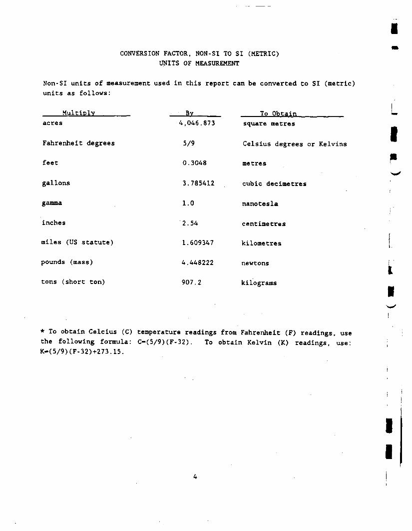
CONVERSION FACTOR, NON-SI TO SI (METRIC)UNITS OF MEASUREMENT
Non-Si units of measurement used in this report can be converted to SI (metric)units as follows:
Multiplyacres
Fahrenheit degrees
feet
gallons
gamma
inches
miles (US statute)
pounds (mass)
tons (short ton)
Bv4,046.873
5/9
0.3048
3.785412
1.0
2.54
1.609347
4.448222
907.2
To Obtainsquare metres
Celsius degrees or Kelvins
metres
cubic decimetres
nanotesla
centimetres
kilometres
newtons
kilograms
I
jiiI
* To obtain Celcius (C) temperature readings from Fahrenheit (F) readings, usethe following formula: C-(5/9)(F-32). To obtain Kelvin (K) readings, use:K-(5/9)(F-32)+273.15.
I
I
1
I
I
I
USE OF THE SITE CHARACTERIZATION AND ANALYSIS PENETROMETER SYSTEM
AT GRANDVILLE. MICHIGAN. SUPERFUND SITE
PART I: INTRODUCTION
Background
1. The Earthquake Engineering and Geosciences Division was tasked by theU. S. Environmental Protection Agency (EPA) and the U. S. Army Toxic andHazardous Materials Agency (USATHAMA) to perform an investigation at a site inGrandville, MI (Figure 1). The site is owned by Organic Chemicals Inc. (OCI) andis on the National Priority List as a Superfund Site. The facility, through theyears, has served many roles, first being an oil refinery and later beingconverted to an industrial chemical recovery/disposal operation. The plant isnow closed pending cleanup activity. The EPA was interested in the ability ofthe Site Characterization and Analysis Penetrometer System (SCAPS) to detect anddelineate hydrocarbon contaminants in the subsurface.
2. Previous work performed at the site includes three investigations doneusing soil borings and monitoring wells by three different contractors (Black andVeatch Engineers -Architects, Prein and Newhof Engineers-Planners, and MaterialsTesting Consultants). Both soil and liquid samples were taken and analyzed inthe laboratory. In addition, a limited amount of trenching and soil gassurveying was performed at the site. A geophysical electromagnetic survey wasalso performed. The laboratory results obtained from the samples taken indicateseveral compounds in the subsurface including benzene, toluene, xylene, styrene,methylene chloride, chlorobenzene, chloroform, acetone, benzoic acid and manyothers. A complete listing of chemical compounds discovered is contained in areport at the EPA Region V office.
Purpose
3. In addition to the many types of industrial chemicals discovered throughlaboratory analysis, the EPA wanted to determine whether or not hydrocarbonstypical of fuels were also present in the subsurface and if so to what extent.The boring program had indicated that hydrocarbons might be present as evidencedby the color and odor of many samples collected. Due to the complex nature ofthe conditions at the site, the EPA was having difficulty assimilating the datainto a clear representation of site conditions. The objective of the SCAPS workat the site was to develop a data set that could be directly compared to results

rigur. 1. Sito »ap shoulng th. „„ lnv«stlgated ,t Grandvllu Mlchlgan
from wells and soils borings and to develop data on the areal and vertical extentof hydrocarbon contamination in the soil above and below the water table. Thework of locating the hydrocarbon contamination was done using a cone penetrometerequipped with a fiber optic fluorometer.
IP
I
1
I
PART II: SITE DESCRIPTION
Geology
4. The site investigated lies in Kent county in the west central part ofthe Lower Peninsula of Michigan. The bedrock in Kent county consists of theedges of bowlike formations that fill the Michigan Basin. The oldest rock is —Marshall Sandstone, which underlies all of the county and is the uppermostbedrock in the southwestern part. Overlapping the Marshall Sandstone in the •central and southeastern parts of the county is the Michigan Formation, which isprimarily limestone, gypsum, and dolomite interbedded with shale and sandstone. •To the northeast, these rocks are progressively overlapped by Bayport Limestone, 'Parma Sandstone, and finally by the coal-bearing Saginaw Formation in thefurthest northeast part of the county. Overlying these rock formations is a massof glacial drift that was deposited during the Wisconsin glacial period. The :
county is situated in an area where the Michigan and Saginaw lobes of theWisconsin ice sheet met. Consequently, a very complex and strongly developed iinterlobate morainic system developed. The deposits of glacial drift range fromless than 10 feet to several hundred feet in thickness within the county. Thedrift ranges from coarse gravel to fine lacustrine clay. It is the parentmaterial in which many of the soils in the county formed. The present surfacefeatures are, for the most part, the results of glacial action. The landscape ',is an undulating plain in which valleys have been cut. Outwash material was Ideposited in the valleys by glacial meltwater streams. Three major physiographicregions are recognized in the county. The one that affects the area of •investigation consists of a number of outwash plains and lake plains in nearlylevel valleys having rather definite boundaries. The glacial drift is typically ^thinnest in these areas, and the bedrock is within a few feet of the surface \along the lower reaches of Buck and Plaster Creeks, near Wyoming and Grandville.The elevation in most of Kent county is 750 to 850 feet above sea level. The \major outwash channels and plains, however, range from 600 to 750 feet inelevation. The Grand River has an elevation of about 617 feet where it entersthe county and of 592 feet where it leaves the county. The water table slopesfrom 600 ft to 587 ft MSL between the site and the nearby Grand River.
5. The parent material of the soils of Kent county were deposited byglaciers or by glacial meltwater. Some of these materials have been reworked andredeposited by the subsequent action of water and wind. Although the parent Mmaterials are of common glacial origin, their properties vary greatly, sometimes ™within small areas, depending on how the materials were deposited. The dominantparent materials in Kent county were deposited as glacial till, outwash deposits,lacustrine deposits, alluvium, and organic material. The glacial till in Kent
8
• I

I
H
I
I
county is calcareous loam, clay loam, or fine sandy loam. From this informationand the information obtained from boring logs, it can be determined that thereis a substantial clay layer underlying the site. This clay layer occurs atvarious elevations throughout the site, but tends to occur at lower elevationstowards the Grand River. To maintain the integrity of this clay layer, no pusheswere made to elevations that would puncture or damage the layer.
General
6. The site once served as an old gravel pit and can be divided in general• into two sections. The southern half of the site, where the OCX facility is• located, does not appear to have had as much gravel removed as the northern half.
„ The northern half does have a lower surface elevation than the southern half, which is in areas as much as 10 ft higher. The northern half of the site has
also undergone extensive filling operations in an attempt to raise the surfaceelevation. The current landowner described the fill material as various typesof construction debris. This includes large pieces of concrete, metal pipes,culverts, bricks, blocks, etc. This debris filling operation was not known to
( WES before the SCAPS work began, and presented quite a problem to the conei penetrometer trying to push through such material. This resulted in many broken
probes and rods, greatly hampering progress.
• 7. The site in general presented a challenge to the cone penetrometertrying to force the push rod through rather large gravels. Four out of sixprobes on hand were damaged trying to push through the gravel layers. Thisnecessitated the use of a dummy probe in many of the probe locations. The dummyprobe is a non- instrumented mechanical device slightly smaller than theinstrumented probe used to make a pilot hole. Once the pilot hole was made tothe depth required, the instrumented probe was used to collect fluorescence data.This technique does not allow the collection of soils data (cone tip resistanceand sleeve friction) for soil classification purposes, but does permit thecollection of fluorescence data. Since the main objective of the project was tocollect fluorescence data, this technique did not hamper the project.

PART III: EQUIPMENT AND METHODS
General
8. The Site Characterization and Analysis Penetrometer System (SCAPS),includes a suite of surface geophysical equipment, survey and mapping equipment,special penetrometers with sensors for contaminant detection, and soil and porefluid penetrometer samplers. The experimental penetrometer system is mounted ina specially-engineered truck (Figure 2) designed with protected work spaces to •allow access to toxic and hazardous sites while minimizing exposure of the workcrew. The SCAPS "screening" penetrometers are equipped with sensors that can mmdetermine certain physical and chemical characteristics of the soil as thepenetrometer tip is forced through the soil. SCAPS includes sensors that candetermine the strength, electrical resistivity, and spectral properties, in thiscase the fluorescence, of soils. All sensors read out in real time, and acomputer-based data collection and analysis system permits a display and partialinterpretation of data in the instrument compartment on the penetrometer truck.The data analysis system also allows processing of various types of surfacegeophysical and mapping data collected on site, and integration of data into aunified data base. Fluid and soil samples can be collected using devices such 'as the commercial "stab type" groundwater and soil samplers that are designed foruse with penetrometers. The SCAPS system is also equipped to seal eachpenetrometer hole with grout as the probe is withdrawn from the hole and the *geotechnical investigation proceeds across a site. The SCAPS unit is built sothat surfaces and compartments exposed to waste can be thoroughly and completely mdecontaminated. Post processing of the data to provide a 3-D visualization ofsite conditions is presently done with a computer work station that can be used >—^at WES or brought to the installation. SCAPS is designed to save time and costsand to minimize exposure of the crew while sensor data or samples are collected.Penetrometer units available commercially do not have this combination ofcapabilities.
Site Mapping
9. The locations of penetrometer push points were determined byestablishing a grid over the site. The OCI site covers approximately five acreswhile the total area of investigation covers approximately eighty acres. A gridwas established on 300 ft centers (Figure 3) with each location to be surveyed Ufor northing, easting, and elevation. The survey points are based on a local *coordinate system provided by EPA, that tied into work performed during thedrilling operations. A local Corps District was used for surveying the grid. •Additional surveying was performed by the WES crew utilizing a total station
10

I
I
I
HOLLOW.3 METERLENGTH PUSH RODS
WIRING RUN INSIDE PUSH PIPE
SLEEVE FRICTIONRESISTANCE. TONS/SO FT(TSF)
OR KILONEWTONS(kN)
POINT PENETRATIONRESISTANCE. TONS/SO FT(TSF)
OR WLONEWTONS(kN)DIAMETER - 3.57 CM
60 DEC CONE TIP
BASIC CONFIGURATION OF SCAPS TRUCKMOUNTED ON ALL WHEEL DRIVE TRUCK (MODIFIED M8U MILTARY CHASSIS)HYDRAULICALLY POWERED PUSH APPARATUS 178-kN PUSHWEIGHT APPROXIMATELY 21.000 KGCOMPUTER AIDED DATA ACQUISITIONMEASUREMENTS OF PENETRATION RESISTANCEAT 1-INCH (2.5 CM) INTERVALSENCLOSED AIR-CONDITIONED WORKSPACE
I
I
Figure 2. Experimental penetrometer system and configuration,
11
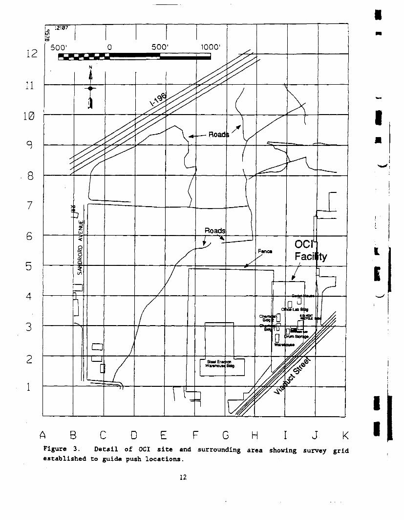
I SIMI Er« ionWarahouM Bug
A B C D F H I J KFigure 3. Detail of OCI site and surrounding area showing survey gridestablished to guide push locations.
I
Lf
II
12

I
electronic distance measuring system (EDM). This additional surveying includedpoints that could not be reached with the push truck due to physical constraints,points investigated between the original 300 ft grid, and points located outsidethe grid.
Geophysical Investigations
10. Geophysical site surveys were undertaken primarily to determine ifthere was metallic debris in the area where the penetrometer unit would beoperating. The geophysical investigations were simply scans of the area before
0B pushing began to insure that no damage would occur to the probe and that no1 pipes, barrels, or other such objects would be punctured. The geophysical
technique used at the OCI site in conjunction with the SCAPS truck consisted ofI ' electromagnetic induction. This technique was selected because of its ease of
use, real-time data analysis, and reliability of metal detection to a maximumdepth of twenty feet.
11. The electromagnetic induction devices are used to measure the earth'sf apparent ground conductivity. The responses from the equipment are directlyI proportional to conductivity and inversely proportional to resistivity. The
basic operation utilizes a transmitter coil (Tx) energized with an alternatingL current at an audio frequency and a receiver coil (Rx) located a short distance~ away. The time varying magnetic field arises from the alternating current in the• transmitter coil inducing currents in the earth. These currents generate a• secondary magnetic field which is sensed, together with the primary field, by the^ receiver coil. In general, this secondary magnetic field is a complicated
• function of the intercoil spacing, the operating frequency, and the groundconductivity. Under certain constraints, called the low induction condition, thesecondary magnetic field is a very simple function of these variables. Underthese constraints, the ratio of the secondary to the primary field is linearlyproportional to the terrain conductivity. The apparent conductivity indicatedby the instruments depends on measurement of the secondary to primary field ratioand assumes low induction conditions. The units of conductivity are the mho(Siemen) per meter or, more conveniently, the millimho per meter.
I
I
12. There are two components of the induced magnetic field measured by theinstrument. The first is the quadrature-phase component which gives the groundconductivity measurement. The second is the inphase component, which is usedprimarily for calibration purposes; however, the inphase component issignificantly more sensitive to large metallic objects and hence very useful whenlooking for buried metal containers. Experiments have indicated that the GeonicsEM-31 can detect a single 45 gal oil drum at a depth of about 12 ft (3.7m) using
13
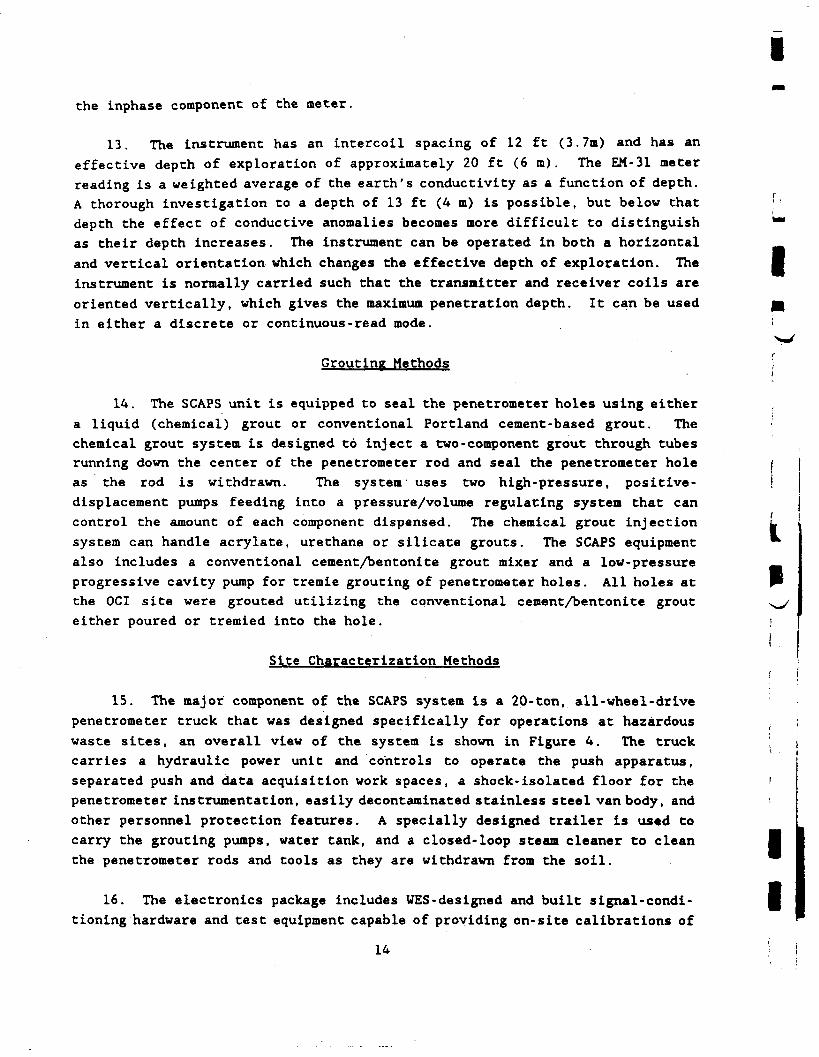
the inphase component of the meter.
13. The instrument has an intercoil spacing of 12 ft (3.7m) and has aneffective depth of exploration of approximately 20 ft (6 m). The EM-31 meterreading is a weighted average of the earth's conductivity as a function of depth.A thorough investigation to a depth of 13 ft (4 m) is possible, but below that <•depth the effect of conductive anomalies becomes more difficult to distinguish *"as their depth increases. The instrument can be operated in both a horizontaland vertical orientation which changes the effective depth of exploration. The •instrument is normally carried such that the transmitter and receiver coils areoriented vertically, which gives the maximum penetration depth. It can be used j|in either a discrete or continuous-read mode. \
>-Grouting Methods ii
14. The SCAPS unit is equipped to seal the penetrometer holes using eithera liquid (chemical) grout or conventional Portland cement-based grout. Thechemical grout system is designed to inject a two-component grout through tubesrunning down the center of the penetrometer rod and seal the penetrometer hole ^as the rod is withdrawn. The system uses two high-pressure, positive- !displacement pumps feeding into a pressure/volume regulating system that cancontrol the amount of each component dispensed. The chemical grout injection L 'system can handle acrylate, urethane or silicate grouts. The SCAPS equipment *•also includes a conventional cement/bentonite grout mixer and a low-pressure _progressive cavity pump for tremie grouting of penetrometer holes. All holes at P"the OCI site were grouted utilizing the conventional cement/bentonite grout >^/either poured or tremied into the hole. !
i .Site Characterization Methods• • ^ " ^ ^ " ^ ^ •• ^ ^ ^ •"• ^ ^ ^ •™ ^ ^ ^ ™ ™ f
15. The major component of the SCAPS system is a 20-ton, all-wheel-drivepenetrometer truck that was designed specifically for operations at hazardouswaste sites, an overall view of the system is shown in Figure 4. The truck L .carries a hydraulic power unit and controls to operate the push apparatus,separated push and data acquisition work spaces, a shock-isolated floor for the fpenetrometer instrumentation, easily decontaminated stainless steel van body, andother personnel protection features. A specially designed trailer is used tocarry the grouting pumps, water tank, and a closed-loop steam cleaner to clean •the penetrometer rods and tools as they are withdrawn from the soil.
16. The electronics package includes WES-designed and built signal-condi- •tioning hardware and test equipment capable of providing on-site calibrations of
14 - i !

Figure A. Photograph of penetrometer truck and grouting trailer.

I
contaminant detectors and load cells used to make penetration resistancemeasurements. Data acquisition and initial data processing are carried out withan on-board computer with a matching computer used for data management and fileintegration. The second computer affords redundancy in the event of a computerfailure. A view of the data collection compartment of the truck is shown inFigure 5.
Soil Strength and Type Determination
17. A sectional view of a penetrometer equipped to measure soil strengthis shown in Figure 6. The point load cell is loaded in compression as the conetip is advanced. The friction sleeve load cell is in the form of a hollow ^cylinder and strain gauged on the inside surface of the cylinder. The cellsurrounds the tip load cell and is also loaded in compression when soil friction (acts on the friction sleeve which jackets the front of the probe. The designemployed in this soil strength unit allows the tip penetration resistance and !sleeve friction measurement to be made independently and continuously.
18. Two calibration procedures are used with the cone employed in this !investigation so that separate calibration curves can be developed for the twoload cells. The point resistance load cell is calibrated by cycling the load fromzero load to approximately 7272 Kgf (equivalent to 16,000 psi) and back to zero Iload several times. The cell is then loaded to selected load increments and backto zero. The load cell output is read for each load increment applied and the •zero load condition at the beginning and end of each loading increment. The load "increments are increased until the compressive force reaches the maximum capacityof the cell. The friction sleeve load cell is calibrated in a similar way. jFigures 7 and 8 show typical calibration curves obtained for a strain-gagedpenetrometer instrument. Each load cell is calibrated independently but the ,output of each cell is measured as the calibration proceeds so that any influence \ •of one cell on the output of the other can be determined. Typically neither cellshows any influence on the other. Calibration test responses are generally ,within 0.5% of the applied load. Load cell calibrations can be done in thefield, but are generally completed prior to field deployment.
19. Due to the nature of the site (gravels and construction debris) and themany broken probes, no soils data was collected at the site for any of the —probes. Therefore no soils classification information is presented in this •report. The depth of penetrometer pushes, selected to extend to the clay layer,was determined from the boring logs in the area rather than from the penetrometersoils information.
16
I

Figure 5. View of data collection and processing section of penetrometer truck.
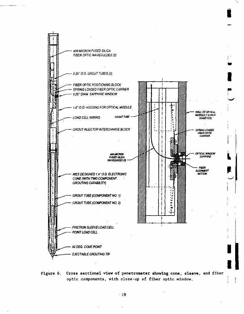
400 MIC.RON FUSED SILICAFIBER OPTIC WAVEGULDES (2)
0.25" 00 GROUT TUBES (2)
FIBER OPTIC POSITIONING BLOCKSPRING LOADED FIBER OPTIC CARRIER025'DIAM. SAPPHIRE WINDOW
1.6" 00. HOUSING FOR OPTICAL MODULE
LOAD CELL WIRING GflO/r TUBE -
GROUT INJECTOR INTERCHANGE BLOCK
400-UCRONFUSED OLCA
WAVKUUXSP)
• mS DESIGNED 1.4"0.0. ELECTRONICCONE (WITH TWO COMPONENTGROUTING CAPABILITY)
GROUT TUBE (COMPONENT NO. 1)
GROUT TUBE (COMPONENT NO. 2)
WALL OF OPTICALUOOUU-(1.6-INCH
DIAMETER)
SPRING LOAD£0FIBEROPTIC
OPTICAL WINDOWSAPPHIC
ALIGNMENTBUTTON
I
(
P
FRICTION SLEEVE LOAD CELLPOINT LOAD CELL
60 DEG. CONE POINT
EJECTABLE GROUTING TIP
Figure 6. Cross sectional view of penetrometer showing cone, sleeve, and fiberoptic components, with close-up of fiber optic window.
I
I
18

I
r
II
0.3
0.2
3<rLJQ.
2
IT0.1
0.2
aa:
tr>—</i
0.1
[_
0
POINT RESISTANCELOAO CELL
5 10 15APPLIED LOAO. POUNDS X 1000
APPLIED LOAD. KILOGRAMS X 1000
FRICTION SLEEVELOAO CELL
1 2 3 4APPLIED LOAO. POUNDS X 1000
1APPLIED LOAO. KILOGRAMS X 1000
20
10
1 11 2
I3
14
15
I6
17
18
|9
Figure 7 and 8. Calibration curves for point resistance and sleeve friction.
19

Soil Fluorescence Measurement Methods
20. The in situ fluorometer is described in detail in the U. S. PatentOffice (1992). Liebennan, Inman and Theriault (1989) had used a fluorometer formeasuring POL fluorescence in seawater, and the fluorescence has been documentedas a useful approach in tracking hydrocarbon pollutants. A schematic of the •system is presented in Figure 9. In making a measurement, the exciting radiation »is produced by firing a pulsed nitrogen laser (emitting wavelengths at 337 run).The laser light is coupled into two fibers, a timing circuit fiber and the •downhole sample irradiation fiber. The light in the timing circuit fiber is usedto set the timing window on the detector. The major part of the laser pulse is pcoupled into a 400-micron optical fiber that passes down the center of thepenetrometer rod. The fiber ends at a 6.35-mm sapphire window that passes the jlight onto the soil surface adjacent to the window. The fluorescence signal that jis a response to the ultra-violet excitation is collected by a second 400-micronfiber and is carried back up through the penetrometer rod to a polychromator. 'In the polychromator the fluorescent signal is dispersed and the energydistribution at the wavelengths of interest is measured using a linear photodiode iiarray. This system is much faster than a scanning spectrofluorometer. Readoutof an entire emission spectrum requires only 15 msec. The rapidity of the ireadout makes it practical to "stack" or add successive pulses and increase the 'sensitivity of the unit. Time resolve fluorometry is also possible although thismay require holding the window in one position for several minutes. »
21. The response of the fluorometer is directly related to the concentrationof aromatic compounds in the soil. Fluorescence of any aromatic compounds with ^-/
basic or acid functional groups is usually pH dependent. Ionized aromaticcompounds will fluoresce at different wavelengths and at different intensitiesfrom the same compounds in a nonionized state. Fluorescing compounds adsorbedon solid surfaces will typically fluoresce with greater intensity than the samecompounds in solution. Decomposition or weathering phenomena also change thefluorescence of fuels. Generally the aromatic (ring) compounds that fluoresceare concentrated in the weathering process because the lighter hydrocarbonsvolatilize and the longer straight-chain hydrocarbons are more easily decomposedby microbial activity.
22. Each fluorescence spectrum consists of photon counts measured at 1024points (over a wavelength range of 300 to 800 run) for every 2-era (0.8-in.) layer •of soil investigated. The present data processing system records all spectral ™intensity measurements and makes corrections for instrument drift duringmeasurement. The corrected data are screened to develop the photon counts for •the peak of interest and the background. A file containing the single equivalent
20

POST PROCESSINGCOMPUTERRAM
POSITIONSENSOR
NITROGEN LASERFIBER OPTICPROBE UMBILICAL CORD
OPTICALMULTICHANNELANALYZER
SLEEVEFRICTION
SENSOR CONDITIONINGRACKPOINT LOAD
SENSORNETWORKSERVER
COMPUTER
Space For ExtraProbes DATA
TRANSLATIONA/D • D/A
DATA ACQUISITIONCOMPUTER
POWERSUPPLY
Figure 9. Flowchart of fiber optic system.

normalized counts, the map coordinates, and the depth below a surveyed datum isprepared from the spectral data. The final data file is transformed into a 3-dimensional gridded file and is displayed using a visualization program.
Method of Converting Counts to Probable Contaminant Concentrations
23. Prior to arrival of the SCAPS truck a WES crew visited the OCI site andobtained soil samples at two locations. These samples were collected in areasthat were known to contain hydrocarbon contaminants or known to be free ofhydrocarbon contaminants based on earlier trenching activity conducted by theEPA. The samples were returned to WES and analyzed in the laboratory for totaloil and grease (O&G), total recoverable petroleums and hydrocarbons (TRPH), andtotal polynuclear aromatics (TPNA). The same samples were investigated with thefiber optic fluorescence system to determine the counts associated with each.The samples were then mixed to form ratios of "clean" to "dirty" at ratios of25:75, 50:50, and 75:25, respectively. The new samples were then analyzed asdescribed above to produce a set of points for each test. The results of the labanalysis and fluorescence data is presented in Table 1. A plot of O&G, TRPH, andTPNA concentrations of contaminants in ppm versus intensity counts (Figure 10)was then created. The intensity counts axis is a ratio of counts obtained fromfiring on the soil samples (Table 1) over counts obtained from firing on therhodamine standard. A best fit line was forced through the data to give threeequations. These equations represent a technique to convert counts from thefiber optic system, into predicted concentrations of ppm based on the datacollected at the OCI site. The equation used to convert all the counts to ppmin this report is based on the TRPH data. The O&G data should give values thatare high because of the inclusion of the greases which do not fluoresce. TheTPNA data should give values that are low because it only includes the aromatics.Therefore, the TRPH data is best representative of the soil fluorometer data.
Table 1. Results of calibration testing for the OCI site.
FluorescenceCounts
LaboratoryO&G , ppm
LaboratoryTRPH , ppm
LaboratoryTPNA, ppm
Dirty 75% Dirty|| 25% Clean
1115
4500
3900
1.4
731
3100
2600
1.0
50% Dirty50% Clean
402
1600
1200
0.6
25% Dirty75% Clean
170
800
600
0.06
Clean
45
230
45
0
I
L
I
I
I22
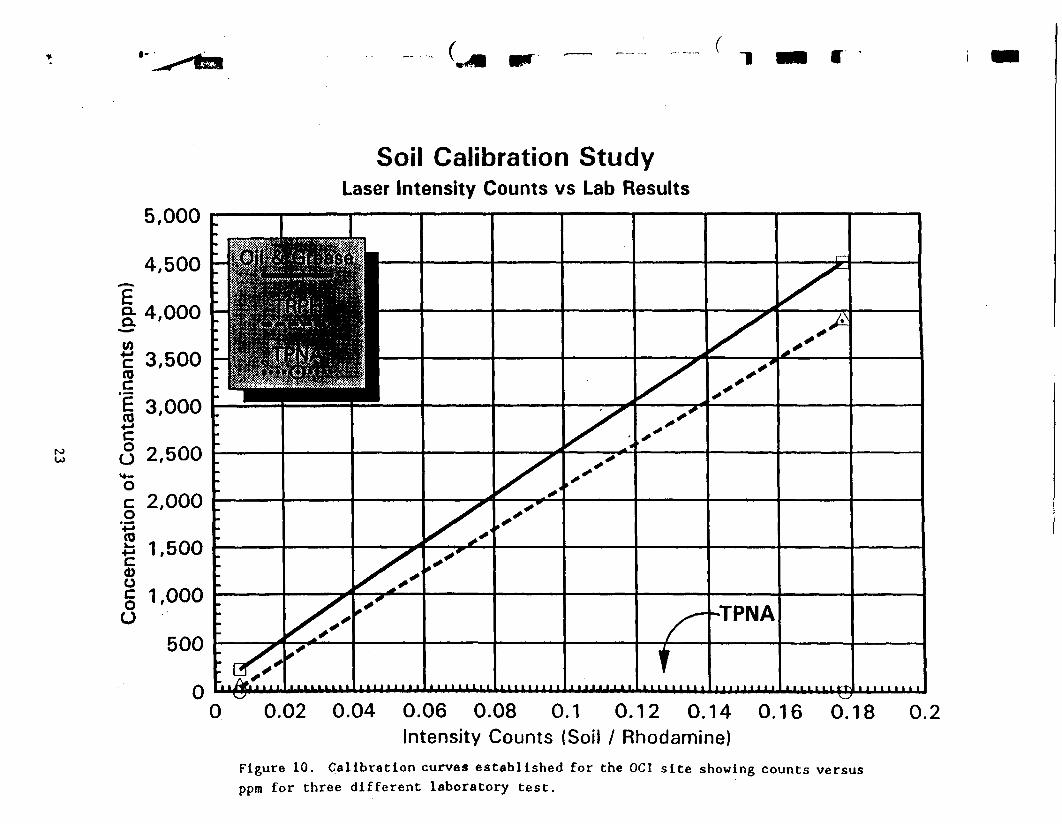
roto
EQ.^
<A•M
(0
CO•M
oO
co'*3(0
5,000
4,500
4,000
3,500
3,000
2,500
2,000
£ 1,5000)ooO
1,000
500
Soil Calibration StudyLaser Intensity Counts vs Lab Results
t
TPNA
0 iiigMiiiiiiiiiiiiiiiiiiiiiiiMimimiiiiiiiiiiiiiiimiiiii.iiMiiiiiiiMiiiiiiiiiiiQi0 0.02 0.04 0.06 0.08 0.1 0.12 0.14 0.16 0.18
Intensity Counts (Soil / Rhodamine)Figure 10. Calibration curves established for the OC1 site showing counts versusppm for three different laboratory test.
0.2
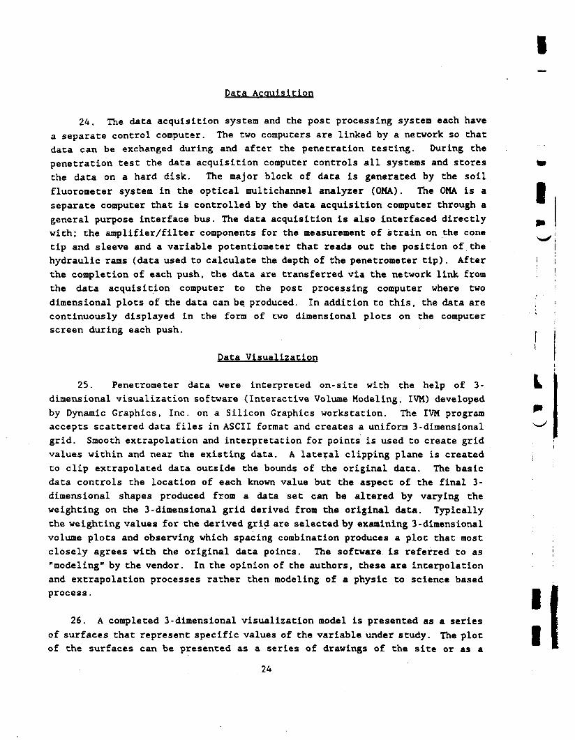
Data Acquisition
24. The data acquisition system and the post processing system each havea separate control computer. The two computers are linked by a network so thatdata can be exchanged during and after the penetration testing. During thepenetration test the data acquisition computer controls all systems and stores tothe data on a hard disk. The major block of data is generated by the soilf luorometer system in the optical multichannel analyzer (OKA.). The OMA is a •separate computer that is controlled by the data acquisition computer through ageneral purpose interface bus. The data acquisition is also interfaced directly _with; the amplifier/filter components for the measurement of strain on the cone ^^ !tip and sleeve and a variable potentiometer that reads out the position of the Ihydraulic rams (data used to calculate the depth of the penetrometer tip). After > Ithe completion of each push, the data are transferred via the network link from . 'the data acquisition computer to the post processing computer where two :
dimensional plots of the data can be produced. In addition to this, the data are ; •continuously displayed in the form of two dimensional plots on the computer ' ;screen during each push. ,
(Data Visualization
25. Penetrometer data were interpreted on-site with the help of 3- kdimensional visualization software (Interactive Volume Modeling, IVM) developedby Dynamic Graphics, Inc. on a Silicon Graphics workstation. The IVM program ^accepts scattered data files in ASCII format and creates a uniform 3-dimensional x—'grid. Smooth extrapolation and interpretation for points is used to create gridvalues within and near the existing data. A lateral clipping plane is createdto clip extrapolated data outside the bounds of the original data. The basicdata controls the location of each known value but the aspect of the final 3-dimensional shapes produced from a data set can be altered by varying theweighting on the 3-dimensional grid derived from the original data. Typicallythe weighting values for the derived grid are selected by examining 3-dimensionalvolume plots and observing which spacing combination produces a plot that mostclosely agrees with the original data points. The software is referred to as"modeling" by the vendor. In the opinion of the authors, these are interpolationand extrapolation processes rather then modeling of a physic to science basedprocess. •
26. A completed 3-dimensional visualization model is presented as a seriesof surfaces that represent specific values of the variable under study. The plot •of the surfaces can be presented as a series of drawings of the site or as a
24

computer-generated video that shows the soil volume with the data boundariespresented in varying colors. The IVM software can rotate the volume so that thelimits of the parameter can be observed from all sides. Subprograms areavailable that allow the volume model to be sliced at various points so that thevariation of the parameter can be observed inside the projected volume. All datacollected at the OCX site was processed in this manner each day to help indirecting the next day's probe siting.
I
I25
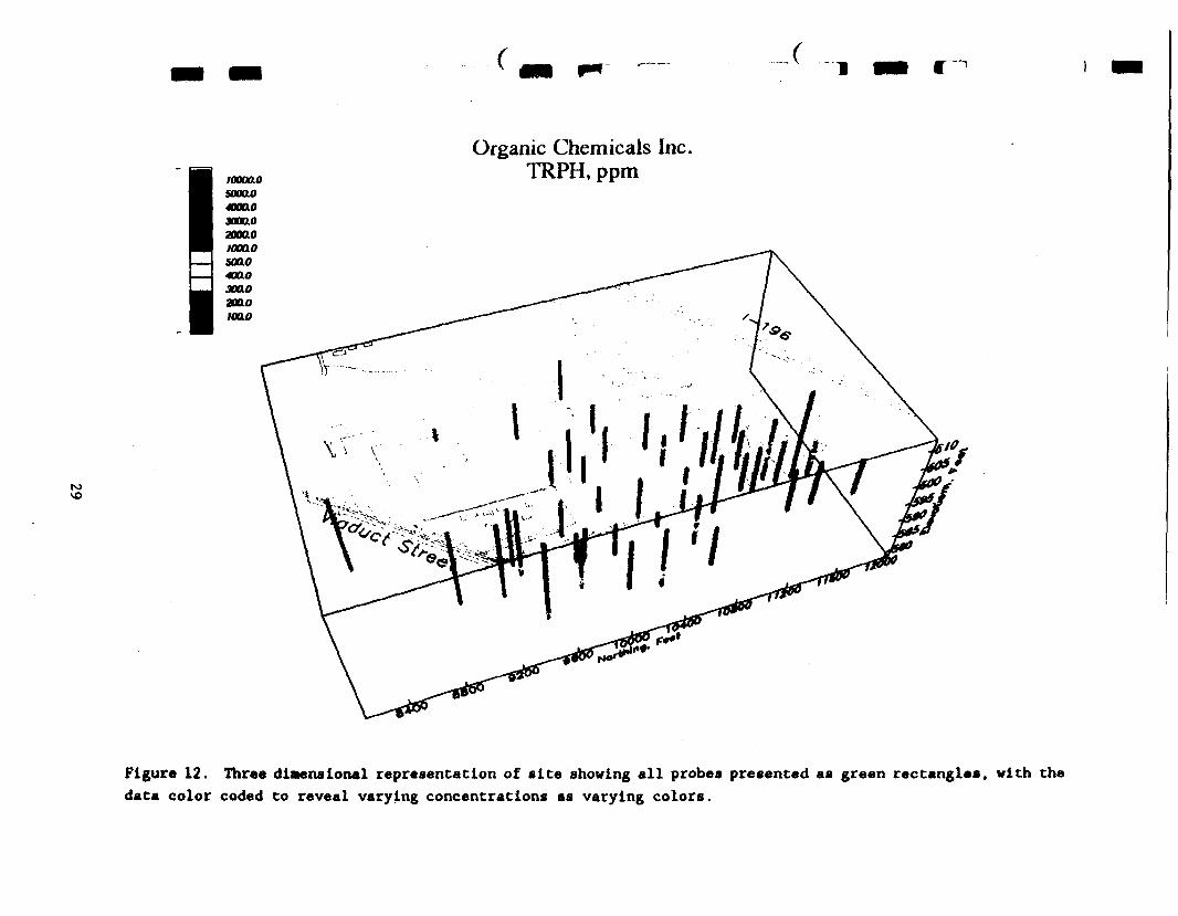
Organic Chemicals Inc.TRPH, ppm
ho
Figure 12. Three diaensional representation of site showing all probes presented as green rectangles, with thedata color coded to reveal varying concentrations as varying colors.
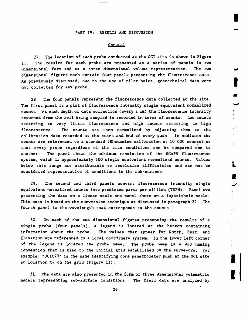
PART IV: RESULTS AND DISCUSSION
General
27. The location of each probe conducted at the OCI site is shown in Figure11. The results for each probe are presented as a series of panels in twodimensional form and as a three dimensional volume representation. The two ^dimensional figures each contain four panels presenting the fluorescence data.As previously discussed, due to the use of pilot holes, geotechnical data were •not collected for any probe. *
*28. The four panels represent the fluorescence data collected at the site.
The first panel is a plot of fluorescence intensity single equivalent normalized s<—'counts. At each depth of data collection (every 2 cm) the fluorescence intensity \returned from the soil being sampled is recorded in terms of counts. Low counts .referring to very little fluorescence and high counts referring to highfluorescence. The counts are then normalized by adjusting them to the [
calibration data recorded at the start and end of every push. In addition thecounts are referenced to a standard (Rhodamine calibration of 10,000 counts) so ,that every probe regardless of the site conditions can be compared one to 'another. The panel shows the minimum resolution of the SCAPS fluorescencesystem, which is approximately 100 single equivalent normalized counts. Valuesbelow this range are attributable to resolution difficulties and can not be ^considered representative of conditions in the sub-surface.
•29. The second and third panels convert fluorescence intensity single ^/
equivalent normalized counts into predicted parts per million (TRPH). Panel twopresenting the data on a linear scale and panel three on a logarithmic scale. iThis data is based on the conversion technique as discussed in paragraph 22. Thefourth panel is the wavelength that corresponds to the counts.
30. On each of the two dimensional figures presenting the results of asingle probe (four panels), a legend is located at the bottom containinginformation about the probe. The values that appear for North, East, andElevation are referenced to a local coordinate system. In the lower left corner :
of the legend is located the probe name. The probe name is a WES naming •convention that is tied to the initial grid established by the surveyors. Forexample, "OCIC70" is the name identifying cone penetrometer push at the OCI site •at location C7 on the grid (Figure 11). •
31. The data are also presented in the form of three dimensional volumetric •models representing sub-surface conditions. The field data are analyzed by
26
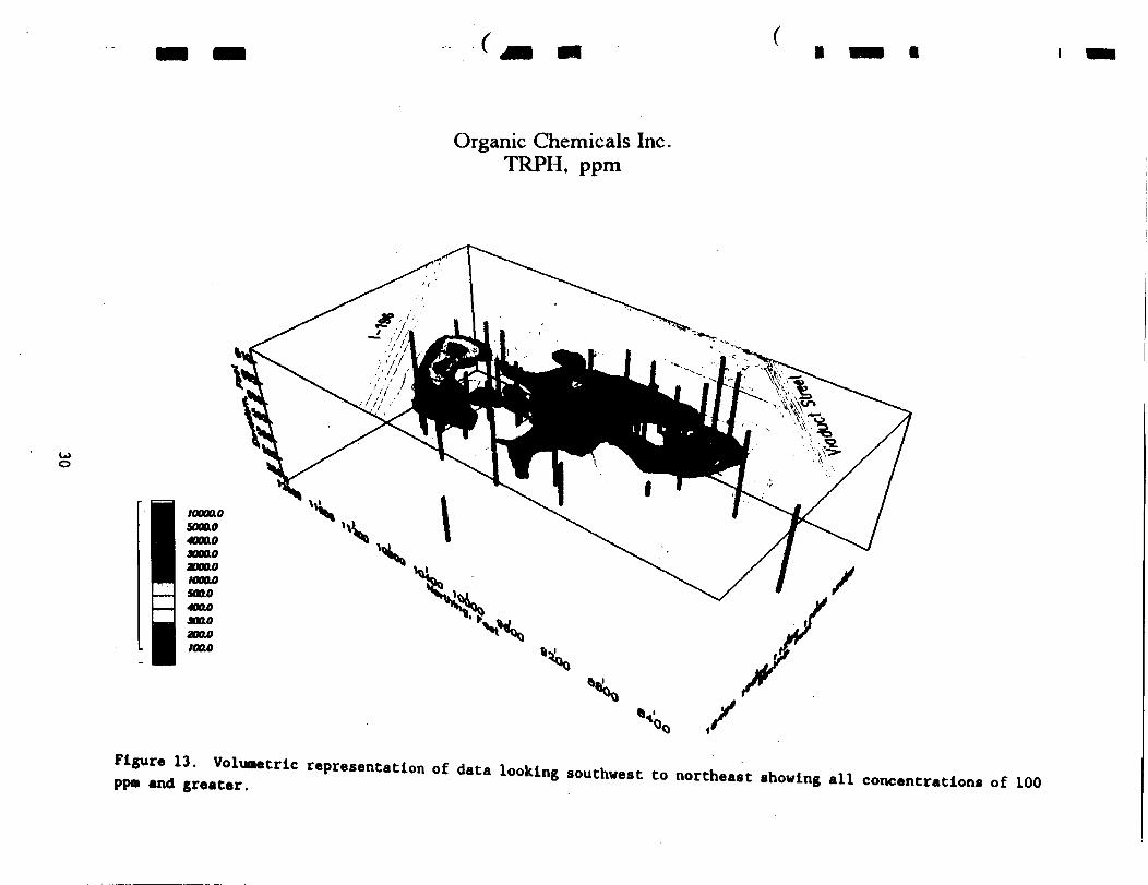
Organic Chemicals Inc.TRPH, ppm
toO
Figure 13. Volumetric representation of data looking southwestppm and greater. to northeast showing all concentrations of 100

I
I
II
12
11
10
8
7
4
3
IMWSf
OCIG50 I OCIH50I QCII50
A BFigure 11
c D• PENETROMETER PUSH LOCATIONS
G H I J KDetail of OCI site and surrounding area showing the locationsof all penetrometer pushes at the site.
27

Organic Chemicals Inc.TRPH, ppm
Figure 14. Volumetric representation of data looking southwest to northeast showing all concentrations of 400ppm and greater.

sophisticated three dimensional data interpolation algorithms. The gridded dataare then formed into a three dimensional volumetric image of the subsurface soilconditions or of the body of contaminated soil. Varying properties of thematerial (contaminant concentrations) are displayed as different color zones.The image can easily and rapidly be manipulated in a number of ways to allowviewing the object from all angles. The location of all data points used tocreate the gridded data are displayed on the figure. Due to the large data set ^collected (every 2 cm) the posted data appear as a solid line. A two-dimensionalplan map of the site investigated can be added to the figure to aid in feature Ilocations. In the lower left corner of the figure is a legend presenting the •color zones and corresponding values represented.
iFluorescence Data
>-i -32. The two dimensional panel plots of the fluorescence data from each •
individual probe conducted at the site are presented in Appendix A, and aresummarized in Table II. Figures 12 through 22 are the volumetric representationsof the data. Figure 12 is a view of the site looking east to west, that shows 'each probe location. The probe locations have been presented as elongatedrectangles that have been color coded, with the legend located in the upper left Icorner of the plot. From a simple presentation like this, one can see thelocations of contaminants extending from the south to north end of the site. The .probes extended from Viaduct Street at the south end to Interstate-196 at the ^north end of the site. The east west boundaries were established by the propertyboundaries of adjacent landowners. A total of 49 probes were completed at the •site. •
>~s33. A more detailed presentation of the data is given in the remaining j
figures. Figures 13 through 16 are all views of the site looking from southwestto northeast. Figure 13 shows all the data obtained at the site with TRFH |concentrations of 100 ppm and above. Figure 14 shows the data withconcentrations of 400 ppm and above, Figure 15 with concentrations of 1000 ppmand above, and Figure 16 with concentrations of 5000 ppm and above. Thesefigures all show that the contaminants are spread out from the OCX site (where :
the buildings and tanks are located) northward toward the Interstate. ,
I
I28

Organic Chemicals Inc.TRPH, ppm
LOto
Figure 15. Volumetric representation of data looking southwest to northeast showing all concentrations of 1000ppm and greater.

_ r
Organic Chemicals Inc.TRPH, ppm
S, /
Figure 16. Volumetric representation of data looking southwest to northeast showing all concentrations of 5000ppm and greater.

iTable II. Summary of probes at OCI site
I
LI
II
PROBE NAME
OCIC70
OCIE50
OCIE60
OCIE70
OCIF60
OCIF70OCIF80
OCIF90
OCIF100
OCIF105
OCIG50
OCIG60
OCIG80
OCIG90
OCIG100
OCIG511
OCIH50
OCIH60OCIH70
OCIH80OCIH90
OCIH92
OCIH100OCIH110
OCII40
OCII50
OCII55
OCII60
OCII70
PROBE LOCATION
C7 on survey gridE5 on survey gridE6 on survey gridE7 on survey gridF6 on survey gridF7 on survey gridF8 on survey gridF9 on survey gridF10 on survey gridBetween F10 & Fllon survey gridG5 on survey gridG6 on survey grid
G8 on survey gridG9 on survey gridG10 on survey gridBetween Gil & Hllon survey gridH5 on survey gridH6 on survey gridH7 on survey gridH8 on survey gridH9 on survey gridBetween H9 & H10on survey gridH10 on survey gridHll on survey grid14 on survey grid15 on survey gridBetween 15 and J5on survey grid16 on survey grid17 on survey grid
ELEV INVESTIGATEDABOVE MSL
600.1 - 587
606.2 - 595602.9 - 594
600.2 - 591
603.6 - 590
600.3 - 588602.5 - 591
602.1 .- 590
597.8 - 580597.8 - 585
608.8 - 598.5603.9 - 594603.8 - 594600.3 - 590600.3 - 588600 - 583
602.7 - 591
603.7 - 595.5
603 - 591602.4 - 589601.7 - 585
601.7 - 589
601.7 - 588602.3 - 590
610.3 - 592601 - 593
601 - 594
600.1 - 591
600.6-596.5
PRODUCT ENCOUNTEREDAT ELEV ABOVE MSL
nonenonenonenonenone598, 594 - 590nonenonenonenone
605 - 603597 - 594602 - 598599.7, 598 - 597589 - 588598 - 596, 594
596 - 593
599, 595.5601-599, 597-592597 - 589none
none
600-597, 594, 591.5none607, 596 - 592
599.5. 593.5596 - 594.5
600, 598.5, 597-591
597.25
34

IPROBE NAME
OCII80
OCII100
OCII110
OCII120
OCIJ40
OCIJ50
OCIJ60OCIJ70OCIJ80
OCIMW2
OCIMW3
OCIMW4
OCIMW5
OCIMW7
OCIMW8
OCIMW16
OCIMW22
OCIMW23
OCIPB16
OCI196
PROBE LOCATION
18 on survey grid110 on survey grid
111 on survey grid
112 on survey gridJ4 on survey gridJ5 on survey gridJ6 on survey gridJ7 on survey gridJ8 on survey gridNear chemical bldg#2, and MW-2West of warehouse,and MW-3Between H3 and H4on survey gridBetween 15 and 16on survey gridNear Gl on surveygird, and MW-7
Between E3 and F3on survey gridGil on survey gridBetween 13 and J3on survey gridNear boiler house,and MW-23Between Hll andH12 on survey gridNear G12 on surveygrid
ELEV INVESTIGATEDADrtT7IT UCT
602.3 - 591603 - 590
603.4 - 590
600.8 - 589607.5 - 601
603 - 591604.4 - 591
604.7 - 589602.3 - 590
610.3 - 599
606 - 584
604.3 - 590
599.1 - 590
606.6 - 585
608.1 - 603.5
600 - 580
614.2 - 592
611.2 - 589
600.8 - 588
605.5 - 578
PRODUCT ENCOUNTEREDAT PT CTT ADnTTE1 MCI
602-600, 595.5-591
none
nonenonenone601-600, 598-592
598, 596-591
596.5 - 591595 - 591
none
none
600, 595.5-591.5
596 - 592
none
none
600 - 585
606-603, 597-593
593 - 589
600 - 592
none
I
Ip
34. The volumetric representation of the data has been rotated upward topresent top views as shown in Figure 17 - 20. Figure 17 is the data having aconcentration of 100 ppm and greater, Figure 18 is a view of concentrations 400ppm and greater, Figure 19 is a view of concentrations 1000 ppm and greater,Figure 20 is a view of concentrations 5000 ppm and greater. In the left topcorner of Figure 17 is a small diagram indicating the volume of the contaminant
I
I35
Organic Chemicals Inc.TRPH, ppm
10000.0sooo.04000.03000.03000.0looao5OO.O100.03OO.O3OO.O100.0
Figure 17. Volumetric representation of data, top view, showing all concentrations of 100 ppm and greater.
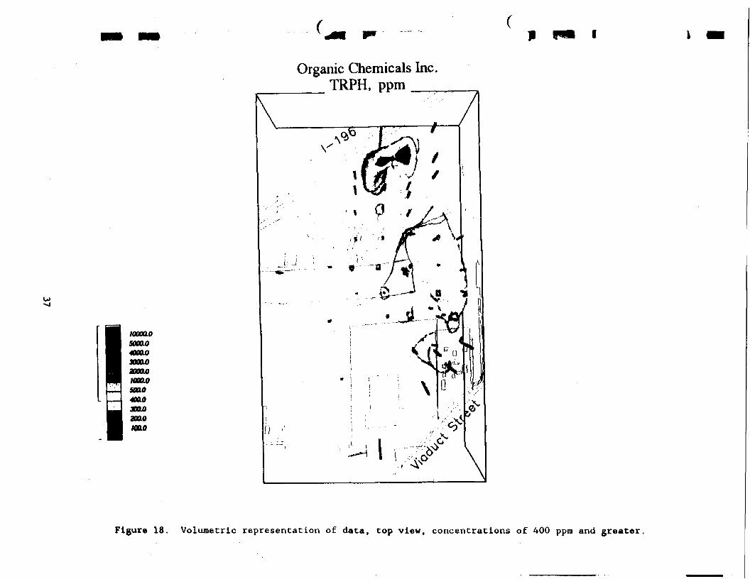
Organic Chemicals Inc.__ TRPH, ppm
loooaosoooo
JOOOL0annoKUO.O
400L0300.0aaaoMao
Figure 18. Volumetric representation of data, top view, concentrations of 400 ppm and greater

00
10000.050000
3000JJaoooo10000500.0400030002000MOO
Organic Chemicals Inc.TRPH, ppm
Figure 19. Volumetric representation of data, top view, concentrations of 1000 ppm and greater,

c
COv£>
IOOOO.O90000400010jooaoaoooo1000.0500.04000JOOOaoooMOO
Organic Chemicals Inc.__ TRPH, ppm _____
i i
Figure 20. Volumetric representation of data, top view, concentrations of 5000 ppra and greater.

I
I
I
plume. The volume is 6,352,734.5 cubic feet of material for concentratins of 100ppm and greater.
35. Figures 21 and 22 are views of the data looking east to west. Bothfigures show concentrations of 100 ppm and greater. Figure 22 is a view of thedata where a cut has been made into the center of the data to reveal the higherconcentrations.
36. Appendix B contains two top views of the contaminant plume that hasbeen superimposed on top of the aerial photograph of the site. Figure Blcontains the data with concentrations of 100 ppm and greater, Figure B2 theconcentrations with 5000 ppm and greater. This presentation gives an excellentview of where the contaminant plume has spread over the site.
37. A final attempt has been made to correlate the findings from the conepenetrometer with actual laboratory data. The soil samples collected prior toarrival of the cone truck, that were used to produce the data in Table 1 andFigure 10, were collected very close to the location between 15 and J5 on thesurvey grid. A push was made in this area, shown in Appendix A as Figure A28,therefore the data from the penetrometer and the laboratory analysis can becompared. Two samples were taken and analyzed, one at a depth of 1 ft and asecond at a depth of 6 feet. From the laboratory analysis, Table 1 (the 1 ftsample is labeled clean, the 6 ft sample is labeled dirty), the concentrationsare 3900 ppm TRPH at 6 ft and 45 ppm TRPH at 1 ft. The O&G concentrations are4500 ppm at 6 ft and 230 ppm at 1 ft. From Figure A28, at a depth of 1 ft theconcentration is less than 100 ppm (does not plot), and at a depth of 6 ft theconcentration is approximately 4500 ppm.
40

r • OT
Organic Chemicals Inc.TRPH, ppm
ftAOO
Figure 2,1. Volumetric representation of data looking east to west showing all concentrations of 100 ppn andgreater.

» m
Organic Chemicals Inc.TRPH, ppm
NJ
Figure 22. Volumetric representation of data looking east to west showing all concentrations of 100 ppn andgreater, with a section sliced away to reveal higher concentrations inside the plune.

I
I
1
I
PART V: CONCLUSIONS
38. Summarizing the results of the probes conducted at the OC1 site,several things are apparent. First, the plume was successfully mapped anddelineated on all sides except for the east side. Property access did not allowpushing any further east, however the plume does appear to extend farther in thatdirection than was mapped. The plume boundaries were successfully delineated onthe north, south, and west sides. The plume does not appear to have spread northof the interstate, but rather is located to the area south of that location.Second, it is entirely possible that there are two seperate rather than one longcontinuous plume. This fact is clearly seen in Figure 17. One plume appears tobe associated with the contaminants from the OCI site, extending from thatlocation north for approximately 1600 ft. The second plume appears to beassociated with a sludge pond located at approximate location Gil on the grid(very near Mtf-16). This pond was approximately 35 to 40 feet in diameter andcontained a very thick, black tar like substance. Third, the contaminants arecaught up in and travelling through the thick gravel layers located at varyingdepths around the site. Although the soil classification data was not collected,the locations of contaminants correlated extremely well with the sounds thatcould be heard as the cone was "crunching" through the gravel layers. Fourth,the direction the plume has travelled from the OCI facility is in the samedirection as the groundwater gradient.
43

I
I
II
II
Appendix A. Two dimensional plots of fluorescence data
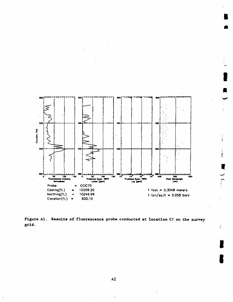
500 400UtoMlM
(«")Probe - OCIC70Easting(ft.) = 10209.20Northing(ft-) = 10246.99Elevotion(ft-) = 600.10
1 foot = 0.3048 meters1 ton/sq.ft - 0.958 bars
t
Figure Al. Results of fluorescence probe conducted at location C7 on the surveygrid.
I
I
A2

I
II
(10
MS
!I600
o
w;
5*
Er—
» i • i i . i0 JO
nummnc*
(10 '
60*
too
595
>
>>»
(10 -
MS
» I III! •• | ' ) 1|f• 1 ^ | '|f
•10 '
(OS
(00
MS
,,«
ntamMlr ^frtnK !•««. TIWH PrMfcM C«M*.. T1VH P««k OxMOnth.-——(««> L*,((*m) (w.)
Probe - OCIE50Eosting(ft.) = 10779.41Northing(ft.) - 9707.36Elevotion(ft.) - 606.19
1 foot = 0.3048 meters1 ton/sq.ft - 0.958 bars
Figure A2. Results of fluorescence probe conducted at location E5 on the survey
grid.
A3

I102
600
sw
Stt
10 20
ProbeEasting(fL)Northing(ft.)Elevation(ft.) - 602.94
604
602
•00
S»4
6WC
01C1(
s
^
604
602
5M
UA
604
602
ftte
M4
M4
M 100 ISO 10* KT* tO* 10* 400 500 CO^ravtatov C4UAF. iwm nvwcted C^w. IRFM ^Mk MMtanftli
»**r (**•<) L>9 (p*m) (rwti)
CIE60)779.41 1 foot -0.3048 meters^07.2B ! ton/sq.ft « 0.958 bors
Figure A3. Results of fluorescence probe conducted at location E6 on the surveygrid.
I
I
A4
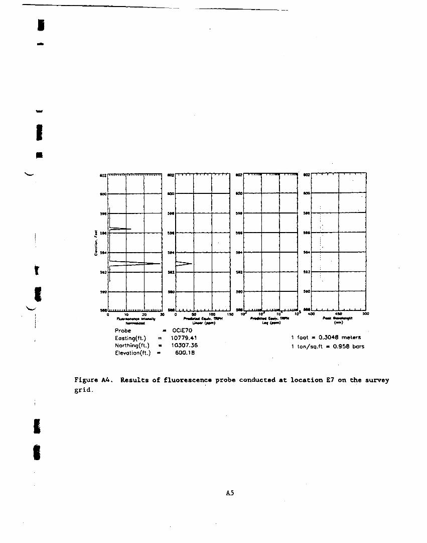
1
tI
602
MO
5W
• 5M
1
HO
Ma0
• •
-~ ——
I ———
•»
~— •«•— =~—
W2
too
M2
MO
«••10 20 30
Probe
>
•02
too
»M
M2
aw
«••) 80 100 150 K
r a i l r*. . TB«U
- OCIE70
1 1 1 IIU
r* to" 10* K
(02
100
sw
M*
M4
H2
5«O
X) 490 50PvBk WowlwUi
Eosting(ft.) = 10779.41 1 foot = 0.3048 metersNorthing(ft-) » 10307.36 1 ton/sq.ft - 0.958 barsElevotion(ft.) - 600.18
EI
Figure A4. Results of fluorescence probe conducted at location E7 on the surveygrid.
A5

•OS
Iw
MO
C
"
^
91Fhim
0 1Cliinnn Mimnnlimi
a vi~.tr
«os
to c
"^
1 91
L
B 1C10 19rapN
«)
105
940
10 1C1* 1C*Mia
r" iciMCwfc.Uf (*»m
' 1CHVH
109
9VU
s"!c
:. _
a MPMkNoi
(«•
10 (0•nium»)
Probe = OCIF60Eosting(ft.) = 11079.41Northing(ft.) = 10007.36Elevotion(ft.) - 603.65
1 foot = 0.3048 meters1 ton/sq.ft - 0.958 bars
I
Figure A5. Results of fluorescence probe conducted at location F6 on the surveygrid.
I
I
A6

I
II
MS
MO
J
| MS
SM
MS
•=3Z
\
<=:<^-
: —— •
i>7=^
^**f
MS
MO
S»S
SM
. MH BHM
" ^
_^B»—— ~
^ • • - ^
^^ ———
-
:=M^
f
— - —— •
=fc
k^
60S
600
SIS
SM
UA
-
r —
> 100 200 JOO 100 200 100 4OO <0* 1Cr* 10* uM •—- - 1V9M
60S
MO
SfS
SM
)•* «
NomMlind ' liMrtom) Lof (*••>
» SCO SO
(Ml)
Probe - OCIF70Eosting(ft.) = 11029.41 1 foot - 0.3048 metersNorthing(ft.) = 10307.36 ! ton/sq.ft - 0.958 boraElevotion(ft.) » 600.28
II
Figure A6. Results of fluorescence probe conducted at location F7 on the surveygrid.
A7

Figure A7. Results of fluorescence probe conducted at locationgrid. F8 on the survey
I
600
MS
590
— . —.*- —— •
c
0 }nuv
^
r=-~~-___r-
0 4
=a>
o t
•OS
aw0 (
^ -L-~~_r —— *
i inni
*—
r=a.
0 1Ct-4 tmm.
n isnm
MM
J»V
96910 tcr1 «
Pmdielr* teMrf r*uf».
* uTMPH
SOS
9VO
MMt
r *c
•
10 StP««k *•<
10 M— -—• -
•Si
1
)
1
1
y
U"»»(»r») U«(wm) («")
Probe - OCIF80Easting(ft.) = 11079.41 1 foot = 0.3048 metersNorthing(ft-) = 10607.36 1 ton/sq.ft - 0.958 barsElevotion(ft.) » 602.52
I
I
A8

I
I
(OS
I s«se
WO
(OS
too
MSSO 100 ISO O
_—— — —
p~
) **»*e
L
•
9 1CIM Uu».MW (MX
10 19
<)
60S
0 1Cr* icfnfx*
r" toMbrtr.U«(p»«
* Ifl? ' «
; :
a so(«
;
0 6CK
T*"Probe = OCIF90Eosting(ft.) = 11079.41Northing(ft.) = 10907.39Elevotion(ft.) - 602.12
1 foot = 0.3048 meters1 ton/sq.ft « 0.958 bors
Figure A8. Results of fluorescence probe conducted at location F9 on the surveygrid.
II
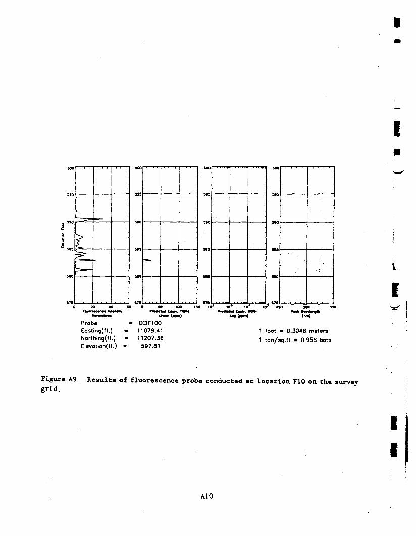
too
590
585
8750
— ' —-— *———
^
2£-:
:s-i
ni
»^—
> «toiMMlM
9 *
sao
»799 0
-
51
L
9 10
KMT (ffM
O 19
»)
875O 10P1 10
ftmf^lr" 10
t»«(wm)
* 10
600
sao
r» 4s0 90
(M
0 SS
»)
fp^«<
fI
i
Io s»X
,
Probe = OCIF100Eosting(ft.) = 11079.41Northing(ft.) = 11207.36Elevotion(ft-) = 597.81
1 foot » 0.3048 meters1 ton/sq.ft - 0.958 bors
Figure A9. Results of fluorescence probe conducted at location F10 on the surveygrid.
I
I
A10

I
iI
SOO
MS
*
1 woo
W
sas
MO0
?—
i
$t
>^•
SO 100 1!nutramnM Mttnttr
Hoffl*<tawl
ProbeEosting(ft.) =Northinq(ft.) =Elevotion(ft.) «
600
595
590
184
MO» <
= 0111
.
k^5.
•00
MS
MO
585
•00
S«4
MO
sas
) SO 100 ISO 102 IOJ 10** 10s 400 MO MlhWteM Uu*r. 1WM PrMMM C*yfc. HWM PMK •vMMfUl
U»«r (W") «-9 (»»") ("»)
CIF105079.41 1 foot = 0.3048 meters367.36 1 ton/sq.ft - 0.958 bars
597.81
II
Figure A10. Results of fluorescence probe conducted between F10 and Fll on thesurvey grid.
All

I610
• ttM
i
c
)^—*-1
* „
c:;
£
*
MRum
i
=—>.
n 40wnMind
0 6C
(10
(02
0 0
^
_^*~1 — — .
>
^
X
L
^f-
0 1O
*»" (fr»
00 191
1)
6tO
00 10
v^>
1* 1Cr" .toU«(wm)
* 1C
•10
I" 400 4ft
(""
'
0 SOI
»)Prob« = OCIG50Eosting(ft.) = 11409.41Northing(ft.) = 9762.36Elevotion(ft.) - 608.80
1 foot « 0.3048 meters1 ton/sq.ft - 0.958 bors
II-/
r
Figure All. Results of fluorescence probe conducted at location GS on the surveygrid.
I
I
A12

Ip
I1
604
•= .*_
•WO
liOA
. ft
\
I
a "•
c
h-———
VV.
r>
10 1O00 15
604
an
00 C
—— . — .^f— — -g
10Pmtfc
: -
00 20M Uuto.
00 30
•04
•02
•00
MX
00 1C
— — . —
~\>
f 1Cfnftf
>
r* u**U*t.
* Kr 4c
r
10 50*•*•*
a «a•taniUi
UnMr(w«)
Probe - OC1G60Easting(ft.) = 11379.41Northing(ft-) = 10007.36Elevotion(fL) - 603.91
l»» (p*m) (urn)
1 foot = 0.3048 meters1 ton/sq.ft - 0.958 bars
II
Figure A12. Results of fluorescence probe conducted at location G6 on the surveygrid.
A13
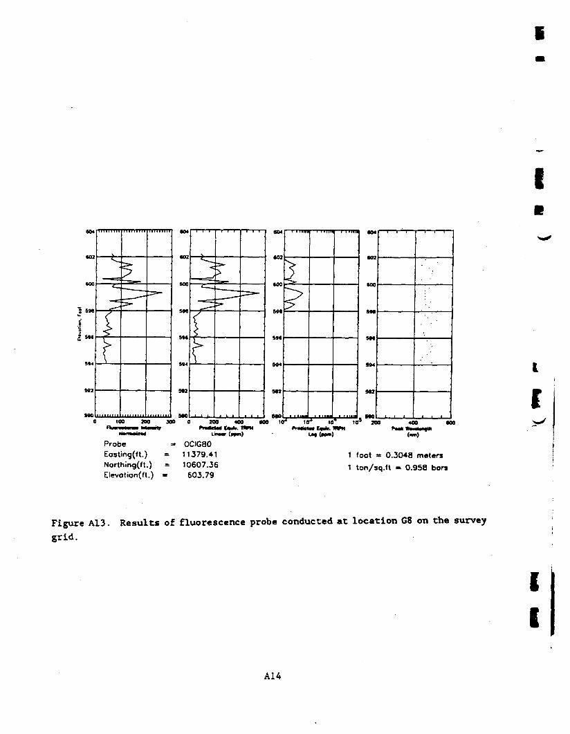
I
Probe =« OCIG80Eostinq(ft.) = 11379.41Northing(ft-) = 10607.36Elevotion(ft-) - 603.79
1 foot = 0.3048 meters1 ton/sq.ft - 0.958 bors
I
C
Figure A13. Results of fluorescence probe conducted at location G8 on the surveygrid.
I
I
A14
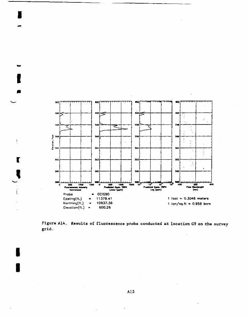
I
rI
SO:
• w«
1?£ »««
S«Z
C
>
"
C^ —— —
X
^
» 1000 IS
<Q2
3V •(
5Moo c
p^
^ —— •
XPraMc
^L_—— •"•
0 IOIM £•*).
~
no isWH
«02
M2
00 1C
^ ^^— -
r* itr«*d
fc.
r5 icMtwW.
' 1CIMM
602
600
|P 4CK> acPMkVtai
•
.
a co•Mnttt
Probe = OCIG90Easting(ft-) = 11379.41Northina,(ft.) = 10937.36Elevotion(ft-) - 600.26
1 foot = 0.3048 meters1 ton/sq.ft - 0.958 bars
II
Figure A14. Results of fluorescence probe conducted at location G9 on the surveygrid.
A15

I(OS
30•
5650
>
j
10
V0 100 30
(OS
O 10
~-c
O 20Pridicl
^
1=
0 XM Im*,.
0 40
€05
MAO 10
\i* 10
IV «akjr> 10M E«i*>.
10mm
S*o
* 400 SOAMk MM
O (OC
II
Probe = OCIG100Easting(ft.) = 11419.41Northing(ft.) = 11207.36Elevotion(ft.) = 600.26
1 foot = 0.3O48 meters1 ton/sq.ft - 0.958 bars
Figure A15. Results of fluorescence probe conducted at location G10 on thesurvey grid.
I
I
A16

I
II
MO
S«
3
Mi
MOC
*» ———— 1
J~'•=— ="
1000 2000 30
ProbeEosting(ft.)Northing(ft.) =Elevotion(ft.) -
MO
MS
MS
MO00 (
- 0111
> ——
J~_ — ->
2000 40Prftcut l+*.
&**(»»
CIG511
529.41507.36
500.00
w
00 M
»)
MO
MS
MO
us
MO00 K
~~_
_?^=y
MO
SM
S90
MS
unr* 1^ to* 10" «oo soo MI
PrMfcM E iir. TUPM PMk W».il«mUlLog (»»m) (nm)
1 foot = 0.3048 meters1 ton/sq.ft - 0.958 bors
Figure A16. Results of fluorescence probe conducted between Gil and Hll on thesurvey grid.
A17

600
-• • I-=sX"
==»3^=-
• •
J 200 4OO M
NWf *M4
ProbeEosting(ft.) =Northing(ft.) =Elevotion(ft.) *
(05
600
SfS
SM
sas10 0
= 0119<
>
=*•-. —«=^=——^^
SCO 101i»<rt«« Uu>».
UMV(M«
CIH50679.41732.36502.66
(OS
600
sto
f*
(OS
600
5»5
5M
90 t»OO IO*1 10^ to* 103 4OO 100 MX
) !••« (W") («")
1 foot = 0.3048 meters1 ton/sq.ft » 0.958 bars
IF
I
Figure A17. Results of fluorescence probe conducted at location H5 on the surveygrid.
I
I
A18

Ipi
II
SO4
«O2
6OO
w
i MBo:
i»«
5*4
5*20
'1 '
>
* — .-?= ••••_
MM
602
600
M6
M6
i*4
-
MM
•02
COO
5»e
M6
•it*
fl*«100 200 30O 100 2OO 300 4OO 1C
Probe - OCIH60
r1 i 10* icFr.fetM t**i. 1*TH
«02
600
9*4
r*9^n 900 ta
Eostng(ft.) = 11679.41 1 foot = 0.3048 metersNorthing(ft-) = 10007.36 i ton/sq.ft - 0.958 barsElevotion(ft.) - 603.68
II
Figure A18. Results of fluorescence probe conducted At location H6 on the surveygrid.
A19

I605
600
3
5A5
>-s~ __V-
0 2000 *a
— 7*
•09
6OO
US
t
^t
M MOO 0 S-0»
ProbeL
= OCIH70
S~*
605
60O
. 59A
5«O
MA
^
^
^
^
•OS
sts
••ft
\
•. •'
\tT 1J>»10' U»10* 10* 10^ 101* 10s 490 900 «Mil CM^V HVH Pnrfictotf EiMlv HVM ^w>k MtavwlMMUiKMT ( ) U) (|>»m) («m)
Easting(ft.) = 11679.41Northinq(ft-) = 10307.36Elevotion(ft.) = 603.00
1 foot = 0.3048 meters1 ton/sq.ft - 0.958 bars
I
Figure A19. Results of fluorescence probe conducted at location H7 on the surveyRrid.
I
I
A20

I
J
609
too
I
MO
MS0
[
|s^~>
^r-i
MOO 4000 tO
ProbeEosting(ft.)Northing(ft-) =Elevotion(U.) -
60S
600
MO
MSDO C
- 0
11
1C
IWS-i
tot
600
s»s
sw
9MA
k^
—
r
60S
6OO
SW
••ftSJ.I tJ»10* li»10* 102 10J 10* I09 4M MO Ml
OMT («fm) Le( («*m) (mn)
CIH80
679.41 1 foot = 0.3048 metersJ647.36 1 ton/sq.ft - 0.958 bars502.44
II
Figure A20. Results of fluorescence probe conducted at location H8 on the surveygrid.
A21

I605
600
90S
9M0.0 0.9 1.0 1.
•OS
sas
SCO9 0 S() 100 18
6O4
0 10f 10J 10' 10-
«os
M5
MO
Pnmetmt I«d». 1KPHSS1 952
n)ProbeEosting(ft.)Northing(ft.)Elevotion(ft.)
- OCIH9011679.4110907.36601.71
1 foot = 0.3048 meters1 ton/sq.ft - 0.958 bors
II
Figure A21. Results of fluorescence probe conducted at location H9 on the surveygrid.
I
I
A22

1
I
I s»»
sas0 20 «0
flmmouM muf
(OS
c
:==~
91Pnric
L
9 1Cto* (••*.r>*tr(ffK
n 19flWM')
(OS
O 1CI2 1CPradtel
r> ic•df^uk1*1 (f*»
* teTHFH
fOS
r* «
:•• '
O SOPMkWx
(*
10 <O
")ProbeEosting(ft.)•Northing(ft.)Elevotion(ft.)
OCIH9211679.4111107.36601.71
1 foot = 0.3048 meters
1 ton/sq.ft - 0.958 bars
I
I
Figure A22. Results of fluorescence probe conducted between H9 and H10 on thesurvey grid.
A23

ICOS
600
590
sas0
- — — —^
>>=
•«fc
==~
^ •»
200 4OO M
Probe£osting(ft.) =Northing(ft.) =Elevotion(ft.) =
(OS
600
S»i
SMO 0
= 01111
J
~-— — 1. ——
>^
=a.
MO 1000 151
CIH100679.41207.41501.71
60S
6OO
S9S
5*0
SMM 10
r?»i>-
(OS
600
SM
SM
i* 10^ 10* 103 400 SOB 601PmtflCtMd CilMir TMPH f^^k ttMiH iMMHl
L*J (wn) (MX)
1 foot = 0.3048 meters1 ton/sq.ft - 0.958 bars
I
Figure A23. Results of fluorescence probe conducted at location H10 on thesurvey grid.
I
I
A2A

I
E
I
I
\
60S
600
j
.|m
s»o
MSC
r^
<^•<=
^__— —
3
^^
^—— .
3
(OS
600
i»S
6*0
MA» 4O (O C
numen*MmHr
ProbeEastinq(ft.)Northing(ft.) =Elevdtion(ft.) »
»= 01111
<
-=4,-—— ———
t_
=r
60S
COO
s*s
SfO
••ASO 100 ISO 1C
fnfettt C**. TWH
CIH110679.41207.36
502.27
•OS
600
MS
i* io-> ic"1 to" 400 MO «a
1 foot = 0.3048 meters1 ton/sq.ft « 0.958 bars
Figure A24. Results of fluorescence probe conducted at location Hll on thesurvey grid.
A25

(IS
(10
US:I
*«
SIS
5flO0 1.0M10' 10K10* J.0»
(19
(00
•go™«
^—
J»1PiWte
L
•M. -
0 «>1
«M«r (ypfl
0 («1
>)
(19
O 10
5-
•
X
^ 10Pfi«irt
1 —— — -.
r" 10MCwri..
^K——
* 1Cmm
(19
(10
r1 «
;i.>
0 90CMkWw
(«
0 «OCr*Probe - OCII40Easting(fL) = 11929.41Nofthing(ft) = 9357.36Elevation(ft.) * 610.30
1 foot = 0.3048 meters1 ton/sq.ft » 0.958 bars
I
Figure A26. Results of fluorescence probe conducted at location 14 on the surveygrid.
I
I
A26

1
I
I
602
<OO
598
594
0
<*
^=T<j
f
\-=——— -
. — • — '
• — — _. — —;=»-^
— -— .
^^
-
600
598
SM
5*4
MA
— • __-^
"- -
: ^—
— _ "- - —
602
•00
. 398
5fC
M2
AA0
-
>
^
1 1 • IMI
«02
600
596
M«
BAC
50 100 ISO 100 ISO 200 290 10* 10* 10* 10* 4OO 900 «O
ProbeEosting(ft.) =Northinq(ft.) =Elevotion(ft-) =
- OCII5011979.419732.36601.00
1 foot = 0.3048 meters1 ton/sq.ft - 0.958 bars
II
Figure A27. Results of fluorescence probe conducted at location IS on the surveygrid.
A27

602
600
!"".1*~
S92G
L— • — ——
f——— '
:=-
1OOO 2OOO X
ProbeEasting(ft) =Northing(ft-)Elevotion(ft-) =
602
600
S9«
S9«
5*200 t
= 0129(
•— -— .
p——:==^^
602
6OO
S»4
IW9
~~—— .
r^^
602
600
598
596
M4
8A9
2000 4000 (000 Iff1 10J 10" 1C3 400 SCO 601frmtOti £*•». 1WM fr»«ct*< Ew*. HVH PMk W«ml»n«lll
C1I55'029.41 1 foot = 0.3048 meters757.36 T ton/sq.ft - 0.958 bars501.00
Figure A28. Results of fluorescence probe conducted between 15 and J5 on thesurvey grid.
I
II
A28

I
II
602
600
598
gm|
JM
MO
saac
x l
• i
7==»->•
5.0x10^ I.OK10* 1.S*FVjorOTCtnc* lnUnity
ProbeEasting(ft.) =Northing(ft.) =Elevotion(ft-) -
602
600
SM
M6
S»4
Ml
MO
,*r,- 0
111C
1
x__
^t :=—•>•
602
600
M6
M4
M2
MO
>
——— —— .
<
^ ,
^
(*
/
>
•02
600
M6
M6
M4
M2
MO
1 1.0*tOU 10»10 3.0»1O* 10"* tor* 10* 10" 400 SOO «X
CII60979.41 1 foot = 0.3048 meters3007.36 i ton/sq.ft = 0.958 bars500.89
Figure A29. Results of fluorescence probe conducted at location 16 on the surveygrid.
A29

I602
too
.1 3*60
£
5940
|
£
/->-
W2
600
W6
at
4*4
• a
5O 100 ISO 1OO 13
ProbeEasting(ft.) =Northing(ft-) =Elevotion(ft.) =*
- OCII7011979.410307.3600.66
•••• ^
O 14O 11U*C«i>. HVH
16
602
600
St6
>
602
600
5*6
0 IO"1 lO' 10* 1C3 450 900 U(^fWctX biw. TWM PMH »»««liinui
1 foot = 0.3048 meters1 ton/sq.ft » 0.958 bars
L1
Figure A30. Results of fluorescence probe conducted at location 17 on the surveygrid.
I
I
A30

I
I«OS
sas
(Oft
too
5*0
Iliilllil mi mi* liiilliii
MO
SO 100 ISO 100 110 IZO ISO Iff* la3 10* to* 4OO SOO 6OOnuvMCMM MMMtr fra«clrt t**.. 1WN >ri<k<«« Cvub. TIVM PMk ttaMWKflll
NwnMaM OMT (p»m) Lof (p»m) (MI)
Probe - OCII100Eosting(ft.) = 11979.41 1 foot = 0.3048 metersNorthing(U.) = 11322.36 1 ton/sq.ft - 0.958 barsElevolion(ft.) - 603.04
I
I
Figure A32. Results of fluorescence probe conducted at location 110 on thesurvey grid.
A31

I60ft
•
=~t__^— —
J^*.
= —
=-i
60S
9VU
MS
& ———
=
S»-
60»
3VO
515
•06
9V9
SM
••
2O 4O H 0 SO 100 ISO lO* tO* 10* 10^ <00MMwilr Pra«cU« Clunr. TWH Pra«CU« U<M. TWH
(nm)
Probe - OCII110Eastinq(ft.) = 11979.41Northing(ft.) = 11507.36Elevotion(ft) = 603.43
1 foot s 0.3048 meters1 ton/sq.ft - 0.958 bars
tIi
Figure A33. Results of fluorescence probe conducted at location 111 on thesurvey grid.
I
I
A32

I
II
I »»
590
M»
X4
> s
•*••
0 1C» 15
80S
3VU
MS10 1C» 1C
PrMfe« 1Mte*.
0 1•mm
590
» 1C? 1CPra«ei
r1 uMta*.
* 1CTWH
•OS
I3 «a scPMk tt*
a 10«•»**
UMT (wm)
Probe - OCII120Eosting(ft.) = 11979.41Northing(ft) = 11857.36Elevotion(ft.) - 600.80
1 foot = 0.3048 meters1 ton/sq.ft « 0.958 bors
KI
Figure A34. Results of fluorescence probe conducted at location 112 on chesurvey grid.
A33

Itot
SM0.0 0.S 1.0 I.
soa
a e 51P<«4k
9 10!•*(•*•.
0 19TWM
toe
0 10f to*•*«
r" 10•«C«M».
10TIWM
6M
* «0 90P«k«to»
o mIIIMUI
Probe = OCIJ40Eostinq(ft-) = 12149.41Northing(ft-) = 9407.36Elevotion(ft.) = 607.50
1 foot = 0.3048 meters
1 ton/sq.ft - 0.958 bors
Figure A35. Results of fluorescence probe conducted at location J.4 on the surveygrid.
I
I
A34

LI
60*
I
.1 MS
60S
600
MS
MS I l I I l I IJ l I I I j0 VCrnlCr" 1.0*10
ProbeEosting(ft.)Northing(ft.)Elevotion(ft-)
OCIJ5012139.419707.36603.04
(OS
MS
s*o
10'
«00
MS
9*0
10* 400 MO
(MI)
1 foot = 0.3048 meters1 ton/sq.ft - 0.958 bars
Figure A36. Results of fluorescence probe conducted at location J5 on the surveygrid.
A35
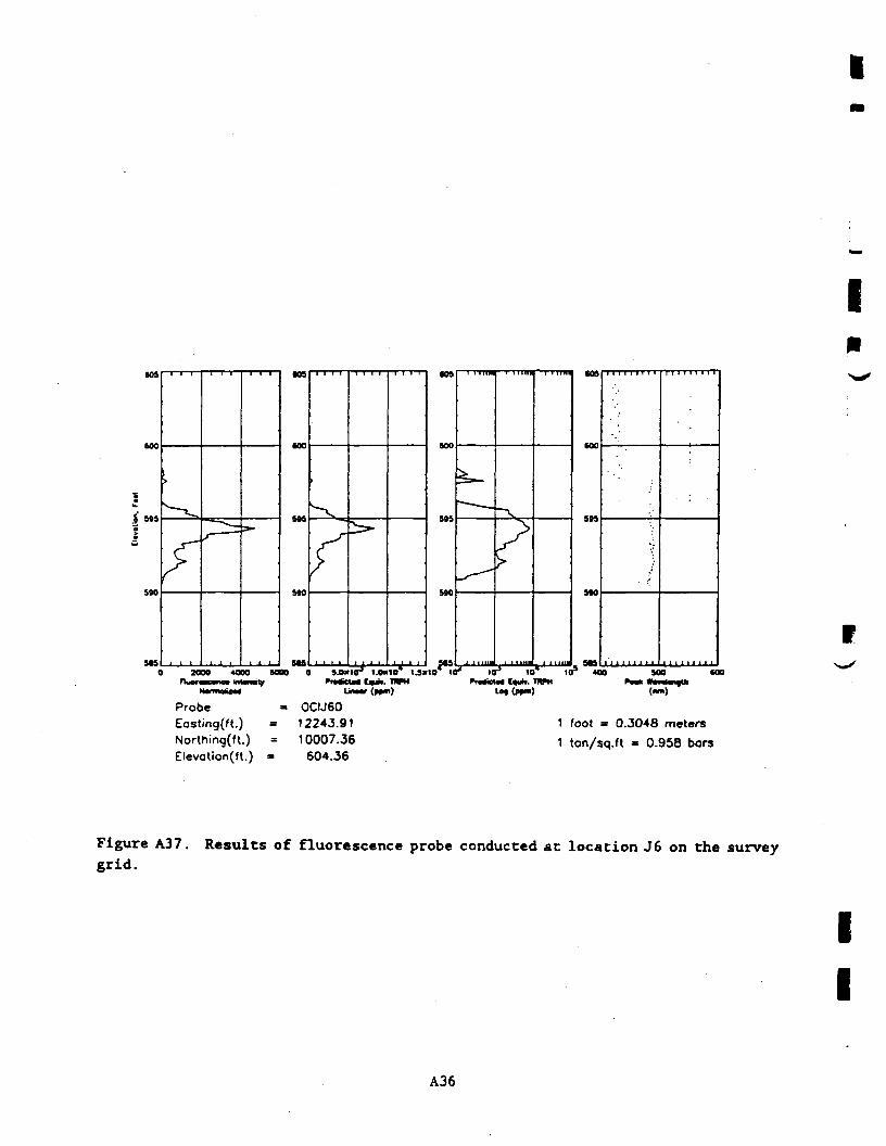
IV
60S
600
590
C
I>
^
"**— .<• —— - ;»•
•09
(00
5*0
«M
2000 4OOO 6000 (
Probe - 0
f i>
i.OKI 1.0*1O* 1JJfrtticlft Uut». TWH
UKMT (r*m)
CIJ60
(OS
600
S9S
S90
U510* 1C
^
-~« ——
^
~-^>>•
(OS
(00
s«s
S90
:;
r* tar1 10* to3 <oo 500 (aPi-MfietM C«ii>. TWM PMH HanHHf*
Easting(ft.) = 12243.91 1 foot = 0.3048 metersNorth!ng(ft.) = 10007.36 1 ton/sq.ft - 0.958 barsElevation(ft.) - 604.36
Figure A37. Results of fluorescence probe conducted at location J6 on the surveygrid.
I
I
A36

I
1
609
«*.S -M
I
590
k_
rr
O 5C
•
^
n 1000 is
ProbeEostinq(ft.) »
605
flflft
•N —— .
r•\<c
605
IUA
----_
\ft
S
^
60S
MA
00 0 1000 MOO MOO 1CT* Iff1 to"1 I03 4OO MO 601
- OCIJ7012239.41 1 foot = 0.3048 meters
Northiog(ft.) « 10246.36 1 ton/sq.ft - 0.958 barsElevation(ft.) - 604.77
II
Figure A38. Results of fluorescence probe conducted at location J7 on the surveygrid.
A37

«04
:S .A.
0
£
w!a
I^~ —
<.
?
10nu*n
^»»_r
o x 0 X
109
10 10
~~—~ ^
««.. — ——ST-~ ——
O 20frUti
^M«K
0 Xtetf (••>.
a 40HVH
so*
SM0 10
^r
>•>
r* 10Pr«<iM
I* 10m*tm~L
' 10nwM
60S
r 400 90»••• *x
0 MM-* — -*•
Probe - OCIJ80Eosting(ft.) = 12239.41Northing(ft.) = 10607.36Elevotion(ft) = 602.27
1 foot = 0.3048 meters
1 ton/sq.ft - 0.958 bars
I
Figure A39. Results of fluorescence probe conducted at location J8 on the surveygrid.
I
I
A38

I
II
I (OSO
60S
too
MS
815
MS
•00
MS
«S
0 SO 100 ISO 0 ^O 100 ISO lO2^ Iff* 10* 10* 400 MO «00rimtuMma inuratr PratfeU* C<lui». 1WM Prrfcl«« C«iii». TI*H Pwtt »«nnml»i
Mormolil«a IJnMr (MKI) lof <p»m) (MI)
Probe = OCIWW2Easting(ft.) = 11963.30 1 foot = 0.3048 metersNorthing(ft.) = 9273.21 , ton/sq.ft - 0.958 barsElevotion(ft.) = 610.30
II
Figure A40. Results of fluorescence probe conducted near Chemical Building *2
(MW-2) on the survey grid.
A39

I(10
(06
600
1
1 S»o£
590
sa5
MO(
t^
^
>s.
i-^^——
V
»10
•OS
600
S»S
MO
M»
ft«0
610
(OS
too
M4
MO
MS
uo
610
60S
6OO
M9
sto
sas
-.
JO 100 190 100 1O2 104 10* 10* Iff* Ifl' I0" 4OO MO MX
robe «Easting(ft.) =Northinq(ft-) =Elevotion(ft-) »
U~-r(p»».)
OCIMW311820.258934.44606.00
Lo« (n>m) (MI.)
1 foot = 0.3048 meters1 ton/sq.ft « 0.958 bars
I
Figure A41. Results of fluorescence probe conducted west of Warehouse (MW-3) onthe survey grid.
I
I
A40

I
II
60S
600
595
590
US0
>
>
\•
.^fS,£ —3=* -
M^W*
100 400 M
SOS
600
S»S
sea» c
7
.• '
^_
^a^w.
60S
600
S9S
s*o
«flA
^1 1 1 HIM
) MO 1OOO 1SOO \<f \o' IO* 1CPrwtteU* C«ut>. TOPH Pr«fi««* C«M. TWH
UXMT (f»m) 109 (ppm)
60S
600
sts
SM
J 4<
•:
» 500 60
(Ml)
Probe = OCIMW4Easting(ft.) =11710 .81 1 foot = 0.3048 metersNorthing(fL) = 9355.65 1 ton/sq.ft = 0.958 barsElevotion(ft.) = 604.30
II
Figure A42. Results of fluorescence probe conducted between H3 and H4 (MW-4) onthe survey grid.
A41

I
5680
><c;
so
>-
O 101» I*10 0
»
>"C
101Fr«ae
=»-
» 201IM (a«.
X 301fflPM
Sf2
M 10
>
<
<* 10rraiffrt
s-
r" 10M C b.
* toIWM
9^0
994
SM
? 40O 90f^A *a>
;
0 (O— — —
I
P
s*
I-j
^Is>
0
(.•Mr (MOT) bo« for") («*">
Probe = OCIMW5£ostinq(ft.) = 11899.76 1 foot = 0.3048 metersNorthinq(ft-) = 9822.47 , ton/sq.ft - 0.958 borsElevotion(ft-) = 599.10
Figure A43. Results of fluorescence probe conducted between 15 and 16 (MW-5) onthe survey grid.
I
I
A42

LI
• 10'
:.9 S»S0
tw
I1
560
„,
>*-
^°~^—- — ..- — — i^X
•=>
(10
MS
A40
U5
MO
^
-
•^"
Z=-
="
-
• 10
MS
6*0
flO
MO
\
50 100 ISO 0 90 100 ISO 10* 10* 10 10' «OO 900 *OO**««•« C*ui>. IWx ^M* »«nnmll>
' <•»•«> L^ (•»«>) (<«•}
1 foot = 0.3048 meters1 ton/sq.ft - 0.958 bars
robe - OCIMW7Eosting(ft.) = 11302.34Northing(ft.) = 8277.15Eievotion((t.) - 606.60
II
Figure A44. Results of fluorescence probe conducted near Gl (MW-7) on the surveygrid.
A43
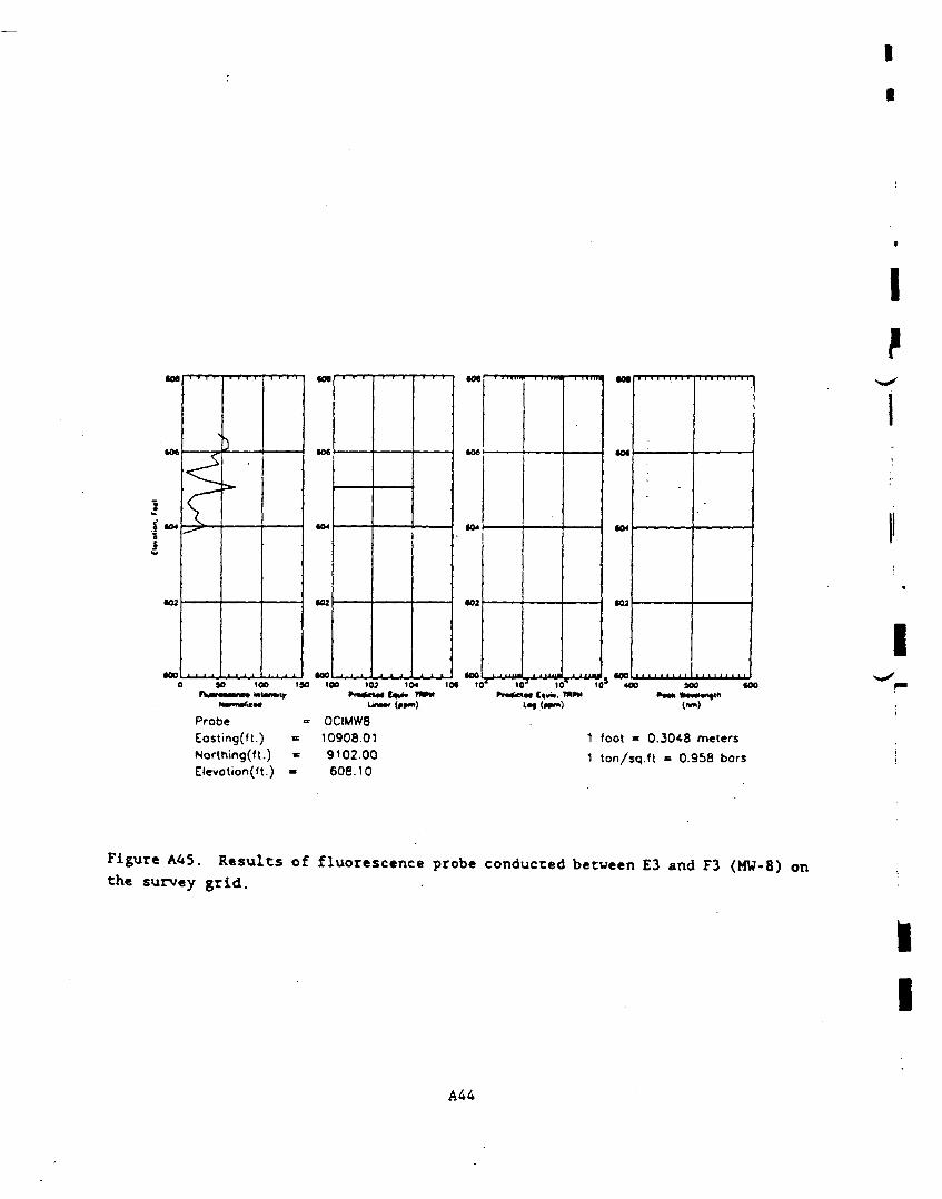
II
«0fl
3
J
•000
O
atrim
s-
} 10O 19
«0«
•00O 10O 10
rnJri} 1CM 1C
TNM
•0*
•02
•00* 1C
———
11 10r™«in
J 10M Cui>.
10m»H
Ml
(02
* «0O X*>«k *•.
o tot
Probe = OCIMW8Eosting(ft.) = 10908.01Northing(ft-) = 9102.00Elevotion(U.) * 608.10
1 foot = 0.30*8 meters1 ton/sq.ft * 0.958 bors
If
I
Figure A45. Results of fluorescence probe conducted between E3 and F3 (MW-8) onthe survey grid.
I
I
A44

II
IV*
5»S
560
575
600
Mi
MO
MS
MO
«oo
sao
• ' • • ' ' ' ' '-' ' ' $79 "•""" "1""" niiiiiii S7S ' i i••" i ""•• I 11iin0 5.0*10 U«10 U»10 0 14J»tO 2Jt*M> 3.0«10 HT 10* 10 10
nuorneim MUmrtf Pr««icu< («•>. 1MM Pr«a«S«d Cqui>. TMPHLOf
575400 MO
Probe = OCIMW16Eastmg(ft.) = 11379.41Northing(ft.) = 11497.36Elevotion(ft.) = 60O.OO
1 foot = 0.3048 meters1 ton/sq.ft = 0.958 bars
II
Figure A46. Results of fluorescence probe conducted at location Gil (MW-16) onthe survey grid.
A45
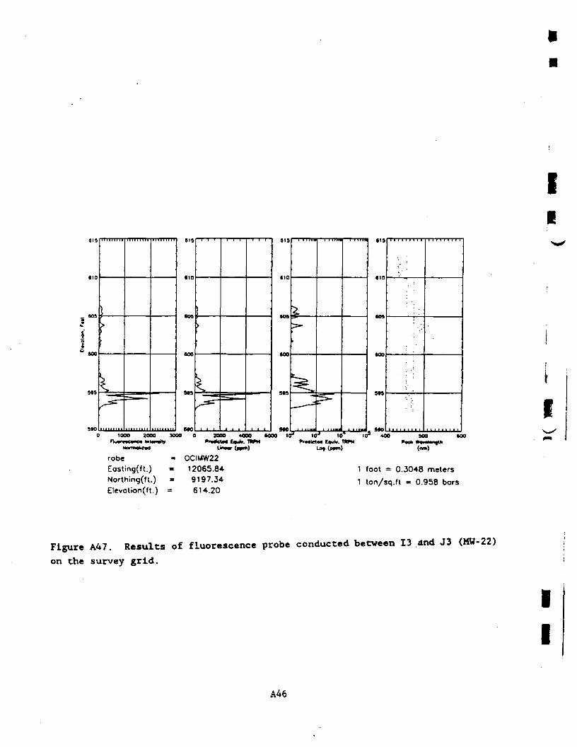
II
615
5*00
|>i
~^-
101
r~»
90 20DO »MO
OO 0
|
>
L.- ^^^^
20r>nic
t=
00 40IM tmitf.
DO fOiWM
«1S
5*0DO 1C
r5"
^_^
1* 1CPrMM
^
3 10•• EMIM.
' toTNPH
C1D
MOr 400 SOa eat
rtilMtll
IUfMir (00m)
robe - OCIMW22Eostinq(ft.) = 12065.84Northinq(ft-) = 9197.34Elevotion(ft.) = 614.20
1 foot = 0.3048 meters1 ton/sq.ft = 0.958 bors
Figure AA7. Results of fluorescence probe conducted between 13 and J3 (MW-22)on the survey grid.
I
I
A46

II
I
615
60S
§ _ _ _6000
I
195
C
>
>•h
X
2C
a^
10 4C•evne* M
10 «LMitv
• 15
• an
S«5» C
*•
X.9C
Pra«c
•w
n 10<•< (•»».
00 IS•ram
MS00 10
vr" K
Pr«c<
3 1C* 1C1WH
•15
595
S 4C
..j:
a M?•<*«•«
j
1
0 60•Imilh
robe = OCIMW23£asting(ft.) = 12252.61Northinq(ft-) = 9432.44Eievation(ft.) = 611.20
1 foot = 0.3048 meters1 ton/sq.ft - 0.958 bars
II
Figure A48. Results of fluorescence probe conducted near Boiler House (MW-23)on the survey grid.
A47

r60S
600
590
USc
It^zz, — — — '3^
60S
600
sasS.O»10J I.OK10* l.S»10* C
Nomtolintf
ProbeEostinq(ft.)Northinq(ft.)Elevotion((t.) =
= 01 111
(
:= ———
, —— ' —
•
^— '
io«io* ijomo' 3Jt*Pra«curi €•«». TIWM
UMV (ypm)
CIPB16
679.41657.36
500.80
60S
SM
S*0
B**t«? 10J 10*W. T
Lof (ppm)
605
600
Mi
SIO
uu . MS103 400
I
1 foot = 0.3048 meters1 ton/sq.ft - 0.958 bars
Figure A49. Results of fluorescence probe conducted between Hll and H12 (nearPrein & Newhoff boring #16) on the survey grid.
I
I
A48

II
,I
620
too
S?
MO
MO0
• B-
^^B-_
wr
'•• ™ i—— E
= ————
;a—
50 100 13
Normalized
620
500
MO
MOa ic10 140 200 29
PrMKUd £«•». TMPM1 J.—.,, ^jTjLjmlLin»or ^ppm;
620
600
960
MOa 10r4 ioj to* ie
Lo, (ppm)
620
600
580
MO5 40
'
' 1
O 500 60C
robe = OCII196Eostng(ft.) = 11379.41 1 foot = 0.3048 metersNorthing(n.) = 11757.36 1 ton/sq. ft = 0.958 borsElevotion(ft.) = 605.50
II
Figure A50. Results of fluorescence probe conducted across Interstate 196 (nearG12).
AA9
I•
rI
II
Appendix B: Aerial photographs with plume superimposed.
I
L
I
I
I
Waterways Experiment Station Cataloglng-ln-Publlcatlon Data
Sharp, Michael K.Use of the site characterization and analysis penetrometer system at
GrandviHe, Michigan Superfund site / by Michael K. Sharp, Raju Kalaand Jeff Powell; prepared for US Environmental Protection Agency, Re-gion V [and] US Army Toxic and Hazardous Materials Agency.
99 p.: ill.; 28 cm. - (Miscellaneous paper; GL-92-38)Includes bibliographical references.1. Environmental impact analysis - Michigan - GrandviHe -
Measurement - Instruments. 2. Penetrometer - Environmental as-pects. 3. Soil surveys - Michigan -- GrandviHe - Geophysical methods -- Environmental aspects. 4. Pollution - Michigan - GrandviHe -Measurement - Instruments. I. Kala, Raju. II. Powell, Jeff F. III.United States. Environmental Protection Agency. Region V. IV. U.S.Army Toxic and Hazardous Materials Agency. V. U.S. Army EngineerWaterways Experiment Station. VI. Title. VII. Series: Miscellaneouspaper (U.S. Army Engineer Waterways Experiment Station); GL-92-38.TA7 W34m no.GL-92-38
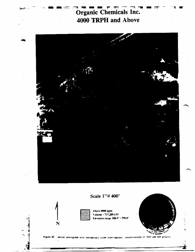
Organic Chemicals Inc.4000 TRPH and Above
N
Scale 1"= 400'
Above 4000 ppmVolume- 717.289.4 ft'Etevation range 588.9' - 596.8'
Figur. ti. A,ri«l phoco(r«ph «Uh conc«Mtn«nt plu»« iup«ri.«po«.d. eonc«ntr«clonJ of SOOC pp- and gre.c.r
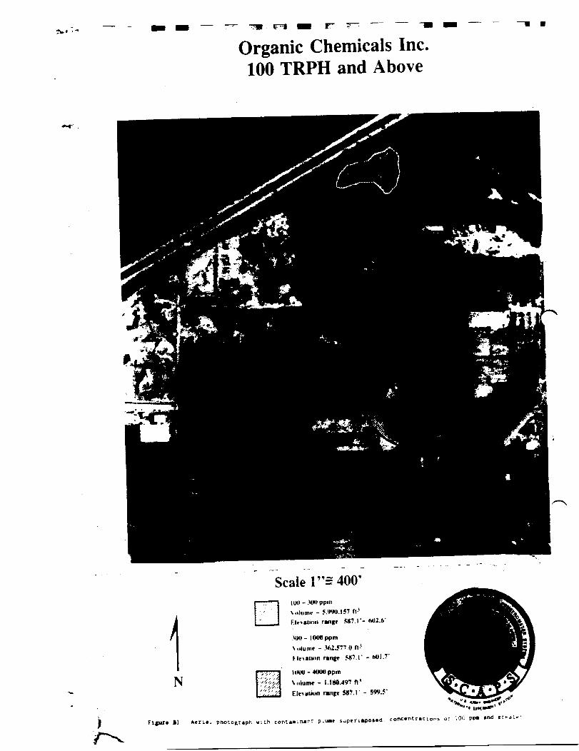
Organic Chemicals Inc.100 TRPH and Above
N
Scale 1"= 400'100 - .MM) ppm\n\umt - 5.WU.IS7 ft-'Fkvatmn rangt 587.1'-
MM)- lOOOppm
\olumt - J«.577.0 II-'rangr 587.1' - MII.7'
I (KK) -4000 ppmVnlumr - 1.180.497 fl'FJonlion ruitt S87.I - 5W.5'
Flpir. »1 (keri.i photogr.phtOEt.ph w i t h contM1n.rr pluM Sup«ri.Po..d conc.ncr.c lOns o: 100 pp. .nd

APPENDIX N
TENTATIVELY IDENTIFIED COMPOUNDRISK EVALUATION

Appendix N
Assumptions in the following list are used to determine what compound willaccurately estimate the toxicity of a tentatively identified compound (TIC).
The following compounds are considered non-toxic or ignored:• Unknown compounds.• Unknown floroalkanes.• Unknown organics for which the number of carbon atoms cannot be
estimated.• Unknown siloxanes.
Aldol.• Argon.• Blank contaminants.• Carbon dioxide.• Laboratory artifacts.Compounds possess the toxic effects of their tentative identifications.Alkanes containing one to eight (Q to C8) carbon atoms whose tentative
identifications are not in the U.S. Environmental Protection Agency (USEPA) toxicdatabases have the same toxic effects as:
• Chemically similar compounds.• N-Hexane.Alkanes containing nine to sixteen (C9 to C16) carbon atoms whose tentative
identifications are not in the USEPA toxic databases have the same toxic effects as:• Chemically similar compounds.• Methyl cyclohexane.Alkanes, alkenes, cyclics and aromatics containing more than sixteen (>C16)
carbon atoms whose tentative identifications are not in the USEPA toxic databaseshave the same toxic effects as:
• Chemical similar compounds.• To be non-toxic.Alkenes, cyclic hydrocarbons, and other unsaturated compounds containing
one to sixteen carbon atoms whose tentative identifications are not in the USEPAtoxic databases have the same toxic effects as:
• Chemically similar compounds.• Methyl cyclohexane.
N-l

TICs and unknown carboxylic acids that are not in the USEPA toxic databaseshave the same toxic effects as:
• Chemically similar compounds.• Benzoic acid.TICs and unknown ketones that are not in the USEPA toxic databases have
the same toxic effects as:• Chemically similar compounds.• Methyl isobutyl ketone if they contain eight or less (< C8) carbon
atoms.• Acetophenone, if they contain more than eight (> C8) carbon atoms.TICs and unknown alcohols that are not in the USEPA toxic databases have
the same effects as:• Chemically similar compounds.• • Propylene glycol.TICs and unknown esters that are not in the USEPA toxic databases have the
same toxic effects as:• Chemically similar compounds.• Methylacetate if they contain eight or less (< Q) carbon atoms.• Butyl benzyl phthalate if they contain more than eight (> C8) carbon
atoms.TICs and unknown organics containing nitrogen that are not in the USEPA
toxic databases have the same toxic effects as:• Chemically similar compounds.• Diphenylamine.TICs and unknown polyaromatic hydrocarbons that are not in the USEPA
toxic databases have the same toxic effects as:• Chemically similar compounds.• Acenaphthene.TICs and unknown aldehydes that are not in the USEPA toxic databases have
the same toxic effects as:• Chemically similar compounds.• Benzaldehyde.TICs and unknown compounds containing chlorine that are not in the USEPA
toxic databases have the same toxic effects as:• Chemically similar compounds.• Trichlorofluoro methanes. S-PTOJ/OCI/PHASET/RI/APPXM/ASSUMP
N-2
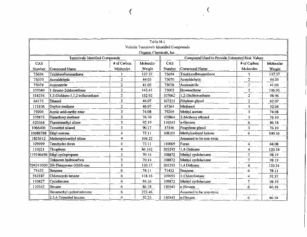
Table N-lVolatile Tentatively Identified Compounds
Organic ChemicalSj Inc.Tentatively Identified Com
CASNumber75694750707507810704035423464175115106792091098754205641066406
1068878818256121099991 10021
119196496
29431303071432542187110827110543
Compound NameTrichlorofluromethaneAcetaldehydeAcetonitrile1 -Bromo-2chloroethane1 ,2-Dichloro- 1 , 1 ,2 trifluroethaneEthanolOxybis-methaneAcetic acid-methy esterDimethoxy methaneFlurotrimethyl silaneTrimethyl silanolEthyl oxiraneMethoxytrimethyl silaneTetrohydro furanThiopheneEthyl cyclopropaneUnknown hydrocarbon2H-Thiopyrane-3(6H)-oneBenzeneChlorocyclo hexaneCyclohexaneHexaneHexamethyl cyclotrisiloxane2,3J4-Trimethyl hexane
sounds# of CarbonMolecules
122222233334444555666666
MolecularWeight137.3744.0541.05143.41152.9246.0746.0774.0876.1092.1990.1772.11104.2272.1184.14270.1470.14130.1778.11118.1684.1686.18222.4692.23
Compound Used to Provide Estimated Risk ValuesCAS
Number75694750707507875003107062107211675617920910986411054357556108101
1 1000950529310887210887250529371432109693108872110543
110543
Compound NameTrichlorofluromethaneAcetaldehydeAcetonilrileBromoethene1 ,2-DichloroethaneEthylene glycolMethanolMethyl acetate2-Methoxy ethanoln-HexanePropylene glycolMethylisobutyl ketoneAssumed to be non-toxicFuran1 ,4-DithianeMethyl cyclohexaneMethyl cyclohexane1,4 DithianeBenzene1 -ChlorobutaneMethyl cyclohexanen-HexaneAssumed to be non-toxicji-IIexane
# of CarbonMolecules
12o
222133636
447746476
6
MolecularWeight137.3744.0541.05106.9598.9662.0732.0474.0876.1086.1876.10100.16
68.08120.2498.1998.19120.2478.1192.5798.1986.18
86.18

Table N-l (Continued)Volatile Tentatively Identified Compounds
Organic Chemicals^Inc.Tentatively Identified Com
CASNumber10365152673895636108678
3073663921471
Compound NamePropyl benzene1 ,2,3-Trimethy benzene1 ,2,4-Trimethyl benzene1 ,3,5-Trimethyl benzeneTrimethyl cyclohexane1,1,3-Trimethyl cyclohexane2,3,4-TrimethylhexaneUnknown akyl benzeneUnknown hydrocarbonUnknown hydrocarbonUnknown hydrocarbonUnknown hydrocarbonUnknown hydrocarbonDecahydro naphthaleneDecamethyl cyclopenta siloxane1 ,4-Diethyl benzeneDihydromethyl indene isomer1,1-Dimethylethyl benzeneDimethylethyl cyclohexaneDimethyl octaneEthylmethyl heptane2-Ethyl- 1 ,4-dimethyl benzeneIsopropyldimethyl cyclopentaneMcthylpropyl benzene
pounds# of CarbonMolecules
99999999999991010101010101010101010
MolecularWeight120.20120.20120.20120.20126.24126.24128.26120.20118.18120.20124.23126.24128.26138.25370.77134.22131.20134.22140.27142.29142.29134.22140.27134.22
Compound Used to Provide Estimated Risk ValuesCAS
Number998289563695636108678108872108872108872998281088721088721088721088721088721 10543
1359889120313598810887210887210887213598810887
135988
Compound NameCumene (isopropyl benzene)1 ,2,4-Trimethyl benzene1 ,2,4-Trimethyl benzene1,3,5-Trimethyl benzeneMethyl cyclohexaneMethyl cyclohexaneMethyl cyclohexaneCumene (isopropyl benzene)Methyl cyclohexaneMethyl cyclohexaneMethyl cyclohexaneMethyl cyclohexaneMethyl cyclohexanen-HexaneAssumed to be non toxicsec-butyl benzeneNaphthaleneSec-butyl benzeneMethyl cyclohexaneMethyl cyclohexaneMethyl cyclohexaneSec-butyl benzeneMethyl cyclohexaneSec-butyl benzene
# of CarbonMolecules
99997779777776
10101077710710
MolecularWeight120.20120.20120.20120.2098.1998.1998.19120.2098.1998.1998.1998.1998.1986.17
134.22128.17134.2298.1998.1998.19134.2298.19m.22

c
Table N-l (Continued)Volatile Tentatively Identified Compounds
Organic Chemicals, Inc.Tentatively Identified Com
CASNumber
91203
51284298
112021421
Compound NameMethyl (Methyl propyl) cyclopentaneMethyl propyl cyclohexaneNaphthaleneUnknown akyl benzeneUnknown hydrocarbonUnknown hydrocarbonUnknown hydrocarbonUnknown hydrocarbonUnknown hydrocarbonUnknown ketone1 ,2-Dimethylpropyl cyclohexaneUnknown hydrocarbonUnknown hydrocarbonUnknown hydrocarbonUnknown hydrocarbonUnknown hydrocarbonUnknown hydrocarbonUndecaneButyl cyclooctaneUnknown hydrocarbonUnknown hydrocarbonUnknown hydrocarbonUnknown hydrocarbonUnknown hydrocarbon
pounds# of CarbonMolecules
10101010101010101010I1111111121212121214
MolecularWeight140.27140.27128.17134.22132.21134.22138.25140.27142.29152.24154.30142.20146.23148.25152.28154.30156.31156.31168.20156.23162.28166.31168.20198.39
Compound Used to Provide Estimated Risk ValuesCAS
Number10887210887291203135988108872108872108872108872108872108941108872108872108872108872108872108872108872108872108872108872108872108872108872108872
Compound NameMethyl cyclohexaneMethyl cyclohexaneNaphthaleneSec-butyl benzeneMethyl cyclohexaneMethyl cyclohexaneMethyl cyclohexaneMethyl cyclohexaneMethyl cyclohexaneCyclohexanoneMethyl cyclohexaneMethyl cyclohexaneMethyl cyclohexaneMethyl cyclohexaneMethyl cyclohexaneMethyl cyclohexaneMethyl cyclohexaneMethyl cyclohexaneMethyl cyclohexaneMethyl cyclohexaneMethyl cyclohexaneMethyl cyclohexaneMethyl cyclohexaneMethvl cyclohexane
# of CarbonMolecules
77101077777677777777777777
MolecularWeight98.1998.19128.17134.2298.1998.1998.1998.1998.1998.1598.1998.1998.1998.1998.1998.1998.1998.1998.1998.1998.1998.1998.1998.19
t proyOCl/PHASE2/Rl/APPXN^ABLFN-l WKJ

Table M-2Semi-volatile Tentative! ' Identified Compounds
Organic Chenicals, Inc.Tentatively Identified Compounds
CASNumber Compound Name594047 Dichloroiodo methane
tetrachloroethane79345 1 , 1 ,2,2 Tetrachloroethane10987568122
2233003
111466111353
53778737
Dimethoxy methaneN,N-Dimethyl formamideTrichloro porpene3,3,3-Trichloro propeneAldo2,2'-Oxybis ethanol3 -Ethoxy- 1 -propanolMethoxy butanol1 -Methoxy-2-butanolMethoxy ethoxy ethanol
20324327 j 1 -(2-Methoxy- 1 -methyl)2 propanal87250487250462531060322
105602108907542187
Methyl Pyrrolidinone1 -Methyl-2-Pyrrolidinone4-Penten-2-ol6-Amino hexanoic acidButoxy ethanolCaprolactamChlorobenzeneChlorocyclohexaneAlkaneAlkene
# of CarbonMolecules
122333344555555556666666
MolecularWeight210.83167.85167.8576.1073.10145.42145.4288.11106.12104.15104.15104.15120.15104.1599.1399.1386.13131.18118.18113.16112.56118.6186.1884.16
Compound Used to Provide Estimated Risk Values. CAS
Number, 75274
7934579345109864790619619596195
1098641098641098641098641098641098641056021056025755664186109864105602108907109693110543108872
Compound NameBromodichloromethane1,1,2,2 Tetrachloroethane1,1,2,2 Tetrachloroethane2-Methoxy ethanolAcrylamide1 ,2,3-Trichloropropene1 ,2,3-TrichloropropeneAssumed to be non-toxic2-Methoxy ethanol2-Methoxy ethanol2-Methoxy ethanol .2-Methoxy ethanol2-Methoxy ethanol2-Methoxy ehtanolCaprolactamCaprolactamPropylene glycolFormic acid2-MethoxyethanolCaprolactamChlorobenzene1 -Chlorobutanen-HexaneMethyl cyclohexane
# of CarbonMolecules
1223333
3333336631366467
MolecularWeight209.82167.85167.8576.1071.08145.42145.42
76.1076.1076.1076.1076.1076.10113.16113.1676.1046.0376.10113.16112.5692.5786.1898.19
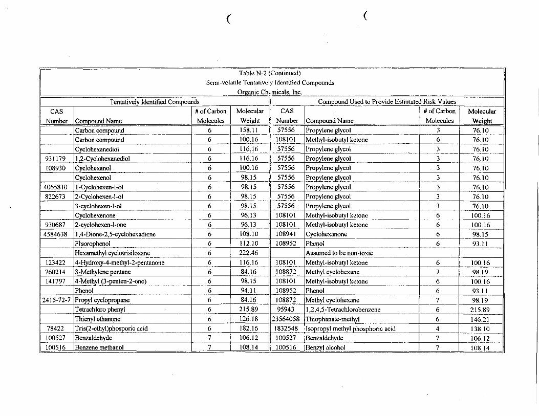
Table N-2 (Continued)Semi-volatile Tentatively Identified Compounds
Organic Chtmicals, Inc.Tentatively Identified Compounds
CASNumber j
931179108930
4065810822673
9306874584638
123422760214141797
2415-72-7
78422100527100516
Compound NameCarbon compoundCarbon compoundCyclohexanediol1 ,2-CyclohexanediolCyclohexanolCyclohexenol1-Cyclohexen-l-ol2-Cyclohexen-l-ol3-cyclohexen-l-olCyclohexenone2-cyclohexen-l-one1 ,4-Dione-2,5-cyclohexadieneFluorophenolHexamethyl cyclotrisiloxane4-Hydroxy-4-methyl-2-pentanone3-Methylene pentane4-Methyl (3-penten-2-one)PhenolPropyl cyclopropaneTetrachloro phenylThienyl ethanoneTris(2-ethyl)phosporic acidBenzaldehydeBenzene methanol
# of CarbonMolecules
666666666666666666666677
MolecularWeight158.11100.16116.16116.16100.1698.1598.1598.1598.1596.1396.13108.10112.10222.46116.1684.1698.1594.1184.16215.89126.18182.16106.12108.14
Compound Used to Provide Estimated Risk ValuesCAS
: Number: 57556
1081015755657556
i 5755657556575565755657556108101108101108941108952
10810110887210810110895210887295943
235640581832548100527100516
Compound NamePropylene glycolMcthyl-isobulyl ketonePropylene glycolPropylene glycolPropylene glycolPropylene glycolPropylene glycolPropylene glycolPropylene glycolMethyl-isobutyl ketoneMethyl-isobulyl ketoneCyclohexanonePhenolAssumed to be non-toxicMethyl-isobutyl ketoneMethyl cyclohexaneMelhyl-isobutyl kelonePhenolMethyl cyclohexane1 ,2,4,5-TetrachlorobenzeneThiophanate-methylIsopropyl methyl phosphoric acidBenzaldehydeBenzyl alcohol
# of CarbonMolecules
3633333336666
6766766477
MolecularWeight76.1076.1076.1076.1076.1076.1076.1076.1076.10100.16100.1698.1593.11
100.1698.19100.1693.1198.19
215.89146.21138.10106.12108.14

Table N-2 (Continued)Semi-volatile Tentatively Identified Compounds
Organic Chemicals, Inc.Tentatively Identified Compounds
CASNumber65850
6972736
5343964453636108883
Compound NameBenzoic acidChloromethyl benzeneCarbon compoundHydrocarbonCarbon isomer2-Hydroxy benzoic acidMethyl benzeneMethyl benzoic acid3-Methyl-2-butanol acetate2-Methvl hexanoic acidToluene
4305264 |6-Acetyloxy-2-hexanone532285619409
Alpha benzene acetonitrile4-Amino-methyl benzoic acid1 ,2 Benzene dicarboxilic acidBenzo thiaphene2-Bis(l -methyl ethyl) ethanolAkyl benzeneCarbon compoundAlkaneHydrocarbonHydrocarbonKetoneDimethyl benzene
# of CarbonMolecules
777777787778888888888888
MolecularWeight122.12126.59148.2096.17
1 Compound Used to Provide Estimated Risk ValuesCAS
Number6585095498111762108872
98.19 I 108872138.12 i, 6585092.14 | 108883136.15146.19130.1992.14158.20117.15151.17166.13134.20
658501117626418610888310810110713186306100210
23564058130.23 > 57556106.17104.15114.15106.17108.18146.76106.17
10041410887210887210887210887210810195476
Compound NameBenzoic acidO-chlorololueneElhylene glycol, monobutyletherMethyl cyclohexaneMethyl cyclohexaneBenzoic acidTolueneBenzoic acidEthylene glycol, monobutyletherFormic acidTolueneMethyl-isobutyl ketoneAcrylonitrileN-Nitrosodiphenyl aminep-Phthalic acidMethyl thiophanatePropylene glycolEthyl benzeneMethyl cyclohexaneMethyl cyclohexaneMethyl cyclohexaneMethyl cyclohexaneMethyl-isobutyl ketonem-xylene
# of CarbonMolecules
7767777761763128638777768
MolecularWeight122.12126.59118,1798.1998.19122.1292.14122.12118.1746.0392.14100.1653.06198.22166.13146.2176.10100.1798.1998.1998.1998.19100.16106.17

Table N-2 (Continued)Semi-volatile Tentatively Identified Compounds
Organic Chemicals, Inc.Tentatively Identified Compounds
CASNumber108383
23586643
1743619100414149575
6321148
4337659124072628682
54965081
Compound Name1 ,3 -Dimethyl benzene1 , 1 '-(3-3-Dimethyl)benzencDimethylphenol4-Ethenyl-l,4-D...cyclohexeneEthyl benzene2-Ethyl hexanoic acid3-Hydroxy-3,5-dimethyl 1-2-hexanoneIsobenzofuranoneMethyl heptanone4 Methyl-2-benzo thialzolamine5 Methyl-3-(l-methyl)cyclohexanoneMono(2-ethyl)-hexanedioc acidOctanoic acid2,2'-Oxybis-ethanol diacetylXyleneC3 Alkyl benzene isomerC9.H20 AlkaneC9,H 10 HydrocarbonC9.H12 HydrocarbonC9.H 18 HydrocarbonC9.H85 Hydrocarbon2,3 Dihydro-2-methyl benzoluranEthenyl methyl benzeneEthyl methyl benzene
# of CarbonMolecules
888888888888888999999999
MolecularWeight106.17108.18138.17110.20106.17144.21144.21134.13146.76164.23124.18174.20144.21190.20106.17120.20128.26118.18120.20126.24148.23134.18118.18120.20
Compound Used to Provide Estimated Risk ValuesCAS
Number954769547610895210887210041464186108101110009108101
215641701089416418664186
i 11176210832399828
: 108872108872
! 108872108872505293
' 1089412501315425013154
Compound Namem-Xylenem-XylenePhenolMethyl cyclohexaneEthly benzeneFormic acidMethyl-isoburyl ketoneFuranMethyl-isobutyl ketone2(Thiocyanomethylthio)-benzothiazoleCyclohexanoneFormic acidFormic acidEthylene glycol, mono butyl etherO-XyleneCumene (isopropyl benzene)Methyl cyclohexaneMethyl cyclohexaneMethyl cyclohexaneMethyl cyclohexane1 ,4-DithianeCyclohexanoneMethyl styreneMethyl styrene
# of CarbonMolecules
886781646961168977774699
MolecularWeight106.17106.1793.1198.19106.1746.03100.1668.08100.16233.3698.1546.0346.03118.18106.17120.2098.1998.1998.1998.19120.2498.15118.18118.18

Table N-2 ( Continued)Semi-volatile Tentatively Identified Compounds
Organic Ch< micals, Inc.Tentatively Identified Compounds j Compound Used to Provide Estimated Risk Values
CASNumber611143620144622968
91645
98839
98828
111842112050103651
1086784130421
Compound Name1 -Ethyl-2-methyl benzene1 -Ethyl-3-methyl benzene1 -Ethyl-4-methyl benzeneEthyl methyl cyclohexane2H-1 Benzopyran-2-oneMethyl benzeneatic acidMethyl benzo[]thiopheneMethyl ethenyl benzene1 -Methyl ethenyl benzeneMethyl ethyl benzenel-Methylethyl benzeneMethyl phenyl ethanoneNonaneNonanoic acidPropyl benzeneTrimethyl benzene1 ,3,5 Trimethyl benzene2,6 Bis (1,1 dimethyl) phenolC4 Akyl benzeneC10.H 12 HydrocarbonC10.H 14 HydrocarbonC10.H 18 HydrocarbonC10.H22 HydrocarbonC10,H20Isomer
# of CarbonMolecules
9999999999999999910101010101010
Molecular jj CASWeight Number120.20120.20120.20126.24148.16150.18148.33118.18118.181 20.20120.20134.18128.26158.24120.20120.20120.20154.25134.22132.21134.22138.25142.29
250131542501315425013154
10887298862100210505293
250131542501315425013154
25013598862108872641869982895636108678108952135988108872108872108872108872
140.27 •; 108872
Compound NameMethyl styreneMethyl styreneMethyl styreneMethyl cyclohexaneAcetophenonep-Phthalic acid1 ,4-DithianeMethyl styreneMethyl styreneMethyl styreneMethyl styreneAcetophenoneMethyl cyclohexaneFormic acidCumene (isopropyl benzene)1 ,2,4-Trimethyl benzene1,3,5 Trimethyl benzenePhenolSec-butyl benzeneMethyl cyclohexaneMethyl cyclohexaneMethyl cyclohexaneMethyl cyclohexaneMethyl cyclohexane
# of CarbonMolecules
9997884999987199961077777
MolecularWeight118.18118.18118.1898.19HO. 15166.13120.24118.18118.18118.18118.18120.1598.1946.03120.20120.20120.2093.11134.2298.1998.1998.1998.1998.19

Table N-2 Continued)Semi-volatile Tentatively Identified Compounds
Organic Chemicals, Inc.Tentatively Identified Compounds
CASNumber
105055
158698933637012
9339828744191758889
6114269670456726754661
25155151527844
10744374291809122576
Compound NameC10,H16KetoneDecamethyl cyclopcnta siloxaneDecanoic acidDiethyl benzene1 ,4-Diethyl benzeneDihydro methyl indeneDimethylethyl benzene2,5 Dimethyl Octanel-(3,4 Dimethyl phenyl)ethanoneEthenyl-dimethyl benzene1 -ethyl-2,3-dimethyl benzenel-ethyl-2,4-dimethyl benzene2-ethyl- 1 ,4-dimethyl benzenel-ethyl-2,4-dimethyl cyclohexane2-ethyl- 1,3-dimethyl cyclohexane2,4,6,7 ,8,8-5(1 H)-AzulenoneMethyl (l-methylethyl)benzene1 -Methyl-2-( 1 -melhylethyl)benzene1 -Methyl-3 -( 1 -methylethyl)benzene2-Methyl( 1 -methylethyl)benzeneMethyl propyl benzene1 -Methyl-3 -propyl benzene1 -Methyl-3-propyl cyclohexane4-phenyl-3-butene-2-one
# of CarbonMolecules
101010101010101010101010101010101010101010101010
MolecularWeight
Compound Used to Provide Estimated Risk ValuesCAS
Number152.24 jj 108941370.77172.27134.22134.22132.21134.22142.29148.21132.21134.22134.22134.22140.27140.27142.16134.22134.22134.22134.22134.22134.22140.27146.18
64186, 135988
13598891203
j 135988108872988629563613598813598813598810887210887210894113598813598813598813598813598813598810887298862
Compound NameCyclohexanoneAssumed to be non-toxicFoimic acidSec-butyl benzeneSec-butyl benzeneNaphthaleneSec-butyl benzeneMethyl cyclohexaneAcetophenone1 ,2,4-Trimethyl benzeneSec-butyl benzeneSec-butyl benzeneSec-butyl benzeneMethyl cyclohexaneMethyl cyclohexaneCyclohexanoneSec-butyl benzeneSec-butyl benzeneSec-butyl benzeneSec-butyl benzeneSec-butyl benzeneSec-butyl benzeneMethyl cyclohexaneAcetophenone
# of CarbonMolecules
6
11010101078910101077610101010101078
MolecularWeight98.15
46.03134.22134.22128.17134.2298.19120.15120.12134.22134.22134.2298.1998.1998.15134.22134.22134.22134.22134.22134.2298.19120.15

Table N-2 (Continued)Semi-volatile Tentatively Identified Compounds
Organic Chemicals, Inc.Tentatively Identified Compounds
CASNumber119642
48823395932
13877935
4132723
4706892173022712049958
54120626
Compound NameTetrahydro naphthaleneTetramethyl benzene1,2,3,4 Tetramethyl benzene1 ,2,4,5 Tetramethyl benzene4-Bicyclo(7,2,0)undec-4-eneCll,H24AlkaneCll,H16AlkeneC11.H 10 HydrocarbonC11.H 14 HydrocarbonC11.H 16 HydrocarbonC11.H20 HydrocarbonC11.H24 HydrocarbonC 1 1 ,H 1 6 Hydrocarbon isomerCll,H16IsomerDihydro-dimethyl-lH IndeneDimethylethyl-methyl benzene1 ,4 Dimethyl-2-( 1 -Methylethyl)benzeneDimethyl methylethyl benzene2,4 Dimethyl- 1 -( 1 -methylethyl)benzene2,5 Dimethylnonane1 , 1 Dimethyl propyl benzeneEthyl-trimethyl-benzeneEthyl- 1 ,2,4-trimethyl benzeneEthylidene- 1 H indene
# of CarbonMolecules
1010101011111
1
MolecularWeight132.21134.22
Compound Used to Provide Estimated Risk ValuesCAS
Number91203135988
134.22 j 135988134.22 , 135988150.26156.31148.25
77736108872108872
142.20 108872146.23 1 108872 •148.25 ' 108872152.28156.31148.25148.25146.23
10887210887210887210887291203
148.25 ! 135988148.25148.25148.25156.31148.25148.25148.25142.20
135988135988135988108872135988135988135988
u 91203
Compound NameNaphthaleneSec-butyl benzeneSec-butyl benzeneSec-butyl benzeneDicyclopentadieneMethyl cyclohexaneMethyl cyclohexaneMethyl cyclohexaneMethyl cyclohexaneMethyl cyclohexaneMethyl cyclohexaneMethyl cyclohexaneMethyl cyclohexaneMethyl cyclohexaneNaphthaleneSec-butyl benzeneSec-butyl benzeneSec-butyl benzeneSec-butyl benzeneMethyl cyclohexaneSec-butyl benzeneSec-butyl benzeneSec-butyl benzeneNaphthalene
# of CarbonMolecules
1010JO10107777777771010101010710101010
MolecularWeight128.17134.22134.22134.22132.2198.1998.1998.1998.1998.1998.1998.1998.1998.19128.17134.22134.22134.22134.2298.19134.22134.22134.22128.17

Table N-2 (Continued)Semi-volatile Tentatively Identified Compounds
Organic Chemicals, Inc.Tentatively Identified Compounds
CASNumber
90120
42929261120214103333120401
294622132650
1346233910358
23586643
573988575417571584575371
Compound NameMethyl naphthalene1 -Methyl naphthaleneMethyl-butenyl-benzenePentyl cyclohexaneUnedecaneAzobenzeneN,N Bis (2-hydroxy docecanamide)C12,H26AlkaneC12,H24AlkeneC12.H1 2 HydrocarbonC12.H 16 HydrocarbonC12.H24 HydrocarbonCyclo dodecaneDibenzothiophenediethyl-methyl benzamideN,N diethyl-3-methyl benzamide2,3 Dihydro-1 , 1 ,3-trimethyl- 1 H-indene1 , l'-(3 ,3 -Dimethyl- 1 -butoyl)benzene1 ,r-(3,3-Dimethyl-l-butenol)ben7.eneDimethyl naphthalene1 ,2-Dimethyl naphthalene1,3 -Dimethyl naphthalene1 ,4-Dimethyl naphthalene1 ,7 -Dimethyl naphthalene
# of CarbonMolecules
111111111112121212121212121212121212121212121212
MolecularWeight142.20142.20146.23154.30156.31182.23231.34170.34168.32156.23
Compound Used to Provide Estimated Risk ValuesCAS
Number912039120313598810887210887210333379061108872108872108872
160.26 i 108872168.32 108872168.32 ,: 108872184.27 505293191.27191.27162.28
790617906192524
160.26 ! 135988176.26156.23156.23156.23
1005169120391203
1 91203156.23 ' 91203156.23 ! 91203
Compound NameNaphthaleneNaphthaleneSec-butyl benzeneMethyl cyclohexaneMethyl cyclohexaneAzobenzeneAcrylamideMethyl cyclohexaneMethyl cyclohexaneMethyl cyclohexaneMethyl cyclohexaneMethyl cyclohexaneMethyl cyclohexane1 ,4 DithianeAcrylamideAcrylamide1,1 BiphenylSec-butyl benzeneBenzyl alcoholNaphthaleneNaphthaleneNaphthaleneNaphthaleneNaphthalene
# of CarbonMolecules
10101077123777777433121071010101010
MolecularWeight128.17128.17134.2298.1998.19182.2371.0898.1998.1998.1998.1998.1998.19
... 120.24 .71.0871.08154.21134.22108.14128.17128.17128.17128.17128.17

Table N-2 i Continued)Semi-volatile Tentative y Identified Compounds
Organic Chemicalsjnc.Tentatively Identified Compounds
CASNumber569415882337112403143077
24402244292197
13363634645152
80079
119619
Compound Name1 ,8 Dimethyl naphthaleneDiphenyl disulfideDodecaneDodecanoic acidEthyl naphthalene2-(2H-benzotriazol)phenol1-IododecaneMethylcycopentyl-benzenePCBs1 , 1 '-Oxybiscyclohexane1 , 1 '-Sulfonyl bis (4-benzene)Tetrachloro biphenylTetrachloro- 1 , 1 '-biphenylTetrahydro-dimetyl naphthaleneTrichloro biphenylTrichloro- 1 , 1 '-biphenylTetrahydro-naphth[]oxiraneBenzophenoneButyl-trimethyl cyclohexaneC13,H28AlkaneC13.H1 2 HydrocarbonC13.H1 4 HydrocarbonC13.H1 8 HydrocarbonC13.H20 Hydrocarbon
# of CarbonMolecules
121212121212121212121212121212121213131313131313
MolecularWeight156.23216.33170.34200.32156.23211.22296.24160.26
182.31218.28291.99291.99160.26257.55257.55172.23182.22182.35184.37168.24
Compound Used to Provide Estimated Risk ValuesCAS
Number912035052931088726418691203
1563662593602108883133636385687
21046451336363133636391203
1336363i 1336363
156366298862108872108872
! 108872170.26 108872174.29 i 108872176.30 ' 108872
Compound NameNaphthalene1 ,4-DithianeMethyl cyclohexaneFormic acidNaphthaleneCarbo furanBromomethaneToluenePolychlorinated biphenylsButyl benzyl phlhalateEthyl-p-nitrophenyl phenyl phosphoro.Polychlorinated biphenylsPolychlorinated biphenylsNaphthalenePolychlorinated biphenylsPolychlorinated biphenylsCarbo furanAcetophenoneMethyl cyclohexaneMethyl cyclohexaneMethyl cyclohexaneMethyl cyclohexaneMethyl cyclohexaneMethyl cyclohexane
# of CarbonMolecules
10471
1012171219141212101212128777777
MolecularWeight128.17120.2498.1946.03128.17221.2694.9492.14
312.37307.31
128.17
221.26120.1598.1998.1998.1998.19981998.19

c
Table N-2 i Continued)Semi-volatile Tentativel / Identified Compounds
Organic Ch< micals, Inc.Tentatively Identified Compounds \: Compound Used to Provide Estimated Risk Values
CASNumber
1142150
629505
2245387
295170
289739797259986282
267301432057490629594
Compound NameCl 3, H26 HydrocarbonC13.H28 HydrocarbonC1.H10S1 -Methoxy-4-(2-phenyl)benzeneMethyl dibenzo thiopheneTridecaneTrimethyl naphthalene1 ,6,7-Trimethyl naphthaleneAnthracenedioneBis(-dimethyl ethyl)phenolC14,H30AlkaneC14.H 12 HydrocarbonC14.H14 HydrocarbonC14.H30 HydrocarbonC14.H1 3 N CompoundCyclotetradecaneDimethyl biphenyl1 ,6, 1 0-Dodecatriene,7 , 1 1 -DimethylDDEEthylcarbazoleMethyl Fluorene7-Methyl tridecane4-(3-Phenyl propyl)pyridineTetradecane
# of CarbonMolecules
131313131313131314141414141414141414141414141414
Molecular CASWeight Number182.35184.37198.29184.24198.29184.37170.26170.26208.22206.33198.39180.25182.27198.39195.26196.38182.27192.35320.05195.26180.25198.39197.28198.39
1 108872108872
. 50529392524
505293108872912039120312012713598810887210887210887210887210891810887292524108872725998674886737108872
| 110861108872
Compound NameMethyl cyclohexaneMethyl cyclohexane1 ,4 Dithiane1,1 Biphenyl1 ,4-DithianeMethyl cyclohexaneNaphthaleneNaphthaleneAnthraceneSec-butyl benzeneMethyl cyclohexaneMethyl cyclohexaneMethyl cyclohexaneMethyl cyclohexaneCyclohexylanineMethyl cyclohexane1,1 BiphenylMethyl cyclohexaneDDECarbazoleFluoreneMethyl cyclohexanePyridineMethy^cyclohexane
# of CarbonMolecules
774124710101410777767127141213757
MolecularWeight98.1998.19120.25154.21120.2598.19128.17128.17178.23134.2298.1998.1998.1998.1999.1898.19154.2198.19320.05167.21166.2298.1979.1098.19
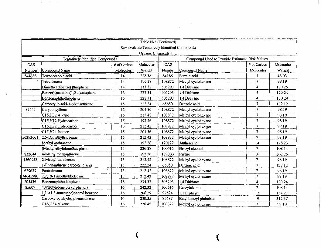
Table N-2 (Continued)Semi-volatile Tentatively Identified Compounds
Organic Chemicalsjnc.Tentatively Identified Compounds
CASNumber544638
87445
56292661
8326441560958
6296297464598020543685609
Compound NameTetradecanoic acidTetra deceneDimethyl dibenzoQthiopheneBenzo(b)naphtho{ 1 ,2-d)thiopheneBenzonaphthothiopheneCarboxylic acid-1-phenantlireneCaryophyylleneC15,H32AlkaneC15.H 12 HydrocarbonC15.H32 HydrocarbonC15,H24Isomer2,5-DimethyltridecaneMethyl anthracene(Methyl ethylidone)bis phenol4-Methyl phenanthrene2-Methyl tetradecane1 -Phenanthrene carboxylic acidPentadccane2,7, 1 0-TrimethyldodecaneBenzonaphthothiophene4,4'Butylidene bis (2 phenol)1 , 1 '-( 1 ,3-butadiene)phenyl benzeneCarboxy-octahydro phenanthreneC16,H34Alkane
# of CarbonMolecules
141414151515151515151515151515151515151616161616
MolecularWeight228.38196.38213.32222.31222.31222 24204.36212.42192.26212.42204.36212.42192.26226.28192.26
Compound Used to Provide Estimated Risk ValuesCAS
Number64186108872505293505293505293
I 65850108872108872108872108872
, 108872108872120127100516129000
212.42 ; 108872222.24 65850212.42212.42234.32242.32206.29230.35226.45
'. 1088721088725052931005169252485687108872
Compound NameFormic acidMethyl cyclohexane1 ,4 Dithiane1 ,4 Dithiane1 ,4 DithianeBenzoic acidMethyl cyclohexaneMethyl cyclohexaneMethyl cyclohexaneMethyl cyclohexaneMethyl cyclohexaneMethyl cyclohexaneAnthraceneBenzyl alcoholPyreneMethyl cyclohexaneBenzoic acidMethyl cyclohexaneMethyl cyclohexane1 ,4 DithianeBenzylalcohol1,1 BipheynlButyl benzyl phthalateMethyl cyclohexane
# of CarbonMolecules
1744477777771471677774712197
MolecularWeight46.0398.19120.25120.24120.24122.1298.1998.1998.1998.1998.1998.19178.23108.14202.2698.19122.1298.1998.19120.24108.14154.21312.3798.19

c
Table N-2 (Continued)Semi-volatile Tentatively Identified Compounds
Organic Chemicals, Inc.Tentatively Identified Compounds
CASNumber
295658
367466654476357103
366538242091294550451081889674
23884682053238846243174629787
Compound NameC16,H32AlkeneC16.H 14 HydrocarbonC16.H34 HydrocarbonC16,H3202AcidCycle hexadecaneDimethyl phenanthrene2,5 Dimethyl penanthreneHexadecaneHexadecanoic acid1 -Hexadecanol9-Hexadecenoic acid6 Propyl tridecane1 , 1 '-( 1 , 1 ,2,2-Tetramethyl)phenyl benzeneBenzo FluoreneBenzo(a)fluoreneBenzo(b)fluoreneC17,H36Alkane1 lH-Benz(a)fluorene7H-Benz(de)anthracen-7 -one1 lH-Benzo(a)fluorene1 lH-Benzo(b)fluoreneHeptadecaneMethyl benzo naphthothiopheneMethyl pyrene
# of CarbonMolecules
161616161616161616161616161717171717171717171717
MolecularWeight224.43206.29226.45256.43224.43206.29206.29226.45256.43242.45254.41226.45212.34216.28216.28216.28240.48218.30
Compound Used to Provide Estimated Risk ValuesCAS
Number1088721088721088726418610887212900012900010887264186575566418610887292524867378673786737
86737234.30 j| 56553218.30218.30240.48248.35216.28
! 8673786737
505293129000
Compound NameMethyl cyclohexaneMethyl cyclohexaneMethyl cyclohexaneFormic acidMethyl cyclohexanePyrenePyreneMethyl cyclohexaneFormic acidPropylene glycolFormic acidMethyl cyclohexane1,1 BiphenylFluoreneFluoreneFluoreneAssumed to be non-toxicFluoreneBenz(a)anthraceneFluoreneFluoreneAssumed to be non-toxic1 ,4 DithianePyrene
# of CarbonMolecules
7771716167131712131313
13181313
416
MolecularWeight98.1998.1998.1946.0398.19202.26202.2698.1946.0376.1
46.0398.19154.21166.22166.22166.22
166.22228.29166.22166.22
120.24202.26

Table N-2 (< Vmtinued)Semi-volatile Tentativel' Identified Compounds
Organic Chemicals, Inc.Tentatively Identified Compounds
CASNumber
23812173442782538238
159197
64401214
Compound Name1 -methyl pyrene2-methyl pyrene1 ,2,3 propane octanoic acid3,12,1 7-trione and rostaneBenzanthracenoneBenzo(c)phenathreneC18,H38AlkaneC18.H20 HydrocarbonC18,H20PhenylAlkeneDichloroterphenyl1 ,3 Dimethyl pyrene
2 1 1 64954 1 7,9 Dimethyl hexadecane109013759345357114
35365594
5,12 NaphthacenedioneOctadecaneOctadecanoic acid9-OctadecyneTrichloroter phenyl
791286 |Triphenyl phosphine oxide
54105678629925
Triphenyl stannaneC19,H40AlkaneCycle hexane derivative + C 1 32,6-dimethyl heptadecaneNonadecane
101019 JNIN11N"-Tripnenyl quanidinc
# of CarbonMolecules
171717171818181818181818181818181818181919191919
MolecularWeight216.28216.28270.46274.36244.29228.24254.50236.36236.36299.20230.31254.50228.29254.50284.48252.49333.65278.29350.01268.53266.51268.53268.53287.35
Compound Used to Provide Estimated Risk ValuesCAS
Number12900012900064186
56553218019
12900
56553
64186
7803512108883
505293
Compound NamePyrenePyreneFormic acidAssumed to be non-toxicBenz(a)anthraceneChryseneAssumed to be non-toxicAssumed to be non-toxicAssumed to be non-toxicPolychlor terphenyls (PCTs)PyreneAssumed to be non-toxicBenz(a)anthraceneAssumed to be non-toxicFormic acidAssumed to be non-toxicPCTsPhosphineTolueneAssumed to be non-toxicAssumed to be non-toxicAssumed to be non-toxicAssumed to be non-toxic1 ,4 Dilhiane
# of CarbonMolecules
16161
1818
16
18
1
7
4
MolecularWeighl202.26202.2646.03
228.29228.29
202.26
r~ 228.29
46.03
34.0092.14
120.24

Table N-2 'Continued)Semi-volatile Tentative!'' Identified Compounds
Organic Cht micals, Inc.Tentatively Identified Compounds
CASNumber
18344371
192972
1985501235741
7663118344371
123795629970646139
535904629992
Compound Name2,6,10,14 TetramethylpentadecaneBenzo pyreneBenzo(e)pyreneBenzofluorantheneC20.H42 AlkaneC20-.H42 HydrocarbonC20,H17N05IsomerPeryleneCarboxylic acid-1-phenanthraceneC21.H44 AlkaneTriphenyl-2-propene stannane2,6, 1 0, 1 4 Tetramethyl-heptadecaneC22.H46 AlkaneC22.H44 02 Acid esterDioctyl ester hexanedioic acidDocosane2 Methyl propyl octadccanoic acidC23.H48 AlkaneC24.H50 AlkaneTetraphenyl StannanePentacosaneC26.H54 AlkaneC27.H56 AlkaneC27.H35 NO2
# of CarbonMolecules
192020202020202021212121
• 222222222223242425262727
MolecularWeight268.53252.32252.32252.32
Compound Used to Provide Estimated Risk Valuesi CASt Number
5032850328
207089282.56282.56351.36252.32298.34296.58391.08296.58310.61340.59366.54310.61340.59324.64338.66497.11352.69366.72380.45405.58
! 1056025032865850
1108883
8568785687
64186
108883
1563662
Compound NameAssumed to be non-toxicBenzo(a)pyreneBenzo(a)pyreneBenzo(k)fluoranlheneAssumed to be non-toxicAssumed to be non-toxicCaprolactamBenzo(a)pyreneBenzoic acidAssumed to be non-toxicTolueneAssumed to be non-toxicAssumed to be non-toxicButyl benzylphthalateButyl benzylphthalateAssumed to be non-toxicFormic acidAssumed to be non-toxicAssumed to be non-toxicTolueneAssumed to be non-toxicAssumed to be non-toxicAssumed to be non-toxicCarbo furan
# of CarbonMolecules
202020
6207
7
1919
1
7
MolecularWeight
252.32252.32252.32
113.16252.32108.14
92.14
312.67312.67
46.03
92.14
221.26

Table N-2 (Continued)Semi-volatile Tentatively Identified Compounds
Organic Chemicals, Inc.Tentatively Identified Compounds
CASNumber630024
Compound NameOctacosaneC29.H60 Alkane
# of CarbonMolecules
2829
MolecularWeight394.77
Compound Used to Provide Estimated Risk ValuesCAS
Number
408.80
i
l~
Compound NameAssumed to be non-toxicAssumed to be non-toxic
# of CarbonMolecules
MolecularWeight
SPROJ/OCI/PH.M^Z/RI/APPXN/TABLEN-J
APPENDIX O
ECOLOGICAL CONTAMINANTS OF POTENTIAL CONCERNPROFILES
APPENDIX 0
ACETONE. Acetone, Chemical Abstract Service Registry No. 67-64-1 is analiphatic ketone also known as 2-propanone and dimethyl ketone. Acetone is acolorless, highly volatile, flammable liquid with an aromatic odor (NIOSH, 1978).Acetone is miscible with water, alcohol, ether, and most oils (Merck 1976).
Acetone is produced in large quantities and may be released to the environmentas stack emissions, fugitive emissions, and in wastewater in its production and useas a chemical intermediate and solvent. Acetone is a product of thephotooxidation of some alkanes and alkenes that are found in urban air and it isalso released from volcanoes and in forest fires. It is a metabolic product releasedby plants and animals (Howard 1990).
If released on soil, acetone will both volatilize and leach into the ground andprobably biodegrade. If released into water, it will probably biodegrade and belost due to volatilization. It has an estimated half-life of 20 hours from a modelriver. Bioconcentration in aquatic organisms and adsorption sediment should notbe significant. In the atmosphere, acetone will be lost by photolysis and reactionwith photochemically produced hydroxyl radicals. Estimated half-lives from thesecombined processes averages 22 days. The general public is exposed to acetone inthe atmosphere from sources such as auto exhaust, solvents, tobacco smoke, andfireplaces, as well as from dermal contact with consumer products such assolvents. In addition, there will be exposure by ingestion of food that maynaturally contain acetone, such as onions, apples, grapes, and tomatoes, orexposure from contaminated drinking water. (Howard 1990)
Acetone is a compound that occurs normally in small amounts in human bloodand urine, is a component of human breath and is of metabolic origin (NIOSH1978).
A 90 day oral gavage study with groups of albino rats at levels of 0, 100, 500, or2500 mg/kg/day resulted in an increase in kidney-to-body and brain weight ratiosfor both sexes in the 2500 mg/kg group. Liver weight and liver-to-body weightratios were also elevated for the 2500 mg/kg group. Females revealed a significantincrease in kidney and liver weights at the 500 mg/kg/day exposure level. TheNOEL for this study is 100 mg/kg/day. Based on this study, U.S.EPA hasestablished a reference dose (RfD) of 0.1 mg/kg/day (IRIS 1994).
POLYNUCLEAR AROMATIC HYDROCARBONS. Polynuclear aromatichydrocarbons are a class of organic compounds that are formed during theincomplete combustion or pyrolysis of organic material containing carbon andhydrogen (USEPA 1984f). Polynuclear aromatic hydrocarbons are found inpetroleum-derived products, asphalts, coal tar, creosote oils, and coal tar pitchesformed by the distillation of coal tar. Polynuclear aromatic hydrocarbons

characteristics are: Multiringed organic compounds usually with densities greaterthan water; low solubility in water; high partition coefficients, which explains theiraffinity for organic matter (high affinity for soil over water); low vapor pressure;and slow biological degradation half-lives, which explains their persistence in soiland other media.
Polynuclear aromatic hydrocarbons are a class of compounds that are formedduring the incomplete combustion or pyrolysis of organic materials containingcarbon and hydrogen (USEPA 1984f).
Polynuclear aromatic hydrocarbons are released to the environment throughnatural and man-made sources with emissions largely to the atmosphere. Naturalsources include emissions from volcanoes and forest fires. Man-made sourcesprovide a much greater release volume than natural sources; the largest singlesource is the burning of wood in homes. Automobile and truck emissions are alsomajor sources of polynuclear aromatic hydrocarbons. On a local scale, hazardouswaste sites can be a concentrated source of polynuclear aromatic hydrocarbons.Polynuclear aromatic hydrocarbons can enter surface water through atmosphericdeposition and from discharges of industrial effluents, municipal wastewater, andimproper disposal of used motor oil. .
In air, polynuclear aromatic hydrocarbons are found sorbed to particulates and asgases (ATSDR 1989b). Benzo(a)anthracene, chrysene, benzo(a)pyrene and benz?(g,ri,i;perylene should exist predominantly in the paniculate sorbed phase in theatmosphere whereas naphthalene, fluoranthene, and pyrene should exist in thevapor phase in the atmosphere (USEPA 1984f). Particulate-bound polynucleararomatic hydrocarbon can be transported long distances and are removed fromthe atmosphere through precipitation and dry deposition (ATSDR, 1989b). Theremoval of polynuclear aromatic hydrocarbons from the atmosphere can occurthrough photochemical reactions; chemical reactions with hydroxy radicals, ozoneand nitrogen oxides; and physical removal mechanisms. The polynuclear aromatichydrocarbons that exist in the vapor phase in the atmosphere are likely to beremoved primarily through direct or indirect photochemical reactions (USEPA1984f).
Three mechanisms that may be responsible for the removal of polynucleararomatic hydrocarbons from aquatic media are volatilization, photochemicalreactions and microbial degradation. Polynuclear aromatic hydrocarbons aretransported from surface waters by volatilization and sorption to settling particles.The compounds are transformed in surface waters by photooxidation, chemicaloxidation and microbial metabolism. In soils and sediments, microbial metabolismis the major process for degradation of polynuclear aromatic hydrocarbons(ATSDR 1989b).
The predominant mechanism for the removal of polynuclear aromatichydrocarbons from soils is likely to be microbial degradation. Based on the

assumption that microbial degradation is greater in soils than in aquatic systems,the half-life of polynuclear aromatic hydrocarbons in soils could range from lessthan a day to a few years. Considering the soil sorption coefficient and watersolubilities, these compounds are not expected to have high mobility in soils.Therefore, significant leaching of these compounds into groundwater is notexpected, particularly from soils with higher organic carbon content (USEPA1984f).
Biological effects of PAHs on terrestrial vegetation have been reviewed by severalauthors as presented in Eisler (1987). In general, these authorities agreed onseveral points. First, plants and vegetables can absorb PAHs from soil throughtheir roots, and translocate them to other plant parts such as developing shoots.Second, above-ground parts of vegetables, especially the outer shell or skin,contained more PAHs than underground parts, and this was attributed to airbornedeposition and subsequent adsorption. Third, PAH-induced phytotoxic effectswere rare; however, the data base on this subject is small. Fourth, most higherplants can catabolize benzo(a)pyrene, and possibly other PAHs, but metabolicpathways have not been clearly defined. Finally, the biomagnification potential ofvegetation in terrestrial and aquatic food PAHs in both field and laboratoryexperiments.
Eisler refers to two articles regarding PAHs and avian wildlife, and bothconcerned mallards (Anas platyrhynchosX In one study, Patton and Dieter (1980),as cited by Eisler (1987), fed mallards diets that contained 4,000 mg PAHs/kg(mostly as napthlenes, napthenes, and phenanthrene) for a period of 7 months.No mortality or visible signs of toxicity were evident during exposure; however,liver weight increased 25% and blood flow to liver increased 30%, when comparedto controls. In the second study, Hoffman and Gay (1981), as cited by Eisler(1987), measured embryotoxicity of various PAHs applied externally, in acomparatively innocuous synthetic petroleum mixture, to the surface of mallardeggs. For benzo(a)pyrene, 0.002 ug/egg did not affect mallard survival, but didcause embryonic growth and an increased incidence of abnormal survivors. At0.01 ug benzo(a)pyrene/egg, 60% died in 18 days; at 0.05 ug/egg, 75% were deadwithin 3 days of treatment. Embryos may contain microsomal enzymes that canmetabolize PAHs to more highly toxic intermediates than can adults, and avianembryos may have a greater capacity to metabolize PAHs in this manner than domammalian embryos and fetuses (as quoted in Hoffman and Gay 1981, as cited byEisler 1987); this observation warrants additional research. Several investigatorshave suggested that the presence of PAHs in petroleum, includingbenzo(a)pyrene, chrysene, and 7,12-dimethylbenz(a)anthracene, significantlyenhances the overall embryotoxicity in avian species, and that the relatively smallpercent of the aromatic hydrocarbons contributed by PAHs in petroleum mayconfer much of the adverse biological effects reported after eggs have beenexposed to microliter quantities of polluting oils (Hoffman and Gay 1981; Albers1983, as cited by Eisler 1987).

Numerous PAH compounds are distinct in their ability to produce tumors in skinand in most epithelial tissues of practically all animal species tested; malignancieswere often induced by acute exposures to microgram quantities. In some cases,the latency period can be as short as 4 to 8 weeks, with the tumors resemblinghuman carcinomas. Certain carcinogen PAHs are capable of passage across skin,lungs, and intestine, and can enter the rat fetus, for example, following intragastricor intravenous administration to pregnant dams. In most cases, the process ofcarcinogenesis occurs over a period of many months in experimental animals, andmany years in man. The tissue affected is determined by the route ofadministration and species under investigation. Thus, 7,12-dimelthylbenz(a)anthracene is a potent carcinogen for the mammary gland ofyoung female rats after oral or intravenous administration; dietary benzo(a)pyreneleads to leukemia, lung adenoma, and stomach tumors in mice; and both PAHcompounds can induce hepatomas in skin of male mice when injected shortly afterbirth. Acute and chronic exposure to various carcinogenic PAHs have resulted indestruction of hematopoietic and lymphoid tissues, ovotoxicity, antispermatogoniceffects, adrenal necrosis, changes in the intestinal and respiratory epithelia, andother effects. For the most part, however, tissue damage occurs at dose levelsthat would also be expected to induce carcinomas, and thus the threat ofmalignancy predominates in evaluating PAH toxicity. There is a scarcity of dataavailable on the toxilogical properties of PAHs which are not demonstrablycarcinogenic to mammals.
Target organs for ?Ari iuxic action are uwcibe, due partly to extensivedistribution in the body and also to selective attack by these chemicals onproliferating cells. Damage to the hematopoietic and lymphoid system inexperimental animals is a particularly common observation. Application ofcarcinogenic PAHs to mouse skin leads to destruction of sebaceous glands and tohyperplasia, hyperkeratosis, and ulceration. Tumors are induced in application ofa large dose, or by the single application of certain noncarcinogenic agents(promotion).
Investigators agree that unsubstituted aromatic PAHs with less than 4 condensedrings have not shown tumorigenic activity; that many, but not all, 4-,5-, and 6-ringPAH compounds are carcinogenic; and that Only a few unsubstituted hydrocarbonswith 7 rings or greater are tumorigenic or carcinogenic. Many PAH compoundscontaining 4 and 5 rings, and some containing 6 or more rings, provoke localtumors after repeated application to the dorsal skin of mice; the tumor incidenceexhibited a significant dose-response relationship (Grimmer et al. 1985 as cited inEisler 1987). Among unsubstituted PAHs containing a nonaromatic ring, e.g.,chloranthrene and acepthanthacene, all active carcinogens retained an intactphenantrene segment. The addition of alkyl substitutents in certain positions inring system of a fully aromatic PAH will often confer carcinogenic, activity ordramatically enhance existing carcinogenic potency. For example, monomethylsubstitution of benz^ajanthracene can lead to strong carcinogenicity in mice, withpotency depending on the position substitution in the order 7 > 6 > 8 = 12 > 9;

a further enhancement of carcinogenic activity is produced by appropriatedimethyl substitution, with 7,12-dimethylbenzene(a)anthracene among the mostpotent PAH carcinogens known. Alkyl substitution of partially aromaticcondensed ring systems may also add considerable carcinogenic activity, as is thecase with 3-methylchIolanthrene. With alkyl substituted longer than methyl,carcinogenicity levels decrease, possibly due to a decrease in transport through cellmembranes.
A good correlation exists between skin tumor initiating activities of variousbenzo(a)pyrene metabolites, and their mutagenic activity in mammalian cellmutagenesis systems (Slaga et al. 1978 as cited in Eisler 1987), although variationsin chromosome number and structure may accompany tumors induced by variouscarcinogenic PAHs in rats, mice, and hamsters (Bayer 1978; EPA 1980 as cite inEisler 1987). Active PAH metabolites, e.g., dihydrodiols or diol epoxides, canproduce sister chromatid exchanges in Chinese hamster ovary cell (Bayer 1978;EPA 1980; Pal 1984 as cited in Eisler 1987). When exchanges were induced bythe diol epoxide, a close relationship exists between the frequency of sisterchromatid exchanges and the levels of deoxyribnucleoside-diol-epoxide adductformation. In general, noncarcinogenic PAHs were not mutagenic.
Laboratory studies with mice have shown that many carcinogenic PAHs adverselyaffect the immune system, thus directly impacting an organism's general health,although noncarcinogenic analogues had no imunosuppressive effect; further, themere carcinogenic the PAH, the greater the immuuosuppression (Ward n n-. .^o->as cited in Eisler 1987).
Numerous studies show that unsubstituted PAHs do not accumulate in mammalianadipose tissues despite their high lipid solubility, probably because they tend to berapidly and extensively metabolized (EPA 1980; Lee and Grant 1981 as cited byEisler 1987).
Many chemicals are known to modify the action of carcinogenic PAHs inexperimental animals, including other PAHs that are weakly carcinogenic ornoncarcinogenic. The effects of these modifiers on PAH metabolism appear tofall into three major categories: those which alter the metabolism appear to fallinto three major categories: those which alter the metabolism of the carcinogen,causing decreased activation or increased detoxification; those which scavengeactive molecular species of carcinogens to prevent their reaching critical targetsites in the cell; and those which exhibit competitive antagonism (DiGiovanni andSlaga 1981as cited by Eisler 1987). For example, benz(a)anthracene, a weakcarcinogen, when applied simultaneously with benz (a)anthracene, a weakcarcinogen, when applied simultaneously with dibenz(a,h)anthracene, inhibited thecarcinogenic action of the latter in mouse skin; a similar case is made forbenzo(e)pyrene or dibenz(a,c)anthracene applied to mouse skin shortly prior toinitiation with 7,12-dimethylbenz(a)antracene, or 3-methylcholanthrene(DiGiovanni and Slaga 1981as cited by Eisler 1987). Benxo(a)pyrene, a known

carcinogen, interacts synergistically with cyclopenta(cd)pyrene, a moderately strongcarcinogen found in automobile exhausts, according to results of mouse skincarcinogenicity studies (Rogan et al. 1983 as cited by Eisler 1987). Other PAHcombinations were cocarcinogenic, such as benxo(e)pyrene to the skins of mice(DiGiovanni and Slaga 1981as cited by Eisler 1987). Effective inhibitors of PAH-induced tumor development include selenium, vitamin E, ascorbic acid, butylatedhydroxytoluene, and hydroxyanisole (EPA 1980 as cited by Eisler 1987). Inaddition, protective effects against PAH-induced tumor formation have beenreported for various naturally occurring compounds such as flavones, retenoids,and vitamin A (EPA 1980 as cited by Eisler 1987). Until these interaction effectsare clarified, the results of single substance laboratory studies may be extremelydifficult to apply to field situations of suspected PAH contamination. Additionalwork is also needed on PAH dose-response relationships, testing relevantenvironmental PAHs for carcinogenicity, and elucidating effects of PAH mixtureson turner formation (Grimmer 1983 as cited, by Eisler 1987).
Eisler (1987) presents toxicity values for several PAHs. Acute oral LDSO's forbenzo(a)pyrene and phenanthrene were 50 and 700 mg/kg (body weight)respectively. Carcinogenic effects were observed for chronic oral doses (mg/kgbody weight) with benzo(a)pyrene (0.002), dibenz(a,h)anthracene (0.006),benz(a)anthracene (2.), benzo(b)fluoranthene (40.0), indeno (1,2,3-cd) pyrene(72.0) and chrysene (99.0). Carcinogenic effects were also observed in mice fortopical external application (mg) of benzo(a)pyrene (0.001), benzo(g,h,i)pery!ene(C.3'. •.:"<! N:rizo(a)anthracene.
Chlordane. Chlordane has been released in the past into the environmentprimarily from its application as an insecticide. The amount of chlordane usedannually in the U.S. prior to 1983 was estimated in 1985 to be greater than 3.6million pounds. Between July 1, 1983 and April 14, 1988, the only approved usefor chlordane in the U.S. was for underground termite control. As of April 14,1988, however, all commercial use of chlordane is a mixture of at least 50compounds; the major constituents of the mixture are cis- and transchlordane,heptachlor, cis- and trans-nonachlor, a, p, and y-chlordene, 3a,4,5,5a,6-exo-hexachloro-la,2,3,3a,5a,5b-hexahydro-l,4-methano-lH-cyclobuta(cd)pentalene, and2,4,4,5,6,6,7,8-octahydro-2,3,3a4,5,7a-hexahydro-l,4-rnethano-lH-indene[ll]. Ifreleased to soil, chlordane may persists for long periods of time. Under fieldconditions, the mean degradation rate has been observed to range from 4.05-28.33%/yr with a mean half-life of 3.3 years. Chlordane is expected to begenerally immobile or only slighly mobile in soil based on field tests, soil columnleaching tests and estimated Koc estimation; however, its detection in variousground water in NJ and elsewhere indicated that movement to groundwater canoccur. Soil volatility tests, have found that chlordane can volatilize significantlyfrom soil surfaces on which it has been sprayed, particularly moist soil surfaces;however, shallow incorporation into soil will greatly restrict volatile losses.Although sufficient biodegradation data are not available, it has been suggested

that chlordane is very slowsly biotransformed in the environment which isconsistent with the long persistence periods observed under field conditions. Ifreleased to water, chlordane is not expected to undergo significant hydrolysis,oxidation or direct photolysis. The volatilization half-life from a river one meterdeep flowing 1 m/sec with a wind velocity of 3 m/sec is estimated to be 7.3-7.9 hrs.at 23 ° C for the y- and trans-isomers, respectively, and 43 hrs for technicalchlordane; the volatilization half-lives from a representative environmental pond,river and lake are estimated to be 18-26, 3.6-5.2 and 14.4-20.6 days, respectively.However, adsorption to sediment signigicanlty attenuates the importance ofvolatilization. Adsorption to sediment is expected to be a major fate processbased on soil adsorption data, estimated Koc values (24,600-15,500), and extensivesediment monitoring data. Bioconcentration is expected to be important based onexperimental BCF values which are generally above 3,200. Sensitized photolysis inthe water column may be possible. The presence of chlordane in sediment coresamples suggests that chlordane may be very persistent in the adsorbed state inthe aquatic environment. The observation that 85% of the chlordane originallypresent in a sealed glass jar under sunlight and artificial lifgt in a river die-awaytest remained at the end of two weeks and persisted at that level through week 8of the experiment; this indicates that chlordane will be very persistent in aquaticenvironments. If released to the atmosphere, it will be expected to bepredominantly in the vapor phase. Chlordane will react in the vapor-phase withphotochemically produced hydroxyl radicals at an estimated half-life rate of 6.2 hr.suggesting that this reaction is the dominant chemical removal process. Thedetection of chlordane in remctc ".i^osph-rc (Picif:: .<t,d Atlantic Oceans; theArctic) indicates that long range transport occurs. It has been estimated that 96%of the airborn reservoir of chlordane exists in the sorbed state which may explainwhy its long range transport possible without chemical transformation. Thedetection of chlordane in rainwater and its observed dry deposition at variousrural locations indicated that physical removal via wet and dry deposition occurs inthe environment. Major general population esposure to chlordane can occurthrough oral consumption of contaminated food and inhalation of contaminatedair. Occupation exposure by dermal and inhalation routes related to the use ofchlordane as an insecticide may be significan (Howard, 1990).
A NOAEL of 0.055 mg/kg-day (1 ppm) was developed from a dietary study withCharles River Fischer rats. A LOAEL of 0.273 mg/kg-day was also reported withregional liver hypertrophy as the effect for females (IRIS 1994).
BARIUM. Barium, CASRN 7440-39-3, is a silvery white metallic element whichoxidizes very easily. It is one of the less expensive metals that have the distinctiveproperties of absorbing gases. It belongs to the alkaline earth group, resemblingcalcium chemically. The most important compounds are the peroxide, chloride,sulfate, carbonate, nitrate, and chlorate. Naturally occurring barium is a mixtureof seven stable isotopes (CRC, 1984).

Traces of barium are very widely distributed. No data exist concerning itspresence or its amount in dust; the content of barium will probably beproportionally related to the calcium content.
Barium is extremely reactive, decomposes in water, and readily forms insolublecarbonate and sulfate salts. Barium is generally present in solution in surface orgroundwater only in trace amounts. Large amounts will not dissolve becausenatural waters usually contain sulfate, and the solubility of barium sulfate isgenerally low. Barium is not soluble at more than a few parts per million in waterthat contains sulfate at more than a few parts per million. However, bariumsulfate may become considerably more soluble in the presence of chloride andother anions. Monitoring programs show that it is rare to find barium in drinkingwater at concentrations greater than 1 mg/liter. Atmospheric transport of barium,in the form of particulates, can occur. Bioaccumulation is not an importantprocess for barium (Clement, 1985).
There are no reports of carcinogenicity, mutagenicity, or teratogenicity associatedwith exposure to barium or its compounds. Insoluble forms of barium, particularlybarium sulfate, are not toxic by ingestion or inhalation because only minimalamounts are absorbed. Accidental ingestion of soluble barium salts have resultedin gastroenteritis, muscular paralysis, and ventricular fibrillation and extra systoles.There are no adequate animal data available for determining the chronic effectsof low level exposure to barium by ingestion. Adequate data for characterizationof toxicity to wildlife and H^ ~f--v's. .li.i:-.;:!: ;-- .^ct r.ci-'ble .'Clement, 1985).
The LOAEL identified in the Perry et al study (5.1 mg/kg/day) has been used inthe derivation of the oral RfD without an additional 10-fold uncertainty factor forthe lack of a NOAEL. The oral reference dose is 5xlO~2 mg/kg/day with anuncertainty factor of 100 (IRIS 1994).
BERYLLIUM. Beryllium, Chemical Abstract Service Registry No. 7440-41-7 is ametal that is also known as glucinium. It is one of the lightest of metals, is widelydistributed geographically, and has found wide application in industry. Somefeatures that has contributed to its wide use in industry are that it is a stablelightweight metal with a high melting point, it has a high strength to weight ratio,and it imparts resistance to corrosion, vibration, and shock when alloyed withother metals.
Beryllium usually exists in nature as a compound. Bextrandixe and beryl ores areused commercially for obtaining beryllium. Beryllium is also found in coal andgasoline (ATSDR, 1987a). Common forms of beryllium are beryllium oxide,fluoride, and hydroxide.
Although beryllium is a naturally occurring substance, the major source of itsemission to air is the combustion of coal and fuel oil, which releases particulatesand fly ash containing beryllium into the atmosphere. The average concentration
of beryllium in coal is 1.8 - 2.2 micrograms per gram. Fuel oil can contain 0.08ppm beryllium. The beryllium released from coal combustion is likely to be in theform of beryllium oxide. Beryllium oxide is relatively insoluble and would not bemobilized in soil or surface water at normal pH ranges. It is believed that mostenvironmental beryllium is present in an insoluble form. This is substantiated byempirical data which indicate that even in polluted rivers, dissolved berylliumlevels are very low. In most type of soils, beryllium is expected to be tightlyabsorbed because it displaces divalent cations which share common absorptionsites. Removal of beryllium from the atmosphere results from wet and drydeposition. No evidence was found that any environmental process results in thevolatilization of beryllium into the atmosphere from water or soil (ATSDR,1987a).
Schroeder and Mitchner (1975 as cited in IRIS 1994) orally administered beryllium(as beryllium sulfate) to rats at dose level of 0 and 0.54 mg/kg/day. The exposurewas for a lifetime, after which the rats were observed for changes in the heart,kidney, liver, and spleen. There were no effects of treatment on these organs noron the number of tumors, the lifespan, urinalysis, serum glucose, cholesterol, anduric acid. Two other studies (Schroeder and Mitchner, 1975 and Morgareidge etal. 1975 as cited in IRIS 1994) indicates higher dose levels may be NOEL (IRIS1994).
Based on the above studies, U.S. EPA established an oral reference dose of 5 x1 °"" rr.g/herylliurn/kg/day with an uncertainty factor of 100 (IR.IS 1994).
A reference dose for inhalation toxicity is not available at this time from USEPAIRIS. Several studies on the inhalation toxicity of beryllium are, however,noteworthy. Hardy and Tabershaw (1946 as cited in IRIS 1994) noted thatdecreased longevity following inhalation exposure to beryllium compounds inhuman is related to the pulmonary effects. Short-term human and animalexposures to high levels of beryllium leads to development of inflammation orreddening and swelling of the lungs (similar to pneumonia). Long-termexposure at much lower levels have been reported to cause berylliosis, which is anoncancerous growth in the lung of humans. A skin allergy has been shown todevelop when beryllium comes in contact with the skin. (ATSDR, 1987a)
Several studies were performed that associated the increases in the rate ofmortality due to cancer to exposure to beryllium (Wagoner et al. 1980, Bayliss andWagoner 1977; Mancuso, 1970, 1979, 1980 as cited in IRIS 1994). When thenumber of expected deaths was adjusted for smoking, the increased incidence wasno longer significant (IRIS 1994).
Despite the inadequate studies performed for human subjects, there does existsufficient animal studies to justify classifying beryllium B2; probable humancarcinogen. Based on the evidence for induction of tumors by a variety ofberyllium compounds in male and female monkeys and in several strains of rats of

both sexes ,via inhalation and intratracheal instillation, and the induction ofosteosarcomas in rabbits by intravenous or intramedullary injection in multiplestudies, an oral slope factor of 4.3 mg/kg/day has been assigned by U.S. EPA(IRIS 1994).
Despite limitations in the human studies, human data was used to establish aninhalation slope factor of 8.4 mg/kg/day. Humans are most likely to be exposed byinhalation to beryllium oxide, rather than other beryllium salts. Animal studies byinhalation of beryllium oxide have utilized intratracheal instillation, rather thangeneral inhalation exposure. (IRIS 1994)
Based on a study with fifty-two weanling Long-Evans rats, each sex received 0 or 5ppm beryllium in drinking water. Exposure was for the lifetime of the animals. ANOEL was observed for 5 ppm or 0.54 mg/kg/day. A body weight of 0.325 kg wasused for the rats. There is no LOAEL for beryllium (IRIS 1994).
Cadmium. Cadmium, Chemical Abstract Service Registry No. 7440-43-9 is asilver-blue-white metal. Pure metallic cadmium is not common in theenvironment. It is most often encountered in combination with other elementssuch as oxygen, chlorine, or sulfur. Metallic cadmium has a low melting point formetals (321°C) and is insoluble in water. (ATSDR 1987d)
Cadmium enter the environment to a limited extent from the natural weatheringin ;v-iir.erals, but to a much greater degree from pollutant sources such asdiscarded metal-containing products, phosphate fertilizers, and fuel combustion(ATSDR 1987d).
Although overall natural sources of cadmium are relatively low, the metal is widelydistributed in the Earth's crust and is commonly found at detectable levels in soil,surface water, and groundwater (ATSDR 1987d).
Atmospheric cadmium is in the form of very small particulate matter, produced bycombustion of fuel containing cadmium. This material is subject to dry depositionand rainwash, so that cadmium levels in the atmosphere are generally less than 3ng/m3 near specific cadmium emitting industries. Cadmium in surface water isusually present at less than 1 ng/L; industrial contaminations can result inconcentrations up to 10 ng/L. There is some concern that soil cadmium levels areincreasing largely from the use of cadmium-contaminated phosphate fertilizer andland disposal of some sewage sludges containing particularly high levels ofcadmium. Consumption of food represents the greatest sources of humanexposure, since plants take up cadmium from the soil (ATSDR 1987d).
Combustion of coal and petroleum products tend to produce cadmium that isadsorbed to small (1 to 2 micron) particles that are persistent in the atmosphereand are easily respirable. In this form, cadmium can be transported to soine
distance and transferred to other environmental compartments via wet or drydeposition (ATSDR 1987d).
Compared to most other heavy metals, cadmium is relatively mobile in theaqueous environment. In natural waters, cadmium may exist as the hydrated ion;as metal-inorganic complexes with CO3"2, OH", Cl" or SO4'2; or as metal-organiccomplexes with humic acids. Cadmium does not form volatile compounds in theaquatic environment, nor does biological methylation occur (ATSDR 1987d).
Concentrations of cadmium in groundwater are kept low by sorption by mineralmatter and clay, binding by humic substances, precipitation as cadmium sulfide inthe presence of sulfide, and precipitation as the carbonate at relatively .highalkalinities (ATSDR 1987d).
Cadmium may be present in soil as free cadmium compounds or in solutiondissolved in soil water. It may also be held to soil mineral or organic constituentsby cation exchange. High soil acidity favors release of cadmium and its uptake byplants (ATSDR 1987d). Cadmium is mobile in soil, as evidenced by the detectionof this element in 100% of the groundwater samples collected from New Jersey(USEPA 1984a).
The acute LC50 for freshwater fish and invertebrates generally ranged from 100 to1,000 ug/liter; salmonids are much more sensitive than other organisms. Saltwaterspecies were in general 10-fold more tolerant to the acute effects of cadmium.Chronic tests have been performed and show that cadmium has cumulativetoxicity and acute-chronic ratios that range of from 66 to 431. Bioconcentrationfactors were generally less than 1,000 but were as high as 10,000 for somefreshwater fish species (Clement, 1985).
A NOAEL of 0.01 mg/kg-day (food) was developed based on human studiesinvoving chronic exposures. A LOAEL was not reported (IRIS 1994).
CHROMIUM. The ammonium and alkali metal salts of hexavalent chromiumare generally water-soluble, but the alkaline metal salts (calcium, strontium) aresparingly soluble or insoluble in water. Hexavalent chromium rarely occurs innature apart from man-made sources because it is readily reduced in the presenceof oxidizable organic matter; however, hexavalent chromium compounds thatoccur most commonly in the form of chromate and dichromate are stable in manynatural waters because of the low concentration of reducing matter. Exceptacetate and nitrate salts, the trivalent chromium compounds are generallyinsoluble in water. In most biological systems, chromium is present in the trivalentform. The physical or chemical forms and the mode by which chromium (III)compounds are incorporated into biological systems are poorly characterized(ATSDR, 1987b).

Chromium occurs naturally in the earth's crust. Continental dust is the primarysource of natural chromium present in the environment; however, chromium isreleased to the environment because of human activities in much larger amounts.Chromium is primarily removed from the atmosphere by fallout and precipitation.Atmospheric chromium removed by physical processes predominantly enterssurface water or soil; however, before their removal, chromium particles ofaerodynamic diameter less than 20 um may remain airborne for long periods andmay be transported long distances (ATSDR 1987b).
Because there are no known chromium compounds that can volatilize from water,transport of chromium from water to the atmosphere is not likely other than bytransport in windblown sea sprays. Most of the chromium (III) is eventuallyexpected to precipitate in sediments. Small amounts of chromium (III) mayremain in solution as soluble complexes. Chromium (VI) will be presentpredominantly in soluble form. These soluble forms of chromium may be stableenough to undergo intramedia transport; however, organic matters present inwater will eventually reduce chromium (VI) to chromium (III). It has beenestimated that the residence time of chromium in lake water is from 4.6 to 18years (ATSDR, 1987b).
Chromium probably occurs as insoluble Cr2O3H2O in soil because the organicmatter in soil is expected to convert soluble cnromate to insoluble Cr2O3.Chromium in soil may be transported to the atmosphere in the aerosol form, andrunoff and leaching may transport chromium from soil ;u suiiaoc wateia anuground water. Runoff could remove both soluble and bulk precipitate with finaldeposition on either a different land area or a water body. Flooding of soils andthe subsequent anaerobic decomposition of plant matter may increasemobilization of chromium in soils because of the formation of soluble complexes.The half-life of chromium in soils may be several years (ATSDR, 1987b).
Chromium is an essential nutrient and is accumulated in a variety of aquatic andmarine biota, especially benthic organisms, to levels much higher than in ambientwater. Levels in biota, however, usually are lower than levels in the sediments.Passage of chromium through the food chain can be demonstrated. The foodchain appears to be a more efficient pathway for chromium uptake than directuptake from seawater.
Water hardness, temperature, dissolved oxygen, species, and age of the testorganism all modify the toxic effects of chromium on aquatic life. Cr III appearsto be more acutely toxic to fish than Cr VI; the reverse is true in long termchronic exposure studies.
None of the plants normally used as food or animal feed are chromiumaccumulators. Chromium absorbed by plants tends to remain primarily in theloots and is poorly translocated to the leaves. There is little tendency forchromium to accumulate along food chains in the trivalent inorganic form.

A bioconcentration factor for manganese in a species of edible fish (striped bass)has been reported to be less than 10. Bioaccumulation of manganese may notoccur significantly with organisms of higher tropic level (USEPA, 1984c).
Both chemical and microbiological interactions may cause speciation of manganesein soils; soil pH and oxidation-reduction potential of soil may influence thespeciation process. It has been suggested that in acid water-logged soils,manganese passes freely into solution and may leach into groundwater. Also,manganese can be leached directly from waste burial sites and from other naturalsoils into groundwater (USEPA, 1984c).
Manganese occurs in many minerals that are widely distributed in the earth's crust>incl. in trace amounts, is an essential element fcr bcth plants and animal:. "~l.jmany different possible manganese compounds may enter the aquatic environmentfrom natural and industrial sources. Manganese and its compounds havemoderate acute and chronic toxicity to aquatic life. Insufficient data are availableto evaluate or predict the short-term and long-term effects to plants, birds, or landanimals.
Manganese and its compounds range in their respective water solubilities fromvery soluble to insoluble. It is also highly persistent with a half-life of greater than200 days. Manganese is expected to be found at about the same levels in fishtissue, as in the surrounding waters (Clement, 1985).
A NOAEL of 0.005 mg/kg-day was established from a human chronic ingestionstudy. A LOAEL was also established as 0.06 mg/kg-day based on CNS effects(IRIS 1994).