Axon - Excel model manual - NET
111
Development of the Danish LRAIC model for fixed networks Excel model manual [Version for 3 rd consultation] Axon Partners Group 1 September 2020 Excellence in Business
-
Upload
khangminh22 -
Category
Documents
-
view
0 -
download
0
Transcript of Axon - Excel model manual - NET
Development of the Danish LRAIC model
for fixed networks Excel model manual
[Version for 3rd consultation]
Axon Partners Group
1 September 2020
Excellence in Business


2020© Axon Partners Group 1
Contents
Contents .............................................................................................................. 1
1. Introduction ................................................................................................... 4
2. Excel model architecture .................................................................................. 5
3. Market and network inputs ............................................................................... 7
3.1. Demand ................................................................................................... 7
3.1.1 Copper shutdown ............................................................................................................ 9
3.2. Asset costs ............................................................................................. 13
3.3. Adjustment for fully depreciated assets ..................................................... 15
3.4. Broadband traffic .................................................................................... 17
3.5. Demand distribution ................................................................................ 18
3.6. Network efficiency adjustment .................................................................. 19
3.7. Non-network overheads ........................................................................... 22
3.8. Ancillary services inputs ........................................................................... 23
3.9. Other network and costing inputs .............................................................. 24
4. Geographical inputs ....................................................................................... 26
4.1. Coverage ............................................................................................... 26
4.2. Access network elements and distribution .................................................. 27
4.3. Core network inputs ................................................................................ 28
4.4. Other geographical inputs ........................................................................ 29
5. Dimensioning module .................................................................................... 30
2020© Axon Partners Group 2
5.1. Dimensioning drivers ............................................................................... 30
5.1.1 Dimensioning drivers’ concept ..................................................................................... 31
5.1.2 Mapping services to drivers .......................................................................................... 31
5.1.3 Conversion from services to drivers ............................................................................. 32
5.2. Transmission network dimensioning .......................................................... 33
5.3. Access Network Dimensioning .................................................................. 43
5.3.1 Copper Access Network Dimensioning ......................................................................... 43
5.3.2 Fibre Access Network Dimensioning ............................................................................. 54
5.3.3 Coax Access Network Dimensioning ............................................................................. 65
6. Resources costing ......................................................................................... 74
6.1. Calculation of network costs ..................................................................... 74
6.2. Calculation of non-network costs............................................................... 77
7. Network costs of the services ......................................................................... 79
7.1. Incremental and common costs calculation ................................................ 79
7.2. Allocation of network costs to services ....................................................... 80
7.2.1 Step 1: Mapping of services and resources .................................................................. 81
7.2.2 Step 2. Calculation of demand for the three allocation criteria ................................... 81
7.2.3 Step 3: Cost Allocation to Services ................................................................................ 82
Annex A. User manual for the Excel model ............................................................. 84
A.1. Getting started ....................................................................................... 84
A.2. General overview of the model ................................................................. 84
A.2.1. Support and control worksheets .................................................................................. 86
2020© Axon Partners Group 3
A.2.2. Step 0: Parameters ........................................................................................................ 87
A.2.3. Step 1: Main inputs ....................................................................................................... 87
A.2.4. Step 2: Advanced inputs ............................................................................................... 88
A.2.5. Step 3: Mapping ............................................................................................................ 89
A.2.6. Step 4: Drivers and demand factors .............................................................................. 90
A.2.7. Step 5: Dimensioning of the network ........................................................................... 91
A.2.8. Step 6: Resource Costing............................................................................................... 92
A.2.9. Step 7: Allocation of costs ............................................................................................. 92
A.2.10. Step 8: Results ............................................................................................................... 93
A.2.11. Additional support sheets ............................................................................................. 93
A.3. Understanding the control panel ............................................................... 94
A.3.1. Execution Panel ............................................................................................................. 95
A.3.2. Input scenarios .............................................................................................................. 96
A.3.3. Results overview ........................................................................................................... 97
A.4. Description of checks ............................................................................... 98
Annex B. Description of the ancillary services ....................................................... 100
Annex C. List of acronyms .................................................................................. 107

2020© Axon Partners Group 4
1. Introduction
Since 2003, the DBA has annually regulated the wholesale prices for several fixed-network
services through a Long Run Average Incremental Cost (LRAIC) model. As presented in
the Model Reference Paper (hereinafter, ‘the MRP’) from October 20191, the relevant
changes that occurred in the fixed Danish market since the last major update of the model
in 2013, merited a new update of the fixed LRAIC model (hereinafter, ‘the model’) to make
sure it is representative of the current situation and can fulfil DBA’s regulatory needs.
The model submitted to consultation represents the 3rd draft model developed by DBA.
This model incorporates the feedback received from the industry in the 1st and 2nd
consultations processes, which took place between earlier in the year. This model has been
developed following the methodological principles laid out in the MRP from October 2019,
which was subject to consultation with the industry between 1st July to 30th August 2019.
For this 3rd consultation process, two different Fixed LRAIC model have been developed:
One model based on TDC and one model based on Norlys (combining Eniig and SE). Each
Fixed LRAIC model consists in two parts:
R model: Used to perform a geographical assessment of the access and transmission
networks in Denmark.
Excel model: Used to calculate services’ costs, following a set of inputs and
calculations. In this case, while the calculations considered for both, TDC and Norlys
are identical, the inputs included in the model differ, as each are based on the data
that operators have been able to provide.
This document represents the Excel model manual. This manual aims to describe the
modelling approach, structure and calculation process followed in the development of the
Excel model. In addition, ‘Annex A - User manual for the Excel model’ presents a simple
set of guidelines to follow when using the Excel model and ‘Annex B - Description of the
ancillary services’, presents a description of the ancillary services included in the model.
1 Link: https://erhvervsstyrelsen.dk/sites/default/files/2019-10/Final%20MRP.pdf
2020© Axon Partners Group 5
2. Excel model architecture
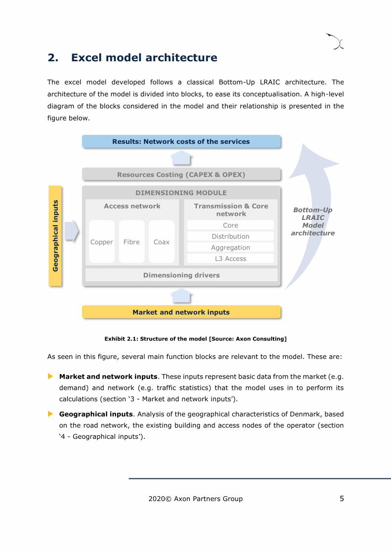
The excel model developed follows a classical Bottom-Up LRAIC architecture. The
architecture of the model is divided into blocks, to ease its conceptualisation. A high-level
diagram of the blocks considered in the model and their relationship is presented in the
figure below.
Exhibit 2.1: Structure of the model [Source: Axon Consulting]
As seen in this figure, several main function blocks are relevant to the model. These are:
Market and network inputs. These inputs represent basic data from the market (e.g.
demand) and network (e.g. traffic statistics) that the model uses in to perform its
calculations (section ‘3 - Market and network inputs’).
Geographical inputs. Analysis of the geographical characteristics of Denmark, based
on the road network, the existing building and access nodes of the operator (section
‘4 - Geographical inputs’).
Resources Costing (CAPEX & OPEX)
DIMENSIONING MODULE
Access network Transmission & Core network
Copper
Dimensioning drivers
Results: Network costs of the services
Market and network inputs
Geo
grap
hic
al
inp
uts
Fibre Coax
Bottom-Up LRAICModel
architecture
L3 Access
Aggregation
Distribution
Core

2020© Axon Partners Group 6
Dimensioning module. Calculation of the number of resources needed for the
network to supply the services provided by the reference operator (section 5 -
Dimensioning module’).
Resources costing. Assessment of the annualized costs of the network, in terms of
operational (OpEx) and capital (CapEx) costs (section ‘6 - Resources costing’).
Network costs of the services: Allocation of the costs of the resources to services
and calculation of the final unit costs of the services considered in the model (section
‘7 - Network costs of the services’).
Each of these modules is presented with a high level of detail in the sections below.

2020© Axon Partners Group 7
3. Market and network inputs
The Excel cost model developed is data-intensive and has been populated with the
information requested from the operators (through various data-gathering processes,
including data reported as part as the public consultation processes), as well as additional
publicly available information and other data available to DBA. Different sets of inputs
have been defined for TDC and Norlys.
The model’s inputs are included under the “Market and network inputs” and the
“geographical analysis” blocks illustrated in Exhibit 2.1. The former is described in this
section, while the latter is presented in section ‘4 - Geographical inputs’ below.
The “Market and network inputs” block includes the following inputs:
Demand
Asset costs
Adjustment for fully depreciated assets
Broadband traffic
Demand distribution
Network efficiency adjustment
Non-network overheads
Ancillary services inputs
Other network and costing inputs
The following sections describe how each of these inputs has been defined in the model.
3.1. Demand
The demand of the modelled services is one of the primary inputs of the cost model and
is crucial to determine the required elements in some parts of the network, as well as to
calculate the unit costs of the services. This input is introduced in worksheet ‘1A INP
DEMAND’ for each of the modelled services and for the whole modelling period (i.e. from
2005 to 2038).

2020© Axon Partners Group 8
We have adopted the approach described below to populate the demand inputs in the
model:
Whenever information was provided by the modelled operator (for past, current and
future years), we mapped it to the relevant modelled services and inputted it to the
model.
• In the case of TDC, information from the modelled operator was used for 69% of
all demand data points.
• In the case of Norlys, information from the modelled operator was used for 41% of
all demand data points.
In the absence of such information, we extracted it from the previous DBA’s model,
provided it was available.
• In the case of TDC, the information from DBA’s previous model allowed us to fill in
an additional 14% of the demand data points.
• In the case of Norlys information from the previous DBA’s model was not
considered.
Finally, when no information was available from any of the two previous sources, it
was estimated based on the information available for other years2 or based on other
parameters (such as reported take-up).
• In the case of TDC, the information from these regression analyses allowed us to
populate the remaining 17% of the demand data points.
• In the case of Norlys, the information based on take-up forecasts reported by the
operator, allowed us to populate the remaining 59% of the demand data points.
Due to the lack of data, the model considers all addresses to be “sellable”.
2 It should be noted that data was found for all the services for at least 4 consecutive years.

2020© Axon Partners Group 9
3.1.1 Copper shutdown
Modelling the copper shutdown
TDC’s model includes a copper-shutdown feature. The objective of this feature is to assess
the effect that a potential shutdown of the copper network in the medium term may have
in the cost of providing fixed services in Denmark.
The copper shutdown consists on assuming that before the last modelling year (2038) the
copper network will be completely shut down, having no users and all assets being
decommissioned.
The copper shutdown is performed by progressively reducing the demand in the copper
network beyond the figures reported by the modelled operator.
Exhibit 3.1: Illustrative example of copper shutdown in 2030 [Source: Axon Consulting]
Where the copper shutdown year (x0) is an input defined in the control panel (see ‘Annex
A - User manual for the Excel model’ for further details).
The migration pattern shown above is governed by a simple logistics curve that shutdowns
all demand over a 5-year period. The formula considered along with the shape of the
pattern is presented in the exhibit below:
-
20
40
60
80
100
Acce
ss c
op
pe
r lin
es
(2
00
5 =
10
0)
No switch-off Switch-off in 2030
x0 = 2030

2020© Axon Partners Group 10
%𝑜𝑓 𝑙𝑖𝑛𝑒𝑠 𝑠ℎ𝑢𝑡𝑑𝑜𝑤𝑛 = 1
1 + 𝑒𝑥0−𝑥−2
Where:
“x0” is the shutdown year (i.e.
2030 in the model’s base case).
“x” is the variable year for the
calculation
Exhibit 3.2: Migration pattern for the copper shutdown, considering 2030 as the year of shutdown
[Source: Axon Consulting]
The lines shutdown from the copper network are not “lost” in the model. In the contrary,
the model estimates whether the lines shall be migrated to other TDC’s networks (coax or
fibre) or to other operators (not included in the model). In order to do this, the model
looks at the different Central Offices where there remains demand of copper network when
the shutdown starts to take place3. For each of the Central Office areas, the model takes
a decision:
If the area has both, coax and fibre coverage, then the model splits the remaining
copper demand between the coax and fibre evenly (50-50). The model reviews whether
the fibre coverage in the area is PON or PTP to ensure the demand is allocated to the
appropriate network.
If the area has either, coax or fibre coverage but not both, then the model assigns the
remaining copper demand to either coax or fibre networks (depending on which
network has coverage). In this case, the model also reviews whether the fibre coverage
in the area is PON or PTP to ensure the demand is allocated to the appropriate network.
If the area does not have neither coax nor fibre coverage, then the copper demand
associated to this network is considered to go to other networks that are not TDC’s
fixed networks.
3 These calculations are included in worksheet ‘4A CALC COPPER SHUTDOWN’.
-
20%
40%
60%
80%
100%
2025 2027 2029 2031
% o
f m
igrate
d lin
e

2020© Axon Partners Group 11
Annualisation of copper shutdown costs
When assessing the impact of a copper shutdown before the end of the modelling period,
it is particularly important to evaluate its implications on the recovery of the capital costs.
In particular, the model calculates and annualises the investment required for copper
access networks over the useful lives of the assets. At the same time, the timeframe of
the model was set in line with the useful lives of these assets to guarantee a consistent
approach in the depreciation of their GRC. However, if the copper network is shut down
before the end of their useful lives, it becomes important to define the treatment to be
given to the annualization of such costs. There are mainly two alternatives to address this
issue:
a) All GRC is annualized within the “active” years of the copper network. This
would imply artificially adjusting the useful lives of the copper access assets to ensure
they are either lower or equal to the modelling timeframe.
b) Only the GRC that, according to the technical useful lives of the assets, is
expected to be annualized during the “active” years of the copper network is
considered. This would imply keeping the originally defined technical useful lives and
consider the default annualisation costs generated by these assets in any year of the
model.
Alternative a) above would naturally lead to higher unit costs for the copper access services
when a copper network shutdown is expected to take place before 2038 (the last year of
the model). On the other hand, if no shutdown of the copper network is expected (or if it
takes place in 2038), both alternatives will lead to the same results.
Even though alternative b) could seem to lead to an under-recovery of costs by the
modelled operator, it is important to clarify that this may not necessarily be the case. This
is because the model considers all non-fully depreciated assets to be newly deployed in
2005, which is a common technique in Current Cost Accounting (CCA) Bottom-Up cost
models but does not reflect the factual situation of the modelled operator. This implies
that the NRC considered in the model in 2005 is notably higher than the Net Book Value
(NBV), even if indexed, registered in the modelled operator’s financials.
As discussed in the previous section, when no copper shutdown is considered, the
difference in the 2005 NRC is offset throughout the modelled period because the model

2020© Axon Partners Group 12
does not consider new reinvestments in the main passive copper access assets while the
modelled operator does in practice (e.g. due to the yearly replacements required). This
means that under this scenario, the cost base recovered in the model and the cost base
expected to be recovered by the modelled operator are broadly similar.
However, if a copper shutdown is considered to take place before 2038, alternative a) may
indeed lead to an over-recovery of the modelled operator’s costs, as the financial NBV
(even if indexed) of the modelled operator could not have enough time to reach, in
practice, the 2005 NRC considered in the model.
The exhibit below provides an illustrative example of the behaviour that should be
expected in the model and in the modelled operator’s financials when no copper shutdown
is considered and when the copper network is expected to be shut down in 2030 (under
alternatives a and b):
Exhibit 3.3: Illustrative behaviour of the model and the modelled operator’s financials under
different copper shutdown scenarios [Source: DBA]
As a base case, the model considers that the shutdown of the copper network will take
place in 2030 and that the GRC is annualized within the “active” years of the copper
network. Those scenarios can be modified by the user through a drop-down list included
in the control panel. Further details on the scenarios and guidelines to operate the Excel
model can be found in ‘Annex A - User manual for the Excel model’.
ALTER
NA
TIV
E B
NO
SH
UTD
OW
N
OPERATOR
MODELGRC: 100NRC: 100
Total amount depreciated: 100
GRC: 150NRC: 30
Total amount depreciated: 100
No new investments
Investment: 30 Investment: 30 Investment: 30
SH
UTD
OW
N 2
02
5
OPERATOR
MODELGRC: 100NRC: 100
Total amount depreciated: 100
GRC: 150NRC: 30
Total amount depreciated: 50
No new investments
Investment: 30ALTER
NA
TIV
E A
OPERATOR
MODELGRC: 100NRC: 100
Total amount depreciated: 60
GRC: 150NRC: 30
Total amount depreciated: 50
No new investments
Investment: 30
20382005 2025

2020© Axon Partners Group 13
3.2. Asset costs
The assets’ costs and associated information are included in worksheet ‘1B INP UNIT
COSTS’ of the model for each of the network elements defined. These inputs are used to
calculate the annualised operational and capital costs which are to be later allocated to
services.
For each of the assets defined in the model, this worksheet includes:
Inputs relevant to capital expenditures.
• Unit CapEx. Includes the costs associated with the purchase and installation of
the network element.
• CapEx trend. Cost trends for CapEx are defined in the cost model to assess the
evolution of prices over the years.
• Useful lives. Useful lives are introduced in the model for the annualisation of the
assets’ CapEx.
Inputs relevant to operational expenditures.
• Unit OpEx. Includes the annual cost of maintenance and operation of the network
element. It also includes rental expenses.
• Percentage of labour work. Percentage of OpEx that is coming from staff costs.
As per the MRP, the prices used in the model should reflect those that an efficient operator
would face, considering the scale of the modelled operator.
To populate these inputs, we have followed the approach illustrated below:

2020© Axon Partners Group 14
Exhibit 3.4: Decision tree adopted to define the assets’ costs inputs [Source: Axon Consulting]
The table below provides a brief summary of the approach adopted for each input for each
of the modelled operators:
Input based on previous model or
Axon’s internal database
Co
st
Mo
de
l
No
Information requested to modelled operator
Previous model or Axon’s internal
database (confidential)
Data providedYes
Aligned with typical industry and previous model values
Input from the modelled operator
No
Information requested to alternative service
providers
Data available and aligned with typical industry and previous model values
Input from alternative service providers
Yes
Yes
No

2020© Axon Partners Group 15
Parameter Input from
the modelled operator
Input from alternative
operator(s)4
Input from existing models
Input from international benchmarks
Unit CapEx
TDC 83%5 5% 10% 1%
Norlys 21% 42% 26% 11%
CapEx trend
TDC 1% 19% 18% 62%
Norlys - 16% 25% 60%
Useful lives
TDC 12% 11% 76% -
Norlys - - 100% -
Unit OpEx
TDC 65% - 28% 5%
Norlys - - 56% 44%
Percentage of labour costs
TDC 100% - - -
Norlys - 65% 35% -
Exhibit 3.5: Summary of the approaches followed to populate the unit costs inputs [Source: Axon
Consulting]
3.3. Adjustment for fully depreciated assets
As presented in the MRP, the model does not take fully depreciated assets in copper and
coax access networks6 into consideration to avoid over-recovering their costs. Particularly,
this consideration applies to the following assets:
Copper networks: Copper cable, including civil infrastructure used to install these
cables (trenches, ducts, etc.).
Coax networks: Coax cable, including civil infrastructure used to install these cables
(trenches, ducts, etc.).
4 This category includes information extracted for official Danish agencies, as StatBank. 5 47% of the inputs are directly extracted from TDC’s data meanwhile the remaining 36% have been extracted based on data reported by the operator, with minor adjustments.
6 No adjustment is applied in the case of fibre networks
2020© Axon Partners Group 16
Therefore, this adjustment applies only to TDC, as no copper or coax networks have been
considered so far with regards to Norlys.
To apply this adjustment, detailed information from TDC’s Fixed Asset Register (FAR) was
required in terms of:
Total gross book value (GBV) of the assets under operation in the copper and coax
access networks.
The year when the assets were originally purchased.
Note that, as explained in the MRP, the useful lives from the existing LRAIC models are
considered instead of the accounting useful lives to ensure consistency with the regulation
adopted by DBA so far.
However, when assessing TDC’s information, three main limitations where identified:
There is no information regarding assets that were fully depreciated by 1995.
Therefore, these could not be accounted for in the calculations performed, leading to
a potential underestimation of the percentage of fully depreciated assets.
Even though the percentage of fully depreciated assets had to be calculated as of the
first year of the model (i.e. 2005), the DBA-Axon team only had access to a detailed
Fixed Asset Register from the modelled operator for the year 2018, meaning that the
calculation of the percentage of fully depreciated assets actually refers to 2018. This
could arguably lead to a potential overestimation of the percentage of fully depreciated
assets.
The usage of the regulatory useful lives could be argued, given that even though these
should be preferred, they were only used for regulatory purposes since the late 2000s.
This means that TDC probably recovered most of the access assets’ costs beforehand,
based on its financial useful lives. Therefore, the adoption of the regulatory useful lives
may lead to a potential underestimation of this percentage.
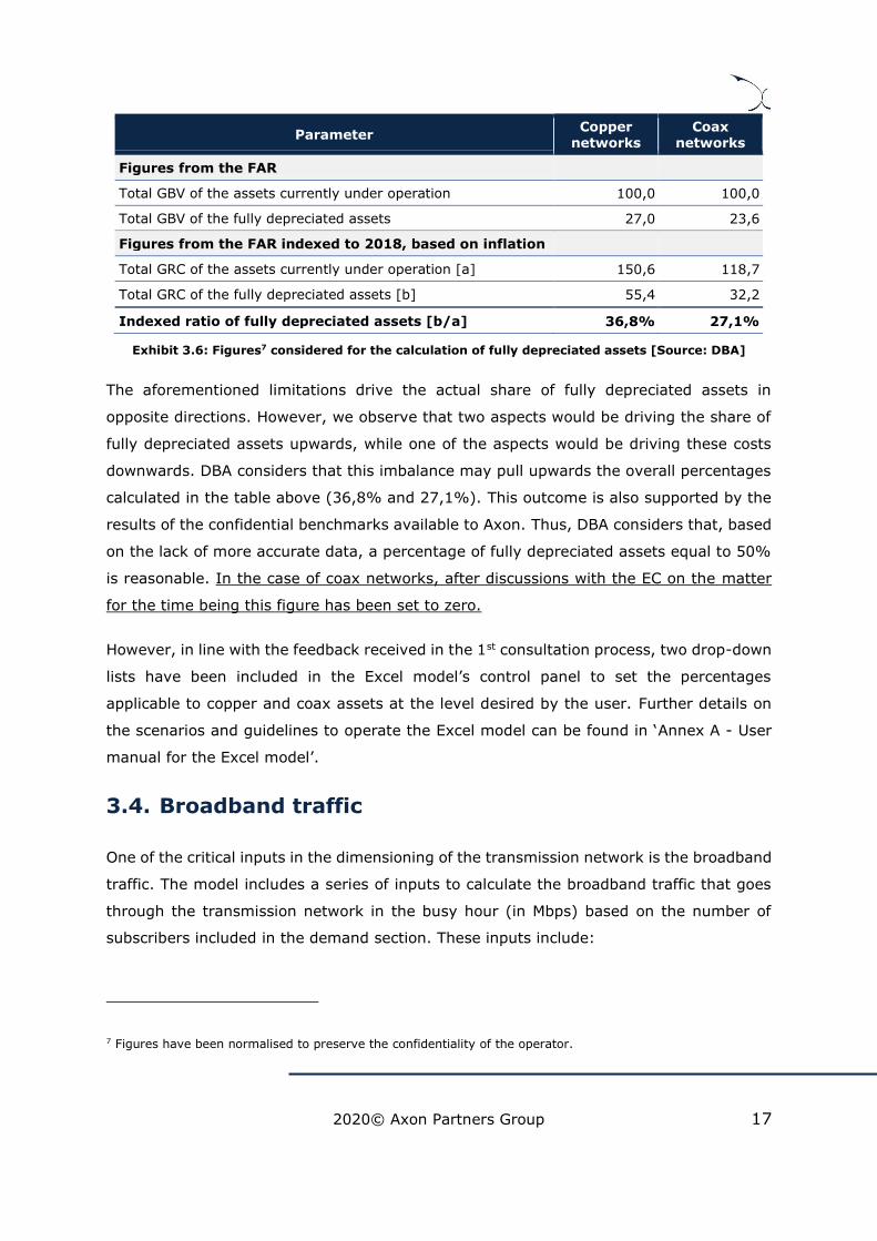
Despite this situation, the table below illustrates the figures obtained from the TDC’s FAR:
2020© Axon Partners Group 17
Parameter Copper
networks Coax
networks
Figures from the FAR
Total GBV of the assets currently under operation 100,0 100,0
Total GBV of the fully depreciated assets 27,0 23,6
Figures from the FAR indexed to 2018, based on inflation
Total GRC of the assets currently under operation [a] 150,6 118,7
Total GRC of the fully depreciated assets [b] 55,4 32,2
Indexed ratio of fully depreciated assets [b/a] 36,8% 27,1%
Exhibit 3.6: Figures7 considered for the calculation of fully depreciated assets [Source: DBA]
The aforementioned limitations drive the actual share of fully depreciated assets in
opposite directions. However, we observe that two aspects would be driving the share of
fully depreciated assets upwards, while one of the aspects would be driving these costs
downwards. DBA considers that this imbalance may pull upwards the overall percentages
calculated in the table above (36,8% and 27,1%). This outcome is also supported by the
results of the confidential benchmarks available to Axon. Thus, DBA considers that, based
on the lack of more accurate data, a percentage of fully depreciated assets equal to 50%
is reasonable. In the case of coax networks, after discussions with the EC on the matter
for the time being this figure has been set to zero.
However, in line with the feedback received in the 1st consultation process, two drop-down
lists have been included in the Excel model’s control panel to set the percentages
applicable to copper and coax assets at the level desired by the user. Further details on
the scenarios and guidelines to operate the Excel model can be found in ‘Annex A - User
manual for the Excel model’.
3.4. Broadband traffic
One of the critical inputs in the dimensioning of the transmission network is the broadband
traffic. The model includes a series of inputs to calculate the broadband traffic that goes
through the transmission network in the busy hour (in Mbps) based on the number of
subscribers included in the demand section. These inputs include:
7 Figures have been normalised to preserve the confidentiality of the operator.

2020© Axon Partners Group 18
Average download traffic for a representative line of each network: Which
represents the traffic, in GB per year, consumed on average by a typical user in each
access network.
Peak to mean ratio: which represents the ratio between peak and average traffic to
calculate the traffic in the busy hour.
These inputs have been populated as described below:
In the case of TDC, most of the data is based on data from the operator:
• Historical figures (2016, 2017 and 2018) are based on the data reported by the
operator.
• Older historical figures (2005-2015) are calculated based on a regression analysis,
considering the interannual growth of these figures under each technology.
• Forecast figures (2019-2038) are determined based on a regression analysis of the
interannual growth under each technology, taking into account that growth rates
are expected to slow down over time.
In the case of Norlys, inputs are also based on data reported by the operator.
3.5. Demand distribution
The demand distribution of the modelled networks determines how the volume of demand
of the services included in worksheet ‘1A INP DEMAND’ is allocated to the different
geotypes defined in the model. This input is introduced in worksheet ‘1F INP DEMAND
DISTRIBUTION’, for the whole modelling period (i.e. from 2005 to 2038) for each geotype
separately for the following networks.
Copper access networks: Calculated based of the distribution laid out in DBA’s
database for broadband demand (active customers).
Fibre PON access network: Given that the coverage and demand inputs for fibre are
dynamic, a different approach has to be followed in this case. The input is calculated
assuming that take-up follows an increasing trend over time. This means that, for a
given year, regions that have been covered earlier will have a higher take up compared
to regions that have been recently deployed. This input then, relies heavily on the
coverage input extracted from the R model.
2020© Axon Partners Group 19
Fibre PTP access network: An equivalent procedure to the one followed for fibre
networks is performed in this case.
Coax access network: Equivalently to the input for copper networks, this input is
calculated considering that that all geotypes have an equivalent take-up. Demand
distribution is considered to be constant for every year, similarly to the coverage input.
All access networks: This input is calculated by weighting the distribution of demand
of the different access networks by the total traffic (Mbps) in each access network. The
total traffic per access network is obtained by multiplying the demand in lines times
the average consumption per line.
Multicast: This input is calculated by calculating the number of Central Offices
associated to each geotype and dividing by the total number of Central Offices in the
network.
Fibre networks: This input is calculated by weighting the distribution of the PTP fibre
and PON fibre, based on their demand.
3.6. Network efficiency adjustment
The deployment of access networks is linked to several complex drivers, including
historical, technical and strategic factors. One of the key decisions to be made is to decide
how many central offices shall be deployed and where they shall be located. Logically, the
higher the number of COs (being the number of buildings covered equal), the closer these
COs will be to the end user. In turn, this implies that, the higher the number of COs, the
lower the costs from the access networks (cables, trenches, ducts) and the higher the
costs from the COs. Finding the optimal balance is thus a complex task.
As part of the geographical analyses performed, we have carried out a detailed comparison
between TDC’s and Norlys’ access networks, especially in terms of their average distance
between the CO and the users’ premise. Particularly, this analysis involved the following
steps:
Step 1: Determining the COs used by TDC and Norlys to cover the area served by
Norlys.
2020© Axon Partners Group 20
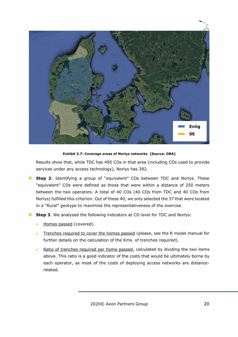
Exhibit 3.7: Coverage areas of Norlys networks [Source: DBA]
Results show that, while TDC has 495 COs in that area (including COs used to provide
services under any access technology), Norlys has 392.
Step 2: Identifying a group of “equivalent” COs between TDC and Norlys. These
“equivalent” COs were defined as those that were within a distance of 250 meters
between the two operators. A total of 40 COs (40 COs from TDC and 40 COs from
Norlys) fulfilled this criterion. Out of these 40, we only selected the 37 that were located
in a “Rural” geotype to maximise the representativeness of the exercise.
Step 3. We analysed the following indicators at CO level for TDC and Norlys:
• Homes passed (covered).
• Trenches required to cover the homes passed (please, see the R model manual for
further details on the calculation of the Kms. of trenches required).
• Ratio of trenches required per home passed, calculated by dividing the two items
above. This ratio is a good indicator of the costs that would be ultimately borne by
each operator, as most of the costs of deploying access networks are distance-
related.
Eniig
SE

2020© Axon Partners Group 21
This analysis showed that, on average, in the 37 COs assessed Norlys’ ratio of trenches
per home passed was 15,46% higher than TDC’s, as shown below.
Table 3.1: Ratio of trenches per home passed [Source: Axon Consulting]
Given all the considerations that have been adopted to perform this exercise, we conclude
that this difference is most likely driven by differences in the access network deployment
between the two operators. More importantly, we consider that the difference is derived
from the fact that for the COs considered in the analysis, 3,86% of the homes covered by
Norlys are more than 10km away from the CO8, whereas this percentage is just 0,04% for
TDC.
DBA considers that it may be argued that the differences above show a less-efficient access
network deployment for Norlys than for TDC. As a result, it has defined an “efficiency
adjustment” factor in worksheet ‘1C INP NW’ of the Excel model to account for this
difference. The efficiency adjustment has two legs:
Adjustment for distance-related assets: This includes the aforementioned
percentage with the differential between TDC and Norlys for the ratio of trenches per
home passed in rural environments. This figure is applied to the results of the KPIs
from the R model for assets that are distance-related (e.g. trenches, cables, ducts).
8 Considering the road distance resulting from the R model.
0
20
40
60
80
100
Rural regions
Me
tre
s o
f tr
en
ch
es /
ho
me
s p
asse
d
TDC Norlys

2020© Axon Partners Group 22
This effectively reduces the number of assets estimated by the R model for Norlys,
seeking alignment with those that would be needed by TDC.
Adjustment for the number of COs: Given that one of the main drivers of the
potential inefficiencies identified stems from the lower amount of central offices
deployed by Norlys. The efficiency adjustment takes this into consideration,
determining that, as a trade-off, to reduce the number of trenches per home passed,
additional COs would need to be deployed. The percentage included in the model has
been calculated to ensure consistency in the number of COs of the operator within the
same region.
3.7. Non-network overheads
Corporate and other non-network overheads represent additional costs that the operators
incur to support their functions. Examples of these costs include costs associated with
corporate headquarters, senior management and internal audits. The Excel model includes
non-network overheads in worksheet “1C INP NW” of the cost model. These costs are
included in the model as a percentage of total network costs (mark-up). The cost
categories that are included in the model are the following:
G&A mark-up: this mark-up represents the costs of general and administrative
activities. This mark-up has been calculated using the following formula:
% 𝐺&𝐴 𝑚𝑎𝑟𝑘 − 𝑢𝑝 =𝑆𝑢𝑝𝑝𝑜𝑟𝑡 𝑎𝑛𝑑 𝑜𝑣𝑒𝑟ℎ𝑒𝑎𝑑𝑠 𝑐𝑜𝑠𝑡𝑠 (𝑟𝑒𝑙𝑒𝑣𝑎𝑛𝑡 𝑓𝑜𝑟 𝐿𝑅𝐴𝐼𝐶 𝑚𝑜𝑑𝑒𝑙)
𝑇𝑜𝑡𝑎𝑙 𝑛𝑒𝑡𝑤𝑜𝑟𝑘 𝑐𝑜𝑠𝑡𝑠(𝑟𝑒𝑙𝑒𝑣𝑎𝑛𝑡 𝑓𝑜𝑟 𝐿𝑅𝐴𝐼𝐶 𝑚𝑜𝑑𝑒𝑙)
Where the total support and overhead costs have been extracted from the Accounting
Separation results of the modelled operator for the products relevant for the LRAIC
model.
IT mark-up: additional costs incurred by operators due to IT platforms. This mark-up
has been calculated using the following formula:
% 𝐼𝑇 𝑃𝑙𝑎𝑡𝑓𝑜𝑟𝑚𝑠 𝑚𝑎𝑟𝑘 − 𝑢𝑝 =𝐼𝑇 𝑝𝑙𝑎𝑡𝑓𝑜𝑟𝑚 𝑐𝑜𝑠𝑡𝑠 (𝑟𝑒𝑙𝑒𝑣𝑎𝑛𝑡 𝑓𝑜𝑟 𝐿𝑅𝐴𝐼𝐶 𝑚𝑜𝑑𝑒𝑙)
𝑇𝑜𝑡𝑎𝑙 𝑛𝑒𝑡𝑤𝑜𝑟𝑘 𝑐𝑜𝑠𝑡𝑠(𝑟𝑒𝑙𝑒𝑣𝑎𝑛𝑡 𝑓𝑜𝑟 𝐿𝑅𝐴𝐼𝐶 𝑚𝑜𝑑𝑒𝑙)
Where the IT platform costs have been extracted from data reported by the modelled
operator for the Columbus IT System that handles customers, orders, agreements,
provisioning and pricing.

2020© Axon Partners Group 23
Wholesale and commercial mark-up: additional costs incurred by operators due to
specific wholesale and commercial costs. This mark-up has been calculated based on
the cost accounts of the modelled operator using the following formula:
% 𝑊ℎ𝑜𝑙𝑒𝑠𝑎𝑙𝑒 𝑚𝑎𝑟𝑘 − 𝑢𝑝 =𝑊ℎ𝑜𝑙𝑒𝑠𝑎𝑙𝑒 𝑎𝑛𝑑 𝑐𝑜𝑚𝑚𝑒𝑟𝑐𝑖𝑎𝑙 𝑐𝑜𝑠𝑡𝑠 (𝑟𝑒𝑙𝑒𝑣𝑎𝑛𝑡 𝑓𝑜𝑟 𝐿𝑅𝐴𝐼𝐶 𝑚𝑜𝑑𝑒𝑙)
𝑇𝑜𝑡𝑎𝑙 𝑛𝑒𝑡𝑤𝑜𝑟𝑘 𝑐𝑜𝑠𝑡𝑠(𝑟𝑒𝑙𝑒𝑣𝑎𝑛𝑡 𝑓𝑜𝑟 𝐿𝑅𝐴𝐼𝐶 𝑚𝑜𝑑𝑒𝑙)
Where the wholesale and commercial costs have been extracted from data reported by
the modelled operator specifically for this purpose.
Working capital mark-up: referring to the costs of maintaining daily operations at
an organization.
% 𝑊𝑜𝑟𝑘𝑖𝑛𝑔 𝑐𝑎𝑝𝑖𝑡𝑎𝑙 𝑚𝑎𝑟𝑘 − 𝑢𝑝 =𝑊𝑜𝑟𝑘𝑖𝑛𝑔 𝑐𝑎𝑝𝑖𝑡𝑎𝑙
𝑇𝑜𝑡𝑎𝑙 𝑛𝑒𝑡𝑤𝑜𝑟𝑘 𝑐𝑜𝑠𝑡𝑠(𝑟𝑒𝑙𝑒𝑣𝑎𝑛𝑡 𝑓𝑜𝑟 𝐿𝑅𝐴𝐼𝐶 𝑚𝑜𝑑𝑒𝑙)
Due to the lack of data, this input is set to zero in the cost model.
Non-network costs are allocated to services based on an equi-proportional mark-up
methodology.
3.8. Ancillary services inputs
The inputs to calculate the costs of ancillary (non-recurring) services are introduced in
worksheet ‘1E INP ANCILLARY SERV’ of the model. The main inputs required to calculate
the costs of these services are:
Wages per employee category (technician and administrative) in DKK per minute of
work.
For each ancillary service, the number of minutes required to perform each one of the
following activities:
• For administrative employees:
- Processing of order
- Customer service
- Annulment fee
• For technicians
- Processing of order

2020© Axon Partners Group 24
- Testing and monitoring/supervision
- Installation
- Projecting and planning
- Customer service
- Transport
For each ancillary service the yearly capital costs associated with the provision of the
service, along with an annual cost trend.
The information used to populate these inputs were provided by the modelled operator
and were cross-checked against different references, such as:
The information included in the previous model for 2018.
Information provided by alternative operators.
For description of ancillary services modelled, please see Annex B.
3.9. Other network and costing inputs
Finally, the model includes other network and costing inputs that are also relevant to either
dimension the network or calculate the costs of the services. These are described below,
grouped between year-independent and year-dependent inputs.
Year-independent inputs (included in worksheet ‘1C INP NW’):
Access network inputs: Includes information concerning the assets available in each
access network, such as the number of pairs per copper cable. This information has
been extracted from the data reported by the modelled operator.
Transmission and core network inputs: Includes inputs such as the capacity of
the transmission ports, redundancy of routers and number of landing stations. This
information has been extracted from the data reported by the modelled operator.
Constants, as the number of bits per byte or the number of seconds in a year. These
constants are industry standards.
Churn, the percentage of lines that are inactive but have a drop installed. This
information has been extracted from the data provided by the modelled operator.
2020© Axon Partners Group 25
Sharing with utility companies: this input represents the percentage of the
trenches that are shared with utility or other types of companies. This input is defined
based on the figures included in the existing LRAIC model.
Other inputs, as the characteristics of the buildings in Denmark.
Year-dependent inputs (included in worksheet ‘1D INP NW EVO’):
Coax spectrum dedicated to each service: Allocation of the spectrum to the
different services provided over the coax network (broadband, TV, VoD). This
information has been extracted from the data provided by the modelled operator.
Traffic per Leased Line: Average traffic in the busy-hour reserved for uncontended
traffic (in Mbps) for each type of leased line (Legacy and IP Fibre). This information
has been extracted from the data provided by the modelled operator.
Inflation: Evolution of prices in the country, used to estimate the OpEx trends.
Extracted from OECD and European Commission databases.
Productivity: Evolution of the efficiency of staff operations. This has been extracted
from OECD databases.
When applicable, these figures have been cross-checked against different references, such
as:
Axon’s internal databases.
Information from the previous DBA’s model for the year 2018.

2020© Axon Partners Group 26
4. Geographical inputs
The design of fixed access networks requires an extensive analysis of the geographical
zones to be covered, as it will have a direct impact on the dimensioning of networks
resources that are dependent on the underlying geography, like cables, trenches, etc. This
analysis is performed in the R model (see the R model manual for detailed explanations
on the calculations and algorithms included in the R model). The results of the R model
are loaded into the Excel model in the control panel (see ‘Annex A - User manual for the
Excel model’ for further details on the process of loading the results of the R model into
the Excel model). Several key inputs are loaded from the R model into the Excel model:
Network coverage
Access network elements and distribution
Core network inputs
Other geographical inputs
Each of these sets of inputs is explained in the subsections below.
4.1. Coverage
Coverage inputs included in worksheet ‘2A INP COVERAGE’ refer to the percentage of
homes passed by each access network per geotype and year. These inputs are defined for
the following networks:
Copper networks
Fibre PON networks
Fibre PTP networks
Coax networks
The coverage percentages outlined in this worksheet can be multiplied by the number of
buildings and the number of homes per building included in worksheet ‘2E INP NW OTHER’
to calculate the total number of homes covered by each technology.
These inputs are presented at geotype level and are loaded from the R model. Please, see
the R model manual for further details on the calculation of these inputs.
2020© Axon Partners Group 27
4.2. Access network elements and distribution
The design of fixed access networks requires an exhaustive analysis of the geographical
areas to be covered, as they will have a direct impact on the dimensioning of the network
assets that are dependent on the underlying geography, such as cables, trenches, etc.
These calculations are performed in the R model and described in the R Model Manual. The
outcomes of the R model are then loaded into the worksheets ‘2B INP NW INVENTORY’
and ‘2C INP NW ELEMENT DIS’ of the Excel Model.
The access network inputs produced in the R model are:
Copper access network:
• Km of copper trenches
• Km of cables (pairs)
• Km of fibre cable for copper network
• Number of street cabinets
• Number of DPs
• Number of MDFs
• Number of COs
• Number of joints
• Others, such as the percentage of homes connected directly to a Central Office and
the distribution of the configurations of the different equipment. All parameters
produced by the R model for the copper access network are available in the
worksheets ‘2B INP NW INVENTORY’ and ‘2C INP NW ELEMENT DIS’ of the Excel
model.
Fibre access network
• Km of fibre trenches
• Km of strands (PON and PTP)
• Number of PON OLT
• Number of joints (PON and PTP)
• Number of DP
2020© Axon Partners Group 28
• Number of PTP MSAN
• Number of ODF
• Trenches shared with coax networks
• Others, such as the number of PON Splitters and the configurations of the different
equipment. All parameters produced by the R model for the fibre access network
are available in the worksheets ‘2B INP NW INVENTORY’ and ‘2C INP NW ELEMENT
DIS’ of the Excel model.
Coax access network
• Km of coax trenches
• Km of coax cables
• Km of fibre cable for coax network
• Number of CMCs
• Number of coax OLTs
• Number of taps
• Number of coax splitters
• Number of DPs
• Others, such as the number of amplifiers and the configurations of the different
equipment. All parameters produced by the R model for the coax access network
are available in the worksheets ‘2B INP NW INVENTORY’ and ‘2C INP NW ELEMENT
DIS’ of the Excel model.
4.3. Core network inputs
As for access networks, transmission networks require an exhaustive geographical
analysis, as they have a direct impact on the dimensioning of the network assets that are
dependent on the underlying geography, such as cables, trenches, etc.
These calculations are also performed in the R model and described in the R Model Manual.
The outcomes of the R model are then loaded into the worksheet ‘2D INP CORE & TX
RINGS’ for each transmission network, namely:
L3 Access network
Aggregation network

2020© Axon Partners Group 29
Distribution network
Core network
The transmission network inputs produced in the R model are:
Number of nodes
Number of rings/chains
Total route length of chains
The total percentage of traffic handled by each chain
4.4. Other geographical inputs
Other geographical inputs are needed for the dimensioning of the networks. These inputs
have been also extracted from the geographical analysis performed in R, they are mainly
related to:
Average dwellings per building
Number of buildings per geotype
Share of allocation of core costs
Share of the core transmission network shared with the access network
Percentage of the network not shared with the access networks
Share of the submarine transmission network shared with the access network
Percentage of Copper COs with other technologies (fibre or coax)
Single dwelling share from SDUs
Effective splitting ratio for PON networks
The detail about the algorithms used for their calculation can be found in the R Model
Manual.

2020© Axon Partners Group 30
5. Dimensioning module
The dimensioning module aims at designing the network and dimensioning the network
resources required to serve the demand of the modelled operator. This dimensioning is
performed in the Excel model and focuses on the calculation of the network elements that
depend on the demand (number of active lines), traffic (Mbps) and Spectrum.
Therefore, the main inputs to this module are:
Network inputs, such as the network parameters presented in section ‘3 - Market and
network inputs’.
Drivers, representing the overall traffic, demand and spectrum.
Geographical inputs, the results obtained from the geographical analysis performed in
R (please see R Model Manual for more details).
This section presents all the calculations followed for the purpose of the dimensioning of
all the network elements. For that, this section has been divided into three different
network sections which are described in detail below:
Dimensioning Drivers, presenting the process for the definition of the drivers
Core and Transmission Network Dimensioning, introducing the algorithms used
for the calculation of Core and Transmission network elements
Access Network Dimensioning, introducing the algorithms used for the calculation
of access network elements
5.1. Dimensioning drivers
The rationale of the dimensioning drivers is to express traffic and demand (at service level)
in a way that facilitates the dimensioning of network resources that are dependent on
demand volumes (e.g. active equipment).
This section presents the following aspects of dimensioning drivers:
Dimensioning drivers’ concept
Mapping services to drivers
Conversion from services to drivers

2020© Axon Partners Group 31
5.1.1 Dimensioning drivers’ concept
The explicit recognition of a dimensioning "Driver" in the model aims at simplifying and
increasing the transparency of the network dimensioning process.
Dimensioning drivers represent, among others, the following requirements:
Number of connections (copper, fibre and coax) for the dimensioning of the access
network.
Mbps for transmission through the different layers of the transmission network.
The following list contains the drivers used in the LRAIC costing model for fixed networks:
VARIABLE
DRIV.Access copper.Connections.Total Active connection
DRIV.Access coaxial.Connections.Total Active connection
DRIV.Access fibre.Connections.Total Active connection
DRIV.Broadband.Traffic.Copper broadband - Access
DRIV.Broadband.Traffic.Fibre broadband - Access
…
DRIV.Video.Traffic.Wholesale VoD - Distribution/Core
Exhibit 5.1: Sample list of drivers used in the model (Sheet ‘0D PAR DRIVERS’). [Source: Axon
Consulting]
Two steps are required to calculate the drivers:
1. Mapping services to drivers
2. Converting traffic units into the corresponding driver units
Each of these two steps is discussed below in more detail.
5.1.2 Mapping services to drivers
To obtain drivers it is necessary to indicate which services are related to them. It should
be noted that each service is generally assigned to more than one driver as drivers
represent traffic in a particular point of the network.

2020© Axon Partners Group 32
For example, broadband copper services should be contained in both the drivers used to
dimension the access network (in order to properly dimension the number of MSANs
required) as well as the core networks.
The following exhibit shows an excerpt of the mapping of services into drivers:
DRIVER (Variable Name) SERVICE (Variable Name)
DRIV.ACCESS COPPER.Connections.Total Active connection Access.Copper.Retail.Access
DRIV.ACCESS COPPER.Connections.Total Active connection Access.Copper.Retail.Access with bonding
DRIV.ACCESS COPPER.Connections.Total Active connection Access.Copper.Wholesale.VULA (POI0)
DRIV.ACCESS COPPER.Connections.Total Active connection Access.Copper.Wholesale.VULA (POI1)
DRIV.BROADBAND.Traffic.Fibre broadband - Aggregation Broadband.Fibre.Retail.broadband
DRIV.BROADBAND.Traffic.Fibre broadband - Aggregation Broadband.Fibre.Wholesale.BSA broadband - POI2
DRIV.BROADBAND.Traffic.Fibre broadband - Aggregation Broadband.Fibre.Wholesale.BSA broadband - POI3
… …
Exhibit 5.2: Excerpt from the mapping of Services into Drivers (Sheet ‘3A MAP DRIVERS’) [source:
Axon Consulting]
5.1.3 Conversion from services to drivers
Once services have been mapped to drivers, volumes need to be converted to obtain
drivers in proper units.
For that purpose, a conversion has been worked out representing the number of driver
units generated by each demand service unit. In general, conversion calculation consists
of two subfactors, in compliance with the following structure:

2020© Axon Partners Group 33
Exhibit 5.3: Conversion Process from Services to Drivers [Source: Axon Consulting]
The conversion factor thus includes the following items:
1. Usage Factor (UF)
2. Conversion Factor (CF)
Finally, the relationship between a given service and a driver is obtained by following the
formula outlined below:
𝐹𝐶 = 𝑈𝐹 ∗ 𝐶𝐹
Usage factor represents the number of times a service makes use of a specific resource.
Conversion Factor represents the need to adapt services’ units (e.g. lines) to those used
by the driver (e.g. Mbps). The application of the conversion factors from services to drivers
is performed using “weights” (Average traffic per line). These weights are calculated in the
worksheet ‘3A MAP WEIGHTS’.
5.2. Transmission network dimensioning
The objective of the dimensioning of the transmission network is the calculation of the
number of network elements required to meet the demand and coverage levels present
from the networks of the modelled operator. These network elements include active
elements (Routers, ports, etc.) and passive elements (trenches, landing stations, fibre
cable, etc.).
SERVICE i
DRIVER j
UNITS CONVERSION
USAGE FACTOR

2020© Axon Partners Group 34
As a first instance, the dimensioning of the transmission network is performed at a national
level, this is, geotypes are not considered in the calculation of the results. The
dimensioning approach is performed separately for each of the layers in the transmission
network:
L3 Access Network
Aggregation Network
Distribution Network
Core Network
A summary of the topology considered is presented in the exhibit below:
Exhibit 5.4: Architecture of the transmission networks [Source: DBA]
L3
Access
Netw
ork
L3 Access Node
Ag
greg
ati
on
N
etw
ork
Dis
trib
uti
on
n
etw
ork
Core
netw
ork
L3 Access Node
Aggregation Router Aggregation Router
Distribution Router Distribution Router
Core Router Core Router
Access Networks
Access Networks
2020© Axon Partners Group 35
However, it should be noted that the algorithms considered for each layer are equivalent.
Thus, below we present the algorithms followed once, capturing any small differences
identified.
Router equipment
The number of routers installed in each network layer is determined based on the number
of nodes and their associated traffic.
As a starting point, the model considers a single router in each network node. This figure
can be increased if the traffic that the router needs to hold is greater than its capacity. In
addition, the model considers router redundancy for core and distribution router nodes.
Hence, in these cases, two routers are installed in each node.
Once the number of routers has been determined, we proceed to the calculation of each
one of its elements. The details of the dimensioning of each element are outlined below:
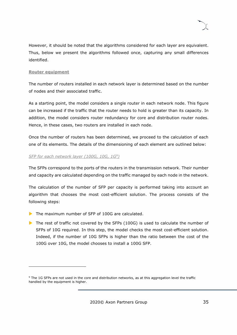
SFP for each network layer (100G, 10G, 1G9)
The SFPs correspond to the ports of the routers in the transmission network. Their number
and capacity are calculated depending on the traffic managed by each node in the network.
The calculation of the number of SFP per capacity is performed taking into account an
algorithm that chooses the most cost-efficient solution. The process consists of the
following steps:
The maximum number of SFP of 100G are calculated.
The rest of traffic not covered by the SFPs (100G) is used to calculate the number of
SFPs of 10G required. In this step, the model checks the most cost-efficient solution.
Indeed, if the number of 10G SFPs is higher than the ratio between the cost of the
100G over 10G, the model chooses to install a 100G SFP.
9 The 1G SFPs are not used in the core and distribution networks, as at this aggregation level the traffic
handled by the equipment is higher.

2020© Axon Partners Group 36
Exhibit 5.5: Algorithm to choose the most cost-efficient solution for SFPs [Source: Axon Consulting]
The same steps presented above are followed considering 10G SFPs and 1G SFPs.
In addition, the model considers the redundancy in the ports of the core routers to ensure
the resiliency of the network.
The output of this process is the number of SFPs required for capacity in the core and
transmission network.
SFP for interconnection between network layers
In addition to the ports associated to the actual routers required for each layer, the model
includes additional ports to interconnect the different network layers (e.g. the distribution
layer to the lower aggregation layer).
The number of SFPs required for interconnection between each transmission layer and the
next lower layer of the network are calculated as follows:
(Cost 100G) /
(Cost 10G SFP)
# of 10G SFPs required for traffic
# of 10G SFPs required for traffic
>(Cost 100G) /
(Cost 10G SFP)
# of 10G SFPs required for traffic
1 x 100G SPF
YesNo

2020© Axon Partners Group 37
Exhibit 5.6: Algorithm for the calculation of the number of SFPs for interconnection required
[Source: Axon Consulting]
The output of this process is the number of SFPs required for interconnection in the core
and transmission network.
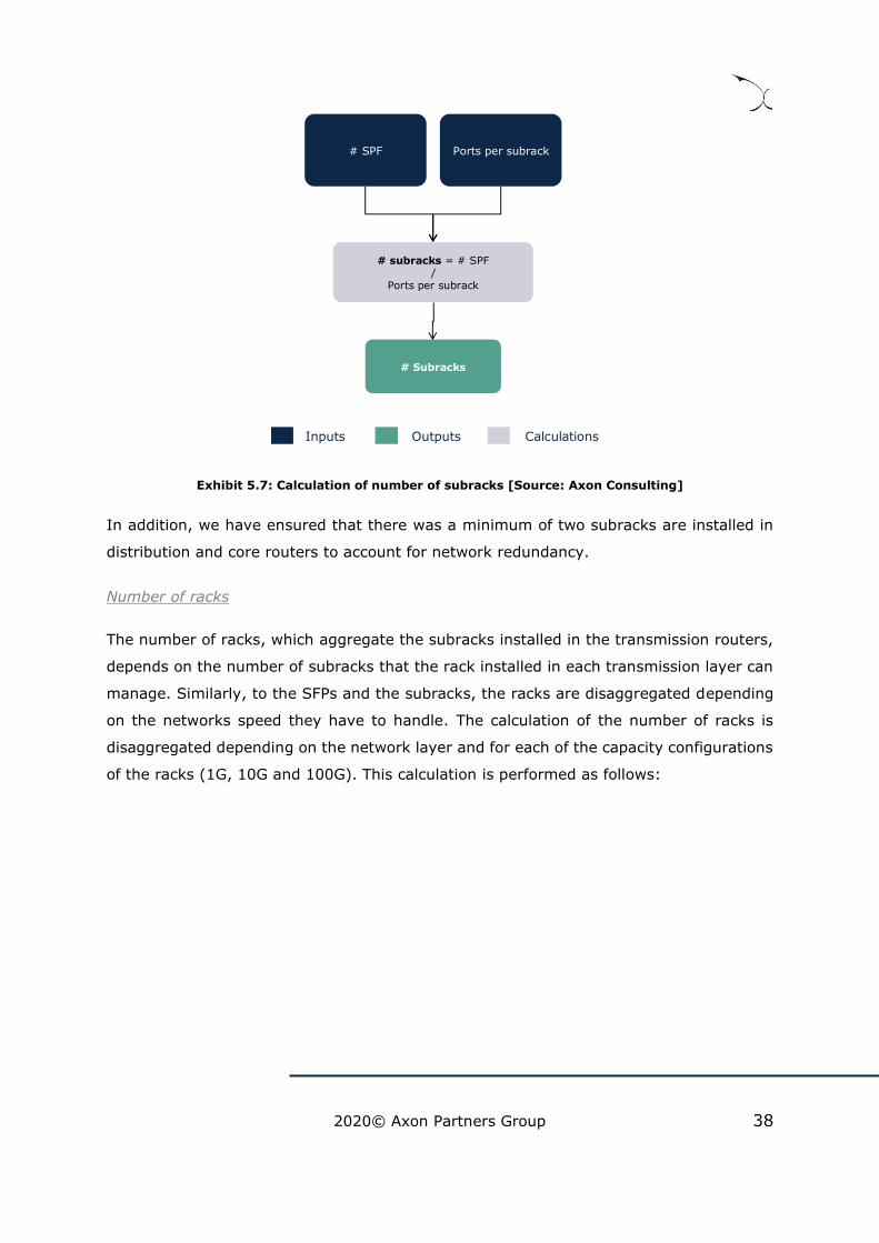
Number of subracks
The number of subracks, which are cards of ports (SFPs) installed in the transmission
routers, depends on the number of ports that the subrack installed in each transmission
layer can manage. Subracks are disaggregated depending on the capacity of the ports
installed in them (1G, 10G or 100G). The calculation of the number of subracks is
performed separately for each layer for each of the different capacity configurations
defined. The process is as follows:
Ports per node# of nodes of the
lower layer
# SFP = ROUNDUP(% of SFPs of 100G in the lower layer)
x(# of nodes of the lower layer)
xPorts per node
# of 100G SPFs for interconnection
% of SFPs of 100G in the lower
layer
% of SFPs of 10G in the lower layer
# SFP = ROUNDUP(% of SFPs of 10G in the lower layer)
x(# of nodes of the lower layer)
xPorts per node
# of 10G SPFs for interconnection
% of SFPs of 1G in the lower layer
# SFP = ROUNDUP(% of SFPs of 1G in the lower layer)
x(# of nodes of the lower layer)
xPorts per node
# of 1G SPFs for interconnection
2020© Axon Partners Group 38
Exhibit 5.7: Calculation of number of subracks [Source: Axon Consulting]
In addition, we have ensured that there was a minimum of two subracks are installed in
distribution and core routers to account for network redundancy.
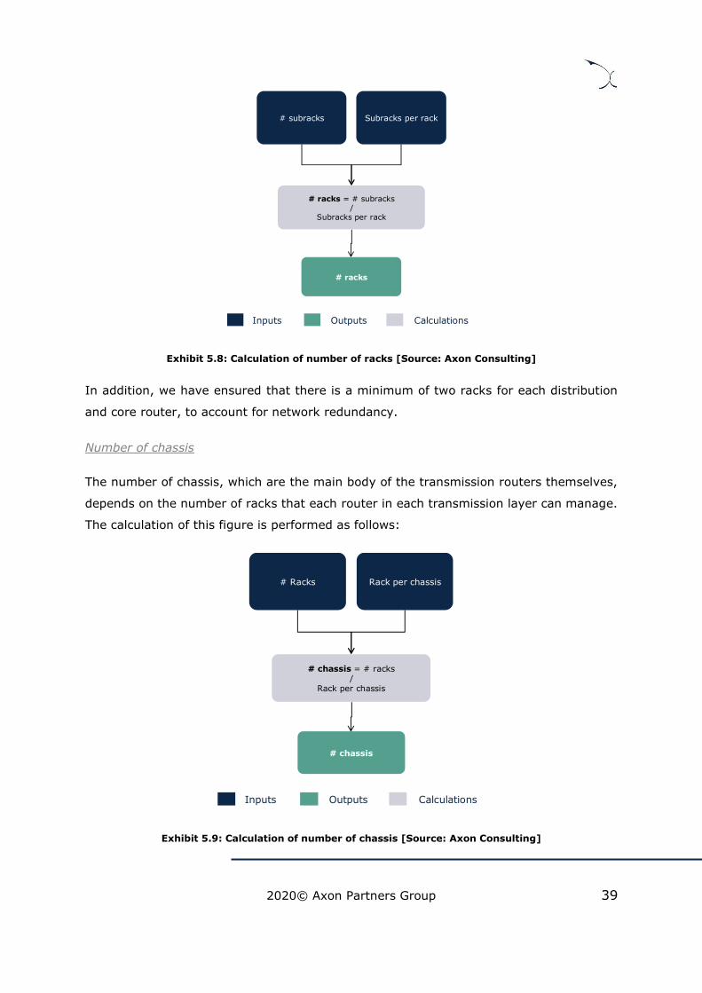
Number of racks
The number of racks, which aggregate the subracks installed in the transmission routers,
depends on the number of subracks that the rack installed in each transmission layer can
manage. Similarly, to the SFPs and the subracks, the racks are disaggregated depending
on the networks speed they have to handle. The calculation of the number of racks is
disaggregated depending on the network layer and for each of the capacity configurations
of the racks (1G, 10G and 100G). This calculation is performed as follows:
Outputs CalculationsInputs
# Subracks
Ports per subrack# SPF
# subracks = # SPF /
Ports per subrack
2020© Axon Partners Group 39
Exhibit 5.8: Calculation of number of racks [Source: Axon Consulting]
In addition, we have ensured that there is a minimum of two racks for each distribution
and core router, to account for network redundancy.
Number of chassis
The number of chassis, which are the main body of the transmission routers themselves,
depends on the number of racks that each router in each transmission layer can manage.
The calculation of this figure is performed as follows:
Exhibit 5.9: Calculation of number of chassis [Source: Axon Consulting]
Outputs CalculationsInputs
# racks
Subracks per rack# subracks
# racks = # subracks/
Subracks per rack
Outputs CalculationsInputs
# chassis
Rack per chassis# Racks
# chassis = # racks /
Rack per chassis

2020© Axon Partners Group 40
Sites
The number of sites, which represent the physical location where the routers are installed,
determined in the model is simply calculated as the total number of node locations of each
network.
DWDM Equipment
The DWDM network is modelled under the assumption that only the core and distribution
networks would need to deploy these network elements. L3 Access and aggregation
networks do not include DWDM equipment, as it is estimated that the traffic these
networks handle is not sufficient to consider these additional investments.
To estimate the number of DWDM network elements, the model inspects, for each network
node in the core and distribution layer the following aspects:
Directions for the DWDM network: this input refers to the number of network nodes to
which each DWDM needs to be connect to. The model installs in each node one platform
(that can be used for a single direction) plus the additional number of directions needed
based on the network’s topology.
Line cards and ports for the DWDM network: The model estimates the number of line
cards necessary for each network node, considering the traffic handled in the network
node and assuming that each line card and port can handle 100 Gbps.
Amplifiers: the model considers that the DWDM platforms in the core network would
require an additional amplifier. No amplifiers are considered for those in the distribution
network.
Submarine cables and Landing stations
The list of submarine cables and their distance used in this network are known (please see
R Model Manual for further details on this aspect). Therefore, the total distance of
submarine cables is equivalent to the sum of the distance of each of the submarine cables
dedicated to each one of the transmission networks.
On the other side, the number of Landing stations is calculated supposing that each
submarine cable needs 2 landing stations.
2020© Axon Partners Group 41
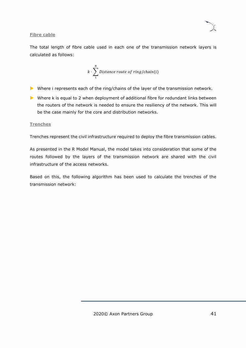
Fibre cable
The total length of fibre cable used in each one of the transmission network layers is
calculated as follows:
𝑘 ·∑𝐷𝑖𝑠𝑡𝑎𝑛𝑐𝑒 𝑟𝑜𝑢𝑡𝑒 𝑜𝑓 𝑟𝑖𝑛𝑔/𝑐ℎ𝑎𝑖𝑛(𝑖)
𝑁
1
Where i represents each of the ring/chains of the layer of the transmission network.
Where k is equal to 2 when deployment of additional fibre for redundant links between
the routers of the network is needed to ensure the resiliency of the network. This will
be the case mainly for the core and distribution networks.
Trenches
Trenches represent the civil infrastructure required to deploy the fibre transmission cables.
As presented in the R Model Manual, the model takes into consideration that some of the
routes followed by the layers of the transmission network are shared with the civil
infrastructure of the access networks.
Based on this, the following algorithm has been used to calculate the trenches of the
transmission network:

2020© Axon Partners Group 42
Exhibit 5.10: Algorithm for the transmission trenches calculation [Source: Axon Consulting]
Allocation of transmission elements into geotypes
The dimensioning of the core and transmission networks is performed independently from
the geotype. Nevertheless, to obtain disaggregated costs, the results of the dimensioning
must be distributed to the geotypes. In order to do so, two drivers10 have been calculated
for each network (L3 Access, Aggregation, Distribution and Core):
Traffic share per geotype: allowing the allocation of the resources depending on the
traffic as routers, cards, ports, etc.
Distance share per geotype, to distribute the resources depending on distance as
cables and trenches.
10 These drivers have been extracted from the geographical analysis.
Outputs CalculationsInputs
Total Km of trenches for transmission
networks
Total km trenches in the access
Total km trenches exclusive for
access
% share cost of trenches shared
between transmission and
access
Total fibredistance in network
% trenches in the transmission
network that are not shared with
access
Trenches not shared with access networks = Total fibre distance in network
X% trenches in the transmission network that
are not shared with access
Km of trenches for transmission networks shared= (Total km trenches in the
access - Total km trenches exclusive for access)
X (%Share of transmission costs for each networks)
Total Km of trenches for transmission networks = Km of trenches for transmission networks shared + Trenches not shared with
access networks
2020© Axon Partners Group 43
Therefore, the results are multiplied by those drivers in order to distribute the transmission
resources in geotypes.
5.3. Access Network Dimensioning
The dimensioning of the access network is performed separately for each of the geotypes
defined, to accurately reflect the impact of the geographical characteristics of Denmark in
the deployment of access network elements. The dimensioning approach employed has
been divided into three different blocks, namely:
Copper Access Network Dimensioning
Fibre Access Network Dimensioning
Coax Access Network Dimensioning
5.3.1 Copper Access Network Dimensioning
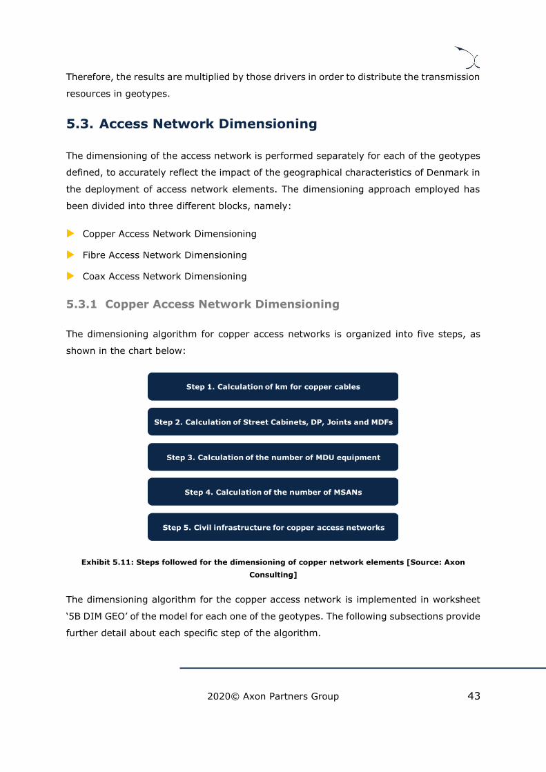
The dimensioning algorithm for copper access networks is organized into five steps, as
shown in the chart below:
Exhibit 5.11: Steps followed for the dimensioning of copper network elements [Source: Axon
Consulting]
The dimensioning algorithm for the copper access network is implemented in worksheet
‘5B DIM GEO’ of the model for each one of the geotypes. The following subsections provide
further detail about each specific step of the algorithm.
Step 1. Calculation of km for copper cables
Step 2. Calculation of Street Cabinets, DP, Joints and MDFs
Step 4. Calculation of the number of MSANs
Step 5. Civil infrastructure for copper access networks
Step 3. Calculation of the number of MDU equipment
2020© Axon Partners Group 44
Step 1. Calculation of km for copper cables
The first step in the dimensioning of the Copper Access Network consists of the calculation
of the number of cables required. As we mentioned in previous sections the Copper Access
network is composed of three main types of cables:
Final Drop Copper Cables
Copper cables used between the FDP and MDF
Fibre cables used between the MDF and CO
The number of such elements is calculated according to the algorithms outlined below:
Final drop copper cables
The final drop cables are used in the copper network to connect the households to their
assigned FDP. The copper drop cables consist of:
A horizontal cable, defined as the direct distance from the house until the side of the
street multiplied by a non-optimal factor.
A vertical cable, representing the internal cabling needed to reach each floor for MDU
buildings.
Therefore, the total length of drop cables is calculated following the algorithm below:

2020© Axon Partners Group 45
Exhibit 5.12: Algorithm for the calculation of the copper drop cables [Source: Axon Consulting]
Please note that the number of homes connected has been calculated based on the data
reported by the operator.
Copper cables used between the FDP and MDF
The total copper cables used to connect from nodes FDP to MDF nodes and the percentage
of each type of cable deployed have been calculated in the R Model. Therefore, considering
this information as input, the kilometres per type of cable have been determined as
follows:
Outputs CalculationsInputs
= ℎ𝑜𝑚𝑒𝑠 𝑐𝑜𝑛𝑛𝑒𝑐𝑡𝑒𝑑 ∗ 𝐴𝑣𝑒𝑟𝑎𝑔𝑒 𝑙𝑒𝑛𝑔𝑡ℎ 𝑜𝑓 𝑑𝑟𝑜𝑝 𝑐𝑎 𝑙𝑒
∗ 1 −%𝑜𝑓 𝑛𝑜𝑛𝑜𝑝𝑡𝑖𝑚𝑎𝑙 𝑙𝑒𝑛𝑔𝑡ℎ ∗ (1 −%𝑜𝑓 𝐷𝑈 𝑡ℎ𝑎𝑡 𝑎𝑟𝑒 𝐿𝐴 )
Km of horizontal drop cable
# homes connected
Average length of
drop cable
% of non-optimal length
% of MDU that are LAN
= 𝐷𝑈 ℎ𝑜𝑚𝑒𝑠 𝑐𝑜𝑛𝑛𝑒𝑐𝑡𝑒𝑑 ∗ (𝐴𝑣𝑒𝑟𝑎𝑔𝑒 𝑜𝑓 𝑓𝑙𝑜𝑜𝑟𝑠 − 1)/
∗ 𝐴𝑣𝑒𝑟𝑎𝑔𝑒 ℎ𝑒𝑖𝑔ℎ𝑡 𝑜𝑓 𝑓𝑙𝑜𝑜𝑟𝑠 ∗ (1 −%𝑜𝑓 𝐷𝑈 𝑡ℎ𝑎𝑡 𝑎𝑟𝑒 𝐿𝐴 )
Km of vertical drop cable
# MDU homes
connected
% of MDU that are LAN
Average # of floors
Average height of
floors
Total km of drop cable =
Km of horizontal drop cable + Km of vertical
drop cable
2020© Axon Partners Group 46
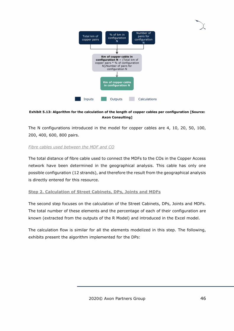
Exhibit 5.13: Algorithm for the calculation of the length of copper cables per configuration [Source:
Axon Consulting]
The N configurations introduced in the model for copper cables are 4, 10, 20, 50, 100,
200, 400, 600, 800 pairs.
Fibre cables used between the MDF and CO
The total distance of fibre cable used to connect the MDFs to the COs in the Copper Access
network have been determined in the geographical analysis. This cable has only one
possible configuration (12 strands), and therefore the result from the geographical analysis
is directly entered for this resource.
Step 2. Calculation of Street Cabinets, DPs, Joints and MDFs
The second step focuses on the calculation of the Street Cabinets, DPs, Joints and MDFs.
The total number of these elements and the percentage of each of their configuration are
known (extracted from the outputs of the R Model) and introduced in the Excel model.
The calculation flow is similar for all the elements modelized in this step. The following,
exhibits present the algorithm implemented for the DPs:
Outputs CalculationsInputs
Total km of copper pairs
Km of copper cable in configuration N = (Total km of copper pairs * % of configuration
N)/Number of pairs for configuration N
Km of copper cable in configuration N
% of km in configuration
N
Number of pairs for
configuration N

2020© Axon Partners Group 47
Exhibit 5.14: Algorithm to determine the number of copper DPs [Source: Axon Consulting]
The modelling of the MDFs, joints and Street Cabinets is equivalent to that of Distribution
Points but considering their configurations. The available configurations for each element
are presented in the table below:
DP configurations SC configurations Joints configurations MDF configurations
Copper DP - 5 pairs Copper SC - 192 subs. Copper joint - 10 pairs MDF - 250 subs.
Copper DP - 10 pairs Copper SC - 384 subs. Copper joint - 50 pairs MDF - 500 subs.
Copper DP - 20 pairs Copper joint - 100 pairs MDF - 2000 subs.
Copper DP - 50 pairs Copper joint - 300 pairs MDF - 12000 subs.
Copper DP - 100 pairs MDF - 48000 subs.
Copper DP - 500 pairs
Copper DP - 1000 pairs
Copper DP - 2000 pairs
Exhibit 5.15: Configurations of Street Cabinets, DPs, Joints and MDFs [Source: Axon Consulting]
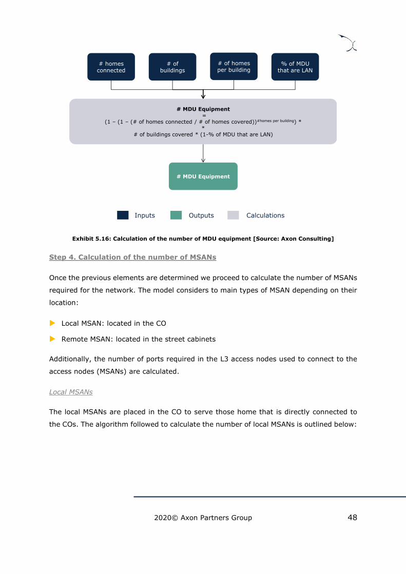
Step 3. Calculation of the number of MDU equipment
The third step presents the calculation of requirements for equipment specific for MDU
buildings. This calculation involves the estimation of the number of connected buildings
that are MDUs. The algorithm followed to calculate the number of MDU equipment is
outlined below:
Outputs CalculationsInputs
Total # DP
# DPs in configuration N = Total # DP
* % of DP configuration N
#DP in configuration N
% DPs in configuration
N
2020© Axon Partners Group 48
Exhibit 5.16: Calculation of the number of MDU equipment [Source: Axon Consulting]
Step 4. Calculation of the number of MSANs
Once the previous elements are determined we proceed to calculate the number of MSANs
required for the network. The model considers to main types of MSAN depending on their
location:
Local MSAN: located in the CO
Remote MSAN: located in the street cabinets
Additionally, the number of ports required in the L3 access nodes used to connect to the
access nodes (MSANs) are calculated.
Local MSANs
The local MSANs are placed in the CO to serve those home that is directly connected to
the COs. The algorithm followed to calculate the number of local MSANs is outlined below:
# MDU Equipment=
(1 – (1 – (# of homes connected / # of homes covered))#homes per building) * *
# of buildings covered * (1-% of MDU that are LAN)
# MDU Equipment
# homes connected
# of buildings
# of homes per building
% of MDU that are LAN
Outputs CalculationsInputs

2020© Axon Partners Group 49
Exhibit 5.17: Algorithm for copper Local MSANs [Source: Axon Consulting]
Remote MSANs
The Remote MSANs are considered as the MSANs that are located in the Street Cabinets
and are placed to serve all the homes that are not directly connected to COs. Therefore,
the calculation performed to determine their number is the same as for local MSAN
considering the number of homes not connected directly to the COs.
Outputs CalculationsInputs
# MDFs
#Local MSAN
Total copper connections
% homes connected directly to
CO
#ports per line card
𝑆𝐴 𝑅𝑎𝑐𝑘𝑠 =
𝑇𝑜𝑡𝑎𝑙 𝑐𝑜𝑝𝑝𝑒𝑟 𝑐𝑜𝑛𝑛𝑒𝑐𝑡𝑖𝑜𝑛𝑠 ∗ % ℎ𝑜𝑚𝑒𝑠 𝑐𝑜𝑛𝑛𝑒𝑐𝑡𝑒𝑑 𝑑𝑖𝑟𝑒𝑐𝑡𝑙 𝑡𝑜 𝐶
𝑝𝑜𝑟𝑡𝑠 𝑝𝑒𝑟 𝑙𝑖𝑛𝑒 𝑐𝑎𝑟𝑑
MSAN racks = max(# MSAN
racks, # MDFs)

2020© Axon Partners Group 50
Exhibit 5.18: Algorithm for copper Local MSANs [Source: Axon Consulting]
Ports for access nodes
These ports are located in the L3 access nodes and are used to connect the copper MSANs
with the core and transmission networks. Therefore, the calculation performed to
determine their number follows the steps below:
1. Calculation of the broadband traffic per node
Outputs CalculationsInputs
# SC
#Remote MSAN
Total copper connections
% homes connected directly to
CO
#ports per line card
𝑅𝑎𝑐𝑘𝑠
=𝑇𝑜𝑡𝑎𝑙 𝑐𝑜𝑝𝑝𝑒𝑟 𝑐𝑜𝑛𝑛𝑒𝑐𝑡𝑖𝑜𝑛𝑠 ∗ % ℎ𝑜𝑚𝑒𝑠 𝑐𝑜𝑛𝑛𝑒𝑐𝑡𝑒𝑑 𝑑𝑖𝑟𝑒𝑐𝑡𝑙 𝑡𝑜 𝐶 )
𝑝𝑜𝑟𝑡𝑠 𝑝𝑒𝑟 𝑙𝑖𝑛𝑒 𝑐𝑎𝑟𝑑
MSAN racks = max(# MSAN
racks, # SCs)

2020© Axon Partners Group 51
Exhibit 5.19: Calculation of the number of ports required to connect the access nodes [Source: Axon
Consulting]
2. Calculation of the number of SFPs ports needed to handle the traffic. The selection
of the SFPs is performed selecting the most-cost efficient solution. The algorithm
followed for this is presented in the section 5.2. Transmission network
dimensioning’.
Step 5. Civil infrastructure for copper access networks
The last step is related to the dimensioning of the civil infrastructure required for the
copper access network. The civil infrastructure required for this technology consists of:
Home-FDP trenches: these are the trenches dug for final drop cables
Road crossing trenches: trenches dug when there is the need to cross a road.
FDP-MDF trenches: required for the buried copper cables used in this part of the
network
MDF-CO trenches: required for the buried fibre cables used in this part of the network
Ducts
Joint holes and Manholes
In the following sections, the calculations done in order to determine these elements are
presented.
# Traffic per rack=
𝑇𝑟𝑎𝑓𝑓𝑖𝑐 𝑐𝑜𝑝𝑝𝑒𝑟 𝑟𝑜𝑎𝑑 𝑎𝑛𝑑
𝑜𝑓 𝑅𝑒𝑚𝑜𝑡𝑒 & 𝐿𝑜𝑐𝑎𝑙 𝑆𝐴 𝑟𝑎𝑐𝑘𝑠 ∗ % 𝑎 𝑝𝑜𝑟𝑡 𝑙𝑜𝑎𝑑 𝑓𝑜𝑟 𝑡𝑟𝑎𝑓𝑓𝑖𝑐
# Traffic per rack
Traffic copper
broadband
# of Remote& Local
MSAN racks
% Max port load for traffic
Outputs CalculationsInputs

2020© Axon Partners Group 52
Home-FDP Trenches
The total km of trenches for the final drop cables are calculated using the following
algorithm:
Exhibit 5.20: Calculation of Home-FDP trenches [Source: Axon Consulting]
Road crossing trenches
In addition, the model includes the trenches related to the road crossings that are
extracted from the geographical analysis.
FDP-MDF trenches
The geographical analysis allowed the calculation of the total trenches required for the
copper access network. However, this total distance contemplates the hypothetical case
where there was no sharing of these trenches, while the trenches could be shared with
other access technologies, the core network or even utility companies.
In this section we present the adjustments done in order to settle the number of km that
are used exclusively for access networks, distinguishing the part that is shared with
transmission and core networks.
Outputs CalculationsInputs
#km of Home-FDP trenches = Home-FDP trenches (MDU) + +Home-FDP trenches (SDU)
Home is Single-
Dwelling ?
Home-FDP trenches (MDU) = (# km of final MDU horizontal drop cable) * (%
final drop buried)
Home-FDP trenches (SDU)= (# km of final SDU horizontal drop cable) *
(% final drop buried) * ((1-% SDU with one home)*(# of trenches for SDU with more than one home) + % SDU with
one home)
# km of final SDU horizontal drop
cable
% final drop buried
% SDU with one home
# of trenches for SDU with more than one home
# km of final MDU horizontal
drop cable
YesNo
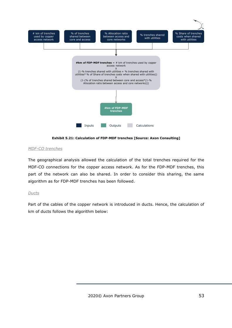
2020© Axon Partners Group 53
Exhibit 5.21: Calculation of FDP-MDF trenches [Source: Axon Consulting]
MDF-CO trenches
The geographical analysis allowed the calculation of the total trenches required for the
MDF-CO connections for the copper access network. As for the FDP-MDF trenches, this
part of the network can also be shared. In order to consider this sharing, the same
algorithm as for FDP-MDF trenches has been followed.
Ducts
Part of the cables of the copper network is introduced in ducts. Hence, the calculation of
km of ducts follows the algorithm below:
Outputs CalculationsInputs
#km of FDP-MDF trenches
#km of FDP-MDF trenches = # km of trenches used by copper access network
X(1-% trenches shared with utilities + % trenches shared with
utilities* % of Share of trenches costs when shared with utilities)) X
(1-(% of trenches shared between core and access*(1-% Allocation ratio between access and core networks)))
# km of trenches used by copper access network
% of trenches shared between core and access
% Allocation ratio between access and
core networks
% trenches shared with utilities
% Share of trenches costs when shared
with utilities
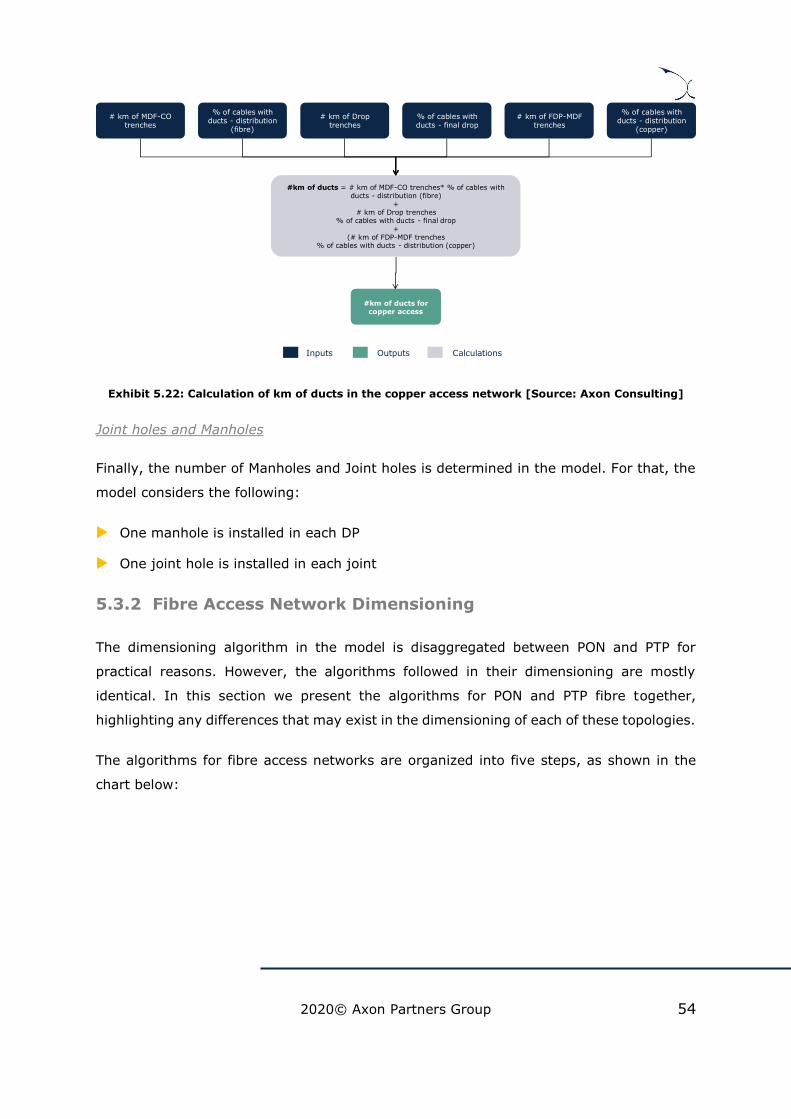
2020© Axon Partners Group 54
Exhibit 5.22: Calculation of km of ducts in the copper access network [Source: Axon Consulting]
Joint holes and Manholes
Finally, the number of Manholes and Joint holes is determined in the model. For that, the
model considers the following:
One manhole is installed in each DP
One joint hole is installed in each joint
5.3.2 Fibre Access Network Dimensioning
The dimensioning algorithm in the model is disaggregated between PON and PTP for
practical reasons. However, the algorithms followed in their dimensioning are mostly
identical. In this section we present the algorithms for PON and PTP fibre together,
highlighting any differences that may exist in the dimensioning of each of these topologies.
The algorithms for fibre access networks are organized into five steps, as shown in the
chart below:
Outputs CalculationsInputs
#km of ducts for copper access
#km of ducts = # km of MDF-CO trenches* % of cables with ducts - distribution (fibre)
+ # km of Drop trenches
% of cables with ducts - final drop+
(# km of FDP-MDF trenches% of cables with ducts - distribution (copper)
# km of MDF-CO trenches
% of cables with ducts - distribution
(fibre)
# km of Drop trenches
% of cables with ducts - final drop
# km of FDP-MDF trenches
% of cables with ducts - distribution
(copper)

2020© Axon Partners Group 55
Exhibit 5.23: Steps followed for the dimensioning of fibre network elements [Source: Axon
Consulting]
The dimensioning algorithm for the fibre access network is implemented in the worksheet
‘5B DIM GEO’ of the model for each one of the geotype. The dimensioning is performed
separately for PON and PTP networks, taking into account the drivers and characteristics
of each one.
The following subsections provide further detail about each specific step of the algorithm.
Step 1. Calculation of km for fibre cables
The first step in the dimensioning of the Fibre Access Network consists of the calculation
of the number of cables required. As we mentioned in previous sections the Fibre Access
network is composed of two main types of cables:
Final Drop Fibre Cables
Fibre cables used between the FDP and CO
The number of such elements is calculated according to the algorithms outlined below.
Final Drop Fibre Cables
The final drop cables are used in the fibre network to connect the households to their
assigned FDP. The fibre drop cables consist of:
Step 1. Calculation of km for fibre cables
Step 2. Calculation of Splitter, DP, Joints and MDFs
Step 4. Calculation of the number of MSANs
Step 5. Civil infrastructure for fibre access networks
Step 3. Calculation of the number of MDU equipment

2020© Axon Partners Group 56
A Horizontal cable, defined as the direct distance from the house until the side of the
street multiplied by a non-optimal factor.
A Vertical cable, representing the internal cabling needed to reach each floor for MDU
buildings.
Therefore, the total length of drop cables is calculated following the algorithm below:
Exhibit 5.24: Calculation of km of fibre drop cable [Source: Axon Consulting]
The fibre drop cables are calculated separately for PON and PTP networks.
In addition, the drop cables are then split between:
Fibre cable - drop cable (immediate installation), calculated as the total drop cables
multiplied by the percentage of connected homes upon deployment.
Fibre cable - drop cable (delayed installation), ), calculated as the total drop cables
multiplied by the percentage of connected homes upon deployment.
Fibre cables used between the FDP and CO
The total fibre cables used to connect from nodes FDP to CO nodes have been calculated
in the R Model, along with the percentage of each configuration of cable deployed.
Therefore, considering this information as input, the kilometres per type of cable have
been determined as follows:
Outputs CalculationsInputs
= ℎ𝑜𝑚𝑒𝑠 𝑐𝑜𝑛𝑛𝑒𝑐𝑡𝑒𝑑 ∗ 𝐴𝑣𝑒𝑟𝑎𝑔𝑒 𝑙𝑒𝑛𝑔𝑡ℎ 𝑜𝑓 𝑑𝑟𝑜𝑝 𝑐𝑎 𝑙𝑒
∗ 1 −%𝑜𝑓 𝑛𝑜𝑛𝑜𝑝𝑡𝑖𝑚𝑎𝑙 𝑙𝑒𝑛𝑔𝑡ℎ ∗ (1 −%𝑜𝑓 𝐷𝑈 𝑡ℎ𝑎𝑡 𝑎𝑟𝑒 𝐿𝐴 )
Km of horizontal drop cable
# homes connected
Average length of
drop cable
% of non-optimal length
% of MDU that are LAN
= 𝐷𝑈 ℎ𝑜𝑚𝑒𝑠 𝑐𝑜𝑛𝑛𝑒𝑐𝑡𝑒𝑑 ∗ (𝐴𝑣𝑒𝑟𝑎𝑔𝑒 𝑜𝑓 𝑓𝑙𝑜𝑜𝑟𝑠 − 1)/
∗ 𝐴𝑣𝑒𝑟𝑎𝑔𝑒 ℎ𝑒𝑖𝑔ℎ𝑡 𝑜𝑓 𝑓𝑙𝑜𝑜𝑟𝑠 ∗ (1 −%𝑜𝑓 𝐷𝑈 𝑡ℎ𝑎𝑡 𝑎𝑟𝑒 𝐿𝐴 )
Km of vertical drop cable
# MDU homes
connected
% of MDU that are LAN
Average # of floors
Average height of
floors
Total km of drop cable =
Km of horizontal drop cable + Km of vertical
drop cable
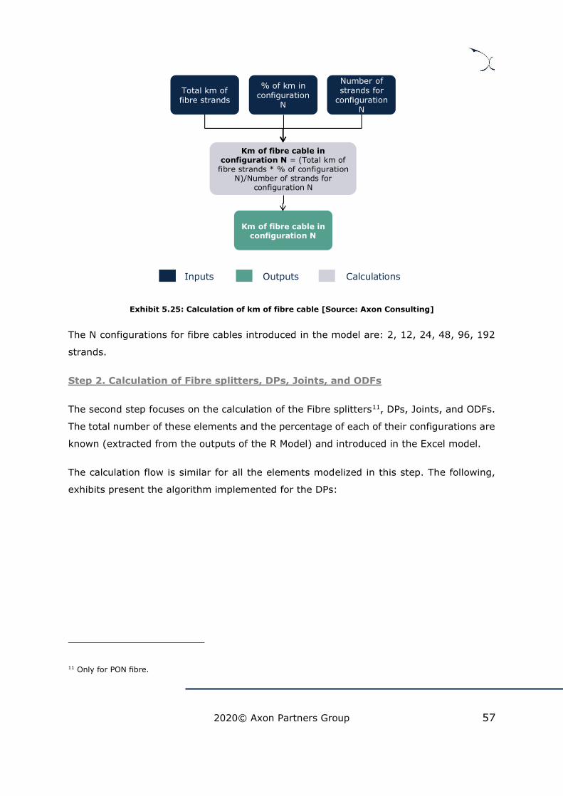
2020© Axon Partners Group 57
Exhibit 5.25: Calculation of km of fibre cable [Source: Axon Consulting]
The N configurations for fibre cables introduced in the model are: 2, 12, 24, 48, 96, 192
strands.
Step 2. Calculation of Fibre splitters, DPs, Joints, and ODFs
The second step focuses on the calculation of the Fibre splitters11, DPs, Joints, and ODFs.
The total number of these elements and the percentage of each of their configurations are
known (extracted from the outputs of the R Model) and introduced in the Excel model.
The calculation flow is similar for all the elements modelized in this step. The following,
exhibits present the algorithm implemented for the DPs:
11 Only for PON fibre.
Outputs CalculationsInputs
Total km of fibre strands
Km of fibre cable in configuration N = (Total km of
fibre strands * % of configuration N)/Number of strands for
configuration N
Km of fibre cable in configuration N
% of km in configuration
N
Number of strands for
configuration N
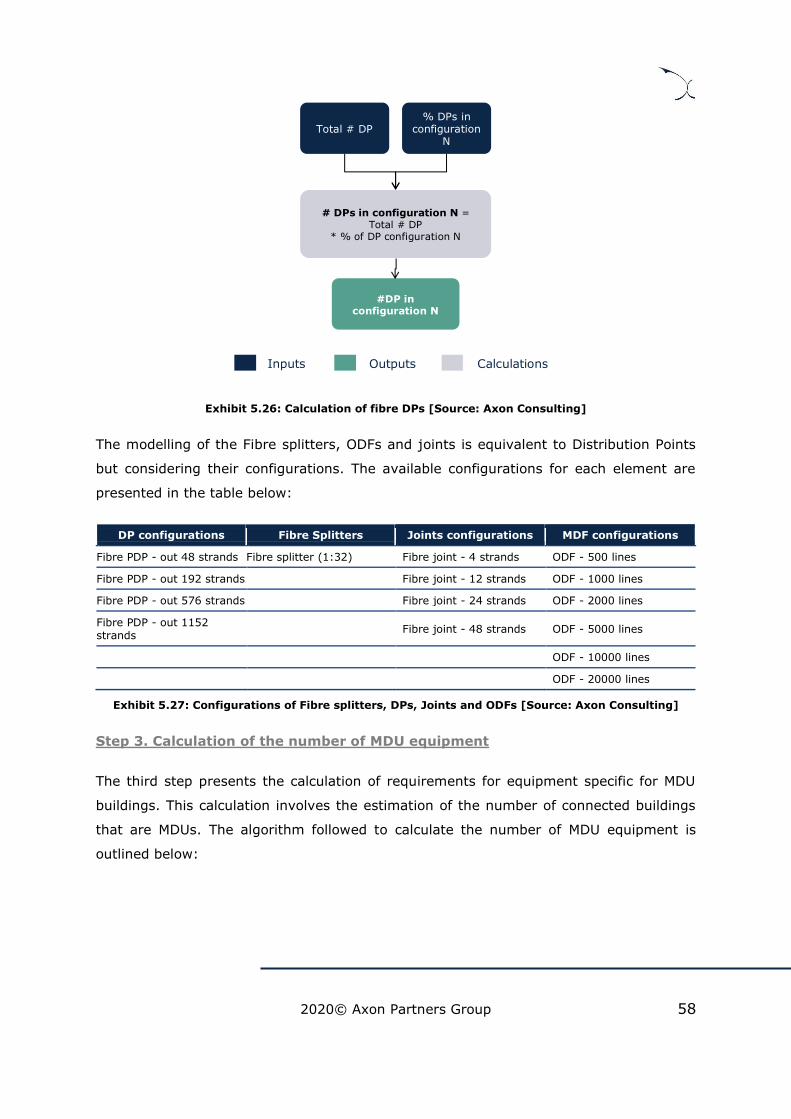
2020© Axon Partners Group 58
Exhibit 5.26: Calculation of fibre DPs [Source: Axon Consulting]
The modelling of the Fibre splitters, ODFs and joints is equivalent to Distribution Points
but considering their configurations. The available configurations for each element are
presented in the table below:
DP configurations Fibre Splitters Joints configurations MDF configurations
Fibre PDP - out 48 strands Fibre splitter (1:32) Fibre joint - 4 strands ODF - 500 lines
Fibre PDP - out 192 strands Fibre joint - 12 strands ODF - 1000 lines
Fibre PDP - out 576 strands Fibre joint - 24 strands ODF - 2000 lines
Fibre PDP - out 1152 strands
Fibre joint - 48 strands ODF - 5000 lines
ODF - 10000 lines
ODF - 20000 lines
Exhibit 5.27: Configurations of Fibre splitters, DPs, Joints and ODFs [Source: Axon Consulting]
Step 3. Calculation of the number of MDU equipment
The third step presents the calculation of requirements for equipment specific for MDU
buildings. This calculation involves the estimation of the number of connected buildings
that are MDUs. The algorithm followed to calculate the number of MDU equipment is
outlined below:
Outputs CalculationsInputs
Total # DP
# DPs in configuration N = Total # DP
* % of DP configuration N
#DP in configuration N
% DPs in configuration
N

2020© Axon Partners Group 59
Exhibit 5.28: Calculation of the number of MDU equipment [Source: Axon Consulting]
For fibre networks this algorithm is performed separately for PON and PTP networks.
Step 4. Calculation of the number of MSANs and OLTs
Once the previous elements are determined we proceed to calculate the number of MSANs
required for the network. The model considers to main types of MSAN depending on their
location:
OLT: Used for the PON architecture
PTP MSAN: Used for the point-to-point architecture
OLTs for PON fibre
The number of PON OLTs can be determined based on two factors:
Coverage: The geographical analysis performed in section determines the number of
OLTs required for the actual coverage of the network
Demand: the number of OLTs required in order to attend the fibre services demand
(active fibre connections). This number is calculated in the Excel model.
Once both numbers are calculated, the highest number of both will be chosen.
# MDU Equipment=
(1 – (1 – (# of homes connected / # of homes covered))#homes per building) * *
# of buildings covered * (1-% of MDU that are LAN)
# MDU Equipment
# homes connected
# of buildings
# of homes per building
% of MDU that are LAN
Outputs CalculationsInputs

2020© Axon Partners Group 60
Therefore, to determine the final number of OLTs, three main steps have been followed:
1. The minimum number of ports required for the OLTs is set equal to the total number
of splitters in the network.
2. The second step involved the calculation of the number of cards required in the
network attending to the demand and to coverage. The algorithm used is presented
below:
Exhibit 5.29: Calculation of OLT line cards [Source: Axon Consulting]
3. Given the number of OLT line cards required in the network, the second step
proceeded to the calculation of the number of OLTs needed to handle these line
cards, and the number of ports required for the total line cards.
Outputs CalculationsInputs
# OLT line cards=
𝑜𝑓 𝐿𝑇𝑠 𝑝𝑜𝑟𝑡𝑠
𝑜𝑓 𝑝𝑜𝑟𝑡𝑠 𝑝𝑒𝑟 𝑙𝑖𝑛𝑒 𝑐𝑎𝑟𝑑
#OLT line cards
OLT line cards= max(#OLT line
cards(demand), #OLT line cards (coverage))
OLT line cards (coverage)=
# OLTs (coverage)X
Number of cards per OLT
Number ofOLTs ports
# of ports per line card
# OLTs racks (coverage)
# of cards per OLT

2020© Axon Partners Group 61
Exhibit 5.30: Calculation of number of OLTs and ports [Source: Axon Consulting]
MSANs for PTP fibre
For the PTP MSAN the exact same calculation flow has been considered considering the
percentage of fibre connections connected through PTP architecture.
Ports for access nodes
These ports are located in the L3 access nodes and are used to connect the fibre PTP
MSANs and the OLTs with the core and transmission networks. Therefore, the calculation
performed to determine their number follows the steps below:
1. Calculation of the broadband traffic per node (PTP MSAN or OLT)
Outputs CalculationsInputs
#OLTs (demand) = #OLT line cards
/ #line cards per OLT
#OLTs
#OLT line cards
#line cards per OLT
# OLTs (coverage)
#OLT= max(#OLTs (demand), #OLTs (coverage))
#OLTs ports (demand) = # OLT line cards
*#Ports per OLT line card
#OLTs ports
# of OLTs ports
(splitters)
# OLT line cards
# Ports per OLT line card
#OLT ports= max (#OLTs ports (demand), # of OLTs
ports (splitters))
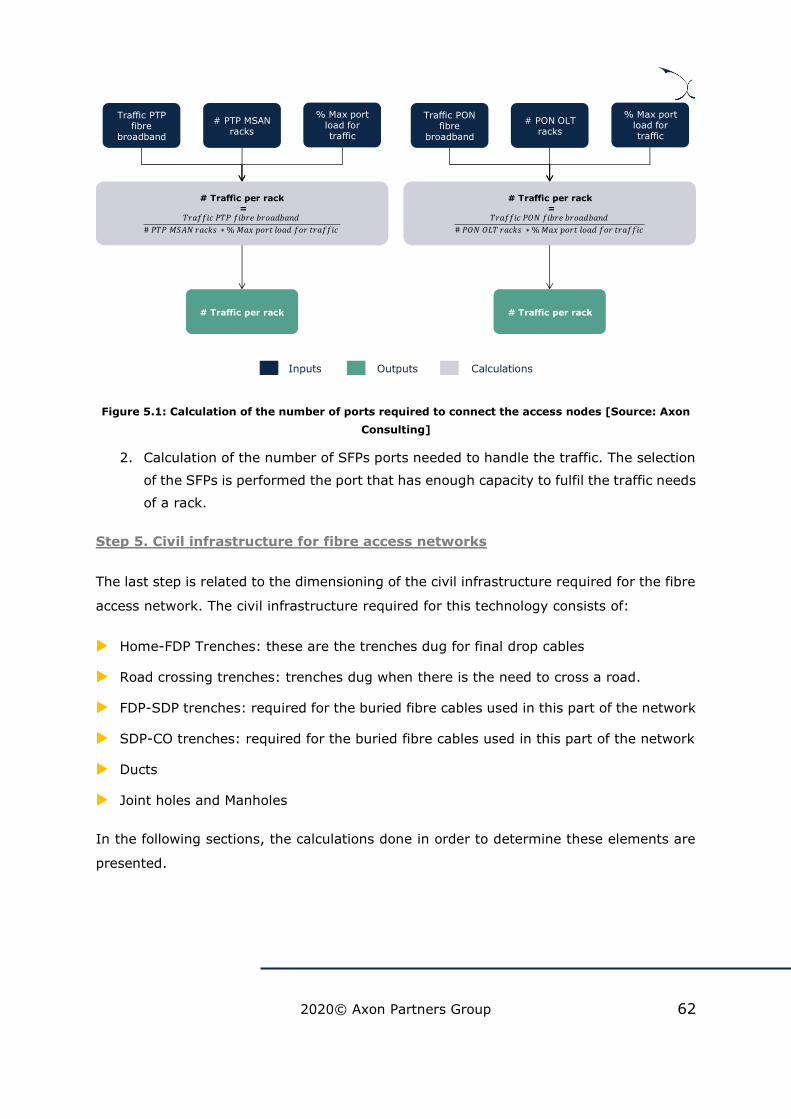
2020© Axon Partners Group 62
Figure 5.1: Calculation of the number of ports required to connect the access nodes [Source: Axon
Consulting]
2. Calculation of the number of SFPs ports needed to handle the traffic. The selection
of the SFPs is performed the port that has enough capacity to fulfil the traffic needs
of a rack.
Step 5. Civil infrastructure for fibre access networks
The last step is related to the dimensioning of the civil infrastructure required for the fibre
access network. The civil infrastructure required for this technology consists of:
Home-FDP Trenches: these are the trenches dug for final drop cables
Road crossing trenches: trenches dug when there is the need to cross a road.
FDP-SDP trenches: required for the buried fibre cables used in this part of the network
SDP-CO trenches: required for the buried fibre cables used in this part of the network
Ducts
Joint holes and Manholes
In the following sections, the calculations done in order to determine these elements are
presented.
# Traffic per rack=
𝑇𝑟𝑎𝑓𝑓𝑖𝑐 𝑃𝑇𝑃 𝑓𝑖 𝑟𝑒 𝑟𝑜𝑎𝑑 𝑎𝑛𝑑
𝑃𝑇𝑃 𝑆𝐴 𝑟𝑎𝑐𝑘𝑠 ∗ % 𝑎 𝑝𝑜𝑟𝑡 𝑙𝑜𝑎𝑑 𝑓𝑜𝑟 𝑡𝑟𝑎𝑓𝑓𝑖𝑐
# Traffic per rack
Traffic PTPfibre
broadband
# PTP MSAN racks
% Max port load for traffic
Outputs CalculationsInputs
# Traffic per rack=
𝑇𝑟𝑎𝑓𝑓𝑖𝑐 𝑃 𝑓𝑖 𝑟𝑒 𝑟𝑜𝑎𝑑 𝑎𝑛𝑑
𝑃 𝐿𝑇 𝑟𝑎𝑐𝑘𝑠 ∗ % 𝑎 𝑝𝑜𝑟𝑡 𝑙𝑜𝑎𝑑 𝑓𝑜𝑟 𝑡𝑟𝑎𝑓𝑓𝑖𝑐
# Traffic per rack
Traffic PON fibre
broadband
# PON OLT racks
% Max port load for traffic
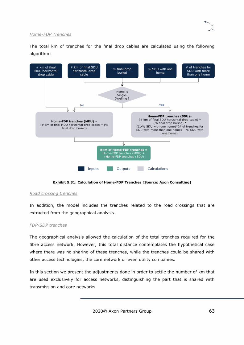
2020© Axon Partners Group 63
Home-FDP Trenches
The total km of trenches for the final drop cables are calculated using the following
algorithm:
Exhibit 5.31: Calculation of Home-FDP Trenches [Source: Axon Consulting]
Road crossing trenches
In addition, the model includes the trenches related to the road crossings that are
extracted from the geographical analysis.
FDP-SDP trenches
The geographical analysis allowed the calculation of the total trenches required for the
fibre access network. However, this total distance contemplates the hypothetical case
where there was no sharing of these trenches, while the trenches could be shared with
other access technologies, the core network or even utility companies.
In this section we present the adjustments done in order to settle the number of km that
are used exclusively for access networks, distinguishing the part that is shared with
transmission and core networks.
Outputs CalculationsInputs
#km of Home-FDP trenches = Home-FDP trenches (MDU) + +Home-FDP trenches (SDU)
Home is Single-
Dwelling ?
Home-FDP trenches (MDU) = (# km of final MDU horizontal drop cable) * (%
final drop buried)
Home-FDP trenches (SDU)= (# km of final SDU horizontal drop cable) *
(% final drop buried) * ((1-% SDU with one home)*(# of trenches for SDU with more than one home) + % SDU with
one home)
# km of final SDU horizontal drop
cable
% final drop buried
% SDU with one home
# of trenches for SDU with more than one home
# km of final MDU horizontal
drop cable
YesNo

2020© Axon Partners Group 64
Exhibit 5.32: Calculation of FDP-SDP Trenches [Source: Axon Consulting]
SDP-CO trenches
The geographical analysis allowed the calculation of the total trenches required for the
SDP-CO connections for the fibre access network. As for the FDP-SDP trenches, this part
of the network can also be shared. In order to consider this sharing, the same algorithm
as for FDP-SDP trenches has been followed.
Ducts
The calculation of km of ducts follows the algorithm below:
Outputs CalculationsInputs
#km of FDP-SDP trenches
#km of FDP-SDP trenches = # km of trenches used by fibre access network
X(1-% trenches shared with utilities + % trenches shared with
utilities* % of Share of trenches costs when shared with utilities)) X
(1-(% of trenches shared between core and access*(1-% Allocation ratio between access and core networks)))
# km of trenches used by fibre access
network
% of trenches shared between core and access
% Allocation ratio between access and
core networks
% trenches shared with utilities
% Share of trenches costs when shared
with utilities
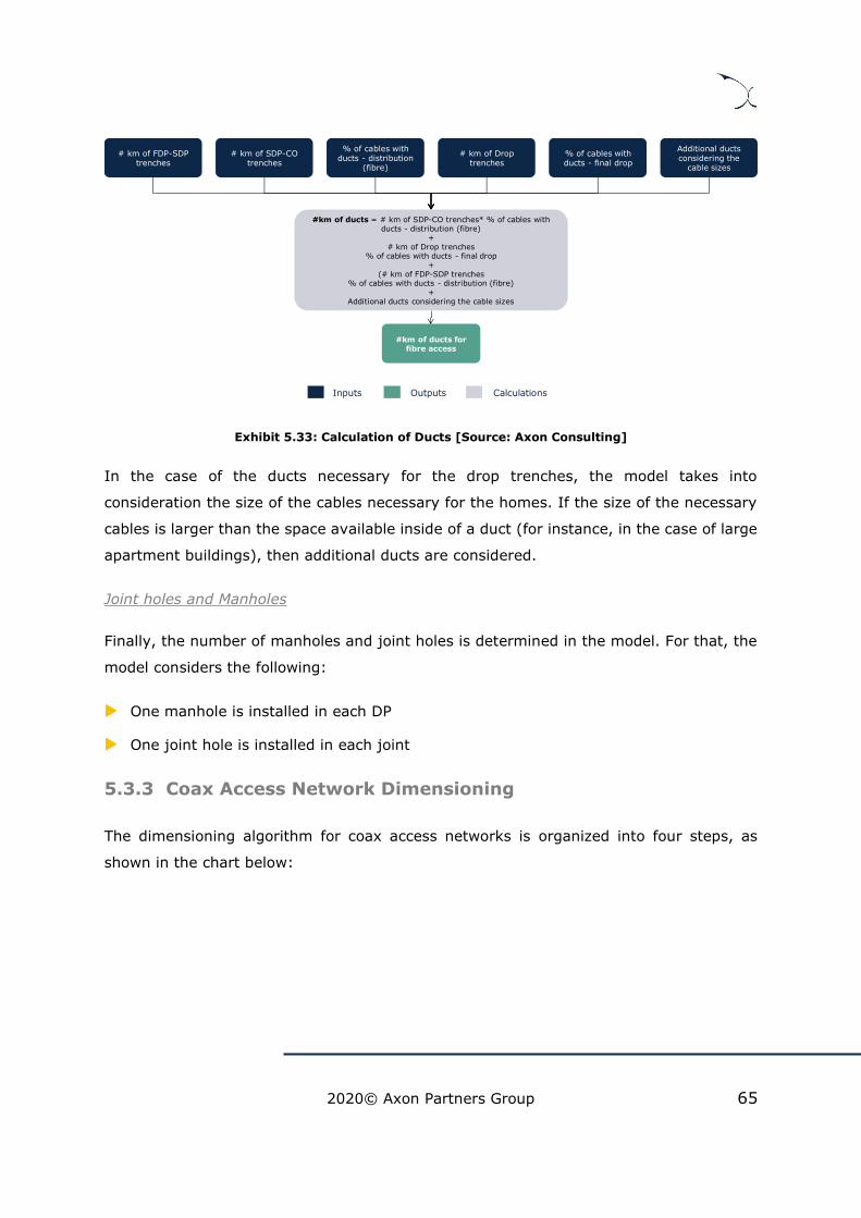
2020© Axon Partners Group 65
Exhibit 5.33: Calculation of Ducts [Source: Axon Consulting]
In the case of the ducts necessary for the drop trenches, the model takes into
consideration the size of the cables necessary for the homes. If the size of the necessary
cables is larger than the space available inside of a duct (for instance, in the case of large
apartment buildings), then additional ducts are considered.
Joint holes and Manholes
Finally, the number of manholes and joint holes is determined in the model. For that, the
model considers the following:
One manhole is installed in each DP
One joint hole is installed in each joint
5.3.3 Coax Access Network Dimensioning
The dimensioning algorithm for coax access networks is organized into four steps, as
shown in the chart below:
Outputs CalculationsInputs
#km of ducts for fibre access
#km of ducts = # km of SDP-CO trenches* % of cables with ducts - distribution (fibre)
+ # km of Drop trenches
% of cables with ducts - final drop+
(# km of FDP-SDP trenches% of cables with ducts - distribution (fibre)
+Additional ducts considering the cable sizes
# km of SDP-CO trenches
% of cables with ducts - distribution
(fibre)
# km of Drop trenches
% of cables with ducts - final drop
# km of FDP-SDP trenches
Additional ducts considering the
cable sizes
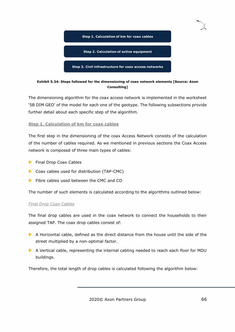
2020© Axon Partners Group 66
Exhibit 5.34: Steps followed for the dimensioning of coax network elements [Source: Axon
Consulting]
The dimensioning algorithm for the coax access network is implemented in the worksheet
‘5B DIM GEO’ of the model for each one of the geotype. The following subsections provide
further detail about each specific step of the algorithm.
Step 1. Calculation of km for coax cables
The first step in the dimensioning of the coax Access Network consists of the calculation
of the number of cables required. As we mentioned in previous sections the Coax Access
network is composed of three main types of cables:
Final Drop Coax Cables
Coax cables used for distribution (TAP-CMC)
Fibre cables used between the CMC and CO
The number of such elements is calculated according to the algorithms outlined below:
Final Drop Coax Cables
The final drop cables are used in the coax network to connect the households to their
assigned TAP. The coax drop cables consist of:
A Horizontal cable, defined as the direct distance from the house until the side of the
street multiplied by a non-optimal factor.
A Vertical cable, representing the internal cabling needed to reach each floor for MDU
buildings.
Therefore, the total length of drop cables is calculated following the algorithm below:
Step 1. Calculation of km for coax cables
Step 2. Calculation of active equipment
Step 3. Civil infrastructure for coax access networks

2020© Axon Partners Group 67
Exhibit 5.35: Calculation of km of fibre drop cable [Source: Axon Consulting]
Coax cables used for distribution (TAP-CMC)
The total coax cables used to connect TAP nodes to CMC nodes have been calculated in
the R Model. As there is only one type of coax cables used for this section of the network,
this number has been attributed fully to the resource of “Coax cables used for distribution
(TAP-CMC)”.
Fibre cables used between the CMC and CO
The total distance of fibre cable used to connect the CMCs to the COs in the Coax Access
network have been determined in the geographical analysis. This cable has only one
possible configuration (12 strands), and therefore the result from the geographical analysis
is directly entered for this resource.
Step 2. Calculation of active equipment
The second step focused on the calculation of the active equipment required for the coax
access network. The active equipment dimensioned is:
Coaxial amplifier
Splitters
Outputs CalculationsInputs
= ℎ𝑜𝑚𝑒𝑠 𝑐𝑜𝑛𝑛𝑒𝑐𝑡𝑒𝑑 ∗ 𝐴𝑣𝑒𝑟𝑎𝑔𝑒 𝑙𝑒𝑛𝑔𝑡ℎ 𝑜𝑓 𝑑𝑟𝑜𝑝 𝑐𝑎 𝑙𝑒
∗ 1 −%𝑜𝑓 𝑛𝑜𝑛𝑜𝑝𝑡𝑖𝑚𝑎𝑙 𝑙𝑒𝑛𝑔𝑡ℎ ∗ (1 −%𝑜𝑓 𝐷𝑈 𝑡ℎ𝑎𝑡 𝑎𝑟𝑒 𝐿𝐴 )
Km of horizontal drop cable
# homes connected
Average length of
drop cable
% of non-optimal length
% of MDU that are LAN
= 𝐷𝑈 ℎ𝑜𝑚𝑒𝑠 𝑐𝑜𝑛𝑛𝑒𝑐𝑡𝑒𝑑 ∗ (𝐴𝑣𝑒𝑟𝑎𝑔𝑒 𝑜𝑓 𝑓𝑙𝑜𝑜𝑟𝑠 − 1)/
∗ 𝐴𝑣𝑒𝑟𝑎𝑔𝑒 ℎ𝑒𝑖𝑔ℎ𝑡 𝑜𝑓 𝑓𝑙𝑜𝑜𝑟𝑠 ∗ (1 −%𝑜𝑓 𝐷𝑈 𝑡ℎ𝑎𝑡 𝑎𝑟𝑒 𝐿𝐴 )
Km of vertical drop cable
# MDU homes
connected
% of MDU that are LAN
Average # of floors
Average height of
floors
Total km of drop cable =
Km of horizontal drop cable + Km of vertical
drop cable
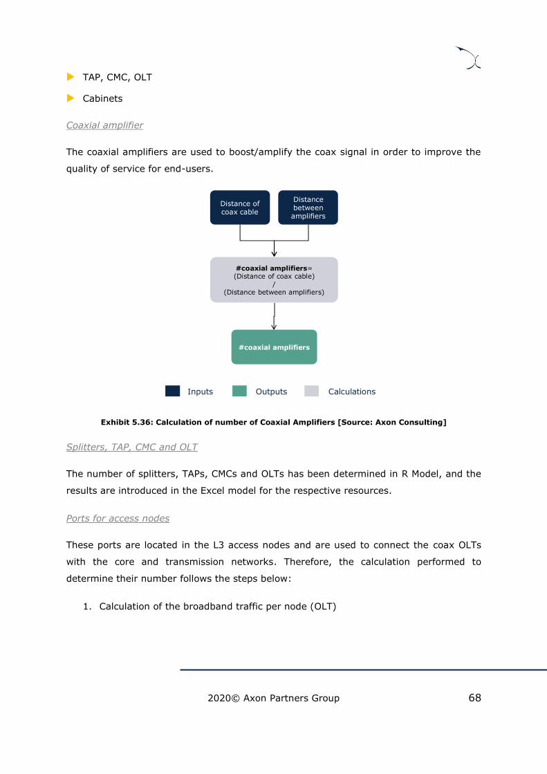
2020© Axon Partners Group 68
TAP, CMC, OLT
Cabinets
Coaxial amplifier
The coaxial amplifiers are used to boost/amplify the coax signal in order to improve the
quality of service for end-users.
Exhibit 5.36: Calculation of number of Coaxial Amplifiers [Source: Axon Consulting]
Splitters, TAP, CMC and OLT
The number of splitters, TAPs, CMCs and OLTs has been determined in R Model, and the
results are introduced in the Excel model for the respective resources.
Ports for access nodes
These ports are located in the L3 access nodes and are used to connect the coax OLTs
with the core and transmission networks. Therefore, the calculation performed to
determine their number follows the steps below:
1. Calculation of the broadband traffic per node (OLT)
Outputs CalculationsInputs
#coaxial amplifiers= (Distance of coax cable)
/(Distance between amplifiers)
#coaxial amplifiers
Distance of coax cable
Distance between amplifiers

2020© Axon Partners Group 69
Figure 5.2: Calculation of the number of ports required to connect the access nodes [Source: Axon
Consulting]
Calculation of the number of SFPs ports needed to handle the traffic. The selection of the
SFPs is performed selecting the most-cost efficient solution. The algorithm followed for
this is presented in the section ‘5.2. Transmission network dimensioning’.
Cabinets
The model includes two types of cabinets (small and large). The small cabinets are used
for the Coaxial amplifiers whilst the Large ones are installed for the CMC. Therefore, the
calculation of these elements follows the algorithm below:
A small cabinet is installed for each Coaxial Amplifier and Coaxial DP
A large cabinet is installed for each CMC
MDU equipment
The third step presents the calculation of requirements for equipment specific for MDU
buildings. This calculation involves the estimation of the number of connected buildings
that are MDUs. The algorithm followed to calculate the number of MDU equipment is
outlined below:
Outputs CalculationsInputs
# Traffic per rack=
𝑇𝑟𝑎𝑓𝑓𝑖𝑐 𝑐𝑜𝑎 𝑟𝑜𝑎𝑑 𝑎𝑛𝑑
𝐿𝑇 𝑟𝑎𝑐𝑘𝑠 ∗ % 𝑎 𝑝𝑜𝑟𝑡 𝑙𝑜𝑎𝑑 𝑓𝑜𝑟 𝑡𝑟𝑎𝑓𝑓𝑖𝑐
# Traffic per rack
Traffic coax broadband
# OLT racks
% Max port load for traffic

2020© Axon Partners Group 70
Exhibit 5.37: Calculation of the number of MDU equipment [Source: Axon Consulting]
Step 3. Civil infrastructure for coax access networks
The last step is related to the dimensioning of the civil infrastructure required for the coax
access network. The civil infrastructure required for this technology consists of:
Home-TAP trenches: these are the trenches dug for final drop cables
Road crossing trenches: trenches dug when there is the need to cross a road.
TAP-CMC trenches: required for the buried coax cables used in this part of the network
CMC-CO trenches: required for the buried fibre cables used in this part of the network
Ducts
Joint holes and Manholes
In the following sections, the calculations done in order to determine these elements are
presented.
Home-TAP Trenches
The total km of trenches for the final drop cables are calculated using the following
algorithm:
# MDU Equipment=
(1 – (1 – (# of homes connected / # of homes covered))#homes per building) * *
# of buildings covered * (1-% of MDU that are LAN)
# MDU Equipment
# homes connected
# of buildings
# of homes per building
% of MDU that are LAN
Outputs CalculationsInputs

2020© Axon Partners Group 71
Exhibit 5.38: Calculation of Home-TAP Trenches [Source: Axon Consulting]
Road crossing trenches
In addition, the model includes the trenches related to the road crossings that are
extracted from the geographical analysis.
TAP-CMC trenches
The geographical analysis allowed the calculation of the total trenches required for the
coax access network. However, this total distance contemplates the hypothetical case
where there was no sharing of these trenches, while the trenches could be shared with
other access technologies, the core network or even utility companies.
In this section we present the adjustments done in order to settle the number of km that
are used exclusively for access networks, distinguishing the part that is shared with
transmission and core networks.
#km of Home-TAP trenches = Home-TAP trenches (MDU) + +Home-TAP trenches (SDU)
Home is Single-
Dwelling ?
Home-TAP trenches (MDU) = (# km of final MDU horizontal drop cable) * (%
final drop buried)
Home-TAP trenches (SDU)= (# km of final SDU horizontal drop cable) *
(% final drop buried) * ((1-% SDU with one home)*(# of trenches for SDU with more than one home) + % SDU with
one home)
# km of final SDU horizontal drop
cable
% final drop buried
% SDU with one home
# of trenches for SDU with more than one home
# km of final MDU horizontal
drop cable
YesNo

2020© Axon Partners Group 72
Exhibit 5.39: Calculation of TAP-CMC trenches [Source: Axon Consulting]
CMC-CO trenches
The geographical analysis allowed the calculation of the total trenches required for the
CMC-CO connections for the coax access network. As for the TAP-CMC trenches, this part
of the network can also be shared. In order to consider this sharing, the same process as
for TAP-CMC trenches has been followed.
Ducts
Part of the cables of the coax network is introduced in ducts. Hence, the calculation of km
of ducts follows the algorithm below:
Outputs CalculationsInputs
#km of TAP-CMC trenches
#km of TAP-CMC trenches = # km of trenches used by coaxaccess network
X(1-% trenches shared with utilities + % trenches shared with
utilities* % of Share of trenches costs when shared with utilities)) X
(1-(% of trenches shared between core and access*(1-% Allocation ratio between access and core networks)))
# km of trenches used by coax access
network
% of trenches shared between core and access
% Allocation ratio between access and
core networks
% trenches shared with utilities
% Share of trenches costs when shared
with utilities

2020© Axon Partners Group 73
Exhibit 5.40: Calculation of ducts for the coax access network [Source: Axon Consulting]
Joint holes and Manholes
Finally, the number of manholes and joints holes is determined in the model. For that, the
model considers the following:
One manhole is installed in each Coaxial amplifier and Splitter
One joint hole is installed in each TAP
Outputs CalculationsInputs
#km of ducts for coax access
#km of ducts = # km of CMC-CO trenches* % of cables with ducts - distribution (fibre)
+ # km of Drop trenches
% of cables with ducts - final drop+
(# km of TAP-CMC trenches% of cables with ducts - distribution (copper)
# km of CMC-CO trenches
% of cables with ducts - distribution
(fibre)
# km of Drop trenches
% of cables with ducts - final drop
# km of TAP-CMC trenches
% of cables with ducts - distribution
(copper)

2020© Axon Partners Group 74
6. Resources costing
Once the model has calculated the number of resources needed to accommodate the
demand and coverage levels in the network, the next step is the calculation of the costs
of the network. This calculation is performed separately for CapEx and OpEx on a nation-
wide aggregated level.
The procedure to assess network costs is presented in the following sections
Calculation of network costs
Calculation of non-network costs
6.1. Calculation of network costs
Two main steps are followed to calculate total network annual costs (including both CapEx
and OpEx):
Exhibit 6.1: Resources Costing [Source: Axon Consulting]
The following sections explain each step in detail.
Step 1: Determination of unit costs throughout the modelling period
The definition of the unit costs is performed separately for CapEx and OpEx components.
Notably, for the definition of the CapEx unit costs of the resources considered in the model,
the following formula is considered:
𝑈𝑛𝑖𝑡 𝐶𝑎𝑝𝐸 𝑖 (𝑛) = 𝑈𝑛𝑖𝑡 𝐶𝑎𝑝𝐸 2018 (𝑛) ∗ (1 + 𝑡 (𝑛))(𝑖−2018)
Where:
Unit ÇapExi (n): Represents the cost of installing and acquiring a unit of network
element “n” in the year “i”. The figure included for the reference year (2018) is input
in the model based on the process
Step 2. Calculation of annual network costs
Step 1. Determination of unit costs throughout the modelling period
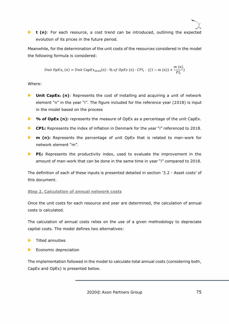
2020© Axon Partners Group 75
t (n): For each resource, a cost trend can be introduced, outlining the expected
evolution of its prices in the future period.
Meanwhile, for the determination of the unit costs of the resources considered in the model
the following formula is considered:
𝑈𝑛𝑖𝑡 𝑝𝐸 𝑖 (𝑛) = 𝑈𝑛𝑖𝑡 𝐶𝑎𝑝𝐸 2018(𝑛) · % 𝑜𝑓 𝑝𝐸 (𝑛) · 𝐶𝑃𝐼𝑖 · ((1 − 𝑚 (𝑛)) +𝑚 (𝑛)
𝑃𝐼𝑖)
Where:
Unit CapExi (n): Represents the cost of installing and acquiring a unit of network
element “n” in the year “i”. The figure included for the reference year (2018) is input
in the model based on the process
% of OpEx (n): represents the measure of OpEx as a percentage of the unit CapEx.
CPIi: Represents the index of inflation in Denmark for the year “i” referenced to 2018.
m (n): Represents the percentage of unit OpEx that is related to man-work for
network element “m”.
PIi: Represents the productivity index, used to evaluate the improvement in the
amount of man-work that can be done in the same time in year “i” compared to 2018.
The definition of each of these inputs is presented detailed in section ‘3.2 - Asset costs’ of
this document.
Step 2. Calculation of annual network costs
Once the unit costs for each resource and year are determined, the calculation of annual
costs is calculated.
The calculation of annual costs relies on the use of a given methodology to depreciate
capital costs. The model defines two alternatives:
Tilted annuities
Economic depreciation
The implementation followed in the model to calculate total annual costs (considering both,
CapEx and OpEx) is presented below.
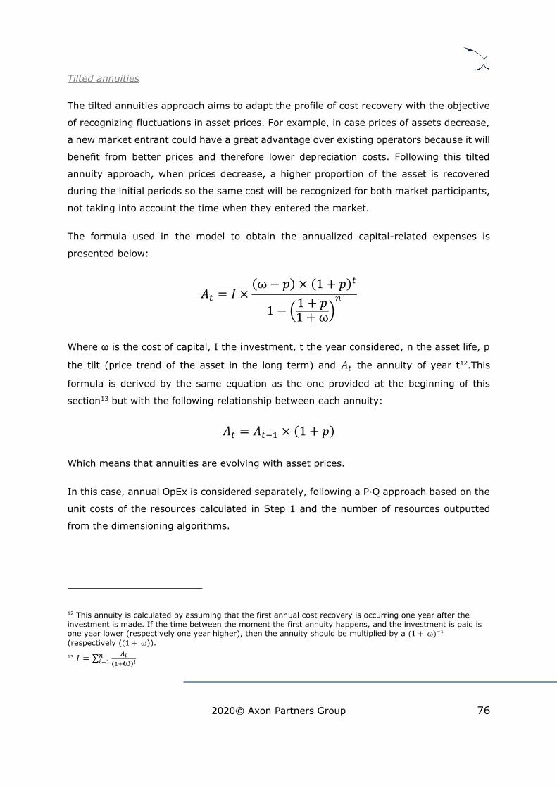
2020© Axon Partners Group 76
Tilted annuities
The tilted annuities approach aims to adapt the profile of cost recovery with the objective
of recognizing fluctuations in asset prices. For example, in case prices of assets decrease,
a new market entrant could have a great advantage over existing operators because it will
benefit from better prices and therefore lower depreciation costs. Following this tilted
annuity approach, when prices decrease, a higher proportion of the asset is recovered
during the initial periods so the same cost will be recognized for both market participants,
not taking into account the time when they entered the market.
The formula used in the model to obtain the annualized capital-related expenses is
presented below:
𝐴𝑡 = 𝐼 ×(ω − 𝑝) × (1 + 𝑝)𝑡
1 − (1 + 𝑝1 + ω)
𝑛
Where ω is the cost of capital, I the investment, t the year considered, n the asset life, p
the tilt (price trend of the asset in the long term) and 𝐴𝑡 the annuity of year t12.This
formula is derived by the same equation as the one provided at the beginning of this
section13 but with the following relationship between each annuity:
𝐴𝑡 = 𝐴𝑡−1 × (1 + 𝑝)
Which means that annuities are evolving with asset prices.
In this case, annual OpEx is considered separately, following a P·Q approach based on the
unit costs of the resources calculated in Step 1 and the number of resources outputted
from the dimensioning algorithms.
12 This annuity is calculated by assuming that the first annual cost recovery is occurring one year after the investment is made. If the time between the moment the first annuity happens, and the investment is paid is
one year lower (respectively one year higher), then the annuity should be multiplied by a (1 + ω)−1 (respectively ((1 + ω)).
13 𝐼 = ∑𝐴𝑖
(1+ω)𝑖𝑛𝑖=1

2020© Axon Partners Group 77
Economic depreciation
The objective of economic depreciation is to adjust the recovery of the asset value to the
economic value it produces.
In particular, economic depreciation adjusts the annuities of the investment by means of
a production factor, defined by the performance that is extracted from the asset. For
instance, if an asset is expected to be used more exhaustively in the future (e. g. due to
an increase in adoption), the application of the economic depreciation results in higher
annuities in the future than in the present (and relatively constant unitary costs).
Particularly, the formula used in the calculation for the economic depreciation is as follows:
𝐴𝑡 = 𝑡 × 𝑝𝑡 ×∑ (1 + ω)j × 𝐼𝑗
𝑛𝑗=1
∑ (1 + ω)j × 𝑗 × 𝑝𝑗𝑛𝑗=1
Where,
𝐴𝑡 represents the annual cost
𝑡 is the production factor of the asset in year t
𝑝𝑡 is the reference price of the asset in year t
𝜔 represents the cost of capital
𝐼𝑗 represents the yearly investment, calculated as the number of assets purchased in
year j multiplied by their unit price in that year. This figure shall accrue the OpEx that
would be incurred in order to operate and maintain the asset throughout its lifetime.
represents the last year in which an asset is used in the network.
As extracted from above, in the case that economic depreciation is considered, OpEx is
not treated separately.
6.2. Calculation of non-network costs
The model also considers the costs not related to the network. This type of cost is included
in the model as a mark-up over total network costs (considering, both, CapEx and OpEx).
The figures have been calculated based on data from the modelled operator. Notably, the
total network costs have been extracted from the Accounting Separation results, as the

2020© Axon Partners Group 78
sum of depreciation and OpEx of all products, excluding those related to voice and mobile
and excluding support/overhead (non-network) expenditures.
As presented in section ‘3.7 - Non-network overheads’, there are 4 different mark-ups
depending on the nature of the costs:
G&A mark-up
IT mark-up
Wholesale and commercial mark-up
Working capital mark-up
These mark-ups are applied to the total network costs (including CapEx and OpEx) to
calculate the total non-network costs borne by the modelled operator. These costs are
then allocated to services following the approach described in section ‘7.2.3 - Step 3: Cost
Allocation to Services’.

2020© Axon Partners Group 79
7. Network costs of the services
This section presents the methodology followed to calculate the incremental and common
costs of the resources, and how these costs will be allocated to the services in order to
obtain unit costs under the LRAIC standard.
7.1. Incremental and common costs calculation
The incremental cost associated with each increment is the reduction in the costs
calculated by the model due to ceasing the provision of the services included in that
increment. This cost is expressed mathematically as the difference between the cost of
total demand and the cost obtained when the level of demand for the services included in
the increment is set to zero, leaving all others unchanged:
𝐼 𝐶𝑅𝐸 𝐸 𝑇𝐴𝐿 𝐶 𝑆𝑇(𝑖𝑛𝑐𝑟𝑒𝑚𝑒𝑛𝑡1) = 𝐹(𝑣1, 𝑣 , 𝑣3, 𝑣 , 𝐶) − 𝐹(0, 𝑣 , 𝑣3, 𝑣 , 𝐶)
Where F is the formula that represents the LRAIC model (which calculates the cost
according to demand and coverage), 𝑣𝑖 represents the demand volume of increment i,
and C represents the coverage.
To calculate the incremental costs, increments are defined as groups of services.
Therefore, services have to be assigned to increments. In the model (sheet ‘0F PAR
OTHER’), one increment has been defined, related to the Demand of all the services
modelled.
Once incremental costs are calculated for this increment, as described previously, common
costs by the resource are obtained as the difference between the total cost base obtained
under Fully Allocated Costs standard (considering all the demand) and the incremental
costs. The following formula shows this calculation:
𝐶 𝐶 𝑆𝑇 = 𝑇 𝑇𝐴𝐿 𝐶 𝑆𝑇𝑆 (𝐹𝑢𝑙𝑙 𝐴𝑙𝑙𝑜𝑐𝑎𝑡𝑒𝑑 𝐶𝑜𝑠𝑡𝑠)
− 𝐼 𝐶𝑅𝐸 𝐸 𝑇𝐴𝐿 𝐶 𝑆𝑇(𝐷𝑒𝑚𝑎𝑛𝑑 𝑖𝑛𝑐𝑟𝑒𝑚𝑒𝑛𝑡)
In the model, resources’ incremental and common costs are calculated in sheet ‘6E RES
INCR-COM COST’.
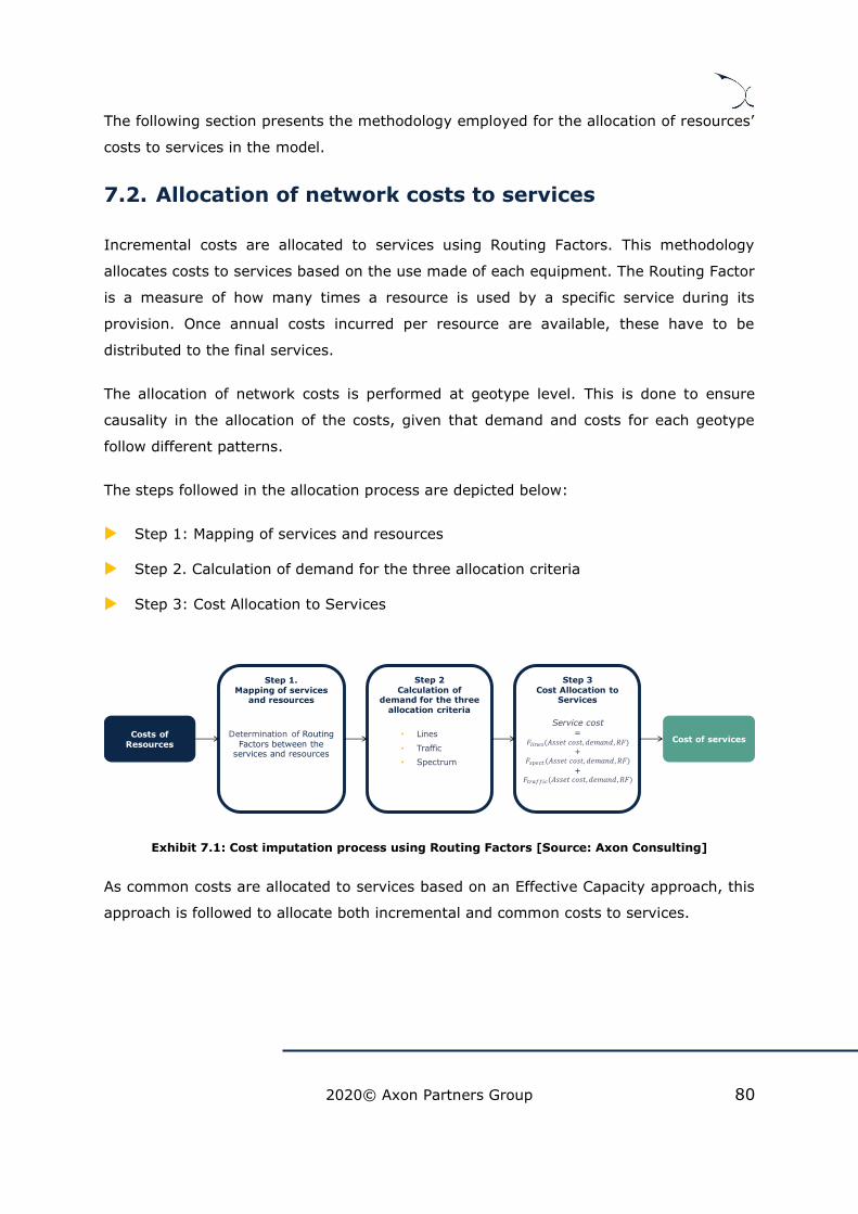
2020© Axon Partners Group 80
The following section presents the methodology employed for the allocation of resources’
costs to services in the model.
7.2. Allocation of network costs to services
Incremental costs are allocated to services using Routing Factors. This methodology
allocates costs to services based on the use made of each equipment. The Routing Factor
is a measure of how many times a resource is used by a specific service during its
provision. Once annual costs incurred per resource are available, these have to be
distributed to the final services.
The allocation of network costs is performed at geotype level. This is done to ensure
causality in the allocation of the costs, given that demand and costs for each geotype
follow different patterns.
The steps followed in the allocation process are depicted below:
Step 1: Mapping of services and resources
Step 2. Calculation of demand for the three allocation criteria
Step 3: Cost Allocation to Services
Exhibit 7.1: Cost imputation process using Routing Factors [Source: Axon Consulting]
As common costs are allocated to services based on an Effective Capacity approach, this
approach is followed to allocate both incremental and common costs to services.
Costs of Resources
Step 1.Mapping of services
and resources
Determination of Routing Factors between the
services and resources
Step 3Cost Allocation to
Services
Cost of services
Step 2Calculation of
demand for the three allocation criteria
• Lines
• Traffic
• Spectrum
Service cost =
𝐹 𝑖𝑛 (𝐴𝑠𝑠𝑒𝑡 𝑐𝑜𝑠𝑡, 𝑑𝑒𝑚𝑎𝑛𝑑, 𝑅𝐹)+
𝐹 𝑡 (𝐴𝑠𝑠𝑒𝑡 𝑐𝑜𝑠𝑡, 𝑑𝑒𝑚𝑎𝑛𝑑, 𝑅𝐹)
+𝐹𝑡 𝑖 (𝐴𝑠𝑠𝑒𝑡 𝑐𝑜𝑠𝑡, 𝑑𝑒𝑚𝑎𝑛𝑑, 𝑅𝐹)

2020© Axon Partners Group 81
7.2.1 Step 1: Mapping of services and resources
Resources’ costs have to be allocated to the services proportionally to the amount of
lines/traffic/spectrum they generate/use and to a “factor of use”, the Routing Factor.
Hence, the more lines/traffic/spectrum a service generates/uses, the higher the cost will
be allocated to it from the asset considered.
The excerpt below illustrates some relationships between resource and services, together
with the applicable routing factor:
Exhibit 7.2: Illustrative extract of the routing factors defined between services and resources
(Sheet ‘3C MAT ROUTING FACTORS’) [Source: Axon Consulting]
7.2.2 Step 2. Calculation of demand for the three allocation
criteria
The cost imputation process is done depending on the resources’ nature. Notably, the
resources introduced in the model can be divided into three main groups based on the
driver shaping the allocation of its cost:
Lines, these are network elements that rely on the number of lines of the service to
allocate the proper amount of costs. These include, for instance, all passive elements
in the access network.
Traffic, these are network elements that rely on the volume of traffic of the service to
allocate the proper amount of costs. These include, for instance, the ports in the
routers in the transmission network.
Spectrum, these are network elements that rely on the spectrum (in MHz) used by
the service to allocate the proper amount of costs. The elements needing this allocation
methodology are in the coax access network, where some elements allocate the
spectrum to TV or broadband services.
Based on these three criteria, to perform an accurate allocation of the services, the
demand of the services has to be transformed into these three main groups. To perform
ServiceAccess fibre.Fibre
drop cable.length
Access fibre.Fibre
cable - 2 strands
(SDP-User).length
Access fibre.Fibre
cable - 12 strands
(SDP-User).length
Access fibre.Fibre
cable - 24 strands
(SDP-User).length
Access fibre.Fibre
cable - 48 strands
(SDP-User).length
Access fibre.Fibre
cable - 96 strands
(SDP-User).length
Access fibre.Fibre
cable - 192
strands (SDP-
User).length
Access.Fibre.Retail.Access 1 1 1 1 1 1 1
Access.Fibre.Wholesale.Raw access (POI0) 1 1 1 1 1 1 1
Access.Fibre.Wholesale.Raw access (POI1) 1 1 1 1 1 1 1
Access.Fibre.Wholesale.VULA access (POI1) 1 1 1 1 1 1 1
Access.Fibre.Wholesale.BSA Access (POI2/POI3) 1 1 1 1 1 1 1

2020© Axon Partners Group 82
this transformation, the demand of the services introduced in the model is multiplied by a
series of factors or weights depending on the relevant allocation driver.
7.2.3 Step 3: Cost Allocation to Services
Once the relationship of each service to each resource has been performed (Step 1) and
ensured that the demand allocation driver is properly analysed in the relevant unit (Step
2), it is possible to distribute all costs to all services.
This step is performed separately for each of the allocation criteria presented in Step 2
and for each geotype independently. The basic relation is the following:
𝑆𝑒𝑟𝑣𝑖𝑐𝑒 𝑐𝑜𝑠𝑡(𝑖, 𝑒𝑎𝑟)
= ∑𝐶𝑜𝑠𝑡 𝑖𝑛 (𝑛, 𝑒𝑎𝑟) · 𝐷𝑒𝑚𝑎𝑛𝑑 𝑖𝑛 (𝑖, 𝑒𝑎𝑟) · 𝑅𝐹(𝑖, 𝑛)
∑ 𝐷𝑒𝑚𝑎𝑛𝑑 𝑖𝑛 (𝑖, 𝑒𝑎𝑟) · 𝑅𝐹(𝑖, 𝑛)𝑖𝑛
+∑𝐶𝑜𝑠𝑡𝑡 𝑖 (𝑛, 𝑒𝑎𝑟) · 𝐷𝑒𝑚𝑎𝑛𝑑𝑡 𝑖 (𝑖, 𝑒𝑎𝑟) · 𝑅𝐹(𝑖, 𝑛)
∑ 𝐷𝑒𝑚𝑎𝑛𝑑𝑡 𝑖 (𝑖, 𝑒𝑎𝑟) · 𝑅𝐹(𝑖, 𝑛)𝑖𝑛
+ ∑𝐶𝑜𝑠𝑡 𝑡 𝑢𝑚(𝑛, 𝑒𝑎𝑟) · 𝐷𝑒𝑚𝑎𝑛𝑑 𝑡 𝑢𝑚(𝑖, 𝑒𝑎𝑟) · 𝑅𝐹(𝑖, 𝑛)
∑ 𝐷𝑒𝑚𝑎𝑛𝑑 𝑡 𝑢𝑚(𝑖, 𝑒𝑎𝑟) · 𝑅𝐹(𝑖, 𝑛)𝑖
+ 𝑛
Where:
Service cost (i, year) is the cost of service “i" in a given year
Cost (n, year) is the cost of resource “n” in a given year. Assets are separated based
on their specific rule for allocation (demand, traffic and spectrum).
Demand (i, year) is the demand of the service “i" in the selected year. As for assets,
the demand considered depends on the allocation rule of the associated asset.
RF (i, n) is the Routing Factor that relates the resource “n” with service “i”.
The allocation of resources’ cost to services is presented in the sheet ` 7C GEO SERV
COSTS ´ and where the formula used allows the implementation of steps described under
this section.
It should be noted that common and joint network costs are also allocated to services
based on this methodology, aligned with the “effective capacity” approach defined in the
MRP.
2020© Axon Partners Group 83
On the other hand, the non-network overheads determined in section ‘3.7 Non-network
overheads’ are distributed to the different services following an equi-proportional mark-
up (EPMU) approach.

2020© Axon Partners Group 84
Annex A. User manual for the Excel model
This section provides guidelines on how to use the Excel model, and is divided among the
following sub-sections:
Getting started, providing a set of high-level specs related to the hardware required
to run the model.
General overview of the model, describing the structure and worksheets of the
Excel model.
Understanding the control panel, presenting the Control Panel of the Excel model,
which is the main user interface where the main options and scenarios are selected.
Additionally, this worksheet contains a ‘RUN’ button to execute the Excel model.
Description of checks, explaining the meaning of the checks included in the model.
A.1. Getting started
To run the Excel model, a computer with at least 1 GB of RAM memory and with Microsoft
Excel version 2010 (or a newer version) is required. For enhanced performance, it is
recommended to run the model on computers with at least 2 GB of RAM memory.
A.2. General overview of the model
The Excel model is comprised of worksheets that are grouped in the following blocks or
calculation steps:
Support and control worksheets
Step 0: Parameters
Step 1: Main inputs
Step 2: Advanced inputs
Step 3: Mapping
Step 4: Drivers and demand factors
Step 5: Dimensioning of the network
Step 6: Resource Costing
Step 7: Allocation of costs

2020© Axon Partners Group 85
Step 8: Results
The Excel model has been developed based on a linear architecture in order to improve
the execution performance and to ease the understanding of its calculation flow. The
exhibit below shows the model calculation flow:
Exhibit 7.3: Calculation flow of the model [Source: Axon Consulting]
The block “Support and Control Worksheets” has not been represented in the previous
exhibit for clarity purposes.
The worksheets contained in the blocks or calculation steps have been labelled according
to the following structure (except for the “Support and Control Worksheets” block):
Step number and ordinal: It is composed of the number of the step (i.e. 0, 1, 2…) and
the order in letter format (i.e. A, B …).
Type of worksheet indicators:
• PAR: Definition of parameters
• INP: Input worksheet
• MAT: Matrix obtaining the relationship between two dimensions
Step 0. Parameters
Step 1. Main inputs
Step 3. Mapping
Step 4. Drivers and demand factors
Step 5. Dimensioning of the network
Step 6. Resource costing
Step 7. Allocation of costs
Step 8. Results
Step 2. Advanced Inputs

2020© Axon Partners Group 86
• MAP: Mapping between two dimensions
• DIM: Dimensioning of network elements
• RES: Summary of the number and costs of the resources in the network
• GEO: Summary of costs disaggregated at geotype level
• RESULTS: Results worksheets
Name of the worksheet
As an example, the worksheet ‘1A INP DEMAND’ is the first (A) worksheet of the Step 1.
It represents an input (INP) related with the demand (DEMAND).
The following sections describe the calculation blocks, including a detailed description of
the worksheets contained in each block. It should be pointed out that sub-section ‘A.2.1-
Support and control worksheets’ does not strictly describe a block of the calculation flow,
but the supporting and control worksheets used within the model.
A.2.1. Support and control worksheets
The support and control worksheets provide general information to understand and run
the model, as well as a number of checks to verify that the model is working properly.
Sheet name Description
CONTENTS
Provides high-level information about the model file (i.e. version,
status and contacts)
Provides a list and description of the model’s worksheets
COVER
This worksheet includes the main modelling options that may be
adjusted to execute the model (e.g. WACC, execution mode,
annualization methodology). At the same time, it includes the
controls for the execution of the model.
MAP
Map that represents the relationship between the model’s
worksheet blocks as well as the overall calculation flow.
Colours have no meaning and have been selected to ease the
identification of the blocks.
COLOUR CODE It contains the colour code used throughout the model.
CHECKS
Multiple checks are performed in this worksheet to ensure that
the model is working properly. Further details on these are
provided in section ‘A.4 - Description of checks’ of this document.
Exhibit 7.4: Support and control worksheets. [Source: Axon Consulting]
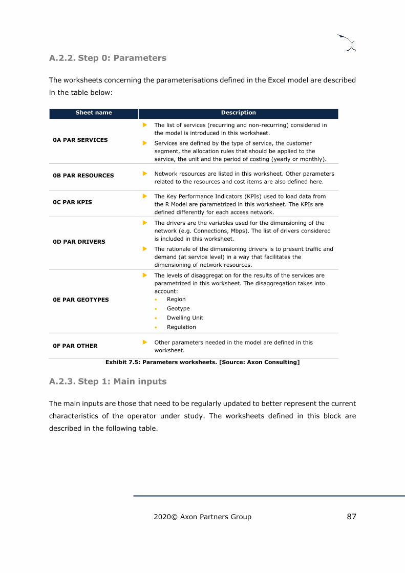
2020© Axon Partners Group 87
A.2.2. Step 0: Parameters
The worksheets concerning the parameterisations defined in the Excel model are described
in the table below:
Sheet name Description
0A PAR SERVICES
The list of services (recurring and non-recurring) considered in
the model is introduced in this worksheet.
Services are defined by the type of service, the customer
segment, the allocation rules that should be applied to the
service, the unit and the period of costing (yearly or monthly).
0B PAR RESOURCES Network resources are listed in this worksheet. Other parameters
related to the resources and cost items are also defined here.
0C PAR KPIS The Key Performance Indicators (KPIs) used to load data from
the R Model are parametrized in this worksheet. The KPIs are
defined differently for each access network.
0D PAR DRIVERS
The drivers are the variables used for the dimensioning of the
network (e.g. Connections, Mbps). The list of drivers considered
is included in this worksheet.
The rationale of the dimensioning drivers is to present traffic and
demand (at service level) in a way that facilitates the
dimensioning of network resources.
0E PAR GEOTYPES
The levels of disaggregation for the results of the services are
parametrized in this worksheet. The disaggregation takes into
account:
• Region
• Geotype
• Dwelling Unit
• Regulation
0F PAR OTHER Other parameters needed in the model are defined in this
worksheet.
Exhibit 7.5: Parameters worksheets. [Source: Axon Consulting]
A.2.3. Step 1: Main inputs
The main inputs are those that need to be regularly updated to better represent the current
characteristics of the operator under study. The worksheets defined in this block are
described in the following table.

2020© Axon Partners Group 88
Sheet name Description
1A INP DEMAND
The demand (subscribers and traffic) that needs to be supported
by the network is introduced in this worksheet. This demand is
provided disaggregated based on the list of services defined in
sheet "0A PAR SERVICES".
1B INP UNIT COSTS
Unitary costs (differentiating CAPEX and OPEX) are defined in this
worksheet for each resource introduced in sheet "0B PAR
RESOURCES". In addition, the percentage of staff costs over
OpEx is included along with the useful lives of the resources used
to depreciate the different resources.
1C INP NW
Network parameters needed for the dimensioning of the network
(for instance, equipment's capacity, standard constants) are
introduced in this worksheet.
1D INP NW EVO This worksheet presents several inputs related to the network
that are expected to evolve over time.
1E INP ANCILLARY SERV The inputs required to calculate the costs of ancillary services are
presented in this worksheet.
1F INP DEMAND
DISTRIBUTION
The distribution of lines per geotype and per technology is
introduced in this worksheet. The sum for each technology and
year must add up to 100%.
Exhibit 7.6: Main inputs worksheets. [Source: Axon Consulting]
A.2.4. Step 2: Advanced inputs
The second type of inputs, named as Advanced Inputs, mostly refers to inputs that have
been extracted from the R model. As such, they are related to geographical information,
technical parameters, etc, which is not expected to change significantly over time. The
worksheets defined in this block are described in the table below:
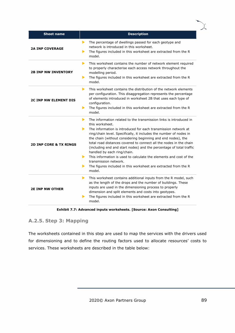
2020© Axon Partners Group 89
Sheet name Description
2A INP COVERAGE
The percentage of dwellings passed for each geotype and
network is introduced in this worksheet.
The figures included in this worksheet are extracted from the R
model.
2B INP NW INVENTORY
This worksheet contains the number of network element required
to properly characterise each access network throughout the
modelling period.
The figures included in this worksheet are extracted from the R
model.
2C INP NW ELEMENT DIS
This worksheet contains the distribution of the network elements
per configuration. This disaggregation represents the percentage
of elements introduced in worksheet 2B that uses each type of
configuration.
The figures included in this worksheet are extracted from the R
model.
2D INP CORE & TX RINGS
The information related to the transmission links is introduced in
this worksheet.
The information is introduced for each transmission network at
ring/chain level. Specifically, it includes the number of nodes in
the chain (without considering beginning and end nodes), the
total road distances covered to connect all the nodes in the chain
(including end and start nodes) and the percentage of total traffic
handled by each ring/chain.
This information is used to calculate the elements and cost of the
transmission network.
The figures included in this worksheet are extracted from the R
model.
2E INP NW OTHER
This worksheet contains additional inputs from the R model, such
as the length of the drops and the number of buildings. These
inputs are used in the dimensioning process to properly
dimension and split elements and costs into geotypes.
The figures included in this worksheet are extracted from the R
model.
Exhibit 7.7: Advanced inputs worksheets. [Source: Axon Consulting]
A.2.5. Step 3: Mapping
The worksheets contained in this step are used to map the services with the drivers used
for dimensioning and to define the routing factors used to allocate resources’ costs to
services. These worksheets are described in the table below:

2020© Axon Partners Group 90
Sheet name Description
3A MAP DRIVERS
Relationships between services and dimensioning drivers for the
different networks.
It must be noted that in order to obtain the drivers it is necessary
to indicate which services are related to them. It should also be
noted that a service is generally assigned to more than one
driver as drivers represent traffic in a particular point of the
network.
3B MAT DRIVERS
This worksheet calculates a relationship matrix between services
and drivers based on the mappings defined in worksheet "3A MAP
DRIVERS".
3C MAP ROUTING
FACTORS
This worksheet defines the relationships between services and
resources by means of the routing factors.
A Routing Factor is a measure of how many times a resource is
used by a specific service during its provision. Hence, the more
traffic a service generates, the higher the cost will be charged
from the asset considered; and the higher utilisation of the asset,
the higher cost taken.
3D MAT ROUTING
FACTORS
This worksheet calculates a relationship matrix between services
and resources based on the mappings defined in worksheet "3C
MAP ROUTING FACTORS".
3E MAP WEIGHTS
This worksheet includes the weights to be considered when
converting the demand introduced in worksheet “1A INP
DEMAND” into the drivers defined in worksheet “0D PAR
DRIVERS”.
Exhibit 7.8: Mapping worksheets [Source: Axon Consulting]
A.2.6. Step 4: Drivers and demand factors
The worksheets contained in this step are used to calculate the drivers that will be used
for the dimensioning of the network and the demand factors used for the allocation of the
resources costs to services. These worksheets are described in the table below:
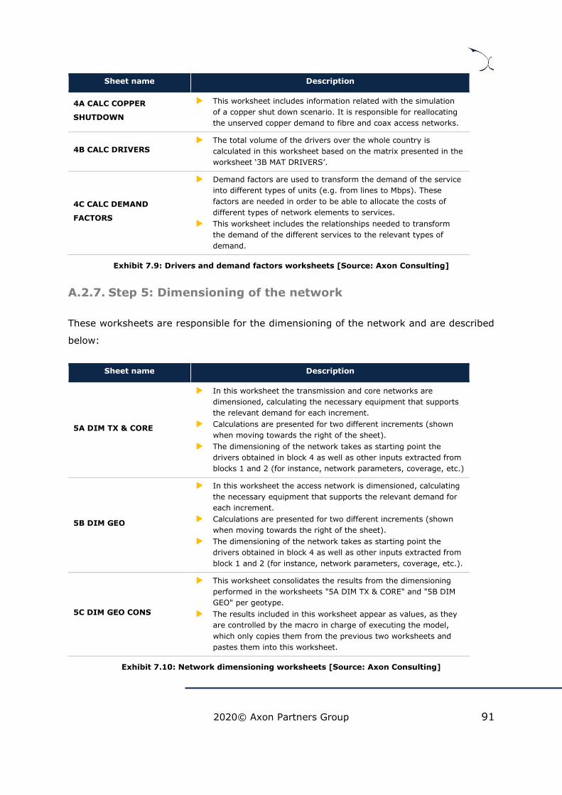
2020© Axon Partners Group 91
Sheet name Description
4A CALC COPPER
SHUTDOWN
This worksheet includes information related with the simulation
of a copper shut down scenario. It is responsible for reallocating
the unserved copper demand to fibre and coax access networks.
4B CALC DRIVERS
The total volume of the drivers over the whole country is
calculated in this worksheet based on the matrix presented in the
worksheet ‘3B MAT DRIVERS’.
4C CALC DEMAND
FACTORS
Demand factors are used to transform the demand of the service
into different types of units (e.g. from lines to Mbps). These
factors are needed in order to be able to allocate the costs of
different types of network elements to services.
This worksheet includes the relationships needed to transform
the demand of the different services to the relevant types of
demand.
Exhibit 7.9: Drivers and demand factors worksheets [Source: Axon Consulting]
A.2.7. Step 5: Dimensioning of the network
These worksheets are responsible for the dimensioning of the network and are described
below:
Sheet name Description
5A DIM TX & CORE
In this worksheet the transmission and core networks are
dimensioned, calculating the necessary equipment that supports
the relevant demand for each increment.
Calculations are presented for two different increments (shown
when moving towards the right of the sheet).
The dimensioning of the network takes as starting point the
drivers obtained in block 4 as well as other inputs extracted from
blocks 1 and 2 (for instance, network parameters, coverage, etc.)
5B DIM GEO
In this worksheet the access network is dimensioned, calculating
the necessary equipment that supports the relevant demand for
each increment.
Calculations are presented for two different increments (shown
when moving towards the right of the sheet).
The dimensioning of the network takes as starting point the
drivers obtained in block 4 as well as other inputs extracted from
block 1 and 2 (for instance, network parameters, coverage, etc.).
5C DIM GEO CONS
This worksheet consolidates the results from the dimensioning
performed in the worksheets "5A DIM TX & CORE" and "5B DIM
GEO" per geotype.
The results included in this worksheet appear as values, as they
are controlled by the macro in charge of executing the model,
which only copies them from the previous two worksheets and
pastes them into this worksheet.
Exhibit 7.10: Network dimensioning worksheets [Source: Axon Consulting]

2020© Axon Partners Group 92
A.2.8. Step 6: Resource Costing
This step contains the worksheets related with the costing of resources. A description of
these worksheets is provided in the following table:
Sheet name Description
6A CALC RES CONS This worksheet consolidates the total number of resources for the
access and core networks at a national level.
6B CALC RES UNIT COST
This worksheet consolidates the unit costs of the resources and
calculates the different unit cost (both CapEx and OpEx) of the
resources throughout the modelling period, considering the unit
costs and their trend.
6C CALC TILTED This worksheet calculates the total CapEx and OpEx under the
tilted annuities methodology.
6D CALC ECO DEP This worksheet calculates the total CapEx and OpEx under the
Economic Depreciation methodology
6E CALC INCR-COM COST
This worksheet calculates the total Incremental and Common
cost for each network element in the network. Additionally, the
cost overheads of the network -such as G&A, IT or wholesale
costs- are calculated in this worksheet
6F CALC ANC SERV COST
This worksheet calculates the costs of the activities from the
ancillary services considering the salary and salary trends
included in sheet ‘1E INP ANCILLARY SERV’.
Exhibit 7.11: Resource costing worksheets [Source: Axon Consulting]
A.2.9. Step 7: Allocation of costs
This step contains the worksheets that are responsible for allocating the costs from the
resources to the services. They are described below:
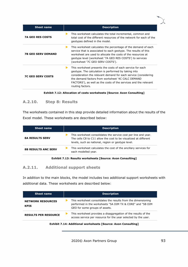
2020© Axon Partners Group 93
Sheet name Description
7A GEO RES COSTS
This worksheet calculates the total incremental, common and
total cost of the different resources of the network for each of the
geotypes defined in the model.
7B GEO SERV DEMAND
This worksheet calculates the percentage of the demand of each
service that is associated to each geotype. The results of this
worksheet are used to allocate the costs of the resources at
geotype level (worksheet ‘7A GEO RES COSTS’) to services
(worksheet ‘7C GEO SERV COSTS’).
7C GEO SERV COSTS
This worksheet presents the costs of each service for each
geotype. The calculation is performed by taking into
consideration the relevant demand for each service (considering
the demand factors from worksheet ‘4C CALC DEMAND
FACTORS’), as well as the costs of the services and the relevant
routing factors.
Exhibit 7.12: Allocation of costs worksheets [Source: Axon Consulting]
A.2.10. Step 8: Results
The worksheets contained in this step provide detailed information about the results of the
Excel model. These worksheets are described below:
Sheet name Description
8A RESULTS SERV
This worksheet consolidates the service cost per line and year.
The cells C8 to C11 allow the cost to be visualized at different
levels, such as national, region or geotype level.
8B RESULTS ANC SERV This worksheet calculates the cost of the ancillary services for
each modelled year.
Exhibit 7.13: Results worksheets [Source: Axon Consulting]
A.2.11. Additional support sheets
In addition to the main blocks, the model includes two additional support worksheets with
additional data. These worksheets are described below:
Sheet name Description
NETWORK RESOURCES
KPIS
This worksheet consolidates the results from the dimensioning
performed in the worksheets "5A DIM TX & CORE" and "5B DIM
GEO for some groups of assets.
RESULTS PER RESOURCE This worksheet provides a disaggregation of the results of the
access service per resource for the year selected by the user.
Exhibit 7.14: Additional worksheets [Source: Axon Consulting]

2020© Axon Partners Group 94
A.3. Understanding the control panel
The control panel represents the main interface between the user and the model, and it is
presented in the “COVER” page. It is used to select the model’s key inputs and
methodological options, to configure the execution mode and to run the model. The
following figure shows a snapshot of the control panel.
Exhibit 7.15: Snapshot of the control panel [Source: Axon Consulting]
The control panel is divided into the following blocks:
Execution Panel
Input scenario
Results overview
These three blocks are described in the following paragraphs.
Important warning: the model needs to be run to see the impact on the results
of any change made in the control panel.
LRAIC Model for Fixed Networks
Control panel
Execution mode Full execution
Execution time 04:53 1
Input scenarios
Demand scenario Base case
selected.demand.scenario
Copper shutdown year 2.030
selected.copper.shutdown GENERAL CHECK
Annualisation of copper shut-down costs GRC annualised within active years OKselection.annualisation.copper.shutdown
% of fully depreciated assets for copper 50%
selection.fully.depreciated.percentage.copper
% of fully depreciated assets for coax -
selection.fully.depreciated.percentage.coax
Annualisation methodology Economic Depreciation
selection.annualisation.method
WACC 4,54%
input.wacc
Risk premium -
input.risk.premium
Year where risk premium starts 2.005 1
input.risk.premium.year
Consider productivity factor? Yes
selection.productivity.factor
RUN
UPDATE
KPIs
CONTENTS
MAP

2020© Axon Partners Group 95
A.3.1. Execution Panel
The Execution Panel displays information regarding the status and progress of the
execution of the model. The following information is shown in this Panel:
Execution mode: It displays the execution mode to be selected. The two options
available are:
• Full execution: The model is completely executed. It takes roughly 4 minutes,
depending on the computer.
• Costing only: The model is run from block 6 (included) onwards. This mode
becomes handy to assess the impact of different costing scenarios when the
number of resources is not expected to change. It takes roughly 2 minutes,
depending on the computer.
• Only regulated areas: The model is run from block 6 (included) onwards. In this
mode, the model performs the costing algorithms only for the geotypes that are
regulated. It takes roughly 2 minutes, depending on the computer.
To obtain the relevant results for the whole network of the operator of the model should
be run in the “Full execution mode”. This includes the results for broadband traffic
services14 for fibre and coax networks. Meanwhile, to obtain the most accurate results
for fibre and coax access services15 in the regulated areas, the model should be run in
the “Only regulated areas”.
Therefore, in order to calculate the complete unit cost for fibre and coax BSA services
in regulated areas, the user shall add the following components: i) The access
component run under the “Only regulated areas” mode and ii) the broadband
component run in the “Full execution” mode.
Execution Time: It displays the duration of the current (or last) model execution.
The execution panel also includes a number of buttons:
RUN: Press this button to launch the execution of the model.
14 Including all “Broadband.Fibre” and “Broadband.Coax” services.
15 Including all “Access.Fibre” and “Access.Coaxial” services.

2020© Axon Partners Group 96
UPDATE KPIs: Press this button to load the KPIs from the R model. When this button
is pressed Excel will prompt a window where the user is requested to select the file
generated by the R model (in case a wrong file is selected the excel will display an
error message).
CONTENTS: Quick link towards the “CONTENTS” worksheet
MAP: Quick link towards the “MAP” worksheet
GENERAL CHECK: It shows an “OK” when no errors are registered in the last
execution and a “Review worksheets” when issues have been found.
A.3.2. Input scenarios
The input scenarios panel includes up to nine options that may be adjusted to tailor the
execution of the model to the user’s objectives. These options are:
Demand scenario: Allows the user to select different demand scenarios that may be
defined in worksheet ‘1A INP DEMAND’.
Copper shutdown year: Allows the user to select the year of the copper shutdown.
Annualization of copper shut-down costs: This option allows the user to select
how copper access costs should be annualized if the network is shut down before 2035.
Percentage of Fully depreciated Assets for Copper. The user may select what
percentage of the GBV for copper networks of the modelled operator correspond to
fully depreciated assets.
Percentage of Fully depreciated Assets for Coax. The user may select what
percentage of the GBV for Coax networks of the modelled operator correspond to fully
depreciated assets.
Annualization methodology: This parameter allows the user to select its desired
annualization methodology (tilted annuities or economic depreciation).
WACC (Weighted Average Cost of Capital): This parameter represents the average
minimum remuneration required for the capital employed. The WACC is employed for
the calculation of the cost of capital associated to fixed investments. A percentage
must be introduced by the user.
Risk premium: This parameter allows the consideration of an additional risk premium
for fibre access network elements.
2020© Axon Partners Group 97
Year where risk premium starts: Allows the user to define the year upon which the
risk premium should be considered in the model.
Consider productivity factor?: This option allows the user to select whether a
productivity factor on human workforce should be considered.
A.3.3. Results overview
This panel allows the user to display the results of three different services, based on his
selection of the following items:
Service: Select a service from the list of services introduced in the model.
Geotype:
• Region: Hovedstaden, Sjælland, Syddanmark, Midtjylland, Nordjylland or all
• Degree or Urbanisation: URBAN, SUBURBAN, RURAL or all
• Type of building: Single-Dwelling, Multi-Dwelling or all
• Regulated areas: Regulated, Not-Regulated or all
Please, note that the results generated by this chart for the different regions or
regulatory status are only indicative, in order to obtain the relevant results for
regulated areas only, the model should be run in execution model “Only regulated
areas”.
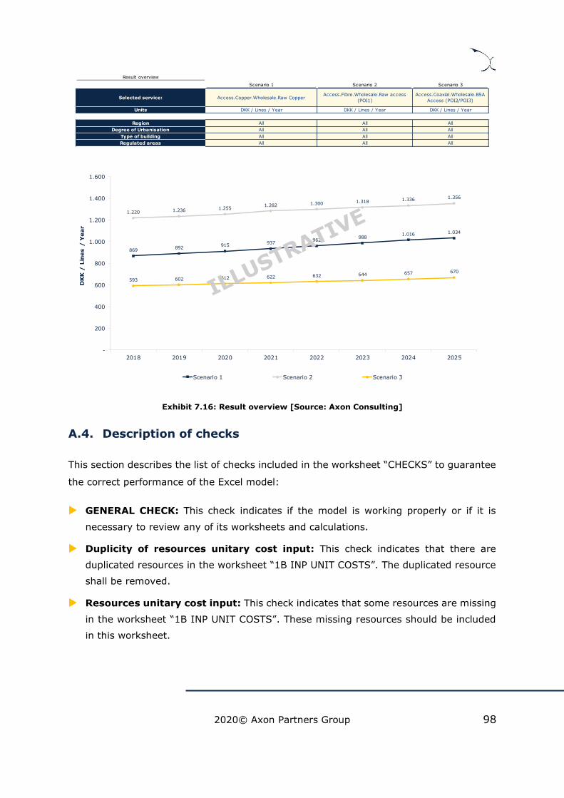
2020© Axon Partners Group 98
Exhibit 7.16: Result overview [Source: Axon Consulting]
A.4. Description of checks
This section describes the list of checks included in the worksheet “CHECKS” to guarantee
the correct performance of the Excel model:
GENERAL CHECK: This check indicates if the model is working properly or if it is
necessary to review any of its worksheets and calculations.
Duplicity of resources unitary cost input: This check indicates that there are
duplicated resources in the worksheet “1B INP UNIT COSTS”. The duplicated resource
shall be removed.
Resources unitary cost input: This check indicates that some resources are missing
in the worksheet “1B INP UNIT COSTS”. These missing resources should be included
in this worksheet.
Result overview
Scenario 1 Scenario 2 Scenario 3
Selected service: Access.Copper.Wholesale.Raw CopperAccess.Fibre.Wholesale.Raw access
(POI1)
Access.Coaxial.Wholesale.BSA
Access (POI2/POI3)
Units DKK / Lines / Year DKK / Lines / Year DKK / Lines / Year
Region All All All
Degree of Urbanisation All All All
Type of building All All All
Regulated areas All All All
869892
915937
962988
1.016 1.034
1.220 1.236 1.2551.282 1.300 1.318 1.336 1.356
593 602 612 622 632 644 657 670
-
200
400
600
800
1.000
1.200
1.400
1.600
2018 2019 2020 2021 2022 2023 2024 2025
DK
K /
Lin
es /
Ye
ar
Scenario 1 Scenario 2 Scenario 3

2020© Axon Partners Group 99
Invalid name of resource: This check indicates that the name of a resource included
in the worksheet “1B INP UNIT COSTS” is not correct and therefore, it should be
adjusted.
Time Period: This check indicates that the time period used in the model fits into the
excel tables considered and thus allows a correct calculation.
Implementation of Economic Depreciation: This check verifies that the sum of the
depreciation and cost of capital charges obtained after calculating the economic
depreciation is equal to the NPV of the resources depreciated.
Calculation of resource costs at geotype level: This check indicates if there is any
mistake in the allocations performed in the worksheet ‘7A GEO RES COSTS’.
Calculation of service costs at geotype level: This check indicates if there is any
mistake in the allocations performed in the worksheet ‘7C GEO SERV COSTS’.
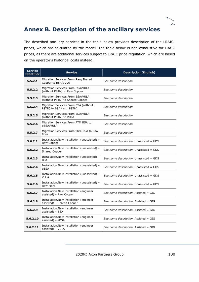
2020© Axon Partners Group 100
Annex B. Description of the ancillary services
The described ancillary services in the table below provides description of the LRAIC-
prices, which are calculated by the model. The table below is non-exhaustive for LRAIC
prices, as there are additional services subject to LRAIC price regulation, which are based
on the operator’s historical costs instead.
Service Identifier
Service Description (English)
5.5.2.1 Migration Services.From Raw/Shared Copper to BSA/VULA
See name description
5.5.2.2 Migration Services.From BSA/VULA (without PSTN) to Raw Copper
See name description
5.5.2.3 Migration Services.From BSA/VULA (without PSTN) to Shared Copper
See name description
5.5.2.4 Migration Services.From BSA (without PSTN) to BSA (with PSTN)
See name description
5.5.2.5 Migration Services.From BSA/VULA (without PSTN) to VULA
See name description
5.5.2.6 Migration Services.From ATM BSA to eBSA/VULA
See name description
5.5.2.7 Migration Services.From fibre BSA to Raw fibre
See name description
5.6.2.1 Installation.New installation (unassisted) – Raw Copper
See name description. Unassisted = GDS
5.6.2.2 Installation.New installation (unassisted) – Shared Copper
See name description. Unassisted = GDS
5.6.2.3 Installation.New installation (unassisted) – BSA
See name description. Unassisted = GDS
5.6.2.4 Installation.New installation (unassisted) – eBSA
See name description. Unassisted = GDS
5.6.2.5 Installation.New installation (unassisted) – VULA
See name description. Unassisted = GDS
5.6.2.6 Installation.New installation (unassisted) –
Raw Fibre See name description. Unassisted = GDS
5.6.2.7 Installation.New installation (engineer assisted) – Raw Copper
See name description. Assisted = GIG
5.6.2.8 Installation.New installation (engineer assisted) – Shared Copper
See name description. Assisted = GIG
5.6.2.9 Installation.New installation (engineer assisted) – BSA
See name description. Assisted = GIG
5.6.2.10 Installation.New installation (engineer assisted) – eBSA
See name description. Assisted = GIG
5.6.2.11 Installation.New installation (engineer assisted) – VULA
See name description. Assisted = GIG

2020© Axon Partners Group 101
Service Identifier
Service Description (English)
5.6.2.12 Installation.New installation (engineer assisted) – Raw Fibre
See name description. Assisted = GIG
5.7.2.1 Additional Services.NTP One time setup of KAP-stik/NTP. To be paid if installation of KAP-stik/NTP is needed when activating the connection
5.7.2.2 Additional Services.NTP incl. Drilling
To be paid when a technician, in continuation of a GIG installation, drills through the outer wall and threads a cable through to finish the setup by installing a NTP
5.7.2.3 Additional Services.Physical rearrangement
To be paid upon rearrangement from one copper/fiber pair to another. Not to be paid if the raw copper connection is only used for PSTN or ISDN2
5.7.2.4 Additional Services.Change of trunk number
To be paid when a change of trunk number is requested
5.7.2.5 Additional Services.Visit by technician "Time and material"-charge for technician time per hour within normal working hours.
5.7.2.6 Additional Services.Unproductive visit (Technician)
To be paid in case the technician cannot get access to the installation, e.g. due to the end user not being home
5.7.2.7 Additional Services.Cancellation-fee II
TDC is entitled to a cancellation fee, if the customer cancels the raw copper/fiber line after receipient of order confirmation from TDC's customer service and until 12.00 on the working day before deliverance day. Cancellations after this deadline are to be regarded as regular termination. Also to be paid if the order after visitation cannot be followed through due to erroneous information from the customer.
A new order would be necessary for installing raw fiber/copper and will be paid in ordance with normal orders.
5.7.2.8 Additional Services.Calculation of attenuation on the line
Calculation of attenuation/150 kHz. To be paid when calculation of attenuation is wanted
5.7.2.9 Additional Services.Unproductive fault handling
To be paid for unjustified or unsuccessful fault handling. In case TDC after attempt of fault handling can render probable that the reported fault is not due to TDC's circumstances.
5.7.2.10 Additional Services.Change of speed One time fee for changing speeds on BSA products
5.7.2.11 Additional Services.Installation of Multichannel
Setup fee for installation of multichannel, per channel
5.7.2.12 Additional Services.Reactivated installation (unassisted)
Reactivation of installation. Same price as regular Installation fee w/o technician assistance (GDS) for Copper BSA and VULA
5.7.2.13 Additional Services.Reactivated installation (engineer assisted)
Reactivation of installation. Same price as regular Installation fee with technician assistance (GIG) for Copper BSA and VULA
5.7.2.14 Additional Services.Conversion from BSA online to BSA without co-production
Surcharge for converting to VULA/BSA without co-production
5.7.2.15 Additional Services.Re-establishing trunks To be paid in case of re-establishing of trunks after TDC's bypass connection on CO, due to an error in operator's equipment
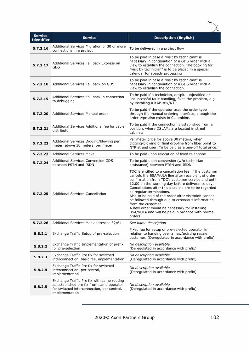
2020© Axon Partners Group 102
Service Identifier
Service Description (English)
5.7.2.16 Additional Services.Migration of 30 or more connections in a project
To be delivered in a project flow
5.7.2.17 Additional Services.Fall back Express on GDS
To be paid in case a "visit by technician" is necessary in continuation of a GDS order with a view to establish the connection. The booking for "visit by technician" is to be placed in a special calendar for speedy processing
5.7.2.18 Additional Services.Fall back on GDS To be paid in case a "visit by technician" is necessary in continuation of a GDS order with a view to establish the connection.
5.7.2.19 Additional Services.Fall back in connection to debugging
To be paid if a technician, despite unjustified or unsuccessful fault handling, fixes the problem, e.g. by installing a KAP-stik/NTP
5.7.2.20 Additional Services.Manual order To be paid if the operator uses the order type through the manual ordering interface, altough the order type also exists in Columbine.
5.7.2.21 Additional Services.Additional fee for cable distributor
To be paid if the connection is established from a position, where DSLAMs are located in street cabinets
5.7.2.22 Additional Services.Digging/blowing per meter, above 30 meters, per meter
Per meter price for above 30 meters, when digging/blowing of final dropline from fiber point to NTP at end user. To be paid as a one-off total price.
5.7.2.23 Additional Services.Move To be paid upon relocation of fixed telephone
5.7.2.24 Additional Services.Conversion GDS between PSTN and ISDN
To be paid upon conversion (w/o technician assistance) between PTSN and ISDN
5.7.2.25 Additional Services.Cancellation
TDC is entitled to a cancellation fee, if the customer cancels the BSA/VULA line after receipient of order confirmation from TDC's customer service and until 12.00 on the working day before deliverance day. Cancellations after this deadline are to be regarded as regular terminations. Also to be paid of the order after visitation cannot be followed through due to erroneous information from the customer. A new order would be necessary for installing BSA/VULA and will be paid in ordance with normal orders
5.7.2.26 Additional Services.Mac addresses 32/64 See name description
5.8.2.1 Exchange Traffic.Setup of pre-selection Fixed fee for setup of pre-selected operator in relation to handing over a new/existing resale customer. (Deregulated in accordance with prefix)
5.8.2.2 Exchange Traffic.Implementation of prefix for pre-selection
No description available (Deregulated in accordance with prefix)
5.8.2.3 Exchange Traffic.Pre fix for switched interconnection, basic fee, implementation
No description available (Deregulated in accordance with prefix)
5.8.2.4 Exchange Traffic.Pre fix for switched interconnection, per central, implementation
No description available (Deregulated in accordance with prefix)
5.8.2.5
Exchange Traffic.Pre fix with same routing as established pre fix from same operator for switched interconnection, per central, implementation
No description available (Deregulated in accordance with prefix)
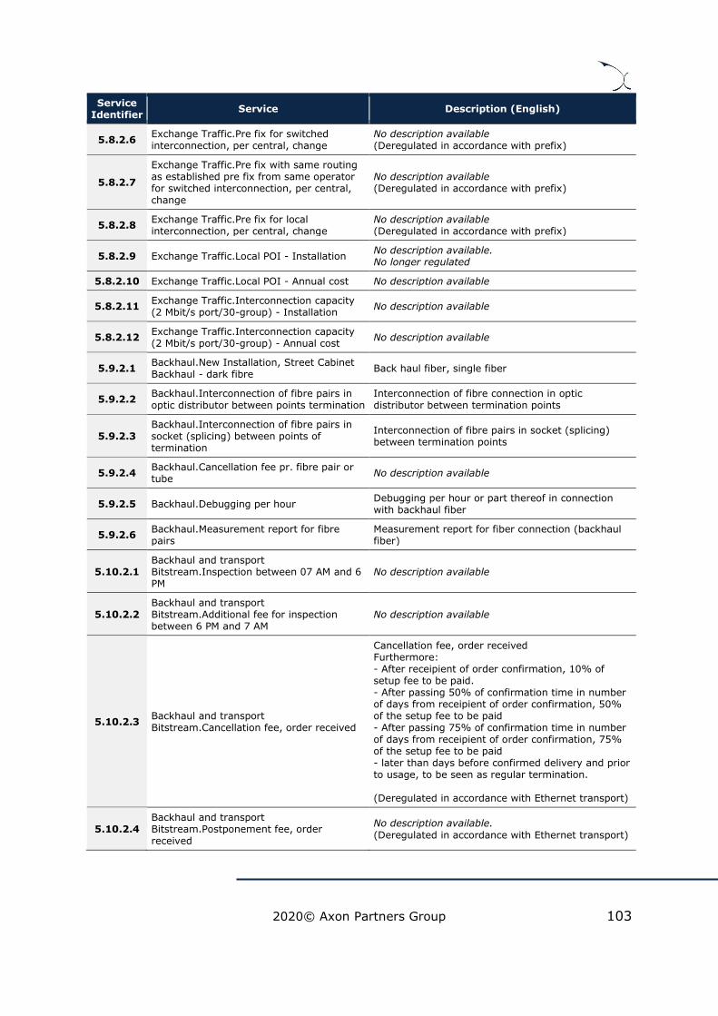
2020© Axon Partners Group 103
Service Identifier
Service Description (English)
5.8.2.6 Exchange Traffic.Pre fix for switched interconnection, per central, change
No description available (Deregulated in accordance with prefix)
5.8.2.7
Exchange Traffic.Pre fix with same routing as established pre fix from same operator for switched interconnection, per central, change
No description available (Deregulated in accordance with prefix)
5.8.2.8 Exchange Traffic.Pre fix for local interconnection, per central, change
No description available (Deregulated in accordance with prefix)
5.8.2.9 Exchange Traffic.Local POI - Installation No description available. No longer regulated
5.8.2.10 Exchange Traffic.Local POI - Annual cost No description available
5.8.2.11 Exchange Traffic.Interconnection capacity (2 Mbit/s port/30-group) - Installation
No description available
5.8.2.12 Exchange Traffic.Interconnection capacity (2 Mbit/s port/30-group) - Annual cost
No description available
5.9.2.1 Backhaul.New Installation, Street Cabinet Backhaul - dark fibre
Back haul fiber, single fiber
5.9.2.2 Backhaul.Interconnection of fibre pairs in optic distributor between points termination
Interconnection of fibre connection in optic distributor between termination points
5.9.2.3 Backhaul.Interconnection of fibre pairs in socket (splicing) between points of termination
Interconnection of fibre pairs in socket (splicing) between termination points
5.9.2.4 Backhaul.Cancellation fee pr. fibre pair or tube
No description available
5.9.2.5 Backhaul.Debugging per hour Debugging per hour or part thereof in connection with backhaul fiber
5.9.2.6 Backhaul.Measurement report for fibre pairs
Measurement report for fiber connection (backhaul fiber)
5.10.2.1 Backhaul and transport Bitstream.Inspection between 07 AM and 6 PM
No description available
5.10.2.2 Backhaul and transport Bitstream.Additional fee for inspection between 6 PM and 7 AM
No description available
5.10.2.3 Backhaul and transport Bitstream.Cancellation fee, order received
Cancellation fee, order received Furthermore: - After receipient of order confirmation, 10% of setup fee to be paid. - After passing 50% of confirmation time in number of days from receipient of order confirmation, 50% of the setup fee to be paid - After passing 75% of confirmation time in number of days from receipient of order confirmation, 75% of the setup fee to be paid - later than days before confirmed delivery and prior to usage, to be seen as regular termination. (Deregulated in accordance with Ethernet transport)
5.10.2.4 Backhaul and transport Bitstream.Postponement fee, order received
No description available.
(Deregulated in accordance with Ethernet transport)

2020© Axon Partners Group 104
Service Identifier
Service Description (English)
5.10.2.5 Backhaul and transport Bitstream.Postponement fee, later than one week before confirmed delivery
No description available. (Deregulated in accordance with Ethernet transport)
5.10.2.6 Backhaul and transport Bitstream.Postponement fee, at point of delivery
At the time of delivery, in addition payment of quarterly rent will also be charged. (Deregulated in accordance with Ethernet transport)
5.10.2.7 Backhaul and transport Bitstream.Unwarranted claim for debugging, transmission
Payment for unproductive or unwarranted error handling, unless otherwise stated in bilateral agreement. (Deregulated in accordance with Ethernet transport)
5.11.2.1 Colocation.Shelf incl. part of the tripod – Installation
One rack section BxDxH = 600x300x400/600x600x400.
5.11.2.2 Colocation.Shelf incl. part of the tripod – Annual cost
One rack section BxDxH = 600x300x400/600x600x400.
5.11.2.3 Colocation.Rack space (1.5 m 2) - Installation
See name description
5.11.2.4 Colocation.Rack space (1.5 m 2) – Annual cost
See name description
5.11.2.5 Colocation.Installation of VAC or VDC power equipment
Installation fee for the power equipments of 5.11.2.6 - 5.11.2.12
5.11.2.6 Colocation.Annual Cost (1 * 48 VCD 16 A 100W)
See name description. Includes usage
5.11.2.7 Colocation.Annual Cost (1 * 48 VCD 16 A 200W)
See name description. Includes usage
5.11.2.8 Colocation.Annual Cost (1 * 48 VCD 16 A 500W)
See name description. Includes usage
5.11.2.9 Colocation.Annual Cost (1 * 48 VDC 30 A) See name description. Includes usage
5.11.2.10 Colocation.Annual Cost (1 * 48 VDC 60 A) See name description. Includes usage
5.11.2.11 Colocation.Annual Cost (1 * 230 VAC 10 A) See name description. Includes usage
5.11.2.12 Colocation.Annual Cost (1 * 230 VAC 10 A service socket)
See name description. Includes usage
5.11.2.13 Colocation.Shift to another power-product One-off fee for migration to another power outlet
5.11.2.14 Colocation.Supervised access Hourly charge rate for supervised access without prior notification, i.e. immediate assistance, during day-time.
5.11.2.15 Colocation.Inquiry
To be paid upon ordering investigations for the possiblity of co-locating technician houses in the central office. The payment will be refunded, if a contract is signed based on offer
5.11.2.16 Colocation.Co-location in technical house Submission of offer on co-locating technician houses in the central office
5.11.2.17 Colocation.Trunk cables PDS 2*cat.5 Installation
No description available (No longer supplied by TDC)
5.11.2.18 Colocation.Trunk cables PDS 2*cat.5 per 10 m
No description available (No longer supplied by TDC)
5.11.2.19 Colocation.Trunk cables PDS 10*cat.5 Installation
No description available (No longer supplied by TDC)
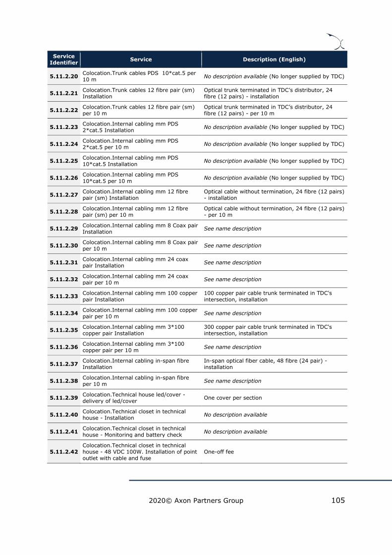
2020© Axon Partners Group 105
Service Identifier
Service Description (English)
5.11.2.20 Colocation.Trunk cables PDS 10*cat.5 per 10 m
No description available (No longer supplied by TDC)
5.11.2.21 Colocation.Trunk cables 12 fibre pair (sm) Installation
Optical trunk terminated in TDC’s distributor, 24 fibre (12 pairs) - installation
5.11.2.22 Colocation.Trunk cables 12 fibre pair (sm) per 10 m
Optical trunk terminated in TDC’s distributor, 24 fibre (12 pairs) - per 10 m
5.11.2.23 Colocation.Internal cabling mm PDS 2*cat.5 Installation
No description available (No longer supplied by TDC)
5.11.2.24 Colocation.Internal cabling mm PDS 2*cat.5 per 10 m
No description available (No longer supplied by TDC)
5.11.2.25 Colocation.Internal cabling mm PDS 10*cat.5 Installation
No description available (No longer supplied by TDC)
5.11.2.26 Colocation.Internal cabling mm PDS
10*cat.5 per 10 m No description available (No longer supplied by TDC)
5.11.2.27 Colocation.Internal cabling mm 12 fibre pair (sm) Installation
Optical cable without termination, 24 fibre (12 pairs) - installation
5.11.2.28 Colocation.Internal cabling mm 12 fibre pair (sm) per 10 m
Optical cable without termination, 24 fibre (12 pairs) - per 10 m
5.11.2.29 Colocation.Internal cabling mm 8 Coax pair Installation
See name description
5.11.2.30 Colocation.Internal cabling mm 8 Coax pair per 10 m
See name description
5.11.2.31 Colocation.Internal cabling mm 24 coax pair Installation
See name description
5.11.2.32 Colocation.Internal cabling mm 24 coax pair per 10 m
See name description
5.11.2.33 Colocation.Internal cabling mm 100 copper
pair Installation
100 copper pair cable trunk terminated in TDC's
intersection, installation
5.11.2.34 Colocation.Internal cabling mm 100 copper pair per 10 m
See name description
5.11.2.35 Colocation.Internal cabling mm 3*100 copper pair Installation
300 copper pair cable trunk terminated in TDC's intersection, installation
5.11.2.36 Colocation.Internal cabling mm 3*100 copper pair per 10 m
See name description
5.11.2.37 Colocation.Internal cabling in-span fibre Installation
In-span optical fiber cable, 48 fibre (24 pair) - installation
5.11.2.38 Colocation.Internal cabling in-span fibre per 10 m
See name description
5.11.2.39 Colocation.Technical house led/cover - delivery of led/cover
One cover per section
5.11.2.40 Colocation.Technical closet in technical house - Installation
No description available
5.11.2.41 Colocation.Technical closet in technical house - Monitoring and battery check
No description available
5.11.2.42 Colocation.Technical closet in technical house - 48 VDC 100W. Installation of point outlet with cable and fuse
One-off fee

2020© Axon Partners Group 106
Service Identifier
Service Description (English)
5.11.2.43 Colocation.Technical closet in technical house - 48 VDC 100W. Each year inclu. Utilities
One 48 VDC outlet incl. usage (100 W)
5.11.2.44 Colocation.Delivery and installation of DSL closet without co-production
No description available (Deregulated in accordance with sub-loops on copper)
5.11.2.45 Colocation.Delivery and installation of DSL closet with co-production
No description available (Deregulated in accordance with sub-loops on copper)
5.11.2.46 Colocation.230 VAC, 4A supply incl. Fuse and monitoring device
No description available (Deregulated in accordance with sub-loops on copper)
5.11.2.47 Colocation.1x100 pair cables and fibre trunk incl. Digging and termination of 1x100 copper pairs and 4 fibres
No description available (Deregulated in accordance with sub-loops on copper)
5.11.2.48 Colocation.1x100 pair cable with termination at TDC
No description available (Deregulated in accordance with sub-loops on copper)
5.11.2.49 Colocation.Fibre trunk with termination of 4 fibres i distributor at TDC
Delivery of only fiber trunk with termination of 4 fibres in TDC's distributor. Both co-location and co-production. Maximum 10 meter, lengths above this requires tender offer
5.11.2.50 Colocation.Fibre trunk with termination of 4 fibres in socket (splicing) at TDC
Delivery of only fiber trunk with termination of 4 fibres in TDC's socket (splicing). Both co-location and co-production. Maximum 10 meter, lengths above this requires tender offer
5.11.2.51 Colocation.Hourly rate for re-registration of co-location, e.g. from quarterly to monthly payment of rent
No description available
Exhibit 7.17: Description of the ancillary services [Source: Axon Consulting]
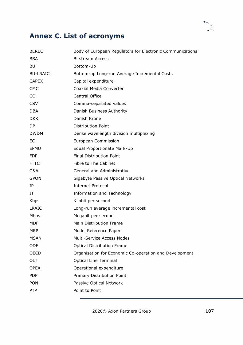
2020© Axon Partners Group 107
Annex C. List of acronyms
BEREC Body of European Regulators for Electronic Communications
BSA Bitstream Access
BU Bottom-Up
BU-LRAIC Bottom-up Long-run Average Incremental Costs
CAPEX Capital expenditure
CMC Coaxial Media Converter
CO Central Office
CSV Comma-separated values
DBA Danish Business Authority
DKK Danish Krone
DP Distribution Point
DWDM Dense wavelength division multiplexing
EC European Commission
EPMU Equal Proportionate Mark-Up
FDP Final Distribution Point
FTTC Fibre to The Cabinet
G&A General and Administrative
GPON Gigabyte Passive Optical Networks
IP Internet Protocol
IT Information and Technology
Kbps Kilobit per second
LRAIC Long-run average incremental cost
Mbps Megabit per second
MDF Main Distribution Frame
MRP Model Reference Paper
MSAN Multi-Service Access Nodes
ODF Optical Distribution Frame
OECD Organisation for Economic Co-operation and Development
OLT Optical Line Terminal
OPEX Operational expenditure
PDP Primary Distribution Point
PON Passive Optical Network
PTP Point to Point

2020© Axon Partners Group 108
SC Street Cabinet
SDP Secondary Distribution Point
SMP Significant Market Power
VoD Video on Demand
VoIP Voice over IP
WACC Weighted Average Cost of Capital

MADRID (HQ)
Sagasta, 18, 3
28004, Madrid
Tel: +34 91 310 2894
Tel: +34 91 310 2894
MEXICO CITY
Torre Mayor Piso 41,Paseo de la
Reforma 505,Cuauhtémoc
Ciudad de México, 06500
Tel: +52 55 68438659
ISTANBUL
Buyukdere Cad. No 255, Nurol
Plaza B 04 Maslak 34450
Tel: +90 212 277 70 47