Automation and Standardization of Measuring Moisture Content and Density of Soil Using the Technique...
139
Purdue University Purdue e-Pubs Joint Transportation Research Program Civil Engineering 1-1998 Automation and Standardization of Measuring Moisture Content and Density of Soil Using the Technique of Time Domain Reflectometry Wei Feng Chih-Ping Lin Richard J. Deschamps Vincent P. Drnevich This document has been made available through Purdue e-Pubs, a service of the Purdue University Libraries. Please contact [email protected] for additional information. Feng, Wei; Lin, Chih-Ping; Deschamps, Richard J.; and Drnevich, Vincent P., "Automation and Standardization of Measuring Moisture Content and Density of Soil Using the Technique of Time Domain Reflectometry" (1998). Joint Transportation Research Program. Paper 27. http://docs.lib.purdue.edu/jtrp/27
Transcript of Automation and Standardization of Measuring Moisture Content and Density of Soil Using the Technique...
Purdue UniversityPurdue e-Pubs
Joint Transportation Research Program Civil Engineering
1-1998
Automation and Standardization of MeasuringMoisture Content and Density of Soil Using theTechnique of Time Domain ReflectometryWei Feng
Chih-Ping Lin
Richard J. Deschamps
Vincent P. Drnevich
This document has been made available through Purdue e-Pubs, a service of the Purdue University Libraries. Please contact [email protected] foradditional information.
Feng, Wei; Lin, Chih-Ping; Deschamps, Richard J.; and Drnevich, Vincent P., "Automation and Standardization of MeasuringMoisture Content and Density of Soil Using the Technique of Time Domain Reflectometry" (1998). Joint Transportation ResearchProgram. Paper 27.http://docs.lib.purdue.edu/jtrp/27
Joint
Transportation
Research
ProgramJTRP
FHWA/IN/JTRP-98/4
Final Report
AUTOMATION AND STANDARDIZATIONOF MEASURING MOISTURE CONTENTAND DENSITY USING TIME DOMAINREFLECTOMETRY
W. Feng
C. Lin
V. P. Drnevich
R J. Deschamps
September 1998
Indiana
Departmentof Transportation
PurdueUniversity

Final Report
FHWA/IN/JTRP-98/4
AUTOMATION AND STANDARDIZATION OF MEASURING MOISTURE CONTENTAND DENSITY USING TIME DOMAIN REFLECTOMETRY
W. Feng
and
C.Lin
Research Assistants
and
V. P. Drnevich
and
R. J. Deschamps
Principal Investigators
School of Civil Engineering
Purdue University
Joint Transportation Research Program
ProjectNo:C-36-5S
File No: 6-6-19
Prepared in Cooperation with the
Indiana Department of Transportation and
the U.S. Department of Transportation
Federal Highway Administration
The contents of this report reflect the views of the authors who are responsible for the facts and
the accuracy of the data presented herein. The contents do not necessarily reflect the official
views or policies of the Federal Highway Administration and the Indiana Department of
Transportation. This report does not constitute a standard, specification or regulation.
Purdue University
West Lafayette, Indiana
September 17, 1998
Digitized by the Internet Archive
in 2011 with funding from
LYRASIS members and Sloan Foundation; Indiana Department of Transportation
http://www.archive.org/details/automationstandaOOfeng
TECHNICAL REPORT STANDARD TITLE PAGE
1. Report No.
FHWA/TN/JTRP-98/4
2. Government Accession No. 3. Recipient's Catalog No.
4. Title and Subtitle
Automation and Standardization ofMeasuring Moisture Content and Density Using Time
Domain Reflectometry
5. Report Date
September 1998
6. Performing Organization Code
7. Authors)
W. Feng, C. Lin, V. P. Drnevich, and R. J. Deschamps8. Performing Organization Report No.
FHWA/IN/JTRP-98/4
9. Performing Organization Name and Address
Joint Transportation Research Program
1284 Civil Engineering Building
Purdue University
West Lafayette, Indiana 47907-1284
10. Work Unit No.
11. Contract or Grant No.
JHRP-018
12. Sponsoring Agency Name and Address
Indiana Department of Transportation
State Office Building
100 North Senate Avenue
Indianapolis, IN 46204
13. Type ofReport and Period Covered
Final Report
14. Sponsoring Agency Code
15. Supplementary Notes
Prepared in cooperation with the Indiana Department of Transportation and Federal Highway Administration.
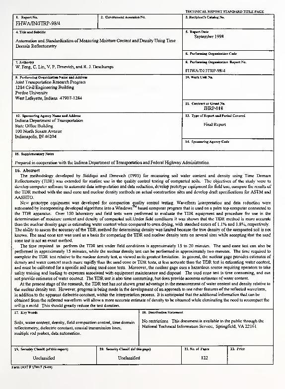
16. Abstract
The methodology developed by Siddiqui and Drnevich (1995) for measuring soil water content and density using Time Domain
Reflectometry (TDR) was extended for routine use in the quality control testing of compacted soils. The objectives of the study were to
develop computer software to automate data interpretation and data reduction, develop prototype equipment for field use, compare the results of
the TDR method with the sand cone and nuclear density methods on actual construction sites and develop draft specifications for ASTM and
AASHTO.New prototype equipment was developed for compaction quality control testing. Waveform interpretation and data reduction were
automated by incorporating developed algorithms into a Windows based computer program that is used on a palm top computer connected to
the TDR apparatus. Over 150 laboratory and field tests were performed to evaluate the TDR equipment and procedure for use in the
determination of moisture content and density of compacted soil.Under field conditions it was shown that the TDR method is more accurate
than the nuclear density gage in estimating water content when compared to oven drying, with standard errors of 1.1% and 1.8%, respectively.
The ability to assess the accuracy of the TDR method for determining density was limited because the true density of the compacted soil is not
known. The sand cone test was used as a basis for comparing the TDR and nuclear density tests on several sites while accepting that the sand
cone test is not an exact method.
The time required to perform the TDR test under field conditions is approximately 1 5 to 20 minutes. The sand cone test can also be
performed in approximately 1 5 minutes, while the nuclear density test can be performed in approximately two minutes. The time required to
complete the TDR test relative to the nuclear density test, is viewed as its greatest limitation. In general, the nuclear gage provides estimates of
density and water content much more rapidly than the sand cone or TDR tests, is less accurate than the TDR test in estimating water content,
and must be calibrated for a specific soil using sand cone tests. Moreover, the nuclear gage uses a hazardous source requiring operators to take
safety training and leading to expenses associated with equipment maintenance and disposal. The sand cone test is time consuming, and can
not provide estimates of water content. The TDR test is also time consuming, but does provide accurate estimates of water content.
At the present stage of the research, the TDR test has not shown great advantage in the measurement of water content and density relative to
the nuclear density test. However, progress is being made in the development of an approach to use other features of the reflected waveform,
in addition to the apparent dielectric constant, within the interpretation process. It is anticipated that the additional information that can be
obtained from the reflected waveform will allow a more accurate estimate of density to be obtained while eliminating the need to recompact the
soil in a mold. This should greatly reduce the test duration.
17. Keywords
Soils, water content, density, field compaction control, time domain
reflectometry, dielectric constant, coaxial transmission lines,
multiple rod probes, data automation.
18. Distribution Statement
No restrictions. This document is available to the public through the
National Technical Information Service, Springfield, VA 22161
19. Security Cbuslf. (of this report)
Unclassified
20. Security Cbusif. (of this page)
Unclassified
21. No. of Pages
122
Form DOT F 1700.7 (8-69)
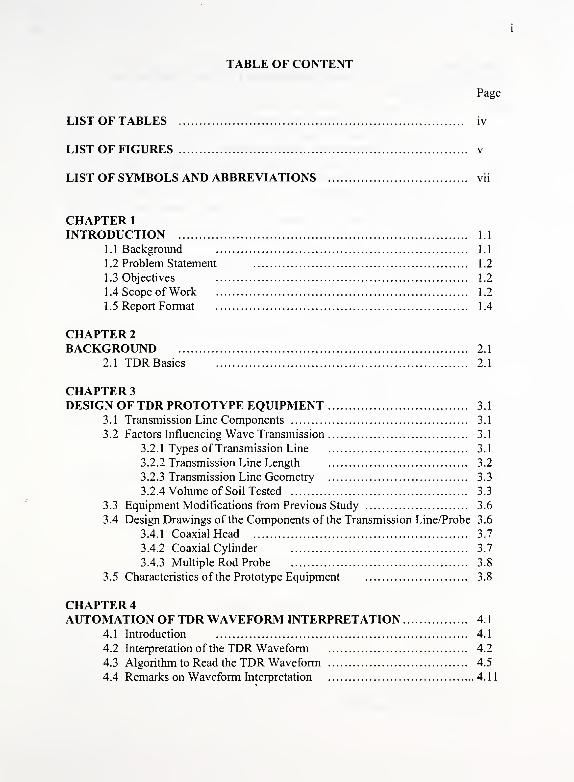
TABLE OF CONTENT
Page
LIST OF TABLES iv
LIST OF FIGURES v
LIST OF SYMBOLS AND ABBREVIATIONS vii
CHAPTER 1
INTRODUCTION 1.1
1 .
1
Background 1.1
1.2 Problem Statement 1.2
1 .3 Objectives 1.2
1.4 Scope of Work 1.2
1.5 Report Format 1.4
CHAPTER 2
BACKGROUND 2.1
2.1 TDRBasics 2.1
CHAPTER 3
DESIGN OF TDR PROTOTYPE EQUIPMENT 3.1
3.1 Transmission Line Components 3.1
3.2 Factors Influencing Wave Transmission 3.1
3.2.1 Types of Transmission Line 3.1
3.2.2 Transmission Line Length 3.2
3.2.3 Transmission Line Geometry 3.3
3.2.4 Volume of Soil Tested 3.3
3.3 Equipment Modifications from Previous Study 3.6
3.4 Design Drawings of the Components of the Transmission Line/Probe 3.6
3.4.1 CoaxialHead 3.7
3.4.2 Coaxial Cylinder 3.7
3.4.3 Multiple Rod Probe 3.8
3.5 Characteristics of the Prototype Equipment 3.8
CHAPTER 4
AUTOMATION OF TDR WAVEFORM INTERPRETATION 4.1
4.1 Introduction 4.1
4.2 Interpretation of the TDR Waveform 4.2
4.3 Algorithm to Read the TDR Waveform 4.5
4.4 Remarks on Waveform Interpretation 4. 1
1
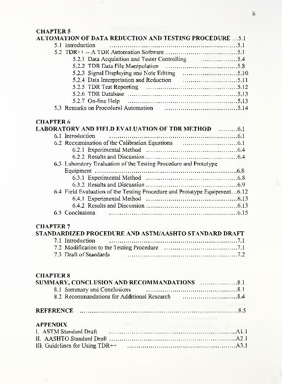
CHAPTER 5
AUTOMATION OF DATA REDUCTION AND TESTING PROCEDURE ...5.1
5 .
1
Introduction 5.1
5.2 TDR++ - A TDR Automation Software 5.1
5.2.1 Data Acquisition and Tester Controlling 5.4
5.2.2 TDR Data File Manipulation 5.8
5.2.3 Signal Displaying and Note Editing 5.10
5.2.4 Data Interpretation and Reduction 5.11
5.2.5 TDR Test Reporting 5.12
5.2.6 TDR Database 5.13
5.2.7 On-line Help 5.13
5.3 Remarks on Procedural Automation 5.14
CHAPTER 6
LABORATORY AND FIELD EVALUATION OF TDR METHOD 6.1
6.
1
Introduction 6.1
6.2 Reexamination of the Calibration Equations 6.1
6.2.
1
Experimental Method 6.4
6.2.2 Results and Discussion 6.4
6.3 Laboratory Evaluation of the Testing Procedure and Prototype
Equipment 6.8
6.3.
1
Experimental Method 6.8
6.3.2 Results and Discussion 6.9
6.4 Field Evaluation of the Testing Procedure and Prototype Equipment... 6. 12
6.4.
1
Experimental Method 6.13
6.4.2 Results and Discussion 6.13
6.5 Conclusions 6.15
CHAPTER 7
STANDARDIZED PROCEDURE AND ASTM/AASHTO STANDARD DRAFT7.
1
Introduction 7.1
7.2 Modification to the Testing Procedure 7.1
7.3 Draft of Standards 7.2
CHAPTER 8
SUMMARY, CONCLUSION AND RECOMMANDATIONS 8.1
8.1 Summary and Conclusions 8.1
8.2 Recommandations for Additional Research 8.4
REFERENCE 8.5
APPENDIXI. ASTM Standard Draft Al.l
II. AASHTO Standard Draft A2.1
III. Guidelines for Using TDR++ A3.1
Ill
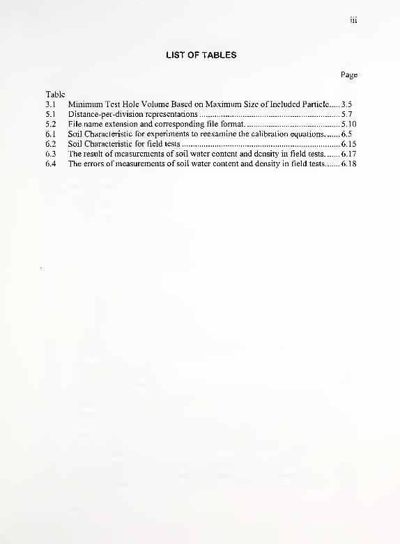
LIST OF TABLES
Page
Table
3.1 Minimum Test Hole Volume Based on Maximum Size of Included Particle 3.5
5.1 Distance-per-division representations 5.7
5.2 File name extension and corresponding file format 5.10
6.1 Soil Characteristic for experiments to reexamine the calibration equations 6.5
6.2 Soil Characteristic for field tests 6.15
6.3 The result of measurements of soil water content and density in field tests 6.17
6.4 The errors of measurements of soil water content and density in field tests 6.18

IV
LIST OF FIGURES
Page
Figure
2.1 A typical TDR test setup in field 2.2
2.2 A typical TDR waveform 2.3
3.1 Configuration of Coaxial Head 3.4
3.2 Configuration of transmission lines 3.5
3.3 Assembly drawing of coaxial head 3.10
3.4 Design drawing ofCH (part 1) 3.11
3.5 Design drawing ofCH (part 2) 3.12
3.6 Design drawing ofCH (part 3) 3.13
3.7 Design drawing ofCH (part 4) 3.14
3.8 Design drawing ofCH (part 5) 3.15
3.9 Design drawing of CH(part 6) 3.16
3.10 Design drawing of CC mold 3.17
3.11 Design drawing of CC ring 3.18
3.12 Design drawing ofCC guide template 3.19
3.13 Design drawing ofMRP guide template 3.20
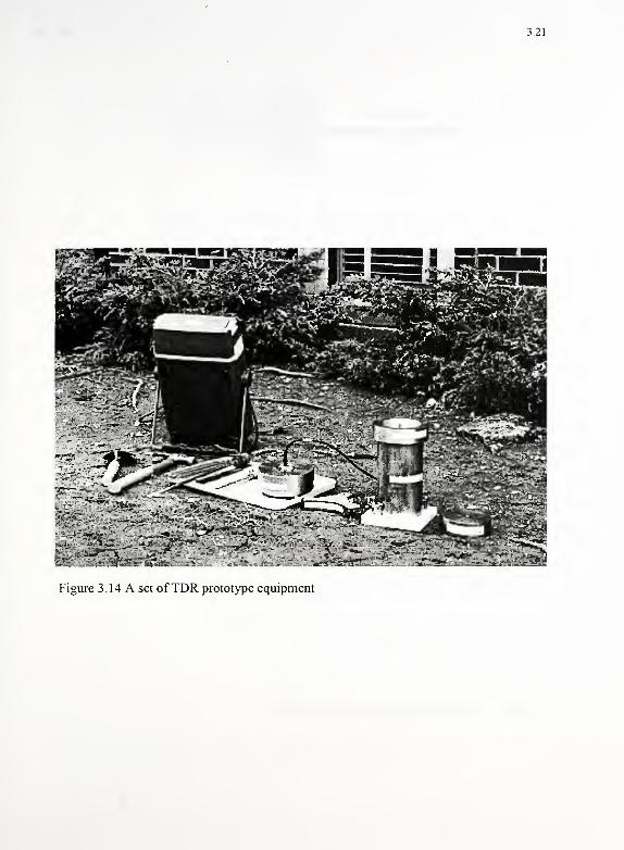
3.14 A set ofTDR prototype equipment 3.21
3.15 Idealized and actual TDR waveforms 3.22
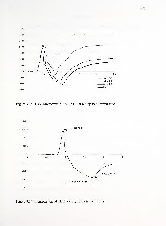
3.16 TDR waveforms of soil in CC filled up to different level 3.23
3.17 Interpretation ofTDR waveform by tangent lines 3.23
4.1 A typical TDR waveform 4.3
4.2 Two methods to determine the first and second reflection point 4.4
4.3 TDR traces with different shapes 4.6
4.4 a) An original waveform b) the smoothed waveform; c) The first derivative of
the original waveform and d) The second derivative of the original waveform. 4.
7
4.5 Illustration of Symbols in the Algorithm 4.10
4.6 TDR readings for different traces using the algorithm in chapter 4 4.12
5.1 The Structure and Functionality ofTDR++ 5.2
5.2 The main form ofTDR++ 5.3
5.3 The layout of the Setting form 5.6
5.4 The layout of the picture box 5.1
1
6.
1
Comparison of the oven-dry water content and the TDR measured water
content for different types of soils (listed in Table 6. 1 ) using Topp's empirical
equation 6.6
6.2 VAT vs.9 relationship for different types of soils (listed in Table 6. 1 ).pes of soils
(listed in Table 6.1) using Topp's empirical equation 6.7
6.3 Density-compensating water content relationship for different types of soils
(listed in Table 6.1) 6.7
6.4 Density-compensating water content relationship for Crosby Till 6.10
6.5 Comparison of the oven-dry water content and the TDR measured water
content for Crosby Till using Topp's empirical equation 6.11
V
6.6 Comparison of the oven-dry water content and the TDR measured water
content for Crosby Till using Density-compensating water content equation. ... 6.1
1
6.7 Variation of error in density measurement with the difference of density in two
CCmold 6.12
6.8 Density-compensating water content relationship for all soil types in field tests.
6.16
6.9 Comparison of the oven-dry water content with the TDR measured water
content and Nuclear gauge measured water content in field tests 6.16
VI
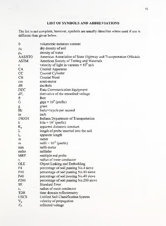
LIST OF SYMBOLS AND ABBREVIATIONS
The list is not complete, however, symbols are usually identifies where used if use is
different than given below.
e
Pd
PwAASHTOASTMc
CACCCHcmdBDECdVs
ft
GgHzin
INDOTk
Ka
Lla
mmmmmrho
MRPr,
OLEP4
P10
P40
P200
SEr
TDRusesVP
Vr
volumetric moisture content
dry density of soil
density of water
American Association of State Highway and Transportation Officials
American Society of Testing and Materials
velocity of light in vacuum = 108m/s
Coaxial Apparatus
Coaxial Cylinder
Coaxial Head
centi-meter
decibels
Data Communication Equipment
derivative of the smoothed voltage
foot
giga = 19(prefix)
gram
hertz=l cycle per second
inch
Indiana Department of Transportation
kilo = 10" (prefix)
apparent dielectric constant
length of probe inserted into the soil
apparent length
meter
milli = 10"3(prefix)
milli-meter
millirho
multiple rod probe
radius of inner conductor
Object Linking and Embedding
percentage of soil passing No.4 sieve
percentage of soil passing No. 10 sieve
percentage of soil passing No.40 sieve
percentage of soil passing No.200 sieve
Standard Error
radius of outer conductor
time domain reflectometry
Unified Soil Classification System
velocity of propagation
reflected voltage

Vll
Vs smoothed voltage
VT transmitted voltage
w gravimetric water content
w D oven dry water content
wTdr TDR water content
Vlll
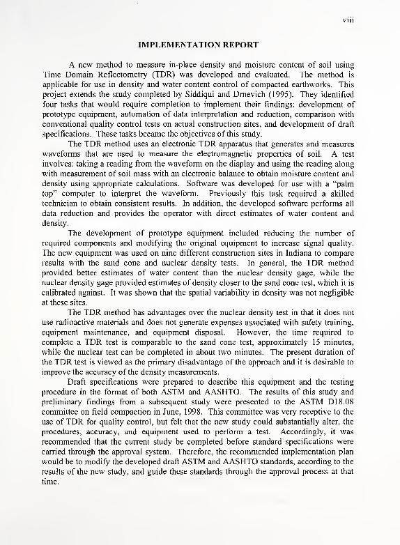
IMPLEMENTATION REPORT
A new method to measure in-place density and moisture content of soil using
Time Domain Reflectometry (TDR) was developed and evaluated. The method is
applicable for use in density and water content control of compacted earthworks. This
project extends the study completed by Siddiqui and Drnevich (1995). They identified
four tasks that would require completion to implement their findings: development of
prototype equipment, automation of data interpretation and reduction, comparison with
conventional quality control tests on actual construction sites, and development of draft
specifications. These tasks became the objectives of this study.
The TDR method uses an electronic TDR apparatus that generates and measures
waveforms that are used to measure the electromagnetic properties of soil. A test
involves: taking a reading from the waveform on the display and using the reading along
with measurement of soil mass with an electronic balance to obtain moisture content and
density using appropriate calculations. Software was developed for use with a "palm
top" computer to interpret the waveform. Previously this task required a skilled
technician to obtain consistent results. In addition, the developed software performs all
data reduction and provides the operator with direct estimates of water content and
density.
The development of prototype equipment included reducing the number of
required components and modifying the original equipment to increase signal quality.
The new equipment was used on nine different construction sites in Indiana to compare
results with the sand cone and nuclear density tests. In general, the TDR method
provided better estimates of water content than the nuclear density gage, while the
nuclear density gage provided estimates of density closer to the sand cone test, which it is
calibrated against. It was shown that the spatial variability in density was not negligible
at these sites.
The TDR method has advantages over the nuclear density test in that it does not
use radioactive materials and does not generate expenses associated with safety training,
equipment maintenance, and equipment disposal. However, the time required to
complete a TDR test is comparable to the sand cone test, approximately 15 minutes,
while the nuclear test can be completed in about two minutes. The present duration of
the TDR test is viewed as the primary disadvantage of the approach and it is desirable to
improve the accuracy of the density measurements.
Draft specifications were prepared to describe this equipment and the testing
procedure in the format of both ASTM and AASHTO. The results of this study and
preliminary findings from a subsequent study were presented to the ASTM D 18.08
committee on field compaction in June, 1998. This committee was very receptive to the
use of TDR for quality control, but felt that the new study could substantially alter, the
procedures, accuracy, and equipment used to perform a test. Accordingly, it was
recommended that the current study be completed before standard specifications were
carried through the approval system. Therefore, the recommended implementation plan
would be to modify the developed draft ASTM and AASHTO standards, according to the
results of the new study, and guide these standards through the approval process at that
time.

1.1
CHAPTER 1
INTRODUCTION
1.1 Background
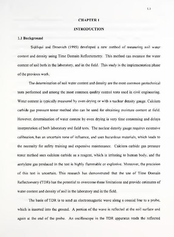
Siddiqui and Dmevich (1995) developed a new method of measuring soil water
content and density using Time Domain Reflectometry. This method can measure the water
content of soil both in the laboratory, and in the field. This study is the implementation phase
of the previous work.
The determination of soil water content and density are the most common geotechnical
tests performed and among the most common quality control tests used in civil engineering.
Water content is typically measured by oven drying or with a nuclear density gauge. Calcium
carbide gas pressure tester method also can be used for obtaining moisture content at field.
However, determination of water content by oven drying is very time consuming and delays
interpretation of both laboratory and field tests. The nuclear density gauge requires extensive
calibration, has an uncertain zone of influence, and uses hazardous materials, which leads to
the necessity for safety training and expensive maintenance. Calcium carbide gas pressure
tester method uses calcium carbide as a reagent, which is irritating to human body, and the
acetylene gas produced in the test is highly flammable or explosive. Moreover, the precision
of this test is uncertain. This research has demonstrated that the use of Time Domain
Reflectometry (TDR) has the potential to overcome these limitations and provide estimates of
water content and density of soil in the laboratory and in the field.
The basis of TDR is to send an electromagnetic wave along a coaxial line to a probe,
which is inserted into the ground. A portion of the wave is reflected at the soil surface and
again at the end of the probe. An oscilloscope in the TDR apparatus reads the reflected
1.2
waveform. The points of reflection are visible on the waveform and the distance between
these two reflection points represents the velocity of wave propagation along the probe. The
wave velocity is related to the dielectric constant of the soil that surrounds the probe. The
measured dielectric constant can then be used to estimate the volumetric water content of the
soil because there is a strong correlation between dielectric constant and volumetric water
content.
1.2 Problem Statement
During the previous study TDR was shown to be capable of measuring both soil water
content and density in the laboratory and in the field. Implementation of the research requires
that the subjectivity of data interpretation and data reduction is eliminated, prototype
equipment is developed and standardized, and the testing procedure is standardized.
1.3 Objectives
The primary objectives of this project were to: 1) develop prototype test equipment;
2) automate TDR waveform interpretation and data reduction; 3) generate additional data with
the new equipment under field conditions to assess the accuracy of the method; and 4)
generate ASTM and AASHTO draft standards for the equipment and procedure.
1.4 Scope of Work
The scope of work is closely aligned with meeting the outlined objectives. The
following sections present specific efforts to meet these goals.
1.3
Equipment Development
During the initial study, several pieces of equipment were developed for measuring the
water content and density of soils. Equipment was designed for tests in the laboratory, in the
field for construction control, and in situ for use within soil borings (Drnevich and Siddiqui,
1995). An objective for this study was to develop prototype equipment for compaction
quality control to improve reflected waveform quality and simplify the test procedure.
Data Interpretation and Procedural Automation
Accurate interpretation of the reflected wavelength is critical for accurate predictions
of water content and density. However, this interpretation can be somewhat subjective and
results are apt to be operator dependent. To eliminate the subjectivity in the readings and to
simplify the data reduction process, an algorithm was developed and incorporated into a
computer program such that data readings and data processing are fully automated and
independent of the operator. Readings of water content and density are displayed directly on
the computer screen.
Laboratory and Field Tests
Approximately 150 water content and density tests have been performed in the
laboratory and the field to assess the adequacy of the prototype equipment, and to improve the
testing procedure. Tests measurements under field conditions were compared with tests using
the nuclear density gauge and the sand cone test, and with oven dried water content.

1.4
Development ofASTM and AASHTO Standards
ASTM and AASHTO draft standards have been developed to standardize the
equipment and testing procedure. It is anticipated that these standards will be improved as
feedback is generated from operators of the equipment.
1.5 Report Format
Chapter 2 of this report provides a brief review of the development and use of TDR,
basic concepts, and related research. Chapter 3 describes the design of the prototype
equipment including factors considered during development, and design drawings. The
algorithm used to automate waveform interpretation is developed in Chapter 4. Chapter 5
describes the software that was developed for data interpretation, data reduction, and output
presentation. The results of laboratory and field tests and comparison to conventional test
methods are presented in Chapter 6. Chapter 7 introduces the proposed testing procedures,
including ASTM and AASHTO draft standards. A summary of the study, conclusions and
recommendations are provided in Chapter 8.

2.1
CHAPTER 2
BACKGROUND
2.1 TDR Basics
Fellner-Feldegg (1969) introduced time domain reflectometry (TDR) as a means of
measuring the complex dielectric permittivity of liquids. Since that time, TDR has been
applied to the measurement of dielectric properties of many materials including soils. In
recent years, intensive studies have been undertaken on the application of TDR to the
measurement of soil water content, bulk soil electric conductivity, and soil density.
A comprehensive review of the literature on TDR, including theoretical background
and equipment was presented in the JHRP final report "A New Method of Measuring Density
and Water Content of Soil Using the Technique of Time Domain Reflectometry" by Siddiqui
and Dmevich (1995) and will not be repeated here. In this section, a brief summary of the
application on TDR to obtain water content and density is provided.
TDR Equipment
TDR equipment includes a TDR apparatus, a coaxial cable, a probe, and a head to
connect the coaxial cable and the probe. A typical test setup for field conditions is shown in
Figure 2.1.
The Tektronix 1502B Metallic TDR Cable Tester was used in this study. It is the
same equipment used by many other TDR researchers. The apparatus transmits a step pulse,
electromagnetic wave along a standard coaxial cable. A built-in oscilloscope receives the
transmitted wave superimposed with the reflected wave. The apparatus is a wide band device,

2.2
with a frequency range of to 10 GHz. The signal is recorded and displayed in the time
domain.
Tektronix Cable Tester
Probe and Head
Laptop Computer
Figure 2.1 A typical TDR test setup in field
For application with soil, the coaxial cable typically leads to a head and a number of
steel rods, or probes, that penetrate the soil. The head connects the coaxial cable and the rods.
The rods are embedded in soil and act as an extension to the coaxial line such that the soil
serves as the insulating material between the rods. At each point along the coaxial system
where there is a discontinuity of impedance, a reflected wave is produced. Discontinuities of
impedance occur where: the coaxial cable is attached to the head, the head is attached to the
rods, the rods enter the soil, and at the ends of the rods. The TDR waveform received by the
oscilloscope is a superposition of these multiple reflections along with the initially transmitted
wave. Thus, differences in the geometry of the head or rods lead to different shapes in the
reflected waveform.

2.3
TDR Waveform Interpretation
The overall shape of the reflected TDR trace is influenced by the impedance and
length of the various components in the transmission line and therefore varies with the
equipment used. Two specific points on the reflected waveform are needed for data
interpretation, namely the reflection that occurs at the top of the soil surface and the reflection
that occurs at the end of the rods. These points are used to interpret the dielectric constant of
the soil surrounding the rods. A typical TDR waveform is shown in Figure 2.2.
ac
f^ Point 1
3.309 m
\-Pobxt2
1 avg. 118.56 miho .25 i
Figure 2.2 A typical TDR waveform
In Figure 2.2, the peak is marked as "Point 1" which represents the reflection at the
soil surface, while the valley is marked as "Point 2" which corresponds to the reflection at the
end of the TDR probe. The TDR device uses a parameter defined as the nominal velocity of
propagation, V . This velocity is multiplied by the travel time of the reflected wave so that
the reading at each horizontal position on the oscilloscope is expressed as a unit of distance.
The distance between Points 1 and 2 on the waveform is defined as the apparent length (la ).
2.4
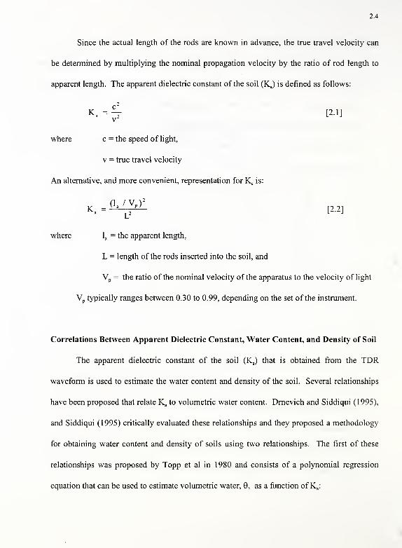
Since the actual length of the rods are known in advance, the true travel velocity can
be determined by multiplying the nominal propagation velocity by the ratio of rod length to
apparent length. The apparent dielectric constant of the soil (KJ is defined as follows:
Ka= 4 [2.1]
v
where c = the speed of light,
v = true travel velocity
An alternative, and more convenient, representation for K, is:
K = fla^p)2
p 2]L2
where la= the apparent length,
L = length of the rods inserted into the soil, and
Vp= the ratio of the nominal velocity of the apparatus to the velocity of light
Vptypically ranges between 0.30 to 0.99, depending on the set of the instrument.
Correlations Between Apparent Dielectric Constant, Water Content, and Density of Soil
The apparent dielectric constant of the soil (KJ that is obtained from the TDR
waveform is used to estimate the water content and density of the soil. Several relationships
have been proposed that relate K, to volumetric water content. Dmevich and Siddiqui (1995),
and Siddiqui (1995) critically evaluated these relationships and they proposed a methodology
for obtaining water content and density of soils using two relationships. The first of these
relationships was proposed by Topp et al in 1980 and consists of a polynomial regression
equation that can be used to estimate volumetric water, 0, as a function of K,:
2.5
= -0.053+2.92xlO-2 Ka-5.5xlQr4 Ka2+4.3xl0-6 Ka3 [2.3]
The second equation, proposed by Siddiqui (1995), relates the ratio of dielectric constant and
soil density to gravimetric water content.
VKaP" = a + bw [2.4]
Pi
where:
Pd = dry density of soil
Pw= density of water
w = gravimetric water content
a, b = soil dependent coefficients
In the previous JHRP study, Siddiqui and Drnevich introduced a procedure to obtain
both the gravimetric water content and soil density using Eqns. 2.3 and 2.4. Briefly, the
procedure entails: 1) making a measurement of the dielectric constant in situ where the
density and water content are unknown; 2) excavating the tested soil and compacting it in a
mold of known volume and remeasuring the dielectric constant; 3) measuring the wet density
of the soil in the mold using a balance; 4) using Topp's equation to estimate the volumetric
water content from which the gravimetric water content can be calculated for the soil in the
mold; and 5) use Eqn. 2.4 to obtain in situ density by assuming the gravimetric water content
is the same in the mold and in situ.
During the present study it was noted that the use of Topp's equation yielded too much
scatter in the measurements of volumetric water content. Although this equation is broadly
used by many investigators, test results performed in this study show that both soil density
and soil type have a significant influence on the G-K^ relationship. Accordingly, an alternative
procedure was developed during this study and will be introduced in Chapter 6.

3.1
CHAPTER 3
DESIGN OF TDR PROTOTYPE EQUIPMENT
3.1 Transmission Line Components
The wave transmission line consists of a coaxial cable, a coaxial head (CH), and either
a coaxial cylinder (CC) or a multiple rod probe (MRP). Each of these coaxial components
contains an inner conductor and an outer conductor. A typical coaxial cable consists of an
inner conducting wire surrounded by a cylindrical casing that acts as the outer conductor.
Each of the other coaxial components is a variation of this system.
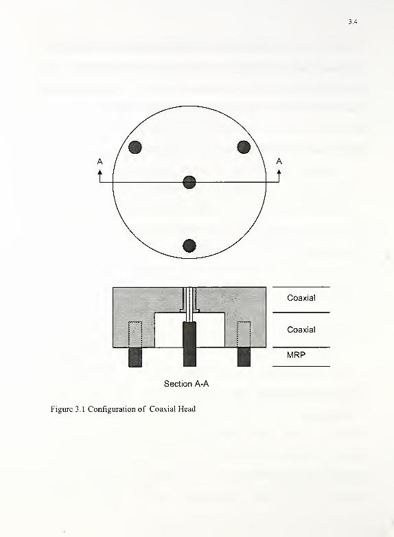
The coaxial head (CH) actually consists of three components, as shown in Figure 3.1 :
1) a coaxial line similar to the coaxial cable; 2) a solid cylindrical head with Delrin® as the
insulating material; and 3) multiple rod section consisting of a center rod and three perimeter
conducting rods with air as the insulating material.
The coaxial cylinder (CC) consists of a central conducting rod and a steel outer
conducting cylinder. The cylinder is filled with soil and serves as the insulating material as
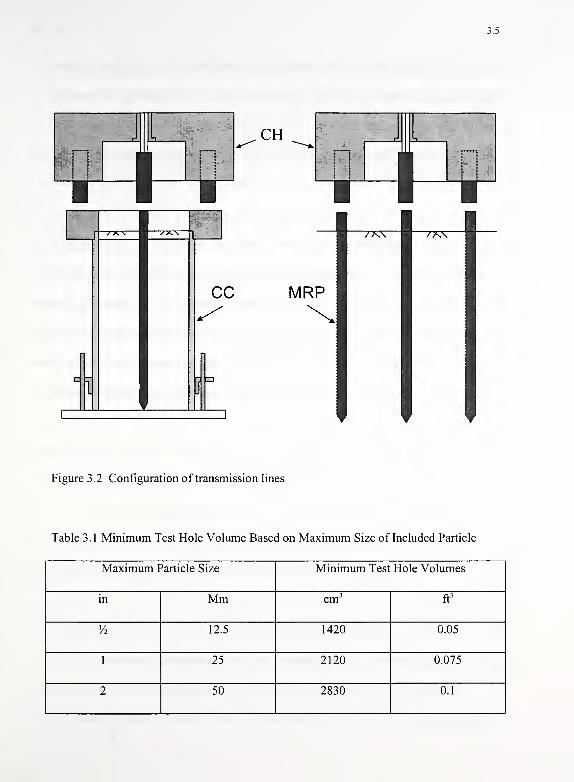
shown in Figure 3.2. The multiple rod probe (MRP) consists of a central rod and three
perimeter rods of the same spacing as the CH. The rods penetrate the soil so that the soil acts
as the insulating material as shown in Figure 3.2.
3.2 Factors Influencing Wave Transmission
The factors that influence wave transmission include the type, length, and geometry of
the transmission line, and the characteristics and volume of soil tested.

3.2
3.2.1 Type of Transmission Line
The types of transmission lines used in this study can be divided into two groups: 1)
those with a bounded outer cylindrical conductor; and 2) those with an unbounded outer
conductor. The coaxial cable and CC are in the first group while the MRP is in the second.
The head actually has components in both groups. Zegelin et. al. (1989) showed that an MRP
with three outer rods provided signals that were essentially the same as those with cylindrical
outer conductors.
3.2.2 Transmission Line Length
The length of the CH transmission line is chosen to be small so that the transient effect
of the head dies out fast. The maximum length that can be used for the CC and MRP with soil
as the insulating medium is controlled by the following factors.
(1) Loss of signal strength along the length of the line.
(2) Spatial resolution of the TDR apparatus.
(3) Ease of installation of rods in soil.
(4) Desired sampling depth.
Based on these factors, an optimum length can be selected.
The signal strength decays as it travels through a conductive medium. The length of
the probe must be short enough that a detectable reflection from the end of the probe is
received. To get a detectable return signal, the ratio of reflected voltage, F/j, to transmitted
voltage, Vf, must be greater than zero. This ratio increases as L decreases. On the other
hand, the variability of the interpreted value of K^ from the TDR measurement increases with
decreasing rod length. Siddiqui (1995) performed a detailed analysis of the controlling
3.3
factors and it was found that the maximum rod length ranged approximately between 0.2 m
for saturated bentonite to 1 meter for clean sands. Accordingly, rod lengths of 0. 1 to 0.2 m
were considered applicable for a wide range in soil types. This is consistent with the desired
test depths of compacted soils, which typically consist of less than 0.3 m.
3.2.3 Transmission Line Geometry
The ratio of the radii of the outer (r ) and inner (r,) conductor is the most important
geometric parameter when considering a cross section through the coaxial system. The ratio
r /r„ and the dielectric constant of the insulating medium determine the impedance of a
transmission line. The magnitude of r or r, does not influence the results, only the ratio.
Measurements are better (less spatial sensitivity) with equipment that has lower values of rjx{.
However, practical limits exist due to the need to have equipment robust enough to penetrate
compacted soils and to minimize the disturbance of soil during penetration.
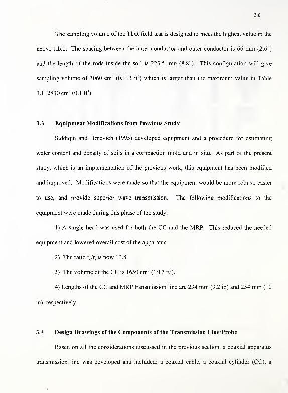
3.2.4 Volume of Soil Tested
The sampling volumes should be as large as practical to minimize the measurement
errors. With the sand cone method, the appropriate test hole volume depends on soil
gradation and should not be smaller than the volumes indicated in Table 3.1 according to
ASTMD1556.
3.4
IlinjCoaxial
Coaxial
MRP
Section A-A
Figure 3.1 Configuration of Coaxial Head
3.5
LgEj
MRP
7K\" /K\
Figure 3.2 Configuration of transmission lines
Table 3.1 Minimum Test Hole Volume Based on Maximum Size of Included Particle
Maximum Particle Size Minimum Test Hole Volumes
in Mm cm3ft
3
y2 12.5 1420 0.05
1 25 2120 0.075
2 50 2830 0.1
3.6
The sampling volume of the TDR field test is designed to meet the highest value in the
above table. The spacing between the inner conductor and outer conductor is 66 mm (2.6")
and the length of the rods inside the soil is 223.5 mm (8.8"). This configuration will give
sampling volume of 3060 cm 3
(0.113 ft3
) which is larger than the maximum value in Table
3.1, 2830 cm 3(0.1 ft
3
).
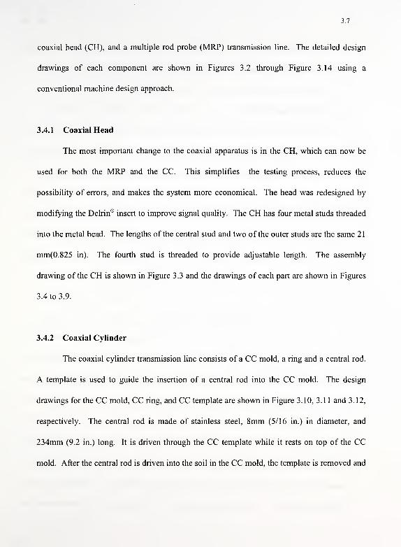
3.3 Equipment Modifications from Previous Study
Siddiqui and Drnevich (1995) developed equipment and a procedure for estimating
water content and density of soils in a compaction mold and in situ. As part of the present
study, which is an implementation of the previous work, this equipment has been modified
and improved. Modifications were made so that the equipment would be more robust, easier
to use, and provide superior wave transmission. The following modifications to the
equipment were made during this phase of the study.
1) A single head was used for both the CC and the MRP. This reduced the needed
equipment and lowered overall cost of the apparatus.
2) The ratio r /r, is now 12.8.
3) The volume of the CC is 1650 cm3(1/17 ft
3
).
4) Lengths of the CC and MRP transmission line are 234 mm (9.2 in) and 254 mm (10
in), respectively.
3.4 Design Drawings of the Components of the Transmission Line/Probe
Based on all the considerations discussed in the previous section, a coaxial apparatus
transmission line was developed and included: a coaxial cable, a coaxial cylinder (CC), a
3.7
coaxial head (CH), and a multiple rod probe (MRP) transmission line. The detailed design
drawings of each component are shown in Figures 3.2 through Figure 3.14 using a
conventional machine design approach.
3.4.1 Coaxial Head
The most important change to the coaxial apparatus is in the CH, which can now be
used for both the MRP and the CC. This simplifies the testing process, reduces the
possibility of errors, and makes the system more economical. The head was redesigned by
modifying the Delrin® insert to improve signal quality. The CH has four metal studs threaded
into the metal head. The lengths of the central stud and two of the outer studs are the same 21
mm(0.825 in). The fourth stud is threaded to provide adjustable length. The assembly
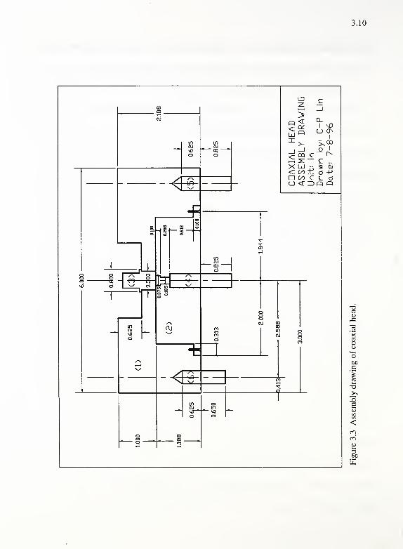
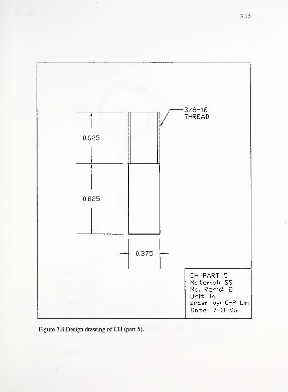
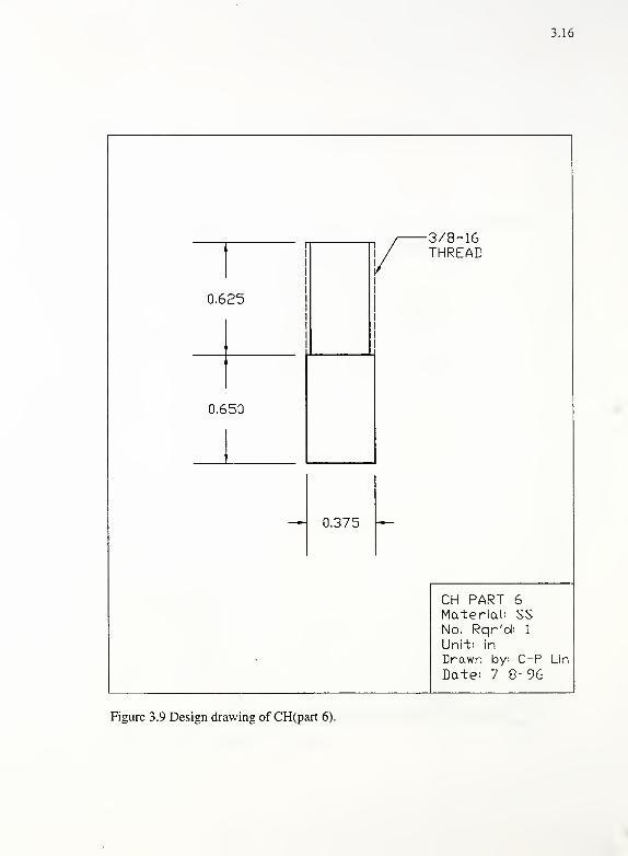
drawing of the CH is shown in Figure 3.3 and the drawings of each part are shown in Figures
3.4 to 3.9.
3.4.2 Coaxial Cylinder
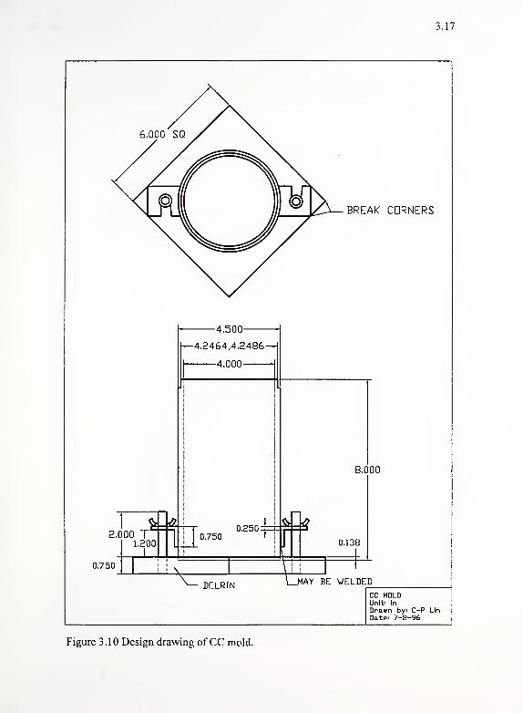
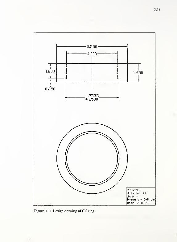
The coaxial cylinder transmission line consists of a CC mold, a ring and a central rod.
A template is used to guide the insertion of a central rod into the CC mold. The design
drawings for the CC mold, CC ring, and CC template are shown in Figure 3.10, 3.1 1 and 3.12,
respectively. The central rod is made of stainless steel, 8mm (5/16 in.) in diameter, and
234mm (9.2 in.) long. It is driven through the CC template while it rests on top of the CC
mold. After the central rod is driven into the soil in the CC mold, the template is removed and
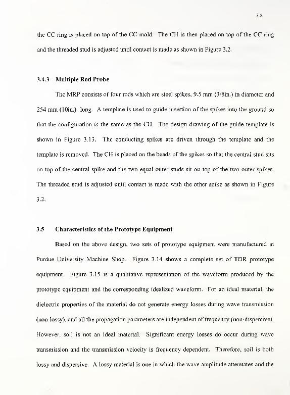
3.8
the CC ring is placed on top of the CC mold. The CH is then placed on top of the CC ring
and the threaded stud is adjusted until contact is made as shown in Figure 3.2.
3.4.3 Multiple Rod Probe
The MRP consists of four rods which are steel spikes, 9.5 mm (3/8in.) in diameter and
254 mm (lOin.) long. A template is used to guide insertion of the spikes into the ground so
that the configuration is the same as the CH. The design drawing of the guide template is
shown in Figure 3.13. The conducting spikes are driven through the template and the
template is removed. The CH is placed on the heads of the spikes so that the central stud sits
on top of the central spike and the two equal outer studs sit on top of the two outer spikes.
The threaded stud is adjusted until contact is made with the other spike as shown in Figure
3.2.
3.5 Characteristics of the Prototype Equipment
Based on the above design, two sets of prototype equipment were manufactured at
Purdue University Machine Shop. Figure 3.14 shows a complete set of TDR prototype
equipment. Figure 3.15 is a qualitative representation of the waveform produced by the
prototype equipment and the corresponding idealized waveform. For an ideal material, the
dielectric properties of the material do not generate energy losses during wave transmission
(non-lossy), and all the propagation parameters are independent of frequency (non-dispersive).
However, soil is not an ideal material. Significant energy losses do occur during wave
transmission and the transmission velocity is frequency dependent. Therefore, soil is both
lossy and dispersive. A lossy material is one in which the wave amplitude attenuates and the
3.9
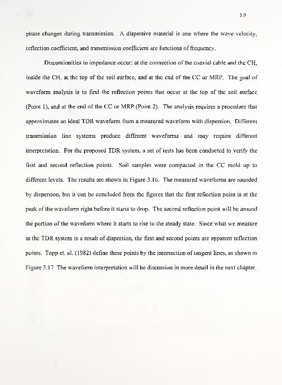
phase changes during transmission. A dispersive material is one where the wave velocity,
reflection coefficient, and transmission coefficient are functions of frequency.
Discontinuities in impedance occur: at the connection of the coaxial cable and the CH,
inside the CH, at the top of the soil surface, and at the end of the CC or MRP. The goal of
waveform analysis is to find the reflection points that occur at the top of the soil surface
(Point 1), and at the end of the CC or MRP (Point 2). The analysis requires a procedure that
approximates an ideal TDR waveform from a measured waveform with dispersion. Different
transmission line systems produce different waveforms and may require different
interpretation. For the proposed TDR system, a set of tests has been conducted to verify the
first and second reflection points. Soil samples were compacted in the CC mold up to
different levels. The results are shown in Figure 3.16. The measured waveforms are rounded
by dispersion, but it can be concluded from the figures that the first reflection point is at the
peak of the waveform right before it starts to drop. The second reflection point will be around
the portion of the waveform where it starts to rise to the steady state. Since what we measure
in the TDR system is a result of dispersion, the first and second points are apparent reflection
points. Topp et. al. (1982) define these points by the intersection of tangent lines, as shown in
Figure 3.17 The waveform interpretation will be discussion in more detail in the next chapter.
3.10
-< -tf3-
-fe-
in I
« w J
OJ
-^7T-\0-
I 1
>Q_
I \DCJ On
X LJ -^ 5 Cw
<L (/) ±1 CS H(/) C L c5
u <c 30 n
—o
oMC
«T3
_>^
sE
3.11
0.625
d0.3751.000
6.000-
4.00354.0000
'
3.37853.3750
2.000-
l/E-28 THREAD
0.188
/\
0.3752.588-
1.000
2.188
1.188
0.625
DRILLED TAP 3/8-16NCX5/8AT 120 DEGREE SPACING
CH PART 1
Material' SSNo. Rqr'd: 1
Unit* in
Drawn by: C-P Lin
Datei 7-9-96
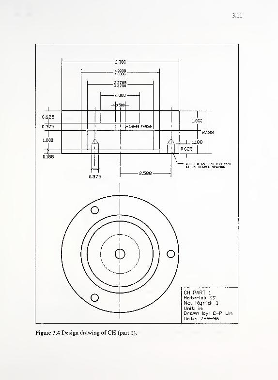
Figure 3.4 Design drawing ofCH (part 1).

3.12
0.388
0.8001.188
CH PART 2
Material: DelrinNo, Rqr'd: 1
Unit: in
Drawn by: C-P Lin
Date: 7-8-96
Figure 3.5 Design drawing of CH (part 2).
3.13
0,500
0.288
0.600
J
0.050 J
^0.185^
0.375
0.500
0.375
0.100fT
Notes'Modify standard BNC Connector(UG-492, 1/2' Diameter, dualFenale) to this drawing.
CH PART 3(BNC CDNNECTDR)No, Rqr'd: 1
Unit: in
Drawn by: C-P Lin
Datei 7-8-96
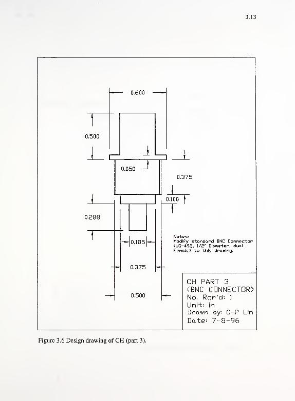
Figure 3.6 Design drawing of CH (part 3).

3.14
0.325
PIN FRDM BNC CDNNECTDR
WELDED
0.750
0.825
r3/8-16THREAD
— 0,375 —CH PART 4Material: SSNo. Rqr'di 1
Unit: in
Drawn by: C-P Lin
Dates 7-8-96
Figure 3.7 Design drawing of CH (part 4).
3.15
3/8-16/1
0,625
/ THREAD
0,825
— 0.375 —
CH PART 5Material: SSNo. Rqr'd: 2
Unit: in
Drawn by: C-P Lin
Date: 7-8-96
Figure 3.8 Design drawing of CH (part 5).
3.16
0.625
0.650
3/8-16THREAD
— 0.375 —
CH PART 6Material: SSNo. Rqr'd; 1
Uni"t: in
Drawn by: C-P
Date: 7-8-96Lin
Figure 3.9 Design drawing of CH(part 6).
3.17
2.000
0.750
1.200
-4.500-
1—4.2464,4.2486-
4.000
0.7500.250: 4
BREAK CDRNERS
8.000
0.138
DELRIN 1AY BE WELDED
CC MOLDUnit' In
Drawn by> C-P Lin
Date' 7-8-96
Figure 3.10 Design drawing of CC mold.
3.18
1,200
5.550-
-4.000-
1,450
0,250
4.25354,2500
ssCC RINGMaterialUnlti in
Drawn byi C-P Lin
Datei 7-8-96
Figure 3.11 Design drawing of CC ring.
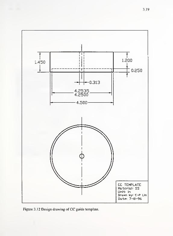
3.19
1.200
0.250
CC TEMPLATEMaterial. SSUnlt> In
Drawn byi C-P Lin
Date> 7-8-96
Figure 3.12 Design drawing of CC guide template.

3.20
3.178
1.044 V
LDCKING CLAMP
WELDED HINGE
MRP TEMPLATEMaterial: SSUnit: in
Drawn by: C-P Lin
Date: 7-8-96
Figure 3.13 Design drawing ofMRP guide template
3.21
Figure 3.14 A set ofTDR prototype equipment

3.22
CH
TDRCoaxial Cable
z,
CC or MRP
z 2
Zo
z.
Figure 3.15 Idealized and actual TDR waveforms
3.23
Figure 3.16 TDR waveforms of soil in CC filled up to different level.
1000
Figure 3.17 Interpretation ofTDR waveform by tangent lines.
4.1
CHAPTER 4
AUTOMATING THE INTERPRETATION OF THE TDR WAVEFORM
4.1 Introduction
The apparent dielectric constant (KJ is the key parameter used in this study for the
interpretation of water content and density of compacted soils. As discussed in Chapter 2, IC,
is obtained from the square of the ratio of apparent length (la) to probe length (L). The probe
length can be measured directly while the apparent length is interpreted from the distance
between two specific points on the reflected waveform. It was noted that a major source of
error in the data interpretation is associated with the determination of la.
The apparent length (la) is determined from a TDR trace. Variation in soil type, water
content and density will lead to different waveforms. Due to the dispersion of
electromagnetic waves along the TDR probe, the desired reflection points are not always
distinct and are often somewhat rounded. Interpretation of the apparent length manually can
therefore be operator dependent.
A primary objective of the present study was to automate the data interpretation
process so that results would be independent of the operator. To accomplish this, an
algorithm was developed and coded in a computer program to obtain the apparent length
directly from the data. The required algorithm must produce consistent readings and have the
capacity to handle variations in waveform shapes. In addition, the algorithm should be able to
recognize poor data and warn the operator that the test should be repeated. Development of
an algorithm with these features proved to be very challenging. Several algorithms were tried
but abandoned when one or more of the desired characteristics could not be met. The
4.2
proposed algorithm has been evaluated on over 100 different TDR waveforms and more than
10 soil types and has performed satisfactorily on all cases tested.
4.2 Interpretation of the TDR Waveform
TDR waveforms are traces of reflected signals recorded by an oscilloscope that is
incorporated into the TDR apparatus. A typical TDR waveform is shown in Figure 4.1. On
the oscilloscope display, the vertical direction represents voltage and the horizontal direction
represents time. The horizontal axis can be transformed from time to distance by multiplying
the time readings by a user-defined velocity of propagation (Vp). Accordingly, the cursor can
be moved along the TDR waveform to obtain distance readings.
An understanding of the nature of the TDR waveform aids in the interpretation of the
apparent length. The source of a TDR signal is a step pulse, which consists of a wide range of
frequency components. All frequency components travel at the same initial velocity in the
coaxial line but at different velocities in the soil because soil is a dispersive material.
Moreover, the wave amplitudes are diminished in the soil because it is a lossy material. When
the traveling waves reach a change in impedance a portion of the wave is reflected. The
relative energy of the reflected to transmitted wave is frequency dependent. Changes in
impedance occur at the head, at the upper soil surface and at the end of the MRP or CC as
discussed in Chapter 3.
The first important reflection point is generated at the upper soil interface (Point 1,
Figure 4.1). This point is distinct and easy to read because the waves that travel to, and are
reflected by, this interface travel at the same velocity, i.e. very little dispersion occurs. The
second important reflection point is associated with the end of the MRP or CC. This point is

4.3
less distinct (Point 2, Figure 4.1) because the soil is dispersive so that waves of different
frequency travel at different velocity, and therefore, have different arrival times back at the
oscilloscope. Identification of the second reference point can be made visually by an
experienced operator or by using a specific procedure.
ac <4-PoinU ! 3.309 m
.Point 2
1 avg. 118.56 miho .25 m.
Figure 4.1 A typical TDR waveform
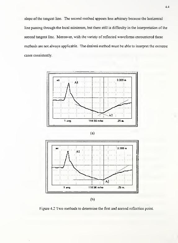
Two methods to identify the second point are shown in Figure 4.2a and 4.2b. They are
both "tangent line" methods, but with different schemes. The first method (Topp et al.,1982)
is shown in Figure 4.2a. The second reflection point (A2) is located at the intersection of the
two lines drawn tangent to the curve at the positions shown. The second scheme was proposed
by Baker and Allmaras (1990). A line parallel to the horizontal axis is drawn tangent to the
smoothed trace at a local minimum. A second tangent is placed at the point of the maximum
first derivative following the local minimum. The intersection of this line with the horizontal
line is Point A2.
Both of these published methods are based on the assumption that the reflected signal
has a linear rising shape. This is true for most cases, but it is often difficult to determine the
4.4
slope of the tangent line. The second method appears less arbitrary because the horizontal
line passing through the local minimum, but there still is difficulty in the interpretation of the
second tangent line. Moreover, with the variety of reflected waveforms encountered these
methods are not always applicable. The desired method must be able to interpret the extreme
cases consistently.
ac• • Ail
•
3.309 m
A2
1 avg. 118.56 mrho .25 m.
(a)
ac 3.309 mAl
A2"
1 avg. 118.56 mrho 25 m.
(b)
Figure 4.2 Two methods to determine the first and second reflection point.
4.5
Figure 4.3 shows six traces with different shapes: a) from a field test of clayey soil, b)
and c) from field tests on two different sandy soils, d) from a lab test of saturated sand, e)
from concrete, and f) from tap water. The potential varieties of waveforms that may be
encountered are evident from these six cases. The desired algorithm for use in TDR data
interpretation needs to work for wide range of possible cases and be consistent with
interpretations made by an experienced operator. In addition, it is desirable for the algorithm
to be able to identify abnormal or spurious results to alert the operator.
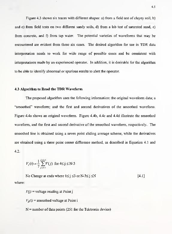
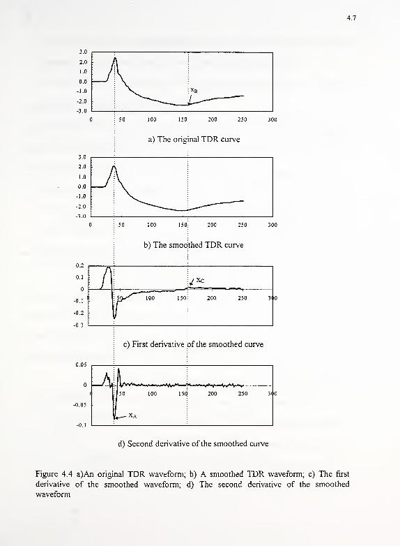
4.3 Algorithm to Read the TDR Waveform
The proposed algorithm uses the following information: the original waveform data; a
"smoothed" waveform; and the first and second derivatives of the smoothed waveform.
Figure 4.4a shows an original waveform. Figure 4.4b, 4.4c and 4.4d illustrate the smoothed
waveform, and the first and second derivative of the smoothed waveform, respectively. The
smoothed line is obtained using a seven point sliding average scheme, while the derivatives
are obtained using a three point center difference method, as described in Equation 4. 1 and
4.2.
^(O =^f>0) for4<j<N-3I y=i-3
No Change at ends where 1 < j <3 or N-3< j <N [4.1]
where:
V(j) = voltage reading at Point j
Vs(i) = smoothed voltage at Point i
N = number of data points (251 for the Tektronix device)

4.6
•-niniifTr-T -
i «e 1057
h/.V>^H \jlr
(a) (b)
AC ; 1.344 -,
/. ... I. ... .
j
/1
1
; ; j
2 3»>j.
(c) (d)
2 erg.
«kC : 0.400
'1"1 j
\ f^~~~J^~
: i : j I : :
!
(e) 09
Figure 4.3 Different TDR waveforms
4.7
300
d) Second derivative of the smoothed curve
Figure 4.4 a)An original TDR waveform; b) A smoothed TDR waveform; c) The first
derivative of the smoothed waveform; d) The second derivative of the smoothed
waveform
4.8
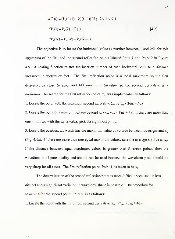
dVs(i) = (V
s(i+i)-V
s(i-V))/2; 2< i<N-l
dVs{\) = V
s(2)-V
s {\) [4.2]
dV5(N) = V
s(N)-V
s(N-l)
The objective is to locate the horizontal value (a number between 1 and 251 for this
apparatus) of the first and the second reflection points labeled Point 1 and Point 2 in Figure
4.5. A scaling function relates the location number of each horizontal point to a distance
measured in meters or feet. The first reflection point is a local maximum so the first
derivative is close to zero, and has maximum curvature so the second derivative is a
minimum. The search for the first reflection point, x,, was implemented as follows:
1. Locate the point with the minimum second derivative (xA ,y"mm) (Fig. 4.4d).
2. Locate the point of minimum voltage beyond xA (xB , ymm ) (Fig. 4.4a), if there are more than
one minimum with the same value, pick the rightmost point;
3. Locate the position, x„ which has the maximum value of voltage between the origin and xB
(Fig. 4.4a). If there are more than one equal maximum values, take the average x value as x,.
If the distance between equal maximum values is greater than 5 screen points, then the
waveform is of poor quality and should not be used because the waveform peak should be
very sharp for all cases. The first reflection point, Point 1, is taken to be x,.
The determination of the second reflection point is more difficult because it is less
distinct and a significant variation in waveform shape is possible. The procedure for
searching for the second point, Point 2, is as follows:
1. Locate the point with the minimum second derivative (xA ,y"
min ) (Fig 4.4d).
4.9
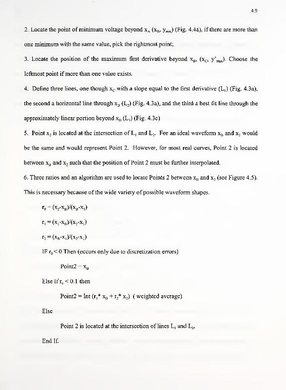
2. Locate the point of minimum voltage beyond xA (xB , ymin) (Fig. 4.4a), if there are more than
one minimum with the same value, pick the rightmost point;
3. Locate the position of the maximum first derivative beyond xB , (xc , y'^J. Choose the
leftmost point ifmore than one value exists.
4. Define three lines, one though xc with a slope equal to the first derivative (L,) (Fig. 4.3a),
the second a horizontal line through xB (L2 ) (Fig. 4.3a), and the third a best fit line through the
approximately linear portion beyond xB (L3 ) (Fig. 4.3c)
5. Point x2is located at the intersection of L, and L
2. For an ideal waveform xB and x
2would
be the same and would represent Point 2. However, for most real curves, Point 2 is located
between xB and x2such that the position of Point 2 must be further interpolated.
6. Three ratios and an algorithm are used to locate Points 2 between xB and x, (see Figure 4.5).
This is necessary because of the wide variety of possible waveform shapes.
r = (x2-xB)/(xB-x,)
ri
= (x2-xB)/(x2
-x,)
r2= (xB-x,)/(x2
-x,)
IF r < Then (occurs only due to discretization errors)
Point2 = xB
r <0.1 thei
Point2 = Int (r,* xB + r2* x
2 ) ( weighted average)
Else
Point 2 is located at the intersection of lines L, and L3 ,
End If.
4.10
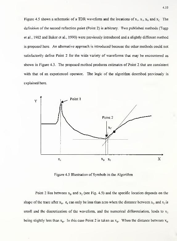
Figure 4.5 shows a schematic of a TDR waveform and the locations of x„ x2 , xB and xc The
definition of the second reflection point (Point 2) is arbitrary. Two published methods (Topp
et al., 1982 and Baker et al., 1990) were previously introduced and a slightly different method
is proposed here. An alternative approach is introduced because the other methods could not
satisfactorily define Point 2 for the wide variety of waveforms that may be encountered as
shown in Figure 4.3. The proposed method produces estimates of Point 2 that are consistent
with that of an experienced operator. The logic of the algorithm described previously is
explained here.
Y
xB X-,
Figure 4.5 Illustration of Symbols in the Algorithm
Point 2 lies between xB and x2(see Fig. 4.5) and the specific location depends on the
shape of the trace after xB . r can only be less than zero when the distance between xB and x:is
small and the discretization of the waveform, and the numerical differentiation, leads to x,
being slightly less than xB . In this case Point 2 is taken as xB . When the distance between xB
4.11
and x2is relative small, r less than 0.1, a weighted average is used to determine Point 2. The
larger the value of r , the closer Point 2 will be to xB . Finally, if the difference between xB and
x2 is large, this indicates a waveform similar to that in Fig. 4.4c, and the intersection of lines
L, and L3are used to define Point 2.
The developed algorithm for reading Points 1 and 2 and the TDR waveform was used
on the curves show in Figure 4.3 with the results show in Figure 4.6. The locations of Points
1 and 2 are all very close to the values that would be selected from manual readings by an
experienced operator.
The criteria used to check if the curve displayed is a valid TDR waveform includes:
1. Horizontal position of Point 2 > Horizontal position of Point 1;
2. Vertical value at Point 1 > Vertical value at Point 2;
3. Horizontal position of Point 1 > 0; Horizontal position of Point 2 > 1 meter;
4. In determining x,, the distance between equal maximum values should be less than 5 units.
Notice that these conditions are necessary for a TDR waveform, but not sufficient.
Therefore, a non-TDR waveform curve that looks similar and satisfies these criteria will be
read as a waveform. But after testing more than 100 waveforms and more than 20 non-
waveforms, no false waveforms were mistakenly interpreted.
4.4 Comments on Waveform Interpretation
The accuracy in reading the apparent length of the waveform will directly influence
the interpreted dielectric constant and therefore the accuracy of the estimated water content
and density. It should be clear from the previous discussion that the determination of the
apparent

4.12
(a) (b)
(c) (d)
;2.430 m
' \
tGi73owfeo 25 m
J120.38 3Kho 1 a.
(e) (f)
Figure 4.6 TDR readings for different traces using the algorithm in this chapter
4.13
length is not exact. The proposed algorithm is believed to be capable of minimizing the errors
of interpretation while being flexible enough to handle a wide range of waveform shapes. As
additional data is gathered, the algorithm will require further verification to confirm
applicability over the broad range in waveform shapes.
The developed algorithm is capable of taking readings for TDR traces with different
horizontal scales as shown in Figure 4.6 where the scale is shown in the lower right corner of
the traces. If a specific waveform is different using different horizontal scales, a different
estimate of the apparent length will be obtained. For example, the apparent length is 0.688 m
using a horizontal scale of 0.1m, and 0.70 using a horizontal scale of 1 m. This difference
occurs because the waveform is made up of only 251 data points. When a large scale is used,
many of the data points are being used to describe the waveform outside the zone of interest,
that is, outside the range of Point 1 to Point 2. This reduces the resolution of the data in the
zone of interest, and therefore, decreases the accuracy of the measured apparent length. An
algorithm is used to adjust the scale of the waveform to attempt to maximize resolution in the
zone of interest; however, the Tektronix device used in this research can only increment the
scale by factors of 2.5. This factor leaves limited flexibility for optimizing the waveform.

5.1
CHAPTER 5
AUTOMATION OF DATA REDUCTION AND THE TESTING PROCEDURE
5.1 Introduction
The goals of this research program are to measure the water content and density of
compacted soils using TDR. There are several steps involved in this procedure, including
data acquisition, data interpretation, data reduction, and data reporting. A comprehensive
software package was developed to handle these operations. The software has many
functional features and was developed in a user-friendly Microsoft Windows™ environment.
Features of the software include, data acquisition and interpretation, report generation,
database management, and on-line help. The software was developed using Microsoft's
Visual Basic™ because it is a user-friendly environment and has an object-oriented structure.
Different toolboxes are conveniently available and can be customized for specific
applications. The software also possesses a straightforward debugging and testing scheme.
The TDR apparatus used in this research (Tektronix 1502B Metallic Cable Test
Apparatus) has an extended function module (SP232), which is a plug-in serial interface that
acts as a DCE (Data Communications Equipment) device. The SP232 allows the user to
control the apparatus by an external computer. This module enables automatic data
acquisition and control of tests with the automation software.
5.2 TDR++: A Software Package for the Automation and Reduction of TDR
Measurements
TDR++ is the computer program developed for the automation and reduction of
measurements of soil water content and density using TDR. The algorithms are based on the
5.2
procedure developed during this and the previous study for measuring soil water content and
density using TDR. They were outlined in Chapter 4.
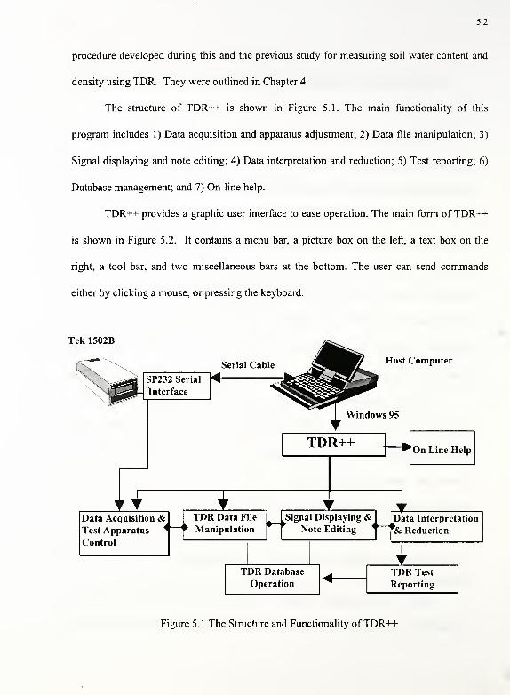
The structure of TDR++ is shown in Figure 5.1. The main functionality of this
program includes 1) Data acquisition and apparatus adjustment; 2) Data file manipulation; 3)
Signal displaying and note editing; 4) Data interpretation and reduction; 5) Test reporting; 6)
Database management; and 7) On-line help.
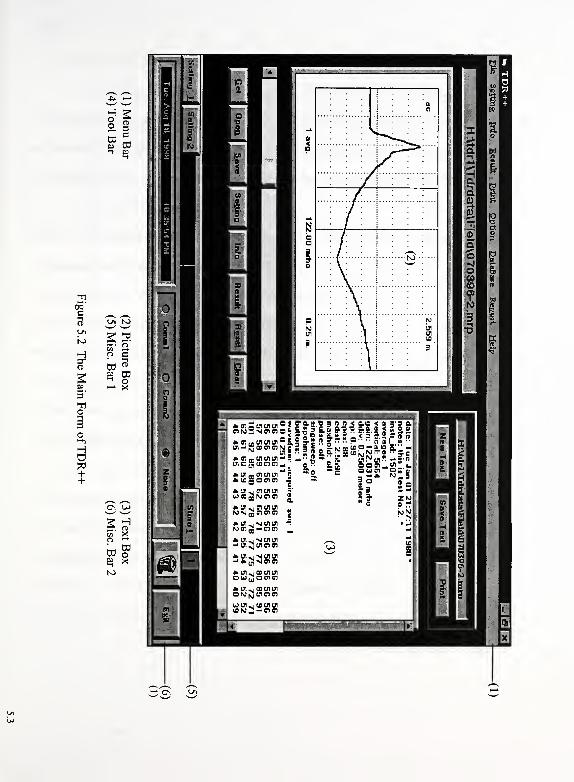
TDR++ provides a graphic user interface to ease operation. The main form of TDR++
is shown in Figure 5.2. It contains a menu bar, a picture box on the left, a text box on the
right, a tool bar, and two miscellaneous bars at the bottom. The user can send commands
either by clicking a mouse, or pressing the keyboard.
Tek 1502B
Serial Cable
SP232 Serial
Interface
Host Computer
Windows 95
TDR++
klData Acquisition &Test Apparatus
Control
<~TDR Data File
Manipulation>-
On Line Help
Signal Displaying &Note Editing <~ ft
1Data Interpretation
& Reduction
TDR Database
Operation
1TDR Test
Reporting
Figure 5.1 The Structure and Functionality ofTDR^
T1
HXTa
5'
o
2,
5
2 2
0\ <*>
en xo «
03 of» X
5.4
5.2.1. Data Acquisition and Test Apparatus Adjustment
Data Acquisition
TDR++ enables the user to obtain TDR test data from the apparatus (Tektronix
1502B) via an RS232 serial interface (SP232). The user can receive TDR waveform test data
by clicking the [Get] button on the tool bar. The time of the acquisition is recorded for test
reporting purposes.
A TDR waveform is limited to 251 data points. Although the vertical scale displaying
voltage can be divided into either 128 or 8192 increments, 8192 increments are used as
default. It takes about 20 seconds to retrieve a TDR waveform. While the data
acquisition is underway, TDR++ locks out other processes and displays a message. After the
data acquisition is complete, the waveform is displayed in the picture box with the horizontal
scale (distance per division), vertical scale (decibels or millirho), filter, and cursor. The file
name label displays "New File" to identify that new data is present and has not been saved. If
data acquisition is interrupted for any reason an error message is display indicating that the
acquisition was unsuccessful.
A connection indicator is included on the bottom tool bar and shows which serial port
of the host computer is currently being used. Every ten seconds a connection check is run to
examine the serial connection between the host computer and the SP232 module of the
Tektronix 1502B. When no connection exists, the indictor shows "None", and all the
commands involving serial communication will be disabled. Therefore, the user knows the
status of connection every ten seconds.
5.5
Test Apparatus Adjustment
Apparatus adjustment is necessary in order to obtain a TDR waveform of optimum
resolution and position to achieve the best quality readings. Necessary adjustments include
resetting the apparatus, selecting appropriate scales for horizontal and vertical axes, and
control of the source wave. All the controlling actions are implemented through
1502B/SP232 Instruction Set.
The TDR apparatus periodically requires resetting similar to a computer to reduce
communication disorder. TDR++ is designed so that when the device is connected to the
computer it will immediately reset, allowing it to clear out memory banks.
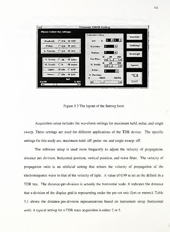
The user can adjust the settings to improve the size and position of the waveform by
clicking on the [Setting] button on the tool bar. A setting form is displayed that allows control
of the instrument, waveform acquisition, software, and cursor distance setup. The layout of
the setting form is shown in Figure 5.3.
Instrument setup allows the user to select the units of vertical scale, horizontal scale
and the light status. There are two vertical scale units: decibels (dB) and millirho (mrho), in
which dB is a log scale unit and mrho is a linear one. The horizontal scale has units of feet or
meters. The display light for the screen of the TDR apparatus can be turned off to conserve
batteries.
5.6
Tektronix 1 502B Setting
ise Select the settings:
Maxho Id C ON (i OFF
Pulse: O ON <m OFF!
I S. Sweep: O ON (• OFF
jV. Scale: f~ db (• miho 1
jH. Scale: r h (• meter 1
Light: <• ON C OFF
Ohms : r- on » OFF 1
Software Setup
VP: 0. EHT± ^^B~*l
Ditt/div: Q r±i
Button: Q r±]
Cut Pox.: 1 4,|
88
1
250
V. Scale 1—
.
43
1 .
255
_ 1*J
Filter vm * 1
V. Position:
56B4 16383
1*1 1 1 L*J
Figure 5.3 The layout of the Setting form
Acquisition setup includes the waveform settings for maximum hold, pulse, and single
sweep. These settings are used for different applications of the TDR device. The specific
settings for this study are, maximum hold: off; pulse: on; and single sweep: off.
The software setup is used more frequently to adjust the velocity of propagation,
distance per division, horizontal position, vertical position, and noise filter. The velocity of
propagation ratio is an artificial setting that relates the velocity of propagation of the
electromagnetic wave to that of the velocity of light. A value of 0.99 is set as the default in a
TDR test. The distance-per-division is actually the horizontal scale. It indicates the distance
that a division of the display grid is representing under the pre-set unit (feet or meters). Table
5.1 shows the distance-per-division representations based on instrument setup (horizontal
unit). A typical setting for a TDR trace acquisition is either 2 or 3.
5.7
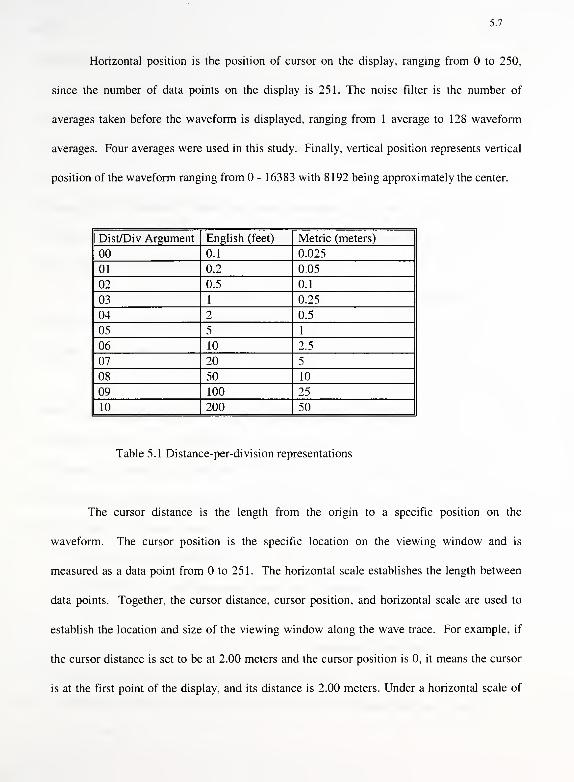
Horizontal position is the position of cursor on the display, ranging from to 250,
since the number of data points on the display is 251. The noise filter is the number of
averages taken before the waveform is displayed, ranging from 1 average to 128 waveform
averages. Four averages were used in this study. Finally, vertical position represents vertical
position of the waveform ranging from - 16383 with 8192 being approximately the center.
Dist/Div Argument English (feet) Metric (meters)
00 0.1 0.025
01 0.2 0.05
02 0.5 0.1
03 1 0.25
04 2 0.5
05 5 1
06 10 2.5
07 20 5
08 50 10
09 100 25
10 200 50
Table 5.1 Distance-per-division representations
The cursor distance is the length from the origin to a specific position on the
waveform. The cursor position is the specific location on the viewing window and is
measured as a data point from to 251. The horizontal scale establishes the length between
data points. Together, the cursor distance, cursor position, and horizontal scale are used to
establish the location and size of the viewing window along the wave trace. For example, if
the cursor distance is set to be at 2.00 meters and the cursor position is 0, it means the cursor
is at the first point of the display, and its distance is 2.00 meters. Under a horizontal scale of
5.8
0.1 meter/div, the display will show a window from 2.00 meter to 3.00 meter, because there
are 10 divisions on the display and 25 subdivisions/div.
When the cursor distance, cursor position, and scale have been selected, the user clicks
the [Set] button in the Setting form to activate the remote control. The change is made on the
next acquisition. More than one iteration may be needed to get a satisfactory waveform;
however, this adjustment is typically necessary only once for a specific soil being tested.
Since TDR waveforms of many soil types have similar horizontal and vertical ranges, it is
possible to determine a setting that is applicable for most conventional TDR tests. TDR++
allows the user to pre-set two settings and save them as Setting 1 and Setting 2. The user can
then simply select buttons [Setting 1] or [Setting 2] on the setting menu. These two settings
can be modified whenever necessary by making adjustments as desired and then clicking the
[Set] button for Setting 1 or 2.
As stated in Chapter 4, the accuracy of the TDR readings relates to the number of
available data points within the zone of interest between Points 1 and 2. The Tektronix device
has limited flexibility in the scale adjustment because of the degree of magnification
associated with a scale increase. Under the most unfavorable conditions as few as 100 points
may define the curve between Points 1 and 2. For this case, measurement errors as large as
2% are possible for each of the two points. It is anticipated the errors associated with a
discretization of only 251 data points will be reduced as new equipment is developed.
5.2.2 TDR Data File Manipulation
TDR++ is able to manipulate different types of files including those with the pre-
defined extensions, *.mrp, *.cc, *.cdt, *.set and *.wfm, which are explained in Table 5.2. The
5.9
file operations possible using TDR++ include 1) Open a file; 2) Get attributes of the current
file; 3) Get included file information; 4) Save a file; 5) Temporarily store a waveform in a file
register. The stored waveforms can be retrieved to Picture Box for viewing or a Text Box to
examine specific data.
The TDR data is saved as a file. In saving a TDR file, the user needs to select the
format first. Five formats with different file name extensions are available for saving a file.
The purpose of each format is shown in Table 5.2. Different file formats are used for data
manipulation and calculation purposes.
There is a file register designed in TDR++, in which the user can temporally store up
to five files, keeping those files accessible for the Picture Box and the Text Box. The purpose
of this is for waveform comparison, which will be explained in detail in the next section.
By clicking the [Open] button on the toolbar, the user can open a file with the name he
or she selects in the dialog box. Upon opening a file, TDR++ can identify if it is a TDR
waveform or not. The program will display the waveform if there is one; otherwise it will
open the file as a plain text file. The name of the file will be displayed as a particular label.
The waveform displayed in the Picture Box will automatically be set to the current file. All
file operations will be with respect to the current file.
Attributes of the current file, such as filename, path, file length, last modified time,
etc., can be viewed via the [Properties] button in the File menu.
Information that is saved can be grouped into Test Info, Soil Info, and Input Info, each
of which can be viewed by clicking the sub menus under the Info menu. Test Info contains
information such as Test ID, Test Type, Test Site, Test Time, etc., and is used in the reduction
of test data and for record keeping. Soil Info relates to the characteristics of the tested soil,

5.10
including Soil Name, Soil ID, USCS and ASSHTO Classifications, Liquid Limit, Plastic
Limit and Clay Fraction. Input Info includes data related to the MRP and CC and is used in
data reduction.
File Name Extension File Format
*.mrp MRP data file
*.cc CC data file
*.cdt Conductivity file
*.set Setting file
*.wfm TDR curve file
Table 5.2 File name extension and corresponding file format.
5.2.3 Signal Displaying and Note Editing
A TDR waveform can be displayed in the Picture Box on the Main Form and the
cursor can indicate the position of each data point. A horizontal scroll bar is assigned to move
the cursor to the left or the right. The position readout is visible in the upper right-hand comer
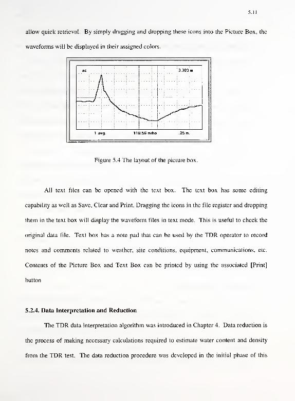
of the screen. The picture box contains several labels showing the vertical and horizontal
scales of the waveform, the noise filter, and the power setting. The layout of the Picture Box
is shown in Figure 5.4.
The Picture Box can display up to 6 different waveforms at the same time to provide a
visual comparison. Using the [Store] button on the Misc. toolbar, the user can temporarily
store up to five waveforms. A colored rectangular icon is created for each waveform stored to
5.11
allow quick retrieval. By simply dragging and dropping these icons into the Picture Box, the
waveforms will be displayed in their assigned colors.
ac 3.309 in
1 avg. 118.5Gmiho .25 m.
Figure 5.4 The layout of the picture box.
All text files can be opened with the text box. The text box has some editing
capability as well as Save, Clear and Print. Dragging the icons in the file register and dropping
them in the text box will display the waveform files in text mode. This is useful to check the
original data file. Text box has a note pad that can be used by the TDR operator to record
notes and comments related to weather, site conditions, equipment, communications, etc.
Contents of the Picture Box and Text Box can be printed by using the associated [Print]
button
5.2.4. Data Interpretation and Reduction
The TDR data interpretation algorithm was introduced in Chapter 4. Data reduction is
the process of making necessary calculations required to estimate water content and density
from the TDR test. The data reduction procedure was developed in the initial phase of this
5.12
study and modified somewhat during the present work. The details of this procedure along
with results of field verification tests are presented in Chapter 6. The implementation of this
procedure into the TDR++ software is discussed here.
Data reduction is straightforward for tests in the coaxial cylinder (CC). Calculation of
the apparent dielectric constant requires the probe length as input and the apparent length of
the reflected waveform interpreted from the algorithm. The wet density of the soil is obtained
from the volume of the CC mold and the mass measured with a balance. The water content is
obtained using the developed correlation between apparent dielectric constant, soil density,
and water content.
The procedure for reduction of multiple rod probe (MRP) test data is linked to the
corresponding results of the test in the CC mold. When reducing the MRP test data, TDR++
will open the linked CC data file in the background and obtain the quantities needed, namely;
water content, dry density, and apparent dielectric constant. The link is established in the Test
Info form of the MRP data. If there is a modification in either the MRP Input or the CC Input,
TDR++ will check the change and recalculate the results. Results are saved in the TDR data
file where they remain easily accessible.
5.2.5 TDR Test Reporting
TDR++ can generate test reports in either a long form or a short form. When the
results of a TDR test are complete, the user can select the desired format from the Report
menu. The reports are generated in Microsoft Excel using a technique called OLE
Automation. A full description of OLE automation is beyond the scope of this report, but
briefly, it allows integration of software tools for a specific functionality. Excel was chosen
5.13
because it is a common spread sheet tool installed on most personal computers. Macros were
written in the Excel modules, including Print Preview, Print and Exit. The user can modify
the macros easily using the Excel™ macro recorder or Visual Basic™.
5.2.6. TDR Database
Development of a database of all TDR measurements will allow assessing and
improving the test procedure and equipment. The TDR procedure for measuring soil water
content and density is based on both theoretical and statistical correlations. The statistical
relationships can be enhanced with the accumulation of additional data. The database is being
generated in Excel and multiple sheets were designed to contain different input data. The
structure of this database is quite flexible and the user can perform various operations on
original or secondary data.
Ten different sheets were designed to hold different information, including Test Info,
Soil Info, waveforms, Settings, MRP Input, CC Input, Curve Readings, MRP Results, CC
Results, and. Reference Info. The Reference sheet is designed to hold measurements from
other methods, including oven dry and nuclear gage moisture content, and sand cone and
nuclear gauge density.
The stored information in this database is expected to improve the calibration
coefficients for different soil types. The accumulation of actual field data, including TDR
curves, and soil indices, can be used to improve correlations between TDR measurements and
soil properties, which is future goal of this research.
5.14
5.2.7 On-line Help
On-line Help is provided in the standard Windows 95™ operating system format. It
provides functions for searching, establishing bookmarks, and indexes to assist the user.
5.3. Comments on Procedural Automation
The description of the TDR++ automation software presented here does not fully
elaborate on all the features of the program. Although the software has been developed in a
user- friendly environment, it is anticipated that proficiency in using the software can be
accelerated by holding training sessions for operators of the equipment.
Every effort has been made to validate and debug the software package. At this time
the software package is working as intended and no known bugs exist. However, it is possible
that some difficulties may arise during routine use of the software in a wide variety of field
situations by different technicians. Moreover, operators may have valuable feedback that will
assist us in improving the system. For this reason we view software development and the
testing procedure as an ongoing activity that can be continually improved. Accordingly, the
members of the TDR research group welcome comments on this software and procedure from
users.

6.1
CHAPTER 6
LABORATORY AND FIELD EVALUATION OF TDR METHOD
6.1 Introduction
Hundreds of tests were performed in the previous study to establish the calibration
equations and evaluate the test procedure. These results were encouraging and showed the
potential for using TDR to measure water content and density of soil in situ. Most of the
initial tests were done under laboratory conditions, on a limited number of soil types, and over
a small range of soil densities. During the present work, additional tests were conducted
using the new prototype equipment and included: field tests on actual construction sites, tests
on a broader group of soils, and tests over a wider range of soil densities. Based on these
results, the procedure that used both Topp's equation and the density-compensating
gravimetric water content equation (see Eqn [2.4] which is repeated below as Eqn [6.3])
developed in the previous study was reexamined to further assess the influence of density on
the accuracy of measurements. It was found that Topp's equation is of insufficient accuracy
to be useful over a wide range in soil densities.
6.2 Reexamination of the Calibration Equations
In the previous study, several calibration equations were reviewed. These include
1. Topp's (1980) "universal" empirical equation
= -0.053 + 2.92 x 1
0'2 K - 5.5 x 1
0"4 K 2 + 4.3 x 1
0"6 K 3
[6.1]
2. A semi-empirical linear calibration equation
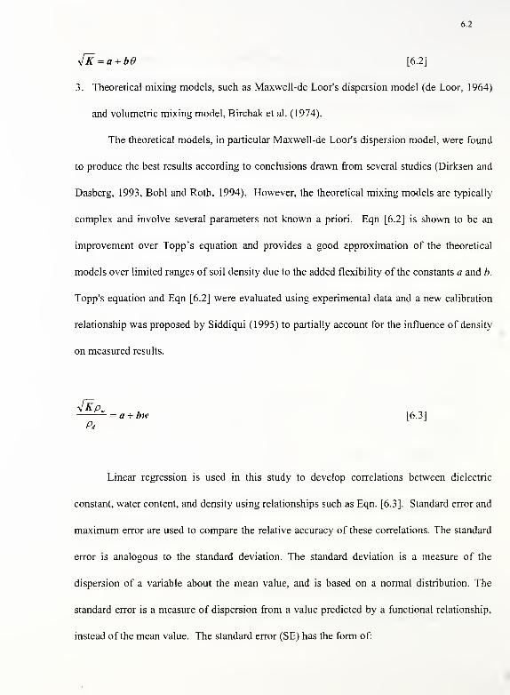
6.2
J~K=a + b0 [6.2]
3. Theoretical mixing models, such as Maxwell-de Loor's dispersion model (de Loor, 1964)
and volumetric mixing model, Birchak et al. (1974).
The theoretical models, in particular Maxwell-de Loor's dispersion model, were found
to produce the best results according to conclusions drawn from several studies (Dirksen and
Dasberg, 1993, Bohl and Roth, 1994). However, the theoretical mixing models are typically
complex and involve several parameters not known a priori. Eqn [6.2] is shown to be an
improvement over Topp's equation and provides a good approximation of the theoretical
models over limited ranges of soil density due to the added flexibility of the constants a and b.
Topp's equation and Eqn [6.2] were evaluated using experimental data and a new calibration
relationship was proposed by Siddiqui (1995) to partially account for the influence of density
on measured results.
= a + bw [6.3]
Linear regression is used in this study to develop correlations between dielectric
constant, water content, and density using relationships such as Eqn. [6.3]. Standard error and
maximum error are used to compare the relative accuracy of these correlations. The standard
error is analogous to the standard deviation. The standard deviation is a measure of the
dispersion of a variable about the mean value, and is based on a normal distribution. The
standard error is a measure of dispersion from a value predicted by a functional relationship,
instead of the mean value. The standard error (SE) has the form of:
6.3
X[(wod)/ -(wtdx),]2
SL J" _« -2
where wOD = oven dry water content
wTDR = predicted water content using TDR correlation
n = number of test samples
The maximum error is the largest error between the measured data and that predicted
by the correlation. It was concluded in the previous study that the standard error and
maximum error of water content measurements using calibration equations, such as Topp's
equation, Eqn [6.2], or Eqn. [6.3] with average coefficients are all about ±1.0% and ±2.0%,
respectively. The standard and maximum errors of water content measurement could be
reduced to ±0.8% and ±1.0%, respectively, if soil specific coefficients are used in Eqns [6.2]
or [6.3].
The laboratory work performed in the previous study to indicate only marginal benefit
in using one calibration equation over another. In fact, the final procedure recommended in
the previous study made use of both Topp's equation and Eqn [6.3]. However, the
experiments from which the above conclusions were drawn in the previous study were limited
to a range in density of 1.4 to 1.65 Mg/m 3. Additional experiments were conducted in this
study on several Indiana soils over a broader range in densities that are consistent with
compacted soil densities used in construction. These additional tests exposed a weakness in
using Topp's equation and resulted in a modification to the recommended procedure for
making measurements.
6.4
6.2.1 Experimental Method
The specific purpose of this study is to measure water content and density of soils used
in highway construction for quality control purposes. Therefore, it is desirable to test actual
Indiana soils over the typical range in compacted densities. Table 6.1 shows the
characteristics of the soils used in the laboratory testing program. The tests were conducted
during standard and modified compaction tests. The testing device used was similar to the CC
transmission line shown in Figure 3.2. The procedure for performing a test is as follows:
1. Prepare the soil at the desired water content and compact the soil in the compaction mold
with standard compaction effort or modified compaction effort, following ASTM D698
and ASTMD 1557.
2. Determine the wet density of the soil in the compaction mold by measuring the mass of
soil in the known volume.
3. Use the CC template to insert the central rod into the compaction mold.
4. Remove the mold from the base plate and place the mold on a nonmetallic base plate.
5. Make a measurement using the TDR device and compute the dielectric constant.
6. Take a sample for measuring water content by oven drying.
7.
6.2.2 Results and Discussion
Topp's equation was used to compute the volumetric water content. The gravimetric
water content was then obtained from the volumetric water content and the measured wet
density. The results were compared with the oven-dry water content, as shown in Figure 6.1.
The standard error is 1.9% and the maximum error is 4.0%. Figure 6.1 illustrates that Topp's
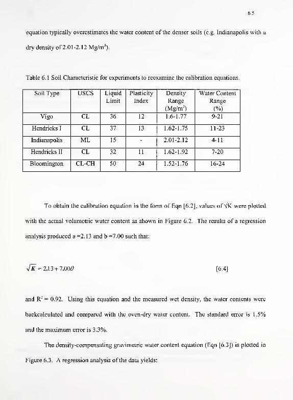
6.5
equation typically overestimates the water content of the denser soils (e.g. Indianapolis with a
dry density of 2.01-2.12 Mg/m3).
Table 6.1 Soil Characteristic for experiments to reexamine the calibration equations.
Soil Type uses Liquid
Limit
Plasticity
Index
Density
Range
(Mg/m3
)
Water Content
Range
(%)
Vigo CL 36 12 1.6-1.77 9-21
Hendricks I CL 37 13 1.62-1.75 11-23
Indianapolis ML 15 - 2.01-2.12 4-11
Hendricks II CL 32 11 1.62-1.92 7-20
Bloomington CL-CH 50 24 1.52-1.76 16-24
To obtain the calibration equation in the form of Eqn [6.2], values of Vk were plotted
with the actual volumetric water content as shown in Figure 6.2. The results of a regression
analysis produced a =2.13 and b =7.00 such that:
<JH = 2.13 + 7.000 [6.4]
and R2 = 0.92. Using this equation and the measured wet density, the water contents were
backcalculated and compared with the oven-dry water content. The standard error is 1.5%
and the maximum error is 3.3%.
The density-compensating gravimetric water content equation (Eqn [6.3]) is plotted in
Figure 6.3. A regression analysis of the data yields:
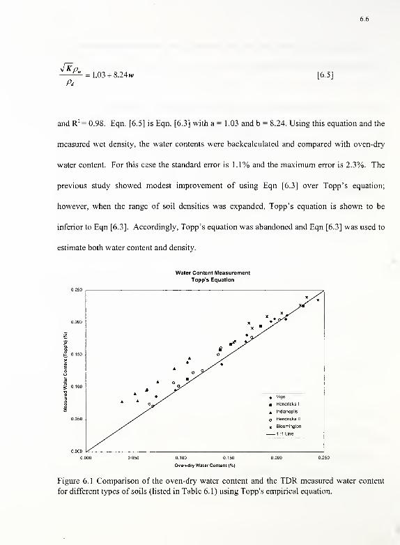
6.6
JKP„= 1.03 + 8.24h- [6.5]
and R2 = 0.98. Eqn. [6.5] is Eqn. [6.3] with a = 1.03 and b = 8.24. Using this equation and the
measured wet density, the water contents were backcalculated and compared with oven-dry
water content. For this case the standard error is 1.1% and the maximum error is 2.3%. The
previous study showed modest improvement of using Eqn [6.3] over Topp's equation;
however, when the range of soil densities was expanded, Topp's equation is shown to be
inferior to Eqn [6.3]. Accordingly, Topp's equation was abandoned and Eqn [6.3] was used to
estimate both water content and density.
g 100
0000
0.000
Water Content MeasurementTopp's Equation
XX
XX
X J*
A
AA
o 9"
1o
.*
A
A
A
A
*
O5-"
/"^
* Vigo
m Hendricks 1
4 Indianoplis
o Hendricks II
x Bloomington
1 1 Line
0.100 0.150
Oven-dry Water Content (•/.)
Figure 6.1 Comparison of the oven-dry water content and the TDR measured water content
for different types of soils (listed in Table 6.1) using Topp's empirical equation.
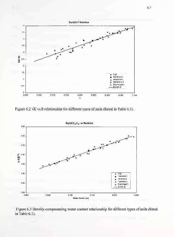
6.7
Sqrt(K)-" Relation
XX--""x
4.5 X ^-^*X ^•^o
4 -
A
% IBr*
3.5 -
A ^ —o
3 -
A
o
o*
2.5 o
2
1.5
* Vigo
a Hendncks
I
1 A Indianoplis
o Hendncks II
0.5x Bloomington
Eqn[6.4)
n .
0.000 050 0.100 0150 200 0.250 0.300 0.350
Figure 6.2 ^iKvs.Q relationship for different types of soils (listed in Table 6.1).
SqrtfKJp^Pj - w Relation
3.00 X ""* X
2 50 .
XXX .
X^^f'
2 00 .
6"q
rt(
K)
1 50 .
Ai^*U
'oo*
1 00 . *> Vigo
a Hendncks I
4 Indianoplis
50 .
Hendncks II
x Bloomington
Eqn (6 5]
00 -
100 150
Water Content (w)
Figure 6.3 Density-compensating water content relationship for different types of soils (listed
in Table 6.1).
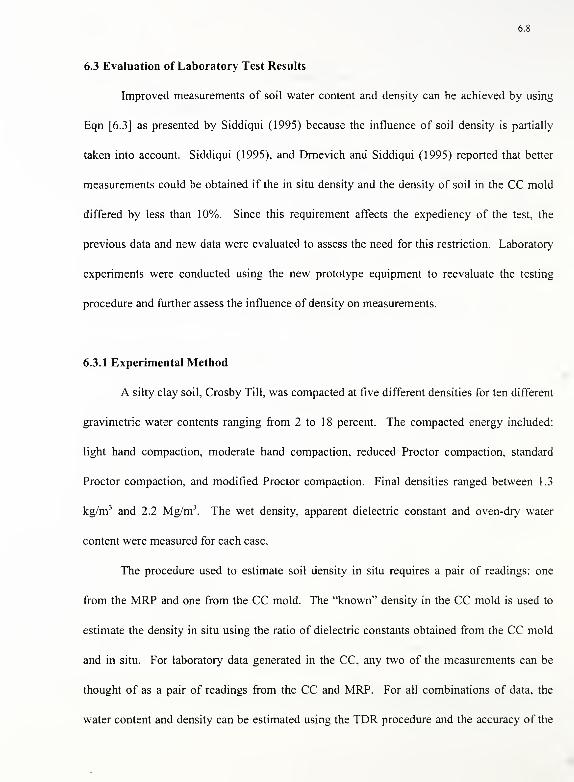
6.8
6.3 Evaluation of Laboratory Test Results
Improved measurements of soil water content and density can be achieved by using
Eqn [6.3] as presented by Siddiqui (1995) because the influence of soil density is partially
taken into account. Siddiqui (1995), and Drnevich and Siddiqui (1995) reported that better
measurements could be obtained if the in situ density and the density of soil in the CC mold
differed by less than 10%. Since this requirement affects the expediency of the test, the
previous data and new data were evaluated to assess the need for this restriction. Laboratory
experiments were conducted using the new prototype equipment to reevaluate the testing
procedure and further assess the influence of density on measurements.
6.3.1 Experimental Method
A silty clay soil, Crosby Till, was compacted at five different densities for ten different
gravimetric water contents ranging from 2 to 18 percent. The compacted energy included:
light hand compaction, moderate hand compaction, reduced Proctor compaction, standard
Proctor compaction, and modified Proctor compaction. Final densities ranged between 1.3
kg/m3and 2.2 Mg/m 3
. The wet density, apparent dielectric constant and oven-dry water
content were measured for each case.
The procedure used to estimate soil density in situ requires a pair of readings: one
from the MRP and one from the CC mold. The "known" density in the CC mold is used to
estimate the density in situ using the ratio of dielectric constants obtained from the CC mold
and in situ. For laboratory data generated in the CC, any two of the measurements can be
thought of as a pair of readings from the CC and MRP. For all combinations of data, the
water content and density can be estimated using the TDR procedure and the accuracy of the
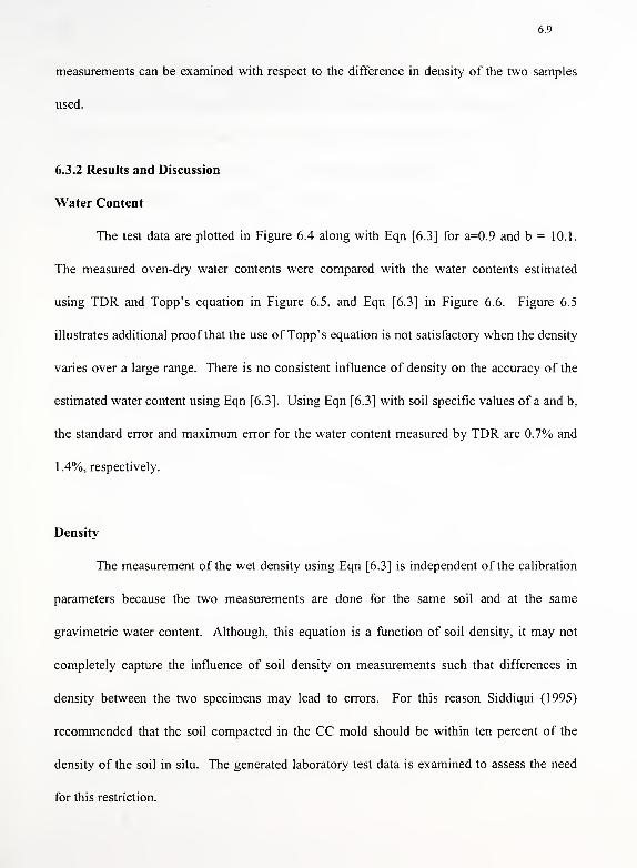
6.9
measurements can be examined with respect to the difference in density of the two samples
used.
6.3.2 Results and Discussion
Water Content
The test data are plotted in Figure 6.4 along with Eqn [6.3] for a=0.9 and b = 10.1.
The measured oven-dry water contents were compared with the water contents estimated
using TDR and Topp's equation in Figure 6.5, and Eqn [6.3] in Figure 6.6. Figure 6.5
illustrates additional proof that the use of Topp's equation is not satisfactory when the density
varies over a large range. There is no consistent influence of density on the accuracy of the
estimated water content using Eqn [6.3]. Using Eqn [6.3] with soil specific values of a and b,
the standard error and maximum error for the water content measured by TDR are 0.7% and
1 .4%, respectively.
Density
The measurement of the wet density using Eqn [6.3] is independent of the calibration
parameters because the two measurements are done for the same soil and at the same
gravimetric water content. Although, this equation is a function of soil density, it may not
completely capture the influence of soil density on measurements such that differences in
density between the two specimens may lead to errors. For this reason Siddiqui (1995)
recommended that the soil compacted in the CC mold should be within ten percent of the
density of the soil in situ. The generated laboratory test data is examined to assess the need
for this restriction.
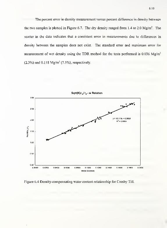
6.10
The percent error in density measurement versus percent difference in density between
the two samples is plotted in Figure 6.7. The dry density ranged from 1.4 to 2.0 Mg/m3. The
scatter in the data indicates that a consistent error in measurements due to differences in
density between the samples does not exist. The standard error and maximum error for
measurement of wet density using the TDR method for the tests performed is 0.036 Mg/m 3
(2.3%) and 0.1 18 Mg/m3(7.5%), respectively.
Sqrt(K)pw/pd - w Relation
'•»
2.50
**^
2.00 .
y= 10 118x +0 8868
R2 = 0.9904
a.
g 1 50
* .^^
Ccrin
1.00
0.50
0.00
0000 0200 0400 0600 0800 1000 1200 0.1400 1600 1800 2000
Water Content
Figure 6.4 Density-compensating water content relationship for Crosby Till.

6.11
Water Content Measurement
Using Topp's Equation
0200 0400 0600 0800 1000 1200 1400 1600 1800 0.2000
Oven-OryWater Content
Figure 6.5 Comparison of the oven-dry water content and the TDR measured water content
for Crosby Till using Topp's empirical equation.
Water Content Measurement
Using Sqrt(K)i<Jp d-w Equation
0180
0.160
0.140Sjg
0.120
0.100 s* X
0080
•Is
V
0.060
j?**
0.040
*}r% w from Siddiqui's
0.020
1:1 Une
0.000
0.0000 0.0200 00400 0.0600 0.0800 1000 0.1200 0.1400 0.1600 0.1800 0.2000
Oven-Dry Water Content
Figure 6.6 Comparison of the oven-dry water content and the TDR measured water content
for Crosby Till using Density-compensating water content equation.
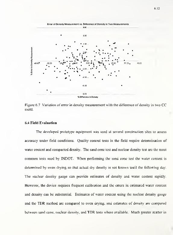
6.12
Error of Density Measurement vs. Difference of Density in Two Measurements
8XK)
£ -40 00*• •
• •
A • •* w » ^— ^ te •-30.00 -20£0* , J»00 00#» TO*0. 20.00 30.00 #
•• • v . • * . : *» • •• -2.00 . • • •
. * *
% Difference in Density
Figure 6.7
mold.
Variation of error in density measurement with the difference of density in two CC
6.4 Field Evaluation
The developed prototype equipment was used at several construction sites to assess
accuracy under field conditions. Quality control tests in the field require determination of
water content and compacted density. The sand cone test and nuclear density test are the most
common tests used by INDOT. When performing the sand cone test the water content is
determined by oven drying so that actual dry density is not known until the following day.
The nuclear density gauge can provide estimates of density and water content rapidly.
However, the device requires frequent calibration and the errors in estimated water content
and density can be substantial. Estimates of water content using the nuclear density gauge
and the TDR method are compared to oven drying, and estimates of density are compared
between sand cone, nuclear density, and TDR tests where available. Much greater scatter in
6.13
the data can be expected under field conditions relative to laboratory tests because of the
inherent spatial variability of soils, water contents, and densities that will result under field
conditions.
6.4.1 Experimental Method
Forty-four quality control tests were performed at 1 1 construction sites. Some sites
have only TDR and one of nuclear or sand cone tests, while some sites have all three tests. At
each test location the TDR, nuclear and/or sand cone test were done as close as practical to
each other. The TDR field test procedure was reviewed in Section 2.2. The soil excavated for
compaction in the CC was taken from within the boundary formed by the MRP and uniformly
from the entire depth of in-place measurement. The soils were placed directly in the CC to
minimize moisture loss and compacted uniformly using either moderate hand compaction or
standard compaction effort. The excavated soil samples from the TDR tests and sand cone
tests were brought back to the lab to determine the oven-dry water content. The density-
compensating gravimetric water content equation (Eqn [6.3]) was used with average values of
a and b generated using all the field test results to calculate water content and density using
the TDR method. Average values were used because soil specific values of a and b were not
determined.
6.4.2 Results and Discussion
A summary of the sites tested and soil characteristics are provided in Table 6.2. Eqn
[6.3] is used to fit the data as shown in Figure 6.8 giving a = 0.8 and 6=10. This relationship
was used to estimate water content and a comparison is made with oven dry water content and
6.14
with nuclear density water content in Figure 6.9. Table 6.3 and 6.4 contain the results of
TDR, nuclear and sand cone tests at all sites.
The water content measurements, obtained from the TDR and nuclear methods (if
available) were compared with oven-dried values. As shown in Figure 6.9 and Table 6.3, the
measurements indicate that the water contents obtained by the TDR method are more accurate
than the nuclear density test. The standard error and maximum error for water content
measured by TDR were 1.1% and 2.8% respectively, and were 1.8% and 4.4% for the nuclear
method.
For a comparison of densities, twenty tests were performed with both the TDR and
nuclear gage (direct transmission method with 6" depth). The results show significant
variability in estimates obtained from the two methods. Thirteen tests with both TDR and
sand cone measurements were made on two construction sites. These results show that there
is also a significant variability between values obtained by TDR and sand cone tests.
However, the accuracy of the sand cone tests on this site was limited by the fact that the
compacted soil on this site consisted primarily of sand with gravel. Finally, at the Gas City
site, eight measurements were done using all three methods on silty clay soil. The results
indicate that the density obtained by the nuclear method compared more favorably to the sand
cone test than did the TDR densities. When compared to the sand cone test, the standard
error, and maximum error, of the difference in dry density measured by TDR was 0.097
Mg/m3
(5.5%) and 0.140 Mg/m 3
(7.7%) respectively, and 0.066 Mg/m3(3.6%) and 0.138
Mg/m 3(7.6%) for the nuclear gauge.
The difference in density that exists among the three methods is attributed partly to the spatial
variability of soil, water content, and density at the construction sites. For example, the
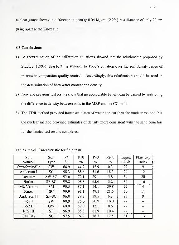
6.15
nuclear gauge showed a difference in density 0.04 Mg/m3
(2.2%) at a distance of only 20 cm
(8 in) apart at the Knox site.
6.5 Conclusions
1
)
A reexamination of the calibration equations showed that the relationship proposed by
Siddiqui (1995), Eqn [6.3], is superior to Topp's equation over the soil density range of
interest in compaction quality control. Accordingly, this relationship should be used in
the determination of both water content and density.
2) New and previous test results show that no appreciable benefit can be gained by restricting
the difference in density between soils in the MRP and the CC mold.
3) The TDR method provided better estimates of water content than the nuclear method, but
the nuclear method provided estimates of density more consistent with the sand cone test
for the limited test results completed.
Table 6.2 Soil Characteristic for field tests.
Soil
Source
Soil
Type
P4
%P10
%P40
%P200
%Liquid
Limit
Plasticity
Index
Crawfordsville SW 64.9 44.2 15.9 0.3 22 9
Anderson I SC 98.3 88.6 51.6 18.3 29 12
Decatur SW-SC 93.6 72.1 29.1 5.8 39 20
Butler SP-SC 99.2 98.8 65.6 5.2 34 16
Mt. Vernon SM 90.5 87.1 74.1 39.8 27 4
Knox SC 99.9 92.1 49.5 21.6 30 11
Anderson II SP-SC 96.0 89.3 59.5 6.3 23 9
1-52 I SW 88.9 76.0 50.9 10.0 - -
1-52 II GW 69.9 52.0 12.1 0.6 - -
1-52 III SP 96.9 85.8 61.9 10.4 - -
Gas City SC 97.5 94.2 58.7 12.5 31 13
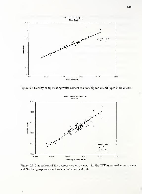
6.16
Calibration Equation
Field Test
3•
25y=1005x*080
a 2
S
Xr°"
1 s
•x-
«*
R2 = 95
1
• •^^**r*
5
Water Content, w
Figure 6.8 Density-compensating water content relationship for all soil types in field tests.
£ 0.100
0.000
0.000
Water Content Measurement
Field Test
m
MyrX
jP" X»/^"
X V/rs xxx
x
< x| x
x x
'
Ovendry
a TDR
x Nuclear
0.100 0.150
Oven-dry Water Content
Figure 6.9 Comparison of the oven-dry water content with the TDR measured water content
and Nuclear gauge measured water content in field tests.
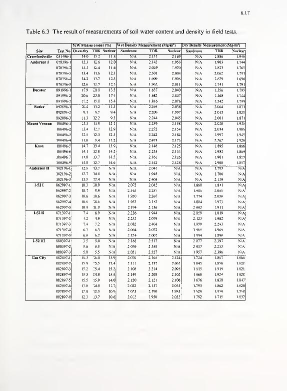
6.17
Table 6.3 The result ofmeasurements of soil water content and density in field tests.
Site Test No.
%VV Measurement (%) Wet Density Measurement (Mg/mJ
) Dry Density Measurement (Mg/mJ
)
Oven dry TDR Nuclear Sandcone TDR Nuclear Sandcone TDR Nuclear
Crawfordsville 051496-1 14.0 13.2 11.8 N/A 2.135 2.169 N/A 1.886 1 940
Anderson I 070396-1 13.3 12.6 12.0 N/A 2.143 1.953 N/A 1 .903 1 "44
070396-2 13.3 12.4 11.6 N/A 2.049 1.970 N/A 1.823 1 765
070396-3 13.4 11.6 12.1 N/A 2.301 2.008 N/A 2.062 1 "91
070396-4 14.2 13.7 12.5 N/A 1.909 1.908 N/A 1.679 1 696
070396-5 12.6 12.7 12.3 N/A 1.962 2.011 N/A 1.741 1 791
Decatur 091996-1 17.9 20.8 13.5 N/A 1.637 2.040 N/A 1.356 1 797
091996-2 20.6 23.0 17.4 N/A 1.682 2.047 N/A 1.368 1 744
091996-3 17.2 17.8 15.4 N/A 1.816 2.076 N/A 1.542 1 799
Butler 092096-1 10.4 11.2 11.3 N/A 2.295 2.038 N/A 2.064 1 831
092096-2 9.1 9.7 9.4 N/A 2.209 1.997 N/A 2.013 1 825
092096-3 11.3 12.2 9.3 N/A 2.244 2.045 N/A 2.001 1 871
Mount Vernon 100496-1 13.3 11.9 12.1 N/A 2.259 2.158 N/A 2.020 1 925
100496-2 13.4 11.7 12.9 N/A 2.272 2.154 N/A 2.034 1 90S
100496-3 12.5 12.3 12.3 N/A 2.242 2.184 N/A 1.997 1 945
100496^t 11.0 9.4 13.2 N/A 2.473 2.173 N/A 2.262 1 920
Knox 100496-5 14.7 13.4 13 9 N/A 2.148 2.125 N/A 1.895 1 866
100496-6 14.1 12.8 14.2 N/A 2.235 2.134 N/A 1.982 1 869
100496-7 14.0 13.7 14 5 N/A 2.161 2.126 N/A 1.901 ] 857
100496-8 14.0 12.7 14.6 N/A 2.142 2.128 N/A 1.900 1 857
Anderson II 102196-1 12.8 13.7 N/A N/A 2.041 N/A N/A 1.795 N/A
102196-2 12.7 14.0 N/A N/A 1.945 N/A N/A 1.706 N A
102196-3 13.5 12.4 N/A N/A 2.405 N/A N/A 2.139 N A
1-52 I 062997-1 10.3 10.9 N/A 2.072 2.042 N/A 1.860 1.841 \ A
062997-2 10.7 9.9 N/A 2.163 2.257 N/A 1.986 2.055 \ A
062997-3 10.6 10.6 N/A 1.930 2.267 N/A 1.774 2.050 N/A
062997-4 10.6 10.6 N/A 1.952 2.182 N/A 1.804 1.973 S A
062997-5 10.9 118 N/A 2.194 2.136 N/A 2.002 1.911 \ A
1-52 II 071397-1 7.4 6.9 N/A 2.226 1.944 N/A 2.059 1.819 \ \
071397-2 4.2 4.9 N/A 2.252 2.079 N/A 2.123 1.982 N A
071397-3 7.4 7.2 N/A 2.082 2.404 N/A 1.979 2.243 N/A
071 397-4 6.3 5.3 N/A 2.064 2.072 N/A 1.968 1.969 N/A
071397-5 6.0 6.2 N/A 2.124 2.007 N/A 1.994 1.890 \ A
1-52 III 080397-1 3.5 5.0 N/A 2.168 2.517 N/A 2.077 2.397 \ A
080397-2 5.6 5.5 N/A 2.076 2.355 N/A 2.017 2.233 N/A
080397-3 5.0 5.5 N/A 2.051 2.527 N/A 1.957 2.396 \ A
Gas City 082897-1 16.3 16.0 13 9 2.076 2.165 2.124 1.724 1.867 1 865
082897-2 15.9 15.5 13.4 2.111 2.137 2.065 1.845 1.850 1 821
082897-3 15.2 15.4 15.2 2.108 2.214 2.098 1.815 1.919 1 821
082897^ 15.3 14.8 15.5 2.149 2.208 2.102 1.860 1.924 1 820
082897-5 15.5 15.9 14.0 2.120 2.121 2.106 1.876 1.830 1 84^
082897-6 13.0 14.8 11.7 2.022 2.137 2.033 1.793 1.862 1 820
082897-7 12.8 13.5 109 2.023 2.190 1.983 1.820 1.930 1 788
082897-8 12.3 13.7 10.6 2.012 1.950 2.032 1.792 1.715 18.17
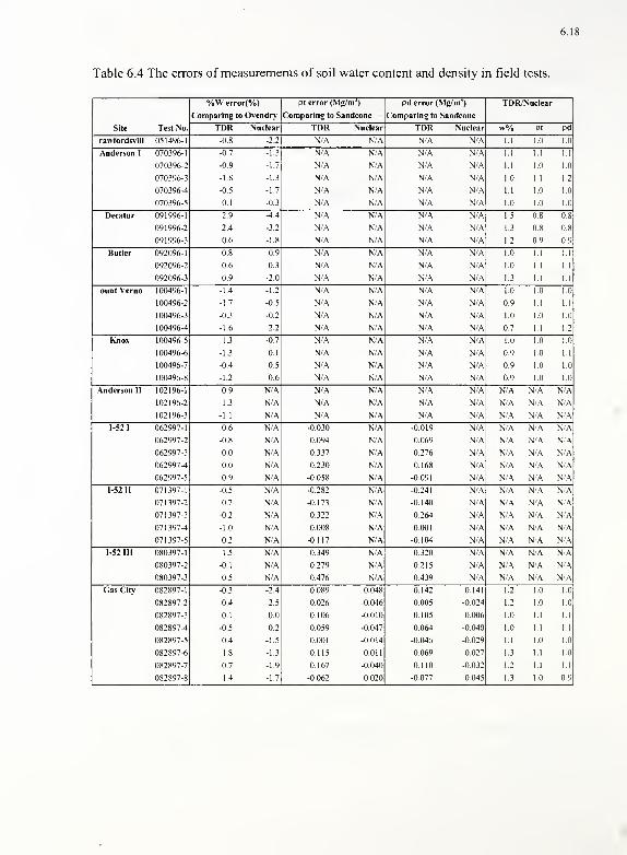
6.18
Table 6.4 The errors of measurements of soil water content and density in field tests.
%W error(%) pt error (Mg/m J
) pd error (Mg/nr1
) TDR/Nuclear
Site Test No.
Comparing to Ovendry Comparing to Sandcone Comparing to Sandcone
TDR Nuclear TDR Nuclear TDR Nuclear w% Pt Pd
rawfordsvill 051496-1 -0.8 -2.2 N'A N'A N'A N'A 1.1 1 1.0
Anderson I 070396-1 -0.7 -1.3 N/A N/A N/A N/A 1 1 11 1.1
070396-2 -0-9 -1.7 N/A N/A N/A N/A 1.1 1 1.0
070396-3 -1.8 -1.3 N/A N/A N/A N/A 1.0 1 1 1.2
070396-4 -0.5 -1.7 N/A N/A N/A N/A 1.1 1 1.0
070396-5 0.1 -0.3 N/A N/A N/A N/A 10 1 1.0
Decatur 091996-1 2.9 -4.4 N/A N/A N/A N/A 1.5 8 0.8
091996-2 2.4 -3.2 N/A N/A N/A N/A 1.3 8 0.8
091996-3 0.6 -1.8 N/A N A N/A N/A 1.2 9 0.9
Butler 092096-1 0.8 0.9 N/A N/A N/A N/A 1.0 i i i 1
092096-2 0.6 0.3 N/A N/A N/A N/A 1.0 1 1 1.1
092096-3 0.9 -2.0 N/A N/A N/A N/A 13 1 1 1.1
ount \ ei no 100496-1 -1 4 -1.2 N/A N/A N/A N/A 10 ; 10
100496-2 -1.7 -0.5 N/A N A N/A N/A 0.9 i 1 1 1
100496-3 -0.3 -0.2 N/A N/A N/A N/A 1.0 l 1.0
100496-4 -1.6 2.2 N/A N/A N/A N/A 0.7 l 1 1.2
Knox 100496-5 -1.3 -0.7 N A N/A N/A N/A 1.0 l 1.0
100496-6 -1.3 0.1 N/A N/A N/A N/A 0.9 l Q i 1
100496-7 -0.4 0.5 N/A N/A N/A N/A 0.9 l 1.0
100496-8 -1.2 0.6 N/A N A N/A N/A 0.9 l 1.0
Anderson II 102196-1 0.9 N/A N/A N/A N/A N/A N/A N \ N A
102196-2 1.3 N/A N/A N/A N/A N/A N/A N/A N/A
102196-3 -1.1 N/A N/A N/A N/A N/A N/A N/A N'A
1-52 I 062997-1 0.6 N/A -0.030 N/A -0.019 N/A N/A N'A N/A
062997-2 -0.8 N/A 0.094 N/A 0.069 N/A N/A N/A N -\
062997-3 0.0 N/A 0.337 N/A 0.276 N/A N/A N/A N \
062997-4 0.0 N/A 0.230 N/A 0.168 N/A N/A N/A N/A
062997-5 0.9 N/A -0.058 N/A -0.091 N/A N/A N/A N/A
1-52 II 071397-1 -0.5 N/A -0.282 N/A -0.241 N/A N/A N'A N/A
071397-2 0.7 N/A -0.173 N/A -0.140 N/A N/A N/A N/A
071397-3 -0.2 N/A 0.322 N/A 0.264 N/A N/A N/A N/A
071397-4 -1.0 N/A 0.008 N/A 0.001 N/A N/A N/A N/A
071397-5 0.2 N/A -0.117 N/A -0.104 N/A N'A N/A \ \
1-52 III 080397-1 1.5 N/A 0.349 N A 0.320 N/A N/A \ A N A
080397-2 -0.1 N/A 0.279 N/A 0.215 N/A N/A N/A N A
080397-3 0.5 N/A 0.476 N/A 0.439 N/A N/A N/A N'A
Gas City 082897-1 -0.3 -2.4 0.089 0.048 0.142 0.141 1.2 10 1.0
082897-2 -0.4 -2.5 0.026 -0.046 0.005 -0.024 1 2 1 D 1 D
082897-3 0.1 0.0 0.106 -0.010 0.105 0.006 I 1 1 1 1
082897-4 -0.5 0.2 0.059 -0.047 0.064 -0.040 1 1 1 1 1
082897-5 0.4 -1.5 0.001 -0.014 -0.046 -0.029 1 1 1 1
082897-6 1.8 -1.3 0.115 0.011 0.069 0.027 1 3 1 1 1.0
082897-7 0.7 -1.9 0.167 -0.040 0.110 -0.032 1 2 1 1 11
082897-8 14 -1.7 -0.062 0.020 -0.077 0.045 1 3 10.9
7.1
CHAPTER 7
STANDARDIZED PROCEDURE AND ASTM/AASHTO DRAFT STANDARDS
7.1 Introduction
A standardized procedure for using TDR to measure the water content and density of
compacted soil is introduced here to aid in obtaining consistent results. The recommended
procedure differs slightly from the procedure outlined in the previous study. Draft standards
have been prepared in the format of both ASTM and AASHTO.
7.2 Modifications to the Testing Procedure
Recommendations for implementing the developed technology were made in the final
report of the previous study (FHWA/IN/JHRP-95/9). Two modifications to the previous work
are recommended. One relates to the testing procedure and the other relates to the
calculations.
Procedure
In the previous study a recommendation was made to compact the soil into the CC
mold such that the density was within 10 percent of the in situ density. This restriction slows
the testing process and requires repeating a test if the criterion is not met. New test data and a
reevaluation of previous data indicate that the scatter in the measurements is not correlated to
the difference in density between the two samples. Accordingly, to expedite the testing
process, this restriction is no longer recommended. The only restriction on compaction in the
CC mold is that the material be compacted as uniformly as possible without macro voids.
7.2
Calculation
As discussed in Chapter 6, Topp's equation is no longer recommended for calculating water
content due to the influence of soil density on accuracy. Eqn [6.3] should be used for this
purpose with either soil specific, or general, coefficients a and b. Recommended values for
general coefficients are a = 0.8 and b = \Q. The a and b values depend on the b/a ratio and
length of the coaxial line. The recommended values reported here differ from those of the
previous study because modifications were made to the equipment geometry.
7.3 Draft of Standards
Drafts standards in the format ofASTM and ASSHTO are provided in Appendix I and
II.
8.1
CHAPTER 8
SUMMARY, CONCULSIONS AND RECOMMENDATIONS
8.1 Summary and Conclusions
Siddiqui and Drnevich (1995) developed a new method of measuring in-place density
and water content of compacted soil. Equipment and a procedure were developed that uses
time domain reflectometry (TDR) to make the measurements. The objectives of the present
study were to evaluate the proposed approach under actual field conditions by developing
prototype equipment, automating data interpretation, conducting tests on actual construction
sites for comparison with other measurement methods, and preparing draft specifications.
The TDR technique is used to measure the apparent dielectric constant of the soil. The
dielectric constant is correlated with the water content and density of the soil. The dielectric
constant is obtained by measuring the velocity of an electromagnetic wave traveling through a
coaxial line while soil is the insulating material. The velocity of a reflected electromagnetic
wave is measured using a TDR apparatus and the coaxial line can either be a coaxial cylinder
(CC) in which soil is compacted, or a multiple rod probe (MRP) that is inserted into the
compacted soil. The dimensions of the CC and MRP have been optimized to obtain the best
quality signal and to test a representative quantity of soil. Siddiqui and Drnevich (1995)
presented a thorough investigation and description of both the spatial and electromagnetic
variables.
Modifications were made to the equipment as part of the present study. The CC was
modified so that the same head could be used for both the CC and MRP thus reducing the
needed equipment. The data interpretation process was automated to eliminate operator

8.2
dependence and expedite testing time. Data reduction was also automated and a database of
test information developed.
Additional tests were conducted over a broader range in soil type and density and it
was shown that the use of Topp's equation to define the relationship between volumetric
water content and density did not have sufficient accuracy because it does not account for
variations in soil density. Accordingly, the soil specific calibration equations of the form
proposed by Siddiqui (1995) are used. When using these relationships the accuracy of results
for tests over a greater density range were consistent with those of the previous study.
During field testing it is necessary to compact the tested soil into the CC mold.
Although Siddiqui (1995) recommended that the density of the soil in the CC mold should be
within 10 percent of the density in situ, additional testing showed that imposing this
restriction did not appreciably improve density estimates. Accordingly, this criterion was
relaxed and the only criterion for compaction of the soil in the CC mold is that the material be
uniform and without macro voids.
The sand cone and nuclear density tests are the most common compaction control tests
used in Indiana. Under field conditions it was shown that the TDR method is more accurate
than the nuclear density gage in estimating water content when compared to oven drying, with
standard errors of 1.1% and 1.8%, respectively. Water content can not be estimated using the
sand cone test. It is more difficult to assess the accuracy of these methods in the
determination of dry density because the true dry density is not known because there are
errors associated with all methods. Although not completely accurate, the sand cone test was
conducted on several sites and is used here to compare the TDR and nuclear density test
results. On sites where TDR, nuclear density, and sand cone tests were performed, the dry

8.3
density estimated by the nuclear density gage was more consistent with the sand cone than
was the TDR method, yielding standard errors of 3.6% and 5.5%, respectively. It must be
recognized that spatial variability with the compacted soil also played a role in the differences
measured. The measured density differed by approximately 0.04 Mg/m3(2.2%) for two
nuclear density tests performed approximately 20 cm (8 in) apart. Under the laboratory
condition, the standard error of the TDR method for density in compacted cylinders where the
density is known accurately is 2.3%.
The time require to perform the TDR test under field conditions is approximately 15 to
20 minutes. The sand cone test can also be performed in approximately 15 minutes while the
nuclear density test can be performed in approximately 2 minutes. The time required to
complete the TDR test relative to the nuclear density test is viewed as its greatest limitation.
In general, the nuclear gage: provides estimates of density and water content much
more rapidly than the sand cone or TDR tests, is less accurate than the TDR test in estimating
water content, and must be calibrated for a specific soil using sand cone tests. Moreover, the
nuclear gage uses a hazardous source requiring operators to take safety training and leading to
expenses associated with equipment maintenance and disposal. The sand cone test is time
consuming, and can not provide estimates of water content. The TDR test is also time
consuming, but does provide accurate estimates of water content. The errors associated with
estimated dry density, when compared to the sand cone test, are larger than the nuclear density
test which is calibrated using the sand cone test.
At the present stage of the research, the TDR test has not shown great advantage in the
measurement of water content and density relative to the nuclear density test. However,
progress is being made in the development of an approach to use other features of the
8.4
reflected waveform, in addition to the apparent dielectric constant, within the interpretation
process. The research has tremendous potential and is described briefly in the next section.
8.2 Recommendations for Additional Research
The present TDR test is based solely on the measurement of the apparent dielectric
constant. The dielectric constant is a single parameter that is obtained from the reflected
electro-magnetic waveform. During the completion of this study it became obvious when
comparing curves of different soil type and at different densities that the reflected waveforms
contained much more information than is currently being utilized. A new study has been
initiated to use the entire waveform to estimate soil type and density. The primary objective
is to increase the accuracy of the density estimate while eliminating the need to excavate and
recompact the soil in the CC mold thereby reducing the test time substantially. Presently, a
numerical model has been developed to simulate the coaxial system and reflected waveform.
The input parameters to the model are soil properties and relative volumes of soil, air and
water. The model captures even subtle features of the reflected waveform. The research is
now directed toward solving the inverse problem of determining the soil parameters from the
measured waveform.
8.5
REFERENCES

8.6
REFERENCES
ASTM, D1556 (1997), "Standard Test Method for Density and Unit Weight of Soil in Place
by the Sand-Cone Method," Annual Book ofASTM Standards, Vol. 04.08, 120-125.
ASTM, D1557 (1997), "Test Method for Laboratory Compaction Characteristics of Soil
Using Modified Effort (56,000 ft-lbf/ft3
(2,700 kN-m/m3))," Annual Book of ASTM
Standards, Vol. 04.08, 125-133.
ASTM, D698 (1997), "Test Method for Laboratory Compaction Characteristics of Soil Using
Modified Effort (12,400 ft-lbf/ft3(600 kN-m/m3
))," Annual Book of ASTM Standards, Vol.
04.08, 77-84.
Baker, J. M. and Allmaras, R. R. (1990), "System for Automating and Multiplexing Soil
Moisture Measurement by Time-Domain Reflectometry," Soil Sci. Soc. Am. J., Vol. 55, 1-6.
Birchak, J. R., Gardner, C. G., Hipp, J. E., and Victor, J. M. (1974), "High Dielectric Constant
Microwave Probe for Sensing Soil Moisture," Proc. IEEE, Vol. 62 (1), 93-98.
Bohl, H. and Roth, K. (1994), "Evaluation of Dielectric Mixing Models to Describe the 0(e)
Relation," Proceedings of the Symposium and Workshop on Time Domain Reflectometry in
Environmental, Infrastructure and Mining Applications, Evanston, IL., Spec. Publ. SP 19-94,
309-319.
de Loor, G. P. (1964), "Dielectric Properties of Heterogeneous Mixtures with a Polar
Constituent," Appl. Sci. Res., Vol. 1 1, 310-320.
Dirksen, C. and Dasberg, S. (1993), "Improved Calibration of Time Domain Reflectometry
Soil Water Content Measurements," Soil Sci. Soc. Am. J., Vol. 57, 660-667.
Fellner-Feldegg, H. (1969), "Measurement of Dielectrics in the Time Domain," Journal of
Physical Chemistry, Vol. 73, 616-623.
Heimovaara, T. J. and Bouten, W. (1990), "A Computer-Controlled 36-Channel Time
Domain Reflectometry System for Monitoring Soil Water Contents," Water Resources
Research, Vol. 26, No. 1 0, 23 1 1 -23 1 6.
Microsoft Corporation (Redmond, WA) (1993), "Visual Basic Programmer's Guide (for
Visual Basic 3, Professional Version)."
Siddiqui, S. I. (1995), "A New Method of Measuring Density and Moisture Content of Soil
Using the Technique of Time Domain Reflectometry,", Ph. D. Theses, Purdue University.
8.7
Siddiqui, S. I. And Dmevich, V. P. (1995), "Use of Time Domain Reflectometry for the
Determination of Water Content and Density of Soil," Joint Highway Research Project
Report, FHWA/TN/JHRP-95/9, Purdue University.
Tektronix (Beaverton, OR) (1989), "SP232 Serial Extended Function Module for 1502B and
1503BMTDRs."
Timlin, D. J. and Pachepsky, Ya. A. (1996), "Comparison of Three Methods to Obtain the
Apparent Dielectric Constant from Time Domain Reflectometry Wave Traces," Soil Sci. Soc.
Am. J., Vol. 60, 970-977.
Topp, G. C, Davis, J. L. and Annan, A. P. (1980), "Electromagnetic Determination of Soil
Water Content: Measurement in Coaxial Transmission Lines," Ware Resources Research,
Vol. 16, 574-582.
Topp, G. C, Davis, J. L., and Annan, A. P. (1982), "Electromagnetic Determination of Soil
Water Content Using TDR: II., Evaluation of Installation and Configuration of Parallel
Transmission Lines," Soil Sci. Soc. Am. J., Vol. 46, 678-684.
Zegelin, S. J., White, I., and Jenskins, D. R. (1989) "Improved Field Probes for Soil Water
Content and Electrical Conductivity Measurement Using Time Domain Reflectomety," Water
Resources Research, Vol. 25, 2367-2376.
8.8
APPENDIX

Al.l
Appendix I ASTM Standard Draft
Standard Test Method for
Determination of Water Content and Density of Soil in Place Using Time DomainReflectometry (TDR)
1. Scope
1.1 This test method may be used to determine the water content of soils and the in-place
density and unit weight of soils using a TDR apparatus.
1 .2 This test method is applicable for soils without an appreciable amount of rock or
coarse materials in excess of 1.5 in. (38 mm) in diameter.
1.3 This test method is suitable for use as a means of acceptance for compacted fill or
embankments.
1 .4 This method may not be suitable for organic and highly plastic soils.
1.5 This standard does not purport to address the safety problems associated with its use.
It is the responsibility of the user of this standard to establish appropriate safety and
health practices and determine the applicability ofregulatory limitations prior to use.
2. Referenced Documents
2.1 ASTM Standards:
D653 Terminology Relating to Soil, Rock, and Contained Fluids
D698 Test Methods for Moisture-Density Relations of Soils and Soil-Aggregate
Mixtures, Using 5.51b (2.49kg) Rammer and 12-in. (305-mm) Drop
D1556 Test Method for Moisture-Density of Soil In-Place by the Sand-Cone Method
D1557 Test Methods for Moisture-Density Relations of Soils and Soil-Aggregate
Mixtures, Using 101b (4.54kg) Rammer and 18-in. (457-mm) Drop
D2167 Test Method for Density of Soil In-Place by the Rubber-Balloon Method
D2216 Method for Laboratory Determination of Water (Moisture) Content of Soil, Rock,
and Soil-Aggregate Mixtures
D2922 Test Methods for Density of Soil and Soil Aggregate and Rock in Place by
Nuclear Methods (Shallow Depth)
D2937 Test Method for Density of Soil In-Place by the Drive-Cylinder Method
D3017 Test Method for Water Content of Soil and Rock In-Place by Nuclear Methods
(Shallow Depth)
D4643 Method for Determination of Water (Moisture) Content of Soil by the Microwave
Oven Method
D4718 Practice for Correction of Unit Weight and Water Content for Soils Containing
Oversize Particles
D4753 Specification for Evaluating, Selecting, and Specifying Balances and Scales for
Use in Soil and Rock Testing
D4914 Test Method for Density and Unit Weight of Soil and Rock in Place by the Sand
Replacement Method
D4944 Test Method for Field Determination of Water (Moisture) Content of Soil by the
Calcium Carbide Gas Pressure Tester Method

A1.2
D4959 Test Method for Determination of Water (Moisture) Content of Soil by Direct
Heating Method
D5030 Test Methods for Density and Unit Weight of Soil and Rock in Place by the Water
Replacement Method
E380 Practice for Use of the International System of Units (SI) (the Modernized Metric
System)
3. Terminology
3.1 Refer to Terminology D653 for standard definitions of terms.
3.2 Description of Terms Specific to This Standard:
3.2.2 Apparent length — The distance between two reflection points in the waveform
measured by the TDR apparatus.
3.2.2 Apparent dielectric constant — The squared ratio of the velocity of light to the
apparent velocity of electromagnetic wave propagation in the soil measured by TDR is
named the apparent dielectric constant of the soil.
4. Summary of Test Method4.1 The dielectric constant of the soil in-situ is determined using a multiple rod probe
(MRP), a coaxial head (CH), and TDR apparatus. A small hole is excavated (1650 cm 3
) at
the location of the in-situ measurement and the soil is compacted in a mold. The wet
density is determined using a balance. The dielectric constant of the soil in the mold is
measured. The moisture content and density of soil in-situ are determined using a
correlation between the dielectric constant, moisture content and dry density.
5. Significance and Use
5.1 This test method can be used to determine the density and water content of compacted
soils placed during the construction of earth embankments, road fill, and structural
backfill.
J
CH
LfiEpflJ
CC MRP
FIG. 1 Configuration of transmission lines.
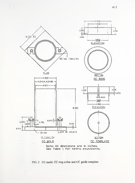
A1.3
1.200
BREAK CORNERS
PLAN
-4.500-
|—4.2464,4.2486—
|
4.000
0.750
8.000
DELRIN
ELEVATION
CC MDLD
MAY BE VELDED
-5.550-
-4.000-
ELEVATION
1.450
CC RING
1
t
4501
III
PI
!
1.200
1 ll.Phll
| 10.313
4.P5354.2500
ELEVATIDN
BOTTOM
CC TEMPLATE
Note' All dimensions are in inches.
See Table 1 for metric equivalents.
FIG. 2 CC mold, CC ring collar and CC guide template
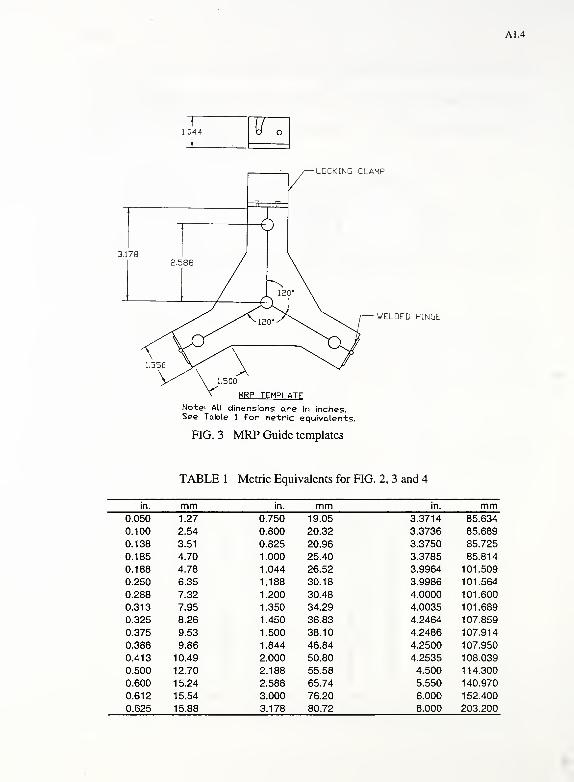
A1.4
1.044 V
LDCKING CLAMP
3.178
WELDED HINGE
MRP TEMPLATF
Note> All dinensions are in inches.See Table 1 for netric equivalents.
FIG. 3 MRP Guide templates
TABLE 1 Metric Equivalents for FIG. 2, 3 and 4
in. mm in. mm0.050
0.100
0.138
0.185
0.188
0.250
0.288
0.313
0.325
0.375
0.388
0.413
0.500
0.600
0.612
0.625
1.27
2.54
3.51
4.70
4.78
6.35
7.32
7.95
8.26
9.53
9.86
10.49
12.70
15.24
15.54
15.88
0.750
0.800
0.825
1.000
1.044
1.188
1.200
1.350
1.450
1.500
1.844
2.000
2.188
2.588
3.000
3.178
19.05
20.32
20.96
25.40
26.52
30.18
30.48
34.29
36.83
38.10
46.84
50.80
55.58
65.74
76.20
80.72
3.3714 85.634
3.3736 85.689
3.3750 85.725
3.3785 85.814
3.9964 101.509
3.9986 101.564
4.0000 101.600
4.0035 101.689
4.2464 107.859
4.2486 107.914
4.2500 107.950
4.2535 108.039
4.500 114.300
5.550 140.970
6.000 152.400
8.000 203.200

A1.5
1.000
-lo.aoi
!4y
2.000-
-2.588—
0.625
~~r~
COAXIAL HEAD - ASSEMBLY
0.625
0.375
TI V-1/Z-2B T>*£AD
P ART 1
list or PASTS
NO-loT DESCRIPTION MATERIAL
1 1 UPPER PART OF CH STEEL
J I LOVER PART OF CH DELRIN
3 1 BNC CONNECTOR4 1 CENTRAL STUD STEEL
5 i OUTER STUD STEEL
6 1 SHORT STUD STEEL
' iFLAT HEAD SCREW STEE t
K DRILLED TAP3/6-16NCX5/8AT 120 DEGREESPACING
H0J85
11 ° 375hf Dlanete
— 0.500-
PART 3
0.100
rNotesModifystandard BNC '
connectorOIG-492. 1/2'
DualFenate) to "this
drawing.
3/8-16TthreadI
I
-| 0.375
PART 4
PART 5
Notei All dlnenslons are In Inches.See Table 1 for metric equivalents.
- 0.375
PART 6
FIG. 4 Coaxial Head (CH)
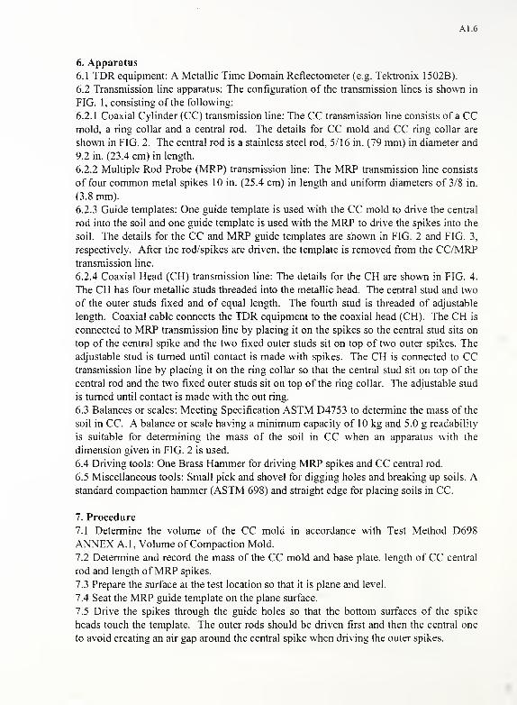
A1.6
6. Apparatus
6.1 TDR equipment: A Metallic Time Domain Reflectometer (e.g. Tektronix 1502B).
6.2 Transmission line apparatus: The configuration of the transmission lines is shown in
FIG. 1, consisting of the following:
6.2.1 Coaxial Cylinder (CC) transmission line: The CC transmission line consists of a CCmold, a ring collar and a central rod. The details for CC mold and CC ring collar are
shown in FIG. 2. The central rod is a stainless steel rod, 5/16 in. (79 mm) in diameter and
9.2 in. (23.4 cm) in length.
6.2.2 Multiple Rod Probe (MRP) transmission line: The MRP transmission line consists
of four common metal spikes 10 in. (25.4 cm) in length and uniform diameters of 3/8 in.
(3.8 mm).
6.2.3 Guide templates: One guide template is used with the CC mold to drive the central
rod into the soil and one guide template is used with the MRP to drive the spikes into the
soil. The details for the CC and MRP guide templates are shown in FIG. 2 and FIG. 3,
respectively. After the rod/spikes are driven, the template is removed from the CC/MRPtransmission line.
6.2.4 Coaxial Head (CH) transmission line: The details for the CH are shown in FIG. 4.
The CH has four metallic studs threaded into the metallic head. The central stud and two
of the outer studs fixed and of equal length. The fourth stud is threaded of adjustable
length. Coaxial cable connects the TDR equipment to the coaxial head (CH). The CH is
connected to MRP transmission line by placing it on the spikes so the central stud sits on
top of the central spike and the two fixed outer studs sit on top of two outer spikes. The
adjustable stud is turned until contact is made with spikes. The CH is connected to CCtransmission line by placing it on the ring collar so that the central stud sit on top of the
central rod and the two fixed outer studs sit on top of the ring collar. The adjustable stud
is turned until contact is made with the out ring.
6.3 Balances or scales: Meeting Specification ASTM D4753 to determine the mass of the
soil in CC. A balance or scale having a minimum capacity of 10 kg and 5.0 g readability
is suitable for determining the mass of the soil in CC when an apparatus with the
dimension given in FIG. 2 is used.
6.4 Driving tools: One Brass Hammer for driving MRP spikes and CC central rod.
6.5 Miscellaneous tools: Small pick and shovel for digging holes and breaking up soils. Astandard compaction hammer (ASTM 698) and straight edge for placing soils in CC.
7. Procedure
7.1 Determine the volume of the CC mold in accordance with Test Method D698
ANNEX A.l, Volume of Compaction Mold.
7.2 Determine and record the mass of the CC mold and base plate, length of CC central
rod and length ofMRP spikes.
7.3 Prepare the surface at the test location so that it is plane and level.
7.4 Seat the MRP guide template on the plane surface.
7.5 Drive the spikes through the guide holes so that the bottom surfaces of the spike
heads touch the template. The outer rods should be driven first and then the central one
to avoid creating an air gap around the central spike when driving the outer spikes.
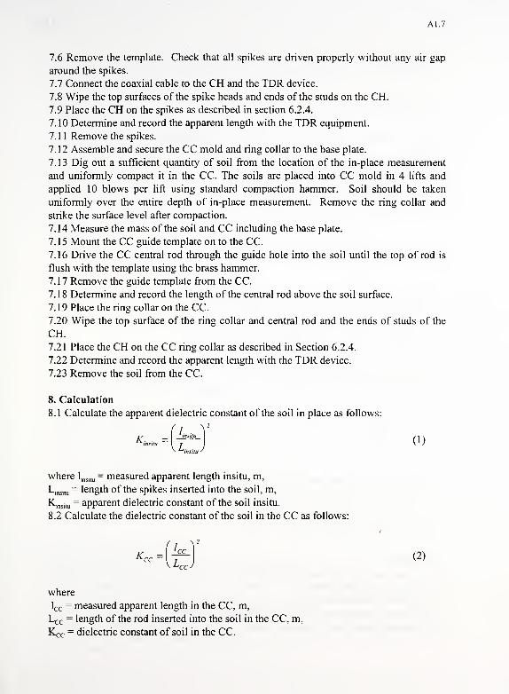
A1.7
7.6 Remove the template. Check that all spikes are driven properly without any air gap
around the spikes.
7.7 Connect the coaxial cable to the CH and the TDR device.
7.8 Wipe the top surfaces of the spike heads and ends of the studs on the CH.
7.9 Place the CH on the spikes as described in section 6.2.4.
7.10 Determine and record the apparent length with the TDR equipment.
7.1
1
Remove the spikes.
7.12 Assemble and secure the CC mold and ring collar to the base plate.
7.13 Dig out a sufficient quantity of soil from the location of the in-place measurement
and uniformly compact it in the CC. The soils are placed into CC mold in 4 lifts and
applied 10 blows per lift using standard compaction hammer. Soil should be taken
uniformly over the entire depth of in-place measurement. Remove the ring collar and
strike the surface level after compaction.
7.14 Measure the mass of the soil and CC including the base plate.
7.15 Mount the CC guide template on to the CC.
7.16 Drive the CC central rod through the guide hole into the soil until the top of rod is
flush with the template using the brass hammer.
7.17 Remove the guide template from the CC.
7.18 Determine and record the length of the central rod above the soil surface.
7.19 Place the ring collar on the CC.
7.20 Wipe the top surface of the ring collar and central rod and the ends of studs of the
CH.
7.21 Place the CH on the CC ring collar as described in Section 6.2.4.
7.22 Determine and record the apparent length with the TDR device.
7.23 Remove the soil from the CC.
8. Calculation
8.1 Calculate the apparent dielectric constant of the soil in place as follows:
K,nsm =[^A (1)
where l,nsitu
= measured apparent length insitu, m,
Ljns.tu= length of the spikes inserted into the soil, m,
K,muu = apparent dielectric constant of the soil insitu.
8.2 Calculate the dielectric constant of the soil in the CC as follows:
K--{t)
(2)
where
lcc = measured apparent length in the CC, m,
Lcc = length of the rod inserted into the soil in the CC, m,
Kcc = dielectric constant of soil in the CC.

A1.8
8.3 Calculate the wet density of the soil in CC as follows:
M, -M2
P,,cc = —T,~
(3)
where
M, = mass of the soil and CC, kg
M2= mass of the CC, kg
Vcc = volume of the CC, m3
,
Pt>cc= wet density of the soil in the CC, kg/m3
.
8.4 Calculate the water content of the soil in the CC and insitu as follows
f^Tc -aPucc 1 P» 1AA ...
"insim = "cc = 7; f== *
!°0 (4)
bp,,cc I P« --JKcc
where
Kcc = apparent dielectric constant of the soil in the CC,
Pt.cc= wet density of the soil in the CC, kg/m3
,
pw = density of water =1 .0 kg/m3
,
a = calibration constant, as0.8 (See Annex)
b = calibration constant, bslO (See Annex)
«cc = water content of the soil in the CC, %,
co ms , tu= water content of the soil insitu, %.
8.6 Calculate the insitu dry density of the soil as follows:
V insitu Pt.CC ,,..
P,,insuu = nr- x V~T.—777^ (5 )
where
Ptcc= wet density of the soil in the CC, kg/m3
,
wcc = gravimetric water content of the soil in the CC, %,
K^c = dielectric constant of soil in the CC,
Kinsitu= dielectric constant of the soil insitu,
Piinsitu= dry density of the soil insitu, kg/m3
.
9. Report
11.1 The report shall include the following:
9.1.1 Test site identification.
9.1.2 Name of the operator(s).
9.1.3 Make, model and serial number of the test instrument.
9.1.4 Visual description of material tested.
A1.9
9.1.5 Water content in percent of dry mass or dry unit weight.
9.1.6 Wet and dry densities in kg/m3.
9.1.7 Calibration constants a and b.
10. Precision and Bias
10.1 Precision:
10.1.1 Data are being evaluated to determine the precision of this test method.
10.2 Bias:
10.2.1 There is no accepted reference value for this test method, therefore, bias cannot be
determined.
11. Keywords
11.1 water content, field density.
Annex
(Mandatory Information)
A.l Calibration Constants
A.l.l Scope
A. 1.1.1 This annex describes the procedure to determine the calibration constants for use
in Equation (4) to estimate soil water content.
A. 1.2 Apparatus
A. 1.2.1 TDR equipment, Tektronix 1502B.
A. 1.2.2 Coaxial Cylinder (CC) transmission line.
A. 1.2. 3 CC Guide templates.
A. 1.2.4 Brass Hammer.
A. 1.2. 5 Miscellaneous tools: Small picks and shovel for removing soils from the CC. Astandard compaction hammer and straight edge for placing soils in CC.
A.1.3 Procedure
A. 1.3.1 Air dry the soil sample.
A. 1.3.2 Thoroughly break up the soil clumps in such a manner as to avoid breaking
individual particles. Pass the material through a No. 4 sieve.
A. 1.3. 3 Prepare five specimens having water contents such that they bracket the
estimated field water content and vary by about 2%. Preparation procedure should be as
specified in Section 10.2 or 10.3 ofASTM D 698
A.l.3.4 Determine the volume of the CC mold in accordance with Test Method D698
ANNEX A.l, Volume of Compaction Mold.
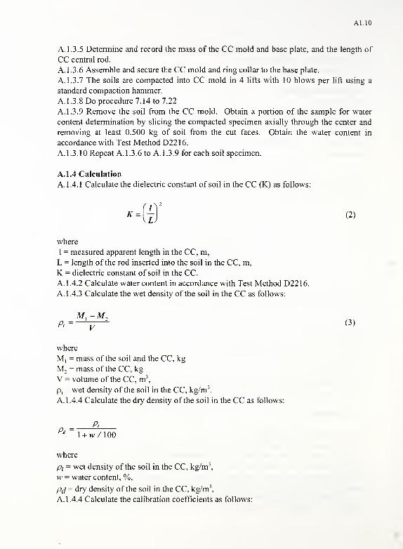
ALIO
A. 1.3. 5 Determine and record the mass of the CC mold and base plate, and the length of
CC central rod.
A. 1.3.6 Assemble and secure the CC mold and ring collar to the base plate.
A. 1.3. 7 The soils are compacted into CC mold in 4 lifts with 10 blows per lift using a
standard compaction hammer.
A.l.3.8 Do procedure 7.14 to 7.22
A. 1.3.9 Remove the soil from the CC mold. Obtain a portion of the sample for water
content determination by slicing the compacted specimen axially through the center and
removing at least 0.500 kg of soil from the cut faces. Obtain the water content in
accordance with Test Method D2216.
A. 1.3. 10 Repeat A. 1.3.6 to A. 1.3.9 for each soil specimen.
A. 1.4 Calculation
A. 1.4.1 Calculate the dielectric constant of soil in the CC (K) as follows:
*-iz)' (2>
where
1 = measured apparent length in the CC, m,
L = length of the rod inserted into the soil in the CC, m,
K = dielectric constant of soil in the CC.
A. 1.4.2 Calculate water content in accordance with Test Method D2216.
A. 1.4. 3 Calculate the wet density of the soil in the CC as follows:
M. -M,A—y-1(3)
where
M, = mass of the soil and the CC, kg
M2= mass of the CC, kg
V = volume of the CC, m 3
,
p t
= wet density of the soil in the CC, kg/m 3
.
A. 1.4.4 Calculate the dry density of the soil in the CC as follows:
PtPd
l + w/100
where
Pt = wet density of the soil in the CC, kg/m3
,
w = water content, %,
Pd = dry density of the soil in the CC, kg/m 3
,
A. 1.4.4 Calculate the calibration coefficients as follows:
Al.ll
Plot v^ p^Pd vs - w -
where
K= dielectric constant of soil in the CC.
Pd = dry density of the soil in the CC, kg/m3
,
pw = density of water, kg/m3
,
w = water content, %.
Find the interception and slope of the best fit line.
a = interception of the best fit line
b = slope of the best fit line.
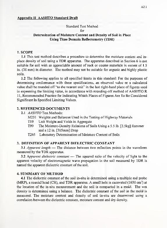
A2.1
Appendix II AASHTO Standard Draft
Standard Test Method
for
Determination of Moisture Content and Density of Soil in Place
Using Time Domain Reflectometry (TDR)
1. SCOPE1.1 This test method describes a procedure to determine the moisture content and in-
place density of soil using a TDR apparatus. The apparatus described in Section 6 is not
suitable for soil with an appreciable amount of rock or coarse materials in excess of 1.5
in. (38 mm) in diameter. The method may not be suitable for organic and highly plastic
soils.
1.2 The following applies to all specified limits in this standard: For the purposes of
determining conformance with these specifications, an observed value or a calculated
value shall be rounded off "to the nearest unit" in the last right-hand place of figures used
in expressing the limiting value, in accordance with rounding-off method of AASHTO R11, Recommended Practice for Indicating Which Places of Figures Are To Be Considered
Significant In Specified Limiting Values.
2. REFERENCED DOCUMENTS2.1 AASHTO Test Methods:
M23 1 Weights and Balances Used in the Testing of Highway Materials
T19 Unit Weight and Voids in Aggregate
T99 The Moisture-Density Relations of Soils Using a 5.5 lb. [2.5kg] Rammerand a 12 in. [305mm] Drop
T265 Laboratory Determination of Moisture Content of Soils
3. DEFINITION OF APPARENT DIELECTRIC CONSTANT3.1 Apparent length — The distance between two reflection points in the waveform
measured by the TDR apparatus.
3.2 Apparent dielectric constant — The squared ratio of the velocity of light to the
apparent velocity of electromagnetic wave propagation in the soil measured by TDR is
named the apparent dielectric constant of the soil.
4. SUMMARY OF METHOD4.1 The dielectric constant of the soil in-situ is determined using a multiple rod probe
(MRP), a coaxial head (CH), and TDR apparatus. A small hole is excavated (1650 cm3
) at
the location of the in-situ measurement and the soil is compacted in a mold. The wet
density is determined using a balance. The dielectric constant of the soil in the mold is
measured. The moisture content and density of soil in-situ are determined using a
correlation between the dielectric constant, moisture content and dry density.
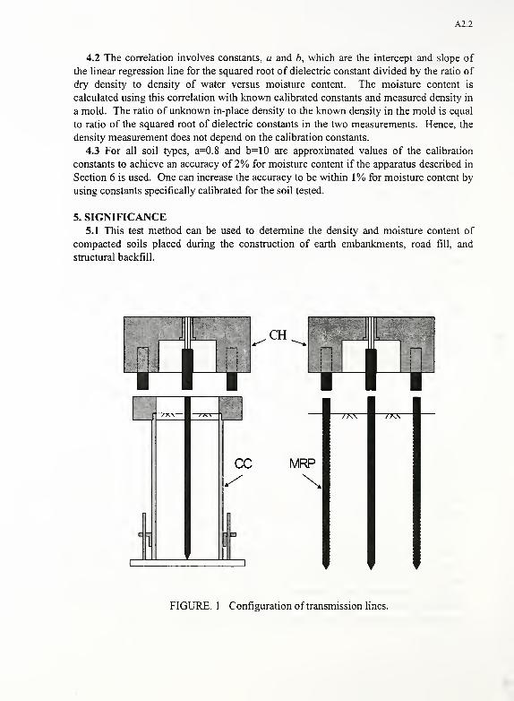
A2.2
4.2 The correlation involves constants, a and b, which are the intercept and slope of
the linear regression line for the squared root of dielectric constant divided by the ratio of
dry density to density of water versus moisture content. The moisture content is
calculated using this correlation with known calibrated constants and measured density in
a mold. The ratio of unknown in-place density to the known density in the mold is equal
to ratio of the squared root of dielectric constants in the two measurements. Hence, the
density measurement does not depend on the calibration constants.
4.3 For all soil types, a=0.8 and b=10 are approximated values of the calibration
constants to achieve an accuracy of 2% for moisture content if the apparatus described in
Section 6 is used. One can increase the accuracy to be within 1% for moisture content by
using constants specifically calibrated for the soil tested.
5. SIGNIFICANCE5.1 This test method can be used to determine the density and moisture content of
compacted soils placed during the construction of earth embankments, road fill, and
structural backfill.
i
-!
1
ccs1
C T 3
MRP
7XV
FIGURE. 1 Configuration of transmission lines.

A2.3
5.550
1T1.200
I! ! !
t
1.4501
7^0.250 i
4.P5.154.2500
BREAK CORNERS
PLAN
-4.500-
f—4.2464, 4.2486—
|
4,000
0.750
1.450
8.000
DELRIN
ELEVATIDN
CC MOLD
may be: velded
ELEVATION
-4.500-
ELEVATION
1.200
zrr 0.250
BOTTOM
CC TEMPLATE
Notei All dimensions are in inches.
See Table 1 for metric equivalents.
FIGURE. 2 CC mold, CC ring collar and CC guide template
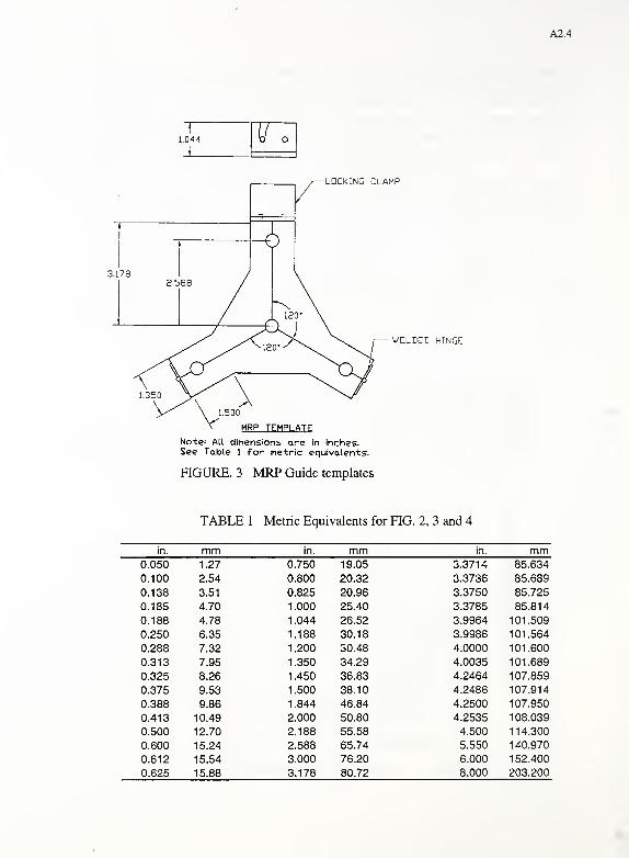
A2.4
1.044 VLOCKING CLAMP
3.178
WELDED HINGE
MRP TEMPLATE
Note' All dinensions are in Inches.See Table 1 for metric equivalents.
FIGURE. 3 MRP Guide templates
TABLE 1 Metric Equivalents for FIG. 2, 3 and 4
in. mm in. mm0.050
0.100
0.138
0.185
0.188
0.250
0.288
0.313
0.325
0.375
0.388
0.413
0.500
0.600
0.612
0.625
1.27
2.54
3.51
4.70
4.78
6.35
7.32
7.95
8.26
9.53
9.86
10.49
12.70
15.24
15.54
15.88
0.750
0.800
0.825
1.000
1.044
1.188
1.200
1.350
1.450
1.500
1.844
2.000
2.188
2.588
3.000
3.178
19.05
20.32
20.96
25.40
26.52
30.18
30.48
34.29
36.83
38.10
46.84
50.80
55.58
65.74
76.20
80.72
3.3714 85.634
3.3736 85.689
3.3750 85.725
3.3785 85.814
3.9964 101.509
3.9986 101.564
4.0000 101.600
4.0035 101.689
4.2464 107.859
4.2486 107.914
4.2500 107.950
4.2535 108.039
4.500 114.300
5.550 140.970
6.000 152.400
8.000 203.200
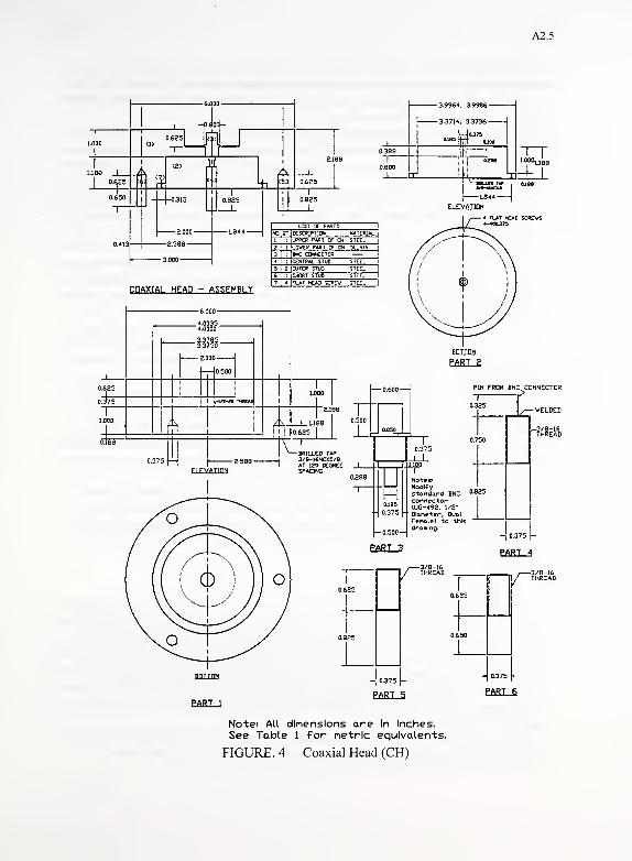
A2.5
-kdool-
-3.9964, 3.9986-
-3.3714, 3.3736
-
-lojra
itt
;| a<2>
ft
A-+0.800
J
2.000 -
-2.588—
I
0.825
L
I VH«3Jj
I
L844 1
r±JL
COAXIAL HEAD - ASSEMBLY
list or parts
>c rr description: material
i : ilppeb part or cm stcc.
2 I !lDVER PART OF CH XLRIN3 : Ibnc C3WCCT0R4 : ICENTRAC STUD STEEL
5 ? ITJUTER STUB steel
6 : |SKJST stud STEEL
7 « IR.AT >«AD SCREW STEEL
J0.625
o!37575
T~1.000
i j i
TlI I i I
1 iri/l-M THIEAB
I
J!|-DRILLED TAP3/8-16NCX5/8AT 120 XOiEESPACING
H
—r
0.375
0.100
~rNotes'Modifystandard BNCconnectorCUG-492, 1/2'0J85
"\ °-375ht Diameter, Dual
Fenale) to tws
0.500H dr"lns -
PART 3
-j 0.375
PART
PAR T 1
- 0.375 (-
PART 5
-| 0.375 (-
PART 6
Note' All dimensions are In Inches.See Table 1 for netrlc equivalents.
FIGURE. 4 Coaxial Head (CH)
A2.6
6. APPARATUS6.1 TDR equipment: A Metallic Time Domain Reflectometer (e.g. Tektronix 1502B).
6.2 Transmission line apparatus: The configuration of the transmission lines is shown
in Figure. 1, consisting of the following:
6.2.1 Coaxial Cylinder (CC) transmission line: The CC transmission line consists of a
CC mold, a ring collar and a central rod. The details for CC mold and CC ring collar are
shown in Figure. 2. The central rod is a stainless steel rod, 5/16 in. (79 mm) in diameter
and 9.2 in. (23.4 cm) in length.
6.2.2 Multiple Rod Probe (MRP) transmission line: The MRP transmission line
consists of four common metal spikes 10 in. (25.4 cm) in length and uniform diameters of
3/8 in. (3.8 mm).
6.2.3 Guide templates: One guide template is used with the CC mold to drive the
central rod into the soil and one guide template is used with the MRP to drive the spikes
into the soil. The details for the CC and MRP guide templates are shown in Figure. 2 and
Figure. 3, respectively. After the rod/spikes are driven, the template is removed from the
CC/MRP transmission line.
6.2.4 Coaxial Head (CH) transmission line: The details for the CH are shown in
Figure. 4. The CH has four metallic studs threaded into the metallic head. The central
stud and two of the outer studs fixed and of equal length. The fourth stud is threaded of
adjustable length. Coaxial cable connects the TDR equipment to the coaxial head (CH).
The CH is connected to MRP transmission line by placing it on the spikes so the central
stud sits on top of the central spike and the two fixed outer studs sit on top of two outer
spikes. The adjustable stud is turned until contact is made with spikes. The CH is
connected to CC transmission line by placing it on the ring collar so that the central stud
sit on top of the central rod and the two fixed outer studs sit on top of the ring collar. The
adjustable stud is turned until contact is made with the out ring.
6.3 Balance: A balance conforming the requirements ofAASHTO M231, Class G20.
6.4 Driving tools: One Brass Hammer for driving MRP spikes and CC central rod.
6.5 Miscellaneous tools: Small pick and shovel for digging holes and breaking up
soils. A standard compaction hammer (AASHTO T99, Section 2.2.1) and straight edge
for placing soils in CC.
7. CALIBRATION7.1 General coefficients of a=0.8 and b=\0 could be used. Alternatively soil specific
calibration of a and b can be completed. Calibration is established by determining the
dielectric constants, moisture contents and densities of five soil specimens prepared such
that they bracket the estimated field moisture content and vary by about 2%, plotting the
squared root of dielectric constant divided by the ratio of dry density to density of water
versus moisture content, and placing a best fit straight line through the resulting points.
The intercept and slope of the straight line are a and b, respectively. Calibration can be
established as follows:
7.1.1 Air dry the soil sample. Thoroughly break up the soil clumps in such a manner
as to avoid breaking individual particles. Pass the material through a No. 4 sieve.
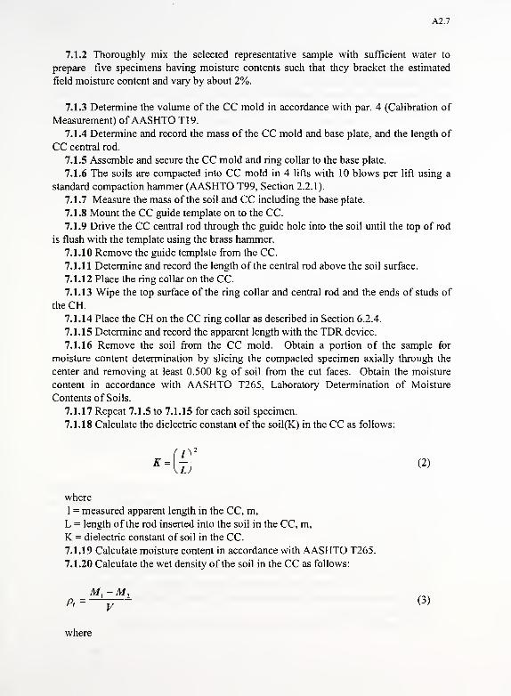
A2.7
7.1.2 Thoroughly mix the selected representative sample with sufficient water to
prepare five specimens having moisture contents such that they bracket the estimated
field moisture content and vary by about 2%.
7.1.3 Determine the volume of the CC mold in accordance with par. 4 (Calibration of
Measurement) ofAASHTO T19.
7.1.4 Determine and record the mass of the CC mold and base plate, and the length of
CC central rod.
7.1.5 Assemble and secure the CC mold and ring collar to the base plate.
7.1.6 The soils are compacted into CC mold in 4 lifts with 10 blows per lift using a
standard compaction hammer (AASHTO T99, Section 2.2.1).
7.1.7 Measure the mass of the soil and CC including the base plate.
7.1.8 Mount the CC guide template on to the CC.
7.1.9 Drive the CC central rod through the guide hole into the soil until the top of rod
is flush with the template using the brass hammer.
7.1.10 Remove the guide template from the CC.
7.1.11 Determine and record the length of the central rod above the soil surface.
7.1.12 Place the ring collar on the CC.
7.1.13 Wipe the top surface of the ring collar and central rod and the ends of studs of
the CH.
7.1.14 Place the CH on the CC ring collar as described in Section 6.2.4.
7.1.15 Determine and record the apparent length with the TDR device.
7.1.16 Remove the soil from the CC mold. Obtain a portion of the sample for
moisture content determination by slicing the compacted specimen axially through the
center and removing at least 0.500 kg of soil from the cut faces. Obtain the moisture
content in accordance with AASHTO T265, Laboratory Determination of Moisture
Contents of Soils.
7.1.17 Repeat 7.1.5 to 7.1.15 for each soil specimen.
7.1.18 Calculate the dielectric constant of the soil(K) in the CC as follows:
K=li)
2
<2>
where
1 = measured apparent length in the CC, m,
L = length of the rod inserted into the soil in the CC, m,
K = dielectric constant of soil in the CC.
7.1.19 Calculate moisture content in accordance with AASHTO T265.
7.1.20 Calculate the wet density of the soil in the CC as follows:
M. -M,a—V* <3>
where
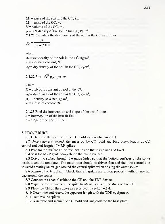
A2.8
M, = mass of the soil and the CC, kg
M2= mass of the CC, kg
V = volume of the CC, m\
p t
= wet density of the soil in the CC, kg/m 3.
7.1.21 Calculate the dry density of the soil in the CC as follows:
PtPd
l + w/100
where
Pt = wet density of the soil in the CC, kg/m3
,
w = moisture content, %,
Pd = dry density of the soil in the CC, kg/m3
,
7.1.22 Plot 4K pjpd vs. w.
where
K = dielectric constant of soil in the CC.
pd = dry density of the soil in the CC, kg/m3
,
Pw = density of water, kg/m3
,
w = moisture content, %.
7.1.23 Find the interception and slope of the best fit line.
a = interception of the best fit line
b = slope of the best fit line.
8. PROCEDURE8.1 Determine the volume of the CC mold as described in 7.1.3
8.2 Determine and record: the mass of the CC mold and base plate, length of CCcentral rod and length ofMRP spikes.
8.3 Prepare the surface at the test location so that it is plane and level.
8.4 Seat the MRP guide template on the plane surface.
8.5 Drive the spikes through the guide holes so that the bottom surfaces of the spike
heads touch the template. The outer rods should be driven first and then the central one
to avoid creating an air gap around the central spike when driving the outer spikes.
8.6 Remove the template. Check that all spikes are driven properly without any air
gap around the spikes.
8.7 Connect the coaxial cable to the CH and the TDR device.
8.8 Wipe the top surfaces of the spike heads and ends of the studs on the CH.
8.9 Place the CH on the spikes as described in section 6.2.4.
8.10 Determine and record the apparent length with the TDR equipment.
8.11 Remove the spikes.
8.12 Assemble and secure the CC mold and ring collar to the base plate.
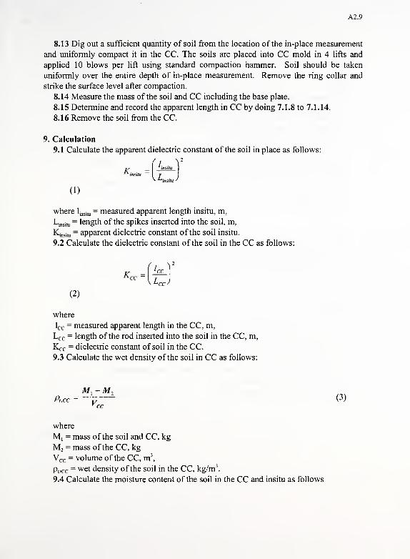
A2.9
8.13 Dig out a sufficient quantity of soil from the location of the in-place measurement
and uniformly compact it in the CC. The soils are placed into CC mold in 4 lifts and
applied 10 blows per lift using standard compaction hammer. Soil should be taken
uniformly over the entire depth of in-place measurement. Remove the ring collar and
strike the surface level after compaction.
8.14 Measure the mass of the soil and CC including the base plate.
8.15 Determine and record the apparent length in CC by doing 7.1.8 to 7.1.14.
8.16 Remove the soil from the CC.
9. Calculation
9.1 Calculate the apparent dielectric constant of the soil in place as follows:
K —insitu ~ I r
(1)
where ljnsjtu
= measured apparent length insitu, m,
Ljnsitu= length of the spikes inserted into the soil, m,
Kinsim= apparent dielectric constant of the soil insitu.
9.2 Calculate the dielectric constant of the soil in the CC as follows:
'cc
(2)
Krr —|
where
lcc = measured apparent length in the CC, m,
Lcc = length of the rod inserted into the soil in the CC, m,
K^ = dielectric constant of soil in the CC.
9.3 Calculate the wet density of the soil in CC as follows:
p,xc =—b
—
L(3>
where
M, = mass of the soil and CC, kg
M2= mass of the CC, kg
Vcc = volume of the CC, m3
,
Ppcc= wet density of the soil in the CC, kg/m3
.
9.4 Calculate the moisture content of the soil in the CC and insitu as follows
A2.10
# "^^xlOO (4)
where
1^= apparent dielectric constant of the soil in the CC,
Puce= wet density of the soil in the CC, kg/m3
,
pw = density of water =1.0 kg/m3
,
a = calibration constant (See Section 7)
b = calibration constant (See Section 7)
wcc = moisture content of the soil in the CC, %,w
jnsjtu= moisture content of the soil insitu, %.
9.5 Calculate the insitu dry density of the soil as follows:
l + cocc /100 *'
where
Pec= wet density of the soil in the CC, kg/m3
,
wcc = gravimetric moisture content of the soil in the CC, %,
Kcc = dielectric constant of soil in the CC,
Kinsitu= dielectric constant of the soil insitu,
Pcunsitu= dry density of the soil insitu, kg/m 3
.
10. Report
10.1 The report shall include the following:
10.1.1 Test site identification.
10.1.2 Name of the operator(s).
10.1.3 Make, model and serial number of the test instrument.
10.1.4 Visual description of material tested.
10.1.5 Moisture content in percent of dry mass or dry unit weight.
10.1.6 Wet and dry densities in kg/m3.
10.1.7 Calibration constants a and b.

A3.1
Appendix HI GUIDELINES OF USING TDR++
1. System Requirements
• A IBM compatible computer with a 486 or higher processor,
• Microsoft Windows 95™ or Windows NT™
• Available serial port,
• Mouse
• Microsoft Excel™ is required for complete functional operation of TDR++.
2. Setup
Insert disk 1 into Drive A (3.5" Floppy Disk Drive). In Windows 95™, click on
[Start], select [Run] in the menu list. Then in the "Run" dialog box, type "a:\setup" and
click on [OK].
A TDR setup form is displayed and a dialog box will prompt the user to enter the
path (directory) where he or she would like to install the program. The default path is
"C:\Program Files\tdr++". The setup program will then install TDR++ and prompt the
user to insert the second and third of the four disks. User then needs to create a directory
"c:\tdr_l" and copy all the files on disk No. 4 (tool and data files) into that directory. The
setup program will generate an icon named "TDR++" in the default or user-specified
directory. The user may create a shortcut to "TDR++" for quick access.
A3 .2
3. Running TDR++
In Windows 95M
, click on "Start" and select "Programs" from the menu list.
Locate the "tdr++" directory in the program list, and click on "tdr++". A loading form
will be displayed informing you that the program is being loaded in the system.
The Main Form of TDR++ is displayed after a successful loading. The program
will automatically check for a serial connection. Without the connection to Tektronix
1502B, TDR apparatus, the connection indicator will show "None". Many functions of
TDR++ will be disabled without this connection.
4. Using TDR++ in a Non-Connected State
The active functions that are possible without the connection to the Tektronix
1502B instrument include TDR data file manipulation, signal displaying, and note
editing. These are described in section 5.2.2 and 5.2.3 of the report. A basic tutorial
follows:
a. Open a waveform file:
Click on the [open] command from the command bar or the [file] menu. An
"open" dialog box will pop up. Select the path to the default data file directory "c:\tdr_l".
A list of files will show. User may select one of the files, for example chose "100496-4".
A TDR waveform will be displayed in the picture box. The name of the opened
waveform file is shown in the panel above the picture box.

A3.3
b. View properties ofthisfile:
Click on [Properties] in the [File] menu list. The information associated with this
waveform file will be displayed on a Properties Form. The form includes file name, path,
the time when last modified, and the file size. Also, several attributes of the TDR
waveform are given, including information on whether the test details, soil details, user
input, and test results have been included in this file.
c. View information associated with the waveform
If the indicators in the File Properties box show that the file contains data, the user
can view the file by giving different commands. By clicking the [Info] button on the
command bar on the [Info] menu, the user can select a specific item for viewing.
Clicking the [Result] button and selecting [Test Result] will display the results of the
TDR test, including moisture content, wet density, and dry density.
d. View the text content ofthe waveform
With the opened waveform on the display click the [store!] button on the misc.
bar and a colored box will appear. A small symbol will appear in this box when it is
clicked with the left mouse key, a small symbol will show up. Drag and drop this symbol
on to the text box and the waveform data will be displayed with the file name at the top.
e. Comparing two waveforms
With one or more waveforms stored in the waveform register (the black box), the
user can open another file, then drag and drop a stored waveform to the picture box. Two
A3 .4
or more waveforms can be displayed at the same time for comparison. Drag and drop the
waveform into the "trash bin" on the bottom misc. bar when it is no longer desired in the
picture box or the waveform register.
/ View the TDR curve readings
The user can perform the TDR curve readings by clicking on the [Result] button
and selecting "Curve Reading". Selecting "Reading" will display the readings of Point 1.
Point 2, and the apparent length in the misc. bar. Selecting "Detail" will produce new
tool bar. Clicking on the [Point 1] button, the user will see an indicator at the location of
Point 1 on the TDR waveform. The [Point 2] button leads to the location of Point 2. The
user can also view a smoothed curve by clicking [Smooth], and the first and second
derivatives by click the corresponding buttons. Clicking on [Back] will recover the
original waveform and the original tool bar.
g. Print a waveform or a text file
With a TDR waveform on the display, the user can get a hard copy of this
waveform by clicking on the [Print] menu and selecting "waveform." For best results,
user should set the page orientation to "Landscape" in the print setup. By clicking the
[Print] menu and selecting "Text" when the text box is open will produce a hard copy of
the text file.
A3.5
h. Other
TDR++ provides the user with several options such as selecting the color of the
picture box and selecting the font in the text box. Also, waveform files can be saved in
different formats. Moreover, test reports can be generated automatically in either long or
short format. User can seek on-line help by clicking Help menu and select [Content].
3. Remarks
a. Report generating and database functioning will invoke Microsoft Excel™. Some
difficulties may be encountered when Excel was not appropriately installed.
b. To put a data file into the TDR database, TDR++ will prompt user to input a
password, type "ddtdr" as the default password.
c. If user finds any problem when using TDR++, please report the problem to the
address listed in "Technical Support".