Automated Essay Scoring and The Repair of Electronics

Dan Preston and Danny Goodman

June 11, 2012

Our efforts in cs341 were focused mainly on a global Automated Essay Scoring competition in whichwe placed 5th out of 159 teams. Since this contest ended with a few weeks left in the quarter, we then brieflyexamined an electronics repair dataset from Flextronics. We describe each effort.

1 Automated Essay Scoring

1.1 Introduction

The Hewlett Foundation sponsored the Automated Student Assessment Prize on kaggle.com, challengingteams to produce essay evaluation models that best approximate human graders. Contestants predicted thescores of standardized-testing essays from grades 7-10. Teams were provided with 8 sets of labeled trainingdata. Each set corresponds to a different essay prompt, grading rubric, and range of possible scores. Ingeneral, grading rubrics cite content, fluidity, spelling, grammar, and vocabulary as major considerations.

Teams submitted predicted grades for an unlabeled test set, and the results were then ranked by a com-plicated scoring metric called mean quadratic weighted kappa. The contest concluded on April 30, 2012.

Automated essay grading is a difficult domain because computers struggle with several of the tasks anexpert human performs during grading, such as implicitly correcting syntax mistakes and evaluating thelogical structure of an argument. The problem is compounded by the poor agreement of individual humangraders.

Computers have traditionally approached the problem by applying machine learning techniques to a mixof simple features extracted from the essays, which do not capture a human’s intuition about what ought tocause a good grade. Past work has been done with student essays written in good faith; that is, the studentsexpected human evaluators. If future students are aware that computers are grading their work, some willattempt to write for the simple heuristic features alone, without constructing a coherent essay. The evaluationsystem must guard against this tactic.

In this paper, we present our current essay evaluation model for the Kaggle contest, and our plans forfuture work.

1.2 Previous approaches

Early approaches to essay assessment generally used statistical methods, such as bag-of-words (unigram,bigrams), part-of-speech N-grams, script length, and error rate. Larkey [3] evaluates a few models based onsimple heuristic features like average word length, essay length, and unique word count. To assign integralscores, the model uses linear regression and chooses thresholds to match the observed proportion of eachscore in the training data. While these test complexity features by no means guarantee a good essay, they arecorrelated with the qualities that make a good essay. Larkey achieved up to 88% correlation with a humangrader on a general achievement test essay.

1

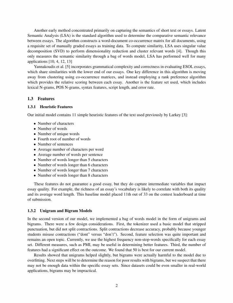
Another early method concentrated primarily on capturing the semantics of short text or essays. LatentSemantic Analysis (LSA) is the standard algorithm used to determine the comparative semantic relevancebetween essays. The algorithm constructs a word-document co-occurrence matrix for all documents, usinga requisite set of manually graded essays as training data. To compute similarity, LSA uses singular valuedecomposition (SVD) to perform dimensionality reduction and cluster relevant words [4]. Though thisonly measures the semantic similarity through a bag of words model, LSA has performed well for manyapplications [10, 4, 12, 13]

Yannakoudis et al. [5] incorporates grammatical complexity and correctness in evaluating ESOL essays,which share similarities with the lower end of our essays. One key difference in this algorithm is movingaway from clustering using co-occurrence matrices, and instead employing a rank preference algorithmwhich provides the relative scoring between each essay. Another is the feature set used, which includeslexical N-grams, POS N-grams, syntax features, script length, and error rate.

1.3 Features

1.3.1 Heuristic Features

Our initial model contains 11 simple heuristic features of the text used previously by Larkey [3]:

• Number of characters• Number of words• Number of unique words• Fourth root of number of words• Number of sentences• Average number of characters per word• Average number of words per sentence• Number of words longer than 5 characters• Number of words longer than 6 characters• Number of words longer than 7 characters• Number of words longer than 8 characters

These features do not guarantee a good essay, but they do capture intermediate variables that impactessay quality. For example, the richness of an essay’s vocabulary is likely to correlate with both its qualityand its average word length. This baseline model placed 11th out of 33 on the contest leaderboard at timeof submission.

1.3.2 Unigram and Bigram Models

In the second version of our model, we implemented a bag of words model in the form of unigrams andbigrams. There were a few design considerations. First, the tokenizer used a basic model that strippedpunctuation, but did not split contractions. Split contractions decrease accuracy, probably because youngerstudents misuse contractions (“dont” versus “don’t”). Second, feature selection was quite important andremains an open topic. Currently, we use the highest frequency non-stop-words specifically for each essayset. Different measures, such as PMI, may be useful in determining better features. Third, the number offeatures had a significant effect on the outcome. We found that 50 is best for our current model.

Results showed that unigrams helped slightly, but bigrams were actually harmful to the model due tooverfitting. Next steps will be to determine the reason for poor results with bigrams, but we suspect that theremay not be enough data within the specific essay sets. Since datasets could be even smaller in real-worldapplications, bigrams may be impractical.

2

1.3.3 Spelling features

When scanning over our dataset, it was obvious that many of the students had poor spelling skills. Gradingrubrics often included spelling, but more importantly, spelling is correlated with overall writing skills. Weintegrated a spellchecker into our codebase and used counts of misspelled words as additional features:

• Number of unique misspelled words• Unique misspelled words divided by total unique words

The spelling data can be converted into features in many other ways, but a few of the more intuitive onesproved to be detrimental. We thought that a better writer would misspell longer words rather than shorterwords, but adding average misspelled word length as a feature decreased the overall score. Perhaps a bettermeasure would be the rarity of the corrected word. The kappa score also decreased when we changed thespelling features to use the total number of misspelled words, instead of number of unique misspelled words.

1.3.4 Sentence transition features

As a simple metric for capturing sentence complexity and flow, we compiled a list of 256 common transitionwords, e.g. words such as “however,” “thus,” “since,” etc. After trying several ways to include these countsas features, we found that the most effective feature was the number of unique transition words in an essay.

1.3.5 Spelling correction

After inspecting some essays in our datasets, we realized that spelling errors and typos must be correctedbefore more advanced features could be useful. In particular, parsing would not work well with misspellings.Even bag-of-words features could benefit from spelling correction, which would reduce sparsity.

Our spelling correction algorithm uses the Hunspell spell corrector to identify misspelled words and gen-erate suggestions. We then evaluate each suggestion on a linear combination of Levenshtein edit distance,unigram probability, and bigram probabilities. The unigram and bigram probabilities were computed using alarge corpus consisting of the entire .uk domain. Each misspelled word is replaced with the highest-scoringsuggestion.

1.3.6 LSA

Given that a simple bag of words model underperformed relative to the results in other works, we performeda more extensive evaluation of Latent Semantic Analysis. In past work, LSA has been shown to closelymodel or represent the kind of knowledge that a human is able to infer from the same text. This providesa significant advantage in the case of automated essay scoring, as our evaluation metric is based on humanagreement (as opposed to some other objective criterion). To leverage other features, we approach theproblem in a slightly different fashion than typical LSA approaches. In our construction, we examine a setof “topics” that are extracted through the use of LSA on the co-occurrence matrix, and use the contributionof each essay to these topics as features in our feature vector.

Our implementation of LSA features works by first constructing a word-document co-occurrence matrixfor all essays. The entities in the matrix are both unigrams and bigrams of the words that appear in all essays,and the values in the matrix represent the number of appearance of each ngram in the corresponding essay.We enforce a minimum of three or more appearances, which was decided empirically after examining theresults of different thresholds. Second, we perform TF-IDF on the matrix to obtain a better model of theunderlying distribution. This conversion was able to improve the score by approximately 0.012 in overallweighted Kappa score.

3

-0.3

-0.2

-0.1

0

0.1

0.2

0.3

0.4

0.5

0.6

0.7

0 0.05 0.1 0.15 0.2 0.25 0.3 0.35 0.4 0.45

Figure 1: This figure shows the top two topics captured via LSA. Each color represents a different grade,which demonstrates the separation between classes, given different topics. The X and Y axis represent thecontribution of each essay (data point) to the topics on each dimension.

Given the newly constructed TF-IDF weighted co-occurrence matrix, singular value decomposition(SVD) is performed to obtain a number of different “topics”. Intuitively, these may represent differentareas of interest to the graders, such as arguments that may resonate well with the reader and/or summariza-tions of components of the essay (if the student essay is the response to a reading). It is interesting to explorewhat this model may be interpreting or inferring from the data. The excerpt in Figure 2 is the last sentenceof a reading students were responding to. The words in Figure 3 represent the most prominent words fortopic #2 of the same essay set, after performing LSA. It is interesting to note the corresponding unigramsbetween these two, as it seems to be modeling the relative importance or prevalence of the summarizationof the essay. We include a demonstration of the separability of the grades within the space of the topics inFigure 5.

When they come back, Saeng vowed silently to herself, in the spring, when the snows melt and the geesereturn and this hibiscus is budding, then I will take that test again.

Figure 2: Last sentence of essay prompt for essay set #3

In addition to word ngrams, we leveraged the information provided by POS tagging as used by Briscoeet al. [4]. The entities extracted from the document are all POS unigrams, bigrams, and trigrams, as theyappear in the text. The Stanford POS tagger was used to extract this data. Two methods were used to modelthis data and include it in our model: First, we attempted to include all entities in the same matrix as theword ngrams. Second, we created a second matrix and LSA model, and used topics from the decompositionof this matrix. In the following table, we summarize the results of these findings to conclude that usingseparate matrices seems to provide the best results.

Including other entities, such as POS tags, in the co-occurrence matrices is one method for improvingthe results of our algorithm. Another idea we proposed was to look at document similarity within the sameLSA model. In this construction, we created a matrix of all training set essays, and found the similaritybetween each pair of essays. With this data, we then find the following features:

• Average similarity score to each set of essays for all grades• Variance for similarity scores across each grade

4

Weight Word0.237 vowed0.233 silently0.231 return0.229 melt0.217 come0.209 snows0.196 budding-0.186 test-0.185 home0.180 back

Figure 3: Top 10 items for topic #2 for essay set #3

Essay Set Combined Matrix Two Matrices1 0.827088 0.8277432 0.697783 0.6904773 0.692148 0.6960514 0.769113 0.7746345 0.813662 0.8156366 0.819210 0.8164267 0.807888 0.8137388 0.697681 0.698229

Overall 0.763039 0.763887

Table 1: Combined matrix vs. separate matrices

• Average similarity score to all essays

Our results show that these features were not helpful to the algorithm, and in fact were harmful to thefinal results. We did not include this in our final model, but we suspect these features could be useful in thecontext of examining nearest neighbors or other possible results. We plan to include this in future work.

1.3.7 Modeling Multiple Graders

In the dataset provided, each essay provides two or more grades, each representing a particular individualgrader. Our hypothesis was that each grader may provide varying grades, and perhaps this could be indicativeof a separation of the underlying distribution. Our hope was that by modeling each grader independently,we could provide some additional context for the final learning model. The overall approach was to first runan end-to-end learning approach on each distribution of grades for each grader. We use the predicted scorefrom each model as a feature for both the train and test sets, and include these in the final feature vectors.Unfortunately, these features had a negligible effect on the final Kappa scores, as seen in the following table.

1.4 Learning

Our system learns a mapping from the previously-described vector space of features to integer grades. Thegoal of learning is to maximize a complicated scoring metric, mean quadratic weighted kappa, on the test

5

Essay Set With Graders Without Graders1 0.830123 0.8277432 0.688289 0.6904773 0.696109 0.6960514 0.773558 0.7746345 0.819741 0.8156366 0.820431 0.8164267 0.810128 0.8137388 0.674161 0.698229

Overall 0.762562 0.763887

Table 2: Results when modeling multiple graders

essays. Our approach optimizes κ indirectly, learning grades by other metrics and hoping that a good modelof grades will result in a good κ. This is because it is analytically intractable to optimize κ more directly.

1.4.1 The Scoring Metric: Mean Quadratic Weighted Kappa

The basic scoring concept in this contest is the quadratic weighted kappa. This score is a measure of howwell two corresponding sets of grades agree – in this case, the agreement is between the human grades onthe test set and the automatic grades. Kappa varies between 0 if there is only random agreement betweengraders, and 1 if there is exact agreement. The score is based on a quadratic loss function w, that assigns aloss to a rating pair i, j, when there are N total ratings, as follows:

wi,j =(i− j)2

(N − 1)2

We observe that this loss function is normalized to be at worst 1. Now consider a histogram of ratings,O, such that Oi,j is the number of essays that have received grade i from the first rater and j from thesecond. The following is therefore the total loss across all essays from the disagreement of the two graders,as reflected in O: ∑

i,j

wi,jOi,j

Is this number good or bad? As a benchmark, we consider a related histogram, E, whereEi,j is the expectednumber of essays that will receive grade i from rater 1 and grade j from rater 2 if we randomly jumble theorder in which grades are submitted. We expect the actual loss to be much less than the following expectedrandom loss: ∑

i,j

wi,jEi,j

Therefore, the following quantity is bounded below by 0 for very good agreement between graders, and canbe above 1 for worse than random agreement:∑

i,j wi,jOi,j∑i,j wi,jEi,j

6

It is undesirable that this score becomes lower as the graders agree more. We therefore define κ as its inverse,varying in practice from 0 for random agreement to 1 for perfect agreement:

κ = 1−∑

i,j wi,jOi,j∑i,j wi,jEi,j

The contest requires submitting automatic grades for a variety of different essay sets. The final score isa weighted average of the kappa scores on the individual essay sets. Each kappa score undergoes the Fishertransform:

z =12

ln1 + κ

1− κ

The results are averaged in Fisher space, and then the inverse transform is applied as follows to produce aweighted average kappa score:

κ =e2z − 1e2z + 1

The Fisher transform is convex and maps [0, 1) to [0,∞); therefore, we achieve a better overall metric byincreasing the variance of the individual kappa scores on the different essay sets.

Since the grades must be exact integers, the kappa score does not vary continuously with learned pa-rameters, so it is difficult to devise a machine learning method that optimizes it directly. Instead, we usestandard ML techniques to learn the individual grade of each essay. One possibility, though, is to invent acontinuous approximation to kappa which might then be optimized directly, for example in a margin-basedclassifier, in the hopes of more directly optimizing the metric. Another possibility is to use cross-validationfor parameter tuning and feature selection, using κ on the validation set at the metric to optimize.

1.4.2 Baseline Learning Model: Linear Regression

Our baseline learning model is a linear regression of grade y on features x:

minα,β

∑i

(yi − α− β · xi)2

Heuristically, the quadratic nature of this loss function should cause similar qualitative behavior to thequadratic κ. Grades are produced by rounding prediction y to the nearest integer, and thresholding at themin and max grade.

1.4.3 Grading on a Curve

We obtain our best model to date by grading on a curve. This involves sorting the training essays by predictedscore y and choosing cutoff scores for each grade such that histogram of predicted grades on the trainingdata equals the histogram of observed grades. This procedure is analogous to a teacher’s process of curvingraw exam scores to produce a desired grade distribution.

Curving, however, fails if there is not sufficient training data to resolve the boundaries between neigh-boring grades. On essay set 8, for example, the range of possible grades is significantly wider, and thereare a number of possible grades that are not assigned to any essay in the training set. We therefore achievebetter performance by rounding on essay 8.

7

1.4.4 Feature Selection

The above linear model uses no regularization and therefore is observed to increasingly overfit the data as weadd more features. To reduce overfitting, we tried feature selection using the Bayes Information Criterion,or BIC score. The BIC score of a model with k free parameters trained on n data points is:

BIC = n · log σ2e + k · log n

σ2e =

1n

n∑i=1

(yi − yi)2

The BIC score penalizes overfitting and therefore can be used to select between models of differing com-plexity [16].

There are 2k possible subsets of a set of k features, so exhaustive search is unworkable. We thereforeemploy 2 different greedy search algorithms. In ‘additive selection’, we start with 0 features and produce asequence of k + 1 models. To produce each subsequent model in the sequence, we consider all remainingfeatures and greedily add the one that results in the best BIC score. In ‘deletive selection’, we start with allfeatures and greedily remove features.

Each procedure produces a sequence of k + 1 models, and we select the model with the best BIC score.In practice, this reduces the gap between train and test κ by roughly 40%. Our linear models achieve thefollowing mean kappa across the essays sets:

Learning Method κ Train κ TestGrade by Rounding 0.796443 0.749813Grade on a Curve 0.810278 0.764033

Additive Feature Selection 0.795350 0.763551Deletive Feature Selection 0.804575 0.775480

Table 3: Kappa score for each linear learning method

Interestingly, deletive selection performs significantly better than additive selection.

1.4.5 Support Vector Machines

The major learning from the Netflix Challenge is that combining many models produces a superior result[17]. We therefore explored two types of support vector machines: Rank SVM and Regression SVM.Neither one produces good results at present, but we expect this to change when we set up a validationpipeline and combine multiple models.

We noted earlier that we can produce excellent grades solely by ranking and then curving the essays,without the need to individually grade them. A Rank SVM is a linear model that learns such a ranking, byenforcing a margin between ranking decisions as a normal SVM does between classification decisions. Leti and j be two essays that produce feature vectors φ(i) and φ(j). Then we learn a parameter vector w suchthat the score w · φ ranks the essays in the correct order. In order that this ranking generalize to new sets ofessays, we enforce a margin constraint on each pair i > j such that i gets a higher grade than j:

w · φ(i) ≥ 1 + w · φ(j)

In practice, it is not possible to perfectly rank the essays, so we then relax these constraints as in a normal

8

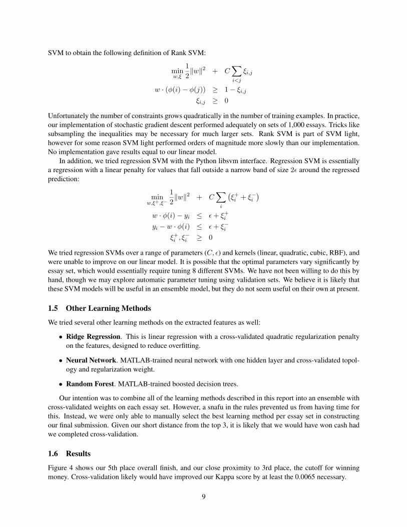
SVM to obtain the following definition of Rank SVM:

minw,ξ

12‖w‖2 + C

∑i<j

ξi,j

w · (φ(i)− φ(j)) ≥ 1− ξi,jξi,j ≥ 0

Unfortunately the number of constraints grows quadratically in the number of training examples. In practice,our implementation of stochastic gradient descent performed adequately on sets of 1,000 essays. Tricks likesubsampling the inequalities may be necessary for much larger sets. Rank SVM is part of SVM light,however for some reason SVM light performed orders of magnitude more slowly than our implementation.No implementation gave results equal to our linear model.

In addition, we tried regression SVM with the Python libsvm interface. Regression SVM is essentiallya regression with a linear penalty for values that fall outside a narrow band of size 2ε around the regressedprediction:

minw,ξ+,ξ−

12‖w‖2 + C

∑i

(ξ+i + ξ−i

)w · φ(i)− yi ≤ ε+ ξ+iyi − w · φ(i) ≤ ε+ ξ−i

ξ+i , ξ−i ≥ 0

We tried regression SVMs over a range of parameters (C, ε) and kernels (linear, quadratic, cubic, RBF), andwere unable to improve on our linear model. It is possible that the optimal parameters vary significantly byessay set, which would essentially require tuning 8 different SVMs. We have not been willing to do this byhand, though we may explore automatic parameter tuning using validation sets. We believe it is likely thatthese SVM models will be useful in an ensemble model, but they do not seem useful on their own at present.

1.5 Other Learning Methods

We tried several other learning methods on the extracted features as well:

• Ridge Regression. This is linear regression with a cross-validated quadratic regularization penaltyon the features, designed to reduce overfitting.

• Neural Network. MATLAB-trained neural network with one hidden layer and cross-validated topol-ogy and regularization weight.

• Random Forest. MATLAB-trained boosted decision trees.

Our intention was to combine all of the learning methods described in this report into an ensemble withcross-validated weights on each essay set. However, a snafu in the rules prevented us from having time forthis. Instead, we were only able to manually select the best learning method per essay set in constructingour final submission. Given our short distance from the top 3, it is likely that we would have won cash hadwe completed cross-validation.

1.6 Results

Figure 4 shows our 5th place overall finish, and our close proximity to 3rd place, the cutoff for winningmoney. Cross-validation likely would have improved our Kappa score by at least the 0.0065 necessary.

9

Figure 4: Final standings in the Automated Essay Scoring competition.

10

1.7 Future Work

The framework we built was intended to examine essays, produce content and structural features, and finallyproduce a score in line with human intuition. Our next challenge will be to apply similar learnings to shortanswers, which are likely to include a higher volume of rows, but shorter text. Because the content is likely tobe more limited, we will be more dependent on the structure of the sentences to produce better results. Thiswill lead us to develop more complex rules and higher-order models that will require a significant amountof processing. Lessons from the massive data set methodologies will be extremely useful in attempting toparallelize building these models as much as possible.

2 Flextronics and the Repair of Electronics

Flextronics (NASDAQ: FLEX) is a $4.5B Singaporean company that manufactures electronics for a widearray of top tier brands such as Microsoft, Dell, Lego, Oracle, Cisco, RIM, Kodak, and Lenovo. They alsohave a thriving electronics repair business about which tons of data is collected. Until now, however, littlebusiness value has been extracted from this data. Hafid Hamadene, a director at Flextronics, believes thatsignificant improvements are possible in the repair business if it is optimized based on the data. He hasawarded us a contract to demonstrate business value based on a sample of this data. [1]

2.1 Dataset

The Flextronics dataset consists of 11 million individual repair actions on 800,000 physical devices totaling3.7GB of data. The data is provided ‘as is’ in CSV format, without documentation; any understanding ofthe structure and meaning of this data was inferred. We give some summary statistics about the data.

All products in the dataset come from 1 company: 2wire. There are 34 different ‘Assembly Names’ –we believe these are product lintes – from 4 different ‘Product Lines’, which we believe are in fact productcategories. We believe the ‘Master Id’ corresponds to a physical device, and therefore that each device isprocessed through 13 ‘Test Stations’ on average during the repair process.

There are 72 distinct ‘Test Stations’ in the dataset, and 141 different employees operate these stations.Each physical device is passed through a sequence of processing steps which consist of a test station, theemployee who operated that test, and a test date which is precise to the millisecond.

2.2 First Pass: Analyzing Test Status

We noticed in addition a column labeled ‘Test Status’ with values PASS and FAIL. This seemed like a goodplace to search for business value. If a certain test always passes in a given context, for example, we mightsave expense by skipping the test. Similarly, if a test is likely to fail, it may be cheaper to replace a devicethan go through a lengthy repair sequence.

Unfortunately, this analysis did not bear fruit. The vast majority of tests PASS, even when there arecomments like ‘defective part’. Therefore, the tests seem to be mostly procedural, and they only fail inunusual, rare circumstances. There are not enough failures to deliver business value predicting them.

2.3 Test Station Timing

Our next approach is to analyze the timing of test stations. This was done with 2 goals in mind:

• Support a Cost Model. Labor is likely a significant cost in Flextronics’ repair business. By iden-tifying the time cost of different repair actions, we can help quantify the expense of different repairdecisions.

11

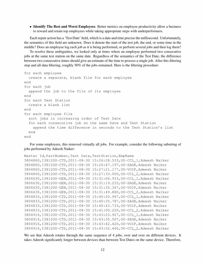
• Identify The Best and Worst Employees. Better metrics on employee productivity allow a businessto reward and retain top employees while taking appropriate steps with underperformers.

Each repair action has a ‘Test Date’ field, which is a date and time precise the millisecond. Unfortunately,the semantics of this field are unknown. Does it denote the start of the test job, the end, or some time in themiddle? Does an employee log each job as it is being performed, or perform several jobs and then log them?

To resolve these ambiguities, we looked only at times where an employee performed two consecutivejobs at the same test station on the same date. Regardless of the semantics of the Test Date, the differencebetween two consecutive times should give an estimate of the time to process a single job. After this filteringstep and all data filtering, roughly 50% of the jobs remained. Here is the filtering procedure:

for each employeecreate a separate, blank file for each employee

endfor each job

append the job to the file of its employeeendfor each Test Station

create a blank listendfor each employee file

sort jobs in increasing order of Test Datefor each consecutive job on the same Date and Test Station

append the time difference in seconds to the Test Station’s listend

end

For some employees, this removed virtually all jobs. For example, consider the following substring ofjobs performed by Adeesh Naiker:

Master Id,PartNumber,Test Date,TestStation,EmpName3804860,I3812OU-CTD,2011-08-30 15:26:28.533,OU-CCL_1,Adeesh Naiker3804860,I3812OU-CTD,2011-08-30 15:26:47.197,OU-SAGE,Adeesh Naiker3804860,I3812OU-CTD,2011-08-30 15:27:21.177,OU-VOIP,Adeesh Naiker3804860,I3812OU-CTD,2011-08-30 15:27:33.000,OU-CCL_2,Adeesh Naiker3806630,I3812OU-GEN,2011-08-30 15:31:06.933,OU-CCL_1,Adeesh Naiker3806630,I3812OU-GEN,2011-08-30 15:31:19.233,OU-SAGE,Adeesh Naiker3806630,I3812OU-GEN,2011-08-30 15:31:35.367,OU-VOIP,Adeesh Naiker3806630,I3812OU-GEN,2011-08-30 15:31:49.880,OU-CCL_2,Adeesh Naiker3804833,I3812OU-CTD,2011-08-30 15:40:20.997,OU-CCL_1,Adeesh Naiker3804833,I3812OU-CTD,2011-08-30 15:40:35.787,OU-SAGE,Adeesh Naiker3804833,I3812OU-CTD,2011-08-30 15:40:43.733,OU-VOIP,Adeesh Naiker3804833,I3812OU-CTD,2011-08-30 15:41:00.220,OU-CCL_2,Adeesh Naiker3804916,I3812OU-CTD,2011-08-30 15:43:23.927,OU-CCL_1,Adeesh Naiker3804916,I3812OU-CTD,2011-08-30 15:43:35.507,OU-SAGE,Adeesh Naiker3804916,I3812OU-CTD,2011-08-30 15:43:42.420,OU-VOIP,Adeesh Naiker3804916,I3812OU-CTD,2011-08-30 15:43:52.460,OU-CCL_2,Adeesh Naiker

We see that Adeesh rotates through the same sequence of 4 jobs, over and over on different devices. Ittakes Adeesh significantly longer between devices than between Test Dates on the same device. Therefore,

12

Figure 5: Average time per Test Station job across all employees.

it seems likely that Adeesh performs some setup and analysis, and then quickly records the results of thatanalysis. Some component of the time between devices must be charged to each of the jobs performedon a device, but it is not trivial to figure out the time for each individual job. This was the motivation forconsidering only consecutive jobs at the same Test Station.

We use the above data to produce an average time per Test Station job for each employee, and thenaverage these numbers for each Test Station. Figure 5 shows that most Test Stations take on the order of oneminute, with some extremely fast (seconds) and some around 15 minutes.

2.4 Path Analysis

The next major analysis we undertook was to examine what the paths for each product that entered the teststation looked like. For example: if there are a cluster of paths that diverge and end up costing the repaircenter more than the cost of a new item, it may allow for extra efficiencies by the company. Our goal isto discover specific path segments or item features that indicate products that should either take a differenttesting route, or ignore testing altogether, to reduce the expected cost of each item. We attempt to segment

13

0

20000

40000

60000

80000

100000

120000

140000

160000

0 20 40 60 80 100 120

Num

ber

of p

aths

Path length

"hist.all"

Figure 6: This figure shows the distribution of paths length.

the data such that we strike a strong balance between the bias and variance of our model.We begin by preprocessing the data, to remove any unknowns from the data. First, we make an assump-

tion that “in-warranty” items are treated differently in the process than items that are not “in-warranty”. Thisreduces the dataset by approximately 15%, from 1, 585, 122 to 1, 344, 626 item instances (number of paths).Furthermore, we collapse all consecutive tests done by a single person and a test station. Because these teststations contain multiple tests, we can aggregate these into a single line-item, which allows us to performpath analyses at a higher level (and reduce computational complexity).

2.4.1 Path length and the “ski” problem

We began by examining the distribution of path lengths. After preprocessing and calculation, we obtain thegraph in Figure 6. As one can see, paths of size 7 to 10 are quite common, but removing these we obtainsomething that resembles a normal distribution. When analyzing this data, we found that the high densityarea between 7 and 10 corresponds largely to items that PASS all initial tests, whereas the remaining (above12) correspond to tests that commonly FAIL. Figure 7 shows the mass around 7 to 10 represents items thatpassed, and the mass with a mean at about 20 represents items that failed.

The “ski problem” states a well-known function that if one rents skis for an unknown number of days,that the optimal choice is to buy the skis on the day that the amount spent on renting the skis is equal to theprice of buying the skis. To this end, we built a simple model that takes a parameter Cf for the full cost ofan item, a parameter Ct for the cost of a test, and a function fC(t) = Ct ∗Ci ∗ t (where Ci is the incrementalcost per extra test). The assumption for the final function is that each consecutive test is likely to cost more.

The ultimate goal is to choose the “cut-off” point, after which Flextronics should send the customer anew item. We found that, though there might be value in this method, it is difficult to know from the dataprovided. We do not have the cost information (i.e., Ct, Ci, Cf are all unknown). Table 8 provides someinsight to the sensitivity of these parameters.

14

0

20000

40000

60000

80000

100000

120000

140000

160000

0 20 40 60 80 100 120

Num

ber

of p

aths

Path length

"hist_pass""hist_fail"

Figure 7: This figure shows the distribution of paths length.

Cf Ct Ci cost savings at optimal cut off10 8 0.1 7.087%

100 8 0.1 2.048%30 1 0.1 2.666%30 10 0.1 5.538%

Figure 8: Sensitivity of parameters for “ski problem” model.

2.5 Cycle Analysis

As a second analysis, continuing to examine the flow of the product through the different test stations, weinstead model each item’s path as a graph. In this way, we may discover some hidden structure in eachsituation, such as cycles. Cycles may indicate that there is redundancy in the process, and that there may bemore optimal testing routes. For example, if there exists a common test path of length 5, and test #3 is thetest failing, it would be suboptimal to force the product through all five steps until #3 is fixed.

2.5.1 Longest Cycle Lengths

We begin by examining the longest subsequences (or subgraphs) that are repeated for each graph in our dataset. This may be indicative of specific paths that have unnecessary tests. Using our example before, we maywant to reduce the test length of the cycle above from five to three, or perhaps to one.

Our algorithm for finding the longest cycles in each graph is analogous to the problem of finding thelongest repeated subsequence in a string. This can be performed in O(N) time, where N is the number ofnodes in the graph (or characters in the string), by using a suffix tree. Essentially, we construct a suffix treeand find the lowest node that is not a leaf.

The graph in Figure 9 shows the distribution of longest cycles. It should be fairly clear from the graphthat the cycles are certainly indicative of products that fail. The graph splits the instances between productsthat PASS and products that FAIL.

15

1

10

100

1000

10000

100000

1e+06

0 2 4 6 8 10 12

Num

ber

of s

ubse

quen

ces

of le

ngth

x

Longest subsequence

Figure 9: This figure shows the distribution of longest subsequences. The solid line represents items thatpassed all tests, the dotted line had at least one test FAIL.

2.5.2 Cycle Repetitions

The cycles found in the previous section are somewhat misleading, in that they indicate only the longestpaths, which are repeated only twice or more. Instead, we may be more interested in cycles that repeatoften. If cycles are repeated three times or more, it may indicate that there is a repair process that isn’tworking correctly or that there are other tests that may be required earlier in the process to cut down onrepetitions.

Figure 10 examines the distribution of the number of cycles for all graphs. It is interesting to note thatthere are thousands of instances of three or more repetitions.

We now examine a specific example. The path “Nguyet Vu, mikael seabury, Trang Nguyen, Saroj Patel”is repeated twice or more in 26258 different path instances. One interesting analysis we also performed wasto split these into two classes: One class is where the cycle only appeared twice, and the other is where thecycle appeared three times or more. For this example, there were 24809 paths in which it repeated twice,and 1449 paths in which it repeated three times or more. We then compute features based on all informationbefore the first cycle ends. In this way, we are comparing two identical situations, and this may providesome clues as to the differences in the paths when there are two versus three or more cycles. The averagefeatures appear in Table 11. In our future work, we expect to examine more features about these classes.It appears, from only two features, that there is some separation in the two classes. This may help us todistinguish between products that are likely to have many more cycles, and those that will be complete afterthe second repetition. If we can do this reliably, we can reduce the expected cost of each repair.

2.6 Future Work

The contract with Flextronics is ongoing. Our next steps are to produce the following two simple models:

• Time-cost model for repairing a product based on it’s type and the number of previous jobs alreadyexecuted on it.

• Comparison of the effectiveness of different employees at each Test Station.

16

1

10

100

1000

10000

100000

1e+06

0 1 2 3 4 5 6 7

Num

ber

of in

stan

ces

with

cyc

les

x

Most number of cycles

Figure 10: This figure shows the distribution of the number of cycles of any subsequence of length three orgreater. The solid line represents items that passed all tests, whereas the dotted line had at least one testingfailure.

Feature Two cycle repetitions > 3 cycle repetitionsAverage Sequence Length before first appearance 23.7244 26.4362Number of failures before first appearance 2.067 2.748

Figure 11: Average features for subsequence “Nguyet Vu, mikael seabury, Trang Nguyen, Saroj Patel”repeating twice or three or more.

These analyses should give Flextronics an idea of what value is hidden in their data.

References

[1] Flextronics Wikipedia page. http://en.wikipedia.org/wiki/Flextronics

[2] Develop an automated scoring algorithm for student-written essays. http://www.kaggle.com/c/asap-aes

[3] Leah Larkey. 1998. Automatic Essay Grading Using Text Categorization Techniques. http://ciir.cs.umass.edu/pubfiles/ir-121.pdf

[4] Ted Briscoe, Ben Medlock, Oistein Andersen. 2010. Automated assessment of ESOL free text exam-inations. http://www.cl.cam.ac.uk/techreports/UCAM-CL-TR-790.pdf

[5] Yannakoudakis, H., Briscoe, T., and Medlock, B. 2011. A New Dataset and Method for AutomaticallyGrading ESOL Texts. Proceedings of the 49th Annual Meeting of the Association for ComputationalLinguistics.

[6] Andrew Hickl and Jeremy Bensley. 2007. A Discourse Commitment-Based Framework for Recogniz-ing Textual Entailment. http://dl.acm.org/citation.cfm?id=1654571

17

[7] Bill MacCartney, Christopher Manning. 2008. An Introduction to Information Retrieval.

[8] Christopher Manning, Prabhakar Raghavan, Hinrich Schutze. 2009. An Introduction to InformationRetrieval. http://nlp.stanford.edu/IR-book/pdf/irbookonlinereading.pdf

[9] Richard Socher, Eric H. Huang, Jeffrey Pennington, Andrew Y. Ng, Christopher D. Manning.2011. Dynamic Pooling and Unfolding Recursive Autoencoders for Paraphrase Detection. http://books.nips.cc/papers/files/nips24/NIPS2011_0538.pdf

[10] T.K. Landauer and P.W. Foltz. 1998. An introduction to latent semantic analysis. Discourse processes,pages 259284.

[11] Tristan Miller. 2003. Essay Assessment with Latent Semantic Analysis. http://files.nothingisreal.com/publications/Tristan_Miller/miller03a.pdf

[12] P. Wiemer-Hastings and I. Zipitria. 2001. Rules for Syntax, Vectors for Semantics. In Proceedings ofthe 23rd Annual Conference of the Cognitive Science Society, Erlbaum, Mahwah, NJ.

[13] P. Wiemer-Hastings. 2000. Adding syntactic information to LSA. In Proceedings of the 22nd AnnualConference of the Cognitive Science Society, pp. 989993, Erlbaum, Mahwah, NJ.

[14] Kanejiya D., Kumar A., and Prasad, S. 2003. Automatic Evaluation of Students Answers usingSyntactically Enhanced LSA. HLT-NAACL-EDUC ’03 Proceedings of the HLT-NAACL 03 workshopon Building educational applications using natural language processing - Volume 2

[15] E.J. Briscoe, J. Carroll, and R Watson. 2006. The second release of the RASP system. In ACL-Coling06 Interactive Presentation Session, pages 7780, Sydney, Australia.

[16] http://en.wikipedia.org/wiki/Bayesian_information_criterion

[17] Yehuda Koren. v2009. The BellKor Solution to the Netflix Grand Prize. http://www.netflixprize.com/assets/GrandPrize2009_BPC_BellKor.pdf

[18] Sanda M. Harabagiu. 1998. WordNet-Based Inference of Textual Cohesion and Coherence. cs.utdallas.edu/˜sanda/papers/flairs98.ps.gz

[19] Ziheng Lin, Hwee Tou Ng and Min-Yen Kan. 2011. Automatically Evaluating Text Coherence Us-ing Discourse Relations. http://www.aclweb.org/anthology-new/P/P11/P11-1100.pdf

18