Autocatalytic reactions in systems with hyperbolic mixing: exact results for the active Baker map
24
arXiv:nlin/0101040v1 [nlin.CD] 22 Jan 2001 Autocatalytic Reactions in Systems with Hyperbolic Mixing: Exact Results for the Active Baker Map Z Toroczkai†, G K´ arolyi‡, ´ A P´ entek§, and T T´ el‖ † Theoretical Division and Center for Nonlinear Studies, Los Alamos National Laboratory, Los Alamos, New Mexico 87545, USA ‡ Department of Civil Engineering Mechanics, Technical University of Budapest, M˝ uegyetem rkp. 3, H-1521 Budapest, Hungary §Marine Physical Laboratory, Scripps Institution of Oceanography, University of California at San Diego, La Jolla, CA 92093-0238, USA ‖ Institute for Theoretical Physics, E¨ otv¨os University, P. O. Box 32, H-1518 Budapest, Hungary E-mail: [email protected], [email protected], [email protected], [email protected] Abstract. We investigate the effects of hyperbolic hydrodynamical mixing on the reaction kinetics of autocatalytic systems. Exact results are derived for the two dimensional open baker map as an underlying mixing dynamics for a two-component autocatalytic system, A + B → 2B. We prove that the hyperboliticity exponentially enhances the productivity of the reaction which is due the fact that the reaction kinetics is catalyzed by the fractal unstable manifold of the chaotic set of the reaction- free dynamics. The results are compared with phenomenological theories of active advection. Submitted to: J. Phys. A: Math. Gen. 1. Introduction The advection of chemically or biologically active particles in imperfectly mixing chaotic hydrodynamical flows received considerable recent interest [1, 2, 3, 4, 5, 6, 7, 8, 9]. By chaotic we understand a smoothly time-dependent, in the simplest case periodic, flow in which the advection dynamics of tracers is chaotic. These tracers undergo chemical or biological interactions while being advected by two-dimensional flows. The distribution of the products along a filamental fractal seems to be a general feature of such reactions. Here we consider tracers as point-like particles which are assumed not to have any influence on the fluid flow itself. The reaction model is of kinetic type where the reactions take place upon particle-particle ‘collisions’: when particles of type A and B are closer to each other than a reaction range σ, then particle A changes to B according to the autocatalytic scheme A + B → 2B. The reaction model is discrete in time, i.e.,
-
Upload
independent -
Category
Documents
-
view
2 -
download
0
Transcript of Autocatalytic reactions in systems with hyperbolic mixing: exact results for the active Baker map
arX
iv:n
lin/0
1010
40v1
[nl
in.C
D]
22
Jan
2001
Autocatalytic Reactions in Systems with Hyperbolic
Mixing: Exact Results for the Active Baker Map
Z Toroczkai†, G Karolyi‡, A Pentek§, and T Tel‖
† Theoretical Division and Center for Nonlinear Studies, Los Alamos National
Laboratory, Los Alamos, New Mexico 87545, USA
‡ Department of Civil Engineering Mechanics, Technical University of Budapest,
Muegyetem rkp. 3, H-1521 Budapest, Hungary
§Marine Physical Laboratory, Scripps Institution of Oceanography, University of
California at San Diego, La Jolla, CA 92093-0238, USA
‖ Institute for Theoretical Physics, Eotvos University, P. O. Box 32, H-1518
Budapest, Hungary
E-mail: [email protected], [email protected], [email protected],
Abstract. We investigate the effects of hyperbolic hydrodynamical mixing on the
reaction kinetics of autocatalytic systems. Exact results are derived for the two
dimensional open baker map as an underlying mixing dynamics for a two-component
autocatalytic system, A + B → 2B. We prove that the hyperboliticity exponentially
enhances the productivity of the reaction which is due the fact that the reaction
kinetics is catalyzed by the fractal unstable manifold of the chaotic set of the reaction-
free dynamics. The results are compared with phenomenological theories of active
advection.
Submitted to: J. Phys. A: Math. Gen.
1. Introduction
The advection of chemically or biologically active particles in imperfectly mixing chaotic
hydrodynamical flows received considerable recent interest [1, 2, 3, 4, 5, 6, 7, 8, 9]. By
chaotic we understand a smoothly time-dependent, in the simplest case periodic, flow in
which the advection dynamics of tracers is chaotic. These tracers undergo chemical or
biological interactions while being advected by two-dimensional flows. The distribution
of the products along a filamental fractal seems to be a general feature of such reactions.
Here we consider tracers as point-like particles which are assumed not to have
any influence on the fluid flow itself. The reaction model is of kinetic type where the
reactions take place upon particle-particle ‘collisions’: when particles of type A and B
are closer to each other than a reaction range σ, then particle A changes to B according
to the autocatalytic scheme A + B → 2B. The reaction model is discrete in time, i.e.,
The Active Baker Map 2
a reaction can only take place at integer multiples of a reaction time τ . In intervals
between successive reactions the particles are passively advected by the flow.
The passive advection dynamics has two essential parameters that influence the
reaction kinetics of the process: a decay or contraction parameter λ and the fractal
dimension D0 of the set around which products accumulate. In open flows this set
turns out to be the unstable manifold of a nonescaping chaotic set characterizing the
passive advection [2, 3], and the role of the contraction parameter is played by the
average negative Lyapunov exponent of the Lagrangian dynamics which expresses the
convergence towards the chaotic set. Due to incompressibility, the positive and negative
Lyapunov exponents have the same absolute value. Particles are advected away from
any neighborhood of the chaotic set along the unstable manifold which leads to an
exponential decay of the passive particles with an escape rate κ. This is, however, not
a new dynamical parameter since it is related to the previous ones via D0 ≈ 2 − κ/λ,
[10, 11]. Here we concentrate on slow reactions whose reaction velocity vr = σ/τ is
much slower than the characteristic velocity of the passive advection dynamics.
In this section we present a heuristic argument for the total area of the product
particles as a function of time. Since the basic ingredients of the argument are
the existence of a fractal backbone and the contracting dynamics acting towards the
backbone, we do not need to actually specify the two-dimensional hydrodynamical flow
itself just to postulate the fractal backbone and the contraction property. We consider
the simplest filamental fractal which is the direct product of a Cantor set of dimension
(D0 − 1) and a line segment of length L so that the total dimension is D0. In addition,
a contraction of rate λ is postulated towards the fractal filaments, see Figure 1. This
simple theory can also be considered to hold for reactions taking place along spatially
fixed fractal catalysts when there is transport of products, resulting in an effective
contraction.
ε(n)backbone:line segment
�������������������������������������������������������������������������������������
�������������������������������������������������������������������������������������
L reactioncontraction
a) c)b) d)
= +2σe −λε(n)e ε(n)ε(n+1)−λ ττ
��������������������������������������������������������������������
��������������������������������������������������������������������
�������������������������������������������������������������������������������������
�������������������������������������������������������������������������������������
B B B
A
A
A A
A A
Figure 1. Schematic drawing of the emptying and fattening process surrounding a
single filament. A line segment of length L ( a)) is covered by material B ( b)). The
width of this stripe is first shrunk ( c)) due to outflow, then it is fattened by a sudden
reaction ( d)).
At time n, right after a reaction takes place, filaments are assumed to be covered by
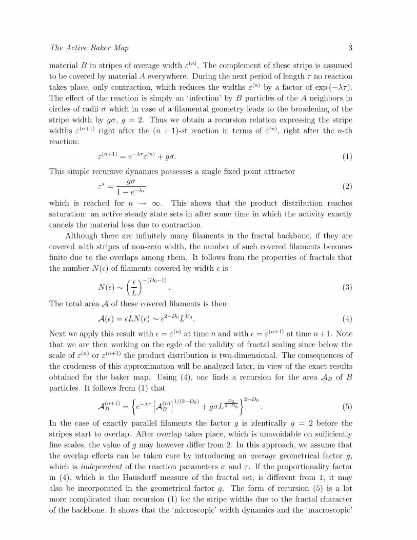
The Active Baker Map 3
material B in stripes of average width ε(n). The complement of these strips is assumed
to be covered by material A everywhere. During the next period of length τ no reaction
takes place, only contraction, which reduces the widths ε(n) by a factor of exp (−λτ).
The effect of the reaction is simply an ‘infection’ by B particles of the A neighbors in
circles of radii σ which in case of a filamental geometry leads to the broadening of the
stripe width by gσ, g = 2. Thus we obtain a recursion relation expressing the stripe
widths ε(n+1) right after the (n + 1)-st reaction in terms of ε(n), right after the n-th
reaction:
ε(n+1) = e−λτε(n) + gσ. (1)
This simple recursive dynamics possesses a single fixed point attractor
ε∗ =gσ
1 − e−λτ(2)
which is reached for n → ∞. This shows that the product distribution reaches
saturation: an active steady state sets in after some time in which the activity exactly
cancels the material loss due to contraction.
Although there are infinitely many filaments in the fractal backbone, if they are
covered with stripes of non-zero width, the number of such covered filaments becomes
finite due to the overlaps among them. It follows from the properties of fractals that
the number N(ǫ) of filaments covered by width ǫ is
N(ǫ) ∼(
ǫ
L
)
−(D0−1)
. (3)
The total area A of these covered filaments is then
A(ǫ) = ǫLN(ǫ) ∼ ǫ2−D0LD0 . (4)
Next we apply this result with ǫ = ε(n) at time n and with ǫ = ε(n+1) at time n+1. Note
that we are then working on the egde of the validity of fractal scaling since below the
scale of ε(n) or ε(n+1) the product distribution is two-dimensional. The consequences of
the crudeness of this approximation will be analyzed later, in view of the exact results
obtained for the baker map. Using (4), one finds a recursion for the area AB of B
particles. It follows from (1) that
A(n+1)B =
{
e−λτ[
A(n)B
]1/(2−D0)+ gσL
D0
2−D0
}2−D0
. (5)
In the case of exactly parallel filaments the factor g is identically g = 2 before the
stripes start to overlap. After overlap takes place, which is unavoidable on sufficiently
fine scales, the value of g may however differ from 2. In this approach, we assume that
the overlap effects can be taken care by introducing an average geometrical factor g,
which is independent of the reaction parameters σ and τ . If the proportionality factor
in (4), which is the Hausdorff measure of the fractal set, is different from 1, it may
also be incorporated in the geometrical factor g. The form of recursion (5) is a lot
more complicated than recursion (1) for the stripe widths due to the fractal character
of the backbone. It shows that the ‘microscopic’ width dynamics and the ‘macroscopic’
The Active Baker Map 4
area dynamics are qualitatively different since the latter is nonlinear. Nevertheless, (5)
possesses a fixed point
A∗
B =
(
gσ/L
1 − e−λτ
)2−D0
L2 (6)
which is the only attractor of the chemical dynamics.
It is worth taking a continuum limit in which the reaction time τ and distance σ
both go to zero, while the reaction velocity vr ≡ σ/τ remains finite. In this limit a
differential equation is obtained for the B area AB(t) as a function of the continuous
time t in the form
AB = −λ(2 − D0)AB + g(2 − D0)vrLD0
2−D0 (AB)−β (7)
where the exponent β is a unique positive expression of the fractal dimension
β =D0 − 1
2 − D0. (8)
The singular-looking reaction term on the right hand side (rhs) of (7) expresses the fact
that the smaller the area, the larger the production rate becomes, just as one expects
for reactions on a fractal catalyst.
Both the discrete-time and the continuous-time area dynamics possess a fixed point
steady state. The corresponding product area of the latter is
A∗
B =(
gvr
λL
)(2−D0)
L2. (9)
Note that this is much larger than the product area along a single non-fractal line
(obtained as the special case D0 = 1) since the expression in the paranthesis is much
less than unity in view of our assumption of the slowness of the active dynamics. This
clearly indicates that the presence of a fractal catalyst makes the reactions much more
efficient. The important caveat is that the fractal backbone is not introduced ‘by hand’
as an imposed mixing rule, it is rather generated naturally by the chaotic advection
dynamics of the fluid flow transporting the tracers. The chaotic set is the union of
unstable bounded orbits. The reactions take place along the outflow curves from these
orbits (the unstable manifold). For a time periodic flow the unstable manifold moves
periodically in the plane of the flow (but does not change its fractal dimension). This
is, however, not a basic difference since on a stroboscopic map the manifold appears to
be still.
In order to illustrate and also check the above general heuristic arguments, in
this paper we consider two variants of the baker map, which describe a discrete mixing
dynamics with hyperbolic chaotic properties. These maps are simple enough to facilitate
an exact analytic approach and yet they incorporate the generic features of mixing from
realistic flows. Within this model we are able to derive exact expressions for the area
dynamics and thus to identify the geometric factor, which was not possible within the
phenomenological theories of active chaos.
Our paper is organized as follows: in Section 2 we introduce a simple variant of
the baker map on which we superimpose the chemical activity, introducing thus a novel
The Active Baker Map 5
reactive dynamical system, the Active baker map. Then we derive the exact stripe
dynamics for this map, including the reaction equation describing the area dynamics of
the reactants in the system. In Section 3 we compare the exact expressions with the
heuristic results given in the Introduction, identifying the exact effects of the fractal
geometry on the geometric factor. In Section 4 we consider a second variant for the
baker map, and show the robustness of the heuristic results. Section 5 is devoted to
discussions and outlook.
2. The active baker map
The passive (reaction-free) baker map is probably the simplest dynamical system which
exhibits chaotic behaviour of purely hyperbolic type. Its simplicity allows for analytic
manipulations, and thus it plays from a theoretical standpoint a crucial role, comparable
to the Ising model from statistical mechanics. There are several variants to this map,
and we shall consider two of them in more detail. Let us give first one variant of the
baker map and then define the active version based on this, then in Sec. 4 introduce
another variant with the associated active counterpart, and then finally compare the
results based on the actual realizations of the maps.
Assuming that we start from a completely filled unit square, one step of the baker
map consists of the following: 1) the lower (upper) half of the unit square is compressed
in the x direction by a factor of a < 1/2 around the fixed point in (0, 0) ((1, 1)), and then
2) the compressed stripes are stretched along the y direction (around the same fixed
points) by a factor of b ≥ 2. For b > 2 there will be ‘material’ reaching over the unit
square, which is clipped and discarded. In this case the map is modeling an open flow.
By taking the unit square as the phase space of the baker map, the characteristic length
L of the dynamics is chosen to be unity. When ab = 1, the baker map is area preserving
in the sense that its Jacobian is uniformly unity, however, it is an open chaotic map
for any b > 2, the chaos being of transient type [11]. Mathematically, the image (x′, y′)
through the baker map of a point (x, y) from the unit square is given by:
x′ = ax + (1 − a)θ (y − 1/2) , x ∈ [0, 1]
y′ = by − (b − 1)θ (y − 1/2) , y ∈ [0, 1](10)
where θ(x) is the Heaviside step function. The map is not defined outside the unit
square (i.e. L = 1) and thus chemical reactions can only occur inside the unit square.
In the following we restrict ourselves to open area preserving systems, i.e., to the regime
b = 1/a > 2. Repeated application of the map will result in a sequence of vertical stripes
of various widths which form the hierarchy of a one dimensional Cantor set in the unit
interval along the x-axis. Contraction towards the vertical filaments is governed by the
Lyapunov exponent
λ = − ln a > 0 . (11)
Since due to the construction, in the vertical direction there is no structure, the map is
effectively one dimensional. The fractal dimension D0 − 1 of the Cantor set on which
The Active Baker Map 6
the stripes reside, is simply calculated to be:
D0 − 1 = −ln 2
ln a. (12)
The decay of the area covered by the material left in the unit square is exponential,
with a rate given by the so called escape rate, κ:
κ = − ln (2a) , (13)
so that D0 = 2 − κ/λ holds for the fractal dimension of the stripes in the unit square.
Initially, the empty space between the stripes is imagined to be filled with ‘material’ A,
while the stripes contain material B.
We call the baker map active when the two materials react with each other. We
consider autocatalytic reactions A+B → 2B (the same as in the Introduction), with the
reactions happening along the (vertical) contact lines. This reaction can alternatively
be considered simply as the surface-growth of material B, and leads to a broadening of
the stripes relative to those of the passive baker map.
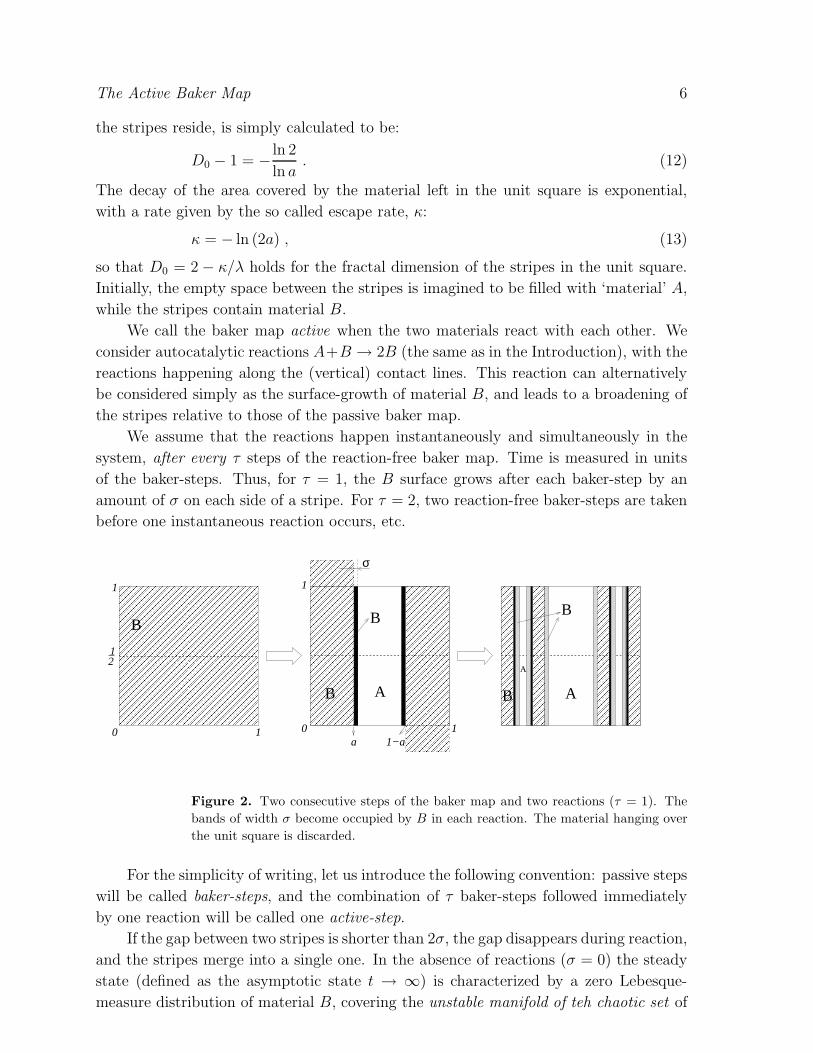
We assume that the reactions happen instantaneously and simultaneously in the
system, after every τ steps of the reaction-free baker map. Time is measured in units
of the baker-steps. Thus, for τ = 1, the B surface grows after each baker-step by an
amount of σ on each side of a stripe. For τ = 2, two reaction-free baker-steps are taken
before one instantaneous reaction occurs, etc.
���������������������������������������������������������������������������������������������������������������������������������������������������������������������������������������������������������������������������������������������������������������������������������������������������������������������������������������������������������������������������������������������������������������������������������������������������������
���������������������������������������������������������������������������������������������������������������������������������������������������������������������������������������������������������������������������������������������������������������������������������������������������������������������������������������������������������������������������������������������������������������������������������������������������������
������������������������������������������
���������������������������������������������������������������
���������������������������������������������������������������
���������������������������������������������������������������
���������������������������������������������������������������
����
������������������������������������������������������������������������������������������������������������������������������������������������������������������������
������������������������������������������������������������������������������������������������������������������������������������������������������������������������
���������������������������������������������������������������������������������������������������������������������������������������������������
���������������������������������������������������������������������������������������������������������������������������������������������������
������������������������������������������
���������������������������������������������������������������
���������������������������������������������������������������
���������������������������������������������������������������
���������������������������������������������������������������
�����������������������������������
�����������������������������������
��������������������������������
��������������������������������
������
������������������������������������������
���������
���������
����
0 1
1
21
1
0 1
σ
a 1−a
B
B A
B
B A
A
B
Figure 2. Two consecutive steps of the baker map and two reactions (τ = 1). The
bands of width σ become occupied by B in each reaction. The material hanging over
the unit square is discarded.
For the simplicity of writing, let us introduce the following convention: passive steps
will be called baker-steps, and the combination of τ baker-steps followed immediately
by one reaction will be called one active-step.
If the gap between two stripes is shorter than 2σ, the gap disappears during reaction,
and the stripes merge into a single one. In the absence of reactions (σ = 0) the steady
state (defined as the asymptotic state t → ∞) is characterized by a zero Lebesque-
measure distribution of material B, covering the unstable manifold of teh chaotic set of
The Active Baker Map 7
dimension D0 of the baker map. In the case of the active baker map, however, there
are new B-areas of width σ appearing after periods τ in the system, and thus a sort of
dynamical balance is expected to set in between the escape dynamics and the growth
dynamics.
2.1. Stripe hierarchy in a simple case: one baker-step per active-step
In spite of the fact that the baker map is one of the simplest maps that exhibits chaotic
dynamics, when chemical activity is also introduced, the reaction kinetics of the system
becomes rather involved.
Let us first start with the simpler case of one reaction per baker-step, i.e., τ = 1.
Figure 2 shows the succession of two such active-steps. The black bands show the B
material coming from the first reaction, while the dotted light gray bands are the B
material emerging from the second reaction. From the point of view of the reaction
kinetics, the distribution and the amount of material A (the gaps) is crucial. If an A
stripe is less wide than 2σ then it will fill up in the next reaction and disappears. During
the baker-steps the hierarchy of gaps builds up with thinner and thinner gaps appearing.
From a certain level on, the reactions are putting a stop to the hierarchy growth. The
question is how in the long time limit the picture stabilizes and the system settles into
a stationary state. Every gap is bounded from left and right by material B. Since the
contraction by a is a point transformation (around the two fixed points at the edges),
each gap will shrink by a factor of a and it will also get closer to the corresponding
fixed point by the same factor a. After the reaction the gaps will lose 2σ from their
width. After one (n = 1) active-step we get one gap of width 1 − 2a − 2σ; after two
active-steps we obtain three gaps: one of width 1−2a−2σ, and two gaps, each of width
a(1 − 2a − 2σ) − 2σ; for n = 3, we have a total of 7 gaps, three just like in the n = 2
case and 4 new members each of width a[a(1− 2a− 2σ)− 2σ]− 2σ, etc. An important
observation is that if gaps appear at a certain level of the hierarchy, there always will
be gaps of precisely the same width and position in the unit square at any later time:
during the next active-step, a particular gap will map precisely down into the location
of two other gaps of the given level. The largest gap (the top level of the hierarchy) is
always located in between the points xl = a + σ and xr = 1 − a − σ. During the next
active-step this particular gap is mapped into two lower level gaps, however its original
position and width is taken over by the new gap appearing as the images of the edges
at x = 0 and x = 1 of the unit square, and modified by σ due to the reaction.
Thus the hierarchy being formed can be described as follows. After n active-steps,
there will be gaps of type n (i.e., the hierarchy will have n levels). If w(j)1 denotes the
width of a gap on level j, and m(j)1 denotes their number (or multiplicity), then one can
write:
w(j)1 = (1 − 2a)aj−1 − 2σ
1 − aj
1 − a, m
(j)1 = 2j−1 . (14)
Observe that the first term on the rhs of the first equation is exactly the width of the
gaps in the reaction free baker map (σ = 0). The second represents the total amount of
The Active Baker Map 8
area-decrease of each gap in j reaction steps: −2σ(1 + a + a2 + ...aj−1). The total area
occupied by the gaps (or material A) after n active-steps is given by
A(n)A =
n∑
j=1
m(j)1 w
(j)1 = 1 − (2a)n −
(
2n − 1 − a1 − (2a)n
1 − 2a
)
2σ
1 − a. (15)
The area occupied by material B is simply the complementer of the above in the unit
square:
A(n)B = 1 −A
(n)A = (2a)n +
(
2n − 1 − a1 − (2a)n
1 − 2a
)
2σ
1 − a. (16)
When n → ∞, A(n)A becomes negative, and later both areas formally diverge which
indicates that this process has to stop after a finite number of steps. This happens by
the closing of the smallest gaps due to the reactions in the n∗-th step: no further gaps
can be created from a certain level down in the hierarchy because the reactions are of
non-zero, finite width σ. By definition, the thinnest gaps of an n-level hierarchy are the
gaps at the lowest (n-th) level of width w(n)1 . The condition for the lowest level to be
filled in n∗ active-steps is w(n∗
−1)1 > 0 and w
(n∗)1 ≤ 0. From this, and Eq. 14, we obtain
n∗ =
{
[u] + 1 , if u is non-integer ,
u , if u is an integer ,(17)
with
u =ln(
1 + (1−a)(1−2a)2σa
)
ln 1a
, (18)
([x] denotes the integer part of x). For n ≥ n∗, w(n)1 ≤ 0 and there are no more gaps
at and below this level. Thus, even if the active-steps are repeated indefinitely, the
hierarchy of gaps stops at j = n∗. Since the gaps at higher level map into gaps at
lower level, a steady state is reached after n∗ steps, and the whole material distribution
becomes stationary. The fact that a stationary state is reached as a balance between
the emptying dynamics and the reactions was numerically observed in all the previously
studied dynamical systems (e.g., flow in the wake of a cylindrical obstacle) [2, 3],
corroborating the generic character of the stationary state.
2.2. Stripe-hierarchy for multiple baker-steps per active-step
In this case there are τ baker-steps taken before an instantaneous reaction occurs. Let
us describe the hierarchy of gaps built up during n active-steps. After the first τ baker-
steps we obtain the usual reaction-free baker hierarchy with τ different types of gaps (a
total of 2τ − 1 gaps). After the first reaction there will be therefore m(1)k = 2k−1 gaps of
type k whose width is w(1)k = ak−1(1 − 2a) − 2σ with k = 1, 2, .., τ . Following the next
active-step, one obtains 2τ types of gaps. The first τ types of gaps are generated by the
k times iterated images of the endpoints x = 0 and x = 1 (k = 1, 2, .., τ) and modified
by the reaction. These have multiplicities widths and positions exactly as those after
the first active-step. The second τ types of gaps are τ times iterated images of the gaps
The Active Baker Map 9
coming from the first active-step. The widths and multiplicities of this second set are
given by w(2)k = aτw
(1)k − 2σ, and m
(2)k = 2τ+k−1 on each level k = 1, .., τ . In general,
if we perform n active-steps, there will be a total of 2nτ − 1 gaps generated with the
following widths and multiplicities:
w(1)k = ak−1(1 − 2a) − 2σ , m
(1)k = 2(k−1) ,
w(j)k = aτw
(j−1)k − 2σ , m
(j)k = 2(j−1)τ+k−1 ,
(19)
where k = 1, .., τ and j = 2, .., n. Analogously to the τ = 1 case, during the iteration,
the gap-hierarchy changes by the addition of finer gaps, and the previously created gap-
structure is not modified by the new reaction. However, in contrast to the τ = 1 case
the new gaps resulted from the new reaction form a sub-hierarchy of τ levels. In the
expressions (19) j denotes the main levels of the hierarchy (related to the state just
after a reaction) while k quantifies the hierarchy on the subtree level (created by the
in-between-reactions baker-steps). Recursion (19) is solved easily, and the result is:
w(j)k = (1 − 2a)a(j−1)τ+k−1 − 2σ 1−ajτ
1−aτ ,
m(j)k = 2(j−1)τ+k−1 ,
j = 1, ..., n . (20)
Obviously the widths are decreasing functions of both j and k (down the hierarchy) as
also seen from (20). Therefore, after n active-steps the thinnest gaps will have the width
of w(n)τ = (1−2a)anτ−1−2σ(1−anτ )/(1−aτ ) and multiplicity of m(n)
τ = 2nτ−1. Another
important consequence of the monotonic behaviour is that the widths found within a
level j are all smaller than the widths found within the level j − 1. This statement is
easily proven by comparing the thinnest and thickest gaps of the neighboring levels.
Thus, the total area of material A after n active-steps is computed as:
A(n)A =
n∑
j=1
τ∑
k=1
m(j)k w
(j)k = 1 − (2a)nτ −
(
2nτ − 1 − aτ (2τ − 1)1 − (2a)nτ
1 − (2a)τ
)
2σ
1 − aτ. (21)
For τ = 1 we indeed recover Eq. (15). The total amount of material B left in the system
will again be the complementary of (21) in the unit square, i.e., A(n)B = 1 −A
(n)A :
A(n)B = (2a)nτ +
(
2nτ − 1 − aτ (2τ − 1)1 − (2a)nτ
1 − (2a)τ
)
2σ
1 − aτ. (22)
As n (time) increases, there will be a critical n∗ = n∗(τ) value at which gaps start to
disappear for the first time. Of course, Eq. (22) is valid only in the regime where no
gaps have been filled yet. This means that for n = n∗ − 1 all the gaps of the hierarchy
(20) exist, but for n = n∗ some of the gaps have disappeared. Let us calculate this value
and see how a stationary state is reached. Since the thinnest gaps of width w(n)τ must
have disappeared at n = n∗ (i.e., w(n∗)τ ≤ 0), but they were present at n = n∗ − 1 (i.e.,
w(n∗−1)
τ > 0), n∗ is calculated as
n∗ =
{
[u] + 1 , if u is non-integer ,
u , if u is an integer ,(23)
where
u =ln(
1 + (1−aτ )(1−2a)2σa
)
ln 1aτ
. (24)
The Active Baker Map 10
This gives the start of the filling in terms of the number of active-steps. However, it is
not necessary that only the thinnest gaps of n∗ have been filled. In principle, all the
gaps of level n∗ can be filled because, as observed above, the widths of gaps at a higher
level are all larger than those of a lower level. How many gaps of level n∗ are filled does
not follow from (24).
Performing another active-step, we may still obtain a partially filled sub-hierarchy
on the main level n∗ + 1, and similarly in the next step, etc. However, since the widths
of the gap additions is strongly decreasing, this process will eventually stop. Once
stopped, the whole material distribution becomes stationary and the system is settled
into a steady state.
The system reaches the steady state when also the thickest (k = 1) gaps are filled
on the next main level. This happens at m∗ for which w(n)1 > 0 if n < m∗, but w
(m∗)1 ≤ 0.
This leads to:
m∗ =
{
[s] + 1 , if s is non-integer ,
s , if s is an integer ,(25)
where
s =ln(
1 + 1aτ
(1−aτ )(1−2a)2σ
)
ln 1aτ
. (26)
Next we compare m∗ and n∗ in order to see how many steps are needed to reach
the steady state, once a filling begins at n∗. From Eqs. (24) and (26) it is obvious that
s > u (the numerator on the rhs of (26) is larger than that of (24) as τ > 1). Let us
introduce the notation:
v ≡(1 − aτ )(1 − 2a)
2σ. (27)
The quantities s and u then become:
s = 1 +ln (aτ + v)
τ ln(
1a
) , and u =1
τ+
ln (a + v)
τ ln(
1a
) . (28)
Simple manipulations lead to:
s − u = 1 −1
τ
1 +ln(
a+vaτ+v
)
ln(
1a
)
< 1 (29)
This means that we have the bounds u < s < u + 1, when τ ≥ 2. (For τ = 1, s and u
are identical.) This implies that
m∗ ∈ {n∗, n∗ + 1} , (30)
i.e., the steady state is reached either on level n∗, or on the next level, n∗ + 1.
When m∗ = n∗, Eq. (21) correctly describes the time evolution of material A over
the whole range n = 1, 2, .., n∗−1, since there are no partially filled main levels. Because
there are no new gaps added on the n∗-th step, in this case A(n∗)A = A
(n∗−1)
A is the steady
state gap-area.
The Active Baker Map 11
0
1
2
3
4
5
6
7
8
9
10
11
12
0 0.05 0.1 0.15 0.2 0.25 0.3 0.35 0.4 0.45 0.5
m
m
*
*
n*
*
a
m*
n*
a)
n (2)
(2)(1)
(1)
(5) (5)0
1
2
3
4
5
0 0.1 0.2 0.3 0.4 0.5a
m*
n*
k*b)
(5)
(5)
(5)
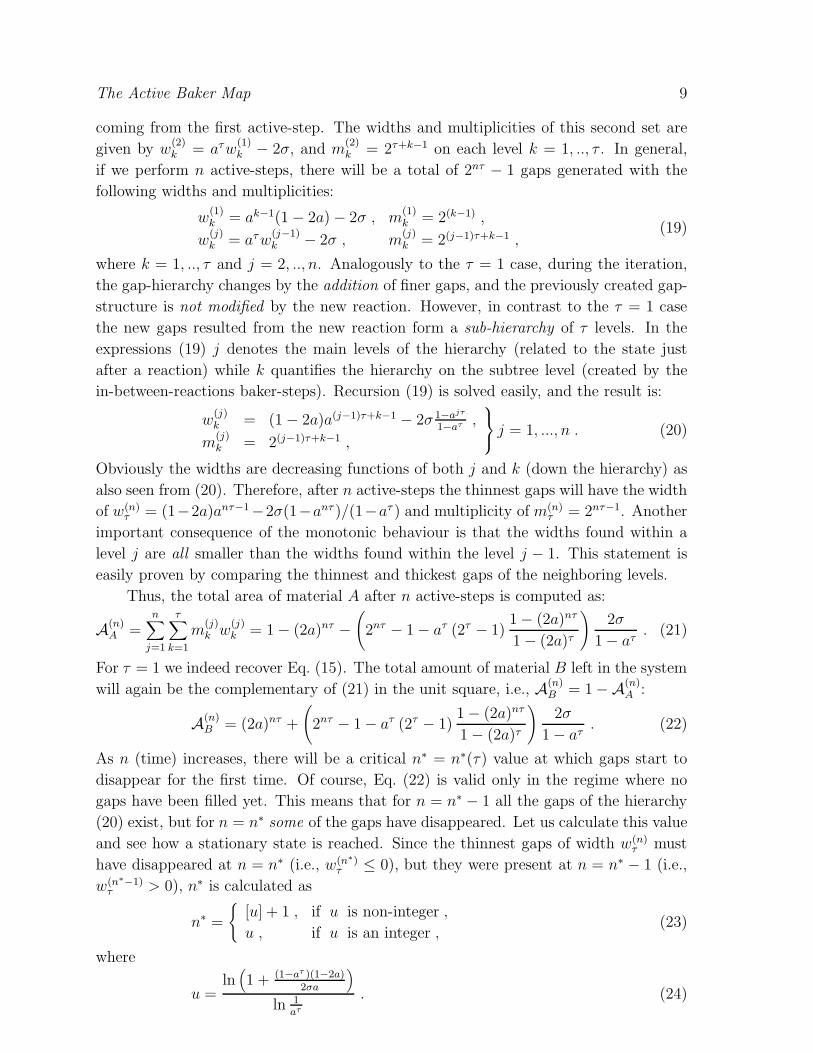
Figure 3. a) Dependence of m∗ and n∗ on a for three τ values: τ = 1, 2, 5. Notice
that relation (30) holds. b) Dependence of m∗ and k∗ on a for τ = 5. k∗ (diamonds)
can take on any value from the set {0, 1, 2, .., τ − 1}. In all cases σ = 10−5.
When m∗ = n∗ + 1, the last main level is partially filled, and in this case
A(n∗+1)A = A
(n∗)A (on the (n∗ + 1)-st step no new gaps are created) is the steady-state
gap-area:
A(n∗)A = A
(n∗−1)
A +k∗
∑
k=1
m(n∗)k w
(n∗)k (31)
where k∗ is defined as the sub-level below which no gaps exist within the main level n∗,
i.e., w(n∗)k > 0 for k ≤ k∗, and w
(n∗)k ≤ 0 for k > k∗. This results in:
k∗ =
{
[y] + 1 , if y is non-integer ,
y , if y is an integer ,(32)
where
y =ln(
1−2a2σ
1−aτ
aτan∗τ
1−an∗τ
)
ln(
1a
) . (33)
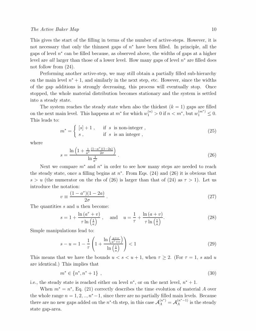
For the m∗ = n∗ case we define k∗ to be zero. Figure 3 shows the values of m∗, n∗ and
k∗ as function of a for a few particular τ values.
2.3. Steady-state areas
Next we analyze the steady-state expression of the area occupied by material B.
When m∗ = n∗, the steady-state value of the B-area is given by A(n∗
−1)B , and for
m∗ = n∗ + 1 by A(n∗)B , the complementary of (31) in the unit square, i.e., A
(n∗)B =
A(n∗
−1)B −
∑k∗
k=1 m(n∗)k w
(n∗)k . The expression of A
(n∗−1)
B is computed from (22), (23), and
(24).
There are two cases in Eq. (23) corresponding to the generic situation when u is
non-integer and to the rather special case when u is an integer. They can be treated on
the same footing by introducing the ‘remainder’:
r ≡
{
{u} , if u is non-integer ,
1 , if u is an integer ,(34)
The Active Baker Map 12
where {x} denotes the fractional part of x (0 < {x} < 1). Thus n∗ − 1 = u − r.
AB*(n )
0
1
2
3
4
5
6
0 0.1 0.2 0.3 0.4 0.5
1
0.1
0.01
1e-3
1e-4
0 0.1 0.2 0.3 0.4 0.5
a
n
k
*
*
a
a) m*
b) AB*(n −1)
Figure 4. The values m∗, n∗ and k∗ at τ = 3 and σ = 10−5 a), and the corresponding
steady state area A(n∗)B
of material B, together with A(n∗
−1)B
, b). Note that the two
areas coincide for k∗ = 0, that is when m∗ = n∗.
From Eq. (24) it follows that auτ = (1 + v/a)−1, where v is given in (27). Using
this expression, and (22), one obtains:
A(n∗
−1)B =
(
2uτ 2σa C + (1 − (2a)τ )D
2σa + (1 − aτ ) (1 − 2a)− 1
)
2σ
1 − (2a)τ, (35)
where
C = (2a)−rτ aτ (2τ − 1)
1 − aτ+ 2−rτ 1 − (2a)τ
1 − aτ, (36)
D = (2a)−rτ a + 2−rτ (1 − 2a) . (37)
Unfortunately the coefficients C and D cannot be simplified further, since they contain,
via r, the fractional-part function which usually hinders analytical manipulations.
The Active Baker Map 13
All these calculations refer to the area of B occupied after n∗−1 active-steps. When
m∗ = n∗ (see Figures 3) and 4a)) A(n∗
−1)B = A
(n∗)B is the steady state area of B. When
m∗ = n∗ + 1 (see Figures 3) and 4a)) we have to substract from A(n∗
−1)B the ‘remainder’
∑k∗
k=1 m(n∗)k w
(n∗)k . This leads to a similar expression as (35), but C and D are changed.
Thus for the steady state area we have
A(n∗)B =
(
2uτ 2σa C ′ + (1 − (2a)τ ) D′
2σa + (1 − aτ ) (1 − 2a)− 1
)
2σ
1 − (2a)τ, (38)
where C ′ and D′ are shorthand notations for
C ′ = 2k∗−rτ 1 − (2a)τ
1 − aτ
(
1 − a(1−r)τ)
+ (2a)(1−r)τ , (39)
D′ = (2a)k∗−rτ a + 2k∗
−rτ (1 − 2a) . (40)
From these we recover (36) and (37) with k∗ = 0, that is, for m∗ = n∗, see figure 4.
This means that the steady states are described by (38), (39), and (40) in all cases.
Note that the steady state area A(n∗)B is a continuous function of a while A
(n∗−1)
B is not
necessarily. However, the derivative of A(n∗)B with respect to a is discontinuous at all the
points where k∗ is discontinuous.
In this section we have derived the dynamics of the areas covered by materials A
and B. Our investigations have been restricted, however, to the time instants right after
the reaction events. In Appendix A we include the whole area dynamics of the active
baker map, i.e., we examine there what happens between subsequent reaction events.
In the next section we make a connection with the existing heuristical theory of
active advection and identify the geometric factor for the active baker map.
3. Comparison with the heuristical theory: derivation of the geometric
factor
The heuristical theory presented in the Introduction and also in detail in Ref. [3, 6]
derives a recursion relation for the area covered by material B in arbitrary open flows
just after the (n + 1)-st reaction as a function of the area occupied by B just after the
n-th reaction. This theory is valid for purely hyperbolic systems. In this section we
show that in the limit of sufficiently small σ the phenomenological expressions derived
in [3, 6] are recovered.
The heuristic formulas were derived with the basic assumption that the material B
in the steady-state is covering the unstable manifold of a chaotic set. The interesting
and novel reaction-kinetics is observed in the parameter region (of σ, τ , D0 and λ) where
the coverage is such that the hierarchical structure of the (fractal) unstable manifold
is preserved in the system over several lengthscales. For example, if σ is too large
then the fractal filamental structure of the unstable manifold is simply washed out
during reactions, and thus the reaction-kinetics will be of the common classical type
of surface reactions [12]. The effects of fractility of the manifold is seen when σ is
small enough so that the coverage of the filaments of the unstable manifold preserves
The Active Baker Map 14
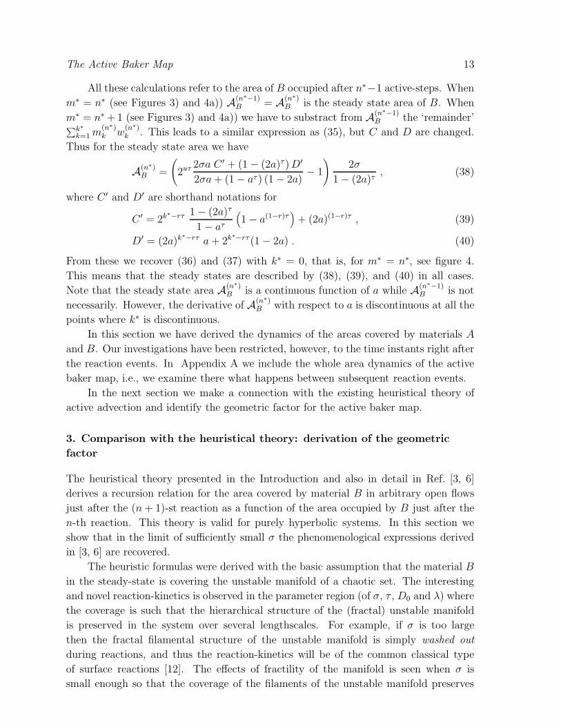
the filamental structures, in forms of stripes of average width ǫ∗ ≪ 1. For the baker
map this means that the number of filaments in the steady state, 2n∗τ , is much greater
than unity: 2n∗τ ≫ 1. From the calculations above follows that this regime is reached
for ‘intermediate’ a values at fixed τ and σ ≪ 1. (If a is close enough to either 0
or 0.5, n∗ is close to unity). However, the smaller σ is the wider the ‘intermediate’
a-range is where fractal behaviour is important, see the expression of u, Eq. (24). In
particular for σ = 10−5 the number of resolved levels is maximum (n∗ = 4) in the
interval a ∈ (0.29, 0.49), see figure 4a). In the following we will assume that we are in
this scaling regime σ ≪ 1.
AB
*(n
)
1
0.1
0.01
1e-3
1e-4
0 0.1 0.2 0.3 0.4 0.5
a
Figure 5. Comparing the approximate expression (41) with the exact (38). The solid
line is Eq. (38), the dashed line is Eq. (41). We have also plotted an upper (using gu,
dotted line) and a lower bound (using gℓ, dashed-dotted line) for Eq. (41). Hereτ = 3
and σ = 10−5.
First observe, that in the fraction multiplying 2u in Eq. (38) one can neglect σ, since
σ ≪ 1. Similarly, it is easy to show that 2u ≃ (v/a)− ln 2/ ln a (according to (27), since
v ≫ 1). It also follows that 2u ≫ 1 and the 1 can be neglected in the curly brackets of
(38). Thus we end up with
A(n∗)B ≃ 2uτ 2σD′
(1 − aτ ) (1 − 2a)= eκτ
(
σg
eκτ/(2−D0) − 1
)2−D0
(41)
with D0 and κ given by Eqs. (12) and (13), and D′ by (40). Here
g =2a
1 − 2a
(
D′
a
)1
2−D0
= 2(2D′)
1
2−D0
1 − 2a, (42)
is a factor which mainly depends on the characteristics of the chaotic baker dynamics.
Equation (41) gives the expression of the steady state B-area just after a reaction. This
The Active Baker Map 15
coincides precisely with the heuristically derived Eq. (6) (see also Eq. (8) of Ref. [3]),
after employing the relation κ/(2−D0) = λ. However, while in (6) and in [3] g appears as
a phenomenological constant, in the present case of the active baker map, its expression
can be given explicitely.
0
0.5
1
1.5
2
2.5
3
3.5
4
0 0.1 0.2 0.3 0.4 0.5a
G G
G
l
u
Figure 6. Comparing the geometrical coefficients G, Gℓ and Gu. Here τ = 3 and
σ = 10−5.
Figure 5 shows (on a linear-log scale) for comparison the a-dependence of the steady
state areas of B for the exact expression of A(n∗)B from (38) and the approximation in
(41). Note that the two are virtually identical in the scaling regime of a.
The explicit expression for g is rather complex due to its dependence on the integer-
part function via D′, see Eq. (40). It can however be shown that D′ is a bounded
variable.
First, D′ ≤ 1 − a. For the geometric factor this leads to the solely a-dependent
upper bound, gu:
g ≤2a
1 − 2a
(
1 − a
a
)
1
2−D0
≡ gu (43)
Second, a lower bound can be derived for g, as follows. Let F (x) = a(2a)−x+(1−2a)2−x,
then D′ = F (rτ − k∗). It can be shown that 0 ≤ rτ − k∗ < 1, and that the function F
The Active Baker Map 16
has a single minimum in the x ∈ [0, 1) interval, at:
xℓ = 1 −1
ln aln
(
(1 − 2a)ln 2
ln 12a
)
(44)
Thus, D′ ≥ F (xℓ) ≡ D′
ℓ and therefore g ≥ gℓ, where gℓ is given by (42) with D′ replaced
by D′
ℓ.
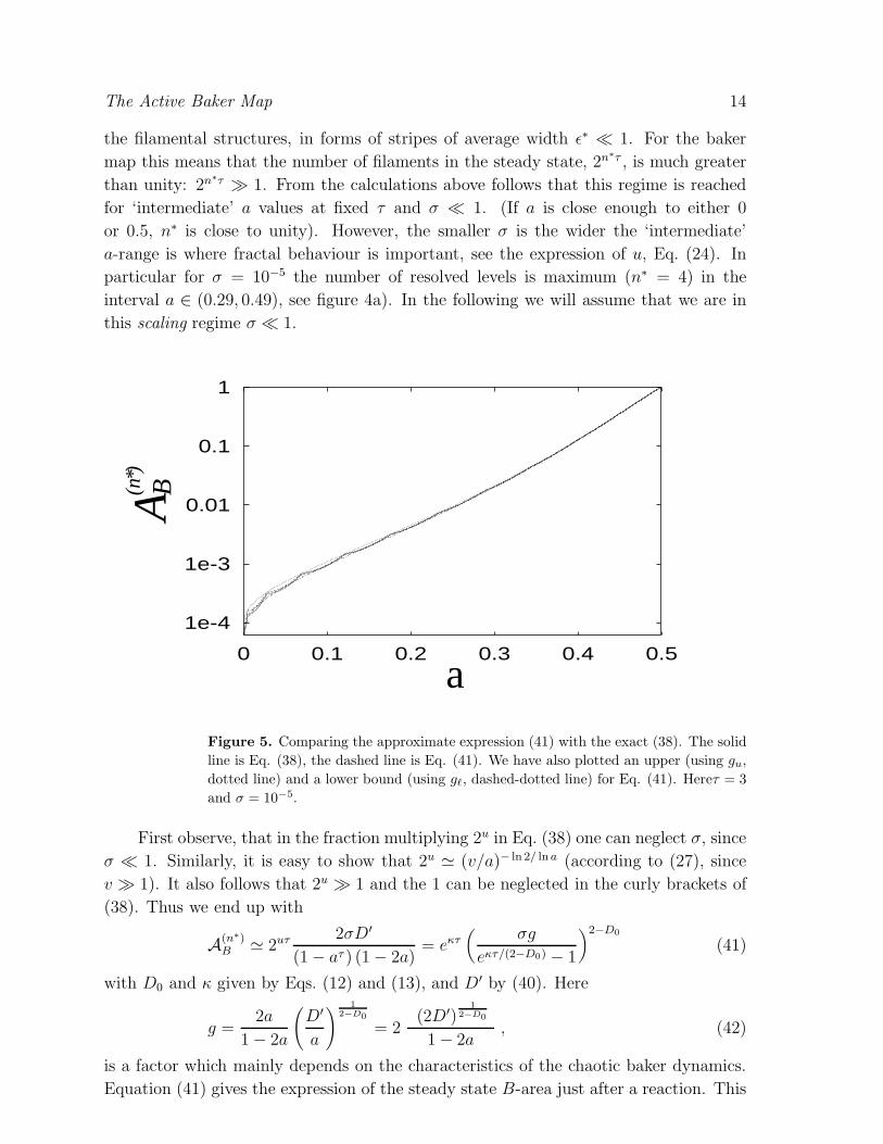
Note that for a → 1/2, g diverges since it is inversely proportional to 1 − 2a. This
divergence, is however cancelled in the expression for the area by the exponent 2 − D0.
In other words, the quantity g2−D0 is well behaved (1 ≤ g2−D0 ≤ 4). Let us introduce
therefore the quantity G ≡ g2−D0. In figure 6 we show G, Gℓ and Gu as functions of a.
Figure 5 shows the corresponding area dependence created with both the upper bound
(dotted line) and the lower bound (dashed-dotted line) .
Both bounds are independent on τ and σ. The two bounds give a rather close
approximation to the exact area expression, as shown in figure 5. This implies that
the factor g is weakly dependent on the reaction range σ and on the reaction time
τ , corroborating our claim that it is only geometrical, i.e., it mainly depends on the
parameters of the mixing dynamics (in this case, on a).
It is also worth comparing the average width of the stripes of material B in the
baker map to that obtained in the Intoduction [see Eq. (2)] and in Ref. [3]. The average
stripe width in the steady state can be obtained as ε∗ = A(n∗)B /2(n∗
−1)τ+k∗
, because there
are 2(n∗−1)τ+k∗
stripes. In the small σ ≪ 1 range this gives
ε∗ ≈2uτ
2(n∗−1)τ+k∗
2σD′
(1 − aτ )(1 − 2a)=
g′σ
1 − aτ, (45)
where g′ is given by
g′ = 2 +2ak∗+1−rτ
1 − 2a. (46)
Equation (45) is exactly the same as (2) and the steady state of Eq. (6) of Ref. [3]
calculated after the reactions. Note that geometrical factor (46) differs from (42). The
reason is that in the heuristic theory of the Introduction and of Ref. [3] the fractal
scaling relation AB ∼ ǫ2−D0 was extended for the steady state stripe width, that is,
for ε∗. For this value of ǫ, we are at the edge of the validity of the above mentioned
scaling, since a crossover to a two-dimensional behavior sets in. This leads to different
geometrical factors for the areas and for the stripe widths.
4. Another form of the baker map
In this section we slightly modify the baker map. One reason to do so is to check whether
the results obtained so far are robust enough. We show that only the geometrical factor
is altered in this case, the main results obtained in the Introduction and in Refs. [2, 3] are
the same. The other reason why another form of the baker map is introduced is based
on the observation that during the reactions there is material hanging over the vertical
edges (the edges parallel to the background flow) of the unit square. The behaviour
The Active Baker Map 17
of this material is not described by the baker map in the form of (10). Moreover,
the cutting of these stripes hanging over the unit square is quite unnatural in terms of
hydrodynamics: there is enough space for the growing of material across the background
flow, the growth is usually not limited by such a sharp obstacle as the edge of the unit
square.
The modified baker map differs from (10) in the location of the fixed points around
which the compression takes place. It consists of two steps: 1) the lower and upper
half of the unit square is compressed in the x direction by a factor of a < 1/2 around
the fixed point in (1/2 − d/2(1 − a), 0) and (1/2 + d/2(1 − a), 1), respectively, where d
is a parameter chosen appropriately, and then 2) the compressed stripes are stretched
along the y direction (around the same fixed points) by a factor of b = 1/a > 2. In
other words, after one baker-step we get two vertical (parallel to the y axis) stripes
centered around (1 − d)/2 and (1 + d)/2. Their centers are at a distance of d. It can
be chosen such that the stripes do not reach the vertical edges of the unit square, thus
there remains enough space for the reactions. An appropriate choice is, e.g., d = 1/2.
The price for this modification is a more involved algebra. In this case, after each
baker-step there are empty areas (i.e., covered by material A) inside the stripes of width
a, into which the unit square is mapped. This means that the gaps are wider than in the
former derivation, and their calculation is not trivial. In fact, it is more convenient to
follow the distance of the centers of the neighbouring stripes. In a baker-step, all existing
central distances are multiplied by a, and a new level of the hierarchy is introduced. This
hierarchy changes only if there are gaps disappearing. Note that the stripe dynamics of
the areas covered by material B is much simpler than in the former baker model: all
stripes of material B have equal widths.
Without going into details, we summarize the results obtained with this modified
baker model for the steady state areas. First let us introduce
σCR =d(1 − 2a)(1 − aτ )
2(1 − a)> 0 . (47)
This is a critical value of the reaction distance for any choice of a and d; if σ > σCR
then there is material B hanging over the vertical edges of the unit square in the steady
state. For σ < σCR, which we assume in what follows, we obtain a steady state where
a Cantor-like hierarchy is produced with N different levels, where N is given by
N =
{
[z] + 1 , if z is non-integer ,
z , if z is an integer ,(48)
where
z =ln(
σCR
σ
)
ln(
1a
) . (49)
The steady state stripe width of material B after the reactions is
ε∗ =2σ
1 − aτ+
aNd
1 − a. (50)
The Active Baker Map 18
This is to be compared to the steady state stripe width (2), using (12) and (11),
which hold for the modified baker map as well. From this equation and from (50) we
obtain
g′ = 2 +1 − aτ
1 − a
aNd
σ. (51)
In case of this modified baker map we have also obtained a correction to the g = 2 value,
which is due to the overlapping of stripes during the reactions. The geometrical factor
depends mainly on parameter a of the baker map, as from (47) and (48) we obtain the
bounds
2 +2a
1 − 2a< g′ ≤ 2 +
2
1 − 2a. (52)
The total area covered by material B is
AB = 2Nε∗ = 2N
(
2σ
1 − aτ+
daN
1 − a
)
. (53)
This is, again, in coincidence with that obtained in Eq. (8) of [3], but the geometrical
factor is different from (51), it is
g =1 − aτ
σaτ
(
2N+τ+1σaτ
1 − aτ+
(2a)N+τd
1 − a
) 1
2−D0
. (54)
The deviation between g and g′ is again the result of the extension of the fractal scaling
to the range of ε∗, to the steady state stripe width.
1
10
100
1000
0 0.1 0.2 0.3 0.4 0.5
a
g, g
, g’,
g’
Figure 7. Compare the geometric factors from Eqs. (42) (solid line), (46) (dashed
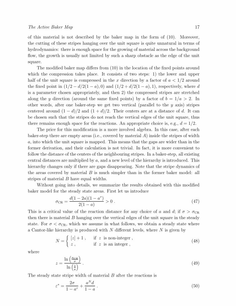
line), and Eqs. (54) (dotted line), (51) (dashed-dotted line). τ = 3, σ = 10−5, d = 1/2.
In Figure 7 we compare the four geometrical factors (42) (solid line) and (54) (dotted
line), and (46) (dashed line), (51) (dashed-dotted line) as function of a. Although the
The Active Baker Map 19
average trend of the curves is the same, there are large deviations due to the fact that
g′ and g′ are discontinuous functions. The deviations, however are less pronounced in
the scaling region where the fractal structures of the maps are better resolved. This
leads us to the conclusion that the geometric factor strongly depends on the particular
realizations and relative positions of the filaments even when these realizations share
the same fractal and dynamical properties (D0, λ).
5. Discussions and outlook
In this paper we have investigated the effects of a fractal geometric catalyst supplied
e.g. by the Langrangian dynamics of an underlying flow on the reaction kinetics of
autocatalytic reactants transported in this flow. The reactive particles were assumed to
simply follow the local velocity of the fluid element at their position and act as simple
passive tracers that do not modify the properties of the flow. For mixing dynamics we
have considered the simplest possible dynamics,namely two variants of the baker map,
in order to be able to generate an analytic description of the reaction process. Even
though the baker map is the simplest map with chaotic mixing, when reactions are
superimposed on the transport dynamics, the analytical calculations become involved
since the reaction range σ introduces a finite nonscaling cutoff which breaks the strict
selfsimilarity. In the limit of slow reactions one is able to recover from these exact
formulas the heuristic expressions derived for general flows, thus validating the latter
approach, and showing that indeed, the fractal backbone does enhance the productivity
of reactions, and acts as a fractal catalyst.
A crucial point in the consistency between the heuristic and exact approach is played
by the so-called geometrical factor g (or its variants g′, g, g′). By definition, it should be
a parameter reflecting mainly the geometrical properties of the mixing dynamics (of the
hydrodynamical flow). In the heuristic theory it is postulated to be independent of the
chemistry parameters σ and τ . The consistency is achieved by showing that it is only
weakly depending on these parameters, in the scaling limit at least. This property follows
from the close bounds (43) and (52) on the geometrical factor(s) depending on a only. A
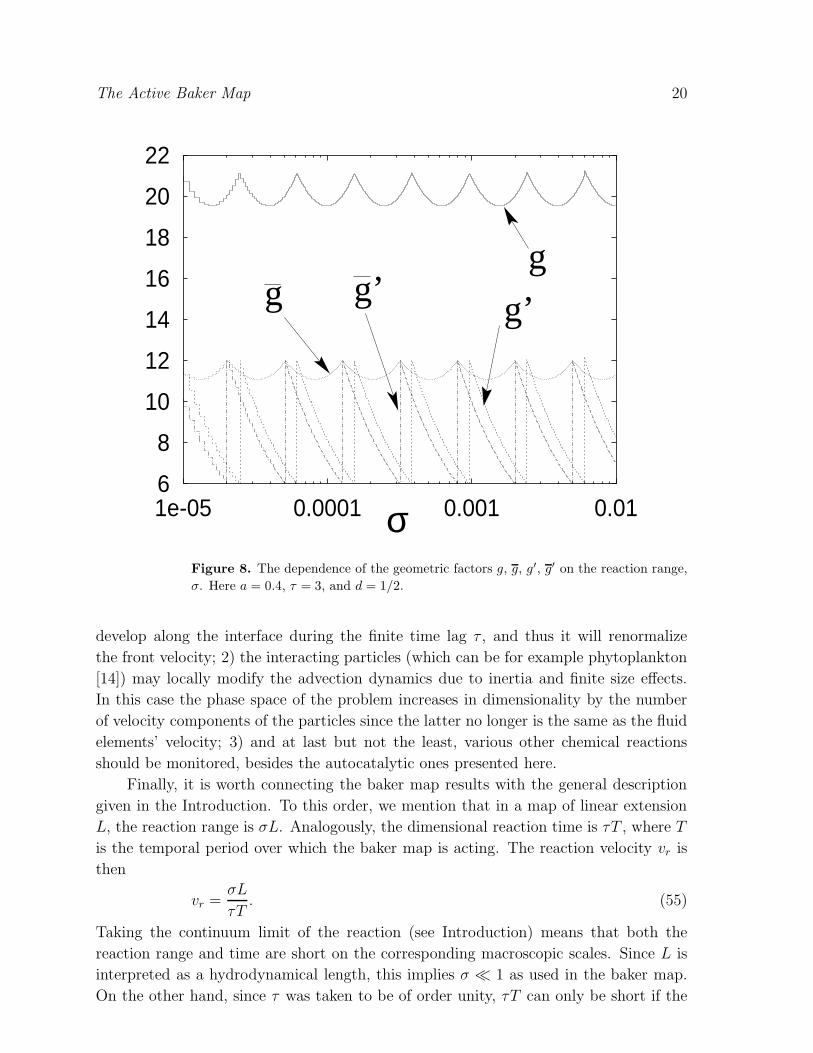
direct plot of the geometrical factors as a function of the reaction range σ (figure 8) also
supports this property and suggests a weak, approximately periodic dependence on the
logarithm of the reaction range, over several orders of magnitude. Note, that the actual
value of the geometrical factor strongly depends on the two independent global chaos
parameters (λ, D0) which determine the chemical kinematics (see Introduction), but
might also depend on other aspects of the chaotic dynamics (as e.g., on the parameter
d of the modified baker map).
Various improvements and extensions to the present theory are possible: 1) one
can consider [13, 15] the more realistic situation of non-simultaneous reactions, i.e.,
the particles have a random phase dispersed among them. We expect that this only
leads to a more rough, fluctuating A − B interface along the manifolds, however these
fluctuations are bounded due to the fact that only correlations of finite length can
The Active Baker Map 20
6
8
10
12
14
16
18
20
22
1e-05 0.0001 0.001 0.01σ
gg g’g’
Figure 8. The dependence of the geometric factors g, g, g′, g′ on the reaction range,
σ. Here a = 0.4, τ = 3, and d = 1/2.
develop along the interface during the finite time lag τ , and thus it will renormalize
the front velocity; 2) the interacting particles (which can be for example phytoplankton
[14]) may locally modify the advection dynamics due to inertia and finite size effects.
In this case the phase space of the problem increases in dimensionality by the number
of velocity components of the particles since the latter no longer is the same as the fluid
elements’ velocity; 3) and at last but not the least, various other chemical reactions
should be monitored, besides the autocatalytic ones presented here.
Finally, it is worth connecting the baker map results with the general description
given in the Introduction. To this order, we mention that in a map of linear extension
L, the reaction range is σL. Analogously, the dimensional reaction time is τT , where T
is the temporal period over which the baker map is acting. The reaction velocity vr is
then
vr =σL
τT. (55)
Taking the continuum limit of the reaction (see Introduction) means that both the
reaction range and time are short on the corresponding macroscopic scales. Since L is
interpreted as a hydrodynamical length, this implies σ ≪ 1 as used in the baker map.
On the other hand, since τ was taken to be of order unity, τT can only be short if the
The Active Baker Map 21
duration of the map is much shorter than the characteristic hydrodynamical time. Even
without further specifying the choice of T , we can derive a useful condition in terms of
a dimensionless number.
In the case of reactions in fluid flows with chaotic mixing properties we have three
distinct levels of time-continuous dynamics built on top of each other:
• the Eulerian description of the hydrodynamics, characterized by one main
parameter, the Reynolds number
Re =UL
ν, (56)
where U is a typical velocity, L is the typical length scale and ν is the kinematic
viscosity;
• the Langrangian description of the dynamics, characterized by the fractal dimension
of the ‘transport manifolds’ (unstable manifolds), and by the contraction dynamics
on them,
D0 = 2 −κ
λ, λ = λ(Re) , κ = κ(Re) ; (57)
• the reaction kinetics, described by a ‘reaction’ Peclet number,
(Per)−1 =
vr
λL, Per = Per(λ(Re)). (58)
Reaction equation (7) can be made dimensionless if the area is measured in units
of L2, and the time in units of the characteristic lifetime of (the Lagrangian) chaos,
1/κ = 1/(λ(2 − D0)):
AB = −AB + g1
Per(AB)−β . (59)
The active baker map’s Peclet number is
(Per)−1 =
σ
τTλ=
σ
τ ln (1/a). (60)
Here we have used that the dimensional Lyapunov exponent of the map is − ln a/T .
With our typical choice of σ = 10−5, τ = 1, 2, 3, and a on the order of 1/4, the reaction
Peclet number is much larger then unity.
It is worth giving the definition of the traditional Peclet number [16] which measures
the importance of diffusion relative to the flow:
(Pe)−1 ≡D
UL=
vd
U(61)
where vd = D/L is the charactersitic diffusion velocity. Large Pe implies weak diffusion.
As suggested by the analogy between the traditional and the reaction Peclet number,
the reaction range plays a similar role as a diffusion length and the reaction velocity
vr as D/L. Furthermore, if molecular diffusion is present but not very strong, it only
renormalizes the reaction front velocity and all the formulas shown here are valid with
vr replaced by an effective reaction front velocity [6].
The Active Baker Map 22
Note that the direct reaction analog of the Peclet number would be vr/U . It is
worth pointing out however that instead we have
(Per)−1 =
vr
U
U
λL=
vr
U
Lyapunov time
hydrodynamical time(62)
which is rather a Lagrangian dynamics based quantity. The difference between Per
and its hydrodynamical analog, vr/U , might be pronounced if the hydrodynamical and
Lyapunov times are not on the same order of magnitude.
The limit of slow reactions implies vr ≪ λL, i.e., Per ≫ 1. It is in this limit
where pronounced fractal product distributions are expected. The steady state product
area A∗
B given by Eq. (9) is by a factor (Per)D0−1 ≫ 1 larger than it would be in
a nonchaotic flow with D0 = 1. Thus we find that a large value of the reaction
Peclet number introduced by Eq.(58) provides a general, neccessary condition for the
existence of filamantal product distributions observable over several orders of magnitude
in reactions taking place in chaotic flows.
Acknowledgments
The authors would like to express special thanks to I. Scheuring for a very helpful input
and discussions. Z.T. was supported by the Department of Energy, under contract
W-7405-ENG-36. G. K. and T. T. acknowledge support of the Hungarian Science
Foundation under grant numbers T032423, F 029637, T 032423 . G.K. is also indebted to
the Bolyai grant and to FKFP 0308/2000 for financial support. Additional support was
provided by the MTA-OTKA/NSF-INT526 grant and the US-Hungarian Joint Grant
(Project No. 501).
Appendix A. Area-dynamics in the active baker map
In Sec. 2 we described the hierarchy of the stripes formed in the active baker map just
after each reaction, calculated the total area occupied by the materials A and B as a
function of the number of active-steps, and proved that a steady state sets in after a given
number of active-steps, m∗. In this appendix we present the full temporal dynamics of
the areas occupied by A and B (not only as a function of the active-steps).
In order to account for the ‘intermediate’ steps as well, we will extend a little bit
the notation introduced in Sec. 2. First we have to observe that once a reaction has
been completed and new passive baker-steps are taken, the existing hierarchy at the end
of the last reaction is doubled and mapped on a level one step lower in the hierarchy
after a passive baker-step, while at the top of the hierarchy there are reaction-free gaps
appearing. If ρ denotes the number of reaction-free baker-steps taken just after the last
reaction, the top gap of width 1−2a appears at ρ = 1, the additional two gaps of width
a(1−2a) appear at ρ = 2, etc., until at ρ = τ the reaction-free tree becomes completed.
All the rest of the gaps coming from earlier reactions are lying under this newly created
‘baker tree’ of length τ . Next a reaction occurs and the whole process repeats itself.
The Active Baker Map 23
0.01
0.1
1
0 5 10 15 20 25 30
(t)
t=nτ+ρ
τ=1τ=2τ=3τ=1τ=2τ=3
a=0.45,a=0.45,a=0.45,a=0.32,a=0.32,a=0.32,
AB
Figure A1. The evolution of the area of material B shown on a log-linear scale for
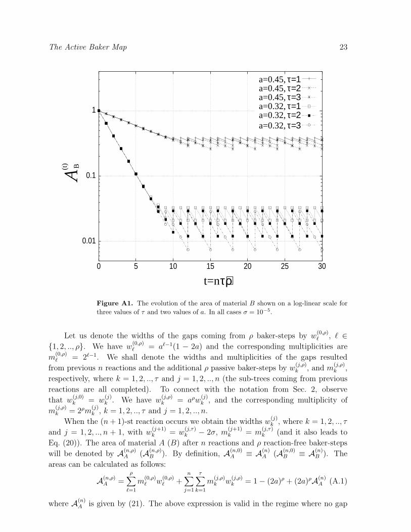
three values of τ and two values of a. In all cases σ = 10−5.
Let us denote the widths of the gaps coming from ρ baker-steps by w(0,ρ)ℓ , ℓ ∈
{1, 2, .., ρ}. We have w(0,ρ)ℓ = aℓ−1(1 − 2a) and the corresponding multiplicities are
m(0,ρ)ℓ = 2ℓ−1. We shall denote the widths and multiplicities of the gaps resulted
from previous n reactions and the additional ρ passive baker-steps by w(j,ρ)k , and m
(j,ρ)k ,
respectively, where k = 1, 2, .., τ and j = 1, 2, .., n (the sub-trees coming from previous
reactions are all completed). To connect with the notation from Sec. 2, observe
that w(j,0)k = w
(j)k . We have w
(j,ρ)k = aρw
(j)k , and the corresponding multiplicity of
m(j,ρ)k = 2ρm
(j)k , k = 1, 2, .., τ and j = 1, 2, .., n.
When the (n + 1)-st reaction occurs we obtain the widths w(j)k , where k = 1, 2, .., τ
and j = 1, 2, .., n + 1, with w(j+1)k = w
(j,τ)k − 2σ, m
(j+1)k = m
(j,τ)k (and it also leads to
Eq. (20)). The area of material A (B) after n reactions and ρ reaction-free baker-steps
will be denoted by A(n,ρ)A (A
(n,ρ)B ). By definition, A
(n,0)A ≡ A
(n)A (A
(n,0)B ≡ A
(n)B ). The
areas can be calculated as follows:
A(n,ρ)A =
ρ∑
ℓ=1
m(0,ρ)ℓ w
(0,ρ)ℓ +
n∑
j=1
τ∑
k=1
m(j,ρ)k w
(j,ρ)k = 1 − (2a)ρ + (2a)ρA
(n)A (A.1)
where A(n)A is given by (21). The above expression is valid in the regime where no gap
The Active Baker Map 24
fillings have occured yet. In terms of the B-material, using (13), (A.1) is equivalent to
A(n,ρ)B = (2a)ρA
(n)B = e−κρA
(n)B (A.2)
just as expected, since between two reactions there is an exponentially emptying
dynamics. The total time is t = nτ + ρ, ρ = 1, 2, .., τ . When ρ = τ , t = (n + 1)τ
and a reaction occurs instantaneously.
Figure A1 shows the t-dependence of the area covered by the material B for three
τ values, for given σ (σ = 10−5) on a log-linear scale at two a values, a = 0.45 and
a = 0.32. Notice the fact that the actual time evolution of the areas follow closely the
simple exponential emptying dynamics. Certainly, between two consecutive reactions,
the emptying is exponential, the deviation from the exponential in the overall run of
the curves occurs in jumps at reaction events.
In order to observe a longer temporal evolution before stationarity sets in, one needs
to choose a very small σ. On the other hand, this means that the overall fattening during
a reaction is very weak, and it is in fact a ‘perturbation’ at early times. It becomes
‘visible’ just before the steady state.
References
[1] Metcalfe G, and Ottino J M 1994 Phys. Rev. Lett. 72 2875
Metcalfe G, and Ottino J M 1995 Chaos, Solitons and Fractals 6 425
Epstein I R 1995, Nature 374, 321
Edouard S, Legras B, Lefevre B, and Eymard R 1996, Nature 384, 444
Edouard S, Legras B, and Zeitlin V 1996, J. Geophys. Res. 101 (D11), 16771
[2] Toroczkai Z, Karolyi G, Pentek A, Tel T and Grebogi C 1998 Phys. Rev. Lett. 80 500
[3] Karolyi G, Pentek A, Toroczkai Z, Tel T and Grebogi C 1999 Phys. Rev. E 59 5468
[4] Pentek A, Karolyi G, Scheuring I, Tel T, Toroczkai Z, Kadtke J, and Grebogi C 1999 Physica A
274 120
[5] Neufeld Z, Lopez C, and Haynes P H 1999 Phys. Rev. Lett. 82 2606
[6] Tel T, Karolyi G, Pentek A, Scheuring I, Toroczkai Z, Grebogi C, and Kadtke J 2000 Chaos 274
120
[7] Neufeld Z, Lopez C, Hernandez-Garcia E, and Tel T 2000 Phys. Rev. Lett. 82 2606
[8] Spall S and Richards K J 2000 Deep-Sea Res. 47 1261
[9] Bracco A, Provenzale A, Scheuring I 2000 Proc. Roy. Soc. Ser. B. 267 1795
[10] Kantz H and Grassberger P 1985 Physica D 17 75
Hsu G H, Ott E, and Grebogi C 1988 Phys. Lett. A 127 199
[11] Tel T 1990 Transient chaos, in Directions in Chaos vol 3 ed Bai-lin Hao (Singapore: World
Scientific) p 149
Tel T 1996, Transient Chaos: a Type of Metastable State, in: STATPHYS’19, ed.: Bai-Lin Hao
(Singapore:World Scientific) p 346
[12] Landau L D, Lifshitz E M 1987 Fluid Mechanics vol 6 in Course of Theoretical Physics 2nd ed
(Oxford: Pergamon)
[13] Santoboni G, Nishikawa T, Toroczkai Z, and Grebogi C 2000 Autocatalytic reactions of active
particles with phase Preprint
[14] Karolyi G, Pentek A, Scheuring I, Tel T, and Toroczkai Z 2000 Proc. Natl. Acad. Sci. USA 97,
13661
[15] 2001 Lopez C, Neufled Z, Hernandez-Garcia E and Haynes P H Phys. Chem. Earth. In press
[16] Liggett J A 1994 Fluid Mechanics (McGraw Hill College)