Author's personal copy Parallel machine scheduling problem with preemptive jobs and transportation...

This article appeared in a journal published by Elsevier. The attachedcopy is furnished to the author for internal non-commercial researchand education use, including for instruction at the authors institution

and sharing with colleagues.

Other uses, including reproduction and distribution, or selling orlicensing copies, or posting to personal, institutional or third party

websites are prohibited.

In most cases authors are permitted to post their version of thearticle (e.g. in Word or Tex form) to their personal website orinstitutional repository. Authors requiring further information

regarding Elsevier’s archiving and manuscript policies areencouraged to visit:

http://www.elsevier.com/authorsrights

http://www.elsevier.com/authorsrights

Author's personal copy

Parallel machine scheduling problem with preemptive jobsand transportation delay

Hesam Shams, Nasser Salmasi n

Department of Industrial engineering, Sharif University of Technology, Tehran, Iran

a r t i c l e i n f o

Available online 18 April 2014

Keywords:SchedulingParallel machine schedulingTransportation delaysMigration delayPreemptionMinimization of makespanMathematical modeling

a b s t r a c t

In this research the parallel machine scheduling problem with preemption by considering a constanttransportation delay for migrated jobs and minimization of makespan as the criterion i.e., Pm|pmtn(delay)|Cmax is investigated. It is assumed that when a preempted job resumes on another machine, it isrequired a delay between the processing time of the job on these two machines. This delay is calledtransportation delay. We criticize an existing mathematical model for the research problem in theliterature [Boudhar M, Haned A. Preemptive scheduling in the presence of transportation times.Computers & Operations Research 2009; 36(8):2387–93]. Then, we prove that there exists an optimalschedule with at most (m�1) preemptions with transportation among machines for the problem.We also propose a linear programming formulation and an exact algorithm for the research problem incase of equal transportation delay. The experiments show that the proposed exact algorithm performsbetter than the proposed mathematical model.

& 2014 Elsevier Ltd. All rights reserved.

1. Introduction

Parallel machine scheduling problems (PMSP) have received agreat amount of attention during last decades based on theirapplications in real world. Fidge [1] discusses about the applicationof PMSP in computer processing, manufacturing lines, preemptivemultitasking, and multi-stage systems as examples of the areas thatparallel machine environment is observed. Several exact and heuristicalgorithms are proposed to solve different types of PMS problems.

In PMSP, preemption is occurred if the process of a job on amachine is interrupted and the process of another job is resumed.The remaining processing time of the preempted job can beperformed later on that machine or on another machine. In moststudies, when a job is preempted on a machine, it is assumed thatthere is no difference between processing the remaining part ofthe processing time of the job on the same machine or on anothermachine. McNaughton [2] studies several scheduling problemswith different objective functions in which the preemption of jobsis allowed. He proposes an exact algorithm to solve the Pm|pmtn|Cmax problem (presented as Pm|prmp|Cmax in literature as well)optimally. Muntz and Coffman [3] propose an exact algorithm tosolve the P2|pmtn, prec|Cmax problem which provides the optimalsolution in a polynomial time.

In real world, the process of a preempted job on anothermachine cannot be resumed immediately since time is required totransfer the job to another machine. Boudhar and Haned [4] namethis changeover time as transportation delay. Rayward-Smith [5]considers the idea of transportation delay in interprocessor com-munication delays. He studies scheduling independent jobs withpreemption on identical parallel machine in order to minimizemakespan by considering equal transportation delay time for jobsamong machines and shows that the problem is NP-complete.Fishkin et al. [6] study the Pm|pmtn(delay)|Cmax problem by con-sidering equal transportation delay among machines. This problemcan be presented as Pm|pmtn(delay¼t)|Cmax. They show that basedon the ratio of transportation delay time and the processing time ofjobs, the problem instances can be classified as easy problems orstrongly NP-hard problems. They propose a heuristic algorithm forthe research problem in case of existing two parallel machines.They also prove that for the P2|pmtn(delay¼t)|Cmax problem thereexists an optimal schedule with at most one preemption withtransportation and for the P3|pmtn(delay¼t)|Cmax problem, thereexists optimal schedule with at most two preemptions on jobs withtransportation. They also conjecture that for the Pm|pmtn(delay¼t)|Cmax problem, there exists an optimal schedule with at most (m�1)preemptions with transportation.

Boudhar and Haned [4] study the Pm|pmtn(delay)|Cmax problem.They assume that the transportation delay times between the twomachines are not equal. They propose a linear programmingformulation and several heuristic algorithms for the researchproblem. They also prove that the problem is NP-hard.

Contents lists available at ScienceDirect

journal homepage: www.elsevier.com/locate/caor

Computers & Operations Research

http://dx.doi.org/10.1016/j.cor.2014.04.0080305-0548/& 2014 Elsevier Ltd. All rights reserved.

n Corresponding author.E-mail addresses: [email protected] (H. Shams),

[email protected] (N. Salmasi).

Computers & Operations Research 50 (2014) 14–23


Haned et al. [7] study the Pm|pmtn(delay)|Cmax problem. Theypropose a heuristic algorithm for a special case of this problemwith identical processing times and not fixed number ofmachines i.e., P|pmtn(delay¼t), pj¼p|Cmax, that solves the pro-blem in a polynomial time. In order to prove that the P|pmtn(delay), pj¼p|Cmax problem is NP-hard by reduction from theHamiltonian chain problem, they consider an arbitrary instanceof the problem. The arbitrary instance of the P|pmtn(delay), pj¼p|Cmax problem is in case of that the number of machines is equalto m, i.e., m¼m, the number of jobs is equal to (mþ1), i.e., n¼(mþ1), the processing time of jobs is also equal to m, i.e.,pj¼p¼m and the transportation delays are equal to 1 and 2.For this special case of the P|pmtn(delay), pj¼p|Cmax problem,they prove that there exists an optimal schedule which thenumber of preempted jobs is equal to m�1. Recall that theconjecture discusses about the Pm|pmtn(delay¼t)|Cmax problem.They also present a dynamic programming algorithm and a fullypolynomial time approximation scheme (FPTAS) to solve the P2|pmtn(delay)|Cmax problem.

In this research we criticize the mathematical model proposedby Boudhar and Haned [4] for the Pm|pmtn(delay)|Cmax problem.Then, we propose a valid mathematical model and an exactalgorithm for the special case of the problem in which thetransportation delay of jobs are equal on machines. We alsoprovide a proof about the conjecture proposed by Fishkin et al.[6] about the number of preemptions with transportation for thePm|pmtn(delay¼t)|Cmax problem.

This paper is organized as follows. The proposed mathematicalmodel by Boudhar and Haned [4] is criticized in Section 2.In Section 3, we prove that for a parallel machine problem withm machines in parallel, there exists an optimal schedule with atmost (m�1) preemptions with transportation among machines. InSection 4, a mathematical formulation and an exact algorithm forthe research problem are proposed. In Section 5, the specificationsof test problems used to compare the performance of the math-ematical model and the exact algorithm are explained. The resultsof the experiments on random test problems with different sizesare presented in Section 6 and finally, the conclusions are given inSection 7.

2. Evaluating the proposed mathematical model by Boudharand Haned [4]

Boudhar and Haned [4] proposed a mathematical model for thePm|pmtn(delay)|Cmax problem. The parameters, decision variables,and the mathematical model are as follows:

The model:

Min Cmax ð1Þ

Subject to

∑m

i ¼ 1qji ¼ pj j¼ 1;…;n ð2Þ

sjiþqjirCmaxj¼ 1;…;n

i¼ 1;…;mð3Þ

sjiþqji�sj0 ir ð1�αjij0 iÞ:B j¼ 1;…;n

sj0 iþqj0 i�sjirαjij0 i:B i¼ 1;…;m

αjij0 iþαj0 iji ¼ 1 j0 ¼ 1;…;n ðja j0 Þ

8>>><>>>:

ð4Þ

sjiþqjiþtii0 :xji�sji0 r ð1�αjiji0 Þ:B j¼ 1;…;n

sji0 þqji0 þtii0 :xji0 �sjirαjiji0 :B i¼ 1;…;m

αjiji0 þαji0ji ¼ 1 i0 ¼ 1;…;m ðia i

0 Þ

8>><>>: ð5Þ

xjirB:qjiqjirB:xji

(j¼ 1;…;n

i¼ 1;…;m

j¼ 1;…;nsji; qjiZ0 i¼ 1;…;m

xji; αjij0 i; αj0iji; αjiji0 ; αji0 jiAf0;1g j0 ¼ 1;…;n ðja j

0 Þi0 ¼ 1;…;m ðia i

0 Þ

ð6Þ

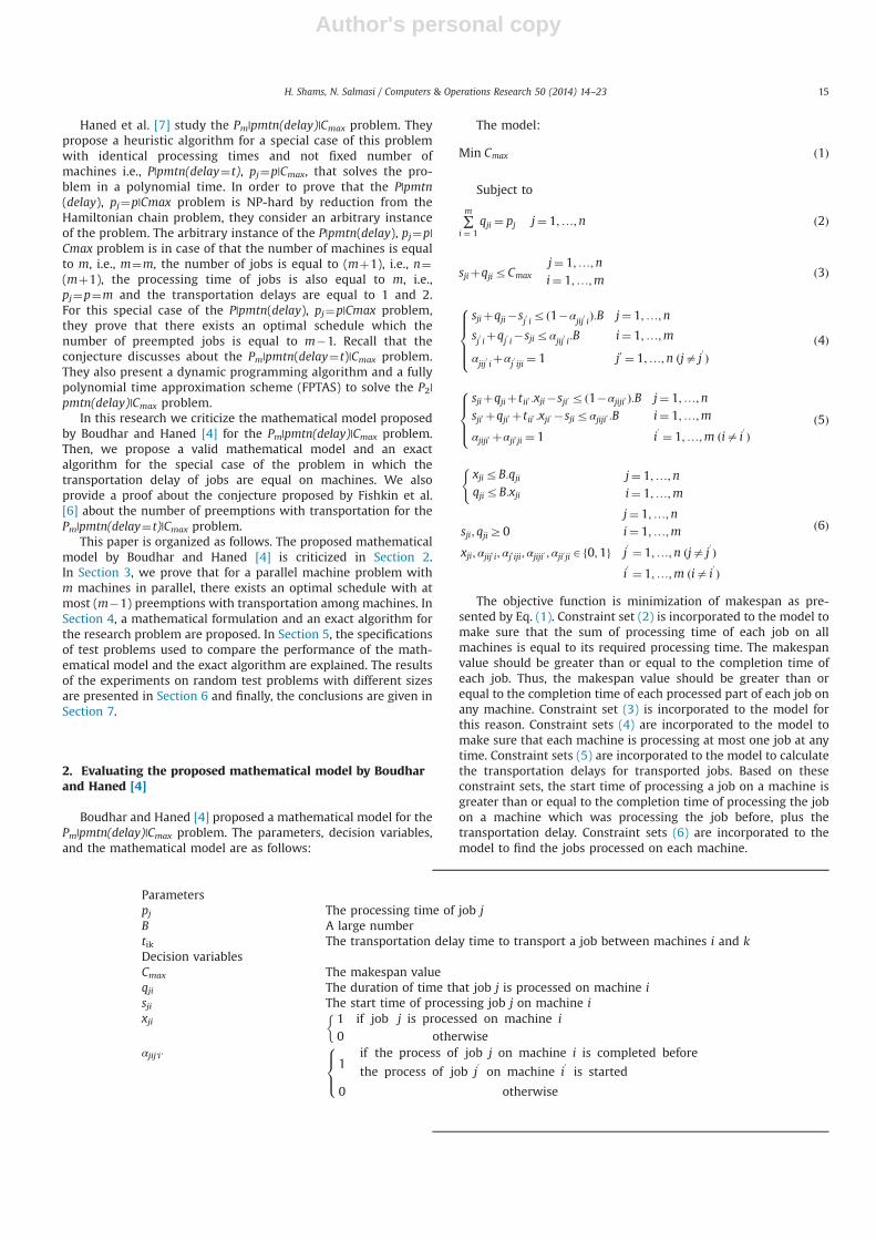
The objective function is minimization of makespan as pre-sented by Eq. (1). Constraint set (2) is incorporated to the model tomake sure that the sum of processing time of each job on allmachines is equal to its required processing time. The makespanvalue should be greater than or equal to the completion time ofeach job. Thus, the makespan value should be greater than orequal to the completion time of each processed part of each job onany machine. Constraint set (3) is incorporated to the model forthis reason. Constraint sets (4) are incorporated to the model tomake sure that each machine is processing at most one job at anytime. Constraint sets (5) are incorporated to the model to calculatethe transportation delays for transported jobs. Based on theseconstraint sets, the start time of processing a job on a machine isgreater than or equal to the completion time of processing the jobon a machine which was processing the job before, plus thetransportation delay. Constraint sets (6) are incorporated to themodel to find the jobs processed on each machine.

Parameterspj The processing time of job jB A large numbertik The transportation delay time to transport a job between machines i and kDecision variablesCmax The makespan valueqji The duration of time that job j is processed on machine isji The start time of processing job j on machine ixji 1 if job j is processed on machine i

0 otherwise

�αjij'i'

1if the process of job j on machine i is completed before

the process of job j0on machine i

0is started

0 otherwise

8><>:

H. Shams, N. Salmasi / Computers & Operations Research 50 (2014) 14–23 15


The authors claim that the model is valid for the problems witharbitrary transportation delay of jobs on machines i.e., Pm|pmtn(delay)|Cmax. In our opinion, the proposed mathematical model isnot a valid one for the proposed research problem. Our reasons areas follows:

1. The authors assume that the period of time that a job isprocessed on a machine i.e., qji is performed in one partwithout any interruption. In other words, the authors assumethat any interruption of processing a job leads to a transporta-tion. There are optimal solutions for the proposed researchproblem in which a job is processed on a machine for a whileand then is preempted and after a while the process of thepreempted job is resumed on the same machine. In this case,the decision variables defined by the authors as qji and tji donot support this situation. Such a situation is presented inExample 1 for the cases of equal transportation delay for thejobs among machines. In this example the solution provided byrelaxing the assumption provides a sequence with betterobjective function value than the one provided by Boudharand Haned [4] mathematical model.

Example 1. Consider a parallel machine problem with threeidentical machines. Assume that four independent jobs should beprocessed with these machines. The processing time of jobs arepresented in Table 1. It is assumed that the transportation delaytime for a job between any two machines is equal to 20 time units.The optimal solution provided by Boudhar and Haned [4] mathe-matical model by using ILOG CPLEX 12.2.2 [8] is a schedule withobjective function value equal to 75 as presented in Fig. 1a.However, a solution can be obtained based on the schedulepresented in Fig. 1b with an objective function value equal to 70.It is clear in Fig. 1b that by preempting J1 (but not transporting it toanother machine) a better solution can be obtained. This exampleshows that the proposed mathematical model by Boudhar andHaned [4] is not a comprehensive mathematical model.

2. The authors assume that the transportation delays of jobs aredifferent for different machines. Then, they assume that if a job

is processed on two different machines, the transportationdelay should be considered between their processing times ofthe jobs on those machines. The authors develop their math-ematical model based on this assumption. In our opinion, thisassumption is not valid if the job is processed on more thantwo machines as explained in Example 2.

Example 2. Consider the same parallel machine problemexplained in Example 1. Assume that the transportation delaytime between any two machines is equal to the ones presentedin Table 2.The solution obtained by Boudhar and Haned [4] mathematicalmodel with the objective function value equal to 75 (solved byusing ILOG CPLEX 12.2.2 [8]) is presented in Fig. 2a. A schedulewith the objective function value equal to 70 can be obtained aspresented in Fig. 2b.In this example, J4 is processed for the length of ten time unitson M1. Then, it is transported to M3 to be processed for thelength of ten time units on M3. Finally, it is transported to M2 tobe processed for the length of ten time units. In this case, sincethe job is not transported directly from M1 to M2, it is notrequired that a transportation delay is considered between theprocessing time of J4 on these machines. This fact is ignored inconstraint sets (5) of the proposed mathematical model byBoudhar and Haned [4]. In this model if a job is processed ontwo different machines, it is assumed that there exists trans-portation delay between them whereas it may be a thirdmachine which the job is transported on it first and thentransported from it. In general, different transportation delaysare not considered in the mathematical model.

3. The authors do not consider the following constraint set in themathematical model:

∑n

j ¼ 1qjirCmax i¼ 1;…;m ð7ÞFig. 1. (a) Solution obtained by the mathematical model for Example 1 and (b) the

optimal schedule for the example.

Table 2The transportation delay time between any two machines.

Machine 1 Machine 2 Machine 3

Machine 1 0 70 20Machine 2 70 0 20Machine 3 20 20 0

Fig. 2. (a) Solution obtained by the mathematical model for the example and(b) optimal schedule for the example.

Table 1The processing time of jobs.

Jobs J1 J2 J3 J4

Processing time (Pj) 60 60 60 30

H. Shams, N. Salmasi / Computers & Operations Research 50 (2014) 14–2316


constraint set (7) implies that the makespan value should begreater than or equal to the processing time of jobs on eachmachine. Incorporating this constraint set to the model canspeed up the solving time of the problem by commercialsoftware since it makes the nodes fathomed faster.

3. The proof of conjecture proposed by Fishkin et al. [6]

Fishkin et al. [6] prove that for the P2|pmtn(delay¼t)|Cmax andthe P3|pmtn(delay¼t)|Cmax problems there exist optimal solutionswith at most one and two transportations, respectively. Kozlov [9]also proves that there exists an optimal solution with at mostthree transportations for the P4|pmtn(delay¼t)|Cmax problem.Fishkin et al. [6] propose the following conjecture for the Pm|pmtn(delay¼t)|Cmax problem.

Conjecture. For the Pm|pmtn(delay¼t)|Cmax problem, there exists anoptimal schedule with at most (m�1) preemptions with transporta-tion of jobs among machines.

In order to prove the conjecture, first we propose two lemmasand then use them for the proof.

Lemma 1. For the Pm|pmtn(delay¼t)|Cmax problem, assume that kjobs are transported among machines. In this case, there exists anoptimal schedule in which any combination of two jobs amongk transported jobs are not processed on more than one commonmachine.

Proof. Assume that for the Pm|pmtn(delay¼t)|Cmax problem that isprocessing n jobs, there exists an optimal schedule with k (krn)transported jobs. Consider two transported jobs such as J1 and J2.Assume that these jobs are processed on S (S41) commonmachines. For any two of S common machines as shown inFig. 3a, we can reschedule the processing time of these jobs asshown in Fig. 3b by processing one of the jobs only on onemachine. Without loss of generality, consider that the processingtime of J1 on M1 is less than or equal to the processing time of J2 onM2. Therefore, we can change the processing time of J1 and J2 inwhich, all of the processing time of J1 is processed on M2 as shownin Fig. 3b. The transportation delay constraint has been satisfied inthe rescheduled solution, since the completion time of processingJ2 on M1 is not changed and the start time of processing J2 on M2 ispostponed. By using this argument, it is easy to prove that thenumber of common machines that are processing both J1 and J2are reduced to one machine.

Lemma 2. For the Pm|pmtn(delay¼t)|Cmax problem, assume thatthere exists an optimal schedule in which k jobs are transported onl different machines that each combination of any two jobs among thek transported jobs are processed on at most one common machine.In this case, there exists an optimal solution in which no other jobwith transportation can be processed by these l machines.

Proof. Consider a sequence of processing jobs that k transportedjobs are processed on l different machines. Assume that eachcombination of two jobs among k transported jobs have only onecommon machine as presented in Fig. 4a. For instance, M2 is theonly machine that is processing both J1 and J2. Now assume that ajob, say JD, is incorporated to this schedule to be processed with atransportation on M1 and Mkþ1 as shown in Fig. 4b.

In order to prove the lemma, we show that there is an optimalsolution in which the process of JD can be processed on only onemachine without any transportation. Two different scenarios canbe observed.

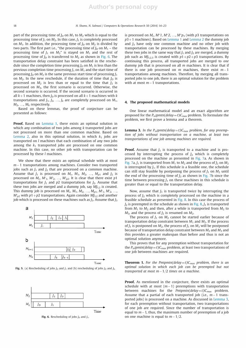
In the first scenario, the duration of time that JD is processed onM1 is less than or equal to the time that J1 is processed on M2, J2 isprocessed on M3, and so on. In this case, a reschedule can beobtained by transferring the processing time of JD on M1 to M2.In this case, the processing time of J1 onM2 is divided by two parts.The first part i.e., “the processing time of J1 on M2 – the processingtime of JD on M1” is transferred to M1 and the rest of processingtime of J1 is stayed on M2 as shown in Fig. 5a. It is clear that thetransportation delay constraint is satisfied with this change.The same transformation is performed until the last machine toprocess JD only on Mkþ1 as shown in Fig. 5b.

In the second scenario, the duration of time that JD is processedon M1 is greater than or equal to the time that J1 is processed onM2. In this case, a reschedule can be obtained by transferring that

Fig. 3. (a) Two of S common machines in the optimal schedule with k transportedjobs and (b) rescheduling of J1 and J2.

Fig. 4. (a) k transported jobs with common machines and (b) the schedule with thejob JD.



part of the processing time of JD on M1 to M2 which is equal to theprocessing time of J1 on M2. In this case, J1 is completely processedon M1. In addition, the processing time of JD on M2 is divided bytwo parts. The first part i.e., “the processing time of JD on M1 – theprocessing time of J1 on M2” is stayed on M1 and the rest ofprocessing time of JD is transferred to M2 as shown in Fig. 6. Thetransportation delay constraint has been satisfied in the resche-dule since the completion time processing JD on M1 is less than theprevious completion time processing J1 on M1 and the start time ofprocessing JD onM2 is the same previous start time of processing J1on M2. In the new reschedule, if the duration of time that JD isprocessed on M2 is less than or equal to the time that J2 isprocessed on M3, the first scenario is occurred. Otherwise, thesecond scenario is occurred. If the second scenario is occurred inall kþ1 machines, then JD is processed on all kþ1 machines with ktransportations and J1, J2, …, Jk are completely processed on M1,M2, …, Mk respectively.

Based on these lemmas, the proof of conjecture can bepresented as follows:

Proof. Based on Lemma 1, there exists an optimal solution inwhich any combination of two jobs among k transported jobs arenot processed on more than one common machine. Based onLemma 2, also in this optimal solution, in which k1 jobs aretransported on l machines that each combination of any two jobsamong the k1 transported jobs are processed on one commonmachine. In this case, no other job with transportation can beprocessed by these l machines.

We show that there exists an optimal schedule with at mostm�1 transportations among machines. Consider two transportedjobs such as J1 and J2 that are processed on a common machine.Assume that J1 is processed on Mc, M1, M2, …, Mp1 and J2 isprocessed on Mc, M'1, M'2, …, M'p2. It is clear that there exist p1transportations for J1 and p2 transportations for J2. Assume thatthese two jobs are merged and a dummy job, say MJ1,2 is created.This dummy job is processed on Mc, M1, M2, …, Mp1, M'1, M'2, …,M'p2 with p1þp2 transportations. Again consider MJ1,2 and anotherjob which is processed on these machines such as J3. Assume that J3

is processed on Mc, M″1, M″2, …, M″p3 (with p3 transportations onp3þ1 machines). Based on Lemma 1 and Lemma 2 the dummy joband J3 have only one common machine and no other job withtransportation can be processed by these machines. By mergingthese two jobs in the same way that J1 and J2 are merged, a dummyjob such as MJ1,2,3 is created with p1þp2þp3 transportations. Bycontinuing this process, all transported jobs are merged to onedummy job that is processed on all m machines. It is clear that ifthere is one job processed on m machines, there exist m�1transportations among machines. Therefore, by merging all trans-ported jobs to one job, there is an optimal solution for the problemwith at most m�1 transportations.

4. The proposed mathematical models

One linear mathematical model and an exact algorithm areproposed for the Pm|pmtn(delay¼t)|Cmax problem. To formulate theproblem, we first prove a lemma and a theorem.

Lemma 3. In the Pm|pmtn(delay¼t)|Cmax problem, for any preemp-tion of jobs without transportation on a machine, at least twotransportations of one job among machines are required.

Proof. Assume that J1 is transported to a machine and is pro-cessed by interrupting the process of J2 which is completelyprocessed on the machine as presented in Fig. 7a. As shown inFig. 7a, J1 is transported from M1 to M2 and the process of J2 on M2

is interrupted by J1. If this schedule is a feasible one, the schedulecan still stay feasible by postponing the process of J1 on M2 untilthe end of the processing time of J2 as shown in Fig. 7b since thetime between processing J1 on these machines in this schedule isgreater than or equal to the transportation delay.

Now, assume that J1 is transported twice by interrupting theprocess of J2 which is completely processed on the machine in afeasible schedule as presented in Fig. 8. In this case the process ofJ2 is preempted in the schedule as shown in Fig. 8, J1 is transportedfrom M1 to M2 and then, after a while is transported from M2 toM3, and the process of J2 is resumed on M2.

The process of J1 on M2 cannot be started earlier because oftransportation delay constraint between M1 and M2. If the processof J1 is postponed on M2, the process of J1 on M3 will be postponedbecause of transportation delay constraint betweenM2 andM3 andthis provides a greater makespan than before and thus is not anoptimal solution anymore.

This proves that for any preemption without transportation forthe Pm|pmtn(delay¼t)|Cmax problem, at least two transportations ofone job between machines are required.

Theorem 1. For the Pm|pmtn(delay¼t)|Cmax problem, there is anoptimal solution in which each job can be preempted but nottransported at most m�1=2 times on a machine.

Proof. As mentioned in the conjecture, there exists an optimalschedule with at most (m�1) preemptions with transportationbetween machines for the Pm|pmtn(delay¼t)|Cmax problem.Assume that a partial of each transported job (i.e., m�1 trans-ported jobs) is processed on a machine. As discussed in Lemma 3,for each preemption without transportation, two transportationsof one job are required. Since the number of transportation isequal to m�1, thus, the maximum number of preemption of a jobon one machine is equal to m�1=2.

Fig. 5. (a) Rescheduling of jobs JD and J1 and (b) rescheduling of jobs JD and Jk.

Fig. 6. Rescheduling of jobs JD and J1.



4.1. The linear programming formulation

A mathematical model which is called Model 1 and an exactalgorithm which is called Algorithm 1 for the Pm|pmtn(delay¼t)|Cmax problem are proposed to solve the problem as the followings:

Model 1:A mathematical model to find the optimal schedule of processing

the jobs on machines is proposed in this section. The parameters,decision variables, and the mathematical model are as following:

The model:

Min Cmax ð8Þ

Subject to

∑m

i ¼ 1∑U

k ¼ 1qjki ¼ pj j¼ 1;…;n ð9Þ

∑n

j ¼ 1∑U

k ¼ 1qjkirCmax i¼ 1;…;m ð10Þ

j¼ 1;…;n

sjkiþqjkirCmax k¼ 1;…;U

i¼ 1;…;mð11Þ

sjkiþqjki�sj0 kir ð1�αjkij0 kiÞ:Bsj0 kiþqj0 ki�sjkirαjkij0 ki:B

αjkij0 kiþαj0 kijki ¼ 1

8>><>>:

j¼ 1;…;n

k¼ 1;…;U

i¼ 1;…;m

j0 ¼ 1;…;nðja j

0 Þ

ð12Þ

sjkiþqjki�sjk0 ir ð1�αjkijk0 iÞ:Bsjk0 iþqjk0 i�sjkirαjkijk0 i:B

αjkijk0 iþαjk0 ijki ¼ 1

8>><>>:

j¼ 1;…;n

k¼ 1;…;Ui¼ 1;…;m

k0 ¼ 1;…;Uðkak

0 Þ

ð13Þ

sjkiþqjki�sjk0 i0 r ð1�αjkijk0 i0 Þ:Bsjk0 i0 þqjk0 i0 �sjkirαjkijk0 i0 :B

αjkijk0 i0 þαjk0 i0 jki ¼ 1

8>><>>:

j¼ 1;…;nk¼ 1;…;U

i¼ 1;…;m

i0 ¼ 1;…;mðia i

0 Þk

0 ¼ 1;…;U

ð14Þ

j¼ 1;…;nsjkiþqjkiþt:xjki�sjk0 i0 r ð1�αjkijk0 i0 Þ:Bsjk0 i0 þqjk0 i0 þt:xjk0 i0 �sjkirαjkijk0 i0 :B

αjkijk0 i0 þαjk0 i0 jki ¼ 1

8>><>>:

k¼ 1;…;U

i¼ 1;…;m

i0 ¼ 1;…;mðia i

0 Þ

k0 ¼ 1;…;U

ð15Þ

xjkirB:qjkiqjkirB:xjki

( j¼ 1;…;n

k¼ 1;…;Ui¼ 1;…;m

sjki; qjkiZ0j¼ 1;…;n

i¼ 1;…;m

xjki; αjkij0 ki; αj0 kijki;αjkijki0 ; αjki0 jki; αjkijk0 i;αjk0 ijkiAf0;1g j0 ¼ 1;…;nðja j

0 Þi0 ¼ 1;…;mðia i

0 Þ

ð16Þ

J1

J2 J1

Time

J1

J2 J1 J2

Time

Fig. 7. (a) A feasible schedule and (b) a feasible schedule.

J1

J2 J1 J2

Time

J1

Fig. 8. An optimal feasible schedule.

Parameterspj The processing time of job jB A large numbert The transportation delay time to transport a job between any two machinesU The maximum possible number of parts of a job on a machine which equals to ðm�1=2Þþ1Decision variablesCmax The makespan valueqjki The length of processing time of the kth part of job j is processed on machine isjki The start time of processing the kth part of job j on machine i

xjki 1; if the kth part of job j is processed on machine i0; otherwise

(

αjkij'k'i'1; if the process of the kth part of job j on machine i is finished before

the process of the k0th part of job j0on machine i

0is started

0; otherwise

8><>:



The objective function is minimization of makespan as pre-sented by Eq. (8). Constraint set (9) is incorporated to the model tomake sure that the sum of the processing time of each job on allmachines is equal to its required processing time. The makespanshould be greater than or equal to the sum of processing time of alljobs on each machine. Constraint set (10) is incorporated to themodel for this reason. The makespan should be greater than orequal to the completion time of each job. Thus, the makespanshould be greater than or equal to the completion time of eachprocessed part of each job on any machine. Constraint set (11) isincorporated to the model for this reason. Constraint sets (12) and(13) are incorporated to the model to make sure that each machineis processing at most one job at any time. Constraint sets (14)support the fact that any job is processed on one machine at anytime. Constraint sets (15) are incorporated to the model tocalculate the transportation delays for transported jobs. Based onthese constraint sets, the start time of processing a job on amachine is greater than or equal to the completion time ofprocessing the job on a machine which was processing theprevious job, plus the transportation delay. Constraint sets (16)are incorporated to the model to find the jobs processed on eachmachine.

4.2. The exact algorithm

The complexity of the problem is originated from twomajor parts. First, assigning jobs to machines i.e., finding asolution including the duration of time that each job is processedon each machine. Second, finding a feasible schedule of proces-sing the jobs on machines based on the provided solution. InModel 1, these two tasks are done simultaneously. In order todecrease the model complexity and still get the optimal solution,we propose a method to solve the problem optimally in severalstages. First, we find the duration of time that each job shouldbe processed on each machine in an optimal solution. Then, wefind a feasible schedule of processing the jobs based on theprovided optimal solution. Based on this motivation, we proposea three step algorithm to solve the problem optimally in a veryefficient way which is called Algorithm 1 in this research as thefollowings:

Algorithm 1. In this algorithm, as the first step only the durationof time that each job is processed on each machine in one of themultiple optimal solutions is calculated by a mathematical modelcalled Model 2. In the provided solution, some jobs might beprocessed on several machines i.e., transported from one machineto another one, and some jobs might be processed on only onemachine. Then, the schedule of processing the transported jobson each machine based on the optimal solution obtained byModel 2 is found as the second step. At the third step, the scheduleof processing the non-transported jobs on each machine is deter-mined. The steps of the proposed algorithm are as the followings:

Step1.In order to find the optimal processing time of each job on each

machine a mathematical model, called Model 2 in this research, isproposed. This mathematical model provides the optimal value forthe makespan as well as the duration of time that each job isprocessed on each machine. The parameters, decision variables, andthe mathematical model for Model 2 are as the followings:

Parameters:The parameters pj, t, B, and U with the same definition in

Model 1 are used in this model.Decision variables:The decision variables Cmax and qjki with the same definition in

Model 1 are used in Model 2. Also the following decision variable

is used for Model 2.

xji1 if any part of job j is processed on machine i

0 otherwise

�

Model 2:Min Cmax ð17Þ

Subject toConstraint sets (13) and (14) from Model 1.

pjþ ∑m

i ¼ 1xji�1

" #:trCmax j¼ 1;…;n ð18Þ

xjirB: ∑U

k ¼ 1qjki

∑U

k ¼ 1qjkirB:xji

8>>>><>>>>:

j¼ 1;…;n

i¼ 1;…;m

qjkiZ0 j¼ 1;…;n

xjiAf0;1gk¼ 1;…;U

i¼ 1;…;m

ð19Þ

Like Model 1, the objective function as minimization of make-span is presented by Eq. (17). The processing time of each job withits required transportation delays on machines should be less thanor equal to the makespan. Constraint set (18) is incorporated to themodel to support this fact. Constraint sets (19) are incorporated tothe model to find the jobs processed on each machine.

As mentioned, Model 2 is only capable of finding the durationof time that each job is processed on each machine in an optimalsolution.

Step2.In order to find a feasible schedule of processing the jobs based

on the optimal solution provided in Step1, a feasible schedule ofprocessing the transported jobs based on the optimal solutionprovided by Step1 is determined in this step. In order to find thisschedule, the optimal solution of Model 2, i.e., the duration ofprocessing each job on each machine, is fed to another mathema-tical model, called Model 3 in this research, to find the transportedjobs schedule in the optimal schedule. The parameters, decisionvariables, and the mathematical model for Model 3 are asfollowing:

Parameters:The parameters pj, t, B, and U with the same definition in Model

1 are used in this model. Also the values of decision variables qjkiand Cmax in the optimal solution of Model 2 are considered as theparameters of Model 3.

Decision variables:The decision variables sjki, xjki, and αjkij'k’i' with the same

definition in Model 1 are considered as the decision variables forModel 3.

Model 3:Min Cmax ð20Þ

Subject toConstraint sets (11), (12), (13), (14), (15), and (16) from Model 1.

qjkiapj ð21Þ

j¼ 1;…; n

sjkiZ0 i¼ 1;…;m

xjki; αjkij0 ki; αj0 kijki; αjkijki0 ; αjki0 jki; αjkijk0 i; αjk0 ijki j0 ¼ 1;…; nðja j

0 ÞAf0;1g i

0 ¼ 1;…;mðia i0 Þ

qjkiapj



Model 3 is a simplification of Model 1 in which the decisionvariables Cmax and qjki in Model 1 are used as parameter in Model3 since their values are obtained from the optimal solution ofModel 2. Also, only the constraint sets that deal with finding theschedule of jobs are incorporated to this model. As it is mentioned,Model 3 finds only the schedule of transported jobs in the optimalschedule.

Step3.In this step, the schedule of non-transported jobs on machines

is determined in the optimal solution provided by Model 2 inStep2 by considering the schedule provided for transported jobsby Model 3 in Step3. With this information, an optimal schedulecan easily be constructed. The schedule of transported jobs in theoptimal schedule are fixed in Model 2, Then, the jobs that are nottransported are scheduled arbitrary on machines during the timethat the machines are not processed the transported jobs.

4.3. Comparison of the methods

Motivated from Naderi and Salmasi [10], the complexity of theproposed mathematical model and Algorithm 1 is compared basedon the number of binary variables (NBV), the number of integervariables (NIV), the number of constraints with Big M, and thenumber of constraints (NC). The results are presented in Table 3. Inthis table n presents the number of jobs, m is the number ofmachines. Moreover, U is the maximum possible number of partsof a job on a machine which equals to ((m�1/2)þ1). It is assumedthat the maximum number of transported jobs occurred inAlgorithm 1 which is equal to (m�1).

Based on NBV, the complexity of Model 1 is calculated byððn�m� UÞþðn2 �m2 � U2ÞÞ. Therefore, the NBV is quadratic inm, n, and U. On the other hand, Algorithm 1 has the complexity ofðm� nþ5� ðm�1ÞÞ which is linear in m and n. the complexityreduction is happened inm, n, and U. This is because, Model 1 triesto schedule all jobs on machines. This scheduling requires a hugenumber of decision variables due to the problem constraints. Incontrast, in Algorithm 1, there is no need to schedule all jobs onmachines and only transported jobs are scheduled on machines.

Considering NIV, the complexity of Model 1 and Algorithm 1equal to 2� ðn�m� UÞ and n�m� Uþðm�1Þ, respectively. TheNIV in both Model 1 and Algorithm 1 are linear in n, m, and U.There is no complexity difference, because of seeking for theamount of processing time of each job on each machine in bothmethods.

As shown in Table 3, the number of constraints including big Mfor Model 1 and Algorithm 1 are 2� n�m� U � ½ð1=nÞþ ð1=UÞþð2=m� UÞþ1� and 2� n�mþ10� ðm�1Þ, respectively. The com-plexity reduction is obtained in U. This is because of assigning alljobs in Model 1 and only transported jobs in Algorithm 1. This isobtained for the total number of constraints similarly which forModel 1 equals to 3� n�m� U � ½ð1=nÞþð1=UÞþð2=m� UÞþ1�þmþn and for Algorithm 1 equals to nþ2� n� mþ15� ðm�1Þ.

5. Test problem specification

In this research, we propose two methods to solve the pro-posed research problem optimally. In the first method, a

mathematical model, i.e., Model 1 is directly used to find theoptimal schedule. In the second method, i.e., Algorithm 1, theproblem is solved optimally in several stages. In order to comparethe performance of Model 1 and Algorithm 1, test problems aregenerated randomly.

Based on experience, the most important factors in determin-ing the degree of complication of the Pm|pmtn(delay¼t)|Cmax

problem are the number of machines, the number of jobs, andthe interval time that the processing time of jobs are generated.Therefore, the classification of generated test problems is per-formed by considering these three parameters as the followings:

Number of machines: test problems by considering the numberof machines in parallel are generated in three different levels. Inthe first level, called L1, problems with 2–5 machines in parallelare considered. In the second level, called L2, problems with 6–10machines in parallel are considered and finally, in the third levelcalled L3, problems with 11–15 machines in parallel are generated.

Number of jobs: the number of jobs is considered between2 and 100. The value of this parameter is generated randomly inthree different levels, using the uniform discrete distribution. Ifthe problem has the number of jobs in the interval of [2, 20], theproblem is considered in the first level based on the number of

Table 3A summary comparison of two methods.

Method NBV NIV Big M NC

Model 1 ðn�m� UÞþðn2 �m2 � U2Þ 2� ðn�m� UÞ 2� n�m� U � 1nþ 1

Uþ 2m�Uþ1

� �3� n�m� U � 1

nþ 1Uþ 2

m�Uþ1� �þmþn

Algorithm 1 m� nþ5� ðm�1Þ n�m� Uþðm�1Þ 2� n�mþ10� ðm�1Þ nþ2� n�mþ15� ðm�1Þ

Table 4The number of problems that can be solved optimally by CPLEX.

Number of machines Number of jobs Number of test problems that can besolved optimally by CPLEX

Model 1 Algorithm 1

[2, 5] [2, 20] 25 30[21, 50] 30 30[51, 100] 30 30

[6, 10] [2, 20] 7 30[21, 50] 22 30[51, 100] 4 30

[11, 15] [2, 20] 3 30[21, 50] 0 23[51, 100] 0 0

Total 121 233

Table 5The average time of solution.

Number ofmachines

Number ofJobs

Number of testproblems solvedoptimally by bothmodels

Average running time (s)

Model 1 Algorithm 1

[2, 5] [2, 20] 25 out of 30 8.06 0.32[21, 50] 30 out of 30 27.87 0.40[51, 100] 30 out of 30 454.13 0.40

[6, 10] [2, 20] 7 out of 30 39.36 0.53[21, 50] 22 out of 30 94.01 0.62[51, 100] 4 out of 30 1054.32 0.51

[11, 15] [2, 20] 3 out of 30 2424.82 0.18[21, 50] 0 out of 30 - -[51, 100] 0 out of 30 - -

Total 121 out of 270 586.08 0.42



jobs factor. The problem is considered in the second and the thirdlevel based on the number of jobs factor if its number of jobs is inthe interval of [21, 50] and [51, 100], respectively.

Processing time of jobs: test problems are generated in threedifferent levels based on their processing time. In the first level,the processing time of jobs are generated randomly from a discreteuniform distribution in the interval of DU [1, 10]. In the secondlevel, the processing time of jobs are generated randomly from adiscrete uniform distribution in the interval of DU [1, 40] andfinally, in the third level, the processing time of jobs are generatedrandomly from a discrete uniform distribution in the interval ofDU [1, 90].

Based on these classifications, 27 different classes of testproblems (3 for the number of machines�3 for the number ofjobs�3 for the processing times) are generated. For each class oftest problems, 10 instances (i.e., 270 random test problems in total)are generated randomly to be solved by Model 1 and Algorithm 1.

Based on Fishkin et al. [6], the Pm|pmtn(delay¼t)|Cmax probleminstances might be easy or strongly NP-hard problems. In thisresearch the test problems are generated in the range of NP-hardinstances. Assume that pmax is equal to the maximum processingtime of all jobs i.e., pmax ¼maxnj ¼ 1pj, L is equal to summation ofprocessing time of all jobs divided by number of machines i.e.,L¼∑n

j ¼ 1pj=m, and Δ¼ max fpmax; Lg. Fishkin et al. [6] prove thatin a problem instance, if the interval value of transportation delayi.e., t has a value that satisfies relation (22), then that problem canbe considered as an NP-hard problem.

t4Δ�pmax ð22ÞThis fact is considered during generating the test problems in

order to generate NP-hard problems.

6. The results

All test problems are solved by both Model 1 and Algorithm 1.ILOG CPLEX 12.2.2 [8] is used to solve the test problems. Theexperiments are performed on a personal computer with 3.1 GHzof Core i3 CPU and 4 GB of RAM.

The results show that Model 1 was able to solve 121 out of 270test problems optimally. The rest of them could not be solved byCPLEX (we faced with out of memory message). However, by usingthe same software, the optimal solution of 233 out of 270 testproblems can be obtained by using Algorithm 1. A comparison ofthe performance of both methods based on the problems solvedoptimally is presented in Table 4. This comparison is presentedbased on different number of machines and number of jobs.

A comparison about the time required solving the test pro-blems is presented for Model 1 and Algorithm 1 in Table 5. This

comparison is performed only based on the test problems solvedby both methods optimally. The results show that Algorithm 1reached to the optimal solution in a significantly shorter time thanModel 1.

The results show that Model 1 was never able to solve aproblem instance optimally that Algorithm 1 was not capable ofsolving it optimally. In contrary, Algorithm 1 was reached to theoptimal solution for 112 out of 270 test problems that Model 1 wasnot able to solve them optimally. The results also show that noneof test problems with more than 14 machines and 35 jobs wassolved optimally with the proposed models.

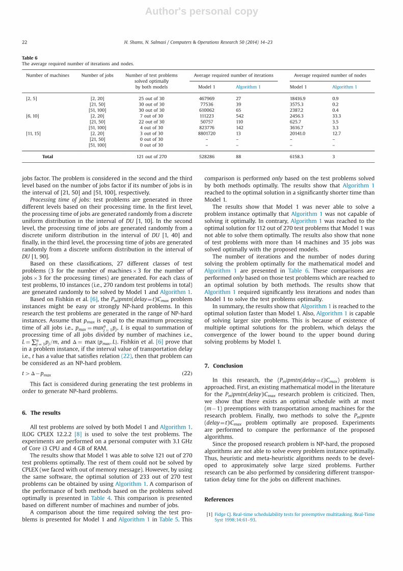
The number of iterations and the number of nodes duringsolving the problem optimally for the mathematical model andAlgorithm 1 are presented in Table 6. These comparisons areperformed only based on those test problems which are reached toan optimal solution by both methods. The results show thatAlgorithm 1 required significantly less iterations and nodes thanModel 1 to solve the test problems optimally.

In summary, the results show that Algorithm 1 is reached to theoptimal solution faster than Model 1. Also, Algorithm 1 is capableof solving larger size problems. This is because of existence ofmultiple optimal solutions for the problem, which delays theconvergence of the lower bound to the upper bound duringsolving problems by Model 1.

7. Conclusion

In this research, the (Pm|pmtn(delay¼t)|Cmax) problem isapproached. First, an existing mathematical model in the literaturefor the Pm|pmtn(delay)|Cmax research problem is criticized. Then,we show that there exists an optimal schedule with at most(m�1) preemptions with transportation among machines for theresearch problem. Finally, two methods to solve the Pm|pmtn(delay¼t)|Cmax problem optimally are proposed. Experimentsare performed to compare the performance of the proposedalgorithms.

Since the proposed research problem is NP-hard, the proposedalgorithms are not able to solve every problem instance optimally.Thus, heuristic and meta-heuristic algorithms needs to be devel-oped to approximately solve large sized problems. Furtherresearch can be also performed by considering different transpor-tation delay time for the jobs on different machines.

References

[1] Fidge CJ. Real-time schedulability tests for preemptive multitasking. Real-TimeSyst 1998;14:61–93.

Table 6The average required number of iterations and nodes.

Number of machines Number of jobs Number of test problemssolved optimallyby both models

Average required number of iterations Average required number of nodes

Model 1 Algorithm 1 Model 1 Algorithm 1

[2, 5] [2, 20] 25 out of 30 467969 27 18416.9 0.9[21, 50] 30 out of 30 77536 39 3575.3 0.2[51, 100] 30 out of 30 610062 65 2387.2 0.4

[6, 10] [2, 20] 7 out of 30 111223 542 2456.3 33.3[21, 50] 22 out of 30 50757 110 625.7 3.5[51, 100] 4 out of 30 823776 142 3616.7 3.3

[11, 15] [2, 20] 3 out of 30 8801720 13 20141.0 12.7[21, 50] 0 out of 30 – – – –

[51, 100] 0 out of 30 – – – –

Total 121 out of 270 528286 88 6158.3 3



[2] McNaughton R. Scheduling with deadlines and loss functions. Manag Sci1959;6:1–12.

[3] Muntz RR, Coffman EG. Optimal preemptive scheduling on two-processorsystems. IEEE Trans Comput 1969;100(11):1014–20.

[4] Boudhar M, Haned A. Preemptive scheduling in the presence of transportationtimes. Comput Oper Res 2009;36(8):2387–93.

[5] Rayward-Smith VJ. The complexity of preemptive scheduling given interpro-cessor communication delays. Inf Process Lett 1987;25:123–5.

[6] Fishkin AV, Jansen K, Sevastyanov SV, Sitters R. Preemptive scheduling ofindependent jobs on identical parallel machines subject to migration delays.Algorithms–ESA 2005. Berlin Heidelberg: Springer; 2005; 580–91.

[7] Haned A, Soukhal A, Boudhar M, Huynh Tuong N. Scheduling on parallelmachines with preemption and transportation delays. Comput Oper Res2012;39(2):374–81.

[8] CPLEX, ILOG. High-performance software for mathematical programming andoptimization. URL: ⟨http://www.ilog.com/products/cplex⟩; 2005.

[9] Kozlov A. To the conjecture on the minimum number of migrations in theoptimal schedule for the Pm| pmtn (delay¼ d)| Cmax problem. Eraerts2011:248.

[10] Naderi B, Salmasi N. Permutation flowshops in group scheduling withsequence-dependent setup times. Eur J Ind Eng 2012;6(2):177–98.


Author's personal copy Parallel machine scheduling problem with preemptive jobs and transportation...

Documents

Transcript of Author's personal copy Parallel machine scheduling problem with preemptive jobs and transportation...