Audio classification and content description - DIVA
63
MASTER’S THESIS 2004:074 TOBIAS ANDERSSON Audio Classification and Content Description MASTER OF SCIENCE PROGRAMME Department of Computer Science and Electrical Engineering Division of Signal Processing 2004:074 CIV • ISSN: 1402 - 1617 • ISRN: LTU - EX - - 04/74 - - SE
-
Upload
khangminh22 -
Category
Documents
-
view
2 -
download
0
Transcript of Audio classification and content description - DIVA
MASTER’S THESIS
2004:074
TOBIAS ANDERSSON
Audio Classificationand Content Description
MASTER OF SCIENCE PROGRAMME
Department of Computer Science and Electrical EngineeringDivision of Signal Processing
2004:074 CIV • ISSN: 1402 - 1617 • ISRN: LTU - EX - - 04/74 - - SE


Audio classification and content description
Tobias Andersson
Audio Processing & TransportMultimedia Technologies
Ericsson Research, Corporate UnitLulea, Sweden
March 2004


Abstract
The rapid increase of information imposes new demands of content management.The goal of automatic audio classification and content description is to meet therising need for efficient content management.
In this thesis, we have studied automatic audio classification and contentdescription. As description of audio is a broad field that incorporates manytechniques, an overview of the main directions in current research is given.However, a detailed study of automatic audio classification is conducted and aspeech/music classifier is designed. To evaluate the performance of a classifier,a general test-bed in Matlab is implemented.
The classification algorithm for the speech/music classifier is a k-NearestNeighbor, which is commonly used for the task. A variety of features are studiedand their effectiveness is evaluated. Based on feature’s effectiveness, a robustspeech/music classifier is designed and a classification accuracy of 98.2 % for 5seconds long analysis windows is achieved.

Preface
The work in this thesis was performed at Ericsson Research in Lulea. I wouldlike to take the opportunity to thank all people at Ericsson for an educatingand giving time. I especially want to thank my supervisor Daniel Enstrom atEricsson Research for valuable guidance and suggestions to my work. I amvery grateful for his involvement in this thesis. I would also like to thankmy examiner James P. LeBlanc at the division of Signal Processing at LuleaUniversity of Technology for valuable criticism and support. And finally, thankyou Anna for all the nice lunch breaks we had.
Contents
1 Introduction 11.1 Backgound . . . . . . . . . . . . . . . . . . . . . . . . . . . . . . 11.2 Thesis Objectives . . . . . . . . . . . . . . . . . . . . . . . . . . . 11.3 Thesis Organization . . . . . . . . . . . . . . . . . . . . . . . . . 2
2 Current Research 32.1 Classification and Segmentation . . . . . . . . . . . . . . . . . . . 3
2.1.1 General Audio Classification and Segmentation . . . . . . 32.1.2 Music Type Classification . . . . . . . . . . . . . . . . . . 42.1.3 Content Change Detection . . . . . . . . . . . . . . . . . . 5
2.2 Recognition . . . . . . . . . . . . . . . . . . . . . . . . . . . . . . 52.2.1 Music Recognition . . . . . . . . . . . . . . . . . . . . . . 52.2.2 Speech Recognition . . . . . . . . . . . . . . . . . . . . . . 62.2.3 Arbitrary Audio Recognition . . . . . . . . . . . . . . . . 6
2.3 Content Summarization . . . . . . . . . . . . . . . . . . . . . . . 62.3.1 Structure detection . . . . . . . . . . . . . . . . . . . . . . 72.3.2 Automatic Music Summarization . . . . . . . . . . . . . . 7
2.4 Search and Retrieval of Audio . . . . . . . . . . . . . . . . . . . . 72.4.1 Content Based Retrieval . . . . . . . . . . . . . . . . . . . 72.4.2 Query-by-Humming . . . . . . . . . . . . . . . . . . . . . 8
3 MPEG-7 Part 4: Audio 93.1 Introduction to MPEG-7 . . . . . . . . . . . . . . . . . . . . . . . 93.2 Audio Framework . . . . . . . . . . . . . . . . . . . . . . . . . . . 10
3.2.1 Basic . . . . . . . . . . . . . . . . . . . . . . . . . . . . . . 113.2.2 Basic Spectral . . . . . . . . . . . . . . . . . . . . . . . . 113.2.3 Spectral Basis . . . . . . . . . . . . . . . . . . . . . . . . . 113.2.4 Signal Parameters . . . . . . . . . . . . . . . . . . . . . . 113.2.5 Timbral Temporal . . . . . . . . . . . . . . . . . . . . . . 123.2.6 Timbral Spectral . . . . . . . . . . . . . . . . . . . . . . . 12
3.3 High Level Tools . . . . . . . . . . . . . . . . . . . . . . . . . . . 123.3.1 Audio Signature Description Scheme . . . . . . . . . . . . 133.3.2 Musical Timbre Description Tools . . . . . . . . . . . . . 133.3.3 Melody Description Tools . . . . . . . . . . . . . . . . . . 133.3.4 General Sound Recognition and Indexing Description Tools 133.3.5 Spoken Content Description Tools . . . . . . . . . . . . . 14
iv
CONTENTS v
4 Audio Classification 154.1 General Classification Approach . . . . . . . . . . . . . . . . . . . 15
4.1.1 Feature Extraction . . . . . . . . . . . . . . . . . . . . . . 174.1.2 Learning . . . . . . . . . . . . . . . . . . . . . . . . . . . . 174.1.3 Classification . . . . . . . . . . . . . . . . . . . . . . . . . 184.1.4 Estimation of Classifiers Performance . . . . . . . . . . . 18
4.2 Feature Extraction . . . . . . . . . . . . . . . . . . . . . . . . . . 194.2.1 Zero-Crossing Rate . . . . . . . . . . . . . . . . . . . . . . 194.2.2 Short-Time-Energy . . . . . . . . . . . . . . . . . . . . . . 194.2.3 Root-Mean-Square . . . . . . . . . . . . . . . . . . . . . . 204.2.4 High Feature-Value Ratio . . . . . . . . . . . . . . . . . . 204.2.5 Low Feature-Value Ratio . . . . . . . . . . . . . . . . . . 214.2.6 Spectrum Centroid . . . . . . . . . . . . . . . . . . . . . . 214.2.7 Spectrum Spread . . . . . . . . . . . . . . . . . . . . . . . 224.2.8 Delta Spectrum . . . . . . . . . . . . . . . . . . . . . . . . 224.2.9 Spectral Rolloff Frequency . . . . . . . . . . . . . . . . . . 234.2.10 MPEG-7 Audio Descriptors . . . . . . . . . . . . . . . . . 23
4.3 Feature Selection . . . . . . . . . . . . . . . . . . . . . . . . . . . 234.4 Classification . . . . . . . . . . . . . . . . . . . . . . . . . . . . . 24
4.4.1 Gaussian Mixture Models . . . . . . . . . . . . . . . . . . 244.4.2 Hidden Markov Models . . . . . . . . . . . . . . . . . . . 254.4.3 k-Nearest Neighbor Algorithm . . . . . . . . . . . . . . . 25
4.5 Multi-class Classification . . . . . . . . . . . . . . . . . . . . . . . 28
5 Applications 295.1 Available commercial applications . . . . . . . . . . . . . . . . . 29
5.1.1 AudioID . . . . . . . . . . . . . . . . . . . . . . . . . . . . 295.1.2 Music sommelier . . . . . . . . . . . . . . . . . . . . . . . 30
6 Experiments and analysis 316.1 Evaluation procedure . . . . . . . . . . . . . . . . . . . . . . . . . 316.2 Music/Speech classification . . . . . . . . . . . . . . . . . . . . . 32
6.2.1 Feature Extraction . . . . . . . . . . . . . . . . . . . . . . 326.2.2 Feature Selection . . . . . . . . . . . . . . . . . . . . . . . 346.2.3 Classification Algorithm . . . . . . . . . . . . . . . . . . . 39
6.3 Performance Evaluation . . . . . . . . . . . . . . . . . . . . . . . 41
7 Conclusion and Future Work 437.1 Conclusion . . . . . . . . . . . . . . . . . . . . . . . . . . . . . . 437.2 Future Work . . . . . . . . . . . . . . . . . . . . . . . . . . . . . 44
A Test-bed Environment 49A.1 Structure . . . . . . . . . . . . . . . . . . . . . . . . . . . . . . . 49A.2 How to build a database . . . . . . . . . . . . . . . . . . . . . . . 51A.3 How to add new features . . . . . . . . . . . . . . . . . . . . . . . 51A.4 How to add new classifiers . . . . . . . . . . . . . . . . . . . . . . 52A.5 How to test new classification schemes . . . . . . . . . . . . . . . 52
B Abbreviations 53
Chapter 1
Introduction
1.1 Backgound
Our daily life is highly dependent on information, for example in formats as textand multimedia. We need information for common routines as watching/readingthe news, listening to the radio, watching a video et cetera. However, we easilyrun into problems when a certain type of information is needed. The immenseflow of information makes it hard to find what you are looking for.
The rapid increase of information imposes new demands of content manage-ment as the media archives and consumer products begin to be very complexand hard to handle. Currently people perform searches in databases with dif-ferent meta-tags, which only describe whole chunks of information with briefconstellations of texts. The meta-tags are constructed by different individualsand one realizes that the interpretation of meta-tags can differ from individualto individual. An automatic system that describes audio would systematize la-belling and would also allow searches on the actual data, not just on labels of it.Better content management is the goal of automatic audio description systems.Some commercial content management applications are already out but manypossible applications are still undeveloped.
For example, a person is listening to the radio and wants to listen to jazz.Unfortunately, all the radio stations play pop music mixed with advertisements.The listener gives up searching for jazz and gets stuck with pop music.
The above example can be solved with an automatic audio description sys-tem. The scenario may then change to the following. The person that wants tolisten to jazz only find pop music on all tuned radio stations. The listener thenpress a ”search for jazz”-button on the receiver and after a couple of seconds thereceiver change radio station and jazz flows out of the speakers. This exampleshows how content management may be an efficient tool that simplifies dailyroutines involving information management.
1.2 Thesis Objectives
The objectives of this thesis form a coherent study of audio classification andcontent description. The objectives are divided into four parts:
1
2 CHAPTER 1. INTRODUCTION
• To get an understanding of audio content classification and feature extrac-tion. Many areas are closely linked with audio classification and featureextraction. Hence, a broad literature study on different research areaswithin content description is done.
• To implement a test-bed for testing content classification algorithms inMatlab. The aim is to make a general framework that can be used forevaluation of different classification schemes.
• To examine existing content classification and feature extraction solutionsand to determine their performance.
• To investigate further enhancements of content classification algorithms.
1.3 Thesis Organization
Chapter 2 gives an overview of current research and what techniques that areused in audio classification and content description. In chapter 3 the currentstandard for description of audio content, MPEG-7, is presented and a briefoverview of the standard is given. In chapter 4 classification in general is ex-plained. Some applications that use content management techniques are pre-sented in chapter 5. The design and evaluation of a speech/music classifier ispresented in chapter 6 and the conclusion is found in chapter 7 as well as consid-erations for future work. An explanation of the implemented test-bed is givenin Appendix A and a list of used abbreviations in the report can be found inAppendix B.
Chapter 2
Current Research
The need for more advanced content management can clearly be seen in theresearch community. Many research groups work with new methods to analyzeand categorize audio. As the need for different content management systemsgrow, different applications are developed. Some applications are well developedtoday where speech recognition is one good example. However, most contentmanagement applications are quite complex and a lot of work has to be doneto implement stable solutions.
In this chapter we present an outline of some of the main directions in currentaudio description research.
2.1 Classification and Segmentation
Audio classification and segmentation can provide powerful tools for contentmanagement. If an audio clip automatically can be classified it can be storedin an organized database, which can improve the management of audio dra-matically. Classification of audio can also be useful in various audio processingapplications. Audio coding algorithms can possibly be improved if knowledgeof the content is known. Audio classification can also improve video contentanalysis applications, since audio information can provide at least a subset ofthe information presented.
An audio clip can consist of several classes. It can consist of music followedby speech, which is typical in radio broadcasting. Hence, segmentation of theaudio clip can be used to find where music and speech begin. This is practicalfor applications as audio browsers, where the user may browse for particularclasses in recorded audio. Segmentation can also improve classification, whenclassification is coarse at points where the audio content type changes in anaudio clip.
2.1.1 General Audio Classification and Segmentation
The basis for many content management applications is that knowledge auto-matically can be extracted from the media. For instance, to insert an audio clipwith speech at the right place in a sorted database it has to be known what
3
4 CHAPTER 2. CURRENT RESEARCH
characteristics this clip of speech has. There is a clear need for techniques thatcan make these classifications and many have been proposed.
However, general audio clips can contain countless differences and similaritiesthat make the complexity of general audio classification very high. The possiblecontent of audio has to be known to make a satisfactory classification. Thismakes a hierarchical structure of audio classes a suitable model, which allowsclassification of audio to be made into a few set of classes at each level. Asan example, a classifier can first classify audio between speech and music. Themusic can then be classified into musical genres and speech into genders of thespeakers.
Zhang [1] describes a general audio classification scheme that can be used tosegment an arbitrary audio clip. The classification is divided into two steps. Thefirst step discriminate the audio between speech and nonspeech segments. In thesecond step speech segments are further processed to find speaker changes andnonspeech segments are discriminated between music, environmental soundsand silence. Audio features, which give information about the examined au-dio, are analyzed in each step of the analysis to make a good discrimination.This approach proves to work well and a total accuracy rate of at least 96% isreported.
Attempts to classify general audio into many categories at once can be diffi-cult. Li [2] achieves accuracy over 90 % in a scheme that classify the audio intoseven categories consisting of silence, single speaker speech, speech and noise,simultaneous speech and music, music, multiple speaker’s speech and environ-mental noise.
Tzanetakis [3] also propose a hierarchy of audio classes to limit the numberof classes that a classifier has to classify between. First, audio is classified intospeech and music. Then, speech and music is classified into even more genres.A reported classification accuracy of 61% for ten music genres is achieved.
A speech/music classifier is presented in Scheirer’s [4] work, where a numberof classification schemes are used. A classification accuracy of 98.6 % is achievedon 2.4 seconds long analysis lengths.
2.1.2 Music Type Classification
Classification of music is somewhat vague. How detailed can one categorizemusic? What is the difference between blues influenced rock and blues? Thatcan be a difficult question even for the most trained musicians to answer. Limi-tations have to be done in order to get a realistic classification scheme that canbe implemented. Simple categorization of music into a few set of classes is oftenused.
When we listen and experience music many concepts give us a feeling of whatwe hear. Features like tempo, pitch, chord, instrument timbre and many moremake us recognize music types. These features can be used in an automaticmusic type classification if they can be extracted from media. It is howeverdifficult to extract these features. Spectral characteristics are easier to workwith and give some promising results.
Han [5] classifies music into the three types; popular, jazz and classical music.A set of simple spectral features in a nearest mean classifier gives reasonableaccuracy. A classification accuracy of 75%, 30% and 60% between popular, jazzand classical music respectively is achieved.
CHAPTER 2. CURRENT RESEARCH 5
Pye [6] look for features that can be extracted directly from encoded music.He extracts features from MPEG layer 3 encoded music. As MPEG layer 3use perceptual encoding techniques, an audio clip of this format may be moredescriptive than a raw audio clip since it only contains what humans here.The features are fast to compute and give good performance with classificationaccuracy of 91%.
Zhang [7] argues for a new feature, Octave-based Spectral Contrast. Octave-based Spectral Contrast can be a measure of the relative distribution of har-monic and non-harmonic components in a spectrum. It measures spectrumpeaks and valleys in several sub-bands and classification is done into baroque,romantic, pop, jazz and rock. The total accuracy is about 82.3 % for classifica-tion of 10 second long clips.
2.1.3 Content Change Detection
Content change detection, or segmentation, techniques analyze different audiofeatures and highlight regions where possible content changes occur. Automaticcontent change detection can be used to simplify browsing in recorded newsprograms, sports broadcasts, meeting recordings et cetera. Possible scenariosare option to skip uninteresting news in a news broadcast, summarize a footballgame to see all goals and so on.
Kimber [8] describes an audio browser that segments audio. Speaker andacoustic classes (e.g. music) changes give indices that render segmentation pos-sible. The accuracy of the segmentation is highly dependent on the audio’squality and error rates are reported between 14% to 1%.
A common and very efficient way to increase positive segmentation indices isto combine audio and visual data. Albiol [9] describe a method that finds indiceswhen specific persons speak in a video clip. The system has been extensivelytested and accuracy of around 93% is achieved for audio only. With combinedaudio-visual data accuracy at 98% is achieved.
2.2 Recognition
One major field within audio classification and content description is recogni-tion of audio. Automatic recognition of audio can allow content managementapplications to monitor audio streams. When a specific signal is recognized theapplication can make a predefined action, as sounding an alarm or logging anevent. Another useful application is in various search and retrieval scenarios,when a specific audio clip can be retrieved based on shorter samples of it.
2.2.1 Music Recognition
As automatic recognition of audio allow monitoring of audio streams and effi-cient searches in databases, music recognition is interesting. Monitoring of audiostreams to recognize music can be of interest for record companies that needto get statistics of how often a song is played on the radio. Efficient searchesin databases can simplify management of music databases. This is importantbecause music is often stored in huge databases and the management of it is
6 CHAPTER 2. CURRENT RESEARCH
very complex. Music recognition can simplify the management of large amountof content.
Another interesting use of automatic music recognition is to identify andclassify TV/Radio commercials. This is done by searching video signals forknown background music. Music is an important way to make consumers rec-ognize different companies and Abe [10] propose a method to recognize TVcommercials. The method finds 100% of known background music with as lowSNR as -10dB, which makes recognition of TV commercials possible.
2.2.2 Speech Recognition
Many applications already use speech recognition. It is possible to control mo-bile phones, even computers, with speech. However, in content managementapplications the techniques aim to allow indexing of spoken content. This canbe done by segmenting audio clips by speaker changes and even the meaning ofwhat is said.
Speech recognition techniques often use hidden Markov models (HMM),where a good introduction to HMM is given by Rabiner [11]. HMM are widelyused and recent articles [12] [13] on speech recognition are also based on them.
2.2.3 Arbitrary Audio Recognition
Apart from music and speech recognition, other useful recognition schemes arebeing developed. They can build a basis of tools for recognition of general scenes.These recognition schemes can of course also be used in music recognition, sincemusic consists of several recognizable elements.
Gouyon [14] uses recognizable percussive sounds to extract time indexesof their occurrences in an audio signal. This is used to calculate rhythmicstructures in music, which can improve music classification. Synak [15], [16] useMPEG-7 descriptors to recognize musical instrument sounds.
The central issue of arbitrary audio recognition is that detailed recognitioncan give much information about what context it is in. As Wold [17] proposes,monitoring sound automatically including the ability to detect sounds can makesurveillance more efficient. For instance, it would be possible to detect a burglarif the sound of a window crash is detected in an office building at nighttime.
2.3 Content Summarization
To find new tools to help administering data, techniques are being developedto automatically describe it. When we want to decide whether to read a bookor not we can read the summary on the back. When we decide whether to seea movie or not we can look at a trailer. Analogous to this, we may get muchinformation of an audio file from a short audio clip that describes it. To manuallyproduce these short clips can be time consuming and because of the amountof media available automatic content summarization is necessary. Automaticcontent summarization would also allow a general and concise description thatis suitable for database management.

CHAPTER 2. CURRENT RESEARCH 7
2.3.1 Structure detection
Structure detection can be informative about how the content in an audio clipis partitioned. The technique aims to find similar structures within the audiostream and label the segments. Casey [18] proposes a method, which is partof the MPEG-7 standard, that structures audio. It is shown to be efficient instructuring music1. The main structures of a song can then be labelled into theintro, verse, chorus, bridge et cetera.
2.3.2 Automatic Music Summarization
Music genres as pop, rock and disco are often based on a verse and choruspattern. The main melody is repeated some times and that is what peoplememorize. Therefore, music summarization can be done by extracting theserepetitive sequences. This works for repetitive music genres but is difficult toachieve for jazz and classical music, which involves significant variations of themain melody.
Logan [19] proposes a method that achieves this in three steps. First, thestructure of the song is found. Then, statistics of the structure are used toproduce the final summarization. Although the first tests are limited the methodgives promising results.
Xu [20] presents an algorithm for pure music summarization. It uses au-dio features for clustering segmented frames. The music summary is gener-ated based on the clustering results and domain-specific music knowledge. Thismethod can achieve better results than Logan’s [19]. However, no tests weremade on vocal music.
2.4 Search and Retrieval of Audio
Extensive research is conducted to develop applications for search and retrievalof audio. This is a very complex task as recognition, classification and seg-mentation of audio has to be used. Further, advanced search algorithms fordatabases have to be used for efficient management. In spite of the complexity,the applications have huge potential and are interesting to develop because oftheir intuitive approach to search and retrieval.
2.4.1 Content Based Retrieval
Retrieval of a specific content can be achieved by searching for a given audioclip, characteristics etc. Other ways to search in databases is to use a set ofsound adjectives that characterize the media clip wanted. Wold [17] describesan application that can search for different categories as laughter, animals, bells,crowds et cetera. The application can also search for adjectives to allow searchesas ”scratchy” sound.
1Casey has an interesting page on the internet about structuring of music. Seewww.musicstructure.com for more information about his work.
8 CHAPTER 2. CURRENT RESEARCH
2.4.2 Query-by-Humming
In order to develop user friendly ways to retrieve music, researchers strive toget away from traditional ways to search for music. People, in general, do notmemorize songs by title or by artists. People often remember certain attributesof a song. Rhythm and pitch form a melody that people can hum for themselves.A logical way to search for music is therefore by humming, which is called query-by-humming (QBH).
Song [21] presents an algorithm that extracts music melody features fromhumming data and matches the melody information to a music feature database.If a match is found retrieval of the desired clip can be done. This shows goodpromise for a working QBH-application.
Liu [22] propose a robust method that can match humming to a databaseof MIDI files. Note segmentation and pitch tracking is used to extract featuresfrom the humming. The method achieves an accuracy of 90% with a query of10 notes.

Chapter 3
MPEG-7 Part 4: Audio
MPEG-7 Part 4 provides structures for describing audio content. It is build uponsome basic structures in MPEG-7 Part 5. For a more detailed discussion aboutstructures in MPEG-7, study the MPEG-7 overview [23]. These structuresuse a set of low-level Descriptors (LLDs) that are different audio features foruse in many different applications. There are also high-level Description Toolsthat include both Descriptors (Ds) and Description Schemes (DSs), which aredesigned for specific applications.
The MPEG-7 standard is continuously being developed and enhanced. Ver-sion 2 is being developed but an overview of the currently available tools of theMPEG-7 Audio standard is seen below.
3.1 Introduction to MPEG-7
In the MPEG-7 overview [23] it is written that MPEG (Moving Picture ExpertsGroup) members understood a need for content management and called for astandardized way to describe media content. In October 1996, MPEG started anew work item that is named ”Multimedia Content Description Interface”. Inthe fall 2001 it became the international standard ISO/IEC 15398. MPEG-7provides a standardized set of technologies for describing multimedia content.The technologies do not aim for any particular application; the standardizedMPEG-7 elements are aimed to support as many applications as possible.
A list of all parts of the MPEG-7 standard can be seen below. For a moredetailed discussion about any specific part, see the overview of the MPEG-7standard [23].
The MPEG-7 consists of 8 parts:
1. MPEG-7 Systems - the tools needed to prepare MPEG-7 descriptionsfor efficient transport and storage and the terminal architecture.
2. MPEG-7 Description Definition Language - the language for definingthe syntax of the MPEG-7 Description Tools and for defining new De-scription Schemes.
3. MPEG-7 Visual - the Description Tools dealing with (only) Visualdescriptions.
9

10 CHAPTER 3. MPEG-7 PART 4: AUDIO
4. MPEG-7 Audio - the Description Tools dealing with (only) Audiodescriptions.
5. MPEG-7 Multimedia Description Schemes - the Description Tools deal-ing with generic features and multimedia descriptions.
6. MPEG-7 Reference Software - a software implementation of relevantparts of the MPEG-7 Standard with normative status.
7. MPEG-7 Conformance Testing - guidelines and procedures for testingconformance of MPEG-7 implementations.
8. MPEG-7 Extraction - and use of descriptions informative material (inthe form of a Technical Report) about the extraction and use of some ofthe Description Tools.
3.2 Audio Framework
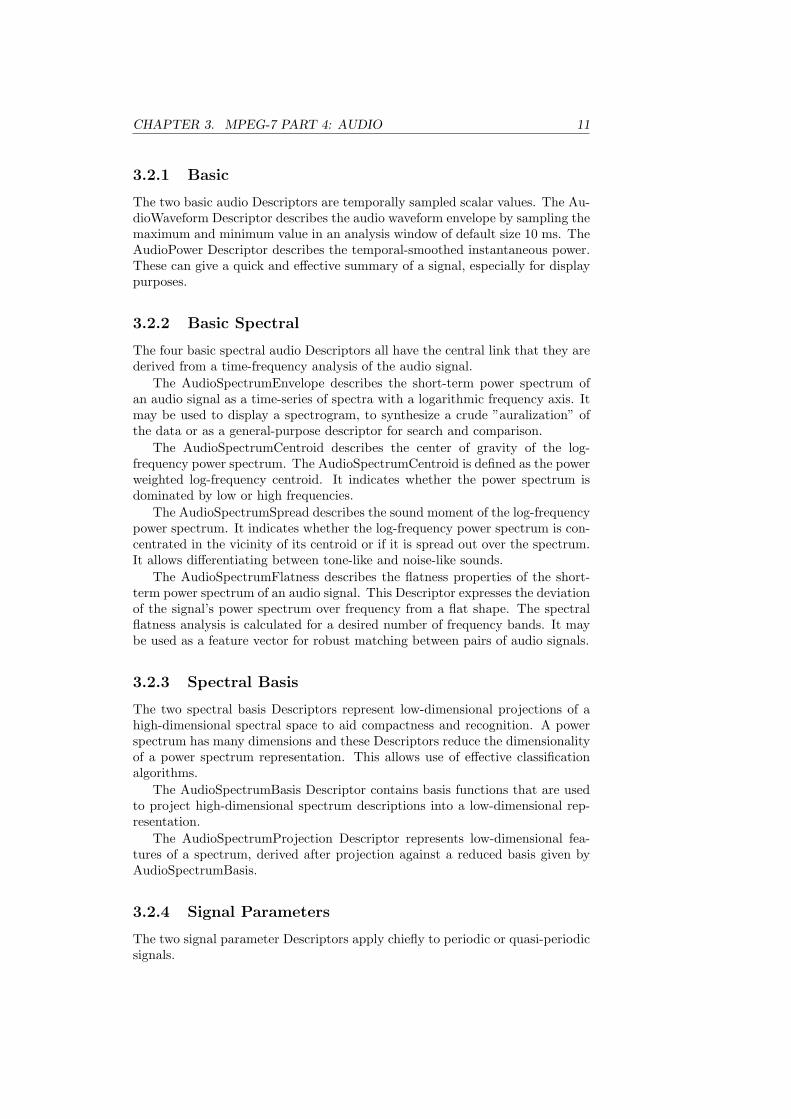
The Audio Framework consists of seventeen low level Descriptors for temporaland spectral audio features. This set of Descriptors is as generic as possible toallow a wide variety of applications to make use of them. They can be dividedinto six groups and, as seen in figure 3.1. Apart from these six groups thereare the very simple MPEG-7 silence Descriptor. It is however very useful andcomplete the Audio Framework. Each group is briefly explained below, andthe explanations are derived from the MPEG-7 overview [23] and the text ofInternational Standard ISO/IEC 15938-4 [24]
Audio Framework
Silence D
Basic AudioWaveform D
AudioPower D
Basic Spectral AudioSpectrumEnvelope D AudioSpectrumCentroid D AudioSpectrumSpread D
AudioSpectrumFlatness D
Spectral Basis AudioSpectrumBasis D
AudioSpectrumProjection D
Timbral Temporal LogAttackTime D
TemporalCentroid D
Timbral Spectral HarmonicSpectralCentroid D HarmonicSpectralDeviation D HarmonicSpectralSpread D
HarmonicSpectralVariation D SpectralCentroid D
Signal Parameters AudioHarmonicity D
AudioFundamentalFrequency D
Figure 3.1: Overview of the MPEG-7 Audio Framework
CHAPTER 3. MPEG-7 PART 4: AUDIO 11
3.2.1 Basic
The two basic audio Descriptors are temporally sampled scalar values. The Au-dioWaveform Descriptor describes the audio waveform envelope by sampling themaximum and minimum value in an analysis window of default size 10 ms. TheAudioPower Descriptor describes the temporal-smoothed instantaneous power.These can give a quick and effective summary of a signal, especially for displaypurposes.
3.2.2 Basic Spectral
The four basic spectral audio Descriptors all have the central link that they arederived from a time-frequency analysis of the audio signal.
The AudioSpectrumEnvelope describes the short-term power spectrum ofan audio signal as a time-series of spectra with a logarithmic frequency axis. Itmay be used to display a spectrogram, to synthesize a crude ”auralization” ofthe data or as a general-purpose descriptor for search and comparison.
The AudioSpectrumCentroid describes the center of gravity of the log-frequency power spectrum. The AudioSpectrumCentroid is defined as the powerweighted log-frequency centroid. It indicates whether the power spectrum isdominated by low or high frequencies.
The AudioSpectrumSpread describes the sound moment of the log-frequencypower spectrum. It indicates whether the log-frequency power spectrum is con-centrated in the vicinity of its centroid or if it is spread out over the spectrum.It allows differentiating between tone-like and noise-like sounds.
The AudioSpectrumFlatness describes the flatness properties of the short-term power spectrum of an audio signal. This Descriptor expresses the deviationof the signal’s power spectrum over frequency from a flat shape. The spectralflatness analysis is calculated for a desired number of frequency bands. It maybe used as a feature vector for robust matching between pairs of audio signals.
3.2.3 Spectral Basis
The two spectral basis Descriptors represent low-dimensional projections of ahigh-dimensional spectral space to aid compactness and recognition. A powerspectrum has many dimensions and these Descriptors reduce the dimensionalityof a power spectrum representation. This allows use of effective classificationalgorithms.
The AudioSpectrumBasis Descriptor contains basis functions that are usedto project high-dimensional spectrum descriptions into a low-dimensional rep-resentation.
The AudioSpectrumProjection Descriptor represents low-dimensional fea-tures of a spectrum, derived after projection against a reduced basis given byAudioSpectrumBasis.
3.2.4 Signal Parameters
The two signal parameter Descriptors apply chiefly to periodic or quasi-periodicsignals.
12 CHAPTER 3. MPEG-7 PART 4: AUDIO
The AudioFundamentalFrequency Descriptor describes the fundamental fre-quency of the audio signal. Fundamental frequency is a good predictor of musicalpitch and speech intonation.
The AudioHarmonicity Descriptor describes the degree of harmonicity of anaudio signal. This allows distinguishing between sounds that have a harmonicspectrum and non-harmonic spectrum, e.g. between musical sounds and noise.
3.2.5 Timbral Temporal
The two timbral temporal Descriptors describe the temporal characteristics ofsegments of sounds. These are useful for description of musical timbre.
The LogAttackTime Descriptor estimates the ”attack” of a sound. TheDescriptor is the logarithm (decimal base) of the time duration between thetime the signal starts to the time it reaches its stable part.
The TemporalCentroid Descriptor describes where in time the energy is fo-cused, based on the sound segment’s length.
3.2.6 Timbral Spectral
The five timbral spectral Descriptors describe the temporal characteristics ofsounds in a linear-frequency space. This makes timbral spectral combined withtimbral temporal Descriptors especially useful for description of musical instru-ment’s timbre.
The SpectralCentroid Descriptor is very similar to the AudioSpectrumCen-troid with its use of a linear power spectrum as the only difference betweenthem.
The HarmonicSpectralCentroid Descriptor is the amplitude-weighted meanof the harmonic peaks of a spectrum. It is similar to the other centroid Descrip-tors but applies only to harmonic parts of the musical tone.
The HarmonicSpectralDeviation Descriptor is the spectral deviation of log-amplitude components from a global spectral envelope.
The HarmonicSpectralSpread Descriptor is the amplitude weighted standarddeviation of the harmonic peaks of the spectrum, normalized by the instanta-neous HarmonicSpectralCentroid.
The HarmonicSpectralVariation Descriptor is the normalized correlation be-tween the amplitude of the harmonic peaks of two adjacent frames.
3.3 High Level Tools
The Audio Framework in the MPEG-7 Audio standard describes how to get fea-tures. These are clearly defined and can give information about audio. Whetherthe information has meaning or not depends on how the feature is analyzed andin what context the features are used in. MPEG-7 Audio describes five sets ofaudio Description Tools that roughly explain and give examples on how LowLevel Features can be used in content management.
The ”high level” tools are Descriptors and Description Schemes. These areeither structural or application oriented and make use of low level Descriptorsfrom the Audio Framework.
CHAPTER 3. MPEG-7 PART 4: AUDIO 13
The high level tools cover a wide range of application areas and functional-ities. The tools both provide functionality and serve as examples of how to usethe low level framework.
3.3.1 Audio Signature Description Scheme
The Audio Signature Description Scheme is based on the LLD spectral flatness.The spectral flatness Descriptor is statistically summarized to provide a uniquecontent identifier for robust automatic identification of audio signals.
The technique can be used for audio fingerprinting, identification of audio insorted databases and, these combined, content protection. A working solutionbased on the AudioSignature DS is the AudioID system developed by FraunhoferInstitute of Integrated Circuits IIS. It is a robust matching system that givesgood results with large databases and is tolerant to audio alternations as mobilephone transmission. That is, the system can find metatags to audio submittedvia a mobile phone.
3.3.2 Musical Timbre Description Tools
The aim of the Musical Timbre Description Tools is to use a set of low leveldescriptors to describe the timbre of instrument sounds. Timbre is the percep-tual features that make two sounds having the same pitch and loudness sounddifferent.
Applications can be various identification, search and filtering scenarioswhere specific types of sound are considered. The technique can be used tosimplify and improve performance of, for example, music sample database man-agement and retrieval tools.
3.3.3 Melody Description Tools
The Melody Description Tools are designed for monophonic melodic informationand forms a detailed representation of the audio’s melody. Efficient and robustmatching between melodies in monophonic information is possible with thesetools.
3.3.4 General Sound Recognition and Indexing Descrip-tion Tools
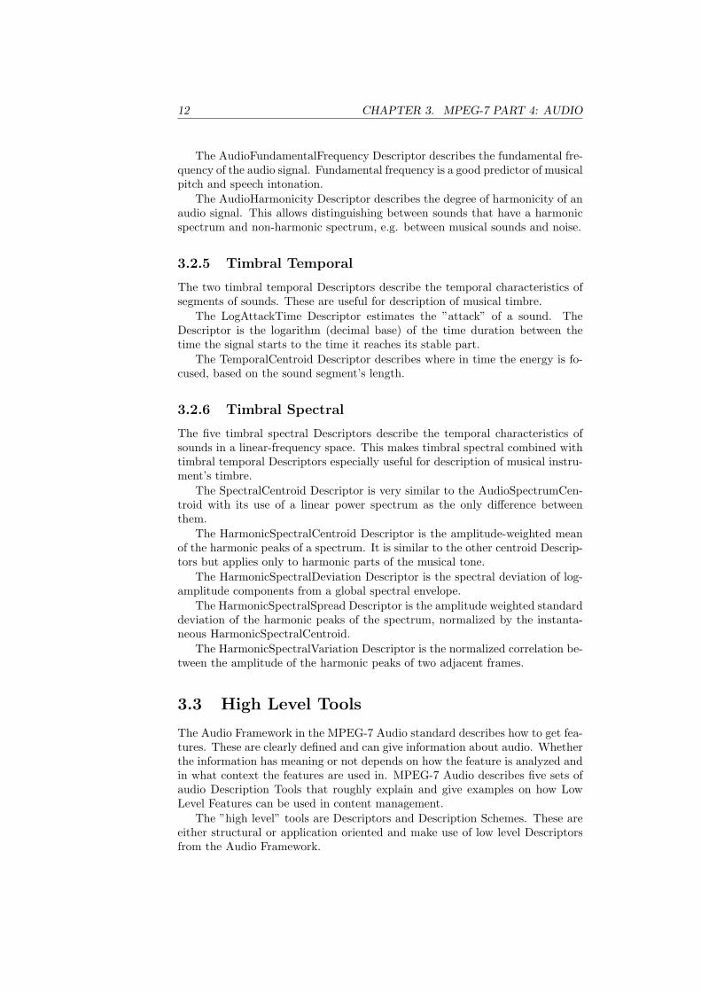
The General Sound Recognition and Indexing Description Tools are a set of toolsthat support general audio classification and content indexing. In contrast tospecific audio classification systems, which can work well for the designed task,these General Sound Recognition Tools aim to be a tool useable for diversesource classification [25]. The tools can also be used to efficiently index audiosegments into smaller similar segments.
The low level spectral basis Descriptors is the foundation to these tools. TheAudioSpectrumProjection D, with the AudioSpectrumBasis D, is used as thedefault descriptor for sound classification. These descriptors are collected fordifferent classes of sounds and a SoundModel DS is created. The SoundModelDS contain a sound class label and a continuous hidden Markov Model. A

14 CHAPTER 3. MPEG-7 PART 4: AUDIO
AudioSpectrumEnvelope
Basis 1 Projection
Observation
x Prediction
Basis 2 Projection
Basis N Projection
HMM 1
HMM N
HMM 2 Maximum likelihood
classificaion
Figure 3.2: Multiple hidden Markov models for automatic classification. Eachmodel is trained for a separate class and a maximum likelihood classification fora new audio clip can be made.
SoundClassificationModel DS combine several SoundModels into a multi-wayclassifier, as can be seen in Figure 3.2.
3.3.5 Spoken Content Description Tools
The Spoken Content Description Tools are a representation of the output of Au-tomatic Speech Recognition. It is designed to work at different semantic levels.The tools can be used for two broad classes of retrieval scenario: indexing intoand retrieval of an audio stream, and indexing of multimedia objects annotatedwith speech.
Chapter 4
Audio Classification
As described, audio classification and content description involves many tech-niques and there are many different applications. The focus in this thesis is onclassification of audio and, therefore, this chapter will outline general classifica-tion techniques and also present features applicable for audio classification.
4.1 General Classification Approach
There are many different ways to implement automatic classification. The avail-able data to be classified may be processed in more or less efficient ways to giveinformative features of the data. Another variation between classifiers is howefficient the features of unknown samples are analyzed to make a decision be-tween different classes. Many books regarding machine learning and patternrecognition is written and many ideas presented here comes from Mitchell’s [26]and Duda’s [27] books, which also are recommended for further reading.
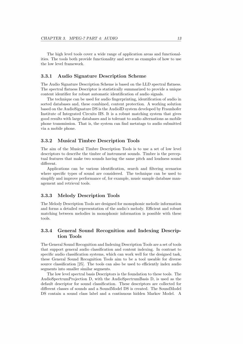
A general approach is shown in Figure 4.1 to illustrate a classifier’s scheme.First a sequence of data has to be observed, which is stored in x. The observedsequence, x, does not say much about what information it contains. Furtherprocessing of the sequence can isolate specific characteristics of it. These char-acteristics are stored in a feature vector y. The feature vector contains sev-eral descriptive measures that can be used to classify the sequence into definedclasses, which is done by the classifier.
Many thinkable applications can use this basic approach to accomplish differ-ent classification tasks. An example is outlined below that show how a medicalapplication classify cells in a tissue sample to normal and cancerous cells.
A tissue sample is observed and a feature is measured. As most cancerous
Feature Extraction Classifier
Observation
x
Feature vector
y Prediction
Figure 4.1: Basic scheme of automatic classification
15
16 CHAPTER 4. AUDIO CLASSIFICATION
0 0.05 0.1 0.15 0.20
20
40
60
80
100
120
Redness →
Num
ber
of s
ampl
es → Decision boundary
NormalCancerous
(a)
0 0.05 0.1 0.15 0.20
20
40
60
80
100
120
Redness →
Num
ber
of s
ampl
es → Decision boundary ?
NormalCancerous
(b)
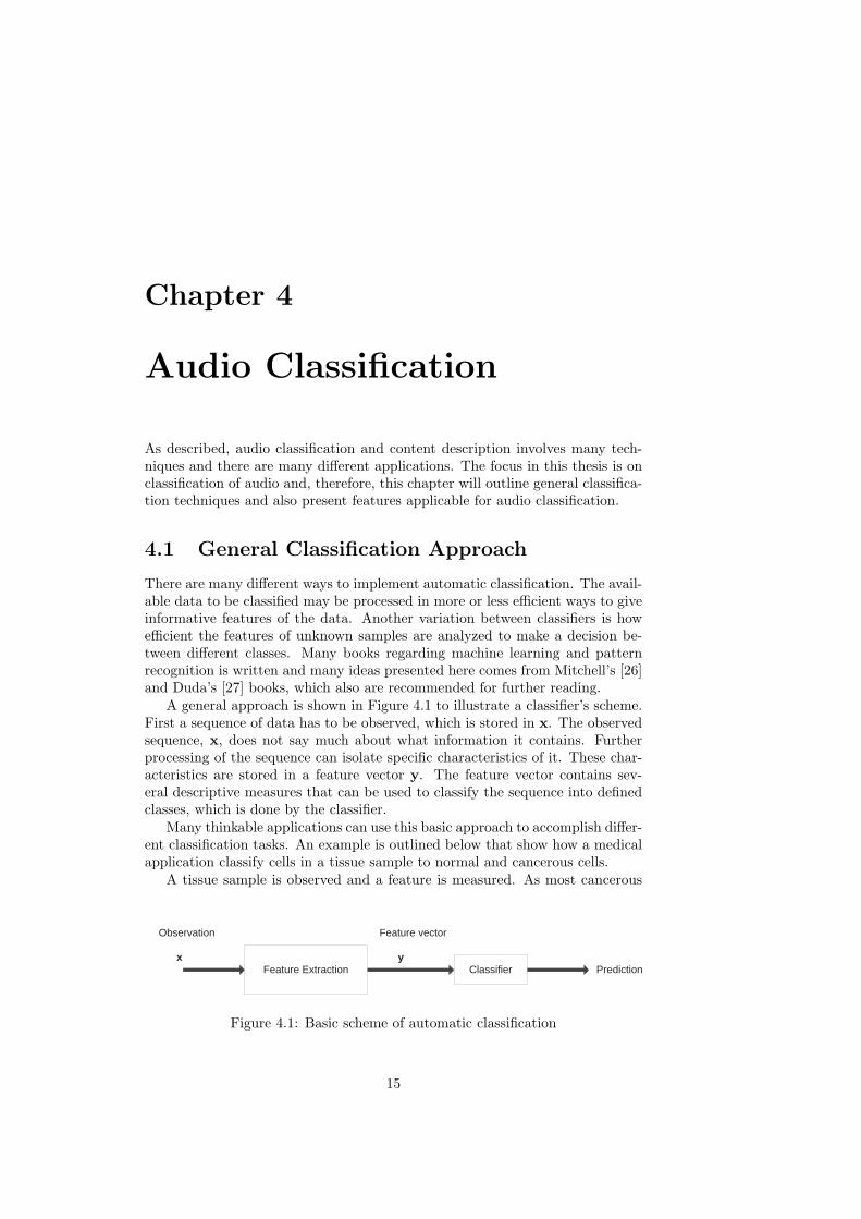
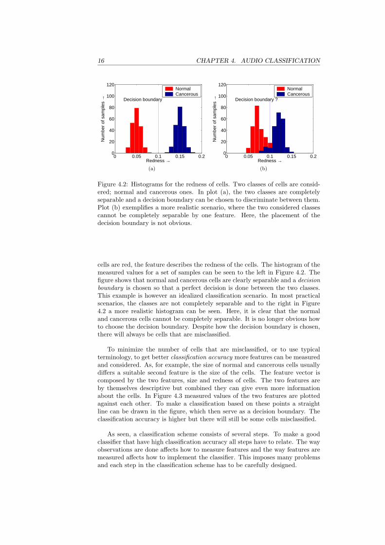
Figure 4.2: Histograms for the redness of cells. Two classes of cells are consid-ered; normal and cancerous ones. In plot (a), the two classes are completelyseparable and a decision boundary can be chosen to discriminate between them.Plot (b) exemplifies a more realistic scenario, where the two considered classescannot be completely separable by one feature. Here, the placement of thedecision boundary is not obvious.
cells are red, the feature describes the redness of the cells. The histogram of themeasured values for a set of samples can be seen to the left in Figure 4.2. Thefigure shows that normal and cancerous cells are clearly separable and a decisionboundary is chosen so that a perfect decision is done between the two classes.This example is however an idealized classification scenario. In most practicalscenarios, the classes are not completely separable and to the right in Figure4.2 a more realistic histogram can be seen. Here, it is clear that the normaland cancerous cells cannot be completely separable. It is no longer obvious howto choose the decision boundary. Despite how the decision boundary is chosen,there will always be cells that are misclassified.
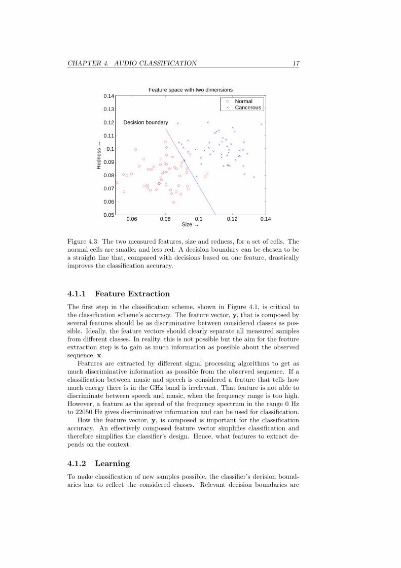
To minimize the number of cells that are misclassified, or to use typicalterminology, to get better classification accuracy more features can be measuredand considered. As, for example, the size of normal and cancerous cells usuallydiffers a suitable second feature is the size of the cells. The feature vector iscomposed by the two features, size and redness of cells. The two features areby themselves descriptive but combined they can give even more informationabout the cells. In Figure 4.3 measured values of the two features are plottedagainst each other. To make a classification based on these points a straightline can be drawn in the figure, which then serve as a decision boundary. Theclassification accuracy is higher but there will still be some cells misclassified.
As seen, a classification scheme consists of several steps. To make a goodclassifier that have high classification accuracy all steps have to relate. The wayobservations are done affects how to measure features and the way features aremeasured affects how to implement the classifier. This imposes many problemsand each step in the classification scheme has to be carefully designed.
CHAPTER 4. AUDIO CLASSIFICATION 17
0.06 0.08 0.1 0.12 0.140.05
0.06
0.07
0.08
0.09
0.1
0.11
0.12
0.13
0.14Feature space with two dimensions
Size →
Red
ness
→
Decision boundary
NormalCancerous
Figure 4.3: The two measured features, size and redness, for a set of cells. Thenormal cells are smaller and less red. A decision boundary can be chosen to bea straight line that, compared with decisions based on one feature, drasticallyimproves the classification accuracy.
4.1.1 Feature Extraction
The first step in the classification scheme, shown in Figure 4.1, is critical tothe classification scheme’s accuracy. The feature vector, y, that is composed byseveral features should be as discriminative between considered classes as pos-sible. Ideally, the feature vectors should clearly separate all measured samplesfrom different classes. In reality, this is not possible but the aim for the featureextraction step is to gain as much information as possible about the observedsequence, x.
Features are extracted by different signal processing algorithms to get asmuch discriminative information as possible from the observed sequence. If aclassification between music and speech is considered a feature that tells howmuch energy there is in the GHz band is irrelevant. That feature is not able todiscriminate between speech and music, when the frequency range is too high.However, a feature as the spread of the frequency spectrum in the range 0 Hzto 22050 Hz gives discriminative information and can be used for classification.
How the feature vector, y, is composed is important for the classificationaccuracy. An effectively composed feature vector simplifies classification andtherefore simplifies the classifier’s design. Hence, what features to extract de-pends on the context.
4.1.2 Learning
To make classification of new samples possible, the classifier’s decision bound-aries has to reflect the considered classes. Relevant decision boundaries are
18 CHAPTER 4. AUDIO CLASSIFICATION
achieved by learning, which is the process when a set of samples is used to tunethe classifier to the desired task. How the classifier is tuned depends on whatalgorithm the classifier use. However, in most cases, the classifier has to begiven a training set of samples, which the classifier uses to construct decisionboundaries.
In general, there are two ways to learn classifiers depending on what type ofclassifier that is considered. The first method to learn a classifier is called super-vised learning. In this method, the training set consists of pre-classified samplesthat the classifier uses to construct decision boundaries. The pre-classificationis done manually. Pre-classification can, in some scenarios, be difficult to make.Much experience and expertise is needed to pre-classify cell samples to be nor-mal or cancerous in our previous example. In music genre classification, thepre-classification can be problematic when the boundaries between differentclasses can be somewhat vague and subjective. A training method without themanual pre-classification is named unsupervised learning. In this method, thetraining set consists of unclassified samples that the classifier uses to form clus-ters. The clusters are labelled into different classes and this way the classifiercan construct decision boundaries.
4.1.3 Classification
Once the classifier has been trained it can be used to classify new samples.A perfect classification is seldom possible and numerous different classificationalgorithms are used with varying complexity and performance. Classifier algo-rithms based on different statistical, instance-based and clustering techniquesare widely used.
The main problem for a classifier is to cope with feature value variation forsamples belonging to specific classes. This variation may be large due to thecomplexity of the classification task. To maximize classification accuracy deci-sion boundaries should be chosen based on combinations of the feature values.
4.1.4 Estimation of Classifiers Performance
Analysis of how well a specific classification scheme work is important to getsome expectation of the classifiers accuracy. When a classifier is designed, thereare a variety of methods to estimate how high accuracy it will have on futuredata. These methods allow comparison to other classifiers performance.
A method described in Mitchell’s [26] and Duda’s [27] books, which also isused by many research groups [1] [3] [4], is cross-validation. Cross-validation isused to maximize the generality of estimated error rates. The error rates areestimated by dividing a labelled data set into two parts. One part is used astraining set and the other as a validation set or testing set. The training set isused to train the classifier and the testing set is used to evaluate the classifiersperformance. A common variation is the ”10-fold cross-validation” that dividesthe data set into 10 separate parts. Classification is performed 10 times, eachtime with a different testing set. 10 error rates are estimated and the finalestimate is simply the mean value of these. This method further generalizes theestimated error rates by iterating the training process with different trainingand testing sets.

CHAPTER 4. AUDIO CLASSIFICATION 19
4.2 Feature Extraction
Due to the complexity of human audio perception extracting descriptive featuresis difficult. No feature has yet been designed that with 100% certainty candistinguish between different classes. However, reasonably high classificationaccuracy, into different categories, has been achieved with a combination offeatures. Below are several features, suitable for various audio classificationtasks, outlined.
4.2.1 Zero-Crossing Rate
Values of the Zero-Crossing-Rate (ZCR) is widely used in speech/music classi-fication. It is defined to be the number of time-domain zero-crossings within aprocessing window, as shown in Equation 4.1.
ZCR =1
M − 1
M−1∑m=0
|sign(x(m))− sign(x(m− 1))| (4.1)
where sign is 1 for positive arguments and 0 for negative arguments, M is thetotal number of samples in a processing window and x(m) is the value of themth sample.
The algorithm is simple and has low computational complexity. Scheirer [4]use the ZCR to classify audio between speech/music, Tzanetakis [3] use it toclassify audio into different genres of music and Gouyon [14] use it to classifypercussive sounds.
Speech consists of voiced and unvoiced sounds. The ZCR correlate withthe frequency content of a signal. Hence, voiced and unvoiced sounds have lowrespectively high zero-crossing rates. This results in a high variation of ZCR.Music does not typically have this variation in ZCR but it has to be said thatsome parts of music has similar variations in ZCR. For instance, a drum introin a pop song can have high variations in ZCR values.
4.2.2 Short-Time-Energy
Short-time energy (STE) is also a simple feature that is widely used in variousclassification schemes. Li [2] and Zhang [1] use it to classify audio. It is definedto be the sum of a squared time domain sequence of data, as shown in Equation4.2
STE =M−1∑m=0
x2(m) (4.2)
where M is the total number of samples in a processing window and x(m) is thevalue of the mth sample.
As STE is a measure of the energy in a signal, it is suitable for discriminationbetween speech and music. Speech consists of words and mixed with silence. Ingeneral, this makes the variation of the STE value for speech higher than music.

20 CHAPTER 4. AUDIO CLASSIFICATION
4.2.3 Root-Mean-Square
As the STE, the root-mean-square (RMS) value is a measurement of the energyin a signal. The RMS value is however defined to be the square root of theaverage of a squared signal, as seen in Equation 4.3.
RMS =
√√√√ 1M
M−1∑m=0
x2(m) (4.3)
where M is the total number of samples in a processing window and x(m) is thevalue of the mth sample.
Analogous to the STE, the variation of the RMS value can be discriminativebetween speech and music.
4.2.4 High Feature-Value Ratio
Zhang [1] propose a variation of the ZCR that especially designed for discrimina-tion between speech and music. The feature is called High Zero-Crossing-RateRatio (HZCRR) and its mathematical definition can be seen in Equation 4.4
HZCRR =1
2N
N−1∑n=0
[sgn(ZCR(n)− 1.5avZCR)) + 1] (4.4)
where N is the total number of frames, n is the frame index, ZCR(n) is thezeros-crossing rate at the nth frame, avZCR is the average ZCR in a 1 secondwindow and sgn(.) is a sign function. That is, HZCRR is defined as the ratioof number of frames whose ZCR is above 1.5-fold average zero-crossing rate ina 1 second window.
The motive of the definition comes directly from the characteristics of speech.Speech consists of voiced and unvoiced sounds. The voiced and unvoiced soundshave low respectively high zero-crossing rates, which results in a high variationof ZCR and the HZCRR. Music does not typically have this variation in ZCRbut it has to be said that some parts of music has similar values in HZCRR.For instance, a drum intro in a pop song can have high HZCRR values.
The HZCRR will be used in a slightly different way. The feature is general-ized to work for any feature values. Hence, high feature-value ration (HFVR)is defined as Equation 4.5
HFV R =1
2N
N−1∑n=0
[sgn(FV (n)− 1.5avFV )) + 1] (4.5)
where N is the total number of frames, n is the frame index, FV(n) is the featurevalue at the nth frame, avFV is the average FV in a processing window andsgn(.) is a sign function. That is, HFVR is defined as the ratio of number offrames whose feature value is above 1.5-fold average feature value in a processingwindow.
CHAPTER 4. AUDIO CLASSIFICATION 21
4.2.5 Low Feature-Value Ratio
Similar to the HZCRR, Zhang [1] propose a variation of the STE feature. Thefeature they propose is called Low Short-Time Energy Ratio. Its mathematicaldefinition can be seen in Equation 4.6
LSTER =1
2N
N−1∑n=0
[sgn(0.5avSTE − STE(n)) + 1] (4.6)
where N is the total number of frames, n is the frame index, STE(n) is theshort-time energy at the nth frame, avSTE is the average STE in a 1 secondwindow and sgn(.) is a sign function. That is, LSTER is defined as the ratio ofnumber of frames whose STE is below 0.5-fold average short-time energy in a 1second window.
LSTER is suitable for discrimination between speech and music signals.Speech consists of words mixed with silence. In general, this makes the LSTERvalue for speech high whereas for music the value is low. The LSTER feature iseffective for discriminating between speech and music but since it is designed torecognize characteristics of single speaker speech it can loose it effectiveness ifmultiple speakers are considered. Also, music can have segments of pure drumpatterns, short violin patterns et cetera that will have the same characteristicsof speech in a LSTER sense.
As with the HZCRR, the feature will be used in a slightly different way. Thefeature is generalized to work for any feature values. Hence, low feature-valueration (LFVR) is defined as Equation 4.7
LFV R =1
2N
N−1∑n=0
[sgn(0.5avFV − FV (n)) + 1] (4.7)
where N is the total number of frames, n is the frame index, FV(n) is the short-time energy at the nth frame, avFV is the average FV in a processing windowand sgn(.) is a sign function. That is, LFVR is defined as the ratio of numberof frames whose feature value is below 0.5-fold average short-time energy in a 1second window.
4.2.6 Spectrum Centroid
Li [2] use a feature named spectral centroid (SC) to classify between noise,speech and music. Tzanetakis [3] use the same feature to classify music intodifferent genres. Spectrum centroid is based on analysis of the frequency spec-trum for the signal. The frequency spectrum, for use in this feature and severalothers, is calculated with the discrete Fourier transform (DFT) in Equation 4.8
A(n, k) =∣∣∣
∞∑m=−∞
x(m)w(nL−M)e−j( 2πL )km
∣∣∣ (4.8)
where k is the frequency bin for the nth frame, x(m) is the input signal, w(m)is a window function and L is the window length. The frequency spectrum canbe analyzed in different ways and the spectrum centroid is calculated as seen in
22 CHAPTER 4. AUDIO CLASSIFICATION
Equation 4.9
SC(n) =
K−1∑k=0
k · |A(n, k)|2
K−1∑k=0
|A(n, k)|2(4.9)
where K is the order of the DFT, k is the frequency bin for the nth frame andA(n,k) is the DFT of the nth frame of a signal and is calculated as Equation4.8. That is, the spectral centroid is a metric of the center of gravity of thefrequency power spectrum.
Spectrum centroid is a measure that signifies if the spectrum contains amajority of high or low frequencies. This is correlates with a major perceptualdimension of timbre; i.e. sharpness [23].
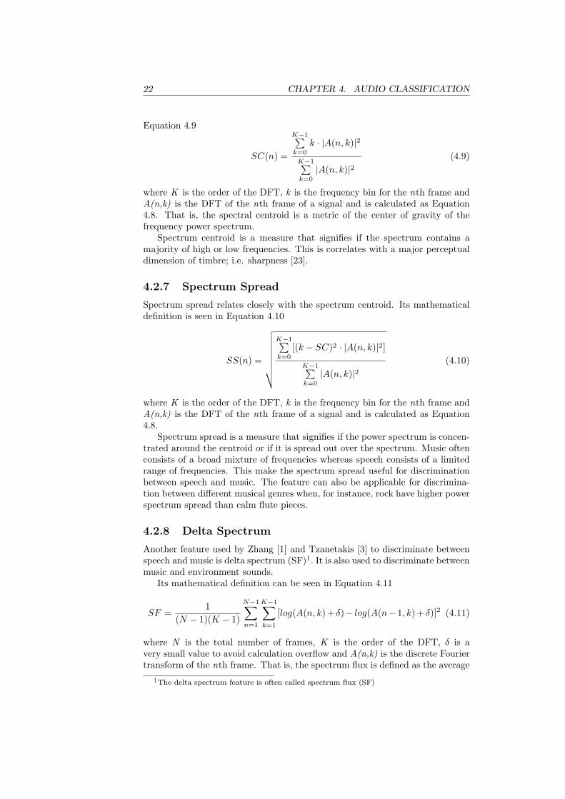
4.2.7 Spectrum Spread
Spectrum spread relates closely with the spectrum centroid. Its mathematicaldefinition is seen in Equation 4.10
SS(n) =
√√√√√√√√
K−1∑k=0
[(k − SC)2 · |A(n, k)|2]K−1∑k=0
|A(n, k)|2(4.10)
where K is the order of the DFT, k is the frequency bin for the nth frame andA(n,k) is the DFT of the nth frame of a signal and is calculated as Equation4.8.
Spectrum spread is a measure that signifies if the power spectrum is concen-trated around the centroid or if it is spread out over the spectrum. Music oftenconsists of a broad mixture of frequencies whereas speech consists of a limitedrange of frequencies. This make the spectrum spread useful for discriminationbetween speech and music. The feature can also be applicable for discrimina-tion between different musical genres when, for instance, rock have higher powerspectrum spread than calm flute pieces.
4.2.8 Delta Spectrum
Another feature used by Zhang [1] and Tzanetakis [3] to discriminate betweenspeech and music is delta spectrum (SF)1. It is also used to discriminate betweenmusic and environment sounds.
Its mathematical definition can be seen in Equation 4.11
SF =1
(N − 1)(K − 1)
N−1∑n=1
K−1∑
k=1
[log(A(n, k)+ δ)− log(A(n− 1, k)+ δ)]2 (4.11)
where N is the total number of frames, K is the order of the DFT, δ is avery small value to avoid calculation overflow and A(n,k) is the discrete Fouriertransform of the nth frame. That is, the spectrum flux is defined as the average
1The delta spectrum feature is often called spectrum flux (SF)
CHAPTER 4. AUDIO CLASSIFICATION 23
variation value of spectrum between the adjacent two frames in a processingwindow.
Speech consists, in general, of short words and the audio waveform is varyingrapidly. Music do not typically have this characteristics, which makes the SFan efficient feature for speech/music classification.
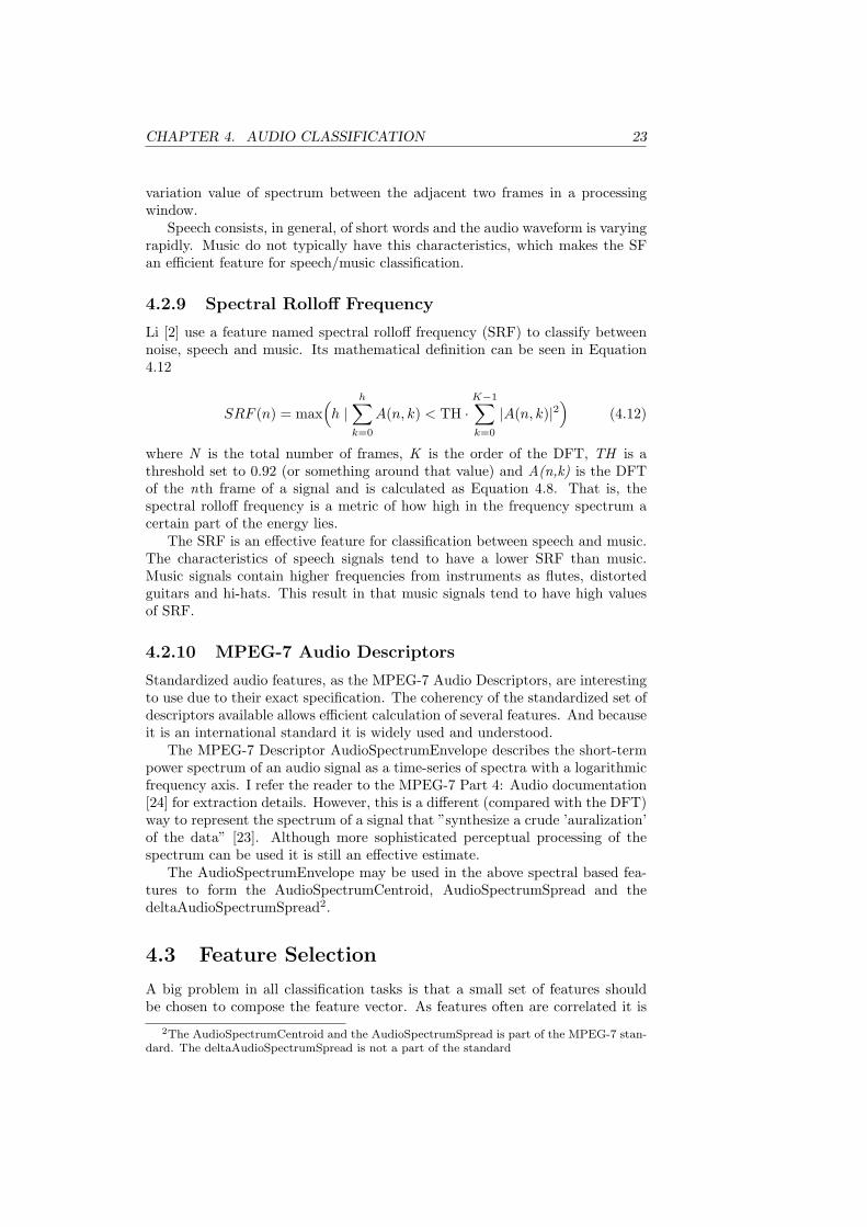
4.2.9 Spectral Rolloff Frequency
Li [2] use a feature named spectral rolloff frequency (SRF) to classify betweennoise, speech and music. Its mathematical definition can be seen in Equation4.12
SRF (n) = max(h |
h∑
k=0
A(n, k) < TH ·K−1∑
k=0
|A(n, k)|2)
(4.12)
where N is the total number of frames, K is the order of the DFT, TH is athreshold set to 0.92 (or something around that value) and A(n,k) is the DFTof the nth frame of a signal and is calculated as Equation 4.8. That is, thespectral rolloff frequency is a metric of how high in the frequency spectrum acertain part of the energy lies.
The SRF is an effective feature for classification between speech and music.The characteristics of speech signals tend to have a lower SRF than music.Music signals contain higher frequencies from instruments as flutes, distortedguitars and hi-hats. This result in that music signals tend to have high valuesof SRF.
4.2.10 MPEG-7 Audio Descriptors
Standardized audio features, as the MPEG-7 Audio Descriptors, are interestingto use due to their exact specification. The coherency of the standardized set ofdescriptors available allows efficient calculation of several features. And becauseit is an international standard it is widely used and understood.
The MPEG-7 Descriptor AudioSpectrumEnvelope describes the short-termpower spectrum of an audio signal as a time-series of spectra with a logarithmicfrequency axis. I refer the reader to the MPEG-7 Part 4: Audio documentation[24] for extraction details. However, this is a different (compared with the DFT)way to represent the spectrum of a signal that ”synthesize a crude ’auralization’of the data” [23]. Although more sophisticated perceptual processing of thespectrum can be used it is still an effective estimate.
The AudioSpectrumEnvelope may be used in the above spectral based fea-tures to form the AudioSpectrumCentroid, AudioSpectrumSpread and thedeltaAudioSpectrumSpread2.
4.3 Feature Selection
A big problem in all classification tasks is that a small set of features shouldbe chosen to compose the feature vector. As features often are correlated it is
2The AudioSpectrumCentroid and the AudioSpectrumSpread is part of the MPEG-7 stan-dard. The deltaAudioSpectrumSpread is not a part of the standard
24 CHAPTER 4. AUDIO CLASSIFICATION
difficult to choose a few number of features that will perform well. In Duda’sbook [27], methods to combine features into lower dimensionality feature sets aredescribed. These are methods like the Principal Component Analysis (PCA) andFisher Linear Discriminant. Because of time limits, this will not be covered inthis thesis. However, the interested reader may further study those techniques.
More practical approaches can be seen in Zhang’s [28] and Scheirer’s [4]work. Zhang compose a ”Baseline” feature vector that contains 4 features. Thebaseline set of features give good classification accuracy alone. Other featuresare then added to the baseline and the difference in classification accuracy givesa measure of the effectiveness of new features.
Scheirer propose a method that indicates how effective features are alone,which give guidance how to compose the feature vector. The effectiveness ofeach feature is approximated by a 10-fold cross validation on the training set.Error rates are estimated for each feature and these indicate what features touse, when low error rates implies that the feature is effective. It has to be saidthat strictly following these values to compose the feature vector would provebad since some features are highly correlated. However, with some knowledgeof what the features measure a good feature vector may be composed.
Both of the above practical approaches do not solve the problem of correlatedfeatures but they give guidance to how to compose the final feature set for aclassifier.
4.4 Classification
There are many proposed techniques for classifying audio samples into multi-ple classes. The most commonly techniques use different statistical approaches,where Gaussian Mixture Models (GMM) and Hidden Markov Models (HMM)give good results, and instance-based approaches, where the k-Nearest Neigh-bor (kNN) algorithm is a good example. A brief outline of the most commonclassification techniques is found below.
4.4.1 Gaussian Mixture Models
GMM are widely used in speech identification and audio classification scenarios.It is an intuitive approach when the model consists of several Gaussian com-ponents, which can be seen to model acoustic features. Much is written aboutthem and the interested reader may study the work published by Reynolds [29].A general overview of GMM will however be given here.
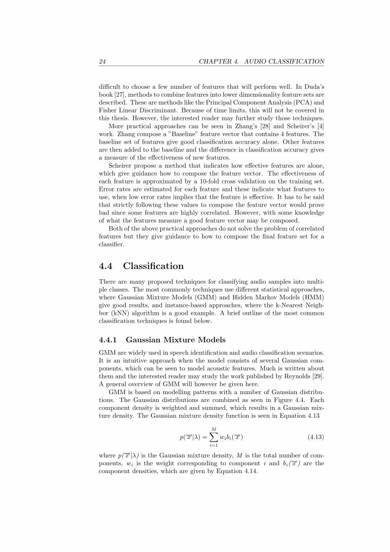
GMM is based on modelling patterns with a number of Gaussian distribu-tions. The Gaussian distributions are combined as seen in Figure 4.4. Eachcomponent density is weighted and summed, which results in a Gaussian mix-ture density. The Gaussian mixture density function is seen in Equation 4.13
p(−→x |λ) =M∑
i=1
wibi(−→x ) (4.13)
where p(−→x |λ) is the Gaussian mixture density, M is the total number of com-ponents, w i is the weight corresponding to component i and bi(−→x ) are thecomponent densities, which are given by Equation 4.14.

CHAPTER 4. AUDIO CLASSIFICATION 25
Figure 4.4: Scheme of Gaussian mixture model.
bi(−→x ) =1
(2π)1L | Σi| 12
exp{−12(−→x −−→µ i)
T Σ−1i (−→x −−→µ i)} (4.14)
The complete Gaussian mixture density is parameterized by the mixtureweights, covariance matrices and mean vectors from all component densities.The notation used is seen in Equation 4.15.
λ = {wi,−→µ i,Σi}, i = 1, 2, ..., M (4.15)
In classification, each class is represented by a GMM and is referred to its modelλ. Once the GMM is trained, it can be used to predict to which class a newsample most probably belong to.
4.4.2 Hidden Markov Models
The theory behind HMM was initially introduced in the late 1960’s but it took tolate 1980’s before they got widely used. Today, many use HMM in sophisticatedclassification schemes. One example is Casey’s work [25], which results are usedin the MPEG-7 standard. A good tutorial on HMM is given by Rabiner [11].
4.4.3 k-Nearest Neighbor Algorithm
The k-Nearest Neighbor Classifier is an instance-based classifier. The instance-based classifiers make decisions based on the relationship between the unknownsample and the stored samples. This approach is conceptually easy to under-stand but can nonetheless give complex decision boundaries for the classifiers.Hence, the k-Nearest Neighbor Classifier is suitable for a variety of applica-tions. For example, Zhang [1] use a k-Nearest Neighbor Classifier to classifyif an audio signal is speech and Tzanetakis [3] use a k-Nearest Neighbor clas-sifier to discriminate music into different musical genres. Many books aboutmachine learning and pattern recognition often include discussions about k-Nearest Neighbor algorithms, where Mitchell’s [26] and Duda’s [27] books are
26 CHAPTER 4. AUDIO CLASSIFICATION
recommended for further reading. However, a discussion on how the classifierworks will be outlined below.
When training a k-Nearest Neighbor classifier, all training samples are sim-ply stored in a n-dimensional Euclidean space, <n. This results in a numberof labelled points in the feature space. For example, figure 4.3 can actuallyrepresent the 2-dimensional Euclidean space for a k-Nearest Neighbor classifier.
As said before, the k-Nearest Neighbor Classifier makes decisions based onthe relationship between a query instance and stored instances. The relationshipbetween instances are defined to be the Euclidean distance, which definition isseen in Equation 4.16
d(xi,xj) = |xi − xj | =√√√√
n∑r=1
(xi(r)− xj(r))2 (4.16)
where d(xi,xj) is the Euclidean distance between two instances, represented bythe two feature vectors xi and xj , in a n-dimensional feature space.
Because the relationship between different instances is measured by the Eu-clidean distance, feature values need to be in the same region. If features withlarge values and low values are used, the feature with low values will have littlerelevance in the relationship measurement. To enhance the performance of thek-Nearest Neighbor algorithm normalization of feature values may be used. Tofurther enhance the performance of the k-Nearest Neighbor algorithm, weight-ing the axes in the feature space is proposed by Mitchell [26]. This correspondto stretching axes in the Euclidean space, shortening the axes correspond toless relevant features, and lengthening the axes correspond to more relevantfeatures.
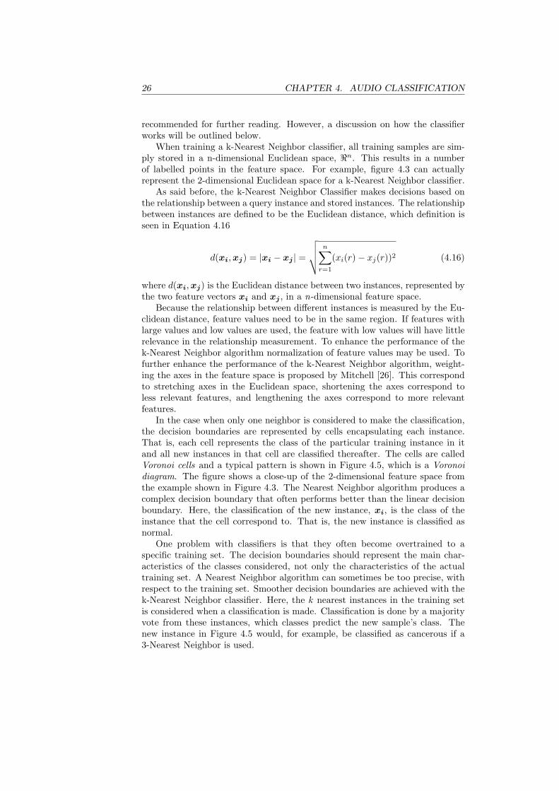
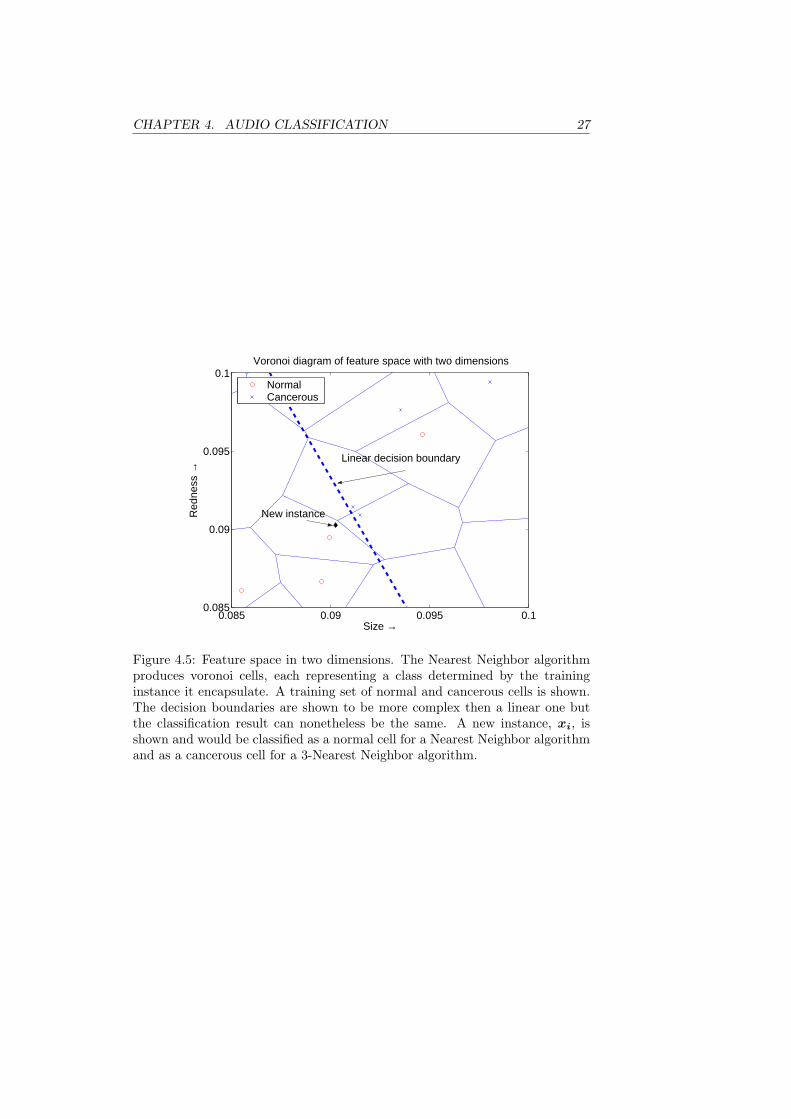
In the case when only one neighbor is considered to make the classification,the decision boundaries are represented by cells encapsulating each instance.That is, each cell represents the class of the particular training instance in itand all new instances in that cell are classified thereafter. The cells are calledVoronoi cells and a typical pattern is shown in Figure 4.5, which is a Voronoidiagram. The figure shows a close-up of the 2-dimensional feature space fromthe example shown in Figure 4.3. The Nearest Neighbor algorithm produces acomplex decision boundary that often performs better than the linear decisionboundary. Here, the classification of the new instance, xi, is the class of theinstance that the cell correspond to. That is, the new instance is classified asnormal.
One problem with classifiers is that they often become overtrained to aspecific training set. The decision boundaries should represent the main char-acteristics of the classes considered, not only the characteristics of the actualtraining set. A Nearest Neighbor algorithm can sometimes be too precise, withrespect to the training set. Smoother decision boundaries are achieved with thek-Nearest Neighbor classifier. Here, the k nearest instances in the training setis considered when a classification is made. Classification is done by a majorityvote from these instances, which classes predict the new sample’s class. Thenew instance in Figure 4.5 would, for example, be classified as cancerous if a3-Nearest Neighbor is used.
CHAPTER 4. AUDIO CLASSIFICATION 27
0.085 0.09 0.095 0.10.085
0.09
0.095
0.1Voronoi diagram of feature space with two dimensions
Size →
Red
ness
→
Linear decision boundary
New instance
NormalCancerous
Figure 4.5: Feature space in two dimensions. The Nearest Neighbor algorithmproduces voronoi cells, each representing a class determined by the traininginstance it encapsulate. A training set of normal and cancerous cells is shown.The decision boundaries are shown to be more complex then a linear one butthe classification result can nonetheless be the same. A new instance, xi, isshown and would be classified as a normal cell for a Nearest Neighbor algorithmand as a cancerous cell for a 3-Nearest Neighbor algorithm.
28 CHAPTER 4. AUDIO CLASSIFICATION
Audio clip
Speech
Music
Female
Male
Sports
Country
Disco
HipHop
Rock
Blues
Reggae
Classical
Pop
Metal
Orchestra
Piano
String Quartet
Choir
Piano
Quartet
Swing
Fusion
Big Band
Cool Jazz
Figure 4.6: Audio classification hierarchy.
4.5 Multi-class Classification
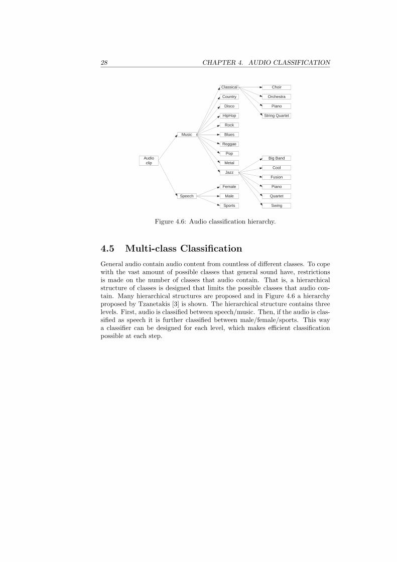
General audio contain audio content from countless of different classes. To copewith the vast amount of possible classes that general sound have, restrictionsis made on the number of classes that audio contain. That is, a hierarchicalstructure of classes is designed that limits the possible classes that audio con-tain. Many hierarchical structures are proposed and in Figure 4.6 a hierarchyproposed by Tzanetakis [3] is shown. The hierarchical structure contains threelevels. First, audio is classified between speech/music. Then, if the audio is clas-sified as speech it is further classified between male/female/sports. This waya classifier can be designed for each level, which makes efficient classificationpossible at each step.
Chapter 5
Applications
The potential audio classification and content description technologies are at-tracting commercial interests and many new products will be released in thenear future. Media corporations need effective storage and search and retrievalof technologies. People need effective ways to consume media. Researchersneed effective methods to manage information. Basically, the information soci-ety needs methods to manage itself.
5.1 Available commercial applications
Many commercial products have already been developed to meet the need ofcontent management. Most existing products are either music recognition orsearch-and-retrieval applications. Two examples of successful (in a technologysense) commercial products are given below.
5.1.1 AudioID
Fraunhofer Institute for Integrated Circuits IIS has developed an automaticidentification/recognition system named AudioID. AudioID can automaticallyrecognize and identify audio based on a database of registered work and deliversinformation about the audio identified. This is basically done by extracting aunique signature from a known set of audio material, which then are stored ina database. Then unknown audio sequence can be identified by extracting andcomparing a signature corresponding to it with the known database.
The system proves to work well, and recognition rates of over 99% are re-ported. The system use different signal manipulations, as equalization and mp3encoding/decoding, to emulate a human perceptibility that makes the systemrobust to distorted signals. Recognition works, for example, with signals trans-mitted with GSM cell phones. The main applications are:
• Identifying music and linking it to metadata. The system can au-tomatically link metadata from a database to a particular piece of music.
• Music sales. Automatic audio identification can give consumers meta-data of unknown music. This makes consumer aware of artists and songsnames, which possibly stimulates music consumption.
29
30 CHAPTER 5. APPLICATIONS
• Broadcast monitoring. The system can identify and monitor broad-casts audio program. This allows verification of scheduled transmission ofadvertisement and logging of played materials to ensure royalties.
• Content protection. Automatic audio identification may possibly beused to enhance copy protection of music.
5.1.2 Music sommelier
Panasonic has developed an automatic music analyzer that classifies music intodifferent categories. The application classifies music based on tempo, beat anda number of other features. Music clips are plotted in an impression map thathas active factors (Active - Quiet) on one axis and emotional factors (Hard -Soft) on the other axis. Different categories may be defined based on musicclip’s locations in the impression map. The software comes with three defaulttypes: Energetic, Meditative and Mellow.
The technique is incorporated into an automatic jukebox that may run onordinary PCs. The SD-Jukebox is a tool for users to manage music content athome and it allow users to choose what type of music to listen to.
Chapter 6
Experiments and analysis
As a second part of the thesis, a test-bed in Matlab was implemented and aspeech/music classifier was designed and evaluated. The test-bed was to beused to evaluate the performance for different classification schemes. For anexplanation of the test-bed, see Appendix A. A speech/music classifier wasdesigned because general audio classification is complex and involves too manysteps to be studied in this thesis. Hence, the first level in the hierarchy shownin Figure 4.6 was implemented and analyzed.
In this chapter, a description of the used evaluation and design procedure isoutlined. The evaluation procedure aims to get generalized evaluation results.In the design procedure, a comparison of feature’s efficiency is conducted anda few feature sets are proposed. The final performance for the speech/musicclassifier is found at the end of this chapter.
6.1 Evaluation procedure
To evaluate the performance of different features and different classificationschemes, a database of audio is collected. The database consists of approxi-mately 3 hours of data collected from CD-recordings of music and speech. Togeneralize the database, care is taken to collect music recordings from differentartists and genres. The speaker content is collected from recordings of bothfemale and male speakers. All audio clips are sampled at 44.1 kHz with 16 bitsper sample. The database is divided into a training set of about 2 hours and atesting set of about 1 hour of data. Special care is taken to ensure that no clipsfrom the same artist or speaker are included in both the training and testingset. These efforts are done to get evaluation results as generalized as possible.
During the design process, features are selected to compose feature vectorsbased on their efficiency. The efficiency is evaluated on the training set only.This ensures that the features are evaluated and chosen by performance on otherdata than the testing set. That is, the features are not chosen to the specifictesting set, which would produce too optimistic results.
The final evaluation of the classifiers performance is done on the testing set.This data has not been used to design the classifier and, therefore, give a goodestimate of the accuracy of the classifiers.
31
32 CHAPTER 6. EXPERIMENTS AND ANALYSIS
6.2 Music/Speech classification
The design of a robust music/speech classifier involves several steps. First, ageneral scheme to extract features is implemented. The scheme is used to extractmany features, which effectiveness can be analyzed. Based on the effectivenessof each feature, a feature vector is composed that is used by a classificationalgorithm to discriminate between music and speech. This section describeshow features are extracted, their effectiveness and how the final classificationscheme is designed.
6.2.1 Feature Extraction
Features are extracted in a scheme that uses different parameters to allow higherand lower resolution of the features. The variable resolution allows comparisonof performance between different analysis lengths. This is interesting to analyze,since shorter analysis windows have several advantages.
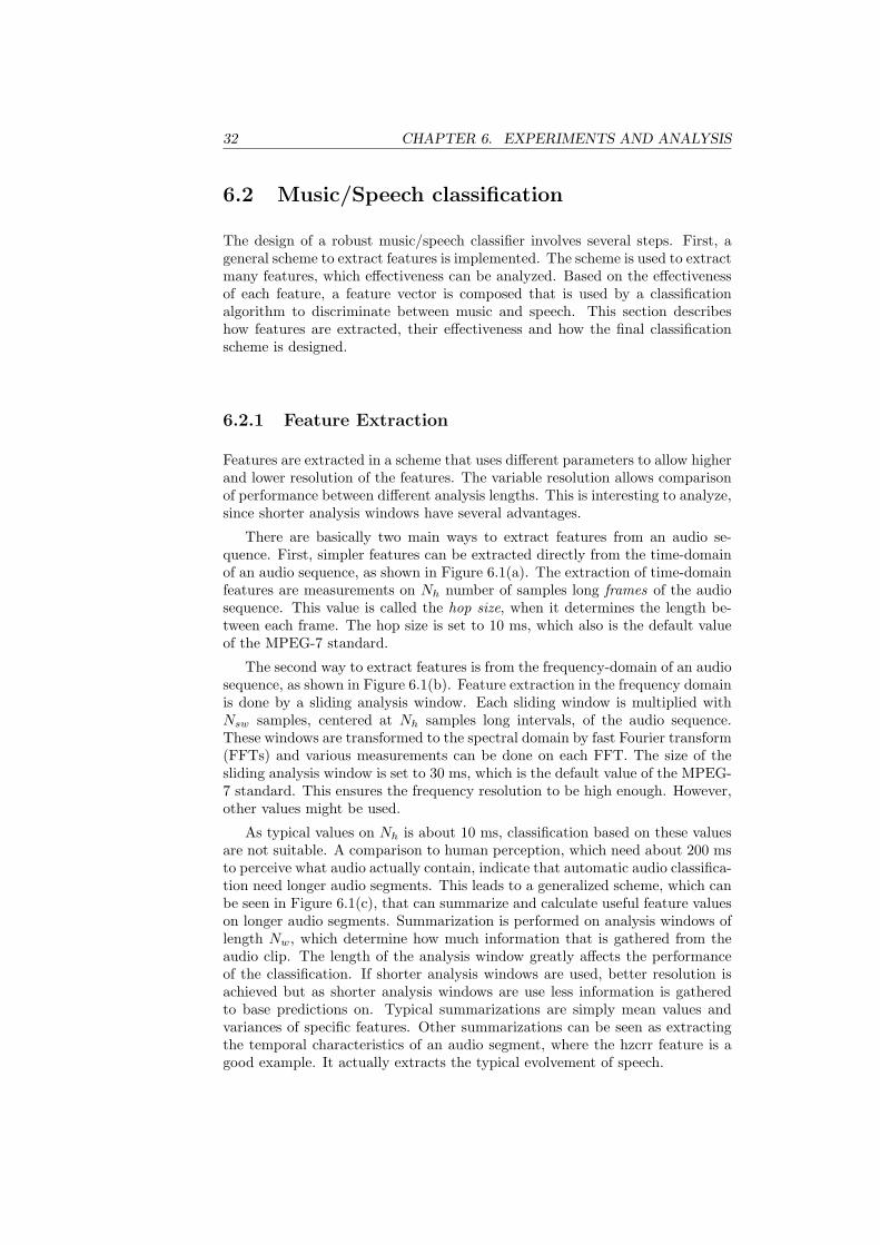
There are basically two main ways to extract features from an audio se-quence. First, simpler features can be extracted directly from the time-domainof an audio sequence, as shown in Figure 6.1(a). The extraction of time-domainfeatures are measurements on Nh number of samples long frames of the audiosequence. This value is called the hop size, when it determines the length be-tween each frame. The hop size is set to 10 ms, which also is the default valueof the MPEG-7 standard.
The second way to extract features is from the frequency-domain of an audiosequence, as shown in Figure 6.1(b). Feature extraction in the frequency domainis done by a sliding analysis window. Each sliding window is multiplied withNsw samples, centered at Nh samples long intervals, of the audio sequence.These windows are transformed to the spectral domain by fast Fourier transform(FFTs) and various measurements can be done on each FFT. The size of thesliding analysis window is set to 30 ms, which is the default value of the MPEG-7 standard. This ensures the frequency resolution to be high enough. However,other values might be used.
As typical values on Nh is about 10 ms, classification based on these valuesare not suitable. A comparison to human perception, which need about 200 msto perceive what audio actually contain, indicate that automatic audio classifica-tion need longer audio segments. This leads to a generalized scheme, which canbe seen in Figure 6.1(c), that can summarize and calculate useful feature valueson longer audio segments. Summarization is performed on analysis windows oflength Nw, which determine how much information that is gathered from theaudio clip. The length of the analysis window greatly affects the performanceof the classification. If shorter analysis windows are used, better resolution isachieved but as shorter analysis windows are use less information is gatheredto base predictions on. Typical summarizations are simply mean values andvariances of specific features. Other summarizations can be seen as extractingthe temporal characteristics of an audio segment, where the hzcrr feature is agood example. It actually extracts the typical evolvement of speech.
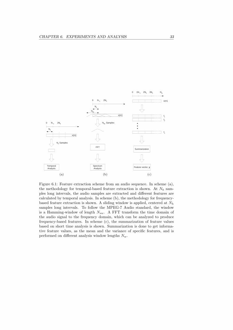
CHAPTER 6. EXPERIMENTS AND ANALYSIS 33
0 N h 2N h
N h
N h Samples
Temporal Analysis
x(m)
(a)
0 N h 2N h
N s w
N h
N s w Samples
FFT
Spectrum Analysis
x(m)
(b)
0 1N h
Summarization
f 1
N w
f 2
f n
Feature vector, y
2N h 3N h
x(m)
(c)
Figure 6.1: Feature extraction scheme from an audio sequence. In scheme (a),the methodology for temporal-based feature extraction is shown. At Nh sam-ples long intervals, the audio samples are extracted and different features arecalculated by temporal analysis. In scheme (b), the methodology for frequency-based feature extraction is shown. A sliding window is applied, centered at Nh
samples long intervals. To follow the MPEG-7 Audio standard, the windowis a Hamming-window of length Nsw. A FFT transform the time domain ofthe audio signal to the frequency domain, which can be analyzed to producefrequency-based features. In scheme (c), the summarization of feature valuesbased on short time analysis is shown. Summarization is done to get informa-tive feature values, as the mean and the variance of specific features, and isperformed on different analysis window lengths Nw.
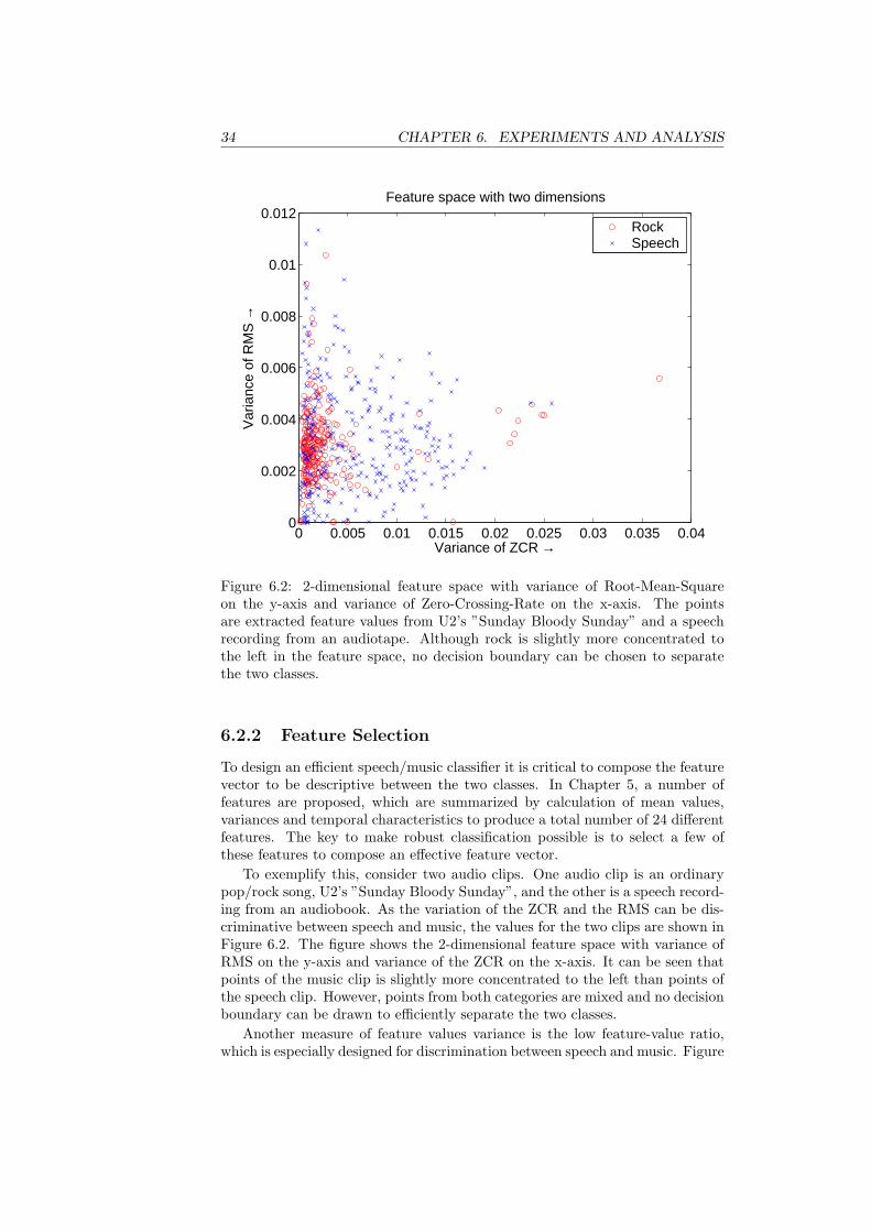
34 CHAPTER 6. EXPERIMENTS AND ANALYSIS
0 0.005 0.01 0.015 0.02 0.025 0.03 0.035 0.040
0.002
0.004
0.006
0.008
0.01
0.012Feature space with two dimensions
Variance of ZCR →
Var
ianc
e of
RM
S →
RockSpeech
Figure 6.2: 2-dimensional feature space with variance of Root-Mean-Squareon the y-axis and variance of Zero-Crossing-Rate on the x-axis. The pointsare extracted feature values from U2’s ”Sunday Bloody Sunday” and a speechrecording from an audiotape. Although rock is slightly more concentrated tothe left in the feature space, no decision boundary can be chosen to separatethe two classes.
6.2.2 Feature Selection
To design an efficient speech/music classifier it is critical to compose the featurevector to be descriptive between the two classes. In Chapter 5, a number offeatures are proposed, which are summarized by calculation of mean values,variances and temporal characteristics to produce a total number of 24 differentfeatures. The key to make robust classification possible is to select a few ofthese features to compose an effective feature vector.
To exemplify this, consider two audio clips. One audio clip is an ordinarypop/rock song, U2’s ”Sunday Bloody Sunday”, and the other is a speech record-ing from an audiobook. As the variation of the ZCR and the RMS can be dis-criminative between speech and music, the values for the two clips are shown inFigure 6.2. The figure shows the 2-dimensional feature space with variance ofRMS on the y-axis and variance of the ZCR on the x-axis. It can be seen thatpoints of the music clip is slightly more concentrated to the left than points ofthe speech clip. However, points from both categories are mixed and no decisionboundary can be drawn to efficiently separate the two classes.
Another measure of feature values variance is the low feature-value ratio,which is especially designed for discrimination between speech and music. Figure
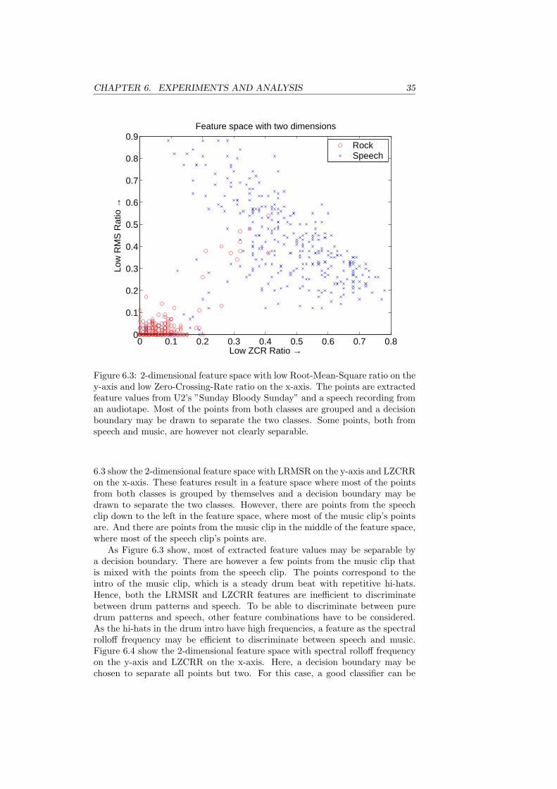
CHAPTER 6. EXPERIMENTS AND ANALYSIS 35
0 0.1 0.2 0.3 0.4 0.5 0.6 0.7 0.80
0.1
0.2
0.3
0.4
0.5
0.6
0.7
0.8
0.9Feature space with two dimensions
Low ZCR Ratio →
Low
RM
S R
atio
→
RockSpeech
Figure 6.3: 2-dimensional feature space with low Root-Mean-Square ratio on they-axis and low Zero-Crossing-Rate ratio on the x-axis. The points are extractedfeature values from U2’s ”Sunday Bloody Sunday” and a speech recording froman audiotape. Most of the points from both classes are grouped and a decisionboundary may be drawn to separate the two classes. Some points, both fromspeech and music, are however not clearly separable.
6.3 show the 2-dimensional feature space with LRMSR on the y-axis and LZCRRon the x-axis. These features result in a feature space where most of the pointsfrom both classes is grouped by themselves and a decision boundary may bedrawn to separate the two classes. However, there are points from the speechclip down to the left in the feature space, where most of the music clip’s pointsare. And there are points from the music clip in the middle of the feature space,where most of the speech clip’s points are.
As Figure 6.3 show, most of extracted feature values may be separable bya decision boundary. There are however a few points from the music clip thatis mixed with the points from the speech clip. The points correspond to theintro of the music clip, which is a steady drum beat with repetitive hi-hats.Hence, both the LRMSR and LZCRR features are inefficient to discriminatebetween drum patterns and speech. To be able to discriminate between puredrum patterns and speech, other feature combinations have to be considered.As the hi-hats in the drum intro have high frequencies, a feature as the spectralrolloff frequency may be efficient to discriminate between speech and music.Figure 6.4 show the 2-dimensional feature space with spectral rolloff frequencyon the y-axis and LZCRR on the x-axis. Here, a decision boundary may bechosen to separate all points but two. For this case, a good classifier can be

36 CHAPTER 6. EXPERIMENTS AND ANALYSIS
0 0.1 0.2 0.3 0.4 0.5 0.6 0.7 0.80
200
400
600
800
1000
1200Feature space with two dimensions
Low ZCR Ratio →
Mea
n of
Spe
ctra
l Rol
loff
Fre
quen
cy →
RockSpeech
Figure 6.4: 2-dimensional feature space with spectral rolloff frequency on they-axis and low Zero-Crossing-Rate ratio on the x-axis. The points are extractedfeature values from U2’s ”Sunday Bloody Sunday” and a speech recording froman audiotape. In comparison to Figure 6.3, only two points from music are notseparable from speech with a decision boundary.
designed with features as SRF and LZCRR.Music is however a complex class of audio, which contain many different
genres and, therefore, have many different characteristics. Good classificationbetween speech and rock can be achieved with features as above. Robust clas-sification between speech and music can however not be achieved with thesefeatures. In Figure 6.5 feature values from a music clip of jazz, Miles Davis’”Blue in Green”, and the same speech clip as before are shown. The featuresvalues of SRF and LZCRR, which where efficient in discriminating between rockand speech, is shown to overlap each other. In this case, the two features areinefficient for discrimination between speech and music.
To design a robust speech/music classifier, different types of speech andmusic have to be considered when selecting features. The main characteristicsthat discriminate speech from music have to be used in the final composition ofthe feature vector. That is, a set of features have to be selected to compose thefeature vector that best discriminate between speech and music. As a total of 24different features are produced from the features in Chapter 5, efficient selectionof features by looking at plots for a variety of music genres and speakers is notpractical. It would be time consuming and, basically, unrealistic to accomplishany good results.
To select a set of features to compose a feature vector some guidance is

CHAPTER 6. EXPERIMENTS AND ANALYSIS 37
0 0.2 0.4 0.6 0.8 10
100
200
300
400
500
600
700
800
900
1000Feature space with two dimensions
Low ZCR Ratio →
Mea
n of
Spe
ctra
l Rol
loff
Fre
quen
cy →
JazzSpeech
Figure 6.5: 2-dimensional feature space with spectral rolloff frequency on they-axis and low Zero-Crossing-Rate ratio on the x-axis. The points are extractedfeature values from Miles Davis’ ”Blue in Green” and a speech recording froman audiotape. In comparison to Figure 6.4, the feature values are mixed and nodecision boundary can separate the two classes.
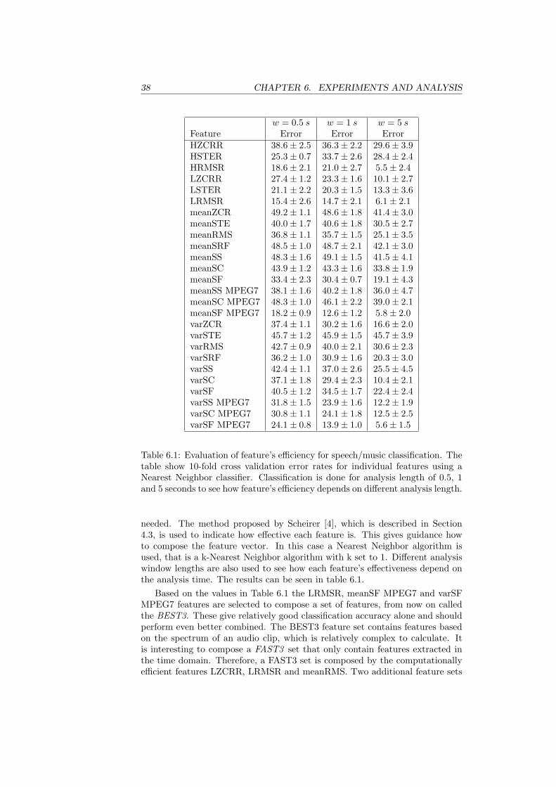
38 CHAPTER 6. EXPERIMENTS AND ANALYSIS
w = 0.5 s w = 1 s w = 5 sFeature Error Error ErrorHZCRR 38.6± 2.5 36.3± 2.2 29.6± 3.9HSTER 25.3± 0.7 33.7± 2.6 28.4± 2.4HRMSR 18.6± 2.1 21.0± 2.7 5.5± 2.4LZCRR 27.4± 1.2 23.3± 1.6 10.1± 2.7LSTER 21.1± 2.2 20.3± 1.5 13.3± 3.6LRMSR 15.4± 2.6 14.7± 2.1 6.1± 2.1meanZCR 49.2± 1.1 48.6± 1.8 41.4± 3.0meanSTE 40.0± 1.7 40.6± 1.8 30.5± 2.7meanRMS 36.8± 1.1 35.7± 1.5 25.1± 3.5meanSRF 48.5± 1.0 48.7± 2.1 42.1± 3.0meanSS 48.3± 1.6 49.1± 1.5 41.5± 4.1meanSC 43.9± 1.2 43.3± 1.6 33.8± 1.9meanSF 33.4± 2.3 30.4± 0.7 19.1± 4.3meanSS MPEG7 38.1± 1.6 40.2± 1.8 36.0± 4.7meanSC MPEG7 48.3± 1.0 46.1± 2.2 39.0± 2.1meanSF MPEG7 18.2± 0.9 12.6± 1.2 5.8± 2.0varZCR 37.4± 1.1 30.2± 1.6 16.6± 2.0varSTE 45.7± 1.2 45.9± 1.5 45.7± 3.9varRMS 42.7± 0.9 40.0± 2.1 30.6± 2.3varSRF 36.2± 1.0 30.9± 1.6 20.3± 3.0varSS 42.4± 1.1 37.0± 2.6 25.5± 4.5varSC 37.1± 1.8 29.4± 2.3 10.4± 2.1varSF 40.5± 1.2 34.5± 1.7 22.4± 2.4varSS MPEG7 31.8± 1.5 23.9± 1.6 12.2± 1.9varSC MPEG7 30.8± 1.1 24.1± 1.8 12.5± 2.5varSF MPEG7 24.1± 0.8 13.9± 1.0 5.6± 1.5
Table 6.1: Evaluation of feature’s efficiency for speech/music classification. Thetable show 10-fold cross validation error rates for individual features using aNearest Neighbor classifier. Classification is done for analysis length of 0.5, 1and 5 seconds to see how feature’s efficiency depends on different analysis length.
needed. The method proposed by Scheirer [4], which is described in Section4.3, is used to indicate how effective each feature is. This gives guidance howto compose the feature vector. In this case a Nearest Neighbor algorithm isused, that is a k-Nearest Neighbor algorithm with k set to 1. Different analysiswindow lengths are also used to see how each feature’s effectiveness depend onthe analysis time. The results can be seen in table 6.1.
Based on the values in Table 6.1 the LRMSR, meanSF MPEG7 and varSFMPEG7 features are selected to compose a set of features, from now on calledthe BEST3. These give relatively good classification accuracy alone and shouldperform even better combined. The BEST3 feature set contains features basedon the spectrum of an audio clip, which is relatively complex to calculate. Itis interesting to compose a FAST3 set that only contain features extracted inthe time domain. Therefore, a FAST3 set is composed by the computationallyefficient features LZCRR, LRMSR and meanRMS. Two additional feature sets

CHAPTER 6. EXPERIMENTS AND ANALYSIS 39
are composed to see if more features than 3 give better results. These are calledFAST3+BEST3, which contain the features in FAST3 and BEST3, and BEST6,which is composed by the LZCRR, LRMSR, meanSF MPEG7, varSF MPEG7,varSC MPEG7 and varSS MPEG7 features.
6.2.3 Classification Algorithm
Only one classification algorithm is studied due to time limitations. However,the chosen algorithm is a commonly used classification algorithm that can pro-duce complex decision boundaries. The classifier is based on a k-Nearest Neigh-bor algorithm and this section describes how features are combined in the clas-sification algorithm and what parameter setting that is chosen.
The k-Nearest Neighbor algorithm is sensitive to how the features are com-bined. As the k-Nearest Neighbor algorithm’s predictions are based on Eu-clidean distance measurements, by Equation 4.16, the range in which featurevalues are is important. If, for instance, a distance measurement is performed onthe feature values shown in Figure 6.4, the distance measure would only reflectdistances along the y-axis. In the figure it clearly can be seen that the featurevalues along the y-axis is much bigger then the feature values on the x-axis,which make the feature along the x-axis irrelevant in the distance measurement.
To combine features, the feature values have to be weighted to suit theEuclidean Space, <n. Normalization of each axis in the feature space may beused to produce a feature space with feature values in the range from 0 to1. This can however result in that some features become less important in thedistance measurement, which the case would be if normalization of feature valueswould be used on Figure 6.4. Better is to normalize the standard deviation foreach axis, which make each feature important and a suitable feature space isachieved. In Figure 6.6, the feature space from Figure 6.4 with normalizedstandard deviation feature values are shown.
The k-Nearest Neighbor only has one parameter to adjust, which is the k-value. Scheirer conclude in his work [4] that varying k in the k-Nearest Neighboralgorithm make only very little difference in classification performance. Tovalidate this, a cross-validation on the training set is performed using an analysiswindow of 1 second and the feature set BEST3 for different values of k. Theclassification accuracy for different k-values is shown in Table 6.7, where it canbe seen that the variation in performance is small. Based on Scheier’s work andthe obtained results, k is chosen to be 3 in the final classifier.
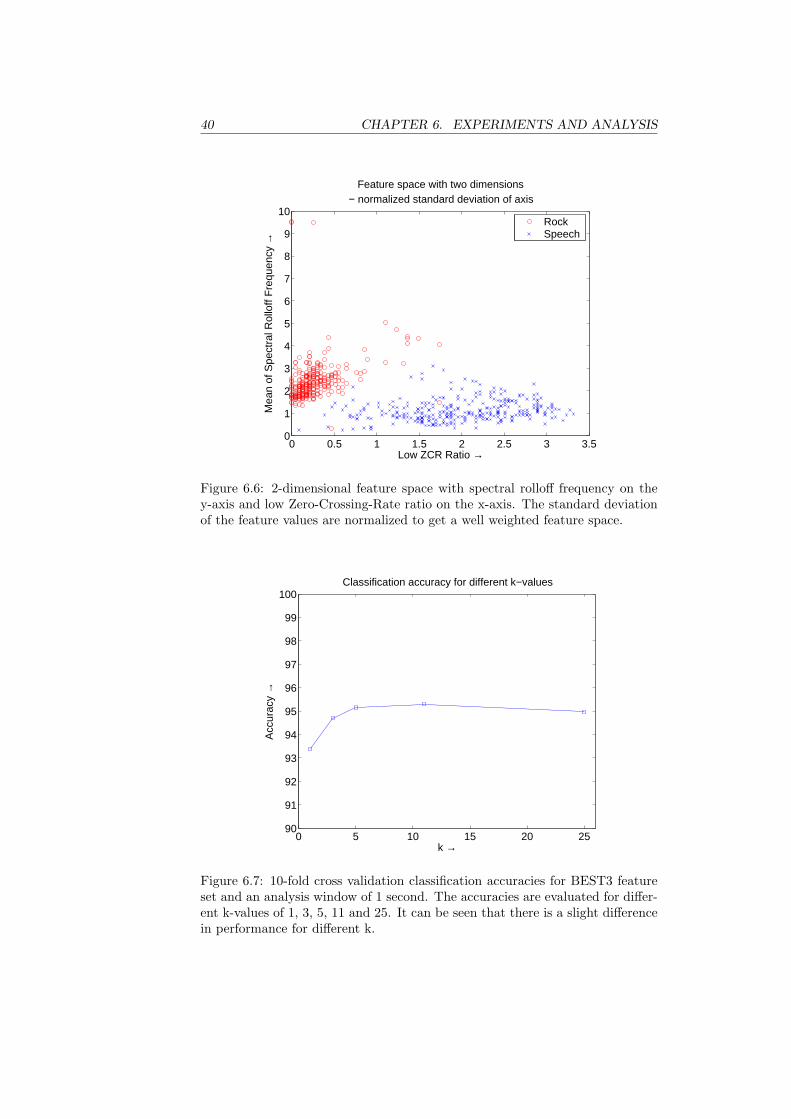
40 CHAPTER 6. EXPERIMENTS AND ANALYSIS
0 0.5 1 1.5 2 2.5 3 3.50
1
2
3
4
5
6
7
8
9
10
Feature space with two dimensions− normalized standard deviation of axis
Low ZCR Ratio →
Mea
n of
Spe
ctra
l Rol
loff
Fre
quen
cy →
RockSpeech
Figure 6.6: 2-dimensional feature space with spectral rolloff frequency on they-axis and low Zero-Crossing-Rate ratio on the x-axis. The standard deviationof the feature values are normalized to get a well weighted feature space.
0 5 10 15 20 2590
91
92
93
94
95
96
97
98
99
100Classification accuracy for different k−values
Acc
urac
y →
k →
Figure 6.7: 10-fold cross validation classification accuracies for BEST3 featureset and an analysis window of 1 second. The accuracies are evaluated for differ-ent k-values of 1, 3, 5, 11 and 25. It can be seen that there is a slight differencein performance for different k.
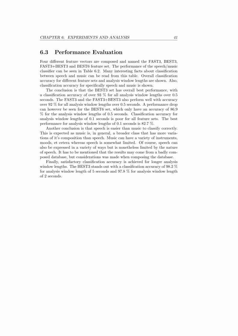
CHAPTER 6. EXPERIMENTS AND ANALYSIS 41
6.3 Performance Evaluation
Four different feature vectors are composed and named the FAST3, BEST3,FAST3+BEST3 and BEST6 feature set. The performance of the speech/musicclassifier can be seen in Table 6.2. Many interesting facts about classificationbetween speech and music can be read from this table. Overall classificationaccuracy for different feature sets and analysis window lengths are shown. Also,classification accuracy for specifically speech and music is shown.
The conclusion is that the BEST3 set has overall best performance, witha classification accuracy of over 93 % for all analysis window lengths over 0.5seconds. The FAST3 and the FAST3+BEST3 also perform well with accuracyover 92 % for all analysis window lengths over 0.5 seconds. A performance dropcan however be seen for the BEST6 set, which only have an accuracy of 86.9% for the analysis window lengths of 0.5 seconds. Classification accuracy foranalysis window lengths of 0.1 seconds is poor for all feature sets. The bestperformance for analysis window lengths of 0.1 seconds is 82.7 %.
Another conclusion is that speech is easier than music to classify correctly.This is expected as music is, in general, a broader class that has more varia-tions of it’s composition than speech. Music can have a variety of instruments,moods, et cetera whereas speech is somewhat limited. Of course, speech canalso be expressed in a variety of ways but is nonetheless limited by the natureof speech. It has to be mentioned that the results may come from a badly com-posed database, but considerations was made when composing the database.
Finally, satisfactory classification accuracy is achieved for longer analysiswindow lengths. The BEST3 stands out with a classification accuracy of 98.2 %for analysis window length of 5 seconds and 97.8 % for analysis window lengthof 2 seconds.

42 CHAPTER 6. EXPERIMENTS AND ANALYSIS
Classifier w = 0.1 s w = 0.5 s w = 1 s w = 2 s w = 5 sBEST3Total accuracy 79.0 93.1 95.7 97.8 98.2Music accuracy 78.0 89.7 93.4 96.8 97.1
Speech accuracy 80.0 96.6 98.1 98.8 99.4FAST3Total accuracy 79.0 92.5 92.9 95.6 93.3Music accuracy 75.6 88.1 87.2 92.2 87.9
Speech accuracy 82.2 97.0 98.7 99.0 98.8FAST3+BEST3Total accuracy 82,7 92.5 93.0 95.5 93.8Music accuracy 78.4 88.1 87.4 92.0 87.7
Speech accuracy 86.8 96.9 98.7 99.0 100BEST6Total accuracy 75.0 86.9 92.0 93.3 96.3Music accuracy 70.9 80.9 85.9 87.8 92.7
Speech accuracy 78.9 93.0 98.2 99.0 100
Table 6.2: Classification accuracy for different feature sets: BEST3, FAST3,FAST3+BEST3 and BEST6. Overall classification accuracy, classification ac-curacy for music and classification accuracy for speech is presented. The analysiswindow length, w, is set to 0.1, 0.5, 1, 2 and 5 seconds. Evaluation is performedon a testing set of about 1 hour of data divided into approximately a 50/50ratio of speech and music. A k-Nearest Neighbor algorithm is used with k setto 3.

Chapter 7
Conclusion and FutureWork
7.1 Conclusion
Content description is a broad field that involve many techniques that aim toprovide tools for content management. Classification, segmentation, recognitionand summarization is examples on techniques being developed to aid users inmedia applications. A study of automatic audio content classification for wasperformed in this thesis and a test-bed in Matlab was implemented for testingcontent classification algorithms.
Audio classification is complex and many problems have to be consideredwhen a classifier is designed. First, knowledge of what content the classifiershould classify between is essential for successful classification. This leads to ahierarchical audio classification scheme to make limitations of possible contentto be classified. The hierarchical structure allows efficient design of classifiersat each level. As speech/music commonly is on the top of the hierarchicalclassification structure, a speech/music classifier have been implemented andanalyzed in this thesis.
Second, features have to be selected that maximizes the discrimination be-tween different classes. This is a problem that can be found in all classificationtasks. Audio classification is often performed by extracting such features aszero-crossing rate, short-term energy and different spectrum measurements. Inthis thesis the performance of commonly used features, and variations of them,have been studied. Interesting to see is the efficiency of features based on theMPEG-7 spectrum descriptor. The main difference between an ordinary fre-quency spectrum and MPEG-7 spectrum descriptor is that the frequency axisis mapped to a logarithmic frequency axis in MPEG-7. As human perceptionis logarithmic, with respect to frequencies, the MPEG-7 spectrum descriptorcan be seen to represent a ”crude auralization” of audio. This results in thatthe efficiency of all spectrum based features is outperformed by ones based onthe MPEG-7 spectrum descriptor. Other efficient features are the LZCRR,LRMSR and meanRMS that all are variations of commonly used features. Thisindicates that no ultimate feature has been proposed and with more researchbetter features may be designed.
43

44 CHAPTER 7. CONCLUSION AND FUTURE WORK
Third, a classification algorithm has to be implemented that make predic-tions of new samples based on extracted feature values. This can be done inseveral ways but this thesis only studies the k-Nearest Neighbor algorithm. Thek-Nearest Neighbor is sensitive to irrelevant features and feature values. If irrel-evant features are considered when classification is performed, the classificationperformance degrades. This can be seen in table 6.2, where the classificationaccuracy of different feature sets is shown. Higher dimensional feature sets asFAST3+BEST3 and BEST6 perform, in general, worse than lower dimensionalfeature sets. If irrelevant feature values are used, the relationship measurementthat is used for the k-Nearest Neighbor’s predictions may be inefficient. Forinstance, if two features with values around 3 and 400 are to compose the fea-ture vector and used in a k-Nearest Neighbor classifier the first feature will notcontribute much to the final prediction. In this thesis, the k-Nearest Neigh-bor normalizes the variance of the feature values to make each feature equallyimportant. This seems to work well and good performance is achieved.
Fourth, the amount of information that is gathered to make predictions ofnew samples highly determines the performance of the classification. In table6.2 classification accuracy for different analysis window lengths are listed. It isshown that performance, in general, is better for longer analysis lengths. Asmore information about the audio is gathered it is logical to see an improve-ment as analysis lengths increase. Hence, a trade-off between resolution in theclassification and classification accuracy has to be done. However, table 6.2 alsoshow that as the analysis length reaches 5 seconds the performance drop. Thisdrop in performance may come from badly designed features that only work forshorter analysis lengths. Another possibility is that the performance drop isrelated to the number of instances in the training set. When a longer analysiswindow is used, less training samples is generated for the same training set ofaudio. As the k-Nearest Neighbor is an instance-based classifier, performancedrop as the number of instances decline.
And finally, as some audio classes are more complex than others, the overallclassification accuracy of a classifier may not be indicative to how well theclassifier performs for a given class. As the results show for the speech/musicclassifier, speech is easier to classify correctly compared to music. Music is abroader class that contain a variety of compositions and this has to be consideredwhen training and testing a classifier.
7.2 Future Work
Many techniques have not been studied closer in this thesis and more workcan be done. Below is a list of possible directions to continue evaluating anddesigning new classifiers.
• Implement more efficient features. To achieve better classificationaccuracy, more efficient features may be designed. For example, extractionof possible tempo in an audio clips, stereo information and better use ofperceptual models (as the MPEG-7 spectrum representation) can resultin more efficient features. Better features can also be designed to work formusic genre classification, speaker classification et cetera.
CHAPTER 7. CONCLUSION AND FUTURE WORK 45
• Implement more efficient classifiers. Although many research groupsconclude that the difference in performance between different classificationalgorithms is limited, much of the computational complexity can be im-proved. Efficient searches in the k-Nearest Neighbor algorithm may beimplemented but to implement completely other classification algorithms,as the GMM or HMM, is also interesting.
• Use other training sets. A better selection of training material canimprove classification accuracy. If more audio clips are used to train theclassifier, better performance should be achieved. The audio content ofthe clips can also be improved to be represent a diverse set of genres ofspeech and music.
• Implement automatic content segmentation. To improve classifica-tion results at transitions between different content in audio clips, auto-matic content segmentation may be used. Good automatic segmentationwould increase classification performance as analysis windows could bepositioned to only contain one class.
• Implement more classifiers. As relatively good accuracy is achievedin the implemented speech/music classifier, a natural step is to implementmore levels in the hierarchical classification structure. When audio isclassified as speech, a classifier can be used to classify the speaker to beeither female or male. And as the audio is classified as music, a classifiercan be used to classify between musical genres.
These are some proposed steps that can be studied with help of the imple-mented test-bed and give more knowledge of automatic audio classification andcontent description.

Bibliography
[1] L. Lu, H.-J. Zhang, and H. Jiang. Content analysis for audio classificationand segmentation. IEEE Transaction on Speech and Audio Processing,10(7):504–516, October 2002.
[2] D. Li, I. K. Sethi, N. Dimitrova, and T. McGee. Classification of gen-eral audio data for content-based retrieval. Pattern Recognition Letters,22(5):533–544, April 2001.
[3] G. Tzanetakis and P. Cook. Musical genre classification of audio signals.IEEE Transactions on Speech and Audio Processing, 10(5):293–302, July2002.
[4] E. Scheirer and M. Slaney. Construction and evaluation of a robust multi-feature speech/music discriminator. ICASSP, IEEE International Confer-ence on Acoustics, Speech and Signal Processing - Proceedings, 2:p 1331–1334, April 1997.
[5] K.-P. Han, Y.-S. Park, S.-G. Jeon, G.-C. Lee, and Y.-H Ha. Genre classifi-cation system of tv sound signals based on a spectrogram analysis. IEEETransactions on Consumer Electronics, 44(1):33–42, February 1998.
[6] D. Pye. Content-based methods for the management of digital music.ICASSP, IEEE International Conference on Acoustics, Speech and SignalProcessing - Proceedings, 4:2437–2440, June 2000.
[7] D.-N. Jiang, L. Lu, H.-J. Zhang, J.-Hua. Tao, and L.-H. Cai. Music typeclassification by spectral contrast feature. Proceedings 2002 IEEE Inter-national Conference on Multimedia and Expo (Cat. No.02TH8604), 1:113–116, August 2002. Conference date 26-29 Aug. 2002.
[8] D. Kimber and L. Wilcox. Acoustic segmentation for audio browsers. Com-puting Science and Statistics. Vol.28. Graph-Image-Vision. Proceedings ofthe 28th Symposium on the Interface. Interface ’96, (295-304), 1997.
[9] A. Albiol, L. Torres, and E. J. Delp. The indexing of persons in newssequences using audio-visual data. Proceedings of the 2003 IEEE Inter-national Conference on Acoustics, Speech, and Signal Processing, ICASSP’03, 3:137–140, April 2003.
[10] M. Abe and M. Nishiguchi. Self-optimized spectral correlation methodfor background music identification. Proceedings 2002 IEEE InternationalConference on Multimedia and Expo (Cat. No.02TH8604), 1(1):333–336,August 2002.
46
BIBLIOGRAPHY 47
[11] L. R. Rabiner. Tutorial on hidden markov models and selected applicationsin speech recognition. Proceedings of the IEEE, 77(2):257–286, February1989.
[12] J.-T. Chien. Linear regression based bayesian predictive classification forspeech recognition. IEEE Transactions on Speech and Audio Processing,11(1):70–79, January 2003.
[13] J. Chen, K. K. Paliwal, and S. Nakamura. Cepstrum derived from differenti-ated power spectrum for robust speech recognition. Speech Communication,41(2-3):469–484, October 2003.
[14] F. Gouyon, F. Pachet, and O. Delerue. On the use of zero-crossing ratefor an application of clasification of percussive sounds. Proceedings of theCOST G-6 Conference on Digital Audio Effects (DAFX-00), December2000.
[15] D. Slezak, P. Synak, A. Wieczorkowska, and J. Wroblewski. Kdd-based ap-proach to musical instrument sound recognition. Foundations of IntelligentSystems. 13th International Symposium, ISMIS 2002. Proceedings (LectureNotes in Computer Science Vol.2366), pages 28–36, June 2002.
[16] D. Slezak, P. Synak, A. Wieczorkowska, and J. Wroblewski. Application oftemporal descriptors to musical instrument sound recognition. Journal ofIntelligent Information Systems, 21(1):71–93, July 2003.
[17] E. Wold, T. Blum, D. Keislar, and J. Wheaton. Content-based classifica-tion, search, and retrieval of audio. IEEE Multimedia, 3(3):27–36, 1996.
[18] M. Casey. Sound Classification and Similarity Tools. Wiley, 2002. B.S. Manjunath (Editor), P. Salembier (Editor), T. Sikora (Editor), ISBN:0-471-48678-7.
[19] B. Logan and S. Chu. Music summarization using key phrases. ICASSP,IEEE International Conference on Acoustics, Speech and Signal Processing- Proceedings, 2:749–752, June 2000.
[20] C. Xu, Y. Zhu, and Q. Tian. Automatic music summarization based on tem-poral, spectral and cepstral features. Proceedings 2002 IEEE InternationalConference on Multimedia and Expo (Cat. No.02TH8604), 1(1):117–120,August 2002.
[21] J. Song, S.-Y Bae, and K. Yoon. Query by humming: matching hummingquery to polyphonic audio. Proceedings 2002 IEEE International Confer-ence on Multimedia and Expo (Cat. No.02TH8604), 1(1):329–332, August2002.
[22] B. Liu, Y. Wu, and Y. Li. A linear hidden markov model for music infor-mation retrieval based on humming. Proceedings of the 2003 IEEE Inter-national Conference on Acoustics, Speech, and Signal Processing, ICASSP’03, 5:533–536, 2003.
[23] Mpeg-7 overview (version 9). ISO/IEC JTC1/SC29/WG11 N5525, March2003.
48 BIBLIOGRAPHY
[24] Text of international standard iso/iec 15938-4 information technology -multimedia content description interface - part 4: Audio. ISO/IEC 15938-4, 2002.
[25] M. A. Casey. Reduced-rank spectra and minimum-entropy priors as con-sistent and reliable cues for generalized sound recognition. Proceedings ofthe Workshop on Consistent and Reliable Cues for Sound Analysis, EU-ROSPEECH 2001, September 2001.
[26] T. M. Mitchell. Machine learning. McGraw-Hill, New York, 1997. ISBN:0-07-042807-7.
[27] R. O. Duda, P. E. Hart, and David G. Stork. Pattern classification. Wiley,New York, 2 ed. edition, 2001. ISBN: 0-471-05669-3.
[28] L. Lu, H.-J. Zhang, and S. Z. Li. Content-based audio classification andsegmentation by using support vector machines. Multimedia Systems,8(6):482–492, April 2003.
[29] D. A. Reynolds and R. C. Rose. Robust text-independent speaker iden-tification using gaussian mixture speaker models. IEEE Transactions onSpeech and Audio Processing, 3(1):72 – 83, January 1995.

Appendix A
Test-bed Environment
This appendix will describe the test-bed implemented as part of this thesis. Thetest-bed is implemented in Matlab and aim to be a general tool for evaluationof classification schemes. A description of the test-bed’s structure and how touse it is outlined below.
A.1 Structure
Test-bed Structure
Extraction Part run_calculateAll
Classification Part run_classify run_testClassifierTS run_testClassifierCV run_testFeatureEfficiency
Figure A.1: Overview of the test-bed’s structure.
The test-bed is initialized with a file called startup.m. It sets all needed pathsand make the test-bed ready to use. The test-bed mainly consist of two partsnamed extraction part and classification part. Figure A.1 show the two partsand their m-files, which make testing of different classification schemes possible.The extraction part is a general framework for extraction of different features.It allows new features to be implemented and used. The classification partuse different classification algorithms to classify test data. Different evaluationmethods may be used to estimate classifiers performance.
Extraction Part
In the extraction part there exists a file called calculateAll.m that extracts fea-ture values for all files in a sorted database. Different parameters are passed tocalculateAll.m, which determines what features and how they will be extracted.
49
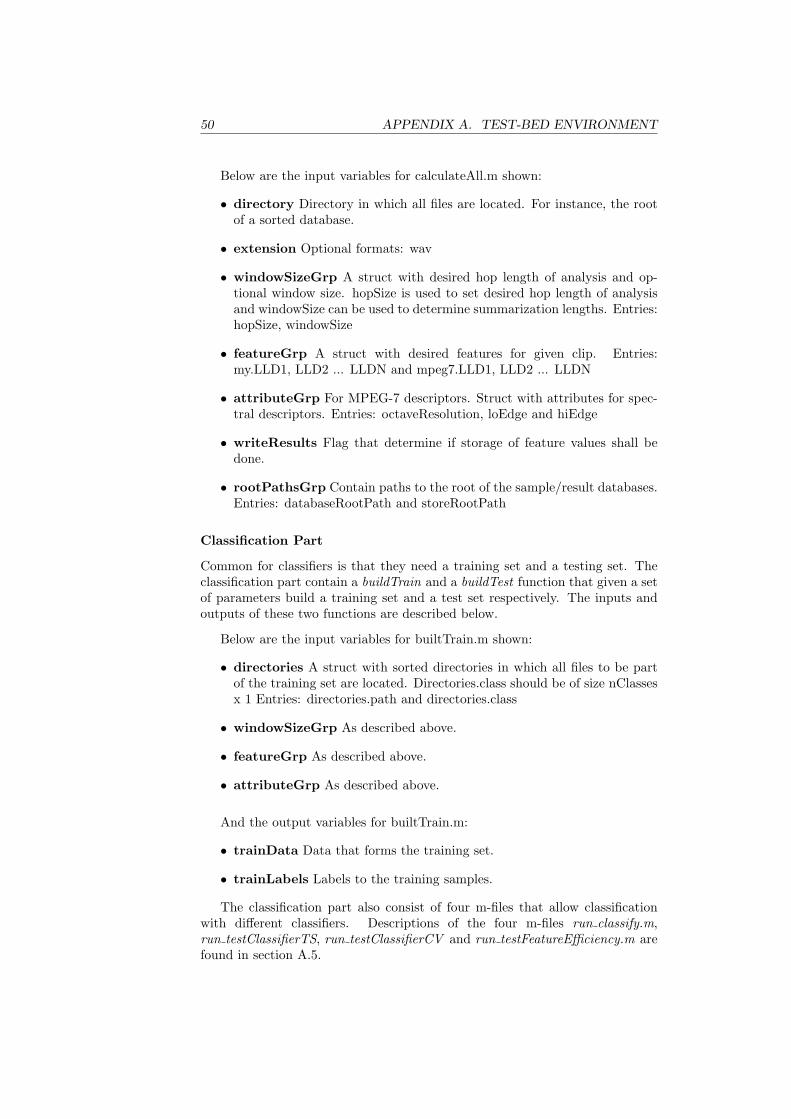
50 APPENDIX A. TEST-BED ENVIRONMENT
Below are the input variables for calculateAll.m shown:
• directory Directory in which all files are located. For instance, the rootof a sorted database.
• extension Optional formats: wav
• windowSizeGrp A struct with desired hop length of analysis and op-tional window size. hopSize is used to set desired hop length of analysisand windowSize can be used to determine summarization lengths. Entries:hopSize, windowSize
• featureGrp A struct with desired features for given clip. Entries:my.LLD1, LLD2 ... LLDN and mpeg7.LLD1, LLD2 ... LLDN
• attributeGrp For MPEG-7 descriptors. Struct with attributes for spec-tral descriptors. Entries: octaveResolution, loEdge and hiEdge
• writeResults Flag that determine if storage of feature values shall bedone.
• rootPathsGrp Contain paths to the root of the sample/result databases.Entries: databaseRootPath and storeRootPath
Classification Part
Common for classifiers is that they need a training set and a testing set. Theclassification part contain a buildTrain and a buildTest function that given a setof parameters build a training set and a test set respectively. The inputs andoutputs of these two functions are described below.
Below are the input variables for builtTrain.m shown:
• directories A struct with sorted directories in which all files to be partof the training set are located. Directories.class should be of size nClassesx 1 Entries: directories.path and directories.class
• windowSizeGrp As described above.
• featureGrp As described above.
• attributeGrp As described above.
And the output variables for builtTrain.m:
• trainData Data that forms the training set.
• trainLabels Labels to the training samples.
The classification part also consist of four m-files that allow classificationwith different classifiers. Descriptions of the four m-files run classify.m,run testClassifierTS, run testClassifierCV and run testFeatureEfficiency.m arefound in section A.5.
APPENDIX A. TEST-BED ENVIRONMENT 51
A.2 How to build a database
To simplify the evaluation procedure, the audio database should be sorted in atraining set and a testing set. This is not necessary but it is advisable to doso. If all audio clips are stored in a sorted training and testing set all calculatedfeature values will be stored in the same sorted way. That is, a sorted featurevalue database is achieved automatically.
Another practical issue about the test-bed is that the audio clips should berelatively short. The implemented feature extraction solution does not handlememory efficiently, which causes Matlab to run slow. The analysis in this thesiswas performed with clips of 30 seconds of audio. Hence, audio clips of 30 secondsare proposed to be used. A m-file to called splitFiles can be used to split allfiles in a sorted database.
Below is a numbered list that to guide users how to build a database:
1. Sample audio and store the audio clips in a sorted database.
2. If the audio files are long, use run splitFiles.m to create a new databasewith shorter clip lengths. This limits inefficient memory use in the featureextraction process.
3. Use calculateAll.m to calculate desired features. Feature values is storedin a sorted database at a desired place.
A.3 How to add new features
Implementation of new features has to follow the framework’s passing of param-eters. That is, a new feature has to have the following input fields:
• audioSampleGrp A struct with information about audio clip to analyze.Entries: fileName, audio, size, sr and nbits
• windowSizeGrp As described above.
• attributeGrp As described above.
and return the result as follows:
• Result A vector of size NxM, where N is the dimensionality of the featureand M is the time index for feature values.
Below is a numbered list to guide users how to add new features:
1. Write a m-file with input and output arguments as shown above.
2. Store the m-file in directory ”testbed\extraction\Feature Analysis......\NEWFEATURENAME\”
3. As the new feature is stored in Feature Analysis. Startup.m can be exe-cuted to set all paths for the test-bed, which allow the new feature to beused.
4. Finally, run calculateAll.m is modified to work as wanted.
52 APPENDIX A. TEST-BED ENVIRONMENT
A.4 How to add new classifiers
Implementation of new classifiers has to follow the framework’s passing of pa-rameters. That is, a new classifiers must have the following input fields:
• testData Data to be classified.
• trainData Data that forms the training set.
• trainLabels Labels to training samples.
• paramaters Classifier specific parameters.
and return the result as follows:
• predictions Predicted class labels for testData.
Below is a numbered list to guide users how to add new features:
1. Write a m-file with input and output arguments as shown above.
2. Store the m-file in directory ”testbed\classification......\CLASSIFIERNAME\”
3. As the new feature is stored in ”classification”. Startup.m can be executedto set all paths for the test-bed, which allow the new classifier to be used.
A.5 How to test new classification schemes
When features and classification algorithms are implemented they can be com-bined to form complete classification schemes. Evaluation of classificationschemes can be done in several ways and the test-bed consists of four func-tions to evaluate classifiers performance.
Below is a list of available functions and a short description of their func-tionality:
• run classify.m Defines all settings used in classify.m and runs it. Thisfunction makes predications on a single audio clip for a defined classifier.Possibility to change audio clip, training set and classifier.
• run testClassifierTS Defines all settings used in testclassifierTS.m andruns it. This function calculates the classification accuracy of a classifierfor a given training and testing set. Possibility to change training set,testing set and classifier.
• run testClassifierCV Defines all settings used in testclassifierCV.m andruns it. This function approximates the classification accuracy of a clas-sifier with n-fold cross-validation. Possibility to change training set, n in”n-fold” and classifier.
• run testFeatureEfficiency.m Defines all settings used in testFeatureEf-ficiency.m and runs it. It approximates individual features efficiency byn-fold cross-validation. Possibility to change training set, n in ”n-fold”and classifier.
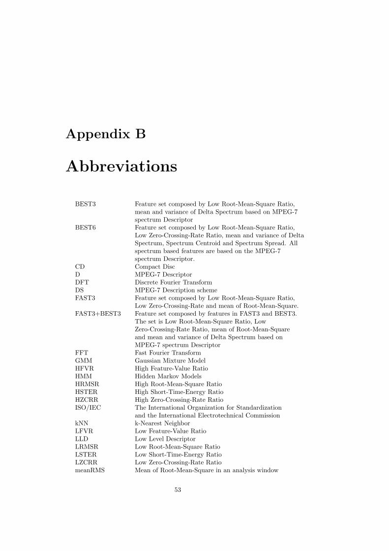
Appendix B
Abbreviations
BEST3 Feature set composed by Low Root-Mean-Square Ratio,mean and variance of Delta Spectrum based on MPEG-7spectrum Descriptor
BEST6 Feature set composed by Low Root-Mean-Square Ratio,Low Zero-Crossing-Rate Ratio, mean and variance of DeltaSpectrum, Spectrum Centroid and Spectrum Spread. Allspectrum based features are based on the MPEG-7spectrum Descriptor.
CD Compact DiscD MPEG-7 DescriptorDFT Discrete Fourier TransformDS MPEG-7 Description schemeFAST3 Feature set composed by Low Root-Mean-Square Ratio,
Low Zero-Crossing-Rate and mean of Root-Mean-Square.FAST3+BEST3 Feature set composed by features in FAST3 and BEST3.
The set is Low Root-Mean-Square Ratio, LowZero-Crossing-Rate Ratio, mean of Root-Mean-Squareand mean and variance of Delta Spectrum based onMPEG-7 spectrum Descriptor
FFT Fast Fourier TransformGMM Gaussian Mixture ModelHFVR High Feature-Value RatioHMM Hidden Markov ModelsHRMSR High Root-Mean-Square RatioHSTER High Short-Time-Energy RatioHZCRR High Zero-Crossing-Rate RatioISO/IEC The International Organization for Standardization
and the International Electrotechnical CommissionkNN k-Nearest NeighborLFVR Low Feature-Value RatioLLD Low Level DescriptorLRMSR Low Root-Mean-Square RatioLSTER Low Short-Time-Energy RatioLZCRR Low Zero-Crossing-Rate RatiomeanRMS Mean of Root-Mean-Square in an analysis window
53
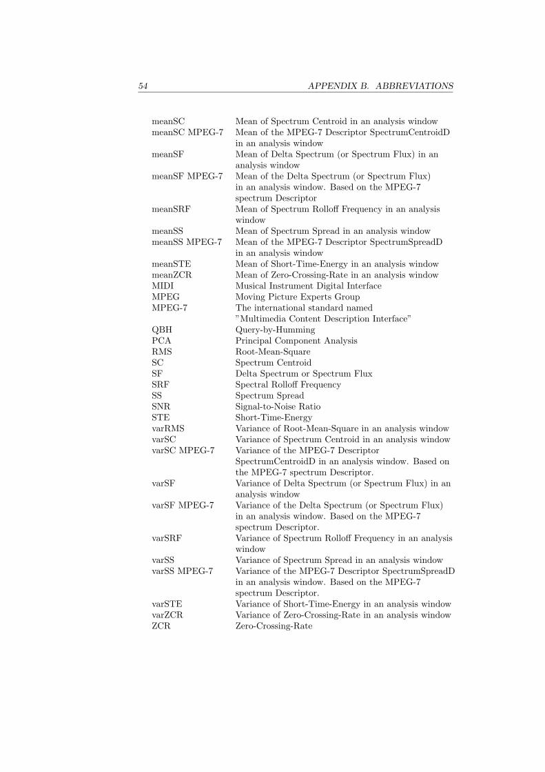
54 APPENDIX B. ABBREVIATIONS
meanSC Mean of Spectrum Centroid in an analysis windowmeanSC MPEG-7 Mean of the MPEG-7 Descriptor SpectrumCentroidD
in an analysis windowmeanSF Mean of Delta Spectrum (or Spectrum Flux) in an
analysis windowmeanSF MPEG-7 Mean of the Delta Spectrum (or Spectrum Flux)
in an analysis window. Based on the MPEG-7spectrum Descriptor
meanSRF Mean of Spectrum Rolloff Frequency in an analysiswindow
meanSS Mean of Spectrum Spread in an analysis windowmeanSS MPEG-7 Mean of the MPEG-7 Descriptor SpectrumSpreadD
in an analysis windowmeanSTE Mean of Short-Time-Energy in an analysis windowmeanZCR Mean of Zero-Crossing-Rate in an analysis windowMIDI Musical Instrument Digital InterfaceMPEG Moving Picture Experts GroupMPEG-7 The international standard named
”Multimedia Content Description Interface”QBH Query-by-HummingPCA Principal Component AnalysisRMS Root-Mean-SquareSC Spectrum CentroidSF Delta Spectrum or Spectrum FluxSRF Spectral Rolloff FrequencySS Spectrum SpreadSNR Signal-to-Noise RatioSTE Short-Time-EnergyvarRMS Variance of Root-Mean-Square in an analysis windowvarSC Variance of Spectrum Centroid in an analysis windowvarSC MPEG-7 Variance of the MPEG-7 Descriptor
SpectrumCentroidD in an analysis window. Based onthe MPEG-7 spectrum Descriptor.
varSF Variance of Delta Spectrum (or Spectrum Flux) in ananalysis window
varSF MPEG-7 Variance of the Delta Spectrum (or Spectrum Flux)in an analysis window. Based on the MPEG-7spectrum Descriptor.
varSRF Variance of Spectrum Rolloff Frequency in an analysiswindow
varSS Variance of Spectrum Spread in an analysis windowvarSS MPEG-7 Variance of the MPEG-7 Descriptor SpectrumSpreadD
in an analysis window. Based on the MPEG-7spectrum Descriptor.
varSTE Variance of Short-Time-Energy in an analysis windowvarZCR Variance of Zero-Crossing-Rate in an analysis windowZCR Zero-Crossing-Rate