ATTI - Firenze University Press

Atti

-21-

ATTI

1. Il controllo terminologico delle risorse elettroniche in rete: tavola rotonda, Firenze 27 gennaio 2000, a curadi Paola Capitani, 2001

2. Commemorazione di Michele Della Corte, a cura di Laura Della Corte, 2001

3. Disturbi del comportamento alimentare: dagli stili di vita alla patologia, a cura di Corrado D'Agostini, 2002

4. Proceedings of the third International Workshop of the IFIP WG5.7 Special interest group on Advancedtechniques in production planning & control : 24-25 February 2000, Florence, Italy, edited by Marco Garetti,MarioTucci, 2002

5. DC-2002: Metadata for E-Communities: Supporting Diversity And Convergence 2002: Proceedings of theInternational Conference on Dublin Core and Metadata for e-Communities, 2002, October 13-17, 2002,Florence, Italy, organized by Associazione Italiana Biblioteche [et al.], 2002

6. Scholarly Communication and Academic Presses: Proceedings of the International Conference, 22 March2001, University of Florenze, Italy, edited by Anna Maria Tammaro, 2002

7. Recenti acquisizioni nei disturbi del comportamento alimentare, a cura di Alessandro Casini, CalogeroSurrenti, 2003

8. Proceedings of Physmod 2003 International Workshop on Physical Modelling of Flow and DispersionPhenomena, edited by Giampaolo Manfrida e Daniele Contini, 2003

9. Public Administration, Competitiveness and Sustainable Development, edited by Gregorio Arena, Mario P.Chiti, 2003

10. Authority control: definizioni ed esperienze internazionali: atti del convegno internazionale, Firenze, 10-12febbraio 2003, a cura di Mauro Guerrini e Barbara B. Tillet; con la collaborazione di Lucia Sardo, 2003

11. Le tesi di laurea nelle biblioteche di architettura, a cura di Serena Sangiorgi, 2003

12. Models and analysis of vocal emissions for biomedical applications: 3rd international workshop: december10-12, 2003 : Firenze, Italy, a cura di Claudia Manfredi, 2004

13. Statistical Modelling. Proceedings of the 19th International Workshop on Statistical Modelling: Florence(Italy) 4-8 july, 2004, edited by Annibale Biggeri, Emanuele Dreassi, Corrado Lagazio, Marco Marchi, 2004

14. Studi per l’insegnamento delle lingue europee : atti della prima e seconda giornata di studio (Firenze, 2002-2003), a cura di María Carlota Nicolás Martínez, Scott Staton, 2004.

15. L’Archivio E-prints dell’Università di Firenze: prospettive locali e nazionali. Atti del convegno (Firenze, 10febbraio 2004), a cura di Patrizia Cotoneschi, 2004

16. TRIZ Future Conference 2004. Florence, 3-5 November 2004, edited by Gaetano Cascini, 2004

17. Mobbing e modernità : la violenza morale sul lavoro osservata da diverse angolature per coglierne il senso,definirne i confini. Punti di vista a confronto. Atti del Convegno Firenze, 20 aprile 2004, a cura di AldoMancuso, 2004

18. Lo spazio sociale europeo. Atti del convegno internazionale di studi Fiesole (Firenze), 10-11 ottobre 2003, acura di Laura Leonardi, Antonio Varsori, 2005

19. AIMETA 2005 Atti del XVII Congresso dell'Associazione Italiana di Meccanica Teorica e Applicata,Firenze, 11-15 settembre 2005, a cura di Claudio Borri, Luca Facchini, Giorgio Federici, Mario Primicerio, 2005

20. Giornata CEFTrain - CEFTrain Day. Conference Proceedings and Partner Contributions. Firenze, Italy, 7may 2005, edited by Elizabeth Guerin, 2005

MODELS AND ANALYSIS

OF VOCAL EMISSIONS

FOR BIOMEDICAL APPLICATIONS

4th INTERNATIONAL WORKSHOP

October 29-31, 2005

Firenze, Italy

Edited by

Claudia Manfredi

Firenze University Press

2005

Models and analysis of vocal emissions for biomedical applications :

4th international workshop: october 29-31, 2005 : Firenze, Italy /

edited by Claudia Manfredi. – Firenze : Firenze university press,

2005.

(Atti, 21)

http://digital.casalini.it/8884533201

Stampa a richiesta disponibile su http://epress.unifi.it

ISBN 88-8453-320-1 (online)

ISBN 88-8453-319-8 (print)

612.78 (ed. 20)

Voce - Patologia medica

Responsibility for the contents rests entirely with the authors. The editors and the organising

committee of the MAVEBA 2003 accept no responsibility for any errors, omissions, or views

expressed in this publication.

No part of this publication can be reproduced, stored in a retrieval system, or transmitted in any form

or by any means without the permission of the editors. Permission is not required to copy abstracts of

papers, on condition that a full reference of the source is given.

Cover: designed by CdC, Firenze, Italy.

© 2005 Firenze University Press

Università degli Studi di Firenze

Firenze University Press

Borgo Albizi, 28, 50122 Firenze, Italy

http://epress.unifi.it/

Printed in Italy

INTERNATIONAL PROGRAM COMMITTEE

S. Aguilera (ES) A. Barney (UK) D. Berckmans (BE) P. Bruscaglioni (I)

S. Cano Ortiz (CU) R. Carlson (SE) M. Clements (USA) J. Doorn (AR)

U. Eysholdt (D) O. Fujimura (JP) H. Herzel (D) D.Howard (UK)

A. Izworski (PL) M. Kob (D) A. Krot (BY) U. Laine (FI)

C. Larson (USA) F. Locchi (I) J. Lucero (BR) C. Manfredi (I)

C. Marchesi (I) W. Mende (D) V. Misun (CZ) C. Moore (UK)

X. Pelorson (F) P. Perrier (F) R. Ritchings (UK) S. Ruffo (I)

O. Schindler (I) A. Schuck (BR) R. Shiavi (USA) H. Shutte (NL)

J. Sundberg (SE) J. Svec (CZ) R. Tadeusiewicz (PL) I. Titze (USA)

U. Uergens (D) G.Valli (I) K. Wermke (D) W. Ziegler (D)

LOCAL ORGANISING COMMITTEE

C. Manfredi, Dept. of Electronics and Telecommunications, Faculty of Engineering - Conference Chair

L. Bocchi, Dept. of Electronics and Telecommunications, Faculty of Engineering

P. Bruscaglioni, Dept. of Physics, Faculty of Maths, Physics and Natural Sciences - Conference Chair

F. Locchi, Dept. of Clinical Physiology, Faculty of Medicine.

C. Marchesi, Dept. of Systems and Computer Science, Faculty of Engineering.

S. Ruffo, Dept. of Energetics, Faculty of Engineering.

G.Valli, Dept. of Electronics and Telecommunications, Faculty of Engineering

SPONSORS

Ente CRF – Ente Cassa di Risparmio di Firenze

ISCA - International Speech and Communication Association

AIIMB - Associazione Italiana Ingegneria Medica e Biologica

INFM – Istituto Nazionale per la Fisica della Materia

CONTENTS

Foreward................................................................................................................................ XI

Special session on Voice pathology classification

C. Berry, T. Ritchings, “A comparative study of intelligent voice quality assessment using

impedance and acoustic signals” .................................................................................................................3-6

C. J. Moore , K. Manickam, N. Slevin, “Voicing recovery in males following radiotherapy

for larynx cancer” .......................................................................................................................................7-10

N. Sáenz-Lechón, J.I. Godino-Llorente, V. Osma-Ruiz, P. Gómez-Vilda, S. Aguilera-Navarro, “A methodology to evaluate pathological voice detection systems” ......................................11-14

N. Sáenz-Lechón, J.I. Godino-Llorente, V. Osma-Ruiz, P. Gómez-Vilda, S. Aguilera-Navarro, “Effects of MP3 encoding on voice pathology detection: results with MFCC

parameters”...............................................................................................................................................15-18

J. Schoentgen, “Towards a classification of phonatory features of disordered voices”........................19-22

W. Sheta, T. Ritchings, C. Berry, “Intelligent voice quality assessment post-treatment using

genetic programming” ..............................................................................................................................23-26

Voice recovering / enhancement

H. Kuwabara, “A method for changing speech quality and its application to pathological

voices .........................................................................................................................................................29-32

R. Pietruch, A. Grzanka, W. Konopka, M. Michalska, “Methods for formant extraction in

speech of patients after total laryngectomy” ...........................................................................................33-36

C. Manfredi, C. Marino, F. Dori, E. Iadanza, ”Optimised GSVD for dysphonic voice quality

enhancement”............................................................................................................................................37-40

Special session on Physical and mechanical models and devices

T. Vampola, J. Horacek, J. Vesely, J. Vokral, “Modelling of influence of velopharyngeal

insufficiency on phonation of vowel /a/”..................................................................................................43-46

R. Zaccarelli, C. Elemans, W.T. Fitch, H. Herzel, “Two-mass models of the bird Syrinx” ..................47-50

N. Ruty, J. Cisonni, X. Pelorson, P. Perrier, P. Badin, A. Van Hirtum, “A physical model

for articulatory speech synthesis. theoretical and numerical principles” ..............................................51-54

F. Avanzini, S. Maratea, C. Drioli, “Physiological control of low-dimensional glottal

models with applications to voice source parameter matching” ............................................................55-58

Models and analysis of vocal emissions for biomedical applications. 4th international workshop. October 29-31, 2005 – Firenze, Italy. Edited by C. Manfredi. ISBN 88-8453-320-1 (online) © 2005 Firenze University Press

P. Gómez, C. Lázaro, R. Fernández, A. Nieto, J.I. Godino, R. Martínez, F. Díaz, A.Álvarez, K. Murphy, V. Nieto, V. Rodellar, F.J. Fernández-Camacho, “Us ing

biomechanical parameter estimates in voice pathology detection”........................................................59-62

R. Orr, B. Cranen, “The effect of the flow mask on phonation” .............................................................63-66

Ch. Jeannin, P. Perrier, Y. Payan, A. Dittmar, B. Grosgogeat, “A non-invasive device to

measure mechanical interaction between tongue, palate and teeth during speech

production” ...............................................................................................................................................67-70

Poster session

P. Alku, J. Horaceck, M. Airas, A.M. Laukkanen, “Assessment of glottal inverse filtering

by using aeroelastic modelling of phonation and fe modelling of vocal tract”......................................73-76

L. Bocchi, S. Bianchi, C. Manfredi, N. Migali, G. Cantarella, “Quantitative analysis of

videokymographic images and audio signals in dysphonia” ........................................ (Paper not available)

P. Bruscaglioni, “A note on jitter estimation”................................................................ (Paper not available)

M. Guarino, A. Costa, S. Patelli, M. Silva, D. Berckmans, “Cough analysis and

classification by labelling sound in swine respiratory disease” .............................................................77-80

J. Hanquinet, F. Grenez, J. Schoentgen, “Wave-morphing in the framework of a glottal

pulse model”..............................................................................................................................................81-83

T. Kitamura, P. Mokhtari, H. Takemoto, “Changes of vocal tract shape and area function

by F0 shift”................................................................................................................................................85-88

M. Kob, J. Stoffers, Ch. Neuschaefer-Rube, “Comparison of LPC analysis and impedance

vocal tract measurements” .......................................................................................................................89-91

C. Manfredi, B. Maraschi, A. Berlusconi, G. Cantarella, “Objective pre- and post-surgical

voice analysis” ................................................................................................................ (Paper not available)

V. Misun, “Source voice characteristics of the artificial vocal folds”...................................................93-96

T. Orzechowski, A. Izworski, I. Gatkowska, M. Rudzinska, “Automatic classification of

voice disorders in course of neurodegenerative disease” .....................................................................97-100

M. Sovilj, T. Adamovic, M. Subotic, N. Stevovic, “Newborn’s cry from risk and normal

pregnancies” ........................................................................................................................................101-104

K. Manickam, H. Li, “Complexity analysis of normal and deaf infant cry acoustic waves” ............105-108

Special session on Methods for voice measurements

A. Fourcin, “Clinical voice measurement using EGG/LX signals”....................................................111-114

R. Shrivastav, “From vocal quality measurement to perception” ......................................................115-118

VIII MAVEBA 2005

J.G. Svec, F. Sram, M. Fric, Q. Qiu, H.K. Schutte, “What can be seen in videokymographic

images?”....................................................................................................................................................... 119

S. Bianchi, L. Bocchi, C. Manfredi, G. Cantarella, N. Migali, “Objective vocal fold

vibration assessment from videokymographic images” ......................................................................121-124

S. Mantha, L. Mongeau, T. Siegmund, “Dynamic digital image correlation of a dynamic

physical model of the vocal folds”........................................................................................................125-128

S. Cieciwa, D. Deliyski, T. Zielinski, “Fast FFT-based motion compensation for laryngeal

high-speed videoendoscopy” ................................................................................................................129-132

H.S. Shaw, D.D. Deliyski, “Vertical motion during modal and pressed phonation:

magnitude and symmetry” ....................................................................................................................133-136

H.S. Shaw, D.D. Deliyski, “Mucosal wave magnitude: presence, extent, and symmetry in

normophonic speakers” ........................................................................................................................137-140

S.T. Takano, K.K. Kinoshita, K.H. Honda, “Measurement of cricothyroid articulation

using high-resolution MRI and 3D pattern matching”........................................................................141-144

Voice modelling and analysis

H.J. Fell, J. MacAuslan, “Vocalisation analysis tools” ......................................................................147-150

P. Svancara, J. Horacek, “Numerical modelling of effect of tonsillectomy on production of

Czech vowels /a/ and /i/” ......................................................................................................................151-154

A. Kacha, F. Grenez, J. Schoentgen, “Generalized variogram analysis of vocal

dysperiodicities in connected speech” ................................................................................................155-158

T. Wurzbacher, R. Schwarz, H. Toy, U. Eysholdt, J. Lohscheller, “Modelling of non-

stationary phonation for classification of vocal folds vibrations”......................................................159-162

F.M. Martinez, J.C. Goddard, A.M. Martinez, “Analysis of Spanish synthesized speech

signals using spectral and basis pursuit representations” ..................................................................163-166

F.R. Drepper, “Voiced excitation as entrained primary response of a reconstructed glottal

master oscillator” .................................................................................................................................167-170

J.J. Turunen, T. Lipping, J.T. Tanttu, “Speech analysis using Higuchi fractal dimension”..............171-174

Special session on Neurological dysfunctions

R. Shiavi, “Quantitative and experimental approaches for investigating neurological/

psychological dysfunction”............................................................................................. (Paper not available)

L. Cnockaert, J. Shoentgen, P. Auzou, C. Ozsancak, F. Grenez, “Effect of Parkinson’s

disease on vocal tremor” ......................................................................................................................177-180

Contents IX

K.S. Subari, D.M. Wilkes, R. Shiavi, S. Silverman, M. Silverman, “Evaluation of speaker

normalization for suicidality assessment” ...........................................................................................181-184

Infant cry – Singing voice

K. Wermke, W. Mende, A. Kempf, C. Manfredi, P. Bruscaglioni, A. Stellzig-Eisenhauer,“Interaction patterns between melodies and resonance frequencies in infants’ pre-speech

utterances” ............................................................................................................................................187-190

R. Nicollas, J. Giordano, L. Francius, J. Vicente, Y. Burtschell, M. Medale, B. Nazarian,M. Roth, M. Ouaknine, A. Giovanni, “Aerodynamical model of human newborn larynx: an

approach of the first cry”......................................................................................................................191-193

S. Adachi, J. Yu, “High-pitched voice simulation using a two-dimensional vocal fold

model” ...................................................................................................................................................195-198

J. Sundberg, “Effect of vocal loudness variation on the voice source” ..................................................... 199

N. Amir, O. Amir, O. Michaeli, “Assessing vibrato quality of singing students” .............................201-203

Non-human sounds

M. Gamba, C. Giacoma, “Vocal production mechanism in ruffed lemurs: a prosimian

model for the basis of primate phonation” ..........................................................................................207-210

J.-M. Aerts, P. Jans, D. Halloy, P. Gustin, D. Berckmans, “Labelling of cough data from

pigs for on-line disease monitoring by sound analysis”......................................................................211-214

Author Index..........................................................................................................................................215-216

X MAVEBA 2005

FOREWARD

Welcome to the 4th

International Workshop on Models and Analysis of Vocal Emissions for Biomedical

Applications, MAVEBA 2005, 29-31 October 2005, Firenze, Italy.

In the light of previous editions, held in 1999, 2001, and 2003 respectively, all in Firenze, the Workshop

aims at investigating into main aspects of voice modelling and analysis, ranging from fundamental research

to all kinds of biomedical applications and related established and advanced technologies. It offers the

participants an interdisciplinary platform for presenting and discussing new knowledge both in the field of

models and analysis of speech signals and in that of emerging imaging techniques.

Contacts between specialists active in research and industrial developments could take advantage from the

Workshop structure, comprising both Special Sessions devoted to a set of relevant topics, and standard

Sessions, covering a wide area of voice analysis research, for biomedical applications.

Four Special Session were organised and co-ordinated by specialists in the field, collecting contributions

about new and emerging techniques. Each Session is introduced by a review paper, presenting the state-of-

the-art in the field, pointing out present knowledge, limitations and future directions. The selected topics are:

1. Voice pathology classification

2. Physical and mechanical models and devices

3. Methods for voice measurements

4. Neurological dysfunctions

As for regular Sessions, the relevant topics are: voice recovering, enhancement of voice quality during

rehabilitation and after surgery, voice modelling and analysis of vocal emissions, newborn and infant cry

analysis, singing voice. A short Session is also devoted to non-human sounds, and their possible

relationships to humans.

All the papers collected in this book of Proceedings are of high scientific level, as they were reviewed by at

least two anonymous referees, and cover the most relevant fields of research in voice signals and images

analysis. We would like to thank the members of the organising committee and all the reviewers, who gave

freely of their time to assess the highly disparate work of the workshop, helping in improving the quality of

the papers.

We have also benefited from the efforts of the administrative staff within our University: office for Research

and International Relations, Logistic office, and the staff of the Faculty of Engineering and of the

Department of Electronics and Telecommunications, that devoted a lot of time and efforts to make this

workshop a successful one. Special thanks to our University Orchestra and Chorus, and to the members of

“Capriccio Armonico” dancing group for their generous participation.

Finally, our gratitude goes to the supporters and sponsors, who contribute much to the success of the

MAVEBA workshop.

Dott. Claudia Manfredi

Conference Chair

Prof. Piero Bruscaglioni

Conference Chair


Special session on

Voice pathology classification


A COMPARATIVE STUDY OF INTELLIGENT VOICE QUALITY ASSESSMENT USING IMPEDANCE AND ACOUSTIC SIGNALS

Carl Berry & Tim Ritchings

School of Computing, Science and Engineering, University of Salford, UK

[email protected]

Abstract: Objective assessment techniques for classifying voice quality for patients recovering from treatment for cancer of the larynx should lead to more effective recovery than the present approach, which is very subjective and depends heavily on the experience of the individual Speech and Language Therapist (SALT). This work follows an earlier study where an Artificial Neural Network (ANN) was trained on parameters derived from electrolaryngograph electrical impedance (EGG) signals recorded while a patient was phonating /i/ as steadily as possible, and gave an indication of voice quality inline with the standard UK Speech and Language Therapist (SALT) seven point scale. The applicability of this approach to voice quality assessment of acoustic signals is described, and the results are found to compare very well with those derived from the impedance signals. It was also noted that for both the impedance and the acoustic signals, the ANNs were able to classify the very good (recovered) and the very poor (abnormal) voices well, but performed quite badly with the mid-range classifications, raising questions about the accuracy of these classifications.

Keywords: Voice quality, classification, Artificial Neural Network, acoustic, impedance.

I. INTRODUCTION

In the UK, voice quality assessment for patients recovering from treatment for cancer of the larynx is undertaken by Speech and Language Therapists (SALT), who use a standard 7-point classification scale ranging from Lx0-Lx6, with Lx0 being a near normal (recovered) voice while Lx6 represents an abnormal, very poor quality voice. The approach taken to reach a classification is very subjective and depends to a large extent on the experience of the SALT.

This work is concerned with a series of investigations aimed at producing an intelligent computer-based system which can provide objective classifications of voice quality in patients recovering from cancer of the larynx patients in line with the UK standard 7-point classification scale.

Previous work [1,2] has demonstrated that accurate classifications could be obtained from a Multi Layer Percepton (MLP) Artificial Neural Network (ANN) which was trained on a combination short-term and long-term parameters derived from electrolaryngograph electrical impedance (EGG) signals while a patient was phonating /i/ as steadily as possible. Although, acoustic signals were recorded at the same time as the impedance signals, they were not analysed as they appeared much noisier than the EGG signals. However, classification of voice quality from the acoustic signals is advantageous, if possible, as highly specialised and expensive equipment (the electrolaryngograph) will not be necessary, and this raises the possibility of screening in a GP’s practice, rather than in the secondary care centres.

A preliminary assessment of the acoustic signals is described here, and the resulting classifications that have been achieved with the ANN approach are compared with those obtained for the impedance signals.

II. TREATMENT OF VOICE SIGNALS

A. Collection of Voice Signals

The patient’s voice data was collected by the Christie Hospital and the South Manchester hospital using an electrolaryngograph PCLX system [3]. The equipment simultaneously records the electrical impedance signal via pads placed at specific positions on the patient’s neck at the same time as the acoustic voice signal using a microphone. In these studies, the patient was attempts to steadily phonate the /i/ sound. This process means that two datasets are collected, one showing the EGG and a second showing acoustic variation, allowing for a direct comparison between the two sets. In the work only the male voices were used as the number of female voices in the dataset was too small to give an accurate assessment, a feature of the dataset is that most cancer of the larynx patients are male. Voice quality was subjectively classified by a SALT for each patient using their 7-point scale. The number of patients in each of the 7 categories is shown in Table 1.

Lx0 Lx1 Lx2 Lx3 Lx4 Lx5 Lx5 22 36 25 33 26 25 11

Table. 1. Patients in each SALT category


B. Signal Pre-processing

In order to be able to extract the short and long term parameters used in the classification process, a number of pre-processing stages were applied to the impedance and acoustic datasets. Initially the signals were stationarised to remove drift, split into 50 ms frames (Hanning windows overlapping by 25 ms) and then converted to the autocorrelation form of the signal to remove some of the noise components. Once these processes were complete, the frames wereexamined to check if they contained silence or sound. This involved comparing the frames with a sample of silence frame recorded under the same conditions, and used zero point crossing and short term amplitudes as checks. Once the silence frames havebeen removed, the remaining frames were separated into voiced and unvoiced frames; voiced frames containing vocal phonation while unvoiced

containing no recognisable speech. This was achieved using the cepstrum based approach as described in [4]. The Fundamental Harmonic Normalisation (FHN) as described in [5] was then calculated from Power Spectrum Density (PSD) and then this structure (typical examples are shown in Fig 2) was modelled by fitting a Gaussian Mixture Model (GMM) in order to reduce the number of parameters needed to describe the signal.

C. Parameter Extraction

A total of 22 short and long term parameters are extracted for use with classification, as detailed in [1,2]. The short term parameters consist of 15 parameters relating to the mean, standard deviation and peak of the gaussians used to describe the fundamental frequency and first four harmonics in the frame (if they can be detected); the value of the fundamental frequency in each frame (F0), the noise threshold value (N0), the FHN Noise Energy

Figure 2a FHN plot of good quality impedance signal Figure 2b FHN plot of good quality acoustic signal

Figure 2c FHN plot of poor quality impedance signal Figure 2d FHN plot of poor quality acoustic signal

4 MAVEBA 2005

(FHNNE) and the Residual Harmonic Energy (RHE). The 3 long-term parameters were extracted from the speaker’s whole voiced speech. These included the mean fundamental frequency across all frames (MF0), a measure of jitter of the fundamental frequency between frames (J0) and the ratio of voiced to unvoiced frames.

D. The classification technique

Once the parameters have been extracted, a 3 layer feed-forward ANN with a sigmoidal activation function in the hidden layer, and using backpropagation of errors, is used for classification purposes. The ANN had 22 inputs, one for each of the short-term and long-term parameters derived from the voice signals, and 7 outputs, corresponding to the SALT categories. The “leave one out” cross validation strategy was used as it generally regarded as one of the most accurate methods and by leaving out a single patient’s voice sample we can ensure to avoid inter versus intra speaker effects [2].

3. COMPARISON OF IMPEDANCE AND ACOUSTIC SIGNALS

A. Observed differences between the signal types.

When the FHN spectra of the impedance and acoustic signals were examined visually, a number of differences can be observed. Figs. 2a and 2b show the spectra derived for of a good quality pathological voice (Lx0) for the impedance and acoustic signals respectively. A clear difference it that for the impedance signal, the largest peak belongs to the fundamental frequency, whilst in the acoustic signal it is the 1st harmonic. This is normal and corresponds to the pattern that would be expected from a human voice. However, even in this good quality voice the acoustic signal only shows six harmonics, as compared for eleven for the impedance signal. It should also be noted that the peak of the fundamental frequency is very small in the acoustic signal, making it difficult to detect with the techniques used for the impedance signals.

This figure also shows typical FHN impedance (Fig 2c) and acoustic (Fig 2d) spectra for a poor quality

voice (Lx5). Again, the impedance signal shows many more harmonic structures. This reduction of harmonics also has an impact on the number of parameters that are available for use with the classification algorithms, and in the case of fig 2b, for example, it would only be possible to extract short term parameters for the fundamental frequency and the first 2 harmonics meaning that the model would be missing 6 short term parameters relating to the 4th and 5th harmonics. In some cases the situation is even worse, and in the extremely bad voices or very poor frames, it is not unusual to find the fundamental frequency and a single harmonic as the only recognisable structures.

Finally, it may be seen from Fig 2d that the acoustic signal suffers from far more noise between the harmonics than the impedance signal, making it much more difficult to fit the Gaussian Mixture Models. This also causes the centres of the harmonic structures to be shifted away from their correct positions in the FHN.

B. Classification differences between the signal types.

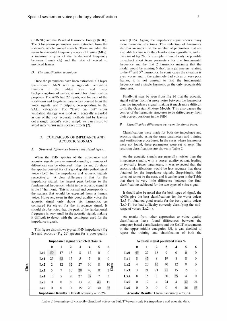
Classifications were made for both the impedance and acoustic signals, using the same parameters and training and verification procedures. In the cases where harmonics were not found, these parameters were set to zero. The resulting classifications are shown in Table 2.

As the acoustic signals are generally noisier than the impedance signals, with a poorer quality output, leading to typically fewer parameters, it was expected that the acoustic classifications would be less accurate that those obtained for the impedance signals. Surprisingly, this turns out to not be the case, and it can be seen in the Table that there is very little difference between the final classifications achieved for the two types of voice signal.

It should also be noted that for both types of signal, the ANNs give the best classifications for the worst voices (Lx5-6), obtained good results for the best quality voices (Lx0-1), but had difficulty correctly classifying the mid- range of voices (Lx2-4).

As results from other approaches to voice quality classification have found differences between the computer-based classifications and the SALT assessments in the upper middle categories [5], it was decided to repeat the training and classification of both the

Impedance signal predicted class %

0 1 2 3 4 5 6

Lx0 50 17 13 8 12 0 0

Lx1 25 48 15 5 7 0 0

Lx2 2 12 12 27 30 8 10

Lx3 5 7 10 28 40 8 2

Lx4 13 5 8 27 37 7 3

Lx5 0 0 8 13 20 43 15

Cla

ss

Lx6 0 0 0 15 20 30 35

Acoustic signal predicted class %

0 1 2 3 4 5 6

Lx0 45 27 18 9 0 0 0

Lx1 8 47 8 19 8 8 0

Lx2 4 20 16 40 12 8 0

Lx3 3 21 21 21 15 15 3

LX4 8 15 8 30 35 4 0

Lx5 0 12 4 24 4 32 24

Cla

ss

Lx6 0 0 0 0 9 36 55

Impedance Results : Overall accuracy = 36.2% Acoustic Results : Overall accuracy = 35.7%

Table 2. Percentage of correctly classified voices on SALT 7-point scale for impedance and acoustic data.

Special session on voice pathology classification 5

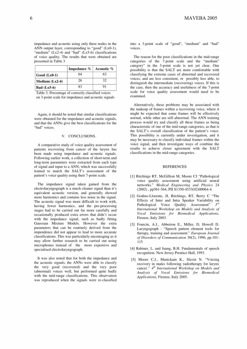
impedance and acoustic using only three nodes in the ANN output layer, corresponding to “good” (Lx0-1), “medium” (Lx2-4) and “bad” (Lx5-6) classifications of voice quality. The results that were obtained are presented in Table 3.

Again, it should be noted that similar classifications were obtained for the impedance and acoustic signals, and that the ANNs give the best classifications for the “bad” voices.

V. CONCLUSIONS.

A comparative study of voice quality assessment of patients recovering from cancer of the larynx has been made using impedance and acoustic signals. Following earlier work, a collection of short-term and long-term parameters were extracted from each type of signal and input to a ANN, which was successfully trained to match the SALT’s assessment of the patient’s voice quality using their 7-point scale.

The impedance signal taken gained from the electrolaryngograph is a much cleaner signal than it’s equivalent acoustic version, and generally showed more harmonics and contains less noise in the signal. The acoustic signal was more difficult to work with, having fewer harmonics, and the pre-processing stages had to be carried out far more carefully and occasionally produced extra errors that didn’t occur with the impedance signal, such as badly fitting Gaussian Mixture Models. However the extra parameters that can be routinely derived from the impendence did not appear to lead to more accurate classifications. This was particularly encouraging as it may allow further research to be carried out using microphones instead of the more expensive and specialised electrolaryngograph.

It was also noted that for both the impedance and the acoustic signals, the ANNs were able to classify the very good (recovered) and the very poor (abnormal) voices well, but performed quite badly with the mid-range classifications. This observation was reproduced when the signals were re-classified

into a 3-point scale of “good”, “medium” and “bad” voices.

The reason for the poor classifications in the mid-range

categories of the 7-point scale and the “medium” category” in the 3-point scale is not yet clear. One possibility is that the SALT are more comfortable with classifying the extreme cases of abnormal and recovered voices, and are less consistent, or possibly less able, to distinguish the intermediate (recovering) voices. If this is the case, then the accuracy and usefulness of the 7-point scale for voice quality assessment would need to be examined.

Alternatively, these problems may be associated with the makeup of frames within a recovering voice, where it might be expected that some frames will be effectively normal, while other are still abnormal. The ANN training process would try and classify all these frames as being characteristic of one of the mid-range categories, as that is the SALT’s overall classification of the patient’s voice. This possibility is currently under investigation, and it may be necessary to classify individual frames within the voice signal, and then investigate ways of combine the results to achieve closer agreement with the SALT classifications in the mid-range categories.

REFERENCES

[1] Ritchings RT, McGillion M, Moore CJ “Pathological voice quality assessment using artificial neural networks.” Medical Engineering and Physics 24 (2002) , pp561-564, PII S1350-4533(02)00064-4.

[2] Godino-Llorente, JI, Ritchings, RT, Berry C “The Effects of Inter and Intra Speaker Variability on Pathological Voice Quality Assessment” 3rd

International Workshop on Models and Analysis of Vocal Emissions for Biomedical Applications, Firenze, Italy 2003.

[3] Fourcin, A.J., Abberton E., Miller, D, Howell D. Laryngograph : “Speech pattern element tools for therapy, training and assessment.” European Journal of Disorders of Communication 30(2), 1996, pp.101-115

[4] Rabiner, L. and Juang, B.H. Fundamentals of speech recognition. New Jersey Prentice Hall, 1993.

[5] Moore C.J., Manickam K., Slavin N. “Voicing recovery in males following radiotherapy for larynx cancer.” 4th International Workshop on Models and Analysis of Vocal Emissions for Biomedical Applications, Firenze, Italy 2005.

Impedance % Acoustic %

Good (Lx0-1) 64 63

Medium (Lx2-4) 26 32

Bad (Lx5-6) 83 91

Table 3. Percentage of correctly classified voices on 3-point scale for impedance and acoustic signals

6 MAVEBA 2005

Abstract: Larynx cancer patients receive radiotherapyas a non-invasive alternative to surgery and cure ratesare high. Inevitably this impacts vocal fold functional-ity. Hence, voice recovery as a pre-requisite for re-suming normal life is of special interest. Voicing re-covery following radiotherapy is studied in this paper.

Complexity analysis, using approximate entropy toconcisely quantify the collective spectral patternderived from the electro-glottogram, has revealed adouble banded male normal voicing referencestandard. Forty-eight male larynx cancer patientshave been studied by applying this technique inparallel with an unrestricted perceptual analysisbefore and one year after radiotherapy.

Two thirds of radiotherapy patients had improvedvoice quality one year after treatment. Approximateentropy increased to reach normal populationreference levels. These patients were predominantly inthe less aberrant perceptual categories. However, aquarter of patients showed reduced approximateentropy and were predominantly in the most aberrantperceptual categories.

Complexity analysis has the potential to be areliable, single parameter measure of voicing qualityfor use in monitoring radiotherapy patient recovery.

I. INTRODUCTION

United Kingdom cancer statistics for 2001 show thatthe larynx is the site for nearly a third of all 7820 newhead and neck cancers and that well over 4 times as manymen than women suffered from the disease [1]. Hence, itis as prevalent as cervix cancer in women, though itattracts far less public attention. The five year survival oflarynx cancer patients following treatment is good, atapproximately two-thirds. Hence, quality of life in termsof voice preservation is important for a large number ofindividuals wishing to resume normal life.

Radiotherapy arguably has fewer side effects thansurgery, which is self evidently more invasive. However,the measure of recovery of voice quality afterradiotherapy has not been concisely and objectivelyquantified. Irradiation effects may leave the targetedtissues intact but they do impact the tissue mechanics andperturb vocal fold functionality for months after treatment[2], which in turn directly influence voice quality [3-6]

Speech and Language Therapists (SALTs) working atthe Christie Hospital have been engaged to assess theimpact of radiotherapy one year after treatment. Apatient’s normal voice, prior to the appearance of cancer,is rarely recorded. Hence, SALT subjective assessmentreflects experience and the audibility of aberrant voicing.Inevitably this is complicated by differences in clinicaltechnique and opinion [7]. Assessment at the Christie,requires patients to phonate vowels and provide a sampleof connected speech. An electro-glottogram (EGG) andacoustic digital recording form the core record of such anexamination [8]. The VPAS scheme guides assessmentwith voice quality eventually binned into a multi-categoryscale, which, at its most challenging, ranges from 0(normal) to 6 (severely aberrant). Throughout assessmenta SALT knows the phase of treatment reached by thepatient, which, along with full knowledge of the stage ofthe cancer itself and examinations such as endoscopy,inevitably heightens expectations and introduces bias.

Mathematical analysis of the entire range of spectralfeatures in voicing is rarely deployed in the routinecancer clinic. Most disconcertingly there is no definitionof what constitutes normal voicing and therefore noscientific or physical reference standard. As a result, ithas not been possible to explain how cancer patientssubjected to intense vocal fold irradiation duringradiotherapy can recover vocal fold functionality to alevel that could be considered to be “normal”.

This paper shows that vocal fold vibration asevidenced through the EGG impedance time series ofvowel phonation can be deployed to differentiate thehealthy normal population, quantify cancer patientvoicing and to track the pattern of cancer patient recoveryfollowing radiotherapy. The approach reported is basedon the regularity statistic ‘approximate entropy’ (ApEn)[9] applied for the first time to detect collective changesacross the entire EGG spectral pattern.

II. THEORY

Vowel phonation is predominantly driven by vocalfold vibration. Vocal folds function is impaired byphysical damage arising from malignant disease andassociated therapy. Fold vibration is accompanied byimpedance variations across the thyroid area. These trans-larynx impedance changes can be detected duringphonation using a laryngograph. Successivemeasurements form a time series that usually has a

VOICING RECOVERY IN MALES FOLLOWINGRADIOTHERAPY FOR LARYNX CANCER

C J Moore1 , K Manickam1, and N Slevin2

1North Western Medical Physics, HQ at Christie Hospital NHS Trust, Manchester, UK2Clinical Department of Oncology, Christie Hospital NHS Trust, Manchester UK


distinctive waveform structure that is known as the EGG[1,2]. This correlates well with vocal fold vibration and isvirtually free from tract resonance. The EGG has notfound widespread use amongst SALTs, at least in the UK.Sustained vowel phonation produces a more or lessregular EGG waveform, which is ideally suited tocharacterisation in the frequency domain via the changesseen in the corresponding power spectral pattern [10,11].

To generate an EGG spectrum, the EGG timeseries are segmented into short frames, stationarised byfinite differencing, variance reduced with a suitablefunction such as the Hanning window, autocorrelated andthen fast Fourier transformed. This produces a sequenceof frame power spectral density estimate (fPSD) [3].However, the dynamic effects of fundamental frequencyvariation from frame to frame need to be removed inorder to maximally reveal spectral shape. Therefore, thefPSD are individually normalised relative to thefrequency and power of the frame fundamental (F0) itself.This fundamental harmonic normalisation approachproduces what the authors call the FHN-PSD for eachframe in which all features are on a common normalisedharmonic scale rather than frequency scale [12]. Theframe FHN-PSD can then be averaged to reinforce anyshared spectral pattern ready for characterisation. Anormal individual would be expected to have vocal foldsthat vibrate most regularly, producing rich harmonicpatterns within an envelope showing lengthy decay. Ifthese patterns have common characteristics, and theliterature is full of examples, then a suitable form ofregularity statistic sensitive to the collective pattern willresolve this into a useful normal population referencestandard.

In a single value ApEn quantifies the repeatabilityof the pattern sampled from a time series itself. Noassumptions need to be made about the shape orfunctional basis of the patterns being sought. Given Ndata points {u(i)}=u(1),u(2),..,u(N) and commencing withthe thi point, vector sequences ( )1x~ to ( )1mNx~ +− areformed from m values ( ) ( ) ( )[ ]1miu,...,iuix~ −+= .The Pincus ApEn [9] is interpreted heuristically as ameasure of the average logarithmic likelihood, over allsequences ( )1x~ to ( )1mNx~ +− , such that any sequencein the data series ( ){ }iu , which is within a tolerance r ofthe given sequence ( )ix~ of length m , remains withinthe same tolerance when the length of both sequences isincreased by one data point. Tolerance r is proportionalto the measured series standard deviation σ , i.e. r = k σwhere k is a constant. It is necessary to determine kempirically so that the widest range of complexity valuesis achieved. ApEn had been used to study complexitychanges in cardiac ECG time series, which show thepresence or absence of vital, highly individual feedbackmechanisms placing demands on the heart.

ApEn was primarily developed for use in time seriesanalysis and was not used for characterising changes inthe spectral pattern, being reserved for comparingfluctuations in a small number of pre-selected peaks. Inthe realms of speech analysis Moore et al reported thedevelopment of a vowel phonation reference standard infor normal males using the ApEn of the truncated FHN-PSD spectral pattern considered collectively [13].

Cancer patients with malignant lesions, possiblyinfiltrating the vocal folds, would be expected to haveabnormal voicing characteristics. However, patientspresent with cancer in different stages of developmentand their treatment planned accordingly. Consequently,their vowel FHN-PSDs and corresponding ApEn valuesmight reasonably be expected to vary from nearly normalto completely aberrant. Moore et al [13] have shown thatthis is indeed the case. Clinical opinion [2] suggests thatthe most obvious side effects of curative radiotherapy arelikely to resolve, leaving stabilised voicing, after oneyear. In this paper pre-therapy and one year post-therapyApEn complexities, derived from vowel phonation, arecompared. The aim is to identify recovery patterns inmale larynx cancer patients, relative to the ApEnreference standard already established for normal males.

III. METHODOLOGY

Eighty-nine male volunteers provided the referencestandard for this study. Each subject was connected to aan electro-laryngograph and asked to phonate sustainedvowel /i/ for up to 4 seconds. The output impedancesignal was digitised at a sampling rate of at 20kHz. Thedigital EGG data files, excluding 4 compromised files,were subjected to ApEn complexity analysis usingsoftware written in IDL from Research SystemsInternational (UK). This software first stationarised thetime series to remove background noise and mainscontamination. The resultant time series were then splitinto consecutive data frames, each 1000 samples long.The auto-covariance of each frame was computed and themaximum used to determine F0. A multiplicative Hanningwindow was applied to each frame to reduce the varianceat high lags before estimating the PSD by fast Fouriertransformation. Each frame PSD was then normalisedusing the FHN approach described by Moore et al [12].This left the harmonics as integer multiples of the frameF0 with all other spectral components at non-integermultiples. The frame FHN-PSD were then averaged foreach subject. Since, spectral shape variation in andaround the normalised F0 peak is minimal, by design, theaveraged FHN PSD was removed below the maximum ofthe first true harmonic peak, H2, and above the maximumof the seventh harmonic peak, H8. The logarithm of thetruncated FHN PSD was then taken in order to minimiseany trend in the spectral pattern. ApEn values were thencalculated as described by Moore et al. [13]

8 MAVEBA 2005


Forty-eight male larynx cancer patients attending the

Christie Hospital for radiotherapy, volunteered and were

consented for approved study. EGG data was collected

prior to and one year after radiotherapy and ApEn

analysed as described for the normal voicing volunteers.

On both occasions each patient was also perceptually

assessed by an experienced SALT. No restriction was

imposed on the data used for the perceptual assessment,

which included acoustic data and access to patient

hospital records. Guided by VPAS, the SALT categorised

patient voice quality onto a seven point scale ranging

from normal (category-0, CAT0) to completely aberrant

(category-7, CAT7).

IV. RESULTS

Fig. 1 shows the ApEn complexity distribution for the

healthy male normals reported by Moore et al. The

bimodal nature of these data was tested by Gaussian

mixtures model fitting using maximum likelihood [28].

They concluded (p<0.001) that two normal groups G1

and G2 existed, characterised by complexity values 0.340

(+/- 0.035) and 0.183 (+/- 0.057) with relative weights

62% and 38% respectively. Members of G1 exhibited

strong EGG FHN-PSD features whilst those in G2 were

weak, especially in the higher frequency harmonics.

ApEn

0

0.1

0.2

0.3

0.4

0.5

0 20 40 60 80

Subject Number

Fig. 1

ApEn (crosses) for normal males. G1 (upper) and

G2 (lower) population means are full horizontal

lines. Standard deviations are dashed lines above

and below.

Fig. 2 and Fig. 3 show the ApEn complexity results for

larynx cancer patients measured before and, health

permitting, one year after radiotherapy, arranged by pre-

treatment SALT perceptual category, CATn (n=1,2,…7).

Post treatment categorisation is indicated by single digit

numbers placed side-on and above the CAT indication.

Dashed boxes indicate the G1 and G2 standard deviation

boundaries as a complexity reference standard for normal

voicing. Patients showing increased ApEn after treatment

appear in Fig. 2 whilst patients showing reduced ApEn

appear in Fig. 3. ApEn values before treatment are

indicated using circular symbols, whilst triangular

symbols indicate those one year post treatment.

ApEn

0

0.1

0.2

0.3

0.4

1 0 1 0 2 0 0 0 1 1 3 1 1 3 4 0 2 0 2 1 3 2 5 0 4 5 3 2 3 0 2

NIL 0 2 0 1 6 3 1 0 4 1 4 0 5

NIL

NIL 2

CAT 0 CAT 1 CAT 2 CAT 3 CAT 4 CAT 5 CAT 6

Patient.Categorisation

Fig. 2

Patients with increased ApEn 1 year after treatment.

ApEn

0

0.1

0.2

0.3

0.4

1 0 1 0 2 0 0 0 1 1 3 1 1 3 4 0 2 0 2 1 3 2 5 0 4 5 3 2 3 0 2

NIL 0 2 0 1 6 3 1 0 4 1 4 0 5

NIL

NIL 2

CAT 0 CAT 1 CAT 2 CAT 3 CAT 4 CAT 5 CAT 6

Patient.Categorisation

Fig. 3

Patients with decreased ApEn 1 year after treatment.

V. DISCUSSION

Of the 48 cancer cases considered, ApEn analysis

indicated that one year after radiotherapy two-thirds

would develop improved vocal fold functionality and

the G1 and G2 reference standards). Only one quarter ofcases would be below normal voicing bounds anddistinctly pathological.

Fig. 2 demonstrates that patients assigned a lessaberrant pre-treatment category by SALT perceptualanalysis have improved ApEn post treatment. This takesthe individual into a normal voicing pattern, with spectralfeatures enhanced at least to the lower level of normalityseen in the G2 male population. Those individualsalready in the G2 normal band prior to treatmentpredominantly improve after one year to becomemembers of the ideal G1 population characterised by welldeveloped harmonics in the vowel FHN-PSD.

Fig. 3 shows the converse is true for patients assignedby SALT perceptual analysis to the most aberrant pre-treatment categories. Whilst a handful show almost nochange, many deteriorate and actually fall below thenormal band defined by the G2 male population.

In 28 cases, the direction of complexity analysischanges agreed with SALTs perceptual assessment. Outof nine cases where the SALT indicated a largeimprovement, only four showed a correspondingimprovement in complexity and five showed a reductionin complexity. The ApEn spectral evidence for thesecases prompted SALT re-assessment of three individualsand a reduced categorisation more in line with thatsuggested by ApEn analysis.

What must not be forgotten, as mentioned in theintroduction, is that the direction of change in SALTcategorisation is undoubtedly biased since the SALTsmust be aware of the patients’ details including theirtreatment stage and pre-treatment categorisation. Theyexpect an improvement in patients’ voice quality one-year after radiotherapy. It is plausible that, in the contextof SALT dealings with cancer patients, the perceptualdefinition of normal voicing equates to the lower ApEn,G2 reference standard. This would explain how SALTscould describe post-cancer, post-irradiation individuals asentirely normal in CAT0. These factors could be pursuedfurther if unlabelled recordings were used for normalvolunteers and patients taken pre and post treatment.

Most of the differences between SALT perception andApEn complexity analysis occur in CAT 4-5. The authorsbelieve that where patients present before radiotherapywith poor voicing then it is simply easier to perceptuallydetect, and as a result overate, voice improvements.Furthermore, it should be remembered that the utility ofperceptual categorisation depends on reliability. In thisstudy there is some evidence, though not conclusive, thatperceptual categorisation onto a 7 point scale has astandard deviation of at least 1 bin, i.e. a variation of upto 2 bins, is highly likely.

VI. CONCLUSION

Spectral ApEn complexity analysis of trans-larynximpedance measurements has allowed the recoverypattern of vocal fold functionality and voicing in maleradiotherapy cancer cases to be examined. Using a singleobjective parameter to quantify the collective spectralpattern of vowel phonation, the majority of radiotherapypatients are seen to recover to levels of normality seen inthe general, healthy population. Many patients recover tothe normal G2 band with its characteristically weakharmonic structures. This probably reflects residualdamage that SALTs find entirely acceptable.

REFERENCES

[1] Cancer-Stats Incidence, CRUK, March 2005.[2] Benninger, S, Gillen J, Thieme P, et al, ‘Factorsassociated with recurrence & voice quality followingradiation therapy for T1 & T2 glottic carcinomas.’Laryngoscope, vol. 104(3), pp. 294-8, 1994.[3] Hoyt D, Lettinga J, Leopold K & Fisher S, ‘The Effect ofHead & Neck Radiation Therapy on Voice Quality’,Laryngoscope, vol.102, pp. 477-480, 1992.[4] Moore C, Slevin N , Winstanley S, et al, ‘ComputerisedQuantification & 3D-Visualisation of Voice QualityChanges following Radiotherapy for Carcinoma of theLarynx’, Brit Comp Soc Procs- Current PerspectivesHealthcare Computing, pp. 137-145, 1999.[5] Spector J G, Sessions D G, Chao K C et al, ‘Stage I (T1,M0, N0) Squamous Cell Carcinoma of the LaryngealGlottis: Therapeutic Results & Voice preservation’, Headand Neck, pp. 707-717, 1999.[6] Verdonck-De Leeuw I & Koopmans-Van Beinum F,‘The effect of radiotherapy on various acoustical, clinicaland perceptual pitch measures’, Procs ICPhS Stockholm4,pp. 610-613. 1995.[7] Baken R & Orlikoff, ‘Voice measurement: Is MoreBetter?’, Logopedics Phoniatrics Vocology, vol. 22:4, pp.147-151, 1997.[8] Fourcin A, ‘Electrolaryngographic Assessment of VocalFold Function’, Jnl Phonetics, vol. 14, pp. 435-442, 1986.[9] Pincus S M, ‘Approximate Entropy as a Measure ofSystem Complexity’. Proc. Natl. Acad. Sci. USA, vol.15; 88 (6), pp. 2297-2301, 1991[10] Priestley M, Spectral Analysis & Time Series,Academic Press. 1981[11] Rabiner L & Schafer R, Digital Processing of SpeechSignals, Prentice Hall, USA, 1978.[12] Moore C, Slevin N & Winstanley S, ‘CharacterisingVowel Phonation By Fundamental Spectral Normalisation ofLx-Waveforms’, Procs Intl Workshop Models & Analysis ofVocal Emissions for Biomedical Appls, Florence, Italy, pp.1-6, 1999.[13] Moore C, Manickam K, Willard T et al, ‘SpectralPattern Complexity Analysis & The Quantification ofSpeech Normality in Healthy & Radiotherapy PatientGroups’, Med Eng Phys, vol. 26, pp, 191-301, 2004.

10 MAVEBA 2005

Abstract: This paper describes some methodological issues to be considered when designing systems for automatic detection of voice pathology, in order to allow comparisons with previous or future experiments.

The proposed methodology is built around Kay Elemetrics voice disorders database, which is the only one commercially available. Discussion about key points on this database is included.

Any experiment should have a cross-validation strategy, and results should supply, along with the final confusion matrix, confidence intervals for all measures. Detector performance curves such as DET plots are also considered.

An example of the methodology is provided, with an experiment based on short-term parameters and Multi-layer Perceptrons.

Keywords: Voice pathology detection, pathological voice databases, cross-validation, Multi-Layer Perceptrons.

I. INTRODUCTION

In the last decade there has been a lot of work done on

automatic detection and classification of voice pathologies, by means of acoustic analysis, parametric and non parametric feature extraction, automatic pattern recognition or statistical methods. A lot of research groups in speech technology have addressed in some moment these problems. However, there is a lack of uniformity in these approaches that makes very difficult to estate valid conclusions throughout the proposed methods.

As it is impossible to compare results when the experiments are performed with a private database, we have decided to concentrate on works with Kay Elemetrics database [1], which is rather extended. But even when this database was employed in the state of the art, there were many differences in the way the files were chosen and handled. Also, the experiments were carried out with such different criteria, that comparisons were fruitless. We aim to develop a method that allows comparing results from different classifiers and features.

Detection of voice pathology is much related to a speaker verification task, where a candidate sample is compared against two different models (target and impostors vs. normal and pathological). The system must provide a hard decision and a confidence score about to which model belongs the sample. So

we have adopted some methodological issues that are usual in speaker verification [2].

The paper is organized as follows: Section II covers the Kay Elemetrics database and discusses some of its particularities. Section III contains an overview of previous work on pathological voice detection using this database. Sections IV and V present the proposed methodology and describe a simple experiment of detection based upon it. Finally, Section VI presents discussion and conclusions.

II. KAY’S DATABASE OVERVIEW

Kay Elemetrics database [1] was delivered in 1994. It was recorded by the MEEI Voice and Speech Lab. and in Kay Elemetrics. It contains recordings of sustained phonation of vowel /a/ (53 normal and 657 pathological) and continuous speech, (53 normal and 661 pathological). For this description we will focus on the former ones.

The database also includes clinical and personal details of the subjects and acoustic analysis data for the recordings, extracted with the Multi-Dimensional Voice Program (MDVP). The recordings were performed in matching acoustic conditions, using Kay Computerized Speech Lab (CSL). Every subject was asked to produce a sustained phonation of vowel /a/ at a comfortable pitch at loudness for at least 3 seconds. The process was repeated three times for each subject, and a speech pathologist chose the best sample for the database.

Although the database is the most widespread and available of all the voice quality databases, it has some key points that should be carefully taken into account when used for research purposes:

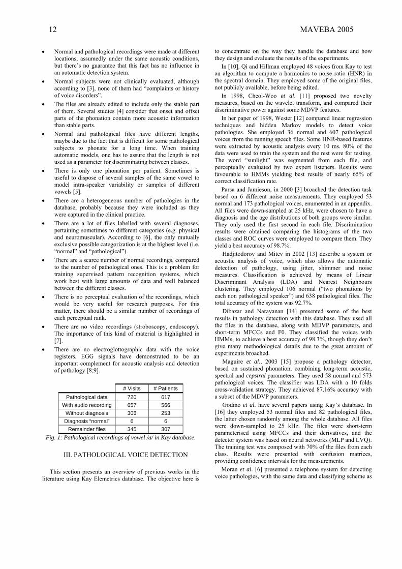
• Not all the pathological patients have a corresponding recording nor diagnose, and there are some patients with more than one recording, from different visits to the clinic. Fig. 1 shows detailed information about the pathological subset of recordings of vowel /a/.

• The files have different sampling frequencies. Normal and a small percentage of pathological files have 50 kHz, whereas most of the pathological ones have 25 kHz. All files should be down-sampled to 25 kHz before further processing.

A METHODOLOGY TO EVALUATE PATHOLOGICAL VOICE

DETECTION SYSTEMS

Nicolás Sáenz-Lechón1, Juan I. Godino-Llorente2, Víctor Osma-Ruiz2, Pedro Gómez-Vilda3, Santiago Aguilera-Navarro1

1 Dept. Tecnología Fotónica, E.T.S.I. Telecomunicación, Universidad Politécnica de Madrid, Ciudad Universitaria, 28040 Madrid (Spain)

2 Dept. Ingeniería de Circuitos y Sistemas, Universidad Politécnica de Madrid, Spain. 3 Dept. Arquitectura y Tecnología de Sistemas Informáticos, Universidad Politécnica de Madrid, Spain.


• Normal and pathological recordings were made at different locations, assumedly under the same acoustic conditions, but there’s no guarantee that this fact has no influence in an automatic detection system.

• Normal subjects were not clinically evaluated, although according to [3], none of them had “complaints or history of voice disorders”.

• The files are already edited to include only the stable part of them. Several studies [4] consider that onset and offset parts of the phonation contain more acoustic information than stable parts.

• Normal and pathological files have different lengths, maybe due to the fact that is difficult for some pathological subjects to phonate for a long time. When training automatic models, one has to assure that the length is not used as a parameter for discriminating between classes.

• There is only one phonation per patient. Sometimes is useful to dispose of several samples of the same vowel to model intra-speaker variability or samples of different vowels [5].

• There are a heterogeneous number of pathologies in the database, probably because they were included as they were captured in the clinical practice.

• There are a lot of files labelled with several diagnoses, pertaining sometimes to different categories (e.g. physical and neuromuscular). According to [6], the only mutually exclusive possible categorization is at the highest level (i.e. “normal” and “pathological”).

• There are a scarce number of normal recordings, compared to the number of pathological ones. This is a problem for training supervised pattern recognition systems, which work best with large amounts of data and well balanced between the different classes.

• There is no perceptual evaluation of the recordings, which would be very useful for research purposes. For this matter, there should be a similar number of recordings of each perceptual rank.

• There are no video recordings (stroboscopy, endoscopy). The importance of this kind of material is highlighted in [7].

• There are no electroglottographic data with the voice registers. EGG signals have demonstrated to be an important complement for acoustic analysis and detection of pathology [8;9].

# Visits # Patients Pathological data 720 617

With audio recording 657 566 Without diagnosis 306 253 Diagnosis “normal” 6 6

Remainder files 345 307 Fig. 1: Pathological recordings of vowel /a/ in Kay database.

III. PATHOLOGICAL VOICE DETECTION

This section presents an overview of previous works in the literature using Kay Elemetrics database. The objective here is

to concentrate on the way they handle the database and how they design and evaluate the results of the experiments.

In [10], Qi and Hillman employed 48 voices from Kay to test an algorithm to compute a harmonics to noise ratio (HNR) in the spectral domain. They employed some of the original files, not publicly available, before being edited.

In 1998, Cheol-Woo et al. [11] proposed two novelty measures, based on the wavelet transform, and compared their discriminative power against some MDVP features.

In her paper of 1998, Wester [12] compared linear regression techniques and hidden Markov models to detect voice pathologies. She employed 36 normal and 607 pathological voices from the running speech files. Some HNR-based features were extracted by acoustic analysis every 10 ms. 80% of the data were used to train the system and the rest were for testing. The word “sunlight” was segmented from each file, and perceptually evaluated by two expert listeners. Results were favourable to HMMs yielding best results of nearly 65% of correct classification rate.

Parsa and Jamieson, in 2000 [3] broached the detection task based on 6 different noise measurements. They employed 53 normal and 173 pathological voices, enumerated in an appendix. All files were down-sampled at 25 kHz, were chosen to have a diagnosis and the age distributions of both groups were similar. They only used the first second in each file. Discrimination results were obtained comparing the histograms of the two classes and ROC curves were employed to compare them. They yield a best accuracy of 98.7%.

Hadjitodorov and Mitev in 2002 [13] describe a system or acoustic analysis of voice, which also allows the automatic detection of pathology, using jitter, shimmer and noise measures. Classification is achieved by means of Linear Discriminant Analysis (LDA) and Nearest Neighbours clustering. They employed 106 normal (“two phonations by each non pathological speaker”) and 638 pathological files. The total accuracy of the system was 92.7%.

Dibazar and Narayanan [14] presented some of the best results in pathology detection with this database. They used all the files in the database, along with MDVP parameters, and short-term MFCCs and F0. They classified the voices with HMMs, to achieve a best accuracy of 98.3%, though they don’t give many methodological details due to the great amount of experiments broached.

Maguire et al., 2003 [15] propose a pathology detector, based on sustained phonation, combining long-term acoustic, spectral and cepstral parameters. They used 58 normal and 573 pathological voices. The classifier was LDA with a 10 folds cross-validation strategy. They achieved 87.16% accuracy with a subset of the MDVP parameters.

Godino et al. have several papers using Kay’s database. In [16] they employed 53 normal files and 82 pathological files, the latter chosen randomly among the whole database. All files were down-sampled to 25 kHz. The files were short-term parameterised using MFCCs and their derivatives, and the detector system was based on neural networks (MLP and LVQ). The training test was composed with 70% of the files from each class. Results were presented with confusion matrices, providing confidence intervals for the measurements.

Moran et al. [6] presented a telephone system for detecting voice pathologies, with the same data and classifying scheme as

12 MAVEBA 2005

[15]. They used 36 short-term parameters based on jitter, shimmer and noise measures. The system yielded 89.1% accuracy for the original data and 74.15% for simulated telephone data.

Marinaki et al. [17] implemented a system to distinguish between 21 normal voices and 42 voices with two different pathologies (vocal fold paralysis and edema). Patients had also others pathologies. They use short-term LPC parameters, Principal Components and LDA to classify the voices. Results yielded nearly 85% of accuracy and were presented through ROC curves.

Although all these works represent novel contributions to pathological voice detection or voice quality assessment, using the same database also, their achievements and conclusions are not easily comparable, due to a lack of uniformity when computing and presenting the results.

IV. METHODOLOGY

Having in mind all of the considerations presented in the previous sections, we aimed to develop a fixed methodology for designing experiments to detect pathological voices from normal ones. This method should allow comparisons between different experiments, in order to outline the benefits of each approach.

The first thing to fix is the database. We decided to use Kay Elemetrics’, due to its availability. We have considered only a subset of all the possible files, 53 normal and 173 pathological voices, according to [3]. Features sex and age are uniformly distributed between the two classes.

Files are arranged in two sets, one for training and one for testing and validating the results. We have chosen a 70%-30% split for these sets. Feature extraction from the files is accomplished after these sets are built.

Once the system is trained, the test set is employed to estimate the performance of the detector. The final results are presented through confusion matrices (Fig. 2), where we define the next measures: True positive (TP) is the ratio between pathological files correctly classified and the total number of pathological voices. False negative (FN) is the ratio between pathological files wrongly classified and the total number of pathological files. True negative (TN) is the ratio between normal files correctly classified and the total number of normal files. False positive (FP) is the ratio between normal files wrongly classified and the total number of normal files. The final accuracy of the system is the sum of TP and TN.

Actual diagnosis

Pathological Normal Pathological TP FP Detector’s

decision Normal FN TN Fig. 2: Typical aspect of a confusion matrix. TP, FP, FN and

TN stand for True Positive, False Positive, False Negative and True Negative respectively. See text for definitions.

We have adopted a cross-validation scheme, namely the

bootstrap method [18; chapter 9] to assess the generalization of the model. Each experiment is repeated N times, with a different test set, randomly chosen from the whole set of files. The final

results are averaged across these repetitions, and confidence intervals are computed using the standard deviation of the measures.

When we use short-term parameters, such as MFCCs, accuracies for both frames and files are presented.

During the system testing, a score representing the likelihood of the input vector for belonging to the desired class (i.e. pathological voice) is produced. These scores are compared to a threshold value in order to compute the confusion matrix. If we move this threshold we obtain a set of possible operating points for the system, which can be represented through a Detector Error Tradeoff (DET) plot [19], widely used in speaker verification. In this plot, the false positives are plotted against the false negatives, for different threshold values (Fig. 3). Another choice is to represent the false positives in terms of the true positives in a Receiver Operating Characteristic (ROC) [20].

V. AN EXAMPLE DETECTOR The goal of the following experiment is not to improve the

results of previous works in the state of the art, but to illustrate the proposed methodology with a brief example. We have designed an automatic system based on 18 short-term MFCCs parameters, following [16], using 20 ms windows with 50% overlapping. The detector is a basic MLP with a hidden layer of 12 neurons. Learning is carried out by backpropagation algorithm with momentum [21, chapter 6]. The input layer has as many inputs as MFCC parameters and the output layer has two neurons.

We repeat the experiment 10 times, combining the files detailed in [3] in the training and test sets randomly. Fig. 3 shows the mean and standard deviation values of the confusion matrix.

Actual diagnosis

Pathological Normal Pathological 91.36±5.34 16.72±5.02 Detector’s

decision Normal 8.64±5.34 83.28±5.02 Fig. 3: Results of the classification (in %) given in a frame basis

(mean ± std dev). The total accuracy of the system is 87.49%±2.80. The

accuracy on file basis (percentage of recordings correctly classified) is 88.97%±4.12. The DET plot on Fig. 4 shows the overall performance of the detector, the chosen point of operation (marked with a star) and the point of minimum error rate (small circle). The DET is drawn from the scores obtained with the 10 test sets.

VI. CONCLUSIONS

The only way to improve and to profit from others works is to have objective means to measure the efficiency of different approaches. We have described a set of requirements that a detector of voice pathologies should meet to allow comparisons between systems.


As far as we know, there were no previous works in the literature addressing these issues. We intend to continue the research in pathological voice detection and classification using the presented methodology.

0.1 0.2 0.5 1 2 5 10 20 40

0.1

0.2

0.5

1

2

5

10

20

40

False Alarm probability (in %)

Mis

s pr

obab

ility

(in

%)

Pathology detector performance

Fig. 4: DET plot for the designed detector.

VII. ACKNOWLEDGEMENTS

This work was supported under the grants: TIC-2003-08956-C02-00 and TIC-2002-0273 from the Ministry of Science and Technology and AP2001-1278 from the Ministry of Education of Spain.

REFERENCES [1] Massachusetts Eye and Ear Infirmary, Voice Disorders Database, Version.1.03 [CD-ROM], Lincoln Park, NJ: Kay Elemetrics Corp, 1994.

[2] Campbell, J. P., "Speaker recognition: a tutorial," IEEE Proceedings, vol. 85, no. 9, pp. 1437-1462, Sept.1997.

[3] Parsa, V. and Jamieson, D. G., "Identification of pathological voices using glottal noise measures," Journal of Speech, Language and Hearing Research, vol. 43, no. 2, pp. 469-485, Apr.2000.

[4] de Krom, G., "Consistency and reliability of voice quality ratings for different types of speech fragments," Journal of Speech and Hearing Research, vol. 37, no. 5, pp. 985-1000, Oct.1994.

[5] Horii, Y., "Jitter and shimmer in sustained vocal fry phonation," Folia Phoniatrica, vol. 37, pp. 81-86, 1985.

[6] Reilly, R. B., Moran, R., and Lacy, P. D., "Voice pathology assessment based on a dialogue system and speech analysis," in Proceedings of the American Association of Artificial Intelligence Fall Symposium on Dialogue Systems for Health Communication, Washington DC, USA, Nov.2004.

[7] Fröhlich, M., Michaelis, D., and Kruse, E., "Image sequences as necessary supplement to a pathological voice database," in Proceedings of Voicedata '98, Utretch, Netherlands, pp. 64-69, Jan.1998.

[8] Ritchings, R. T., McGillion, M. A., and Moore, C. J., "Pathological voice quality assessment using artificial neural networks," Medical Engineering & Physics, vol. 24, no. 8, pp. 561-564, 2002.

[9] Childers, D. G. and Sung-Bae, K., "Detection of laryngeal function using speech and electroglottographic data," IEEE Transactions on Biomedical Engineering, vol. 39, no. 1, pp. 19-25, Jan.1992.

[10] Qi, Y. and Hillman, R. E., "Temporal and spectral estimations of harmonics-to-noise ratio in human voice signals," Journal of the Acoustical Society of America, vol. 102, no. 1, pp. 537-543, 1997.

[11] Cheol-Woo, J. and Dae-Hyun, K., "Analisys of disordered speech signal using wavelet transform," in Proceedings of ICSLP '98, Sidney, Australia, 1998.

[12] Wester, M., "Automatic classification of voice quality: comparing regression models and hidden Markov models," in Proceedings of Voicedata '98, Utretch, Netherlands, pp. 92-97, Jan.1998.

[13] Hadjitodorov, S. and Mitev, P., "A computer system for acoustic analysis of pathological voices and laryngeal disease screening," Medical Engineering & Physics, vol. 24, no. 6, pp. 419-429, July2002.

[14] Dibazar, A. A., Narayanan, S., and Berger, T. W., "Feature analysis for automatic detection of pathological speech," in Proceedings of the Second Joint EMBS/BMES Conference, vol. 1, Houston, TX, USA, pp. 182-183, Nov.2002.

[15] Maguire, C., deChazal, P., Reilly, R. B., and Lacy, P. D., "Identification of voice pathology using automated speech analysis," in Proceedings of MAVEBA 2003, Florence, Italy, pp. 259-262, Dec.2003.

[16] Godino-Llorente, J. I. and Gómez-Vilda, P., "Automatic detection of voice impairments by means of short-term cepstral parameters and neural network based detectors," IEEE Transactions on Biomedical Engineering, vol. 51, no. 2, pp. 380-384, Feb.2004.

[17] Marinaki, M., Kotropoulos, C., Pitas, I., and Maglaveras, N., "Automatic detection of vocal fold paralysis and edema," in Proceedings of ICSLP '04, Jeju Island, South Korea, Nov.2004.

[18] Duda, R. O., Hart, P. E., and Stork, D. G., Pattern classification, 2 ed., Wiley Interscience, 2000.

[19] Martin, A. F., Doddington, G. R., Kamm, T., Ordowski, M., and Przybocki, M. A., "The DET curve in assessment of detection task performance," in Proceedings of Eurospeech '97, vol. IV, Rhodes, Crete, pp. 1895-1898, 1997.

[20] Hanley, J. A. and McNeil, B. J., "The meaning and use of the area under a receiver operating characteristic (ROC) curve," Radiology, vol. 143, no. 1, pp. 29-36, Apr.1982.

[21] Haykin, S., Neural networks, New York: Macmillan, 1994.

14 MAVEBA 2005

Abstract: This paper presents a performance comparison for a voice pathology detection system dealing with different types of audio data. Several files of sustained phonation of vowel /a/, from Kay Elemetrics database, were encoded with MP3 algorithm with various bit rates (160, 48 and 24 kbps). A multilayer perceptron classifier is then used to automatically detect the normal from the pathologia files. Results are compared with those obtained for the original database, using confusion matrices and DET plots.

There are no significant differences between the designed detectors

Keywords: Voice pathology detection, Multi-Layer Perceptrons, MPEG Audio layer 3 (MP3).

I. INTRODUCTION

There are several studies in the literature dealing with

automatic detection of voice pathologies, based on speech databases gathered in matching acoustic conditions, which yielded high accuracy rates [1-3]. Recently, there has been some work done on voice pathology detection under non-ideal conditions, such as [4], where they evaluate the performance of a detector when the voices are transmitted over conventional telephone lines.

In this work, we were interested in studying how MP3 encoding of speech signals affects the capability of a system to detect voice pathologies. MP3 is an interesting format because of its capability for the transmission of speech samples over the Internet or through low speed data channels (like GSM).

The paper is organized as follows: Section II describes the MP3 audio encoding process, Section III presents the database and the speech corpora used in this work. Sections IV to VII describe the detection system. Finally, Section VIII shows the results and Section IX presents some conclusions and discussion.

II. TYPES OF DIGITAL AUDIO CODING

PCM (Pulse Code Modulation) [5] is a common

method for storing and transmitting uncompressed digital audio. Since it is a generic format, it can be read by most audio applications. PCM is a straight representation of the binary digits (1s and 0s) of sample values.

WAV is the default format for digital audio on Windows PCs. WAV files are usually coded in PCM format, which means they are uncompressed and take up a lot of space (WAV files can also be coded in other formats, including MP3).

MPEG is a working group established under the joint direction of the International Standards Organisation / International Electrotechnical Commission (ISO/IEC) to create standards for digital video and audiophonic compression [6]. More precisely, MPEG defines the syntax of audio and video format needing low data rates, as well as operations to be undertaken by decoders. MPEG Audio is based on perceptual encoding techniques, which take advantage of the characteristics of human hearing and remove sounds that most people can’t hear. The file extension for the audio layer (layer 3) of a MPEG file is MP3 [7;8]. This layer uses perceptual audio coding and psychoacoustic compression to remove redundant or irrelevant sound signals (Fig. 1). It uses a hybrid filter bank which consists of a polyphase filter and a Modified Discrete Cosine Transform (MDCT), to increase the resolution of the frequency at certain bands.

Filter Encoding Framepacking

Psychoacousticalgorithm

PCM MP3Filter Encoding Framepacking

Psychoacousticalgorithm

PCM MP3

Fig. 1: Basic scheme of the MP3 encoding process.

EFFECTS OF MP3 ENCODING ON VOICE PATHOLOGY DETECTION:

RESULTS WITH MFCC PARAMETERS

Nicolás Sáenz-Lechón1, Juan I. Godino-Llorente2, Víctor Osma-Ruiz2, Pedro Gómez-Vilda3, Santiago Aguilera-Navarro1

1 Dept. Tecnología Fotónica, E.T.S.I. Telecomunicación, Universidad Politécnica de Madrid, Ciudad Universitaria, 28040 Madrid (Spain)

2 Dept. Ingeniería de Circuitos y Sistemas, Universidad Politécnica de Madrid, Spain. 3 Dept. Arquitectura y Tecnología de Sistemas Informáticos, Universidad Politécnica de Madrid, Spain.


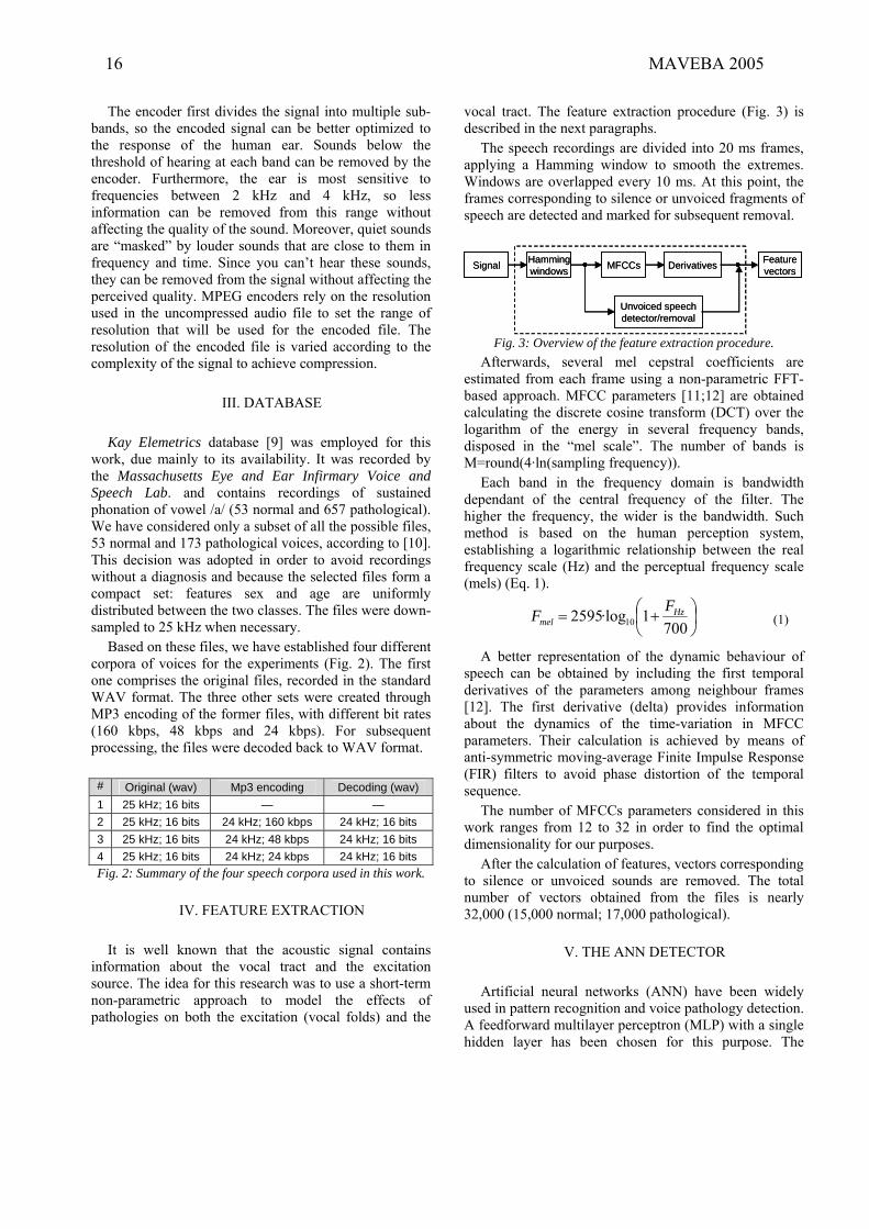
The encoder first divides the signal into multiple sub-bands, so the encoded signal can be better optimized to the response of the human ear. Sounds below the threshold of hearing at each band can be removed by the encoder. Furthermore, the ear is most sensitive to frequencies between 2 kHz and 4 kHz, so less information can be removed from this range without affecting the quality of the sound. Moreover, quiet sounds are “masked” by louder sounds that are close to them in frequency and time. Since you can’t hear these sounds, they can be removed from the signal without affecting the perceived quality. MPEG encoders rely on the resolution used in the uncompressed audio file to set the range of resolution that will be used for the encoded file. The resolution of the encoded file is varied according to the complexity of the signal to achieve compression.

III. DATABASE

Kay Elemetrics database [9] was employed for this

work, due mainly to its availability. It was recorded by the Massachusetts Eye and Ear Infirmary Voice and Speech Lab. and contains recordings of sustained phonation of vowel /a/ (53 normal and 657 pathological). We have considered only a subset of all the possible files, 53 normal and 173 pathological voices, according to [10]. This decision was adopted in order to avoid recordings without a diagnosis and because the selected files form a compact set: features sex and age are uniformly distributed between the two classes. The files were down-sampled to 25 kHz when necessary.

Based on these files, we have established four different corpora of voices for the experiments (Fig. 2). The first one comprises the original files, recorded in the standard WAV format. The three other sets were created through MP3 encoding of the former files, with different bit rates (160 kbps, 48 kbps and 24 kbps). For subsequent processing, the files were decoded back to WAV format.

# Original (wav) Mp3 encoding Decoding (wav) 1 25 kHz; 16 bits — — 2 25 kHz; 16 bits 24 kHz; 160 kbps 24 kHz; 16 bits 3 25 kHz; 16 bits 24 kHz; 48 kbps 24 kHz; 16 bits 4 25 kHz; 16 bits 24 kHz; 24 kbps 24 kHz; 16 bits Fig. 2: Summary of the four speech corpora used in this work.

IV. FEATURE EXTRACTION

It is well known that the acoustic signal contains information about the vocal tract and the excitation source. The idea for this research was to use a short-term non-parametric approach to model the effects of pathologies on both the excitation (vocal folds) and the

vocal tract. The feature extraction procedure (Fig. 3) is described in the next paragraphs.

The speech recordings are divided into 20 ms frames, applying a Hamming window to smooth the extremes. Windows are overlapped every 10 ms. At this point, the frames corresponding to silence or unvoiced fragments of speech are detected and marked for subsequent removal.

Hammingwindows MFCCs Derivatives

Unvoiced speechdetector/removal

Signal Featurevectors

Hammingwindows MFCCs Derivatives

Unvoiced speechdetector/removal

Signal Featurevectors

Fig. 3: Overview of the feature extraction procedure.

Afterwards, several mel cepstral coefficients are estimated from each frame using a non-parametric FFT-based approach. MFCC parameters [11;12] are obtained calculating the discrete cosine transform (DCT) over the logarithm of the energy in several frequency bands, disposed in the “mel scale”. The number of bands is M=round(4·ln(sampling frequency)).

Each band in the frequency domain is bandwidth dependant of the central frequency of the filter. The higher the frequency, the wider is the bandwidth. Such method is based on the human perception system, establishing a logarithmic relationship between the real frequency scale (Hz) and the perceptual frequency scale (mels) (Eq. 1).

⎟⎠⎞

⎜⎝⎛ +=

7001·log2595 10

Hzmel

FF (1)

A better representation of the dynamic behaviour of speech can be obtained by including the first temporal derivatives of the parameters among neighbour frames [12]. The first derivative (delta) provides information about the dynamics of the time-variation in MFCC parameters. Their calculation is achieved by means of anti-symmetric moving-average Finite Impulse Response (FIR) filters to avoid phase distortion of the temporal sequence.

The number of MFCCs parameters considered in this work ranges from 12 to 32 in order to find the optimal dimensionality for our purposes.

After the calculation of features, vectors corresponding to silence or unvoiced sounds are removed. The total number of vectors obtained from the files is nearly 32,000 (15,000 normal; 17,000 pathological).

V. THE ANN DETECTOR Artificial neural networks (ANN) have been widely

used in pattern recognition and voice pathology detection. A feedforward multilayer perceptron (MLP) with a single hidden layer has been chosen for this purpose. The

16 MAVEBA 2005

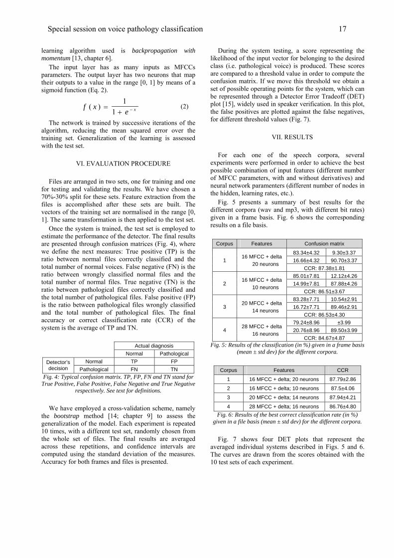
learning algorithm used is backpropagation with momentum [13, chapter 6].

The input layer has as many inputs as MFCCs parameters. The output layer has two neurons that map their outputs to a value in the range [0, 1] by means of a sigmoid function (Eq. 2).

f xe x( ) =

+ −

1

1 (2)

The network is trained by successive iterations of the algorithm, reducing the mean squared error over the training set. Generalization of the learning is assessed with the test set.

VI. EVALUATION PROCEDURE

Files are arranged in two sets, one for training and one

for testing and validating the results. We have chosen a 70%-30% split for these sets. Feature extraction from the files is accomplished after these sets are built. The vectors of the training set are normalised in the range [0, 1]. The same transformation is then applied to the test set.

Once the system is trained, the test set is employed to estimate the performance of the detector. The final results are presented through confusion matrices (Fig. 4), where we define the next measures: True positive (TP) is the ratio between normal files correctly classified and the total number of normal voices. False negative (FN) is the ratio between wrongly classified normal files and the total number of normal files. True negative (TN) is the ratio between pathological files correctly classified and the total number of pathological files. False positive (FP) is the ratio between pathological files wrongly classified and the total number of pathological files. The final accuracy or correct classification rate (CCR) of the system is the average of TP and TN.

Actual diagnosis

Normal Pathological

Normal TP FP Detector’s decision Pathological FN TN

Fig. 4: Typical confusion matrix. TP, FP, FN and TN stand for True Positive, False Positive, False Negative and True Negative

respectively. See text for definitions. We have employed a cross-validation scheme, namely

the bootstrap method [14; chapter 9] to assess the generalization of the model. Each experiment is repeated 10 times, with a different test set, randomly chosen from the whole set of files. The final results are averaged across these repetitions, and confidence intervals are computed using the standard deviation of the measures. Accuracy for both frames and files is presented.

During the system testing, a score representing the likelihood of the input vector for belonging to the desired class (i.e. pathological voice) is produced. These scores are compared to a threshold value in order to compute the confusion matrix. If we move this threshold we obtain a set of possible operating points for the system, which can be represented through a Detector Error Tradeoff (DET) plot [15], widely used in speaker verification. In this plot, the false positives are plotted against the false negatives, for different threshold values (Fig. 7).

VII. RESULTS

For each one of the speech corpora, several

experiments were performed in order to achieve the best possible combination of input features (different number of MFCC parameters, with and without derivatives) and neural network paramenters (different number of nodes in the hidden, learning rates, etc.).

Fig. 5 presents a summary of best results for the different corpora (wav and mp3, with different bit rates) given in a frame basis. Fig. 6 shows the corresponding results on a file basis.

Corpus Features Confusion matrix

83.34±4.32 9.30±3.37 16.66±4.32 90.70±3.37 1

16 MFCC + delta 20 neurons

CCR: 87.38±1.81 85.01±7.81 12.12±4.26 14.99±7.81 87.88±4.26 2


CCR: 86.51±3.67 83.28±7.71 10.54±2.91 16.72±7.71 89.46±2.91 3


CCR: 86.53±4.30 79.24±8.96 ±3.99 20.76±8.96 89.50±3.99 4


CCR: 84.67±4.87 Fig. 5: Results of the classification (in %) given in a frame basis

(mean ± std dev) for the different corpora.

Corpus Features CCR

1 16 MFCC + delta; 20 neurons 87.79±2.86



4 28 MFCC + delta; 16 neurons 86.76±4.80 Fig. 6: Results of the best correct classification rate (in %)

given in a file basis (mean ± std dev) for the different corpora. Fig. 7 shows four DET plots that represent the

averaged individual systems described in Figs. 5 and 6. The curves are drawn from the scores obtained with the 10 test sets of each experiment.


Fig. 7: DET plots comparing the performance of the averaged

systems.

VII. CONCLUSIONS As it can be seen from Fig. 7, the performance of the

original WAV files seems to be better than the mp3. But if we considered the confidence intervals, as reflected in Fig. 5 by the standard deviations, we must conclude that there are no significant differences between such systems.

MP3 coding transforms the energy in bands in a similar way than MFCCs. The part of the signal that is lost due to the compression seems to be not significant for pathology detection. Performance with MP3 may be somewhat inferior to that with the original WAV files, but MP3 needs less storage space.

More experiments have to be carried out to confirm this conclusion. We have to test also the performance of this detector with maximum MP3 compression (bit rate of 8 kbps).

VII. ACKNOWLEDGEMENTS

This work was supported under the grants: TIC-2003-08956-C02-00 and TIC-2002-0273 from the Ministry of Science and Technology and AP2001-1278 from the Ministry of Education of Spain.

REFERENCES

[1] Gavidia-Ceballos, L. and Hansen, J. H. L., "Direct speech feature estimation using an iterative EM algorithm for vocal fold pathology detection," IEEE Transactions on Biomedical Engineering, vol. 43, no. 4, pp. 373-383, Apr.1996.

[2] Godino-Llorente, J. I. and Gómez-Vilda, P., "Automatic detection of voice impairments by means of short-term cepstral parameters and neural network based

detectors," IEEE Transactions on Biomedical Engineering, vol. 51, no. 2, pp. 380-384, Feb.2004.

[3] Ritchings, R. T., McGillion, M. A., and Moore, C. J., "Pathological voice quality assessment using artificial neural networks," Medical Engineering & Physics, vol. 24, no. 8, pp. 561-564, 2002.

[4] Reilly, R. B., Moran, R., and Lacy, P. D., "Voice pathology assessment based on a dialogue system and speech analysis," in Proceedings of the American Association of Artificial Intelligence Fall Symposium on Dialogue Systems for Health Communication, Washington DC, USA, Nov.2004.

[5] ITU G.711 (11/88). Pulse code modulation (PCM) of voice frequencies. 1988.

[6] "Audio & multimedia MPEG audio layer 3," Fraunhofer Institute for Digital Media Technology, available at http://www.iis.fraunhofer.de/amm/techinf/layer3/index.html, 2005.

[7] ISO/IEC 11172-3. ISO-MPEG Audio Layer-3. Information technology - Coding of moving pictures and associated audio for digital storage media at up to about 1,5 Mbit/s. Part 3: Audio. 1993.

[8] ISO/IEC 13818-3. Generic coding of moving pictures and associated audio information. Part 3: Audio. 1998.

[9] Massachusetts Eye and Ear Infirmary, Voice Disorders Database, Version.1.03 [CD-ROM], Lincoln Park, NJ: Kay Elemetrics Corp, 1994.

[10] Parsa, V. and Jamieson, D. G., "Identification of pathological voices using glottal noise measures," Journal of Speech, Language and Hearing Research, vol. 43, no. 2, pp. 469-485, Apr.2000.

[11] Davis, S. B. and Mermelstein, P., "Comparison of parametric representations for monosyllabic word recognition in continuously spoken sentences," IEEE Transactions on Acoustics, Speech and Signal Processing, vol. 28, no. 4, pp. 357-366, Aug.1980.

[12] Rabiner, L. R. and Juang, B. H., Fundamentals of speech recognition, Englewood Cliffs, NJ: Prentice Hall, 1993.

[13] Haykin, S., Neural networks, New York: Macmillan, 1994.

[14] Duda, R. O., Hart, P. E., and Stork, D. G., Pattern classification, 2 ed., Wiley Interscience, 2000.

[15] Martin, A. F., Doddington, G. R., Kamm, T., Ordowski, M., and Przybocki, M. A., "The DET curve in assessment of detection task performance," in Proceedings of Eurospeech '97, vol. IV, Rhodes, Crete, pp. 1895-1898, 1997.

1. wav

3. mp3, 48 kbps

2. mp3, 160 kbps

4. mp3, 24 kbps

18 MAVEBA 2005

TOWARDS A CLASSIFICATION OF PHONATORY FEATURES OF DISORDERED VOICES

J. Schoentgen

National Fund for Scientific Research, Belgium Department “Signals and Waves”, Faculty of Applied Sciences, Université Libre de Bruxelles, Brussels

[email protected]

The purpose of the presentation is to give an overview of phonatory features of disordered voices and propose a classificatory framework. Generally speaking, phonatory features are numerical cues that summarize properties of speech signals or other voice-related signals that are obtained non-invasively, and which are clinically relevant. The object of a classificatory framework is to ease the planning of future experiments and the exploitation of the existing literature, which is diverse with regard to pathologies studied, speaker tasks, speaker performance, speech material, vocal symptoms, sensors and sought for relations with other levels of description.

I. INTRODUCTION The purpose of the presentation is to give an overview of phonatory features of disordered voices and propose a classificatory framework. Generally speaking, phonatory features are numerical cues or measurements that are clinically relevant and that summarize properties of speech signals or other signals that are obtained non-invasively, and which report on a speaker’s voice. Typically, the acquisition of phonatory features involves the (non-invasive) recording of signals that are relevant to laryngeal function, the signal processing that discards irrelevant signal properties and the summary of the clinically-relevant properties by means of a handful of numbers. The purpose of the extraction of phonatory features in a clinical framework is the documentation of the voice of patients, their longitudinal follow-up during treatment (e.g. before and after surgery) as well as comparisons with normophonic speakers. The goal of the presentation is not to discuss a classification of the mathematical forms of clinical cues per se. This would be an ineffectual exercise because most of the extant features are heuristically defined and their mathematical or statistical properties have been explored superficially only. The goal is rather to classify phonatory cues in relation to the use they have been put to.

Indeed, the scientific as well as clinical literature devoted to phonatory features of voice disorders is abundant. However, its diversity is impressive with regard to the pathologies or handicaps that have been studied, the vocal symptoms that have been described, the vocal tasks speakers have been asked to carry out and the linguistic, paralinguistic and extralinguistic performances that have been examined, the sensors that have been used and the speech material that has been recorded, as well as the correlations that have been examined.

As a consequence, it is difficult to distil general rules or compare results obtained in different frameworks. The purpose of a classification is therefore to ease the planning of future experiments and the exploitation of the existing literature.

II. CLASSIFICATORY FRAMEWORK The following is a proposal of a grid that may be used to classify different feature-based approaches to the assessment of voice disorders. Etiology The types of pathologies or handicaps the effects on voice of which have been investigated are wide and varied. Typically, one distinguishes voice problems that are the consequences of organic alterations of the vocal folds from those that are dysfunctional, i.e. voice disorders that are not the consequence of observable structural changes of the vocal folds [1]. Voice problems caused by motor disorders are a third category. An example of the latter is the voice of Parkinson speakers. A separate category are substitution voices, the purpose of which is to enable speech communication by speakers who have lost the capacity of producing voice by means of the vibration of the true vocal folds. Whether voice disorders that have different causes must be described by different sets of phonatory features is not clear at present. Generally speaking, speech and voice problems owing to motor disorders are kept separate from voice disorders that are the consequence of laryngeal pathologies [6]. A possible exception is vocal fold paralysis.


Speech material One major distinction between approaches to voice assessment rests on the speech material. Indeed, the speech material that is analyzed may be connected speech or sustained speech sounds. Sustained speech sounds may again be subdivided according to whether onsets and offsets are included in the analysis frame or not. Connected speech is often presented as ideal; analyses of stationary speech fragments are the rule, however [5]. The reason is that many signal processing schemes are based on assumptions of local stationarity and local periodicity. These assumptions may not be valid in the case of hoarse speakers emitting connected speech [2]. Speaker tasks Tasks refer to what is requested from a speaker during vocal assessment. Tasks that subjects are the most frequently asked to carry out are speaking, which includes sustaining speech sounds, singing (when appropriate), vocal loading, as well as profiling. Vocal loading consists in recording the phonatory features of a speaker, followed by reading out loud a text for some time (e.g. 45 minutes) and recording the same features again. The purpose is to track vocal alterations that are the consequence of burdening the larynx [7]. Finally, profiling is the discovery of the limits of phonatory performance, e.g. loudest possible voice, softest possible voice, highest possible pitch, lowest possible pitch, maximum phonation time, etc [9]. Speaker performance Speaker performance refers to the actual capacity that is examined. Phonatory performance may be subdivided into registers, phonation types, voicing, prosody and vocal quality.

Known speech registers are creak, modal voice and falsetto. Examples of phonation types are breathy voice, soft voice, modal voice, loud voice, pressed voice and so forth [3].

Voicing is the capacity of the speaker to voice and un-voice speech sounds. Prosody refers to the capacity to control intonation, accentuation, and rhythm, as well as speech rate. Voice quality, finally, designates vocal timbre, e.g. hoarseness, roughness, vocal tremor or quaver, and so forth.

Instrumentation Instrumentation refers to the equipment that is used to obtain signals non-invasively that report on the phonatory performance of speakers. The microphone signal is the most often used; it evolves proportionally to acoustic pressure and therefore proportionally to the speech signal that is recorded by the ear of a listener. Other signals that can be obtained non-invasively are the electroglottogram and photoglottogram. The former is reported to evolve proportionally to the vocal fold contact surface and the latter to the glottal area. One other sensor that is used frequently is the flow mask that enables recording airflow rate, as well as, occasionally, intra-oral pressure. Signals One major distinction is the one between features that describe the phonatory source signal and those that describe the speech signal. The phonatory signal is the acoustic signal that is generated at the glottis via the vibration of the vocal fold and pulsatile airflow. The speech signal is emitted at the mouth consequent to the propagation of the acoustic wave through the vocal tract. Observing the glottal source signal directly is difficult. Often, it is replaced by auxiliary signals such as the photoglottographic or electroglottographic signals that report on glottal properties directly. Transform domains At present, a systematic classification of clinical signal processing schemes is not possible because most schemes involve a heuristic processing stage that may differ from task to task and from study to study. A possible processing-related categorization is based on the type of signal transform that is involved. Examples are Fourier, Hilbert or Wavelet transforms. When no signal transformation is carried out, the corresponding phonatory features are temporal; otherwise they acquire properties that are typical of the corresponding transform domains [8]. Vocal symptoms One core distinction between phonatory features is the one that pertains to vocal symptoms. Vocal symptoms are the speech properties that are believed to be clinically relevant, that report on the state of the glottis and that the signal processing is aimed at. Typically one distinguishes between signal dysperiodicity,

20 MAVEBA 2005

signal morphology, and supra-segmental as well as coordinative features.

Coordinative features refer to the onset and offset of voicing in relation to supra-glottal events. Examples of relevant supra-glottal events are obstruent check and release or resonant onset and offset. The most often studied coordinative cue is vocal onset time, which is the signed time interval between the release of an obstruent and the onset of voicing, on which hinges the distinction between voiced and unvoiced obstruents. This language-typical interval, which may be short, requires a fine control of glottal adduction and abduction with regard to supra-glottal articulation. Voice onset time is therefore frequently studied in relation to motor speech disorders or substitution voices, which are suspected to impede fine control of voicing [10]. Supra-segmental features pertain to intonation, accentuation, rhythm, speech rate as well as average phonatory frequency, the variability of the phonatory frequency, and average loudness, i.e. sound pressure level. In a clinical framework, speech rate, the average and spread of phonatory frequency, as well as sound pressure level are the most popular. Morphological features refer in practice to the shape attributes of the glottal source signal. Examples are the open quotient, closing quotient, speed quotient, the amplitude of the volume velocity as well as the amplitude of the negative peak of the differentiated volume velocity [3]. An example of a spectral morphological feature is the spectral balance, which quantifies harmonic richness. Morphological features have been mainly used to characterize phonation types. Morphological, supra-segmental as well as coordinative features are not confined to clinical applications. These features have been widely studied by phoneticians, linguists, psychologists and engineers because they report on speech and voice production as well as perception in general.

Features that are typically clinical are those that describe irregularities of the movement of the vocal folds. Generally speaking, one distinguishes between non-modal vibratory regimes that cause diplophonia, biphonation and random cycles, and external perturbations (i.e. modulation noise), turbulence noise and breathiness (i.e. additive noise), unsolicited vibrations of the false vocal folds or ary-epiglottal folds, as well as uncontrolled transients, such as voice breaks, register breaks, octave jumps and so forth. External perturbations give rise to vocal jitter and shimmy, as well as vocal frequency and amplitude tremor. The main contribution to shimmy and amplitude tremor of the speech

cycles is the modulation distortion by the vocal tract of phonatory jitter and phonatory frequency tremor. Other causes are the transfer of acoustic energy from cycle to cycle, as well as tremor of the speech articulators. Phonatory shimmy or phonatory amplitude tremor contribute only feebly to speech shimmy or speech amplitude tremor [4]. Correlation More often than not, clinicians attempt to correlate observed acoustic features with data recorded at other levels of description. Data, correlations with which are sought for, are typically diagnostic, glottal, aerodynamic or perceptual, with a preference for the latter.

III. KNOWN PROBLEMS Known problems with extant phonatory features are the following. Signal processing The most popular acoustic features are those that quantify the degree of irregularity of the vocal cycles. Typical examples are the period perturbation quotient, amplitude perturbation quotient, jitter in %, harmonics-to-noise ratio and so forth. More often than not, the signal processing involves methods that are based on assumptions of local stationarity and local periodicity that enable heuristics to detect and isolate vocal cycles or spectral harmonics. These heuristics may fail in the case of severely hoarse voices. As a consequence, insertion or omission errors are frequent in the case of highly irregular signals. These errors bias the values of the calculated features. As a consequence, phonatory features that describe vocal perturbations are thought to be reliable only when extracted from sustained speech sounds uttered by feebly or moderately hoarse speakers. Another issue is measurement precision. Indeed, perturbations of cycle length may be small, e.g. less than one percent for speech cycle lengths, less than ten percent for speech cycle amplitudes. As a consequence, signal processing request precautions with regard to measurement precision. Otherwise, measurements may be biased by quantization noise, for instance. Labelling Labelling refers to the custom of giving phonatory features names that allude to vocal symptoms rather than to the measurements that are actually performed. For instance, features


that summarize the dysperiodicity of glottal cycle lengths are often referred to as vocal jitter, although cycle length dysperiodicity may also be influenced by average phonatory frequency, additive noise, frequency tremor, non-modal dynamic regimes of the vocal folds and non-flat intonation, for instance. Redundancy The number of phonatory features that have been proposed in the literature is large. Software that is sold for clinical assessment of voice typically comprises tens of numerical cues that can be computed for a single sustained sound. Studies have shown that sub-sets of phonatory features are correlated with each other. Sub-sets of correlated features are roughly coextensive with the groups of vocal symptoms that are discussed above [5]. Interpretation Even very simple measurements are influenced by multiple factors. Examples are given above for the perturbations of the speech cycle lengths, as well as for the perturbations of the speech cycle amplitudes, which are generated via modulation distortion. These observations suggest that phonatory features are difficult to interpret because they are determined by multiple causes that may be interdependent. Stationary fragments of sustained speech sounds One of the more frequently heard complaints is that many acoustic cues can only be obtained reliably for stationary fragments of sustained speech sounds. The reasons have been discussed in the section on signal processing. A consequence is that, at present, the effects of voice disorders on connected or natural speech are less well understood. Problems that are non-resolved are not only issues in signal processing, but also the choice of the phonatory features, the choice of speech material, as well as the perceptual assessment of connected speech fragments that are short or phonetically complex.

IV. SUMMARY The following Table summarizes some of the factors that distinguish different approaches to voice assessment.

Etiology organic, dysfunctional, and motor disorders, substitution voices

Transforms Fourier, Hilbert, and Wavelet transforms (if applicable)

Signals glottal source, speech signal

Material connected speech, sustained speech sounds, stationary fragments of sustained

speech sounds

Symptoms dysperiodic, morphologic, supra-segmental, coordinative

Tasks speaking, singing, loading, profiling

Performance registers, phonation types, voicing, prosody, voice quality

Sensors microphone, electroglottograph, photoglottograph, flow mask

REFERENCES

The synthetic description of feature-based vocal assessment that is given here rests on a large number of articles, which cannot be listed because of lack of space. References that are cited below are only pointers to further reading. [1] Boone D., McFarlane S. (1996) The voice and voice therapy, Prentice Hall, NJ. [2] Bettens F., Grenez F., Schoentgen J. (2005) Estimation of vocal dysperiodicities in disordered connected speech by means of distant-sample bidirectional linear predictive analysis, J. Acoust. Soc. Am., 117, 1, 328-337. [3] Alku P., Vilkman E. (1996) A comparison of glottal voice source quantification parameters in breathy, normal and pressed phonation of female and male speakers, Folia Phoniatrica et Logopaedica, 48, 240-254. [4] Schoentgen J. (2003) Spectral models of additive and modulation noise in speech and phonatory excitation signals, J. Acoust. Soc. Am., 113, 1, 553-562. [5] Dejonckere Ph., Remacle M., Fresnel-Elbaz E., Woisard V., Crevier-Buchman L., Millet B. (1996) Differential perceptual evaluation of pathological voice quality: reliability and correlations with acoustic measurement, Rev. Laryngol. Otol. Rhinol., 117, 3, 219-224. [6] Till J., Yorkston K., Beukelman D. (1994) Motor speech disorders – Advances in assessment and treatment, Brookes Publ., Baltimore. [7] Vilkman E., Lauri E., Alku P., Sala E., Sihvo M. (1999) Effects of prolonged oral reading on F0, SPL, sub-glottal pressure and amplitude characteristics, J. Voice, 13, 2, 303-315. [8] Baken R., Daniloff R. (1991) Readings in clinical spectrography of speech, Singular Publ., San Diego. [9] Heylen L., Wuyts F., Mertens F., De Bodt M., Van de Heyning P. (2002) Normative voice range profiles of male and female professional voice users, J. Voice, 16, 1, 1-7. [10] Ziegler W., Deger K. (1998) Clinical Phonetics and Linguistics, Whurr Publ., London, 435-449.

22 MAVEBA 2005

INTELLIGENT VOICE QUALITY ASSESSMENT POST-

TREATMENT USING GENETIC PROGRAMMING

Walaa Sheta1, Tim Ritchings

2 & Carl Berry

2

1Mubarak City for Scientific Research,

Burg El-Arab, Egypt

[email protected]

2School of Computing, Science and Engineering,

University of Salford, UK

Abstract: Objective techniques for assessing and

classifying voice quality for patients recovering

from treatment for cancer of the larynx have

largely focussed on they use of Artificial Neural

Networks (ANN). The results of a preliminary

study are reported, where a Genetic Programming

(GP) has been trained to classify recovered

(normal) and abnormal voices in acoustic data,

and produced much more accurate results than an

ANN. In addition, the GP is able to provide impact

factors for the various voice parameters, and

suggests that only 6 of the 22 short-term and long-

term parameters used in the current ANN studies

are contributing significantly to the classifications.

Keywords: Voice quality, classification, Artificial

Neural Network, Genetic Algorithms, acoustic

signals.

I. INTRODUCTION

The use of intelligent computer-based techniques to

support decision making in clinical applications, have

been investigated over the years for a wide variety of

clinical data. Although Genetic Programming (GP)

has not been used extensively for medical

applications to date, the early results for cancer

diagnosis [1,2] were found to be better than with an

Artificial Neural Network (ANN). In another study

[3], a grammar-based GP variant was used for

knowledge extraction from medical databases, where

the rules for the diagnosis were derived from an

algorithm that uncovers relationships among data

attributes. The outcomes of different types of

classifiers, including ANNs and genetic programs

have also been reported [4].

This study is part of a larger project which is

concerned with developing objective techniques for

voice quality assessment in patients recovering from

cancer of the larynx. The earlier investigations have

concentrated on the use of Artificial Neural Networks

(ANN) to firstly distinguish recovered (normal) and

abnormal voices [5] on the basis of a collection of

short-term and long-term parameters derived from the

patient’s voice signals, and more recently, classify voices

on the 7-point scale for voice quality used by Speech and

Language Therapists (SALT) in the UK [6]. Similar

classifications have now been obtained for both electrical

impedance (EGG) and acoustic data, with the best results

for voices in the extremes categories on this scale (normal

and abnormal), while those for the mid-categories have

been poor [7].

A preliminary assessment of use of Genetic

Programming to classify normal (recovered) and

abnormal acoustic signals is described here. The resulting

classifications are compared with those obtained from an

ANN for the same signal parameters and training

regimes..

II. TREATMENT OF VOICE SIGNALS

A. Collection of Voice Signals

The patient’s voice data was collected by the Christie

Hospital and the South Manchester hospital using an

electrolaryngograph PCLX system [8]. The equipment

simultaneously records the electrical impedance signal via

pads placed at specific positions on the patient’s neck at

the same time as the acoustic voice signal using a

microphone. In these studies, the patient was attempts to

steadily phonate the /i/ sound. Although two datasets are

collected, only the acoustic data have been used to date in

this study. In the work only the male voices were used as

the number of female voices in the dataset was too small

to give an accurate assessment, a feature of the dataset is

that most cancer of the larynx patients are male.

Voice quality was subjectively classified by a SALT for

each patient using their standard 7-point classification

scale ranging from Lx0-Lx6, with Lx0 being a near

normal (recovered) voice while Lx6 represents an

abnormal, very poor quality voice. The approach taken to

reach a classification is very subjective and depends to a

large extent on the experience of the SALT In this study

the Lx0 and Lx1 voices were combined and considered as

the normals, while Lx5 and Lx6 voices were combined to

give the abnormals, The number of patients in these two

categories is shown in Table 1.


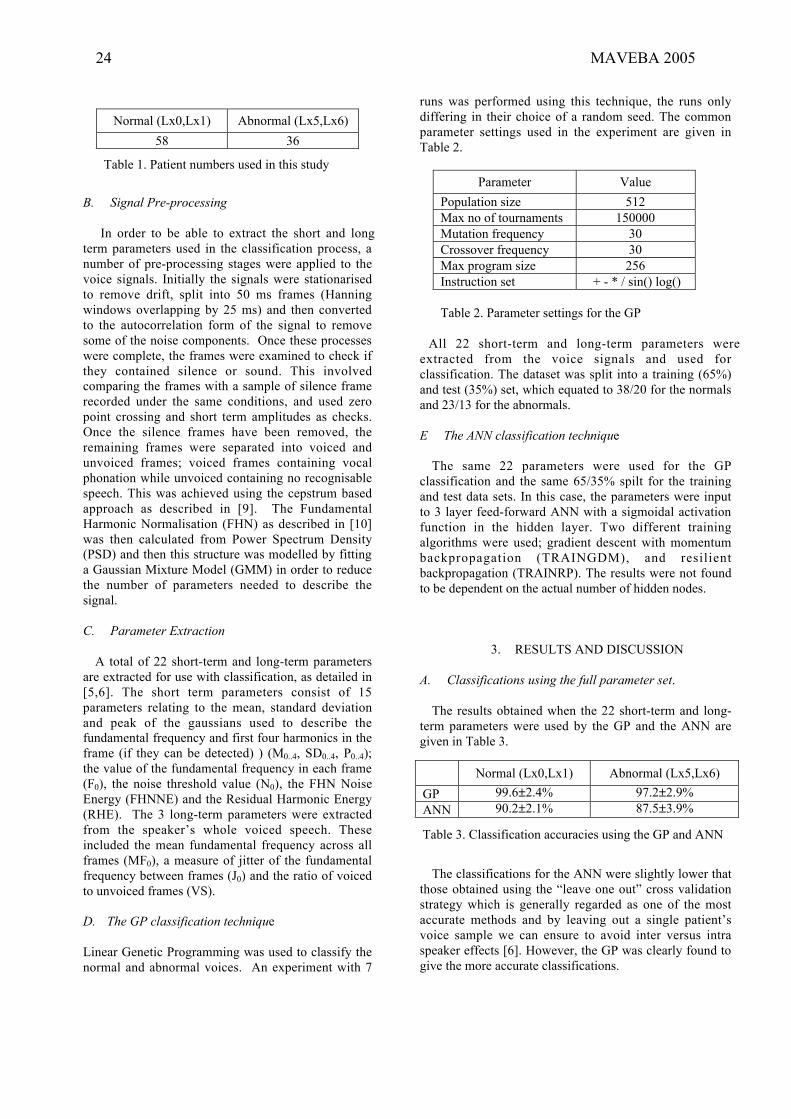
Normal (Lx0,Lx1) Abnormal (Lx5,Lx6)

58 36

Table 1. Patient numbers used in this study

B. Signal Pre-processing

In order to be able to extract the short and long

term parameters used in the classification process, a

number of pre-processing stages were applied to the

voice signals. Initially the signals were stationarised

to remove drift, split into 50 ms frames (Hanning

windows overlapping by 25 ms) and then converted

to the autocorrelation form of the signal to remove

some of the noise components. Once these processes

were complete, the frames were examined to check if

they contained silence or sound. This involved

comparing the frames with a sample of silence frame

recorded under the same conditions, and used zero

point crossing and short term amplitudes as checks.

Once the silence frames have been removed, the

remaining frames were separated into voiced and

unvoiced frames; voiced frames containing vocal

phonation while unvoiced containing no recognisable

speech. This was achieved using the cepstrum based

approach as described in [9]. The Fundamental

Harmonic Normalisation (FHN) as described in [10]

was then calculated from Power Spectrum Density

(PSD) and then this structure was modelled by fitting

a Gaussian Mixture Model (GMM) in order to reduce

the number of parameters needed to describe the

signal.

C. Parameter Extraction

A total of 22 short-term and long-term parameters

are extracted for use with classification, as detailed in

[5,6]. The short term parameters consist of 15

parameters relating to the mean, standard deviation

and peak of the gaussians used to describe the

fundamental frequency and first four harmonics in the

frame (if they can be detected) ) (M0..4, SD0..4, P0..4);

the value of the fundamental frequency in each frame

(F0), the noise threshold value (N0), the FHN Noise

Energy (FHNNE) and the Residual Harmonic Energy

(RHE). The 3 long-term parameters were extracted

from the speaker’s whole voiced speech. These

included the mean fundamental frequency across all

frames (MF0), a measure of jitter of the fundamental

frequency between frames (J0) and the ratio of voiced

to unvoiced frames (VS).

D. The GP classification technique

Linear Genetic Programming was used to classify the

normal and abnormal voices. An experiment with 7

runs was performed using this technique, the runs only

differing in their choice of a random seed. The common

parameter settings used in the experiment are given in

Table 2.

Parameter Value

Population size 512

Max no of tournaments 150000

Mutation frequency 30

Crossover frequency 30

Max program size 256

Instruction set + - * / sin() log()

Table 2. Parameter settings for the GP

All 22 short-term and long-term parameters were

extracted from the voice signals and used for

classification. The dataset was split into a training (65%)

and test (35%) set, which equated to 38/20 for the normals

and 23/13 for the abnormals.

E The ANN classification technique

The same 22 parameters were used for the GP

classification and the same 65/35% spilt for the training

and test data sets. In this case, the parameters were input

to 3 layer feed-forward ANN with a sigmoidal activation

function in the hidden layer. Two different training

algorithms were used; gradient descent with momentum

backpropagation (TRAINGDM), and resilient

backpropagation (TRAINRP). The results were not found

to be dependent on the actual number of hidden nodes.

3. RESULTS AND DISCUSSION

A. Classifications using the full parameter set.

The results obtained when the 22 short-term and long-

term parameters were used by the GP and the ANN are

given in Table 3.

The classifications for the ANN were slightly lower that

those obtained using the “leave one out” cross validation

strategy which is generally regarded as one of the most

accurate methods and by leaving out a single patient’s

voice sample we can ensure to avoid inter versus intra

speaker effects [6]. However, the GP was clearly found to

give the more accurate classifications.


GP 99.6±2.4% 97.2±2.9%

ANN 90.2±2.1% 87.5±3.9%

Table 3. Classification accuracies using the GP and ANN

24 MAVEBA 2005

B. Classifications using the impact parameter set.

One of the advantages of using the GP is that it

provides the impact factor of each parameter on the

classification. Table 4 shows how each parameter

contributed in the generated program. The Table

shows the frequency percentage of the best thirty

generated programs containing the referenced input;

the average effect of removing all instances of that

input, and the maximum impact of that input. In these

cases, the greater the value, the more impact removal

of that input had.

It may be seen from the Table that only 6 of the 22

parameters were found to have a significant impact on

the classification. These parameters were N0, M0, P0,

MF0, J0, and VS.

Both the GP and the ANN were re-trained and

tested using just these 6 parameters, and the results

are shown in Table 5.

V. CONCLUSIONS.

A preliminary study has been made involving the use of

GP to classify recovered (normal) voices and abnormal

voices in acoustic signals taken from patients recovering

from cancer of the larynx. Initially, a collection of 22

short-term and long-term parameters were extracted from

the signal and used as input to the GP, and also an ANN.

The GP provided much more accurate classifications than

the ANN.

Examination of the impact factors for the voice

parameters suggests that there are only 6 significant

factors. The results obtained from both the GP and the

ANN using just these parameters were only slightly

poorer than for the full parameter set, again with the GP

providing the more accurate classifications.

One of the advantages of the ANN is the ability to

produce multiple outputs, enabling classifications to be

made corresponding to the 7-point scale for voice quality

used by SALTS. Work is now taking place to extend the

GP approach to multiple classifications.

REFERENCES

[1] Gray, H., Maxwell, R., Martinez-Perez, I., Arus, C.

and Cerdan, S. “Genetic programming for

classification of brain tumours from nuclear magnetic

resonance biopsy spectra ,in Genetic Programming”,

1st International Conference on Genetic

Programming, GP-96, Stanford, US, 1996.

[2] Nordin, P., Keller, R., and Francone, F. “Genetic

Programming: an introduction on the automatic

evolution of computer programs and its applications.”

Wolfgang Banzhaf Publishers, Inc. 2002.

[3] Ngan, P., M. Wong, M., Leung, K. and Cheng, J.

“Using grammar based genetic programming for data

mining of medical knowledge, in Genetic

Programming” 3rd

International Conference on

Genetic Programming, GP-98, Madison, US, 1998.

[4] Somorjai, R., Nikulin, A., Pizzi, N., Jackson, D.,

Scarth, G., Dolenko, B., Gordon, H., Russell, P.,

Lean, C., Delbridge, L., Mountford, C. and Smith, I.

”Computerized consensus diagnosis - A classification

strategy for the robust analysis of MR spectra1.

Application to H-1 spectra of thyroid neoplasma”,

Magn. Reson. Med. 33, 257–263, 1995.

[5] Ritchings RT, McGillion M, Moore CJ “Pathological

voice quality assessment using artificial neural

networks.” Medical Engineering and Physics 24

(2002), pp561-564, PII S1350-4533(02)00064-4.

Parameter FrequencyAverage

Impact

Maximum

impact

VS 1.00 13.69 17.78

MF0 0.67 7.41 10.50

J0 0.77 4.45 9.78

N0 0.23 1.13 2.20

M0 0.17 0.32 0.45

P0 0.27 0.27 0.27

RHE 0.17 0 0

SD0 0.10 0 0

P1 0.10 0 0

SD3 0.10 0 0

P3 0.10 0 0

M1 0.07 0 0

SD1 0.07 0 0

P4 0.07 0 0

FHNNE 0.07 0 0

SD2 0.03 0 0

P2 0.03 0 0

M4 0.03 0 0

M2 0 0 0

M3 0 0 0

SD4 0 0 0

F0 0 0 0

Table 4. Contribution of each parameter


GP 99.2±3.1% 96.4±3.7%

ANN 88.6±2.7% 81.5±4.2%

Table 5. Classification accuracies using GP and ANN


[6] Godino-Llorente, JI, Ritchings, RT, Berry C “The

Effects of Inter and Intra Speaker Variability on

Pathological Voice Quality Assessment” 3rd

International Workshop on Models and Analysis

of Vocal Emissions for Biomedical Applications,

Firenze, Italy 2003

[7] Berry, C and Ritchings, RT. “A comparative

study of intelligent voice quality assessment

using impedance and acoustic signals.” 4th

International Workshop on Models and Analysis

of Vocal Emissions for Biomedical Applications,

Firenze, Italy 2005.

[8] Fourcin, A.J., Abberton E., Miller, D, Howell D.

Laryngograph : “Speech pattern element tools for

therapy, training and assessment.” European Journal

of Disorders of Communication 30(2), 1996, pp.101-

115

[9] Rabiner, L. and Juang, B.H. Fundamentals of speech

recognition. New Jersey Prentice Hall, 1993.

[10] Moore C.J., Manickam K., Slavin N. “Voicing

recovery in males following radiotherapy for larynx

cancer.” 4th

International Workshop on Models and

Analysis of Vocal Emissions for Biomedical

Applications, Firenze, Italy 2005.

.

26 MAVEBA 2005

Voice recovering / enhancement


A METHOD FOR CHANGING SPEECH QUALITY AND ITS

APPLICATION TO PATHOLOGICAL VOICES

Hisao Kuwabara

Teikyo University of Science & Technology, Uenohara, Kitatsuru-gun, Yamanashi 409-01, JapanTel: (0554)63-4411, Fax: (0554)63-4431, E-mail: [email protected]

Abstract: Speech quality is an interesting and veryimportant aspect not only from linguistic and/orphonetic viewpoint but also from the viewpoint ofspeech technology. This study has been conductedfrom the latter point of view. A method has beendeveloped based on the analysis-synthesis techniquewhich enables to control voice quality byindependently manipulating the voice source and thevocal tract resonant characteristics. Through thismethod, it is possible to investigate the amount ofcontribution of individual acoustic parameters to acertain voice quality including voice individuality.Formant frequencies and their bandwidths are usedas the acoustic parameters to characterize the vocaltract configuration and the pitch frequency as thevoice source. These acoustic parameters extractedfrom a natural speech are modified or changed tosome extent and then a is synthesized making use ofthe modified acoustic parameters. Speechintelligibility and voice individuality are found to becontrolled by this method. An application to apathological voice has also been made to control thevoice quality. It has been found that the method iscapable of improving the so-called “roughness” or“hoarseness” of the pathological voice to a certainextent.

I. INTRODUCTION

Using the analysis-synthesis system we have developed[1], voice quality of natural speech has been controlledby changing formant trajectories that are supposed tohave a close relation with such voice qualities asintelligibility, clearness, articulateness, and so on.Correlation analysis between psychological and acousticdistances reveals that the formant trajectory has thelargest correlation with the voice quality of announcer’sspeech sounds, followed by pitch frequency [2]. Thisresult suggests that the quality of speech sound of non-professional speakers may possibly be improved byaltering the dynamics of formant trajectory patterns.Based on the experimental evidence mentioned above, anexperiment has been performed to change and improvethe quality of natural speech making use of the analysis-synthesis system.Formant trajectories are extracted from voiced portionsby LPC method and the dynamics of these trajectoriesare altered depending on the formant pattern itself. The

method for altering the formant pattern is the same asthat we have proposed earlier for the normalization ofcoarticu-lated vowels in continuous speech. [3]. Thismethod is applied to the formant and pitch trajectoriesextracted from a natural speech, and the quality-controlled speech sounds are synthesized using theanalysis-synthesis system to present to listeners forperceptual judgments.

II. ANALYSIS-SYNTHESIS SYSTEM

Fig. 1 illustrates the block diagram of the analysis-synthesis system. Low-pass filtered input speech isdigitized in 12 bits at a rate of 15 kHz. A short timeLPC analysis based on the autocorrelation method isperformed to obtain LPC coefficients and the residualsignals. Formant frequencies and their bandwidths areestimated by solving a polynomial equation. Amodification of the spectral envelope is equivalent to amanipulation of the coefficients that would result in afrequency response of the filter equal to the modifiedenvelope. These acoustic parameters (pitch periods, LPCcoefficients, formant frequencies, bandwidths, residualsignals) are stored for later synthesis. This analysis-synthesis system is capable of analyzing input speecheither pitch synchronously or non-synchronouslydependent on the type of input speech and the aim ofspeech analysis or synthesis. When we analyze apathological speech, as described in a later section,which is difficult or impossible to define pitch periodsfrom the input speech, analysis is generally performedwith a fixed frame length.

III. METHOD OF FORMANT TRAJECTORYMANIPULATION


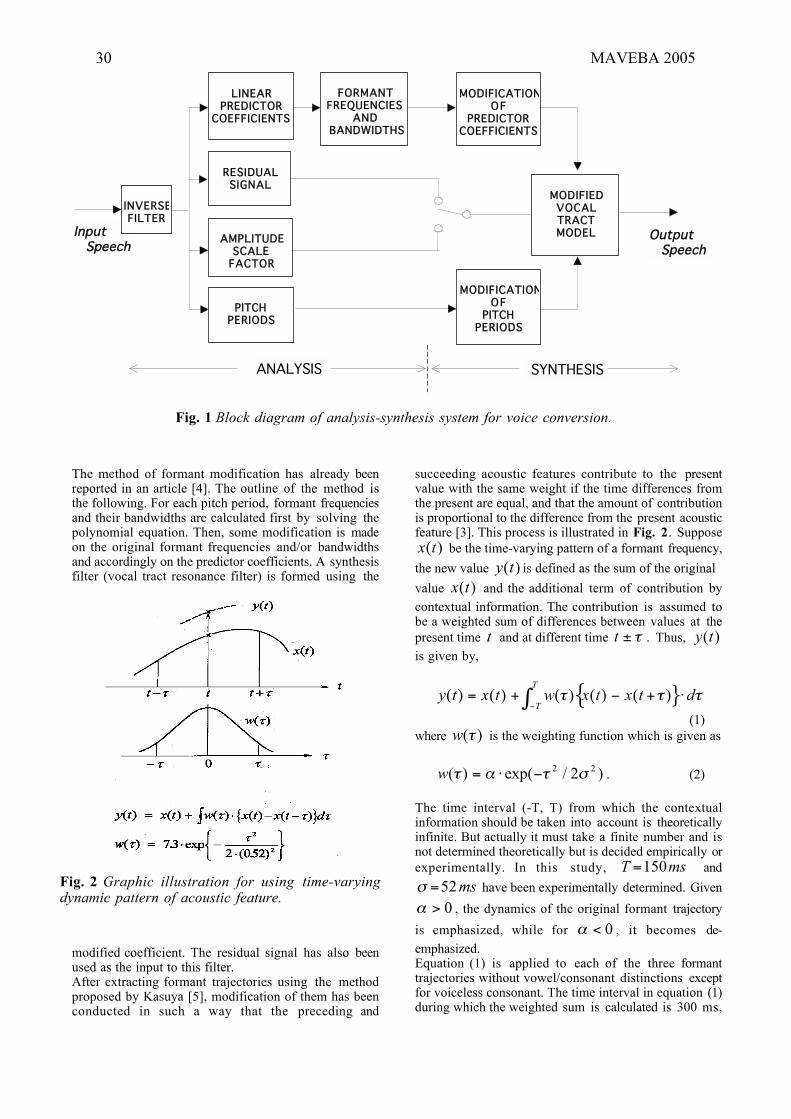
The method of formant modification has already beenreported in an article [4]. The outline of the method isthe following. For each pitch period, formant frequenciesand their bandwidths are calculated first by solving thepolynomial equation. Then, some modification is madeon the original formant frequencies and/or bandwidthsand accordingly on the predictor coefficients. A synthesisfilter (vocal tract resonance filter) is formed using the

modified coefficient. The residual signal has also beenused as the input to this filter.After extracting formant trajectories using the methodproposed by Kasuya [5], modification of them has beenconducted in such a way that the preceding and

succeeding acoustic features contribute to the presentvalue with the same weight if the time differences fromthe present are equal, and that the amount of contributionis proportional to the difference from the present acousticfeature [3]. This process is illustrated in Fig. 2. Suppose

x t( ) be the time-varying pattern of a formant frequency,

the new value y t( ) is defined as the sum of the original

value x t( ) and the additional term of contribution by

contextual information. The contribution is assumed tobe a weighted sum of differences between values at the

present time t and at different time t ± . Thus, y t( )

is given by,

}{y t x t w x t x t dT

T

( ) ( ) ( ) ( ) ( )= + +

(1)

where w( ) is the weighting function which is given as

w( ) exp( / )=2 22 . (2)

The time interval (-T, T) from which the contextualinformation should be taken into account is theoreticallyinfinite. But actually it must take a finite number and isnot determined theoretically but is decided empirically or

experimentally. In this study, T ms=150 and

=52ms have been experimentally determined. Given

0> , the dynamics of the original formant trajectory

is emphasized, while for 0< , it becomes de-

emphasized.Equation (1) is applied to each of the three formanttrajectories without vowel/consonant distinctions exceptfor voiceless consonant. The time interval in equation (1)during which the weighted sum is calculated is 300 ms,

Fig. 2 Graphic illustration for using time-varyingdynamic pattern of acoustic feature.

MODIFICATIONOF

PREDICTORCOEFFICIENTS

LINEARPREDICTOR

COEFFICIENTS

FORMANTFREQUENCIES

ANDBANDWIDTHS

RESIDUALSIGNAL

AMPLITUDESCALE

FACTOR

PITCHPERIODS

MODIFICATIONOF

PITCHPERIODS

MODIFIEDVOCALTRACTMODEL Output

Speech

ANALYSIS

Input Speech

INVERSEFILTER

SYNTHESIS

Fig. 1 Block diagram of analysis-synthesis system for voice conversion.

30 MAVEBA 2005

a 150 ms forward and backward each. This is the result

for =7 3. which, in our previous study, represents a

proper value for the purpose of normalizingcoarticulation effects of vowels in continuous speech. Itis noticed from the figure that the new formanttrajectories are emphasized their up-and-down dynamicmovements as compared to those of the raw formants.As far as we have tested, this method of incorporatingcontextual information is capable of not onlynormalizing the coarticulation effect of vowels incontinuous speech but also has some advantage forvowel recognition using the formant frequencies withconventional Euclidean distance from the referencevowel. The method is also capable of improving theintelligibility of some lazily spoken continuous speech.

IV. METHOD OF PITCH MANIPULATION

Pitch frequency manipulation is quite simple asdescribed in Fig.3. At the pitch synchronous analysisstage, the residue signal obtained for each pitch periodhas exactly the same data length as the pitch period. Ifwe give the residue signal as an input to the vocal tractmodel, exactly the same waveform as the original speech

will be obtained. Thus, pitch frequency change canbasically be given by controlling the length of theresidual signal.To raise pitch frequency, some data at the last part of theresidue are eliminated and to lower the frequency, zero

signals are added to the last part of the residue.Of course there are some discrepancies on the frequencydomain between the pitch-modified speech and theoriginal speech. However, there is no serious voicechange in terms of perceptual voice quality when thepitch frequency change is less than 50% form theoriginal.

V. ENHANCEMENT OF PATHOLOGICALSPEECH

An attempt has been made to improve the quality of apathological speech using the analysis-synthesis systemwe have developed. The pathological speech used in thisexperiment is a voice uttered by a patient who has adisease in his vocal cord. Because of malfunction of thevocal cord vibration, the resultant speech wave lacksclear periodicity and its voice quality is “hoarse”. Theexperiment has been designed to create the fundamentalfrequencies into the pathological speech waves in orderto improve the quality as close to a normal speech aspossible.Fig. 4 represents the block diagram to improve thequality of pathological speech. It requires two kinds ofinput speech: a pathological speech to be improved and a

normal speech utterance of the samesentence from another speaker. From thepathological speech inputted, voicedportions are at first detected and thespectral envelopes are extracted throughLPC analysis. Next, the normal speechis analyzed by the same method and thepitch frequencies are detected to combinewith the spectral information extractedfrom the pathological speech. If thenormal speech of the same content cannot immediately be available, artificialpulse trains could be used as the voicesource.In the analysis stage, after makingvoiced/voiceless distinction, thevoiceless portions (voiceless consonantsand devocalized vowels) are thoroughlykept in memory and the LPC analysis isperformed for the voiced portions toobtain the LPC coefficients that carryspectral information and the residualsignals from which pitch periods can beestimated. For the pathological speech,the frame length (analysis window) isset at 20 ms and the frame shift is a halfof the window length.In the feature extraction stage, theresidual signals for the pathologicalspeech are discarded after obtainingspectral information. Contrary to this,only the pitch frequency contour isneeded from the normal speech.For the normal speech, however, a

process of time alignment has been undertaken beforefeeding to analysis in Fig.4. This process is shown inFig.5 . The voiced parts of the normal speech areanalyzed pitch synchronously and the length for each part

1/H1(f)

1/H2(f)

1/H3(f)

Synthesis FilterResidual Signal

T1

T2

T3

Pitch ModifiedSpeech Wave

T1

T2

T3

SYNTHESIS

Speech Wave

H1(f)

H2(f)

H3(f)

Analysis Filter Residual Signal

ANALYSIS

Fig.3 A method of manipulating fundamental frequency.

Voice recovering / enhancement 31

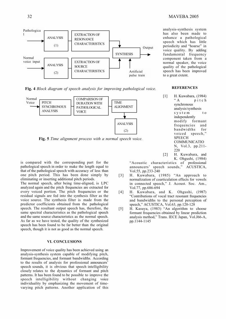
is compared with the corresponding part for thepathological speech in order to make the length equal tothat of the pathological speech with accuracy of less thanone pitch period. This has been done simply byeliminating or inserting additional pitch periods.The normal speech, after being time-aligned, is LPCanalyzed again and the pitch frequencies are extracted forevery voiced portion. The pitch frequencies or theresidual signals are fed into the synthesis filter as thevoice source. The synthesis filter is made from thepredictor coefficients obtained from the pathologicalspeech. The resultant output speech has, therefore, thesame spectral characteristics as the pathological speechand the same source characteristics as the normal speech.As far as we have tested, the quality of the synthesizedspeech has been found to be far better than the originalspeech, though it is not as good as the normal speech.

VI. CONCLUSIONS

Improvement of voice quality has been achieved using ananalysis-synthesis system capable of modifying pitch,formant frequencies, and formant bandwidths. Accordingto the results of analysis for professional announcers’speech sounds, it is obvious that speech intelligibilityclosely relates to the dynamics of formant and pitchpatterns. It has been found to be possible to improve thespeech intelligibility without changing voiceindividuality by emphasizing the movement of time-varying pitch patterns. Another application of this

analysis-synthesis systemhas also been made toenhance a pathologicalspeech which has littleperiodicity and “hoarse” invoice quality. By addingfundamental frequencycomponent taken from anormal speaker, the voicequality of the pathologicalspeech has been improvedto a great extent.

REFERENCES

[1] H. Kuwabara, (1984)“ A p i t c hsynchronousanalysis/synthesiss y s t e m t oindependentlymodify formantfrequencies andbandwidths forvoiced speech,”SPEECHCOMMUNICATION, Vol.3, pp.211-220

[2] H. Kuwabara, andK. Ohgushi, (1984)

“Acoustic characteristics of professionalannouncers’ speech sounds,” ACUSTICA,Vol.55, pp.233-240

[3] H. Kuwabara, (1985) “An approach tonormalization of coarticulation effects for vowelsin connected speech,” J. Acoust. Soc. Am.,Vol.77, pp.686-694

[4] H. Kuwabara, and K. Ohgushi, (1987)“Contributions of vocal tract resonant frequenciesand bandwidths to the personal perception ofspeech,” ACUSTICA, Vol.63, pp.120-128

[5] H. Kasuya, (1983) “An algorithm to chooseformant frequencies obtained by linear predictionanalysis method,” Trans. IECE Japan, Vol.J66-A,pp.1144-1145

Fig. 4 Block diagram of speech analysis for improving pathological voice.

Fig. 5 Time alignment process with a normal speech voice.

Artificialpulse train

Output

Pathological

Normalvoice input

ANALYSIS

(1)

ANALYSIS

(2)

EXTRACTION OF

RESONANCE

CHARACTERISTICS

EXTRACTION OF

SOURCE

CHARACTERISTICS

SYNTHESIS

NormalVoice PITCH

SYNCHRONOUS

ANALYSIS

COMPARISON OF

DURATION WITH

PATHOLOGICAL

VOICE

TIME

ALIGNMENT

ANALYSIS

(2)

32 MAVEBA 2005

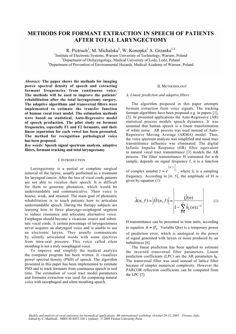
Abstract: The paper shows the methods for imaging

power spectral density of speech and extracting

formant frequencies from continuous voice.

The methods will be used to improve the patients’

rehabilitation after the total laryngectomy surgery.

The adaptive algorithms and transversal filters were

implemented to estimate the transfer function

of human vocal tract model. The estimation methods

were based on statistical, Auto-Regressive model

of speech production. The pilot study on formant

frequencies, especially F1 and F2 formants, and their

linear separation for each vowel has been presented.

The method for recognition pathological voice

has been proposed.

Key words: Speech signal spectrum analysis, adaptive

filters, formant tracking and total laryngectomy

I. INTRODUCTION

Laryngectomy is a partial or complete surgical

removal of the larynx, usually performed as a treatment

for laryngeal cancer. After the loss of vocal cords patients

are not able to vocalize their speech. It is difficult

for them to generate phonation, which would be

understandable and communicative. Their voice is

hoarse, weak, and strained. The main goal of phoniatric

rehabilitation is to teach patients how to articulate

understandable speech. During the therapy subjects are

learning how to force pharyngo-esophageal segment

to induce resonance and articulate alternative voice.

Esophagus should become a vicarious source and substi-

tute vocal cords. A certain percentage of laryngectomees

never acquires an alaryngeal voice and is unable to use

an electronic larynx. They usually communicate

by silently articulated words with some ejectives

from intra-oral pressure. This voice called silent

mouthing is not a truly oesophageal voice.To improve and simplify the medical analysis

the computer program has been written. It visualizes

power spectral density (PSD) of speech. The algorithm

presented in this paper has been implemented to estimate

PSD and to track formants from continuous speech in real

time. The estimation of vocal tract model parametersand formants extraction was used for comparing naturalvoice with oesophageal and silent mouthing speech.

II. METHODOLOGY

A. Linear prediction and adaptive filters

The algorithm proposed in this paper attempts

formant extraction from voice signals. The trackingformant algorithms have been proposed e.g. in papers [1],[2]. In presented applications the Auto-Regressive (AR)statistical process models speech dynamics. It wasassumed that human speech is a linear transformationof white noise. AR process was used instead of Auto-Regressive Moving Average (ARMA) model. Thus,the voice spectrum analysis was simplified and nasal tracttransmittance influence was eliminated. The digitalInfinite Impulse Response (IIR) filter equivalentto natural vocal tract transmittance [3] models the AR

process. The filter transmittance H estimated for n-th

sample, depends on signal frequency f, it is a function

of complex number Sf

fj

ez =2

, where fS is a sampling

frequency. According to [4, 5], the amplitude of H isgiven by equation (1):

=

==p

k

k

k znh

nQfnHfnA

1

)(ˆ1

)(ˆ),(ˆ),(ˆ (1)

H transmittance can be presented in time units, according

to equation Stfn = . Variable Q(n) is a temporary power

of prediction error, which is analogical to the power

of signal generated with larynx or noise produced by air

turbulences [6].

The linear prediction has been applied to estimate

the inversed transversal filter parameters. Linear

prediction coefficients (LPC) are the AR parameters hk.

The transversal filter was used instead of lattice filter

because of simpler numerical complexity. However the

PARCOR reflection coefficients can be computed from

the LPC [7].

METHODS FOR FORMANT EXTRACTION IN SPEECH OF PATIENTS

AFTER TOTAL LARYNGECTOMY

R. Pietruch1, M. Michalska

2, W. Konopka

2 A. Grzanka

1,3

1Institute of Electronic Systems, Warsaw University of Technology, Warsaw, Poland

2Department of Otolaryngology, Medical University of Lodz, Lodz, Poland

3Department of Prevention of Environmental Hazards, Medical Academy of Warsaw, Poland


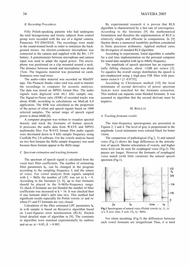
B. Recording Procedures

Fifty Polish-speaking patients who had undergone

the total laryngectomy and twenty subjects from control

group were recorded with the use of a digital camera,

Panasonic NV-DS65EGE. The recordings were made

in the sound-treated booth in order to minimize the back-

ground noises. An electret-condenser microphone was

connected to the camera and supplied with the R6, 1.5V

battery. A potentiometer between microphone and camera

input was used to adapt the signal power. The micro-

phone was positioned on a clip mounted around a neck.

The distance between mouth and microphone was about

15cm. The linguistic material was presented on cards.

Sentences were read twice.

The audio-video material was recorded on MiniDV

tape. The Pinnacle Studio video card was used to transfer

the recordings to computer for acoustic analyses.

The data was stored on MPEG format files. The audio

signals were digitized with 44,1 kHz sample rate.

The Signal-to-Noise ratio (SNR) of recorded tracks was

about 45dB, according to calculations on MatLab 6.0

application. The SNR was calculated as the proportion

of the power of silent and speech signals based on 1000

selected samples. The actual range of speech signal

power is about 60dB [8].

A computer program was written to visualize spectral

density and track the formants of human speech.

It processes the audio data from WAVE and MPEG

multimedia files. For WAVE format files audio signals

were decimated down to 8 kHz sample frequency using

CoolEdit Pro 2.0 software. For the vowels analysis based

on two first formats the 8kHz sample frequency was used

because these formats appear in the 4kHz range.

C. Spectrum estimation and tracking formants

The spectrum of speech signal is calculated from the

vocal tract filter coefficients. The number of estimating

filter parameters hk, can be changed in the programaccording to the sampling frequency fs and the natureof voice. For vowel analysis from signals sampledwith fs = 8kHz the number of LPC was set to k = 8.According to the literature [3, 8], up to four formantsshould be placed in the 0-4kHz-frequency range.To check if formants are not blended the number of filtercoefficients was increased to k = 16. It was checked thenif one formant didn’t split into two. This method hadsignificant results especially for Polish vowels /o/ and /u/where F1 and F2 formants are very closed.

Calculation of the filter estimated LPC parameters hk

in n-th sample is based on Recursive algorithm based

on Least-Squares error minimization (RLS). Haykin

listed detailed steps of algorithm in [9]. The constants

in algorithm were matched experimentally by authors

and set as: α = 0.05, = 0.985.

By experimental research it is proven that RLS

algorithm is characterized by a fast rate of convergence.

According to the literature [9] the mathematical

formulation and therefore the implementation of RLS is

relatively simple and efficient in computation. In [9]

Haykin shows a numerical instability problem considered

in finite precision arithmetic. Applied method cures

the divergence of standard RLS algorithm.

According to experiments, listed algorithm is suitable

for a real time implementation on the personal computer

for sound data sampled with up to 44kHz frequency.

The amplitude of speech spectrum has an exponent-

tially falling character, about -12dB per octave [3].

To equalize the overall energy distribution the speech is

pre-emphasized using a high-pass FIR filter with para-

meter vector h = [1 -0.9735].

According to Christensen method [10] the local

minimums of second derivative of power spectrum

A(m,n) were searched for the formants extraction.

This method can separate some blended formants. It was

assumed in algorithm that the second derivate must be

negative.

III. RESULTS

A. Tracking formants results.

The time-frequency spectrograms are presented in

Figures 2, 3 and 4. The level of gray is proportional to the

amplitude. Local minimums were colored black for better

vision.

The comparison of pathological (Fig.2, 3) and natural

voice (Fig.1) shows the huge differences in the articula-

tion of speech. Shorter articulation of vowels, and higher

noise level can be seen for esophageal voice (Fig.2). The

pauses are longer. However the formants of esophageal

voice match (with little variation) the natural speech

spectrum (Fig.1).

Fig.1 Spectrogram of natural voice (Polish vowels /a/, /i/, /e/

/y/), X axis: time, Y axis: f/fS, fS= 8kHz.

For silent mouthing (Fig.3) the differences between

each vowel formants are insignificant Thus, it is hard

34 MAVEBA 2005

to recognize each vowel from the spectrum. Presence

of noise is more evident than in the alaryngeal group.

Fig.2 Spectrogram of esophageal speech (Polish vowels /a/, /i/,

/e/ /y/), X axis: time, Y axis: f/fS, fS= 8kHz.

Fig.3 Spectrogram of silent mouthing voice (Polish vowels /a/,

/i/, /e/ /y/), X axis: time, Y axis: f/fS, fS= 8kHz.

It is evident that there are higher frequencies of first

formant for silent mouthing vowels articulation (Fig. 3).

In this speech no fundamental frequency excitation

sources are involved in speech production. Although the

vocal tract parameters are similar, the transfer function is

different because of other source of air turbulences [3].

Moreover, the speech is distorted and the spectrum

covered by the air turbulences noise from tracheotomy

tube and its spectrum with regular resonances. Thus, the

spectrum is distorted and the speech less intelligible.

B. Vowels classification.

It is well known that vowels are identified mostly

through their formant frequencies [9] and therefore

a major part of the perceptual information contained

in voiced speech is encoded in these formant frequencies

[7]. This paper is concerned with the differences between

the formant frequencies of normal and pathological voice.

Mean values and deviations of the first and second

formants of the vowels produced by normal, esophageal

and silent mouthing voices have been presented

in Figures 4, 5 and 6. The measurements were performed

for 3 subjects of each group.

The universal vowel production characteristics were

obtained for alaryngeal and normal speech. The acoustic

characteristics presented in Fig. 4 and 5, match the

theoretical frequencies of Polish vowels formants from

[3]. It can be seen, that for the normal speech the vowels

subspaces in F1 and F2 formants dimensions can be

linearly separated (Fig. 4). The relative positions

of formant frequencies were maintained for alaryngeal

voice (Fig. 5).

0

500

1000

1500

2000

2500

3000

3500

0 200 400 600 800 1000

F1[Hz]

F2[Hz]

a

i

e

o

u

y

Fig 4. Vowels in normal speech (Polish) in the F1 and F2

formants dimensions

0

500

1000

1500

2000

2500

3000

3500

0 200 400 600 800 1000 1200

F1[Hz]

F2[Hz]

a

i

e

o

u

y

Fig 5. Vowels in esophageal speech (Polish) in the F1 and F2

formants dimensions

Voice recovering / enhancement 35

The Fig. 6 shows how the pathology affects the

speech spectrum. For the patients, who haven’t learned

the esophageal voice, it is impossible to recognize vowels

by two first formants. Moreover, it has been observed that

the formants of vowels in the silent mouthing are more

dispersed, unclear and less stable than in alaryngeal

voice. Significant deviations of temporal formant

frequencies are seen on Fig. 6.

1000

1500

2000

2500

3000

3500

400 600 800 1000 1200 1400 1600

F1[Hz]

F2[Hz]

a

i

e

o

u

y

Fig 6. Vowels in silent mouthing speech (Polish) in the F1 and

F2 formants dimensions

The figures with objective data prove how important

the rehabilitation and learning an esophageal voice is.

The pronunciation of vowels causes the biggest problems

to laryngectomees. Vowels should be articulated with the

use of low fundamental frequency. Patients should then

learn how to use the source of phonation alternative

to laryngeal voice, to acquire useful intelligible voice

production.

IV. DISCUSSION

Initial tests’ results show the field for the future work

on improving pathological speech with the computer

methods. A linear or nonlinear separation methods,

e.g. neural networks or SVM can be used for vowel

recognition. However, we are not able to recognize silent

mouthing speech based on two first formants; therefore

we use other parameters, e.g. lips and jaw expression

from image analysis.

V. CONCLUSION

It has been presented that formant frequenciesequivalent to vocal tract coefficients are very sensitiveto pathology of speech organs. This indicates thatformants are objective descriptors for evaluationof rehabilitation after the laryngeal surgery and speech

intelligibility. Our approach is developed for efficient and

accurate tracking formants from the smooth AR

spectrum. Eliminating noise and fundamental frequency

with its harmonics due to the use of adaptive algorithm

allows extracting formants in a simple way.

The computer program on formant extraction can be used

for objective analysis of vicarious voice of larynge-

ctomees.

REFERENCES

[1] B. Chen and P.C. Loizou, “Formant Frequency

Estimation in Noise” in IEEE Int. Conf. Acoustics,

Speech, and Signal Processing, vol. I, Montreal, 2004,

pp.581-584.

[2] L. J. Lee, H. Attias, L. Deng and A. Acero,

“A structured speech model with continuous hidden

dynamics and prediction-residual training for tracking

vocal tract resonances” in Proceedings of the 2004 IEEE

International Conference on Acoustics, Speech, and

Signal Processing, Montreal, 2004.

[3] R. Tadeusiewicz, Sygna_ mowy, 1st ed., Warsaw:

Wydawnictwa Komunikacji i Lacznosci, 1988,

pp.158-186.

[4] R. Goldberg and L. Riek, Chapter 3, 4 in A Practical

Handbook of Speech Coders, Boca Raton: CRC Press,

2000.

[5] T. Zielinski, Od teorii do cyfrowego przetwarzania

sygna_ów, Krakow: Wydzial EAIiE AGH, 2002.

[6] L. Rutkowski, Filtry adaptacyjne i adaptacyjne

przetwarzanie sygna_ow: teoria i zastosowania, Warsaw:

Wydawnictwa Naukowo Techniczne, 1994, pp.49-85

[7] S. Saito, Speech Science and Technology, Tokyo:

Ohmsha, 1992, pp. 63-94.

[8] Z. Zyszkowski, Podstawy elektroakustyki, 3 rd ed.,

Warsaw: Wydawnictwa Naukowo Techniczne, 1984,

pp.218-277

[9] S. Haykin, Adaptive filter theory, Englewood Cliffs:

Prentice Hall, 1991, pp. 477-485.

[10] R. Christensen, W. Strong and P. Palmer “A

comparison of three methods of extracting resonance

information from predictor-coefficient coded speech” in

IEEE Trans. Acoust., Speech, and Sig. Proc. ASSP-24(1),

1976, pp. 8-14.

36 MAVEBA 2005

OPTIMISED GSVD FOR DYSPHONIC VOICE QUALITY ENHANCEMENT

Claudia Manfredi, Cloe Marino, Fabrizio Dori, Ernesto Iadanza

Department of Electronics and Telecommunications Università degli Studi di Firenze, Via S.Marta 3, 50139 Firenze, Italy

[email protected]

Abstract: This paper concerns the problem of enhancing voice quality for people suffering from dysphonia, caused by airflow turbulence in the vocal tract, for irregular vocal folds vibration. A generalized subspace approach is proposed for enhancement of speech corrupted by additive noise, regardless of whether it is white or not. The clean signal is estimated by nulling the signal components in the noise subspace and retaining the components in the signal subspace. Two approaches are compared, taking into account both signal and noise, or signal only, eigenvalues. An optimised adaptive comb filter is applied first, to reduce noise between harmonics. Objective voice quality measures demonstrate improvements in voice quality when tested with sustained vowels or words corrupted with “hoarseness noise”. The intention is to provide users (disabled people, as well as clinicians) with a device allowing intelligible and effortless speech for dysphonics, and useful information concerning possible functional recovering. This will be of use to people in social situations where they interact with non-familiar communication partners, such as at work, and in everyday life. Keywords: hoarseness, voice denoising, GSVD, comb filtering, voice quality, pitch, noise, formants.

I. INTRODUCTION Signal subspace methods are used frequently for denoising in speech processing, mainly with speech communication [1], [2]. Until now, few results are available concerning their application for voice quality enhancement in the biomedical field [3]. In this paper, the objective of noise reduction is to improve noisy signals due to irregular vocal folds vibration. This problem is of great concern, for rehabilitation and from the assistive technology point of view. Commonly, surgical and/or pharmacological treatments allow restoring voice quality, with patient’s recovering to an acceptable or even excellent level. However, sometimes patients can only partly recover, with heavy implications on their quality of life. The idea behind subspace methods is to project the noisy signal onto two subspaces: the signal subspace (since the signal dominates this subspace), and the noise subspace. The noise subspace contains signals from the noise

process only, hence an estimate of the clean signal can be made by removing or nulling the components of the signal in the noise subspace and retaining only the components of the signal in the signal subspace. The decomposition of the space into two subspaces can be done using either the singular value decomposition (SVD) [4], [5] or the Quotient SVD (QSVD) or GSVD [1],[6],[11]. Though computationally expensive, GSVD was found robust and effective in reducing noise due to turbulences in the vocal tract, which is typically coloured. GSVD is implemented here with two choices for separating the signal and the noise subspaces, to compare performance. Specifically, the first choice is based on classical GSVD, where both the signal and the noise subspace eigenvalues are used for filtering [6]. The second one corresponds to retaining the signal subspace eigenvalues only [1]. An adaptive comb filter is applied first, as it was shown to significantly reduce noise between the harmonics in the spectrum. The comb filter is optimised, in the sense that it is applied on windows whose length varies according to varying pitch. Real data coming from dysphonic subjects are successfully denoised with the proposed approaches.

II. MATERIALS AND METHODS Firstly, optimised adaptive comb filtering is performed on data windows of varying length, obtained with a new two-step robust adaptive pitch estimation technique [7]. The essence of comb filtering is to build a filter that passes the harmonics of the noisy speech signal y, while rejecting noise frequency components between the harmonics [8],[9]. Ideally, spacing between each “tooth” in the comb filter should correspond to F0 (1/T0) in Hz, which is often highly unstable in pathological voices. The proposed comb filter, based on an adaptive two-step pitch estimator, is capable to adapt to fast pitch variations and successfully reduces noise as evaluated by an adaptive implementation of the Normalised Noise Energy technique (ANNE) [7], thus being suited as a pre-filtering step. The filter that has been used in this paper has a Hamming window shape, which is obtained from the following equation (with K=3):

∑−=

+π+

+π+=

K

Ki)1K2/i2cos(46.054.0

)1K2/i2cos(46.054.0)i(a (1)


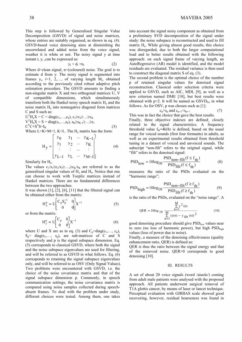
This step is followed by Generalised Singular Value Decomposition (GSVD) of signal and noise matrices, whose entries are suitably organised, as shown in eq. (4). GSVD-based voice denoising aims at diminishing the uncorrelated and added noise from the voice signal, weather it is white or not. The noisy signal y at time instant t, yt ,can be expressed as:

yt = dt +nt (2) Where d=clean signal, n=(coloured) noise. The goal is to estimate d from y. The noisy signal is segmented into frames yi, i=1, 2,…, of varying length Mi, obtained according to the previously cited robust adaptive pitch estimation procedure. The GSVD amounts to finding a non-singular matrix X and two orthogonal matrices U, V of compatible dimensions, which simultaneously transform both the Hankel noisy speech matrix Hy and the noise matrix Hn into nonnegative diagonal form matrices C and S such as: UTHyX = C = diag(c1,…,ck), c1≥c2≥…≥cK VTHnX = S = diag(s1,…,sk), sK≥sK-1≥…≥s1 CTC+STS=IK (3) Where L+K=M+1, K<L. The Hy matrix has the form:

−−

−

=

1My...Ly1Ly:...::Ky...2y1y

1Ky...1y0y

yH (4)

Similarly for Hn. The values c1/s1≥c2/s2≥…,≥cK/sK are referred to as the generalised singular values of Hy and Hn. Notice that one can choose to work with Toepliz matrices instead of Hankel matrices. There are no fundamental differences between the two approaches. It was shown [1], [2], [6], [11] that the filtered signal can be obtained either from the matrix:

11

pppy X

000SCUH −

−

= (5)

or from the matrix:

1ppy X

000C

UH −

= (6)

where U and X are as in eq. (3) and Cp=diag(c1,…, cp), Sp= diag(s1,…, sp), are sub-matrices of C and S respectively and p is the signal subspace dimension. Eq. (5) corresponds to classical GSVD, where both the signal and the noise subspace eigenvalues are used for filtering, and will be referred to as GSVD in what follows. Eq. (6) corresponds to retaining the signal subspace eigenvalues only, and will be referred to as OSV (Only Signal Values). Two problems were encountered with GSVD, i.e. the choice of the noise covariance matrix and that of the signal subspace dimension p. Commonly, in speech communication settings, the noise covariance matrix is computed using noise samples collected during speech-absent frames. To deal with the problem under study, different choices were tested. Among them, one takes

into account the signal noisy component as obtained from a preliminary SVD decomposition of the signal under study: the noise subspace is reconstructed and used to fill matrix Hn. While giving almost good results, this choice was disregarded, due to both the larger computational load and to better results obtained with the following approach: on each signal frame of varying length, an AutoRegressive (AR) model is identified, and the model residuals are evaluated. The residual variance is then used to construct the diagonal matrix S of eq. (3). The second problem is the optimal choice of the number p of retained singular values for denoised signal reconstruction. Classical order selection criteria were applied to GSVD, such as AIC, MDL [9], as well as a new criterion named DME [10], but best results were obtained with p=2. It will be named as GSVDfix in what follows. As for OSV, p was chosen such as [1]:

cp>sp and cp+1<sp+1 (7) This was in fact the choice that gave the best results. Finally, three objective indexes are defined¸ closely related to the signal characteristics. A frequency threshold value fth=4kHz is defined, based on the usual range for voiced sounds (first four formants) in adults, as well as on experimental results obtained from threshold tuning in a dataset of voiced and unvoiced sounds. The subscript “non-filt” refers to the original signal, while “filt” refers to the denoised signal:

(8))thf(ffiltPSD

)thf(ffiltnonPSD1010loglowPSD

≤

≤−=

measures the ratio of the PSDs evaluated on the “harmonic range”;

(9))thf(ffiltPSD

)thf(ffiltnonPSD1010loghighPSD

≥

≥−=

is the ratio of the PSDs, evaluated on the “noise range”. A

good denoising procedure should give PSDlow values near to zero (no loss of harmonic power), but high PSDhigh values (loss of power due to noise). Finally, a measure of the denoising effectiveness (quality enhancement ratio, QER) is defined as: QER is thus the ratio between the signal energy and that of the removed noise. QER>0 corresponds to good denoising [10].

III. RESULTS A set of about 20 voice signals (word /aiuole/) coming from adult male patients were analysed with the proposed approach. All patients underwent surgical removal of T1A glottis cancer, by means of laser or lancet technique. Perceptual evaluation with GIRBAS scale showed good recovering, however, residual hoarseness was found in

(10)M

1n2(n))filty(y(n)

M

1n(n)2y

1010logQER∑=

−

∑==

38 MAVEBA 2005

Special session on

Physical and mechanical models and devices


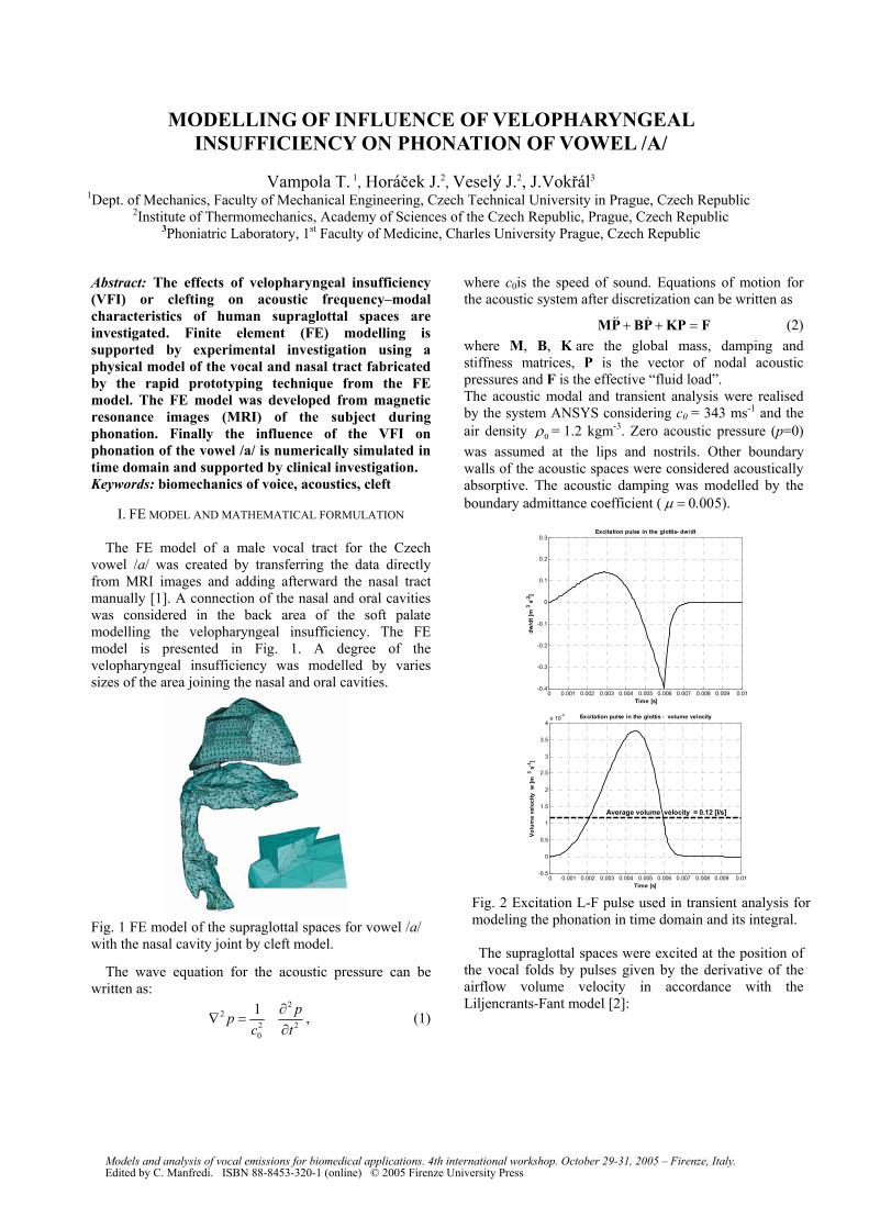
Abstract: The effects of velopharyngeal insufficiency (VFI) or clefting on acoustic frequency–modal characteristics of human supraglottal spaces are investigated. Finite element (FE) modelling is supported by experimental investigation using a physical model of the vocal and nasal tract fabricated by the rapid prototyping technique from the FE model. The FE model was developed from magnetic resonance images (MRI) of the subject during phonation. Finally the influence of the VFI on phonation of the vowel /a/ is numerically simulated in time domain and supported by clinical investigation. Keywords: biomechanics of voice, acoustics, cleft

I. FE MODEL AND MATHEMATICAL FORMULATION

The FE model of a male vocal tract for the Czech

vowel /a/ was created by transferring the data directly from MRI images and adding afterward the nasal tract manually [1]. A connection of the nasal and oral cavities was considered in the back area of the soft palate modelling the velopharyngeal insufficiency. The FE model is presented in Fig. 1. A degree of the velopharyngeal insufficiency was modelled by varies sizes of the area joining the nasal and oral cavities.

The wave equation for the acoustic pressure can be written as:

22

2 20

1 ppc t

∂∇ =

∂, (1)

where c0is the speed of sound. Equations of motion for the acoustic system after discretization can be written as

+ + =MP BP KP F&& & (2) where M, B, K are the global mass, damping and stiffness matrices, P is the vector of nodal acoustic pressures and F is the effective “fluid load”. The acoustic modal and transient analysis were realised by the system ANSYS considering c0 = 343 ms-1 and the air density 0ρ = 1.2 kgm-3. Zero acoustic pressure (p=0) was assumed at the lips and nostrils. Other boundary walls of the acoustic spaces were considered acoustically absorptive. The acoustic damping was modelled by the boundary admittance coefficient ( µ = 0.005).

The supraglottal spaces were excited at the position of the vocal folds by pulses given by the derivative of the airflow volume velocity in accordance with the Liljencrants-Fant model [2]:

0 0.001 0.002 0.003 0.004 0.005 0.006 0.007 0.008 0.009 0.01-0.4

-0.3

-0.2

-0.1

0

0.1

0.2

0.3

Time [s]

dw

/dt [

m 3

s-2

] Excitation pulse in the glottis- dw/dt

0 0.001 0.002 0.003 0.004 0.005 0.006 0.007 0.008 0.009 0.01-0.5

0

0.5

1

1.5

2

2.5

3

3.5

4x 10-4

Time [s]

Vol

ume

velo

city

w [m

3 s

-1]

Excitation pulse in the glottis - volume velocity

Average volume velocity = 0.12 [l/s]

Fig. 2 Excitation L-F pulse used in transient analysis for modeling the phonation in time domain and its integral.

Fig. 1 FE model of the supraglottal spaces for vowel /a/ with the nasal cavity joint by cleft model.

MODELLING OF INFLUENCE OF VELOPHARYNGEAL INSUFFICIENCY ON PHONATION OF VOWEL /A/

Vampola T. 1, Horáček J.2, Veselý J.2, J.Vokřál3

1Dept. of Mechanics, Faculty of Mechanical Engineering, Czech Technical University in Prague, Czech Republic 2Institute of Thermomechanics, Academy of Sciences of the Czech Republic, Prague, Czech Republic

3Phoniatric Laboratory, 1st Faculty of Medicine, Charles University Prague, Czech Republic


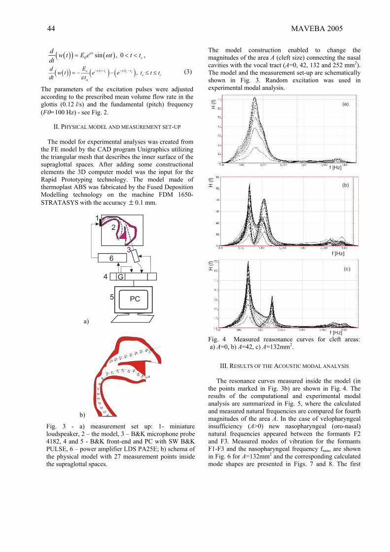
( )( ) ( )0 sin , 0te

d w t E e t t tdt

α ω= < < ,

( )( ) ( ) ( )( ( ,e c et t t tee c

a

Ed w t e e t t tdt t

ε ε

ε− − − −= − − ≤ ≤ (3)

The parameters of the excitation pulses were adjusted according to the prescribed mean volume flow rate in the glottis (0.12 l/s) and the fundamental (pitch) frequency (F0=100 Hz) - see Fig. 2.

II. PHYSICAL MODEL AND MEASUREMENT SET-UP The model for experimental analyses was created from the FE model by the CAD program Unigraphics utilizing the triangular mesh that describes the inner surface of the supraglottal spaces. After adding some constructional elements the 3D computer model was the input for the Rapid Prototyping technology. The model made of thermoplast ABS was fabricated by the Fused Deposition Modelling technology on the machine FDM 1650-STRATASYS with the accuracy ± 0.1 mm.

The model construction enabled to change the magnitudes of the area A (cleft size) connecting the nasal cavities with the vocal tract (A=0, 42, 132 and 252 mm2). The model and the measurement set-up are schematically shown in Fig. 3. Random excitation was used in experimental modal analysis.

III. RESULTS OF THE ACOUSTIC MODAL ANALYSIS

The resonance curves measured inside the model (in the points marked in Fig. 3b) are shown in Fig. 4. The results of the computational and experimental modal analysis are summarized in Fig. 5, where the calculated and measured natural frequencies are compared for fourth magnitudes of the area A. In the case of velopharyngeal insufficiency (A>0) new nasopharyngeal (oro-nasal) natural frequencies appeared between the formants F2 and F3. Measured modes of vibration for the formants F1-F3 and the nasopharyngeal frequency fnaso.

are shown in Fig. 6 for A=132mm2 and the corresponding calculated mode shapes are presented in Figs. 7 and 8. The first

a)

2625

2423

2221

2019

1015

5

1

1716

1413

1211

9

87

4

2

6

3

27

18

12

3

4

5 PC

G

6

b)

2625242322212019

1015

5

1

1716

14131211

9

8

7

4

2

6

3

27

18

Fig. 3 - a) measurement set up: 1- miniature loudspeaker, 2 – the model, 3 – B&K microphone probe 4182, 4 and 5 - B&K front-end and PC with SW B&K PULSE, 6 – power amplifier LDS PA25E; b) schema of the physical model with 27 measurement points inside the supraglottal spaces.

H (f

)

f [Hz]

(a)

f [Hz]

(b)H (f

)

f [Hz]

(c)H (f)

Fig. 4 Measured reasonance curves for cleft areas: a) A=0, b) A=42, c) A=132mm2.

44 MAVEBA 2005

calculated oro-nasal acoustic mode shape with the predominant vibrations in the horizontal direction (see Fig. 8a) was not excited in the experiments.

0

500

1000

1500

2000

2500

3000

3500

0 50 100 150 200 250 300A [mm2]

f [H

z]

f naso

F3

F2F1

Fig. 5 Calculated (——) and measured (------) formant (F1-F3) and nasopharyngeal frequencies for the vowel /a/ for increasing area A of the cleft.

(a)

nasal tract

lips

⇓ interconnection (cleft)⇔

loudspeaker(vocal folds)

⇓

⇓

⇓nostrils

(b)

(c)

(d)

Fig. 6 Measured acoustic mode shapes of vibration for the cleft size A=132 mm2. The double amplitudes of the pressure are shown in 27 measurement points along the vocal and nasal tracts - a) F1= 679 Hz, b) F2= 884 Hz, c) fnaso= 1266 Hz, d) F3= 3042 Hz.

Fig. 7 Computed acoustic mode shapes of vibration for the cleft size A=132mm2.

Fig. 8 Computed acoustic oro-nasal modes of vibration for the cleft size A=132mm2 (fnaso= 1432 Hz and 1492 Hz).

IV. NUMERICAL SIMULATION OF PHONATION

The behavior of the FE model was tested by a broadband frequency pulse. The power spectral density of this pulse is presented in the Fig. 9.

0 2 4 6 8 10 12-140

-120

-100

-80

-60

-40

Frequency (kHz)

Pow

er/fr

eque

ncy

(dB/

Hz)

Power Spectral Density - broadband pulse

Fig. 9 Power spectral density of the broadband frequency pulse for testing the FE model by the transient analysis.

Special session on physical and mechanical models and devices 45

The results of transient analysis in the frequency domain are presented in Fig. 10 for the broadband frequency pulse and in the Fig. 11 for L-F pulse model.

Fig. 10 Power spectral density of the pressure near the lips for Czech vowel /a/ for broadband frequency pulse and the cleft size A=132mm2.

Fig. 11 Power spectral density of the pressure near the lips for vowel /a/ for L-F pulse (A=132mm2).

Fig. 12 Acoustic pressure near the lips for LF pulse. The formant frequencies F1≈630 Hz, F2≈987 Hz and

F3≈2893 Hz can be found in the frequency response functions in Fig. 11. The formant frequencies are in good agreement with the data known for Czech vowels. Another resonant frequencies fnaso ≈1432, 1492 Hz appears in Fig. 5 and 11 due to the velopharyngeal insufficiency.

V. CLINICAL INVESTIGATION The theoretical results were compared with the results

of the acoustic voice analysis. Eight adults with mild velopharyngeal insufficiency phonated vowel /a/ and pronounced the interconnection /ama/. The nasal and oral signals were picked up by microphones of the head part of Nasometer 6200-3 (Kay Elemetrics Corp.) and analysed by Multi-Speech (Kay El. Corp.) programme. The new resonant region (formant) was found between formants F2 and F3. Its position was located between 1800 Hz to 2050 Hz, the relative intensity of harmonics in this region was between –7 dB to +3 dB with regard the formant F3. The example of the acoustic analysis is shown in Fig. 13.

Fig. 13 Acoustic analysis of the pronounced interconnection /ama/.

VI. CONCLUSIONS

The time response functions for the pressure near the lips were obtained by the transient analysis of the FE models of the vocal tract for the model excited by a broadband frequency pulse and L-F pulse. The formant frequencies F1 – F3 evaluated from the resonances of the calculated frequency response functions are in good agreement with the experimental data. The existence of calculated oro-nasal formant was verified by the measurements on physical model as well as on subjects suffered by the velopharyngeal insufficiency.

ACKNOWLEDGEMENT This research is supported by the Grant Agency of the Czech Republic by the project No 106/04/1025 “Modeling of vibroacoustic systems focusing on human vocal tract”.

REFERENCES

[1] Dedouch, K.; Horáček, J.; Vampola, T.; Kršek, P.; Švec, JG, 2001. Mathematical modelling of male vocal tract. In: Proc. MAVEBA, Sept.13-15, 2001, Firenze, pp. 6-8 [2] Fant, G.; Liljencrants, J.; Lin, Q., 1985. A Four Parameter Model of Glottal Flow. In STL-QPSR 4, KTH, Stockholm, Sweden, pp.1-13. [3] Vohradník, M., 2001. Communication disorders by velopharyngeal insufficiency. Prague - Dolni Brezany: Scriptorium, 2001, pp.134-145 (in Czech).

0.5 1 1.5 2 2.5 3 3.5 4 4.5 5 5.5

-70 -65 -60 -55 -50 -45 -40 -35 -30 -25

Frequency (kHz)

PSD - lips pressure - wovel A - broadband pulse

1 2 3 4 5 6-90

-80

-70

-60

-50

-40

-30

Frequency (kHz)

Pow

er/fr

eque

ncy

(dB/

Hz)

PSD - lips pressure - wovel A - LF pulse

0 0.01 0.02 0.03 0.04 0.05 0.06-2

-1.5

-1

-0.5

0

0.5

1

1.5

2

2.5x 10-5

Time [s]

Soun

d pr

essu

re [P

a]

Time response - wovel A - lips pressure - LF pulse

46 MAVEBA 2005

� � � � � � � � � � � � � � � � � ! � " $ ! � ' )

* + - - 0 2 4 6 7 0 - - 0 2 ; < < + ? @ B 6 ; D F < ; G 0 D J L @ M O Q ; - S G J ; U V + X - U Z @ [ 0 D J \ ; X ; 2 [ ; 2 ^ ; < ?

_ S < ` b c @ b c c f

g i j l m n o l

q r s u w y { y } � � � r � � � � � � } � � � y � � } � � � } � r y � � � � � � u � � � � y� � r y � � { s � } r � { y � � � y � � � r } � � � } � � w � � y y � � � r s y � � r ¡ � y } y � y } r � } � � } � � s s � r £ � r y r � } r � � r � r � y �� r y � � s r � � r � y � � � � u } � r � r s s w ¥ � � � � � � � r s � u � { � � �� s u � s � � � � � � } � � � y � ¨ � � r � � r � ª � � � � r s � � � r s � u

} � r y � � � � � � u � � � � � � � � r � y � � } � � � { � r � � r y � � �} � � } } � r � � } r � y � } � � u � � � � � � � � y � r £ r � � y y } � � � � s � � �} � r � r � � r } � � � u } � r � � � � � } � � � } � y y { r � � � } � r � � � � � � �£ � r y y { � r � � � y s r � � y } � � � � y � { y y � � � � � � � � � � y � � �� } � � s } � r y } � r � � } � � u � � r � } � � r y �

¯ ° ± l m ² ³ ´ o l µ ² ±

� � w � � y y � � � r s y � u � � � � s u � s � y � � � � � } � � � y � � � r� r r � { y r � y { � � r y u { s s � } � � r y � � � � r } � r � � � � � s � � � � r

· ¸ ª ¹ º ª � � � � s u � s � £ � � � s � y � r y · ¼ ª ½ ª ¾ ª ¿ º ª £ � � � � } � � �� y r } · Á º ª � � � � r � � y } � � � s � } � r y � } � � � � £ � r y y { � r y · Â º� � y � { � � r w } � � � } � � { £ s � � � · Ã ª ¸ Ä º � Å � s s r � � � � Æ � � y r �

· ¸ ¸ º � � � Ç s r � � � y r } � s � · ¸ ¹ º � � � r y � � � � } � � } y � { � �� r � r � � } � � � � � � � � � � � � � y � y � � � { � r � � s y � � � � � � � w} r � � � } � � � � r } � r r � � � � É � � � � � � � � � r � � � � � � � s � � w� � � } � � � y � u s � � � � � � } � � � ¥ r � r � � r � � � � � r y � Í � � wy r Î { r � } s � ª � � � � r � � � � � � � s � � � r s y � � � � r r � £ s � � } r �

} � y } { � � } � r y � { � � � r � r � � } � � � � � } � r � � � � y y � � � � �· ¸ ¼ ª ¸ ½ ª ¸ ¾ º �

Ï � } � � y £ � £ r � � r � � � £ } } � r � r s s w ¥ � � � � y � � £ s � ¡ r �} � � w � � y y � � � r s } � } � r � � � r � y � � � y � u � y � � � � � � �� r � } � y } { � � } � r � � y r } � u y � { � � � r � r � � } � � � � � �� } � � s � u � � � � r � � � � � � � � � y Ð � � r � } � � r y Ñ � Ï � � ¡ � y }

� � � r s � r � y � � � � r y � � £ s � � r y � � s r } � r } � � w � � y y } � } � ry � Ò r � u � y � � � � � � � y � � � � � � � r � � r � r � � � r � y � � r w

� � � } � � � r � r � s � y } � � � � � r s � r y � � � � � � � } � r y � � � � � � uÓ Ô Õ Ö × Ø Ù Ú Û Ü Ý Þ ß à á â Þ Û ã ä Ý â Û Þ Û Õ Û à æ Ø á ç è à Ø á à Û Þ é ê Ù ë Þ Ø Ù Ø ì ã

í ä ç ë î ä Ý ß ê Ù Þ Ú à Ý â Û á ï ð ñ ò ó ô õ ö õ õ ÷ ë à á Ù Þ Ý ò ø à á Ö ê Ý ãù ú û ü à á Þ Ö à Ý Û ê Ù ý Ø Ø Ù Ø ì ã ø á Ø Õ ü ò þ ê ì à Ý Þ Ý ì à Ý Ü Ý Þ ß à á â Þ Û ã� ï � ï ë Ø û ñ ñ � ò � � ö ö � Ô þ ê ì à Ý Þ Ý ì à Ý ò ç è à à Û è à á Ù ê Ý Ú â� é è Ø Ø Ù Ø æ � â ã é è Ø Ù Ø ì ã ò Ü Ý Þ ß à á â Þ Û ã Ø æ Û ï � Ý Ú á à � â ò Û ï� Ý Ú á à � â ò � Þ æ à ò � � õ � � � � ò é Ø Û Ù ê Ý Ú

� � � � � � � � r � r ¡ � � } � � } � � } � � � � r s y r � � � � � } y r s u wy { y } � � � r � � y � � s s � } � � � y � } � r � s � y } � � £ � � � � r } r � � � s { r y �

Ï � } � r � s � y y � � � s } � � w � � y y � � � r s � � s s � y � � � � � � { � y � }� � � � r � £ � r y y { � r y s r � � � � � } � y } � � � � � � � � � � � � y � Í � � w

} � � � � s � ª � � } � r � � � r s � u } � r � � � r y � � � � � � � s s � y � � � � y� � � � � r � s r � � � � � } � � � � r £ { � r } � � r y � � � � � s s � ª � r � r w

s � } r } � r y r � � y r � � � } � � � y } � } � r � � � r s � � � y � { y y r � } � £ � �� y � � � } � � s } � r � � } r � y � } � � u } � r � � � � � � � � � � y

· ¸ ¿ ª ¸ Á ª ¸ Â ª ¸ Ã º �

� ! l " ² ³ j n ± ³ $ ! j ´ % l j

� r � � � r s y � � y � { y y r � � � } � � y £ � £ r � � � r y ¥ r } � � r � � �� { � r ¸ � � � � � � { � r ¹ � � } � } � r £ � � � � r } r � y s � y } r � � �

} � r � � � � r y £ � � � � � � } � � s r y � � r ¡ � y } � � � r s y } � � � � s �� r y r � � s r y } � r � � � r s � { y r � y � � £ s � ¡ r � } � � w � � y y � � w� r s � u � � � � s u � s � y � � � � � } � � � y · ¾ ª Á ª Â º �Ï � } � � y � � � r s } � r � � y y r y � r £ � r y r � } } � r � � � � � w} � � � s � � � � � u y � � � � � � � y � � � � � � � � � } � } � r ¡ � � � � � y� u Å � s s r � � � � Æ � � y r � · ¸ ¸ º � � r y r � � � � � � � r s � y� � � £ } r � } � } � r y � � � � � � u � � � � � � � � r · ¸ ¹ º � ' r � r { £ w

£ r � � � � s � � r � � � y y r y � � r ) � � � r � � � £ s � } r y s r � � � � �} � � � { � � y � � � } � r � y � � £ r � u } � r � � � � � } � � � } � y y { r �

� r r Î { � } � � � y � u � � } � � � y � u � � } � � � � r s y � r � � � yu � s s � � y +

,- / 1 2 / Ð ¸ Ñ,2 / 1 ¸

4 /5 6 / 7 9 / 2 / 7 < / - / ? A / ?

7 < C Ð - / 7 - F Ñ H Ð ¹ Ñ,- F 1 2 F Ð ¼ Ñ

,2 F 1 ¸4 F

5 6 F 7 9 F 2 F 7 < F - F ? A F7 < C Ð - F 7 - / Ñ H Ð ½ Ñ

� r £ � r y y { � r u � � � r y 6 L � � r � r � � � r � u � � � } � rM r � � � { s s � r Î { � } � � � � � � } � r ) r } � y y { � £ } � � � Ð y r r · ¾ º

u � � � r } � � s y Ñ � � r � � s s � y � � � u � � � r y A L � � r � � � y r � � y � �


0

0

d1

d1 + d2

x axis

z axis

Trachea

Vocal tract

x1

x2

Ps

� � � � � � � � � � � � � � � � � � � � � � � � � � � & � � � � ( � �) � � � � � � + � � ( - /

� � � � � � � � � � � � � � � � � �! � � � # � $ & � $ � # � � � � � ) * + � �

- . / � 1 � � � � � � � � � � ) * ) ) 5 7 � � :- . : � � � � � � � � � � � � ) * ) ) 7 > ? � � :A / 7 B C � � � � � $ � � G � � � � ) * 7 � �A : 5 I J � � � � � $ � � G � � � � ) * ) 5 � �L / 7 B C � � � � ) * ) ) 7 ? #L : 5 I J � � � � ) * ) ) ) + #M / 7 B C � � � � � � � O � � � � ) * ) Q # R � � :M : 5 I J � � � � � � � O � � � � ) * ) ) Q # R � � :S � � � � � # � � � � � � � U S / V S : W ) * ) ) 5 # R � �M X � � � � � # � � � � � � � ) * ) ) 5 ? # R � � :

� � ) � � Z � � � � � � � � & � � � � � � � � � � � � � � � � � � �� ( � ( � � � /

� � � � � � � � � � � ; < > < ? @ /� � � � � A � � � � � � � � ( � � � & � � & � � � � � � � ( � � � � � � � � �

� � � ( � & � � � ( � � � � � ( � M � � � � � \ ] � ( � P � � + � ( � � � � _ �( � � � � / R � � � � ( � � � � � � � � � � � ( � � M � � � � � � & � � � � � � � � � � � � � � ( ) ) � � � U / U U V W V � � � � ` Y & � �� M M � � M � � � � M � � � � � � � / � � M � � ( � � a � ( � � � & �

� � ( � � � + � � ( � � � � � � � � � � � � � � � � � ( � ( � � � � � ( � � � ( �� ( � � � � � � � � � ( � � P � � � ( � W � � � M � � � � � /V Y /R ( � � � � � > � � � � � � � � � ( � � & � � � � � ( � � � � � � � � � � � ( & � � � � � � � � � P � ( � M � � � � � W \ ] U / U > Y / f P (� � � � � � � � � � � M � � � � � � � � � � � � � � � ( M � � � � � P <

� / / � � � � � � � � � ( � � � � � � � � / i � ( � j � ( � � + < � � � M � � � � � � ( � � � � � V � � � � � � � � � ( � � � � � � ( � � � / l � � � � � � + � � � � � � � � � � ( & � � � � � � � � � + ( � � � � P � ( � � � � � � � �� < � / / � & � � � + � � ( - � � � � � � � � ( � � � � � M � � � � � � ( /Z � � ) � ) � + ( � � � � P � � � � � � � � � ( � � � � � + � � � � � �

0 x02 x01 w

d

D +d

D + 2d

x axis

z axis

m2

m1

x2

x1

length l

Ps

� � � � � p � � � � � � � � & � � � � ( � � � P � + � � ( - � � � M � � ( � � � � � � � � � � � ( � ) + � � � � � � � � � � � M � � � � /

� � � � � � � � � � � � � � � � � �c 1 � � $ & � $ � � � � � $ � � ) * + � �

! � � � # � $ & � $ � � � � � $ � � ) * + � �f � � � � � � � � g � 1 � � $ ) * 7 ? � �A 7 B C � � � � $ � � # $ � ) * ) ? � �A i k 5 I J � � � � $ � � # $ � ) * 5 ? � �L � � � � � � U L / V L : W ) * ) ) ? #M � � � O � � � � ) * 7 # R � � :

S � � � � � # � � � � � � � ) * ) 7 # R � �M X � � � � � # � � � � � � � ) * ) ) 5 ? # R � � :

� � ) � p � Z � � � � � � � � & � � � � � � � & � � � � ( � � � P � + � � ( - W � � � � / p Y

M ( � � � � � � � � � ( � � & M � � � � � � � � � ( � � ( � � q � � �M � � � � � ( � � � & � � ( � � � � � � � � ) � � ( � W � � � � � � p Y / � � � � � � � � � � � � ( � � � � � � � � � � � � � � � � � � ( q � � � � �

� � � ( � & � � � + � � ( - � ( � � � � � � P � ( � M � � � � � � � ( � � �� + � � ( � � � � � � � ( � ( � � � + � & � � � � � ( � � � � � ( � � ( � & � � �� M � � � � ( � � � j � � � M � � ( � � ( � � � P � � � ( � /

m n r s t u s s r v w

R � � � � ) ( � � � � ( � ) � P � � � � � � � � � � ) � � � � � � �( � � � � � � � � � � � � � � ( � � � + � P � � M � � � � � � � � ) P � � � �

& � � � P � ) � � � � � ( � � � ( ) � � � M � � � � � � � � � � ) � � � �� + � � ( - / � � � � � � � ( � M � � � � � � ( � � � � � ( � � � - � � � �

) + � � � � � M � � ( � � M � � � ( � � � M ( � ( � M � � � �� M � � � � � � � � P � � � P � ) � � � � ( � � � � � � � � � � M � � �� ( � � � � � ( � � � � � � � � � M � � � � � � � � � � � � � � � �

� � � � ( � � � � � & � � � / � � & � ( � � � ( � � � & � j � ( � + � �� P � ( � ) + � � � � � � � ( � � � � _ ( � � � & � � P � ) � � � � ( �

� � � � � / a � � � � � � � + � � ( P � � ( � � � � M � � � � � � ( � � � � � �

48 MAVEBA 2005

� � � � � � � � � � � � � � � � � � � � � � � � � � � � � # � � � � � � % # � � # � ( � � � � + � # � - . /� # � � � � � � # � � � � � � % � # � 7 � � � # + � 8 � � � � 9 � : � � -

; � � � � � � � 8 � � � � � � � : � � � � � � / � � # � 7 � � � � � � � # � % # � � � � E 7 7 � � # � 8 � : # � � � � � / H � � � # � � � � + � E I� � � � 7 � 7 � � � � � M � � � � � � � � : � � � � � � 7 � � � �

� � � + � � 8 � : # � � � � + � # � � � # � ( � � � � 7 � � E # � � S � . /H � � � � � � � � � E � � � � � � � � � � � � � � E � # � � � � �: � � � � � � % # � � # � � # � � � � � � � E � � � # 7 � � � � # �� /9 � � � 7 � � � � � � � # 7 � � � � � � � # � 7 � � � � � � � ; � M � � � � 8 � # � � : � � / H � � � � 7 � � � � 8 � # � � � � � 7 � � % � # �

� � � � � # � � � � � � � � # � � � � � � � � 8 � : # � � � � � ( � / � /� � � # � � � � � % : � � # � � � � � � � � � � � ; � � � � � + � # � \ . /H � � � � # � � � � � � ; � � 7 � 7 � � � � _ � � � � � � � � � + � # �

- � # � � + � � # 7 � � � � % % � � # � � � � + � � # % # � � # � � � �� /

A

B

0.1 0.2 0.3 0.4 0.5k1

0.002

0.004

0.006

0.008

0.01

Ps

� � + � # � \ � � � # � � � � � � � � � � � � � � % # � � # � � � % � � � � � +� � � � � � � � � � � � � % � � � � � � � � � I � / � / � � � � � �# � � � � � 8 � � E � # # � 7 � � � � � % : � � # � � � � � I ; � � 8 � � � �� % � ; � # % � � # � 7 � � � � h � ; � � # � 8 � � � 8 � ( � �� + � # � j . /

H � � � # 7 � � � � � � � � # � � + � � 8 � E # � � S � � � � �� # � � � � � � � � % � # � 7 � � � # � 8 � � � # 8 � # E� � + � % # � � # � / n � � � M � � � � � E I � � # 7 � � � � # � � � # � E; � � _ / 9 � � � � 7 � � � � � � � # � 8 � � � � � � � � � � � � � � � � � � � � � 8 � # � � � � � � % � � � � # � � + � E � � � � � � � q + � # � � � � �� E # � � S � � � � � � 7 � � � � � � � � � E � � � # � �

� � � � 7 � � � � � � � # 7 � � � /9 � � # � � � � � � + � � : � � � � : � � � � � � � � � # � � � � � # �7 � � � � � : � # � � � + u - v I - w I - x I - y I z { | / � � � �: � # � � � + � � � � � � _ � � ; � � � � � � � � � � � 7 � � � � �� # + E � � � � � � � � 8 � # � � � � u - x | / � � ; � 8 � # I � � � 7 � % � � # � + # � 7 8 � # E % # � � � � � � � � 8 � # � � � � � # � 8 � � : � �

2 4 6 8 10

10−5

100

freq (kHz)

1st model (Ps = 0.0035)

1st model (Ps = 0.008)

2nd model (Ps = 0.05)

� � + � # � j � � � ; � # % � � # � � � � ; � � � � � # � � � # � + � 7 � � # # � % � � � � � + � � � � � � � � � � # � ( � � � � � � � � . � � � �

( � � � � � � � � . � � � � + / \ / n � � � � � � � � � � % : � � # � � � � � � % � � � � ( � . ( � � { / { { \ j . ; � � : � # 8 � � � � � �

� � � � � � # 7 � � � / 9 � � � � � _ + # � E � � � � # � � # � � � � �# � � + � � 8 � 7 � � � � /

u - - | / H � � # � � # � � � 7 � � � � � � � 7 � � % � � � u - w | � # � � � � # � � � � I : � # � � � � � � q � � � � � # � � � � � � � # � 8 � # � � � � /9 � � � � � + � � � + � � � � � � � � : � � � � � + � � � � : E � �

7 � � � � � � � � � % % # � % # � � � � 7 � � � � / H � � # � � � � % � �% � # I � � � � � � � � / � � � � � # � � � � � � ; 8 � # E � � + � # � � � � � � � q + � # � � � � � � � � % % # � � � � � � � � � � # 7 � � � � �% � + � � � u - v | /

0 5 10 15

0

2

4

6

8

10x 10

−3

time (ms)

Ps = 0.05a1

a2

� � + � # � � � 9 # � � � � � � # � � 8 � # � � � � � � � � # � � + � � � � � � � � �� # � � + � � 8 � E # � � S 7 � � � � � � 8 � � ; � � � � � � + �% # � � # � � � � � # � � � # � � � ; � E + # � � � � # � � � � � � # � /

H � � � � % � % � # ; � � � 8 � � � ; � � � � � � � � + � � 7 � � # E� � � � � � # � � % � � � � � � � � � � E # � � S � � � � h � � � �

� � � � � # 7 � � � % � � # � � # � � � � � � E / � � # � 7 � � � � % % � #7 � � � � � # � � � � + � � � # + � � 7 � � # E I � � � � � � � � � � � � � +� � � # � � + � � # 7 � � � � � : � � 8 � � � � � � � � E � � � # � � �% � � � � � � � � � � � � / � � � � + � � # % # � � # � � � � � � # � � � � +

� # � ; � � � � : � # � M � � # � � � � � � 7 � � � � � � � � � � � / 9 � �


� � � � � � � � � � � � � � � � � � � � � � � � � � � � � � � � � " � � � � $ � � & � " �� & � � � � � " - � & � $ � � � 1 $ � - $ 3 � � � � � � $ $ � $ " � � � �

7 9 : 9 < � � � � � & � � � � � & � � � " � � � � � � � � " � � C D E F H J 1 � &� 3 � � � � " � � � 1 � � � � � � � � � & � 9 : 9 N � � � " � � � � � 1 � � � �

� � $ � � � � � � � � � � � � � � � � � & � � $ � � � � � 1 � - HV � � 1 � � � � � � � � � $ � � � � � & � � $ � � � & � � � � � X � 1 � � � � � �� Y 1 � � 1 3 3 � � � � � � � N � � $ � � � � � � � 1 � � � � � � � � � � _

� � � � � � � � � � � � � & � � & 3 � � � � 1 � � � H : & � � � � 3 � � � 1 $ � " � -� 1 � � � � � � � � � � � � � � � � � � � � & � � 1 " � - � � � � � � � 3 � � � � 1 � �� " � � & $ � � � � � H� � � � � � � � 1 � � � � � � � � � � � � � � � � � � � � c � � � � � � � � � � � � C D D F

� & � � � & � � � � � � $ � � � & � � $ � � � � � � 1 � � � � � � � 3 � � � � � � -3 & � � � � � � � � � � � � � � � N � � � � � � � � � � � H : & � � � $ 3 � � � � � & � �� - $ $ � � � � � � " � � N � � � � 1 � e � N � � � � � e � N � � � & � � � �

& � � � � � " � � � g � � � � � � � � � � 1 � � H : & � � N � � � " � � � � � � � �� $ � � � � � 3 & � � � � � � � � � $ � � � � H � 1 � � � $ 1 � � � � � � � � � �� X � � � � � � 3 � � N � � � � $ � � � � � � � � � � � � $ � � � � � � � � � � & �� - � � � k H V � � 1 " � � Y 1 � � � � � 1 � � � � N � N � � � � � � � � 3 � � � � �

� & � 9 : 9 � � � � & � � - � � $ � � � � � � � � � � � � & � � � � � � � _� � � � $ 1 � � � � � H

� l n � o p � � � q � � � o r

s � � � g � � N � � � � � � 1 3 3 � � � � � � $ � & � � 1 � � � & �� & 1 � � � � � $ � � � � � & � � � 7 � � � � � � � D E w x � y < H

� � � � z � o n � {

� | � � } ~ � � � � � � � � � } � } � � � � � � � � � � � � � � � � � � � � � � � � � �� " � � � � $ �� } � � � � } � � � � } � } � � | � | & � � � | & � � � | � � & �

� & � ) } � � � � � � � � � � } � � � � � � � � � � � + } + } � � � � � � � � � � � } � } � }� � - � � � � � � � } � � � � � � � � � � � � � � � � � � � � � � � � � � � � � � � � � �� / � � � � � � � � � � � 1 � � � � � � � � � � � � � � � � � � � � � � � � � � �� } � � � � � � � � � � � � � � � � 2 � � � � � � � � � �� $ � � } � � � � � � } � � � } � � } � � � � � ¡ | � � � ¡ � | � | � � ¡ �

� � � � } ~ � � � � � � � � } � � � � � � � � } � � � � � � � � � � � � � � � � � � � � � � �� £ � � � � � � � � � � � � � � � � $ � � � � � } � � � �� } � | ¤ ¡ � � � � � � � � � | � � � �

� ¡ � � } ¥ } � � � � � � ¦ } � } � � � � � � � } + } ¦ � � � � � � � } � � � � � � � ��

� 8 � � � � � � � � � � � � � � � £ � � � � � � � � $ � } � � � � � } � � � � } + � � } �� ¡ � � � � ¡ � | � � & �

� � � ~ } � � � � � � � � � � � } � � � � � � � � � � � � � � � � � � � � � � � � � � � � � � � � � �£ � � � � � � � � � � � � � � $ � � } � � � � � � } � � � } � � } � � � � | � � ¡ � | � � ¡

� | � � � �

� � � � } � � � � � � � � � } � � � � � � � ~ } + } � � � � � $ ~ � � � � � � � � � � � � � � � �� £ � � � � � � � � � � � � � � � � $ � }� � � � � � } � � � } � � } � | ¤ � � & � � � � � ¤ ¤ & � & ¤ ¤ ¤ �

� � � � } � � � � � � � � � } � � � � � � � � } � � � � � � � � � � � � } � � � � � � � § }¥ � � � � � � � � � � � � � � � � � � � � � � � � £ � � � � � � � � � � � � � � � � � � �� $ } � } � � � � � � } � � � } � � } � | ¤ ¡ �¡ � ¡ � ¡ � ¤ � | � � � �

� � � � } � } � � � � � � � } ¨ � � � � � � } � � � � � � � � � � � � � � � � � � � � � � � �£ � � � � � � � � � � � � � � � � � � � � £ � � � � � � � � � $ � } � � � � � � } � � � }� � } � | | ¤ � & | & ¤ � & | & � � & ¤ ¤ | �

� � � � } � � � � � � � � � } � � � � � � � � � � � � � � � � � � � � � � � � � � � � � � �� £ � � � � � � � � � $ � � � � � � " � � � � � � � � � � � � � & & �

| ¡ | � | � ¡ � | � � � �

� | ¤ � � } � � � � � � � � � � � � } � } � � � � � � } � � � � � � � � � � � � � � � � � � �� ~ � � � � � � � � � � � $ � � � � � � � � � � � � � � � � }

� | | � } ¦ � � � � � � � } � } � � � � � � � � � � � � � � � � � � � � � � � � � � � �� $ � � � � � } � � � � } � � � � } � � � } § � � �� ¡ � | ¡ � � � � | ¡ � � | � | � � � �

� | & � " } � } � } ¥ � � � � � � � � } � } � � � � � � � § } � } � � � � � � � � � } � }£ � � � � � � � � � � } ¦ � � � � � � � � � � � � � � � � � � � � � � � � � � � � �� £ � K � � � � � � $ � � � � � � � � ¡ � | � | ¡ � � | ¡ � � & ¤ ¤ ¡ �

� | � � � } � } � � � � } � � � � � � � � � � } � � � � � � � � � } � � � � � � � � � � �� £ � � � � �� $ � � � � � � � � � � � � � � � � | � | � � � �

� | ¡ � � } � } � � � � � � � � � � � � � � � � � � � / � � � � � � � � � £ � � � � � � � � �� $ � � } � � � � � } � � � � } � | � � � ¡ � � � ¡ � | � | � � � �

� | � � + } � � - � � ¦ } � } � � � � � � � � � ª � £ � � � � � � � � � � � � � � � � � � � � �$ � � � � � } + � £ } � � � � } � � � � & � � | ¤ & � & ¤ ¤ & �

� | � � � } + � � � � � ¦ } � } � } � � � � � � � � � } � � � £ � � � � + } � } � � � � � � � �� ~ � 1 � � � � � � � � � � � � � � � � � � � � � £ � � � � � � � � � 2 � � � � � � �

� � � � � � � � £ � � $ � � � � � � � � � � ¥ � � � � � � � � � � � � � � � � � � & ¤ � �¡ ¤ & � � ¡ ¤ � � � & ¤ ¤ ¡ �

� | � � ª } � } � � � � � � + } � } � � � � � � � � � � � � � � � � � � � � � � � �� Q $ � � } � � � � � � } � � � } � � } �� & & � � � & � | � � ¡ �

� | � � � } � � � � � � � � � } � � � � � � � � } � � � � � � � � � } � � � � � � � ~ � � � �� / � � � � � � � � � � � � � � � � � � � � � � � � Q $ � ¥ � � � � � � � � � ¤ � & & � �

& � � � | � � & �

� | � � ¦ } � } � } � � � � � � � � + } � } � � � � � � � � " } � � � " � � � � � � � � � �� 2 � � � � � � � � � � � � � � � � � � £ � � �� $ � � � � � } � � � � } � � � � } � � � } § � � � | ¤ ¤ � � � � & � � � � �

� & ¤ ¤ � �

� & ¤ � ¦ } � } � } � � � � � � � � � } � } � � � � � � � + } � } � � � � � � � � � � � � � � �� $ �" � � � � � � � � � � � � � � | ¡ � | � � & � | � � � � & ¤ ¤ ¡ �

� & | � � } � } � � � � � � � � � � � � � � � � � � � � � � � � � � � � � � � � � � � � � �� ~ � � � � � �� $ � � } " � � } � � � � � � � } � } � | � � � � & � � � � �

� & ¤ ¤ & �

� & & � " } � } � } ¥ � � � � � � � � � � � � � � � � � � � � � � � � � � � � � � � � � � � � �� + � � � � � £ � � � Y Z [ ] ^ Z _ ^ ] ` a c [ a f _ [ a c � $ � � � ª

� � � � � � � ¥ � � � � � � � � � � ¨ � � � � � � ¦ � � � � � � � � � � � � � � § � � �£ � � � � � � � � & � | ¤ � � & ¤ ¤ ¡ �

50 MAVEBA 2005

�

��

��

��

� ��

� ��

!� �� "� �� !��

�� #��

��$��

��

��%&��&��'(��&)��*��

�

�� !� �� + ��

�� ,-� ��

�� !��

�� (��,.�� /(.0� � ��

�� 123�� ,� ��

� ��

�� .�!�� 2� �� !� ��

��$�� !�� 4� "�

� �� !�� #��4452 �� = ��

��

�#�� 6�

�

( ) ( ) ( )

( )( ) ( )

( ) ( )72

0/

25��

4

4

4

4

��

��

��

��

��

�

�

<<−

−=

<=

−

−−

ε

εε

α π

��4� "�

� "�

��

4� ��

� ��"��52=ε � �� α �� !� ��

��173"�� 4� "�

� "�

��

�� )��

�� !� ��

��

'�� !��

�� !��

'�� "��

�� 183� ��

�� .�!�� 7��

�� ,��

� �� 193��

�� 6� �� /�0"�

��/:"�:�0��!�/�0��

�� "� ��

�� #�� #�� 1;3��

��

�� /��!� (�� <��,� �=� �� 0�

�� !� � � ��

!� ��

�� "� ��

��

��

�� #��

��

��!� �� '��

�� !��/�� 0� ��

�� .�!��8��

�

��

�

'� �� !��

�� 1>3�� .�� !� ��

��

�� '�"��/�0��

�� /�0��

�� !�� 6�

�� [ ] ( )805/05/0"/ ��

++−= −+ �

�

�� "� � � �� "� +

�� −

��

��!��!��/�0��

'��!��

/�0��/�?20"� �� 6�

( ) ( ) ( )90/0/05/05/

0/0/2

05/05/2

22

22

2

��

��

��

��

��

�

��

�−+

++

−+

−+

++

+

−+

+=++−

−=+−−

�

�� !�� /�0"�

2+�� "� ��

2+�� /�?20��

�� !� �� !��

��/�?20��!��6�

( );0/05/05/

0/05/0/

2

22

��

��

��

��

−+

+−

−+

+++

+−−=++−=

φβ

��

��

��

��

+−=

+

+

2

2 � ��

�� /�0"��−=2β ��

��+=2φ �� !��

� ��

��

��

�

��2"�@��

2"�A��*��

2"�*��*��

2"�*��+��

2"�'��B��%��

2�

��

2�� *��C�"�D�;44E,��)"�� * ��#��F�� "�.��


�� "� ��

!� �� 24

=� ��

� �� !�

��

�

��

�

��

�� !��

�� !��

� ��1G36�

�

( ) ( ) ( )( ) ( )>757222

7 ��

+−= ρπ�

�� #�� /��

�� 0"� H� �� "� �� "�

-I7J�5�"��#��"�2� ��-��+��1G3�

�� 2"��2� ��)�� 2��

�� "� ��

+��)�� F��K�"�

�� $��

� �� !6�

�

( )( ) ( )G52

527

7

��

��

�

�

ρπρπ

+−=

�

�� !"��

�

��!��(.�� !� �� "��

��!�� "�

�� I�4�� "� �� !��

��

��

��

� ��"�� !� ��

/�I40� �� !��

��

�� !� ��)��

�� !� ��

� �� !� ��"� ��

��

��

�

�

��.��D��%&��&��'(��D'��D&��'(��D'��

�

��#��$��%� %��

�

��

�� "� � �� "� ��

��#��&�� 5= L�� '&&

�5= �� !��

� ��

� ��!��(�� "��

� �� /��

��!��0� �� #��

�� -�� !��

��#�� !� ��

�� "��!��!�� !��

�� 1M3��.��"��!�� /�0�

�� !��!��"��

��!�� #��

��!��/�0��6��

( )M0/

0��/

0/0/0/7

2�

'

'�

�

�

��$$(

$

�$$

$

�$$

��$�% −⋅−⋅

−⋅⋅== �

= π

π

�

N�� "��

� � �� .�� .��

��$ 52= "�

�$ 52= "� �� N � ��

/%��!0�� "��2��7��

�� "� ��

� ��

�

�

��)��%��

�

N �� !��#��

�� '��

�� 1E3"� ��

��..�� -��

��"� �� !� �� !� ��

��

�� !��

��!��#�� M4444%$��

�� !�� !� � � ��

� �� $��

�� #��!��!��4�

��94444%$"�� 2;7 ��

..�� !�� .� ��

�� "� �� -��

� ��

�

�B��&)(�)�'��)))��

��#��%��

�

�� !�

� �� !��

��

�� !� ��

�� 1243�� ..��

�� +��.�!��9�

� �� !� ��#�� M4444%$"� ��

� �� #�� /4�442�� 4�47�0��

.� �� !��

� ��!� �� 24O� ��

�� #��

52 MAVEBA 2005

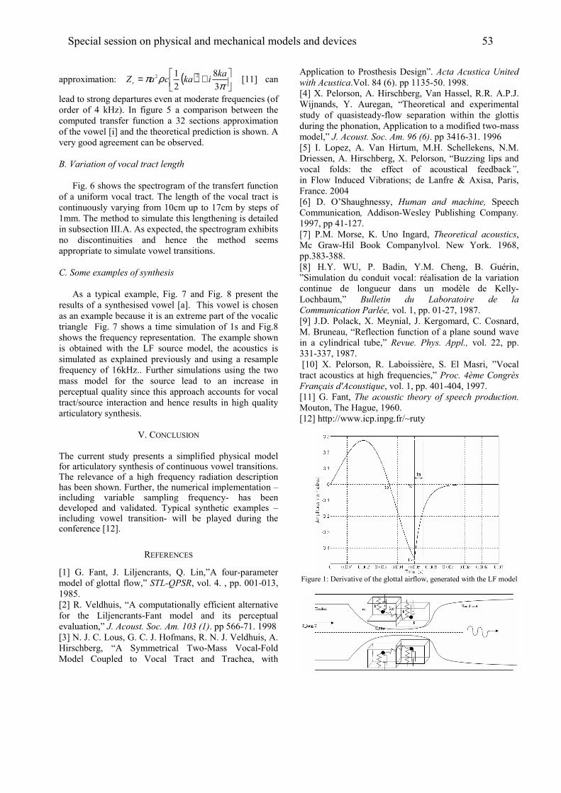
�� 6� ( ) ��

��

� +=π

ρπ8

M

7

2 77 ��

�� 1223� ��

�� !�� #��/ ��

�� 9� -%$0�� !�� ;� ��

� �� 87� ��

�� 1�3�� '�

��! ��!��

�

��#��"��

�

.�!��>�� !��

�� !��

� �� !�� 24�� 2G��

2�� !��!��

�� '��'�� "�� !��

� � ��

��

�

�� %��

�

'�� "� .�!�� G� ��.�!�� M� ��

�� 1�3��

��

��!�� .�!��G� �� 2��.�!�M�

�� #��

�� (.� � �� "� ��

�� !� ��

��#�� 2>-%$��.�� !� ��

��

��#��

��5� �� !��#��

��

�B��()��

�� !�� #�� .��"�� P��!� �� !� ��#��,� �� P��!� � �� ,� �� !� �� 1273��

��&.&�&�&)�

�123� F�� .��"� @�� (��"� Q�� (��"R'� � ��,��

� �� !� �� "R��$&*+,��"�� 9��"��442,428"�

2EM;��

173��B��"�S'��

� �� (��,.��

�� "R�� -./�0-1��;>>,G2��2EEM�

183��@��( ��"�F��@��% ��"��@��B��"�'��

%��!"� S'� )�� ,D�� B ��,. ��

D �� B �� "� ��

'�� *� ��!�R�� 2��

3�� B ��M9�/>0��228;,;4��2EEM��

193�A��*�� "�'��%��!"�B��%��"��'�*�@��

N ��"� T�� '��!��"� S��

�� #��,�� !� ��

��!�� "�'�� ,��

� ��"R�� 45�051��892>,82��2EE>�

1;3� �� ( ��$"� '�� B�� %��"� D�%�� )��-��"� ��D��

��"�'��%��!"�A��*�� "�S+�$$��!��

� �� 6� �� -6"��

�� .� �� B�� L� �� (�� U� ' ��"� *��"�

.��7449�

1>3� �� =)��!��"� 7�� 8� )��

�� 8� '�� ,N �� *��!� ��

2EEG"��92,27G��

1G3� *�D�� D ��"� :�� !��"� $�� "�

D�� F��,%�� + -� �� T �-�� 2E>M"�

��8M8,8MM��

1M3� %�T�� N"� *�� +��"� T�D�� !"� +�� F�C��"�

R)�� 6��C��

� �� !�� V�� :��,

( ��"R� �� &�9��

��,��:8�� 2"��42,7G"�2EMG��

1E3�@��* ��-"�A��D��"�@��:��! ��"�� "�

D��+��"�S��

�� "R��"�� ,�% �� 8�� 77"� ��

882,88G"�2EMG��

�1243� A�� *�� "� �� (�� V��"� )�� &�� D��"� RB ��

�� !��#��"R�,��;<��< �

��=�� >�� ?�"�� 2"��942,949"�2EEG��

1223�F��.��"�$�� %� ��

D �� "��%�!��"�2E>4��

1273��655��!��5W��

�

�.�!��26�� !� �� "�!��(.��

�

�


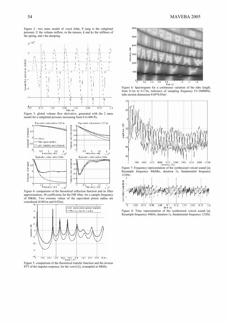
.�!�� 7�6� �� "� *X��!� �� !� ��"�� "��"�-��-��

��!"��!��

�

�.�!�� 86� !� �� "� !�� 7� ��

� �� !� ��!�� 4�� >44�*��

�.�!��96��

�� "�84�� .��"�� #��

�� M4-%$�� #�� /4�442��4�47�0��

�.�!��;6��

..�� "�� 1�3"��99-%$��

�

�.�!�� >6� )�� !�� !��"�� 4�2�� 4�2G�"� �� !� ��#�� .�I74444%$"�

�� 4�49Y4�48�Z��

�

�.�!��G6�.��#�� $�� 1�3��

�� #�� 99-%�$"� �� 2�"� �� #��

278%$��

�.�!�� M6� �� $�� 1�3��

��#��99-%$"�� 2�"��#��278%$��

��

�

�

�

54 MAVEBA 2005

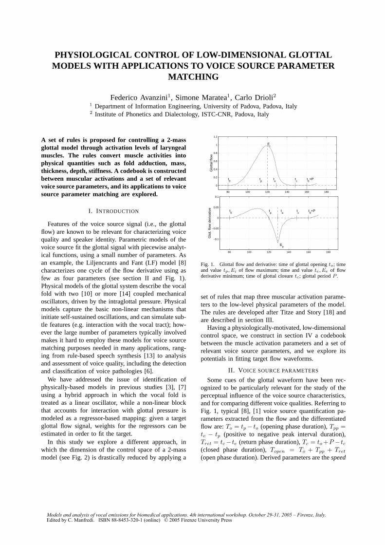
PHYSIOLOGICAL CONTROL OF LOW-DIMENSIONAL GLOTTALMODELS WITH APPLICATIONS TO VOICE SOURCE PARAMETER

MATCHING

Federico Avanzini1, Simone Maratea1, Carlo Drioli21 Department of Information Engineering, University of Padova, Padova, Italy2 Institute of Phonetics and Dialectology, ISTC-CNR, Padova, Italy

A set of rules is proposed for controlling a 2-massglottal model through activation levels of laryngealmuscles. The rules convert muscle activities intophysical quantities such as fold adduction, mass,thickness, depth, stiffness. A codebook is constructedbetween muscular activations and a set of relevantvoice source parameters, and its applications to voicesource parameter matching are explored.

I. I NTRODUCTION

Features of the voice source signal (i.e., the glottalflow) are known to be relevant for characterizing voicequality and speaker identity. Parametric models of thevoice source fit the glottal signal with piecewise analyt-ical functions, using a small number of parameters. Asan example, the Liljencrants and Fant (LF) model [8]characterizes one cycle of the flow derivative using asfew as four parameters (see sectionII and Fig. 1).Physical models of the glottal system describe the vocalfold with two [10] or more [14] coupled mechanicaloscillators, driven by the intraglottal pressure. Physicalmodels capture the basic non-linear mechanisms thatinitiate self-sustained oscillations, and can simulate sub-tle features (e.g. interaction with the vocal tract); how-ever the large number of parameters typically involvedmakes it hard to employ these models for voice sourcematching purposes needed in many applications, rang-ing from rule-based speech synthesis [13] to analysisand assessment of voice quality, including the detectionand classification of voice pathologies [6].

We have addressed the issue of identification ofphysically-based models in previous studies [3], [7]using a hybrid approach in which the vocal fold istreated as a linear oscillator, while a non-linear blockthat accounts for interaction with glottal pressure ismodeled as a regressor-based mapping: given a targetglottal flow signal, weights for the regressors can beestimated in order to fit the target.

In this study we explore a different approach, inwhich the dimension of the control space of a 2-massmodel (see Fig.2) is drastically reduced by applying a

80 100 120 140 160 180

0

0.2

0.4

0.6

0.8

1

1.2

Ei

t0

tp

te

tc

t0+P

Glo

ttal f

low

80 100 120 140 160 180

−0.1

−0.05

0

0.05

0.1

t0

tp

te

Ee

tc

t0+P

Glo

t. flo

w d

eriv

ativ

e

Fig. 1. Glottal flow and derivative: time of glottal openingto; timeand valuetp, Ei of flow maximum; time and valuete, Ee of flowderivative minimum; time of glottal closuretc; glottal periodP .

set of rules that map three muscular activation parame-ters to the low-level physical parameters of the model.The rules are developed after Titze and Story [18] andare described in sectionIII .

Having a physiologically-motivated, low-dimensionalcontrol space, we construct in sectionIV a codebookbetween the muscle activation parameters and a set ofrelevant voice source parameters, and we explore itspotentials in fitting target flow waveforms.

II. V OICE SOURCE PARAMETERS

Some cues of the glottal waveform have been rec-ognized to be particularly relevant for the study of theperceptual influence of the voice source characteristics,and for comparing different voice qualities. Referring toFig. 1, typical [8], [1] voice source quantification pa-rameters extracted from the flow and the differentiatedflow are:To = tp− to (opening phase duration),Tpp =te − tp (positive to negative peak interval duration),Tret = tc− te (return phase duration),Tc = to +P − tc(closed phase duration),Topen = To + Tpp + Tret

(open phase duration). Derived parameters are thespeed


��

��

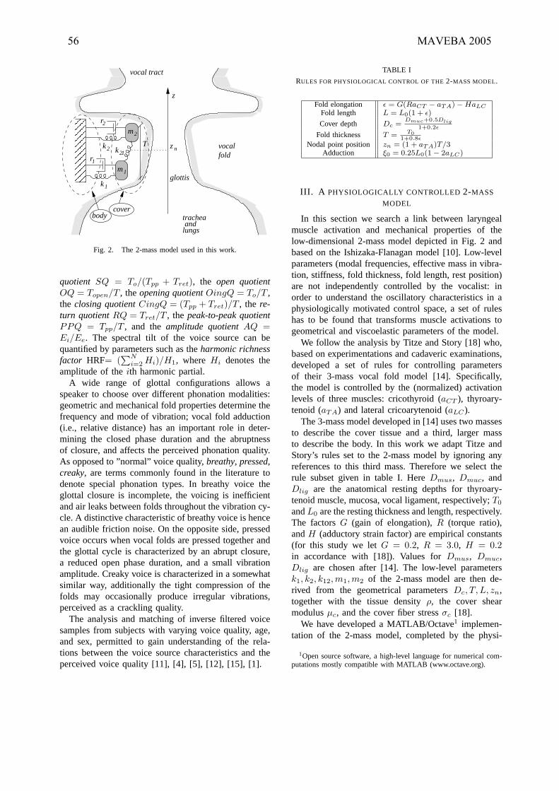
andtrachea

lungs

k1

k2 vocalfold1k2

1r

2r

2m

1m

vocal tract

nT

z

z

glottis

bodycover

Fig. 2. The 2-mass model used in this work.

quotient SQ = To/(Tpp + Tret), the open quotientOQ = Topen/T , theopening quotientOingQ = To/T ,the closing quotientCingQ = (Tpp + Tret)/T , the re-turn quotientRQ = Tret/T , the peak-to-peak quotientPPQ = Tpp/T , and theamplitude quotientAQ =Ei/Ee. The spectral tilt of the voice source can bequantified by parameters such as theharmonic richnessfactor HRF= (

∑Ni=2 Hi)/H1, where Hi denotes the

amplitude of theith harmonic partial.A wide range of glottal configurations allows a

speaker to choose over different phonation modalities:geometric and mechanical fold properties determine thefrequency and mode of vibration; vocal fold adduction(i.e., relative distance) has an important role in deter-mining the closed phase duration and the abruptnessof closure, and affects the perceived phonation quality.As opposed to ”normal” voice quality,breathy, pressed,creaky, are terms commonly found in the literature todenote special phonation types. In breathy voice theglottal closure is incomplete, the voicing is inefficientand air leaks between folds throughout the vibration cy-cle. A distinctive characteristic of breathy voice is hencean audible friction noise. On the opposite side, pressedvoice occurs when vocal folds are pressed together andthe glottal cycle is characterized by an abrupt closure,a reduced open phase duration, and a small vibrationamplitude. Creaky voice is characterized in a somewhatsimilar way, additionally the tight compression of thefolds may occasionally produce irregular vibrations,perceived as a crackling quality.

The analysis and matching of inverse filtered voicesamples from subjects with varying voice quality, age,and sex, permitted to gain understanding of the rela-tions between the voice source characteristics and theperceived voice quality [11], [4], [5], [12], [15], [1].

TABLE I

RULES FOR PHYSIOLOGICAL CONTROL OF THE2-MASS MODEL.

Fold elongation ε = G(RaCT − aTA)−HaLC

Fold length L = L0(1 + ε)

Cover depth Dc =Dmuc+0.5Dlig

1+0.2ε

Fold thickness T = T01+0.8ε

Nodal point position zn = (1 + aTA)T/3Adduction ξ0 = 0.25L0(1− 2aLC)

III. A PHYSIOLOGICALLY CONTROLLED 2-MASS

MODEL

In this section we search a link between laryngealmuscle activation and mechanical properties of thelow-dimensional 2-mass model depicted in Fig.2 andbased on the Ishizaka-Flanagan model [10]. Low-levelparameters (modal frequencies, effective mass in vibra-tion, stiffness, fold thickness, fold length, rest position)are not independently controlled by the vocalist: inorder to understand the oscillatory characteristics in aphysiologically motivated control space, a set of ruleshas to be found that transforms muscle activations togeometrical and viscoelastic parameters of the model.

We follow the analysis by Titze and Story [18] who,based on experimentations and cadaveric examinations,developed a set of rules for controlling parametersof their 3-mass vocal fold model [14]. Specifically,the model is controlled by the (normalized) activationlevels of three muscles: cricothyroid (aCT ), thyroary-tenoid (aTA) and lateral cricoarytenoid (aLC).

The 3-mass model developed in [14] uses two massesto describe the cover tissue and a third, larger massto describe the body. In this work we adapt Titze andStory’s rules set to the 2-mass model by ignoring anyreferences to this third mass. Therefore we select therule subset given in tableI. Here Dmus, Dmuc, andDlig are the anatomical resting depths for thyroary-tenoid muscle, mucosa, vocal ligament, respectively;T0

andL0 are the resting thickness and length, respectively.The factorsG (gain of elongation),R (torque ratio),andH (adductory strain factor) are empirical constants(for this study we letG = 0.2, R = 3.0, H = 0.2in accordance with [18]). Values forDmus, Dmuc,Dlig are chosen after [14]. The low-level parametersk1, k2, k12,m1,m2 of the 2-mass model are then de-rived from the geometrical parametersDc, T, L, zn,together with the tissue densityρ, the cover shearmodulusµc, and the cover fiber stressσc [18].

We have developed a MATLAB/Octave1 implemen-tation of the 2-mass model, completed by the physi-

1Open source software, a high-level language for numerical com-putations mostly compatible with MATLAB (www.octave.org).

56 MAVEBA 2005

ological link between laryngeal muscle activation andmechanical properties of the model, with the activationsaTA, aLC andaCT varying in the range[0, 1].

IV. N UMERICAL SIMULATIONS

The 2-mass model with physiological control wasused to run a set of simulations for the exploration ofthe control space(aTA, aLC , aCT ). All the simulationsused a sampling rateFs = 22.05 kHz. The subglottalpressureps was held fixed at the value0.8 kPa. Theanatomical resting depths of layers of vocal folds tissuewere chosen in accordance with Titze and Story [14].

A. Phonation regions

A first set of simulations was performed in order todetermine the phonation region in the control space.Simulations were run using two configurations. First anideally open glottis (i.e., with zero supraglottal pressure)was considered. Second, a vocal tract load was takeninto account by coupling the 2-mass glottis model witha cylindrical vocal tract model.

The phonation region was searched for each of thetwo configurations. Following Titzeet al. [18], at eachpoint (aTA, aLC , aCT ) the existence of self-sustainedstable phonation was determined by applying a zero-crossing multiple-detector to the last 50 ms of thesimulated glottal area signal. In this way we arbitrarilynot consider “always-open glottis” phonation.

For both configurations, phonation regions are com-parable with results by Titze and Story [18] on the 3-mass model. In particular,aCT has little influence onthe shape of the self-sustained phonatory region. For theopen-glottis configuration, it simply acts as a switch thatrestricts phonation in the rangeaCT ∈ [0, 0.7], whilefor the cylindrical vocal tract configuration phonationoccurs in the entire rangeaCT ∈ [0, 1].

The 2-D phonation region in theaLC-aTA plane(with aCT fixed) is wedge-shaped. For the open-glottisconfiguration, the region is contained in the rectangleaTA ∈ [0, 0.9] and aLC ∈ [0.35, 0.5], while forthe cylindrical vocal tract configuration the boundingrectangle is given byaTA ∈ [0, 1] andaLC ∈ [0.2, 0.5].Thus, following expectations the phonation region islarger when a vocal tract load is coupled to the glottis.Given the similarity between these results and thosereported in [18], we consider our selected rules a validlink between laryngeal muscle activation and mechani-cal properties of the 2-mass model.

B. A physiological-to-acoustic codebook

Having determined the phonation regions in thecontrol space, we analyze the properties of thevoice source signal in such regions. We chosea set of relevant acoustic parameters, namely

TABLE II

PHYSIOLOGICAL-TO-ACOUSTIC CODEBOOK: RANGES FOR THE

RELEVANT VOICE SOURCE PARAMETERS.

F0 SQ OQ OingQ CingQ RQOpen-glottis configuration

Mean value 251 1.36 0.63 0.36 0.26 0.02Min. value 217 0.90 0.51 0.29 0.19 0Max. value 367 2.01 0.94 0.52 0.43 0.13

Cyl. vocal tract configurationMean value 253 1.66 0.80 0.49 0.30 0.02Min. value 179 1.13 0.35 0.23 0.12 0Max. value 816 2.79 0.90 0.59 0.41

F0, SQ,OQ, OingQ, CingQ, RQ (see section IIfor definitions) and developed a MATLAB/Octavescript for automatic analysis and extraction of theseparameters from the glottal flow signal. Using this tool,the signals produced by every tripleaTA, aLC , aCT

in the phonation region were analyzed, resulting in aphysiological-to-acoustic codebook of the form

(aTA, aLC , aCT ) 7→ (F0, SQ,OQ, OingQ,CingQ,RQ).

Table II provides indications about the ranges of thevoice source parameters within the codebook. Fromthis, a few remarks can be made.

First, F0 values appear to be high, considering that aset of parameters typical for males has been used. Thissuggests that the choice of physical parameters made insectionIII (specifically, keeping the same values usedin [18] for the vocal fold cover tissue, while discardingany description of the vocal fold body) is not optimal.

Second, values for the return quotientRQ are ex-tremely low. This reflects a general limitation of low-dimensional physical models of the glottis, in whichglottal closure always occurs abruptly and results inpoor modeling of the closing phase.

The codebook has been tested in order to verifyits potentials in fitting target flow waveforms. Targetsignals were constructed by superimposing a noisycomponent to synthetic glottal flow waveforms obtainedfrom the LF model [8]. The fitting procedure works asfollows:1. The setF0, SQ, OQ,OingQ, CingQ, RQ of voicesource parameters is extracted from the target signal.2. A triple aTA, aLC , aCT is determined in such a waythat it minimizes the distance between its image in thecodebook and the target voice source parameter vector.3. A fitting signal is resynthesized with the 2-massmodel controlled by the selected tripleaTA, aLC , aCT .

Figure3 shows an example of the results. The open-ing, closing, and flow maximum points (to, tc, te) areaccurately matched. On the other hand the opening and


0.01 0.011 0.012 0.013 0.014 0.015 0.016 0.017

0

0.2

0.4

0.6

0.8

1

1.2

time (s)

Glo

ttal f

low

(m

3 /2)

target waveform Fit from 2−mass model

Fig. 3. Results from the fitting procedure. The target waveform isconstructed by superimposing a noisy component to synthetic glottalflow waveforms obtained from the LF model.

especially the closing phases are poorly matched. Asalready mentioned, this is an intrinsic limitation of the2-mass model. As a consequence the time and value ofthe negative peak of the flow derivative are mismatched.

V. D ISCUSSION

The results presented in this work are still very pre-liminary. Among the points that need further discussionand refinements, the following can be mentioned.

The codebook described in sectionIV does notinclude the subglottal pressureps among the varyingphysiological parameters. The parameterps is knownto have a major influence on relevant voice sourceparameters, in particular the phonation fundamentalfrequency is known to increase almost linearly withps [16]. For this reason the physiological control spaceshould be expanded to includeps.

A second limitation of the results comes from thecharacteristics of the vocal tract load: neither the openglottis nor the cylindrical vocal tract configurationsprovide a realistic simulation of the load, while itis known that the load characteristics also influencerelevant voice source parameters (e.g., the glottal flowskeweness). Better simulations of voice source/vocaltract interaction can be realized, see e.g. [17].

Finally, as already mentioned, the 2-mass modelprovides a poor description of the glottal flow nearclosure. While accurate finite-element models are ableto provide qualitative behaviors in agreement withobservations of glottal closure during normal voiceproduction [9], such behaviors are not easily simulatedwith a low-dimensional model.

Nonetheless, the preliminary results suggests that theproposed approach can be successfully used for voicesource parameters matching applications. The followingpoints can be mentioned.

First,the nuscle activation control space allow explo-ration of a wide region of the voice source parameterspace. Second, with respect to our previous works [3],[7], this approach leads to more robust resynthesis,since no regressor-based black-box element is used andconsequently stability is guaranteed by construction.Finally, the same approach can be extended to lowerdimensional glottal models (e.g., [2]), in order to con-struct an efficient analysis/synthesis tool.

REFERENCES

[1] P. Alku and E. Vilkman. A comparison of glottal voice quantifi-cation parameters in breathy, normal and pressed phonation offemale and male speakers.Folia Phoniatr. Logop., 48(5):240–254, Sep. 1996.

[2] F. Avanzini, P. Alku, and M. Karjalainen. One-delayed-massmodel for efficient synthesis of glottal flow. InProc. EurospeechConf., pages 51–54, Aalborg, Sep. 2001.

[3] F. Avanzini, C. Drioli, and P. Alku. Synthesis of the VoiceSource Using a physically informed model of the glottis. InProc. Int. Symp. Mus. Acoust. (ISMA’01), pages 31–34, Perugia,Sep. 2001.

[4] D. Childers and C. Lee. Vocal quality factors: analysis,synthesis, and perception.J. Acoust. Soc. Am., 90(5):2394–2410, November 1991.

[5] D. G. Childers and C. Ahn. Modeling the glottal volume-velocity waveform for three voice types.J. Acoust. Soc. Am.,97(1):505–519, Jan. 1995.

[6] M. Dollinger, U. Hoppe, F. Hettlich, J. Lohscheller, S. Schu-berth, and U. Eysholdt. Vibration parameter extraction fromendoscopic image series of the vocal folds.IEEE Trans.Biomedical Engineering, 49(8):773–781, Aug. 2002.

[7] C. Drioli and F. Avanzini. Hybrid parametric physiologicalglottal modelling with application to voice quality assessment.Medical Engineering & Physics, 24(7–8):453–460, Sep. 2002.

[8] G. Fant, J. Liljencrants, and Q. guang Lin. A four-parametermodel of glottal flow.STL-QPSR, 26(4):1–13, 1985.

[9] H. E. Gunter. A mechanical model of vocal-fold collisionwith high spatial and temporal resolution.J. Acoust. Soc. Am.,113(2):994–1000, Feb. 2003.

[10] K. Ishizaka and J. L. Flanagan. Synthesis of voiced soundsfrom a two-mass model of the vocal cords.Bell Syst. Tech. J.,51:1233–1268, 1972.

[11] P. J. Price. Male and female voice source characteristics: inversefiltering results. Speech Commun., 8(2):261–277, February1989.

[12] E. L. Riegelsberger and A. K. Krishnamurthy. Glottal sourceestimation: Methods of applying the LF-model to inverse fil-tering. In Proc. IEEE Int. Conf. Acoust. Speech and SignalProcess. (ICASSP’93), pages 542–545, Minneapolis, 1993.

[13] M. Sondhi. Articulatory modeling: a possible role in concate-native text-to-speech synthesis. InProc. 2002 IEEE Workshopon Speech Synthesis, pages 73–78, S. Monica (CA), Sep. 2002.

[14] B. Story and I. Titze. Voice simulation with a body cover modelof vocal folds. J. Acoust. Soc. Am., 97:1249–1260, 1995.

[15] H. Strik. Automatic parametrization of differentiated glottalflow: Comparing methods by means of synthetic flow pulses.J.Acoust. Soc. Am., 103(5):2659–2669, May 1998.

[16] I. R. Titze. On the relation between subglottal pressure andfundamental frequency in phonation.J. Acoust. Soc. Am.,85(2):901–906, Feb. 1989.

[17] I. R. Titze and B. H. Story. Acoustic interactions of thevoice source with the lower vocal tract.J. Acoust. Soc. Am.,101(4):2234–2243, Apr. 1996.

[18] I. R. Titze and B. H. Story. Rules for controlling low-dimensional vocal fold models with muscle activation.J.Acoust. Soc. Am., 112(3):1064–1027, Sep. 2002.

58 MAVEBA 2005

USING BIOMECHANICAL PARAMETER ESTIMATES IN VOICE PATHOLOGY DETECTION

P. Gómez, C. Lázaro, R. Fernández, A. Nieto, J. I. Godino, R. Martínez, F. Díaz, A. Álvarez, K. Murphy, V. Nieto, V. Rodellar, F. J. Fernández-Camacho

GIAPSI, Facultad de Informática, Universidad Politécnica de Madrid Campus de Montegancedo, s/n, 28660, Boadilla del Monte, Madrid, Spain

It has been shown in previous work that biomechanical parameters related to the cord body dynamics can be indirectly estimated from the power spectral density of the mucosal wave correlate [4]. In the present study the use of these measurements to estimate the presence of parameter unbalance will be shown. The role of these parameters together with the classical distortion ones in relation to pathology detection and classification will be explored. Results using normophonic as well as pathologic voice will be presented and discussed.

I. INTRODUCTION

Classically, Voice Processing focused onto detecting pathological voice by means of distortion parameter estimation directly from the voice trace [7][2], albeit the detection process being masked by the vocal tract and other supra-structures of the vocal apparatus. More advanced methods remove the influence of the vocal tract, to obtain an indirect estimation of the glottal source [1]. The first and second derivatives of the glottal source are correlates of the glottal aperture and the relative speed between cord centers of mass [3][5]. The glottal aperture correlate can be seen as being composed of two main parts: a slow-varying average movement, which is referred to as “the average acoustic waveform” [8], and a fast-varying waveform, resulting from the mucosal wave traveling on the body-cover structure [10][11]. The dynamics of the body would be reflected in the average glottal aperture, whereas the dynamics of the cover would be retained by the mucosal wave correlate (see Figure 1).

Body

Cover

Upper Lip (supraglottal)

Lower Lip (subglottal)

a) Body mass

k-1 Cover masses

b)

Figure 1. a) Cross-section of the left vocal cord

showing the body and cover structures (taken from [9]). b) k-mass model of the body and cover.

It may be expected that the power spectral density (psd) of the average acoustic wave would be determined by

the dynamics of the cord center of masses, whereas the power spectral density of the mucosal wave correlate would be mostly influenced by the cover dynamics. Moving one step ahead, separating both signals would become an important target for estimating vocal fold biomechanics. In a previous work [4] it was shown that estimates of the cord mass and stiffness could be obtained from the power spectral density of the average acoustic waveform. Through this paper the methodology for parameter unbalance estimation will be presented. Experiments using pathologic and normophonic samples will also be given.

II. CORD BODY BIOMECHANICAL ESTIMATES

Glottal source reconstruction by inverse filtering, as used in the present study, is due to Alku [1]. Relevant details on its recursive implementation by paired lattices are to be found in [5]. By removing the vocal tract influence a given voice trace can be processed to render the relative speed between cords, the glottal aperture and the glottal source as shown in Figure 2.

Figure 2. Glottal source estimation. a) input voice

(sample 00B), b) second and c) first derivatives of the glottal source, d) glottal source (unlevelled).

Detecting the cord body mass, stiffness and damping is based on the inversion of the integro-differential equation of the one-mass cord model

∫∞−

++=t

lblb

xllblblbxl dtv

C1

dtdv

MRvf (1)


where the biomechanical parameters involved are the lumped masses Mlb, the elastic parameters Clb and the losses Rlb. The equivalent model is shown in Figure 4.

Figure 3. Estimation of the mucosal wave correlate: a)

Levelled first derivative of the glottal source, b) Levelled glottal source, c) average acoustic waveform,

d) mucosal wave correlate

The estimation of the body biomechanical parameters is related to the inversion of this model, associating the force fxl on the body with the velocity of the cord centre of masses vlb in the frequency domain.

Figure 4. Electromechanical equivalent of a cord body

The relationship between velocity and force in the frequency domain is expressed as the cord body admittance. It will be assumed that the power spectral density of the levelled glottal aperture (1st derivative of the glottal source) is related to the square modulus of the body admittance Ybl(s) as

( )( ) 12lb

21lblb

2

xl

lb2blmb

RCM

)(F)(V

Y)(T

−−

⎥⎦⎤

⎢⎣⎡ +−=

===

ωω

ωω

ω

(2)

which shows a maximum value at

2lb

brmb1 R

G)(TT === ωω (3)

lblbr CM

1=ω (4)

where Gb is a factor of scale between the average acoustic waveform power spectral density and the

22223

8

1)3( rmbTT⎞⎛

=== ωω

3 lblbr RM +⎟⎠

⎜⎝

ω (5)

From this expression the following estimate for the body mass may be obtained

1331

31 33 21

TTM

⎤⎢⎡ −

=88

rTT rr

lb ωω=⎥

⎦⎣ (6)

31

3113 TT

TTr

−=

The value of Clb rve fitting after estimating the biomechanical parameters for

(7)

could be derived from (4). The cu

a real trace (sample 00B) is shown in Figure 5.

Figure 5. Parametric fitting of a specific average

acoustic waveform for sample 00B (full line) against th

A slight unb es may be observed in Figure 3.a) and c). Even cycles appear to be

e

Rlb Mlb fxl

Clb

vxl

+

admittance approximation (dot line)

III. PARAMETER UNBALANCE

alance between waveform cycl

larger than odd ones. As estimations of mass, stiffness and damping will be available on a cycle frame basis, the unbalance of these parameters (BMU – Body Mass Unbalance, BLU – Body Losses Unbalance and BSU – Body Stiffness Unbalance) may be defined as

( ) ( )( ) ( )( ) ( )1bkbk1bkbkuk

1bkbk1bkbkuk

CCCCc −−

−−

+−=

(8)

where 1≤k≤K is the cycle window

1bkbk1bkbkuk

RRRRr

MMMMm −−

+−=

+−=

index and bkbkbk Cand,R,M are the k-th cycle estimates of mass,

parameters of inlosses and compliance on a given voice sample. Other

terest are the deviations of the average values of mass, losses and compliance for the j-th sample bjbjbj Cand,R,M relative to average estimates from a normophonic set of speakers (inter-speaker) as square modulus of the cord body admittance. The value

of the third harmonic will be given by

60 MAVEBA 2005

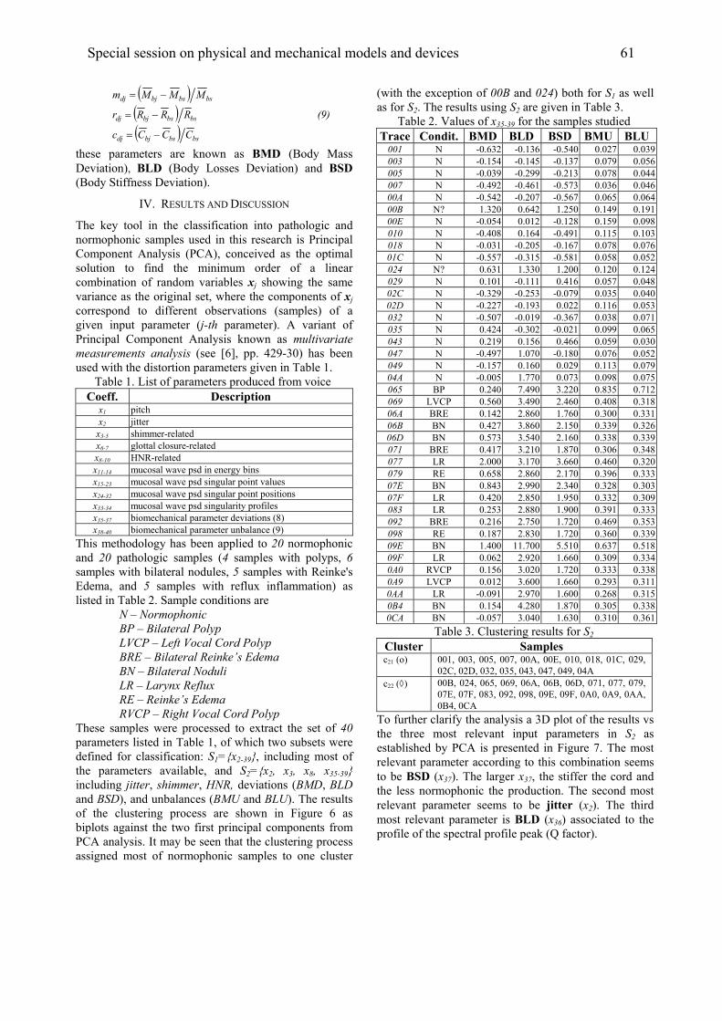
( )( )( ) bsbsbjdj

bsbjdj

CCCc

MM

−=

−=

bsbsbjdj

bs

RRRr

Mm

−= (9)

these parameters are know ass n as BMD (Body MDeviation), BLD (Body Losses Deviation) and BSD (Body Stiffness Deviation).

IV. RESULTS AND DISCUSSION

The key tool in the classification into pathologic and normophoni is Principal c samples used in this research Component Analysis (PCA), conceived as the optimal solution to find the minimum order of a linear combination of random variables xj showing the same variance as the original set, where the components of xj correspond to different observations (samples) of a given input parameter (j-th parameter). A variant of Principal Component Analysis known as multivariate measurements analysis (see [6], pp. 429-30) has been used with the distortion parameters given in Table 1.

Table 1. List of parameters produced from voice Coeff. Description

x1 pitch x jitter 2

x3-5 shimmer-related x6-7 glottal closure-related x related 8-10 HNR-x11-14 mucosal wave psd in energy bins x15-23 mucosal wave psd singular point values x24-32 mucosal wave psd singular point positions x33-34 mucosal wave psd singularity profiles x35-37 biomechanical parameter deviations (8) x38-40 biomechanical parameter unbalance (9)

Thi tho ophonic and th polyps, 6

s me dology has been applied to 20 normhologic samples (4 samples wi 20 pat

samples with bilateral nodules, 5 samples with Reinke's Edema, and 5 samples with reflux inflammation) as listed in Table 2. Sample conditions are

N – Normophonic BP – Bilateral Polyp LVCP – Left Vocal Cord Polyp BRE – Bilateral Reinke’s Edema BN – Bilateral Noduli LR – Larynx Reflux RE – Reinke’s Edema RVCP – Right Vocal Cord Polyp

These sa extract the set of 40 paramete subsets were

mples were processed tors listed in Table 1, of which two

defined for classification: S1={x2-39}, including most of the parameters available, and S2={x2, x3, x8, x35-39} including jitter, shimmer, HNR, deviations (BMD, BLD and BSD), and unbalances (BMU and BLU). The results of the clustering process are shown in Figure 6 as biplots against the two first principal components from PCA analysis. It may be seen that the clustering process assigned most of normophonic samples to one cluster

(with the exception of 00B and 024) both for S1 as well as for S2. The results using S2 are given in Table 3.

Table 2. Values of x35-39 for the samples studied Trace Condit. BMD BLD BSD BMU BLU

001 N -0.632 -0.136 -0.540 0.027 0.039003 N -0.154 -0.145 -0.137 0.079 0.056005 N -0.039 -0.299 -0.213 0.078 0.044007 N -0.492 -0.461 -0.573 0.036 0.04600A N -0.542 -0.207 -0.567 0.065 0.06400B N? 1.320 0.642 1.250 0.149 0.19100E N -0.054 0.012 -0.128 0.159 0.098010 N -0.408 0.164 -0.491 0.115 0.103018 N -0.031 -0.205 -0.167 0.078 0.07601C N -0.557 -0.315 -0.581 0.058 0.052024 N? 0.631 1.330 1.200 0.120 0.124029 N 0.101 -0.111 0.416 0.057 0.04802C N -0.329 -0.253 -0.079 0.035 0.04002D N -0.227 -0.193 0.022 0.116 0.053032 N -0.507 -0.019 -0.367 0.038 0.071035 N 0.424 -0.302 -0.021 0.099 0.065043 N 0.219 0.156 0.466 0.059 0.030047 N -0.497 1.070 -0.180 0.076 0.052049 N -0.157 0.160 0.029 0.113 0.07904A N -0.005 1.770 0.073 0.098 0.075065 BP 0.240 7.490 3.220 0.835 0.712069 L VCP 0.560 3.490 2.460 0.408 0.31806A BRE 0.142 2.860 1.760 0.300 0.33106B BN 0.427 3.860 2.150 0.339 0.32606D BN 0.573 3.540 2.160 0.338 0.339071 BRE 0.417 3.210 1.870 0.306 0.348077 LR 2.000 3.170 3.660 0.460 0.320079 RE 0.658 2.860 2.170 0.396 0.33307E BN 0.843 2.990 2.340 0.328 0.30307F LR 0.420 2.850 1.950 0.332 0.309083 LR 0.253 2.880 1.900 0.391 0.333092 BRE 0.216 2.750 1.720 0.469 0.353098 RE 0.187 2.830 1.720 0.360 0.33909E BN 1.400 11.700 5.510 0.637 0.51809F LR 0.062 2.920 1.660 0.309 0.3340A0 R VCP 0.156 3.020 1.720 0.333 0.3380A9 L VCP 0.012 3.600 1.660 0.293 0.3110AA LR -0.091 2.970 1.600 0.268 0.3150B4 BN 0.154 4.280 1.870 0.305 0.3380CA BN -0.057 3.040 1.630 0.310 0.361

Table 3. eri ul S2Clust ng res ts for Cluster Samples c21 (o) , 01C, 029,

02C, 02D, 032, 035, 043, 047, 049, 04A 001, 003, 005, 007, 00A, 00E, 010, 018

c22 (◊) 00B, 024, 065, 069, 06A, 06B, 06D, 071, 077, 079, 07E, 07F, 083, 092, 098, 09E, 09F, 0A0, 0A9, 0AA, 0B4, 0CA

To her c the three m vant input parameters in S as

furt larify the analysis a 3D plot of the results vsost rele 2

established by PCA is presented in Figure 7. The most relevant parameter according to this combination seems to be BSD (x37). The larger x37, the stiffer the cord and the less normophonic the production. The second most relevant parameter seems to be jitter (x2). The third most relevant parameter is BLD (x36) associated to the profile of the spectral profile peak (Q factor).


Figure 6. Left) Clusters for S1. Right) Clusters for S2.

Figure 7. 3D Clustering Plot showing the separation in the manifold defined by the parameter subset {x37, x2

and x36} – ordered by relevance

The behaviour of cases 00B and 024, classified as pathological by PCA analysis deserves a brief comment. These appear in Figure 7 (encircled) not quite far from normal cases 001-04A, but showing a stiffness that doubles those of normophonic samples. Apparently this detail was determinant in their classification as not normophonic by PCA. This fact was confirmed by their values for the BSD in Table 2, being 1.25 and 1.2 respectively, or 225% and 220%.

V. CONCLUSIONS

The methodology presented detects biomechanical unbalance from voice records for pathology detection by common pattern recognition techniques. Normophonic samples show small unbalance indices, as opposed to pathologic ones. There is not a specific pattern of unbalance related to a given pathology (although more cases need to be studied). Biomechanical parameter unbalance is a correlate to pathology quantity rather than quality. Mild pathologies may appear as normophonic from subjective analysis. Adequately combining classical distortion parameters with deviation

parameters renders fairly good results in pathology detection. These conclusions need to be confirmed by more experiments.

VI. ACKNOWLEDGMENTS

This research carried out under grant Nos. TIC2002-2273, TIC2003-08756 and TIC2003-08956-C02-00, from Programa de las Tecnologías de la Información y las Comunicaciones, Ministry of Education and Science, Spain.

VII. REFERENCES

[1] Alku, P., “An Automatic Method to Estimate the Time-Based Parameters of the Glottal Pulseform”, Proc. of the ICASSP’92, pp. II/29-32.

[2] Godino, J. I., Gómez, P., “Automatic Detection of Voice Impairments by means of Short Term Cepstral Parameters and Neural Network based Detectors”, IEEE Trans. on Biomed. Eng., Vol. 51, No. 2, 2004, pp. 380-384.

[3] Gómez, P., Godino, J. I., Díaz, F., Álvarez, A., Martínez, R., Rodellar, V., “Biomechanical Parameter Fingerprint in the Mucosal Wave Power Spectral Density”, Proc. of the ICSLP’04, 2004, pp. 842-845.

[4] Gómez, P., Martínez, R., Díaz, F., Lázaro, C., Álvarez, A., Rodellar, V., Nieto, V., “Estimation of vocal cord biomechanical parameters by non-linear inverse filtering of voice”, Proc. of the 3rd Int. Conf. on Non-Linear Speech Processing NOLISP’05, Barcelona, Spain, April 19-22 2005, pp. 174-183.

[5] Gómez, P., Godino, J. I., Álvarez, A., Martínez, R., Nieto, V., Rodellar, V., “Evidence of Glottal Source Spectral Features found in Vocal Fold Dynamics”, Proc. of the ICASSP’05, 2005, pp. V.441-444.

[6] Johnson, R. A., Wichern, D. W., Applied Multivariate Statistical Analysis, Prentice-Hall, Upper Saddle River, NJ, 2002.

[7] Kuo, J., Holmberg, E. B., Hillman, R. E., “Discriminating Speakers with Vocal Nodules Using Aerodynamic and Acoustic Features”, Proc. of the ICASSP’99, 1999, pp. I.77-80.

[8] Titze, I., “Summary Statement”, Workshop on Acoustic Voice analysis, National Center for Voice and Speech, 1994.

[9] The Voice Center of Eastern Virginia Med. School: http://www.voice-center.com/larynx_ca.html.

[10] Story, B. H., and Titze, I. R., “Voice simulation with a bodycover model of the vocal folds”, J. Acoust. Soc. Am., Vol. 97, 1995, pp. 1249–1260.

[11] Titze, I. R., “The physics of small amplitude oscillation of the vocal folds”, J. Acoust. Soc. Am., Vol. 83, 1988, pp. 1436-1552.

62 MAVEBA 2005

http://www.voice-center.com/larynx_ca.html

This study is an investigation of the effect of the presence of

the flow mask on voicing behaviour. Microphone and flow

recordings were inverse filtered and compared to examine

the possible effects of the flow mask. Closing quotient

(ClQ), open quotient (OQ) and the amplitude difference

between the first and second harmonics (H1-H2) were the

parameters used to characterise the inverse filtered signals.

The presence of the flow mask used for the recording of oral

flow had an effect on these parameters, which is interpreted

as being indicative of a more tense or more efficient voicing

behaviour in the presence of the mask.

I. INTRODUCTION

One source of objective characteristics of phonation is the

inverse filtered oral flow or sound pressure wave, e.g.

[1,2,3]. The former is registered with a flow mask [1] and

the latter with a pressure sensitive microphone at a short dis-

tance from the mouth. Similar parameters can be extracted

from both, with the exception of DC flow, which cannot be

extracted from microphone recordings.

Each type of voice recording has its own advantages and

drawbacks. Microphone recordings are non-intrusive, may

produce more natural voicing, and are more practical for

field-work, but do not easily provide a measure of DC flow.

Flow recordings do provide DC flow, but the experimental

setup is more complicated, and the flow mask may affect

voicing behaviour. Obvious practical advantages make the

microphone the instrument of choice for speech recordings

in voice research. Furthermore, the information gained from

the DC flow measure is not fully understood.

DC flow has been investigated by numerous researchers,

e.g [4.5.6], and is used in some measures of breathiness and

vocal efficiency [4,6]. However, the precise relationship of

DC flow to voice quality is unclear. Large values of DC

flow indicate insufficient glottal closure extending into the

membranous part of the vocal folds during maximum glottal

closure, while small values [6] may indicate glottal opening

in the cartilaginous part of the vocal folds during maximum

closure. In [7], it is suggested that there may be two types of

incomplete glottal closure, each of which has different im-

plications for the shape of the glottal waveform.

A glottal chink in both the membraneous and cartilagin-

ous parts of the vocal folds (diag. a in Fig. 1), may indicate

more gradual glottal opening/closing, leading to a more si-

nusoidal waveform. When the glottal chink is found in only

the cartilaginous parts of the vocal folds, the glottal wave-

form may show abrupt changes in flow, despite presence of

DC flow (diag. b in Fig. 1). Thus, DC flow may not be an

Fig. 1. Two ways to model glottal leakage: a) a linked leak

created by abduction and b) a parallel chink in the car-

tilaginous portion of the glottis. Taken from [7].

accurate means of determining voice efficiency. It is even

suggested [6] that small amounts of DC may be due to

vertical phasing as a result of a mucosal wave, in voices

where there is complete closure.

As long as the relationship between DC and the glottal

waveform remains unclear and even contradictory, there is

no reason to prefer flow recordings over microphone re-

cordings for voice analysis, and it may be preferable to fo-

cus on the parameters which do indicate a consistent rela-

tionship, although this depends on assumptions made about

the relationship between flow and microphone recordings.

Theoretically, parameters extracted from either type of re-

cording should represent the same information [8]. In earlier

work [9], flow derivative and sound pressure were compared

for a group of 70 subjects. The recordings were made in a

loosely controlled situation, where subjects were asked to

phonate as naturally as possible. The recordings were in-

verse filtered, and source parameters were extracted from

each voicing condition for each subject. Since the subjects

produced the two recordings within a relatively short period

of time of about five minutes, large between-session vari-

ance was not expected. Perceptual tests were not carried out,

as the mask distorts the acoustical signal so that perceptual

comparisons are not possible.

The results of a microphone/flow comparison were not

similar. When the data for each subject were analysed, the

flow and microphone parameter values did not correlate.

Moreover, analyses of variance indicated that there were

statistically significant differences between flow and micro-

phone results. A number of possible reasons were suggested

for this. Normal within-subject variation may be large

enough [4] that direct comparisons of separate utterances for

the same speaker cannot be made in a loosely controlled ex-

perimental setup. Subjects were sometimes perceived to be

uncomfortable with the mask, and this may have introduced

physical tension in the voicing apparatus in general. The

acoustic distortion produced by the mask may also have an

effect on the data. Auditory feedback for the subject wearing

the mask is muffled, and this could also lead to some change

THE EFFECT OF THE FLOW MASK ON PHONATION

R. Orr and B. Cranen

Department of Language and Speech, Radboud University Nijmegen, The Netherlands

ba


in voicing strategy in phonation production in the presence

of the mask.

While it is very difficult to make direct comparisons on

different utterances, such large differences between flow and

microphone data were not expected. A more thorough un-

derstanding of the comparability of flow and microphone

signals is important, as research on the voice source in the

speech community comes from both flow and microphone

data, and both are used to characterise aspects of voice

quality for many purposes. The aim of this study then was to

compare, under more controlled circumstances, phonation

produced with and without a flow mask. A single subject

experiment was designed to give maximal control over the

possible confounding factors suggested from the results of

the previous work and we present here the data that was

collected from such a setup.

II. METHODOLOGY

Subject: The subject was a female phonetician with experi-

ence in producing experimental speech, and who was famili-

ar with the aims of the experiment. A single subject was

chosen for this analysis for three reasons.

Firstly, laryngeal settings for normal voice production can

differ considerably from subject to subject. Distinctive indi-

vidual differences within a subject group may make the

comparison and interpretation of mean scores spurious for

this particular investigation.

Secondly, a speaker with some experience and under-

standing of the production of different voice qualities was

required. In order to get an impression of whether the in-

verse filtering produced realistic parameter values for both

flow and microphone utterances, the subject was required to

produce three different voice qualities for which relative val-

ues are already established in other published research. If

the relative values produced for the different voice qualities

concur with those of other research, this would help to con-

firm that the signal processing procedure was robust.

Thirdly, it was necessary to control phonation in order to

limit within-speaker variability as much as possible. The

production of voice tokens which are as similar as possible

requires insight and control which naïve subject groups may

not have. We therefore wanted a speaker who was properly

trained in the area of voice production.

Although the results of a single subject experiment cannot

be generalised to the population as a whole, if a single

trained speaker does not produce comparable voicing beha-

viour for mask and no-mask conditions, then we would reas-

on that an untrained speaker is even less likely to do so.

Phonation Task: The utterance /paepaepaepae/ was pro-

duced by the subject, at a rate of about 1.5 syllables per

second, using modal voice, and also using assumed breathy

and creaky voice. For each voice quality, 20 repetitions of

the utterance were recorded first with a pressure sensitive

microphone and then with a Rothenberg mask. In total, 40

utterances in each voice quality were recorded. A voice

therapist was present during all recordings to ensure that the

required voice qualities were actually produced.

Fundamental frequency was kept constant at around 173 Hz,

using a tuning fork for reference at the beginning of each

sequence of utterances.

Measurements: Microphone recordings were made with a

Bruel and Kjaer (B&K) microphone (4133) at approximately

10cm from the mouth and a B&K amplifier 2619.

Oral flow was measured with a circumferentially vented

pneumotachograph mask (Glottal Enterprises) with a heated

double screen wire mesh, in combination with a Glottal

Enterprises amplifier (MS-100A2). Before and after the

flow recordings, the flow sensors were calibrated in order to

get absolute flow measures and to ensure the consistency of

the measurements.

The signals were recorded synchronously on an analogue

14-channel FM-recorder (TEAC XR510). The recordings

were made at a tape speed of 19.05 cm/s allowing a flat

frequency response up to 5kHz. The microphone signals

were recorded on 3 different channels with low, medium and

high input gains. In this way, at least one version of each

signal would have an acceptable SNR. Flow signals were

similarly recorded at two different levels on two different

channels.

Signal Processing: All signals were synchronously digitised

at a 10kHz sampling rate.

The microphone signal, which prior to digitisation had

already been filtered by means of an analogue high-pass fil-

ter (cut-off frequency 22.4Hz) in the B&K amplifier, was

treated with a second digital high-pass filter to eliminate any

remaining low frequency distortions, using a linear phase

filter and with a cut-off frequency of approximately 20 Hz

and a flat frequency response above 70Hz. It was then

phase-corrected to compensate for phase distortion intro-

duced by the analogue high-pass filter of the microphone

amplifier. This signal was automatically inverse filtered by

means of pitch synchronous inverse filtering using covari-

ance LPC on the closed glottis interval (CGI). The start of

the CGI was determined from the peak in the EGG derivat-

ive. The inverse filtered signal was then low-pass filtered at

1500Hz, again using a linear phase filter.

The calibrated flow signal was inverse filtered in the same

way as the microphone signal and low-pass filtered with a

linear phase filter with a cut-off frequency of 1500Hz.

Characterisation of the acoustic voice source: OQ and ClQ

were extracted from each glottal cycle over the stable sta-

tionary parts of the vowel in order to compare results from

the most reliably inverse filtered speech samples. A modal

value was determined for each utterance. Fig. 2 shows the

moments on the source wave which were used to calculate

OQ and ClQ. The spectral parameter H1-H2 was calculated

from the sections at the start of the final vowel. These

64 MAVEBA 2005

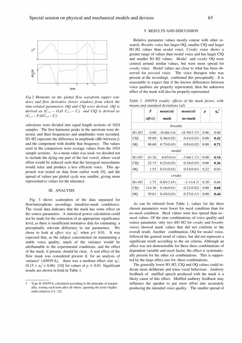
Fig.2 Moments on the glottal flow waveform (upper win-

dow) and flow derivative (lower window) from which the

time-related parameters OQ and ClQ were derived. OQ is

derived as (Ci+1 – Oi)/( Ci+1 – Ci) and ClQ is derived as

(Ci+1 – Pi)/(Ci+1 – Ci)

selections were divided into equal length sections of 1024

samples. The first harmonic peaks in the spectrum were de-

tected, and their frequencies and amplitudes were recorded.

H1-H2 repesents the difference in amplitude (dB) between f0

and the component with double that frequency. The values

used in the comparison were average values from the 1024

sample sections. As a mean value was used, we decided not

to include the dying out part of the last vowel, where vocal

effort would be reduced such that the laryngeal musculature

would relax and produce a less efficient voice. This ap-

proach was tested on data from earlier work [9], and the

spread of values per glottal cycle was smaller, giving more

representative values for the utterance.

III. ANALYSIS

Fig. 3 shows scatterplots of the data separated for

flow/microphone recordings (mask/no-mask conditions).

The visual data indicates that the mask has some effect on

the source parameters. A statistical power calculation could

not be made for the estimation of an appropriate significance

level, as there is insufficient normative data for estimating a

perceptually relevant difference in our parameters. We

chose to look at effect size �p2, when p� 0.01. It was

expected that, as the subject concentrated on maintaining a

stable voice quality, much of the variance would be

attribuatable to the experimental conditions, and the effect

of the mask, if present, should be clear. A real effect of the

flow mask was considered present if, for an analysis of

variance1 (ANOVA), there was a medium effect size �p2,

(0.15 > �p2 > 0.06) [10] for values of p � 0.01. Significant

results are shown in bold in Table 1.

1 Type II ANOVA, calculated according to the principle of margin-

ality, testing each term after all others, ignoring the term's higher

order relatives [11, 12]

V. RESULTS AND DISCUSSION

Relative parameter values mostly concur with other re-

search. Breathy voice has larger OQ, smaller ClQ and larger

H1-H2 values than modal voice. Creaky voice shows a

greater range of values than modal voice and has larger ClQ

and smaller H1-H2 values. Modal and creaky OQ were

centred around similar values, but were more spread for

creaky voice. Modal values are close to what has been ob-

served for pressed voice. The voice therapist who was

present at the recordings confirmed this perceptually . It is

reasonable to expect that if the known differences between

voice qualities are properly represented, then the unknown

effect of the mask will also be properly represented.

Table 1. ANOVA results: effects of the mask factor, with

means and standard deviations (sd)

F

(df=1)

mean(sd)

mask

mean(sd)

no-mask

p �p2

breathy

H1-H2 0.00 -16.60(3.0) -16.59(5.57) 0.96 0.00

ClQ 39.69 0.36(0.02) 0.41(0.03) 0.00 0.42

OQ 98.60 0.73(0.03) 0.81(0.02) 0.00 0.71

modal

H1-H2 43.26 -0.87(0.8) -2.94(1.12) 0.00 0.54

ClQ 23.73 0.21(0.02) 0.24(0.03) 0.00 0.36

OQ 1.53 0.51(0.03) 0.53(0.01) 0.22 0.03

creaky

H1-H2 1.72 -0.85(2.43) -2.11(4.2) 0.20 0.04

ClQ 114.36 0.16(0.01) 0.21(0.02) 0.00 0.68

OQ 39.61 0.43(0.03) 0.57(0.11) 0.00 0.44

As can be inferred from Table 1, values for the three

chosen parameters were lower for mask condition than for

no-mask condition. Mask values were less spread than no-

mask values. Of the nine combinations of voice quality and

source parameter, only two (H1-H2 for creaky and breathy

voice) showed mask values that did not conform to the

overall result. Another combination, OQ for modal voice,

followed the general trend of values, but did not represent a

significant result according to the set criteria. Although an

effect was not demonstrable for these three combinations of

dependent variable and mask factor, the effect is systematic-

ally present for the other six combinations. This is suppor-

ted by the large effect size for these combinations.

The generally lower H1-H2, ClQ and OQ values could in-

dicate more deliberate and tense vocal behaviour. Auditory

feedback of muffled speech produced with the mask is a

likely cause of this effect. Muffled auditory feedback may

influence the speaker to put more effort into accurately

producing the intended voice quality. The smaller spread of

0

Ug

0

dU g/d

t

time

Ci Ci+1Oi Pi


mask values may reflect extra focussing on the phonation

task. It is interesting to note that the mask seems to reduce

parameter variability on a subconscious level, but that the

speaker was not able to consciously limit variability.

V. CONCLUSION

There was a systematic difference between source para-

meters extracted from flow and microphone speech. Flow

mask recordings produced lower parameter values than mi-

crophone recordings. This may indicate increased vocal

tension, more deliberate vocal behaviour caused by muffled

auditory feedback, or a combination of both. This effect

should be noted in future comparisons of flow and micro-

phone data

REFERENCES

[1] M. Rothenberg, “A new inverse-filtering technique for

deriving the glottal flow waveform during voicing”, J. Ac.

Soc. Am., vol. 56(6), pp. 1632-1645, 1993.

[2] P. Alku, “Glottal wave analysis with pitch synchronous

iterative adaptive inverse filtering”, Speech Comm. 11(2-3),

109-118, 1992.

[3] A. Ní Chasaide & C. Gobl, “Voice Source Variation” in

Handbook of Phonetic Sciences, J. Laver & W. Hardcastle,

Eds. Blackwell. 1995, pp. 427-462.

[4] E. Holmberg, Aerodynamic Measurements of Normal

Voice, Stockholm University, Sweden, 1993.

[5] J. Iwarsson, Breathing and Phonation, Stockholm,

Sweden, 2001.

[6] S. Hertegård, Vocal Fold Vibrations as Studied with

Flow Inverse Filtering, Stockholm, Sweden, 1994.

[7] B. Cranen & J. Schroeter, “Modelling a leaky glottis”,

J. Phonetics, 20, pp. 165-177, 1995.

[8] J. L. Flanagan, Speech Analysis, Synthesis and Percep-

tion, Springer, Berlin, 1972.

[9] R. Orr, B. Cranen & F. de Jong, “An investigation of

the parameters derived from the inverse filtering of flow and

microphone signals”, in Voice Quality: Functions, Analysis

and Synthesis (VOQUAL '03)”, C. d'Alessandro & K. R.

Scherer, Eds. Geneva, Switzerland, 2003, pp. 35-40.

[10] J. Cohen, Statistical Power Analysis for the Behaviour-

al Sciences, Lawerence Erlbaum Assoc. Hillsdale, NJ, 1988.

[11] J. Fox, Applied Regression, Linear Models, and Re-

lated Methods, Sage, 1997

[12] T. Rietveld & R. van Hout, Statistical Techniques for

the Study of Language and Language Behaviour, Mouton de

Gruyter, 1993.

Fig. 3 Scatterplots of the three voice qualities, modal, breathy and creaky, showing the mask and no-mask conditions for

three combinations of the parameters OQ, ClQ and H1-H2. Note that the y-axes are different for each plot.

66 MAVEBA 2005

ptIidvdlppid

i

tpatHoaIieHnecc

A non-invasive device to measure mechanical interaction between tongue, palate and teeth during speech production

Christophe Jeannin1,5, Pascal Perrier1, Yohan Payan2, André Dittmar3, Brigitte Grosgogeat4,5 1Institut de la Communication Parlée, INPG, Grenoble, France

2 TIMC, Grenoble, France 3 Laboratoire des microsystèmes et microcapteurs biomédicaux, INSA, Lyon, France

Abstract This paper describes an original experimental

rocedure to measure the mechanical interaction between he tongue and teeth and palate during speech production. t consists in using edentulous people as subjects and to nsert pressure sensors in the structure of their complete ental prosthesis. Hence, there is no perturbation of the ocal tract cavity due to the sensors themselves. Several uplicates are used with transducers situated at different ocations of the complete denture according to alatography’s results, in order to carefully analyze the roduction of specific sounds such as stop consonants.. It s also possible to measure the contact pressure at ifferent locations on the palate for the same sound.

Index Terms—speech production, tongue/palate

nteraction, complete denture, pressure transducer

I. INTRODUCTION

Speech motor control has been often compared with he control of other skilled human movements such as ointing or grasping [1]. This approach was very helpful nd permitted the elaboration of important hypotheses hat were the basis of major speech production theories. owever, a peculiarity of speech movement has been ften overseen, namely the fact that speech articulators, nd especially the tongue, are not moving in a free space. ndeed, the vocal tract is a very narrow space, and tongue s most of the time in mechanical interaction with xternal structures, such as the palate or/and the teeth. amlet & Stone [2] and Fuchs et al. [3] have found a umber of evidences supporting the hypothesis that these xternal structures would be integrated in speech motor ontrol strategies, and would, consequently, significantly ontribute to the control of speech movement accuracy.

Now, two questions can be raised: (1) What is the quantitative nature of the

interaction between tongue and external structures? In other words, are these structures only geometrical limits of the space in which tongue is allowed to move, or are they mechanical objects that are actually used to position and shape the tongue?

(2) What are the changes in speech motor control strategies induced by dramatic modifications of these external structures, as it is the case for instance for edentulous people?

Quantitative measurements of the intensity of the force exerted by the tongue on the teeth provide an interesting basis to address these issues. In addition, this technique provides interesting information about the order of magnitude of the intensity of muscular forces involved in the generation of tongue movements during speech production.

In this aim, a number of experimental set-ups have been developed in the past to measure tongue pressure against the palate in various experimental conditions [4]. The limits of these techniques, beside the inherent complexity of their calibration, lie in the fact that they actually induce slight perturbations of the speech production, because they modify the geometry of the vocal tract. Honda et al. [5] have shown that speakers can compensate quite easily and quite quickly for brutal changes in the thickness of an inflated palate, in that sense that they could adapt tongue positions in reference to the variable palatal shapes. However, it is not clear whether the intensity of the palate/tongue interaction was or not affected by these brutal changes.

In this paper, we will present a new experimental procedure that aims

(1) at measuring the interaction between tongue, teeth and palate without perturbing the production of speech, and

(2) at studying how speech motor control strategies evolve for edentulous people, from the moment where an artificial denture is put back in the mouth. Finally, preliminary results of a pilot study will be presented.

4 Laboratoire d’Etude des Interfaces et des biofilms en Odontologie, Lyon, France 5 Hospices Civils de Lyon, Service d’odontologie, Lyon, France

[email protected], [email protected]

II. EXPERIMENTAL DEVICE AND METHODS

The basic principle and the originality of the method presented in this paper is to use edentulous people as subjects, and to insert pressure sensors in their complete dental prosthesis, in such a way that the geometry of the vocal tract remains exactly the same as when their normal dental prosthesis is in place. A. Experimental device General description

The complete denture, in which the pressure sensor is included, is placed inside the mouth. A sheath goes from the premolar area to the connector placed outside the mouth, via the labial commissure. Then, a wire goes from the connector to the amplifier, from the connector to a data sampling board and then to the computer.


mailto:[email protected]

A microphone is also connected to an amplifier to record the acoustic speech signal simultaneously with the pressure exerted by the tongue against the palate and/or the teeth. This amplifier is in turn linked to the data sampling board. Description of the complete dental prosthesis

The dental prosthesis is made of resin and consists of complete artificial denture and of an artificial palate. Artificial teeth are similar in shape and size to natural teeth. The artificial palate must be at least 3mm thick to avoid breakage. Hence, both the pressure sensor and the wires connecting it with the connector outside of the mouth can be easily inserted in the prosthesis, without creating any additional change of the oral cavity (fig. 1).

For each edentulous patient, the dental prosthesis that is designed for obvious medical purposes is accurately duplicated thanks to a specific prosthesis design technique. Several duplicates are thus realized, in order to have different possible positions for the pressure sensor. Thus, the sensor can be inserted in the prostheses before the experiment with the patient, and no time is wasted during the experiment itself, when the tongue palate/teeth interaction is measured at different locations.

Figure 1: Complete dental prosthesis with a sensor inserted in a front incisor. The wire connecting the sensor to the external connector can be seen on the

right hand side of the picture, at the level of the first premolar. It goes then to the sensor inside the

structure of the palate.

Pressure sensor description

The sensor is made of a strain gauge sensor which is composed of thirteen layers (fig. 2). Each layer plays an important role in measuring capabilities of the transducer.

The intraoral area is a very difficult environment mainly because of three factors:

• Permanent moisture due to saliva

• Variable temperature • Mechanical constrains

Therefore, the sensor must be electrically insulated and water proof. Moreover, it must be sturdy in order to go through several experiments.

5mm3mm 5mm3mm 5mm3mm

Figure 2: The 13 layers of the pressure sensor

The middle layer is made of a steel cantilever beam which is 10/100 mm thick. It supports on each side an active strain gauge. The gauges (Vishay, ref EA06 062 AQ 350) are placed in a half Wheatstone bridge configuration.. This strain gauge has been chosen because of its stability in temperature.

Gauges are bonded on a metallic support with M-Bond 200 adhesive (Vishay measurement group). Wires of 0,1mm diameter are soldered with tin on the gauge. The area of solder is 1mm2 small and there are 4 points, 2 by side.

The two next layers are made of protective coating. M-Coat A (Vishay measurement group).

Sensor

In any case, during the

construction, the thickness of all the liquid components such as protective coating or bonding must be very small, in order to preserve the mechanical properties of the sensor. Consequently just one application of each component by layer can be done.

3mm

Wire inserted in the resin

5mm

Figure 3 shows a detailed picture of such a sensor.

Figure 3: The pressure sensor connected to its wire.

68 MAVEBA 2005

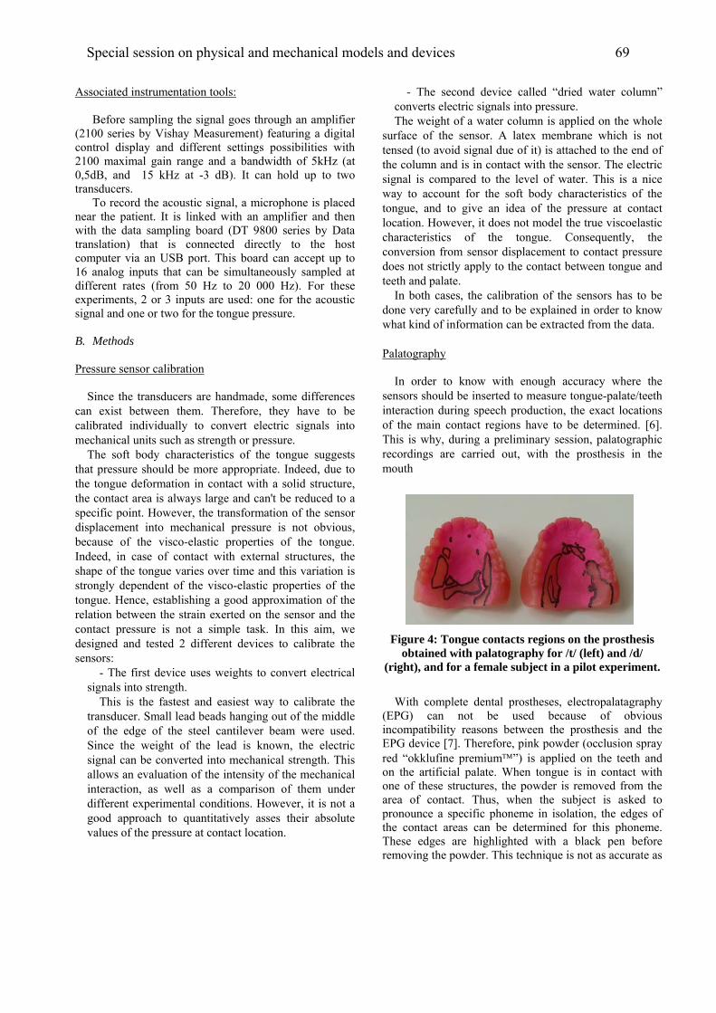
Associated instrumentation tools:

Before sampling the signal goes through an amplifier (2100 series by Vishay Measurement) featuring a digital control display and different settings possibilities with 2100 maximal gain range and a bandwidth of 5kHz (at 0,5dB, and 15 kHz at -3 dB). It can hold up to two transducers.

To record the acoustic signal, a microphone is placed near the patient. It is linked with an amplifier and then with the data sampling board (DT 9800 series by Data translation) that is connected directly to the host computer via an USB port. This board can accept up to 16 analog inputs that can be simultaneously sampled at different rates (from 50 Hz to 20 000 Hz). For these experiments, 2 or 3 inputs are used: one for the acoustic signal and one or two for the tongue pressure. B. Methods Pressure sensor calibration

Since the transducers are handmade, some differences can exist between them. Therefore, they have to be calibrated individually to convert electric signals into mechanical units such as strength or pressure.

The soft body characteristics of the tongue suggests that pressure should be more appropriate. Indeed, due to the tongue deformation in contact with a solid structure, the contact area is always large and can't be reduced to a specific point. However, the transformation of the sensor displacement into mechanical pressure is not obvious, because of the visco-elastic properties of the tongue. Indeed, in case of contact with external structures, the shape of the tongue varies over time and this variation is strongly dependent of the visco-elastic properties of the tongue. Hence, establishing a good approximation of the relation between the strain exerted on the sensor and the contact pressure is not a simple task. In this aim, we designed and tested 2 different devices to calibrate the sensors:

- The first device uses weights to convert electrical signals into strength.

This is the fastest and easiest way to calibrate the transducer. Small lead beads hanging out of the middle of the edge of the steel cantilever beam were used. Since the weight of the lead is known, the electric signal can be converted into mechanical strength. This allows an evaluation of the intensity of the mechanical interaction, as well as a comparison of them under different experimental conditions. However, it is not a good approach to quantitatively asses their absolute values of the pressure at contact location.

- The second device called “dried water column” converts electric signals into pressure. The weight of a water column is applied on the whole

surface of the sensor. A latex membrane which is not tensed (to avoid signal due of it) is attached to the end of the column and is in contact with the sensor. The electric signal is compared to the level of water. This is a nice way to account for the soft body characteristics of the tongue, and to give an idea of the pressure at contact location. However, it does not model the true viscoelastic characteristics of the tongue. Consequently, the conversion from sensor displacement to contact pressure does not strictly apply to the contact between tongue and teeth and palate.

In both cases, the calibration of the sensors has to be done very carefully and to be explained in order to know what kind of information can be extracted from the data.

Palatography

In order to know with enough accuracy where the sensors should be inserted to measure tongue-palate/teeth interaction during speech production, the exact locations of the main contact regions have to be determined. [6]. This is why, during a preliminary session, palatographic recordings are carried out, with the prosthesis in the mouth

Figure 4: Tongue contacts regions on the prosthesis obtained with palatography for /t/ (left) and /d/

(right), and for a female subject in a pilot experiment.

With complete dental prostheses, electropalatagraphy

(EPG) can not be used because of obvious incompatibility reasons between the prosthesis and the EPG device [7]. Therefore, pink powder (occlusion spray red “okklufine premium™”) is applied on the teeth and on the artificial palate. When tongue is in contact with one of these structures, the powder is removed from the area of contact. Thus, when the subject is asked to pronounce a specific phoneme in isolation, the edges of the contact areas can be determined for this phoneme. These edges are highlighted with a black pen before removing the powder. This technique is not as accurate as


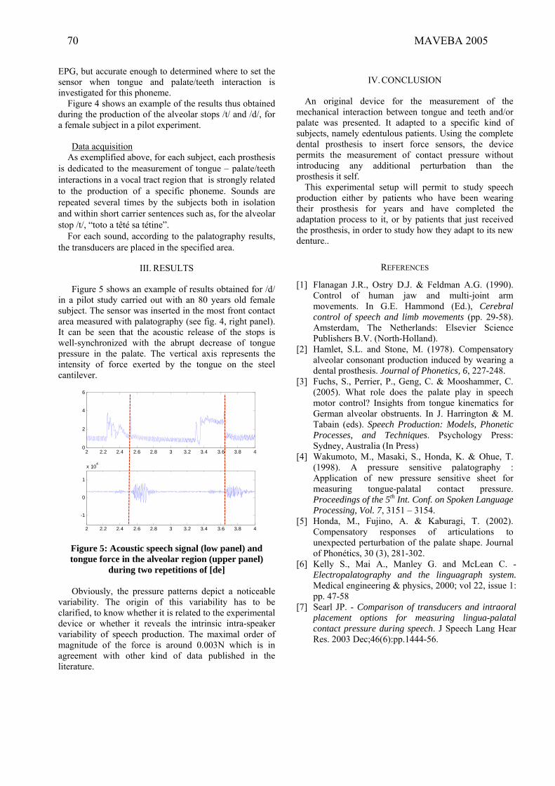
EPG, but accurate enough to determined where to set the sensor when tongue and palate/teeth interaction is investigated for this phoneme.

Figure 4 shows an example of the results thus obtained during the production of the alveolar stops /t/ and /d/, for a female subject in a pilot experiment.

Data acquisition

As exemplified above, for each subject, each prosthesis is dedicated to the measurement of tongue – palate/teeth interactions in a vocal tract region that is strongly related to the production of a specific phoneme. Sounds are repeated several times by the subjects both in isolation and within short carrier sentences such as, for the alveolar stop /t/, “toto a têté sa tétine”.

For each sound, according to the palatography results, the transducers are placed in the specified area.

III. RESULTS

Figure 5 shows an example of results obtained for /d/

in a pilot study carried out with an 80 years old female subject. The sensor was inserted in the most front contact area measured with palatography (see fig. 4, right panel). It can be seen that the acoustic release of the stops is well-synchronized with the abrupt decrease of tongue pressure in the palate. The vertical axis represents the intensity of force exerted by the tongue on the steel cantilever.

2 2.2 2.4 2.6 2.8 3 3.2 3.4 3.6 3.8 40

2

4

6

2 2.2 2.4 2.6 2.8 3 3.2 3.4 3.6 3.8 4

-1

0

1

x 104

Figure 5: Acoustic speech signal (low panel) and tongue force in the alveolar region (upper panel)

during two repetitions of [de] Obviously, the pressure patterns depict a noticeable

variability. The origin of this variability has to be clarified, to know whether it is related to the experimental device or whether it reveals the intrinsic intra-speaker variability of speech production. The maximal order of magnitude of the force is around 0.003N which is in agreement with other kind of data published in the literature.

IV. CONCLUSION

An original device for the measurement of the

mechanical interaction between tongue and teeth and/or palate was presented. It adapted to a specific kind of subjects, namely edentulous patients. Using the complete dental prosthesis to insert force sensors, the device permits the measurement of contact pressure without introducing any additional perturbation than the prosthesis it self.

This experimental setup will permit to study speech production either by patients who have been wearing their prosthesis for years and have completed the adaptation process to it, or by patients that just received the prosthesis, in order to study how they adapt to its new denture..

REFERENCES

[1] Flanagan J.R., Ostry D.J. & Feldman A.G. (1990).

Control of human jaw and multi-joint arm movements. In G.E. Hammond (Ed.), Cerebral control of speech and limb movements (pp. 29-58). Amsterdam, The Netherlands: Elsevier Science Publishers B.V. (North-Holland).

[2] Hamlet, S.L. and Stone, M. (1978). Compensatory alveolar consonant production induced by wearing a dental prosthesis. Journal of Phonetics, 6, 227-248.

[3] Fuchs, S., Perrier, P., Geng, C. & Mooshammer, C. (2005). What role does the palate play in speech motor control? Insights from tongue kinematics for German alveolar obstruents. In J. Harrington & M. Tabain (eds). Speech Production: Models, Phonetic Processes, and Techniques. Psychology Press: Sydney, Australia (In Press)

[4] Wakumoto, M., Masaki, S., Honda, K. & Ohue, T. (1998). A pressure sensitive palatography : Application of new pressure sensitive sheet for measuring tongue-palatal contact pressure. Proceedings of the 5th Int. Conf. on Spoken Language Processing, Vol. 7, 3151 – 3154.

[5] Honda, M., Fujino, A. & Kaburagi, T. (2002). Compensatory responses of articulations to unexpected perturbation of the palate shape. Journal of Phonétics, 30 (3), 281-302.

[6] Kelly S., Mai A., Manley G. and McLean C. - Electropalatography and the linguagraph system. Medical engineering & physics, 2000; vol 22, issue 1: pp. 47-58

[7] Searl JP. - Comparison of transducers and intraoral placement options for measuring lingua-palatal contact pressure during speech. J Speech Lang Hear Res. 2003 Dec;46(6):pp.1444-56.

70 MAVEBA 2005

Poster session


Performance of glottal inverse filtering (IF) is evaluated in this paper by using speech material produced with computational modelling of voice production represented by an aeroelastic model of vocal folds and a Finite Element (FE) model of the vocal tract. An inverse filtering algorithm was used in order to estimate the glottal flow from the speech pressure signal generated by the model. Comparison between the estimated glottal flow and the original flow generated by computational modelling shows that the IF method is able to yield an accurate estimate for the glottal flow.

I. INTRODUCTION Inverse filtering (IF) is a non-invasive method to estimate the source of voiced speech, the glottal volume velocity waveform. In this technique, a model for the vocal tract transfer function is first computed. The effect of the vocal tract is then cancelled from the produced speech waveform by filtering this through the inverse of the model. As an input to IF, it is possible to use either the oral flow recorded in the mouth with a flow mask (e.g. [1]) or the pressure waveform captured by a microphone in free field outside the mouth (e.g. [2]). Performance of an inverse filtering method is practically impossible to assess with natural speech. This comes from the fact that it is not possible to analyse how closely the estimated glottal flow given by an inverse filtering algorithm corresponds to the true glottal flow because the latter can not be measured. It is, however, possible to assess inverse filtering by using synthetic speech that has been created using a known, artificial waveform of the glottal excitation. This kind of evaluation, however, is not truly objective, because speech synthesis and inverse filtering analysis are typically based on similar models of the human voice production apparatus (e.g. the source filter model [3]). In the current study, we combine physical modelling of voice production in order to synthesize speech with a

known, realistic glottal flow waveform. By using the pressure signals given by the physical models as an input to an inverse filtering method, it is then possible to analyze how closely the obtained estimate of the voice source matches the original glottal flow. The paper first describes in section II the methodology used both in physical modelling (sections IIA and IIB) and in inverse filtering (section IIC). The results obtained for a sustained male vowel are described in section III and the paper is finished with short conclusions in section IV.

II. METHODOLOGY

A. Aeroelastic model of the vocal folds

Recently an aeroelastic model was developed by Horáček et al. [4, 5] that allows numerical simulation of self-oscillations of the vocal folds. The incompressible 1-D fluid flow theory is used in the model for expressing the unsteady aerodynamic forces and the Hertz model is used for the impact forces. The parameters of the model, i.e., the mass, stiffness and damping matrices are approximately related to the geometry, size and material density of real vocal folds as well as to a prescribed fundamental frequency (F0) and damping. In this contribution, the output of the numerical simulation, i.e., the intraglottal airflow rate is used to excite an FE model of human vocal tract representing the vowel /a/. Symmetric oscillations are assumed and hence the vibration of only one vocal fold is modelled. Vocal fold oscillations are simulated by a vibrating element of length L with mass m and moment of inertia I with two-degrees-of-freedom supported by an elastic foundation in the wall of a channel conveying air (Fig. 1). The motion of an equivalent three mass system on two springs can be described by the following equation:

0FVKVBVM =+++ &&& , (1)

where KBM ,, are the structural mass, damping and stiffness matrices, respectively, and TV=[V1(t),V2(t)] is the

ASSESSMENT OF GLOTTAL INVERSE FILTERING BY USING AEROELASTIC MODELLING OF PHONATION AND FE MODELLING OF

VOCAL TRACT

P. Alku1, J. Horáček 2, M. Airas1, A-M. Laukkanen3 1Lab. of Acoustics and Audio Signal Processing, Helsinki University of Technology, Finland

2Institute of Thermomechanics, Academy of Sciences of the Czech Republic, Prague, Czech Republic 3Dept. of Speech Communication and Voice Research, University of Tampere, Finland


vector for rotation and translation of the vibrating element. The vector for nonlinear aerodynamic and collision forces can be expressed as TF = [F1(t), F2(t)],

F1,2 ( )[ ] ( )[ ]∑ ∑= =

=2

0,

2

0,

)(2

)(1,,,

2,1

ji lk

ljkilkji tVtVKρ

(2)

where the superscripts of V1 and V2 denote the order of time derivatives and Ki,j,k,l are constant coefficients. For the numerical simulations Eq. 1 was transformed into a system of four 1st order ordinary differential equations and 4th order Runge-Kutta method was used for the calculations. The following parabolic function is used to approximate the geometry of the vocal folds: a(x) = 1.858 – 159.86 x2 (3) The airflow velocity U0 at the inlet (x=0) to the glottal region is simply related to the mean glottal volume velocity according to 0 02Q U H h= and to the static subglottal pressure according to:

[ ]{ }22sub 0 0 01/ 2 / ( )P U H H a Lρ= − (4)

During the vocal folds collision, the static subglottal pressure is constant that equals the pressure in the lungs (Plungs). H0 and h denote the height and width of the channel, respectively. Using tissue density

hρ =1020kg/m3, thickness L=6.8mm and length of the vocal fold h=10mm, eccentricity (e), total mass (m) and moment of inertia (I) were calculated. As the value of air density we used ρ =1.2kg/m3. A tuning procedure was used to adjust the stiffness of the elastic foundation of the vibrating element and the damping coefficients in order to approximate the fundamental frequency F0 by setting the natural frequencies f1=F0, f2=F0+5Hz and 3dB half-power bandwidths ∆f1,2 of both resonances. The optimum distance between the two supporting springs was adjusted to l=0.344L, for which the real values of the stiffness coefficients c1, c2 can be calculated for the prescribed frequencies f1, f2. In the example studied in this paper, the following values were used for the input data: prephonatory glottal half-width g=0.2mm, F0≅100Hz, ∆f1=23Hz, ∆f2=29Hz, U0=1.6m/s, Q=0.18l/s, Plungs=380Pa and the Hertz coefficient for the vocal folds collisions kH=730Nm-2/3. The following main output data resulted from the simulation: open quotient OQ=0.72, skewing (speed) quotient QS=1.56, closing quotient CQ=0.28, fundamental frequency F0=1/T=100.77Hz

calculated from the period T of the self-oscillations, maximum glottis opening GO=1.27mm, maximum impact stress IS=1328Pa and supraglottal pressure SPL=124dB.

Figure 1. Two-degrees of freedom model of the vocal fold. B. FE model of the vocal tract FE modelling was used in numerical simulation of the vocal tract filtering by using the Czech vowel /a/ produced by a male speaker. The model was designed based on MRI data described in [6]. The vocal tract geometry was obtained from a native Czech speaker during phonation. The MRI of the vocal tract for the mid-sagittal cross-section and the designed FE model are shown in Fig. 2. The vocal tract was modelled by the ANSYS FE code using acoustics finite elements FLUID 30 with speed of sound c0=343m/s and ρ =1.2kg/m3. The acoustic pressure p is described by the equation:

2

2

20

2 1tp

cp

∂∂

=∇ (5)

and in FE formulation it can be written in the matrix form in the global co-ordinate system as

)(tfPKPBPM =++ &&& (6)

where M, B, K are the mass, acoustic boundary damping and stiffness matrices, respectively; P and f are the vectors of nodal acoustic pressures and excitation forces, respectively. The transient analysis with the Newmark integration method was used for numerical simulation of

74 MAVEBA 2005

the acoustic signal near the lips whereas the excitation was applied at the position of the vocal folds. The effect of outgoing acoustic energy was modelled by an absorption boundary condition at the lips, where a boundary admittance was prescribed in correspondence to the 3dB half-power bandwith known for formant (acoustic resonant) frequencies. The excitation signal was the intraglottal airflow volume velocity Q(t) resulting from the aeroelastic model of the vocal folds.

/á/

Figure 2. MRI of the male subject during phonation (upper) and FE model of the vocal tract for the Czech vowel /a/ (lower). C. Inverse filtering

The inverse filtering method used is based on our previous experiments in developing automatic methods to estimate the glottal flow from the speech pressure waveforms with the Iterative Adaptive Inverse Filtering (IAIF) method [7]. The current method, the flow diagram of which is shown in Fig. 3, is a slightly modified version from our previous ones. Parametric spectral models that are used in various blocks of the flow diagram are computed with the Discrete All-pole Modeling (DAP) method [8] instead of the conventional linear predictive analysis. This makes it possible to obtain estimates of the formant frequencies that are less biased by the harmonic

structure of the speech spectrum. The detailed description of the IAIF-method can be found in [9].

The IAIF method has limitations. It is based on straightforward linear modelling of speech production without taking into account, for example, the interaction between the glottal source and the vocal tract. Moreover, the digital model of the vocal tract is a pure all-pole filter, which is not accurate for nasals. Despite these inherent limitations, the proposed technique provides a promising method to estimate the glottal flow especially given the fact that the method can be implemented (if desired) in a completely automatic manner with a reasonable computational cost.

1. Highpass filtering

2. DAP-analysis (order 1)

3. Inverse filtering 4. DAP-analysis (order p)

5. Inverse filtering 6. Integration

7. DAP-analysis (order g)

8. Inverse filtering 9. Integration

10. DAP-analysis (order r)

11.Inverse filtering 12. Integration

Figure 3. Block diagram of the IAIF method

s(n)

Hg1(z)

Hvt1(z)

Hg2(z)

Hvt2(z)

g(n)

III. RESULTS

The vowel sound produced by the physical modelling

was inverse filtered with the IAIF method by using the following parameters (see Fig. 3): p = r = 12, g = 4. The sampling frequency was 10 kHz. The length of the analysis window was 50 ms. The lip radiation effect

Poster session 75

(blocks no 6, 9 and 12 in Fig 3) was cancelled by a first order all-pole filter with its pole at z = 0.96.

The glottal flow estimate computed by the IAIF method is shown together with the original flow generated by physical modelling in Fig. 4. Both of the two time-domain waveforms were parameterised using the Normalized Amplitude Quotient (NAQ) [10]. The value of the NAQ parameter equalled 0.2085 and 0.2038 for the original and estimated flow, respectively. Hence, in terms of the NAQ parameter, the difference between the estimated glottal flow and the original one was approximately 2 %.

Figure 4. Speech pressure signal (top) and glottal flow (middle) generated by physical modelling. Estimated glottal flow (bottom) given by inverse filtering. All signals are in the time-domain, length of panel 40 ms.

IV. CONCLUSIONS

Evaluation of inverse filtering methods is problematic because direct measurements of the glottal flow are difficult, if not impossible. In addition, using synthetic speech as test material does not make a fully objective evaluation possible, because voice synthesis and inverse filtering are typically based on the same voice production models.

The present study aimed to avoid these fundamental limitations by using a vowel produced with physical modelling in evaluation of inverse filtering. The results were encouraging in showing that the difference between

the original flow generated by physical modelling and estimated one was small.

The experiments of the present study were based on single vowel sound. In order to better understand the limitations of inverse filtering, the characteristics of the test material should be expanded. In particular, the range of F0 values used in the evaluation should be expanded to cover the pitch range of female speech.

ACKNOWLEDGEMENTS This study was supported by the Academy of Finland (projects 200859 and 205962) and by the Grant Agency of the Academy of Sciences of the Czech Republic, project No IAA20766401 Mathematical modelling of human vocal folds oscillations.

REFERENCES [1] M. Rothenberg, “A new inverse-filtering technique for deriving the glottal airflow waveform during voicing,” J. Acoust. Soc. Amer., vol. 53, pp. 1632-1645, 1973. [2] D.Y Wong, J.D. Markel, and A.H. Gray, Jr., “Least squares glottal inverse filtering from the acoustic speech waveform,” IEEE Trans. on Acoust., Speech, and Signal Proc., vol. 27, pp. 350-355, 1979. [3] G. Fant, The Acoustics Theory of Speech Production, the Hague: Mouton, 1960. [4] J. Horáček, P. Šidlof, and J.G. Švec, “Numerical modelling of leakage-flow-induced vibrations of human vocal folds with Hertz impact forces,” In: 3rd International Workshop MAVEBA 2003, pp. 143-146. [5] J. Horáček, P. Šidlof, and J.G. Švec, “Numerical simulation of self-oscillations of human vocal folds with Hertz model of impact forces,” In: Langre E, Axisa F, eds. Flow-Induced Vibration. Ecole Polytechnique, Paris, pp. 143-148. [6] K. Dedouch, J. Horáček, J.G. Švec, P. Kršek, R. Havlík, and J. Vokřál, “Acoustic analysis of a male vocal tract for Czech vowels,” In: Proc. Phoniatric Days of Eva Sedláčková, 11-13 Sept. 2003, Brno, pp 60-63. [7] P. Alku, “Glottal wave analysis with pitch synchronous iterative adaptive inverse filtering,” Speech Comm., vol. 11, pp. 109-118, 1992. [8] A. El-Jaroudi and J. Makhoul, “Discrete all-pole modeling”, IEEE Trans. Signal Proc., vol. 39, pp. 411-423, 1991. [9] P. Alku, B. Story, and M. Airas, “Evaluation of an inverse filtering technique using physical modeling of voice production,” in CD Proc. of Int. Conf. on Spoken Lang. Proc. 2004. [10] P. Alku, T. Bäckström, and E. Vilkman, “Normalized amplitude quotient for parameterization of the glottal flow,” J. Acoust. Soc. Amer., vol. 112, pp. 701-710, 2002.

76 MAVEBA 2005

I. INTRODUCTION Coughing is one of the most frequent presenting

symptoms of many diseases affecting the airways and the lungs of both humans and animals. In piggeries, the continuous on-line monitoring of cough sound can be used to build an intelligent alarm system for the early detection of diseases [1,2,3]. In a first study, with experiments under laboratory conditions, algorithms have been developed to detect cough sounds and to classify the animals whether they were ill or not. In this study, the algorithm was tested in field conditions.

Sound analysis is an interesting method to monitor health status since it needs no physical contact with the animals. Moreover the used microphone in these tests is a very cheap type.

When a pig is infected with a respiration disease, the respiration system is changing, causing the characteristics of the air going through the air pipe to produce a different sound. When it is possible to monitor and analyze the sound of a cough signal, an on-line disease monitor can be developed.

A main application is early detection of disease to reduce the use of antibiotics. In previous studies, an accurate algorithm is presented to detect citric acid induced coughing originating from healthy individual piglets. An intelligent free field recognizer is proposed to distinguish between coughing, evoked in absence or presence of a respiratory infection.

Health care management is a critical and demanding issue in current livestock production. Discarding the economic cost related to large scale diseases, early detection of diseases is important considering public health care issues like reducing antibiotics residuals. Also for reasons of animal welfare and monitoring and tracing of the food production chain, online disease monitoring is important. Therefore currently great effort is spent to the development and application of sensors and sensing techniques for diagnosis in the agricultural sector [4]. With respect to objective and automated detection of respiratory diseases in livestock, it has been shown that artificial intelligence is successfully applicable to obtain automated cough recognition from free field cough recognition.

In the work of Van Hirtum and Berckmans [6] an accurate algorithm is presented to detect citric acid induced coughing originating from healthy individual piglets under laboratory test conditions. In their work an intelligent free field recognizer is proposed to distinguish between coughing evoked in absence or presence of a respiratory infection. A drawback of the developed algorithm is that it is time consuming to run, what can cause problems when applying it in practice. Furthermore, the results are obtained on a database which is registered on individual subjects housed in a laboratory test-installation consisting of a laboratory inhalation-chamber. The test-installation, described by Van Hirtum and Berckmans [6] and Urbain et al. [7], allows to control environmental housing conditions, medical follow-up and to reduce environmental noises. So cough sounds are registered in optimal environmental sound conditions. Therefore the performance of the developed algorithms to recognize cough in field conditions needs to be assessed in order to validate the usage of sound analysis in livestock health management.

To this purpose, in a previous study [8], coughs were registered in field conditions keeping one microphone near the animal.

In that study, limiting the spectral frequency to the range from 2 kHz to 14 kHz allowed to eliminate low-frequency noises from mechanical origin, while the cough sound exhibited an important energy-peak in this range.

The main objective of this study was to evaluate the accuracy of cough recognition algorithm on labeled coughs from all other sounds, recorded simultaneously with background noises using two microphones, one for noise and one for cough recording.

II. METHODOLOGY

Animals: 350 pigs (commercial crosses) were in the first period of the finishing phase, their mean weight at the beginning of the trial was around 75 kg and their mean age was 170 days. The fattening room was wide 14 x 21,10 m and was divided in 16 boxes with totally slatted floor.

COUGH ANALYSIS AND CLASSIFICATION BY LABELLING SOUND IN SWINE RESPIRATORY DISEASE

M. Guarino1, A. Costa1, S. Patelli1, M. Silva2, D. Berckmans2

1Department of Veterinary and Technological Sciences for Food safety, Faculty of Veterinary Medicine, via Celoria, 10, 20133 Milan, Italy

2Laboratory for Agricultural Buildings Research Katholieke Universiteit Leuven, Kasteelpark Arenberg 303001 Leuven, Belgium


The walls were made of concrete bricks and insulated (PVC thick sheet) and the roof is made of prefab plates of concrete. Roof inclination was 30 %. A serological assay on blood sample to verify the presence of Pleuropneumonitis antibodies has been conducted on sick pigs to verify the source of coughing. After the slaughtering, Pleuropolmonitis was confirmed by the autopsy examine performed by the farm veterinarian. Measurements: Pigs cough was recorded using a microphone linked to the PC sound card (Conexant, AC link audio16 bit).. This was done to record the cough sound in practical field conditions, without taking the acoustical characteristics of the stable into account. The recordings were made at a sample rate of 44100 Hz, with a resolution of 16bits. The coughs were sampled with a frequency of 22050Hz to gain calculation time. The microphones where placed in the middle of the room, in the corridor, at 3 m and 18 m far from the entrance door. The data, collected in 5 days in a piggery, were labeled first by a veterinarian and then re-labeled in laboratory. The main objective of these tests was to evaluate the accuracy of cough recognition algorithm on labeled coughs from all other sounds. In the dataset there was a total of 396 different sounds.

Cough analysis: To visualize a sound the amplitude can be plotted in time. This representation method doesn’t give any information about the frequency characteristics. In a spectrogram, the signal is analyzed using Fourier transformation in order to show how the frequencies change over time. An example of an amplitude-time representation of a cough is given in figure 1.

0 2000 4000 6000 8000 10000 12000-0.8

-0.6

-0.4

-0.2

0

0.2

0.4

0.6

0.8

AM

PLI

TUD

E

TIME

Figure 1. Amplitude variation in time (in samples) of a

cough signal

The Spectrogram of the same signal is shown in figure 2. The signal represented in figure 1 was a typical cough

sound of a pig, the duration is only 0.7s.

Time

Freq

uenc

y

0 500 1000 1500 2000 2500 3000 3500 4000 4500 50000

0.1

0.2

0.3

0.4

0.5

0.6

0.7

0.8

0.9

1

Figure 2. Spectrogram of the cough signal represented in

figure 1. Classification of the sounds: In order to classify a sound, it has to be compared with a reference sound. This is done using a method called “dynamic time warping”, already used successfully in a previous work (Van Hirtum et al., 2003), in which each sound is divided into frames of equal length and the features of each frame are stored in a feature vector. Thus, each sound is represented by a sequence of data feature vectors that form a sound template. The different duration of the cough sound results from non-uniform stretching and compression of the various portions in the cough sound. Consequently simple linear time alignment is not appropriate to compare two sounds of unequal duration. In order to compare two sound templates, the DTW algorithm uses one of them as a test pattern and the other one as a reference pattern. Taking frame by frame of the test sound template, DTW looks for the frame-path in the training template that results in the minimum distortion. For each test frame a set of specified frames in the training template is allowed for comparison. Now, to test whether or not a certain sound is part of a specific class (cough, grunt, sneeze,…) the labeled sounds are divided into two groups: one test set and one training set. Every sound in the test set is compared with all the sounds in the training set. If, at least, half of the sounds in the training set classifies the tested sound as a cough, the tested sound is marked as cough. If, on the other hand, more than half of the sounds in the training set classify the tested sound as non-cough, the sound is assumed not cough. In order to have a good idea of the performance of the algorithm that was used to recognize the sounds, a method is required that shows how many sounds where classified in the correct way. This involves the number of coughs that were classified as coughs out of the total set

78 MAVEBA 2005

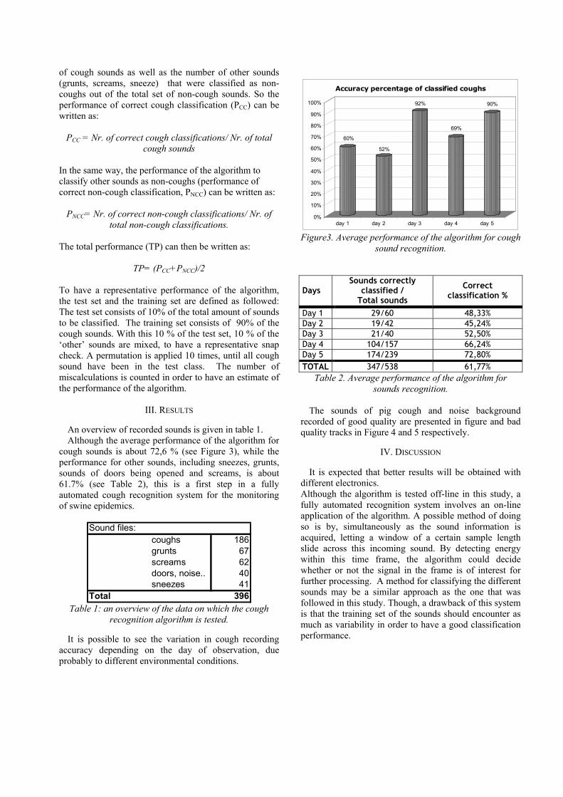
of cough sounds as well as the number of other sounds (grunts, screams, sneeze) that were classified as non-coughs out of the total set of non-cough sounds. So the performance of correct cough classification (PCC) can be written as:

PCC = Nr. of correct cough classifications/ Nr. of total cough sounds

In the same way, the performance of the algorithm to classify other sounds as non-coughs (performance of correct non-cough classification, PNCC) can be written as:

PNCC= Nr. of correct non-cough classifications/ Nr. of total non-cough classifications.

The total performance (TP) can then be written as:

TP= (PCC+PNCC)/2 To have a representative performance of the algorithm, the test set and the training set are defined as followed: The test set consists of 10% of the total amount of sounds to be classified. The training set consists of 90% of the cough sounds. With this 10 % of the test set, 10 % of the ‘other’ sounds are mixed, to have a representative snap check. A permutation is applied 10 times, until all cough sound have been in the test class. The number of miscalculations is counted in order to have an estimate of the performance of the algorithm.

III. RESULTS

An overview of recorded sounds is given in table 1. Although the average performance of the algorithm for

cough sounds is about 72,6 % (see Figure 3), while the performance for other sounds, including sneezes, grunts, sounds of doors being opened and screams, is about 61.7% (see Table 2), this is a first step in a fully automated cough recognition system for the monitoring of swine epidemics.

Sound files:

coughs 186grunts 67screams 62doors, noise.. 40sneezes 41

Total 396 Table 1: an overview of the data on which the cough

recognition algorithm is tested.

It is possible to see the variation in cough recording accuracy depending on the day of observation, due probably to different environmental conditions.

60%

52%

92%

69%

90%

0%

10%

20%

30%

40%

50%

60%

70%

80%

90%

100%

day 1 day 2 day 3 day 4 day 5

Accuracy percentage of classified coughs

Figure3. Average performance of the algorithm for cough

sound recognition.

Days Sounds correctly

classified / Total sounds

Correct classification %

Day 1 29/60 48,33% Day 2 19/42 45,24% Day 3 21/40 52,50% Day 4 104/157 66,24% Day 5 174/239 72,80% TOTAL 347/538 61,77%

Table 2. Average performance of the algorithm for sounds recognition.

The sounds of pig cough and noise background

recorded of good quality are presented in figure and bad quality tracks in Figure 4 and 5 respectively.

IV. DISCUSSION

It is expected that better results will be obtained with

different electronics. Although the algorithm is tested off-line in this study, a fully automated recognition system involves an on-line application of the algorithm. A possible method of doing so is by, simultaneously as the sound information is acquired, letting a window of a certain sample length slide across this incoming sound. By detecting energy within this time frame, the algorithm could decide whether or not the signal in the frame is of interest for further processing. A method for classifying the different sounds may be a similar approach as the one that was followed in this study. Though, a drawback of this system is that the training set of the sounds should encounter as much as variability in order to have a good classification performance.

Figure4: PSD of a signal acquired from a good quality recording. The black line represents the cough signal,, the grey line represents the noise in that signal.

Figure 5: PSD of a signal acquired from a bad quality recording. The black line represents the cough signal, the grey line represents the noise in that signal.

V. CONCLUSION

In the future other methods for classification should be examined. For example, using sound models that serve as a “template” of a certain sound.

These models can be “mapped” onto the specific sound and by adjusting the model parameters, it might be possible to search for the best model of a certain sound. One might conclude that online model based sound analysis has a high potential for animal monitoring, but there is much to be done before such a fully automated on-line sound classification system can reach the daylight.

This research could lead, in future, to a real time automatic system of cough recognition in piggeries, that might be useful in preventing the spreading of respiratory diseases and lowering the excessive use of antibiotics in pig management. The algorithm presented here can be seen as a start to extrapolated existing techniques of voice

analysis towards less conventional “sounds” as coughs, grunts and pig screams. Although some research has been performed on cough analysis, the applications remain poor. By applying such experiments in field conditions, it might bring this approach of bio-acoustics as a possible disease monitoring system closer to reality. In this case the object is the swine, but this can easily be expanded to other species like cattle and poultry.

REFERENCES

[1] A. V. Hirtum and D. Berckmans, "Objective recognition of cough-sound as biomarker for aerial pollutants," International Journal of Indoor Air Quality and Health, in press.

[2] Hiew Y., Smith J., Earis J., Cheethma B. and Woodcock A., “Dsp algorithm for cough identification and counting”, Proc. ICASSP ’02, Orlando, Florida, pp. 3888-3891, 2002

[3] Aerts JM, Jans P, Halloy D, et al. Labeling of cough data from pigs for on-line disease monitoring by sound analysis. Transactions of the ASAE 48 (1): 351-354. Jan-Feb 2005

[4] I. Tothill, "Biosensors developments and potential applications in the agricultural diagnosis sector," Computers and Electronics in Agriculture, vol. 30, pp. 205-218, 2001.

[5] V. Hirtum, A. and Berckmans D., “Fuzzy approach for improved recognition of citric acid induced piglet coughing from continuous registration”, J. Sound and Vibration, vol. 266, pp. 667-686, 2003

[6] V. Hirtum, A. and Berckmans D., “Intelligent free field cough sound recognition”, Proc. ICONS ’03, Faro, Portugal, pp. 453-58, 2003

[7] B. Urbain, J. Provoust, D. Beerens, O. Michel, B. Nicks, M. Ansay, and P. Gustin, "Chronic exposure of pigs to airborne dust and endotoxins in an environmental chamber," Veterinary Research Communications, vol. 27, pp. 569-578, 1996.

[8] A. Van Hirtum , M. Guarino M., A. Costa., P. Jans., K. Ghesquire, D. Berckmans, P. Navarotto. 2003. Automatic detection of chronic pig coughing from continuous registration in field situations. Proceedings of the 3rd International Workshop on Models and Analysis of Vocal Emissions for Biomedical Applications. Florence 10-12 Dicembre 2003. pp. 251, 254.

0 0.1 0.2 0.3 0.4 0.5 0.6 0.7 0.8 0.9 1-40

-35

-30

-25

-20

-15

-10

-5

0

5

Frequency

Pow

er S

pect

rum

Mag

nitu

de (d

B)

PSD of poor quality signal in field conditions

cough signalenvironmental noise

0 0.1 0.2 0.3 0.4 0.5 0.6 0.7 0.8 0.9 1-80

-70

-60

-50

-40

-30

-20

-10

Frequency

Pow

er S

pect

rum

Mag

nitu

de (d

B)

PSD of good quality signal in laboratory conditions

cough signalenvironmental noise

80 MAVEBA 2005

WAVE-MORPHING IN THE FRAMEWORK OF A GLOTTAL PULSE MODEL

Julien Hanquinet1, Francis Grenez1 , Jean Schoentgen1,2

1Department "Signals and Waves", Université Libre de Bruxelles, 50, Avenue F.-D. Roosevelt, 1050 Brussels, Belgium, [email protected]

2National Fund for Scientific Research, Belgium

ABSTRACT

The presentation concerns a method of wave-morphing applied to a model of the phonatory excitation, the instantaneous frequency and the harmonic richness of which are controlled. This method is based on an interpolation between the Fourier coefficients of two template waveforms. The method enables morphing continuously from one waveshape to another. Possible applications are the simulation of diplophonia, biphonation and different phonation types.

I. INTRODUCTION

The presentation concerns a method of wave-morphing based on Fourier series. It enables continuously changing one waveform into another. This method is applied to a model of the phonatory excitation signal, which is the acoustic signal generated by the vibrating vocal folds and pulsatile glottal airflow. Conventionally, glottis signals are modeled by means of a concatenation of curves that approximate the glottal pulse shape. The most popular model based on this technique is the Fant-Liljencrants model [1]. A sustained glottis signal is generated by repeating the basic pulse shape periodically. We proposed here an alternative based on the Fourier signal representation, which offers a more flexible approach to phonatory excitation modeling. It enables controlling continuously the instantaneous frequency and harmonic richness of the synthetic phonatory excitation, as well as glottal pulse morphing. The morphing is carried out by interpolating the Fourier series coefficients between two different template glottal cycles.

II. MODEL OF THE PHONATORY EXCITATION

The model used to synthesize the phonatory excitation is based on Fourier coefficients. The Fourier coefficients are computed for a template cycle of the desired phonatory signal. The template cycle can be modeled or extracted from real speech. Here, we use the Fant-Liljencrants (LF) model [1] to synthesize the desired template. The LF parameters are chosen so that the condition of area balance is fulfilled, i.e. the cycle average is zero.

A discrete periodic signal y of cycle length N can be approximated by its Fourier series truncated at Nh harmonics .

).2sin()2cos(21)(

10 n

Nkbn

Nkaany k

Nh

kk

ππ++≈ ∑

=

(1)

In expression (1), coefficients ak and bk encode the shape of the cycles of signal y and parameter N represents the cycle length. By changing the value of N, one can create signals with the same shape as y, but with different cycle lengths. Note that the following condition must be respected.

2NNh < .

(2)

If N is assumed to be real, expression (1) can be written as follows.

),sin()cos(21)(

10 nk

Nh

knk kbkaany θθ ++= ∑

=

(3)

where ∆+= − fnn πθθ 21 , is the instantaneous frequency of signal y(n) and ∆ is the sampling step. Condition (2) becomes the following.

f

ff

Nh sampling 12

< . (4)

The generalization of N to real values, because of letting assume any real positive value, introduces a quantization error of one sample at most in the cycle length. For many applications, this error is negligible when the sampling frequency is chosen sufficiently high.

f

Therefore, by means of a glottal cycle template, a signal with the same cycle shape, but the instantaneous frequency of which is controlled, can be synthesized by means of (3). Figure 1 shows an example of a phonatory excitation, for which the instantaneous frequency evolves continuously and linearly in time.

Figure 1 : Synthetic phonatory excitation, the instantaneous frequency of which evolves linearly from 75 to 200 Hz. The vertical axis is in arbitrary


mailto:[email protected]

units, and the horizontal axis is labeled in number of samples.

The harmonic richness of the synthetic signal can be controlled by modifying the Fourier coefficients as follows. This choice has been loosely inspired by [2].

,'

,'

kk

kk

kk

kk

bAbb

aAaa

=>−

=>− with . 10 << A

(5)

One sees in expression (5) that the harmonics decrease, when the parameter A is less than one, the faster the higher their order.

Figure 2 : The graph to the left shows two different cycles of the phonatory excitation. The dashed line is obtained with parameter A set to 1 and the solid line is obtained with parameter A set to 0.5. The vertical axis is in a.u. and the horizontal axis is labeled in samples. The graph to the right shows, dashed, the values in db of

kk jba + and, solid, the values in db of

kk jba '' + with A set to 0.5. The horizontal axis is labeled in the values of Fourier index k. The control of the harmonic richness of the phonatory excitation may also be used to simulate onsets and offsets as illustrated in Fig.3.

Figure 3 : Synthetic phonatory excitation where parameter A evolves linearly from 0 to 1 and from 1 to 0. The vertical axis is in a.u. and the horizontal axis is labeled in number of samples.

III. WAVE-MORPHING

Given two sets of Fourier coefficients X1 and X2 ,in complex notation, computed for two different template cycles, intermediary shapes can be synthesized by interpolating the Fourier coefficients as follows (Figure 4).

Intk

Intkk XXX 2

11−= ,

(6)

where Int is an interpolation coefficient comprised between 0 and 1. As a consequence, the Fourier phase and the logarithm of the Fourier magnitude are linearly interpolated. Therefore, coefficients ak and bk change as follows :

))()1)((sin(2

))()1)((cos(2

212)1(

1

212)1(

1

IntXArgIntXArgXXN

b

IntXArgIntXArgXXN

a

KKInt

KInt

Kk

KKInt

KInt

Kk

+−=

+−=

−

−

(7)

To avoid possible phase distortions in morphed signals, care should be exercised to respect the following condition. )arg()arg()arg()arg( 121121 ++ −<− kkkk XXXX

(8)

To satisfy this condition, one computes the arguments of the two sets of complex Fourier coefficients X1, X2, and subtracts 2π from the argument of X2 if condition (8) is not satisfied. The reason is that the phase of the morphed shape must be intermediary between the phases of the template cycles, which is possible provided that the arguments of coefficients X1 and X2 evolve quasi-monotonously.

Figure 4 : Above, the graphs show the magnitude in db (to the left) and phase in radians (to the right) of the complex Fourier coefficients. Below, the dotted lines correspond to the template glottal cycles, and the solid line corresponds to the interpolated glottal cycle, with interpolation coefficient Int set to 0.5. Above, the horizontal axis is labeled in the values of Fourier index k. Below, the horizontal axis is labeled in number of samples.

IV. RESULTS

A. MORPHING

Figure 5 illustrates the phonatory excitation signal while morphing from one cycle template to another, e.g. illustrating the transition from one phonation

82 MAVEBA 2005

type to another. The interpolation coefficient evolves, between samples 600 and 3600, linearly from zero to one.

Figure 5 : Morphed synthetic phonatory excitation. The vertical axis is in a.u. and the horizontal axis is labeled in number of samples.

B. DIPLOPHONIA

Diplophonia refers to periodic phonatory excitation signals whose mathematical periods comprise several unequal glottal cycles. A repetitive sequence of different glottal cycle shapes can be simulated by modulating the interpolation coefficient, i.e. by continuously interpolating the Fourier coefficient between two sets of template coefficients X1, X2, computed from two different reference glottal cycles. Similarly, a modulation of the instantaneous frequency may simulate a repetitive sequence of glottal cycles of unequal lengths. The temporal evolution of the interpolation coefficient as well as phase may then be written as follows.

))/sin(1(21 QInt nn θ+= (9)

))/sin((2 101 Qff nnn θπθθ +∆+=+ (10)

The instantaneous frequency oscillates between f0 – f1 and f0 + f1 . Parameter Q fixes the number of different glottal cycles within the mathematical period of the phonatory excitation. In practice, parameter Q is a small integer.

Figure 6 shows an example of diplophonia obtained by modulating the interpolation coefficient as well as the phase according to expressions (9) and (10), with Q set to two.

Figure 6 : Synthetic phonatory excitation demonstrating diplophonia. The vertical axis is in a.u. and the horizontal axis is labeled in number of samples.

C. BIPHONATION

Biphonation is also characterized by a sequence of glottal cycles of different shapes and lengths. But in this case, two glottal cycles are never identical. Biphonation reflects the presence in the spectrum of the signal of at least two harmonic series, the fundamental frequency of which form an irrational ratio. Biphonation is therefore characterized by discrete spectra with irrational ratios between the frequencies of some of the partials. Biphonation is also simulated by means of expression (9) and (10), with parameter Q equal to an irrational number.

Figure 2 shows an example of biphonation obtained with Q set to the constant e ( 2.71).

Figure 7 : Synthetic phonatory excitation demonstrating biphonation. The vertical axis is in a.u. and the horizontal axis is labeled in number of samples. Note that diplophonia and biphonation can also be simulated by modulating phase (10) and parameter A instead of interpolation (9). This is because parameter A controls the harmonic richness and therefore the shape of the cycle. The control is less flexible however.

V. CONCLUSION

This presentation concerns a model of the phonatory excitation based on Fourier series. This model enables the control of the instantaneous glottal cycle length, instantaneous harmonic richness and glottal cycle shape via distinct parameters. This model also enables interpolating between two template cycle shapes. The shape of the cycles of the phonatory excitation may morph continuously from one shape to another. These possibilities are useful to simulate onsets and offsets, intonation, phonation type transients as well as diplophonia and biphonation.

REFERENCES

[1] Fant G., Liljentcrants J., Lin Q., " A four- parameter model of glottal flow ", STL-QSPR, 4: 1-13, 1985. [2] Schoentgen, J., "Shaping function models of the phonatory excitation signal", J.Acoust. Soc. Am. 114(5): 2906-2912, 2003.

Abstract: Articulatory variation due to the production

of vowels at five pitch frequency (F0) levels (110 Hz,

123 Hz, 130 Hz, 146 Hz, and 164 Hz) was analyzed by

volumetric magnetic resonance imaging (MRI). Three

Japanese male subjects produced sustained Japanese

vowels /a/ and /i/. Observation of vocal tract area

functions extracted from the MRI data revealed that

F0 shift in vowel production affects not only the length

of the vocal tract but also its shape. Analysis

employing coefficient of variation for length-

normalized area functions revealed that the shape of

the vocal tract does not change proportionately by F0

shift and that each subject adopt different strategies

for controlling F0 while maintaining the phonetic

identity of the vowel.

I. INTRODUCTION

The larynx and the supra-laryngeal articulators are

connected mechanically and interact with each other to

produce speech sounds [1]. Vocal tract shape is thus

affected by F0 change. Except for a few previous studies

[2][3], however, effects of F0 shift on vocal tract shape

have not been studied. In addition, differences of the

effects among individuals and their acoustic

manifestation have not been reported. The present study

therefore aims to investigate possible effects of F0 shift

on vocal tract shape and area function by examining

individual variations of the interaction and their

corresponding acoustic effects.

Effects on the shape of the vocal tract by changing F0

have been measured using several imaging systems. For

instance, Hirai et al. [2] described differences in vocal

tract shape during production of the Japanese vowel /a/

associated with 1.5-octave F0 falling by using magnetic

resonance imaging (MRI). They also investigated

mechanisms of F0 control in detail and proposed a

physiological articulatory model with tongue-larynx

coupling mechanism. Tom et al. [3] reported differences

in vocal tract area function during production of the

vowel /a/ under two registers, five F0 levels, and two

loudness levels by using electron-beam computed

tomography (EBCT).

However, those studies reported the results only for a

single vowel of a single subject. Because each vowel has

a different constriction location, effects on vocal tract

shape may be different among vowels. Also, each speaker

may adopt different strategies to control F0. In this study,

we thus investigated changes in articulation of a front and

a back vowel at different F0 levels for three male

subjects. Magnetic resonance images were acquired

during producing the Japanese vowels /a/ and /i/ at five

F0 levels, and analyzed for the effects on vocal tract

shapes and area functions, as well as for the

corresponding acoustic effects using a transmission line

model.

II. MRI DATA ACQUISITION

Magnetic resonance images of three Japanese male

subjects were obtained during sustained production of

Japanese vowels /a/ and /i/ with a Shimadzu-Marconi

ECLIPSE 1.5T Power Drive 250 at the ATR Brain

Activity Imaging Center. The subjects are denoted below

as A, B, and C. The imaging sequence was a sagittal

Fourier Acquired Steady State (FAST) series with 3.0-

mm slice thickness, no slice gap, a 256 256 mm field

of view (FOV), a 512 512 pixel image size, 18 slices,

90o

flip angle (FA), 9-ms echo time (TE), and 4,900-ms

repetition time (TR). The total acquisition time was

approximately 15 sec. These parameters were selected to

complete data acquisition in a single breath.

Each subject was positioned to lie supine on the

platform of the MRI unit and put on non-magnetic intra-

aural headphones. Harmonic complex tones whose

fundamental frequency was 110, 123, 130, 146, or 164

Hz were presented through the headphones during

scanning. The subjects were instructed to adjust their F0

to the fundamental frequency of the harmonic complex

tone while maintaining steady phonation during scanning.

Each subject's voice during the scan was recorded

through an optical microphone (phone-or FOMRI). After

the scan, each utterance was examined to confirm

whether the subjects adjusted their F0 as instructed. Any

MRI data outside a margin of F0 error of ± 5 Hz was

excluded from further analysis. The data for the lowest

F0, from subject B, were excluded on this basis.

III. METHOD

A. Morphological analysis

The effects of F0 on vowel articulation were analyzed

with reference to the rigid structures. When the subjects'

head position in the MR images was different across F0

levels, the MR images were aligned with reference to the

CHANGES OF VOCAL TRACT SHAPE AND AREA FUNCTION BY F0 SHIFT

T. Kitamura1, P. Mokhtari

1, H. Takemoto

1

1Department of Biophysical Imaging, ATR Human Information Science Laboratories, Kyoto, Japan


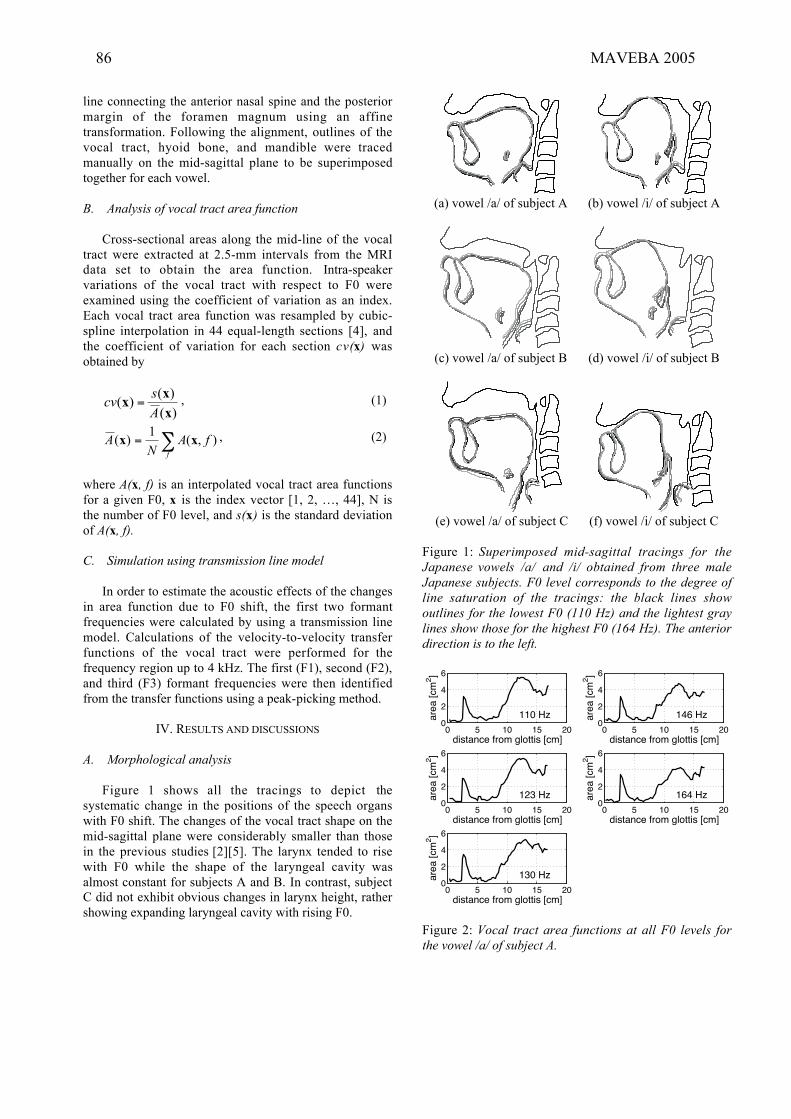
line connecting the anterior nasal spine and the posterior

margin of the foramen magnum using an affine

transformation. Following the alignment, outlines of the

vocal tract, hyoid bone, and mandible were traced

manually on the mid-sagittal plane to be superimposed

together for each vowel.

B. Analysis of vocal tract area function

Cross-sectional areas along the mid-line of the vocal

tract were extracted at 2.5-mm intervals from the MRI

data set to obtain the area function. Intra-speaker

variations of the vocal tract with respect to F0 were

examined using the coefficient of variation as an index.

Each vocal tract area function was resampled by cubic-

spline interpolation in 44 equal-length sections [4], and

the coefficient of variation for each section cv(x) was

obtained by

)(

)()(

x

xx

A

scv = , (1)

=f

fAN

A ),(1

)( xx , (2)

where A(x, f) is an interpolated vocal tract area functions

for a given F0, x is the index vector [1, 2, …, 44], N is

the number of F0 level, and s(x) is the standard deviation

of A(x, f).

C. Simulation using transmission line model

In order to estimate the acoustic effects of the changes

in area function due to F0 shift, the first two formant

frequencies were calculated by using a transmission line

model. Calculations of the velocity-to-velocity transfer

functions of the vocal tract were performed for the

frequency region up to 4 kHz. The first (F1), second (F2),

and third (F3) formant frequencies were then identified

from the transfer functions using a peak-picking method.

IV. RESULTS AND DISCUSSIONS

A. Morphological analysis

Figure 1 shows all the tracings to depict the

systematic change in the positions of the speech organs

with F0 shift. The changes of the vocal tract shape on the

mid-sagittal plane were considerably smaller than those

in the previous studies [2][5]. The larynx tended to rise

with F0 while the shape of the laryngeal cavity was

almost constant for subjects A and B. In contrast, subject

C did not exhibit obvious changes in larynx height, rather

showing expanding laryngeal cavity with rising F0.

(a) vowel /a/ of subject A (b) vowel /i/ of subject A

(c) vowel /a/ of subject B (d) vowel /i/ of subject B

(e) vowel /a/ of subject C (f) vowel /i/ of subject C

Figure 1: Superimposed mid-sagittal tracings for the

Japanese vowels /a/ and /i/ obtained from three male

Japanese subjects. F0 level corresponds to the degree of

line saturation of the tracings: the black lines show

outlines for the lowest F0 (110 Hz) and the lightest gray

lines show those for the highest F0 (164 Hz). The anterior

direction is to the left.

0 5 10 15 200

2

4

6

110 Hz

distance from glottis [cm]

area

[cm

2 ]

0 5 10 15 200

2

4

6

123 Hz


area

[cm

2 ]

0 5 10 15 200

2

4

6

130 Hz


area

[cm

2 ]

0 5 10 15 200

2

4

6

146 Hz


area

[cm

2 ]

0 5 10 15 200

2

4

6

164 Hz


area

[cm

2 ]

Figure 2: Vocal tract area functions at all F0 levels for

the vowel /a/ of subject A.

86 MAVEBA 2005

Table 1: Vocal tract length [cm] associated with

variations in F0 and Pearson's correlation coefficient r

between them.

Subject A Subject B Subject C

F0 /a/ /i/ /a/ /i/ /a/ /i/

110 Hz 16.6 16.8 --- --- 17.2 16.0123 Hz 16.4 16.7 17.3 16.1 17.6 16.2130 Hz 16.4 16.7 17.1 16.1 17.6 16.0146 Hz 16.2 16.6 16.8 15.8 17.2 15.8164 Hz 16.0 16.2 16.5 15.7 17.4 16.3

r -0.99 -0.93 -1.00 -0.96 -0.04 0.26

B. Analysis of vocal tract area function

Figure 2 depicts vocal tract area functions for the

vowel /a/ of subject A indicating that the F0 shift during

vowel production affects not only the length of the vocal

tract but also its shape. The areas of the oral cavity of the

subject tended to decrease with rising F0 for the subject,

although the changes of the vocal tract shape on the mid-

sagittal plane were considerably small. This tendency was

also found for the other subjects.

Figure 3 depicts the length-normalized mean area

functions and their coefficients of variation (CVs) for

each section. Non-uniform CV patterns demonstrate that

the shape of the vocal tract does not vary proportionately

with F0 shift, and sharp peaks of the CVs indicate large

changes of the cross-sectional area at the sections among

the data. The peak of the CV at the seventh section from

the glottis for the vowels of subject A indicates that the

junction between the lower pharyngeal and laryngeal

cavities varies in location with F0 shift. The peak near the

junction can also be found for the vowel /i/ of subject B.

The peak of the CV at the 23rd section for the vowel /a/

of subject B indicates that the ratio of oral and the

pharyngeal cavity lengths altered with F0 shift.

Additionally, the sharp peak near the 42nd section for the

vowel /i/ of all the subjects corresponds with movements

of the lips with F0 shift.

The CVs at constricted sections are relatively smaller

than those at non-constricted sections for the vowel /i/.

Because vowel acoustics are relatively sensitive to

changes in constriction area [7], this strategy contributes

to preserving vowel features regardless of the F0 level.

In contrast to the local change of the shape of the

vocal tract for subjects A and B, the lower pharyngeal

and the laryngeal cavities (from the first section to the

15th section) of subject C varied widely with F0 changes.

Thus, inter-speaker differences of the CV pattern indicate

that the strategy to control F0 and vowel articulation

varies from subject to subject.

Table 1 shows vocal tract length measured for each

condition and Pearson's correlation coefficients with F0.

These results indicate that there are strong negative

correlations between vocal tract length and F0 for

(a) subject A

(b) subject B

(c) subject C

Figure 3: Average and coefficient of variation (CV) of the

length-normalized area function for three male subjects.

subjects A and B, but not for subject C. The results are

consistent with the observation that the larynx position

rises with rising F0 for subjects A and B.

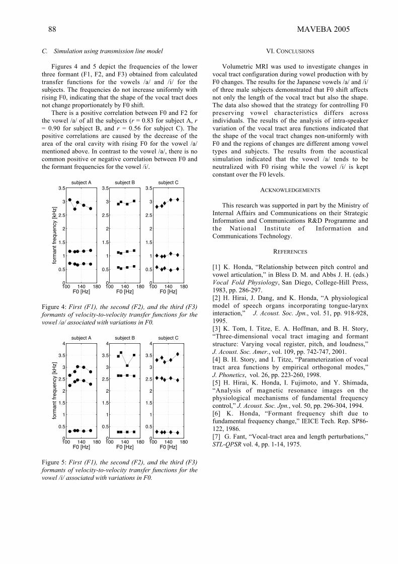
C. Simulation using transmission line model

Figures 4 and 5 depict the frequencies of the lower

three formant (F1, F2, and F3) obtained from calculated

transfer functions for the vowels /a/ and /i/ for the

subjects. The frequencies do not increase uniformly with

rising F0, indicating that the shape of the vocal tract does

not change proportionately by F0 shift.

There is a positive correlation between F0 and F2 for

the vowel /a/ of all the subjects (r = 0.83 for subject A, r

= 0.90 for subject B, and r = 0.56 for subject C). The

positive correlations are caused by the decrease of the

area of the oral cavity with rising F0 for the vowel /a/

mentioned above. In contrast to the vowel /a/, there is no

common positive or negative correlation between F0 and

the formant frequencies for the vowel /i/.

100 140 1800

0.5

1

1.5

2

2.5

3

3.5

form

ant f

requ

ency

[kH

z]

F0 [Hz]

subject A

100 140 1800

0.5

1

1.5

2

2.5

3

3.5

F0 [Hz]

subject B

100 140 1800

0.5

1

1.5

2

2.5

3

3.5

F0 [Hz]

subject C

Figure 4: First (F1), the second (F2), and the third (F3)

formants of velocity-to-velocity transfer functions for the

vowel /a/ associated with variations in F0.

100 140 1800

0.5

1

1.5

2

2.5

3

3.5

4

form

ant f

requ

ency

[kH

z]

F0 [Hz]

subject A

100 140 1800

0.5

1

1.5

2

2.5

3

3.5

4

F0 [Hz]

subject B

100 140 1800

0.5

1

1.5

2

2.5

3

3.5

4

F0 [Hz]

subject C

Figure 5: First (F1), the second (F2), and the third (F3)

formants of velocity-to-velocity transfer functions for the

vowel /i/ associated with variations in F0.

VI. CONCLUSIONS

Volumetric MRI was used to investigate changes in

vocal tract configuration during vowel production with by

F0 changes. The results for the Japanese vowels /a/ and /i/

of three male subjects demonstrated that F0 shift affects

not only the length of the vocal tract but also the shape.

The data also showed that the strategy for controlling F0

preserving vowel characteristics differs across

individuals. The results of the analysis of intra-speaker

variation of the vocal tract area functions indicated that

the shape of the vocal tract changes non-uniformly with

F0 and the regions of changes are different among vowel

types and subjects. The results from the acoustical

simulation indicated that the vowel /a/ tends to be

neutralized with F0 rising while the vowel /i/ is kept

constant over the F0 levels.

ACKNOWLEDGEMENTS

This research was supported in part by the Ministry of

Internal Affairs and Communications on their Strategic

Information and Communications R&D Programme and

the National Institute of Information and

Communications Technology.

REFERENCES

[1] K. Honda, “Relationship between pitch control and

vowel articulation,” in Bless D. M. and Abbs J. H. (eds.)

Vocal Fold Physiology, San Diego, College-Hill Press,

1983, pp. 286-297.

[2] H. Hirai, J. Dang, and K. Honda, “A physiological

model of speech organs incorporating tongue-larynx

interaction,” J. Acoust. Soc. Jpn., vol. 51, pp. 918-928,

1995.

[3] K. Tom, I. Titze, E. A. Hoffman, and B. H. Story,

“Three-dimensional vocal tract imaging and formant

structure: Varying vocal register, pitch, and loudness,”

J. Acoust. Soc. Amer., vol. 109, pp. 742-747, 2001.

[4] B. H. Story, and I. Titze, “Parameterization of vocal

tract area functions by empirical orthogonal modes,”

J. Phonetics, vol. 26, pp. 223-260, 1998.

[5] H. Hirai, K. Honda, I. Fujimoto, and Y. Shimada,

“Analysis of magnetic resonance images on the

physiological mechanisms of fundamental frequency

control,” J. Acoust. Soc. Jpn., vol. 50, pp. 296-304, 1994.

[6] K. Honda, “Formant frequency shift due to

fundamental frequency change,” IEICE Tech. Rep. SP86-

122, 1986.

[7] G. Fant, “Vocal-tract area and length perturbations,”

STL-QPSR vol. 4, pp. 1-14, 1975.

88 MAVEBA 2005

Comparison of LPC analysis and impedance vocal tract measurements

M. Kob, J. Stoffers, Ch. Neuschaefer-Rube

Chair of Phoniatrics and Pedaudiology, RWTH Aachen University – University Hospital Aachen

Pauwelsstr. 30, 52074 Aachen, Germany

1 Introduction

The acoustic measurement of the resonances in the spacebetween vocal folds and lips, the vocal tract, allows anon-invasive, objective analysis of the spectral energy dis-tribution for different articulatory cases. Whereas a con-ventional LPC analysis is successful only when appliedto more or less stationary voice signals, an external ex-citation with subsequent measurement of the vocal tractimpedance at the mouth can give reliable results whenthe voice signal is not stable or even missing.

This contribution adresses the problem how to compareresults from impedance measurements with LPC mea-surements. For a set of normal speakers, both measure-ments have been performed simultaneously. Based uponthe evaluation of the LPC curves, similar values for reso-nance frequency, amplitude and bandwidth were derived.In a study of 81 normal speakers the results from theevaluations are compared.

2 Method

The measurement set-up and the software used to eval-uate the measurements allow a sequence of measure-ments consisting of three parts: the LPC analysis of thevoice signal, the impedance measurement during phona-tion, and the impedance measurement without phona-tion. The concept for measurement of the vocal tractimpedance at the mouth, VTMI, is described in detailin [2], and the procedure of clinical measurements is de-scribed in [4].

Measurements were performed in a group of 35 femaleand 46 male healthy speakers, using a simplified set-upwithout velocity sensor. One reason is the problem ofclipping which can occur in the velocity sensor at highsound velocities. Comparisons between this set-up andthe original 2-sensor set-up showed that results from bothmethods yield comparable results for the performed task.

A sample rate of 22050 Hz was chosen, and subsequentevaluations were limited to the frequency range 100..5000Hz.

2.1 LPC measurement

The “linear predictive coding” method (LPC) is a well-established method to identify the formant structure of

a voice signal. The LPC curves are derived from a win-dowed part of the voice signal.

For the calculation of the LPC curves 28 coefficients wereused to achieve a rather high pole density but not toomany wrong identifications of formants. A Hammingwindow of 9525 samples was applied to the voice sig-nal. The onset of the voice signal was automatically dis-carded.

2.2 Impedance measurement

All impedance measurements were performed using a lin-ear swept sine from 250 Hz to 6000 Hz with a durationof 0.74 seconds. The signal-to-noise ratio was improvedby application of a symmetric Hanning window of 15 mslength.

3 Evaluation and normalisation

3.1 Parameters

From the LPC curves the formant frequency, the formantbandwidth (3 dB decay), and the relative amplitude ofthe formants were calculated. The amplitude differencewas calculated with respect to the highest formant in thefrequency range 150..5000 Hz.

The resonances frequencies of the impedance curve werecalculated from the minima of the impedance functionZ(f). Since no measures for the amplitude and band-width of the resonances could be directly derived fromthe impedance function, new measures had to be calcu-lated: the slope between a local minimum and maximumnear a resonance was used, as well as the amplitude differ-ence between these points. These values were normalisedas well by division of the local amplitude difference by thedifference between the absolute maximum and minimumin the frequency range of the evaluation.

3.2 Normal ranges

From each three LPC measurements of the six phonemes/a:/, /æ:/, /i:/, /o:/, /u:/, /l:/ the first four formantswere evaluated with respect to mean values standard de-viations of the formant frequencies, amplitudes and thebandwidths.

From the resonance and LPC curves the above parame-ter were automatically calculated and stored in an XML


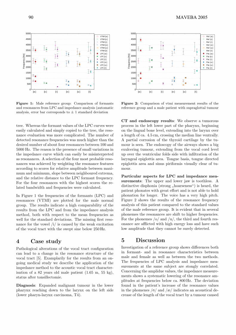
0

500

1000

1500

2000

2500

3000

3500

4000

4500

5000

[a:] [ε:] [i:] [o:] [u:] [l:]

Fre

quen

cy [H

z]

VTMI [a:]

VTMI [ε:]

VTMI [i:]

VTMI [o:]

VTMI [u:]

VTMI [l:]

LPC [a:]

LPC [ε:]

LPC [i:]

LPC [o:]

LPC [u:]

LPC [l:]

Figure 1: Male reference group: Comparison of formantsand resonances from LPC and impedance analysis (automaticanalysis, error bar corresponds to ± 1 standard deviation

tree. Whereas the formant values of the LPC curves wereeasily calculated and simply copied to the tree, the reso-nance evaluation was more complicated. The number ofdetected resonance frequencies was much higher than thedesired number of about four resonances between 100 and5000 Hz. The reason is the presence of small variations inthe impedance curve which can easily be misinterpretedas resonances. A selection of the four most probable reso-nances was achieved by weighting the resonance featuresaccording to scores for relative amplitude between maxi-mum and minimum, slope between neighboured extrema,and the relative distance to the LPC formant frequency.For the four resonances with the highest scores the re-lated bandwidth and frequencies were calculated.

In Figure 1 the frequencies of the formants (LPC) andresonances (VTMI) are plotted for the male normalgroup. The results indicate a high comparability of theresults from the LPC and from the impedance analysismethod, both with respect to the mean frequencies aswell for the standard deviations. The missing first reso-nance for the vowel /i/ is caused by the weak excitationof the vocal tract with the swept sine below 250 Hz.

4 Case study

Pathological alterations of the vocal tract configurationcan lead to a change in the resonance structure of thevocal tract [5]. Examplarily for the results from an on-going medical study we describe the application of theimpedance method to the acoustic vocal tract character-isation of a 82 years old male patient (1.65 m, 55 kg),status after tonsillectomie.

Diagnosis: Expanded malignant tumour in the lowerpharynx reaching down to the larynx on the left side(lower pharyn-larynx carcinoma, T4).

0

500

1000

1500

2000

2500

3000

3500

4000

4500

5000

[a:] [ε:] [i:] [o:] [u:] [l:]

Fre

quen

cy [H

z]

Ref. [a:]

Ref. [ε:]

Ref. [i:]

Ref. [o:]

Ref. [u:]

Ref. [l:]

Pat. [a:]

Pat. [ε:]

Pat. [i:]

Pat. [o:]

Pat. [u:]

Pat. [l:]

Figure 2: Comparison of vtmi measurement results of thereference group and a male patient with supraglottal tumour

CT and endoscopy results: We observe a tumorousprocess in the left lower part of the pharynx, beginningon the lingual bone level, extending into the larynx overa length of ca. 4.5 cm, crossing the median line ventrally.A partial corrosion of the thyroid cartilage by the tu-mour is seen. The endoscopy of the airways shows a bigexulcering tumour, extending from the vocal cord levelup over the ventricular folds side with infiltration of thelaryngeal epiglottis area. Tongue basis, tongue directedepiglottis area and sinus piriformis visually clear of tu-mour.

Particular aspects for LPC and impedance mea-

surements: The upper and lower jaw is toothless. Adistinctive disphonia (strong

”hoarseness“) is heard, the

patient phonates with great effort and is not able to holdphonation for longer. The voice has a very high pitch.Figure 2 shows the results of the resonance frequencyanalysis of this patient compared to the standard valuesof the male reference group. It is evident that in severalphonemes the resonances are shift to higher frequencies.For the phonemes /o/ and /u/, the third and fourth res-onance are afflicted with high energy loss and have suchlow amplitude that they cannot be surely detected.

5 Discussion

Investigation of a reference group shows differences bothin formant- and in resonance characteristics betweenmale and female as well as between the two methods.The frequencies of LPC analysis and impedance mea-surements at the same subject are stongly correlated.Concerning the amplidue values, the impedance measure-ments shows a systematic lowering of the resonance am-plitudes at frequencies below ca. 800 Hz. The deviationfound in the patient’s increase of the resonance valuesin the phomenes /a/ and /æ/ indicates an acoustical de-crease of the length of the vocal tract by a tumour caused

90 MAVEBA 2005

narrowed supraglottal space. The absence of higher for-mants in /o/ and /u/ could be caused by a higher sound-absorption of the alterated tissue. A systematic exami-nation of further patients with similar diseases is plannedand should give additional clues in view of a correlation ofphysiological and acoustical properties of the vocal tract.

References[1] M. Kob, Ch. Neuschaefer-Rube (2001): A method

for measurement of the vocal tract mouth impedance.Conference CD-ROM, 2nd Int. Workshop on Modelsand Analysis of Vocal Emissions for Biomedical Appli-cations – MAVEBA, file ”papers/26.pdf” 1-6.

[2] M. Kob und Ch. Neuschaefer-Rube (2002): A methodfor measurement of the vocal tract impedance at themouth. Medical Engineering & Physics, 24, 467-471.

[3] M. Kob, Ch. Neuschaefer-Rube (2003): Acousticanalysis of overtone singing. Proceedings 3rd Int.Workshop on Models and Analysis of Vocal Emissionsfor Biomedical Applications – MAVEBA, 187-190.

[4] M. Kob, J. Stoffers, M. Lievens, R. Katzer,Ch. Neuschaefer-Rube (2004): Application ofimpedance measurements for the diagnosis of artic-ulatory dysfunction. Proceedings CFA/DAGA 2004,1145.

[5] S. Koppetsch und K. Dahlmeier (2003): FunktionelleStorungen der Artikulation bei intra-oralen Tumoren –eine pra- und postoperative Langzeitstudie. Sprache–Stimme–Gehor, 155-160.

SOURCE VOICE CHARACTERISTICS OF THE ARTIFICIAL VOCAL

FOLDS

V. Misun

Department of solids of bodies, mechatronics and biomechanics. Brno University of Technology,

Brno, Czech Republic

Abstract: Specialised literature presents a number of

models describing the function of the vocal folds. In

most of those models an emphasis is placed on the

effect of Bernoulli’s air underpressure during the air

passage through the glottis. The author defines a

principle of the vocal folds function with a working

version name „principle of the compressed air

bubble“. The paper deals with the experimental

analysis of these artificial vocal folds and, first of all,

with the properties and characteristics of the source

voices generated by them. The main forces acting on

the vocal folds during phonation are as follows :

subglottal air pressure, elastic and inertia forces of

the vocal folds structure.

I. INTRODUCTION

There have been several modified versions of the

vocal folds function described in literature – [1], [2].

Most of them are based on the principle of the

myoelasto-dynamic theory. They share a common

predominant view whose central idea is that of an

expressive effect of what is called Bernoulli´s

underpressure (negative pressure) produced within the

space of the glottis at an increased speed of the airflow

which passes between the vocal folds in motion.

Due to the numerous weak points found in the

principles as defined by different authors in the

literature there has been another principle defined and

developed, preliminary called „compressed air

bubbles“, in short „bubbles“ - [3]. The paper deals with

the experimental analysis of these artificial vocal folds

and, first of all, with the properties of the source voices

generated by them [6].

II. DEFINITION OF THE „COMPRESSED AIR

BUBBLES“ PRINCIPLE

The transport of the compressed air bubbles (air

column, small air volume) through the glottis from the

subglottal to the supraglottal space are the fundamental

idea of this principle. The air bubbles with the higher

subglottal pressure should be shifted as soon as

possible to the upper part of the glottis. After the glottis

opening the bubbles expand from the higher subglottal

air pressure so that the acoustic pressure amplitude to be

source voice generated has the highest value in this

case. This condition is very important for a higher

intensity of voice generation.

According to this principle of the vocal folds function,

the main forces acting on the vocal folds during

phonation are as follows :

• the subglottal air overpressure acts on the

relatively large inner subglottal surface, producing a

considerable higher force opening the vocal folds,

• resilient forces of the vocal folds muscles which act

against the opening of the vocal folds,

• forces of inertia of the vocal folds structure.

The forces of inertia of the air bubbles cannot play a

significant role with regard to the low value of air

density, a small size of the moved bubbles and also to

small changes of the airflow speed.

The driving phenomenon for the vocal folds during

phonation is the compressed air in the subglottal space,

which always reaches a higher resulting air pressure

value here than within the supraglottal space, and is the

function of the glottis opening g. So that the basic

characteristics of the vocal folds motion and the model

function is the relation of the resulting subglottal air

pressure and the opening between the vocal folds in the

form defined by relation pRSG(g) – [6].

III. EXPERIMENTAL ANALYSIS OF THE

ARTIFICIAL VOCAL FOLDS

Based on the compressed air bubble principle there

have been artificial vocal folds developed for speaking

aloud [4], [5]. Their design allows for changing the

fundamental frequency of the source voice to match the

male or female voice.

In order to test and verify the above defined

principle of the bubbles there were some experiments

carried out. Fig.1 represents a diagram of experimental

analysis of a specific type of artificial vocal folds

(geometry, arrangement, frequency tuning). The

substitute vocal folds are placed inside the vocal folds

box in the way dividing its space into two areas : the

subglottal area – 1, the supraglottal area – 2. Into the

subglotal area 1 is taken compressed air from the

pressure vessel. In each area, a required acoustic

pressure is measured with an appropriate microphone

M1, M2 .


B. Additional masses of vocal folds

Fig.1 Diagram of the vocal folds location in the vocal

folds box

The general measurement set is shown in Fig.2. In

addition, a static mean value of the subglottal air

pressure pSGS is measured in the subglottal area, using a

water column height, h. By setting of its mean value,

the intensity of the source voice during phonation may

be simulated by means of artificial vocal folds.

Fig.2 Measurement set of the vocal folds

experimental analysis

The following variables were recorded during the

phonation measurement - Fig.2 :

• water column height, h, characterizing the set mean

value of the subglottal air pressure, p SGS

• microphone M1 recorded variable air pressure in

the subglottal space (measured by PULSE), p SG(t)• microphone M2 recorded acoustic pressure in the

supraglottal space (measured by PULSE), p SPG(t)• the course of the opening g(t) between the two

vocal folds during their phonation (recorded by a

high-speed Olympus camera).

The synchronization of all variables to be measured

was ensured by means of trigger switch, S.

IV. MEASUREMENT RESULTS

The characteristics of the artificial vocal folds vary,

of course, depending on the type of the vocal folds

measured. The individual types are distinguished by

capital letters : C – basic type, M, N. They differ in

geometry and in their additional masses, mj (j = C , M,N) which in turn also changes their fundamental

frequency tuning F0j .The parameters of the individual vocal folds type :

a) type C – basic type: mC=0 , F OC = 240 Hz

b) type M : mM , F OM = 132 Hz

c) type N : mN , F ON = 144 Hz.

Fig.4 represents the course of variable subglottal air

pressure pSG(t) of a type C vocal folds, measured at a

water column height of h = 119 mm, which corresponds

to value pSGS = 1120 Pa.

Fig.5 represents the spectrum of supraglottal

acoustic pressure pSPG(t) behind the vocal folds. This

acoustic pressure presented is the source voice

generated by the type C vocal folds. The spectrum

contains significant discrete components, which are

harmonic components to the fundamental phonation

frequency (F0 = 240 Hz) of the vocal folds. All those

harmonic components together form the „source voice“

of a given artificial vocal fold type.

Through the analysis of the high-speed camera

recordings we shall obtain the course of the openings

between the vocal folds as a time function - g(t). Fig.6

represents the evaluation of the course of opening g(t)based on the high-speed camera recordings.

2 1

expanded

air outlet

vocal folds

140 mm

microphon M1microphon M2

compressed

air inlet

pSGS h =const.trigger switch

synchronization

M2 M1

pSG(t)

pSPG(t)

S

PULSE

h

compressed

air inlet

high speed

camera: g(t)vocal folds

box

g

elastic

vocal folds

distance

piece

a) mC = 0 b) mN c) mM

A. Scheme of the vocal folds

Fig.3 Types of the artificial vocal folds measured

94 MAVEBA 2005

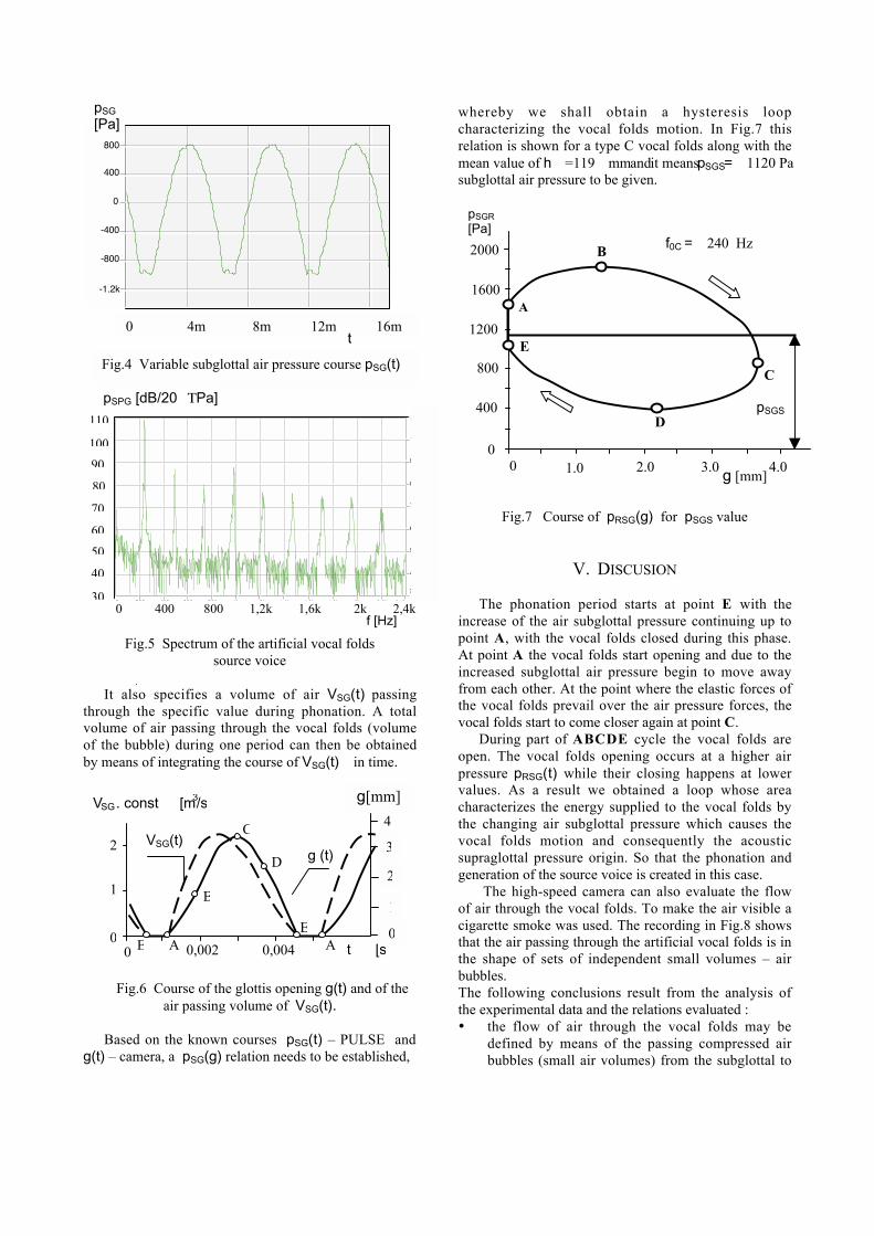
Fig.5 Spectrum of the artificial vocal folds

source voice

It also specifies a volume of air VSG(t) passing

through the specific value during phonation. A total

volume of air passing through the vocal folds (volume

of the bubble) during one period can then be obtained

by means of integrating the course of VSG(t) in time.

Fig.6 Course of the glottis opening g(t) and of the

air passing volume of VSG(t).

Based on the known courses pSG(t) – PULSE and

g(t) – camera, a pSG(g) relation needs to be established,

whereby we shall obtain a hysteresis loop

characterizing the vocal folds motion. In Fig.7 this

relation is shown for a type C vocal folds along with the

mean value of h =119 mm and it means pSGS= 1120 Pa

subglottal air pressure to be given.

Fig.7 Course of pRSG(g) for pSGS value

V. DISCUSION

The phonation period starts at point E with the

increase of the air subglottal pressure continuing up to

point A, with the vocal folds closed during this phase.

At point A the vocal folds start opening and due to the

increased subglottal air pressure begin to move away

from each other. At the point where the elastic forces of

the vocal folds prevail over the air pressure forces, the

vocal folds start to come closer again at point C.

During part of ABCDE cycle the vocal folds are

open. The vocal folds opening occurs at a higher air

pressure pRSG(t) while their closing happens at lower

values. As a result we obtained a loop whose area

characterizes the energy supplied to the vocal folds by

the changing air subglottal pressure which causes the

vocal folds motion and consequently the acoustic

supraglottal pressure origin. So that the phonation and

generation of the source voice is created in this case.

The high-speed camera can also evaluate the flow

of air through the vocal folds. To make the air visible a

cigarette smoke was used. The recording in Fig.8 shows

that the air passing through the artificial vocal folds is in

the shape of sets of independent small volumes – air

bubbles.

The following conclusions result from the analysis of

the experimental data and the relations evaluated :

• the flow of air through the vocal folds may be

defined by means of the passing compressed air

bubbles (small air volumes) from the subglottal to

0 400 800 1,2k 1,6k 2k 2,4k0 200 400 600 800 1k 1 2k 1 4k 1 6k 1 8k 2k 2 2k 2 4k

30

40

50

60

70

80

90

100

110

0 200 400 600 800 1k 1 2k 1 4k 1 6k 1 8k 2k 2 2k 2 4k

30

40

50

60

70

80

90

100

110

pSPG [dB/20 Pa]

30

50

70

90

110

40

60

80

100

f [Hz]

0 4m 8m 12m 16m t

-1.2k

-800

-400

0

400

800

-1.2k

-800

-400

0

400

800

pSG

[Pa]

Fig.4 Variable subglottal air pressure course pSG(t)

0 t [s0,002 0,004

VSG(t)g (t)

VSG . const [m3/s

0

1

2

g[mm]

3

2

1

0

4

pSGS

2000

2.0

pSGR

[Pa]f0C = 240 Hz

D

E

A

B

C

3.0 4.01.0 0 g [mm]

1600

1200

800

400

0

B

AE

E

A

C

D

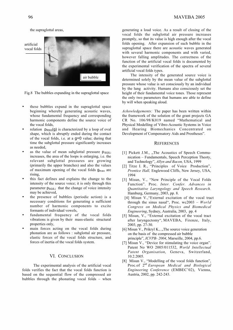
the supraglottal areas,

Fig.8 The bubbles expanding in the supraglottal space

• these bubbles expand in the supraglottal space

beginning whereby generating acoustic waves,

whose fundamental frequency and corresponding

harmonic components define the source voice of

the vocal folds,

• relation pRSG(g) is characterized by a loop of oval

shape, which is abruptly ended during the contact

of the vocal folds, i.e. at a g=0 value; during that

time the subglottal pressure significantly increases

as needed,

• as the value of mean subglottal pressure pSGS,i

increases, the area of the loops is enlarging, i.e. the

relevant subglottal pressures are growing

(primarily the upper branches) and also the values

of maximum opening of the vocal folds gmax are

rising,

• this fact defines and explains the change to the

intensity of the source voice; it is only through this

parameter pSGS,i that the change of voice intensity

may be achieved,

• the presence of bubbles (periodic action) is a

necessary conditions for generating a sufficient

number of harmonic components to excite

formants of individual vowels,

• fundamental frequency of the vocal folds

vibrations is given by their mass-elastic structural

properties only,

• main forces acting on the vocal folds during

phonation are as follows : subglottal air pressure,

elastic forces of the vocal folds structure, and

forces of inertia of the vocal folds system.

VI. CONCLUSION

The experimental analysis of the artificial vocal

folds verifies the fact that the vocal folds function is

based on the sequential flow of the compressed air

bubbles through the phonating vocal folds – when

generating a loud voice. As a result of closing of the

vocal folds the subglottal air pressure increases

promptly, so that its value is high enough after the vocal

folds opening. After expansion of such bubble in the

supraglottal space there are acoustic waves generated

with several harmonic components and with varied,

however falling amplitudes. The correctness of the

function of the artificial vocal folds is documented by

the experimental verification of the spectra of several

artificial vocal folds types.

The intensity of the generated source voice is

determined solely by the mean value of the subglottal

pressure whose value is set consciously by an individual

by the lung activity. Humans also consciously set the

height of their fundamental voice tones. Those represent

the only two parameters that humans are able to define

by will when speaking aloud.

Ackowledgements: The paper has been written within

the framework of the solution of the grant projects GA

CR No. 106/98/K019 named “Mathematical and

Physical Modelling of Vibro-Acoustic Systems in Voice

and Hearing Biomechanics Concentrated on

Development of Compensatory Aids and Prostheses”.

REFERENCES

[1] Pickett J.M., „The Acoustics of Speech Commu-

nication – Fundamentals, Speech Perception Theoty,

and Technology”, Allyn and Bacon, USA, 1999

[2] Titze I. R., “Principles of Voice Production”,

Prentice Hall, Englewood Cliffs, New Jersey, USA,

1994

[3] Misun, V., “New Principle of the Vocal Folds

Function”. Proc. Inter. Confer. Advances in

Quantitative Laryngology and Speech Research.

Hamburg, Germany, 2003, pp. 8.

[4] Misun V.,“External excitation of the vocal tract

through the sinus nasal“, Proc. wc2003 – World

Congress on Medical Physics and Biomedical

Engineering, Sydney, Australia, 2003, pp. 4

[5] Misun, V., “External excitation of the vocal tract

after laryngectomy“, MAVEBA, Firenze, Italy,

2003, pp. 27-30.

[6] Misun V., Prikryl K., „The source voice generation

on the basis of the compressed air bubble

principle”, ICVPB- 2004, Marseille, 2004, pp.6.

[7] Misun V., “Device for stimulating the voice organ”.

Patent No WO 2005/011532, World Intellectual

Patent Organisation, Geneva, Switzerland,

10.2.2005.

[8] Misun V., “Modelling of the vocal folds function”,

Proc.of 2nd

European Medical and Biological

Engineering Conference (EMBEC’02), Vienna,

Austria, 2002, pp. 242-243.

air bubble

artificial

vocal folds

96 MAVEBA 2005

AUTOMATIC CLASSIFICATION OF VOICE DISORDERS IN COURSE OF

NEURODEGENERATIVE DISEASE

T. Orzechowski1, A. Izworski

1, I. Gatkowska

2, M. Rudzinska

3

1Department of Automatics, AGH University of Science and Technology, Krakow, Poland

2Computer Linguistic, Jagiellonian University, Krakow, Poland

3Collegium Medicum, Jagiellonian University, Krakow, Poland

I. INTRODUCTION

The study presented in this publication is the first

from the planned complex, interdisciplinary studies. The

examination was carried out on patients of CM-UJ clinic

in Krakow who suffered from neurodegenerative disease

with the damage of the extrapiramidal system with

dysarthria-type changes in speech. Control examinations

of healthy persons have also been carried out. The

elements whose realization was tested had been chosen

based on the linguistic knowledge in the scope of

phonetics as well as on experience resulting from long-

term practice as a speech pathologist. The linguistic

material was selected in such a way as to pinpoint voice

changes characteristic for patients with dysarthria. During

the examination, phrases based on Polish idioms were

aslo recorded for further analyses.

II. VOICE PHYSIOLOGY

Voice and speech production requires close

cooperation of numerous organs which from the

phoniatric point of view may be divided into organs:

• producing expiration air stream necessary for

phonation (lungs, bronchi, trachea),

• amplifying the initaial tone (larynx),

• forming tone quality and forming speech sounds

(root of the tongue, throat, nasal cavity, oral cavity).

III. VOICE PATHOLOGY

Apart from typical changes caused by

neurodegenarative disease (e.g. shivering of the body,

limbs, muscle stiffness) changes in the voice may also be

observed. The research shown in work (Intensive voice

treatment LSVT® 2001) indicate the serious problem of

speech pathology occurance with as much as 75% of

patients. Thus it may be concluded that voice constitutes

one of the more crucial components of neurological

diagnosis.

Patients suffering from neurodegenerative diseases (and

such patients were examined by the authors) show

dysarthria-type speech alternations. Dysarthria is a group

phonation and articulation disorder which result from

damage to the movement control systems of the central or

peripheral nervous system also responsible for the speech

apparatus. The disorders occur although the speech plan

is preserved [3]. Other definitions characterize dysarthria

as handicapped production of articulated speech sounds

resulting from disturbances to nervous mechanisms of

voice production, modulation, intensity, timbre and

resonance [2]. Nowadays dysarthria is described as a

group of motor speech impairment result from a

disruption of muscular control due to lesions of either the

central or peripheral, or both, nervous systems.

Communication Independence for the Neurologically

Impaired CINI – 1994).

Due to the dominating symptom of disorder [3] 6 types of

dysarthria have been specified. In our study, patients

suffered from hypokinetic and hyperkinteic types.

Parkinson disease and Parkinson syndrome (damage to

the extrapramidal system; speech impairment related to

slowness) are accompanied by hypokinetic dysarthria-

type changes in speech. Its most important characteristics

in relation to isolated sounds are: distortions, loudness

limitations. Distorted articulation is caused by quick and

limited tongue and lips movements, sounds reduced down

to slurring. Impairment in the speech process consist in

sudden pauses in phonation. The voice is monotonous,

quiet, weak and vanishing. The other type of dysarthria

occurring in neurodegenerative diseases of the

extrapyramidal system is hyperkinetic dysarthria.

Phonation is distorted, sudden pauses in speech may

occur. Moreover, incorrect articulation occurs as well as

irregular breaks in articulation, sound elongation,

repetition of sounds caused by abnormal muscular

tension. Hypernasality may also occur, and the loss of air

caused by throat and palate impairment result in the

shortening of phrases. There are variations of speech

loudness, the voice is trembling, tense and stifled, weak,

with breaks.

IV. CHARACTERIZATION AND CLASSIFICATION OF SOUNDS

USED IN THE EXAMINATION

During the examination both consonants and

vowels were used. Patients were asked to pronounce the

sounds in isolation.


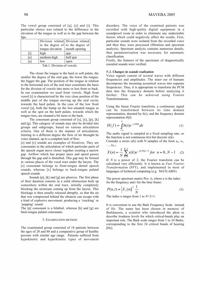
The vowel group consisted of [a], [e] and [i]. This

particular choice was related to the difference in the

elevation of the tongue as well as to the gap between the

lips.

Division related

to the degree of

tongue elevation

Division related

to the degree of

mouth opening

[i] high ajar

[e] medium-high half ajar

[a] low open

Tab.1. Division of vowels.

The closer the tongue to the hard or soft palate, the

smaller the degree of the oral gap, the lower the tongue,

the bigger the gap. The position of the tongue in relation

to the horizontal axis of the oral tract constitutes the basis

for the division of vowels into more or less front or back.

In our examination we used front vowels. High front

vowel [i] is characterized by the very close position of the

middle part of the tongue moving up the oral cavity

towards the hard palate. In the case of the low front

vowel [a], both the hump on the low-situated tongue as

well as the spot on the harb palate, towards which the

tongue rises, are situated a bit more to the back.

The consonant group consisted of [s], [x], [p], [k]

and [g]. This category of sounds may also be divided into

groups and subgroups, based on various articulation

criteria. One of them is the manner of articulation,

limiting to a different degree the flow of air throught he

voice channel, up to a complete lack of flow.

[s] and [x] sounds are examples of fricatives. They are

consonants in the articulation of which particular parts of

the speech organ move closer together creating a narrow

gap. Airflow which has proper mass and speed passes

through the gap and is disturbed. This gap may be formed

in various places of the vocal tract under the larynx. The

[s] consonant belongs to front-tongue dental speech

sounds, whereas [x] belongs to back-tongue palatal

speech sounds.

Sounds [p], [k] and [g] are plosives. The first phase

of their duration consists in a solid obstruction built up

somewhere within the oral tract, initially completely

blocking the airstream coming up from the larynx. This

blockage is then usually released abruptly, so that the air

that was compressed behind the obstacle can escape with

a kind of explosive movement, producing a ‘cracking’ or

‘popping’ sound.

The [p] consonant is a bilabial, whereas [k] and [g] are

back-tongue palatal consonants.

5. EXAMINATION METHOD

The examinated group consisted of 18 patients between

the ages of 20 and 80 and a comparative group of healthy

persons with similar age range. Patients suffered from

hypokinetic and hyperkinetic types of movement

disorders. The voice of the examined patients was

recorded with high-qiality digital equipment in a

soundproof room in order to eliminate any undesirable

factors which could negatively affect the results. First,

particular sounds were isolated from the recorded voice

and then they were processed (filtration and spectrum

analysis). Spectrum analysis contains numerous details,

thus parameterization was necessary for automatic

classification.

Firstly, the features of the spectrums of diagnostically

essential sounds were verified.

V.1. Changes in sounds realization

Voice signals consist of several waves with different

frequencies and amplitudes. The inner ear of humans

decomposes the incoming acoustical waves into separate

frequencies. Thus, it is appropriate to transform the PCM

data into the frequency domain before analyzing it

further. This can be achieved using Fourier

Transformations.

Using the linear Fourier transform, a continuous signalcan be transformed between its time domainrepresentation, denoted by h(t), and the frequency domainrepresentation H(f).

= dxethfH ftj2)()( (1)

The audio signal is sampled at a fixed sampling rate, sothe function is not continuous h(t) but discrete x(k).

Consider a series x(k) with N samples of the form x0, x1,

… ,xN-1

1..0)(1

)(1

0

/2==

=

NnforekxN

nXN

k

Nnjk (2)

If N is a power of 2, the Fourier transform can becalculated very efficiently. It is known as Fast FourierTransformation (FFT), and implemented in most of

languages of technical computing (e.g. MATLAB®).

The power spectrum matrix P(n; t), where n is the indexfor the frequency and t for the time frame:

NnXtnP

t

1)(),(2

= (3)

The index n ranges from 1 to N=2+1.

It is convenient to use the Bark Frequency Scale instead

of Hz. The name has been chosen in memory of

Barkhausen, a scientist who introduced the phon to

describe loudness levels for which critical-bands play an

important role. The Bark scale ranges from 1 to 24 Barks,

corresponding to the first 24 critical bands of hearing

[Hz].

98 MAVEBA 2005

frequency [Hz]

Fig.1. Charakteristic of Bark Frequency Scale

A critical-band value is calculated by summing up the

values of the power spectrum within the respective flow(i)

and fhigh(i) frequency limits of the i critical-band.

{ }(i)ff(n) (i)f:)(

),(

highlow

)(

<=

=

niI

tnPCB

iIn (4)

where i, t, n are indexes, CB is a matrix containing thepower within the i-th criticalband at a specific timeinterval t.

With the patients, changes in sounds articulation are

visible (precisely, transition into another sound during

realization). It is both audible and detectable through

spectrum comparison. These changes were particularly

observable for the following consonants, for which the

occurring change has also been indicated:

• [k] [a] / [k] [y]

• [g] [y] / [g] [e]

• [s] [y]

• [h] [a]

Fig.2a. Voice signal [k] without changes

Fig.2b. Voice signal [k] with changes [k] [a]

Fig.3a. Voice signal [s] without changes

Fig.3b. Voice signal [s] with changes [s] [y]

Each piece of voice is represented by CB matrix. Firstly,

the information represented each group of people was

combined using median method. The median proved to

be the simplest approach with a comparable quality to

other more complex methods. Classification was done

using simple distance comparation between CB matrixes.

This distance can be used as another voice

characterization parameter.

Ther result of this distortion is caused by the weakening

of the elasticity of the larynx muscles, that is why a

consonant is followed by a vowel, which does not require

as much tension.

V.2. Intensity of sounds pronouced many times in

isolation

The patients were asked to repeat the same plosive four

or more times. The request was based on the knowledge

that during the realization of a sequence of the same

sounds, sound sequence distortions could be expected and

slurring could occur. By analysing the duration and

intensity of consecutive sounds, it was noticed with most

of the patients that the intensity of the last sounds was

respectively lower than the intensity of the first sound.

This is due to muscle stiffness, characteristic for

Prakinson disease. These sypmtoms were not observed

with most of the members of the control group.

Fig.4a. Last 3 sounds of the healthy person, [p]

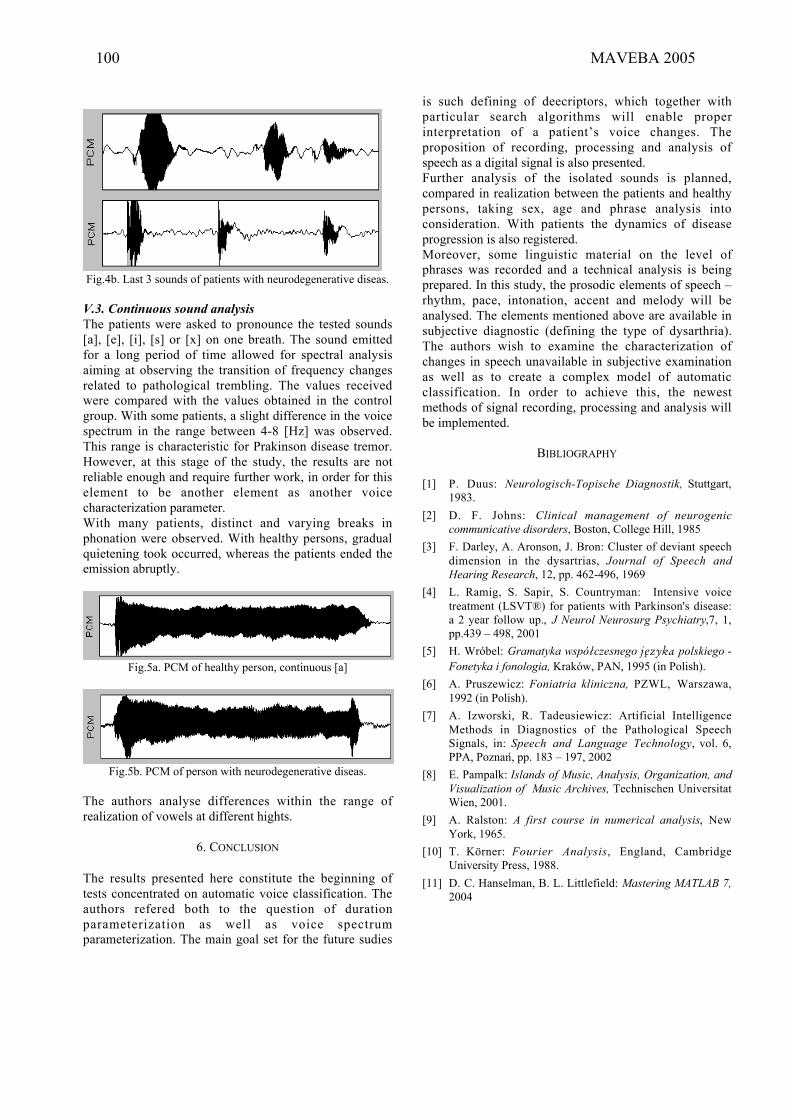
Fig.4b. Last 3 sounds of patients with neurodegenerative diseas.

V.3. Continuous sound analysis

The patients were asked to pronounce the tested sounds

[a], [e], [i], [s] or [x] on one breath. The sound emitted

for a long period of time allowed for spectral analysis

aiming at observing the transition of frequency changes

related to pathological trembling. The values received

were compared with the values obtained in the control

group. With some patients, a slight difference in the voice

spectrum in the range between 4-8 [Hz] was observed.

This range is characteristic for Prakinson disease tremor.

However, at this stage of the study, the results are not

reliable enough and require further work, in order for this

element to be another element as another voice

characterization parameter.

With many patients, distinct and varying breaks in

phonation were observed. With healthy persons, gradual

quietening took occurred, whereas the patients ended the

emission abruptly.

Fig.5a. PCM of healthy person, continuous [a]

Fig.5b. PCM of person with neurodegenerative diseas.

The authors analyse differences within the range of

realization of vowels at different hights.

6. CONCLUSION

The results presented here constitute the beginning of

tests concentrated on automatic voice classification. The

authors refered both to the question of duration

parameterization as well as voice spectrum

parameterization. The main goal set for the future sudies

is such defining of deecriptors, which together with

particular search algorithms will enable proper

interpretation of a patient’s voice changes. The

proposition of recording, processing and analysis of

speech as a digital signal is also presented.

Further analysis of the isolated sounds is planned,

compared in realization between the patients and healthy

persons, taking sex, age and phrase analysis into

consideration. With patients the dynamics of disease

progression is also registered.

Moreover, some linguistic material on the level of

phrases was recorded and a technical analysis is being

prepared. In this study, the prosodic elements of speech –

rhythm, pace, intonation, accent and melody will be

analysed. The elements mentioned above are available in

subjective diagnostic (defining the type of dysarthria).

The authors wish to examine the characterization of

changes in speech unavailable in subjective examination

as well as to create a complex model of automatic

classification. In order to achieve this, the newest

methods of signal recording, processing and analysis will

be implemented.

BIBLIOGRAPHY

[1] P. Duus: Neurologisch-Topische Diagnostik, Stuttgart,

1983.

[2] D. F. Johns: Clinical management of neurogenic

communicative disorders, Boston, College Hill, 1985

[3] F. Darley, A. Aronson, J. Bron: Cluster of deviant speech

dimension in the dysartrias, Journal of Speech and

Hearing Research, 12, pp. 462-496, 1969

[4] L. Ramig, S. Sapir, S. Countryman: Intensive voice

treatment (LSVT®) for patients with Parkinson's disease:

a 2 year follow up., J Neurol Neurosurg Psychiatry,7, 1,

pp.439 – 498, 2001

[5] H. Wróbel: Gramatyka wspólczesnego jezyka polskiego -

Fonetyka i fonologia, Kraków, PAN, 1995 (in Polish).

[6] A. Pruszewicz: Foniatria kliniczna, PZWL, Warszawa,

1992 (in Polish).

[7] A. Izworski, R. Tadeusiewicz: Artificial Intelligence

Methods in Diagnostics of the Pathological Speech

Signals, in: Speech and Language Technology, vol. 6,

PPA, Poznan, pp. 183 – 197, 2002

[8] E. Pampalk: Islands of Music, Analysis, Organization, and

Visualization of Music Archives, Technischen Universitat

Wien, 2001.

[9] A. Ralston: A first course in numerical analysis, New

York, 1965.

[10] T. Körner: Fourier Analysis, England, Cambridge

University Press, 1988.

[11] D. C. Hanselman, B. L. Littlefield: Mastering MATLAB 7,

2004

100 MAVEBA 2005

NEWBORN'S CRY FROM RISK AND NORMAL PREGNANCIES

Mirjana Sovilj, Tatjana Adamovic, Misko Subotic, Nikoleta StevovicInstitute for Experimental Phonetics and Speech Pathology, Belgrade, Serbia and Montenegro

Abstract. Previous researches of the prelingual

period indicated that primal cry and the first cry

represent the inception of verbal communication.

The aim of this work was to study qualitative

characteristics of crying of newborns from risk

pregnancies and newborns from regular pregnancies

in the function of prediction of verbal

communication development.

The research was carried out on the sample of N=10

babies divided into two groups, aged 15 days. E

group (N=5) comprised newborns from risk

pregnancies, and C group (N=5) comprised

newborns from normal pregnancies. Crying in the

examined sample was digitally recorded and

spectrographically analyzed.

The research results point to the possibility that

certain acoustic characteristics of crying can be used

in the prediction of verbal communication

development and that the researches in this area

should be intensified and continued.

Key words: newborn's cry, verbal communication,

prelingual period, spectrographic analysis

1. INTRODUCTION

Newborn's cry, as an elementary particle of the

development of verbal communication, was the topic of

numerous scientific researches aimed not only at

broadening the knowledge of controlling the process of

crying production and brain organization itself, but only

at examining the possibilities of crying as a diagnostic-

differential instrument.

The firs baby's cry, as stated by Kostic (1991), appears

as a spontaneous physiological reaction that does not

depend on its communication with the social

environment [2]. The same author thinks that, during

the first two months of life, a newborn reacts to hunger,

discomfort and pain by crying. Physiological needs of a

child's organism are the means of sound expressed

through crying and thus they lie in the basis of

communication between a child and his parents (Kostic,

1980) [3].

Researches of Sovilj and Djokovic (1993) support the

fact that the development of speech communication is

commenced by the first cry. Proceeding from the

standpoint that the first cry contains all acoustic

elements of the speech acoustic structure: formant

forms, noise forms and combined formant-noise forms

of acoustic structure, which are normally present in

speech (Kostic, Stosic 1963) [4], Sovilj and Djokovic

analyzed the first cry-(ing) from birth until the end of

the first month, reaching the results that indicate the

existence of phases in the development of cry-(ing),

from the first cry to crying (30 days), which are

significant not only for the monitoring of the

development of hearing, and future speech and

language, but also for the development of

methodological procedure for early detection of speech

and hearing impairment and speech habilitation of

hearing impaired children, which is carried out from the

first month, in the prelingual phase [6].

Sovilj (1995) [7] also emphasizes that the first day after

birth global control connection between hearing and

voce is established. On the basis of spectrographic

analyses, Truby and Lind (1965) established three

important types of crying: basic phonation cry,

turbulent, dysphonic cry, and strongly expressed

hyperphonation cry [9].

The most complete model for the production of these

types of cries was developed by Golub (1980),

separating crying production into subglottal, glottal and

supraglottal production zone connecting muscle activity

with each type of crying [1].

Proceeding from the assumption that crying of hearing

impaired children differs from crying of their normally

hearing peers, due to the lack of auditory feedback,

Moller and Schonweiler (1997) reached the results that

coincided indicating that crying of normally hearing

babies differs from crying of those with profound

hearing impairment. Main statistically significant

differences were found in the distribution of energy in

different frequency ranges, duration of crying, and some

melodic parametres [5].

In this paper, which is a pilot research, crying was

studied through the analysis of ranging of the

movement of the basic laryngeal voice in newborns’

crying as the carrier of the quantitative monitors of

speech (QMS): intensity, frequency and duration. QMS

are the carriers of suprasegment speech structure and

their variation forms the matrix. In the later period of

speech-language development, sounds, syllables, words

and sentences, followed by the development of accents

of words, accents of melodies and melody sentence are

built into this matrix. Previous researches at the Institute


for Experimental Phonetics and Speech Pathology

(Sovilj, 2002) as well as the results of foreign

researchers, indicated that suprasegment structure of

mother tongue develops as early as in the fetal period

[8]. This fact points even more to the necessity and

significance of researching the cry as a nucleus of

verbal communication and finding ways of its use in

early detection and diagnostics, i.e. early prediction of

hearing, speech and language development.

2. AIM

The aim of this research was to study qualitative

characteristics of crying of newborns from risk

pregnancies and newborns from regular pregnancies in

the function of prediction of verbal communication

development.

3. METHODOLOGY

For the needs of spectrographic analysis of a

newborn's cry, crying before nursing was digitally

recorded in home conditions, on the 30th

day after birth,

because of the clear stabilization of the acoustic field of

crying when a child has physiological needs, compared

to the inception of vocalization, when a child is in

homeostasis. The research was carried out on the

sample of N=10 newborn babies, 15 days of age,

divided into two groups. The experimental group (E)

comprised N=5 newborns from risk pregnancies, and

the control group (C) comprised N=5 newborns from

normal pregnancies. Newborns from E group were born

from the pregnancies with the risk of a miscarriage from

6-7 month. All newborns were born normally in the 9th

month.

During the recording, we used the directed

microphone that was positioned near newborn's mouth

on the defined distance of 10 cm. The recording lasted

for about 3 minutes, which was a sufficient time period

for obtaining the repeated stable characteristics of

crying. Digitalized recordings were transferred into

COOL program, from which the trained researcher, by

means of auditory control and visual control of the

recording, selected the signal (cry) that occurred most

frequently, and transferred it to PRATT program for

spectrographic signal analysis. The recorded cry was

digitalized by the speed of choice 22050 Hz, 16-bit

resolution, and it was recorded on one channel (mono).

Spectrographic analysis obtained: minimal, maximal

and mean values and their standard deviations of

duration (Du), intensity (I) and frequency (FFo) of basic

laryngeal tone.

Besides crying, for the psyhophysiological

assessment of newborns we provided the data on body

size at birth (body weight – BW and body length - BL).

The obtained data were statistically processed by the

application of T-test significance of the differences

between the examined groups.

4. RESULTS AND DISCUSSION

In order to obtain more reliable and objective indices

of crying characteristic in the monitored groups, we

proceeded from the fact that newborn's voice in the

monitored period (15 days) is not connected with the

control of the movement of speech organs meant for

speech production, but solely with its general

physiological state and needs.

In that sense, newborn’s body was observed from the

aspect of the complete resonatory and energy space,

whose influence on the voice (crying) can be

represented by longitudinal mass (LM), which

represents the relation of BW and BL given in the

formula

BW

LM= ___

BL

Having on mind that constitution plays an important

role in voice impostation, we normalized intensity and

frequency values on crying duration and newborn’s

longitudinal mass.

Normalized IFo and FFo values were calculated

according to the following mathematical formulas:

x IFo (average crying intensity)

CIFo= ______

(coefficient of DU• LM

crying intensity)

x FFo (average crying frequency)

CIFo = ______

(coefficient of DU• LM

crying intensity)

Intensity

Table 1 Crying intensity in E and C group

Statisti

cal

parame

tres

dB-

min

dB-

max

dB-

avera

ge

dB-

SD

Experimental group

X 73.37 83.12 79.79 1.97

SD 4.87 3.90 5.45 0.95

Control group

X 78.83 88.22 83.94 2.20

SD 7.26 2.03 5.39 1.60

102 MAVEBA 2005

Results of the movement of the laryngeal tone

intensity in newborns’ crying (Table 1) indicate that

mean value of Fo intensity in C group is 83.94 dB, and

79.79 dB in E group, which indicates that newborns’

crying from normal pregnancies (C group) is 5% more

intense.

Average value of Fo minimal intensity in C group is

(78.83 dB: 73,37 dB) 7% higher than in E group,

whereas average value of maximal intensity of Fo

crying in C group (88,22 dB: 83,12 dB) is 6.8% higher

than in E group.

Frequency

Table 2 Frequency of Fo crying in E and C group

Average Fo frequencyStatistical

parametres Hz

min

Hz

max

Hz

average

Hz

SD

Experimental group

X245.2

6

500.9

9369.17 71.18

SD 93.59 31.53 58.70 39.01

Control group

X223.5

0

498.0

8361.80 75.69

SD 79.80 44.01 72.20 24.79

Table 2 presents the results of laryngeal voice

frequency in newborns’ crying. Mean value of FFo

crying in C group is 361.80 Hz, and in E group it is

369.17 Hz, i.e. laryngeal voice of newborns’ crying

from risk pregnancies is 2% higher compared to

newborns from regular pregnancies.

Average minimal value of frequency in C group is

(223.50Hz : 245.26Hz) about 9% lower compared to E

group.

Average value of maximal frequency in C group

(498.08 Hz: 500.99 Hz), is about 0.6% lower compared

to E group.

Duration

Table 3 Crying duration in E and C group

DU in groupStatistical

parametres E group C group

X 1.08 1.70

SD 0.26 0.73

Results of laryngeal voice duration in newborns'

crying (Table 5) in the examined sample, indicate that

average duration of crying in C group is 1.7 sec, and in

E group it is 1.08 sec. i.e. that crying of newborns from

normal pregnancies is 36.5% longer.

The analysis of average BW values (Table 4)

indicated that newborns from C group had 19% higher

BW compared to E group, but the differences between

he groups are not statistically significant.

Table 4 Body weight in E and C group

BWStatistical


X 2790 3440

SD 803 305

Table 5 Body length in E and C group

BLStatistical


X 48.00 51.40

SD 5.15 2.97

Results of the average value of BL (Table 5) indicate

that newborns from C group had about 7% greater BL

compared to E group.

Table 6 C- IFo E and C group

T-Test C-FFo C and E group

C group E group

X 3.375906279 6.508190577

df 4

Tab._ test -5.574036129

p(T<=t) 0.002538411

_ critical 2.131846486

Graph 1 C IFo in E and C group

0

0.2

0.4

0.6

0.8

1

1.2

1.4

1.6

1.8

0 1 2 3 4 5 6

K

E

Data in Table 6 and Graph 1 indicate that C-IFo

average value in E group is 1.373, and in C group

0.741. Comparing mean C-IFo values in E and C group,

we obtained statistically highly significant difference on

the level p = 0.007, which indicates that this coefficient

can be a reliable parametre for assessment of newborns’

crying characteristics and further researches, on a larger

sample, will enable their use not only for the early

detection of difficulties in speech and language

development, but also for the assessment of the general

psychophysiological development.

Results in Table 7 and Graph 2 indicate that average

value C-FFo in E group is 6,508, and in C group 3,375.

Comparing mean values of C-FFo E and C group, we

obtained statistically highly significant difference on the

level p = 0,002, which indicates that this coefficient can

be a reliable parametre in the assessment of newborns’

crying characteristics, and further researches will enable

their use not only for the early detection of difficulties

in speech and language development, but also for the

assessment of the general psychophysiological status of

a newborn child.

Table 7 C-FFo in E and C group

Graph 2 C-FFo coefficient in E and C group

0

1

2

3

4

5

6

7

8

0 1 2 3 4 5 6

K

E

On a more precise level, C-IFo and C-FFo indicated

the presence of regularities in the connection of three

parametres: intensity of crying frequency, duration, and

newborn’s longitudinal mass i.e. their interdependence,

as the expression of psychophysiological state of a

child, which classifies them as rather precise measures

for the prediction of speech development and

psychophysiological status.

CONCLUSION

The results obtained in our research, when comparing

the values of QMS parametres in newborns' crying on

the 15th

day after birth from E and C group, indicate the

following:

- C-IFo and C-FFo represent valid parametres for the

assessment of newborn’s crying characteristics

- when the characteristics and tendencies of the

characteristics of laryngeal voice in newborns’ crying

are perceived globally, it is noted that crying of

newborns from normal pregnancies (C group) has the

tendency of: larger intensity, lower tone and longer

duration compared to crying of newborns from risk

pregnancies, whose crying, according to the movement

of QMS, can be characterized as crying of the shorter

expiratory fork, hypotonic and hypertensive.

- the obtained tendencies of crying characteristics

indicate that newborn’s crying can be relevant

parametre for the prediction of not only speech and

language development, but also of the

psychophysiological status of a newborn child.

Further researches, on a larger sample, will enable

defining of limit values of coefficients for population of

newborns from normal and risk pregnancies.

This research was financed by the Ministry of

Science and Environment Protection of the republic of

Serbia, within the project of basic researches, N° 1784.

LITERATURE

[1] Golub H. L. (1980): A physioacoustic model of the

infant cry and its use for medical diagnosis and

prognosis, Thesis, Massachusetts Institute of

Technology, Boston.

[2] Kostic Dj. (1991): Cooing and Babbling, Notes and

discussion, No 2, IEPSP, Belgrade.

[3] Kostic Dj. (1980): Speech and the Hearing Impaired

Children, Indian Statistical Institute, Calcutta.

[4] Kostic Dj., Stosic M. (1963): Acoustic Structure of a

Newborn's Cry, IEPSP, Belgrade.

[5] Moller S., Schonweiler R. (1997): Analysis of Infant

Cries for the Early Detection of Hearing Impairment, in:

Proc. 5th

European Conf. on Speech Communication

and Technology (Eurospeech `97), Europ. Speech Com.

Ass. ESCA, GR-Rhodes.

[6] Sovilj M., Djokovic S. (1993): Development of

Newborn's Cry-(ing) from Birth Until the end of the

First Month, Defectological theory and practice,

Belgrade.

[7] Sovilj M. (1995): The Development of New-born

Infant`s Cry(-ing) from Birth Until the End of the First

Month, European Decade of the Brain, Amsterdam,

1995.

[8] Sovilj M. (2002): Children's Speech – Quantitative

Monitors of Speech, Zaduzbina Andrejevic, Belgrade.

[9] Truby, H. M., Lind, L. (1965): Newborn Infant Cry,

Almquist & Wiksells, Uppsala.

T test C- IFo E and C group

C group E group

X 0.7417 1.3733

df 4

Tab._-test -4.1408

p (T<=t) 0.0071

_ critical 2.1318

104 MAVEBA 2005

COMPLEXITY ANALYSIS OF NORMAL AND DEAF INFANT CRY

ACOUSTIC WAVES

Kathiresan Manickam, Haizhou Li,

Institute of Infocomm Research (I2R), 21 Heng Mui Keng Terrace, Singapore 119613

Abstract: This work describes the complexity found in

the normal and the deaf crying acoustic waves. Using

approximate entropy, in a single figure, the complexity

of the auto-covariance of the signal is computed. Thus,

using this complexity value, we are able to discriminate

the normal and the deaf infants crying domains with

(P<<0.01).

Keywords: Infant Cry, Complexity, deaf infant

1. INTRODUCTION

The infant crying waves, seemingly chaotic, carry

useful and nevertheless essential information to establish

its culture. Such entity vividly clarifies an infant’s

physiological anatomy and psychological condition.

Physiological quantities from the laryngeal configuration,

i.e. the length of the vocal tract, in return exemplify the

resonance and formant effects. Psychologically, the

infant’s mental stamina correlates with the origins of a cry

type. Modes of cries are unequivocally classified as

normal, pathological, pain, hunger, etc. Hitherto, cry from

a “normal” and “deaf” infant has been notably studied in

literature [1]. Curiosity may result in the selection of the

deaf population as the target group. Deaf infants cry

exhibit contrasting acoustical characteristics compared to

their rivals, the healthy infant population. Following

investigation, it became apparent that the caseload for the

deaf population is ever increasing in most institutions. It

also came to light that both deaf and healthy infants

commonly share attributes like pain or hunger cry. But,

the hearing impaired infants acquired anatomical

deficiency. Despite this setback, paediatricians have

expressed that infant’s cry is reciprocal to adult’s speech.

Modes of infant’s cry can be qualitatively

characterised with commonly employed acoustics cues.

Accordingly, normal crying features constitute of raising-

falling pitch pattern, ascending-descending melody and

high intensity seen from the spectrum [2-3]. Pathological

infant crying correlate well with some normal infant’s

acoustics features. Spectral intensity will be lower than

normal, rapid pitch shifts, generally glottal plosives, weak

phonations and silences during the crying. Parameters,

incorporating the pitch and formant descriptions, have

been well utilised in the infant cry analysis up till now.

Clement et al have substantiated that variations in the pitch

between hearing impaired and normal groups become

meaningful from 8.5 months onwards [1]. In reality,

this time gap is a result of lack of auditory feedback on

the speech. Thus, evidence proves that a deaf group

tends to voice louder since they want to hear

themselves.

Pitch, a famously captured feature, aids in

distinguishing cry types, as well as for a diagnostic

tool, etc. La Gasse states, “The cry has enormous

potential diagnostic”. His quotation suggests that

extremely high pitched cry indicates the pathological

status of the infant which needs urgent medical

attention [4]. A typical example is when infants

exposed to drugs tend to have high pitch with variation

at lower amplitude. The consequent effect of these

drugs is the instability of the neural control of the

vocal tract. Consequently, the vocal tract configuration

determines the structure of the formant. Nevertheless,

estimating the exact formant frequencies is complex

[5]. A Fort et al has incorporated a parametric model

using poles and zeros method to estimate fundamental

frequency and formants from an infant cry, the

conventional method involving the glottal pressure and

tract configurations.

Regardless of these scientific features, experts

in this field are able to distinguish the modes of cries.

Garcia has mentioned that parents are specialists who

were able to differentiate modes of cry solely using

their instincts and comparing different types of crises

[2-3]. However, uncertainty in the therapeutic service

has brought irrefutable questions. A professional has

quoted, “A deaf infant’s characteristic varies from one

another based on three factors: degree of loss; type and

period of rehabilitation and the age of pathology

identification”. Consequently, concrete answers are

unavailable scientifically (energy, pitch, duration, etc)

regarding cry prosodic information which has forced

us to lead this research in order to create an expert

system to verify the cry status. The expert system

should be able to analyse and classify modes of cry

signals and probably, being realistic, at a later stage,

diagnostic applications. Because the cry signals are

noisy and evidences are showing their chaotic features,

currently, analysing such signals itself has become

problematic.

Deaf infants revealed more variations in their

phonation using false vocal cords producing falsetto


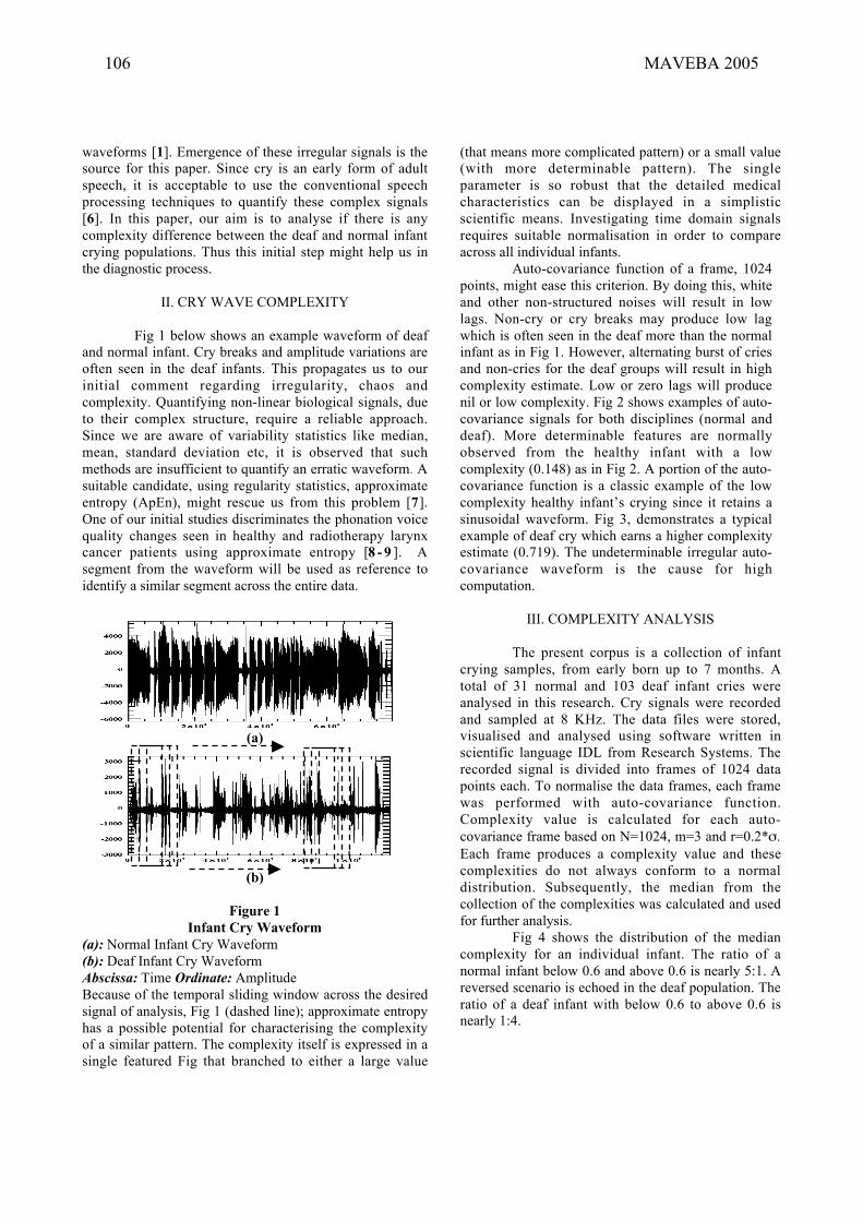
waveforms [1]. Emergence of these irregular signals is the

source for this paper. Since cry is an early form of adult

speech, it is acceptable to use the conventional speech

processing techniques to quantify these complex signals

[6]. In this paper, our aim is to analyse if there is any

complexity difference between the deaf and normal infant

crying populations. Thus this initial step might help us in

the diagnostic process.

II. CRY WAVE COMPLEXITY

Fig 1 below shows an example waveform of deaf

and normal infant. Cry breaks and amplitude variations are

often seen in the deaf infants. This propagates us to our

initial comment regarding irregularity, chaos and

complexity. Quantifying non-linear biological signals, due

to their complex structure, require a reliable approach.

Since we are aware of variability statistics like median,

mean, standard deviation etc, it is observed that such

methods are insufficient to quantify an erratic waveform. A

suitable candidate, using regularity statistics, approximate

entropy (ApEn), might rescue us from this problem [7].

One of our initial studies discriminates the phonation voice

quality changes seen in healthy and radiotherapy larynx

cancer patients using approximate entropy [8 - 9 ]. A

segment from the waveform will be used as reference to

identify a similar segment across the entire data.

(a)

(b)

Figure 1

Infant Cry Waveform

(a): Normal Infant Cry Waveform

(b): Deaf Infant Cry Waveform

Abscissa: Time Ordinate: Amplitude

Because of the temporal sliding window across the desired

signal of analysis, Fig 1 (dashed line); approximate entropy

has a possible potential for characterising the complexity

of a similar pattern. The complexity itself is expressed in a

single featured Fig that branched to either a large value

(that means more complicated pattern) or a small value

(with more determinable pattern). The single

parameter is so robust that the detailed medical

characteristics can be displayed in a simplistic

scientific means. Investigating time domain signals

requires suitable normalisation in order to compare

across all individual infants.

Auto-covariance function of a frame, 1024

points, might ease this criterion. By doing this, white

and other non-structured noises will result in low

lags. Non-cry or cry breaks may produce low lag

which is often seen in the deaf more than the normal

infant as in Fig 1. However, alternating burst of cries

and non-cries for the deaf groups will result in high

complexity estimate. Low or zero lags will produce

nil or low complexity. Fig 2 shows examples of auto-

covariance signals for both disciplines (normal and

deaf). More determinable features are normally

observed from the healthy infant with a low

complexity (0.148) as in Fig 2. A portion of the auto-

covariance function is a classic example of the low

complexity healthy infant’s crying since it retains a

sinusoidal waveform. Fig 3, demonstrates a typical

example of deaf cry which earns a higher complexity

estimate (0.719). The undeterminable irregular auto-

covariance waveform is the cause for high

computation.

III. COMPLEXITY ANALYSIS

The present corpus is a collection of infant

crying samples, from early born up to 7 months. A

total of 31 normal and 103 deaf infant cries were

analysed in this research. Cry signals were recorded

and sampled at 8 KHz. The data files were stored,

visualised and analysed using software written in

scientific language IDL from Research Systems. The

recorded signal is divided into frames of 1024 data

points each. To normalise the data frames, each frame

was performed with auto-covariance function.

Complexity value is calculated for each auto-

covariance frame based on N=1024, m=3 and r=0.2* .

Each frame produces a complexity value and these

complexities do not always conform to a normal

distribution. Subsequently, the median from the

collection of the complexities was calculated and used

for further analysis.

Fig 4 shows the distribution of the median

complexity for an individual infant. The ratio of a

normal infant below 0.6 and above 0.6 is nearly 5:1. A

reversed scenario is echoed in the deaf population. The

ratio of a deaf infant with below 0.6 to above 0.6 is

nearly 1:4.

106 MAVEBA 2005

(a)

(b)

Figure 2

Normal Infant Cry Waveform

(a): Cry Waveform

(b): Auto-Covariance Cry Waveform

Top: Entire Frame Signal

Bottom: Portion of Frame Signal

Abscissa (a): Time Abscissa (b): Lag Ordinate: Amplitude

The distribution clearly shows a distinct separation

between the deaf and normal infant population. Assuming

that these two populations (deaf and normal) are

independent, Wilcoxon Rank Sum Test showed that these

two populations were indeed significantly different with

(P<<0.01). Deafness is the most common of all forms of

permanent damage following meningitis. Early detection

and therapy might reduce the effect or severity following

such disease.

(a)

(b)

Figure 3

Deaf Infant Cry Waveform

(a): Cry Waveform

(b): Auto-Covariance Cry Waveform

Top: Entire Frame Signal

Bottom: Portion of Frame Signal

Abscissa (a): Time Abscissa (b): Lag Ordinate:

Amplitude

IV. CONCLUSION

Despite successfully discriminating the

normal and deaf infant crying modes using complexity

analysis (approximate entropy), further research has to

be carried out in order to reduce the over-lapping

portion between the two domains. Nevertheless, this

initial study on the infant cry wave analysis is

encouraging but more features need to be incorporated

like pitch, formant, and energy to enhance the

findings.

0

5

10

15

20

25

30

0.25 0.35 0.45 0.55 0.65 0.75 0.85 0.95

Normal

Deaf

(a)

0

1

2

0 0.5 1

Series1

Series2Normal

Deaf

(b)

Figure 4

(a): Histogram of Normal & Deaf Infant Cry Complexity

Abscissa: Median Complexity

Ordinate: Frequency of the Complexity

(b): Probability Density Function of Normal & Deaf Infant

Cry Complexity

Abscissa: Median Complexity

Ordinate: Probability Density

REFERENCES

[1] Clement, Chris J. / Koopmans-van Beinum,

Florien J. / Pols, Louis C. W. (1996): "Acoustical

characteristics of sound production of deaf and normally

hearing infants", ICSLP, 1549-1552.

[2] Jose Orozco Garcia and Carlos A Reyes

Garcia, (2003) “Acoustic Features Analysis for

Recognition of Normal and Hipoacusic Infant Cry

Based on Neural Networks” Lecture Notes in

Computer Science, 2687:615 – 622, ISSN: 0302-9743

[3] Jose Orozco Garcia and Carlos A Reyes

Garcia, (2003) “A Study on the Recognition of

Patterns of Infant Cry for the Identification of

Deafness in Just Born Babies with Neural Networks.”

8th Iberoamerican Congress on Pattern Recognition,

CIARP 2003, Havana, Cuba, 342-349, ISBN 3-540-

20590.

[4] Medical News Today: Babies cry linked to

their neurological and medical status, 16 May 2005.

www.medicalnewstoday.com

[5] K Wermke, W Mende, C Manfredi, P

Bruscaglioni, (2002) “Developmental aspects of

infant’s cry melody and formants”, Medical

Engineering Physics 24:501-514.

[6] Qiabing Xie, Rabab K Ward and Charles A

Laszlo, (1996) “Automatic Assessment of Infants’

Levels-of-Distress from the Cry Signals”, IEEE Trans

Speech and Audio Processing 4:4:253-265.

[7] Pincus S M, (2001), “Assessing Serial

Irregularity and its Implications for Health”, Ann NY

Acad Sci, 954:245-267.

[8] Moore C J, Manickam K, Willard T, Jones S,

Slevin N, Shalet S, (2004) ‘Spectral Pattern

Complexity Analysis and the Quantification of Voice

Normality in Healthy & Radiotherapy Patient Groups’,

Medicine Engineering Physics’, 2004,26(4), 291:301

[9] Manickam K, Moore C J, Willard T and

Slevin N, ‘Quantifying Aberrant Phonation Using

Approximate Entropy in Electro- Laryngography’

(Journal of Speech Communications-In press

Corrected Proof)

108 MAVEBA 2005

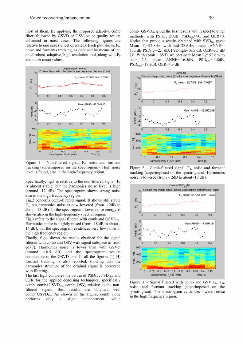
most of them. By applying the proposed adaptive comb filter, followed by GSVD or OSV, voice quality results enhanced in most cases. The following figures are relative to one case (lancet operated). Each plot shows F0, noise and formants tracking, as obtained by means of the cited robust, adaptive, high-resolution tool, along with F0 and noise mean values.

0 0.1 0.2 0.3 0.4 0.5 0.650

100

150

F 0 [H

z]

Original signal - non filt.Fundam. freq.(+red), noise (.black), spectrogram and formants (*blue)

F0 mean= 93.5637 Std= 6.5553

Sampling freq. Fs=25 (kHz) Time [s]

Fre

q. [H

z]

0 0.1 0.2 0.3 0.4 0.5 0.60

2000

4000

6000

0 0.1 0.2 0.3 0.4 0.5 0.6

-30

-20

-10

0

10

AN

NE

[dB

])

Mean ANNE= -12.0049 dB

Figure 1 – Non-filtered signal: F0, noise and formant tracking (superimposed on the spectrogram). High noise level is found, also in the high-frequency region. Specifically, fig.1 is relative to the non-filtered signal: F0 is almost stable, but the harmonics noise level is high (around -12 dB). The spectrogram shows strong noise also in the high-frequency region. Fig.2 concerns comb-filtered signal. It shows still stable F0, but harmonics noise is now lowered (from -12dB to about -18 dB). In the spectrogram, lower noise energy is shown also in the high-frequency spectral region. Fig.3 refers to the signal filtered with comb and GSVDfix. Harmonics noise is slightly raised (from -18 dB to about -14 dB), but the spectrogram evidences very low noise in the high frequency region. Finally, fig.4 shows the results obtained for the signal filtered with comb and OSV with signal subspace as from eq.(7). Harmonics noise is lower than with GSVD (around -16.5 dB) and the spectrogram results comparable to the GSVD one. In all the figures (1)-(4) formant tracking is also reported, showing that the harmonics structure of the original signal is preserved with filtering. The last fig.5 compares the values of PSDlow, PSDhigh and QER for the applied denoising techniques, specifically comb, comb+GSVDfix, comb+OSV, relative to the non-filtered signal. Best results are obtained with comb+GSVDfix. As shown in the figure, comb alone performs only a slight enhancement, while

comb+GSVDfix gives the best results with respect to other methods, with PSDlow ≅0dB, PSDhigh>>0, and QER<0. Notice that previous results obtained with SVDfix gave: Mean F0=97.8Hz with std=28.6Hz, mean ANNE=-11.1dB PSDlow=-2.1 dB, PSDhigh=16.5 dB, QER=3.1 dB [3]. With comb + SVD, we obtained: Mean F0= 92.6 with std= 7.3, mean ANNE=-16.5dB, PSDlow=-1.8dB, PSDhigh=17.2dB, QER=4.3 dB.

0 0.1 0.2 0.3 0.4 0.550

100

150

Comb-filt. Fundam. freq.(+red), noise (.black), spectrogram and formants (*blue)

F 0 [H

z]

F0 mean= 92.7489 Std= 7.0697

0 0.1 0.2 0.3 0.4 0.5-30-20-10

010

AN

NE

[dB

]) Mean ANNE= -18.0652 dB


Fre

q. [H

z]

0 0.1 0.2 0.3 0.4 0.50

2000

4000

6000

Figure 2 – Comb-filtered signal: F0, noise and formant tracking (superimposed on the spectrogram). Harmonics noise is lowered (from -12dB to about -18 dB).

0 0.1 0.2 0.3 0.4 0.550

100

150

Comb+GSVDfix-filt. Fundam. freq.(+red), noise (.black), spectrogram and formants (*blue)

F 0 [H

z]

F0 mean= 92.7042 Std= 7.3323

0 0.1 0.2 0.3 0.4 0.5-30-20-10

010

AN

NE

[dB



Fre

q. [H

z]

0 0.05 0.1 0.15 0.2 0.25 0.3 0.35 0.4 0.450

2000

4000

6000

Figure 3 – Signal filtered with comb and GSVDfix. F0, noise and formant tracking (superimposed on the spectrogram). The spectrogram evidences lowered noise in the high frequency region.

Voice recovering/enhancement 39

0 0.1 0.2 0.3 0.4 0.550

100

150

Comb+OSV- filtFundam. freq.(+red), noise (.black), spectrogram and formants (*blue)

F 0 [H

z] F0 mean= 92.5693 Std= 7.2932

0 0.1 0.2 0.3 0.4 0.5-30-20-10

010

AN

NE

[dB



Fre

q. [H

z]

0 0.05 0.1 0.15 0.2 0.25 0.3 0.35 0.4 0.450

2000

4000

6000

Figure 4 - Signal filtered with comb and OSV with signal subspace as from eq.(7): F0, noise and formant tracking (superimposed on the spectrogram). Spectrogram comparable to fig.3.

0 1000 2000 3000 4000 5000 6000-60

-50

-40

-30

-20

-10

0PSD(comb)low=-0.21819 PSD(comb)high=2.1904 [dB]

PSD(comb+GSVD)low=-0.5; PSD(comb+GSVD)high=20.6PSD(comb+OSV)low=-2.1; PSD(comb+OSV)high=19.4

QERcomb=-2.8; QERcomb+GSVD=-3.1; QERcomb+OSV=-4.11 [Hz]

PS

D [d

B]

Blu

e(so

lid):

pre-

filt.;

Red

(dot

): co

mb-

filt.

Bla

ck(d

ashd

ot):

com

b+G

SV

D-fi

lt.;G

reen

(das

h): c

omb+

OS

V-fi

lt.)

PSDs AND SNRs

Figure 5 – Comparison among PSD and QER values obtained from eqs. (8)-(10) for comb, comb+GSVDfix, comb+OSV, related to the non-filtered signal. Best results are obtained with comb+GSVDfix. This means that with SVD alone F0 becomes more unstable and harmonics noise is increased. By pre-filtering with adaptive comb, results become comparable to comb+GSVDfix and comb+OSV, although a little bit worse. Similar results were obtained over all the dysphonic voices data set.

IV. FINAL REMARKS A hoarse voice denoising procedure is proposed, based on an optimised comb filtering and low-order GSVD decomposition of voice data matrices. An automatic tool

is provided, for robust pitch, noise and formant tracking. The whole procedure was found effective in increasing the quality of voice, as measured by few but effective objective indexes, while preserving the harmonic structure of the original signal. A perceptual comparison of results with GIRBAS scale will be available in the next future. This tool could be of help both for clinicians, in order to follow patient’s rehabilitation, after surgery or drug treatment, and for dysphonic subjects, for testing and enhancing their fluent speech quality by means of a simple and cheap mobile device. As a drawback, GSVD has a significant computational load, and for time being it is only used as an off-line algorithm. Recursive updating of GSVD, instead of re-computing it on each data window, would be desirable for real-time voice signal processing and is a topic of current research.

REFERENCES

[1] Jensen S., Hansen P., Hansen S., Sorensen J.,

“Reduction of broad-band noise in speech by truncated QSVD”, IEEE Trans. on SAP, vol.3, p.439-448, 1995.

[2] Asano F, Hayamizu S, Yamada T, Nakamura S. Speech enhancement based on the subspace method. IEEE Trans. Speech Audio Proc. P.497-507, 2000.

[3] Manfredi C., D'Aniello M., Bruscaglioni P., "A simple subspace approach for speech denoising", Log. Phon. Vocol., vol.26, p.179-192, 2001.

[4] Ephraim Y, Van Trees H L. “A signal subspace approach for speech enhancement”. IEEE Trans.Speech Audio Proc.,1995; n.3, p.251-266.

[5] Rao B D., Arun K S. “Model based processing of signals: a state space approach”. Proc. IEEE n.80, p.283-309, 1992.

[6] Ju G., Lee L., “Speech enhancement based on Generalised Singular Value Decomposition approach”, Proc.ICSLP 2002, p.1801-1804, 2002.

[7] Manfredi C. Adaptive noise energy estimation in pathological speech signals. IEEE Trans. Biomed. Eng. 2000; 47: 1538-1542.

[8] Lim J.S., Oppenheim A.V., Braida L.D., “Evaluation of an adaptive comb filtering method for enhancing speech degraded by white noise addition”, IEEE Trans. Acoust.,Speech,Signal Proc., n.4, p.354-358, 1978.

[9] Deller J R, Proakis J G, Hansen J H L. Discrete-time Processing of Speech Signals. New York: Maxwell McMillan, 1993.

[10] Manfredi C., Peretti G., “A new insight into post-surgical objective voice quality evaluation. Application to thyroplastic medialisation”, IEEE Trans. Biom.Eng., 2005 (to appear).

[11] Hu Y., Loizou P.C., “A generalised subspace approach for enhancing speech corrupted by coloured noise”, IEEE Trans. Speech Audio Proc., vol.11, p.334-341, 2003.

40 MAVEBA 2005

Special session on

Methods for voice measurements


I. INTRODUCTION

The use of non-invasive electrical sensing, during fluent speech production, of vocal fold contact has especial research and clinical advantage in the definition of: ● contact closure epoch ● instantaneous period & intra period irregularity ● peak acoustic excitation ● closure duration value and variability ● precision stroboscopic trigger instants. The approach also makes it feasible to link objective measurement to pitch perceptual processing.

II. METHODOLOGY Using pitch perception to guide voice measurement For most practical purposes the really important aspects of voice are those that can be heard, and the dominant dimension in hearing voice is pitch. This simple concept leads to the possibility of using some simple quantitative criteria to detect and quantify the differences between “good” and “bad” voices. Classically, pure tones provide a basic reference for both the definition and perceptual investigation of pitch. Subjective psychophysical data have been stably established over many years. Maximum discriminability is reached between 1 kHz, C6, near the top of the soprano register, and 2kHz with an average best just noticeable difference, jnd, of about 0.7% at 200Hz and 0.4% or 4 Hz in the region of 1kHz with individual jnd sensitivities going down to 0.1% [2]. Auditory pitch detection for the frequency ranges of the speaking and singing voice appear to employ mechanisms which operate on the basis of temporal processing [2]. This level of pitch discrimination implies an average ability to detect temporal differences between successive periods of about 4 µs, and for some individuals, 1µs. This temporal signal processing ability for pitch perception is

paralleled in auditory lateralisation where interaural time differences of about 2µs to 10µs are detectable. For steady complex tones and vowels in the fundamental frequency range of conversational speech, the pitch discrimination jnds are even smaller than those obtained with pure tones. Wier and Moore [2], within the range 200 to 600 Hz, reported jnd values from about 0·15% to 0·3%. For vowel-like sounds with simple changing fundamental frequency contours, however, the ability to perceive differences in fundamental frequency is drastically reduced and the jnd may be 8% at about 100 Hz . This increase in, and magnitude of, jnd has also been found for whole word utterances with simple intonation contours, the jnd here never being less than 6%. When more complex contours are used, the differences needed to achieve reliable detection may be as great as 20% . The subjective results for these stimulus types are not as well established as for sustained sounds and there is a dependence on the duration of the tone. There is, however, a good working consensus between a large number of reported observations [t’Hart, 2]. These established observations give clear implications in respect of the accuracy criteria which should be aimed at for the analysis of the separate categories of sustained sounds and connected speech. A basic set of tools for accurate voice pitch measurement Tool 1 Most methods of voice pitch analysis depend on the use of the acoustic signal of speech sampled at low rates which do not correspond to the requirements imposed by the pitch dL performance of the ear. The essential need which has to be met is best defined by an example taken from the singing voice. At a voice frequency of 1000Hz in the soprano range the human ear can detect changes of

CLINICAL VOICE MEASUREMENT USING EGG/LX SIGNALS 4TH INTERNATIONAL MAVEBA WORKSHOP

Adrian Fourcin1 2

1Department of Phonetics & Linguistics, University College London, UK, [email protected] 2Laryngograph Ltd. www.laryngograph.com

Abstract

Nearly fifty years ago, Philippe Fabre[1] initiated a method for the non-invasive electrical measurement of vocal fold vibration that is now known generically as “electro-glottography” — egg. The name has arisen from the initial misinterpretation of the waveform, but the technique itself has now come into widespread daily use in the voice clinic, although for vocal fold contact rather than glottal opening measurements. The present extremely brief discussion is concerned with three particular aspects of the ways in which the approach can be usefully linked to basic aspects of voice perception and production — the psychophonetic use of the data in the measurement of sustained vowels and connected speech production; the use of these criteria in “pitch” based quantitative assessments; and the application of the technique in vocal fold closed phase duration appraisal. Particular attention is given to pathological voice analysis.


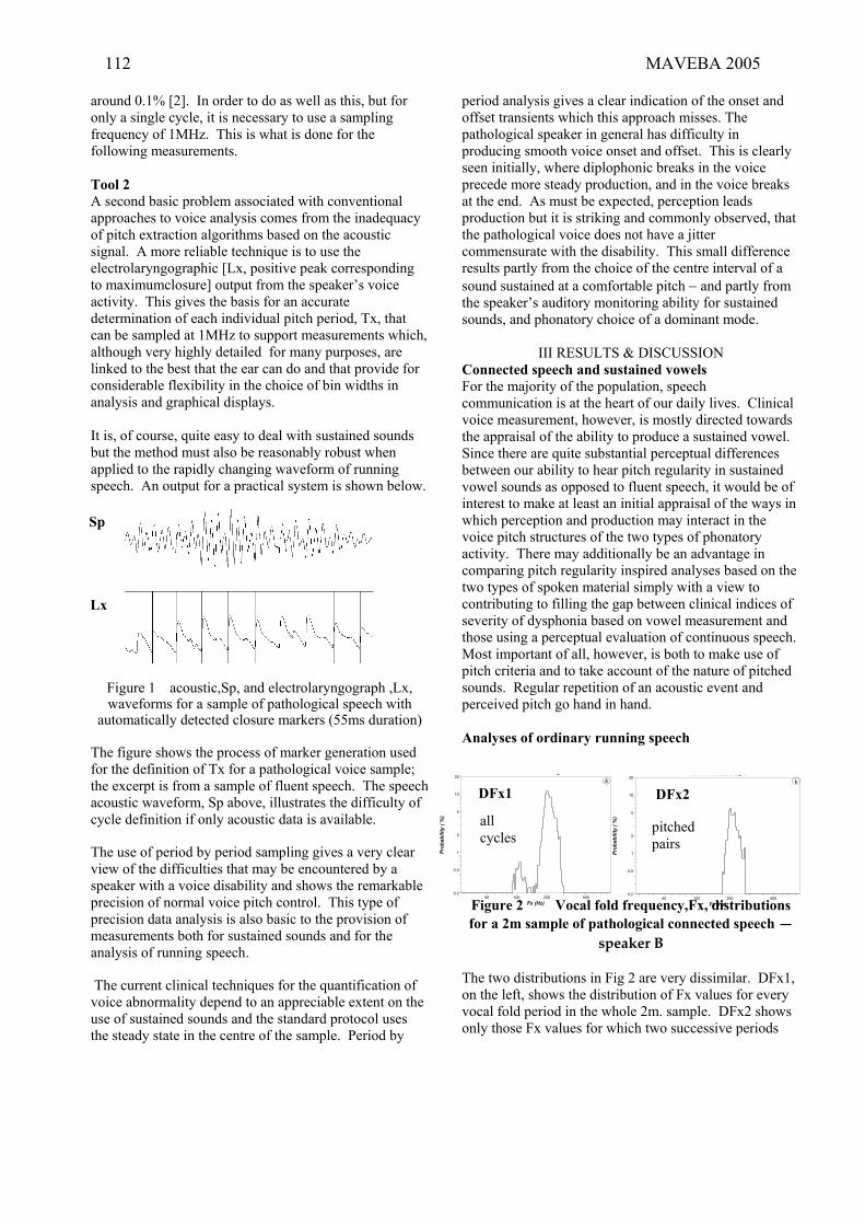
around 0.1% [2]. In order to do as well as this, but for only a single cycle, it is necessary to use a sampling frequency of 1MHz. This is what is done for the following measurements. Tool 2 A second basic problem associated with conventional approaches to voice analysis comes from the inadequacy of pitch extraction algorithms based on the acoustic signal. A more reliable technique is to use the electrolaryngographic [Lx, positive peak corresponding to maximumclosure] output from the speaker’s voice activity. This gives the basis for an accurate determination of each individual pitch period, Tx, that can be sampled at 1MHz to support measurements which, although very highly detailed for many purposes, are linked to the best that the ear can do and that provide for considerable flexibility in the choice of bin widths in analysis and graphical displays. It is, of course, quite easy to deal with sustained sounds but the method must also be reasonably robust when applied to the rapidly changing waveform of running speech. An output for a practical system is shown below.

Figure 1 acoustic,Sp, and electrolaryngograph ,Lx, waveforms for a sample of pathological speech with

automatically detected closure markers (55ms duration) The figure shows the process of marker generation used for the definition of Tx for a pathological voice sample; the excerpt is from a sample of fluent speech. The speech acoustic waveform, Sp above, illustrates the difficulty of cycle definition if only acoustic data is available. The use of period by period sampling gives a very clear view of the difficulties that may be encountered by a speaker with a voice disability and shows the remarkable precision of normal voice pitch control. This type of precision data analysis is also basic to the provision of measurements both for sustained sounds and for the analysis of running speech. The current clinical techniques for the quantification of voice abnormality depend to an appreciable extent on the use of sustained sounds and the standard protocol uses the steady state in the centre of the sample. Period by

period analysis gives a clear indication of the onset and offset transients which this approach misses. The pathological speaker in general has difficulty in producing smooth voice onset and offset. This is clearly seen initially, where diplophonic breaks in the voice precede more steady production, and in the voice breaks at the end. As must be expected, perception leads production but it is striking and commonly observed, that the pathological voice does not have a jitter commensurate with the disability. This small difference results partly from the choice of the centre interval of a sound sustained at a comfortable pitch − and partly from the speaker’s auditory monitoring ability for sustained sounds, and phonatory choice of a dominant mode.

III RESULTS & DISCUSSION Connected speech and sustained vowels For the majority of the population, speech communication is at the heart of our daily lives. Clinical voice measurement, however, is mostly directed towards the appraisal of the ability to produce a sustained vowel. Since there are quite substantial perceptual differences between our ability to hear pitch regularity in sustained vowel sounds as opposed to fluent speech, it would be of interest to make at least an initial appraisal of the ways in which perception and production may interact in the voice pitch structures of the two types of phonatory activity. There may additionally be an advantage in comparing pitch regularity inspired analyses based on the two types of spoken material simply with a view to contributing to filling the gap between clinical indices of severity of dysphonia based on vowel measurement and those using a perceptual evaluation of continuous speech. Most important of all, however, is both to make use of pitch criteria and to take account of the nature of pitched sounds. Regular repetition of an acoustic event and perceived pitch go hand in hand. Analyses of ordinary running speech

Figure 2 Vocal fold frequency,Fx, distributions for a 2m sample of pathological connected speech —

speaker B The two distributions in Fig 2 are very dissimilar. DFx1, on the left, shows the distribution of Fx values for every vocal fold period in the whole 2m. sample. DFx2 shows only those Fx values for which two successive periods

50 100 200 5000.2

0.5

1

2

5

10

20

Fx (Hz)

Prob

abili

ty (

%)

pLx

all cycles

DFx1

50 100 200 5000.2

0.5

1

2

5

10

20

Fx (Hz)

Prob

abili

ty (

%)

HUTHWAITEEAR.speLx

DFx2

pitched pairs

Sp

Lx

112 MAVEBA 2005

have been essentially the same. Two modes of vocal fold vibration are shown. The main at about 200 Hz is well defined. At about an octave below, the lower mode is more diffuse and is evidently associated with considerable period to period irregularity since the values of DFx1 and DFx2 are so different. Different pathologies give rise to different types of modal structural differences but for most cases the presence of voice pathology will be associated with marked discrepancies in magnitude and shape between these two forms of representation. Figure 3 Overlaid Fx distributions for a normal

sample (speaker A) AND for its “pitched” components The use of accurate period by period information makes it easy to plot the occasions when two successive pitch periods have essentially the same value. For the normal voice this happens very often indeed. The pathological voice, however, is very easily identified by the ear as having period to period irregularity. This important feature is shown in the inner of the two distributions above in Figure 3. The two distributions together give an immediate insight into important aspects of voice quality − pitch height and range, modal structure, and regularity. These first and second order distributions are especially useful in general in pathological voice analysis. Jitter and irregularity in connected speech

Figure 4 Vocal fold period crossplots, CFx

speaker A on the left, B on the right

Jitter and intonation The procedure basic to the ordinary application of the jitter criterion is applied only to sustained sounds and requires that the voiced sound being measured is held at as constant a pitch as possible by the speaker. The

essential concept, however, is directed at obtaining a quantitative assessment of pitch variability. The idea is just as applicable to ordinary connected speech so as to get an appraisal of the irregularity which may be inherent to the social use of a pathological voice. An obvious first approach to the measurement of pitch irregularity in a sample of running speech is to determine the standard deviation of the spread of cycle to cycle differences in regard to periods or frequencies. A difficulty with this approach is that it will necessarily include ordinary intonational variations as part of the estimate of irregularity. The problem is perhaps best illustrated with reference to actual data. When vocal fold vibration is essentially regularly periodic the use of a period by period crossplot, as in Figure 4 A, gives a clearly defined diagonal line − since successive periods have almost the same values, apart from the variations arising from the intonational frequency related changes of connected speech. For the pathological voice, however, the shape of the crossplot is not so simply defined because successive vocal fold periods are very often markedly different and are not totally under the speaker’s cognitive control. This method of plotting the range of variability in period to period coherence is effectively similar to the application of the jitter criterion, used for sustained sounds, to the whole of a connected speech sample. The interpretation of jitter in running speech, however, is not at all the same as that for sustained sounds. First, the pitch dLs are quite different in the two cases. The bin sizes needed for the adequate representation of significant changes in the present data involves 6% steps. The 0·1% resolution required for the analysis of sustained sounds is not appropriate. Second, the presence of intonational changes makes it necessary to ignore variations which are part of the normal patterning of vocal fold frequency change in running speech. Figure 4 A shows that there is indeed a centre continuous core of variation for the whole of the vocal fold frequency range and this is found for all normal speakers. If the pitch difference limen value of 6% is applied to this data then it becomes possible to apply a theoretically founded criterion which makes it feasible in practice to separate the variability arising from intonation from that due to other causes. It is then only necessary to determine all the pitch deviations which are more than 6% away from the centre line in the graph showing Fx1 against Fx2 − where Fx1 is the frequency value of the first vocal fold cycle in any pair of cycles in the whole utterance and Fx2 is the frequency value of the immediately following cycle of the pair. Fx is used to denote the frequency value of a single vocal fold cycle,

50 100 200 5000.1

0.2

0.5

1

2

5

10

20

50

100

Fx (Hz)

Prob

abili

ty (

%)

Lx

DFx1 & DFx2

50 100 200 500

50

100

200

500

Fx1 (Hz)

Fx2

(Hz)

Lx

50 100 200 500

50

100

200

500

Fx1 (Hz)

pLx

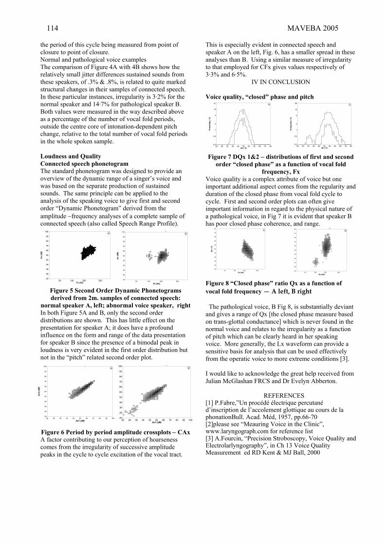
the period of this cycle being measured from point of closure to point of closure. Normal and pathological voice examples The comparison of Figure 4A with 4B shows how the relatively small jitter differences sustained sounds from these speakers, of .3% & .8%, is related to quite marked structural changes in their samples of connected speech. In these particular instances, irregularity is 3·2% for the normal speaker and 14·7% for pathological speaker B. Both values were measured in the way described above as a percentage of the number of vocal fold periods, outside the centre core of intonation-dependent pitch change, relative to the total number of vocal fold periods in the whole spoken sample. Loudness and Quality Connected speech phonetogram The standard phonetogram was designed to provide an overview of the dynamic range of a singer’s voice and was based on the separate production of sustained sounds. The same principle can be applied to the analysis of the speaking voice to give first and second order “Dynamic Phonetogram” derived from the amplitude −frequency analyses of a complete sample of connected speech (also called Speech Range Profile).

Figure 5 Second Order Dynamic Phonetograms derived from 2m. samples of connected speech:

normal speaker A, left; abnormal voice speaker, right In both Figure 5A and B, only the second order distributions are shown. This has little effect on the presentation for speaker A; it does have a profound influence on the form and range of the data presentation for speaker B since the presence of a bimodal peak in loudness is very evident in the first order distribution but not in the “pitch” related second order plot.

Figure 6 Period by period amplitude crossplots − CAx A factor contributing to our perception of hoarseness comes from the irregularity of successive amplitude peaks in the cycle to cycle excitation of the vocal tract.

This is especially evident in connected speech and speaker A on the left, Fig. 6, has a smaller spread in these analyses than B. Using a similar measure of irregularity to that employed for CFx gives values respectively of 3·3% and 6·5%.

IV IN CONCLUSION

Voice quality, “closed” phase and pitch Figure 7 DQx 1&2 − distributions of first and second

order “closed phase” as a function of vocal fold frequency, Fx

Voice quality is a complex attribute of voice but one important additional aspect comes from the regularity and duration of the closed phase from vocal fold cycle to cycle. First and second order plots can often give important information in regard to the physical nature of a pathological voice, in Fig 7 it is evident that speaker B has poor closed phase coherence, and range. Figure 8 “Closed phase” ratio Qx as a function of vocal fold frequency — A left, B right The pathological voice, B Fig 8, is substantially deviant and gives a range of Qx [the closed phase measure based on trans-glottal conductance] which is never found in the normal voice and relates to the irregularity as a function of pitch which can be clearly heard in her speaking voice. More generally, the Lx waveform can provide a sensitive basis for analysis that can be used effectively from the operatic voice to more extreme conditions [3]. I would like to acknowledge the great help received from Julian McGlashan FRCS and Dr Evelyn Abberton.

REFERENCES [1] P.Fabre,”Un procédé électrique percutané d’inscription de l’accolement glottique au cours de la phonationBull. Acad. Méd, 1957, pp.66-70 [2]please see “Meauring Voice in the Clinic”, www.laryngograph.com for reference list [3] A.Fourcin, “Precision Stroboscopy, Voice Quality and Electrolarlyngography”, in Ch 13 Voice Quality Measurement ed RD Kent & MJ Ball, 2000

20 26 32 38 44 50 56 62 68 74 800.2

0.5

1

2

5

10

20

Qx ( %)

Prob

abili

ty (

%)

Lx

20 26 32 38 44 50 56 62 68 74 800.2

0.5

1

2

5

10

20

Qx ( %)

Prob

abili

ty (

%)

pLx

20 28 36 44 52 60 68 76 84 92 10020

28

36

44

52

60

68

76

84

92

100

Ax1 (dB)

pLx

20 28 36 44 52 60 68 76 84 92 10020

28

36

44

52

60

68

76

84

92

100

Ax1 (dB)

Ax2

(dB

)

pLx

50 100 200 50020

26

32

38

44

50

56

62

68

74

80

Fx (Hz)

pLx

50 100 200 50020

26

32

38

44

50

56

62

68

74

80

Fx (Hz)

Qx

( %)

pLx

50 100 200 50020

28

36

44

52

60

68

76

84

92

100

Fx (Hz)

Ax

(dB

)

Lx

50 100 200 50020

28

36

44

52

60

68

76

84

92

100

Fx (Hz)

Ax

(dB

)

pLx

114 MAVEBA 2005

FROM VOCAL QUALITY MEASUREMENT TO PERCEPTION

Rahul Shrivastav

[email protected]

Department of Communication Science & Disorders, University of Florida, Gainesville

Abstract: Quantification of vocal quality of a speech

signal is essential in a number of applications.

However, existing measures for this purpose are

often characterized by poor sensitivity and specificity

to perceptual judgments. These shortcomings may

have arisen because (1) these measures are often

validated against “noisy” perceptual data and (2) the

non-linear and multidimensional relationships

between the physical signal and perceptual

judgments have often been ignored. This paper

describes the psychometric principles underlying

quantification of subjective judgments and the use of

an auditory processing model as a signal processing

front-end when measuring “breathy” voice quality.

Preliminary data for quantification of “roughness” is

also discussed.

INTRODUCTION

The speech signal is rich in information and conveys a

large amount of information to a listener. For example,

apart from the meaning contained in the utterance, the

speech signal conveys such information as emotions,

speaker identity, age and gender. A number of

applications require accurate quantification of such

perceptual attributes of a speech signal. In the clinical

domain, one may need to quantify aspects such as

speech intelligibility, voice quality, nasality, etc. These

attributes are important because these are often affected

by disease and are frequently the target of surgical,

pharmacological or behavioral treatment. Precise

quantification of these attributes can enhance the

assessment and rehabilitation procedures by providing a

baseline against which any change can be measured.

Various techniques to quantify these perceptual

attributes have been developed over the years. Some of

these require listeners to make a subjective decision

using a particular rating scale (for example, the CAPE-V

developed by the American Speech-Language and

Hearing Association). Others use a variety of signal

processing techniques to quantify certain aspects of the

speech acoustic signal [1-4]. Unfortunately, all of these

methods have been compromised by a variety of

problems. The accuracy of subjective judgments has

been measured by calculating the reliability and

agreement within and across listeners. Reliability

measures the degree to which one listener’s ratings on a

set of stimuli follow the same trends as that of another

listener. Agreement, on the other hand is a measure of

the probability that two listeners give the same stimulus

the same exact rating. Unfortunately, both reliability and

agreement have been found to be poor for subjective

ratings of voice quality [5-7]. Similarly, the accuracy of

automated measures to quantify perception is measured

by calculating the correlation between these measures

and perceptual judgments of voice quality.

Unfortunately, most automated measures have been

observed to show poor to moderate correlation with

perceptual data. Additionally, these measures often lack

consistency and show poor sensitivity and specificity to

the perceptual construct that they intend to quantify [8].

When attempting to quantify attributes such as voice

quality, it is important to remember that these are

inherently perceptual constructs. Attributes such as

voice quality, nasality or “acceptability” of speech

essentially reflect a listener’s judgment about that

particular construct. The speech signal itself does not

possess quality; rather, it “evokes it in the listener” [8].

Therefore, any method to quantify such perceptual

attributes must be validated against perceptual

judgments made by listeners. These perceptual

judgments serve as the gold standard for any other

method to quantify perceptual attributes of speech.

Unfortunately, perceptual judgments made by a listener

are highly variable and are affected by a number of

factors [9, 10]. While some of these factors are related to

the stimulus characteristics, others are related to

extraneous variables such as listener experience and

training, instructions given to the listeners, nature of the

scaling task and the experimental design. These

extraneous variables introduce “noise” in the perceptual

data, thereby, making it difficult to interpret the true

perceptual magnitude of a given stimulus. However,

these errors can be minimized through the use of

appropriate experimental designs to obtain perceptual

judgments [11]. These procedural modifications include

multiple presentations of each stimulus to each listener,

randomizing the order of stimulus presentation,

modifying the instructions given to the listeners, etc.

Once a good estimate of the perceptual magnitude of an

attribute has been obtained for several stimuli, these

judgments may be used to develop a model that predicts

listener judgments based on various stimulus

characteristics. Such a model can be used to generate

automated measures of vocal quality or other perceptual

attributes of the speech signal. The development of such

a model requires attention to the sensitivity of the

human auditory system and the characteristics of the


acoustic-auditory transduction process. Previous

research has shown that the relationship between a

physical stimulus and its perceptual consequence is

often non-linear. For example, the relationship between

intensity and loudness may be described with a power

law [12] and that between frequency and pitch is better

described using non-linear scales such as the Bark, Mel

or ERB-scales [13, 14]. In a similar manner, the

perception of complex attributes such as voice quality

may be best characterized by a non-linear function of

specific stimulus characteristics. When the goal of

measurement is to quantify perception, we need to (a)

determine what aspects of the speech acoustic signal are

perceptually relevant, and (b) determine the nature of

the relationship between these stimulus characteristics

and their perceptual consequences. One method to

account for some of these non-linear processes is

through the use of an auditory-processing model as a

signal processing front-end. The general form of such a

model is shown in Figure 1. The use of such front-ends

has been shown to give better estimates of the

perceptual judgments of voice quality [15, 16].

Figure 1: General form of an auditory processing

model.

This paper describes a series of experiments to

understand the perception of dysphonic voice quality.

The first section describes the psychometric principles

used to obtain a good estimate of the perceptual

magnitude of dysphonic voice quality. In the second

section, one particular auditory processing model and its

utility in the quantification of “breathy” voice quality is

described. And finally, preliminary data is presented on

the perception of “rough” voice quality.

PYSCHOMETRIC THEORY TO QUANTIFY SUBJECTIVE

JUDGMENTS OF VOICE QUALITY

A variety of techniques have been used for scaling

perceptual magnitude of a physical stimulus [17]. It is

necessary to differentiate two aspects in this process –

sensory capability and response proclivity [18]. Sensory

capability refers to the resolving power of the sensory

mechanism; it defines the limits of the sensory system.

On the other hand, response proclivity refers to the

tendency of a listener to respond in a specific manner

when encountering a specific stimulus. Since proclivity

is affected by several factors, many unrelated to the

stimulus itself, it is necessary to take appropriate steps

to minimize “noise” in perceptual judgments.

For example, inter- and intra-rater reliability (measured

as the correlation between ratings made within- or

across-listeners) in perceptual ratings can be minimized

by averaging multiple ratings of each stimulus by each

listener [11]. Such precautions can avoid errors such as

those arising due to “order-effects” and frequently seen

with rating scales. If measurement of “agreement” (i.e.

the probability that two raters would give the same

stimulus exactly the same rating) is essential, the ratings

from individual listeners should be normalized using

standardized scores (z-scores) or other procedures.

Figure 2 shows the improvement in reliability and

agreement for perceptual ratings of breathiness when

these procedures are used.

Figure 2: Improvement in reliability and agreement

when multiple ratings of each stimulus from each

listener are used. Each listener’s ratings were converted

to corresponding z-scores.

0

0.2

0.4

0.6

0.8

1

Single Rating Averaged Ratings

Ag

reem

en

t. o

r R

eliab

ilit

y

Agreement Reliability

Although these techniques help improve agreement and

reliability of rating scale data, these measures may not

necessarily indicate the true magnitude of the stimulus.

Rather, rating scale measures may only provide the rank

ordering of the stimuli tested in the experiment. Other

techniques, such as magnitude estimation, magnitude

production, matching or paired comparisons may be

better suited to obtain an accurate estimate of perceptual

“distance” between two stimuli.

AUDITORY PROCESSING MODEL AS A SIGNAL-PROCESSING

FRONT END TO QUANTIFY “BREATHY” VOICE QUALITY

Breathiness in voices has been found to correlate with a

number of acoustic measures, including aspiration noise,

Voice Spectrum

Band pass filter for external ear

Band pass filter for middle ear

Filter Bank:

Transform sound spectrum to excitation pattern

Compressive function to obtain specific loudness

Calculate area under specific loudness curve to obtain total

loudness

116 MAVEBA 2005

frequency/intensity perturbation and spectral slope.

However, the correlation between these measures and

perceptual judgments of breathiness has been found to

be inconsistent across different experiments.

Auditory processing models can allow us to estimate

how acoustic signals may be represented in the auditory

system. Several such models have been proposed [19-

21]. One such model, proposed by Moore et al. (1997)

was implemented for the study of breathy voice quality

[15, 16]. This model simulates the outer and middle ear

as band pass filters. The cochlear filtering is simulated

with a filter-bank of asymmetric rounded-exponential

filters. Finally, the neural excitation is modeled as a

non-linear compressive function. The total neural

excitation for a given sound provides an estimate of the

loudness of that sound. The neural excitation within

each “channel” is called the specific loudness.

This auditory processing model can also be used to

simulate masking. Masking refers to the phenomenon

where the loudness of a sound is reduced if it is

presented along with a background noise. The loudness

of a specific component, when it is presented

simultaneously with an auditory masker is called the

partial loudness.

The utility of this auditory processing model in

predicting perceptual judgments of breathiness was

tested in separate experiments [15, 16]. One experiment

studied 13 voice stimuli, and compared the results to

perceptual judgments obtained using a multidimensional

scaling design. The other studied 27 stimuli and

compared the results to perceptual judgments made on a

5-point rating scale. In both these experiments, the voice

stimuli were first separated into a periodic component

representing the complex wave produced by vocal fold

vibration and an aperiodic component representing the

aspiration noise. The auditory processing model was the

used to estimate the partial loudness of the complex

wave, while treating the aspiration noise as an auditory

masker. In both these experiments, the partial loudness

of the complex wave was found to correlate highly with

the perceptual judgments of breathiness. This measure

accounted for greater variance in the perceptual ratings

of breathiness than any other acoustic measure of

breathiness. Figure 3 shows the relationship between

partial loudness of the complex wave and perceptual

judgments of breathiness.

The use of an auditory-processing model accounts for

multiple factors that may affect breathiness – the overall

intensity of the complex wave and aspiration noise, the

spectral shape of these components as well as the non-

linear interaction between the two. This, presumably,

accounts for greater variance in the perceptual data than

using conventional acoustic measures such as measures

of noise or spectral slope. The change in partial loudness

patterns for different voices is shown in Figure 4.

Figure 3: Linear regression predicting ratings of

breathiness using partial loudness of the complex wave

(and assuming that aspiration noise acts as an auditory

masker).

y = -3.3583x + 19.997

R2 = 0.7938

0

4

8

12

16

20

1 2 3 4 5

Breathiness Ratings

Par

tial L

oudn

ess

(Son

es)

Figure 4: Partial loudness patterns for voices identified

as normal, mild-, moderate- and severely- breathy.

ERB

363330272421181512963

Part

ial L

oudness

of

Sig

nal (

Sone)

1.2

1.1

1.0

.9

.8

.7

.6

.5

.4

.3

.2

.1

0.0

-.1

Normal

Mild

Moderate

Severe

ACOUSTIC CORRELATES FOR “ROUGHNESS” IN VOICES –

PRELIMINARY DATA

Many voices frequently observed in voice clinics are

described as “rough.” A number of acoustic correlates

for roughness have been proposed. These include,

frequency/intensity perturbation, estimates of noise in

the signal and the presence of subharmonics. However,

as with breathy voices, these findings lack sensitivity

and specificity.

From a psychoacoustic perspective, the perception of

roughness is related to the amplitude and frequency

modulation of a carrier wave. More specifically, the

roughness of a sound is related to the amplitude

modulation within a given critical-band [22]. The

perception of roughness of a carrier wave is most

sensitive to specific modulation frequencies.

A much simplified implementation of this model for

roughness is obtained by: (1) determining the

modulation frequencies in the vowel, (2) selecting a

subset of these modulating frequencies, (3) calculating

the “modulation amplitude” for these frequencies, and

(4) determining the average modulation due to these

frequencies.

The average modulation amplitude thus obtained was

first normalized to the fundamental frequency of each

stimulus, and was then used to predict perceptual

judgments of roughness for 34 vowel samples. An

exponential fit was found to account for 80.2% of the

variance in the perceptual data. These data are shown in

Figure 5. Measures such as shimmer, jitter and signal-

to-noise ratio accounted for considerably less variance

in the same perceptual data.

Figure 5: Perceptual ratings of roughness predicted by

the normalized modulation amplitude of selected

modulation frequencies.

y = 0.0321e0.8058x

R2 = 0.802

0

1

2

3

4

1 2 3 4 5

Roughness

CONCLUSIONS

Voice quality is essentially a perceptual construct. Any

method to quantify perception must be validated against

perceptual judgments. However, since perceptual

judgments are highly variable, one needs to devise

experiments that minimize response variability

associated with non-stimulus factors. Additionally,

methods to quantify perception are more likely to be

successful if they simulate the mechanisms involved in

the auditory-perceptual process. One way to achieve this

is through the use of auditory-processing models as a

signal-processing front end. The success of this

approach is shown for quantification of “breathiness”

and “roughness” in dysphonic voices.

ACKNOWLEDGEMENTS

Research funded by a grant from NIH/NIDCD

(R21DC006690). Part of this work is being done in

collaboration with David Eddins.

REFERENCES

1. Hillenbrand, J., R.A. Cleveland, and R.L. Erickson,

Acoustic correlates of breathy vocal quality. Journal of

Speech & Hearing Research, 1994. 37(4): p. 769-78.

2. Deal, R.E. and F.W. Emanuel, Some waveform and

spectral features of vowel roughness. Journal of Speech &

Hearing Research, 1978. 21(2): p. 250-64.

3. de Krom, G., A cepstrum-based technique for

determining a harmonics-to-noise ratio in speech signals.

Journal of Speech & Hearing Research, 1993. 36(2): p.

254-66.

4. Milenkovic, P., Least mean square measures of voice

perturbation. Journal of Speech & Hearing Research, 1987.

30(4): p. 529-38.

5. Kreiman, J., et al., Individual differences in voice

quality perception. Journal of Speech & Hearing Research,

1992. 35(3): p. 512-20.

6. Kreiman, J., et al., Perceptual evaluation of voice

quality: review, tutorial, and a framework for future

research. Journal of Speech & Hearing Research, 1993.

36(1): p. 21-40.

7. Rabinov, C.R., et al., Comparing reliability of

perceptual ratings of roughness and acoustic measure of

jitter. Journal of Speech & Hearing Research, 1995. 38(1):

p. 26-32.

8. Kreiman, J. and B. Gerratt, Measuring voice quality, in

Voice Quality Measurement, R.D. Kent and M.J. Ball,

Editors. 2000, Singular Publishing Group: San Diego. p.

73-101.

9. Poulton, E.C., Bias in quantifying judgments. 1989,

Hove, U.K.: Lawrence Erlbaum Associates Ltd.

10. Thurstone, L.L., The measurement of values. 1959,

Chicago: University of Chicago Press.

11. Shrivastav, R., C. Sapienza, and V. Nandur,

Application of Psychometric Theory to the Measurement of

Voice Quality Using Rating Scales. Journal of Speech,

Language, & Hearing Research, In Press.

12. Stevens, S.S., A scale for the measurement of a

psychological magnitude: L o u d n e s s . Psychological

Review, 1936. 43: p. 403-416.

13. Stevens, S.S., J. Volkmann, and E.B. Newman, A scale

for the measurement of psychological magnitude: Pitch.

Journal of the Acoustical Society of America, 1937. 8: p.

185-190.

14. Moore, B.C.J., An Introduction to the Psychology of

Hearing. 4th ed. 1997, San Diego, CA: Academic Press.

15. Shrivastav, R., The Use of an Auditory Model in

Predicting Perceptual Ratings of Breathy Voice Quality.

Journal of Voice, 2003. 17(4): p. 502-512.

16. Shrivastav, R. and C. Sapienza, Objective Measures of

Breathy Voice Quality Obtained Using an Auditory Model.

Journal of the Acoustical Society of America, 2003.

114(4): p. 2217-2224.

17. Stevens, S.S., Mathematics, Measurement and

Psychophysics, in Handbook of Experimental Psychology,

S.S. Stevens, Editor. 1951, John Wiley & Sons, Inc.: New

York.

18. Watson, C.S., Psychophysics, in Handbook of General

Psychology, B.B. Wolman, Editor. 1973, Prentice Hall,

Inc.: Englewood Cliffs, NJ.

19. Moore, B.C.J., B.R. Glasberg, and T. Baer, A model

for the prediction of thresholds, loudness and partial

loudness. Journal of Audio Engineering Society, 1997.

45(4): p. 224-239.

20. Lopez-Poveda, E.A. and R. Meddis, A human

nonlinear cochlear filterbank. J Acoust Soc Am, 2001.

110(6): p. 3107-18.

21. Seneff, S., Ajoint synchrony/mean-rate model of

auditory speech processing. Journal of Phonetics, 1988. 16:

p. 55-76.

22. Terhardt, E., On the perception of periodic sound

fluctuations (Roughness). Acustica, 1974. 30: p. 201-213.

Modula

tion/F

0

118 MAVEBA 2005

Abstract: Kymographic imaging refers to a special

way of displaying vibrations by putting together a

great number of successive images of a vibrating

object viewed through a thin slit. In medicine, the

method has been found particularly well suited for

imaging vibrations of the vocal folds, which are the

ultimate source of human voice. Here we address the

question on which vibratory characteristics of the

vocal folds can be identified in high-speed

videokymographic images and used in clinical

practice when diagnosing origins of voice problems?

The ultimate long-term goal of the research is to relate

the displayed vibration characteristics to the tissue

properties of the vocal folds and design strategies how

undesirable tissue properties can be altered through

conservative or surgical treatment.

ACKNOWLEDGMENTS:The research has been supported in the Netherlands bythe STW project G5973 and in the Czech Republic by theEUREKA E!2614 project.

WHAT CAN BE SEEN IN VIDEOKYMOGRAPHIC IMAGES?

J. G. Svec1,2

, F. Sram 2, M.Fric

2, Q.Qiu

1, H. K. Schutte

1

1 Groningen Voice Research Lab, Department of BioMedical Engineering, University Medical Center Groningen,

University of Groningen, the Netherlands2 Center for Communication Disorders, Medical Healthcom, Ltd., Prague 8, the Czech Republic


OBJECTIVE VOCAL FOLD VIBRATION ASSESSMENT FROM

VIDEOKYMOGRAPHIC IMAGES

S. Bianchi, L. Bocchi, C. Manfredi, G.Cantarella*, N. Migali*

Department of Electronics and Telecommunications, Università degli Studi di Firenze

Via S. Marta 3, 50139 Firenze, Italy

* Otolaryngology Department, University of Milan, Ospedale Maggiore IRCCS, Via F. Sforza 35, 20122 Milano, Italy

Abstract - Vocal folds oscillation crucially influences

all the basic qualities of voice, such as pitch and

loudness, as well as the spectrum. Stroboscopy

provides the standard view of the larynx.

Videokymography is a new diagnostic tool developed

to overcome specific limitations of stroboscopy in

severely dysphonic patients with an aperiodic signal.

It registers the movements of the vocal folds with a

high time resolution on a line perpendicular to the

glottis.

The main focus of this paper is on measuring and

tracking quantitative parameters for objective vocal

fold function assessment from videokymographic

(VKG) examinations of subjects with normal and

pathological laryngeal function. Active contour

search is realised, by properly adjusted snake

algorithm. Examples are reported, showing the

robustness and reliability of the proposed technique.

I. INTRODUCTION

Vibration of the vocal-folds is a highly relevant aspect

of voice production, both in normal and in pathological

voices. The periodicity, or lack of periodicity, critically

determines the quality of voice. It is typically described

in terms of jitter and/or shimmer, period to-period

correlation, or by spectral characteristics. Another

method for acquisition of physiological data is direct

visual inspection of the vocal folds vibration by means

of stroboscopy. An admitted limitation of the

stroboscopic image is that vocal fold vibration must be

relatively periodic to visualize a slow motion

representation of the phonatory cycle. In fact,

aperiodicities associated with some voice qualities make

stroboscopy inappropriate, since any disturbance of the

vibration distorts the resulting stroboscopic image.

The kymographic concept introduced by [1], [2] seems

to be an optimal solution, since each vibratory cycle is

documented in terms of a sequence of several images,

which can be acquired directly from a single-line

camera [1] or by extraction from high-speed image

sequences[3],[4]. Videokymography allows isolation of

specific portions of the glottic image (taken at up to

7812 images per second) to be analyzed for closure.

Such kymographic images give a good view of the

movements of the vocal folds, periodic or nonperiodic,

but only for part of the image, i.e., the single line. This

study aims at offering an automatic quantitative method

to obtain vibration properties of human vocal folds via

videokymography, by developing a digital image

processing algorithm optimized for the analysis of

videokymography (VKG) recordings, such as intensity

adjustment, noise removal and glottis identification. The

presented method extends previous work [5] and

combines an active contour model with a parameter

extraction algorithm that can accurately track the

vibrational wave in videokymograms and automatically

quantify its properties in terms of few parameters,

useful for clinicians. Tracking parameters, other than

simply measuring their mean value and std, is in fact

considered of utmost importance by clinicians, as

irregular patterns can be found at their instant of

occurrence during phonation and put into relation with

images and acoustic signal analysis. Specifically, the

amplitude and period ratios between right and left vocal

fold, as well as the ratio between opening and closing

phase are considered [6]. When required, more

parameters could be added, on analogy to [7].

Examples are given concerning pathological subjects,

that show the robustness of the contour detection

algorithm.

II. MATERIALS AND METHODS

Videokymography (VKG) is based on a special camera,

which can operate in two different modes: standard and

high-speed. In the standard mode, the camera provides

standard images displaying the whole vocal folds at

standard video frame rate (30/25 frames/s, with

720x486/768x576 pixels of resolution). In the high-

speed mode, the video camera delivers images from

only a single line selected from the whole image, at the

speed of approximately 7875/7812.5 line-images/s and

720x1/768x1 pixels resolution. The resulting high-speed

image, called “videokymogram”, displays the vibratory

pattern of the selected part of the vocal folds.

Kymographic recording is divided into video frames,

i.e. segments of approx. 15/18 ms duration. Images are

not in colour, and continuous high-intensity light is

desirable.


E

snake= E

intv s( ) ds + E

extv s( ) ds

The vibratory pattern displayed in kymographic images

is dependent on the measuring position. There are two

factors which influence the resulting image:

1- position along the glottal axis

2- angle with respect to the glottal axis.

In normal cases, the position in the middle of the vocal

folds is usually considered to provide the representative

vibratory pattern of the whole vocal folds. In case of

vocal fold lesions, however, the vibration characteristics

generally differ along the glottal axis.

The angle of the measuring line is, as a standard,

adjusted to be perpendicular to the glottal axis. When

using VKG, the measuring position is adjusted prior to

the examination.

Usually, there is only limited time available for the

examination. Therefore, phonation at comfortable pitch

and loudness is mostly targeted for kymographic

imaging.

Despite its usefulness, in our knowledge, until now no

quantitative analysis of VKG images is commercially

available, and only few work has been made towards its

fulfillment [6], [7]. At present, physicians perform only

qualitative evaluation of VKG parameters, basically by

visual inspection of subsequent frames, or by manual

measures from printed images. Such analysis prevents

from reliable comparison among wide sets of data, and

hence from finding and defining standard reference

values for classification and assessment of treatment

effectiveness. Based on such requirements, this work

aims at providing first results that would allow filling

this gap.

Parameter extraction is obtained here by means of two

subsequent stages: image analysis, for vocal folds

contours detection, followed by signal analysis, for

parameter evaluation from data sets representing vocal

folds edges. Specifically, and with reference to Fig.2,

the parameters to be measured and tracked are:

• Ramp, the ratio between the right and left vocal fold

amplitudes, related to possible asymmetries

between the two folds;

• Rper, the ratio between the right and the left

vibratory periods, inversely related to possible

frequency variations due to pathology;

• Roc, the ratio between opening and closing phase

(Open and Closed, respectively), basically related

to glottal insufficiency.

For healthy voices, such parameters should be equal or

close to one, and almost constant during all phonatory

cycles. Any asymmetry due to pathology can thus be

quantified by evaluating and tracking the above-

mentioned parameters.

A First stage: Edge detection

The correct detection of the vocal folds contour is

carried out in a two-step process, the first one aiming at

finding an initial contour to which active snakes are

applied in the second step.

Figure 2: Main parameters for objective

videokymographic image analysis (from [1]).

A.1 First step: initial contour

The following routine, that handles some basic settings,

is executed before the snake. It normalises grey levels,

initialises contour, takes notice of black lines, to be

disregarded by the algorithm, thus finding the

significant rows in the image. Then, it sets to 0 the level

of the image outside the right and left edges, defined by

the user. This allows avoiding noisy fluctuations of the

grey levels not overlapped with the vocal folds. The

routine scans the significant rows and, for each of them,

determines the largest interval of pixels with a grey

level lower than a pre-specified threshold. A first

contour is thus obtained, by storing the interval co-

ordinates for each line in two separate arrays.

A.2 Second step: snake active contour

Snakes are planar deformable contours that are useful in

several image analysis tasks. They are often used to

approximate the locations and shapes of object

boundaries on the basis of the reasonable assumption

that boundaries are piecewise continuous or smooth [8].

Representing the position of a snake parametrically by

v(s)=(x(s),y(s)) with s in [0,1], its energy can be written

as:

(1)

where Eint represents the internal energy of the snake

due to bending and it is associated with a priori

constraints, Eext is an external potential energy which

depends on the image and accounts for a posteriori

information. The final shape of the contour corresponds

to the minimum of this energy.

In the original technique [9] the internal energy is

defined as:

Eint

v s( ) =1

2

a s( )v s( )

s

2

+ b s( )2

v s( )

s2

2

. (2)

This energy is composed of a first order term controlled

by a(s) (tension of the contour) and a second order term

controlled by b(s) (rigidityof the contour).

122 MAVEBA 2005

The external energy couples the snake to the image. It is

defined as a scalar potential function whose local

minima coincide with intensity extremes, edges, and

other image features of interest:

Eext v s( ) = c Gs I x, y( )( (

2(3)

where I(x,y) is the image intensity, Gs is a Gaussian of

standard deviation s, is the gradient operator and c a

weight associated with image energies [8], [9], [10].

As concerns the energy minimization, the original

model employs the variational calculus to iteratively

minimize the energy. There may be a number of

problems associated with this approach such as

algorithm initialization, existence of local minima, and

selection of model parameters. Among existing

methods, the greedy algorithm [10] exhibits a low

computational cost, provided the initial position of the

snake is relatively close to the desired contour. In our

application, the technique described in step 1 provides a

fairly good approximation of the real contour, therefore

allowing us to utilize the active contour and the snake

algorithm to perform a fine tuning of the contour on the

image. Each vocal fold has been modelled as an

independent snake, having its extreme point constrained

to belong to the first and the last scan line of the image,

respectively. Notice that, differently from [7], the snake

is applied on the whole contour and not on sequential

rows. This makes the search particularly efficient and

robust.

B Second stage: parameter extraction and tracking

In this stage, data consist of (time, edge value) pairs, for

each fold, obtained as described in the previous steps.

As already said, three clinically relevant parameters are

extracted from data.

Ramp = ratio between the average amplitude of the left

vocal fold and that of the right vocal fold. The

amplitude is defined as the distance between each point

and a fictitious closed-fold point, chosen to be halfway

between the minimum values of the folds.

Rper = ratio between the right vocal fold period and the

left vocal fold period. The period is defined as the mean

value among all periods in the frame. Each period is

obtained by evaluating the distance between consecutive

maximum edge values, determined relatively to the

closed-fold point axis.

Roc = ratio between the opening and closing phase of the

folds, determined searching consistent, non noise-

generated interruptions of the time coordinate.

Following [7] as well as future clinicians suggestions,

more parameters could be easily added and extracted.

III. EXPERIMENTAL RESULTS

Algorithms were applied to a set of VKG recordings

(Kay Elemetrics VKG Camera, Model 8900 ), ORL

Dept., Ospedale Maggiore, Milano, Italy, belonging to

both normal and pathological patients. Specifically, 11

patients (6 male, 5 female, age 24-81, mean 52 years)

were analysed, affected by: leucoplachia, granuloma,

polyp, dysphonia, and possibile vocal fold paralysis.

The work was carried out under C++ development

environment.

Each image has been processed and visually inspected

to qualitatively assess the contour identification. Both

the results of the first step (before the application of the

snake algorithm), and of the second one, as optimized

through the active contour, are considered. Notice that

the first step works reasonably well in about 80% of the

test cases, although there is a considerable amount of

noise which reduces the reliability of the measured

parameters. In the remaining 20% of cases, the images

present few dark zones, which cause the detection

of artefacts appearing as anomalous contours. The

application of the active contour method, however,

greatly reduces the presence of both noise and artefacts,

achieving an accurate contour detection.

Fig.3 shows the results obtained with the first step

(Fig.3a) and the second step (Fig.3b) for one patient:

male, 75 years old, affected by leucoplachia on the left

vocal fold. The figure is relative to a single VKG frame

out of about 450, for about 2min. total duration of the

whole visit, which comprises laryngoscopic, VKG and

simultaneous audio recording of sustained /a/. Notice

that the first step gives almost irregular initial contours,

while the second one smoothes the lines and

successfully removes outliers.

(a)

(b)

Figure 3 – Edge contour deetection. (a) first step:

preliminary contour; (b) second step: final contour.

Fig.4 shows the tacking of the three parameters Roc,

Ramp, Rper on a set of about 90 subsequent frames.

Notice that, due to the length of the exam, the emission

slightly changed with time, ranging from /a/ to /ae/ and

/ao/ (F0 varied in the range 140Hz-230Hz).

Figure 4 - Roc, Ramp, Rper tracking along 90 VKG frames

This fact, in conjunction with pathology, and the

difficulty of the operator to keep the endoscope fixed on

the same line through the whole analysis, caused

possible changes in the VKG parameters, as pointed out

in fig.4 as far as Roc is concerned, which shows a mean

value Roc-mean=1.96, with 0.8 std. Instead, Ramp and Rper

are quite stable: Ramp-mean=0.99, std=0.2, Rper-mean=1,

std=0.02, according to the pathology under study, that

does not causes strong irregularities in the vocal folds

oscillation.

Similar results were obtained with the other recordings.

Both visual inspection of contours and objective

parameters tracking have provided clinicians with useful

details and information, also in cases not clearly

distinguishable with stroboscopy alone.

IV. FINAL REMARKS

Kymographic imaging provides valuable information on

the dynamic behaviour of the laryngeal tissues that is

not so clearly distinct in the classical stroboscopic

viewing, especially in case of early or non-specific

lesions, irregular closure patterns, vocal fold weakness,

paralysis, that may also allow for the differentiation of

weakness due to overuse, aging, paresis, or early stages

of neurological conditions. The information can be used

in basic research, vocal fold modelling, as well as in

clinical practice, as, for instance, in evaluating the

results achieved by phonosurgery.

Hence, the need for automatic evaluation and tracking

of objective parameters, extracted from VKG images, is

of great concern. This paper aims at providing a basic

set of such parameters, by means of active contour

techniques for edge detection. Specific adjustments

were made in a first step, in order to deal with high

varying and noisy images as those under study.

Current research focuses on refinements of the proposed

technique, as well as on the estimation of a wider set of

parameters. A user-friendly interface is also under

construction, with the aim of making the analysis fully

automatic and allowing easily storing and retrieving

patient’s data.

V. REFERENCES

[1] Svec, J.G., and Schutte, H.K. (1996),

Videokymography: High-Speed Line Scanning of

Vocal Fold Vibration," J. Voice 10, 201-205.

[2] Schutte, H.K., fivec, J.G. and firam, F., 1997.

Videokymography: Research and Clinical Issues.

Log. Phon. Vocol., 22(4): 152-156.

[3] Tigges, M., Mergell, P., Herzel, H., Wittenberg,

T., and Eysholdt, U. (1997), Observation and

modelling glottal biphonation," Acustica/Acta

acustica 83, 707-714.

[4] Larsson, H., Hertegard, S., Lindestad, P.-A ., and

Hammarberg, B. (2000). ‘‘Vocal Fold

Vibrations: High-Speed Imaging, Kymography

and Acoustic Analysis,’’ Laryngoscope 110,

2117–2122.

[5] C. Manfredi, L. Bocchi, G. Peretti, “First results

on quantitative analysis of videokymographic

images”, MEDICON04 Conf., 1-5 Aug. 2004,

Ischia Island, Italy.

[6] G. Peretti, C. Piazza, M. Giudice, C. Balzanelli,

C . M e n s i , M . R o s s i n i

(2001):"Videokymography", Acta Phon. Lat., 24,

pp.71-77.

[7] Q. Qiu, H.K. Schutte, L. Gu, Q. Yu (2003), “An

Automatic Method to Quantify the Vibration

Properties of Human Vocal Folds via

Videokymography”, Folia Phoniatrica et

Logopaedica, 55:128-136.

[8] Cheung, K.-W., Yeung, D.-Y., And Chin, R. T.

(2002): ’On deformable models for visual pattern

recognition’. Pattern Recognition, 35,

pp.1507–1526.

[9] M. Kass, A. WitkinD. Terzopoulos, (1988):

’Snakes: Active contour models”. Int. J.

Computer Vision, 1, pp. 321–331.

[10] McInerney, T. and Terzopoulos, D. (1996):

’Deformable models in medical image analysis: a

survey’. Medical Image Analysis, 1, pp.91–108.

[11] J.G.Svec, F.Sram (2002): “Kymographic imaging

of the vocal folds oscillations”, Proc. ICSLP-

2002, Sept. 16-20, 2002, Denver, CO, USA,

vol.2, pp.957-960.

124 MAVEBA 2005

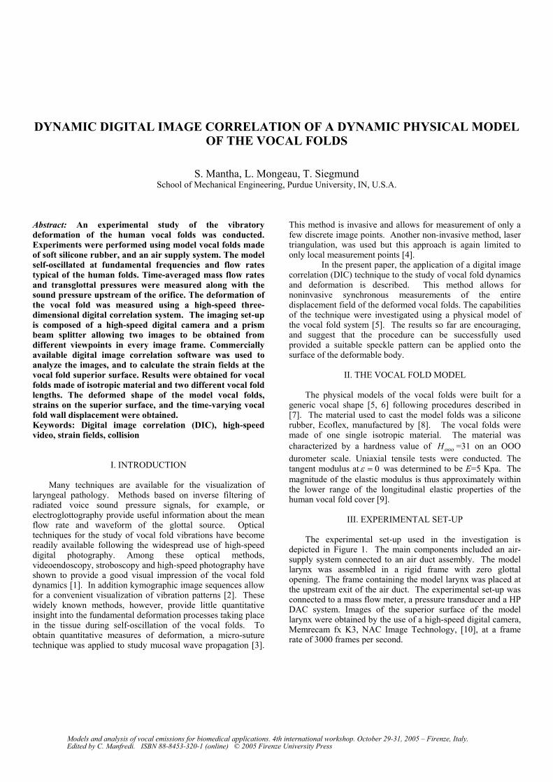
DYNAMIC DIGITAL IMAGE CORRELATION OF A DYNAMIC PHYSICAL MODEL OF THE VOCAL FOLDS

S. Mantha, L. Mongeau, T. Siegmund School of Mechanical Engineering, Purdue University, IN, U.S.A.

Abstract: An experimental study of the vibratory deformation of the human vocal folds was conducted. Experiments were performed using model vocal folds made of soft silicone rubber, and an air supply system. The model self-oscillated at fundamental frequencies and flow rates typical of the human folds. Time-averaged mass flow rates and transglottal pressures were measured along with the sound pressure upstream of the orifice. The deformation of the vocal fold was measured using a high-speed three-dimensional digital correlation system. The imaging set-up is composed of a high-speed digital camera and a prism beam splitter allowing two images to be obtained from different viewpoints in every image frame. Commercially available digital image correlation software was used to analyze the images, and to calculate the strain fields at the vocal fold superior surface. Results were obtained for vocal folds made of isotropic material and two different vocal fold lengths. The deformed shape of the model vocal folds, strains on the superior surface, and the time-varying vocal fold wall displacement were obtained. Keywords: Digital image correlation (DIC), high-speed video, strain fields, collision

I. INTRODUCTION

Many techniques are available for the visualization of laryngeal pathology. Methods based on inverse filtering of radiated voice sound pressure signals, for example, or electroglottography provide useful information about the mean flow rate and waveform of the glottal source. Optical techniques for the study of vocal fold vibrations have become readily available following the widespread use of high-speed digital photography. Among these optical methods, videoendoscopy, stroboscopy and high-speed photography have shown to provide a good visual impression of the vocal fold dynamics [1]. In addition kymographic image sequences allow for a convenient visualization of vibration patterns [2]. These widely known methods, however, provide little quantitative insight into the fundamental deformation processes taking place in the tissue during self-oscillation of the vocal folds. To obtain quantitative measures of deformation, a micro-suture technique was applied to study mucosal wave propagation [3].

This method is invasive and allows for measurement of only a few discrete image points. Another non-invasive method, laser triangulation, was used but this approach is again limited to only local measurement points [4].

In the present paper, the application of a digital image correlation (DIC) technique to the study of vocal fold dynamics and deformation is described. This method allows for noninvasive synchronous measurements of the entire displacement field of the deformed vocal folds. The capabilities of the technique were investigated using a physical model of the vocal fold system [5]. The results so far are encouraging, and suggest that the procedure can be successfully used provided a suitable speckle pattern can be applied onto the surface of the deformable body.

II. THE VOCAL FOLD MODEL

The physical models of the vocal folds were built for a generic vocal shape [5, 6] following procedures described in [7]. The material used to cast the model folds was a silicone rubber, Ecoflex, manufactured by [8]. The vocal folds were made of one single isotropic material. The material was characterized by a hardness value of oooH =31 on an OOO durometer scale. Uniaxial tensile tests were conducted. The tangent modulus at 0ε = was determined to be E=5 Kpa. The magnitude of the elastic modulus is thus approximately within the lower range of the longitudinal elastic properties of the human vocal fold cover [9].

III. EXPERIMENTAL SET-UP

The experimental set-up used in the investigation is

depicted in Figure 1. The main components included an air-supply system connected to an air duct assembly. The model larynx was assembled in a rigid frame with zero glottal opening. The frame containing the model larynx was placed at the upstream exit of the air duct. The experimental set-up was connected to a mass flow meter, a pressure transducer and a HP DAC system. Images of the superior surface of the model larynx were obtained by the use of a high-speed digital camera, Memrecam fx K3, NAC Image Technology, [10], at a frame rate of 3000 frames per second.


Figure 1: Experimental set-up.

(a)

(b)

Figure 2: Tracking a point on the superior vocal fold surface from (a) a reference to (b) a deformed state through

gray value patterns in subsets. A 3D-DIC system was employed. The analysis consists of

two steps: (a) a stereo correlation technique to determine in plane displacements (u, v) [11] and (b) stereo triangulation [12] to obtain the out-of-plane deformation (w). For the determination of the in-plane displacements through a DIC analysis, images of the object under consideration at two different stages of deformation were compared; see Fig. 2(a) for the image of the reference state and Fig. 2(b) for the image of the deformed state. The stereo correlation analysis requires that any point in the undeformed stage of the object, 0x is matched with the corresponding point in the deformed stage, 0x x u= + . In DIC, such a correlation is obtained by searching for matching gray scale patterns in corresponding images. So-called “subsets”, i.e. parts of digital images, are traced via their gray value distribution from the undeformed reference image to the deformed image, as shown Fig. 2. The uniqueness of the matching lies on the creation of a non-repetitive speckle pattern on the object’s surface. To obtain the speckle pattern, first a white pigment was mixed into the silicone rubber material during model preparation. Subsequently, black enamel paint was used to obtain the speckle pattern on the superior surface of the pseudo vocal folds. The application of the speckle pattern to the pseudo vocal folds is non-invasive and did not add any significant mass to the system.

For the stereo triangulation, two images of the object at each stage of deformation are required in order to obtain the out-of-plane displacement information. This was accomplished by obtaining two images of the object simultaneously in one single CCD frame at each time instant through the placement of a beam splitter in the optical axis

between the camera and the model larynx, Fig. 3. With this set-up two images of the model larynx are obtained at offset image positions and are recorded on a common digital image frame. These images provide a “left” and “right” view of the model larynx. Thus, the deformed shape of the vocal folds can be obtained by triangulation.

“Left” Image CCD “Right” Image

Mirror

Vocal Folds

Prism

Mirror

Air

Figure 3: Image set-up with beam splitter. (Figure not to

scale) The digital image correlation analysis was performed using

the program VIC-3D [13]. In the specific version of the program employed here, the image correlation was accomplished using an iterative spatial domain-correlation algorithm [14]. Calibration for focal length, image center and lens distortion was performed using a calibration target.

IV. RESULTS

Experiments were conducted on two larynx models with

lengths L = 17 mm and 22 mm, respectively. First, for each model, the airflow rate was increased stepwise until self-oscillation was detected. Table 1 summarizes the phonation onset data. Phonation frequencies and onset pressures were within the range of physiological values. Six measurements were undertaken at higher mass flow rates, beyond the phonation threshold. The phonation frequency changed slightly as the mass flow rate was increased, Fig. 4(a). A maximum in the measured phonation frequency was reached for a flow rate of 550 cc/s. As discussed in the following, this behavior is associated with the onset of the occurrence of vocal fold closure and collision. Collision occurred at a vocal fold length dependent critical mass flow rate. For both models a linear relationship between pressure and mass flow rate was obtained, Fig. 4(b).

Kymographic images, shown in Figure 5, were obtained for L=22 mm at flow rates of 406 and 690 cm3/s. These images clearly demonstrate the difference between the vibration processes at low and high flow rates. At low flow rates, no closing or collision of the vocal folds was observed. At larger flow rates, significant closure and collision takes place. Low and high flow rate regimes are distinguished based on the flow rate – frequency response such that a drop in frequency was observed for flow rates beyond the onset of closure/collision.

L=17 mm L=22 mm Onset pressure 0.73 Kpa 0.87 Kpa Mass flow rate 165 cm3/s 406 cm3/s Phonation frequency 92.9 Hz 88.75Hz

Table 1: Phonation onset data of model larynx.

0x

0xu

High Speed Digital

Camera

Beam Splitter Physical Model and the Air Duct Assembly

126 MAVEBA 2005

(a)

(b)

Figure 4: (a) Phonation frequency vs. Subglottal Pressure;

(b) Subglottal pressure vs. mass flow rate for the model with L=17 mm and 22 mm

(a) (b) Figure 5: Sequence of five kymographic images (produced

from a single kymographic image) for (a) flow rate of 406 cm3/s (the phonation threshold), and (b) flow rate of 690 cm3/s. The Kymographic image location indicated by a line in Figs.

6(a) and (c). L=22 mm. Figure 6 shows typical digital image analysis results.

Superior views of the model larynx are shown for a flow rate of 690 cm3/s at maximum glottal opening, Fig. 6(a), and during the stage of glottal closure, Fig. 6(c). Figures 6(b) and (d)

shows the distribution of the transverse strain component, xxε obtained from DIC on the superior surface for the images in Fig. 6(a) and (c), respectively. The strain contours are shown on the deformed superior surface. In the position of maximum opening the vocal folds are deformed by a combination of a bulging-type deformation and the opening motion. The maximum value of the out-of-plane displacement was determined to be maxw = 3.5 mm. This value is larger than that reported in humans, e.g. in [4] maxw = 1.5 mm was reported. At the point of maximum glottal opening, the transverse strain, xxε , is less than zero at the mid-section of the superior surface. During the closing process vocal fold contact occurs, Fig. 6(c). Closure of the glottal opening is not complete and two distinct open areas are visible during the closing stage. These open areas are located at the anterior and posterior ends of the model larynx; see Fig. 6(c). Such incomplete closure has been observed in actual glottal measurements [15] and 3D finite element simulations [16]. Even during the closing stage the model larynx retains some of the bulging deformation. A local minimum of the out- of-plane displacement is seen at the midsection of the superior surface, 1.65w = mm, while the two locations of maximum out-of-plane displacement, 1.81w = mm, coincide with the locations of partial opening. During closure the characteristics of the strain fields changes significantly. At the midsection of the vocal folds the strain, xxε , is positive (tensile stress) and significant in amplitude, 0.1xxε ≈ .

(a) (b)

(c) (d)

Figure 6: The model larynx ( L = 22 mm, flow rate of 690 cm3/s) (a) Image at maximum open position; and (b) contour of

xxε ; (c) image for closed state; and (d) contour of xxε .

0.1-0.047

Time = 11.33 ms

(a)−10 −5 0 5 10

0

0.5

1

1.5

2

2.5

3

Y [mm]

W [m

m] d

urin

g C

losi

ng

(b)−10 −5 0 5 10

0

0.5

1

1.5

2

2.5

3

Y [mm]

W [m

m] d

urin

g O

peni

ng

(c)−10 −5 0 5 10

0

0.5

1

1.5

Y [mm]

U [m

m] d

urin

g C

losi

ng

(d)−10 −5 0 5 10

0

0.5

1

1.5

Y [mm]

U [m

m] d

urin

g O

peni

ng

Figure 7: Out-of plane (a, b) and in-plane (c,d) displacements along the medial surface. L=22mm

The DIC method was also used to extract details of the

time history of the wall displacement. Figure 7 shows the out-of-plane ( w ) and in-plane ( u ) displacements obtained for points along a line parallel to the medial surface at a position 1.5 mm from the centerline of the undeformed larynx for a flow rate of 406 cm3/s. Fig. 7(a) and (b) show that the model larynx remains in a bulged state due to the mean static pressure in all stages, maxw =2.63 mm and minw =1.72 mm. The main out-of-

plane vibratory displacements occur in the center of the vocal fold over a span of around L/2 with the outer parts of the folds almost fixed during oscillation. The range of the out-of-plane displacement was found to be w∆ = 0.91 mm. Figs. 7(c) and (d) illustrate the process of glottal opening. The model larynx remains in an open state due to the mean static pressure in all stages, maxu =1.45 mm and min 0.40u = mm. The main vibratory displacement occurs again in the center section of the vocal fold over a length of 3L/4. The range of the in-plane displacement was u∆ = 1.10 mm.

V. CONCLUSION

The application of a three-dimensional DIC method for the

non-contact and non-invasive measurements of displacement and strain fields in self-oscillating vocal folds has been described. The method was implemented and applied in the laboratory to measurements of the superior vocal fold surface of a rubber physical model. It provided time-resolved, full field measurements of several parameters of interest in phonation studies, including the out-of-plane displacements (the so-called mucosal wave height), the glottal opening displacement, as well as the strain fields corresponding to these displacements. The study demonstrates the linear dependence of subglottal pressure over mass flow rate and also the effectiveness of DIC method in estimating the strain fields. Furthermore, it was found that while the out-of-plane displacements exceed those of the in-plane displacements, the vibration amplitudes of these two degrees of freedom are similar. Stress will be obtained from measured mechanical properties of the solid in future studies. The outlook for applications in clinical studies is promising. ACKNOWLEDGMENTS

This work was supported by grant R01 DC005788 from the National Institute for Deafness and other Communication Disorders (NIH-NIDCD). REFERENCES [1] Tigges, M., et al., Proc. SPIE Vol. 2927 (1996) 209-216. [2] Švec, J. G., et al., J. Acoust. Soc. Am. 108 (2000) pp. 1397. [3] Berry, D.A., et al., J. Acoust. Soc. Am. 110(2001) pp. 2539. [4] Manneberg, G., et al., Opt. Eng. 40 (2001) 2041-2044. [5] Thomson, S. L., Ph.D. Thesis, Purdue University, 2004 [6] Scherer, R.C., et al., J. Acoust. Soc. Am. 109 (2001) pp.1616. [7] Thomson, S. L., et al. MAVEBA 2003. [8] Smooth-On, Inc. [9] Zhang, K., et al., J. Acoust. Soc. Am. (2005) submitted. [10] NAC Image Technology, Inc. [11] Chu, C.T., et al., Exp. Mech. 25 (1985) pp. 232. [12] Helm, J.D., Opt. Eng. 36 (1997) pp. 2361. [13] Correlated Solutions, Inc. [14] Sutton P., et al., Image Vision Comp. 4 (1986) pp. 143. [15] Holzrichter, J.F., et al. J. Acoust. Soc. Am. 117 (2005) pp. 1373. [16] de Oliveira Rosa, M., et al. J. Acoust. Soc. Am. 114 (2003) pp. 2893.

128 MAVEBA 2005

Abstract: Six methods for endoscopic motion com-pensation for laryngeal high-speed videoendoscopy(HSV) are compared. Two of them are based ontracking the maximum of the cross-correlation func-tion of two images; two are based on minimization ofthe L2–norm and L2-like distance between two ima-ges; and the other two make use of the peak presentin the cross-power FFT-based spectrum of twoimages. All six methods are applied to compensatethe motion, at the sub-pixel level, of the endoscopiclens relative to the vocal folds in HSV recordings. Thenew motion compensation methods based on FFTcross-power spectrum demonstrated remarkablecomputational speed and acceptable accuracy. Whileaccuracy was best for the L2-minimization techni-ques, they were slower and had a limited motion-tracking range.

I. INTRODUCTION

Sub-pixel compensation of endoscopic (camera lens)motion in high-speed videoendoscopy (HSV) is animperative preprocessing operation making furtherautomatic evaluation of vocal fold movement possible[1]. Endoscopic motion affects the time alignment of theHSV image pixels, which makes it difficult to track thedynamic characteristics of the laryngeal anatomicstructures (Fig.1). Successful applications of HSVmotion compensation (MC) techniques have beenrecently reported in [1], where the MC method wasbased on minimizing the L2-distortion of the smoothtime differential of HSV using convolution. The resultsdemonstrated that sub-pixel endoscopic MC is a valid,reliable, and accurate technique with immediatepossibility of implementation in laryngeal HSV and thatthe MC technique can be further optimized for speed andperformance. No other studies specifically addressingMC of HSV have been published.

This study proposed, implemented and tested severaltechniques, optimized for speed, as an alternative to [1].Of particular interest is a new, and very fast, FFT-basedmethod [2-6], which allows the estimation of the spatialshift of two similar images. The different versions of thismethod are compared in [7].

The problem of endoscopic MC for HSV is complexdue to the dynamics of the vocal folds during phonation(Fig.1). Laryngeal HSV is essentially different from anyother medical image because it registers the motion of anorgan that moves very fast (70-400 Hz), affectingpractically all connected tissues and creating motion

across the whole image. The motion of the connectedtissues contains a fast component, comparable in speedwith the vocal folds, but also slower components, someof which are comparable with the speed of theendoscopic motion (less than 15 Hz). No clear spatialoutlier can show the motion relative to the camera lenslocated on the tip of the endoscope. Fortunately, theendoscopic motion and the changes in the glottis duringphonation have different dynamics. This dynamicdifference is used to build the missing outlier bycomputing the time differentials of the HSV imagesequence pixel by pixel [1].

Fig. 1. Open and closed phase of the vocalfolds in two different x-y positions.

Fig. 2. Smoothed time-differential images ofvocal folds in two different x-y positions.

In order to dynamically separate the fast vocal foldmovements from the slow camera lens motion it isnecessary to smooth the HSV. Smoothing of the timedifferential of the HSV image (Fig.2) has been found tobe very effective when building the missing spatialoutlier for endoscopic motion tracking [1]. Largersmoothing enhances MC when low-pitch or irregularvocal fold vibrations are present, however it might limitthe responsiveness of the MC techniques to fastendoscopic motion.

FAST FFT-BASED MOTION COMPENSATIONFOR LARYNGEAL HIGH-SPEED VIDEOENDOSCOPY

Szymon Cieciwa1, Dimitar D. Deliyski2, Tomasz P. Zielinski1

1 Department of Instrumentation and Measurement, AGH University of Science and Technology, Cracow, Poland2 Department of Communication Sciences and Disorders, University of South Carolina, Columbia, South Carolina, USA


II. METHODOLOGY

A. Motion Compensation Methods

Given that f1(x, y ) and f2(x, y) are two continuousfunctions, in this case two images, where the secondfunction is a shifted in space version of the first one:f2(x, y) = f1(x−x0, y-y0), we can find the displacement{x0, y0} making use of one of the following methods.

a

-100-50

050

100

-100

0

100

1

2

3

4

5

x 107

dxdy

z

b

-20

2

-20

2

5.35

5.4

5.45

5.5

5.55

x 107

dxdy

z

-100

10

-100

10

2

3

45

6

x 105

dxdy

z

c

-20

2

-20

2

1.5

2

2.5

x 105

dxdy

z

-10-5

05

10

-10

0

10

0

0.2

0.4

xy

z

-20

2

-20

2

-0.2

0

0.2

0.4

0.6

dxdy

z

Fig. 3. Detection matrices (similarity measures) for differentmethods used for HSV motion detection: left – higher searchingrange; right – lower searching range after interpolation (dx = a,dy = b); a) maximum of correlation similarity; b) minimum of L2-

like similarity; c) peak for cross-power spectrum similarity.

Correlation function methods. The classic method for{x0, y0} detection relies on the properties of theconvolution (cross-correlation) function of f1(x, y) andf2(x, y), which is defined as follows:

DC (a,b) = f1(x, y) f2 (x + a, y + b)dxdy

-∞

∞

∫-∞

∞

∫ (1)

The function DC(a, b) reaches its maximum for a = x0

and b = y0. However, the maximum is flat (as shown inFig.3a) and computation is time consuming. We canobserve that f2(x, y) is shifted back by x and y dimensionsby a and b, to fit the original image f1(x, y). This methodcan be realized by computing the convolution function oftwo images, which is slow. Speed optimization can beachieved by defining equation (1a) D∆∆(a, b)=DC(a, b)for a limited range of a and b [1]. Such approach isappropriate when estimating small shifts within 5 pixels.L2–norm and L2-difference minimization methods. Thespatial shifts can be determined simply by minimizing

the difference between two images while artificiallyshifting one of them and computing a similarity measureof their difference, such as:

D

|∆|2(a,b) = f1(x, y) − f2 (x + a, y + b)

2dxdy

-∞

∞

∫-∞

∞

∫ (2)

D|∆|(a,b) = f1(x, y) − f2 (x + a, y + b) dxdy

-∞

∞

∫-∞

∞

∫ (3)

where (2) represents the L2-norm measure of the imagedifference, while (3) is a L2-like measure known as theaverage magnitude difference function (AMDF). Theminima of such functions are flat as it is shown inFig.3b.

FFT-based cross-power spectrum method. It is knownthat Fourier spectra of images f1(x, y) and f2(x, y) arerelated as:

F2 (ωx ,ωy ) = F1(ωx ,ωy ) " e j (ωx .x0 +ωy .y0 ) (4)

where F1(ωx, ωy) and F 2(ωx, ωy) denote Fouriertransforms of both images. Since it can be shown that:

G12 (ωx ,ωy ) =F2 (ωx ,ωy ) " ′F1(ωx ,ωy )

F2 (ωx ,ωy ) " ′F1(ωx ,ωy )= e j (ωx .x0 +ωy .y0 ) (5)

the inverse Fourier transform of G12(ωx, ωy) results in:

g12 x, y( ) = Fourier−1 G12 ωx ,ωy( )#

$%& (6)

characterized by a sharp Dirac delta function centered at(x0, y0) (Fig.3c-left). This property is very useful formotion detection. In the discrete case above, the propertystill holds, and direct and inverse fast Fourier transformalgorithms can be applied. Thus, the Dirac impulse takesa form of a 2D sinc function, the interpolation of whichis presented in Fig.3c-right.

φ x, y( ) =sin π x + x0( )#

$%&

π x + x0( )'sin π y + y0( )#

$%&

π y + y0( ) (7)

The project described herein studied a variety of sub-pixel adaptations based on this method. Only the mostsuccessful two of these are presented.

Sub-pixel extensions. Similarity matrices DC(a, b) (1),D∆∆(a, b) (1a), D |∆|

2(a, b) (2), D |∆|(a, b) (3), andΦ(x, y) (7) can be easily interpolated as it is shown inFig.3-right for sub-ranges (-amax, amax) and (-bmax, bmax)around the extrema. Adaptive strategies for changing thevalues of a and b can be applied.

Such strategy is to replace the interpolation of the 2Dsinc Dirac impulse (7) (Fig.3c-left) with more effectivetechniques, as presented below.

For discrete images (4) can be presented as follows:

)//(212 ),(),( cr NccNrrjecrFcrF ∆"+∆""= π (8)

130 MAVEBA 2005130 MAVEBA 2005

where r and c denote row and column index,respectively, and Nr and N c designate number of rowsand columns. Phases of these spectra are related by:

[ ] [ ] !"

#$%

& Λ(+

∆(+Φ=Φ

cr Nc

cNr

rcrFcrF π2),(),( 12

or equivalently:

[ ] [ ] [ ] [ ]crcrFcrFcr !+!=Φ−Φ=Φ βα),(),(, 12,

where:

α = 2π∆r / Nr ,

β = 2π∆c / Nc

(9)

As shown, Φ[r, c] is a 2D discrete function describinga plane in 3D space (i.e. points Φ(ri, ci) lay on a plane).After estimation of α and β coefficients’ values on thisplane, we can calculate the shift between images from(9). The computation of α and β is reduced to a simpleleast square problem easily solvable when the values ofthe function Φ[r, c] are known for at least two points

r1 c1

r2 c2

n nrK cK

!

"

#####

$

%

&&&&&

α

β

!

"#$

%& =

Φ(r1,c1)

Φ(r2 ,c2 )

nΦ(rK ,cK )

!

"

#####

$

%

&&&&&

(10)

Ax = b

that can be solved in a least square (LS) sense:

x = (AT A)−1AT b = pinv(A) "b (11)

In Matlab language (11) is equivalent to x = A\b.

B. Experimental Design

Initial Testing of Basic Methods: The first step towarddeveloping a robust MC algorithm was to test theaccuracy and speed performance of the basic functionsfor detection of spatial shifts described in the previoussection. The performance of the following basicfunctions was compared on artificially shifted by x and yimages at different shift directions and magnitudes:Convolution DC(a, b) (1), Correlation D∆∆(a, b) (1a), L2-norm D|∆|

2(a, b) (2), AMDF D|∆|(a, b) (3), FFT CPΦ(x, y) (7), and FFT LS which is FFT CP with an LSextension replacing the interpolation. Three parameterswere reported: average execution time (in ms); meanabsolute error εM (in pixels by x and y); and absoluterange of error εR (in pixels by x and y ). Thesemeasurements do not warrant accuracy of the whole MCimplementation.

MC Algorithm: The MC algorithm implemented in theseexperiments was the same algorithm used in [1] with the

basic functions replacing the Convolution function. Itconsists of the following main steps: (i) Establishingdynamic vocal fold outliers for MC by computing pixelby pixel the time differentials of the HSV imagesequence; (ii) Eliminating the high-frequencycomponents of the vibrating vocal folds via smoothing;(iii) Suppressing the effect of the boundarydiscontinuities of the image frames (only necessary forConvolution); (iv) Detecting the displacement betweenadjacent frames by using one of the six methods;(v) Computing the displacement vectors (motiontrajectories); (vi) Subtracting the motion trajectoriesfrom the spatial coordinates of the original HSV imageusing two-dimensional spline interpolation.

Performance on Simulated Motion: To assess theaccuracy in extreme conditions, the MC method wastested on simulated data with known motion trajectories.These data are identical to and described in more detailin [1]. Although the proposed methods are expected towork better for lower motion frequencies, these dataallow for a thorough testing in extreme conditions, inwhich all frequencies of the covered range 0.1 to 15 Hzare equally represented. The data consisted of 2-secondlong (4000 frames) HSV movies with exactly knownmotion trajectories. Motion varied from 0 to 8 pixels byx and y in nine different magnitudes. Two types ofmotion curves, a random and a cyclic, were added to tworeal HSV recordings, one of a male and one of a femalespeaker, totaling 34 HSV recordings with simulatedmotion. The data were analyzed by each modifiedtechnique. The following parameters were reported:average speed of computation SC (in seconds per onesecond of HSV data); mean absolute error εM andabsolute range of error εR (in pixels) as defined in [1].Assessing the MC method on data with simulated motionwas important to show whether the detected trajectoriesreally correspond to motion and to assess the accuracy ofthe method in extreme motion conditions with knowncharacteristics.

Performance on Real Motion: Testing the MC methodson real HSV data is important to account for factorsunaccounted for in simulated motion such as nonuniformillumination, quality of the image, scaling, cameraartifacts, and differences in glottal shapes, which arelikely to affect the reliability of MC. The error iscomputed by iterating the MC process since theestimated motion trajectory at the second iteration is theresidual motion not compensated for during the firstiteration.

III. RESULTS AND DISCUSSION

Basic Methods: The results obtained from testing thebasic MC methods are presented in Table 1. The FFT-based techniques were found to be several times fasterrelative to the correlation and L2-based techniques. L2-

norm and FFT LS were found to be the most accurate.Additional observations include: noise was not found tobe destructive for tracking shifts, and all methods exceptfor FFT CP were more sensitive to horizontalmovement, since vocal folds are vertical.

Table 1: Comparison of accuracy and speed of the newlyimplemented basic methods for motion compensation.

εM

[pixels]εR

[pixels]MC methodTime[ms]

by x by y by x by y

Convolution 2700 0.07 0.07 0.16 0.12Correlation 380 0.14 0.09 0.51 0.15L2-norm 460 0.09 0.07 0.24 0.13AMDF 460 0.20 0.17 0.27 0.21FFT CP 140 0.23 0.22 0.52 0.57FFT LS 60 0.08 0.07 0.40 0.22

Data with Simulated Motion: The results from testingthe MC algorithms on simulated motion are shown inTable 2. They generally agree with the results fromtesting the basic methods. All MC methods demonstratedsatisfactory sub-pixel accuracy and all alternative tech-niques were significantly faster relative to Convolution.

Table 2: Accuracy (average with range in partheses) andspeed of computation results from testing six MCalgorithms on 34 HSV samples with simulated motion.

MC methodSC

[s/s]εM

[pixels]εR

[pixels]

Convolution 513.3060.168

(0.000-0.331)0.380

(0.000-0.931)

Correlation 33.5560.064

(0.000-0.181)0.221

(0.000-0.664)

L2-norm 35.2590.064

(0.000-0.181)0.221

(0.000-0.664)

AMDF 34.4300.069

(0.000-0.188)0.229

(0.000-0.677)

FFT CP 14.0390.091

(0.000-0.351)0.538

(0.000-2.904)

FFT LS 7.6440.272

(0.002-0.577)0.606

(0.003-2.241)

Correlation, L2-norm and AMDF had almost identicalperformance and best accuracy of all methods. Theirmean absolute error was 0.065 pixels and their speed ofcomputation was 15 times higher relative toConvolution. The serious disadvantage of these threemethods is their limited range of shift tracking, whichlimits their implementation for certain types of HSVmaterial. They would have difficulties with recordingsincluding phonatory breaks, vocal offsets and onsets, orintermittent obstructions in the view of the vibratingvocal folds, making it difficult to recover when visiblevibration resumes. Convolution, FFT CP and FFT LS donot have this limitation.

The fastest methods were FFT LS and FFT CPoutperforming C o n v o l u t i o n 67 and 37 times,respectively. The accuracy of these two methods waslower but still acceptable at the sub-pixel level. Theincreased error was mainly due to the extreme frequencytesting conditions to which the methods were subjected.Considering the exceptional robustness of the FFT LSmethod, further investigation is necessary to understandand eliminate the sources of errors in order to build apractical tool for motion compensation, which is highlynecessary.

Data with Real Motion: A limited testing on real clinicalHSV recordings (14 samples) was performed. Resultswere consistent with the data from Table 2. Speed ratiosand accuracy data were found to be in the sameproportions. On the 2nd iteration the residual errors werefound to be smaller relative to the data with simulatedmotion. As expected, Correlation, L2-norm and AMDFcould not track over shifts including voice offsets, onsetsand breaks, while Convolution, FFT CP and FFT LScould. No instances of data degradation were reported upto the 4th iteration for Convolution, FFT CP and FFT LS.

IV. CONCLUSION

The fast FFT-based approach has been appliedsuccessfully for the endoscopic motion compensation inHSV recordings of vocal folds. Results demonstratedthat application of the FFT-based cross-power spectrumapproach is highly beneficial: the method is 67 timesfaster than the convolution-based approach and offersacceptable sub-pixel accuracy. Further improvement ofaccuracy is possible and testing on a large dataset of realHSV recordings is recommended.

REFERENCES[1] D. Deliyski: “Endoscope Motion Compensation forLaryngeal High-Speed Videoendoscopy,” Journal of Voice,vol. 19, no. 3, pp. 485-496, 2005.[2] H. Shekarforoush, M. Berthod, J. Zerubia: “Subpixel ImageRegistration by Estimating the Polyphase Decomposition of theCross Power Spectrum,” Int. Conf. on Computer Vision andPattern Recognition, 1996.[3] H. Foroosh, J. Zerubia, M. Berthod: “Extension of phasecorrelation to sub-pixel registration,” IEEE Trans. on ImageProcessing, vol. 11, no.3, pp. 188-200, 2002.[4] H. Stone, M. Orchard, E.-C. Chang, S. Martucci: “A fastdirect Fourier-based algorithm for subpixel registration ofimages,” IEEE Trans. on Geo. and Remote Sensing, vol. 39,no. 10, pp.2235-2243, Oct. 2001.[5] Y. Keller, A. Averbuch: “A projection-based extension ofthe phase correlation method,” submitted to the IEEETransactions on Signal Processing, 2005.[6] H. Tuo, L. Zhang, Y. Liu: “An FFT-based registrationmethods for images from different bands,“ Int. Conf. onInformation Technology & Applications iCITA'05, Sidney2005[7] V. Argyriou, T. Vlachos: “Using gradient correlation forsub-pixel motion estimation of video sequences,” IEEE Int.Conference on Acoustics, Speech and Signal ProcessingICASSP-2004, Montreal 2004.

132 MAVEBA 2005132 MAVEBA 2005

Abstract: Vertical motion of the vocal folds during

phonation is a possible diagnostically significant

feature. However, it is difficult to judge vertical

motion through the typical two-dimensional

stroboscopic display. Through high-speed videoendo-

scopy (HSV), the dynamics of vocal fold vibration are

easier to appreciate; however, the traditional HSV is

also two-dimensional. Recently, a method to display a

three-dimensional (3D) image of vocal fold vibration

was published. This method, as well as stroboscopy

and HSV, was utilized to study vertical motion

magnitude and symmetry during modal and pressed

phonations in normophonic speakers. Vertical motion

judgments were rated as at least 16% more possible

from the HSV-derived playbacks than from

stroboscopy. The assessments from the 3D playback

were different than those from the two-dimensional

HSV playback for magnitude, however a similar trend

was realized. The findings demonstrate consistently

greater magnitudes of vertical motion during pressed

phonations. Asymmetry of vertical motion was

appreciated in both modal and pressed phonations.

The results of this study concur with the concept of

increased vertical motion during pressed phonation

and recommend further investigations of the

typicality of this important feature of vocal fold

vibration in various modes and registers of normal

and pathologically influenced phonation.

I. INTRODUCTION

Visualizing vocal fold vibratory behavior is widely

accepted as an integral part of a complete voice

evaluation. This vibratory behavior is known to move in

three dimensions: laterally, longitudinally, and vertically.

The lateral movement of vocal fold vibration is the most

widely discussed and utilized in clinical voice evaluations

as an indication of vocal fold stiffness. The longitudinal

motion of vocal fold vibration has begun to be

investigated and used as part of the clinical visualization

protocol. However, the normal limits of variation in

longitudinal motion remain unclear. The third dimension

of vocal fold vibration, vertical motion is not a common

feature rated during the stroboscopic evaluation. While

furthering our knowledge of lateral and longitudinal vocal

fold vibratory deviations and their prevalence in various

disorders is an important task, this paper narrows its

scope to investigating the vertical motion of vocal fold

vibration.

Vertical motion of vocal fold vibration has been

suggested to have an increased magnitude during pressed

or heavy phonations [1]. Hirano has related pressed

phonation to be a result of the contraction of the

thyroarytenoid muscle and relaxation of the vocal

ligament [2]. This relation of the physiological

components has been furthered to provide the concept

that the relaxed vocal ligament may lead to an increase in

pliable tissue, which may then be prone to move

vertically during pressed phonation [1]. Conversely, less

vertical motion may be appreciated during modal and,

especially, falsetto phonations due to increased tension in

the vocal ligament.

An increase in vertical motion during pressed

phonation is a suggested contributing factor in the vocal

fold pathologies of nodules and varices [1,3,4]. Pressed

phonation is often realized in persons with voice

disorders characterized by strain and muscle tension

dysphonia. Given the relation between these common

features of functional voice disorders and pressed

phonation, it is natural to continue the investigation of

vertical motion by studying the vibratory patterns during

differing modes of phonation.

An in-depth paper on the presence and hypothetical

detrimental impact of vertical motion in vocal fold

vibration was accomplished [1]. The increase of vertical

motion in pressed versus falsetto phonation was

demonstrated, as was the intra-cycle variability of vertical

motion during pressed phonation. These findings for

vertical motion rely on visualization techniques, such as

HSV, that provide true intra-cycle information.

Studies of the medial surface of the vocal folds in

excised larynges using HSV have allowed for the

observation of the vertical motion of vocal fold vibration

from a view not achievable clinically [5,6]. Within such

investigations, the presence of lateral, longitudinal, and

vertical components of vocal fold vibration have been

documented and relatively quantified. The variation of

subglottal and supraglottal pressure as well as vocal fold

tension has been noted to impact these components of

vocal fold vibration in excised larynges.

While vertical motion appears to be a fundamental

feature of vocal fold vibration, the difficulty of rating a

three-dimensional behavior with intra-cycle variations

from stroboscopy, a two-dimensional representation

without intra-cycle information, remains. Recently, a

comprehensive set of representations and image

VERTICAL MOTION DURING MODAL AND PRESSED PHONATION:

MAGNITUDE AND SYMMETRY

Heather S. Shaw, Dimitar D. DeliyskiDepartment of Communication Sciences and Disorders, University of South Carolina, Columbia, South Carolina, USA


processing techniques to extract significant vocal fold

features from HSV images was introduced [7]. Of

particular interest to this paper is the vertical motion

display, which allows for the observation of vertical

motion from a three-dimensional (3D) playback. This

technique capitalizes on the fact that the pixel intensity of

the image is a quadratic function of the distance between

the vocal folds, and the light source and camera lens.

Thus, allowing pixel intensity to provide information

regarding vertical motion. The specific implementation of

the 3D display was presented at the Voice Foundation

Symposium in June 2005.

The purpose of this study is to provide a preliminary

investigation of the vertical motion inherent in vocal fold

vibration. The research questions to achieve this goal

were:

1. Can vertical motion be assessed through a

three-dimensional display?

2. What is the variation in vertical motion and

vertical level of approximation for

normophonic speakers?

3. Does the amount of vertical motion vary with

mode of phonation?

II. METHODOLOGY

Participants: Fifty-two vocally normal participants

ranging in age from 18-65 years old were recruited from

Columbia, SC and Charlotte, NC. Twenty-four male and

twenty-eight female participants were divided among

three age ranges, 18-33, 34-49, and 50-65. The data

collection, storage, and use were in accordance with

human subjects regulations. The data for this study was

recorded at Presbyterian Hospital’s Voice Center in

Charlotte, NC. The speech-language pathologists

involved with data collection were specifically trained in

voice and followed a specified protocol. During the

process of accepting participation in the study through the

informed consent form, the participants completed a short

medical and voice history, as well as a modified voice

quality self-assessment. Speech-language pathologists

utilized the history, self-assessment, and perceptual

judgment to determine vocal normality.

Instrumentation and Procedures: Stroboscopy and

HSV were utilized during data collection. Data collection

from new methods and those routinely used in the clinic

allowed for a comparison between assessment methods.

Data collection occurred in quiet rooms typically

employed for the assessment of voice patients in the

hospital clinic.

Endoscopy and Stroboscopy: Standard clinical

procedures were utilized for endoscopy and stroboscopy.

The locating of the vocal folds and the initial phonation

were conducted with continuous halogen light.

Stroboscopy was used to capture phonation at habitual

pitch and loudness allowing both intensity and frequency

to be controlled for during each sample. A Kay

Elemetrics Rhino-Laryngeal Stroboscopic system Model

9100B coupled to a 70-degree rigid endoscope was used.

A laryngeal contact microphone was utilized to track

vocal fold vibratory frequency.

High-Speed Videoendoscopy: Kay Elemetrics High-

Speed Video System Model 9700 equipped with a camera

that captured 2,000 frames per second with 120 x 256

pixel resolution was utilized. A 70-degree rigid

endoscope (Kay Elemetrics Model 9106), the same as

that used in the above described procedures, and a 300 W

constant Xenon light source (Kay Elemetrics Model

7152) were coupled with the system. The recording of

HSV was synchronized with the acoustic recording,

captured via a head-mount condenser microphone, to

allow for comparisons between physiological and

acoustic events. Participants were instructed to phonate

the vowel /i/ at habitual pitch and during pressed

phonation. To achieve pressed phonation, participants

were asked to phonate “as if lifting a heavy box”. The

speech-language pathologists also provided models of

pressed phonation.

The HSV images were processed for motion

compensation [8] and removal of reflection spots

resulting in the HSV playback. Subsequently, the 3D

playback movie, a multi-colored image relating to the

extent of vertical motion of the vocal folds, was

produced, as seen below in Fig. 1.

Fig. 1. Three-dimensional graphic representations of a

closed and open phase within a single glottal cycle.

Visual Perceptual Judgments: Visual perceptual

parameters were developed to assess vertical motion from

the three playbacks, stroboscopy, HSV playback, and the

3D playback. Two voice scientists perceptually evaluated

the dynamic visual images obtained from the fifty-two

participants. The recordings of habitual phonation from

the three playbacks amounted to 156 images that were

judged by each perceptual rater. From HSV and 3D

playbacks, 104 pressed phonation recordings were also

rated. Twenty percent of the recordings were randomly

introduced into the data set to obtain intra-rater reliability.

Therefore, both perceptual raters judged 312 images for

the features of vertical motion and vertical level of

approximation. The entire data set was randomized prior

to perceptual ratings.

Vertical motion was assessed for presence or absence,

magnitude, and for left-to-right vocal fold symmetry of

134 MAVEBA 2005

magnitude through stroboscopy, HSV playback, and 3D

playback. Magnitude of vertical motion was rated,

separately for the left and right vocal folds, on a six-point

scale, with 0=absent, 1=severely decreased,

2=moderately decreased, 3=typical, 4=moderately

increased, and 5=severely increased. Presence of vertical

motion was understood if the magnitude was assigned a

rate of 1-5. Vertical motion symmetry was calculated by

the differences in magnitude ratings. If the ratings of the

left versus right vertical motion magnitude differed, then

the vertical motion magnitude was considered

asymmetrical. Additionally, vertical level of

approximation and ability to judge vertical motion from

the images were rated categorically, as present or absent

and able to judge or not able to judge, respectively.

Statistical Analysis: Measures from the visual-

perceptual judgment of the stroboscopic, HSV, and 3D

playbacks were compared. The instances and percentage

of typical and atypical ratings were calculated.

Correlation and paired t-tests were employed to

determine intra-rater and inter-rater reliability. A

correlation of above 0.70 and/or an alpha level above

0.20 on a paired t-test was considered to demonstrate a

substantial reliability. An alpha level above 0.20 was

utilized to determine the lack of statistically significant

variation between and within the perceptual raters.

III. RESULTS

Presence of vertical motion was noted bilaterally in

stroboscopy, HSV, and 3D playbacks for all instances of

modal and pressed phonations. No cases of unilateral or

absent vertical motion were rated from the recordings of

vocal fold vibration from normophonic speakers. No

differences between stroboscopy, HSV, or the 3D

playbacks was realized.

The magnitude of vertical motion was rated as typical

during modal phonation for 60, 49, and 54% of playbacks

for stroboscopy, HSV, and 3D playbacks, respectively.

For pressed phonation, magnitude of vertical motion was

less likely to be rated as typical, 34 and 42% of cases for

HSV and 3D playbacks. Reduced vertical motion was

realized in 15, 13, and 25% of modal phonations as

visualized through stroboscopy, HSV, and the 3D

playbacks. While during pressed phonations, vertical

motion was appreciated to be reduced in only 10 and 14%

of HSV and 3D playbacks. Increased vertical motion was

apparent in 25, 38, and 21% of visualizations of modal

phonation as displayed by stroboscopy, HSV, and 3D

playbacks. Pressed phonations visualized through HSV

and 3D playbacks were rated as having increased vertical

motion in 56 and 44% of cases.

Asymmetry of vertical motion magnitude was noted in

22, 27, and 12% of modal phonations visualized through

stroboscopy, HSV, and 3D playbacks. For pressed

phonation, 22 and 14% of recordings were perceived as

revealing asymmetrical magnitudes of vertical motion

when viewed by HSV and 3D playbacks.

Vertical level of approximation was rated as unequal

in 14.5, 11, and 14% of modal phonations as viewed by

stroboscopic, HSV, and 3D playbacks. Similarly, for

pressed phonations 11 and 14% of cases rated from HSV

and 3D playbacks had perceivably unequal vertical levels

of approximation.

The ability to judge vertical motion was calculated

from each of the three playbacks. The raters reported not

being able to judge vertical motion for 19% of

stroboscopic files, 3% of 3D playback files, and 1% of

HSV playback files. Files rated as not able to be judged

were excluded from presence, magnitude, symmetry, and

vertical level results.

Intra-rater reliability, as assessed by correlation and t-

tests, was moderate to high for HSV playback and

stroboscopy over both pressed and modal phonation,

ranging from 0.52 to 0.94. For correlations below 0.70,

the t-test had a p-value above 0.30 with the exception of

symmetry rated from stroboscopy by judge 2. Correlation

and t-tests revealed lower intra-rater reliability for

judgments of magnitude from the 3D playback. Inter-

rater reliability as assessed through percent agreement

within one scalar level ranged from 87 to 100%, with a

mean of 96.5%.

IV. DISCUSSION

Presence of vertical motion was apparent throughout

all evaluations of normophonic speakers. Presence was

equally likely during modal and pressed phonations.

Additionally, the three types of displays viewed were

equally sensitive and specific to the presence of vertical

motion. Given the consistency of vertical motion

presence in normophonic speakers, it would be

interesting to ascertain whether persons with voice

disorders, especially those resulting from or resulting in

decreased vocal fold mucosa pliability, demonstrate a

similar consistency.

Magnitude of vertical motion was rated as typical for

58% of the images across all displays for modal

phonation, and for 57% of the images rated from the two

HSV-derived playbacks. These centralized ratings give

credence to the ability to judge the vibratory feature of

magnitude of vertical motion for normophonic speakers

and the ability to utilize the ratings for preliminary

estimates of the typicality of magnitude variations. The

majority of participants exhibited increased magnitude of

vertical motion during pressed phonations. However,

normophonic speakers also demonstrated typical or

decreased vertical motion during pressed phonation.

Typical or decreased vertical motion may have been the

result of achieving the vocal quality of pressed phonation

by manipulating the laryngeal mechanism differently.

Since increased medial compression of the vocal folds

from the contraction of the thyroarytenoid muscles would

lead to an increased amount of pliable tissue, with the

inclusion of the vocal ligament available to move

vertically, it may be hypothesized that decreased medial

compression with increased respiratory volume was

utilized.

While symmetry of vertical motion magnitude has not

been specifically discussed in the literature, a number of

articles have discussed lateral and longitudinal

asymmetries. Given the possible significance of vertical

motion, assessing asymmetry allows for a more

comprehensive view of vibratory behavior. The results

indicate that an average of 19% of normophonic speakers

exhibited asymmetry of vertical motion. The cause of

variation in ratings from the 3D playback, versus the

stroboscopic and HSV playback should be further

explored. It is likely that the added dimension, allowing

for increased accuracy when judging vertical motion, and

the novelty of the 3D playback are the causes of the

differences.

Vertical level of approximation was found to be

unequal for at least 11% of normophonic speakers in

modal and pressed phonations. A difference of 3.5% was

noted between the playbacks. Vertical level was

perceived as unequal more often from the 3D playback

than for the HSV playback. This may be related to the

additional information available from the 3D playback

and the subsequent ability of the raters to use the

information when making judgments of vertical level.

The prevalence of unequal vertical level in normophonic

speakers was unexpected.

The relatively large amount of recordings rated as not

able to be judged from the stroboscopic as compared to

the other playbacks is indicative of the difficulty of rating

this vibratory feature through stroboscopic playbacks.

This difference in ability to judge vertical motion is likely

due to the fact that stroboscopy does not provide true

intra-cycle information. This difficulty is highlighted by

the clinical lack of reporting and utilization of vocal fold

vertical motion as an indicator of laryngeal function. The

widely used visual-perceptual vocal fold rating protocols

include vertical level of approximation, but not vertical

motion. Perhaps clinically important information is being

disregarded.

V. CONCLUSION

The increased magnitude of the vertical motion of

vocal fold vibration during pressed phonation for

normophonic speakers strengthens the hypothesis of the

detrimental impact of this type of phonation on the vocal

fold tissue. There is undoubtedly additional information

regarding vocal fold vibration available through the study

of vertical motion. It is important to understand the

typicality and variation of vertical motion for

normophonic speakers as well as persons with laryngeal

pathology through the clinical perspective of

videoendoscopy, as well as to further investigate vertical

motion using excised larynges.

Given the results of presence, magnitude, and

asymmetry of vertical motion of vocal fold vibration, the

clinical significance of these findings is compelling. An

additional feature of vocal fold vibration that provides

insight into the pliability of the vocal fold mucosa would

be valuable. The finding of unequal vertical level of

approximation in normophonic speakers questions the

typicality of variation in vertical level. Further research to

ascertain the normal limits of vertical level differences

should be undertaken. Additionally, further investigation

of the influence of mode and register of phonation on

vertical motion should be conducted. Studying the effect

of manipulating subglottal pressure during these

productions in vivo will increase our knowledge of the

mechanisms driving vertical motion during phonation.

Since observing vertical motion is reliant on the ability to

visualize intra-cycle information, it is likely that

technological advancements leading to the ability to

capture vocal fold vibration at higher frame rates would

be beneficial. Refinement of the 3D playback to eliminate

the artifacts of light reflection is also necessary.

REFERENCES

[1] A. Sonninen, and A. Laukkanen, “Hypothesis of

whiplike motion as a possible traumatizing mechanism in

vocal fold vibration,” Folia Phoniatrica et Logopaedica,

vol. 55, 189-198, 2003.

[2] M. Hirano, “Vocal mechanisms in singing:

Laryngological and phoniatric aspects,” Journal of Voice,

vol. 2, 51-69, 1998.

[3] I. Hochman, R.E. Hillman, R.T. Sataloff, S.M.

Zeitels, “Ectasias and varices of the vocal fold: Clearing

the striking zone,” Annuals of Otology, Rhinology, and

Laryngology, vol. 108, 10-16, 1999.

[4] P. Grey, “Microlaryngostroboscopy and ‘singers

nodes’,” Journal of the Otolaryngological Society of

Aust, vol. 3, 525-527, 1973.

[5] D.A. Berry, D.W. Montequin, and N. Tayama, “High-

speed digital imaging of the medial surface of the vocal

folds,” Journal of the Acoustical Society of America, vol.

110 (5), 2539-2547, 2001.

[6] I.R. Titze, J.J. Jiang, and T.Y. Hsiao, “Measurement

of mucosal wave-propagation and vertical phase

differences in vocal folds vibration,” Annals of Otology

Rhinology and Laryngology, vol. 102(1), 58-63, 1993.

[7] D.D. Deliyski, and P.P. Petrushev, “Methods for

Objective Assessment of High-Speed Videoendoscopy,”

Proceedings: 6th International Conference: Advances in

Quantitative Laryngology, Voice and Speech Research

AQL-2003, Hamburg, Germany, 28, 1-16, 2003.

[8] D.D. Deliyski, “Endoscope motion compensation for

Laryngeal High-Speed Videoendoscopy,” Journal of

Voice, vol. 19(3), 485-496, 2005.

136 MAVEBA 2005

Abstract: Visualization of the vocal fold structure and

function is imperative for accurate diagnoses and

optimal treatment for persons with voice disorders.

With the advent of commercial High-Speed Video-

endoscopy (HSV) systems, an increased amount of

variation has been appreciated in the diagnostically

relevant features of mucosal wave presence, magni-

tude, and symmetry. This study presents findings

from the assessment of mucosal wave from strobo-

scopy, HSV playback, mucosal wave playback, and

mucosal wave kymography playback. The results

from this study demonstrate the prevalence of featur-

es of ‘atypical’ mucosal wave during modal produc-

tions of /i/ by normophonic persons. Utilizing modal

and pressed phonations, an increased understanding

of the effect of medial compression and increased

subglottal pressure on mucosal wave was realized.

I. INTRODUCTION

One diagnostically significant feature of vocal fold

vibration is the mucosal wave. The mucosal wave is the

propagation of the epithelium and superficial layer of the

lamina propria from the inferior to the superior surface of

the vocal folds during phonation. A typical mucosal

wave, as viewed through stroboscopy, should travel one-

half of the width of the superior surface of the vocal fold

during modal phonation [1]. The mucosal wave of vocal

fold vibration is an accepted indicator of tension and

pliability of the vocal fold tissue. The mucosal wave is

usually reduced during high pitch phonations due to the

excessive tension on the tissues. A reduced mucosal

wave during modal phonation signifies stiffness, which

may result from a lesion, edema, or scar. Conversely, a

larger than normal mucosal wave signifies flaccidity of

the laryngeal musculature underlying the vocal fold

tissue, possibly indicating paresis or muscle atrophy due

to aging. Thus, the importance of assessing mucosal wave

during functional evaluations and for medical diagnoses

is evident. For example, mucosal wave has been the sole

feature of vocal fold vibration that could provide visual

information upon which cysts and polyps could be

differentiated [2].

The characteristics of normal mucosal waves have

been investigated via stroboscopy. Multiple research

articles have included mucosal wave as a dependent

variable to answer various questions regarding normal

and pathological vocal fold movement. Two main areas

of research have investigated the impact of vocal fold

elongation, such as that seen in high frequency

productions, and the impact of variations in subglottal

pressure on mucosal wave magnitude and velocity.

Of interest is a conclusion regarding the typicality of

lateral phase of mucosal wave symmetry in normophonic

speakers in [3]. The results of reviewing fifty-seven

videostroboscopic laryngeal examinations indicated that

asymmetry was appreciated in 10.5% of normophonic

participants during modal and falsetto phonations and in

36.5% of participants during falsetto phonations only.

The conclusion was that the degree of magnitude and not

merely presence of asymmetry should be considered the

diagnostically significant feature. This conclusion leads

to the necessity of further investigation of the symmetry

and magnitude of mucosal waves.

The findings of a prevalent ‘normal’ amount of

asymmetry may lead to an increase in over-diagnoses of

laryngeal pathology, unless the typicality of variation is

understood. Additionally, there is a possibility that

symmetrical mucosal waves with supposed atypical

magnitude may be present in persons with and without

laryngeal pathologies. This finding would modify the

conclusions from [3,4]. Given the prevalence of

asymmetry seen in stroboscopic images and the increased

amount of laryngeal dynamics visible through HSV, it is

intuitive that an even larger population of normophonic

speakers would have apparent variations in mucosal wave

as viewed through HSV in comparison to stroboscopy.

Preliminary studies of the horizontal and vertical

displacements, velocity, and vertical phase of the

mucosal wave have been accomplished utilizing excised

canine larynges [5,6,7]. The results are commensurate

with the findings from in vivo human stroboscopic

studies of mucosal wave. No further investigations of the

typicality of variation in mucosal magnitude or symmetry

have been published.

The purpose of this research was to investigate the

normality of variation of mucosal wave presence,

magnitude, and symmetry and to compare modal and

pressed phonation across these features. The specific

research questions were:

1. What is the variation in mucosal wave

magnitude for normophonic speakers?

2. What degree of mucosal wave magnitude

asymmetry can be appreciated in normophonic

speakers?

3. How do the features of mucosal wave compare

across modal and pressed phonations?

MUCOSAL WAVE MAGNITUDE:

PRESENCE, EXTENT, AND SYMMETRY IN NORMOPHONIC SPEAKERS

Heather S. Shaw, Dimitar D. DeliyskiDepartment of Communication Sciences and Disorders, University of South Carolina, Columbia, South Carolina, USA


II. METHODOLOGY

Participants: Fifty-two vocally normal participants

ranging in age from 18-65 years old were recruited from

Columbia, SC and Charlotte, NC. Twenty-four male and

twenty-eight female participants were divided among

three age ranges from 18-33, 34-49, and 50-65. The data

collection, storage, and use were in accordance with

human subjects regulations. The data for this study was

recorded at Presbyterian Hospital’s specialized voice

center in Charlotte, NC. The speech-language

pathologists involved with data collection were

specifically trained in voice. During the process of

accepting participation in the study through the informed

consent form, the participants completed a short medical

and voice history, as well as a modified voice quality

self-assessment. Speech-language pathologists utilized

the history, self-assessment, and perceptual judgment to

determine vocal normality.

Instrumentation and Procedures: Data collected for

this study included: information from case history

reports, stroboscopy, and high-speed videoendoscopy

(HSV). Data collection from methods routinely used in

the clinic and those that are new, allowed for a

comparison between assessment methods. Data collection

occurred in quiet rooms typically employed for

assessment of voice clients in the hospital clinic.

Endoscopy and Stroboscopy: Standard clinical

procedures were utilized for endoscopy and stroboscopy.

The locating of the vocal folds and the initial phonation

were conducted with continuous light. The stroboscopic

light was used to capture phonation at three different

pitch levels, habitual, low, and high, held at a near-

constant intensity. The participants were asked to phonate

at their habitual loudness while varying their pitch over

samples. This allowed both intensity and frequency to be

controlled for during each sample. A Kay Elemetrics

Rhino-Laryngeal Stroboscopic System Model 9100B

coupled to a 70-degree rigid endoscope was used. A

laryngeal contact microphone was utilized to track vocal

fold vibratory frequency.

High-Speed Videoendoscopy: Kay Elemetrics High-

Speed Video System Model 9700 equipped with a camera

that captures at 2000 frames per second (fps) with 120 x

256 pixel resolution was utilized. High-speed cameras

require an intense light source for visualization of the

vocal folds to be realized. A 70-degree rigid endoscope

(Kay Elemetrics Model 9106), the same as that used in

stroboscopy and a 300 W constant Xenon light sources

(Kay Elemetrics Model 7152) were coupled with the

system. The recording of HSV was synchronized with the

acoustic recording, captured via a head-mount condenser

microphone, to allow for comparisons between physical

and acoustic events. Participants were instructed to

phonate /i/ at habitual pitch and during pressed

phonation. To achieve pressed phonation, participants

were asked to phonate “as if lifting a heavy box”.

Additionally, auditory examples of pressed phonation

were provided.

Image Processing: Image processing included: motion

compensation [8] and removal of reflection spots. These

pre-processing techniques allowed for valid and accurate

results from the kymographic playbacks. The

compensation techniques were necessary to secure that

anatomical structures subjected to kymography are time-

aligned. It has been noted that if endoscope motion is

unaccounted for it may affect the validity of the data [9].

The image processing techniques allowed for the

evaluation of mucosal wave from the visual image.

Fig. 1. Frames of Mucosal Wave (MW) playback (top) at

different phases of the intra-glottal cycle and the

corresponding HSV frames (bottom). The opening phase

velocity on the MW images is encoded in shades of

green, and the closing phase velocity is displayed in red.

Fig. 2. Mucosal Wave Kymography (MKG) of consecutive

glottal cycles during sustained phonation. The mucosal wave

extent appears as a double edge during the closing phase.

Images were obtained using both stroboscopy and

HSV. From stroboscopy, one image, the stroboscopy

playback was rated. Stroboscopy provides a view of

mucosal wave without true cycle-to-cycle information.

From HSV, three playbacks were rated: the high-speed

videoendoscopy playback, the mucosal wave (MW)

playback, and the mucosal wave kymography (MKG)

playback. HSV playback was defined as the typical

138 MAVEBA 2005

playback of the recording after motion compensation.

The HSV playback provided a view of mucosal wave,

which allowed for the visualization of true cycle-to-cycle

information. Playback of the image with the mucosal

wave highlighted in green for opening phase and red for

closing phase was defined as MW playback (Fig. 1). The

MW playback utilized velocity, encoded as intensity, to

highlight the medial edges of the vocal folds and possibly

provide easier magnitude ratings. The image from the

mucosal wave playback presented as a movie from

posterior to anterior was termed MKG playback. The

MKG playback provides a view in which mucosal wave

propagation and magnitude variations in the time domain

may be more easily judged (Fig. 2).

Visual Perceptual Judgments: The motion images

obtained from the fifty-two participants were visually

evaluated and rated for specific features of the mucosal

wave by two voice specialist. Images from fifty-two

participants in four different views for two modes of

phonation amounted to 394 images that were rated. In

addition, 20% of the images were randomly repeated to

obtain intra-rater reliability. Therefore, a total of 473

images were judged for features of mucosal wave.

Mucosal wave magnitude was rated, separately for the

left and right vocal folds, on a six-point scale, with

0=absent, 1=severely decreased, 2=moderately decreased,

3=typical, 4=moderately increased, and 5=severely

increased. Presence of mucosal wave was understood if

the magnitude was assigned a rate of 1-5. Mucosal wave

asymmetry was calculated by the differences in

magnitude ratings. If the ratings of the left versus right

mucosal wave magnitude differed, then the mucosal wave

magnitude was considered asymmetrical. Mild

asymmetry was characterized by a rating difference of

one-point, moderate asymmetry by a difference of two-

points, severe asymmetry by a difference of three-points,

and profound asymmetry by a difference of four or more

points.

III. RESULTS

The results for bilateral presence of mucosal wave,

mucosal wave magnitude of the right and left vocal folds,

and symmetry of mucosal wave magnitude are displayed

in Tables 1-3, respectively.

Strobe HSV MW MKG

Habitual 79 72 66 65

Pressed 79 88 71

Table 1. Mean percent of recordings rated as having

present mucosal wave bilaterally.

Rating Strobe HSV MW MKG

Typical 24 14 14.5 13

Decreased 61 49 58 55Right

Increased 5 4 2 2

Typical 32 15 17 10.5

Decreased 60 39 58 50Left

Increased 5 5 3 2

Table 2. Mean percent of habitual phonation recordings

rated as having typical, decreased, or increased mucosal

wave magnitude for the right and left vocal folds.

Rating HSV MW MKG

Typical 14 16 15

Decreased 40 58 53Right

Increased 13 4 26

Typical 20 25 16

Decreased 45 58 50Left

Increased 11 4 2

Table 3. Mean percent of pressed phonation recordings

rated as having typical, decreased, or increased mucosal

wave magnitude for the right and left vocal folds.

Rating Strobe HSV MW MKG

Asymmetrical 24 27 21 21Habitual

(Mild) (7) (23) (19) (18)

Asymmetrical 39 37 21Pressed

(Mild) (39) (33) (19)

Table 4. Mean percent of recordings rated as displaying

any asymmetry of mucosal wave magnitude, and mean

percent of recordings rated as displaying only mild

asymmetry of mucosal wave magnitude.

Intra-rater reliability was judged high with a mean

agreement of 94.8 and 93.8% for raters 1 and 2,

respectively. Inter-rater reliability was similarly high with

percent agreement within one scalar level of 82, 88, 91,

and 73% for HSV, MW, MKG, and stroboscopy. Due to

these results, the mean ratings were reported for presence,

magnitude, and symmetry.

IV. DISCUSSION

Mucosal wave absence was noted for at least 22% of

vocal fold vibration samples from normophonic speakers

across all displays, as seen in Table 1. Whether the

playback viewed was kymographic or not appeared to

decrease the ratings of presence from habitual phonation

samples by at least 8%. Ratings of pressed phonation

demonstrated an increase in likelihood of allowing for the

visualization of mucosal wave. The limitation of 2000 fps

capturing of the HSV images can help to explain the

absence of mucosal wave noted via HSV-derived

playbacks. However, a similar absence of mucosal wave

was noted via stroboscopy.

The narrow definition of mucosal wave used for this

experiment was inclusive only of the differential between

the lower and upper margins of the vocal fold. Since

ratings of absent mucosal wave are not thought to be

typical even with mild voice disorders, it is apparent that

clinicians are utilizing additional visual features to rate

mucosal wave. It is probable that clinicians are also

utilizing the vertical motion of the surface propagation.

Alternatively, it is possible that ratings of mucosal wave

are confounded with ratings of glottal width or amplitude

of vocal fold vibration.

Mucosal wave magnitude was overall reduced for

ratings from HSV and HSV-derived playbacks, as seen in

Table 2 and 3. It is likely that the norm for stroboscopy

does not apply to HSV. The capture rate of the

commercially available HSV camera, of 2000 fps was not

sufficient to provide multiple samples within the closing

phase of vibration for persons with Fo above 200 Hz.

This insufficient sampling may reduce the perception of

mucosal waves as well as reduce their perceived

magnitude. However, a significant number of recordings

were rated as exhibiting decreased magnitude through

stroboscopy.

Mucosal wave asymmetry of vocal fold vibration was

realized in a more than one-fifth of the normophonic

participants for habitual phonation, as seen in Table 4.

Differences between pressed and habitual phonations

were less evident during the MKG playback, than during

HSV and MW playbacks. All of the asymmetries, from

HSV-derived techniques, were rated as mild or moderate.

That is, the vocal folds did not vary more than two points

in magnitude. The magnitude of asymmetry may be a

future guideline for assessment. The results of this study

are consistent with previously reported results from

stroboscopy [4] in that mucosal wave asymmetry was

perceived in normophonic speakers. However, an

increased percent of asymmetries were perceived in this

study for all playbacks. The asymmetry of mucosal wave

magnitude via the HSV playback was consistently

increased in comparison to the other playbacks for both

habitual and pressed phonations.

V. CONCLUSION

The results of this study reinforce the presence of

asymmetrical mucosal waves in the vocal fold vibration

of normophonic speakers. This asymmetry was noted in

both pressed and modal productions. Additionally,

‘atypical’ findings were abundant for mucosal wave

magnitude. These findings should be referred to when

determining the abnormality of mucosal wave variations

during clinical visualization procedures. The variation of

ratings across the HSV-derived playbacks demonstrates

the strength of utilizing different views providing a

balance between specificity and sensitivity. Thus, the

HSV-derived playbacks should be used as an ensemble to

maximize the benefit of visualization. A major

conclusion of this investigation is the finding that 2000

fps is insufficient to record the intra-cycle information

necessary to assess features of mucosal wave.

REFERENCES

[1] M. Hirano, and D. Bless, Videostroboscopic

examination of the larynx. San Diego, CA: Singular

Publishing Group, 1993.

[2] J.A. Shohet, M.S. Courey, M.A. Scott, and R.H.

Ossoff, “Value of videostroboscopic parameters in

differentiating true vocal fold cysts from polyps,”

Laryngoscope, vol. 106(1), 19-26, 1996.

[3] C.M. Haben, K. Kost, and G. Papagiannis, “Mucosal

wave asymmetries in the clinical voice laboratory,”

Journal of Otolaryngology, vol. 31(5), 275-280, 2002.

[4] C.M. Haben, K. Kost, and G. Papagiannis, “Lateral

phase mucosal wave asymmetries in the clinical voice

laboratory,” Journal of Voice, vol.17 (1), 3-11, 2003.

[5] D.A. Berry, D.W. Montequin, and N. Tayama, “High-

speed digital imaging of the medial surface of the vocal

folds,” Journal of the Acoustical Society of America, vol.

110 (5), 2539-2547, 2001.

[6] S.H. Sloan, G.S. Berke, B.R. Gerratt, J. Kreiman, and

M. Ye, “Determination of vocal fold mucosal wave

velocity in an in vivo canine model,” Laryngoscope, vol.

103, 947-953, 1993.

[7] I.R. Titze, J.J. Jiang, and T.Y. Hsiao, “Measurement

of mucosal wave-propagation and vertical phase

differences in vocal folds vibration,” Annals of Otology

Rhinology and Laryngology, vol. 102(1), 58-63, 1993.

[8] D.D. Deliyski, “Endoscope motion compensation for

Laryngeal High-Speed Videoendoscopy,” Journal of

Voice, vol. 19(3), 485-496, 2005.

[9] D.D. Deliyski, and P.P. Petrushev, “Methods for

Objective Assessment of High-Speed Videoendoscopy,”

Proceedings: 6th International Conference: Advances in

Quantitative Laryngology, Voice and Speech Research

AQL-2003, Hamburg, Germany, 28, 1-16, 2003.

140 MAVEBA 2005

This study investigates the actions of the cricothyroid joint for F0 changes based on high-resolution MRI and 3D image analysis. The data from a male speakerʼs phonation at two fundamental frequencies were analyzed with a 3D pattern matching method to obtain displacement and angular changes of the thyroid and cricoid cartilages. Results show displacement of the two cartilages relative to each other in 3D. The largest difference between 110 Hz and 165 Hz was found to be 1.2 mm horizontally and 0.6 mm vertically with respect to the translation of the cricothyoroid joint. This action is interpreted to be caused by the contraction of the cricothyroid muscle which draws the thyroid and cricoid cartilages together, and results in stretching of the vocal folds.

I. INTRODUCTION

It has been widely acknowledged that the cricothyroid joint offers a biomechanical basis for fundamental frequency (F0) control and that its action consists of two components, rotation and translation (gliding). While joint rotation has been believed to be an effective factor for stretching the vocal folds, the contribution of joint translation has been in question [1, 2]. This is because the measurement of the 3D actions of the cricothyroid joint during phonation is so difficult that it has never been examined. Many researchers have investigated the actions of

the cricothyroid joint both from laryngeal observation during phonation and examination of the mechanical mobility of excised cartilages. Using X-ray photography, Sonninen [3] reported that the cricothyroid joint translates anteroposteriorly by 3 mm for a three-octave change in F0. On the other hand, observations on laryngeal specimen reached two different conclusions. Mayet and Mundnich [4] and Maue [5] reported that the cricothyroid joint does not translate because the ligaments connecting the joint prevent it. On the other hand, Fink [1] noted that the cricothyroid joint does translate 1-2 mm by manually applying force on the excised larynx. Also, Vilkman et al. [2], basing on their examination on joint mobility, showed that joint translation is greater when its rotation is less extreme. Since the cricothyroid joint involves bilateral articulation

on both sides of the cricoid cartilage, its mobility can be three-dimensional and asymmetric. Therefore, observation of joint actions in vivo requires volume imaging techniques, such as magnetic resonance imaging (MRI). The use of MRI has been limited to morphological studies of the excised larynges [6] because its application to laryngeal observation in vivo faces two problems: insufficient image resolution due to the small size of the laryngeal structure and motion artifact due to respiratory and phonatory movements of the larynx. To solve these problems, the present authors attempted laryngeal MRI with a custom larynx coil for higher resolution and phonation-synchronized scan to minimize motion artifacts [7]. Preliminary experiments with these techniques showed that the cricothyroid joint exhibits both rotation and translation between two frequencies in half an octave range and further suggested that accurate measurement of joint actions requires 3D image analysis. This study therefore investigates actions of the cricoid and thyroid cartilages using a 3D pattern matching algorithm to describe six degrees of freedom of joint actions.

II. METHOD

MRI experiments were conducted to measure relative movement of the thyroid and cricoid cartilages during sustained phonation at two fundamental frequencies (F0).

MEASUREMENT OF CRICOTHYROID ARTICULATION USING

HIGH-RESOLUTION MRI AND 3D PATTERN MATCHING

Sayoko Takano1, Keisuke Kinoshita1, and Kiyoshi Honda1

1ATR Human Information Science Laboratories, Kyoto, Japan

Fig. 1 Tracings and 3D reconstruction of the thyroid and the cricoid cartilages based on high-resolution MRI.

mid-sagittal 6 mm right 12 mm right 16 mm right

Projection of tracings(A: anterior) 3D reconstruction

A


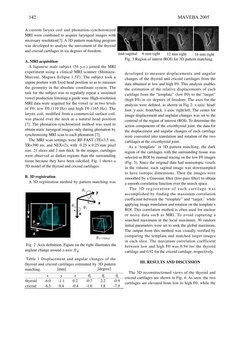
A custom larynx coil and phonation-synchoronized MRI were combined to acquire laryngeal images with necessary resolution[7]. A 3D pattern matching program was developed to analyze the movement of the thyroid and cricoid cartilages in six degrees of freedom.

A. MRI acquisition A Japanese male subject (54 y.o.) joined the MRI

experiment using a clinical MRI scanner (Shimazu-Marconi, Magnex Eclipse 1.5T). The subject took a supine posture with fixed head position so as to measure the geometry in the absolute coordinate system. The task for the subject was to regularly repeat a sustained vowel production listening a guide tone. High-resolution MRI data were acquired for the vowel /a/ in two levels of F0: low F0 (110 Hz) and high F0 (165 Hz). The larynx coil, modified from a commercial surface coil, was placed over the neck at a natural head position [7]. The phonation-synchronized method was used to obtain static laryngeal images only during phonation by synchronizing MRI scan to each phonation [7]. The MRI scan settings were RF-FAST (TE=3.5 ms,

TR=390 ms, and NEX=2), with 0.25 × 0.25 mm pixel size, 21 slices and 2 mm thick. In the images, cartilages were observed as darker regions than the surrounding tissue because they have been calcified. Fig. 1 shows a 3D model of the thyroid and cricoid cartilages.

B. 3D registration A 3D registration method by pattern matching was

developed to measure displacements and angular changes of the thyroid and cricoid cartilages from the data obtained at low and high F0. This analysis enables the estimation of the relative displacements of each cartilage from the “template” (low F0) to the “target” (high F0) in six degrees of freedom. The axes for the analysis were defined, as shown in Fig 2: x-axis: head/foot, y-axis: front/back, z-axis: right/left. The center for image displacement and anglular changes was set to the centroid of the region of interest (ROI). To determine the action components of the cricothyroid joint, the data for the displacement and angular changes of each cartilage were converted into translation and rotation of the two cartilages at the cricothyroid joint. As a “template” in 3D pattern matching, the dark

region of the cartilages with the surrounding tissue was selected as ROI by manual tracing on the low F0 images (Fig. 3). Since the original data had nonisotopic voxels in the volume, each sagittal image was downsampled to have isotopic dimensions. Then the images were smoothed by a Gaussian filter (low-pass filter) to obtain a smooth correlation function over the search space. The 3D reg is t ra t ion of each car t i l age was

accomplished by finding the maximum correlation coefficient between the “template” and “target,” while applying image translation and rotation on the templateʼs ROI. This correlation method is often used for unclear or noisy data such as MRI. To avoid capturing a searched maximum in the local maximum, 30 random initial parameters were set to seek the global maximum. The output from this method was visually verified by comparing the template and matched target images in each slice. The maximum correlation coefficient between low and high F0 was 0.94 for the thyroid cartilage and 0.92 for the cricoid cartilage, respectively.


The 3D reconstructioned views of the thyroid and cricoid cartilages are shown in Fig. 4. As seen, the two cartilages are elevated from low to high F0, while the

θz =10[deg]

θzθx

θy

Fig. 2 Axis definition. Figure on the right illustrates the angluar change around z-axis:θz;

mid-sagittal 6 mm right 12 mm right 16 mm rightFig. 3 Region of interst (ROI) for 3D pattern matching.

Table 1 Displacement and angular changes of the thyroid and cricoid cartilages estimated by 3D pattern matching.

x y z θx θy θz

thyroid -6.0 -1.1 0.2 -0.7 2.2 -0.9cricoid -6.5 0.4 -0.4 -1.0 1.8 -7.9

[mm] [degree]

142 MAVEBA 2005

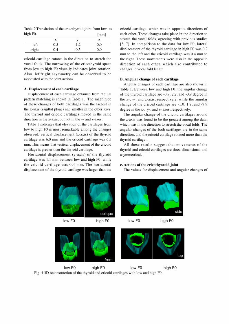
cricoid cartilage rotates in the direction to stretch the vocal folds. The narrowing of the cricothyroid space from low to high F0 visually indicates joint rotation. Also, left/right asymmetry can be observed to be associated with the joint actions.

A. Displacement of each cartilage Displacement of each cartilage obtained from the 3D

pattern matching is shown in Table 1. The magnitude of these changes of both cartilages was the largest in the x-axis (sagittal plane) and smaller in the other axes. The thyroid and cricoid cartilages moved in the same direction in the x-axis, but not in the y- and z-axes. Table 1 indicates that elevation of the cartilages from

low to high F0 is most remarkable among the changes observed: vertical displacement (x-axis) of the thyroid cartilage was 6.0 mm and the cricoid cartilage was 6.5 mm. This means that vertical displacement of the cricoid cartilage is greater than the thyroid cartilage. Horizontal displacement (y-axis) of the thyroid

cartilage was 1.1 mm between low and high F0, while the cricoid cartilage was 0.4 mm. The horizontal displacement of the thyroid cartilage was larger than the

cricoid cartilage, which was in opposite directions of each other. These changes take place in the direction to stretch the vocal folds, agreeing with previous studies [3, 7]. In comparison to the data for low F0, lateral displacement of the thyroid cartilage in high F0 was 0.2 mm to the left and the cricoid cartilage was 0.4 mm to the right. These movements were also in the opposite direction of each other, which also contributed to changes in vocal fold length.

B. Angular change of each cartilage Angular changes of each cartilage are also shown in

Table 1. Between low and high F0, the angular change of the thyroid cartilage are -0.7, 2.2, and -0.9 degree in the x-, y-, and z-axis, respectively, while the angular change of the cricoid cartilage are -1.0, 1.8, and -7.9 degree in the x-, y-, and z- axes, respectively. The angular change of the cricoid cartilages around

the z-axis was found to be the greatest among the data, which was in the direction to stretch the vocal folds. The angular changes of the both cartilages are in the same direction, and the cricoid cartilage rotated more than the thyroid cartilage. All these results suggest that movements of the

thyroid and cricoid cartilages are three-dimensional and asymmetrical.

c. Actions of the cricothyoroid joint The values for displacement and angular changes of

Table 2 Translation of the cricothyroid joint from low to high F0.

low F0

low F0

high F0

high F0

low F0 high F0

low F0 high F0

oblique

front

side

top

Fig. 4 3D reconstruction of the thyroid and cricoid catrilages with low and high F0.

x y zleft 0.5 -1.2 0.0

right 0.4 -0.5 0.0

[mm]

Voice modelling and analysis


Abstract: We offer two tools for automated vocalization

analysis. The Syllable tool uses the Stevens landmark

theory to find landmarks in vocalizations digitized as

"wav" files. The landmarks are grouped to identify

syllable-like productions in these vocalizations and the

results are summarized. The Vocalization-Age tool is

intended for pre-speech vocalizations. It uses the

landmark and syllable information to yield a vocaliza-

tion age that has been shown to clinically distinguish

typically-developing children from children who are at-

risk for later speech impairment.

I. INTRODUCTION

Many speech-related studies result in voluminous

acoustic data and our projects are no exception. We have

therefore developed two tools for automated vocalization

analysis. One tool extracts and summarizes features from

acoustic waveforms. The other tool computes a perform-

ance level of pre-speech productions. Beta-test versions

of our software are now available for Matlab users.

Examples:

We have applied these tools to recordings collected in

several studies.

• In the Early Vocalization Analysis (EVA) project

[1], typically and atypically developing infants were

recorded for 45 minutes at a time, for a total of more

than 100 sessions.

• In a study of emotional stress in voice [2], we ana-

lyzed about 400 single-word, pre-existing audio

recordings [SUSAS] of several subjects speaking

many tokens in sometimes noisy environments.

• In the visiBabble project [3], 30 ten-minute in-home

audio recordings of several children with severe

speech delays were processed in real-time in a

single-case-study design.

• In the UCARE project [4], 40 hours of pre-existing

[5] video-taped sessions of children with physical or

neurological impairments were analyzed with these

tools.

Most of these recordings were made in less-than-ideal

environments. Babies crawled on the floor and played

with toys. Mothers, siblings, and graduate students were

present and sometimes talked. The recordings also con-

tain other environmental sounds such as air-conditioners

or vacuum cleaners. Because our tools use knowledge-

based speech-processing, they are robust to many of these

contaminating sounds. For more subtle cases, e.g. a sib-

ling talking nearby, the researcher can specify recording

sections to ignore.

II. THE SYLLABLE TOOL

The Syllable tool uses the Stevens landmark theory [6]

to find acoustically abrupt events, consonantal land-

marks, in vocalizations digitized as "wav" files. The tool

also determines voicing intensity and fundamental

frequency (F0) contours.

Figure 1: Syllable Analysis of "two" spoken by an adult

female. The waveform (top) is shown with labeled landmarks

(onset/offset of: b, bursts/frication; g, voicing; s, syllabicity) and

strength of voicing; V denotes the nominal vocalic center of the

syllable. The spectrogram (bottom) is shown with the F0

contour and its 10th harmonic (dashed line). Voice onset time

VOT is measured by the interval between start of burst +b and

onset of voicing +g.

Figure 2: Syllable Analysis of "seven" spoken by an adult

female. In the waveform (top), V denotes the nominal vocalic

center of each syllable. Notice that voicing persists without a

complete oral closure between the syllables. The second sylla-

ble is identified by a landmark-based rule, i.e., a syllable onset

(+s) that is not closely preceded by a voicing onset (+g).

VOCALIZATION ANALYSIS TOOLS

H. J. Fell1 and J. MacAuslan

2

1College of Computer and Information Science, Northeastern University, MA, USA

2Speech Technology and Applied Research, Bedford, MA USA


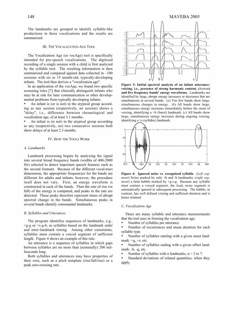
The landmarks are grouped to identify syllable-like

productions in these vocalizations and the results are

summarized.

III. THE VOCALIZATION AGE TOOL

The Vocalization Age (or vocAge) tool is specifically

intended for pre-speech vocalizations. The digitized

recording of a single session with a child is first analyzed

by the syllable tool. The resulting information is then

summarized and compared against data collected in ~100

sessions with six to 15 month-old, typically-developing

infants. The tool thus derives a "vocalization age".

In an application of the vocAge, we found two specific

screening rules [7] that clinically distinguish infants who

may be at risk for later communication or other develop-

mental problems from typically developing infants:

• An infant is (or is not) in the atypical group accord-

ing as any session (respectively, no session) shows a

"delay", i.e., difference between chronological and

vocalization age, of at least 3.1 months.

• An infant is (is not) in the atypical group according

as any (respectively, no) two consecutive sessions both

show delays of at least 2.3 months.

IV. HOW THE TOOLS WORK

A. Landmarks

Landmark processing begins by analyzing the signal

into several broad frequency bands (widths of 400-2000

Hz) selected to detect important speech features such as

the second formant. Because of the different vocal-tract

dimensions, the appropriate frequencies for the bands are

different for adults and infants; however, the procedure

itself does not vary. First, an energy waveform is

constructed in each of the bands. Then the rate of rise (or

fall) of the energy is computed, and peaks in the rate are

detected. These peaks therefore represent times of abrupt

spectral change in the bands. Simultaneous peaks in

several bands identify consonantal landmarks.

B. Syllables and Utterances

The program identifies sequences of landmarks, e.g.,

+g-g or +s-g-b, as syllables based on the landmark order

and inter-landmark timing. Among other constraints,

syllables must contain a voiced segment of sufficient

length. Figure 4 shows an example of this rule.

An utterance is a sequence of syllables in which gaps

between syllables are no more than (nominally) 200 mil-

liseconds long.

Both syllables and utterances may have properties of

their own, such as a pitch template (rise/fall/rise) or a

peak zero-crossing rate.

Figure 3: Initial spectral analysis of an infant utterance:

voicing, i.e., presence of strong harmonic content, (bottom)

and five frequency bands' energy waveforms. Landmarks are

identified by large, abrupt energy increases or decreases that are

simultaneous in several bands. (a) Too few bands show large,

simultaneous changes in energy. (b) All bands show large,

simultaneous energy increases immediately before the onset of

voicing, identifying a +b (burst) landmark. (c) All bands show

large, simultaneous energy increases during ongoing voicing,

identifying a +s (syllabic) landmark.

Figure 4: Ignored noise vs. recognized syllable. (Left seg-

ment) Noise marked by only +b and -b landmarks; (right seg-

ment) a faint babble marked by +g-s-g. Because any syllable

must contain a voiced segment, the loud, noise segment is

automatically ignored in subsequent processing. The babble, in

contrast, has well defined voicing and sufficient duration and is

hence retained.

C. Vocalization Age

There are many syllable and utterance measurements

that the tool uses in forming the vocalization age:

• Number of syllables per utterance

• Number of occurrences and mean duration for each

syllable type

• Number of syllables starting with a given onset land-

mark: +g, +s, etc.

• Number of syllables ending with a given offset land-

mark: -b, -g, etc.

• Number of syllables with n landmarks, n = 2 to 7.

• Standard deviations of related quantities, when they

apply.

a b c

148 MAVEBA 2005

The Syllable tool can be set to extract and summarize

exactly those measurements that are needed to compute

the vocalization age.

V. USING THE TOOLS

We have applied these tools to recordings collected in

several studies and we hope that other researchers will

use the tools on their own data. Also, as we improve the

feature collection capabilities of our tools, we, and per-

haps others, will want to use them repeatedly on previ-

ously collected recordings. These tools can be run on all

the recordings for a single "wav" file, a complete session,

all the sessions of a subject, or an entire study with a sin-

gle invocation. (See Figure 5.)

A. System Requirements

Currently, our software requires Matlab and the Matlab

Signal Processing Toolbox. We run it under the Win-

dows XP operating system.

B. Preparing Data

All sound files must be in "wav" format. Because

much of our own data was collected using Entropic's

ESPS-WAVES and saved in "sd" files, we also provide

software to convert Entropic "sd" files to "wav" format.

A user can run the Syllable and Vocalization Age tools

on a single recording or on a directory tree containing

recordings of (see Figures 5 and 6):

• a single session with a subject,

• all sessions of a subject,

• an entire study.

A simple text file may be included for any recording to

indicate sections that should not be analyzed.

Figure 5: Arrangement of session data in a study. This

figure represents a study with two sessions for each of three

subjects.

Figure 6: A session directory. This figure shows a folder

containing three audio files from a single session, a text ("ax")

file that marks segments to be ignored in one of the "wav" files,

and a text file with the researcher's comments about the session.

C. Single-Subject Experiments

Single case study designs [8] are particularly suited to

studies on a small heterogeneous group of subjects. For

example, in our preliminary tests of visiBabble, a real-

time visual-feedback system, we ran sessions in a variety

of formats:

1) Baseline (recording, no graphic display);

2) Response (graphic display is always present, while

recording);

3) A-B-A (display off-on-off).

Data was collected during all phases of all formats to

allow a comparison of behavior during the baseline and

feedback phases. The Syllable tool can analyze the

landmarks and syllables for the A and B phases combined

or separately.

D. Reports

A dialog box allows the user to select particular fea-

tures to be summarized by the Syllable tool (see Figure

7). The tool will then generate, in the data directory, a

tab-delimited report that can be easily copied into a

spreadsheet for future analysis (see Table 1).

Figure 7: Dialog box for selecting report features.

VI. FURTHER DEVELOPMENT

We anticipate adding capabilities over the next two

years while our visiBabble project is under development.

We encourage other researchers to try a beta-test version

and to suggest enhancements that would be useful to

them.

ACKNOWLEDGEMENTS

The authors appreciate the encouragement and testing

by Prof. Cynthia Cress, Univ. of Nebraska-Lincoln. We

also thank Jun Gong for his programming contributions.

This work was funded in part by National Institutes of

Health STTR grant R42 DC005534.

Table 1: Summary of a Short Sample Session

The report summarizes the landmark, syllable, and utterance statistics of a sample, 30-second session.

These statistics are among those used in the vocAge tool.

Total

SyllableType Count Mean StdDev

+g-g 3 704.000 532.626

+s-g 1 408.000 0.000

+g-g-b 3 96.000 36.368

+g+s-g 1 48.000 0.000

+b+g-g-b 1 344.000 0.000

+g+s-g-b 1 64.000 0.000

+g+s-s-g 1 160.000 0.000

+g+s+s 1 696.000 0.000

Total 12 343.333 382.559

2 lm/syl 4

3 lm/syl 5

4 lm/syl 3

5 lm/syl 0

6 lm/syl 0

7 lm/syl 0

Avg 2.917

DiffSyl 8

Utts Count AvDur StDev

8 531.000 486.982

REFERENCES

[1] H.J. Fell, J. MacAuslan, L.J. Ferrier, K. Chenausky,

"Automatic Babble Recognition for Early Detection of Speech

Related Disorders," Journal of Behaviour and Information

Technology, 1999, 18, no. 1, 56-63.

[2] H.J. Fell, J. MacAuslan, "Automatic Detection of Stress in

Speech," Proceedings of MAVEBA 2003, Florence, Italy, pp. 9-12.

[3] H.J. Fell, J. MacAuslan , C. J. Cress

, L. J. Ferrier, "Using

Early Vocalization Analysis for visual feedback," Proceedings

of MAVEBA 2003, Florence, Italy.

[3] H.J. Fell, J. MacAuslan, C. Cress, L.J. Ferrier, "visiBabble

for Reinforcement of Early Vocalization," Proceedings of

ASSETS 2004, Atlanta, GA., pp. 161-168.

[4] C.J. Cress, S. Unrein, A. Weber, S. Krings, H. Fell, J.

MacAuslan, J. Gong, "Vocal Development Patterns in Children

at Risk for Being Nonspeaking," submitted to ASHA 2005.

[5] C.J. Cress, Communicative and symbolic precursors of AAC.

Unpublished NIH CIDA Grant: University of Nebraska-

Lincoln, 1995.

[6] K.N. Stevens, S. Manuel, S. Shattuck-Hufnegel, and S. Liu,

“Implementation of a model for lexical access based on

features,” Proc. ICSLP (Int. Conf. on Speech & Language

Processing), Banff, Alberta, 1, 499-502, 1992.

[7] H.J. Fell, J. MacAuslan, L.J. Ferrier, S.G. Worst, and K.

Chenausky, “Vocalization Age as a Clinical Tool,” Proc. ICSLP

(Int. Conf. on Speech & Language Processing), Denver,

September 2002.

[8] L.V. McReynolds, K.P. Kearns, Single Subject Experimental

Designs in Communication Disorders, Baltimore: University

Park Press, 1983.

mean duration of all syllables

number of syllables with 2 landmarks

mean duration of +g-g syllables

average number of landmarks/syllable

number of syllable types occurring

total number of utterances

150 MAVEBA 2005

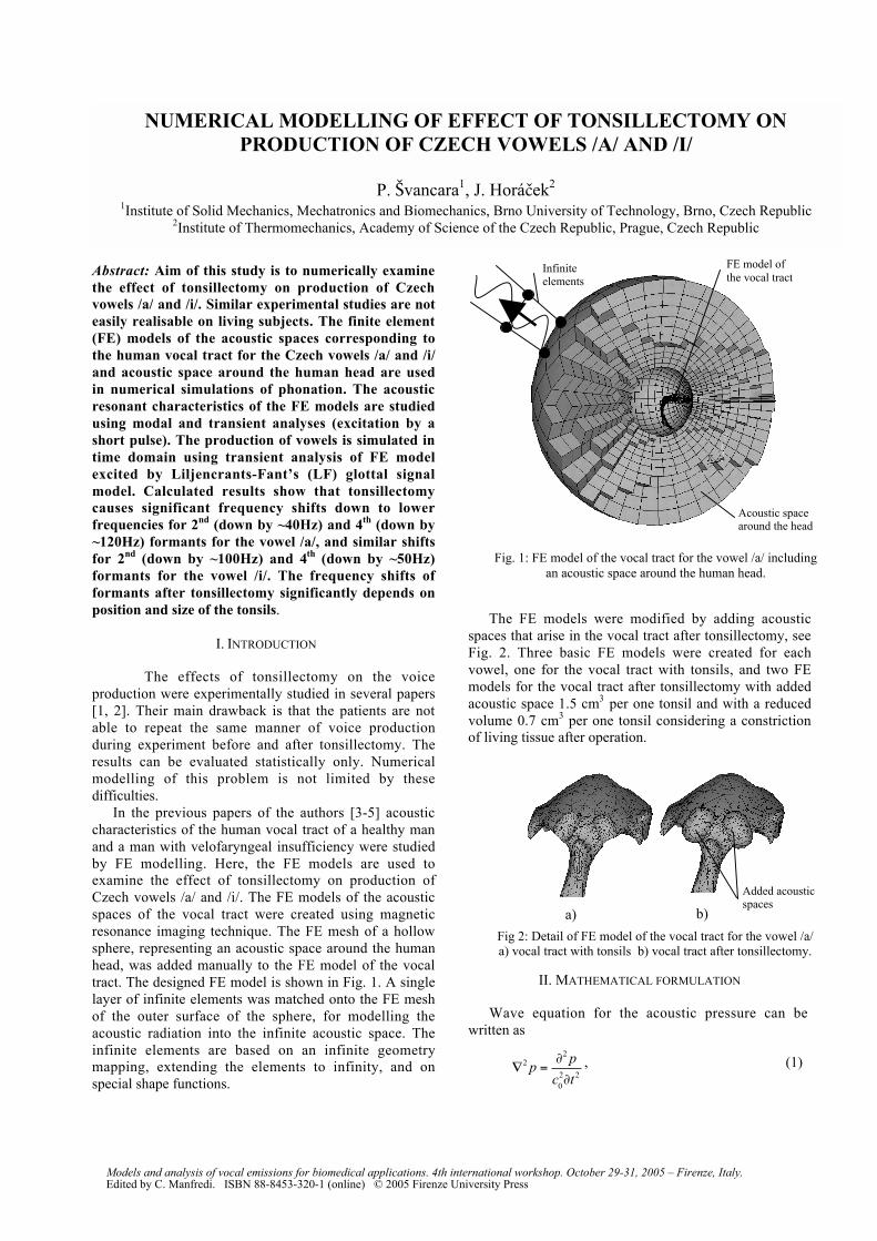
Abstract: Aim of this study is to numerically examine

the effect of tonsillectomy on production of Czech

vowels /a/ and /i/. Similar experimental studies are not

easily realisable on living subjects. The finite element

(FE) models of the acoustic spaces corresponding to

the human vocal tract for the Czech vowels /a/ and /i/

and acoustic space around the human head are used

in numerical simulations of phonation. The acoustic

resonant characteristics of the FE models are studied

using modal and transient analyses (excitation by a

short pulse). The production of vowels is simulated in

time domain using transient analysis of FE model

excited by Liljencrants-Fant’s (LF) glottal signal

model. Calculated results show that tonsillectomy

causes significant frequency shifts down to lower

frequencies for 2nd

(down by ~40Hz) and 4th

(down by

~120Hz) formants for the vowel /a/, and similar shifts

for 2nd

(down by ~100Hz) and 4th

(down by ~50Hz)

formants for the vowel /i/. The frequency shifts of

formants after tonsillectomy significantly depends on

position and size of the tonsils.

I. INTRODUCTION

The effects of tonsillectomy on the voiceproduction were experimentally studied in several papers[1, 2]. Their main drawback is that the patients are notable to repeat the same manner of voice productionduring experiment before and after tonsillectomy. Theresults can be evaluated statistically only. Numericalmodelling of this problem is not limited by thesedifficulties.

In the previous papers of the authors [3-5] acousticcharacteristics of the human vocal tract of a healthy manand a man with velofaryngeal insufficiency were studiedby FE modelling. Here, the FE models are used toexamine the effect of tonsillectomy on production ofCzech vowels /a/ and /i/. The FE models of the acousticspaces of the vocal tract were created using magneticresonance imaging technique. The FE mesh of a hollowsphere, representing an acoustic space around the humanhead, was added manually to the FE model of the vocaltract. The designed FE model is shown in Fig. 1. A singlelayer of infinite elements was matched onto the FE meshof the outer surface of the sphere, for modelling theacoustic radiation into the infinite acoustic space. Theinfinite elements are based on an infinite geometrymapping, extending the elements to infinity, and onspecial shape functions.

The FE models were modified by adding acousticspaces that arise in the vocal tract after tonsillectomy, seeFig. 2. Three basic FE models were created for eachvowel, one for the vocal tract with tonsils, and two FEmodels for the vocal tract after tonsillectomy with addedacoustic space 1.5 cm3 per one tonsil and with a reducedvolume 0.7 cm3 per one tonsil considering a constrictionof living tissue after operation.

II. MATHEMATICAL FORMULATION

Wave equation for the acoustic pressure can bewritten as

2p =

2p

c0

2t

2

, (1)

Fig 2: Detail of FE model of the vocal tract for the vowel /a/a) vocal tract with tonsils b) vocal tract after tonsillectomy.

Fig. 1: FE model of the vocal tract for the vowel /a/ includingan acoustic space around the human head.

NUMERICAL MODELLING OF EFFECT OF TONSILLECTOMY ON

PRODUCTION OF CZECH VOWELS /A/ AND /I/

P. fivancara1, J. Horáæek2

1Institute of Solid Mechanics, Mechatronics and Biomechanics, Brno University of Technology, Brno, Czech Republic2Institute of Thermomechanics, Academy of Science of the Czech Republic, Prague, Czech Republic

FE model ofthe vocal tract

Acoustic spacearound the head

Infiniteelements

a) b)

Added acousticspaces


where c0 is the speed of sound, with boundary conditionsas follows• on acoustically hard area

p / n = 0 ,

• on acoustically absorptive area a normal impedance

Z = p / v

n can be prescribed,

where n is the normal to the boundary area and vn isnormal velocity.

Equations of motion after discretization can bewritten as

M p t( ) +C p t( ) +K p t( ) = f t( ) , (2)

where M, C, K are mass, damping and stiffness matrices,p is the vector of nodal acoustic pressures and f is thevector of nodal acoustic forces. Newmark integrationmethod was used for solution in time domain.

The acoustic transient and modal analysis wererealized by the software code SYSNOISE 5.5 consideringthe speed of sound c0 = 353 ms-1 and the air density

0 = 1.2 kgm-3. Boundary walls of the vocal tract wereconsidered acoustically absorptive with normalimpedance Z = 83 666 kgm-2s-1 assuming for the softtissue the Young modulus E = 5 MPa and density_ = 1400 kgm-3 [6].

III. FREQUENCY MODAL AND RESONANTCHARACTERISTICS

Firstly the eigenfrequencies of the FE models of thevocal tract without the acoustic space around the headwere studied using modal analysis, assuming zeroacoustic pressure at the nodes belonging to the area of thelips and acoustically hard boundary walls. Calculatedformant frequencies for both vowels and all three FEmodels are summarized in Table 1.

Then the resonant characteristics of the FE modelswith acoustic space around the head, infinite elementsand absorption on the vocal tract walls were computed bytransient analysis in time domain. The FE models wereexcited by a very short pulse of differential glottal flow(duration 0.25 ms) at the faces of FE elements in position

of the vocal folds. The spectra of the excitation pulse andthe sound pressure calculated near the lips are shown inFigs. 3 and 4, respectively. The evaluated acousticresonant frequencies were close to the formantfrequencies obtained by the modal analysis.

Results calculated by both methods for FE models withthe tonsils are in good agreement with experimental dataknown for formants of the Czech vowels /a/ and /i/ [7, 8].Tonsillectomy for the vowel /a/ caused the biggestdecrease of formants F2 and F4 of about 40 Hz and120 Hz, respectively. And for vowel /i/, the tonsillectomycaused the biggest frequency shift down of about 100 Hzfor the formant F2, and about 50 Hz for the formants F4and F5. For the model with consideration of constrictionof tissue after operation the frequency shifts of the

Fig. 3: Spectrum of the excitation pulse.

Fig. 4: Spectrum of the pressure response near thelips for the vowel /a/.

Table 1: Calculated resonant frequencies.

Vowel /a/

formantWithtonsil.[Hz]

Aftertonsill.[Hz]

Diff.[Hz]

Aftertonsill.reducedvol. [Hz]

Diff.[Hz]

F1 678 683 5 686 8

F2 1177 1137 -40 1150 -27

F3 2869 2875 6 2904 35

F4 4113 3992 -121 4038 -75

F5 4286 4308 22 4312 26

F6 4442 4494 52 4492 50

Vowel /i/

formantWithtonsil.[Hz]

Aftertonsill.[Hz]

Diff.[Hz]

Aftertonsill.reducedvol. [Hz]

Diff.[Hz]

F1 258 248 -10 251 -7

F2 2374 2267 -107 2307 -67

F3 3188 3213 25 3198 10

F4 3809 3763 -46 3794 -15

F5 4778 4722 -56 4741 -37

152 MAVEBA 2005

formants are approximately two times smaller. We shouldnote that the eigenfrequency F5 for the vowel /a/ isassociated with a lateral acoustic mode shape of vibrationin the horizontal direction.

As a next step a sensitivity of formants frequencyshift on the position and size of tonsils were examined.Firstly, a penetration of the volumes of the tonsils and thevocal tract was changed, i.e., the portion of tonsil volumeinterference with the acoustic space of the vocal tract.Three cases of tonsil-vocal tract volume interference wereconsidered: 1/2 (this case was used in previouscalculations), 3/4 and 1/4. The results are summarized inFig. 5.

Then for case of 1/2 of the tonsil-vocal tract volumeinterference, the volume of the tonsils was varied, andagain three cases were analyzed for the tonsil volumes1.5 cm3 (as in the previous calculations), 2 cm3 and 1 cm3

per one tonsil. The obtained differences in formantfrequencies are shown in Fig. 6.

The results show that some formant frequencies arevery sensitive to the change of position and size of thetonsils. For example, the difference in formant frequencyF3 for the vowel /a/ changed from -137 Hz to +168 Hzwith changing the portion of the tonsil volumeinterference with the acoustic space of the vocal tract.

The frequency changes of the most formants are more orless proportional to the size of the tonsils.

IV. NUMERICAL SIMULATION OF PRODUCTION OF VOWELS

The production of the vowels was simulated usingtransient analysis of FE model in time domain withexcitation by Liljencrants-Fant’s (LF) glottal signalmodel [9]. The LF model describes differentiated airflowin time domain. Each fundamental period of the glottalsignal can be expressed as

dUg

t( )dt

=

E0e t

singt , 0 t < t

e

Ee

ta

et t

e( )e

tc

te( )( ) , te

t < tc

, (3)

where t is in the range [0,tc], tc is equal to thefundamental period T 0. The so-called waveshapeparameters tp, te, ta, and Ee together with T0 completelydetermine the shape of differential flow dUg(t). Figure 7illustrates these waveshape parameters. Here, thefollowing normalized parameters derived from thewaveshape parameters were used:• Ra the ratio of ta to tc-te ,

• Rk the ratio of te-tp to tp ,

• Rg the ratio of half fundamental period T0/2 to tp.

The parameters corresponding to a normal phonationwere used (R a = 0.05 ms, R k = 0.34, R g = 1.12,Ee = 0.4 m3s-2). The FE models were excited at the facesof FE elements in position of vocal folds by fifteensubsequent pulses of differential glottal flow with theperiod corresponding to the fundamental (pitch)frequency F0 = 100 Hz. The numerical solution wasrealised by the transient analysis within the softwareSYSNOISE with the time step nt = 1.10-5 s. The timeresponses – sound pressures and their spectra werecalculated at distance 0.2 m in front of the lips (see theexample in Fig. 8).

-200

-150

-100

-50

0

50

100

150

200

F1 F2 F3 F4 F5 F6

Formant frequencies

Diffe

rence [

Hz]

1/4 of volume

1/2 of volume

3/4 of volume

Fig. 5: Difference of formant frequencies before and aftertonsillectomy for different positions of tonsils for the vowel /a/.

-200

-150

-100

-50

0

50

100

F1 F2 F3 F4 F5 F6

Formant frequencies

Diffe

rence [

Hz]

1 cm^3

1.5 cm^3

2 cm^3

Fig. 6: Difference of formant frequencies before and aftertonsillectomy for different size of tonsils for the vowel /a/.

Fig. 7: Derivative glottal flow wave shape used foracoustic excitation of the vocal tract.

tp te te+ta tc

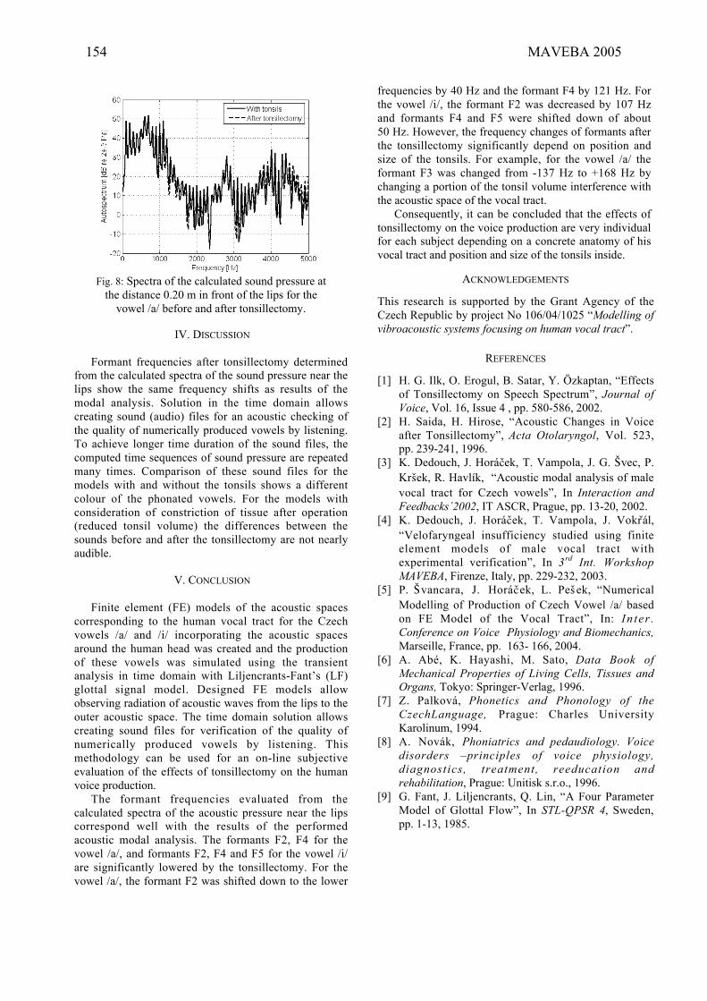
IV. DISCUSSION

Formant frequencies after tonsillectomy determinedfrom the calculated spectra of the sound pressure near thelips show the same frequency shifts as results of themodal analysis. Solution in the time domain allowscreating sound (audio) files for an acoustic checking ofthe quality of numerically produced vowels by listening.To achieve longer time duration of the sound files, thecomputed time sequences of sound pressure are repeatedmany times. Comparison of these sound files for themodels with and without the tonsils shows a differentcolour of the phonated vowels. For the models withconsideration of constriction of tissue after operation(reduced tonsil volume) the differences between thesounds before and after the tonsillectomy are not nearlyaudible.

V. CONCLUSION

Finite element (FE) models of the acoustic spacescorresponding to the human vocal tract for the Czechvowels /a/ and /i/ incorporating the acoustic spacesaround the human head was created and the productionof these vowels was simulated using the transientanalysis in time domain with Liljencrants-Fant’s (LF)glottal signal model. Designed FE models allowobserving radiation of acoustic waves from the lips to theouter acoustic space. The time domain solution allowscreating sound files for verification of the quality ofnumerically produced vowels by listening. Thismethodology can be used for an on-line subjectiveevaluation of the effects of tonsillectomy on the humanvoice production.

The formant frequencies evaluated from thecalculated spectra of the acoustic pressure near the lipscorrespond well with the results of the performedacoustic modal analysis. The formants F2, F4 for thevowel /a/, and formants F2, F4 and F5 for the vowel /i/are significantly lowered by the tonsillectomy. For thevowel /a/, the formant F2 was shifted down to the lower

frequencies by 40 Hz and the formant F4 by 121 Hz. Forthe vowel /i/, the formant F2 was decreased by 107 Hzand formants F4 and F5 were shifted down of about50 Hz. However, the frequency changes of formants afterthe tonsillectomy significantly depend on position andsize of the tonsils. For example, for the vowel /a/ theformant F3 was changed from -137 Hz to +168 Hz bychanging a portion of the tonsil volume interference withthe acoustic space of the vocal tract.

Consequently, it can be concluded that the effects oftonsillectomy on the voice production are very individualfor each subject depending on a concrete anatomy of hisvocal tract and position and size of the tonsils inside.

ACKNOWLEDGEMENTS

This research is supported by the Grant Agency of theCzech Republic by project No 106/04/1025 “Modelling of

vibroacoustic systems focusing on human vocal tract”.

REFERENCES

[1] H. G. Ilk, O. Erogul, B. Satar, Y. Özkaptan, “Effectsof Tonsillectomy on Speech Spectrum”, Journal of

Voice, Vol. 16, Issue 4 , pp. 580-586, 2002.[2] H. Saida, H. Hirose, “Acoustic Changes in Voice

after Tonsillectomy”, Acta Otolaryngol, Vol. 523,pp. 239-241, 1996.

[3] K. Dedouch, J. Horáæek, T. Vampola, J. G. fivec, P.Kr¢ek, R. Havlík, “Acoustic modal analysis of malevocal tract for Czech vowels”, In Interaction and

Feedbacks´2002, IT ASCR, Prague, pp. 13-20, 2002.[4] K. Dedouch, J. Horáæek, T. Vampola, J. Vokrál,

“Velofaryngeal insufficiency studied using finiteelement models of male vocal tract withexperimental verification”, In 3

rd Int. Workshop

MAVEBA, Firenze, Italy, pp. 229-232, 2003.[5] P. fivancara, J. Horáæek, L. Pe¢ek, “Numerical

Modelling of Production of Czech Vowel /a/ basedon FE Model of the Vocal Tract”, In: In ter .

Conference on Voice Physiology and Biomechanics,

Marseille, France, pp. 163- 166, 2004.[6] A. Abé, K. Hayashi, M. Sato, Data Book of

Mechanical Properties of Living Cells, Tissues and

Organs, Tokyo: Springer-Verlag, 1996.[7] Z. Palková, Phonetics and Phonology of the

CzechLanguage, Prague: Charles UniversityKarolinum, 1994.

[8] A. Novák, Phoniatrics and pedaudiology. Voice

disorders –principles of voice physiology,

diagnostics, treatment, reeducation and

rehabilitation, Prague: Unitisk s.r.o., 1996.[9] G. Fant, J. Liljencrants, Q. Lin, “A Four Parameter

Model of Glottal Flow”, In STL-QPSR 4, Sweden,pp. 1-13, 1985.

Fig. 8: Spectra of the calculated sound pressure atthe distance 0.20 m in front of the lips for the

vowel /a/ before and after tonsillectomy.

154 MAVEBA 2005

GENERALIZED VARIOGRAM ANALYSIS OF VOCAL DYSPERIODICITIES IN CONNECTED SPEECH

A. Kacha1, F. Grenez1, J. Schoentgen1,2

1 Department Signals and Waves, Faculty of Applied Sciences, Université Libre de Bruxelles, Brussels, Belgium

2 National Fund for Scientific Research, Belgium [email protected], [email protected], [email protected]

A generalized variogram is used to track vocal dysperiodicities in connected speech, which are summarized by means of a signal-to-dysperiodicity marker. To evaluate the variogram-based analysis, signal-to-dysperiodicity estimates are correlated with scores obtained by means of perceptual ratings of the degree of hoarseness, which are based on comparative judgments of pairs of speech samples. The corpora comprise four French sentences as well as vowels [a] produced by 22 male and female normophonic and dysphonic speakers.

I. INTRODUCTION Many voice disorders cause voiced speech to deviate from perfect cyclicity. Dysperiodicities may be caused by additive noise owing to turbulence and modulation noise owing to external perturbations of the glottal excitation signal, as well as irregular dynamics of the vocal folds and involuntary transients between different dynamic regimes.

Techniques that have been proposed to estimate vocal dysperiodicities have been applied to sustained vowels, mainly. Indeed, many techniques lack robustness and accuracy when they are used to estimate vocal dysperiodicities in continuous speech or vowels including onsets and offsets spoken by severely hoarse speakers. The lack of robustness is a consequence of the assumptions of local stationarity and periodicity that are at the base of many speech analysis methods, and which are not valid in the case of speech produced by hoarse speakers. Up to date, there exists a comparatively small number of studies devoted to vocal dysperiodicities in continuous speech [2, 3].

In [4], we have proposed a generalized form of the variogram, as an alternative to the long-term prediction-based approach proposed in [5], to estimate speech signal dysperiodicities due to vocal disorders. The generalized variogram is derived from the conventional one. It enables tracking cycle length and cycle shape dysperiodicities and is unaffected by waveform changes that are segmental or suprasegmental in origin. In [4], synthetic vowels have been used to investigate the

performance of the generalized variogram while measuring dysperiodicities caused by jitter, shimmer and additive noise.

In the framework of this presentation, the variogram-based approach is evaluated by correlating signal-to-dysperiodicity estimates (SDR) with scores obtained by means of a perceptual rating of the degree of hoarseness, which is based on comparative judgments of pairs of speech samples.

II. METHODS A

. Corpora

Speech data comprise sustained vowels [a], including onsets and offsets, and four French sentences produced by 22 normophonic or dysphonic speakers (10 male and 12 female speakers). The corpus includes 20 adults (from 20 to 79 years), one boy aged 14 and one girl aged 10. Five speakers are normophonic, the other are dysphonic.

The sentences are the following: “Le garde a endigué l’abbé”, “Bob m’avait guidé vers les digues”, “Une poule a picoré ton cake” and “Ta tante a appâté une carpe”. Hereafter, they are referred to as S1, S2, S3 and S4, respectively. They have the same grammatical structure, the same number of syllables and roughly the same number of resonants and plosives. Sentences S1 and S2 are voiced by default, whereas S3 and S4 include voiced and unvoiced segments.

Speech signals have been recorded at a sampling frequency of 48 kHz. The recordings were made in an isolated booth by means of a digital audio tape recorder (Sony TCD D8) and a head-mounted microphone (AKG C41WL) at the laryngology department of a university hospital in Brussels, Belgium. The recordings have been transferred from the DAT recorder to computer hard disk via a digital-to-digital interface. Silent intervals before and after each recording have been removed. B

. Generalized Variogram

For a periodic signal x(n) of period T0, one can write: x(n) = x( n + kT0), k = . . .- 2, - 1, 0, 1, 2, . . . (1)


A measure of the departure from periodicity over an interval of length N is an indication of the amount of signal irregularity. For stationary signals, the dysperiodicity energy may be estimated via the minimum of the following expression. The expression between accolades is known as the variogram of the speech signal.

21- ⎪⎫

⎪⎧N

expressions E and E

[ ] (2) , ⎬⎨ +−= ∑ )Tn(x)n(xminarg)T(γ 0 ⎪⎭⎪⎩ Formally, the bracketed expression in (2) is equivalent to the difference between the contents of the current and a lagged analysis frame of length N. Index n positions speech samples within the analysis frame. When lag T is positive, the lagged frame is positioned to the right of the current frame, otherwise it is positioned to the left. Note that lag T is not requested to be equal to the glottal cycle length. Expression (2) is defined irrespective of whether the signal is voiced or unvoiced, regular or irregular.

Boundaries Tmin and Tmax are, in number of samples, the shortest and longest acceptable glottal cycle lengths. They are fixed to 2.5 ms and 20 ms, respectively (i.e. 50 Hz ≤ F0 ≤ 400 Hz). The search for the minimum of (2) is performed to the left and right of the current window position, because comparing speech frames across phonetic boundaries is meaningless. In the case of cross-boundary comparisons, deviations from periodicity are due to differences in segment identity rather than dysperiodicity. The analysis frame length is fixed to 2.5 ms to include one cycle at most. Another reason, for choosing a short frame, is that cycle lengths are expected to evolve owing to intonation and segment-typical phonatory frequencies.

Speech signals are expected to be locally stationary at best. The signal amplitude evolves from one speech frame to the next owing to onsets and offsets, segment-typical intensity, as well as accentuation and loudness. Introducing a weighting coefficient to account for these slow changes in signal amplitude, definition (1) becomes:

x(n)= ax(n + T 0), 0 ≤ n ≤ N – 1. (3) Accordingly, the generalized empirical variogram may be written as follows.

The perceptual assessment exploits the ability of listeners to compare two stimuli in terms of grade, i.e., perceived overall degree of deviance of the voice. The aim is to hierarchize a set of recordings from the least to the most anomalous via comparative judgments of all possible sample pairs within the set. The procedure is the following.

Definition (4) is interpreted as the local energy of the signal dysperiodicities in a frame of length N. Weight a is constrained to be positive. It is defined to equalize the

signal energies in the current and shifted analysis windows:

(5)

T are the signal energies of the current

and lagged frames,

The analysis is carried out frame by frame. The analysis frame is shifted by 2.5 ms. Together with the choice of the analysis frame length, this guarantees that each signal fragment is included exactly once. The instantaneous value of the dysperiodicity is estimated as follows, with Topt equal to the lag that minimizes generalized variogram (4) for the current frame position. Lag Topt may be positive or negative. e(n )= x(n) - ax(n + Topt), 0≤ n ≤N – 1 (6) C. Signal-to-Dysperiodicity Ratio The marker that summarizes the amount of dysperiodicity within an utterance is defined as follows [7]. where L is the number of samples in the analysis interval and = x(n) – e(n) is an estimate of the clean signal. )n(xThe approximation of the optimal lag by an integer number of the sampling period introduces quantization noise, which has been reduced by over-sampling the signal by a factor of 8 and analysing the over-sampled signal. D. Perceptual Ratings by Comparative Judgment of Speech Samples

1. The list of all possible different pairs of items is formed. An item is a recording belonging to a set of identical stimuli.

=nT

,Ea =T

n(N

1

0

2−

=

−

=

N

T

E

,)xE ∑= .∑ += )Tn(xE 1

0

2

n n.TTTTTT maxminminmax ≤≤−≤≤− and with

(7) 101

0

2

1

0

2

⎥⎥⎥⎥⎥

⎦

⎤⎢⎡∑L

)nx

⎢⎢⎢⎢

⎣

=

∑−

=

−

=L

n

n

)n(e

(

logSDR

1-

0 ⎪⎭

⎪⎬

⎪⎩

⎪⎨ +−= ∑

=

N

nT)Tn(ax)n(xminarg)T(γ [ ] (4) ,

2 ⎫⎧

.TTTTTT maxminminmax ≤≤−≤≤− and with

156 MAVEBA 2005

2. All scores are initialized to zero. 3. A randomly selected pair of speech recordings is presented to the listener, who is asked to point out the recording with the highest perceived hoarseness. The listener has also the option to label both recordings of a pair as equally hoarse. 4. The total score of the recording labeled as the most hoarse is increased by one. If both items of the pair are judged to be equally hoarse, the score of both recordings is increased by 0.5. 5. Steps 3 and 4 are repeated until all possible pairs that belong to a same session have been presented. 6. The samples are hierarchized on the base of their scores.

Sound samples have been presented via a digital-to-analog audio interface (Digidesign Mbox) and dynamic stereo headphones (Sony MDR-7506). Loudness has been fixed at a comfortable level by the listener. Listening sessions have been held in a quiet room. Each session has taken about one hour. At half-time, listeners have taken a rest of about five minutes. The group of judges has been comprised of six naive listeners (one female, five males), i.e. listeners without training in speech therapy or laryngology. All reported normal hearing. Their ages ranged from 24 to 57. One listening session was devoted to a set of 22 stimuli. The total number of sessions has therefore been equal to 6 listeners x 5 stimuli = 30. The same experiment has been repeated by three listeners after a period of a day at least to gauge intra-judge reliability. The total number of retest sessions has therefore been equal to 3 x 5 = 15.

III. RESULTS A

. Scores of Perceived Hoarseness

Concordance between judges has been expressed by means of Pearson’s product moment correlation (ρP) between listener scores. The scores of the four sentences have been arranged for a given judge into a single series by stacking the sentence scores. Correlation coefficients have been calculated by means of the score series of each listener. The values for sustained vowel [a] and sentences S1 to S4 are given below and above the diagonal of Table 1, respectively. While testing for the statistical significance of the Pearson product moment correlations, the method of Bonferroni has been used to account for multiple comparisons [6]. The number of independent measures involved in the test has been set equal to 22. The null hypothesis (ρP = 0) has been rejected for all table entries (one-tailed test, ρcrit = 0.56, p < 0.05).

Table 1: Pearson’s product moment correlation values between scores obtained via comparative judgments by six listeners for sustained vowel [a] (below the diagonal) and sentences S1 to S4 (above the diagonal).

J1 J2 J3 J4 J5 J6

J1 ⎯ 0.91 0.83 0.86 0.76 0.86

J2 0.87 ⎯ 0.86 0.90 0.82 0.91

J3 0.90 0.87 ⎯ 0.83 0.74 0.84

J4 0.96 0.80 0.91 ⎯ 0.90 0.94

J5 0.84 0.69 0.80 0.89 ⎯ 0.92

J6 0.91 0.90 0.94 0.92 0.85 ⎯ Intra-judge agreement has been examined by calculating Pearson’s product moment correlation between the scores obtained during the test and retest sessions of three judges. For each judge, the scores of the four sentences have been stacked into a single series. The results are listed in Table 2. To account for multiple comparisons, Bonferroni’s method has been used. The number of independent realizations involved in the test has been set equal to 22. The null hypothesis (ρP = 0) has been rejected for all table entries (one-tailed test, ρcrit = 0.46, p < 0.05). Table 2: Pearson’s product moment correlation values between scores obtained via comparative judgments during test and retest sessions for three listeners.

J1 J2 J3 [a] 0.96 0.98 0.90

S1 to S4 0.92 0.95 0.95 B

. Measured Signal-to-Dysperiodicity Ratios

The SDR values of the speech signals corresponding to vowel [a] and four sentences have been computed for corpora comprising 22 speakers. The quartiles of the SDR values are given in Table 3. Fig. 1(a) shows as an example phonetic segments [lœ] of French sentence S1 that has been assigned a median hoarseness score of 20 and a SDR value of 8.9 dB. Fig. 1(b) shows the corresponding sample-by-sample dysperiodicity (6). C. Correlation Between Scores of Perceived Hoarseness and Measured Signal-to-Dysperiodicity Ratios Pearson’s product moment correlation values between SDR estimates and listener scores are given in Table 4 for sustained vowels [a] as well as sentences S1 to S4. Bonferroni’s method has been applied to account for multiple comparisons (one-tailed test, ρcrit = 0.60, p < 0.05). The number of independent realizations involved in the statistical test has been set equal to 22.

(a)

(b)

Fig. 1: Segments [lœ] of sentence S1 spoken by a hoarse speaker (SDR = 8.9 dB) (a) and its sample-by-sample dysperiodicity (b). Table 3: Quartiles of SDRs estimates in dB obtained via generalized variogram analyses of vowel [a] and sentences S1-S4 produced by 22 speakers.

[a] S1 S2 S3 S4 Min (dB) 5.61 8.3 7.1 8.6 7

Quartile 1 (dB) 18 15.7 17.2 16.4 13.9 Median (dB) 20 17.3 18 18 15.7

Quartile 3 (dB) 22.6 18.2 19.5 18.9 17.1 Max (dB) 26.3 20.6 22.6 22.4 19.4

Table 4: Pearson’s product moment correlation between SDR values and hoarseness scores assigned by six judges for sustained vowel [a] and sentences S1 to S4. Median correlations are given in the last column.

J1 J2 J3 J4 J5 J6 Med. [a] 0.75 0.61 0.67 0.76 0.76 0.67 0.72 S1 0.74 0.71 0.79 0.66 0.53 0.65 0.69 S2 0.72 0.67 0.71 0.64 0.61 0.6 0.66 S3 0.66 0.66 0.73 0.62 0.55 0.59 0.64 S4 0.58 0.66 0.66 0.64 0.61 0.63 0.64

IV. DISCUSSION AND CONCLUSION

0 1 2 3 4 5 6 7

x 1 0 4

Experiments demonstrate the validity of perceptual rating of hoarseness based on comparative judgments of pairs of speech samples. Inter-listener and intra-listener agreement is well above statistical significance for both sustained vowel [a] and sentences S1 to S4 (Tables 1 and 2).

Correlation analyses show that the generalized variogram obtains SDR estimates that are statistically significantly correlated with the hoarseness scores assigned perceptually for vowel [a], as well as sentences S1 to S4. One sees in Table 4 that the highest correlation values are associated with sentences S1 and S2 as well as vowel [a], which are voiced throughout. Smallest correlations are observed for sentences S3 and S4 which include voiced and unvoiced segments. This observation agrees with the report of the listeners who designated sentences S3 and S4 as more difficult to assess than sentences S1 and S2. A possible explanation is that SDR values are determined by the vocalic segments in connected speech [5]. SDR values are therefore expected to correlate better with perceived hoarseness of all-voiced speech fragments, which are perceptually more prominent and more relevant to perceived hoarseness. The interquartile ranges of the correlation values between hoarseness scores and signal-to-dysperiodicity ratios are 0.66 – 0.76 for vowel [a] and 0.61 – 0.71 for sentences S1 to S4. These compare favourably with published values which are in the range 0.4 – 0.7 for typical phonatory features extracted from sustained vowels [a] [1].

REFERENCES

[1] P. H. Dejonckere et al., “Differentiated perceptual evaluation of pathological voice quality: reliability and correlations with acoustic measurements,” Rev. Laryngol. Otol. Rhinol., vol. 117, pp. 219-224, 1996. [2] F. Klingholz, “Acoustic recognition of disorders: a comparative study of running speech versus sustained vowels,” J. Acoust. Soc. Am., vol. 7, pp. 2218-2224, 1990. [3] F. Parsa and D. G. Jamieson., “Acoustic discrimination of pathological voice: sustained vowels versus continuous speech,” J. Speech, Language, and Hearing Research , vol. 44, pp. 327-339, 2001. [4] A. Kacha, F. Grenez and J. Schoentgen, “Dysphonic speech analysis using generalized variogram,” ICASSP, pp. 917-920, Philadelphia, March 2005. [5] F. Bettens, F. Grenez and J. Schoentgen, “Estimation of vocal dysperiodicities in connected speech by means of distant-sample bi-directional linear predictive analysis,” J. Acoust. Soc. Am., vol. 117, pp. 328-337, 2005. [6] D. Moore and G. McCabe, Introduction to the practice of statistics, Freeman, New York, 1999. [7] Y. Qi, R. E. Hillman and C. Milstein, “The estimation of signal-to-noise ratio in continuous speech of disordered voices,” J. Acoust. Soc. Am., vol. 105, pp. 2532-2535, 1999.

-0 . 0 1 5

-0 . 0 1

-0 . 0 0 5

0

0 . 0 0 5

0 . 0 1

0 . 0 1 5

S a m p le s

0 1 2 3 4 5 6 7

x 1 04

-0 . 0 1 5

-0 . 0 1

-0 . 0 0 5

0

0 . 0 0 5

0 . 0 1

0 . 0 1 5

S a m p le s

158 MAVEBA 2005

In contrast to the endoscopic examination of a stationary phonation, the examination of a non-stationary phonation screens a broader spectrum of vocal fold oscillations. For this reason, vocal fold vibrations are investigated and recorded with a high-speed camera system in eight normal and in eight pathological voices during a pitch raise. A quantitative analysis of the observed vocal fold dynamics in terms of symmetry and regularity is done with a time-dependent two-mass model of the vocal folds. The model's parameters are numerically optimized to emulate the observed non-stationary vocal fold vibrations. These parameters permit an objective interpretation of vocal fold oscillating asymmetries and allow a classification in normal and pathological cases. The practicability of the optimization algorithm is demonstrated with a set of 242 synthetically generated data sets. By applying the optimization procedure to the recordings of the 16 subjects a correct classification into groups of normal and pathological cases was achieved.

I. INTRODUCTION

Vocal fold examination in clinical routine is based on

laryngeal endoscopic techniques. Conventionally, the examination condition for the assessment of vocal fold oscillation is a stationary sustained phonation, i.e. phonating a vowel at a constant pitch and intensity. Only fractions of the voice disorder that appear at this pitch and intensity level can be registered. This limits the diagnosis of voice disorders. To overcome this drawback a non-stationary phonation is investigated that screens a broad phonation range. A "monotonous pitch raise" (MPR) paradigm is explored, where the proband is free to choose the starting and the end pitch of phonation [1].

High-speed glottography (HGG) is the state of the art real-time recording technique, which allows to observe the non-stationary vocal fold vibrations [2]. Objective medical diagnosis demands to extract parameters from the observed HGG vibrations that describe symmetry and regularity of vocal fold oscillations. These parameters enable a classification of vocal fold oscillation patterns. Quantitative parameters can be derived by adapting a biomechanical two-mass model (2MM) of vocal folds to the HGG vibration patterns. Recently, the adaptation of the vibration behavior of a 2MM succeeded in stationary

vibration patterns of normal voices and in cases of unilateral recurrent laryngeal nerve paralysis [3, 4]. However, the 2MM is restricted to the steady state section after the vocal onset i.e. on a stationary phonation. In order to model a pitch raise a time-dependent 2MM for the interpretation of MPR-based high-speed recordings is presented. The model's dynamic is adjusted with five time-dependent parameters, which are used to determine asymmetries in vocal fold vibrations. These parameters are numerically optimized in the sense that the vibration behavior of the 2MM is adapted to the HGG observed vocal fold vibrations. The performance of the proposed algorithm is tested with 242 predefined data sets and is applied to eight normal and to eight pathological cases.

II. METHODOLOGY

A. Examination Conditions

Eight young female subjects (average age of 20.3 years with standard deviation of 3.7 years) served as subjects for the endoscopic investigations. The subjects had a normal voice and exhibited no history or clinical signs for voice disorders. Eight further subjects (38.3 ± 13.4 years) suffered from different voice disorders as functional dysphonia (3), Reinke's Edema (1), unilateral vocal fold paralysis (3), and vocal fold polyp (1). All subjects were instructed to increase monotonically the pitch during the phonation of the vowel /a/ from a comfortable frequency up to an arbitrary higher one (MPR). No more instructions about pitch shift duration or frequency range were given.

For each subject a MPR-HGG sequence was recorded with a frame rate of 4.000 frames per second (High-Speed Endocam, Wolf corp., Knittlingen, Germany) [2].

The dynamics of the vocal folds are represented by the motions of the vocal fold edges. Their movements are extracted from the HGG sequences by image processing at the medial glottal third, as the oscillation amplitude of the vocal folds is largest in this region [5]. The time-varying deflections of two opposing vocal fold edge points from glottal midline are regarded as experimental trajectories da

HGG(t) for the left (a = l) and right (a = r) side. In the following all characteristics that are marked by superscript HGG refer to the experimental trajectories.

MODELLING OF NON-STATIONARY PHONATION FOR CLASSIFICATION OF VOCAL FOLD VIBRATIONS

4TH INTERNATIONAL MAVEBA WORKSHOP

T. Wurzbacher, R. Schwarz, H. Toy, U. Eysholdt, J. Lohscheller Department of Phoniatrics and Pediatric Audiology, University Hospital Erlangen, Medical School, Erlangen, Germany


B. Two-Mass Model, its Time-Dependent Extensions, and Symmetry Factors

To emulate experimental trajectories da

HGG(t) a 2MM is chosen, since the model is able to represent the dominant modes of vocal fold vibrations [3], [6]. In the following a brief summary of the time-dependent extensions of the 2MM is depicted. Within the 2MM one vocal fold is represented by two coupled oscillators, which are set into vibrations by a subglottal air pressure Ps(t). Incorporated nonlinearities are the driving Bernoulli force and the impact forces. These impact forces, which are represented by spring constants cia (t), act as additional restoring forces when the model's masses get into contact. Indices used for the parameters indicate the lower (i = 1) and upper (i=2) plane of the model. The vibrating masses and spring tensions of the model are denoted by the parameters mia(t) and kia(t). The coupling between the lower and upper masses is represented by the spring constants kca(t). The rest positions x0,a(t) of the upper and lower spring constants are assumed to be equal and the glottal length of the model is signed as l(t). The model is described by a system of differential equations:

d/dt(x) = A(t) x + b(x,t) . (1)

Matrix A(t) contains the aforementioned tissue properties while the non-linear parts are captured in vector b(x,t). The vector x contains positions and velocities of the left, right, lower and upper masses (T transposed vector)

xT = [x1l v1l x2l v2l x1r v1r x2r v2r] . (2)

In accordance with the vocal fold oscillations the model dynamic is described by the minimum opening formed by the vibrating masses. These 2MM oscillations are called theoretical trajectories da(t). In equation (1) the more general form of Newton's second law

Fia = mia(t) d/dt( via(t) ) + via(t) d/dt( mia(t) ) (3)

has been accounted for. Hence, the time derivatives of masses mia(t) are incorporated in the equations of motion. Equation (1) is numerically solved by a fourth order Runge-Kutta method with a step size h fixed to the frame rate of the HGG recordings h=1/4000.

The time-dependent parameters summarized in A(t) and b(x,t) influence the oscillation behavior of the model. The subglottal pressure Ps(t) mainly affects the amplitude of the model's oscillation and to some minor extend the oscillation frequency [1]. Ps(t) can be seen as a measure for the energy flowing into the system [3]. Furthermore, the masses mia(t) and tensions kia(t) predominantly influence the frequency as well as the amplitude of the oscillation [1]. In the model the parameters mia(t), kia(t),

..., are expressed in terms of Ishizaka's and Flanagan's [8] standard parameters k0,ia, m0,ia, ..., by introducing factors Qa(t), Ra(t), and U(t):

kia(t) = k0,ia Qa(t), kca(t) = k0,ca(t) Qa(t), mia(t) = m0,ia/Qa(t), cia(t) = c0,ia(t) Qa(t), (4) x0,a(t) = x0,a Ra(t), Ps(t) = Ps0 U(t).

As a measure of asymmetry between the oscillations of the left and right side of the model the ratios

Q(t) = Ql(t) / Qr(t) and R(t) = Rl(t) / Rr(t) (5)

are introduced [7]. If Ql(t) and Qr(t), respectively Rl(t) and Rr(t) differ from each other the model's oscillation become asymmetric. Time-varying irregularities within non-stationary vocal fold vibrations are captured in time variations of the two symmetry factors. These irregularities can be described and visualized by a curve

C(t) := C( Q(t), R(t) ) (6)

in the Q(t)—R(t) plane. A curve C(t) that represents symmetric and regular vibrations is close to the point of perfect symmetry (1,1), while a wide dithering of the curve indicates oscillating irregularities. Thus, from this curve C(t) two characteristics can be derived that describe the degree of asymmetries in vocal fold vibrations:

• The distance dg of the center of gravity of the curve C(t) to the point (1,1) describes the mean degree of oscillation symmetry.

• The radius rc of a circle that encloses 90 % of C(t) is a measure of the oscillation stability over time.

A rating value Rv for vocal fold oscillation asymmetries is defined by the combination of both criteria:

Rv := dv+rc . (7)

C. Parameter Optimization of Time-Dependent Two-Mass Model

In order to derive the curve C(t) a parameter set of the 2MM S(t) = [Ql(t) Qr(t) Rl(t) Rr(t) U(t)] has to be determined by an optimization procedure. Here, optimization means to find proper values of the parameter set S(t) that adapts the model dynamics da(t) to experimental trajectories da

HGG(t). Due to the time-dependency of non-stationary vibrations, for each sampling point the parameter set S(t) has to be optimized. The optimization of an entire non-stationary trajectory of about one second (number of samples N = 4.000) spans an optimization space of 20.000 parameters. The change of the parameters S(t) is continuous over time.

160 MAVEBA 2005

Fig. 1. Schematic overview of the period by period ASA (Adaptive Simulated Annealing [8]) optimization. Theperiods overlap by one sample. The number of samples in period κ is N κ . The parameters in gray-filled boxes areoptimized, while the others are obtained by linear interpolation.

In the following an algorithm is introduced that takes advantage of the continuous parameter variation and reduces the dimensionality of the solution space. A schematic overview of the algorithm is depicted in Fig. 1. The algorithm divides the trajectories da

HGG(t) in K blocks. Each block κ represents one period of oscillation with N κ samples. The time samples of the parameters and trajectories are indexed as tn, κ , where κ represents the period and n the time sample within the period κ . The time constants of the parameter set S(t) can be assumed to be beyond the period length. Thus, it is sufficient to optimize just the first S(t0, κ ) and the last S(tN κ , κ ) values of the parameter set of one period. The parameter values in between are obtained by linear interpolation. The continuity of the parameters of consecutive periods is ensured by an overlap of one sample, see Fig. 1.

The optimization of the parameter set S(t) starts at period κ =0 of the experimental trajectories da

HGG(t). Initial values for the parameters Qa(tn,0) with n={0, N0} are derived by using a simple mass-spring oscillator equation [3]

Qa(t0,0) = Qa(tN0,0) = 2 π fa ( m0,1a / k0,1a )1/2 (8) where fa is the frequency of period κ =0. The factors Ra(t) and U(t) are set to one. Following initialization the parameter optimization is performed. Therefor, the error, also called objective function, e κ =1/N κ ∑ |da(tn, κ ) - da

HGG(tn, κ )|2, κ = 0, ..., K-1 (9) between experimental and theoretical trajectories is minimized. Since the behavior of the 2MM is non-linear and the objective function is non-convex, a stochastic optimization procedure, ASA [8], is used to find the best fit. ASA adjusts the ten optimization parameters so that the objective function e0 gets minimal.

After the optimization of the first period κ =0 all the consecutive periods are processed. Due to the periods' overlap of one sample, the end state S(tN κ -1, κ -1) of period κ -1 is identical to the start state S(t0, κ ) of period κ . Only one parameter set S(tN κ , κ ) at the last time index of the following periods is needed for optimization. Hence, the optimization space has just five dimensions compared to the first period. Finally, a lowpass filter is applied to the elements of S(t) to remove artifacts caused by the period by period processing.

D. Verification and Accuracy of the Optimization In order to estimate the performance of the proposed optimization algorithm, 242 synthetically non-stationary trajectories with the 2MM where produced. For this, different predefined parameter sets S*(t) with varying slopes of pitch increase, subglottal pressure levels, and rest positions were generated. These sets were compared to the outcome of the ASA period by period optimization S(t), The objective function is more sensitive to variations of Qa(t) than to variations of Ra(t). Hence, the factors Qa(t) match very closely with a relative error of about 2.7%, whereas the factors Ra(t) show a relative error of about 17.9%.

III. RESULTS The optimization algorithm was applied to the experimental trajectories da

HGG(t) of 16 subjects. For each subject the curve C(t) (solid line) within the Q(t)—R(t) plane is depicted in Fig. 2. The curves C(t) of the normal voices are located closer to the symmetry point (1,1) and they spread less across the plane than for the pathological cases. The resulting rating value Rv is shown for the normal and for the pathological cases in Fig. 3. The mean rating value of the normal voices is 0.25 and 0.51 for the pathological ones, respectively. Furthermore, the mean values of dg and rc are increased for the pathological vocal fold vibrations.

Fig. 2. Plots of the curve C(t) for normal andpathological cases in the Q(t)–R(t) plane. Perfectsymmetry is located at the point (1,1). A circle is drawn around the center of gravity for each curve. Theradius rc is determined so that 90% of the curve C(t) liesinside the circle. The subject number is printed in thelower left corner.

IV. DISCUSSION

The adaptation of a time-dependent 2MM to non-stationary vocal fold oscillations enables to derive a two dimensional parameter curve C(t) = C( Q(t), R(t) ). From the curve C(t) a rating Rv is calculated that quantifies different degrees of vocal fold asymmetries. Within this rating the mean degree of asymmetry is captured by the distance dg of the point of gravity to the symmetry point (1,1). The distance dg can be regarded as counterpart of the asymmetries that are observable in stationary phonation. In contrast, the value rc describes irregularities resulting from non-stationary vocal fold vibrations. In Fig. 3 a clear distinction between normal and pathological vocal fold vibrations is only possible by the combined evaluation of dg and rc. The rating value rc — that can not be revealed in case of a stationary phonation — makes an important contribution to describe irregularities in non-stationary vocal fold vibrations. The rating Rv can be used as an objective measurement of voice quality in terms of vocal fold oscillation symmetries and regularities. It enables the classification of healthy and pathological voices in non-stationary phonation.

Further investigations will focus on the potential to classify even different kinds of voice disorders, the severity of dysphonia, and to quantify the outcome of voice therapy.

V. CONCLUSION

Dynamical changes of the vocal folds can be accessed by phonating a pitch increase during an endoscopic high-speed recording. Voice quality in terms of vocal folds' oscillation symmetry and regularity is expressed by a two

dimensional parameter curve. This time-dependent curve gives quantitative information on the dynamical state changes of the vocal folds. A classification of vocal fold vibrations into a healthy and a pathological group is possible.

REFERENCES [1] U. Hoppe, F. Rosanowski, M. Döllinger, J. Lohscheller, U. Eysholdt, “Visualization of the laryngeal motorics during a glissando,” J. Voice, vol. 17, pp. 370–376, 2003. [2] T. Wittenberg, M. Moser, M. Tigges, U. Eysholdt, “Recording, processing and analysis of digital high speed sequences in glottography,” Mach. Vision. Appl., vol. 8, pp. 399–404, 1995. [3] M. Döllinger, U. Hoppe, F. Hettlich, J. Lohscheller, S. Schuberth, U.Eysholdt, “Vibration parameter extraction from endoscopic image series of the vocal folds,” IEEE Trans. Biomed. Eng., vol. 49, pp. 773–781, 2002. [4] R. Schwarz, J. Lohscheller, T. Wurzbacher, U. Eysholdt, U. Hoppe, Modeling vocal fold vibrations in case of unilatereal vocal fold paralysis, IASTED Biomed. Eng. Innsbruck, ACTA PRESS, Feb 2004. [5] U. Eysholdt, M. Tigges, T. Wittenberg, U. Pröschel, “Direct evaluation of high-speed recordings of vocal fold vibrations,” Folia Phoniatr. Logop., vol. 48, pp. 163–170, 1996. [6] K. Ishizaka, J. Flanagan, “Synthesis of voiced sounds from a two-mass model of the vocal coords,” Bell Syst. Techn. J., vol. 51, pp. 1233–1268, 1972. [7] P. Mergell, I. R. Titze, and H. Herzel, “Irregular vocal fold vibration - high speed observation and modeling,” J. Acoust. Soc. Am., vol. 108, pp. 2996–3002, 2000. [8] L. Ingber. Adaptive Simulated Annealing. [Online]. Available: http://www.ingber.com/

Fig. 3. Rating Rv of the normal and pathologicalsubjects. Small values indicate a symmetrical andregular vibration. The rating is composed out of thedistance dg (light gray) from the center of gravity fromthe point (1,1) and of the 90% radius rc (dark gray), seeFig. 2.

162 MAVEBA 2005

In speech, the sounds involved in an utterance are not produced independently of one another, but rather reflect the result of a complex process of sound concatenation. It is important to study these coarticulation effects in representations of speech signals since, for example, their cues can be helpful in the development of robust speech recognition systems. Representational tools, such as the spectrogram, are useful for visualizing spectral characteristics along the time axis; most of these tools are based on second-order statistics, and it is interesting to consider other methods which might be useful in studying the problem of coarticulation. In recent years, sparse signal representations using suitable dictionaries of functions seem to provide an attractive alternative. With this alternative in mind, the present paper applies spectral and basis pursuit techniques to spanish synthesized signals. The results on a reduced vocabulary show that some prosodic and coarticulatory cues can be obtained from the basis pursuit method compared to the spectral representation.

I. INTRODUCTION

In speech, it is well known that sounds are not

produced in isolation, but influence and affect one other. This complex process of sound concatenation is called coarticulation. Coarticulation is related to the speed and the coordination of the movements of the vocal fold. For example, a vowel (V) produced between two nasal consonants (C), such an /m/, presents modifications in its spectral representation due to the effects of these adjacent consonants. In a CV segment with a stop consonant, the spectral representation shows the obstruction of the air flow and then the release of the accumulated air at the moment of the closing and opening of the vocal fold. Graphical representations of these acoustic events sometimes lack clarity when analyzing changes within the same speaker, so different types of analysis and representation methods could prove useful.

In the field of speech processing there are several methods of analysis and representation. The spectrogram is an efficient tool to visualize the spectral characteristics of the signal along the time axis; it is based on second-order statistics. Alternative representations might improve this one, for example, by showing ‘hidden’ elements hard to identify in the spectrograms. The information obtained by higher order statistics, for

example, might be useful since it may provide clues about new model configurations of speech signals that could be better than existing ones [1]. The most important problem with this kind of alternative signal analysis is a lack of understanding of their properties when applied to speech signals. Furthermore, the computational load is usually greater compared to the traditional second-order statistics based analysis [1], [2].

In a preliminary exploration of alternative techniques, this paper presents spectral and basis pursuit representations of speech signals using two different synthesized voices, spanish and mexican; spectrogram and basis pursuit algorithms were applied to the signals in order to study coarticulation effects.

The paper is organized as follows: in the next section the words selected, the effects to be analyzed and the speech representation methods are described. Results are presented and a discussion and conclusions are given.

II. METHODOLOGY

The data selected and the representation methods are described in this section.

A. Data

A set of two spanish words was selected. These words presented different combinations of spanish sounds, e.g. CV segments (stop-vowel or fricative vowel), CVV segments (liquid semivowel-diphthong) or CVC segments (liquid-vowel-fricative, stop-vowel-fricative, nasal-vowel, nasal). For each word three different synthesized utterances were produced using mbrola [3]; tables 1 and 2 shows the acoustic characteristics of each utterance for the figures presented in this paper. The idea of studying synthesized utterances was because of the control available for specifying certain acoustic events precisely. Table 1: Acoustic characteristics of the synthesized word

‘areas’ phoneme name

duration (ms) position of the pitch target (%)

pitch value (Hz)

a 108/108/108 30/30/30 130/130/130 r 50/50/50 - /50/ - - / - / - e 90/90/90 -/100/- -/150/130 a 90/90/130 -/99/30 - / - / -

ANALYSIS OF SPANISH SYNTHESIZED SPEECH SIGNALS USING SPECTRAL AND BASIS PURSUIT REPRESENTATIONS

F. M. Martinez1, J. C. Goddard, A2. M. Martinez2

1Biomedical Engineering, 2 Computer and Systems, Department of Electric Engineering, Universidad Autonoma Metropolitana, Mexico City, Mexico


s 110/110/110 99/99/99 80/80/80 Table 2: Acoustic characteristics of the synthesized word

‘gatos’ phoneme name

duration (ms) position of the pitch target (%)

pitch value (Hz)

g 50/50/50 - / - / - - / - / - a 120/90/90 - /90/90 - /100/150 t 85/85/85 - / - / - - / - / - o 90/35/35 90/60/60 100/123/350 s 110/110/110 - / - / - - / - / -

For each utterance the spectrogram and the basis

pursuit representations were obtained. B. Spectrogram

The spectrogram algorithm splits the signal into overlapping segments and applies a window [4]. For each segment it computes the discrete-time Fourier transform for a given length (nfft) to produce an estimate of the short-term frequency contents. The matlab algorithm to compute the spectrograms was applied to the signals [5]. The spectrogram is computed from

( ) ∑∞

−∞=

−=Γ

kky N

kC πωδπω 22 2

where ( )ωyΓ is the power density spectrum for a periodic signal y(n), Ck the associated coefficients [6]

The set of parameters used is the following: - sampling frequency = 16 KHz - nfft = 256 - hamming window of nfft length - no overlap between windows.

C. Basis Pursuit

In the last few years a number of papers have been

devoted to the study of different ways of representing signals using dictionaries of suitable functions [7], [8]. A dictionary D is a collection of parameterized waveforms ( )

Γ∈γγφ , and a representation of the signal s in terms of

D is a decomposition of the form

∑Γ∈

=γ

γγφas (1)

Some commonly used dictionaries are the traditional Fourier sinusoids (frequency dictionaries), Dirac functions, Wavelets (time-scale dictionaries), Gabor functions (time-frequency dictionaries), or combinations of these. In this paper a wavelet symmlet was employed. An important criterion for choosing a method consists in obtaining a sparse representation of the signal; Here,

this means that ‘a few’ of the coefficients γa in (1) are to be different from zero.

Chen et al [9] propose a method, called Basis Pursuit (BP), which is designed to produce such a sparse representation. A suitable representation is found by optimization with respect to the l1 norm. More precisely if the signal s has length n and there are p waveforms in the dictionary, then the problem to solve is:

1min a subject to sa =Φ (2)

where a is a vector in nℜ representing the coefficients and Φ is a p x n matrix giving the values of the p waveforms in the dictionary. It can be shown that the problem can be converted to a standard linear program, with only positive coefficients, by making the substitution a ← [u,v] and solving

[ ]vulT ,min subject to [ ][ ] svu =Φ−Φ ,, , vu,0 ≤ (3)

This formulation can be solved efficiently and exactly with interior point linear programming methods.

III. RESULTS Figs 1 and 2 show the spectrogram and BP representations of the synthesized utterances of the word ‘areas’ produced by a spanish voice. Figs 3 and 4 show the spectrogram and BP representations of the synthesized utterances of the word ‘gatos’ produced by a mexican voice. In each of the figures the segment to be analyzed is selected between the lines: the fricative-diphthong (CVV) segment for the word ‘areas’ and the vowel-stop-vowel (VCV) segment for the word ‘gatos’.

Fig.1 Spectrogram of the word “areas” (spanish synthesized voice)

164 MAVEBA 2005

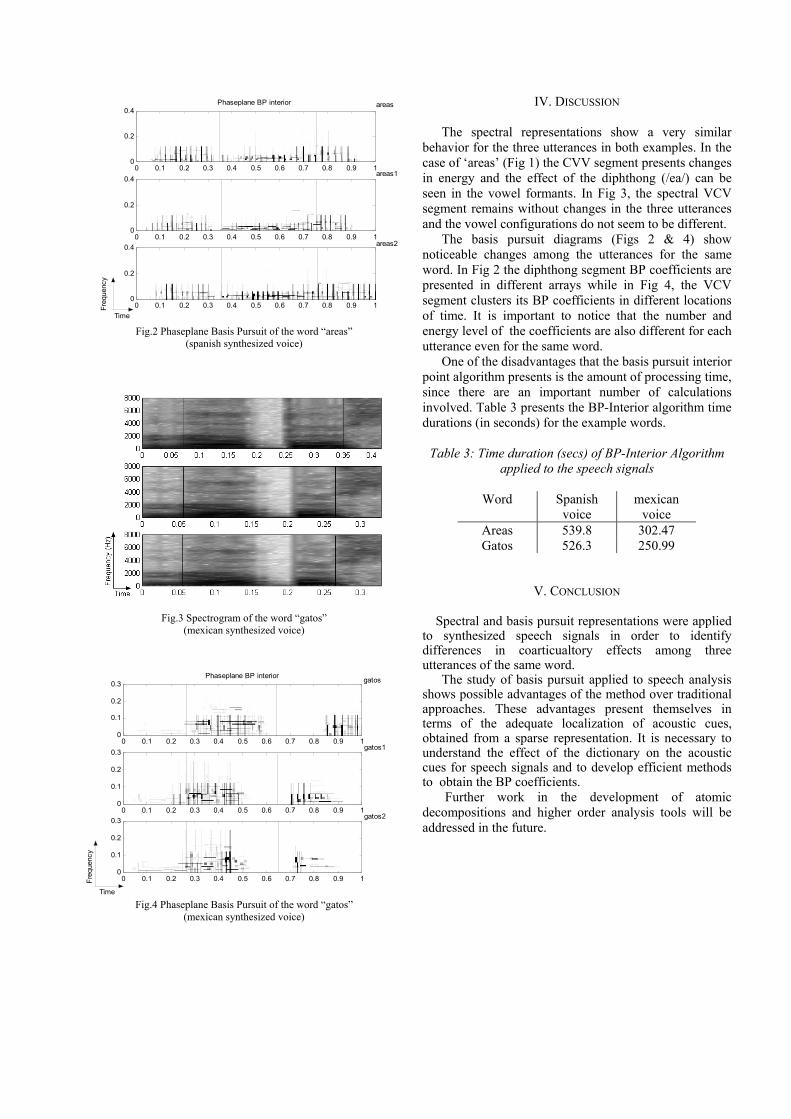
Phaseplane BP interior

0 0.1 0.2 0.3 0.4 0.5 0.6 0.7 0.8 0.9 10

0.2

0.4

areas1

0 0.1 0.2 0.3 0.4 0.5 0.6 0.7 0.8 0.9 10

0.2

0.4

areas2

Time

Freq

uenc

y

0 0.1 0.2 0.3 0.4 0.5 0.6 0.7 0.8 0.9 10

0.2

0.4

areas

Fig.2 Phaseplane Basis Pursuit of the word “areas”

(spanish synthesized voice)

Fig.3 Spectrogram of the word “gatos”

(mexican synthesized voice)

Phaseplane BP interior

0 0.1 0.2 0.3 0.4 0.5 0.6 0.7 0.8 0.9 10

0.1

0.2

0.3

gatos1

0 0.1 0.2 0.3 0.4 0.5 0.6 0.7 0.8 0.9 10

0.1

0.2

0.3

gatos2

Time

Freq

uenc

y

0 0.1 0.2 0.3 0.4 0.5 0.6 0.7 0.8 0.9 10

0.1

0.2

0.3

gatos

Fig.4 Phaseplane Basis Pursuit of the word “gatos”

(mexican synthesized voice)

IV. DISCUSSION The spectral representations show a very similar

behavior for the three utterances in both examples. In the case of ‘areas’ (Fig 1) the CVV segment presents changes in energy and the effect of the diphthong (/ea/) can be seen in the vowel formants. In Fig 3, the spectral VCV segment remains without changes in the three utterances and the vowel configurations do not seem to be different.

The basis pursuit diagrams (Figs 2 & 4) show noticeable changes among the utterances for the same word. In Fig 2 the diphthong segment BP coefficients are presented in different arrays while in Fig 4, the VCV segment clusters its BP coefficients in different locations of time. It is important to notice that the number and energy level of the coefficients are also different for each utterance even for the same word.

One of the disadvantages that the basis pursuit interior point algorithm presents is the amount of processing time, since there are an important number of calculations involved. Table 3 presents the BP-Interior algorithm time durations (in seconds) for the example words.

Table 3: Time duration (secs) of BP-Interior Algorithm applied to the speech signals

Word Spanish

voice mexican

voice Areas 539.8 302.47 Gatos 526.3 250.99

V. CONCLUSION Spectral and basis pursuit representations were applied to synthesized speech signals in order to identify differences in coarticualtory effects among three utterances of the same word.

The study of basis pursuit applied to speech analysis shows possible advantages of the method over traditional approaches. These advantages present themselves in terms of the adequate localization of acoustic cues, obtained from a sparse representation. It is necessary to understand the effect of the dictionary on the acoustic cues for speech signals and to develop efficient methods to obtain the BP coefficients. Further work in the development of atomic decompositions and higher order analysis tools will be addressed in the future.

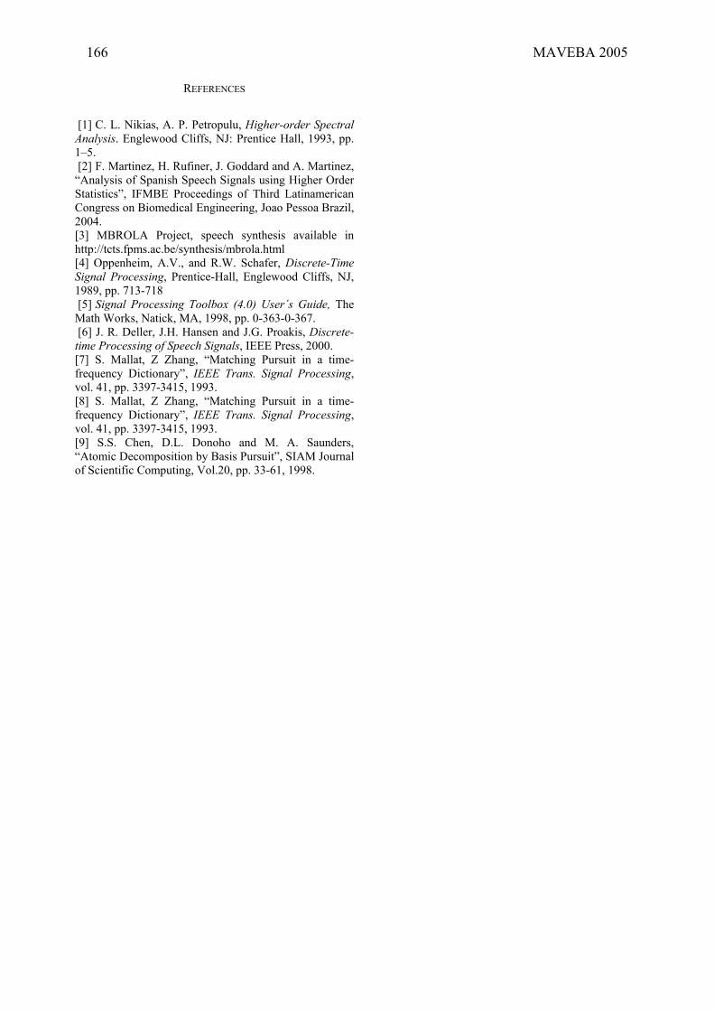
REFERENCES [1] C. L. Nikias, A. P. Petropulu, Higher-order Spectral Analysis. Englewood Cliffs, NJ: Prentice Hall, 1993, pp. 1–5. [2] F. Martinez, H. Rufiner, J. Goddard and A. Martinez, “Analysis of Spanish Speech Signals using Higher Order Statistics”, IFMBE Proceedings of Third Latinamerican Congress on Biomedical Engineering, Joao Pessoa Brazil, 2004. [3] MBROLA Project, speech synthesis available in http://tcts.fpms.ac.be/synthesis/mbrola.html [4] Oppenheim, A.V., and R.W. Schafer, Discrete-Time Signal Processing, Prentice-Hall, Englewood Cliffs, NJ, 1989, pp. 713-718 [5] Signal Processing Toolbox (4.0) User´s Guide, The Math Works, Natick, MA, 1998, pp. 0-363-0-367. [6] J. R. Deller, J.H. Hansen and J.G. Proakis, Discrete-time Processing of Speech Signals, IEEE Press, 2000. [7] S. Mallat, Z Zhang, “Matching Pursuit in a time-frequency Dictionary”, IEEE Trans. Signal Processing, vol. 41, pp. 3397-3415, 1993. [8] S. Mallat, Z Zhang, “Matching Pursuit in a time-frequency Dictionary”, IEEE Trans. Signal Processing, vol. 41, pp. 3397-3415, 1993. [9] S.S. Chen, D.L. Donoho and M. A. Saunders, “Atomic Decomposition by Basis Pursuit”, SIAM Journal of Scientific Computing, Vol.20, pp. 33-61, 1998.

166 MAVEBA 2005

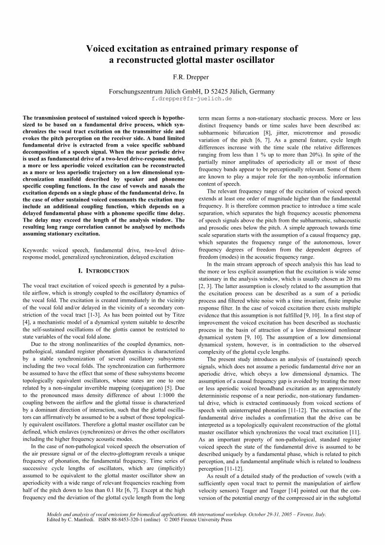
Voiced excitation as entrained primary response ofa reconstructed glottal master oscillator

F.R. Drepper

Forschungszentrum Jülich GmbH, D 52425 Jülich, [email protected]

The transmission protocol of sustained voiced speech is hypothe-sized to be based on a fundamental drive process, which syn-chronizes the vocal tract excitation on the transmitter side and evokes the pitch perception on the receiver side. A band limited fundamental drive is extracted from a voice specific subband decomposition of a speech signal. When the near periodic drive is used as fundamental drive of a two-level drive-response model, a more or less aperiodic voiced excitation can be reconstructed as a more or less aperiodic trajectory on a low dimensional syn-chronization manifold described by speaker and phoneme specific coupling functions. In the case of vowels and nasals the excitation depends on a single phase of the fundamental drive. In the case of other sustained voiced consonants the excitation may include an additional coupling function, which depends on a delayed fundamental phase with a phoneme specific time delay. The delay may exceed the length of the analysis window. The resulting long range correlation cannot be analysed by methods assuming stationary excitation.

Keywords: voiced speech, fundamental drive, two-level drive-response model, generalized synchronization, delayed excitation

I. INTRODUCTION

The vocal tract excitation of voiced speech is generated by a pulsa-tile airflow, which is strongly coupled to the oscillatory dynamics of the vocal fold. The excitation is created immediately in the vicinity of the vocal fold and/or delayed in the vicinity of a secondary con-striction of the vocal tract [1-3]. As has been pointed out by Titze [4], a mechanistic model of a dynamical system suitable to describe the self-sustained oscillations of the glottis cannot be restricted to state variables of the vocal fold alone.

Due to the strong nonlinearities of the coupled dynamics, non-pathological, standard register phonation dynamics is characterized by a stable synchronization of several oscillatory subsystems including the two vocal folds. The synchronization can furthermore be assumed to have the effect that some of these subsystems become topologically equivalent oscillators, whose states are one to one related by a non-singular invertible mapping (conjugation) [5]. Due to the pronounced mass density difference of about 1:1000 the coupling between the airflow and the glottal tissue is characterized by a dominant direction of interaction, such that the glottal oscilla-tors can affirmatively be assumed to be a subset of those topological-ly equivalent oscillators. Therefore a glottal master oscillator can be defined, which enslaves (synchronizes) or drives the other oscillators including the higher frequency acoustic modes.

In the case of non-pathological voiced speech the observation of the air pressure signal or of the electro-glottogram reveals a unique frequency of phonation, the fundamental frequency. Time series of successive cycle lengths of oscillators, which are (implicitly) assumed to be equivalent to the glottal master oscillator show an aperiodicity with a wide range of relevant frequencies reaching from half of the pitch down to less than 0.1 Hz [6, 7]. Except at the high frequency end the deviation of the glottal cycle length from the long

term mean forms a non-stationary stochastic process. More or less distinct frequency bands or time scales have been described as: subharmonic bifurcation [8], jitter, microtremor and prosodic variation of the pitch [6, 7]. As a general feature, cycle length differences increase with the time scale (the relative differences ranging from less than 1 % up to more than 20%). In spite of the partially minor amplitudes of aperiodicity all or most of these frequency bands appear to be perceptionally relevant. Some of them are known to play a major role for the non-symbolic information content of speech.

The relevant frequency range of the excitation of voiced speech extends at least one order of magnitude higher than the fundamental frequency. It is therefore common practice to introduce a time scale separation, which separates the high frequency acoustic phenomena of speech signals above the pitch from the subharmonic, subacoustic and prosodic ones below the pitch. A simple approach towards time scale separation starts with the assumption of a causal frequency gap, which separates the frequency range of the autonomous, lower frequency degrees of freedom from the dependent degrees of freedom (modes) in the acoustic frequency range.

In the main stream approach of speech analysis this has lead to the more or less explicit assumption that the excitation is wide sense stationary in the analysis window, which is usually chosen as 20 ms [2, 3]. The latter assumption is closely related to the assumption that the excitation process can be described as a sum of a periodic process and filtered white noise with a time invariant, finite impulse response filter. In the case of voiced excitation there exists multiple evidence that this assumption is not fulfilled [9, 10]. In a first step of improvement the voiced excitation has been described as stochastic process in the basin of attraction of a low dimensional nonlinear dynamical system [9, 10]. The assumption of a low dimensional dynamical system, however, is in contradiction to the observed complexity of the glottal cycle lengths.

The present study introduces an analysis of (sustained) speech signals, which does not assume a periodic fundamental drive nor an aperiodic drive, which obeys a low dimensional dynamics. The assumption of a causal frequency gap is avoided by treating the more or less aperiodic voiced broadband excitation as an approximately deterministic response of a near periodic, non-stationary fundamen-tal drive, which is extracted continuously from voiced sections of speech with uninterrupted phonation [11-12]. The extraction of the fundamental drive includes a confirmation that the drive can be interpreted as a topologically equivalent reconstruction of the glottal master oscillator which synchronizes the vocal tract excitation [11]. As an important property of non-pathological, standard register voiced speech the state of the fundamental drive is assumed to be described uniquely by a fundamental phase, which is related to pitch perception, and a fundamental amplitude which is related to loudness perception [11-12].

As result of a detailed study of the production of vowels (with a sufficiently open vocal tract to permit the manipulation of airflow velocity sensors) Teager and Teager [14] pointed out that the con-version of the potential energy of the compressed air in the subglottal


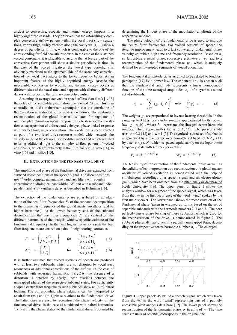
airduct to convective, acoustic and thermal energy happens in a highly organized cascade. They observed that the astonishingly com-plex convective airflow pattern within the vocal tract (flow separa-tions, vortex rings, swirly vortices along the cavity walls, …) show a degree of periodicity in time, which is comparable to the one of the corresponding far field acoustic response. In the case of the sustained voiced consonants it is plausible to assume that at least a part of the convective flow pattern will show a similar periodicity in time. In the case of the voiced fricatives the vowel type periodicity is obviously restricted to the upstream side of the secondary constrict-tion of the vocal tract and/or to the lower frequency bands. As an important feature of the highly organized energy cascade theirreversible conversion to acoustic and thermal energy occurs at different sites of the vocal tract and happens with distinctly differentdelays with respect to the primary convective pulse.

Assuming an average convection speed of less than 5 m/s [1, 15] the delay of the seconddary excitation may exceed 20 ms. This is in contradiction to the mainstream assumption that the correlation of the excitation is restricted to the analysis windows. The continuous reconstruction of the glottal master oscillator for segments of uninterrupted phonation opens the possibility to describe the excita-tion as superposition of a direct and a delayed phase locked response with correct long range correlation. The excitation is reconstructed as part of a two-level drive-response model, which extends the validity range of the classical source-filter model and which is suited to bring additional light to the complex airflow pattern of voicedconsonants, which are extremely difficult to analyse in vivo [14], in vitro [15] and in silico [15].

II. EXTRACTION OF THE FUNDAMENTAL DRIVE

The amplitude and phase of the fundamental drive are extracted fromsubband decompositions of the speech signal. The decompositionsuse 4th order complex gammatone bandpass filters with roughly approximate audiological bandwidths F and with a subband inde-pendent analysis - synthesis delay as described in Hohmann [16].

The extraction of the fundamental phase t is based on an adap-tation of the best filter frequencies j of the subband decompositionto the momentary frequency of the glottal master oscillator (and its higher harmonics). At the lower frequency end of the subband decomposition the best filter frequencies j are centred on the different harmonics of the analysis window specific estimate of thefundamental frequency. In the next higher frequency range the best filter frequencies are centred on pairs of neighbouring harmonics.

F

F

1

1

)1( Fjj

FjFj for (1a)

116

61

j

j

1

1

2 F

FFj for . (1b)

116

61

j

j

It is further assumed that voiced sections of speech are producedwith at least two subbands, which are not distorted by vocal tract resonances or additional constrictions of the airflow. In the case of subbands with separated harmonics, 61 j , the absence of a distortion is detected by nearly linear relations between the unwrapped phases of the respective subband states. For sufficiently adapted centre filter frequencies such subbands show an (n:m) phase locking. The corresponding phase relations can be interpreted to result from (n:1) and (m:1) phase relations to the fundamental drive. The latter ones are used to reconstruct the phase velocity of the fundamental drive. In the case of a subband with paired harmonics,

, the phase relation to the fundamental drive is obtained by

determining the Hilbert phase of the modulation amplitude of therespecttive subband.

116 j

The phase velocity of the fundamental drive is used to improvethe centre filter frequencies. For voiced sections of speech theiterative improvement leads to a fast converging fundamental phase velocity t with a high time and frequency resolution. Based on a, so far, arbitrary initial phase, successive estimates of t lead to a reconstruction of the fundamental phase t , which is uniquely defined for uninterrupted segments of voiced phonation.

The fundamental amplitude t is assumed to be related to loudnessperception [17] by a power law. The exponent

A/1 is chosen such

that the fundamental amplitude represents a linear homogenous function of the time averaged amplitudes tiA , of a synthesis suited set of subbands,

vN

jtjjt AgA

1

1, )( with . (2) 1

1

N

jjg

The weights j are proportional to inverse hearing thresholds. In the range up to 3 kHz they can be roughly approximated by the power law , where jh represents the (integer) centre harmonic number, which approximates the ratio 1 . The present study uses

g

jj hg/ FFj

3.0 [18] and 1 [3]. The synthesis suited set of subbands is generated by replacing the over complete subband set 116 jby a set Nj6 , which is spaced equidistantly on the logarithmicfrequency scale with 4 filters per octave,

(3) 14/)5(25 FF j

j 14/)5(2 FF j

j

The feasibility of the extraction of the fundamental drive as well asthe validity of its interpretation as a reconstruction of a glottal masteroscillator of voiced excitation is demonstrated with the help ofsimultaneous recordings of a speech signal and an electro-glotto-gram, which have been obtained from the pitch analysis database of Keele University [19]. The upper panel of figure 1 shows theanalysis window for a segment of the speech signal, which was taken from the /w/ in the first occurrence of the word “wind” spoken by the first male speaker. The lower panel shows the reconstruction of thefundamental phase (given in wrapped up form), based on the set of separable subbands with the harmonic numbers 2, 3 and 5. The near perfectly linear phase locking of these subbands, which is used for the reconstruction of the drive, is demonstrated in figure 2. Thesubband phases j are given in a partially unwrapped form, depen-ding on the respective centre harmonic number . The enlarged jh

Figure 1, upper panel: 45 ms of a speech signal, which was takenfrom the /w/ in the word “wind” representing part of a publicly accessible pitch analysis data base [19]. The lower panel shows the reconstruction of the fundamental phase in units of . The timescale (in units of seconds) corresponds to the original one.

0.5 0.51 0.52 0.53

-0.2

0

0.2

signal

0.5 0.51 0.52 0.530

1

2

168 MAVEBA 2005

Figure 2: Relation of subband phases j , )6...,,2,1( j , obtained from the speech signal of figure 1, to the fundamental phase . Thesubbands 2, 3 and 5 are characterized by near perfectly linear phase relations, whereas the other subbands are found to be unsuited for the reconstruction of the fundamental phase.

Figure 3: Relation between the wrapped up fundamental phase s ,obtained from the speech signal, and the fundamental phase e ,obtained from the electro-glottogram.

range of the subband phases is normalized by the same centre harmonic number. Alternatively the fundamental phase can also be obtained from a subband decomposition of the electro-glottogram.The exchangeability of the two phases is demonstrated in figure 3,which shows the relation between the two fundamental phases forthe speech segment, which covers the “win” part of the word “wind”, uttered by the first female speaker. The phase shift between the twophases did not change significantly during the 160 ms being covered.

In spite of the arbitrariness of the initial fundamental phase, the reconstruction of the glottal master oscillator can be used as funda-mental drive of a two level drive – response model, which is suited to describe voiced speech as secondary response. The additional sub-system describes the excitation of the vocal tract as primary response of the fundamental drive and the classical secondary response sub-

system describes the more or less resonant “signal forming” on the way through the vocal tract as action of a linear autoregressive filter. The subband decomposition (1) and (3) being used for the recon-struction of the fundamental drive can also be used with advantage to achieve a numerically robust reconstruction of the excitation.

III. ENTRAINMENT OF THE PRIMARY RESPONSE

Due to the slow velocity of the glottal tissue (compared to the velo-city of sound) the excitation tj of a voiced subband with indexE ,

Nj1 can be assumed to be restricted (enslaved or entrained) to a generalized synchronization manifold (surface) in the combinedstate space of drive and response [20-22]. In the simplest case the time dependence of subband excitation tj can thus be replaced by a dependence on the simultaneous state of the fundamental drive. More generally, the dependence of the state of the primary response on the state of the fundamental drive may degenerate to a multi-valued mapping, which can, however, be expressed by a unique function of the unwrapped fundamental phase

E ,

t [11-12],

pjSk

tkjttpjttj p

kicAGAE,

)exp()( ,,, . (4)

As part of the improved time scale separation the generalized syn-chronization manifold is assumed to be the product of the slowly variable fundamental amplitude and the potentially fast varyingcomplex coupling function

tA)(, tpjG , the real part of which describes

the subband excitation. In its general form, )(, tpjG represents a p2 periodic function of the unwrapped fundamental phase t

with an integer period number and can thus be well approxi-mated by the finite Fourier series in equation (4). Voiced excitationsare characterized by values of p, which are distinctly smaller than thenumber of fundamental cycles within the analysis window. The case

1p

1p corresponds to the normal voice type characterized by a unique mapping [20], whereas 2p is suited to describe the perioddoubling voice type [4]. The unwrapped fundamental phase can beassumed to be approximately proportional to time. When p2exceeds the length of the analysis window, equation (4) is therefore suited to describe a fully general excitation, including the unvoiced case.

The excitation parameters kj cannot be determined indepen-dently from the parameters, which characterize the vocal tract reso-nances. In the standard approach the parameter estimation is per-formed hierarchically, by making the higher level assumption that the excitation has a nearly white (or tilted) spectrum. To achieve acomparable numerical robustness, the parameter estimation is done separately for the different frequency bands. The band limitation can be used to reduce the number of resonances (poles of the auto-regressive filter), which are relevant for the respective subband. Thecomplex subband

c ,

tjX , can thus be described by the following nonlinear conditional stochastic process with a two-level drive –response model as deterministic part (skeleton) [11-12],

tjjttpjttjjtj AGAXbX ,,,, )( , (5)

where denotes the subband specific prediction step length, jb thecomplex subband specific resonator parameter, tj , a (0,1) Gaussiancomplex white noise process and j the time independent part of the standard deviation. As an important computational advantage theestimation of the complex excitation and resonator parameters kjc ,

and j can be reduced to multiple linear regression. The summationindex set pj of equation (4) is chosen in accordance to the respect-tive bandpass filter. The decomposition into subbands is used to estimate equation (5) with a subband specific integer time step

bS ,

0 0.5 1 1.5 20

0.5

1

1.5

2

1

0 1 20

0.5

1

1.5

2

2

0 0.5 1 1.5 20

0.5

1

1.5

2

3

0 1 20

0.5

1

1.5

2

4

0 0.5 1 1.5 20

0.5

1

1.5

2

5

0 1 20

0.5

1

1.5

2

6

0 0.2 0.4 0.6 0.8 1 1.2 1.4 1.6 1.8 20

0.2

0.4

0.6

0.8

1

1.2

1.4

1.6

1.8

2

s

e

Voice modelling and analysis 169

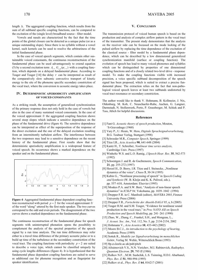
length . The aggregated coupling function, which results from the sum of all subband specific coupling functions, can be compared to the excitation of the (single level) broadband source - filter model.

Vowels and nasals are characterized by the fact that the timepoints of the glottal closure can be detected as a unique pulse (or as a unique outstanding slope). Since there is no syllable without a vowel kernel, such kernels can be used to resolve the arbitrariness of the initial fundamental phase.

In the case of voiced speech segments, which contain other sus-tainnable voiced consonants, the continuous reconstructtuion of thefundamental phase can be used advantageously to extend equation (5) by a second excitation term )(, tpjt GA with a coupling func-tion, which depends on a delayed fundamental phase. According to Teager and Teager [14] the delay can be interpreted as result ofthe comparatively slow subsonic convective transport of kinetic energy to the site of the phoneme specific secondary constriction of the vocal tract, where the conversion to acoustic energy takes place.

IV. DETERMINISTIC APERIODICITY AMPLIFICATIONOF VOICED CONSONANTS

As a striking result, the assumption of generalized synchronization of the primary response does not only hold in the case of vowels but also in the case of many sustained voiced consonants. In the case of the voiced approximant /l/ the aggregated coupling function showsseveral steep slopes which indicate a sensitive dependence on the phase of the fundamental drive (figure 4). The sensitive dependence can be interpreted as effect of the superposition of the response of the direct excitation and the one of the delayed excitation resulting from an intermittently turbulent airflow. The interference betweenthe two responses may lead to a sensitive dependence on the recent history of the fundamental phase. First results show that the deterministic aperiodicity amplification is a widespread feature of voiced speech. Its occurrence shows a marked dependence on the speaker and on the fundamental phase.

Figure 4: Aggregated fundamental phase dependent coupling func-tion reconstructed with period for the voiced approximant /l/ of the word “along” uttered by the first male speaker. The two curves correspond to the odd and even periods. The disagreement of the two curves shows a marked dependence on the fundamental phase.

2p

The continuous reconstruction of the fundamental phase for speechsegments with uninterrupted phonation opens the possibility to complement the analysis of the spectral properties of the speechsignal by a run time analysis. The run time differences may refer either to a travel time difference of the primary acoustic pulse or to a build up time of the turbulence at the seconddary constricttion of thevocal tract. The coupling functions with periodicity 2p are suited to describe a voice type, which cannot be classified uniquely by using cycle lengths differences (figure 4). It is hypothesized that the fundamental phase dependent coupling functions are suited to serve as additional cue for phoneme recognition and as fingerprint for speaker identification.

V. CONCLUSION

The transmission protocol of voiced human speech is based on the production and analysis of complex airflow pattern in the vocal tract of the transmitter. The present study demonstrates that the analysison the receiver side can be focussed on the mode locking of the pulsed airflow by replacing the time dependence of the excitation of the classical source - filter model by a fundamental phase depen-dence, which can be described by a low dimensional generalized synchronization manifold (surface or coupling function). Theevolution of speech has lead to many voiced phonemes and syllableswhich can be distinguished by properties of one dimensionalcoupling functions and of a closely related two-level drive - response model. To make the coupling functions visible with increased precision, a voice specific subband decomposition of the speech signal has been proposed, which is suited to extract a precise fun-damental phase. The extraction relies on the fact that non-patho-logical voiced speech leaves at least two subbands undistorted byvocal tract resonance or secondary constriction.

The author would like to thank V. Hohmann, B. Kollmeier, J. Nix,Oldenburg, M. Kob, C. Neuschaefer-Rube, Aachen, G. Langner, Darmstadt, N. Stollenwerk, Porto, P. Grassberger, M. Schiek and P. Tass, Jülich for helpful discussions.

References

[1] Fant G. Acoustic theory of speech production, Mouton,‘S-Gravenhage (1960)

[2] Vary P., U. Heute, W. Hess, Digitale Sprachsignalverarbeitung,B.G. Teubner Verlag, Stuttgart (1998)

[3] Schroeder M.R., Computer Speech, Springer (1999)[4] Titze I.R., Acta Acustica 90, 641-648 (2004) [5] Kantz H., T. Schreiber, Nonlinear time series analysis,

Cambridge Univ. Press (1997) [6] Winholtz W.S. and L.O. Ramig, J.Speech Hear. Res. 35, 562-573

(1992)[7] Schoentgen J. and R. de Guchteneere, Speech Communication,

21, pp. 255-272 (1997) [8] Herzel H., D. Berry, I.R. Titze and I. Steinecke, „Nonlinear

dynamics of the voice“, Chaos 5, 30-34 (1995) [9] Kubin G., “Nonlinear processing of speech” in Speech Coding

and Synthesis (W. B. Kleijn and K. K. Paliwal, eds.),pp. 557–610, Amsterdam: Elsevier (1995)

[10] Moakes P.A. and S.W. Beet, “Analysis of non-linear speechdynamics” in ICSLP 94, Yokohama, pp. 1039–1042 (1994)

[11] Drepper F.R. in C. Manfredi (editor), MAVEBA 2003, Firenze University Press (2004)

[12] Drepper F.R., Fortschritte der Akustik-DAGA’05, a, b (2005)[14] Teager H.M. and S.M. Teager, “Evidence for nonlinear sound

production in the vocal tract,” in Proc NATO ASI on Speech Production and Speech Modelling, pp. 241–261 (1990)

[15] Zhao, W., Zhang, C., Frankel, S.H., and Mongeau, L.,J. Acoust. Soc. Am., Vol. 112, No. 5, pp. 2134-2154, 2002

[16] Hohmann V., Acta Acustica 10, 433-442 (2002)[17] Moore B.C.J., An introduction to the psychology of hearing,

Academic Press (1989)[18] Sottek R., Modelle zur Signalverarbeitung im menschlichen

Gehör, Verlag M. Wehle, Witterschlick/Bonn (1993)[19] ftp.cs.keele.ac.uk/pub/pitch[20] Afraimovich V.S., N.N. Verichev, M.I. Rabinovich, Radiophys.

Quantum Electron. 29, 795 ff (1986)[21] Rulkov N.F. , M.M. Sushchik, L.S. Tsimring, H.D.I. Abarbanel,

Phys. Rev. E 51, 980-994 (1995)[22] Rulkov et al., Phys. Rev. E 64, 016217 (2001)

0 0.2 0.4 0.6 0.8 1 1.2 1.4 1.6 1.8 2

-2

0

2

Ex

170 MAVEBA 2005

Speech analysis for identification and recognition purposes is a demanding task, especially to find recognition parameters for some consonants. In this paper, we show the initial analysis results of speech corpus, sampled with two sampling rates, 22050 and 8000 Hz, using Higuchi fractal dimension. The study shows that it might be possible to use fractal dimension value for classification of for example plosives /k/, /p/ and /t/. However, the analysis seems to be very sensitive to the sampling frequency in speech analysis.

I. INTRODUCTION

Linear speech analysis and models has served

successfully the speech processing areas for decades. However, there has also been an interest to research and evaluate nonlinear methods in order to find better way to model speech, especially for speech recognition purposes.

Several studies have found evidences for nonlinear behavior in speech. Different nonlinear techniques have been tested with time series over several decades in order to improve modeling and estimation when compared to linear methods. For example, the logarithmic a-law/µ-law compression in Pulse Code Modulation (PCM) coding has worked successfully over the years. However, the precise “practical” nonlinearity form for vocal tract model is not known and the search for good alternatives for the describing the human vocal tract with linear methods is currently going on. The Hammerstein model, Volterra series and Wiener filters have been tested experimentally as well as the chaotic time series modeling with very good results. However, the disadvantages are, when compared to the linear models, the more complex parameter computations and in some cases, the stability preservation. Also, different types of neural networks have been tested for several purposes in speech processing. Neural network is easy to design, train and test but there still remains a fear that the unique and documented experiment is unrepeatable even with the same data [1-17].

The nonlinear signal processing field is enormous, in that sense that the number of different functions, equations and/or systems that can be used for speech modeling and analysis is practically infinite.

The chaotic models have worked successfully for vowels and nasals [4, 5] and Teager energy operator [18

,19] has been used to indicate several features of speech, for example speech resonances and modulations.

In this paper we study the effect of Higuchi Fractal dimension for different phonemes.

II. METHODS AND DATA

Higuchi fractal dimension [20] is a method developed for estimating the amount of self-similarity of the data. Higuchi [20] used his method for magnetic field data and in [21, 23-25] Higuchi’s method was used for electroencephalography data.

Method described in [20], defines the discrete time series:

X[1], X[2], … ,X[n]

to be constructed to a new time series:

km

kk

mNmXkmXkmXmXX mk

,...,2,1

),][(],...,2[],[],[;

=

−+++

where m is the initial time and k is the interval time, N is the total number of samples. For example if k=3 and N=100, three time series are obtained as follows:

)99(),...,9(),6(),3(;

)98(),...,8(),5(),2(;

)100(),...,7(),4(),1(;

33

23

13

XXXXX

XXXXX

XXXXX

The length of the curve, defined in [20] is:

k

kk

mNNkimXikmX

kL

kmN

i

m

−

−

−+−+

=

∑

−

=

1)1(()(

)(

1

Lm(k) represents normalized sum of “segment length”. Each “segment length” represents the absolute value of difference between magnitude values of pair of points distant k samples, starting from mth . sample. The length of the curve L(k) is mean of k values Lm(k), for m=1,2,…k. The fractal dimension D is the least square estimate of the slope of the curve evaluated on 1..kmax values on L(k). If the curve is plotted on doubly logarithmic scales, for 1..kmax in ln(1/k) and L(k) in

SPEECH ANALYSIS USING HIGUCHI FRACTAL DIMENSION

Jari Turunen, Tarmo Lipping & Juha T. Tanttu

Tampere University of Technology, Pori P.O.Box 300, Pohjoisranta 11, FIN-28101 Pori

{jari.turunen, tarmo.lipping, juha.tanttu}@pori.tut.fi


ln(L(k)), the data should fall on a straight line with a slope (-D). It should be noted that Higuchi fractal dimension is not related with chaotic attractor dimension.

For example, the Higuchi value of white noise, with maximum amplitudes [-1,1] with kmax =10, is 1, and straight line with slope is zero.

The algorithm and evaluation was performed using Matlab environment. In our preliminary experiments, several kmax values were tested. If the kmax values was increased beyond 25 the Higuchi fractal dimension values tend to get closer to one as the kmax increases. Similarily, if the kmax value was decreased below 8, the Higuchi values tend to progress towards zero. The kmax value 10 gave best results in our experiments.

Table 1. Phonemes and their corresponding example words.

phon. word phon. word phon word /p/ pin /tS/ chin /i/ see /b/ bay /dZ/ jam /a/ father /t/ toy /m/ me /O/ sort /d/ die /n/ not /Î/ bird /k/ key /N/ sing /u/ too /g/ get /l/ light /ei/ day /f/ five /r/ ring /ai/ fly /v/ van /w/ win /Oi/ boy /T/ thick /j/ yes /ou/ go /D/ then /I/ sit /au/ cow /s/ see /e/ get /i«/ ear /z/ zinc /Q/ cat /u«/ tour /S/ ship /Ã/ hut /e«/ air /Z/ measure /A/ hot /q/ [silence] /h/ he /U/ put /«/ banana

Table 2. Number of different phonemes in each phoneme category.

phon. # phon. # phon # /p/ 83 /tS/ 89 /i/ 154 /b/ 61 /dZ/ 52 /a/ 96 /t/ 191 /m/ 72 /O/ 162 /d/ 66 /n/ 236 /Î/ 92 /k/ 140 /N/ 48 /u/ 145 /g/ 60 /l/ 61 /ei/ 156 /f/ 211 /r/ 152 /ai/ 216 /v/ 107 /w/ 106 /Oi/ 96 /T/ 138 /j/ 48 /ou/ 151 /D/ 61 /I/ 153 /au/ 95 /s/ 205 /e/ 173 /i«/ 44 /z/ 115 /Q/ 72 /u«/ 37 /S/ 80 /Ã/ 130 /e«/ 68 /Z/ 38 /A/ 72 /q/ 3 /h/ 48 /U/ 48 /«/ 30

The OTAGO speech corpus [22] was used in the tests. The phonemes were manually checked and identified. The data, which was used in experiments, is presented in Table 1 and Table 2. The sampling frequency was 22050 Hz and total number of samples was 4661.

The phoneme lengths varied from minimum of 143 samples in /b/ to 10949 samples in /a/ sampled with 22050 Hz frequency. The /q/ is a silence “phoneme” recorded by the microphone (background noise). We preformed two tests with Higuchi analysis: the first one with 22050 sampling frequency and the second one with 8000 Hz sampling frequency. The lower sampling frequency was obtained by resampling the data from the original data by using Matlab “resample” command.

III. RESULTS

The results are shown in Figures 1-6. The Figures 1-3

show the fractal dimension values for phonemes sampled at 22050 Hz and Figures 4-6 show the fractal dimension values for 8000 Hz data.

In the figures, the boxes show the lower quartile, median and the upper quartile of all sampled phoneme values. The lines show the deviation for the rest of phoneme data and outliers are presented with ‘+’ sign.

/p/ /b/ /t/ /d/ /k/ /g/ /f/ /v/ /T/ /D/ /s/ /z/ /S/ /Z/ /h/

0

0.2

0.4

0.6

0.8

1

1.2

1.4

Val

ues

Phoneme

Figure 1. The fractal dimension values for phonemes /p/ to /h/ sampled at 22050 Hz frequency

/tS/ /dZ/ /m/ /n/ /N/ /l/ /r/ /w/ /j/ /I/ /e/ /Q/ /Ã/ /A/ /U/

0

0.2

0.4

0.6

0.8

1

1.2

1.4

Val

ues

Phoneme

Figure 2. The fractal dimension values for phonemes /tS/ to /U/ sampled at 22050 Hz frequency

172 MAVEBA 2005

/i/ /a/ /O/ /Î/ /u/ /ei/ /ai/ /Oi/ /ou/ /au/ /i«/ /u«/ /e«/ /q/ /«/

0

0.2

0.4

0.6

0.8

1

1.2

1.4

Val

ues

Phoneme

Figure 3. The fractal dimension values for phonemes /i/ to /«/ sampled at 22050 Hz frequency

/p/ /b/ /t/ /d/ /k/ /g/ /f/ /v/ /T/ /D/ /s/ /z/ /S/ /Z/ /h/0

0.2

0.4

0.6

0.8

1

1.2

Val

ues

Phoneme

Figure 4. The fractal dimension values for phonemes /p/ to /h/ sampled at 8000 Hz frequency

/tS/ /dZ/ /m/ /n/ /N/ /l/ /r/ /w/ /j/ /I/ /e/ /Q/ /Ã/ /A/ /U/0

0.2

0.4

0.6

0.8

1

1.2

Val

ues

Phoneme

Figure 5. The fractal dimension values for phonemes /tS/ to /U/ sampled at 8000 Hz frequency

/i/ /a/ /O/ /Î/ /u/ /ei/ /ai/ /Oi/ /ou/ /au/ /i«/ /u«/ /e«/ /q/ /«/0

0.2

0.4

0.6

0.8

1

1.2

Val

ues

Phoneme

Figure 6. The fractal dimension values for phonemes /i/ to /«/ sampled at 8000 Hz frequency

IV. DISCUSSION

When looking the Figures 1-3 with Fs=22050 Hz, the Higuchi Fractal dimension reveals interesting things from the phonemes. For example plosives /p/, /t/ and /k/ has been very difficult to separate from each other by using other methods, but is seems that they are possible to separate by using Higuchi fractal dimension. The quartile bars and the whole data deviation in plosive /k/ does not separate from /t/ as well as the /p/, although the median is different by visual inspection. In addition, the grouping of the fricatives can be seen from the figures 1-2. The fricatives /s/, /z/, /f/, /Ts/, /Tz/ and /q/ (that means background noise) medians are concentrated near one (from 0.8 to 1.2). This may also be interpreted that the Higuchi fractal dimension is very sensitive to background noise.

The nasals /n/ and /m/, semivowels /v/ and /w/ and all vowels have median values below 0.5. The Higuchi values of vowels, interestingly, seem to correlate with the vowel production mechanism somehow, in the sense of tongue position in the mouth. For example, lower fundamental frequency vowel /U/ has smaller Higuchi value when compared to higher fundamental frequency vowel /i/.

All seems to separate nicely with 22050 Hz recordings but unfortunately speech is usually sampled and transferred with much lower, 8000 Hz sampling frequency. The interesting phenomena do not appear in same depth anymore in lower sampling frequency. When looking the figures 4-6 the phonemes do not show similar behavior as they did in figures 1-3. The plosives /t/ and /p/ do separate in figure 4, but the quartile bars are much closer (and slightly overlapping) to each other than in figure 1. The values of phoneme /k/ are higher than in previous analysis. The fricatives /s/, /z/, /f/, /Ts/, /Tz/ and /q/ show overall dropping in median values especially in

Voice modelling and analysis 173

the case of /z/. Also phonemes seem to have overall increase in the median values. The Higuchi values for vowels have higher values than in 22050 Hz sampling frequency, but in the case of vowel /i/, the fractal dimension values are dropped. When thinking the Higuchi fractal dimension value computation, the differences between two sampling frequency results seems to follow the filtering properties. The Higuchi fractal dimension measures the amount of self-similarity by searching the difference between adjacent samples. The downsampling will smooth the fine structure of the signal. The selection of kmax. parameter is also very important for the analysis. In our case the both sampling frequencies 22050 and 8000 Hz the kmax=10 seems to be good for speech analysis purposes. Several kmax values were tested, well beyond 50, because in vowels the fundamental cycle repetition is approximately 50-140 samples in 8000 Hz sampling frequency. kmax values beyond 50 provided fractal dimension values that are all approaching one rather than providing better separation between consonants and vowels. With lower sampling frequencies some critical information may be lost, which may be useful for recognition purposes with this method. Higuchi fractal dimension is useful tool, and the algorithm is very simple and easy to compute providing single number for example analysis and recognition purposes.

REFERENCES

[1] Kubin G., “Nonlinear Processing of Speech”,

Speech Coding and Synthesis, Elsevier Science, Amsterdam, 1995.

[2] Townshend B., ”Nonlinear prediction of speech”, IEEE ICASSP: 425-428,1991.

[3] Langi A., Soemintaputra K. & Kinsner W., “Multifractal Processing of Speech Signals”, IEEE ICICS: 527-531, 1997.

[4] Banbrook M., McLaughlin S. & Mann I., “Speech Characterisation and Synthesis by Nonlinear Methods”, IEEE Trans. Speech and Audio Proc, 7 (1): 1-17,1999

[5] Miyano T., Nagami A., Tokuda I., Kazuyuki A., “Detecting nonlinear determinism in voiced sounds of Japanese vowel /a/”, in Int. Journal of Bifurcation and Chaos, 10 (8), 1973-1979, 2000.

[6] Thyssen J., Nielsen H. & Hansen S., “Non-linear short term prediction in speech coding”, IEEE ICASSP, (1): 185-188, 1994.

[7] Kumar A. & Gersho A., “LD-CELP Speech Coding with Nonlinear Prediction”, IEEE Signal Processing Letters, 4 (4), 89-91,1997.

[8] Ma N. & Wei G., “Speech Coding with Nonlinear Local Prediction Model”, IEEE ICASSP: 1101-1104, 1998.

[9] Birgmeier M., Bernhard H. & Kubin G.,”Nonlinear Long-Term Prediction of Speech Signals”, IEEE ICASSP: 1283-1286, 1997.

[10] Kubin G., ”Synthesis and Coding of Continuous Speech with The Nonlinear Oscillator Model”, IEEE ICASSP: 267-270, 1996.

[11] Ohmura H. & Tanaka K., ”Speech Synthesis Using a Nonlinear energy Damping Model for The Vocal Folds Vibration Effect”, IEEE ICSLP, (2): Acoustic Analysis, #11, 1996.

[12] Abarbanel H., “Chaotic Signals and Physical Systems”, IEEE ICASSP, (4): 113-116, 1992.

[13] Singer A., Wornell G. & Oppenheim A., ”Codebook Prediction: A Nonlinear Signal Modeling Paradigm”, IEEE ICASSP (5), 325-328, 1992.

[14] Díaz-de-Maria F. & Figueiras-Vidal A., “Radial Basis Functions for Nonlinear Prediction of speech in Analysis-by-Synthesis Coders”, IEEE ICASSP: 788-791, 1995.

[15] Hennebert J., Hasler M. & Dedieu H., "Neural networks in speech recognition", Proc. 6th Microcomputer School, Prague, 1994.

[16] Fackrell J., “Bispectral Analysis of Speech Signals”, doctoral dissertation, University of Edinburgh, 1996.

[17] Turunen J., Tanttu J., & Loula P., ”Hammerstein model for speech coding”, in Eurasip JASP (12), 1238-1249, 2003.

[18] Teager H., “Some Observations on Oral Air Flow During Phonation”, in IEEE Transactions on ASSP: 28, 599-601, 1980.

[19] Teager H., & Teager S., “Evidence ofor Nonlinear Production Mechanisms on Vocal Tract” in NATO adv. Study Inst. On Speech Production and Speech Modelling, Kluwer, Bonas France,1990.

[20] Higuchi T., “Approach to an irregular time series on the basis of the fractal theory”, in Physica D, 31, 277-283, 1988.

[21] Accardo A., Affinito M., Carrozzi M. & Bouquet F., “Use of fractal dimension for the analysis of electroencephalographic time series”, in Biological Cybernetics, 77 (5), 339-350, 1997.

[22] OTAGO speech corpus, available URL: http://translator.kedri.info/datasets/corpus/otago.

[23] T. Lipping, E. Olejarczyk and M. Parts. Fractal dimension analysis of the effects of photic and microwave stimulation on the brain function. Proceeedings of the World Congress on Biomedical Engineering and Medical Physics, Sydney, Australia, 24-29.08.2003 (on CD ROM).

[24] T. Lipping, E. Olejarczyk and M. Parts. Analysis of photo-stimulation and microwave stimulation effects on EEG signal using Higuchi’s fractal dimension method. In Optical Methods, Sensors, Image Processing, and Visualization in Medicin, A. Nowakowski and B. B. Kosmowski eds., Proc. SPIE, vol. 5505 (SPIE, Bellingham, WA, 2004), pp. 174-178.

[25] A. Anier, T. Lipping, S. Melto, S. Hovilehto. Higuchi fractal dimension and spectral entropy as measures of depth of sedation in intensive care unit. Proc of the 26th IEEE EMBS Annual International Conference, San Fracisco, USA, September 1-5, 2004, pp. 526-529.

174 MAVEBA 2005

Special session on

Neurological dysfunctions


EFFECT OF PARKINSON’S DISEASE ON VOCAL TREMOR

L. Cnockaert1∗, J. Schoentgen1†, P. Auzou23, C. Ozsancak34 and F. Grenez1

1 Universite Libre de Bruxelles, Department Waves and Signals, Brussels, Belgium2 Service d’explorations fonctionnelles neurologiques, Groupe HOPALE, Berk sur Mer, France

3 EA 2683, CHRU Lille, France4 Service de Neurologie, Centre Hospitalier de Boulogne sur Mer, France

[email protected]

Vocal tremor is encountered in different neurologicaldiseases and could be used for their characterisa-tion. In this paper, vocal tremor features have beenextracted for speakers with Parkinson’s disease andcontrol speakers. It is shown that Parkinson’s diseasehas significant effects on vocal tremor features. Forspeakers with Parkinson’s disease, the average vocalfrequency is higher and the vocal tremor frequency ishigher. This can be explained by higher vocal tremorcomponents in the frequency band8 − 12Hz.

I. I NTRODUCTION

The objective of this paper is to report data about thevocal tremor features of parkinsonian and control speakers,as well as an improvement to the vocal tremor analysispresented in [1].

Vocal tremor is a narrow-band low-frequency pertur-bation of the vocal frequency. It is characterised by itsaverage amplitude and average frequency. The amplitudeof the perturbation is about a few percent of the averagevocal frequency. The tremor frequency range is subject todiscussion. A definition including most of the frequencyranges is given by Titze who defines the vocal tremor asthe 1-15Hz modulation of the vocal frequency [2]. Theorigins of vocal tremor are reported to be neurologic or dueto an interaction between neurological and biomechanicalproperties of the vocal folds [2]. Influence of blood flow,heartbeat and breath are also reported [3]. The lowerfrequency limit should be chosen in accordance with theeffects that should be taken in account.

In this paper, the estimation of vocal tremor featureshas been obtained by means of an improvement of theanalysis developed in [1]. The vocal frequency trace is firstcalculated. The vocal frequency estimates are obtained foreach time sample by means of the instantaneous frequencycalculated in an automatically selected frequency-band ofawavelet transform of the speech signal. Using this method,no windowing of the signal is necessary and instantaneous

∗The first author is a fellow with the FRIA (Belgium).†The second author is a Senior Research Associate with the Fonds

National de la Recherche Scientifique (Belgium).

F0 variations can be tracked. A second wavelet transformhas been introduced, in order to improve the precisionand robustness of the method. This is necessary to trackcorrectly fastF0 variations and to handle speech signalsfrom a clinical environment, where older and dysphonicspeakers are encountered. Instantaneous values of the vocaltremor features are then obtained by means of a wavelettransform of the vocal frequency trace.

In this paper, the vocal tremor features have been ex-tracted for parkinsonian and control speakers and statisticalresults about the differences between both groups arepresented.

II. V OCAL FREQUENCY ESTIMATION

The instantaneous frequencyIF (t) of a band-pass signals(t) is usually defined by means of its Hilbert transformH[s(t)] and its associated analytical signalsa(t)[4].

sa(t) = s(t) + jH[s(t)] (1)

Φ(t) = arg[sa(t)] (2)

IF (t) =dΦ(t)

dt(3)

The IF can also be defined by means of a continuouswavelet transformCWT (λ, t) using an analytical waveletψa(t) [5]. The continuous wavelet transform of a signalx(t) is defined as

CWT (λ, t) =

∫ +∞

−∞

x (u)1√

λψ∗

(

u − t

λ

)

du, (4)

whereψ(t) is an analytical mother wavelet andCWT (λ, t)is the wavelet transform coefficient for a scale factorλ, at time t. The amplitude and phase of the complexCWT coefficients thus obtained are the envelope andinstantaneous phase of the spectral components of thesignal in the frequency-band centred on the central fre-quencyfc of the wavelet [6]. The time-derivative of thephase of the complex CWT coefficients is therefore anestimate of the instantaneous frequency (IF) of the signalin that frequency-band. The evolution of the IF in differentfrequency-bands of the signal can thus be studied by meansof the CWT coefficients.


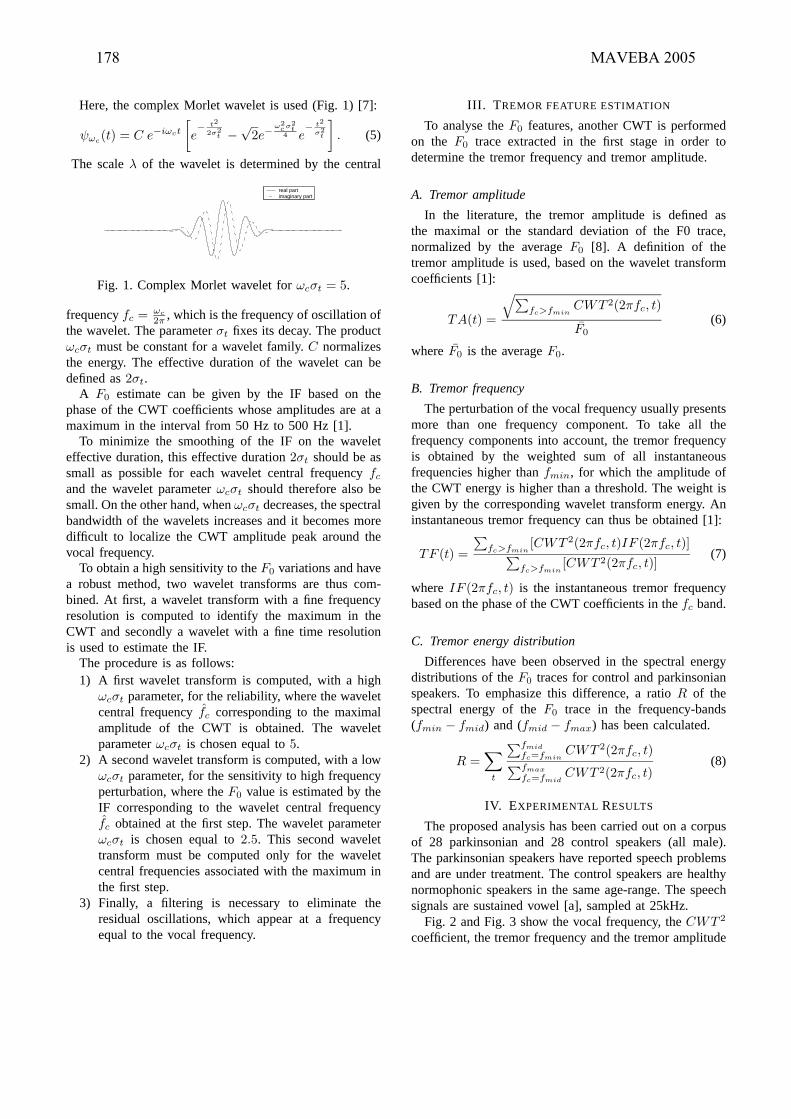
Here, the complex Morlet wavelet is used (Fig. 1) [7]:

ψωc(t) = C e−iωct

[

e−

t2

2σ2t −

√

2e−ω2c

σ2t

4 e−

t2

σ2t

]

. (5)

The scaleλ of the wavelet is determined by the central

real partimaginary part

Fig. 1. Complex Morlet wavelet forωcσt = 5.

frequencyfc = ωc

2π, which is the frequency of oscillation of

the wavelet. The parameterσt fixes its decay. The productωcσt must be constant for a wavelet family.C normalizesthe energy. The effective duration of the wavelet can bedefined as2σt.

A F0 estimate can be given by the IF based on thephase of the CWT coefficients whose amplitudes are at amaximum in the interval from 50 Hz to 500 Hz [1].

To minimize the smoothing of the IF on the waveleteffective duration, this effective duration2σt should be assmall as possible for each wavelet central frequencyfc

and the wavelet parameterωcσt should therefore also besmall. On the other hand, whenωcσt decreases, the spectralbandwidth of the wavelets increases and it becomes moredifficult to localize the CWT amplitude peak around thevocal frequency.

To obtain a high sensitivity to theF0 variations and havea robust method, two wavelet transforms are thus com-bined. At first, a wavelet transform with a fine frequencyresolution is computed to identify the maximum in theCWT and secondly a wavelet with a fine time resolutionis used to estimate the IF.

The procedure is as follows:1) A first wavelet transform is computed, with a high

ωcσt parameter, for the reliability, where the waveletcentral frequencyfc corresponding to the maximalamplitude of the CWT is obtained. The waveletparameterωcσt is chosen equal to5.

2) A second wavelet transform is computed, with a lowωcσt parameter, for the sensitivity to high frequencyperturbation, where theF0 value is estimated by theIF corresponding to the wavelet central frequencyfc obtained at the first step. The wavelet parameterωcσt is chosen equal to2.5. This second wavelettransform must be computed only for the waveletcentral frequencies associated with the maximum inthe first step.

3) Finally, a filtering is necessary to eliminate theresidual oscillations, which appear at a frequencyequal to the vocal frequency.

III. T REMOR FEATURE ESTIMATION

To analyse theF0 features, another CWT is performedon the F0 trace extracted in the first stage in order todetermine the tremor frequency and tremor amplitude.

A. Tremor amplitude

In the literature, the tremor amplitude is defined asthe maximal or the standard deviation of the F0 trace,normalized by the averageF0 [8]. A definition of thetremor amplitude is used, based on the wavelet transformcoefficients [1]:

TA(t) =

√

∑

fc>fminCWT 2(2πfc, t)

F0

(6)

whereF0 is the averageF0.

B. Tremor frequency

The perturbation of the vocal frequency usually presentsmore than one frequency component. To take all thefrequency components into account, the tremor frequencyis obtained by the weighted sum of all instantaneousfrequencies higher thanfmin, for which the amplitude ofthe CWT energy is higher than a threshold. The weight isgiven by the corresponding wavelet transform energy. Aninstantaneous tremor frequency can thus be obtained [1]:

TF (t) =

∑

fc>fmin[CWT 2(2πfc, t)IF (2πfc, t)]

∑

fc>fmin[CWT 2(2πfc, t)]

(7)

whereIF (2πfc, t) is the instantaneous tremor frequencybased on the phase of the CWT coefficients in thefc band.

C. Tremor energy distribution

Differences have been observed in the spectral energydistributions of theF0 traces for control and parkinsonianspeakers. To emphasize this difference, a ratioR of thespectral energy of theF0 trace in the frequency-bands(fmin − fmid) and (fmid − fmax) has been calculated.

R =∑

t

∑fmid

fc=fminCWT 2(2πfc, t)

∑fmax

fc=fmidCWT 2(2πfc, t)

(8)

IV. EXPERIMENTAL RESULTS

The proposed analysis has been carried out on a corpusof 28 parkinsonian and 28 control speakers (all male).The parkinsonian speakers have reported speech problemsand are under treatment. The control speakers are healthynormophonic speakers in the same age-range. The speechsignals are sustained vowel [a], sampled at 25kHz.

Fig. 2 and Fig. 3 show the vocal frequency, theCWT 2

coefficient, the tremor frequency and the tremor amplitude

178 MAVEBA 2005

C P

100

150

200

(a) Av. vocal frequency (Hz)C P

0.5

1

1.5

2

2.5

(b) Av. tremor amplitude (%)

C P

4

5

6

7

8

(c) Av. tremor frequency (Hz)

C P0

5

10

15

20

25

30

(d) Av. tremor energy ratio

Fig. 5. Distributions of the average vocal frequency and ofthe average vocal tremor features, for a 5-sec-long speechsegment (C: control, P: parkinsonian).

TABLE I. Effects of the health state on average vocalfrequency, average vocal tremor amplitude, average vocaltremor frequency and average vocal tremor energy ratio(3Hz − 7Hz/7Hz − 15Hz).

F pAv. vocal frequency 11.874 .001Av. VT amplitude .718 .401Av. VT frequency 16.277 .000Av. VT energy ratio 9.575 .003

Fig. 4, where the spectrum of the control speaker decreasesabove5Hz and where an energy peak is present around10Hz for the parkinsonian speaker.

This is also confirmed by the statistical analyses: themultivariate analysis of variance of the vocal tremor fea-tures shows that there is a significant difference betweenthe features of parkinsonian and control speakers. Theunivariate analyses of variance show that there are sig-nificant differences for the average vocal frequency, theaverage vocal tremor frequency and the average vocaltremor energy ratio (3Hz − 7Hz/7Hz − 15Hz), taken ontheir own. The vocal tremor amplitude is not significantlydifferent for parkinsonian and control speakers.

For parkinsonian speakers, the average vocal tremorfrequency is significantly higher and the average vocaltremor energy ratio is significantly lower. These featuresare highly correlated,PearsonCorrelation : −.653, p <

.001. Both show that higher frequency components arepresent in the spectrum of the vocal frequency for parkin-sonian speakers than for control speakers.

VI. CONCLUSION

In this paper, we have improved an analysis method ofvocal tremor and applied it to the extraction of the vocaltremor features for parkinsonian and control speakers. Sta-tistical test have show a significant difference between bothgroups: parkinsonian speakers present a higher averagevocal frequency and higher tremor frequency. Observationof the tremor energy spectrum has emphasized the presenceof spectral peaks around8− 12Hz, that could explain thehigher tremor frequency. The average tremor amplitudeis not significantly different between parkinsonian andcontrol speakers.

VII. A CKNOWLEDGEMENTS

The authors would like to thank Mary Jan from the CHURouen, France for providing the corpus of parkinsonianand control speakers.

REFERENCES

[1] L. Cnockaert, F. Grenez, and J. Schoentgen, “Fun-damental frequency estimation and vocal tremor anal-ysis by means of morlet wavelet transforms,”Proc.ICASSP, Philadelphia (USA), pp. 393–396, 2005.

[2] I.R. Titze, “Definitions and nomenclature related tovoice quality,” in Vocal Fold Physiology, O. Fujimuraand M. Hirano, Eds., pp. 335–342. San Diego, singularedition, 1995.

[3] R.F. Orlikoff and R.J. Baken, “Fundamental frequencymodulation of the human voice by the heartbeat: pre-liminary results and possible mechanisms,”J. Acoust.Soc. Am., vol. 85, pp. 888–893, 1989.

[4] B. Boashash, “Estimation and interpreting the instan-taneous frequency of a signal - part i : Fundamentals,”Proceedings of the IEEE, vol. 80, no. 4, pp. 520 – 539,1992.

[5] T. Le-Tien, “Some issues of wavelet functions forinstantaneous frequency extraction in speech signals,”Proc. IEEE Tencon 1997, pp. 31–34, 1997.

[6] St. Mallat, A Wavelet Tour of Signal Processing, SanDiego: Academic Press, 2nd edition, 1999.

[7] D.B. Percival and A.T. Walden, Wavelet methodsfor time series analysis, Cambridge University Press,2000.

[8] J. Schoentgen, “Modulation frequency and modulationlevel owing to vocal microtremor,”J. Acoust. Soc. Am.,vol. 112, no. 2, pp. 690 –700, 2002.

180 MAVEBA 2005

EVALUATION OF SPEAKER NORMALIZATION FOR

SUICIDALITY ASSESSMENT

Khazaimatol S. Subari2,D. Mitchell Wilkes

2 , Stephen E. Silverman

3, Marilyn K. Silverman

3,

and Richard G. Shiavi1

1 Department of Biomedical Engineering, Vanderbilt University, Nashville, Tennessee, USA

2Department of Electrical and Computer Engineering, Vanderbilt University, Nashville, Tennessee, USA

3Department of Psychiatry, Yale University School of Medicine, New Haven, Connecticut, USA

Abstract: When reviewing his clinical experience in

treating suicidal patients, one of the authors

observed that successful predictions of suicidality

were often based on the patient’s voice

independent of content. Using the Gaussian

mixture model to represent the mel-cepstral

features of voiced speech, speech of suicidal

persons can be distinguish from that of depressed

and control persons. The question then becomes

can warping of the frequency axis improve the

classification. The results show that warping of the

frequency axis using the third format or Gaussian

mixture model technique produces the best

classification results.

Keywords: Speech, suicide, mel-cepstrum, frequency

warping, classification

I. INTRODUCTION

Identification of individuals at imminent suicidal

risk requires gathering and weighing a variety of

information and data from numerous sources by

experienced clinicians [1]. Our own studies are

showing that near-term suicidality is associated with

changes in speech production and articulation that

differ from non-suicidal persons [2],[3]. One of the

challenges that immediately arose is what speaker

normalization method best improves speaker

categorization? While studies on normalization

mostly concentrate on reducing error rates in word or

speaker recognition systems, none have been

conducted on emotionally disturbed patients. Vocal

tract length normalization (VTLN) is an acoustic

normalization aiming at decreasing speech variability

due to differing vocal tract lengths among speakers.

VTLN performs a transformation in the frequency

domain known as frequency warping in order for the

formants of all the speakers to be located at the same

frequency in the spectrum [4]. There are two main

methods; formant-based normalization, and

maximum-likelihood-based normalization. The

former determines the warping factor directly based

on the location of the formant frequencies. The latter,

generates a model and designates the warping factor

that maximizes the likelihood of the test data given

the statistical model. Eide et al. [5] and Zhan et al. [6]

also proposed that a nonlinear warping may be more

effective than linear warping.

The model of VTLN is crucial for the

implementation of the normalization method

correctly. For the formant-based normalization, the

models will be based on the median of the formants of

the training speakers, while for the maximum-

likelihood based normalization; Gaussian Mixture

Models (GMM) will model the form of the standard

speaker. Gender dependant and gender independent

models of VTLN and the effects of linear and

nonlinear warping are also investigated.

II. DATABASE FORMULATION

Analyses were performed on sets of audio

recordings for 15 males and 15 females. Each set

contained 5 near-term suicidal patients, 5 depressed

patients, and 5 non-depressed control subjects

collected from existing databases. All the patients

used in this research were white Caucasians between

the ages of 25 and 65. Because of the inability to

record psychiatric speech in controlled settings, all of

the speech samples were recorded during real-life

situations. A high-risk, near-term suicidal patient was

defined as one who has committed suicide or

attempted suicide and failed within minutes to weeks

from the time of their voice recordings. The audio

recordings of the depressed and control groups were

extracted from the database of an ongoing study in the

Vanderbilt University Department of Psychiatry. The

selected non-depressed control subjects met the

following criteria: 1) a Hamilton rating scale (17 item

version) for a depression score of 7 or less [7]; 2) a

Beck depression score of 7 or less [8]. The depressed

patients met the following criteria: 1) major

depressive disorder as defined by the research

diagnostic criteria [9]; 2) a Beck depression score of

20 or greater; 3) a Hamilton rating scale for

depression score 14 or greater.

All of the selected audio recordings were

digitized using a sixteen-bit analog to digital

converter. The sampling rate was 10 KHz, with an

anti-aliasing filter (i.e., 5KHz low-pass) precisely

matched to the sampling rate. The digitized speech

waveforms were then imported into a MicroSound

Editor where silence pauses exceeding 0.5 seconds

were removed to obtain a record of continuous


speech. Thirty seconds of continuous speech from

each subject were stored for analyses.

III. METHODS

A. General Procedures

For all audio recordings, the formants were

estimated by taking the roots of the autocorrelation

LPC function of each voiced sample segment of the

waveform. Subsequently, the speech was divided into

overlapping segments of 30 ms per segment sample.

The sample segments went through a voiced/unvoiced

classification process and the unvoiced segments were

discarded.

Three different normalization procedures were

compared: normalization based on median of the third

formant; normalization based on the first three

formants; and normalization based on the Gaussian

Mixture model (GMM). The features used for

classification were the cepstral coefficients. A GMM

was used to model the features and each was trained

using the hold-out procedure [10]. The Maximum

Likelihood (ML) classifier was used to classify each

pattern in pair-wise comparisons and assess the

effectiveness of the normalizations.

B. Mel-Cepstral Feature Extraction

The mel-cepstral features were extracted using

the following procedure:

1. Each signal is divided into segments of 30

ms of voiced speech,

2. The logarithm of the discrete Fourier

transform (DFT) of each segment is

computed,

3. Each log-spectrum is filtered with 16

triangular filters whose center frequencies

are based on the mel-scale,

4. The frequency scale is normalized to account

for variations in vocal tract length,

5. The inverse DFT is calculated to obtain the

cepstral coefficients,

6. The first four coefficients are retained as

features [10].

C. Normalization based on median of F3

In order for a segment to be included in the

warping factor estimation, the following criteria had

to be met:

1. The probability that the segment is voiced is

(pv > 0.8),

2. F1 > 400 Hz

3. 2000 Hz < F3 < 3000 Hz

For the sequence of Ti segments that meet these

requirements for a speaker i, the median of the third

formant is calculated and stored. This process was

repeated for all 30 speakers. The normalization factor

i, for a given speaker i, would be the median of

his/her third formant over the median of the third

formant of the remaining speakers. This is represented

by the following equation:

i=

median F3 i

{ }t=1

Ti

median F3 i

{ }t=1

Ti

i=1

30

(1)

where the numerator is a representation of the speaker

i’s vocal tract length and the denominator is a

representation of the baseline vocal tract length.

D. Normalization based on median of F1, F2, F3

The median of the first three formant frequencies

for each speaker was recorded. The warping function

_i, for a given speaker i, was subsequently computed

by calculating the slope of a plot with the median of

the formant frequencies F1, F2 and F3 of speaker i, on

the abscissa, over the average of the median of each

formant of all remaining speakers in the training set

on the ordinate. These formants are represented by

the following equations:

for new speaker i;

[Fn]i= median F

n{ }t=1

Ti (2)

for the standard speaker:

Fn= median [F

n]i{ }

i=1

30 (3)

For n = 1, 2 ,3, where Ti is the number of sample

segments for speaker i, and Fn are the formant

frequencies. The best-fit line is set to intercept at zero,

and the calculated slope represents the warping factor

for that given speaker. This process is repeated for all

30 recordings in the database.

E. Normalization based on one GMM model for all

warping factors

The acoustic vectors used to train and test the

model are the Mel-cepstral coefficients of speech as

described in A1. The procedure used to determine the

best warping factor is a multi-step procedure

developed by Welling et al. [11].

1. For each class, one Gaussian probability

density function is trained on all

unnormalized features for that class.

2. Using the class conditional density functions

determined in step 1, the warping factor that

maximizes the maximum likelihood function

for each subject is chosen as the first

estimate of the subject's i. Warping factors

ranging from 0.80 to 1.12 with an increment

of 0.02 were used [12].

182 MAVEBA 2005

3. Using the warping factors in step 2 a four

component GMM was developed for each

class. Using the GMM, step 2 was repeated

to determine the best warping factor for each

subject.

F. Gender Dependant and Independent Normalization

Two sets of warping factors were calculated for

each subject. One set was gender-dependant and

constructed from two subsets of 15 females and 15

male speakers considered separately. The gender-

independent set was determined by combining the

male and female data into one data base.

G. Nonlinear Warping

For nonlinear warping the warping equation is

f ' = f 3 f 8000

(4)

IV. RESULTS AND DISCUSSION

Table 1 presents the sample statistics of the

warping factors derived from the three techniques.

Female speakers are shown to have lower warping

factors when compared to the male speakers in the

gender-independent computations.

Table 1. Average, Ave, and standard deviation, Std, of

warping factors for male, m, and female, f, subjects for the

three methods and gender independence and dependence.

Independent Dependant

GMM F31-3

F2,GMM F3

1-3

F2,

Ave-f 1.04 1.00 0.99 1.06 1.01 1.00

Std-f 0.02 0.04 0.06 0.02 0.05 0.07

Ave-m 1.05 1.02 1.02 1.04 1.00 1.00

Std-m 0.02 0.04 0.05 0.02 0.05 0.05

These results are somewhat inconsistent with that of

the researches who proposed this technique [13].

Females, due to their shorter vocal tracts are expected

to present higher warping factors (greater than 1.00).

This is slightly true for the gender dependent factors.

However, there is no clear distinction between the

warping factors of males and females in both gender

dependant and gender independent computation of the

warping factor. Both genders exhibit warping factors

around the 1.00 value.

Table 2 tabulates the classification performance

results using the baseline system with no VTLN, the

various speaker normalization techniques grouped

under gender dependant and gender independent

models, and implementation of these techniques

through linear or nonlinear warping functions,

whenever possible. The first row reports the

classification rate observed when testing with

unwarped feature vectors.

Table 2: Results of Classification rates. Highest in each main category is highlighted

% Correct Classification

Warping Factor

Derivation

Warping Function Control-Depressed Control-Suicidal Depressed-Suicidal

Baseline (No VTLN) 85 80 75

GENDER INDEPENDENT

Linear 80 85 801. GMM

Non-linear 85 85 85

Linear 85 80 802. F3 Non-linear 80 85 85

3. Slope F1, F2, F3 Linear 85 75 85

Average F3+ F4 [24] Linear 75 80 80

Gender Dependant

Linear 80 85 751. GMM

Non-linear 80 80 80

Linear 80 85 802. F3

Non-linear 80 85 85

3. Slope F1, F2, F3 Linear 90 80 85

Implementation of the various normalization

techniques yielded encouraging results. The ML

classifier yielded a classification as high as 90%

between control and depressed patients and 85%

between depressed and suicidal subjects.

Surprisingly, for our baseline investigation, the results

obtained were relatively higher than some obtained

with normalization. In a comparison between gender

independent and gender dependant normalizations,

gender independent normalizations showed superior

classification performance. Except for the formant-

based technique via the use of the first three formant

frequencies, all classification rates using gender

independent models are consistently high (up to 85%)

for all three diagnostic classes. The Maximum-

likelihood technique with nonlinear warping seems to

be the best, yielding 85% in all cases. Although

warping with the third format is slightly less effective

but its simplicity makes the arguement for its use on a

large scale. In a comparison between linear and

nonlinear frequency warping, nonlinear frequency

warping showed an overall superior classification

performance for all diagnostic classes.

REFERENCES

[1] W. J. Fremouw, M. Perczel, and T. E. Ellis,

Suicide Risk: Assessment and Response

Guidelines. New York: Pergamon Press,

1990.

[2] D. J. France, R. G. Shiavi, S. E. Silverman,

and W. D.M., "Acoustical properties of

speech as indicators of depression and

suicidal risk," IEEE transactions on

Biomedical Engineering, vol. 47, pp. 829-

837, 2000.

[3] A. Ozdas, R. Shiavi, D. Wilkes, M.

Silverman, and S. Silverman, "Analysis of

fundamental frequency for near term suicidal

risk assessment," presented at Conference on

Systems, Man, and Cybernetics, Nashville,

TN, 2000.

[4] P. Dognin, A. El-Jaroudi, and J. Billa,

"Parameter Optimization for Vocal Tract

Length Normalization," presented at

ICASSP, Istanbul, 2000.

[5] E. Eide and H. Gish, "A parametric

Approach to Vocal Tract Length

Normalization," presented at ICASSP,

Atlanta, GA, 1996.

[6] P. Zhan and M. Westphal, "Speaker

Normalization Based on Frequency

Warping," presented at ICASSP, Munich,

Germany, 1997.

[7] M. Hamilton, " A rating scale for

depression," J Neurol Neurosurg Psychiatry,

vol. 23, pp. 56-62, 1960.

[8] A. T. Beck, C. Ward, M. Mendelson, J.

Mock, and J. Erbough, "An inventory for

measuring depression," Arch Gen

Psychiatry, vol. 4, pp. 561-571, 1961.

[9] R. Spitzer, J. Endicott, and E. Robins,

"Research diagnostic criteria: rationale and

reliability," Archives Geneneral Psychology,

vol. 35, pp. 773-782, 1978.

[10] A. Ozdas, R. G. Shiavi, D. M. Wilkes, M. K.

Silverman, and S. E. Silverman, "Analysis of

Vocal Tract Characteristics for Near-term

Suicidal Risk Assessment," Methods of

Information in Medicine, vol. 43, pp. 36-38,

2004.

[11] L. Welling, S. Kanthak, and H. Ney,

"Improved Methods for Vocal Tract

Normalization," presented at ICASSP,

Phoenix, AZ, 1999.

[12] L. Lee and R. C. Rose, "A Frequency

Warping Approach to Speaker

Normalization." , Vol. 6, No. 1, pp. 49-60,

Jan. 1998.," IEEE Transactions on Speech

and Audio Processing, vol. 6, pp. 49-60,

1998.

[13] E. B. Gouvea and R. M. Stern, "Speaker

Normalization through Formant-based

Warping of the Frequency Scale," presented

at Eurospeech, Rhodes, Greece, 1997.

184 MAVEBA 2005

Infant cry – Singing voice


INTERACTION PATTERNS BETWEEN MELODIES AND RESONANCE

FREQUENCIES IN INFANTS’ PRE-SPEECH UTTERANCES

Kathleen Wermke1, Werner Mende

2, Anne Kempf

1, Claudia Manfredi

3, Piero Bruscaglioni

4, Angelika Stellzig-Eisenhauer

1

1Center for Pre-Speech Development & Developmental Disorders, Department of Orthodontics, Julius-Maximilians-University Wuerzburg,

Germany; 2Berlin-Brandenburg Academy of Science, Berlin, Germany; 3Dept. of Electronics and Telecommunications, Faculty of

Engineering, University of Firenze, Italy; 4Dept. of Physics, Faculty of Mathematics, Physics and Nat. Sci., University of Firenze, Italy

INTRODUCTION

Melody, the time function of the fundamental frequency is a

key quantity for characterizing infants’ utterances during the

first months of life. However, additional quantities, describing

the voluntary control of the vocal tract become increasingly

important during pre-speech development. From a

physiological point of view laryngeal phonation and vocal tract

based articulation are anatomically different and independently

controlled systems. For speech acquisition these two systems

have to interact systematically. For instance, melody

movements increasingly influence resonance frequencies of the

vocal tract and vice versa.

A prominent phenomenon of a melody - resonance frequency

interaction is the increasing occurrence of periods of close

parallel synchronous movements of melodies and lower

resonance frequencies. We call such movements ‘tuning

periods’ when a resonance frequency moves inside a close

neighborhood, a ‘vicinity tube’, of one of the lower harmonics

and when this situation lasts for at least 20 ms. Vicinity is

given by our analysis bandwidth. Tuning develops either by

movements of resonance frequencies to track the melody, or

conversely, by movements of the melody to approach certain

resonances, or by both processes taking place simultaneously.

Here, the term ‘tuning’ is used in a purely descriptive sense,

without considering the mechanisms that are producing this

phenomenon as well as without considering what is cause or

effect. It is not yet clear, how much mechanical couplings

inside the vocal system contribute, and how much intentional

neuro-physiological control contribute to the production of

longer tuning periods.

Another prominent feature of melody-resonance interaction is

resonance frequency transition. Here, transition is defined as

coherent and smooth movements of a resonance frequency

from the vicinity of one harmonic to the vicinity of another

harmonic. The duration of a transition depends on several

factors, e.g., neuro-physiological maturity and integrity of the

underlying control systems, achieved training level, type of

utterance or syllable-structure.

Such well-formed and smooth transitions and the above-

mentioned coherent tuning periods represent probably the

predispositions for fast couplings (and de-couplings) of

phonation and articulation and for acquiring the necessary

flexibility for producing fast sequences of phonological

structures in later fluent speech. At about babbling age,

phonation and articulation are acting completely in concert.

The production of babble - syllables is characterized by fast

formant transitions which lay already within the time range of

fluent speech (e.g. Oller 2000).

METHODS

Data Acquisition. Spontaneous cry utterances were recorded

from the 8th

week until the 25th

week of life in home

environment by trained persons using SONY-DAT-recorders

(TCD-D100, 48 KHz/16 bit, mono) and SONY-microphones

(ECM-MS957).

Data Analysis. We selected for analysis a set of 800 voiced

utterances with a high signal-to-noise ratio out of our cry

database. Beside broad- and narrow-band spectrograms high

resolution melody computations were made using a CSL-

Speech Lab 4400/ MDVP (KAY Elemetrics) in combination

with a post-processing and interactive removal of outliers and

macro-pitch errors. Our basic resolution in time was down to

one pitch period and the frequency resolution was about 3 Hz

at 500 Hz. An additional low-pass (Gaussian~40 Hz) filtering

of the melody was applied to reduce the short-time variability

of the melody. Resonance frequency estimation was performed

by means of the LPC analysis tool of the CSL (adaptive

coefficient estimation, frame length 10-20 ms, frame step 5

ms). If necessary, an interactive frame by frame check was

done with different frame lengths and polynomial degrees in

order to exclude critical cases with overlapping resonances.

Our standard analysis bandwidth (10 ms frame ÷ 100 Hz) in

resonance frequency estimation corresponds to a theoretical

relative error band of ±20% at 500 Hz or ±0.2 / # for the

resonance in the vicinity of the #-th

harmonic. However, in

analyzing pre-speech data with mean fundamental frequencies

not higher than 350 Hz and in case of a smooth sequence of

consecutive resonance points (from LPC-frames) we got a

much lower uncertainty than formally given by the frame-

window related analysis bandwidth. For statistical evaluations

of the transition times and tuning durations the analysis was

confined to signals with fundamental frequencies under 450 Hz

in order to avoid uncertainties of the LPC coding algorithms

for higher F0. Recordings with overlapping broad resonances

were checked using the bandwidth graphics provided by the

CSL-speech Lab and resonances which could not be separated

were excluded from further analysis Here, the focus was set to

the two lowest resonance tracks in the frequency range up to

4000 Hz (R1, R2).

For a quantitative characterization of melody-resonance

interactions we measured and evaluated two quantities, tuning

times and transition times. Tuning time was defined as the

duration of a parallel synchronous movement of a resonance

within the vicinity tube of a harmonic that lasts longer than 20

ms. Transition time between two tuning phases was defined as

the residence time of a resonance in the intermediate space

between the two vicinity tubes.

DIAGRAMS

The displayed time-frequency diagrams contain the melody

and its harmonics on a linear frequency scale. The diagrams are

designed in order to visualize the interaction of resonance

tracks with the harmonics of the melody. The maximum

intensity of a resonance frequency is drawn as a point in the

diagram. Consecutive points yield frame by frame the

resonance track synchronous to the melody.

In the diagrams a resonance frequency point with a distance

100 Hz from the nearest harmonic at a given time point is

marked red. The (red-coloring) vicinity tube around each

harmonic coincides precisely with our analysis bandwidth.

Only periods of more than four successive red points (>20 ms)

are considered as tuning periods. Resonance points in the

intermediate space deviating more than 100 Hz from both


adjacent harmonics were marked by blue points. So,

transitions consist of a relatively smooth sequence of blue

points meeting at both ends the tuning periods at two different

harmonics.

Note that in the black and white printed version red and blue

points appear grey and black in the diagrams.

SUBJECTS

Subjects were eight infants, six healthy infants and two infants

suffering from a cleft-lip-palate (CLP-infants). All infants were

term-born German infants.

The six healthy infants were participants of the German

Language Development Study (www.glad-study.de),

established at the Children’s Hospital Lindenhof / Charité,

Berlin. These infants were without neurological or

developmental disorders. Within the GLaD-study, regular

medical and developmental check-ups were carried out. The

status of language acquisition at 24 months was assessed by

standardized tests for German children. Children below the

critical values in both tests at two years, were regarded as SLI-

at-risk infants (N=2) in the present investigation. Children

above the critical values in both tests form the normal language

development group (N=4). Specific language impairment (SLI)

is defined as an impairment of oral language despite of having

normal intelligence, and adequate learning environment, and

despite of having physical or emotional or hearing problems

(Bishop & Edmundson 1987). Hence, four of the six healthy

infants had a normal language outcome, whereas two of them

were retarded at two years (SLI-at-risk infants).

The two CLP-infants, suffering from a unilateral cleft-lip-

palate were treated at the Department of Orthodontics of the

University Würzburg. CLP-infants exhibit different resonance

conditions mainly caused by an open oro-nasal space and a

velum dysfunction. The CLP-infants had no other

malformations and no neurological disorders.

RESULTS

The interactive tracking method of resonance frequencies and

the analysis of their interaction with the melody using a special

visualization concept allowed an assessment of the stepwise

development of articulatory activity in very young infants. Two

characteristic patterns of interaction of melody and resonance

could be detected and investigated, namely tuning and

transition phenomena.

Developmental changes exhibiting an increasing perfection of

tuning between melody and the two lowest resonance

frequencies were found. Moreover, increasingly faster

resonance transitions were observed.

Averaging over the observation period, the mean duration of

transitions between tuning phases for the four healthy infants

with normal language development was 61.5 ms (range 20 –

148 ms). Compared to these infants, the two infants exhibiting

an at-risk state for SLI at 24 months showed significantly

longer mean transition times (mean 75 ms; range 35 – 470 ms).

Distributions of observed transition times and developmental

changes will be shown at the conference. In contrast to SLI-at-

risk infants, the two CLP-infants produced resonance

frequency transitions as fast as the normal infants, but only

when carrying a special palatal plate, which separates the oral

space from nasal space.

From our observation period, representative examples are

presented for typical interaction patterns between melodies

having low resonance frequencies.

As a representative example of early melody-resonance-

interaction, in Figure 1 a mitigated cry of a healthy infant

about 9 weeks old is displayed. The cry has a relatively simple

melody in form of a single rising-falling arc and shows

already longer periods of tuning with stable and coherent

tracks of R1 and R2 following the melody. This seems to be a

first trace of intentional ‘playing’ with the resonances. At this

early age, a coupling between melody and resonances

occurred regularly in healthy infants. But, the resonances R1

and R2 often still show a swing in behavior at the beginning

of an utterance. This is interpreted as a sign for a yet immature

control capacity for phonatory - articulatory couplings.

The example in Figure 1 demonstrates also a behavior

observed in many other utterances, a tendency to correct

larger deviations from a preceding tuning not in the direction

to the instantaneously nearest harmonic, but to force a

restoration toward the former tuning situation. This points to

an underlying neuro-pysiological re-directional control

process instead to mechanical forces. R1 and R2 seem to

stabilize each other, which is particularly effective in cases

where the resonances have octave distance (Fig. 1).

Fig.1: This cry contains relatively long periods of tuning with stable

and coherent tracks of R1 and R2 following the melody. A kind of

‘playing’ with the resonances possibly released by nearby laying

strong harmonics is observable. At this age, many utterances still

show a tendency to correct stronger deviations from the tuning

condition not by moving resonances in direction to the nearest

harmonic but to force a back-movement to the former tuning situation.

In Figure 2, a more developed interaction feature in form of

coherent and well-formed resonance transitions of R1 and/or

R2 is displayed.

Figure 3 demonstrates that resonance transitions occur not

only between consecutive harmonics, but also over two

harmonics. The observed strong and parallel movements of

R1 and R2 as well the aptitude to climb two harmonics

upwards or downwards straightforwardly in only one step are

interpreted as an advanced transition feature.

Fig.2: An important feature of articulatory development: In R1 and R2

a transition from one harmonic to another (3rd – 2nd and 7th – 6th)

occurs at the same time. R2-transitions exhibit higher fluctuations and

are less stable. After a long tuning period of about 600 ms a relatively

soft, but coherent R1-transition downward follows. After a short

tuning period at the 2nd harmonic the cry ends with a free running R1.

188 MAVEBA 2005

A subsequent stage of pre-speech development is shown in

Figure 4. In this babbling utterance complex interactions in

form of fast transitions and accurate tunings occur and

produce fast changes of the resonances with short residence

times on certain harmonics. The interaction processes in R2

proceed essentially parallel to R1, but often with somewhat

lower stability and coherency.

Fig. 3: A two-step R1-transition upwards is followed by a one-step

transition downwards. After a longer perfect tuning a further

downward R1-transition occurs. The melody consists of two arcs

with the frequency maximum of the first arc occurring about 80 ms

later than the R1-resonance maximum.

The two investigated SLI-at-risk infants exhibited a kind of

poverty of melody complexity and a sparseness of resonances

in their pre-speech utterances. Particularly, R1-transitions

were prolonged and unstable. Compared to the healthy infants

with normal language development, the SLI-at-risk infants

had a significantly longer mean transition time of 75 ms

(range 35 – 470 ms). Here a typical example for such a more

instable and longer lasting transition is displayed (Fig. 5).

Fig. 4: In syllable-like utterances fast transitions in R1 and R2

alternate with tuning intervals.

In Figure 6 an example is displayed for demonstrating the

observation that CLP-infants carrying a palatal plate are

capable of exhibiting transition processes comparable to those

found in healthy infants with normal language development.

However, it was found that CLP-infants more often show

instable R2 or higher resonances.

Fig. 5: In SLI-at-risk infants prolonged and unstable transitions of R1 and

R2 were regularly observed. Here, the second R1-transition is considerably

prolonged and unstable, even in this relatively simple transition from the

first to the second harmonic. The development of R2 is also disturbed.

Fig. 6: This mitigated cry consists of a vibrato-like melody

modulation while the lowest resonance frequency (R1) moves two

times up and down, like in non-cleft infants at this age. The

movement of R1 is adjusted to the melody by transitions from the

second to the third harmonic of the melody wile exhibiting strong

tuning phases at both harmonics.

DISCUSSION

The present investigation confirmed and complemented earlier

results concerning a systematic training and a first

establishment of articulation activity during infants’ crying at a

very early age (Wermke et al. 2002, 2005). The establishment

of tuning between melody and resonance frequencies and a

mastering of fast transitions seems to require a training period

before being at disposal for intentional use in vocal production.

At about the fourth month of life, a rapid expansion of the

infant’s pre-speech repertoire occurs. Utterances contain more

vowel-like elements and near-syllables. So, it was anticipated

that voluntary articulatory activity has to be trained step by step

well before this age. The presented results strongly supported

this hypothesis.

Here, characteristic interaction phenomena, namely transitions

of resonance frequencies between harmonics of the melody

could be identified for the first time in infants younger than

four months. The mastering of such advanced transitions is an

essential prerequisite for performing fast and accurate shifts

between vowel formants in speech. Based on our experience,

we interpret the systematicity in the production of advanced

transitions as a training phase enabling the brain to establish a

prospective time organization in vocal sound production

necessary for fluent speech: Vocal tract articulators often have

to be pre-adjusted to anticipated, but nevertheless in parallel

threads planned melody movements. The observed time

organization, were resonance movements often lead the course

of the melody, points to higher cerebral control mechanisms

underlying sound production already in young infants (see Fig.

3 for the 80 ms time lead of resonances).

It is hypothesized that the observed interaction patterns are not

produced by chance. Particularly, the investigated transitions of

lower resonance frequencies share many features with later

formant transitions necessary for vowel articulation in speech-

like babbling and word production. The observed

developmental changes suggest that the fast resonance

transitions are necessary presuppositions for the extremely

short transitions between the phonological units in later speech.

The identification of such transitions as well as the

demonstration of increasingly stronger tunings between

phonation and articulation supports the idea of learning and

training of language-related features during infants’ crying and

points to a continuous developmental path from crying to word

production. This hypothesis is also supported by the finding,

that fast switches between tuning and resonance transition are

generally learnt in healthy infants with normal language

outcome within a short time span. In contrast to them, infants

being at risk for developing SLI exhibit the displayed training

phases over a much longer time span; sometimes they need

even several months. Moreover, the longer mean resonance

transition times observed in SLI-at-risk infants point to a

relation of these early articulatory activities to later language

performance. Concerning processing auditive information in

the brain, a disturbed time organization is reported for SLI-at-

risk infants and is interpreted as an important component in

developing a Specific Language Impairment (e.g. Tallal 1989,

Jusczyk 1997, Weber et al. 2004). The present findings suggest

the idea that also in controlling vocal production a disturbed

time organization may characterize SLI-at-risk infants.

In CLP-infants, the finding that a palatal plate seems to enable

the infants to produce transition phenomena comparable to

those in healthy non-cleft infants is very important for

treatment strategies to minimize later speech and language

impairments caused by the malformation. Both infants received

a special palatal plate during the first days after birth and the

plates were only removed by the parents to clean them after

feeding. For a next investigation to be conducted, it is

hypothesized that CLP-infants who were not supplied with a

palatal plate will exhibit more deviations in the observed

melody-resonance-interaction patterns.

However, in face of the high variability between infants, the

cases studied here were not yet sufficient to and further work is

necessary to confirm the formulated hypotheses and to

generalize the presented results..

CONCLUSION

The present paper provided time functions (tracks) of the

resonance frequencies and investigated the interaction between

these tracks and harmonics of the melody. This approach

allowed to investigate pre-articulatory activity at a very early

age and to observe early developmental processes directed

toward speech and language acquisition. An increasing

unfolding of tuning between melody and lower resonance

frequencies as well as resonance frequency transitions were

found in utterances of 2- to 3-months-old infants. This vocal

behavior was interpreted as an early articulatory activity in

infant’s crying. In a broader perspective, it is seen as a

language-related behavior, preparing formant tuning and

focalization in later speech. Far reaching medical applications

are seen for infants with disturbances of the time organization

of vocal production and for CLP-infants. .

References

1. Oller, D. K. The Emergence of the Speech Capacity.

Lawrence Erlbaum Associates, Mahwah, NJ, 2000.

2. Wermke, K., Mende W., Manfredi C., Bruscaglioni, P.

Developmental aspects of infants’ cry melody and

formants. Med. Eng. Phys. 2002;24: 501-514

3. Wermke K., Mende W., Manfredi C., Bruscaglioni, P. &

Stellzig-Eisenhauer A. Tuning phenomena of melodies

and resonance frequencies (formants) in infants’ pre-

speech utterances. Poster presented at the 149th

Meeting

of the ASA, Vancouver 16-20 May 2005

4. Bishop D.V.M., Edmundson A. Specific language

impairment as a maturational lag: Evidence from

longitudinal data on language and motor development.

Dev Med Child Neurol. 1987;29:442-459

5. Tallal P., Ross R., Curtiss S. Familial aggregation in

specific language impairment. J Speech Hear Disord.

1989;54:167-173

6. Jusczyk P. (ed.). The discovery of spoken language.

Bradford, Cambridge, MA, 1997

7. Weber Ch., Hahne A., Friedrich M., Friederici A.D.

Discrimination of word stress in early infant perception:

Electrophysiological evidence. Cog Brain Res.

2004;18:149-161

Acknowledgement

We thank Peter Wermke for his engaged work in all aspects of

data analysis. The data characterizing the developmental state

of the six healthy subjects were kindly provided by Volker

Hesse, head of the pediatric clinic of the Krankenhaus

Lichtenberg, teaching hospital of the Charité, Berlin. The status

of language outcome of these six infants were kindly made

available by Zvi Penner and Petra Schulz, principal

investigators of the research group „language production and

comprehension“ at the Charité – University Medical Center

Berlin, Department of Audiology and Phoniatrics, headed by

Prof. Dr. M. Gross.

The study was supported in part by the Deutsche

Forschungsgemeinschaft (German Research Foundation, DFG)

(WE-1724/4-1) as part of the Research Group 381 -

Frühkindliche Sprachentwicklung und spezifische

Sprachentwicklungsstörungen. Further support was provided

by the Gruter Institute of Law and Behavioral Research Portola

Valley,USA.

190 MAVEBA 2005

AERODYNAMICAL MODEL OF HUMAN NEWBORN LARYNX:

AN APPROACH OF THE FIRST CRY

R Nicollas1, J Giordano

2, L Francius

2, J Vicente

2, Y Burtschell

2, M Medale

2, B Nazarian

3,

M Roth3, M Ouaknine

1, A Giovanni

1

1 Laboratoire d'Audiophonologie clinique et expérimentale. Université de la Méditerranée. CHU Timone, 264

Rue Saint Pierre. 13385 Marseille cedex 05. France2 Laboratoire de l'IUSTI, UMR 6595 CNRS-Université de Provence. Technopôle de Chateau-Gombert, 5 Rue

Enrico Fermi 13453 Marseille cedex 13. France3 IRM fonctionnelle. IFR sciences du cerveau. CHU Timone, 264 Rue Saint Pierre. 13385 Marseille cedex 05.

France

Abstract: First cry has been much

studied especially from an acoustical

point of view. However, the mechanisms

of sound production are unclear. Thus,

following studies we previously

performed, we extend in this present

work our simulations to a more realistic

geometry obtained by MRI images of a

fetal larynx. This work confirms the

major role of vortices and may be that

of the supraglottis and the fluid flow

interactions.

Introduction: Vocal folds of newborns are

histologically different from children and

adults. Reinke’s space is not clearly

individualized. As shown by Titze, this

structure is absolutely needed for vocal

fold vibration [1]. The hypothesis for vocal

production in newborn is that the air

column generates itself the acoustic waves

from which the voice appears. Some other

possible vibrators within the mammalian

production system include the vocal tract

[2].

Anatomical measurements were performed

and a preliminary virtual model was

designed to modelize turbulences with

vocal folds in phonatory position [3].

Despite acoustic waves were not detected

through this simplified geometry, those

results however suggested that newborn

phonation is a vortex effect coupled with a

vibration of supraglottic structures.

Fig. 1: Saggital view of a MRI acquisition of a

human fetal larynx. Those data were used for

computing a realistic geometrical model

exported to Fluent®

Material and methods: Therefore, in the

present study, we have undertaken a much

more realistic geometrical model based on

3D MRI images (fig. 1) of a fetal human

laryngotracheal tract. These frames

allowed us to build a 3D numerical model

using 18 horizontal slices with 50 points on

each perimeter. It was exported to Gambit®

in order to build up the mesh (fig. 2) to be

computed with Fluent®. Moreover, based

on this 3D geometry, a 2D axisymmetric

model was also built to be used with

Fluent® and CARBUR. The later is a


research code developed in our laboratory

and is dedicated to the study of

compressible fluid flows [4]. This code is

based on the discretization of the Navier-

Stokes equations by a finite volume

method. A second order scheme, for both

space and time, with a Van Leer slope

limiter has been used to solve the set of

compressible Navier-Stokes nd energy

equations.

Fig. 2: Example of mesh obtained after

exporting MRI slices to Gambit®.

Results: The fluid flow computations

performed with Fluent® consider the flow

as fully compressible and unsteady for the

duration of the cry. The fluid flow is driven

by a pressure drop of 6000 Pa, imposed

between the inlet and the outlet of the

computational domain. Furthermore, a no-

slip boundary condition is imposed on the

laryngotracheal wall. Several probe points

have been considered in the computational

domain in order to extract fluid flow

characteristics such as acoustical waves,

dynamical vortices, etc.

In this first step, the ability of a rigid wall

configuration to produce acoustic waves is

studied as well as the amplification by the

supraglottic structures. In order to validate

numerical results obtained on the realistic

model, calculations were also performed

with both CARBUR and Fluent® on a

simplified geometry.

Thus, on the simplified geometry, we

found highly unsteady flow with vortex

generation upon the vocal folds. The main

source of vortices is the Kelvin-

Helmholtz’s instability which appears on

the shear layer. Fig. 3 shows a Schlieren of

the fluid flow obtained with CARBUR

where typical vortices structure are

displayed. Moreover, the time evolution

shows that subglottic pressure waves

increase vortices shedding.

Fig. 3: Vortex structure induced by the

instability behind the sharp channel expansion

over the vocal folds.

We confirm with this realistic model the

presence of vortices structures we observed

in our previous study with a simplified

geometric shape. Fig. 4, where are plotted

streamlines coloured by velocity

magnitude, shows the acceleration of the

fluid flow in the glottic area and the

192 MAVEBA 2005

creation of vortices. One can note a

boundary detachment just upon the

posterior part of the glottis, where two

counter rotative vortices are generated.

Whatever the code and the geometrical

model, the maximum velocity just upon the

glottis is about 110 m/s.

Computations are actually in process to

determine the implication of these vortices

in sound generation.

Fig. 4: Streamlines coloured by the velocity

magnitude on the 3D realistic model.

In a second step of our study, fluid-

structure interaction will be considered

using a dedicated research code we have

developped [4]. This code is based on the

coupling of CARBUR and MARCUS. The

later, another research code developed in

our laboratory, deals with the dynamics of

deformable structures [4]. The space

discretization is carried by a finite element

method, whereas, the temporal time

discretization is achieved with the

Newmark’s algorithm. The numerical

coupling between the fluid flow and the

structural dynamics models is performed

through boundary conditions. The fluid

flow imposes a pressure distribution on the

structure boundary, which in return

imposes a new geometry to the fluid

domain [4].

Conclusion and perspectives: Sound

production by the neonatal larynx is a

multifactorial problem, which needs the

understanding of multiphysic phenomena

such as the vortex sound generation, the

coupling between the aerodynamic and the

supraglottic structures. Our numerical

simulations have pointed out the vortex

generation upon the glottis and an

amplification of the vortex shedding by the

pressure waves. We also observed a high

degree of instability of the outflow, which

let us suppose that fluid-structure

interaction phenomena may occur. The

next step will be to calculate the sound

radiation due to source terms previously

identified [5].

Keywords: newborn, phonation, vocal

folds, aerodynamic, modelization, fluid-

structure interaction.

References

1. Titze IR, Talkin DT: A theoretical

study of the effects of various laryngeal

configurations of the acoustics of

phonation. J Acoust Soc Am 1979 ; 66 : 60-

74.

2. Fitch WT, Neubauer J, Herzel H:

Calls out of chaos: the adaptive

significance of nonlinear phenomena in

mammalian vocal production. Animal

behav 2002 ; 63 : 404-418.

3. Nicollas R1, Ouaknine M

1, Giovanni

A1, Berger J

2, To JP

2, Dumoulin D

2,

Triglia JM1: Physiology of vocal

production in the newborn. MAVEBA

Firenze Dec 2003

4. Giordano J, Jourdan G, Burtschell Y,

Medale M, Zeitoun DE, Houas L: Shock

wave impacts on deforming panel, an

application of fluid-structure interaction.

Shock Waves Feb 2005, DOI

(10.1007/s00193-005-0246-9).

5. Gloerfelt X, Bailly C., Juvé D: Direct

computation of the noise radiated by a

subsonic cavity flow and application of

integral method. Journal of sound and

Vibration 2003 ; 266 : 119-146.

HIGH-PITCHED VOICE SIMULATION USING A TWO-DIMENSIONALVOCAL FOLD MODEL

Seiji Adachi† and Jason Yu‡ATR Human Information Science Laboratories, Keihanna Science City, Kyoto 619-0288 Japan†

School of Engineering Science, Simon Fraser University, 8888 University Dr. Burnaby, BC V5A 1S6 Canada‡

Voiced sounds were simulated with a computer modelof the vocal fold composed of a single mass vibratingboth parallel and perpendicular to the airflow. Themajor improvement of the present model over the two-mass model is that it has a wider continuous frequencyrange where self-excitation is possible both below andabove the first formant frequency of the vocal tract.The two-dimensional model can therefore successfullybe applied to the sound synthesis of a high-pitched so-prano singing, where the fundamental frequency some-times exceeds the first formant frequency.

I. I

An acoustic tube generally yields an inductive load inthe frequency below a resonance peak, while the load turnsout to be capacitive in the frequency above the peak. Inspeech, the fundamental frequency (F0) is usually lowerthan the first formant frequency (F1) of the vocal tract.Therefore, the vocal folds always vibrate with an inductiveload.

In high-pitched soprano singing, however, F0 entersthe range of F1 in normal speech. The soprano singerthen raises F1 as F0 approaches F1 by increasing the jawopening.[1] As a result, F1 is always tuned close to F0. Amore recent measurement of the vocal tract resonance[2, 3]confirms this effect in the middle range of soprano singing.It also shows that F1 cannot be raised above a certain point(roughly 1 kHz), and the order of F0 and F1 is reversedin the high range. These observations imply that the vocalfolds should vibrate in the vicinity of the frequency regionnear F1 where the acoustic load can be both inductive andcapacitive.

In speech synthesis by simulating all the processes inthe voice production, the two-mass model of the vocal foldvibration[4] has been widely used. It was shown that thismodel can simulate self-sustained oscillation with a capac-itive acoustic load of the vocal tract. As shown in SectionIV, however, self-sustained oscillation can not be obtainedin a large frequency range just above F1. This means thatmusical tones in this range can not be synthesized. Thevoice range simulated by the two-mass model, therefore,becomes narrower.

†[email protected]

This paper proposes a model of vocal fold vibrationthat can successfully simulate self-excited oscillation in awide frequency range on both sides of F1 with no disconti-nuity of vibration. The model approximates the vocal foldsas a pair of single masses that can vibrate both paralleland perpendicular to the airflow. The high-pitched singingvoice is simulated as well as the normal speech voice inthis paper. In addition, the mechanism for self-excitationboth in the capacitive and inductive acoustic loads is dis-cussed.

II. T-

The proposed model was originally developed to sim-ulate the vibration of a brass player’s lips.[5] The modelis a combination of two earlier models: the swinging-doormodel and the transverse model.[6] The former employsa valve (lips or vocal folds) that operates by the pressuredifference between the upstream and downstream regions.The latter employs a valve that operates by the Bernoullipressure generated by a flow passing through the valveaperture.

The complete description of the model including theequation of motion can be found in [7]. The pair of mod-eled vocal folds are schematically represented by parallel-ograms with two sets of a spring and a damper as shownin Fig. 1 (a). The left and right vocal folds are assumedto vibrate symmetrically. The vocal fold simultaneouslyexecutes both swinging and elastic motions. The formeris driven by the trans-glottal pressure difference, and thelatter is driven by the Bernoulli pressure generated at theglottis. The swinging motion implies that the motions par-allel and perpendicular to the airflow are not independentbut coupled with each other. This differentiates the currentmodel from other two-dimensional models, such as thoseproposed by Liljencrants[8] and Flanagan and Ishizaka[9].During one cycle of oscillation depicted in Fig. 1 (b), thetip of the vocal fold makes an elliptic trajectory, while theglottis retains a rectangular shape.

Forces acting on the vocal fold are illustrated in Fig. 1(c). These are Bernoulli force ~fB(t) in the glottis, forcedue to the pressure difference ~f∆p(t), contact force ~fC(t),and restoring force ~fR(t) from both springs. Figure 1 (c)also shows the lateral dimension (width) w and the length


Vocal Tract

Tracheaand Lungs

Airflow

r(t) =[x(t), y(t)]

o x

y

[0, y ]a

opening

max opening

closing

closure

Vocal TractTrachea and Lungs Bf Cf

Rfld

2w

f p∆

(a) (b) (c)

Figure 1: The two-dimensional model of vocal fold vibration: (a) Schematic diagram of the model. (b) Motion of the vocalfolds allowed in this model. Four different phases in a single cycle of oscillation are shown. (c) Forces acting on the vocalfold and the dimensions of the vocal fold.

l and thickness d of the vocal fold. To simulate vocal foldvibration, we have to know the external forces ~fB(t) and~f∆p(t), both acting on the vocal folds. These forces aredetermined by the acoustic response of the vocal tract andfluid dynamics.

Synthesized sound can be obtained by solving the equa-tion of motion for the vocal fold vibration, a modeled equa-tion for the air flowing through the glottis and the inputimpedance of the vocal tract that can be determined fromthe shape of the vocal tract by the transmission line method.The parameters that can control the system of the voiceproduction are the rest position of the vocal fold (x0, y0),subglottal pressure p0 and the resonance frequency of thevocal fold fr.

III. V

As a typical sound generated by the two-dimensionalvocal fold model, simulation result of vowel /e/ is shownin Fig. 2. The control parameters are set to x0 = 0.2 mm,y0 = −0.02 mm, p0 = 800 Pa and fr = 120 Hz.

The trajectory of the vocal fold has a smooth oval shape,and the oscillation is in the counter-clockwise direction forthe upper mass. This result is in accord with commonobservations of vocal fold vibration.[10] The glottal areawaveform has a symmetric shape in the opening and clos-ing phases with the duty ratio of 0.68. The simulated glot-tal flow is a more symmetric shape than that assumed bythe Rosenberg model[11]. This may be due to the inclu-sion of the flow generated by the mechanical motion of thevocal folds. The simulated pressure waveforms both at theentrance and at the exit of the vocal tract resemble those bythe two-mass model.

The five Japanese vowels /i/, /e/, /a/, /o/ and /u/ are sim-

0 0.5 1 1.5−0.5

00.5

1VF Trajectory

x (mm)

y (m

m)

100 105 110 115 120 125 1300

0.1

0.2

Glottal Area (cm2)

100 105 110 115 120 125 1300

500

Volume Flow (cm3/s)

100 110 120 130−1000

0

1000Pressure at Entrance of Vocal Tract (Pa)

100 110 120 130−100

0

100Mouth Output Sound Pressure (Pa)

Time (ms)

Figure 2: Simulation results for vowel /e/ showing trajec-tory of the vocal fold, glottal area, volume flow, pressure atentrance of vocal tract, and output pressure.

ulated with the vocal tract shapes obtained from a Japanesemale speaker. The sound spectra of the simulated vow-els are shown in Fig. 3. F0’s of the simulated sounds are126.3, 133.7, 134.1, 130.8 and 127.7 Hz for vowels /i/, /e/,/a/, /o/ and /u/, respectively. Each simulated vowel has thetypical first and second formant frequencies. A simple lis-tening test also confirms that the simulated vowels havethe same quality as those synthesized with the two-massmodel.

196 MAVEBA 2005

0 2000 40000

50

100

Spectrum: /i/

Frequency (Hz)

Mag

nitu

de (

SP

L)

0 2000 40000

50

100

Spectrum: /e/

Frequency (Hz)

Mag

nitu

de (

SP

L)0 2000 4000

0

50

100

Spectrum: /a/

Frequency (Hz)

Mag

nitu

de (

SP

L)

0 2000 40000

50

100

Spectrum: /o/

Frequency (Hz)

Mag

nitu

de (

SP

L)

0 2000 40000

50

100

Spectrum: /u/

Frequency (Hz)

Mag

nitu

de (

SP

L)

Figure 3: Simulated sound spectra for vowels /i/, /e/, /a/,/o/ and /u/. The solid lines show the spectrum envelopesestimated by LPC analysis.

IV. H-

The response of the two-dimensional and two-mass mod-els with a capacitive acoustical load was investigated bydriving the oscillation frequency to values between the firstresonance frequency (F1) and the first anti-resonance fre-quency (F1′).

A. Straight tube load

The two vocal fold models were attached to a cylinderof 17 cm length and 5 cm2 cross-sectional area. CalculatedF1 and F1′ are 516 and 977 Hz, respectively, the capac-itive region lies between F1 and F1′. The models werethen driven at the range of the vocal fold resonance fre-quency fr, and the sound frequency was measured. Whenincreasing the fr, the subglottal pressure p0 should also beincreased to obtain self-excitation. The other parameters x0

and y0 are set to 0.2 and −0.05 mm, respectively, in this ex-periment. The relationship between sound frequency andfr for the two-dimensional model is plotted with a solidline in Fig. 4 (a). The relationship for the two-mass modelis shown in Fig. 4 (b). In these figures, p0 change is alsoplotted with dash-dot lines.

When the sound frequency increases beyond F1, theacoustic load changes from the inductive to capacitive be-havior. The sound frequency of the two-dimensional modelincreases smoothly with fr. Self-excitation is possible inthe capacitive region continuously nearly up to F1′. On theother hand, the two-mass model has a jump in frequency at

(a)

200 400 600 800 1000150

450

750

1050

1350

Sou

nd F

requ

ency

(H

z)

p0

F0

Vocal Fold Resonance Frequency (Hz)

Indu

ctiv

eC

apac

itive

Indu

ctiv

e

200 400 600 800 10000

1000

2000

Sub

glot

tal P

ress

ure

(Pa)

(b)

200 400 600 800 1000150

450

750

1050

1350

Sou

nd F

requ

ency

(H

z) F0

p0


Indu

ctiv

eC

apac

itive

Indu

ctiv

e

200 400 600 800 10000

3000

6000

Sub

glot

tal P

ress

ure

(Pa)

Figure 4: Straight-tube simulation. (a) Two-dimensionalmodel. (b) Two-mass model.

F1. The jump covers about the lower half of the capacitiveregion. Therefore, no self-excitation can be generated be-tween 506 and 735 Hz. Hence, the two-dimensional modelis capable of producing a wider continuous range of fre-quencies for self-excitation than the two-mass model.

B. Vocal tract load

The same experiment was performed with an acousti-cal load of an actual vocal tract of a female speaker pro-nouncing vowel /a/. F1 and F1′ of this vocal tract are cal-culated to be 874 and 1014 Hz, respectively. The resultof the two-dimensional model is shown in Fig. 5 (a). Theresult of the two-mass models is shown in Fig. 5 (b).

We can observe similarities with the previous experi-ment. The two-dimensional model is capable of continuingself-excitation beyond F1. The sound frequency increasessmoothly over F1 and falls into the capacitive region. Onthe other hand, the two-mass model again has a jump inthe frequency when it reaches F1. In this case, however,the frequency jump is between 842 and 1106 Hz, and noself-excited oscillation can be generated in the entire ca-pacitive region.

V. D

The circular motion of the vocal fold is schematicallyillustrated in the left panel of Fig. 6. This section clarifiesthat this motion makes possible the self-sustained oscilla-tion both with an inductive and capacitive vocal tract load.

The glottis is maximally opened at phase 2 and com-pletely closed near phase 4. Therefore, a glottal area wave-

(a)

200 400 600 800 1000150

450

750

1050

1350

Sou

nd F

requ

ency

(H

z) F0

p0


Inductive

Capacitive

Inductive

200 400 600 800 10000

1000

2000

Sub

glot

tal P

ress

ure

(Pa)

(b)

200 400 600 800 1000150

450

750

1050

1350

Sou

nd F

requ

ency

(H

z) F0

p0


Inductive

Capacitive

Inductive

200 400 600 800 10000

3000

6000

Sub

glot

tal P

ress

ure

(Pa)

Figure 5: /a/ vowel simulation. (a) Two-dimensionalmodel. (b) Two-mass model.

1

2

3

4

A

U

2 244 41 13 3

2 244 41 13 3

2 244 41 13 3

t

t

t

x

y

Vocal fold trajectory

Glottalarea

Volumeflow

Pressurep

resistiveinductivecapacitive

Figure 6: Schematic vocal fold trajectory and waveformsof glottal area, volume flow and pressure at the vocal tractentrance. Solid lines are for the case where the acousticload is resistive (F0 ≈ F1), dashed lines are for the induc-tive load (F0 < F1) and dash-dot lines are for the capacitiveload (F0 > F1).

form A(t) shown in the upper-right panel is generated. WhenF0 is well below F1, the vocal tract acoustic load is induc-tive. In this case, according to [12], the volume flow U(t)has a waveform with the slower rise and the abrupt fall asindicated by the dashed line in the middle-right panel. Be-cause the phase of pressure p(t) at the vocal tract entranceleads U(t) up to 90 degree, p(t) has a waveform as plottedby the dashed line in the lower-right panel. We then findthat the glottal pressure, which is not very far from p(t),pushes the vocal fold at phase 1 and sucks it at phase 3.Because the direction of the pressure is the same as that ofthe velocity of the vocal fold, the pressure becomes a driv-ing force. This is the same mechanism for the one-mass

vocal fold model to maintain self-sustained oscillation.When F0 is close to F1, the vocal tract acoustic load

becomes large and resistive. In this case, volume flowand pressure waveforms become symmetrical as indicatedby the solid line. In this case, the glottal pressure doesnot drive the oscillation. Instead, p(t) pushes the vocalfold upstream at phase 2 and downstream at phase 4 andbecomes a driving force. This mechanism works even ifthe acoustic load becomes capacitive when F0 exceeds F1.The waveforms of volume flow and pressure are depictedin the dash-dot line. Pressure p(t) takes its maximum be-tween phase 2 and 3 and its minimum between phase 4and 1. This causes a force in the direction of the vocal foldvelocity.

Acknowledgment: This research was conducted as partof ‘Research on Human Communication’ with funding fromthe National Institute of Information and CommunicationsTechnology.

R

[1] J. Sundberg, The science of the singing voice (Northern Illi-nois Univ. Press., DeKalb, 1987) pp. 124–129.

[2] E. Joliveau, J. Smith and J. Wolfe, “Tuning of vocal tractresonance by sopranos,” Nature 427 116 (2004).

[3] E. Joliveau, J. Smith and J. Wolfe, “Vocal tract resonances insinging: The soprano voice,” J. Acoust. Soc. Am. 116 2434–2439 (2004).

[4] K. Ishizaka and J.L. Flanagan, “Synthesis of voiced soundsfrom a two-mass model of the vocal cords,” Bell Syst. Tech.J. 51(6), 1233–1268 (1972).

[5] S. Adachi and M. Sato, “Trumpet sound simulation using atwo-dimensional lip vibration model,” J. Acoust. Soc. Am.99 1200–1209 (1996).

[6] S. Adachi and M. Sato, “Time-domain simulation of soundproduction in the brass instrument,” J. Acoust. Soc. Am. 973850–3861 (1995).

[7] S. Adachi and J. Yu, “Two-dimensional model of vocal foldvibration for sound synthesis of voice and soprano singing,”J. Acoust. Soc. Am. 117 3213–3224 (2005).

[8] J. Liljencrants, “A translating and rotating mass model of thevocal folds,” STL Quarterly Progress and Status Report, 1,Speech Transmission Laboratory (Royal Institute of Tech-nology (KTH), Stockholm, Sweden), 1–18 (1991).

[9] J.L. Flanagan and K. Ishizaka, “Computer model to charac-terize the air volume displaced by the vibrating vocal cords,”J. Acoust. Soc. Am. 63 1559–1565 (1978).

[10] T. Baer, “Observation of vocal fold vibration: Measure-ment of excised larynges,” in Vocal folds physiology, editedby K.N. Stevens and M. Hirano (University of Tokyo Press,Tokyo 1981), pp. 119–133.

[11] A.E. Rosenberg, “Effect of glottal pulse shape on the qualityof natural vowels,” J. Acoust. Soc. Am. 49, 583–590 (1971).

[12] M. Rothenberg, “Acoustic interaction between the glottalsource and the vocal tract,” in Vocal folds physiology, editedby K.N. Stevens and M. Hirano (University of Tokyo Press,Tokyo 1981), pp. 305–323.

198 MAVEBA 2005

EFFECT OF VOCAL LOUDNESS VARIATION ON THE VOICE SOURCE

J. Sundberg

Abstract: The physiological correlate of

perceived vocal loudness is the overpressure of

air under the glottis, or the subglottal pressure

Psub. Variation of vocal loudness, i.e., of Psub

has strong effects on the waveform of the

transglottal airflow, also called the voice source.

As the voice source is the primary sound itself,

which after filtering by the vocal tract resonator

is radiated through the lip opening, variation of

Psub has strong effects on the voice timbre. The

waveform of the voice source , called the flow

glottogram, can be obtained by inverse filtering,

which implies that the vocal sound is filtered by

the inverted frequency curve of the vocal tract.

A flow glottogram is characterized by triangular

air pulses, occurring when the vocal folds open

the glottis and allows an airstream to pass. These

air pulses are interleaved by episodes of zero

airflow occurring when the vocal folds close the

glottis, arresting the air stream. Important flow

glottogram characteristics are (1) the relative

duration of the closed phase, or Qclosed, (2) the

peak amplitude of the flow pulse and (3) the

maximum flow declination rate corresponding to

the steepness of the trailing end of the flow pulse.

These voice source characteristics show a

reasonably simple relationship to acoustic

properties of vocal sounds. The peak-to-peak

amplitude of the flow pulse is strongly correlated

with the amplitude of the lowest spectrum

partial, the fundamental.

The maximum flow declination rate determines

the sound level and Qclosed is strongly

correlated with the dominance of the

fundamental in the spectrum.

When Psub is increased from very low to low,

Qclosed increases markedly, but an increase

from a high to a very high Psub does not affect

Qclosed appreciably. An increase of Psub also

leads to an increase of maximum flow

declination rate and generally also of the peak-

to-peak amplitude. Another consequence of an

increased Psub is that the higher partials in the

spectrum gain more in sound level than the

lower partials. Thus, a 10 dB increase of the

overall sound level of a vowel is typically

accompanied by a 15 dB increase of the partials

near 300 Hz. This means that the slope of the

spectrum, and hence also of a long-term-average

spectrum varies with. All these effects of Psub

variation on the voice source imply that

comparisons of acoustic spectrum characteristics

of a voice, e.g., before and after treatment, must

be made for the same degree of vocal loudness. If

this condition is not met, the effect of the

loudness difference between the recordings

compared must be compensated for.


Many studies have been carried out on vibrato in the singing voice, though usually on singing of professional singers. In the present study we examine vibrato quality in sustained notes as sung by students, rather than professionals, in an attempt to find objective measures for assessing vibrato quality in singing students. A set of 78 notes was assessed subjectively by 5 experiences musicians. A set of acoustic measures was then extracted, and analyzed statistically to obtain two indicators: presence or absence of vibrato, and in the case of presence – an indication of vibrato quality. Discrimination between presence and absence of vibrato was 82% correct; the predictor of vibrato quality achieved a significant correlation coefficient of 0.7395 with the subjective judgments.

I. INTRODUCTION

Vibrato in the singing voice has been the subject of

several previous studies. Recent studies have focused on quantitative analysis of vibrato parameters, examining the rate of pitch modulation, changes in this rate, and depth of pitch variation [1,2].

Some of these studies have tried to find correlations between acoustical parameters and perception of vibrato quality. These were conducted on the vibrato of accomplished singers. From their conclusions, it seems that perceptual evaluation of vibrato quality in these cases is strongly influenced by individual musical taste, since these singers usually have very good control over their vibrato parameters.

A previous study we carried on the effect of vocal warm-up on singer's voices [3], on the other hand, left us with the impression that amongst students of singing, quality of vibrato varies to a very large extent. This motivated us to examine whether some acoustic measures could be found, that would correlate well with perceptual judgments made by singing teachers. Eventually, this could lead to a form of visual feedback that would aid these students in assessing their vibrato quality.

In the present study we used the same recordings that were used in the warm-up study [3], and submitted them for judgment of vibrato quality to 5 singing teachers. We then carried out a detailed acoustic analysis of the pitch over the closing two seconds of each recording, using various quantitative measures extracted from the raw pitch contour. Statistical analyses were then applied to

find the acoustic measures which correlated best with the subjective assessment of vibrato quality.

II. METHODOLOGY

Participants: Twenty young female singers participated in this study. All participants had professional classical voice training for a mean period of 5.4 years (SD = 2.9). Sixteen singers were conservatory students, and the remaining four were graduates of a music academy. Overall mean age was 18.62 years (SD = 3.2), mean weight was 61.5 kg. (SD = 13.4) and mean height was 164.9 cm. (SD = 6.1). All singers were healthy, with no remarkable medical history.

Recording procedures: Participants were recorded

individually in a quiet room while sustaining the vowel /a/ in three different pitches: 20, 50 and 80% of their vocal range. Each reference tone was presented by a piano in a random order, and the singer was asked to sustain the produced vowels (target tones) as accurately as possible for 3-5 seconds. The singers were not specifically instructed to produce vibrato in their sung tones. All vocal productions were recorded through a microphone (ACO Pacific, Inc.) situated approximately 15 cm from the subject’s mouth, using a Sony-TCD D7 digital recorder (Sony, Tokyo, Japan). Sampling rate for the recording was set for 48 kHz (16 bits per sample). Vocal productions of duration less than 2 seconds were also excluded from the analysis, leaving 78 recordings that were analyzed in all.

Subjective Evaluation: The 78 recordings that were

chosen for this study were presented, in a random order, to five judges for evaluation. Of the judges, three were singers and two were musicians with extensive experience in accompanying singers. Mean age of the judges was 23 years (SD = 2.12).

Each judge was, independently, presented with a simple computerized questionnaire. For each recording, the judges were, first, required to decide whether it contained vibrato or no. If a recording was judged to contain vibrato, the judge was asked to rate its quality on a 4-point scale, where 1 represents “poor”, 2 “fair”, 3 “good”, and 4 “very good”. The judges were allowed to listen to each recording only once, yet they could advance through the recordings at their own pace. Recordings that were judged by four or more listeners as containing

ASSESSING VIBRATO QUALITY OF SINGING STUDENTS

N. Amir, O. Amir, O. Michaeli

Department of Communication Disorders, Sackler School of Medicine, Tel Aviv University, Tel-Aviv, Israel


vibrato were considered, for the purpose of this study, as containing vibrato.

Acoustic Analysis: Vibrato is defined as a periodic

variation in fundamental frequency. It is most often found to be closely sinusoidal, with a frequency in the range of 5 to 7 Hertz (see, for example, Prame's papers, [1,2]). We implemented a Pitch Detection Algorithm (PDA) in Matlab, based on the autocorrelation method. Although the original recorded productions varied in length between 5 seconds and 1.5 seconds, only the last two seconds of each recording were analyzed. Pitch detection was performed over successive 20 ms windows, with overlap of 10 ms, with a worst-case frequency resolution of 0.12 Hz. For the windowing scheme described, this resulted in 200 pitch points for each file.

Most previous studies performed relatively basic analyses on the raw data, usually measuring vibrato rate and extent. Evidently, when studying the vibrato of professional singers, the vibrato is steady enough for these to be the dominant factors in determining its quality. In contrast, in the present study, we found these features to be insufficient, and in some cases even inapplicable. In fact, the wide range in pitch contours produced by the students examined here, required the use of more generalize measures that would be able to detect whether vibrato exists at all, and assess its quality if it is present.

In order to do so, we implemented the methods used in detecting pitch itself. Since pitch is defined as periodic oscillation in the voice signal, periodic oscillation of the pitch can be measured with the same methods. We therefore applied two further analyses to the pitch contour: autocorrelation (after removal of DC) and the Fourier transform. Several illustrative examples are provided in Figures. 1-3. Figure 1 demonstrates a pitch curve, which was rated by the listeners, as not containing vibrato, Figure 2 demonstrates an unsteady vibrato, which was rated by the listeners at 1.4, and Figure 3 demonstrates an example of a steady vibrato, rated at 2.75. Each figure includes (from top to bottom): (a) the pitch contour, after average has been removed; (b) the autocorrelation of the pitch contour; (c) the Fourier transform of the pitch contour.

0 50 100 150 200 250-1

0

1

Frame no.

Pitc

h flu

ctua

tions

[Sem

itone

s]

File 27 - vibrato rated at 0

0 50 100 150 200 250-1

0

1

Lag

Aut

ocor

rela

tion

(nor

mal

ized

)

0 1 2 3 4 5 6 7 8 9 100

10

20

Frequency [Hz]

FFT

ampl

itude

(a)

(b)

(c)

Fig. 1 – An example of a production with no vibrato

0 50 100 150 200 250-0.5

0

0.5

Frame no.

Pitc

h flu

ctua

tions

[Sem

itone

s]

File 17 - vibrato rated at 1.4

0 50 100 150 200 250-1

0

1

Lag

Aut

ocor

rela

tion

(nor

mal

ized

)

0 1 2 3 4 5 6 7 8 9 100

10

20

Frequency [Hz]

FFT

ampl

itude

(a)

(b)

(c)

Fig. 2 – An example of a production with poor vibrato

0 50 100 150 200 250-1

0

1

Frame no.

Pitc

h flu

ctua

tions

[Sem

itone

s]

File 13 - vibrato rated at 2.75

0 50 100 150 200 250-1

0

1

Lag

Aut

ocor

rela

tion

(nor

mal

ized

)

0 1 2 3 4 5 6 7 8 9 100

50

Frequency [Hz]

FFT

ampl

itude

(a)

(b)

(c)

Fig. 3 – An example of a production with good

vibrato

202 MAVEBA 2005

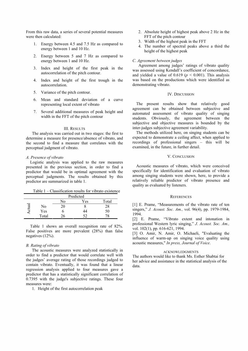
From this raw data, a series of several potential measures were then calculated:

1. Energy between 4.5 and 7.5 Hz as compared to energy between 1 and 10 Hz.

2. Energy between 5 and 7 Hz as compared to energy between 1 and 10 Hz.

3. Index and height of the first peak in the autocorrelation of the pitch contour.

4. Index and height of the first trough in the autocorrelation.

5. Variance of the pitch contour.

6. Mean and standard deviation of a curve representing local extent of vibrato

7. Several additional measures of peak height and width in the FFT of the pitch contour

III. RESULTS

The analysis was carried out in two stages: the first to determine a measure for presence/absence of vibrato, and the second to find a measure that correlates with the perceptual judgment of vibrato. A. Presence of vibrato

Logistic analysis was applied to the raw measures presented in the previous section, in order to find a predictor that would be in optimal agreement with the perceptual judgments. The results obtained by this predictor are summarized in table 1.

Table 1 – Classification results for vibrato existence

Predicted No Yes Total

No 20 8 28 Yes 6 44 50 A

ctua

l

Total 26 52 78 Table 1 shows an overall recognition rate of 82%.

False positives are more prevalent (28%) than false negatives (12%).

B. Rating of vibrato

The acoustic measures were analyzed statistically in order to find a predictor that would correlate well with the judges’ average rating of those recordings judged to contain vibrato. Eventually, it was found that a linear regression analysis applied to four measures gave a predictor that has a statistically significant correlation of 0.7395 with the judge's subjective ratings. These four measures were:

1. Height of the first autocorrelation peak

2. Absolute height of highest peak above 2 Hz in the FFT of the pitch contour

3. Width of the highest peak in the FFT 4. The number of spectral peaks above a third the

height of the highest peak

C. Agreement between judges Agreement among judges’ ratings of vibrato quality

was assessed using Kendall’s coefficient of concordance, and yielded a value of 0.619 (p < 0.001). This analysis was based on the productions which were identified as demonstrating vibrato.

IV. DISCUSSION

The present results show that relatively good agreement can be obtained between subjective and automated assessment of vibrato quality of singing students. Obviously, the agreement between the subjective and objective measures is bounded by the inter-judges subjective agreement variability.

The methods utilized here, on singing students can be expected to demonstrate a ceiling affect, when applied to recordings of professional singers – this will be examined, in the future, in further detail.

V. CONCLUSION

Acoustic measures of vibrato, which were conceived specifically for identification and evaluation of vibrato among singing students were shown, here, to provide a relatively reliable predictor of vibrato presence and quality as evaluated by listeners.

REFERENCES

[1] E. Prame, “Measurements of the vibrato rate of ten singers,” J. Acoust. Soc. Am., vol. 96(4), pp. 1979-1984, 1994. [2] E. Prame, “Vibrato extent and intonation in professional Western lyric singing,” J. Acoust. Soc. Am., vol. 102(1), pp. 616-621, 1994. [3] O. Amir, N. Amir, O. Michaeli, "Evaluating the influence of warm-up on singing voice quality using acoustic measures," In press, Journal of Voice.

ACKNOWLEDGMENTS The authors would like to thank Ms. Esther Shabtai for her advice and assistance in the statistical analysis of the data.

Non-human sounds


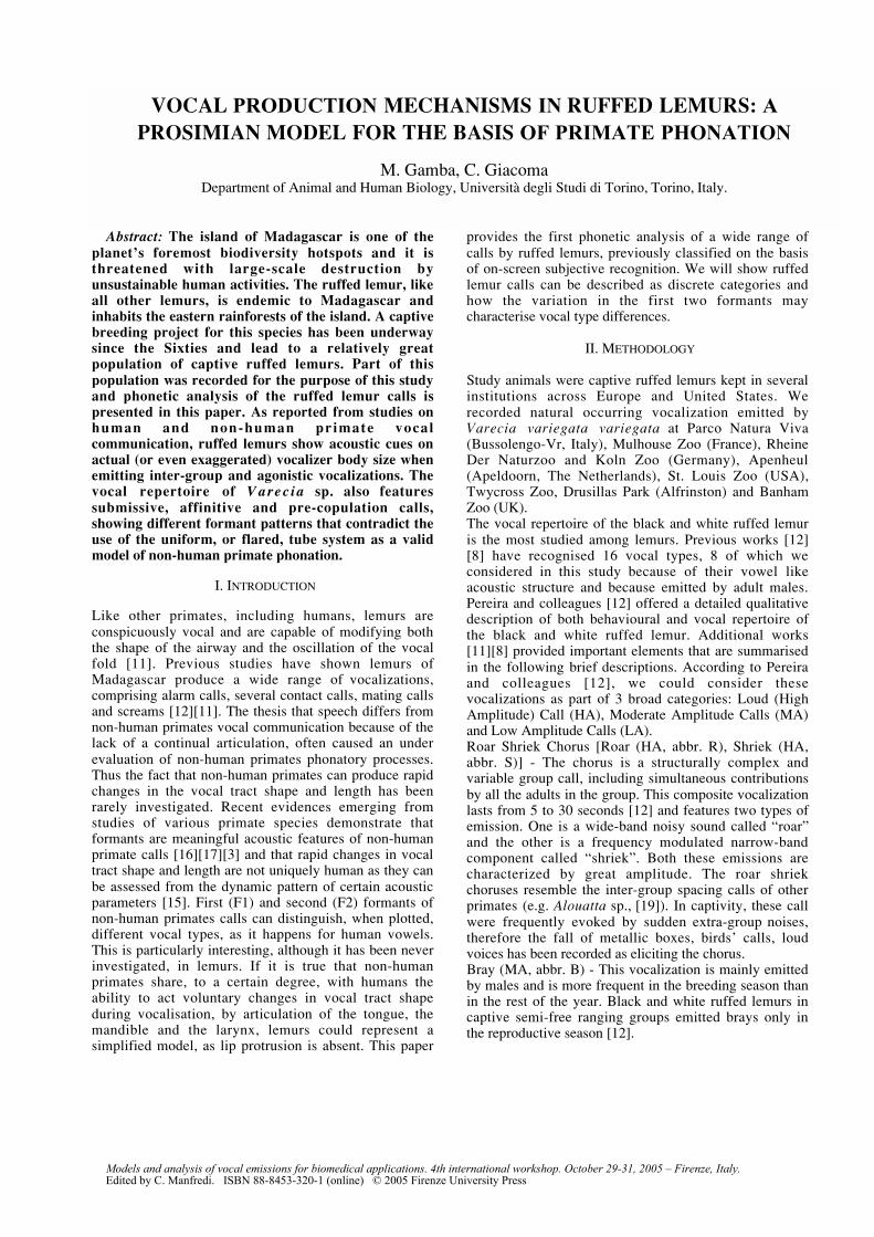
Abstract: The island of Madagascar is one of theplanet’s foremost biodiversity hotspots and it isthreatened with large-scale destruction byunsustainable human activities. The ruffed lemur, likeall other lemurs, is endemic to Madagascar andinhabits the eastern rainforests of the island. A captivebreeding project for this species has been underwaysince the Sixties and lead to a relatively greatpopulation of captive ruffed lemurs. Part of thispopulation was recorded for the purpose of this studyand phonetic analysis of the ruffed lemur calls ispresented in this paper. As reported from studies onhuman and non-human primate vocalcommunication, ruffed lemurs show acoustic cues onactual (or even exaggerated) vocalizer body size whenemitting inter-group and agonistic vocalizations. Thevocal repertoire of Varec ia sp. also featuressubmissive, affinitive and pre-copulation calls,showing different formant patterns that contradict theuse of the uniform, or flared, tube system as a validmodel of non-human primate phonation.

I. INTRODUCTION

Like other primates, including humans, lemurs areconspicuously vocal and are capable of modifying boththe shape of the airway and the oscillation of the vocalfold [11]. Previous studies have shown lemurs ofMadagascar produce a wide range of vocalizations,comprising alarm calls, several contact calls, mating callsand screams [12][11]. The thesis that speech differs fromnon-human primates vocal communication because of thelack of a continual articulation, often caused an underevaluation of non-human primates phonatory processes.Thus the fact that non-human primates can produce rapidchanges in the vocal tract shape and length has beenrarely investigated. Recent evidences emerging fromstudies of various primate species demonstrate thatformants are meaningful acoustic features of non-humanprimate calls [16][17][3] and that rapid changes in vocaltract shape and length are not uniquely human as they canbe assessed from the dynamic pattern of certain acousticparameters [15]. First (F1) and second (F2) formants ofnon-human primates calls can distinguish, when plotted,different vocal types, as it happens for human vowels.This is particularly interesting, although it has been neverinvestigated, in lemurs. If it is true that non-humanprimates share, to a certain degree, with humans theability to act voluntary changes in vocal tract shapeduring vocalisation, by articulation of the tongue, themandible and the larynx, lemurs could represent asimplified model, as lip protrusion is absent. This paper

provides the first phonetic analysis of a wide range ofcalls by ruffed lemurs, previously classified on the basisof on-screen subjective recognition. We will show ruffedlemur calls can be described as discrete categories andhow the variation in the first two formants maycharacterise vocal type differences.

II. METHODOLOGY

Study animals were captive ruffed lemurs kept in severalinstitutions across Europe and United States. Werecorded natural occurring vocalization emitted byVarecia variegata variegata at Parco Natura Viva(Bussolengo-Vr, Italy), Mulhouse Zoo (France), RheineDer Naturzoo and Koln Zoo (Germany), Apenheul(Apeldoorn, The Netherlands), St. Louis Zoo (USA),Twycross Zoo, Drusillas Park (Alfrinston) and BanhamZoo (UK).The vocal repertoire of the black and white ruffed lemuris the most studied among lemurs. Previous works [12][8] have recognised 16 vocal types, 8 of which weconsidered in this study because of their vowel likeacoustic structure and because emitted by adult males.Pereira and colleagues [12] offered a detailed qualitativedescription of both behavioural and vocal repertoire ofthe black and white ruffed lemur. Additional works[11][8] provided important elements that are summarisedin the following brief descriptions. According to Pereiraand colleagues [12], we could consider thesevocalizations as part of 3 broad categories: Loud (HighAmplitude) Call (HA), Moderate Amplitude Calls (MA)and Low Amplitude Calls (LA).Roar Shriek Chorus [Roar (HA, abbr. R), Shriek (HA,abbr. S)] - The chorus is a structurally complex andvariable group call, including simultaneous contributionsby all the adults in the group. This composite vocalizationlasts from 5 to 30 seconds [12] and features two types ofemission. One is a wide-band noisy sound called “roar”and the other is a frequency modulated narrow-bandcomponent called “shriek”. Both these emissions arecharacterized by great amplitude. The roar shriekchoruses resemble the inter-group spacing calls of otherprimates (e.g. Alouatta sp., [19]). In captivity, these callwere frequently evoked by sudden extra-group noises,therefore the fall of metallic boxes, birds’ calls, loudvoices has been recorded as eliciting the chorus.Bray (MA, abbr. B) - This vocalization is mainly emittedby males and is more frequent in the breeding season thanin the rest of the year. Black and white ruffed lemurs incaptive semi-free ranging groups emitted brays only inthe reproductive season [12].

VOCAL PRODUCTION MECHANISMS IN RUFFED LEMURS: A

PROSIMIAN MODEL FOR THE BASIS OF PRIMATE PHONATION

M. Gamba, C. GiacomaDepartment of Animal and Human Biology, Università degli Studi di Torino, Torino, Italy.


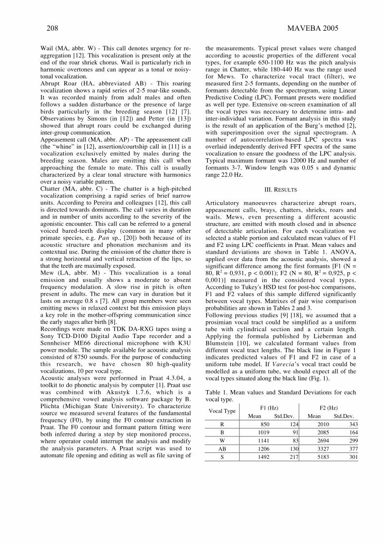
Wail (MA, abbr. W) - This call denotes urgency for re-aggregation [12]. This vocalization is present only at theend of the roar shriek chorus. Wail is particularly rich inharmonic overtones and can appear as a tonal or noisy-tonal vocalization.Abrupt Roar (HA, abbreviated AB) - This roaringvocalization shows a rapid series of 2-5 roar-like sounds.It was recorded mainly from adult males and oftenfollows a sudden disturbance or the presence of largebirds particularly in the breeding season [12] [7].Observations by Simons (in [12]) and Petter (in [13])showed that abrupt roars could be exchanged duringinter-group communication.Appeasement call (MA, abbr. AP) - The appeasement call(the “whine” in [12], assertion/courtship call in [11] is avocalization exclusively emitted by males during thebreeding season. Males are emitting this call whenapproaching the female to mate. This call is usuallycharacterized by a clear tonal structure with harmonicsover a noisy variable pattern.Chatter (MA, abbr. C) - The chatter is a high-pitchedvocalization comprising a rapid series of brief narrowunits. According to Pereira and colleagues [12], this callis directed towards dominants. The call varies in durationand in number of units according to the severity of theagonistic encounter. This call can be referred to a generalvoiced bared-teeth display (common in many otherprimate species, e.g. Pan sp., [20]) both because of itsacoustic structure and phonation mechanism and itscontextual use. During the emission of the chatter there isa strong horizontal and vertical retraction of the lips, sothat the teeth are maximally exposed.Mew (LA, abbr. M) - This vocalization is a tonalemission and usually shows a moderate to absentfrequency modulation. A slow rise in pitch is oftenpresent in adults. The mew can vary in duration but itlasts on average 0.8 s [7]. All group members were seenemitting mews in relaxed context but this emission playsa key role in the mother-offspring communication sincethe early stages after birth [8].Recordings were made on TDK DA-RXG tapes using aSony TCD-D100 Digital Audio Tape recorder and aSennheiser ME66 directional microphone with K3Upower module. The sample available for acoustic analysisconsisted of 8750 sounds. For the purpose of conductingthis research, we have chosen 80 high-qualityvocalizations, 10 per vocal type.Acoustic analyses were performed in Praat 4.3.04, atoolkit to do phonetic analysis by computer [1]. Praat usewas combined with Akustyk 1.7.6, which is acomprehensive vowel analysis software package by B.Plichta (Michigan State University). To characterizesource we measured several features of the fundamentalfrequency (F0), by using the F0 contour extraction inPraat. The F0 contour and formant pattern fitting wereboth inferred during a step by step monitored process,where operator could interrupt the analysis and modifythe analysis parameters. A Praat script was used toautomate file opening and editing as well as file saving of

the measurements. Typical preset values were changedaccording to acoustic properties of the different vocaltypes, for example 650-1100 Hz was the pitch analysisrange in Chatter, while 180-440 Hz was the range usedfor Mews. To characterize vocal tract (filter), wemeasured first 2-5 formants, depending on the number offormants detectable from the spectrogram, using LinearPredictive Coding (LPC). Formant presets were modifiedas well per type. Extensive on-screen examination of allthe vocal types was necessary to determine intra- andinter-individual variation. Formant analysis in this studyis the result of an application of the Burg’s method [2],with superimposition over the signal spectrogram. Anumber of autocorrelation-based LPC spectra wasoverlaid independently derived FFT spectra of the samevocalization to ensure the goodness of the LPC analysis.Typical maximum formant was 12000 Hz and number offormants 3-7. Window length was 0.05 s and dynamicrange 22.0 Hz.

III. RESULTS

Articulatory manoeuvres characterize abrupt roars,appeasement calls, brays, chatters, shrieks, roars andwails. Mews, even presenting a different acousticstructure, are emitted with mouth closed and in absenceof detectable articulation. For each vocalization weselected a stable portion and calculated mean values of F1and F2 using LPC coefficients in Praat. Mean values andstandard deviations are shown in Table 1. ANOVA,applied over data from the acoustic analysis, showed asignificant difference among the first formants [F1 (N =80, R2 = 0,931, p < 0.001); F2 (N = 80, R2 = 0,925, p <0,001)] measured in the considered vocal types.According to Tukey's HSD test for post-hoc comparisons,F1 and F2 values of this sample differed significantlybetween vocal types. Matrixes of pair wise comparisonprobabilities are shown in Tables 2 and 3.Following previous studies [9] [18], we assumed that aprosimian vocal tract could be simplified as a uniformtube with cylindrical section and a certain length.Applying the formula published by Lieberman andBlumstein [10], we calculated formant values fromdifferent vocal tract lengths. The black line in Figure 1indicates predicted values of F1 and F2 in case of auniform tube model. If Varecia’s vocal tract could bemodelled as a uniform tube, we should expect all of thevocal types situated along the black line (Fig. 1).

Table 1. Mean values and Standard Deviations for eachvocal type.

F1 (Hz) F2 (Hz)Vocal TypeMean Std.Dev. Mean Std.Dev.

R 850 124 2010 343

B 1019 91 2085 164

W 1141 83 2694 299

AB 1206 130 3327 377

S 1492 217 5183 301

208 MAVEBA 2005

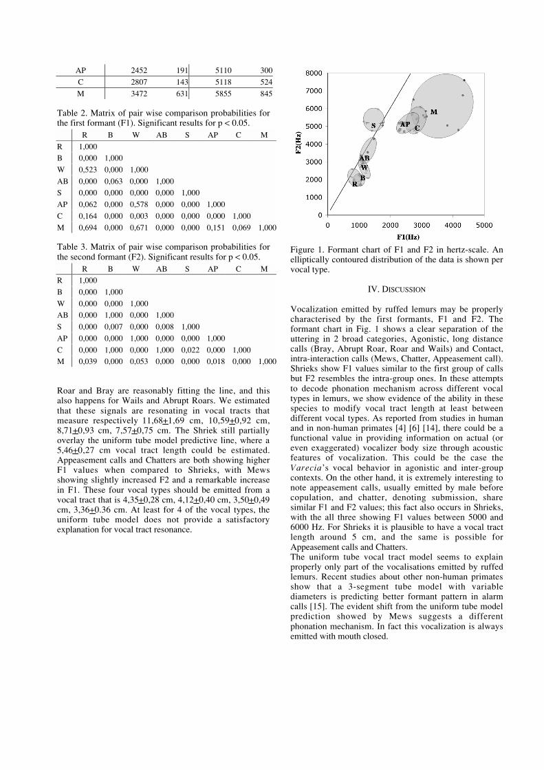
AP 2452 191 5110 300

C 2807 143 5118 524

M 3472 631 5855 845

Table 2. Matrix of pair wise comparison probabilities forthe first formant (F1). Significant results for p < 0.05. R B W AB S AP C M

R 1,000

B 0,000 1,000

W 0,523 0,000 1,000

AB 0,000 0,063 0,000 1,000

S 0,000 0,000 0,000 0,000 1,000

AP 0,062 0,000 0,578 0,000 0,000 1,000

C 0,164 0,000 0,003 0,000 0,000 0,000 1,000

M 0,694 0,000 0,671 0,000 0,000 0,151 0,069 1,000

Table 3. Matrix of pair wise comparison probabilities forthe second formant (F2). Significant results for p < 0.05. R B W AB S AP C M

R 1,000

B 0,000 1,000

W 0,000 0,000 1,000

AB 0,000 1,000 0,000 1,000

S 0,000 0,007 0,000 0,008 1,000

AP 0,000 0,000 1,000 0,000 0,000 1,000

C 0,000 1,000 0,000 1,000 0,022 0,000 1,000

M 0,039 0,000 0,053 0,000 0,000 0,018 0,000 1,000

Roar and Bray are reasonably fitting the line, and thisalso happens for Wails and Abrupt Roars. We estimatedthat these signals are resonating in vocal tracts thatmeasure respectively 11,68 + 1,69 cm, 10,59 + 0,92 cm,8,71 + 0,93 cm, 7,57 + 0,75 cm. The Shriek still partiallyoverlay the uniform tube model predictive line, where a5,46 + 0,27 cm vocal tract length could be estimated.Appeasement calls and Chatters are both showing higherF1 values when compared to Shrieks, with Mewsshowing slightly increased F2 and a remarkable increasein F1. These four vocal types should be emitted from avocal tract that is 4,35 + 0,28 cm, 4,12 + 0,40 cm, 3,50 + 0,49cm, 3,36 + 0.36 cm. At least for 4 of the vocal types, theuniform tube model does not provide a satisfactoryexplanation for vocal tract resonance.

Figure 1. Formant chart of F1 and F2 in hertz-scale. Anelliptically contoured distribution of the data is shown pervocal type.

IV. DISCUSSION

Vocalization emitted by ruffed lemurs may be properlycharacterised by the first formants, F1 and F2. Theformant chart in Fig. 1 shows a clear separation of theuttering in 2 broad categories, Agonistic, long distancecalls (Bray, Abrupt Roar, Roar and Wails) and Contact,intra-interaction calls (Mews, Chatter, Appeasement call).Shrieks show F1 values similar to the first group of callsbut F2 resembles the intra-group ones. In these attemptsto decode phonation mechanism across different vocaltypes in lemurs, we show evidence of the ability in thesespecies to modify vocal tract length at least betweendifferent vocal types. As reported from studies in humanand in non-human primates [4] [6] [14], there could be afunctional value in providing information on actual (oreven exaggerated) vocalizer body size through acousticfeatures of vocalization. This could be the case theVarecia’s vocal behavior in agonistic and inter-groupcontexts. On the other hand, it is extremely interesting tonote appeasement calls, usually emitted by male beforecopulation, and chatter, denoting submission, sharesimilar F1 and F2 values; this fact also occurs in Shrieks,with the all three showing F1 values between 5000 and6000 Hz. For Shrieks it is plausible to have a vocal tractlength around 5 cm, and the same is possible forAppeasement calls and Chatters.The uniform tube vocal tract model seems to explainproperly only part of the vocalisations emitted by ruffedlemurs. Recent studies about other non-human primatesshow that a 3-segment tube model with variablediameters is predicting better formant pattern in alarmcalls [15]. The evident shift from the uniform tube modelprediction showed by Mews suggests a differentphonation mechanism. In fact this vocalization is alwaysemitted with mouth closed.

V. CONCLUSION

The vocal repertoire of the ruffed lemurs shows theseprosimians possess the ability to change the configurationof the vocal tract. Each vocal type is characterized by thevalues of formants F1 and F2 and vocalizations within agiven type usually show similar formants. According tothe model suggested in previous studies, we consideredthe primate vocal tract during vocalization as a uniform(or flared) tube and calculated F1 and F2 as the modelwould predict. Predicted formants were plotted againstthe one we measured. Agonistic long distance calls,showing longer vocal tract estimation, are situated alongthe line (Fig. 1). Other vocalization, whose contextual useis different, showed higher values in both formants.These calls show F1 values higher than predicted and donot fit the black line in Fig.1.Prosimian primates diverged from the anthropoid branch(monkeys, apes, and humans) more than 60 million yearsago and these results suggest that, even in lemurs, theflared tube model do not provide valid predictions whenapplied across the vocal repertoire.This research was supported by the Università degli Studidi Torino and by grants to M.G. from the Parco NaturaViva – Centro Tutela Specie Minacciate.

REFERENCES

[1] P. Boersma, “Praat, a system for doing phonetics bycomputer,” Glot International 5:9/10, 341-345, 2001.[2] D.G. Childers, Modern spectrum analysis, IEEEPress. pp. 252-255, 1978.[3] W.T. Fitch, “Vocal tract length and formant frequencydispersion correlate with body size in rhesus macaques”,J. Acoust. Soc. Am., 102, pp. 1213-1222, 1997.[4] W.T. Fitch, “The phonetic potential of nonhumanvocal tracts: comparative cineradiographic observationsof vocalizing animals,” Phonetica 57, pp205-218, 2000.[5] W.T. Fitch, ‘‘The evolution of speech: A comparativereview,’’ Trends Cogn. Sci. 4, pp. 258–267, 2000.[6] W.T. Fitch, “Comparative Vocal Production and theEvolution of Speech: Reinterpreting the Descent of theLarynx,” in A. Wray ed., The Transition to Language.Oxford, Oxford University Press, 2002.[7] M. Gamba, C. Trinchero, and C. Giacoma,“Development of vocalisations in Varecia variegatavariegata,” in D. Formenti, 13th Meeting of the ItalianPrimatological Society. Folia Primatol 71, pp. 288-298,2000.[8] M. Gamba, C. Giacoma, and C. Avesani Zaborra,“Monitoring the vocal behaviour of ruffed lemurs in thenest-box,” Eaza News, 43, pp. 28-29, 2003.[9] P. Lieberman, “Primate vocalization and humanlinguistic ability,” J. Acoust. Soc. Am. 44, pp. 1574-1584,1968.[10] P. Lieberman and S.E. Blumstein, S p e e c hphysiology, speech perception, and acoustic phonetics,Cambridge Studies in Speech Science andCommunication. Cambridge: Cambridge UniversityPress, 1988.

[11] J.M. Macedonia and K.F. Stanger, “Phylogeny of theLemuridae revisited: Evidence from communicationsignals,” Folia Primatol. 63, pp. 1-43, 1994.[12] M.E. Pereira, M.L. Seeligson, and J.M. Macedonia,“The behavioral repertoire of the black-and-white ruffedlemur, Varecia variegata variegata (Primates:Lemuridae)”, Folia Primatol. 51, pp. 1-32, 1988.[13] J.J. Petter and P. Charles-Dominique, “Vocalcommunication in prosimians,” in The Study ofProsimian Behavior. eds. G.A. Doyle and R.D. Martin.Academic Press: New York, 1979.[14] D. Rendall, S. Kollias, C. Ney, and P. Lloyd “Pitch(F0) and formant profiles of human vowels and vowel-like baboon grunts: The role of vocalizer body size andvoice-acoustic allometry,” J. Acoust. Soc. Am. 117, 2, pp.944-955, 2005.[15] T. Riede, E. Bronson, H. Hatzikirou and K.Zuberbuehler, “Vocal production mechanisms in a non-human primate: morphological data and a model,” Journ.Hum. Evol. 48, pp. 85-96, 2005.[16] T. Riede and K. Zuberbuehler, “Pulse registerphonation in Diana monkey alarm calls,” J. Acoust. Soc.Am., 113, pp. 2919-2926, 2003.[17] T. Riede and K. Zuberbuehler, “The relationshipbetween acoustic structure and semantic information inDiana monkey alarm vocalization,” J. Acoust. Soc. Am.,114, pp. 1132, 2003.[18] C. Shipley, E.C. Carterette, and J.S. Buchwald, “Theeffect of articulation on the acoustical structure of felinevocalization,” J. Acoust. Soc. Am., 89, pp. 902-909, 1991.[19] R. Vercauteren Drubbel and J.P. Gautier, “On theoccurence of nocturnal and diurnal loud calls, differing instructure and duration, in Red Howlers of FrenchGuiana,” Folia Primatol. 60, pp. 195-209, 1993.[20] J.A.R.A.M. Van Hooff, “The facial displays of thecatarrhine monkeys and apes” in Primate Ethology, D.Morris Ed., London, Widenfeld and Nicolson, 1967, pp7-67.

210 MAVEBA 2005

LABELING OF COUGH DATA FROM PIGS FOR ON-LINE DISEASEMONITORING BY SOUND ANALYSIS

J.-M. Aerts1, P. Jans1, D. Halloy2, P. Gustin2, D. Berckmans1

1Laboratory of Agricultural Building Research, Department of Agro-Engineering and Economics, Katholieke Universiteit Leuven,

Belgium;

2Department of Pharmacology, Pharmacotherapy and Toxicology, Universite de Liege, Belgium.

Abstract. More objective and automated detection of

respiratory diseases in pig houses should be possible

by on-line sound analysis of cough monitoring. To

develop automatic algorithms for pig cough

recognition, experiments and well-labeled cough data

are needed. The objectives of this article are: (1) to

give a short overview of the attained results in cough

recognition, and (2) to define a methodology to label

the cough data in a pig house. Human observers

labeled coughs by audiovisual observation in a

laboratory test installation with ten pigs during

periods ranging from two days to two weeks.

Simultaneously, sound registration was done with

audio equipment. The sound registrations were

listened to by another observer to compare the

number of coughs in the registration with the number

labeled during the experiment. It was found that

there were underestimations of up to 94% in the

number of coughs. The underestimation in the

number of coughs could be reduced to 10% when the

observer used an additional labeling sound signal on

the scene each time coughing was observed. In

addition, differences were found between two

independent observers scoring pig's coughs in an

audiovisual manner on the scene. For future

research, we suggest an investigation of how an

observer using software labeling could improve the

labeling results.

I. INTRODUCTION

is not only crucial for the animals' health and welfare

[6,7], but also for the consumer because early detection

of animal diseases can reduce residuals of antibiotics in

meat products [8]. Therefore, great effort is spent to the

development and application of sensors and sensing

techniques for diagnosis in livestock farming [9]. Sound

production by animals is a candidate bio-signal that can

be measured easily at a distance and without causing

additional stress. Research has been reported on sound

analysis applied to animal sounds in general

[10,11,12,13,14,15] and to farm animals in particular

[16,17,18,19]. Sounds produced by pigs have been

analyzed in relation with communication [20,21,22,23]

stress [24,25], welfare [10,17], pain [26,27], and health

[19]. Because respiratory diseases cause important

economic losses in pig production [19], several

researchers in recent years have focused on cough

detection algorithms. Examples can be found in the work

of [28,18,13]. A common characteristic of the developed

algorithms is that they are trained based on data sets

(training data sets) in order to classify the measured

sounds (e.g., with neural networks). As a consequence,

the failure or success of the development of an algorithm

depends highly on the quality of the training data set. In

order to quantify the success rate of such algorithms, the

data sets (training as well as validation) are labeled. This

means that the recorded files are listened to by a human

and every sound is marked and described. However, the

person who labels the sound files in the laboratory is not

necessarily the same person who attends the experiments

on the scene (observer). In some cases, e.g.,

measurements at night, an observer is not even present

during the experiments. Because listening to sounds in

general and cough sound files in particular is prone to

subjectivity and human error, questions have arisen

about the accuracy of the classical labeling procedure. In

the reported research, the objective was to analyze the

accuracy of the labeling of cough sounds in pig and to

improve the labeling procedure for cough sounds.

II. METHODOLOGY

Animals and Housing

Throughout the experiments, the same group of ten

piglets (Belgian Landrace) was used. They weighed

about 9 kg at the start of the experiment. The pigs were

housed in a 2 5 m pen with a partially slotted floor that

was situated in the test facilities of the Faculty of

Veterinary Medicine, Université de Liège (Belgium).

Room air temperature was 20°C ±2°C. The ventilation

rate was 8 m3 h

-1 per pig. A light scheme of 16 h of light

and 8 h of darkness was applied. Light intensity was 60

lx during the light period. During the experiments, the

piglets were fed a commercial feed, and water was freely

available.

Digital Sound Recording

The sounds were recorded by using a standard

multimedia microphone (U.S. Blaster, 20 Hz to 20 kHz

frequency response), connected to a sound card (Sound


Blaster, 16 bit). The microphone was positioned 0.3 m

above the pen. The sound files were recorded as .wav

files (plain sound file) with a frequency of 22.050 Hz. In

the laboratory, the sound files were listened to by Cool

Edit Pro (version 1.2a).

Experiments

In total, four experiments were carried out. During the

first three experiments (Exp1, Exp2, and Exp3), the pigs'

coughs were scored during one hour a day (0830 h to

0930 h) in the test installation by an observer. The

experiments lasted 22, 19, and 17 days for Exp1, Exp2,

and Exp3, respectively (see table 1). During the

recording time, an observer was present in the test

facility in order to score (count) the coughs. The

recorded sound files were then scored by a second

person in the laboratory by looking at the shape of the

signal (in the time domain) on a computer screen and by

listening to the sound file by headphone at the same time

(i.e., audiovisual scoring).

In the fourth experiment (Exp4), the listening time was

extended to five 1 h periods a day (0830 h to 0930 h,

1330 h to 1430 h, 1830 h to 1930 h, 2330 h to 0030 h,

and 0430 h to 0530 h), during five non-consecutive days

(see table 1). Each time a cough was observed, the

observer produced a typical sound, called a "ping," to

label the sound as a cough. The "ping" was made by

hitting a glass bottle with a metal stick. The hypothesis

was that this typical sound could be easily recognized by

the person scoring the sounds afterwards in the

laboratory.

The first day of Exp4 was carried out with two observers

in the test installation. They could both see and hear the

piglets, but they could not see each other. For this part of

the experiment, no labeling sound ("ping") was used.

Statistics Used

Statistical significance between mean values of coughs

counted was tested using a two-sample t-test. Since the

observations on the two populations of interest were

collected in pairs, a paired t-test was used [29]. In order

to test the hypothesis on the equality of the mean

numbers of coughs counted on the scene and in the

laboratory (see table 1), the data from Exp1, Exp2, and

Exp3 were used. The data from Exp4 were not used for

this analysis since the observations were made in a

different way (labeling sound). For testing the hypothesis

on the equality of the mean numbers of coughs counted

by observer 1 and observer 2 during the first 24 h of

Exp4 (see table 2), the data of the five observation

periods were used.


Table 1 gives an overview of the counted coughs in the

four experiments. In this research, we used a total of 83 h

of audiovisual observations of the pigs' coughs.

Table 1. Scoring of the cough sounds by observer present in

the test installation compared with audiovisual scoring

afterwards in the laboratory on the recorded audio file.

From table 1, we see clearly that it is not possible to

make a well-labeled reference data set just by

audiovisual scoring of the recorded files in the laboratory

because underestimations of up to 94% occur. It could be

demonstrated that the average number of coughs counted

by audiovisual scoring in the laboratory was

significantly different from the number of coughs

counted by the observer in the test installation (P < 0.2).

This implies that reliable labeling demands at least one

observer in the pig house, which is a time-consuming

and mentally exhausting job. When the coughs are

marked by a well-recognizable sound ("ping") in the

audio file (Exp4), an underestimation of about 10%

between the different scoring methods was observed.

This deviation could be the result of an over- (or under-)

estimation of the number of coughs in a series (bout).

When, in practice, a bout of coughing occurs, the

observer could only make his labeling sound at the end

of the series.

Another possible problem, which cannot be put easily

into figures, is the conditioning aspect of the labeling

sound. Since the pigs could hear the labeling sound

themselves, it is possible that, by hearing the labeling

sound each time they cough, the pigs get used to it and

after a while begin to cough voluntary to hear the

labeling sound. Studies with humans have shown that

voluntary cough sounds have different features from

"normal" cough sounds [14]. Indications for this

conditioning effect might be found in the fact that the

average counted number of coughs per hour of

observation in Exp4 (with labeling sound) was on

average 10, whereas the average counted number of

coughs (on the scene) per hour for Exp1, Exp2, and

Exp3 (without labeling sound) ranged between 2 and 5.

However, for a more in-depth analysis of the possible

conditioning effects of labeling sounds, more

experiments should be performed. Although the use of a

typical labeling sound reduced the underestimation to

10%, this is not the way a reliable reference data set of

cough sounds can be achieved.

Number of Coughs Counted

by Audiovisual Scoring:Experiment Listening

Protocol

Duration

(days)

On the Scene In the Lab

Under-

Estimation

(%)

Exp1 1 h/day 22 47 18 62

Exp2 1 h/day 19 97 6 94

Exp3 1 h/day 17 43 17 61

Exp4 5 h/day[a] 5 265 239 10[a] During Exp4, a labeling sound ("ping") was used.

212 MAVEBA 2005

When looking at table 2, we see that there is a difference

(but not statistically significant) between the two

observers counting the coughs of the same animals at the

same time. This gives rise to the thought that there is no

real completely objective way to label pigs' cough

sounds in practice. We could approach a more objective

labeling by mixed subjective observations, but then we

would need a number of observers in the pig house,

which leads to other problems (e.g., increased costs).

Table 2. Number of cough sounds counted of the same

animals at the same time by two different observers in the

pig house during the first 24 h of Exp4.

Number of Coughs Counted by:No. of

Observations

Time of the

Observation Observer 1 Observer 2

1 0830 h - 0930 h 8 10

2 1330 h - 1430 h 13 12

3 1830 h - 1930 h 7 8

4 2330 h - 0030 h 0 0

5 0430 h - 0530 h 12 7

An alternative to the auditory labeling of cough sounds

is software labeling. While recording the sounds in a pig

house on a portable computer, we can run an extra

program. Whenever a cough sound is heard, a key on the

portable computer is pressed, and the program keeps

record of the relative time in the recorded audio file. This

way, we could get around the problem that pigs might

cough to hear the label sound, and we can label each

cough, even when coughs come in a series.

In general, it is not easy to reliably distinguish between

different animal vocalizations (classification). In order to

solve this problem, several authors used signal analysis

techniques in combination with classification procedures

to identify individual vocalizations in a more objective

way [21,25,27]. They used classification techniques

based on training data sets. Most of the time, individual

sounds are labeled by ethologists listening to the

recorded data in the laboratory (e.g., [16,17]). Due to

(mechanical) background noises, it is not always easy to

reliably label individual sounds [16]. As described in the

reported research, labeling individual cough sounds of

pigs can be performed most reliably by at least one

observer on the scene in the pig house. However, in most

cases described in the literature, labeling was performed

on recorded sound data, and no indication is given of the

accuracy of the labeling procedure compared with

labeling results of observers during the experiment.

Accuracy of the labeling procedure is sometimes

expressed as the correlation between the scores of two

independent persons listening to the recorded sound data.

Weary and Fraser [17] used this method for labeling the

calls of piglets at weaning and found a correlation

between two independent scorers of 0.98. In our

experiments, the correlation between the scores of two

independent observers in the pig house was 0.85.

All together, we can state that labeling individual sounds

in an audio file, to use as a reference set in algorithm

training, is a difficult task and must be done very

carefully.

IV. CONCLUSION

With the rising interest in animal vocalizations as a

valuable biological response variable, there is a growing

need for good labeling methods. Cough recognition

algorithms cannot satisfy in-field situations when they

are not developed, or trained, by a stable, reliable

reference set.

Audiovisual observation on a recorded pig sound file is

clearly insufficient for accurate labeling of cough

sounds. Up to 94% underestimation of the number of

cough sounds was scored in an audiovisual way on the

computer. Audiovisual observation of the animal on the

scene, together with a typical labeling sound, reduced the

underestimation to 10%. Since the labeling sound can

possibly stimulate the pigs to cough (due to

conditioning), this method is probably not suited for

generating high-quality data sets (for training and

validation). Therefore, we suggest performing additional

research to test alternative labeling methods. One of the

possible alternatives is to put at least one audiovisual

observer in the pig house with a portable computer.

While recording the sound file, another program could

keep track of the elapsed time. When a cough sound is

heard, the observer could press a key on the portable

computer. As a result, we could get a sound file and a

relative time for all cough sounds during the period of

observation, without influencing the animals with

labeling sounds.

There were also differences between two independent

observers who labeled pigs' cough sounds in an

audiovisual way on the scene in the pig house.

V. REFERENCES

[1] Gates, R. S., L. W. Turner, H. Chi, and J. L. Usry.

1995. Automated weighing of group-housed, growing-

finishing swine. Trans. ASAE 38(5): 1479-1486.

[2] Korthals, R. L., R. A. Eigenberg, G. L. Hahn, and J.

A. Nienaber. 1995. Measurements and spectral analysis

of tympanic temperature regulation in swine. Trans.

ASAE 38(3): 905-909.

[3] Aarnink, A. J. A., and M. J. M. Wagemans. 1997.

Ammonia volatilization and dust concentration as

affected by ventilation systems in houses for fattening

pigs. Trans. ASAE 40(4): 1161-1170.

[4] Wang, X., Y. Zhang, L. Y. Zhao, and G. L.

Riskowski. 2000. Effect of ventilation rate on dust

spatial distribution in a mechanically ventilated airspace.

Trans. ASAE 43(6): 1877-1884.

[5] Wathes, C. M., J. B. Jones, H. H. Kristensen, E. K.

M. Jones, and A. J. F. Webster. 2002. Aversion of pigs

and domestic fowl to atmospheric ammonia. Trans.

ASAE 45(5): 1605-1610.

[6] Predicala, B. Z., R. G. Maghirang, S. B. Jerez, J. E.

Urban, and R. D. Goodband. 2001. Dust and bioaerosol

concentrations in two swine-finishing buildings in

Kansas. Trans. ASAE 44(5): 1291-1298.

[7] Van Hirtum, A., and D. Berckmans. 2004. Objective

cough-sound recognition as a biomarker for aerial

factors. Trans. ASAE 47(1): 351-356.

[8] Mottier, P., V. Parisod, E. Gremaud, P. A. Guy, and

R. H. Stadler. 2003. Determination of the antibiotic

chloramphenicol in meat and seafood products by liquid

chromatography-electrospray ionization tandem mass

spectrometry. J. Chromatogr. A 994(1-2): 75-84.

[9] Tothill, I. 2001. Biosensors developments and

potential applications in the agricultural diagnosis sector.

Comput. Electron. Agric. 30: 205-218.

[10] Weary, D. M., and D. Fraser. 1995. Signaling need:

Costly signals and animal welfare assessment. Appl.

Animal Behav. Sci. 44(2-4): 159-169.

[11] Hayward, T. J. 1996. Classification by multiple-

resolution statistical analysis with application to

automated recognition of marine mammal sounds. J.

Acoust. Soc. America 101(3): 1516-1526.

[12] Murray, S. O., E. Mercado, and H. L. Roitblat.

1998. Characterizing the graded structure of false killer

whale (Pseudorca crassidens) vocalizations. J. Acoust.

Soc. America 104(3): 1679-1688.

[13] Van Hirtum, A., and D. Berckmans. 2002a.

Assessing the sound of cough towards vocality. Med.

Eng. and Phys. 24(7-8): 535-540.

[14] Van Hirtum, A., and D. Berckmans D. 2002b.

Automated recognition of spontaneous versus voluntary

cough. Med. Eng. and Phys. 24(7-8): 541-545.

[15] Madsen, P. T., D. A. Carder, W. W. L. Au, P. E.

Nachtigall, B. Møhl, and S. H. Ridgway. 2003. Sound

production in neonate sperm whales. J. Acoust. Soc.

America 113(6): 2988-2991.

[16] Weary, D. M., and D. Fraser. 1997. Vocal response

of piglets to weaning: Effect of piglet age. Appl. Animal

Behav. Sci. 54(2-3): 153-160.

[17] Ikeda, Y., G. Jahns, W. Kowalczyk, and K. Walter

K. 2000. Acoustic analysis to recognize individuals and

animal conditions. CIGR Paper No. P8207. Bonn,

Germany: CIGR.

[18] Chedad, A., D. Moshou, J.-M. Aerts, A. Van

Hirtum, H. Ramon, and D. Berckmans. 2001.

Recognition system for pig cough based on probabilistic

neural networks. J. Agric. Eng. Res. 79(4): 449-457.

[19] Van Hirtum, A., and D. Berckmans. 2003. Fuzzy

approach for improved recognition of citric acid induced

piglet coughing from continuous registration. J. Sound

Vib. 266(3): 667-686.

[20] Weary, D. M., G. L. Lawson, and B. K. Thompson.

1996. Sows show stronger responses to isolation calls of

piglets associated with greater levels of piglets need.

Animal Behav. 52(6): 1247-1253.

[21] Weary, D. M., M. C. Appleby, and D. Fraser. 1999.

Responses of piglets to early separation from the sow.

Appl. Animal Behav. Sci. 63(4): 289-300.

[22] Appleby, M. C., D. M. Weary, A. A. Taylor, and G.

Illmann. 1999. Vocal communication in pigs: Who are

nursing piglets screaming at? Ethology 105(10): 881-

892.

[23] Marchant, J. N., X. Whittaker, and D. M. Broom.

2001. Vocalisations of the adult female domestic pig

during a standard human approach test and their

relationships with behavioural and heart rate measures.

Appl. Animal Behav. Sci. 72(1): 23-39.

[24] Schrader, L., and D. Todt. 1998. Vocal quality is

correlated with levels of stress hormones in domestic

pigs. Ethology 104(10): 859-876.

[25] Schön, P.-C., B. Puppe, and G. Manteuffel. 2000.

Classification of stress calls of the domestic pig (Sus

scrofa) using LPC-analysis and a self-organizing

neuronal network. Arch. Tierz. 43: 177-183.

[26] Weary, D. M., L. A. Braithwaite, and D. Fraser.

1998. Vocal response to pain in piglets. Appl. Animal

Behav. Sci. 56(2-4): 161-172.

[27] Taylor, A. A., and D. M. Weary. 2000. Vocal

responses of piglets to castration: Identifying procedural

sources of pain. Appl. Animal Behav. Sci. 70(1): 17-26.

[28] Van Hirtum, A., J.-M. Aerts, D. Berckmans, B.

Moreaux, and P. Gustin. 1999. On-line cough recognizer

system. J. Acoust. Soc. America 106(4:2): 2191-2191.

[29] Wonnacott, T. H., and R. J. Wonnacott. 1977.

Introductory Statistics. New York, N.Y.: John Wiley and

Sons.

214 MAVEBA 2005

AUTHOR INDEX

Adachi S., 195

Adamovic T., 101

Aerts J.-M., 211

Aguilera-Navarro S., 11, 15

Airas M., 73

Alku P., 73

Alvarez A., 59

Amir N., 201

Amir O., 201

Auzou P., 177

Avanzini F., 55

Badin P., 51

Berckmans D., 77, 211

Berry C., 3, 23

Bianchi S., 121

Bocchi L., 121

Bruscaglioni P., 187

Burtschell Y., 191

Cantarella G., 121

Cieciwa S., 129

Cisonni J., 51

Cnockaert L., 177

Costa A., 77

Cranen B., 63

Deliyski D.D., 129, 133, 137

Diaz F., 59

Dittmar A., 67

Dori F., 37

Drepper F.R., 167

Drioli C., 55

Elemans C., 47

Eysholdt U., 159

Fell H.J., 147

Fernandez R., 59

Fernandez-Camacho F.J., 59

Fitch W.T., 47

Fourcin A., 111

Francius L., 191

Fric M., 119

Gamba M., 207

Gatkowska I., 97

Giacoma C., 207

Giordano J., 191

Giovanni A., 191

Goddard J.C., 163

Godino J.I., 59

Godino-Llorente J.I., 11, 15

Gomez P., 59

Gomez-Vilda P., 11, 15

Grenez F., 81, 155, 177

Grosgogeat B., 67

Grzanka A., 33

Guarino M., 77

Gustin P., 211

Halloy D., 211

Hanquinet J., 81

Herzel H., 47

Honda K.H., 141

Horacek J., 43, 73, 151

Iadanza E., 37

Izworski A., 97

Jans P., 211

Jeannin Ch., 67

Kacha A., 155

Kempf A., 187

Kinoshita K.K., 141

Kitamura T., 85

Kob M., 89

Konopka W., 33

Kuwabara H., 29

Laukkanen A.M., 73

Làzaro C., 59

Li H., 105

Lipping T., 171

Lohscheller J., 159

MacAuslan J., 147

Manfredi C., 37, 121, 187

Manickam K., 7, 105

Mantha S.,125

Maratea S., 55

Marino C., 37

Martinez A.M., 163

Martinez F.M., 163

Martinez R., 59

Medale M., 191

Mende W., 187

Michaeli O., 201

Michalska M., 33

Migali N., 121

Misun V., 93

Mokhtari P., 85

Mongeau L., 125


Moore C. J., 7

Murphy K., 59

Nazarian B., 191

Neuschaefer-Rube Ch., 89

Nicollas R., 191

Nieto A., 59

Nieto V., 59

Orr R., 63

Orzechowski T., 97

Osma-Ruiz V., 11, 15

Ouaknine M., 191

Ozsancak C., 177

Patelli S., 77

Payan Y., 67

Pelorson X., 51

Perrier P., 51, 67

Pietruch R., 33

Qiu Q., 119

Ritchings T., 3, 23

Rodellar V., 59

Roth M., 191

Rudzinska M., 97

Ruty N., 51

Sáenz-Lechón N., 11, 15

Schoentgen J., 19, 81, 155, 177

Schutte H.K., 119

Schwarz R., 159

Shaw H.S., 133, 137

Sheta W., 23

Shiavi R., 181

Shrivastav R., 115

Siegmund T., 125

Silva M., 77

Silverman M.K., 181

Silverman S.E., 181

Slevin N., 7

Sovilj M., 101

Sram F., 119

Stellzig-Eisenhauer A., 187

Stevovic N., 101

Stoffers J., 89

Subari K.S., 181

Subotic M., 101

Sundberg J., 199

Svancara P., 151

Svec J.G., 119

Takano S.T., 141

Takemoto H., 85

Tanttu J.T., 171

Toy H., 159

Turunen J.J., 171

Vampola T., 43

Van Hirtum A., 51

Vesely J., 43

Vicente J., 191

Vokral J., 43

Wermke K., 187

Wilkes D.M., 181

Wurzbacher T., 159

Yu J., 195

Zaccarelli R., 47

Zielinski T., 129

216 MAVEBA 2005

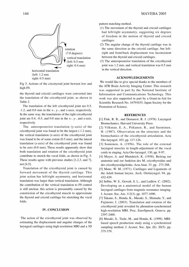
the thyroid and cricoid cartilages were converted into the translation of the cricothyroid joint, as shown in Table 2. The translation of the left cricothyroid joint are 0.5,

-1.2, and 0.0 mm in the x-, y-, and z-axes, respectively. In the same way, the translations of the right cricothyroid joint are 0.4, -0.5, and 0.0 mm in the x-, y-, and z-axis, respectively. The anteroposterior translation (y-axis) of the

cricothyroid joint was found to be the largest (-1.2 mm), the vertical translation (x-axis) of the cricothyroid joint was found to be of some extent (0.5 mm), and the lateral translation (z-axis) of the cricothyroid joint was found to be zero (0.0 mm). These results apparently show that both translation and rotation of the cricothyroid joint contribute to stretch the vocal folds, as shown in Fig. 5. These results agree with previous studies [1,2,3, and 7], not [4,5]. Translation of the cricothyroid joint is caused by

forward movement of the thyroid cartilage. This joint action has left/right asymmetry, and horizontal translation was larger than vertical translation. Although the contribution of the vertical translation to F0 control is still unclear, this action is presumably caused by the constriction of the cricothyroid muscle to approximate the thyroid and cricoid cartilage for stretching the vocal folds.

IV. CONCLUSION

The action of the cricothyroid joint was observed by estimating the displacement and angular changes of the laryngeal cartilages using high-resolution MRI and a 3D

pattern matching method.(1) The movement of the thyroid and cricoid cartilages

had left/right asymmetry, suggesting six degrees of freedom in the motion of thyroid and cricoid cartilages.

(2) The angular change of the thyroid cartilage was in the same direction as the cricoid cartilage, but left-right and front/back displacement was inconsistent between the thyroid and cricoid cartilages.

(3) The anteroposterior translation of the cricothyroid joint was 1.2 mm, and vertical translation was 0.5 mm in the vertical direction.

ACKNOWLEDGEMENTSWe would like to give special thanks to the members of

the ATR Brain Activity Imaging Center. This research was supported in part by the National Institute of Information and Communications Technology. This work was also supported in part by a Grant-in-Aid for Scientific Research No. 16791035, Japan Society for the Promotion of Science.

REFERENCES[1] Fink, R. B., and Demarest, R. J. (1978). Laryngeal

Biomechanics. Harvard University Press.[2] Vilkman, E. A., Pitkanen, R., and Suominen,

H. (1987). Observation on the structure and the biomechanics of the cricothyroid articulation. Acta Oto-laryngol, 103, pp. 117-126.

[3] Sonninen, A. (1956). The role of the external laryngeal muscles in length-adjustment of the vocal cords in singing. Acta Oto-laryngol, 130, pp. 9-97.

[4] Mayet, A. and Mundnich, K. (1958). Beitrag zur anatomie und zur funktion des M. cricothyroidus und der cricothyreoidgelenke, Acta Anat. 33, pp. 273-288.

[5] Maue, W. M. (1971). Cartilages and Ligaments of the Adult human larynx, Arch. Otolaryngol, 94, pp. 432-439.

[6] Selbie, W. S., Gewalt, S. L., and Ludlow, C. (2002). Developing an a anatomical model of the human laryngeal cartilages from magnetic resonance imaging. J. Acoust. Soc. Am, 112(3). pp. 1077-1090.

[7] Takano, S., Honda, K., Masaki, S., Shimada, Y., and Fujimoto, I. (2003). Translation and rotation of the cricothyroid joint revealed by phonation-synchronized high-resolution MRI. Proc. EuroSpeech. Geneva, pp. 2397-2400.

[8] Masaki, S., Tiede, M., and Honda, K. (1999). MRI-based speech production study using a synchronized sampling method, J. Acoust. Soc. Jpn. (E). 20(5). pp. 375-379.

Fig 5. Actions of the cricotyroid joint beween low and high F0.

rotation(7.0 degrees)

horizontal translation(left: 1.2 mmright: 0.5 mm)

vertical translation(left: 0.5 mmright: 0.4 mm)

144 MAVEBA 2005

ATTI - Firenze University Press

Documents

Transcript of ATTI - Firenze University Press