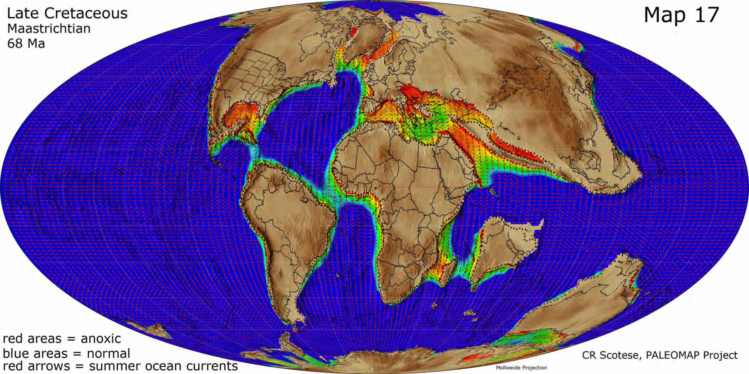
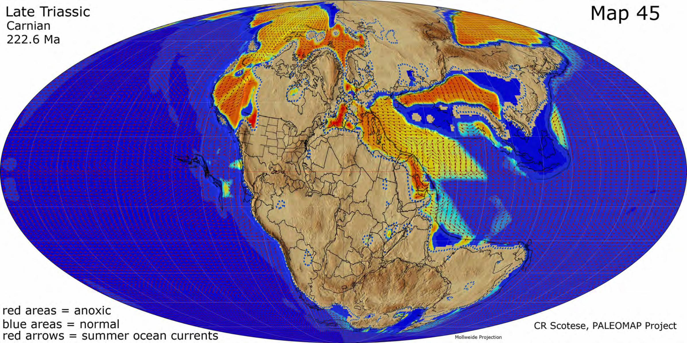
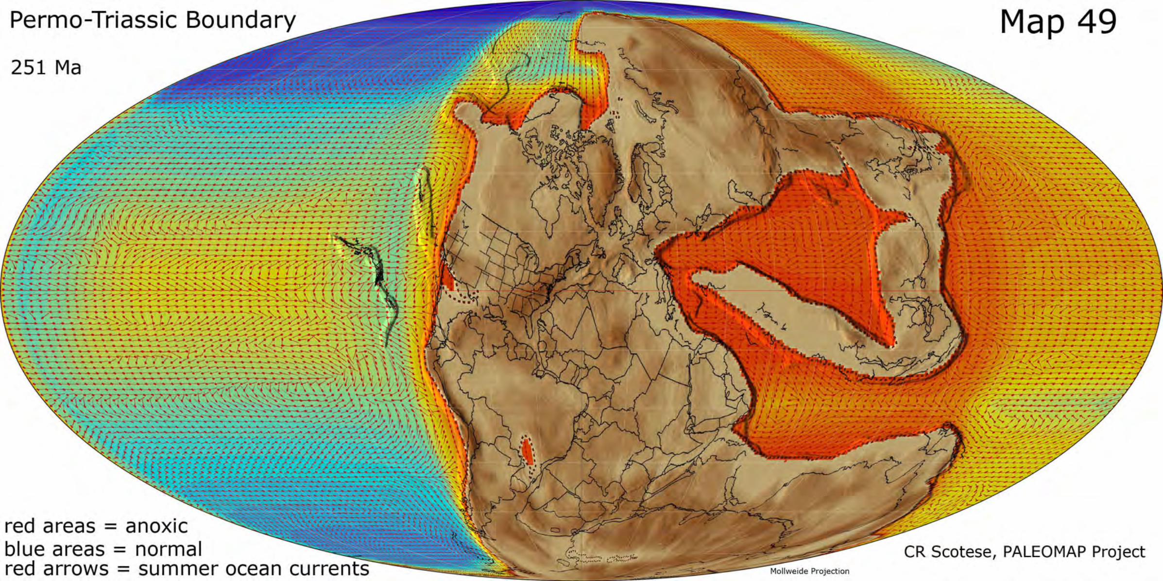
Atlas of Phanerozoic Oceanic Anoxia This Atlas of Phanerozoic Oceanic Anoxia shows the patterns of oceanic anoxia for 22 time periods from the base of the Cambrian (542 Ma) to the Middle/Late Miocene (Serravallian & Tortonian, 10.5 Ma), plus one additional map for the Neoproterozoic (Middle Ediacaran, 600 Ma). Regions where anoxic conditions may have existed are shown in red. Regions where well-oxygenated waters occurred are shown in blue. Various shades of green, yellow and orange indicate somewhat dysoxic conditions. Red arrows indicate the direction of surface ocean currents during the summer months (June-July-August). These plate tectonic and paleogeographic maps are the work of C. R. Scotese. The paleoclimate simulations were done by T.L. Moore using the FOAM (Fast Ocean and Atmosphere) Climate Simulation Program. The differences in color and symbology from map to map are due to the fact that these figures were originally published in four separate reports (Scotese et al., 2007; 2008; 2009; & 2011). These estimates of anoxic oceanic conditions have been made by calculating the degree of “restriction” in each sedimentary basin. Restriction is a quantitative estimate of the degree of connection between any marine region and the open ocean. Restriction values ranged from 0 (not restricted) to 100 (very restricted). For example a marine region that is completely surrounded ocean would be classified as “nonrestricted” and would have a restriction value near zero. On the other hand, a marine embayment that is surrounded mostly by land grid cells would be considered very restricted and would have a high restriction value (>80). The restriction value was determined by calculating the average distance of each marine grid cell to the nearest land grid cell. Distance measurements were made in 8 compass directions (N,NE,E,SE,S,SW,W,and NW). When the average distance to from each marine grid cell to the nearest land cells was small, it indicated that the marine cell was surrounded by land cells, and hence was “restricted” and likely to be prone to anoxic conditions. Conversely, if the average distance between a marine grid cell and the surrounding land grid cells was very large then it could be inferred that the grid cell was in the “open ocean”, and hence not prone to anoxic conditions. In our approach we use “restriction” as a proxy for oceanic anoxia. It should be clear from the above description that this simple method of estimating oceanic anoxia does not take into account any geochemical measurements of anoxia, or bring into play any aspects of ocean dynamics (e.g. upwelling, surface currents or salinity). This approach is purely geographical, and consequently, has a few drawbacks. Firstly, high values of anoxia along ocean-facing coastlines are suspect. Also all of the estimates of oceanic anoxia have been made only for surface waters. In other words, the restriction calculation indicates how well connected the surface waters are to the open ocean but doesn’t say anything about the connectedness of the deeper portions of the basin. An exception is the map of oceanic anoxia for the Permo-Triassic Boundary (Map 49, 251 Ma). In this case, the degree of restriction was calculated for a water depth of 1000m. This was done in order to highlight the degree to which the Paleotethys ocean basin was restricted from the Panthalassic ocean basin. The restriction of deep waters in the Paleotethys may have contributed to the global anoxic oceanic conditions that are thought to have played an important role in the great Permo-Triassic extinction.

A third artifact is sometimes apparent in the maps. Because the restriction calculation were made in only the cardinal compass directions, diagonal streaks are sometimes apparent (e.g. Maps 39 and 45). Despite the simple method employed to estimate oceanic anoxia, some obvious patterns emerge from these maps. Ocean basins are most likely to become restricted, and hence anoxic, at two times during their tectonic history: 1) shortly after their initial opening when they are narrow (Maps 21, 27, 31, and 35), and then again 2) when the ocean basin closes, prior to continent-continent collision (Maps 9, 17, 45, 65 and 75). It therefore comes as no surprise that times of widespread oceanic anoxia, such as the mid-Mesozoic oceanic anoxic events (OAEs), are often coincident with times during which numerous, narrow, poorly connected ocean basins are beginning to open or close. A complimentary set of surface ocean currents for the winter months (December-January-February) are plotted in the Atlas of Phanerozoic Salinity and Ocean Currents. Though similar to the results shown here, there are maps that show opposite flow directions due to monsoonal changes in wind directions. The maps are from volumes 1-6 of the PALEOMAP PaleoAtlas for ArcGIS (Scotese, 2014a,b,c,d). Absolute age assignments are from Gradstein, Ogg & Smith (2008). The following maps are included in the Atlas of Phanerozoic Oceanic Anoxia: Map 5 Middle/Late Miocene (Serravallian & Tortonian, 10.5 Ma) Map 7 Early Miocene (Aquitainian & Burdigalian, 19.5 Ma) Map 9 Early Oligocene (Rupelian, 31.1 Ma) Map 12 early Middle Eocene (middle Lutetian, 44.6 Ma) Map 17 Late Cretaceous (Maastrichtian, 68 Ma) Map 21 Mid-Cretaceous (Turonian, 91.1 Ma) Map 23 Early Cretaceous (late Albian, 101.8 Ma) Map 27 Early Cretaceous (early Aptian, 121.8 Ma) Map 31 Early Cretaceous (Berriasian, 143 Ma) Map 35 Late Jurassic (Oxfordian, 158.4 Ma) Map 39 Early Jurassic (Toarcian, 179.3 Ma) Map 45 Late Triassic (Carnian, 222.6 Ma) Map 49 Permo-Triassic Boundary (251 Ma) Map 54 Early Permian (Artinskian, 280 Ma) Map 57 Late Pennsylvanian (Gzhelian, 301.2 Ma) Map 63 Middle Mississippian (early Visean, 341.1 Ma) Map 65 Late Devonian (latest Famennian, 359.2 Ma) Map 70 Early Devonian (Emsian, 394.3 Ma) Map 75 Early Silurian (late Llandovery, 432.1 Ma) Map 82 Early Ordovician (Tremadoc, 480 Ma) Map 88 Cambrian – Precambrian Boundary (542 Ma) Map 90 Late Neoproterozoic (Middle Ediacaran, 600 Ma) This work should be cited as Scotese, C.R., and Moore, T.L., 2014. Atlas of Phanerozoic Oceanic Anoxia (Mollweide Projection), Volumes 1-6, PALEOMAP Project PaleoAtlas for ArcGIS, PALEOMAP Project, Evanston, IL.

References Cited: Scotese, C.R., Illich, H., Zumberge, J, and Brown, S., and Moore, T., 2007. The GANDOLPH Project: Year One Report: Paleogeographic and Paleoclimatic Controls on Hydrocarbon Source Rock Deposition, A Report on the Methods Employed, the Results of the Paleoclimate Simulations (FOAM), and Oils/Source Rock Compilation, Conclusions at the End of Year One: Cenomanian/Turonian (93.5 Ma), Kimmeridgian/Tithonian (151 Ma), Sakmarian/Artinskian (284 Ma), Frasnian/Famennian (375 Ma), February, 2007. GeoMark Research Ltd, Houston, Texas, 142 pp. Scotese, C.R., Illich, H., Zumberge, J, and Brown, S., and Moore, T., 2008. The GANDOLPH Project: Year Two Report: Paleogeographic and Paleoclimatic Controls on Hydrocarbon Source Rock Deposition, A Report on the Methods Employed, the Results of the Paleoclimate Simulations (FOAM), and Oils/Source Rock Compilation, Conclusions at the End of Year Two: Miocene (10Ma), Aptian/Albian (120 Ma), Berriasian/Barremian (140 Ma), Late Triassic (220 Ma), and Early Silurian (430 Ma), July, 2008. GeoMark Research Ltd, Houston, Texas, 177 pp. Scotese, C.R., Illich, H., Zumberge, J, and Brown, S., and Moore, T., 2009. The GANDOLPH Project: Year Three Report: Paleogeographic and Paleoclimatic Controls on Hydrocarbon Source Rock Deposition, A report on the Results of the Paleogeographic, Paleoclimatic Simulations (FOAM), and Oils/Source Rock Compilation, Conclusions at the End of Year Three: Eocene (45Ma), Early/Middle Jurassic (180 Ma), Mississippian (340 Ma), Neoproterozoic (600 Ma), August 2009. GeoMark Research Ltd, Houston, Texas, 154 pp. Scotese, C.R., Illich, H., Zumberge, J, and Brown, S., and Moore, T., 2011. The GANDOLPH Project: Year Four Report: Paleogeographic and Paleoclimatic Controls on Hydrocarbon Source Rock Deposition, A report on the Results of the Paleogeographic, Paleoclimatic Simulations (FOAM), and Oils/Source Rock Compilation, Conclusions at the End of Year Four: Oligocene (30 Ma), Cretaceous/Tertiary (70 Ma), Permian/Triassic (250 Ma), Silurian/Devonian (400 Ma), Cambrian/Ordovician (480 Ma), April, 2011. GeoMark Research Ltd, Houston, Texas, 219 pp. Scotese, C.R., 2014a, The PALEOMAP Project PaleoAtlas for ArcGIS, version 2, Volume 1, Cenozoic Plate Tectonic, Paleogeographic, and Paleoclimatic Reconstructions, Maps 1-15, PALEOMAP Project, Evanston, IL. Scotese, C.R., 2014b, The PALEOMAP Project PaleoAtlas for ArcGIS, version 2, Volume 2, Cretaceous Plate Tectonic, Paleogeographic, and Paleoclimatic Reconstructions, Maps 16-32, PALEOMAP Project, Evanston, IL. Scotese, C.R., 2014c, The PALEOMAP Project PaleoAtlas for ArcGIS, version 2, Volume 3, Triassic and Jurassic Plate Tectonic, Paleogeographic, and Paleoclimatic Reconstructions, Map 33-48, PALEOMAP Project, Evanston, IL. Scotese, C.R., 2014d, The PALEOMAP Project PaleoAtlas for ArcGIS, version 2, Volume 4, Late Paleozoic Plate Tectonic, Paleogeographic, and Paleoclimatic Reconstructions, Map 49-74, PALEOMAP Project, Evanston, IL. Scotese, C.R., 2014e, The PALEOMAP Project PaleoAtlas for ArcGIS, version 2, Volume 5, Early Paleozoic Plate Tectonic, Paleogeographic, and Paleoclimatic Reconstructions, Maps 75-88, PALEOMAP Project, Evanston, IL.

Scotese, C.R., 2014f, The PALEOMAP Project PaleoAtlas for ArcGIS, version 2, Volume 6, Precambrian Plate Tectonic, Paleogeographic, and Paleoclimatic Reconstructions, Maps 89-103, PALEOMAP Project, Evanston, IL.