Asymptotic normality of the Nadaraya-Watson estimator for

non-stationary functional data and applications to

telecommunications.

L. ASPIROT∗, K. BERTIN†, G. PERERA∗

† Departamento de Estadıstica, CIMFAV, Universidad de Valparaıso, Chile

∗ Instituto de Matematica y Estadıstica “Rafael Laguardia”,

Facultad de Ingenierıa, Uruguay.

July 6, 2007

Abstract

We study a non-parametric regression model where the explanatory variable is a non-stationary dependent functional data and the response variable is scalar. Supposing thatthe explanatory variable is a non-stationary mixture of stationary processes and generalconditions of dependence of the observations (implied in particular by weakly dependence),we obtain the asymptotic normality of the Nadaraya-Watson estimator. Under some ad-ditional regularity assumptions on the regression function, it can be obtained asymptoticconfidence intervals for the regression function. We apply this result to the estimation of thequality of service on the Internet where the cross traffic is non-stationary.

Keywords: Non-parametric regression, functional data, asymptotic normality, non-stationarity,dependence, quality of service.

AMS subject classification: 62G05, 62G08, 62G20.

1 Introduction

We study the problem of estimating a non-parametric regression function φ when the explana-tory variable is functional and may be non-stationary and dependent. We observe {X,Y } ={(Xi, Yi) : i = 0, . . . , n− 1} such that

Yi = φ(Xi) + εi, i = 0, . . . , n− 1, (1)

where φ is a function φ : D → R, Xi ∈ D, Yi ∈ R, the εi’s are centered and independent of theXi’s and D is a semi-normed linear space with semi-norm ‖ · ‖.

∗Instituto de Matematica y Estadıstica “Rafael Laguardia”, (IMERL), Facultad de Ingenierıa, Julio Herreray Reissig 565, Montevideo 11200, Tel-fax: (5982)7110621, Emails: aspirot@fing.edu.uy, pereragonzalo@yahoo.fr

†Departamento de Estadıstica, CIMFAV, Universidad de Valparaıso, Gran Bretana 1091, 4to piso, PlayaAncha, Valparaıso, Chile, Tel: (56)322508324, Email: karine.bertin@uv.cl

1

Asymptotic normality of the Nadaraya-Watson estimator for non-stationary data 2

Our aim is to find the asymptotic distribution of the estimator

φn(x) =

∑n−1i=1 YiK

(||x−Xi||

hn

)

∑n−1i=1 K

(||x−Xi||

hn

) (2)

for x ∈ D where the kernel K is a positive function and the sequence hn > 0 is the bandwidth.We use the convention 0/0 = 0.

The estimator (2) is a generalization of the Nadaraya-Watson estimator (cf. [1]). Theasymptotic normality of the Nadaraya-Watson estimator is proved in [2] when the observations(Xi, Yi) are independent, and for dependent observations, in [3].

Ferraty, Goia and Vieu ([4], [5]) proposed the estimator (2) to estimate the regression functionwhen the explanatory variable is functional. For weakly dependent and stationary observations,they proved the complete convergence of (2) and obtained rates of convergence when the func-tion φ satisfies some regularity conditions. Aspirot et al. (2005) ([6]) have generalized the resultof complete convergence for the estimator (2) to a non-stationary case. Masry (2005) ([7]) hasproved the asymptotic normality of φn for stationary weakly dependent random variables. Fer-raty, Mas and Vieu (2007) ([8]) consider asymptotic normality of the estimator φn in the case ofindependence from theoretical and practical point of view. Related work on density estimationwith functional data can be found in [9] and [10] for mode estimation and in [11] for asymptoticnormality of kernel estimators. Surveys on functional data analysis can be found in Ramsay andSilverman (2005) ([12]) and in Ferraty and Vieu (2006) ([13]) for the non-parametric case.

Our goal in this article is to generalize the result of [7] to the case when X is a non-stationary mixture of stationary processes. More precisely, we suppose that there exist tworandom processes ξ = {ξn : n ∈ N}, Z = {Zn : n ∈ N} and a function ϕ : D × R → D such thatξ is stationary with values in D, ξ is independent of Z, Z takes values in a finite set {z1, . . . , zm}of R and X satisfies

Xi = ϕ(ξi, Zi), i = 0, . . . , n− 1. (3)

We suppose general conditions of dependence (cf. assumptions in Subsection 3.1), impliedin particular by weakly dependence of the observations and of the process ξ, but the process Zmay be non-stationary and non-weakly dependent. In Theorem 1, under these conditions anda set of technical assumptions, we obtain the asymptotic normality of the estimator (2). Thisresult is based on central limit theorems for fields indexed in N or Z

d. In Proposition 1 and 2,we prove results of central limit theorems for triangular arrays of a R

m -valued centered station-ary random field indexed in N or Z

d. For these fields the existence of a central limit theoremdepends strongly on the geometry of the subset of Z

d where the observations are indexed. Weapply these results to our model, in which we have a mixture of stationary fields X = ϕ(ξ, Z)where Z is non-stationary but X = ϕ(ξ, Z) conditioned to Z is stationary. We consider here ourobservations indexed in the level sets of Z. Some assumptions about the field Z should be madein order to ensure properties of the level sets and to have a central limit theorem in this case.In theorem 2, supposing additionally some regularity assumptions on the regression function φand on the bandwidth hn, we obtain the asymptotic normality of φn(x)−φ(x) for x ∈ D, whichallows us to construct asymptotic confidence interval for φ(x).

Asymptotic normality of the Nadaraya-Watson estimator for non-stationary data 3

The non-stationary assumption for the data appears naturally when modelling the Internettraffic (cf. [14], [15], [16]). In this paper, we are interested in estimating the quality of service forvoice and video applications. We call quality of service parameters some network characteristicslike delay, packet loss, etc.. The interest in voice or video applications is based in the fact thatthese network traffic (the same as many real time applications) have high quality of servicerequirements (very low delay and losses, etc.). In Section 4, we use the model (3) to estimatequality of service parameters for traffic over the Internet. We assume that these parametersare a function of the Internet traffic, represented by X = ϕ(ξ, Z). In the literature, it is usualto assume that the traffic is piecewise stationary, in this model Z is a non-stationary randomprocess that selects between different stationary behaviors. The process Z indicates for exampleif the network is very much loaded or not and it could describe seasonal or periodic behaviors.The process ξ is related with obtained measurements variations. We give simulations of theestimator (2) and confidence interval, for simulated and real traffic on the Internet.

The organization of the paper is as follows. In Section 2, we give some preliminaries onthe notions of asymptotically measurable sets and fields and state a central limit theorem fortriangular arrays of R

m-valued centered stationary random fields. In Section 3, we give ourresult on the asymptotic normality of the estimator φn and we make the assumptions underwhich we obtain this result. Section 4 describes the application of our result to the problem ofestimating the quality of service on the Internet. Section 5 is devoted to the proofs.

2 Preliminaries

In this section we present some preliminary results. In subsection 2.1 we define the notionof asymptotically measurable subsets that allows, in subsection 2.2, to give a central limittheorem for triangular arrays of R

m-valued centered stationary random fields. In subsection2.3 we present the notion of asymptotically measurable field that allows to state a central limittheorem for a field described by equation (3). In this section, we consider both the case whenthe field is indexed in N and in Z

d and in the following, L stands for N or Zd.

When we have L = N, we denote `(n) = n and for a set A ⊂ N, An = A ∩ {0, 1, . . . , n− 1}and Ac

n = A ∩ {0, 1, . . . , n− 1}.When we have L = Z

d, we denote `(n) = (2n + 1)d and for a set A ⊂ Zd, An = A ∩

{−n, . . . , n}d and Acn = Ac ∩ {−n, . . . , n}d.

2.1 Notion of asymptotically measurable subsets

In what follows card(A) indicates the cardinal of subset A.

Definition 1. A subset A ⊂ L is said to be an asymptotically measurable subset if, for all k ∈ L,the following limit exists

F (k,A) = limn→∞

card{Acn ∩ (An − k)}

`(n).

The function F (., A) is called the border function of the subset A.

Definition 2. The subset family{Ai : i = 1, . . . ,m

}in L is an asymptotically measurable family

if, for all i ∈ {1, . . . ,m}, the subsets Ai are asymptotically measurable and, for all k ∈ L and

Asymptotic normality of the Nadaraya-Watson estimator for non-stationary data 4

i, j ∈ {1, . . . ,m}, the following limit exists

F(k,Ai, Aj

)= lim

n→∞

card{Ain ∩ (Aj

n − k)}

`(n).

2.2 Central limit theorem for triangular arrays of Rm-valued centered sta-

tionary random field

In the following, the notationw

=⇒ means convergence in law and Nd(0,Σ) represents a zero meannormal distribution in dimension d with covariance matrix Σ. Moreover, for Xn = (Xn

k )k∈L

a Rm-valued centered stationary random field, we denote the components of Xn by Xn =

(X1,n, . . . , Xm,n) and Xnk = (X1,n

k , . . . , Xm,nk ) for k ∈ L.

Definition 3. We define the class B(L) as the class of Rm- valued centered stationary random

fields Xn = (Xnk )k∈L that satisfies the following conditions:

(H1) For all i, j ∈ {1, . . . ,m} and n ∈ N, we have

∑

k∈L

∣∣∣E{Xi,n

0 Xj,nk

}∣∣∣ <∞.

(H2) Let Xn,J = (X1,n,J , . . . , Xm,n,J) be the truncation by J of Xn, defined for k ∈ L and J > 0by

Xn,Jk = Xn

k 1{‖Xnk‖≤J} − E

[Xn

k 1{‖Xnk‖≤J}

],

where ‖ · ‖ represents the euclidian norm on Rm.

(i) There exists a sequence γ(k) ≥ 0 such that∑

k∈Lγ(k) < ∞ and such that for all

k ∈ L, n ∈ N, i, j ∈ {1, . . . ,m} and J > 0 we have

∣∣∣E{Xi,n,J

0 Xj,n,Jk

}∣∣∣ ≤ γ(k).

(ii) There exists a sequence b(J) such that limJ→∞ b(J) = 0 and for all set B ⊂ L,i ∈ {1, . . . ,m}, n ∈ N and J > 0

E[(Sn

(B,Xi,n

)− Sn

(B,Xi,n,J

))2]≤b(J)card(Bn)

`(n),

where

Sn(B,Xi,n) =1

(`(n))1/2

∑

k∈Bn

Xi,nk .

(H3) There exists a sequence of reals numbers C(J) such that for all B ⊂ L, n ∈ N, J > 0 andi ∈ {1, . . . ,m} we have

E[Sn

(B,Xi,n,J

)4]≤ C(J)

(card(Bn)

`(n)

)2

.

Asymptotic normality of the Nadaraya-Watson estimator for non-stationary data 5

(H4) There exist a function h : R+ → R+, such that limx→+∞ h(x) = 0 and a function g : R+×R

m → R+, with g(J, t) <∞ for all fixed J > 0 and supt∈Rm g(J, t) = gJ <∞, such that

∣∣∣E[eiSn(B∪C,〈t,Xn,J 〉)

]− E

[eiSn(B,〈t,Xn,J 〉)

]E[eiSn(C,〈t,Xn,J 〉)

]∣∣∣ ≤ g(J, t)h(d(B,C)),

for all disjoint sets B,C ⊂ L, all n ∈ N, J > 0 and t ∈ Rm. Here 〈·, ·〉 represents the

scalar product on Rm.

(H5) There exist sequences γJ(i, j, k) and γ(i, j, k), i, j ∈ {1, . . . ,m}, k ∈ L such that for allJ > 0 we have

limn→∞

E{Xi,n,J

0 Xj,n,Jk

}= γJ(i, j, k),

andlim

J→∞γJ(i, j, k) = γ(i, j, k) (4)

for i, j ∈ {1, . . . ,m} and k ∈ L.

We have the two following propositions proved in Section 5.

Proposition 1. If Xn = (Xnk )k∈N belongs to B(N) , then for any asymptotically measurable

family{Ai : i = 1, . . . ,m

}in N, we have as n tends to ∞

(Sn(A1, X1,n), . . . , Sn(Am, Xm,n))w

=⇒ Nm(0,Σ),

where for i, j ∈ {1, . . . ,m}

Σ(i, j) = γ(i, j, 0)F (i, j, 0) +∑

k≥1

{γ(i, j, k)F (i, j, k) + γ(j, i, k)F (j, i, k)}

and

F (i, j, k) = limn→∞

card{Ain ∩ (Aj

n − k)}

n.

Proposition 2. If Xn = (Xnk )k∈Zd belongs to B(Zd), then for any asymptotically measurable

family{Ai : i = 1, . . . ,m

}in Z

d, we have as n tends to ∞

(Sn(A1, X1,n), . . . , Sn(Am, Xm,n))w

=⇒ Nm(0,Σ),

where for i, j ∈ {1, . . . ,m}

Σ(i, j) =∑

k∈L

γ(i, j, k)F (i, j, k)

and

F (i, j, k) = limn→∞

card{Ain ∩ (Aj

n − k)}

(2n+ 1)d.

Asymptotic normality of the Nadaraya-Watson estimator for non-stationary data 6

2.3 Notion of asymptotically measurable field

In what followsa.s.−→

nmeans almost sure convergence as n tends to ∞ and 1A is the indicator

function of a set A. In the case L = N, we set D(n) = {0, . . . , n − 1} and if L = Zd, we set

D(n) = {−n, . . . , n}d.

Definition 4. The Rm-valued random field Z = (Zn)n∈L is an asymptotically measurable field

in L if there exists a random probability measure R0 in B, where B is the Borel σ-algebra in Rm,

such that1

`(n)

∑

m∈D(n)

1{Zm∈B}a.s.−→

nR0(B)

and for all k ∈ L−{0} there exists a random measure Rk in B2, where B2 is the Borel σ-algebrain R

2m, such that for all B,C ∈ B

1

`(n)

∑

m∈D(n)

1{Zm∈B}1{Zm−k∈C}a.s.−→

nRk(B × C).

If the limit measure is non-random Z is called a regular field in L.

The following proposition (cf. Proof in [17]) relates asymptotically measurable and regularfields with asymptotically measurable subsets.

Proposition 3. If Z = (Zn)n∈L is an asymptotically measurable field, B1, B2, . . . , Bm aredisjoint subsets of B and Ai = {n ∈ L : Zn ∈ Bi} for i = 1, . . . ,m, then, conditionally to Z thefamily {A1, . . . , Am} is an asymptotically measurable family with F (k,Ai, Aj) = Rk(B

i, Bj) andF (0, Ai, Aj) = R0(B

i)δij, where δij is the Kronecker delta.

Remarks: In the next sections we will assume further hypotheses on Z for the field describedin (3) in order to prove the results, but the previous proposition is the tool for conditioning onlevel sets of the field Z and applying the results for stationary fields to the non-stationary case(3).

3 Results

In the following, we consider a fixed x ∈ D and we will study the asymptotic normality of φn(x)given by (2). Proofs of the results are in Section 5.

The estimator φn can be also written

φn(x) =gn(x)

fn(x),

where

gn(x) =1

nψ(hn)

n−1∑

i=0

YiKn(Xi),

fn(x) =1

nψ(hn)

n−1∑

i=0

Kn(Xi) (5)

Asymptotic normality of the Nadaraya-Watson estimator for non-stationary data 7

with

Kn(u) = K

(‖u− x‖

hn

), u ∈ D. (6)

and ψ(hn) is given in assumption (A1). We recall that we use the convention 0/0 = 0.

In Subsection 3.1, we give the assumptions under which the asymptotic normality of φn(x)is obtained and in Subsection 3.2 we give our results.

3.1 Assumptions

We make the following assumptions on the distribution of (X,Y ).

(A1) There exist positive functions ψ,ψ1, . . . , ψm defined on R+×D, functions c1, . . . , ck definedon D and a subset ∆ of {1, . . . ,m} such that for all h > 0

P [‖ϕ(ξ1, zk) − x‖ ≤ h] = ck(x)ψk(h, x),

where limh→0ψk(h, x)

ψ(h, x)= 1 if k ∈ ∆, and limh→0

ψk(h, x)

ψ(h, x)= 0 if k ∈ ∆C .

In the following, to simplify the notation, we replace ψ(hn, x) by ψ(hn), but the quantityψ(hn) still depends of x.

(A2) The functions u 7→ ψk(u, x) are differentiable on R+, with differential function denotedψ′

k(u, x) and satisfy

limh→0

h

ψk(h, x)

∫ 1

0K(u)ψ′

k(uh, x)du = dk(x),

where the dk’s are functions defined on D.

(A3) The process Z is regular and satisfies for k ∈ {1, . . . ,m} as n tends to ∞ that

√nψ(hn)

(1

n

n−1∑

i=0

1{Zi=zk} −1

n

n−1∑

i=0

P (Zi = zk)

)P

=⇒ 0, (7)

whereP

=⇒ means convergence in probability. For k ∈ {1, . . . ,m}, denote by pk the limit

pk = limn→∞

1

n

n−1∑

i=0

P (Zi = zk).

Let the R2m-value random process Xn = (X1,n, . . . , X2m,n) defined for i ∈ N as follows:

• for l ∈ {1, . . . ,m}

X l,ni =

1√ψ(hn)

Kn (ϕ(ξi, zl)) (φ(ϕ(ξi, zl)) + εi)

−1√ψ(hn)

E [Kn (ϕ(ξi, zl))φ(ϕ(ξi, zl))] ,

Asymptotic normality of the Nadaraya-Watson estimator for non-stationary data 8

• for l ∈ {m+ 1, . . . , 2m}

X l,ni =

1√ψ(hn)

Kn (ϕ(ξi, zl)) −1√ψ(hn)

E [Kn (ϕ(ξi, zl))] ,

where Kn is defined by (6).

Moreover we assume the following hypotheses.

(A4) The R2m-value random process Xn belongs to B(N).

(A5) The function φ is continuous.

(A6) The estimator fn(x) defined by (5) converges in probability to f(x) > 0 where the functionf is defined by

f(u) =∑

k∈∆

pkdk(u)ck(u), u ∈ D.

We suppose the following hypothesis on the estimator φn.

(A7) The function K is a positive function with support [0, 1].

(A8) The bandwidth hn satisfieslim

n→∞hn = 0

andlim

n→∞nψ(hn) = ∞.

Remarks on the assumptions:

• The conditions (A1) and (A2) mean that, conditionally on Z, the distance between theobservation Xi and the estimation point x has a density. The quantity ψk(h, x) plays arole analogous to hd for multidimensional estimation.

• The hypothesis (A3) means that the variable Z does not behave too irregularly. It isassumed that the process has some kind of ”stationarity in mean”. However this is not astrong assumption, and for example (A3) could be satisfied by periodic or semi-periodicrandom variables. The relation (7) is satisfied for example if the variables 1Zi=zk

satisfy acentral limit theorem for each k = 1, . . . ,m.

• The hypothesis (A4) can be replaced by various sets of hypothesis doing a trade-off betweenconditions on the moments of Y and conditions of mixing. Perera (1997) ([18]) describesseveral sets of conditions that imply the previous hypotheses.

• In the hypothesis (A6), f(x) > 0 means roughly that there is a positive probability offinding observations Xi near (in the sense of the semi-norm on D) the point x where wewant to compute the estimator.” The function f play the role of the density of the wholeprocess X = ϕ(ξ, Z). Moreover the convergence in probability can be obtained under theconditions (A1) y (A2), conditions on the moments of Yi and conditions of mixing (cf.Proof in [6]).

• The hypothesis (A5), (A7) and (A8) are classical for obtaining asymptotic normality.

Asymptotic normality of the Nadaraya-Watson estimator for non-stationary data 9

3.2 Asymptotic normality of φn(x)

The asymptotic normality of φn(x) is obtained in three stages: asymptotic normality of thefield Xn in Proposition 4, of (gn(x) −E(gn(x)), fn(x) −E(fn(x))) in Proposition 5 and then ofφn(x) in Theorem 1. Theorem 2 gives the asymptotic normality of φn(x) − φ(x) which allowsto construct asymptotic confidence interval for φ(x).

Proposition 4. For l ∈ {1, . . . ,m}, denote Al = {k ∈ N, Zk = zl} and Al+m = Al. If Zis asymptotically measurable, then under Assumption (A4), conditionally on Z, we have, as ntends to ∞

(Sn(A1, X1,n), . . . , Sn(A2m, X2m,n))w

=⇒ N2m(0,Σ),

where for i, j ∈ {1, . . . , 2m}

Σ(i, j) = γ(i, j, 0)F (i, j, 0) +∑

k∈N

{γ(i, j, k)F (i, j, k) + γ(j, i, k)F (j, i, k)} ,

with γ(i, j, k), k ∈ N, defined by (4) for the field Xn and

F (i, j, k) = limn→∞

card{Ain ∩ (Aj

n − k)}

n.

Proposition 5. Under Assumptions (A3) and (A4), we have, as n tends to ∞, that

√nψ(hn)

(gn(x) − E(gn(x)), fn(x) − E(fn(x))

)w

=⇒ N2(0, A),

where

A =

(a1(x) a2(x)a2(x) a3(x)

)

with

a1(x) =m∑

i,j=1

Σ(i, j), a2(x) =m∑

i=1

2m∑

j=m+1

Σ(i, j), a3(x) =2m∑

i,j=m+1

Σ(i, j).

Theorem 1. Under Assumptions (A1)–(A8), we have as n tends to ∞

√nψ(hn)

(φn(x) −

E(gn(x))

E(fn(x))

)w

=⇒ N1(0, σ2(x)),

where

σ2(x) =a1(x) − 2a2(x)φ(x) + a3(x)φ

2(x)

f2(x). (8)

Theorem 2. We suppose that

(B1) the function φ satisfies|φ(u) − φ(v)| ≤ L‖u− v‖β ,

with β > 0 and L a positive constant,

Asymptotic normality of the Nadaraya-Watson estimator for non-stationary data 10

(B2) there exist M > 0 and a function α such that for each k ∈ {1, . . . ,m} and h > 0, we have

∣∣∣∣P [‖ϕ(ξ1, zk) − x‖ ≤ h]

ψk(h, x)− ck(x)

∣∣∣∣ ≤Mα(h) ∀α > 0.

(B3) the bandwidth hn satisfieslim

n→∞α(hn)

√nψ(hn) = 0

andlim

n→∞hβ

n

√nψ(hn) = 0

(B4) for each k ∈ {1, . . . ,m}, we have

limn→∞

√nψ(hn)

(1

n

n−1∑

i=0

P (Zi = zk) − pk

)= 0.

Then under Assumptions (A1)–(A8), (B1)–(B4), we have as n tends to ∞,

√nψ(hn)

(φn(x) − φ(x)

)w

=⇒ N1(0, σ2(x)),

where σ2(x) is defined by (8).

4 Application to end-to-end quality of service estimation

4.1 Motivation and model

Nowadays new services are offered over the Internet like voice and video. For these new applica-tions the need to measure the network performance has increased. Multimedia applications haveseveral requirements in terms of delay, losses and other quality of service parameters. Theseconstraints are stronger than the ones for usual data transfer applications (mail, etc.). Measure-ments of the Internet performance are necessary for different reasons, for example to advancein understanding the behavior of the Internet or to verify the quality of service assured to thenew services.

There are several measuring techniques, most of them with software implementations, thatcan be classified in active (sending controlled traffic called probe packets) and passive measures(generally measures at the routers). The aim of these techniques is to detect different charac-teristics of the network that can be the topology or some performance parameters (delay, losses,available bandwidth, etc.). There are also several problems to measure the performance param-eters, for example the route of the packets can change, the traffic bit rate is not constant andnormally is in bursts, the probe packets can be filtered or altered by one ISP (Internet ServiceProvider) in the path, there is not clock synchronization between routers and end equipments,etc.. Normally the internal routers in the path between two points of interest are not under thecontrol of only one user or one ISP. Therefore, it is not very useful to have measuring proceduresthat depend on the information of the internal routers. For this reason end-to-end measures isone of the most developed methodologies during the last years (cf. [19], [20],[21]).

We consider a single link and a voice or video traffic that we want to monitor, that is wewant to know the quality of service parameters when this traffic goes between two points over

Asymptotic normality of the Nadaraya-Watson estimator for non-stationary data 11

the network. The link is shared by this multimedia traffic and many other traffics in the networkthat are unknown and that is called cross traffic and could be modelled as a stochastic process.The performance parameter for packets of a multimedia traffic could be delay, packets losses,delay variation (or all of them together) and we will consider it as a random variable Y . Thisperformance parameter could be modeled as a function of the cross traffic stochastic process,the video or voice stochastic process, the link capacity and the buffer size. We want to estimateY without sending video or voice traffic during long time periods. Active measurements, thatsend traffic, are useful if they do not charge the network, so they consist on small probe packetssent during short time periods.

The link capacity and the buffer size are not known but it is assumed that they are constantsduring the monitoring process. The multimedia traffic is also known therefore we can supposethat Y = φ(X) where X is a characterization of the cross traffic stochastic process. We cannot measure the cross traffic process but we can obtain data closely related with this process.This data is described in the following subsection. The cross traffic process on the Internetis a dependent non-stationary process (c.f [14] or [15]). To take into account non-stationarybehaviors we will suppose that X satisfies the relation (3).

4.2 Measurement procedure

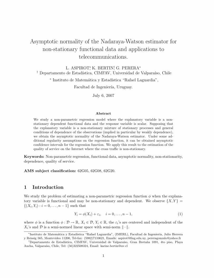
In what follows we describe the procedure to estimate the function φ. We divide the experimentin two phases: first, we send a burst of small probe packets (pp) of fixed size spaced by a fixedtime. Immediately after the burst we send during a short time a video stream. We repeat theprevious procedure during some time lapse, sending a new burst and a video probe after a timeinterval measured from the previous end of the video stream as it is shown in the scheme infigure 1.

pp video

Figure 1: Measurement procedure scheme

With the probe packets burst we infer the cross traffic of the link. We measure at the outputof the link the interarrival time between consecutive probe packets. This time serie is stronglycorrelated with the cross traffic process that shares the link with the probe traffic. We computethe empirical distribution function of probe packets interarrival times because this distribution isrelated with the queue behavior in the network. Using this cross traffic estimation and measuringthe delay Y over the video, we want to estimate the function φ.

From each probe packet burst and video sequence j we have a pair (Xj , Yj), where Xj is theempirical distribution function of interarrival times and Yj is the performance metric of interestmeasured from the video stream j.

Therefore, our estimation problem has been transformed into the problem of inferring afunction φ : D → R where D is the space of the probability distribution functions and R is thereal line such that the (Xj , Yj) satisfy (1).

Asymptotic normality of the Nadaraya-Watson estimator for non-stationary data 12

We did the estimations both with simulated and real traffic. Real data are obtained witha software that do the active measures described before between a server and its users. Forsimulated data, the variable Y is the one-way delay which is the delay between two points. Forreal data, we measure round trip time (RTT) delay that is the delay in the whole trip betweentwo points in a path and in the reverse path.

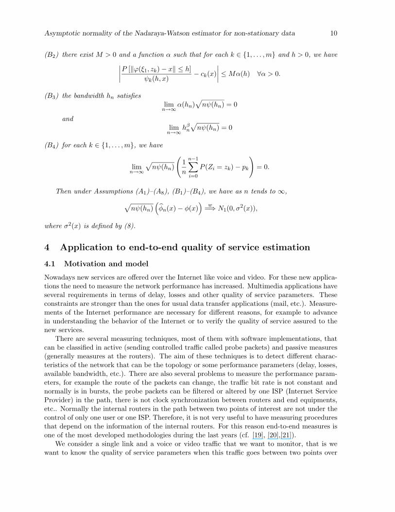
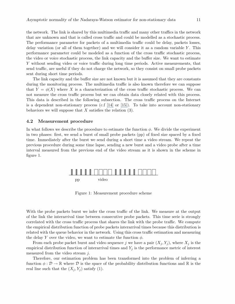
For simulated traffic, we have 360 observations (Xj , Yj). For each j ∈ {1, . . . , 359}, we

calculate the estimator φj defined by (2) using the observations (X1, Y1), . . . , (Xj , Yj) and we

represent on figures 2 and 3 the values of Yj+1 and of its prediction φj(Xj+1). Moreover for each

j ∈ {1, . . . , 359}, we calculate a confidence interval around φj(Xj+1) using a block-bootstrap.

The estimator φj is calculated using the kernel K(x) = (x2 − 1)21[−1,1](x), the bandwidth thatminimizes the sum of the relative error in the estimation before the time j and the L1 norm.The figure 4 represents the relative error of the estimation. The results are relatively accuratefor sample of size larger than 100.

For real data, we have 50 observations (Xj , Yj) and we realize the same type of estimation.In figure 5, we represents for each j ∈ {1, . . . , 49}, the values of Yj+1 and of its prediction

φj(Xj+1) and a confidence a confidence band around φj(Xj+1) using a block-bootstrap. Thefigure 6 represents the relative error of the estimation. The results are less accurate than in thecase of simulated data but the estimations are calculated with samples of small size.

0 50 100 150 200 250 300 350 4000

0.1

0.2

0.3

0.4

0.5

0.6

0.7

Sample number

Del

ay(m

s)

Figure 2: Estimated delays for all simulated data

Asymptotic normality of the Nadaraya-Watson estimator for non-stationary data 13

230 235 240 245 250 255 260 265

0.02

0.04

0.06

0.08

0.1

0.12

Sample number

Del

ay(m

s)

Prediction delayMeasured delayUpper bound confidenceLower bound confidence

Figure 3: Estimated delays for simulated data observations between 230 and 270

0 50 100 150 200 250 300 350 4000

0.1

0.2

0.3

0.4

0.5

0.6

0.7

0.8

0.9

1

Sample number

Rel

ativ

e er

ror

Figure 4: Relative error for simulated data

Asymptotic normality of the Nadaraya-Watson estimator for non-stationary data 14

0 10 20 30 40 50−50

0

50

100

150

200

250

300

350

Sample number

Del

ay(m

s)

Prediction delayMeasured delayUpper bound confidenceLower bound confidence

Figure 5: Estimated RTT for real data

0 10 20 30 40 500

0.5

1

1.5

2

2.5

3

Rel

ativ

e er

ror

Sample number

Figure 6: Relative error for real data

Asymptotic normality of the Nadaraya-Watson estimator for non-stationary data 15

5 Proof of the propositions and theorems

5.1 Proof of Propositions 1 and 2

This result is obtained by means of Bernshtein method (cf. [18], [22]) and it is a gener-alization of the theorem 4.15 on triangular arrays for R-valued random fields obtained byTablar (2006) ([23], p 86) to R

m-valued random fields. To prove that the vectorial field(Sn(A1, X1,n), . . . , Sn(Am, Xm,n))

w=⇒ Nm(0,Σ), it is sufficient to prove that for all λ ∈ R

m

〈λ, Sn〉w

=⇒ N(0, λtΣλ) where Sn = (Sn(A1, X1,n), . . . , Sn(Am, Xm,n)) and λt = (λ1, . . . , λm).We have that

〈Sn, λ〉 =m∑

i=1

λiSn(Ai, Xi,n) =m∑

i=1

1

(`(n))1/2λi

∑

k∈Ain

Xi,nk

=1

(`(n))1/2

∑

k∈D(n)

m∑

i=1

λiXi,nk 1{k∈Ai

n}

Let us consider a real valued field Xn(λ) where Xi,nk (λ) = λiX

i,nk if k ∈ Ai

n. Then 〈Sn, λ〉 =Sn

(D(n), Xn(λ)

). As the field Xn(λ) verifies the hypotheses in the work of [23] we can apply

the theorem for a real valued random field in order to obtain the result of propositions 1 and 2.

5.2 Proof of Proposition 4

Since Z is asymptotically measurable, conditionally to Z, the subset family (A1, . . . , A2m) is anasymptotically measurable family in N. Then applying Proposition 1 to X which belongs toB(N), we deduce the result.

5.3 Proof of Proposition 5

Before proving Proposition 5, here we prove the following lema.

Lemma 1. Let k ∈ {1, . . . ,m}. Under the Assumptions (A1), (A2), (A3), (A5), (A7) and (A8),we have

1) the following limit

limn→∞

1

ψ(hn)E [Kn(ϕ(ξ1, zk))] = dk(x)ck(x)1{k∈∆},

2) for β > 0,

limn→∞

1

ψ(hn)E

[∥∥∥∥ϕ(ξ1, zk) − x

hn

∥∥∥∥β

Kn(ϕ(ξ1, zk))

]≤ dk(x)ck(x),

3) that the estimator fn(x) satisfies

limn→∞

E(fn(x)) = f(x),

Asymptotic normality of the Nadaraya-Watson estimator for non-stationary data 16

4) and the estimator gn(x) satisfies

limn→∞

E(gn(x)) = φ(x)f(x).

Proof. The results 1) and 2) of this lemma come from the fact that under Assumption (A1), thedensity of ‖ϕ(ξ1, zk) − x‖ is the function u→ ck(x)ψ

′k(u, x). Then under Assumption (A7)

E [Kn(ϕ(ξ1, zk))] = hnck(x)

∫ 1

0K(u)ψ′

k(uhn, x)du

and

E

[∥∥∥∥ϕ(ξ1, zk) − x

hn

∥∥∥∥β

Kn(ϕ(ξ1, zk))

]= hnck(x)

∫ 1

0K(u)uβψ′

k(uhn, x)du

and it is sufficient to use Assumptions (A2) and (A8) to conclude.Here we prove 3) and 4). We have for i ∈ {1, . . . , n},

E(Kn(Xi)) = E{E(Kn(Xi)|Zi)} =

m∑

k=1

E{Kn(ϕ(ξi, zk))}P (Zi = zk).

As (ϕ(ξi, zk))i=1,...,n is identically distributed, we obtain that,

E(fn(x)) =m∑

k=1

(1

ψ(hn)E (Kn(ϕ(ξ1, zk)))

1

n

n−1∑

i=0

P (Zi = zk)

). (9)

Now applying (A3) and the assertion 1) of this lemma in (9), we obtain 3). Similar calculus givethat

E(gn(x)) =m∑

k=1

(1

ψ(hn)E (φ (ϕ(ξ1, zk))Kn(ϕ(ξ1, zk)))

1

n

n−1∑

i=0

P (Zi = zk)

).

Then we haveE(gn(x)) = φ(x)E(fn(x)) +Rn,

where

Rn =m∑

k=1

(1

ψ(hn)E ({φ (ϕ(ξ1, zk)) − φ(x)}Kn(ϕ(ξ1, zk)))

1

n

n−1∑

i=0

P (Zi = zk)

)

≤ supu:‖x−u‖≤hn

|φ(u) − φ(x)|E(fn(x))

and we obtain 4) using the continuity of function φ (Assumption (A5)) and using that limn→∞E(fn(x)) =f(x).

Conditionally to Z, we have

√nψ(hn)

(gn(x)−E(gn(x)|Z), fn(x)−E(fn(x)|Z)

)=

m∑

j=1

Sn(Aj , Xn,j),2m∑

j=m+1

Sn(Aj , Xn,j)

.

Asymptotic normality of the Nadaraya-Watson estimator for non-stationary data 17

Using Proposition 4, we obtain that, conditionally to Z,

m∑

j=1

Sn(Aj , Xn,j),2m∑

j=m+1

Sn(Aj , Xn,j)

w=⇒ N2(0, A).

Since Z is regular, the matrix A is not random and then we have

√nψ(hn)

(gn(x) − E(gn(x)|Z), fn(x) − E(fn(x)|Z)

)w

=⇒ N2(0, A).

Now

(gn(x) − E(gn(x)), fn(x) − E(fn(x))) = (gn(x) − E(gn(x)|Z), fn(x) − E(fn(x)|Z))

+ (E(gn(x)|Z) − E(gn(x)), E(fn(x)|Z) − E(fn(x))).

We have

E(fn(x)|Z) − E(fn(x)) =2m∑

j=1

E(Kn(ξ1, zj))

ψ(hn)

(card(Aj

n)

n−

1

n

n−1∑

i=0

P [Zi = j]

).

Under Assumption (A3) and using assertion 1) of Lemma 1, we have that√nψ(hn) (E(fn(x)|Z) − E(fn(x)))

converges in probability to 0 as n tends to ∞. Using Assumption (A3),√nψ(hn) (E(gn(x)|Z) − E(gn(x)))

converges in probability to 0 as n tends to ∞. Using the lemma of Slutsky, we obtain the resultof the proposition.

5.4 Proof of Theorem 1

We have

φn(x) −E(gn(x))

E(fn(x))=Qn(x) −Bn(x)(fn(x) − E (fn(x)))

fn(x),

where

Bn(x) =E(gn(x))

E(fn(x))− φ(x)

andQn(x) = (gn(x) − E(gn(x))) − φ(x)(fn(x) − E(fn(x))).

Using 3) y 4) of Lemma 1, we deduce that

limn→∞

Bn(x) = 0.

Then using (A6), we have that fn(x) converges in probability to f(x) > 0 and then it impliesthat

Bn(x)(fn(x) − E (fn(x)))

fn(x)(10)

converges in probability to 0.Finally, using (A6), (10) and Proposition 5, applying Slutsky Lemma, we deduce the result ofthe proposition.

Asymptotic normality of the Nadaraya-Watson estimator for non-stationary data 18

5.5 Proof of Theorem 2

Theorem 2 is obtained using Theorem 1 and the following lemma.

Lemma 2. Under Assumptions (B1)− (B4) and Assumptions (A1), (A2), (A6), (A7) and (A8),we have that

limn→∞

√nψ(hn)

(E(gn(x))

E(fn(x))− φ(x)

)= 0.

Proof. We have the following decomposition

E(gn(x))

E(fn(x))− φ(x) =

1

E(fn(x))[E(gn(x)) − f(x)φ(x)] +

φ(x)

E(fn(x))[f(x) − E(fn(x))] . (11)

Here we study first the quantity E(fn(x)) − f(x). As in Lemma 1, we have

E(fn(x)) =

m∑

k=1

(1

ψ(hn)E (Kn(ϕ(ξ, zk)))

1

n

n−1∑

i=0

P (Zi = zk)

)

and then

E(fn(x)) − f(x) =m∑

k=1

(1

ψ(hn)E (Kn(ϕ(ξ, zk))) − dk(x)ck(x)1{k∈∆}

)1

n

n−1∑

i=0

P (Zi = zk)

+m∑

k=1

dk(x)ck(x)1{k∈∆}

(1

n

n−1∑

i=0

P (Zi = zk) − pk

).

Under the Assumptions (B2), (B3) and (B4) imply that

limn→∞

√nψ(hn) (E(fn(x)) − f(x)) = 0. (12)

Here we study the term E(gn(x)) − f(x)φ(x). It satisfies

|E(gn(x)) − f(x)φ(x)| ≤ |φ(x)| |E(fn(x)) − f(x)| + |E(gn(x)) − E(fn(x))φ(x)|.

We have

|E(gn(x)) − E(fn(x))φ(x)| =

∣∣∣∣∣1

ψ(hn)

m∑

k=1

E [Kn(ϕ(ξ, zk)) (φ(ϕ(ξ, zk)) − φ(x))]1

n

n−1∑

i=0

P (Zi = zk)

∣∣∣∣∣

≤ Lhβn

m∑

k=1

1

ψ(hn)E

[Kn(ϕ(ξ, zk))

∥∥∥∥ϕ(ξ, zk) − x

hn

∥∥∥∥β]

1

n

n−1∑

i=0

P (Zi = zk)

≤ L1hβn(1 + o(1)), (13)

where the second line comes from Assumption (B1) and the third is a consequence of assertion2) of Lemma 1. From (12), (13) and Assumption (B3), we deduce that

limn→∞

√nψ(hn) (E(gn(x)) − f(x)φ(x)) = 0. (14)

Assertion 1) of Lemma 1, (12) and (14) applying in (11) imply the proposition.

Asymptotic normality of the Nadaraya-Watson estimator for non-stationary data 19

6 Acknowledgement

This work has been supported by the ARTES group. Karine Bertin has been supported byProject DIPUV 33/05, Project FONDECYT 1061184 and the Laboratory ANESTOC ACT-13. Laura Aspirot has been partially supported by PDT (Programa de Desarrollo Tecnologico)S/C/OP/46/. The authors would like to thank Yoana Donoso for her contributions to thesimulations programs.

References

[1] Nadaraya, E. A., 1989, Nonparametric estimation of probability densities and regressioncurves, Mathematics and its Applications (Soviet Series), 20. Dordrecht: Kluwer AcademicPublishers Group.

[2] Rosenblatt, M., 1969, Conditional probability density and regression estimators. Multivari-ate Analysis, II (Proc. Second Internat. Sympos., Dayton, Ohio, 1968), 25–31. New York:Academic Press.

[3] Robinson, P. M., 1983, Nonparametric estimators for time series. J. Time Ser. Anal., 4,185–207.

[4] Ferraty, F., Goia, A. and Vieu, P., 2002, Functional nonparametric model for time series:a fractal approach for dimension reduction. Test, 11, 317–344.

[5] Ferraty, F. and Vieu, P., 2004, Nonparametric models for functional data, with applicationin regression, time-series prediction and curve discrimination. J. Nonparametr. Stat., 16,111–125.

[6] Aspirot, L., Belzarena, P., Bazzano, B. and Perera, G., 2005, End-To-End Quality of ServicePrediction Based On Functional Regression. Proc. Third International Working Conferenceon Performance Modelling and Evaluation of Heterogeneous Networks (HET-NETs 2005),Ilkley, UK, July 2005.

[7] Masry, E., 2005, Nonparametric regression estimation for dependent functional data:asymptotic normality. Stochastic Process. Appl., 115, 155–177.

[8] Ferraty, F., Mas, A. and Vieu, P., 2007, Nonparametric regression on functional data:inference and pratical aspects. Australian and New Zealand Journal of Statistics, 11.

[9] Gasser, T., Hall, P. and Presnell, B., 1998, Nonparametric estimation of the mode of adistribution of random curves. J. R. Stat. Soc. Ser. B Stat. Methodol., 60, 681–691.

[10] Dabo-Niang, S., Ferraty, F., and Vieu, P., 2004, Estimation du mode dans un espacevectoriel semi-norme. C. R. Math. Acad. Sci. Paris, 339, 659–662.

[11] Oliveira, P., 2005, Nonparametric density and regression estimation functional data. Pre-Publicacoes do Departamento de Matematica, Universidade de Coimbra, 05-09.

[12] Ramsay, J. O. and Silverman, B. W., 2005, Functional data analysis (2nd edn), SpringerSeries in Statistics. New York: Springer.

Asymptotic normality of the Nadaraya-Watson estimator for non-stationary data 20

[13] Ferraty, F. and Vieu, P., 2006, Nonparametric Functional data analysis: Theory and Prac-tice, Springer Series in Statistics. New York: Springer.

[14] Karagiannis, T., Molle, M., Faloutsos, M. and Broido, A., 2004, A nonstationary Poissonview of Internet traffic. Proc. of INFOCOM 2004. Twenty-third Annual Joint Conferenceof the IEEE Computer and Communications Societies, 3, 1558–1569.

[15] Zhang, Y., Paxson, V. and Shenker, S., 2000, The Stationarity of Internet Path Properties:Routing, Loss, and Throughput. ACIRI Technical Report.

[16] Zhang, Y. and Duffield, N., 2001, On the constancy of internet path properties. IMW ’01:Proceedings of the 1st ACM SIGCOMM Workshop on Internet Measurement, 197–211.

[17] Perera, G., 2002, Irregular sets and central limit theorems. Bernoulli, 8, 627–642.

[18] Perera, G., 1997, Geometry of Zd and the central limit theorem for weakly dependent

random fields. J. Theoret. Probab., 10, 581–603.

[19] Bolot, J., 1993, End-to-end packet delay and loss behavior in the internet. SIGCOMM’93: Conference proceedings on Communications architectures, protocols and applications,289–298.

[20] Jain, M. and Dovrolis, C., 2002, Pathload: A measurement tool for end-to-end availablebandwidth. Proc. of Passive and Active Measurements (PAM) Workshop, Mar. 2002.

[21] Corral, J., Texier, G. and Toutain, L., 2003, End-to-end Active Measurement Architecturein IP Networks (SATURNE). PAM 2003, A workshop on Passive and Active Measurements.

[22] Perera, G., 1997, Applications of central limit theorems over asymptotically measurablesets: regression models. C. R. Acad. Sci. Paris Ser. I Math., 324, 1275–1280.

[23] Tablar, A., Estadıstica de procesos estocasticos y Aplicaciones a Modelos Epidemicos, PhDtesis, submitted to Departamento de Graduados de la Universidad Nacional del Sur forevaluation, december 2006.