Assessment of Disease Progression in the Rare Disease ...

24

Thesis submitted in accordance with the requirements of the

University of Liverpool for the degree of Doctor of Philosophy

by Leah Frances Taylor

April, 2018

Assessment of Disease Progression in the Rare

Disease Alkaptonuria by Quantitative Image

Analysis

25

ACKNOWLEDGMENTS

I would first and foremost like to express the greatest thanks to my number one

supervisor Professor Jim Gallagher. Firstly, for giving me the opportunity to

undertake this PhD and secondly, for his consistent support and guidance throughout

the time I have been a part of his lab. I can honestly say it has been a pleasure to be

a part of your group. I could not have felt more supported along the way with you

and Jane who have looked after me like a daughter. I would also like to thank Jane

for all the proof reading she has done for me, especially for correcting my awful

grammar! I would also like to thank you both for pushing me to further my career

and for supporting me to make the best decisions for my future. For this I will be

forever thankful.

To Professor Ranganath I owe a huge thank you for always believing in me and

supporting me and my work. Without your input, support and guidance this thesis

would not have been possible.

Thank you to Dr Nathan Jeffery for his invaluable imaging knowledge and for giving

me the opportunity to demonstrate Anatomy alongside my PhD. Thanks also to the

following people; Sobhan Vinjamuri for facilitating my work in the nuclear medicine

department; Mark Baker, for his hard work providing me with the patient scans and

teaching me how to use the sophisticated software in the nuclear medicine

department; Eftychia Psarelli for her invaluable guidance on statistical analysis.

A very important thank you goes to the AKU patients without whom this PhD would

not have been possible. My gratitude for this work also goes to the Royal Liverpool

University Hospital and The University of Liverpool for providing the funding for this

work.

My next thanks go to my fellow colleagues. Hazel Sutherland for always being there

for me. Your support was invaluable, you have been a true friend. A ‘not so big’ thanks

goes to Pete and Dr Craig for taking the ‘mick’ out of me constantly for three years!

However, I would not have expected anything less! You two have provided me with

many laughs and have taught me not to take life too seriously, which I think is a very

important lesson to learn…. even if I did want to punch your lights out for it.

Eddie and Brendan. We have shared many happy times together including lots of

eating, drinking and introducing our friend to Western society, I know for that he will

be forever grateful! There are lots of new members of Jim’s group now including

Juliette and Eman that I have had the pleasure of working with, I thank you all too for

your support.

Finally, I would like to thank my family and friends. Firstly, I would like to thank my

Mum & Barry and my Dad & Sue for supporting me both emotionally and financially

throughout my life and always supporting my decisions and guiding me to make the

right choices. Mum, thank you for your unconditional love and always having my back

through thick and thin. I know I can always count on you anytime, anywhere. Dad,

26

thank you for everything especially your sense of humour and your ‘happy go lucky’

attitude to life. I have learnt to be more like this because of you. Without your

support I would not be where I am today. Having said that, I am fully aware that you

still haven’t got a clue about what I have spent the last three and a half years doing!

Thank you to my sister Ceri for always supporting me and teaching me how to be

tough and to never give up. Thank you for listening to many of my talks however, I

can still bet that I can put you to sleep as soon as I start talking. That is a skill!

I am especially grateful to my Gran and Nan for always showing interest in what I do

and always being proud of me. I know that Grandad and Taid would be proud too.

Thank you to my Aunty Karen for being a great walking partner and keeping me

knowledgeable about health and wellbeing. I would also like to thank the rest of my

family for always looking after me and supporting what I do.

Last, but not least, thank you to my best friends, Nicky and Kate. As nuts as you are I

want to thank you for being such good friends to me and for always supporting me

through the good, the bad and the ugly! Thank you for the laughs and the good times.

Here is to many more great times ahead!

A big thank you also goes to all my good friends in Liverpool, Preston and back at

home for your support, company and laughter. Long may this continue.

The support I have received throughout my life as well as the academic support I have

been lucky enough to receive throughout this PhD has all had a massive part to play

in this achievement. For this I will be forever thankful. I hope this thesis and

everything I continue to do makes you all proud.

Leah

27

ABSTRACT

Alkaptonuria (AKU) arises from a genetic deficiency of homogentisate 1,2 dioxygenase (HGD) an

enzyme involved in tyrosine metabolism. AKU is characterised by high circulating homogentisic

acid (HGA) some of which is deposited as ochronotic pigment in connective tissues, mainly

cartilage, leading to multisystemic damage dominated by premature severe osteoarthropathy.

Pathological changes in the spine as a result of ochronosis can be imaged using fluorine-18

labelled sodium fluoride positron emission tomography (18F-NaF PET). This imaging modality

allows quantitative assessment of focal bone remodelling by measuring the uptake of 18F into the

hydroxyapatite crystal of bone and calcified cartilage. The mean standardised uptake value

(SUVm), a mathematically derived ratio of tissue radioactivity in a region of interest (ROI) and the

decay corrected injected dose per kilogram of the patient's body weight has common place in

oncology. The functional changes that 18F-NaF PET detects have led to this modality being re-

evaluated for its advantages in skeletal diseases such as osteoarthritis and AKU.

AKU patients underwent a variety of clinical testing and imaging including 18F-NaF PET scanning

at the Royal Liverpool University Hospital. Semi-quantitative analysis of the PET scans was utilised

to investigate the anatomical distribution of increased 18F uptake. Quantitative SUVms were also

obtained as a measure of Fluoride uptake in the bony vertebrae and cartilaginous intervertebral

discs (IVD). Other clinical data were taken from the case notes for correlation.

The anatomical distribution of increased 18F uptake was confirmed to primarily affect the weight

bearing joints. The quantitative SUVm methodology revealed a striking variation between AKU

and control SUVms in the IVDs thought to represent calcification of the IVDs in AKU. The

mechanism proposed is that calcium hydroxyapatite or calcium pyrophosphate dihydrate are

deposited in the fibrocartilaginous IVDs in AKU due to biochemical alterations of the disease. 18F

binds to the calcium deposits resulting in high SUVms compared to the control. The SUVms

obtained from the vertebrae in both AKU and control patients are similar across the lumbar and

thoracic spine suggesting that generalised rates of bone turnover in AKU and control patients are

comparable.

With age the AKU SUVms of the IVDs followed an interesting trend (the inverted ‘U’ shaped trend)

that was strikingly different to that of the control group that appears to remain stable with age.

It is proposed that the AKU trend demonstrates the process of disc degeneration. In the bony

vertebrae, an age-related decline in SUVm was observed in both AKU and control groups, thought

to represent reduced bone turnover with age.

Correlations were made with the IVD SUVms and other clinical data. Reduced vertebrae SUVm

and increased IVD SUVm were found to be associated with higher clinical scores, pain scores,

excessive spinal curvature angles, lower BMD T-scores and spinal flexibility measurements. The

proposed reason for this is primarily due to reduced BMD with age and spinal arthropathy

associated with calcified IVDs.

All in all, this thesis has provided new insights into spinal arthropathy in AKU. The utilisation of novel quantitative techniques demonstrated in this thesis can be used to aid in clinical interpretation of PET scans as well as providing a measure of disease severity and to analyse disease progression and response to therapy.

28

ABBREVIATIONS

AC - Articular cartilage

ACC - Articular calcified cartilage

AKU - Alkaptonuria

AKUSSI – Alkaptonuria severity score index

AT – Anatomical threshold

B-AT – Bone-anatomical threshold

BMD – Bone mineral density

BQA - Benzoquinone acetic acid

C-AT – Cartilage-anatomical threshold

CT – Computed tomography

DEXA – Dual-energy x-ray absorptiometry

DICOM – Digital imaging and communications in Medicine

ECM - Extracellular matrix

ENT – Ear, nose and throat

EO - Endochondral ossification

18F-NaF – Fluorine-18- labelled Sodium Fluoride

FDA – Food and Drug Administration

HA - Hyaluronan

HAC - Hyaline articular cartilage

HDMPs - High density mineralised protrusions

HGA - Homogentisic acid

HGD - Homogentisate 1,2-dioxygenase

HPPA - 4-hydroxyphenylpyruvic acid

HPPD - 4-hydroxyphenylpyruvate dioxygenase

HT1 - Tyrosinemia type 1

IL-11 – Interleukin 11

IO - Intramembranous ossification

ITM -Interterritorial matrix

IVD - Intervertebral disc

JPEG – Joint photographic experts group

29

KL – Kellgren and Lawrence

LC-MS/MS- Liquid chromatography tandem mass spectrometry

MIP – Maximum intensity projection

MRI – Magnetic resonance imaging

NAC- National Alkaptonuria Centre

NIH - National Institute of Health

NTBC - Nitisinone

OA - Osteoarthritis

PA view- Posteroanterior view (X-Ray)

PACS – Picture archiving and communication systems

PCM – Pericellular matrix

PET – Positron emission tomography

QCT – Quantitative computer tomography

RA – Rheumatoid arthritis

RLBUHT- Royal Liverpool and Broadgreen University Hospital Trust

ROI – Region of interest

RGB – Red, green, blue

SB -Subchondral bone

SEM – Standard error of the mean

s-HGA - serum homogentisic acid

SOFIA - Subclinical ochronotic features in alkaptonuria

SONIA1 - Suitability of nitisinone in alkaptonuria 1

SONIA2 - Suitability of nitisinone in alkaptonuria 2

SPECT - Single-photon emission computed tomography

SUV- Standardised uptake value

SUVm – Mean standardised uptake value

TM – Territorial matrix

TSC – Trans axial, sagittal, coronal

TIFF – Tagged image file format

TOF – Time of flight

u-HGA- urine homogentisic acid

30

WHO – World Health Organisation

3D - Three dimensional

31

TABLE OF CONTENTS

Acknowledgements i-ii

Abstract iii

Abbreviations iv-vi

Table of Contents vii-xiv

List of Figures xv-xxii

List of Tables xxii

1.0 INTRODUCTIO N 1

1.1 Alkaptonuria 2

1.1.1 History 2

1.1.2 Epidemiology 5

1.1.3 Genetic defect 6

1.1.4 Homogentisic acid 7

1.1.5 Clinical presentation 8

1.1.6 The initiation of ochronotic pigment (the exposed 11

collagen hypothesis)

1.1.7 Pathogenesis of joint destruction 12

1.1.8 Diagnosis 13

1.1.9 Therapy 16

1.1.9.1 Vitamin C 16

1.1.9.2 Low protein diet 17

1.1.9.3 Nitisinone 18

1.1.9.4 Other treatments 19

1.1.10 Assessment 22

1.2 AKU society and the National Alkaptonuria Centre 23

1.3 DevelopAKUre 24

1.3.1 Suitability of Nitisinone in Alkaptonruia 1 (SONIA 1) 25

1.3.2 Suitability of Nitisinone in Alkaptonruia 2 (SONIA 2) 26

1.3.3 Subclinical Ochronotic features in Alkaptonuria (SOFIA) 26

1.4 Cartilage 27

32

1.4.1 Articular cartilage structure 28

1.4.1.1 Superficial zone 29

1.4.1.2 Middle zone 29

1.4.1.3 Deep zone 29

1.4.1.4 Calcified zone 30

1.4.2 Extracellular matrix 32

1.4.3 Chondrocytes 35

1.4.4 Collagen 37

1.5 Bone 39

1.5.1 Bone formation 40

1.5.2 Bone matrix 41

1.5.3 Bone cells 42

1.5.4 Bone remodelling 43

1.5.5 Subchondral bone 44

1.5.6 Osteoarthritis 44

1.5.7 Osteoarthritis and Alkaptonuria 45

1.5.8 Intervertebral disc anatomy 46

1.5.9 Intervertebral disc degeneration 49

1.5.10 Diagnostic imaging in OA 50

1.6 Medical imaging in AKU 51

1.6.1 History of medical imaging 51

1.6.2 Radiography 53

1.6.2.1 Basic principles of radiography 54

1.6.3 Bone densitometry 56

1.6.3.1 Basic principles – DEXA 57

1.6.3.2 Basic principles- QCT 58

1.6.4 Computed tomography 60

1.6.4.1 Basic principles – CT 61

1.7 Nuclear medicine 62

1.7.1 History of nuclear medicine 63

33

1.7.2 PET Imaging – physical principles 64

1.7.3 Bone imaging radiopharmaceuticals 65

1.7.3.1 Mechanism of 18F-NaF uptake 67

1.7.4 Quantitative measurement of 18F-NaF 69

1.7.4.1 SUV measurements in osteoarthritis 71

1.7.5 Maximum intensity projection 72

2.0 MATERIALS AND METHODS 73

2.1 Ethical approval 74

2.2 Patient groups 74

2.2.1 NAC 74

2.2.2 SONIA 2 75

2.2.3 Control group 75

2.3 PET/CT protocol 76

2.4 18F-NaF PET threshold application 76

2.4.1 Image type 76

2.4.2 ImageJ Software 76

2.4.3 Histogram analysis 76

2.4.4 Threshold application 79

2.4.5 Anatomical scoring 80

2.4.6 Cartilage-anatomical threshold score 82

2.4.7 Bone anatomical threshold score 83

2.4.8 Total anatomical threshold score 83

2.4.9 Total clinical score 84

2.5 Obtaining the standardised uptake value 84

2.5.1 Hermes Hybrid Viewer 1.4 84

2.5.2 Measuring the standardised uptake value – spine 85

2.5.3 Measuring the standardised uptake value – hip and 85

shoulder

2.6 Cobb angle measurements 91

2.6.1 X-ray scoliosis measurement 91

34

2.6.2 X-ray thoracic kyphosis and lumbar lordosis 92

measurement

2.6.3 MRI thoracic kyphosis and lumbar lordosis 92

measurement

2.7 Spinal flexibility measurements 94

2.7.1 Lumbar side flexion measurement 94

2.7.2 Cervical spine rotation measurement 94

2.8 Statistical analysis 95

2.8.1 Parametric tests 95

2.8.2 Non-parametric tests 96

2.8.3 Regression analysis 96

2.8.3.1 Multiple linear regression 96

2.8.3.2 Simple linear regression and Pearson’s 96

correlation

2.8.4 Trend lines 97

3.0 SKELETAL DISTRIBUTION OF INCREASED 18F PET UPTAKE IN 98

PATIENTS WITH ALKAPTONURIA

3.1 INTRODUCTION 99

3.2 DESIGN OF STUDY 101

3.2.1 Patient group 101

3.2.2 Image analysis 101

3.2.3 Anatomical scoring 101

3.3 RESULTS 102

3.3.1 Skeletal distribution of increased 18F uptake with age 102

in the skeleton

3.3.2 Skeletal distribution of increased 18F uptake with 110

age in cartilaginous joints

3.3.3 Cartilage anatomical threshold score with age 116

3.3.4 Bone anatomical threshold score with age 117

3.3.5 Total clinical score vs total anatomical threshold 118

score

35

3.4 DISCUSSION 122

3.4.1 Increased 18F uptake in bone-mechanical loading 124

3.4.2 Increased 18F uptake in bone- vascularity 125

3.4.3 Increased 18F uptake in the vertebrae 126

3.4.4 Bone AT score with age 127

3.4.5 Pathogenesis of increased 18F uptake in cartilage 127

3.4.6 Increased uptake of 18F in cartilage 128

3.4.7 Assessment of methodology 129

3.4.8 Summary 130

3.4.9 Limitations 130

3.4.10 Future work 132

4.0 APPLICATION OF 18F-NaF STANDARDISED UPTAKE VALUE FOR THE 133

DETECTION OF ARTHROPATHY IN AKU

4.1 INTRODUCTION 134

4.2 FEASIBILITY STUDY 136

4.2.1 Design of feasibility study 136

4.2.2 Results of feasibility study 137

4.2.2.1 Mean standardised uptake value – Hip 137

4.2.2.2 Mean standardised uptake value – Shoulder 141

4.2.2.3 Mean standardised uptake value – Spine 145

4.2.3 Discussion of feasibility study 148



4.3.2 Measuring the SUVms 150

4.4 RESULTS 151

4.4.1 Vertebrae and IVD SUVms 151

4.4.2 SUVm with age 154

4.4.3 Gender and SUVm 162

4.4.4 Individual change in SUVm over one year 163

4.5 DISCUSSION 170

36

4.5.1 Discussion of feasibility study and SONIA2 results 171

4.5.2 IVD SUVm 172

4.5.3 Vertebrae SUVm 174

4.5.4 Vertebrae SUVm with age 176

4.5.5 IVD SUVm with age 177

4.5.6 Gender and SUVm 178

4.5.7 Individual changes in SUVm 179

4.5.8 Limitations of the SUVm 180

4.5.9 Summary 181

4.5.10 Further work 182

5.0 PROGRESSION OF SPINAL ARTHROPATHY IN RESPONSE TO 183

NITISINONE IN AKU MONITORED BY 18F-NaF STANDARDISED

UPTAKE VALUE.





5.2.3 Correlations (QCT, CTX AND PAIN SCORES) 187

5.3 RESULTS 188

5.3.1 Comparison between lumbar and thoracic vertebrae 188

and IVD SUVms


5.3.3 Individual change in SUVm across 5 visits 197

5.3.4 SUVm correlation with clinical and anatomical 203

threshold scores

5.3.5 Lumbar spine quantitative computer tomography 208

5.3.6 Femur quantitative computer tomography 211

5.3.7 C-Terminal telopeptide 1 (CTX-1) bone marker 214

5.3.8 Lumbar and thoracic pain scores 217

5.4 DISCUSSION 221

37

5.4.1 Comparison between lumbar and thoracic 221

vertebrae and IVD SUVms

5.4.2 Annual change in SUVm in the vertebrae and IVD 222


5.4.4 Individual changes in SUVm across the 5 visits 224

5.4.5 Correlation between SUVm and clinical and 226

anatomical threshold scores

5.4.6 SUVm with lumbar spine and femur QCT T-score 228

5.4.7 C-Terminal telopeptide (CTX-1) bone marker 231

5.4.8 Lumbar and thoracic pain scores 234

5.4.9 Summary 236

5.4.10 Further work 237

6.0 SUVm CORRELATION WITH SONIA2 CLINICAL DATA 238





6.2.3 Patient data obtained 241

6.2.3.1 X-Ray and MRI Cobb angle measurements 242

6.2.3.2 Lumbar side flexion and cervical rotation 243 measurements 6.2.3.3 Serum and urine HGA 244

6.3 RESULTS 245

6.3.1 Serum HGA correlations 245

6.3.2 Total urine HGA correlations 247

6.3.3 Lumbar side flexion correlations 250

6.3.4 Cervical spine rotation correlations 255

6.3.5 Cobb angle correlation with SUVm 259

6.3.6 Cobb angle MRI vs X-ray 263

6.3.7 DEXA lumbar spine T-score 266

38

6.3.8 DEXA femur T-score 270

6.3.8.1 Comparison between DEXA and QCT results 273

6.4 DISCUSSION 274

6.4.1 Serum HGA correlation 274

6.4.2 Urine HGA correlation 276

6.4.3 Lumbar side flexion correlation 277

6.4.4 Cervical spine rotation correlations 279

6.4.5 Cobb angle correlation with SUVm 279

6.4.6 Cobb angle MRI vs X-ray 283

6.4.7 Bone mineral density T-score comparisons 285

6.4.8 DEXA lumbar spine T-score 288

6.4.9 DEXA femur T-scores 291

6.4.10 Summary 292

7.0 GENERAL DISCUSSION 296

8.0 REFERENCES 306

39

LIST OF FIGURES

CHAPTER 1

Figure 1.1 The tyrosine metabolic pathway. 4

Figure 1.2 Formation of ochronotic pigment. 5

Figure 1.3 Progression of ochronosis in the joint. 14

Figure 1.4 The initiation of ochronotic pigment-the exposed collagen hypothesis. 15

Figure 1.5 Zones and morphology of articular cartilage. 31

Figure 1.6 Chondrocyte structure. 34

Figure 1.7 The molecular arrangement of extracellular matrix in cartilage. 36

Figure 1.8 Anatomy of the intervertebral disc. 48

Figure 1.9 Generation of X-rays in an X-ray tube. 55

Figure 1.10 Set up of a chest radiograph. 56

Figure 1.11 Dual-energy X-ray absorptiometry report. 60

Figure 1.12 Positron emission schematic. 65

Figure 1.13 Standardised uptake value calculation. 70

CHAPTER 2 Figure 2.1 Histogram plot of MIP PET image pixel value distribution. 77

Figure 2.2 Histogram plot of MIP PET image pixel value distribution analysing 78 the darkest pixels in the image.

Figure 2.3 Threshold application. 8-bit 18F MIP PET image with a threshold 79

value of 70 applied.

Figure 2.4 18F MIP PET images of lumbar vertebrae and intervertebral discs. 81

Figure 2.5 Labelled skeletal map of a human skeleton. 82

Figure 2.6 18F-Na PET/CT scan showing trans-axial (far left), sagittal (middle), 87 coronal (far-right) and CT (top left image) views.

Figure 2.7 18F-NaF PET/CT sagittal view of spine. 88

Figure 2.8 18F-NaF PET trans axial view with ROI placed in the centre of the 88 IVD.

Figure 2.9 18F-NaF PET/CT trans-axial section through the hip joint 89 demonstrating ROI’s placed in the head of femur (A), acetabulum (B) and the articular cartilage (C).

40

Figure 2.10 18F-NaF PET/CT trans-axial section through the hip joint 90 demonstrating ROI’s placed in the head of the humerus (A), glenoid fossa (B), and articular cartilage (C).

Figure 2.11 PA X-Ray (A), lateral X-Ray (B) and T1 weighted whole spine 93

MRI- sagittal view (C) to measure scoliosis, thoracic kyphosis and lumbar

lordosis Cobb angles.

CHAPTER 3 Figure 3.1 Percentage incidence of increased 18F uptake in the bones of the 104 skeleton.

Figure 3.2 Skeletal distribution of increased 18F PET uptake with age in the 105 bones of the skeleton represented on a skeletal map.

Figure 3.3 Percentage incidence of 18F uptake in the lumbar vertebrae 106 with age.

Figure 3.4 Percentage incidence of 18F uptake in the thoracic vertebrae 107 with age in the youngest patient groups.

Figure 3.5 Percentage incidence of 18F uptake in the thoracic vertebrae 108 in the oldest patient groups.

Figure 3.6 Percentage incidence of increased 18F uptake in the cervical 109 vertebrae with age.

Figure 3.7 Percentage incidence of increased 18F PET uptake in 111 cartilaginous joints.

Figure 3.8 Percentage incidence of increased 18F uptake in the 113 cartilaginous joints by age.

Figure 3.9 Skeletal distribution of increased 18F PET uptake with age in the 114 cartilaginous joints of the skeleton.

Figure 3.10 Percentage incidence of increased tracer uptake in the shoulder, 116 hip and knee joints with age.

Figure 3.11 Correlation between cartilage-anatomical threshold (C-AT) 117 score with age.

Figure 3.12 Scatter plot showing the correlation between bone-anatomical 118 threshold (B-AT) score and age.

Figure 3.13 Correlation between the total clinical score and total anatomical 119 threshold (AT) score.

Figure 3.14 Correlation between the total anatomical threshold (AT) score 120 with age.

Figure 3.15 Correlation between the total clinical score with age. 121

Figure 3.16 18F-NaF images of the spine in arthritic and non-arthritic patient. 131

41

CHAPTER 4

Figure 4.1 SUVm of the articular cartilage, acetabulum and head of femur 138 in the AKU group with age.

Figure 4.2 SUVm of the articular cartilage, acetabulum and head of femur 139 in the control group with age.

Figure 4.3 Box and whisker plot comparison of AKU and control SUVm in 140 the articular cartilage, acetabulum and head of femur of the hip joint.

Figure 4.4 SUVm of the articular cartilage, glenoid fossa and head of the 142 humerus of the shoulder in the AKU group with age.

Figure 4.5 SUVm of the articular cartilage, glenoid fossa and head of 143 humerus in the control group with age.

Figure 4.6 Box and whisker plot comparison of AKU and control SUVm 144 in the articular cartilage, glenoid fossa and head of the humerus of the shoulder joint.

Figure 4.7 SUVm of mean lumbar and thoracic vertebrae in AKU and 146 control groups.

Figure 4.8 SUVm of mean lumbar and thoracic intervertebral discs in 147 AKU and control groups.

Figure 4.9 SUVm of mean lumbar and thoracic vertebrae and IVD 153 across all AKU and control patients.

Figure 4.10 SUVm of mean lumbar vertebrae with age in individual 155 AKU and control patients.

Figure 4.11 SUVm of mean thoracic vertebrae with age in individual 157 AKU and control patients.

Figure 4.12 SUVm of mean lumbar IVDs with age in individual AKU 159 and control patients.

Figure 4.13 SUVm of mean thoracic IVDs with age in individual AKU 161 and control patients.

Figure 4.14 Mean lumbar and thoracic vertebrae and IVD’s SUVm in 162 males and females.

Figure 4.15 Individual patient mean lumbar vertebrae SUVm at V1 and 166

V3 in four age groups.

Figure 4.16 Individual patient mean thoracic vertebrae SUVm at V1 and 167

V3 in four age groups.

Figure 4.17 Individual patient mean lumbar IVD SUVm at V1 and V3 in 168

four age groups.

Figure 4.18 Individual patient mean thoracic IVD’s SUVm at V1 and V3 169

in four age groups.

42

CHAPTER 5

Figure 5.1 Mean lumbar and thoracic vertebrae and IVD SUVm 189

comparisons between visit one and visit 5.

Figure 5.2 Mean AKU lumbar and thoracic vertebrae and IVD SUVm 190

across 5 annual visits.

Figure 5.3 Mean lumbar IVD SUVm with age in individual AKU and 193

control patients across 5 visits.

Figure 5.4 Mean thoracic IVD SUVm with age in individual AKU and 194

control patients across 5 visits.

Figure 5.5 Mean lumbar vertebrae SUVm with age in individual AKU 195

and control patients across 5 visits.

Figure 5.6 Mean thoracic vertebrae SUVm with age in individual AKU 196

and control patients across 5 visits.

Figure 5.7 Mean lumbar IVD SUVm across 5 visits in individual patients 199

grouped by age.

Figure 5.8 Mean thoracic IVD SUVm across 5 visits in individual patients 200

grouped by age.

Figure 5.9 Mean lumbar vertebrae SUVm across 5 visits in individual 201

patients grouped by age.

Figure 5.10 Mean thoracic vertebrae SUVm across 5 visits in individual 202

patients grouped by age.

Figure 5.11 Scatter graph demonstrating a positive correlation between 204

the average lumbar and thoracic IVD SUVm with the total clinical score

for visit 1.

Figure 5.12 Scatter graph demonstrating a negative correlation between 205

the average lumbar and thoracic vertebrae SUVm with the total clinical

score for visit 1.

Figure 5.13 Scatter graph demonstrating the correlation between the 205

average lumbar and thoracic IVD SUVm with the total anatomical

threshold for visit 1.

Figure 5.14 Scatter graph demonstrating the correlation between 206

the average lumbar and thoracic vertebrae SUVm with the total

anatomical threshold score for visit 1.

Figure 5.15 Scatter graph between the average lumbar and thoracic 207

IVD SUVm with the cartilage anatomical threshold score for visit 1.

Figure 5.16 Scatter graph between the average lumbar and thoracic 207

vertebrae SUVm with the bone anatomical threshold score for visit 1.

43

Figure 5.17 Scatter graph demonstrating correlation between lumbar 209

(L1-L3) Quantitative Computer Tomography T-score and age in males

and females (visit 1).


(L1-L3) Quantitative Computer Tomography T-score and the average

lumbar IVD SUVm in males and females (visit 1).


(L1-L3) Quantitative Computer Tomography T-score and the average

lumbar vertebrae SUVm in males and females (visit 1).

Figure 5.20 Scatter graph demonstrating a correlation between lumbar 212

spine and femur QCT T-score with age (visit 1).

Figure 5.21 Correlation between spine and femur QCT T-scores. 212

Figure 5.22 Scatter graph demonstrating correlation between femur 213

Q-CT T-score and the average lumbar IVD SUVm in males and females

(visit 1).

Figure 5.23 Scatter graph demonstrating correlation between femur 213

Q-CT T-score and the average lumbar vertebrae SUVm in males and

females (visit 1).

Figure 5.24 Scatter graph demonstrating the correlation between serum 215

CTX with age in males and females for visit 1.

Figure 5.25 Scatter graph demonstrating the correlation between spine 215

and femur T-scores with CTX bone resorption marker.

Figure 5.26 Correlation between CTX and average lumbar and thoracic 216

IVD SUVm in males and females at visit 1.

Figure 5.27 Correlation between CTX and average lumbar and thoracic 216

vertebrae SUVm in males and females at visit 1.

Figure 5.28 Correlation between the lumbar and thoracic pain scores 218

with age at visit 1.

Figure 5.29 Correlation between average lumbar IVD SUVm with lumbar 219

pain score at visit 1.

Figure 5.30 Correlation between the average thoracic IVD SUVm with 219

thoracic pain score at visit 1.

Figure 5.31 Correlation between average lumbar vertebrae SUVm with 220

lumbar pain score at visit 1.

Figure 5.32 Correlation between average thoracic vertebrae SUVm 220 with thoracic pain score at visit 1.

44

CHAPTER 6

Figure 6.1 Correlation between serum HGA pre-nitisinone (µmol/L) 246

with age in males and females at visit 1.

Figure 6.2 Correlation between serum HGA µmol/L (pre-nitisinone) 246

with the average lumbar and thoracic vertebrae SUVm at visit 1 in

males and females.

Figure 6.3 Correlation between serum HGA µmol/L (pre-nitisinone) 247

with the average lumbar and thoracic IVD SUVm at visit 1 in males and

females.

Figure 6.4 Correlation between total urine HGA pre-nitisinone with 248

age in males and females at visit 1.

Figure 6.5 Correlation between total urine HGA pre-nitisione with 249

the average lumbar and thoracic vertebrae SUVm at visit 1 in males

and females.

Figure 6.6 Correlation between total urine HGA pre-nitisione with 249

the average lumbar and thoracic IVDs SUVm at visit 1 in males and

females.

Figure 6.7 Correlation between lumbar side flexion (cm) with age in 252

males and females at visit 1.

Figure 6.8 Correlation between lumbar side flexion (cm) with average 253

lumbar and thoracic vertebrae SUVm in males and females at visit 1.

Figure 6.9 Correlation between lumbar side flexion (cm) with average 254

lumbar and thoracic IVD SUVm in males and females at visit 1.

Figure 6.10 Correlation between cervical spine rotation with age in 256

males and females at visit 1.

Figure 6.11 Correlation between cervical spine rotation with the 257

average lumbar and thoracic vertebrae SUVm in males and

females at visit 1.

Figure 6.12 Correlation between cervical spine rotation with the 258

average lumbar and thoracic IVD SUVm in males and females at

visit 1.

Figure 6.13 Correlation between the average thoracic vertebrae SUVm 260

with thoracic kyphosis X-Ray Cobb angle in AKU patients at visit 1.

Figure 6.14 Correlation between average lumbar vertebrae SUVm 261

with lumbar lordosis X-Ray Cobb angle in AKU at visit 1.

Figure 6.15 Correlation between average thoracic IVD SUVm with 261

thoracic kyphosis X-Ray Cobb angle in AKU patients at visit 1.

45

Figure 6.16 Correlation between average lumbar IVD SUVm with 262

lumbar lordosis X-Ray Cobb angle in AKU patients at visit 1.

Figure 6.17 Correlation between average thoracic and lumbar IVD 262

SUVm with scoliosis X-Ray Cobb angle in AKU patients at visit 1.

Figure 6.18 Correlation between average thoracic and lumbar 263

vertebrae SUVm with scoliosis X-Ray Cobb angle in AKU patients

at visit 1.

Figure 6.19 Correlation between X-Ray and MRI thoracic kyphosis 264

Cobb angles in AKU patients at visit 1.

Figure 6.20 Correlation between X-Ray and MRI lumbar lordosis 265

Cobb angles in AKU patients at visit 1.

Figure 6.21 Correlation between DEXA lumbar spine (L2-L4) T-score 268

and age in males and females at visit 1.

Figure 6.22 Correlation between DEXA lumbar spine T-score and 268

average lumbar vertebrae SUVm at visit 1 in males and females.


the average lumbar IVD SUVm at visit 1 in males and females.


the thoracic kyphosis cobb angle in males and females.

Figure 6.25 Correlation between DEXA lumbar spine T-score and the 270

lumbar lordosis cobb angle in males and females.

Figure 6.26 Correlation between DEXA femur T-score and the 272

average lumbar vertebrae SUVm at visit 1 in males and females.

Figure 6.27 Correlation between DEXA femur T-score and the average 272

lumbar IVD SUVm at visit 1 in males and females.

Figure 6.28 Correlation between DEXA spine T-score and femur T-score 273

with age in AKU patients at visit 1.

46

LIST OF TABLES

CHAPTER 1

Table 1.1 Information regarding the various current and future therapies 21 to treat AKU.

Table 1.2 AKUSSI table. 23

Table 1.3 Kellgren-Lawrence radiographic classification scale for OA 50 severity.

Table 1.4 World Health Organisation definitions of bone mineral density 59 levels.

Table 1.5 Comparison between the characteristics of 18F-NaF and 67 Tc-99m MDP bone imaging agents.

Table 1.6 Advantages of 18F-NaF PET for studying bone tracer kinetics. 69

CHAPTER 2

Table 2.1 Patient demographic characteristics for the 4 groups of 75 patients analysed.

CHAPTER 6

Table 6.1 Thoracic kyphosis and lumbar lordosis mean Cobb angles 265 obtained from MRI and X-ray imaging modalities.

1

1.0 INTRODUCTION

2

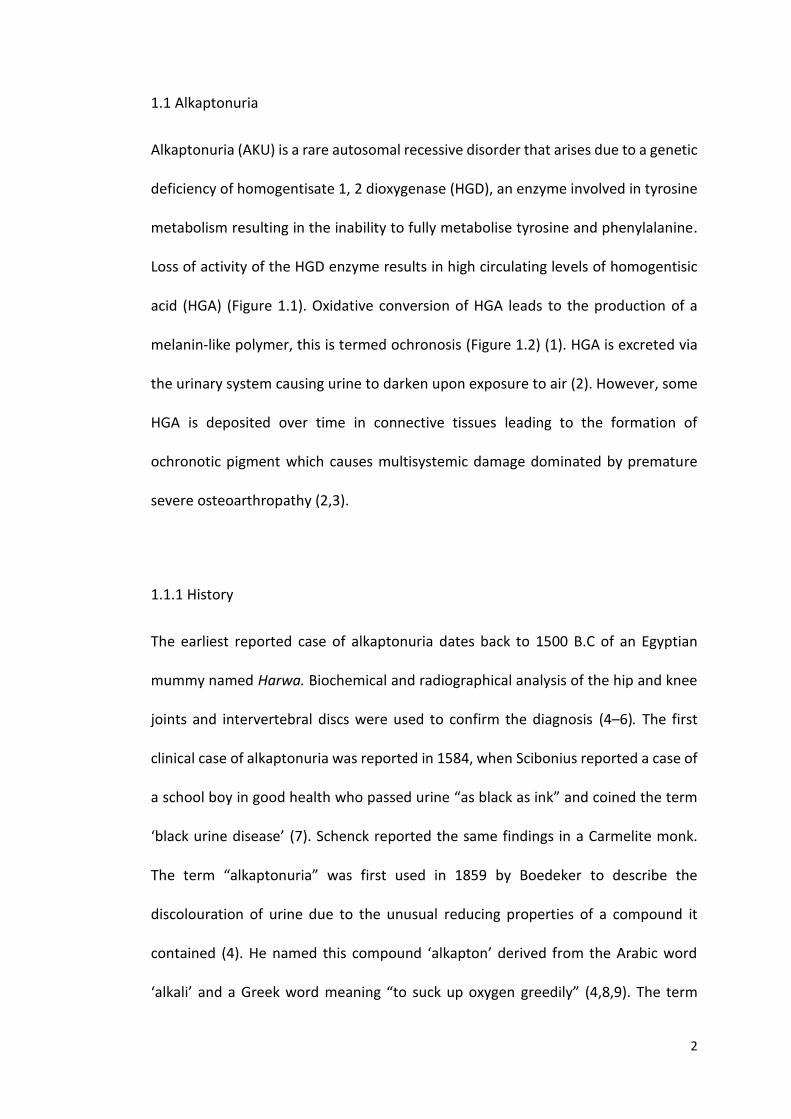
1.1 Alkaptonuria

Alkaptonuria (AKU) is a rare autosomal recessive disorder that arises due to a genetic

deficiency of homogentisate 1, 2 dioxygenase (HGD), an enzyme involved in tyrosine

metabolism resulting in the inability to fully metabolise tyrosine and phenylalanine.

Loss of activity of the HGD enzyme results in high circulating levels of homogentisic

acid (HGA) (Figure 1.1). Oxidative conversion of HGA leads to the production of a

melanin-like polymer, this is termed ochronosis (Figure 1.2) (1). HGA is excreted via

the urinary system causing urine to darken upon exposure to air (2). However, some

HGA is deposited over time in connective tissues leading to the formation of

ochronotic pigment which causes multisystemic damage dominated by premature

severe osteoarthropathy (2,3).

1.1.1 History

The earliest reported case of alkaptonuria dates back to 1500 B.C of an Egyptian

mummy named Harwa. Biochemical and radiographical analysis of the hip and knee

joints and intervertebral discs were used to confirm the diagnosis (4–6). The first

clinical case of alkaptonuria was reported in 1584, when Scibonius reported a case of

a school boy in good health who passed urine “as black as ink” and coined the term

‘black urine disease’ (7). Schenck reported the same findings in a Carmelite monk.

The term “alkaptonuria” was first used in 1859 by Boedeker to describe the

discolouration of urine due to the unusual reducing properties of a compound it

contained (4). He named this compound ‘alkapton’ derived from the Arabic word

‘alkali’ and a Greek word meaning “to suck up oxygen greedily” (4,8,9). The term

3

ochronosis was first described by Virchow in 1866 after discovering black pigmented

articular cartilage of a 67-year-old man. He examined the pigment microscopically

and found the pigment was actually yellow/brown (ochre) in colour leading him to

describe the findings as ochronosis (10). Wolkow and Bauman identified HGA as the

causative compound by 1891 (9). Albrecht, made the link between between AKU and

ochronosis in 1902, when he explained that AKU results in ochronosis over a number

of years. In 1908 Archibald Garrod brought AKU into the spotlight in his Croonian

lectures when he used the disease to illustrate his theory of ‘the inborn error of

metabolism’ (11,12). He provided evidence of the dynamic nature of metabolism

demonstrating that normal metabolic pathways can be made variant by mendelian

inheritance. He identified a familial pattern of inheritance and concluded that an

inherited biochemical abnormality must result in the passage of an abnormal

intermediate in the urine. Garrod identified that AKU was a recessive disorder and

thus became the first genetic disease to conform to mendelian autosomal recessive

inheritance. Garrod’s lectures today are considered as landmarks in the history of

genetics, medicine and biochemistry, and his contribution to understanding AKU is

by far the most important in the history of the disease (11). Almost half a century

after Garrod identified that AKU conformed to mendelian inheritance, La Du and

colleagues discovered that AKU was a result of the deficiency of an enzyme involved

in the tyrosine and phenylalanine metabolic pathway and called this enzyme HGD

(13).

4

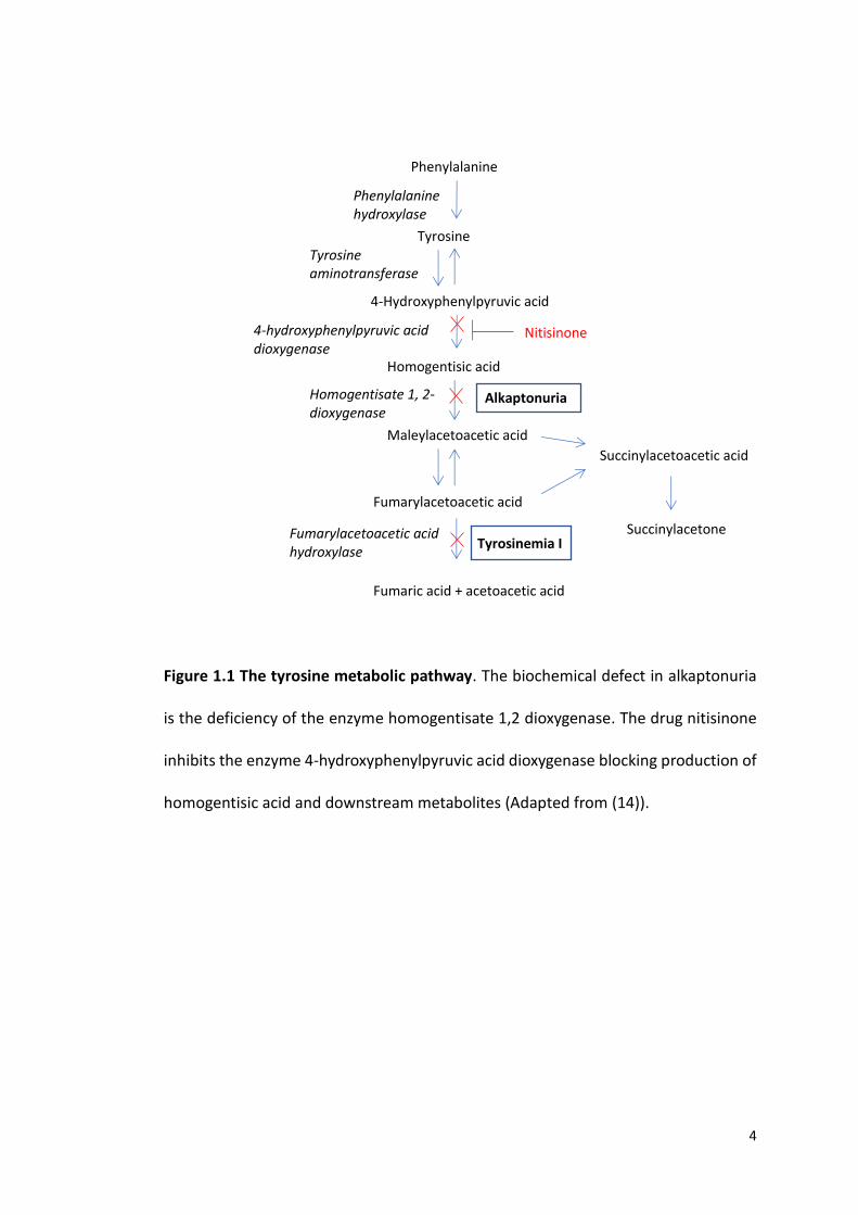
Figure 1.1 The tyrosine metabolic pathway. The biochemical defect in alkaptonuria

is the deficiency of the enzyme homogentisate 1,2 dioxygenase. The drug nitisinone

inhibits the enzyme 4-hydroxyphenylpyruvic acid dioxygenase blocking production of

homogentisic acid and downstream metabolites (Adapted from (14)).

Succinylacetone

Tyrosine

4-Hydroxyphenylpyruvic acid

Homogentisic acid

Maleylacetoacetic acid

Fumarylacetoacetic acid

Fumaric acid + acetoacetic acid

Tyrosine aminotransferase

4-hydroxyphenylpyruvic acid dioxygenase

Nitisinone

Homogentisate 1, 2-dioxygenase

Alkaptonuria

Fumarylacetoacetic acid hydroxylase

Tyrosinemia I

Succinylacetoacetic acid

Phenylalanine

Phenylalanine hydroxylase

5

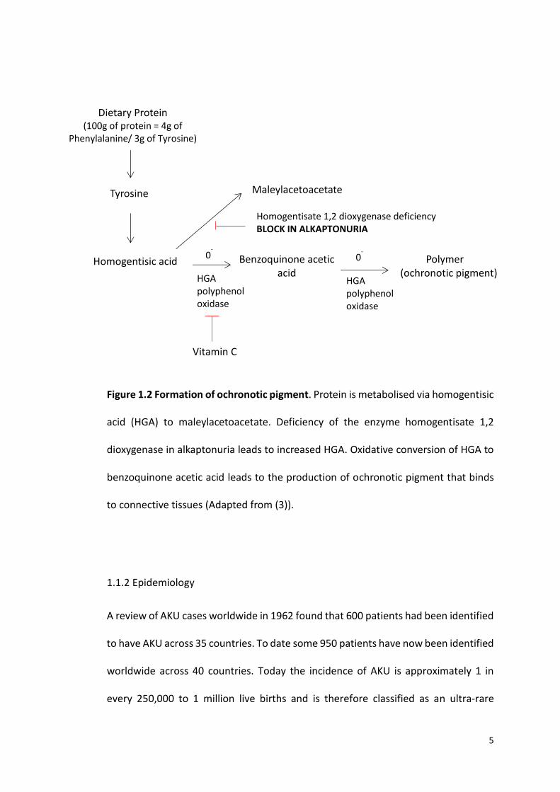
Figure 1.2 Formation of ochronotic pigment. Protein is metabolised via homogentisic

acid (HGA) to maleylacetoacetate. Deficiency of the enzyme homogentisate 1,2

dioxygenase in alkaptonuria leads to increased HGA. Oxidative conversion of HGA to

benzoquinone acetic acid leads to the production of ochronotic pigment that binds

to connective tissues (Adapted from (3)).

1.1.2 Epidemiology

A review of AKU cases worldwide in 1962 found that 600 patients had been identified

to have AKU across 35 countries. To date some 950 patients have now been identified

worldwide across 40 countries. Today the incidence of AKU is approximately 1 in

every 250,000 to 1 million live births and is therefore classified as an ultra-rare

Polymer (ochronotic pigment)

Dietary Protein (100g of protein = 4g of

Phenylalanine/ 3g of Tyrosine)

Tyrosine

Homogentisic acid

Maleylacetoacetate

Homogentisate 1,2 dioxygenase deficiency BLOCK IN ALKAPTONURIA

Benzoquinone acetic acid HGA

polyphenol oxidase

HGA polyphenol oxidase

0- 0

-

Vitamin C

6

disease (8,9). Hotspots have been identified in Slovakia, Dominican Republic, Jordan

and India, with the highest incidences found in the North-West region of Slovakia

reaching greater than 1:20,000. A possible reason for this is genetic isolation and the

founder effect (loss of genetic variation) due to living in isolated hamlets (15). Also

consanguineous marriages may explain the increased incidence in countries such as

Jordan and India (8,13,16). The reason for this can be explained by the offspring of a

consanguineous marriage receiving two defective gene copies derived from a

common ancestor (17). High numbers of novel mutations of the HGD gene have been

identified in Slovakia and Jordan demonstrating the high incidence of the disease in

these countries (18). Research suggests that reporting of new cases of AKU has

increased due to the increased awareness of the features of the disease. However,

the number of cases worldwide is much less than what we might expect based on the

incidence (8).

1.1.3 Genetic defect

AKU arises due to a genetic deficiency of the enzyme HGD. HGD converts HGA into

maleylacetoacetate and has a major role in the catabolism of tyrosine and

phenylalanine (Figure 1.1). Fernandez-Canon et al., 1996 (19) identified that the

enzymatic loss in AKU is caused by mutations within the HGD gene. The human HGD

gene is a single copy gene, spanning 54,363 bp of genomic sequence and is mapped

to chromosome 3q13.33 (1). The HGD transcript is split into 14 exons ranging from

35 – 360 bp that encodes the HGD protein (20,21). The crystalline structure of the

HGD protein has been resolved and the protein is composed of 445 amino acids that

7

forms a dimer of trimers giving rise to a functional hexamer (22). Northern blot

hybridisation shows expression of HGD in the liver, prostate, small intestine, colon

and kidney. The first human HGD mutations were described by Fernandez-Canon (19)

in Spanish AKU families and were found to have missense mutations. To date 149

different HGD variants have been identified, of which 116 are mutations and 33 are

polymorphisms (23). The mutations are spread throughout the entire gene with some

prevalence in exons 3,6,7,8 and 13. Missense mutations are the most common

followed by splicing, frameshift, nonsense, deletions and expansion. It has been

identified that some mutations are spread throughout the world and some are

specific to certain countries where there are hotspots of AKU e.g. Slovakia, India and

Jordan (20). There is currently no genotype-phenotype correlation due to the

complex hexameric structure of the enzyme.

1.1.4 Homogentisic acid

HGA is a small water-soluble molecule. It is an intermediate in the catabolism of

tyrosine and phenylalanine (Figure 1.1). HGA is usually broken down by HGD into

maleylacetoacetic acid in the liver, however in AKU the enzymatic deficiency of HGD

results in a build-up of HGA. Upon oxidation (addition of NaOH or in the presence of

O2) HGA forms the highly reactive benzoquinone acetic acid (BQA). BQA polymerises

to form the pigmented polymer termed ochronosis (24). HGA has also been found to

be present in a bacterial plant pathogen as well as in yeast of which it has been

associated with the production of brown pigment and has been identified as a

precursor of melanin synthesis (25).

8

1.1.5 Clinical Presentation

AKU is characterised by three distinct features; homogentisic acidurea, ochronosis

and ochronotic osteoarthropathy and tissue damage. The first feature to be detected

from birth is the high concentrations of HGA in urine. HGA oxidises in air (or

alkalinisation) and turns black. This feature is pathognomonic to AKU and leads to

21% of patients being diagnosed with the condition before the age of 1 (8). However,

darkening may not occur for several hours so this often goes unnoticed by the patient

(26). Chromatographic testing of urine samples for the presence of HGA is the gold

standard for diagnosis. Plasma HGA concentrations in AKU patients ranges from

0.018 – 0.165mM, compared to 0.014 – 0.071µM in the non AKU patient. Additionally

genetic testing would determine if the patient was homozygous or compound

heterozygous for the condition (1,8). The reason urine turns black in AKU is a result

of oxidative conversion of the excess HGA to benzoquinone acetic acid, and this in

turn forms a melanin like polymer that results in the urine slowly turning black (Figure

1.2). The HGA that is not excreted undergoes oxidation and polymerisation in

connective tissues of skeletal, cardiovascular and ocular systems, leading to a

pathological blue-black discolouration termed ochronosis (7).

Black pigmentation of the sclera and the pinna of the ear are two of the most obvious

features externally, however these features are not commonly seen before age 25-

30. Pigmentation of the ear and eyes has been reported in 70% and 50% of AKU

patients respectively. Pigmentation of bodily fluids including perspiration leads to the

discolouration of skin. Discolouration of the hands, nose and gums has also been

documented (7,8). Continued polymerisation of HGA in tissues, specifically cartilage

9

over time, leads to rapid early onset osteoarthropathy around the third to fourth

decade of life.

Ochronotic arthropathy primarily affects the axial and weight bearing joints. Both

synovial and intervertebral joints are affected. The first clinical symptom often starts

in the spine as lower back pain (17). In a study of 163 cases of AKU, the spine was

found to be involved in 159 patients compared to much lower frequencies of

involvement found in the knee and hip (27). Radiological observations of the spine

include wafer-like disc calcification, IVD space narrowing with vacuum phenomenon

(radiolucent collection of gas), osteophyte formation and in most severe cases fusion

of vertebrae (17,26). Symptoms worsen from the fourth decade and include

progressive kyphoscoliosis and impaired spinal mobility. This has been shown to

cause secondary effects on pulmonary inflation, disc herniation and cord

compression (1).

Involvement of the large weight bearing joints usually occurs several years after the

spinal changes. The knees, hips and shoulders are most frequently involved with

relative sparing of the small joints of the hands and feet in most cases (28).

Radiographic observations of the large peripheral joints are similar to that of

osteoarthritis (OA) including, joint space narrowing, subchondral bone (SB) sclerosis

and osteophytosis, and as a result AKU is often misdiagnosed as OA (17). Ochronotic

arthropathy is crippling and inevitably leads to the patient requiring multiple joint

replacements. By the age of 55, 50% of AKU patients have undergone at least one

joint replacement (29).

10

AKU is often diagnosed intraoperatively when a blackened joint is exposed (30).

Autopsy results from a 74-year-old female with AKU who died of disseminated

ovarian cancer revealed extensive osteoarthropathy. The patient had undergone

surgery to replace both knee joints, both hip joints and the left shoulder joint and had

OA of both ankles and the right shoulder. Thoracic scoliosis and lumbar lordosis was

evident and marked pigmentation on the annulus fibrosus of the IVDs was observed

with bony bridging between vertebral bodies. OA of the shoulder was identified with

extensive bony exposure and a narrow rim of pigmented cartilage and debris present

(31). In AKU the pigmented tissues often become weak and brittle and are susceptible

to chipping and splintering hence the pigmented debris present at autopsy. This

process results in rapid joint deterioration coupled with inflammatory processes in

some cases (17).

Apart from joint damage other manifestations of AKU include renal, salivary gland,

prostate and gall bladder stones. Ligament and tendon calcification and ruptures

have also been documented (8). Osteopenia and fractures are less common but have

been documented. Fisher et al. (4) documented a case of a 69 year old AKU patient

presenting with a low trauma fracture of the distal femur, and distal radius. She had

no other contributing risk factors that may have predisposed her to fractures such as

vitamin D deficiency, osteoporosis or history of osteoporotic fractures. Bone changes

are thought to be less common in frequency and severity than cartilage changes. This

is thought to be due to the remodelling properties of bone limiting the ability to

reduce the cross linking of the collagen fibrils that result in connective tissue failure

(4).

11

The cardiac manifestations of AKU are not un-common. Many studies have

documented pigmentation associated with the cardiac valves and atherosclerotic

plaques. At autopsy Helliwell et al. (31) found prominent pigmentation of the mitral

valve as well as calcification and mild fusion of the aortic valve therefore AKU is a

predisposing factor for valve calcification, stenosis and regurgitation. Patients with

AKU exhibit a high frequency of aortic valve involvement acquiring this condition in

the seventh to eighth decade of life. The aortic sinus region also contained

pronounced pigmentation. Interestingly no pigmentation was observed in the venous

components of circulation and the tricuspid valve and the pulmonary valve showed

minimal pigmentation. It was proposed that pigmentation of the aortic and mitral

valves as well as the carotid sinus region is due to the high blood pressure and

turbulent blood flow that is associated with those structures and that deposition of

pigment may be linked to areas of high blood pressure and other haemodynamic

factors. It is still unclear whether the pigment alone causes increased stiffening of the

valve or whether it is a result of pigment related damage to the collagen fibres.

Echocardiographic screening is recommended for all AKU patients (32). Currently

there is no effective licenced therapy to treat AKU. Joint replacements and pain relief

are offered to help ease the pain but do not combat the cause.

1.1.6 The Initiation of ochronotic pigmentation (the exposed collagen hypothesis)

The pathogenesis of ochronosis is still not fully understood and it wasn’t until recently

that possible mechanisms to explain the initiation of pigmentation were elucidated.

In 2009 Taylor et al. (33,34) described the relationship between HGA and fibrillar

12

collagen suggesting there was a binding site for HGA on collagen. Taylor et al.

identified that pigmentation is initiated in the pericellular matrix surrounding

chondrons of the articular calcified cartilage. Further studies revealed that tissues are

initially resistant to pigmentation but become susceptible following mechanical or

biochemical damage to the extracellular matrix such as repetitive mechanical

loading, chemical attack and ageing (35). It is proposed that the collagen fibre has

sites which HGA can bind to, however these are protected in healthy collagen by

proteoglycans (Figure 1.4). Following mechanical or biochemical damage,

proteoglycans are lost, and these binding sites become exposed and available for

HGA to attach. The initial binding of HGA is comparable to a nucleation event; once

HGA has bound there is rapid deposition of HGA as an ochronotic polymer. Binding

of HGA to collagen results in stiffening of the fibre leading to further mechanical

damage. This process results in progressive ochronosis (Figure 1.4) (13). This process

is thought to be as a result of ageing and is thought to occur in non-AKU connective

tissues also.

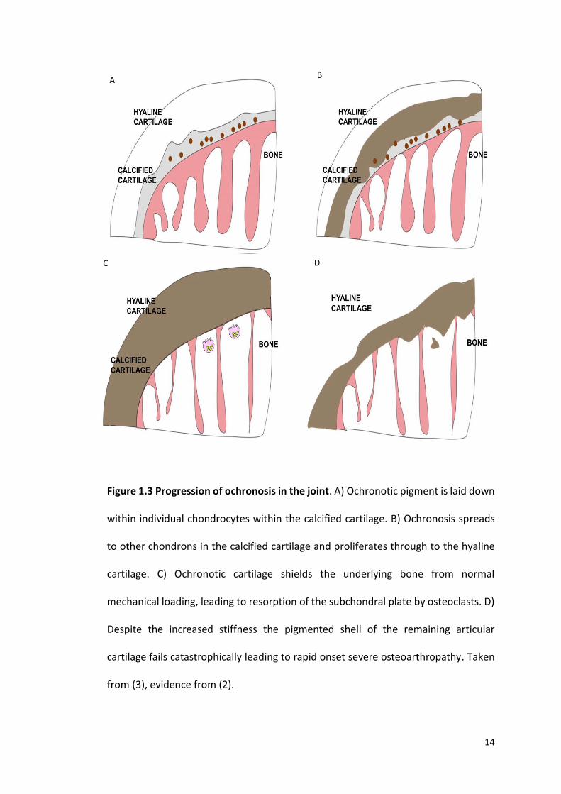
1.1.7 Pathogenesis of Joint Destruction

Initial pigmentation is laid down in individual chondrocytes and their territorial matrix

within the calcified cartilage. Pigmentation spreads to other chondrons within the

calcified cartilage and proliferates through the hyaline cartilage. Pigmented hyaline

cartilage becomes stiff and shields the underlying bone from normal mechanical

loading leading to aggressive resorption of the subchondral plate by osteoclasts

resulting in degeneration of the joint (Figure 1.3) (13,35,36).

13

1.1.8 Diagnosis

Currently, the diagnosis of AKU is based on the detection of a significant amount of

HGA in a urine sample by gas chromatography-mass spectrometry analysis. The

amount of HGA excreted per day in urine in individuals with alkaptonuria is usually

between 1-8 g compared to 20-30 mg in an individual without AKU. Genetic testing

is required to determine if the individual is homozygous or compound heterozygous.

Identification of biallelic pathogenic variants confirms the diagnosis and allows family

studies and counselling (1,37).

Once the HGD pathogenic variants have been identified in an alkaptonuric family

member, prenatal testing and preimplantation genetic diagnosis for a pregnancy at

increased risk for the disease are optional (37).

https://www.ncbi.nlm.nih.gov/books/n/gene/glossary/def-item/preimplantation-genetic-diagnosis/

14

Figure 1.3 Progression of ochronosis in the joint. A) Ochronotic pigment is laid down

within individual chondrocytes within the calcified cartilage. B) Ochronosis spreads

to other chondrons in the calcified cartilage and proliferates through to the hyaline

cartilage. C) Ochronotic cartilage shields the underlying bone from normal

mechanical loading, leading to resorption of the subchondral plate by osteoclasts. D)

Despite the increased stiffness the pigmented shell of the remaining articular

cartilage fails catastrophically leading to rapid onset severe osteoarthropathy. Taken

from (3), evidence from (2).

A B

C D

15

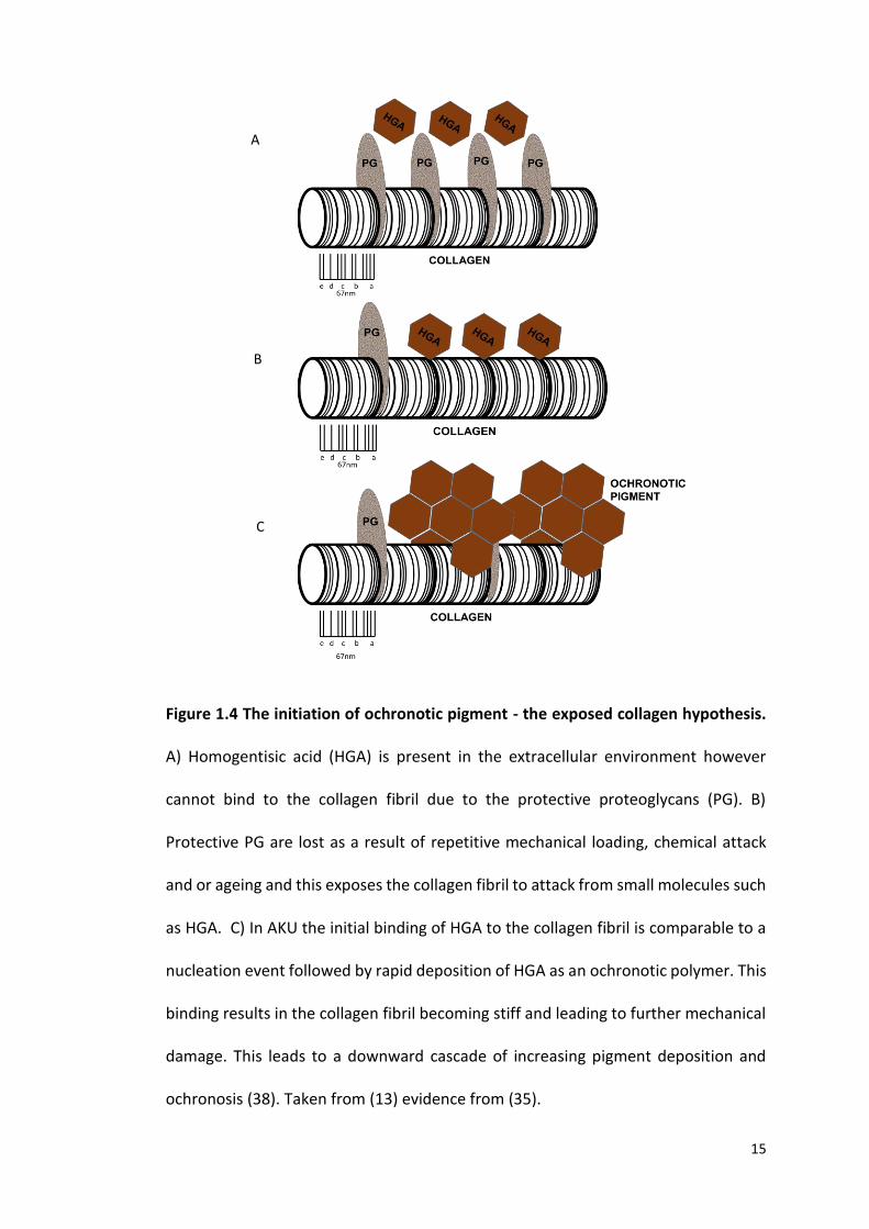
Figure 1.4 The initiation of ochronotic pigment - the exposed collagen hypothesis.

A) Homogentisic acid (HGA) is present in the extracellular environment however

cannot bind to the collagen fibril due to the protective proteoglycans (PG). B)

Protective PG are lost as a result of repetitive mechanical loading, chemical attack

and or ageing and this exposes the collagen fibril to attack from small molecules such

as HGA. C) In AKU the initial binding of HGA to the collagen fibril is comparable to a

nucleation event followed by rapid deposition of HGA as an ochronotic polymer. This

binding results in the collagen fibril becoming stiff and leading to further mechanical

damage. This leads to a downward cascade of increasing pigment deposition and

ochronosis (38). Taken from (13) evidence from (35).

A

B

C

16

1.1.9 Therapy

Several therapeutic approaches have been tried to treat AKU with little effect.

Currently there is no effectively therapy licenced to treat AKU. The only available

treatments focus on reducing the symptoms, and do not tackle the intrinsic cause (1).

Palliative management of AKU includes joint replacement therapy, physiotherapy

and pain management (8). Table 1.1 summarises all the therapies that have been

tried in AKU.

1.1.9.1 Vitamin C

Vitamin C was first used to treat AKU in 1940 by Sealock et al. (39). He reported that

Vitamin C therapy delayed the darkening of urine presumably by preventing the

oxidation of HGA. Studies have shown that Vitamin C acts by blocking the conversion

of HGA to benzoquinone acetic acid (BQA) by inhibiting the enzyme HGA polyphenol

oxidase (Figure 1.2) [8]. BQA is an intermediary product in the formation of

ochronotic pigment, therefore the hypothesis was that preventing the oxidative

conversion of HGA to BQA would prevent ochronosis. Wolff et al. (40) reported that

the administration of relatively large amounts of Vitamin C resulted in the

disappearance of BQA in the urine. However, it did not change the amount of HGA

excreted. It was also found that HGA concentration doubled after administration of

Vitamin C in young infants and the authors proposed that this was due to activation

of the enzyme hydroxyphenylpyruvate dioxygenase (HPPD) that converts 4-

hydroxyphenylpyruvic acid (HPPA) to HGA (Figure 1.1) (40). Other studies found that

Vitamin C caused HGA production to increase, contributing to the production of renal

17

oxalate stones, increasing their risk of developing these further. This evidence

confirms that Vitamin C is not an effective treatment in AKU.

1.1.9.2 Low Protein Diet

Reducing dietary intake of protein seems the most logical form of treatment. By

reducing dietary intake of phenylalanine and tyrosine this will reduce the amount of

HGA produced, therefore reducing ochronosis. Haas et al. (41) from the Netherlands

found a significant decrease in the excretion of HGA with a low protein diet of 1 g/kg

per day however this was age dependant. They found that children below the age of

twelve had reduced HGA production but above the age of twelve there was no effect.

They concluded that protein restriction in older patients is probably useless but

restriction should be advised in younger patients. This would require strict specialist

supervision during growth periods to ensure adequate levels of essential amino acids,

vitamins and minerals are available for growth (1). Another report from the

Netherlands described reduced joint pain after receiving a low protein diet in children

(42). Other studies also reported no change in HGA excretion with protein restriction

(9). Approximately only 6% of dietary protein is degraded via HGA, however, nearly

all HGA is produced by dietary intake of protein. Additionally reducing dietary protein

is very hard to comply with long term and it appears small reductions in protein intake

do not have a noticeable effect (1). It was concluded that restricting protein intake

was not the most appropriate treatment option.

18

1.1.9.3 Nitisinone

Nitisinone, 2-(2-nitro-4-trifluromethylbenzoyl)cyclohexane-1,3-dione (NTBC), a very

effective herbicide, is a potential disease modifying therapy for AKU. Nitisinone acts

by inhibiting the enzyme HPPD (HPPD coverts HPPA into HGA), therefore blocking the

production of the culprit HGA (Figure 1.1). It is administered orally and has high

affinity for HPPD in the liver (1). Nitisinone has been used since 1992 for the rare

disease tyrosinemia type 1 (HT1) and has proven to be well tolerated long and short

term. Nitisinone operates several steps before the defect in HT1 and the dosage given

is 1-2mg/kg body weight. Nitisinone acts on the very reaction that causes AKU

therefore it was proposed that a lower dosage may be required. An early study

revealed the dose to treat AKU was 30-fold lower than that used to treat HT1 (43).

Current experience with nitisinone in AKU is limited. Suwannarat et al. (14) at the NIH

investigated the safety and efficacy of nitisinone in a study of 9 AKU patients over a

period of 4 months. A dose of 2.1mg was given, and this was shown to decrease

urinary HGA concentrations by 95% (from an average of 4.0 to 0.2g/day) and increase

plasma tyrosine levels 11-fold (from 68 µmol/L to 760 µmol/L). The tyrosinemia did

not cause any corneal toxicity, and six out of seven patients that received nitisinone

reported decreased pain in their joints (14).

In a second study Introne et al. (44) conducted a three year randomised therapeutic

NIH trial of nitisinone (2.1mg/day) on 40 AKU patients. Nitisinone was shown to

reduce mean urinary HGA by 98% (from 5.1 to 0.125 g/day). Mean plasma HGA levels

reduced by 95% from 5.74 to 0.306 mg/l. Hip rotation was used as the defining

parameter to determine the efficacy of the drug, however the results were

19

inconclusive from a rheumatological aspect (44). Ranganath et al. (45) suggested one

possible reason for this could be that an optimal dose was not used. Ranganath and

his team conducted a dose response study to investigate the effect of nitisinone on

urinary HGA (SONIA 1). The study had 5 groups of patients each containing 8 patients

and the 5 dosages were 0,1,2,4, and 8mg. A clear dose-response relationship was

observed at 4 weeks, the adjusted geometric mean u-HGA in 24 hours was

31.53mmol, 3.26mmol, 1.44mmol, 0.57mmol for the 1mg, 2mg, 4mg and 8mg doses,

respectively. The 8mg dose daily was most effective, corresponding to a mean

reduction of u-HGA of 98.8% compared with baseline. No safety concerns were

reported in this short study, however the long-term safety and efficacy of the drug is

not fully understood so a 2mg dose is what is usually prescribed in clinic today (45).

Life-long therapy is required to maintain reduced levels of HGA. The

pathophysiological and clinical significance of tyrosinemia is not fully understood,

however it can cause corneal irritation as well as other serious side effects such as

thrombocytopenia, leukopenia and porphyria which are associated with neurological

complications such as tremor, ataxia, delayed development and intellectual

impairment (8).

1.1.9.4 Other treatments

A variety of options are available to treat AKU and these are summarised in Table 1.1.

Lifestyle counselling can be beneficial. Siblings with the same mutation and gender

can have very different symptoms. Assessing lifestyle choices can have a positive

impact on symptoms. Minimising joint loading in all areas of life is likely to be

20

important. Physiotherapy is used to increase joint motion and activity. Pain control is

vital but often is only partially effective. A wide variety of drugs are prescribed to

tackle the pain such as paracetamol, non-steroidal anti-inflammatories, opioids,

anticonvulsants, local anaesthetics and gabapentin. Physical modalities are also used

such as acupuncture, nerve blocks and trans-cutaneous nerve stimulation. Organ

transplantation has been associated with resolving AKU however it is not justified in

a disease where longevity is rarely affected. Multiple joint replacement therapy and

spinal surgery are inevitable and are often required multiple times throughout life

(1).

Nitisinone is most effective in reducing the causative agent however it is imperfect

because it is acting as a metabolic block and therefore causes secondary effects on

tyrosine levels. A perfect treatment would involve replacing the missing enzyme by

utilising gene or enzyme replacement therapy. This would result in decreasing HGA

without affecting the rest of the tyrosine metabolic pathway. However, there are

potentially fatal complications with this therapy. The HGD enzyme would have to be

delivered to the exact location of tyrosine metabolism within the hepatocytes of the

liver to be successful. If the HGD enzyme was present in the blood and the

extracellular fluid this would result in succinylacetone to spontaneously form from

maleylacetoacetate and fumarylacetoacetate (Figure 1.1). These products are toxic

and highly mutagenic resulting in serious complications as the enzymes required to

break these products down would not be present unlike in the liver (8).

21

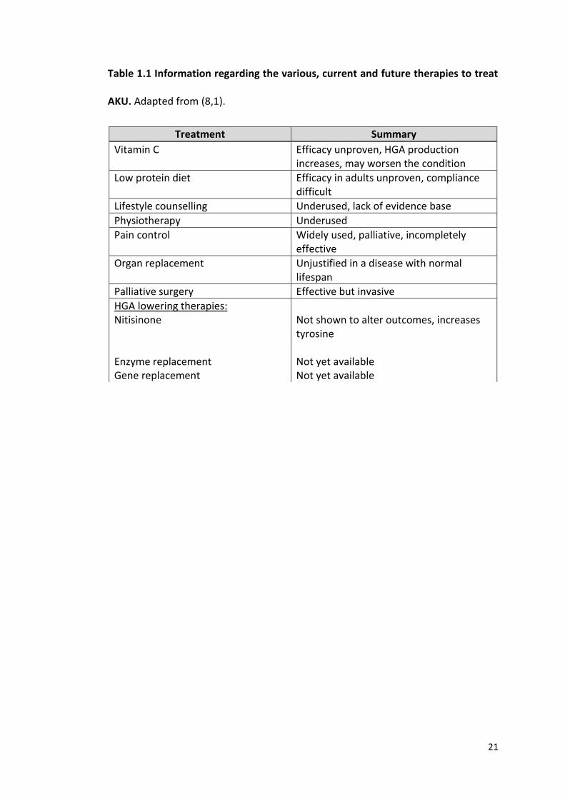
Table 1.1 Information regarding the various, current and future therapies to treat

AKU. Adapted from (8,1).

Treatment Summary

Vitamin C Efficacy unproven, HGA production increases, may worsen the condition

Low protein diet Efficacy in adults unproven, compliance difficult

Lifestyle counselling Underused, lack of evidence base

Physiotherapy Underused

Pain control Widely used, palliative, incompletely effective

Organ replacement Unjustified in a disease with normal lifespan

Palliative surgery Effective but invasive

HGA lowering therapies: Nitisinone Enzyme replacement Gene replacement

Not shown to alter outcomes, increases tyrosine Not yet available Not yet available

22

1.1.10 Assessment

AKU is present from birth however these patients experience an asymptomatic pre-

ochronotic phase from birth up until around the third decade of life. This delay in

ochronotic deposition is still not fully understood. A major difficulty in clinical

research is the lack of suitable quantifiable methodology to describe disease severity

(46). Until recently, most descriptions of AKU were qualitative and there was no

methodology to quantify the disease, or to define an objective measure of disease

severity. Without an appropriate method to quantify the disease, clinicians were

unable to make comparisons of disease severity between patients. This issue has

been rectified recently with the introduction of the AKU severity score index

(AKUSSI). This score is based on a quantitative, validated, multidisciplinary

assessment that can be used for patient assessment in the AKU clinical trials (1).

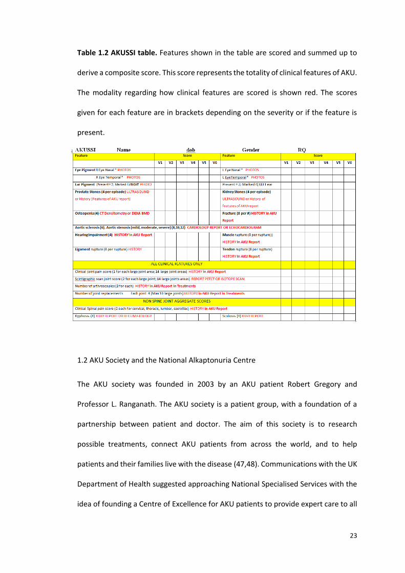
The AKUSSI quantifies the clinical features of AKU systematically in a standardised

manner. Table 1.2 is the AKUSSI which represents the clinical features that are scored

and summed to derive a composite score. The features of AKU are broken down into

three categories, features due to excess circulating HGA (prostate, kidney, salivary

and gall stones), features due to ochronosis (ear/eye pigmentation, teeth and skin

pigment, osteopenia, ENT features and cardiac valve disease) and features due to

damage of connective tissue (fractures, tendon/ligament/muscle ruptures, as well as

spinal and joint disease). The early appearing features were scored lower and the

latter appearing features were scored higher (46). A questionnaire based severity

score index, has also been described and is easy to use and could be used at any

hospital around the world.

23

Table 1.2 AKUSSI table. Features shown in the table are scored and summed up to

derive a composite score. This score represents the totality of clinical features of AKU.

The modality regarding how clinical features are scored is shown red. The scores

given for each feature are in brackets depending on the severity or if the feature is

present.

1.2 AKU Society and the National Alkaptonuria Centre

The AKU society was founded in 2003 by an AKU patient Robert Gregory and

Professor L. Ranganath. The AKU society is a patient group, with a foundation of a

partnership between patient and doctor. The aim of this society is to research

possible treatments, connect AKU patients from across the world, and to help

patients and their families live with the disease (47,48). Communications with the UK

Department of Health suggested approaching National Specialised Services with the

idea of founding a Centre of Excellence for AKU patients to provide expert care to all

24

patients with AKU. In 2012 the Robert Gregory National Alkaptonuria Centre (NAC),

was established by the NHS Highly Specialised Services Commissioning Group at the

Royal Liverpool University Hospital. The NAC delivers expert care and advice from

leading experts in the field. The NAC provides off-label nitisinone to patients who

receive annual check-ups and follow up blood, and urine tests post nitisinone.

Patients confirmed with alkaptonuria are commenced on 2 mg dose of nitisinone that

they take on alternative days, for three months with daily dose thereafter.

Monitoring and clinical assessments are performed annually. Currently 58 patients

with AKU have been enrolled at the NAC for treatment with nitisinone. Twenty-three

females (mean age 53 years, range 22-75) and 35 males (mean age 48 years, range

22-70). The NAC is an on-going service that is transforming the lives of AKU patients

through patient support, community building and medical research (47,48).

1.3 DevelopAKUre

Research into the use of nitisinone in AKU started in the 1990’s however, the results

were underpowered and were not statistically significant. A goal for the AKU society

was to further investigate the efficacy of nitisinone (48). In 2012 a series of

international clinical trials was founded called the DevelopAKUre consortium with

Sobi (the pharmaceutical company with the licence for nitisinone) (49). The

DevelopAKUre consortium is coordinated by Professor L. Ranganath, at the Royal

Liverpool University Hospital. Two other clinical sites are involved outside of the UK;

The National Institute of Rheumatic Disease, Piestany, Slovakia and Hospital Necker

and Institute Necker in France. The objective is to study the efficacy and safety of

nitisinone to obtain marketing authorisation for the treatment of AKU. The duration

25

of DevelopAKUre is approximately 75 months, and is due to conclude in 2019 (49). If

nitisinone is proven to be effective in AKU, the consortium will apply for marketing

authorisation and approval of Nitisonone by the European Medicines Agency.

DevelopAKUre involves three studies, a dose response study called ‘Suitability of

Nitisinone in Alkaptonuria 1’ (SONIA 1), an efficacy study called ‘Suitability of

Nitisinone in Alkaptonuria 2 (SONIA 2) and a cross sectional study called ‘Sub-clinical

Ochronotic Features in Alkaptonuria (SOFIA) (49).

1.3.1 Suitability of Nitisnone in Alkaptonuria 1 (SONIA 1)

This study was designed to identify the most appropriate dose of nitisinone to be

used over a patient’s lifetime, as well as the most effective dose in reducing HGA

levels. Forty patients were recruited for the trial and were split up into five age

dependent groups of eight. Each group received varying doses of nitisinone (0mg,

1mg, 2mg, 4mg, and 8mg). SONIA 1 began in May 2013, and lasted 4 weeks (45). Two

centres were involved, the Royal Liverpool University Hospital and the National

Institute of Rheumatic Disease, Piestany. The 8mg dose showed the least variability

and was found to reduce urinary HGA levels down by on average 99.4%, as well as

reducing serum HGA to undetectable levels in 7/8 patients (45,50).

26

1.3.2 Suitability of Nitisinone in Alkaptonuria 2 (SONIA 2)

This study is designed to test whether nitisinone slows down the progression of the

disease in AKU. SONIA 2 commenced in 2014 and is expected to finish in 2019. 138

patients were enrolled and were randomly divided into two equal groups of 69. One

group receives nitisinone (10mg/day) and the other group does not. This trial is based

across three clinical sites in Liverpool, Piestany and Paris. Patients attend their

allocated test centre a total of six times, each visit lasting up to 4 days. SONIA 2 aims

to elucidate the impact of nitisinone on HGA levels in the body over a period of 4

years; this will define whether nitisinone has a positive impact on HGA levels and

whether it is safe long term. If nitisinone is proven to be beneficial in the treatment

of AKU the DevelopAKUre consortium will apply for a drug license for AKU (49,50).

1.3.3 Subclinical Ochronotic Features in Alkaptonuria (SOFIA)

This study is an observational cross-sectional study that commenced early 2017.

SOFIA is designed to investigate the onset of ochronosis and to define the best time

to begin treatment with nitisinone. Thirty patients (15 males, 15 females) were

recruited for SOFIA from a range of ages. They were split into 8 age groups (16-20,

21-25, 26-30, 31-35, 36-40, 41-45, 45-50, 50+) with 4 patients in each group (2 males,

2 females). This trial will involve study patients visiting the clinical site in Liverpool for

three days where a series of tests will be performed including urine tests, blood tests,

MRI scan, ear cartilage biopsy and gait analysis. All samples will be analysed for

ochronosis, and will be compared with 30 healthy volunteers without AKU (49,50).

27

1.4 Cartilage

Cartilage is an avascular, flexible connective tissue found throughout the body,

providing support to adjacent tissues. Cartilage is devoid of blood vessels, lymphatics

and nerves; it therefore derives oxygen and nutrients via diffusion. This results in

cartilage having a limited capacity to repair (51). Cartilage is composed of

chondrocytes, embedded within an extracellular matrix. Chondrocytes maintain and

regulate the turnover of extracellular matrix (52). There are three different types of

cartilage in the body, hyaline cartilage, fibrocartilage and elastic cartilage. These

three types differ slightly in term of the structure and function (53). Hyaline cartilage

is the most abundant type. It is found at the ventral ends of the ribs, the tracheal

rings, larynx and bronchi and it also forms the articular surfaces of long bones

(articular cartilage). Hyaline cartilage matrix consists of type II collagen and the

glycosaminoglycan chondroitin sulphate and is covered externally by perichondrium,

a fibrous membrane that contains vessels that provide oxygen and nutrition (except

articular cartilage) (53). Fibrocartilage contains abundant collagen and fibrous tissue.

Fibrocartilage is distinct in that it contains Type I and Type II collagen. Type I collagen

provides considerable tensile strength and the ability to resist compressive forces,

therefore fibrocartilage is found in regions requiring these properties such as the

annulus fibrosus of the intervertebral discs, pubic symphysis, menisci of the knee and

the temporomandibular articular disc. Lastly, elastic cartilage histologically looks

similar to hyaline cartilage in that it contains type II collagen and chondroitin

sulphate, however it also contains many elastic fibres that lie in a solid matrix,

providing this type of cartilage with great flexibility that can withstand repeated

bending. Elastic cartilage can be found in the pinna of the ear and the epiglottis (53).

28

1.4.1 Articular Cartilage Structure

Articular cartilage (AC) is highly specialised hyaline cartilage of diarthrodial joints. It

functions to provide a smooth, lubricated surface for articulation, and to facilitate

load transmission through the joint. Typically, AC is 2-5mm thick, and is completely

avascular, aneural and is devoid of lymphatic drainage. AC is composed of

chondrocytes embedded in a dense extracellular matrix (ECM) of water, collagen and

proteoglycans and has a layered, organised structure (54). Morphologically AC is

organised into four zones (Figure 1.5); the uppermost layer is the superficial

(tangential) zone, immediately deep to this layer is the middle (transitional) zone,

followed by the deep zone and calicifed zone. The superficial, middle and deep layers

are un-mineralised and often referred to as the hyaline articular cartilage (HAC). The

calcified zone is mineralised and is often referred to as the articular calcified cartilage

(ACC) (52). AC provides an extremely smooth, firm yet deformable layer that

increases contact area between bones and therefore reduces contact stress.

29

1.4.1.1 Superficial zone

The thin superficial zone acts to protect the deeper layers, and provides a gliding

surface for articulation. The superficial zone makes up 10% to 20% of the overall HAC

thickness. The collagen fibres (mainly collagen type II and IX) are packed tightly and

arranged parallel to the articular surface (54). The chondrocytes are flattened and

relatively high in number and express lubricin (essential for lubrication). This layer is

in contact with the synovial fluid, and acts to resist shear, tensile and compressive

forces. The integrity of this layer is paramount for the protection of the deeper layers,

and is often the first layer to show changes in OA (Figure 1.5) (51).

1.4.1.2 Middle Zone

The middle zone provides an anatomical and functional bridge between the

superficial and deep zones and represents approximately 40-60% of the overall HAC

thickness. It contains obliquely orientated collagen fibrils and low density spherical

chondrocytes embedded in dense ECM that is rich in proteoglycans such as aggrecan

(54). The middle zone functions to resist compressive forces and transfers them from

the superficial zone to the deeper zones (Figure 1.5) (52).

1.4.1.3 Deep Zone

The deep zone represents approximately 30% of the overall HAC volume, and

contains the highest number of proteoglycans and the largest diameter of collagen

fibrils. It therefore, functions to provide the greatest resistance to compressive

forces. The collagen fibrils and spherical chondrocytes are arranged in vertical

columns perpendicular to the joint surface. Cellular density is lowest in the deep zone

30

(approximately 1/3 the density of the superficial layer) however it contains the

largest amount of aggrecan (Figure 1.5) (52,54).

1.4.1.4 Calcified zone

The calcified zone, also known as the ACC plays an integral role in securing the

cartilage to bone by anchoring the collagen fibrils of the deep zone to the SB. The

basophilic tidemark distinguishes the deep zone from the ACC. The cell population is

scarce and the chondrocytes are hypertrophic and synthesise type X collagen that

calcifies the surrounding matrix. Calcification of the matrix provides structural

integrity important for shock absorption (51,54). The SB is located beneath the ACC

and includes the subchondral plate (comprises the ACC and a thin cortical bone layer)

and the underlying trabecular bone (Figure 1.5).

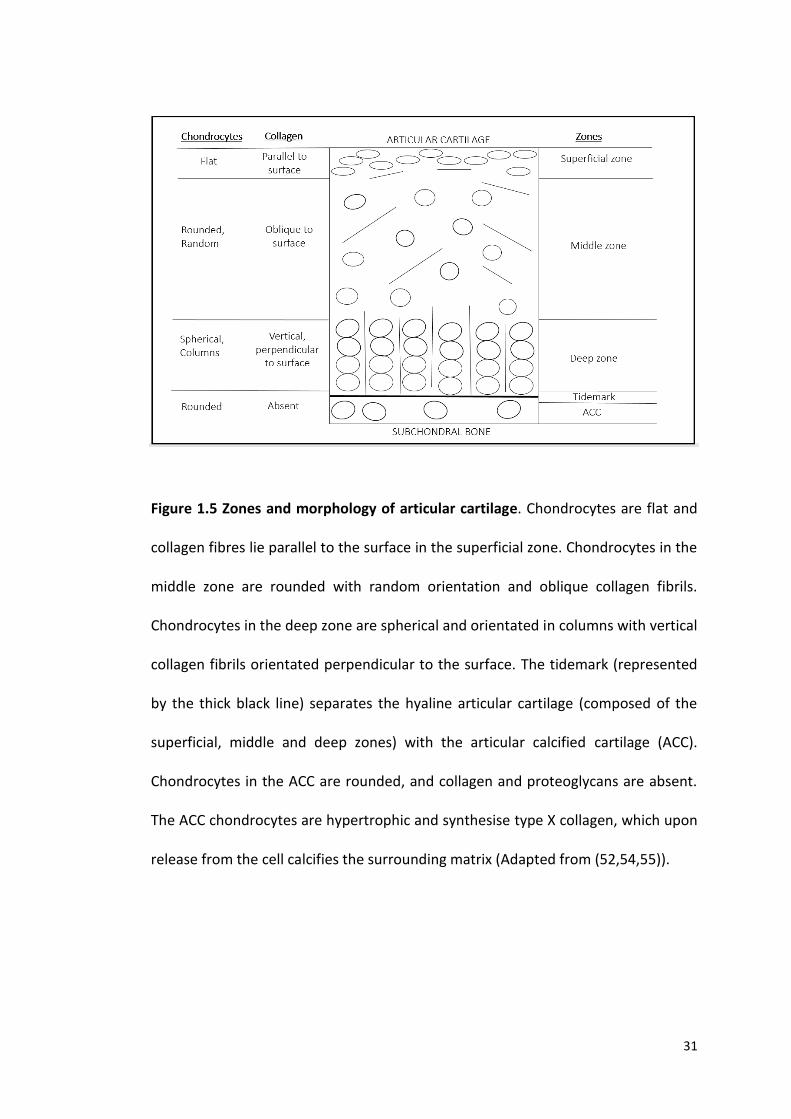
31

Figure 1.5 Zones and morphology of articular cartilage. Chondrocytes are flat and

collagen fibres lie parallel to the surface in the superficial zone. Chondrocytes in the

middle zone are rounded with random orientation and oblique collagen fibrils.

Chondrocytes in the deep zone are spherical and orientated in columns with vertical

collagen fibrils orientated perpendicular to the surface. The tidemark (represented

by the thick black line) separates the hyaline articular cartilage (composed of the

superficial, middle and deep zones) with the articular calcified cartilage (ACC).

Chondrocytes in the ACC are rounded, and collagen and proteoglycans are absent.

The ACC chondrocytes are hypertrophic and synthesise type X collagen, which upon

release from the cell calcifies the surrounding matrix (Adapted from (52,54,55)).

32

1.4.2 Extracellular matrix

As well as the zonal regions, the ECM has distinct regions based on the proximity to

the chondrocyte and collagen composition and organisation. The ECM can be divided

into the pericellular, territorial and interterritorial regions (Figure 1.6) (54). The

pericellular matrix (PCM) directly surrounds the chondrocyte and contains mainly

proteoglycans and glycoproteins. This region is thought to play a functional role in

initiation of signal transduction in response to load (56). The territorial matrix (TM)

surrounds the pericellular matrix and is composed of a network of fine collagen fibrils

that protect the chondrocytes against mechanical stresses. The interterritorial matrix

(ITM) is the largest and is characterised by abundant proteoglycans and the random

organisation of collagen fibres (Figure 1.6) (54).

AC contains between 65%-80% tissue fluid. Water is the most abundant component.

The flow of water through the ECM and across the articular surface distributes

oxygen and nutrients to the chondrocytes as well as providing lubrication (54). The

dry weight of the ECM is composed of collagen, proteoglycans and a small number of

lipids, phospholipids, non-collagenous proteins and glycoproteins (Figure 1.7).

Collagen is the most abundant structural molecule in the ECM and accounts for up to

60% of the dry weight of cartilage. Type II collagen represents approximately 90% of

the collagen within the ECM (54). Collagen types I, IV, V, VI, IX and XI are also present

but in small amounts and help to stabilise the type II collagen fibrillar network.

Collagen fibres provide tensile strength to the cartilage and provide a binding site for

proteoglycans. Proteoglycans contribute 10% - 15% of the wet weight. Proteoglycans

33

are composed of a protein core with one or more glycosaminoglycan chains

covalently attached that extend out from the core and remain separate due to the

charge repulsion. AC contains many essential proteoglycans. The largest (250,000d)

and most abundant is aggrecan. Aggrecan is highly glycosylated proteoglycan,

composed of 90% carbohydrate derived from two types of glycosaminoglycan;

chondroitin sulphate and keratin sulphate. Aggrecan interacts with hyaluronan (HA)

via link proteins to form large protein aggregates (Figure 1.7). The entrapment of

these large aggregates within the collagen matrix provides the unique mechanical

properties of cartilage (52). Chondrocytes are the only cell type responsible for

synthesising ECM as well as regulating ECM turnover, however they only represent

5% of the total volume of the cartilage (52).

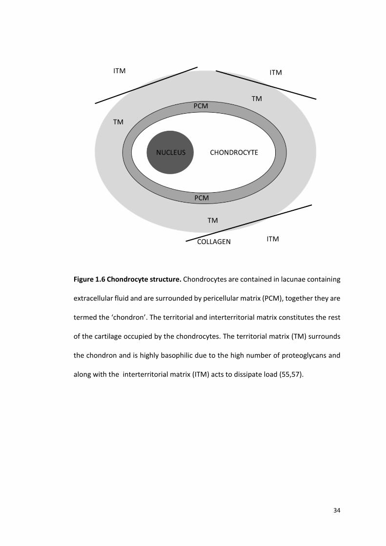
34

Figure 1.6 Chondrocyte structure. Chondrocytes are contained in lacunae containing

extracellular fluid and are surrounded by pericellular matrix (PCM), together they are

termed the ‘chondron’. The territorial and interterritorial matrix constitutes the rest

of the cartilage occupied by the chondrocytes. The territorial matrix (TM) surrounds

the chondron and is highly basophilic due to the high number of proteoglycans and

along with the interterritorial matrix (ITM) acts to dissipate load (55,57).

35

1.4.3 Chondrocytes

Chondrocytes are highly specialised, metabolically active cells found in cartilage that

function to synthesise, maintain and repair ECM. Chondrocytes constitute

approximately 2% of the total volume of AC and vary in number and size across the

various zones of AC (54). Each chondrocyte establishes a specific microenvironment

and is responsible for the turnover of ECM in its immediate vicinity. The chondrocyte

and pericellular matrix forms a functional unit called an ‘chondron’ (58). Rarely do

chondrocytes form cell-to-cell contacts for direct signal transduction, however they

are responsive to a variety of stimuli including growth factors, cytokines, mechanical

load and hydrostatic pressures (59). Under normal physiological conditions

chondrocytes maintain ECM, however when cartilage becomes damaged,

chondrocytes respond by secreting inflammatory cytokines (including interleukin 1

and tumor necrosis factor -α) that result in increased synthesis of metalloproteinases

that in turn break down ECM (60). The ageing process also influences the organisation

of chondrocytes, their response to external factors and therefore the composition of

the ECM that ultimately results in degradation of the articular surface. This results in

OA, and is accelerated by injury or disease. OA affects approximately 60% of men and

70% of women older than 65 years (52,61), and it has been forecast that 25% of the

adult population (18 years and older) will be affected by the disease by the year 2020

(62).

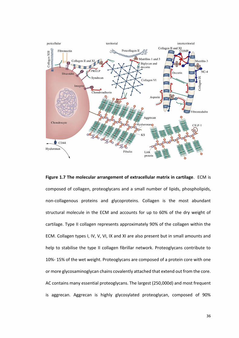
36

Figure 1.7 The molecular arrangement of extracellular matrix in cartilage. ECM is

composed of collagen, proteoglycans and a small number of lipids, phospholipids,

non-collagenous proteins and glycoproteins. Collagen is the most abundant

structural molecule in the ECM and accounts for up to 60% of the dry weight of

cartilage. Type II collagen represents approximately 90% of the collagen within the

ECM. Collagen types I, IV, V, VI, IX and XI are also present but in small amounts and

help to stabilise the type II collagen fibrillar network. Proteoglycans contribute to

10%- 15% of the wet weight. Proteoglycans are composed of a protein core with one

or more glycosaminoglycan chains covalently attached that extend out from the core.

AC contains many essential proteoglycans. The largest (250,000d) and most frequent

is aggrecan. Aggrecan is highly glycosylated proteoglycan, composed of 90%

37

carbohydrate derived from two types of glycosaminoglycan; chondroitin sulphate

and keratin sulphate (KS). Aggrecan interacts with hyaluronan via link proteins to

form large protein aggregates. The entrapment of these large aggregates within the

collagen matrix provides the unique mechanical properties of cartilage (52) (Image

taken from (63)).

1.4.4 Collagen

Collagen is the most abundant macromolecule in ECM and accounts for

approximately 60% of the dry weight of cartilage. Fifteen distinct collagen types have

been identified and despite their structural diversity all have the characteristic triple

helix, composed of three α-polypeptide chains (64). Type II collagen represents 95%

of the total collagen in the ECM, however types I, IV, V, VI, IX and XI are also present

but at much lower frequencies. Type II collagen consists of three α1(II)- polypeptide

chains containing a glycine residue every third position resulting in a ‘Gly-X-Y’ repeat,

X being proline and Y being hydroxyproline to provide stability via hydrogen bonds

along the chain (65). This triple helical structure provides AC with impressive shear

and tensile properties, stabilising the matrix. Type I collagen is the most abundant

collagen in bone forming 90% of the organic mass. The collagen I triple helix is formed

by a heterotrimer of two identical α1(I)- chains and one α2(I)- chain. Type I collagen

provides tensile strength and torsional stiffness and provides bone with great load

bearing qualities (64). The biosynthesis of collagen is a complex, multistep process

involving intra and extracellular processes. The first step of collagen biosynthesis is

transcription of the collagen genes within the nucleus producing mRNA. The

ribosome bound mRNA is then translated into procollagen α-chains in the rough

38

endoplasmic reticulum. The proline and lysine residues are then hydroxylated

forming hydroxyproline and hydroxylysine residues respectively (requiring vitamin-

C). Hydroxyproline is necessary for intermolecular hydrogen bonds essential for the

stability of the triple helix. Hydroxylysine is responsible for the cross linking of

collagen molecules during fibril formation. Glucose and galactose are added to the

hydroxyl group of lysine (glycosylation). The hydroxylated and glycosylated pro-

peptides form the triple helix, and the procollagen is transported to the golgi complex

where they are packaged into secretory vesicles for further processing. From here

the procollagen trimers are secreted out into the extracellular space and the

procollagen is cleaved at the C- and N-propeptides by specific enzymes forming

tropocollagen. The final stage involves self-assembly of tropocollagen into fibrils and

cross linkage of the collagen fibril for stabilisation (64,65).

39

1.5 Bone

Bone is characterised by its strength and rigidity, providing support and protection

for the body, as well as the power to regenerate and repair itself. Unlike cartilage,

bone is highly vascular with a high cell content, allowing bone to adapt to changing

mechanical demands (modelling) and to repair and regenerate following injury. Bone

also undergoes remodelling to remove old bone with new, stronger bone, preserving

bone strength (66). Gross inspection of bone has revealed two forms of bone tissue,

cortical or compact bone which is dense, solid and surrounds the marrow space, and

trabecular or cancellous bone that is found interspersed in the bone marrow

compartment, composed of a honeycombed-like network of trabeculae. Cortical and

trabecular bone have the same matrix composition. However, the mass of cortical

bone matrix per unit volume is much greater. Cortical bone is usually limited to the

outer shell of bone providing rigid articular surfaces, and is described as having an

outer periosteal and inner endosteal surface. Trabecular bone has a much larger

surface area and is found internally (67). Although cortical and trabecular bone have

the same composition, the differences in arrangement and distribution facilitate the

varied mechanical properties of different bones.

Another categorisation of bone is based on the pattern of collagen forming the

osteoid. Again, there are two types, woven bone which is characterised by

disorganised and irregular arrangement of collagen fibres, and lamellar bone which

is characterised by organised, parallel alignment of collagen fibrils organised into

sheets. This structure gives lamellar bone great mechanical strength. Woven bone

lacks this organised structure and is produced when osteoblasts lay down osteoid

40

rapidly. This occurs in all foetal bones during development as well as in fracture

healing, however the woven bone is later reorganised into lamellar bone. Lamellar

bone makes up almost all of a healthy adult skeleton (68). The arrangement of

lamellae varies depending on the specific bone. The organisation of trabecular and

the periosteal and endosteal surfaces of cortical bone, the lamellae form continuous

circumferential layers located parallel to the bony surfaces. The central regions of

cortical bone however are arranged in concentric cylinders around neurovascular

channels called Haversian canals. Mineralisation is a gradual process that slows over

time. Immature woven bone mineralises faster than lamellar bone. In cortical bone

lamellae take on the form of cylindrical osteons. These structures mineralise from

inside out, therefore the concentration of mineral is highest in the older peripheral

layers and lowest in the inner newest layers (68).

1.5.1 Bone Formation

Bone formation or ossification occurs by two distinct processes during foetal

development; intramembranous ossification (IO) and endochondral ossification (EO).

IO is initiated by mesenchymal stem cells resulting in bone being laid down in the

primitive connective tissue or mesenchyme. This process occurs in the skull, clavicle,

and mandible. IO also occurs in the healing process of compound fractures. EO is the

formation of bone from a hyaline cartilage precursor. This process occurs in the long

bones and involves the ossification of bone in two different anatomical regions

(primary ossification centre located in the centre of the diaphysis, and the secondary

ossification centres located at both epiphyses) followed by the formation of AC and

41

epiphyseal plate. This process is essential during the natural healing of long bones

(66,68).

1.5.2 Bone Matrix

Calcified bone matrix is a composite material made up of organic and inorganic parts.

The organic component constitutes approximately 25% of the wet weight of bone,

the inorganic component constitutes approximately 70% with water contributing to

approximately 5% of the remaining wet weight of bone. The organic component

primarily consists of collagen type I (approximately 90%) and other structural

proteins such as proteoglycans and glycoproteins. This gives bone its form and ability

to resist tension (66). The inorganic or mineral component consists of hydroxyapatite

(99%) giving bone its hardness, rigidity and strength and is the main reason bone is

seen on radiographs. Bone mineral also has an important carbonate component and

a small amount of calcium phosphate (67). Hydroxyapatite [Ca10(PO4)6(OH)2] is the

chief mineral salt of bone, contributing to approximately a quarter of the volume and

half of the mass of adult bone. Hydroxyapatite is deposited along the collagen fibril

where the crystals are packed close together. The major ions in bone mineral are

calcium, phosphate, hydroxyl and carbonate. Fluoride ions can substitute for

hydroxyl ions (as in 18F PET imaging) and carbonate can substitute for hydroxyl or

phosphate ions. The calcium and inorganic phosphate are derived from nutritional

sources obtained from blood plasma. Calcium phosphate matures through several

steps to produce hydroxyapatite (66).

42

1.5.3 Bone cells

The cellular components of bone are associated with specific functions. Osteoblasts

form new bone, osteocytes maintain bone, and osteoclasts resorb bone. Bone cells

originate from two cell lines: a mesenchymal stem cell line where osteoblasts and

osteocytes develop and a haematopoietic stem cell line where osteoclasts develop.

Osteoblasts are mononucleated cells that line up along the surfaces of new bone and

are responsible for the deposition of new bone matrix. They are also responsible for

the regulation of osteoclasts in response to systemic hormones such as parathyroid

hormone and local cytokines (66,67). As the osteoblasts secrete bone matrix some of

them ultimately get trapped giving rise to osteocytes which gradually stop secreting

osteoid. Osteocytes are mononucleated and represent terminally differentiated

osteoblasts. Osteocytes are the most abundant cell in bone and constitute 90% of

cells in the mature skeleton. They are thought to act as mechanosensors instructing

osteoblasts when and where to make new bone and instructing osteoclasts when and

where to resorb it. They are also thought to play a role in regulating the response of

bone to mechanical loading (69,70). Osteoclasts are multinucleated cells responsible

for resorbing bone matrix. Unlike osteoblasts and osteocytes, osteoclasts are derived

from the hematopoietic stem-cell precursor and contain abundant mitochondria and

lysosomes. Osteoclasts have an extremely efficient method to destroy bone matrix,

they migrate to the bone surface and resorb bone via a phagocytic method by

establishing an acidic environment to solubilise bone matrix and then secreting acid

proteases to degrade the remaining matrix (67).

43

1.5.4 Bone Remodelling

Bone remodelling is the process whereby bone is continually renewing itself

throughout life. Bone remodelling is a lifelong active and dynamic process that relies

on the correct balance between bone formation by osteoblasts and bone resorption

by osteoclasts. These two functions are tightly coordinated, and vital to maintain

bone homeostasis. When this coupling is lost the skeleton can become compromised.

An increase in osteoclast activity or a decrease in osteoblast activity leads to

reduction in bone loss and osteoporosis. In contrast osteopetrosis is the result of

failure of osteoclasts to resorb bone leading to increased bone mass (71).

Bone remodelling maintains the structural integrity of the bone and serves its

metabolic function of storing calcium and phosphorus. Remodelling also allows the

substitution of infantile bone for the stronger organised adult bone, removal and

repair of micro fractured or ischaemic bone, acts to maintain correct calcium

homeostasis, as well as responding to mechanical loading (thus bone is laid down in

areas experiencing increases in load to provide increased strength) (66). The bone

remodelling cycle includes a series of highly controlled steps involving osteoblasts

and osteoclasts. The first phase is the activation phase where different inputs such as

microfracture, an increase in mechanical loading detected by osteocytes, or factors

released in the bone microenvironment activate quiescent osteoblasts (lining cells).

The next phase is the resorption phase where osteoclasts adhere to the bone surface

and begin to dissolve the bone followed by the reverse phase where the debris

produced during matrix degradation is removed. The final stage is the formation

44

phase where osteoblasts produce new bone matrix initially as non-calcified osteoid

then promoting mineralisation (71).

1.5.5 Subchondral bone

SB is the zone of epiphyseal bone beneath the ACC and includes the subchondral

plate and underlying trabecular bone (Figure 1.5). The subchondral plate includes the

ACC and thin layer or cortical bone. SB is a key player in protecting the joint due to

its important shock absorbing and supportive functions to the joint and has been

shown to attenuate 30% of the joint load, providing a mechanical base for cartilage

(72). SB not only provides important mechanical support to cartilage but it provides

important nutrients and facilitates removal of waste products. SB undergoes

constant adaptation in response to alterations in the biomechanical environment

including increases in mechanical loading due to increased body mass, weakened

muscles with age and joint instability due to injury (73). SB is known to be extremely

important in the pathogenesis of OA and has been used as a key target for treatment.

SB changes have also been associated with ochronotic arthropathy in AKU.

1.5.6 Osteoarthritis

OA is the most common degenerative joint disease in the world and is characterised

by loss of AC, SB remodelling and osteophyte formation. OA is a polymorphic disease

presenting with a variety of clinical symptoms including chronic pain, joint instability,

stiffness and radiographic joint space narrowing (62). The aetiology of OA is

multifactorial, and several risk factors have been linked to the pathogenesis such as

45

ageing, menopause, joint injuries, genetic predisposition and obesity. Ageing is

considered as one of the most common risk factors. Collagen fibre network stiffens

with age resulting in a gradual loss of proteoglycan and water content, this

predisposes collagen fibrils to damage via physiological mechanical loading during

daily activities (73). Additionally ageing chondrocytes are associated with increased

oxidative stress resulting in cell senescence and altered mitochondrial function as

well as reduced repair response (62). SB undergoes changes during the OA process

including, increased bone turnover, microfractures, angiogenesis and in later stages

bone sclerosis subsequently leading to alterations in the mechanical properties of

overlying cartilage. SB stiffness is thought to decrease the viscoelastic properties

resulting in a reduction in shock absorbing qualities of SB and leading to extra

mechanical loading being distributed to cartilage. This ultimately destroys the joint

(72). With such a multifactorial aetiology the molecular mechanisms are still to be

fully understood. Hence this is why there is still no treatment to restore degraded

cartilage or to stop the progression of OA.

1.5.7 Osteoarthritis and Alkaptonuria

Rare diseases have been a neglected area of study in OA research. It is widely

recognised that research into rare diseases can provide us with valuable lessons that

apply to much more common disorders. Often rare diseases have extreme

phenotypes and disease progression is often much more rapid and predictable

making it easier to identify the pathological changes. Investigating AKU

(characterised by rapid early onset osteoarthritis) has already provided important

46

lessons in the understanding of OA however, more work is needed to fully

understand the initiation and progression of both disorders. Although AKU is a

metabolic disorder and the mechanism of joint destruction being due to the molecule

HGA resulting in ochronosis, there are many parallels between the pathophysiology

of OA and AKU (74). Age related changes lead to alterations in the organisation and

composition of the ECM. In AKU HGA is the culprit whereas in non-AKU joints,

reaction with sugar molecules leads to the production of advanced glycation end-

products. This leads to a stiffening effect on the collagen fibrils resulting in a

reduction in the ability to resist mechanical loading leading to structural damage.

These changes are initiated in the calcified cartilage, then they spread through to the

hyaline cartilage resulting in aberrant transmission of mechanical loading to bone

ultimately resulting in resorption of the subchondral plate (74). Knowledge gained

from AKU research of great significance is the identification of high density

mineralised protrusions (HDMPs). Studies using AKU tissue samples and the AKU

mouse model revealed microanatomical cracks in the subchondral plate termed

HDMPs that have never been previously identified. Later these changes were

identified for the first time in OA indicating that they are widespread in OA too

(13,75). Future research aims to make a significant contribution to the development

of effective therapies and identification of novel biomarkers for OA.

1.5.8 Intervertebral disc anatomy

The IVD is a fundamental building block of the spine located between adjacent

vertebrae in the vertebral column (Figure 1.8). Each IVD forms a fibrocartilaginous

47

joint allowing slight movement and flexibility of the spinal column. The function of

the IVDs is to act as shock absorbers and to transmit and absorb mechanical loading

down the spine (76). The IVDs occupy one-third of the height of the spinal column in

a healthy adult and are approximately 3-5mm in height in the cervical region, 7mm

in the thoracic region and 10mm in the lumbar region with a diameter of

approximately 4cm in the lumbar region (77). The healthy IVD consists of three

components: the central gelatinous nucleus pulposus; an outer fibrous ring, the

annulus fibrosus; and the cartilaginous endplate that connects to the vertebral body.

The annulus fibrosus consists of several (15-25) layers of concentric lamellae

composed of type I and type II collagen. Type I collagen is organised around the

periphery of the disc where it provides mechanical strength. Elastin fibres lie between

the lamellae thought to help the disc return to its original arrangement after bending

(77).

The central nucleus pulposus contains collagen fibres, that are organised randomly

and elastin fibres that are arranged radially embedded in a highly hydrated aggrecan

containing gel (77). The nucleus pulposus functions to aid in distributing pressure

evenly across the disc and acts as a shock absorber (78). The IVD is often likened to

articular cartilage and resembles this in many ways, particularly in the biochemical

components present.

The third morphologically distinct region is the cartilage endplate, a thin horizontal

layer usually less than 1mm thick of hyaline cartilage. This interfaces the disc and the

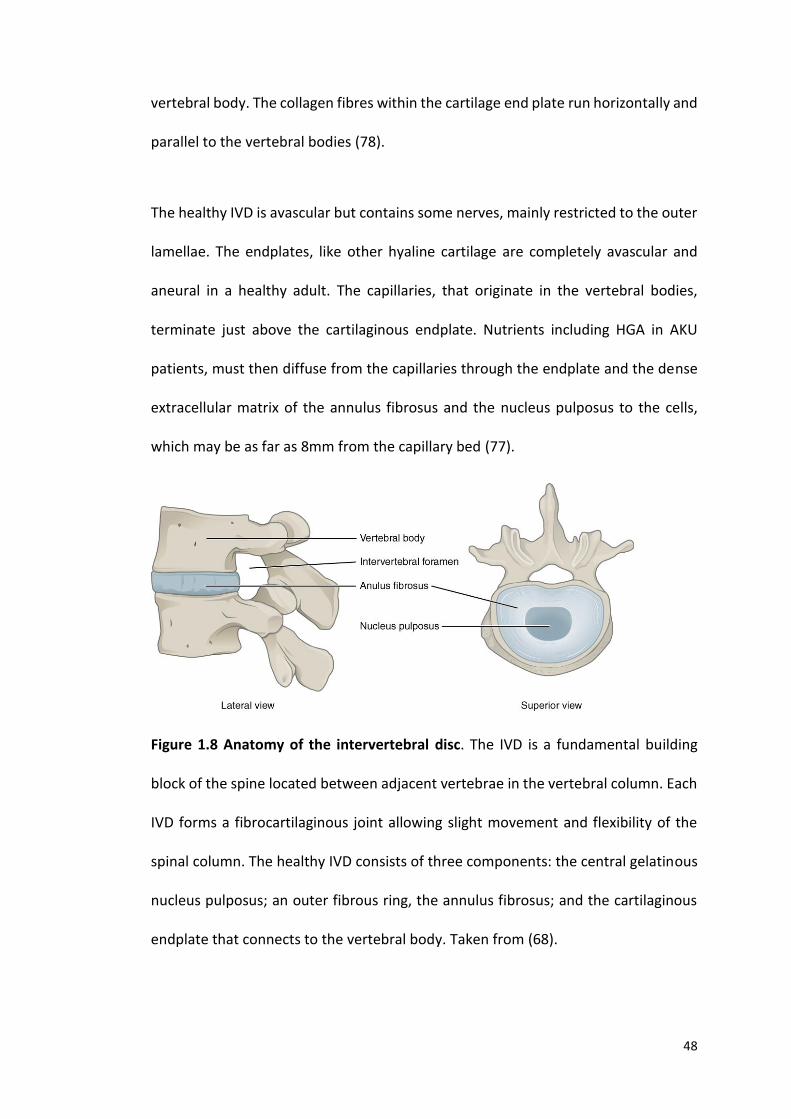
48

vertebral body. The collagen fibres within the cartilage end plate run horizontally and

parallel to the vertebral bodies (78).

The healthy IVD is avascular but contains some nerves, mainly restricted to the outer

lamellae. The endplates, like other hyaline cartilage are completely avascular and

aneural in a healthy adult. The capillaries, that originate in the vertebral bodies,

terminate just above the cartilaginous endplate. Nutrients including HGA in AKU

patients, must then diffuse from the capillaries through the endplate and the dense

extracellular matrix of the annulus fibrosus and the nucleus pulposus to the cells,

which may be as far as 8mm from the capillary bed (77).

Figure 1.8 Anatomy of the intervertebral disc. The IVD is a fundamental building

block of the spine located between adjacent vertebrae in the vertebral column. Each

IVD forms a fibrocartilaginous joint allowing slight movement and flexibility of the

spinal column. The healthy IVD consists of three components: the central gelatinous

nucleus pulposus; an outer fibrous ring, the annulus fibrosus; and the cartilaginous

endplate that connects to the vertebral body. Taken from (68).

49

1.5.9 Intervertebral disc degeneration

IVD degeneration has been identified as one of the leading causes of back pain and

motor deficiency. IVD degeneration is thought to be due to both age-related changes

and tissue damage caused by multiple stresses. With age the nucleus pulposus

dehydrates and its shock absorbing capacity reduces (76). The annulus fibrosus also

weakens and is more likely to tear resulting in herniations. The end plates

progressively thin and lead to sclerosis of the subchondral plate. The most significant

biochemical change to occur in disc degeneration is the loss of proteoglycan which

has a major effect on the discs loading properties (76). With loss of proteoglycan, the

osmotic pressure of the disc falls and the disc is less able to maintain hydration under

load resulting in the discs bulging. Importantly the loss of proteoglycan with

degeneration links in with the exposed collagen hypothesis of AKU described by

Taylor et al. where it has been suggested that tissues are initially resistant to the

deposition of HGA due to the protective proteoglycans present. Following mechanical

damage to the IVDs the protective proteoglycans are lost and HGA is able to bind to

exposed collagen resulting in pigmentation, stiffening and further mechanical

damage (76,79).

The clinical features of a degenerating IVD are typically a reduction in disc height,

structural deterioration, loss of lumbar lordosis and widespread calcification (76,79).

Patients with ochronotic arthropathy usually present with lower back pain as a result

of disc deterioration as the initial joint manifestation of AKU. Symptoms worsen from

the fourth decade leading to painful spinal disease resulting in spinal stenosis and

often changes to the curvature of the spine (kyphosis and scoliosis) (1).

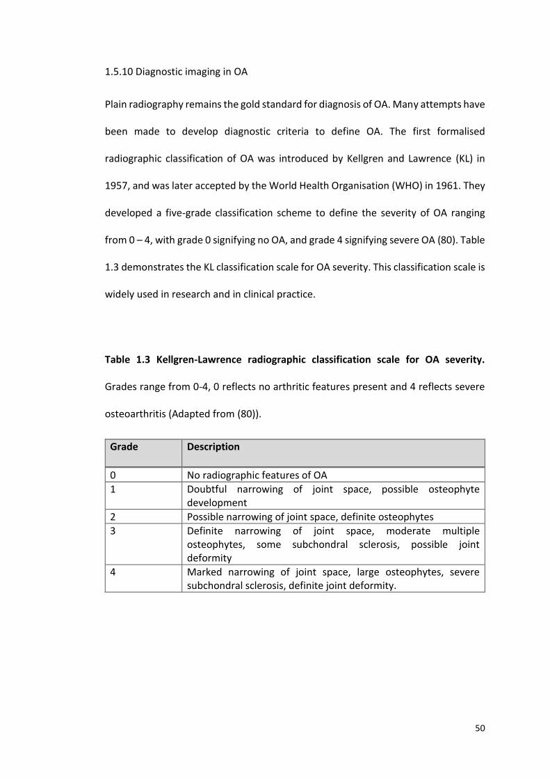
50

1.5.10 Diagnostic imaging in OA

Plain radiography remains the gold standard for diagnosis of OA. Many attempts have

been made to develop diagnostic criteria to define OA. The first formalised

radiographic classification of OA was introduced by Kellgren and Lawrence (KL) in

1957, and was later accepted by the World Health Organisation (WHO) in 1961. They

developed a five-grade classification scheme to define the severity of OA ranging

from 0 – 4, with grade 0 signifying no OA, and grade 4 signifying severe OA (80). Table

1.3 demonstrates the KL classification scale for OA severity. This classification scale is

widely used in research and in clinical practice.

Table 1.3 Kellgren-Lawrence radiographic classification scale for OA severity.

Grades range from 0-4, 0 reflects no arthritic features present and 4 reflects severe

osteoarthritis (Adapted from (80)).

Grade Description

0 No radiographic features of OA

1 Doubtful narrowing of joint space, possible osteophyte development

2 Possible narrowing of joint space, definite osteophytes

3 Definite narrowing of joint space, moderate multiple osteophytes, some subchondral sclerosis, possible joint deformity

4 Marked narrowing of joint space, large osteophytes, severe subchondral sclerosis, definite joint deformity.

51

1.6 Medical Imaging in AKU

Medical imaging refers to several different technologies that are used by a clinician

to visualise both the morphology and the function of the human body to diagnose,

monitor and treat medical conditions. Medical imaging is utilised routinely for all AKU

patients that attend the NAC and the SONIA 2 clinical trial. These AKU patients

undergo the following investigations annually; X-ray of the spine, bone mineral

density testing (DEXA scan) or quantitative computer tomography (QCT), Tc99m

isotope bone scintigraphic scan or 18F-NaF PET/CT scan (post 2016), whole body MRI

as well as echocardiogram and abdominal ultrasound (46). These images are

repeated annually for each patient documenting longitudinal pathological changes.

1.6.1 History of medical imaging

120 years ago, physicians could only rely on external signs and symptoms to diagnose

and treat a patient. If they needed to look inside, surgery was the only option. This

changed in November 1895 when X-rays were first discovered, this remains the most

important discovery in the history of medical technology and enabled physicians and

medical professionals to obtain images of inside the body for the first time (81).

Wilhelm Conrad Röntgen, a German professor of physics discovered the X-ray by

chance. Röntgen discovered this with an early cathode ray tube, he noticed that the

invisible rays could penetrate some solid objects (human flesh) better than others

(bone and metal). He first introduced the radiographs at the Würzburg Physical

Medical Society, where he sent a report with the famous X-ray picture of a hand and

wedding ring, believed to be his wife’s Bertha. Röntgen was a pioneer in medical

52

imaging, the most important of his findings was that he identified the ability of

various materials of the same thickness to transmit X-rays and this is dependent on

their densities, he found also that the ability of samples of the same material to

transmit X-rays depends on their thickness; an increase in thickness of the material

decreases the transmission of the rays, and he found that photographic plates are

sensitive to X-rays (82).

The commercialisation and mass production of X-ray tubes spread worldwide quickly

after his work was published and Roentgen was later awarded the first Nobel Prize in

Physics in 1901 (83). By the 1920’s Fluoroscopy was introduced. Radio-opaque

barium swallow or enema was administered, this enabled the radiologist to visualise

motion through the gastrointestinal tract. Planar radiographs represent the anatomy

in projections, so that the anatomical structures of the region scanned are

superimposed on top of each other. X-rays therefore poorly depict small changes in

density between tissues (81). X-ray tomography was later introduced in the 1940’s

that sparked great fascination within the medical community. This imaging modality

allowed visualisation of sections through the body without superimposition. X-ray

tomography produces ’tomograms’ that display the anatomy slice by slice. This was

achieved by rotating the X-ray tube around the patient so that only the desired slice

of tissue stayed in focus.

The first computer was made in 1946, and by 1970s Allan MacLeod Cormack and

Godfrey Newbold Hounsfield invented computed tomography (CT), pairing the

discovery of X-rays with the development and refinement of computational

techniques (83). They were awarded the Nobel Prize for Physiology or Medicine in

53

1979. The first CT scan was performed in 1971, where an X-ray tube rotated around

the patient and various detectors detected X-rays that were not absorbed, refracted

or reflected as they passed through the body. Early computers took all night to

process the images that today takes a few milliseconds (82).

The risks of imaging using radiation were realised including the increased risk of

developing cancer in the future. In 1973 Paul. C. Lauterbur an American Chemist,

published his work on magnetic resonance imaging (MRI) that does not utilise X-rays.

He utilised resistive magnets with weak magnetic fields producing images initially

with low spatial resolution, however the soft tissue discrimination was seen to be

superior to that of CT (84). In the late 1970’s Peter Mansfield an English Physicist

developed the echo-planar imaging technique that would lead to clearer scans that

take seconds rather than hours. In 2003 Paul Lauterbur and Peter Mansfield were

awarded the Nobel Prize for Physiology or Medicine for their discoveries of MRI (83).

1.6.2 Radiography

Plain radiographs form the most basic, least expensive imaging tests carried out on

patients with arthropathy. Radiographs have a useful role in symptomatic joint

disease and highlight destructive lesions such as osteophytes, subchondral sclerosis

and cysts. Radiography can also illustrate joint space width which determines AC loss

as well as cartilage calcification (85).

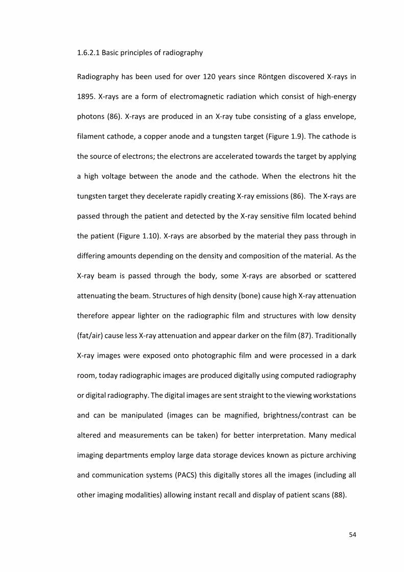
54

1.6.2.1 Basic principles of radiography

Radiography has been used for over 120 years since Röntgen discovered X-rays in

1895. X-rays are a form of electromagnetic radiation which consist of high-energy

photons (86). X-rays are produced in an X-ray tube consisting of a glass envelope,

filament cathode, a copper anode and a tungsten target (Figure 1.9). The cathode is

the source of electrons; the electrons are accelerated towards the target by applying

a high voltage between the anode and the cathode. When the electrons hit the

tungsten target they decelerate rapidly creating X-ray emissions (86). The X-rays are

passed through the patient and detected by the X-ray sensitive film located behind

the patient (Figure 1.10). X-rays are absorbed by the material they pass through in

differing amounts depending on the density and composition of the material. As the

X-ray beam is passed through the body, some X-rays are absorbed or scattered

attenuating the beam. Structures of high density (bone) cause high X-ray attenuation

therefore appear lighter on the radiographic film and structures with low density

(fat/air) cause less X-ray attenuation and appear darker on the film (87). Traditionally

X-ray images were exposed onto photographic film and were processed in a dark

room, today radiographic images are produced digitally using computed radiography

or digital radiography. The digital images are sent straight to the viewing workstations

and can be manipulated (images can be magnified, brightness/contrast can be

altered and measurements can be taken) for better interpretation. Many medical

imaging departments employ large data storage devices known as picture archiving

and communication systems (PACS) this digitally stores all the images (including all

other imaging modalities) allowing instant recall and display of patient scans (88).

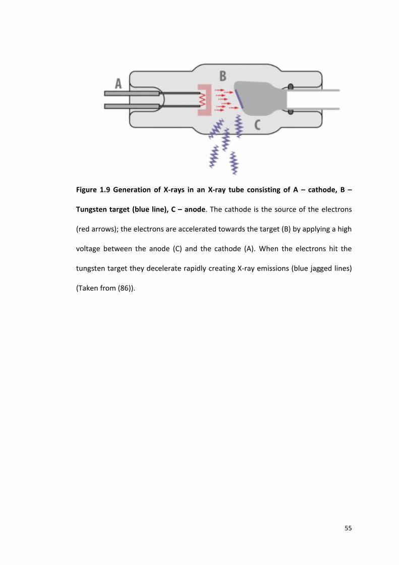
55

Figure 1.9 Generation of X-rays in an X-ray tube consisting of A – cathode, B –

Tungsten target (blue line), C – anode. The cathode is the source of the electrons

(red arrows); the electrons are accelerated towards the target (B) by applying a high

voltage between the anode (C) and the cathode (A). When the electrons hit the

tungsten target they decelerate rapidly creating X-ray emissions (blue jagged lines)

(Taken from (86)).

56

Figure 1.10 Set up of a chest radiograph. Posteroanterior X-ray where the X-ray beam

originates from the X-ray tube passes through the patient and strikes the

radiographic film (Taken from (87)).

1.6.3 Bone densitometry

Until recently plain radiographs were used to determine bone density, however this

was an estimation and bone loss was not observed until bone loss exceeded 25-30%

of its density. This led to finding more sophisticated methods of measuring bone

density with the ability to detect early changes. The two most common tools used to

measure bone mineral density (BMD) are dual-energy x-ray absorptiometry (DEXA)

and quantitative computer tomography (QCT). These techniques are used to

diagnose osteoporosis and to evaluate the risk of fracture. These imaging modalities

are carried out routinely in both the NAC and the SONIA 2 clinical trial as it is widely

recognised that changes in cartilage composition have direct implications for bone in

AKU. The NAC patients have bi-annual QCT scans, and the SONIA 2 patients have

57

annual DEXA scans. In AKU it is proposed that chronic arthritis can impair bone

architecture which then may predispose AKU patients to fractures (89). It is still

however under debate as to whether bone lesions cause osteoarthritis or whether

cartilage disease results in bone lesions, extensive research is still ongoing to

understand this further.

1.6.3.1 Basic principles- DEXA

DEXA has long been used as the gold standard in the clinical diagnosis of

osteoporosis. DEXA determines BMD in two dimensions and is based on the emission

of two X-rays of two distinct energies (90). The fundamental principle of DEXA is the

measurement of X-ray transmission through the body at high and low energies and

the assumption that the body is a two-compartment model made up of bone mineral

and soft tissue. The two X-ray beams of differing intensities are used to differentiate

between bone and soft tissue. The ratio of attenuation of the two photon energies is

analysed in anatomical sites containing bone and areas just containing soft tissue.

The ratio of attenuation in areas of soft tissue can then be subtracted away leaving

just the BMD (91,92).

BMD is measured in g/cm², however it is more commonly referred to as the T-score.

It is expressed as the number of standard deviations above or below the mean BMD

of a healthy 30-year old adult (peak bone density) of the same sex and ethnicity as

the patient. Figure 1.11 represents a DEXA report of an AKU patient. Table 1.4

illustrates the WHO definitions of BMD levels. Osteoporosis is defined as a T-score

equal to or below -2.5, Osteopenia as a T-score of below or equal to -1.0 and normal

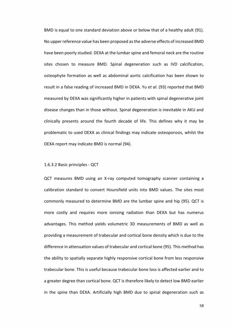
58

BMD is equal to one standard deviation above or below that of a healthy adult (91).

No upper reference value has been proposed as the adverse effects of increased BMD

have been poorly studied. DEXA at the lumbar spine and femoral neck are the routine

sites chosen to measure BMD. Spinal degeneration such as IVD calcification,

osteophyte formation as well as abdominal aortic calcification has been shown to

result in a false reading of increased BMD in DEXA. Yu et al. (93) reported that BMD

measured by DEXA was significantly higher in patients with spinal degenerative joint

disease changes than in those without. Spinal degeneration is inevitable in AKU and

clinically presents around the fourth decade of life. This defines why it may be

problematic to used DEXA as clinical findings may indicate osteoporosis, whilst the

DEXA report may indicate BMD is normal (94).

1.6.3.2 Basic principles - QCT

QCT measures BMD using an X-ray computed tomography scanner containing a

calibration standard to convert Hounsfield units into BMD values. The sites most

commonly measured to determine BMD are the lumbar spine and hip (95). QCT is

more costly and requires more ionising radiation than DEXA but has numerus

advantages. This method yields volumetric 3D measurements of BMD as well as

providing a measurement of trabecular and cortical bone density which is due to the

difference in attenuation values of trabecular and cortical bone (95). This method has

the ability to spatially separate highly responsive cortical bone from less responsive

trabecular bone. This is useful because trabecular bone loss is affected earlier and to

a greater degree than cortical bone. QCT is therefore likely to detect low BMD earlier

in the spine than DEXA. Artificially high BMD due to spinal degeneration such as

59

calcification and osteophyte formation can therefore be avoided (94). QCT yields

both BMD in g/cm³ and T-scores however, the WHO definition of osteoporosis (Table

1.4) is specific to DEXA and should not be applied to QCT. It is important to note that

QCT T-scores cannot be used to compare with DEXA T-scores. More often than not

the QCT T-score results in a lower T-score than that of the DEXA report. It has been

reported that a DEXA T-score of -2.5 equals an average T-score of -3.4 in QCT,

therefore DEXA is currently the only method to diagnose osteopenia or osteoporosis

from T-scores (96). This is due to a variety of factors such as the physiological effects

of ageing and the menopause, the technical effects of increased mineral density due

to osteophytes and aortic calcification, increased BMI as well as bone size (94). These

effects will be discussed further in Chapter 5.

Table 1.4 World Health Organisation definitions of bone mineral density levels.

BMD- bone mineral density, SD- standard deviation (Adapted from (91)).

Level Definition

Normal BMD within 1 SD of the young adult mean

Osteopenia BMD is between 1 and 2.5 SD below the young

adult mean

Osteoporosis BMD is 2.5 SD or more below the young adult

mean

60

Figure 1.11 Dual-energy X-ray absorptiometry report. BMD is measured in g/cm³ of

bone. The young adult T-score value represents how BMD compares to a healthy 30-

year old adult of the same sex and ethnicity (values of +1 or -1 represent normal BMD,

values between -1 and -2.5 indicate osteopenia, values below -2.5 indicate

osteoporosis). Age matched Z score compares BMD to others of the same age as the

patient.

1.6.4 Computed tomography

CT is considered more sensitive than conventional X-ray imaging due to high spatial

resolution and high contrast between low attenuating cartilage and high attenuating

bone. Whole body CT and arthrography are utilised in AKU to determine cartilage

damage and cartilage loss in the major joints affected. CT arthrography is excellent

at depicting cortical bone and soft tissue calcifications as well as subchondral bone

sclerosis and osteophytes associated with severe changes of OA (85).

61

1.6.4.1 Basic Principles - CT

The word tomography is derived from the Greek word tomos, meaning slice. This

definition demonstrates the fundamental limitations of the radiograph and

represents the downfall that anatomical structures are viewed in a single plane and

superimposed on top of each other. This led to the development of CT; an imaging

modality whereby cross sectional images are obtained using X-rays (97). A CT scanner

produces serial images that represent the X-ray attenuation of the various structures

of the body. In CT scanning the patient is passed through a rotating gantry that has

an X-ray tube on one side and a set of detectors on the other side (86). A fan shaped

beam of X-rays is produced as the gantry spins around the patient and thousands of

sectional views of the body are generated that are reconstructed into 2D cross

sectional images. CT scans can be acquired very quickly and have a much higher

resolution than conventional X-rays providing far more detailed images. The data

captured by the scanner is digitally converted into reconstructed images using

various algorithms (88). The individual volume elements that make up the image are

represented as 2D pixels that correspond to the attenuation properties of that area

(represented as Hounsfield units (HU)). In CT water is assigned an attenuation value

of 0 HU, structures that are less dense than water have negative values (e.g. air = -

1000 HU, fat = -120 HU), structures that are more dense have positive values (e.g.

muscle = 40 HU, bone = 500 HU). As in plain X-rays high density objects such as bone

cause more attenuation of the X-rays and are therefore displayed as white or light

grey, and the lower density tissues such as fat and air are displayed as dark grey or

black (88).

62

1.7 Nuclear Medicine

Nuclear medicine involves the application of radioactive substances in the diagnosis

and treatment of disease. The purpose of radionuclide imaging is to obtain a picture

of the distribution of the radioactive-labelled tracer around the body after it has been

administered (either orally or intravenously). The emissions from the radioactive

tracers are detected by cameras externally and are then converted into an image.

Nuclear medicine in AKU uses phosphate analogues to visualise bone metabolism,

changes of which occur in response to alterations in cartilage composition and

structure (89). Positron emissions tomography (PET) is a branch of nuclear medicine

where a positron-emitting radionuclide is injected into the subject. Fluoride 18-

labelled PET imaging provides a unique non-invasive method to visualise bone

metabolism, and molecular and cellular changes in affected joints. Changes in bone

metabolism occur before clear morphological signs in OA and AKU, therefore PET

imaging can be used to detect early pathological changes. PET also has a common

place in oncology, used to diagnose bony metastasis as well as assess response to

therapy (98,99). Hybrid imaging techniques involving fusion of PET data with CT data

provide the clinician with cross-sectional functional and anatomical information used

for more accurate diagnosis (89).

PET imaging has superior spatial resolution compared to other functional imaging

techniques such as SPECT (single-photon emission computed tomography). SPECT is

similar to PET in that it utilises radiotracers and detects gamma rays however, SPECT

radionucleotides directly emit gamma radiation without annihilation. The coincident

detection of the photons in PET imaging provides more radiation event localisation

63

therefore better spatial resolution. SPECT imaging is performed using the gamma

camera and acquires multiple 2D images that are reconstructed into a 3D images. PET

imaging is performed using PET/CT scanner and acquires 4D images (100).

1.7.1 History of Nuclear Medicine

The development of nuclear medicine has been a multidisciplinary effort due to

advances in physics, mathematics, chemistry, computer science and biology (101).

The discovery of X-rays in 1895 lead to Henri Becquerel’s discovery of ‘mysterious

rays’. Becquerel used salt of uranium and potassium and he noticed once exposed to

sunlight the salt emitted radiation that blackened a photographic plate. This inspired

many scientists to investigate this further and in 1897 Marie and Pierre Curie tried to

isolate the substances that emitted these rays in doing so they discovered polonium

and radium. They coined the term and confirmed the existence of ‘radioactivity’

(102). In 1909 Sir Ernest Rutherford demonstrated what happens to an element

during radioactive decay. Positron emission tomography (PET) is a branch of nuclear

medicine that utilises the detection of a pair of gamma rays that are emitted

indirectly by a positron-emitting radiotracer.

The history of PET dates back to the late 1920’s, where the discovery of the positron,

artificial radiation, invention of the cyclotron and recognition of radionuclides were

among the important advances (101). In the 1950’s Hal Anger developed the first

gamma camera; the Anger scintillation camera, a 2D planar detector that produces a

2D projection image. Radon, developed the mathematical method to reconstruct

projections in 1917 however, it was the 1970’s before its use in medical imaging came

64

to light. The first PET system was built in the 1970’s and used for phantom studies.

The first human PET system was built soon after by Phelps and Hoffman et al. in 1975

followed by Sokoloff et al. producing the first true image of the human brain in 1976

(86). PET imaging continued to advance from here, in 2000 Beyer et al. conducted the

first PET/CT scan marrying together both functional and anatomical information.

Furthermore the development of technology and computer based algorithms

enhanced image resolution and improved the use of PET as a clinical tool that has

contributed to more accurate diagnosis of many diseases (103).

1.7.2 Positron emission tomography- physical principles

Proton rich isotopes decay via positron emission, in which a proton in the nucleus

decays into a neutron, and a positron and neutrino (104). Upon administration of the

radiotracer the radioactive atom decays resulting in a positron being ejected from

the nucleus. The positron travels a few millimetres before colliding with an electron

resulting in an annihilation event producing two 511 KeV photons that travel in

opposite directions. PET image acquisition is based on the simultaneous (coincident)

detection of these two photons (Figure 1.12). The PET scanner consists of many

photon detectors that are positioned surrounding the subject. During a PET scan

millions of coincident detections are detected, that are reconstructed into electrical

signals providing information about the distribution of the radiotracer (105).

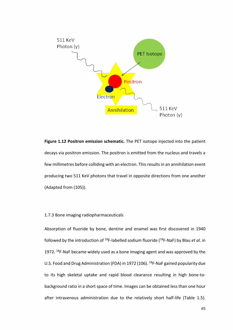
65

Figure 1.12 Positron emission schematic. The PET isotope injected into the patient

decays via positron emission. The positron is emitted from the nucleus and travels a

few millimetres before colliding with an electron. This results in an annihilation event

producing two 511 KeV photons that travel in opposite directions from one another

(Adapted from (105)).

1.7.3 Bone imaging radiopharmaceuticals

Absorption of fluoride by bone, dentine and enamel was first discovered in 1940

followed by the introduction of 18F-labelled sodium fluoride (18F-NaF) by Blau et al. in

1972. 18F-NaF became widely used as a bone imaging agent and was approved by the

U.S. Food and Drug Administration (FDA) in 1972 (106). 18F-NaF gained popularity due

to its high skeletal uptake and rapid blood clearance resulting in high bone-to-

background ratio in a short space of time. Images can be obtained less than one hour

after intravenous administration due to the relatively short half-life (Table 1.5).

66

Although 18F-NaF was the first widely used bone imaging agent it quickly fell into

disuse. One limitation of 18F bone imaging was the requirement of imaging with high

energy rectilinear scanners equipped with thick Sodium Iodide crystals due to the

high energy (511 KeV) annihilation photons. Logistical challenges of the 110 minute

half-life of 18F-NaF , the introduction of cheaper radiopharmaceuticals (technetium-

Tc-99m) and the development of the Anger gamma camera designed for the 140 KeV

photons of Tc-99m resulted in the FDA withdrawing its approval in 1975 (107). The

widespread availability of Tc-99m generators resulted in Tc-99 labelled bone imaging

agents to become the most commonly performed imaging procedure in nuclear

medicine.

The challenges associated with 18F-NaF imaging were reassessed in 1992 when

Dahlbom et al. (108) used 18F-NaF in the development of a whole-body PET technique

that demonstrated increased spatial resolution, and greater photon capture due to

coincident detection of photons. 18F-NaF whole body PET skeletal imaging was later

introduced in 1993 with early studies showing promising results for both malignant

and metabolic bone disorders. This led to the FDA re-issuing approval of 18F-NaF for

skeletal imaging in 2000 (106). Since then the development of combined PET/CT

scanners, ease of production in a cyclotron (previously 18F-NaF was produced in a

nuclear reactor with a two-step reaction) coupled with shortages of Tc-99m

generators, has led to 18F-NaF being the preferred bone imaging agent once again

(109).

As a skeletal imaging agent 18F-NaF has superior skeletal kinetics compared to Tc-99m

including faster blood clearance and two-fold higher bone uptake providing superior

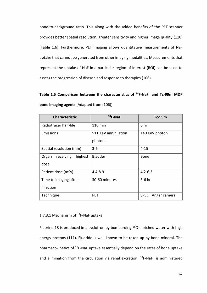
67

bone-to-background ratio. This along with the added benefits of the PET scanner

provides better spatial resolution, greater sensitivity and higher image quality (110)

(Table 1.6). Furthermore, PET imaging allows quantitative measurements of NaF

uptake that cannot be generated from other imaging modalities. Measurements that

represent the uptake of NaF in a particular region of interest (ROI) can be used to

assess the progression of disease and response to therapies (106).

Table 1.5 Comparison between the characteristics of 18F-NaF and Tc-99m MDP

bone imaging agents (Adapted from (106)).

Characteristic 18F-NaF Tc-99m

Radiotracer half-life 110 min 6 hr

Emissions 511 KeV annihilation

photons

140 KeV photon

Spatial resolution (mm) 3-6 4-15

Organ receiving highest

dose

Bladder Bone

Patient dose (mSv) 4.4-8.9 4.2-6.3

Time to imaging after

injection

30-60 minutes 3-6 hr

Technique PET SPECT Anger camera

1.7.3.1 Mechanism of 18F-NaF uptake

Fluorine 18 is produced in a cyclotron by bombarding 18O-enriched water with high

energy protons (111). Fluoride is well known to be taken up by bone mineral. The

pharmacokinetics of 18F-NaF uptake essentially depend on the rates of bone uptake

and elimination from the circulation via renal excretion. 18F-NaF is administered

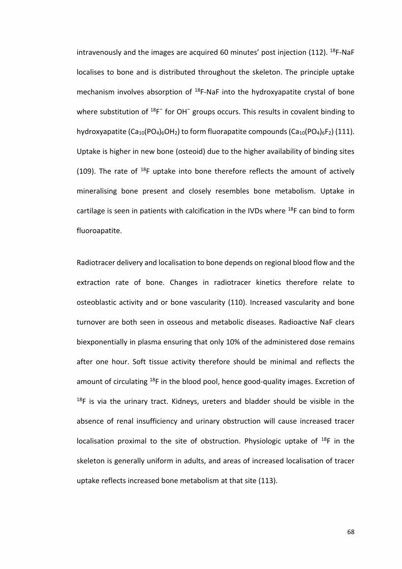
68

intravenously and the images are acquired 60 minutes’ post injection (112). 18F-NaF

localises to bone and is distributed throughout the skeleton. The principle uptake

mechanism involves absorption of 18F-NaF into the hydroxyapatite crystal of bone

where substitution of 18Fˉ for OHˉ groups occurs. This results in covalent binding to

hydroxyapatite (Ca10(PO4)6OH2) to form fluorapatite compounds (Ca10(PO4)6F2) (111).

Uptake is higher in new bone (osteoid) due to the higher availability of binding sites

(109). The rate of 18F uptake into bone therefore reflects the amount of actively

mineralising bone present and closely resembles bone metabolism. Uptake in

cartilage is seen in patients with calcification in the IVDs where 18F can bind to form

fluoroapatite.

Radiotracer delivery and localisation to bone depends on regional blood flow and the

extraction rate of bone. Changes in radiotracer kinetics therefore relate to

osteoblastic activity and or bone vascularity (110). Increased vascularity and bone

turnover are both seen in osseous and metabolic diseases. Radioactive NaF clears

biexponentially in plasma ensuring that only 10% of the administered dose remains

after one hour. Soft tissue activity therefore should be minimal and reflects the

amount of circulating 18F in the blood pool, hence good-quality images. Excretion of

18F is via the urinary tract. Kidneys, ureters and bladder should be visible in the

absence of renal insufficiency and urinary obstruction will cause increased tracer

localisation proximal to the site of obstruction. Physiologic uptake of 18F in the

skeleton is generally uniform in adults, and areas of increased localisation of tracer

uptake reflects increased bone metabolism at that site (113).

69

Table 1.6 Advantages of 18F-NaF PET for studying bone tracer kinetics (Adapted from

(110)).

1.7.4 Quantitative measurement of 18F-NaF – SUVm

Quantitative measurements in PET imaging are used as a tool to supplement visual

interpretation providing a method that is less user-dependant and can be used for

intra- and inter-patient comparisons. Today, uptake measurements are most widely

used in oncology to assess response to therapies and to distinguish degrees of

pathology (114). 18F-NaF PET has been applied to several kinds of bone disorders as

18F-NaF binds to both osteoblastic and osteolytic lesions. Uptake values have been

investigated for the early detection of OA (115). The standardised uptake value (SUV)

is a common method of expressing the uptake of PET tracers. The SUV is a measure

of radioactivity in a region of interest, normalised against injected activity and the

subject’s body weight. The calculation can be seen in Figure 1.13 where the SUV is

defined as the activity concentration in the ROI (kBq/mL) as measured by the PET

scanner divided by the decay corrected injected dose of 18F-NaF divided by the

patient body weight (kg) that acts as a surrogate for the distribution volume of tracer

(116). If all the injected 18F-NaF is retained and uniformly distributed throughout the

18F-NaF Advantages

Superior spatial resolution of PET scanner

18F-NaF shows rapid bone uptake

18F-NaF clears rapidly from blood

High bone to soft tissue background

18F-NaF easily generated in cyclotron by irradiation of 18O-enriched water

PET scanners widely available

70

body, the SUV will be 1g/ml under the assumption that 1ml of tissue weighs 1g. Larger

SUVs represent proportionally higher concentrations of radiotracer. The uptake is

represented by pixel or voxel intensity value in the ROI, which is then converted into

the activity concentration (117). SUV can be expressed as SUVm (mean SUV in ROI),

SUVmin (minimum SUV in ROI) or SUVmax (maximum SUV in ROI). SUVs have been

described in the literature as quantitative measurements of disease state. SUVs can

be used to assess disease progression and response to therapy and has more recently

been proposed as a diagnostic tool.

Figure 1.13 Standardised uptake value calculation. Where ‘r’ is the radioactivity

concentration (kBq/ml) in a ROI, divided by ‘a’ the decay corrected injected dose

(kBq) divided by body weight (kg) (118).

SUV = r

(a / w)

71

1.7.4.1 SUV measurements in osteoarthritis

PET imaging has been applied to OA for the visualisation of bone metabolism.

Currently plain X-ray is the gold standard for diagnosing OA, however it is realised

that functional abnormalities can exist without radiographic evidence. 18F-NaF PET

has been shown to detect early changes in OA by identifying areas of accelerated

bone remodelling associated with OA pathology. Kobayashi et al. (115) measured the

SUV at the hip and revealed accelerated bone remodelling in late-stage OA. The

SUVm was significantly associated with the radiographic stage of OA (KL grade), as

well as the severity of pain. These authors suggested that hip pain may be related to

subchondral bone abnormality caused by mechanical stress (115).

The molecular kinetics of 18F-NaF PET is based on bone metabolism, other studies

have assessed the use of 18-F fluorodeoxyglucose (18F-FDG), utilised to visualise

inflammation by detecting accelerated glucose metabolism. However, 18F-FDG has

been shown to be more suitable for the detection of soft tissue inflammation as seen

in synovitis or rheumatoid arthritis. Several studies have stated that there is no

specific SUV that defines either benign or malignant lesions (119). However

Kobayashi et al. (120) stated that a SUVm of 6.4 can be used to predict OA incidence

or progression. SUVm has been used in the literature over SUVmin or max as the

mean SUV in the ROI provides a better representation of the uptake in that site. The

utilisation of SUVs in AKU has not previously been investigated. Considering the

pathology of OA is comparable to that of AKU, it can be appreciated that these

quantitative measurements could be beneficial in assessing AKU disease pathology

as well as in the clinical trials to assess response to nitisinone.

72

Currently AKU patient 18F-NaF scans are analysed as part of the AKUSSI (Table 1.2) to

assess the extent and burden of arthropathy. The scans are assessed by a nuclear

medicine consultant and a visual assessment of the whole skeletal system is

conducted, involving mapping of the various large joints with arthritic changes. The

14 large joint areas scored include the hips, knees, ankles, feet, shoulders, elbows,

hands including wrists. Spine involvement was also scored and included the cervical,

thoracic and lumbar regions. The nuclear medicine consultant gives a score of 1 if

there is increased tracer uptake at that anatomical site, and gives a score of 0 if there

is normal uptake. These scores are then fed into the AKUSSI and contributes to an

overall composite score of disease severity (46). Additionally an index of the relative

activity of arthropathy is also given by visual assessment of the intensity of skeletal

uptake, for example the scoring ranges from 0-3, where 0 = normal, 1 = mild, 2 =

moderate and 3 = intense uptake (89). The AKUSSI describes the extent of disease

manifestations but does not quantify disease burden. This thesis introduces for the

first time, quantitative SUV measurements of bone and cartilage to assess disease

state and progression in AKU.

1.7.5 Maximum Intensity Projection

A maximum intensity projection (MIP) image is a method of visualisation where the

voxels with the highest intensity are projected on to a two-dimensional image. This

method displays bone and contrast material - filled structures preferentially and

other low attenuation structures are not well visualised. This method is useful

clinically to visualise areas of high uptake of 18F into the skeleton or calcified tissues.

73

2.0 MATERIALS AND METHODS

74

2.1 ETHICAL APPROVAL

Ethical approval for the NAC was approved by the Health and Life Sciences

Committee on Research Ethics, University of Liverpool for ‘analysis of data from the

National Alkaptonuria Service which could help us better understand AKU’

(reference:0310), dated 26/05/2017.

Ethical approval for the SONIA 2 clinical trial was granted by the National Research

Ethics Service (REC reference: 13/NW/0567), dated 17/9/2013.

2.2 PATIENT GROUPS

2.2.1 NAC

Forty three adult AKU patients (17 females, 26 males) with a mean age of 49 (SD±14.8

range 21-74) attended the National Alkaptonuria Centre in the Royal Liverpool

University Hospital, Liverpool, England for baseline tests in 2012. A plethora of

assessments and tests are carried out including the following; blood samples, urine

samples, X-Ray, MRI, DEXA, PET/CT, ultrasound (abdomen and pelvis), clinical eye

photographs, ear cartilage biopsies and echocardiograms. Patients all received 2mg

of off-label nitisinone daily after the baseline visit. Twenty two of the forty three

patients have attended the NAC annually for four visits after baseline providing

longitudinal analysis of nitisinone.

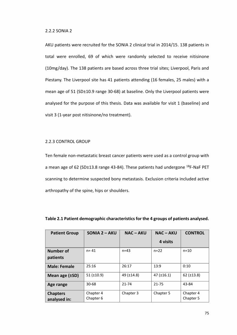
75

2.2.2 SONIA 2

AKU patients were recruited for the SONIA 2 clinical trial in 2014/15. 138 patients in

total were enrolled, 69 of which were randomly selected to receive nitisinone

(10mg/day). The 138 patients are based across three trial sites; Liverpool, Paris and

Piestany. The Liverpool site has 41 patients attending (16 females, 25 males) with a

mean age of 51 (SD±10.9 range 30-68) at baseline. Only the Liverpool patients were

analysed for the purpose of this thesis. Data was available for visit 1 (baseline) and

visit 3 (1-year post nitisinone/no treatment).

2.2.3 CONTROL GROUP

Ten female non-metastatic breast cancer patients were used as a control group with

a mean age of 62 (SD±13.8 range 43-84). These patients had undergone 18F-NaF PET

scanning to determine suspected bony metastasis. Exclusion criteria included active

arthropathy of the spine, hips or shoulders.

Table 2.1 Patient demographic characteristics for the 4 groups of patients analysed.

Patient Group SONIA 2 – AKU NAC – AKU NAC – AKU

4 visits

CONTROL

Number of

patients

n= 41 n=43 n=22 n=10

Male: Female 25:16 26:17 13:9 0:10

Mean age (±SD) 51 (±10.9) 49 (±14.8) 47 (±16.1) 62 (±13.8)

Age range 30-68 21-74 21-75 43-84

Chapters analysed in:

Chapter 4 Chapter 6

Chapter 3 Chapter 5 Chapter 4 Chapter 5

76

2.3 PET/CT PROTOCOL

Two hundred Mbq of 18F-fluoride was injected into the patient intravenously by direct

venepuncture or intravenous catheter. Whole body PET and low dose CT views were

acquired 60 minutes’ post injection.

2.4 18F-NaF PET THRESHOLD APPLICATION

2.4.1 IMAGE TYPE

Maximum intensity projection (MIP) PET images were used for the threshold

application study. MIP PET images are 3D reconstructions of PET data representing

the maximum pixel value on every view. This method displays bone and calcified

tissue preferentially providing a clearer image by blocking low attenuating structures

like soft tissue that may occlude visualisation.

2.4.2 IMAGEJ SOFTWARE

ImageJ (1.49j) is a public domain, Java-based image processing program developed

at the National Institute of Health. ImageJ can display, edit, analyse and process 8-

bit, 16-bit, 32-bit and RGB files and can read many file formats e.g. TIFF, JPEG, DICOM

including stacks (121).

2.4.3 HISTOGRAM ANALYSIS

Baseline 8-bit MIP PET images of the 43 NAC patients were imported into Image J

(1.49j). A histogram plot was created for each patient to analyse the distribution of

pixel values within the image. The pixel values within the image ranged from 0-255

77

(0 = black, 255= white) (Figure 2.1). A large proportion of the pixel values in the image

are white representing the background as demonstrated by the large spike around

245, a small spike can be seen at pixel value 0 representing the areas of high uptake

of 18F into bone and calcified tissue.

Figure 2.1 Histogram plot of MIP PET image pixel value distribution. Pixel values

ranging from 0 – 255 (0 = black, 255 = white) (NAC patient 9).

Another histogram was created to further analyse the small spike at 0 as this

represented the areas of high uptake of 18F thought to be associated with disease

pathology (Figure 2.2A). A threshold value was then identified from the histogram

and the pixel value was selected on the graph where the pixel counts start to increase

(position indicated by the red line- pixel value 70) (Figure 2.2A). A threshold value

was identified this way for every patient.

0 20 40 60 80 100 120 140 160 180 200 220 240 260

0

10000

20000

30000

40000

50000

60000

70000

Pixel value

Co

un

t

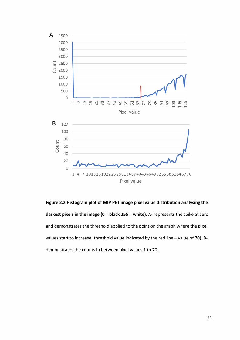
78

Figure 2.2 Histogram plot of MIP PET image pixel value distribution analysing the

darkest pixels in the image (0 = black 255 = white). A- represents the spike at zero

and demonstrates the threshold applied to the point on the graph where the pixel

values start to increase (threshold value indicated by the red line – value of 70). B-

demonstrates the counts in between pixel values 1 to 70.

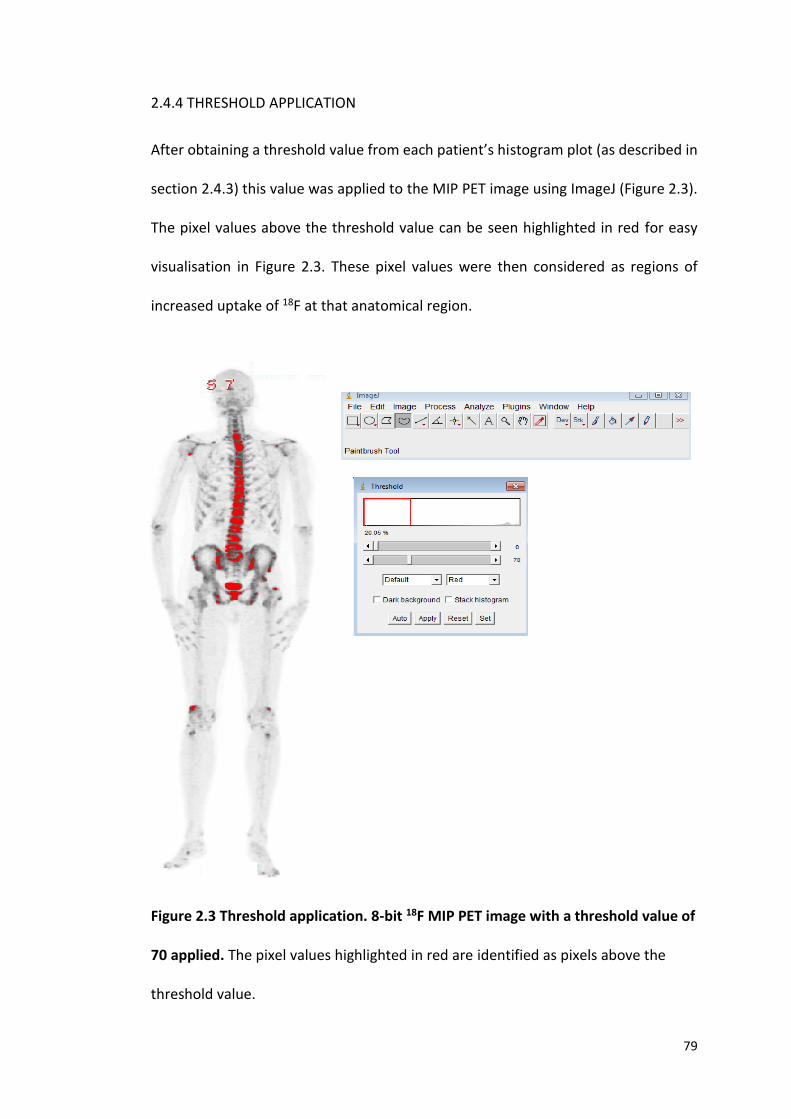
79

2.4.4 THRESHOLD APPLICATION

After obtaining a threshold value from each patient’s histogram plot (as described in

section 2.4.3) this value was applied to the MIP PET image using ImageJ (Figure 2.3).

The pixel values above the threshold value can be seen highlighted in red for easy

visualisation in Figure 2.3. These pixel values were then considered as regions of

increased uptake of 18F at that anatomical region.

Figure 2.3 Threshold application. 8-bit 18F MIP PET image with a threshold value of

70 applied. The pixel values highlighted in red are identified as pixels above the

threshold value.

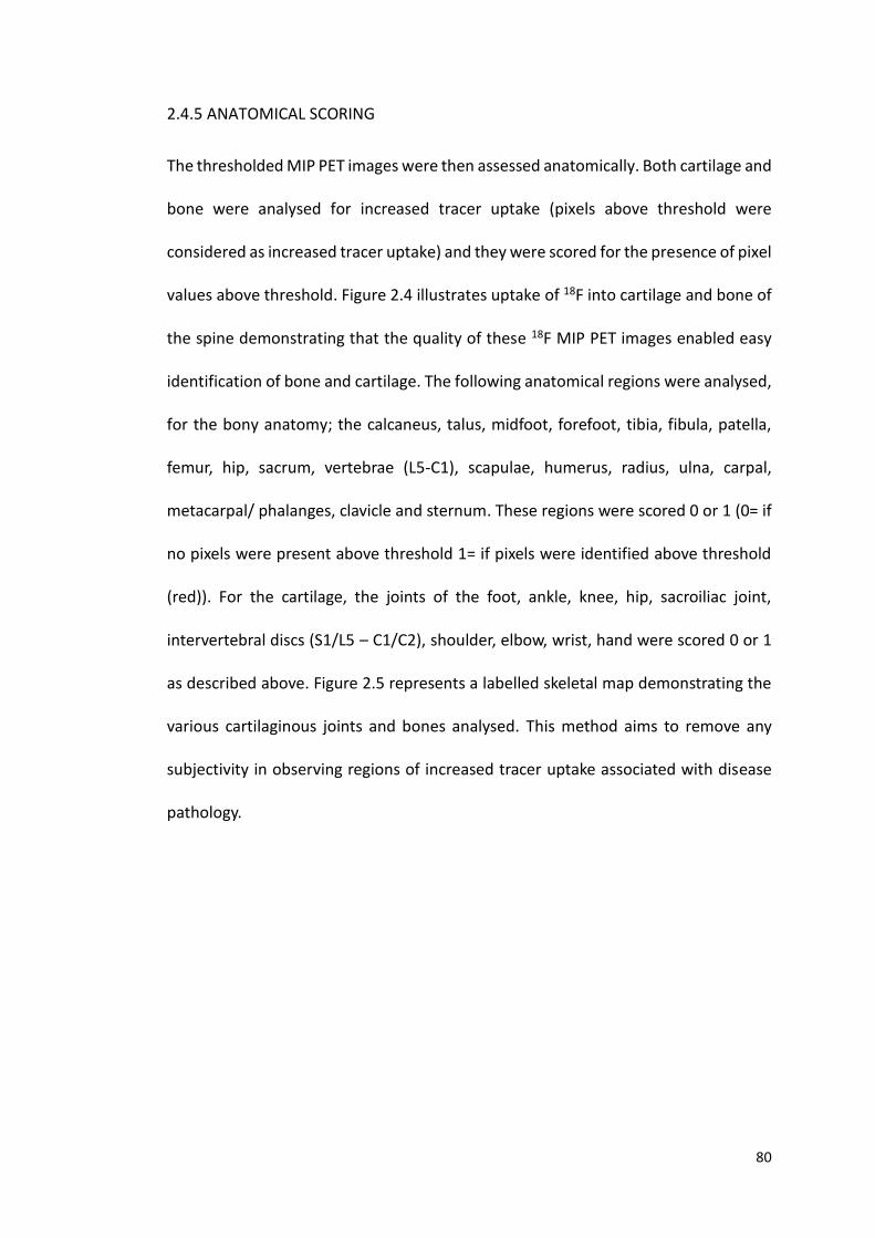
80

2.4.5 ANATOMICAL SCORING

The thresholded MIP PET images were then assessed anatomically. Both cartilage and

bone were analysed for increased tracer uptake (pixels above threshold were

considered as increased tracer uptake) and they were scored for the presence of pixel

values above threshold. Figure 2.4 illustrates uptake of 18F into cartilage and bone of

the spine demonstrating that the quality of these 18F MIP PET images enabled easy

identification of bone and cartilage. The following anatomical regions were analysed,

for the bony anatomy; the calcaneus, talus, midfoot, forefoot, tibia, fibula, patella,

femur, hip, sacrum, vertebrae (L5-C1), scapulae, humerus, radius, ulna, carpal,

metacarpal/ phalanges, clavicle and sternum. These regions were scored 0 or 1 (0= if

no pixels were present above threshold 1= if pixels were identified above threshold

(red)). For the cartilage, the joints of the foot, ankle, knee, hip, sacroiliac joint,

intervertebral discs (S1/L5 – C1/C2), shoulder, elbow, wrist, hand were scored 0 or 1

as described above. Figure 2.5 represents a labelled skeletal map demonstrating the

various cartilaginous joints and bones analysed. This method aims to remove any

subjectivity in observing regions of increased tracer uptake associated with disease

pathology.

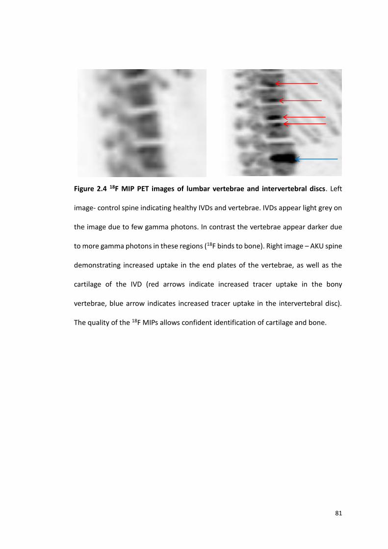
81

Figure 2.4 18F MIP PET images of lumbar vertebrae and intervertebral discs. Left

image- control spine indicating healthy IVDs and vertebrae. IVDs appear light grey on

the image due to few gamma photons. In contrast the vertebrae appear darker due

to more gamma photons in these regions (18F binds to bone). Right image – AKU spine

demonstrating increased uptake in the end plates of the vertebrae, as well as the

cartilage of the IVD (red arrows indicate increased tracer uptake in the bony

vertebrae, blue arrow indicates increased tracer uptake in the intervertebral disc).

The quality of the 18F MIPs allows confident identification of cartilage and bone.

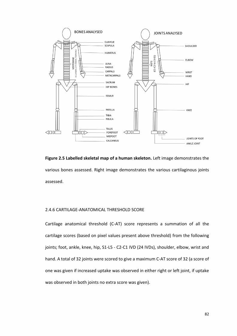
82

Figure 2.5 Labelled skeletal map of a human skeleton. Left image demonstrates the

various bones assessed. Right image demonstrates the various cartilaginous joints

assessed.

2.4.6 CARTILAGE-ANATOMICAL THRESHOLD SCORE

Cartilage anatomical threshold (C-AT) score represents a summation of all the

cartilage scores (based on pixel values present above threshold) from the following

joints; foot, ankle, knee, hip, S1-L5 - C2-C1 IVD (24 IVDs), shoulder, elbow, wrist and

hand. A total of 32 joints were scored to give a maximum C-AT score of 32 (a score of

one was given if increased uptake was observed in either right or left joint, if uptake

was observed in both joints no extra score was given).

83

2.4.7 BONE-ANATOMICAL THRESHOLD SCORE

Bone anatomical threshold (B-AT) score represents a summation of all the bone

scores (based on pixel values present above threshold) from the following bones;

calcaneus, talus, midfoot, forefoot, tibia, fibula, patella, femur, hip, sacrum, L5-C1

vertebrae (24 vertebrae), scapula, humerus, radius, ulna, carpal,

metacarpal/phalanges, clavicle and sternum. A total of 42 bones scored to give a

maximum B-AT score of 42 (a score of one was given if increased uptake was

observed in either right or left specific bone, if uptake was observed in both no extra

score was given).

2.4.8 TOTAL ANATOMICAL-THRESHOLD SCORE

The total anatomical threshold (AT) score was added up to correlate with the total

clinical score (based on the AKUSSI). The reason for this correlation was to see if the

threshold methodology (Section 2.4.3, 2.4.4, 2.4.5) correlated with the nuclear

medicine report assessed by the consultant (2.4.6). The total AT score was created by

adding up the scores from the following joints (shoulder, elbow, wrist and hand, hip,

knee, ankle, foot and lumbar, thoracic and cervical spine) to give a maximum total AT

score of 10. Lumbar, thoracic and cervical spine was scored 1 if there were pixels

above threshold identified in any of the vertebrae in the region, also right and left

joints were not distinguished. If increased uptake was observed in one joint a score

of 1 was given irrespective of if the other joint was affected too, exactly comparable

to the total clinical score. Other anatomical regions analysed were excluded from this

analysis as they were not scored as part of the AKUSSI.

84

2.4.9 TOTAL CLINICAL SCORE

The total clinical score is based on the AKUSSI. The nuclear medicine consultant scores

the MIP PET images ‘by eye’ scoring each large joint and spine based on increased

uptake at that site. Increased uptake (subject to consultant’s opinion) is given a score

of 1 in each large joint (shoulder, elbow, wrist and hands, hip, knee, ankle, foot and

lumbar, thoracic and cervical spine). Right and Left joints were not distinguished in

this score at baseline. Therefore, if increased uptake was observed in either the right

or left joint a score of 1 was given, no extra scores were given if both joints were

involved. These scores were added up to give a total clinical score that could be a

maximum value of 10.

2.5 OBTAINING THE STANDARDISED UPTAKE VALUE

2.5.1 HERMES HYBRID VIEWER 1.4

The medical imaging software Hermes hybrid viewer version 1.4 (Hermes medical

solutions, Stockholm, Sweden) was accessed in the nuclear medicine department in

the Royal Liverpool and Broadgreen University Hospital Trust, England. This

diagnostic imaging software was used to view the PET/CT scans as well as to obtain

the SUVms for Chapters 4 and 5.

85

2.5.2 MEASURING THE MEAN STANDARDISED UPTAKE VALUE – SPINE

Hermes hybrid viewer 1.4 was opened, the appropriate patient was uploaded and

whole-body PET and the time of flight (TOF) files were opened. The trans-axial,

sagittal, coronal and CT (TSC+CT) views were selected to view the images (Figure 2.6).

The centre of selected vertebrae and IVDs was defined by counting the number of CT

slices the structure extended and selecting the middle slice. The triangulation point

was used to align all viewing planes along the same axis and was placed in the middle

slice at the centre of the vertebrae and IVDs (Figure 2.7). The circular region of

interest (ROI) tool with a diameter of 1cm was selected (0.785cm2). The ROI was

placed in the appropriate anatomical location in the trans-axial PET image (in the

centre of appropriate vertebrae or IVDs) (Figure 2.8) and the SUV (mean, minimum

and maximum values) was automatically calculated for each ROI.

2.5.3 MEASURING THE STANDARDISED UPTAKE VALUE – HIP AND SHOULDER

Hermes hybrid viewer 1.4 was opened, the appropriate patient was uploaded and

whole-body PET and TOF files were opened. The trans-axial view was selected for

each of the three modalities (CT, PET/CT and PET) as seen in Figure 2.9. The

triangulation point was placed in the centre of the hip joint where the head of the

femur articulates with the acetabulum and ROIs (0.5cm diameter, 0.196cm2) were

placed in the acetabulum, head of femur and the AC, SUVms were obtained for each

location (Figure 2.9). N.B. SUVms could only be obtained from the PET data so the

ROIs were placed in the PET scan as seen in Figure 2.8. The triangulation point was

then moved to the centre of the shoulder joint where the head of the humerus

86

articulates with the glenoid fossa and ROIs (0.5cm diameter, 0.196cm2) were placed

in the glenoid fossa, head of the humerus and the AC (Figure 2.10), and SUVms were

obtained for each location. Exclusion criteria for this analysis included bilateral hip

and/or shoulder replacements. The right shoulder and hip were chosen for analysis.

If the right side was replaced the left side was measured.

87

Figure 2.6 18F-NaF PET/CT scan showing trans-axial (far left), sagittal (middle), coronal (far-right) and CT (top left image) views. The

triangulation point can be seen placed in the centre of the fourth lumbar vertebrae (triangulation point is the point where the vertical and

horizontal lines intersect). When selected, this brings the triangulation point into view in each plane.

88

Figure 2.7 18F-NaF PET/CT sagittal view of spine. Triangulation point (intersection

of the orange lines) selected in the centre of the vertebrae (on the left) and in the

centre of the IVD (on the right).

Figure 2.8 18F-NaF PET trans axial view with ROI placed in the centre of the IVD.

Triangulation point placed in appropriate position as shown in Figure 2.7, the ROI

(1cm in diameter, 0.785cm2) was then placed in the trans-axial PET image.

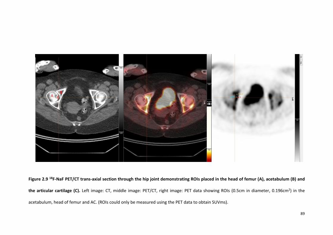
89

Figure 2.9 18F-NaF PET/CT trans-axial section through the hip joint demonstrating ROIs placed in the head of femur (A), acetabulum (B) and

the articular cartilage (C). Left image: CT, middle image: PET/CT, right image: PET data showing ROIs (0.5cm in diameter, 0.196cm2) in the

acetabulum, head of femur and AC. (ROIs could only be measured using the PET data to obtain SUVms).

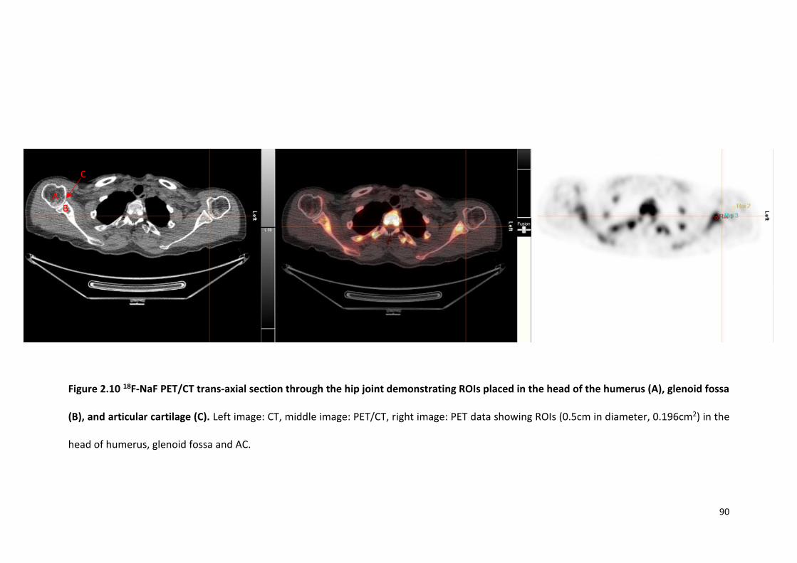
90

Figure 2.10 18F-NaF PET/CT trans-axial section through the hip joint demonstrating ROIs placed in the head of the humerus (A), glenoid fossa

(B), and articular cartilage (C). Left image: CT, middle image: PET/CT, right image: PET data showing ROIs (0.5cm in diameter, 0.196cm2) in the

head of humerus, glenoid fossa and AC.

A B

C

91

2.6 COBB ANGLE MEASURMENTS

Cobb angles are used to standardise spinal curvatures. Thoracic kyphosis is the

outward curvature of the thoracic spine. Normal thoracic kyphosis ranges from 20-

45 degrees, hyperkyphosis exceeds 45 degrees (122). Lumbar lordosis is the inward

curvature of the lumbar spine. There is no defined measurements that determine

hyper or hypo lumbar lordosis as muscular strength, flexibility and BMI all affect this

angle (123). Scoliosis is defined as a lateral curvature of the spine of 10 degrees or

more to the right or left (124). Spinal kyphosis, lordosis and scoliosis Cobb angles

were measured for all SONIA 2 patients using the picture archiving and

communications system (PACS) software. X-Ray and MRI images were electronically

stored and accessed via PACS, and Cobb angles were generated for both scans for

each patient. Access to the PACS system was via the Royal Liverpool and Broadgreen

University Hospital Trust computer.

2.6.1 X-RAY SCOLIOSIS MEASUREMENTS

Whole body posteroanterior (PA) X-Ray view was selected to analyse scoliosis. Using

the Cobb angle tool the end vertebrae of the curve were selected and lines were

drawn to demarcate the vertebrae that lie at the upper and lower limits of the curve

(the vertebrae that tilt the most towards the apex of the curve) (Figure 2.11A). The

Cobb angle was automatically generated measuring the intersection of the two lines

drawn. Scoliosis is clinically defined as a spinal curvature of more than 10 degrees to

the right or left (124).

92

2.6.2 X-RAY THORACIC KYPHOSIS AND LUMBAR LORDOSIS MEASUREMENTS

Lateral X-ray view was selected to measure thoracic kyphosis and lumbar lordosis

Cobb angles. Using the Cobb angle tool the lower border of the twelfth thoracic

vertebrae (T12) and the upper border of the fourth thoracic vertebrae (T4) were

selected to define thoracic kyphosis (125) (Figure 2.11B). The Cobb angle was

automatically generated by measuring the intersection between the lines selected.

Normal kyphosis ranges from 20-45 degrees, hyper kyphosis is defined as more than

45 degrees (122). Lumbar lordosis was measured from the lower border of the fifth

lumbar (L5) vertebrae and the upper border of the first lumbar vertebrae (L1).

Lumbar hyperlordosis is not defined by a Cobb angle (Figure 2.11B).

2.6.3 MRI THORACIC KYPHOSIS AND LUMBAR LORDOSIS MEASUREMENTS

Thoracic kyphosis and lumbar lordosis Cobb angles were also measured on MRI

(Figure 2.11C). The MRI whole spine was selected using the PACS and the

methodology of measuring thoracic kyphosis and lumbar lordosis was exactly as

described in section 2.6.2.

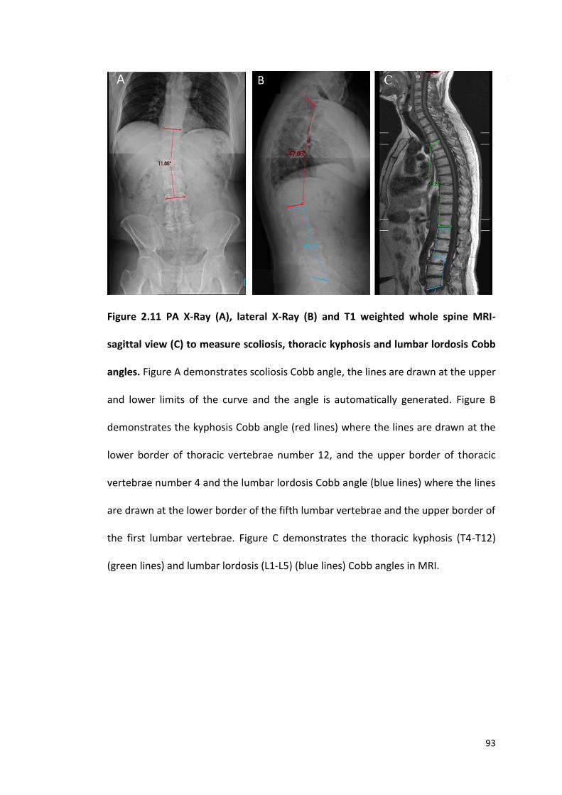
93

Figure 2.11 PA X-Ray (A), lateral X-Ray (B) and T1 weighted whole spine MRI-

sagittal view (C) to measure scoliosis, thoracic kyphosis and lumbar lordosis Cobb

angles. Figure A demonstrates scoliosis Cobb angle, the lines are drawn at the upper

and lower limits of the curve and the angle is automatically generated. Figure B

demonstrates the kyphosis Cobb angle (red lines) where the lines are drawn at the

lower border of thoracic vertebrae number 12, and the upper border of thoracic

vertebrae number 4 and the lumbar lordosis Cobb angle (blue lines) where the lines

are drawn at the lower border of the fifth lumbar vertebrae and the upper border of

the first lumbar vertebrae. Figure C demonstrates the thoracic kyphosis (T4-T12)

(green lines) and lumbar lordosis (L1-L5) (blue lines) Cobb angles in MRI.

94

2.7 SPINAL FLEXIBILITY MEASUREMENTS

2.7.1 LUMBAR SIDE FLEXION MEASUREMENTS

Lumbar side flexion was measured by a senior physiotherapist at the RLBUHT.

Lumbar side flexion was measured by firstly asking the patient to stand up straight

against the wall with their shoulders back and feet 12 inches apart. The distance

between the tip of the middle finger and the floor was measured on the left and right

sides. The patient was then asked to side flex and then the physiotherapist applied

slight over pressure to push the patient further into the range, the distance between

the tip of the finger and the floor was re-measured on both the left and right sides to

obtain the passive range of motion. The difference between the two measurements

on both the right and the left was calculated reflecting passive lumbar side flexion of

the patient to the right and to the left in cm (126,127). The passive range of

movement determines the maximum amount of movement possible at the joint, and

is usually higher than the active range of movement which is the distance before the

physiotherapist applies the slight over pressure to push the patients further into the

range. The passive range of motion was used for analysis in this thesis.

2.7.2 CERVICAL SPINE ROTATION MEASURMENTS

Cervical spine rotation was measured by a senior physiotherapist at the RLBUHT.

Cervical spine rotation was measured by firstly asking the patient to stand up straight

against the wall with their shoulders back in a neutral position with the head facing

forwards. The distance between the gnathion (midpoint of the lower border of the

95

mandible) of the chin to the lateral aspect of the acromion of the scapula was

measured with the head looking straight forwards on both the right and left sides.

The patient was then asked to turn their head to the right side with the

physiotherapist applying over pressure to push the patient further into the range.

The distance between the gnathion and lateral aspect of the acromion was re-

measured and the difference between the two values was then calculated to obtain

the value for passive cervical spine rotation. These measurements were then

repeated on the left (126,127).

2.8 STATISTICAL ANALYSIS

All statistical analysis was carried out using Stats Direct statistical software (Version:

3.0.171). The data was plotted using Stats Direct to see if the data was normally

distributed using the Kolmogorov-Smirnov (K-S) test. The K-S test produces a p value,

if p>0.05 the data is assumed to be normally distributed. Histograms were plotted to

confirm these distributions. Parametric tests were carried out on normally

distributed data. Non-parametric tests were carried out on non-normally distributed

data.

2.8.1 PARAMETRIC TESTS

Independent samples t-tests were carried out to compare the means of a normally

distributed interval dependant variable for two independent groups. Paired

(samples) t-test were carried out to compare means from the same individual. The

result of these tests provided p values a p≤0.05 was statistically significant. A p≤0.05

96

typically indicates strong evidence against the null hypothesis, so the null hypothesis

is rejected. The null hypothesis states that there is no relationship between two

measured phenomena.

2.8.2 NON-PARAMETRIC TESTS

Wilcoxon-Mann-Whitney test is a non-parametric analog to the independent samples

t-test and was used when the dependant variable was not normally distributed. The

Wilcoxon signed rank sum test is the non-parametric version of a paired samples t-

test. This test was used when the distribution was not normally distributed.

2.8.3 REGRESSION ANALYSIS

2.8.3.1 Multiple linear regression

A multivariate statistical technique was used to examine the linear correlations

between two or more independent variables and a single dependent variable.

Multiple linear regression analysis was used to compare control and AKU patients

SUVm (in thoracic and lumbar vertebrae and IVDs) with age. The outcome variable

was mean lumbar/thoracic IVD/vertebrae. The grouping variable was either V1 (AKU)

vs control group, or V3 (AKU) vs control group and the other variable tested was age.

2.8.3.2 Simple linear regression and Pearson’s correlation

Simple linear regression and Pearson’s correlation was used to test the correlation

between two variables. Pearsons r value defines the strength of the relationship, and

97

has a value between +1 and -1, where 1 is total positive linear correlation, 0 is no

correlation and -1 is total negative correlation. The p value defines the significance

level of the correlation (p≤0.05 is statistically significant). The R2, the coefficient of

determination is a statistical measure of how close the data are fitted to the

regression line which was plotted on the graphs.

2.8.4 TREND LINES

Trend lines were added to graphs using Excel. The distribution of the data was

assessed and the most appropriate trend line was selected based on the distribution.

A linear trend line was applied when the data set had a simple linear correlation. In

situations where the data did not indicate a linear relationship, polynomial models

were tested. The criteria for selecting a polynomial fit was as follows:

1. In situations where the relationships were hypothesised to be curvilinear. For

example, the relationship between uptake of 18F into the lumbar and thoracic

IVDs (Figure 4.12 and 4.13), as discussed in Section.

2. A visible inspection indicated the data are bivariate, for example the inverted

‘U’ shaped trends shown in Figure 4.12 and 4.13.

3. When an inspection of residuals reveals that a linear model is not appropriate

Where appropriate a second order polynomial line was applied to data that had one

peak or trough.

98

3.0 SKELETAL DISTRIBUTION OF INCREASED 18F PET UPTAKE IN PATIENTS WITH

ALKAPTONURIA

99

3.1 INTRODUCTION

Early osteoarthropathy is an inevitable consequence of AKU resulting in considerable

pain and suffering in peak adulthood due to premature joint and spinal disease.

Weight bearing joints are thought to be predominantly affected due to increased

mechanical damage (1). The purpose of this study was to investigate the natural

history of alkaptonuria using the novel imaging modality 18F-NaF PET. A semi-

quantitative approach was used to assess the anatomical distribution of

osteoarthropathy with age.

Plain X-Ray is still the gold standard imaging modality to diagnose arthritic disease,

however it is realised that functional abnormalities can exist without radiographic

evidence. 18F-NaF PET is a valuable tool to detect functional skeletal involvement and

is routinely used in diagnosing skeletal metastatic disease. However, more recently it

has been utilised in identifying arthropathy in OA and in AKU. 18F-NaF PET provides

highly sensitive, three-dimensional imaging of the skeleton with advantages such as

high spatial resolution, superior image quality and hybrid PET/CT imaging providing

accurate anatomical localisation (89). Upon injection of the radiotracer 18F covalently

binds to hydroxyapatite crystals of newly forming bone and therefore reflects the

amount of actively mineralising bone present and closely resembles bone

metabolism (110). A positive or abnormal scan manifests itself as an area of increased

radiotracer uptake and reflects the increased osteogenic activity at that site.

Radiotracer delivery is also dependent on regional blood flow therefore the scan also

provides an index of vascularity of bone (89). Increased osteogenic activity and

100

vascularity are features of a degenerating joint due to the inflammatory and healing

processes that occur in response to injury hence why this imaging modality is useful

in AKU (89).

Until recently there has been a lack of semi-quantifiable methodology to describe

AKU disease severity. The AKUSSI attempts to assess all features of AKU in a

standardised manner producing a composite score representing the totality of clinical

features. Table 1.2 represents the AKUSSI. The 18F-NaF PET scans are analysed by an

experienced nuclear medicine consultant. The large joint areas scored are the

shoulder, elbow, wrist and hands, hip, knee, ankle, foot and the cervical, thoracic and

lumbar spine based on increased uptake at that site. Increased uptake is given a score

of 1 in each large joint and a score of zero is given if the joint has normal uptake. These

scores are then fed into the AKUSSI and contribute the final aggregated score. It is

important to note that this scoring is based on the opinion of the nuclear medicine

consultant and therefore is subjective. This work attempts to develop a semi-

quantitative method that demarcates the boundary between increased tracer uptake

and normal bone uptake that could be used as an alternative or a complementary

non-subjective method to score the 18F-NaF PET scans by the clinician.

101

3.2 DESIGN OF STUDY

3.2.1 PATIENT GROUP

43 adult patients (17 females, 26 males, mean age 49, SD±14.8, range 21-74) from

the National Alkaptonuria Centre (see section 2.2.1) underwent 18F-NaF PET scanning.

Baseline (pre-nitisinone) PET images were analysed for each patient (see section 2.3

for PET protocol). Patients were included only if a whole-body MIP scan was present.

Five patients (Patients 9,11,23,27,30) were excluded from the correlation with the

clinical score as the AKUSSI analysis was not available.

3.2.2 IMAGE ANALYSIS

Baseline 8-bit MIP PET images of the 43 NAC patients were imported into Image J

(1.49j). A histogram plot was created for each patient to analyse the distribution of

pixel values within the image. A threshold was applied (as described in 2.4.4)

highlighting the pixel values that represent increased tracer uptake that are

associated with AKU disease pathology.

3.2.3 ANATOMICAL SCORING

The MIP PET images were then analysed anatomically (as described in section 2.4.5)

and were scored based on the presence or absence of pixel values above threshold.

A score of 0 or 1 was given (0= no pixels present above threshold, 1= at least one pixel

identified above threshold in the various anatomical regions). Pixels above threshold

represent increased tracer uptake at that site associated with disease pathology. This

method aims to remove any subjectivity in observing regions of increased tracer

uptake associated with disease pathology.

102

3.3 RESULTS

Each patient was scored for the presence or absence of pixels above the threshold

value in the various anatomical locations. Both cartilaginous joints and bones were

analysed. For the bony anatomy the calcaneus, talus, midfoot, forefoot, tibia, fibula,

patella, femur, hip, sacrum, vertebrae (L5-C1), scapulae, humerus, radius, ulna, carpal,

metacarpal/ phalanges, clavicle and sternum were scored 0 or 1 (0= if no pixels were

present above threshold 1= if pixels were identified above threshold). For the

cartilaginous joints, the joints of the foot, ankle, knee, hip, sacroiliac joint,

intervertebral discs (S1/L5 – C1/C2), shoulder, elbow, wrist and hand were scored 0

or 1 as described above. The percentage incidence of increased tracer uptake (pixel

values above threshold) was calculated and plotted on a skeletal map (Figure 2.5

shows a skeletal map of regions analysed) demonstrating the bones and joints most

affected by the disease. The percentage incidence was calculated by adding up the

scores from all patients at each anatomical site. The cohort was split into five age

dependant groups (21-30 n=8, 31-40 n=5, 41-50 n=7, 51-60 n=12, 61-70+ n=11) to

assess distribution with age.

3.3.1 SKELETAL DISTRIBUTION OF INCREASED 18F UPTAKE WITH AGE IN THE BONES

OF THE SKELETON

Figure 3.1 demonstrates the skeletal distribution of increased 18F PET uptake in the

bones of the skeleton. The highest incidences of increased tracer uptake were found

in the hip, sacrum and thoracic and lumbar vertebral bodies (93%, 64%, 73% and 80%

incidence respectively) (Figure 3.1). The lowest incidences were found in the bones

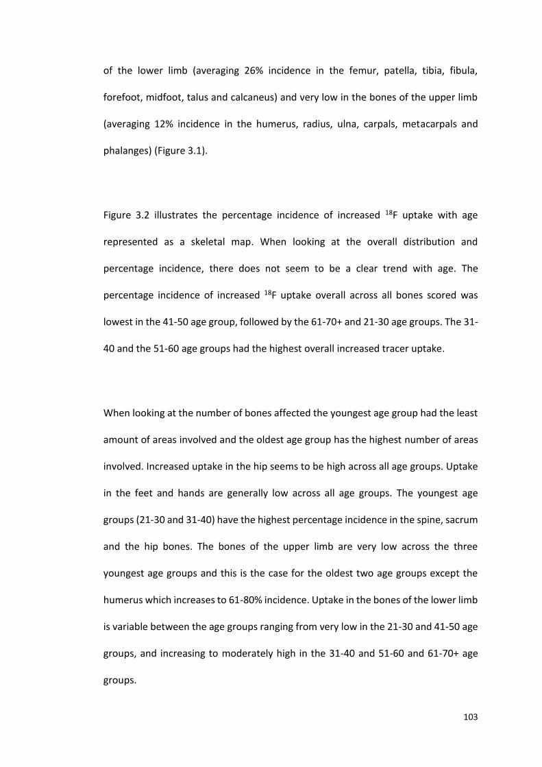
103

of the lower limb (averaging 26% incidence in the femur, patella, tibia, fibula,

forefoot, midfoot, talus and calcaneus) and very low in the bones of the upper limb

(averaging 12% incidence in the humerus, radius, ulna, carpals, metacarpals and

phalanges) (Figure 3.1).

Figure 3.2 illustrates the percentage incidence of increased 18F uptake with age

represented as a skeletal map. When looking at the overall distribution and

percentage incidence, there does not seem to be a clear trend with age. The

percentage incidence of increased 18F uptake overall across all bones scored was

lowest in the 41-50 age group, followed by the 61-70+ and 21-30 age groups. The 31-

40 and the 51-60 age groups had the highest overall increased tracer uptake.

When looking at the number of bones affected the youngest age group had the least

amount of areas involved and the oldest age group has the highest number of areas

involved. Increased uptake in the hip seems to be high across all age groups. Uptake

in the feet and hands are generally low across all age groups. The youngest age

groups (21-30 and 31-40) have the highest percentage incidence in the spine, sacrum

and the hip bones. The bones of the upper limb are very low across the three

youngest age groups and this is the case for the oldest two age groups except the

humerus which increases to 61-80% incidence. Uptake in the bones of the lower limb

is variable between the age groups ranging from very low in the 21-30 and 41-50 age

groups, and increasing to moderately high in the 31-40 and 51-60 and 61-70+ age

groups.

104

Figure 3.1 Percentage incidence of increased 18F uptake in the bones of the

skeleton. Percentage incidence = the number of patients identified to have increased

tracer uptake at a specific anatomical site as a percentage. n=43 (17 females, 26

males, mean age 49, SD±14.8, range 21-74).

CA

LC

AN

EU

S

TA

LU

S

MID

FO

OT

FO

RE

FO

OT

TIB

IA

FIB

UL

A

PA

TE

LL

A

FE

MU

R

HIP

SA

CR

UM

L5

L4

L3

L2

L1

T1

2

T1

1

T1

0

T9

T8

T7

T6

T5

T4

T3

T2

T1

C7

C6

C5

C4

C3

C2

C1

SC

AP

UL

A

HU

ME

RU

S

RA

DIU

S

UL

NA

CA

RP

AL

ME

TA

CA

RP

AL

/ …

CL

AV

ICL

E

0

10

20

30

40

50

60

70

80

90

100

BONES

PER

CEN

TAG

E IN

CID

ENC

E (%

)

% incidence

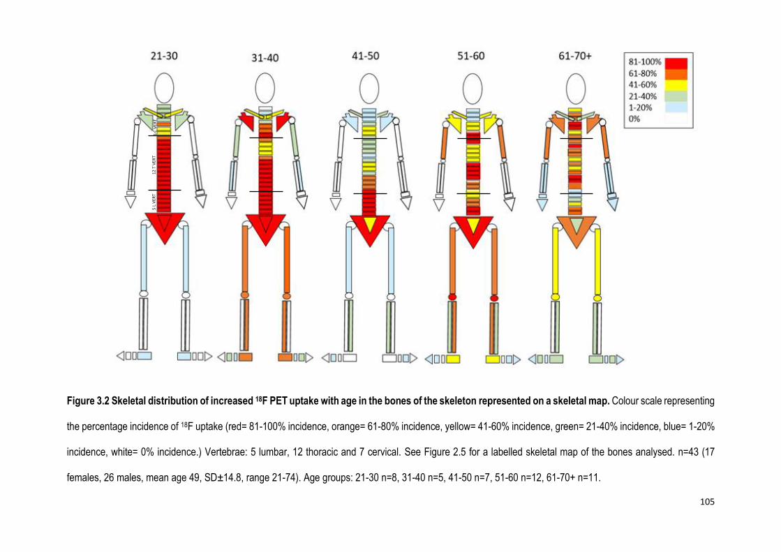
105

Figure 3.2 Skeletal distribution of increased 18F PET uptake with age in the bones of the skeleton represented on a skeletal map. Colour scale representing

the percentage incidence of 18F uptake (red= 81-100% incidence, orange= 61-80% incidence, yellow= 41-60% incidence, green= 21-40% incidence, blue= 1-20%

incidence, white= 0% incidence.) Vertebrae: 5 lumbar, 12 thoracic and 7 cervical. See Figure 2.5 for a labelled skeletal map of the bones analysed. n=43 (17

females, 26 males, mean age 49, SD±14.8, range 21-74). Age groups: 21-30 n=8, 31-40 n=5, 41-50 n=7, 51-60 n=12, 61-70+ n=11.

5 L

VER

T

12 T

VER

T

6 C

VER

T

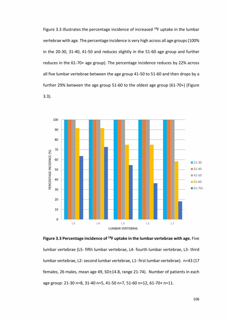
106

Figure 3.3 illustrates the percentage incidence of increased 18F uptake in the lumbar

vertebrae with age. The percentage incidence is very high across all age groups (100%

in the 20-30, 31-40, 41-50 and reduces slightly in the 51-60 age group and further

reduces in the 61-70+ age group). The percentage incidence reduces by 22% across

all five lumbar vertebrae between the age group 41-50 to 51-60 and then drops by a

further 29% between the age group 51-60 to the oldest age group (61-70+) (Figure

3.3).

Figure 3.3 Percentage incidence of 18F uptake in the lumbar vertebrae with age. Five

lumbar vertebrae (L5- fifth lumbar vertebrae, L4- fourth lumbar vertebrae, L3- third

lumbar vertebrae, L2- second lumbar vertebrae, L1- first lumbar vertebrae). n=43 (17

females, 26 males, mean age 49, SD±14.8, range 21-74). Number of patients in each

age group: 21-30 n=8, 31-40 n=5, 41-50 n=7, 51-60 n=12, 61-70+ n=11.

L 5 L 4 L 3 L 2 L 1

0

10

20

30

40

50

60

70

80

90

100

LUMBAR VERTEBRAE

PER

CEN

TAG

E IN

CID

ENC

E (%

)

21-30

31-40

41-50

51-60

61-70+

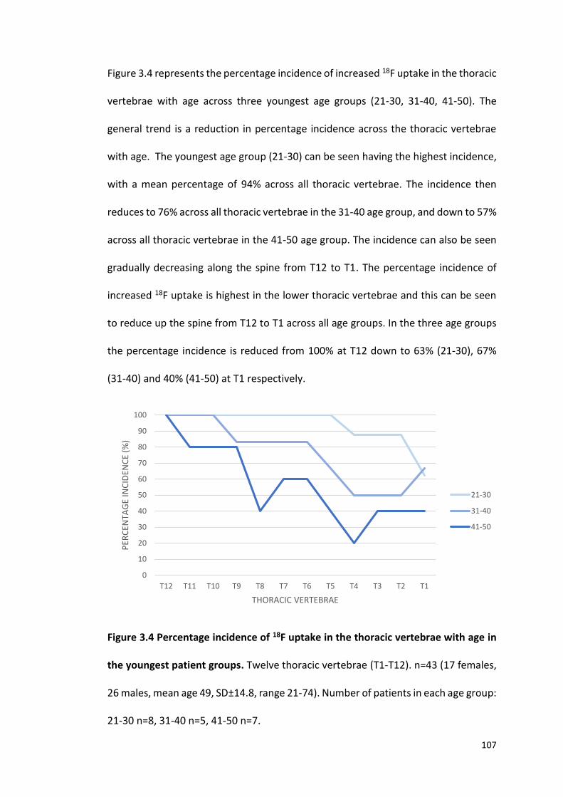
107

Figure 3.4 represents the percentage incidence of increased 18F uptake in the thoracic

vertebrae with age across three youngest age groups (21-30, 31-40, 41-50). The

general trend is a reduction in percentage incidence across the thoracic vertebrae

with age. The youngest age group (21-30) can be seen having the highest incidence,

with a mean percentage of 94% across all thoracic vertebrae. The incidence then

reduces to 76% across all thoracic vertebrae in the 31-40 age group, and down to 57%

across all thoracic vertebrae in the 41-50 age group. The incidence can also be seen

gradually decreasing along the spine from T12 to T1. The percentage incidence of

increased 18F uptake is highest in the lower thoracic vertebrae and this can be seen

to reduce up the spine from T12 to T1 across all age groups. In the three age groups

the percentage incidence is reduced from 100% at T12 down to 63% (21-30), 67%

(31-40) and 40% (41-50) at T1 respectively.

Figure 3.4 Percentage incidence of 18F uptake in the thoracic vertebrae with age in

the youngest patient groups. Twelve thoracic vertebrae (T1-T12). n=43 (17 females,

26 males, mean age 49, SD±14.8, range 21-74). Number of patients in each age group:

21-30 n=8, 31-40 n=5, 41-50 n=7.

0

10

20

30

40

50

60

70

80

90

100

T12 T11 T10 T9 T8 T7 T6 T5 T4 T3 T2 T1

PER

CEN

TAG

E IN

CID

ENC

E (%

)

THORACIC VERTEBRAE

21-30

31-40

41-50

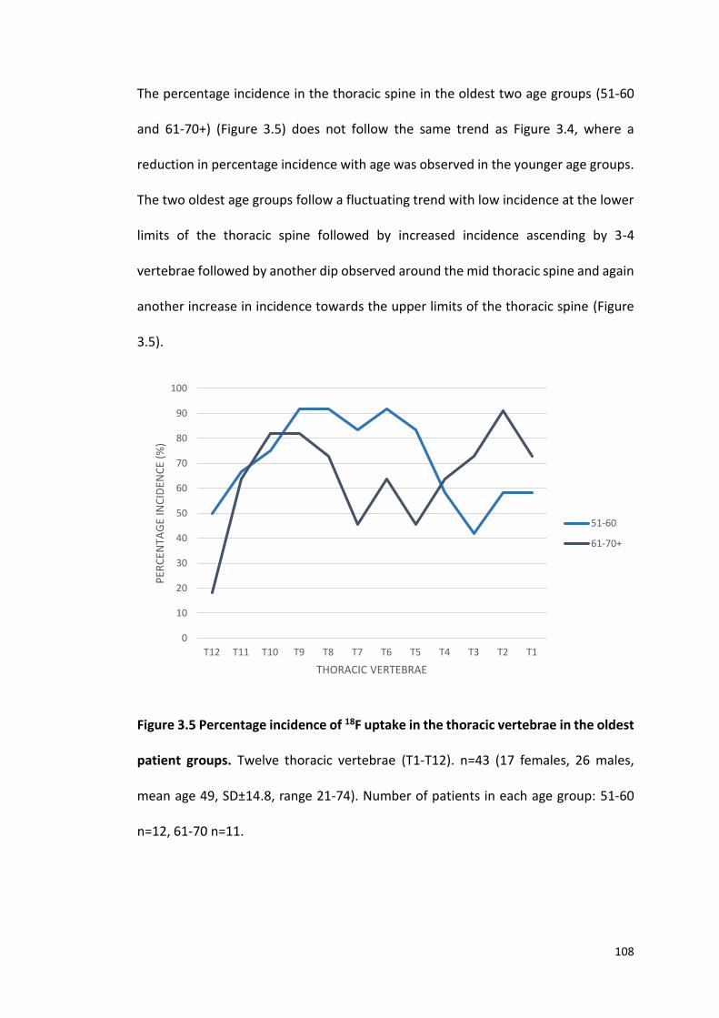
108

The percentage incidence in the thoracic spine in the oldest two age groups (51-60

and 61-70+) (Figure 3.5) does not follow the same trend as Figure 3.4, where a

reduction in percentage incidence with age was observed in the younger age groups.

The two oldest age groups follow a fluctuating trend with low incidence at the lower

limits of the thoracic spine followed by increased incidence ascending by 3-4

vertebrae followed by another dip observed around the mid thoracic spine and again

another increase in incidence towards the upper limits of the thoracic spine (Figure

3.5).

Figure 3.5 Percentage incidence of 18F uptake in the thoracic vertebrae in the oldest

patient groups. Twelve thoracic vertebrae (T1-T12). n=43 (17 females, 26 males,

mean age 49, SD±14.8, range 21-74). Number of patients in each age group: 51-60

n=12, 61-70 n=11.

0

10

20

30

40

50

60

70

80

90

100

T12 T11 T10 T9 T8 T7 T6 T5 T4 T3 T2 T1

PER

CEN

TAG

E IN

CID

ENC

E (%

)

THORACIC VERTEBRAE

51-60

61-70+

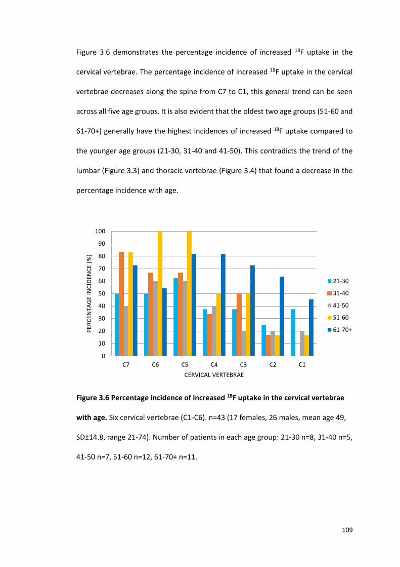
109

Figure 3.6 demonstrates the percentage incidence of increased 18F uptake in the

cervical vertebrae. The percentage incidence of increased 18F uptake in the cervical

vertebrae decreases along the spine from C7 to C1, this general trend can be seen

across all five age groups. It is also evident that the oldest two age groups (51-60 and

61-70+) generally have the highest incidences of increased 18F uptake compared to

the younger age groups (21-30, 31-40 and 41-50). This contradicts the trend of the

lumbar (Figure 3.3) and thoracic vertebrae (Figure 3.4) that found a decrease in the

percentage incidence with age.

Figure 3.6 Percentage incidence of increased 18F uptake in the cervical vertebrae

with age. Six cervical vertebrae (C1-C6). n=43 (17 females, 26 males, mean age 49,

SD±14.8, range 21-74). Number of patients in each age group: 21-30 n=8, 31-40 n=5,

41-50 n=7, 51-60 n=12, 61-70+ n=11.

0

10

20

30

40

50

60

70

80

90

100

C7 C6 C5 C4 C3 C2 C1

PER

CEN

TAG

E IN

CID

ENC

E (%

)

CERVICAL VERTEBRAE

21-30

31-40

41-50

51-60

61-70+

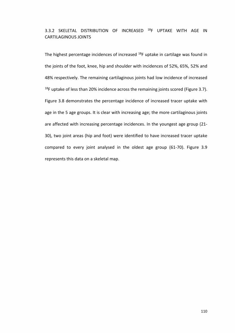
110

3.3.2 SKELETAL DISTRIBUTION OF INCREASED 18F UPTAKE WITH AGE IN

CARTILAGINOUS JOINTS

The highest percentage incidences of increased 18F uptake in cartilage was found in

the joints of the foot, knee, hip and shoulder with incidences of 52%, 65%, 52% and

48% respectively. The remaining cartilaginous joints had low incidence of increased

18F uptake of less than 20% incidence across the remaining joints scored (Figure 3.7).

Figure 3.8 demonstrates the percentage incidence of increased tracer uptake with

age in the 5 age groups. It is clear with increasing age; the more cartilaginous joints

are affected with increasing percentage incidences. In the youngest age group (21-

30), two joint areas (hip and foot) were identified to have increased tracer uptake

compared to every joint analysed in the oldest age group (61-70). Figure 3.9

represents this data on a skeletal map.

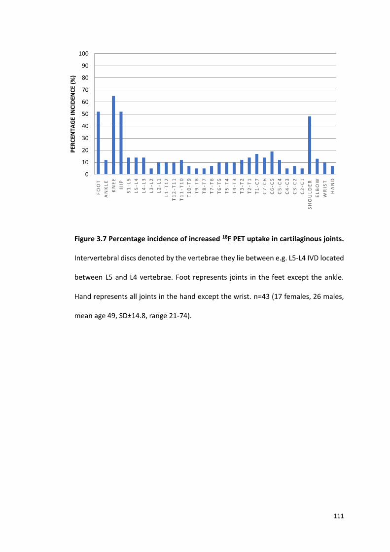
111

Figure 3.7 Percentage incidence of increased 18F PET uptake in cartilaginous joints.

Intervertebral discs denoted by the vertebrae they lie between e.g. L5-L4 IVD located

between L5 and L4 vertebrae. Foot represents joints in the feet except the ankle.

Hand represents all joints in the hand except the wrist. n=43 (17 females, 26 males,

mean age 49, SD±14.8, range 21-74).

FO

OT

AN

KL

E

KN

EE

HIP

S1

-L5

L5

-L4

L4

-L3

L3

-L2

L2

-L1

L1

-T1

2

T1

2-T

11

T1

1-T

10

T1

0-T

9

T9

-T8

T8

-T7

T7

-T6

T6

-T5

T5

-T4

T4

-T3

T3

-T2

T2

-T1

T1

-C7

C7

-C6

C6

-C5

C5

-C4

C4

-C3

C3

-C2

C2

-C1

SH

OU

LD

ER

EL

BO

W

WR

IST

HA

ND

0

10

20

30

40

50

60

70

80

90

100

PER

CEN

TAG

E IN

CID

ENC

E (%

)

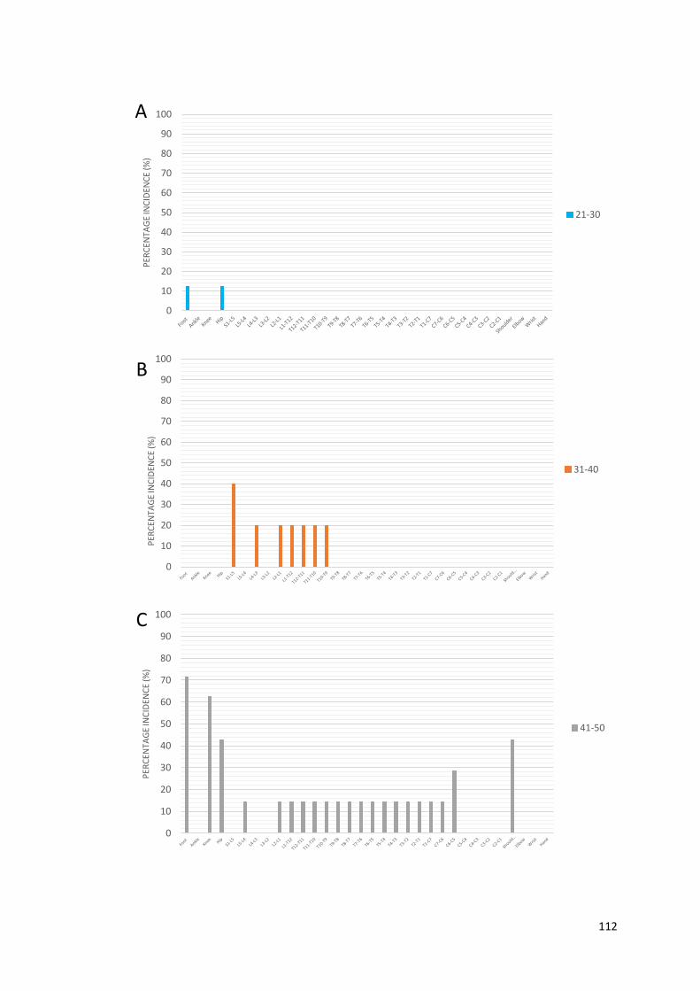
112

0

10

20

30

40

50

60

70

80

90

100

PER

CEN

TAG

E IN

CID

ENC

E (%

)

21-30

0

10

20

30

40

50

60

70

80

90

100

PER

CEN

TAG

E IN

CID

ENC

E (%

)

31-40

0

10

20

30

40

50

60

70

80

90

100

PER

CEN

TAG

E IN

CID

ENC

E (%

)

41-50

A

B

C

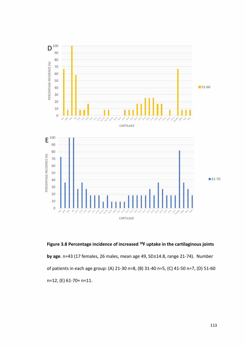
113

Figure 3.8 Percentage incidence of increased 18F uptake in the cartilaginous joints

by age. n=43 (17 females, 26 males, mean age 49, SD±14.8, range 21-74). Number

of patients in each age group: (A) 21-30 n=8, (B) 31-40 n=5, (C) 41-50 n=7, (D) 51-60

n=12, (E) 61-70+ n=11.

0

10

20

30

40

50

60

70

80

90

100P

ERC

ENTA

GE

INC

IDEN

CE

(%)

CARTILAGE

51-60

0

10

20

30

40

50

60

70

80

90

100

PER

CEN

TAG

E IN

CID

ENC

E (%

)

CARTILAGE

61-70

E

D

114

Figure 3.9 Skeletal distribution of increased 18F PET uptake with age in the cartilaginous joints of the skeleton. Colour scale representing the percentage

incidence of 18F uptake (red= 81-100% incidence, orange= 61-80% incidence, yellow= 41-60% incidence, green= 21-40% incidence, blue= 1-20% incidence,

white= 0% incidence or not analysed). IVDs: 5 lumbar, 12 thoracic and 7 cervical. See Figure 2.5 for a labelled skeletal map of the joints analysed. n=43 (17

females, 26 males, mean age 49, SD±14.8, range 21-74). Age groups: 21-30 n=8, 31-40 n=5, 41-50 n=7, 51-60 n=12, 61-70+ n=11.

5 L IVDs

12 T IVDs

7 C IVDs

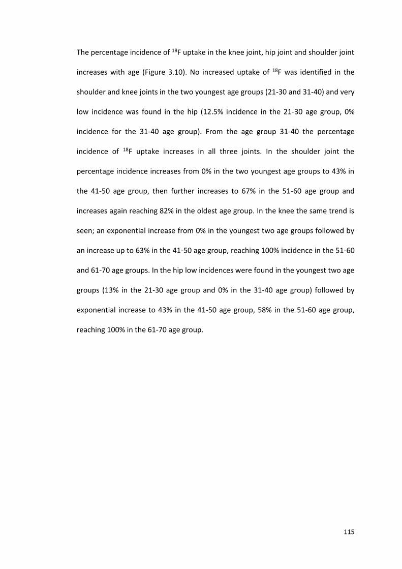
115

The percentage incidence of 18F uptake in the knee joint, hip joint and shoulder joint

increases with age (Figure 3.10). No increased uptake of 18F was identified in the

shoulder and knee joints in the two youngest age groups (21-30 and 31-40) and very

low incidence was found in the hip (12.5% incidence in the 21-30 age group, 0%

incidence for the 31-40 age group). From the age group 31-40 the percentage

incidence of 18F uptake increases in all three joints. In the shoulder joint the

percentage incidence increases from 0% in the two youngest age groups to 43% in

the 41-50 age group, then further increases to 67% in the 51-60 age group and

increases again reaching 82% in the oldest age group. In the knee the same trend is

seen; an exponential increase from 0% in the youngest two age groups followed by

an increase up to 63% in the 41-50 age group, reaching 100% incidence in the 51-60

and 61-70 age groups. In the hip low incidences were found in the youngest two age

groups (13% in the 21-30 age group and 0% in the 31-40 age group) followed by

exponential increase to 43% in the 41-50 age group, 58% in the 51-60 age group,

reaching 100% in the 61-70 age group.

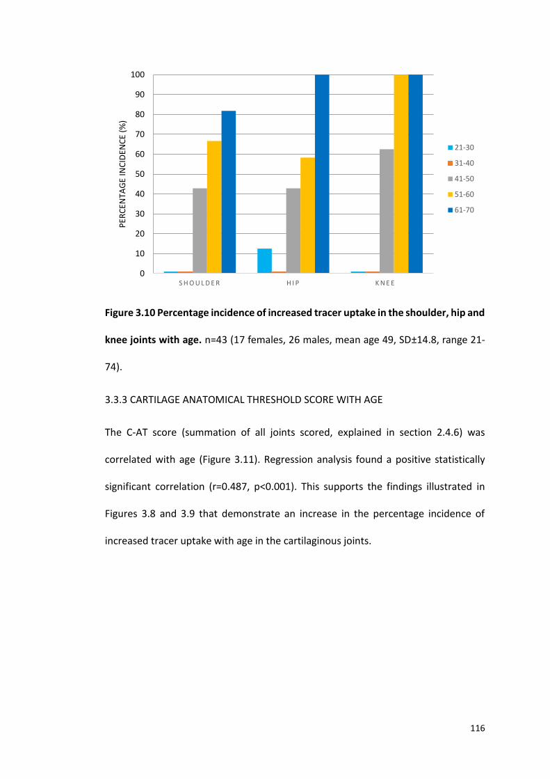
116

Figure 3.10 Percentage incidence of increased tracer uptake in the shoulder, hip and

knee joints with age. n=43 (17 females, 26 males, mean age 49, SD±14.8, range 21-

74).

3.3.3 CARTILAGE ANATOMICAL THRESHOLD SCORE WITH AGE

The C-AT score (summation of all joints scored, explained in section 2.4.6) was

correlated with age (Figure 3.11). Regression analysis found a positive statistically

significant correlation (r=0.487, p<0.001). This supports the findings illustrated in

Figures 3.8 and 3.9 that demonstrate an increase in the percentage incidence of

increased tracer uptake with age in the cartilaginous joints.

S H O U L D E R H I P K N E E 0

10

20

30

40

50

60

70

80

90

100

PER

CEN

TAG

E IN

CID

ENC

E (%

)

21-30

31-40

41-50

51-60

61-70

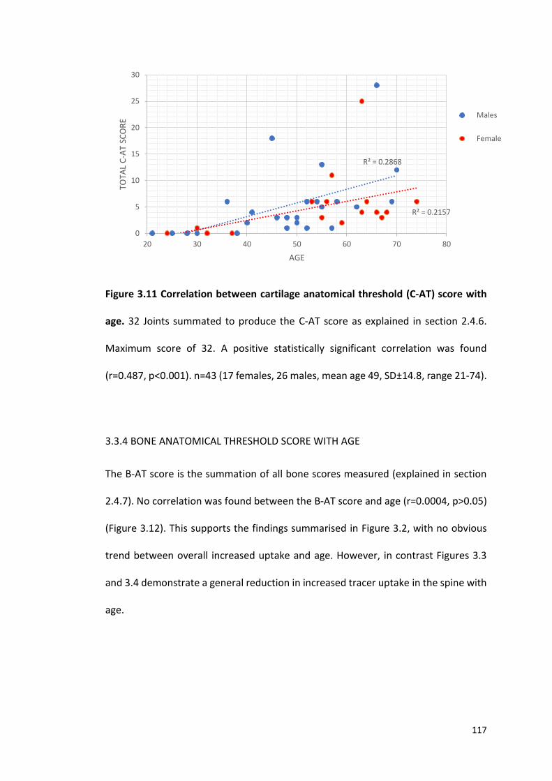
117

Figure 3.11 Correlation between cartilage anatomical threshold (C-AT) score with

age. 32 Joints summated to produce the C-AT score as explained in section 2.4.6.

Maximum score of 32. A positive statistically significant correlation was found

(r=0.487, p<0.001). n=43 (17 females, 26 males, mean age 49, SD±14.8, range 21-74).

3.3.4 BONE ANATOMICAL THRESHOLD SCORE WITH AGE

The B-AT score is the summation of all bone scores measured (explained in section

2.4.7). No correlation was found between the B-AT score and age (r=0.0004, p>0.05)

(Figure 3.12). This supports the findings summarised in Figure 3.2, with no obvious

trend between overall increased uptake and age. However, in contrast Figures 3.3

and 3.4 demonstrate a general reduction in increased tracer uptake in the spine with

age.

R² = 0.2868

R² = 0.2157

0

5

10

15

20

25

30

20 30 40 50 60 70 80

TOTA

L C

-AT

SCO

RE

AGE

Males

Female

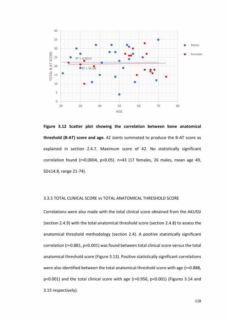
118

Figure 3.12 Scatter plot showing the correlation between bone anatomical

threshold (B-AT) score and age. 42 Joints summated to produce the B-AT score as

explained in section 2.4.7. Maximum score of 42. No statistically significant

correlation found (r=0.0004, p>0.05). n=43 (17 females, 26 males, mean age 49,

SD±14.8, range 21-74).

3.3.5 TOTAL CLINICAL SCORE vs TOTAL ANATOMICAL THRESHOLD SCORE

Correlations were also made with the total clinical score obtained from the AKUSSI

(section 2.4.9) with the total anatomical threshold score (section 2.4.8) to assess the

anatomical threshold methodology (section 2.4). A positive statistically significant

correlation (r=0.881, p<0.001) was found between total clinical score versus the total

anatomical threshold score (Figure 3.13). Positive statistically significant correlations

were also identified between the total anatomical threshold score with age (r=0.888,

p<0.001) and the total clinical score with age (r=0.956, p<0.001) (Figures 3.14 and

3.15 respectively).

R² = 5E-06

R² = 0.0013

0

5

10

15

20

25

30

35

40

20 30 40 50 60 70 80

TOTA

L B

-AT

SCO

RE

AGE

Males

Females

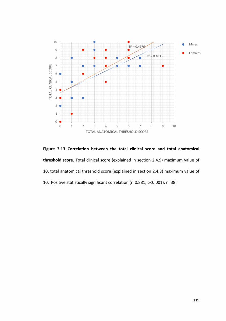
119

Figure 3.13 Correlation between the total clinical score and total anatomical

threshold score. Total clinical score (explained in section 2.4.9) maximum value of

10, total anatomical threshold score (explained in section 2.4.8) maximum value of

10. Positive statistically significant correlation (r=0.881, p<0.001). n=38.

R² = 0.4033

R² = 0.4676

0

1

2

3

4

5

6

7

8

9

10

0 1 2 3 4 5 6 7 8 9 10

TOTA

L C

LIN

ICA

L SC

OR

E

TOTAL ANATOMICAL THRESHOLD SCORE

Males

Females

120

Figure 3.14 Correlation between the total anatomical threshold score with age.

Total anatomical threshold score explained in section 2.4.8. Positive statistically

significant correlation (r=0.888, p<0.001). n=43 (17 females, 26 males, mean age 49,

SD±14.8, range 21-74).

R² = 0.7451

R² = 0.5089

0

1

2

3

4

5

6

7

8

9

10

20 25 30 35 40 45 50 55 60 65 70 75 80

TOTA

L A

NA

TOM

ICA

L TH

RES

HO

LD S

CO

RE

AGE

Males

Females

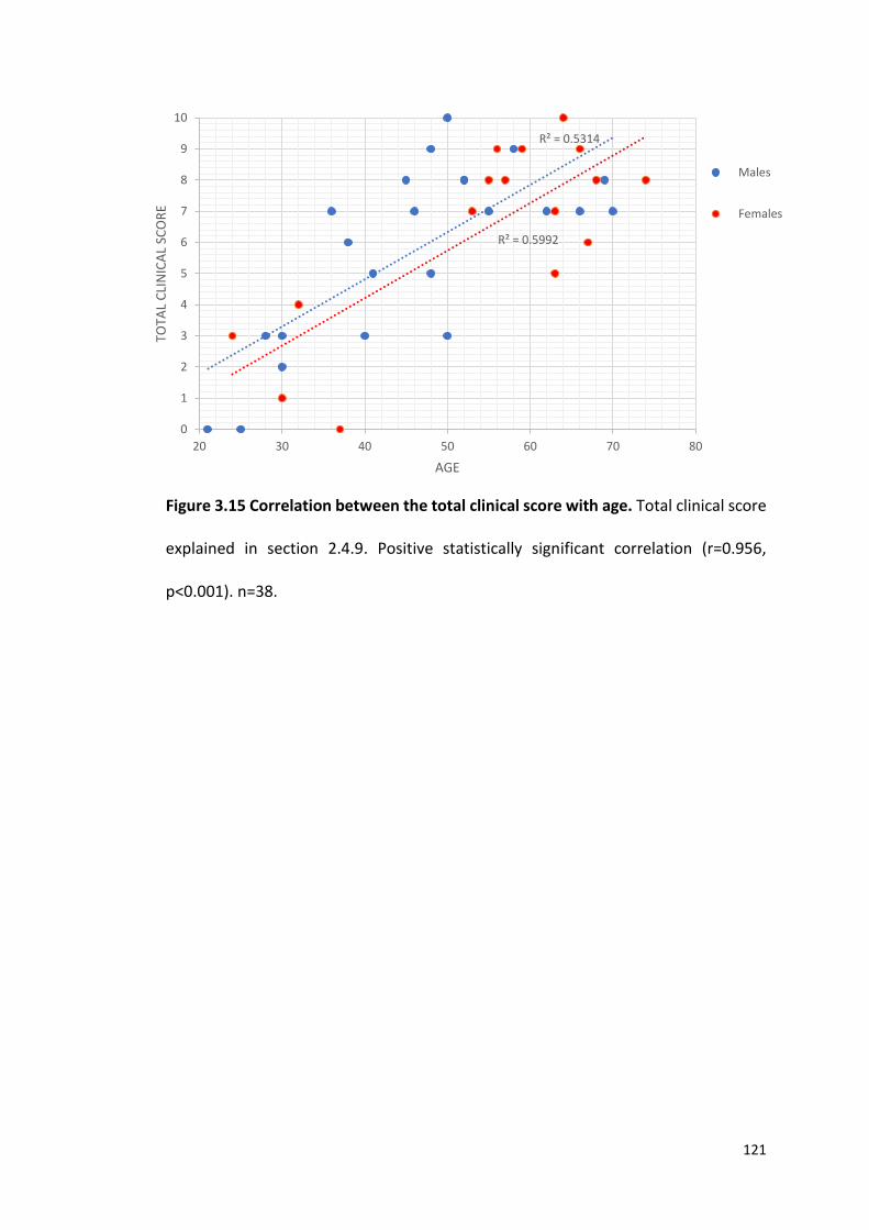
121

Figure 3.15 Correlation between the total clinical score with age. Total clinical score

explained in section 2.4.9. Positive statistically significant correlation (r=0.956,

p<0.001). n=38.

R² = 0.5314

R² = 0.5992

0

1

2

3

4

5

6

7

8

9

10

20 30 40 50 60 70 80

TOTA

L C

LIN

ICA

L SC

OR

E

AGE

Males

Females

122

3.4 DISCUSSION

18F has been utilised as a bone imaging radionuclide since the 1960’s. Although 18F-

NaF was the first widely used bone imaging agent it quickly fell into disuse.

Limitations included, logistical challenges of the 110 minute half-life of 18F-NaF , the

introduction of cheaper radiopharmaceuticals such as technetium (Tc-99m) and the

development of the Anger gamma camera designed for the 140 KeV photons of Tc-

99m resulted in the FDA to withdraw its approval in 1975 (107). The challenges

associated with 18F-NaF imaging were reassessed in 1992 when Dahlbom et al. (108)

used 18F-NaF in the development of a whole-body PET technique that demonstrated

increased spatial resolution and greater photon capture due to coincident detection

of photons. During the past decade nuclear imaging with 18F-NaF PET has re-emerged

as an attractive, specific, non-invasive method of detecting bone metabolism in

osseous diseases (109). The development of combined PET/CT scanners, ease of

production in a cyclotron (previously 18F-NaF was produced in a nuclear reactor with

a two-step reaction) coupled with shortages of Tc-99m generators, has led to 18F-NaF

being the preferred bone imaging agent once again (109). The pharmacokinetics of

18F-NaF depends on both bone uptake and elimination from the circulation. Uptake

of 18F into the skeleton reflects the amount of actively mineralising bone present and

resembles bone metabolism (109). The principle uptake mechanism involves 18F

being deposited onto the crystalline structure of hydroxyapatite of newly forming

bone by exchanging fluoride with hydroxyl ions forming fluorapatite (109,128). The

application of 18F-NaF PET to detect areas of increased bone remodelling and

inflammation has been demonstrated in many studies in various osseous diseases

(110,115,129,130). X-ray is the gold standard for imaging arthritic changes in OA.

123

Pathological changes appear with the progression of the disease and are graded

depending on the extent of involvement (KL grading scale see Table 1.3). However,

often functional abnormalities occur before clear radiographic signs appear (115).

Functional PET imaging has been shown to identify these early changes. Kobayashi et

al. (115), demonstrated the use of 18F-NaF PET in detecting bone remodelling in early

stage osteoarthritis (OA) of the hip. Increased 18F uptake was found to be associated

with increased radiographic stage of OA (KL grading scale) and the severity of hip

pain. They proposed this could be useful in deciding on a treatment strategy in early

stage OA. Watanabe et al. (129) demonstrated the coupling of inflammation and

accelerated bone turnover in rheumatoid arthritis (RA) using 18F-FDG and 18F-NaF

PET/CT. They found that accumulation of 18F-NaF correlated with clinical assessment

and physical disability in RA. Frost et al. (130) demonstrated the effect of the

antiresorptive drug risedronate on lumbar vertebrae bone metabolism in OA

measured by 18F-NaF PET. They found that osteoclastic and osteoblastic activity

displayed a significant decrease after 6 months on risedronate due to the close

coupling of bone resorption and bone formation, demonstrating the effects of the

treatment. These studies demonstrate the usefulness of 18F-NaF PET in the detection

and treatment of metabolic bone diseases.

In AKU HGA deposition over time results in ochronosis of connective tissues including

cartilage (36). It is understood that HGA deposition within cartilage alters the

mechanical properties within the tissue leading to aberrant transmission of

mechanical loading to bone resulting in resorption of the subchondral plate and

calcified cartilage. The end stage of the pathogenesis of ochronosis in the joint is

124

failure. Secondary to this the cartilage becomes calcified and becomes visible on the

PET images due to 18F binding to the calcifications forming fluorapatite. It is

understood that ochronotic cartilage becomes stiff, it is not yet fully understood

whether the calcifications form inside the ochronotic cartilage or if they are forming

on the surface despite this the calcifications must be accessible for 18F to bind. It is

unknown if binding of 18F is altered by the presence of ochronotic pigment although

it is agreed that the weight bearing joints are predominantly affected by the disease

possibly due to mechanical damage (1). AKU has pathological parallels with OA

therefore 18F-NaF PET imaging can be utilised in AKU. This is the first study to date

that looks at the distribution of 18F-NaF PET in the rare disease AKU.

3.4.1 INCREASED 18F UPTAKE IN BONE - MECHANICAL LOADING

In bone the highest incidences of increased 18F signal was found in the hip, sacrum,

thoracic and lumbar vertebrae (93%, 64%, 73% and 80% respectively) (Figure 3.1).

These bones are classically weight bearing bones and it has been proposed that there

is a link between mechanical stress and 18F uptake. It was demonstrated by Kobayashi

et al. (115) that mechanical loading enhances interleukin 11 (IL-11) gene expression

that stimulates osteoblast differentiation. The function of IL-11 is believed to be

inhibition of Dickkopf 1 and 2, which are inhibitors of Wnt signalling. Wnt signalling

has been shown as an important regulatory pathway in osteogenic differentiation.

Induction of Wnt signalling promotes bone formation, while inactivation leads to

osteopenia. If bone formation is promoted this increases the availability of

hydroxyapatite for 18F to bind. It is believed that a reduction in IL-11 with age may be

one of the factors contributing to osteoporosis (131,132).

125

Sanchez et al. (133) also demonstrated a link between mechanical stress and

increased expression of genes involved in bone remodelling and bone formation in

human osteoblasts. This chapter has demonstrated that the non-weight bearing

bones of the upper limb had very low incidences averaging 12% in comparison to the

bones of the lower limb and foot that had an average incidence of 26% (Figure 3.1).

This supports the theory that weight bearing bones experiencing mechanical loading

are associated with increased bone formation and increased 18F uptake.

Win et al. (117) described the uptake of 18F in various skeletal sites in a control

population and found that different skeletal sites have different amounts of fluoride

uptake. The proposed reason for this variation is the composition of bone at different

sites. They found that 18F tends to have greater deposition in the axial skeleton (e.g.

vertebrae and pelvis) than in the appendicular skeleton (limbs), this supports the

results described in this chapter where the highest incidences were found in the hip,

sacrum and lumbar and thoracic spine (Figures 3.1 and 3.2).

3.4.2 INCREASED 18F UPTAKE IN BONE- VASCULARITY

Uptake of 18F in bone depends on regional blood flow, osteoblastic activity and renal

clearance (117). Trabecular bone is highly vascular and contains abundant red

marrow, which may explain the increased incidence of 18F uptake in the vertebrae

and hip that contain mostly trabecular bone in contrast to relatively lower trabecular

bone in the long bones of the limbs (Figure 3.1) (134).

126

3.4.3 INCREASED 18F UPTAKE IN THE VERTEBRAE

Interestingly the incidence of increased 18F uptake in the lumbar vertebrae decreases

with age (Figure 3.3). This trend can also be seen in the three youngest age groups in

the thoracic vertebrae (Figure 3.4). It has been described that with age there is a

reduction in red marrow and an associated decrease in perfusion to bone (134).

Reduced perfusion to bone would result in reduced 18F transport to that area. This

may explain the reduction in the incidence of 18F uptake with age. It is widely agreed

that BMD decreases with age. Riggs et al. (135) found that bone diminution in the

vertebrae began in young adulthood and was linear with increasing age. A reduction

in BMD with age may explain the reduction in the incidence of increased 18F uptake

with age; if there is less hydroxyapatite available, less fluorapatite can form. Not only

does the incidence of 18F reduce with age in the spine but it also reduces up spine

from T12-T1 (Figure 3.4). The larger bones located towards the lower ends of the

spine have more of a weight-bearing role, therefore have increased uptake compared

to the smaller bones located further up. The cervical vertebrae follow a similar trend

where the percentage incidence of 18F uptake decreases as you travel up the spine

from C7-C1 (Figure 3.6). However, in the cervical vertebrae, generally the oldest two

age groups (51-60 and 61-70+) have higher incidences of 18F signal compared to the

younger age groups (21-30, 31-40, and 41-50). Interestingly, pain in the cervical

region has been reported in older patients with AKU. Generally lower incidences

were seen in the cervical and upper thoracic spine compared to the lower thoracic

spine and lumbar vertebrae in the youngest three age groups (Figure 3.2), this could

be due to the reduced mechanical load experienced by the cervical vertebrae

compared to the lower thoracic and lumbar vertebrae.

127

3.4.4 BONE ANATOMICAL THRESHOLD SCORE WITH AGE

No correlation (r=0.0004, p>0.05) was identified between the B-AT score with age

(Figure 3.12) suggesting that when looking at the overall skeletal distribution of

increased 18F uptake there is no direct trend with age (Figure 3.2). A reduction in

increased uptake of 18F with age was expected due to a reduction in bone turnover,

BMD and vascularity associated with ageing, however this trend was not evident. It

is thought that increased 18F uptake is individual to the patient depending on where

the disease affects them and at what stage in time. AKU can affect all cartilaginous

joints although each patient can present differently, with different joints being

affected and at different severities. Plotting the incidence of increased 18F uptake per

patient and correlating the results with the clinicians notes to obtain information like

pain scores, and radiographic signs may provide a better representation of uptake in

bone for each patient and this would test the reliability of the method.

3.4.5 PATHOGENESIS OF INCREASED 18F UPTAKE IN CARTILAGE

AKU is primarily a cartilage disease with secondary effects in bone. It is therefore not

surprising that we have identified uptake in cartilage as well as bone. In terms of the

pathophysiology of AKU, HGA is deposited in individual chondrocytes within the

calcified cartilage. With time ochronosis spreads through to the hyaline cartilage

causing it to become stiff, resulting in aberrant transmission of mechanical loading to

bone. This leads to resorption of the subchondral plate including calcified cartilage

and bone. This results in destruction of the joint where pigmented cartilage becomes

impacted on the underlying trabecular bone and embedded in the marrow space (3).

128

3.4.6 INCREASED UPTAKE OF 18F IN CARTILAGE

High incidence of 18F uptake was found in the joints of the foot, knee, hip and

shoulder joints with incidences of 52%, 65%, 52% and 48% respectively. Low

incidences (less than 20%) were found in the rest of the cartilaginous joints scored

(Figure 3.7). The incidence of 18F uptake was found to increase with age in the three

large joints (shoulder, hip and knee) and was found to reach 100% in the hip and knee

in the oldest age group (61-70) (Figure 3.10). The hip and the knee are largely weight

bearing joints experiencing large amounts of mechanical loading. It is therefore not

surprising that these joints have been found to be most affected by AKU. A positive

statistically significant correlation (r=0.487, p<0.001) was identified between the C-

AT score with age (Figure 3.11), this supports the findings illustrated in Figures 3.8

and 3.9 that demonstrate an increase in the percentage incidence of increased tracer

uptake with age in cartilage.

Age related changes to cartilage results in the disarray of the extracellular matrix due

to disruption of collagen fibrils and proteoglycans which is exacerbated by trauma.

These changes render exposed collagen vulnerable to the reactive molecule HGA in

AKU resulting in ochronosis (136). The uptake of 18F in cartilage represents binding of

18F to calcifications within the cartilage due to ochronosis. 18F binds to newly formed

hydroxyapatite; therefore, the uptake in cartilage must represent newly formed

mineral forming within the cartilage. Chondrocalcinosis is a disease in which calcium

pyrophosphate is deposited within cartilage leading to osteoarthritis. This disease

process is characterised by chondrocyte hypertrophy, matrix mineralisation and

many structural changes to the joint (136). Mineralisation within cartilage has been

129

documented in OA, especially in severe OA where deposition of calcium

pyrophosphate and basic calcium phosphate crystals (including hydroxyapatite) have

been frequently identified (137). It is proposed that this could also be the case in AKU

due to the many parallels OA and AKU share. Uptake of 18F in cartilage reflects the

severity of AKU osteoarthropathy and confirms the anatomical distribution of

increased 18F uptake into cartilaginous joints that localise to areas of high mechanical

loading. It therefore can be said that these areas are more susceptible to attack by

HGA and mineral deposition within cartilage resulting in mechanical changes,

eventually leading to multisystemic damage dominated by premature severe

osteoarthropathy. Interestingly we found low incidence throughout all the IVDs,

however these patients are known to suffer from spinal arthropathy. This could be

due to the resolution of the 18F MIP PET images not enabling differentiation between

calcified IVDs and bone in the osteoarthritic spine seen in later stages of AKU.

3.4.7 ASSESSMENT OF METHODOLOGY

Correlations were made between the total clinical score and the total anatomical

threshold score to assess the methodology (Figure 3.13). The total clinical scores

were consistently higher than the total anatomical threshold scores and a positive

statistically significant correlation (r=0.881, p<0.001) was identified. This suggests

that the anatomical threshold method may not be sensitive enough to identify

smaller increases in tracer uptake that reflects areas affected by the disease. Positive

statistically significant correlations were also identified between the total anatomical

threshold score with age (Figure 3.14) (r=0.888, p<0.001) and the total clinical score

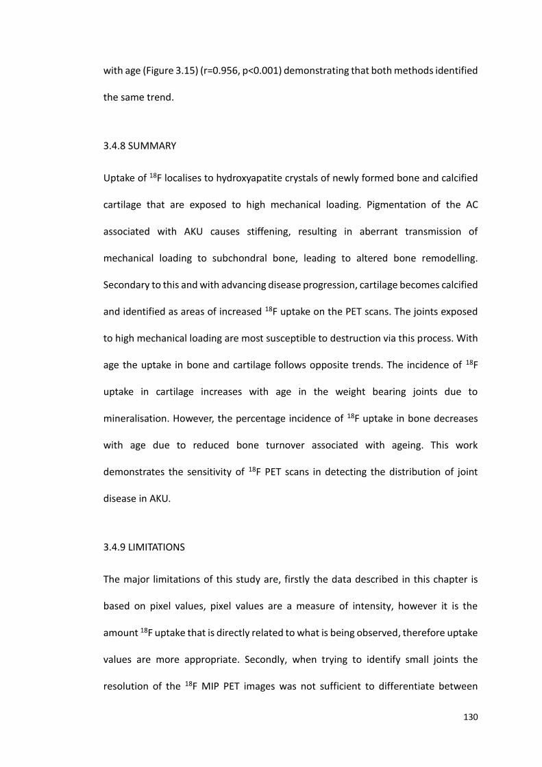
130

with age (Figure 3.15) (r=0.956, p<0.001) demonstrating that both methods identified

the same trend.

3.4.8 SUMMARY

Uptake of 18F localises to hydroxyapatite crystals of newly formed bone and calcified

cartilage that are exposed to high mechanical loading. Pigmentation of the AC

associated with AKU causes stiffening, resulting in aberrant transmission of

mechanical loading to subchondral bone, leading to altered bone remodelling.

Secondary to this and with advancing disease progression, cartilage becomes calcified

and identified as areas of increased 18F uptake on the PET scans. The joints exposed

to high mechanical loading are most susceptible to destruction via this process. With

age the uptake in bone and cartilage follows opposite trends. The incidence of 18F

uptake in cartilage increases with age in the weight bearing joints due to

mineralisation. However, the percentage incidence of 18F uptake in bone decreases

with age due to reduced bone turnover associated with ageing. This work

demonstrates the sensitivity of 18F PET scans in detecting the distribution of joint

disease in AKU.

3.4.9 LIMITATIONS

The major limitations of this study are, firstly the data described in this chapter is

based on pixel values, pixel values are a measure of intensity, however it is the

amount 18F uptake that is directly related to what is being observed, therefore uptake

values are more appropriate. Secondly, when trying to identify small joints the

resolution of the 18F MIP PET images was not sufficient to differentiate between

131

cartilage and bone. This was especially evident in the osteoporotic spine where it was

very difficult to distinguish between calcified IVDs and bone (Figure 3.16). Overlying

CT data would help with anatomical localisation.

Figure 3.16 18F-NaF images of the spine in a non-arthritic and arthritic patient. Left

image demonstrating severe arthropathy; uptake of 18F-NaF is uniform throughout

the spine, therefore very difficult to distinguish between IVD and bone. Right image

demonstrating non-arthritic spine with bands of increased uptake in the vertebrae,

with very little uptake in the IVDs.

132

3.4.10 FUTURE WORK

Future work is needed to develop quantitative measures of 18F uptake within bone

and cartilage which could be used to assess disease progression, and response to

therapy. Utilising PET/CT will improve resolution and localisation of areas of

increased 18F uptake, this will enable precise localisation of anatomical regions such

as vertebral end plates and IVDs.

133

4.0 APPLICATION OF 18F-NaF PET STANDARDISED UPTAKE VALUE FOR THE

DETECTION OF ARTHROPATHY IN AKU

134

4.1 INTRODUCTION

Chapter 3 of this thesis looked at the skeletal distribution of 18F in AKU patients. The

method used was based on the distribution of pixel values in the image. As described

in the limitations section (3.4.9) the data described in Chapter 3 was based on pixel

values. Pixel values are a measure of intensity. However, it is the amount of 18F uptake

that is directly related to what is being observed. Therefore, uptake values are more

appropriate. Additionally, the anatomical localisation of the spine proved to be

difficult to distinguish between bone and calcified IVDs due to the resolution of the

image. This chapter resolves these issues by utilising measurements of radioactivity

instead of pixel values, as well as utilising PET/CT for improved anatomical

localisation.


interpretation providing a method that is less user-dependent and that can be used

for intra and inter patient comparisons. Uptake measurements are used to assess

response to therapies and to distinguish degree of pathology (114). 18F-NaF PET has

been used to visualise many bone disorders as 18F-NaF binds to bone mineral

associated with both osteoblastic and osteolytic lesions (115). 18F-NaF PET scanning

is routinely carried out annually as part of the NAC as well as for the SONIA 2 clinical

trial (see sections 2.2.1 and 2.2.2).

The mean standardised uptake value (SUVm) is a common method of expressing the

uptake of PET tracers. The SUVm is a measure of radioactivity in a region of interest,

normalised against the injected activity and the subjects body weight. The SUVm is

defined as the activity concentration in the ROI ((kBq/mL) as measured by the PET

135

scanner) divided by the decay corrected injected dose of 18F-NaF (kBq) divided by

the patient body weight (kg) that acts as a surrogate for the distribution volume of

tracer (SUVm= radioactivity concentration / (decay corrected injected dose / body

weight)) (116). If all the injected 18F-NaF is retained and uniformly distributed

throughout the body, the SUVm will be 1g/ml under the assumption that 1ml of tissue

weighs 1g. Larger SUVms represent proportionally higher concentrations of

radiotracer. The uptake is represented by pixel or voxel intensity value in the ROI,

which is then converted into the activity concentration (117). PET imaging allows

quantitative SUVm measurements allowing the clinician to quantify disease state,

progression and response to therapy. More recently, SUVm measurements in 18F-NaF

PET have been reported to have potential as a diagnostic tool in OA (116). This

chapter introduces for the first time, quantitative SUVm measurements of bone and

cartilage to identify active spondyloarthropathy and to quantify disease state in AKU.

136

4.2 FEASIBILITY STUDY

A feasibility study was first undertaken to assess the viability and practicality of

obtaining SUVm measurements from both cartilage and bone in the large joints and

spine. The purpose was to objectively identify the strengths and weaknesses of the

methodology and the feasibility of measuring small anatomical regions such as

articular cartilage (AC).

4.2.1 DESIGN OF FEASIBILITY STUDY

Ten female non-metastatic breast cancer patients were used as a control group

(mean age of 62, SD±13.8, range 43-84, see section 2.2.3) exclusion criteria included

active arthropathy in the shoulder, hip and spine. Ten randomly selected female AKU

(NAC) patients (mean age of 60, SD±6.47, range 52-72, section 2.2.1) were included

for comparison. Hermes hybrid viewer (section 2.5.1) was utilised to obtain SUVms

from the hip and shoulder (see section 2.5.3) and lumbar and thoracic spine (see

section 2.5.2). The knee and ankle could not be included in this analysis as the control

patients were not scanned below the knee. For the hip, the SUVm was obtained from

the head of the femur, acetabulum and AC (ROI= 0.5cm diameter, 0.196cm2). For the

shoulder, SUVms were obtained from the head of the humerus, glenoid fossa and AC

(ROI= 0.5cm diameter, 0.196cm2). SUVms were also obtained from the centre of each

thoracic (T1-T12) and lumbar (L1-L5) vertebrae, and from the centre of the

corresponding IVD below (T1/T2 – L5-S1) (ROI= 1cm diameter, 0.785cm2). The

feasibility of measuring SUVms at these anatomical sites was assessed.

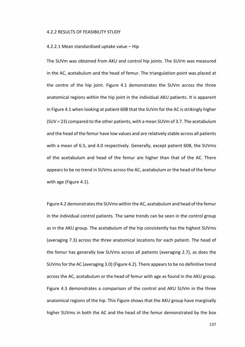
137

4.2.2 RESULTS OF FEASIBILITY STUDY

4.2.2.1 Mean standardised uptake value – Hip

The SUVm was obtained from AKU and control hip joints. The SUVm was measured

in the AC, acetabulum and the head of femur. The triangulation point was placed at

the centre of the hip joint. Figure 4.1 demonstrates the SUVm across the three

anatomical regions within the hip joint in the individual AKU patients. It is apparent

in Figure 4.1 when looking at patient 60B that the SUVm for the AC is strikingly higher

(SUV = 23) compared to the other patients, with a mean SUVm of 3.7. The acetabulum

and the head of the femur have low values and are relatively stable across all patients

with a mean of 6.5, and 4.0 respectively. Generally, except patient 60B, the SUVms

of the acetabulum and head of the femur are higher than that of the AC. There

appears to be no trend in SUVms across the AC, acetabulum or the head of the femur

with age (Figure 4.1).

Figure 4.2 demonstrates the SUVms within the AC, acetabulum and head of the femur

in the individual control patients. The same trends can be seen in the control group

as in the AKU group. The acetabulum of the hip consistently has the highest SUVms

(averaging 7.3) across the three anatomical locations for each patient. The head of

the femur has generally low SUVms across all patients (averaging 2.7), as does the

SUVms for the AC (averaging 3.0) (Figure 4.2). There appears to be no definitive trend

across the AC, acetabulum or the head of femur with age as found in the AKU group.

Figure 4.3 demonstrates a comparison of the control and AKU SUVm in the three

anatomical regions of the hip. This Figure shows that the AKU group have marginally

higher SUVms in both the AC and the head of the femur demonstrated by the box

138

plot (X denotes the mean value), and slightly lower SUVms in the acetabulum.

Independent t-tests revealed no statistically significant differences between AKU and

control SUVm in the AC (p>0.05), acetabulum (p>0.05) or the head of the femur

(p>0.05).

Figure 4.1 SUVm of the articular cartilage, acetabulum and head of femur in the

AKU group with age. 10 female AKU patients (mean age of 60, SD±6.47, range 52-

72). ROI = diameter 0.5cm 0.196cm2, obtained from each anatomical location at the

centre of the hip joint.

0

5

10

15

20

25

52 53 54 57 60A 60B 61 65 67 72

SUV

m

Patient age

Articular Cartilage

Acetabulum

Head of Femur

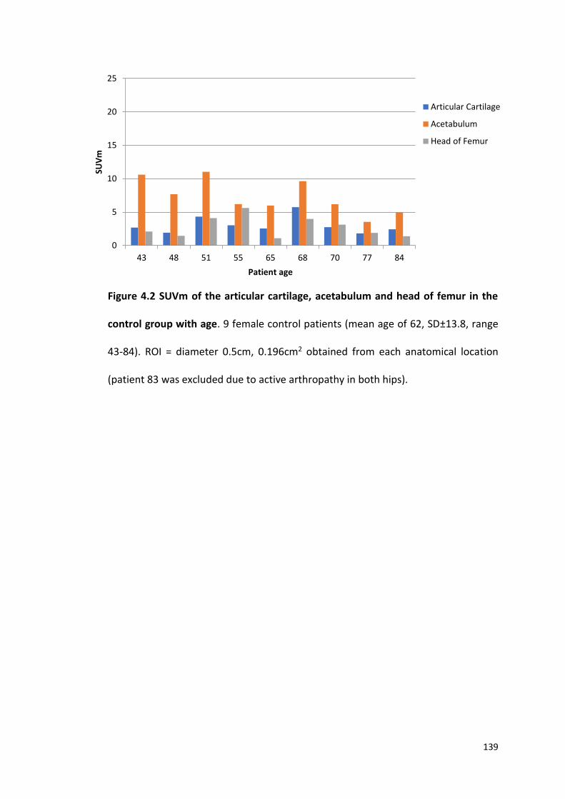
139

Figure 4.2 SUVm of the articular cartilage, acetabulum and head of femur in the

control group with age. 9 female control patients (mean age of 62, SD±13.8, range

43-84). ROI = diameter 0.5cm, 0.196cm2 obtained from each anatomical location

(patient 83 was excluded due to active arthropathy in both hips).

0

5

10

15

20

25

43 48 51 55 65 68 70 77 84

SUV

m

Patient age

Articular Cartilage

Acetabulum

Head of Femur

140

Figure 4.3 Box and whisker plot comparison of AKU and control SUVm in the

articular cartilage, acetabulum and head of femur of the hip joint. Independent t-

tests found no statistically significant differences between AKU and control in the

articular cartilage (p>0.05), acetabulum (p>0.05) and the head of the femur (p>0.05).

Box and whisker plot: height of box = interquartile range (upper quartile, lower

quartile), X = mean value, line within box = median value. Whiskers show the range.

Individual data points are plotted, the majority are hidden by the plotted boxes. Ten

female control patients (mean age of 62, SD±13.8, range 43-84), Ten female AKU

patients (mean age of 60, SD±6.47, range 52-72).

141

4.2.2.2 Standardised uptake value (mean) – Shoulder

SUVms were obtained from AKU and control shoulder joints. The SUVm was

measured in the AC, glenoid fossa of the scapula and the head of the humerus, with

the triangulation point placed at the centre of the shoulder joint. Figure 4.4

demonstrates the SUVm across the three anatomical regions within the shoulder

joint in the individual AKU patients. Again, for patient 60B the SUVm for the AC is

strikingly higher (SUVm= 27) than the other patients, who have a mean SUVm of 2.7.

The glenoid fossa and the head of the humerus all have similar low values with a

mean of 6.6 and 3.1 respectively across all AKU patients, this is similar to what was

seen in the hip joint. Generally (except patient 60B), the SUVms of the glenoid fossa

and head of the humerus are higher than that of the AC. The SUVm of the glenoid

fossa is consistently higher than the AC and the head of the humerus, again reflecting

what was observed in the corresponding regions of the hip. There appears to be no

trend across the three anatomical regions with age.

Figure 4.5 demonstrates the SUVms within the AC, glenoid fossa and head of the

humerus in the individual control patients. The glenoid fossa of the scapula

consistently has the highest SUVms (mean = 6.1) across the three anatomical

locations for each patient. The head of the humerus has generally low SUVms across

all patients (mean = 2.0), as does the SUVms for the AC (mean = 2.2).

Figure 4.6 compares control and AKU SUVms across the three anatomical regions of

the shoulder. This Figure shows that the AKU group had marginally higher SUVms

compared to the control group across the three anatomical regions of the shoulder

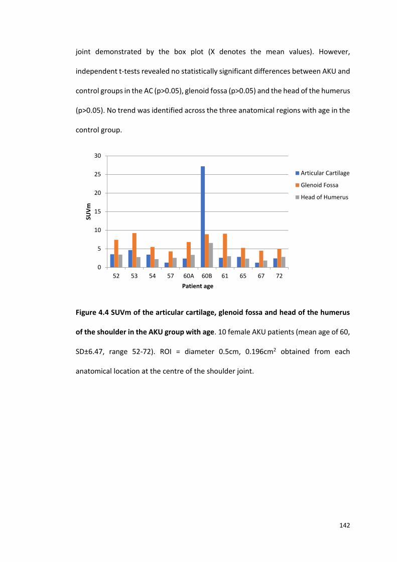
142

joint demonstrated by the box plot (X denotes the mean values). However,

independent t-tests revealed no statistically significant differences between AKU and

control groups in the AC (p>0.05), glenoid fossa (p>0.05) and the head of the humerus

(p>0.05). No trend was identified across the three anatomical regions with age in the

control group.

Figure 4.4 SUVm of the articular cartilage, glenoid fossa and head of the humerus

of the shoulder in the AKU group with age. 10 female AKU patients (mean age of 60,

SD±6.47, range 52-72). ROI = diameter 0.5cm, 0.196cm2 obtained from each

anatomical location at the centre of the shoulder joint.

0

5

10

15

20

25

30

52 53 54 57 60A 60B 61 65 67 72

SUV

m

Patient age

Articular Cartilage

Glenoid Fossa

Head of Humerus

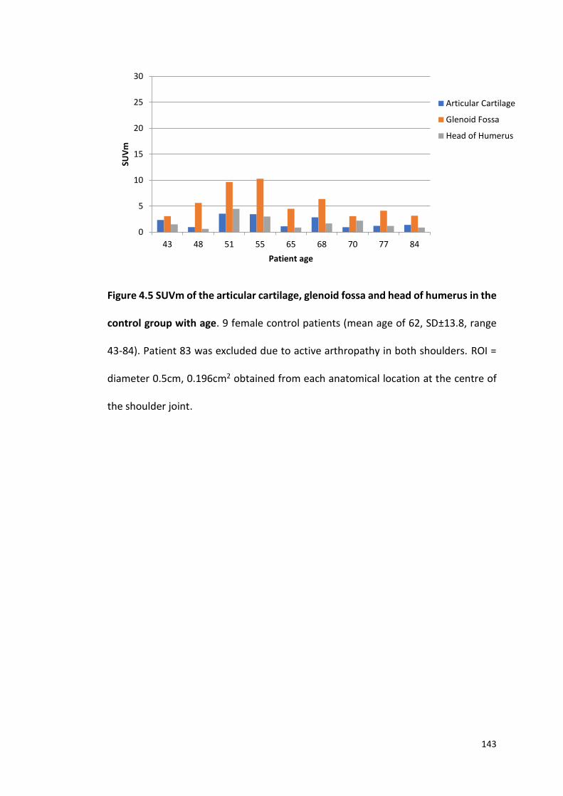
143

Figure 4.5 SUVm of the articular cartilage, glenoid fossa and head of humerus in the

control group with age. 9 female control patients (mean age of 62, SD±13.8, range

43-84). Patient 83 was excluded due to active arthropathy in both shoulders. ROI =

diameter 0.5cm, 0.196cm2 obtained from each anatomical location at the centre of

the shoulder joint.

0

5

10

15

20

25

30

43 48 51 55 65 68 70 77 84

SUV

m

Patient age

Articular Cartilage

Glenoid Fossa

Head of Humerus

144

Figure 4.6 Box and whisker plot comparison of AKU and control SUVm in the

articular cartilage, glenoid fossa and head of the humerus of the shoulder joint.

Independent t-tests found no statistically significant differences between AKU and

control in the articular cartilage (p>0.05), glenoid fossa (p>0.05) and the head of the

humerus (p>0.05). Box and whisker plot: height of box = interquartile range (upper

quartile, lower quartile), X = mean value, line within box = median value. Whiskers

show the highest and the lowest value. Individual data points are plotted, the

majority are hidden by the plotted boxes. Ten female control patients (mean age of

62, SD±13.8, range 43-84). Ten female AKU patients (mean age of 60, SD±6.47, range

52-72).

145

4.2.2.3 Standardised uptake value – Spine

Figure 4.7 demonstrates the SUVm across the lumbar and thoracic vertebrae in the

AKU and control groups. Statistically there was no significant difference (p>0.05)

between the SUVm of AKU vertebrae (mean SUVm=7.6, SD=1.3) and control

vertebrae (mean SUVm=7.9, SD=0.6). There appears to be a gradual increase in

SUVms in the AKU group along the vertebrae from L5-T1 ranging from 5.75 at the

lower lumbar region to 10.05 at the upper thoracic region. The control group SUVms

appear to be slightly more stable across the vertebrae ranging from 6.84 to 8.91.

Figure 4.8 demonstrates the SUVm across the lumbar and thoracic IVDs in the AKU

and control groups. AKU IVDs are consistently higher compared to the control group

with a mean SUVm of 12.01 (SD= 1.28) and 3.81 (SD=1.26) respectively. The control

group SUVms across the IVDs ranged from 1.54-5.63 and the AKU IVDs ranged from

10.28- 14.95. No trend could be identified in the AKU group regionally along the spine

reflected by the shallow fluctuations around SUVm of 12. A slight increase in SUVm

is evident in the control group from L4/L3 IVD to T1/T2 rising from a SUV of around 2

to 6 ascending the spine. Independent t-tests identified a statistically significant

difference (p<0.01) between AKU and control IVDs SUVms across all levels (Figure

4.8).

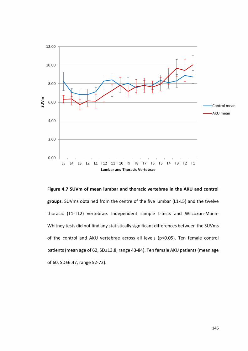
146

Figure 4.7 SUVm of mean lumbar and thoracic vertebrae in the AKU and control

groups. SUVms obtained from the centre of the five lumbar (L1-L5) and the twelve

thoracic (T1-T12) vertebrae. Independent sample t-tests and Wilcoxon-Mann-

Whitney tests did not find any statistically significant differences between the SUVms

of the control and AKU vertebrae across all levels (p>0.05). Ten female control

patients (mean age of 62, SD±13.8, range 43-84). Ten female AKU patients (mean age

of 60, SD±6.47, range 52-72).

0.00

2.00

4.00

6.00

8.00

10.00

12.00

L5 L4 L3 L2 L1 T12 T11 T10 T9 T8 T7 T6 T5 T4 T3 T2 T1

SUV

m

Lumbar and Thoracic Vertebrae

Control mean

AKU mean

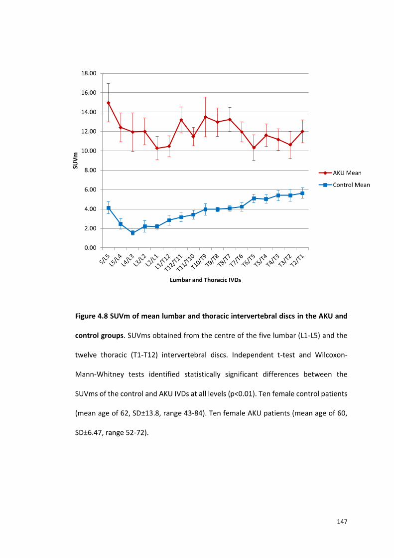
147

Figure 4.8 SUVm of mean lumbar and thoracic intervertebral discs in the AKU and

control groups. SUVms obtained from the centre of the five lumbar (L1-L5) and the

twelve thoracic (T1-T12) intervertebral discs. Independent t-test and Wilcoxon-

Mann-Whitney tests identified statistically significant differences between the

SUVms of the control and AKU IVDs at all levels (p<0.01). Ten female control patients

(mean age of 62, SD±13.8, range 43-84). Ten female AKU patients (mean age of 60,

SD±6.47, range 52-72).

0.00

2.00

4.00

6.00

8.00

10.00

12.00

14.00

16.00

18.00SU

Vm

Lumbar and Thoracic IVDs

AKU Mean

Control Mean

148

4.2.3 DISCUSSION OF FEASIBILITY STUDY

This feasibility study was undertaken to evaluate the practicality and viability of

obtaining accurate SUVms in the bone and cartilage of the hip (acetabulum, AC and

head of femur), shoulder (glenoid fossa, AC and head of humerus) and the spine

(thoracic and lumbar vertebrae and IVDs).

In terms of the methodology, obtaining the SUVms from the spine did not prove

difficult. The IVDs were large enough in the thoracic and lumbar regions (IVD height

approximately 7-10 mm) to ensure that the ROI was placed within the cartilaginous

disc. The cervical region was excluded from the analysis for this reason, as the IVDs

were too thin (less than 3-5mm), meaning that the SUVm did not reflect cartilage

uptake alone. Statistically significant results were obtained when analysing the spine

which provides confidence in the methodology (Figures 4.7 and 4.8). Figure 4.7

suggests that generalised rates of bone turnover within the thoracic and lumbar spine

of the control and AKU groups are similar with no significant differences found (mean

SUVm of AKU vertebrae = 7.6, and mean SUVm of control vertebrae = 7.9). This

corresponds to the SUVs reported by Win et al. (116) who reported lumbar and

thoracic SUVs in 11 normal vertebrae (SUV of 7.3) and Puri et al. (134) who reported

SUVs of the lumbar spine in 12 healthy postmenopausal women (mean SUVm of 6).

This therefore provides further evidence that this methodology is reliable and the

results are in line with other published studies.

Figure 4.8 demonstrates the SUVms in the IVDs of the AKU and control groups,

statistically significant differences were found at each level. The AKU group had much

higher SUVms reflecting increased tracer uptake in the cartilage which has not been

149

previously identified in AKU. It is thought that this is the first time SUVms have been

explored in cartilaginous IVDs. It is proposed that this is demonstrating calcification

of the IVDs in AKU.

Obtaining the SUVms from the hip and shoulder proved more difficult. There was no

problem obtaining SUVms from the bony acetabulum, glenoid fossa, head of femur

and head of humerus when the triangulation point was placed at the center of the

joint, as these structures were large and thick enough for the ROI (0.5cm diameter,

0.196cm2) (Figures 2.9 and 2.10). However, the AC proved difficult to ensure the ROI

was placed in cartilage alone without any bony tissue as normal AC diameter ranges

from 0.2-0.5cm. AKU results in destruction of articular cartilage, therefore many

patients had very thin AC in both the hip and shoulder joints. The smallest ROI

available was 0.5cm and therefore in some patients with arthropathy it was difficult

to ensure cartilage alone was measured. Additionally, the curvature of the joint

influenced the reliability of placing the ROI within the cartilage, due to slices

containing part cartilage and part bone. It is thought that these issues are reflected

in the results (Figure 4.1, 4.2, 4.4 and 4.5) excluding patient 60B in the AKU group,

and it is likely that the results of the AC reflected some bony uptake. After looking at

the patient noted patient 60B had active arthropathy in both hips and shoulders.

After completing this feasibility study, we discovered issues with obtaining accurate

SUVms within the AC of the hip and shoulder due to the nature of the very thin AC.

Some very promising results were identified when analysing the SUVms of the IVDs

between AKU and control groups. The AKU IVDs were found to have increased uptake

of 18F, thought to be the first time this phenomenon has been identified in AKU. As

150

this thesis is interested in looking at the differences in uptake of 18F-NaF in both bone

and cartilage the decision was made to exclude the shoulder and hip from any further

analysis and to only study spinal arthropathy in a larger group of patients.

4.3 DESIGN OF STUDY

4.3.1 PATIENT GROUP


the SONIA 2 clinical trial (see section 2.2.2) underwent 18F-NaF PET/CT imaging at

baseline (V1), and again one year later (V3). V1 was carried out in 2014/15 pre-

treatment and V3 one year later post-treatment (V2 was a safety visit at 3 months).

One group receives 10mg of nitisinone, one group receives no treatment - the

treatment and non-treatment groups are blinded until the end of the clinical trial in

2019 (see section 1.3.2 for more information). Ten non-metastatic breast cancer

‘control’ patients were used as a comparison (see section 2.2.3). These patients had

undergone 18F-NaF PET/CT to determine bony metastasis, of which all patients were

reported as negative for any cancerous involvement.

4.3.2 MEASURING THE SUVms

Hermes Hybrid Viewer (see section 2.5.1) was used to measure the SUVms (section

2.5.2). Based on the results of the feasibility study, the SUVs obtained from all lumbar

and thoracic vertebrae were not statistically different. It was therefore decided that

the upper most, lower most and middle vertebrae and IVDs were analysed for the

main study. The SUVm was obtained from the centre of three lumbar (L5, L3, L1) and

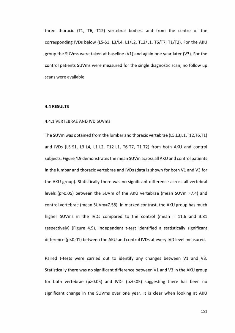
151

three thoracic (T1, T6, T12) vertebral bodies, and from the centre of the

corresponding IVDs below (L5-S1, L3/L4, L1/L2, T12/L1, T6/T7, T1/T2). For the AKU

group the SUVms were taken at baseline (V1) and again one year later (V3). For the

control patients SUVms were measured for the single diagnostic scan, no follow up

scans were available.

4.4 RESULTS

4.4.1 VERTEBRAE AND IVD SUVms

The SUVm was obtained from the lumbar and thoracic vertebrae (L5,L3,L1,T12,T6,T1)

and IVDs (L5-S1, L3-L4, L1-L2, T12-L1, T6-T7, T1-T2) from both AKU and control

subjects. Figure 4.9 demonstrates the mean SUVm across all AKU and control patients

in the lumbar and thoracic vertebrae and IVDs (data is shown for both V1 and V3 for

the AKU group). Statistically there was no significant difference across all vertebral

levels (p>0.05) between the SUVm of the AKU vertebrae (mean SUVm =7.4) and

control vertebrae (mean SUVm=7.58). In marked contrast, the AKU group has much

higher SUVms in the IVDs compared to the control (mean = 11.6 and 3.81

respectively) (Figure 4.9). Independent t-test identified a statistically significant

difference (p<0.01) between the AKU and control IVDs at every IVD level measured.

Paired t-tests were carried out to identify any changes between V1 and V3.

Statistically there was no significant difference between V1 and V3 in the AKU group

for both vertebrae (p>0.05) and IVDs (p>0.05) suggesting there has been no

significant change in the SUVms over one year. It is clear when looking at AKU

152

vertebrae and IVDs that the vertebrae have consistently lower SUVms (mean SUVm

= 7.58) than the IVDs (mean SUVm = 11.16), which was statistically significant at every

level (p<0.01). When comparing the SUVms for the vertebrae and IVD in the control

group, the opposite is seen. The SUV of the vertebrae (mean SUVm = 7.4) is

consistently higher than the SUV of the IVDs (mean SUVm = 3.81). The control mean

IVD SUVm was much lower in the control group (3.81) compared to what was found

in the AKU group (11.16). This suggests that newly deposited mineral is being laid

down in the IVDs in AKU due to calcification of the cartilage.

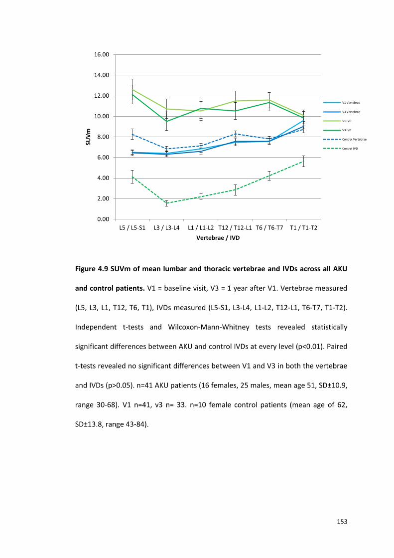
153

Figure 4.9 SUVm of mean lumbar and thoracic vertebrae and IVDs across all AKU

and control patients. V1 = baseline visit, V3 = 1 year after V1. Vertebrae measured

(L5, L3, L1, T12, T6, T1), IVDs measured (L5-S1, L3-L4, L1-L2, T12-L1, T6-T7, T1-T2).

Independent t-tests and Wilcoxon-Mann-Whitney tests revealed statistically

significant differences between AKU and control IVDs at every level (p<0.01). Paired

t-tests revealed no significant differences between V1 and V3 in both the vertebrae

and IVDs (p>0.05). n=41 AKU patients (16 females, 25 males, mean age 51, SD±10.9,

range 30-68). V1 n=41, v3 n= 33. n=10 female control patients (mean age of 62,

SD±13.8, range 43-84).

0.00

2.00

4.00

6.00

8.00

10.00

12.00

14.00

16.00

L5 / L5-S1 L3 / L3-L4 L1 / L1-L2 T12 / T12-L1 T6 / T6-T7 T1 / T1-T2

SUV

m

Vertebrae / IVD

V1 Vertebrae

V3 Vertebrae

V1 IVD

V3 IVD

Control Vertebrae

Control IVD

154

4.4.2 SUVm WITH AGE

The mean lumbar vertebrae (L5, L3, L1) SUVm was plotted for both visits (V1 and V3)

against age for AKU and control groups (Figure 4.10). There is an obvious trend

demonstrating a clear reduction in SUVm with age in both AKU and control groups.

Generally, the youngest patients have the highest SUVms and the oldest have the

lowest.

Paired t-tests revealed no significant difference (p>0.05) between the lumbar

vertebrae SUVms for V1 and V3 in the AKU patients. The control mean lumbar

vertebrae can be seen to have slightly increased SUVms compared to the AKU

patients however independent t-tests revealed no significance between V1 and the

control and V3 and the control (p>0.05).

The negative relationship with age was clear in both the AKU and control groups

demonstrated by the regression lines. Multiple variate linear regression was applied

to analyse the trend between the mean lumbar vertebrae SUVm with age in both

AKU and control groups. Interestingly, age was found to be statistically significant to

the mean lumbar vertebrae SUVm (p<0.01). Age affects mean lumbar vertebrae

SUVm outcome negatively. For every year increase in age the SUVm decreases by

0.100 in both AKU and control groups.

155

Figure 4.10 SUVm of mean lumbar vertebrae with age in individual AKU and control

patients. V1 – baseline, V3 -1 year after V1. MEAN L VERT (SUV mean of mean lumbar

vertebrae (of L5, L3, L1)). Paired t-tests revealed no significant differences between

V1 and V3 mean lumbar vertebrae SUVm. Independent t-tests also revealed no

statistically significant differences between the SUVms of AKU (V1 and V3) and the

control group (control vs V1 p>0.05, control vs V3 p>0.05). Multiple linear regression

analysis identified a significant difference (p<0.01) between age and mean lumbar

SUVm in both control and AKU groups. n=41 AKU patients (16 females, 25 males,

mean age 51, SD±10.9, range 30-68). V1 n=41, V3 n= 33. n=10 female control patients

(mean age of 62, SD±13.8, range 43-84).

0

2

4

6

8

10

12

20 30 40 50 60 70 80 90

SUV

m

Age

V1 MEAN L VERT

V3 MEAN L VERT

CONTROL MEAN LVERT

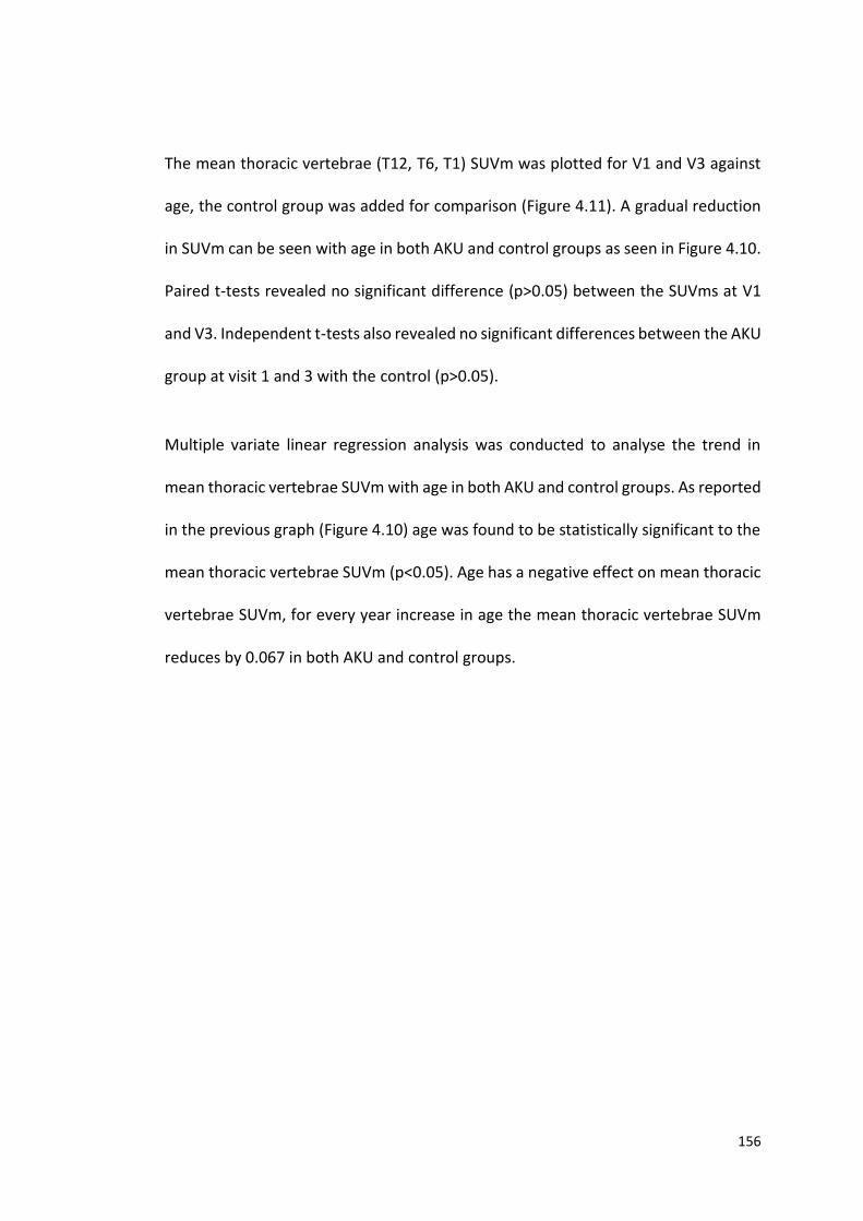
156

The mean thoracic vertebrae (T12, T6, T1) SUVm was plotted for V1 and V3 against

age, the control group was added for comparison (Figure 4.11). A gradual reduction

in SUVm can be seen with age in both AKU and control groups as seen in Figure 4.10.

Paired t-tests revealed no significant difference (p>0.05) between the SUVms at V1

and V3. Independent t-tests also revealed no significant differences between the AKU

group at visit 1 and 3 with the control (p>0.05).

Multiple variate linear regression analysis was conducted to analyse the trend in

mean thoracic vertebrae SUVm with age in both AKU and control groups. As reported

in the previous graph (Figure 4.10) age was found to be statistically significant to the

mean thoracic vertebrae SUVm (p<0.05). Age has a negative effect on mean thoracic

vertebrae SUVm, for every year increase in age the mean thoracic vertebrae SUVm

reduces by 0.067 in both AKU and control groups.

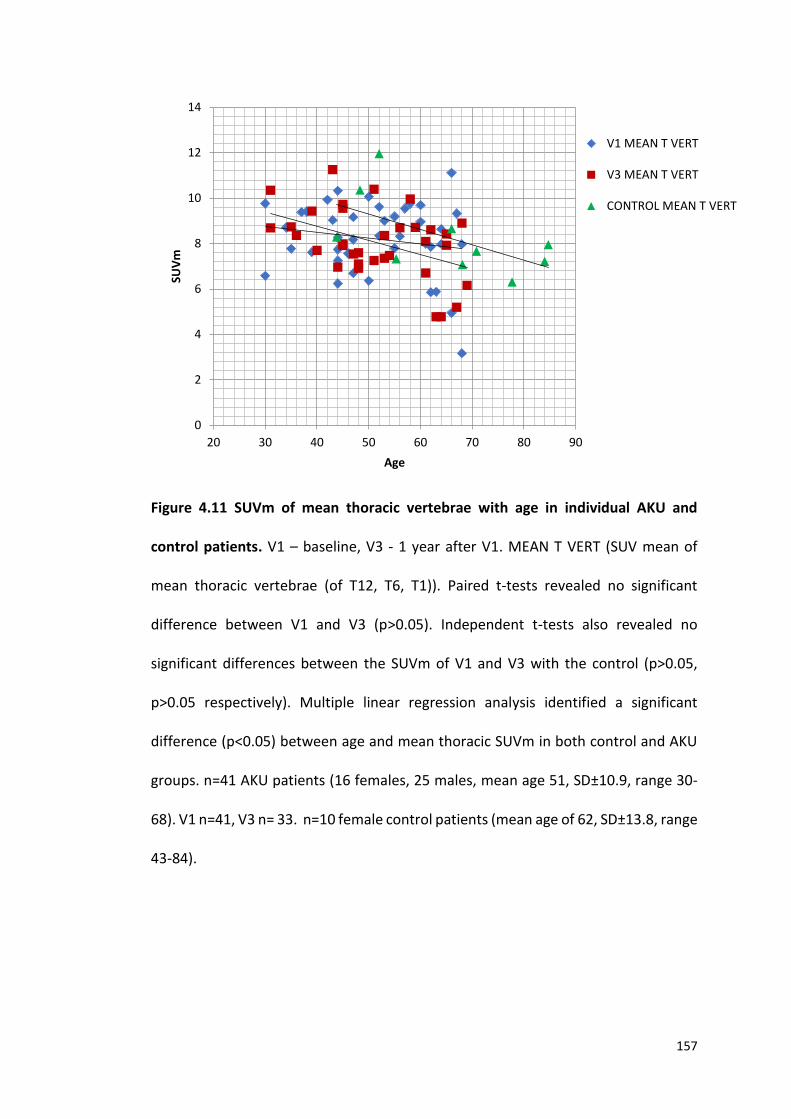
157

Figure 4.11 SUVm of mean thoracic vertebrae with age in individual AKU and

control patients. V1 – baseline, V3 - 1 year after V1. MEAN T VERT (SUV mean of

mean thoracic vertebrae (of T12, T6, T1)). Paired t-tests revealed no significant

difference between V1 and V3 (p>0.05). Independent t-tests also revealed no

significant differences between the SUVm of V1 and V3 with the control (p>0.05,

p>0.05 respectively). Multiple linear regression analysis identified a significant

difference (p<0.05) between age and mean thoracic SUVm in both control and AKU

groups. n=41 AKU patients (16 females, 25 males, mean age 51, SD±10.9, range 30-

68). V1 n=41, V3 n= 33. n=10 female control patients (mean age of 62, SD±13.8, range

43-84).

0

2

4

6

8

10

12

14

20 30 40 50 60 70 80 90

SUV

m

Age

V1 MEAN T VERT

V3 MEAN T VERT

CONTROL MEAN T VERT

158

Figure 4.12 demonstrates the mean lumbar IVD SUVm with age in AKU and control

groups. Paired t-tests revealed no significant difference between V1 and V3 in the

AKU group (p>0.05). The SUVms of the control patients are consistently lower (SUVm

= 2.5) compared to the AKU group (V1 SUVm = 11, V3 SUVm = 10). Independent t-

tests revealed statistically significant differences between both V1 and V3 mean

lumbar IVD with the control mean lumbar IVDs (p<0.01).

In the control group no trend was identified with age. In contrast, the trendline for

the AKU group at both V1 and V3 shows a gradual increase in SUVm with age followed

by a decline in the later years. The youngest AKU patients have the lowest SUVms

(SUVm = below 5) that are in line with the SUVms of the control group. However,

from the age of approximately 40 the SUVm can be seen to increase reaching a

maximum SUV of 20 around the age of 50/55 years. From here, a general reduction

in SUVm can be seen where the oldest patients (between 60 and 70) have a reduction

in SUVms decreasing to values similar to that of the controls.

Multivariate linear regression found a significant difference between the AKU and

control groups with age (p<0.01). In the AKU group the mean lumbar IVD SUVm

increases by 0.238 every year, compared to no change in the control group. However,

looking at the graph this trend in the AKU group does appear to stop around the age

of 50/55.

159

Figure 4.12 SUVm of mean lumbar IVDs with age in individual AKU and control

patients. V1 – baseline, V3 - 1 year after V1. MEAN L IVD – SUV mean of mean lumbar

IVD (L5/S1, T3/T4, L1/L2). Polynomial function was fitted to the AKU data (order 2

polynomial line used when the data has one hill), with R² values of V1 (R²= 0.458) V2

(R²= 0.435). Linear regression line for the control had a R² value of 0.133. Paired t-

tests revealed no significant difference between V1 and V3 in the AKU group (p>0.05).

Independent t-tests revealed statistically significant results between both V1 and V3

mean lumbar IVD SUVm with the control mean lumbar IVDs SUVm (p<0.01).

Multivariate linear regression found a significant difference between the groups (AKU

vs control) with age (p<0.01). n=41 AKU patients (16 females, 25 males, mean age 51,

SD±10.9, range 30-68). V1 n=41, V3 n= 33. n=10 female control patients (mean age

of 62, SD±13.8, range 43-84).

0

5

10

15

20

25

20 30 40 50 60 70 80 90

SUV

m

Age

V1 MEAN L IVD

V3 MEAN L IVD

CONTROL MEAN L IVD

160

The same trend can be seen when looking at the SUVm of the mean thoracic IVDs in

AKU and control groups (Figure 4.13). The youngest AKU patients have similar SUVms

to the controls (control mean SUVm = 4). From the age of around 40 the SUVm of the

AKU patients increases reaching a maximum of 18 around the age of 50-55 years. The

oldest AKU patients (over the age of 60) have lower SUVms reducing towards the

values of the controls as seen in Figure 4.12. There is a slight decrease in SUVm with

age in the thoracic vertebrae of the control group.

No significant difference was found between the SUVms of V1 and V3 (paired t-test,

p>0.05). Independent t-tests revealed significant differences between the mean

thoracic IVD SUVm in the AKU groups (V1 and V3) compared to the control mean

thoracic IVD SUVm (p<0.01).

Multivariate linear regression found a significant difference between the AKU and

control groups with age (p<0.01). In the AKU group the mean thoracic IVD SUVm

increases by 0.293 every year, compared to little change in the control group.

However, looking at the graph this trend does appear to stop around the age of 50/55

consistent to what was described in Figure 4.12.

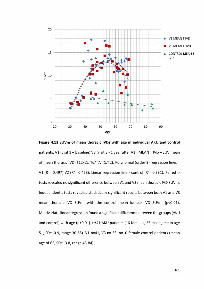
161

Figure 4.13 SUVm of mean thoracic IVDs with age in individual AKU and control

patients. V1 (visit 1 – baseline) V3 (visit 3 - 1 year after V1). MEAN T IVD – SUV mean

of mean thoracic IVD (T12/L1, T6/T7, T1/T2). Polynomial (order 2) regression lines =

V1 (R²= 0.497) V2 (R²= 0.458). Linear regression line - control (R²= 0.331). Paired t-

tests revealed no significant difference between V1 and V3 mean thoracic IVD SUVm.

Independent t-tests revealed statistically significant results between both V1 and V3

mean thoracic IVD SUVm with the control mean lumbar IVD SUVm (p<0.01).

Multivariate linear regression found a significant difference between the groups (AKU

and control) with age (p<0.01). n=41 AKU patients (16 females, 25 males, mean age

51, SD±10.9, range 30-68). V1 n=41, V3 n= 33. n=10 female control patients (mean

age of 62, SD±13.8, range 43-84).

0

5

10

15

20

20 30 40 50 60 70 80 90

SUV

m

Age

V1 MEAN T IVD

V3 MEAN T IVD

CONTROL MEAN TIVD

162

4.4.3 GENDER AND SUV

Figure 4.14 demonstrates the SUVm across the lumbar and thoracic vertebrae and

IVDs in males and females. The SUVms across the lumbar and thoracic vertebrae are

very similar in males and females. Independent t-test identified no significant

difference between the vertebrae SUVms of the males and females at all vertebral

levels (mean p>0.05). The SUVms across the lumbar and thoracic IVDs can be seen to

be consistently higher compared to the vertebrae. The male group can be seen to

have higher SUVms consistently across the lumbar and thoracic IVDs compared to the

female group. However, independent t-tests found no statistically significant

differences across all levels (mean p>0.05).

Figure 4.14 SUVm of mean lumbar and thoracic vertebrae and IVDs in males and

females. Independent sample t-tests revealed no statistically significant differences

between the vertebrae (p>0.05) and IVDs (p>0.05) at every level of males and

females. n=41 AKU patients (16 females, 25 males, mean age 51, SD±10.9, range 30-

68).

0

2

4

6

8

10

12

14

16

L5 L3 L1 T12 T6 T1

SUV

m

Vertebrae / IVD

Vertebrae - Male

Vertebrae - Female

IVD - Male

IVD - Female

163

4.4.4 INDIVIDUAL CHANGE IN SUV OVER ONE YEAR

The AKU patients were separated into four age-dependent groups to look at the

individual change in SUVm over one year in the vertebrae and IVDs. Figure 4.15

demonstrates the individual patient changes in the mean lumbar vertebrae SUVm at

V1 and V3 in four age groups (30-39, 40-49, 50-59, 60-70). The red lines demonstrate

a reduction in SUVm over one year, the blue lines demonstrate an increase in SUVm

and green lines represent no change in SUVm. It is evident in graph A that the

youngest patients have little change in SUVm over one year, with the other three age

groups (Figure 4.15 B, C and D) having more of a change demonstrated by the steeper

lines. In the 40-49-year-old age group there appears to be more of a reduction in

SUVm over the one-year period, however, in the oldest two age groups patients can

be seen to have either a reduction or increase in SUVm at equal rates. It is clear that

the youngest age group has the highest SUVms and the oldest age group has the

lowest SUVms supporting the age-related trend shown in Figure 4.10.

Figure 4.16 demonstrates the individual patient changes in the mean thoracic

vertebrae SUVm at V1 and V3 in four age groups. It is clear in the youngest patients

(Figure 4.16 A) that there is little change if any in SUVms across the two visits

equivalent to what was found in the lumbar vertebrae (Figure 4.15 A). In the next age

group (Figure 4.16 B) the results are more variable with some patients having an

increase some having a decrease and some having no change in SUVm. The oldest

two age groups (Figures 4.16 C and D) have more patients with a reduction in SUVm

over one year. Comparable to what was seen in the lumbar vertebrae the youngest

age group has the highest SUVms and the oldest age group has the lowest SUVms

164

supporting what was found in Figure 4.11 that demonstrates a reduction in SUVm

with age.

The same analysis was carried out on the lumbar and thoracic IVDs. Figure 4.17

demonstrates the individual mean lumbar IVDs at V1 and V3 in the four age groups.

In terms of the change in SUVm over one year, the youngest age group has mostly

little change, with the oldest three age groups having more of a change over one year

like we have seen in the lumbar and thoracic vertebrae. The oldest age group has the

biggest changes in SUVms over the one-year period. The 40-49 age group (Figure 4.17

B) has more patients having a reduction in SUVm over one year. The next age group

(Figure 4.17 C), the majority of patients appear to have a slight increase in SUVm

across the visits. The oldest age group (Figure 4.17 D) has patients increasing and

decreasing equally. Looking at the SUVms the youngest age group has the lowest

values; the 40-49 group reaches the highest SUVms and the oldest age group can be

seen reducing back to lower values. This supports the trend that was seen in Figure

4.12, that demonstrates the youngest patients have the lowest SUVms followed by

an exponential increase in SUVm up to around the age of 45-50 followed by a plateau

at around the age group 50-60 then followed by a steady decline in the oldest

patients.

A very similar trend can be seen in Figure 4.18 that demonstrates the mean thoracic

IVDs SUVm at V1 and V3 in four age groups. Again, little change is seen in the

youngest age group (Figure 4.18 A), with more of a change seen in the other three

age groups. The patents in the oldest age group (Figure 4.18 D) mostly have a

reduction in SUVm over the one-year period. In terms of SUVms the youngest

165

patients have the lowest SUVms, the age group 50-59 have the highest SUVms and

the oldest age group can be seen having lower SUVms. This confirms the findings in

Figure 4.13 that demonstrates the youngest patients have the lowest SUVms

followed by an exponential increase up to around the age of 50, followed by a plateau

up to around the age of 60, followed by a steady decline in the oldest patients.

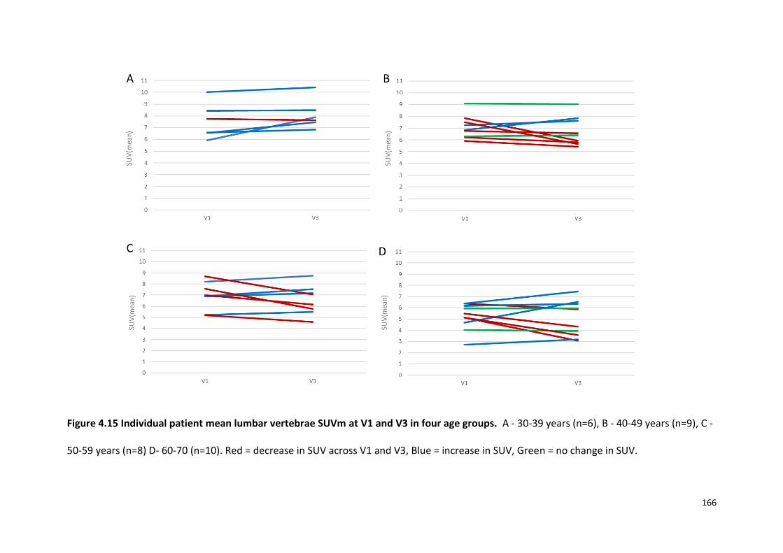
166

Figure 4.15 Individual patient mean lumbar vertebrae SUVm at V1 and V3 in four age groups. A - 30-39 years (n=6), B - 40-49 years (n=9), C -

50-59 years (n=8) D- 60-70 (n=10). Red = decrease in SUV across V1 and V3, Blue = increase in SUV, Green = no change in SUV.

167

Figure 4.16 Individual patient mean thoracic vertebrae SUVm at V1 and V3 in four age groups. A - 30-39 years (n=6), B - 40-49 years (n=9), C

- 50-59 years (n=8) D- 60-70 (n=10). Red = decrease in SUV across V1 and V3, Blue = increase in SUV, Green = no change in SUV.

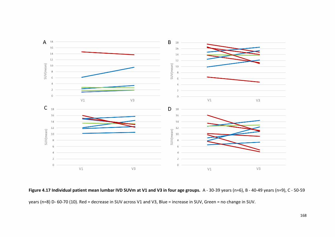
168

Figure 4.17 Individual patient mean lumbar IVD SUVm at V1 and V3 in four age groups. A - 30-39 years (n=6), B - 40-49 years (n=9), C - 50-59

years (n=8) D- 60-70 (10). Red = decrease in SUV across V1 and V3, Blue = increase in SUV, Green = no change in SUV.

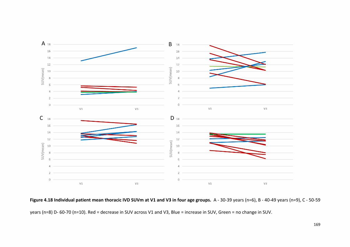
169

Figure 4.18 Individual patient mean thoracic IVD SUVm at V1 and V3 in four age groups. A - 30-39 years (n=6), B - 40-49 years (n=9), C - 50-59

years (n=8) D- 60-70 (n=10). Red = decrease in SUV across V1 and V3, Blue = increase in SUV, Green = no change in SUV.

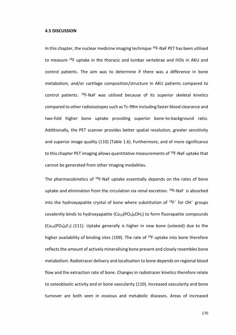
170

4.5 DISCUSSION

In this chapter, the nuclear medicine imaging technique 18F-NaF PET has been utilised

to measure 18F uptake in the thoracic and lumbar vertebrae and IVDs in AKU and

control patients. The aim was to determine if there was a difference in bone

metabolism, and/or cartilage composition/structure in AKU patients compared to

control patients. 18F-NaF was utilised because of its superior skeletal kinetics

compared to other radioisotopes such as Tc-99m including faster blood clearance and

two-fold higher bone uptake providing superior bone-to-background ratio.

Additionally, the PET scanner provides better spatial resolution, greater sensitivity

and superior image quality (110) (Table 1.6). Furthermore, and of more significance

to this chapter PET imaging allows quantitative measurements of 18F-NaF uptake that

cannot be generated from other imaging modalities.

The pharmacokinetics of 18F-NaF uptake essentially depends on the rates of bone

uptake and elimination from the circulation via renal excretion. 18F-NaF is absorbed

into the hydroxyapatite crystal of bone where substitution of 18Fˉ for OHˉ groups

covalently binds to hydroxyapatite (Ca10(PO4)6OH2) to form fluorapatite compounds

(Ca10(PO4)6F2) (111). Uptake generally is higher in new bone (osteoid) due to the

higher availability of binding sites (109). The rate of 18F uptake into bone therefore

reflects the amount of actively mineralising bone present and closely resembles bone

metabolism. Radiotracer delivery and localisation to bone depends on regional blood

flow and the extraction rate of bone. Changes in radiotracer kinetics therefore relate

to osteoblastic activity and or bone vascularity (110). Increased vascularity and bone

turnover are both seen in osseous and metabolic diseases. Areas of increased

171

localisation of tracer uptake reflect increased bone metabolism at that site, although

physiologic uptake of 18F in the skeleton is generally uniform in adults (113).


interpretation providing a method that is less user-dependent and that can be used

for comparison between patients. The mean standardised uptake value (SUVm) is a

common method of expressing the uptake of PET tracers. The SUVm is a measure of

radioactivity in a region of interest, normalised against injected activity and the

subject’s body weight (Figure 1.13). If all injected 18F is retained and uniformly

distributed the SUV should be 1g/ml; larger SUVms represent proportionally higher

uptake of 18F at that specific site. This chapter investigates the SUVm of the lumbar

and thoracic vertebrae and IVDs in AKU and control patients.

4.5.1 Discussion of feasibility study and SONIA 2 results

The feasibility study described at the start of this chapter identified and described

the accuracy and robustness of the method of obtaining accurate SUVms

representative of cartilage and bone in the spine. Figure 4.8 demonstrates the mean

lumbar and thoracic IVD SUVm in the control and AKU groups. The SUVms were

strikingly higher in the AKU group averaging SUVm of 12.01 across the IVDs compared

to a mean SUVm of 3.8 in the control IVDs. Statistically significant differences were

identified at each IVD level (p<0.01). In contrast, when analysing the vertebrae, the

SUVms were similar to the control and the data points overlapped with no significant

differences identified (Figure 4.7). This data was representative of ten AKU and ten

control patients. The main study of this chapter was to repeat this analysis on a larger

172

cohort of AKU patients; 41 SONIA 2 patients were recruited and analysed. Five lumbar

and twelve thoracic vertebrae and IVDs were measured in the feasibility study and

the results across the vertebrae and IVDs were consistent (as seen in Figures 4.7 and

4.8). Therefore, only three lumbar and three thoracic vertebrae were measured in

the main study (the lower-most, middle and upper-most vertebrae of that region).

Figure 4.9 illustrates the results of the SONIA 2 data. The SUVms for the SONIA 2 IVDs

were in line with the values identified in the feasibility study averaging SUVm of 11.6

compared to SUVm of 12.01 in the feasibility study. Again, independent t-tests

revealed statistically significant differences (p<0.01) between AKU and control IVDs

at every level. Additionally, the vertebrae SUVms also corresponded very accurately

with the results of the feasibility study, with a mean SUVm of 7.4 in the SONIA 2 group

and 7.6 in the feasibility study. These results demonstrate the robustness of the

method and reliability of the results.

4.5.2 IVD SUVm

AKU patients with ochronotic arthropathy usually present with lower back pain

resulting from disc degeneration as the initial joint manifestation of AKU. Symptoms

worsen from the fourth decade leading to painful spinal disease often resulting in

spinal stenosis (1). Therefore, it is not surprising that a significant difference between

the SUVm of IVDs was identified in AKU patients compared to controls. The SUVms

of the AKU IVDs are three times higher than that of the control (Figures 4.8 and 4.9).

It is understood in AKU that IVDs become calcified as part of the disease

pathophysiology. Calcification of IVDs is a consistent feature reported in many AKU

173

case reports along with disc space narrowing, loss of lumbar lordosis and in severe

cases osteophytes (79,138–141). Jebaraj et al. (142) states that disc calcifications in

spinal ochronosis usually occur as lamellar calcifications of the nucleus pulposus

which begins in the lumbar disc and ascends the spine. They described the

calcifications as calcium hydroxyapatite crystals or calcium pyrophosphate dihydrate

crystals and suggested it was due to the biochemical alterations of the disease. IVD

calcification or chondrocalcinosis occurs with age and the prevalence has been

previously reported as 5-6% of the general adult population through conventional

radiography. The prevalence in AKU has not been described but is considered a well-

known radiological feature (143). Calcification in the discs likely accounts for the

increased uptake of 18F observed in AKU demonstrated by the increased SUVm. It is

proposed that 18F is binding to the calcium hydroxyapatite crystals / calcium

pyrophosphate dihydrate crystals in the IVDs hence why fluoride uptake can be

measured in these regions. The control patients have low uptake of 18F in the discs

due to IVDs being avascular and healthy IVDs not containing calcified deposits.

Interestingly the SUVms of the IVDs were significantly higher than the vertebrae at

every level in AKU patients suggesting that IVDs are more actively mineralising than

bone. A possible reason for this is that 18F binds preferentially to newly laid down

hydroxyapatite in the IVDs due to the higher availability of binding sites due to active

disease processes.

174

4.5.3 Vertebrae SUVm

18F binds to hydroxyapatite in bone to form fluorapatite. The uptake of NaF into bone

depends on the blood flow to the area, regional osteoblastic activity and renal

clearance. The rapid uptake of 18F occurs preferentially at high osteoblastic activity

where bone remodelling is greatest. The spinal vertebrae are an ideal site for

quantitative assessment of bone metabolism as the spine has a greater turnover of

bone than other skeletal sites. This is due to factors such as the spine is subjected to

mechanical stress which enhances interleukin 11 expression which stimulates

osteoblast differentiation. This leads to increased bone turnover and increased

osteoblastic activity which results in high 18F uptake (117). Additionally, the vertebrae

consist of mostly trabecular bone which is highly vascularised and is less dense

compared to cortical bone, thus trabecular bone has higher SUVms compared to

cortical bone.

The results of this study revealed that the SUVms of AKU vertebrae (SUV = 7.4) were

very similar to control vertebrae (SUVm = 7.58) suggesting that generalised rates of

bone turnover in AKU and control patients are very similar. This reflects that bone

turnover in AKU is normal. It is believed that this is the first time SUVm measurements

have been reported for AKU patients even though, there are several reports of SUVs

of the spine in the normal skeleton. Win et al. (116) reported SUVs in the cervical,

thoracic and lumbar vertebrae in 11 normal patients (excluding patients with

abnormal renal function, history of cancer or metabolic bone disease). Interestingly,

the SUVs for the vertebrae in this study were very similar to the results of this

chapter. Win et al. (118) reported the mean SUV(max) of the thoracic and lumbar

175

vertebrae to be 7.31, which was very similar to the SUVm of the thoracic and lumbar

vertebrae of the AKU and the control patients analysed in this study which had

SUVms of 7.4 and 7.5 respectively. Puri et al. (134) also reported SUVs of the lumbar

vertebrae in 12 post-menopausal women, they reported the mean SUV to be 6

corresponding to the results we have reported. These findings provide confidence in

the method and quality of the results reported in this chapter.

In terms of the SUVms along the spine, the SUVms are slightly higher in the thoracic

vertebrae compared to the lumbar vertebrae (Figures 4.7 and 4.9) and appear to

slightly increase up the spine from L5-T1. This was also found by Kaneta et al. (144)

who reported SUV measurements of normal thoracic and lumbar vertebrae using

SPECT/CT Tc-99m. The SUVm gradually increased from the lower lumbar spine to the

upper thoracic spine however this was not statistically significant. This finding is

unexpected given that the lumbar vertebrae have the highest mechanical forces

acting on them, and therefore increased bone turnover compared to areas of the

spine with fewer forces acting upon them. It was expected that the lumbar vertebrae

would have the highest SUVms. A possible reason for this could be the thoracic spine

has increased axial forces acting upon it due to its flexibility. Additionally, in AKU the

lumbar spine is known to be affected by osteoarthropathy to a higher extent than the

thoracic spine. The end stage of spinal arthropathy results in spinal fusion. This could

result in reduced SUVms due to low bone turnover at sites of bony fusion, due to less

new mineralisation.

176

4.5.4 Vertebrae SUVm with age

This chapter describes a reduction in SUVm with age in the thoracic and lumbar

vertebrae in both AKU and control groups (Figures 4.10 and 4.11). Essentially this

means less mineral available for fluoride to bind and or decreased blood flow. This

supports what was found in the previous chapter where a reduction in the

percentage incidence of increased 18F uptake with age was described in the lumbar

vertebrae (Figure 3.3) as well as the thoracic vertebrae (Figure 3.4). This is consistent

with the literature. Win et al. (116) found a negative trend in SUV(max) with age in

the T5, T7, T12 and L2 vertebrae but without statistical significance. It is widely

agreed that bone deteriorates in composition, structure and function with age. In the

first three decades of life bone turnover is coupled very tightly maintaining a steady

state between bone resorption and bone formation. Peak bone mass is reached

around the age of 20 in women and older in men. After this bone turnover continues

at a slower rate resulting in a steady reduction in bone mass (145).

The menopause in women greatly increases bone resorption due to low levels of

oestrogen, accelerating bone loss. Daly et al. (146) conducted a ten-year population

based observational study and reported that the annual percentage rate of loss in

forearm BMD was 1.5 to 2.0-fold higher in females compared to males over the age

of 60. Therefore, a reduction in BMD results in less hydroxyapatite for 18F to bind,

therefore resulting in a lower SUVms.

A reduction in red marrow is associated with ageing. Chen et al. (147) identified that

the rate of vertebral bone marrow perfusion revealed a significant decrease in

177

subjects older than 50 years. Females were found to have a marked decrease in

marrow perfusion compared to males over the age of 50. Reduced perfusion to bone

due to reduced vascularity was proposed to result in a reduction of 18F that is

transported to that area resulting in lower SUVms and it was expected that females

would have a reduction in SUVm for this reason. Figure 4.14 demonstrates the gender

differences in SUVms in the vertebrae and IVDs. No statistical difference was

identified between the vertebrae SUVms between males and females demonstrating

no differences in uptake 18F. A study by Aliberti et al. (148) assessed bone metabolism

in ochronotic patients by evaluating bone turnover markers and bone mass. They

described an imbalance in bone metabolism, leading to osteopenia or osteoporosis

in ochronotic patients and hypothesised that HGA deposited into the bone matrix

and osteocytes plays a pathophysiological role in accelerating bone loss. Figure 4.10

demonstrates the reduction in SUVm with age in the lumbar vertebrae. It can be seen

that the AKU group have reduced SUVms compared to the control across all ages

which could be due to reduction in BMD exacerbated by the disease process.

4.5.5 IVD SUVm with age

The AKU SUVms of the IVDs display an interesting trend (Figure 4.12 and 4.13);

‘inverted U’ curve on the graph, demonstrating the SUVm increasing from the

youngest patients up to around the age of 50. At this point the curve plateaus up to

around the age of 60 and then reduces again in the oldest patients. This trend is

evident in both the lumbar and thoracic IVDs in both V1 and V3. The 30-40-year-old

patients have low IVD SUVms in line with the control group. From the age of 40 a

sharp increase is observed in SUVms, this age corresponds to the age of the onset of

178

arthritic pain, of which starts first in the spine. It is proposed that this increase in

SUVm at this age could correspond to the deposition of hydroxyapatite / calcium

pyrophosphate dihydrate crystals. By the age of 60-70 the IVDs may well be fused in

some cases, or deposition is reduced reflecting the reduction in SUVm in the late

stages of the disease. The previous chapter found low incidences throughout the IVDs

and there was no trend with age. This was suggested to be due to the resolution of

the 18F MIP images, inhibiting accurate identification of the IVDs and the bony

vertebrae. The results of this chapter demonstrate for the first time the process of

disc calcification, illustrated by changes in radiotracer uptake in AKU.

4.5.6 Gender and SUVm

Little has been published regarding gender differences in SUVms in the spine. Figure

4.14 demonstrates vertebral and IVD SUVms of males and females. From this graph,

it is clear that there is no difference between the thoracic and lumbar vertebrae

between males and females, however when looking at the SUVms of the IVDs, males

seem to have higher SUVms than females at each vertebral level, however this was

not statistically significant. A possible reason for this could be that males generally

weigh more than females therefore have increased forces acting through the spine.

Additionally, increased weight may compress the discs to a higher extent in males.

Win et al. (116) demonstrated a positive correlation between SUVm and weight and

explained that increased weight puts mechanical stress on the spine, this results in

increased osteoblastic activity therefore increased 18F uptake. Kaneta et al. (144)

commented on gender differences in the vertebrae of normal spines, and reported

that males had higher SUVms compared to females and suggested this was due to

179

males having higher BMD than females. This was despite the mean age of the males

being 5 years older than the females therefore this finding was thought to be

significant.

4.5.7 Individual changes in SUVm

It is clear from Figures 4.9 - 4.13 that there is no significant difference between the

SUVms of V1 and V3 in the lumbar and thoracic vertebrae or IVDs. Figures 4.15 – 4.18

demonstrate individual changes in SUVms across V1 to V3 in the vertebrae and IVDs.

The individual comparisons try to shed light on what is happening over a period of 1

year on an individual basis in the IVDs and vertebrae with age. The results are

generally very varied, some patient’s SUVms increase some decrease and some are

unchanged. It is hoped that once the SONIA 2 clinical trial has ended, and the

additional visits have been analysed some interesting trends may be identified as the

patients will have been taking the drug for a longer period. Additionally, the

treatment group will be revealed so any changes in response to nitisinone can be

analysed. The patients that show a reduction in SUVm over one year may be on the

drug and those that are increasing may be the no treatment group. This data suggests

that there appears to be a possibility of change after one year, in the clinic patients

report improvement in symptoms soon after taking nitisinone therefore a change in

SUVm could demonstrate this. This will be elucidated in 2019.

180

4.5.8 Limitations of the SUVm

Due to the relatively high radiation exposure of PET imaging it is unethical to scan

healthy patients to use as controls. The control group used in this thesis to compare

SUVms with AKU patients is all female ranging from 43-84 years of age. These patients

were all positive for breast cancer who underwent PET scanning due to suspected

bony metastasis. No male scans were available, additionally there were no patients

available younger than 43 years of age due to the nature of the disease. This

therefore is a limitation as the control data represents females some of which may

be post-menopausal, so this is a caveat particularly when comparing young males.

There are many factors affecting quantitation using SUVms, that the radiologist is

responsible for. These are described as biological factors and technical factors

(149,150). The main biological factor includes the uptake duration between injection

and scan. This linearly affects SUVm, increasing over time. The half-life of 18F is 110

minutes, therefore all patients are scanned 60 minutes post injection (or as close to

this as feasibly possible) in order to maintain consistency and to minimise variability

between patients (149). Additionally, synchronisation of clocks is imperative for

accurate radioactive decay calculations. Technical factors include residual activity in

the syringe after patient injection. The SUVm calculation (Figure 1.12) takes into

account the injected dose, therefore the residual activity in the syringe must be

incorporated to avoid error in SUV (ignoring the residual activity introduces

underestimation of SUV by approximately 2%) (150). The SUVm calculation also

normalises for body weight; patient weight therefore must be measured on a

181

calibrated scale. Finally, correct data entry and quality of administration is vital to

obtain accurate readings.

4.5.9 Summary

18F-NaF PET imaging allows quantitative measurements of tissue radioactivity. The

SUV is a common method of expressing the uptake of 18F into calcified tissues. This

chapter has revealed the variation between AKU and control SUVms in the vertebrae

and IVDs and its use in detecting areas of arthropathy in AKU. The results of this

chapter have described a significant difference between AKU and control IVD SUVms

due to calcification of the IVDs in AKU. It has been proposed that calcium

hydroxyapatite or calcium pyrophosphate dihydrate are deposited in the

fibrocartilaginous IVDs in AKU due to biochemical alterations of the disease. 18F binds

to these calcium deposits in AKU resulting in high SUVms. With age the IVD SUVms

follow an interesting trend (inverted ‘U’). SUVms of the youngest patients are in line

with that of the control. The SUVm increase exponentially then plateau at around the

age of 55, before steadily declining again after the age of 60. This increase in SUVm

illustrates the deposition of calcifications in the disc, the plateau illustrates maximum

turnover, and the decline illustrates a reduction in turnover due to possible fusion of

the vertebrae. Bone metabolism appears to be unaffected by the disease

demonstrated by very similar SUVms between the AKU and control vertebrae

measurements. A decline in vertebral SUVm was observed with age in both AKU and

control groups. The AKU group was found to have lower SUVms with age reflecting

reduced BMD that appears to be exacerbated by the disease process.

182

This chapter demonstrates the feasibility and utility of measuring vertebrae and IVD

SUVms to identify active arthropathy and to quantify disease state in AKU. This

methodology will provide clinicians with a quantitative tool to aid in visual

interpretation of scans and to aid in assessing inter and intra patient differences.

4.5.10 Further work

Now we have established the application of the SUVm as a quantitative tool to

measure spinal arthropathy in AKU, next we want to assess if the SUVms can

accurately track changes longitudinally in a group of patients receiving treatment.

183

5.0 PROGRESSION OF SPINAL ARTHROPATHY IN RESPONSE TO NITISINONE IN AKU

MONITORED BY 18F-NaF STANDARDISED UPTAKE VALUE

184

5.1 INTRODUCTION

In Chapter 4 it was demonstrated that SUVms can be used to identify active

arthropathy in the spine and to quantify disease state in AKU. The utility of SUVms in

a clinical setting could provide clinicians with a quantitative tool to aid visual

interpretation of scans and to aid in assessing inter and intra patient differences. In

this chapter, the aim was to utilise this quantitative measurement to track disease

progression in AKU longitudinally and to see if any trends could be identified in

response to nitisinone (all patients analysed in this chapter all receive nitisinone).

AKU is characterised by a deficiency of the enzyme HGD that functions to break down

HGA. Nitisinone is a potential disease modifying therapy for AKU. It acts by inhibiting

the enzyme HPPD (HPPD converts HPPA into HGA) therefore blocking the production

of the culprit molecule HGA (Figure 1.1). The NAC provides off-label nitisinone (2mg)

to patients that attend the service. Annual assessments are included in this service

where the patients undergo a variety of tests and scans to monitor HGA and tyrosine

levels as well as tracking the progression of the disease in terms of pain, ochronotic

arthropathy and monitoring the other clinical manifestations associated with AKU

such as cardiac and ocular involvement.

This chapter utilises quantitative SUVm measurements in the spine (vertebrae and

IVDs) across five visits, each with a year in between with the aim of determining if the

same trends could be identified in this patient group as described in the previous

chapter on the SONIA 2 patients. Correlations with clinical scores obtained from the

18F-NaF PET scan, pain scores obtained from the patient questionnaire and other data

185

such as CTX-1 concentrations and quantitative CT densitometry (QCT) T-scores will

define whether this SUVm data correlates well with other tests.

In recent years, cellular components of the bone matrix have been identified and

categorised as either markers of bone formation or resorption. Although these

markers have been used in research for a long time they are only now being

recognised as tools in the clinical management of bone disease (151). C-terminal

telopeptide 1 (CTX-1), measured in serum, is a marker of bone resorption and is a by-

product of collagen degradation. This data will be used along with QCT T-scores of

bone densitometry to explore the correlations with other methods of monitoring

AKU pathophysiology. This 5-year longitudinal data should provide an insight into the

progression of the disease, and possibly the effect of nitisinone.

186

5.2 DESIGN OF STUDY

5.2.1 PATIENT GROUP

58 patients enrolled at the NAC for treatment with nitisinone, of which 22 adult

patients (9 females, 13 males, mean age 47, SD±16.05, range 21-75) attended the

centre and undergone 18F-NaF PET/CT imaging annually for five consecutive visits. It

is these 22 patients that were included in this chapter. The first visit was baseline,

pre-treatment, the consecutive four visits, each patient received 2mg of nitisinone

daily. Not every one of the patients were present for every visit, V1 n=19, V2 n=16,

V3 n=22, V4 n=18, V5 n=11. Ten non-metastatic breast cancer patients were used as

non-AKU control for comparison. These patients had undergone 18F-NaF PET to

determine bony metastasis, all of which were reported as negative. The ten control

patient data was only available for a single diagnostic scan and there were no follow

up scans available.


Hermes hybrid viewer (see section 2.5.1) was used to measure SUVms (section 2.5.2).

The SUVm was obtained from the centre of three lumbar (L5, L3, L1) and three

thoracic (T1, T6, T12) vertebral bodies, and from the centre of the corresponding IVDs

below (L5-S1, L3/L4, L1/L2, T12/L1, T6/T7, T1/T2). The SUVms were obtained for each

visit (visit 1-5) to assess any longitudinal changes.

187

5.2.3 CORRELATIONS (QCT, CTX-1 AND PAIN SCORES)

Correlations were made with the SUVm data to see if other parameters that measure

AKU symptoms correlate. Data was extracted from the NAC case notes from the

baseline visit (pre-nitisinone). Lumbar and femur QCT T-scores were extracted for

each of the patients (for more information see section 1.6.3.2) as well as serum CTX-

1 (ug/L). Spinal pain scores that ranged from 0-10, 0= no pain, 10= most severe pain,

were also extracted from the patient questionnaire.

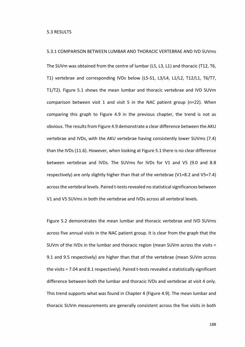
188

5.3 RESULTS

5.3.1 COMPARISON BETWEEN LUMBAR AND THORACIC VERTEBRAE AND IVD SUVms

The SUVm was obtained from the centre of lumbar (L5, L3, L1) and thoracic (T12, T6,

T1) vertebrae and corresponding IVDs below (L5-S1, L3/L4, L1/L2, T12/L1, T6/T7,

T1/T2). Figure 5.1 shows the mean lumbar and thoracic vertebrae and IVD SUVm

comparison between visit 1 and visit 5 in the NAC patient group (n=22). When

comparing this graph to Figure 4.9 in the previous chapter, the trend is not as

obvious. The results from Figure 4.9 demonstrate a clear difference between the AKU

vertebrae and IVDs, with the AKU vertebrae having consistently lower SUVms (7.4)

than the IVDs (11.6). However, when looking at Figure 5.1 there is no clear difference

between vertebrae and IVDs. The SUVms for IVDs for V1 and V5 (9.0 and 8.8

respectively) are only slightly higher than that of the vertebrae (V1=8.2 and V5=7.4)

across the vertebral levels. Paired t-tests revealed no statistical significances between

V1 and V5 SUVms in both the vertebrae and IVDs across all vertebral levels.

Figure 5.2 demonstrates the mean lumbar and thoracic vertebrae and IVD SUVms

across five annual visits in the NAC patient group. It is clear from the graph that the

SUVm of the IVDs in the lumbar and thoracic region (mean SUVm across the visits =

9.1 and 9.5 respectively) are higher than that of the vertebrae (mean SUVm across

the visits = 7.04 and 8.1 respectively). Paired t-tests revealed a statistically significant

difference between both the lumbar and thoracic IVDs and vertebrae at visit 4 only.

This trend supports what was found in Chapter 4 (Figure 4.9). The mean lumbar and

thoracic SUVm measurements are generally consistent across the five visits in both

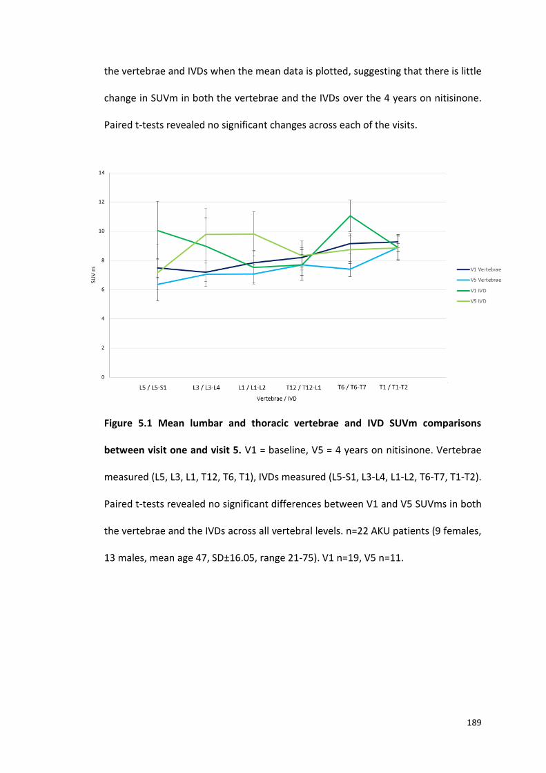
189

the vertebrae and IVDs when the mean data is plotted, suggesting that there is little

change in SUVm in both the vertebrae and the IVDs over the 4 years on nitisinone.

Paired t-tests revealed no significant changes across each of the visits.

Figure 5.1 Mean lumbar and thoracic vertebrae and IVD SUVm comparisons

between visit one and visit 5. V1 = baseline, V5 = 4 years on nitisinone. Vertebrae

measured (L5, L3, L1, T12, T6, T1), IVDs measured (L5-S1, L3-L4, L1-L2, T6-T7, T1-T2).

Paired t-tests revealed no significant differences between V1 and V5 SUVms in both

the vertebrae and the IVDs across all vertebral levels. n=22 AKU patients (9 females,

13 males, mean age 47, SD±16.05, range 21-75). V1 n=19, V5 n=11.

190

Figure 5.2 Mean AKU lumbar and thoracic vertebrae and IVD SUVm across 5 annual

visits. Each visit was one year apart, V1 (Visit 1) = baseline (pre-nitisinone), V2, V3,

V4 and V5 each with a year in-between on nitisinone. Paired t-tests revealed a

significant difference between lumbar vertebrae and IVDs (p<0.05), and thoracic

vertebrae and IVDs (p<0.05) at visit 4 only. n=22 AKU patients (9 females, 13 males,

mean age 47, SD±16.05, range 21-75). V1 n=19, V2 n=16, V3 n=22, V4 n=18, V5 n=11.

5.3.2 SUVm WITH AGE

The AKU and control mean lumbar IVD SUVm was plotted against age (Figure 5.3).

The AKU patients were plotted for each visit; V1- V5 (Figure 5.3 A-E). The control

patients were plotted against V1 only however, will be used as a comparison across

the five visits. Polynomial (second order) lines were fitted to the AKU data for each

graph. The youngest patients have low IVD SUVms that are in line with the SUVm of

the controls. With age IVD SUVm increases reaching the highest values around the

age of 60. From here the SUVm declines. Due to the lower number of patients in this

0

2

4

6

8

10

12

V1 V2 V3 V4 V5

SUV

m

Visits

MEAN L VERT

MEAN T VERT

MEAN L IVD

MEAN T IVD

191

group the trend is not as convincing as was seen in the previous chapter. However,

the trend is reminiscent of what was seen in Figures 4.12 and 4.13 with a bigger

patient number (41 patients). In contrast to the control data, there is an obvious

difference in the trend of SUVm with age between the two groups where the control

data consistently has low SUVm measurements across all ages. Independent t-tests

revealed a significant difference between the mean lumbar IVD SUVm compared to

the control group (p<0.01). This supports what was found in Figure 4.12. In terms of

change in SUVm across the visits the maximum values that are seen around the age

of 60 reduces upon each visit from V1 to V5. The maximum values in visit 1 (Figure

5.3A) reach a maximum SUVm of 24, by visit 2 (Figure 5.3B) the maximum values have

reduced to 21, by visit 3 (Figure 5.3C) they have reduced to 18, and by visits 4 (Figure

5.3D) and 5 (Figure 5.3E) the maximum values are 15 and 16 respectively.

Figure 5.4 demonstrates the AKU and control mean thoracic IVD SUVm with age. The

same trend is observed in the thoracic IVDs (Figure 5.4) however, is not as convincing

as what was seen in Figure 4.13 in the previous chapter. In terms of change in the

thoracic SUVm across the visits the highest SUVm is seen at V1 with a SUVm of 19

(Figure 5.4A), by V2 the highest value is around 15 (Figure 5.4B) and this further

reduces to 13 in V5 (Figure 5.4E). Independent t-tests revealed a significant difference

between the mean thoracic SUVm of the AKU and control group (p =< 0.01).

The lumbar and thoracic vertebrae SUVm were analysed across the five visits. Figure

5.5 demonstrates the mean lumbar vertebrae SUVm with age in individual AKU and

control patients. A negative statistically significant correlation was identified

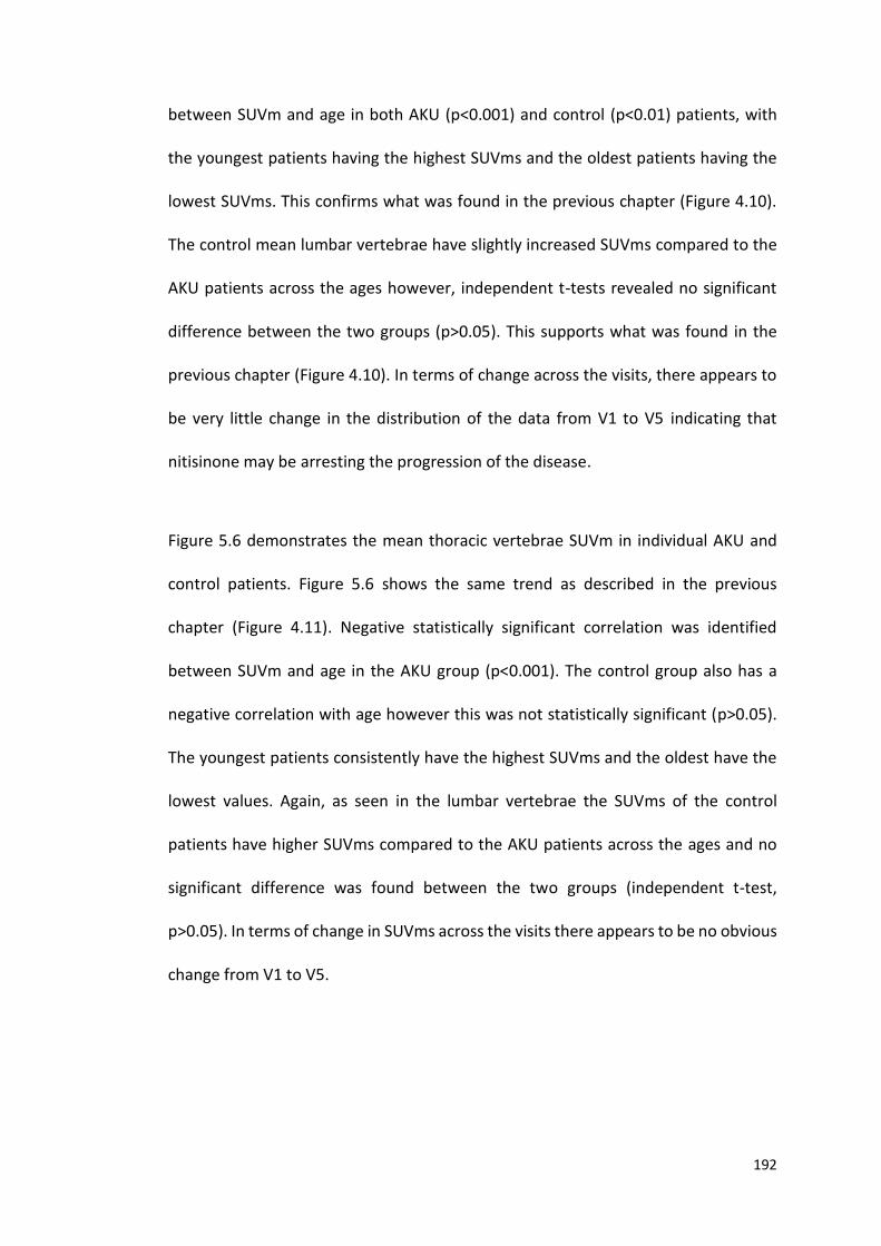
192

between SUVm and age in both AKU (p<0.001) and control (p<0.01) patients, with

the youngest patients having the highest SUVms and the oldest patients having the

lowest SUVms. This confirms what was found in the previous chapter (Figure 4.10).

The control mean lumbar vertebrae have slightly increased SUVms compared to the

AKU patients across the ages however, independent t-tests revealed no significant

difference between the two groups (p>0.05). This supports what was found in the

previous chapter (Figure 4.10). In terms of change across the visits, there appears to

be very little change in the distribution of the data from V1 to V5 indicating that

nitisinone may be arresting the progression of the disease.

Figure 5.6 demonstrates the mean thoracic vertebrae SUVm in individual AKU and

control patients. Figure 5.6 shows the same trend as described in the previous

chapter (Figure 4.11). Negative statistically significant correlation was identified

between SUVm and age in the AKU group (p<0.001). The control group also has a

negative correlation with age however this was not statistically significant (p>0.05).

The youngest patients consistently have the highest SUVms and the oldest have the

lowest values. Again, as seen in the lumbar vertebrae the SUVms of the control

patients have higher SUVms compared to the AKU patients across the ages and no

significant difference was found between the two groups (independent t-test,

p>0.05). In terms of change in SUVms across the visits there appears to be no obvious

change from V1 to V5.

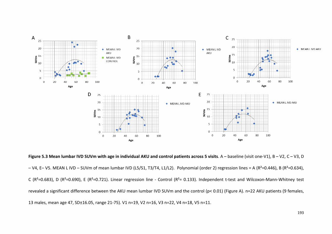
193

Figure 5.3 Mean lumbar IVD SUVm with age in individual AKU and control patients across 5 visits. A – baseline (visit one-V1), B – V2, C – V3, D

– V4, E– V5. MEAN L IVD – SUVm of mean lumbar IVD (L5/S1, T3/T4, L1/L2). Polynomial (order 2) regression lines = A (R²=0.446), B (R²=0.634),

C (R²=0.683), D (R²=0.690), E (R²=0.721). Linear regression line - Control (R²= 0.133). Independent t-test and Wilcoxon-Mann-Whitney test

revealed a significant difference between the AKU mean lumbar IVD SUVm and the control (p< 0.01) (Figure A). n=22 AKU patients (9 females,

13 males, mean age 47, SD±16.05, range 21-75). V1 n=19, V2 n=16, V3 n=22, V4 n=18, V5 n=11.

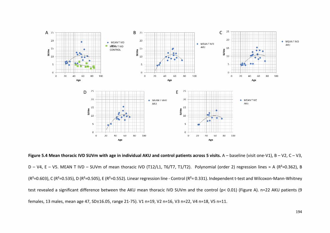
194

Figure 5.4 Mean thoracic IVD SUVm with age in individual AKU and control patients across 5 visits. A – baseline (visit one-V1), B – V2, C – V3,

D – V4, E – V5. MEAN T IVD – SUVm of mean thoracic IVD (T12/L1, T6/T7, T1/T2). Polynomial (order 2) regression lines = A (R²=0.362), B

(R²=0.603), C (R²=0.535), D (R²=0.505), E (R²=0.552). Linear regression line - Control (R²= 0.331). Independent t-test and Wilcoxon-Mann-Whitney

test revealed a significant difference between the AKU mean thoracic IVD SUVm and the control (p< 0.01) (Figure A). n=22 AKU patients (9

females, 13 males, mean age 47, SD±16.05, range 21-75). V1 n=19, V2 n=16, V3 n=22, V4 n=18, V5 n=11.

MEAN T IVD CONTROL

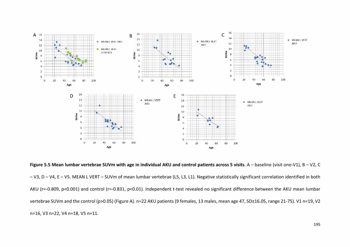
195

Figure 5.5 Mean lumbar vertebrae SUVm with age in individual AKU and control patients across 5 visits. A – baseline (visit one-V1), B – V2, C

– V3, D – V4, E – V5. MEAN L VERT – SUVm of mean lumbar vertebrae (L5, L3, L1). Negative statistically significant correlation identified in both

AKU (r=-0.809, p<0.001) and control (r=-0.831, p<0.01). Independent t-test revealed no significant difference between the AKU mean lumbar

vertebrae SUVm and the control (p>0.05) (Figure A). n=22 AKU patients (9 females, 13 males, mean age 47, SD±16.05, range 21-75). V1 n=19, V2

n=16, V3 n=22, V4 n=18, V5 n=11.

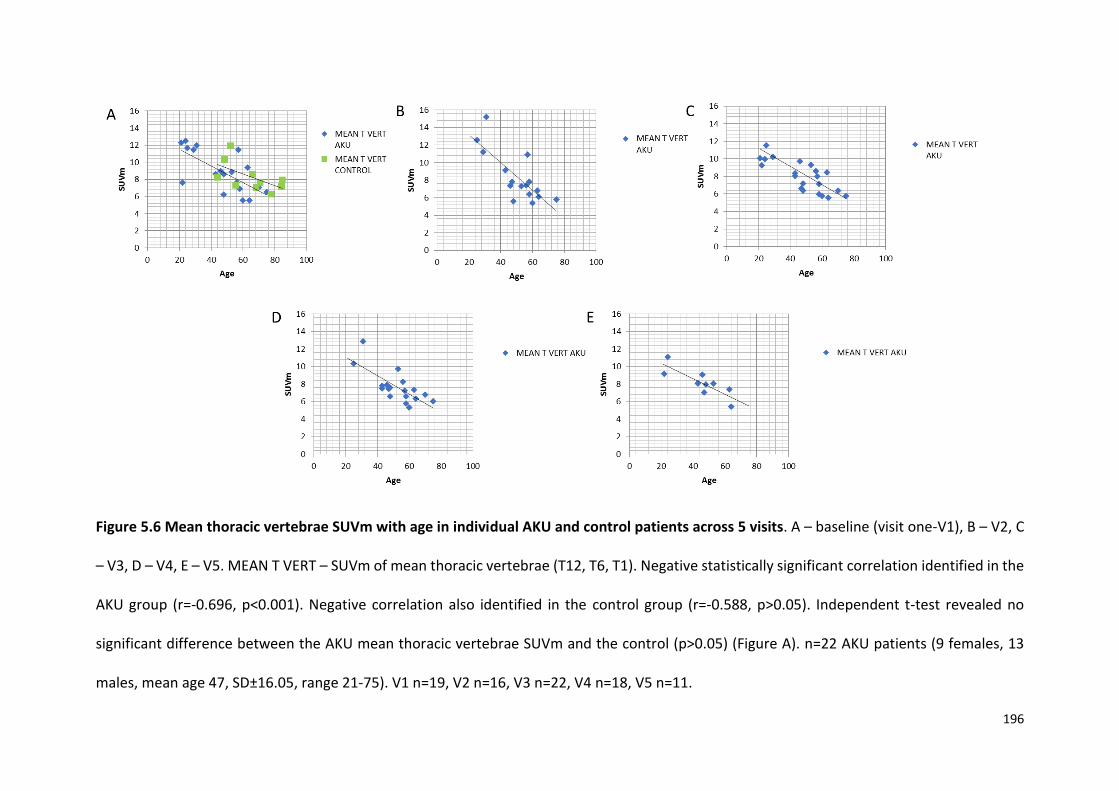
196

Figure 5.6 Mean thoracic vertebrae SUVm with age in individual AKU and control patients across 5 visits. A – baseline (visit one-V1), B – V2, C

– V3, D – V4, E – V5. MEAN T VERT – SUVm of mean thoracic vertebrae (T12, T6, T1). Negative statistically significant correlation identified in the

AKU group (r=-0.696, p<0.001). Negative correlation also identified in the control group (r=-0.588, p>0.05). Independent t-test revealed no

significant difference between the AKU mean thoracic vertebrae SUVm and the control (p>0.05) (Figure A). n=22 AKU patients (9 females, 13

males, mean age 47, SD±16.05, range 21-75). V1 n=19, V2 n=16, V3 n=22, V4 n=18, V5 n=11.

197

5.3.3 INDIVIDUAL CHANGE IN SUVm ACROSS 5 VISITS

The AKU patients were divided into four age groups; 20-31 years, 40-49 years, 50-59 years,

60+ years, to look at the individual change in SUVm over five visits in the thoracic and lumbar

vertebrae and IVDs. Figure 5.7 demonstrates the mean lumbar IVD SUVm across the five visits

in the four age groups. The age dependent trend (inverted ‘U’ trend) in SUVm is evident across

the four graphs as seen in Figures 5.3 and 5.4. The inverted ‘U’ trend reflects the youngest

age group (21-30) having the lowest SUVms (Figure 5.7A), the 50-59 age group reaching the

highest (Figure 5.7C), and the oldest age group having reduced SUVms (Figure 5.7D). When

looking at the change in SUVm in the mean lumbar IVDs across the five visits in the individual

patients there appears to be no direct trend (Figure 5.7). When the IVD SUVm is high initially

it appears to always come down across the visits in most cases. Generally, there is little change

in the mean lumbar IVD SUVm in the youngest patients across the five visits (Figure 5.7A). In

the 40-49 and the 50-59 age groups, the SUVm fluctuates across the five visits, with generally

little change between V1 and V5 (Figure 5.7B and C). The SUVm in the oldest age group (60+

Figure 5.7D) is generally consistent across each of the visits.

Figure 5.8 shows the mean thoracic IVD SUVm in the four age groups. There is a small

reduction in SUVm across the five visits in the youngest patients (Figure 5.8A). In the patients

aged 40-49 (Figure 5.8B) there appears to be fluctuations in SUVms across the visits again

with little difference between the values at V1 and V5. The patients in the oldest two age

groups (Figures 5.8 C and D) generally have consistent SUVms across the five visits with

minimal change between visits.

198

Figure 5.9 demonstrates the mean lumbar vertebrae SUVm in the four age groups across the

five visits. A reduction in SUVm can be seen across the four age groups (Figures 5.9 A-D) with

the youngest patients reaching the highest SUVms (Figure 5.9A) and the oldest patients

having the lowest SUVms (Figure 5.9D) as seen in Chapter 4 (Figure 4.10). Generally, the

SUVms across the five visits are very consistent with little change between the visits in each

of the patient groups.

The same trends are seen in the thoracic vertebrae (Figure 5.10) with the youngest patients

reaching the highest SUVms (Figure 5.10A) and the oldest having the lowest SUVms (Figure

5.10D) as seen in the previous chapter (Figure 4.11). Again, there is little change in SUVm

across the five visits (Figures 5.10).

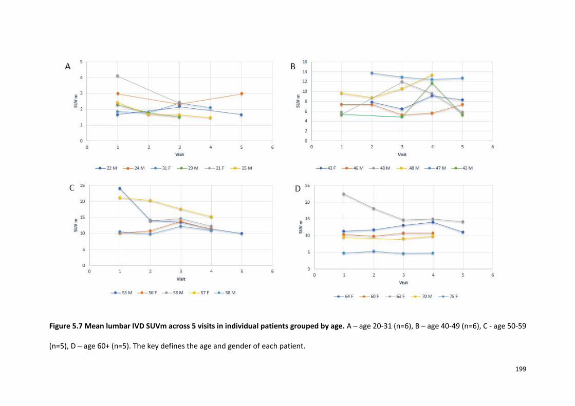
199

Figure 5.7 Mean lumbar IVD SUVm across 5 visits in individual patients grouped by age. A – age 20-31 (n=6), B – age 40-49 (n=6), C - age 50-59

(n=5), D – age 60+ (n=5). The key defines the age and gender of each patient.

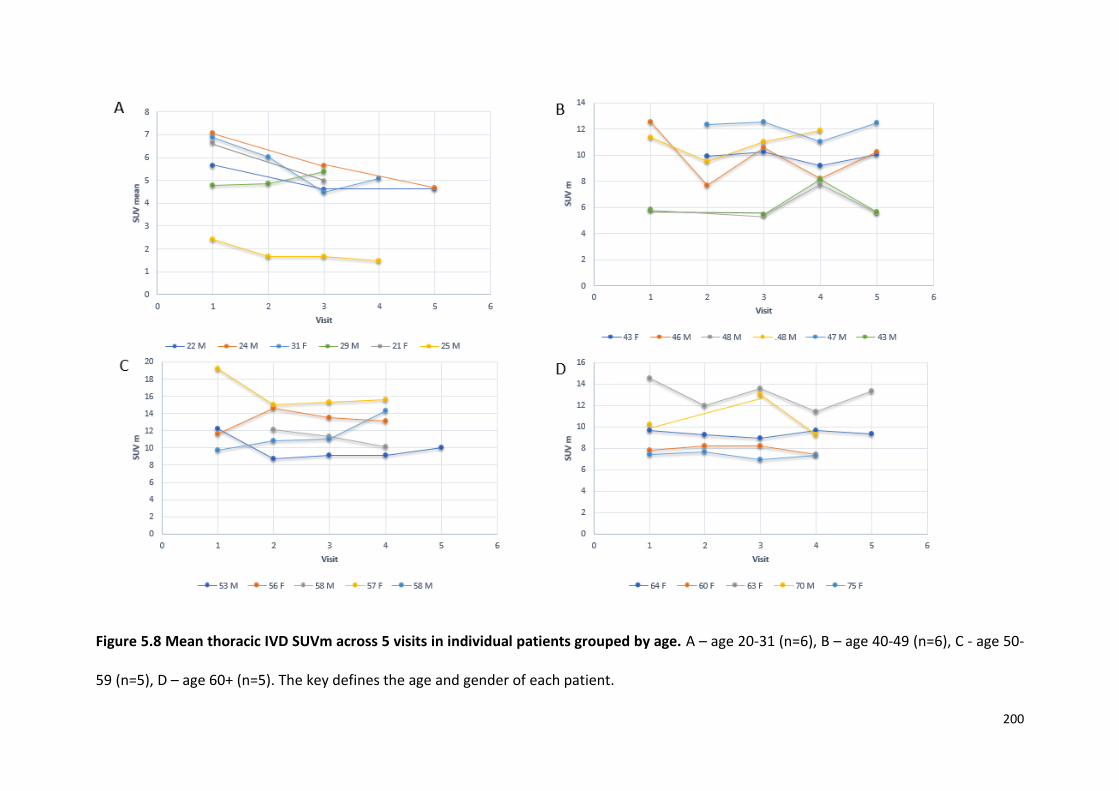
200

Figure 5.8 Mean thoracic IVD SUVm across 5 visits in individual patients grouped by age. A – age 20-31 (n=6), B – age 40-49 (n=6), C - age 50-

59 (n=5), D – age 60+ (n=5). The key defines the age and gender of each patient.

201

Figure 5.9 Mean lumbar vertebrae SUVm across 5 visits in individual patients grouped by age. A – age 20-31 (n=6), B – age 40-49 (n=6), C - age

50-59 (n=5), D – age 60+ (n=5). The key defines the age and gender of each patient.

202

Figure 5.10 Mean thoracic vertebrae SUVm across 5 visits in individual patients grouped by age. A – age 20-31 (n=6), B – age 40-49 (n=6), C -

age 50-59 (n=5), D – age 60+ (n=5). The key defines the age and gender of each patient.

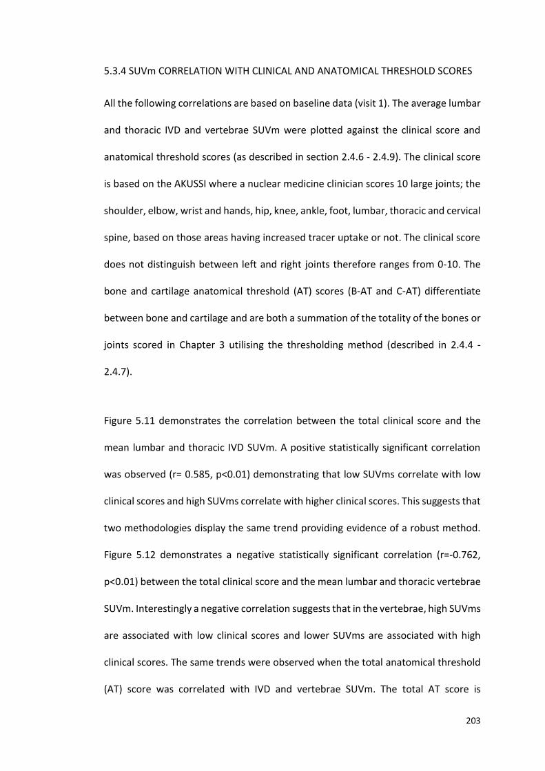
203

5.3.4 SUVm CORRELATION WITH CLINICAL AND ANATOMICAL THRESHOLD SCORES

All the following correlations are based on baseline data (visit 1). The average lumbar

and thoracic IVD and vertebrae SUVm were plotted against the clinical score and

anatomical threshold scores (as described in section 2.4.6 - 2.4.9). The clinical score

is based on the AKUSSI where a nuclear medicine clinician scores 10 large joints; the

shoulder, elbow, wrist and hands, hip, knee, ankle, foot, lumbar, thoracic and cervical

spine, based on those areas having increased tracer uptake or not. The clinical score

does not distinguish between left and right joints therefore ranges from 0-10. The

bone and cartilage anatomical threshold (AT) scores (B-AT and C-AT) differentiate

between bone and cartilage and are both a summation of the totality of the bones or

joints scored in Chapter 3 utilising the thresholding method (described in 2.4.4 -

2.4.7).

Figure 5.11 demonstrates the correlation between the total clinical score and the

mean lumbar and thoracic IVD SUVm. A positive statistically significant correlation

was observed (r= 0.585, p<0.01) demonstrating that low SUVms correlate with low

clinical scores and high SUVms correlate with higher clinical scores. This suggests that

two methodologies display the same trend providing evidence of a robust method.

Figure 5.12 demonstrates a negative statistically significant correlation (r=-0.762,

p<0.01) between the total clinical score and the mean lumbar and thoracic vertebrae

SUVm. Interestingly a negative correlation suggests that in the vertebrae, high SUVms

are associated with low clinical scores and lower SUVms are associated with high

clinical scores. The same trends were observed when the total anatomical threshold

(AT) score was correlated with IVD and vertebrae SUVm. The total AT score is

204

described in section 2.4.8. This score is directly comparable to the total clinical score

in terms of the joints scored therefore also has a maximum of 10. Figure 5.13

demonstrates a positive statistically significant correlation (r=0.658, p<0.01) between

the total AT score and the mean thoracic and lumbar IVD SUVm as seen in Figure

5.11. Figure 5.14 demonstrates a negative statistically significant correlation (r=-

0.612, p<0.01) between the total AT score and the mean lumbar and thoracic

vertebrae SUVm as seen in Figure 5.12.

Figure 5.11 Scatter graph demonstrating a positive correlation between the mean

lumbar and thoracic IVD SUVm with the total clinical score for visit 1. The ages are

represented next to each point. Positive statistically significant correlation (r= 0.585,

p<0.01). Males are plotted in blue, females in red.

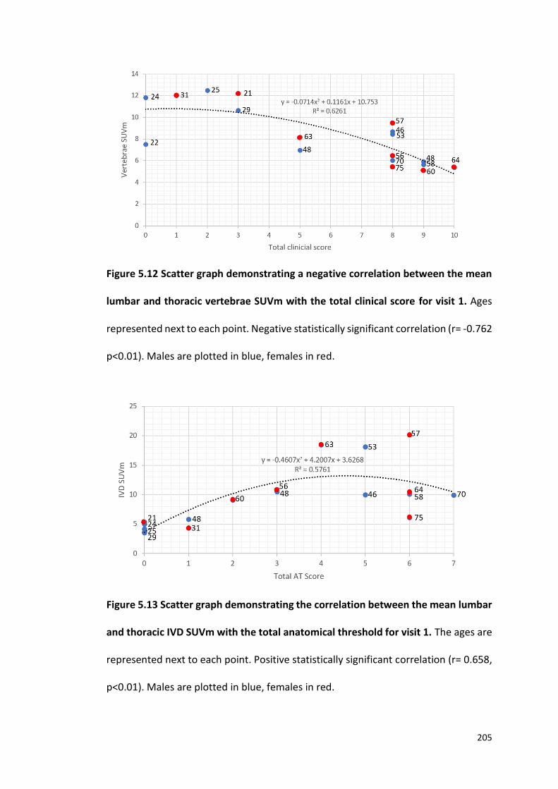
205

Figure 5.12 Scatter graph demonstrating a negative correlation between the mean

lumbar and thoracic vertebrae SUVm with the total clinical score for visit 1. Ages

represented next to each point. Negative statistically significant correlation (r= -0.762


Figure 5.13 Scatter graph demonstrating the correlation between the mean lumbar

and thoracic IVD SUVm with the total anatomical threshold for visit 1. The ages are

represented next to each point. Positive statistically significant correlation (r= 0.658,


206

Figure 5.14 Scatter graph demonstrating the correlation between the mean lumbar

and thoracic vertebrae SUVm with the total anatomical threshold score for visit 1.

The ages are represented next to each point. Negative statistically significant

correlation (r=-0.612, p<0.01). Males are plotted in blue, females in red.

Correlations were also made between the total C-AT score and total B-AT score with

the mean thoracic and lumbar IVD SUVm and vertebrae SUVm respectively. The C-AT

and B-AT scores differentiate between bone and cartilage (described in sections

2.4.6, 2.4.7). Figure 5.15 demonstrates no correlation between the mean lumbar and

thoracic IVD SUVm with the C-AT score (r= 0.09, p>0.05). Figure 5.16 also

demonstrates no correlation between the mean lumbar and thoracic vertebrae

SUVm with the B-AT score (r=-0.169, p>0.05).

207

Figure 5.15 Scatter graph between the mean lumbar and thoracic IVD SUVm with

the cartilage anatomical threshold score for visit 1. The ages are represented next

to each point. No correlation (r= 0.09, p>0.05). Males are plotted in blue, females in

red.

Figure 5.16 Scatter graph between the mean lumbar and thoracic vertebrae SUVm

with the bone anatomical threshold score for visit 1. The ages are represented next

to each point. No correlation (r=-0.169, p>0.05). Males are plotted in blue, females in

red.

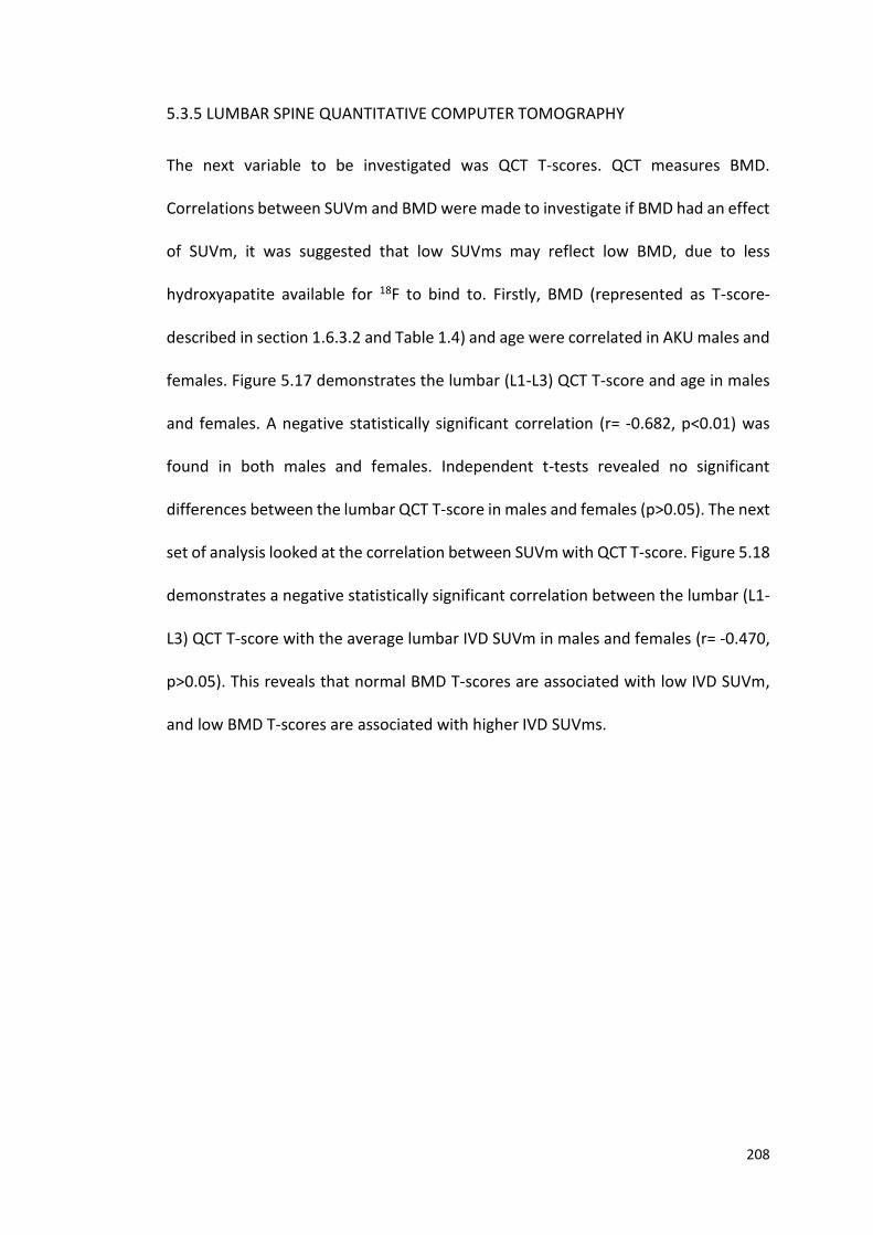
208

5.3.5 LUMBAR SPINE QUANTITATIVE COMPUTER TOMOGRAPHY

The next variable to be investigated was QCT T-scores. QCT measures BMD.

Correlations between SUVm and BMD were made to investigate if BMD had an effect

of SUVm, it was suggested that low SUVms may reflect low BMD, due to less

hydroxyapatite available for 18F to bind to. Firstly, BMD (represented as T-score-

described in section 1.6.3.2 and Table 1.4) and age were correlated in AKU males and

females. Figure 5.17 demonstrates the lumbar (L1-L3) QCT T-score and age in males

and females. A negative statistically significant correlation (r= -0.682, p<0.01) was

found in both males and females. Independent t-tests revealed no significant

differences between the lumbar QCT T-score in males and females (p>0.05). The next

set of analysis looked at the correlation between SUVm with QCT T-score. Figure 5.18

demonstrates a negative statistically significant correlation between the lumbar (L1-

L3) QCT T-score with the average lumbar IVD SUVm in males and females (r= -0.470,

p>0.05). This reveals that normal BMD T-scores are associated with low IVD SUVm,

and low BMD T-scores are associated with higher IVD SUVms.

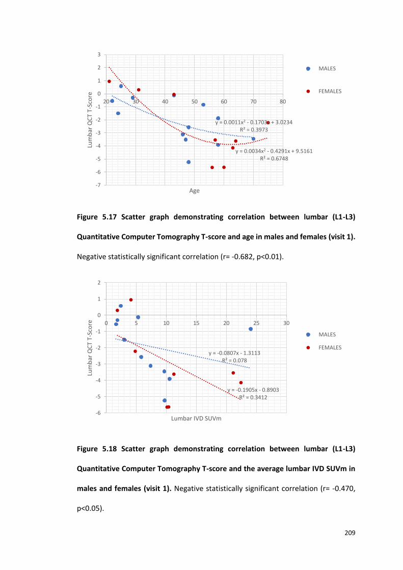
209

Figure 5.17 Scatter graph demonstrating correlation between lumbar (L1-L3)

Quantitative Computer Tomography T-score and age in males and females (visit 1).

Negative statistically significant correlation (r= -0.682, p<0.01).


Quantitative Computer Tomography T-score and the average lumbar IVD SUVm in

males and females (visit 1). Negative statistically significant correlation (r= -0.470,

p<0.05).

y = 0.0011x2 - 0.1703x + 3.0234R² = 0.3973

y = 0.0034x2 - 0.4291x + 9.5161R² = 0.6748

-7

-6

-5

-4

-3

-2

-1

0

1

2

3

20 30 40 50 60 70 80

Lum

bar

QC

T T-

Sco

re

Age

MALES

FEMALES

y = -0.0807x - 1.3113R² = 0.078

y = -0.1905x - 0.8903R² = 0.3412

-6

-5

-4

-3

-2

-1

0

1

2

0 5 10 15 20 25 30

Lum

bar

QC

T T-

Sco

re

Lumbar IVD SUVm

MALES

FEMALES

210

Figure 5.19 demonstrates the correlation between the lumbar QCT T-score and the

average lumbar vertebrae SUVm. Interestingly a positive statistically significant

correlation was found between lumbar QCT T-score and lumbar vertebrae SUVm in

both males and females (r=0.735, p<0.01) (Figure 5.19). Low lumbar QCT T-scores are

associated with low lumbar vertebrae SUVm suggesting that patients with low bone

density in the vertebrae have low uptake of 18F in that region.


Quantitative Computer Tomography T-score and the average lumbar vertebrae

SUVm in males and females (visit 1). Positive statistically significant correlation (r= -

0.735, p<0.01.

y = -0.0303x2 + 0.9443x - 7.1572R² = 0.4252

y = 0.1329x2 - 1.5859x + 0.3982R² = 0.8077

-6

-5

-4

-3

-2

-1

0

1

2

5 7 9 11 13 15

Lum

bar

QC

T T-

Sco

re

Lumbar vertebrae SUVm

MALES

FEMALES

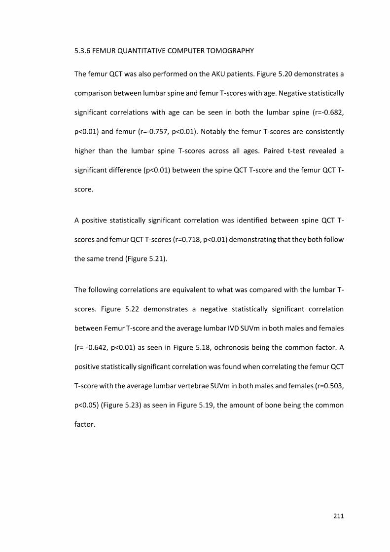
211

5.3.6 FEMUR QUANTITATIVE COMPUTER TOMOGRAPHY

The femur QCT was also performed on the AKU patients. Figure 5.20 demonstrates a

comparison between lumbar spine and femur T-scores with age. Negative statistically

significant correlations with age can be seen in both the lumbar spine (r=-0.682,

p<0.01) and femur (r=-0.757, p<0.01). Notably the femur T-scores are consistently

higher than the lumbar spine T-scores across all ages. Paired t-test revealed a

significant difference (p<0.01) between the spine QCT T-score and the femur QCT T-

score.

A positive statistically significant correlation was identified between spine QCT T-

scores and femur QCT T-scores (r=0.718, p<0.01) demonstrating that they both follow

the same trend (Figure 5.21).

The following correlations are equivalent to what was compared with the lumbar T-

scores. Figure 5.22 demonstrates a negative statistically significant correlation

between Femur T-score and the average lumbar IVD SUVm in both males and females

(r= -0.642, p<0.01) as seen in Figure 5.18, ochronosis being the common factor. A

positive statistically significant correlation was found when correlating the femur QCT

T-score with the average lumbar vertebrae SUVm in both males and females (r=0.503,

p<0.05) (Figure 5.23) as seen in Figure 5.19, the amount of bone being the common

factor.

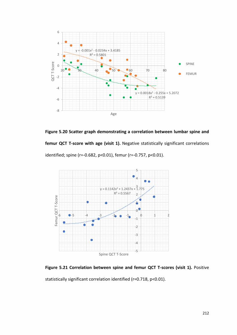
212

Figure 5.20 Scatter graph demonstrating a correlation between lumbar spine and

femur QCT T-score with age (visit 1). Negative statistically significant correlations

identified; spine (r=-0.682, p<0.01), femur (r=-0.757, p<0.01).

Figure 5.21 Correlation between spine and femur QCT T-scores (visit 1). Positive

statistically significant correlation identified (r=0.718, p<0.01).

y = 0.0018x2 - 0.255x + 5.2072R² = 0.5139

y = -0.001x2 - 0.0234x + 3.4185R² = 0.5801

-8

-6

-4

-2

0

2

4

6

20 30 40 50 60 70 80

QC

T T-

Sco

re

Age

SPINE

FEMUR

y = 0.1142x2 + 1.2437x + 1.775R² = 0.5567

-5

-4

-3

-2

-1

0

1

2

3

4

5

-6 -5 -4 -3 -2 -1 0 1 2

Fem

ur

QC

T T-

Sco

re

Spine QCT T-Score

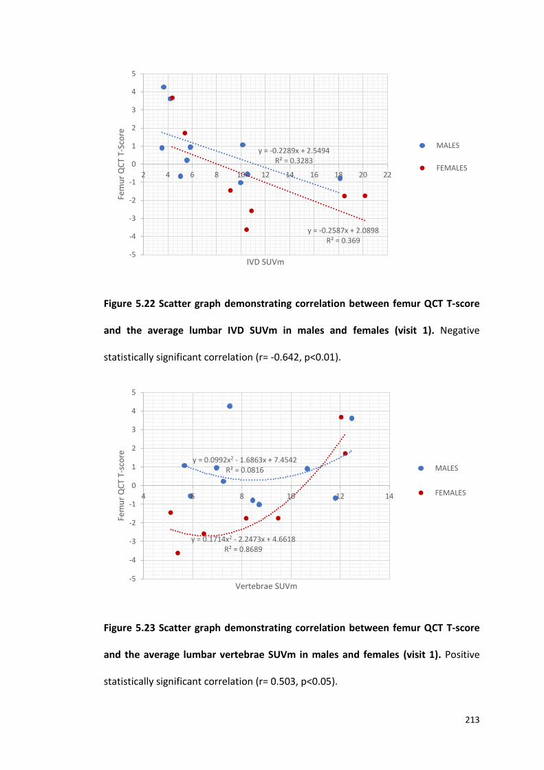
213

Figure 5.22 Scatter graph demonstrating correlation between femur QCT T-score

and the average lumbar IVD SUVm in males and females (visit 1). Negative

statistically significant correlation (r= -0.642, p<0.01).

Figure 5.23 Scatter graph demonstrating correlation between femur QCT T-score

and the average lumbar vertebrae SUVm in males and females (visit 1). Positive

statistically significant correlation (r= 0.503, p<0.05).

y = -0.2289x + 2.5494R² = 0.3283

y = -0.2587x + 2.0898R² = 0.369

-5

-4

-3

-2

-1

0

1

2

3

4

5

2 4 6 8 10 12 14 16 18 20 22

Fem

ur

QC

T T-

Sco

re

IVD SUVm

MALES

FEMALES

y = 0.0992x2 - 1.6863x + 7.4542R² = 0.0816

y = 0.1714x2 - 2.2473x + 4.6618R² = 0.8689

-5

-4

-3

-2

-1

0

1

2

3

4

5

4 6 8 10 12 14

Fem

ur

QC

T T-

sco

re

Vertebrae SUVm

MALES

FEMALES

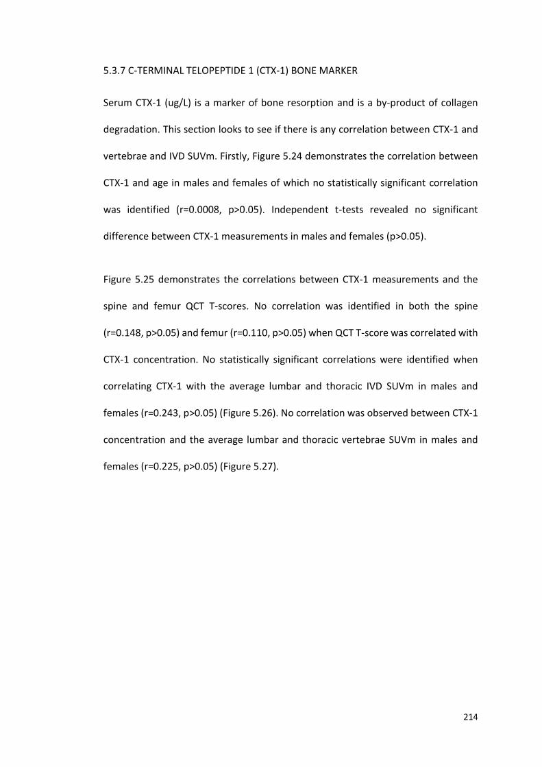
214

5.3.7 C-TERMINAL TELOPEPTIDE 1 (CTX-1) BONE MARKER

Serum CTX-1 (ug/L) is a marker of bone resorption and is a by-product of collagen

degradation. This section looks to see if there is any correlation between CTX-1 and

vertebrae and IVD SUVm. Firstly, Figure 5.24 demonstrates the correlation between

CTX-1 and age in males and females of which no statistically significant correlation

was identified (r=0.0008, p>0.05). Independent t-tests revealed no significant

difference between CTX-1 measurements in males and females (p>0.05).

Figure 5.25 demonstrates the correlations between CTX-1 measurements and the

spine and femur QCT T-scores. No correlation was identified in both the spine

(r=0.148, p>0.05) and femur (r=0.110, p>0.05) when QCT T-score was correlated with

CTX-1 concentration. No statistically significant correlations were identified when

correlating CTX-1 with the average lumbar and thoracic IVD SUVm in males and

females (r=0.243, p>0.05) (Figure 5.26). No correlation was observed between CTX-1

concentration and the average lumbar and thoracic vertebrae SUVm in males and

females (r=0.225, p>0.05) (Figure 5.27).

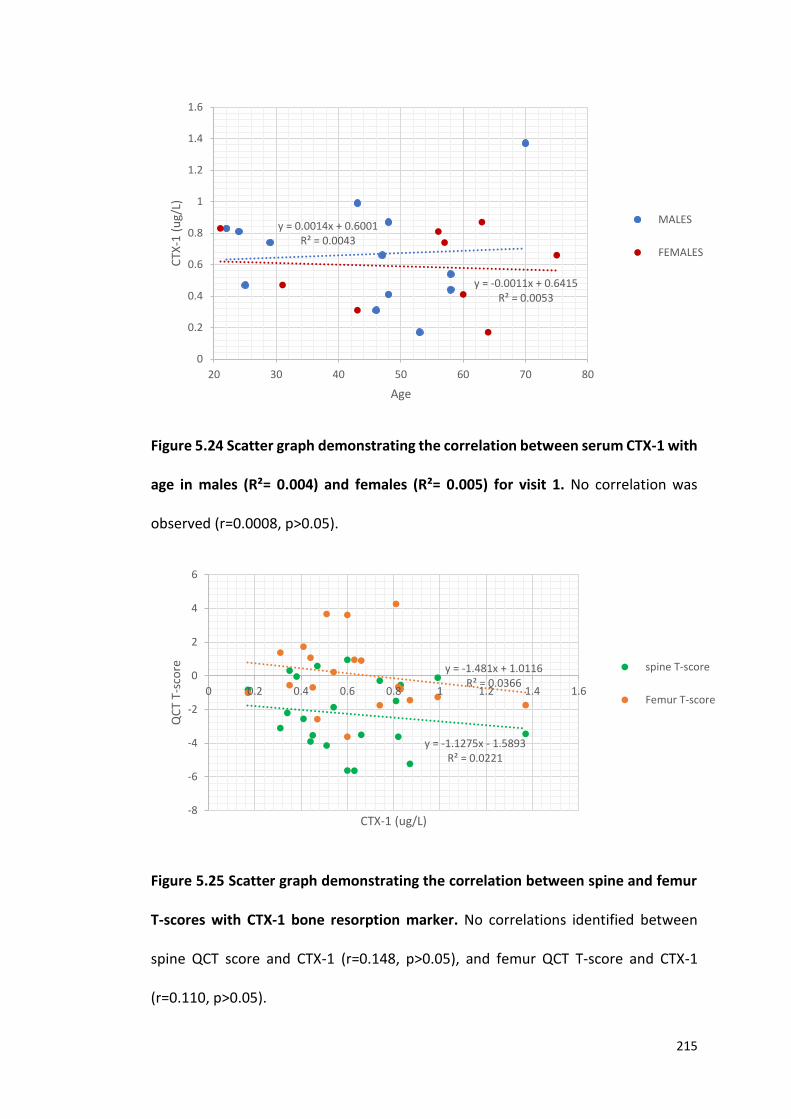
215

Figure 5.24 Scatter graph demonstrating the correlation between serum CTX-1 with

age in males (R²= 0.004) and females (R²= 0.005) for visit 1. No correlation was

observed (r=0.0008, p>0.05).

Figure 5.25 Scatter graph demonstrating the correlation between spine and femur

T-scores with CTX-1 bone resorption marker. No correlations identified between

spine QCT score and CTX-1 (r=0.148, p>0.05), and femur QCT T-score and CTX-1

(r=0.110, p>0.05).

y = 0.0014x + 0.6001R² = 0.0043

y = -0.0011x + 0.6415R² = 0.0053

0

0.2

0.4

0.6

0.8

1

1.2

1.4

1.6

20 30 40 50 60 70 80

CTX

-1 (

ug/

L)

Age

MALES

FEMALES

y = -1.1275x - 1.5893R² = 0.0221

y = -1.481x + 1.0116R² = 0.0366

-8

-6

-4

-2

0

2

4

6

0 0.2 0.4 0.6 0.8 1 1.2 1.4 1.6

QC

T T-

sco

re

CTX-1 (ug/L)

spine T-score

Femur T-score

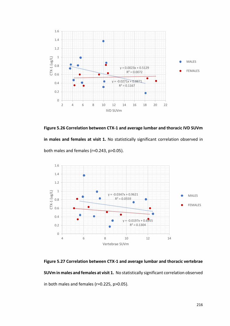
216

Figure 5.26 Correlation between CTX-1 and average lumbar and thoracic IVD SUVm

in males and females at visit 1. No statistically significant correlation observed in

both males and females (r=0.243, p>0.05).

Figure 5.27 Correlation between CTX-1 and average lumbar and thoracic vertebrae

SUVm in males and females at visit 1. No statistically significant correlation observed

in both males and females (r=0.225, p>0.05).

y = -0.0271x + 0.8871R² = 0.1167

y = 0.0023x + 0.5129R² = 0.0072

0

0.2

0.4

0.6

0.8

1

1.2

1.4

1.6

2 4 6 8 10 12 14 16 18 20 22

CTX

-1 (

ug/

L)

IVD SUVm

MALES

FEMALES

y = -0.0347x + 0.9621R² = 0.0559

y = -0.0197x + 0.6955R² = 0.1304

0

0.2

0.4

0.6

0.8

1

1.2

1.4

1.6

4 6 8 10 12 14

CTX

-1 (

ug/

L)

Vertebrae SUVm

MALES

FEMALES

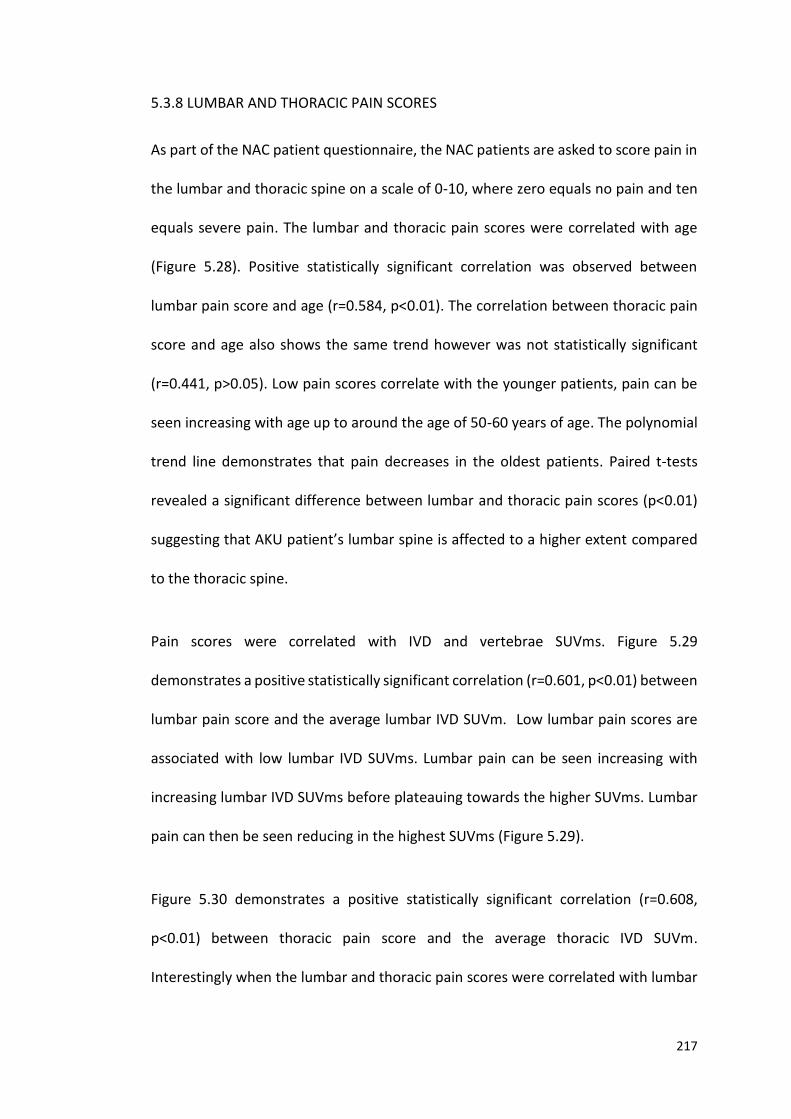
217

5.3.8 LUMBAR AND THORACIC PAIN SCORES

As part of the NAC patient questionnaire, the NAC patients are asked to score pain in

the lumbar and thoracic spine on a scale of 0-10, where zero equals no pain and ten

equals severe pain. The lumbar and thoracic pain scores were correlated with age

(Figure 5.28). Positive statistically significant correlation was observed between

lumbar pain score and age (r=0.584, p<0.01). The correlation between thoracic pain

score and age also shows the same trend however was not statistically significant

(r=0.441, p>0.05). Low pain scores correlate with the younger patients, pain can be

seen increasing with age up to around the age of 50-60 years of age. The polynomial

trend line demonstrates that pain decreases in the oldest patients. Paired t-tests

revealed a significant difference between lumbar and thoracic pain scores (p<0.01)

suggesting that AKU patient’s lumbar spine is affected to a higher extent compared

to the thoracic spine.

Pain scores were correlated with IVD and vertebrae SUVms. Figure 5.29

demonstrates a positive statistically significant correlation (r=0.601, p<0.01) between

lumbar pain score and the average lumbar IVD SUVm. Low lumbar pain scores are

associated with low lumbar IVD SUVms. Lumbar pain can be seen increasing with

increasing lumbar IVD SUVms before plateauing towards the higher SUVms. Lumbar

pain can then be seen reducing in the highest SUVms (Figure 5.29).

Figure 5.30 demonstrates a positive statistically significant correlation (r=0.608,

p<0.01) between thoracic pain score and the average thoracic IVD SUVm.

Interestingly when the lumbar and thoracic pain scores were correlated with lumbar

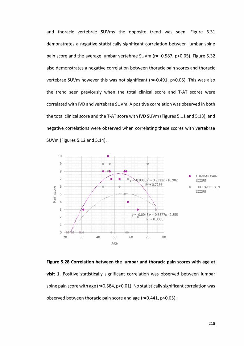
218

and thoracic vertebrae SUVms the opposite trend was seen. Figure 5.31

demonstrates a negative statistically significant correlation between lumbar spine

pain score and the average lumbar vertebrae SUVm (r= -0.587, p<0.05). Figure 5.32

also demonstrates a negative correlation between thoracic pain scores and thoracic

vertebrae SUVm however this was not significant (r=-0.491, p>0.05). This was also

the trend seen previously when the total clinical score and T-AT scores were

correlated with IVD and vertebrae SUVm. A positive correlation was observed in both

the total clinical score and the T-AT score with IVD SUVm (Figures 5.11 and 5.13), and

negative correlations were observed when correlating these scores with vertebrae

SUVm (Figures 5.12 and 5.14).

Figure 5.28 Correlation between the lumbar and thoracic pain scores with age at

visit 1. Positive statistically significant correlation was observed between lumbar

spine pain score with age (r=0.584, p<0.01). No statistically significant correlation was

observed between thoracic pain score and age (r=0.441, p>0.05).

y = -0.0088x2 + 0.9311x - 16.902R² = 0.7256

y = -0.0048x2 + 0.5377x - 9.855R² = 0.3066

0

1

2

3

4

5

6

7

8

9

10

20 30 40 50 60 70 80

Pai

n s

core

Age

LUMBAR PAINSCORE

THORACIC PAINSCORE

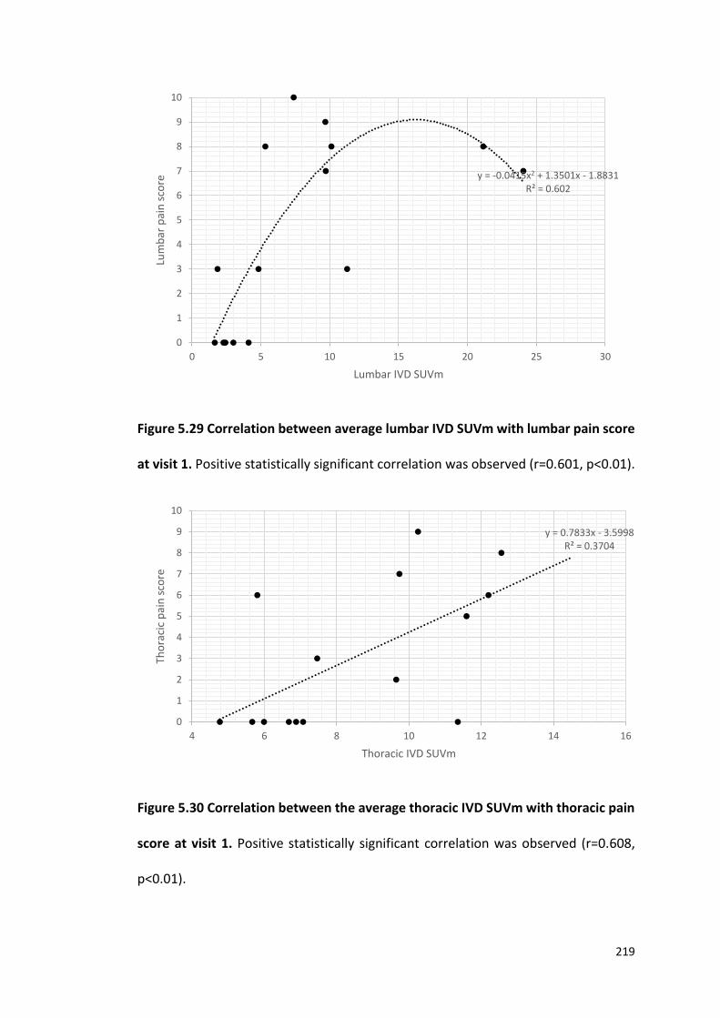
219

Figure 5.29 Correlation between average lumbar IVD SUVm with lumbar pain score

at visit 1. Positive statistically significant correlation was observed (r=0.601, p<0.01).

Figure 5.30 Correlation between the average thoracic IVD SUVm with thoracic pain

score at visit 1. Positive statistically significant correlation was observed (r=0.608,

p<0.01).

y = -0.0415x2 + 1.3501x - 1.8831R² = 0.602

0

1

2

3

4

5

6

7

8

9

10

0 5 10 15 20 25 30

Lum

bar

pai

n s

core

Lumbar IVD SUVm

y = 0.7833x - 3.5998R² = 0.3704

0

1

2

3

4

5

6

7

8

9

10

4 6 8 10 12 14 16

Tho

raci

c p

ain

sco

re

Thoracic IVD SUVm

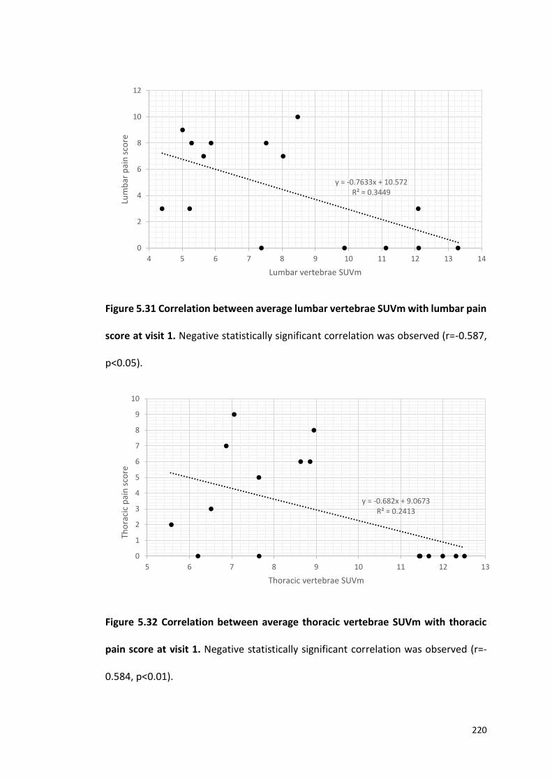
220

Figure 5.31 Correlation between average lumbar vertebrae SUVm with lumbar pain

score at visit 1. Negative statistically significant correlation was observed (r=-0.587,

p<0.05).

Figure 5.32 Correlation between average thoracic vertebrae SUVm with thoracic

pain score at visit 1. Negative statistically significant correlation was observed (r=-

0.584, p<0.01).

y = -0.682x + 9.0673R² = 0.2413

0

1

2

3

4

5

6

7

8

9

10

5 6 7 8 9 10 11 12 13

Tho

raci

c p

ain

sco

re

Thoracic vertebrae SUVm

y = -0.7633x + 10.572R² = 0.3449

0

2

4

6

8

10

12

4 5 6 7 8 9 10 11 12 13 14

Lum

bar

pai

n s

core


221

5.4 DISCUSSION

This chapter aims to assess the progression of spinal arthropathy, over a period of

five years, in response to nitisinone, the potentially disease modifying therapy

monitored by 18F-NaF SUVm.

5.4.1 COMPARISON BETWEEN LUMBAR AND THORACIC VERTEBRAE AND IVD SUVms

In this chapter, the analysis described in Chapter 4 has been repeated on a different

patient group, this chapter reporting on the NAC patients and Chapter 4 reporting on

the SONIA 2 patients. The main difference between the two patient groups being that

the NAC patients included in this analysis have attended the NAC 5 times, each with

a year in between, compared to just 2 visits for SONIA 2 (with one year in between).

Another main difference is that all the NAC patients have been prescribed nitisinone

(2mg daily) in contrast to the SONIA 2 patients where half received 10mg of nitisinone

in a blinded design. This chapter aims to look at the longitudinal change in SUVm over

a period of five years in response to nitisinone.

When looking at the comparison between the lumbar and thoracic vertebrae and

IVDs in the NAC patients (Figure 5.1) the results were slightly different compared to

the SONIA 2 patients (Figure 4.9). For the SONIA 2 patients the mean SUVm for the

vertebrae was 7.4, and for the IVDs was 11.6 with significant differences identified at

every level (except T1/ T1/T2). For the NAC patients, no significant differences were

found between the vertebrae and IVDs at every level. The mean SUVm across the

vertebrae was 8.2, and the mean SUVm across the IVDs was 9.0. The proposed reason

for the similar results between the SUVm of the vertebrae and IVDs in the NAC

222

patients may be due to the age range of the patients. In the SONIA 2 patient group,

41 patients were analysed (16 females, 25 males, mean age 51 SD±10.9, range 30-

68), in the NAC patient group, 22 patients were analysed (9 females, 13 males, mean

age 47, SD±16.05, range 21-75). The age range of patients in the NAC patient group

starts almost 10 years younger (21 years compared to 30 in the SONIA 2). As identified

the youngest patients have low IVD SUVms (Figures 4.12, 4.13, 5.3 and 5.4) and high

vertebral SUVms (Figures 4.10, 4.11, 5.5 and 5.6). It is proposed that these younger

patients have resulted in the means of the vertebrae and IVDs to fall closer together.

The SONIA 2 patient age range starts from the age of 30, by the age of 40 the SUVm

are almost 3 times that of the youngest patients, with almost double the number of

patients in this group.

5.4.2 ANNUAL CHANGE IN SUVm IN THE VERTEBRAE AND IVDs

The main purpose of this chapter was to look at the annual change in SUVm over a

period of 4 years. Figure 5.2 demonstrates the mean AKU lumbar and thoracic

vertebrae and IVD SUVm across the 5 visits. It is evident that there is very little change

in SUVm across the 5 visits for the lumbar and thoracic vertebrae and IVDs. Paired t-

tests revealed no statistically significant differences between V1 and V5 in both

lumbar and thoracic IVD and vertebrae SUVms. This supports what was found in the

previous chapter where there was very little change in SUVm over a period of 1 year.

At the very most nitisinone is thought to arrest ochronosis and or slow progression

of the disease, it is widely agreed that it is very unlikely for nitisinone to reverse

ochronosis. Figure 5.2 demonstrates small changes in SUVm across the visits with a

223

small reduction seen in the lumbar vertebrae, thoracic vertebrae and thoracic IVDs

from V1 to V5. Unfortunately, a control group could not be used as a comparison

longitudinally, as we only had data representative of a single visit for each control

patient. The control patients were non-metastatic breast cancer patients that only

had one scan to determine bony metastasis. This would have been useful as a control

group would have provided an insight into normal change in SUVm across a period of

5 years. It is therefore not possible to comment on the effectiveness of nitisinone on

SUVm in this group at this stage.

5.4.3 SUVm WITH AGE

The SUVm was plotted against age in the thoracic and lumbar vertebrae and IVDs for

each of the five visits for comparison with the SONIA 2 data (Figures 5.3 – 5.6).

Significant differences were identified between the AKU and control groups when

comparing both the mean lumbar and thoracic IVD SUVms (independent t-test

p<0.01 for both comparisons; Figures 5.3 and 5.4). This demonstrates that AKU IVD

SUVms are significantly different to that of the control group. When analysing the

difference between AKU mean lumbar and thoracic vertebrae SUVms compared to

that of the control no significant differences were found (Figures 5.5 and 5.6). The

trend with age for the AKU vertebrae SUVms supports the findings described in the

previous chapter (Figure 4.10 and 4.11). The SUVm in AKU vertebrae decreases with

age (Figures 5.5 and 5.6), supporting the idea that this is due to reduced bone mass

with ageing (145). Reduced bone mass results in less hydroxyapatite for 18F to bind

to, therefore resulting in lower SUVms. Additionally this process could be

224

exacerbated by AKU as Aliberty, et al. (148) described ochronotic patients have an

imbalance in bone metabolism, resulting in osteopenia and osteoporosis.

The SUVm in AKU IVDs also followed the same trend as what was found in the

previous chapter; the inverted ‘U’ curve (Figures 4.12, 4.13, 5.5.3 and 5.4). From the

age of 40 an exponential increase can be seen, which corresponds to the onset of

arthropathy, of which the spine is widely affected. The results of this chapter support

the suggested reason for this explained in Chapter 4. It is proposed that the increase

in SUVm could be due to deposition of hydroxyapatite / calcium pyrophosphate

dehydrate crystals of which the plateau corresponds to complete calcification of the

IVD, and the reduction in SUVm corresponds to reduced turnover due to fusion of the

vertebrae.

5.4.4 INDIVIDUAL CHANGES IN SUVm ACROSS THE FIVE VISITS

It is clear from Figure 5.2 that when the mean SUVms are plotted for the lumbar and

thoracic vertebrae and IVDs across the five visits, little change is observed from one

year to the next. Small fluctuations are observed, however the SUVm at V1,

compared to the SUVm at V5 are very similar. As in Chapter 4, the next step was to

plot individual patient changes to see if any trends could be identified with age.

Figures 5.7 – 5.10 represent the individual changes across the five visits in the lumbar

and thoracic vertebrae and IVDs in four age groups (20-31, 40-49, 50-59, 60+). These

graphs try to shed light on what is happening to the SUVm over 4 years on an

individual basis. No definitive trends were identified in any of the patients, generally

the SUVms remain stable across the visits with very little change in the values. The

lumbar and thoracic vertebrae SUVms are particularly stable (Figures 5.9 and 5.10)

225

reflecting a robust methodology. These results may also demonstrate the

stabilisation of the disease by nitisinone. The SUVm of the lumbar and thoracic IVDs

were slightly more variable. Especially so, in the 40-49 age group where the SUVm

can be seen fluctuating, however when comparing the SUVms at V1 and V5, they

were very similar. It was noted that if the SUVm was high at V1, it can be seen

reducing across the visits in a few patients (Figure 5.7 C and D and 5.8 C). The effect

of nitisinone on IVD and vertebrae SUVm cannot be confirmed due to fact that no

AKU control group (no treatment group) was available for comparison to elucidate

normal changes in SUVm across a period of 4 years. However, it can be commented

that it would not be unreasonable to have expected an increase in IVD SUVm that

reflects disease progression especially over a period of 4 years in those patients aged

40 and over. Vertebrae SUVm was expected to decrease as we have shown this occurs

with age. Future work includes comparing these results with an AKU non-treatment

group to investigate changes without nitisinone.

The systemic effects of nitisinone have been widely studied in terms of HGA levels in

urine and in serum (44,45). Nitisinone (2.1 mg/day) has been shown to reduce urinary

HGA down by 98% (from 5.1 to 0.125 g/day) and mean plasma HGA levels down by

95% from 5.74 to 0.306 mg/l (44). The SONIA 1 clinical trial revealed a clear dose

response relationship between nitisinone and urinary HGA. The five dosages given

were 0,1,2,4 and 8mg/day, with the 8mg dose reducing urinary HGA from 31.53mmol

to 0.15mmol after 4 weeks (45). The long-term safety and efficacy of nitisinone has

not fully been elucidated hence why the 2mg dose is routinely prescribed currently.

HGA is the culprit molecule in AKU and nitisinone has been shown to effectively

226

reduce this down to negligible levels. This chapter has found no clear trends in SUVm

over the four-year period in the 22 patients analysed. It is proposed that changes in

response to nitisinone, measured by fluoride uptake in cartilage and bone, cannot be

elucidated until a no treatment group is analysed. It may also be questioned whether

four years is enough time to see any definite changes in 18F uptake in the spine.

Changes to cartilage and bone in AKU occur over many years, continued

polymerisation of HGA in cartilage leads to osteoarthropathy. In terms of monitoring

fluoride uptake as a measure of radioactivity and detecting osteoarthropathy, this

method is capable of identifying arthritic changes in the spine. However, it could be

proposed that for the effect of nitisinone on the spine to be elucidated, many more

years of data will be required to assess the long-term effects. This method may

demonstrate the effect of nitisinone on cartilage in AKU if a comparison was made

between a group of patients that have been taking nitisinone for decades compared

to a group of patients with no treatment. The increased SUVms may occur much

younger in the non-treatment group compared to the treatment group.

5.4.5 CORRELATION BETWEEN SUVm AND CLINICAL AND ANATOMICAL THRESHOLD

SCORES

The average lumbar and thoracic IVD and vertebrae SUVms were plotted against the

total clinical score (described in section 2.4.9). A positive statistically significant

correlation was identified (r=0.585, p<0.01) between the total clinical score and the

average lumbar and thoracic IVD SUVm before plateauing at the higher total clinical

scores (Figure 5.11). This demonstrates that higher IVD SUVms are associated with

227

higher total clinical scores. In Chapter 3 it was reported that the total clinical score

had a positive correlation with age (Figure 3.15). Additionally, in Chapter 4 it was

reported the age-related trend in IVD SUVm (Figure 4.12 and 4.13) that occurs with

disease progression (the inverted ‘U’ curve) where SUVm increases up to around the

age of 40 then stabilises and then reduces back down in the oldest patients. This

trend was proposed to be due to calcification of the IVDs that occurs with disease

progression. These two previous findings are reflected in these results (Figure 5.11).

The patients with the highest total clinical scores are associated with the oldest

patients as the more joints are affected. The lowest IVD SUVms and low clinical scores

are associated with the younger patients less affected by the disease. This trend was

also observed when correlating the total anatomical threshold score (explained in

section 2.4.8) with IVD SUVm (Figure 5.13) suggesting that both the clinical and

anatomical threshold methods are robust and demonstrate the same trend.

Interestingly, the opposite trend was seen when plotting vertebrae SUVms with the

total clinical score. A negative statistically significant correlation was observed when

correlating the total clinical score with the average lumbar and thoracic vertebrae

SUVm (Figure 5.12, r=-0.762, p<0.001) demonstrating that high vertebrae SUVms are

associated with low total clinical scores, and these patients were identified as the

youngest. This supports what was described in Chapter 4, where a reduction in the

mean lumbar and thoracic vertebrae SUVm was identified with age (Figures 4.10 and

4.11). The oldest patients have the highest total clinical scores and lower vertebrae

SUVms. As described in Chapter 4, high SUVms in the vertebrae of younger patients

reflects active bone remodelling that reduces with age, this is due to reduced bone

228

turnover and often reduced BMD with age. Again, the same trend was identified

when correlating the average lumbar and thoracic vertebrae SUVm with the total

anatomical threshold score (Figure 5.14).

5.4.6 SUVm WITH LUMBAR SPINE AND FEMUR QCT T-SCORE

It is widely recognised that changes in cartilage composition as seen in AKU have

direct implications to bone. QCT was therefore performed on these patients to assess

BMD. In AKU it is proposed that chronic arthritis can impair bone architecture which

then may predispose AKU patients to fractures (89). Aliberti et al. (148) reported an

imbalance in bone metabolism in 7 AKU patients, leading to osteopenia and

osteoporosis. It was hypothesised that HGA deposition in bone matrix and osteocytes

may play a pathophysiological role in accelerating bone loss in AKU (148).

QCT measures BMD using an X-ray computed tomography scanner containing a

calibration standard to convert Hounsfield units into BMD values. The sites most

commonly measured to determine BMD are the lumbar spine and hip (95). QCT has

the ability to spatially separate highly responsive cortical bone from less responsive

trabecular bone. This is useful because osteoarthropathy affects the trabecular bone

earlier and to a greater degree than cortical bone. QCT is therefore likely to detect

low BMD earlier in the spine than DEXA. Artificially high BMD has been identified in

DEXA reports of spinal arthropathy patients due to calcification and osteophyte

formation, resulting in unusually high T-values (148). This is because DEXA estimates

the amount of total mineral in the path of the X-ray beam in the region of L2-L4. This

can be avoided in QCT as this method specifically measures volumetric trabecular

229

BMD and does not include the IVDs unlike DEXA (94). QCT imaging often results in

lower T-scores than that of the DEXA in cases of spinal arthropathy due to the

increased mineral content of the calcified IVDs and/or bony osteophtyes. The lower

T-scores of QCT compared to DEXA may be due to a variety of factors such as the

physiological effects of ageing and the menopause (that affects trabecular bone first),

therefore QCT can detect changes earlier than DEXA (96). The size of the patient also

affects DEXA scores as DEXA cannot exclude soft tissue, therefore obese patients

have higher T-scores, volumetric measurements of QCT are not affected by size (94).

Although QCT has many benefits over DEXA it is important to note that QCT T-scores

are not comparable to DEXA T-scores and are not used to diagnose osteopenia or

osteoporosis from the WHO definition of T-scores (a DEXA T-score of -2.5 equates to

a QCT T-score of -3.4) (96). At present DEXA is the only modality accepted as the

leading method in clinical decision making. However, as discussed QCT may provide

a more accurate measure of BMD in patients with spinal arthropathy in AKU. This

chapter explores the trends between QCT T-score and SUVms as it was proposed that

low BMD may be the reason for low SUVms in the vertebrae a result of less

hydroxyapatite available for 18F to bind to.

Firstly, a negative statistically significant correlation was identified between the

lumbar spine QCT T-score with age (r= -0.682, p<0.01) (Figure 5.17). Independent t-

test revealed no significant difference between the lumbar QCT T-scores of males and

females (p>0.05). It is widely agreed that bone deteriorates in composition, structure

and function with age. Peak BMD is reached around the age of 20 in women and

slightly older in men, after this bone turnover continues at a slower rate resulting in

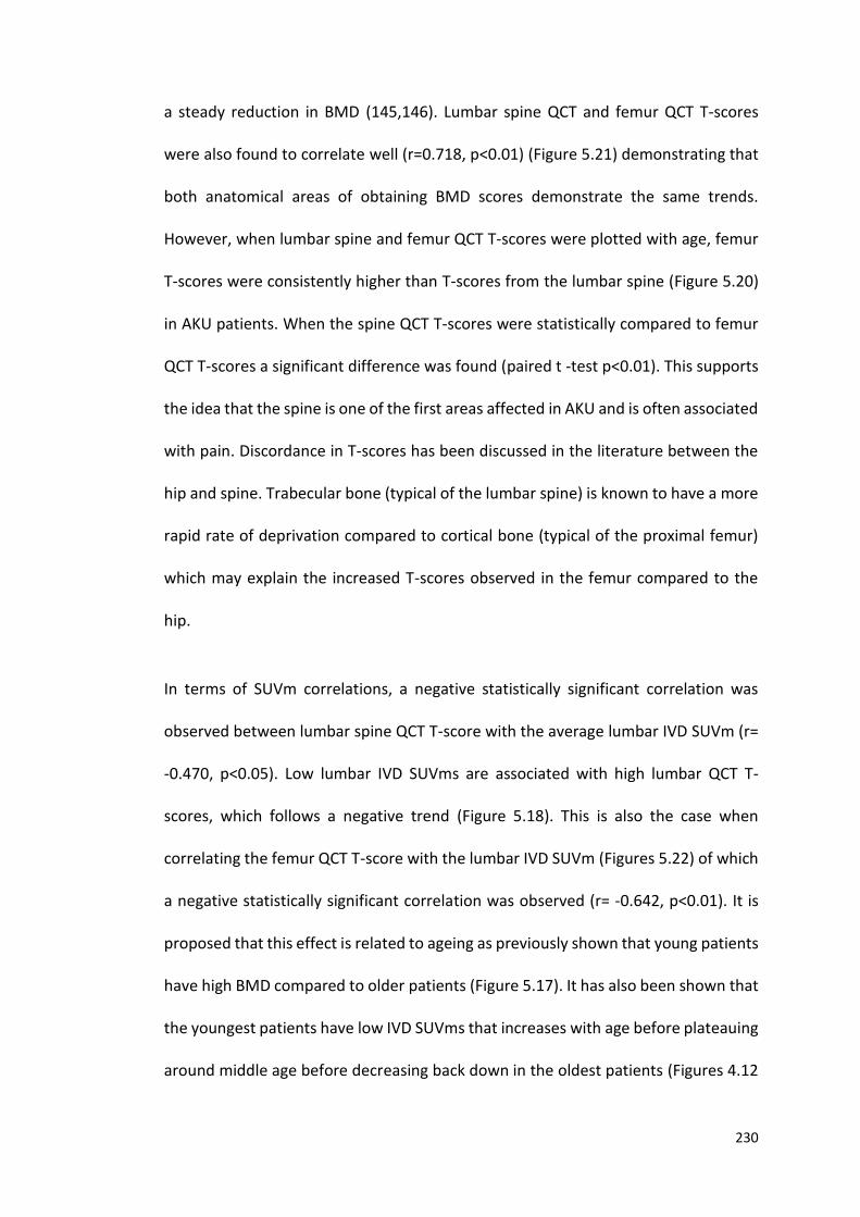
230

a steady reduction in BMD (145,146). Lumbar spine QCT and femur QCT T-scores

were also found to correlate well (r=0.718, p<0.01) (Figure 5.21) demonstrating that

both anatomical areas of obtaining BMD scores demonstrate the same trends.

However, when lumbar spine and femur QCT T-scores were plotted with age, femur

T-scores were consistently higher than T-scores from the lumbar spine (Figure 5.20)

in AKU patients. When the spine QCT T-scores were statistically compared to femur

QCT T-scores a significant difference was found (paired t -test p<0.01). This supports

the idea that the spine is one of the first areas affected in AKU and is often associated

with pain. Discordance in T-scores has been discussed in the literature between the

hip and spine. Trabecular bone (typical of the lumbar spine) is known to have a more

rapid rate of deprivation compared to cortical bone (typical of the proximal femur)

which may explain the increased T-scores observed in the femur compared to the

hip.

In terms of SUVm correlations, a negative statistically significant correlation was

observed between lumbar spine QCT T-score with the average lumbar IVD SUVm (r=

-0.470, p<0.05). Low lumbar IVD SUVms are associated with high lumbar QCT T-

scores, which follows a negative trend (Figure 5.18). This is also the case when

correlating the femur QCT T-score with the lumbar IVD SUVm (Figures 5.22) of which

a negative statistically significant correlation was observed (r= -0.642, p<0.01). It is

proposed that this effect is related to ageing as previously shown that young patients

have high BMD compared to older patients (Figure 5.17). It has also been shown that

the youngest patients have low IVD SUVms that increases with age before plateauing

around middle age before decreasing back down in the oldest patients (Figures 4.12

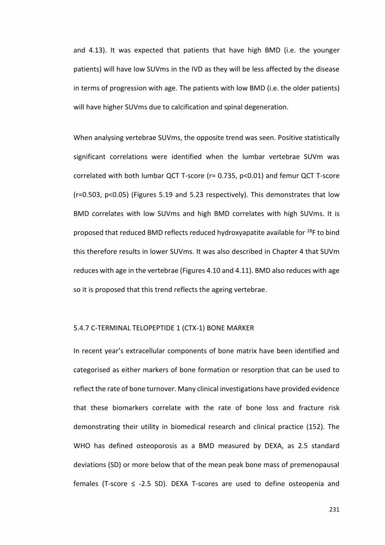
231

and 4.13). It was expected that patients that have high BMD (i.e. the younger

patients) will have low SUVms in the IVD as they will be less affected by the disease

in terms of progression with age. The patients with low BMD (i.e. the older patients)

will have higher SUVms due to calcification and spinal degeneration.

When analysing vertebrae SUVms, the opposite trend was seen. Positive statistically

significant correlations were identified when the lumbar vertebrae SUVm was

correlated with both lumbar QCT T-score (r= 0.735, p<0.01) and femur QCT T-score

(r=0.503, p<0.05) (Figures 5.19 and 5.23 respectively). This demonstrates that low

BMD correlates with low SUVms and high BMD correlates with high SUVms. It is

proposed that reduced BMD reflects reduced hydroxyapatite available for 18F to bind

this therefore results in lower SUVms. It was also described in Chapter 4 that SUVm

reduces with age in the vertebrae (Figures 4.10 and 4.11). BMD also reduces with age

so it is proposed that this trend reflects the ageing vertebrae.

5.4.7 C-TERMINAL TELOPEPTIDE 1 (CTX-1) BONE MARKER

In recent year’s extracellular components of bone matrix have been identified and

categorised as either markers of bone formation or resorption that can be used to

reflect the rate of bone turnover. Many clinical investigations have provided evidence

that these biomarkers correlate with the rate of bone loss and fracture risk

demonstrating their utility in biomedical research and clinical practice (152). The

WHO has defined osteoporosis as a BMD measured by DEXA, as 2.5 standard

deviations (SD) or more below that of the mean peak bone mass of premenopausal

females (T-score ≤ -2.5 SD). DEXA T-scores are used to define osteopenia and

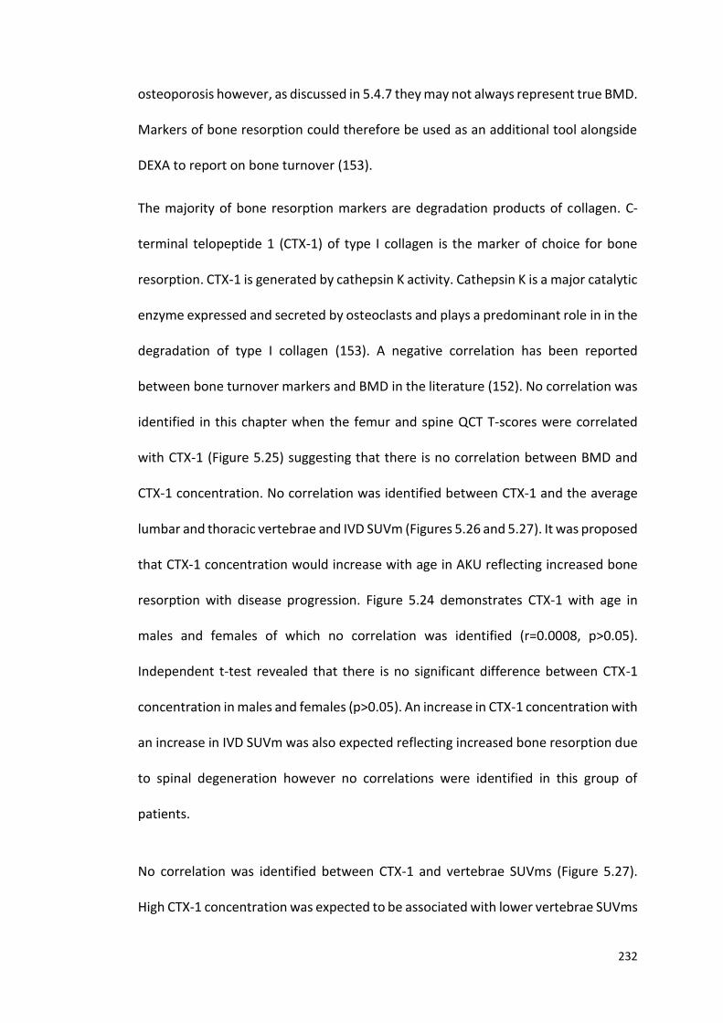
232

osteoporosis however, as discussed in 5.4.7 they may not always represent true BMD.

Markers of bone resorption could therefore be used as an additional tool alongside

DEXA to report on bone turnover (153).

The majority of bone resorption markers are degradation products of collagen. C-

terminal telopeptide 1 (CTX-1) of type I collagen is the marker of choice for bone

resorption. CTX-1 is generated by cathepsin K activity. Cathepsin K is a major catalytic

enzyme expressed and secreted by osteoclasts and plays a predominant role in in the

degradation of type I collagen (153). A negative correlation has been reported

between bone turnover markers and BMD in the literature (152). No correlation was

identified in this chapter when the femur and spine QCT T-scores were correlated

with CTX-1 (Figure 5.25) suggesting that there is no correlation between BMD and

CTX-1 concentration. No correlation was identified between CTX-1 and the average

lumbar and thoracic vertebrae and IVD SUVm (Figures 5.26 and 5.27). It was proposed

that CTX-1 concentration would increase with age in AKU reflecting increased bone

resorption with disease progression. Figure 5.24 demonstrates CTX-1 with age in

males and females of which no correlation was identified (r=0.0008, p>0.05).

Independent t-test revealed that there is no significant difference between CTX-1

concentration in males and females (p>0.05). An increase in CTX-1 concentration with

an increase in IVD SUVm was also expected reflecting increased bone resorption due

to spinal degeneration however no correlations were identified in this group of

patients.

No correlation was identified between CTX-1 and vertebrae SUVms (Figure 5.27).

High CTX-1 concentration was expected to be associated with lower vertebrae SUVms

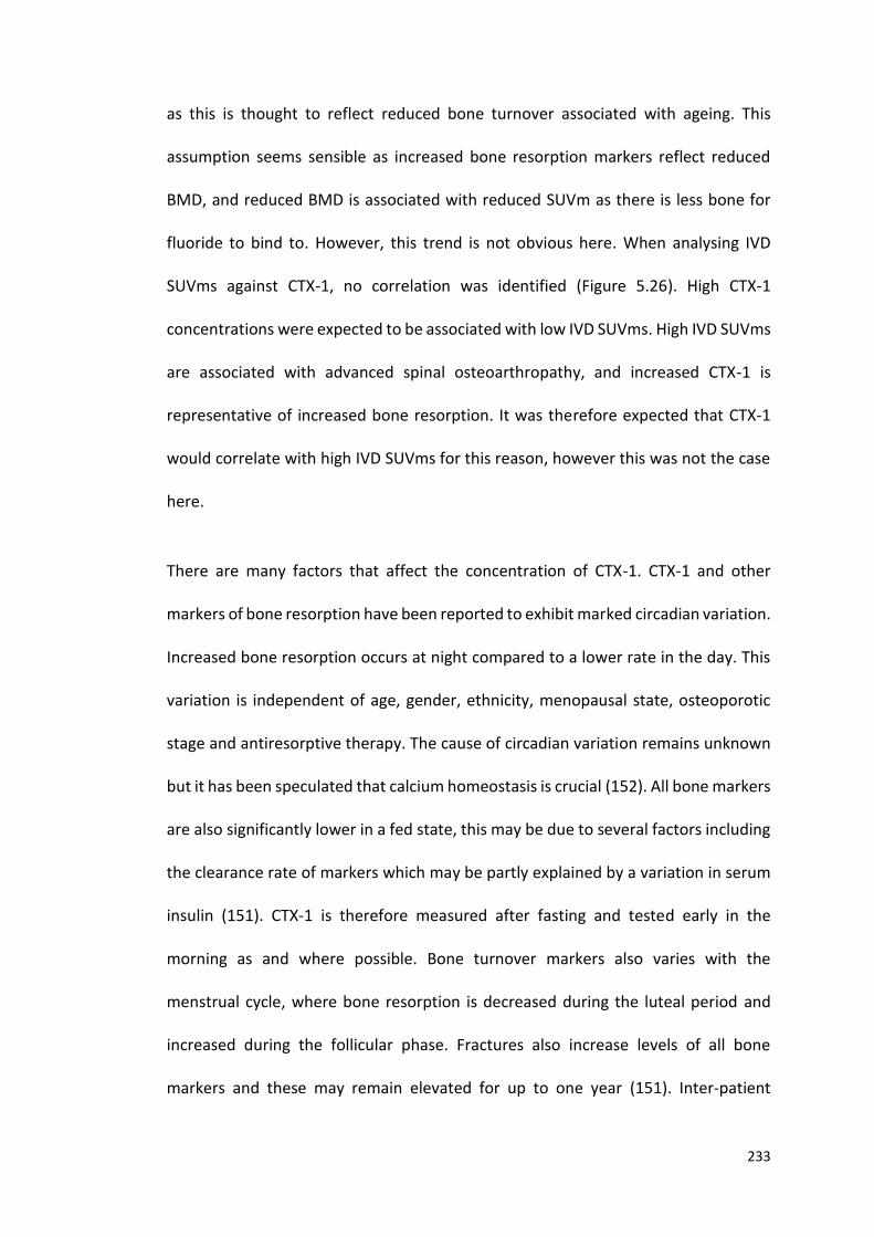
233

as this is thought to reflect reduced bone turnover associated with ageing. This

assumption seems sensible as increased bone resorption markers reflect reduced

BMD, and reduced BMD is associated with reduced SUVm as there is less bone for

fluoride to bind to. However, this trend is not obvious here. When analysing IVD

SUVms against CTX-1, no correlation was identified (Figure 5.26). High CTX-1

concentrations were expected to be associated with low IVD SUVms. High IVD SUVms

are associated with advanced spinal osteoarthropathy, and increased CTX-1 is

representative of increased bone resorption. It was therefore expected that CTX-1

would correlate with high IVD SUVms for this reason, however this was not the case

here.

There are many factors that affect the concentration of CTX-1. CTX-1 and other

markers of bone resorption have been reported to exhibit marked circadian variation.

Increased bone resorption occurs at night compared to a lower rate in the day. This

variation is independent of age, gender, ethnicity, menopausal state, osteoporotic

stage and antiresorptive therapy. The cause of circadian variation remains unknown

but it has been speculated that calcium homeostasis is crucial (152). All bone markers

are also significantly lower in a fed state, this may be due to several factors including

the clearance rate of markers which may be partly explained by a variation in serum

insulin (151). CTX-1 is therefore measured after fasting and tested early in the

morning as and where possible. Bone turnover markers also varies with the

menstrual cycle, where bone resorption is decreased during the luteal period and

increased during the follicular phase. Fractures also increase levels of all bone

markers and these may remain elevated for up to one year (151). Inter-patient

234

variability also proves a problem when comparing between patients as bone

metabolism rates vary between males, females, pubertal stage, menopausal stage,

as well as age. Antiresorptive therapy will also reduce CTX-1 concentration. All these

factors should be taken into account when analysing the results.

In terms of AKU CTX-1 is used as an additional measurement reflecting bone turnover

that can be used to compare between visits. This data is representative of the

baseline visit pre-nitisinone, therefore these CTX-1 concentrations are not

representative of the effect of nitisinone.

5.4.8 LUMBAR AND THORACIC PAIN SCORES

Clinical pain scores were extracted from the patient questionnaires at baseline (pre-

nitisinone). The patients were asked to score pain on a scale of 0-10 where zero

equals no pain, and ten equals severe pain, in the thoracic and lumbar spine. The

spine has been described as the first region to experience pain in AKU. Pain was

scored in both the lumbar and thoracic regions. Interestingly paired t-test revealed a

significant difference between lumbar and thoracic pain scores. Figure 5.28

demonstrates that lumbar pain reaches higher pain scores, therefore suggesting that

the lumbar spine is affected to a higher degree compared to the thoracic spine. This

is thought to be due to the increased mechanical stress that the lumbar spine

experiences.

An interesting correlation was identified with age in both the lumbar and thoracic

pain scores that is proposed to be representative of spinal degeneration and

progression with age (Figure 5.28). A positive statistically significant correlation was

235

identified between the lumbar pain score and age (r=0.584 p<0.01). With a

polynomial trend line applied, pain can be seen increasing with age with the highest

pain scores observed around the mid 40’s, from here pain can be seen decreasing

from around the mid 50’s. This is representative of what was described in Figures

4.12 and 4.13 that demonstrates the trend between the IVD SUVm with age. In

Chapter 4 an inverted ‘U’ trend was described between age and IVD SUVm where

SUVm is low in the youngest patients, SUVm then increases up to around the age of

50 where it then stabilises before reducing back down in the oldest patients between

60 and 70 (Figures 4.12 and 4.13). It is proposed that Figure 5.28 pain scores reflect

the trend in IVD SUVm with age. The reduction in both IVD SUVm and pain in the

oldest patients reflects the end-point of spinal arthropathy which is spinal fusion that

has been associated with reduced pain. To support this a positive statistically

significant correlation (r=0.601, p<0.01) was observed between the lumbar IVD SUVm

and lumbar pain scores (Figure 5.29). A positive statistically significant correlation

was also identified between thoracic IVD SUVm and thoracic pain (r=0.608, p<0.01)

(Figure 5.30). These graphs demonstrate that the highest SUVms are representative

of calcified IVD and disc degeneration, this undoubtedly results in high pain scores.

In contrast, negative statistically significant correlations were observed between the

lumbar and thoracic pain scores with vertebrae SUVms (Figure 5.31 and 5.32). Again,

this supports what was described in Chapter 4 (Figures 4.10 and 4.11) where a

reduction in SUVm can be seen with age. Therefore, the youngest patients have high

SUVms reflecting active bone turnover and have low pain scores. Low SUVms have

236

been shown to be associated with older patients, with reduced bone turnover and

increased pain.

5.4.9 SUMMARY

This chapter has confirmed the findings identified in Chapter 4, and confirmed the

repeatability and validity of the SUVm methodology. This chapter has revealed

differences between AKU and control SUVms in the spine. This was most strikingly

observed in the IVDs where the SUVms were significantly higher than the control. The

proposed explanation for this is that in AKU, deposition of calcifications in the IVDs

occurs with disease progression, which levels out around the sixth decade due to

reduced turnover seen in advancing spinal disease. The SUVm then reduces in the

oldest patients due to spinal fusion. It has also been identified that bone metabolism

in the spine of AKU patients is normal and in-line with age matched controls. Age

related changes in the SUVms of AKU vertebrae were reported, where the SUVm

reduces with age due to reduced bone turnover, and BMD with ageing. However, the

longitudinal changes in SUVm in response to nitisinone were not significant and very

small. It is proposed that four years on nitisinone may not be long enough to identify

any changes in fluoride uptake, therefore for the effect of nitisinone on the spine to

be elucidated, many more years of data will be required to assess the long-term

effects. Additionally, when the SONIA 2 clinical trial is complete longitudinal data will

be available on a non-treatment AKU group for comparison which is key to

understanding if nitisinone is having an effect.

237

Positive correlations were described between IVD SUVm with the total clinical score

and the T-AT scores, demonstrating that increased IVD SUVms represent disc

degeneration which is related to age. The opposite negative trend was identified

when correlating vertebrae SUVm with the total clinical score, total anatomical

threshold score and pain scores demonstrating that high vertebrae SUVms are

associated with active bone turnover in the youngest patients. High IVD SUVms were

also associated with low QCT T-scores reflecting osteoarthritic spine with disease

progression. The opposite was seen when correlating QCT T-scores with vertebrae

SUVms where high vertebrae SUVms correlated with high T-scores. High vertebrae

SUVms reflect active bone remodelling and normal BMD. The trend in spinal pain

when correlated with IVD and vertebrae SUVms also confirmed what was described

previously. An increase in spinal pain was associated with increased IVD SUVm up to

around middle-age before plateauing and decreasing in the oldest patients. In

contrast, a negative correlation was identified when correlating pain with vertebrae

SUVm. Therefore, SUVm in the spine and IVDs could also be used as an indicator of

pain.

5.4.10 FURTHER WORK

The next step will be to correlate the SONIA 2 SUVm data from Chapter 4 with other

data extracted from the clinical trial site files such as urine and plasma HGA levels,

spinal flexion and DEXA and Cobb angle measurements. This will determine if the

SUVm measurements correlate well with other data that has been extracted from

the SONIA 2 patients.

238

6.0 SUVm CORRELATION WITH SONIA 2 CLINICAL DATA

239

6.1 INTRODUCTION

Chapter 4 demonstrates the utility of SUVms to identify active arthropathy in the

spine and to quantify disease state in the SONIA 2 patient group. Chapter 5

demonstrates the repeatability and validity of the method in the NAC patient group,

as well as reported some interesting correlations in this patient group with other data

obtained at the NAC. This chapter aims to look at the correlations between the SONIA

2 SUVm data reported in Chapter 4 with other patient data obtained as part of the

clinical trial at visit one (baseline; pre-nitisinone). Correlations made with other data

obtained from the same patient group is important to analyse to observe if the data

follows similar trends, this provides evidence of a robust methodology.

Serum and urine HGA levels were recorded at baseline (pre-nitisinone). Serum HGA

(s-HGA) concentration provides a measure of HGA that is circulating around the body.

Urine HGA (u-HGA) concentration provides a measure of HGA that is excreted out of

the body. As explained previously HGA is the culprit molecule in AKU that is deposited

in connective tissues resulting in ochronosis that ultimately leads to early onset

osteoarthropathy.

Cobb angles are used to standardise spinal curvatures. Obtaining Cobb angles of

thoracic kyphosis, lumbar lordosis and scoliosis provide the clinician with detailed

information regarding the curvatures of the spine, and these can be assessed

annually to observe if there are any changes. The spine has naturally three

curvatures: cervical lordosis, thoracic kyphosis, lumbar lordosis. Normal thoracic

kyphosis is said to range from 20-45 degrees, hyper kyphosis is defined as more than

45 degrees and the most common reason for this being osteoporosis (122). Lumbar

240

lordosis is characterised by increased inward curving of the lumbar spine. There is no

definition of normal lumbar lordosis or is there a definition for lumbar hyperlordosis

as many factors affect this angle such as muscular strength, flexibility and BMI (123).

Scoliosis is defined as a lateral spinal curvature of 10 degrees or more to the right or

left (124). Measurements of lumbar side flexion and cervical rotation measured in cm

by the physiotherapist were also obtained to assess spinal flexibility.

241

6.2 DESIGN OF STUDY

6.2.1 PATIENT GROUP


the SONIA 2 clinical trial (see section 2.2.2) underwent a series of tests and

examinations in 2014/15. This chapter is based on the baseline data obtained at visit

1 (pre-nitisinone). Each patient underwent 18F-NaF PET/CT, X-ray, MRI and DEXA

imaging. Physiotherapy assessments were carried out to assess spinal motion and

flexibility and blood and urine was extracted to measure circulating and excreted

HGA. These data were used to correlate with the SUVms reported in Chapter 4.


Hermes hybrid viewer (see section 2.5.1) was used to measure SUVms (section 2.5.2).

The SUVm was obtained from the centre of three lumbar (L5, L3, L1) and three

thoracic (T1, T6, T12) vertebral bodies, and from the centre of the corresponding IVDs

below (L5-S1, L3/L4, L1/L2, T12/L1, T6/T7, T1/T2). The SUVms utilised in this chapter

were obtained from the baseline visit; visit 1 (pre-nitisinone).

6.2.3 PATIENT DATA OBTAINED

The DEXA images were accessed on the PACS system at the RLBUHT computer and

the data from visit 1 was recorded (for more information regarding DEXA see section

1.6.3.1). Table 1.4 demonstrates the WHO definitions of BMD. X-ray images were also

accessed on the PACS system and the Cobb angles were measured using this software

242

(method explained in section 6.2.3.1 and 6.2.3.2). The physiotherapy measurements

of lumbar side flexion and cervical rotation were obtained from the site files at the

RLBUHT and visit 1 data was recorded. Urine and serum HGA levels for visit 1 were

analysed in the biochemistry lab at the RLBUHT and were provided by the lab in an

excel file.

6.2.3.1 X-RAY AND MRI COBB ANGLE MEASURMENTS

Whole body posterioanterior (PA) X-Ray view was selected to analyse scoliosis. Using

the Cobb angle tool the end vertebrae of the curve were selected and lines were

drawn to demarcate the vertebrae that lie at the upper and lower limits of the curve

(the vertebrae that tilt the most towards the apex of the curve) (Figure 2.11A). The

Cobb angle was automatically generated measuring the intersection of the two lines

drawn.

Lateral X-ray view was selected to measure the thoracic kyphosis and lumbar lordosis

Cobb angles. Using the Cobb angle tool, the lower border of the twelfth thoracic

vertebrae (T12) and the upper border of the fourth thoracic vertebrae (T4) were

selected (Figure 2.11B). The Cobb angle was automatically generated by measuring

the intersection between the lines selected. Normal kyphosis ranges from 20-45

degrees, hyper kyphosis is defined as more than 45 degrees (122). Lumbar lordosis

was measured from the lower border of the fifth lumbar (L5) vertebrae and the upper

border of the first lumbar vertebrae (L1). Lumbar hyperlordosis is not defined by a

Cobb angle (Figure 2.11B).

243

Thoracic kyphosis and lumbar lordosis Cobb angles were also measured on MRI

(Figure 2.11C). The MRI whole spine was selected using the PACS and the

methodology of measuring thoracic kyphosis and lumbar lordosis was exactly as

described as above.

6.2.3.2 LUMBAR SIDE FLEXION AND CERVICAL ROTATION MEASUREMENTS

Lumbar side flexion was measured by a senior physiotherapist at the RLBUHT. The

patient was asked to stand up straight against the wall with their feet 12 inches apart.

Firstly, the distance was measured (in cm) between the tip of the middle finger to the

floor with the patient standing up straight on both the right and left sides. The patient

was then asked to side flex to the right with the physiotherapist applying over

pressure to push the patient further into the range and the distance between the tip

of the middle finger to the floor was measured again. This was then repeated on the

left. The difference between the two measurements was calculated and this value

reflects the passive lumbar side flexion of the patient in cm (126,127).

Cervical spine rotation was measured by a senior physiotherapist. The patient was

asked to stand up straight against the wall with shoulders back in a neutral position

with the head facing forwards. The distance between the gnathion of the chin to the

lateral aspect of the acromion was measured with the head looking straight forward

on both the right and left sides. The patient was then asked to look over to the right

with the physiotherapist applying over pressure to push the patient further into the

range, and this distance was re-measured. This was then repeated on the left side.

244

The difference between the two values was then calculated to obtain the value of

passive cervical spine rotation (126,127).

6.2.3.3 SERUM AND URINE HGA

A fasting blood sample and acidified 24-hour urine sample (25mL of 5 N sulphuric acid

added to 2.5 L urine collection bottle) were collected at visit 1 (pre-nitisinone). Blood

samples were collected into plain serum tubes from all subjects in a fasting state,

centrifuged and serum acidified with perchloric acid (5.8 M, at a ratio of 1:11). The

acidified urine and serum were analysed for HGA using liquid chromatography

tandem mass spectrometry methodology (LC-MS/MS). Serum HGA is HGA

concentration (µmol/L), urine HGA is total HGA output in 24 hours (µmol/24hr).

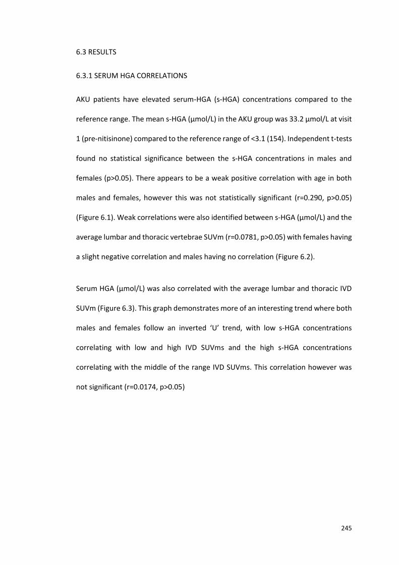
245

6.3 RESULTS

6.3.1 SERUM HGA CORRELATIONS

AKU patients have elevated serum-HGA (s-HGA) concentrations compared to the

reference range. The mean s-HGA (µmol/L) in the AKU group was 33.2 µmol/L at visit

1 (pre-nitisinone) compared to the reference range of <3.1 (154). Independent t-tests

found no statistical significance between the s-HGA concentrations in males and

females (p>0.05). There appears to be a weak positive correlation with age in both

males and females, however this was not statistically significant (r=0.290, p>0.05)

(Figure 6.1). Weak correlations were also identified between s-HGA (µmol/L) and the

average lumbar and thoracic vertebrae SUVm (r=0.0781, p>0.05) with females having

a slight negative correlation and males having no correlation (Figure 6.2).

Serum HGA (µmol/L) was also correlated with the average lumbar and thoracic IVD

SUVm (Figure 6.3). This graph demonstrates more of an interesting trend where both

males and females follow an inverted ‘U’ trend, with low s-HGA concentrations

correlating with low and high IVD SUVms and the high s-HGA concentrations

correlating with the middle of the range IVD SUVms. This correlation however was

not significant (r=0.0174, p>0.05)

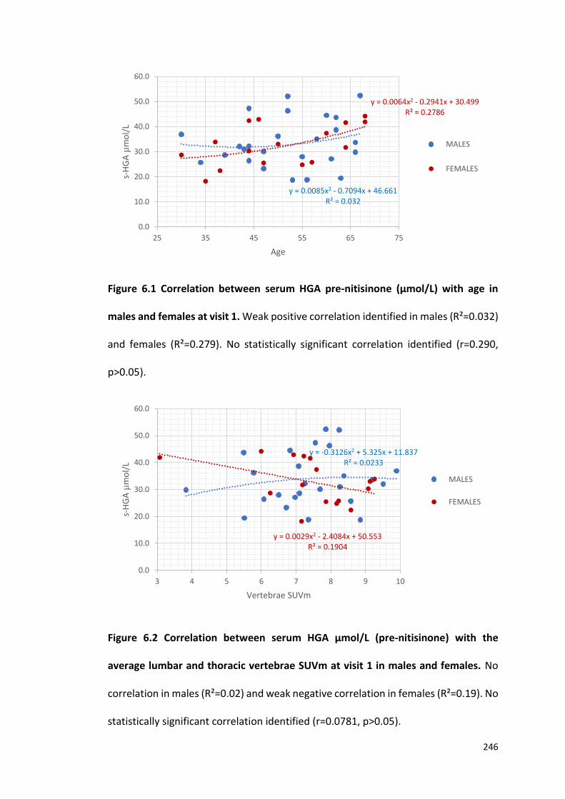
246

Figure 6.1 Correlation between serum HGA pre-nitisinone (µmol/L) with age in

males and females at visit 1. Weak positive correlation identified in males (R²=0.032)

and females (R²=0.279). No statistically significant correlation identified (r=0.290,

p>0.05).

Figure 6.2 Correlation between serum HGA µmol/L (pre-nitisinone) with the

average lumbar and thoracic vertebrae SUVm at visit 1 in males and females. No

correlation in males (R²=0.02) and weak negative correlation in females (R²=0.19). No

statistically significant correlation identified (r=0.0781, p>0.05).

y = 0.0085x2 - 0.7094x + 46.661R² = 0.032

y = 0.0064x2 - 0.2941x + 30.499R² = 0.2786

0.0

10.0

20.0

30.0

40.0

50.0

60.0

25 35 45 55 65 75

s-H

GA

µm

ol/

L

Age

MALES

FEMALES

y = -0.3126x2 + 5.325x + 11.837R² = 0.0233

y = 0.0029x2 - 2.4084x + 50.553R² = 0.1904

0.0

10.0

20.0

30.0

40.0

50.0

60.0

3 4 5 6 7 8 9 10

s-H

GA

µm

ol/

L

Vertebrae SUVm

MALES

FEMALES

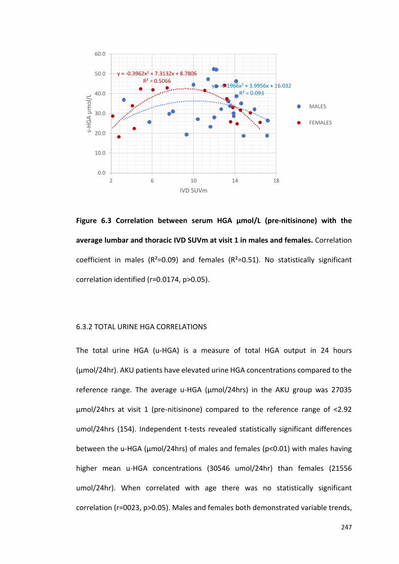
247

Figure 6.3 Correlation between serum HGA µmol/L (pre-nitisinone) with the

average lumbar and thoracic IVD SUVm at visit 1 in males and females. Correlation

coefficient in males (R²=0.09) and females (R²=0.51). No statistically significant

correlation identified (r=0.0174, p>0.05).

6.3.2 TOTAL URINE HGA CORRELATIONS

The total urine HGA (u-HGA) is a measure of total HGA output in 24 hours

(µmol/24hr). AKU patients have elevated urine HGA concentrations compared to the

reference range. The average u-HGA (µmol/24hrs) in the AKU group was 27035

µmol/24hrs at visit 1 (pre-nitisinone) compared to the reference range of <2.92

umol/24hrs (154). Independent t-tests revealed statistically significant differences

between the u-HGA (µmol/24hrs) of males and females (p<0.01) with males having

higher mean u-HGA concentrations (30546 umol/24hr) than females (21556

umol/24hr). When correlated with age there was no statistically significant

correlation (r=0023, p>0.05). Males and females both demonstrated variable trends,

y = -0.1966x2 + 3.9956x + 16.032R² = 0.093

y = -0.3962x2 + 7.3132x + 8.7806R² = 0.5066

0.0

10.0

20.0

30.0

40.0

50.0

60.0

2 6 10 14 18

s-H

GA

µm

ol/

L

IVD SUVm

MALES

FEMALES

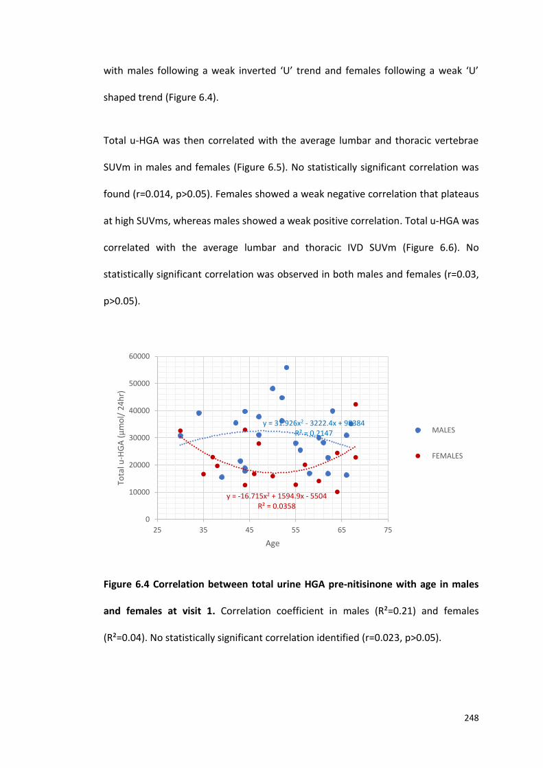
248

with males following a weak inverted ‘U’ trend and females following a weak ‘U’

shaped trend (Figure 6.4).

Total u-HGA was then correlated with the average lumbar and thoracic vertebrae

SUVm in males and females (Figure 6.5). No statistically significant correlation was

found (r=0.014, p>0.05). Females showed a weak negative correlation that plateaus

at high SUVms, whereas males showed a weak positive correlation. Total u-HGA was

correlated with the average lumbar and thoracic IVD SUVm (Figure 6.6). No

statistically significant correlation was observed in both males and females (r=0.03,

p>0.05).

Figure 6.4 Correlation between total urine HGA pre-nitisinone with age in males

and females at visit 1. Correlation coefficient in males (R²=0.21) and females

(R²=0.04). No statistically significant correlation identified (r=0.023, p>0.05).

y = -16.715x2 + 1594.9x - 5504R² = 0.0358

y = 31.926x2 - 3222.4x + 98384R² = 0.2147

0

10000

20000

30000

40000

50000

60000

25 35 45 55 65 75

Tota

l u-H

GA

(µ

mo

l/ 2

4h

r)

Age

MALES

FEMALES

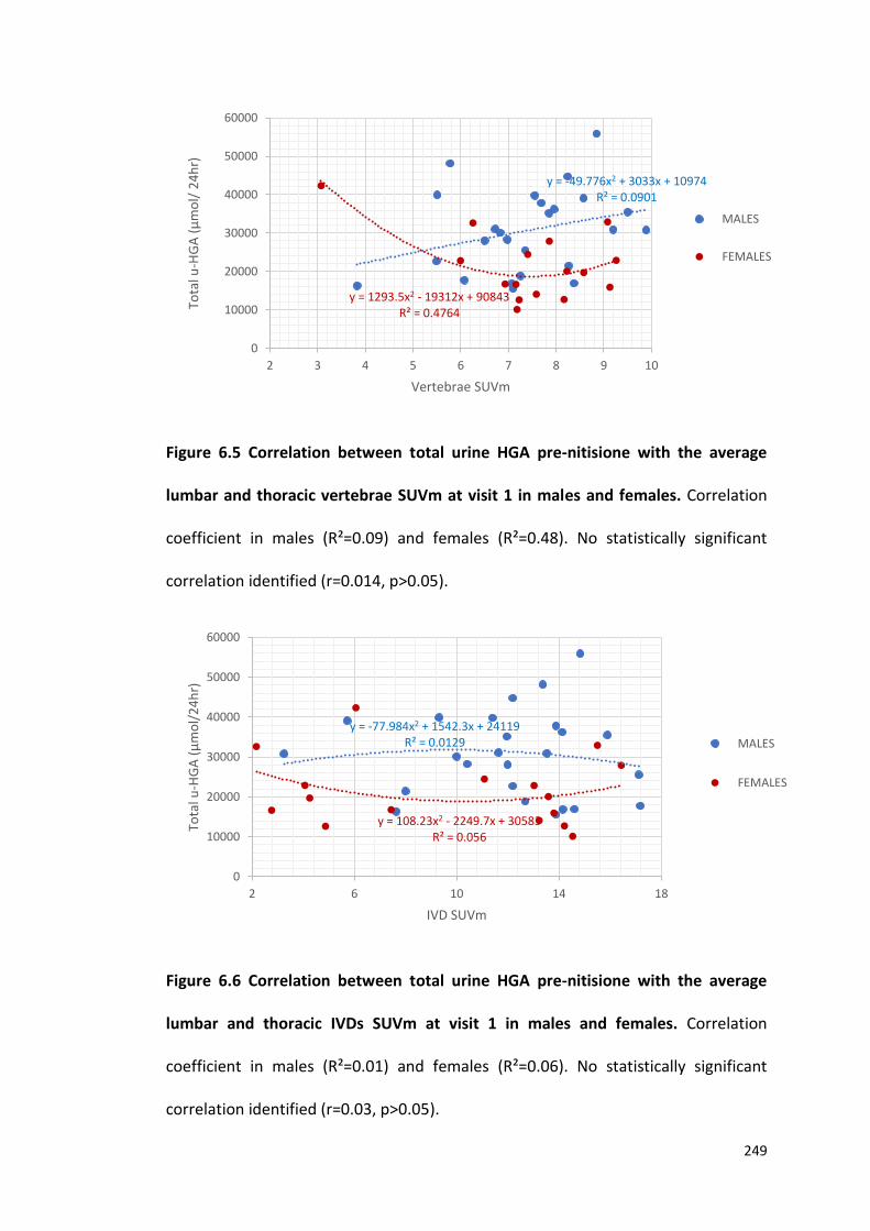
249

Figure 6.5 Correlation between total urine HGA pre-nitisione with the average

lumbar and thoracic vertebrae SUVm at visit 1 in males and females. Correlation



Figure 6.6 Correlation between total urine HGA pre-nitisione with the average

lumbar and thoracic IVDs SUVm at visit 1 in males and females. Correlation



y = -49.776x2 + 3033x + 10974R² = 0.0901

y = 1293.5x2 - 19312x + 90843R² = 0.4764

0

10000

20000

30000

40000

50000

60000

2 3 4 5 6 7 8 9 10

Tota

l u-H

GA

(µ

mo

l/ 2

4h

r)

Vertebrae SUVm

MALES

FEMALES

y = -77.984x2 + 1542.3x + 24119R² = 0.0129

y = 108.23x2 - 2249.7x + 30583R² = 0.056

0

10000

20000

30000

40000

50000

60000

2 6 10 14 18

Tota

l u-H

GA

(µ

mo

l/2

4h

r)

IVD SUVm

MALES

FEMALES

250

6.3.3 LUMBAR SIDE FLEXION CORRELATIONS

Lumbar side flexion (cm) was measured by a senior physiotherapist at the RLBUHT.

Negative correlations were identified in both males and females when lumbar side

flexion was correlated with age (Figure 6.7 A and B). A negative statistically significant

correlation was identified (r=-0.850, p<0.001) between right passive lumbar side

flexion and age (Figure 6.7A). Right passive lumbar side flexion was highest in the

younger patients and this decreased linearly with age in both males and females with

the oldest patients having the smallest range of motion in the spine. The same trend

can be seen when correlating passive lumbar side flexion on the left side with age in

both males and females (Figure 6.7B). A negative statistically significant correlation

was identified between left passive lumbar side flexion with age (r=-0.806, p<0.001).

Independent t-tests found no statistically significant differences between the lumbar

side flexion (cm) on both the right and left sides between males and females.

Interestingly, when lumbar side flexion was plotted against the average lumbar and

thoracic vertebrae SUVm, positive correlations were identified in both males and

females (Figure 6.8 A and B). A positive statistically significant correlation was

observed between the right passive lumbar side flexion and the average lumbar and

thoracic vertebrae SUVm (r=0.588, p<0.05). A positive statistically significant

correlation was also identified between the left passive lumbar side flexion and the

average lumbar and the average lumbar and thoracic vertebrae SUVm (r=0.616,

p<0.05). This trend supports what has been described in Chapter 4 and 5 with high

vertebrae SUVms being associated with the younger patients with increased range of

motion in the spine.

251

Weak inverted ‘U’ shaped trends were identified when correlating lumbar side flexion

with the average lumbar and thoracic IVD SUVm in both males and females (Figure

6.9 A and B). Suggesting that reduced lumbar flexion is associated with middle of the

range IVD SUVms, and that high and low IVD SUVms are associated with increased

lumbar side flexion. However, this was not statistically significant on both the right

and left sides.

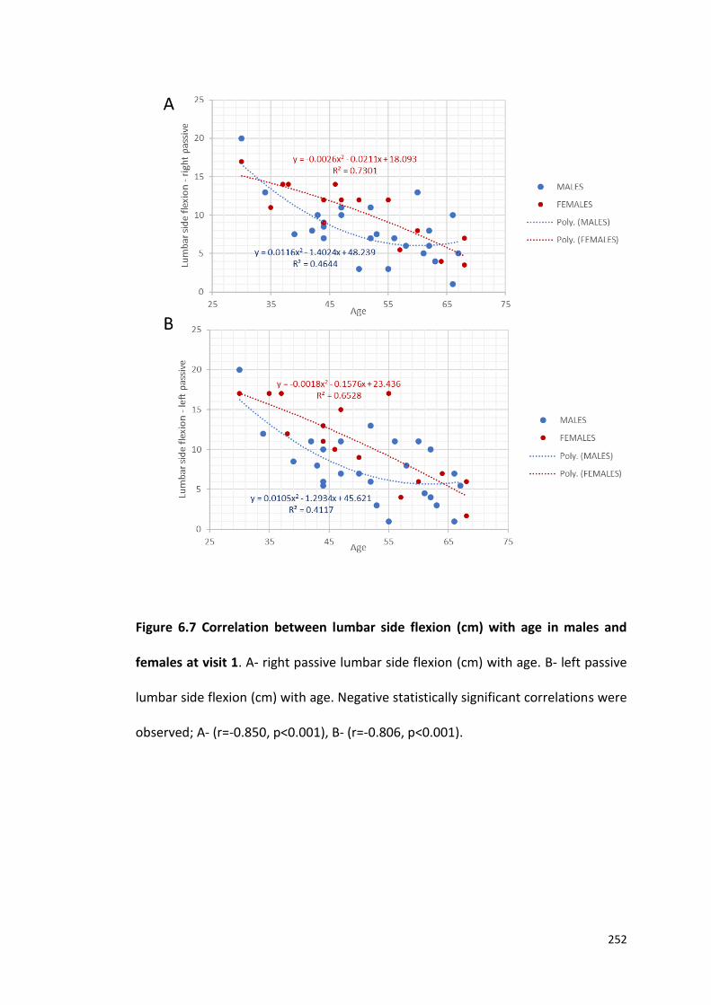
252

Figure 6.7 Correlation between lumbar side flexion (cm) with age in males and

females at visit 1. A- right passive lumbar side flexion (cm) with age. B- left passive

lumbar side flexion (cm) with age. Negative statistically significant correlations were

observed; A- (r=-0.850, p<0.001), B- (r=-0.806, p<0.001).

253

Figure 6.8 Correlation between lumbar side flexion (cm) with average lumbar and

thoracic vertebrae SUVm in males and females at visit 1. A- right passive lumbar side

flexion (cm) with vertebrae SUVm. B- left passive lumbar side flexion (cm) with

vertebrae SUVm. Positive statistically significant correlations were observed; A-

(r=0.588, p<0.05), B- (r=0.616, p<0.05).

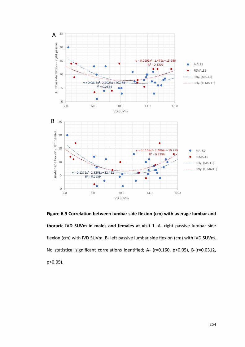
254

Figure 6.9 Correlation between lumbar side flexion (cm) with average lumbar and

thoracic IVD SUVm in males and females at visit 1. A- right passive lumbar side

flexion (cm) with IVD SUVm. B- left passive lumbar side flexion (cm) with IVD SUVm.

No statistical significant correlations identified; A- (r=0.160, p>0.05), B-(r=0.0312,

p>0.05).

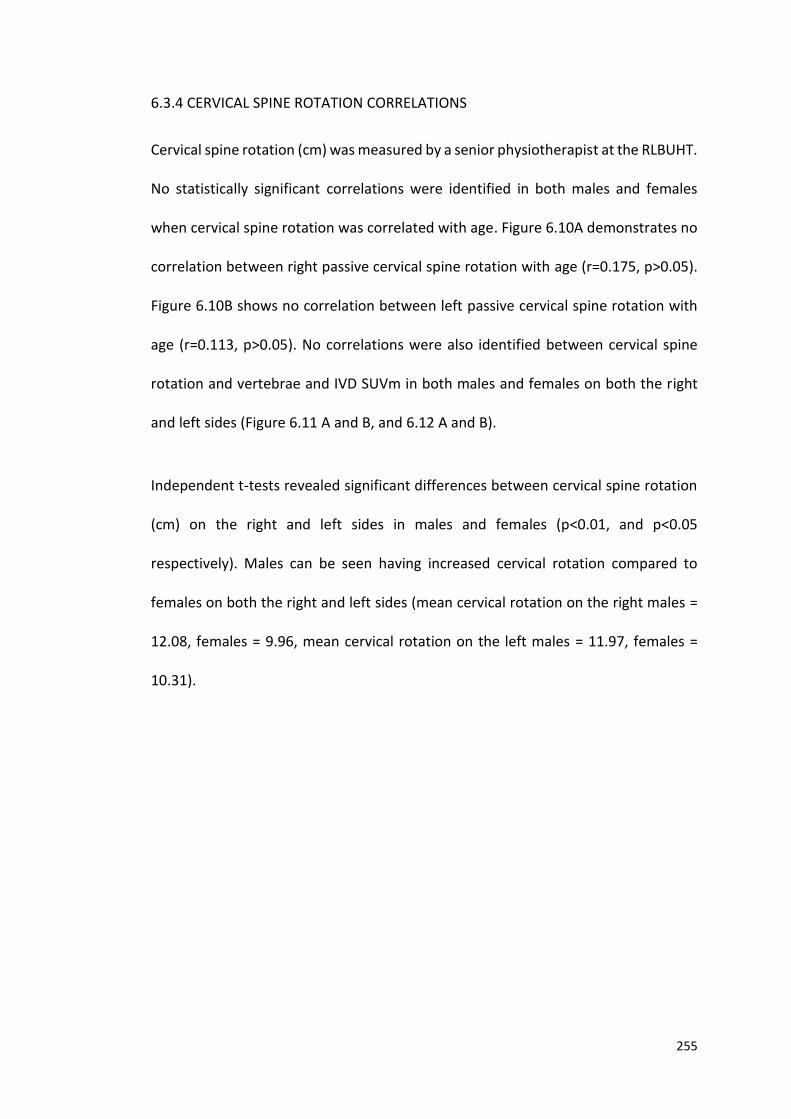
255

6.3.4 CERVICAL SPINE ROTATION CORRELATIONS

Cervical spine rotation (cm) was measured by a senior physiotherapist at the RLBUHT.

No statistically significant correlations were identified in both males and females

when cervical spine rotation was correlated with age. Figure 6.10A demonstrates no

correlation between right passive cervical spine rotation with age (r=0.175, p>0.05).

Figure 6.10B shows no correlation between left passive cervical spine rotation with

age (r=0.113, p>0.05). No correlations were also identified between cervical spine

rotation and vertebrae and IVD SUVm in both males and females on both the right

and left sides (Figure 6.11 A and B, and 6.12 A and B).

Independent t-tests revealed significant differences between cervical spine rotation

(cm) on the right and left sides in males and females (p<0.01, and p<0.05

respectively). Males can be seen having increased cervical rotation compared to

females on both the right and left sides (mean cervical rotation on the right males =

12.08, females = 9.96, mean cervical rotation on the left males = 11.97, females =

10.31).

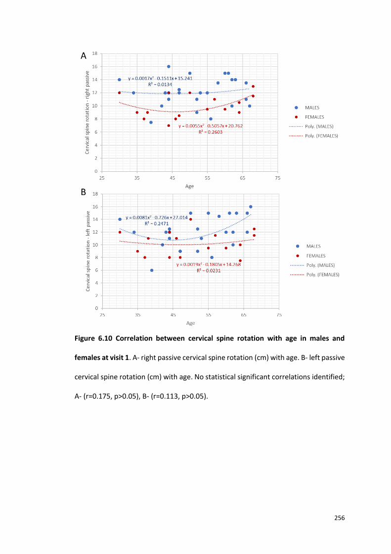
256

Figure 6.10 Correlation between cervical spine rotation with age in males and

females at visit 1. A- right passive cervical spine rotation (cm) with age. B- left passive

cervical spine rotation (cm) with age. No statistical significant correlations identified;

A- (r=0.175, p>0.05), B- (r=0.113, p>0.05).

257

Figure 6.11 Correlation between cervical spine rotation with the average lumbar

and thoracic vertebrae SUVm in males and females at visit 1. A- Right passive

cervical spine rotation (cm) with average vertebrae SUVm, B- Left passive cervical

spine rotation (cm) with average vertebrae SUVm. No statistical significant

correlations identified; A- (r=0.258, p>0.05), B- (r=0.248, p>0.05).

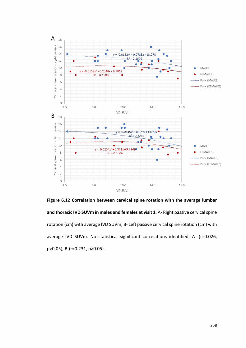
258

Figure 6.12 Correlation between cervical spine rotation with the average lumbar

and thoracic IVD SUVm in males and females at visit 1. A- Right passive cervical spine

rotation (cm) with average IVD SUVm, B- Left passive cervical spine rotation (cm) with

average IVD SUVm. No statistical significant correlations identified; A- (r=0.026,

p>0.05), B-(r=0.231, p>0.05).

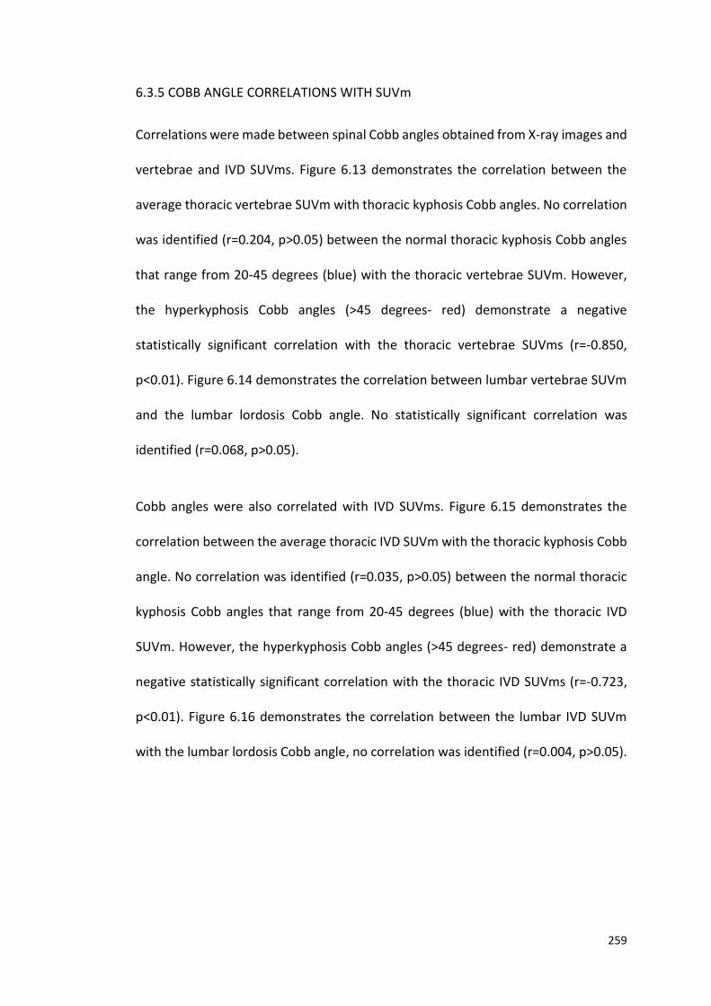
259

6.3.5 COBB ANGLE CORRELATIONS WITH SUVm

Correlations were made between spinal Cobb angles obtained from X-ray images and

vertebrae and IVD SUVms. Figure 6.13 demonstrates the correlation between the

average thoracic vertebrae SUVm with thoracic kyphosis Cobb angles. No correlation

was identified (r=0.204, p>0.05) between the normal thoracic kyphosis Cobb angles

that range from 20-45 degrees (blue) with the thoracic vertebrae SUVm. However,

the hyperkyphosis Cobb angles (>45 degrees- red) demonstrate a negative

statistically significant correlation with the thoracic vertebrae SUVms (r=-0.850,

p<0.01). Figure 6.14 demonstrates the correlation between lumbar vertebrae SUVm

and the lumbar lordosis Cobb angle. No statistically significant correlation was

identified (r=0.068, p>0.05).

Cobb angles were also correlated with IVD SUVms. Figure 6.15 demonstrates the

correlation between the average thoracic IVD SUVm with the thoracic kyphosis Cobb

angle. No correlation was identified (r=0.035, p>0.05) between the normal thoracic

kyphosis Cobb angles that range from 20-45 degrees (blue) with the thoracic IVD

SUVm. However, the hyperkyphosis Cobb angles (>45 degrees- red) demonstrate a

negative statistically significant correlation with the thoracic IVD SUVms (r=-0.723,

p<0.01). Figure 6.16 demonstrates the correlation between the lumbar IVD SUVm

with the lumbar lordosis Cobb angle, no correlation was identified (r=0.004, p>0.05).

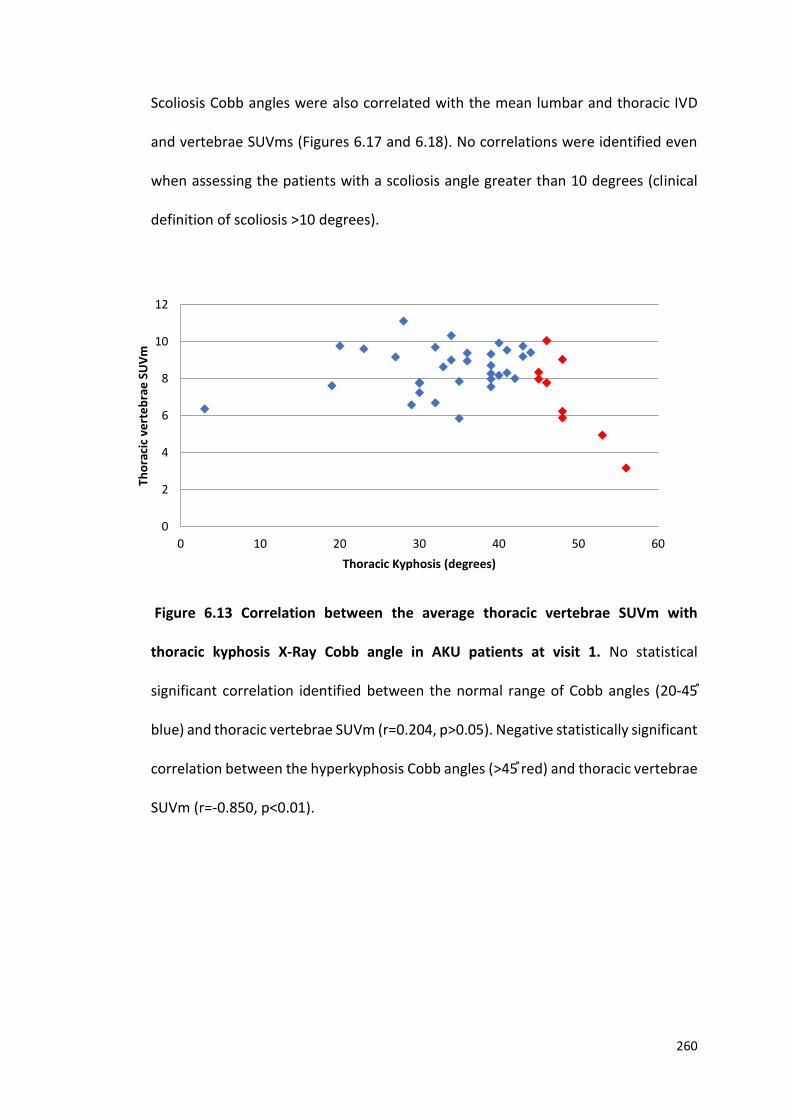
260

Scoliosis Cobb angles were also correlated with the mean lumbar and thoracic IVD

and vertebrae SUVms (Figures 6.17 and 6.18). No correlations were identified even

when assessing the patients with a scoliosis angle greater than 10 degrees (clinical

definition of scoliosis >10 degrees).

Figure 6.13 Correlation between the average thoracic vertebrae SUVm with

thoracic kyphosis X-Ray Cobb angle in AKU patients at visit 1. No statistical

significant correlation identified between the normal range of Cobb angles (20-45 ֯

blue) and thoracic vertebrae SUVm (r=0.204, p>0.05). Negative statistically significant

correlation between the hyperkyphosis Cobb angles (>45֯ red) and thoracic vertebrae

SUVm (r=-0.850, p<0.01).

0

2

4

6

8

10

12

0 10 20 30 40 50 60

Tho

raci

c ve

rte

bra

e S

UV

m

Thoracic Kyphosis (degrees)

261

Figure 6.14 Correlation between average lumbar vertebrae SUVm with lumbar

lordosis X-Ray Cobb angle in AKU at visit 1. No statistical significant correlation


Figure 6.15 Correlation between average thoracic IVD SUVm with thoracic kyphosis

X-Ray Cobb angle in AKU patients at visit 1. No statistical significant correlation

between the normal thoracic kyphosis Cobb angles (20-45֯ -blue) with the thoracic

IVD SUVm (r=0.035, p>0.05). Negative statistically significant correlation between the

hyperkyphosis Cobb angles (>45 ֯ red) and thoracic IVD SUVm (r=-0.723, p<0.01).

y = -0.0016x2 + 0.1109x + 5.0394R² = 0.0422

0

2

4

6

8

10

12

10 20 30 40 50 60

Lum

bar

ve

rte

bra

e S

UV

m

Lumbar Lordosis (degrees)

0

5

10

15

20

0 10 20 30 40 50 60

Tho

raci

c IV

D S

UV

m

Thoracic Kyphosis (degrees)

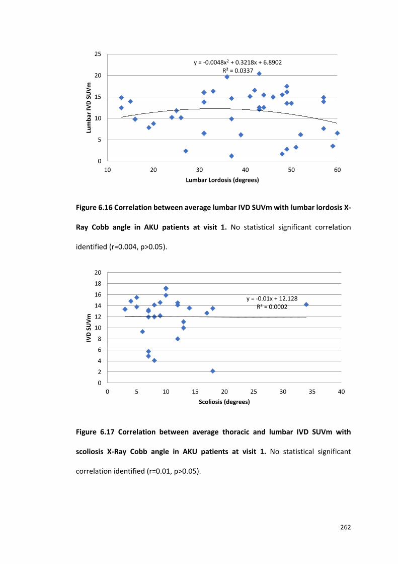
262

Figure 6.16 Correlation between average lumbar IVD SUVm with lumbar lordosis X-

Ray Cobb angle in AKU patients at visit 1. No statistical significant correlation


Figure 6.17 Correlation between average thoracic and lumbar IVD SUVm with

scoliosis X-Ray Cobb angle in AKU patients at visit 1. No statistical significant


y = -0.0048x2 + 0.3218x + 6.8902R² = 0.0337

0

5

10

15

20

25

10 20 30 40 50 60

Lum

bar

IVD

SU

Vm


y = -0.01x + 12.128R² = 0.0002

0

2

4

6

8

10

12

14

16

18

20

0 5 10 15 20 25 30 35 40

IVD

SU

Vm

Scoliosis (degrees)

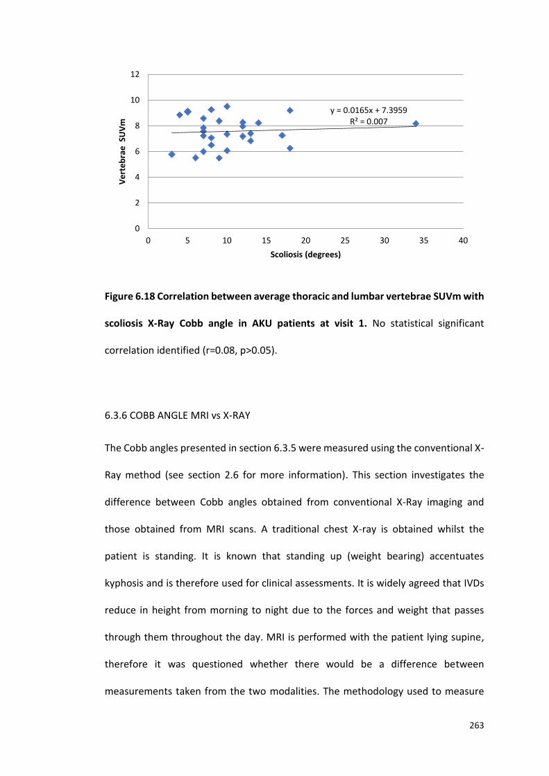
263

Figure 6.18 Correlation between average thoracic and lumbar vertebrae SUVm with

scoliosis X-Ray Cobb angle in AKU patients at visit 1. No statistical significant


6.3.6 COBB ANGLE MRI vs X-RAY

The Cobb angles presented in section 6.3.5 were measured using the conventional X-

Ray method (see section 2.6 for more information). This section investigates the

difference between Cobb angles obtained from conventional X-Ray imaging and

those obtained from MRI scans. A traditional chest X-ray is obtained whilst the

patient is standing. It is known that standing up (weight bearing) accentuates

kyphosis and is therefore used for clinical assessments. It is widely agreed that IVDs

reduce in height from morning to night due to the forces and weight that passes

through them throughout the day. MRI is performed with the patient lying supine,

therefore it was questioned whether there would be a difference between

measurements taken from the two modalities. The methodology used to measure

y = 0.0165x + 7.3959R² = 0.007

0

2

4

6

8

10

12

0 5 10 15 20 25 30 35 40

Ve

rte

bra

e S

UV

m

Scoliosis (degrees)

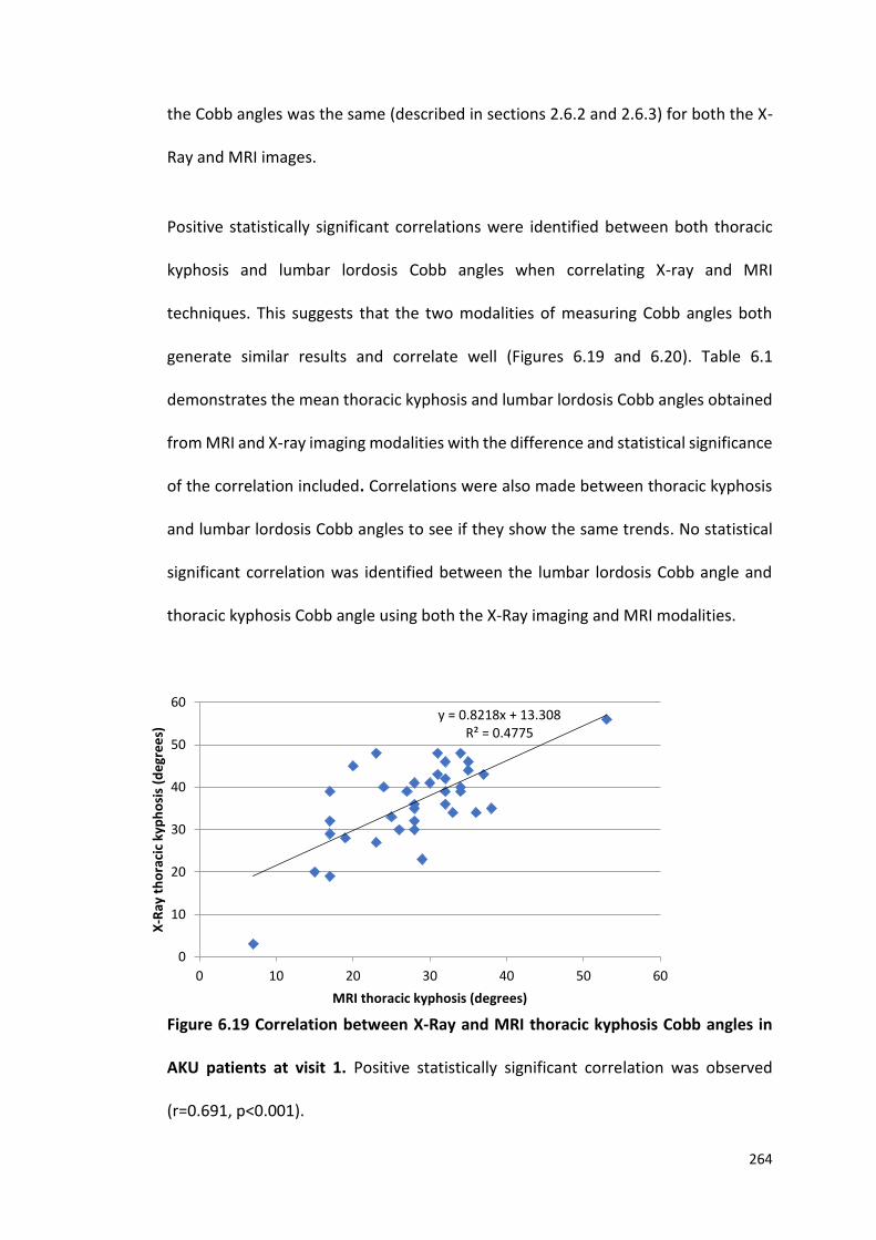
264

the Cobb angles was the same (described in sections 2.6.2 and 2.6.3) for both the X-

Ray and MRI images.

Positive statistically significant correlations were identified between both thoracic

kyphosis and lumbar lordosis Cobb angles when correlating X-ray and MRI

techniques. This suggests that the two modalities of measuring Cobb angles both

generate similar results and correlate well (Figures 6.19 and 6.20). Table 6.1

demonstrates the mean thoracic kyphosis and lumbar lordosis Cobb angles obtained

from MRI and X-ray imaging modalities with the difference and statistical significance

of the correlation included. Correlations were also made between thoracic kyphosis

and lumbar lordosis Cobb angles to see if they show the same trends. No statistical

significant correlation was identified between the lumbar lordosis Cobb angle and

thoracic kyphosis Cobb angle using both the X-Ray imaging and MRI modalities.

Figure 6.19 Correlation between X-Ray and MRI thoracic kyphosis Cobb angles in

AKU patients at visit 1. Positive statistically significant correlation was observed

(r=0.691, p<0.001).

y = 0.8218x + 13.308R² = 0.4775

0

10

20

30

40

50

60

0 10 20 30 40 50 60

X-R

ay t

ho

raci

c ky

ph

osi

s (d

egr

ee

s)

MRI thoracic kyphosis (degrees)

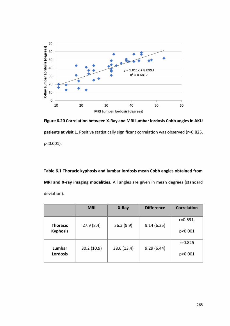
265

Figure 6.20 Correlation between X-Ray and MRI lumbar lordosis Cobb angles in AKU

patients at visit 1. Positive statistically significant correlation was observed (r=0.825,

p<0.001).

Table 6.1 Thoracic kyphosis and lumbar lordosis mean Cobb angles obtained from

MRI and X-ray imaging modalities. All angles are given in mean degrees (standard

deviation).

MRI X-Ray Difference Correlation

Thoracic Kyphosis

27.9 (8.4) 36.3 (9.9) 9.14 (6.25) r=0.691,

p<0.001

Lumbar Lordosis

30.2 (10.9) 38.6 (13.4) 9.29 (6.44) r=0.825

p<0.001

y = 1.011x + 8.0993R² = 0.6817

0

10

20

30

40

50

60

70

10 20 30 40 50 60

X-R

ay L

um

bar

Lo

rdo

sis

(de

gre

es)

MRI Lumbar lordosis (degrees)

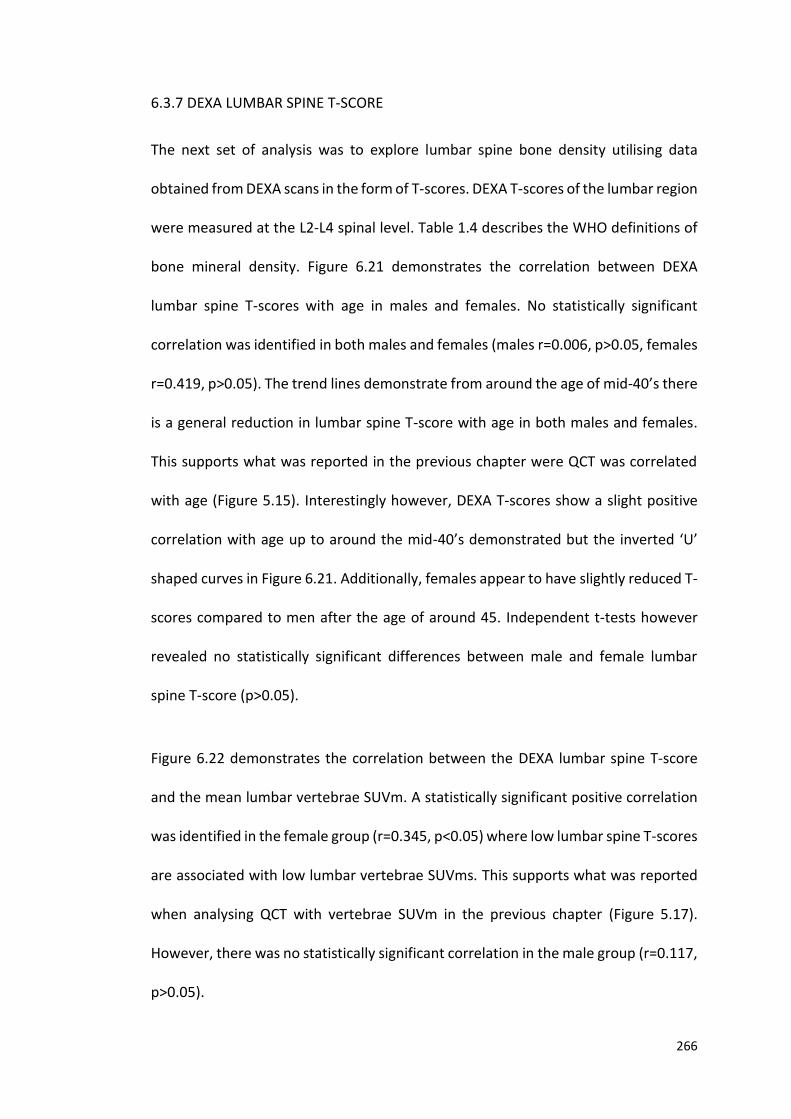
266

6.3.7 DEXA LUMBAR SPINE T-SCORE

The next set of analysis was to explore lumbar spine bone density utilising data

obtained from DEXA scans in the form of T-scores. DEXA T-scores of the lumbar region

were measured at the L2-L4 spinal level. Table 1.4 describes the WHO definitions of

bone mineral density. Figure 6.21 demonstrates the correlation between DEXA

lumbar spine T-scores with age in males and females. No statistically significant

correlation was identified in both males and females (males r=0.006, p>0.05, females

r=0.419, p>0.05). The trend lines demonstrate from around the age of mid-40’s there

is a general reduction in lumbar spine T-score with age in both males and females.

This supports what was reported in the previous chapter were QCT was correlated

with age (Figure 5.15). Interestingly however, DEXA T-scores show a slight positive

correlation with age up to around the mid-40’s demonstrated but the inverted ‘U’

shaped curves in Figure 6.21. Additionally, females appear to have slightly reduced T-

scores compared to men after the age of around 45. Independent t-tests however

revealed no statistically significant differences between male and female lumbar

spine T-score (p>0.05).

Figure 6.22 demonstrates the correlation between the DEXA lumbar spine T-score

and the mean lumbar vertebrae SUVm. A statistically significant positive correlation

was identified in the female group (r=0.345, p<0.05) where low lumbar spine T-scores

are associated with low lumbar vertebrae SUVms. This supports what was reported

when analysing QCT with vertebrae SUVm in the previous chapter (Figure 5.17).

However, there was no statistically significant correlation in the male group (r=0.117,

p>0.05).

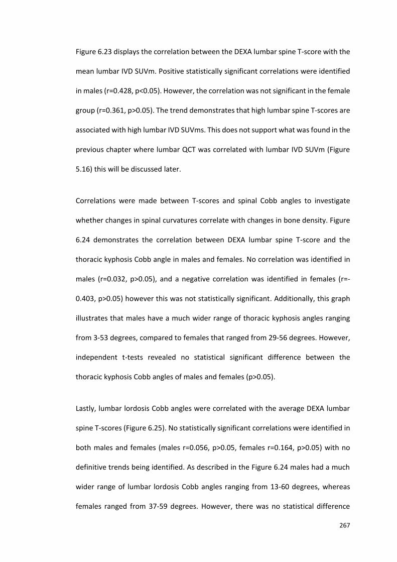
267

Figure 6.23 displays the correlation between the DEXA lumbar spine T-score with the

mean lumbar IVD SUVm. Positive statistically significant correlations were identified

in males (r=0.428, p<0.05). However, the correlation was not significant in the female

group (r=0.361, p>0.05). The trend demonstrates that high lumbar spine T-scores are

associated with high lumbar IVD SUVms. This does not support what was found in the

previous chapter where lumbar QCT was correlated with lumbar IVD SUVm (Figure

5.16) this will be discussed later.

Correlations were made between T-scores and spinal Cobb angles to investigate

whether changes in spinal curvatures correlate with changes in bone density. Figure

6.24 demonstrates the correlation between DEXA lumbar spine T-score and the

thoracic kyphosis Cobb angle in males and females. No correlation was identified in

males (r=0.032, p>0.05), and a negative correlation was identified in females (r=-

0.403, p>0.05) however this was not statistically significant. Additionally, this graph

illustrates that males have a much wider range of thoracic kyphosis angles ranging

from 3-53 degrees, compared to females that ranged from 29-56 degrees. However,

independent t-tests revealed no statistical significant difference between the

thoracic kyphosis Cobb angles of males and females (p>0.05).

Lastly, lumbar lordosis Cobb angles were correlated with the average DEXA lumbar

spine T-scores (Figure 6.25). No statistically significant correlations were identified in

both males and females (males r=0.056, p>0.05, females r=0.164, p>0.05) with no

definitive trends being identified. As described in the Figure 6.24 males had a much

wider range of lumbar lordosis Cobb angles ranging from 13-60 degrees, whereas

females ranged from 37-59 degrees. However, there was no statistical difference

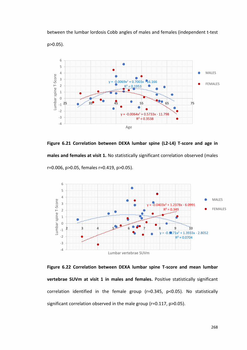
268

between the lumbar lordosis Cobb angles of males and females (independent t-test

p>0.05).

Figure 6.21 Correlation between DEXA lumbar spine (L2-L4) T-score and age in

males and females at visit 1. No statistically significant correlation observed (males

r=0.006, p>0.05, females r=0.419, p>0.05).

Figure 6.22 Correlation between DEXA lumbar spine T-score and mean lumbar

vertebrae SUVm at visit 1 in males and females. Positive statistically significant

correlation identified in the female group (r=0.345, p<0.05). No statistically

significant correlation observed in the male group (r=0.117, p>0.05).

y = -0.0069x2 + 0.7003x - 16.166R² = 0.1953

y = -0.0064x2 + 0.5733x - 11.798R² = 0.3538

-4

-3

-2

-1

0

1

2

3

4

5

6

25 35 45 55 65 75

Lum

bar

sp

ine

T-Sc

ore

Age

MALES

FEMALES

y = -0.1171x2 + 1.3933x - 2.8052R² = 0.0704

y = -0.0403x2 + 1.2378x - 6.0991R² = 0.349

-4

-3

-2

-1

0

1

2

3

4

5

6

2 3 4 5 6 7 8 9 10

Lum

bar

sp

ine

T-Sc

ore


MALES

FEMALES

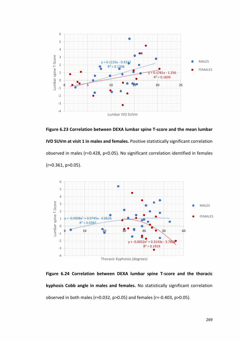
269

Figure 6.23 Correlation between DEXA lumbar spine T-score and the mean lumbar

IVD SUVm at visit 1 in males and females. Positive statistically significant correlation

observed in males (r=0.428, p<0.05). No significant correlation identified in females

(r=0.361, p>0.05).

Figure 6.24 Correlation between DEXA lumbar spine T-score and the thoracic

kyphosis Cobb angle in males and females. No statistically significant correlation

observed in both males (r=0.032, p>0.05) and females (r=-0.403, p>0.05).

y = 0.1781x - 1.256R² = 0.1839

y = 0.1135x - 0.9333R² = 0.1308

-4

-3

-2

-1

0

1

2

3

4

5

6

0 5 10 15 20 25

Lum

bar

sp

ine

T-Sc

ore

Lumbar IVD SUVm

MALES

FEMALES

y = -0.0008x2 + 0.0745x - 0.6626R² = 0.0387

y = -0.0052x2 + 0.3143x - 3.7828R² = 0.1919

-4

-3

-2

-1

0

1

2

3

4

5

6

0 10 20 30 40 50 60

Lum

bar

sp

ine

T-Sc

ore

Thoracic Kyphoisis (degrees)

MALES

FEMALES

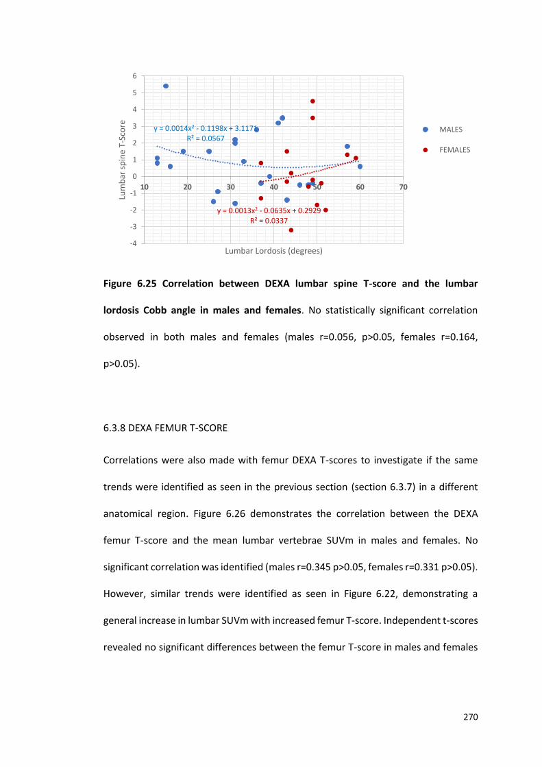
270

Figure 6.25 Correlation between DEXA lumbar spine T-score and the lumbar

lordosis Cobb angle in males and females. No statistically significant correlation

observed in both males and females (males r=0.056, p>0.05, females r=0.164,

p>0.05).

6.3.8 DEXA FEMUR T-SCORE

Correlations were also made with femur DEXA T-scores to investigate if the same

trends were identified as seen in the previous section (section 6.3.7) in a different

anatomical region. Figure 6.26 demonstrates the correlation between the DEXA

femur T-score and the mean lumbar vertebrae SUVm in males and females. No

significant correlation was identified (males r=0.345 p>0.05, females r=0.331 p>0.05).

However, similar trends were identified as seen in Figure 6.22, demonstrating a

general increase in lumbar SUVm with increased femur T-score. Independent t-scores

revealed no significant differences between the femur T-score in males and females

y = 0.0014x2 - 0.1198x + 3.1171R² = 0.0567

y = 0.0013x2 - 0.0635x + 0.2929R² = 0.0337

-4

-3

-2

-1

0

1

2

3

4

5

6

10 20 30 40 50 60 70

Lum

bar

sp

ine

T-Sc

ore


MALES

FEMALES

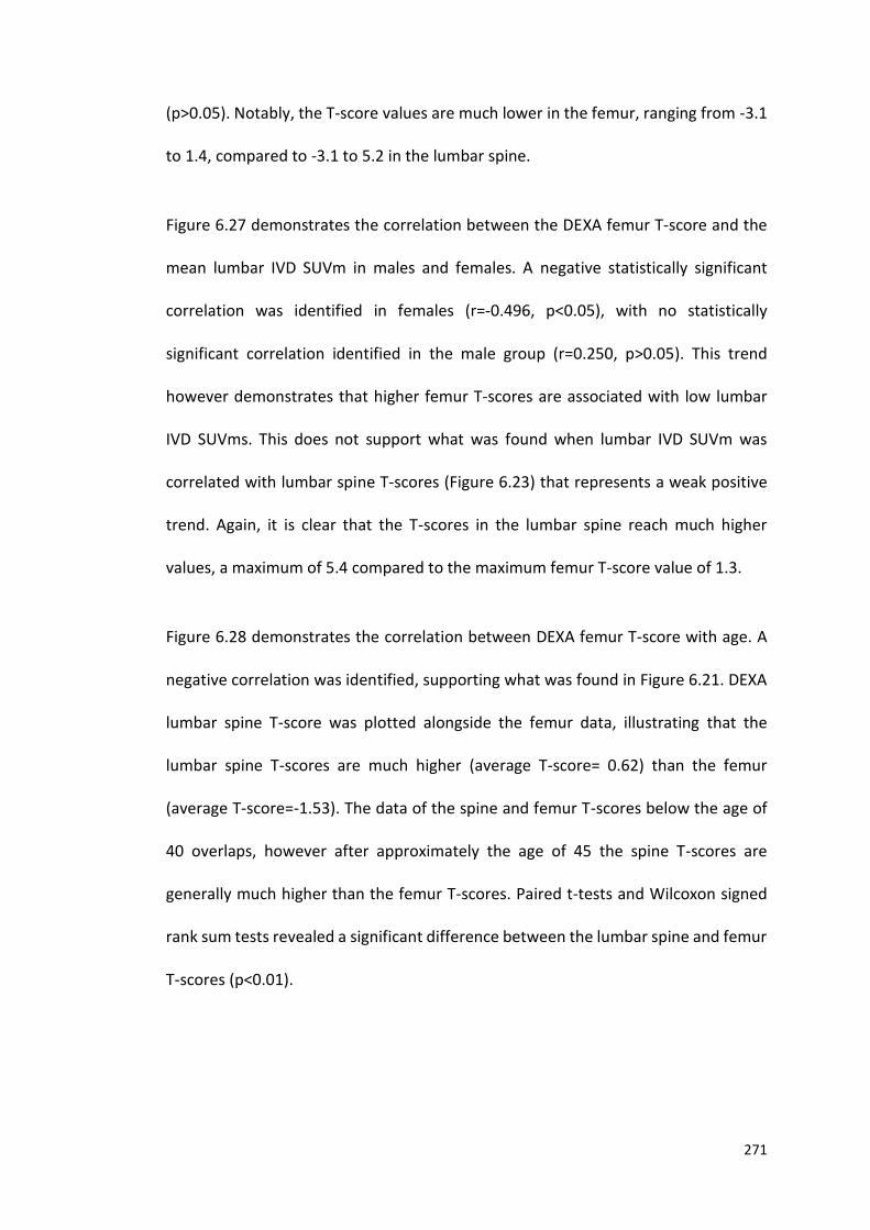
271

(p>0.05). Notably, the T-score values are much lower in the femur, ranging from -3.1

to 1.4, compared to -3.1 to 5.2 in the lumbar spine.

Figure 6.27 demonstrates the correlation between the DEXA femur T-score and the

mean lumbar IVD SUVm in males and females. A negative statistically significant

correlation was identified in females (r=-0.496, p<0.05), with no statistically

significant correlation identified in the male group (r=0.250, p>0.05). This trend

however demonstrates that higher femur T-scores are associated with low lumbar

IVD SUVms. This does not support what was found when lumbar IVD SUVm was

correlated with lumbar spine T-scores (Figure 6.23) that represents a weak positive

trend. Again, it is clear that the T-scores in the lumbar spine reach much higher

values, a maximum of 5.4 compared to the maximum femur T-score value of 1.3.

Figure 6.28 demonstrates the correlation between DEXA femur T-score with age. A

negative correlation was identified, supporting what was found in Figure 6.21. DEXA

lumbar spine T-score was plotted alongside the femur data, illustrating that the

lumbar spine T-scores are much higher (average T-score= 0.62) than the femur

(average T-score=-1.53). The data of the spine and femur T-scores below the age of

40 overlaps, however after approximately the age of 45 the spine T-scores are

generally much higher than the femur T-scores. Paired t-tests and Wilcoxon signed

rank sum tests revealed a significant difference between the lumbar spine and femur

T-scores (p<0.01).

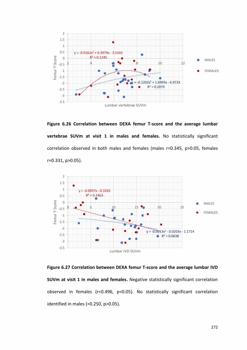
272

Figure 6.26 Correlation between DEXA femur T-score and the average lumbar

vertebrae SUVm at visit 1 in males and females. No statistically significant

correlation observed in both males and females (males r=0.345, p>0.05, females

r=0.331, p>0.05).

Figure 6.27 Correlation between DEXA femur T-score and the average lumbar IVD

SUVm at visit 1 in males and females. Negative statistically significant correlation

observed in females (r=0.496, p<0.05). No statistically significant correlation

identified in males (=0.250, p>0.05).

y = -0.0162x2 + 0.3979x - 3.5243R² = 0.1245

y = -0.1202x2 + 1.6993x - 6.9733R² = 0.2079

-3.5

-3

-2.5

-2

-1.5

-1

-0.5

0

0.5

1

1.5

2

2 4 6 8 10 12

Fem

ur

T-Sc

ore


MALES

FEMALES

y = -0.0013x2 - 0.0203x - 1.1714R² = 0.0638

y = -0.0937x - 0.3263R² = 0.2463

-3.5

-3

-2.5

-2

-1.5

-1

-0.5

0

0.5

1

1.5

2

0 5 10 15 20 25

Fem

ur

T-Sc

ore

Lumbar IVD SUVm

MALES

FEMALES

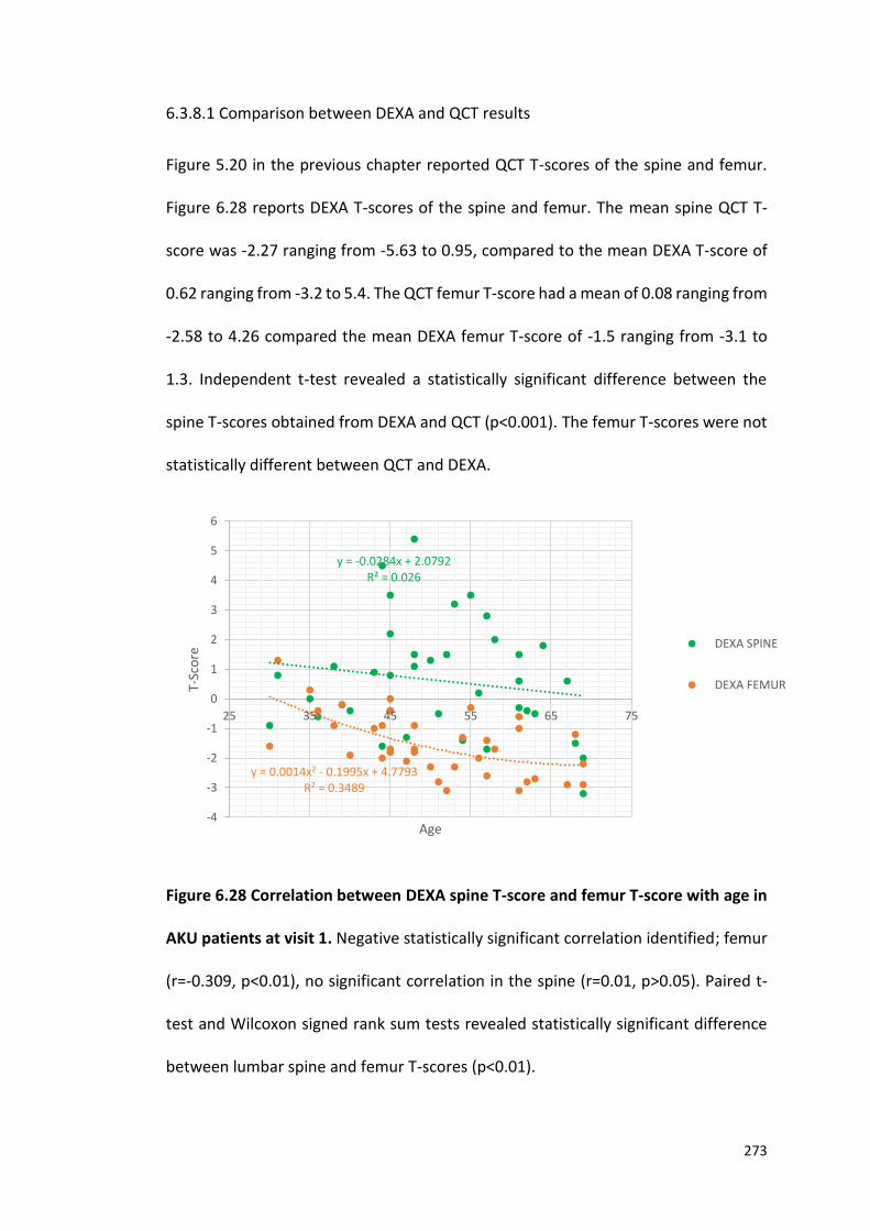
273

6.3.8.1 Comparison between DEXA and QCT results

Figure 5.20 in the previous chapter reported QCT T-scores of the spine and femur.

Figure 6.28 reports DEXA T-scores of the spine and femur. The mean spine QCT T-

score was -2.27 ranging from -5.63 to 0.95, compared to the mean DEXA T-score of

0.62 ranging from -3.2 to 5.4. The QCT femur T-score had a mean of 0.08 ranging from

-2.58 to 4.26 compared the mean DEXA femur T-score of -1.5 ranging from -3.1 to

1.3. Independent t-test revealed a statistically significant difference between the

spine T-scores obtained from DEXA and QCT (p<0.001). The femur T-scores were not

statistically different between QCT and DEXA.

Figure 6.28 Correlation between DEXA spine T-score and femur T-score with age in

AKU patients at visit 1. Negative statistically significant correlation identified; femur

(r=-0.309, p<0.01), no significant correlation in the spine (r=0.01, p>0.05). Paired t-

test and Wilcoxon signed rank sum tests revealed statistically significant difference

between lumbar spine and femur T-scores (p<0.01).

y = -0.0284x + 2.0792R² = 0.026

y = 0.0014x2 - 0.1995x + 4.7793R² = 0.3489

-4

-3

-2

-1

0

1

2

3

4

5

6

25 35 45 55 65 75

T-Sc

ore

Age

DEXA SPINE

DEXA FEMUR

274

6.4 DISCUSSION

This chapter has focused on correlating the vertebrae and IVD SUVm with other

clinical data obtained from the clinical trial site files from SONIA 2. Correlating other

data such as, serum and urine HGA concentrations, spinal flexibility, spinal curvature

angles and DEXA T-scores with the SUVm method will allow us to find common trends

between types of examination and imaging methods as well as allowing us to see if

these show any statistical relationships.

6.4.1 SERUM HGA CORRELATIONS

The serum HGA (s-HGA) concentration was obtained from a fasting blood sample

collected at visit 1 pre-nitisinone using LC-MS/MS by a biochemist at the RLBUHT.

After plotting the data provided by the biochemistry lab, AKU patients clearly have

elevated s-HGA concentrations (33.2umol/L) compared to the reference range

(<3.1umol/L) pre-nitisinone, which was one of the important findings reported in the

SONIA 1 clinical trial (45). When analysing male and female s-HGA there was no

significant difference between the two groups (independent t-test p>0.05). The

difference between male and female s-HGA in AKU has not been reported in the

literature and this data has revealed no significant differences suggesting that the

concentration of HGA in serum of patients with AKU is not affected by gender. Weak

positive correlations were reported between s-HGA and age in both males and

females (Figure 6.1) suggesting that age does not influence s-HGA concentration

significantly. The weak positive correlation however may represent reduced renal

function with age. It has been recognised for decades that there is an age associated

loss of kidney function associated with progressive decreases in glomerular filtration

275

rate and renal blood flow. In AKU this would result in increased HGA circulating in the

blood due to reduced efficiency of the kidneys (155).

It is clear that s-HGA concentration is elevated in AKU patients without treatment.

The SONIA 1 clinical trial elucidated a clear dose response relationship with increasing

dosages of nitisinone (1,2,4 and 8mg) with the highest dose reducing HGA by 99.4%

(45). Serum HGA concentrations in the SONIA 1 group went from 30.3 umol/L at

baseline to 0.7umol/L after one year on nitisinone. Without treatment s-HGA remains

elevated demonstrating the effectiveness of the drug at lowering the culprit molecule

HGA (45).

Correlations were also made between s-HGA and the average lumbar and thoracic

IVD and vertebrae SUVm (Figures 6.2 and 6.3). No statistically significant correlations

were identified between both the s-HGA and the vertebrae SUVm (r=0.0781, p>0.05)

(Figure 6.2), or the s-HGA and IVD SUVm (r=0.0174, p>0.05) (Figure 6.3). This suggests

that the concentration of HGA that is circulating in the blood, pre-treatment at visit

1, does not correlate with the SUVms. This may be because s-HGA concentration does

not appear to be affected by age and remains relatively stable across the population.

Whereas in contrast we have seen how the SUVm changes with age in both the

vertebrae and IVDs due to the progression of the disease (Figures 4.10- 4.13).

Additionally, s-HGA represents the concentration of s-HGA circulating in the blood at

a single time-point, before treatment. The SUVm is a measure of fluoride uptake that

represents years of HGA accumulation in the spine. Therefore, it is not the circulating

s-HGA concentration that is important, it is the life-long exposure to HGA that is key

in AKU ochronosis that results in osteoarthropathy.

276

6.4.2 URINE HGA CORRELATION

Acidified 24-hour urine samples were obtained from all SONIA 2 patients at visit 1,

pre-nitisinone. The acidified urine was analysed for HGA using LC-MS/MS by a

biochemist at the RLBUHT and is representative of the total amount of HGA excreted

in 24 hours. The data was provided by the biochemistry lab and was plotted against

age. AKU patients have elevated urine HGA (u-HGA) (27035 umol/L) compared to the

reference range (<2.9 umol/L) which again was one of the main findings in the SONIA

1 clinical trial (45). Interestingly there was a statistical significant difference between

the u-HGA of males and females with males having a higher mean u-HGA (30546

umol/24hr) than females (21556 umol/24hr). This may be due to the increased

dietary intake of protein in males compared to females. It is known that dietary intake

of tyrosine/phenylalanine results in the accumulation of HGA. The more

tyrosine/phenylalanine ingested, the more HGA is therefore produced and excreted.

It is widely agreed that males are generally larger than females and require more

calories and more fluid, and they therefore excrete more urine which may represent

why males have increased u-HGA umol/24hrs.

As in section 6.4.1 no statistically significant correlations were identified between u-

HGA and the average lumbar and thoracic vertebrae and IVD SUVms. This suggests

that the total urinary HGA output in 24hrs does not correlate with fluoride uptake in

the vertebrae and IVDs. This is not unexpected as it is not the amount u-HGA that is

excreted that is important in terms of ochronosis and arthropathy of the spine but it

is the amount that is bathing the tissues over many years that results in ochronosis

and spinal arthropathy.

277

6.4.3 LUMBAR SIDE FLEXION CORRELATION

A senior physiotherapist at the RLBUHT measured lumbar side flexion (for more

information see section 2.7.1) on all SONIA 2 patients at visit 1, pre-nitisinone.

Lumbar side flexion measurements can be used as a standardised measurement to

quantify spinal flexibility. Lumbar side flexion provides a good picture of spinal

flexibility in contrast to lumbar flexion (forward bending) as it is not augmented by

hip joint movement. Additionally, practically it is often easier to ask patients with

back pain to flex to the side rather than bend forwards (156). When correlating

lumbar side flexion on the right and left sides with age, negative statistically

significant correlations were identified (p<0.001 on both the left and right sides) with

no statistical difference between males and females (Figure 6.7 A and B). Lumbar side

flexion was highest in the younger patients and lower in the older patients. As

expected younger patients have increased flexibility compared to older patients. It is

widely agreed that with increasing age, BMD reduces, that is associated with

increased risk of fractures. Collagen production reduces with age meaning response

to repair is reduced. Tendons and ligaments become stiffer and elasticity is reduced

and muscles supporting the joints become weak. All these factors contribute to

reduction in flexibility with age.

In AKU raised HGA levels in plasma and extracellular fluid lead to ochronosis. HGA

polymers are deposited in connective tissues such as cartilage, tendons and

ligaments. The affected tissues often become weak and brittle, and prone to bone

fracturing, and tendon snapping. This ultimately reduces flexibility and impacts on

mobility due to pain and discomfort of the major joints such as the spine, hip and

278

knees (36). This clearly explains why there is a reduction in lumbar side flexion with

age in AKU. This trend would also be expected in a control population. However, the

slope on Figure 6.7 A and B would be expected to be shifted over to the right as AKU

patients suffer from pain and arthropathy decades before that of control patients.

Physiotherapy is routine practice for most AKU patients and it is encouraged that all

patients participate in exercises set by the physiotherapist to try to increase flexibility

and range of motion at the joint and to try to keep joints supple, reducing pain (157).

Interestingly, positive statistically significant correlations were identified between

lumbar side flexion (on both the right and left sides) and the average lumbar and

thoracic vertebrae SUVm in both males and females (Figure 6.8 A and B). This

demonstrates that increased spinal flexibility is associated with increased vertebrae

SUVms. This trend reflects what has been described in Chapter 4, where SUVm can

be seen decreasing with age due to reduced BMD with age (Figures 4.10 and 4.11).

Younger patients are associated with high vertebrae SUVms and high BMD due to

increased hydroxyapatite for 18F to bind. Older patients are associated with low

SUVms and low BMD as there is less bone turnover with age. These findings reflect

that younger patients have increased flexibility; higher BMD values therefore have

increased SUVms. In contrast the older patients have reduced spinal flexibility,

reduced BMD and reduced SUVms.

No statistical correlations were identified when correlating the lumbar side flexion

(on the right and left sides) with the average lumbar and thoracic IVD SUVm in both

males and females which was disappointing. It was expected that with increased IVD

SUVm there would be a reduction in lumbar side flexion, as increased IVD SUVm

279

reflects calcification of the IVDs and it would be assumed that calcified IVDs would be

less flexible due to pain and or spinal fusion.

6.4.4 CERVICAL SPINE ROTATION CORRELATION

Cervical spine rotation is a measure of range of motion of the neck. No statistically

significant correlations were identified between cervical spine rotation (on the right

and left sides) with age. Suggesting that cervical flexibility is not influenced by age

(right side r=0.175, left side r=0.113). This is surprising as although the cervical spine

is not weight bearing and is not one of the major regions affected in AKU, cervical

mobility has been reported to be reduced in AKU along with cervical disc space

narrowing, spinal cord compression and disc herniations at the cervical level (158). It

was therefore expected that cervical flexibility would be reduced in the older AKU

patient’s as it is one of the regions where these patients report pain. No correlations

were identified between cervical spine rotation and lumbar and thoracic vertebrae

and IVD SUVms suggesting that lumbar side flexion may be a better indicator of

disease state and progression compared to cervical rotation.

6.4.5 COBB ANGLE CORRELATION WITH SUVm

The Cobb angle is a standardised measure of spinal curvature. Cobb angles are used

clinically to measure thoracic kyphosis, lumbar lordosis and scoliosis, if present. In

AKU patients these measurements are repeated annually to assess if there are any

changes to the curvatures of the spine. The data presented in this chapter was from

visit 1, pre-nitisinone. Normal thoracic kyphosis ranges from 20-45 degrees and

280

hyperkyphosis is defined as more than 45 degrees (122). Clinically there is no range

for normal lumbar lordosis neither is there an angle to define hyper or hypo-lordosis

as there are many factors that influence the lumbar spine such as muscular strength,

flexibility and BMI (123). Scoliosis is defined as a spinal curvature of 10 degrees or

more to the left or the right (124). No statistically significant correlations were

identified between lumbar lordosis and age (r=0.01, p>0.05) or thoracic kyphosis and

age (r=0.07, p>0.05).

Correlations were made between the spinal Cobb angles and vertebrae and IVD

SUVms to see if there was a relationship between spinal curvature and bone and or

IVD 18F uptake. When the thoracic kyphosis Cobb angle and the thoracic vertebrae

SUVm was correlated no correlation was identified between the normal thoracic

kyphosis Cobb angles that range from 20-45 degrees, and the thoracic vertebrae

SUVm. Looking at the graph (Figure 6.13) the normal thoracic kyphosis Cobb angles

all have SUVm that are higher up the scale ranging from 6-11 suggesting that normal

thoracic curvatures are associated with uptake of fluoride consistent with the

younger less affected patients. As we have previously reported there is a negative

trend with vertebrae SUVm with age (see Figures 4.10 and 4.11). Interestingly it can

be seen in Figure 6.13 that the hyperkyphosis Cobb angles (>45ᵒ) demonstrate a

negative correlation with thoracic vertebrae SUVm and this was found to be

statistically significant (r=-0.850, p<0.01). This suggests that the patients with

increasingly hyperkyphotic spines have reduced thoracic vertebrae SUVms. This

supports what we have seen previously in Figures 4.10 and 4.11 where a negative

trend was identified between vertebrae SUVm and age. It was proposed that this

281

reduction in vertebrae SUVm was due to reduced BMD with age. It is also proposed

that this is what this trend is demonstrating (Figure 6.13), that the hyperkyphotic

spines have low BMD which is one of the main reasons for this hyperkyphotic

curvature (125). Hyperkyphosis also may result from either muscle weakness and

degenerative disc disease, leading to vertebral fractures all of which are common in

AKU patients (125).

Interestingly, when the hyperkyphotic Cobb angles were correlated with thoracic IVD

SUVms (Figure 6.15) a negative statistically significant correlation was identified (r=-

0.723, p<0.01). This suggests that increasingly hyperkyphotic spines have reduced

thoracic IVD SUVms. The negative correlation of the hyperkyphosis Cobb angles with

thoracic IVD SUVm supports what has been presented previously in Figure 4.13.

Figure 4.13 demonstrates the inverted ‘U’ shaped trend of thoracic IVD SUVms with

age. It is clear in the oldest patients, around the age of 55-60, that there is a reduction

in IVD SUVm with age. It is proposed that this reduction in SUVm is likely to be due

to reduced deposition of hydroxyapatite/calcium pyrophosphate dihydrate crystals

into the IVDs that occurs as part of AKU disease pathophysiology. This reduction in

deposition may be due to complete calcification of the IVD and or spinal fusion. Once

this has been achieved deposition of hydroxyapatite/calcium pyrophosphate

dihydrate crystals into the IVDs stops. It is understood that 18F binds preferentially to

newly laid down hydroxyapatite due to the higher availability of binding sites, once

new hydroxyapatite / calcium pyrophosphate dihydrate crystals stop being laid down

18F does not preferentially bind to those regions therefore the SUVms in those regions

reduce.

282

When analysing the correlations between lumbar lordosis Cobb angles and the

lumbar vertebrae and IVD SUVm no correlations were identified (Figures 6.14 and

6.16). There is no clinical definition of lumbar hyper or hypo lordosis in terms of using

a Cobb angle. Clinicians often visually assess lumbar lordosis by assessing the arch

and pelvic tilt (159). Lumbar lordosis is a unique structural characteristic of the

normal human spine and phylogenetically is considered the key structural adaptation

to bipedalism. An increased lumbosacral angle is known to augment the pressure on

the posterior ligaments and facet joints of the spine, and ultimately causes lower back

pain. Most clinicians advise their patients to abolish lumbar lordosis by carrying out

flexion exercises to strengthen the muscles. Interestingly, a loss of lumbar lordosis is

the most distinctive finding of the aging spine (160), and it is widely known the

prevalence of lower back pain increases with age (161). Therefore, a positive

correlation was expected between lumbar lordosis Cobb angle and lumbar vertebrae

SUVm. Demonstrating that lower lumbar lordosis Cobb angles correlate with lower

vertebrae SUVms, associated with older patients. However, when age was correlated

with lumbar lordosis in this group no correlation was identified (r=0.01, p>0.05)

which may explain why these results were not found.

Lastly scoliosis Cobb angles were correlated with the IVD and vertebrae SUVms of

which no correlations were identified (Figures 6.17 and 6.18). Scoliosis is

characterised by a lateral deviation of the spine in the coronal plane and is clinically

defined as a spinal curvature of ten degrees or more (124,162). The prevalence of

adult scoliosis in the USA has been reported as ranging from 2%-32% (163). In the

SONIA 2 AKU patient group, 32.5% of the patients have clinically defined

283

degenerative scoliosis. Degenerative scoliosis is a deformity that develops from a

previously straight spine, caused by accelerated degeneration of the spine with

progressive disc and facet degeneration (163). In AKU it is understood that the spine

degenerates with radiological signs such as reduced IVD height, IVD calcifications,

osteophyte formation and in severe cases spinal fusion. These changes to the spine,

if more severe on one side compared to another, can lead to degenerative scoliosis.

It was expected therefore that the scoliosis Cobb angle would be associated with

increased IVD SUVms due to calcification of the IVDs resulting in spinal changes.

Additionally, it was expected that higher scoliosis Cobb angles would also be

associated with reduced vertebrae SUVms as this would reflect reduced BMD in the

vertebrae with disease progression.

6.4.6 COBB ANGLE MRI vs X-Ray

Standing plain radiographs remain the gold standard for measuring spinal curvatures.

Clinicians utilise the Cobb angle methodology to obtain measurements of scoliosis,

thoracic kyphosis and lumbar lordosis. Several studies have shown the variability and

reliability of Cobb angle measurements. Loder et al. (164) described the interobserver

variance of 11.8ᵒ and intraobserver variance of 9.6ᵒ when using the Cobb angle

method to measure scoliosis using plain radiographs. Carman et al. (165) described

that interobserver variations for measurements of the Cobb angle on radiographs of

patients who had kyphosis (3.3ᵒ) were comparable with those on the radiographs of

patients who had scoliosis (3.8ᵒ). It has been investigated in the literature whether

alternative imaging modalities may be superior to the conventional X-Ray in

obtaining more accurate measurements. In the literature, idiopathic scoliosis is the

284

deformity that has been investigated in terms of utilising alternative imaging

methodologies as scoliosis is common in developing children and it is of concern that

these patients are exposed to repeated ionizing radiation. Lee et al. (166)

demonstrated the relationship between adolescent idiopathic scoliosis Cobb angle

measurements obtained with standing plain radiographs and standard supine

magnetic resonance images (MRI). They found that Cobb angles measured from

supine MRI of the spine can be directly translated to Cobb angle measurements

obtained from plain radiographs with an acceptable degree of accuracy. They

proposed that this method could significantly reduce radiation exposure to these

patients (166).

Tauchi et al. (167) discussed that measuring Cobb angles with X-rays is difficult as the

resolution of the images makes it difficult to define the appropriate end plates of the

vertebrae to measure. They stated that 3D-CT can provide more detailed images and

hypothesised that Cobb angles in congenital scoliosis can be measured more

accurately using this technique. This study concluded that Cobb angles assessed using

the X-ray method produced similar variances as 3D-CT images suggesting that plain

X-rays are clinically useful. However, they concluded that 3D-CT can provide more

detailed images and can contribute greatly to the development of strategies for

surgical treatment but exposes the patient to high levels of radiation.

Vavruch et al. (168) commented that 3D imaging is needed for the assessment of

scoliosis due to the 3D nature of the disorder. The advantage of MRI is that it does

not use radiation, however this method is time consuming and expensive. CT is

superior to conventional radiographs however requires relatively high radiation

285

doses. They correlated the Cobb angles obtained from low dose CT and that

measured from radiographs and found that the correlation was strong.

As presented, the literature primarily focuses on using scoliosis Cobb angles to

compare different imaging modalities such as the conventional radiography with MRI

and CT. In this chapter, thoracic kyphosis and lumbar lordosis were used to compare

the Cobb angles obtained from X-ray and MRI images to see if standing and lying

down alters the spinal measurements. The results obtained from the SONIA 2 group

at visit one are consistent with the literature. Figure 6.19 demonstrates a positive

statistically significant correlation between the thoracic kyphosis Cobb angle

obtained from MRI and plain X-ray (r=0.691, p<0.001) and the difference being 9.14ᵒ

between the two modalities (Table 6.1). A positive statistically significant correlation

was also identified between the lumbar lordosis Cobb angles obtained from plain X-

ray and MRI (r=0.825, p<0.001) (Figure 20). These results reflect that obtaining the

thoracic kyphosis and lumbar lordosis Cobb angles from both MRI and plain X-ray

both show very similar results and the pros and cons of both imaging modalities

should be assessed to determine what modality is best for the patient.

6.4.7 BONE MINERAL DENSITY T-SCORE COMPARISONS

The assessment of BMD in AKU is important to measure as it is widely understood

that arthritic changes to the IVDs with disease progression has direct implications to

the bony vertebrae. It has also been hypothesised that in AKU HGA deposition in bone

matrix and osteocytes may play a pathophysiological role in accelerating bone loss

(148). DEXA is the gold standard for obtaining BMD T-scores and the WHO

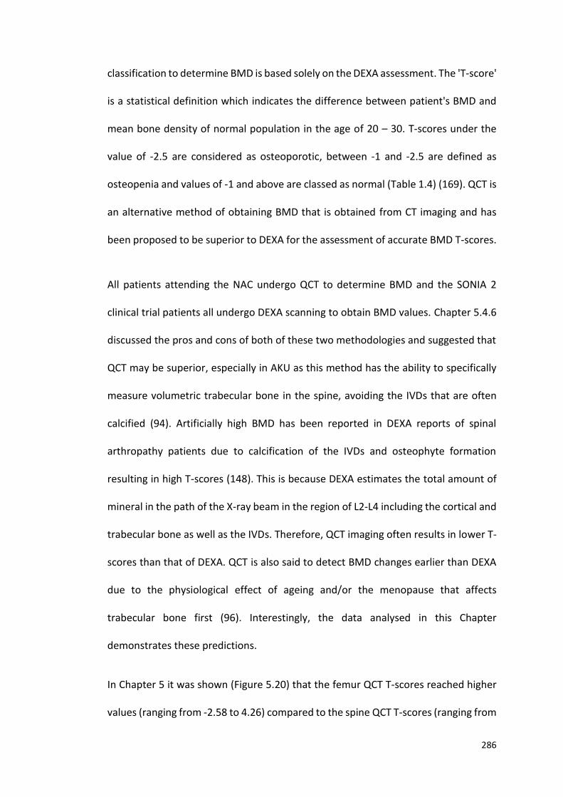
286

classification to determine BMD is based solely on the DEXA assessment. The 'T-score'

is a statistical definition which indicates the difference between patient's BMD and

mean bone density of normal population in the age of 20 – 30. T-scores under the

value of -2.5 are considered as osteoporotic, between -1 and -2.5 are defined as

osteopenia and values of -1 and above are classed as normal (Table 1.4) (169). QCT is

an alternative method of obtaining BMD that is obtained from CT imaging and has

been proposed to be superior to DEXA for the assessment of accurate BMD T-scores.

All patients attending the NAC undergo QCT to determine BMD and the SONIA 2

clinical trial patients all undergo DEXA scanning to obtain BMD values. Chapter 5.4.6

discussed the pros and cons of both of these two methodologies and suggested that

QCT may be superior, especially in AKU as this method has the ability to specifically

measure volumetric trabecular bone in the spine, avoiding the IVDs that are often

calcified (94). Artificially high BMD has been reported in DEXA reports of spinal

arthropathy patients due to calcification of the IVDs and osteophyte formation

resulting in high T-scores (148). This is because DEXA estimates the total amount of

mineral in the path of the X-ray beam in the region of L2-L4 including the cortical and

trabecular bone as well as the IVDs. Therefore, QCT imaging often results in lower T-

scores than that of DEXA. QCT is also said to detect BMD changes earlier than DEXA

due to the physiological effect of ageing and/or the menopause that affects

trabecular bone first (96). Interestingly, the data analysed in this Chapter

demonstrates these predictions.

In Chapter 5 it was shown (Figure 5.20) that the femur QCT T-scores reached higher

values (ranging from -2.58 to 4.26) compared to the spine QCT T-scores (ranging from

287

-5.63 to 0.95). This suggests that the spine is affected by a loss of BMD to a higher

extent than the femur which is consistent to what has been reported in the literature.

This could be due to several reasons. The difference between velocities of bone loss

in different parts of human body could be the main reason. Trabecular bone, found

in the lumbar spine is known to have a more rapid rate of bone loss compared to

cortical bone, typical of proximal femur. In addition, the hip is primarily weight

bearing, which can result in increased BMD that has been shown to affect the hip and

head of femur (169).

When T-scores of the spine and femur obtained from DEXA were plotted the range

of T-scores were statistically different from the T-scores obtained from QCT. Figure

6.28 demonstrates the spine and femur T-scores obtained from DEXA. It is clear that

the spine T-scores obtained from DEXA reach much higher values compared to that

of the femur which is the opposite to what was found in Figure 5.20. The Spine T-

scores range from -3.2 to 5.4 compared to -3.1 to 1.3 in the femur.

Importantly, independent t-tests revealed a significant difference (p<0.001) between

the spine T-scores obtained from DEXA and QCT. The spine QCT T-scores are much

lower (ranging from -5.63 – 0.95) than the DEXA spine T-scores (ranging from -3.2 –

5.4) which supports what has been stated in the literature. This increase in spine T-

scores obtained from DEXA evident in Figure 6.28 is thought to represent IVD

calcification and spinal arthropathy in AKU. It is clear in the literature that BMD

measured by DEXA is variable depending on the site measured with significant

differences identified between the T-scores obtained from the hip and spine (170).

Increased calcification within the laminae and facet joints and increased

288

development of vascular calcifications, spondylophytes and endplate sclerosis is

thought to render DEXA scanning of the lumbar spine unreliable (170). Discordance

has also been reported between hip and spine BMD using DEXA that can affect overall

diagnosis of osteoporosis (171). Because of this discordance in 2000, the WHO

updated the guidelines stating that diagnostic use of T-scores should be reserved for

the use of hip DEXA BMD measurements only and no other T-scores are to be used

to diagnose osteoporosis. BMD measurements at sites other than the hip can be used

however to assess relative risks of osteoporosis and fracture risk (172). These finding

suggests that maybe QCT imaging is most appropriate to determine true hip and

lumbar vertebrae BMD in AKU.

6.4.8 DEXA LUMBAR SPINE T-SCORE

It is agreed in the literature that BMD reduces with age in both males and females

(145). Peak BMD is reached in women around the age of 20, and slightly older in men.

Women experience a more rapid decline in BMD compared to males around the

onset of the menopause as it is understood that reduction in oestrogen levels results

in increased bone resorption and decreased BMD (146). Figure 6.21 demonstrates

that in AKU after the age of around 45 there is a steady decline in the lumbar spine

T-score with females having lower T-scores compared to males. This supports what

has been stated in the literature. This was also found when the lumbar T-scores

obtained from QCT were plotted with age where a statistically significant correlation

was found (r= -0.682, p<0.01) (Figure 5.17).

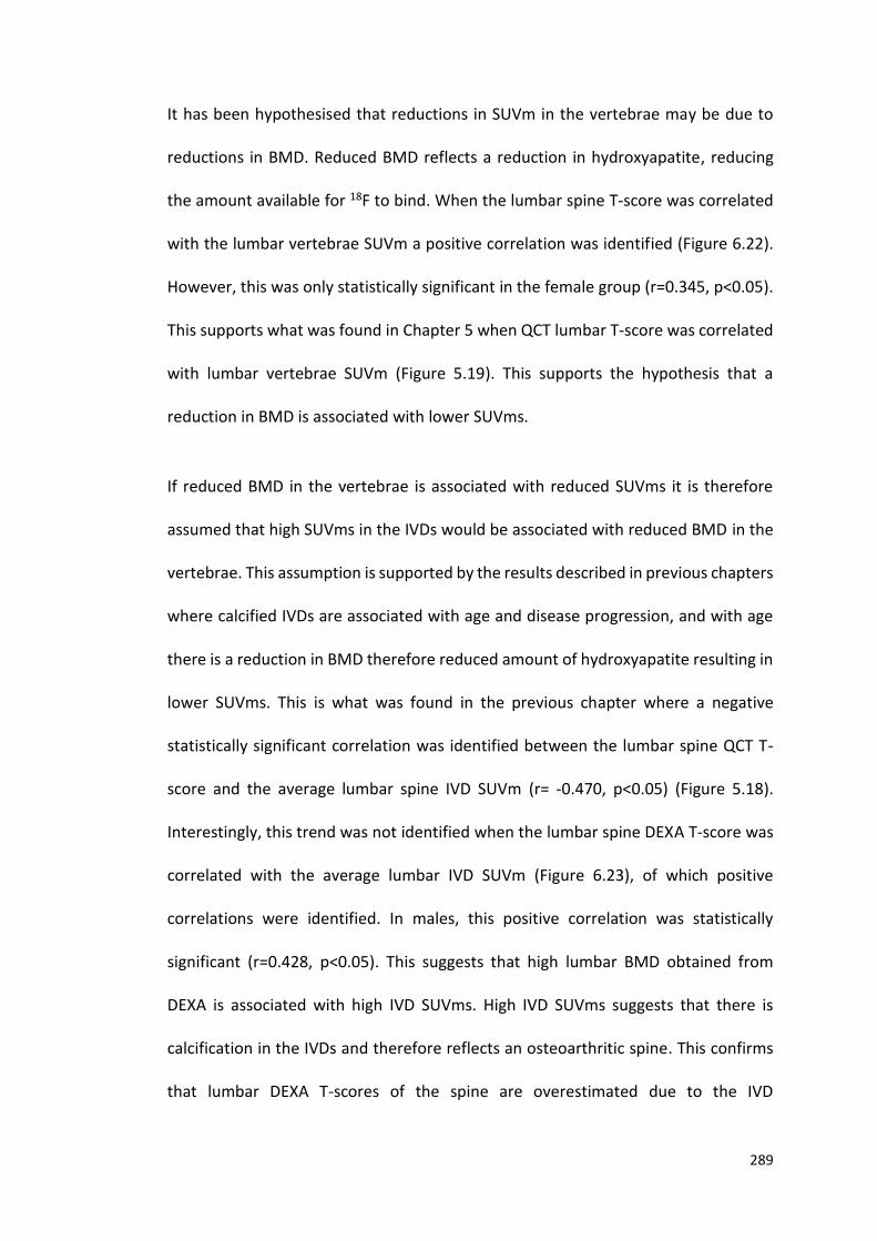
289

It has been hypothesised that reductions in SUVm in the vertebrae may be due to

reductions in BMD. Reduced BMD reflects a reduction in hydroxyapatite, reducing

the amount available for 18F to bind. When the lumbar spine T-score was correlated

with the lumbar vertebrae SUVm a positive correlation was identified (Figure 6.22).

However, this was only statistically significant in the female group (r=0.345, p<0.05).

This supports what was found in Chapter 5 when QCT lumbar T-score was correlated

with lumbar vertebrae SUVm (Figure 5.19). This supports the hypothesis that a

reduction in BMD is associated with lower SUVms.

If reduced BMD in the vertebrae is associated with reduced SUVms it is therefore

assumed that high SUVms in the IVDs would be associated with reduced BMD in the

vertebrae. This assumption is supported by the results described in previous chapters

where calcified IVDs are associated with age and disease progression, and with age

there is a reduction in BMD therefore reduced amount of hydroxyapatite resulting in

lower SUVms. This is what was found in the previous chapter where a negative

statistically significant correlation was identified between the lumbar spine QCT T-

score and the average lumbar spine IVD SUVm (r= -0.470, p<0.05) (Figure 5.18).

Interestingly, this trend was not identified when the lumbar spine DEXA T-score was

correlated with the average lumbar IVD SUVm (Figure 6.23), of which positive

correlations were identified. In males, this positive correlation was statistically

significant (r=0.428, p<0.05). This suggests that high lumbar BMD obtained from

DEXA is associated with high IVD SUVms. High IVD SUVms suggests that there is

calcification in the IVDs and therefore reflects an osteoarthritic spine. This confirms

that lumbar DEXA T-scores of the spine are overestimated due to the IVD

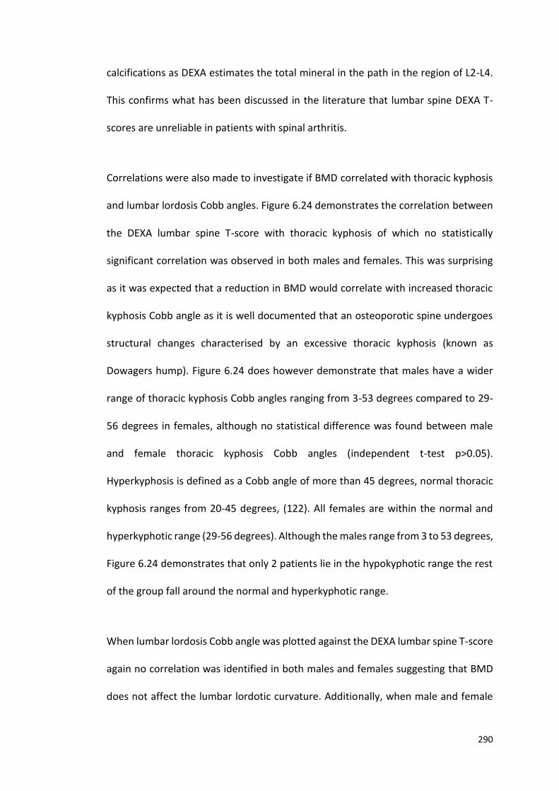
290

calcifications as DEXA estimates the total mineral in the path in the region of L2-L4.

This confirms what has been discussed in the literature that lumbar spine DEXA T-

scores are unreliable in patients with spinal arthritis.

Correlations were also made to investigate if BMD correlated with thoracic kyphosis

and lumbar lordosis Cobb angles. Figure 6.24 demonstrates the correlation between

the DEXA lumbar spine T-score with thoracic kyphosis of which no statistically

significant correlation was observed in both males and females. This was surprising

as it was expected that a reduction in BMD would correlate with increased thoracic

kyphosis Cobb angle as it is well documented that an osteoporotic spine undergoes

structural changes characterised by an excessive thoracic kyphosis (known as

Dowagers hump). Figure 6.24 does however demonstrate that males have a wider

range of thoracic kyphosis Cobb angles ranging from 3-53 degrees compared to 29-

56 degrees in females, although no statistical difference was found between male

and female thoracic kyphosis Cobb angles (independent t-test p>0.05).

Hyperkyphosis is defined as a Cobb angle of more than 45 degrees, normal thoracic

kyphosis ranges from 20-45 degrees, (122). All females are within the normal and

hyperkyphotic range (29-56 degrees). Although the males range from 3 to 53 degrees,

Figure 6.24 demonstrates that only 2 patients lie in the hypokyphotic range the rest

of the group fall around the normal and hyperkyphotic range.

When lumbar lordosis Cobb angle was plotted against the DEXA lumbar spine T-score

again no correlation was identified in both males and females suggesting that BMD

does not affect the lumbar lordotic curvature. Additionally, when male and female

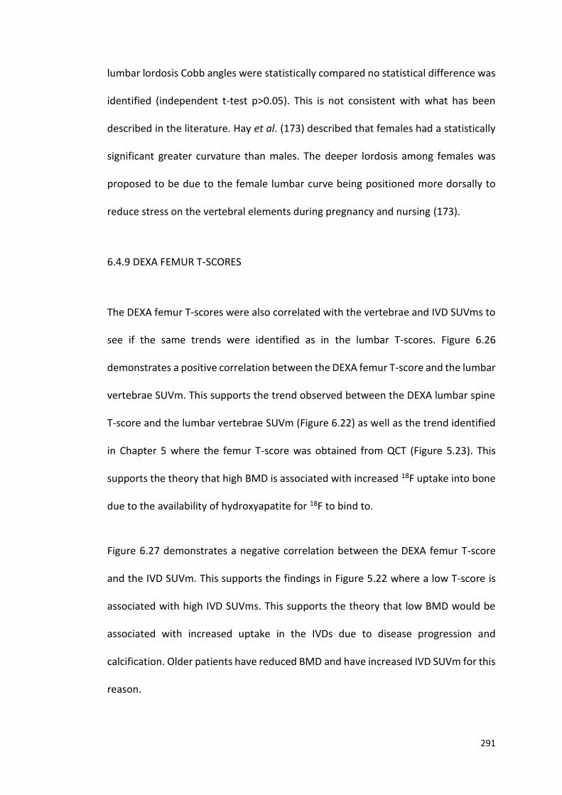
291

lumbar lordosis Cobb angles were statistically compared no statistical difference was

identified (independent t-test p>0.05). This is not consistent with what has been

described in the literature. Hay et al. (173) described that females had a statistically

significant greater curvature than males. The deeper lordosis among females was

proposed to be due to the female lumbar curve being positioned more dorsally to

reduce stress on the vertebral elements during pregnancy and nursing (173).

6.4.9 DEXA FEMUR T-SCORES

The DEXA femur T-scores were also correlated with the vertebrae and IVD SUVms to

see if the same trends were identified as in the lumbar T-scores. Figure 6.26

demonstrates a positive correlation between the DEXA femur T-score and the lumbar

vertebrae SUVm. This supports the trend observed between the DEXA lumbar spine

T-score and the lumbar vertebrae SUVm (Figure 6.22) as well as the trend identified

in Chapter 5 where the femur T-score was obtained from QCT (Figure 5.23). This

supports the theory that high BMD is associated with increased 18F uptake into bone

due to the availability of hydroxyapatite for 18F to bind to.

Figure 6.27 demonstrates a negative correlation between the DEXA femur T-score

and the IVD SUVm. This supports the findings in Figure 5.22 where a low T-score is

associated with high IVD SUVms. This supports the theory that low BMD would be

associated with increased uptake in the IVDs due to disease progression and

calcification. Older patients have reduced BMD and have increased IVD SUVm for this

reason.

292

6.4.10 SUMMARY

This chapter aimed to investigate the correlations between the SONIA 2 SUVms

reported in Chapter 4 with other patient data obtained from the clinical trial at visit

1, pre-nitisinone. This chapter focuses on the baseline data (pre-nitisinone) to

exclude trends that may be associated with the drug nitisinone. The data used to

correlate with the SUVms included serum and urine HGA concentrations, spinal

flexibility measurements obtained from the physiotherapist, spinal curvature Cobb

angles and DEXA BMD scores.

No statistically significant correlations were identified when correlating serum HGA

with vertebrae and IVD SUVms. Serum HGA also did not correlate with age suggesting

that the concentration of circulating HGA is not affected by disease progression with

no differences identified between males and females. It is important to note that

serum HGA represents the concentration of circulating HGA in the blood at a single

time point, whereas age, vertebrae and IVD SUVms all represent lifelong exposure to

HGA that is key to the progression of the disease. This was proposed to explain why

no significant correlations were identified between these parameters. Correlations

with urine HGA also did not show any significant correlations with SUVm suggesting

that the total urinary output of HGA in 24 hours does not correlate with fluoride

uptake in the vertebrae or IVDs. Again, it was proposed that it is not the amount of

excreted HGA that is important in terms of disease progression it is the amount

circulating and bathing the tissues over many years that is key to ochronosis hence

why no correlations were identified.

293

When analysing spinal flexibility measurements obtained from the physiotherapist,

negative statistically significant correlations were identified between lumbar side

flexion and age. This reduction in flexibility with age is thought to represent reduced

elasticity of tendons and ligaments due to deposition of HGA polymers rendering

them stiff and brittle as well as solidifying IVDs. Interestingly positive statistically

significant correlations were identified between lumbar side flexion and vertebrae

SUVm supporting the hypothesis that SUVm decreases with age due to reduced BMD

that will result in reduced spinal flexibility which are both linked to age. No

statistically significant correlations were identified between cervical rotation with

age or with vertebrae and IVD SUVms suggesting that lumbar side flexion may be a

better indicator of disease state and progression.

In addition to this when the hyperkyphosis Cobb angles were correlated with thoracic

vertebrae SUVm a negative trend was identified. This suggests that patients with

hyperkyphotic spines have reduced thoracic vertebrae SUVms and this was proposed

to be due to the reduction in BMD with age as reduced BMD in the spine is one of the

main reasons for hyperkyphosis. When the hyperkyphotic Cobb angles were

correlated with thoracic IVD SUVms a negative statistically significant correlation was

found suggesting that hyperkyphosis is associated with reduced thoracic IVD SUVms.

This supports the theory that the older patients have the most severe spinal

deformity reflected by reduced IVD SUVms due to reduced deposition of calcium into

the IVDs at the late stage of spinal arthropathy. This is characterised by complete

calcification and spinal fusion and once this has been achieved it is thought that

294

calcium deposition stops therefore 18F uptake stops hence the reduction in IVD

SUVm.

Furthermore, positive correlations were also identified between the DEXA lumbar

vertebrae T-score and lumbar vertebrae SUVm this supports the theory that

reductions in SUVm is due to reductions in BMD. This was also the case when the

DEXA femur T-score was correlated with lumbar vertebrae SUVm supporting this

further that high BMD is associated with increased 18F uptake into bone due to the

availability of binding sites for 18F to attach to. Additionally, negative correlations

were found between the DEXA femur T-score and the IVD SUVm which supports the

theory that low BMD is associated with increased uptake of 18F into the IVDs due to

disease progression and calcification.

Some interesting comparisons were also made in this chapter. This chapter included

an investigation into whether Cobb angles obtained from conventional X-ray imaging

and that obtained from MRI that showed a strong correlation. Thoracic kyphosis and

lumbar lordosis Cobb angles were measured using the same technique on both X-ray

and MRI modalities. Interestingly and in support of what has been documented in the

literature a strong statistically significant correlation was identified between X-ray

and MRI imaging modalities when both the lumbar lordosis and thoracic kyphosis

Cobb angles were measured. It can be commented that it was easier to see the

margins of bone using MRI compared to X-ray therefore, it could be said that it was

easier to calculate the Cobb angles using MRI. However, the pros and cons of both

modalities should be considered to determine which modality is best for the patient.

295

Another interesting comparison was made in this chapter between T-scores obtained

from DEXA and QCT. It was described in Chapter 5 that QCT may be superior to DEXA

in obtaining accurate BMD T-scores especially in AKU, as QCT can specifically measure

volumetric trabecular bone in the spine avoiding the IVDs. This is particularly

beneficial in AKU as the IVDs become calcified and this has been shown to result in

artificially high BMD T-scores obtained from DEXA reports. This is thought to be

because the DEXA scan estimates the total amount of mineral in the path of the X-

ray beam in the region of L2-L4 including trabecular and cortical bone as well as the

IVDs. In this chapter when T-scores of the spine obtained from DEXA were compared

with that obtained from QCT the results were significantly different. The DEXA spine

T-scores reached much higher values compared to that obtained from QCT and this

is thought to represent the IVD calcification in AKU. It was suggested that the imaging

modality QCT may be more appropriate to use in AKU for this reason.

This chapter has demonstrated the validity of the SUVm as a measure of arthropathy

by providing evidence that this method correlates with other clinical manifestations

of AKU.

296

7.0 GENERAL DISCUSSION

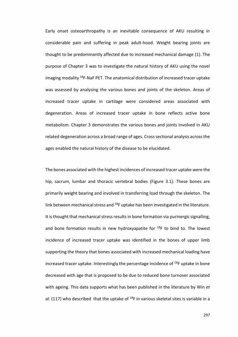
297

Early onset osteoarthropathy is an inevitable consequence of AKU resulting in

considerable pain and suffering in peak adult-hood. Weight bearing joints are

thought to be predominantly affected due to increased mechanical damage (1). The

purpose of Chapter 3 was to investigate the natural history of AKU using the novel

imaging modality 18F-NaF PET. The anatomical distribution of increased tracer uptake

was assessed by analysing the various bones and joints of the skeleton. Areas of

increased tracer uptake in cartilage were considered areas associated with

degeneration. Areas of increased tracer uptake in bone reflects active bone

metabolism. Chapter 3 demonstrates the various bones and joints involved in AKU

related degeneration across a broad range of ages. Cross sectional analysis across the

ages enabled the natural history of the disease to be elucidated.

The bones associated with the highest incidences of increased tracer uptake were the

hip, sacrum, lumbar and thoracic vertebral bodies (Figure 3.1). These bones are

primarily weight bearing and involved in transferring load through the skeleton. The

link between mechanical stress and 18F uptake has been investigated in the literature.

It is thought that mechanical stress results in bone formation via purinergic signalling,

and bone formation results in new hydroxyapatite for 18F to bind to. The lowest

incidence of increased tracer uptake was identified in the bones of upper limb

supporting the theory that bones associated with increased mechanical loading have

increased tracer uptake. Interestingly the percentage incidence of 18F uptake in bone

decreased with age that is proposed to be due to reduced bone turnover associated

with ageing. This data supports what has been published in the literature by Win et

al. (117) who described that the uptake of 18F in various skeletal sites is variable in a

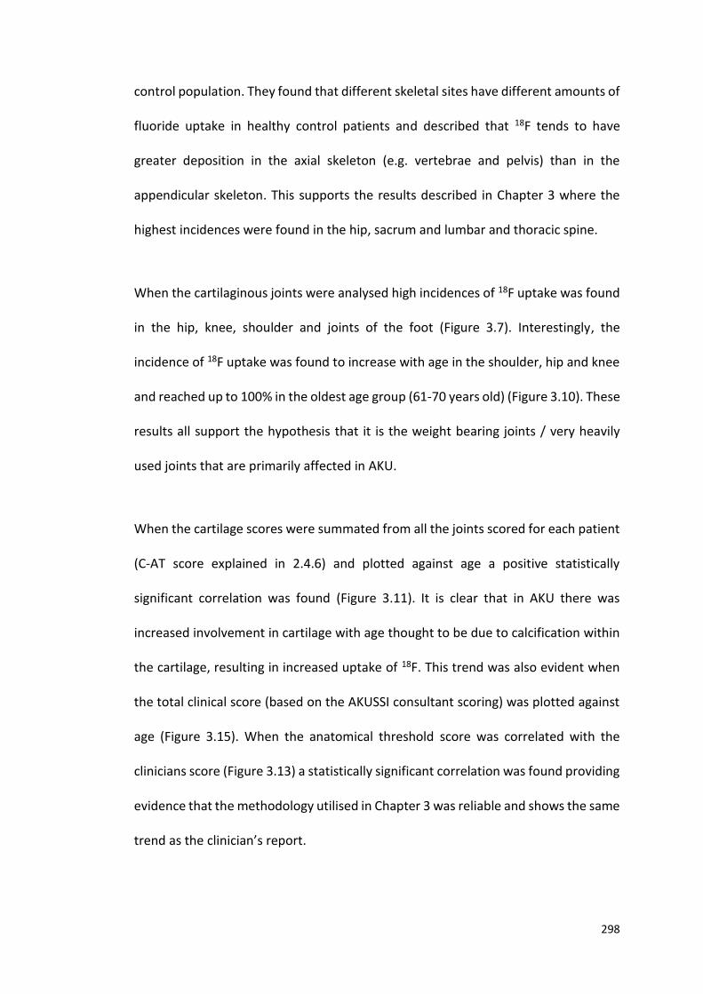
298

control population. They found that different skeletal sites have different amounts of

fluoride uptake in healthy control patients and described that 18F tends to have

greater deposition in the axial skeleton (e.g. vertebrae and pelvis) than in the

appendicular skeleton. This supports the results described in Chapter 3 where the

highest incidences were found in the hip, sacrum and lumbar and thoracic spine.

When the cartilaginous joints were analysed high incidences of 18F uptake was found

in the hip, knee, shoulder and joints of the foot (Figure 3.7). Interestingly, the

incidence of 18F uptake was found to increase with age in the shoulder, hip and knee

and reached up to 100% in the oldest age group (61-70 years old) (Figure 3.10). These

results all support the hypothesis that it is the weight bearing joints / very heavily

used joints that are primarily affected in AKU.

When the cartilage scores were summated from all the joints scored for each patient

(C-AT score explained in 2.4.6) and plotted against age a positive statistically

significant correlation was found (Figure 3.11). It is clear that in AKU there was

increased involvement in cartilage with age thought to be due to calcification within

the cartilage, resulting in increased uptake of 18F. This trend was also evident when

the total clinical score (based on the AKUSSI consultant scoring) was plotted against

age (Figure 3.15). When the anatomical threshold score was correlated with the

clinicians score (Figure 3.13) a statistically significant correlation was found providing

evidence that the methodology utilised in Chapter 3 was reliable and shows the same

trend as the clinician’s report.

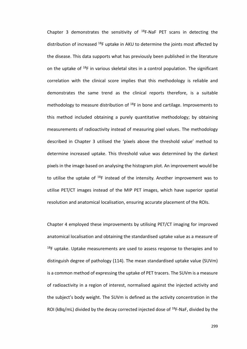
299

Chapter 3 demonstrates the sensitivity of 18F-NaF PET scans in detecting the

distribution of increased 18F uptake in AKU to determine the joints most affected by

the disease. This data supports what has previously been published in the literature

on the uptake of 18F in various skeletal sites in a control population. The significant

correlation with the clinical score implies that this methodology is reliable and

demonstrates the same trend as the clinical reports therefore, is a suitable

methodology to measure distribution of 18F in bone and cartilage. Improvements to

this method included obtaining a purely quantitative methodology; by obtaining

measurements of radioactivity instead of measuring pixel values. The methodology

described in Chapter 3 utilised the ‘pixels above the threshold value’ method to

determine increased uptake. This threshold value was determined by the darkest

pixels in the image based on analysing the histogram plot. An improvement would be

to utilise the uptake of 18F instead of the intensity. Another improvement was to

utilise PET/CT images instead of the MIP PET images, which have superior spatial

resolution and anatomical localisation, ensuring accurate placement of the ROIs.

Chapter 4 employed these improvements by utilising PET/CT imaging for improved

anatomical localisation and obtaining the standardised uptake value as a measure of

18F uptake. Uptake measurements are used to assess response to therapies and to

distinguish degree of pathology (114). The mean standardised uptake value (SUVm)

is a common method of expressing the uptake of PET tracers. The SUVm is a measure

of radioactivity in a region of interest, normalised against the injected activity and

the subject’s body weight. The SUVm is defined as the activity concentration in the

ROI (kBq/mL) divided by the decay corrected injected dose of 18F-NaF, divided by the

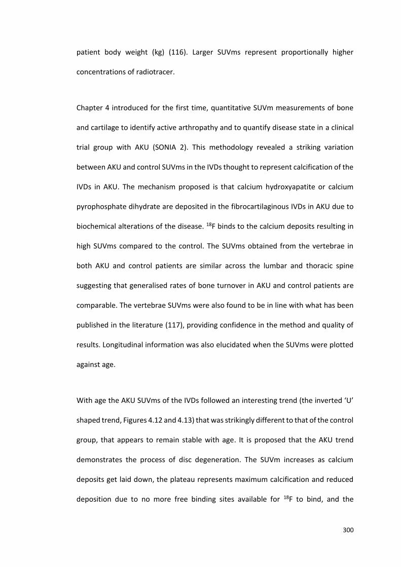
300

patient body weight (kg) (116). Larger SUVms represent proportionally higher

concentrations of radiotracer.

Chapter 4 introduced for the first time, quantitative SUVm measurements of bone

and cartilage to identify active arthropathy and to quantify disease state in a clinical

trial group with AKU (SONIA 2). This methodology revealed a striking variation

between AKU and control SUVms in the IVDs thought to represent calcification of the

IVDs in AKU. The mechanism proposed is that calcium hydroxyapatite or calcium

pyrophosphate dihydrate are deposited in the fibrocartilaginous IVDs in AKU due to

biochemical alterations of the disease. 18F binds to the calcium deposits resulting in

high SUVms compared to the control. The SUVms obtained from the vertebrae in

both AKU and control patients are similar across the lumbar and thoracic spine

suggesting that generalised rates of bone turnover in AKU and control patients are

comparable. The vertebrae SUVms were also found to be in line with what has been

published in the literature (117), providing confidence in the method and quality of

results. Longitudinal information was also elucidated when the SUVms were plotted

against age.

With age the AKU SUVms of the IVDs followed an interesting trend (the inverted ‘U’

shaped trend, Figures 4.12 and 4.13) that was strikingly different to that of the control

group, that appears to remain stable with age. It is proposed that the AKU trend

demonstrates the process of disc degeneration. The SUVm increases as calcium

deposits get laid down, the plateau represents maximum calcification and reduced

deposition due to no more free binding sites available for 18F to bind, and the

301

reduction in SUVm represents vertebral fusion, complete calcification and/or

reduced turnover (18F binds preferentially to newly laid down and active bone). The

initial increase in SUVm with age in the cartilage of AKU patients supports what was

found in Chapter 3 where an increase in percentage incidence of 18F uptake was

found with age. In the bony vertebrae there was an age-related decline in SUVm in

both AKU and control groups that is thought to represent reduced bone turnover

with age. This also supports what was found in Chapter 3 where the percentage

incidence of 18F uptake in bone decreases with age. However, the vertebrae SUVms

in the AKU group were lower compared to the control group. The proposed reason

for this being that they have reduced BMD compared to controls of the same age.

This is thought to be due to AKU patients having an imbalance in bone metabolism

resulting in loss of BMD (148).

In summary, Chapter 4 introduced for the first time a quantitative measure of 18F

uptake in cartilage and bone of AKU patients. This data has provided new insights

into bone metabolism and IVD degeneration in AKU and can be used to identify active

arthropathy in the spine. The utility of SUVms in a clinical setting could provide

clinicians with a quantitative tool to aid visual interpretation of PET images and to

assess inter and intra patient differences.

Chapter 5 utilised the vertebrae and IVD SUVm methodology to assess a group of NAC

patients that had visited the centre annually for four consecutive years. Visit one was

baseline data, and thereafter the patients were all prescribed 2mg of nitisinone daily.

The aim of this chapter was to utilise this quantitative measurement to track disease

302

progression in AKU longitudinally in response to nitisinone. The results described in

this chapter support what was found in the previous chapter based on the SONIA 2

patients. The differences between AKU and control SUVms in the spine were

reminiscent of what was seen in Chapter 4. The inverted ‘U’ trend was observed in

the AKU group with age where the SUVms of the IVDs reached significantly higher

values in the AKU group compared to the control (Figures 5.3 and 5.4). The negative

trend observed when the vertebrae SUVms were plotted against age (Figures 5.5 and

5.6) was also observed in this chapter providing evidence of the repeatability and

validity of the SUVm methodology.

The longitudinal changes in SUVms did not show any significant changes across the

visits from baseline. The effect of nitisinone could not be fully elucidated as there was

no AKU no-treatment control group to draw a comparison to. However, this result

could be demonstrating that nitisinone is stabilising the progression of the disease.

When the SONIA 2 clinical trial is complete longitudinal data will be available on a no-

treatment AKU group for comparison allowing this important comparison to be

made. It was also proposed that four years on nitisinone may not be long enough to

identify any changes in 18F uptake into bone and cartilage since years of HGA

exposure causes ochronosis over a period of many years. At the very least, nitisinone

could be expected to slow the progression of the AKU. Therefore, for the effect of

nitisinone on the spine to be further investigated, many more years of data will be

required to assess the long-term effects of the drug.

303

Correlations were made between the IVD and vertebrae SUVms with the total clinical

score and the total anatomical threshold score (method used in Chapter 3). Positive

statistically significant correlations were identified between both the total clinical and

total anatomical threshold scores with the IVD SUVms. Negative statistically

significant correlations were identified when the vertebrae SUVms were correlated

with the total clinical and total anatomical threshold scores. These correlations

suggest that the 3 methodologies all demonstrate the same trends.

Spinal pain scored by the patient was also correlated with IVD and vertebrae SUVms.

Increased IVD SUVms were associated with increased spinal pain as well as the total

clinical and anatomical threshold scores and is hypothesised to be due to disc

calcification and degeneration with age. In contrast a negative correlation was

identified between spinal pain and vertebrae SUVms. High vertebrae SUVms are

associated with low pain scores and lower total clinical and total anatomical threshold

scores proposed to be due to active bone remodelling in a healthy spine.

BMD was also investigated to determine if AKU patients had altered bone

metabolism. Interestingly high IVD SUVms correlated with low lumbar QCT T-scores

reflecting an osteoarthritic spine with calcified IVDs. Conversely high vertebrae

SUVms correlated with high lumbar T-scores reflecting active bone remodelling and

normal BMD.

Chapter 5 demonstrated the repeatability of the SUVm methodology and confirmed

the potential use of this method in a clinical setting as a quantitative measure of

304

arthropathy in the spine. Chapter 5 also revealed that the methodology correlates

well with the clinician’s report, the anatomical threshold methodology as well as

patient pain scores. The aim of Chapter 6 was to utilise the SONIA 2 SUV data to

correlate with other patient data obtained as part of the SONIA 2 clinical trial. Chapter

6 focused on baseline data (pre-nitisinone) to exclude trends that may be associated

with nitisinone. The clinical data used to correlate with the SUV data included serum

and urine HGA concentrations, spinal flexibility measurements, spinal curvature Cobb

angles and DEXA BMD scores.

A reduction in spinal flexibility was found with age, thought to represent reduced

elasticity of tendons, ligaments and IVDs due to the deposition of HGA in AKU

rendering them stiff and brittle. Interestingly, when correlated with the SUVm data a

positive correlation was identified between lumbar side flexion and vertebrae SUVm.

This supports the hypothesis that the SUVm decreases with age due to reduced BMD

with age and this is associated with reduced spinal flexibility. Lumbar side flexion was

concluded to be a good indicator of disease progression in contrast to cervical spine

rotation that found no clinical significant correlations.

To support this, hyperkyphotic Cobb angles demonstrated a negative correlation with

thoracic vertebrae SUVms suggesting that patients with hyperkyphotic spines have

reduced thoracic SUVms proposed to be due to reduced BMD with age, as reduced

BMD in the spine is one of the main reasons for hyperkyphosis. The hyperkyphosis

Cobb angle also demonstrated a negative correlation with the thoracic IVD SUVm

suggesting that the hyperkyphosis is associated with reduced IVD SUVms. This

305

supports the hypothesis that older patients have the most severe spinal degeneration

reflected by reduced IVD SUVms.

When DEXA lumbar vertebrae T-score and the lumbar vertebrae SUVm was

correlated, a statistically significant positive correlation was observed supporting the

theory that reductions in vertebrae SUVm may be due to reductions in BMD. This

correlation was also identified in Chapter 4 where the lumbar QCT T-score

demonstrated a positive correlation with the lumbar vertebrae SUVm. A comparison

was also made between DEXA and QCT to determine what imaging modality was

superior in terms of measuring BMD. DEXA scores were found to reach much higher

T-scores in the spine compared to QCT. The proposed reason for this being due to

calcification of the IVDs. It was concluded that QCT may be superior to DEXA as QCT

measures volumetric trabecular bone unlike DEXA that measures all the mineral in

the path of the X-ray beam in the region of L2-L4 including the IVDs. Chapter 6 has

demonstrated the validity of the SUVm as a measure of arthropathy by providing

evidence that this method correlates with other clinical manifestations of AKU.

All in all this thesis has provided new insights into spinal arthropathy in AKU, the

utilisation of novel quantitative techniques demonstrated in this thesis can be used

to aid in clinical interpretation of PET scans as well as providing a measure of disease

severity and to analyse disease progression and response to therapy.

306

8.0 REFERENCES

307

1. Ranganath LR, Jarvis JC, Gallagher JA. Recent advances in management of alkaptonuria (invited review; best practice article). J Clin Pathol. 2013 May;66(5):367–73.

2. Taylor AM, Boyde A, Wilson PJM, Jarvis JC, Davidson JS, Hunt JA, et al. The role of calcified cartilage and subchondral bone in the initiation and progression of ochronotic arthropathy in alkaptonuria. Arthritis Rheum. 2011 Dec;63(12):3887–96.

3. Gallagher J, Taylor A, Boyde A, Jarvis J, Ranganath L. Recent advances in understanding the pathogenesis of ochronosis:Najnowsze postępy w zrozumieniu patogenezy ochronozy. Reumatologia. 2012 Sep50(4):316-323.

4. Fisher AA, Davis MW. Alkaptonuric ochronosis with aortic valve and joint replacements and femoral fracture: a case report and literature review. Clin Med Res. 2004 Nov;2(4):209–15.

5. Stenn F, Milgram J, Lee S, Weigand R, Veis A. Biochemical identification of homogentisic acid pigment in an ochronotic egyptian mummy. Science. 1977 Aug;197(4303):566-568.

6. Lee SL, Stenn FF. Characterization of Mummy Bone Ochronotic Pigment. JAMA J Am Med Assoc. 1978 Jul;240(2):136.

7. Aquaron R. Alkaptonuria: A very rare metabolic disorder. Vol. 50, Indian Journal of Biochemistry and Biophysics. 2013 Oct;50(5):339–44.

8. Mistry JB, Bukhari M, Taylor AM. Alkaptonuria. Rare Dis. 2013 Dec;18;1.e27475. DOI: 10.4161/rdis.27475.

9. Phornphutkul C, Introne WJ, Perry MB, Bernardini I, Murphey MD, Fitzpatrick DL, et al. Natural History of Alkaptonuria. N Engl J Med. 2002 Dec;347(26):2111–21.

10. Benedek TG. Rudolph virchow on ochronosis. Arthritis Rheum. 1966 Feb;9(1):66–71.

11. Scriver CR. Garrod's Croonian Lectures (1908) and the charter 'Inborn Errors of Metabolism': Albinism, alkaptonuria, cystinuria, and pentosuria at age 100 in 2008. J Inherit Metab Dis. 2002 Oct;31(5):580-98.

12. Garrod AE, Oxon MA. The Incidence of Alkaptonuria: A Study in Chemical Individuality 1902. Yale J Biol Med. 2002 Jul-Aug;75(4):221–31.

13. Gallagher JA, Dillon JP, Sireau N, Timmis O, Ranganath LR. Alkaptonuria: An example of a “fundamental disease”-A rare disease with important lessons for more common disorders. Semin Cell Dev Biol. 2016 Apr;52(3):53–7.

14. Suwannarat P, O’Brien K, Perry MB, Sebring N, Bernardini I, Kaiser-Kupfer MI, et al. Use of nitisinone in patients with alkaptonuria. Metabolism. 2005 Jun;54(6):719–28.

15. Zatková a, de Bernabé DB, Poláková H, Zvarík M, Feráková E, Bosák V, et al. High frequency of alkaptonuria in Slovakia: evidence for the appearance of multiple mutations in HGO involving different mutational hot spots. Am J Hum Genet. 2000 Nov;67(5):1333–9.

308

16. Al-Sbou M, Mwafi N. Nine cases of Alkaptonuria in one family in southern Jordan. Rheumatol Int. 2012 Mar;32(3):621–5.

17. Mannoni A, Selvi E, Lorenzini S, Giorgi M, Airò P, Cammelli D, et al. Alkaptonuria, Ochronosis, and Ochronotic Arthropathy. Vol. 33, Seminars in Arthritis and Rheumatism. 2004 Feb;33(4):239–48.

18. Al-Sbou M. Novel mutations in the homogentisate 1,2 dioxygenase gene identified in Jordanian patients with alkaptonuria. Rheumatol Int. 2012 Jun;32(6):1741–6.

19. Granadino B, Beltran-Valero de Bernabe D, Fernandez-Canon JM, Penalva MA, Rodriguez de Cordoba S. The human homogentisate 1,2-dioxygenase (HGO) gene. Genomics. 1997 Jul;43(2):115–22.

20. Zatkova A, Nemethova M. Genetics of alkaptonuria – an overview. Acta Fac Pharm Univ Comenianae. 2015 May;62(11):27–32.

21. Zatkova A. An update on molecular genetics of Alkaptonuria (AKU). J Inherit Metab Dis. 2011 Dec;34(6):1127–36.

22. Vilboux T, Kayser M, Introne W, Suwannarat P, Bernardini I, Fischer R, et al. Mutation spectrum of homogentisic acid oxidase (HGD) in alkaptonuria. Human Mutat. 2009 Dec;30(12): 1611–9.

23. Nemethova M, Radvanszky J, Kadasi L, Ascher DB, Pires DE V, Blundell TL, et al. Twelve novel HGD gene variants identified in 99 alkaptonuria patients: focus on “black bone disease” in Italy. Federica Genov Jozef Rovensky Eur J Hum Genet. 2016 Jan;24(1):66–72.

24. Martin JP, Batkoff B. Homogentisic acid autoxidation and oxygen radical generation: implications for the etiology of alkaptonuric arthritis. Free Radic Biol Med. 1987 Jun;3(4):241–50.

25. Kotob SI, Coon SL, Quintero EJ, Weiner RM. Homogentisic acid is the primary precursor of melanin synthesis in Vibrio cholerae, a Hyphomonas strain, and Shewanella colwelliana. Appl Environ Microbiol. 1995 Apr;61(4):1620–2.

26. Kahveci R, Ergüngör MF, Günaydin A, Temiz A. Alkaptonuric patient presenting with “black” disc: A case report. Acta Orthop Traumatol Turc. 2013 May;47(2):134–8.

27. O’Brien WM, La Du BN, Bunim JJ. Biochemical pathologic and clinical aspects of alcaptonuria, ochronosis, and ochronotic arthropathy: Review of World Literature (1584–1962). Am J Med. 1963 Dec;36(6):813–38.

28. Acar MA, Erkocak ÖF, Aydin BK, Altan E, Şenaran H, Elmadaǧ NM. Patients with black hip and black knee due to ochronotic arthropathy: Case report and review of literature. Oman Med J. 2013 Nov;28(6):448–9.

29. Wilke A, Steverding D. Ochronosis as an unusual cause of valvular defect: a case report. J Med Case Rep. 2009 Nov;27(3):9302.

30. Ozmanevra R, Guran O, Karatosun V, Gunal I. Total knee arthroplasty in ochronosis: a case report and critical review of the literature. Eklem Hastalik Cerrahisi. 2013 Mar;24(3):169–72.

309

31. Helliwell TR, Gallagher JA, Ranganath L. Alkaptonuria - A review of surgical and autopsy pathology. Histopathology. 2008 Nov;53(5):503–12.

32. Hannoush H, Introne WJ, Chen MY, Lee SJ, O’Brien K, Suwannarat P, et al. Aortic stenosis and vascular calcifications in alkaptonuria. Mol Genet Metab. 2012 Feb;105(2):198–202.

33. Taylor AM, Fraser WD, Wilson PMJ, Ranganath LR, Gallagher JA. Ultrastructural studies on the binding of ochronotic pigment to collagen fibres in cartilage and bone in vivo and in vitro. Calcif Tissue Int. 2009 Aug;85(2):187.

34. Taylor AM, Wlodarski B, Prior IA, Wilson PJM, Jarvis JC, Ranganath LR, et al. Ultrastructural examination of tissue in a patient with alkaptonuric arthropathy reveals a distinct pattern of binding of ochronotic pigment. Rheumatology (Oxford). 2010 Jul;49(7):1412–4.


36. Gallagher J, Taylor A, Boyde A, Jarvis J. Recent advances in understanding the pathogenesis of ochronosis. Reumatologia. 2012 Sep;50(4):316-323.

37. Introne WJ, Gahl WA. Alkaptonuria. GeneReviews. University of Washington, Seattle; 1993-2018. Available from https://www.ncbi.nlm.nih.gov/books/NBK1454/

38. Gallagher JA, Dillon JP, Sireau N, Timmis O, Ranganath LR. Alkaptonuria: An example of a “fundamental disease”-A rare disease with important lessons for more common disorders. Semin Cell Dev Biol. 2016 Apr;52:53–7.

39. Sealock RR, Galdston M, Steele JM. Administration of Ascorbic Acid to an Alkaptonuric Patient. Exp Biol Med. 1940 Jun;44(2):580–3.

40. Wolff JA, Barshop B, Nyhan WL, Leslie J, Seegmiller JE, Gruber H, et al. Effects of ascorbic acid in alkaptonuria: alterations in benzoquinone acetic acid and an ontogenic effect in infancy. Pediatr Res. 1989 Aug;26(2):140–4.

41. De Haas V, Carbasius Weber EC, de Klerk JB, Bakker HD, Smit GP, Huijbers WA, et al. The success of dietary protein restriction in alkaptonuria patients is age-dependent. J Inherit Metab Dis. 1998 Dec;21(8):791–8.

42. Morava E, Kosztolányi G, Engelke UFH, Wevers RA. Reversal of clinical symptoms and radiographic abnormalities with protein restriction and ascorbic acid in alkaptonuria. Ann Clin Biochem. 2003 Jan;40(1):108–11.

43. McKiernan PJ. Nitisinone for the treatment of hereditary tyrosinemia type I. Expert Opin Orphan Drugs. 2013 Apr;1(6):491–7.

44. Introne WJ, Perry MB, Troendle J, Tsilou E, Kayser MA, Suwannarat P, et al. A 3-year randomized therapeutic trial of nitisinone in alkaptonuria. Mol Genet Metab. 2011 Aug;103(4):307–14.

45. Hall AK, Ranganath LR, Milan A, Hughes A, Olsson B, Szamosi J, et al.

310

Suitability Of Nitisinone In Alkaptonuria 1 (SONIA 1): Results of a dose- response study of once-daily nitisinone on 24-hour urinary homogentisic acid excretion (u-HGA 24 ) in patients with alkaptonuria. Ann Rheum Dis. 2016 Feb;75(2):362-7.

46. Cox TF, Ranganath L. A quantitative assessment of alkaptonuria. J Inherit Metab Dis. 2011 Dec;34(6):1153–62.

47. Welcome To The Alkaptonuria Society - AKU Society [Internet]. [cited 2017 Mar 19]. Available from: http://www.akusociety.org.

48. Lock E, Ranganath LR, Timmis O. The Role of Nitisinone in Tyrosine Pathway Disorders. Curr Rheumatol Rep. 2014 Nov;16(11):457

49. Partners in DevelopAKUre [Internet] Retrieved from http://pathlabs.rlbuht.nhs.uk/developakure.pdf.

50. DevelopAKUre Home [Internet]. [cited 2017 Mar 19]. Available from: http://www.developakure.eu/.

51. Cucchiarini M. Biological Systems: Open Access The Biology of Articular Cartilage: An Overview? Biol Syst Open Access. 2013;2(1):104-105.

52. Ulrich-Vinther M, Maloney MD, Schwarz EM, Rosier R, O’Keefe RJ. Articular cartilage biology. J Am Acad Orthop Surg. 2003 Nov-Dec,11(6):421–30.

53. Martini FH, NathJL, Bartholomew EF. Fundamentals of Anatomy and Physiology, ninth edition; Pearsons Eduction;2012.

54. Sophia Fox AJ, Bedi A, Rodeo SA. The basic science of articular cartilage: structure, composition, and function. Sports Health. 2009 Nov;1(6):461–8.

55. Poole CA. Articular cartilage chondrons : form, function and failure. J Anat. 1997 Jul;191(1):1–13.

56. Alexopoulos LG, Setton L a, Guilak F. The biomechanical role of the chondrocyte pericellular matrix in articular cartilage. Acta Biomater. 2005 May;1(3):317–25.

57. Sobol E, Shekhter A, Guller A, Baum O, Baskov A. Laser-induced regeneration of cartilage. J Biomed Opt. 2011 Aug;16(8):80902.

58. Poole, C A, Ayad S, Gilbert RT. Chondrons from Articular Cartilage. J Cell Sci. 1992 Sep;103(4):1101–10.

59. Akkiraju H, Nohe A. Role of Chondrocytes in Cartilage Formation, Progression of Osteoarthritis and Cartilage Regeneration. J Dev Biol. 2015 Dec;3(4):177–92.

60. Liacini A, Sylvester J, Li WQ, Huang W, Dehnade F, Ahmad M, et al. Induction of matrix metalloproteinase-13 gene expression by TNF-α is mediated by MAP kinases, AP-1, and NF-κB transcription factors in articular chondrocytes. Exp Cell Res. 2003 Aug;288(1):208–17.

61. Hochberg MC, Yerges-Armstrong L, Yau M, Mitchell BD. Genetic epidemiology of osteoarthritis: recent developments and future directions. Curr Opin Rheumatol. 2013 Mar;25(2):192–7.

311

62. Chen D, Shen J, Zhao W, Wang T, Han L, Hamilton JL, et al. Osteoarthritis: toward a comprehensive understanding of pathological mechanism. Bone Res. 2017 Jan 17;5:16044.

63. Lindahl A. From gristle to chondrocyte transplantation: treatment of cartilage injuries. Philos Trans R Soc London B Biol Sci. 2015 Oct;19(370):1680.

64. Gelse K, Pöschl E, Aigner T. Collagens--structure, function, and biosynthesis. Adv Drug Deliv Rev. 2003 Nov;55(12):1531–46.

65. Hulmes DJS. Collagen diversity, synthesis and assembly. In: Collagen: Structure and Mechanics. 2008. p.15–47.

66. Kini U, Nandeesh BN. Physiology of Bone Formation, Remodeling, and Metabolism. In: Radionuclide and Hybrid Bone Imaging. Berlin, Heidelberg: Springer Berlin Heidelberg; 2012. p.29–57.

67. Buckwalter JA, Glimcher MJ, Cooper RR, Recker R, A Buckwalter BJ, Iowa City Md, et al. Bone Biology Bone Biology Part I: Structure, blood supply, Cells, Matrix, and Mineralisation. J Bone Jt Surg J Bone Jt Surg Am. 1995;77:1256–75.

68. Standring S. Gray’s Anatomy: The Anatomical Basis of Clinical Practice. Vol. 2, Development. 2008. p.1389-1406.

79. You L, Temiyasathit S, Lee P, Kim CH, Tummala P, Yao W, et al. Osteocytes as mechanosensors in the inhibition of bone resorption due to mechanical loading. Bone. 2008 Jan;42(1);172-9.

70. Bonewald LF, Johnson ML. Osteocytes, mechanosensing and Wnt signaling. Vol. 42, Bone. 2008. p.606–15.

71. Rucci N. Molecular biology of bone remodelling. Clin Cases Miner Bone Metab. 2008 Jan-Apr;5 (1):49–56.

72. Castañeda S, Roman-Blas JA, Largo R, Herrero-Beaumont G. Subchondral bone as a key target for osteoarthritis treatment. Biochem Pharmacol. 2012 Feb;83(3):315–23.

73. Wen C, Lu WW, Chiu KY. Importance of subchondral bone in the pathogenesis and management of osteoarthritis from bench to bed. J Orthop Transl. 2014 Jan;2(1):16–25.

74. Gallagher JA, Ranganath LR, Boyde A. What does the arthropathy of alkaptonuria teach us about disease mechanisms in osteoarthritis and ageing of joints? Rheumatology (Oxford). 2016 Jul;55(7):1151–2.

75. Boyde A, Davis GR, Mills D, Zikmund T, Cox TM, Adams VL, et al. On fragmenting, densely mineralised acellular protrusions into articular cartilage and their possible role in osteoarthritis. J Anat. 2014 Oct;225(4):436–46.

76. Wang F, Cai F, Shi R, Wang X-H, Wu X-T. Aging and age related stresses: a senescence mechanism of intervertebral disc degeneration. Osteoarthr Cartil. 2016 Mar;24(3):398–408.

77. Urban JPG, Roberts S. Degeneration of the intervertebral disc. Arthritis Res

312

Ther. 2003;5(3):120–30.

78. Ouyang Z-H, Wang W-J, Yan Y-G, Wang B, Lv G-H. The PI3K/Akt pathway: A critical player in intervertebral disc degeneration. Oncotarget. 2015 Jun;8(34):57870-57881.

79. Etzkorn E, Oliver AM. Not just another case of low back pain. BMJ Case Rep. 2014 Apr. DOI 10.1136/bcr-2014-204085.

80. Kohn MD, Sassoon AA, Fernando ND. Classifications in Brief: Kellgren-Lawrence Classification of Osteoarthritis. Clin Orthop Relat Res. 2016 Aug;474(8):1886–93.

81. Siemens AG, Healthcare. Background Information: The History of Computed Tomography at Siemens. [Internet]. [cited 2017 April 15]. Available from: https://www.siemens.com/press/pool/de/feature/2015/healthcare/2015-07-ct-40/background-history-ct-siemens-e.pdf

82. Cierniak R. Some Words About the History of Computed Tomography. In: X-Ray Computed Tomography in Biomedical Engineering. 2011. p.1–14.

83. Bradley WG. History of medical imaging. Proc Am Philos Soc. 2008 Sep;152(3):349–61.

84. Scatliff JH, Morris PJ. From Roentgen to magnetic resonance imaging: the history of medical imaging. N C Med J. 2014 Mar;75(2):111–3.

85. Hayashi D, Roemer FW, Jarraya M, Guermazi A. Imaging of osteoarthritis. In: Geriatric Imaging. 2013. p.93–121.

86. Suetens P. Fundamentals of medical imaging. In: Fundamentals of Medical Imaging. 2009. p.128–58.

87. Herr KD. Radiology 101: The Basics and Fundamentals of Imaging, 3rd ed. Acad Radiol. 2010. p.269-275.

88. Lisle D. Imaging for students. Hodder Arnold; 2007. p.283.

89. Vinjamuri S, Ramesh CN, Jarvis J, Gallagher JA, Ranganath LL. Nuclear medicine techniques in the assessment of alkaptonuria. Nucl Med Commun. 2011 Oct;32(10):880–6.

90. Mandl P, Kainberger F, Friberg Hitz M. Imaging in osteoporosis in rheumatic diseases. Best Pract Res Clin Rheumatol. 2016 Aug;30(4):751–65.

91. Oei L, Koromani F, Rivadeneira F, Zillikens MC, Oei EHG. Quantitative imaging methods in osteoporosis. Quant Imaging Med Surg. 2016 Dec;6(6):680–98.

92. Toombs RJ, Ducher G, Shepherd JA, De Souza MJ. The Impact of Recent Technological Advances on the Trueness and Precision of DXA to Assess Body Composition. Obesity. 2012 Jan;20(1):30–9.

93. Yu W, Glüer CC, Fuerst T, Grampp S, Li J, Lu Y, et al. Influence of degenerative joint disease on spinal bone mineral measurements in postmenopausal women. Calcif Tissue Int. 1995 Sep;57(3):169–74.

94. Li N, Li X-M, Xu L, Sun W-J, Cheng X-G, Tian W. Comparison of QCT and DXA:

313

Osteoporosis Detection Rates in Postmenopausal Women. Int J Endocrinol. 2013 Mar 27;2013:895474.


96. Kabayel DD, Kabayel D. The role of quantitative computed tomography and magnetic resonance imaging in diagnosis and follow-up of osteoporosis: A review. Turk J Phys Med Rehab. 2016;62(3):288–95.

97. Fallis A. Computed Tomography- Principles, Design, Artifacts, and Recent Advances. Vol. 53, Journal of Chemical Information and Modeling. 2013. p.1689-1699.

98. Hashefi M, Curiel R. Future and upcoming non-neoplastic applications of PET/CT imaging. Ann N Y Acad Sci. 2011 Jun;1228(1):167–74.

99. Boesen M, Ellegaard K, Henriksen M, Gudbergsen H, Hansen P, Bliddal H, et al. Osteoarthritis year in review 2016: imaging. Osteoarthr Cartil. 2017 Feb;25(2):216–26.

100. Rahmim A, Zaidi H. PET versus SPECT: strengths, limitations and challenges. Nucl Med Commun. 2008 Mar;29(3):193–207.

101. Rich DA. A brief history of positron emission tomography. J Nucl Med Technol. 1997 Mar;25(1):4–11.

102. Carlson S. A Glance At The History Of Nuclear Medicine. Acta Oncol (Madr). 1995 May;34(8):1095–102.

103. Portnow LH, Vaillancourt DE, Okun MS. The history of cerebral PET scanning: From physiology to cutting-edge technology. Neurology. 2013 Mar;80(10):952–6.

104. Kim EE, Inoue T, Lee MC, Wong WH. Clinical PET and PET/CT: Principles and applications. Clinical PET and PET/CT: Principles and Applications. 2013. p.1-398.

105. Raichle ME. Positron Emission Tomography. Nature. 1985 Oct;317(6):574–575.

106. Mick CG, James T, Hill JD, Williams P, Perry M. Molecular imaging in oncology: (18)F-sodium fluoride PET imaging of osseous metastatic disease. AJR Am J Roentgenol. 2014 Aug;203(2):263–71.

107. Grant FD, Fahey FH, Packard AB, Davis RT, Alavi A, Treves ST. Skeletal PET with 18F-fluoride: applying new technology to an old tracer. J Nucl Med. 2008 Jan;49(1):68–78.

108. Dahlbom M, Hoffman EJ, Hoh CK, Schiepers C, Rosenqvist G, Hawkins RA, et al. Whole-body positron emission tomography: Part I. Methods and performance characteristics. J Nucl Med. 1992 Jun;33(6):1191–9.

109. Raynor W, Houshmand S, Gholami S, Emamzadehfard S, Rajapakse CS, Blomberg BA, et al. Evolving Role of Molecular Imaging with 18F-Sodium Fluoride PET as a Biomarker for Calcium Metabolism. Curr Osteoporos Rep.

314

2016 Aug;14(4):115–25.

110. Blake GM, Siddique M, Frost ML, Moore AEB, Fogelman I. Imaging of Site Specific Bone Turnover in Osteoporosis Using Positron Emission Tomography. Curr Osteoporos Rep. 2014 Dec;12(4):475–85.

111. Czernin J, Satyamurthy N, Schiepers C. Molecular mechanisms of bone 18F-NaF deposition. J Nucl Med. 2010 Dec;51(12):1826–9.

112. Wong KK, Piert M. Dynamic bone imaging with 99mTc-labeled diphosphonates and 18F-NaF: Mechanisms and applications. J Nucl Med. 2013 Apr;54(4):590–9.

113. Segall G, Delbeke D, Stabin MG, Even-Sapir E, Fair J, Sajdak R, et al. SNM Practice Guideline for Sodium 18F-Fluoride PET/CT Bone Scans 1.0. J Nucl Med. 2010 Nov;51(11):1813–20.

114. Thie JA. Understanding the standardized uptake value, its methods, and implications for usage. J Nucl Med. 2004 Sep;45(9):1431–4.

115. Kobayashi N, Inaba Y, Tateishi U, Yukizawa Y, Ike H, Inoue T, et al. New application of 18F-fluoride PET for the detection of bone remodeling in early-stage osteoarthritis of the hip. Clin Nucl Med. 2013 Oct;38(10):379-83.

116. Win AZ, Aparici CM. Factors Affecting Uptake of NaF-18 by the Normal Skeleton. J Clin Med Res. 2014 Dec;6(6):435–42.

117. Win AZ, Aparici CM. Normal SUV values measured from Na18F- PET/CT bone scan studies. Boswell CA, editor. PLoS One. 2014 Sep 25;9(9):108429.

118. Kinahan PE, Fletcher JW. Positron emission tomography-computed tomography standardized uptake values in clinical practice and assessing response to therapy. Semin Ultrasound CT MR. 2010 Dec;31(6):496–505.

119. Zasadny KR, Wahl RL. Standardized uptake values of normal tissues at PET with 2-[fluorine-18]-fluoro-2-deoxy-D-glucose: variations with body weight and a method for correction. Radiology. 1993 Dec;189(3):847–50.

120. Kobayashi N, Inaba Y, Yukizawa Y, Ike H, Kubota S, Inoue T, et al. Use of 18 F-fluoride positron emission tomography as a predictor of the hip osteoarthritis progression. Mod Rheumatol. 2015 Sep;25(6):925–30.

121. National Institute of Health. ImageJ [Internet]. [cited 2017 May 31]. Available from: https://imagej.nih.gov/ij/

122. Lafage V, Schwab F, Patel A, Hawkinson N, Farcy J-P. Pelvic Tilt and Truncal Inclination. Spine (Phila Pa 1976). 2009 Aug;34(17):E599–606.

123. Chernukha K V, Daffner RH, Reigel DH. Lumbar lordosis measurement. A new method versus Cobb technique. Spine (Phila Pa 1976). 1998 Jan;23(1):74-80.

124. Kim H, Kim HS, Moon ES, Yoon C-S, Chung T-S, Song H-T, et al. Scoliosis Imaging: What Radiologists Should Know. RadioGraphics. 2010 Nov;30(7):1823–42.

125. Katzman WB, Wanek L, Shepherd JA, Sellmeyer DE. Age-related hyperkyphosis: its causes, consequences, and management. J Orthop Sports

315

Phys Ther. 2010 Jun;40(6):352–60.

126. Clarkson H GG 1989. Musculoskeletal Assessment: Joint Range of Motion and Manual Muscle Strength. Williams Wilkins, Balt. 2000; p.158–160.

127. Levangie PK, Norkin CC. Joint Structure and Function: A Comprehensive Analysis. F A Davis Co. 2005; p.393–436.

128. Wong KK, Piert M. Reply: Regarding Dynamic Bone Imaging with 99mTc-Labeled Diphosphonates and 18F-NaF: Mechanisms and Applications. J Nucl Med. 2013 Dec;54(12):2190–1.

129. Watanabe T, Takase-Minegishi K, Ihata A, Kunishita Y, Kishimoto D, Kamiyama R, et al. (18)F-FDG and (18)F-NaF PET/CT demonstrate coupling of inflammation and accelerated bone turnover in rheumatoid arthritis. Mod Rheumatol. 2016 Jul;26(2):180–7.

130. Frost ML, Cook GJR, Blake GM, Marsden PK, Benatar NA, Fogelman I. A prospective study of risedronate on regional bone metabolism and blood flow at the lumbar spine measured by 18F-fluoride positron emission tomography. J Bone Miner Res. 2003 Dec;18(12):2215–22.

131. Rutkovskiy A, Stenslokken K-O, Vaage IJ. Osteoblast Differentiation at a Glance. Med Sci Monit Basic Res. 2016 Sep;26(22):95–106.

132. Kim JH, Liu X, Wang J, Chen X, Zhang H, Kim SH, et al. Wnt signaling in bone formation and its therapeutic potential for bone diseases. Ther Adv Musculoskelet Dis. 2013 Feb;5(1):13–31.

133. Sanchez C, Pesesse L, Gabay O, Delcour JP, Msika P, Baudouin C, et al. Regulation of subchondral bone osteoblast metabolism by cyclic compression. Arthritis Rheum. 2012;64(4):1193–203.

134. Puri T, Frost ML, Curran KM, Siddique M, Moore AEB, Cook GJR, et al. Differences in regional bone metabolism at the spine and hip: a quantitative study using 18F-fluoride positron emission tomography. Osteoporos Int. 2013 Feb;24(2):633–9.

135. Riggs BL, Wahner HW, Dunn WL, Mazess RB, Offord KP, Melton LJ. Differential changes in bone mineral density of the appendicular and axial skeleton with aging: relationship to spinal osteoporosis. J Clin Invest. 1981 Feb;67(2):328–35.

136. Gallagher JA, Ranganath LR, Boyde A. Lessons from rare diseases of cartilage and bone. Curr Opin Pharmacol. 2015 Jun;22:107–14.

137. Abhishek A, Doherty M. Pathophysiology of articular chondrocalcinosis—role of ANKH. Nat Rev Rheumatol. 2011 Feb;7(2):96–104.

138. Gürkanlar D, Daneyemez M, Solmaz I, Temiz C. Ochronosis and lumbar disc herniation. Acta Neurochir (Wien). 2006 Aug;148(8):891–4.

139. Palazzi C, D’Angelo S, Leccese P, Nigro A, Olivieri I. Ochronotic arthropathy of the spine limited to the thoracic section. Rheumatology (Oxford). 2013 May;52(5):799.

316

140. Chakraverty JK, Lawson TM, Herdman G. Not just simple degenerative disc disease (alkaptonuria). Spine J. 2013 Aug;13(8):985–6.

141. Khan UN, Wenokor C, Altschuler EL. Back Pain in a Middle-Aged Man. Am J Phys Med Rehabil. 2015 May;94(5):42.

142. Jebaraj I, Chacko BR, Chiramel GK, Matthai T, Parameswaran A. A simplified staging system based on the radiological findings in different stages of ochronotic spondyloarthropathy. Indian J Radiol Imaging. 2013 Jan;23(1):101–5.

143. Tarihi G, Aktafi I, Akgün K, Çakmak B. Intervertebral disc calcification in the elderly: a case report. Turkish J Geriatr. 2007 Oct;10(1):37–9.

144. Kaneta T, Ogawa M, Daisaki H, Nawata S, Yoshida K, Inoue T. SUV measurement of normal vertebrae using SPECT/CT with Tc-99m methylene diphosphonate. Am J Nucl Med Mol Imaging. 2016 Sep;6(5):262–8.

145. Demontiero O, Vidal C, Duque G. Aging and bone loss: new insights for the clinician. Ther Adv Musculoskelet Dis. 2012 Apr;4(2):61–76.

146. Daly RM, Rosengren BE, Alwis G, Ahlborg HG, Sernbo I, Karlsson MK. Gender specific age-related changes in bone density, muscle strength and functional performance in the elderly: a-10 year prospective population-based study. BMC Geriatr. 2013 Jul; 6(1);13:71.

147. Chen W-T, Shih TT-F, Chen R-C, Lo S-Y, Chou C Te, Lee J-M, et al. Vertebral Bone Marrow Perfusion Evaluated with Dynamic Contrast-enhanced MR Imaging: Significance of Aging and Sex. Radiology. 2001 Jul;220(1):213–8.

148. Aliberti G, Pulignano I, Schiappoli A, Minisola S, Romagnoli E, Proietta M. Bone metabolism in ochronotic patients. J Intern Med. 2003;254(3):296–300.

149. Adams MC, Turkington TG, Wilson JM, Wong TZ. A systematic review of the factors affecting accuracy of SUV measurements. AJR Am J Roentgenol. 2010 Aug;195(2):310–20.


151. Wheater G, Elshahaly M, Tuck SP, Datta HK, van Laar JM. The clinical utility of bone marker measurements in osteoporosis. J Transl Med. 2013 Aug 29;11(1):201.

152. Leeming DJ, Alexandersen P, Karsdal MA, Qvist P, Schaller S, Tankó LB. An update on biomarkers of bone turnover and their utility in biomedical research and clinical practice. Eur J Clin Pharmacol. 2006 Oct;62(10):781–92.

153. Garnero P. The Utility of Biomarkers in Osteoporosis Management. Mol Diagn Ther. 2017 Aug;21(4):401–18.

154. Davison AS, Milan AM, Hughes AT, Dutton JJ, Ranganath LR. Serum concentrations and urinary excretion of homogentisic acid and tyrosine in normal subjects. Clin Chem Lab Med. 2015 Feb;53(3):81-3.

317

155. Weinstein JR, Anderson S. The Aging Kidney: Physiological Changes. Adv Chronic Kidney Dis. 2010 Jul;17(4):302–7.

156. Jonsson E, Ljungkvist I, Hamberg J. Standardized Measurement of Lateral Spinal Flexion and Its Use in Evaluation of the Effect of Treatment of Chronic Lower Back Pain. Ups J Med Sci. 1990 Mar;95(1):75–86.

157. Laxon S, Ranganath L, Timmis O. Living with alkaptonuria. BMJ. 2011 Sep;29;343:d5155.

158. Rana AQ, Saeed U, Abdullah I. Alkaptonuria, more than just a mere disease. J Neurosci Rural Pract. 2015 Apr-Jun;6(2):257–60.

159. Chun S-W, Lim C-Y, Kim K, Hwang J, Chung SG. The relationships between low back pain and lumbar lordosis: a systematic review and meta-analysis. Spine J. 2017 Aug;17(8):1180–91.

160. Takeda N, Kobayashi T, Atsuta Y, Matsuno T, Shirado O, Minami A. Changes in the sagittal spinal alignment of the elderly without vertebral fractures: a minimum 10-year longitudinal study. J Orthop Sci. 2009 Nov;14(6):748–53.

161. Dionne CE, Dunn KM, Croft PR. Does back pain prevalence really decrease with increasing age? A systematic review. Age Ageing. 2006 May 1;35(3):229–34.

162. Ohrt-Nissen S, Cheung JPY, Hallager DW, Gehrchen M, Kwan K, Dahl B, et al. Reproducibility of thoracic kyphosis measurements in patients with adolescent idiopathic scoliosis. Scoliosis Spinal Disord. 2017 Feb;21(1):12-4.

163. Kotwal S, Pumberger M, Hughes A, Girardi F. Degenerative Scoliosis: A Review. HSS Journal. 2011 Oct;7(3):257–64.

164. Loder RT, Urquhart A, Steen H, Graziano G, Hensinger RN, Schlesinger A, et al. Variability in Cobb angle measurements in children with congenital scoliosis. J Bone Joint Surg Br. 1995 Sep;77(5):768–70.

165. Carman DL, Browne RH, Birch JG. Measurement of scoliosis and kyphosis radiographs. Intraobserver and interobserver variation. J Bone Joint Surg Am. 1990 Mar;72(3):328–33.

166. Lee MC, Solomito M, Patel A. Supine magnetic resonance imaging cobb measurements for idiopathic scoliosis are linearly related to measurements from standing plain radiographs. Spine (Phila Pa 1976). 2013 May;38(11):656-61.

167. Tauchi R, Tsuji T, Cahill PJ, Flynn JM, Flynn JM, Glotzbecker M, et al. Reliability analysis of Cobb angle measurements of congenital scoliosis using X-ray and 3D-CT images. Eur J Orthop Surg Traumatol. 2016 Jan;26(1):53–7.

168. Vavruch L, Tropp H. A Comparison of Cobb Angle: Standing Versus Supine Images of Late-onset Idiopathic Scoliosis. Polish J Radiol. 2016 Jun;81:270–6.

169. Moayyeri A, Soltani A, Tabari NK, Sadatsafavi M, Hossein-neghad A, Larijani B. Discordance in diagnosis of osteoporosis using spine and hip bone densitometry. BMC Endocr Disord. 2005 Dec 11;5(1):3.

318

170. Lo HC, Kuo DP, Chen YL. Impact of beverage consumption, age, and site dependency on dual energy X-ray absorptiometry (DEXA) measurements in perimenopausal women: A prospective study. Arch Med Sci. 2017 Aug;13(5):1178–87.

171. El Maghraoui A, Mouinga Abayi DA, Rkain H, Mounach A. Discordance in Diagnosis of Osteoporosis Using Spine and Hip Bone Densitometry. J Clin Densitom. 2007 Aug;10(2):153–6.

172. Kanis JA, Glüer CC. An update on the diagnosis and assessment of osteoporosis with densitometry. Committee of Scientific Advisors, International Osteoporosis Foundation. Osteoporos Int. 2000 Feb;11(3):192–202.

173. Hay O, Dar G, Abbas J, Stein D, May H, Masharawi Y, et al. The lumbar lordosis in males and females, revisited. PLoS One. 2015 Aug;10(8):e0133685.

1. Ranganath LR, Jarvis JC, Gallagher JA. Recent advances in management of alkaptonuria (invited review; best practice article). J Clin Pathol. 2013 May;66(5):367–73.


3. Gallagher J, Taylor A, Boyde A, Jarvis J, Ranganath L. Recent advances in

319

understanding the pathogenesis of ochronosis:Najnowsze postępy w zrozumieniu patogenezy ochronozy. 2012;

4. Fisher AA, Davis MW. Alkaptonuric ochronosis with aortic valve and joint replacements and femoral fracture: a case report and literature review. Clin Med Res. 2004;2(4):209–15.

5. Stenn F, Milgram J, Lee S, Weigand R, Veis A. Biochemical identification of homogentisic acid pigment in an ochronotic egyptian mummy. Science (80- ). 1977;197(4303).

6. Lee SL, Stenn FF. Characterization of Mummy Bone Ochronotic Pigment. JAMA J Am Med Assoc. 1978 Jul 14;240(2):136.

7. Aquaron R. Alkaptonuria: A very rare metabolic disorder. Vol. 50, Indian Journal of Biochemistry and Biophysics. 2013. p. 339–44.

8. Mistry JB, Bukhari M, Taylor AM. Alkaptonuria. Rare Dis (Austin, Tex). 2013;1:e27475.

9. Phornphutkul C, Introne WJ, Perry MB, Bernardini I, Murphey MD, Fitzpatrick DL, et al. Natural History of Alkaptonuria. N Engl J Med. 2002;347(26):2111–21.

10. Benedek TG. Rudolph virchow on ochronosis. Arthritis Rheum. 1966 Feb;9(1):66–71.

11. Scriver CR. Garrod_s Croonian Lectures (1908) and the charter FInborn Errors of Metabolism_: Albinism, alkaptonuria, cystinuria, and pentosuria at age 100 in 2008.

12. Garrod AE, Oxon MA. The Incidence of Alkaptonuria: A Study in Chemical Individuality. YALE J Biol Med. 2002;75:221–31.

13. Gallagher JA, Dillon JP, Sireau N, Timmis O, Ranganath LR. Alkaptonuria: An example of a “fundamental disease”-A rare disease with important lessons for more common disorders. Vol. 52, Seminars in Cell and Developmental Biology. 2016. p. 53–7.

14. Suwannarat P, O’Brien K, Perry MB, Sebring N, Bernardini I, Kaiser-Kupfer MI, et al. Use of nitisinone in patients with alkaptonuria. Metabolism. 2005;54(6):719–28.

15. Zatková a, de Bernabé DB, Poláková H, Zvarík M, Feráková E, Bosák V, et al. High frequency of alkaptonuria in Slovakia: evidence for the appearance of multiple mutations in HGO involving different mutational hot spots. Am J Hum Genet. 2000;67(5):1333–9.

16. Al-Sbou M, Mwafi N. Nine cases of Alkaptonuria in one family in southern Jordan. Rheumatol Int. 2012;32(3):621–5.

17. Mannoni A, Selvi E, Lorenzini S, Giorgi M, Airò P, Cammelli D, et al. Alkaptonuria, Ochronosis, and Ochronotic Arthropathy. Vol. 33, Seminars in Arthritis and Rheumatism. 2004. p. 239–48.

18. Al-Sbou M. Novel mutations in the homogentisate 1,2 dioxygenase gene

320

identified in Jordanian patients with alkaptonuria. Rheumatol Int. 2012;32(6):1741–6.

19. Granadino B, Beltran-Valero de Bernabe D, Fernandez-Canon JM, Penalva MA, Rodriguez de Cordoba S. The human homogentisate 1,2-dioxygenase (HGO) gene. Genomics. 1997;43(2):115–22.

20. Zatkova A, Nemethova M. Genetics of alkaptonuria – an overview. Acta Fac Pharm Univ Comenianae. 2015;62(s11):27–32.

21. Zatkova A. An update on molecular genetics of Alkaptonuria (AKU). J Inherit Metab Dis. 2011;34(6):1127–36.

22. Vilboux T, Kayser M, Introne W, Suwannarat P, Bernardini I, Fischer R, et al. Mutation spectrum of homogentisic acid oxidase (HGD) in alkaptonuria. Vol. 30, Human Mutation. 2009. p. 1611–9.

23. Nemethova M, Radvanszky J, Kadasi L, Ascher DB, Pires DE V, Blundell TL, et al. Twelve novel HGD gene variants identified in 99 alkaptonuria patients: focus on “black bone disease” in Italy. Federica Genov Jozef Rovensky Eur J Hum Genet. 2015;1860(2410):66–72.

24. Martin JP, Batkoff B. Homogentisic acid autoxidation and oxygen radical generation: implications for the etiology of alkaptonuric arthritis. Free Radic Biol Med. 1987;3(4):241–50.

25. Kotob SI, Coon SL, Quintero EJ, Weiner RM. Homogentisic acid is the primary precursor of melanin synthesis in Vibrio cholerae, a Hyphomonas strain, and Shewanella colwelliana. Appl Environ Microbiol. 1995;61(4):1620–2.

26. Kahveci R, Ergüngör MF, Günaydin A, Temiz A. Alkaptonuric patient presenting with “black” disc: A case report. Acta Orthop Traumatol Turc. 2013;47(2):134–8.

27. O’Brien WM, La Du BN, Bunim JJ. Biochemical pathologic and clinical aspects of alcaptonuria, ochronosis, and ochronotic arthropathy: Review of World Literature (1584–1962). Am J Med. 1963;36(6):813–38.

28. Acar MA, Erkocak ÖF, Aydin BK, Altan E, Şenaran H, Elmadaǧ NM. Patients with black hip and black knee due to ochronotic arthropathy: Case report and review of literature. Oman Med J. 2013;28(6):448–9.

29. Wilke A, Steverding D. Ochronosis as an unusual cause of valvular defect: a case report. J Med Case Rep. 2009;3:9302.

30. Ozmanevra R, Guran O, Karatosun V, Gunal I. Total knee arthroplasty in ochronosis: a case report and critical review of the literature. Eklem Hastalik Cerrahisi. 2013;24(3):169–72.

31. Helliwell TR, Gallagher JA, Ranganath L. Alkaptonuria - A review of surgical and autopsy pathology. Vol. 53, Histopathology. 2008. p. 503–12.

32. Hannoush H, Introne WJ, Chen MY, Lee SJ, O’Brien K, Suwannarat P, et al. Aortic stenosis and vascular calcifications in alkaptonuria. Mol Genet Metab. 2012;105(2):198–202.

321

33. A.M. T, W.D. F, P.J.M. W, L.R. R, J.A. G. Ultrastructural studies on the binding of ochronotic pigment to collagen fibres in cartilage and bone in vivo and in vitro. Calcif Tissue Int. 2009;85(2):187.

34. Taylor AM, Wlodarski B, Prior IA, Wilson PJM, Jarvis JC, Ranganath LR, et al. Ultrastructural examination of tissue in a patient with alkaptonuric arthropathy reveals a distinct pattern of binding of ochronotic pigment. Rheumatology (Oxford). 2010 Jul 1;49(7):1412–4.


36. Gallagher J, Taylor A, Boyde A, Jarvis J. Recent advances in understanding the pathogenesis of ochronosis. Reumatologia. 2012;

37. Introne WJ, Gahl WA. Alkaptonuria. GeneReviews(®). University of Washington, Seattle; 1993.

38. Gallagher JA, Dillon JP, Sireau N, Timmis O, Ranganath LR. Alkaptonuria: An example of a “fundamental disease”-A rare disease with important lessons for more common disorders. Semin Cell Dev Biol. 2016 Apr;52:53–7.

39. Sealock RR, Galdston M, Steele JM. Administration of Ascorbic Acid to an Alkaptonuric Patient. Exp Biol Med. 1940 Jun 1;44(2):580–3.

40. Wolff JA, Barshop B, Nyhan WL, Leslie J, Seegmiller JE, Gruber H, et al. Effects of ascorbic acid in alkaptonuria: alterations in benzoquinone acetic acid and an ontogenic effect in infancy. Pediatr Res. 1989;26(2):140–4.

41. de Haas V, Carbasius Weber EC, de Klerk JB, Bakker HD, Smit GP, Huijbers WA, et al. The success of dietary protein restriction in alkaptonuria patients is age-dependent. J Inherit Metab Dis. 1998 Dec;21(8):791–8.

42. Morava E, Kosztolányi G, Engelke UFH, Wevers RA. Reversal of clinical symptoms and radiographic abnormalities with protein restriction and ascorbic acid in alkaptonuria. Ann Clin Biochem. 2003 Jan 1;40(Pt 1):108–11.

43. McKiernan PJ. Nitisinone for the treatment of hereditary tyrosinemia type I. Expert Opin ORPHAN DRUGS. 2013;1(6):491–7.

44. Introne WJ, Perry MB, Troendle J, Tsilou E, Kayser MA, Suwannarat P, et al. A 3-year randomized therapeutic trial of nitisinone in alkaptonuria. Mol Genet Metab. 2011;103(4):307–14.

45. Hall AK, Ranganath LR, Milan A, Hughes A, Olsson B, Szamosi J, et al. Suitability Of Nitisinone In Alkaptonuria 1 (SONIA 1): Results of a dose- response study of once-daily nitisinone on 24-hour urinary homogentisic acid excretion (u-HGA 24 ) in patients with alkaptonuria.

46. Cox TF, Ranganath L. A quantitative assessment of alkaptonuria. J Inherit Metab Dis. 2011 Dec 9;34(6):1153–62.

47. Welcome To The Alkaptonuria Society - AKU Society [Internet]. [cited 2017 Mar 19]. Available from:

322

http://www.akusociety.org/?gclid=CNKphMvG4tICFYoQ0wodCa4OQA

48. Lock E, Ranganath LR, Timmis O. The Role of Nitisinone in Tyrosine Pathway Disorders. Vol. 16, Current Rheumatology Reports. 2014.

49. Partners in DevelopAKUre.

50. DevelopAKUre Home [Internet]. [cited 2017 Mar 19]. Available from: http://www.developakure.eu/

51. Cucchiarini M. Biological Systems: Open Access The Biology of Articular Cartilage: An Overview? Biol Syst Open Access. 2013;2.

52. Ulrich-Vinther M, Maloney MD, Schwarz EM, Rosier R, O’Keefe RJ. Articular cartilage biology. J Am Acad Orthop Surg. 11(6):421–30.

53. Martini & Nath J. Fundamentals of Anatomy and Physiology. Vol. 7th, Learning. 2009. 1123 p.

54. Sophia Fox AJ, Bedi A, Rodeo SA. The basic science of articular cartilage: structure, composition, and function. Sports Health. 2009;1(6):461–8.

55. Poole CA. Articular cartilage chondrons : form, function and failure. J Anat. 1997;10:1–13.

56. Alexopoulos LG, Setton L a, Guilak F. The biomechanical role of the chondrocyte pericellular matrix in articular cartilage. Acta Biomater. 2005;1:317–25.

57. Sobol E, Shekhter A, Guller A, Baum O, Baskov A. Laser-induced regeneration of cartilage. J Biomed Opt. 2011;16(8):80902.

58. Poole, C A, Ayad S, Gilbert RT. Chondrons from Articular Cartilage. J Cell Sci. 1992;103:1101–10.

59. Akkiraju H, Nohe A. Role of Chondrocytes in Cartilage Formation, Progression of Osteoarthritis and Cartilage Regeneration. J Dev Biol. 2015 Dec 18;3(4):177–92.

60. Liacini A, Sylvester J, Li WQ, Huang W, Dehnade F, Ahmad M, et al. Induction of matrix metalloproteinase-13 gene expression by TNF-α is mediated by MAP kinases, AP-1, and NF-κB transcription factors in articular chondrocytes. Exp Cell Res. 2003;288(1):208–17.

61. Hochberg MC, Yerges-Armstrong L, Yau M, Mitchell BD. Genetic epidemiology of osteoarthritis: recent developments and future directions. Curr Opin Rheumatol. 2013;25(2):192–7.

62. Chen D, Shen J, Zhao W, Wang T, Han L, Hamilton JL, et al. Osteoarthritis: toward a comprehensive understanding of pathological mechanism. Bone Res. 2017 Jan 17;5:16044.

63. Lindahl A. From gristle to chondrocyte transplantation: treatment of cartilage injuries. Philos Trans R Soc London B Biol Sci. 2015;370(1680).

64. Gelse K, Pöschl E, Aigner T. Collagens--structure, function, and biosynthesis. Adv Drug Deliv Rev. 2003 Nov 28;55(12):1531–46.

323

65. Hulmes DJS. Collagen diversity, synthesis and assembly. In: Collagen: Structure and Mechanics. 2008. p. 15–47.

66. Kini U, Nandeesh BN. Physiology of Bone Formation, Remodeling, and Metabolism. In: Radionuclide and Hybrid Bone Imaging. Berlin, Heidelberg: Springer Berlin Heidelberg; 2012. p. 29–57.

67. Buckwalter JA, Glimcher MJ, Cooper RR, Recker R, A Buckwalter BJ, Iowa City Md, et al. Bone Biology Bone Biology PART I: STRUCrURE, BLOOD SUPPLY, CELLS, MATRIX, AND MINERALIZATION*. J Bone Jt Surg J Bone Jt Surg Am. 1995;77:1256–75.

68. Standring S. Gray’s Anatomy: The Anatomical Basis of Clinical Practice. Vol. 2, Development. 2008. 1389-1406 p.

69. You L, Temiyasathit S, Lee P, Kim CH, Tummala P, Yao W, et al. Osteocytes as mechanosensors in the inhibition of bone resorption due to mechanical loading. 2007;

70. Bonewald LF, Johnson ML. Osteocytes, mechanosensing and Wnt signaling. Vol. 42, Bone. 2008. p. 606–15.

71. Rucci N. Molecular biology of bone remodelling. Clin Cases Miner Bone Metab. 2008;5:49–56.

72. Castañeda S, Roman-Blas JA, Largo R, Herrero-Beaumont G. Subchondral bone as a key target for osteoarthritis treatment. Vol. 83, Biochemical Pharmacology. 2012. p. 315–23.

73. Wen C, Lu WW, Chiu KY. Importance of subchondral bone in the pathogenesis and management of osteoarthritis from bench to bed. J Orthop Transl. 2014;2(1):16–25.

74. Gallagher JA, Ranganath LR, Boyde A. What does the arthropathy of alkaptonuria teach us about disease mechanisms in osteoarthritis and ageing of joints? Rheumatology (Oxford). 2016 Jul;55(7):1151–2.

75. Boyde A, Davis GR, Mills D, Zikmund T, Cox TM, Adams VL, et al. On fragmenting, densely mineralised acellular protrusions into articular cartilage and their possible role in osteoarthritis. J Anat. 2014;225(4):436–46.

76. Wang F, Cai F, Shi R, Wang X-H, Wu X-T. Aging and age related stresses: a senescence mechanism of intervertebral disc degeneration. Osteoarthr Cartil. 2016 Mar;24(3):398–408.

77. Urban JPG, Roberts S. Degeneration of the intervertebral disc. Arthritis Res Ther. 2003;5(3):120–30.

78. Ouyang Z-H, Wang W-J, Yan Y-G, Wang B, Lv G-H. The PI3K/Akt pathway: A critical player in intervertebral disc degeneration. Oncotarget. 2015 Jul 18;

79. K. E. Not just another case of low back pain. BMJ Case Rep. 2014;no pagination.

80. Kohn MD, Sassoon AA, Fernando ND. Classifications in Brief: Kellgren-Lawrence Classification of Osteoarthritis. Clin Orthop Relat Res. 2016 Aug

324

12;474(8):1886–93.

81. Siemens AG, Healthcare. Background Information: The History of Computed Tomography at Siemens.

82. Cierniak R. Some Words About the History of Computed Tomography. In: X-Ray Computed Tomography in Biomedical Engineering. 2011. p. 1–14.

83. Bradley WG. History of medical imaging. Proc Am Philos Soc. 2008 Sep;152(3):349–61.

84. Scatliff JH, Morris PJ. From Roentgen to magnetic resonance imaging: the history of medical imaging. N C Med J. 75(2):111–3.

85. Hayashi D, Roemer FW, Jarraya M, Guermazi A. Imaging of osteoarthritis. In: Geriatric Imaging. 2013. p. 93–121.

86. Suetens P. Fundamentals of medical imaging. In: Fundamentals of Medical Imaging. 2009. p. 128–58.

87. Herr KD. Radiology 101: The Basics and Fundamentals of Imaging, 3rd ed. Acad Radiol. 2010;17(10):1321.

88. Lisle D. Imaging for students. Hodder Arnold; 2007. 283 p.

89. Vinjamuri S, Ramesh CN, Jarvis J, Gallagher JA, Ranganath LL. Nuclear medicine techniques in the assessment of alkaptonuria. Nucl Med Commun. 2011 Oct;32(10):880–6.

90. Mandl P, Kainberger F, Friberg Hitz M. Imaging in osteoporosis in rheumatic diseases. Best Pract Res Clin Rheumatol. 2016 Aug;30(4):751–65.


92. Toombs RJ, Ducher G, Shepherd JA, De Souza MJ. The Impact of Recent Technological Advances on the Trueness and Precision of DXA to Assess Body Composition. Obesity. 2012 Jan 14;20(1):30–9.

93. Yu W, Glüer CC, Fuerst T, Grampp S, Li J, Lu Y, et al. Influence of degenerative joint disease on spinal bone mineral measurements in postmenopausal women. Calcif Tissue Int. 1995 Sep;57(3):169–74.

94. Li N, Li X-M, Xu L, Sun W-J, Cheng X-G, Tian W. Comparison of QCT and DXA: Osteoporosis Detection Rates in Postmenopausal Women. Int J Endocrinol. 2013 Mar 27;2013:895474.


96. Kabayel DD, Kabayel D. The role of quantitative computed tomography and magnetic resonance imaging in diagnosis and follow-up of osteoporosis: A review. Turk J Phys Med Rehab. 2016;62(3):288–95.

97. Fallis A. Computed Tomography- Principles, Design, Artifacts, and Recent Advances. Vol. 53, Journal of Chemical Information and Modeling. 2013. 1689-1699 p.

325

98. Hashefi M, Curiel R. Future and upcoming non-neoplastic applications of PET/CT imaging. Ann N Y Acad Sci. 2011 Jun;1228(1):167–74.

99. Boesen M, Ellegaard K, Henriksen M, Gudbergsen H, Hansen P, Bliddal H, et al. Osteoarthritis year in review 2016: imaging. Osteoarthr Cartil. 2017 Feb;25(2):216–26.

100. Rahmim A, Zaidi H. PET versus SPECT: strengths, limitations and challenges. Nucl Med Commun. 2008 Mar;29(3):193–207.

101. Rich DA. A brief history of positron emission tomography. J Nucl Med Technol. 1997;25(1):4–11.

102. Carlson S. A Glance At The History Of Nuclear Medicine. Acta Oncol (Madr). 1995;34(8):1095–102.

103. Portnow LH, Vaillancourt DE, Okun MS. The history of cerebral PET scanning: From physiology to cutting-edge technology. Neurology. 2013;80(10):952–6.

104. Kim EE, Inoue T, Lee MC, Wong WH. Clinical PET and PET/CT: Principles and applications. Clinical PET and PET/CT: Principles and Applications. 2013. 1-398 p.

105. Raichle ME. POSITRON EMISSION TOMOGRAPHY. Ann Rev NeuroJcL. 1983;6:249–67.

106. Mick CG, James T, Hill JD, Williams P, Perry M. Molecular imaging in oncology: (18)F-sodium fluoride PET imaging of osseous metastatic disease. AJR Am J Roentgenol. 2014 Aug;203(2):263–71.

107. Grant FD, Fahey FH, Packard AB, Davis RT, Alavi A, Treves ST. Skeletal PET with 18F-fluoride: applying new technology to an old tracer. J Nucl Med. 2008;49(1):68–78.

108. Dahlbom M, Hoffman EJ, Hoh CK, Schiepers C, Rosenqvist G, Hawkins RA, et al. Whole-body positron emission tomography: Part I. Methods and performance characteristics. J Nucl Med. 1992 Jun;33(6):1191–9.

109. Raynor W, Houshmand S, Gholami S, Emamzadehfard S, Rajapakse CS, Blomberg BA, et al. Evolving Role of Molecular Imaging with 18F-Sodium Fluoride PET as a Biomarker for Calcium Metabolism. Curr Osteoporos Rep. 2016 Aug 15;14(4):115–25.

110. Blake GM, Siddique M, Frost ML, Moore AEB, Fogelman I. Imaging of Site Specific Bone Turnover in Osteoporosis Using Positron Emission Tomography. Curr Osteoporos Rep. 2014 Dec 29;12(4):475–85.

111. Czernin J, Satyamurthy N, Schiepers C. Molecular mechanisms of bone 18F-NaF deposition. J Nucl Med. 2010;51(12):1826–9.

112. K.K. W, M. P. Dynamic bone imaging with <ovid:sup>99m</ovid:sup>Tc-labeled diphosphonates and <ovid:sup>18</ovid:sup>F-NaF: Mechanisms and applications. J Nucl Med. 2013;54(4):590–9.

113. Segall G, Delbeke D, Stabin MG, Even-Sapir E, Fair J, Sajdak R, et al. SNM Practice Guideline for Sodium 18F-Fluoride PET/CT Bone Scans 1.0. J Nucl

326

Med. 2010 Nov 1;51(11):1813–20.

114. Thie JA. Understanding the standardized uptake value, its methods, and implications for usage. J Nucl Med. 2004;45(9):1431–4.

115. Kobayashi N, Inaba Y, Tateishi U, Yukizawa Y, Ike H, Inoue T, et al. New application of 18F-fluoride PET for the detection of bone remodeling in early-stage osteoarthritis of the hip. Clin Nucl Med. 2013;38(10):e379-83.

116. Win AZ, Aparici CM. Factors Affecting Uptake of NaF-18 by the Normal Skeleton. J Clin Med Res. 2014;6(6):435–42.

117. Win AZ, Aparici CM. Normal SUV values measured from NaF18- PET/CT bone scan studies. Boswell CA, editor. PLoS One. 2014 Sep 25;9(9):e108429.


119. Zasadny KR, Wahl RL. Standardized uptake values of normal tissues at PET with 2-[fluorine-18]-fluoro-2-deoxy-D-glucose: variations with body weight and a method for correction. Radiology. 1993 Dec;189(3):847–50.

120. Kobayashi N, Inaba Y, Yukizawa Y, Ike H, Kubota S, Inoue T, et al. Use of 18 F-fluoride positron emission tomography as a predictor of the hip osteoarthritis progression. Mod Rheumatol. 2015 Sep 8;25(6):925–30.

121. National Institute of Health. ImageJ [Internet]. [cited 2017 May 31]. Available from: https://imagej.nih.gov/ij/

122. Lafage V, Schwab F, Patel A, Hawkinson N, Farcy J-P. Pelvic Tilt and Truncal Inclination. Spine (Phila Pa 1976). 2009 Aug 1;34(17):E599–606.

123. Chernukha K V, Daffner RH, Reigel DH. Lumbar lordosis measurement. A new method versus Cobb technique. Spine (Phila Pa 1976). 1998 Jan 1;23(1):74-9-80.

124. Kim H, Kim HS, Moon ES, Yoon C-S, Chung T-S, Song H-T, et al. Scoliosis Imaging: What Radiologists Should Know. RadioGraphics. 2010 Nov 1;30(7):1823–42.

125. Katzman WB, Wanek L, Shepherd JA, Sellmeyer DE. Age-related hyperkyphosis: its causes, consequences, and management. J Orthop Sports Phys Ther. 2010 Jun;40(6):352–60.

126. Clarkson H GG 1989. Musculoskeletal Assessment: Joint Range of Motion and Manual Muscle Strength. Williams Wilkins, Balt. 2000;PP:158–160.

127. Levangie PK, Norkin CC. Joint Structure and Function: A Comprehensive Analysis. F A Davis Co. 2005;393–436.

128. Wong KK, Piert M. Reply: Regarding Dynamic Bone Imaging with 99mTc-Labeled Diphosphonates and 18F-NaF: Mechanisms and Applications. J Nucl Med. 2013 Dec 1;54(12):2190–1.

129. Watanabe T, Takase-Minegishi K, Ihata A, Kunishita Y, Kishimoto D, Kamiyama R, et al. (18)F-FDG and (18)F-NaF PET/CT demonstrate coupling of

327

inflammation and accelerated bone turnover in rheumatoid arthritis. Mod Rheumatol. 2016 Jul 3;26(2):180–7.

130. Frost ML, Cook GJR, Blake GM, Marsden PK, Benatar NA, Fogelman I. A prospective study of risedronate on regional bone metabolism and blood flow at the lumbar spine measured by 18F-fluoride positron emission tomography. J Bone Miner Res. 2003 Dec 1;18(12):2215–22.

131. Rutkovskiy A, Stensløkken K-O, Vaage IJ. Osteoblast Differentiation at a Glance. Med Sci Monit Basic Res. 2016;22:95–106.

132. Kim JH, Liu X, Wang J, Chen X, Zhang H, Kim SH, et al. Wnt signaling in bone formation and its therapeutic potential for bone diseases. Ther Adv Musculoskelet Dis. 2013;5(1):13–31.

133. Sanchez C, Pesesse L, Gabay O, Delcour JP, Msika P, Baudouin C, et al. Regulation of subchondral bone osteoblast metabolism by cyclic compression. Arthritis Rheum. 2012;64(4):1193–203.

134. Puri T, Frost ML, Curran KM, Siddique M, Moore AEB, Cook GJR, et al. Differences in regional bone metabolism at the spine and hip: a quantitative study using 18F-fluoride positron emission tomography. Osteoporos Int. 2013 Feb 12;24(2):633–9.

135. Riggs BL, Wahner HW, Dunn WL, Mazess RB, Offord KP, Melton LJ. Differential changes in bone mineral density of the appendicular and axial skeleton with aging: relationship to spinal osteoporosis. J Clin Invest. 1981 Feb 1;67(2):328–35.

136. Gallagher JA, Ranganath LR, Boyde A. Lessons from rare diseases of cartilage and bone. Curr Opin Pharmacol. 2015 Jun;22:107–14.

137. Abhishek A, Doherty M. Pathophysiology of articular chondrocalcinosis—role of ANKH. Nat Rev Rheumatol. 2011 Feb 23;7(2):96–104.

138. Gürkanlar D, Daneyemez M, Solmaz I, Temiz C. Ochronosis and lumbar disc herniation. Acta Neurochir (Wien). 2006 Aug 29;148(8):891–4.

139. Palazzi C, D’Angelo S, Leccese P, Nigro A, Olivieri I. Ochronotic arthropathy of the spine limited to the thoracic section. Rheumatology (Oxford). 2013 May 1;52(5):799.

140. Chakraverty JK, Lawson TM, Herdman G. Not just simple degenerative disc disease (alkaptonuria). Spine J. 2013 Aug;13(8):985–6.

141. Khan UN, Wenokor C, Altschuler EL. Back Pain in a Middle-Aged Man. Am J Phys Med Rehabil. 2015 May;94(5):e42.

142. Jebaraj I, Chacko BR, Chiramel GK, Matthai T, Parameswaran A. A simplified staging system based on the radiological findings in different stages of ochronotic spondyloarthropathy. Indian J Radiol Imaging. 2013 Jan;23(1):101–5.

143. Tarihi G, Aktafi ‹lknur, Akgün K, Çakmak B. Intervertebral disc calcification in the elderly: a case report. Turkish J Geriatr. 2007;10(10212):37–9.

328

144. Kaneta T, Ogawa M, Daisaki H, Nawata S, Yoshida K, Inoue T. SUV measurement of normal vertebrae using SPECT/CT with Tc-99m methylene diphosphonate. Am J Nucl Med Mol Imaging. 2016;6(5):262–8.

145. Demontiero O, Vidal C, Duque G. Aging and bone loss: new insights for the clinician. Ther Adv Musculoskelet Dis. 2012 Apr;4(2):61–76.

146. Daly RM, Rosengren BE, Alwis G, Ahlborg HG, Sernbo I, Karlsson MK. Gender specific age-related changes in bone density, muscle strength and functional performance in the elderly: a-10 year prospective population-based study. BMC Geriatr. 2013 Jul 6;13:71.

147. Chen W-T, Shih TT-F, Chen R-C, Lo S-Y, Chou C Te, Lee J-M, et al. Vertebral Bone Marrow Perfusion Evaluated with Dynamic Contrast-enhanced MR Imaging: Significance of Aging and Sex. Radiology. 2001 Jul;220(1):213–8.

148. Aliberti G, Pulignano I, Schiappoli A, Minisola S, Romagnoli E, Proietta M. Bone metabolism in ochronotic patients. J Intern Med. 2003;254(3):296–300.

149. Adams MC, Turkington TG, Wilson JM, Wong TZ. A systematic review of the factors affecting accuracy of SUV measurements. Vol. 195, American Journal of Roentgenology. 2010. p. 310–20.


151. Wheater G, Elshahaly M, Tuck SP, Datta HK, van Laar JM. The clinical utility of bone marker measurements in osteoporosis. J Transl Med. 2013 Aug 29;11(1):201.

152. Leeming DJ, Alexandersen P, Karsdal MA, Qvist P, Schaller S, Tankó LB. An update on biomarkers of bone turnover and their utility in biomedical research and clinical practice. Vol. 62, European Journal of Clinical Pharmacology. 2006. p. 781–92.

153. Garnero P. The Utility of Biomarkers in Osteoporosis Management. Vol. 21, Molecular Diagnosis and Therapy. 2017. p. 401–18.

154. Davison AS, Milan AM, Hughes AT, Dutton JJ, Ranganath LR. Serum concentrations and urinary excretion of homogentisic acid and tyrosine in normal subjects. Vol. 53, Clinical Chemistry and Laboratory Medicine. 2015. p. e81–3.

155. Weinstein JR, Anderson S. The Aging Kidney: Physiological Changes. Vol. 17, Advances in Chronic Kidney Disease. 2010. p. 302–7.

156. Ljungkvist I, Hamberg J. Standardized Measurement of Lateral Spinal Flexion and Its. Ups J Med Sci. 1990;95(1):75–86.

157. Laxon S, Ranganath L, Timmis O. Living with alkaptonuria. BMJ. 2011;343(7827).

158. Rana AQ, Saeed U, Abdullah I. Alkaptonuria, more than just a mere disease. J Neurosci Rural Pract. 2015;6(2):257–60.

329

159. Chun S-W, Lim C-Y, Kim K, Hwang J, Chung SG. The relationships between low back pain and lumbar lordosis: a systematic review and meta-analysis. Spine J. 2017 Aug;17(8):1180–91.

160. Takeda N, Kobayashi T, Atsuta Y, Matsuno T, Shirado O, Minami A. Changes in the sagittal spinal alignment of the elderly without vertebral fractures: a minimum 10-year longitudinal study. J Orthop Sci. 2009 Nov;14(6):748–53.

161. Dionne CE, Dunn KM, Croft PR. Does back pain prevalence really decrease with increasing age? A systematic review. Age Ageing. 2006 May 1;35(3):229–34.

162. Ohrt-Nissen S, Cheung JPY, Hallager DW, Gehrchen M, Kwan K, Dahl B, et al. Reproducibility of thoracic kyphosis measurements in patients with adolescent idiopathic scoliosis. Scoliosis Spinal Disord. 2017;12(1).

163. Kotwal S, Pumberger M, Hughes A, Girardi F. Degenerative Scoliosis: A Review. Vol. 7, HSS Journal. 2011. p. 257–64.

164. Loder RT, Urquhart a, Steen H, Graziano G, Hensinger RN, Schlesinger a, et al. Variability in Cobb angle measurements in children with congenital scoliosis. J Bone Joint Surg Br. 1995;77:768–70.

165. Carman DL, Browne RH, Birch JG. Measurement of scoliosis and kyphosis radiographs. Intraobserver and interobserver variation. J Bone Joint Surg Am. 1990;72(3):328–33.

166. Lee MC, Solomito M, Patel A. Supine magnetic resonance imaging cobb measurements for idiopathic scoliosis are linearly related to measurements from standing plain radiographs. Spine (Phila Pa 1976). 2013;38(11).

167. Tauchi R, Tsuji T, Cahill PJ, Flynn JM, Flynn JM, Glotzbecker M, et al. Reliability analysis of Cobb angle measurements of congenital scoliosis using X-ray and 3D-CT images. Eur J Orthop Surg Traumatol. 2016;26(1):53–7.

168. Vavruch L, Tropp H. A Comparison of Cobb Angle: Standing Versus Supine Images of Late-onset Idiopathic Scoliosis. Polish J Radiol. 2016;81:270–6.

169. Moayyeri A, Soltani A, Tabari NK, Sadatsafavi M, Hossein-neghad A, Larijani B. Discordance in diagnosis of osteoporosis using spine and hip bone densitometry. BMC Endocr Disord. 2005 Dec 11;5(1):3.

170. Lo HC, Kuo DP, Chen YL. Impact of beverage consumption, age, and site dependency on dual energy X-ray absorptiometry (DEXA) measurements in perimenopausal women: A prospective study. Arch Med Sci. 2017;13(5):1178–87.

171. El Maghraoui A, Mouinga Abayi DA, Rkain H, Mounach A. Discordance in Diagnosis of Osteoporosis Using Spine and Hip Bone Densitometry. J Clin Densitom. 2007;10(2):153–6.

172. Kanis JA, Glüer CC. An update on the diagnosis and assessment of osteoporosis with densitometry. Committee of Scientific Advisors, International Osteoporosis Foundation. Osteoporos Int. 2000;11(3):192–202.

173. Hay O, Dar G, Abbas J, Stein D, May H, Masharawi Y, et al. The lumbar

330

lordosis in males and females, revisited. PLoS One. 2015;10(8).

Assessment of Disease Progression in the Rare Disease ...

Documents

Transcript of Assessment of Disease Progression in the Rare Disease ...