Aquatic Ecology31: 379–394, 1998. 379c 1998Kluwer Academic Publishers. Printed in the Netherlands.

Assessment and comparison of the Marennes-Oleron Bay (France) andCarlingford Lough (Ireland) carrying capacity with ecosystem models

C. Bacher1, P. Duarte2, J.G. Ferreira3, M. Heral4 and O. Raillard51CREMA, Place du Seminaire, B.P. 5, 17137 L’Houmeau, France (E-mail: cbacher@ifremer.fr);2UniversidadeFernando Pessoa, Dep. de Ciencias e Tecnologia, Prac¸a 9 de Abril, 349, 4200 Porto, Portugal (E-mail:nop57746@mail.telepac.pt);3Universidade Nova de Lisboa, Fac. Ciencias e Tecnologia, DCEA, Quinta da Torre,2825 Monte de Caparica, Portugal (E-mail: JGFerreira@compuserve.com;4CREMA, Place du Seminaire, B.P.47, 17137 L’Houmeau, France (E-mail: mheral@ifremer.fr);5CETYS, B.P. 33000, 13791 Aix-en-Provence, Cedex3 France

Accepted 16 January 1998

Key words:production, aquaculture, box model,Crassostrea gigas, population dynamics

Abstract

Based on the individual growth, food limitation, population renewal through seeding, and individual marketablesize, a theoretical model of the cultured species population dynamics was used to assess the carrying capacity of anecosystem. It gave a dome-shape curve relating the annual production and the standing stock under the assumptionof individual growth limited by the available food in an ecosystem. It also showed the influence of mortality rateand marketable size on this curve and was introduced as a means to explore the global properties resulting from theinteractions between the ecophysiology of the reared species and the environment at the ecosystem level.

In a second step, an ecosystem model was built to assess the carrying capacity of Marennes-Oleron bay, the mostimportant shellfish culture site in France, with a standing stock ofCrassostrea gigasaround 100 000 tonnes freshweight (FW) and an annual production of 30 000 tonnes FW. The ecosystem model focused on the oyster growthrate and considered the interaction between food availability, residence time of the water, oyster ecophysiology andnumber of individuals. It included a spatial discretization of the bay (box design) based on a hydrodynamic model,and the nitrogen or carbon cycling between phytoplankton, cultured oysters, and detritus. From simulations of theoyster growth with different seeding values, a curve relating the total annual production and the standing stock wasobtained. This curve exhibited a dome shape with a maximum production corresponding to an optimum standingstock. The model predicted a maximum annual production of 45 000 tonnes FW for a standing stock around 115 000tonnes FW. The prediction confirmed some results obtained empirically in the case of Marennes-Oleron bay andthe results of the theoretical model. Results were compared with those obtained in Carlingford Lough (Ireland)using a similar ecosystem model. Carlingford Lough is a small intertidal bay where the same species is cultured ata reduced scale, with current biomass less than 500 tonnes FW. The model showed that the standing stock can beincreased from 200 tonnes FW to approximately 1500 tonnes FW before any decrease of the production.

Introduction

Carrying capacity assessment is a major concern forthe development of the shellfish aquaculture. The rela-tionship between the production and standing stock ofoysters in Marennes-Oleron Bay (France) is outlinedby Heral (1993) who showed that the production isbelow a maximum value by using an empirical model

based on mortality, growth, production and stock timeseries. Heral (1993) found that the maximum annualproduction of the Marennes-Oleron Bay lies around40 000 tonnes fresh weight (FW) and that the produc-tion is more or less stable beyond 100 000 tonnes FWstanding stock. These two values indicate the carryingcapacity of the bay and it is assumed that it is driven bythe food limitation. This is a restricted assessment of

380

the carrying capacity concept (for a review see Kashi-wai, 1995), but it is appropriate for ecosystems sup-porting cultured filter-feeders where typical featuressuch as food limitation, man-controlled seedings, rear-ing time and marketable weight have to be consideredin the carrying capacity assessment.

In this context, understanding the link between theenvironmental conditions and the filter-feeder growthcannot be avoided. Dame (1993) emphasizes the coup-ling between transport of particles in coastal areas,ecophysiology and primary production as a way tounderstand the relationship between the filter-feedersand their environment. In his scheme, the food sources(phytoplankton, detritus) and the trophic interactionswith the filter-feeders are the keys to the assessmentof the filter-feeders growth and impact on the envir-onment. Ecophysiological studies have been develop-ing for the last 10 years and ecophysiology modelshave been published recently by Van Haren & Koo-ijman (1993), Smaal & Scholten (1997) onMytilusedulis, Powell et al. (1992) onCrassostrea virgin-ica and Raillard et al. (1993), Barille et al. (1997)onCrassostrea gigas. These mechanistic models gen-erally describe and quantify physiological processeswhich control the energy gain and loss, and resultin the individual growth. The physiological processesare driven by temperature, food concentration (par-ticulate organic matter, phytoplankton) and total sus-pended matter concentration (TPM) which includesorganic and inorganic particles and acts on the abil-ity of the individual to ingest or to reject a fraction ofthe available food as pseudofaeces. Not all the foodcan be used by the filter-feeders: a fraction is rejectedwithout ingestion because of the high particle concen-tration. Another fraction of the ingested part is notassimilated (due to short gut passage time). Tidal cur-rents, river flows or geographical situation of the filter-feeders may also result in a low percentage of foodused by the filter-feeder populations. The food sourcesand their dynamics are, therefore, of primary interestin carrying capacity assessment. Most of the ecosys-tem models focusing on the food limited growth ofthe filter-feeders include a water transport and mixingsubmodel, primary production and ecophysiology sub-models (Grant et al., 1993; Herman, 1993; Raillard &Menesguen, 1994; Powell et al., 1994; Gerritsen et al.,1994). The other component often considered in suchmodels deals with the filter-feeders population dynam-ics. Powell et al. (1992, 1994) use a simple equationbased on individual growth rates, mortality and recruit-ment to represent the temporal variation of cohorts in

harvested oyster populations. For the cultured specieswhich are concerned by carrying capacity studies, theabove description is still valid since the productionis the product of the individual weights after a giv-en amount of time (rearing time) and the number ofsurvivals.

The main objectives of this paper are: (i) to trans-late the carrying capacity concept into mathematicalterms which underlie the ecosystem modelling, (ii) topresent the carrying capacity assessment of Marennes-Oleron Bay as an illustration of some of the model-ling concepts mentioned above, and (iii) to highlightand interpret the differences in the carrying capacit-ies of Marennes-Oleron Bay and Carlingford Loughwhich were studied in a similar way (Ferreira et al.,this volume).

A theoretical model that is presented assumesfood limitation at a global scale. Combined with thecultured population dynamics and some constraintsdue to the economic market, it lead to a predict-able stock/production relationship. The key notion is,therefore, that there is a biological optimum stand-ing stock, yielding a maximum production under someconstraints due to the population dynamics and the cul-ture practice. In the second part, the Marennes-OleronBay model is described and used to assess the carry-ing capacity. The results are then compared with theCarlingford Lough case and discussed.

The theoretical model

The consequence of the food limitation assumption isthat the individual growth rate of the cultured speciesis a decreasing function of the stock of oysters, sincethe larger the stock, the lesser food is available for eachindividual. The following type of function was chosenfor its simplicity in the calculations:

G = G0e�aS

; (1)

whereG is the annual individual growth rate (g yr�1),G0 is the maximum growth andS is the standing stockexpressed in thousands of tonnes fresh weight (FW).Parameters were chosen to give plausible values (Fig-ure 1). In this example, the maximum growth rate wasequal to 40 gFW yr�1 and was divided by 2 for astanding stock equal to 100 000 tonnes FW to reflectthe values typically found in the Marennes-Oleron Bay.

The population dynamics was described by theclassical equation:

@n

@t+G

@n

@w= �m � n; (2)

381

Figure 1. Theoretical curve relating the annual growth rate G (gFW ind�1 yr�1) to the standing stock S (thousands of tonnes FW).

wheren(w; t) dw is the number of individuals havinga weight betweenw andw + dw at timet, andm isthe annual mortality rate. In our theoretical case, weassumed thatm andG were independent of weightand time. The previous equation simply states that thevariation ofn(w; t) in time includes the loss of theindividuals due to the mortality, the individuals leavingthe weight classw�dw and arriving in the weight classw at the rateG, and the individuals leaving the weightclassw at the same rate. The population is increasedby the arrival of new individuals (seeding), which wasconsidered as a continuous input of individuals per yearR having a null weight. The continuous seeding is theonly way to control the stock level of the system sincedecreasingR results in a lower number of animals ineach weight class. In the following, we consideredonly the case whereR is constant. Consequently, theweight distribution of the population stabilizes, so thatthe population dynamics equation (2) can be simplifiedin:

Gdndw

= �m � n; (3)

wheren is only a function ofw.

Knowing that the number of individuals enteringthe population at each time step was equal toR, thedistribution of individualsn in the weight classw wasgiven by:

n =R

Ge�(m=G)w: (4)

A major characteristic of the system is based on thecultivation specifications. The one considered here isrelated to the marketable weight that the animals mustreach at the end of their growth period. This featurewas quite crucial in the behaviour of our dynamicalsystem and lead to define the variableT (yr) as thegrowth time for an animal. This variable dependedon the total number of animals since the growth ratewas a decreasing function of the stock. Our model,therefore, accounted for the time needed to reach amarketable weightwm (gFW ind�1). Assuming thatthe animals reaching the weightwm were removedfrom the system, we calculated the total stock as theintegral of the weight distribution between the weights0 andwm. First, because of the constant growth rateG, we wrote:

G � T = wm (5)

382

which was derived from:

dwdt

= G:

The relationship between the growth time and thestock was then derived from the functionG = f(S)

(see Equation (1)) when the marketable weightwmequalled 80 gFW ind�1 (Figure 2). For the maximumgrowth rate, the growth time was, therefore, 3.5 yearsfor a standing stock of 100 000 tonnes FW.

The total number of individuals is the integrationof the number of individuals of each weight class:

N =

wmZ0

n(w) dw; (6)

Integrating the former equations yielded:

N =R

m� (1� e�(m=G)wm): (7)

In the case wherem = 0, the total number was simply(see the development of the the previous formula in thevicinity of 0):

N =R

Gwm;

which means that the total number is equal to the num-ber of individuals entering the system each year if theindividual reaches the marketable weight within oneyear (i.e.,G = wm).

The standing stock is the integration of the weightof each weight class:

S =

wmZ0

n(w)w dw: (8)

Integrating by parts yielded:

S = R �G �

��

1m(Te�mT ) +

1m2

(1� e�mT )

�:

(9)

For the particular case wherem = 0, a simple calcu-lation showed that:

S =RGT 2

2:

Therefore, we had:

R =S

G �

��

1m(Te�mT ) +

1m2

(1� e�mT )

� (10)

and, in the case wherem = 0:

R =2 � SG � T 2

:

The productionP (tonnes FW yr�1) was derived fromthe number of individuals reaching the final weightwm:

P = R � e�mTwm: (11)

Equations (10) and (11) were used to calculate therelationship betweenS andP for S varying between10 000 and 300 000 tonnes FW, values of the mortalityrate between 0 and 0.4 yr�1, and a constant marketableweightwm = 80 gFW ind�1 (Figure 3).

As an example, for a mortality rate equal to 0.1yr�1, the maximum production was obtained whenthe stockS equalled 154 000 tonnes FW and the pro-duction equalled 55 600 tonnes FW. The maximum ofproduction equalled 66 200 tonnes FW and the corres-ponding stock was 180 000 tonnes FW when a zeromortality rate was considered. For an extreme value ofthe mortality rate of 0.4 yr�1, the maximum of produc-tion decreased until 34 300 tonnes FW, and the optim-um standing stock reached 111 000 tonnes FW. Theseresults not only showed that the production exhibiteda maximum value when the mortality rate was given,but also the sensitivity of the optimum values to themortality rate.

Other calculations also showed that the productionwas very sensitive to the marketable weight – since alarger marketable weight means that the animals shouldstay longer in the system. Results were obtained for thesame range of standing stocks as before and for differ-ent values of the marketable weight – from 40 to 100gFW ind�1 (not shown). For a mortality rate equal to0.1 yr�1 and a marketable weight of 40 gFW ind�1,the maximum production was then equal to 121 000tonnes FW and the corresponding standing stock was166 000 tonnes FW. Increasing the marketable weightup to 100 gFW ind�1 yielded a maximum of produc-tion of 42 700 tonnes FW and an optimum standingstock of 149 000 tonnes FW. This can be explained bythe growth time which depended on the stock and,here,also on the marketable weight (Figure 4). For a market-able weight of 100 gFW ind�1, the growth time reached12 years at the optimum standing stock, which had theeffect of a dramatic decrease in the number of anim-als surviving until the marketable weight was reached.Therefore, even if the marketable weight was twice aslarge as in the other case, the mortality was responsiblefor the decrease in the production. For low marketable

383

Figure 2. Growth timeT (years) as a function of the standing stockS (thousands of tonnes FW).

Figure 3. Production (thousands of tonnes FW) calculated with the theoretical model for different values of the annual mortality rate m – range0–0.4 – and the standing stock S (thousands of tonnes FW).

384

weight – e.g., 40 gFW ind�1 – the growth time variedbetween 1 and 5 years (depending on the stock) and theloss of biomass due to the mortality was, therefore, lessimportant. From an economic point of view, this doesnot mean that the benefits in the two extreme cases –e.g., low/large marketable weight – will support thesame comparison, because a higher marketable weightyields a higher price. The economic response shouldalso be considered to evaluate the optimum stock aswell as the optimum marketable weight.

The theoretical model predicted the shape of theproduction and the standing stock functional rela-tionship and its dependence on some key parametersrelated to the population dynamics, assuming that foodwas limiting the growth. In Marennes-Oleron bay andCarlingford Lough, this relationship was assessed byusing an ecosystem model which computed the quant-ity of available food, its use by the filter-feeders andits effect on the growth in a more realistic but morecomplex way, as described below.

Marennes-Oleron Bay ecosystem model

Marennes-Oleron Bay (M.O.) is the most importantoyster production area in France – with a stock around100 000 tonnes FW and an annual production around30 000 tonnes FW. It is a macrotidal ecosystem withimportant areas of tidal flats and high current velocit-ies due to the tidal circulation. The water circulationhas two main components: a residual tidal circulationwhich is responsible for the transit of the water massesfrom north of the bay towards the south, and watermixing during the tide at a typical length scale of a fewkilometers. The residence time of the water in the partof the bay where oyster cultivation occurs, is short,less than 10 days. Transport and mixing are import-ant physical factors which partly control the primaryproduction and availability of food (detritus and phyto-plankton) for the oysters. Also of major concern for theoyster growth is the high turbidity level, depending onthe season, tidal level, bathymetry, currents and wind(Raillard et al., 1994). The turbidity acts on the primaryproduction through light limitation and on oyster pro-duction as a food dilution factor. Concentrations ofsuspended sediment typically range from 50 to 200 mgl�1. Primary production is controlled also by the nutri-ent inputs from the Charente river (Ravail-Legrand,1993), whose flow generally varies between 10 m3 s�1

in summer and 100 m3 s�1 in spring, with extremevalues up to 400 m3 s�1.

The nutrient inputs, mixing and transport by thecurrents, the turbidity level and the ecophysiology ofthe oysters are the main components of the box mod-el developed by Raillard & Menesguen (1994), whichwas adapted to address the issue of the carrying capa-city assessment. These authors gave some clues on thecarrying capacity of the bay through the sensitivity ana-lysis of the oyster growth to the standing stock, usinga spatial box model describing the nitrogen cyclingbetween the dissolved phase, phytoplankton, detritusand cultured oysters (Figure 5). One of their conclu-sions was that the oyster population did not exert astrong control on the phytoplankton biomass becauseof the low residence time of the water. Due to turbid-ity, the planktonic primary production is not very highso that the bay can be characterized as a low produc-tion/high water turnover system. In these conditions,the carrying capacity is somehow inversely correlatedto the water residence time: the food renewal is mainydue to the ability of the bay to very quickly transportthe phytoplankton locally produced or imported. Evenunder these constraints however, the oyster growthis sensitive to the standing stock. This is why somemore equations were added to the ecosystem mod-el used by Raillard & Menesguen (1994). Moreover,the box design was modified to include other partsof the bay (Figure 6) and the numerical code was re-written to provide facilities to run simulations withdifferent standing stock conditions. After some trials,the zooplankton compartment was removed from themodel because of its very small influence on the phyto-plankton dynamics compared with the oyster grazing.Since the core of the equations describing the nitro-gen cycling did not change, the list of the equations ispresented in Table 1 and the description will focus onthe population dynamics equations introduced in themodel.

The production model

The recruitment (seeding) was a discrete process whichwas defined as the input of a 0-age class through spatsettlement at the beginning of each year. The oysterpopulation was divided into 10 age classes represen-ted by a number of individualsN having an averageash-free dry weightW and an average fresh weightFW (Table 1). The last-named variable was a newstate variable in the model. The experimental studieshave shown that the filter-feeders are sensitive to thevariation in food and particulate matter (Barille et al.,

385

Table 1. System of differential equations (from Raillard & Menesguen, 1994). See also Figure 5

Nutrients (�molN l�1):

dNMINb

dt= �Pgrowthb � NPHYb + Nremin� NDETb +

BX

c=1

Qc;b

Vb� NMINc �

BX

c=1

Qb;c

Vb� NMINb

Phytoplankton (�molN � l�1):

dNPHYb

dt= Pgrowthg � NPHYb � Pmort� NPHYb � Psed� NPHYb � Tingphyb +

BX

c=1

Qc;b

Vb� NPHYc +

BX

c=1

Qb;c

Vb� NPHYb

Pelagic detritus (�molN l�1):

dNDETb

dt= Pmort� NPHYb � Nremin� NDETb + Nresusp�

NBENb

hwaterb�

Nsedim

hwaterb� NDETb +

BX

c=1

Qc;b

Vb� NDETc �

BX

c=1

Qb;c

Vb� NDETb

Benthic detritus (mmolN m�2):dNNENb

dt= Nsedim� NDETb � Nresusp� NVENb + (Tfecphyb + Tfecdetb) � hwaterb

Mean oyster dry weight (g) for the age class i in the box b:dWi

b

dt= Wsfgi

b � Spawnib

Mean oyster fresh weight (g) for the age class i in the box b:dFWi

b

dt= FWsfgi

b

Number of oysters in the box b and the age class i:dNOYSi

b

dt= �mi � NOYSi

b

Mineral seston (mg� l�1):

dSESb

dt=

BX

c=1

Qc;b

Vb� SESc �

BX

c=1

Qb;c

Vb� SESb

Notation Parameter

Pgrowthb Phytoplankton growth rate (depending on the local characteristics of the box b)

Pmort Phytoplankton mortality rate

Psed Phytoplankton sedimentation rate

Tingphyb Phytoplankton ingestion by the oyster population

Tingdetb Detritus ingestion by the oyster population

Tfecphyb Phytoplankton egestion by the oyster population

Tfecdetb Detritus egestion by the oyster population

Wsfgib Individual oyster scope for growth (dry weight)

FWsfgib Individual oyster scope for growth (fresh weight)

Spawnib Individual oyster spawning

Nremin Detritus mineralization

Nsedim Detritus sedimentation rate

Nresusp Detritus resuspension

hwaterb Water height

mi Mortality rate for the age class i

B Number of spatial boxes

Qc;b Flow from the box c to the box b

Qb;c Flow from the box b to the box c

Vb Volume of the box b

Xb State variable X in box b - X= NPHY, NDET, NMIN, SES, W, NBEN, NOYS

386

Figure 4. Growth time (years) related to the standing stock S (thousands of tonnes FW) and the marketable weight Wm – range 40 to 100 gFWind�1.

1993) and the responses are correlated to the dry weight(Bougrier et al., 1995). Because the marketable weightdeals with the fresh weight and not the dry weight, wehave to include this variable in the model.Some authorshave established correlations between the size of theanimal and the dry weight (Powell et al., 1992). Inour case, however, it appeared that a relation betweenthe total fresh weight (in which the shell weight hasthe major contribution) and the dry weight could notbe fitted. High fluctuations of the dry weight withinthe year were generally masked by the more or lessconstant growth in total fresh weight. The variation ofthe total fresh weight was, therefore, based on threeprinciples. Due to the importance of the shell weight,it was first assumed that the total fresh weight couldnot decrease. Second, the total fresh weight increasewas a function of the energy budget when the budgetwas positive, i.e. only if the animal gained enoughenergy for its somatic growth. Third, a constraint onthe total fresh weight was defined from the maxim-um total fresh weight an animal of a given dry weightmight reach. These calculations involved the compu-tation of the individual energy budget and we used theequations and parameters describing the oyster eco-

physiology as a function of detritus, phytoplankton,total suspended matter and temperature derived fromRaillard & Menesguen (1994).

It may happen that the food limitation is so strongthat the annual growth rate (in dry weight) is null ornegative, even if the spring growth is still observed. Insuch a case, the total fresh weight growth was limitedby the previous constraint, which may even preventthe animal from reaching the marketable weight afterseveral years in the bay. This constraint was derivedfrom data on dry weight and fresh weight (Deslous-Paoli & Heral, 1988). For one given dry weight, themaximum fresh weight was defined as the value underwhich 90% of the observations were found. It was,therefore, necessary to divide the observations intodry weight classes and to calculate the distributionof the fresh weights for each class. A logistic modelwas fitted to the data coming from the analysis of thedry weight/fresh weight values distribution. Approx-imately 1500 values were used to estimate the uppervalue of the fresh weight for a given dry weight. Giventhis maximum, the fresh weight increased as a func-tion of the energy budget calculated for the dry weight.Though the fresh weight gain may be important, the

387

Figure 5. Conceptual scheme of the nitrogen cycling in one spatial box. State variables are represented by circles and processes (nitrogen flows)by arrows (see Table 1 for the equations).

energy used for this growth is generally very low dueto the low organic content of the shell which is themajor component of the fresh weight. It is, therefore,important to note that the fraction of energy devotedto the fresh weight growth was not taken into accountin the equation of the dry weight variation (Raillard &Menesguen, 1994).

In the model, this calculation was achieved at eachtime step for each age class in all the boxes containingoysters. The population dynamics was described verysimply. Neither the import of oysters from other baysnor the transportation of oysters within different loca-tions within the bay were considered. It was assumedthat the seeding took place at the beginning of the year

388

Figure 6. Spatial box scheme in the Marennes-Oleron (M.O.) model.

and that the oysters remained in the same place untilthey reached the marketable weight. Since the com-mercialization of the oysters generally occurs at theend of the year, a test was performed to decide whetheror not one age class in a given box would be removedfrom the bay at the end of one simulated year. If not, theage class was increased by one, the number of oystersin the new age class decreased the next year with thesame mortality rate, and the individual growth – indry weight and fresh weight – was simulated for onemore year. Each age class in each box had, therefore,its own dynamics and the model had to be run to sim-ulate several years before the system became stable,i.e. simulated growth curves for each age class in eachbox did not change from one year to the other. Sincethe growth performance varied between the boxes, thegrowth time also differed and some age class couldstay longer than others.

There were two major differences with the theor-etical approach. First the mortality rate was not con-stant but depended on the age of the animal. Similarly,the individual growth rate depended on the individualweight – allometric functions usually describe the eco-physiological functions of the animal. Following theavailable information, the mortality rate equalled 0.3yr�1 for the first age class, and 0.1 yr�1 for the othersand the marketable size was equal to 80 gFW.

With this set of parameters, a simulation with astandard value of the standing stock and a cultivationtime of 3 years was first carried out to calculate thefresh weight of one age class during 3 years in orderto check the relevance of the model outputs. The indi-vidual fresh weight was compared with the observedvalues that were collected between 1979 and 1981(Deslous-Paoli & Heral, 1988). Second, the modelwas run with different annual seedings which yieldeddifferent standing stocks. Several simulations were,

389

therefore, performed with different seeding intensitiesand the model output was used to compute the annualproduction versus the stock at the equilibrium situ-ation – e.g., the model simulated 10 years with thesame forcing functions (temperature, light, seeding)and boundary conditions. The rearing time is the timeneeded for an oyster to reach the marketable size –as in the theoretical model. The relationship betweenstock and production was expressed in various ways.Since the output of the model typically represents timeseries of individual ash-free dry weight (AFDW orWfor short), individual total weight – or fresh weight(FW ) – and number of individuals for each age classin six different boxes, the results were summarized andstandardised to enable comparisons between differentsystems. First the results were summed or averagedover the spatial boxes. The rearing time, for instance,was averaged over the boxes with a weight equal to thenumber of oysters in the last age class in this box. Aspreviously mentioned, the stock was dependent on theseeding. Therefore the stock was calculated from thenumber of oysters in the different age classes and boxesat the end of the year. The production was expressedin total FW, total AFDW or as a fraction of the stock.In all cases, the production was based on the numberand mass of oysters removed from the bay at the end ofthe year – e.g., when the individual fresh weight wasgreater or equal to the marketable size (80 gFW).

Results

In the standard simulation, there was a good agreementbetween the predicted and observed values during the3 years (Figure 7), although the ash-free dry weightwas underestimated in the second and third year (notshown). Due to the structure of the ecophysiology mod-el, there was no impact of the fresh weight growth onthe dry weigh (see above).

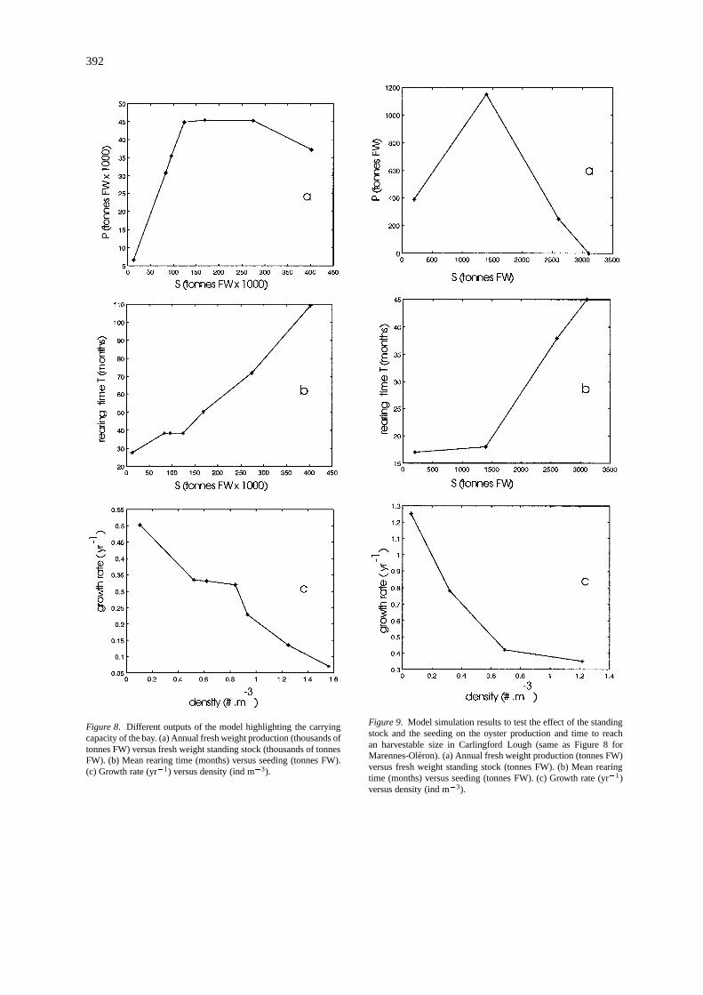
The production/stock relationship (P = f(S)) wasderived from several simulations (Figure 8a). After alinear increase of the production from 5000 to 45 000tonnes FW, the production stabilized at 45 000 tonnesFW for standing stocks above 115 000 tonnes FW, andeventually decreased for standing stocks greater than270 000 tonnes FW. The mortality rate was respons-ible for the dome shape of theP = f(S) relationship.Increasing the rearing time, because of the food lim-itation resulting from the overstocking, resulted in adecreasing production due to the decreasing numberof individuals reaching the marketable size. The rear-

ing time (in months) was averaged over the boxes andplotted versus the standing stock (Figure 8b). It had anexponential type shape - the first values were about 2years, the last one was almost 10 years for a stock equalto 400 000 tonnes FW. The rearing time correspondingto the maximum production (45 000 tonnes FW) andthe standing stock 115 000 tonnes FW was equal to 40months.

Figure 8c depicts the decrease of the annual growthrate as a function of the density (equal to the totalnumber of oysters divided by the volume of water inboxes containing cultured areas). Because individualperformances are better described with the dry weight,the growth rate G (yr�1) was calculated from the ash-free dry weight increase per gram during one year. It isa standardized way to express the carrying capacity ofa bay since the scale effect of the system was removed.The maximum annual weight increase in one year wasequal to 0.5 when the oyster density was very low –around 0.1 ind m�3. It decreased to 0.05 with a densityequal to 1.5 ind m�3.

The M.O. model confirmed the general trend in therelationship between the production and the standingstock obtained by Heral (1993) with an empirical mod-el based on mortality, growth, production, and stocktime series. However, the empirical model does notpredict any decrease of the production, opposite to theecosystem model which predicted a maximum produc-tion of 45 000 tonnes FW for a standing stock around115 000 tonnes FW and a rearing time of 3–4 years. Inthe latter, annual production decreased for high stocksdue to the combination of mortality rates and increas-ing rearing times.

Comparison of Marennes-Oleron Bay andCarlingford Lough carrying capacity anddiscussion

It is interesting to compare the Marennes-Oleron(M.O.) carrying capacity with the carrying capacityof Carlingford Lough (C.L.), which was also assessedwith an ecosystem model (Ferreira et al., this volume).In Carlingford Lough, the oysters need about 1.5 yearsto reach a commercially valuable size, the periodrequired in Marennes-Oleron when oyster culture wasinitiated, in clear contrast with the present 4-year peri-od (Raillard & Menesguen,1994). The methodology ofthe Carlingford Lough and the Marennes-Oleron mod-els was very similar. Both models were based on thecoupling between physical and biological processes at

390

Figure 7. Simulation of the fresh weight (gFW ind�1) during three years with the M.O. model and comparison with a time series of observationsin the center of the bay.

the scale of spatial boxes of several kilometers length.The major differences were related to the populationdynamics of the cultured oyster. The C. L. model used40 weight classes instead of 10 age classes. Insteadof computing the growth of different age classes (seeabove), the C.L. model used a discretized formulationof the continuous equation representing the variationof the population abundance in size and time – seefor instance the equation used to build the theoreticalmodel at the beginning of this paper. It was, there-fore, designed to give more clues than the M.O. modelon the growth and size variability among the popula-tion. Another difference between the two models wasrelated to the relationship between the fresh and thedry weights. In the C.L. case, a fixed ratio was usedbecause the oysters did not lose weight through gam-ete release. In the M.O. model, it was necessary todescribe the oyster growth with 2 different variables –fresh weight and dry weight – to account for the dryweight decrease due to food depletion and spawning.

The production, standing stock, rearing time, meangrowth rate and densities were simulated as in the M.O.case to assess the carrying capacity of the bay, with a

marketable weight of 80 gFW. The marketable weightdiffers from that used in Ferreira et al. (this volume).The total standing stock varied between 200 and 3000tonnes FW and the related annual production between10 and 1400 tonnes FW (Figure 9a). The productionwas maximum for a standing stock around 1200 tonnesFW. It dramatically decreased for greater stocks and,for stocks over 3000, the production was less than 10tonnes FW. The rearing time was positively correlatedto the standing stock (Figure 9b). It varied from 17months to 45 months, with a steep slope from 18 to 40months as the production collapsed. Another clue tothe decline of the production for high standing stocksis shown by the mean annual growth rate G (yr�1)plotted against the density (Figure 9c). Growth ratevalues greater than one were obtained for biomasseslower than 0.2 ind m�3 and became lower than 0.5 fordensities over 0.5 ind m�3. The increase in the rear-ing time was negatively correlated to the growth rate(compare Figures 9b and 9c). Therefore, increasing theseeding yielded a dramatic decrease of the growth rateand resulted in an increased rearing time required toreach marketable size.

391

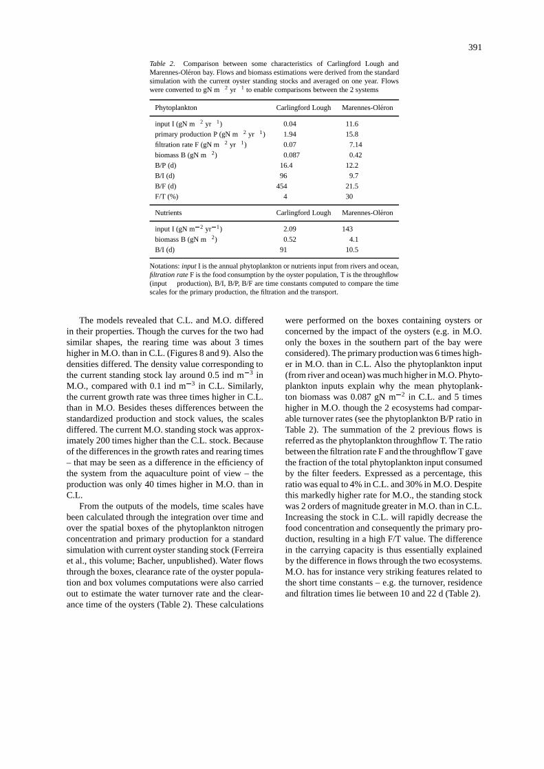
Table 2. Comparison between some characteristics of Carlingford Lough andMarennes-Oleron bay. Flows and biomass estimations were derived from the standardsimulation with the current oyster standing stocks and averaged on one year. Flowswere converted to gN m�2 yr�1 to enable comparisons between the 2 systems

Phytoplankton Carlingford Lough Marennes-Oleron

input I (gN m�2 yr�1) 0.04 11.6

primary production P (gN m�2 yr�1) 1.94 15.8

filtration rate F (gN m�2 yr�1) 0.07 7.14

biomass B (gN m�2) 0.087 0.42

B/P (d) 16.4 12.2

B/I (d) 96 9.7

B/F (d) 454 21.5

F/T (%) 4 30

Nutrients Carlingford Lough Marennes-Oleron

input I (gN m�2 yr�1) 2.09 143

biomass B (gN m�2) 0.52 4.1

B/I (d) 91 10.5

Notations:input I is the annual phytoplankton or nutrients input from rivers and ocean,filtration rateF is the food consumption by the oyster population, T is the throughflow(input+ production), B/I, B/P, B/F are time constants computed to compare the timescales for the primary production, the filtration and the transport.

The models revealed that C.L. and M.O. differedin their properties. Though the curves for the two hadsimilar shapes, the rearing time was about 3 timeshigher in M.O. than in C.L. (Figures 8 and 9). Also thedensities differed. The density value corresponding tothe current standing stock lay around 0.5 ind m�3 inM.O., compared with 0.1 ind m�3 in C.L. Similarly,the current growth rate was three times higher in C.L.than in M.O. Besides theses differences between thestandardized production and stock values, the scalesdiffered. The current M.O. standing stock was approx-imately 200 times higher than the C.L. stock. Becauseof the differences in the growth rates and rearing times– that may be seen as a difference in the efficiency ofthe system from the aquaculture point of view – theproduction was only 40 times higher in M.O. than inC.L.

From the outputs of the models, time scales havebeen calculated through the integration over time andover the spatial boxes of the phytoplankton nitrogenconcentration and primary production for a standardsimulation with current oyster standing stock (Ferreiraet al., this volume; Bacher, unpublished). Water flowsthrough the boxes, clearance rate of the oyster popula-tion and box volumes computations were also carriedout to estimate the water turnover rate and the clear-ance time of the oysters (Table 2). These calculations

were performed on the boxes containing oysters orconcerned by the impact of the oysters (e.g. in M.O.only the boxes in the southern part of the bay wereconsidered). The primary production was 6 times high-er in M.O. than in C.L. Also the phytoplankton input(from river and ocean) was much higher in M.O. Phyto-plankton inputs explain why the mean phytoplank-ton biomass was 0.087 gN m�2 in C.L. and 5 timeshigher in M.O. though the 2 ecosystems had compar-able turnover rates (see the phytoplankton B/P ratio inTable 2). The summation of the 2 previous flows isreferred as the phytoplankton throughflow T. The ratiobetween the filtration rate F and the throughflowT gavethe fraction of the total phytoplankton input consumedby the filter feeders. Expressed as a percentage, thisratio was equal to 4% in C.L. and 30% in M.O. Despitethis markedly higher rate for M.O., the standing stockwas 2 orders of magnitude greater in M.O. than in C.L.Increasing the stock in C.L. will rapidly decrease thefood concentration and consequently the primary pro-duction, resulting in a high F/T value. The differencein the carrying capacity is thus essentially explainedby the difference in flows through the two ecosystems.M.O. has for instance very striking features related tothe short time constants – e.g. the turnover, residenceand filtration times lie between 10 and 22 d (Table 2).

392

Figure 8. Different outputs of the model highlighting the carryingcapacity of the bay. (a) Annual fresh weight production (thousands oftonnes FW) versus fresh weight standing stock (thousands of tonnesFW). (b) Mean rearing time (months) versus seeding (tonnes FW).(c) Growth rate (yr�1) versus density (ind m�3).

Figure 9. Model simulation results to test the effect of the standingstock and the seeding on the oyster production and time to reachan harvestable size in Carlingford Lough (same as Figure 8 forMarennes-Oleron). (a) Annual fresh weight production (tonnes FW)versus fresh weight standing stock (tonnes FW). (b) Mean rearingtime (months) versus seeding (tonnes FW). (c) Growth rate (yr�1)versus density (ind m�3).

393

The box model is the best which can be presentlyachieved. However, it does not take into account all thecomplexity and variability of the system and should beimproved. In the M.O. case for instance, the complex-ity is related to the interaction between the physicaland the biological processes. Some ecophysiologicalprocesses (gametogenesis, local density-dependenceeffect, mortality), still not studied, may influence theresponse of the oyster to environmental forcing. Themixing of the water is responsible for the resuspensionof organic and inorganic matter, which both affect theoyster growth. These factors are difficult to account,having a typical time scale of hours and a spatial scaleof a hundred meters (Raillard et al., 1994). As for thebiology, only recently some attempts have been madeto incorporate gametogenesis and some related pro-cesses (Barille et al., 1997; Soletchnick et al., 1997).Food limitation due to local density-dependence effects(Butman et al., 1994) was not considered here, assum-ing that the food depletion was related to the oysterconsumption at the scale of the bay. However, mortal-ity rates should increase at high stocking densities dueto local conditions (Frechette et al., 1996). For veryhigh standing stocks, overestimated production couldresult from not accounting for mortality.

Conclusion

The interactions between biological processes(primary production, oyster growth) and physical pro-cess (transport and mixing) were successfully mod-elled to assess the carrying capacity of CarlingfordLough (C.L.) and Marennes-Oleron Bay (M.O). Thefirst site has a very low density of cultured oysters andthe second one is overstocked. Experimental data andmodelling tools were developed to simulate the growthof cultured molluscs as a function of the available food– phytoplankton, organic matter and inorganic particu-late matter. The relation between the annual productionand the total stock was assessed by simulating differentscenarios. The definition of the carrying capacity wasthen derived in different ways from the odelling res-ults. Therefore, the modelling methodology proved tobe powerful. The model predicted the optimum stand-ing stock in C.L. and M.O. In C.L. the productionincreased while the standing stock increased from 200tonnes FW to approximately 1500 tonnes FW. The pro-duction decreased for higher standing stocks. In M.O.,the model predicted a maximum production of 45 000tonnes FW for a standing stock around 115 000 tonnes

FW and a rearing time of 3–4 years. The difference inthe carrying capacity of the two systems was essentiallyexplained by the difference in biological and physicalflows derived from the models outputs.

The interactions between the oyster ecophysiology,the population dynamics and the food production weresummarized in the theoretical model. This modeldemonstrated the dome-shaped curve of the produc-tion/stock relationship and its sensitivity to ecologic-al parameters (e.g. mortality rate) and economic con-straint (e.g. the marketable weight).

Acknowledgements

The authors gratefully acknowledge the financial sup-port provided for this work by the EU FAR project AQ-2500 ‘Trophic capacity of an estuarine ecosystem’, theFAR project AQ-2516 ‘Development of an Ecologic-al Model for Mollusc Rearing Areas in Ireland andGreece’ and by EU Concerted Action AIR3-CT94-2219 ‘Trophic capacity of coastal zones for rearingoysters, mussels and cockles’.

References

Barille L, Prou J, Heral M and Bougrier S (1993) No influenceof food quality but ration-dependent retention efficiencies in theJapanese oysterCrassostrea gigas. J Exp Mar Biol Ecol 171:91–106

Barille L, Heral M and Barille-Boyer AL (1997) Modelisation del’ ecophysiologie de l’huitreCrassostrea gigasdans un environ-nement estuarien. Aquat Living Resour 10: 31–48 Bougrier S,Geairon P, Deslous-Paoli JM, Bacher C and Jonquieres G (1995)Allometric relationships and effects of temperature on clearanceand oxygen consumption rates ofCrassostrea gigas(Thunberg).Aquaculture 134: 143–154

Butman CA, Frechette M, Geyer WR and Starczak VR (1994) Flumeexperiments on food supply to the blue musselMytilus edulisL.as a function of boundary-layer flow. Limnol Oceananogr 39:1755–1768

Dame R. F. (Ed.) (1993) Bivalve filter feeders in estuarine and coastalecosystem processes. Springer-Verlag, Berlin, 579 pp

Deslous-Paoli JM and Heral M (1988) Biochemical composition andenergy value ofCrassostrea gigas(Thunberg) cultured in the bayof Marennes-Oleron. Aquat Living Resour 1: 239–249

Ferreira JG, Duarte P and Ball B (1998) Trophic capacity of Carling-ford Lough for oyster culture – analysis by ecological modelling.Aquat Ecol 31: 361–378.

Frechette M, Bergeron P and Gagnon P (1996) On the use of self-thinning relationships in stocking experiments. Aquaculture 145:91–112

Gerritsen J, Holland AF and Irvine DE (1994) Suspension-feedingbivalves and the fate of primary production: an estuarine modelapplied to Chesapeake Bay. Estuaries 17: 403–416

394

Grant J, Dowd M, Thompson K, Emerson C and Hatcher A(1993) Perspectives on field studies and related biological mod-els of bivalve growth and carrying capacity. In: Dame RF (ed.)Bivalve filter feeders in estuarine and coastal ecosystem processes(pp. 371–420) Springer-Verlag, Berlin

Heral M (1993) Why carrying capacity models are useful toolsfor management of bivalve molluscs culture. In: Dame RF (ed.)Bivalve filter feeders in estuarine and coastal ecosystem processes(pp. 465–477) Springer-Verlag, Berlin Herman PMJ (1993) A setof models to investigate the role of benthic suspension feedersin estuarine ecosystems. In: Dame RF (ed.) Bivalve filter feed-ers in estuarine and coastal ecosystem processes (pp. 421–454)Springer-Verlag, Berlin

Kashiwai M (1995) History of carrying capacity concept as an indexof ecosystem productivity (Review). Bull Hokkaido Natl FishRes Inst 59: 81–101

Powell EN, Hofmann EE, Klinck JM and Ray SM (1992) Modelingoyster populations. I. A commentary on filtration rate. Is fasteralways better? J Shellfish Res 11: 387–398

Powell EN, Klinck JM, Hofman EE and Ray SM (1994) Modelingoyster populations. IV: rates of mortality, population crashes andmanagement. Fish Bull 92: 347–373

Raillard O, Deslous-Paoli JM, Heral M and Razet D (1993)Modelisation du comportement nutritionnel et de la croissancede l’huitre japonaiseCrassostrea gigas. Oceanol Acta 16: 73–82

Raillard O and Menesguen A (1994) An ecosystem model for estim-ating the carrying capacity of a macrotidal shellfish system. MarEcol Prog Ser 115: 117–130

Raillard O, Le Hir P and Lazure P (1994) Transport de sediments finsdans le bassin de Marennes-Oleron: mise en place d’un modelemathematique. La Houille Blanche 4: 63–71

Ravail-Legrand B (1993) Incidences du debit de la Charente sur lacapactie biotique du bassin ostreicole de Marennes-Oleron. Thesede Doctorat, Univ. Nantes, 171 pp

Smaal AC and Scholten H (1997) An ecophysiological model ofthe musselMytilus edulis(EMMY). In: Smaal A.C. Food supplyand demand of bivalve suspension feeders in a tidal system. PhDthesis State University Groningen: 147–190

Soletchnick P, Razet D, Geairon P, Faury N and Goulletquer P (1997)Ecophysiologie de la maturation sexuelle et de la ponte de l’huitrecreuseCrassostrea gigas. Reponses metaboliques (respiration)et alimentaires (filtration, absorption) en fonction des differentsstades de maturation. Aquat Living resour 10: 179–186

Van Haren RJF and Kooijman SALM (1993) Application of adynamic energy budget model to Mytilus edulis (L.). Neth J SeaRes 31: 119–133