Assessing the performance of a foraminifera-based transfer function to estimate sea-level changes in...

Assessing the performance of a foraminifera-based transfer function to estimatesea-level changes in northern Portugal

Eduardo Leorri a,⁎, Francisco Fatela b, Alejandro Cearreta c, João Moreno b, Carlos Antunes d, Teresa Drago e

a Department of Geological Sciences, East Carolina University, Graham Building, Room 103b, Greenville, NC 27858-4353, USAb Universidade de Lisboa, Faculdade de Ciências, Centro e Departamento de Geologia, Campo Grande, 1749-016, Lisboa, Portugalc Departamento de Estratigrafía y Paleontología, Facultad de Ciencia y Tecnología, Universidad del País Vasco/EHU, Apartado 644, Bilbao 48080, Spaind Universidade de Lisboa, Faculdade de Ciências, IDL-LATTEX e Departamento de Engenharia Geográfica, Geofísica e Energia, Campo Grande, 1749-016 Lisboa, Portugale Instituto Nacional de Recursos Biológicos I.P., L-IPIMAR, 8700-305 Olhão, Portugal

a b s t r a c ta r t i c l e i n f o

Article history:

Received 14 April 2010

Available online 15 December 2010

Keywords:

Salt marsh foraminifera

Transfer function

Sea level

Minho and Lima estuaries

N. Portugal

We assessed the performance of a transfer function model for sea-level studies using salt-marsh foraminifera

from two estuaries of northern Portugal. An independent data set of 12 samples and 13 sub-fossil samples

from a core were used to evaluate if reconstructions and errors derived from current models are adequate.

Initial transfer function models provided very strong results as indicated by cross-validation (component 2;

r2=0.80–0.82; RMSEP ranged from 10.7 to 12.3 cm) and improved its performance by ca. 10% when sample

size reached ca. 50. Results derived using an independent test data set indicate that cross-validation is a very

effective approach and produces conservative errors when compared to observed errors. We additionally

explored the possible effect of transforming the concentration data into percent in the error estimations by

comparing the results obtained based on the use of both concentration and compositional data. Results

indicate that this type of transformation does not affect the performance of the transfer function. Results

derived from a reconstruction of sub-fossil samples from a core indicate that high-resolution sea-level

reconstructions are possible, but show that depositional environments have to be selected carefully in order

to minimize the impact of possible taphonomical loss.

© 2010 University of Washington. Published by Elsevier Inc. All rights reserved.

Introduction

Phleger (1965) first suggested the existence of vertical zonation ofsalt-marsh foraminifera that corresponded to major marsh zones ofvascular plants. This zonation indicates a response of foraminifera tostrong variations linked to the penetration of tides and to freshwaterinflux from inland sources. Besides the great environmental variabilityof marsh environments, marsh surface foraminiferal distributions areroughly similar in all temperate areas: highest tidal levels are dominatedby the Jadammina macrescens/Trochammina inflata assemblage,replaced by Haplophragmoides spp andMiliammina fuscawith decreas-ing salinity (e.g., Hayward et al., 2004; Fatela et al., 2009). Mid-tidalelevations tend to reflect local variables (e.g., fresh water input anddistance to the mouth of the estuary) and calcareous species becomemore abundant, although dependant on the availability of calciumcarbonate (Phleger, 1970; Moreno et al., 2007; Valente et al., 2009).

Marsh foraminifera are considered the most accurate proxies forelevation and able to predict elevations to within ±0.05 m or better

(Southall et al., 2006; Kemp et al., 2009) due to the strong correlation ofthe assemblages of agglutinatedmarsh foraminiferawith elevation abovemean tidal level (e.g., Gehrels et al., 2008). Since their introduction byGuilbault et al. (1996), foraminifera-based transfer functions havebecome a widely used tool in high-resolution sea-level reconstructions(see Discussion section for references). Through the use of transferfunctions, the modern relationship between marsh foraminifera andelevation is used to calibrate core sediments in order to reconstruct pasttide levels, determining the relative height of marsh sediment in the tidalframe. In fact, estimation of sea-level rise rates based on foraminiferaltransfer functions and tide-gauge sea-level estimates are in goodagreement for the 20th century (Church et al., 2008).

This research is especially relevant under the present scenario ofrapid sea-level rise (19 cm for the 20th century, Jevrejeva et al., 2008)resulting from the global warming (IPCC, 2007). Furthermore, pre-20thcentury instrumental records are sparse and geographically very limitedmaking difficult to resolve when the global sea-level accelerationstarted (Jevrejeva et al., 2006; Miller and Douglas, 2007). It is thereforedesirable to provide sea-level curves at high resolution that aregeographically distributed to supplement existing instrumental datasets and, importantly, extend these data sets back in time in order toaccurately resolve the timingof the sea-level acceleration and the causes

Quaternary Research 75 (2011) 278–287

⁎ Corresponding author. Fax: +1 252 328 4391.

E-mail address: [email protected] (E. Leorri).

0033-5894/$ – see front matter © 2010 University of Washington. Published by Elsevier Inc. All rights reserved.

doi:10.1016/j.yqres.2010.10.003

Contents lists available at ScienceDirect

Quaternary Research

j ourna l homepage: www.e lsev ie r.com/ locate /yqres

of the present sea-level rise. These records can be used to narrow downthe uncertainties of current model predictions of future sea-level rise.

However, in the development of transfer functions, the “predictor”variable in the training sets is “height” (e.g., Kemp et al., 2009;Woodroffe, 2009). However, height is not an ecological or environmen-tal variable. Theecological parameter that directly controls foraminiferaldistributions isflooding duration (Gehrels, 2000). Furthermore, transferfunctions are almost exclusively based on raw percent data (closedcompositional data), despite the limitations that compositional data setspresent (Loubere and Qian, 1997; Kucera and Malmgren, 1998). Oneadditional limitation of this method is the lack of independent data setsto test the reliability of the reconstructions and their prediction ability isonly assessed by cross-validation methods.

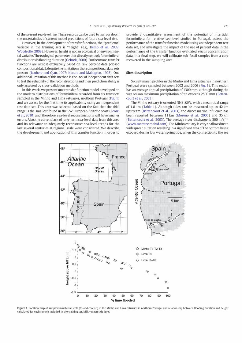
In this work, we present one transfer functionmodel developed onthe modern distributions of foraminifera recorded from six transectssampled in the Minho and Lima estuaries, northern Portugal (Fig. 1)and we assess for the first time its applicability using an independenttest data set. This area was selected based on the fact that the tidalrange is the smallest found in the SW European Atlantic coast (Leorriet al., 2010) and, therefore, sea-level reconstructions will have smallererrors. Also, the current lack of long-term sea-level data from this areaand its relevance to adequately reconstruct sea-level trends for thelast several centuries at regional scale were considered. We describethe development and application of this transfer function in order to

provide a quantitative assessment of the potential of intertidalforaminifera for relative sea-level studies in Portugal, assess theperformance of the transfer function model using an independent testdata set, and investigate the impact of the use of percent data in theperformance of the transfer function evaluated versus concentrationdata. In a final step, we will calibrate sub-fossil samples from a corerecovered in the sampling area.

Sites description

Six salt marsh profiles in the Minho and Lima estuaries in northernPortugal were sampled between 2002 and 2006 (Fig. 1). This regionhas an average annual precipitation of 1300 mm, although during thewet season maximum precipitation often exceeds 2500 mm (Betten-court et al., 2003).

The Minho estuary is oriented NNE-SSW, with a mean tidal rangeof 1.81 m (Table 1). Although tides can be measured up to 42 kmupstream (Bettencourt et al., 2003), the direct marine influence hasbeen reported between 11 km (Moreno et al., 2005) and 35 km(Bettencourt et al., 2003). The average river discharge is 300 m3s−1

(www.maretec.mohid.com). TheMinho estuary is very shallow due towidespread siltation resulting in a significant area of the bottom beingexposed during lowwater spring tide, when the connection to the sea

Figure 1. Location map of sampled marsh transects (T) and core (C) in the Minho and Lima estuaries in northern Portugal and relationship between flooding duration and height

calculated for each sample included in the training set. MTL=mean tide level.

279E. Leorri et al. / Quaternary Research 75 (2011) 278–287

is restricted to two shallow channels (1 to 2 m belowmean tidal level;Alves, 1996).

The Lima estuary is oriented ENE-WSW and is located about 20 kmsouth of the Minho estuary (Fig. 1). The mean tidal range of ~2.10 meffects can bemeasured 20 km upstream (Table 1; Alves, 2003; Ramoset al., 2006). The mean fluvial flux is 62 m3s−1 (www.maretec.mohid.com). The lower part of this estuary has been strongly modified byanthropogenic activities (installation of industrial and commercialfacilities) and is subjected to periodic dredging to maintain channelnavigation. The Lima estuary becomes very shallow upstream wheresalt marsh and several tidal islands develop. These islands are justbelow low spring water levels (Alves, 2003; Ramos et al., 2006).

Materials and methods

We sampled the uppermost centimeter of surface sediment alongsix transects that followed the elevational gradients. A total of 78sediment samples were collected for micropaleontological analysis inthe Minho–Lima area. Because the height above mean tide level wasof primary interest, we obtained samples from as many elevations aspossible. The absolute orthometric height of the marsh transects, tidalelevation and sampling location were obtained in the field using aZeiss Elta R55 total station from previously selected bench marks. Thebench marks were referenced to the national altimetric datum usingdifferential GPS equipment in combination with a regional geoidmodel (Catalão, 2006) then linked to local chart datum. The regionalgeoid model was adjusted to local bench marks by using thedifferential GPS in RTK mode. All data are presented relative to thelocal hydrographical chart datum of Viana do Castelo which is 2.00 mbelow the mean sea level at Cascais in 1938.

Since the mean tidal range for the different salt marshes variesbetween 1.81 m (Minho; Table 1) and 2.05 to 2.10 m (Lima; Table 1)[Fig. 1], the height of surface samples was standardized to a commondatum. We used a linear height normalization technique (e.g., Hortonet al., 1999; Gehrels et al., 2001; Hamilton and Shennan, 2005; Leorriet al., 2008), here elevations are expressed as a standardized water-level index (SWLI):

SWLIn =100 hn−hMTLð Þ

hMHHW−hMTL

+ 100

where SWLIn is the standardized water-level index for sample n, hnthe elevation of sample n (m above local ordnance datum-alod), hMTL

the mean tide level elevation (m alod), hMHHW the mean higher highwater elevation (m alod). This technique produces a SWLI for eachmodern sample. An SWLI of 100 represents mean tide level (MTL) andan SWLI of 200 corresponds to mean higher high water (MHHW).

To assess the ability of the transfer function to reconstruct formersea-level changes and to identify suitable areas for high resolutionstudies (i.e., the depth at which marsh sediments occurred) themicropaleontological content of 21 samples were sampled from theupper 3 m of a borehole drilled in the Minho estuary close to transect3 in 2003. One sample (2.6 m depth) was analyzed for radiocarboncontent at Beta Analytic Inc. (USA) in order to provide a chronologicalframework.

Foraminiferal samples

At each sampling site 10 cm3was extruded by pressing down a hardplastic syringe into the surface layer. The top 1 cm of oxygenatedsediment was placed in a bottle containing alcohol rose Bengal solution[1 g l−1] (Lutze, 1964). Modern samples were sieved through a 63-micron mesh and washed to remove clay and silt material and theremaining residue was analyzed. Samples were stained using roseBengal (Walton, 1952; Lutze, 1964; Murray and Bowser, 2000) toidentify live specimens at the time of collection. Here, we used theunstained assemblages (dead) since they represent the time-averagedaccumulation of foraminiferal tests (Murray, 1991) and are a betteranalogue for reconstructing past sea level (Horton, 1999; Horton andEdwards, 2003, 2006; Horton et al., 2005; Leorri et al., 2008).Foraminifera were collected using a micropipette and a wet pickingprocedure under a stereoscopic binocular microscope using reflectedlight. When possible, at least 100 individuals were counted in eachsample from the dead assemblage as recommended by Fatela andTaborda (2002) for these environments. Identification of the foraminif-era followed Loeblich and Tappan (1988) generic classification. Coresamples were subsampled into 1 cm thick sections and analyzed asdescribed previously but were not stained. In total, 99 samples wereanalyzed and more than 9300 foraminifera were examined.

Although infaunal populations of agglutinated foraminifera livingat depths of 10 cm have been reported from the USAmid-Atlantic andsoutheast coastal salt marshes (Goldstein et al., 1995; Hippensteelet al., 2000), they are not analyzed here. Our analysis from the Limaestuary (Portugal, unpublished data) and in the northern Iberianpeninsula (Leorri et al., 2008) suggests that living individuals areconcentrated in the uppermost interval (0–2 cm) and do notsignificantly modify the assemblage downcore. This observation isalso supported by results obtained elsewhere (e.g., Patterson et al.,2004; Culver and Horton, 2005; Tobin et al., 2005).

Statistical analysis

When key environmental factors (i.e., tidal flooding and salinity)are autocorrelated in the training set, they may influence the ability toreconstruct past conditions (Loubere and Qian, 1997). Moreover,positive spatial autocorrelation (the tendency of sites close to eachother to resemble one anothermore than randomly selected sites) is aproperty of most ecological data that makes the predictive power ofsome models over-optimistic and misleading. Combined training setsfrom various sites provide a more realistic analogue for (sub)fossilassemblages than local data sets (Gehrels et al., 2001). We, therefore,selected six transects that represent different estuarine areas, inaddition, this minimizes the possible effect of intercorrelation ofelevation and salinity and spatial autocorrelation. Furthermore,Telford and Birks (2005) demonstrated that weighted-averagingpartial least squares model (WA-PLS) is least sensitive to these effects.

WA-PLS regression (Juggins, 2004)was used as the transfer functionmodel based on results from detrended correspondence analysis (DCA)and detrended canonical correspondence analysis (DCCA). Thesetechniques help detect the species response, i.e., whether unimodal(Gaussian) or linear models are appropriate (Sejrup et al., 2004). DCCAprovides an estimate (as the length of DCCA axis 1) of the gradientlength in relation to x (environmental variable) in standard deviation(SD) units (Birks, 1995; Korsmanand Birks, 1996). If the gradient lengthis longer than 2 SD units, several species will have their optima locatedwithin the gradient and then unimodal-based methods of regressionand calibration are most appropriate. WA-PLS is an extension of theunimodalmethodweight averaging (WA),whichconsiders thevariancealong the environmental variable of interest (i.e., tidal flooding). Otherenvironmental variables (e.g., salinity) influence foraminiferal distribu-tions, and this may distort the microfaunal-environment relationships.In WA-PLS, further components are calculated orthogonal to earlier

Table 1

Tidal parameters of themarsh transects studied (m referred to the hydrographical chart

datum, 2 m belowmean sea level): HAT=Highest Astronomical Tide; MHHW=Mean

Highest HighWater; MHW=Mean HighWater; MTL =Mean Tide Level; and MLW=

Mean Low Water.

HAT MHHW MHW MTL MLW Mean tidal range

T1-T3 4.26 3.81 3.47 2.56 1.66 1.81

T4 4.28 3.88 3.53 2.51 1.48 2.05

T5-T6 3.97 3.56 3.20 2.15 1.10 2.10

280 E. Leorri et al. / Quaternary Research 75 (2011) 278–287

components and they are obtained as WA of the residuals for theenvironmental variable, improving the predictions as it considers thecombined influence of additional environmental variables (ter Braakand Juggins, 1993). Statistical analyses were performed using CANOCO4.0 (ter Braak and Smilauer, 1998) and C2 (Juggins, 2004) software. Tostatistically assess the predictive power of different transfer functionmodels and select the best model, jack-knife and bootstrapping cross-validation statistical tests were performed (Birks et al., 1990; Line et al.,1994; Sejrup et al., 2004; Telford and Birks, 2005). The models wereselected based on low root-mean-square of the error of prediction(RMSEP), lowmaximum bias, high squared correlation (r2) of observedversus predicted values, and the smallest number of “useful” compo-nents. The RMSEP indicates the systematic differences in predictionerrors, whereas the r2 measures the strength of the relationship ofobserved versus predicted values. In general terms, we considered a“useful” component when improved the previous component perfor-mance by at least 5% of the component 1 (Birks, 1995). In a further stepto evaluate the performance of the differentmodels, we semi-randomlyselected a subset of samples to use them as an independent test data set(i.e., samples were clustered into three groups representing differentelevations and randomly selected within these clusters, so the data setrepresented a variety of elevations). Removing samples from theoriginal data set reduces the model performance but, in turn, thisprovides information of the effect in the model performance ofincreasing the number of samples. We used bootstrapping to derive astandard error of prediction (SEpred; Birks et al., 1990; Line et al., 1994),whichvaries fromsample to sampledependingupon the compositionofthe test set and thepresence or absenceof taxawithaparticularly strongsignal for the environmental variable of interest (Birks, 1995). SEpredwas estimated using 1000 cycles.

The initial data set was built up using percent data fromunscreened samples above mean low high water (MLHW; seeDiscussion section below). In order to identify the effect ofstandardizing the data set we created a second data set usingconcentration data (foraminiferal abundances per unit of sedimentvolume), comprising all samples above MLHW. In order to assess theperformance of these transfer functions, we semi-randomly removedthe same twelve samples in both data sets to use them as anindependent test data set.

Results

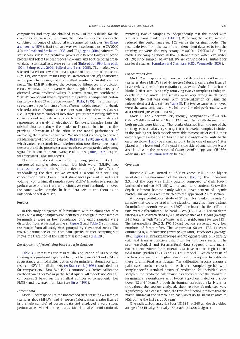
In this study 44 species of foraminifera with an abundance of atleast 2% in a single sample were identified. Although in most samplesforaminifera were in low abundance, only eight samples werediscarded from statistical analysis. Figure 2 and Table 2 summarizethe results from all study sites grouped by elevational zones. Therelative abundance of the dominant species at each sampling siteshows the transition of the different assemblages (Fig. 2B).

Development of foraminifera-based transfer functions

Table 3 summarizes the results. The application of DCCA to thetraining sets produced a gradient length of between 2.10 and 2.74 SD,suggesting a unimodal distribution of foraminiferal abundance withrespect to SWLI for all data sets. ter Braak et al. (1993) concluded thatfor compositional data, WA-PLS is commonly a better calibrationmethod than eitherWA or partial least square. All models useWA-PLScomponent 2 based on the smallest number of components, lowRMSEP and low maximum bias (see Birks, 1995).

Percent data

Model 1 corresponds to the unscreened data set using 49 samples(samples above MHLW) and 44 species (abundances greater than 2%in a single sample) of percent data and displayed a very strongperformance. Model 1b replicates Model 1 after semi-randomly

removing twelve samples to independently test the model withsimilarly strong results (see Table 3). Removing the twelve samplesreduced the performance ca. 10% versus the original model. Theresults derived from the use of the independent data set to test thetraining set were also very strong (r2=0.91; RMSE=6.8). Thesemodels use samples above MLHW (a standardized water-level indexof 120) since samples below MLHW are considered less suitable forsea-level studies (Hamilton and Shennan, 2005; Woodroffe, 2009).

Concentration data

Model 2 corresponds to the unscreened data set using 49 samples(samples above MHLW) and 44 species (abundances greater than 2%in a single sample) of concentration data, while Model 2b replicatesModel 2 after semi-randomly removing twelve samples to indepen-dently test the model. The results were very strong in all caseswhether the test was done with cross-validation or using theindependent test data set (see Table 3). The twelve samples removedwere the same ones used in Model 1b and model performance wasalso reduced (between 7 and 9%).

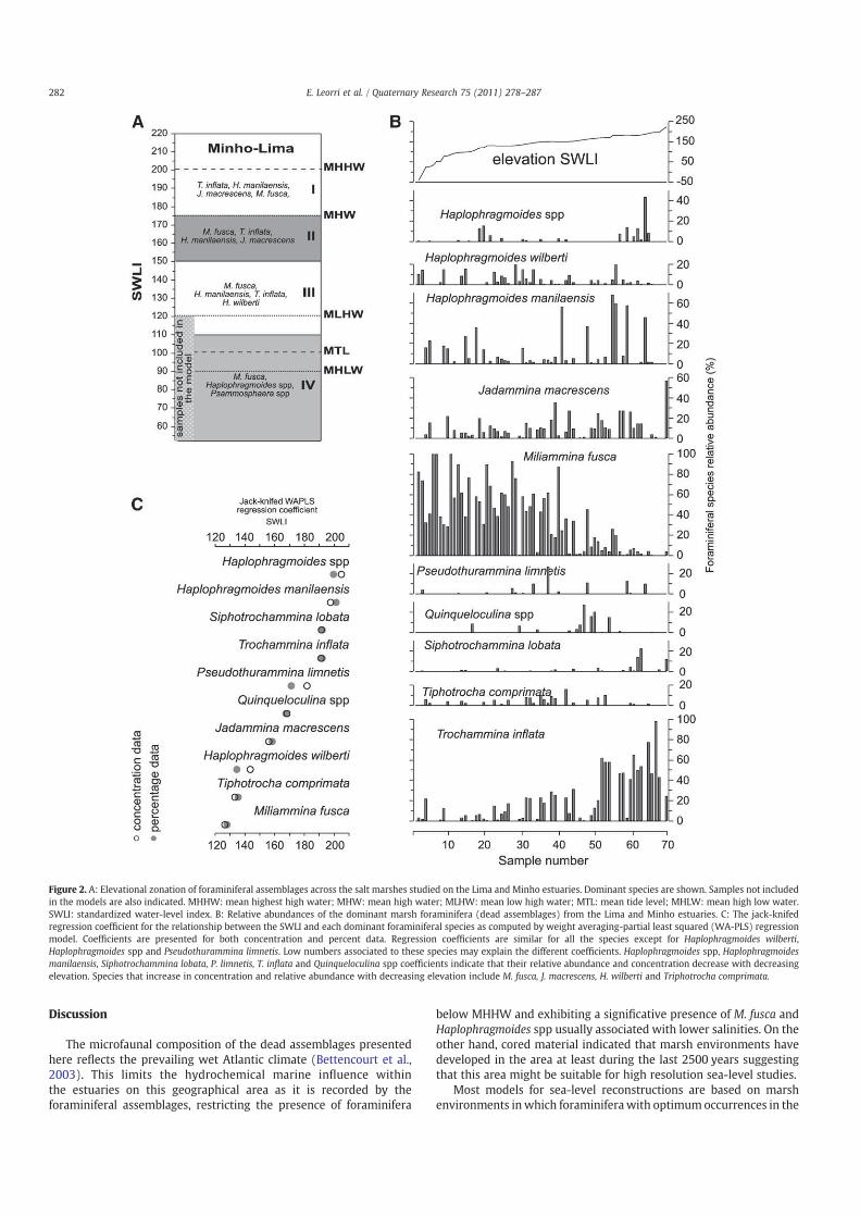
Models 1 and 2 perform very strongly (component 2; r2=0.80–0.82; RMSEP ranged from 10.7 to 12.3 cm). The results derived fromboth models were identical. The results obtained from the use of thetraining set were also very strong. From the twelve samples includedin the training set, both models were able to reconstruct within theirerror range the elevations of ten of them and only two fell outside theerror envelope (Fig. 3) by a small amount. In the case of sample 1, it isplaced at the lower end of the gradient considered and sample 9 wasassociated with the presence of Quinqueloculina spp. and Cibicides

lobatulus (see Discussion section below).

Core data

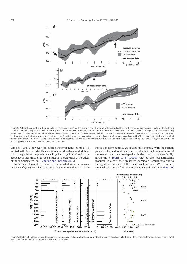
Borehole C was located at 1.505 m above MTL in the highervegetated sub-environment of the marsh (Fig. 1). The uppermost2.6 m of the core was highly organic composed of dark brownlaminated mud (ca. 90% silt) with a small sand content. Below thisdepth, sediment became sandy with a lower content of organicmatter. Our analysis was restricted to the uppermost 2.6 m section.

A micropaleontological study of 21 samples resulted in only 13samples that could be used in the statistical analysis. Three distinctforaminiferal assemblage zones (FAZ), dominated by five differenttaxa, were differentiated. The basal 80 cm (FAZ 3, 260–170 cm depthinterval) was characterized by a high dominance of T. inflata (average34%) together with Paratrochammina cf. guaratibaensis (average 11%).The intermediate (FAZ 2, 170–60 cm) section presented very lownumbers of foraminifera. The uppermost 60 cm (FAZ 1) weredominated byH. manilaensis (average 48%) and J. macrescens (average10%). Figure 4 summarizesmicropalaeontological results, bulk densitydata and transfer function calibration for this core section. Thesedimentological and foraminiferal data suggest a salt marshenvironment where foraminiferal taxa have optima high in thetidal frame (within FAZs 3 and 1). Thus, Model 1, which consists ofmodern samples from higher elevations is adequate to calibratethese foraminiferal assemblages. The calibration process assigns apaleomarsh-surface elevation to each core sample together withsample-specific standard errors of prediction for individual coresamples. The predicted paleomarsh elevations reflect the changes inforaminiferal assemblages with bootstrapped estimated errors be-tween 12 and 15 cm. Although the dominant species are fairly similarthroughout the section analyzed, their relative abundances varysignificantly. As a consequence, the transfer function predicts that themarsh surface at the sample site has varied up to 30 cm relative toMSL during the last ca. 2500 years.

One radiocarbon analysis (Beta-181635) at 260 cm depth yieldedan age of 2345 cal yr BP (cal yr BP 2365 to 2320; 2 sigma).


Discussion

The microfaunal composition of the dead assemblages presentedhere reflects the prevailing wet Atlantic climate (Bettencourt et al.,2003). This limits the hydrochemical marine influence withinthe estuaries on this geographical area as it is recorded by theforaminiferal assemblages, restricting the presence of foraminifera

below MHHW and exhibiting a significative presence of M. fusca andHaplophragmoides spp usually associated with lower salinities. On theother hand, cored material indicated that marsh environments havedeveloped in the area at least during the last 2500 years suggestingthat this area might be suitable for high resolution sea-level studies.

Most models for sea-level reconstructions are based on marshenvironments inwhich foraminifera with optimumoccurrences in the

Figure 2. A: Elevational zonation of foraminiferal assemblages across the salt marshes studied on the Lima and Minho estuaries. Dominant species are shown. Samples not included

in the models are also indicated. MHHW: mean highest high water; MHW: mean high water; MLHW: mean low high water; MTL: mean tide level; MHLW: mean high low water.

SWLI: standardized water-level index. B: Relative abundances of the dominant marsh foraminifera (dead assemblages) from the Lima and Minho estuaries. C: The jack-knifed

regression coefficient for the relationship between the SWLI and each dominant foraminiferal species as computed by weight averaging-partial least squared (WA-PLS) regression

model. Coefficients are presented for both concentration and percent data. Regression coefficients are similar for all the species except for Haplophragmoides wilberti,

Haplophragmoides spp and Pseudothurammina limnetis. Low numbers associated to these species may explain the different coefficients. Haplophragmoides spp, Haplophragmoides

manilaensis, Siphotrochammina lobata, P. limnetis, T. inflata and Quinqueloculina spp coefficients indicate that their relative abundance and concentration decrease with decreasing

elevation. Species that increase in concentration and relative abundance with decreasing elevation include M. fusca, J. macrescens, H. wilberti and Triphotrocha comprimata.


high part of the flooding duration gradient are dominant, i.e., highmarsh assemblages (e.g., Gehrels, 2000). On the contrary, tidal-flatassemblages contain foraminiferal species whose optimum occurs atthe bottom end of the gradient, well below the optima of otherspecies. Small changes in the abundance of these latter speciesconsiderably affect the predicted indicative meaning of the forami-niferal assemblages and, as a result, the error of the model increases(Gehrels, 2000; Woodroffe, 2009). We, therefore, removed allsamples below local MLHW. The performance of the resultingmodel was very strong.

However, while in the literature transfer functions for sea-levelstudies are based almost exclusively on height normalization andclosed compositional data (percent), these two approaches are notexempt of errors. From an ecological point of view, marsh foraminif-era are controlled by sub-aerial exposure, hence, by flooding duration.The relationship between height and flooding duration is non-linear,particularly for the upper marsh surface and, therefore, the time ofsub-aerial exposure is very sensitive to small changes in height. Thisnormalization has been recommended as the best option because itproduces smaller standard errors for the indicative meaning of

foraminiferal assemblages than normalization according to height(Gehrels, 2000). Reconstruction of environmental variables based ontransfer functions should be done when these variables are eitherecologically important determinants in the system (e.g., floodingtime) or linearly related to such determinants (Birks, 1998). This doesnot rule out the use of height normalization and, in fact, the aim ofthese transfer functions is to reconstruct the former elevation of thedepositional environments, but it should be considered carefully.

The second issue is the effect of closed compositional data. In thesetransfer functions micropaleontological data are expressed as relativeabundances. Transformation of any data into such a form gives rise tothe constant-sum constraint, a circumstance violating basic assump-tions upon which standard statistical analyses are designated (Kuceraand Malmgren, 1998). In fact, Loubere and Qian (1997) demonstratedthat the conversion of concentration data to percentages can yieldartificial correlations among species. This effect, named as matrixclosure, creates linear distortion in the ecological response patterns ofthe taxa within the data sets (Mekik and Loubere, 1999).

Overall, matrix closure has a homogenizing effect on taxonresponse by spreading the environmental signals from species thatcarry a strong environmental signal to those species that do notrespond to it, becoming a potential source of error in paleoenviron-mental estimations (Mekik and Loubere, 1999). Moreover, the totalnumber of tests per volume unit may provide additional informationsince foraminifera vanish towards the very top of the intertidal area.This is important because most accurate transfer functions for sealevel tend to concentrate on narrow vertical ranges of the highestintertidal zone (e.g., Southall et al., 2006) and, therefore, theinformation provided by the variance of each individual species isvery valuable (i.e., concentration data).

Our aim here is not to provide a new approach to resolve formersea-level changes but instead to assess if the errors calculated usingthe current models are realistic or some additional sources of errorshould be considered. Furthermore, Szkornik (2009) proposed toconsider errors as much as twice larger than currently used forreconstructions based on diatoms. We, therefore, expected that whencomparing Models 1 and 2 based on percent and concentration datarespectively, we should obtain errors significantly smaller usingModel 1 after reducing the noise of the data set. However, bothmodels provided very similar results using either jack-knife (1%difference) or bootstrapped (3% difference) cross-validation. In orderto fully assess their performance, we semi-randomly removed twelvesamples from the data set to use it as an independent test data set. Toour knowledge, this validation has never been attempted before insea-level studies. The first direct outcome was the reduction of thetransfer function performance between 7 and 9%. Figure 3 sum-marizes the results of the reconstruction of the test data set versus theobserved elevation. Results derived from both models were identical,where ten of twelve samples fell within the bootstrapped errors.

Table 2

The most abundant forms found in these marshes clustered by Autochthonous and

Allochthonous species and elevational zones (I to IV). See also Figure 2.

Mean Range

Autochthonous

M. fusca 40 0–100

Haplophragmoides spp 17 0–90

T. inflata 12 0–88

J. macrescens 7 0–58

Allochthonous

Cibicides spp. 6 0–40

Zone I


H. manilaensis 27 0–68


M. fusca 7 0–26

Zone II

M. fusca 25 2–87




Quinqueloculina spp 5 0–20

C. lobatulus 7 0–28

Zone III

M. fusca 53 1–93


T. inflata 6 0–23

H. wilberti 6 0–20

Zone IV

M. fusca 64 0–100

Haplophragmoides spp 9 0–25

Psammosphaera spp 6 0–53

Table 3

Statistics summary of the performance ofWeighted Averaging-Partial Least Squares (WA-PLS) for the foraminiferal assemblages from theMinho–Limamarshes. Model performance,

jack-knife cross-validation, and fall-test set results are presented. Root-Mean Square of the Error Prediction (RMSEP) andmaximum bias of cross-validation are also presented as % of

the gradient analyzed to allow comparison between the performances of different models. Fall-test results are presented in meters.

Model performance Cross-validation Independent

data setJack-knife Bootstraping

Model name Model RMSE r2 Maximum

bias

r2jack Maximum

biasjack

RMSEP r2boot Maximum

biasboot

RMSEP r2 RMSE

Model 1 Standardized data

(full data set)

WA-PLS Component 2

(SWLI)

7.19 0.88 10.74 0.81 11.84 9.23 0.82 10.74 10.08

Model 2 Concentration data

(full data set)

WA-PLS Component 2

(SWLI)

7.47 0.87 9.12 0.80 12.75 9.35 0.81 12.26 10.39

Model 1b Standardized data

(partial data set)

WA-PLS Component 2

(SWLI)

7.09 0.89 10.47 0.77 10.44 10.18 0.78 11.12 11.18 0.91 6.8

Model 2b Concentration data

(partial data set)

WA-PLS Component 2

(SWLI)

7.61 0.87 8.69 0.78 11.29 9.99 0.78 11.60 11.32 0.90 7.0


Samples 1 and 9, however, fall outside the error range. Sample 1 islocated in the lower end of the elevations considered in ourModel andthis strongly limits the predictive ability. Basically, it is related to theadequacy of thesemodels to reconstruct sample elevation at the edgesof the sampling area (see Hamilton and Shennan, 2005).

In the case of sample 9, the offset is associated with the unusualpresence of Quinqueloculina spp. and C. lobatulus in high marsh. Since

this is a modern sample, we related this anomaly with the currentpresence of a sand treatment plant nearby that might release some ofthe treated sands that are deposited in the marsh surface artificially.Furthermore, Leorri et al. (2008) rejected the reconstructionsproduced in a core that presented calcareous foraminifera due tothe significant increase of the reconstruction errors. We, therefore,removed this sample from the independent training set in Figure 3C

Figure 3. A: Elevational profile of training data set (continuous line) plotted against reconstructed elevations (dashed line) with associated errors (grey envelope) derived from

Model 1b (percent data). Arrows indicate the only two samples unable to provide reconstructions within the error range. B: Elevational profile of training data set (continuous line)

plotted against reconstructed elevations (dashed line) with associated errors (grey envelope) derived fromModel 2b (concentration data). Note the great similarity with Figure 3A.

C: Elevational profile of training data set (continuous line) plotted against reconstructed elevations (dashed line) with associated errors (RMSE; grey envelope with white border)

derived from Model 1b (percent data) after removing the samples not able to provide reconstructions within the error range as indicated by the arrows in Figures 3A and B. The

bootstrapped error it is also indicated (SEP) for comparison.

Figure 4. Relative abundance of main foraminiferal species, predicted paleoelevation produced by the transfer function, bulk density (dots), foraminiferal assemblage zones (FAZs)

and radiocarbon dating of the uppermost section of borehole C.


since fossil samples including these taxa should be avoided in thistype of studies.

However, the poor performance could also respond to the lack ofadequacy in the training data set. In the case of cored samples, it couldbe a response to either, an environmental change or taphonomicalproblems (see further discussion).

The results obtained strongly support the use of standardized datasince they do not seem to affect model performance significantly.Using the independent test data set we can also explore the effect ofbootstrapping on each individual sample. We mentioned previouslythat the overall performance of the transfer function was affected byreducing its predictive ability ca. 10%. This is a result of the largerindividual SEP errors that on average increased 10%. We need tounderstand, however, how these errors are generated. Sample-specificerrors can be calculated using two components. The first part (vi1; asnoted by Birks et al., 1990) represents the effect that the variability ofthe taxa has on the inferred environmental parameter for each sample.This part of the error tends to decrease in magnitude as the size of thetraining set increases, and in samples dominated by taxa that arefrequent and abundant in the training set. The second part (vi2)includes the error caused by imperfections in the calibration functionand model specification error (see Birks et al., 1990 for furtherdiscussion). The second part can be only calculated in the training set.In our analysis, vi2 only increased by 6%betweenModel 1 andModel 1bas a result of removing the 12 samples, while the vi1 increased by 19%.More interesting is that average SEP of the independent test data setincreased by 13% versus average SEP obtained from the same sampleswhen included inModel 1. Considering that vi2 cannot be calculated forthe independent test data set (or sub-fossil samples) since observedvalues are not available, this part is calculated as the mean across thetraining data set (Birks et al., 1990) which only increased by 6%.Therefore, the remaining 7% increase is related to an increase of 36% invi1, associatedwith variability of the taxon parameters. This increase isapparently too large if we consider that ten of twelve samples from theindependent test data set are within ±6.8 SWLIs versus the ±11.3SWLIs average calculated from bootstrapped methods (Fig. 3C).Although we are aware that the independent test data set is small,we are limited by the possible sampling areas. As most transferfunctions for sea-level studies are limited to 30–50 samples, weconsider that these results are really promising, showing that boot-strapped errors provide a high confident range that overcomes thepossible limitations of using percent data and elevation instead offlooding frequency, and that the matrix closure does not affect theperformance of thesemodels. On this basis,we can assume that SEP is aconservative error.

On the other hand, these results can help to identify suitablesampling strategies for sea-level studies. Considering that a large part ofthe error is associatedwith variability of the taxonparameters and tendsto decrease with increasing training data set size, large training setsrestricted to thehighest highmarshwhere thenumber and variability ofspecies is in theminimumshould provide a smaller SEP error. This effectis also apparent in the Sado estuary where Leorri et al. (2010) produceda transfer function based on 20 samples from a single transect limited toelevations above MHW. Only eight species were present with anabundanceof N2% andonly two specieswere above10%. Besides the lownumber of samples studied, jack-knife errors were very small (6.27 inSWLIs units) and it could be anticipated that increasing the number ofsamples would reduce the error even more.

The precision of the transfer function obtained here, expressed as apercentage of the range of the modern environmental gradient sampled,is comparable to other foraminifera-based transfer functions developedfrom the northern Atlantic Ocean. These models have a precision thatranges between±11.5% and±12.6%. These values are in the low rangeoferror compared with several transfer function approaches (e.g., bottom-water summer-salinity, pH, etc.; see Sejrup et al., 2004) including othersea-level transfer functions (see Leorri et al., 2008) which typically range

between 8 and 20% of the gradient analyzed. Although some transferfunctions perform better [e.g., ~4% for bottom waters summer temper-ature (Sejrup et al., 2004) and ~5% for tide level (Massey et al., 2006)], inthe case of estuarine transfer functions for sea level, the improvement ofthe performance responds to the inclusion in the models of lowerelevation samples which significantly reduce their reconstructioncapabilities (Gehrels, 2000; Woodroffe, 2009). When the errors arepresented as height, our results (ca. ±0.12 m) are also in the lower rangeof error compared with other foraminifera-based transfer functions forsea level. Errors of ca. ±0.10 m have been reported from thesouthwestern European Atlantic coast (Leorri and Cearreta, 2008; Leorriet al., 2010), and errors ranging from ±0.12 m (in SWLI units; Hortonet al., 1999; Horton and Edwards, 2006), between ±0.18 and ±0.29 m(Gehrels et al., 2001) to ±0.29 m (Massey et al., 2006) have beenreported in other areas from the northeastern Atlantic Ocean. On thenorthwestern Atlantic Ocean the errors reported ranged from ±0.18 mto ±0.25 m (Edwards et al., 2004 and Gehrels, 2000, respectively).Smaller errors (ca. ±0.05 m) have been only reported from microtidalareas (e.g., Gehrels et al., 2005; Southall et al., 2006; Kemp et al., 2009).

To illustrate fully the potential application of the transfer functiontechnique, we used the transfer function to calibrate the coredsamples. The transfer function provided estimates around MHW(Fig. 4) as expected, since the dominant species have their optima inthe higher elevations (Fig. 2C). Estimations were between 166 and191 SWLIs and fall well within the sampled elevational range withreconstructing errors below 15 cm. These results indicate that highresolution sea-level studies could be performed in this area and thatthe transfer function technique is a suitable methodology, at least inthis area. We cannot, however, attempt to reconstruct sea-levelchanges from this core due to a very poor chronology and a highdegree of sediment compaction that would significantly affect thereconstruction (Fig. 4).

This core reconstruction provides some additional and significantinformation. Within this core there are two species with a statisticallysignificant presence in relation to the training data set. Those are P. cf.guaratibaensis andM. fusca. In the training data set, P. cf. guaratibaensisis secondary (b9% in any single sample) and associated toM. fusca andT. inflata at high elevations. This is similar to the findings reported byDebenay et al. (2002) who reported this assemblage at the transitionto the dry fields and in agreement with the general distribution ofthese species (e.g., Hayward and Hollis, 1994). In two core samples,however, reaches values ca. 20%. This could affect the transfer functionperformance providing unreliable reconstructions. In order to assessthat, we artificially manipulated the test data set increasing P. cf.guaratibaensis values (that range from 0 to 8.5%) to 20% for everysample and performed the reconstruction again. The reconstructedvalues presented no significant differences when compared to theoriginal reconstruction using Model 1b. This might suggest that thisparticular species has not strong influence in sea-level reconstructionsand the signal is carried by the remaining species.

On the other hand,M. fusca values decrease downcore, becoming asecondary species while it is highly dominant in the training data set.This could represent the current environment where the core wasrecovered, within the Zone I (see Table 2 and Fig. 2). This Zone Ipresents an average value of 5% ofM. fusca, similar to the results founddowncore. However, it cannot be fully discarded a possible taphono-mical loss. In fact, M. fusca has been suggested to be susceptible totaphonomic degradation (Goldstein et al., 1995; Hippensteel et al.,2000). In order to assess the possible taphonomical effect in thetransfer function performance, we followed a similar approach to thatindicated previously. We artificially modified the relative values ofM. fusca in the test data set. If we completely removeM. fusca from thetest data set, five sample reconstructions fell outside the error ranges.These samples are associated withM. fusca values of N30%. Moreover,the transfer function performance will be significantly affected whenwe reduced M. fusca values between 25 and 38%. Considering the fact


that we aimed the highest marsh elevation where M. fusca is lessdominant (mean value 5%) and that high-resolution sea-level studieswill be restricted to the uppermost 0.5 to 1 m, we expecttaphonomical problems to be minimized.

Conclusions

This studywas aimed to assess the performance of transfer functionsfor sea-level studies in marsh sediments using salt marsh foraminifera.The analysis performed here indicates that elevational and samplingerrors, the loss of informationbyusingheight as “predictor” variable andthe limitations that compositional data sets present arewell captured bycross-validation methods. Furthermore, reconstructions are very pre-cise (observed error values arebelow7 cm)andRMSEPare conservativevalues compared with the difference between the predicted and theobserved value. This fact, confirms the usefulness of salt-marshforaminifera as sea-level proxies in the Atlantic Iberian coast and thetemporal extent of these environments back in time up to at least ca.2500 years. Although salinity is one of the most important environ-mental factors controlling the foraminiferal distribution at regionallevel, tidal flooding (and, hence, height above local mean tide level) isthe main control in the marsh environment. In fact, foraminifera-basedtransfer functions offer a quantitative and robust methodology toreconstruct former sea levels from salt-marsh sediments.

The strong correlation of the agglutinated salt-marsh foraminiferaassemblageswith elevation abovemean tidal level has been successfullyused to reconstruct cored samples. Furthermore, our findings alsosuggest that taphonomic loss could affect downcore reconstructions ifthe depositional environment is dominated by delicate taxa such asM. fusca.

Therefore, it is suggested that modern transects should be collectedfrom the same environment aimed to be reconstructed, including ca. 50samples, and focusing mainly in high marsh areas dominated by fewspecies that are also more resistant to degradation and less prone to bebiased.

Acknowledgments

Nieves González kindly helped with the graphical design and typingof the manuscript. The research was funded by the following projects:EnviChanges (PDCTM/PP/MAR/15251/99; FCT), WesTLog (PTDC/CTE/105370/2008; FCT), Acção Integrada Luso-Espanhola n° E-20/80/AcciónIntegrada Hispano-Portuguesa HP2007-0098, UPV/EHU-Ihobe contracton recent sea-level changes, TANYA project (MICINN, CGL2009-08840)and by East Carolina University Coastal-Maritime Council. We thankProf. Ronald E. Martin, Dr. Jaime Urrutia Fucugauchi, Dr. Richard Millerand an anonymous reviewer for their comments and suggestions thatgreatly improved the original manuscript. This is a contribution to theIGCP Project 588, Northwest Europe working group of the INQUACommission on Coastal and Marine Processes and Departamento deGeodesia of the Sociedad de Ciencias Aranzadi. Dr. Leorri was awarded aRalph E. Powe Junior Faculty Enhancement Awards. It representsContribution #3 of the Geo-Q Research Unit (Joaquín Gómez de LlarenaLaboratory).

References

Alves, A., 1996. Causas e processos da dinâmica sedimentar na evolução actual do litoraldo alto Minho. Unpublished PhD thesis, Universidade de Minho, Braga, 442 pp.

Alves, A., 2003. O estuário do rio Lima: pressão antrópica e caracterização ambiental.Ciências da Tierra (UNL). Special publication 5, H5-H9 (CD-ROM).

Bettencourt, A., Ramos, L., Gomes, V., Dias, J.M.A., Ferreira, G., Silva, M., Costa, L., 2003.Estuários Portugueses. Ed. INAG—Ministério das Cidades, Ordenamento do Territórioe Ambiente, Lisboa, 311 pp.

Birks, H.J.B., 1995. In: Maddy, D., Brew, J.S. (Eds.), Quantitative paleoenvironmentalreconstructions. Statistical Modelling of Quaternary Science Data, Technical Guide,5. Quaternary Research Association, Cambridge, pp. 161–254.

Birks, H.J.B., 1998. Numerical tools in palaeolimnology — progress, potentialities, andproblems. Journal of Paleolimnology 20, 307–332.

Birks, H.J.B., Line, J.M., Juggins, S., Stevenson, A.C., ter Braak, C.J.T., 1990. Diatom and pHreconstruction. Philosophical Transactions of the Royal Society of London 327, 263–278.

Catalão, J., 2006. Iberia-Azores gravity model (IAGRM) using multi-source gravity data.Earth, Planets, Space 58, 277–286.

Church, J.A., White, N.J., Aarup, T., Wilson, W.S., Woodworth, P.L., Domingues, C.M.,Hunter, J.R., Lambeck, K., 2008. Understanding global sea levels: past, present andfuture. Sustainability Science 3, 9–22.

Culver, S.J., Horton, B.P., 2005. Infaunal marsh foraminifera from the Outer Banks, NorthCarolina, USA. Journal of Foraminiferal Research 35, 148–170.

Debenay, J.P., Guiral, D., Parr, M., 2002. Ecological factors acting on the microfauna inmangrove swamps. The case of foraminiferal assemblages in French Guiana.Estuarine. Coastal and Shelf Science 55, 509–533.

Edwards, R.J., van de Plassche, O., Gehrels, W.R., Wright, A.J., 2004. Assessing sea-leveldata from Connecticut, USA, using a foraminiferal transfer function for tide level.Marine Micropaleontology 51, 239–255.

Fatela, F., Taborda, R., 2002. Confidence limits of species proportions in microfossilassemblages. Marine Micropaleontology 45, 169–174.

Fatela, F., Moreno, J., Moreno, F., Araujo, M.F., Valente, T., Antunes, C., Taborda, R.,Andrade, C., Drago, T., 2009. Environmental constraints of foraminiferal assem-blages distribution across a brackish tidal marsh (Caminha, NW Portugal). MarineMicropaleontology 70, 70–88.

Gehrels, W.R., 2000. Using foraminiferal transfer functions to produce high-resolutionsea-level records from salt-marsh deposits, Maine, USA. Holocene 10, 367–376.

Gehrels, W.R., Hayward, B.W., Newnham, R.M., Southall, K.E., 2008. A 20th century sea-level acceleration in New Zealand. Geophysical Research Letters 35, L02717.

Gehrels, W.R., Kirby, J.R., Prokoph, A., Newnham, R.M., Achterberg, E.P., Evans, E.H.,Black, S., Scott, D.B., 2005. Onset of recent rapid sea-level rise in the westernAtlantic Ocean. Quaternary Science Reviews 24, 2083–2100.

Gehrels, W.R., Roe, H.M., Charman, D.J., 2001. Foraminifera, testate amoebae anddiatoms as sea-level indicators in UK saltmarshes: a quantitative multiproxyapproach. Journal of Quaternary Science 16, 201–220.

Goldstein, S.T., Watkins, G.T., Kuhn, R.M., 1995. Microhabitats of salt marsh foraminifera:St. Catherines Island, Georgia, USA. Marine Micropaleontology 26, 17–29.

Guilbault, J.P., Clague, J.J., Lapointe, M., 1996. Foraminiferal evidence for the amount ofcoseismic subsidence during a late Holocene earthquake on Vancouver Island, westcoast of Canada. Quaternary Science Reviews 15, 931–937.

Hamilton, S., Shennan, I., 2005. Late Holocene relative sea-level changes and theearthquake deformation cycle around upper Cook inlet, Alaska. Quaternary ScienceReviews 24, 1479–1498.

Hayward, B.W., Hollis, C.J., 1994. Brackish foraminifera in New Zealand: a taxonomicand ecologic review. Micropaleontology 40, 185–222.

Hayward, B.W., Scott, G.C., Grenfell, H.R., Carter, R., Lipps, J.H., 2004. Techniques forestimation of tidal elevation and confinement (salinity) histories of shelteredharbours and estuaries using benthic foraminifera: examples from New Zealand.Holocene 14, 218–232.

Hippensteel, S.P.,Martin, R.E., Nikitina, D., Pizzuto, J., 2000. The transformation ofHolocenemarsh foraminifera assemblages, middle Atlantic coast, USA: implications forHolocene sea-level changes. Journal of Foraminiferal Research 30, 272–293.

Horton, B.P., 1999. The contemporary distribution of intertidal foraminifera of CowpenMarsh, Tees Estuary, UK: implications for studies of Holocene sea-level changes.Palaeogeography, Palaeoclimatology, Palaeoecology 149, 127–149.

Horton, B.P., Edwards, R.J., 2003. Seasonal distributions of foraminifera and theirimplications for sea-level studies. SEPM. Special Publication 75, 21–30.

Horton, B.P., Edwards, R.J., 2006. Quantifying Holocene sea level change using intertidalforaminifera: lessons from the British isles. Journal of Foraminiferal ResearchSpecial Publication 40, 1–97.

Horton, B.P., Edwards, R.J., Lloyd, J.M., 1999. A foraminiferal-based transfer function:implications for sea-level studies. Journal of Foraminiferal Ressearch 29, 117–129.

Horton, B.P., Gibbard, P.L., Milne, G.M., Stargardt, J.M., 2005. Holocene sea levels andpaleoenvironments of the Malay-Thai Peninsula, Southeast Asia. Holocene 15,1199–1213.

IPCC, 2007. Climate Change 2007: The Physical Science Basis. In: Solomon, S., Qin, D.,Manning, M., Chen, Z., Marquis, M., Averyt, K.B., Tignor, M., Miller, H.L. (Eds.),Contribution of Working Group I to the Fourth Assessment Report of the Intergovern-mental Panel on Climate Change. Cambridge University Press, Cambridge. 996 pp.

Jevrejeva, S., Grinsted, A., Moore, J.C., Holgate, S., 2006. Nonlinear trends and multiyearcycles in sea level records. Journal of Geophysical Research 111, C09012. doi:10.1029/2005JC003229.

Jevrejeva, S., Moore, J.C., Grinsted, A., Woodworth, P.L., 2008. Recent global sea levelacceleration started over 200 years ago? Geophysical Research Letters 35, L08715.doi:10.1029/2008GL033611.

Juggins, S., 2004. C2, Version 1.4. Newcastle University, UKweb site http://www.campus.ncl.ac.uk/staff/Stephen.Juggins/index.html2004.

Kemp, A.C., Horton, B.P., Culver, S.J., Corbett, D.R., van de Plassche, O., Gehrels, W.R.,Douglas, B.C., 2009. The timing and magnitude of recent accelerated sea-level rise(North Carolina, USA). Geology 37, 1035–1038.

Korsman, T., Birks, H.J.B., 1996. Diatom-based water chemistry reconstructions fromnorthern Sweden: a comparison of reconstruction techniques. Journal ofPaleolimnology 15, 65–77.

Kucera, M., Malmgren, B.A., 1998. Logratio transformation of compositional data — aresolution of the constant sum constraint. Marine Micropaleontology 34, 117–120.

Leorri, E., Cearreta, A., 2008. Recent sea-level changes in the southern Bay of Biscay:transfer function reconstructions from salt-marshes compared to instrumentaldata. Scientia Marina 73, 287–296.


Leorri, E., Gehrels, R.W., Horton, B.P., Fatela, F., Cearreta, A., 2010. Distribution offoraminiferal assemblages in salt marshes along the east North Atlantic coast: toolsto reconstruct past sea-level variations. Quaternary International 221, 104–115.

Leorri, E., Horton, B.P., Cearreta, A., 2008. Development of a foraminifera-based transferfunction in the Basque marshes, N. Spain: implications for sea-level studies in theBay of Biscay. Marine Geology 251, 60–74.

Line, J.M., Ter Braak, C.J.T., Birks, H.J.B., 1994. WACALIB version 3.3-A computer programto reconstruct environmental variables from fossil assemblages by weightedaveraging and to derive sample-specific errors of prediction. Journal of Paleolim-nology 10, 147–152.

Loeblich, A.R., Tappan, H., 1988. Foraminiferal Genera and their Classification: VanNostrand Reinhold Company. v. 1, 970 p., v. 2, 847 pl.

Loubere, P., Qian, H., 1997. Reconstructing paleoecology and paleoenvironmental variableusing factor analysis and regression: some limitations. Marine Micropaleontology 31,205–217.

Lutze, G.F., 1964. Zum Farben Rezenter Foraminiferen. Meyniana 14, 43–47.Massey, A.C., Gehrels, W.R., Charman, D.J., White, S.V., 2006. An intertidal foraminifera-

based transfer function for reconstructing Holocene sea-level change in southwestEngland. Journal of Foraminiferal Research 36, 215–232.

Mekik, F., Loubere, P., 1999. Quantitative paleo-estimation: hypothetical experimentswithextrapolation and the no-analog problem. Marine Micropaleontology 36, 225–248.

Miller, L., Douglas, B.C., 2007. Gyre-scale atmospheric pressure variations and theirrelation to 19th and 20th century sea level rise. Geophysical Research Letters 34,L16602.

Moreno, J., Fatela, F., Andrade, C., Cascalho, J., Valente, T., Moreno, F., Drago, T., 2005.Living foraminiferal assemblages fromMinho/Coura estuary (Northern Portugal): astressful environment. Thalassas 21, 17–28.

Moreno, J., Valente, T., Moreno, F., Fatela, F., Guise, L., Patinha, C., 2007. Calcareousforaminifera occurrence and calcite-carbonate equilibrium conditions — a casestudy in Minho/Coura estuary (N Portugal). Hydrobiologia 597, 177–184.

Murray, J.W., 1991. Ecology and palaeoecology of benthic foraminifera. Longman,Harlow. 397 pp.

Murray, J.W., Bowser, S.S., 2000. Mortality, protoplasm decay rate, and reliability ofstaining techniques to recognize “living” foraminifera: a review. Journal of Foraminif-eral Research 30, 66–70.

Patterson, R.T., Gehrels, W.R., Belknap, D.F., Dalby, A.P., 2004. The distribution of saltmarsh foraminifera at Little Dipper Harbour, New Brunswick, Canada: implicationsfor development of widely applicable transfer functions in sea-level research.Quaternary International 120, 185–194.

Phleger, F.B., 1965. Patterns of marsh foraminifera, Galveston Bay, Texas. Limnology andOceanography 10, 169–180.

Phleger, F.B., 1970. Foraminiferal populations and marine marsh processes. Limnologyand Oceanography 15, 522–534.

Ramos, S., Cowen, R.K., Ré, P., Bordalo, A.A., 2006. Temporal and spatial distributions oflarval fish assemblages in the Lima estuary (Portugal). Estuarine, Coastal and ShelfScience 66, 303–314.

Sejrup, H.P., Birks, H.P.B., Kristensen, D.K., Madsen, H., 2004. Benthonic foraminiferaldistributions and quantitative transfer functions for the northwest Europeancontinental margin. Marine Micropaleontology 53, 197–226.

Southall, K.E., Gehrels, W.R., Hayward, B.W., 2006. Foraminifera in a New Zealand saltmarsh and their suitability as sea-level indicators. Marine Micropaleontology 60,167–179.

Szkornik, K., 2009. Assessing the accuracy of diatom-based transfer function inHolocene sea-level studies: An example from Ho Bugt, western Denmark. INQUA-IGCP 495 meeting, Decadal to millenium-scale land-ocean ineractions in thegeological record: Blueprints for the 21st century? Egmond Aan Zee, Netherlands.

Telford, R.J., Birks, H.J.B., 2005. The secret assumption of transfer functions: problemswith spatial autocorrelation in evaluating model performance. Quaternary ScienceReviews 24, 2173–2179.

ter Braak, C.J.F., Juggins, S., 1993. Weighted averaging partial least-squared regression(WA-PLS)— an improved method for reconstructing environmental variables fromspecies assemblages. Hydrobiologia 269, 485–502.

ter Braak, C.J.F., Smilauer, P., 1998. CANOCO reference manual and user's guide toCanoco for Windows: software for canonical community ordination (version 4).Microcomputer Power, Ithaca, New York. 352 pp.

ter Braak, C.J.F., Juggins, S., Birks, H.J.B., van der Voet, H., 1993. Weighted averagingpartial least squares regression (WA-PLS): definition and comparison with othermethods for species-environment calibration. Chapter 25. In: Patil, G.P., Rao, C.R.(Eds.), Multivariate Environmental Statistics. Elsevier Science Publishers B.V,Amsterdam, pp. 525–560.

Tobin, R., Scott, D.B., Collins, E.S., Medioli, F.S., 2005. Infaunal benthic foraminifera insome north American marshes and their influence on fossil assemblages. Journal ofForaminiferal Research 35, 130–147.

Valente, T., Fatela, F.,Moreno, J.,Moreno, F., Guise, L., Patinha, C., 2009. A comparative studyof the influence of geochemical parameters on the distribution of foraminiferalassemblages in two distinctive tidal marshes. Journal of Coastal Research SI 56,1439–1443 Proceedings of the 10th International Coastal Symposium.

Walton, W.R., 1952. Techniques for recognition of living foraminifera. Journal ofForaminiferal Research Special Publication 3, 56–60.

Woodroffe, S.A., 2009. Recognising subtidal foraminiferal assemblages: implications forquantitative sea-level reconstructions using a foraminifera-based transfer function.Journal of Quaternary Science. doi:10.1002/jqs.1230.


Assessing the performance of a foraminifera-based transfer function to estimate sea-level changes in...

Documents

Transcript of Assessing the performance of a foraminifera-based transfer function to estimate sea-level changes in...