Assessing survivability of smart grid distribution network designs accounting for multiple failures

CONCURRENCY AND COMPUTATION: PRACTICE AND EXPERIENCEConcurrency Computat.: Pract. Exper. (2014)Published online in Wiley Online Library (wileyonlinelibrary.com). DOI: 10.1002/cpe.3241

SPECIAL ISSUE PAPER

Assessing survivability of smart grid distribution network designsaccounting for multiple failures

Daniel Sadoc Menasché1, Alberto Avritzer2,*,† , Sindhu Suresh2,Rosa M. Leão1, Edmundo de Souza e Silva1, Morganna Diniz3, Kishor Trivedi4,

Lucia Happe5 and Anne Koziolek5

1Federal University of Rio de Janeiro, Rio de Janeiro, Brazil2Siemens Corporation, Princeton, NJ 08540, USA

3University of the State of Rio de Janeiro, Rio de Janeiro, Brazil4Duke University, Durham, NC 27706, USA

5Karlsruhe Institute of Technology, Karlsruhe, Germany

SUMMARY

Smart grids are fostering a paradigm shift in the realm of power distribution systems. Whereas tradition-ally different components of the power distribution system have been provided and analyzed by differentteams through different lenses, smart grids require a unified and holistic approach that takes into consid-eration the interplay of communication reliability, energy backup, distribution automation topology, energystorage, and intelligent features such as automated fault detection, isolation, and restoration (FDIR) anddemand response. In this paper, we present an analytical model and metrics for the survivability assessmentof the distribution power grid network. The proposed metrics extend the system average interruption dura-tion index, accounting for the fact that after a failure, the energy demand and supply will vary over timeduring a multi-step recovery process. The analytical model used to compute the proposed metrics is builton top of three design principles: state space factorization, state aggregation, and initial state conditioning.Using these principles, we reduce a Markov chain model with large state space cardinality to a set of muchsimpler models that are amenable to analytical treatment and efficient numerical solution. In case demandresponse is not integrated with FDIR, we provide closed form solutions to the metrics of interest, such as themean time to repair a given set of sections. Under specific independence assumptions, we show how the pro-posed methodology can be adapted to account for multiple failures. We have evaluated the presented modelusing data from a real power distribution grid, and we have found that survivability of distribution powergrids can be improved by the integration of the demand response feature with automated FDIR approaches.Our empirical results indicate the importance of quantifying survivability to support investment decisions atdifferent parts of the power grid distribution network. Copyright © 2014 John Wiley & Sons, Ltd.

Received 10 December 2013; Accepted 22 January 2014

KEY WORDS: survivability; transient analysis; smart grid; fault tolerance; demand response; reliabilitymetrics; FDIR

1. INTRODUCTION

Information and communication technologies are being deployed to the distribution power grid tofacilitate the management of energy demand and supply. The automatic management of customerdemand in response to variations in available power or as a result of power failures is referred toas demand response. The automatic detection, isolation, and restoration of failures is known as

*Correspondence to: Alberto Avritzer, Siemens Corporation, Princeton, NJ 08540, USA.†E-mail: [email protected]

Copyright © 2014 John Wiley & Sons, Ltd.

D. S. MENASCHÉ ET AL.

distribution automation (DA). The automation of the smart grid brings novel challenges to the powergrid engineers, such as the assessment of the tradeoffs involved to accurately engineer the powerdistribution reliability.

The introduction of automation (intelligence) to power distribution networks has created a needfor the holistic assessment of the distribution network. The distribution network reliability is a func-tion of the correct operation of several architecture artifacts such as electrical power components,telecommunications, distribution network topology, failure detection isolation and restoration,demand response, and distributed generation (DG) and storage. The automation of power distribu-tion requires a more integrated perspective across these domains. However, in the current mode ofoperation, they are still being engineered separately.

Traditionally, the reliability of power systems has been quantified using average metrics, such asthe system average interruption duration index (SAIDI). SAIDI is used by public service commis-sions in the USA to assess utilities’ compliance with the commission rules. It was developed to trackmanual restoration times, and according to standard 166-1998, the median value for North Americanutilities is roughly one and a half hours. In smart grid networks, power failure and restoration eventswill have a finer level of granularity, because of the deployment of reclosers, which isolate faultysections, and demand side management system activities, such as distributed generators and demandresponse application systems. Therefore, there is a need to extend the SAIDI metric and to developnew models and tools for the accurate computation of customer interruption indexes after powerfailure events occur, even if the occurrence of such events is rare. The survivability of a mission-critical application is the ability of the system to continue functioning during and after a failure ordisturbance [1].

In [2], we presented a proposal for a common analysis framework to support the survivabil-ity analysis of DA using extensions of the International Electrotechnical Commission-standardizedcommon information model. The paper presented a case study of the application of the proposedmethod to the survivability analysis of a simple DA network that was derived from a real power dis-tribution network. In [3], we have evaluated the impact of available active and reactive power supplyafter a section failure on the distributed automation survivability metric, and we derived closed-formexpressions for certain survivability-related metrics. In [2–4], the survivability model accounted forsingle failures.

In this paper, we present an analytical model to assess the survivability of distributed automationpower grids and to predict SAIDI and related metrics as a function of different system parametersrelated to communications, DG, demand response, and other smart grid features, accounting formultiple failures. We use a performability model to capture how the system recovers from a failure.Our model accounts for the fact that the topology is sectionalized. Given a failure in section i , ourkey insight is to aggregate the sections of the network that may be fed by backup sources into asingle node, denoted by iC. This aggregation allows us to efficiently quantify transient metrics ofthe network after a failure, also referred to as survivability metrics. For example, our model allowsus to compute how the energy not supplied (ENS) after a failure varies over time as a function ofthe available backup power, the demand response application, and the state of the information andcommunication network.

After a power failure event, some power grid areas of the network may experience restorationtimes of the order of magnitude of minutes, while other power grid areas may require hours for themanual repair events to take place. Our model allows for the accurate assessment of the power gridnetwork survivability by tracking the time-dependent state of the system under study.

The main contributions of this paper are the following.Survivability model, accounting for multiple failures: We present a Markov chain model that

supports the survivability assessment of power grid metrics accounting for the sectionalizing ofDA topology, the available excess power, the unreliability of the telecommunications network, andthe interaction with the demand response application. Our model can be generated and solved in acost-efficient manner.

Implications of system integration: We bring awareness to the importance of accurate holisticpower engineering that considers the interactions between the telecommunications reliability and thereliability benefits of integration with other DA features, such as the integration of failure recovery

Copyright © 2014 John Wiley & Sons, Ltd. Concurrency Computat.: Pract. Exper. (2014)DOI: 10.1002/cpe

ASSESSING SURVIVABILITY OF SMART GRID DISTRIBUTION NETWORK DESIGNS

with demand response. In particular, we show that if demand response can be activated after a failureoccurs, the survivability of the system significantly increases.

Extension of the SAIDI metric to support distributed automation: We present an extension of theSAIDI metric that captures the dynamic nature of the smart grid by taking into account the numberof customers impacted by the service interruption, the service impact of the interruption (e.g., ENS),and the duration of each phase of a multiphase recovery period. We use the analytical solution ofthe survivability model to capture the time spent in each state during the recovery period and thereward rate associated with each state to capture the service impact of the interruption.

The outline of this paper is as follows. In Section 2, we present a survey of the related literature. InSection 3, we present an overview of demand response and failure detection isolation and restorationapplications. In Section 4, we introduce the survivability metrics that can be derived from our model.We present the model used in this paper in Section 5 and its extension to account for multiple failuresin Section 6. The analysis of our empirical results is presented in Section 7. Section 8 presents ourconclusions and suggestions for future research.

2. LITERATURE REVIEW

The available literature on power systems reliability is extensive [5–7]. Recently, researchers havestudied how to improve power systems reliability with smart grid techniques [8, 9]. To our knowl-edge, our work is the first to assess survivability metrics of power systems accounting for theimplications of electro-mechanical and computer-based strategies to address failures in an integratedmanner.

Elmakias [6] presents a review of computational methods in power system reliability. The focusof the review is on the application of Markov models to reliability assessment. To address failuresin the distribution system, the author studied a number of approaches such as the reduction of mainfeeder line length, the introduction of sectionalizer switches, and the automatic connection of backuppower supply to sections isolated by a failure. The analysis focuses on steady-state metrics, whereasin this paper, our focus is on studying the transient behavior after a failure occurs. Conditioningthe initial state to be a failure state is important in order to evaluate metrics such as the mean ENSuntil recovery.

The impact of adding DG as a backup source in a power system has been studied in [8, 10–12].Waseem [8] and Zou et al. [10] analyzed the impact of DG placement on SAIDI, comparing severalmain feeder topologies. They concluded that placing the DG source at the end of the main feeder lineprovided the best improvement in power system reliability. Wang et al. [11] proposed an analyticalmodel to evaluate system reliability. They used the model to obtain the placement and sizing ofDG’s that maximized power reliability. An approach for the optimal sizing of DG’s is also presentedby Zhang and Bo [12]. These papers are related to ours, as these results can be used to obtain theprobability that a backup source can supply energy to the affected sections.

Janev [13] presented the implementation and evaluation of a power flow algorithm for powerdistribution grids with DG.

Specifically, the power flow approach presented in [13] was evaluated using an adaptation ofa power distribution benchmark [14]. This benchmark employs the following types of renewablepower generation equipment: photovoltaic solar energy (PV), wind, small hydro, and biomass.

Martins and Borges [15] presented a model for active distribution systems expansion planningthat considers DG together with traditional alternatives for distribution expansion such as re-wiring,network reconfiguration, and installation of protection devices. The authors evaluated differentalternatives for DA using average reliability metrics (SAIDI and system average interruptionfrequency index (SAIFI)) and cost.

Brown [5, Section 2.2.5] presented a detailed discussion of the shortcomings of existing indicesto assess reliability of power systems. In addition, the author proposed a novel metric, the systemaverage interruption duration exceeding threshold, or SAIDET. In this paper, we argue thatsurvivability metrics also play a key role in the assessment of smart grid networks.

Heegaard and Trivedi [16] studied the survivability of telecommunication systems. They pre-sented a phased recovery model to capture the transient properties of the system after a failure.



In this paper, we account for features that are specific to the smart grid domain and leverage suchfeatures for the efficient solution of the proposed model (see Section 5.1).

Performability metrics have been defined to assess the ability of a system to continue to operateafter a component failure but at (possibly) different performance levels [17, 18]. Performability isusually concerned with the quality of service provided that the system as a whole is operational. Theinitial system state is chosen accordingly. In this paper, in turn, our focus is on survivability metrics.In this case, the initial state of the system is set to a failure state, so survivability may be viewed as“conditional performability” [19].

Keshav and Rosenberg [20] argued that concepts pioneered by the Internet are applicable to thedesign of smart grids, and suggest the initiation of a dialogue between the Internet community andthe electrical grid research community. Our work is a product of such a dialogue [16, 21].

3. DISTRIBUTION SYSTEMS BACKGROUND

In this section, we introduce some background on distribution systems, focusing on the aspectsrelevant to our model, namely (1) the demand response application and (2) fault detection, isolation,and restoration (FDIR). Currently, the two features are implemented by separate DA systems, sowe discuss the potential benefits of the integration of demand response and FDIR features. We startwith a brief primer on DA.

3.1. Distribution automation primer

The smartening of distribution networks can bring significant benefits to operators and customersbut will require considerably more effort than the smartening of transmission networks. Distribu-tion networks have many more nodes to be instrumented and managed, and there is a need tomeet stringent requirements for communication reliability. Distribution systems connect to nearlyall electricity customers (excluding some large industrial customers that are connected directly tothe transmission system). In addition, future distribution networks will become very complex withthe introduction of new technologies, such as DG and variable/dispatchable resources, and new loadtypes, such as electric vehicles. Therefore, there is a need to quantitatively engineer and manage theDA technology complexity and the associated costs, with the goal of optimizing the power grid tothe benefit of all the stakeholders: power utilities, regulatory entities, and customers.

The integration of smart grid-related technology into the distribution side will lead to significantchanges in the power system configuration. The current power grid distribution system is designedto meet the expected power load requirements. In the future, the DA feature will be responsible formaintaining power reliability.

Specifically, several alternatives will be available to reconfigure the power system distributiontopology after a power event such as a failure. Two alternatives are as follows: (1) depending onthe load that is required to be met to recover from a power failure, demand response applicationsor distributed generators might be initiated, and (2) if several power distribution areas are intercon-nected through the use of tie line switches, spare power from one area can be used to meet the powerdemand from the failed area.

Therefore, the interconnection of several distribution areas and the introduction of distributionside energy management schemes like demand response, electric vehicle, energy storage, and DGcan help manage power reliability by decreasing the mean fault clearing times and reducing theburden to be carried by the power protection devices.

3.2. Demand response application

Demand response are a set of the incentive payments designed to induce lower electricity use attimes of high wholesale market prices or when system reliability is jeopardized. Demand responsecan be defined as the action taken by consumers to reduce electricity demand in response to price,monetary incentives, or utility directives so as to maintain reliable electric service or avoid highelectricity prices.



Table I. Model parameters (rates are given in units of events per hour).

Parameter Description Value

� Mean time for recloser to isolate failed section � 0˛ Automatic restoration rate 30ˇ Demand response rate 4� Communication repair rate 1ı Manual repair rate 1/4

A decade ago, distribution side networks were considered mostly demand nodes, while now, theycan act both as a power generation source and as a power demand sink. Bidirectional power flowcan have a significant impact on the protection and reliability of the system. In addition, evolution ofthe nodal market creates a location-based pricing mechanism, where the price not only is a functionof the available energy but also depends on the congestion.

The introduction of demand response applications and the emergence of wholesale energy andreliability markets create new opportunities for demand-side resources by enabling customer loadsto participate in the wholesale energy market. In addition, the application of demand response hasthe potential of enhancing power reliability and helping operators manage peak demand by reducingcongestion on critical transmission lines.

3.3. Fault detection, isolation, and restoration

The FDIR is concerned with the detection of faults on the feeder line, determining the location ofthe fault as defined by the two feeder switches that determine the fault boundary, isolation of thefaulty feeder section, and automated restoration of power to the feeder sections located outside thefault boundary, that is, the non-faulty feeder sections.

The granularity of FDIR depends on the type of switch/recloser used for dividing the feeder lineinto sections, and the availability of backup power to feed the healthy sections of the feeder line.

The time required for fault detection isolation and restoration depends on the level of automationimplemented in the infrastructure deployed by the utility to support the FDIR feature. Customersusually report outages 5–10 min after a fault occurrence. Power can be automatically restored to thehealthy sections of the feeder line in about 2 min, when automated FDIR is implemented. Whenautomated fault detection and isolation is not implemented, it may take up to 1 h for power to berestored to the healthy sections of the feeder, because manual fault location and manual switchinghave to be performed. Repair of the faulty section of the feeder line may take 1 to 4 h. When thefeeder line is connected to a tie switch, the healthy parts of the feeder line can be powered by asecondary substation, after the faulty section is isolated. Table I, which will be further discussedwith the model presented in Section 5, summarizes the aforementioned numbers. The numbers inTable I reflect the multiple time scales at which repairs occur. In this paper, these numbers are setbased on expert knowledge, but they could as well be adjusted based on time series or event logs.

3.4. Integration of demand response and failure recovery

In current distribution systems, demand response services are not integrated with failure recoveryservices. Usually, these two services are designed independently. Nonetheless, in this paper, weconsider the possibility of demand response being activated in response to a failure event with theaim of improving the power distribution survivability.

4. SURVIVABILITY METRICS

Survivability has been defined by American National Standards Institute as the transient perfor-mance of a system after an undesirable event [22]. The metrics used to quantify survivability varyaccording to applications and depend on a number of factors such as the minimum level of perfor-mance necessary for the system to be considered functional, and the maximum acceptable outage



instantaneousmetrics

cumulativemetrics

survivabilityrelated metrics

1) probability that all sections, except section i, have their power recovered by time t2) probability that section i has been recovered by time t

accumulatedup to time t

accumulatedup to certain event

3) mean accumulated downtime of section i by time t4) mean accumulated energy not supplied to the system by time t

5) mean time to recover section i6) mean accumulated energy not supplied to the system up to full system recovery

performance metric: energy supplied per hour

Figure 1. A taxonomy of survivability-related metrics.

duration of a system. Survivability metrics are transient metrics computed after the occurrence ofa failure. In the remainder of this paper, time t refers to the time since a failure occurred and ismeasured in hours.

Survivability metrics are computed with respect to a measure of interest M, also referred toas the performance metric [16]. In the realm of power systems, the performance metric M is theenergy supplied per hour, measured in kilowatt hour. Assuming that M has value � just before afailure occurs, the survivability behavior is quantified by attributes such as the relaxation time forthe system to restore the value of M to �. In this paper, we compute metrics related to the relaxationtime, focusing on the mean ENS per hour after a failure occurs.

4.1. Metrics taxonomy

Figure 1 shows the taxonomy of the survivability-related metrics considered in this paper. We clas-sify the metrics into two broad categories. Instantaneous metrics are transient metrics that capturethe state of the system at time t . An example of an instantaneous metric is the probability that agiven section i has been recovered by time t .

Cumulative metrics are obtained in our model by assigning reward rates to system states. Areward is gained per time unit in a state, as determined by the reward rate assigned to that state.The accumulated reward is the result of the accumulation of rewards since the failure up to timet or up to a certain event. The mean accumulated downtime of a given section by time t and themean accumulated ENS by time t are examples of cumulative metrics computed up to time t . Themean accumulated ENS up to the full recovery of the system is an example of a cumulative metriccomputed up to a certain event. The mean time to recover a given section is also an example ofthe latter class of metrics, where the accumulated reward in this case is the time itself, obtained byassigning a reward of one per time unit at every state. Other definitions of transient metrics can befound in [23, 24]. In Section 7, we present the evaluation of the metrics described earlier as appliedto the case study presented in this paper.

4.2. From system average interruption duration index to survivability-related metrics

We now define and extend one of the key metrics of interest in the realm of power systems, theSAIDI. SAIDI is an important measure of the power utility’s ability to cope with recovery fromfailures. It is a measure of average customer impact of system interruptions as it computes the sumof customer interruption durations over the total number of customers [5, 25].

Given a topology with C sections, letN be the total number of customers, letNj;k be the numberof customers in the system impacted by the k-th failure at section j , and letKj be the number of fail-ures at section j during a pre-established large observation period, j D 1; : : : ; C , k D 1; : : : ; Kj .Let 'j;k be the outage duration due to the k-th failure that occurred at section j , measured in hours.Let 'j be the average outage duration due to all failures at section j . Let �j be the average numberof failures at section j , during the same pre-established observation period. The observation periodis usually assumed to be 1 year so that 'j and �j are the annual average outage duration and numberof failures, respectively.



Definition 4.1The SAIDI index is the average outage duration for each customer served,

SAIDI DCXjD1

KjXkD1

'j;kNj;k

N(1)

After a failure, the ENS will vary over time during a multi-step recovery process. Let¹mj .t/; t > 0º be a stochastic process in which the random variable mj .t/ characterizes the ENSper unit time, after a failure in section j , j D 1; : : : ; C , t units of time after the failure; mj .t/accounts for the effect of one single failure in section j . If a full system recovery occurs at time T ,we set mj .t/ D 0 for t > T . Let mj .t/ be the mean value of mj .t/. In the remainder of this paper,given a random variable Z, we denote its mean by Z.

Let Mj .�/ be the accumulated ENS by time � after a failure in section j , j D 1; : : : ; C ,

M j .�/ D

Z �

tD0

mj .t/dt; j D 1; : : : ; C (2)

Note that the total energy demanded per unit time can also vary during recovery. This occurs, forinstance, if demand response is integrated with failure recovery. Let ¹dj .t/; t > 0º be a stochasticprocess in which the random variable dj .t/ characterizes the total energy demanded per unit timeat time t during the recovery from a failure in section j . Let Dj .�/ be the energy demanded overthe first � time units during the recovery from a failure in section j ,

Dj .�/ D

Z �

tD0

d j .t/dt; j D 1; : : : ; C (3)

Let �j be the expected number of failures at section j during a pre-established large observationperiod (typically 1 year). We define the extended SAIDI index (ESAIDI) as the outage durationaccounting for the energy demanded and not supplied during the first � units of time after a failureat a section, averaged over all sections.

Definition 4.2The extended SAIDI index is given by

ESAIDI.�/ DCXjD1

�j �

M j .�/

Dj .�/

!(4)

The term inside parentheses in equation (4) is the fraction of the mean ENS over the mean energydemanded by time � after a failure. Note that we assumed that � is a scalar value. Alternatively, letXj be a random variable characterizing the time to full system recovery after a failure at sectionj , j D 1; : : : ; C , and X D .X1; : : : ; XC /. Replacing � in (4) by the corresponding mean recoverytimes yields

ESAIDI.X/ DCXjD1

�jEŒXj �

E�M j .Xj /

�E�Dj .Xj /

�!

(5)

where

E�M j .Xj /

�D lim�!1

M j .�/ (6)

Let M j D EŒM j .Xj /�, and let Nj be the average number of customers affected by a failure atsection j . The equality in equation (6) follows from the fact that if a full system recovery occursat time T , m.t/ D 0 for t > T . Quantity mj .t/ is precisely that defined by American NationalStandards Institute [22] as survivability. Cumulative quantities such asM j are defined as extensionto the basic survivability measure and called excess loss due to failures [26].



Next, we show conditions according to which Definition 4.1 follows as a special case of Definition4.2. To this goal, assume that the energy demanded per user per unit time is constant and equal toE and that the number of customers affected by a failure at section j is also constant and equal toNj . Therefore, mj .t/ D NjE, and d j .t/ D NE. In addition, we also assume that the mean outageduration due to one failure at section j is � and the number of failures at section j is independentof the outage duration due to a failure at that section, 'j D EŒXj ��j D ��j . Let O'j be the meanoutage duration due to one failure at section j , O'j D 'j =�j . Then, ESAIDI. O'/ D SAIDI, whereO' D . O'1; : : : ; O'C /.

ESAIDI.�/ is a function of �j ,Dj .�/, andM j .�/, j D 1; : : : ; C . �j is computed from an avail-ability model while Dj .�/ and M j .�/ are computed from a survivability model. In the remainderof this paper, our focus will be on the survivability model, which allows us to compute the termsin parentheses in equations (4) and (5), as described in Section 5 and illustrated in a case studyin Section 7.

5. SURVIVABILITY MODEL

In this section, we present the model used to compute survivability metrics of power distributionsystems. We describe the modeling challenges and design principles, followed by the modeloverview and the specific model instantiation used throughout the remainder of the paper.

5.1. Challenges and design principles

Survivability assessment of the power grid distribution topology is implemented by taking advantageof the power line design that uses sections for failure isolation.

Initially, we attempted to characterize the individual behavior of each of the sections by con-ducting an exhaustive quantitative analysis accounting for the failure rates of each of the sectionsand their multiple possible states. During this initial model design phase, we encountered thefollowing challenges:

� Capturing the state of each section individually leads to a large state space, as the number ofstates grows exponentially as a function of the number of sections;� Generating, storing, and solving a model with a very large state space are computationally

challenging;� Accounting for component failures that occur at a much coarser level of granularity than the

failure repair yields a model that is numerically hard to solve.

The methodology presented in this paper addressed the aforementioned challenges by relyingon three key principles: (1) state space factorization; (2) state aggregation; and (3) initial stateconditioning.

5.1.1. State space factorization. Our methodology encompasses a set of models, where each modelcharacterizes the system evolution after the failure of a given section. Given a topology with Csections, our methodology yields C models, where each model is tailored to the characteristics ofthe failed section. The advantages of such a state space factorization are as follows:

1. Flexibility: Having a model tailored to a given section enables us to capture specific detailsabout the impacts of failures on that particular section;

2. Reduced complexity: The computational complexity to compute the metrics of interest isreduced by considering a set of models as opposed to a single model with cardinality Ctimes larger. Consider a DA topology that has C sections, and let K be the number of statesat which a section can be found. The computational complexity to solve the non-factorizedmodel is O.C 3K3/, using, for instance, the Grassmann-Taksar-Heyman Method (GTH) solu-tion method [27] to compute the steady-state probabilities of an associated ergodic model(described in the Appendix), without taking advantage of any possible special structure in themodel. The decomposition approach, in contrast, requires the solution of C models, each one



requiring O.K3/ steps to be solved, which results in a complexity of O.CK3/. A similarcomment holds for the transient solution as well [28, 29].

State factorization assumes that there are no interaction effects among failures. In Section 6, weconsider multiple failures, and we show conditions under which state factorization can still be usedto analyze the system under multiple failures even if different sections share resources such asbackup power sources. Analyzing interaction effects among failures in full generality is left forfuture work.

5.1.2. State aggregation. One of the insights of this paper is the observation that after a failure of agiven section, the remaining sections of the DA topology can be aggregated into groups of affectedand non-affected sections. In the scenario considered in the remainder of this paper after the failureof section i , section i is isolated, and the non-failed sections can be aggregated into two groups: thedownstream sections that are aggregated into a set of sections i� and are served by their originalsubstation and the upstream sections that are aggregated into a set of sections iC and might beserved by a backup substation, if enough backup power is available (see Figure 2). State aggregationyields significant reduction in the computational complexity required to obtain the desired metrics,as the system state space can be described in terms of the aggregated section states.

5.1.3. Initial state conditioning. The computations of the survivability-related metrics of interestare performed by assuming that the initial state is a failure state. Survivability models do not cap-ture the failure rates of different components. Instead, the models are parameterized by using theconditional probability that specific system components are still operational after a specific section

ii- i+

substationdownstream upstreamfailure

substationtie switchopen

(a)

(b)

I

I

backup substation

II A B C D E F

A B C D E F

backup substation

II

section served by its main substation

failed section

section served by backup substation

closed recloser

open recloser

tie switchclosed

1 2 3 4 5 6 7 8 9

1 2 3 4 6 7 8 95

Figure 2. Failed section and its upstream and downstream.



Table II. Table of notation.

Variable Description

C Number of sectionsi Failed sectioniC Upstream of section i (sections ¹i C 1; : : : ; C º)i� Downstream of section i (sections ¹1; : : : ; i � 1º)p Probability that communication works after failureq Probability that backup power suffices to supply

Isolated sectionsr Probability that demand response is effective after failure

failure. Results are then combined with failure rates via the extended SAIDI where failure rates areconsidered (see Section 4).

In the remainder of this paper, we will consider conditional probabilities to account for the prob-ability that a substation backup power is able to supply isolated sections (q), the reliability of thetelecommunications network (p), and the effectiveness of the demand response application (r). Thenotation used throughout the paper is summarized in Table II.

5.2. Model overview

Automatic and manual restoration events are initiated after a section failure event. The restorationprocess is a combination of electro-mechanical and computer-based events. In what follows, wedescribe the sequence of events initiated after the failure of section i .

The isolation of the failed section is automatically performed by reclosers, within 10–50 ms afterthe failure, and the power is instantaneously restored to the downstream sections (i�). The upstreamsections (iC) have their power restored depending on the following factors:

� Communication: Communication is needed for all failure detection, isolation, and recoveryoperations. In particular, communication is used by the supervisory control and dataacquisition system at a substation to detect failure location, recalculate flow, and close the tieswitch to feed the upstream sections (iC);� Backup power: Sufficient spare backup power must be available at a backup substation;� Demand response: Demand response applications can reduce the load in the system after a

failure, increasing the probability that the available backup power is able to supply energy tothe upstream sections.

Recall from Section 3.3 that, after a section failure, if the communication system is available andthe backup power is able to restore energy to the upstream sections, it takes an average of 1–2 min toexecute the automated restoration feature (see Table I). If there is not enough available backup powerfor the restoration of the upstream sections but communication is available, the demand responsefeature might be used to adjust the demand accordingly. When the demand response is effective, thedemand of sections iC can be lowered to the target values within 15 min on average. Note that wedo not explicitly model demand that is shifted to a later point in time (i.e., load shedding [30]). Ifthe communication system is not available after the section failure, a 1-h repair time is required formanual restoration of the communication system. This time is dominated by the time it takes for atruck to arrive at the failure site.

Finally, section i may require manual repair, for example, to remove weather-related damageand restore the damaged components to their original condition. After section i is repaired, if theupstream sections are still not recovered, these sections will be connected to the main substationthrough section i . The average time to manually repair a section is 4 h.

5.3. Model description

A Markov chain with reward rates is used to model the phased recovery of the DA network. Thestates of the model correspond to the different recovery phases at which the system might be found



failureat section i

communication OK,enough backup energy for i+ due to demand response

communication OK,NOT enough backupenergy for i+

NO communication

no failure

pq/ε

p(1-q)/ε

(1-p)/ε

α

γq

δsection iremains to be fixed

β r

γ(1-q)

δ

δ

δ

0

2

3

4

5 6

communication OK,enough backup energy for i+

1

α

δ

failure at section i

section i isolated, i- fixed

section i isolated, i- fixed, i+ fixed

system repaired

Figure 3. Phased recovery model.

as shown in Figure 3. Each state is associated with a reward rate that corresponds, for instance, to theENS per hour or the number of customers not served per hour in that state. In this paper, we assumethat state residence times are exponentially distributed, which serves to illustrate our methodologyin a simple setting. Future work consists of extending the model to allow for general distributionsfor the state residence times [31]. The system states and the state reward rates are described in thefollowing subsections.

5.3.1. Phased recovery model. The phase recovery model is characterized by the following statesand events. After a section failure, the model is initialized in state 0. The residence time at state 0corresponds to the time required for the recloser to isolate the section, which takes an average of �time units. As mentioned in Section 5.2, a recloser isolates a section within 10–50 ms after a failure,so in the remainder of this paper, we assume � D 0. Let p be the probability that the communicationnetwork is still operational after a section failure and q be the probability that there is sufficientbackup power to supply energy for sections iC. After the isolation of section i is completed, themodel transitions to one of the three states:

1. With probability pq, the model transitions to state 1, where the distribution network isamenable to automatic restoration;

2. With probability 1 � p, the model transitions to state 4, where the communication systemrequires manual repair, which occurs at rate � ;

3. With probability p.1� q/, the model transitions to state 3, where the effectiveness of demandresponse will determine if the system is amenable to automatic restoration.

At state 3, demand response takes place after a period of time with average duration 1=ˇ. Let rbe the probability that demand response effectively reduces the load of the system to a level thatis supported by the backup substation. In this case, the model transitions from state 3 to state 2with rate ˇr . When the model is in state 1 or 2, the distribution network is amenable to automaticrestoration, which occurs after a period of time with average duration 1=˛. What distinguishes state



1 from state 2 is the fact that state 1 can be reached in one step transition after a failure, whereasstate 2 is reached only after the successful activation of the demand response feature. Therefore, thestate reward rates associated to states 1 and 2, such as the ENS per hour at those states, are usuallydifferent. A manual repair of section i takes on average 1=ı hours (and can occur while the systemis in states 1–5). After a manual repair, the model transitions to state 6, which corresponds to a fullyrepaired system.

We now describe the computation of the survivability metric (ENS) by using the phased recoverymodel described in Figure 3. In each state of the model of Figure 3, we associate the ENS per hourat that state, the state reward rate. Let �k.t/ be the transient probability associated with state k andk be the reward rate (e.g., mean ENS per hour) associated with state k, k D 0; : : : ; 6. Let L.t/ be arandom variable characterizing the reward accumulated by time t after a failure (e.g., accumulatedENS by time t ). The mean reward accumulated by time t is

L.t/ D

6XkD0

Z t

yD0

k�k.y/dy (7)

Let sk be the residence time at state k before reaching state 6 (i.e., up to full system recovery),k D 0; : : : ; 5. Let L be a random variable characterizing the accumulated ENS up to full systemrecovery. The mean reward accumulated up to full system recovery is

L D limt!1

L.t/ D

5XkD0

ksk (8)

Note that equation (7) is the mean ENS in the interval Œ0; t � after a failure, defined in equation (2),and equation (8) is the excess loss due to failures measure defined in equation (6), with subscript jdropped since we consider a single failure. In the Appendix, we show how to compute sk and �k.t/and present their closed form solutions when r D 0 and � D 0.

5.4. Model solutions

To compute the metrics of interest presented in Section 4, we used standard techniques for thesolution of Markov chains. In the Appendix, we show that if r D 0, that is, demand response isnot enabled, closed form solutions can be derived for the probability distributions of states 1–6 ofthe Markov model shown in Figure 3. If r > 0, we can still find closed form solutions, althoughthey cannot be written in a compact form. Therefore, when r > 0, we use standard Markov chainnumerical methods to solve the model. For the computation of the average accumulated reward at agiven point in time, we use the techniques based on uniformization implemented at the Tangram-IItool [32, 33].

6. EXTENDED PHASED RECOVERY MODEL

In this section, we extend the survivability model introduced in Section 5 to address multiple fail-ures. Multiple failures occur, for instance, in face of big disasters such as hurricanes, as discussedin Section 6.1.

In Section 6.2, we extend the phased recovery model to account for multiple failures in three dif-ferent setups, with increasing level of dependence among failures. In Section 6.2.2, we consider thecase of F independent failures over distinct feeder lines (Figure 4(a)), by replicating the proposedphased recovery F times (Figure 6(a)). Each of the replicas of the phased recovery model is treatedindependently, and resulting metrics, such as the average ENS in each feeder line, are summed toobtain system wide metrics. Then, in Section 6.2.3, we consider multiple failures in a single feederline, extending the time for the k-th manual recovery to account for the sequential recovery ofsections according to an established contingency plan (Figure 4(b)). In this paper, we assume thatthe time up to the k-th manual recovery as specified by the contingency plan, k D 1; 2; : : : ; F ,



i={16}i i

downstream upstreamfailure tie switchopen

11 12 13 14 17 18 19

i={5}i i

downstream upstreamfailure

I

tie switchclosed

1 2 3 4 6 7 8 95

15 16

i={4, 5, 6} +i-i

downstream upstreamfailure tie switchopen

1 2 3 4 7 8 95 6

(a) multiple failures over multiple feeder lines

(b) multiple failures over single feeder line

substation

III

substation

I

substation

substation

II

substation

IV

substation

II

section served by its main substation

failed section

section (possibly) served by backup substation

closed recloser open recloser

isolated section (not failed, but not served)

a hurricane causes the concomitant failure of the two sections

A B C

A B C

D E F

Figure 4. Multiple failures (a) over multiple feeder lines and (b) over a single feeder line.

i+1

i+2

i+3

multiple failures in the radial topology: multiple tie-switches

substationI

substationIV

substationIII

substationII

Figure 5. Multiple failures yield multiple islands, each of which associated to a phased recovery model.

can be characterized by an Erlang distribution (Figure 6(b)). Finally, in Section 6.2.4, we considera radial topology wherein F failures disrupt the network into F multiple islands (Figure 5), and Fphased recovery models are used to capture the recovery of each of the islands (Figure 6(a)).

6.1. Hurricanes and multiple failures

Hurricane Sandy, at the 2012 season, is the largest recorded Atlantic hurricane with a measureddiameter of 945 miles [34]. The five largest recorded Atlantic hurricanes range in diameter from



phased recovery model for fail at section i phased recovery model for fail at section i

aggregate metrics for the system with multiple failures are obtained from thesum of these models

Multiple failures over multiple feeder lines or at radial topology

(a)

(b)

Figure 6. Phased recovery model for multiple failures (a) over multiple feeder lines or in the radial topologyand (b) over a single feeder line.

780–945 miles. They occurred between 1996 and 2012. After hurricane Sandy left the easternseaboard of the USA, 8.4 million people were left without power, because of fallen trees andflooding due to the record storm surge that caused physical damage to power equipment. Powerrestoration times ranged widely, depending on power density. Regions with lower power densityexperienced restoration times for up to 2 weeks and faced winter weather with no heating andcooling available.

In [16], a hurricane failure model was used for survivability analysis of communication networks.In that analysis, it was assumed that six communication nodes and nine communication links willfail as a result of a hurricane. In what follows, we build upon [16] and extend the phased recoverymodel presented in Section 5 to account for multiple failures. The detailed failure model of theimpact of hurricanes of different category and diameter on power networks is a topic for furtherresearch, though, as it involves the detailed characterization of many factors: the geography andpower density of the area, the potential for severe damage, the specific weather conditions, likeocean tides, and the potential for flooding.

6.2. Modeling multiple failures

Figures 4 and 5 illustrate the effects of multiple failures (e.g., due to a hurricane) in a power dis-tribution network, in three different setups. Note that the multiple failures break the network intomultiple groups.

We consider three failure setups, with increasing level of dependence among failures. In the firstscenario (Figure 4(a)), we have multiple failures, and each failure occurs in a different feeder line.In the second scenario, we have multiple failures at a single feeder line (Figure 4(b)). In the thirdscenario, we have multiple failures, which occur in a radial topology with multiple tie switches to



control the energy supply to the isolated sections (Figure 5). In what follows, we describe how toadapt the phased recovery model of Figure 3 to the different setups.

6.2.1. Metrics of interest. After F failures occur, let ij be the j -th failed section, j D 1; 2; : : : ; F ,and let iCj be the upstream associated to the j -th failure (see Figures 4 and 5). Certain averagecumulative metrics, such as the average energy supplied up to full system recovery, are additive.They can be computed separately for each upstream and then summed up to obtain aggregate values.Other metrics, such as mean time to recover all failed sections, are obtained by taking the maximumof F exponentially distributed random variables. Let Xi be an exponential random variable withrate ı. Then, P.max.X1; : : : ; XF / > x/ D 1 � P.max.X1; : : : ; XF / < x/ D e�F ıx .

In Section 6.2.3, we present an approximation, which allows us to compute all the metrics ofinterest presented in Section 4 in face of multiple failures. The exact analysis of metrics such as themean time to recover a given subset of sections in face of multiple failures, or the mean ENS upto full system recovery, requires an adaptation of the phased recovery model to be derived and issubject for future work.

6.2.2. Feeder line topology with failures in different feeder lines. Multiple failures can occur atdifferent feeder lines, as illustrated in Figure 4. Let F be the number of failures that disrupt theF feeder lines (see Figure 4(a)). We replicate the phased recovery model presented in Figure 3, Ftimes, to characterize system recovery, as shown in Figure 6(a). Average metrics, such as the averageenergy supplied up to full system recovery, can be computed separately for each of the models andthen summed up to obtain the aggregate values.

6.2.3. Feeder line topology with failures in single feeder line. We now consider the more challeng-ing setup in which multiple failures occur at the same feeder line. A simplified approach to analysisconsists of assuming that all failed sections fail together and must be repaired concomitantly. Then,the phased recovery model presented in Figure 3 describes the system recovery, replacing the failedsection i by the respective set of failed sections. Alternatively, gradual repairs can occur and mightlead the system to intermediary states wherein one needs to keep track of the sections that are work-ing and the ones that have failed. In this case, we add a new set of states to the phased recoverymodel in Figure 3 and keep track of the number of recovered sections (see Figure 6(b)). Let state6:j be the state in which j out of the F failed sections still require repair (state 6:0 is synonym tostate 6).

We assume that a contingency plan is set up in advance in such a way that the order at which thesections will be repaired is well known. Hence, the reward rates at states 6:j , j D 1; : : : ; F , can becomputed as a function of such a plan. We denote by 1=ı0 the mean time to repair a section after thefirst one was fixed. The transition rate from state 6:j to 6:.j � 1/ equals ı0, for 1 < j < F . Recallthat the mean time to manually repair the first section is 1=ı D 4 h. Henceforth, we assume that themean time to repair each additional section after the first is 1 h (1=ı0 D 1 h).

6.2.4. Radial topology. The radial topology consists of a substation feeding sections disposed ina tree. We consider the case in which there are multiple tie switches to control the energy fed tothe upstream sections. We assume that each failed section, with its corresponding upstream, can betreated as a separate entity for restoration purposes. Then, F replicas of the phased recovery modelpresented in Figure 3 describe the system recovery, as shown in Figure 6(a). As failures occur, theydisrupt the network into a single downstream set of sections and possibly multiple sets of upstreamsections. Therefore, one of the replicas must account for the energy supplied to the downstreamsections, whereas the others account for their respective upstream only. That way, average metrics,such as the average energy supplied up to full system recovery, can be computed separately for eachof the models and then summed up to obtain the aggregate values.



7. ANALYSIS

In this section, we present the analysis of the empirical results obtained using the analyticalmodeling approach introduced in Section 5.

7.1. Single failure

7.1.1. Setup description. Our experimental setup is based on an adaptation of the data, reported in[8], about the energy load in a number of sections in the US state of Virginia. Figure 2 illustratesthe topology considered in our experiments. The topology consists of nine sections. The averagenumber of customers and load per section, in kilowatt, are shown in Table III.

The energy supplied and not supplied per hour at each of the model states can be obtained fromTable III and is presented in Table IV. We consider the worst case scenario in which section 1 fails,i D 1, maximizing the demand placed on the backup substation to supply the iC sections. Table VIIshows the values of the reward rates at the different model states. In states 0, 1, 3, and 4, the ENSper hour is 542.27 kW, which corresponds to the average power demand placed on the distributionnetwork (underlined elements in Tables III and IV). In state 2, the ENS per hour decreases by 32.33(sum of elements in bold in Table III), to 509.94 kW, because of the activation of demand response.In state 5, the ENS per hour is 49.5 kW as section 1 remains to be fixed (double-underlined elementsin Tables III and IV). The energy supplied in state 5, in turn, depends on whether demand responsewas enabled. To simplify presentation, we set the energy supplied per hour in state 5 to its lowerbound, 460.38 kW, assuming that demand response is always enabled at that state. Because theapproximation has minimal impact in the results that follow, we proceed with our analysis undersuch simplification, noting that a straightforward extension of the model consists of splitting state5 into two states, to account for whether demand response is enabled or not at state 5. Finally, weassume that the failed section 1 is not affected by demand response.

In the next subsections, we evaluate how the metrics introduced in Section 4 vary as a functionof the following parameters: the probability that the substation backup power is able to supply theisolated sections iC (q), the reliability of the telecommunications network (p), and the effectivenessof the demand response application (r).

Table III. Load per section (in kilowatt).

Load amenable toSection Users Load demand response Net load

1 21 49.50 2.03 47.472 25 54.80 0.00 54.803 9 12.00 4.07 7.934 15 23.22 11.58 11.635 28 47.80 0.00 47.806 111 142.25 15.28 126.977 12 27.40 0.00 27.408 50 178.40 0.00 178.409 4 6.90 1.40 5.50Total 275 542.27 34.36 507.80

Table IV. Reward rates: lower bound on energy supplied perhour (ES/h) and energy not supplied per hour (ENS/h).

State 0–1 2 3–4 5 6

ES/h 0.00 0.00 0.00 460.38 542.27ENS/h 542.27 509.94 542.27 49.50 0.00



In what follows, we present experimental results for the time to recover (Section 7.1.2) and for theENS (Section 7.1.3). The results presented in Section 7.1.2 are independent of the reward rates atdifferent states and of the index of the failed section because in this experiment, we did not includethe capacity of the backup stations as an exogenous parameter. Instead, we captured the substationbackup capacity indirectly through the parameter q. In contrast, the results presented in Section7.1.3 depend on the reward rates and the index of the failed section as presented earlier.

7.1.2. Upstream recovery time. We consider the probability that the upstream iC sections haverecovered by time t . When r D 0, the expression of the probability that iC has been recoveredby t is given by equation (11) in the Appendix. Figure 7(a) shows how the probability that iC hasrecovered increases over time. We observe that if q, the probability of the backup energy beingsufficient to supply iC, is small, the communication infrastructure is ineffective to recover the iCstations. In contrast, Figure 7(b) shows that if demand response is integrated with failure recovery(r D 1), the mean time for the system to recover decreases. Furthermore, with demand response,communication significantly impacts the probability that iC has been recovered by time t . Weobserve that with demand response, the probability that iC has been recovered by time t is roughly1 for t greater than 3. Otherwise, this probability does not reach 0.9 even after 5 h.

0 1 2 3 4 50

0.1

0.2

0.3

0.4

0.5

0.6

0.7

0.8

0.9

1

t (hours)

prob

abili

ty th

at i+

rec

over

ed b

y tim

e t

0 1 2 3 4 5

0.1

0.2

0.3

0.4

0.5

0.6

0.7

0.8

0.9

t (hours)

prob

abili

ty th

at i+

rec

over

ed b

y tim

e t

(a) (b)

Figure 7. Probability of iC being recovered by time t , varying (a) p and q (no demand response enabled,r D 0); (b) p and r (backup power suffices to supply iC with probability 0:5, q D 0:5).

0

0.5

1

1.5

2

2.5

0 1 2 3 4 5 t (hours)

mea

n a

ccu

mu

late

d

do

wn

tim

e o

f i+

up

to

t

demand response enabled (r=1),high probability that backup powersuffices to supply i+ (q=0.9)

Figure 8. Mean accumulated downtime of iC.



Figure 8 shows the mean accumulated downtime of the upstream iC sections as a function of theparameters evaluated in this study. If the evaluated parameter settings do not allow for the automatedrecovery of the iC sections, the accumulated downtime will grow until a manual repair event occurs.

In contrast, if the evaluated parameter settings allow for automated recovery of the iC sections,the mean accumulated downtime will level off after a shorter period of time. For example, for theparameter values of p D 0:9, q D 0:1, and r D 0:5, Figure 8 shows that the mean accumulateddowntime of iC levels off after 1 h and never surpasses 0.5 h.

Closely related to the mean accumulated downtime is the mean time to recover iC, shown inFigure 9. The mean time to recover decreases as p or q increase. As r increases from 0 to 0.5,the impact of q decreases because if demand response is integrated with failure recovery, demandresponse can reduce the load demand to the power grid after a section failure.

7.1.3. Quantifying energy not supplied. In this subsection, we present the computation of the accu-mulated ENS, from the time of occurrence of a failure event up to time t . We use the reward ratesassociated with each of the model states as described in Section 7.1.1. Figure 10(a) and 10(b) showsthe mean accumulated ENS by time t , and the fraction of mean ENS over mean energy demandedby time t , as a function of time. The former corresponds to M.t/ (equation (2)), and the latter

0 0.2 0.4 0.6 0.8 10

0.5

1

1.5

2

2.5

3

3.5

4

p

mea

n tim

e to

rec

over

i+ (

hour

s)

q=0.00

q=0.30

q=0.60

q=0.90

q=0.00

q=0.30

q=0.60

q=0.90

demand response not enabled (r=0)

increasingprobabilitythat backuppowersuffices to supply i+

demand response enabled, but notalways effective (r=0.5)

increasing reliablity of telecommunication network

increasing probability that backup power suffices to supply i+

Figure 9. Mean time to recover iC, varying p, q, and r . Dotted and solid lines correspond to demandresponse not enabled (r D 0) and enabled but not always effective (r D 0:5), respectively.

0

200

400

600

800

1000

1200

1400

1600

1800

0 1 2 3 4t (hours)

(a)

5 6 7 8 0 1 2 3 4t (hours)

5 6 7 8

mea

n ac

cum

ulat

ed e

nerg

y

low probability thatbackup power suffices to supply i+(q=0.1)

high probability thatbackup power suffices to supply i+(q=0.9)


demand response enabled (r=1) 0

0.1

0.2

0.3

0.4

0.5

0.6

0.7

(b)

frac

tion

of m

ean

accu

mul

ated

en

ergy

not

sup

plie

d ov

er m

ean

accu

mul

ated

ene

rgy

dem

ande

d

demand response not enabled (r=0) low probability that

backup power suffices to supply i+(q=0.1)

demand response enabled (r=1)

high probability thatbackup power suffices to supply i+ (q=0.9) n

ot s

uppl

ied

Figure 10. (a) Mean accumulated energy not supplied, by time t , M.t/, and (b) fraction of mean accumu-lated energy not supplied over mean accumulated energy demanded, by time t , M.t/=D.t/ (p D 0:9).



corresponds to the term inside parentheses in the definition of ESAIDI.t/, M.t/=D.t/

(equation (4)). M.t/ and D.t/ are computed using equation (7), setting rewardk to the mean ENSper hour and the mean energy demanded per hour, respectively. If q D 0:9, that is, there is a highprobability that the backup power suffices for sections iC, demand response does not have a signif-icant impact on the ENS, because the backup station is likely to support the additional load demandeven in the absence of demand response. In contrast, if q D 0:1, demand response plays a key role,because sections iC can be automatically restored when demand response is effective. The plots inFigure 10(a) and 10(b) also demonstrate the significant impact of integrated demand response onthe mean accumulated ENS when the probability that backup power suffices to supply iC is low(q D 0:1).

The curves corresponding to q D 0:9; r D 0, and q D 0:1; r D 1 cross each other in Figure 10(a)and 10(b) because during the first moments after a failure, it is beneficial to have a high valueof q independently of the value of r , as demand response takes an average of 15 min to becomeoperational. After 2 h, the mean accumulated ENS is smaller when q D 0:1; r D 1 as opposed toq D 0:9; r D 0.

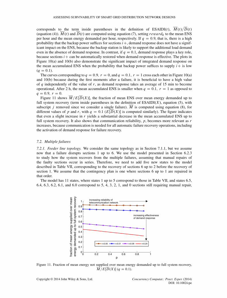
Figure 11 shows M=EŒD.X/�, the fraction of mean ENS over mean energy demanded up tofull system recovery (term inside parentheses in the definition of ESAIDI.X/, equation (5), withsubscript j removed since we consider a single failure). M is computed using equation (8), fordifferent values of p and r , with q D 0:1 (EŒD.X/� is computed similarly). The figure indicatesthat even a slight increase in r yields a substantial decrease in the mean accumulated ENS up tofull system recovery. It also shows that communication reliability, p, becomes more relevant as rincreases, because communication is needed for all automatic failure recovery operations, includingthe activation of demand response for failure recovery.

7.2. Multiple failures

7.2.1. Feeder line topology. We consider the same topology as in Section 7.1.1, but we assumenow that a failure disrupts sections 1 up to 6. We use the model presented in Section 6.2.3to study how the system recovers from the multiple failures, assuming that manual repairs ofthe faulty sections occur in series. Therefore, we need to add five new states to the modeldescribed in Table VII, corresponding to the recovery of sections 6 up to 2 before the recovery ofsection 1. We assume that the contingency plan is one where sections 6 up to 1 are repaired inthat order.

The model has 11 states, where states 1 up to 5 correspond to those in Table VII, and states 6.5,6.4, 6.3, 6.2, 6.1, and 6.0 correspond to 5, 4, 3, 2, 1, and 0 sections still requiring manual repair,

0 0.2 0.4 0.6 0.8 10

0.1

0.2

0.3

0.4

0.5

0.6

0.7

0.8

0.9

1

p

frac

tion

of m

ean

ener

gy s

uppl

ied

over

mea

n e

nerg

y de

man

ded

up to

full

syst

em r

ecov

ery

increasing reliability oftelecommunication network

increasing effectivenessof demand response

Figure 11. Fraction of mean energy not supplied over mean energy demanded up to full system recovery,M=EŒD.X/� (q D 0:1).



respectively (see Section 6.2.3). We use the data in Table III to derive the mean energy supplied andthe mean ENS at each state. The mean ENS at each state per unit time, and a lower bound on themean energy supplied at each state per unit time are shown in Table V.

7.2.1.1. Results for feeder line topology. Figure 12 presents the results for the feeder line topologywherein sections 1–6 fail together. The shapes of the curves in Figure 12 are similar to those inFigure 10, which indicates that the model present qualitative similar behavior in face of one ormultiple failures. Nonetheless, the absolute values of mean ENS and of mean ENS over mean energydemanded are larger in face of multiple failures. After the first section is manually repaired, therepair of the other sections follows an Erlang distribution, therefore increasing not only the meanENS but also the mean time for full system recovery.

Table V. Reward rates: lower bound on energy supplied per hour (ES/h) and energy not supplied perhour (ENS/h).

State 0–1 2 3–4 5 6.5 6.4 6.3 6.2 6.1 6.0

ES/h 0.00 0.00 0.00 211.30 338.27 386.07 397.71 405.64 460.44 542.27ENS/h 542.27 540.87 542.27 329.57 187.32 139.52 116.30 104.30 49.50 0.00

mea

n ac

cum

ulat

ed e

nerg

y

frac

tion

of m

ean

accu

mul

ated

en

ergy

not

sup

plie

d ov

er m

ean

accu

mul

ated

ene

rgy

dem

ande

d

t (hours)

(a) (b)

0

0.1

0.2

0.3

0.4

0.5

0.6

0.7

0.8

0.9

1demand response not enabled (r=0)

low probability thatbackup power suffices to supply i+(q=0.1)


high probability that backup power suffices to supply i+ (q=0.9)

0

500

1000

1500

2000

2500

0 1 2 3 4 5 6 7 8

t (hours)0 1 2 3 4 5 6 7 8

low probability that backup power suffices to supply i+ (q=0.1)




not

sup

plie

d

Figure 12. Scenario with multiple failures in feeder line topology, wherein sections 1–6 fail together and arerecovered progressively (see Section 6.2.3). (a) Mean accumulated energy not supplied, by time t , M.t/,and (b) mean accumulated energy supplied, by time t ,D.t/�M.t/ (p D 0:9). This figure is to be compared

with Figure 10, where a single failure at section 1 occurs.

Figure 13. Case study for radial circuit.



7.2.2. Radial circuit. We consider the DA network benchmark presented by Rudion et al. [14],derived from a German medium voltage distribution network. The network supplies a small townand the surrounding rural area. The load values are taken from Janev [13], without consideringDG in this work. Furthermore, we assume that 10% of the load is amenable to reduction due todemand response.

The resulting network is shown in Figure 13. We assume two failures in sections 4 and 8. Thisleaves three unpowered branches: iC1 with sections 5 and 6, iC2 with sections 9–11, and iC3

with section 7. These unpowered branches can be restored individually by backup substations I,II, and III. The three models, which capture the behavior of the three unpowered branches, areparameterized using Table VI as described in Table VII.

Table VI. Load per section (in kilowatt).

amenable toSection Load demand response Net load

1 59.97 6.00 53.972 0.00 0.00 0.003 59.97 6.00 53.974 65.67 6.57 59.105 65.67 6.57 59.106 65.67 6.57 59.107 56.17 5.62 50.558 65.67 6.57 59.109 56.17 5.62 50.5510 59.97 6.00 53.9711 65.67 6.57 59.10total 620.58 62.06 558.52

Table VII. Reward rates: lower bound on energy supplied per hour (ES/h)and energy not supplied per hour (ENS/h).

State 0–1 2 3–4 5 6

iC1 ES/h 119.94 119.94 119.94 238.14 316.94iC1 ENS/h 197.00 177.30 197.00 65.67 0.00iC2 ES/h 0.00 0.00 0.00 163.62 181.81iC2 ENS/h 181.81 163.62 181.81 0.00 0.00iC3 ES/h 0.00 0.00 0.00 50.55 121.84iC3 ENS/h 121.84 109.65 121.84 65.67 0.00

0

200

400

600

800

1000

1200

1400

1600

1800

2000

0 1 2 3 4 5 6 7 8 0

100

200

300

400

500

600

700

ii

i

i

ii

mea

n ac

cum

ulat

ed e

nerg

y su

pplie

d

mea

n ac

cum

ulat

ed e

nerg

y

t (hours)

(a)

0 1 2 3 4 5 6 7 8

t (hours)

(a)

not s

uppl

ied

Figure 14. Multiple failures in radial topology (a) mean accumulated energy not supplied, by time t , M.t/,by branch, and (b) mean accumulated energy supplied, by time t , by branch, D.t/ �M.t/ (p D 0:9; q D

0:1; r D 0).



7.2.2.1. Results for radial circuit. Next, we present the results obtained with the proposed modelin the setup of Figure 13. Figures 14 and 15 show the average energy supplied and not supplied bytime t , calculated using the phased recovery model described in Section 6.2.4. Figure 14(a) showsthe average energy supplied by time t . Note that the model capturing the set of sections iC1 alsoaccounts for the energy supplied to the downstream sections (sections 1–3 in Figure 13), whichexplains why the average energy supplied calculated using the model for iC1 is larger than the otherones. Similarly, the model capturing the set of section iC3 accounts for section 8 (and the modelcapturing iC2 does not). Figure 14(b) shows the average ENS by time t . As the branches associatedto iC1, iC2, and iC3 have a decreasing number of associated sections, the corresponding curvesindicate that the average ENS is dominated by the model that captures iC1.

Aggregating the results presented in Figure 14(a) and 14(b), we obtain the top curves inFigure 15(a) and 15(b), respectively. Using the same methodology and adapting the model parame-ters, we obtain the other curves shown in Figure 15. Comparing Figure 15 with Figure 10, we notethat the qualitative behavior of the system under multiple failures is the same as the one under asingle failure.

7.3. Discussion

Figure 16 summarizes the empirical results presented in this section. The plots show the aver-age ENS after a failure, as a function of time, for the different setups analyzed earlier. Theseplots illustrate how different survivability-related metrics can be derived using the proposed model

0

200

400

600

800

1000

1200

1400

1600

1800

0 1 2 3 4 5 6 7 8 0

0.1

0.2

0.3

0.4

0.5

0.6

0.7

0.8

0.9low probability that backup power suffices to supply i+ (q=0.1)




t (hours)

(a)

0 1 2 3 4 5 6 7 8

t (hours)

(b)

mea

n ac

cum

ulat

ed e

nerg

y

frac

tion

of m

ean

accu

mul

ated

en

ergy

not

sup

plie

d ov

er m

ean

accu

mul

ated

ene

rgy

dem

ande

d

demand response not enabled (r=0) low probability that

backup power suffices to supply i+(q=0.1)


high probability that backup power suffices to supply i+ (q=0.9)no

t sup

plie

d

Figure 15. Multiple failures in radial topology (a) Mean accumulated energy not supplied, by time t , M.t/,and (b) fraction of mean accumulated energy not supplied over mean accumulated energy demanded, by

time t , M.t/=D.t/ (p D 0:9).

0

100

200

300

400

500

600

0 5 10 15 20 25 30

time (hours)

expe

cted

ene

rgy

not

q=0.1, r=0, p=0.9

q=0.1, r=1, p=0.9

one failure

0

100

200

300

400

500

600

feeder line topology,q=0.1, r=0, p=0.9

feeder line topology,q=0.1, r=1, p=0.9

radial topology,q=0.1, r=1, p=0.9

radial topology,q=0.1, r=0, p=0.9

multiple failures

(a)

0 5 10 15 20 25 30

time (hours)

(b)

supp

lied

per

hour

expe

cted

ene

rgy

not

supp

lied

per

hour

Figure 16. Expected energy not supplied per hour as a function of time after failure considering (a) onefailure and (b) multiple failures.



[16, Figure 1]. Figure 16(a) considers a single failure. Under the same setup as in Section 7.1.1, itindicates that the expected ENS per hour sharply decreases when the demand-response applicationis enabled, and the decay is slower when demand-response is not integrated with FDIR. Figure 16(b)considers the multiple failure setup. The parameters for the feeder line topology and radial topologyare those described in Sections 7.2.1 and 7.2.2, respectively.

With the presented results, investment decisions for the studied circuit can be based on survivabil-ity considerations. With the extended SAIDI as presented in equation (4), different options of how toimprove reliability and survivability can be evaluated and compared with each other. For example,the effect of investing in the reliability of the communication infrastructure (e.g., by adding redun-dancy) can be compared with investing in demand response mechanisms (e.g., by subsidizing smartmeters at the consumer).

8. CONCLUSION

In this paper, we have argued, using analytical models, that new metrics are important to assess thequality of future intelligent power grids. Specifically, it was shown that survivability metrics can beused to drive a holistic engineering approach and are able to capture dynamic behavior of the smartgrid after the occurrence of events of interest, for example, section failures.

We have proposed a methodology to assess the impact of different system parameters on thesurvivability of DA power grids. Specifically, we have shown the interactions between three keyparameters evaluated in this study and their impact on six survivability metrics. The empirical resultsobtained indicate that the integration of demand response with failure recovery can yield signifi-cant reductions in the amount of ENS after a failure. In addition, the communications reliabilityparameter is most important when demand response is integrated.

Under certain independence assumptions, we have shown how the proposed methodology can beadapted to quantify the ENS in face of multiple failures, in the feeder line and radial topologies.Multiple failures will likely occur, for instance, after hurricanes or because of cascades. This workis a first attempt to quantify the survivability of critical systems in such extreme situations.

We believe that our work opens up several avenues for future exploration. Our models can serveto quantify the tradeoffs between investment cost and reliability gains. In face of such tradeoffs,one can devise algorithms to issue recommendations on how to invest on smart grids in light ofprospective survivability gains. Our results illustrate the need for holistic and accurate approachesto guide investment decisions on different parts of the network.

APPENDIX: CLOSED FORM SOLUTIONS

Next, we present closed form solutions to the proposed model. We consider the case in which thetime it takes for a recloser to isolate a section is zero, � D 0 (in practice, it is much smaller than allthe other time intervals considered in the system) and demand response is not integrated with thefailure recovery system, r D 0.

Let Yk be the k-th visited state after a failure, Y0 D 0. Let P.Y1 D j / be the system initialcondition after the failure, which is determined by p and q, P.Y1 D 1/ D pq, P.Y1 D 3/ Dp.1� q/, and P.Y1 D 4/ D 1� p. Let �k.t/ be the probability that the system is at state k at timet , t > 0. Then,

�k.t/ D

6XlD1

�k.t jY1 D l/P.Y1 D l/; k D 1; : : : ; 6 (9)

To compute �k.t jY1 D j /, we note that there is at most one sample path from each state to everyother. Let ‡i;j be the sample path from state i to state j . Let ‡j;i .k/ be the k-th state in thepath ‡j;i , 1 6 k 6 j‡j;i j. Let P.‡j;i / be the probability that Yk D ‡j;i .k/, k D 1; : : : ; j‡j;i j,conditioned on Y1 D j . Then,



�k.t jY1 D j / D �k.t jY1 D j;‡j;i /P.‡j;i / (10)

Substituting equation (10) into equation (9) yields closed form expressions for �k.t/, k D 0; : : : ; 6,

�0.t/ D �2.t/ D 0

�1.t/ D e�.˛Cı/tpqC.e�.�Cı/t�e�.˛Cı/t /

��q.1�p/

˛ � �

��3.t/ D e

�ıtp.1 � q/C .1 � q/.e�t � 1/e�.ıC�/t .1 � p/

�4.t/ D e�.ıC�/t .1 � p/

�5.t/ D .1 � e�˛t /e�ıtpqC

e�ıt �

˛e�.ıC�/t��e�.ıC˛/t

˛ � �

!q.1�p/

�6.t/ D 1 � e�tı

The probability that iC has been recovered by time t is �5[6.t/ and is given by

�5[6.t/ D �5.t/C �6.t/ (11)

We now compute the mean time to fix iC, that is, to reach state 5 or 6 (M , the mean time to reachstate 6, defined by equation (6), follows similarly). To this goal, we consider a Markov chain withstate space 0 and infinitesimal generator Q0 , where is a real valued parameter. The states in 0

are indexed by 1, 3, 4, and ?, and the infinitesimal generator Q0 is obtained from Figure 3 after (i)replacing the transitions to states 5 and 6 by transitions to state ? and (ii) adding transitions fromstate ? to states 1, 3, and 4 with rates pq, p.1 � q/, and .1 � p/, respectively,

Q0 D

266664�.˛ C ı/ 0 0 ˛ C ı

0 �ı 0 ı

�q �.1 � q/ �.ı C �/ ı

pq p.1 � q/ .1 � p/ �

377775

1

3

4

?

(12)

Let � 0 be the steady-state solution of the Markov chain (MC) described earlier, satisfying � 0Q0 D 0and � 01 C �

03 C �

04 C �

0? D 1. Then,

� 01 D ıq.� C ıp/=� (13)

� 03 D .˛ C ı/.1 � q/.� C ıp/=� (14)

� 04 D ı.˛ C ı/.1 � p/=� (15)

� 0? D ı.˛ C ı/.ı C �/=� (16)

where � is a normalization constant to ensure � 01 C �03 C �

04 C �

0? D 1.

Let C be a random variable characterizing the time to reach state ? immediately after leaving?. This corresponds to the mean time to reach states 5 or 6 in the original Markov chain, startingfrom state 0. The mean time to repair iC is given by EŒC �. It follows from equations (13)–(16) and[35, Chapter III] that

EŒC � D �1.1=� 0? � 1/ (17)

Equation (17) is used to obtain the curves in Figure 7.



Let sk.¹5; 6º/ be the mean time spent at state k before reaching state 5 or 6 from state 0 in theoriginal Markov chain, k D 1; 3; 4. It follows from equations (13)–(17) that

sk.¹5; 6º/ D� 0k

�� 01 C �

03 C �

04

� � 1

� 0?� 1

�; k D 1; 3; 4

Let L.¹5; 6º/ be the mean accumulated reward up to reaching state 5 or 6 of the originalMarkov chain,

L.¹5; 6º/ DX

iD1;3;4

ksk.¹5; 6º/ (18)

In this appendix, we have shown how to compute sk.¹5; 6º/, k D 1; 3; 4, andL.¹5; 6º/. The meantime spent at state k before reaching state 6, sk , k D 1; 3; 4; 5, and the mean accumulated rewardup to reaching state 6, L, defined by equation (8), follow similarly. An adaptation of equation (18)is used to obtain the curves in Figure 11.

Although, in this appendix, we assumed that r D 0 and � D 0, a similar approach is applicablewhen r > 0 or � > 0.

ACKNOWLEDGEMENTS

This work was supported in part by grants from CNPq, FAPERJ/ Brazil, and Siemens Corporate Research,Inc.

REFERENCES

1. Ma Z. Towards a unified definition for reliability, survivability and resilience (I): the conceptual framework inspiredby the handicap principle and ecological stability. Aerospace Conference, 2010 IEEE, Big Sky, Montana, USA,March 2010; 1–12.

2. Koziolek A, Happe L, Avritzer A, Suresh S. A common analysis framework for smart distribution networks appliedto survivability analysis of distribution automation. 2012 International Workshop on Software Engineering for theSmart Grid (SE4SG), Zurich, Switzerland, June 2012; 23–29.

3. Menasché D, Leão RMM, de Souza e Silva E, Avritzer A, Suresh S, Trivedi K, Marie RA, Happe L,Koziolek A. Survivability analysis of power distribution in smart grids with active and reactive power modeling.Greenmetrics Workshop (to appear in special issue of Performance Evaluation Review), London, England, 2012.http://www.sigmetrics.org/greenmetrics/2012/papers/Menasche.pdf.

4. Avritzer A, Suresh S, Menasché DS, Leão RMM, de Souza e Silva E, Diniz MC, Trivedi K, Happe L,Koziolek A. Survivability models for the assessment of smart grid distribution automation network designs.Proceedings of the ACM/SPEC International Conference on International Conference on Performance Engineering,Prague, Czech Republic, 2013; 241–252.

5. Brown ER. Electric Power Distribution Reliability (2nd edn). CRC Press: Boca Raton, Florida, 2002.6. Elmakias DE. New Computational Methods in Power System Reliability. Springer: New York, USA, 2010.7. Chowdhury AA, Agarwal S, Koval D. Reliability modeling of distributed generation in conventional distribution

systems planning and analysis. IEEE Transactions on Industry Applications 2003; 39(5):1493–1498.8. Waseem I. Impacts of distributed generation on the residential distributed network operation. M.Sc. Thesis, Virginia

Polytechnic Institute, 2008.9. Moslehi K, Kumar R. A reliability perspective of the smart grid. IEEE Transactions on Smart Grid 2010; 1(1):57–64.

10. Zou K, Keerthipala W, Perera S. SAIDI minimization of a remote distribution feeder. AUPEC 2007, Perth, WesternAustralia, 2007dec.; 1–5.

11. Wang S, Zhao W, Chen Y. Distribution system reliability evaluation considering DG impacts. International Confer-ence of the Electric Utility Deregulation and Restructuring and Power Technologies, Nanjing, China, April 2008;2603–2607.

12. Zhang J, Bo Z. Research of the impact of distribution generation on distribution network loss. Universities PowerEngineering Conference 2010, Cardiff, Wales, September 2010; 1–4.

13. Janev V. Implementation and evaluation of a distribution load flow algorithm for networks with distributedgeneration. M.Sc. Thesis, Swiss Federal Institute of Technology, Zurich, 2009.

14. Rudion K, Orths A, Styczynski Z, Strunz K. Design of benchmark of medium voltage distribution network forinvestigation of DG integration. Power Engineering Society General Meeting, 2006. IEEE, Montreal, Canada,2006; 6.


http://www.sigmetrics.org/greenmetrics/2012/papers/Menasche.pdf


15. Martins V, Borges C. Active distribution network integrated planning incorporating distributed generation and loadresponse uncertainties. Power Systems, IEEE Transactions on 2011; 26(4):2164–2172.

16. Heegaard PE, Trivedi KS. Network survivability modeling. Computer Networks 2009; 53(8):1215–1234.17. Meyer J. On evaluating the performability of degradable computing systems. IEEE Transactions on Computers 1980;

29:720–731.18. Meyer JF. Performability: a retrospective and some pointers to the future. Performance evaluation 1992; 14:139–156.19. Liu Y, Trivedi K. Survivability quantification: the analytical modeling approach. International Journal of Performa-

bility Engineering 2006; 2(1):29–44.20. Keshav S, Rosenberg C. How internet concepts and technologies can help green and smarten the electrical grid. ACM

SIGCOMM Computer Communication Review 2011; 41(1):109–114.21. Ghosh R, Kim D, Trivedi KS. System resiliency quantification using non-state-space and state-space analytic models.

Reliability Engineering and System Safety 2013; 116:1–29.22. ANSI T1A1.2. Working group on network survivability performance. Technical Report on enhanced network

survivability performance. TR No 68, ANSI, 2001.23. de Souza e Silva E, Gail R. Computational Probability. Kluwer: Alphen aan den Rijn, South Holland, 2000.24. Trivedi KS. Probability & Statistics with Reliability, Queuing and Computer Science Applications. John Wiley &

Sons: Hoboken, NJ, USA, 2008.25. Short T. Electric Power Distribution Handbook. CRC: Hoboken, NJ, USA, 2003.26. Liu Y, Mendiratta V, Trivedi K. Survivability analysis of telephone access network. Issre, Saint-Malo, Bretagne,

France, November 2004; 367–377.27. Grassmann W, Taksar MI, Heyman D. Regenerative analysis and steady state distributions for Markov chains.

Operations Research 1985; 33(5).28. de Souza e Silva E, Leão RM, Marie R. Efficient transient analysis of Markovian models using a block reduction

approach. INFORMS Journal on Computing Fall 2013; 25(4):743–757.29. Reibman A, Trivedi K. Numerical transient analysis of Markov models. Computers & Operations Research 1988;

15(1):19–36.30. Boudec JYL, Tomozei D. Satisfiability of elastic demand in the smart grid. Energy, New York, NY, USA, 2011.31. Horváth A, Paolieri M, Ridi L, Vicario E. Transient analysis of non-markovian models using stochastic state classes.

Performance Evaluation 2012; 69(7):315–335.32. de Souza e Silva E, Figueiredo DR, Leão RMM. The TANGRAM-II integrated modeling environment for computer

systems and networks. SIGMETRICS Performance Evaluation Review 2009; 36(4):64–69.33. de Souza e Silva E, Gail HR. The uniformization method in performability analysis. In Performability Modeling:

Techniques and Tools. John Wiley & Sons: Hoboken, NJ, USA, 2001.34. Wikipedia. HurricaneSandy, 2013. (Available from: http://en.wikipedia.org/wiki/Hurricane_Sandy) [access on

3 March 2014].35. Kemeny J, Snell J. Finite Markov Chains. Springer, 1983.


http://en.wikipedia.org/wiki/Hurricane_Sandy

Assessing survivability of smart grid distribution network designs accounting for multiple failures

Documents

Transcript of Assessing survivability of smart grid distribution network designs accounting for multiple failures