Chapter 5 Failures Resulting from Static Loading
66
Chapter 5 Failures Resulting from Static Loading Lecture Slides
-
Upload
khangminh22 -
Category
Documents
-
view
0 -
download
0
Transcript of Chapter 5 Failures Resulting from Static Loading

Chapter 5
Failures Resulting from
Static Loading
Lecture Slides

Chapter Outline
Shigley’s Mechanical Engineering Design

Failure Examples
Failure of truck driveshaft spline due to corrosion fatigue
Shigley’s Mechanical Engineering Design
Fig. 5–1
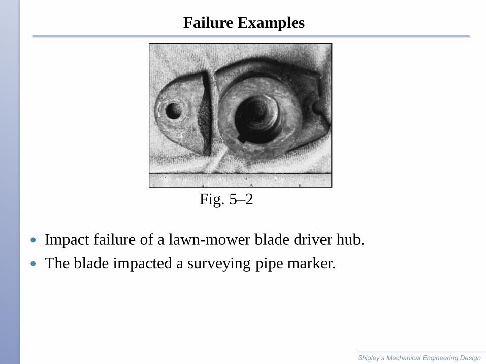
Failure Examples
Impact failure of a lawn-mower blade driver hub.
The blade impacted a surveying pipe marker.
Shigley’s Mechanical Engineering Design
Fig. 5–2

Failure Examples
Failure of an overhead-pulley retaining bolt on a weightlifting
machine.
A manufacturing error caused a gap that forced the bolt to take
the entire moment load.
Shigley’s Mechanical Engineering Design
Fig. 5–3

Failure Examples
Chain test fixture that failed in one cycle.
To alleviate complaints of excessive wear, the manufacturer decided to
case-harden the material
(a) Two halves showing brittle fracture initiated by stress concentration
(b) Enlarged view showing cracks induced by stress concentration at
the support-pin holes Shigley’s Mechanical Engineering Design
Fig. 5–4

Failure Examples
Valve-spring failure caused by spring surge in an oversped
engine.
The fractures exhibit the classic 45 degree shear failure
Shigley’s Mechanical Engineering Design
Fig. 5–5

Static Strength
Failure of the part would endanger human life, or the part is made in
extremely large quantities; consequently, an elaborate testing program
is justified during design.
The part is made in large enough quantities that a moderate series of
tests is feasible.
The part is made in such small quantities that testing is not justified at
all; or the design must be completed so rapidly that there is not enough
time for testing.
Experimental test data is better, but generally only warranted for large
quantities or when failure is very costly (in time, expense, or life)
The part has already been designed, manufactured, and tested and
found to be unsatisfactory. Analysis is required to understand why the
part is unsatisfactory and what to do to improve it.
Shigley’s Mechanical Engineering Design

Ductility and Percent Elongation
Ductility is the degree to which a material will deform before
ultimate fracture.
Percent elongation is used as a measure of ductility.
Ductile Materials have % Ɛ 5%
Brittle Materials have % Ɛ < 5%
For machine members subject to repeated or shock or impact
loads, materials with % Ɛ > 12% are recommended.

Ductile materials - extensive plastic deformation and
energy absorption (toughness) before fracture
Brittle materials - little plastic deformation and low energy
absorption before failure

• Ductile
fracture is
desirable!
• Classification:
Ductile:
warning before
fracture
Brittle: No
warning
DUCTILE VS BRITTLE FAILURE
(a) (b) (c)

• Resulting
fracture
surfaces
(steel)
particles serve as void
nucleation sites.
50 µm
DUCTILE FAILURE
1 µm = 1 X 10⁻⁶ m = 0.001 mm
• Evolution to failure:
“cup and cone” fracture

Stress Concentration
Localized increase of stress near discontinuities
Kt is Theoretical (Geometric) Stress Concentration Factor
Shigley’s Mechanical Engineering Design

Theoretical Stress Concentration Factor
Graphs available for
standard configurations
See Appendix A–15 and
A–16 for common
examples
Many more in Peterson’s
Stress-Concentration
Factors
Note the trend for higher
Kt at sharper discontinuity
radius, and at greater
disruption
Shigley’s Mechanical Engineering Design

Stress Concentration for Static and Ductile Conditions
With static loads and ductile materials
◦ Highest stressed fibers yield (cold work)
◦ Load is shared with next fibers
◦ Cold working is localized
◦ Overall part does not see damage unless ultimate strength is
exceeded
◦ Stress concentration effect is commonly ignored for static
loads on ductile materials
Stress concentration must be included for dynamic loading (See
Ch. 6)
Stress concentration must be included for brittle materials, since
localized yielding may reach brittle failure rather than cold-
working and sharing the load.
Shigley’s Mechanical Engineering Design

Need for Static Failure Theories
Failure theories are used to predict if failure would occur under
any given state of stress
The generally accepted theories are:
Ductile materials (yield criteria)
oMaximum shear stress (MSS),
oDistortion energy (DE),
oDuctile Coulomb-Mohr (DCM),
Brittle materials (fracture criteria)
oMaximum normal stress (MNS),
oBrittle Coulomb-Mohr (BCM),
oModified Mohr (MM),
Shigley’s Mechanical Engineering Design

Maximum Shear Stress Theory (MSS)
Theory: Yielding begins when the maximum shear stress in a
stress element exceeds the maximum shear stress in a tension
test specimen of the same material when that specimen begins to
yield.
For a tension test specimen, the maximum shear stress is s1 /2.
At yielding, when s1 = Sy, the maximum shear stress is Sy /2 .
Could restate the theory as follows:
◦ Theory: Yielding begins when the maximum shear stress in a
stress element exceeds Sy/2.
Shigley’s Mechanical Engineering Design

Maximum Shear Stress Theory (MSS)
For any stress element, use Mohr’s circle to find the maximum
shear stress. Compare the maximum shear stress to Sy/2.
Ordering the principal stresses such that s1 ≥ s2 ≥ s3,
Incorporating a design factor n
Or solving for factor of safety
Shigley’s Mechanical Engineering Design
max
/ 2ySn

Maximum Shear Stress Theory (MSS)
To compare to experimental data, express max in terms of
principal stresses and plot.
To simplify, consider a plane stress state (one of the principal
stress is zero)
Let sA and sB represent the two non-zero principal stresses, then
order them with the zero principal stress such that s1 ≥ s2 ≥ s3
Assuming sA ≥ sB there are three cases to consider
◦ Case 1: sA ≥ sB ≥ 0
◦ Case 2: sA ≥ 0 ≥ sB
◦ Case 3: 0 ≥ sA ≥ sB
Shigley’s Mechanical Engineering Design

Maximum Shear Stress Theory (MSS)
Case 1: sA ≥ sB ≥ 0
◦ For this case, s1 = sA and s3 = 0
◦ Eq. (5–1) reduces to sA ≥ Sy
◦ sA = Sy/n.
Case 2: sA ≥ 0 ≥ sB
◦ For this case, s1 = sA and s3 = sB
◦ Eq. (5–1) reduces to sA − sB ≥ Sy
◦ (sA − sB ) = Sy/n.
Case 3: 0 ≥ sA ≥ sB
◦ For this case, s1 = 0 and s3 = sB
◦ Eq. (5–1) reduces to sB ≤ −Sy
◦ sB = -Sy/n.
Shigley’s Mechanical Engineering Design

Maximum Shear Stress Theory (MSS)
Plot three cases on
principal stress axes
Case 1: sA ≥ sB ≥ 0
◦ sA ≥ Sy
Case 2: sA ≥ 0 ≥ sB
◦ sA − sB ≥ Sy
Case 3: 0 ≥ sA ≥ sB
◦ sB ≤ −Sy
Other lines are
symmetric cases
Inside envelope is
predicted safe zone
Shigley’s Mechanical Engineering Design
Fig. 5–7

Maximum Shear Stress Theory (MSS)
Comparison to
experimental data
Conservative in all
quadrants
Commonly used for
design situations
Shigley’s Mechanical Engineering Design

Distortion Energy (DE) Failure Theory
Also known as:
◦ Octahedral Shear Stress
◦ Shear Energy
◦ Von Mises
◦ Von Mises – Hencky
Shigley’s Mechanical Engineering Design

Distortion Energy (DE) Failure Theory
Originated from observation that ductile materials stressed
hydrostatically (equal principal stresses) exhibited yield
strengths greatly in excess of expected values.
Theorizes that if strain energy is divided into hydrostatic
volume changing energy and angular distortion energy, the
yielding is primarily affected by the distortion energy.
Shigley’s Mechanical Engineering Design
Fig. 5–8

Distortion Energy (DE) Failure Theory
Theory: Yielding occurs when the distortion strain energy per
unit volume reaches the distortion strain energy per unit volume
for yield in simple tension or compression of the same material.
Shigley’s Mechanical Engineering Design
Fig. 5–8
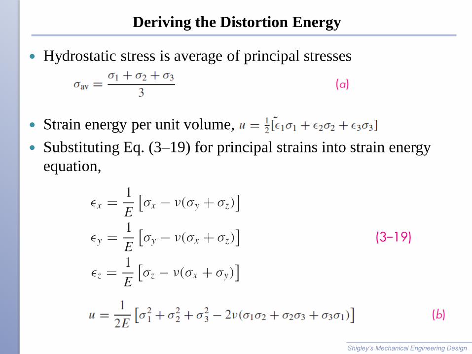
Deriving the Distortion Energy
Hydrostatic stress is average of principal stresses
Strain energy per unit volume,
Substituting Eq. (3–19) for principal strains into strain energy
equation,
Shigley’s Mechanical Engineering Design
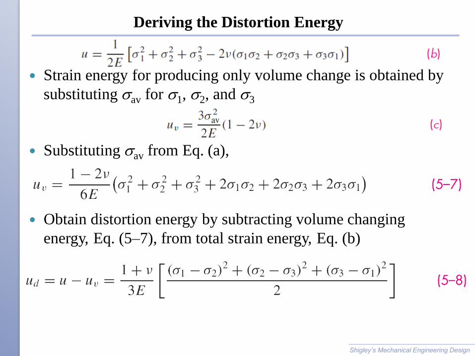
Deriving the Distortion Energy
Strain energy for producing only volume change is obtained by
substituting sav for s1, s2, and s3
Substituting sav from Eq. (a),
Obtain distortion energy by subtracting volume changing
energy, Eq. (5–7), from total strain energy, Eq. (b)
Shigley’s Mechanical Engineering Design

Deriving the Distortion Energy
Tension test specimen at yield has s1 = Sy and s2 = s3 =0
Applying to Eq. (5–8), distortion energy for tension test
specimen is
DE theory predicts failure when distortion energy, Eq. (5–8),
exceeds distortion energy of tension test specimen, Eq. (5–9)

Von Mises Stress
Left hand side is defined as von Mises stress
For plane stress, simplifies to
In terms of xyz components, in three dimensions
In terms of xyz components, for plane stress

Distortion Energy Theory With Von Mises Stress
Von Mises Stress can be thought of as a single, equivalent, or
effective stress for the entire general state of stress in a stress
element.
Distortion Energy failure theory simply compares von Mises
stress to yield strength.
Introducing a design factor,
Expressing as factor of safety,
ySn
s

Failure Theory in Terms of von Mises Stress
Equation is identical to Eq. (5–10) from Distortion Energy
approach
Identical conclusion for:
◦ Distortion Energy
◦ Octahedral Shear Stress
◦ Shear Energy
◦ Von Mises
◦ Von Mises – Hencky
Shigley’s Mechanical Engineering Design
ySn
s

DE Theory Compared to Experimental Data
Plot von Mises stress on
principal stress axes to
compare to experimental
data (and to other failure
theories)
DE curve is typical of data
Note that typical equates to
a 50% reliability from a
design perspective
Commonly used for
analysis situations
MSS theory useful for
design situations where
higher reliability is desired
Shigley’s Mechanical Engineering Design
Fig. 5–15

Shear Strength Predictions
Shigley’s Mechanical Engineering Design
For pure shear loading, Mohr’s circle shows that sA = −sB =
Plotting this equation on principal stress axes gives load line for
pure shear case
Intersection of pure shear load line with failure curve indicates
shear strength has been reached
Each failure theory predicts shear strength to be some fraction of
normal strength
Fig. 5–9

Example 5-1

Example 5-1

Example 5-1

Example 5-1
Shigley’s Mechanical Engineering Design Fig. 5−11

Mohr Theory
Some materials have compressive strengths different from
tensile strengths
Mohr theory is based on three simple tests: tension,
compression, and shear
Plotting Mohr’s circle for each, bounding curve defines failure
envelope
Shigley’s Mechanical Engineering Design
Fig. 5−12

Coulomb-Mohr Theory
Curved failure curve is difficult to determine analytically
Coulomb-Mohr theory simplifies to linear failure envelope using
only tension and compression tests (dashed circles)
Shigley’s Mechanical Engineering Design
Fig. 5−13

Coulomb-Mohr Theory
From the geometry, derive
the failure criteria
Shigley’s Mechanical Engineering Design
Fig. 5−13

Coulomb-Mohr Theory
To plot on principal stress axes, consider three cases
Case 1: sA ≥ sB ≥ 0 For this case, s1 = sA and s3 = 0
◦ Eq. (5−22) reduces to
Case 2: sA ≥ 0 ≥ sB For this case, s1 = sA and s3 = sB
◦ Eq. (5-22) reduces to
Case 3: 0 ≥ sA ≥ sB For this case, s1 = 0 and s3 = sB
◦ Eq. (5−22) reduces to
Shigley’s Mechanical Engineering Design

Coulomb-Mohr Theory
Plot three cases on principal stress axes
Similar to MSS theory, except with different strengths for
compression and tension
Shigley’s Mechanical Engineering Design
Fig. 5−14

Coulomb-Mohr Theory
Incorporating factor of safety
For ductile material, use tensile and compressive yield strengths
For brittle material, use tensile and compressive ultimate
strengths
Shigley’s Mechanical Engineering Design
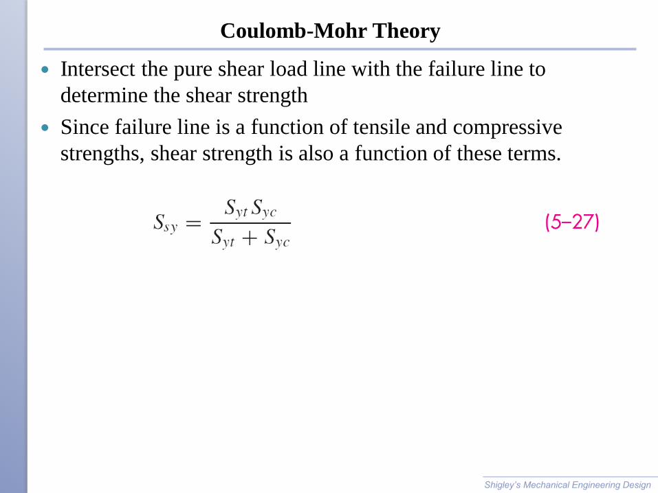
Coulomb-Mohr Theory
Intersect the pure shear load line with the failure line to
determine the shear strength
Since failure line is a function of tensile and compressive
strengths, shear strength is also a function of these terms.
Shigley’s Mechanical Engineering Design

Example 5-2
Shigley’s Mechanical Engineering Design

Example 5-2
Shigley’s Mechanical Engineering Design

Example 5-3
Shigley’s Mechanical Engineering Design Fig. 5−16

Example 5-3
Shigley’s Mechanical Engineering Design

Example 5-3
Shigley’s Mechanical Engineering Design

Example 5-4
Shigley’s Mechanical Engineering Design
Fig. 5−17

Shigley’s Mechanical Engineering Design

Example 5-4
Shigley’s Mechanical Engineering Design Fig. 5−17

Example 5-4
Shigley’s Mechanical Engineering Design

Example 5-4
Shigley’s Mechanical Engineering Design

Failure of Ductile Materials Summary
Either the maximum-shear-stress
theory or the distortion-energy
theory is acceptable for design and
analysis of materials that would fail
in a ductile manner.
For design purposes the
maximum-shear-stress theory is
easy, quick to use, and
conservative.
If the problem is to learn why a part
failed, then the distortion-energy
theory may be the best to use.
For ductile materials with unequal
yield strengths, Syt in tension and
Syc in compression, the Mohr
theory is the best available.

Maximum-Normal-Stress Theory for Brittle Materials
The maximum-normal-stress (MNS)
theory states that failure occurs whenever
one of the three principal stresses equals
or exceeds the ultimate strength.
For a general stress state in the ordered
form σ1 ≥ σ2 ≥ σ3. This theory then
predicts that failure occurs whenever
where Sut and Suc are the ultimate tensile
and compressive strengths, respectively,
given as positive quantities.
MNS theory is not very good at predicting
failure in the fourth quadrant of the sA,
sB plane. Hence not recommended for
use (has been added for historical reason!)

Maximum Normal Stress Theory
Theory: Failure occurs when the maximum principal stress in a
stress element exceeds the strength.
Predicts failure when
For plane stress,
Incorporating design factor,
Shigley’s Mechanical Engineering Design

Brittle Coulomb-Mohr
Same as previously derived, using ultimate strengths for failure
Failure equations dependent on quadrant
Shigley’s Mechanical Engineering Design
Quadrant condition Failure criteria
Fig. 5−14

Brittle Failure Experimental Data
Coulomb-Mohr is
conservative in 4th quadrant
Modified Mohr criteria
adjusts to better fit the data
in the 4th quadrant
Shigley’s Mechanical Engineering Design
Fig. 5−19

Modified-Mohr
Shigley’s Mechanical Engineering Design
Quadrant condition Failure criteria

Example 5-5
Shigley’s Mechanical Engineering Design
Fig. 5−16

Example 5-5
Shigley’s Mechanical Engineering Design
Table A24,
P1046

Example 5-5
Shigley’s Mechanical Engineering Design

Selection of Failure Criteria
First determine ductile vs. brittle
For ductile
◦ MSS is conservative, often used for design where higher
reliability is desired
◦ DE is typical, often used for analysis where agreement with
experimental data is desired
◦ If tensile and compressive strengths differ, use Ductile
Coulomb-Mohr
For brittle
◦ Mohr theory is best, but difficult to use
◦ Brittle Coulomb-Mohr is very conservative in 4th quadrant
◦ Modified Mohr is still slightly conservative in 4th quadrant, but
closer to typical
Shigley’s Mechanical Engineering Design

Selection of Failure Criteria in Flowchart Form
Shigley’s Mechanical Engineering Design
Fig. 5−21