Assessing Asphalt and Concrete Pavement Surface Texture in ...

Journal of Engineering Volume 22 May 2016 Number 5

92

Assessing Asphalt and Concrete Pavement Surface Texture in the Field

Saad I. Sarsam Huda N. Al Shareef

Professor MSc. Student

College of Engineering/ University of Baghdad College of Engineering/ University of Baghdad

E-Mail: [email protected] E-Mail: [email protected]

ABSTRACT

The incorporation of safety characteristics into the traditional pavement structural design or in the

functional evaluation of pavement condition has not been established yet. The design has focused

on the structural capacity of the roadway so that the pavement can withstand specific level of

repetitive loading over the design life. On the other hand, the surface texture condition was neither

included in the AASHTO design procedure nor in the present serviceability index measurements.

The pavement surface course should provide adequate levels of friction and ride quality and

maintain low levels of noise and roughness. Many transportation departments perform routine skid

resistant testing, the type of equipment used for testing varies depending on the preference of each

transportation department. It was felt that modeling of the surface texture condition using different

methods of testing may assist in solving such problem. In this work, Macro texture and Micro

texture of asphalt and cement concrete pavement surface have been investigated in the field using

four different methods (The Sand Patch Method, Outflow Time Method, British Pendulum Tester

and Photogrammetry Technique). Two different grain sizes of sand have been utilized in conducting

the Sand Patch while the Micro texture was investigated using the British Pendulum tester method

at wet pavement surface conditions. The test results of the four methods were correlated to the skid

number. It was concluded that such modeling could provide instant data in the field for pavement

condition which may help in pavement maintenance management.

Keywords: texture, pavement, surface condition, testing, modeling.

موقعيا للرصفة السطح االسفلتي والخرساني جةتقييم نس سعد عيسي سرسم هدى نضر الشريف

طانبت ياجسخش اسخار

جايؼت بغذاد, كهت انهذست, لسى انهذست انذت جايؼت بغذاد, كهت انهذست, لسى انهذست انذت

الخالصة

ىظف نظشوف انشصفت نى حؼخذ نحذ ا. انخصى سكض يساهت خصائص انساليت ف حصى انشصفت انخمهذ او ف انخمى ان

ػه انمذسة انهكهت نهطشك بحث ا انشصفت ك ا حسذ يسخىي يؼ ي انخحم انخكشس طهت ػش انشصفت. ي احت

نشصفت ا سطح ا ( وال ف لاساث يؤشش خذيت انطشك.AASHTOاخشي ظشوف سجت انسطح نى حض ف خطىاث حصى )

اػخذث .انحفاظ ػه يسخىاث يخفضت ي انضىضاء وانخشىتجب ا ىفش يسخىاث كافت ي االحخكان, ىػت انمادة, و

انؼذذ ي الساو انمم اخخباس يماويت اضالق سوح, ىع انؼذاث انسخخذيت ف االخخباسخخهف اػخادا ػه انفضم نذي الساو

ظشوف سج انسطح باسخخذاو طشق يخخهفت نالخخباس ك ا حساػذ ف حم يثم هكزا يشكهت. زجت بأانمم. نمذ حب

ف هز انذساست, اخخبشث يىلؼا انسجت اناكشوت, وانسجت اناكشوت نهشصفت االسفهخت وانشصفت انكىكشخت بأسخخذاو اسبغ

انبشطا, وحمت انفىحىكشايخش(. ىػ يخخهف ي انشيم طشق )طشمت سلؼت انشيم, صي جشا اناء, جهاص انبذول

نبشطا ػه سطح انخىل اػخذ ف طشمت سلؼت انشيم با انسجت اناكشوت اخخبشث باسخخذاو طشمت جهاص انبذول ا

كزا زجت حسخطغ ا حىفش خائج االخخباس نالسبغ طشق زجج وسبطج ف سلى اضالق. ونمذ اسخخج ا يثم ه انشصفت انشطبت.

ا حساػذ ف اداسة صات انشصفت. بااث نحظت يىلؼا نظشوف انخبهظ انخ ك

mailto:[email protected]



03

.: نسجة السطح, الرصفة, حالة السطح, الفحص, النمذجة الكممات الرئيسية1. INTRODUCTION

1.1 General

Deterioration of the pavement surface (smoothing or polishing of the pavement surface), along with

surface water accumulation in the form of rain, snow, or ice, can result in inadequate provision of

skid resistance. Inadequate skid resistance can lead to higher incidences of skid related crashes,

Sarsam, 2009-a. There is currently no agreement on what standards to use for optimizing skid

resistance, or on a standardized testing procedure to adopt despite a significant amount of research

conducted. Roadway pavements surface deteriorate with time as a result of traffic passes,

environmental conditions, and poor pavement maintenance management. If this deterioration is not

properly addressed, the amount of surface distress that can affect skid resistance will increase and

be prejudicial to traffic, Noyce et al, 2007. In this sense, pavement surface characteristics are a

significant issue because of its influence in preserving roadway safety. Maintaining these

characteristics during pavement construction or rehabilitation may mitigate or even prevent crashes

and incidents related to loss of vehicle control, hydroplaning, and/or excessive skidding, Masad et

al, 2010 . The surface quality of a pavement determines to a large degree the conditions under

which safety can be maintained. Driver control of vehicles is strongly dependent upon pavement

surface characteristics, geometrics, driver speed, and vehicle variables such as tire pressure, type of

tread, and wheel loads. Important surface characteristics include pavement micro texture, macro

texture, and drainage attributes, Sarsam, 2009-b. Loss of adhesion between vehicle`s tires and the

road surface occurs in many road accidents whether or not it is the actual cause of the accident.

Over the years, tire manufacturers have done a lot of research into different types of rubber and

tread pattern to improve the safety of motor vehicles. The pavement- tire interaction is affected by

the texture characteristics of the pavement such as the coefficient of friction, skid resistance, and

hydroplaning effect on wet surface, Noyce et al, 2005. Until recently, the most common test

methods for determining macro texture were labor intensive and time consuming. New

developments in high resolution profiler have produced methods for estimating macro texture depth

at different speeds, Fuentes et al, 2010. The fundamental questions that need to be addressed are:

(1) How effectively and simply does such equipment characterize pavement micro and macro

texture?

(2) How this information could be used if it were available.

1.2 Research Objectives

The main objectives of this research work are:

a.) Evaluating the cement concrete and asphalt concrete pavement surface condition from the skid

resistance point of view using field tests. The micro and macro textures were evaluated using four

different testing techniques.

b.) Evaluating the significance, feasibility of using such different field tests to measure the skid

resistance.

2. MATERIALS AND METHODS

This field work was conducted at University of Baghdad in Aljadriah campus roadway, and

walkway network. Rigid pavement and flexible pavement were tested, 150 locations have been

selected for each pavement type. The distance between one location and another was 1.2 meter

minimum. Every test location was prepared for testing by thoroughly sweeping using a plastic

brush. Then, the location was visually examined so that various pavement texture could be


03

included, and each test location does not contain any cracks or irregularities. Then, each location

was subjected to the texture determination by using various testing procedures. Similar work was

reported by Sarsam, 2011.

2.1 Sand Patch Test:

A specific volume of each type of graded sand prepared in the laboratory by sieving (passing

sieve no. 25 and retained on sieve No. 52) was spread by using a specific plastic tool on the

pavement surface in a circular motion. Two types of graded sand were used. Table 1 shows the

types of sand and their densities. Then, the mean texture depth (MTD) was calculated by using

equation (4), ASTM, 2009.

2.2 Outflow Time:

The outflow time (OFT) was measured by using the outflow meter. Outflow meter was

manufactured in local market by using plastic transparent jar of 1000 ml capacity rests on rubber

annulus placed on the pavement. A valve at the bottom of the cylinder is closed and the cylinder is

filled with water. The valve is then opened and the time required for cylinder to be empty is

measured with a stopwatch and was reported as the outflow time (OFT). This test was conducted in

accordance to ASTM, 2009, standard procedures for determining outflow time.

2.3 British Pendulum Test:

British Pendulum Tester is operated by releasing a pendulum from a height that is adjusted so

that a rubber slider on the pendulum head contacts the pavement surface over a fixed length.

Friction between the slider and the pavement surface reduces the kinetic energy of the head, and the

reduced kinetic energy is converted to potential energy as the pendulum breaks contact with the

surface and approaches its maximum recovered height. The pavement surface was wetted with 1000

ml of water to ensure that the surface voids are saturated, and the temperature was fixed at (25±3)ºC

during the work to prevent the effect of temperature on the British Pendulum test results. The

difference between the initial and recovered pendulum heights represents the loss in energy due to

friction between the slider and the pavement surface. The BPT is equipped with a scale that

measures the recovered height of the pendulum in terms of British Pendulum Number (BPN). The

slip speed of the BPN is very slow (typically about 6 mph). This test was conducted in accordance

to ASTM, 2009, standard procedures for determining British Pendulum Number.

2.4 Photogrammetry Technique

2.4.1 Direct Geo-referencing

Image orientation is a key element in any photogrammetric project, since the determination of

three-dimensional coordinates from images require the image orientation to be known. In aerial

Photogrammetry this task has been exclusively and very successfully solved by using aerial

triangulation for many decades. Thus, aerial triangulation has become a key technology and an

important cost factor in mapping and Geographic Information System (GIS), Jasim, 2011. In this

work, there was two cameras their brand Panasonic fz50 orthogonally positioned on the pavement

surface by using a frame designed and manufactured especially for this research work. Where

Exterior Orientation Parameters (EOP) were defined such as height of flight and it was 1.2 m, and

the rotation angles (ω, φ, κ) , so there was no need to Differential Global Position System Receiver

(DGPS), and Inertial Navigation System (INS) as they are used for determining EOP for direct geo-


09

reference. The distance between the centers of the cameras lenses was 53.4 cm. The overlap

between the two shots was 45%. This technique was adopted for 15 shot locations on rigid

pavement and 15 shot locations on flexible pavement. The camera properties were mentioned in

Table 2. The stereo photo pair were fed to the ERDAS 8.4 software that has been used for image

processing. This procedure was in agreement with the work reported by Sarsam and AL Shareef,

2015.

2.4.2 Image processing procedure adopted

Two overlap shots for each location were inserted in ERDAS 8.4 software. Pyramid layers

were generated for every shot. Cameras properties, interior and exterior orientation such as height

of flight and three rotation angles (ω, φ, κ). Such shots locations were the same for the previous

testing techniques. The software convert the two overlap shots to a three dimensional photo and

calculate the texture depth by selecting several tie points in every two shots, and aerial

triangulation process was applied. Such procedure was in agreement with Sarsam et al, 2015-a.

3. MODELING OF PAVEMENT SURFACE TEXTURE

An effort has been made to find a direct relationship between micro and macro texture, using BPN,

Outflow Time, Mean Texture Depth (Sand Patch Method and Photogrammetry Technique). Many

statistics software have been tried including Statistica, SPSS, and ANN but the models were weak

from the statistical point of view. So it was decided to examine the feasibility of using the indirect

correlation using the well-known mathematical models of skid resistance and skid number (SN) as

shown in equations 1, 2, and 3.

SN = SNo. Exp – (PNG / 100 ) V

(1)

SNo = 1.32 BPN – 34.9 (2)

PNG = 0.157 (MTD) – 0.47 (3)

Where:

SN: Skid Number.

SNo: Skid Number at Zero Speed.

PNG: Percent Normalized Gradient.

V: Vehicle Speed.

BPN: British Pendulum Number (percent).

MTD: Mean Texture Depth (cm).

MTD was calculated from sand patch method by using both river and silica sand. The

mathematical equation used is illustrated below, ASTM, 2009:

MTD = (4)

Where:

V: volume of the sand (cm³).

D: diameter of the circular patch of the sand (cm).


00

Another mathematical expression (equation 5) was obtained from the literature, Noyce et al.,

2005, which correlate OFT with MTD and implemented in the SN calculation. Two cases of such

relation have been tried, the first one is to calculate MTD using the equation below:

MTD = (5)

Where:

MTD: Mean texture depth (cm).

OFT: Outflow time (seconds).

It was found that the relation could give MTD close to one cm, then the second case tried was to

take MTD value equivalent to OFT. Such finding was further supported when plotting the OFT

calculated using both calculation cases as demonstrated in Fig.1 for asphalt concrete.

3.1 Asphalt Concrete Pavement

3.1.1 Effect of Sand Gradation Type on Skid Number

Fig. 2 illustrates the relationship between SN when using two different sand types in the sand patch

test (fine and coarse sand). It shows that the effect of sand type on skid number was not significant

for the range of sand types adopted, the coefficient of determination was 0.9997. Such results

agrees well with the work of Sarsam, 2009-a.

3.1.2 Effect of Testing Technique on Skid Number

Fig. 3, 4, 5, and 6 show the variation of skid number when two testing techniques were

implemented. The SN calculated using sand patch (natural sand) or (silica sand) was plotted on the

x-axis, while the SN calculated using OFT equivalent to MTD or calculated from Equation 5 was

plotted on y-axis. Both figures indicate very good statistical relationship, however, it was noticed

that at high values of skid number, (above 30), the mode start to change, and the scatter of test

results are away from the trend line. Such behavior correlates well with Doty, 1974; and Sarsam,

2012 findings.

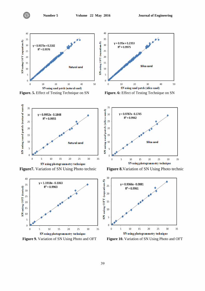
3.1.3 Effect of Photogrammetry testing technique on Skid Number

Fig. 7, 8, 9, and 10 shows the variation of skid number when three testing techniques were

implemented, the SN calculated using MTD obtained from photogrammetry technique was plotted

on the x-axis, while the SN calculated using sand patch (silica and natural) sand and OFT

equivalent to MTD or calculated from Equation 5 were plotted on y-axis. Each figure indicates

very good statistical relationship, however, it was noticed that at high values of skid number,

(above 20) the mode start to change, and the scatter of test results are away from the trend line.

Table 3 shows summary of the statistical models developed for asphalt concrete pavement and

Table 4 illustrates other researchers’ models and their coefficient of determination. Models are

similar to those developed by Sarsam, 2010; and Sarsam and Ali, 2015.

3.2. Cement Concrete Pavement

3.2.1. Effect of Sand Gradation Type on Skid Number

Fig.11 exhibit OFT calculated using both calculation cases for cement concrete pavement. Fig.12

illustrates the relationship between SN when using two different types of sand in the sand patch


03

test (silica and natural sand). It shows that the effect of sand types on skid number was not

significant for the range of sand types adopted, the coefficient of determination was 0.9997.

3.2.2. Effect of Testing Technique on Skid Number

Fig.13, 14, 15, and 16 show the variation of skid number when two testing techniques were

implemented, the SN calculated using sand patch (silica sand) or (natural sand) was plotted on the

x-axis, while the SN calculated using OFT equivalent to MTD or calculated from Equation 5 was

plotted on y-axis. Both figures indicate very good statistical relationship, however, it was noticed

that at high values of skid number up to 40. Similar findings are reported by Sarsam et al, 2015-b.

3.2.3 Effect of Photogrammetry testing technique on Skid Number

Fig.17, 18, 19, and 20 show the variation of skid number when three testing techniques were

implemented, the SN calculated using photogrammetry technique was plotted on the x-axis, while

the SN was calculated using sand patch (silica and natural sand) and OFT equivalent to MTD or

calculated from Equation 5 were plotted on y-axis. Each figure indicate very good statistical

relationship, however, it was noticed that at high values of skid number,(above 25) the mode start

to change , and the scatter of test results are away from the trend line. Such findings are in

agreement with the work reported by Table 5 shows summary of the statistical models developed

for cement concrete pavement.

4. CONCLUSIONS

Based on the field work and the testing adopted, the following conclusions can be drawn:

1. The OFT (sec) and the sand patch (MTD-cm) correlates well with each other and can be

substituted with each other when skid number is determined.

2. Both of silica and natural sand with types limits of (passing sieve No. 25 and retained on

sieve No. 52) show equivalent MTD values when implemented in sand patch method.

3. MTD obtained from photogrammetry technique correlates well with MTD obtained from

sand patch or OFT.

4. OFT as tested using outflow meter correlates well with MTD calculated from statistical

model (Equation 5) when substitute OFT when SN is adopted.

5. The statistical models obtained for SN calculation for cement concrete pavement adopted for

all the tested values of SN up to 40 while for asphalt concrete the model represents SN

values up to an average SN values of 25 only.

6. Each of the testing techniques adopted (sand patch, outflow time, photogrammetry

technique) for macro texture determination and British Pendulum Test for micro texture

determination are considered good enough for evaluation of pavement surface texture for the

limited site condition tested.


03

REFERENCES

ASTM, 2009, Road and Paving Materials, Annual Book of ASTM Standards, Volume

04.03, American Society for Testing and Materials, USA.

Doty R., 1974, A Study of the Sand Patch and Outflow Meter Methods of Pavement Surface

Texture Measurement, ASTM Annual Meeting Symposium on Surface Texture and

Standard Surfaces, Washington.

Fuentes L., Gunaratne M., and Daniel H., 2010, Evaluation of the Effect of Pavement

Roughness on Skid Resistance, Journal of Transportation Engineering, ASCE, Volume: 136,

JULY.

Henault J., 2011, characterizing the Macro texture of Asphalt Pavement Designs in

Connecticut, Research Project: SPR-2243, Report 2, Report No. CT-2243-2-10-3.

Jasim L. K. 2011, Simulation Model for the Assessment of Direct and Indirect Geo-

referencing Techniques in Analytical Photogrammetry, University of Baghdad, Surveying

Engineering.

Masad E., Rezaei A., Chowdhury A., and Freeman T. 2010, Field Evaluation of Asphalt

Mixture Skid Resistance and its Relationship to Aggregate Characteristics", Report No.

FHWA/TX-10/0-5627-2.

Noyce D. A., Bahia H. U., Yambo J., Chapman J., and Bill A. 2007, Incorporating Road

Safety into Pavement Management: Maximizing Surface Friction for Road Safety

Improvements, Report No. MRUTC 04-04.

Noyce D., Bahia H., Yambó J., and Kim G. 2005, Incorporating Road Safety into Pavement

Management: Maximizing Asphalt Pavement Surface Friction for Road Safety

Improvements, Midwest Regional University Transportation Center, Traffic Operations and

Safety (TOPS) Laboratory.

Sarsam S. I. 2009-a, Assessing Asphalt Concrete Deterioration Model from In-Service

Pavement Data, TRB Conference, Developing a Research Agenda for Transportation

Infrastructure Preservation and Renewal Conference, TRB, Keck Center of the National

Academies, November 12–13, Washington, D.C.

Sarsam S. I. 2009-b, Modeling Asphalt Pavement Surface Texture Using Field

Measurements, TRB Conference, Developing a Research Agenda for Transportation

Infrastructure Preservation and Renewal Conference, TRB, Keck Center of the National

Academies, November 12–13, Washington, D.C.

Sarsam S. I., 2011, Evaluating Asphalt Concrete Pavement surface texture characteristics,

4TH International Scientific conference of Salah Alden University, Erbil, 18-20 October.

Sarsam, S. I and AL Shareef H. N., 2015, Assessment of texture and skid variables at

pavement surface, Applied Research Journal ARJ, Vol.1, Issue, 8, pp.422-432, October.


03

Sarsam S., Daham A., Ali A., 2015-a, Implementation of Close Range Photogrammetry to

Evaluate Distresses at Asphalt Pavement Surface, International Journal of Transportation

Engineering and Traffic System IJTETS, Vol. 1: Issue 1, pp.31-44.

Sarsam S. I., 2012, Field evaluation of Asphalt Concrete Pavement surface texture and skid

characteristics, Proceedings, 5TH Euroasphalt &Eurobitume Congress, 13-15 / June,

Istanbul.

Sarsam S. I. 2010, Visual evaluation of Asphalt Concrete surface condition using an expert

system VEACPSC, Indian Highways IRC Vol.38. No.9, India.

Sarsam S. and Ali A., 2015, Assessing Pavement Surface Macro-texture Using Sand Patch

Test and Close Range Photogrammetric Approaches, International Journal of Materials

Chemistry and Physics, Public science framework, American institute of science Vol. 1, No.

2, pp. 124-131.

Sarsam S., Daham A., Ali A., 2015-b, Comparative Assessment of Using Visual and Close

Range Photogrammetry Techniques to Evaluate Rigid Pavement Surface Distresses, Trends

in Transport Engineering and Applications. STM Journals, TTEA; 2(2): pp.28–36.

LIST OF Symbols

AASHTO: American Association of State Highway and Transportation Officials.

ASTM: American Society for Testing and Materials.

BPN: British Pendulum Number.

DGPS: Differential Global Position System Receiver.

EOP: Exterior Orientation Parameters.

GIS: Geographic Information System.

INS: Inertial Navigation System.

MTD: Mean Texture Depth.

OFT: Outflow Time.

SN: Skid Number.

Table 1. Properties of Sand

Types of Sand Density

Silica Sand (yellow) 1.44 gm./ cm³

River Sand (gray) 1.31 gm./ cm³

Table 2. Properties of the Digital Camera

Property Specifications

Brand Panasonic fz50

Focal Length 35 mm

Pixel Size 1.9 micron


03

Table 3. Summary of the Statistical Models Developed for asphalt concrete pavement

Table 4. Other Researchers Models

Table 5. Summary of the Statistical Models Developed for cement concrete pavement

Mathematical Model R2

Y- axis SN X-axis SN

y = 0.9864x - 0.0153

0.9997 MTD (cm),sand patch,

silica sand

MTD (cm), sand patch, natural

sand

y = 1.1949x + 0.2705

0.9977 OFT (sec) MTD (cm), sand patch, natural

sand.

y = 1.2111x + 0.2923 0.9976 OFT (sec) MTD (cm),sand patch, silica sand

y = 0.9373x + 0.2182

0.9976 MTD (cm),OFT,eq.5 MTD (cm), sand patch, natural

sand

y = 0.95x + 0.2353 0.9975 MTD (cm),OFT,eq.5 MTD (cm),sand patch, silica sand

y = 0.7844x + 0.0054 1 MTD (cm),OFT,eq.5 OFT (sec)

y = 0.9952x - 0.1848

0.9955 MTD (cm), sand

patch, natural sand

MTD, photo. technique

y = 0.9787x - 0.1745 0.9942 MTD(cm),sand patch,

silica sand

MTD, photo. technique

y = 1.1918x - 0.1063 0.9963 OFT (sec) MTD, photo. technique

y = 0.9366x - 0.0881 0.9961 MTD (cm),OFT,eq.5 MTD, photo. technique

Tests The thesis Models Sarsam, 2009-a

Eq. R2

Eq. R2

SN sand patch

(silica & natural)

y = 0.9864x - 0.0153

0.9997 y = 1.002 x-0.0123

0.993

SN sand patch (silica

sand) & OFT (tested)

y = 1.2111x + 0.2923 0.9976 y= 1.279 x +0.4541

0.993

SN sand patch (natural

sand) & OFT (tested)

y = 1.1949x + 0.2705 0.9977 y = 1.277 x + 0.3195

0.993

Mathematical Model R2

Y- axis (SN) X-axis (SN)

y = 0.9946x - 0.0011 0.9997 MTD(cm),sand patch, silica sand MTD (cm), sand patch,

natural sand

y = 1.2134x - 0.0567

0.9984 OFT tested (sec) MTD (cm), sand patch,

natural sand

y = 1.2201x - 0.057

0.9989 OFT tested (sec) MTD(cm),sand patch,

silica sand

y = 0.9531x - 0.0486

0.9984 MTD (cm)

,OFT,equation-5

MTD (cm), sand patch,

natural sand

y = 0.9583x - 0.0488

0.9989 MTD (cm),OFT, equation-5 MTD(cm),sand patch,

silica sand


03

Figure. 1. OFT Calculated Using Two Cases Figure. 2. Variation of Skid Number with

Sand type

Figure. 3: Effect of Testing Technique on SN Figure. 4: Effect of Testing Technique on

SN

y = 0.7854x - 0.0038 1 MTD (cm),OFT, equation-5 OFT tested (sec)

y = 0.9977x - 0.1354 0.9931 MTD (cm), sand patch, natural sand MTD, photo. technique

y = 0.9841x - 0.0881 0.9908 MTD(cm),sand patch, silica sand MTD, photo. technique

y = 1.1802x - 0.1975 0.9878 OFT tested (sec) MTD, photo. technique

y = 0.9274x - 0.1515 0.9882 MTD (cm),OFT, equation-5 MTD, photo. technique


02

Figure. 5. Effect of Testing Technique on SN Figure. 6: Effect of Testing Technique on SN

Figure7. Variation of SN Using Photo technic Figure 8.Variation of SN Using Photo technic

Figure 9. Variation of SN Using Photo and OFT Figure 10. Variation of SN Using Photo and OFT


33

Figure11. OFT Calculated Using Two Cases Figure12.Variation of Skid Number with Sand type

Figure 13. Effect of Testing Technique on SN Figure14. Effect of Testing Technique on SN


33

Figure 15. Effect of Testing Technique on SN Figure 16.Effect of Testing Technique on

SN

Figure 17. Variation of SN Using Photo Figure18.Variation of SN Using Photo .

Figure 19. Variation of SN Using Photo and OFT Figure 20.Variation of SN Using Photo and OFT.


1

Prediction of Ryznar Stability Index for Treated Water of WTPs Located on

Al-Karakh Side of Baghdad City using Artificial Neural Network (ANN)

Technique

Asst. Prof. Dr. Awatif Soaded

Alsaqqar Department of Civil Engineering

College of Engineering

University of Baghdad

Asst. Prof. Dr. Basim Hussein

Khudair Department of Civil Engineering



Lect. Dr. Sura Kareem Ali

Department of Civil Engineering



Email: [email protected] Email: [email protected] Email: [email protected]

ABSTRACT

In this research an Artificial Neural Network (ANN) technique was applied for the

prediction of Ryznar Index (RI) of the flowing water from WTPs in Al-Karakh side (left side) in

Baghdad city for year 2013. Three models (ANN1, ANN2 and ANN3) have been developed and

tested using data from Baghdad Mayoralty (Amanat Baghdad) including drinking water quality

for the period 2004 to 2013. The results indicate that it is quite possible to use an artificial neural

networks in predicting the stability index (RI) with a good degree of accuracy. Where ANN 2

model could be used to predict RI for the effluents from Al-Karakh, Al-Qadisiya and Al-Karama

WTPs as the highest correlation coefficient were obtained 92.4, 82.9 and 79.1% respectively. For

Al-Dora WTP, ANN 3 model could be used as R was 92.8%.

Key words: artificial neural network; Reynar index; water stability; water treatment plants;

correlation coefficient.

علي جانب الكرخ هن هذينة بغذاد هحطات تصفية الواءلوياه الوعالجة هن ( لRIاالستقرار)وؤشر بالتنبؤ

(ANN)باستخذام تقنية الشبكات العصبية االصطناعية

سرى كرين علي د.م. باسن حسين خضير د. أ.م. عواطف سؤدد عبذالحويذد. أ.م.

قسى انذسح انذح

جايعح تغذاد/كهح انذسح





الخالصة

ي انا (RI)ؤشش االسرقشاستنهرثؤ (ANN)ف زا انثحث ذى ذطثق ذقح انشثكاخ انعصثح االصطاعح

قذ طسخ فحصد ثالثح . 2013خ )انجاة األسش( ف يذح تغذاد نهعاو ف انجاة انكش يحطاخ ذصفح اناءانرذفقح ي

2004تاسرخذاو انثااخ ي أياح تغذاد تا ف رنك عح يا انششب نهفرشج ي ( ANN1, ANN2, and ANN3ارج )

انرثؤ تؤشش االسرقشاس انقاس . ذشش انرائج إنى أ ي انك جذا اسرخذاو انشثكاخ انعصثح االصطاعح ف 2013انى

(RIيع دسجح جذج ي انذقح ). انرج ث ك اسرخذاوح (ANN2( نرثؤ )RI ،نا انرجح ي يحطاخ انرصفح انكشخ )

تا ك اسرخذاو .% عهى انران79.1 82.9، 92.4انقادسح انكشايح تأعهى يعايم االسذثاط انزي ذى انحصل عه

%.92.8حث كا يعايم االسذثاط ( نحطح ذصفح انذسج ANN3رج )ان

انشثكاخ انعصثح االصطاعح، يؤشش االسرقشاسح، اسرقشاسح اناء، يحطاخ ذصفح اناء، يعايم الكلوات الرئيسية:

االسذثاط.



2

1. INTRODUCTION

Water quality measurements include a variety of physical, chemical and biological

parameters. Basic problem in the case water quality monitoring is the complexity associated with

the analyzing the large number of variables. Different multivariate statistical techniques, such as

cluster analysis, principal component analysis and factor analysis are used for the interpretation

of complex data, Vesna et al., 2010. Water quality modeling using mathematical simulation

techniques in fact classical process based modeling approach could provide good prediction for

different water quality parameters. However these models rely on lengthy data and require a

large number of input data which may be not available or unknown. Artificial Intelligence

techniques (Artificial Neural Network, ANN) have proven their ability and applicability for

simulating and modeling various physical phenomena in the water engineering field. In addition

this technique (ANN) captures the embedded spatial and unsteady behavior in the investigated

problem using its architecture and nonlinearity nature compared with other modeling techniques,

Najah et al. 2009. Recently applications of ANNs in water engineering, ecological science and

environmental engineering, have been reported and used intensively.

In 2005 Diamantopoulou et al., used ANN to drive and develop models to predict the monthly

of same water parameters at the Axioupolis station of Axios River, Greece. These parameters

included, DO, conductivity, NO3, Na, Ca and Mg. The monthly values of these parameters and

six other water parameters with the discharge at this station for the period 1980 to 1994 were

selected for this analysis. A feed forward and supervised ANN was achieved with kalman's

learning rule to modify the ANN weights. The results indicated that the ANN models can be

used for the prediction of these parameters and allowed the filling of missing values of time

series of water quality parameters which are very serious problem in most of the Greek

monitoring stations.

Aoyama et al., 2007, developed a model for purification mechanisms in Tamagawa River,

Tokyo, Japan. The model was proposed to express changes in BOD, COD, Total Nitrogen and

Total Phosphorus concentrations as the combination of inflows, streams and weirs for data in

2002. The ANN model used in this study constructed of functions based on observations and

then used the derivatives to evaluate the cause and effect of pollution in the river. The model

suggested that the cause of pollution in streams from inflows of sewage, the Tamagawa River

has purification functions for COD and Total Phosphorus, but little ability for Total Nitrogen.

Mozejko and Gniot, 2008, applied ANNs for timeseries modeling of Total Phosphorus (P)

concentrations in the Odra River Szczecin, Poland. Different types of ANN models were

employed in this study, where the optimal model which gave the minimum error and best

correlation between the predicated and observed data was the Generalized Regression Neural

Network (GRNN) with two hiddenlayers. Data of the year's 1991 to2004 were used for the

development of the model. The model performed satisfactory over the range of the data used for

calibration with mean absolute error (MAE) of 0.032 mg P/dm3 and correlation coefficient (R)

0.931. As for the prediction of P concentration in year 2005 the model gave MAE of 0.024 and R

0.865.

Predication of fecal coliform concentration in the Achencovil River, India using an ANN model

was developed by Swapna and Vijayan in 2009. Water quality parameters used in this study

were, DO, pH, temperature and turbidity in the river for the period of 1996 to 2000. The best

ANN model achieved the highest correlation coefficient (R2) was 0.911 using eight neurons in


3

the hidden layer. Using the same input parameters, a statistical model was developed using SPSS

which gave R2 0.874. Hence it can be inferred that the ANN model slightly outperforms the

statistical model and thus can be used for predicating coliform concentrations with better

accuracy.

In 2010, Vesna et al., developed a feed forward neural network (FNN) model to predict DO

concentration in the Gruza reservoir, Serbia. Monthly sampling of water quality was carried out

during the period of 2000 to 2003from three sites in the reservoir. Water parameters included

pH, NO3, NO2, NH4, Cl, Fe, Mn, P, temperature and conductivity. From the sensitivity analysis,

the most effective input parameters were pH and temperature. The Levenberg Marquardt

algorithm was used to train the FNN model. The results obtained that the best FNN model was

having 15 hidden neurons with the highest correlation coefficient (R2) of 0.974 for training and

0.8738 for testing. The respective values of mean absolute error (MAE) and mean square error

(MSE) for the three sets were 0.4693 and 0.667 for training, 1.179 and 2.7585 for testing as for

training + testing the model determined 0.5797 and 0.9923 respectively.

2. WATER TREATMENT PLANTS UNDER STUDY

The sampling sites were chosen to be the effluents from the water treatment plants on the

Tigris River in Baghdad City. In Baghdad City there are eight water treatment plants located on

the banks of the Tigris River along a distance of 50–60 km. These plants are Al-Karakh, Al-

Karama, Al-Qadisiya and Al-Dora in Al-Karakh side (left) of the city. Where on Al-Rasafa side

(right) are East Tigris, Al-Wathba, Al-Wahda and Al-Rashed WTPs. The water quality of the

treated water from these plants was taken as the necessary water parameters for the

determination of the water stability index (Ryznar) in this study. The different water parameters

required for these calculations were provided from Baghdad Mayoralty (Amanat Baghdad) for

the period from January 2004 to December 2013 for the recorded of these WTPs, which

included: pH value, Alkalinity, Total Dissolved Solids, Calcium concentration and Temperature.

3. WATER STABILITY

Corrosive water can dissolve minerals and other types can deposit minerals known as

scaling water, this behavior of water is known as stability. Corrosive or scaling water can be

harmful to the distribution systems as it can dissolve minerals that detriment water quality or

dissolve harmful metals such as lead and copper. Scaling water deposits a film of minerals that

may reduce the carrying capacity of the pipes (but it may be a protective layer to prevent pipe

corrosion). Also, excessive scaling may damage water heaters (boilers) and increase the friction

coefficient in the pipes. Therefore the most desirable water is of stability in the range of slight

scaling, Qasim et al., 2000. In general there are several ways to calculate the water stability such

as Langelier and Ryznar index.

4. COMMON METHODS USED TO MEASURE WATER STABILITY

The US Environmental Protection Agency (USEPA) has recommended the use of

Langelier (LSI) and Ryznar (RSI) Stability Indices to monitor the corrosion potential of water,

Degremont, 1991, Kawamura, 2000. Qasim, et al., 2000 and MWH, 2005. In this study,

Ryznar index is used. This index is a quantitative index of the amount of calcium carbonate scale


4

that would be formed and to predict the corrosiveness of waters that are not scale forming. The

equation for the determination of RI is:

RI = 2pH saturation - pH actual (1)

Where:

pH actual = measured pH of water.

pH saturation = (pk`2 – pk`s) + pCa+2 + pAlk + S (2)

(pk`2 – pk`s) = dissociation constant based on temperature and total dissolved solids or ionic

strength.

pk`2 = acidity constant for the dissociation of bicarbonate.

pk`s = mixed solubility constant for CaCO3pCa+2 = - log (calcium ion in moles / liter).

pAlk = - log (total alkalinity in equivalent of CaCO3/ liter).

S = salinity correction term = 2.5 µ ½ / (1+5.3 µ ½ + 5.5 µ ) (3)

Where µ = ionic strength.

For total dissolved solids content less than 500 mg/L, the ionic strength may be estimated by

2.5 x 10-5

x TDS. An alternate approximation of ionic strength can be made using the total

hardness and total alkalinity, Millete et al., 1980. Table 1 lists the scale formation or corrosive

tendencies of waters with various Ryznar index values, Qasim et al., 2000.

5. ARTIFICAL NEURAL NETWORK (ANN)

Forecasting models can be divided into statistical and physically based approaches.

Statistical approaches determine relationships between historical data sets, whereas physical

based approaches models the underlying process directly. Multilayer Perception (MLP) networks

are one type of Artificial Neural Networks (ANN) suited for forecasting applications and are

closely related to statistical models, (the modeling philosophy for ANN is similar to that used in

traditional statistical approaches), Najah et al., 2009.

ANN models are specified by network topology, node characteristics and training or learning

rules. It is an interconnection set of weights that contains the knowledge generated by the model,

Hafizan et al., 2004. Different types of ANNs exist; the most common types are the feed

forward network and backward network multilayer perceptron. In these networks, the artificial

neurons or processing units are arranged in a layered configuration as:

Input layer - connecting the input information to the network.

Hidden layer (one or more) – acting as the intermediate computational layer.

Output layer – producing the desired output.

Units in the input layer introduce normalized of filtered values of each input into the network.

Units in the hidden and output layers are connected to all of the units in the preceding layer.


5

Each connection carries a weighting factor. The weighted sum of all inputs to a processing unit is

calculated and compared to a threshold value. An activation signal then is passed through a

mathematical transfer function to create an output signal that is sent to processing units in the

next layer. Training an ANN is a mathematical exercise that optimizes all of the network weights

and threshold values, using some fraction of the available data. ANN learns as long as the input

data set contains a wide range of patterns that the network can predict. The final model is likely

to find those patterns and successfully use them in its prediction ,Stewart, 2002.

Several neural network softwares are available; Neuframe 4 has been used in this study. Three

ANN models were constructed for the prediction of the Ryznar index (RI) for the four water

treatment plants on the Al-Karakh Side(Al-Karakh, Al-Karama, Al-Qadisiya And Al-Dora

WTPs) for the year 2013 which was considered the target year. The first step for the

determination of the ANN model is the selection of the data to be the input variables.The inputs

chosen for each model are listed in Table 2. The effect of the different combinations of these

parameters has a great influence on the model performance.

The data have to be divided into three sets, training, testing and validation. This step is achieved

by trial and error to select the best division with respect to the lowest testing error followed by

training error and high correlation coefficient of the validation set. The general strategy adopted

for finding the optimal network architecture and internal parameters that control the training

process is by trial and error using the default parameters of the software. In this step, first the

nodes of the hidden layer are increased until no significant improvement is gained in the model

performance. Then the model is tested by changing the default parameters of the software, the

momentum term which is 0.8 and the learning rate 0.2. Finally the transfer functions of the input

and hidden layers are tested where the default functions of the software are, linear in the input

layer and sigmoid in the hidden layer. The default alternatives of the software are to test the

following functions: linear, sigmoid and hyperbolic tangent (tanh). The effect of the different

combinations of these parameters will be discussed in the following section.

6. RESULTS AND DISCUSSION

1-Ryznar Stability Index (RI) was calculated using Eq.(1) for the data supplied from Baghdad

Mayoralty (Amanat Baghdad) for the period from January 2004 to December 2013 for the eight

WTPs in Baghdad City, which included: pH value, Alkalinity, Total Dissolved Solids, Calcium

concentration and Temperature. The treated water is within the drinking water standards but the

Ryznar Index of this water shows that it is corrosive to very corrosive water (RI more than 6.8).

2-ANN models that were the result of applying Neuframe 4 software and the effect of the

different combinations of the input parameters are summarized in Table 3 which shows the best

model performance according to the lowest testing error and the highest correlation coefficient

(R2).All models have three layers (input layer with 5 inputs, one hidden layer with one node and

one output layer). Almost all models worked best with the default parameters of the software,

momentum rate 0.8 and learning rate 0.2. Finally the transfer functions of the input, hidden and

output layers where also the default functions of the software which is, linear in the input layer

and sigmoid in the hidden and output layers.

Model ANN 3 gave the highest R2 (97.4%) but not the less testing error (4.0274%) where model

ANN 1 for Al-Karakh WTP had the less testing model (3.7049%) and R2 (94.3%). These three


6

models were tested to predict RI in the year 2013 for the four WTPs on Al-Karakh side of

Baghdad city. Table 4 shows correlation coefficient (R2%) in each plant between the predicated

and observed RI values using the suggested models in Table 3. From this table it is clear that RI

could be predicted by ANN 2 model in Al-Karakh, Al-Karama and Al-Qadisiya WTPs as the

highest correlation coefficient were obtained 92.4, 82.9 and 79.1% respectively. For Al-Dora

WTP ANN3 model could be used as R2 was 92.8%. Fig. 1 to 4 show the variation of RI in year

2013 for each plant according to the best model represented in Table 4.

REFERENCES

Aoyama Tomoo, Junko Kambe, Aiko Yamauchi and Umpei Nagashima, 2007,

Construction of a Model for Water Purification Mechanisms in a River by

Using a Neural Network Approach, J. Comput. Chem. JPN., Vol. 6, No.2, PP.

135-144.

Degremont, 1991, Water Treatment Handbook, 6th

edition, Lavoisier

Publishing, France.

Diamantopoulou, M. J., V. Z. Antonopoulos and D. M. Papamichail, 2005,

The Use of a Neural Network Technique for the Prediction of Water Quality

Parameters of Axios River in Northern Greece, EWRA European Water

11/12, 55-62.

Hafizan Juahir, Sharifuddin M. Zain, Mohd Ekhwan, Mazlin Mokhtar and

Hasfalina Man, 2004, Application of Artificial Neural Network Models for

Predicting Water Quality Index, Journal Kejuruteraan Awam Vol. 16, No. 2,

PP. 42-55.

Kawamura, S., 2000, Integrated Design and Operation of Water Treatment

Facilities, 2nd

edition, John Wiley & Sons, Inc. New York.

MWH, 2005, Water Treatment Principles and Design, 2nd

edition, .John Wiley

& Sons, Inc. Hoboken N.J.

Mozejko J. and R. Gniot, 2008, Application of Neural Networks for the

Prediction of Total Phosphorus Concentration in Surface Waters, Polish J. of

Environ. Stud. Vol. 17, No. 3, PP. 363-368.

Millette, J. R., Arthur F. Hammonds, Michael F. Pansing, Edward C. Hansen,

and Patrick J. Clark, 1980, Aggressive Water: Assessing the Extent of the

Problem, AWWA, Vol. 72, No. 5, PP. 262-266.

Najah Ali, Ahmed Elshafie, Othman A. Karim and Othman Jaffer, 2009,

Prediction of Jobor River Water Quality Parameters Using Artificial Neural

Network, European Journal of Scientific Research,Vol. 28, No.3, PP. 422-435.


7

Qasim S. R., E. M. Motley and G. Zhu, 2000, Water Works Engineering

Planning, Design and Operation, Prentice Hall PTR. USA.

Stewart A. Rounds, 2002, Development of a Neural Network Model for

Dissolved Oxygen in the Tualatin River, Oregon, Proceedings of the 2nd

Federal Interagency Hydrologic Modeling Conference, Las Vegus, Nevada

July 29- August 1.

Swapna Varma and N. Vijayan, 2009, Prediction of Fecal Coliform

Concentration in Surface Water Using Artificial Neural Network, 10th

National Conference on Technology Trends (NCTT09) 6-7 Nov.

Vesna Rankovic, Jasna Radulovic, Ivana Radojevic, Aleksandar Ostojic and

Ljiljana Comic, 2010, Neural Network Modeling of Dissolved Oxygen in the

Gruza Reservoir, Serbia, J. Ecological Modelling, 221, PP. 1239-1244,

Elsevier.


8

Figure 1. Calculated and predicted RI for Al-Karakh WTP during 2013 by ANN2.

Figure 2. Calculated and predicted RI for Al-Karama WTP during 2013 by ANN2.

R2 =92.4%

R2 =82.9%


9

Figure 3. Calculated and predicted RI for Al-Qadisiyia WTP during 2013 by ANN2.

Figure 4. Calculated and predicted RI for Al-Dora WTP during 2013 by ANN3.

R2 =79.1%

R2 =92.8%


10

Table 1. Scale and corrosion tendencies of water with various Ryznar index (RI) values (Qasim

et al., 2000).

RI Range Indication

Less than 5.5 Heavy scale formation

5.5 to 6.2 Some scale will form

6.2 to 6.8 Non-scaling or corrosive

6.8 to 8.5 Corrosive water

More than 8.5 Very corrosive water

Table 2. Data used in ANN models.

Output Input Model

RI for each plant in year 2013 Water quality from each plant for

2004 to 2012 ANN 1

RI for each plant in year 2013 Water quality from the 8 plants in

Baghdad for 2004 only ANN 2

RI for each plant in year 2013 Water quality from 4 plants on Al-

Karakh side from 2004 to 2012 ANN 3

Table 3. ANN Models, optimization and stopping criteria.

ANN model Momentum

rate

Learning

rate

Testing

error (%)

Training

error (%)

Correlation

coefficient

(R2%)

ANN 1

Al-Karakh WTP 0.8 0.2 3.7049 4.9451 94.3

Al-Karama WTP 0.75 0.2 4.0542 5.1127 94.9

Al-Qadisiya

WTP 0.78 0.2 6.4884 4.9715 90.9

Al-Dora WTP 0.8 0.2 6.1195 4.9809 90.2

ANN 2 0.79 0.18 4.9415 4.9286 96.5

ANN 3 0.8 0.2 4.0274 5.3908 97.4

Table 4. Correlation coefficient (R2%) in each plant.

ANN

Model

WTP

Al-Karakh Al-Karama Al-Qadisiya Al-Dora

ANN 1 79.6 72.8 77.2 90.4

ANN 2 92.4 82.9 79.1 83.3

ANN 3 87.2 56.8 61 92.8


11

Field Observation of Soil Displacements Resulting Due Unsupported

Excavation and Its Effects on Proposed Adjacent Piles

Dr. Ala Nasir Al-Jorany Ghusoon Sadik Al-Qaisee

Professor Asst. Lecture

College of Engineering - University of Baghdad Institute of Baghdad Technology

[email protected] eng_g76@ yahoo.com

ABSTRACT

Soil movement resulting due unsupported excavation nearby axially loaded piles imposes

significant structural troubles on geotechnical engineers especially for piles that are not designed

to account for loss of lateral confinement. In this study the field excavation works of 7.0 m deep

open tunnel was continuously followed up by the authors. The work is related to the project of

developing the Army canal in the east of Baghdad city in Iraq. A number of selected points

around the field excavation are installed on the ground surface at different horizontal distance.

The elevation and coordinates of points are recorded during 23 days with excavation progress

period. The field excavation process was numerically simulated by using the finite element

package PLAXIS 3D foundation. The obtained analysis results regarding the displacements of

the selected points are compared with the field observation for verification purpose. Moreover,

finite element analysis of axially loaded piles that are presumed to be existed at the locations of

the observation points is carried out to study the effect of excavation on full scale piles

behaviors. The field observation monitored an upward movement and positive lateral ground

movement for shallow excavation depth. Later on and as the excavation process went deeper, a

downward movement and negative lateral ground movement are noticed. The analyses results

are in general well agreed with the monitored values of soil displacements at the selected points.

It is found also that there are obvious effects of the nearby excavation on the presumed piles in

terms of displacements and bending moments.

Key words: excavation, axially loaded pile, deflection, bending moment

ركيسة في التربة الىاتجة عه الحفريات غير المسىذة وتاثيرها على عه االزاحاتالموقعية ظات حالمال

مجاورة افتراضية

غصون صادق القيسي

د. عالء واصر الجوراوي

أعخبر ذسط غبػذ

جبؼت بغذاد -و١ت اذعت اجبؼت اخم١ت اعط – /بغذادؼذ حىج١ب

الخالصة

ذة , ا االصادت اجبب١ت خشبت ابشئت ػ اذفش٠بث اجبسة غ١ش اغذة راث حبر١ش ػ سو١ضة جبسة ساع١ت ذت

ت حبر١ش االصادت االفم١ت شبو اشبئ١ت وب١شة ف جبي اذعت اج١حى١ى١ت خبصت ف دبت اشوبئض غ١ش اصت مب

حط٠ش ششع فك امخشح اشبؤ فاربء حف١ز اػبي اذفش٠بث 0.0 بؼكذفش٠بث الؼ١ت ا خببؼت اػبيح خشبت .

اذفش٠بث دي االسض عطخ ػ اخخبسة اشالبت امبط ػذد حزب١ج ح. ششق ذ٠ت بغذاد ف اؼشاق اج١ش لبة

اذفش , ػ١بث أربء غخش بشى ٠ 32 مبط خالي االدذار١بث ابع١ب , عجج خخفت أفم١ت بغبفبث فك الؼ١ت

خبئج مبست ح. ( PLAXIS) ابالوغظ بشبج ببعخخذا اذذدة اؼبصش ظش٠ت ببعخخذاع١ش ػ١بث اذفش ح حز١

ببالضبفت ا رهاخذمك غشض ا١ذا١ت اشالبت غ اذذدة مبطببالصادبث ٠خؼك ف١ب ػ١ب اذصي ح اخ اخذ١


12

عو١ت ػ اشالبت ذساعت حبر١ش اذفش٠بث مبط لغ فظ ف ضؼب ح سأع١ب ذت فشدة مخشدت شوبئض أجش اخذ١

ذفش( حذذد اشالبت الؼ١ت سصذث ػ ا اذشوت اصؼد٠ت اذشوت اجبب١ت اال٠جبب١ت ) ػىظ احجب ا .اشوبئض افؼ١ت

ف دبت اذفش٠بث اضذت اؼك , جت اخش عجج اذشوت ابط١ت اذشوت اجبب١ت اغب١ت )بأحجب اذفش(

. ا٠ضب ذفش٠بث اؼ١مت , بشى ػب فب اشالبت الؼ١ت ذشوت اخشبت اجبب١ت مبط اخخبسة خافمت غ اجبب اؼذد

ش٠بث اجبسة ػ اشوبئض االفخشاض١ت د١ذ االسادبث ػض االذبء . بن حبر١ش اضخ ذف

: الحفريات , ركيزة عمودية محملة رأسيا , الهبوط , عزوم االنحناء الكلمات الرئيسية

1. INTRODUCTION

Constructing the foundation of a new structure close to existing adjacent ones is a common

geotechnical problem that is often encountered in practice. Such a problem becomes more

complicated when the new structure requires a deep unsupported excavation such as constructing

open tunnels or deep rafts for high rise buildings. Such type of excavation may cause severe

damages to the adjacent structures resulting due loss of lateral confinement of the foundation

soil. The design of these excavations should include an estimation of the ground movement as

well as stability check of the adjacent buildings. For example, a deep foundation pit nearby a

subway in Taipei was excavated, which caused the line tunnel damages and great economic

losses, Zhang, and Mo, 2014. Fig.1 presents case study of collapsed 13-floor building in

Shanghi, China, Ahmed, 2014 that was due to adjacent deep excavation. Fig.2 shows lateral

deformation of sheet pile nearby excavation in Baghdad, 2015.

The maintaining structural integrity of the pile foundations require the information of these

additional loads, deflections is of great importance. It is also important to study the behavior of

the structures during and after failure in order to expand knowledge of engineers after the

serviceability limits of the structures, Poulos, 1997.

Buildings adjacent to excavation may exhibit several phenomena, Korff, and Mair, 2013:

Pile capacity is reduced as smaller stress levels.

Soil settlement below the base of pile.

The variation of skin friction (negative or positive) due to relative movements of the soil

and the pile shaft.

Rearrangement of load between the piles.

Lateral pile deformations.

Ong, et al., 2004, examined the case study for a building erected on soil strata including soft

clay subsequent by stiffer soils. Unsupported 5-m deep slope excavation is executed beside a

capped 4-pile group of 0.90m diameter bored piles during the excavation of basement. The piles

were provided with strain gauges and inclinometer. Unfortunately, during the course of

excavation, the slope excavation failed due to heavy rainfall. Fig.3 shows the difference of pile

deflection, lateral soil movements and maximum bending moment on the pile throughout the

excavation. When the lateral movements increased, it causes increasing of induced bending

moment and the pile deflection and the amount of pile deflections was significantly lesser than

the consistent soil movements at the same depth. The measured bending moment override the

ultimate bending moment. Severely damaged of the adjacent piles were observed due to that

extreme soil movements as a result from excavation and were replaced by another group.

Assessment of the influence of excavation on nearby piles is necessary but full scale tests were


13

considered time consuming, and needed additional cost to perform, therefore, centrifuge

modeling technique was adopted to simulate the problem.

Poulos, 2007, exanimated the excavation for new pile cap nearby existing piles in soft to

medium clay with 3.0 m and 10m depth and width of pile cap, respectively. No lateral support

was available for the excavation. The examination showed the maximum bending moment was

significant for the piles adjacent to the excavation. The nearby pile attempted to move upwards

slightly as a result of the excavation as there was no surface pressure, while it settleed when

there was surface pressure. Thus, it would be observed that the bending moment and shear in the

pile were developed due to lateral movement.

The case study for commercial project was carried out on the island of Java, Indonesia; it

included the erection of three buildings: an organization building, a hotel, and a shopping mall.

The investigation details showed the soil strata were soft to very soft silt underneath by firmer

silt. The driven cast-in-situ piles of 0.5 m and 20 m diameter and depth respectively. The ninety

piles are casted for the organization building. An excavation was progressed nearby to the

shopping center where the unbraced excavation closest to the pile group with excavation depth

of 4m. Horizontal movement of the soft silty soil in the direction of the excavation was observed,

and it was difficult to finish the excavation. Stabilization of the excavation was attempted by

steel I-beams, while it was not feasible. Also it was specified that some of the steel I-beams lied

closely to the excavation were shafted more than 1m in the direction of the excavation, thereafter

the building began to incline slightly. The ultimate pile capacity was significantly exceeded the

design capacity due to uncontrolled excavation , Poulos, 2007. Displacement of the corner piles

produces a transfer of the building load to the close columns of the building and causes

additional bending moment in the beam and slab. Thus, cracking of the beams and slab

happened, leading to additional redistribution of building loads to closely columns and slabs, and

then additional cracking. The rigidity of the structure causes the inclination of building and then

an increase of bending moment is caused by the eccentricity of the building load, and the tilting

is worsened. Thus, the initial weakness of the piles as a result of the soil movements that caused

a gradual failure of the foundation and structure throughout duration of 2 - 3 months

approximately is evaluated.

Fig.4a shows the picture of cracked pile group for case study in West Malaysia throughout the

construction of pile cap. Bending moment was developed in piles and leaded to crack and

destroy of piles. PLAXIS 3D FOUNDATION with Hardening-Soil model was adopted to

simulate the behavior of these piles throughout the excavation as shown in Fig. 4b, Kok, et al.,

2009.

In this study, an attempt is made to investigate and evaluate some of the above mentioned side

effects that result due to unsupported excavation.

2. FIELD WORK

The field work during the execution of excavation works for proposed tunnel is 7.0 m deep in the

project of developing the army canal. The site location is close to east of Zayona district in the

east of Baghdad city in Iraq. The project of Zayona tunnel is located between the army canal at

one side and parking at Omar bin Al-Katab street in other side as presented in Fig.5. The tunnel

occupies an approximate area about (45Χ28) m2.

Five observations points are located at two sides close to tunnel boundaries at horizontal distance

that ranges between 1.25-3.25 m from tunnel excavation edges as present in Fig.6.


14

Fig.7. shows plates of in situ points before excavation. Many difficulties are encountered after

the installation and throughout the excavation due to the site activities; vehicles and worker

movements, in spite of the area of points are surrounded with caution tape. The point coordinates

and elevations are measured using total station before and throughout the excavation. Table 1

shows the point horizontal distance from face of excavation and coordinates before excavation.

The excavation works started in 26 June 2013 and continued for 23 days to reach the final

excavation depth of 7.0 m below the natural ground level. Point’s coordinates are monitored

throughout the excavation period. Fig.8 presents plates of tunnel project after excavation.

3. RESULTS OF FIELD WORK

Fig.9 displays the variation of point’s displacements with time until reaching the 7.0 m depth of

excavation. All points are exposed to vertical upward (positive) displacement with increasing

depth of excavation until reaching depth 4.0 m (at the ten the day) after that downward vertical

(negative) displacements are detected. In general the vertical displacement of points whether it is

positive or negative increased with decreasing the horizontal distance between points and

excavation face.

Figs.10 and 11 indicate the variation of points displacement x and y with excavation time, all

points vary with excavation progress. In the beginning of excavation to excavation depth 4.0 m

(at the ten the day), the positive variation is observed of points displacement whether at x or y.

After that depth, negative variation of point displacement is noticed (towards the excavation).

4. NUMERICAL MODELING

4.1. Numerical Modeling of Field Work

In first part of numerical analysis, a series of 3D finite element analyses are performed using

PLAXIS 3D foundation program to model the ground movement at location of observation

points nearby the excavation. Single pile is then assumed to be installed at same location of

observation points. The pile deflection and bending moment profile are examined for each pile

with excavation depth. The soil profile in the project site is consisting of approximately 20 m of

Silty clay low plasticity. The Silty clay layer is modeled with hardening soil model and soil

properties are listed in Table 2 depending on soil tests and investigation report of the project.

The numbers of excavation stages are five stages at 1, 2, 3, 5 and 7 m respectively.Fig.12

displays the top view of outer boundaries of tunnel and the observation points.

4.2. Results of Numerical Modeling of Field Work

Fig.13 presents the distribution of vertical ground movement for each excavation depth. The

upward vertical ground surface movement (positive) is observed for all observation points;

generally, the positive vertical movement of observation points increase with increasing depth of

excavation until 5.0 m deep and then decrease. The upward (positive) vertical movement is range

from 15 to 60 mm in central area of tunnel pit while it is range from 3 to 15 mm at the location

of observation points.

Fig.14 presents the distribution of lateral ground movement for each excavation depth. Firstly,

the lateral grounds surface movements reverse to excavation direction (positive) are detected

when the excavation depth is less than or equal 3.0m deep and that lateral grounds surface

movements are increased with increasing excavation depth until reach excavation depth is less

than or equal 3.0m deep. After that depth of excavation , the lateral grounds surface movements


15

reverse to the excavation (positive) are reduced and the negative lateral grounds movements

(towards the excavation) developed below the level of ground surface.

The comparisons are made between the field measurements and numerical analysis regarding the

vertical ground movement of observation points that are shown in Fig. 15. Good agreements are

noticed in distributions and magnitudes for depth about 4-5 m (less than the 10 days); meanwhile

less agreement is observed when the depth of excavation exceeded 5 m (more than the 10 days).

4.3 Numerical Modeling of Large Scale Model Pile Performance

The response of proposed full scale axially single pile was studied due to nearby excavation of

tunnel. Single pile is installed separately at each location of observation points of length and

diameter 13m and 0.28 m respectively of L/deq ratios equal 46. The axial working load is

evaluated about 250 KN.

Fig. 16 and 17 present the variation of pile deflection and bending moment along pile length for

five excavation depths 1, 2, 3, 5 and 7 m and with 1.25m, 2.25m and 3.25 m horizontal distance

from face of excavation. It can be observed that for depth of excavation less than or equal 3.0 m

the pile deflection and bending moment are slightly affected compared to that occur of the

deeper excavation. When the excavation depth is equal or more than 5.0 m (L/2), the pile

deflection is almost changed to be towards the excavation (negative).The pile deflection and

bending moment values decreases with increasing the horizontal distance of excavation for all

depth of excavation as the comparisons present in Fig. 18 and 19 with respect to each depth of

excavation and different horizontal distance of excavation. The maximum deflection is located at

pile head that reached about 8% and 10% of pile diameter for horizontal distance of excavation

3.25m and 1.25m, respectively. The minimum deflection is located at pile tip about 1/3

maximum deflection at pile head. The pile bending moments exhibits double curvature response

when the excavation depth is more than 5.0 m (L/2) for all examined horizontal distance of

excavation 1.25, 2.25 and 3.25 m.

5. CONCLUSIONS

1. Insignificant effect of excavation on pile head deflection and bending moment as the

excavation depth less than half pile length.

2. Noticeable effect of excavation as the excavation depth is equal or more than 5.0 m (L/2) ,the

pile deflection is almost changed to be towards the excavation (negative).

3. The pile deflection and bending moment values decreases with increasing the horizontal

distance of excavation for all depth of excavation.

4. The pile bending moments are exhibited double curvature response when the excavation

depth is more than half pile length (L/2) for all examined horizontal distance of excavation.


16

REFRENCES

Ahmed S.A., 2014, State-of-the-Art Report: Deformations Associated with Deep

Excavation and Their Effects on Nearby Structures, Ain Shams University, Faculty of

Engineering, Structural Engineering Dept. Geotechnical Engineering Group DOI:

10.13140/RG.2.1.3966.9284.

Kok, S. T., Haut, B.K., Noorzaei, j. and Jaafar, M.S., 2009, Modeling of Passive Piles,.

EJGE, Vo. 16 ,Bund P.

Korff, M. and Mair, R.J. , 2013, Response of Piled Buildings to Deep Excavations in Soft

Soils, Proceedings of the 18th International Conference on Soil Mechanics and

Geotechnical Engineering, Paris 2013, 2035-2039.

Ong, D.E.L. Leung, C.F. and Chow, Y.K., 2004, Pile Behavior Behind a Failed

Excavation, International Conference on Structural and Foundation Failures, August 2-4,

2004, Singapore.

Poulos, H. G. and Chen, L. T., 1997, Pile Response Due to Excavation-Induced Lateral

Soil Movement, ASCE, Journal of Geotechnical and Geoenvironmental Engineering,

Vol.123 No.2, pp.94-99.

Poulos, H. G., 2007, The Influence of Construction “Side Effects” On Existing Pile

Foundations, Lane Cove West, NSW, Australia, and Emeritus.

Poulos, H. G., 2007, Ground Movement- A Hidden Source of Loading on Deep

Foundations, DFI Journal Vol. No.1, 37:54.

Plaxis 3D foundation; Material models manual V1.6 (2006).

Zhang, A and Mo, H., (2014) , Analytical Solution for Pile Response Due to Excavation-

induced Lateral Soil Movement, Journal of Information & Computational Science, 1111–

1120.


17

Figure 2. Lateral movement of sheet pile due to nearby deep excavation, Baghdad ,2015.

Figure 1. Failure of a building in China in 2009 that was initiated by a nearby deep

excavation, Ahmed, 2014.


18

Figure 4. (a) Picture showing a 3-pile group of broken piles: (b) Excavation profile for final

phase of staged construction ,Kok et al., 2009.

Figure 3. The induced bending moment of pile with depth for sandy soil , Chow et al., 2004.


19

Parking

Army Canal Canal Excavation

Boundaries

Figure 5. The project of Zayona tunnel at army canal and surrounding activities .

Omar Bin Al-Katab Street

Figure 6. The project of Zayona tunnel at army canal and observation points.

Observation Points

Observation Points

x

y


20

Figure 7. Photos of points installation before excavation of Zayona tunnel at army canal.

Figure 8. Photos of excavation work of Zayona tunnel at army canal project.

Figure 9. Vertical displacement of observation points.


21

Figure 10. X- coordinates variation of observation points.

Figure 11. Y- coordinates variation of observation points.

Figure 12. Top view of tunnel boundaries and on of observation points.


22

Figure 13. Vertical ground movement distribution with excavation depth.

Ex. Dep. =2.0 m

Ex. Dep. =3.0 m

Ex. Dep. =5.0 m

Ex. Dep. =7.0 m


23

Figure 14. Lateral ground movement distribution with excavation depth

Ex. Dep. =2.0 m

Ex. Dep. =3.0 m

Ex. Dep. =5.0 m Ex. Dep. =7.0 m


24

Point1 Point2

Point3 Point4

Point5

Figure 15. The comparisons of the field and numerical vertical ground movement of

observation points.


25

Figure 16. The variation of pile deflection with excavation depth and for each horizontal

distance of excavation.

Figure17. The variation of pile bending moment variation with depth and for each horizontal


Ex.Dis=3.25 m

Ex.Dis=1.25 m Ex.Dis=2.25 m

Ex.Dis=3.25 m

Ex.Dis=1.25 m Ex.Dis=2.25 m


26

Figure 18. Comparisons of piles deflection with excavation depth and horizontal distance of

excavation.


27

Figure 19. Comparisons of piles bending moment with excavation depth and horizontal



28

Table 1. Location and global coordinates before excavation of observation points.

Point Perpendicular distance

from excavation face, m x y Z

1 1.25 450493.517 3688077.891 33.363

2 2.25 450494.225 3688078.589 33.339

3 1.25 450498.727 3688065.220 33.500

4 2.25 450499.461 3688064.558 33.504

5 3.25 450500.164 3688063.851 33.508

Table 2. Material properties of in situ soil.

Parameter Name Value Unit

Material model Model Hardening soil

model

-

Type of material behavior Type Drained -

Unit weight of soil γunsat 18.0 KN/m3

Young's Modules E ref

50 6500 KN/m2

Eref

oed 6500 KN/m2

Eref

ur 15000 KN/m2

Poisson's ratio ν 0.30 -

Cohesion Cref 75.0 KN/m2

Friction angle ɸ 15.0 °


42

Experimental Behavior of Laced Reinforced Concrete One Way Slab

under Static Load

Abaas Abdulmajeed Allawi Hussain Askar Jabir

Assistant. Professor Assistant Lecture

College Engineering - University of Baghdad College Engineering - University of Wassit

E-mail:[email protected] E-mail:[email protected]

ABSTRACT

Test results of eight reinforced concrete one way slab with lacing reinforcement are reported.

The tests were designed to study the effect of the lacing reinforcement on the flexural behavior

of one way slabs. The test parameters were the lacing steel ratio, flexural steel ratio and span to

the effective depth ratio. One specimen had no lacing reinforcement and the remaining seven had

various percentages of lacing and flexural steel ratios. All specimens were cast with normal

density concrete of approximately 30 MPa compressive strength. The specimens were tested

under two equal line loads applied statically at a thirds part (four point bending test) up to

failure. Three percentage of lacing and flexural steel ratios were used: (0.0025, 0.0045 and

0.0065). Three values of span to effective depth ratio by (11, 13, and 16) were considered, the

specimens showed an enhanced in ultimate load capacity ranged between (56.52% and 103.57%)

as a result of increasing the lacing steel ratio to (0.0065) and decreasing the span to effective

depth ratio by (31.25%) respectively with respect to the control specimen. Additionally the

using of lacing steel reinforcement leads to significant improvements in ductility by about

(91.34%) with increasing the lacing steel ratio to (0.0025) with respect to the specimen without

lacing reinforcement.

Key words: one way slab, laced reinforced concrete, ductility, crack, static loading.

جصرف البالطات االحادية االججاه والحاوية على حذيذ محعرج جحث جأثير االحمال الساكنة

حسين عسكر جابر عباس عبذ المجيذ عالوي

مدزس مساعد أسداذ مساعد

اسطجامعث و-كلث الهندسث جامعث بغداد -كلث الهندسث

الخالصة

ديييييث ا خسييييياا مسيييييلش و اويييييثعل افييييي ليييييرا الةشيييييت خيييييم منالثيييييث النديييييايه الع لييييي ل ا يييييث ب ييييياج سسيييييا ا

خسييييييلج مدعييييييسم. اذ الغييييييسد مييييييي لييييييرا الةشييييييت لييييييى دزاسيييييي خيييييي س اسييييييد ا الدسييييييلج ال دعييييييسم عليييييي سييييييلى

,0.0025 ,0(لييييييييي و ال دعيييييييييسمالة ييييييييياج ا اديييييييييث ا خسييييييييياا. وكا يييييييييح ال دغيييييييييساج سيييييييييةث ديييييييييد الدسيييييييييلج

و سييييييييييييييةث ال ييييييييييييييى )0.0065 ,0.0025,0.0045وليييييييييييييي , سييييييييييييييةث الشييييييييييييييد السيسيييييييييييييي(0.0065 ,0.0045

. ا ييييييد العنيييييياج خشدييييييى عليييييي دييييييد مدعييييييسم امييييييا (11 , 13,16 ول الصيييييياف اليييييي الع يييييي ال عييييييا للة ييييييث

بنيييييح النديييييايه . والسيسييييي ال دةقييييي فتا يييييح خشديييييى علييييي سيييييا م دل يييييث ميييييي ديييييد الدسيييييلج ال دعيييييسم العنييييياج

بنسييييييةث دسيييييي سييييييد دا الشدييييييد ال دعييييييسم (56,52% الع لييييييث بيييييياذ الدش ييييييس التليييييي للة يييييياج خشسييييييي ب قييييييداز

ب قييييييييداز سييييييييةث ال ييييييييى الصيييييييياف اليييييييي الع يييييييي ال عييييييييا كندسييييييييث لدقلييييييييس ( 103,57%( و ب قييييييييداز 0.0065

ذ اسيييييد دا الشديييييد فييييي ا ييييي ا يييييسي . مييييييللة ييييياج الشاويييييث علييييي ديييييد مدعيييييسم بنسيييييا مدسييييياوث (31,25%)

( %91,34ال دعييييييسم سييييييي وبثييييييتس ملشييييييى معامييييييس ال لييييييث للة يييييياج ييييييت كا ييييييح سييييييةث ال ييييييادت ييييييىال

خسلج مدعسم. دد الة ث بدوذ ( مقاز ث مع0.0025للة ث ذاج سةث خسلج مدعسم

.ال دعسم, ال لث, الدثق , الدش س الساكيث ا ادث ا خساا, سسا ث الشدد ة لا :لرئيسيةالكلمات ا


43

1. INTRODUCTION

Conventional reinforced concrete (RC) is known to have limited ductility and concrete

confinement capabilities. The structural properties of RC can be improved by modifying the

concrete matrix and by suitably detailing the reinforcements. A laced element is reinforced

symmetrically, i.e., the compression reinforcement is the same as the tension reinforcement, The

straight flexural reinforcing bars on each face of the element and the intervening concrete are

tied together by the truss action of continuous bent diagonal bars as shown in Fig. 1. The dashed

lacing bar indicates the configuration of the lacing bar associated with the next principal steel

bar. In other words, the positions of the lacing bars alternated to encompass all temperature steel

bars. LRC enhances the ductility and provides better concrete confinement, UFC 3-340-02,

2008.

The primary purpose of shear reinforcement is not to resist shear forces, but rather to improve

performance in the large-deflection region by tying the two principal reinforcement mats

together. In the design of conventional structures, the primary purpose of shear reinforcement is

to prevent the formation and propagation of diagonal tension cracks, Stanley C. Woodson,

1992.

The lacing bar permits the element to attain large deflections and fully develop the reinforcement

through its strain hardening region. The maximum deflection of a laced element corresponds to

12 degrees support rotation; the maximum deflection of an element with single leg stirrups is

limited to 6 degrees support rotation under flexural action or 12 degrees under tension membrane

action, thus the shear reinforcement is significantly effect in enhancing the ductility of flexural

element, UFC 3-340-02, 2008.

Extensive experimental investigations were carried out by Parameswaran et al., 1986, showed

that the end support rotations are varied between 6o to 8

o. The results of the investigations

suggested that a plastic hinge rotation of 4o at end supports and 8

o at all other plastic hinge

locations in continuous construction. The continuous lacings are normally inclined at 45º and 60º

to horizontal. The significance of shear resistance in enhancing the ductility of a flexure element

can be observed. A sudden shear failure is obvious in the event of inadequate capacity. A test

programme to understand the behavior of laced reinforced concrete structural elements under

blast loading was undertaken by Keshava Rao et al., 1992, to see whether the ductility realized

in monotonic tests could be achieved under blast loading, whether an increase of 25% in strength

as recommended can be used in design.

Anandavlli N. et al., 2012, A new approach for finite element modeling of RC/LRC structural

elements that are primarily under flexure is proposed. The current approach considers RC/LRC

as a homogenous material whose stress-strain characteristics are derived based on the moment

curvature relationship of the structural component. The proposed model is extended for the

application to the LRC slab, where the slab is simply supported on all four sides and subjected to

uniform pressure loading.

Madheswaran C.K. et al., 2015, Describes the ductility behavior of Laced Reinforced

Geopolymer concrete beam (LRGPC), for the beams with shear span-to-depth ratio is less than

2.5, for these beams the ductile failure of Reinforced Concrete (RC) with conventional stirrups is

not possible. Therefor they improved ductile failure of these members by proper detailing of

reinforcement with inclined bars in the case of normal concrete mix. Monotonic load testing on

two specimens with 45° lacing are conducted.


44

2. RESEARCH SIGNIFICANCE

Knowledge of the effectiveness of the lacing reinforcement on the behavior of the one way slab.

A better understanding of the contributions of the shear reinforcement will allow the designer to

compare the benefits of using (or not using) shear reinforcement. The static behavior of laced

reinforced concrete one way slab under four point loads was studied experimentally. The tests

focused on the influences of lacing steel ratio, flexural steel ratio and clear span to effective

depth ratio of slab.

3. TEST SPECIMENS

The slabs were designed to reflect the interaction of the lacing reinforcement with the other

primary parameters. All slabs were designed to be simply supported conditions, the dimensions,

and steel reinforcement ratios were selected according to ACI 318M-2014 code, and to satisfy

and meeting with UFC 3-340-02, 2008, requirements for the laced reinforced concrete

structures. Details of the test specimens, both with and without laced reinforced steel are

discussed hereafter. The dimensions of the tested slabs are (2000mm × 700mm) and different

thickness of (H=135mm, 160mm and 185mm). One of these slabs were without lacing

reinforcement (Reference specimen), and seven specimens were have the lacing reinforcement

with various tension steel ratio (ρt=0.0025, 0.0045, and 0.0065) lacing steel ratio (ρs=0.0025,

0.0045, and 0.0065), and clear span to effective depth ratio (L/d=11, 13, 16), as shown in Fig. 2.

A total of eight specimens (SS45/0, SS45/25, SS45/45, SS45/65, SS25/45, SS65/45, SM45/25

and SL45/25) were tested. The specimen designation can be explained as follows. The first

symbol indicates the type of load (S=static load) the second symbol indicates the thickness of

slab (S=small thickness=135mm, M=medium thickness=160mm, and L=large

thickness=185mm), the third symbol before slash indicates the flexural steel ratio (25=0.0025,

45=0.0045, and 65=0.0065), and the last symbol denotes to the lacing steel ratio (0=no lacing

reinforcement, 25=0.0025, 45=0.0045, and 65=0.0065). The entire characteristics and details of

the tested specimens are listed in Table 1, and Table 2 shows the details of each group.

The properties of the steel used in the reinforcing mats of the slabs are listed in Table 3. The

specimens were constructed using a normal density concrete with a compressive strength of

approximately 30 MPa. A mechanical mixer was used to produce the concrete using normal

portland cement, fine aggregate, and crushed coarse aggregate of 19 mm maximum nominal size.

The mixing processes were performed according to the procedure of ASTM C192-2002. Table

4 lists the final strengths based on the average values from the tests performed on at least three

150 x 300mm cylinders for each test specimen. The tensile strength of the concrete was

determined by performing the split cylinder tests.

4. INSTRUMENTATION

The instrumentation of the slab specimens was designed to register the maximum quantity and

most reliable data of local strains, deflections and crack widths, to achieve the behavior of the

laced reinforced concrete one way slab. Uniaxial electrical resistance (foil) strain gage was the

adopted method to measure the strain in both concrete and steel. Two different sizes of pre-wired

strain gages of (120Ώ) resistance, made in Japan for TML, were used in the test, All the used

types of strain gages were normally installed by the recommended adhesive (CN-E and CN-Y)

before which the contact surface was suitably prepared. In order to measure the vertical


45

deflection of the tested slabs LVDT (Linear variable deferential transformer) was adopted tool to

measure the deflection at mid span and at the two thirds part of the tested slab, were attached to

lower steel beams of the testing machine under the tension face of the specimens.

5. TEST PROCEDURE

All specimens were tested using the hydraulic testing frame. The specimens were a simply

supported condition where supported on the shorter opposite sides as shown in Fig. 3 the

specimens placed inside the testing frame so that supports lines, points load, LVDT were fixed in

their correct locations, as shown in Fig. 4. Four point bending test were carried out by load

increment of (3.5 kN) applied statically by using a hydraulic jack of (500 kN) capacity.

At each loading stage, the test measurements included the magnitude of the applied load,

deflection of the slab at three locations, cracks width, strain in steel reinforcements (flexural and

lacing), and strain in compressive face of slab were recorded also. At the end of each test, the

cracks propagated were marked and the crack pattern and mode of failure for each specimen

were carefully examined.

6. TEST RESULTS AND DISCUSSION

6.1 General Behavior and Crack Patterns

The first crack (flexural) occurred at the tension face for the middle third of slab, and then

growths slowly across the width of the slab (i.e. parallel to the supports). Development and

formed of flexural cracks occurred parallel to that crack and slowly propagated throughout the

thickness of the slab, on increasing the application of static load. Fig. 5-a to 5-h shows the crack

pattern of the tested specimens. It is clear from these figures that the generated of flexural cracks

are approximately parallel and did not show any cracking on either side of the specimen near the

support regions. Generally it is notice that the cracks develops and growths throughout the slab

thickness on increasing the applied load are parallel and vertically up to failure for the specimen

without lacing reinforcement. While the cracks are curved and connected together through the

slab thickness for the specimens with lacing reinforcement, and this overlap increase as the

lacing steel ratio increased, as illustrated in Fig. 6-a and 6-b respectively. Finally, the modes of

failure for specimens were occurs by excessive yielding of tension steel reinforcement and

followed by concrete crushing at the top surface of the slab at failure.

6.2 Cracking and Failure Loads

The experimental results for cracking and ultimate loads of all specimens are given in Table 5.

The test results show that, the initial crack, there was compatibility between all the tested

specimens. The first cracks (flexural) occurred at a load range of about (18.6% to 22.58%) of the

ultimate load capacity of these specimens. Also, it is clear that from the experimental test results,

the ultimate load capacity enhanced by about (56.52%) for the specimen with the highest lacing

steel ratio with respect to the specimen SS45/0. And the ultimate load was decreased by about

(3.13%) for the specimens with highest flexural steel ratio with respect to the specimens

SS45/25. As a result of increasing the stiffness and the moment of inertia of the specimen due to

increase the slab thickness, the load capacity were improved by about (103.57%) for the

specimen SL45/25 that have the largest thickness compared with the specimen SS45/25.


46

6.3 Load-Deflection Response

The behavior of the specimens is compared to the behavior of control specimen for each group at

two load stages: a service load stage and the failure load stage. The serviceability limit is about

(70-75%) of the peak load Tan and Zhao, 2004. In the presented discussion of deflections, the

service loads are considered to 70% of the peak load of control specimens. The failure loads of

the control specimens are equal to the recorded load, in Table 5.

Generally when a specimen is subjected to a gradually load increase, the deflection increases

linearly with the load in an elastic manner. After the cracks start developing, deflection of the

slab increases at a faster rate. After cracks have developed in the slab, the load-deflection curve

is approximately linear up to the yielding of flexural reinforcement after which the deflection

continues to increase without an appreciable increment in load.

Fig. 7 illustrated that the effect of increasing the lacing steel ratio and compared with the control

specimen without lacing reinforcement. The experimental test results show that, the influence of

the lacing ratio on the recorded deflections at service stage is relatively small, where the

deflection reduced by about (4.15%, 12.89% and 19.82%) for the specimens SS45/25, SS45/45

and SS45/65 at service load with the respect to the control specimen SS45/0. At failure, these

percentages increases to (10.64%, 45.54% and 55.94%) compared with the control specimen.

From Fig. 8 it can be observed that, there is a maximum decrease in the recorded deflection at

service load was (23.53%) for the specimen with the highest flexural steel ratio. At failure load,

there is no significant decrease in the recorded deflection just by a bout (2.11%) for the specimen

SS45/45 compared with the specimen SS25/45. As expected, the deflection will be decrease as

the slab thickness increase, where it is reduced by about (68.72%) for the specimen SL45/25 at

the service load, and by about (86.20%) at the failure load of the control specimen, as shown in

Fig. 9. All percentages of central deflection of tested specimens at service and ultimate loads are

listed in Table 6.

6.4 Load-Strain Relations

The load-strain relations of steel reinforcements and the compression concrete surface were

measured to get a better understanding for the response and behavior of the laced reinforced

concrete one way slab. Generally, it is so clear that the effect of lacing reinforcement to restrain

the flexural reinforcement through its plastic region for all specimens with lacing reinforcement

compare with the specimen without lacing reinforcement SS45/0. It is notice that from Fig. 10-a

to 10-c the flexural steel reinforcement are yielded and the maximum compressive strain at the

top of concrete surface is (2245) microstrain, while the lacing reinforcement within the elastic

limit, at service load stage. At ultimate load, the concrete is crushed and the lacing

reinforcements are yielded. Fig. 11-a to 11-c showing that the flexural steel reinforcement are

yielded, the concrete uncrushed with recorded microstrain by a bout (2558.4), and the lacing

reinforcement within the elastic limit, at the service load of the specimens. At failure, the

concrete reached to crushing with the range of microstrain by about (4873 - 5637), and the lacing

reinforcement were yielded. As expected, as the slab thickness increase the strain will be

decrease compared with the specimen with the smallest thickness, this is illustrated in Fig. 12-a

to 12-c where the maximum compressive microstrains in concrete reached to (1913), and the

lacing reinforcement still within the elastic limit, at the service load of the specimens, whereas

the flexural steel reinforcement are yielded. Thereafter, the concrete excess the crushing strain

and the lacing reinforcement are yielded at the failure load of the specimens.


47

6.5 Ductility Factor

The ductility factor defined as the ratio of deflection at failure (ultimate deflection) to the

deflection at steel yielding for the tested specimens. Thus, it is notice that from Fig. 13 the

ductility factor for all specimens with lacing reinforcement was found to be the higher compared

with the specimen without lacing reinforcement, and it is recorded the maximum enhancement in

ductility factor by about (91.34%) for the specimen with the lower lacing steel ratio.

As demonstrated in Fig. 14 the ductility factor decreased by about (29.42%) for the specimen

with the highest flexural steel ratio with respect to the specimen SS25/45, this is due to

increasing the stiffness of the slab as the flexural steel ratio increased.

Fig. 15 show the clear dropping in the ductility factor of the tested slabs as the slab thickness

increase, where the ductility factor decrease by about (29.95% and 34.94%) respectively for the

specimens SM45/25 and SL45/25 with respect to the specimen SS45/25, this is due to increasing

the flexural stiffness of the slabs. The ductility factor is calculated and tabulated, as shown in

Table 7.

7. CONCLUSIONS

A series of experimental tests were performed on eight one-way simply-supported slabs

reinforced with alternative lacing bars. As predicted that all specimens were failed in flexural

mode by yielding of tension steel reinforcement, the first flexural crack always initiated at the

bottom face of the slabs at the middle third of slab (constant moment) and propagated across the

width and depth of the slab in the direction Parallel to the supports axis, and it was observed that

the cracks were curved and connected together for the specimens with lacing reinforcement, and

also notice that for all slabs with lacing steel reinforcement the crack width smaller than what

observed in the control slab (specimen without lacing reinforcement) during the same loading

stage.

Increasing the lacing steel reinforcement causes an increasing in the cracking load by (20%) and

improving the ultimate load capacity by about (56.52%) with respect to the control specimen,

and there is no significantly affected on enhanced the ultimate load capacity of the specimens

when increasing the flexural steel reinforcement, whereas the ultimate load capacity increased by

about (103.57%) as a result of decreasing the (L/d) ratio by (31.25%) with respect to the control

specimen. While the deflection at the service load was decreased by about (19.82%) for the slab

with the highest lacing steel ratio, and reduced by about (23.53%) and (68.72%) for the

specimens with the highest flexural steel ratio and with the smallest (L/d) ratio respectively.

The load strain response for the flexural steel reinforcement of all the specimens with lacing

reinforcement was similar, and it is so clear that the effect of lacing reinforcement to re-strain it

through the plastic region, while the concrete strain at the extreme compressive fiber behaved

non-linearly with load until failure of the specimen.

The ductility factor of all the laced slabs were observed more than that the slab without lacing

reinforcement, where it is enhanced by about (91.34%) for the specimen with the lower lacing

ratio, however the ductility factor decrease with increasing the lacing steel ratio. Also, the

ductility factor of the slabs increased with decrease the flexural steel ratio, and with increasing

the (L/d) ratio.


48

REFERENCES

ACI Committee 318, 2014, Building Code Requirements for Structural Concrete ACI

318M-14 and commentary, American Concrete Institute, Farmington Hills,503pp.

Anandavalli, N., Lakshmanan, N., G.M. Samuel Knight, 2012, Simlified Approach for

Finite Element Analysis of Laced Reinforced Concrete Beams, ACI Structural Journal,

Vol. 109, No.1, pp. 91-100, February.

ASTM Designation C192/C192M-02, 2002, Making and Curing Concrete Test

Specimens in Laboratory, Annual Book of ASTM Standards, American Society for

Testing and Materials, Philadelphia, Pennsylvania, Vol. 4, 02.

Keshava Rao, M.N., Lakshmanan, N., Srinivasulu, P. and Dharaneepathy, M. V., 1992,

Application of Laced Reinforced Concrete Construction Techniques to Blast Resistant

Structures - Phase II, Report No. S-015, CSIR-SERC.

Madheswaran C.K., Gnanasundar G. and Gopalakrishnan N., 2015, Performance of

Laced Reinforced Geopolymer Concrete (LRGPC) Beams under Monotonic Loading,

Advances in Structural Engineering, mechanics, Vol. 1, pp 355-367.

Parameswaran, V.S., Lakshmanan, N., Srinivasulu, P, Krishnamoorthy, T.S.,

Balasubramanian, K., Thandavamoorthy, T.S. and Arumugam, M.,1986, Application of

Laced Reinforced Concrete Construction Techniques to Blast Resistant Structures,

Report No. RCC-SR-86-1, CSIR-SERC.

Stanley C. Woodson, 1992, Lacing Versus Stirrups an Experimental Study of Shear

Reinforcement in Blast Resistant Structures, U.S. Army Engineer Waterways Experiment

Station, 3909 Halls Ferry Road, Vicksburg, March.

Tan, K. G. And Zhao, H. , 2004, Strengthening of Openings in One-Way Reinforced-

Concrete Slabs Using Carbon Fiber-Reinforced Polymer Systems, Journal of Composites

for construction ,ASCE, Vol. 8, No. 5, pp. 393-402.

Unified Facilities Criteria UFC 3-340-02, 2008, Structures to Resist the Effects of

Accidental Explosions, Department of Army, Navy and the Air Force, U.S.A.,

Washington, 05 December.


49

Lacing steel details

Lacing

angle

(

Lacing

steel

ratio

(

Tension

steel

ratio

( )

ratio

Slab

thickness

(mm)

Specimen

designation No.

Without lacing - 0 0.0045 16 135 SS45/0 1

∅ 45° 0.0025 0.0045 16 135 SS45/25 2

∅ 45° 0.0045 0.0045 16 135 SS45/45 3

∅ 45° 0.0065 0.0045 16 135 SS45/65 4

∅ 45° 0.0045 0.0025 16 135 SS25/45 5

∅ 45° 0.0045 0.0065 16 135 SS65/45 6

∅ 45° 0.0025 0.0045 13 160 SM45/25 7

∅ 45° 0.0025 0.0045 11 185 SL45/25 8

Specimens Description Group

1. SS45/0 (ρs=0)

2. SS45/25 (ρs=0.0025)

3. SS45/45 (ρs=0.0045)

4. SS45/65 (ρs=0.0065)

(Lacing)

(Lacing)

I

1. SS25/45 (ρt=0.0025)

2. SS45/45 (ρt=0.0045)

3. SS65/45 (ρt=0.0065)

II

1. SS45/25 (d=112.5mm, L/ d=16)

2. SM45/25 (d=137.5mm, L/ d=13)

3. SL45/25 (d=162.5mm, L/ d=11)

III

Nominal

diameter

(mm)

Measured

diameter

(mm)

Yield

stress fy

MPa

Ultimate

strength fu

MPa

6 5.83 724.4 777.4

8 7.87 626.24 775.34

Table 1. Characteristics of the tested slabs.

Table 2. Details of slabs groups.

Table 3. Properties of steel reinforcement.


50

Specimens

Crack

load (Pcr)

(kN)

Ultimate

load (Pu)

(kN)

%

Pcr/Pu

%Increase in

first cracking

load with

respect to

control

%Increase in

ultimate load

with respect

to control

Group

I

SS45/0 18.15 83.49 21.74 Ref. Ref.

SS45/25 21.78 101.64 21.43 20 21.74

SS45/45 21.78 116.16 18.75 20 39.13

SS45/65 21.78 130.68 16.67 20 56.52

Group

II

SS25/45 18.15 116.16 15.63 Control Control

SS45/45 21.78 116.16 18.75 20 0.00

SS65/45 25.41 112.53 22.58 40 -3.13

Group

III

SS45/25 21.78 101.64 21.43 Control Control

SM45/25 29.04 156.09 18.6 33.33 53.57

SL45/25 43.56 206.91 21.05 100 103.57

Specimen ID

Compressive strength at

time of specimen testing

(MPa)

Modulus of

rupture fr at

time of

specimen

testing

(MPa)

Splitting

tensile

strength ft at

time of

specimen

testing

(MPa)

Modulus of

elasticity at

time of

specimen

testing

(GPa) fcu f

'c

SS45/0 42.92

35.28 3.87 3.57 24.43

SS45/25 43.96

34.85

3.82 3.29 22.32

SS45/45 43.35

33.92

3.7 3.42 22.79

SS45/65 45.22

34.36

3.91 3.15 27.35

SS25/45 45.19

35.31

3.41 3.2 24.18

SS65/45 47.07

36.27

3.63 3.35 24.72

SM45/25 44.89

37.12

3.51 3.6 24.71

SL45/25 46.87

35.81

3.9 3.25 25.67

Table 4. Mechanical properties of concrete.

Table 5. Cracking and ultimate loads of the tested slabs.


51

Specimens

Deflection at

service load of

control

specimen

(mm)

% Decrease in

deflection at

service load

Deflection at

ultimate load

of control

specimen (mm)

% Decrease in

deflection at

ultimate load

Group

I

SS45/0 14.23 Ref. 40.40 Ref.

SS45/25 13.64 4.15 36.10 10.64

SS45/45 12.40 12.86 22.00 45.54

SS45/65 11.41 19.82 17.80 55.94

Group

II

SS25/45 22.10 Control 64.22 Control

SS45/45 20.80 5.88 62.86 2.11

SS65/45 16.90 23.53 * *

Group

III

SS45/25 23.40 Control 77.4 Control

SM45/25 9.82 58.03 15.54 79.92

SL45/25 7.32 68.72 10.68 86.20

Specimens Ultimate

load (kN)

Yield

deflection (mm)

Ultimate

deflection (mm)

Ductility

factor

Group

I

SS45/0 83.49 12.05 40.40 3.35

SS45/25 101.64 12.08 77.40 6.41

SS45/45 116.16 12.26 62.85 5.13

SS45/65 130.68 13.53 61.54 4.55

Group

II

SS25/45 116.16 11.25 64.22 5.71

SS45/45 116.16 12.26 62.85 5.13

SS65/45 112.53 12.37 49.86 4.03

Group

III

SS45/25 101.64 12.08 77.40 6.41

SM45/25 156.09 13.14 59.09 4.49

SL45/25 206.91 13.64 56.99 4.17

Table 6. Central deflections of the tested slabs at service and ultimate loads.

Table 7. Ductility factor of the tested slabs.

*Ultimate load of control specimen is beyond the failure load of specimen SS65/45.


52

Figure 1. Typical laced reinforced concrete structural element.

Figure 2. Details and dimensions of the test slab specimens.

b. Longitudinal section in slab with lacing reinforcement.

100 100 600 mm 600 mm 600 mm

Temp. & Shrin. Reinf. bars Ø6 mm

Flex. Steel Reinf. bars Ø8mm at 100mm c/c

Slab Thick.. 135mm

P/2 P/2

Flex. Steel Reinf. bars Varied Ratio

100 100 600 mm 600 mm 600 mm

Temp. & Shrin. Reinf. bars Ø6 mm

Varied Thick.. 135 to 185mm

Lacing Steel bars Varied Ratio

P/2 P/2

a. Longitudinal section in slab without lacing reinforcement.


53

Figure 3. Photograph of specimen setup.

Figure 4. Photograph of instruments setup.


54

Figure 5. Cracks pattern for the tension face of specimens tested after failure.

g. specimen SM45/25

c. specimen SS45/45

a. specimen SS45/0 b. specimen SS45/25

d. specimen SS45/65

e. specimen SS25/45 f. specimen SS65/45

h. specimen SL45/25

Figure 6. Typical cracks pattern for the side face of specimens tested after failure.

a. specimen without lacing reinforcement. b. specimen with lacing reinforcement.


55

0

20

40

60

80

100

120

140

0 10 20 30 40 50 60 70 80

Lo

ad

(k

N)

Central Deflection (mm)

SS45/0

SS45/25

SS45/45

SS45/65

0

20

40

60

80

100

120

140

0 10 20 30 40 50 60 70 80

Load

(k

N)


SS25/45

SS45/45

SS65/45

0

20

40

60

80

100

120

140

160

180

200

220

0 10 20 30 40 50 60 70 80

Lo

ad

(k

N)


SS45/25

SM45/25

SL45/25

Figure 7. Influence of the lacing steel ratio on load-central deflection behavior for group (I).

Figure 8. Influence of the flexural steel ratio on load-central deflection behavior for group (II).

Figure 9. Influence of the L/d ratio on load-central deflection behavior for group (III).


56

0

20

40

60

80

100

120

140

0 5000 10000 15000 20000 25000

Lo

ad

(k

N)

Flexural Steel Microstrain

SS45/0

SS45/25

SS45/45

SS45/65

0

20

40

60

80

100

120

140

0 1000 2000 3000 4000 5000

Lo

ad

(k

N)

Lacing Steel Microstrain

SS45/25

SS45/45

SS45/65

Figure 10. Influence of the lacing steel ratio on load–strain curves at mid-span for group (I).

a. Load–strain curves at the flexural steel reinforcement.

b. Load–strain curves at the top surface of concrete.

c. Load–strain curves at the lacing steel reinforcement.

0

20

40

60

80

100

120

140

0 1000 2000 3000 4000 5000 6000

Load

(k

N)

Concrete Microstrain

SS45/0

SS45/25

SS45/45

SS45/65


57

0

20

40

60

80

100

120

140

0 3000 6000 9000 12000 15000

Lo

ad

(k

N)


SS25/45

SS45/45

SS65/45

0

20

40

60

80

100

120

140

0 1000 2000 3000 4000 5000

Lo

ad

(k

N)


SS25/45

SS45/45

SS65/45




Figure 11. Influence of the flexural steel ratio on load–strain curves at mid-span for group (II).

0

20

40

60

80

100

120

140

0 1000 2000 3000 4000 5000 6000

Load

(k

N)


SS25/45

SS45/45

SS65/45


58

0

20

40

60

80

100

120

140

160

180

200

220

0 1000 2000 3000 4000 5000

Lo

ad

(k

N)


SS45/25

SM45/25

SL45/25




Figure 12. Influence of the L/d ratio on load–strain curves at mid-span for group (III).

0

20

40

60

80

100

120

140

160

180

200

220

0 3000 6000 9000 12000 15000

Load

(k

N)


SS45/25

SM45/25

SL45/25

0

20

40

60

80

100

120

140

160

180

200

220

0 1000 2000 3000 4000 5000 6000

Load

(k

N)


SS45/25

SM45/25

SL45/25


59

3

3.5

4

4.5

5

5.5

6

6.5

7

0 0.001 0.002 0.003 0.004 0.005 0.006 0.007

Du

ctil

ity

Fa

cto

r

Lacing Steel Ratio

𝜌𝑡=0.0045

L/d=16

3

3.5

4

4.5

5

5.5

6

6.5

7

0.0025 0.0035 0.0045 0.0055 0.0065 0.0075

Du

ctil

ity F

act

or

Flexural Steel Ratio

𝜌𝑠=0.0045

L/d=16

3

3.5

4

4.5

5

5.5

6

6.5

7

11 12 13 14 15 16 17

Du

ctil

ity F

act

or

L/d Ratio

𝜌𝑠=0.0025

𝜌𝑡=0.0045

Figure 13. Ductility factor versus lacing steel ratio.

Figure 15. Ductility factor versus L/d ratio.

Figure 14. Ductility factor versus flexural steel ratio.


60

Three-Dimensional Finite Element Simulation of the Buried Pipe Problem in

Geogrid Reinforced Soil

Hala Hamed. Mohammed Al-Kalali

Graduate student

College Engineering - University of Baghdad

Email: [email protected]

Bushra Suhail. Zbar Mohammed Yousif. Fattah

Assistant Professor Professor

College of Engineering – University of Baghdad Building and Construction Department

Email: [email protected] University of Technology


ABSTRACT

Buried pipeline systems are commonly used to transport water, sewage, natural oil/gas and other

materials. The benefit of using geogrid reinforcement is to increase the bearing capacity of the soil

and decrease the load transfer to the underground structures.

This paper deals with simulation of the buried pipe problem numerically by finite elements method

using the latest version of PLAXIS-3D software. Rajkumar and Ilamaruthi's study, 2008 has

been selected to be reanalyzed as 3D problem because it contain all the properties needed by the

program such as the modulus of elasticity, Poisson's ratio and angle of internal friction. It was found

that the results of vertical crown deflection for the model without geogrid obtained from PLAXIS-

3D are higher than those obtained by two-dimensional plane strain by about 21.4% while this

percent becomes 12.1 for the model with geogrid, but in general, both have the same trend. The two

dimensional finite elements analysis predictions of pipe-soil system behavior indicate an almost

linear variation of pipe deflection with applied pressure while 3-D analysis exhibited non-linear

behavior especially at higher loads.

Key words: buried flexible pipe, finite elements, static loads, soil reinforcement.

تمثيل ثالثي االبعاد لمسألت االنابيب المذفونت في تربت مسلحت بشبكت بطريقت العناصر المحذدة

هالت حامذ محمذ الكاللي

تاحصح

ظاعح تغذاد-ميح اىذسح د. محمذ يوسف فتاح زبار هيلد. بشرى س

اسرار اسرار ساعذ

ذسح اىثاء اإلشاءاخ / اىعاعح اىرنىظح ظاعح تغذاد-اىذسحميح

الخالصت

اسرخذا فائذذسرخذ شثناخ األاتة اىذفح عادج ىقو اىا اىصشف اىصح اىفط اىطثع / اىغاص غشا اىاد.

حاماج ثحساىا راه ز.اىشذج ذحد األسض خاىشآإىى و اىاصو ذقيو قو اىح اصادج قذسج ذحي ذسيح ف اىرشتحشثنح

ذ PLAXIS-3D (2013) األاتة اىذفح عذدا تاسرخذا طشقح اىعاصش اىحذدج تاسرخذا أحذز سخح تشاط سؤىح


61

ألا ذحري سؤىح شالشح االتعاد ذ اخراس ز اىذساسح م اىسؤىح ذحيو عذأ( 2002 ،شاىثسساظناس )ساتقح ه دساسح اخز

.اىذاخيثشاط صو عاو اىشح، سثح تاس، صاح االحرناك اىعيى ظع اىخصائص اىر حراظا

أعيى PLAXIS-3D ىرض د شثنح ظىظح ذ اىحصه عيا فعاه اىشأس ىقح االثبالقذ ظذ أ رائط ا

ىيرض ع 12.1، ف ح ذصثح ز اىسثح 21.2صائح األتعاد تح م سظناس عذا حيو اىسؤىح ذيل اىر حصو عيا

تصسج عاح اىرائط ق ذحيو اىسؤىح مصائح االتعاد ظش ذصشف خط ىذا فس االذعا. عا سج، ىن تصذسيحشثنح

شح ظش ذصشف الخط خصصا تاالحاه اىنثشج.تا ف اىسؤىح اىصال

: االاثة اىش اىذف، اىعاصش اىحذدج، االحاه اىسامح، ذسيح اىرشتحكلماث مفتاحيت

1. INTRODUCTION

Many engineering problems that not always could solve through analytical calculations can now be

solved with numerical analyses using the finite element method (FEM). The finite element method,

known for nearly 50 years, has been effectively implemented in various computer software packages

aiding the designing and analysis of engineering structures, such packages are ABAQUS, ANSYS,

PLAXIS, Kliszczewicz, 2013.

A numerical model of the soil-pipe system is necessary to analyze or predict the detailed behavior of

buried pipelines. Analytical theories of soil-structure interaction such as Burns-Richard method

provides mathematical model that is used to design or analyze buried pipelines. These theories do

not account for the actual interaction between the pipe and the surrounding soil during construction,

service, and ultimate conditions, due to the nonlinearities, no homogeneity and other complexities.

Numerical modeling is the best approach to adequately model the pipe-soil system. The finite

element method is the most common numerical technique that can be used to analyze and design

buried pipelines, Bashir, 2000.

The problem is usually analyzed as a two-dimensional problem, even though the system is clearly

three-dimensional. For long culverts, treating the problem as a plane-strain two-dimensional

problem is generally not a serious limitation, but in some cases the three-dimensional effects cannot

be neglected. There are three-dimensional finite element analysis programs available, but generally

they do not have the proper constitutive relationship for modeling soil and do not provide interface

elements that allow slip between the soil and the pipe. In these cases, it may be necessary to

compare two- and three-dimensional solutions for conditions that can be modeled and then to

extrapolate to the real case.

Bildik et al., 2012, studied the behavior of buried pipe numerically by finite elements method. Their

results showed that, the pipe behavior influenced by the intensity of the surcharge load. The pipe

displacements increased linearly with increase in surcharge load. Also their results showed that the

pipe displacement decreased with increase of embedment ratio. This behavior can be explained

using stress- displacement behavior. The vertical stresses decrease with increase on embedment

ratio. The variation of vertical stress with embedment ratio from the PLAXIS analyses showed

generally similar behavior with Boussinesq theory. The pipe behavior was strongly influenced by

the relative density of sand. The displacement of the pipe decreased with the increase in relative

density of sand. The results showed that, pipe displacement decreased with increase on rigidity of

pipe and the concrete pipe displacements were less than PE pipes.


62

Kliszczewicz, 2013, presented 3D numerical analysis of interaction of a pipeline structure with

stratified subsoil loaded across a certain area. The analysis enabled to evaluate the effort state of the

pipe and the changes taking place in the soil mass. The impact of the load was particularly evident in

the sub-surface soil layers immediately within the load working area. A distribution zone of the

stresses excited by a load working within the entire soil mass, especially in the direct surrounding of

the pipelines, can also be identified. Considering the stratification of the subsoil with a layer of low-

bearing ground with varied thickness and the fact of varied material parameters in the zones of

virgin soil, bedding and backfill in the excavation, one can observe clear disturbances in the

distribution of stresses in the direct surrounding of the pipe (excavation) and in the further zones of

the soil. As the load is situated specifically as shifted in relation to the pipe axis, the deformation

and effort state of the pipe side surface is non-uniform. This signifies irregular distribution of

generalized internal forces in such structure. Such results of the activity of surface loads onto the

pipe structure situated in stratified subsoil are identifiable only by building numerical pipe- soil

system models and by analyzing their behavior when simulating the activity of loads..

The objective of the present study is to investigate the dimensional effects of numerical simulation

of the buried pipe problem. The problem is conventionally analyzed as two-dimensional plane

strain, but in present paper it is reanalyzed as three dimensional problems. Geogrid reinforcement

layer is placed above the pipe to reduce load transfer.

2. PLAXIS-3D NONLINEAR SOLUTION STRATEGY

PLAXIS-3D employs a solution strategy known as the direct iterative method, or more simply called

trial and error. This method has proven to be robust and readily accommodates the wide variety of

nonlinear models such as tensile cracking and elastic-plastic behavior of pipe models, hyperbolic

constitutive laws for soil models, frictional sliding and separation for interface models, and

geometric nonlinearity for large deformation analysis ,Plaxis Manual, 2013. When two consecutive

iterations produce the same stiffness matrices for all elements within small error limits, then the

solution has converged and we proceed to the next load step. Once a converged solution increment

has been found, all the mechanical responses were updated based on the last iteration solution,

Plaxis Manual, 2013.

3. MATERIAL PROPERTIES

Rajkumar and Ilamparuthi ,2008, described numerically and experimentally the interaction

between the soil and flexible PVC pipes buried in sand bed and subjected to surface pressures. The

tests were conducted with and without Netlon Geogrid reinforcement. They studied the behavior of

the soil-pipe interaction by using of the 2D Finite element analysis software PLAXIS. Moreover, in

the presence and absence of geogrid reinforcement, they measured the variation of the vertical

crown deflection due to the applied surface pressure, with a noticeable difference between the

numerical and experimental results for both cases.

Table 1 shows the values of material properties that were used by, Rajkumar and Ilamparuthi,

2008. PLAXIS-2D software was used by, Rajkumar and Ilamparuthi, 2008 to model the behavior

of PVC pipes buried in dense sand under surface loads. The results were compared with those

measured experimentally and expected numerically by ,Rajkumar and Ilamparuthi, 2008.


63

4. BOUNDARY CONDITIONS AND MODELING

The finite element analysis was performed to model the response of the buried flexible plastic pipes

in different backfills, embedded at different levels and compare the behavior with the

experimentally obtained results.

The dimensions of the soil model adopted by, Rajkumar and Ilamparuthi, 2008 were (1200 mm ×

600 mm). The pipe model system was considered a plane strain condition with 15-node elements.

Mohr-Columbe plasticity model was specified to solid element which symbolizes soil around the

pipe. The pipe used in the analysis had a diameter of 200 mm and wall thickness of 0.5 mm. To

exactly simulate the experimental model the right hand boundary was selected at 1.5D away from

the trench center with a restricted horizontal displacement and free vertical displacement. The

bottom boundary was located at 1.2 m below the surface with a restricted vertical displacement and

free horizontal displacement. Six circular segment elements were used to represent the pipe. Fifteen

nodded plane strain triangular elements were used by, Rajkumar and Ilamparuthi, 2008 to model

the backfill. The numerically simulated model is as shown in Fig. 1.

The study consists of two stages, the first one deals with the vertical crown deflection on the pipe

under 50, 100, 150 kPa surface loads with 400 mm backfill cover without geogrid reinforcement as

shown in Fig. 1. To reduce the effect of surface load on the pipe and increase the performance of it,

the geogrid are used in the second stage as shown in Fig. 2. Table 1 summarizes the material

properties of sand, pipe and geogrid. Fig. 3 shows the problem in Plaxis-3D.


In the presentation of results, standard terms have been used throughout presentation of the results.

These terms are defined below:

The definition of the Vertical Diametric Strain (VDS) of a pipe is shown in Fig. 4 and relates to the

change of the internal vertical diameter of a pipe compared to its external diameter. The Horizontal

Diametric Strain (HOS) conversely relates to the change of the internal horizontal diameter of the

pipe compared to its external diameter. A positive VDS or HOS denotes a decrease in pipe diameter

and both are expressed as a percentage.

In order to inquest the Plaxis-3D software, the model has been prepared and run by using the same

data and boundary conditions under the same load stages. Then the results of crown strain and

diametrical strain with applied surface load for both loose and dense sand are compared with those

obtained by, Rajkumar and Ilamparuthi, 2008 as shown in Figs. 5 to 8.

It can be seen from Fig. 5 that the results of vertical crown deflection for the model without geogrid

obtained from PLAXIS-3D are higher than those obtained by two-dimensional plane strain

,Rajkumar and Ilamparuthi, 2008 by about 21.4% while this percent becomes 12.1 for the model

with geogrid, but in general, both have the same trend. The difference increases as the applied

surface load increases.

The match with the experimental data was reasonably good owing to inadequacies of the 2D

predictions involving the assumption of a rigid side boundary. The walls of the laboratory test box

may not have been perfectly rigid and this factor could have influenced the finite element analysis


64

predictions. The correspondence of the finite elements analysis output with the horizontal pipe strain

was less satisfactory. It is also apparent that the two dimensional finite elements analysis predictions

of pipe-soil system behavior indicate an almost linear displacement of pipe deflection with applied

pressure while 3-D analysis exhibited non-linear behavior especially at higher loads.

In Figs. 5 and 6, the applied pressure and the corresponding crown deflection of the pipe are

compared for 400 mm of backfill cover with and without geogrid reinforcement in dense and loose

conditions of sand, respectively.

Geogrid functions in two ways: reinforcement and separation which are the techniques of improving

poor soil with geo-grid, to increase the stiffness and load carrying capacity of the soil through

frictional interaction between the soil and geo-grid material.

A geogrid reinforced soil is stronger and stiffer and gives more strength than the equivalent soil

without geo-grid reinforcement. Geo-grids provide improved aggregate interlock in stabilizing road

infrastructure through soil restraint reinforcement applications. Geogrid reinforcement provided

between the soil layers carries the shear stress induced by vehicular loads.

Geogrid mesh provides better interlocking with the soil particles thus ensuring adequate anchorage

during loading. The improvement in the load carrying capacity could be attributed to improved load

dispersion through reinforced soil. This in turn, results in lesser intensity of stresses getting transfer

to underlying soil, thus leading to lesser distress in the pipe.

Figs. 7 and 8 show the results of diametric and crown strain of the pipe both vertically and

horizontally plotted against the surface pressure under backfill cover of 400 mm versus the applied

surface load which was obtained from ,Plaxis 3D, 2013 program by entering the data of Table 1.

The results of, Rajkumar and Ilamparuthi, 2008 are drawn on the same figure to facilitate the

comparison process. The upper half of the diagram consists of negative diametric strains or

compression of the pipe at the crown. The lower half consists of positive or extensions of the pipe at

the level of the spring line. The Fig. shows that 3-D analysis reveals higher strains than 2-D.

The pipe response to the applied pressure is almost linear both in 2-D and 3-D analysis which

results in an elliptical deformed shape of the pipe. The pipe deformations were quite localized. The

greatest reduction in diameter vertically occurred under the centre of the loading plate. The pipe

crown deflected most directly beneath the centre of the loading plate. The invert of the pipe suffered

little movement but tended to rise slightly well away from the loaded area. It can be seen in Figs. 7

and 8 which represent the pipe strain with applied pressure that the vertical diametric strain is

usually significantly higher than the horizontal strain. This is true in 2-D and 3-D analyses.

The deformation response of the pipe soil system to the external loading was nonlinear. The pipes

were usually observed to regain their shapes after they were recovered from the buried pipe

installation.

It is noticed from Fig. 8 that there is clear convergence in results. The small difference between the

two results is because the problem is solved by ,Rajkumar and Ilamparuthi, 2008 as plane strain

while the current analysis considers the problem as three dimensional problems. It is acceptable

difference.


65

These results are expected and compatible with those obtained by ,Hosseini and Moghddas

Tafreshi, 2002 who studied the laboratory tests of small diameter pipes buried in reinforced sand

and found that the deflection behavior and failure mechanism of the system highly depend on soil

density. The results are also compatible with the findings of, Arockiasamy et al., 2006 who studied

the soil pipe interaction, and interpreted that whatever the soil is well compacted it absorbs the bulk

of the load transferred to the pipe and thus reduce the strain of the pipe's wall. However, in relatively

loose soils, due to weak contacts and poor interlocking of the grains and special arrangement of the

soil fabric, regardless of the embedment depth, even under low loads, the failure of the system

usually occurred in low applied load due to local buckling or large deflection of the pipe together

with excessive settlement of the loading plate.

Figs. 9 to 17 present visualization of the output map results generated in PLAXIS 3D.software.

A uniformly distributed load of the surcharge causes soil mass deformation shown with a deformed

net of the pipe soil system model Fig. 9 presents the deformed mesh. Fig. 10 presents the total

volumetric strain εν, while Fig. 11 shows the total displacement |u| (which represents absolute total

displacement). Fig. 12 presents the total horizontal displacement ux, the resultant displacements are

displayed in characteristic sections of the model, i.e. in planes perpendicular and parallel to the pipe

axis. It is pointed out by analyzing the maps that the impact of the surcharge load is most important

directly in the place of its application, covering a significant area of the soil mass and reaching the

pipeline placement zone.

Fig. 14 presents total mean stress p, Fig. 15 shows the deviator stress q which indicates that the most

stressed zone extends to a depth of about (1.0-1.5) the footing width (loaded area).

Fig. 16 presents Cartesian total stress ζzz, it can be shown that the influence zone by the surface

load extent to reach the pipe while Fig. 17 shows the plastic points around the pipe. The impact of

the load is particularly evident in the sub-surface soil layers immediately within the load working

area. A distribution zone of the stresses excited by a load working within the entire soil mass,

especially in the direct surrounding of the pipelines, can also be identified.

The maximum vertical displacement of nodes on the soil mass model reaches 0.02 m. The maximum

vertical displacement of the pipe model nodes are 0.003 m and occur in the central part of the

surface model.

6. CONCLUSIONS

1. The results of vertical crown deflection for the model without geogrid obtained from

PLAXIS-3D are higher than those obtained by two-dimensional plane strain by about 21.4%

while this percent becomes 12.1 for the model with geogrid, but in general, both have the

same trend.

2. The two dimensional finite elements analysis predictions of pipe-soil system behavior

indicate an almost linear displacement of pipe deflection with applied pressure while 3-D

analysis exhibited non-linear behavior especially at higher loads.

3. The pipe response (strain) to the applied pressure is almost linear both in 2-D and 3-D

analysis which results in an elliptical deformed shape of the pipe. The pipe deformations

were quite localized. The greatest reduction in diameter vertically occurred under the centre

of the loading plate.


66

4. The reliability of the outcomes obtained is linked to the correct construction of the model

including correct model dimensions, discretization density, selection of appropriate material

parameters and an adequate constitutive model of soil and of the modeled structure.

Numerical analyses can be regarded as an attractive tool for examining limit states of the

bearing capacity and serviceability of buried piping

REFERENCES

Arockiasamy, M., Chaallal, O., Limpeteeparakarn, T., 2006, Full-Scale Field Tests on Flexible

Pipes Under Live Load Application, Journal of Performance of Constructed Facilities", ASCE,

Vol. 20, No. 1, pp. 21-27.

Bashir R., 2000, Analysis and Design of Buried Pipelines, M.Sc. Thesis, King Fahd University

of Petroleum and Minerals, Dhahran, Saudi Arabia.

Bildik, S., Laman, M. and Suleiman, M.T., 2012, Parametric Studies of Buried Pipes Using

Finite Element Analysis , 3rd International Conference on New Developments in Soil Mechanics

and Geotechnical Engineering, Near East University, Nicosia, North Cyprus.

Byrne J. H., 1987, Analysis of a Corrugated Steel Box-Type Culvert, M.Sc. Thesis, Ohio

University.

Gerscovich, D.M.S., Sieira A.C.C.F., 2008 , Fereira A.M. , Numerical Simulation of the

Mechanical Behavior of Buried Pipes in Trench , The 12th International Conference of

International Association for Computer Methods and Advances in Geomechanics (IACMAG),

India, Goa, 2008.

Goltabar, A. M, Shekarachi M., 2010, Investigation of Traffic Load on the Buried Pipeline by

Using Real Scale Experiment and Plaxis-3D Software , Research Journal of Applied Sciences,

Engineering and Technology 2(2), pp.107-113.

Hosseini, M. M., S.M. and Moghddas Tafreshi, S. N., 2002, Soil-Structure Interaction of

Embedded Pipes Under Cyclic Loading Conditions , International Journal of Engineering, Vol.

15, No. 2, July 2002, pp. 117-124.

Janson, L. E., 1996, Plastic Pipes for Water Supply and Sewage Disposal, Published by

Borealis.

Madryas, C., Kolonko A., Wysocki L., 2002, Constructions of Sewage Pipes, Publishing House

of Wroclaw University, Wrocław.

Moghaddas Tafreshi, S. N., and Khalaj, O, 2008, Laboratory Tests of Small-Diameter HDPE

Pipes Buried in Reinforced Sand under Repeated-Load, Geotextiles and Geomembranes, 26, pp.

145–163.

Plaxis 3D Manual, Geotechical Finite Element Software, Delft University of Technology &

PLAXIS bv, The Netherlands.

Rajkumar, R. and Ilamparuthi, K., 2008, Experimental Study on the Behavior of Buried Flexible

Plastic Pipe, Electronic Journal of Geotechnical Engineering EJGE, Vol. 13, pp. 1-10.

Zienkiewicz O. C., 1977, The Finite Element Method, McGraw Hill Book Company.

NOMENCLATURE

D0= original external diameter (mm).

V.D.S= vertical diametric strain.


67

δ= change in internal diameter (mm).

ζzz = vertical stress.

εv= volumetric strain.

|u|= absolute total displacement.

ux = the total horizontal displacement.

Table 1. Material properties of the soil-pipe system, Rajkumar and Ilamparuthi, 2008.

Properties Loose sand Dense sand PVC pipe Netlon geogrid

Dry unit weight

(kN/m3)

15 17 _ _

Modulus of

elasticity E

(kN/m2)

9000 19000 0.933*106 _

Poisson ratio ν 0.3 0.3 0.31 _

32 42 _ _

Dilation angle ψ 2 12 _ _

Axial stiffness

(kN/m) _ _ _ 60


68

Figure 1. Two-dimensional geometric model

of soil-pipe without reinforcement,

after Rajkumar, et al., 2008.

Figure 2. Geometry model of soil pipe

with geogrid reinforcement,

after Rajkumar, et al., 2008.

(a) general view (b) mesh view (c) structure & interface view

Figure 3. Geometrical model of 3D soil pipe, ,


69

Figure 4. Definition of vertical diametric strain.

Figure 5.Comparison of the vertical crown deflection of the pipe obtained from PLAXIS-3D with

experimental and numerical results of Rajkumar and Ilamparuthi, 2008 with and without geogrid

reinforcement in dense sand.

0

0.5

1

1.5

2

2.5

3

0 20 40 60 80 100 120 140 160

Ver

tica

l cr

ow

n d

efle

ctio

n,

mm

Surface pressure, kPa

Rajkumar and Ilamparuthi expermental.

Rajkumar and Ilamparuthi FEM

Rajkumar and Ilamparuthi exp. without geogrid

Rajkumar and Ilamparuth FEM without geogrid

Plaxis-3D without geogrid

Plaxis-3D with geogrid


70

Figure 6. Comparison of vertical crown deflection of the pipe obtained from PlAXIS =3D with

experimental and numerical results of Rajkumar and Ilamparuthi, 2008 with and without geogrid

reinforcement in loose sand.

Figure7. Comparison of dimetric strain of the pipe obtained from PLAXIS-3D with the results of

Rajkumar and Ilamparuthi, 2008 in loose sand.

0

0.5

1

1.5

2

2.5

3

3.5

4

0 20 40 60 80 100 120 140 160Ver

tica

l cr

ow

n d

efle

ctio

n,

mm

Surface pressure, kPa

Rajkumar and Ilamparuthi expermental

Rajkumar and Ilamparuthi FEM

Rajkumar and Ilampurthi expermental without geogrid

Rajkumar and Ilampurthi FEM without geogrid

plaxis-3d without geogrid

Plaxis-3d with geogrid

-0.05

3E-16

0.05

0.1

0.15

0.2

0.25

0.3

0 20 40 60 80 100 120 140 160

Dia

met

ric

stra

in %

Applied surface pressure kN/m2

horizantal strain

vertical strain

Rajkumarand Ilamparurthi horizantal strain

Rajkumarand Ilamparurthi vertical strain


71

Figure 8.Comparison of crown strain of the pipe obtained from PLAXIS-3D with the results of

Rajkumar and Ilamparuthi, 2008 in dense sand.

Figure 9. Results of Plaxis 3D representing the

deformed mesh.

Figure 10. Results of Plaxis 3D representing

total volumetric strain εν.

-0.5

-0.3

-0.1

0.1

0.3

0.5

0.7

0.9

0 20 40 60 80 100 120 140 160

Dia

met

ric

stra

in (

%)

Applied surface pressure (kN/m2)

horizantal strain

vertical strain

Rajkumarand Ilamparurthi horizantal strain

Rajkumarand Ilamparurthi vertical strain


72


total absolute displacement (m).


total horizontal displacement ux


the total vertical displacement, uz.


the total mean stress p (kN/m2).


73


the deviatoric stress q (kN/m2).


the total vertical stress ζzz (kN/m2).

Figure 17. Result of Plaxis 3D represent plastic point.


74

Production of Methyl Ester (Biodiesel) from Used Cooking Oils via Trans-

esterification process

ABSTRACT

Used cooking oil was undergoing trans-esterification reaction to produce biodiesel fuel. Method of

production consisted of pretreatment steps, trans-esterification, separation, washing and drying. Trans-esterification of treated oils was studied at different operation conditions, the methanol to oil

mole ratio were 6:1, 8:1, 10:1, and 12:1, at different temperature 30, 40, 50, and 60 º C, reaction time

40, 60, 80, and 120 minutes, amount of catalyst 0.5, 1, 1.5, and 2 wt.% based on oil and mixing speed

400 rpm. The maximum yield of biodiesel was 91.68 wt.% for treated oils obtained by trans-

esterification reaction with 10:1 methanol to oil mole ratio, 60 º C reaction temperature, 80 minute

reaction time and 0.5 wt.% of NaOH catalyst. The physical properties such as specific gravity,

kinematic viscosity, acid number, flash point, pour point, and water content, were measured and

compared them with American Standard Test Methods (ASTM D6751). The results of these

properties for biodiesel product at (6:1, 8:1, 10:1, and 12:1 of methanol to oil mole ratio) were within

the range of American Standard Test Methods (ASTM D6751).

Keywords:Biodiesel, trans-esterification, used cooking oils

االسترة انتبادنتعمهت بواسطت تانطه انمستخذم مثم استر )انذسل انحوي( مه زوثاوتاج ان

انخالصت

طزقت االخاج حضج انعاندت, االسخزة انخبادنت, .خضع سج انطه انسخخذو نخفاعم االسخزة انخبادنت الخاج وقىد انذشل انحى

درسج االسخزة انخبادنت نهشىث انعاندت ف ضزوف حشغم يخخهفت, انسبت انىنت نهثاىل ان انشج ..انفصم, انغسم وانخدفف

دققت, كت 611و11, 11, 01, سي انخفاعم ⁰و11و 01, 01, 01عذ درخاث حزارة يخخهفت 6:61و 6:61, 6:1, 6:1كاج

11,16اعه اخاج ي وقىد انذشل انحى كا .دورة بانذققت 011سبت وست وسزعت انخهظ %1و 0,6, 6, 0,1انعايم انساعذ

سبت يىنت نهثاىل ان 6:61سبت وست ي انشىث انعاندت انخ حى انحصىل عهها ع طزق حفاعم االسخزة انخبادنت يع

.% سبت وست ي هذروكسذ انصىدىو انعايم انساعذ 0,1دققت سي انخفاعم, 11درخت حزارة انخفاعم, ⁰و11انشج, ثى قسجيثم انكثافت انىعت, انهشوخت, عذد انحضت, قطت انىيض, قطت االسكاب و انحخىي انائ, انفشائت انخىاص

, 6:1, 6:1خائح هذ انخصائض نخح وقىد انذشل انحى عذ ) ASTM D6751. طزقت االخخبار االيزكت انقاست قىرج يع

. D6751 ASTMي انثاىل ان انشج كسبت يىنت( كاج ض يذي يعاز 6:61و 6:61

انسخخذيتوقىد انذشل انحى, االسخزة انخبادنت, سىث انطه انكهماث انرئست:

Student. Fatima Lateef Mohammed

Department of Energy Engineering



Emil:[email protected]

Asst. Prof. Sameer Mohammed

Salman Department of Energy Engineering




.com

Asst. Prof. Malik Mustafa Mohammed Department of Biochemical Engineering

College of Al kwarizmi Engineering

University of Baghda


فاطمت نطف محمذطانبت.

قسى هذست انطاقت

كهت انهذست/خايعت بغذاد

سمر محمذ سهمان أ.و.

هذست انطاقتقسى

كهت انهذست/خايعت بغذاد

مانك مصطفى محمذأ.و.

قسى انهذست انكائت االحائت

كهت انهذست انخىارسي/خايعت بغذداد


75

1. INTRODUCTION

Biodiesel is a mono alkyl ester of long chain fatty acids biodegradable, nontoxic fuel oil that is

essentially free from sulfur and aromatics, producing lower exhaust emissions than conventional

diesel fuels derived from renewable lipid such as vegetable oils and animal fats, Hassan et al., 2013.

In view of the crises of petroleum fuel depletion and the rise in price of petroleum fuel. Therefore,

there are a strong need to reduce the world's dependence on fossil fuels and replace it with other more

sustainable energy sources such as geothermal energy, solar energy, tidal energy, wind energy, and

biofuel, Nakpong and Wootthikanokkhan, 2010 and Ayodeji et al., 2014. Biodiesel is renewable

and contributes less to global warming than petroleum fuel due to its closed carbon cycle. The

primary feedstock can grow season after season and most of carbon in the fuel was originally

removed from the air by the plant. Fig. 1, shows the biodiesel carbon cycle, Prah, 2010. Biodiesel

also contains little or no sulphur and it has a higher flash point. The higher flash point of biodiesel

allows safe handling and storage, Kumar et al., 2010. Biodiesel is safe can be used in diesel engines

with few or no modifications needed, faster biodegradation. Biodiesel has greater lubricity than

conventional diesel, which results in longer engine component life. All these advantages will make

biodiesel as a friendly fuel for environment, Jaichandar and Annamalai, 2011.

This work, intend to produce methyl ester (biodiesel) from used cooking oils. Used cooking oils

are a promising alternative to vegetable oil for biodiesel production because it is cheaper than pure

vegetable oil. Selecting used cooking oil can lead to reduce the water pollution from pouring the used

cooking oils into river, also the restaurants can no longer reused of used cooking oils which may

causes the cancer from dioxin, because during frying many harmful compounds are formed, Fan et

al., 2009. The concentration of free fatty acid in used cooking oil, indicating whether esterification

must be performed or not, in this work the concentration of free fatty acid less than 3%, therefore the

acid-catalyzed esterification was not necessary, Ribeiro et al., 2011. This research focused on

biodiesel production from used cooking oils via alkali-catalyst trans-esterification. Various

parameters were used to produce biodiesel such as alcohol (methanol) to oil mole ratio, reaction

temperature, reaction time, and amount of catalyst (sodium hydroxide).

2. TRANS-ESTERIFICATION REACTION

Trans-esterification is the method in which the vegetable oils or animal fats are reacted with

alcohol in the presence of a suitable catalyst to form esters and glycerol, trans-esterification reaction

of triglyceride by presence of a catalyst can be shown in Eq. (1), Riberiro et al., 2011.

H2C-OCOR1 R1-OCOR H2C-OH

HC-OCOR2 + 3ROH ↔ R2-OCOR + HC-OH (1)

H2C-OCOR3 R3-OCOR H2C-OH

Triglyceride Alcohol Esters Glycerol

Trans-esterification has the sole aim of lowering the viscosity of the oil, Jaichandar and

Annamalai, 2011.

3. EXPERIMENTAL WORK

3.1 Material

The materials used in this study are summarized in Table 1.


76

3.2 Equipment

The equipment used in this study to produce biodiesel from used cooking oil is summarized in

Table 2.

3.3 Estimation of Free Fatty Acid (FFA)

The free fatty acid in the used cooking oil was analyzed using titration method. 10 g of filtered oil

mixed with 40 ml of iso-propyl alcohol and 2-3 drops of phenolphthalein, Gadwal and naik., 2014.

The mixture put on conical flask and then titrated with 0.1N of sodium hydroxide solution (4 gram of

sodium hydroxide in 1 liter of water) with constant shaking until a pink color persists for 30 second.

The percentage of free fatty acid was calculated using Eq. (2), Gadwal and naik., 2014.

3.4 Apparatus

A three neck flask was placed on a hotplate stirrer, an overhead stirrer was fixed on center neck

of three neck flask, a reflux condenser and thermometer in other two neck as shown in Fig. 2. A

condenser was used to condense any escaped vapors, and a thermometer is used to monitor the

temperature of the reaction.

3.5 Biodiesel Production

1. The first step of biodiesel production is pretreatment of used cooking oil, used cooking oils

contain considerable amount of solid particles, and water. To get rid of water, the used cooking

oils heated on hotplate stirred at 120 º C for 2 hours. Solid particles are can very easily be

removed using Buchner funnel and filtering flask. Used cooking oils poured through a filter

paper (Ø 125 mm) in a Buchner funnel. The solid particles are trapped by filter paper and oil is

drowning through the funnel into filtering flask below by a vacuum pump.

2. Mixing of alcohol and catalyst, the volume of alcohol (methanol) was measured and poured into

conical flask. The catalyst (sodium hydroxide) in pellet form was weight and mixed with alcohol

to produce alkoxide solution (sodium alcoxide). The mixture was then heated to desirable

temperature and shaking until all the catalyst dissolved. The flask was covered with watch glass

during shaking to reduce the loss of alcohol by evaporate easily.

3. The trans-esterification reaction is carried out at constant agitation at 400 rpm. The operation

parameters were the mole ratio of methanol to oil 6:1, 8:1, 10:1, and 12:1, reaction temperature

were 30, 40, 50, and 60 º C, the amount of sodium hydroxide were 0.5, 1, 1.5, and 2 wt.% based

on oil, and at different reaction time 40, 60, 80, and 120 minutes. The pretreated oil of 100 ml

was measured and poured into the three-neck flask and heated until reached to the reaction

temperature. The alcohol and catalyst mixture is transferred into three-neck flask containing

heated oil and the agitation started. The reaction considered starting at this moment.

4. After trans-esterification reaction is completed, the mixture was placed in a separating funnel.

Then allowed to settle down overnight to ensure complete separation the reaction mixture into

two layers, the upper layer is biodiesel (yellow) and lower layer is glycerol (red to orange) and

may contains unreacted oil, methanol and catalyst. The lower layer was drained off from the

mixture. The upper layer was drained for next steps.

5. After trans-esterification the upper ester layer (biodiesel) was separated from the bottom glycerol

phase. The biodiesel layer may contain sodium hydroxide (NaOH), methanol and traces of


77

glycerol. The biodiesel was washed with warm distilled water (40-60) º C and the volume of

distilled water added was approximately 20% of biodiesel volume, Ahmed et al., 2009. Washing is carried out by spraying warm water into the top of the separating funnel, stirred

gently for few minutes to prevent the soap formation. After that the washed biodiesel allowed to

settle in the separating funnel. The washing process was repeated for several times (3-6) times,

until pH of washed water became equal to the 7 by using Universal indicator paper.

6. After washing step was completed, the biodiesel may contain some traces of water and methanol.

Biodiesel was placed in oven at 110 º C for 1 hour to remove the remaining methanol and traces

of water, Gadwal and Naik, 2014. And then the final product of biodiesel stored for further

use.

3.6 Properties Measurement of the Biodiesel

Specific gravity, kinematic viscosity, acid number, flash point, pour point, and water content

properties of used cooking oil and biodiesel were determined by using various methods according to

American Standard Test Methods (ASTM D6751).

3.6.1 Specific gravity (Sp.gr) (15 º C)

Density is the weight of a unit volume of fluid while the specific gravity is the ratio of the

weight of the same volume of the oil to the weight of the same volume of water, Balat and Balat,

2008. This property is usually measured at 15 º C , Mata et al., 2010.

Specific gravity measurements were carried out using a pycnometer in accordance with ASTM

D-941 standards. The specific gravity was calculated using Eq. (3).

Where

W1= weight of empty pycnometer

W2= weight of pycnometer with water

W3= weight of pycnometer filled oil.

3.6.2 Kinematic viscosity

Kinematic viscosity is a measure of the resistive flow of a fluid under gravity, Samuel et al.,

2013. Kinematic viscosity was measured for used cooking oil and biodiesel at 40 º C, by measuring

the time for a volume liquid to flow under gravity through U-Tube Viscometer in accordance with

ASTM D-445.

3.6.3 Acid number

Acid Number id define as the quantity of base, expressed in milligram of potassium hydroxide,

that is required to neutralize all acidic (free fatty acid) constituents present in one gram of oil, Fan et

al., 2009. It is determined for used cooking oil and biodiesel according to the ASTM D-664.

3.6.4 Flash point

The flash point of a fuel is the minimum temperature at which the fuel will ignite (flash) on

application of an ignition source. Minimum flash point temperature is required for proper safety and

handing of diesel fuel, Samuel et al., 2013. Flash point was determined by Pensky-Martens Closed

Cup test until accordance with ASTM D-93.


78

3.6.5 Pour point

Pour point refers to the temperature at which the oil in solid form starts to pour, Yap et al., 2011.

Pour point is useful in estimating the relative amount of wax in oil, Balat and Balat, 2008. It is

determined in accordance with ASTM D- 97.

3.6.6 Water content

Water content for used cooking oil and biodiesel product was determined in accordance

with ASTM D-2709.

4. RESULT AND DISSCUSIONS

4.1 Determination of Fatty Acid Composition

The fatty acid composition of used cooking oil was determined using gas chromatography

(UNITED TECHNOLOGIES PACKARD) using a column SE-30, and flame ionization detector

(FID). The initial column temperature 100 º C, and then increased to 300

º C at 10

º C/minute. Injector

temperature was 300 º C and detector temperature was 325

º C. The flow rates of gases helium He

(carrier gas), the flow rate of carrier gas was 30 ml/minute this process was carried out in Ibn Sina

Center. The fatty acid composition of used cooking oil determined using gas chromatography with

flame ionization detector is shown in table 3, shows that the major fatty acid is stearic acid with mass

concentration of 49.3065%.

4.2 Effect of Reaction Temperature on the Biodiesel Yield

Reaction temperatures were that used in this work from 30 to 60 º C, the highest reaction

temperature 60 º C was selected because it is near the boiling point of methanol (64

º C) with reaction

time 40, 60, 80, 120 minutes. All experiences carried out at 40 minute of reaction time for different

temperature to choose the best reaction temperature for different mole ratio.

Fig. 3, shows the biodiesel yield with reaction temperature and mole ratio of the trans-

esterification reaction at 40 minute. The lower yield of biodiesel was 70.81 wt.% at the reaction

temperature 30 º

C with 12:1 methanol to oil mole ratio. The best yield percentage was 90.185 wt%

obtained using 60 º C reaction temperature with 10:1 methanol to oil mole ratio. As shown in Fig. 3,

the biodiesel yield increased with reaction temperature.

Higher reaction temperature increases the reaction rate and shortened the reaction time due to the

reduction in viscosity of oils, increasing the temperature causes an increase in molecule activity. This

means that more molecule have more energy; thus, the possibility of molecule to collision increased.

Then consequently, higher conversion values that lead to increase in yield of product material are

obtained. However, the increase reaction temperature beyond the optimal level (60 º C) leads to

decrease of biodiesel yield, because higher reaction temperature accelerates the saponification of

triglycerides and causes methanol to vaporize resulting in decreased yield. And the trans-

esterification reaction temperature should be below the boiling point of alcohol (methanol) to prevent

the alcohol evaporation, if the temperature of reaction is high, methanol lend to evaporate faster and

finally the reaction loses one of the important ingredients.

4.3 Effect of Reaction Time on the Biodiesel Yield

Fig.4 shows the biodiesel yield with reaction time and mole ratio. After choosing the best

temperature for each mole ratio, the experiments were carried out at different times with the best

temperature. The lower yield of biodiesel was 70.95 wt% at reaction time 120 minutes with 12:1

methanol to oil mole ratio. The best yield percentage was 91.68 wt.% obtained after 80 minutes

reaction time with 10:1 methanol to oil mole ratio.


79

Biodiesel yield increased clearly from 40 to 80 minute. However, the reaction time was increased

beyond 80 minute, the biodiesel yield was decreased. This behavior was clear at minute 120. Effect

longer reaction time gives higher yield than using shorter time. So, 80 minute of reaction time gave a

good result than other reaction times used here, in other words, the biodiesel yield increases with

increasing the reaction time. However, based on the results, it shows that the biodiesel yields were

lower when reaction time of 120 minute was used. This undesirable result may be due to the higher

soap formation when longer reaction time was used. Thus, the rate of soap formation was also

increased.

4.4 Effect of Catalyst Concentration on the Biodiesel Yield

The yield of biodiesel is also affected by the concentration of catalyst. The type and amount of

catalyst required in the trans-esterification process usually depend on the level of free fatty acid and

water content on oil, which is used to produce biodiesel, Kumar et al., 2010. Used cooking oil,

which has been used in the present work, has low level of free fatty acid and water, alkali catalyst

trans-esterification is suitable to be used, Kumar et al., 2010. Sodium hydroxide was used as alkali

catalyst, because it is cheaper and is widely used, Ma and Hanna, 1999.

Fig. 5 shows the biodiesel yield with concentration of NaOH catalyst at different methanol to oil

mole ratio. Four different catalyst percentages, 0.5, 1, 1.5, and 2 wt.% of sodium hydroxide, were

selected for trans-esterification reaction. These percentages were weight fraction based on oil. The

results show that the biodiesel yield decreases with increasing amount of catalyst from 0.5 to 2 wt.%.

The best yield of biodiesel was achieved at 0.5 wt.% of NaOH catalyst at different methanol to oil

mole ratio. The lower yield of biodiesel was 32.21% with 2 wt.% of NaOH catalyst, at 6:1 methanol

to oil mole ratio and 60 º C. The best conditions of reaction temperature 60

º C, reaction time 80

minute, and methanol to oil mole ratio 10:1, the experimental carried out for 0.3 and 0.7 wt.%, when

the catalyst was 0.3 wt.%, the yield of biodiesel was 89.09%, while at 0.7 wt.%, the yield of biodiesel

was 86.7%. Increasing the catalyst concentration from 0.3 to 0.5 wt.% the biodiesel yield increased .

Increasing the catalyst concentration from 0.7 to 2 wt.% the biodiesel yield decreased. Restricted

according to the reaction level of NaOH in methanol if it above or not. The results showed that the

best suited catalyst concentration giving the best yields and viscosities of the ester is 0.5 wt.% for

higher values the yields were lower. Catalyst concentration is closely related to the free acidity of the

oil. When there is free fatty acid content, the addition of more sodium hydroxide, compensates this

acidity and avoids catalyst deactivation. The addition of an excessive amount of catalyst, however,

giving rise to the formation of an emulsion, which increase the viscosity and leads to the formation of

gels that because NaOH became above saturation in sodium methoxide solution. These hinder the

glycerol separation and, hence, reduce the apparent ester yield. Increases in catalyst concentration

will not increase the conversation and will lead to extra costs because it is necessary to remove it

from the reaction medium at the end.

4.5 Effect of Methanol to Oil Mole Ratio on Biodiesel Yield

The mole ratio of alcohol to oil is most important factors that influence the conversion of oils to its

ester. Theoretically, three moles of alcohol are required for each mole of triglyceride to produce three

moles of biodiesel and one mole of glycerol. But since trans-esterification is a reversible reaction,

excess amount of alcohol are used to ensure that oils will be completely converted to ester, Anitha

and Dawn, 2010. In reality the mole ratio should be higher than the theoretical ratio to drive the

reaction to completion.

Methanol was used as alcohol in this work, because of its low cost. Adding the methanol has an

ability to react with triglycerides quickly and sodium hydroxide is easily dissolved in it, Ahmed et

al., 2009.


80

Alcohol to oil mole ratio always has positive effect on biodiesel yield. Experiments were

conducted with methanol to oil mole ratio of 6:1, 8:1, 10:1, and 12:1 using a constant mixing speed

of 400 rpm. Fig. 6 shows the increasing of biodiesel yield with temperature. The biodiesel yield

increased as the mole ratio increased, with best results 90.182 wt.% being for a mole ratio 10:1 at 60 º

C. nevertheless, a later increase of mole ratio to 12:1 did not result in an increase in the yield, at

higher reactant ratio a large amount of alcohol is present in the trans esterified products, requires

large amount of energy to distill the products, since a lower value is obtained 88.36 wt.%

Fig. 7 shows the evolution of biodiesel with catalyst concentration. The biodiesel yield increased

as the methanol to oil mole ratio increased. As can be observed, with 6:1 methanol to oil mole ratio,

the biodiesel yield was 85.58 wt.% at 0.5 wt.% of NaOH. While, the best results 91.684 wt.% being

for a mole ratio 10:1. As shown in Fig. 7, increasing catalyst concentration from 0.5 to 2 wt.%, cause

decreasing in biodiesel yield, but at a high methanol to oil mole ratio the decreases is lower. As can

be observed the yield of biodiesel when the catalyst concentration increased from 0.5 to 2 wt.% with

6:1, the result decreased from 85.58 to 32.21 wt.%, while the biodiesel yield with 12:1 mole ratio

decreased from 88.36 to 64.62 wt.% when NaOH concentration increased from 0.5 to 2 wt.%.

The higher alcohol to oil mole ratio interferes with the separation of glycerol because there is an

increase of solubility of alcohol in glycerol. In addition, an excess of alcohol was able increase the

conversion of di-monoglycerides, but there is possibility of recombination of esters and glycerol to

form monoglycerides because of their high ratio and increasing during the course of the reaction, in

other words the reactions conducted with low mole ratio. At the beginning ester yield increases with

increase in mole ratio of methanol to oil but the incremental gain in ester yield decreases with

increase in the mole ratio.

4.6 Selection of Best Operation Conditions and Effect of Mole Ratio on Physical

Properties

The best operation conditions of the trans-esterification process to produce biodiesel from used

cooking oil, which gives the higher yield of biodiesel were, 10:1 methanol to oil mole ratio, 60 º C

reaction temperature, 80 minute reaction time and 0.5 wt.% of NaOH catalyst at constant stirring

speed 400 rpm. The higher yield was achieved at these condition was 91.68 wt.%.

The used cooking oil and biodiesel were tested to determine the physical properties according to

ASTM. Table 4 shows the test result for used cooking oil and biodiesel product at 6:1, 8:1, 10:1, and

12:1 methanol to oil mole ratio. These physical properties depend on the practical parameters which

used to produce biodiesel.

As shown in Table 4 the kinematic viscosity of used cooking oil was 50.099 cSt. Kinematic

viscosity is a very important property of a diesel fuel because it affects the engine fuel injection

system predominantly at low temperature, Balat and Balat, 2008.The high viscosity may lead to

poor atomization of the fuel, incomplete combustion, choking of the injectors, ring carbonization and

accumulation of the fuel in the lubricating oils, one of the best way to avoid those problems and

reduce the viscosity is trans-esterification process. After trans-esterification process the kinematic

viscosity of biodiesel from 6:1, 8:1, 10:1, and 12:1 methanol to oil mole ratio were, 6.098, 6.098, 5.6,

and 5.28 respectively. Hence, an increase in the methanol to oil mole ratio reduced the kinematic

viscosity as shown in Fig.8. These results show that the value of kinematic viscosity of biodiesel

were at the same range of ASTM standard (1.9 to 6) cSt, but these value are higher than value of

diesel (2.6 cSt). So it is preferable to get biodiesel of low viscosity that can not cause any problems in

fuel injection.

Specific gravity is another important property of the fuels that affects the fuel injection system.

The specific gravity is measured at 15 º C for used cooking oil and biodiesel product at different

methanol to oil mole ratio. The specific gravity of used cooking oil was 0.9276, and for biodiesel

were, 0.887, 0.8776, 0.873, and 0.861 at 6:1, 8:1, 10:1, and 12:1 respectively of methanol to oil mole


81

ratio. It is note the value of specific gravity decreased after trans-esterification reaction, and it is

decreased with increasing methanol to oil mole ratio as shown in Fig.9. The values of specific gravity

were within the range of ASTM standard (0.86 to 0.9), which is higher than that of the petroleum

diesel (0.85). So that the biodiesel produced has a good specific gravity.

The flash point for used cooking oil was 180 º C, while the flash point of biodiesel which

produced at 6:1, 8:1, 10:1, and 12:1 methanol to oil mole ratio were 150, 166, 100, and 80 º C

respectively, shown in Fig.10. Biodiesel have higher flash point than the petroleum diesel meaning

that they are less flammable hence they are safer to handle and storage, though the flash point of

biodiesel is high, still some storage precautions are needed to be taken. The flash point for each 6:1,

8:1, and 10:1 mole ratio are higher than diesel flash point, while the flash point of biodiesel at 12:1

mole ratio it's within the value of flash point of diesel as (50 to 80) º C , Ahmed et al., 2009.

Pour point refers to the temperature at which the oil in the solid form starts to pour or melt. In

cases where the temperatures fall below the pour point, the entire fuel system including all fuel lines

and fuel tank will need to be heated. Pour point for used cooking oil was -8 º C, while the pour point

for biodiesel which produce at different methanol to oil mole ratio were, -6, -5, -8, and -10 at 6:1, 8:1,

10:1, and 12:1 respectively. The pour point of biodiesel is higher than pour point of petroleum diesel

fuel.Fig.11 shows the value of pour point at different methanol to oil mole ratio. These results of

pour point of biodiesel were found to be agreement with ASTM biodiesel standard (-15 to 10) º C.

The water content in used cooking oil was 0.095% by volume. The presence of water in biodiesel

can cause corrosion of metallic engine parts or produce soaps when it reacts with triglycerides. Water

may also induce the formation of microorganisms, due to these negative effects. The ASTM standard

limit for water content was 0.05% by volume of biodiesel, Fan et al., 2009. In this experimental, it

was found that there was no water content in biodiesel produced from used cooking oil at different

methanol to oil mole ratio.

Acid number is used as a guide in the quality control as well as monitoring oil degradation during

storage. Acid number for used cooking oil was measured and it was found 1.04 mg KOH/g of oil.

The ASTM standard for acid number for biodiesel is 0.8 mg KOH/g of oil. The acid number of

biodiesel in this work as shown in Fig.12 at 6:1, 8:1, 10:1, and 12:1 methanol to oil mole ratio were,

0.53, 0.5, 0.43, and 0.39 respectively, these results are positive character of biodiesel.

5. CONCLUSION

The biodiesel production from used cooking oil was affected by, methanol to oil mole ratio,

temperature of reaction, reaction time and catalyst concentration, the following conclusions were

obtained

1. At the gas chromatography analysis found the major fatty acid composition is Stearic acid with

mass concentration of 49.3065%.

2. Biodiesel yield was increasing with temperature of reaction within the range of (30-60 º C).

3. Biodiesel yield was slightly affected by reaction time, it was increased when the reaction time

increases from 40 to 80 minutes then the yield decreases beyond 80 minute of reaction time.

4. Increasing the methanol to oil mole ratio causes the yield to increase up to methanol to oil ratio of

10:1, then it will decrease beyond 10:1.

5. There was a negative effect of increasing sodium hydroxide concentration on the biodiesel yield.

6. The maximum yield of biodiesel produced by trans-esterification was 91.68 wt.% at the

conditions methanol to oil mole ratio 10:1, reaction temperature 60 º C, 80 minute of reaction

time and 0.5 wt.% based on oil of sodium hydroxide concentration.

7. The characterization results of biodiesel produced such as specific gravity, kinematic viscosity,

acid number, flash point, pour point and water content at 10:1 methanol to oil mole ratio were

0.873, 5.6, 0.43mg KOH/g of oil, 100 º C, -8

º C and 0 respectively, they were within the range of

ASTM D6751.


82

REFERENCES

- Ahmed, M., Rashid, S., Khan, M.A., Zafar, M., Sultana, S., Gulzar, S., 2009, Optimization of Base

Catalyzed Transesterification of Peanut Oil Biodiesel, African Journal of Biotechnology, Vol.8,

No.3, pp.441-446.

- Anitha, A., and Dawn, S. S., 2010, Performance Characteristics of Biodiesel Production from

Waste Groundnut Oil Using Supported Heteropolyacids, International Journal of Chemical

Engineering and Applications, Vol.1, No.3.

- Ayodeji, A., Wonderatt, Idongesit, S., 2014, INVESTIGATION ON BIODIESEL PRODUCTION

USING TWO BASE CATALYSTS, Impact Journals, Vol.2, pp.99-104.

- Balat, M., and Balat, H., 2008, A Critical Review of Bio-Diesel as a Vehicular Fuel, Energy

Conversion and Management, Vol.49, pp. 2727-2741.

- Fan, X., Burton, R., Austic, G., 2009, Preparation and Characterization of Biodiesel from

Recycled Canola Oil, The Open Fuels& Energy Science Journal, Vol.2, pp.113-118.

- Gadwal, R.,and Naik, G. R., 2014, Hibiscus Species Seed Oils as Potential Feedstock for Biodiesel

Production, its Performance in Compression Ignition Engine Along with its Blends, Journal of

Chemical and Pharmaceutical Research, Vol.6, No.10, pp. 212-223.

- Hassan, F. M., Alibory, I. F., Kassim, T. I., 2013, An Attempt to Stimulate Lipids for Biodiesel

Production from Iocally Isolated Microalgae in Iraq, Baghdad Science Journal, Vol.10, No.1.

- Jaichandar, S., and Annamalai, K., 2011, The Status of Biodiesel as an Alternative Fuel for Diesel

Engine- An Overview, Journal of Sustainable Energy & Environment, Vol.2, pp. 71-75.

- Kumar, G., Kumar, D., Singh, S., Kothari, S., Bhatt, S., Singh, C. P., 2010, Continuous Low Cost

Transesterification Process for the Production of Coconut Biodiesel, Energies, Vol.3, pp. 43-56.

- Ma, F., and Hanna, M. A., 1999, Biodiesel Production: a Review, Bioresource Technology, Vol.70,

pp. 1-15.

- Mata, T. M., Cardoso, N., Ornelas, M., Neves, S. and Caetano, N. S., 2010, Sustainable Production

of Biodiesel from Tallow, Lard and Poultry Fat and its Quality Evaluation, CHEMICAL

ENGINEERING TRANSACTIONS, Vol.19.

- Nakpong, P., and Wootthikanokkhan, S., 2010, Mixtures of Vegetable Oil and Used Frying Oils as

Feedstock for Biodiesel Production iN THAILAND, Suranaree J.Sci. Technol., Vol.17, No.2, pp. 193-

202.

- Prah, E., 2010, Biodiesel Analytical Development and Characterisation, Thesis (Chemical

Engineering) In the Department of Process Engineering, Stellenbosch University.

- Riberiro, A., Castro, F., Carvalho, J., 2011, Influence of Free Fatty Acid Content in Biodiesel

Production on Non-Edible Oils, Wastes: Solutions, Treatments and Opportunities, 1st International

Conference.


83

- Samuel, O. D., Waheed, M. A., Bolaji, B. O., Dario, O. U., 2013, Production of Biodiesel from

Nigerian Restaurant Waste Cooking Oil using Blender, INTERNATIONAL JOURNAL OF

RENEWABLE ENERGY RESEARCH, Vol.3, No.4.

- Yap, Y. H. T., Abdullah, N. F., Basri, M., 2011, Biodiesel Production via Transesterification of

Palm Oil Using NaOH/Al2O3 Catalysts, Sains Malaysiana, Vol.40, No.6, pp. 587-594.

Figure 1. Biodiesel carbon cycle.

Figure 2. Equipment of trans-esterification Reaction.


84

Figure 3. Effect of temperature on the biodiesel yield.

Figure 4. Effect of time on the biodiesel yield.

Figure 5. Effect of catalyst concentration on biodiesel yield.


85

Figure 6. Effect of methanol to oil mole on biodiesel yield at different temperature.

Figure 7. Effect of methanol to oil mole ratio biodiesel yield at different catalyst concentration.

Figure 8. Kinematic viscosity of biodiesel at different methanol to oil mole ratio.


86

Figure 9. Specific gravity of biodiesel at different methanol to oil mole ratio.

Figure 10. Flash point of biodiesel at different methanol to oil mole ratio.

Figure 11. Pour point of biodiesel at different methanol to oil mole ratio.


87

Figure 12. Acid value of biodiesel at different methanol to oil mole ratio.

Table 1. The materials used and their sources.

No Materials Sources

1 Used cooking oil kitchen

2 Methanol (CH3OH) LOBAL Chemie (local market)

3 Sodium hydroxide pellets (NaOH) LOBAL Chemie (local market)

4 Iso-propyl alcohol ((CH3)2CHOH) THOMAS BAKER

5 Phenolphthalein C20H14O4 THOMAS BAKER

Table 2. The Apparatus used and their sources or origin.

No Name of equipment Sources/ origin

1 Hotplate stirrer DAIHAN LABTECH CO., LTD/ Lab Tech

2 Buchner funnel and filter flask Germany

3 Reflux condenser Germany

4 Mercury thermometer Germany

5 Three-neck flask Germany

6 Digital overhead stirrer PHOENIX instrument RSO 20D

7 Electronic balance KEREN (max 320g)

8 Separation funnel ISOLAB/ Germany


88

Table 3. Fatty acid composition of used cooking oil.

Common Name C: D Retention Time, minute Mass concentration %

Palmitic acid C16:0 13.103 6.1262

Stearic acid C18:0 15.287 49.3065

Oleic acid C18:1 16.655 1.1993

Linoleic acid C18:2 14.24 0.0228

M.Wav 881.454g/mol

C= Carbon atoms, D= Double bond

M.Wav= Average Molecule Weight.

Table 4. Shows the physical property of the used cooking oil and biodiesel.

Physical property

Used

cooking oil

6:1

8:1

10:1

12:1

Specific gravity (g/cm3) 0.9276 0.887 0.877 0.873 0.861

Kinematic viscosity ,cSt 50.099 6.098 6.098 5.6 5.28

Flash point , º C 180 150 166 100 80

Pour point, º C -8 -6 -5 -8 -10

Water content, Vol% 0.095% 0 0 0 0

Acid number, mg KOH/g of oil 1.04 0.53 0.5 0.43 0.39


89

Encoding of QC-LDPC Codes of Rank Deficient Parity Matrix

Mohammed Kasim Mohammed Al-Haddad

Lecturer

College of Engineering - University of Baghdad


ABSTRACT

The encoding of long low density parity check (LDPC) codes presents a challenge compared to its

decoding. The Quasi Cyclic (QC) LDPC codes offer the advantage for reducing the complexity for

both encoding and decoding due to its QC structure. Most QC-LDPC codes have rank deficient

parity matrix and this introduces extra complexity over the codes with full rank parity matrix. In this

paper an encoding scheme of QC-LDPC codes is presented that is suitable for codes with full rank

parity matrix and rank deficient parity matrx. The extra effort required by the codes with rank

deficient parity matrix over the codes of full rank parity matrix is investigated.

Key words: Low density Parity Check (LDPC) Codes, Quasi-Cyclic (QC), Circulant Matrix.

رات مصفوفة التطابق ناقصة الرتبة QC-LDPCترميز

محمذ قاسم محمذ الحذاد

مدزض

جبمعخ ثغداد –كهخ انهىدسخ

قسم انهىدسخ االنكتسووخ

الخالصة

عمهخ فك انتسمص. ثىمب ثف حبل انسمىش انطىهخ تمثم تحد مقبزوخ (LDPC)تسمص فحص انتطبثق ذو انكثبفخ انىاطئخ ان عمهخ

تب عمبت انتسمص وفك انتسمص ثسجت ثىخ انـ هنه محبسه نتقهم حجم انتعقد انر تتطهجه ك (QC)انشجه دائس LDPCتسمص انـ

QC معضم حبالد تسمص انـ .QC-LDPC كىن نهب مصفىفخ انتطبثق ذاد زتجخ وبقصخ وهرا ؤد ان شبدح ف انتعقد مقبزوب

مالئمخ QC-LDPCجس استعساض طسقخ نتسمص كبمهخ انستجخ. ف هرا انجحث ثحبالد انتسمص انت كىن نهب مصفىفخ تطبثق

نكال حبنت مصفىفخ انتطبثق انكبمهخ انستجخ وانىبقصخ انستجخ. وقد جسي حسبة انجهد االضبف انر تتطهجه حبالد مصفىفخ انتطبثق

تجخ انكبمهخ.ذاد انستجخ انىبقصخ عه انجهد انر تتطهجه حبالد مصفىفخ انتطبثق ذاد انس


90

1. INTRODUCTION:

Low Density Parity Check (LDPC ) codes are subclass of linear block codes, it was first discovered

by Gallager in 1962, but due to the available technology at that time and the codes computational

demand the LDPC codes remained outside the fields of practice and research until it was

rediscovered by McKay, 1999. The advantage of the LDPC codes over the algebraic codes comes

from the fact that their decoding complexity is linear with code length which makes it practical to

design long codes that approach Shannon channel capacity limit. The main disadvantage of the

LDPC codes is that their encoding complexity is very high. The only competitor of LDPC codes is

the turbo codes which are also Shannon limit approaching codes with slightly lower performance

than LDPC codes but with better encoding complexity. The research in construction and encoding of

LDPC codes is still an open field.

An LDPC code is defined by the mn parity check matrix H that should be a sparse matrix from

which Tanner graph is constructed. Tanner graph consists of two groups of nodes, the first is the

variable nodes (or bit nodes) representing each bit in the code and the check nodes (or constraint

nodes) representing the parity-check equations with connections, called edges, between the variable

nodes and the check nodes each connection (or edge) represents a 1 in the H matrix. So, if there is a

1 in the ith

row and the jth

column of H then the ith

check node would be connected to the jth

variable

node as shown in Fig. 1. A cycle in a Tanner graph is defined as the number of edges counted

starting from a certain node and ending in the same node, the minimum size cycle is called the girth

which is an important parameter of the code because the larger the girth the better error correcting

capability of the code. A code with no cycles is said to have infinite girth, and the minimum possible

value of the girth is 4, Moreira, and Farrell, 2006. Codes with girth equal to 4 show degraded

performance, so, the cycles of size 4 should be removed from the H matrix in the construction of an

LDPC code. These size-4 cycles can be easily located in the H matrix if there are 4 1’s forming a

rectangle.

LDPC codes fall into two main categories, regular and irregular codes. If the rows and columns of H

have a constant weight (number of bits), then the code is regular, if not, it is irregular code. Irregular

codes have the advantage of larger girth and hence better bit error correction capability but their lack

of structure makes the encoder and decoder implementation more complex. In regular code, the

coding rate can be given in terms of the column weight wc and row weight wr

r

c

w

w

n

mR 11 (1)

Here the equality holds if H is a full rank matrix. More will be said about rank of parity matrix later.

2. CONSTRUCTIONS OF LDPC CODES:

The construction of LDPC codes is basically the construction of its parity matrix H. There is no

specific way for constructing LDPC code; instead there are constraints or guidelines. The first

constraint is that the H matrix should be sparse, this is important for the decoding complexity

reduction. The second is that there should be no two rows (or two columns) that have two 1’s in the

same positions; this is called the row-column (RC) constraint which makes the LDPC code free of

cycles of size 4. Basically there are two main categories of approaches used in construction LDPC

codes; the first is the random-like LDPC codes such as Gallager, 1962 codes and Mckay, 1999


91

codes, progressive-edge-growth (PEG) codes, approximate cycle extrinsic message degree (ACE)

codes. The second category is the structured quasi cyclic LDPC codes like protograph codes and

codes based on the finite fields and finite geometry mathematics. In general the LDPC code that

possesses a structure is preferred over the nonstructured codes because of the reduced complexity in

encoding and decoding. The QC-LDPC codes are elegantly structured codes and can be encoded

efficiently using shift registers. Song et al., 2009 prsented a unified approach for constructing QC-

LDPC codes based on finite fields the construction is based on primitive elements, additive

subgroups, and cyclic subgroups of finite fields.Tao et al., 2011 presented a search algorithm to first

construct a QC-LDPC codes of column-row weigt (k,k) and girth g and then a random LDPC codes

was derived with coumn-row weight (2,k) and girth 2g a girth of up to 36 was achieved. Park et al.,

presented a search method based on graph theoretic approach to detect subgraphs that cause short

cycles in order to be avoided in the construction of the LDPC code, the design achieved codes of

girth greater than 14. Huang and Lee, 2013 constructed a block circulant RS based LDPC codes

which have the advantage over the random RS based LDPC codes interms of decoding complexity.

Wang et al., 2013 constructed a high girth hierarchical quasi-cyclic (HQC) LDPC codes in the form

of a hierachy of block circulant submatrices instead of the common block circulant based QC-LDPC

codes. Since we are interested in the encoding of QC-cyclic LDPC codes an examples of

constructing such codes will be provided later.

3. DECODING OF LDPC CODES:

Unlike algebraic codes like Reed-Solomon (RS) codes, LDPC codes can be decoded with

complexity linearly proportional to code length and this is a very important feature of LDPC codes

making it possible to implement long codes that can approach Shannon capacity limit. The decoding

of LDPC codes is based on message-passing iterative algorithms, where messages are passed along

the edges of the Tanner graph of the code between the variable nodes and the check nodes. The

process is iterated until all parity check equations are satisfied or until a predetermined number of

iterations is reached. In case of hard decision decoding the algorithm is called bit flipping where

each bit of the code is recalculated using the remaining bits using all the parity check equations and

based on the majority logic of the outcomes of the parity check equations, that bit may be flipped or

kept as it is. In case of soft decision the information passed along the edges of the Tanner graph

represents the probability (or likelihood) that each parity check equation is satisfied according to the

possible of the code bit 0 or 1. This algorithm is called belief propagation and has many variations

like the sum product algorithm. Although the message passing algorithms are in fact suboptimal

algorithms but their impressive performance in error correction gives them significant advantage

over algebraic codes.

4. ENCODING OF LDPC CODES:

Although the decoding of long LDPC codes is manageable in term of complexity, the encoding in

general presents a challenge. In coding theory, a linear code such as the LDPC codes, the length of

the code is n=k+m bits where k is the number of message bits and m is the parity bits, there is an

mn parity-check matrix H and a kn generator matrix G such that GHT=0, where 0 is km zero

matrix. If G is in systematic form then G=[Ik PT] where Ik is kk identity matrix and P

T is the

transpose of the km P matrix. The G matrix can be obtained by transforming the H matrix to the

form H=[P Im], where Im is mm identity matrix and GHT=0 is satisfied. Now, if H is the parity


92

matrix of an LDPC code then it is a sparse matrix (low density) and by applying the elementary row

operation to H in order to get H=[P Im], the result is that H or particularly P is no longer a sparse

matrix and that produce a dense G matrix Moreira, and Farrell, 2006. Therefore, if traditional

brute force implementation of the encoding as v=uG, where v is the code vector and u is the

message vector, and if we assume that on average that the P matrix has equal number of 1’s and 0’s,

then the number of XOR gates needed for the encoding and the amount of storage required for

storage of the P matrix will be proportional to km or (n-m)(n-k) that is almost proportional to n2

and for very long codes this is a very big number that is impractical to implement. The alternative

approach is that instead of encoding using the generator matrix G, the parity check matrix H is used

for encoding, where the parity check equations are solved for the parity bits.

vHT=0 (2)

The first novel approach for solving the parity equations is by Richardson and Urbanke in 2001

where the H matrix is decomposed using column permutation such that

EDC

TBAH (3)

Where T is the largest lower triangular matrix that can be obtained using column permutations with

dimensions (m-g)(m-g) and E is a g(m-g) matrix. The form of the H matrix is called Approximate

Lower Triangle (ALT). The algorithm is based on making the value of g (called the gap) as small as

possible and this can make the complexity proportional to n+g2. Although Richardson’s algorithm

works just fine for small values of g, the problem is that not every H matrix of LDPC codes can be

decomposed into the form for Eq. (3) with small value of g by simple column permutations

especially the quasi cyclic codes. In the case of QC- LDPC codes, the encoding can be performed

using shift registers. Li et al., 2006 presented an elegant approach for encoding QC-LDPC codes by

first constructing the generator matrix in systematic form with block circulant structure. The block

circulant structure of the generator matrix makes it possible to use shift registers that are loaded with

the first row of the generator matrix and by circularly shifting its contents the remaining rows of the

circulant block is generated. This saves the amount of the required storage and the number of XOR

gates. Li presented two methods for constructing the generator matrix, the first is for a full rank

parity matrix where the generator matrix is a block circulant matrix, the complexity in terms of

storage, logic gates and number of clocks is provided. The second method is for a rank deficient

parity matrix where the generator matrix is not fully block circulant and the complexity is increased

but no metric for complexity for this case was provided. Xia et al., 2008 proposed a method of

construction of the H matrix using permutation matrices in a way to further reduce the computations

required by Richardson’s method. Freundlich et al. 2008 worked on constructing LDPC codes

having ALT with g=√ in order to make encoding complexity proportional to n. Huang et al. 2014

used Galois Fourier Transform for encoding QC-LDPC codes. Lu and Moura, 2010 presented the

label and decide algorithm suitable for linearly encoding LDPC codes that have tree or pseudo-tree

structures.


93

5. ENCODING OF QC-LDPC CODES

Given that the parity matrix H is a block circulant matrix, which is given in the form

][ 21

321

22221

11211

HH

AAAA

AAA

AAA

H

abaaa

b

b

(4)

Where H is ab array of sparse qq circulant matrices Ar,s where 1≤r≤a and 1≤s≤b making H a

sparse QC parity matrix of dimension aqbq. The H matrix is better partitioned as two parts H=[H1

H2], the first part H1 is (b-a)a array of circulants and the second part is aa array of circulants and

by applying the appropriate matrix operations, the H2 part is converted to the identity matrix and the

H matrix is transformed as H=[H1 H2][P Im] as discussed earlier.

Since the circulant matrix is the building block of the QC-LDPC parity matrix, it is worthwhile at

this point to discuss its main properties, Lu and Moura, 2010. First the matrix multiplication is

commutative, if A and B are circulants then AB=BA. Second the circulant matrix is characterized by

its first row which is called the generator row, the subsequent rows are simply the circular shift of

this generator row. If the generator row consists of one nonzero element, then each row and column

will have only one nonzero element and circulant will be a permutation matrix and it is called

circulant permutation matrix CPM. If the generator row is represented as a polynomial of x where

the powers of x are the position and the coefficients are the elements of the generator row, then there

will be a one-to-one mapping between circulants and binary polynomials, and the matrix addition

and multiplication is replaced by polynomial addition and multiplication modulo xq+1. This is called

isomorphism where mathematically it is represented by, Joyner, et al. 2004

)()()( BABA (5a)

)()()( BABA (5b)

Where (·) is any one-to-one onto mapping. The polynomial ring is referred to as GF2[x]/[1+xq],

where GF2 represent the binary field {0,1}. In a ring not every element has an inverse, therefore if α

and are elements of a ring and α=0, it is possible to have α0 and 0, in this case α and are

called zero-divisors and zero-devisors do not have multiplicative inverse. In our case of binary

polynomials GF2[x]/[1+xq] there are some examples of zero-divisor polynomials like Lu and

Moura, 2010

0)1)(( 12 qxxxx (6)


94

Where (1)=0 which means that (x) has even number of terms, here both polynomials multiply to

zero meaning that both polynomials are zero-divisors and hence have no inverses and the

corresponding circulants will be rank deficient. Another example is

)1( 2 pqpp xxx (7)

Where p is a divisor of q, here shifting by p positions will generate the same polynomial and the

corresponding circulant will have repeated rows and hence will be rank deficient. The fact that rings

having elements with no multiplicative inverse makes the equation

x (8)

Does not always have a solution where α and are elements of a ring. Interestingly Eq. (8) can have

a solution even though the element α does not have a multiplicative inverse but for a certain

condition. To see this, consider the ring of integers modulo- n (mathematically referred to as Z/Zn)

where n is any integer. Equation (8) can now be written as Joyner, et al. 2004

nx mod qnx qnx

The above equation can have a solution if gcd(α,n) divides Meyer, 2000, where gcd(α,n) is the

greatest common divisor of α and n. Note, as a special case, if n is a prime then the ring becomes a

field and every element has a multiplicative inverse and Eq. (8) always have a solution, on the other

hand gcd(α,n)=1 which always divides . Although this result is shown to apply to ring of integers,

it also applies to ring of polynomials and hence circulants and the condition of Eq. (8) to have a

solution modifies to gcd(α(x),xr+1) divides (x) where α(x) and (x) are the generator polynomials

of the circulants α and . From the above it can be seen that Eq. (8) can have a solution even if the

circulant α is not a full rank matrix, but still there is no guarantee that Eq. (8) always has a solution.

In general it is desirable to transform the H matrix into the form given by Eq. (9) using elementary

row operations.

qabaaa

qab

qab

aq

IPPP

IPPP

IPPP

IPH

00

00

00

),(2,1,

),(22,21,2

),(12,11,1

(9)

Where Pr,s are qq block circulant matrices, 1≤ r ≤a, 1≤s≤b-a, Iq is an qq identity matrix and 0 is

the all zero matrix, P is an a(b-a) array of circulant. It can be seen from the transformed form of H

in Eq. (9) that the H matrix is a full rank matrix, i.e., rank=aq. The form of Eq. (9) can only be

obtained if the original parity matrix H in Eq. (4) is a full rank matrix Li et al., 2006, and this is true


95

if the partition matrix H2 is invertible and hence P=H1H2-1

. In terms of polynomials if h2(x) is the

matrix of polynomial corresponding to the partition of circulants H2, then H2 is invertible if and only

if det[h2(x)] is not a zero-divisor, Lu and Moura, 2010. An example of such matrix is shown in Fig.

2 where the 1’s are shown as black dots.

The QC-LDPC code can be encoded using Linear Feedback Shift Registers (LFSR) and simple logic

circuits. Since for the case of a full rank QC parity check matrix H, the P matrix is also QC and this

makes it possible to store only the generator row of each Pr,s circulant in a shift register (SR) and

generating the remaining rows by cyclically shifting the SR contents. Therefore the H matrix in Eq.

(9) can be reduced to an a(b-a) array of 1q vectors by taking the generator rows pr,s of the

circulants Pr,s and the result is an r(b-a)q parity generator matrix PG as below

)(,2,1,

)(,22,21,2

)(,1212,1

abaaa

ab

ab,

ppp

ppp

ppp

PG

(10)

The remaining rows of the circulants Pr,s can be expressed as the cyclic shift of pr,s denoted as pr,s(t)

where t is the shift, 0≤t≤q, and pr,s(0)

=pr,s(q)

=pr,s.

By representing the codeword in systematic form as c=[u v] where u is the message bits vector of

length q(b-a) bits and v is the parity bits vector of length aq bits, the problem of encoding reduces to

evaluating the v vector. Since each codeword c satisfies the parity equations given by the H matrix,

then cHT=[u v] [P Im]

T=0, so v=uP

T. Using the form of the H matrix in Eq. (9), the parity bits vi,

1≤i≤m=aq can be expressed in terms of the message bits uj, 1≤j≤k=n-m=(b-a)q as

aqipuvqab

j

jiji

1)(

1

, (11)

Where vi is the ith

parity bit of the vector v and pi,j is the matrix element in the ith

row and jth

column

of the matrix P. The direct realization of Eq. (11) is referred to as brute force realization, it is

inefficient in terms of cost and it is general to any structure of the parity matrix H. An efficient

realization of Eq. (11) would obviously require the utilization of the QC structure of the parity

matrix P. This suggests dividing both the message vector u and the parity vector v into blocks of

size q resulting in (b-a) q-size message blocks us 1≤s≤b-a, u=[u1 u2 … ub-a] and a q-size parity

blocks vr 1≤r≤a, v=[v1 v2 … va]. According to this, Eq. (11) can be rewritten as

ab

s

tsr

ab

s

t

srsi wv1

,,

1

T)(

, ][ pu (12)

1)1( tqri


96

Where 1≤r≤a, 0≤t≤q-1, and the notation [ ]T is used for transpose. From Eq. (12), the r

th block of the

parity vector vr is obtained by fixing r and incrementing the shift index t from 0 to q-1. Note that the

product inside the summation is a row-vector product and can be expressed as

q

t

srs

t

r,stsr puw1

),(

,

T)(

,, ][

pus (13)

Where usl is the l

th element of the block vector us, 1≤l≤q, and ),(

,

t

srp is the lth

element of the generator

row pr,s after shifting t positions. The quantity wr,s,t represents the partial sums generated by Eq. (13)

which will be summed by Eq. (12) to produce the respective parity bit. The circuit implementation

of Eq. (13) is shown in Fig. 3 and it is the building block of the encoder, it consists of a shift register

and modulo-2 adder (XOR), so it is referred to as shift register-adder (SRA) and it is one of the

encoder implantation adopted by Li Li, et al., 2006. The overall encoder implementation is shown in

Fig. 4, the number of the SRA’s in the encoder will equal to b-a blocks, each block will be parallel

loaded a times with the generator rows of the rth

row of the PG matrix and shifted q-1 times. The

contents are multiplied by the message vector u and the results are added modulo- 2 (XOR) to

generate parity bit pi with every clock cycle, which will be a total of m=aq which is the number of

the parity bits. In case of rank deficient H matrix there will be more SRA’s as will be shown later.

6. PARITY MATRIX WITH RANK DEFICIENCY

Transforming a QC sparse rank-deficient parity matrix as in Fig. 5 into the form of Eq. (9) results in

a random P matrix and not a block circulant as in Fig. 6. In this case, there will be no way of

efficient implementation of the encoding of the corresponding LDPC code. The main aim of this

paper is to present and algorithm that transforms the H matrix into a form that is as close as possible

to the form of Eq. (9) while maintaining the QC structure. This will make it possible to make the

encoding using the circuit of Fig. 4 with some modifications. Specifically speaking, a rank deficient

H matrix cannot be diagonalized while keeping the QC structure and since the latter is more

important, the goal will be to make H2 matrix a sparse lower triangular matrix, so the parity bits can

be evaluated in back substitution manner. The core of the approach of this paper is to work the

Gauss-Jordan elimination on circulant blocks rather than on individual bits. This is to guarantee that

the H matrix remains in the QC format because the result of addition and multiplication of circulants

is also a circulant this is obvious from the circulant-polynomial isomorphism. Since in this case the

H matrix is rank deficient, it is expected that there is a number of redundant parity equation and a

number of redundant (free) parity bits. The application of Gaussian elimination algorithm on bit

level will make the matrix in reduced echelon form Meyer, 2000 where some of the diagonal

elements are zeros and some rows will be an all zero row. The column positions of the zero diagonal

elements correspond to the free parity bits or simply free bits and basically can be used as message

bits. The all zero rows represent the redundant parity equation.

The application of Gauss-Jordan algorithm on circulant block level to H matrix in order to

diagonalize the H2 matrix, two objectives are needed to be accomplished

1- Set every block Ar,s above and below the block diagonal of H2 (i.e. sr+ba) to all zero matrix.

This is equivalent to solving the matrix equation BAX (14)


97

for the X matrix where A is a diagonal block of H2 (Ar,r+b-a) and B is nondiagonal block that is in the

same column i.e B=Ak,r+b-a, kr. So, by applying the elementary row operation

XHHH ,:,:,: rkk (15)

The Ak,r+b-a block will be eliminated. Here the notation Hk,: means the kth

row of the matrix H.

2- Set every block on the diagonal (Ar,r+b-a) to the identity matrix Iq. This is equivalent to solving

the equation

qIAX (16)

For the X matrix where A is a diagonal block Ar,r+b-a. By applying the elementary row operation

XHH ,:,: rr (17)

The Ar,r+b-a block is converted to the identity matrix. Because the elementary row operations

involved in the steps above are applied on the block circulant level, the blocks Ar,s remain circulants

and hence maintain the QC structure of the H matrix. If the solutions, X, of Eqs. (14) and (16) exist

for each step, the H matrix will be converted to the form of Eq. (9) and the circuit of Fig. 4 can be

used for the encoding. Solving Eqs. (14) and Eq. (16) is performed by augmenting the matrix A and

the first column of matrix B and Iq respectively and performing Gauss-Jordan elimination. After

diagonlizing matrix A, the last column of the augmented matrix will be the first column of matrix X

and the remaining columns of matrix X is generated by circular shifts of the first column. This is

explained in Eq. (18) below

]|[]|[ 1:,1:, XIBA q (18a)

]|[]|[ 1:,1:,XIIA qq (18b)

Unfortunately, for a rank-deficient H matrix, the solution of Eqs. (14) and (16) does not exist for all

the steps and hence the H matrix cannot be reduced to the form of Eq. (9). In order to evaluate the

parity bits in a cost efficient manner, the H parity matrix will be transformed as below

][][ 21 TPHHH (19)

Where P is the dense parity matrix in a block circulant form and T is a sparse lower block triangular

matrix also in block circulant form. The parity bits are evaluated in terms of the message bits and the

previously evaluated parity bits unlike the work presented by Li et al., 2006 where the parity pits are

evaluated in terms of the message bits only.

In order to evaluate the parity bits, the location of the free parity bits must be determined in advance

and this is achieved by applying Gauss-Jordan elimination to the H matrix on the bit level and the

free parity bits are identified where there is a zero pivot. The column indices of the matrix T where


98

the free bits appear are stored in the set FP. The location and number of the free parity bits are used

to define two vectors, fn and fl. The vector fn=[fn1, fn2,…,fna] is 1a vector where a is the number

of block columns of the T matrix, the components of fn are the number of free bits in each block

column of the H2 matrix. The vector fl=[fl1, fl2,…,flqa] is 1aq vector and it is a q fold extension of

the fn vector, i.e. each component of the fn vector is repeated q times in the fl vector. To explain

this, consider the example where H is an array of 3x6 circulants each circulant is a 1010 matrix.

This makes the H2 matrix to have 3 block columns and 30 bit columns, so the fn and fl vectors will

have 3 and 30 components respectively. Assuming that two free bits appeared in the 1st and 11

th

columns of the H2 matrix, then FP={1,11}, and since q=10, this means that the 1st and 2

nd block

columns of H2 each has one free bit and the 3rd

does not have any, so fn=[1 1 0]. The first 20

components of fl, fl1-fl20, will be all 1’s and the last 10 components, fl21-fl30 will be all 0’s. It has

been mentioned earlier that the Gauss-Jordan elimination is implemented starting from last column

instead of the first and this makes the free parity bits to appear in the beginning of each block

column. These definitions help in relating the parity bit index to the respective row index of the H

matrix which is actually the equation used to evaluate the parity bit. This is because of the presence

of the free bits; the evaluated parity bit will no longer have the same index which is represented as i

in Eq (11). So, Eq. (11) will be modified to

FP11

1

,'

)(

1

,'

iaqitvpuzyvi

k

kik

rab

j

jijiii (20)

Where

iflii ' (21)

Eq. (21) gives a correction factor for relating the evaluated parity bit and the evaluating parity

equation, so the example above will have the parity bits evaluated as follows: the parity bits 1 and

11 are not evaluated as they are free, parity bits 2-10 and 12-20 will use equations 1-9 and 11-19

respectively (i=i’-1), equations 10 and 20 are redundant and parity bits 21-30 will use equations 21-

30 (i=i’). The temporary variables yi and zi correspond to the first and second summation of Eq. (20)

respectively and they will help in the encoder description later. The bits components vk in the second

summation are not all parity bits, some of them are the free bits that can either be extra message bits

or simply set to zero according to the designer’s preference, they are given the same parity bits

notation only as a matter of convenience. Because the matrix T is a sparse matrix as will be seen in

the results section, the summation over k actually does not involve many computations as it might

seem, since only few entries ti,j are nonzero.

The algorithm of conveting the H matrix in the form of Eq. (19) is presented by the steps below.

1- Locating the free bits: As explained earlier, the free bits are used as extra message bits, in this

case the coding rate will be

bq

n

b

a

bq

nqab

n

kR

fpfp

1

)(

(22)


99

Where nfp is the total number of the free parity bits. Gauss-Jordan algorithm is applied to the H

matrix on the bit level to diagonlize H2 and after identifying the free bits; FP, fn and fl are

determined as described earlier. The diagonalizatoin of H2 may not be so straightforward, because

rank(H2) should be equal to rank(H), if it is not, then column permutations is performed on the

block level to preserve the QC structure of the H matrix. In order to have rank(H2)=rank(H), any all

zero row in H2 there should be a corresponding all zero row in H1.

2- Pivoting: For the sth

column, b-a+1≤s≤b, find the block circulant Ak,s, 1≤k≤a, whose rank is

maximum and move it to diagonal position by making block row interchange between the kth

block

row and the rth

block row where r=s-(b-a).

3- Solve Eq. (14) using Gauss-Jordan elimination: Because of the pivoting performed in the

previous step, the possibility for having a solution for Eq. (14) is maximized since in this case the

circulant A will have the maximum possible number of linearly independent rows and hence

minimum number of linearly dependent rows that will be reduced to all zeros rows when

transforming the augmented matrix [A|B:,1] to the reduced echelon form, and it is known that the

system [A|B:,1] is consistent if a row of the form, Meyer, 2000.

[0 0 0,….0 | x], x0 (23)

Never appears. If Eq. (14) fails to have a solution for at least one block Ar,s, the sth

column of the is

permuted with a block column in the left side of H. This column permutation is repeated so that Eq.

(14) should have a solution for all circulants above the diagonal position in order to have all blocks

circulant above the diagonal are eliminated by the next step, this is necessary to transform H2 to the

lower block triangular matrix T. The column permutation of this step must be performed in

accordance with the column permutations in the first step such that if step 1 and step 3 require

column permutation at block columns s1 and s2 respectively with s1>s2, the column permutation at s1

is performed. The column permutation is performed with a left side (lower index) column; the

algorithm is stopped and started all over.

5- Elimination of blocks above and below the diagonal: For every column in H2, this process is

performed a-1 times using Eq. (15). This step is very much related to the previous step because it

depends on the solution of Eq. (14).

6- Transform the diagonal blocks to identity matrix: This is performed by Solving Eq. (16) using

Gauss-Jordan elimination. This step is very much like step 3 but with different purpose, here it is

required to find the matrix X that is the inverse of the diagonal matrix (Ar,r+b-a) and by multiplying

the rows by the inverses of the diagonal blocks (with the elimination step) the H2 matrix is

converted to a diagonal matrix, but that does not happen if H is rank deficient and in this case some

of the diagonal blocks will be rank deficient. If a diagonal block is rank deficient, it does not mean

that it should be left as it is because it is no longer sparse due to the row operations of step 4. Since

we know that there are free bits located in the H2 matrix and these free bits are located by the first

step, then the entries of the row generator of the diagonal block corresponding to these free bits need

to be set to 1’s in order to be taken into account in the evaluation of the parity bit that comes next to

these free bits. The polynomial of the generator row of the diagonal of T should be

rnf

i

i

rr x0

,t (24)


100

Note that if the rth

column of the H2 (or T) matrix does not have free bits then nfr=0 and hence the

polynomial in Eq. (24) reduces to the polynomial of the identity matrix which is 1.The augmented

column of Eq. (16b) is modified accordingly; this will make Eq. (16) to have a solution.

Due to the rank deficiency of the H matrix and the presence of the rank deficient circulants in the

block diagonal positions, it is expected that not all nondiagonal block circulants are eliminated even

after exhausting all possible column permutations in step 3, but it is still possible that the H2 matrix

can be transformed into the T matrix. Now by looking at Fig. 7 where the H matrix for two typical

different cases is shown, important common features can be observed upon which the circuit

implementation shown in Fig. 8 is made as described below.

1- The P matrix is a dense block circulant matrix and it corresponds to the temporary variable yi

shown in Eq. (20). The implementation of this part is similar to the implementation of the full rank

case shown in Fig. 4.

2- In the T matrix, the diagonal blocks corresponding to the columns where the there are free bits,

there is no identity matrix, instead there are multiple parallel bit level diagonals which are

consequence of Eq. (24). The number of these diagonal blocks is denoted by d. For this part, the

corresponding temporary variable zi given by Eq. (20) can be expressed as.

1

)1(

i

fnik

kqri

r

vz (25)

Where i=(r-1)q+t, fnr+1≤t≤q-1, 1≤ r ≤d. Equation (25) is a reduced form of the second summation in

Eq. (20) where the positions of 1’s only are taken into account. An important case is that when there

is only one free bit per block column, in such case d=nfp, fnr=1 and Eq. (25) reduces to

1)1( iqri vz (26)

The implementation of this part is made by first parallel loading the free bits corresponding to rth

block column of T into the first SR and after evaluating the current parity bit vi=yi+zi using the left

summator, it will be serially shifted into the SR for the evaluation of the subsequent parity bit and so

on until the SR is full. This is repeated d times and the parity bits are linearly shifted continuously

into the subsequent SR’s until all the d SR’s are full, the parity bits will appear in reverse order in

the SR’s as shown in Fig. 8.

3- There are nonzero block circulants below the d rank deficient diagonal blocks mentioned above.

These circulants that are not eliminated can be either dense as in Fig. 7a or sparse as in Fig. 6b.

These nonzero block circulants appeared in one row for all the LDPC codes tested by this algorithm.

To evaluate the parity bits in the next block column (r=d+1), the previously evaluated parity bits

will be required which are now all stored in the SR’s from the previous step. Noting that the

subsequent column has no free bits and the diagonal block is identity matrix, the evaluation of the

temporary variable zi is made by adding the previously evaluated parity bits that correspond to the

nonzero pits in these nonzero circulants of T that are not eliminated


101

FP)1(1

1,

1

iqdidqvyzyvdq

tk

kiiii

ki

(27)

These nonzero positions can be picked up by hardwiring and directly added by XOR gates without

using AND gates, these hardwiring are shown as random taps in Fig. (8) taken from the SR’s to the

right summator. The block circulant structure of T is employed such that the contents of the SR’s are

now circularly shifted in order to generate the subsequent rows of the respective circulants of T. A

2-to-1 multiplexers are used in the input of the SR’s in order to control the choice of linear shifting

and the circular shifting and also to control the evaluation of vi according to Eq. (25,26) or Eq. (27),

all multiplexers have a common control signal x. The complexity of this part is not much affected by

the nonzero circulants being sparse or dense as long as they appear in one raw since hardwiring is

used. If more than one row appears with non zero circulants in the T matrix, AND gates will be

needed as used in the SRA described earlier. The cases that were considered in this work have all

resulted in a single nonzero block raw in the T matrix, which suggest the using of hardwiring and no

AND gates are needed for the implementation of the zi part.

4- The next diagonal blocks where d+2≤r≤a are identity matrices and all circulants to the left are

zero circulants, therefore zi=0 and hence vi=yi and no further process is needed.

7. RESULTS

Before discussing results, the construction of a QC-LDPC code is presented. In general the

construction of QC-LDPC codes is based on finite fields or finite geometry. The codes used in this

work are based on finite field and the construction is explained as follows, Ryan and Lin, 2009: Let

GF(p) be a finite field of p elements where p is a prime number or a power of a prime. Let α be a

primitive element of the field such that every nonzero element can be represented as αi where

0≤i<q=p-1 with the special case of 0= α-

by convention. Define the 1q vector

(αi)=[ 0 1…q-1] (28)

where i=1 and the remaining q-1 components are all zeros, this is called the location vector of the

element αi and (0) is the all zero 1q vector. Generate a qq A matrix whose rows are the location

vectors of the elements αjα

i 0≤j<q. Note that the first row of A is the location vector of α

i and the

subsequent rows are each the right cyclic shift of the row above by one position. Now A is a

circulant permutation matrix (CPM) assigned for each element of GF(p) and it is called the

dispersion matrix of the element αi. It is clear that for any two different elements of GF(p) their

dispersion matrices are different CPM’s over GF(2). Now construct the circulant matrix


102

0111

1011

1101

1110

32

312

21

12

1

0

qqq

qq

q

qw

w

w

W (29)

Where the generator row w0=αi-1, 0≤i≤q-1, next replace each element of W by its respective

dispersion CPM to obtain the array of CPM’s

0

0

0

0

321

312

211

121

,

AAA

AAA

AAA

AAA

H qqq

qq

q

dispqc (30)

Where the CPM Ai is the dispersion matrix of the element αi-1, 0≤i≤q-1. Hqc,disp is a qq array of

CPM’s each of size qq and the diagonal blocks are qq matrices. The QC-LDPC code parity

matrix H is taken as an ab subarray from the Hqc,disp matrix where 1≤a<b≤q, if this subarray is

chosen such that it lies either above or below the main diagonal of Hqc,disp, then it contain no zero

submatrix and hence will have a constant row and column weights and therefore will make a regular

QC-LDPC code. The constructed QC-LDPC code satisfies the RC-constraint mentioned earlier and

hence has a girth of at least 6, Ryan and Lin, 2009. The choice of the parameters a and b controls

the choice of the code size (n=bq) and the code rate which is at least (b-a)/b. In this work the H

matrix is chosen as the subarray from the bottom left corner of Hqc,disp, this will impose the condition

a+b≤q in order to have a regular code, otherwise the code is irregular. The values of p are all chosen

as prime numbers. Table 1 below shows the chosen code parameters along with the amount of

component needed by the circuit of Fig. 8 in terms of number of FF’s and XOR gates. It has been

noticed that for all codes used in the result analysis that after the block diagonalization, the free bits

are distributed such that there is one free bit in each block column, this means that d=nfp. Different

codes parameters are used for the analysis, the codes length ranges from n=48 to n=5000 with

coding rate of R=0.5 to R=0.72. It has been assumed that the P matrix has an equal number of zeros

and 1’s and it will be taken as a benchmark for measuring the extra hardware required by the T

matrix which is due to the rank deficiency of the matrix H. As discussed before there will be extra

FF’s and XOR gates needed to work on the part of the T matrix where there are some block

circulants that are not eliminated. Table 1 shows both the numbers of these FF’s and XOR gates and

there percentage relative to the number of FF’s and XOR’s needed by the P part. This is due to the

fact that the effort required to implement the P matrix part is the same whether the H matrix is full

rank or rank deficient. The number of FF and XOR gates needed by the P matrix according to the

circuit implementation of Fig. 4 is k and k/2 respectively because all the information bits are needed

to be stored and the number of XOR gates equals the number of 1’s (which are assume to equal the

number of 0’s) in the generator rows pr,s. The number of FF’s and XOR gates required by the T


103

matrix are shown under the column title FF and XOR respectively and their percentages are shown

under the column titles F and X.

Table 1. The number of FF’s and XOR gates needed to implement the T matrix part for QC-LDPC

codes with different parameters.

Code Parameters Results Parameters Code Parameters Results Parameters

p a b n k R d FF XOR F X p a b n k R d FF XOR F X

13 4 8 96 48 0.50 3 36 3 75.0 12.5 19 6 13 234 126 0.54 4 72 4 57.1 7.4

13 4 9 108 60 0.56 2 24 2 40.0 8.3 19 6 14 252 144 0.57 3 54 29 37.5 53.7

13 4 10 120 72 0.60 1 12 9 16.7 37.5 31 7 14 420 210 0.50 6 180 6 85.7 5.7

13 5 10 120 60 0.50 1 12 5 20.0 16.7 31 7 15 450 240 0.53 6 180 6 75.0 5.7

17 5 10 160 80 0.50 4 64 4 80.0 10.0 31 7 16 480 270 0.56 6 180 6 66.7 5.7

17 5 11 176 96 0.55 4 64 4 66.7 10.0 31 8 16 480 240 0.50 7 210 7 87.5 5.8

17 5 12 192 112 0.58 3 48 3 42.9 7.5 31 8 17 510 270 0.53 7 210 7 77.8 5.8

17 5 13 208 128 0.62 2 32 14 25.0 35.0 31 8 18 540 300 0.56 7 210 7 70.0 5.8

17 5 14 224 144 0.64 1 16 9 11.1 22.5 31 8 19 570 330 0.58 7 210 7 63.6 5.8

17 6 12 192 96 0.50 3 48 17 50.0 35.4 31 8 20 600 360 0.60 7 210 7 58.3 5.8

17 6 13 208 112 0.54 2 32 16 28.6 33.3 31 8 22 660 420 0.64 7 210 7 50.0 5.8

17 6 14 224 128 0.57 1 16 7 12.5 14.6 31 8 24 720 480 0.67 5 150 71 31.3 59.2

17 7 14 224 112 0.50 1 16 9 14.3 16.1 31 8 28 840 600 0.71 1 30 13 5.0 10.8

19 4 8 144 72 0.50 3 54 3 75.0 8.3 53 10 20 1040 520 0.50 9 468 9 90.0 3.5

19 4 9 162 90 0.56 3 54 3 60.0 8.3 53 15 50 2600 1820 0.70 1 52 21 2.9 5.4

19 5 10 180 90 0.50 4 72 4 80.0 8.9 53 15 30 1560 780 0.50 14 728 14 93.3 3.6

19 5 11 198 108 0.55 4 72 4 66.7 8.9 53 20 40 2080 1040 0.50 11 572 281 55.0 54.0

19 5 12 216 126 0.58 4 72 4 57.1 8.9 73 20 40 2880 1440 0.50 19 1368 19 95.0 2.6

19 5 13 234 144 0.62 4 72 4 50.0 8.9 73 25 50 3600 1800 0.50 21 1512 725 84.0 80.6

19 6 12 216 108 0.50 5 90 5 83.3 9.3 101 25 50 5000 2500 0.50 24 2400 24 96.0 1.9

It can be seen that the number of FF is directly proportional to the value of d and actually it equals

dq, (see Fig. 8). The number of XOR gates is not exactly proportional to d because as has been

mentioned earlier that the block circulants that has not been eliminated in the T matrix can be either

dense or sparse and that affect the number of the XOR gates. A frequency analysis of the value X

shows that about 65% of the codes have the value of X below 10%. This means that many codes

have their T matrix with sparse nonzero block circulants which significantly reduces the number of

XOR gates.

8. CONCLUSION

An encoding scheme of QC-LDPC codes that have rank defficien H matrix is presented. The low

density block circulant H matrix is diagonlized on the block level so each pariy bit is evaluated in

terms of the message bits, free parity bits and the previously evaluated parity bits. In this way the

parity bits can be evaluated serially. Extra logic is needed for the renk deficient case ove the full

rank case which is investigated and the results shows that QC-LDPC codes of certain parameters can

have a very small amount of the extra logic compared to the overall required logic.


104

REFERENCES

Andrews, K., Dolinar, S., and Thorpe, J., Encoders for Block-Circulant LDPC codes, IEEE

International Symposium on Information Theory, 2005. ISIT, Australia, 2005.

Freundlich, S, Burshtein, D., and Litsyn, S., Approximately Lower Triangular Ensembles of

LDPC Codes with Linear Encoding Complexity, IEEE Transactions on Information Theory,

Vol. 53, No. 4, April 2007.

Gallager, R. G., Low Density Parity-Check Codes, IRE Trans. Information Theory, vol. 8,

No. 1, pp. 21–28, January 1962.

Huang, Q., Tang, L., He, S., Xiong, Z., and Wang, Z., Low-Complexity Encoding of Quasi-

Cyclic Codes Based on Galois Fourier Transform, IEEE Transactions on Communications,

Vol. 62, No. 6, June 2014.

Hwang, S., and Lee, H., Block-Circulant RS-LDPC Code: Code Construction and Efficient

Decoder Design, IEEE Transactions On Very Large Scale Integration (VLSI) Systems, Vol.

21, No. 7, July 2013.

Joyner, D., Kreminski, R. and Turisco, J., Applied Abstract Algebra, Johns Hopkins Press,

2004.

Li, Z., Chen, L., Zeng, L., Lin, S., and Fong, W. H., Efficient Encoding of Quasi-Cyclic Low-

Density Parity-Check Codes, IEEE Trans. Communications, Vol. 54, No. 1, 2006.

Lu, J. and Moura, J. M. F., Linear Time Encoding of LDPC Codes, IEEE Transactions on

Information Theory, Vol. 56, No. 1, January 2010.

MacKay, D., Good Error Correcting Codes Based on Very Sparse Matrices, IEEE Trans.

Information Theory, Vol. 45, no. 3, pp. 399–431, March 1999.

Meyer, C. D., Matrix Analysis and Applied Linear Algebra, SIAM, 2000.

Moreira, J. C, and Farrell, P. G., Essentials of Error-Control Coding, John Wiley, 2006.

Park, H., Hong, S., No, J. S. and Shin, D. J., Protograph Design With Multiple Edges for

Regular QC LDPC Codes Having Large Girth, IEEE International Symposium on

Information Theory Proceedings, St. Petersburg, 2011.

Richardson, T. J. and Urbanke, R., Efficient Encoding Of Low-Density Parity-Check Codes,

IEEE Trans. Information Theory, vol. 47, no. 2, pp. 638–656, February 2001.

Ryan, W. E. and Lin, S., Channel Codes Classical and Modern, Cambridge University Press,

2009.

Tao, X., , Zheng, L., Liu, W., and Liu, D., Recursive Design of High Girth (2,k) LDPC

Codes from (k,k) LDPC Codes, IEEE Communications Letters, Vol. 15, No. 1, January 2011

Song, S., Zhou, B., Lin, S., and Abdel-Ghaffar, K. A Unified Approach to the Construction

of Binary and Nonbinary Quasi-Cyclic LDPC Codes Based on Finite Fields, IEEE

Transactions on Communications, Vol. 57, No. 1, January 2009.

Wang, Y., Draper S. C., and Yedidia, J. S, Hierarchical and High-Girth QC LDPC Codes,

IEEE Transactions On Information Theory, Vol. 59, No. 7, July 2013.

Xia, D, He, H., Xu, Y. and Cai, Y., A Novel Construction Scheme with Linear Encoding

Complexity for LDPC Codes, IEEE 4th International Conference on Wireless

Communications, Networking and Mobile Computing, 2008, China.

http://ieeexplore.ieee.org.tiger.sempertool.dk/xpl/mostRecentIssue.jsp?punumber=10215




105

Figure 1. Tanner graph of girth equals to 6.

Figure 2. The diagonalizationof a full rank QC parity matrix.

∑

wr,s,t

p1 p2 p3 p4 ... ... ... ... ... pq

u1

u2

u3

u4

uq

…..

Figure 3. An SRA block of a QC-LDPC encoder.

Variable Nodes

Check Nodes


106

pi1

…

pi2

…

pi,(b-a)

…...

Storage of the circulants

generators pij for parallel load

∑

pj

m

Figure 4. Encoder circuit of QC LDPC code with full rank parity matrix.

Figure 5. A QC parity matrix with rank deficiency.

Figure 6. Bit level diagonalization of a rank deficient H matrix of Fig. 2.


107

(a) T matrix with nonzero dense circulant

(b) T matrix with nonzero sparse circulants

Figure 7. Block level diagonalization of a rank deficient H matrix.

vd

…

v2

…

v1

…

Load the free bits

∑

yi

v1 vqvj1

MUX MUXMUX

MUX

∑

xxx

x

vj2 vjavq v1 vq v1………

vi

…

Figure 8. The encoder circuit of QC LDPC code with rank deficient parity matrix.


108

Numerical Investigation Using Harmonic and Transient Analysis

To Rotor Dynamics

Prof. Adnan Naji Jameel Al Tamimi Ph.D. Student. Jassim Farij Thijeel Al Draji

Department of Mechanical Engineering Department of Mechanical Engineering

College of Engineering College of Engineering

University of Baghdad University of Baghdad

Email: [email protected] Email: [email protected]

ABSTRACT

The rotor dynamics generally deals with vibration of rotating structures. For designing

rotors of a high speeds, basically its important to take into account the rotor dynamics

characteristics. The modeling features for rotor and bearings support flexibility are described

in this paper, by taking these characteristics of rotor dynamics features into standard Finite

Element Approach (FEA) model. Transient and harmonic analysis procedures have been

found by ANSYS, the idea has been presented to deal with critical speed calculation. This

papers shows how elements BEAM188 and COMBI214 are used to represent the shaft and

bearings, the dynamic stiffness and damping coefficients of journal bearings as a matrices

have been found with the variation of rotation speed of the rotor which are vary with

eccentricity of journal with bearings and this eccentricity is a function of Sommerfeld

number, the first critical speed analysis has been done from Campbell diagram, the critical

speed it is the speed at which resonance case happen, the unbalance response analysis has

been done with changing the unbalance mass then finding the maximum response of the

rotor for each unbalance mass case, by Campbell diagram plot recognizing the stability of

the system and find the line of un stability, above and down this line the system is stable and

if speed lies on this line the system is unstable, the main reason of analysis of rotor

dynamics is to help Engineers to characterize the lateral dynamics characteristics of a given

design with Campbell diagram plot, can find the critical speed, the unbalance response and

the system stability .

Key words: rotor dynamics, critical speed, unbalance response, stability

اسق والوقتي للمحور الذوارحليل الحركي المتندراسة عذدية للت

جاسم فرج ثجيل الذراجي طالب دكتوراه. عذنان ناجي جميل التميمي .استار

قسى انهذست انكاكت قسى انهذست انكاكت

جايؼت بغذاد/ كهت انهذست جايؼت بغذاد / كهت انهست

الخالصة

ا حشكت انحاوس انذواسة بصىسة ػايت حخؼايم يغ اهخضاصاث انهاكم , نغشض حصى انحاوس راث انسشػت انؼانت

ا يضاث حثم انحىس يغ انحايم ض انشوت قذ ا أخز بانحسبا انخصائص انحشكت نهحىس انذواس. انهىي

دسسج ف هزا انبحذ,وبأخز هز انخصائص ػ طشق انخحهم بىاسطت انششحت انحذدة وقذ وجذث طشقت نهخحهم

, ا انفكشة االساست ه كفت انخؼايم يغ حساباث انسشػت انحشجت وحى انخبا ANSYSانخاسق وانىقخ بىاسطت ال

نخثم انحىس انذواس وانحايم انهذسونكت, ا COMBI214وىع BEAM188كفت اسخخذاو انششحت ىع ػ

انخىنذحا ف انحايم خجت انحشكت انذوسات كقى يصفىفاث حى اجادها يغ حغش بانسشع انذوسات انابضت وانخخذ

نحايم انزي ؼم يؼها وا هز اناليشكضت ه باالساط دانت نشقى وانخ بذوسها حخغش يغ اناليشكضت ب انحىس وا

Sommerfeld حى اجاد انسشػت انحشجت االونى ي يخطظ ,Campbell وه انسشػت انخ ححذد ػذها حانت ال

Resonance نت ي وكزانك حى اجاد االسخجابت نهحىس يغ انخغش ف كخهت ػذو انخىاص واجاد اػهى اسخجابت نكم حا

حى ححذذ يطقت االسخقشاست حذ ا اناطق اسفم واػهى Campbellكخهت ػذو انخىاص وكزنك ي خالل سسى يخطظ

خظ االفق االول ه ياطق اسخقشاس حشك ايا ارا وقؼج ػهى انخظ فأ انظاو غش يسخقش, ا انسبب انشئس نهخحهم ان




109

نؼشفت خصائص انحشكت انؼىدت ػهى يشكض يحىس انذوسا وبىجىد انحشك نهحىس انذواس هى نساػذة انهذس

نخىاص واسخقشاست انظاو يك ا ؼشف انسشػت انحشجت, اسخجابت انظاو بىجىد كخهت ػذو ا Campbellيخطظ

انحشك.

., انسشػت انحشجت, اسخجابت ػذو االحضا, االسخقشاستحشكت انحىسالكلمات الرئيسية:

1. INTRODUCTION

Because the rotors are wide used in industry like steam turbines, gas turbines, fans and

stator of electric motors. The growth in power and more difficult design of turbomachines

accompanied by higher requirements to their reliability. To increase the life of rotors is also

one of the main targets to get better quality, modern computational method is used to

determine strength and reliability characteristics. Generally the rotor dynamics is a main

branch of engineering to studies the lateral and torsional vibrations of rotors with objective

of expecting the rotor vibrations and containing the vibration level with acceptable

limitations, the main components of a rotor dynamic system are the shaft of rotor with disk,

the bearings and the seals, the shaft with the disk is the rotating part of the system Nagaraju

and Srinivas, 2014.

Basically there are three types of vibrations associated with the motion of the rotor,

axial, torsional and lateral vibrations. The axial vibration is the dynamics of the rotor in the

axial direction while torsional vibration is the dynamics of the shaft in the rotational

direction, basically this is very little influenced by the bearings that support the rotor and

that is not a major problem, lateral vibration, the primary concern is the vibration of the

rotor in lateral directions, Abdul Ghaffar, at al., 2010.

The bearings could be regarded as important parts in finding the lateral vibrations of the

rotor, we will investigate the basic concepts of lateral dynamics of the rotor, with ever

increase in demand for large size and speed in modern machines, rotor dynamics becomes

more important in the mechanical engineering design. It is famous that torsional vibration in

rotating machines, reciprocating machines installation and geared system, whirling of

rotating shaft, the effect of flexible bearing, instability because of asymmetric cross-section

shafts, hydrodynamics bearings, hysteresis, balancing of rotor can be understood only on the

basis of rotor dynamics studies. Rotor dynamics is an important branch of the discipline of

dynamics that pertains to the behavior of a huge assortment of rotary machines, Maurice,

2010. The aim of a standard rotor dynamics analysis and design checking is to help to

characterize the transverse dynamic design characteristics but analysis of some rotary

equipment may need analysis specific to the unit, a general method has used for performing

the standard lateral analysis of vibration by using FEA with selected BEAM188 element for

shaft and COMBI214 element for bearings in the ANSYS software.

2. FUNDAMENTAL EQUATIONS

2.1 Fluid Film Bearings

There are many parameters and physics phenomena that control the rotors apart from

stationary structures but the main differences is the fluid film supports if we want to


110

understand the rotor dynamics as in Fig.1, In the past they were believe that the lubricant in

the cavity of the bearing will decrease the friction and minimize the losses, and then they

discovered that the fluid film doing many things more than the losses of the friction. If

looking at Fig.2, the bearing center C and the journal center will form an attitude of the

bearing and makes the angle with the vertical load (W), the clearance h will varying

between two values.

From the bearing geometry and speed, eccentricity, pressure and attitude angle

Sommerfeld derived such parameter to give an indication about the bearing eccentricity as,

Michael, et al,.2012.

.

/

( )

The radial and tangential forces is

( )

( ) ⁄ ( )

The force opposes the sliding motion so that the power dissipation , the

resultant force on the bearing must be opposite to the load applied to the rotor.

√

( ) (.

/ ) ⁄ ( )

If the load on bearing is known then the modified Sommerfeld number is given by Yukio

and Toshio, 2012.

( )

These forces are applied on both bearing bush and the journal, the tangential force

opposes the sliding motion so that the power dissipation is .The resultant force

on the rotor (through the bush) must be equal and opposite to the load applied on the rotor,

from Eq. (2), the magnitude of the resultant force as in Eq. (3), a vertical resultant force is

common, where the load is due to the rotor weight; in this case, the position the journal takes

in the bearing ensures that the load is indeed vertical. If the magnitude of this load is known,

then the bearing eccentricity may be obtained by rearranging Eq. (3) to give Eq. (5), where

from Eq. (4) is called modified Sommerfeld number or Ocvirk number and is known for a

particular speed, load, and oil viscosity, Michael, et al,.2012.

( ( )) ( ) ( )

The values of eccentricity ratio

always taken between 0-1 so the value of

has been found by iteration method from 0 to 6000 RPM by computer program of

MATLAB.


111

When a linear bearing model is used in machine, the displacement should be checked to

be small because a linear analysis does not include any constraints on the displacement, we

considered only short bearing so the matrices is for stiffness and damping matrices

could be found as , Michael, et al,.2012.

0

1 [

] ( )

F/(h× )[

] 0

1 ( )

Where

( ( ) ) ⁄ ( )

( ( ) ) ( )

(( ( ) ) )

√ ( )

( ( )( ) ( ))

√ ( )

( ( )

( )

( ) ( )

√

( ( ) ) ( )

( ( ) ) ( )

(( ( ) ) )

√ ( )

The stiffness matrix is not symmetric, therefore, hydrodynamic bearings is anisotropic

supports in to the machine. The MATLAB computer program has been designed to study the

relations between eccentricity and modified Sommerfeld number, then getting the relation

between modified Sommerfeld number and stiffness and Sommerfeld with damping. We

take in to account the effect of dynamic forces acting on the bearings, generally the force-

displacement relation is nonlinear but, its provided that amplitude of resultant is small, so

can assume a linear force-displacement relation. We consider short bearing (L/D<1), where

the matrix are 2×2 , the stiffness and damping matrices may be written in closed form in

term of eccentricity and load as shown in Eqs.(6) and (7). The representation of spring and

damper of COMBI214 is 2-dimensions element with longitudinal tension and compression

capability as shown in Fig.3.


112

2.2 Dynamic Equations

The concept of rotor dynamics has demonstrated by using the rotor which has disk lies at

un equal distance from bearings, the bearings that taken with the rotor is short journal

bearing L< D and as shown in Fig. 1

The rotor consists of long flexible shaft with flexible journal bearing on both ends the

bearings has support stiffness , , and associated with damping , ,

and .

in both ends in bearing 1 and bearing 2 as shown in Fig.3, there is a disk of mass md and the

mass of shaft is ms, the equivalent mass of the rotor is, Michael, et al,.2012.

( )

The center of gravity of disk is offset from the shaft geometry center by an eccentricity ,

the motion of disk center is described by two translational displacements (xr, yr).

The main form of equation of motion for all vibration problems is given by Xu, et al, 2004.

, -*( ) + (, - , -){ } (, - , -){ } * + ( )

Where

, - = symmetric mass matrix, , - = symmetric damping matrix, , -= symmetric stiffness

matrix, * += external force vector, * += generalized coordinate vector.

The Eq. (17) is for motion a symmetric rotor and rotates at constant speed about its spin

axis but it is accompanied by skew symmetric gyroscopic matrix , - and skew symmetric

circulatory matrix , -. Both of , - , - matrices are affected by rotational speed .

When the speed is zero, the , - , - in Eq. (17) vanished represents an ordinary

stand still structure, the , - matrix has inertia terms and derived from kinetic energy

because of the gyroscopic moments acting on the rotary parts of the machine, if this

equation is described in rotary reference body this gyroscopic matrix , - Also has the

terms which associated with Coriolis acceleration. The circulatory matrix , - is come

mainly from internal damping of rotating elements, Nagaraju and Srinivas, 2014.

From Newton's second law of motion in x and y directions to get the equations of motion

including the stiffness and damping of bearings

∑ ( )

∑ ( )


113

( + 1+ 2) ( ) ( ) ( )

( ( ) ( )

( ) ( ) ( ) ( )

( ( ) ( )

Where is the phase angle of mass unbalance, the above equations of motion gives

indications about the motions in x and y directions are both decoupled in case of static and

dynamic for this model therefore they can be solved separately to find response amplitude in

x and y directions at any time.

2.3 Modeling and Design Data Input

The modeling features for rotor and bearing support flexibility are described in this

papers and show how element BEAM188, COMBI214 are used to model the shaft with

bearings and MASS21for disk to model the masses. The stiffness and damping of both

bearings with cross coupling directions and stiffness with damping of the shaft has been

taken into account in this analysis including their variations with the changing of rotational

spin speed to get accurate results. Beam element (BEAM188) is good for analyzing slender

to moderately stubby or thick beam structures, it is a linear (2 –nodes) as shown in Fig.4,

beam188 element has six or seven degrees of freedom at each node, with the number of

degrees of freedom depending on the KEYOPT(1) value, when KEYOPT(1) = 0 at each

node, these include translations in the x,y and z directions and rotations about x,y and z axes,

when KEYOPT(1) =1, a seven degree of freedom (warping magnitude) is also considered,

this element is well suited for linear large relation and/or large strain nonlinear applications,

MASS21 element for lamped mass disk is a point element having up to six degree of

freedom displacement in x,y,z directions and rotation about x,y and z axes. A different mass

and rotary inertia may be assigned to each coordinate direction, Nagaraju and Srinivas,

2014.

Tables 1 and 2 represent the values of stiffness and damping of bearings with the

variations of spin speed so can represent the COMBI214 element in ANSYS for each

bearing and at any speed, the results are from MATLAB program which has been designed

to solve a set of equations from Eqs. (1) to (15). The values of damping coefficients

decreased with rotational speed till to 2000 RPM then its change very small and its

approximately considered constant values but the cross coupling values continue decreasing

while the stiffness also change rapidly till to 2000, is seem stable and stiffness in cross

coupling directions is not equal and varied small amounts as shown in Figs. (5) and (6).


Modal analysis without any rotation is performed on the rotor model. The Eigen

frequency obtained for the rotor model at 0 RPM are drawn in Fig. 7 which shows first

mode shape of operation 6000 rpm by ANSYS, Table 4 shows the dimension of the

selected model (A ). For Critical Speed and Campbell Diagram, In this analysis, the first


114

Eigen frequency analysis are done on the rotor model for speed range from 0 to 6000 rpm

with an increment of 100 rpm using multiple load step, the fundamental Eigen frequency of

the rotor model corresponding to different rotational spin speeds are plotted in Campbell

diagram with limitation of the stability of the rotor as shown in Fig.8.

The Campbell diagram is used to find critical speed of the system by ANSYS which is

4920 RPM, often rotor critical speed against natural frequency of the system, the rotor is

supported by two tilting pad short bearings, stiffness and damping coefficients of bearings

are varied with spin speed and in this case the natural frequency of the system are varied, if

the natural frequency equal to rotating spin speed, the speed is called critical speed, as

shown in Campbell diagram the stability limit at 80.4 Hz and it called threshold limit so if

the frequency less than threshold, it mean under the purple color line and the system is

stable, if the frequency more than threshold, it mean up the purple color line and the system

is stable too, if the frequency is 80.4 it mean, it is on the purple color line and the system is

unstable.

For the harmonic analysis it has been showed that the unbalance response of the rotor

at the disk location by apply the unbalance forces at the center position to get the

displacement which vary sinusoidal at the same know frequency domain then the

comparison has been done by changing the value of unbalance masses (0.5g, 1g, 1.5g, 2g

and 2.5g) as shown in Table 5, to understand its effect on the rotor while its operating, it can

be conclude that by increasing the unbalance masses, the displacement will also increase at

the disk region and the relation between them shown in Fig.13 , the unbalance harmonic

response shown in Figs. 9, 10, 11 , 12 , 13 and 14. The maximum displacement happens at

the critical speed case, the dynamic amplitude plotted against the unbalance mass as shown

in Fig.15, the amplitude vary nonlinear till to 1g unbalance mass then it varies

approximately linear after 1g to 2.5g.

For the transient analysis at start up, the response of the rotor system at the disk region to

arbitrary time-varying load to find the stability of the system at different spin speeds, if the

amplitude of the rotor decrease with the time, that means the system is stable otherwise the

system is not stable. Also the values like rise time (tr), overshoot (PM), settling time (ts) has

been calculated for transient start up case with changing the speed from 0 to 6000 rpm and

for (0.5g, 1g, 1.5g, 2g, and 2.5g) unbalance mass as listed in Table 6, the transient has been

compared just only as a behavior of the curves with Ignacio, et al, 2013, the comparison

also has been done just only for understanding the behavior of curve for transient bending

stress in z and y directions with Ignacio, et al, 2013. where blue color is bending stress in y

direction and red color is bending stress in z direction, the maximum stress in y direction is

,while in z direction the maximum stress

, both of them happens at

6.55sec. the behaviors were in good agreement if compare with transient stress as in

Ignacio, et al, 2013 as shown in Figs.16, 17, 18, 19, 20 and 21 for displacement and

Figs.22 and 23 for bending stress for a rotor has 1g unbalance mass.


115

4. CONCLUSION

It can be conclude that.

1- The Eigen frequency calculated as a first critical speed by ANSYS, to get the

fundamental frequency and mode shape by using Campbell diagram which is the

resonance speed, it found 4920 rpm for a given dimensions of rotor as in Table.4,

resonance speed is more dangerous case to avoid it by making its period of time as

small as possible to avoid failure.

2- The harmonic analysis has been taken for many unbalance masses 0.5g to 2.5g (step

0.5g) and finding the response for each case, the peak value of response happen at

80.4 Hz on frequency-response relation and also could be conclude that the

unbalance response varies nonlinear with unbalance mass till to 1g then it became

approximately linear variation with unbalance masses from 1g to 2.5g.

3- The transient response and transient bending stresses has been studied and compared

as a behavior of curve, it found in good agreement, the rise time changed from 0.2%

- 1% as increasing percentage from 0.5g to 2 g while its 20% increasing if change

from 2g to 2.5g but the overshoot not varies so much, the settling time jumped to

8.312 sec. at 2.5g unbalance mass, the peak response of transient case also increases

by increasing the unbalance mass, from the other hand the bending stress in y-

direction is more than in z-direction and the maximum case of response and stresses

happen at 6.55sec. the transient response and stresses has been compared as a

behavior of curves with Ignacio, et al, 2013, it found in good agreements.

REFERENCES

Abdul Ghaffar Abdul Rahman, Ong Zhi Chao and Zubaidah Ismail, 2010,

Effectiveness of Impact-Synchronous Time Averaging in Determination of Dynamic

Characteristics of a Rotor Dynamic System, Technical Paper, Mechanical

Engineering Department, Faculty of Engineering, University of Malaya, 50603

Kuala Lumpur, Malaysia.

Chen Y. S , Cheng Y. D , Liao J. J and Chiou C. C, 2008, Development of A Finite

Element Solution Module for the Analysis of the Dynamic Behavior and Balancing

Effects of an Induction Motor System, Technical Paper, Department of Mechanical

Engineering, Yuan-Ze University, Chungli 320 Taiwan, ROC.

Ignacio Ramirez Vargas, Luis Manuel Palacios Pineda, and Humberto Corro

Hernandez, 2013, Vibrational Response of a Rotor Supported in Hydrodynamics

Short Bearings, Memories Del Xix International Congress of Her Annual Somim, 25

Al 27 De September, 2013 PACHUCA, HIDALGO, MEXICO.

o Kris Matthys, Marco Perucchi and Koenraad De Bauw, Rotor Dynamic

modeling as powerful support tool for vibration Analysis on large Turbo

machinery.


116

Maurice L, Adams, 2001, Rotating Machinery Vibration, From analysis to

Troubleshooting, Marcel Dekker, Inc.

Michael, I. Friswell., John E. T. Penny, and Arthur W. Lees, 2012 , Dynamics of

Rotating Machines, Cambridge University Press, 32 Avenue of the Americas New

York NY 10013-2473 USA, First Published 2010, Reprinted 2012, pp177-183.

Nagaraju Tena and Srinivas Kadivendi, 2014, Rotor Dynamic Analysis of Steam

Turbine Rotor Using ANSYS. IJMERR, ISSN2278-0149, Vol.3, No1.

Xu Yang, Zhao Lei and Yu Suyuan, 2004, Dynamics Analysis of Very Flexible Rotor

,Technical Paper, Institute of Nuclear Energy Technology, Tsinghua University,

Beijing 100084, P.R.China.

Yukio Ishida and Toshio Yamamoto, 2012, Linear and Nonlinear Rotor

Dynamics,(A Modern Treatment with Applications, 2nd Enlarged and Improved

Edition, Wiley-VCH Verlag, Germany, pp307-320.

NUMENCLATURE

= factor of stiffness of bearing in x-direction.

= factor of cross coupling stiffness of bearing in xy-direction.

= factor of cross coupling stiffness of bearing in yx-direction.

= factor of stiffness of bearing in y-direction.

= damping parameter of bearing in x-direction.

= cross coupling damping parameter in xy-direction.

= cross coupling damping parameter in yx-direction.

= damping parameter of bearing in y-direction.

C = center of bearing.

= center of journal.

= damping of bearing in x-direction, N.s/m

= cross coupling damping of bearing in xy-direction, N.s/m

= cross coupling damping of bearing in yx-direction, N.s/m

= damping of bearing in y-direction, N.s/m

Ds = shaft diameter, m

E = Young's modulus of elasticity,

F = resultant force in bearing, N

= radial force in bearing, N

= tangential force in bearing, N

H = disk thickness, m

h = clearance between shaft and bearing, m.

= stiffness of bearing in x-direction, N /m

= cross coupling stiffness of bearing in xy-direction, N /m


117

= cross coupling stiffness of bearing in yx-direction, N /m

= stiffness of bearing in y-direction, N /m

= stiffness of rotor in y-direction, N /m

L = length of journal bearing, m

m = equivalent mass of rotor, Kg

= mass of disk, Kg

= mass of shaft, Kg

N = rotational speed, RPM

O = center of shaft before rotation.

S = Sommerfeld number.

= modified Sommerfeld number.

t = time, sec.

u = generalized coordinate with lateral direction.

w = weight effect on bearing, N

x, y, z coordinates of the rotor

= constant, 22/7

= eccentricity ratio.

= excitation angular velocity, rad/sec.

= angle of hydrodynamic pressure, rad.

= viscosity of oil of bearing,

= pressure angle of oil film bearing, rad.

= mass density of shaft material,

= Poisson's Ratio.


118

Figure 1. The bearings that taken with the rotor springs and damper representation.

Figure 2. Fluid film bearing shows the eccentricity between shaft and bush.

Figure 3. Springs and dampers with cross coupling of oil film journal bearing COMBI214

element geometry.


119

Figure 4.Element Beam188 type 6 degree of freedom system, Kris, et a.l,

Table 1. Properties of Bearing number 1, (Stiffness and damping).

Speed

RPM

Eccentricity

ratio

1*

1*

1*

1*

1*

1*

1*

1*

500 0.4419 3010 1646.8 -5273.5 3307.5 92.808 -58.21 -58.21 171.52

1000 0.2938 3199.2 3584.5 -5992.5 2345.2 78.512 -30.726 -30.726 104.39

1500 0.2158 3275.2 5448.3 -7221.7 2032.2 74.329 -20.916 -20.916 86.99

2000 0.1690 3311.0 7291.4 -8682.6 1895.6 72.552 -15.839 -15.839 79.988

2500 0.1382 3330.2 9133.1 -10272 1825.0 71.689 -12.737 -12.737 76.550

3000 0.1167 3341.4 10965 -11927 1784.4 71.157 -10.640 -10.640 74.581

3500 0.1008 3348.5 12804 -13636 1759.0 70.870 -9.1422 -9.1422 73.406

4000 0.0887 3353.2 14634 -15365 1742.2 70.641 -8.0095 -8.0095 72.593

4500 0.0791 3356.6 16475 -17128 1730.4 70.532 -7.1259 -7.1259 72.080

5000 0.0714 3359.0 18303 -18893 1721.9 70.411 -6.4174 -6.4174 71.668

5500 0.0650 3360.8 20149 -20685 1715.6 70.377 -5.8368 -5.8368 71.418

6000 0.0597 3362.2 21973 -22466 1710.7 70.288 -5.3523 -5.3523 71.165

Table 2. Properties of bearing number 2, (Stiffness and damping).

Speed

RPM

Eccentricity

ratio

2*

2*

2*

2*

2*

2*

2*

2*

500 0.3703 2251.4 1760.4 -3956.9 2008.4 85.47 -43.38 -43.38 132.91

1000 0.2289 2364.4 3663.7 -5025.7 1504.7 75.68 -22.658 -22.658 102.74

1500 0.1624 2401.8 5527.7 -6496.4 1361.4 73.096 -15.318 -15.318 79.99

2000 0.1249 2417.7 7385.5 -8131.4 1303.3 72.096 -11.556 -11.556 76.079

2500 0.1012 2425.7 9237.4 -9842.1 1274.7 71.588 -9.2718 -9.2718 74.169

3000 0.0849 2430.2 11094 -11601 1258.6 71.337 -7.739 -7.739 73.142

3500 0.0731 2433.0 12944 -13381 1248.7 71.156 -6.6406 -6.6406 72.488

4000 0.0641 2434.9 14806 -15189 1242.2 71.069 -5.8144 -5.8144 72.118

4500 0.0571 2436.1 16655 -16997 1237.7 71.007 -5.1708 -5.1708 71.817

5000 0.0515 2437.1 18494 -18802 1234.5 70.901 -4.6553 -4.6553 71.558

5500 0.0469 2437.7 20330 -20611 1232.1 70.811 -4.2331 -4.2331 71.355

6000 0.0430 2438.3 22193 -22450 1230.3 70.823 -3.8811 -3.8811 71.281


120

0 1000 2000 3000 4000 5000 600010

-2

10-1

100

101

102

Bearing S

tiff

ness (

MN

/m)

Rotor spin speed (rev/min)

Kxx

Kxy

Kyx

Kyy

Table 3. Shaft material AISI4140 Properties.

Figure 5. Stiffness of the journal bearing verses spin speed of rotor.

Figure 6. Rotor spin speed verses damping of fluid film bearing.

0 1000 2000 3000 4000 5000 600010

1

102

103

104

Be

ari

ng

Da

mp

ing

(K

Ns/m

)

Rotor spin speed (rev/min)

C xx

C xy = C yx

C yy

Material Properties

Young Modulus (E) 2.05× N/

Poisson's Ratio ( ) 0.29

Density ( ) 7850 Kg/


121

Table 4. Dimensions of Selected model For Study.

Description Dimensions of selected model

Total shaft length (m) 0.654 m

Shaft diameter (m) 0.048 m

Disk diameter (m) 0.34 m

Distances between disk and

bearings (m)

A=0.414m , B =0.24m

Disk thickness (m) 0.02m

Total rotor mass (Kg) 23.25 kg

Figure 7. Mode shape of the rotor for first natural damped frequency.

Element 11, maximum

Deflection (mm) Bearing displacement

Origin of shaft

First mode shape


122

Figure 8. Campbell diagram of the rotor shows the critical speed at 4920 rpm.

Table 5. Response of the rotor in disk region of harmonic unbalance at critical speed.

Unbalance mass (g) Response of the rotor in disk

region (m) at 4920 rpm

% Percentage of changing

response

0.5 0.7762E-03 0

1 0.8954E-03 13.31

1.5 0.1119E-02 19.98

2 0.1343E-02 16.67

2.5 0.1492E-02 9.986

Critical speed line

of un stability Critical speed


123

Figure 9. Response displacement for 0.5 g Harmonic unbalances mass.

Figure 10. Response displacement for 0.5 g Harmonic unbalances mass, to show exact

response value.


124

Figure 11. Response displacement for 1 g Harmonic unbalances mass.


Figure 13. Response displacement for 2 g Harmonic unbalances mass.


125


Figure 15. Response displacement verses unbalance mass at speed 4932 rpm.

Table 6. Transient response analysis at start up.

Transient analysis at start up for changes of unbalance mass

Parameter Time in

second for

0.5g

Time in

second for

1g

Time in

second for

1.5g

Time in

second for

2g

Time in

second for

2.5g

Rise time tr 6.172 6.187 6.253 6.285 7.9166

Settle time ts 8.28 8.30 8.35 8.45 9.583

% overshoot

MP

66.49 66.48 66.48 66.493 66.48

Maximum

displacement

near disk

0.7462E-03m

at 6.478sec.

0.895E-03m

at 6.50 sec.

0.1119E-02 m

at 6.58 sec

0.1343E-02m

at 6.650 sec.

0.1492E-2m

at 8.312 sec.

0 0.5 1 1.5 2 2.50

0.2

0.4

0.6

0.8

1

1.2

1.4

1.6x 10

-3

unbalance mass (g)

dyn

am

ic d

isp

lace

me

nt a

t re

so

na

nce

fre

qu

en

cy (

m)


126

Figure 16. Transient Response Analysis Verses the Time for speed 0 to 6000 rpm with 0.5g

unbalance mass.

Figure 17. Transient Response Analysis Verses the Time for speed 0 to 6000 rpm with 1g

unbalance mass.

Figure 18. Transient Response Analysis Verses the Time for speed 0 to 6000 rpm with 1.5g

unbalance mass.


127

Figure 19. Transient Response Analysis Verses the Time for speed 0 to 6000 rpm with 2g

unbalance mass.

Figure 20. Transient response analysis verses the time for speed 0 to 6000 rpm with 2.5g

unbalance mass.

Figure 21. Transient response analysis verses the time as in, Ignacio, et al., 2013.


128

Figure 22. Bending stresses in z and y direction verses the time for transient at start up.

Figure 23: Bending stresses in z and y direction verses the time for transient at start up,

Ignacio, et al., 2013.


129

Temperature Effect on Power Drop of Different Photovoltaic Modules

Emad Talib Hashim Akram Abdulameer Abbood

Assistant Professor M.Sc. Student

Department of Energy Engineering Department of Energy Engineering

College of Engineering/ University of Baghdad College of Engineering/ University of Baghdad

[email protected] [email protected]

ABSTRACT

Solar module operating temperature is the second major factor affects the performance of

solar photovoltaic panels after the amount of solar radiation. This paper presents a performance

comparison of mono-crystalline Silicon (mc-Si), poly-crystalline Silicon (pc-Si), amorphous

Silicon (a-Si) and Cupper Indium Gallium di-selenide (CIGS) photovoltaic technologies under

Climate Conditions of Baghdad city. Temperature influence on the solar modules electric output

parameters was investigated experimentally and their temperature coefficients was calculated.

These temperature coefficients are important for all systems design and sizing. The experimental

results revealed that the pc-Si module showed a decrease in open circuit voltage by -0.0912V/ºC

while mc-Si and a-Si had nearly -0.07V/ºC and the CIGS has -0.0123V/ºC. The results showed

a slightly increase in short circuit current with temperature increasing about 0.3mA/ºC

,4.4mA/ºC and 0.9mA/ºC for mc-Si , pc-Si and both a-Si and CIGS. The mc-Si had the largest

drop in output power about -0.1353W/ºC while -0.0915, -0.0114 and -0.0276 W/ºC for pc-Si, a-

Si and CIGS respectively. The amorphous silicon is the more suitable module for high operation

temperature but it has the lowest conversion efficiency between the tested modules.

Key words: photovoltaic system, solar module, temperature effect, temperature coefficient

تأثير درجت الحرارة على انخفاض القذرة ألنواع هختلفت هن االلواح الفوتوفولتائيت

أكرم عبذ األهير عبود عواد طالب هاشن

طبلت هبجسزش أسزبر هسبػذ

/كلخ الهذسخ/جبهؼخ ثغذاد قسن هذسخ الطبقخ قسن هذسخ الطبقخ/كلخ الهذسخ/جبهؼخ ثغذاد

الخالصت

قذم الشوسخ الفىرىفىلزبئخ ثؼذ هقذاس االشؼبع الشوس. روثل دسجخ حشاسح الىح الشوس الؼبهل الثب االكثش ربثشا ف أداء الوظىهبد

السثغ اىاع هخزلفخ هي االلىاح الفىرىفىلزبئخ : سلكىى احبدي الزجلىس، سلكىى هزؼذد الزجلىس، سلكىى غشهزظن هقبسخ اداء هزا الجحث

ذىم ب هي .حذ الظشوف الوبخخ لوذخ ثغذادثبئ السلبذ ر )غبلىم(الزجلىس وحبس ا رأثش دسجخ الحشاسح ػلى هخشجبد رن الزحقق ػول

زبئج خ.فىرىفىلزوالز لهب الزبثش الوجبشش ػلى رصون ورقذش سؼخ الوظىهبد ال ورن حسبة هؼبهالد دسجخ الحشاسح االلىاح الشوسخ ثذ ال

خ اى لىح السلكىى هزؼذد الزجلىس أظهش هجىط ف هقذاس فىلزخ الذائشح الوفزىحخ ثوقذاس فىلذ/دسجخ هئىخ، ثوب للىح 0.0912- الؼول

0.0123-فىلذ/دسجخ هئىخ وللىح الحبس كبى هقذاس الهجىط حىال 0.07-السلكىى احبدي الزجلىس والسلكىى غش هزظن الزجلىس


130

4.4ش/دسجخ هئىخ ، هل أهج 0.3كوب أظهشد الزبئج صبدح طففخ ف ربس دائشح القصش هغ صبدح دسجخ الحشاسح ثوقذاس فىلذ/دسجخ هئىخ.

هل أهجش/دسجخ هئىخ لكل هي لىح 0.9هل أهجش/دسجخ هئىخ للىح السلكىى احبدي الزجلىس،السلكىى هزؼذد الزجلىس ػلى الزىال و

س اظهش االخفبض بلسجخ للقذسح الؼظوى الخبسجخ هي اللىح الشوس، لىح السلكىى احبدي الزجلىثالسلكىى غش هزظن الزجلىس والحبس.

0.0276-و 0.0114-،0.0915-/دسجخ هئىخ ثوب كبى االخفبض واط 0.1353-ح الوذسوسخ ثوؼبهل حشاسح حىال ااالكجش هي ثي االلى

/دسجخ هئىخ للىح السلكىى هزؼذد الزجلىس، السلكىى غش هزظن الزجلىس ولىح الحبس ػلى الزىال.واط

الفىرىفىلزبئ، اللىح الشوس، رأثش دسجخ الحشاسح، ػبهل دسجخ الحشاسح.الظبم كلواث رئيسيت:

1. INTRUDUCTION

Nowadays we get about 80% of the supplied energy is from depleted pollutant energy

sources, e.g. fossil fuels. The environment damaged by the emissions currently generated by the

use of fossil fuels such as serious environmental problems e.g., greenhouse effect, acid rain and

ozone layer depletion, which are irreversible, Dincar, 2003. Recently, the enormous

consumption of fossil fuel resulted in great interest to develop renewable energy sources such as

solar energy. Photovoltaic power is a well-known technology and has lately experienced rapid

growth over the last twenty years.

The solar cell is a p-n semiconductor junction exposed to sunlight, and generate electrical

direct current. PVs have several advantages such as: no environmental pollution, high reliability,

no noise and low maintenance cost. PV systems represents one of the most promising means of

maintaining our energy intensive need. Like any other solar energy technology, PV system

depends mainly on the amount of the incident solar radiation. In the other hand, the operating

temperature of the PV cell has a noticeable influence on the performance of the PV system.

Solar photovoltaic cells like to be kept cool – they perform very well in strong winter

sunshine. But Solar cells convert around 80% of absorbed sunlight into heat which gets trapped

in the module and increases its operating temperature by as much as 20-30ºC above ambient

Mattei et al., 2006. Thus it can reach 70°C or more in hot climates, Building integrated

photovoltaic (BIPV), Concentrated photovoltaic (CPV) systems. Solar power Systems designers

make sure to permit an effective ventilation and cooling to remove the heat as much as possible.

The problems of PV in Iraq were various natural parameters such as solar irradiance, ambient

temperature, wind speed, and relative humidity. Iraq has a dry hot climate dominated in summer

from March to November. Iraq is located near the equator where day length in summer lasts for

12-14 hours with a bright sunshine of 6-8 hours and monthly mean temperature is 40-50oC. In

such a climate, the working temperature of photovoltaic (PV) modules was measured as high as

75oC.

In literature, it is well documented that the electrical efficiency decrease with an increase in

the working temperature of PV module. Many researchers have investigated that influence in a

controlled environment using a sun simulator and/or environmental chamber. Other authors

made their experiments under outdoor exposure for more realistic behavior and actual operation

environment. In such experiments, all other variables for example, irradiance, wind speed, etc.

are kept constant.


131

Many researchers have been examined the effect of temperature on different PV technologies.

Vokas et al., 2006, showed the electrical efficiency of the PV panel reduces with temperature

increases. Makrides et al., 2009 evaluated the temperature influence of 13 PV modules of

different types, which exposed to actual conditions in Stuttgart, Germany and Nicosia, Cyprus.

The temperature coefficient for mono crystalline varied -0.353 to -0.456 %/ºC, for multi

crystalline and amorphous silicon was -0.403 to - 0.502 %/ºC and -0.039 to - 0.461%/ºC

respectively. Makrides et al., 2012 analyzed the temperature effect on different PV

technologies in Cyprus. The results showed that the highest average losses in annual energy

yield were for mono crystalline silicon about 8% and 9% for poly crystalline silicon modules.

For thin film technologies, the average losses were 5%. Buday (2011) studied the effect of solar

radiation, module temperature and the incidence angle on PV module performance in United

Solar Ovonic (USO), Michigan, USA. The PV modules were mc-Si, a-Si also CIGS. Mc-Si

module had a power drop of -0.5%/°C, while -0.24%/°C and -0.0021%/°C for CIGS and a-Si

respectively.

If the Cell temperature increased, this will increase the reverse saturation current of the PV

cell which significantly decreases the open circuit voltage. Also, the band gap of the PV

material decreases which leads to a small increase in photo generated current Nelson, 2003.

This paper presents a comparison study of experimental testing results for the performance of

four different solar modules (mono-crystalline silicon, poly-crystalline silicon, amorphous

silicon and copper indium gallium di-selenide) under natural sun and outdoor exposure in

Baghdad for five consecutive months. The data collected were, the open circuit voltage, short

circuit current and maximum power output with a wide range of ambient temperatures and

keeping the incident solar radiation constant. Also, to investigate how the operating module

temperature affect the performance of the used solar modules by presenting accurate

temperature coefficients. The importance of these coefficients serves as a guide for the design

and sizing of any PV systems in similar climates around the globe.

2. PHOTOVOLTAIC MODULE OUTPUT PARAMETERS

The short-circuit current , is the current that flows through the external circuit when the

electrodes of the solar cell are short circuited. The short-circuit current of a solar cell

depends on the photon flux density incident on the solar cell, that is determined by the

spectrum of the incident light. The depends on the area of the solar cell.

The open-circuit voltage , is the voltage at which no current flows through the external

circuit. It is the maximum voltage that a solar cell can deliver. The corresponds to the

forward bias voltage, at which the reverse saturation current compensates the photo-current.

The maximum power output, is a key parameter since solar cells are used to produce

electrical energy. When a solar cell is in an open-circuit or short-circuit state, it produces no

power. At a defined point known as the maximum power point (MPP), a solar cell reaches

its maximum power and thus , and and this is clear in Fig.1. The

power of a solar cell can produce at the MPP is always lower than the hypothetical value

obtained by multiplying open-circuit voltage by short-circuit current . The ratio of


132

to the product of and is a key measurement value of a solar cell, along with

efficiency. This ratio is known as the Fill Factor, FF as shown in Eq.(1):

The fill factor is a measure of the squareness of the current-voltage (I−V) curve and it is an

indicator for how the total internal electrical resistances effect the output current. A squarer

curve indicates a greater maximum power and ideality. The closer this number is to 1 the

more square the curve is but that is in an ideal non-exist case. Commercially available solar

cells’ fill factor ranges from around 60% to 80%, while this factor for lab cells can go as

high as about 85%.

3. EXPERIMENTAL SETUP

Performance of four different (PV) solar modules are tested for five months from 1st January

to 1st June 2015 under solar radiation of 1000 W/m

2. The four tested solar modules were mono-

crystalline silicon, poly-crystalline silicon, amorphous silicon and copper indium gallium

diselenide (see Fig.2). The tests were done under the outdoor exposure in Baghdad city, at the

energy laboratory / department of energy Engineering / Baghdad University. The electrical

specifications of the modules at standard test conditions STC (solar radiation of 1000W/m2, air

mass AM 1.5, cell temperature 25°C) are presented in Table 1.

The four modules were placed on a steel holding stand which is not fixed to the ground but

movable to follow the sun and keep the incident irradiance at the required value (1000 W/m2) as

shown in Fig.3. Solar module analyzer PROVA 200A is used to test the characteristics

( , , , and ), efficiency and Fill Factor of solar panel, also provides the IV and PV

curves. Solar radiation was kept constant as possible, Solar Power Meter TES1333R is used to

measure the total incident solar radiation (see Fig.4). The temperature of the modules was

measured using digital thermometer (TPM-10) attached firmly to the back of the module. Table

2 provides some of the technical specifications of the apparatus used in this study.


The monthly average temperature of the four modules and the ambient are shown in Fig.5

only for the time of doing the tests which was mostly between 9 AM to 1 PM for the months 1st

January until 1st June, 2015. The pattern of how much the modules were heated does not change

noticeably. The poly-crystalline module which has large area had nearly 20ºC above the ambient

temperature while the temperature of the CIGS module with much smaller area was 15ºC. In

June or July, it is expected that the tendency of the solar module still to heat up in the same and

may be more because of the solar radiation and the shortage in wind speed. Usually in summer,

in the afternoon time where the solar radiation reaches its maximum values, the recorded


133

ambient temperature in those months may reach 50ºC, which means the solar modules may has

operation temperature over 75ºC.

In general, current-voltage curve is the most informative curve for testing the performance of

any PV module or array. Fig.6 illustrates the effect of temperature on the I-V curve for the four

modules. Two arbitrary selected temperatures showed great influence on the output voltage

especially on open circuit voltage while small increase in the output current has been noticed.

Another important characteristic curve is the P-V curve which is shown in Fig.7.

A scatter plot is used to analyze the data of the maximum power output, open circuit voltage

and short circuit current against the operating module temperatures. The scatter plot shows that

there is a linear relationship between them and the operating module temperature. The

temperature coefficient (TCO) is defined as the amount of change in , or with

temperature. TCO considered to be equal to the slope of the linear equation as given in Eq.(2),

the value of the slope of each straight line equation is provided by Microsoft Office/Excel using

linear regression fitting option. the TCOs of , or are symbolized as the following:

Temperature variation effects greatly on the output voltage as the open circuit voltage have a

logarithmic relationship with the inverse of the reverse saturation current which is greatly

influenced by temperature. In Fig.8, pc-Si module showed a decrease by -0.0912V/ºC while

both mc-Si and a-Si had nearly the same with nearly -0.07V/ºC and the CIGS has -

0.0123V/ºC. The voltage ratio which is the measured open circuit voltage to the value at STC

decreased from 98% to 85% when the temperature increased from 22ºC to 63ºC for mc-Si as

presented in Fig.9 on the other hand the pc-Si, a-Si and CIGS lost 17%, 11.5% and 14%

respectively. The difference in between the four modules is due to the value of the band gap

energy characterized for each semiconductor and the recombination rates which greatly

increased with temperature level. Another factor influence the decrease in open circuit voltage is

the impurities and the deformation in the semiconductors crystals which represents a source of

recombination. That explains why the pc-Si has the largest .

A scatter plot illustrates the linear relationship represented by a linear regression equation

with the positive slope which shows slightly increase in with temperature increasing and this

effect can be neglected as shown in Fig.10. Both ploy-crystalline silicon and amorphous silicon

modules have larger than the other two modules. This increasing of the output current is a

result of the decrease in the band gap energy because the electrons gain thermal energy added to

the electromagnetic radiation energy required to liberate the electrons from the valence band in

the semiconductor material to the conduction band where the electrons are free to move and the

current is generated. This increase is still relatively small and compensate slightly the drop in

voltage which is clear in mc-Si module where the temperature effect on can be neglected.


134

In Fig.11 the maximum power plotted against the module temperature. mc-Si showed a

degradation of 0.1353W for each degree centigrade. pc-Si, a-Si and CIGS have of -0.0915,

-0.0114 and -0.0276W/oC respectively.

For better representation of how much does the module temperature decreases the output

power, change the temperature coefficient in the form of the performance ratio (PR) which is

defined as the output power produced at any condition to the power produced at STC:

Fig.12 shows the monthly average performance ratio (PR). In May, the mono-crystalline

silicon module lost about 15% of its power in January and it’s expected to reach more than 20%

in June or July. While the Amorphous silicon lost only about 5.5% in May.

The relation of the fill factor with module temperature is important to understand the effect of

temperature on the combination of series and shunt resistances. The results is shown in

Fig.13.The results showed that the fill factor decrease with about 0.1-0.17%/oC for the different

module. Which, means that the temperature does not have the great influence on the resistances.

Table 3 summarize the temperature coefficients of the aforementioned output parameters of

the four PV module used in this work. Table 4 introduces a comparison between the

temperatures coefficients of maximum power obtained in this work with the a sample of other

previous work such as Radziemska, 2003, Virtuani et al., 2010, El-Shaer et al., 2014,

Spataru et al., 2014, Dash and Gupta, 2015, Shaari et al., 2009, Makrides et al., 2009 and

Buday, 2011. Those works studied the temperature effect on the performance of different types

of PV modules.

5. CONCLUSION

From the previous results, the following points can be concluded:

- Regardless the wind speed effect on the module temperature, the module temperature on

the most is greater by 10-15ºC than the ambient temperature.

- It is found from the analysis that a-Si and CIGS photovoltaic modules seem to be better

option in hot climates considering the temperature loss to be minimum due to low

temperature coefficient. However the choice still depend on the module efficiency,

installation area and the capital cost.

- With temperature increasing, the reverse saturation current increases rapidly causes

major drop in voltage rate. Also the photon generation slightly increases as a result of the

reduction in band gap. Hence this leads to marginal changes in current.

- Fill Factor seemed to be has little dependence on the module temperature for tested

modules. Therefore the temperature effect on the parasitic internal resistances can be

neglected.


135

REFERENCES

Buday, M. S., 2011, Measuring Irradiance, Temperature and Angle of Incidence Effects on

Photovoltaic Modules in Auburn Hills, Michigan. Thesis for Master of Science/Sustainable

Systems (Natural Resources and Environment) at the University of Michigan.

Dash, P. K., Gupta, N. C. , 2015, Effect of Temperature on Power Output from Different

Commercially available Photovoltaic Modules, Journal of Engineering Research and

Applications, Vol. 5, Issue 1( Part 1), PP.148-151.

Dincar, I., 2003, The Role of Energy in Energy Policy Making. Energy Policy Vol 30, PP.

137-149.

El-Shaer, A., Tadros, M. T. Y., Khalifa, M. A., 2014, Effect of Light intensity and

Temperature on Crystalline Silicon Solar Modules Parameters , International Journal of

Emerging Technology and Advanced Engineering, Volume 4, Issue 8, PP. 311-326.

Lim, J.L., Woo, S.C., Jung, T.H., Min, Y.K., Won, C.S., Ahn, H.K., 2013, Analysis of

Factor on The Temperature Effect on The Output of PV Module. Transactions of the Korean

Institute of Electrical Engineers, 62, PP. 365-70.

Makrides, G., Bastian, Z., George, E.G., Markus, S., Jurgen, H.W., 2009, Temperature

Behaviour of Different Photovoltaic Systems Installed in Cyprus and Germany. Solar

Energy Materials and Solar Cells, 93: PP.1095-99.

Makrides, G., Zinsser, B., Phinikarides, A., Schubert, M. and Georghiou, G.E., 2012,

Temperature and Thermal Annealing Effects on Different Photovoltaic Technologies.

Renewable Energy; 43: PP.407-17.

Mattei, M., Notton, G., Cristofari, C., Muselli, M. and Poggi, P., 2006, Calculation of The

Polycrystalline PV Module Temperature Using a Simple Method Of Energy Balance .

Renewable Energy, Vol. 31, PP.553–567.

Nelson, J., 2003, The Physics of Solar Cells: Properties of Semiconductor Materials .

Imperial College Press, London.

Radziemska, E. , 2003, The Effect of Temperature on The Power Drop in Crystalline Silicon

Solar Cells, Renewable Energy, (28) PP. 1–12.

Shaari, S., Sopian, K., Amin N. and Kassim M., 2009, “The Temperature Dependence

Coefficients of Amorphous Silicon and Crystalline Photovoltaic Modules Using Malaysian

Field Test Investigation. American Journal of Applied Sciences 6 (4): PP.586-593.


136

Spataru, S., Sera, D., Kerekes, T., 2014, Teodorescu, R., Cotfas, P. A., and Cotfas, D. T.,

Experiment Based Teaching of Solar Cell Operation and Characterization Using the

SolarLab Platform. 7th International Workshop on Teaching in Photovoltaics.

Virtuani, A., Pavanello, D., Friesen, G. , 2010, Overview of Temperature Coefficients of

Different Thin Film Photovoltaic Technologies, Proc. 25th Europ. Photovolt. Solar Energy

Conf, PP.4248–4252.

Vokas, G., Christandonis N, Skittides F., 2006, Hybrid Photovoltaic Thermal Systems for

Domestic Heating and Cooling- Theoretical Approach. Solar Energy; 80: PP.607–15.

NOMENCLATURE

= diode ideality factor, dimensionless.

= surface area of the solar module, m2.

AM = air mass, dimensionless.

= output current of the solar module, A.

= current at maximum power point, A.

= short circuit current, A.

= number of solar cells connected in series.

= power at maximum power point, W.

PR = performance ratio, dimensionless.

T = temperature, ºC.

TCO = temperature coefficient, X/ºC where X=V, A or W.

= output voltage of the solar module, V.

= voltage at maximum power point, V.

= open circuit voltage, V.

= temperature coefficient of X where X is , or .


137

Table 1. Solar module specifications (available from the manufacturer datasheet).

mc-Si pc-Si a-Si CIGS Area [m

2] 0.26 0.46 0.147 0.055

[V] 22 23 27 3.5

[A] 1.9 1.7 0.35 2.7

[V] 17 17.45 18 2.8

[A] 1.76 1.375 0.227 2.5

[W] 30 26 5 7

Ns 36 40 18 6

Table 2. Measurement apparatus range, resolution and accuracy.

Measuring range Resolution Accuracy

Solar module analyzer PROVA 200A

DC voltage measurements 0-60 V 0.001-0.01 V ±1% ±(1% of Voc±0.09 V)

DC current measurements 0-6 A 0.1-1 A ±1% ±(1% of Isc±0.9 mA)

Solar power meter TES1333R

Solar Radiation measurements 0-2000 W/m2 0.1 W/m

2

±10 W/m2 or ±5%. higher temperature

induced error of ±0.38 W/m2/°C from 25°C

Digital thermometer TPM-10

Temperature measurement -50~70 °C 0.1 °C ±1 °C

Table 3. Temperature coefficients summary.

mc-Si pc-Si a-Si CIGS

V/ºC -0.0734 -0.0912 -0.0727 -0.0123

%/ºC -0.3336 -0.3965 -0.2693 -0.3514

A/ºC 0.0003 0.0044 0.0009 0.0009

%/ºC 1.58E-4 0.00251 0.00257 0.0003

W/ºC -0.1353 -0.0915 -0.0114 -0.0276

%/ºC -0.45 -0.352 -0.228 -0.39

Table 4. Maximum power degradation comparison with some previous studies.

mc-Si pc-Si a-Si CIGS

W/ºC %/ºC W/ºC %/ºC W/ºC %/ºC W/ºC %/ºC

Our Results 0.1353 0.45 0.0915 0.352 0.0114 0.228 0.0276 0.39

Radziemska, 2003 - 0.65 - - - - - -

Shaari et al., 2009 0.1742 - 0.2525 - 0.1036 - - -

Makrides et al., 2009 - 0.456 - 0.502 - 0.0461 - -

Virtuani et al., 2010 - - - - - 0.13 - 0.36

Buday, 2011 - 0.5 - - - 0.0021 - 0.24

El-Shaer et al., 2014 - 0.25 - 0.14 - - - -

Spataru et al., 2014 - 0.4546 - - - 0.04 - -

Dash and Gupta, 2015 - 0.446 - 0.387 - 0.234 - -


138

Figure 1. Characteristic curves I-V and P-V of a mono-crystalline silicon solar cell with a cell

area of 102 cm2.

Figure 2. The four PV modules used in the test and close up views.


139

Figure 3. Experimental setup.

Figure 4. Measuring apparatus from left to right: solar module analyzer, Solar Power meter

and digital thermometer.

Figure 5. The monthly average temperature of the four modules and the ambient.


140

(a) (b)

(c) (d)

Figure 6. Current-Voltage curve at solar radiation of 1000W/m2 and two different selected

temperatures in °C, for (a) mc-Si (b) pc-Si (c) a-Si (d) CIGS modules.

(a) (b)

(c) (d)

Figure 7. Power -Voltage curve at solar radiation of 1000W/m2 and two different selected

temperatures in °C, for (a) mc-Si (b) pc-Si (c) a-Si (d) CIGS modules.


141

Figure 8. Experimental open ciruit voltage vs. module temperature for the four modules.

Figure 9. Open ciruit voltage ratio vs. module temperature for the four modules.


142

Figure 10. Experimental short ciruit current vs. module temperature for the four modules.

Figure 11. Maximum power output vs. module temperature for the four modules.


143

Figure 12. Monthly averaged perfromance ratio for the four modules.

Figure 13. Temperature effect on the fill factor


144

Experimental Investigation of Convection Heat Transfer Enhancement in

Horizontal Channel Provided with Metal Foam Blocks

Dr. Mohammed Abdulraouf Nima Abbas Husain Hajeej

Lecturer MSc. Student

Mechanical Engineering Department Mechanical Engineering Department

College of Engineering- Baghdad University College of Engineering- Baghdad University

E-mail: [email protected] E-mail: [email protected]

ABSTRACT

Convection heat transfer in a horizontal channel provided with metal foam blocks of two

numbers of pores per unit of length (10 and 40 PPI) and partially heated at a constant heat flux is

experimentally investigated with air as the working fluid. A series of experiments have been

carried out under steady state condition. The experimental investigations cover the Reynolds

number range from 638 to 2168, heat fluxes varied from 453 to 4462 W/m2, and Darcy number

1.77x10-5

, 3.95x10-6

. The measured data were collected and analyzed. Results show that the wall

temperatures at each heated section are affected by the imposed heat flux variation, Darcy

number, and Reynolds number variation. The variations of the local heat transfer coefficient and

the mean Nusselt number are presented and analyzed. The mean Nusselt number enhancement

was found to be more than 80% for all the studied cases.

Key words: convection heat transfer, metal foam, constant heat flux.

كتم من رغوة معذنيتب مزودة أفقيت تحسين انتقال انحرارة بانحمم في قناةدراست عمهيت ن

عباس حسين هجيج انمذرس انذكتور محمذ عبذ انرؤوف نعمت

ذسح انكاكحقسى انه قسى انهذسح انكاكح

جايعح تغذاد -كهح انهذسح جايعح تغذاد -كهح انهذسح

انخالصت

ثقة 40و 10) وحذج طىلانساياخ نكم ي انحرارج تانحم ف قاج أفقح يسودج تكرم راخ رغىج يعذح نعذدأرقال

ذى أجراء عذد ي وترسخ جسئ تثثىخ انفض انحرار قذ ذى دراسره عهآ يع أسرخذاو انهىاء كائع يشغم. نكم تىصح(

636نذي رقى رىنذز ي شهد انذراسح انعهح .ذى جع انثااخ وذحههها عذ انىصىل نحانح االسرقراروانرجارب انعهح

واط/و 453وفض حرار يرغر ي 2166ان 2

واط/و 4462ان 2

1.77x10 ورقى دارس -5

, 3.95x10-6

أظهرخ .

ذغر رىنذز ودارس.غر رقى انرائج ذؤثر درجاخ حرارج انجذار ف كم جسء يسخ ترغر انفض انحرار انسهط وذ

أكثر ي يرىسط رقى سهد ف رحسانأ وجذ يعايم أرقال انحرارج انىضع و يرىسط رقى سهد قذ ذى أظهارها وذحههها.

.نجع انحاالخ انر ذى دراسرها 60%

رغوه معذنيت، فيظ حراري ثابج. ،أنتقال انحرارة بانحمم :انرئيسيتانكهماث




145

1. INTRODUCTION

Convection heat transfer in a horizontal channel that provided with heated metal foam blocks

of different PPI has a considerable technological interest. This is due to the wide range of

applications such as electronic cooling, heat exchangers, nuclear power generation, filtration, and

separation. A porous medium is considered as an effective enhancement method of heat transfer

due to their intense mixing of the flow and their large surface area to volume ratio. Because of

the random structures of porous mediums, they are different in their engineering, physical and

thermal properties. Metal foams are class of porous materials with unique properties that are

used in several structural and heat transfer applications. Metal foams are being produced as

open-cell (functional) and closed-cell foams (structural). Open-cell metal foam consists of pores

that are open to their neighboring pores and allow the fluid to pass through them. The closed-cell

metal foams have a thin layer of metal dividing the individual pores. Huang and Vafai, 1994

performed a numerical study of forced convection in a channel with four porous blocks. The

Brinkman-Forchheimer-extended Darcy model was used to simulate the flow in the porous

medium and the Navier-Stokess equation in the fluid region. They showed that a significant heat

transfer augmentation can be achieved by adding the porous blocks. Hadim, 1994 studied

numerically the laminar forced convection in a fully or partially filled porous channel contains

with discrete heat sources flush-mounted on the bottom wall. In the both cases, partial and fully

porous channel, results show that the Nusselt number increased when the Darcy number was

decreased. Results also show that the heat transfer in the both cases was almost the same increase

(especially at low Darcy number), while the pressure drop was much lower in the partially filled

channel. Rachedi and Chick, 2001 investigated numerically the electronic cooling

enhancement by insertion of foam materials. This technique based on inserting the porous or

foam material between the components on a horizontal board. The Darcy -Brinkman-

Forchheimer model was used to describe the fluid motion in the porous media. Results indicated

that for a high thermal conductivity porous substrate, substantial enhancement is obtained

compared to the fluid case even if the permeability is low. In the mixed convection case,

inserting the foam between the blocks lead to a remarkable reduction in temperature of

50%.Chikh et al., 1998 numerically studied force convection heat transfer in a parallel plate

channel, with equally spaced porous blocks attached on the partially heated lower plate. The

Darcy-Brinkman-Forchheimer equation was used to simulate the flow in the porous regions.

Results show that for porous blocks with low permeability, recirculation zones appear between

the blocks and prevent the fluid from going through the next blocks. The local Nusselt number

was increased with a decreased in the wall temperature up to 90% by insertion of porous blocks.

Guerroudj and Kahalerras, 2010 studied numerically mixed convection in a channel provided

with porous blocks of various shapes that subjected to constant heat flux from the lower plate.

The considered shapes vary from the rectangular shape (γ= 90º) to the triangular shape (γ=

50.2º). Results indicated that when the mixed convection (Gr/Re2) increased, the global Nusselt

number increased, especially at small values of permeability for triangular shape. At small values

of the Reynolds number, Darcy number, thermal conductivity ratio and porous blocks height, the

triangular shape lead to high rate of heat transfer. The highest pressure drop was obtained with

the rectangular shape due to its volume which the highest in comparison to the others shapes.


146

Kurtabas and Celik, 2009 investigated experimentally the mixed convective heat transfer in

rectangular channel where the channel filled with open-cells aluminium foams with different

number of pores per unit of length (PPI) with constant porosity (ε=0.93). The channel was

heated from the top and bottom by uniform heat flux. Results indicated that the average Nusselt

number increased relative to the pore densities. Results also showed that at high values of the

Reynolds number and Grashof number, the local Nusselt number increased rapidly.

To the best of the authors' knowledge, there is no existing experimental study on the

convection heat transfer in a horizontal channel that provided with metal foam blocks of

different number of pores per unit of length (PPI) and partially heated at constant heat flux. So

the present study was proposed to cover this shortage in the understanding of the fluid flow and

heat transfer characteristics in metal foam with convection effects.

In the present work, convection heat transfer in a horizontal channel that provided with metal

foam (copper foam) blocks of different (PPI) and subjected to a constant heat flux, is

experimentally examined with air as the working fluid. The main objective is to study the

influence of convection heat transfer on the flow field and the associated heat transfer process in

such system. The influence of heat flux, Darcy number, and Reynolds number variation on wall

temperatures and Nusselt number are investigated and analysed.

2. EXPERIMENTAL APPARATUS AND PROCEDURE

2.1 Experimental Apparatus

The experimental investigation is carried out in the apparatus shown in Fig.1. The

apparatus has been constructed in the Heat Transfer Lab, at the Mechanical Engineering

Department, University of Baghdad to achieve the requirements of the present study and it

consists of the following major assemblies:

1- The Wind Tunnel

A driven type, low speed wind tunnel with solid wood walls was used in the present

work. The general arrangement of this tunnel is shown photographically in Fig.2 .The wind

tunnel has the following parts and features;

A conical inlet section of 500 mm length. The conical section inlet diameter is 70 mm

and its outlet is designed as a rectangular section (100 mm x 50 mm).

A calming (entry) section of 150 mm length.

The test section is made up from Perspex material (10 mm thickness) from three sides

(left, right and top) while the bottom side is made up of solid wood. The left and right

sides dimensions are (250 mm x 100mm), and the top and bottom sides dimensions

are (250 mm x 50 mm) as sketched in Fig.3.

Exit section of 1500 mm length.

A blower that driven by a one phase A.C motor with a speed of 2800 RPM.

The valve by which the flow rate of air can be controlled and bypass.

2- Heating System


147

Three heaters are used in the present study. Each heater is made from the zigzag coil with

a 0.5mm diameter and length 1050 mm made from nickel-chrome wire, putting on a mica sheet

of 0.4mm thick to ensure electrical insulation. The zigzag coils as shown in Fig.3a are covered

from the top and bottom with mica sheets. Bottom side of the each heater was insulated by a

Teflon plate (16 mm thickness) and the top side served as the heating surface unit that covered

by copper plate (1.5mm thickness) to ensure a uniform distribution of the supplied heat flux. The

Teflon was chosen because of its low thermal conductivity in order to reduce the heat loss from

the heaters bottom. Then the test section is well insulated from bottom with a glass wool and

kaowool layer of 20, 60 mm thickness respectively. The heaters are supplied with the AC-current

in series from a two transformer (Variac), to control the incoming current according to the heat

flux desired. Thermal grease is used between the heated section and the metal foam blocks to

achieve better contact between them.

3- The Thermocouples Network

The temperature distribution of the enclosure test section was measured by twenty four

K-type thermocouples. There are fifteen thermocouple used to measure the air bulk temperature

distribution inside the test section and distributed within five sections along the test section as

sketched in Fig.4a. Three thermocouples are positioned on each heater to measure the

temperature distribution along the copper plate surface. The mean value of the measured air

temperature is used as the air temperature at that section.

The thermocouples were fixed on the copper plate surface by drilling (V) holes of 1 mm

in diameter and 0.5 mm deep. Then the thermocouples junctions were fixed by the solder. The

excess solder was removed and the copper plate surface was cleaned carefully by fine grinding

paper. All the thermocouples wires and heater terminals were taken out the test section through

the Perspex material and the insulation material, respectively.

In the case of adding full length rectangular metal foam blocks, another seven K-type

thermocouples are added for each block as shown in Fig.4b. Four thermocouples are used to

measure the metal foam wall temperature distribution by soldering them with metal foam wall.

The other three thermocouples are used to measure the air bulk temperature that flow through the

metal foam block.

The outer covering shield is removed from each thermocouple in order to reduce the

space it takes inside the metal foam block. The thermocouples are fixed on the metal foam

surface by the solder.

Finally, the temperature distribution on the lower surface of the insulation shield was

measured by employing two K-type thermocouples distributed in an equal pitch, to calculate the

heat transfer lost during the experiment, which is found to be approximately 3% during the

whole range of the imposed heat flux.

2.2 Measuring Systems

1- Temperature Measuring System


148

The thermocouples were connected to a data acquisition system, consisting of NI

CompactDAQ chassis with three NI 9213 16-channel thermocouple input model, with LabVIEW

2009 software to record the temperature measurements.

2- Pressure Drop Measuring System

The measurement of pressure drop is interesting consideration to study in the metal foam

as it related to the characteristics of the metal foam blocks.

3- Pressure Taps Positions

For pressure drop measurements, four pressure taps of inner diameter 3 mm were placed

on four locations long the flow direction on the top side with a uniform spacing of 75 mm as

sketched in Fig.4a. The pressure drop in the test section is measured by micromanometer.

4- Electrical Power Measurement

The constant heat flux is supplied by using electrical circuit of alternating current that

includes:

A) Voltage regulator.

B) Transformer.

C) Voltmeter.

D) Clamp meter.

2.3 Experimental Procedure

The experiments are repeated with varying some parameters to study their effect on the

temperature distribution, pressure drop and Nusselt number. These parameters are:

1. Porosity (90.302%) for 10 PPI and (89.81%) for 40 PPI.

2. Air flow rate range (3, 7, and 9 m3/hr.).

3. Heat flux range (453, 1862, 3007, and 4462 W/m2).

The experiments has been started by operating the blower and adjusting the required air flow rate by

regulating valve, then the electrical power switched on and the heaters input voltage is adjusted by

the transformer (Variac) to give the required voltage and current to calculate the electrical power

in accordance to the heat flux required. The apparatus is left at least for two hours to reach the

steady state condition. The thermocouples readings are recorded every half an hour by the data

acquisition system until the reading became almost constant (temperature did not vary by more

than 0.5˚C in 30 min), a final reading is recorded at the steady state condition. During each test

run, the following readings were recorded:

a- Thermocouples reading in ˚C.

b- Micro manometer reading (pressure drop) in Pa with the pressure of the metal

foam.

c- The heater voltage in volts.

d- The heater current in amperes.


149

3. HEAT TRANSFER CALCULATIONS

The net heat flux that supplied at the copper plate is determined from recording the

electrical power that supplied to the heater and applying the following equation;

Po=I×Vh (1)

(2)

where Po is the electrical power that consumed by the heaters, I is the current that flow through

the heaters, Vh is the voltage across the heaters, and surface area of each heated section.

The Reynolds Number and Darcy number are prescribed, following as;

(3)

(4)

The local friction coefficient is given by:

(5)

The local heat transfer coefficient at the heated wall can be defined as:

(6)

Hence, the local and the mean Nusselt number can be calculated as, Nield and Bejan, 2006:

(7)

∫

(8)

where Xi is the position of the block i from the channel entrance.

4. POROSITY AND DENSITY OF METAL FOAM

In general, porosity ( ) is the important property of metal foams, which depends on the

volume of pores and the total volume of the sample that contains the copper foams. Measuring

the volume of the copper foam sample was done after taken three readings for volume of three

different samples for the same (PPI) and dimensions, and takes the average of these readings.

Then porosity can be found from the equation;

X 100 % (9)

where ,theoretical density of pure copper (8933 kg/m3), Incropera et al. 2007.


150

For the copper foams the average porosity was obtained at (90.302%) for 10 PPI and

(89.81%) for 40 PPI. The average density of the copper foams was measured (866.301 kg/m³) for

10 PPI and (909.575 kg/m³) for 40 PPI.

5. PERMEABILITY OF THE METAL FOAM

The permeability can be found from a Darcy- Forchheimer relation:

√ (10)

(11)

By comparing Eq. (10) with Eq. (11), permeability and inertial coefficient for each metal

foam block can be written as:

(12)

√

(13)

The permeability (K) and inertial coefficient (C) of each metal foam block are

experimentally determined by measuring the pressure drop across the test section at different air

flow rate. To find permeability and inertial coefficient for each metal foam block, first A and B

constants in Eq. (11) must be calculate by making a curve fitting (second order polynomial) for

each curve in Fig.5. A and B values for each curve are listed in Table 1. Table 2 lists the

permeability and inertial coefficient for each metal foam block.


A series of experiments have been carried out with a heat flux range from q = 453 W/m2 to

4462 W/m2

and Re= 638 to 2168. The temperature distribution along the three heaters surfaces is

measured and presented. The influence of heat flux, Darcy number, and Reynolds number

variation on the local heat transfer coefficient and the mean Nusselt number is discussed and

analyzed.

6.1 Wall Temperature Distribution of the Heated Section

Figs. 6 and 7 show the effect of the imposed heat flux variation and Reynolds number

variation on the distribution of the wall temperature at each heated section for the case of without

metal foam blocks (fluid case) at q=453,1862, and 3007 W/m2 and Re=638,1594,and 2168. As

expected, Fig.6 shows that the wall temperature is increased at each heated section as the heat

flux increased for the same Reynolds number value. When the imposed heat flux is increased

(with a constant Reynolds number), the buoyancy effect increases and causes a faster growth in

the thermal boundary layer along the surface at each heated section.

Fig.7 shows the influence of Reynolds number variation on the wall temperature

distribution at each heated section for q = 1862 W/m2. It is obvious that the increasing of

Reynolds number reduces the wall temperature at each heated section as heat flux is kept

Darcy

term Forchheimer

term


151

constant. When the Reynolds number is increased the thermal boundary layer retreat along the

heated wall at each heated section.

Another observation can be made from Fig.7 that the difference between the temperature

distribution values for different Reynolds number at the first heated section is maximum while

this difference is minimum at the third heated section. This can be attributed to the fact that the

thermal boundary layer thickness over the third heated section is greater than that over the first

heated section and as a result the Reynolds number variation has a smaller effect on the

temperature variation at the third heated section.

A general trend can be seen from Figs.8-10 that the wall temperature values at the third

heated section are higher than that at the first heated section due to the largest thickness of the

thermal boundary layer over the third heated section. Fig.8 shows the influence of the imposed

heat flux variation on the the distribution of the wall temperature at each heated section for

Re=1594,and Da=1.77 x10-5

. It can be seen that wall temperature is increased at each heated

section as the heat flux increased for the same Reynolds number value. When the imposed heat

flux is increased, the buoyancy effect increases and causes a faster growth in the thermal

boundary layer along the surface at each heated section.

Fig.9 shows the effect of Reynolds number variation on the wall temperature distribution

at each heated section for q = 1862 W/m2

,and Da=3.95 x10-6

. It is obvious that the increasing of

Reynolds number reduces the wall temperature at each heated section for the same heat flux

value. When the Reynolds number is increased the thermal boundary layer retreat along the

heated wall at each heated section.

Fig.10 shows the effect of insert metal foam blocks on the wall temperature distribution

at each heated section for q=1862 W/m2, Re=1594, and Da=1.77 x10

-5, 3.95 x10

-6. It can be seen

that the wall temperature in the case of insert metal foam blocks is much lower than that in the

case of without metal foam blocks (fluid case). The presence of the metal foam blocks caused

part of heat to transfer from the heated section by mean of conduction through the metal foam

blocks and the other part by mean of convection to the incoming fluid that passed over the heated

section. The conducted heat through the metal foam block is then transferred to the incoming

fluid by means of convection due to the high mixing that provided by the metal foam. The above

mechanism that works in the case of metal foam presence increased the heat transfer from the

heated section to the incoming fluid and increases the bulk temperature of air which means that

air will gain more heat from the hot wall which leads to decrease the wall temperature at each

heated section. The wall temperature at each heated section reduces more with a Darcy number

decrease because of increasing in mixing which leads to increase in convected heat by air.

6.2 Local Heat Transfer Coefficient

A general behavior can be seen from the distribution of the local heat transfer coefficient in

Figs. 11-13 that the local heat transfer coefficient in all cases decreases with increase in the axial

distance at each heated section. Since the heat transfer coefficient is based on the temperature

difference with respect to the bulk temperature, this trend is expected as the largest temperature

difference between the heated wall and the incoming cold fluid occurs at the leading edge of the

heated section especially at higher Reynolds number. Therefore, the highest heat transfer rate


152

occurs at the leading edge of the heated section especially at first heated section which is nearest

to the inlet. Fig.11 shows the influence of the imposed heat flux variation on the distribution of the local

heat transfer coefficient at each heated section for Re =2168 and Da=1.77 x10-5

. It can be seen

that the local heat transfer coefficient is increased at each heated section as the heat flux

increased for the same Reynolds number value. This can be attributed to the fact that for higher

heat fluxes the buoyancy effect increases and the thermal boundary layer growth is more rapidly

and causes a smaller temperature difference between the fluid bulk temperature and the heated

wall temperature at each heated section.

Fig.12 shows the influence of Reynolds number variation on the distribution of the local heat

transfer coefficient at each heated section for q = 1862 W/m2

and Da= 3.95 x10-6

. It can be seen

that the local heat transfer coefficient is increased as the Reynolds number increased for the same

heat flux value. When the Reynolds number is increased, a reduction in the thermal boundary

layer thickness occurs with the domination of the incoming cold-fluid effect and this will cause a

larger fluid mixing and higher local heat transfer coefficient values especially at first heated

section which is nearest to the inlet.

Fig.13 shows the effect of Darcy number on the local heat transfer coefficient at each heated

section for q= 1862 W/m2

and Re=1594. It can be seen that the local heat transfer coefficient in

the case of insert metal foam blocks is much higher than that in the case of without metal foam

blocks (fluid case). Fig.13 also shows that the local heat transfer coefficient for lower Darcy

Number (Da= 3.95 x10-6

) is higher than that for higher Darcy Number (Da= 1.77 x10-5

). This

can be attributed to the heat transfer enhancement that caused by the higher fluid mixing in the

lower Darcy number metal foam block.

6.3 Mean Nusselt Number

A general behavior can be seen from Figs.14-16 that the maximum mean Nusselt number

value is located at the first block. This trend is expected as the largest temperature difference

between the heated wall and the incoming cold fluid occurs at the first block. Therefore, the

highest heat transfer rate occurs at the first heated section.

The variation of the mean Nusselt number with imposed heat flux along the heated wall at

each block is presented in Fig.14 for Re=1594 and Da= 1.77 x10-5

. It can be noticed from Fig.14

that the mean Nusselt number is increased as the heat flux increased at each block number for the

same Reynolds number value.

Fig.15 shows the influence of Reynolds number variation on the mean Nusselt Number at

each block for q = 1862 W/m2

and Da= 3.95 x10-6

. It can be seen that the mean Nusselt number

is increased at each block as the Reynolds number increased for the same heat flux value. This

can be attributed to the higher fluid mixing that associated with the domination of the incoming

cold-fluid effect.

Fig.16 shows the effect of Darcy number on the mean Nusselt number at each block for q=

1862 W/m2

and Re=1594. It can be seen that the mean Nusselt number in case insert of metal

foam blocks enhanced the heat transfer from the heated sections compared with the pure fluid


153

case. Fig.16 also indicate that the mean Nusselt number for Da= 3.95 x10-6

is higher than that of

Da= 1.77 x10-5

due to the higher fluid mixing in the lower Darcy number. The adding of the

metal foam blocks caused a remarkable enhancement in the mean Nusselt number from that in

the fluid case as in case of q=1862 W/m2 and Re=1594 (95% first block, 93% second block, and

93% third block) for Da=3.95 x10-6

, (91% first block,89% second block,and 85% third block )

for Da=1.77 x10-5

.

6.4 Temperature Distribution through the Metal Foam Blocks

Fig.17 shows the influence of Darcy number on the temperature distribution, through the

metal foam blocks at each heated section. It can be seen that the temperature distribution is

decreased at each heated section as the Darcy number decreased for the same Reynolds number

and heat flux. This can be attributed to the fact that for higher surface area of the metal foam

especially for lower Darcy number (3.95 x 10-6

).

6.5 Local Friction Coefficient

Fig.18 shows the effect of the local friction coefficient on the Reynolds number for different

Darcy number. This figure shows that the local friction coefficient is affected by the Darcy

number of the metal foam. It shows that the local friction coefficient increases with Darcy

number decreasing because of the increase in the resistance to the axial flow. So the local friction

coefficient also decreases with increase in Reynolds number.

7. COMPARISON WITH PREVIOUS EXPERIMENTAL RESULTS

Hadim, 1994 conducted a numerical study on the force convective heat transfer in a channel

filled partially porous with discrete heat source. This work is the closest previous published work

that found in the literature using the same setup with convection heat transfer except that it is a

theoretical study and different properties such as Pr=10 and =0.97. Additionally, thermal

conductivity ratio (Rk= keff. / kf) was set equal to 1 which means that the thermal conductivity of

the porous medium is equal to the thermal conductivity of the fluid. But in our present work the

thermal conductivity of the porous blocks material has great influence of the overall heat transfer

and fluid flow characteristics.

It can be seen from Fig.19 that the average Nusselt number increases when the Reynolds

number is increased and when the Darcy number increased. The behavior shown in Fig. 19

agrees with the present work results that shown in Fig.15 (the mean Nusselt number increases as

Reynolds number is increased for the same Darcy number value at each block) and in Fig.16 (the

mean Nusselt number is increased as Darcy number decreased for the same Reynolds number

value at each heated section).

8. CONCLUSIONS

The main conclusions of the present work are:

1- The wall temperature at each heated section increases as the imposed heat flux is

increased of two cases without (fluid case) and with metal foam blocks.


154

2- The wall temperature at each heated section decreases as the Reynolds number (the same

heat flux value) is increased of two cases without (fluid case) and with metal foam blocks.

3- The local heat transfer coefficient and the mean Nusselt number increased with the

increased of the imposed heat flux and Reynolds number.

4- The local heat transfer coefficient and the mean Nusselt number is increased with the

decreased of the Darcy number.

5- The enhancement in the mean Nusselt number for all the studied cases is over 80 % from

the fluid case.

REFERENCES

Chikh S, Boumedien A, Bouhadef K, Lauriat G., 1998 , Analysis of Fluid Flow and Heat

Transfer in Channel with Intermittent Heated Porous Blocks, Heat Mass Transfer, Vol.

33, pp.405–413.

D. A. Nield, A. Bejan, 2006, Convection in Porous Media, New York, Springer.

Guerroudj N. and Kahalerras H., 2010, Mixed Convection in a Channel Provided with

Heated Porous Blocks of Various Shapes, Energy Conversion and Management, Vol. 51,

pp. 505-517.

Hadim A., 1994, Forced Convection in a Porous Channel with Localized Heat Sources, J

Heat Transfer, Vol. 116, pp.465–471.

Huang, P. C., and Vafai, K., 1994, Analysis of Forced Convection Enhancements in a

Channel Using Porous Blocks, Journal of Thermophysics and Heat Transfer, Vol. 8,No.

3, pp. 563-573.

Incropera, F. P., DeWitt, D. P., Bergman, T. L., and Lavine, A. S.,2007, Fundamentals of

Heat Mass Transfer, Sixth Edition, John Wiley & Sons, U.S.A.

Kurtbas, I. and Celik, N., 2009, Experimental Investigation of Forced and Mixed

Convection Heat Transfer in a Foam-Filled Horizontal Rectangular Channel, Int. J. Heat

Mass Transfer , Vol. 52 , pp.1313–1325.

Rachedi R. and Chikh S., 2001, Enhancement of Electronic Cooling by Insertion of Foam

Materials, Heat Mass Transf, Vol. 37, pp.371–378.

NOMENCLATURE

C= inertia coefficient.

Da= Darcy number.

Dh = hydraulic diameter, m.

= local heat transfer coefficient, W/m2.K.

k= thermal conductivity of fluid, W/m .K.

keff.= effective thermal conductivity , W/m .K.

L =thickness of metal foam block in flow direction, m.

p = pressure, pa.

PPI= pores per inch.

q = heat flux, W/m2.


155

Re= Reynolds number.

T = temperature, °C.

uin= inlet velocity, m/s.

W= width of the copper foam block, m.

permeability, m2.

= Nusselt number.

= Prandtl Number.

= kinematic viscosity, m2/s.

= dynamic viscosity, kg m/s.

= density of air, ⁄ .

Subscript Meaning

m = mean.

= wall.

Pores per inch (PPI) Porosity ) (%) A B

10 90.302 234.89 728

40 89.81 1052 1444

Table 1. The values of A, and B constants.

Table 2. Measured permeability and inertial coefficient of the metal foam.

Pores per inch

(PPI)

Porosity 𝜀 )

(%)

Permeability†

(K) (m2)

Inertial

coefficient

(C)

Darcy number††

(Da)

10 90.302 7.859 x 10-8

0.17 1.57 x 10-5

40 89.81

1.75 x 10-8

0.159 3.51 x 10-6

12).† Calculated experimentally with the use of Eq. )

)(14†† Calculated from Eq.

Pores per inch

(PPI)

Porosity

𝜺 ) (%)

Permeability

† (K) (m2)

Inertial

coefficient

(C)

Darcy

number†† (Da)

10 90.302 7.859 x 10-8

0.17 1.77 x 10-5

40 89.81 1.75 x 10-8

0.159 3.95 x 10-6

† Calculated experimentally with the use of Eq. (12).

†† Calculated from Eq. (4).

Figure 1. Schematic of the experimental apparatus.


156

b) With metal foam blocks.

Figure 3. Schematic of the test section (All dimensions are in mm).

a) Without metal foam blocks.

Perspex

Wood


157

Copper plate

a) Without metal foam blocks.

Calming section Test section Exit section

Air

Pressure drop measurement

Temperature measurement

Air bulk temperature

probes Metal foam wall

temperature probes

b) With metal foam full rectangular block.

Calming section Test section Exit section

Air

Figure 4. Thermocouples distribution and pressure taps. (All dimensions in mm).


158

y = 1444x2 + 1052x

R² = 1

y = 728x2 + 234.89x

R² = 1

0

1000

2000

3000

4000

5000

6000

0 0.5 1 1.5 2

∆P

/L (

Pa

/m)

uin (m/s)

40 PPI

10 PPI

Figure 5. Variation of pressure drop across the metal foam with

the velocity at the inlet.

Figure 7. Variation of the wall temperature

(fluid case) with the axial distance for different

Reynolds numbers.

Figure 6. Variation of the wall temperature (fluid

case) with the axial distance for different heat fluxes.


159

Figure 8. Variation of the wall temperature with

the axial distance for different heat fluxes.

.

Figure 9. Variation of the wall temperature with

the axial distance for different Reynolds numbers.

.

Figure 10. Variation of the wall Temperature

with the axial distance for different Darcy number.

.

Figure 11. Local heat transfer coefficient with

the axial distance for different heat fluxes.


160

Figure 12. Local heat transfer coefficient with the

axial distance for different Reynolds numbers. Figure 13. Local heat transfer coefficient with the

axial distance for different Darcy number.

Figure 14. Mean Nusselt number with block

number for different heat fluxes. Figure 15. Mean Nusselt number with block

number for different Reynolds numbers.


161

Figure 16. Mean Nusselt number with block

number for different Darcy number. Figure 17. Variation of the metal foam temperature

with the length of block for different Darcy Number.

Figure 18. Local friction coefficient with the

Reynolds numbers for different Darcy number. Figure 19. Variation of the average Nusselt Number

over each heated section with Darcy and Reynolds

numbers, Hadim, 1994.


162

Improving the Accuracy of Handheld GPS Receivers Based on NMEA File

Generating and Least Squares Adjustment

Zahraa Ezzulddin Hussein

Assistant Lecturer

College of Engineering - University of Baghdad

E-mail: [email protected]

ABSTRACT

This study aims to improve the quality of satellites signals in addition to increase accuracy level

delivered from handheld GPS data by building up a program to read and decode data of handheld

GPS. Where, the NMEA protocol file, which stands for the National Marine Electronics

Association, was generated from handheld GPS receivers in real time using in-house design

program. The NMEA protocol file provides ability to choose points positions with best status

level of satellites such as number of visible satellite, satellite geometry, and GPS mode, which

are defined as accuracy factors. In addition to fix signal quality, least squares technique was

adopted in this study to minimize the residuals of GPS observations and enhance its accuracy.

Moreover, one hundred reference control points were established using geodetic GPS receiver

(GR5 receiver), and fixing them in a specified sites of the University of Baghdad, Al Jadriya

campus, which selected as a study area, to evaluate positioning accuracy of handheld GPS before

and after adjustment. The study findings showed significant decrease in root mean square error

(RMSE) in both horizontal and vertical directions from 9.4 m to 3.2 m and 6.8 m to 2.4 m

respectively.

Key words: handheld GPS, least square adjustment, accuracy, NMEA file.

وتقنية التصحيح بأقل NMEAالقائمة على تىليذ ملف المحمىلة GPSلـ اجهسةا مىاقع دقة حسينت

المربعات

حسين زهراء عسالذينم م.

قسى هندست انساحت

دبغداكهيت انهندست/جايعت

الخالصة

انحىنات GPS الجهاصة انا دقاتان يساخىي شياادة إن باإلضافت انصناعيت األقاز إشازاث جىدة ححسين إن اندزاست هره حهدف

وانخا ,NMEA بسوحىكاىل يها حاى اناااء حيا . تحىناان GPS يعانجت بياناث اجهصة انا و نقساءة بسنايج حصيى خالل ين

بسنااايجان باسااخاداو انحقيقاا انىقااج فاا انحىناات GPSاناا يسااخقبالث ياان ,انبحسياات نإلنكخسونياااث انىطنياات نجعيااتا حااايس اناا

انسئيات االقااز عادد يثام انصاناعيت األقااز وضع ين يسخىي أفضم يع اننقاطيىاقع اخخياز ايكانيت انه هرا يىفس. صىان

ونقد حى االعخاد عه حقنيت اقم . اندقت عىايم بأنها حعسف انخ ,GPSحانت اقاز ان و (HDOP, GDOP) انفضائيت وانهندست

انا اقام ياا يكان و GPS زصاداث انا يان انخبقا اناطاأ نخقهيام اإلشاازة جاىدة حثبيج إن ضافتانسبعاث ف هره اندزاست أ

فا وحثبيخهاا GR5 receiver)باساخاداو انساخقبالث انجيىدسايت ) يسجعيات نقطات يائت إنااء حى ,ذنك عه وعالوة. دقخها حعصيص

GPS اجهاصة انا يىاقاع دقات نخقيايى, دزاسات نطقاتك اخخياسث انخا انجاايع انحاسو / انجادزيات/ بغاداد جايعات يىاقاع يعينات يان

( RMSE) اناطأ يسبع يخىسظ جرزب ا"يهحىظ ا"انافاض أظهسث اندزاست هره نخائج(. صحيحانخ اثإجساء وبعد قبم) انحىنت

. يخس عه انخعاقب 2.4يخس ان 4.2وين سيخ 4.2 إن يخس 8.6 حىان ين GPS ف كال انىاقع انساسيت واالفقيت نه

.NMEA, يه , يعايالث اندقتانخصحيح بأقم انسبعاث, انىاقع انحىل نظاو ححديد :الكلمات الرئيسية



163

1. INTRODUCTION In general, usage of handheld GPS for several applications is very economic; however it is

limited because of its low accuracy. This is due to the fact that the handheld GPS suffers from

lacking in generating raw data in real time, Syedul Amin, et al., 2013. National Marine

Electronics Association produced uniform protocol, which defined as NMEA protocol, to

exchange data between different marine electronics devices. NMEA protocol has special format,

which was defined for all marine devices such as GPS. In this paper, the program was designed

to read this special format in real time, using a pc as a collector of logging observation. The

NMEA standard provides conforming devices those speak the same language, Parmar, 2011.

This language can be interpreted by a PC program like the one designed in this study. The

accuracy of handheld GPS is not homogeneous and they are ranging between 5-10 meters.

Where, the accuracy of GPS devices is based on several factors such as a number of visible

satellites, signal strength, period of observation and the geometry of satellites , which are

determined by dilution of precision (DOP) or geometric dilution of precision (GDOP), Meduri,

and Bramhanadam, 2012. Additionally, the DOP is determined for each of horizontal (HDOP),

vertical (VDOP), 3D position (PDOP), and time dilution of precision (TDOP). Accuracy level of

GPS observations can be improved by minimizing its residual using least square adjustment

method, which provides the best fitting for all GPS track points. Thus, increasing accuracy of

handheld GPS is an important factor to give possibility of using it in specific applications

consistent with the resulting accuracy. Improving accuracy of low cost GPS was considered by

some of researchers in previous studies. This accuracy may be enhanced by decoding the specific

format of handheld GPS and generating the RINEX file depending on a developed program in

addition to commercial software, Schweiger, 2003. Other hand, the Web services offers the

ability to improve the accuracy of low cost GPS receivers a few centimeters or more by

exchanging Continuously Operating Reference Stations (CORS) network data using wireless

mobile devices, Fraser, et al., 2004. The differential relative positioning technique, which based

on using two or more than one receiver in a same time, was applied to get a sub-metric accuracy

level less than 5 meters, Acosta, and Toloza, 2012. Thus, the results of this study show best

accuracy and simplest approach comparing with previous studies.

2. NMEA STRUCTURE

The National Marine Electronics Association (NMEA) has applied to define the interface

between various marine electronic. Information of marine electronics can be sent to computers

and to other marine equipment for post-processing. Communication for most GPS receiver is

defined within standard of NMEA, Sinivee, 2010. The notion of NMEA is to transmit a line of

data named a sentence that is fully autonomous. There are regular signal sentences for each

device kind and there is also the capability to define proprietary sentences for usage by the

specific company. All devices that use the standard sentences are defined by a two letter prefix in

this sentence form, Amin, et al., 2014. Moreover, the NMEA standard relies on ASCII

(American standard code for information interchange) format. Each sentence starts with the

character of dollar, $, and ends with a carriage return and a line feed. Identifier and data fields

are between the beginning and the end, separated by commas. The first two characters following

the $ include the "talker" identifier, describing the type of instrument sending the data. For

example $ZA for atomic clock or $GP for GPS receiver. A three letter code, which identifying

the type of signal sentence, is followed the talker ID such as GSA referring to GNSS Satellites

active, Bosy, et al.,2007; Rajendran, 2010. Additionally, message of NMEA contains

information about position, time and velocity which identified as follow, Adrdalan, and

Awange, 2000 and Park, et al., 2013.


164

A. GNSS Fix Data (GGA) refers to position, time, and fix regarding data for a GPS receiver.

The format of GGA sentences is illustrated in Table 1.

B. Geographic Position – Latitude/Longitude (GLL) stands for longitude of vessel position,

latitude, and time of position. The format of these elements is explained in Table 2.

C. GNSS Satellites Active (GSA) refers to DOP values, satellites used in the navigation solution

which mentioned by the GGA or GNS sentence and GPS receiver operating mode. This

sentence is listed in Table 3.

D. GNSS Satellites in View (GSV) represents each of satellite ID numbers, number of satellites

(SV) in view, elevation, azimuth, and SNR value. Format of this sentence is explained in

Table 4.

E. Recommended Minimum Specific GNSS Data (RMC) stands for position, time, date, path

and speed data determined by a GNSS navigation receiver. Format of RMC is decoded in

Table 5.

F. Course over Ground and Ground Speed (VTG) represent the elements of actual course and

speed relative to the ground. The solution of this format is explained in Table 6.

3. METHODOLOGY

The positioning accuracy of handheld GPS is inhomogeneous along period of observation,

because of the constant changing in both of number and geometry of satellites. Thus, the

methodology of this study was considered to fix the quality of received GPS signal in addition to

increase the level of accuracy. The main stages of this methodology are explained as following:

A. The designed program

Graphical user interface (GUI), using MATLAB Language, was employed and designed to read

the NMEA file in addition to adjust the coordinates of GPS track points observed by handheld

GPS, (illustrated in Fig.1). The program code includes two steps as follow:

1. In the first step, the designed program downloads NMEA data in real time for any period of

observation time. Then, this data were processed depending on the quality of satellites signals to

determine the positions for all GPS track points. For example, this program downloads the initial

GGA sentence of NMEA file as following, Ince, and Sahin, 2000 and Amin, et al., 2013:

$GPGGA,090726,3316.4104,N,04422.6311,E,1,04,3.6,49.5,M,3.4,M,,*45

where:

$GPGGA : Protocol header

090726 : UTC position which equals to 09h 07m 26s

3316.4104 : Latitude which equals to 33° 16.4104'

N : North

04422.6311: Longitude which equals to 044° 22.6311'

E : East


165

1 : Position Fix Indicator, where number 1 refers to GPS SPS Mode, fix valid

04 : Satellites used which range 0 to 12

3.6 : Horizontal Dilution of Precision (HDOP)

49.5 : Mean sea level

M : Units in meters

3.4 : Geoid separation

M : Units in meters

*45 : Checksum (detect errors in the data)

While, the next GGA sentence for specific period of observations is shown as follow:

$GPGGA,093112,3316.4079,N,04422.6435,E,1,07,1.9,32.1,M,3.4,M,,*4B

By comparing between the initial GGA sentence and the next sentence, we can find the

following:

Period of observation equals to 23m

46.33s which is computed by subtracting the UTC

values between the next sentence of GGA and the initial sentence.

Increasing number of observed satellite from 4 to 7 refers to improve the accuracy of

positioning, Meduri, and Bramhanadam, 2012.

Decreasing HDOP factor from 3.6 to 1.9 refers to increase the level of accuracy, see

Table 7.

Logging rate of this period of observation equals to 2s, which is computed by subtracting

the UTC values between two sequential sentences, see Appendix A.

2. Least square adjustment was applied in the second step to find the best fitting of GPS track

points based on existence of two control points, which are often available from previous surveys

with accuracy less than 1 cm derived from practical experiments of this study. In this program,

baseline vectors were created between the reference points and the GPS track points to adjust

their positions as shown in Fig. 2. Where, the least squares adjustment method is considered to

minimize the residual of observations (coordinates of GPS track points) based on the following

observational equations, Witchayangkoon, 2000; Amiri-Simkooei, and Sharifi, 2004 :

( ) (1)

( ) (2)

( ) (3)

where, ( , , and ) are the coordinates of GPS track points, ( , , and ) are the

coordinates of reference control points, ( , , and ) are the baseline vectors, ( ,


166

, and ) are the residual of observations, and ( , , and ) are the correction of

unknowns (baseline vectors).

B. The fieldwork

For accuracy assessment purpose of handheld GPS positions after adjustment, one hundred

reference points (as shown in Fig. 3.), were established in Baghdad University campus using

differential technique (DGPS), with period of observation equals to 25 minutes (static method).

These reference points were observed by handheld GPS receiver (Garmin eTrex) to collect GPS

track points using two methods of observation, which are observation with adjustment procedure

(generating and processing NMEA file) and observation without adjustment. Firstly, GPS track

points were collected without the adjustment procedures of this study. While, in the second

method of observation, handheld GPS was connected with a PC using the serial port (RS232) to

gather NMEA files of track points (for 10 minute period of observation) by the designed

program as shown in Fig. 4. In later method, GPS track points were adjusted based on the best

fitting tools, which is used in this study (processing of NMEA files and least squares technique).

Consequently, the handheld positioning, which resulted from both methods, were evaluated by

compare them with the reference points.

C. Accuracy assessment

Accuracy assessment of GPS track points can be applied based on computation of root mean

square error (RMSE) for the delivered observations. For specific number of GPS track points (n)

defined by geocentric coordinates ( , the vertical and horizontal RMSE, in addition to

the total 3D RMSE are explained as following, Misra and Enge, 2001 and Diggelen, 2007:

√∑

(4)

√∑

(5)

√∑

(6)

where refers to the coordinates difference between GPS track points observed by

handheld GPS and reference points measured by DGPS. Additionally, the distance error (D-

error) between track and reference points can be calculated as following, Boal, 1992:

√ (7)

4. RESULTS

The results delivered from this study refer to significant improvement of positioning accuracy for

all GPS track points, which were adjusted based on the methodology suggested in this study. The

results showed that the vertical accuracy of GPS track points, which was computed based on the

RMSE values, decreased from 6.8 m to 2.4 m by applying the adjusted procedures. Additionally,

both of horizontal accuracy and three dimensional accuracy values were reduced with a

percentage reaches to 66% and 65% respectively as shown in Table 8. Thus, distance error were

computed for all GPS track points (before and after adjustment technique), and summarized in

Fig. 5. It is remarkable that a considerable improvement in the homogeneity of the resulting


167

coordinates, which was delivered by decreasing the standard deviation value from 2.3713 m to

1.0909 m. Thus, differences of coordinates values, which computed relative to the reference

points, were summarized in Table 9, for some of GPS track points.

5. CONCLUSIONS

This study showed the ability to enhance the quality of handheld GPS signals using a designed

program for receiving and processing NMEA files. Additionally, the accuracy of handheld GPS

positioning were increased to about 3m based on least squares adjustment technique with

existing two control points. Moreover, decreasing of standard deviation to around 75% refers to

the homogeneity improvement regarding distribution of errors on all GPS track points.

Therefore, this study give the facility to use the low cost GPS in certain applications compatible

with accuracy of 3 meters such as for GIS applications.

REFERENCES

Acosta, N., and Toloza, J., 2012, Techniques to Improve the GPS Precision, International

Journal of Advanced Computer Science and Applications, Vol.3, No.8, PP.125-130.

Adrdalan, A., and Awange, J.L., 2000, Compatibility of NMEA GGA with GPS Receivers

Implementation, GPS Solutions journal, Vol.3, No.3, PP.1-3.

Amin, M. S., Reaz, M. B. I., Bhuiyan, M. A. S., and Nasir, S. S., 2014, Kalman Filtered

GPS Accelerometer Based Accident Detection and Location System: A Low-Cost

Approach, Current Science, Vol.106, No.11, PP.1548-1554

Amiri-Simkooei, A., and Sharifi, M., 2004, Approach for Equivalent Accuracy Design of

Different Types of Observations, Journal of Surveying Engineering, Vol.130, No.1, PP.1-

5.

Boal, J. D., 1992, Guidlines and Specifications for GPS Surveys, Geodetic Survey

Division, Canada.

Bosy, J., Graszka, W., and Leończyk, M., 2007, ASG‐EUPOS. A Multifunctional Precise

Satellite Positioning System in Poland, European Journal of Navigation Vol.5, No.4,

PP.2‐6.

Diggelen, F. v., 2007, GNSS Accuracy: Lies, Damn Lies, and Statistics, GPS World,

Vol.18, No.1, PP.26-32.

Fraser, R., Mowlam, A., and Collier, P., 2004, Augmentation of Low–Cost GPS Receivers

via Web Services and Wireless Mobile Devices, Positioning,Vol.1, No.08, PP.85-94.

Ince, C. D., and Sahin, M., 2000, Real-time Deformation Monitoring with GPS and

Kalman Filter, Earth, planets and space, Vol.52, No.10, PP.837-840.

Meduri, S.R, and Bramhanadam, P.S, 2012, Comparison of Dilution of Precision (DOP)

in Multipath and Error free Environment Using Single Frequency Global Positioning


168

System, International Journal of Engineering and Advanced Technology (IJEAT), Vol.1,

No.5, PP.445-448.

Misra, P. and Enge, P., 2001, Global Positioning System. Signals, Measurements and

Performance. Ganga-Jamuna Press, Massachusetts, U.S.

Park, B., Lee, J., Kim, Y., Yun, H., and Kee, C., 2013, DGPS Enhancement to GPS

NMEA Output Data: DGPS by Correction Projection to Position-Domain. Journal of

Navigation, Vol.66, PP.249-264.

Parmar, S. N., 2011, Design and Implementation of GPS based Navigation System for

Location based Services, in International Conference on Technology Systems and

Management (ICTSM) proceedings published by International Journal of Computer

Applications (IJCA), PP.24-27.

Rajendran, G., Arthanari, M., and Sivakumar, M., 2010, A Simplified NMEA Sentence

Generator for the Simulation of GPS Tracking, Global Journal of Computer Science and

Technology Vol.10, No.14, PP.19-26.

Schwieger, V., 2003, Using Handheld GPS Receivers for Precise Positioning, 2nd FIG

Regional Conference, Marrakech, Morocco, December 2-5, 2003.

Sinivee, V., 2010, Simple Yet Efficient NMEA Sentence Generator for testing GPS

Reception Firmware and Hardware, Novel Algorithms and Techniques in

Telecommunications and Networking, Springer Netherlands, PP.207-210.

Syedul Amin, Md., Bhuiyan, M.A.S., Reaz, M.B.I. and Nasir, S.S., 2013, GPS and Map

Matching Based Vehicle Accident Detection System, IEEE Student Conference on

Research and Development (SCOReD), Putrajaya, 16-17 December 2013.

Witchayangkoon, B., 2000, Elements of GPS Precise Point Positioning, Maine:

University of Maine.

Table 1. Format of signal sentences regarding to GGA – GNSS Fix Data, Adrdalan, and

Awange, 2000 and Park, et al., 2013.

Field Name Explanation

hhmmss.ss UTC Time UTC of position in hhmmss.sss format

llll.lll Latitude Latitude in ddmm.mmmm format

A N/S Indicator ‘N’ = North, ‘S’ = South

yyyyy.yyy Longitude Longitude in dddmm.mmmm format

A E/W Indicator ‘E’ = East, ‘W’ = West

X GPS quality indicator GPS quality indicator

Uu Satellites Used Number of satellites in use, (00 ~ 24)

v.v HDOP Horizontal dilution of precision, (00.0

~ 99.9)

w.w Altitude Mean sea level altitude in meter

x.x Geoid separation In meter


169

Zzzz DGPS Station ID Differential reference station ID,

NULL when DGPS not used

Hh Detect errors in the data

Table 2. Format of GLL – Geographic Position – Latitude/Longitude, Adrdalan, and Awange,

2000; Park, et al., 2013 and Amin, et al., 2014.


llll.lll Latitude Latitude in ddmm.mmmm arrangement

A N/S Indicator ‘N’ = North, ‘S’ = South

yyyyy.yyy Longitude Longitude in dddmm.mmmm arrangement

B E/W Indicator ‘E’ = East, ‘W’ = West

hhmmss.sss UTC Time UTC of position in hhmmss.sss arrangement

A Status A= data adequate, V= data not adequate


Table 3. Format of GSA – GNSS Satellites Active and DOP, Adrdalan, and Awange, 2000 and Park, et al., 2013.


A Mode

Mode

‘M’ = Manual, required to run in 2D or 3D style

‘A’ = Automatic, acceptable to mechanically shift

X Mode Fix form

1= Fix not accessible, 2= 2dimention, 3= 3dimention

xx’s Satellite ID In the best way 12 satellites are involved in each

GSA sentence.

u.u PDOP Position dilution of precision (00.0 to 99.9)

v.v HDOP Horizontal dilution of precision (00.0 to 99.9)

z.z VDOP Vertical dilution of precision (00.0 to 99.9)


Table 4. Format of GSV – GNSS Satellites in View, Adrdalan, and Awange, 2000 and Park, et

al., 2013 . Field Name Explanation

X Number of message Whole number of GSV messages to be transferred (1-3)

U Order number Order number of current GSV message

Xx Satellites in view Total number of satellites in view (00 ~ 12)

Uu Satellite ID Greatly 4 satellites are included in each GSV sentence.

Vv Elevation Elevation of satellite in degrees, (00 ~ 90)

Zzz Azimuth Satellite azimuth angle in degrees, (000 ~ 359 )

Ss SNR C/No in dB (00 ~ 99)

Useless when not tracking



170

Table 5. Format of RMC – Recommended Minimum Specific GNSS Data, Adrdalan, and

Awange, 2000; Park, et al., 2013 and Amin, et al., 2014. Field Name Explanation

hhmmss.ss UTC Time UTC time in hhmmss.sss format

X Situation

Situation

‘A’ = Data Suitable

‘V’ = Navigation receiver caution

llll.lll Latitude Latitude in dddmm.mmmm format.

A N/S Indicator North=’N’, South=’S’

yyyyy.yyy Longitude Longitude in dddmm.mmmm arrangement

A E/W Indicator East=‘E’, West=‘W’

x.x Speed above ground Speed above ground in knots (000.0 ~ 999.9)

u.u Track above ground Track above ground in degrees (000.0 ~ 359.9)

Xxxxxx UTC Epoch UTC epoch of position solution, ddmmyy

V Style index

Style index

‘N’ = Files not adequate, ‘A’ = at large style

‘D’ = differed style, ‘E’ = Expected style


Table 6. Format of VTG – Course over Ground and Ground Speed, Awange, 2000 and Amin, et

al., 2014. Field Name Explanation

x.x Course Track above ground, degrees Right (000.0 ~ 359.9)

y.y Course Track above ground, degrees Magnetic (000.0 ~ 359.9)

u.u Quickness Quickness above ground in knots (000.0 ~ 999.9)

v.v Quickness Quickness above ground in kilometers per hour (0000.0 ~

1800.0)

M Style index

Style index

‘N’ = not adequate, ‘A’ = at large style, ‘D’ = = differed style,

’s’ = Expected style


Table 7. Values of dilution of precision, Awange, 2000 and Amin, et al., 2014.

DOP Value Ranking Explanation

Poor Observations are inaccurate

10-20 Fair

Denotes a low confidence level. Positional

observations should be used only to show a very

irregular estimate of the current location.

5-10 Mild Positional observations could be used for designs,

however the fix quality could still be improved

2-5 Good Positional observations could be used to make

reliable in-route navigation plans to the user.

1-2 Excellent For precise positional observations

Ideal For peak possible confidence level


171

Table 8. Resulting errors of GPS track points.

GPS points RMSE

(vertical

error)

RMSE

(horizontal

error)

RMSE

(three dimensional

error)

standard deviation

Before

adjustment 6.8131 9.3847 11.5970 2.3713

After

adjustment 2.4012 3.1667 3.9741 1.0909

Table 9. Difference of coordinates between reference points and GPS track points for arbitrary

sample of points.

No. Reference Control Points GPS Track Points

(before adjustment)

GPS Track Points

(after adjustment)

X(m) Y(m) Z(m) DX(m) DY(m) DZ(m) DX(m) DY(m) DZ(m)

1 3681756.653 442080.126 37.055 11.801 10.756 10.388 1.5184 1.2763 3.9442

2 3681814.996 442074.611 37.173 9.6115 6.6597 5.0265 2.8727 1.6527 0.3945

3 3681817.526 442012.727 37.141 1.5255 7.8554 10.368 2.9382 2.5492 0.2954

4 3681819.211 441960.039 37.186 3.2952 10.082 0.84906 0.4820 3.9264 1.9872

5 3681881.184 441960.216 37.516 4.5455 3.218 1.8351 0.0897 0.2153 0.5635

6 3681930.842 441955.21 37.563 7.572 3.7965 11.509 3.5739 1.8633 2.2434

7 3681930.848 441955.224 37.552 5.9841 8.8633 0.15307 1.9778 0.2711 3.5906

8 3681987.892 441960.177 37.495 7.2642 6.9174 9.6885 1.1543 1.0762 2.3768

9 3682054.395 441961.244 37.476 7.8596 10.539 10.828 1.9035 1.4732 2.6224

10 3682052.282 442019.832 37.492 1.8268 2.311 9.4917 3.7528 2.4817 1.1314

11 3682010.698 442017.069 37.811 0.72846 4.6779 3.5996 0.8207 1.7565 0.1090

12 3681954.797 442014.695 38.057 8.8102 1.2505 9.5109 3.5047 2.4404 0.8144

13 3681882.434 442007.819 37.835 9.3927 6.3888 3.0402 2.0797 0.2153 3.4487

14 3681871.347 441911.405 38.302 0.85146 7.5096 0.29618 1.7717 2.1920 2.2674

15 3681857.675 441846.845 38.312 0.74451 1.5553 5.4074 2.7216 1.4855 0.3129

16 3681848.25 441795.361 38.224 8.068 10.273 5.9813 1.8254 0.1914 2.9530

17 3681858.177 441742.009 38.025 0.58541 3.766 7.6996 0.1520 3.8170 2.9695

18 3681867.205 441687.375 38.277 9.4366 3.4698 5.9744 3.7498 2.0535 0.9636

19 3681866.141 441626.473 37.76 9.8212 7.1415 6.4371 1.0399 3.0359 3.9734

20 3681932.233 441634.247 37.025 3.9705 4.9403 9.5281 1.4268 3.0114 0.4402

21 3681944.419 441677.567 37.735 4.1185 5.5513 4.4139 2.3882 1.7224 2.9229

22 3682021.664 441668.044 37.394 8.1548 6.8133 7.8213 1.0447 0.3792 1.8039

23 3682012.264 441608.496 37.133 5.8934 4.7815 5.7298 2.5603 0.5282 1.8113

24 3682036.929 441743.654 37.454 0.79905 4.9323 11.629 2.6088 3.3080 1.2323

25 3681988.463 441755.84 37.518 9.3687 8.7482 9.1878 1.6095 3.5369 2.8023

26 3682012.79 441805.479 37.993 9.079 10.119 9.2419 0.9675 3.0393 1.1637

27 3682055.342 441793.475 37.249 11.744 1.3363 4.7529 1.1098 0.0244 1.4988

28 3682055.827 441839.834 37.307 5.9047 3.0971 0.44359 1.7477 1.2172 1.1634

29 3682013.483 441859.114 37.814 11.693 8.7171 1.7756 0.9701 3.7467 3.4408


172

30 3681949.014 441882.158 38.02 1.7747 8.4579 4.5719 1.5889 1.9177 2.2600

31 3681936.117 441836.105 38.215 0.91694 4.9301 1.7159 1.9585 1.0792 3.9590

32 3681909.788 441784.371 38.321 9.587 11.163 0.056634 0.7347 3.4466 0.1305

33 3681791.576 441619.32 37.623 7.8005 8.1424 3.0435 1.3278 2.9950 2.1731

34 3681718.139 441620.216 37.704 10.118 3.5275 0.32232 0.6770 3.8088 3.6619

35 3681745.826 441734.395 37.71 1.1197 9.5746 8.5368 1.0057 2.3143 1.7710

36 3681798.809 441731.341 36.987 9.4009 7.4871 9.905 3.5824 1.9300

37 3681737.609 441778.682 38.166 0.42027 4.8657 2.996 1.2470 0.2213 3.0152

38 3681728.833 441826.792 38.28 5.7708 10.57 3.3682 0.5278 1.4237 1.5835

Figure 1. Designed program for loading and processing NMEA file.

Figure 2. Illustrative sketch for the GPS baselines, which created between the GPS track points

and the control points using the designed program.

GPS track points

P5

P4

P3

P2 R1

P1

R2

Reference control points


173

Figure 3. Distribution of reference control points in the campus of the University of Baghdad.

Figure 4. The connection between a Pc and Garmin GPS for data post - processing.


174

Figure 5. The histogram of distance error for all GPS track points before and after adjustment.

0

2

4

6

8

10

12

14

16

18

20

1 6

11

16

21

26

31

36

41

46

51

56

61

66

71

76

81

86

91

96

Dis

tan

ce E

rro

r (D

-err

or)

, m

GPS Track Points

D-error (after adjusment)

D-error (before adjusment)

Assessing Asphalt and Concrete Pavement Surface Texture in ...

Documents

Transcript of Assessing Asphalt and Concrete Pavement Surface Texture in ...