Transportation Research Part A 46 (2012) 1177–1193

Contents lists available at SciVerse ScienceDirect

Transportation Research Part A

journal homepage: www.elsevier .com/locate / t ra

Assessing air quality and health benefits of the Clean Truck Programin the Alameda corridor, CA

Gunwoo Lee a,⇑, Soyoung (Iris) You b, Stephen G. Ritchie b, Jean-Daniel Saphores b,c,d,R. Jayakrishnan b, Oladele Ogunseitan e

a Maritime Policy and Safety Department, Maritime Industry and Logistics Division, Korea Maritime Institute, Republic of Koreab Department of Civil & Environmental Engineering, Institute of Transportation Studies, University of California, Irvine, CA 92697, United Statesc Department of Planning, Policy and Design, University of California, Irvine, CA 92697, United Statesd Department of Economics, University of California, Irvine, CA 92697, United Statese Department of Population Health & Disease Prevention, Program in Public Health University of California, Irvine, CA 92697, United States

a r t i c l e i n f o

Article history:Received 24 December 2011Received in revised form 2 May 2012Accepted 16 May 2012

Keywords:Microscopic simulationAir pollutionDispersion analysisHealth impactsFreight transportationDrayage trucks

0965-8564/$ - see front matter � 2012 Elsevier Ltdhttp://dx.doi.org/10.1016/j.tra.2012.05.005

⇑ Corresponding author. Tel.: +82 2 2105 4964; faE-mail addresses: gunwoo@kmi.re.kr (G. Lee), soy

rjayakri@uci.edu (R. Jayakrishnan), oladele.ogunseit

a b s t r a c t

In this paper, vehicle microscopic simulation and emission models were combined with anair pollutant dispersion model and a health assessment tool to quantify some social costsresulting from urban freight transportation in the Alameda corridor that links the Portsof Los Angeles and Long Beach to downtown Los Angeles. Traffic on two busy freeways,the I-710 and the I-110, and some heavily trafficked arterial roads was analyzed to esti-mate the health impacts caused by drayage truck emissions of particulate matter (PM)for four different years: 2005, which serves as a baseline for various pollution inventories,as well as 2008, 2010 and 2012. These years correspond to deadlines for the Clean TruckProgram (CTP), which was put in place to improve air quality in the Alameda corridor.Results show that the health costs from particulate matter (PM) emitted by drayage trucksexceeded 440 million dollars in 2005. However, these costs decreased by 36%, 90%, and 96%after accounting for the requirements of the 2008, 2010, and 2012 CTP deadlines. Theseresults quantify the magnitude of the social costs generated by drayage trucks in the Ala-meda corridor, suggest that these costs justified replacing drayage trucks operating there,and indicate that the Clean Truck Program likely exceeded its target.

� 2012 Elsevier Ltd. All rights reserved.

1. Introduction

The last few years have seen increasing concerns for the social costs of freight transportation (Delucchi and McCubbin,2011; Friedrich and Quinet, 2011) in busy urban corridors because they undermine environmental quality, public health,and economic prosperity. A number of recent papers have focused on congestion (Weisbrod and Fitzroy, 2008; Figliozzi,2011), estimated emissions (Lee et al., 2009; Demir et al., 2011), measured the concentrations of various air pollutants result-ing from freight transportation (Fruin et al., 2008; Kozawa et al., 2009), assessed the health and environmental justiceimpacts of exposure to various air pollutants (Houston et al., 2008; Wu et al., 2009), or pointed out unintended consequencesof some freight policies (Sathaye et al., 2010).

This study contributes to this growing literature by proposing an integrated modeling approach that combines vehiclemicroscopic simulation (TransModeler) and emission estimation (MOVES) with a regional air dispersion model (CALPUFF)

. All rights reserved.

x: +82 2 2105 2799.oungy@uci.edu (Soyoung (Iris) You), sritchie@uci.edu (S.G. Ritchie), saphores@uci.edu (J.-D. Saphores),

an@uci.edu (O. Ogunseitan).

1178 G. Lee et al. / Transportation Research Part A 46 (2012) 1177–1193

and a health assessment tool (BenMAP) to estimate some health impacts of road freight transportation in a busy urban trans-portation corridor. In addition, it assesses the effectiveness of the Clean Truck Program (CTP), which was implemented todecrease the emissions of air pollutants from drayage trucks (heavy-duty trucks that transport containers, bulk, andbreak-bulk goods to and from ports and intermodal rail yards).

The area studied (Fig. 1) extends along the Alameda corridor. It stretches from the two largest container ports in the coun-try (the Ports of Los Angeles and Long Beach, also known as the San Pedro Bay Ports, or SPBP) to downtown Los Angeles, some22 miles away.

Several policies that target emissions from ocean-going vessels, harbor crafts, locomotives, cargo handling equipment andtrucks have been put in place to reduce the emissions of air pollutants as part of the SPBP Clean Air Action Plan (SPBP, 2006).In particular, this plan created the Clean Truck Program (CTP) to modernize the fleet of drayage trucks with the goal of reduc-ing by 80% their air pollution emissions by 2012.

This paper analyzes the effectiveness of the CTP by contrasting selected health impacts resulting from air pollutants emit-ted by drayage trucks in the study area for 2005, which serves as a baseline, and for all three CTP deadlines (2008, 2010 and

Fig. 1. Study area.

G. Lee et al. / Transportation Research Part A 46 (2012) 1177–1193 1179

2012), as explained in the background material presented in Section 2. Section 3 gives an overview of the methodology used,introduces key assumptions, and presents the data. Section 4 discusses results and Section 5 summarizes conclusions.

2. Background on the Clean Truck Program

The Clean Truck Program (CTP) is a key component of the SPBP Clean Air Action Plan. In order to reduce air pollution fromdrayage trucks, the CTP progressively banned the oldest and most polluting drayage trucks from serving the SPBP and it cre-ated a funding mechanism to help truck owners replace older vehicles with new, lower-emission trucks.

The CTP created three deadlines. First, on October 1, 2008, it precluded all pre-1989 trucks from entering the SPBP. Sec-ond, starting January 1, 2010, all 1989–1993 trucks were banned along with the 1994–2003 trucks that had not been retro-fitted; in addition, trucks whose engines did not comply with the 2007 Emission Standards established by the California AirResource Board and the U.S. Environmental Protection Agency were subject to a $35 fee per 20-foot equivalent containereffective February 2009. Third, after December 31, 2011, trucks not complying with 2007 Emission Standards were bannedfrom the SPBP.

In addition, trucks operating in the SPBP must be operated by drivers who meet security requirements, they are requiredto be equipped with radio frequency identification (RFID) tags, and they must be registered with the Drayage Truck Registry,a database that centralizes information on truck age, model year, engine year, and fuel type.

As a result of these requirements, the Port of Los Angeles estimated that at least 1500 pre-1989 diesel trucks were re-moved from drayage operations (POLA, 2011a). In addition, approximately 1100 trucks with 1989–2003 engines and5000 trucks with non-retrofitted 2004–2006 engines were targeted by the January 1, 2010 CTP deadline (Kanter, 2009),while the third CTP deadline concerned approximately 1500 trucks (POLA, 2011b). Overall, the fleet of drayage trucks servingthe SPBP had shrunk by almost one third by 2012 compared to 2005. It is important to note that this reduction was alsocaused by the recent economic recession and by an increasing interest in moving containers by rail.

To alleviate the hardship of CTP measures on trucking companies and especially on independent owner operators, the CTPcreated a mechanism to subsidize the replacement of non-compliant drayage trucks serving the SPBP with new trucksthat meet both state and federal emission standards. Subsidies are funded partly by monies from Proposition 1B (www.dot.ca.gov/hq/transprog/ibond.htm) and by the $35 fee per loaded 20-foot equivalent container mentioned above.

Many truckers chose to upgrade their vehicles without the benefit of these subsidies, however (according to the Port ofLos Angeles, approximately 20% of the current fleet of drayage trucks serving the Port of Los Angeles received incentives;POLA, 2011b) partly because of privacy concerns and partly to retain operational flexibility. Indeed, owners of subsidizeddrayage trucks are required to install a GPS unit to ensure that their vehicles are used to serve the SPBP, and the CTP imposesrequirements on the use of subsidized drayage trucks. Overall, it is estimated that the CTP had attracted over $1 billion inprivate investment in truck purchases and upgrades by January 1, 2012 (POLA, 2011b).

It is important to note differences in the CTP between the Port of Los Angeles and the Port of Long Beach. For example, thelatter exempted some older drayage trucks purchased under the Gateway Cities program from the $35 container fee (POLB,2009). More importantly, the Port of Los Angeles (but not the Port of Long Beach) implemented a concession program thatcreated a contractual relationship with licensed motor carriers (LMCs) and made them responsible for meeting truck emis-sions standards and for complying with vehicle safety requirements. This concession program also required LMCs to hiretheir drivers as employees instead of as independent contractors in order to shift the responsibility for maintaining drayagetrucks from typically low-paid drivers to trucking firms. Various aspects of the concession program were challenged in Courtand the employee-driver mandate was struck down by the ninth circuit U.S. Court of Appeals. As of the end of March 2012the legal battle about the concession program appeared to be headed to the U.S. Supreme court (Mongelluzzo, 2012).

3. Methodology and data

The study area for this project (see Fig. 1) extends from the SPBP gates to downtown Los Angeles, located 22 miles away.In addition to a rail link, the SPBP complex is served by two major freeways, the I-710 and the I-110, and by major truckarterials. Both the I-110 and especially the I-710 carry a high percentage of trucks: the maximum truck AADT for theI-110 exceeds 24,200 (or approximately 9% of a total AADT of 270,000 vehicles), and the I-710 has a maximum truck AADTof 38,600 (or almost 17% of a total AADT of 229,000 vehicles).

In general, the health impacts of air pollutants depend on the level of emissions, on meteorological conditions, and onboth the spatial distribution and the characteristics of the affected populations. In order to isolate the impacts of the CleanTruck Program from those of other programs like PierPass (Giuliano and O’Brien, 2008) and from the economic recession, thisstudy updated only the level of air pollutant emissions from drayage trucks to reflect CTP-mandated fleet upgrades. Trafficpatterns, population characteristics, and meteorological conditions for 2005, 2008, 2010, and 2012 were kept constant. Withthis approach, the same traffic simulation results could be used for the different years studied, which allowed proper com-parisons and saved substantial time because microscopic traffic simulation on a large network is very time-consuming.

The integrated approach used in this paper (see Fig. 2 for an overview) combines TransModeler (Caliper, 2008), a micro-scopic traffic simulation model, with MOVES (U.S. EPA, 2009) to estimate vehicle emissions at the microscopic level, followed

Fig. 2. Integrated framework for assessing impacts of traffic air pollutant emissions on health.

1180 G. Lee et al. / Transportation Research Part A 46 (2012) 1177–1193

by the CALPUFF dispersion model (Lakes Environmental Software, 2006) and the BenMAP health impact assessment tool(U.S. EPA, 2010a). For more details, see (Lee, 2011).

3.1. Traffic simulation

3.1.1. OverviewMicroscopic traffic simulation has become a popular tool in transportation studies when operational conditions are of

interest. Its main advantage is its ability to represent individual vehicle movements, especially vehicle accelerations anddecelerations, which are essential for modeling emissions of air pollutants (van Woensel et al., 2001), whereas traditionalplanning models rely on averaged speeds.

TransModeler was selected for this project because of its seamless interface with geographic information system (GIS)software, its ability to represent detailed vehicle movements, and the ease with which vehicle trajectory data can be pro-cessed to estimate emissions by common microscopic emissions models.

Since it takes many weeks of work for performing iterative dynamic origin–destination demand estimations and for cal-ibrating network supply characteristics for a given day, simulating traffic for multiple days was not considered feasible. Afterexamining speed contours for 2005, March 9th, 2005 was selected as a typical weekday. In March of 2005, the SPBP complexwas open from 8 AM to 6 PM. In order to capture truck movements before and after official service hours, traffic was modeled1 h before the SPBP opened and 1 h after it closed. In addition, a 30 min warm-up period was added to the simulation to loadtraffic onto the network, for a total simulation time of 12.5 h. This is considerably longer than is typically attempted inmicroscopic simulations for traffic operations studies.

3.1.2. Network geometryTo represent the study area in TransModeler, basic freeway and arterial layouts were extracted from a GIS layer provided

by the California Department of Transportation (Caltrans) and basic freeway characteristics (such as the number of lanes andspeed limits) were obtained from Caltrans’ freeway Performance Measurement System (PeMS, 2011). Additional geometricdetails were extracted from TerraServer and Google Earth maps.

To select arterials that carry the most drayage trucks in the study area, port-truck GPS data provided by the Port of LongBeach were examined. In addition, members of the research team obtained arrival volumes and signal operations data for17% of the 150 traffic signals in the study area from the City of Los Angeles Department of Transportation (LADOT) and col-lected field data for another 20% of traffic signals, focusing on signals located on heavily trafficked roads that were deemed tohave substantial effects on simulation results. Based on information provided by local traffic engineers and our knowledge ofthe study area, most traffic signals were modeled as actuated signals. For signalized intersections where traffic signal datacould not be obtained, signal timing was assumed to be similar to that of neighboring locations and signal timing parameters

G. Lee et al. / Transportation Research Part A 46 (2012) 1177–1193 1181

were manually adjusted to smooth traffic patterns during simulation. At intersections with no traffic signals, stop signs oryield signs were installed based on information from Google Earth.

3.1.3. Origin and destination dataA key piece of information for traffic microscopic simulation is origin and destination (O–D) demand inputs. Initial O–D

demands were obtained from a Southern California Association of Governments (SCAG) traffic study (SCAG, 2008a, 2008b)that combined existing SCAG travel demand data with stated drayage truck demand data from a survey conducted for thePort of Long Beach. The SCAG data included ten vehicle types: single, high, and very high occupancy passenger vehicles, light,medium, and heavy-duty trucks (LDT, MDT, and HDT), as well as single occupancy port vehicles and heavy-duty port trucks.Initial O–D demand data were generated using TransCAD 5.0 (Caliper, 2008) by extracting the sub-area network from SCAGdata and re-assigning O–D demands.

These O–D demands were then adjusted to match traffic flow data from PeMS in 15 min intervals based on 126 freewaymainline loop detectors and 77 freeway on-ramp detectors for the 12.5 h of simulation. Since PeMS traffic flow data were notavailable on the I-710 south of the I-405, AADT data provided by Caltrans were used for that section.

For O–D estimation, the dynamic origin–destination algorithm described by Choi et al. (2009) was used because thisapproach captures time-dependent traffic patterns better than static O–D estimation and generates more realistic congestiondynamics, which is potentially important for estimating vehicular emissions. The method proposed by Choi et al. (2009) re-lies on a path-flow approach and iterative simulations, coupled with an algorithm to find a seed O–D table. Dynamic O–Destimation was a key step in this study, even though its application to a large-scale transportation network is time-consum-ing and rarely attempted in a theoretically sound fashion. Indeed, to our knowledge, this project had among the largest trulydynamic O–D trip tables ever estimated for an urban area simulation, which included 50 time periods for 270 zones over12.5 h, with a total demand of nearly 2 million vehicles.

Since no automated traffic counts were available for arterials, bidirectional traffic count data provided at 64 locations bythe LADOT were used; they were supplemented by a study conducted by the Ports of Los Angeles and Long Beach. A portionof the data included counts based on intersection movements: through, left turn, and right turn. For intersections withoutsuch data, turning flow fractions similar to those of neighboring locations were assumed.

3.1.4. Goodness of fitA key concern in traffic simulation is how well simulation results match reality. This question has different answers based

on the purpose of a simulation. For instance, if the goal is to assess alternative traffic control options to alleviate recurrentcongestion during a specific time period over a specific stretch of highway, calibration should show sufficient match betweenspeed contour plot patterns from simulation and observed data. For emission studies, however, the focus should instead beon simulating representative levels of congestion with transient queue formation, dissipation, and stop-and-go conditionsover an entire network. For this purpose, the current accepted practice, as recommended by the FHWA (Dowling et al.,2004), is to rely on the GEH statistic to validate simulations. This approach was adopted in this study but a number of addi-tional checks (see below) were performed to assess simulation results.

The Geoffrey E. Havers (GEHs) statistic is a modified Chi-squared statistic that considers differences between observedand simulated traffic counts. It is defined by:

GEH ¼

ffiffiffiffiffiffiffiffiffiffiffiffiffiffiffiffiffiffiffiffiffiffiffiffiðM � SÞ2

0:5ðM þ SÞ

s; ð1Þ

where M and S respectively represent observed and simulated traffic flows, both in vehicles per hour, for each simulated link.To obtain an accurate representation of network traffic conditions, Chu et al. (2004) recommend that over 85% of selected

loop detectors achieve GEH values under 5, but GEH values under 10 are considered acceptable, especially for simulationsthat are not focused on the design or analysis of local traffic control or highway geometry. If these conditions are met, a sim-ulation model is considered adequate for the purpose of estimating traffic emissions.

As accelerations and decelerations in vehicle trajectories are a primary determinant of emissions, some parameters inTransModeler’s default car-following model were adjusted to eliminate unrealistic vehicular behavior. In addition, in prepa-ratory simulations and during iterations of the O–D estimation algorithm, some signal timing parameters (e.g., changes ingreen times) were also adjusted in order to prevent unrealistic vehicle queues from developing. These steps are part ofthe supply-side model calibration process while the O–D estimation described above helped calibrate the demand-side.

To further assess the match between simulation results and actual freeway traffic, average speeds from simulation andobserved speeds from PeMS were compared at different times and for a range of freeway links. Moreover, simulated averagespeeds on arterial roads were sampled at various locations to ensure that their magnitude was reasonable (unfortunatelyavailable traffic data for arterials was very limited due to a lack of detectors).

3.2. Emissions estimations

Vehicle emissions models can be classified as macroscopic (macro-scale) or microscopic (individual vehicle level). To takeadvantage of second-by-second vehicular speeds and accelerations provided by microscopic simulation, a microscopic

1182 G. Lee et al. / Transportation Research Part A 46 (2012) 1177–1193

emission model is necessary. This rules out macroscopic models such as EMFAC 2007 (CARB, 2006a), although it is still cur-rently required for regulatory work in California.

There are currently three main microscopic emission models in the U.S.: VT-micro (Ahn et al., 1999), which was devel-oped at Virginia Tech; CMEM (Scora and Barth, 2006), which was created at the University of California, Riverside; andMOVES (U.S. EPA, 2010b), which was developed for federal regulatory purposes. Since CMEM cannot estimate PM emissionsand VT-micro cannot capture emissions varying by vehicle model year, MOVES was used for this study.

Depending on data availability, MOVES (U.S. EPA, 2010b) offers three approaches for estimating vehicular emissions atthe project level: (1) link average speed; (2) link driving schedule; and (3) vehicle operating mode (OpMode).

The link average speed approach is simple and attractive, especially for larger networks, but it fails to capture specificvehicle interactions in congested, stop-and-go conditions, which motivated using microscopic simulation for this projectin the first place.

The link driving schedule approach also suffers from significant drawbacks. It can compute emissions either from second-by-second vehicle trajectory data for each link, which is desirable but computationally demanding for the network consid-ered, or from representative link speed profiles, which is much faster but requires selecting representative speed profilesfrom a variety of link speed profiles.

To circumvent these obstacles, the OpMode approach was adopted. It relies on modal binning based on vehicle specificpower (U.S. EPA, 2009), and on vehicle speeds and accelerations from second-by-second trajectory data. OpMode can there-fore estimate emissions resulting from stop-and-go traffic conditions, but its computational requirements are much lowerthan those of the link driving schedule approach if, as suggested by Claggett (2011), look-up tables are used, which was donein this project.

TransModeler allows five vehicle categories versus 16 with two fuel types (diesel and gasoline) and two road types (free-way and arterial) for MOVES. To estimate emissions of all MOVES categories, random drawings from a uniform distributionwere performed for each vehicle type to match the distribution of vehicles in the study area. Information about the distri-butions of vehicle types, model years, and fuel type for Los Angeles County was extracted from the EMFAC model followingthe procedure recommended in Bai et al. (2008). This was supplemented with data about the fleet distribution of heavy dutydrayage trucks from the Port of Long Beach 2005 Air Emission Inventory (POLB, 2007) to estimate 2005 truck emissions.Fig. 3 shows the distribution of drayage trucks based on engine model year. For the 2005 baseline, the engine year variesfrom 1988 to 2006 but for 2010 and 2012, the oldest engine year is 2004 and 2007 respectively in order to match the CleanTruck Program requirements.

For consistency with CARB’s 2006 plan (CARB, 2006b) for reducing emissions related to ports and goods movement inCalifornia, 2005 was selected as a base year. Year 2005 emissions were then compared with estimated emissions for2008, 2010 and 2012 after the implementation of each CTP deadline (see above) based on the same traffic patterns and vol-umes but after changing the emission characteristics of drayage trucks according to CTP requirements.

3.3. Pollutant dispersion

After calculating drayage truck emissions of various air pollutants in the study area, a dispersion model was used to esti-mate their spatial concentrations. The U.S. EPA recommends a handful of models to assess the air quality impacts of near-roadway emissions for regulatory applications: AERMOD, CALPUFF, CALINE 4, and CAL3QHC/CAL3QHCR (U.S. EPA, 2008).

0

10

20

30

40

50

60

>=1988 1990 1992 1994 1996 1998 2000 2002 2004 2006 2008 2010

Per

cent

(%

)

Engine Year

2005(Base) 2008 2010 2012

Fig. 3. Age distributions of drayage trucks. Source: Ports of Los Angeles and Long Beach.

G. Lee et al. / Transportation Research Part A 46 (2012) 1177–1193 1183

AERMOD (U.S. EPA, 2004) is a steady-state Gaussian dispersion model designed for short-range (<50 km) transport anddispersion of air pollution from a stationary source. Although it can handle complex terrains, it is unable by nature to esti-mate emission concentrations when winds are light or calm.

CALINE4 (Caltrans, 1989) was developed by Caltrans, as an update of the earlier version, CALINE3 which is also still rec-ommended for use by U.S. EPA (2010c). This Gaussian plume dispersion model was designed to analyze carbon monoxideemissions (CO) from motor vehicles operating under free flow conditions. Unfortunately, it only considers simple linesources and it is limited to 20 receptors.

The line-source dispersion model CAL3QHC was developed by the U.S. EPA (1995) to predict CO and particulate matter(PM) from moving or idling vehicles at signalized intersections. CAL3QHC calls CALINE3 for estimating queuing and hot spotsat intersections. Unfortunately, CAL3QHC is limited to 120 roadway links and 60 receptors.

CALPUFF (Scrie et al., 2000), on the other hand, is a multi-layer, multi-species non-steady-state Lagrangian puff dispersionmodel, which can simulate continuous pollutant releases from multiple sources. It can handle complex terrain effects, coast-al interactions, and building downwash under dynamic meteorological conditions for a wide range of time-scales. AlthoughCALPUFF was designed to study the transport of air pollutants over distances exceeding 50 km, Oshan et al. (2006) and Walk-er et al. (2003) showed that CALPUFF and AERMOD perform similarly for predicting short-range air pollutant concentrations.

Given the capabilities of CALPUFF and the limitations of the other models recommended by the EPA, CALPUFF VIEW (auser-friendly, commercial version of CALPUFF) was selected to model the dispersion of various pollutants over this project’snetwork. CALPUFF VIEW has three components: CALMET, which processes meteorological data, land use, and coordinate sys-tems; CALPUFF, which estimates pollutant dispersion; and CALPOST, which processes results (Lakes Environmental Software,2006).

To represent traffic-related air pollutants emissions, freeways and arterials in the study area were split into 67 areasources with emission rates varying on an hourly basis. To describe meteorological conditions in CALMET, hourly MM5 data(National Center for Atmospheric Research/Penn State Meso-scale Model) from 2005 were purchased from Lakes Environ-mental, which distributes CALPUFF View.

3.4. Estimation of health impacts

BenMAP (Benefit Mapping and Analysis), which was conceived by the U.S. EPA (2010a), was used to assess the healthimpacts of emissions from drayage trucks serving the SPBP complex. BenMAP is a GIS-based program that combines air pol-lutant concentration information with concentration–response and valuation functions to estimate the health impacts andmonetary benefits associated with changes in ambient air quality. The overall framework of BenMAP is summarized in Fig. 4.It has been mostly used to assess the benefits of reducing PM and ozone pollution (see Fann and Risley, 2011, and the ref-erences herein).

BenMAP proceeds in four main steps: (1) The spatial distribution of population characteristics and of air pollutants is pro-vided; (2) Changes in population exposure to air pollutants between baseline levels and new concentrations are calculated;(3) Selected adverse health impacts are estimated using concentration–response (C–R) functions from epidemiological stud-ies; and (4) Health impact costs are calculated using valuation functions. Conceptually, this health impact analysis can besummarized by (U.S. EPA, 2010a,b,c).

Health effect ¼ Air quality change�Health effect multiplier� Exposed population�Health incidence; ð2Þ

Fig. 4. Overall BenMAP framework. Source: U.S. EPA, 2010c.

1184 G. Lee et al. / Transportation Research Part A 46 (2012) 1177–1193

where the ‘‘Air quality change’’ for an air pollutant is the difference between a baseline concentration and a new level; the‘‘Health effects multiplier’’ is the percentage change in an adverse health effect for a unit change in ambient air pollution;‘‘Exposed population’’ quantifies the number of people affected by a change in air pollution; and ‘‘Health incidence’’ is anestimate of the average number of health effects per person and per unit of time.

After estimating health effects, BenMAP calculates their economic value using either the value of a statistical life (VSL),i.e., the monetary value that people are willing to pay for reducing the risk of premature mortality, or the medical costs of thehealth outcome considered (U.S. EPA, 2010c).

In this study, health effects at the block group level were analyzed using demographic data from the 2005 U.S. Censusestimates for Los Angeles County. Since CALPUFF provides concentrations of air pollutants at points on a grid, BenMAP needsto interpolate these concentrations to perform health impacts calculations. Of the three spatial interpolation methods avail-able in BenMAP, the Voronoi Neighbor Averaging approach was chosen because it is preferred by the U.S. EPA for regulatoryanalyses (Hubbell et al., 2004).

PM (particulate matter) was the focus of this study because according to CARB (2008), diesel PM accounts for approxi-mately 80% of the potential ambient air toxic cancer risks in California and South Coast Air Basin residents are exposed tohigher risks than average. Exposure to diesel PM is hazardous, particularly to children whose lungs are developing and tothe elderly with compromised lung functions. Moreover, approximately 94% by mass of diesel PM particles have a diameterunder 2.5 lm (CARB, 1998), which enables them to penetrate deep into the lungs and carry toxics into the bloodstream. Anumber of population-based studies around the world have demonstrated a strong link between elevated PM levels and pre-mature deaths (Pope et al., 2002; SCAQ, 2008c; Krewski et al., 2009), increased hospitalizations for respiratory and cardio-vascular causes, asthma and other lower respiratory symptoms, as well as acute bronchitis (Pope et al., 2004; Silverman andIto, 2010).

A recent health effect study conducted in Los Angeles by Krewski et al. (2009) was the basis for the analysis of PM2.5 mor-tality. Krewski et al. (2009) reported a relative risk (RR) of 1.17 for a 10 lg/m3 change in average annual PM2.5 exposure inthe Los Angeles region. Reliable mortality data are only available for people aged 30 years or older, reflecting the history ofresearch dealing with air quality and morbidity in the pediatric and young adult populations. Some recent research has ad-dressed infant mortality and PM exposure in California, but those studies are limited either by the breadth of their geo-graphic and seasonal scope or by their small sample size (Karr et al., 2006; Woodruff et al., 2006). For chronic bronchitis,results from Abbey et al. (1995) were used; they found a relative risk (RR) of 1.14 for a 10 lg/m3 change in average annualPM2.5 exposure.

4. Results

4.1. Traffic simulation results

A summary of traffic simulation results is presented in Table 1. It shows that over 85% of the 267 loop detectors (126 onfreeways, 77 on ramps, and 64 ‘‘modeling’’ detectors on arterials) have GEH values below 10 (over 50% were below 5). Webelieve this to be satisfactory given that this study is not a standard traffic operations modeling project.

Three performance measures were considered: vehicle miles traveled (VMT), vehicle hours traveled (VHT), and averagevehicle speed (Q, in miles per hour, mph). As expected, the morning peak had the largest VMT and VHT on both freeways andarterials, and the lowest average speed of all time periods considered. The evening peak had a slightly lower VMT. Con-versely, the mid-day period had the smallest hourly VMT and VHT. The average speed on freeways was 42.4 mph duringthe morning peak, 56.5 mph during the evening peak, and 57.4 mph during mid-day. At the same time, average speeds

Table 1Summary of traffic simulation results.

Road type Average performance measures

VMT: vehicle VHT: vehicle Q: average speed (mph)Miles traveled Hours traveled

Morning peak (7–9 AM)Freeways 849,805 20,353 42.4Arterials 89,358 4518 20.1

Mid-day (9 AM to 3 PM)Freeways 686,331 11,972 57.4Arterials 57,098 1924 29.7

Evening peak (3–7 PM)Freeways 794,950 14,076 56.5Arterials 67,014 2432 27.7

Notes: 1. SPBP trucks include all heavy duty trucks: bobtail, chassis, and container heavy duty trucks.2. Results above were obtained with a simulation that involved 1779,101 light duty vehicles, 49,694 light-duty trucks, 23,633 medium-duty trucks, and29,056 heavy duty trucks. Among trucks, 39,674 were assumed to be SPBP trucks (i.e., drayage trucks).

G. Lee et al. / Transportation Research Part A 46 (2012) 1177–1193 1185

on arterials ranged from 20 mph to 30 mph. Overall, one complete simulation involved 1.779 million light duty vehicles and0.102 million trucks, 38.8% of which are drayage trucks.

An investigation of the effects of the variability of microscopic simulation (primarily because vehicles from various cat-egories are released randomly on the network) showed that such variability had only negligible impacts on these results,which was expected given the large number of vehicles involved and the duration of the simulations performed.

4.2. Emission results

Table 2 presents average emissions of CO, NOx, HC, and PM by vehicle and road type for 12 h of vehicle operations in thestudy area. It shows that approximately 80% of the emissions of the pollutants considered came from freeways for all 4 yearsconsidered (from 902.6/1090.9 = 82.7% in 2005, to 392.7/492.9 = 79.7% in 2012). Most of the HC and CO emissions were gen-erated by passenger cars (LDV) whereas heavy duty trucks together with drayage trucks contributed the bulk of NOx and PMemissions. Moreover, in 2005 drayage trucks alone contributed 55.4% of the NOx and 56.6% of the PM (which were 85.2% and85.0% respectively, of emissions from all trucks), although they represented only 38.8% of all trucks simulated and their VMTpercentage was even lower (around 30% in the simulations that were performed). This is due to the age of the fleet of drayagetrucks, the nature of port operations, and the high degree of congestion in the Alameda corridor.

By 2008, all vehicular emissions of NOx and PM were down approximately 16% and 21% respectively compared to 2005because drayage truck emissions decreased by 29% for NOx and by almost 36% for PM. By contrast, the percentage reductionof CO and HC was insignificant (�0.6% for the former and �2.2% for the latter), which is not surprising since drayage trucksaccount for only a small percentage of these pollutants.

By 2010, total vehicular emissions were down substantially for both NOx (�45%) and PM (�51%) compared to 2005 due toa sharp decrease in emissions from drayage trucks (�81% for NOx and �89% for both PM2.5 and PM10). Moreover, as for 2008,emissions of CO and HC had changed much less (�3% for the former and �10% for the latter) by 2010 compared to 2005.

By 2012, further improvements were seen in both NOx and PM emissions, which went down approximately 48% and 55%respectively compared to 2005. The third stage of the CTP (in 2012) had a more modest impact than the second stage (2010)because a substantial part of the fleet of drayage trucks had already been upgraded and the worst polluters had beenremoved.

If only drayage trucks are considered, the percentage reduction in their air pollutant emissions for 2012 exceeded 90%compared to 2005 for the four pollutants considered. This shows that the Clean Truck Program had a very substantial impacton emissions of NOx and PM in the study area. To fully understand the implications of these gains, we then considered esti-mates of health impacts linked to PM emissions, after conducting a dispersion analysis.

4.3. Pollutants dispersion results

To grasp seasonal impacts, dispersion analyses were performed for four time periods: winter (January–March), spring(April–June), summer (July–September), and fall (October–December). Emission rates from drayage trucks were assumedto be constant throughout the year, but hourly changes in estimated emissions from 7 AM to 7 PM were modeled, with zeroemissions from drayage trucks before 7 AM and after 7 PM. Because of CALPUFF limitations, it was assumed for this disper-sion analysis that emissions took place every day (including on weekends). For the health impact analysis, however, esti-mated pollutant concentrations were scaled down by a factor 5/7 to account for weekends (when drayage truck activityis minimum or nil). This assumption is in the spirit of calculating 24 h pollutant concentrations for health purposes.

The maximum PM10 concentrations of estimated 24-h averages are presented in Table 3. Because of wind patterns, theseconcentrations were highest in the fall and lowest in the spring. As expected, these concentrations decreased substantiallyfor each season from 2005 to 2008, and from 2008 to 2010, but not as much (in absolute values) from 2010 to 2012.

Fig. 5 displays the fall and spring concentrations of PM10 from freeways and arterials in 2005, 2008, 2010, and 2012. Itshows that the areas affected by PM10 were much larger in the fall than in the spring. In the fall, PM10 emissions extendedmostly from the SPBP complex to the Commerce rail yard along the I-710. In particular, PM plumes were heavier around theI-405, the I-110, and the I-91. On the other hand, spring PM concentrations were highest mostly along the I-710, and in a fewlocations along the I-110 mostly south of the I-405.

As expected, the areas affected by PM10 in both 2010 and 2012 shrank considerably compared to 2005, while the gainsfrom PM in 2008 were relatively smaller. In the 2008, 2010 and 2012 fall seasons, PM10 concentrations were higher mostlyalong the I-710 and up to 2 miles from the I-710 on arterials south of the I-105, in addition to a few spots along the I-110, alsosouth of the I-105. During the 2008, 2010 and 2012 spring seasons, similar patterns can be observed. These dispersion resultssuggest that the Clean Truck Program sharply decreased air pollutant concentrations; a health impact analysis was then per-formed to quantify that decrease.

4.4. Health assessment results

As mentioned above, because of its importance as a pollutant and also because of epidemiological data limitations, thisstudy focused on the health impacts from PM2.5. More specifically, mortality from all causes was considered in addition tochronic bronchitis, which is an inflammation of the main airways in the lungs. The health impact analysis for PM2.5 does not

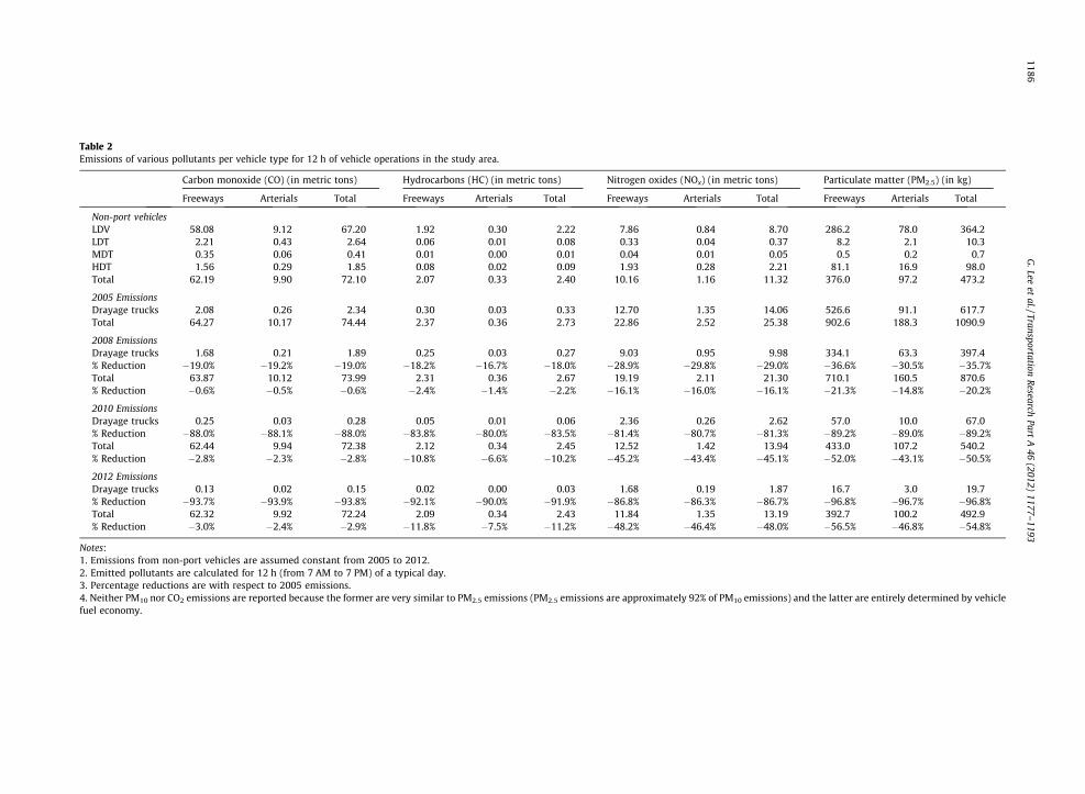
Table 2Emissions of various pollutants per vehicle type for 12 h of vehicle operations in the study area.

Carbon monoxide (CO) (in metric tons) Hydrocarbons (HC) (in metric tons) Nitrogen oxides (NOx) (in metric tons) Particulate matter (PM2.5) (in kg)

Freeways Arterials Total Freeways Arterials Total Freeways Arterials Total Freeways Arterials Total

Non-port vehiclesLDV 58.08 9.12 67.20 1.92 0.30 2.22 7.86 0.84 8.70 286.2 78.0 364.2LDT 2.21 0.43 2.64 0.06 0.01 0.08 0.33 0.04 0.37 8.2 2.1 10.3MDT 0.35 0.06 0.41 0.01 0.00 0.01 0.04 0.01 0.05 0.5 0.2 0.7HDT 1.56 0.29 1.85 0.08 0.02 0.09 1.93 0.28 2.21 81.1 16.9 98.0Total 62.19 9.90 72.10 2.07 0.33 2.40 10.16 1.16 11.32 376.0 97.2 473.2

2005 EmissionsDrayage trucks 2.08 0.26 2.34 0.30 0.03 0.33 12.70 1.35 14.06 526.6 91.1 617.7Total 64.27 10.17 74.44 2.37 0.36 2.73 22.86 2.52 25.38 902.6 188.3 1090.9

2008 EmissionsDrayage trucks 1.68 0.21 1.89 0.25 0.03 0.27 9.03 0.95 9.98 334.1 63.3 397.4% Reduction �19.0% �19.2% �19.0% �18.2% �16.7% �18.0% �28.9% �29.8% �29.0% �36.6% �30.5% �35.7%Total 63.87 10.12 73.99 2.31 0.36 2.67 19.19 2.11 21.30 710.1 160.5 870.6% Reduction �0.6% �0.5% �0.6% �2.4% �1.4% �2.2% �16.1% �16.0% �16.1% �21.3% �14.8% �20.2%

2010 EmissionsDrayage trucks 0.25 0.03 0.28 0.05 0.01 0.06 2.36 0.26 2.62 57.0 10.0 67.0% Reduction �88.0% �88.1% �88.0% �83.8% �80.0% �83.5% �81.4% �80.7% �81.3% �89.2% �89.0% �89.2%Total 62.44 9.94 72.38 2.12 0.34 2.45 12.52 1.42 13.94 433.0 107.2 540.2% Reduction �2.8% �2.3% �2.8% �10.8% �6.6% �10.2% �45.2% �43.4% �45.1% �52.0% �43.1% �50.5%

2012 EmissionsDrayage trucks 0.13 0.02 0.15 0.02 0.00 0.03 1.68 0.19 1.87 16.7 3.0 19.7% Reduction �93.7% �93.9% �93.8% �92.1% �90.0% �91.9% �86.8% �86.3% �86.7% �96.8% �96.7% �96.8%Total 62.32 9.92 72.24 2.09 0.34 2.43 11.84 1.35 13.19 392.7 100.2 492.9% Reduction �3.0% �2.4% �2.9% �11.8% �7.5% �11.2% �48.2% �46.4% �48.0% �56.5% �46.8% �54.8%

Notes:1. Emissions from non-port vehicles are assumed constant from 2005 to 2012.2. Emitted pollutants are calculated for 12 h (from 7 AM to 7 PM) of a typical day.3. Percentage reductions are with respect to 2005 emissions.4. Neither PM10 nor CO2 emissions are reported because the former are very similar to PM2.5 emissions (PM2.5 emissions are approximately 92% of PM10 emissions) and the latter are entirely determined by vehiclefuel economy.

1186G

.Leeet

al./TransportationR

esearchPart

A46

(2012)1177–

1193

Table 3Estimated maximum 24-h average PM10 concentration (in lg/m3).

Year Winter Spring Summer Fall

2005 8.81 7.00 7.74 9.062008 5.45 4.45 4.91 6.032010 0.88 0.75 0.83 0.972012 0.24 0.22 0.29 0.26

Note: The California air quality standard is 50 lg/m3 for the 24-h average for particulate matter (PM).

G. Lee et al. / Transportation Research Part A 46 (2012) 1177–1193 1187

cover all age groups because of limitations in available concentration–response functions, so only two age groups could beconsidered: people between 30 and 65 and people over 65.

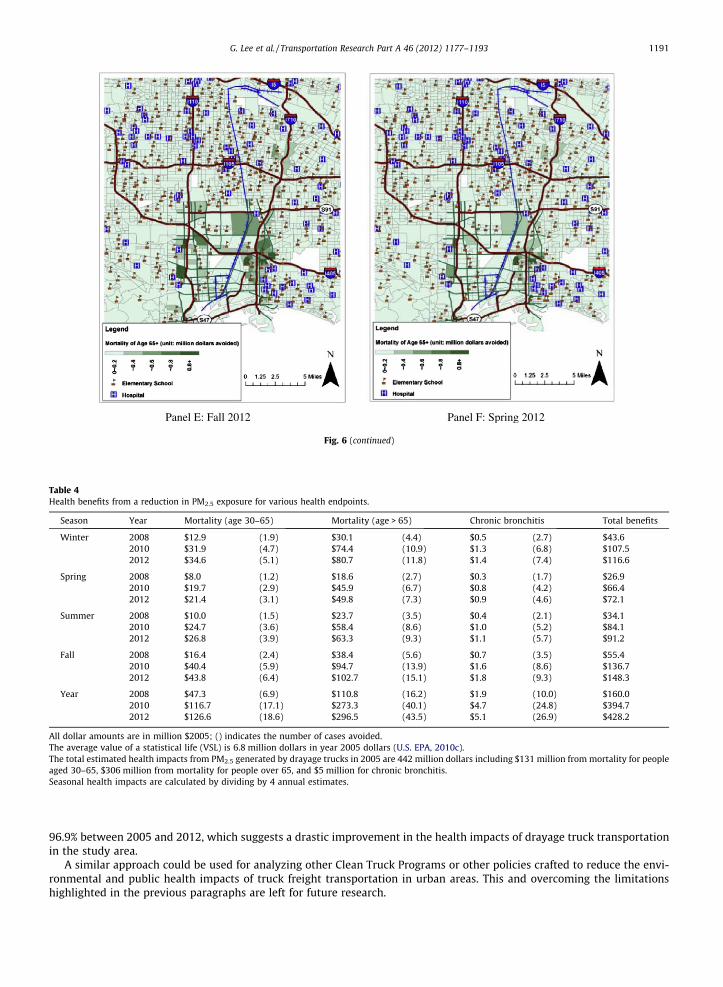
Fig. 6 shows spatial results for mortality from PM2.5 exposure in 2008, 2010 and 2012 compared to the 2005 baseline (forpeople 65 and older). For mortality, the most improved area is mainly south of the SR-91. In particular, the area near the ICTFrail yard sees large impacts.

Aggregated health impact results for PM2.5 are summarized in Table 4. During the 2008, 2010 and 2012 spring seasons(when exposure is smallest), the total number of mortality cases avoided was 3.9, 9.6 and 10.4 respectively, and the corre-sponding social benefits reached $27 million, $66 million and $71 million, respectively. For the fall season (when exposure islargest), the estimated numbers of mortality cases avoided (with associated monetary benefits in parentheses) were 8($55 million) in 2008, 20 ($135 million) in 2010, and 21.5 ($146.5 million) in 2012. In particular, the health impacts ofPM2.5 on people over 65 exceed the health costs for people between 30 and 65. The social costs of chronic bronchitis wererelatively smaller, but they were still substantial: estimated social benefits from reducing PM concentration for that healthoutcome were approximately $2 million in 2008 and $5 million in both 2010 and 2012. Overall, the estimated social benefitsfrom implementing the Clean Truck Program for the health outcomes considered were $160 million in 2008, $395 million in2010 and $430 million for 2012.

With annual health costs from drayage truck emissions in excess of $440 million (the estimated health impacts fromPM2.5 exposure in 2005), the payback period for replacing all of the 11,000 drayage trucks serving the SPBP complex is nomore than 4 years, assuming that a new truck costs $150,000. Even this admittedly simplistic calculation suggests thatthe social benefits of implementing the Clean Truck Program far exceed the costs of this program and clearly justify itsimplementation.

One way to contextualize these results is to compare the estimated number of statistical deaths from PM exposure in thestudy area in 2005 with an estimate of the number of traffic fatalities for the exposed population. A GIS analysis of the dataused to generate Panel A on Fig. 5 shows that approximately 275,000 people aged 30 or older were exposed to PM from roadvehicles in the study area in 2005, which corresponds to 22 traffic deaths given Los Angeles County’s traffic fatality of 7.9 per100,000 people in 2005 (City-data.com, 2010). In contrast, 64 statistical lives were lost in 2005 in the study area as a result ofPM exposure, which is almost three times as many as from traffic fatalities. Nationwide studies of transportation external-ities suggest the reverse, i.e., that the external costs of traffic accidents outweigh traffic health externality costs by at least afactor 3 (see Lemp and Kockelman, 2008). This comparison illustrates the tremendous health burden imposed on Alamdeacorridor residents by freight transportation before the full implementation of the Clean Truck Program. Broader external costmeasures were not used to contextualize results here because estimates of non-fatality health impacts are very limited andcould paint a distorted picture of the health consequences of freight transportation in the study area.

5. Conclusions and future research

This study proposed an integrated approach to analyze some of the environmental and health impacts from urban freighttransportation in the transportation corridor that links the SPBP complex to downtown Los Angeles, and to assess the effec-tiveness of the Clean Truck Program. This integrated approach, which combined a microscopic traffic simulation modelincluding freeways and arterials with an emissions model, a spatial dispersion model, and a health impact model, shouldbe widely applicable for studying the health impacts of freight corridor operations, and it should be of broad interest as anumber of ports in the US, including the Ports of New York/New Jersey, Oakland, and Tacoma, have started programs to re-duce emissions from drayage trucks (Environmental Leader, 2010).

Results show that the health impacts from drayage truck operations exceed $440 million per year for particulate matter(PM) alone. Moreover, this estimate is a lower bound for several reasons.

First, for the representative day simulated, no traffic-disrupting incident (such as collisions) was simulated on the net-work, even though such incidents occur almost daily and increase congestion. This was not done simply because there iscurrently no agreed-upon procedure for doing so and because no information about the characteristics of ‘‘representative’’incidents in the study area could be found.

Second, this analysis accounts only for limited health outcomes due to gaps in the availability of concentration–responsefunctions for mortality, particularly with respect to young adults and children, either because pertinent epidemiologic data

Panel A: PM10 concentrations (Fall 2005) Panel B: PM10 concentrations (Spring 2005)

Panel C: PM10 concentrations (Fall 2008) Panel D: PM10 concentrations (Spring 2008)

Fig. 5. PM dispersion and wind direction in fall and spring.

1188 G. Lee et al. / Transportation Research Part A 46 (2012) 1177–1193

are not available for specific outcomes and age groups, or because published studies address populations that differ from thepeople who live in the study area.

Third, this analysis does not account for emissions within the SPBP complex (see Giuliano and O’Brien, 2007), especiallywhen drayage trucks are waiting to be loaded or unloaded, because no detailed information about truck movements withinthe Ports was available, although extending this analysis to capture these activities is conceptually simple.

In addition, in order to isolate the impact of the Clean Truck Program, this analysis did not account for the PierPass pro-gram (Giuliano and O’Brien, 2008), which was implemented voluntarily by marine terminal operators on July 23, 2005 to

Panel E: PM10 concentrations (Fall 2010) Panel F: PM10 concentrations (Spring 2010)

Panel G: PM10 concentrations (Fall 2012) Panel H: PM10 concentrations (Spring 2012)

Fig. 5 (continued)

G. Lee et al. / Transportation Research Part A 46 (2012) 1177–1193 1189

preempt regulations such as California Assembly Bill (AB) 2650. AB 2650 required marine port terminals to reduce truckqueues at terminal gates. It also imposed a $250 fine on terminal operators for each truck idling more than 30 min whilewaiting at terminal gates unless gate service was extended or a gate appointment system was created. PierPass extendedgate hours (thus exempting all marine terminals from AB 2650) and assessed a Traffic Mitigation Fee (TMF) during specifichours on eligible containers going through the SPBP to defray the cost of extended hours. For details about PierPass and ananalysis of its impacts, see Giuliano and O’Brien (2008).

Panel A: Fall 2008 Panel B: Spring 2008

Panel C: Fall 2010 Panel D: Spring 2010

Fig. 6. Decrease in mortality from PM2.5 for people aged 65 and over.

1190 G. Lee et al. / Transportation Research Part A 46 (2012) 1177–1193

Despite these limitations, these results suggest that the social benefits of the Clean Truck Program, which was imple-mented by the SPBP to curb air pollution from drayage trucks, exceed its costs. Moreover, the CTP likely exceeded its goalof reducing air pollution from drayage trucks by 80% by 2012. Indeed, results indicate that by 2012, NOx and PM emissionswould only be 13.3% and 3.2% of their 2005 values for these two pollutants. Although the incremental gains from the 2012deadline compared to the 2010 deadline appear modest, they contribute to further reducing air pollution in the Los Angelesair basin where air quality is a perennial concern. As a result of these reductions, mortality from PM exposure decreased by

Panel E: Fall 2012 Panel F: Spring 2012

Fig. 6 (continued)

Table 4Health benefits from a reduction in PM2.5 exposure for various health endpoints.

Season Year Mortality (age 30–65) Mortality (age > 65) Chronic bronchitis Total benefits

Winter 2008 $12.9 (1.9) $30.1 (4.4) $0.5 (2.7) $43.62010 $31.9 (4.7) $74.4 (10.9) $1.3 (6.8) $107.52012 $34.6 (5.1) $80.7 (11.8) $1.4 (7.4) $116.6

Spring 2008 $8.0 (1.2) $18.6 (2.7) $0.3 (1.7) $26.92010 $19.7 (2.9) $45.9 (6.7) $0.8 (4.2) $66.42012 $21.4 (3.1) $49.8 (7.3) $0.9 (4.6) $72.1

Summer 2008 $10.0 (1.5) $23.7 (3.5) $0.4 (2.1) $34.12010 $24.7 (3.6) $58.4 (8.6) $1.0 (5.2) $84.12012 $26.8 (3.9) $63.3 (9.3) $1.1 (5.7) $91.2

Fall 2008 $16.4 (2.4) $38.4 (5.6) $0.7 (3.5) $55.42010 $40.4 (5.9) $94.7 (13.9) $1.6 (8.6) $136.72012 $43.8 (6.4) $102.7 (15.1) $1.8 (9.3) $148.3

Year 2008 $47.3 (6.9) $110.8 (16.2) $1.9 (10.0) $160.02010 $116.7 (17.1) $273.3 (40.1) $4.7 (24.8) $394.72012 $126.6 (18.6) $296.5 (43.5) $5.1 (26.9) $428.2

All dollar amounts are in million $2005; () indicates the number of cases avoided.The average value of a statistical life (VSL) is 6.8 million dollars in year 2005 dollars (U.S. EPA, 2010c).The total estimated health impacts from PM2.5 generated by drayage trucks in 2005 are 442 million dollars including $131 million from mortality for peopleaged 30–65, $306 million from mortality for people over 65, and $5 million for chronic bronchitis.Seasonal health impacts are calculated by dividing by 4 annual estimates.

G. Lee et al. / Transportation Research Part A 46 (2012) 1177–1193 1191

96.9% between 2005 and 2012, which suggests a drastic improvement in the health impacts of drayage truck transportationin the study area.

A similar approach could be used for analyzing other Clean Truck Programs or other policies crafted to reduce the envi-ronmental and public health impacts of truck freight transportation in urban areas. This and overcoming the limitationshighlighted in the previous paragraphs are left for future research.

1192 G. Lee et al. / Transportation Research Part A 46 (2012) 1177–1193

Acknowledgements

Support for this research from the University of California Transportation Center (Award 65A016-SA5882) is gratefullyacknowledged. We also thank Thomas Jelenic, Shashank Patil, Carlo Luzzi, and Eric Shen from the Port of Long Beach for theirvery valuable assistance.

References

Abbey, D., Ostro, B., Petersen, F., Burchette, R., 1995. Chronic respiratory symptoms associated with estimated long-term ambient concentrations of fineparticulates less than 2.5 microns in aerodynamic diameter (PM2.5) and other air pollutants. Journal of Exposure Analysis and EnvironmentalEpidemiology 5 (2), 137–159.

Ahn, K., Trani, A., Rakha, H., Van Aerde, M., 1999. Microscopic fuel consumption and emission models. In: Proceedings of the TRB 78th Annual Meeting. CD-ROM. Transportation Research Board, National Research Council, Washington, DC.

Bai, S., Eisinger, D., Niemeier, D., 2008. MOVES vs. EMFAC: A Comparative Assessment Based on a Los Angeles County Case Study, U.C. Davis-Caltrans AirQuality Project. <http://AQP.engr.ucdavis.edu/> (July 2010).

Caliper, 2008. TransModeler User’s Guide: Traffic Simulation Software.Caltrans, 1989. CALINE4 – A Dispersion Model for Predicting Air Pollutant Concentrations Near Roadways, Final Report, Report FHWA/CA/TL-84/15.

<www.weblakes.com/products/calroads/resources/docs/CALINE4.pdf>.California Air Resources Board (CARB), 1998. The Report on Diesel Exhaust. <www.arb.ca.gov/toxics/dieseltac/de-fnds.htm>.California Air Resource Board (CARB), 2006a. EMFAC 2007 user’s Guide, Sacramento, CA.California Air Resource Board (CARB), 2006b. Emission Reduction Plan for Ports and Goods Movement in California.California Air Resources Board (CARB), 2008. Rail Yard Health Risk Assessments and Mitigation Measures. <www.arb.ca.gov/railyard/hra/hra.htm>.Choi, K., Jayakrishnan, R., Kim, H., Yang, I., Lee, J., 2009. Dynamic O–D estimation using dynamic traffic simulation model in an urban arterial corridor.

Transportation Research Record: Journal of the Transportation Research Board 2133, 133–141.Chu, L., Liu, H.X., Oh, J.S., Recker, W., 2004. A calibration procedure for microscopic traffic simulation. In: Proceeding of TRB’s 83rd Annual Meeting (CD-

ROM), Washington, DC.City-data.com, 2010. Los Angeles County, California (CA). <http://www.city-data.com/county/Los_Angeles_County-CA.html>.Claggett, M., 2011. OpMode look-up tables for linking traffic simulation models and MOVES emissions. In: Proceedings of TRB’s 90th Annual Meeting.

Transportation Research Board, National Research Council, Washington, DC.Delucchi, M., McCubbin, D., 2011. External costs of transport in the United States. In: de Palma, A., Lindsey, R., Quinet, E., Vickerman, R. (Eds.), A Handbook of

Transport Economics, Northampton, MA, USA.Demir, E., Bektas�, T., Laporte, G., 2011. A comparative analysis of several vehicle emission models for road freight transportation. Transportation Research

Part D 16 (5), 347–357.Dowling, R., Skabardonis, A., Alexiadis, V., 2004. Traffic Analysis Toolbox Volume III: Guidelines for Applying Traffic Microsimulation Modeling Software,

FHWA. U.S. Department of, Transportation, No. FHWA-HRT-04-040.Environmental Leader, 2010. Port Authority Launches Clean Truck Program at the Port of NY/NJ. <http://www.environmentalleader.com/2010/03/11/port-

authority-launches-clean-truck-program-at-the-port-of-nynj/>.Fann, N., Risley, D., 2011. The public health context for PM2.5 and ozone air quality trends. Air Quality and Atmospheric Health. http://dx.doi.org/10.1007/

s11869-010-0125-0.Figliozzi, M.A., 2011. The impacts of congestion on time-definitive urban freight distribution networks CO2 emission levels: results from a case study in

Portland, Oregon. Transportation Research Part C 19, 766–778.Friedrich, R., Quinet, E., 2011. External costs of transport in Europe. In: de Palma, A., Lindsey, R., Quinet, E., Vickerman, R. (Eds.), A Handbook of Transport

Economics, Northampton, MA, USA.Fruin, S., Westersahl, D., Sax, T., Sioutas, C., Fine, P.M., 2008. Measurements and Predictors of on-road ultrafine particle concentrations and associated

pollutants in Los Angeles. Atmospheric Environment 42, 207–219.Giuliano, G., O’Brien, T., 2007. Reducing port-related truck emissions: the terminal gate appointment system at the Ports of Los Angeles and Long Beach.

Transportation Research Part D 12, 460–473.Giuliano, G., O’Brien, T., 2008. Evaluation of Extended Gate Operations at the Ports of Los Angeles and Long Beach. METRANS Project 05-12. Draft Final

Report.Houston, D., Krudysz, M., Winer, A., 2008. Diesel truck traffic in port-adjacent low-income and minority communities; environmental justice implications of

near-roadway land use conflicts. Transportation Research Record: Journal of the Transportation Research Board 2076, 38–46.Hubbell, B.J., Hallberg, A., McCubbin, D.R., Post, E., 2004. Health-related benefits of attaining the 8-h ozone standard. Environmental Health Perspectives 113

(1). http://dx.doi.org/10.1289/ehp.7186.Kanter, R., 2009. Clean Trucks Program Update. Presentation to the Board of Harbor Commissioners December 21, 2009. <http://www.polb.com/civica/

filebank/blobdload.asp?BlobID=6950> (15.04.12).Karr, C., Lumley, T., Shepherd, K., Davis, R., Larson, T., Ritz, B., Kaufman, J., 2006. A case-crossover study of wintertime ambient air pollution and infant

bronchiolitis. Environmental Health Perspectives 114, 277–281. http://dx.doi.org/10.1289/ehp.8313.Kozawa, K.H., Fruin, S.A., Winer, A.M., 2009. Near-road air pollution impacts of goods movement in communities adjacent to the Ports of Los Angeles and

Long Beach. Atmospheric Environment 43 (18), 2960–2970.Krewski, D., Jerrett, M., Burnett, R.T., Ma, R., Hughes, E., Shi, Y., Turner, M.C., Pope, C.A., 3rd, Thurston, G., Calle, E.E., Thun, M.J., Beckerman, B., DeLuca, P.,

Finkelstein, N., Ito, K., Moore, D.K., Newbold, K.B., Ramsay, T., Ross, Z., Shin, H., Tempalski, B., 2009. Extended Follow-up and Spatial Analysis of theAmerican Cancer Society Study Linking Particulate Air Pollution and Mortality. Boston: Health Effects Institute, vol. 140, pp. 5–114.

Lakes Environmental Software, 2006. CALPUFF View User’s Guide, Waterloo, Ontario, Canada.Lee, G., 2011. Integrated Modeling of Air Quality and Health Impacts of a Freight Transportation Corridor. Ph.D. Dissertation, University of California, Irvine,

213 pp.Lee, G., You, S., Ritchie, S.G., Saphores, J.-D., Sangkapichai, M., Jayakrishnan, R., 2009. Environmental impacts of a major freight corridor: a study of the I-710

in California. Transportation Research Record 2123, 119–128.Lemp, J.D., Kockelman, K.M., 2008. Quantifying the external costs of vehicle use: evidence from America’s top-selling light-duty models. Transportation

Research Part D 13, 491–504.Mongelluzzo, B., 2012. Supreme court seeks solicitor general’s opinion in clean-trucks case. Journal of Commerce (March 27), <http://www.joc.com/

drayage/supreme-court-seeks-solicitor-generals-opinion-clean-trucks-case> (30.03.12).Oshan, R., Kumar, A., Masuraha, A., 2006. Application of the USEPA’s CALPUFF model to an urban area. Environmental Progress 25, 12–17.Freeway Performance Measurement System (PeMS), 2011. <pems.eecs.berkeley.edu/>.POLA (Port of Los Angeles), 2011a. Clean Truck Program Fact Sheet. <http://www.portoflosangeles.org/ctp/CTP_Fact_Sheet.pdf> (15.04.12).POLA (Port of Los Angeles), 2011b. New Year’s Day marks End of Dirty Trucks for Port of Los Angeles Clean Truck Program. <www.portoflosangeles.org/ctp/

ctp_news.asp> (15.04.12).

G. Lee et al. / Transportation Research Part A 46 (2012) 1177–1193 1193

POLB (Port of Long Beach), 2007. Port of Long Beach Air Emissions Inventory – 2005. <http://www.polb.com/civica/filebank/blobdload.asp?BlobID=4436>(April 2010).

POLB (Port of Long Beach), 2009. Clean Truck Fee – Who Pays, Who Doesn’t Pay. <http://www.polb.com/civica/filebank/blobdload.asp?BlobID=6401>(February 2012).

Pope III, C.A., Burnett, R.T., Thun, M.J., Calle, E.E., Krewski, D., Ito, K., Thurston, G.D., 2002. Lung cancer, cardiopulmonary mortality, and long-term exposureto fine particulate air pollution. Journal of the American Medical Association 287, 1132–1141.

Pope III, C.A., Burnett, R.T., Thurston, G.D., Thun, M.J., Calle, E.E., Krewski, D., Godleski, J.J., 2004. Cardiovascular mortality and long-term exposure toparticulate air pollution: epidemiological evidence of general pathophysiological pathways of disease. Circulation 109, 71–77.

Sathaye, N., Harley, R., Madanat, S., 2010. Unintended environmental impacts of nighttime freight logistics activities. Transportation Research Part A 44,642–659.

South Coast Air Quality Management District (SCAG), 2008a. Analysis of Goods Movement Emission Reduction Strategies.South Coast Air Quality Management District (SCAG), 2008b. Regional Transportation Improvement Program.South Coast Air Quality Management District (SCAQMD), 2008c. Multiple Air Toxics Exposure Study in the South Coast air Basin, 2008. <http://

www.aqmd.gov/prdas/matesIII/MATESIIIFinalReportSept2008.html>.Scora, G., Barth, M., 2006. Comprehensive Modal Emission Model (CMEM), Version 3.01 User’s Guide. <www.cert.ucr.edu/cmem/docs/

CMEM_User_Guide_v3.01d.pdf>.Scrie, J.S., Strimaitis, D.G., Yamartino, R.J., 2000. A User’s Guide for the CALPUFF Dispersion Model (Version 5). Earth Tech Inc.Silverman, R.A., Ito, K., 2010. Age-related association of fine particles and ozone with severe acute asthma in New York City. Journal of Allergy and Clinical

Immunology 125, 367–373.San Pedro Bay Ports (SPBP), 2006. Clean Air Action Plan – Overview. <http://www.polb.com/civica/filebank/blobdload.asp?BlobID=3452>.United States Environmental Protection Agency (U.S. EPA), 1995. User’s Guide to CAL3QHC Version 2.0: A Modeling Methodology for Predicting Pollutant

Concentrations Near Roadway Intersections. United States Environmental Protection Agency, No. EPA-454/R-92-006.United States Environmental Protection Agency (U.S. EPA), 2004. AERMOD: Description of Model Formulation’. United States Environmental Protection

Agency, No. EPA-454/R-03-004.United States Environmental Protection Agency (U.S. EPA), 2008. Emission and Air Quality Modeling Tools for Near-Roadway Applications. United States

Environmental Protection Agency, No. EPA-600/R-09/001.United States Environmental Protection Agency (U.S. EPA), 2009. Motor Vehicle Emission Simulator (MOVES) 2009: Software Design and Reference Manual.United States Environmental Protection Agency (U.S. EPA), 2010a. BenMAP: Environmental Benefits Mapping and Analysis Program; User’s Manual, Office of

Air Quality Planning and Standards. U.S. Environmental Protection Agency, August.United States Environmental Protection Agency (U.S. EPA), 2010b. Motor Vehicle Emission Simulator (MOVES): User Guide for MOVES2010.United States Environmental Protection Agency (U.S. EPA), 2010c. Dispersion Modeling. <http://www.epa.gov/ttn/scram/dispersionindex.htm> (May 2010).van Woensel, T., Creten, R., Vandaele, N., 2001. Managing the environmental externalities of traffic logistics: the issue of emissions. Production and

Operations Management 10 (2), 207–223.Walker, J.I., Scaplen, M., George, F., 2003. ISCST3, AERMOD and CALPUFF: a comparative analysis in the environmental assessment of a sour gas plant. In:

Proceedings of Guideline on Air Quality Models, Mystic, CT, Air and Waste Management Association.Weisbrod, G., Fitzroy, S., 2008. Defining the range of urban congestion impacts on freight and their consequences for business activity. In: Proceedings of

TRB’s 87th Annual Meeting, Washington, DC.Woodruff, T.J., Parker, J.D., Schoendorf, K.C., 2006. Fine particulate matter (PM2.5) air pollution and selected causes of postneonatal infant mortality in

California. Environmental Health Perspectives 114, 786–790. http://dx.doi.org/10.1289/ehp.8484.Wu, J., Houston, D., Lurmann, F., Ong, P., Winer, A., 2009. Exposure of PM2.5 and EC from diesel and gasoline vehicles in communities near the ports of Los

Angeles and Long Beach, California. Atmospheric Environment 43, 1962–1971.