Aspects of the drainage process in soils

Univers

ity of

Cap

e Tow

n

1

ASPECTS OF mE lltAINAGE PROCESS IN SOILS

Submitted to the University of Cape Town in partial fulfilment of the

requirements for the degree of Master of Science in Engineering.

Gavin Roger Wardle

Febuary 1986. ·

,_, ____________ ,,_.. ____________ ,.. The University of Cape Town has been given the right to reproduce this thesis In whole or in part. Copyright Is held by the author.

Univers

ity of

Cap

e Tow

nThe copyright of this thesis vests in the author. No quotation from it or information derived from it is to be published without full acknowledgement of the source. The thesis is to be used for private study or non-commercial research purposes only.

Published by the University of Cape Town (UCT) in terms of the non-exclusive license granted to UCT by the author.

ii

DECLARATION . BY CANDIDATE

'I, Gavin Roger Wardle, hereby declare that this thesis represents my

own work, carried out under the supervision of Prof A.D.W. Sparks of the

University of Cape Town, and is according to the requirements of the

regulations of the University for the award of the degree, Master of

Science in Engineering.'

G.R. Wardle ·

Febuary 1985.

iii

DFJ>ICATION

TO NEIL, IRENE, AND ELAINE

iv

SYNOPSIS

The initial portion of this thesis contains a review of basic theory.

An experimental programme was also undertaken to measure soil

parameters; and to observe heads and seepage rates during transient flow

conditions in experiments. These experimental values were compared with

results from finite element calculations. It was necessary for the

candidate to devise a system for modifying an existing main-frame finite

element package (ADINAT) in order to cope with the transient partly

saturated draining state which exists above a falling water table. Good

agreement was found between observed and computed transient heads. The

experimental work of other investigators was also analysed by using this

Finite Element program, and again good agreement was found between

observed and computed transient conditions. It was decided in

conjunction with the supervisor to limit this thesis to two-dimensional

flow in the vertical plane.

v

ACXNOWLEDGEKENTS

I would like to express my sincere gratitude to the following:

Professor A.D.W. Sparks, under whose supervision this thesis was

·conducted.

Hr N. Hassen, for his assistance in the laboratory.

Mr c. Doig and Mr G. Jack, for their suggestions and advice, in relation

to the design of the electrical circuitary needed for the experiments.

Mr D Joubert, for the use of the electrical pressure transducers he had

designed and built.

Professor w.s. Doyle, for his encouragement and permission, fn relation

to the use of ADINAT.

Miss D Sutherland, for her patience and immaculate typing of this

thesis.

All the staff of the Department of Civil Engineering for their help and

friendship during this period.

The Council of Scientific and Indus trial Research for their financial

assistance.

)

Declaration

Dedication

Synopsis

Acknowledgements

Contents

CHAPTER 1 INTRODUCTION.

1 .1 General.

1.2 Aims and Objectives.

OONTENTS

CHAPTER 2 A Review of the Physical Process of Drainage.

2.1 Introduction.

2.2 Properties of a porous media.

2.3 Properties of water.

2.4 Flow of water in saturated soils.

2.5 Generalization of Darcy's Law.

2.5.1 Isotropic medium.

Anisotropic medium. 2.5.2

2.5.3 Range of Validity of Darcy's Law.

2.6 Flow of water in unsaturated soil.

2.7 Extension of Darcy's Law.

2.8 Soil moisture characterstic curve.

2.8.1 · Hysteresis.

2.8.2 Spee if ic mo is tu re capacity.

2.9 General equation of saturated-unsaturated flow.

2 .9 .1 The continuity equation.

2.9.2 The combined flow equation.

vi

ii

iii

iv

v

vi

1

1

1

4

4

4

7

10

13

14

15

18

18

21

22

23

24

26

26

27

2.10 Calculation of the Hydraulic Conductivity of Saturated Soils. 28

2.10.1

2.10.2

2.10.3

Theoretical prediction.

Laboratory measurement.

Field measurement.

28

29

32

2.11 Calculation of the Hydraulic Conductivity of Unsaturated Soils. 39

2.11.1

2.11.2

Theortical prediction.

Laboratory measurement.

39

41

2.11.3 Field measurement.

2.12 Calculation of the Soil-moisture Characteristic Curve.

2.12.1 Theoretical prediction.

2.12.2 Laboratory and field measurements.

CHAPTER 3 Pressure Recording Apparatus.

3.1 Introduction.

3.2 Transducers.

3.2.1 Selection criteria.

3.2.2 Transducer requirements.

3.2.3 Transducer performance.

3.2.4 Transducer selection and recommendations.

3.2.S Transducer input interfacing.

3.3 Analog to Digital Conversion and Multiplexing.

Introduction. 3.3.1

3.3.2 Analog to digital converter selection criteria.

3.4 System Hardware.

3 .S Real Time.

3.5.1

3.5.2

Introduction.

Real time clock design.

3.6 Data Acquisition Software.

3.7 Calibration.

3 .8 Limitations.

CHAPTER 4 Experimental Apparatus and Testing Procedure.

4.1 Introduction.

4.2 Classification Properties of Cape Flats' sand.

4.3 Saturated Hydraulic Conductivity.

4.4 Unsaturated Hydraulic Conductivity.

4.5 Soil-moisture Characteristic Curve.

4.6 Experimental Apparatus.

4.7 Experiment number one.

4.7.1

4.7.2

4.7.3

Definition of problem.

Experimental simulation.

Measurement techniques.

4.8 Experiment number two.

4.8.l Definition of problem.

vii

43

45

45

47

50

so 52

53

54

56

58

61

63

63

65

66

70

70

71

71

77

79

81

81

81

82

88

94

97

98

98

99

100

103

103

4.8.2

4.8.3

Experimental simulation.

Measurement techniques.

CHAPTER 5 Analysis of Experimental and Test Results.

5.1 Introduction.

5.2 Saturated Hydraulic Conductivity.

5.3 Unsaturated Hydraulic Conductivity.

5.4 Soil-moisture Characteristic Curve.

5.5 Experiment No. One Analysis.

5.5.1 Introduction.

5.5.2 Drainage Outflow.

5.5.3 Sidewall Piezometers.

5.5.4

5.5.5

Transducer Monitored Tensiometers.

Analysis of Results.

5.5.6 Summary and Conclusions.

5.6 Experiment No. Two Analysis.

5.6.1 Introduction.

5.6.2 Drainage Outflow.

5.6.3

5.6.4

5.6.5

5.6.6

Sidewall Piezometers.

Transducer Monitored Tensiometers.

Analysis of Results.

Summary and Conclusions.

CHAPTER 6 Modelling of Fluid Flow in a Saturated-Unsaturated

Domain Using the Finite Element Method.

6.1 Introduction.

6.2 History of the Finite Element Method.

6.3 Basic Formulation of the Partial Differential Equation.

6.4 General Representation.

6.5 The Finite Element Method.

The Finite Element Concept.

Discretisation.

viii

103

105

106

106

106

112

119

125

125

129

131

131

133

146

147 .

147

151

151

151

155

156

157

157

162

163

165

169

169

170

6.5.1

6.5.2

6.5.3

6.5.4

6.5.5

6.5.6

6.5.7

Approximation and Interpolation. 170

Derivation of Element Equations. 170

Assembly of Global Equations and Boundary Conditions. 171

Solution of Equations. 172

Summary. 174

6.6 A Simple Example.

6.6.1 Summary of the Basic Steps of the Finite

Element Method.

6. 7 Application to. Flow in Porous Media.

6.8 Operation of the Finite Element Program Package.

6.9 Finite Element Material Models.

6.9.1

6.9.2

6.9.3

Constant Saturated Hydraulic Conductivity Model.

Steady-state Phreatic Surface Seepage Model.

Saturated-unsaturated Flow model.

6.10 Output from the Finite Element Package.

6.11 Finite Element Examples and Program Verification.

6.11.1

6.11.2

6.11.3

6.11.4

6.11.5

6.11.6

Introduction.

Example No. 1:

Example No. 2:

Example No. 3:

Example No. 4:

Saturated Confined Seepage.

Unconfined Free Surface Steady

state Flow

Drainage from a Saturated

unsaturated System.

Non-steady State Flow Between

Drains after Rapid Drawdown

Summary and Conclusion.

6.12 Experiment Verification Using the Finite Element Method.

ix

175

185

186

188

190

190

193

193

196

197

197

198

198

201

204

208

208

6.12.1

6.12.2

Introduction. 208

6.12.3

Experiment No. 1: Unsteady flow through a

Rectangular Dam.

Experiment No. 2: Saturated-unsaturated Flow in a

Slab of Soil Between Drains

After Rapid Drawdown.

6.12.4 Conclusion.

CHAPTER 7 Sununary and Conclusions.

7.1 Comparison of Experimental and Numerical Results.

7.2 Practical Application.

7.3 Field and Laboratory Parameters Required for the Finite

Element Method Material Model.

7.4 Future Possibilities.

7.5 Concluding Remarks.

208

212

215

216

216

217

218

219

220

REFERENCES

APPENDIX A

Courses Passed By Candidate

APPENDIX B

B-1 TABLE: Specific Gravity of Water.

B-2 TABLE: Viscosity Corrections.

APPENDIX C

C-1 FIGURE: Pressure Transducer and Amplification Circuit.

x

223

A.1

B. l

B.1

C. l

C-2 Method of Priming the Transducer Input Interface with Fluids. C.2

C-3 FIGURE: Circuitry for 32 Channel High-speed A/D Converter. C.4

C-4 LISTING: Machine Language Routines for A/D Control. C.5

C-5 FIGURE: Circuitry for Real Time Clock. C.12

C-6 LISTING: Machine Language Routines for Time Circuit Control. C.13

C-7 LISTING: Program "TIME". C.20

C-8 LISTING: Program "DATA". C.21

C-8 Transducer Calibration. C.22

APPENDIX D

D-1 Specific Gravity Test.

D-2 Particle Size Analysis.

APPENDIX E

E-1 Saturated Hydraulic Conductivity Tests.

D.1

D.4

E. l

E-2 Unsaturated Hydraulic Conductivity Tests. E.11

E-3 Soil-moisture Characteristic Curve Tests. E.16

E-4 Measured Outflow from the Drainage Face of Experiment No. 1 E.23

E-5 Sidewall Piezometer Levels of Experiment No. 1 E.26

E-6 Transducer Monitored Tensiometers of Experiment No. 1 E.30

E-7 Approximate Moisture Transfer Analysis of Experiment No. 1 E.39

E-8 Measured Outflow from the Drainage Face of Experiment No. 2 E.50

E-9 Sidewall Piezometer Levels of Experiment No. 2 E.58

E-10 Transducer Monitored Tensiometers of Experiment No. 2 E.60

E-11 Approximate Moisture Transfer Analysis of Experiment No. 2 E.87

xi

APPENDIX F

F-1 LISTING: Example of Input and Output from an ADINAT analysis. F.1

F-2 Using ADINAT. F.11

1

al.APTER 1

IR'l'RODOCflON.

1.1 General.

The flow of water or seepage through a rigid porous media is of great

importance in many fields of engineering, agriculture and groundwater

geology. Traditionally attention was focused on the saturated zone in

analyzing seepage through earth structures and the subsurface. However,

the unsaturated zone also plays a big part in the movement of

moisture. This is important when we have a changing water table

(phreatic surface) in transient problems, e.g., earth dam with a

variable reservoir head, or a land mass being drained to a ditch or to a

river. Also a large number of problems take place in the unsaturated

zone, e.g., above the water table (phreatic surface). Examples are the

recharge of the water table from a ditch, canal or pond; the irrigation

of land, and the movement of toxic leachatee beneath sanitary

landfills. An understanding of the flow in the unsaturated region is

also important because of negative pore-water pressures that are

important for stability analysis, but cannot be calculated from the

classical free-surface approach. Most problems are one of an unconfined

aquifer with flow taking place both above and below the phreatic

surface.

In general the problem is to determine the pressure distribution and

velocity of the water in the interior of a soil mass with given boundary

conditions. Mathematically speaking the problem is in the class known

as boundary-value problems. However, before it is possible to make a

theoretical analysis of the flow of water in a rigid porous medium, it

is necessary to understand the soil-moisture relationship.

1 .2 Aw and Objective~

The aim of this thesis was to describe both the parameters that are

important for the flow of water in a draining saturated-unsaturated

2

rigid porous media, and to develop an Effective method for solving this

type of problem. The investigation was taken further, and the actual

parameters for a soil were measured;

planned; and a theoretical verification

element method.

an experimental program was

was made by using the finite

In order to achieve this, the principal aim was divided into a number of

initial secondary objectives, namely:-

a) A literature survey on soil-moisture relationships, in connection

with drainage.

b) A literature survey on the methods for obtaining the parameters that

are import!lnt in the drainage of soils.

c) A review of the finite element method with application to the

solution of two-dimensional seepage problems.

d) An experimental program to investigate the flow of water in a

saturated-unsaturated rigid porous medium.

e) Design and construction of experimental equipment needed for the

experimental program.

f) The design and construction of a data-acquisition unit to record the

output signals from pressure transducers.

g} The finite element method program packages available at the

University of Cape Town were investigated to seek one that might be

used for the solving of seepage problems.

h) The existing finite element method program packages were not

suitable for transient seepage with partly saturated zones above the

phreatic surface. The candidate therefore decided to modify and add

an extra option to an existing computer package.

3

i) Verification of the experimental results with the finite element

method was undertaken.

j) It was hoped that useful suggestions in the use of the finite

element method for different flow problems, will arise from this

thesis.

4

Qi.APTER 2

A REVIEW OF 'lllE PHYSICAL PROCESS OF DRAINAGE.

2 .1 Introduction.

'

The parameters that affect the drainage process are numerous. In this

thesis the porous medium through which seepage (drainage) occurs is

assumed to be rigid and made up of solid particles. The fluid used for

the examples and the analysis considered is water. The air phase in the

medium is assumed to be free to 100ve and at atmospheric pressure. (ie. A

one-phase flow is considered.) The fluid (water) remains a liquid and

no phase change is considered as its temperature is near room

temperature. (18 °c)

2.2 Properties of a Porous Kedia.

A porous medium is assumed to consist of a mass of discrete solid

particles, which form voids of varying sizes. Each void or pore is

taken to be connected to others by constricted passages. The whole

forms a complex of irregular interconnected passages through which

fluids may flow •. A void that is isolated from others will not allow

fluid to pass through it. Fluid flowing through these tortuous three

dimensional passages is subjected to acceleration and deceleration,

accompanied by a dissipation of mechanical energy.

The velocity distribution of the fluid flowing through the passages may

resemble that in a capillary tube, but it is essentially non-uniform in

the direction of flow, al though the flow may be steady. On the

macroscopic level taken over an area large enough compared with the pore

sizes, the discharge per unit area normal to the direction of flow will

be much more uniform. This area on the macroscopic level, surrounding a

point P, must be smaller than the size of the entire flow domain,

otherwise the resulting average cannot represent what happens at P. On

the other hand, it should also be large enough to include a sufficient

number of voids (passages) to permit a meaningful statistical average.

s

With this generalization, details of the flow are lost, but much is

gained, in that this macroscopic behaviour can be described roore easily

mathematically than the microscopic behaviour.

It was noted earlier that the porous medium consists of discrete solid

particles in the form of a matrix with voids between. These voids may

be filled completely with water and air. If the voids are completely

filled with water then the medium is saturated, .but if only partially

filled then it is unsaturated (partially-saturated).

Volumes Weights

(a) (b)

Fig 2.1: Relationship mong phases fa soil. (a) Elewmt of 11&tural

soil. (b) Idealised form, ele11e11t separated fnto phases.

In this thesis a one-phase drainage flow approach is considered, meaning

that the air phase in the voids is considered to be at atmospheric

pressure and free to move in the voids. To understand the properties of

a porous medium it is advantageous to adopt an idealized form of diagram

as shown in figure (2 .1). The porous medium has a total volume V and a

volume of solid particles that summates to vs. The volume of the

voids, Vv, is (V - Vs)• From a study of figure (2.1) the following may

be defined:

Void ratio (e)

e = volume of voids

= v

v

volume of solids V s

(2.1)

Porosity (n)

Degree of

volume of voids n =

total volume

v v n = - =

v

saturation (Sr)

volume s = r volume

of water

of voids

e =

1 + e

v (usually expressed w

as a percentage.) = v v

Volumetric moisture content or water content (9)

9 = volume of water v

w = -total volume V

6

(2.2)

(2.3)

(2.4)

(2.5)

Classification of a porous medium is a difficult task. This is because

the range of particles that could make up a soil is very large. As an

example, sand and clay could.be considered for simplicity.

Sands are mainly composed of macroscopic particles that are

rounded or angular in shape. Sands drain readily, do not swell,

possess a small capillary potential and when dry exhibit little

or no shrinkage. Forces acting on fluids flowing in the pore

passages are mainly due to mechanical forces (eg. forces due to

pressure gradients, gravity, inertia and friction.)

Clays on the other hand, are composed of microscopic particles of

platel ike shape. Clays are highly impervious, exhibit

considerable swelling, possess a high capillary potential, and

have a considerable volume reduction upon drying. In addition to

mechanical forces, molecular and electro-chemical forces are

important in acting on seeping fluids and the particles of the

clay. In clays, both the chemistry of the percolating water and

the mineralogical structure of the clay are important.

7

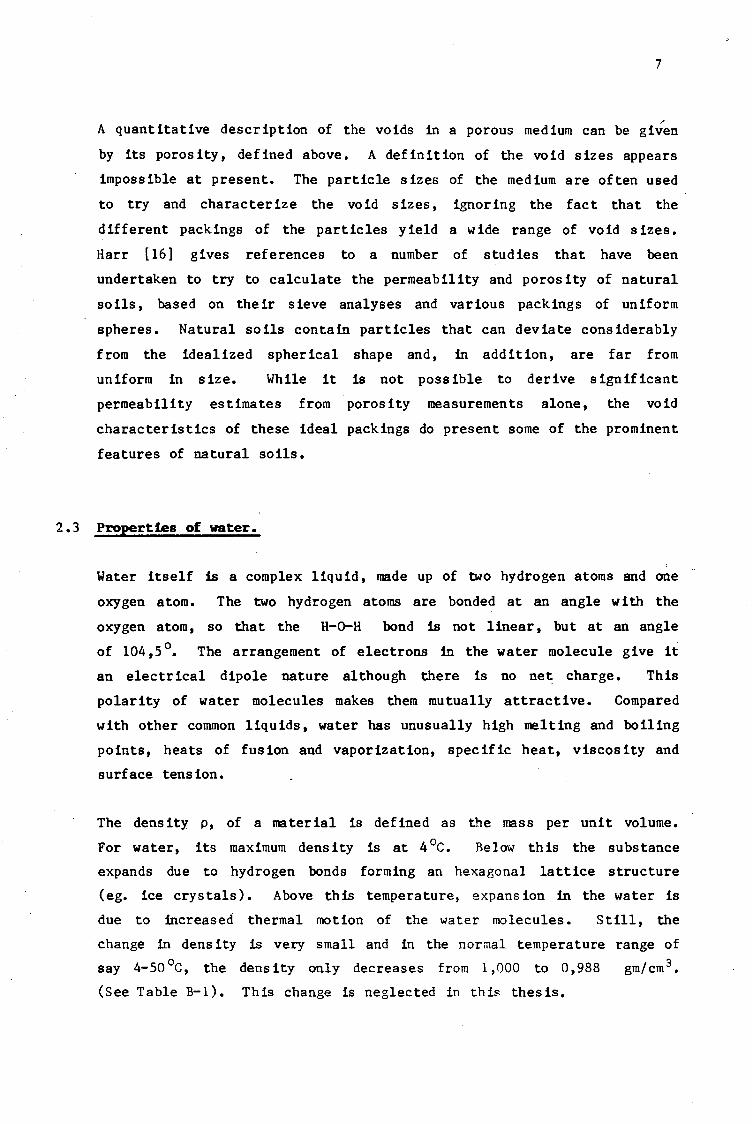
A quantitative description of the voids in a porous medium can be gi.;'en

by its porosity, defined above. A definition of the void sizes appears

impossible at present. The particle sizes of the medium are often used

to try and characterize the void sizes, ignoring the fact that the

different packings of the particles yield a wide range of void sizes.

Harr [16] gives references to a number of studies that have been

undertaken to try to calculate the permeability and porosity of natural

soils, based on their sieve analyses and various packings of uniform

spheres.

from the

uniform

Natural soils contain particles that can deviate considerably

idealized spherical shape and, in addition, are far from

in size. While it is not possible to derive significant

permeability estimates from porosity measurements alone, the void

characteristics of these ideal packings do present some of the prominent

features of natural soils.

2.3 Properties of water.

Water itself is a complex liquid, made up of two hydrogen atoms and one

oxygen atom. The two hydrogen atoms are bonded at an angle with the

oxygen atom, so that the H-0-H bond is not linear, but at an angle

of 104, 5 °. The arrangement of electrons in the water molecule give it

an electrical dipole nature although there is no ne~ charge. This

polarity of water molecules makes them mutually attractive. Compared

with other common liquids, water has unusually high melting and boiling

points, heats of fusion and vaporization, specific heat, viscosity and

surface tension.

The density p, of a material is defined as the mass per unit volume.

For water, its maximum density is at 4 °c. Below this the substance

expands due to hydrogen bonds forming an hexagonal lattice structure

(eg. ice crystals). Above this temperature, expansion in the water is

due to increased thermal motion of the water molecules. Still, the

change in density is very small and in the normal temperature range of

say 4-So 0 c, the density only decreases from 1,000 to 0,988 gm/cm 3•

(See Table B-1). This change is neglected in this thesis.

8

The compressibility of water is defined as the relative change in the

density with a change in pressure. In the soil-water relationships

considered in this thesis, where the pressure changes are not great,

(about one to two metres head of water) the water is assumed to be

incompressible. This assumption cannot always be made, as for example,

with 'confined aquifers the water may be subjected to very large

pressures and then the compression of the water must be considered.

At the interface of the water and air a phenomenon occurs called surface

tension. The water surface behaves as if it were covered by an elastic

membrane in a constant state of tension, tending to cause the surface to

contract. If the interface between water and air is not planar, but

curved (eg. concave or convex), a pressure difference between the two

phases is indicated, since equilibrium normal to the surface must

exist. This pressure difference is balanced by the curved surface,

surface tension forces, that have a resultant force, normal to the

surface. For example, water with a bulging (convex) surface to the

atmosphere indicates a pressure greater than atmospheric, and vice

versa, a dished (concave) surface indicates the water has a sub

atmospheric pressure just under the surface •.

If a drop of water is placed on a solid surf ace it will spread to a

certain extent, coming to rest with the water-air surface forming a

typical angle at the edges where it makes contact with the solid

surface. This angle is called the contact angle. (See figure 2 .2a).

The angle can vary between 0°, where the drop of water would completely

flatten for a perfect wetting of the solid, to 180° (if it were

possible) for a completely non-wetting liquid, and the drop retains a

spherical shape (assuming no gravity effects). The contact angle can be

different between the condition when water is advancing upon the solids

(the wetting or advancing angle) and the condition when water is

receding upon the solid surface (the retreating or receding angle).

If a thin clean capillary tube is dipped in water, the water level will

rise in the tube, due to capillary forces. Capillary forces depend on

the contact angle between the water and the tube wall and the surface

tension of the water.

9

Solid

Solid

'Fig 2.2: The contact mgl.e of the water-air surface with a solid

surface. (a) Of a drop nstfng apon a plane surface. (b) Of

a meniscus ID a cap Ulary tube.

In the case of the clean capillary tube, an acute contact angle forms,

with a concave water surface towards the air. (See figure 2 .2b). Due

to surface tension and a curved water surface, the level of the water is

forced up the tube, as the water and the air are both at atmospheric

pressure. The water level will come to rest in the tube where the

downward force due to the weight of the raised colunm of water will

balance the resultant upward force from the surface tens ion in the

concave water surface. The resultant force which develops due to the

contact angle being acute and the surface tension is known as the

capillary force.

For water to flow through a porous medium, viscous forces have to be

overcome. This is because the fluid is forced to move against shear

forces ( ie adjacent layers of the water are made to slide over each

other). The activating force required is proportional to the shear

forces. The proportionality factor is called the viscosity ~. Also the

ratio of the viscosity ~ to the density of the water is called the

kinematic viscosity v. With water, as with any fluid, the viscosity is

a function of temperature, decreasing with a rise in temperature.

(See Table B-2).

10

2 .4 Flow of water in saturated soils.

The movement or flow of water through a saturated porous medium can be

expressed by Darcy's Law. Henry Darcy was a French hydraulic engineer

who investigated the flow of water through horizontal beds of sand to be

used for water filtration. In 1856 he reported (see Todd [37]):

"I have attempted by precise experiments to determine

the law of the flow of water through filters... The

experiments demonstrated positively that the volume of

water which passes through a bed of sand of a given

nature is proportional to the pressure and inversely

proportional to the thickness of the bed traversed;

thus in calling s the surf ace area of a f 11 ter, k a

coefficient depending on the nature of the sand, e the

thickness of the sand bed, P - H0

the pressure below the

filtering bed, P + H the atmospheric pressure added to

the depth of water on the filter; one has for flow of

this last condition Q = (ks/e)(H + e + H0), which

reduces to Q = (ks/e)(H + e) when H0

= 0, or when the

pressure below the filter is equal to the weight of the

atmosphere."

This statement, that the flow rate in a porous media is proportional to

the head loss and inversely proportional to the length of the flow path,

is known as Darcy's Law. Figure (2.3) shows an experimental set µp to

show:

Q = (2.6) L

where k, (a coefficient of proportionality), is known as the hydraulic

conductivity or coefficient of permeability, A is the constant cross

sectional area of the porous media through which flow is taking place,

.6$ = ( $1 - ¢12) is the total head loss or energy loss per unit weight of

fluid and L is the length over which this total head loss occurs.

11

~ I I

i M= 4>1-¢2

- - ~

Z1

-ff/ ~·' Area Z2

Fig 2.3: Seepage through a fnclined filter due to a total bead

dlf ference. (Darcy's Experlaent.)

The total energy heads above a datum plane may be expressed by the

Bernoulli equation:

Pl P2 + + = + + (2. 7)

2 g 2 g

where p 1s pressure, y the specific weight of water, v the velocity of

flow, g the acceleration of gravity, z the elevation head above a chosen

datum level, and ~¢ the head loss. Because velocities in porous media

are usually low, velocity heads may be neglected without appreciable

error. Therefore the total head ¢, 1s defined as:

¢ = + z (2.8)

or

¢ = q, + z (2.9)

12

where ~' the pressure head or suction head is defined as:

~ = (2.10) y

which could be negative or positive depending on the pore-water pressure

Pw· Hence, rewriting equation (2.7), the total head loss becomes:

The macroscopic fluid velocity (flux) is given as:

Q q = =

A

or expressed fn general terms:

d 4> q = - k

dL

(2.11)

(2.12)

(2.13)

where d4>/dL is the hydraulic gradient and is negative as flow is fn the

direction of decreasing head. Equation (2.13) can be rewritten as:

k = q

(-~ ) dL

(2.14)

so that the hydraulic conductivity k, is defined as the ratio of the

flux to the hydraulic gradient. Plotting the flux q, versus the

hydraulic gradient - d4> I dL, for different flow rates, gives a linear

relationship where the gradient of the line is the hydraulic

conductivity.

13

The hydraulic conductivity can be affected by a number of parameters;

The structure and texture of the porous medium. (eg. The hydraulic

conductivity is greater when a soil is highly porous and fractured

then when it is compacted and dense. )

The porosity and size of conducting pores. (eg. The hydraulic

conductivity of a sandy soil with large pores is greater than that

of a clayey soil with small pores, even though the total porosity of

the clay is generally greater. )

The chemical, physical and biological changes that can occur due to

water flowing through the soil. (eg. Ion-exchange can occur in the

water. Also entrapped air in the soil or air given off from the

water due to a temperature change can block the pore passages,

decreasing the hydraulic conductivity.)

The viscosity of the water. (eg. A change in temperature causes a

change in the viscosity of water and therefore the boundary friction

forces acting on the fluid will change.)

2.5 Generalization of Darcy's I.ml.

If the hydraulic conductivity is the same throughout the domain of a

porous medium, that is, if it is independent of position within the

domain, the medium is said to be homogeneous with respect to the

hydraulic conductivity. Otherwise if it varies from point to point, the

medium is said to be heterogeneous. If the hydraulic conductivity, at a

point is the same in all directions throughout the domain of a porous

medium, the medium is said to be isotropic with respect to the hydraulic

conductivity. But if the hydraulic conductivity at each point in the

domain varies with direction, (eg. the horizontal hydraulic conductivity

at each point may be greater, or smaller, than the vertical hydraulic

conductivity), then the medium is said to be anisotropic with respect to

the hydraulic conductivity.

14

2.5.1 Isotropic medium.

The experimentally derived form of Darcy's Law· (for an homogeneous

material and incompressible fluid) was limited to one-dimensional

flow. Generalisation of Darcy's Law to three dimensions, the flux at a

pofot, which is a vectorial quantity, can be character.ize.d by its

magnitude and its direction. (see Bear [6]). In cartesian coordinates,

equation (2.13) results in the form:

q = - k grad 4> = - k V 4> (2.15)

where q is the specific flux vector (macroscopic fluid velocity) with

components qx, qy and qz in the directions of the Cartesian x, y and z

coordinates respective!>', 'and grad4> is the hydraulic gradient with 04> 04> - .2! components - ox ' - oy ' oz in the x, y and z directions

respectively. The total head 4>, is given as before by:

4>= 4'+ z (2.16)

where, the z-axis is taken as positive upwards from a chosen datum

level, so that gravity acts in the negative z-direction.

When flow takes place through a homogeneous isotropic medium, the

coefficient k, is a scalar constant and we may write equation (2.15) as

three equations:

04> qx = - k-

ox (2.17a)

04> qy = - k-

oy (2.17b)

04> qz - k-

oz (2.17c)

Equations (2.17) remain valid for three-dimensional flow through a

nonhomogeneous isotropic medium where k = k(x,y,z).

15

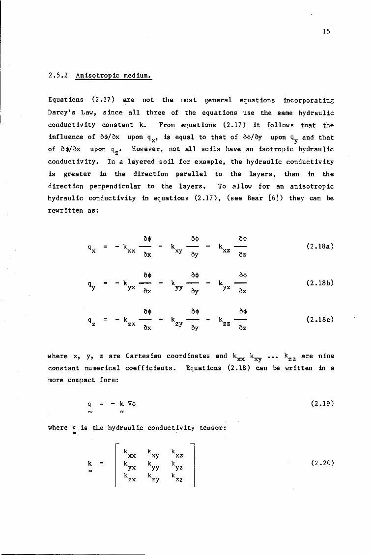
2 .5 .2 Anisotropic medium.

Equations (2.17) are not the most general equations incorporating

Darcy's Law, since all three of the equations use the same hydraulic

conductivity constant k. From equations ( 2 .17) it follows that the

influence of a$/ax upon qx, is equal to that of a$/ay upon qy and that

of a$/az upon qz. However, not all soils have an isotropic hydraulic

conductivity. In a layered soil for example, the hydraulic conductivity

is greater in the direction parallel to the layers, than in the

direction perpendicular to the layers. To allow for an anisotropic

hydraulic conductivity in equations (2 .17), (see Bea·r [6]) they can be

rewritten as:

a$ a$ a$

qx = - k -- - k - - k (2.18a) xx

ax xy ay xz

az

a$ a$ a$

qy = - k - - k - - k (2 .18b) yx

ax yy ay

yz az

a$ a$ a$

qz = - k - - k - - k (2 .18c) zx

ax zy

ay zz

az

where x, y, z are Cartesian coordinates and kxx kxy ••• kzz are nine

constant numerical coefficients. Equations (2.18) can be written in a

more compact form:

q = - k V$ (2.19) ,,.

where k is the hydraulic conductivity tensor: "'

k k k xx xy xz

k = k k k ,,. yx yy yz

(2.20)

k k k zx zy zz

16

Because the hydraulic conductivity tensor k, to satisfy the conservatioD "'

of energy, is a symmetrical tensor (ie.: kxy = kyx)' only six different

coefficients are necessary to define it.

If the direction of the axes is changed to x', y' and z', then the

specific flux vector in the direction of the new axes, can be found as:

q' x

q' = q' y (2.21)

q' z

= L q (2.22)

where L is a transformation matrix of direction cosines. Similarly, the "' new vector of the hydraulic gradients is:

- V4>' = (2.23)

= L V4> (2.24) .. combining equations (2.22) and (2.24) yields:

q' = - k' V4>' (2.25) ""

where the new hydraulic conductivity tensor:

_l k' = L k L (2.26) .. rv ~ rv

17 .

With this type of transformation, it is possible to find three

orthogonal directions x', y' and z' for which k' reduces to a diagonal

matrix:

k x' x'

0 0

k' = 0 k 0 .. y'y' (2.27)

0 0 k z'z'

substituted into equation (2.25) gives:

k 0 0 x'x'

q' = 0 k 0 y' y'

(2.28)

0 0 k z' z'

These directions are known as the principal axes of the porous medium.

Thus knowing the hydraulic conductivity of an anisotropic porous media

in its three principal directions, the hydraulic conductivity tensor can

be found with respect to a differently orientated orthogonal axes

system, by means of a simple transformation matrix.

Darcy's Law

Valid

Hydraulic Gradient

(a)

Fig 2.4: Limits of Darcy's law.

Yield Hydraulic Gradient

(b)

(a) Deviation from Darcy's law at

high flux, where flow becomes turbulent. (b) Possible

deviations from Darcy's law at low gradients. (Exhibiting a

Bingham liquid property.)

18

2.5.3 Range of validity of Darcy 1 s Law.

Darcy's Law only applies as long as the flow of water is laminar within

the pore passages. (See figure 2 .4a). With turbulent flow through the

pore passages, which may occur at high flux rate, (eg. In coarse sands

with hydraulic gradients near or in excess of unity) Darcy's Law will

not always be valid.

Also at low hydraulic gradients and with a soil that has very small pore

passages, it has been reported (and disputed) that the f lCM rates of the

water can be zero or less than proportional to the hydraulic gradient.

A possible reason for this (see Hillel [18]) is that the water :fn close

proximity to the particles acts roore rigid than ordinary water, and

exhibits the properties of a Bingham liquid ( ie. having a yield va'lue),

rather than a Newtonian liquid. See figure (2.4b)

2 .6 Flow of water fn unsaturated soil.

Movement of water above the water table (in the zone of aeration) takes

place in an unsaturated porous medium. Such flow is in general quite

complicated and difficult to describe quantitatively. This is because

changes :fn the state of the soil and the water can occut during flow.

These changes invol:ve the complex relationship between the volumetric

moisture content 9, suction head (negative pressure head) ~' and

conductivity k, whose interrelationships may be further complicated by

bys teres is.

It was stated in a previous section that flow in the saturated soil

takes place in the direction of decreasing total head, that the rate of

flow (flux) is proportional to the hydraulic gradient and is affected by

the geometric properties of the pore channels through which flow takes

place. These principles also. apply in unsaturated soils. In saturated

soils the moving force is the total head ¢, which is the sum of the

pressure head and elevation head ( + z), the pressure head being

positive below the phreatic surface. The same total head is the driving

force in unsaturated soils, but the local pressure head is

19

subatmospheric. This subatmospheric pressure head is sometimes referred

to as the suction head. In the unsaturated soil there is a matrix

suction due to the physical affinity of water to the soil particle

surfaces and capillary pores. This means that water tends to be drawn

from zones where the capillary menisci are less curved to where they are

more highly curved. This means that at the same elevation, water flows

from a lower matrix suction to a zone of higher matrix suction. (ie. If

the soil is homogeneous, then water will migrate horizontally from zones

where thicker layers of water surround the particles, to the zones where

those water layers are thinner.) If there is a change in elevation,

this must be taken into account and movement will only occur where there

is a difference in total head cp.

One of the most important differences between saturated and unsaturated

soils is the hydraulic conductivity. When the soil is saturated, all of

the pores are water filled and conducting, so that continuity and hence

conductivity is at a maximum. In an unsaturated soil, some of the pores

are partly air filled and the conductive cross-sectional area of the

soil decreases correspondingly. As a soil becomes more unsaturated, the

matrix suction develops, emptying the largest pores first, which are the

most conductive and leaving water to flow in the smaller pores only. As

more pores empty, (in a more unsaturated soil) discontinuous pockets of

water, as shown in figure (2.5), may remain almost entirely in capillary

wedges at the contact points of the particles. For these reasons, the

transition from saturation to unsaturation generally has a steep drop in

hydraulic conductivity as shown in figure (2 .6). At very high suction

or low volumetric moisture content, the moisture left in a soil may al:l

be bound to soil particles, by capillary forces and as bonded

moisture. The conductivity is therefore very low (approaching zero)

near the residual saturation, indicating no flow.

At saturation, soils with the largest continuous pore passages are

normally the most conductive, while the least conductive are soils with.

very small pore passages (eg. sands and clays, respectively). However,

the opposite may be true when the soils are unsaturated. As a suction

develops, a soil with large pores empties more quickly, compared with a

soil with small pores which can retain the water against the applied

20

suction. Thus the initially high hydraulic conductivity of a large pore

soil decreases steeply and, at a particular suction, may be less than

that of a soil with very small pores, whose hydraulic conductivity has

not decreased as drastically.

Fig 2.5:

Fig 2.6:

Water

Capillary Water

Illustration of: (a) Vater fn an lDlS&turated coarse-textured

soil; (b) Bonded and Capillary water.

>-4.J

•.-1 ...... . 6 ..... .0 ell cii

E .4 cii c. cii :> .2 Residual ..... 4.J

~turation ce ...... cii 0 i:.::

0 . 2 .4 .6 .8

Degree of Saturation s r

Relative hydraulic conductivity, (Ratio of the·lDlSaturated to

the saturated hydraulic conductivity) as a function of

saturation. ' '

21

2.7 Extensi~n of Darcy's Law.

The hydraulic conductivity k, originally introduced by Darcy for

saturated soils, was extended by Buckingham (1907) and Richards, (See

R !chards [ 36]), to unsaturated flow, with the prov is ion that the

conductivity is now a function of the volumetric moisture content, i.e.

k = k(9). From a theoretical viewpoint, k(0) can be expressed as:

k( 9) = k k ( 9) rw

(2.29)

where k is the hydraulic conductivity or coefficient of permeability of

a saturated soil, and krw( 9) is the relative hydraulic conductivity

which varies from O, for a completely dry soil (below the residual

saturation), to 1, for a fully saturated soil. See figure (2.6). The

specific flux vector in three dimensions can now be extended to an

unsaturated soil by substituting equation (2.29) into (2.19) in the

form:

q = - k( 9) v • (2.30) rd

or

q = - k [ k (9) v • l (2.31) IOI rw

where k is the hydraulic conductivity tensor for the saturated soil.

There is just one problem in that the relationship of krw = krw( 0), is

affected by wetting and drying bys teres is. The degree of bys teres is is

much less than the hysteresis between the suction head ~' and volumetric

moisture content e. Because of the hysteresis in the relationship of

krw = krw(0), being much less, compared with the relationship of

~ = ~( 9), it is assumed in most literature that a single relationship

exists between k and e, but which still leaves the problem of dealing rw with the hysteresis in the relationship between ~ and 9.

22

2.8 Soil m>isture characterstic curve.

The total head for water in a rigid soil as defined previously is given

as:

 = <Ii + z (2.32)

where <Ii is the pressure head and z the elevation head above some datum

plane. <Ii takes on negative values in the unsaturated zone and positive

values in the saturated zone. If we consider a point P, in a soil mass

that is initially saturated and then becomes unsaturated, we get a plot

of the suction head versus volumetric moisture 9, as shown in

.figure (2.7) for the pressure at point P. Initially as the negative

pressure increases, little or no change in the saturation will occur

(i.e. no air will penetrate the sample) until the critical suction is

exceeded at which time the largest pores begin to drain. This critical

suction can be called one of the following; air-entry suction, critical

capillary head, bubbling pressure or the air-entry pressure.

l/J

~ .,, Ct! Q.l

.c: c: 0 ..... ..., u ;:l

ti)

0

t: 0

·-: ..., Wetting ti) .... _, drying curv-e ..., ti) II)

.... Q.l 4-J Scanning drying curves Ct! )

Q) ...... --e:::::::-Air - Entry suction ,£:j ..... -Drainage u ;:l (or drying) .,, Q.l .... ....

H Scanning wetting curve

Starting with a ~saturated sample

.... ~..._~~~~~~~~-+-~;_,.""'"'4~

~ 6 0 Entr~pped air

(may be removed with time,e.g. ,by water flow)

F ig 2. 7 : Soil-mo is tu re character is t 1c curve.

relationship of 4' = +( 0).

Bysteres is in the

23

With the increase in suction, more water will drain out of the

relatively large pores. This gradual increase in suction will result in

the emptying of progressively smaller pores until, at high suction

values, the only water remaining is held as bonded moisture to the

particles and by large capillary forces between the particles. See

figure (2.Sb).

2.8.1 Hysteresis.

The relationship between the suction head (i.e. the negative pressure

head) <Ii and the volumetric moisture content e, is not a single valued

function, but has different curves for wetting and drying, See figure

(2.7). The equilibrium moisture content e, at a given pressure head$,

is path dependent and this dependency is called hysteresis.

The hysteresis effect may be attributed to several causes (Hillel [ 18]):

Fig

1) Geometric nonuniformity of the individual pores resulting in the

"inkbottle" effect, figure (2 .8a).

2) The contact-angle effect which is different for an advancing

meniscus as opposed to a receding one. The angle is smaller for

the receding one and therefore exhibits greater suction than an

advancing one, figure (2.8b).

3) Entrapped air upon rewetting.

4) If the soil is not rigid, compaction or consolidation can change

the total volume and soil structure.

2.8:

l Drainage Rewetting

(a) (b)

Factors causing

characteristic curve:

raindrop effect.

hysteresis in the soil-moisture

(a) The ink-bottle effect; (b) The

24

If the last two cases are not considered then the drainage and wetting

curves form a closed loop, figure (2. 9b). If we consider the ink bottle

effect with hypothetical pores shown in figure (2.8a) The pores consist

of relatively wide .voids with narrow channels. If :Initially saturated,

the pores will only drain when the suction exceeds the tension due to

capillary forces :In the narrow channels. However, for the pores to be

rewet, the suction must be decreased to below the tension due to

capillary forces of the relatively large pores, and then only will the

pores fill. The tension due to capillary forces for the small channels

is greater than that of the larger pores, and therefore drainage and

rewetting occurs at two different suction pressures.

The two main complete characteristic curves, from saturation to dryness

and vice versa, are called the Main or Boundary curves of the hysteretic

soil moisture characteristic curve. When a partially wetted soil begins

to drain or a partially drying soil is rewetted, the relation q, = Qi( 9)

follows some intermediate curve (scanning curve) as it moves from one

Boundary curve to another. Cyclic changes often involve wetting and

drying scanning curves, which may form closed loops between the main

branches. As long as the soil remains rigid (i.e. there is no

consolidation) the hysteresis loop can usually be repeatedly traced.

The relationship of = <ti( 0) is seen to be very complicated. If there

is only nonotonic wetting or drying in a particular problem, it may be

justifiable to use only one of the main soil moisture characterstic

curves. This thesis will deal with monotonic drainage ( ie. drying

curves apply).

2.8.2 Specific moisture capacity.

The specific moisture capacity c, is generally defined as the slope of

the soil-moisture characteristic curve, which is the change of

volumetric moisture content 9, per unit change of pressure head ~:

c ( 9) d9

d~

(2.33)

The specific moisture capacity c is also non-linear and is path

dependent (ie. Hysteresis effects apply). (See figure 2.9c).

(a)

(b)

k rw

0

0

0 e

e

e sat

e sat

(c)

s-scanning d-drying w-wetting

-lj! 0

ae alj!

+lj!

25

Fig 2.9: Typlcal functional relationships for saturated-unsaturated

soils: {a) R.elative hydraulic conductivity versus volumetric

moisture content;

moisture content;

pressure bead.

z

{b) Pressure head versus volumetric

{c) Specific moisture capacity versus

Fig 2.10: The continuity principle: A wlume of soil gaining or losing

vater fn accordance vitb the divergence of the flux.

26

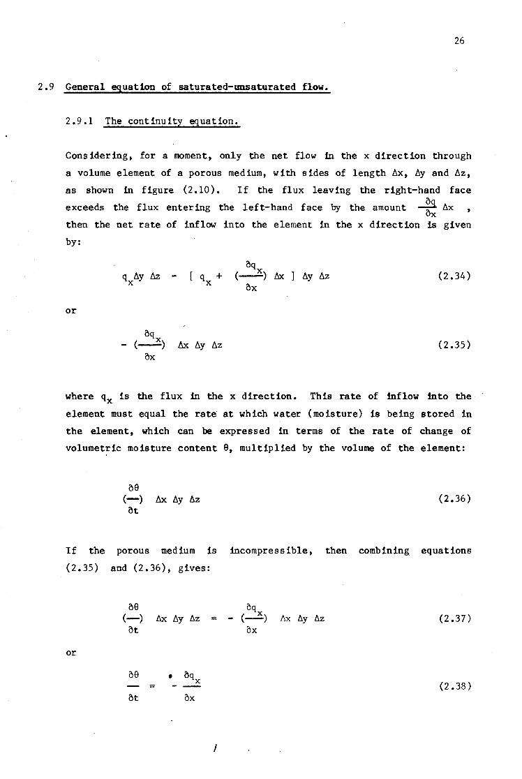
2.9 General equation of saturated-unsaturated flow.

2.9.l The continuity equation.

Considering, for a moment, only the net flow in the x direction through

a volume element of a porous medium, with sides of length !::,.x, !::,.y and l::,.z,

as shown in figure (2.10). If the flux leaving the right-hand face

exceeds the flux entering the left-hand face by the amount ~ /::,.x ox

then the net rate of inflow into the element in the x direction is given

by:

or

q /::,.y ~ x

[ q + x

oq x - (----) bx t:,.y /::,.z

ox

oq (---2!.) /j,x. J t:,.y /::,.z

ox (2.34)

(2.35)

where qx is the flux in the x direction. This rate of inflow into the.

element must equal the rate at which water (moisture) is being stored in

the element, which can be expressed in terms of the rate of change of

volumetric moisture content 0, multiplied by the volume of the element:

09 (-) bx t:,.y bz ot

(2.36)

If the porous medium is incompressible, then combining equations

(2.35) and (2.36), gives:

09 oq (-) bx t:,.y /::,.z = - (~) /::,.x !::,.y /::,.z (2 .37)

ot ox

or

09 • oq x (2.38) = - --

ot ox

I

27

If the fluxes in the y and z directions are also ·considered, the three

dimensional form of the continuity equation is obtained, namely:

= at

oq - (--2S +

ox

oq oq .....:.z + -2-) (2 .39), oy oz

where qx' qy' qz are the fluxes in the x, y, z directions,

can be rewritten as: respectively. Equation (2.39)

ae = - V•q (2.40)

ot

or

oe = - div q (2.41)

at

2.9.2 The combined flow equation.

The equation for the generalized Darcy's Law for saturated-unsaturated

flow was given by equation (2.30) as:

q = - k ( 0) v 4> (2.42) "'

where k the hydraulic conductivity tensor is a function of the

volumetric moisture content e, and the total head gradient Vlj>. The

hysteresis of the soil-moisture characteristic curve is taken into

account in the relationship between <Ii and e. By substituting

equation (2.42) into the continuity equation (2.40) we obtain the

general flow equation:

ae = v • [ k (e) v 4> J (2.43)

at "'

where e is the yolumetric moisture content, t the time, 4> the total head

(q, + z) and k(0) the hydraulic conductivity. The air in the voids is "' assumed to be at atmospheric pressure and free to move, and the water is

incompressible.

28

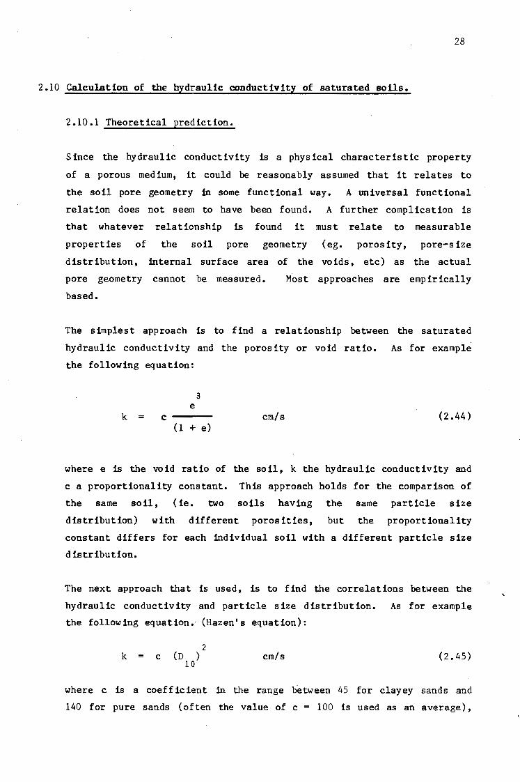
2.10 Calculation of the hydraulic conductivity of saturated soils.


Since the hydraulic conductivity is a physical characteristic property

of a porous medium, it could be reasonably assumed that it relates to

the soil pore geometry in some functional way. A universal functional

relation does not seem to have been found. A further complication is

that whatever relationship is found it must relate to measurable

properties of the soil pore geometry (eg. porosity, pore-size

distribution, internal surface area of the voids, etc) as the actual

pore geometry cannot be measured. Most approaches are empirically

based.

The simplest approach is to find a relationship between the saturated

hydraulic conductivity and the porosity or void ratio. As for example

the following equation:

3 e

k = c---- cm/s (2.44) (1 + e)

where e is the void ratio of the soil, k the hydraulic conductivity and

c a proportionality constant. This approach holds for the comparison of

the same soil, ( ie. two soils having the same particle size

distribution) with different porosities, but the proportionality

constant differs for each individual soil with a different particle size

distribution.

The next approach that is used, is to find the correlations between the

hydraulic conductivity and particle size distribution. As for example

the following equation. (Hazen' s equation):

2 k = c (D )

10 cm/s (2.45)

where c is a coefficient in the range between 45 for clayey sands and

140 for pure sands (often the value of c = 100 is used as an average),

29

and D10 is the effective grain size diameter in cm. (See se.::tion 4.2).

Problems with this approach are that the particles of a soil having the

same effective grain size diameter n10 , can be packed differently,

yielding a different hydraulic conductivity to that predicted.

Purely theoretical formulae have been obtained from theories based on

the relation of the hydraulic conductivity to the geometric properties

of the porous media (ie. from theoretical derivations of Darcy's Law).

One such example is the Kozeny-Carman equation. (see Bear [6}):

k = c

3 n

2 2 (1 - n) a

(2.46)

where n is the porosity, a the specific,surface exposed to the fluid and

c a constant representing a particle shape factor. The theory is based

on the concept of a hydraulic radius. The hydraulic radius is measured

by the ratio of the volume to the surface of the voids, or the averag~

ratio of the cross-sectional area of the voids to their circumferences.

Other approaches have also been investigated, but each has some or other

limitation that prevents it from being universally used.

2.10.2 Laboratory measurement.

Methods have been devised to measure the hydraulic conductivity of a

soil sample in the laboratory. Problems with these measurements made in

the laboratory are that they often do not correspond to the hydraulic

conductivity of the soil in the field. ( ie. In-situ soil) This is

because soil samples are disturbed and repacked in the laboratory with

porosities, packing and grain orientations markedly changed, and

consequently the hydraulic conductivity is modified. Laboratory tests

however permit the relationship between the hydraulic conductivity and

the void ratio to be studied.

Two commonly used laboratory methods for the determination of the

30

hydraulic conductivity are the "Constant head permeameter" and "Variable

head permeameter" tests;

a) Constant head permeameter.

The constant head permeameter as shown in figure (2.lla) is used

to measure the hydraulic conductivity. By noting the head loss

t.h over the sample length L, and the flow rate of the water

through the soil sample, it is possible to calculate the

hydraulic conductivity from Darcy's Law:

k = ti.h L

Reservoir

l:ih

Qt in Time t

(a)

Soil

Area a

Fig 2.11: Laboratory permeameter tests:

Variable head.

(2.47)

h 1

(t 1

Screen

Area a

h 2

(t ) 2

Soil

Qt in Time t

(b)

(a) Constant bead; (b)

31

where k is the hydraulic conductivity, Qt the quantity of water

to flow through the sample in time t and A the cross-sectional

area of the sample. By repeating the test using different flow

rates q = Qt/t, a plot of Qt/ At versus !:ih/L can be made. The

gradient of a straight line fitted to the plotted points is the

hydraulic conductivity.

b) Variable head permeameter.

The variable head permeameter uses a similar lay-out to that of

the constant head permeameter, except that instead of a constant

supply head, a falling head is used, as shown in figure

(2.llb). Here the water is added to a tall column of known

cross-sectional area. The water then passes upwards through the

sample and is collected as it overflows. The test cons is ts of

noting times at which the water level passes various height

graduations on the tube. The cross-sectional area and the length

of the sample are measured. If two graduations are used, as

shown in figure (2.llb), then h1 and h2 must be known. The time

required for the water level in the tube to fall from h1 to bi is

measured as t.

The differential form of Darcy's Law can be written as:

Ah dt dQ =

t k---- (2.48) L

If a is the cross-sectional area of the tube and the water level

height changes by -dh, then:

- a dh (2.49)

Substituting into equation (2.48) gives:

A h dt - a dh k--- (2.50)

L

Rearranging and simplifying, equation (2.50) becoDes:

dh A dt -- = k---

h a L

Integrating yields:

At - ln h = k - + C

aL

when t = o, h = h1 , thus:

c = :- ln h1

Inserting this into equation (2. 52) and rearranging gives:

aL k =

At

32

(2.51)

(2.52)

(2.53)

(2.54)

Therefore, by measuring the time for the water level to drop from

h1 to hz and knowing the cross-sectional area's of the tube and

the soil sample, plus its length, the hydraulic conductivity can

be calculated from equation (2.54).

2.10.3 Field measurement.

The pumping tests on wells, that extend below the water table, are

important for the evaluation of the hydraulic properties of an

aquifer. Parameters predicted by these tests are well yields; position

of the water table or piezometric surface; and recharge rates of the

aquifer. Other techniques for use in the field have been developed, for

determining more specifically the hydraulic conductivity of the soil in

situ. The tests differ, depending on where the water table is. If the

water table is near the surface, the tests are done below the water

table in the saturated zone. If the water table is relatively deep, the

33

hydraulic conductivity is measured above the water table, ( ie. the

vadose zone) using tests that first artificially wet an area until

saturated. The in situ test results are mainly used for surface

subsurface water relations (eg. Infiltration), to design drainage

systems and to estimate seepage from channels. Some methods, for the

measuring of the hydraulic conductivity in soils, as near as possible to

saturation, either above or below the phreatic surface, are given below.

a) Pumping tests

Pumping tests are done with wells, to determine the hydraulic

properties of the aquifer. By pumping the water out of the well,

at a constant rate, and observing the drawdown of the piezometric

surface or the water table in observation wells at some distance

from the pumped well, the aquifer's hydraulic properties can be

determined. The type of the test can vary, either being a steady

state or transient test and applied to a confined or unconfined

aquifer. A number of methods for the evaluation of the aquifer

parameters from the pumping tests results have been developed by

several investigators (eg. Theis solution; Chow solution; Jacob

solution; etc). Most of the methods are based on a graphical

method for the solution.

The same measurements can be made during a recovery test. This

is a test started when the pumping of a well is stopped and the

rise of the water levels in the observation wells are recorded.

b) Rate of rise tests

Tests in this category are to do with wells that penetrate below

the water table. To do the tests, the static water table level

must be visible in the well. A quantity of water is removed from

the well (to lower the water level) and the rate at which the

water level rises is recorded.

A number of tests based on the above are given in Bouwer [7], for

example, the Slug test, Auger-hole method and Piezometer

method. With each of these methods there are variations adopted

by different investigators.

i·:ith the Slug test, (See figure 2.12) both vertical and

horizontal conductivity is measured. Water is removed from the

well and the rate of rise is noted. Using type curves ( ie.

graphical method) similar to the Theis procedure for pumping

tests, the solution of the Transmissivity and Storativity of a

2r c

l Water Table

y

-

L I 'W

I 2r w

Impermeable

Fig 2.12: Schematic diagram of slug test. Bouwer (7)

l Water Table

y -

L w

2r w H

Impermeable or Very Permeable

Fig 2.13: Schematic diagram of auger-hole method. Bouwer [7]

35

confined aquifer can be found. Bouwer [ 7] and Rice developed a

slug-test procedure applicable to both confined and unconfined

aquifers, from which the hydraulic conductivity can be obtained.

The Auger-hole method (See figure 2 .13) is similar to the Slug

test method for wells, but the water level rise is measured in an

unlined auger hole. This test has been developed by different

investigators, and the water level rise in the auger-hole and the

geometry thereof are related to the hydraulic conductivity.

The P iezometer method (See figure 2 .14) is just a variation on

the Auger-hole method, in that a pipe is jetted into the soil,

instead of an augered hole, and the water level is rapidly

lowered. Its rise back to the water table level is recorded.

From this the value of the hydraulic conductivity around the pipe

tip is calculated by a given equation.

c) Hydraulic· conductivity in the vadose zone

Measurement of the hydraulic conductivity in the vadose zone is

important if infiltration or seepage through this zone needs to

be predicted. The basis of calculating the hydraulic

conductivity of the soil is to artificially wet a portion of the

soil and to evaluate the hydraulic conductivity from a flow

system created within the wetted zone. A problem with this

method is that it is difficult to achieve full saturation of the

soil and so the resulting hydraulic conductivity measured is less

than that at saturation. A few of the methods described by

Bouwer [7), are the Air-entry permeameter method; Infiltration

gradient technique; Double-tube method and Well Pump-in

technique.

The Air-entry permeameter (See figure 2.15) is a surface

device. It consists of a metal cylinder with one end opened,

which is pressed into the soil, and the top end is closed.. A

stand pipe with a reservoir is fixed to the cylinder. The soil

within the cylinder is wet with water via the stand pipe. Noting

the drop of the water level in the reservoir, the flow rate of

L w

L e

y

Water Table

Pipe

H

Cavity

Impermeable or Very Permeable

Fig 2.14: Schematic diagram of the piezometer JEthod. Bouwer [7]

H r

G

Vacuum Gauge\

-Reservoir

Valve

-Air Escape Valve

l-~~~=1,- Sand ..... ~~--,..,...,~1--.---·-·)r)~)~\~\1--~.,..,."7':"~~

\ . Wetting front

36

Fig 2.15: Schematic diagram of the air-entry permeameter. Bouwer [7]

37

the water entering the cylinder can be determined. Once the

wetting front, in the soil, reaches the open end of the cylinder,

the stand pipe is closed and the build up of negative pressure is

noted. The highest recorded negative value is the air-entry

value. With this reading and measuring the depth of the wetting

front from the surface, the hydraulic conductivity can be

calculated using a modified form of Darcy's equation. This

modified form takes the air-entry value into account.

The infiltration-gradient technique (See figure 2 .16) is similar

to the air-entry permeameter in principle, but the vertical

gradient is measured directly with tensiometers. To ensure

vertical flow, two concentric cylinders are used to wet the

soil. The open ends of the cylinders are pushed into the soil.

The infiltration rate for the inner cylinder is measured, ,while

the water level in both cylinders is kept level as they drop.

From the measurement of the infiltration rate and the vertical

gradient (from the tensiometer readings) the hydraulic

conductivity can be calculated.

The double-tube method allows the hydraulic conductivity of the

soil to be measured without the use of tensiometers or knowing

the air-entry value and wet depth of the soil. The test is

performed by first wetting the soil below both cylinders. (as

with the infiltration-gradient technique.) The water level in

the outer cylinder is kept at a constant height while that in the

inner cylinder is allowed to drop. This infiltration rate is

noted. The test is then repeated, but this time the water level

in the outer cylinder is adjusted so that it falls at the same

rate as the inner cylinder. By noting the different flow rates,

( ie. the dropping rate of the water level) and knowing the

geometry of the equipment the hydraulic conductivity can be

calculated.

The well pump-in technique (See figure 2.17) is the reverse test

to the auger-hole method. Water is added to an augered-hole and

the flow rate necessary to keep the water level constant in the

38

hole is measured. By knowing the physical dimensions of the

augered hole, the hydraulic conductivity can be calculated.

Outer Tube -

Inner Tube

-To Manomc·ter or Pressure Transducer

Sand

ensionometer

Wetted Zone

Fig 2.16: Schematic diagram of the fnfiltration-gradient technique.

Bouver [7]

s. l

2r w

Wetted Zone

Impermeable

Fig 2.17: Schematic diagram of well pump-in Ethod. Bouver [7]

39

2.11 Calculation of the hydraulic conductivity of tm.Saturated soils.


Various models are used for predicting the hydraulic conductivity of

unsaturated soils. The models are either theoretical, empirical or

semi-empirical based. (See Mualem [27) and [28)). The approaches can

be divided into two main groups. The first is based on the relative

hydraulic conductivity krw' being a power function of the effective

saturation Se, ie.:

k( 9) k = ( )

rw k (2.55)

sat

= S a e

(2.56)

where

( e - e ) s

, r = e

(0 - e ) sat r

(2.57)

where 0 and er are the actual and the residual volumetric moisture

contents respectively. Mualem [28) gives references to various

investigations in which the value for a has been derived theoretically

as well as empirically. A value within the range of 2 to 24 is reported

by Mualem for 50 soil samples investigated, with a = 3 ,5 being the ioost

common value.

A theoretical analysis reported by Mualem [28) showed that a may be

lower than 3 for a granular porous medium and higher than 3 for a fine-

grained so 11. These findings are verified by experimental data

presented for the 50 sous·.

The second approach makes use of the measured capillary head versus

volumetric moisture content relation ( ie. <Ji = <Ji( 9), the soil-moisture

characteristic curve) to derive the hydraulic conductivity of the

40

unsaturated soil. The underlying concept of this method is relating the

relative hydraulic conductivity krw with the porous medium's pore-size

distribution. From the soil-moisture characteristic curve, using a

statistical approach, the number of conducting interconnected pores is

determined. This is related to the relative hydraulic conductivity. ·

(See Mualem (27); Jackson (21] and King (23]).

Using the ratio of the measured to the calculated saturated hydraulic

conductivity ksat/k1 , as a matching factor, to adequately represent

experimental data, Jackson's ( 21] formulation is as follows:

m _2

e ~ E ( ( 2j + 1 - 2 i) q,j

ki = k (_L) j=l (2.58) s e m _2

sat E ((2j - 1) q,j j=l

where ki is the hydraulic conductivity at a volumetric moisture content

value ei, m is the number of increments of e ( ie. equal intervals from

dryness to saturation of 9), <iii is the suction head at the midpoint of

each e increment, and j and i are summation indices. Finally ~ is an

arbitrary constant assigned a value of between 0 to 4/3 by various

investigators. Jackson (21) found that the value of 1 is satisfactory.

Hill el ( 18] notes that as this second approach is based on the pore

sizes, it can be expected that the above theory referenced, applies more

to coarse-grained than to fine-grained soils, whereas the power function

approach can be applied to both.

A problem with the theoretical predictions is that even if a certain

formula is suitable for a particular class of soils, the coefficients

may vary form soil to soil within that class. Therefore the merit of

most empirical and semi-empirical methods is there use in an analytical

solution, based on experimental data from which coefficients are found,

rather than being an effective solitary tool for predicting •

•

41

2.11.2 Laboratory measurement.

Laboratory tests can be done on a sample of soil to find the relation

between the hydraulic conductivity k and the volumetric moisture

content e or suction head qi. Bouwer [7] and Youngs (40] report on a

most direct method of measuring the hydraulic conductivity of an

unsaturated soil. The technique also used by Childs, consists of a

long, soil-filled vertical column. Water is applied to the top of the

column,

sample.

column.

at a constant rate less than that required to saturate the

The water is allowed to drain freely from the bottom of the

iQ

-e

collected in Time t

Fig 2 .18: Long soil column to determine the unsaturated hydraulic

conductivity k, fn relation to the suction bead k = k(cli), or

volumetric 111>isture content k = k(0)

42

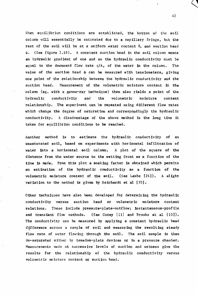
When equilibrium conditions are established, the bottom of the soil

column will essentially be saturated due to a capillary fringe, but the

rest of the soil will be at a uniform water content e, and suction head

~. (See figure 2.18). A constant suction head in the soil column means

an hydraulic gradient of one and so the hydraulic conductivity must be

equal to the downward flow rate q/A, of the water in the column. The

value of the suction head ~ can be measured with tensiometers, giving

one point of the relationship between the hydraulic conductivity and the

suction head. Measurement of the volumetric moisture content in the

column (eg. with a gamma-ray technique) then also yields a point of the.

hydraulic conductivity and the volumetric moisture content

relationship. The experiment can be repeated using different flow rates

which change the degree of saturation and correspondingly the hydraulic

conductivity. A disadvantage of the above method is the long time it

takes for equilibrium conditions to be reached.

Another method is to estimate the hydraulic conductivity of an

unsaturated soil, based on experiments with horizontal infiltration of

water into a horizontal soil column. A plot of the square of the

distance from the water source to the wetting front as a function of the

time is made. From this plot a soaking factor is obtained which permits

an estimation of the hydraulic conductivity as a function of the

volumetric moisture content of the soil. (See Lambe {24]). A slight

variation to the me tho.cl is given by Reichardt et al { 35].

Other techniques have also been developed for determining the hydraulic

conductivity versus suction head or volumetric moisture content

relations. These include pressure-plate-outflow; instantaneous-profile

and transient flCM methods. (See Corey {11] and Brooks et al [10]).

The conductivity can be measured by applying a constant hydraulic head

difference across a sample of soil and measuring the resulting steady •

flow rate of water flowing through the soil. The soil sample is then

de-saturated either by tension-plate devices or in a pressure chamber.

Measurements made at successive levels of suction and wetness give the

results for the relationship of the hydraulic conductivity versus

volumetric moisture content or suction head.

43

As the relationship is hysteretic (path dependent) the tests must be

done in both direct ions ( ie. from a saturated sample to a dry sample and

vice versa), to obtain the complete relationship.

2.11.3 Field Measurement.

Field tests are important because small disturbed samples tested in the

laboratory often are not fully representative of actual field

conditions. Several in situ methods have been developed to measure the

hydraulic conductivity of unsaturated soils. (S~e Hillel [18]).

a) Sprinkling infiltration.

With this method, described in principle by Youngs [40], water is

sprinkled on the surface at a constant rate, less than that to

cause saturation of the soil (ie. no ponding on the surface).

Eventually, once steady-state conditions are established, a

constant flux and a steady moisture distribution in the

conducting soil will result. In a uniform soil, the suction head

gradients will tend to zero and with only a unit elevation head

gradient in effect, the hydraulic conductivity becomes equal to

the flow rate. The test is normally started with a dry soil and

a series of successively increased flow rates are used. By

measuring the volumetric moisture content of the soil, it is

possible to obtain the relationship of the hydraulic conductivity

versus the volumetric moisture content. The problem with this

test is the rather elaborate equipment needed to be able to apply

the very small sprinkling flow rates.

b) Infiltration through an impeding layer.

This method suggested by Hillel and Gardner [19] is based on a

similar principle to the sprinkling infiltration method above.

The difference is that instead of using elaborate equipment to

supply ~ flow rate lower than that needed to saturate the soil, a

layer of soil with a lower saturated hydraulic conductivity is

spread over the soil being tested. This means that the

infiltration rates applied to the lower soil being tested can be

adjusted by the capping crust used. By using a series of

different impeding layers, a

giving different flow rates.

44

series of tests are performed,

This gives the results for the

relationship of the hydraulic conductivity versus the volumetric

moisture content.

The volumetric moisture content may be determined, in both cases, by a

neutron probe or gamma-ray technique.

c) Internal drainage.

Th is method is based on the approach of roon i tor ing the transient

state internal drainage of a soil profile. (See Hillel et al (20]

for a detailed description of a simplified procedure). The

method is performed by selecting a large enough surface area so

th.at processes at the centre of the site are not affected by the

boundaries. A neutron access tube is placed in the centre so

that the volumetric moisture content can be measured at different

depths. Next to the tube, but far enough away so that the

neutron readings are not affected, a vertical row of tensiometers

are placed, so that the soil suction can be monitored at

different dep.ths. Water is then ponded on the plot, until the

tensiometer readings indicate that steady state conditions

exist. Irrigation is then stopped. The surface is then covered

to prevent any further flux crossing the surface (eg. water

evaporation). As the internal drainage process proceeds,

periodic readings of the volumetric moisture content and

tensiometers are ma.de. The volumetric moisture content readings

are made at depths corresponding to the tens iometers. From the

volumetric moisture content readings at different times, the soil

moisture movement between each depth increment can be

calculated. From the tens iometer readings, the hydraulic

gradient at each depth can be calculated. From the above, the

hydraulic conductivity can be calculated at different depths for

the corresponding volumetric moisture content.

By plotting the results corresponding to the different depths,

for each time step, the hydraulic conductivity versus the

volumetric moisture content relationship for each depth is

45

found, For each depth, the relationship could be different if

the soil is heterogenous. Otherwise the relationship for each

depth should be the same if the soil is homogeneous.

2.12 Calculation of the soil-moisture characteristic curve.


The soil-moisture characteristic curve is strongly affected by soil

texture. The greater the clay content in general, the greater the water

retention at any particular suction, and the nx>re gradual the slope of

the curve. In a sandy soil, most of the pores are relatively large and

once these large pores have been emptied at a given suction, only a

small amount of water remains. In a clayey soil, the pore-size

distribution is nx>re uniform and ioore of the water is retained, so that

by increasing the soil moisture suction only a gradual decrease is

caused in the volumetric moisture content.

There seems to be no satisfactory theory that exists for the prediction

of the soil moisture suction head <Ji, versus the volumetric moisture

content relationship, from the basic soil properties. Several empirical

equations have been proposed, but they only describe the soil-moisture

characteristic curve for some soils within limited suction ranges. One

such equation presented by Brookes and Corey [10] is:

( e - er)

< e - e ) sat r

= (2.59)

where the suction head 4i must be greater than the air-entry suction

<lie· The exponent f.. is termed the pore-size distribution index, 0 the

volumetric moisture content (a function of the suction head ~), esat the

saturated volumetric moisture content and 0 is the residual volumetric r moisture content.

Theoretical methods proposed normally fall short in not being able to

46

account for the hysteresis effect between the relationship of the

suction head and volumetric moisture content. Not only being limited to

particular suction ranges, the equations only describe either the

wetting or drying curve of the relationship.

A hysteresis model is introduced by Mualem [26] and expanded by

Mualem and Miller [29]. The hysteresis model is based on the

independent domain concept, to account for the hysteresis. With this

method, only the nain drying and wetting curves and one drying scanning

curve is needed to calibrate the model. Using the data from these

curves, the method predicts the wetting and drying scanning curves.

Parlange [ 34] extended the method used by Mualem, so that only one of

the main boundary curves is needed, instead of two, to predict the

wetting and drying scanning curves.

With most of the theoretical methods published, some actual measurements

are required from the soil being investigated, in order to be able to

use the methods for prediction.

Ground Surface

Unsaturated Soil

Porous Cup - •

z = 0

-water (yw)

p

p =Y""'I' -ymljl p 2

Fig 2.19: Schematic diagram of a tensiometer.

'I' 2

'I' l

z

47

2.12.2 Laboratory and field measurement.

Two methods are mainly used to measure the suction head. In the field

an instrument known as a tens iometer is used, whereas in the laboratory

use is often made of a tension plate or pressure plate apparatus. A

tensiometer can also be used in the laboratory.

A gamma-ray or neutron moisture meter can be used for measuring the

volumetric moisture content while tests are in progress.

By testing the soils' s suction head at different volumetric moisture

contents, the soil-moisture characteristic curve can be found. A test

done must be made in both directions (ie. from a saturated soil to a dry

soil and vice versa) because of the hysteresis nature of the curve.

a) The tensiometer (See figure 2.19)

The tens iometer is used for measuring the capillary pressure

(suction head) fn an unsaturated soil. The tensiometer consists

of a porous cup, with which contact with the soil is

established. The tensiometer is filled with water that comes

into hydraulic contact with the soil-moisture through the pores

of the porous cup walls. As the water is fn hydraulic contact,

the pressure of the water in the tensiometer tends to equilibrate

with the soil-moisture pressure. The soil-moisture of an

unsaturated soil is at sub-atmospheric pressure and this is

balanced by a negative hydrostatic pressure in the instrument.

The pres sure in the instrument can be indicated by a manometer,

which may be a simple water or mercury-filled U-tube, a vacuum

gauge or an electrical pressure transducer.

There is normally a time lag between the initial instant when the

porous cup is placed in contact with the soil and for the water

pressure in the tensiometer to equilibrate with the soil water.

This lag can be minimized by the use of a null-flow

tensiometer. With this type of device, rigid tubing and a

transducer type manometer is used. This is so that the

tensiometer water can adjust to the soil-moisture pressure

48

changes with practically no flow of water through the porous cup.

The suction range of the tensiometer is limited by two things

mainly. One is the air-entry value of the porous cup. The

tens iometer cannot measure suet ions lower than th is value as air

is drawn into the instrument. The second is that the water

pressure within the instrument cannot go below about 0.8 bar

suction pressure because of general macroscopic failure of the

water (ie. cavitation) in the instrument below this pressure.

b) Tension plate

The tension plate works on the same principle as the

tensiometer. The soil-moisture suction head is determined by

means of a tens ion plate which is the same as the porous cup in a

tensiometer. A sample of soil is placed on the plate. The soil

moisture then comes into contact with the water in the tension

plate assembly through the pores of the plate. The pressures are

allowed to equilibrate and thus the suction can be measured.

For samples that have very high suction heads (eg. below 1 bar) a

pressure plate is used. (See figure 2.20) The instrument is

similar to that of the tension plate, but instead of atmospheric

pressure surrounding the sample, a pressure cell is placed around

both the sample and porous plate. The air pressure around the

sample is increased and the suction head of the soil-moisture is

determined from the difference between the applied pressure and

that measured through the porous plate.

Pressure~~~~~--~~~~

Source

Mercury ----Manometer Cell at Atmospheric

Pressure

Plate

Outlet

Fig 2.20: Schematic diagram of a pressure plate apparatus.

49

c) Vapour pressure measurement.

The vapour pressure with in the air phase in the soil sample can

be measured to provide an indirect method for estimating the

tension in the porewater. This method is suited to measuring

high tensions in fairly dry samples.

so

CHAPTER 3

PRESSURE REOORDING APPARATUS.

3.1 Introduction.

The ability to measure the soil-moisture pressure was of great

importance in the experiments and some of the tests conducted for this

thesis. If the pressure had changed slowly, and there was an abundance

of time in which to take a reading, then a manometer or pressure gauge

with pencil and paper to record the data could have been used. However,

manual sampling was impractical because of the high rate of pressure

change and the number of different pressure readings required at one

instance. A joint decision with the author's supervisor was therefore

made to automate the system of getting pressure readings. This would be

done by using a computer-based data-collection scheme that would reduce

the amount of operator interaction and still allow the collection of

large amounts of data. The number of pressure points requiring sampling

was greater than one, therefore some form of switching system was

required so that the data from the different points could be collected.

A computer based system to achieve the above aims is illustrated in

figure (3.1). Taking the point at which the value of the pressure (be

it air or water) is to be measured as the starting point, then the

system is as follows:

First a transducer is required so that the measured value (pressure

in this case) is converted into a convenient form or signal (eg.

electrical potential). This signal is then transmitted to a

recording device via electrical conducting wires (serial

connection). The value of the signal can also be amplified to

increase its strength and to match that of the converter.

The converter (in this case an analog to digital) converts the

signal (electrical voltage) to that of a digital equivalent (a

binary number). The digital equivalent which appears on the output

bus of the converter is read by the computer via a parallel

Keyboard (on line to control

computer when prompted.)

Disc (Storage on disc)

Measured Value (Pressure)

Input (via tensiometer)

Transducer (Converts measured value

to signal)

Si nal (series)

Transmission (Includes any neccesary modification of signal.

ie. Amplification.)

Multiplexer (Switch to connect correct

signal to Converter.)

A/D Converter (Converts signal from an

analog to digital.)

Coaputer (Controls system and

manipulates data collected.

Printer. (Document on printer)

Fig 3.1: Generalized measuring system.

(B) (C)

Display (Display on CRT.)

51

52

connection. This digital equivalent, read into the computer, is

then either manipulated, sent to an output device such as the

screen, to a storage device or a storage area. The method of

storage depends on memory availability of the computer and whether

the data is required again for manipulation. As there is more than

one transducer, a multiplexer is required, so that the signal from

only one transducer is sent to the converter at any one time.

Both the switching of the multiplexer and the conversion operation

of the converter is controlled by the computer, allowing full

automation.

Each component in the system is discussed more fully below.

The advantage of the automated data-collection system, is that the

pressures which cannot be measured and recorded by conventional means,

due to rapidly varying conditions, can be recorded by rapid sampling and

data storage to allow for later analysis.

A system was designed and constructed to measure low heads of water,

utilizing up to seventeen pressure transducers and connected to a micro

computer. The layout of the design was based on the system shown in

figure (3 .1).

3.2 Transducers.

A transducer is defined by Bass {3] as being:

"a device which converts a measured value (measurand) into

a convenient form (signal)"

This signal is usually, but not necessarily, electrical. There are a

vast number of different transducers for applications in all fields of

measurement.

53

The classification of transducers could be done in a number of ways.

(See Joubert [22]). For example, to classify according to:

a) Their input .circuitry. Those requiring an external power source

and those extracting the power from the measurand.

b) The nature of the process measured.

c) The nature of the output signal, eg. Analog (constantly varying)

or Digttal (piecewise varying).

d) The physical (electrical) principle behind their operation,

eg. resistance, capacitance or inductance.

e) Their use, eg. displacement, pressure or force transducers.

This last classification system is for those interested in the

application of the transducer and who are not really concerned about the

workings of it.

3.2.1 Selection criteria.

The transducers used for experimental work in this thesis were selected

by Sparks and Joubert [22]. The following set of criteria, whereby a

suitable transducer system, for the use in soil mechanics

experimentation should be selected by, was given:

a) Size, such that it can be used in (relatively) small experiments.

b) Insulated from water, as water pressure is to be measured.

c) Adaptable for use in a variety of different experiments.

d) Relative ease of assembly and maintenance.

e) Reliability and repeatability of results.

54

Further criteria the author considered important are:

f) A near null-flow pressure measurement system. (eg. if the

transducer uses a force-displacement measurement, then the

strains to operate the transducer must be very small.)

g) The output signal must be an electrical analog voltage, which can

be converted to an equivalent digital signal which the computer

can read.

Once a transducer system had been selected, it could be checked to see

if the above criteria were satisfied.

3.2.2 Transducer requirements.

Joubert [22] gives the requirements of a transducer, subdivided into two

groups, static and dynamic quantities.

Static quantities:

a) The relationship between the measured and the output signal

should be linear, over the range of interest.

b) The sensitivity should be such that a sufficient electrical

output signal be produced for the expected mechanical input.

c) The sensitivity should be constant with respect to time,

temperature and extraneous sources.

Dynamic quantities:

a) All the requirements for static quantities as outlined above.

b) The transducer should not interfere with the process being

measured.

c) The device must be capable of operating at frequencies greater

than the internal frequencies of measurements required.

55

d) The phase difference ( ie. the time a response takes to occur)

should be constant between mechanical input and signal output and

should, ideally, be small.

e) The natural frequency of the transducer should differ markedly

from the operating frequency of the other equipment involved in

the system. (eg. if the frequency is near that of the

alternating current supply, the output signal could be affected).

f) The transducer should have a good transient reponse (ie. the

electrical output signal should follow as closely as possible to

the mechanical input, which varies with time).

Fig 3.2:

Fig 3.3:

{- ""• - m)

Output Signal

Input Signal

Perforaance curve for a perfect transducer.

Output Signal

Maximum Signal

Input Signal

Performance curve for a realistic transducer.

56

3.2.3 Transducer performance. (See Bragg [9])

As stated above, a linear relationship should exist between the

measurement (input) and the output signal, over the range of interest.

An ideal transducer would have. an infinite reading and response range,

as shown in figure (3. 2). This is umrealistic as an infinite input

would be required.

where a value of

A realistic response is, as shown in figure (3.3),

maximum signal anticipated is specified. Many

tranducers are, however, not necessarily linear, but tend to have a

proportional relationship, as shown in figure (3.4). (This is

occasionally done on purpose. If a transducer is responding to .; and

we wish to obtain x eventually, it is often possible to arrange the

device to measure x2 and give x as the output signal).

Fig 3.4:

Output Signal

Input Signal

Ronl:lnear transducer perforll8.1lce curve.

Output Signal

Input Signal

Fig 3.5: Transducer performance curve with hysteresis. (A bysterf.cal.

transducer.)

57

Should the transducer have differing values of signal output for the

same input, depending upon the direction of approach to the input

signal, the transducer is said to have hysteresis, as shown in

figure (3.5). This type of transducer response should be avoided as the

direction of the signal must be known, so that the output signal can be

properly interpreted. Care should be exercised to avoid extraneous

effects (generally called noise) that could affect the general

performance of the transducer output, as shown in figure (3.6).

A further important characateristic in the performance of transducers is

their time dependency. To evaluate this a series of test input signals

have been devised, as shown in figure (3.7) (see Bass [3]). These input

signals are applied to the transducer input and the output signal

response is measured.

Output Signal

Input Signal

Fig 3.6: Transducer perforll&Ilce affected by noise •

.µ ;:l p.. c:

H

Time

(a)

.µ ;:l p.. c:

H

Time

(b)

Fig 3.7: Standard test input signals:

Sinusoid.

.µ ;:l p.. c:

H

(a) Step;

Time

( c)

(b) Ramp; (c)

58

Ideal Response Ideal Response Ideal Response

cu \ cu \/· cu I m m / m c: c: c: 0 0 0 p. p.. p.. IPl IPl IPl cu cu cu ~ I

\ \ I i:i: i:i: Time i:i: \/ \.,J

Lag Actual Response Actual Response Actual Response

Time Time Time

(a) (b) (c)

Fig 3.8: Output :responses to standard fnput signals.

The general form (the exact form can be analysed theoretically) of the

responses is shown in figure (3 .8). On applying a change in signal

input, there is a time lag before the output signal starts indicating a

change., These effects are important when considering dynamic

situations. A dynamic calibration must be performed if the transducer

is going to be used in a dynamic situation. (A static calibration for a

rap idly varying input is incorrect).

The performance characteristics of a transducer are imp~Ftant as a false

performance assumption can cause large errors.

3.2.4 Transducer selection and recommendation.

Types of transducers available; the physical property that they can

measure; their method of construction and operation, as well as their

output signal, is covered by Joubert [22]. A commercially available

semiconductor pressure transducer was decided on by Sparks and Joubert

[ 22] for soil mechanics experimental work. The reasons for his choice

are as follows:

a) These transducers are extremely versatile in application.

b) They can be isolated against water.

c) The high manufacturing standard of semiconductor integrated

circuits (IC), and therefore their reliability.

59

d) The size of the units.

e) The application to various experiments would only require minor

changes.

f) The availability of the transducers commercially.

g) The ability to be assisted by Mr C Doig in solving technical

problems.

Semiconductor pressure transducers are the most recently developed of

all pressure transducers. The heart of the transducer is a monolithic

silicon chip with a cavity etched out to form a diaphragm. The effect of

pressure on the diaphragm causes it to deform and this in turn results

in a change in current (or voltage) passing through the crystal.

The device selected was a National Semiconductor LX0503A pressure

transducer. The LX0503A converts an applied pressure into an output

voltage signal. The operating range of the input pressure is 0 to 30

pounds per square inch (psi). Normal atmospheric pressure is about 14,7

psi. The device is pictured in figure (3.9), having an inlet port on

the top and eight leads coming out the bottom, five being active.

9,525 (mm)

,, T0-5 CAN

_ 8 Leads (5 Active)

Fig 3.9: National Semiconductor LX0503A pressure transducer, having a

T0-5 metal-can transistor with a sing1e inlet pressure port

on top. Suitable for use with non-ionic working fluids.

Excitation VoJtage T t

V Negativ~ Terminal empera ure 2

V GND G

V Positive Terminal l

60

Fig 3.10: Schematic diagram of the LX0503A pressure transducer, showing

that the device :ls essentially a bridge with a piezoelectric

element.

Figure (3.10) shows a schematic diagram of the LX0503A. A piezoelectric

crystal element forms one leg of the bridge. A voltage supply to the

transducer can be supplied directly either to the VE or VT terminal.

Voltage output is measured between v2 and v1• This is a differential

type of output in which v2 goes more negative and v1 goes more positive

as the pressure increases. The output voltage changes by approximately

between 2 to 8 mV per 1 psi pressure change. Therefore over a range of

30 psi there will be a change in output _of 60 to 240 mV. This voltage

range is very small and some amplification is therefore required.

An amplification circuit was designed by Mr C Doig for Joubert [22], as

shown in appendix (C-1). The amplification circuit is a linear

inverting amplification circuit, increasing the output signal of the

LX0503A by about 30 times. The output voltage after amplification is

therefore between 60 and 240 mV per psi pressure change. See

figure (3.11) Also provided with the amplification circuit is a

variable resistor, which allows the offset of the output signal to be

set.

The output signal from each transducer and amplif !cation circuit is

connected to a switching device (multiplexer). This is so that the

output signal from each transducer, can in turn be recorded via a

converter, by the computer.

61

3.2.5 Transducer input interfacing.

The problem with the LX0503A pressure transducer selected is that the

top side of the diaphragm contains the pressure sensing circuitry. The

pressure inlet allows the working fluid to make contact with the circuit

side of the diaphragm. Therefore water, ionic and other aqueous fluids

must be kept out of the pressure inlet to avoid electrical failure.

The author overcame this problem by using an intermediate fluid between

the water whose pressure is being measured, and the diaphragm. A

circuit, as shown in figure (3.12), was designed and constructed using

heavy gauge nylon tubing, brass connectors and an interface block

housing various valves and a stop-cock. Within the interface block,

which is constructed from perspex, the interface between the water being

measured and the intermediate fluid can be observed.

b

Off set

Amplification

x 30 :: (a+b) a

/ No Amplification

Applied Pressure

Fig 3.11: Typical voltage output signal versus pressure input before

and after linear amplification.

62

One of the selection criteria was that the measuring system be a null-

flow system. This immediately excludes the use of air as the

intermediate fluid, as a change in pressure at the point of measurement

would cause the air to compress or expand and flow to occur, in or out

of the system. Joubert [22], in consultation with his supervisor (Prof.

A D W Sparks), decided to use oil as the intermediate fluid. A pure

mineral oil (with no additives at all), a Mobil product "Rubex 100", was

decided on by Sparks and Joubert [22]. This was after discussion with

Mr N Jones of Mobil-Oil (SA) (Pty) Ltd and Dr Harper from the Special

Projects Department within Mobil. The main reason for selecting oil was

that it would not affect the electrical circuitry. Pure mineral oil was

selected, so that no gases would be given off which could form afr

bubbles in the piping system. The intermediate fluid used was therefore

"Rubex 100". The interface between the oil and the water is visible

through the clear perspex of the interface block.

The method used for filling the transducer input interface tubing with

oil, water and excluding the air from the system is given in

appendix (C-2).

Interface Block

Nylon Tube (filled '"'i th water)

Tensiometer Point'

-----~~~~~~~-' A

B

Vent \

Nylon Tube Oil Filled

\ G

Output Si g~al

--1

~Tra~sducer D -......._ Connector

........._ Interface Position

c \

Vent

'(Oil and Water)

Fig 3.12: Circuit diagraa of the transducer input interfacing with a

tens iometer.

63

As the system is a null-flow one, the interface between the oil and

water does not move, therefore the densities of the oil and water or the

ratio thereof does not need to be known. Pressure is transmitted via

the water and oil from the point of measurement to the diaphragm in the

transducer. A change at the measuring point causes an exact pressure

change in the transducer input port {at the diaphragm).

3.3 Analog to digital conversion and multiplexing.

3.3.1 Introduction.

The system as shown in figure {3 .1) is used to measure the pressure, at

pressure measuring points, which can vary as a function of time. A

transducer is used, which takes the physical parameter pressure and

converts it into an electrical voltage or current. The computer, while

quite proficient when handling binary voltages is not directly able to

handle the analog type of voltage that comes from the transducers being

used. To resolve this problem an interface called an analog to digital

(A/D) converter is needed.

The function of an A/D converter is to transform an analog quantity

(voltage) into a digital equivalent which can be accepted by a

computer. This transformation involves sampling the continuous analog

voltage, representing the voltage as a discrete value and then formating

this quantity for the computer. Figure (3.13) shows a continuous analog

signal, represented by discrete values.

The design criteria for the A/D converter needed is based on the

particular application for which it is required. The criteria being the

resolution (dR), relative system error and sampling frequency (Fs).

a) Resolution.

The resolution of an A/D converter is the smallest analog voltage

difference that can be detected with the converter. The

resolution will therefore be equal to the magnitude of a unit

change in the least significant digit of the digital output from

64

Continuous

Discrete

Time

Fig 3.13: A cont:lnuous aoa1og slgnal and a discrete i:epresentation

thereof.

the converte.r. The resolution is determin~d by dividing the

maximum analog input voltage range (Vmax) that the A/D converter

can accept, by the maximum number of digit intervals (k) that

represent the input range. That is:

Resolution dR = v max

k

b) Relative system error.

Accuracy of the total system is related to the ability to

represent the actual value of the unknown pressure by a digital

equivalent. Accuracy is therefore a function of the linearity of

the system, gain and offset errors, A/D resolution and the

magnitude of the signal being measured. In general the

resolution of the A/D converter is the main source of system

inaccuracy. For a given system, the relative system error will

be minimized when the unknown input voltage range to the A/D

converter from the transducer output nearly matches the input

range of the A/D converter.

65

Interpreted /.Signal Input

Sampling Pulses ~---''---L-~-L-~1---a.~--~_.___..____.._~~~~~~~~~~~~~

Fig 3 .14: Alias 1ng error caused by an inadequate sampling rate.

c) Sampling theory.

An A/D converter samples the analog input signal, sequentially

with respect to time. The sampling rate determines the ability

to detect time dependent changes in the input signal. Therefore

the sampling rate determines the maximum frequency component

which can theoretically be detected. If the sampling rate is too

slow, aliasing errors can occur, which result when a high

frequency input signal impersonates a low frequency signal. See

figure (3 .14). A good rule of thumb is to set the sampling rate

at least greater than twice the maximum frequency component of

the input signal. (See Hallgren [15])

3.3.2 A/D converter selection criteria.

The original selection criteria for the A/D converter, at the start of

the author's thesis was given by his supervisor as follows:

a) 17 transducers needed to be monitored, and from each one at least

5 readings taken within a second.

b) It was hoped that the resolution of the system would allow

detention of a 0 ,5 mm water head change of pressure in the

transducer input port.

66

To satisfy the first criteria, two separate designs are needed. One is

the design of a switching device, so that each of the transducer's

output signal can sequentially be connected to the input port of the A/D

converter for conversion. The second is the design of the A/D converter

for its speed.

The A/D converter can only sample the next transducer's signal, once it

has finished converting the present signal it is sampling. Also, after

each conversion, the digital output has to be read and stored by the

computer. All of this takes time, how long is not known until a system

is constructed and tested. To overcome this problem, an A/D converter

is chosen, a circuit designed and then it is calculated to check if the

sampling rate is within limits (ie. 5 x 17 = 85 samples/sec).

The second criteria, the resolution of the system is also dependent on

what A/D converter is used in the circuit design. A similar approach is

adopted with this criteria as with the above.

An A/D converter is therefore chosen, a circuit designed and a check

then made to see if the above requirements are satisfied. If not, the

process is repeated by ~electing a different A/D converter and repeating

the design.

3.4 System hardware.

After studying the literature of various A/D converter integrated chips

commercially available, and consulting the various supply agents, the

author decided to use the following. A fast, complete 12-bit A/D

converter with a built-in microprocessor interface; from ANALOG Devices

Inc. The Pill574A from ANALOG devices is a successive approximation

type A/D converter. The highlights of the product are as follows:

a) The Pill574A interfaces to most popular microprocessors with an 8-,

12- or 16-bit bus without external buffers or peripheral

interface controllers.

67

b) Four calibrated input ranges are provided, 0 to +10 and 0 to

+20 volts uni-polar or -5 to +5 and -10 to +10 volts bi-polar.

c) An internal buried zener reference trimmed to 10 volt with 1%

maximum error and 15 ppm/°C typical temperature compensation.

d) The two-chip construction renders the AD574A inherently more

relaible than hybrid multi-chip designs.

The switching device selected was two, 16 channel CMOS Analog

Multiplexers. The DG506 selected, from Sil icon ix, is a single-pole

16-position (plus OFF) electronic switch array, designed to function as

analog switches. The ON-OFF state of each switch is controlled by

drivers, which are in turn controlled by a 4-bit binary word plus an

enable-inhibit input.

By using two 16 channel multiplexers it was possible to design a

switching device for 32 input channels. The binary control of the

multiplexers 1s done through the output bus of a Peripheral interface

adaptor (PIA).

The PIA used was the MC6821. The MC6821 PIA selected, from Motorola, 1s

designed to provide a universal means of interfacing peripheral

equipment to the MC6800 Microprocessing unit (MPU). The author used

this chip with the 6502 MPU (Apple Ile Computer) to provide a means of

interfacing peripheral equipment to it. The device is capable of

interfacing the MPU to peripherals via two 8-bit bidirectional

peripheral data buses and four control lines, two of them being

bidirectional. In the design one of the two 8-bit bidirectional

peripheral data buses is programmed, in software, as an output bus for

controlling the two DG506 multiplexers. Via the PIA with software in

the computer it is possible to select any one of the 32 channels.

As a PIA is being used for the interface of the multiplexers to the MPU,

the second 8-bit bidirectional bus could be used for interfacing the A/D

converter chip to the MPU, even though this was not necessary. The

8-bit bidirectional bus is programmed in software to be an input bus to

68

receive digital data output from the A/D converter for the computer.

The control of the A/D converter, namely the start and end of conversion

is done by using the control lines provided on the PIA. The A/D

converter (AD574A) .is a 12-bit converter and the Apple Computer has only

an 8-bit input bus. It is therefore necessary to transfer the 8 Most

Significant Bits (MSB) via the PIA to the MPU, first and then the 4

Least Significant Bits (LSB).

A circuit layout for the multiplexers, A/D converter, peripheral

interface adaptor and connection to the 6502 MPU was designed by the

author, as shown in appendix (C-3). The circuit layouts were discussed

with Mr G Jack (Post-graduate, Dept. of Electrical Eng. u.c.T.), to

confirm whether they were feasible and if no errors had been made.

Software (in 6502 machine code) was· then written (See appendix C-4) to

perform the following very simple operations:

Initialise the PIA so one 8-bit bus is an output bus and the other

an input bus.

Switch the multiplexer to the input channel number one.

Control the A/D converter to do a conversion of the input signal.

Once conversion is complete, to transfer the digital binary output

from the PIA to the MPU and store the result in memory.

Then to switch off the multiplexer.

Table. 3.1: Delays expected in the execution of one read cycle

DELAY Time (µsec)

Software to initialize the PIA: 108 Software to switch the Multiplexer to a channel: 6 Multiplexer delay: 882 Software to initiate conversion of the A/D converter: 37 Maximum time for a conversion by the A/D converter: 1 Software to take a reading via the MPU of the 8 MSB digits output by the A/D converter and storing them: 10 Software to take a reading via the MPU of the 4 LSB digits output by the A/D converter and storing them: 18 Software to switch off the Multiplexer: 6 Multiplexer delay: 6

Total: 1076

69

Once the layout of the circuit was complete with the corresponding

software, it could be checked to see if it satisfied the selection

criteria.

The first criteria being that at least 85 readings per second be made by

the system. This could be checked by giving a layout of the approximate

delays that would be expected from a read cycle. (See Table 3.1).

The sampling rate is 1076.10-6 seconds, therefore in 1 second

1/1076.10-6 = 929 readings could be made. This is much greater than the

selection criteria of 85 readings per second, even with a very long

delay routine included. It must just be noted that until a complete

system is constructed and tested, filters incorporated to smooth out any

noise in the input signal and changes in the software (for more flexible

switching of the multiplexer and manipulation of the recorded data), the

exact number of readings per second cannot be predicted accurately.

With 929 readings per second the author was confident that the final

system, when built, would still satisfy the above requirement.

The second criteria is that the system resolution must be less than 0 ,5

mm head of water. The minimum output from the transducer after initial

amplification is about 60 to 160 mV per psi. (See section 3.2.4).

Using the conversion factor of 1 psi ~ 6,9 ~/m2 or 1 psi ~ 690 Illll head

of water, the transducer output is therefore about 0 ,087 mV to 0 ,232 mV

per mm head of water. If the 0 to 10 Volt input calibration range is

used on the A/D converter (AD574A), the resolution of the 12-bit A/D

converter is lOV/4096 = 2,44 mV. (2 12 = 4096). Therefore to get the

required system accuracy required, the output signal from the transducer

would need further amplification. The arnplif ication to give the

required resolution is therefore between 56 and 21 times

(2,44/(0,087x0,S) = 56). An amplification of 33 times was designed for

by the author. This does not satisfy the selection criteria of a 0,5 mm

head of water resolution, for all the transducers performing within

specification. The author however adopted 33 because any further

amplification would correspondingly also amplify noise. Also, with 33

times ampl if !cation a resolution of 1 mm is achieved for all

transducers. The author was satisf ie.d with a 1 mm head of water

70

resolution for the experimental work he envisaged performing for this

thesis. Also, in these preliminary calculations it is assumed that some

of the transducers give the lowest specification output. (About 2 mV

per psi). Most of the transducers perform better then this and a

further increase in the resolution of the system is gained. Only once a

calibration of the individual transducers is done (see section 3. 7)

would it be possible to know the exact resolution of each transducer.

3 .S Real Tfme.

3.5.1 Introduction.

In exp er !mental work that has transient changes, it is required that

there be some form of time base with which to be able to identify

collected data. The collected data in this case is the output from the

pressure transducers. As the computer used (an Apple Ile) does not have

a clock that can be reference~ to obtain the time, another method had to

be developed.

One method which could be used, would be to use Software Timing. This

is accomplished by putting a delay routine in the software, which would

give a specified delay between each set of readings. There are problems

with this approach, as the time taken for a program to be executed by

the processor can vary, depending on the hardware attached. Another

limitation is that while the computer is busy with a delay routine it

cannot carry out other tasks.

To overcome the problems of the software approach a hardware circuit or

a hardware/software combination that accurately records time with

respect to an external observer is needed. This is known as a real-time

clock.

Hardware circuits can take on many forms, but generally such real-time

clocks fall into two categories, namely, the heartbeat-interrupt or

time-of-day clocks. The heartbeat-interrupt clock is less expensive and

uses fewer or simpler components, but more software interaction is

71

needed to perform all the housekeeping chores. The output line from the

clock circuit is connected to an interrupt input on the processr. Every

time the clock ticks, the processor stops what it is doing and

increments an elapsed-ticks counter in memory. When the processor needs

to knov.r the real time, it must calculate the time from the number of

ticks counted. The time-of-day clock on the other hand, does almost

everything with hardware, requiring relatively little interaction with

software. The time is stored directly in memory. (usually in the

hardware circuit) When the processor needs the time it just reads the

relevant memory register.

3.5.2 Real time clock design.

The author decided to build a time-of-day clock that would keep track of

the time in hardware and free the processor for other operations. A

battery back-up ensures that the time is kept even when the processor is

switched off. Therefore the clock does not require setting each time

the processor is switched on. The device used for the design was the

MM58167A versatile real-time clock chip by National Semiconductor

Corporation, which has been designed for connection to the data buses of

common MPU. The MM58167A is a low threshold metal gate CMOS circuit

that functions as a real-time clock. It contains a 14-digit counter

chain, clocked from a 32 768Hz crystal-reference oscillator. The time

is kept in increments from 1 I 10 000 of a second to months. To be able

to address the MM58167A with the 6502 MPU, a PIA is needed to interface

the two. A similar PIA chip (6821) as used with the A/D converter and

two multiplexer is used. Appendix (C-5) shows the layout of the Clock

circuit. To reset the clock chip and then to read its various

registers, to obtain the time, software is needed: Appendix (C-6)

shows a listing of software needed (coded in 6502 machine code) to

initialize the PIA, reset the clock registers and reaa them.

3 .6 Data Acquisition Software.

The computer used for the acquisition system is an Apple Ile, which uses

a 6502 MPU. Because the A/D converter works at speeds faster than the

72

high level language (BASIC) that the Apple Ile works with, the

subroutines controlling the acquisition system are

machine language via the 6502 Assembler language.

mostly written in

The speeds at which

the MPU processes the machine language instructions is compatible with

the speeds of the A/D converter.

The general layout for the acquisition software is as follows:

The user writes his own high-level BASIC program. In this program

he can select to read or reset the time, specify which transducer

channels he is going to read and then read them. This is done by

using the relevant subroutines given below. A subdivision of the

software is shown in figure (3.15).

There are two subroutines written in highlevel language BASIC, one for

the operations dealing with the clock (TIME) and the other for

operations of the A/D converter (DATA). These two subroutines call

various machine language coded subroutines. Once the user has obtained

the time or data requested, he can then display it on a screen or store

it on a disc.

User's Prograa DATA Go sub DATA - - Set of programs

for either the User's reseting or the program reading of data written from the

in A/D converter BASIC hardware circuit.

(User's writes his own TIME programs to control the Go sub

system and manipulate TIME Set of programs data collected.) for either the

reseting or the reading of data

from the real-time-clock

registers.

Fig 3.15: Subdivision of the software to control the data-acquistion system.

TIME

NO

YES

t I=O -

FLAG CHECK

I=l

I=2 --

1=3 -

I=4 -

ERROR Print message.

STOP

RESET PIA CALL C BINT

RETURN

READ SEC. CALL C SEC

Read sec:-; min. and hours.

RETURN

READ DAY CALL C DAY

Read day of week, day of month and month.

RETURN

RESET CJ.OCK CALL C RESET

Reset clock to initial values.

RETURN

RESET REG. CALL C REG

Reset clock-registers to selected values

RETURN

73

Fig 3.16: Flowchart of the software programs' -rIKE".

a) Subroutine "TIME"

This subroutine is for selecting, via a flag, which operation

must be performed in connection with the clock hardware

circuit. The flag used is the integer I and can have a value

from 0 to 4. A flowchart is shown in figure (3.16). The various

operations are, briefly, as follows:

I = 0 The PIA is reset (used after the MPU has been switched on or

a CONTROL-RESET performed on the keyboard of the Apple Ile)

I

I

I

I

74

= 1 The time in seconds (0 - 60); minutes (0 - 60); and hours

(1 - 24) is read and passed back to the user's program.

= 2 The time in Day of the week (1 - 7); Day of the month (1 -

? ) • . ' and Month of the year (1 - 12) is read and passed back

to the user's program.

= 3 A full reset of the clock is done setting all readings to

=

their initial values.

4 The user can specify which register he wants to reset and to

which value. ( ie. Register 2 is seconds, register 3 is

minutes, ••• and register 7 is roon ths. )

Appendix (C-7) gives a listing of the subroutine "TIME" and all

the supporting assembler language subroutines needed are in

appendix ( C-6).

DATA

NO

YES

+ I=O FLAG

CHECK

I=l --

!=2 -

ERROR Print message.

STOP

RESET PIA CALL A/D_BINT

RETURN

TABLE Poke channel no.s

into look up table. RETURN

READ DATA CALL A/D BOPT

Read the data from the channels in the

look up table RETURN

Fig 3.17: Flowchart of the software programs' ""DATA".

75

b) Subroutine "DATA"

This subroutine is for selecting, via a flag, what operations

must be performed in connection w 1th the A/D converter circuit.

The flag us_ed is the integer I and can have the value from

0 to 2. A flowchart is shown in figure (3 .17). The various

operations are, briefly, as follows:

I = 0 The PIA is reset (used after the MPU has been switched on or

a CONTROL- RESET performed on the keyboard of the Apple Ile)

I = 1 The look up table of the channels to be recorded is set. -

(Before data is read a look up table must be set so that the

multiplexer knows which channels to switch to during a read

cycle).

I = 2 The channels listed in the look up table are read via the

A/D converter and passed back to the user's program. (The

value read is a decimal number between 0 and 4 095. By

using the calibration of the transducer this number can be

converted to a pressure).

Appendix (C-8) gives a listing of the subroutine "DATA" and all

the supporting assembler language subroutines needed are in

appendix (C-4).

Table. 3.2: Time taken for 85 (5 X 17) transducer readings.

Time Readings recorded of 17 transducers (sec) 1 2 3 4 5 6 7 8 9 10 11 12 13 14. 15 16 17

0,35 79 130 80 12 44 2 60 58 55 58 39 86 2 98 155 53 139 79 130 80 12 44 2 60 58 55 58 39 86 2 98 155 53 139 79 130 80 12 44 2 61 57 55 58 39 86 2 99 155 53 139 79 130 80 12 44 2 60 58 55 58 39 86 2 98 155 53 139

~ 79 130 80 12 44 2 61 57 55 57 39 86 2 98 155 54 139

0,46 sec total differance in time between first and last set of readings

76

c) Testing the whole system.

Once the system had been constructed and the software written,

the system could be tested to see if the selection criteria were

satisfied.

A short user program was written to make a time reading and five

sets of readings, of all 17 transducers, so that the speed of the

readings could be checked. Table (3.2) shows the results and it

can be seen that all the readings taken are within 1 second.

This therefore satisfies the first selection criteria.

In section (3.7) a calibration of all the semiconductor pressure

transducer is done. It can be seen that all the transducers

satisfy the author's requirement of 1 mm head of water pressure

resolution. About 50 % of the transducers have a resolution of

better than 0,5 nun head of water.

The hardware as described earlier and the supporting software as

given in appendix (C-7) and (C-8) was therefore used by the

author for the work in this thesis.

d) Using the data acquistion software.

The two subroutines described above with their supporting

assembler language subroutines are stored on a floppy disc. To

use the system with the programs provided, the following is a way

in which this could be done.

The computer, printer and A/D converter would be switched on.

(An initia_lized disc must be in the disc drive when the computer

is switched on.) The user would then either write a program for

collecting data and the time, or a pre-written one would be

loaded from disc storage into the computer memory. The program

written or loaded from disc storage, must include the subroutines

TIME and DATA if they are going to be used. The subroutines TIME

and DATA can be loaded (eg. LOAD TIME) into the computer memory

from the disc provided with the system. Before the program, that

has been written by the user, is run, the following machine

77

language routines must be loaded (eg. BLOA.T) A/D_BOPT) into the

computer memory. If the subroutine TIME is going to be used then

the following must be loaded into memory:

C BINT

C READ

C RESET

C REG

If the subroutine DATA is going to be used then the following

must be loaded into memory:

A/D_BINT

A/D_BOPT

After these subroutines have been loaded into memory from disc,

the user can then run his program.

3. 7 Calibration.

In order to be able to use the pressure transducers, they need to be

calibrated. Calibration is necessary, so that the digital equivalent

which the A/D converter outputs can be related to the phys !cal_ pres sure

being measured.

The purpose of calibrating the pressure transducers is two-fold. One,

is to show that the transducer output is linear to the input, and

therefore no hysteresis, and secondly, to get the calibration of the

transducer. To do the actual calibration, each transducer was connected

up to an absolute pressure measuring device (ie. A U-tube manometer) and

the inlet port was subjected to a series of different known pressures.

The pressure was recorded by the acquisition unit. Appendix (C79)

gives a listing of recordings made for the calibration of the

transducers.

78

The apparatus used for the calibration consisted of a U-tube manometer

filled with de-aired water, and a metre rule. See figure (3.18). The

pressure applied to the transducer was measured as the difference in

water heads (in mm) of the U-tube. (The density of water taken as one:

p = 1,000 g/cm3).

To Transducer

U-Tube

To Atmospheric Pressure

Water or Mercury

F!g 3 .18: A manometer used to supply a known pressure to the

transducers for calibration purposes.

50CRLIBRRTION OF TRANSDUCER No.

4BB

E 3BB E

2BB

I. IBB II .... "' B 3:

... -IBB 0

"'CJ -2BB

"' al -lBB I

-1BB

-see B see Dec: lmal

Y m X + c m = -0.4888 c = 875.1

JBBe 1500 20Bil 2500 3000 ~500 400B

Output from A/D Converter.

Fig 3.19: Calibration result for transducer no. 1. Plot of known

pressures supplied to the transducer as a head of water

versus the digital equivalent output, read by the computer.

79

By making a number of pressure readings at various applied pressures and

by the use of the "least-squares approximation method", a straight line

could be fitted to the data. Figure (3.19) shows the calibration curve

for transducer no • .1. In appendix (C-9) the calibration curves for

all 17 transducers are shown.

The actual calibration was carried out in a very short space of time and

start and ending applied pressures were approximately the same. The

author therefore made no correction for any change in the atmospheric

pressure that may have occured during the calibration of the

trans duce rs.

3 .8 L:laitations.

There are various limitations on the different components used in the

data acquisition system.

a) Transducers.

The main limitation to the transducer is the applied pressure to

the inlet port. This is limited to between 0 and 30 psi absolute

pressure. When the transducer is connected to the A/D converter

this range is further limited in range. This is because the

output voltage of the transducer is amplified, but the input

range of the A/D converter is only 0 to 10 Volts.

b) Multiplexers.

The multiplexers can only switch a voltage of less then 12 volts

supply through to the A/D converter, because the supply voltages

to them are only 12 Volts.

c) A/D converter.

The input range of the A/D converter is limited to between 0 and

10 Volts. The output is a 12-bit binary number betWeen 0 and

4096 decimal. The resolution is therefore 2,44 mV per digit.

80

d) Clock circuit

The clock can only keep real time for four years {No leap year).

e) Apple Ile.

Memory is very limited and the architecture of it is very badly

laid out. Strings used :In BASIC use up memory very rapidly, as "./

old ones are not deleted from the memory. Programs have to be

extremely small if it is intended to use graphics, as the

graphics page uses up a lot of programming memory and is located

in the centre of the memory stack. Editing of programs is

extremely difficult and time consuming. These problems are

compounded by the poor manuals supplied.

81

QlAPTER 4

EXPERIMENTAL APPARATUS AND TFSTING PROCEDURE.

· 4 .1 Introductloo.

In this chapter, the apparatus and procedures of the various tests and

experiments performed for this thesis are discussed. The tests are

necessary to find the parameters that are important in analysing

saturated-unsaturated flow in a porous medium. The experiments are to

study the seepage of water in saturated-unsaturated domains. For these

tests and experiments a porous medium is required. The medium selected

was a coarse grained sand, with a fairly high hydraulic conductivity. A .

relatively high hydraulic conductivity was selected so that experiments

could be performed without too much delay in waiting for the soil to

drain. The sand was also selected for a capillary fringe compatible

with the experimental apparatus the author intended to use.

The material used was a whit !sh-yellow (pearl coloured) coarse sand

consisting of well rounded particles. This material is from a limited

stock of special sand used by Prof. Sparks for seepage experiments. It

is apparently a washed river sand obtained some years ago from a

supplier near Stellenbosch. The aim of the testing program was to find

the parameters of the soil, namely:-

a) a rough classification of the soil in terms of grain size;

b) the saturated hydraulic conductivity of the soil;

c) the relative hydraulic conductivity of the unsaturated soil;

d) and the soil-moisture characteristic curve.

4.2 Classification properties of Cape Flat's sand.

Two "standard" tests were performed, to classify the soil. A specific

gravity test and a grain size analysis. Appendix (D) gives the

procedure of these tests and the results obtained.

The averages of the results obtained are as follows:-

Particle size distribution:

Sieve aeerture size (mm) % Pass ins (by mass)

2 100

1 81

0,850 46

0 ,710 7

0,600 3

0,425 0,6

0 ,300 0,3

Figure (4.1) shows a distribution curve of the particle sizes.

Specific gravity:

Effective size (D1o>:

Uniformity coefficient (U):

= o,91 I o,n

2,64

0 ,72 mm

(D60/D10>

= 1,3 (uniform soil)

Description: whitish-yellow (pearl coloured) coarse sand,

uniformly graded, rounded particles.

4.3 Saturated hydraulic conductivity.

82

The hydraulic conductivity can be measured (in the laboratory) by two

methods:

-Falling head permeameter

-Constant head permeameter

The reason the laboratory tests were done, was to find the relationship

of the saturated hydraulic conductivity of the soil with the void

ratio. The test used by the author was the Constant head method. See

Lambe and 'Whitman [25].

83

PARTICLE SIZE DISTRIBUTION.

11.t.T. --~al~-

TEST No. PSD/ A01,/ A02/ A03/ A04 SUHHARY Of' RESULTS. DATE. 8/85

TESTED By. _ _..;:G~WARD==L=E----t

CLAY SILT SAND GRAVEL f"lne ltlilllu. Coarae f"lne ltlidlua Caarae r1ne ltlidlu. Coara• r1ne

100 ·-~~t--....--.~--. ......... ~---.-......... --"T'TT~---_..,.---...~.,.....,..--~~..--..-.-.,.....,M'T"'~ ..... 91 1-~1--~"4-4-+-f-++-~-+--+--+-1-+-++++~-+-+-++++H+-~+-+-t-+++1~~~~~+--i-+-t-tt~

I 8 1 -+-++-t-t-1"+1

~ 791-~1--~1-+-~-++-~-+--+--+-1-+-++++~-+-+-+++++t+-~+-+-t-+++1H1t-~-+--+--+-H-IH"H 1111

-I s1~~1--~1-+-~~~-+--+--+-tr-H-+++~-+-+-+-+-+~+-~+-+-i-+'++11-i+-~-+--+--+-+-T-ttt1 >-.. ~ 51 ~~l--~H-f-H#-~+--+-+-+-+-++++~-+-+-+++++1+-~t-+-t-+++1it+-~-+--+-+-11-Hl-tti c .. '46: - 41~~1--~H-f-H#-~+--+-+-+-+-++++~-+-+-+++++1+-~t-+-t-+++IHf--=-+--+-+-1-Hl-tti c • 0

~ 31~~1--~H-f-H#-~-+--+-+-+-+-+-+++~-+-+-+++++11+-~t-+-t+++liit-~-+--+-+-1-Ht-ttl ..

REMARKS: SUMMARY OF RESULTS FROM.PARTICLE SIZE TESTS.

Fig 4.1:

Sieve aperture size (mm)

2 1 0,850 0, 710 0,600 0,425 0,300

Percent passing (By mass)

100 81 46

7 3

0,6 0,3

Particle size distribution curve for the soil used.

......... , .. ...... -.. D.t.t. ·-

84

Figure ( 4. 2) shows the experimental set-up needed to do the Constant

head test. The sample of soil to be tested is placed in a tube that has

piezometers within the sample length. A constant head supply tank of

water is connected to one end of the sample tube. At the outlet .a

facility is required to collect the water leaving the sample.

The procedure adopted for doing the tests is as follows:

A dry sample of soil, mass Ws' is placed with a loose uniform

density in the sample tube ( permeameter). The sample is then

saturated with water. This can be done by two methods. In the

first method, the sample tube is sealed and a vacuum applied. After

waiting a while for the removal of air, the soil is saturated by

introducing de-aired water from the bottom of the sample.

Fig 4.2:

. i L

)j Qt collected in

Time t

Zz

Screen

3

h 2

Constant Head Water

h Supply l

'°"Flow Regulator

Schematic diagram of a constant head permeability set-up.

l

85

The second method is to pass de-aired water through the sample so

that quick sand conditions develop. With the soil in this agitated

condition, any air with in the sample of so 11 is removed with the

passing water. The second method of flushing the air out of the

sample was used for the test.

After saturating the soil,

Measurements are made of the

length L, of the soil sample.

the flow regulator is closed.

tube diameter d, and the total

The distances z1 and z2 between the

piezometer points are also measured.

Flow is started by opening the flow regulator (See figure 4 .2). .The

flow regulator must not be opened too much, or quick sand conditions

will occur. After the flow has reached equilibrium conditions, the

flw rate is measured. This is done by measuring the time t, taken

for a quantity of water Qt' to be collected, from the outlet of the

sample tube. The temperature T, of the water is also recorded every

few minutes. "'While the water is being collected from the outlet of

the sample tube, the heights h, of the water levels in the

piezometer tubes is recorded.

The flow rate is then altered, by changing the setting of the flow

regulator. The test is repeated by waiting for equilibrium

conditions to be reached, and a new set of readings taken. After

the test has been repeated for 3 or more different flow rates, the

void ratio of the sample is changed.

The flCM of water through the soil is stopped and the void ratio of

the soil is decreased by tapping the side of the sample tube or by

rodding the saturated sand in the permeameter. The new sample

length L is measured and the test repeated for different flow rates.

The saturated hydraulic conductivity can be determined by applying

Darcy's Law:

k = (4.1)

86

where· k is the hydraulic conductivity to be calculated, Qt is the total

quantity of water which flowed through the soil in time t. h is the

total head loss between two piezometers separated by a length z. A is

the cross-sectional area of the sample tube. The values for Qt and t

are measured directly. h, the total head loss, is the vertical distance

between the water levels in the piezometer tubes (h1 - h2). A, the

cross-sectional area, is calculated from the tube diameter (n d2/4).

For a series of tests, equation (4 .1) is not used directly to calculate

the hydraulic conductivity, but the results of the tests are plotted as

the Darcian velocity versus the hydraulic gradient. The slope of a line

fitted to the plotted points gives the coefficient of permeability k.

This can be shown by rewriting equation (4.1) as:

Qt

A t k = (4.2)

h z

or

v k = - (4.3)

i

where v = Qt/At is the Darcian velocity and i = h/z is the hydraulic

gradient. The effect of temperature has not been considered yet. With

a change in temperature the viscosity ~ of the water changes.

to standardise all the tests to 20 °c the viscosity

Therefore

change is

Then at considered. If at temperature T the Darcian velocity vT = v.

temperature T = 20 °c, the Darcian velocity is:

Tlr v -T

(4.4) ~20

where llr is the viscosity of the water at temperature T. See

Lambe [ 24].

87

Equation (4.3) is therefore rewritten as:

i

= (4.5) i

The results from the tests are plotted as the Darcian velocity at

20°c v20 , versus hydraulic gradient i. For each different Darcian

velocity there is a corresponding hydraulic gradient. For a particular

void ratio of the soil, at least 3 tests are done. Therefore, using the

method of "least squares approximation" a straight line can be fitted to

the plot of the data. The slope of the line is the coefficient of

permeability ~O in Darcy's Law (ie. hydraulic conductivity):

= (4.6)

The void ratio is calculated from the mass of the dry soil and its

volume V, in the sample tube: 2

d v = L 1t- (4.7)

4

w v s =

s (4.8)

p

v = v - v (4.9) v s

v v (4.10) e

v s

where Vs is volume of the solids, p the mass density of the solids, vv

the volume of the voids and e the void ratio. The void ratio can

therefore be determined and the corresponding hydraulic conductivity

obtained from the plot of the Darcian velocity versus the hydraulic

gradient.

88

4.4 Unsaturat'""ed hydraulic conductivity.

The unsaturated hydraulic conductivity can be expressed as a function of

either the volumetric moisture content k = k( 0) or the suction head

k = k(q,). The functional relationship depends on whether the volumetric

moisture content or the suction head is considered. The relationship

between the hydraulic conductivity and volumetric moisture content is

physically more meaningful, but in flow calculations the relation

between the hydraulic conductivity and suction head is more useful.

The relationship between the volumetric moisture content and the suction

head is dependent on the pore configuration and this relationship

displays hysteresis. The method therefore employed in th is test is to

determine the hydraulic conductivity as a function of the volumetric

moisture content. The relation between the volumetric moisture content

and the suction head is determined from the soil-moisture characteristic

curve. {See section 4.5). By combining the two relationships, the

relationship between the hydraulic conductivity and the suction head can

therefore also be estimated.

To determine the hydraulic conductivity versus the volumetric moisture

content relationship, a direct experimental method is used. (See

Bouwer [7] and Youngs [40)). The apparatus consists of a long, soil

filled vertical column, with tensiometers or pressure tappings, as shown

in figure (4.3). A constant flow of water is applied to the top of the

sand column, but less then that required to saturate the soil. (ie. It

must not cause ponding on the surface). The water is allowed to drain

freely from the bottom of the column, but provision is made for

collecting it.

As no neutron or gamma-ray technique for determining the volumetric

moisture content was available, an alternative had to be used. The

method suggested by the author's supervisor was used. That is, the

volumetric moisture content was determined by obtaining the mass the

complete apparatus. See figure (4.3).

Transducers

Balance

Tensiometer Pipes Hinged

\

Reference

89

Constant

Water Supply

L

:w.+--t- Soil Column

Wire Gauze

\~/--Freely Draining //_ Water Collected

~I Qt C~llected rn LJ Ti.me t

Fig 4 .3: Schematic diagram of the experiaental apparatus for

deterafning the unsaturated hydraulic conductivity.

The procedure adopted for the test is as follows:

The mass Wa of an empty vertical column, with tensiometers

connected, was found. A dry sample of soil, mass Ws, is placed with

a loose, uniform density in the vertical column. The soil is then

saturated with de-aired water. This is done by closing the top and

bottom of the column and applying a vacuum to the soil. After

waiting a while for the air to be removed, the soil is saturated by

introducing de-aired water from the bottom of the soil column.

After saturating the soil column, the bottom is opened, allowing

water to drain, while at the same time water is applied to the top

of the sand column, at a flow rate less than that which would cause

ponding on the surface. This produces an unsaturated flow of water

90

within the sand column. Measurements are made of the column tube

diameter d, the length L of the soil column and the distances z

between the tensiometer points.

and the bottom of the column

conditions will be es ta bl ished.

If the flow rate is kept constant

is free to drain, equilibrium

The upper port ion of the soil

column will have a uniform volumetric llK)isture content e, and

suction head ~ (See figure 2.18). The water content will be higher

at the bottom of the soil column due to the capillary effect at an

outflow surface. The flow rate is measured after equilibrium

conditions have been reached, by measuring the time t, taken for a

quantity of water Qt, to be collected from the bottom of the soil

column. The temperature T, of the water is also recorded. While

the water is being collected from the bottom of the sand column, the

local heights h, of the tensiometer readings are recorded. The

total mass WT, of unsaturated sand and apparatus is also recorded.

The test is then repeated for a different flow rate to yield another

point in the unsaturated hydraulic conductivity versus suction head

relationship.

t t must be noted that at very small flow rates, a very long time is

needed for equilibrium conditions to be established before readings

can be made.

After the test has been repeated for a sufficient number of times to

get a relationship of the hydraulic conductivity versus the

volumetric moisture content, the void ratio of the sample is

changed. Th is is done . by tapping the side of the column tu be and

noting the new sample length L. The complete test is then repeated

for the new void ratio.

The unsaturated hydraulic conductivity is calculated by applying Darcy's

Law even though the soil is not saturated. The hydraulic conductivity

is therefore determined corresponding to a certain volumetric moisture

content of the soil. The volumetric moisture content is determined from

the total mass of the system recorded for each flow rate.

The volume of the soil sample is:

2 d

V = L 1t -

4

91

(4.11)

where L is the length of the soil sample during the test. The volume of

moisture in the soil at a particular flow rate is determined from the

mass of the moisture. The mass of moisture is:

W = WT - (W + W ) w a s

and the volume of moisture is therefore

v w

w w = -

p

(4.12)

(4.13)

where p is the mass density of water, taken as 1,000 g/cm3 • (See

section 2.3). The volumetric moisture content is therefore:

e = v

w

v

Darcy's Law can be written as:

k = t h A

(4.14)

(4.15)

where k is the hydraulic conductivity to be calculated, Qt is the total

quantity of water (millilitres) collected in time t. h is the total

head loss between the tensiometers separated by the vertical length z.

A is the cross-sectional area of the column tube. The values of Q and t

are measured directly. A, the cross-sectional area, is calculated from

the tube diameter ( 1t d2 I 4).

Equation (4 .15) can be re,.;rr it ten in the following form:

k =

or

k = v

i

h z

92

(4.16)

(4.17)

where v = Qt/At is the Darcian velocity of the unsaturated soil and

i = h/z is the hydraulic gradient. The calculation of the hydraulic

gradient, at equilibrium, should be equal to one. The reason is h, the

total head loss between two tens iometers T 1 and T2 in figure ( 4. 3), can

be rewritten as:

h = (4.18)

~here ~l and ~2 are the suction heads at tensiometers .1 and 2, and z the

vertical distance between the two. At equilibrium the volumetric

moisture content and the suction head are constant along the whole

length of the column of soil except at the bottom where the capillary

effect causes a higher saturation. At equilibrium therefore throughout

most of the column ~l ~ ~2 • Therefore i = h/z = z/z = 1.

The effect of temperature also needs to be considered.

section (4.3) Equation (4.17) can be rewritten as:

1T v-

T Tl20

i

= i

As in

(4.19)

(4.20)

93

to take temperature into account. At each flow rate the hydraulic

gradient i, is calculated. (Should be 1). The Darcian velocity

standardised to 20 °c is also determined from:

= (4.21) A t TJ20

The unsaturated hydraulic conductivity can therefore be obtained which

corresponds to the volumetric moisture content of the unsaturated soil

calculated above. The test is repeated at a different flow rate causing

a change in the degree of saturation. A new unsaturated hydraulic

conductivity, which corresponds to the changed volumetric moisture

content, is then obtained by repeating the above calculations.

The void ratio at which the set of tests are done can be determined from

the sample length. The volume of the soil sample is given as V, in

equation (4 .11). The volume of solids is:

v = s

w s

p (4.22)

where p is the mass density of the solids. The volume of voids in the

soil is:

v = v - v v s

The void ratio is therefore:

e = v

v

v s

(4.23)

(4.24)

To repeat all the tests at a different void ratio, this is done by just

changing the length of the soil sample in the column.

94

4 .5 Soll m:>isture characteristic curve.

To find the soil-moisture characteristic curve in the laboratory, a

sample of soil must be subjected to various suction heads and the

corresponding volumetric moisture content measured. The suctions

imposed must either be in increasing or decreasing increments so that

the envelopes of the hysteresis can be observed. (eg. the soil must

either be drained from a saturated case or wetted from a dry state).

Secondary scanning curves in the relationship are determined by a change

in direction of wetting or drying during a test. (See figure 2.7)

The apparatus used to determine the relation between the volumetric

moisture content 9, and the moisture suction head ~' is a pot to contain

a soil sample; a drainage pipe with which to apply a suction; and a

tensiometer to measure the suction head. The complete apparatus is

mounted on a scale so that its mass can be measured at any time. See

figure (4.4). The pot used is a short, large diameter perspex tube with

a flat base. At the base of the tube two holes are made. Through one,

a nylon drainage tube is passed and a tensiometer through the other.

The test is started by measuring the mass of the empty pot Wa. A sample

of dry sand, mass Ws' is placed loosely with a uniform density into the

pot.

Balance

1 Cotton Wool

WT in End of Pipe

~]1 Transducers I

Drainage Soi 1 d

Pipe ~.J' ower:J

Reference

Fig 4.4: Schematic diagram of the experimental apparatus for

determining the soil-moisture characteristic curve.

95

The sample of sand in the pot is then saturated. This is done by

closing off the top of the pot and applying a vacuum to the pot for a

while, to remove the air. De-aired water is then introduced via the

drainage pipe to saturate the sand. The tensiometer is referenced, by

recording the pressure of the water, with its level just above the sand

in the pot. The water level is then lowered to the surf ace of the sand

in the pot (zero datum level) and the mass of the total saturated system

is found. The diameter d, of the pot and the height L, of the sand

therein is recorded.

The measurements of the relation between the volumetric 100isture content

and suction head is started by applying a suction to the soil in the

pot. This is done by lowering the drainage pipe outlet in small

increments (10 to 20 mm). Between each increment of lowering the outlet

there is a time delay, so that the system can drain until an equilibrium

is reached. Once an equilibrium condition has been reached (ie. no more

flow out the drainage pipe) , a tens iome ter reading is taken and the

total mass of the system 'WT, recorded. The lowering of the drainage

tube outlet is continued until further lowering of the tube causes very

little change in the total mass of the system.

The reverse process is then proceeded with. In this case the drainage

tube outlet is raised a small increment and de-aired water added to the

open end of the tube. When equilibrium is reached (ie. no water level

change in the drainage tube) a tensiometer reading is taken and the

total mass of the system, measured. The raising of the drainage tube

outlet is continued until the water level is at the top of the soil

sample in the pot {ie. back to zero suction head).

The process of draining the soil and rewetting it can be repeated to

obtain secondary curves in the soil-moisture characteristic curve.

The calculations needed are to find the volumetric moisture content,

corresponding to a tens iometer reading. This then allows a plot to be

made of the soil-moisture characteristic curve. At the start of the

test the dry mass of the soil and apparatus is recorded. During the

test the total mass is measured, which includes the mass of the water in

the pot. Therefore the mass of water is:

W = WT - (W + W ) w s a

The volume of water is therefore:

v = w

w w

p

96

(4.25)

(4.26)

where p is the mass density of water, taken as 1,000 g/cm3 • (See

section 2. 3) The volume of the soil in the pot is:

v = L 1t

2 d

4

Therefore the volumetric moisture content is:

e = v w

v

(4.27)

(4.28)

The tensiometer reading is given in nun head of water and is a negative

value, being the suction head q,. Plotting the volumetric moisture

content versus the suction head, the soil-moisture characteristic curve

is obtained. (See figure 2.7)

The void ratio of the soil in the pot can also be calculated. The

volume of solids is:

v = s

w s

p (4.29)

Where p is the mass density of the solids. The volume of voids in the

soil· is:

v = v - v v s

The void ratio is therefore:

e = v

v

v s

(4.30)

(4.31)

97

4.6 Experimental apparatus.

Experimental work was carried out on the flow of water through coarse

sand in an open flume. (The flow conditions were then analysed by the

finite element method and the experimental and calculated results

compared).

The open flume used in the laboratory was 312 ,4 mm (12 ,3 inches) wide,

450 mm (17,7 inches) deep and 2885 mm (113,6 inches) long. See

figure (4.5). The sides were made of clear perspex for viewing

purposes. Within the perspex of the one side wall, a set of piezometers

had been constructed on a 50,8 by 101,6 mm (2 by 4 inch) grid. This

allowed positive water heads to be measured. For the experiments

performed, a vertical embankment was considered on the drainage end of

the flume. A vertical wire screen was therefore positioned to hold the

soil in this position and to prevent scouring of the material when

drainage occurred out of the face. Flow through the vertical face was

removed by a large diameter drainage pipe, resulting in a zero tailwater

depth. (No analysis of the stability of the embankment was considered).

At the other end of the flume, two types of embankment were used. For

the one, a vertical screen similar to the drainage face was used. This

allowed water to flow in or out of the soil, depending on the level of

the upstream water level. The second embankment used was an impermeable

barrier. This allowed no flow in or out of the "upstream" face and was

used to represent a line of symmetry.

Preliminary experiments showed that it was essential to use de-aired

water in these seepage models. If de-aired water was not used (eg. tap

water) then air bubbles came out of solution during the experiment and

·the coefficient of permeability to water flow changed during these model

experiments. (Note that in is not essential to use de-aired water in an

upwards flow permeameter if the soil is periodically brought to the

quick sand boiling condition which drives off the air bubbles.)

Clear Perspex Sides

Overflow

with Gate

450mm

~ . p· Drainage 1pe

98

Fig 4.5: Lay-out of the Open Flu• used for the drainage experlaents.

4. 7 £xperlaent mmber 1.

4.7.1 Definition of problem.

Figure (4.6) shows a schematic diagram of the first flow domain

considered. It consists of a rectangular dam of homogenous, isotropic

soil, underlain by a horizontal impermeable layer. The upstream water

level is maintained constant with time. The downstream water level is

the same as the upstream level for time t<O ( ie. a horizontal phrea tic

surface). At time t = 0 the downstream water level is lowered to the

level of the impervious layer and drainage out of the embankment occurs

through the vertical face. The seepage of the water within the domain

was investigated.

99

4.7.2 Experimental simulation.

The experiment was performed in the laboratory on the rectangular dam

which was 1066 ,8 lll!ll (42 inches) long, 355 ,6 mm (14 inches) high and

312,4 mm (12,3 inches) wide. (See figure 4.6). The soil was placed as

uniformly as possible in the flume between the perspex walls on the

sides, and the vertical screens at the two ends. (The base of the flume

is impervious). The upstream end of the flume was supplied with an

overflow pipe to provide an upstream reservoir with a constant head for

the upstream face of the dam. At the downstream end the stop cock of

the drainage pipe was kept closed, for the time t<O, keeping the water

level, and the same as the upstream side. At time t = 0 the stop cock

was opened very rapidly and· the water level in the downstream reservoir

dropped rapidly to zero. Flow within the soil started to occur as the

dam drained.

The boundary conditions applied to the dam were as follows:

a) Vertical upstream face.

A constant head of water was kept in contact with this face and

the water was allowed to flow into the soil.

t < 0 _. ====- ----- - -~-- - - -+::!!!!::---- ---- - ----......

Impervious

Fig 4.6: Sche11atic diagraa of the drainage experlaent no. 1 with a

declining water table due to a instantaneous drop fn the

down-stream water level. ·

100

b) Vertical downstream face.

Seepage out of the face was allowed and the outflow rate was

recorded.

c) Top surface.

No flow took place across this face.

d) Horizontal bottom.

This was a horizontal impervious base, allowing no flow across

it.

From the time when the stop cock was opened, the following measurements

were made:

a) the outflow volume with respect to the time;

b) the heights of the water levels in the side wall p iezometers;

c) the pressure at pressure. points (tens iometers) located at

specific points within the dam.

This experiment was repeated several times. On each occasion de-aired

water was initially placed in the system.

4.7.3 Measurement techniques.

The methods of making the different measurements in the experiment were

as follows:

The outflow from the drainage face ·was collected in calibrated

containers from time t = O. Initially, with a large outflow, the

containers were alternated every 5 seconds. Therefore the quantity

of water seeping out of the face in a 5 second interval was

recorded, as well as the cumulative outflow. As the rate of seepage

decreased, the intervals over which the water was collected were

lengthened.

The water levels in the side-wall piezometers were marked straight

onto the perspex. Thus, as the water level dropped during an

101

experiment, the levels in the piezometers were marked at different

time intervals. Then at a later stage, after the experiment was

over, the heights at different time steps could be measured by

measuring the markings on the side walls. The pencil used to make

the markings on the perspex was a "DERMATOGRAPH" LIBERTY * 7600

(China-marker) which does not leave a permanent mark.

The method of measuring the pressure at specific points within the

dam was done by using the transducers and data-acquisition system

that had been constructed. Each tensiometer consisted of a nylon

pipe going from the pressure point within the soil to a transducer

interface block located on a table next to the experiment. Each

nylon tube

(pressure

figure 4. 7)

was filled with de-aired water between the experiment

point) and the transducer interface block. (See

At the pressure point end of the nylon tube, a tensiometer was

simply made by pressing cotton wool into the end of the nylon tube

to provide a form of porous tip. The pressure at the other end of

the tube was therefore recorded, via the transducers, by ·. ~he

computer. The pressure could be either positive or negative with

respect to atmospheric pressure as the tensiometers and transducers

can measure both. The actual digital readings made by the computer

first have to be converted via software to a pressure reading using

the calibration of the transducer. (See section 3.7). To ensure

that atmospheric pressure did not affect the transducer readings, a

reference was used. One of the transducers measured the atmospheric

pressure and any changes were added to the tens iometer readings

made.

From the readings from the piezometers in the side-walls and the

tensiometers at specific points within the soil, the pressure

distribution within the soil could be found.

In each case corrections to the readings were necessary because of the

relative height difference between the elevation of the tip of the

tensiometer within the soil and the elevation of the oil-water

102

interface. (ie. the elevation of the transducer) This correction due to

relative elevation was taken into account as follows:

Before the experiment was performed the flume was filled with de-

aired water. A reading was made of the pressure acting on each

transducer and recorded to zero all future readings made. These

zero reference readings were adjusted so as to give the total

hydraulic head above the base of the flume for each transducer. The

adjustment was made by measuring the depth of the water in the flume

at the time when a reference reading was made.

Transducer in box with Amplification circuit (17 No.)

Serial connection (Analog signal)

Oil - Water

Nylon tube filled with de-aired water .

..---Tensiometer Tube

Coarse Sand

Dam model

Cotton wool in tip

Multiplexer and A/D Converter circuit (32 input channels)

Apple Ile /Computer

Parallel connection / '==~~~~r=====.....

(Digital signal)

Fig 4.7: Schematic diagram of the data-acquisition lay-out fn

connection with an experiment :In the flume

103

4.8 !xpert.ent uuaber 2.

4.8.l Definition of problem.

Figure (4.8) shows a schematic diagram of the second flow domain

considered. It consists of a slab of homogenous isotropic soil

underlain by a horizontal 1rnpermeable layer and divided by equaly spaced

trenches. At time t<O, the waterlevel in the trenches is at a initial

height above the 1rnpervious layer. At time t = 0 the water level in the

trenches is dropped to the height of the slab base. The water level

within the slab therefore drops as drainage takes place. Because of

symmetry, only the cross-hatched section in figure (4.8) need be

considered.

4.8.2 Experimental simulation~

An experiment was performed in the laboratory on a slab of soil,

2717,8 nun (107 inches) long, 401,3 non (15,8 inches) high and 312,4 mm

(12 ,3 inches) wide, which corresponds to the cross-hatched domain in

figure (4.8). The soil was placed as uniformly as possible in the

flume, between the perspex walls on the sides, the vertical screen at

the drainage end and an impermeable barrier at the other end of the

flume. (The bSse of the flume is 1rnpervious).

/Drainage Trenches _..........Line of Synnnetry I

---------sz - - - - - - - - - --- - ---

Impervious

---

"-t ~ 0

Fig 4.8: Schematic diagram of the drainage experiment no. 2 with a

declining water table due to the instantaneous drop of the

water level fn the drainage trenches.

104

At the drainage end the stop cock was initially kept closed and the

flume was filled with de-aired water to a height of 381 mm (15 inches)

above the base.

At time t = 0 the stop cock was opened very rapidly and the water level

in the reservoir dropped capidly to zero. Drainage of the soil started

as the water was allowed to seep out of the vertical embankment.

The boundary conditions applied to the dam were as follows:

a) Vertical "upstream" face.

No flow took place across this boundary as an impervious boundary

was used. (line of symmetry.)

b) Vertical drainage end.

Seepage was allowed out of this face and the outflow rate was

recorded.

c) Top surf ace.

No flow took place across this face.

d) Horizontal bottom.

This was a horizontal impervious base, allowing no flow across

it.

From the time when the stop cock was opened, the following measurements

were made:

a) the outflow volume with respect to the time;

b) the heights of the water levels, in the side-wall piezometers;

c) the pressure at pressure points (tensiometers) located at

specific points within the dam.

The experiment was repeated several times. Each time de-aired water was

placed initially within the soil.

105

4.8.3 Measurement techniques.

The method of making the different measurements in the experiment are

the same as for experiment number 1. The outflow was measured by using

calibrated containers and noting the quantity collected for each time

interval.

The water levels in the side-wall piezometer were marked onto the

perspex at different time intervals.

The pressure at specific points within the soil were measured using the

transducers and data-acquisition system.

From the results of the piezometers in the

tensiometers at specific points within the

distribution within the soil could be found.

side-wall

soil, the

and the

pressure

Later analysis of the results showed that the response time of the

sidewall piezometers was not fast enough to accurately portray the

dynamic transient pressure distributions in the soil whereas the

tensiometers attached to the transducers were roost satisfactory.

106

CJIAPTKR 5

ANALYSIS OF EXPERIMENTAL AND TEST RESULTS.

5.1 Introduction.

In this chapter the results obtained from the preliminary tests and

subsequent experiments are analysed. The results from the tests are

analysed first. This is to obtain the soil-moisture parameters tha~ are

used in the theoretical analysis of the experiments. The tests (see

Chapter 4) were as follows:

a) Saturated hydraulic conductivity

Nine - Constant head tests with varying void ratio.

b) Unsaturated hydraulic conductivity

Two - Direct experimental tests with differing void ratio.

c) Soil-moisture characteristic curve

Three - Direct experimental tests.

The two subsequent experiments were to study the flow of water in a

draining soil. The first experiment was on a rectangular dam with an

instantaneous dropping tail-water level. The second experiment was on a

rectangular slab of soil with drainage from one face being considered.

The monotonic lowering of the phreatic surface (water table) was

investigated in both cases.

5.2 Saturated hydraulic conductivity.

Nine tests were performed to determine the relationship of the saturated

hydraulic conductivity of the soil, versus the void ratio. (See

appendix E-1). The lowest void ratio tested was 0 ,452 and the highest

was 0,663.

A constant head test was used and the procedure is given in section

(4.3). Figure (4.2) shows a schematic diagram of the constant head

permeability test set-up. If we consider test number "CHPAOl" given in

107

appendix (E-1), the following is an example of the typical calculations

involved in determining the saturated hydraulic conductivity and the

corresponding void ratio:

Data from experimental set-up (See figure 4.2)

Inside diameter of permeameter tube

Path length between piezometer tips

Mass density (See section 4.2)

Mass of dry so i1

Soil sample length

Data for run no. 1

d

Temperature T

Quantity of water collected from outlet Qt

Time in which water was collected t

P iezometer readings hi

Calculations

h2

h3

Cross-sectional area of permeameter tube A

= 'lt.7,3662/4

Bulk volume of soil sample

..= 34,3 • 42,61

Volume of solid soil particles

= 2 658,2/2,64

Volume of voids

= 1 461,7 - 1 006,9

v

=

=

7,366 cm

12,75 cm

= 12,70

= 2,64

= 2 658,2

= 34,3

= =

= =

= =

= =

15,5

880

270

46,6

42,5

38,3

= L.A

= 1 461,7

=

=

= v - v s = 454,8

0

cm

g/cm3

g

cm

sec

cm

cm

cm

cm2

cm3

cm3

cm3

Therefore void ratio

= 454,8/l 006,9

Flow rate

= 880/270

Darcian velocity at 15,5 °c

= 3,26/42,61

Darcian velocity at 20 °c

(See Table B-2)

= 0,076 • 1,1 202

e

Q

Hydraulic gradient between piezometers 1 & 2

i1

= (46,6,- 42,5)/12,75

Similarly fi and

= (46,6 - 38.,3)/(12,75 + 12,70)

Therefore the average hydraulic gradient

108

= 0,452

= =

= Q/A

=

=

=

= =

= =

0,076 cm3/s

0,086 cm3/sec

(bl- h2)/(z1+ z2)

0,326

iaverage = (il + i2 +i3)/ 3

= (0,322 + 0,331 + 0,326)/3 = 0,326

The above calculations were repeated for each data run made. Figure

( 5 .1) shows a graph of the hydraulic gradient ( iaverage) versus the

Darcian veloci~y (v20oc) for test no. CHPAOl. A straight line has been

fitted to the data, (v versus i) using the method of "least squares

approximation". The slope of the line, shown in figure (5.1), is

0,269. As k = v/i, the hydraulic conductivity is represented by the

slope of the line. Therefore ~O = 0,269 cm/sec when this void ratio is

0,452.

The data and the results for all nine tests performed, are given in

appendix (E-1). Also shown w 1th the data for each test, is a plot of

the results. The results from the plots are summarised in Table (5.1),

109

giving the void ratio of the soil and the corresponding hydraulic'

conductivity determined from the tests.

'1& 5.1:

Table. 5.1:

~

u : Hydraulic Gradient v's Darcfan Velocity ~ .1 u

IJ • 1 D

D > c .es • IJ

T•st No. 1 CHPA01 Vold Ratio e • 0.452 k 28 • 0.26S cm/sec

~ B!l!'-w.bwiUWJ:!"""'W....w>hJi........lWJ.U<"1:!!wiwWi.uwa~..i....1&w1 i::i Iii .2 ·" .s .e

Hydraull~ Gradient I• h/I I DI -n• I an I .it•)

The b;Jdraulic gradient 'Versus the Darcian ~ocity (at 20 °c) for the con.atant-bead test no. •QIPAOl".

Listing of the saturated hydraulic conductivity (at 20 °c) versus the void ratio of the soil, obtained from the constant-head tests.

Test no. e k'at (cm sec)

CHPAOl 0,452 0,269 CHPA02 0,604 0,562 CHPA03 0,549 0,433 CHPA04 0,493 0,286 CHPAOS 0 ,583 0,506 CHPA06 0,663 0,740 CHPA07 0,516 0,358 CHPA08 0,595 0,563 CHPA09 0 ,570 0,515

110

To find a relationship between the void ratio and the hydraulic

conductivity, the results presented in Table (5 .1) are plotted in the

form of some function of the void ratio e, against some function of the

hydraulic conductivity. Two plots drawn (See figures 5.2 and 5.3) show

the relationship of k versus e 3 /(1 + e), e2/(l + e), e2 and e on one

plot and e _versus log (k) on the other. By a visual ob.servation of

figures (5.0) and (5.3), the plot of the hydraulic conductivity k versus

e3( 1 + e), gives the best relationship. This is observed by looking at

the straight line fitted to the relationships plotted, using the method

of "least squares approximation". The relation used for the straight

line is y = m x + c, where y is the vertical axis, x the horizontal,

m is the slope of the line and c the y intercept of figures (5.2) and

(5.3). Except for the two tests "CHPAOl" and "CHPA04" with the lowest

void ratios (0 ,452 and 0,493 respectively), the results from the tests

match the straight line relation of k versus e3/(l + e) very well.

,.... o Sat. Permeability v's Void Ratio Function : .a ' e + 0 ~ .7 u Cl ( c) ( d) «I ,, .6

IS) N

+' .s + Ill

>-+'

• 4 -.Cl

"' .3 Q) E +

+ !... Q)

a.. .2 ,, Cll

LINE. y .. m x + c No. Type m c a e"3/Cl+e) 4.444 -0.04 b et"2/( l+e) 3.988 -0. 33

+'

"' • 1 !...

c e."'2 2. 104 -0. IS d e 2.325 -0. 83

:J +'

"' U1 0 0 . l .2 .3 .4 .s .6 .7 .8

Void Ratio Function. (Dimensionless)

Fig 5.2: Saturated permeability (at 20°c) -versus trial functions of

the -void ratio for the results from the constant-bead tests.

. 7

'? '? Q)

c: 0

'? .6 c: Q)

E ~

Cl

. 5 0

+'

"' [}'.'.

-0

0 > • 4

Void Ratio v's Sat. Permeability

v +/

7

I /

I + v I

I

.1 .2 .3 .4 .5 .6

~/

Y [Log(X)-Log(c)J/m m = +2.258 c = +0.025

Saturated Permeabll ity at 20 degC (cm/sec)

111

Fig 5.3: The wid ratio versus the log of the saturated permeability

for the EeSUlts from the constant bead tests.

Also the y intercept is very close to zero, which it should be, if the

water is an ideal Newtonian fluid.

For the experiments performed, the relationship of the saturated

hydraulic conductivity versus the void ratio is taken as (See

figure 5.2):

k = sat

3 e

4 ,444 ( ) 1 + e

0,04 cm/sec

In section (2.10.1) Hazen's formula was introduced. Namely:

k = 2

c D10 cm/sec

(5.1)

(5.2)

where n10 is the 10 % finer from the grain-size distribution curve,

given in centimetres and c a constant between 45 for clayey sands and

112

140 for pure sands. A value of c = 100 is often used as an average even

for clean sands. For the soil used in this thesis the n10 = 0,072 cm

(See section 4.2). Therefore if c = 100 is used:

2 k = 100 D10

2 = 100 (0,072)

= 0,518 cm/sec

If we consider figure (5.2) and k = 0,518 cm/sec, we see that this

corresponds to a void ratio of about e = 0,580, which is mid-range of

the void ratio's tested. This indirectly confirms that the results

obtained are correct in terms of order of magnitude.

5.3 Unsaturated hydraulic conductivity.

To determine the relationship of the unsaturated hydraulic conductivity,

versus the volumetric moisture content of the sand, two tests . were

performed. (See appendix E-2).

A direct method of testing was used which consisted of a vertical column

of sand. The vertical unsaturated flow rate in the sand was then

measured to determine the unsaturated hydraulic conductivity. The

procedure of the test is given fn section (4.4). Figure (4.3) gives a

schematic diagram of the test equipment set-up.

The tensiometers used in the vertical column were connected to

transducers via a nylon pipe filled with de...,aired water. One extra

transducer, connected to an open reservoir of water, was used as a \

reference to measure any ·change fn atmospheric pressure. Section (3 .6)

gives the operation of the transducers and data-acquisition system. To

reference all transducers to zero, a reading was taken with the

tensiometers located at their correct heights, but with the open sensing

end, open to atmospheric pressure. Saturated cotten wool existed fn

each open end of these nylon tubes. This was· known as the "zero"

reference reading. All subsequent readings were scaled to this reading

so that the print-out from the computer gave the local pressure change

113

from "zero", at the tensiometer point.

If we consider test no. "USPAOl", given in appendix (E-2), the following

is an example of the typical calculations involved in determining the

unsaturated hydraulic conductivity and the corresponding degree of

saturation:

Data from experimental set-up (See figure 4.3)

Inside diameter of permeameter tube

Path length between tens iometer tips

Mass density (See section 4.2)

Mass of empty apparatus

Mass of dry soil

Soil sample length

Tensiometers readings of reference

("zero" readings, run no. "r"

made before the first run

of the test.)

Data for run no • .1

Temperature

run.

Quantity of water collected from outlet

Time in which water was collected

Mass of wet soil and apparatus

Tens iometer readings of run no. "1"

d

zl

z2

Z3

Z4 p

wa

ws

L

Tl

T2

T3

T4

Ts

Tref

T

Qt t

wt

Tl

T2

T3

T4

Ts

= 4,40 cm

= lS,00 cm

= lS,OS cm

= lS,00 cm

= lS,00 cm

= 2,64 g/cm3

= 631,1 g

= 2 102,8 g

= 83,7 cm

= h1r = hir = h3r = h4r

= hsr = hrr

= lS,S oc

= 318 cm3

= 9S7 sec

= 2 982,9 g

= h11

= h21 = h31

= h41 = hs1

Calculations

Cross-sectional area of permeameter tube A

= 'It • (4,4) 2/4

Bulk volume of soil sample V

= 83,7 • 15,21


= 2 102,8/2,64

Volume of voids

= 1 272,7 - 796,5


= 476,2/796,5

Tensiometer reading

(ie. local heads; suction negative)

Similarly

e

= = =

=

= =

= L.A

= 1 272 t 7

= w /p s = 796 ,5

= v - vs = 476,2

=

9,6

9,0

0,598

h3 = 9 ,7

Flow rate

= 318/957

Darcian velocity at 15,5 °c = 0,332/15,21

Darcian velocity at 20 °c (See Table B-2)

h4 = 9,6

h 5 = - 10, 9

Q = =

= Q/A

=

=

114

cm2

cm3

cm3

cm3

cm

cm

cm

cm

cm

= 0,022 • 1,1 202 = 0,024 cm3/sec

Hydraulic gradient between tensiometer 1 & 2

il

= (- 9,6 + 15,00 + 9,0)/15,00

Similarly

Average hydraulic gradient 1average = (0,96 + 1,05 + 0,99 + 1,02)/4

Mass of water in the whole so U sample

= 2 982,9 - (631,1 + 2 102,8)

= =

= =

= = =

= =

1,05

0,99

1,09

115

(i1+ i2+ i3+ i4)/4

1,02

249,0 g

Volume of water in the soil sample Vw = Ww/p

(p the mass density of water is taken as 1,000 g/cm3)

= 249 ,O/l

Therefore the volumetric nx>isture content 0

= 249,0/1 272,7

and the degree of saturation

= 249,0/476,2

The unsaturated hydraulic conductivity

(at 20 °c) = 0,024/1,02

The saturated hydraulic conductivity

(at 20 °c) (See section 5.2)

= 4,444 . 0,5983/(1 + 0,598) - 0,04

Therefore the relative permeability

at volumetric moisture content e = 0,024/0,556

k( 0)

=

krw

= 249,0

= o, 196

= 0,523

= 0,024 cm/sec

3 e

4,444 --- 0,04 (l+e)

0,556 cm/sec

= k( 0)/ksat

= 0,043

116

The above calculations are repeated for each data run made. A plot is

made of the results to show the relationship between the unsaturated

hydraulic conductivity and the volumetric moisture content. The plot

could either show . the unsaturated hydraulic conductivity versus the

volumetric moisture content or the relative permeability (krw = unsaturated hydraulic conductivity/saturated hydraulic conductivity)

versus the degree of saturation Sr. A plot in figure (5.4) shows the

relationship of the relative permeability versus the degree of

saturation, from the results for test no. "USPAOl".

A scatter of the results is observed. This can be attributed to two

ma in reasons. The first is the effect of hysteresiS in soil suction

pressures between the drying and the wetting soil. This can be seen in

figure (5.4) by the relative positions of the drying and the wetting

+' Ill II)

..:(

' L UJ

.::t .9

.8 3 L .7 ..:(

>- .6 +'

.5 .c : • 4 E L

~ .3

~ . 2

+' Ill • 1

QJ

Relative Permeabi 1 ity v's Degree of Saturation

Test No. Vold Ratio k ssat

ro

USPA01 0.598 0.556 cm/s 0. 18

d

d rPdJI

+

~ 0 IUWllllU.WU1!'+11JJ..WJJUJWUWJHl.WWU1WU1UWJJJJJJ.JLJ.lW.WU1W.WUWJl1llU.WJ

0 .1 .2 .3 .4 .5 .6 .7 .8 .9 Degree of Saturation Sr (Dimensionless)

Fig 5.4: The relative permeability wrsus the degree of saturation for

test no. ·usPAOl". (key: w = vetting, d = drying)

117

Table. 5.2: Residual saturation, recorded in the tests for determining the unsaturated hydraulic conductivity, versus the void ratio of the soil.

Test no.

USPAOl USPA02

e

0,598 0,527

0,18 0,22

points. The second is the long time that is needed for equilibrium

conditions to be reached. Readings may have been made before

equilibrium had been reached, as a slight scatter of the tens iometer

readings is noticed for some of the data runs (See appendix E-2).

In section (2 .11.1) a power function of the effective saturation was

introduced. Namely:

k = rw (5.3)

where Se is the effective saturation defined in equation (2.57),

rewritten as:

s = e (5.4)

where Sr and Sro are the actual and residual saturation respectively •

. Equation (5.3) is used to try to find a relationship between the

relative permeability and the degree of saturation (or effective

saturation).

Table (5.2) gives the residual saturation recorded for the two

unsaturated hydraulic conductivity tests performed. Using the values in

Table (5.2) and the results from tests "USPAOl" and "USPA02", a graph

is plotted of the relative permeability versus the effective saturation,

as shown in figure (5.5). Also shown in figure (5.5) are the curves for

118

equation (5. 3) where a = 3; 3, 5; and 4. By a visual observation, the

curve for a = 3, fits the test data best. If there were roore results a

numerical approximation method could have been used to find the best

fitting curve. A value for the residual saturation Sro needs to be

selected before equation (5.3) can be used. This is done in a

subsequent section. (See section 5.5). It is also assumed that the

water phase is non-continuous at the degree of saturation Sro' hence krw

is zero at this saturation value.

+'

"' Ill ....,

I.. UJ

Relative Permeability v's Effective Saturation

.:i. .9 k rw .. Sealpha

3 L.

.:i.

" +'

_g td Q)

E L. ll

a.. ll > +' td

Q) Q:

Fig 5.5:

.B ---- alpha = 3

.7 alpha .. 3.5

alpha "" 4 .6

.5

.4

• 3

.2

• 1

0 0 . 1 .2 .3 .4 .5 .6 .7 .8 .9 Effective Saturation Se CDimensfonless)

The relative permeability versus the effective saturation for

the tmSaturated hydraulic conductivity tests. (Effective

saturation Se is defined fn equation 5.4).

119

.5 .4 Soil-moisture characteristic curve.

To determine the relationship of the soil-moisture suction head versus

the volumetric moisture content of the soil, three tests were

performed. (See appendix E-3).

A direct method of testing was used for measuring the suction head in a

sample of unsaturated soil. Figure (4 .4) gives a schematic diagram of

the test equipment set-up. The equipment consists of a pot with a

tensiometer into which the soil sample to be tested is placed. The

tensiometer in the pot was connected to a transducer via a nylon pipe,

filled with de-aired water. A second transducer, connected to an open

reservoir of water, was .used as a reference to measure any change in

atmospheric pressure. The procedure that was used in the test is given

in section (4.5).

To reference the tensiometer to zero head, a reading was taken of the

"zero" pressure, when the soil in the pot was saturated and the water

table was at the surface of the soil. This reading was known as the

reference reading. All the other readings were scaled to this reading,

so that the print-out from the computer gives the local pressure changes

from "zero" at the tensiometer point.

If we consider test number "SMH.AOl" from appendix (E-3), the following

is an example of the typical calculations involved in determining the

relationship of the suction head versus the volumetric moisture content

or degree of saturation:

Data from experimental set-up

Inside diameter of pot d = 8,35 cm

Mass density (See section 4.2) p = 2,64 g/cm3

Mass of empty apparatus wa = 239,3 g

Mass of dry soil Ws = 329,4 g

Soil sample height L = 3,63 cm

Tensiometer readings of reference run.

("zero" readings, run no. "1"

made for the first run of the

test.)

Data for run no. 2

Temperature

Mass of wet soil and apparatus

Tens iometer readings of run no.

Calculations

Cross-sectional area of pot 2 = 1' • 8,35 /4

"2"

Bulk volume of soil sample fn pot

= 3,63 • 54,76


= 329,4/2,64

Volume of voids

= 198,8 - 124,8


= 74,0/124,8

Tensiometer reading

(ie. local head; suction negative)

Mass of water in the soil sample

= 642,5 - (239,3 + 329,4)

T

wt

Tl

Tref

A

v

e

= = - 7

= =

= 20,0

= 642,5

= h12

= hr2

= =

= L.A

= 198,8

= =

= v - v s = 74,0

= =

= =

120

oc

g

mm

121

Volume of water in the soil sample v = w /p w w (p the mass density of water is taken as 1,000 g/cm3)

= 73,8/1 = 73,8 cm3

Therefore the volumetric moisture content 9 = Vw/V

= 73,8/198,8 = 0 ,371

and the degree of saturation Sr = Vw/Vv

= 73,8/74,0 = 0,997

The above calculations were repeated for each data run of readings

made. A plot was made of the results to show the relationship between

the soil suction head and the volumetric rooisture content. The plot

could either show the suction head versus the volumetric moisture

content or the degree of saturation. The relationship obtained for the

suction head versus the degree of saturation from the results of test

no. "SMHAOl", is shown in figure (5.6).

A scatter of the results is observed. This can be attributed to the

long time that is needed for equilibrium conditions to be reached.

Readings may have been made before equilibrium had been reached.

To be able to fit a curve to the results from the tests (See

appendix E-3), a plot is made of the suction head versus the effective

saturation. (See figure 5.7). The effective saturation Se defined in

equation (5.4). Table (5.3) gives the residual saturation recorded for

Table. 5.3: Residual saturation, recorded in the tests for determining the soil-moisture characteristic curve, versus the void ratio of the soil.

Test no.

SMHAOl SMHA02 SMHA03

e

0,593 0' 557 0,569

0 ,11 0,10 0 ,11

122

the tests. A curve (Dotted line in figure 5.7) is fitted to the drying

curve of the plotted results. Table (5.4) gives the co-ordinates for

the average curve fitted to the results. The drying curve is selected

because the chosen experiments in this thesis deal with a draining soil

Soil-moisture Characteristic Curve

200

180

160

·Test No. SMHA01 Vold Ratio 0.583

140 Air entry -40 mm s 0. 1 1 ro

d drying -E Ill - wetting E 120

Ill s... :l 100 ~ ~ Ill s... c.. Ill 80 > +' Ill en 60 (1J

c: '

'"C 40 Ill (1J

..c c: 20 0

+' u :l

U1

Degree of Saturation Sr (Dimensionless)

_F_ig __ s...;.._6: The soil-moisture charcteristic curve for test no.

•sttHA01·. The suction head versus the degree of saturation.

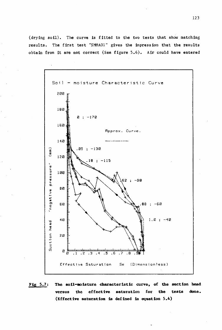
123

(drying soil). The curve is fitted to the two tests that show matching

results. The first test "SMHAOl" gives the impression that the results

obtain from it are not correct (See figure 5.6). Air could have entered

E E

ll I... :i

"' "' Ill L Q..

ll > +' IO m Q)

c '

-0 IO Ill

..c c 0

+' u :i

lJ1

Soi 1 - moisture Characteristic Curve

200

180

0 -170

160

Approx. Curve.

140

.05 ; -130

120 -115

100

-90

80

60 -60

40 1. 0 -40

20

Effective Saturation Se (Dimensionless)

Fig 5.7: The soil-moisture characteristic curve, of the auction head

versus the effective saturation for the tests done.

(Effective saturation is defined fn equation 5.4)

124

Table. 5.4: Tabulated soil-moisture characteristic curve. Suction head ~versus the effective saturation Se (Equation 5.4) of the soil.

~ (mm) Se

- 170 0 - 130 0,05 - 115 0,18

90 0,62 60 0,88 40 1,00 0 1,00

the tensiometer and caused the recorded suction not to be as great as it

should have been.

neglected.

The results for the first test are therefore

The average curve of the results (Tabulated in Table 5.4) is given with

respect to the effective saturation. Therefore to use Table (5 .4) in

the analysis of experiments (See later), a residual saturation is

selected, based on the void ratio of the experiment. Table (5.4) is

then rewritten as a function of the degree of saturation.

For the average curve, proposed in Table (5 .4), the air-entry value is

taken as 40 mm of water head. If we consider Table (5.5) from

Harr [16], we see that the air-entry value of the soil used, is of the

Table. 5 .5: Typical values of height of capillary rise. Harr. [16]

Soil type. Height of capillary rise (mm)

Coarse sand 20 - 50 Sand 120 - 350

Fine sand 350 - 700 Silt 700 - 1500 Clay 2000 - 4000 & greater.

125

same order as the capillary heights of a coarse sand. The sand used

for the test was a coarse sand (See section 4.2) and therefore the

result show an agreement in order of magnitude.

5. 5 Experiment No. 1 Analysis.

5.5.1 Introduction.

The set up and procedure for the experiment has been given in section

(4.7). The basic problem is to observe the drainage flow through a

rectangular dam, as shown in figure (4.6), with a constant upstream

water level and a tail water level that has dropped to zero elevation at

time t = O.

No attempt has been made to ioodel an actual large scale drainage problem

( ie. a large dam scaled down in the laboratory) as the purpose of this

investigation was to monitor an actual laboratory drainage problem and

to try and verify the observation with a numerical analysis. To make

any analysis, the soil-moisture parameters of the soil used in the

experiment are needed. For the soil used these have--been obtained in

sections (4.2), (5.2), (5.3) and (5.4).The shape of the dam is

rectangular with length 1 066,~ nun (42 inches), height 355,6 mm

(14 inches) and a width of 312,4 nun (12,3 inches). The dry mass of sand

used to construct the dam was 202 ,2 kg. The lay-out of the experiment

is shown in figure (5 .8). The void ratio of the dam is calculated as

follows:

Bulk volume of soil V

= 1 066,8 nun x 355,6 nun x 312,4 nun

= Length x height x width

= 118,5 • 10 3 cm3

Mass of sand used

Volume of solid particles

(Mass density p ~ 2,64 g/cm3 ,

= 202,2 • 10 3/2,64

vs see section 4.2)

=

=

=

3 202 ,2 • 10 g

76 ,6 • 103 cm3

126

Volume of voids within the soil vv = v - v s = 118 ,5 . 106 - 76,6 . 106 = 41,9 . 10 3 cm3

Therefore the void ratio e = Vv/V s

= 41,9/76,6 = 0,547

Using equation (5.1) from section (5.2), the saturated hydraulic

conductivity at 20 °c is obtained. The saturated hydraulic conductivity

ksat at 20 °c is therefore:

3 e

k = 4,444 ( ) 0,04 sat 1 + e

0,5473

= 4,444 ( ) 0,04 1 + 0,547

= 0,430 cm I sec

The temperature of the experiment differed from that of 20 °c and was 0 measured at 16 ,6 C. The saturated hydraulic conductivity is therefore

adjusted for this difference, by considering the ratio of viscosity of

the water at 16,6 °c and 20 °c. The saturated hydraulic conductivity ks

at 16 ,6 °c is therefore:

k k T120

= s sat 1T 1

= 0,430 1,0887

= o, 395 cm I sec

where ks is the hydraulic conductivity at 16 ,6 °c and the ratio of the

viscosities is given in Table (B-2).

127

35' 5"

14"

1 "

Tensiorneter Piezorneter ~I

~7 ?T~4 p 7 Ph pi!j7: Pa7 Ph ,,...._ Pb Tf4 ~ p 7 Pb PA7 T~A

N § Ii Ii ~ Ii 6 6 Ii

'° 6 6 6 Ii 6

N

5 T~3 If)

Tf3 5 T~~ 5 5 5 : 5 5 If) 5 5 5 N

C"")

'-' 4 4 ~ 4 4 : 4 4 : 4 4 4 4 4

N ~

3 3 T~2 3 3 3 3 3 Tf2 3 3 3 T~§ :

C"") N

2 2 2 2 2 ! ! 2 ! : Tf 1 N

L 4" I • • 4" J ""Impervious

42" ( 1 066 Smm)

Fig 5.8: Lay-out of experiment no. 1, giving the dimensions and

showing the locations of the p:lezoaeters and tens1oaeters.

In this thesis the factors affecting the res !dual saturation Sro have

not been studied. Therefore there is no relationship presented relating

it to the void ratio or particle size distribution (eg. as the hydraulic

conductivity is related to the void ratio). For the tests done in

sections (5.3) and (5.4), (See Tables 5.2 and 5.3), the residual

saturation varies between O,l and 0,22. A value for the residual

saturation is therefore assumed to be 0, 15. This value is used in the

analysis of the experiment.

From section (5 .3), the relationship for the hydraulic conductivity

§ 0 0 C"")

(j)

u : l't! ~ ~

00 ())

w ct! 0.. ()) ())

VJ

128

versus the effective saturation is given as a power function. Namely:

k = (S ) ex rw e

s - s ex ( r ro ) =

1 - s ro

on the results of tests Based "USPAOl" and "USPA02" shown in figure

(5.5), the value of ex= 3 is selected for equation (5.3) to be used in

the analysis of the experiments performed. Sro the residual saturation

is taken as 0, 15 (see above) and Sr is the degree of saturation of the

so 11. Therefore

k rw

= s - 0,15

r (----) 0,85

ex (5.5)

is used for the relationship of the relative hydraulic conductivity

versus the degree of saturation.

The soil-moisture characteristic curve for the relationship of the

suction head versus the effective saturation of the soil is given by

Table (5.4) fn section (5.4). As the residual saturation of the soil

used fn the experiment is taken as 0, 15, Table (5 .4) can be rewritten as

the relationship of the suction head versus the degree of saturation of

the soil. Table (5.6) therefore shows the relationship used fn the

analysis of this experiment with Sro = 0,15.

Table. 5.6: Tabulated soil-moisture ~ versus the degree Residual saturation Sro

~ (mm)

- 170 - 130 - 115

90 60 40

0

characteristic curve. Suction head of saturation Sr of the soil. "' 0' 15

Sr

0,15 0,19 0,30 0,68 0,90 1,00 1,00

The experiment was performed 5 times.

started from the same initial posit ion.

129

Each time the experiment was

The initial position was taken

at complete saturation with the water table in the upstream reservoir

at 317 nun and due to a leak, the downstream reservoir at 300 nun. To

reach this position the dam was first completely flooded for a day or

two and then the water level was lowered to 317 mm and 300 mm for the

upstream and downstream reservoirs respectively. Each time the

experiment was performed various measurements were recorded. The

average of the readings made was then used in the analysis of the

experiment. The actual readings recorded while the experiment was

underway were that of the outflow of the water, at the drainage face;

and the change in pressure at various pressure points. The recordings

made are listed in appendix (E-4), (E:_S), (E-6) and (E-7).

The experiment was run until the outflow drainage rate stopped changing

by an appreciable amount. This was after about 150 sec from time t = O. Steady state flow conditions were soon achieved.

5.5.2 Drainage outflow.

The drainage outflow is the water that left the dam via the vertical

drainage face of the dam. This water seeping out of the drainage face

was measured to find its flow rate. The technique of collecting the

water with respect to time is given in section (4. 7 .3). If a quantity

of water 6Qt was collected in a time interval of t.t, then the flow rate

at the center of the time interval is taken as approximately equal to:

Q = (5.6)

In appendix (E-4) the quantities of water collected for the different

time intervals are listed.

intervals, calculated by

times.

Also listed is the average flow rate for the

using equation (5.6) and the mid-interval

From the results a plot is made of the outflow seepage rate, as shown in

figure (5.9). The results for more than one run of the experiment have

been plotted on the graph. By averaging the results, an approximate

130

Floui Rate v's T.i me u u 140 Ill

' 130 Exper lment no. E Run 1 u no. a

121!1 Run no. 2 b :> b b u 110 b a

• "

100 ... .. .. 90 a: 3 81!1 0 Time Q

!&.. 70

(sec) (cm3 /s) 8 b b a • . 60 10 125 b

3 0 50 12,5 120,3 ...

15 115 '5 ... '10 :>

0 30 22,5 103,3 u 30 95 Cll 20 Id 45 85 D.

Ul " 60 77 ,5 " lfl 0 0 10 2B 30 40 50 60 7B 80 90 1B0 1 IB 12B 130 14B 150

Time from .start of Exp. (.sec)

Fig 5.9: Seepage outflow, flow rate -versus time measured at the

drainage face for experf.ment no. 1.

E u

:> u

3 0

... ... :>

0

u > ... .. :> E :I u

Cumulative Outflow v's Ttme 11BBB

IB000

9B00 Experf~ent no. I

8000

?BBB

6BBB

5000

4BBB

3BBB

2BB0

!BBB

BB 1B 20 3B 4B SB GB 7B 80 90 10B l 1B 12B 130 1'10 151!1

Time from .start of Exp. (.sec)

Fig 5.10: Cumulative seepage outflow, at the drainage face -versus time

for experiment no. 1.

131

outflow curve is also shown. By integrating under the curve with

respect to time, the curve for the cumulative outflow can be plotted, as

shown in figure (5.10). With time the outflow rate decreases and tends

to a value which represents the flow rate for steady state flow through

the dam. Therefore the flow rates above this value are all due to the

water draining out of the soil above the steady state phreatic surface.

5.5.3 Sidewall piezometers.

While the experiment was in progress, the water levels in the piezometer

tubes were recorded. Figure (5.8) gives the locations of the

piezometers in the experimental lay-out. The technique of making the

recordings is given in section (4.7.3). The results for the experiment

are listed in appendix (E-5). Some of the piezometers are shown as

faulty in the listing of the results. These were piezometers which were

blocked and whose water levels did not drop, and so no recording could

be made. As the water table in the soil dropped with time, some of the

piezometers ended up above the water table and drained empty. These

piezometers are shown as above the water table (AWT), from the time the

water level dropped below the piezometer point. (ie. Their water levels

coincided with the levels of the connecting holes to the soil.)

The results from the sidewall piezometers are used later for the

plotting of contours of the total pressure heads in the experiment. The

results are used more as a guide for transient heads, because the

results recorded were erratic. The reason for this could be due to the

fact that the piezometers are not null-flow devices, and they are unable

to quickly match the dynamic changes occurring within the soil.

5.5.4 Transducer monitored tensiometers.

At specific points within the soil mass of the dam a set of tensiometers

were located. The set-up and technique of recording the pressure is

given in section (4.7.3). The results of the pressures recorded with

respect to the time for the 5 independent runs are listed in

appendix (E-6). The positions at which the tensiometers were located is

shown in figure ( 5. 8). Each transducer is referenced according to its

132

position (eg. TAl for colunm A of A, B and C and 1 for the lower row of

4 tens iometer rows).

Figure ( 5 .11) shows the results for transducer "TB4", of the total

pressure head versus time elapsed from time t = O. The elapsed time was

measured from the instant when the drainage outlet of the downstream

reservoir was opened. The results for all 5 runs have been plotted on

the single graph. The results plotted for the rest of the transducers

are given in appendix (E-6).

The results obtained from the tensiometers were relatively consistent

and accurate for the repeated runs, but problems were encountered. In

some tensiometers, not all the air was removed when primed with de-aired

water and so the result is correct until the entrapped air came out of

solution. This affects the result in that the pressure being

transferred to the transducer from the tens iometer was not the same as

that being experienced at the tensiometer point. A second pro bl em

encountered was that at a certain suction, air could enter the

tensiometer through the cotton wool and have the same effect as

described above. This could have been overcome by using a finer porous

320

280

240

200

160

120

80

40

0

0

Experiment no. 1 I Transducer no. TB4

Total head (mm) v' s Time (sec)

20 40 60 80 100 120

Time (sec)

140

Fig 5.11: Total head above the base of the fluae versus time, measured

by transducer ""TB4", for experillent no. 1.

133

medium than cotton wool. A third problem was encountered only when all

the transducers were connected up to the A/D converter via the

multiplexer switch. The problem was that, for certain readings made,

the result recorded would randomly be a value of about 80 to 100 nun

below that which it should have been. This last error was caused by

some sort of electrical noise in the data acquisition system, and was

only observed by the author in the later stages of experimental

analysis. Some of the errors discussed above can be observed in

figure (S.11) and also in the plots given in appendix (E-6).

5 • 5. 5 Analysis of results.

To analyse and get some sort of confirmation of the experimental

results, the mass transfer of the water within the dam is studied. The

dam is considered as a rectangular brick volume with 6 sides. 4 of the

sides do not need to be considered, because no flow takes place across

them (ie. the sides and the bottom of the flume are impermeable and no

external water flows out or into the top surf ace. Neglecting

evaporation). The transfer of roo is tu re is therefore considered by

looking at the transfer of water flowing in and out of the ups!ream and

downstream faces respectively and the change of-the-phreati~~rface and

the total volume of water within the dam with respect to time.

To be able to do this study of the mass transfer of water, the analysis

is made on the following line:

A contour plot of the total heads within the dam at a specific time

after t = O, is made. This is done by using the results from the

piezometers and tensiometers. Then, by using the soil-moisture

characteristic curve, a contour plot is made of the degree of

saturation of the soil. The movement of the water is then

considered in 3 spec if ic areas. That is, the volume of water

flowing in and out of the soil and change of water volume within

the soil.

The method of doing this can be shown more clearly if we consider a

specific time after the start of the experiment and show the full

Contours of Total Head (rrnn)

A

0 0 !"")

B

134

C Time t 15 sec D

Fig 5.12: Contour plot of the .total head for experiment no. 1 at 15

seconds after the start of the experiment. Contour plot

based on the results of the pressure recorded at specific

points.

A B

--- --- --Phreatic/ Surface

c Time t = 1 S sec D

"-'s -->s = ·- ..(,, -.......

Fig 5.13: Contour plot of the degree of saturation for experiment no. 1

at 15 seconds after the start of the experiment. Plot mde

from the pressure head distribution via the soil-moisture

characteristic curve.

135

procedure. If we consider the time 15 sec after the start of the

experiment, then the following is an example of the analyses done. (or

for other time steps.)

Figure (5.12) shows a contour plot of the total heads recorded within

the dam. Also shown is the phreatic surf ace and the results from the

tensiometers. The contour map is plotted by using the results of the

tensiometer readings and the sidewall piezometer readings (Not shown).

The final result shown was obtained by a trial and error process,

similar to that used for plotting a flow net for a steady state flow

problem. The actual readings recorded were used as the bases for the

contour plot.

It can be seen in figure (5.12), that the total head contours are all

sloping towards the drainage face. The value of the contours decrease

from the upstream face. which is at 317 nun to the drainage face. The

instantaneous seepage flow within the dam, which is perpendicular to the

contour lines of the total pressure heads, varies in direction from

horizontal along the base of the dam to nearly vertical within the

unsaturated zone near the drainage face. By converting the total heads

to local pressure heads and using the soil-moisture characteristic curve

a contour plot of the degree of saturation is made, as shown in figure

(5.13). The local pressure head is obtained by subtracting the value of

the elevation head from the total head (eg. 4i = 41 - z). The soil

moisture drainage characteristic curve is used in that a given suction

head corresponds to a degree of saturation. See Table (5.6). Below the

phreatic surface the local pressure is positive and therefore the soil

is taken as saturated. As the air entry value of the soil used is

greater than zero, (= 40 mm) full saturation extends above the phreatic

surface. This can be seen in figure (5 .13) , as the phreatic surface is

shown, by a dotted line, below the start of the unsaturated zone.

To study the flow of water into and out of the dam, an approximate

method is used. The method is shown by considering the upstream face as

an example. The flow across a section A-A shown in figures (5.12) and

(5.13) is considered. A profile of the local pressure head along A-A

with respect to the elevation is made from figure (5.12).

136

£xp. ti .I Sec\fo1'l1 A .I Time t IS ••c -44 1.e .93 .e1 ,UI

341! -2 1.e I.lie .ez ,1119

322 l.l!J l.IU! .114 .113S 381! 1.e I.Ill! ,1111 .1113 2811 1.11 1.1111 .II! .1111 Hll 1.1 l.lll!J .11 .1116 !41!

!21!1 !Ill!

1811 1.11 1.ee .11 , 118 1611

1411

12111 1.e 1.811 .11 ,11!1 11111 Bl!

GI!

41!

Zll

II !Ill J.8 1.118 .11 , 113 Heigh\ ,_, Local Head , ... , Deg. s.i. kr• lh Vr""kr ... lh

Fig 5.14: Profile plots ._de for section A-A (Fig 5.12) fn experi.llent

no. 1 at 15 seconds after the start. All with mspect to

elevation: (a) Local bead; (b) Degree of saturation; (c)

Relative hydraulic conductivity; (d) Horizontal hydraulic

gradient; (e) B.elative horizontal Darci.an -.loclty.

Table. 5.7: Results listed of the values for the profile plots, with respect to elevation, made in figure (5.14), at section A-A in experiment no. 1, 15 seconds after the start.

Height Local Head Deg. Sat. Rel. Perm. Hydraulic Grad. ~ x 1ii (mm) (mm)

356 -44 0,98 0,926 ·0,01 0,008 340 -29 1,00 1,000 0,02 0,018 320 -9 1,00 1,000 0,04 0,035 300 11 1,00 1,000 0,10 0 ,103 280 31 1,00 1,000 0,10 0 ,101 260 51 1,00 1,000 0,11 0,106 180 131 1,00 1,000 0,11 0,110 120 191 1,00 1,000 0,11 0' 113

0 310 1,00 1,000 0,11 0,113

Width 312,4 mm Temp T 16,6 Oc Void Ratio e 0,547 Sat. Perm. ks 0,395 cm/sec Eff. Sat. Area 125,7 mm Rel. Flow Rate 35,2 mm

Flow Rate 43,4 cm3/sec

137

Figure (5.14a) shows a plot of the profile of the local pressure

heads. Next a profile of

respect to the elevation is

the degree of saturation along A-A with

made. This can be made either from the

local pressure head profile, using the soil-moisture characteristic

curve Table (5.6) or from figure (5.13). From the profile of the degree

of saturation with respect to elevation, a profile of the relative

hydraulic conductivity can be made. This is done by using

equation (5.5) which relates the relative hydraulic conductivity to the

degree of saturation. Namely:

k rw = s - 0,15

r (----) 0,85

3

(5. 7)

As the soil was placed very carefully with a uniform density, it is

assumed to be homogenous and isotropic with respect to the hydraulic

conductivity.

The hydraulic gradient 1Ii the horizontal direction is determined next.

This is done by calculating the head loss and scaling its corresponding

horizontal path length across section A-A in figure (5.12).

Figure (5 .15) shows graphically how this is done. By doing this at

different elevations a profile plot is made of the horizontal hydraulic

gradient acting across A-A with respect to the elevation, as shown in

figure (S.14d).

From the two profiles of the relative hydraulic conductivity and the

horizontal hydraulic gradient, a profile of the relative horizontal

Darcian velocity can be determined.

This is done by taking the multiple of the relative hydraulic

conductivity and the horizontal hydraulic gradient at each elevation,

(eg. vr = krw x ~). Figure (5 .14e) shows a plot of this profile with

respect to elevation. To obtain the horizontal Darcian velocity at any

elevation, the relative hydraulic Darcian velocity is multiplied by the

saturated hydraulic conductivity of the soil, determined from the void

ratio. (See section 5. 5 .1).

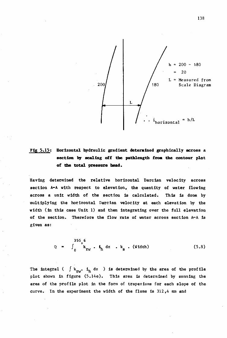
L

138

h = 200 - 180

= 20

L = Measured from Scale Diagram

i • l = h/L horizon ta

Fig 5.15: Horizontal hydraulic gradient deteralned graphically across a

section by scaling off the pathlengtb fma the contour plot

of the total pressure bead.

Having determined the relative horizontal Darcian velocity across

section A-A with respect to elevation, the quantity of water flowing

across a unit width of the section is calculated. This is done by

multiplying the horizontal Darcian velocity at each elevation by the

width (in this case Unit 1) and then integrating over the full elevation

of the section. Therefore the flow rate of water across section A-A is

given as:

Q = k • (Width) 6

(5.8)

The integral ( f krw. ih dz ) is determined by the area of the profile

plot shown in figure (5 .14e). This area is determined by summing the

area of the profile plot in the form of trapeziums for each slope of the

curve. In the experiment the width of the flume is 312,4 llUll and

139

Table (5. 7) gives the value of the integral as 35 ,2 mm. (Relative flow

rate). Therefore using ks = 0,395 cm/s in equation (5.8):

355 6

Q = ' f 0

krw • ~ dh

35,2 312,4 =

10 10

3 = 43,4 cm I sec

k (Width) s

0,395 3

cm I sec

(Across the whole width and height of section A-A)

The above calculations are repeated for section D-D in figure (5.12),

located at the drainage face. The respective profiles determined with

respect to elevation are shown in figure (5.16) and the values in

Table (5.8).

Exp. •1 / ha~lan1 D / Tl-• 15 ••~ -122

341!1 -IH

ne -1a 31!11!1

Hl!I 261!1 241!1

221!1 2.BI!

IH ICl!I 141!1 121!1 11!11!1

BB 61!1

41!1 21!1

e !Wight (-)

7

18

lll 4f 57

71

n 1ee

Loc:•l H.ad

,1 .11

.5 .1

•• ,9

.11

1.11 1.11 1.11 1.e 1.e 1.111 1.e '.l!I 1.111 1.111 1.11

----'1.11

11.8111 .1111 ,117

• 24 ,37

.59 .711

1.n 1.111!1

1.811 1.a l.llll 1,811 1.1111 1.a 1.a 1.u 1.ae

----' l,llll lh

,II! .117 ... ... .88 .ee

••• .43 .411

.52

.s:s .59 .!I&

.5e

111.aa .11111 .184 .112111 .n2 .as .1171

.4• .4U ,411

.519

.s!& .548 .556 .!118

Vr-krOI. lh

Fig 5.16: Profile plots made for section D-D (Fig 5.12) fn experiment

no. 1 at 15 seconds after the start. All with respect to


Relative hydraulic conductivity; (d) Horizontal hydraulic

gradient; (e) Relative horizontal Darcian velocity.

140

Table. 5.8: Results listed of the values for the profile plots, with respect to elevation, made in figure (5.16), at section D-D :In experiment no. 1, 15 seconds after the start.

Height Local Head Deg. Sat. (mm) (mm)

Rel. Perm. Hydraulic Grad. krw x ~

356 340 320 300 280 260 240 220 200 180 160 140 120 100 80 60 40 20

0

Width

-122 -114 -102 -90 -79 -65 -53 -39 -29 -16 -4

7 18 31 44 57 71 83

100

Void Ratio e Eff. Sat. Area

312,4 0,547

110,4

0,25 0,32 o,so 0,68 0,76 0,86 0,93 1,00 1,00 1,00 1,00 1,00 1,00 1,00 1,00 1,00 1,00 1,00 1,00

mm

mm

0,002 0,008 0,069 0,238 0,373 0,586 0,784 1,000 1,000 1,000 1,000 1,000 1,000 1,000 1,000 1,000 1,000 1,000 1,000

Temp T Sat. Perm. ks

Rel. Flow Rate Flow Rate

0,05 0,07 0,06 0,08 0,06 0,06 0,09 0,13 0'17 0,20 0,31 0,40 0,43 0,49 0,52 0,53 0 ,SS 0,56 0,58

16,6 0 ,395

94,4 116 ,s

o,ooo 0,001 0,004 0,020 0,022 0,035 0,071 0,133 0,167 0,200 0,308 0,400 0,432 0,488 0,519 0,526 0,548 0,556 0,580

OC cm/sec mm ctn3/sec

Also in Table (5.8) is the value for the integral (Relative flow rate.)

given as 94,4 mm. Therefore using ks= 0,395 emfs in equation (5.8):

355 6

' Q = J 0 krw • ~ db

94,4 312,4 =

10 10

3

k • (Width) s

0,395

= 116 '5 cm I sec

(Across the whole width and height of section D-D)

3 cm I sec

141

This computed result (116,5 cm3/sec) compares very well with the outflow

rate determined previously (Q z 115 cm3/sec), as shown in figure (5.9).

The next problem is to determine the quantity of water within the soil

(between sections A and D), at the time of 15 sec after the start. This

is done by an approximate method of considering the effective volumetric

moisture content at 4 sections indicated in figure {5.12) and taking an

average value of this between the sections. The volumetric moisture

content at a specific elevation is obtained from the degree of

saturation profile. The volumetric moisture content is obtained by

multiplying the degree of saturation by the porosity of the soil. The

effective volumetric moisture for a unit width of soil at a section is

obtained by summing vertically the volumetric 100isture content over the

full elevation. (Effective Saturated Area.) This is the same as

integrating the area under the degree of saturation profile with respect

to elevation and multiplying by the constant porosity n. Written as:

Eff. Sat. Area = 355 6

t

J 0

Sr dz • n (5.9)

where the porosity is determined from the void ratio of the soil. If we

consider section B-B in figure (5.13), the profile of the degree of

saturation is given in figure (5.17b) and the values in Table (5.9).

The method of integrating the area under the curve is the same as that

used to determine the area under the relative horizontal Darcian

velocity profile given earlier. Table (5.9) gives the result for the

integral of the profile given in figure (5.17b) as:

355 6 , J S dz o r • n

= 124,7 mm

Once the effective volumetric 100isture (Effective Saturated Area) at two

sections has been determined, the volume of moisture between the two

sections is calculated. This is done by taking the average of the

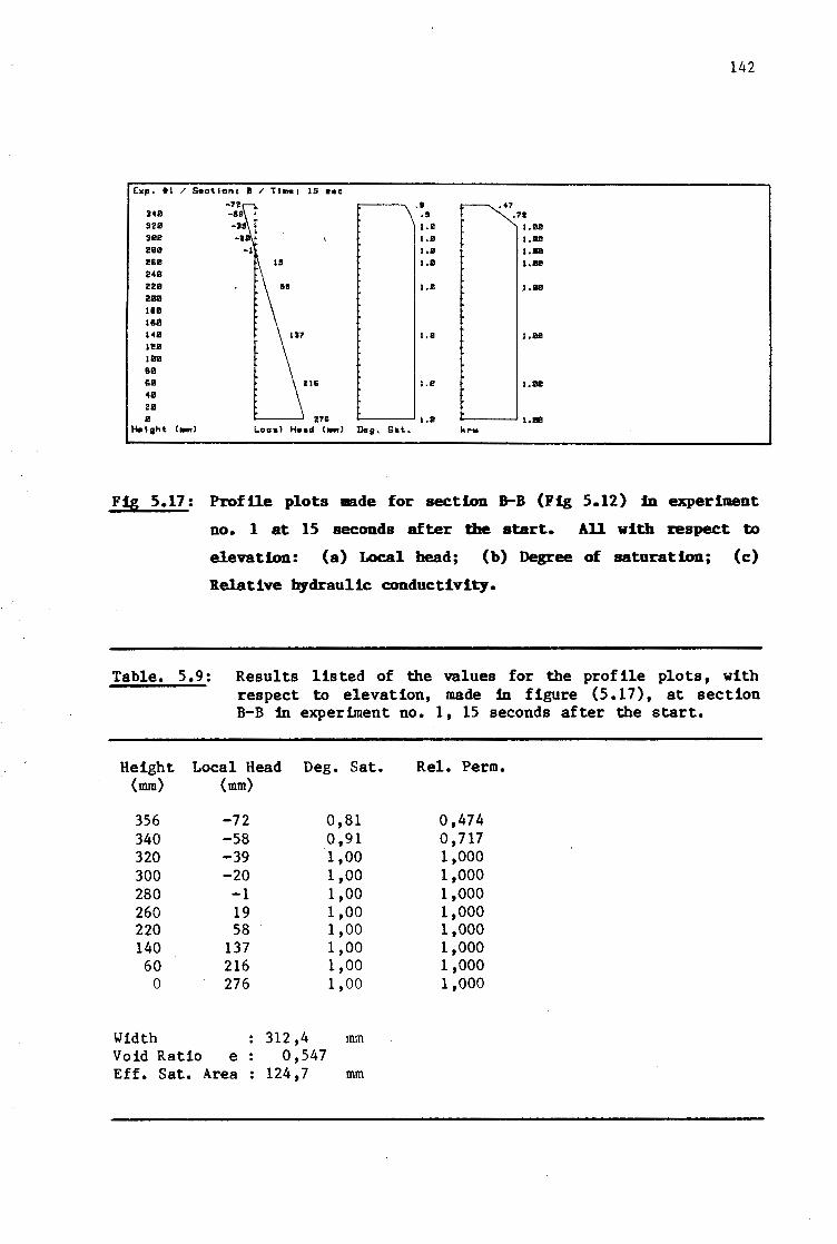
142

!:><p. ti / Seot.fanc I!/ Tl-1 15 sec

-n .I .47 348 -158 .s .7! 3215 l.11 I.Bl!! 388 1.11 I.Ill! l!BB 1.e 1.1111 He 1.ll I.Ile 248 228 1.a i.ae 288 11111 168 148 13? i.e 1.ee 128 Ull!I BB 68 ZI& 1.B 1.llll 4B 28 e Z75 1.B 1.1111!

Height (-) l..acal H•ad (-) tlGg. Sat.. i. ....

Fig 5.17: Prof Ue plots 11ade for section B-B (Fig 5.12) fn experiment

no. 1 at 15 seconds after the start. All with ~spect ta


Relative hydraulic conductivity.

Table. 5.9: Results listed of the values for the profile plots, with respect to elevation, made in figure (5 .17), at section B-B in experiment no. 1, 15 seconds after the start.

Height Local Head Deg. Sat. Rel. Perm. {mm) {mm)

356 -72 0,81 0,474 340 -58 0,91 0,717 320 -39 1,00 1,000 300 -20 1,00 1,000 280 -1 1,00 1,000 260 19 1,00 1,000 220 58 1,00 1,000 140 137 1,00 1;000 60 216 1,00 1,000

0 276 1,00 1,000

Width 312,4 mm Void Ratio e 0,547 Eff. Sat. Area 124 '7 mm

[~p. •1 / S•atlant C / Tlm•t

•Ill• 348 -a JU -8

388 "" 218 268 248 tt8 288 1118

168 148

128 188 88 68 48 28 B

•

IS HC

.5 .e

·' .18 .e .as

.a .53 1.B .1111 1.11 1 •. 11B 1.11 1.118 I.I 1.1111

1.11 I.Bil

1.1

211 I.I --~I.BB Hel11ht (-) ·Local H••d (-) Deg, Sat. k~w

143

Fig 5.18: Profile plots •de for section 0-C {Fig 5.12) in experiaent

no. 1 at 15 seconds after the start. All with respect to

elevation: (a) Local head; (b) Degree of saturation; (c)

Relative hydraulic conductivity.

Table. 5.10: Results listed of the values for the profile plots, with respect to elevation, made in figure (5 .18), at section C-C fn experiment no. 1, 15 seconds after the start.

Height Local Head Deg. Sat. Rel. Perm. Hydraulic Grad. krw x 1b (mm) (mm)

356 -104 0,46 0,050 340 -95 0,61 0,158 320 -80 0,75 0,353 300 -63 0,88 0,627 280 -46 0,97 0,903 260 -28 1,00 1,000 240 -10 1,00 1,000 220 9 1,00 1,000 160 65 1,00 1,000 80 140 1,00 1,000

0 218 1,00 1,000

Width 312,4 mm Void Ratio e 0,547 Eff. Sat. Area . 119 ,o mm

144

effective volumetric moisture of the two sections and multiplying this

by the distance between the two sections and the width of the flume.

For figure (5.13) the effective volumetric moisture at the sections A,

B; C, and D for a unit width are calculated as: 125,7; 124,7; 119,0 and

110,4 mm respectively. (See Tables 5.7, 5.8, 5.9 and 5.10). Therefore

the total volume of rooisture between sections A and D is the sum of the

moisture between sections AB, BC, and CD. The distances between

sections A, B, C and D as shown in figure (5.12), are 304,8 mm

(12 inches), 355 ,6 mm (14 inches) and 304 ,8 mm respectively. The width

is 312,4 mm. The total moisture between sections AB is determined as:

V (AB) = 304 ,8 w

125,7 + 124,7

2

6 3 = 11,92 • 10 mm

3 3 = 11,92 • 10 cm

3 312,4

Table (5.11) shows the results for the volume of misture calculated

between the sections BC and CD as well. Also shown is the total swn of

the volume of rooisture calculated, between sections A-A and D-D for the

time of 15 seconds after the start, time t = 0. This volume is given 3 3 as 36,372 • 10 cm •

Table. 5 .11: Summary of results calculated for the sections different times considered in experiment no. 1.

Time Volume of misture between: Flow rate at: t AB BC

(cm3) CD Total A-A D-D

(sec) (cm3/sec)

10 11 921 13 642 11 259 36 822 34 ,8 131,4 15 11 918 13 532 10 922 36 372 43,4 116 ,5 30 11 884 13 290 10 274 35 448 49,0 93,9 60 11 838 12 895 9 483 34 216 64,3 80,1

All these results are computed from the observed flow field.

at

145

Other times of 10, 30 and 60 seconds after the start are also considered

(See appendix E-7) and the final results obtained are also presented in

Table (5 .11). The methods of calculation used for those times are

similar to those for_ the example given above.

15 sec after the start.)

(ie. for the time of

The difference in the result for the inflow and outflow rate at sections

A and D respectively should be compensated for by the rate of change of

the volume of moisture within the soil mass between sections A and D.

If we consider the results in Table (5.11) for the time at 10 seconds,

then the rate of change in the volume of misture at the 10 second time

step, should be equal to the difference of 34,8 and 131,4 = 96 ,6 cm3 /sec. Similarly, at 15 seconds the rate of change in the volume

of moisture is 73,1 cm3/sec. The total volume of moisture calculated at

the 10 and 15 seconds time steps is given in Table (5.11) as 36,822. 103

and 36 ,372 • 103 cm3 respectively. The change in the volumes occurs

during the 5 seconds between the 10 and 15 second time step. The

average rate of change of the volume of moisture between these intervals

is therefore:

3 3 (36,822 • 10 - 36,372 • 10 )

= ~t 5

3 = 90 cm I sec

This value lies within the bounds of the rate of change in moisture

determined as 96,6 and 73,1 cm3/sec at the 10 and 15 seconds time steps

respectively. (As shown in Table 5.12)

The above calculations are repeated for the time intervals between

15 and 30, and 30 and 60 seconds. The results are presented in

Table (5.12). For the results shown in Table (5.12), good agreement is

shown for both the outflow predicted to that measured (See

figure 5.9). The average rate of change in the volume of moisture,

(last colunm in Table 5 .12) compares reasonably with the range in

146

Table. 5.12: Results calculated for the moisture transfer in experiment no. 1 at different times.

Time Inflow Outflow Difference Total "Storage" Average t (A-A) (B-B) storage change change

(sec) (cm3/s) (cm3/s) (cm3/s) (A-~) (cm ) (cm3)

t:f te (cm /sec)

10 34,8 131,4 96 ,6 36 822 450 90

15 43,4 116 ,5 73,1 36 372 924 62

30 49,0 93,9 44,9 35 448 1232 41

60 64,3 80,l 15,8 34 216


column 4 of Table (5 .12) calculated by the difference in the inflow and

outflow rates at different times.

5.5.6 Summary and conclusion.

The calculations made on the results obtained for the experiment were

made to confirm that the contouring of the total heads was done

correctly. Also to show that the different readings made are consistent

with each other. The results from the tensiometers were far more

accurate than the piezometer readings. The latter even contradicted

each other in places. The reason for the erratic piezometer readings,

as noted before, could be due to partially blocked tubes in the walls of

the seepage tank.

Based on the above, the author felt that if more tens iometers connected

to transducers could have been used, the contouring of the total

pressure heads could have been done more easily and more accurately. A

further verification of the results obtained is made in Chapter 6, by

using the finite element method.

147

5.6 Ex.periaent No. 2 analysis.

5.6.1 Introduction.

The arrangement and procedure for the experiment has been given in

section (4.8). The basic problem (See figure 4.8) in this second

experiment is similar to the first, fn that drainage is to be observed,

but in this case the upstream face of the rectangular slab is

impermeable and the soil is allowed to completely drain. Figure (5.19)

shows the lay-out of the problem.

As with the first experiment, no attempt has been made to model an

actual large scale drainage problem. The experiment is done to observe

the actual drainage encountered in this tank and to make a numerical

verification.

Attempts were made to overcome some of the problems encountered in the

first experiment. · The main problem was that there were too few

tensiometers. To overcome this, in the second experiment, sets of

tens iometers ( ie. nylon pipes with cotton wool pressed into the front)

were located on a regular grid. See figure (5.19). The experiment was

then repeated a number of times, each time the transducers were

connected to a different set of tube tensiometers. In this way it was

hoped to increase the amount of data collected, without increasing the

number of transducers required.

The soil-moisture parameters of the soil used, are as given in sections

(4.2), (5.2), (5.3) and (5 .4). The shape of the slab drained is

rectangular, with length 2 717,8 mm (107 inches); .height 401,3 mm

(15 ,8 inches) and a width of 312 ,4 mm (12 ,3 inches). The mass of the

sand used to cons true t the slab was 5 71 , 5 kg. The void ratio of the

slab of soil is calculated the same way as shown in section (5.5.1):

Bulk volume of soil v 340 ,8 103 cm3

Mass of sand used ws = 571,5 103 g

Volume of solid particles vs = 216,5 103 cm3

Volume of voids within the soil vv = 124,3 103 cm3

Scep:1·':'.e f ,1c e 0

"I

: w ~I· _, t4 L_

~E

~[

N

Tensiometer

~ Ill ,...

~ u ,...

: Q ,...

: ... ....

: i.. ,...

: " ,...

: J: ,...

: .. ,...

: ., ....

: ~

: .J ,...

: I: ....

: z ....

\ .~ 1 ' " ) w

\

• ...

• ...

• ...

• ...

•

• ...

• ...

• ...

• ...

• ...

• ...

4" 4"

• ...

•

~11 : LI"\

o~.

3

'"""' ~

co r-.

r-.

N '-'

= r-. 0

..... Piezometers

_Impervious base

Irr:pervio~ face

148

Fig 5.19: Lay-out of experiment no. 2, givfng the diaensions and

sho~ing the locations of the piezoaeters and tensioaeters.

(

\

149

Therefore the void ratio e = 0,574

Using equation (5.1) from section (5.2), the saturated hydraulic

conductivity at 20 °c is:

3 0,574

k = 4,444 ( ) 0,04 sat 1,574

= 0,494 cm I sec

The temperature of the experiment differed from that of 20 °c and was

measured at 18 °c. Using the viscosity of the water at the different

temperatures, the hydraulic conductivity is adjusted for this

temperature difference as before. The saturated hydraulic conductivity

ks at 18 °c is therefore:

TJ20 k = k

s sat 1T

1 = 0,494

1,0507

= 0,470 cm I sec

where TJiol"T the ratio of the viscosities is given fn Table (B-2).

The residual saturation is taken as:

for the

s ro

same

= 0,15

reasons as given in the first experiment,

section (5.5.1). As the residual saturation is the same as before, the

relative hydraulic conductivity is given by equation (5.5), written as:

k rw

= s - 0,15

(-r----) 0,85

3

150

Th is equation gives the relationship of the relative hydraulic

conductivity as a function of the degree of saturation.

The soil-moisture characteristic curve from the first experiment can be

used again for this experiment, as the residual saturation is the

same. Table (5.6) 1n section (5.5.1), therefore shows the relationship

of the suction head versus the degree of saturation of the soil used in

the analysis of this experiment.

In most respects this second experiment is similar to the first. The

experiment was performed 4 times. Each time the experiment was started

from the same initial position. The difference was that the transducers

were connected up to different tens iometers for each run. The same

recordings were made, as before, while the test was in progress.

Namely, the outflow with respect to time and the change in pressure at

various pressure points was measured. The main difference in the set-up

was that the upstream face of the soil was impermeable. Therefore no

water flowed into the soil through the upstream face, and as drainage

continued, a corresponding drop in the phreatic surface took place.

The initial position of the experiment was with the phreatic surface at

381 mm (15 inches) above the base of the flume and the soil saturated.

The experiment was started by dropping the drainage reservoir at time

t = 0 to zero elevation and measuring the outflow of the water seeping

out of the drainage face. The initial position for the experiment was

reached by first submerging the complete slab of soil in the flume for a

few days with de-aired water. The water level was then lowered to the

position of 381 mm above the flume base. This level was kept for a

while in the drainage reservoir to make certain that the phreatic

surface within the soil had also achieved the level of 381 mm. Once

these equilibrium conditions had been reached the experiment could be

performed.

The recordings made while the experiment was underway are listed in

appendices (E-8), (E-9) and (E-10). The experiment was run until the

outflow drainage rate had dropped to a very small value. This was after

about 3 600 seconds (1 hour) from time t = O.

151

5.6.2 Drainage outflow.

The determination of the approximate flow rate from the drainage outflow

was performed the .same way as described in section (5.5.2), for the

first experiment. Appendix (E-8) lists the quantities of water

collected for the different time intervals and also the calculated

average flow rates.

From the results, a plot is made, as shown in figure ( 5. 20). The

results from the repeated runs are all plotted on the one graph. To

this data an approximate outflow curve is fitted. By integrating under

the curve with respect to time, the curve for the cumulative outflow is

plotted, as shown in figure (5.21).

The curve of the drainage flow rate tends towards zero with respect to

time, because the soil tends to a completely drained state and no ioore

water can drain out. The curve for the cumulative outflow plot tends to

a horizontal line, which corresponds to the total volume of water in

drainable storage within the soil at time t = O.

5.6.3 Sidewall piezometers.

While the experiment was in progress, the water level in the piezometer

tubes was recorded, as before. Appendix (E-9) gives a listing of the

results. The results are listed as a single value for each vertical set

of piezometers. This is because the drop in the water levels in the

piezometers was much slower than in experiment one and the results for a

vertical set were all nearly the same. An average of the results was

therefore recorded. The results are used later for the plotting of the

total head contours in the experiment at different times.

5.6.4 Transducer monitored tensiometers.

The tensiometers were located at specific points within the soil.

Figure (5.19) shows where the tensiometers were located. As noted

earlier, for each run a different set of tensiometers were connected to

the transducers. Therefore for each run a different set of tensiometers

152

Fl Ol.U Rate v's Time u 200 ll ti 190

' E 180 u

170 :I 160

Experiment no. 2 Time Q u 150 (min) (cm 3 Is)

u 140 .. 130 Ill 5 48,5 Q'. 120

3 11111 10 30,5 0

100 15 22,3 LL. 90 22,5 14,8 . 3 80 30 9,9 0 70

'+- 60 .. ::I 50 0

40 GI

30 m Ill

20 12. ll 10 u

UI 00 5 10 15 20 25 30 35 40 4 50 55 60

Time from start of Exp. (min)

Fig 5.20: Seepage outflow, flow rate versus time masured at the

drainage face for exper:lllent DD. 2.

Flow Rate v's Time

100000

90080

88880 Experiment no. 2

E u

78800 ::I u

60080

50800 3 0

'+- 48808 .. .::J 0 30000 ll > - 28000 .. Ill

::I 18080 l! ::I u

5 10 15 20 25 30 35 40 45 50 55 60

Time from start of Exp. (min)

Fig 5.21: Cumulative seepage outflow, at the drainage face versus time

for experf.llent no. 2.

153

were monitored. Appendix (E-10) gives a listing of the results for the

respective experimental runs. The readings are listed with respect to

time and are referenced to which tensiometer was monitored. From the

listing the results. can be plotted with respect to time. Figure (5 .22)

shows a plot of the total pressure head above the flume base for

tensiometer ''TE4" with respect to time. The results plotted for the

rest of the tensiometers are shown in appendix (E-10).

The results obtained from the tensiometers show the same problems as

encountered before. Namely, that certain readings have been affected by

erratic electrical noise or air has come out of solution in the

connecting nylon pipe between the tens iometer and transducer. The

readings made for experiment run No. 2, (See appendix E-10) are for

certain of the readings, most erratic due to electrical noise. This

seems to be, because the reference transducer's reading must have been

affected and this in turn affected all the other readings. The

transducers affected due to air coming out of solution cannot be seen

straight off from the results. These are only discovered when a contour

plot is attempted and a reading does not seem to fit in with the general

pattern of the readings made.

Experiment no. 2 I Transducer no. TE4

Total head (mm) v' s Time (min)

400 l -350 r I

r -1 'F- -!

300 I- -I I- -I

250 .... _J

I!. _J

200 I~ I I \. I

150 ' ' I r '- -, r- ............ .,

100 i- .........__ -j

i- -~-. -j

50 ~ ......... +++ •• • + ~ -!

I-.. .. + + ... :t.!

0

0 10 20 30 40 50 60

Time (min)

Fig 5.22: Total head above the base of the fiUlle versus t:lme 11 measured

by transducer "TE4 .. , for exper:lllent no. 2.

~ A

C

on

tou

rs

of

To

tal

Hea

d 4>

(m

m)

B

c T

ime

t 5

min

A

CIQ

C

") CIQ

8 t

<

0 "O

8

ID

~ n

I; s

8 g

Seep

ag

e

c:: Cl

o c::

h 11

CIQ

11

....-

fa C

E'

'8 ~ -~

V

I

d 11

' 11

' 26

0 24

0 22

0 20

0 1

80

El

t

~

0 "'

i' 0

CIQ

i -

• CIQ

""'

-·

ID

Clo

i: tr

8 CIQ

-tr

~

g e i:

~ 11

A

C

on

tou

rs

of

Deg

ree

of

Satu

rati

on

S

B

c T

ime

t =

5

min

D

r t

<

0 CIQ

c::

tr ....

Clo

"' CIQ

Seep

ag

e

0 S'

--

Ph:a~i; S

urf

ace/

------

,,,,. f

ric

e CIQ

11

---

Sr

==

"""'

g -

---

-1

g. 11

~

---

"' --

-ID

ID

t

' 0

"O

0 11

11

"""' s

-ID

-

CIQ

m

1:1)

tr c::

11'

11

ID

8 ~

! •

s ID

N

...

11

~ Cl

o

r ID

Cl

o w

-

Ill

"' 0

\JI

"' •

0 +:

-

155

5.6.5 Analysis of results.

To analyse and get some sort of confirmation of the experimental

results, once again the mass transfer of 'the water within the soil is

studied. As the soil has only one face across which flow can take place

(the drainage face), only this face need be considered in terms of water

flowing in or out of the soil. The in or out-flow must be matched with

a corresponding rate of volume changes of water within the soil.

The approximate method, as used in experiment one, is used again. The

outflow out of the drainage face is determined by taking a section near

the face and plotting the relative horizontal Darcian velocity. From

this, the flow rate across the section is determined. Section ( 5 .5 .5)

of experiment one, discusses how this is done. The volume of water

within the soil is determined by taking an average . of the effective

volume of moisture determined at a number of sections. This is also

discussed in section (5.5.5) for experiment one.

For this experiment, three times are considered. Namely, 5; 15; and

30 minutes after the start of the experiment. Figure (5 .23) shows the

contour plot for the 5 minute time step and where the sections are

located for this analysis. Table (5.13) gives the final results

obtained for the calculations performed at the different times.

Table. 5.13: Results calculated for the moisture transfer in experiment no. 2 at different times •

Time Outflow Total .. Storage" Average t storage change change

(min) (cm3/s) (A-~) (cm ) (cm3)

138te (cm /sec)

05 47,9 96 995 20 601 34,3

15 21,3 76 394 13 873 15,4

30 10,0 62 521


156

Appendix (E-11) lists the tables and values used in the various

calculations. Also shown are the contour plots of the total pressure

heads and degree of saturation for the different time steps analysed.

5.6.6 Summary and conclusions.

For this second experiment, the results for the mass transfer

calculation show agreement with the outflow measured. This is seen by

the results given in Table (5 .13) and the values measured as shown in

figure (5.20). The analysis done therefore indirectly confirms that the

contour plots made could be correct. A verification of the results is

done in chapter 6. using a numerical method of analysis (The finite

element method.).

The problem of not having enough tensiometers in experiment one was not

really overcome by using a larger number of tens iometers. The reason

for this 1s that a lot of the readings obtained were incorrect due to

air being entrapped when connected up to the transducer. To overcome

this, a better system 1s needed for priming the tensiometers already

located within the soil. For this second experiment the heads changed

slowly in the piezometer tubes located far from the drainage face, hence

the heads in these tubes were not subject to signficant response time

errors, and they were used to check the transducer readings.

CHAPTER 6

MODELLING OF FLUID FLOW IN A SATURATEJrUNSATURATED OOMAIN

USING 'lllE FINITE ELEMENT METHOD.

6.1 Introduction.

157

In section (2.9.2) the combined flow equation ,was developed in the form

of a partial differential equation, based on a set of assumptions which

simplified the complex real world. (Equation 2.43). To find the

unknown total head ~' a function of space and time, the partial

differential equation, subject to specific initial and boundary

conditions needs to be solved. The geometry of the flow domain and its

various storage and transport coefficients must be known. (ie. specific

moisture capacity and hydraulic conductivity). Three classes of methods

exist for solving such problems. (Bear [6]):

- analytical methods

- methods based on the use of models and analogs

- numerical methods.

Each method has its

problem encountered

advantages

and the

and the method used depends on the

facility available, (eg. skilled

manpower). A brief paragraph is given to introduce each method. The

method selected by the writer and expanded in this chapter is a

numerical method, and more specifically, the finite element method.

a) Analytical methods.

The analytical method is the most superior of all the methods.

An advantage of using it is that the solution can be applied to

different values of the parameters defining the problem. The

influence of each parameter can then clearly be seen. Problems

with this method are that for irregularly shaped domains,

encountered in practice, an analytical solution is sometimes not

possible. Also, the partial differential equation for saturated

unsaturated flow is non-linear. As a result of these problems,

analytical methods are seldom used in practice.

158

b) Analog methods.

Analogs (and models) may be regarded as special purpose

computers, when compared with digital computers. An analog

system is usually constructed to solve a particular flow

problem. Once this has been done, as long as the geometry of the

system considered does not change, a number of cases (eg. with

different inputs and outputs) can be considered. In models used,

the dependent variable and its derivatives are related to each

other in a similar manner to the system being investigated,

therefore allowing it to be solved.

The following models and analogs could be used for studying

various flow problems:

- Sand box model

- Vertical and horizontal Hele-Shaw analogs

- Electric analogs of the elctrolytic tank type; of the

conducting paper type; of the RC-network type

(ie. Resistor and Capacitor network)

- Ion motion analog

- Membrane analog

The use of the sand box model involves many technical

difficulties. The vertical Hele-Shaw analog can only be used for

two-dimensional flows in the vertical plane, but is a useful tool

for studying sea water intrusion in coastal aquaf iers. Also,

problems with a phreatic surface can be solved. The horizontal

Hele-Shaw analog is used essentially to study two-dimensional

flow in a confined aq uaf ier. The electrolytic tank and

conducting paper are usually used for steady flow only. The

presence of a phreatic surface requires special techniques. The

RC-network is used for the solution of regional forecasting

problems. A disadvantage of the RC-network is its cost,

especially that of the peripheral equipment for input, output and

boundary conditions.

159

c) Numerical methods.

Numerical methods are merely tools used to enable one to replace

the partial differential equations valid in a domain with an

approximate set of algebraic equations in a similar domain which

are then solved. The two most popular methods are:

- Finite difference method

- Finite element method.

Both of theses methods are merely structured procedures for

approximating the differential system. Computer based numerical

methods are the most practically used tools for solving flow

problems at the moment. They are used because they allow for the

solution of problems involving irregularly shaped boundaries;

materials with high variations in properties; non-linear partial

d iff eren t ial equations; and complex boundary conditions which

may be insolvable by analytical means. Furthermore, with a

numerical method, changes in the problem - geometry and physical

parameters - are more easily accommodated than with an analytical

method which may require a complete re-analysis of the problem.

However, analytical solutions are useful for serving as standards

for comparisons of numerically computed results.

Numerical methods for the solving of partial differential

equations have often been published and, in many cases, these are

in the form of computer programs. The use of these programs for

the solving of saturated flow problems is relatively easy and can

be done with a minimal background knowledge in numerical

methods. For unsaturated flow, the equations become more

involved and care needs to be exercised when dealing with such

problems.

Finite difference method

The finite difference method involves the process of' replacing a

derivative based on a small differential distance dx by an

approximation of a difference based on some finite

160

distances b.x. In making this approximation, an error is

introduced. The finite difference theory is concerned with

ensuring that the error is of a magnitude tolerable within the

constraints of the problem under study. The differential

equation which holds for the entire domain is replaced by a

number of discrete approximations to the differential equation

for the domain. The domain is subdivided (discretized) by

selecting points or nodes at which the approximations are used.

The approximation at one point depends to some degree on the

values at nearby points. The continuous unknown variable

appearing in the partial differential equation is therefore

replaced by a discrete variable at the nodes. The set of

simultaneous finite difference equations is then solved

numerically on a digital computer to yield the results of the

unknown variable at the nodes.

Finite element method

An object within the finite element method is to transform the

partial differential equation into an integral equation which

involves derivatives of the first order only. The integration is

performed numerically over elements into which the domain has

been subdivided. The functions selected are typically

polynomials of some sort and the solution required can be

expressed as a sum involving these polynomials. The differential

equation is approximated and is not necessarily satisfied

exactly, hence the solution may contain an error. The solution

to the problem is obtained by requiring that the average error

over the entire domain be as small as possible.

The methods of finite difference and finite element have a lot in

common and borrowing of concepts by one method from the other has

taken place. This cross-breeding of the two methods, which has

been accelerated in the last decade makes it difficult to point

out the unique features of either method. Table (6.1) reproduced

from Gray [14) gives a list of elementary differences between the

two methods.

161

Table. 6 .1: A finite list of elementary differences: The elements of finite differences which are different from finite elements. Gray [14].

Finite Difference.

Approximates derivatives of functions directly.

Provides approximations at points which borrow information from neighboring points to whatever degree des ired.

Traditionally uses a regular mesh

Approximations developed via curve fitting or Taylor Series expansions.

Resultant difference expression explicitly provided by the programmer to the code. Approximations may be "seen".

Complete freedom to select nodes to be used in a discrete approximation provided

On a regular grid, similar approximations are made at different nodes.

Difference expressions are generally in terms of function values only.

Though not typically done, derivatives with respect to one independent variable may be weighted over another variable (eg. a time derivative approximation may be a sum of time derivatives evaluated at different spatial locations).

Finite Element.

Approximates the functions themselves.

Provides global approximations which are restricted to neighborhoods of the grid to whatever degree desired.

Structure of method readily lends itself to irregular, curved gr ids.

Approximations developed from families of basis functions and integration over grid.

Resultant difference expression provided implicitly to the code which performs the integrations. Approximation is buried in the integrals.

Nodes included in discrete approximation determined by basis functions, integration rule, and weighting function.

Even on a regular grid, different approximations may be made at different nodes (eg. 9-node Lagrangian elements).

Difference expressions are often written in terms of function values and derivatives of the functions (eg. Hermitian cubic elements).

Though typically weighted over different coordinates, derivatives may sometimes be lumped by selection of an appropriate nodal integration formula (eg. trapezoidal rule for bilinear elements).

Table 6.1: Cont.

Commonly uses ADI requiring a tridiagonal matrix solver.

Staggered grid easily implemented because of regular rectangular nodal placement.

Boundary conditions applied by altering the basic computational molecule.

Moving boundary problems are traditionally difficult.

Large gradients require a fine mesh for resolution.

For a regular mesh, a zone requiring high resolution determines grid spacing.

Data input may be simple because of regularity.

Regular grid interfaces easily with computer graphics.

Commonly uses banded, frontal, or sparse matrix solver.

Staggered grid virtually impossible because of grid irregularities. However mixed interpolation is a partially staggered grid.

Boundary conditions are applied through the boundary integral obtained after application of Green's theorem

Moving boundary problems are conceptually straightforward.

162

Functional implanting may minimize need for fine mesh near steep gradients.

Localized refinement of computational grid is easily accomplished

Data input is complex and undiscovered data errors can be a cause of trouble.

Graphics interface may be complicated by an irregular mesh and isoparametric elements.

The finite element method is discussed in more detail in the rest

of this chapter. Its use is shown in solving some saturated

unsaturated flow problems and in the verification of the

experimental work covered in earlier chapters.

6.2 History of the finite element method.

The finite element method was first developed in the 1950s, mainly by

structural engineers in the aircraft industry, for solving stress

163

analysis problems of complex geometrical configurations of solids.

Although little related work was published by mathematicians, it was the

practical demands of the engineer coupled with the development of the

electronic digital computer which caused rapid development in the

method. It was only in the late sixties that mathematicians took a

widespread interest in the method and subsequently contributed to the

theoretical understanding of the method. Initially the method was

strongly related to variational methods which rely on the calculus of

variations and the finding of a stationary value of a given functional

for the solution of a physical problem. (eg. Rayleigh Ritz). The

variational method, though having mathematical advantages

(i.e. providing existence proofs) also has inherent limitations. In

some cases it is very difficult to find the variational formulation

which parallels a partial differential equation whose solution is

required. This disadvantage was overcome by the use of Weighted

Residual methods, which begin with the governing differential equation

of the problem and gives the identical equations to those given by the

variational method. The Galerkin method is used extensively with the

Weighted Residual method.

A description and the application of the basic steps of the finite

element method are discussed later. First the theoretical development

of the Galerkin Weighted Residual method is discussed.

6.3 Basic formulation of the partial differential equation.

For a numerical solution of equation (2.43) (Section 2.9.2), and because

both saturated and unsaturated regions in the domain are of interest, it

is necessary to consider the total head 4>, instead of the volumetric

moisture content 9, as the independent variable. The governing equation

for the movement of water (moisture) in a saturated-unsaturated porous

rigid medium can therefore be written as:

c (q,) = v [ k (4>) • v 4> J ( 6 .1) ot "'

where 4> is the independent variable, c is the specific moisture.

c 0

Subdomain ne (e 1 ement)

-B(¢) = 0

164

F!g 6.1: Problem domain Q enclosed by a boundary r.

capacity and the local pressure head q, = 4> - z, z being the elevation

from a reference datum level. The specific moisture capacity c is

defined as:

d0 c ( q,) = (6.2)

dq,

The problem to be solved, is that we seek an unknown function 4> such

that it satisfies equation (6.1) in the domain Q enclosed by a

boundary r, on which three types of boundary conditions are generally

encountered (Yeh [39]). See figure (6.1).

With the first type of boundary condition (Dirichlet), the local

pressure head or total head is prescribed as:

cl> = ~ ( t) on r 1 (6.3)

where r1 is a portion of the boundary r and l(t) is a given function of

time of the total head. With the second type of boundary condition

(Neumann), the flux q(t), is prescribed as:

- n [ k(Qi) •V cl> ] = q(t) (6.4)

where n is the directional cosine of the outward unit vector, normal on

the r 2 port ion of the boundary r. With the third type of boundary

165

condition, it's a variable boundary condition, in the sense that, either

the Neumann or Dirichlet conditions may prevail:

 = 1°(t) (6.5a)

or

- n [ k(~) •V ] = q(t) (6.5b) , .. where °4>( t) and q( t) are two known input functions of time on r3 which

is a port ion of boundary r.

6.4 General representation.

The partial differential equation (6 .1) governs the behaviour of the

unknown over the domain Q. A

approximation to the unknown <1>.

methods to perform this derivation.

Our next step is to find the

As noted earlier there are two

The variational method (energy

method) and the Weighted Residual method. The more commonly adopted

approach, that of the Galerkin Weighted Residual method, is adopted in

the discussion that follows. Equation (6.1) can be rewritten as:

,. L () = v [ k • v

"'

and with boundary conditions:

,. B () = - q n

and =

,. ,.

 ]

[ k • v "'

o~ c-

at



in Q

on r q

(6.6)

(6.7a)

(6.7b)

where L() and B() are the respective errors involved in satisfying

equations (6.1),(6.3),(6.4) and (6.5), by an approximation of <j>.

166

,.. We therefore seek to find the unknown $ which satisfies the differential

equation:

L (4l) .. 0 (6 .8)

within the domain Q and also satisfies the boundary conditions:

B (4l) "" 0 (6.9)

on the boundary r. Since equation (6.1) holds throughout the domain Q,

it follows that:

,. f 0 w L ($) do - o (6.10)

where w is a arbitrary function. We can assert that if equation (6 .10)

is satisfied for any w then the differential equation (6.6) must be ,.

satisfied by • at all points of the domain. The proof of the validity

of this statement is obvious if one considers the possibility that ,.

L( •> t. 0 at any point or part of the domain. Immediately a function w

can be found, which makes the integral of equation (6 .10) non-zero and

hence, the point is proved. Similar reasoning, applied to the boundary

conditions results in the integral statement:

(6.11)

Thus if equation (6.11) is satisfied for any w and w, then ~ satisfies

both the differential equation and the boundary conditions. Of course, ,.

reasonable restrictions are placed on w and w, and 4l for the integral to

exist. We limit the choice of w and w, to single finite value fuctions, ,.

where as • must have the degree of continuity required so that its

derivatives, to the order of differentiation involved in L( •> and B( qi), are finite and single valued. It is possible to reduce the order of

differentiation in the integrands of equation (6 .11) via integration by

parts (e.g. Green's Theorem) and replace it by an alternative statement

of the following form:

" ,.. f Q c < w) n <qi) do + fr E <W'> F < $) dr - o (6.12)

167

" Thus, the continuity requirements on $ have been relaxed, but those of w

and w, have been constrained further. i.e. The opera tors D and F

contain lower order derivatives than those occuring in the operators L

and B. The integral statement equation (6 .12) is termed a "weak form"

of the equation (6.11). Sometimes this "weak form" represents a

physical quantity, not immediately apparent from the differential

equation. (Zienkiewicz [41].)

A

Thus far, in equation (6 .6) to (6 .12), the approximate function 4> has

been arbitrary, apart from the continuity restrictions. If the unknown

function 4> is approximated by the expansion:

"' 4> = N 4> (6.13)

where Ni are interpolation functions over the domain Q and r is some

finite value, then it is impossible to satisfy both the differential

equation (6.1), and the boundary conditions in a general case. However

the integral statement (6.11) or (6.12) allows an approximation to be

made if, in place of any function w, we put a finite set of prescribed

functions:

w = w. J

' j = 1,2 ••• u (6.14)

where n is the number of unknown parameters 4>1 entering the problem

(n < r). Substituting equations (6.13) and (6.14) into equations (6.11)

and (6.12) yields a set of equations from which the parameter 4>i can be

determined. i.e. For equation (6.11) we have a set of n equations:

f w.B(N 4>) dr = r J ...,.,..,

0 j = 1,n (6.15)

or from equation (6.12):

f C(w j) D(N $) dQ + Q ,..., .....

f E (w j ) F ( N 4>) d r = 0 r ,..., "'

j = l ,n (6.16)

Clearly, almost any set of independent functions wj and wj, could be

used for the purpose of weighting. Depending on which choice of

168

functions are used, a different name is given for the process.

(e.g. Point collocation, subdomain collocation, Galerkiri method ••• ) The

choice adopted here is the Galerkin method. In the Galerkin method we

choose the weights to correspond to the approximating functions Ni so

that:

w. = Nj J j = 1,2, ••• n (6.17a)

and

w. = N. J J

j = 1,2, ••• n (6.17b)

Substituting for cl> "' ~~' expansion (6 .13), into equation (6 .15) and

setting wj = N. gives: J

3(~ ~) I Nj { v [ k • v (N cl>) ] - c } dQ

Q "' ~

J Nj { q + n k • v (N 4>) ] } dr = o r ,.., ,,.

j = 1,n (6.18)

where Q is the domain of interest, r q are parts of the boundary r on

which Neumann boundary conditions are imposed and assuming that the

boundary condition cl> = l> is automatically satisfied by the choice of

functions ~~ on the boundary r 4>" There are j = 1,n equations of this

form. By rearranging (the order of summation) and integrating by parts

(Green's Theorem), as with equation (6.16), we obtain:

I k V N Q

fr N. q ar = q J

dQ ] 4> + [ JQ c Nj N dQ

0 j = 1,n

which can be expressed in matrix form as:

at

(6.19)

(6.20)

169

where the time derivative of the total head ~ is given by:

• t =

at

and the components of the matrices are:

Q = i

=

= JQ 'iJT N k 'iJ N dQ i .,. j

Ir Ni Ci dr q

(6.21)

(6.22a)

(6.22b)

(6.22c)

where prescribed values of ~ are imposed on boundaries r ~· The

unknown ~j j l,n can be obtained by solving the set of

equations (6.20). Having found ~j' the approximation to~ is given by:

(6.23)

The above method has one serious shortcoming. There is no systematic

method for the choosing. of interpolation functions Nj, which could be

difficult over complex domains. (e.g. three-dimensional). The above

difficulty is resolved by the finite element method.

6.5 The finite element method.

6.5.1 The finite element concept.

The main idea of the finite element method, is to define interpolation

functions N. as piecewise functions over subregions Qe, (finite J

elements), of the domain Q. Over these subregions use is made of very

simple functions. (e.g. polynomials). This provides a general and

systematic technique for constructing basis functions. (Interpolation

functions). Nodes are located along the boundaries and within each

subdomain. Each basis function is identified with a specific node.

Depending on the form of the basis functions, certain of their

derivatives may also be continuous across element boundaries.

170

6.5.2 Discretisation.

The domain Q is subdivided into a number of distinct non-overlapping

regions Qe known as finite elements, interconnected at a discrete number

of points or nodes, over which the variable ' is interpolated. The

shape and type of element employed depends to a large extent on the

nature of the domain. For example, a triangular or rectangular element

would be used for a two-dimensional domain, whereas a terahedral or

hexahedral "brick" element would be chosen for a three-dimensional

domain. The nodes are distributed in a logical manner around the

perimeter of an element and in some instances within the element

itself. Using coordinate transformations, a complex or awkward domain

can be discretised into a complete finite element mesh from fixed master

elements.

6.5.3 Approximation and interpolation.

The unknown ' is approximated throughout the domain O, by approximating

it piecewise over each element Qe. The nodes provide a convenient way

for utilising interpolation functions. This is· done by the

approximation of the unknown ' over each element as:

.. ' =

(6.24)

where Ni are the appropriate interpolation functions (e.g. Lagrange

interpolation polynomials) defined piecewise element by element and

'i are the nodal values of '· Ni = N~ when the point concerned is

within a particular element e and i is a point (Node) associated with

that element. If the point (Node) i does not occur within the element

Ni = O. The outcome of the finite element method is eventually to give

the nodal values 'i of the unknown '· The assumed distribution then

gives an approximation for ' over the whole of the discretised domain.

(Using equation 6.24).

6.5.4 Derivation of element equations.

The integral form of equation (6.11) permits approximation to be

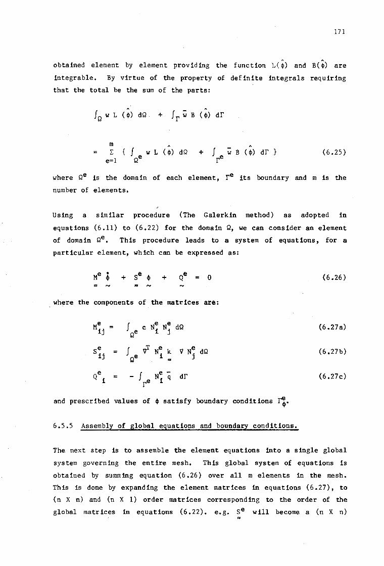
171

A A

obtained element by element providing the function 1($) and B($) are

integrable. By virtue of the property of definite integrals requiring

that the total be the sum of the parts:

= m E

e=l

A

{ I w L ( 4>) dQ Qe

+ A

I ~ B < 4>) dr } re

(6.25)

where Qe is the domain of each element, re its boundary and m is the

number of elements.

Using a similar procedure (The Galerkin method) as adopted in

equations (6.11) to (6.22) for the domain Q, we can consider an element

of domain Qe. This procedure leads to a system of equations, for a

particular element, which can be expressed as:

Me • Se 4> + 4> + Qe = 0 (6.26)

"' ... -where the components of the matrices are:

e I e

e e dQ Mij = c Ni Nj Q

(6.27a)

e I e

VT Ne k v N~ dQ sij = i J Q "'

(6 .27b)

Qe - I e - dr = Ni q i re

(6.27c)

and prescribed values of 4> satisfy boundary conditions ~·

6.5.S Assembly of global equations and boundary conditions.

The next step is to assemble the element equations into a single global

system governing the entire mesh. This global system of equations is

obtained by summing equation (6 .26) over all m elements in the mesh.

This is done by expanding the element matrices in equations (6.27), to

(n X n) and (n X 1) order matrices corresponding to the order of the

global matrices in equations (6.22). e.g. se will become a (n X n) ..

17 2

matrix 5e with zeros everywhere except those rows and columns "'

corresponding to nodes within element Qe. The global matrix equation

representing the domain Q, may be written as:

• M ~ + s ~ + Q = 0 (6.28)

which is similar to equation (6.20), but where the global matrices M, S .. .. and g are assembled from the various element matrices Me , Se and ge

"' "" respectively:

M = (6.29a) "' e=l ""

s = (6.29b) "" e=l ""

Q = (6.29c) - e=l

Prescribed boundary conditions on boundary r ~ are directly translated

into their equivalent positions, for the global system, in

equation ( 6 • 28 ) • The next step is to solve the resulting system of

equations for the unknown nodal values.

6.5.6 Solution of equations.

The system is now a set of algebraic equations from which the unknown ~

may be solved for. Boundary conditions are first imposed and then the

solving of the equations can be done in a variety of ways. Direct

methods (e.g. Gaussian elimination), or iterative methods may be

employed. If the time dependence from equation (6. 28) is removed , then

the unknown ~ can be solved for, from a set of simultaneous equations.

If not, then the initial values of ~ at t = 0 are generally specified

and a numerical recurrence process is required to find the solution at

subsequent times.

Two approaches can be adopted. One is by extending the Galerkin finite

element process, so that the unknown ~ is not only a function of spatial

17 3

Table. 6.2: Listing of Alternative Numerical Schemes. Yeh [39J.

Time Marching Mass Matrix

Numerical Central Backward Mid- Without With Schemes Difference Difference Difference Lumping Lumping

1 x x 2 x x 3 x x 4 x x 5 x x 6 x x

position in x, y and z, but also a function of time t. The domain used

would be subdivided into finite elements in both space and time. This

method is not that common as a vast amount of computer storage is

required. The second and more common approach is to discretize the time

domain into a sequence of finite intervals 6t, and nodal values of 4> are

solved, subject to initial conditions at t = O, by using a finite

difference "time marching" , or "time stepping", technique. (e.g. the

Runge - Kutta and "predictor - correction" methods). Table (6.2),. by

Yeh [39] lists six alternative numerical schemes by which

equation (6.28) could be solved. Each one dependent on the method of

time marching and treatment of the mass matrix M. If a one-step method

is used, in which it is assumed that:

(t + a 6t) t + 6t.i tt ) • ( t = (6.30a)

~t

and

(t + a ~t) t (t + ~t) .i = ( 1-a:) .i + a .i (6.30b)

where (0 ( a <: 1), and t4> is the value of the unknown at time t. Then

174

these assumptions correspond to the following time intei:.;ration

techniques, [2], [4]:

a = a = a· =

0

1/2

1

Euler .forward-difference (explicit)

Mid-difference or Crank-Nicolson (implicit)

Euler backward-difference (implicit)

On solving for the unknown <P at a specific time step t, the specific

flux vector (macroscopic fluid velocity), can be obtained from

equation (2.42), by using:

q (6.31)

This approach gives good results for the flux (velocity) at the optimal

(integration) points of the element, but yields discontinuity in the

flux at the nodal points and element boundaries. (See

Z ienk iew iez [ 41 ] • ) If the flux ts required at nodal points and element

boundaries, then the nodal gradient a•, must also be treated as an

unknown 1n the solution process.

Results of the flux are usually only given at the optimal points within

an element. ( ie. The Gauss Numerical integration points.)

6.5.7 Summary.

It has been shown that the flow of water in the saturated-unsaturated

domain can be expressed by a governing differential equation. This

equation can then be numerically solved by the Galerkin finite element

method, which gives an approximation to the solution of the flow

problem. From the solution, secondary values such as the flux, can be

relatively easily obtained. What makes the finite element method of

great value, is that it can be easily coded, as a computer program,

which can then be used for solving a variety of flow problems.

175

6 .6 A simple example.

To show the application of the finite element method, a simple example

of steady state vertical saturated flow through 3 layers of soil is

considered, as shown in figure (6.2). The problem considered consists

of three layers, each of a different hydraulic conductivity, placed on

top of each other. At the bottom face (Face A), the total seepage head

is prescribed to equal 8,0 units and at the top face (Face B), the total

seepage head is prescribed to equal 20 ,O units. The thickness of the

layers is 4 units each, and the hydraulic conductivity is: 2 ,O; 1,0 and

0,5 from the top layer down, respectively.

The governing differential equation is a one-dimensional steady state

version of equation (6.1) and can be written as:

d

dz

d 4> [ k (-) ]

dz = 0 (6.32)

where 4> is the unknown total head distribution. Two types of boundary

conditions may exist. Namely, Dirichlet, where the total head is

4

4

4

Fig 6.2:

FACE B (Total Seepage Head = 20,0)

FACE A

Units

}

Layer 3 k = 2 0

3 '

}

Layer 2 k = 1 0

2 '

} Layer 1 k = 0 5

l '

(Total Seepage Head = 8,0) Units

(a)

• •

2

l

Nodes

03

Element 3

n2 Element 2

n1 Element

(b)

-

-4 1

z

' z

z'

, I ~

'

Problem considered: (a) A three layered soil with prescribed

total heads at top and bottom faces; ( b} Modelled using

three, two noded one-dimensional elements.

prescribed as:

~(z.) J

176

= (6.33)

where z. is the position ( ie. node) of the boundary at which the total J .

seepage head is prescribed. In the example considered the total seepage

head boundary conditions are equal to 20 and 8 at the top and bottom

boundaries of the 3 layers, respectively. The second boundary condition

that may exist is Neumann, where the flux is prescribed as:

-

d~ k (-)

dz = q (6.34)

where q is the prescribed flux boundary condition. In the example

considered no such boundary condition is imposed.

For the sake of simplicity and to show the finite element method, a 2-

node-one-dimens ional element, which has a node at each end, is used. If

a single element 1s first considered, the 1 inear .shape functions over

the element are shown in figure (6.3) where:

Nf =

N~ =

and the length

=

e (z2 - ze)

1e

e (z -

e z i)

,._e

of the element

e z2 -

is:

where Z is the coordinate in the direction of the element.

noticed that:

N~ (zj) { : 0 i * j 1 i = j

(6.35)

(6.36)

(6.37)

It is

(6.38)

177

By equation (6.24), given earlier, the total seepage head over the

element can be approximated by the express ion:

¢ie = + (6.39)

where Ni and Nz are the shape functions over the element, given above

and ~i and ~Z are the nodal values of ~.

z Ii

£3

.e2

.el z

l

Fig 6.3:

Nl N2

_, ce ,._,

.n ell 0 u

.--' 0 c_;,...::

Global Basis Functions

Local Element Shape Functions

Nodal Numbering Local and Global

Three element representation of problem.. (In Figure 6.2}

4> . Ii

• l

(l 3

(l2

n1

178

If the derivative of the total head is required, within an element, then

it can be obtained from equation (6. 39) by simply differentiating so

that:

= + (6.40) dz dz dz

dN~

dz dz r:n =

1 1 =

JJ...e

The pro bl em given in figure ( 6. 2) can be subdivided in to 3 elements ,

each layer being an element. Figure (6 .3) shows the three element

representation of the problem, with 4 nodes located at zl' z2 , z3 and z4 • These nodes correspond to the boundaries of the layers.

For each element, there are local shape functions which make up the

global bas is functions for the problem.

that:

This can be seen by noting

Consider any point P (at height z) where the total head is required;

Nl coincides with Np>when P is element 1, z1 <z<z2

Nl is zero when P is elsewhere, z2 <z<z4

N2 coincides with N(l)when P is element 1, z1 <z<z2 2

N2 coincides with N( 2)when P is element 2' z2 <z<z3 1

N2 is zero when P is elsewhere, z3 <z<z4 (6.41)

N3 coincides with N( 2 >when P is element 2, z2 <z<z3 2

N3 coincides with N(3)when P is element 3, z3 <z<z4 1 N3 is zero when P is elsewhere, z1 <z<z2

N4 coincides with NP)when P is element 3, z3 <:z<:z4 N4 is zero when P is elsewhere, z1 <:z<:z3

179

Thus at any point P (at height z) within the mesh (ie. domain of three

elements) the total head is given as:

(6.42)

A solution to the approximation of the unknown <1>, given by

equation (6.42) can be found by using the Galerkin Weighted Residual

method. If equation (6 .42) is inserted into equation (6 .32), then the

left-hand side of equation (6.32) will not necessarily be zero but will

have a resulting error which may be written as:

d d<l>4 L( <l>4) = ( k- ) (6.43)

dz dz

and with boundary conditions: ..

A d B( <l>4) = - q k (-) (6.44)

dz

and

<l>i = <l>i (6.45)

A solution for the set of unknown <l>i is therefore needed to satisfy the

equation:

for j = 1, •• 4 (6.46)

where typically with the Galerkin Weighted Residual method, the weights

w j are taken as the bas is functions Nj" It is therefore possible to

write:

z4 d d<l>4 f N. [ -- ( k - ) dz

0 J dz dz

d<l>4 + f N. [ - q - k (-)

r J dz dr 0 j = 1, •• 4 (6.47)

180

This formulation (equation 6.47) requires second derivatives of $4 • A

"weak" formulation is therefore considered, based only on the first

derivative of 4>4 • By integrating by parts and rearranging,

equation (6.47) can be rewritten in the form:

Z1.t dN j d4>1.t I k - dz -

O dz dz I N. q dr r J

0 j = 1, •• 4 (6.48)

Substituting for the bas is functions, equation (6 .48) can be rewritten

as:

Z1+ dNj I k

O dz

dN1 [-dz

f N. q dr r J

' ...

0 j = 1, •• 4 (6.49)

This integration holds for the total system. If the relationships given

by (6.41) are used, then the basis functions can be replaced by the

• relevant shape functions. Thus if only one element is considered for

the moment with the shape functions of figure -(6.3),

equation (6.49) for one element can be written as:

dNI dN~ [- '-]

dz dz

I N. q dr re. J

0 j = 1,2

then __

(6.50)

The shape functions and their derivatives have been given in

equations (6.35) and (6.36) above. On substituting equations (6.35), 1

(6.36) and (6.40) into equation (6.50) a system of two equations for an

element is obtained in the form:

= (6.51)

where Se is the element stiffness matrix composed of four entries:

e e e z2 dN i dN.

J (ke - _l) dz e

z 1 dz dz

and ge is the force vector due to boundary conditions:

[:! ]

181

(6.52)

(6.53)

The integral 1n equation (6.52) is evaluated over the element. If one .

element is considered, then the first entry in the stiffness matrix in

equation (6.51) is:

Similarly

Similarly

and

e S11 =

z~ 1 = ke I <- -

e oe Zl A

=

1

= --

e S22 =

dN~ - ) dz dz

1 - -)

1e

dN~ -) dz

dz

1

dz

+-) dz 1e

(6.54)

(6.55)

(6.56)

(6.57)

182

The element stiffness matrix for a single element can therefore be

written as:

1

.le - 1

(6.58)

By virtue of the property of definite integrals, the total integral

given in equation (6 .46) must be equal to the sum of the parts:

,. ,.

J w 1(4>) dQ + J ; B( 4>) dr Q r

4 = E { J e w L( 4>) dQ + J e w B(4>) dr } (6.59)

e=l Q r

The element stiffness matrix that is obtained from equation (6 .46) can

be assembled from the stiffness matrix obtained for each element. On

assembling:

= 4 E

e=l

or where the global stiffness matrix for all the elements is:

11----1-1

s =

1s11 s12 I 1 ,y----1

ls21 1s22 I · 1 I . 2 I 2

L_ - - .!_+ 2S_DJ ,42_ J_ - - , I s21 1 s22 1 1 1

1 + sI1 1 si2 1 1-----1-3 ~ 3 I

1 s21 s22 1 L _____ .J

(6.60)

(6.61)

If we consider the example where .le = 4 units for all three elements.

Then the stiffness matrix for each element is:

= [_ : - 1 1 1 -

(6.62) 4

183

The global stiffness matrix for the example in figure (6.2) is

therefore:

s = 1/4 .. (6.63)

The values for ke have been given earlier as:

kl = 0,5 units k2 = 1,0 units k3 = 2,0 units

The global system of equations is written as a combination of all the

pertinent element equations (from equation 6.51). ie. The global system

of equations is:

s 4> : Q .. ....,

where boundary conditions imposed are: ·

4>1 = 8,0 units

4>4 = 20 ,O units

-- ----f6~4)

Therefore using the assembled global stiffness matrix as given in

equation (6.63) and the boundary conditions imposed, the set of global

equations to be solved are:

,------1 8 I 0,5/4 -0,5/4 -t- ql

1-0,5/4 :~5/4 I - - -1 I I L __ ~ _!_,0/4_J

1-!..!_0/4---+ _ $2 0

-1 -I -1,0/4 I 1,0/4 I I (6.65) I I I I

$3 0 L ___ t_'!:.,~4_J-2,o/4I l_:-22 0/4 _ ~o~ 20 q4

18 l~

where q1 and q4 are the unknown fluxes at the boundary nodes and <1> 1 and <1>4 (Prescribed total heads) have been inserted in their correct

locations. By removing the equations 1 and 4 ( <1>1 and <1>4 are already

known) from the set of equations alters the terms on the right hand side

and, the following set of equations need to be solved:

1,5

-1,0

Solving for <1>2 and <1>3 gives:

= =

-1,0

3,0

14,857

18,286

units

units

4

(6.66)

40

Knowing <1>1 <1>2 <1>3 and <1>4 the flux at any point can be calculated. If

element number one is considered:

~l = 8 units

~2 = 14,857 units

kl = 0,5 ,a.I = 4

Then

1 ~<!> q = k ..,. (6 .67)

1

(14,857 - 8) = 0,5

4

= 0,857 unit length/time

185

For element number three:

Then

q =

= 2,0

= 0,857

~l = 18,286 units

~2 = 20 units

k 1 = 2,0

l 1 = 4

(20 - 18,286)

4

unit length/time

(6.68)

The flux in element one equals that in element three as there is no

storage in any element and the continuity equation must hold. The

results obtain here are the same as those given in appendix (F-1) for

the same example analysed by using a finite element program

ADINAT [2]. (See section 6.8).

6.6.1 Summary of the basic steps of the finite element method.

The following is a brief summary of the main steps which are followed in

a finite element analysis, which does not include changes in the time

domain:

a) The structure is divided into a mesh of finite elements;

b) For each element the "stiffness" matrix and the "load" vector are

evaluated;

c) The element stiffness matrices and load vectors are assembled

into their respective positions in the overall stiffness matrix

and load vector;

d) The prescribed boundary conditions are imposed and the set of

equations solved for the unknown values of total head at the

186

nodes;

e) The subsidiary element quantities, such as fluxes, are

evaluated. (eg. at internal points within the elements.)

6.7 Application to flow fn porous Edia.

The numerical solution of equation (6.1) with applied boundary

conditions, and all the features as described above, for a

two-dimensional vertical domain, are incorporated in the code of a

computer program. The program used is ADINAT [2], which is a program

for the "Automatic Dynamic Incremental Non-linear Analysis of

Temperatures". The program ADINAT, was written .to solve the same

governing differential equation (6 .1), as this is also the governing

equation for the temperature distribution $, over a domain Q. For

seepage the unknown $, is the total head, defined as the local pressure

head plus the elevation head ( q, + z). Some changes have had to be made

to the coding of ADINAT to take this fnto account. The changes have

been incorporated into ADINAT, for two-dimensional elements orientated

fn the vertical plane, fn the form of a new non-linear material model.

(See appendix F-2).

The relative hydraulic conductivity ~(0) is a function of the

volumetric moisture content e, but the volumetric moisture content e, is

also a function of the local pressure head q,, see figure (2.9).

Therefore the relative hydraulic conductivity krw' is also a function of

the local pressure head q,. If the hysteresis nature of the relationship

between 4i and 0 is neglected, the relative hydraulic conductivity krw,

is a single value function of the local pressure head q,. Similarly, the

specific moisture capacity c, is a single value function of the pressure

head q,. See figure (6 .4). The assumption to neglect hysteresis is

possible, if either a monotonic wetting or drying domain is being

considered, as only a primary wetting or drying curve, of the soil

moisture characteristic curve, is being considered. (Ref Hillel [18]).

See figure (2. 9). Depending on the accuracy of the solution required

this assumption could also be made for a simultanuous wetting and drying

domain.

(a)

(b)

187

P2rtly Saturated .~.__~-+-~•~Saturated with Water

-lji 0

0

0

k rw Relative hydraulic conduc~ivity

+lji

Specific Moisture Capacity c

Pressure +lji (~ - z) head

Fig 6.4: Sfngle value function relationships for a saturated

unsaturated soils (all wrsus pressure bead •>= (a) Relative

hydraulic conductivity; (b) Specific moisture capacity.

Hysteresis is not considered in the present analysis. Only a single

functional relationship is considered between 4>, krw and c. This is

incorporated into the program analysis by linear interpolation between

discrete tabulated values in the input data of the program, where k {4>) rw

and c{<l>) are considered as non-linear material parameters in the

model. It is therefore assumed that:

k ( 4>) = 1 for 4> > 0 (6.69a) rw

and

0 <: k ( 4>) ( 1 for 4> <: 1 (6.69b) rw

where k ( 4>) is assumed as a non-linear material. see figure (6.4). rw

The nature of ADINAT, allows both confined and unconfined problems to be

188

solved. The candidate incorporated saturated-unsaturated conditions

within ADINAT. In the program, the total head ¢, is treated as the

unknown variable. Specific values of 4> or q can be specified as a

function of time for the nodes and boundary surfaces with Dirichlet or

Neumann boundary conditions respectively. (See figure 6.5). The

relative hydraulic conductivity ~ and the specific moisture capacity

c, can be tabulated as functions of: either time t; the unknown total

head 4>; or the pressure head 4i ( 4i = 4> - z, where z is the vertical

elevation), with constant material model parameters over each element

within the saturated-unsaturated domain.

Some of these features are demonstrated later by examples. Firstly the

input and output data for the program ADINAT is discussed.

6 • 8 Operation of the f fnite e1ement prograa package.

The finite element program package used for the fµiite element analysis

done, was ADINAT, version 84.00 {2]. Modifications were made to the

program material model (see Section 6.9), so that the material

parameters could be entered as functions not only of total head, but of

pressure head as well.

q

!Dropping tHead

~(t) = H1 (t)

r

This program package was loaded on the

= 0

Surface

Saturated Pervious Material n = z Seepage

'\ Impervious q = 0 r

2

Fig 6.5: Saturated-unsaturated flow do11afn Q enclosed by a boundary r.

189

University of Cape Town's mainframe computer (Sperry Univac llOO) and

permission to use the program was granted by Prof. W S Doyle.

Data input is entered in fixed format as specified by the users'

manual [2). Character variables may appear anywhere in the space set

aside. Integer variables must be right-adjusted in the spaces set

aside. Real number variables may be written with or without a decimal

point in the space set aside. If the decimal point is not included then

the real number must be right-adjusted. In the users' manual [2] each

card or card group is identified by name and the format used on the

card(s), 'with the name of the variables being given. The meaning of the

variables and notes are also provided.

The general groups of data input are as follows:

Group 1: Heading

Group 2: Master Control Data

This group is always input and includes the following:

number of nodes;. number of linear and non-linear element

groups; solution nnde; number of time-steps; time of

solution start and output interval; form of generated

input data, output; analysis type; convergence

tolerances; method of time integration; and control of

output.

Group 3: Time step Data

This controls the number and size of the time step.

Group 4: Nodal point Data

This is the nodal coordinate data.

Group 5: Initial Conditions

This specifies the initial conditions for the total heads

at all nodes.

190

Group 6: Boundary Condition Control Data

This specifies the number of nodes involved with boundary

conditions.

Group 7: Definition of Time Functions

This specifies the time function curves for the various

boundary conditions.

Group 8: Applied Seepage Flow Data

This includes the prescribed nodal values and flux

conditions.

Group 9: Element Group Data and Topology

This includes the following: element type; number of

elements in group; problem type; number of nodes per

element; order of integration; material poperties (see

sections 6.9.1, 6.9.2 and 6.9.3); and nodes that make up

each element {topology).

An example of an Input data file, for the problem considered In section

(6.6), is given In appendix (F-1).

6.9 Finite eleaent 1111terial 11>dels.

For the analysis of seepage pro bl ems presented in th is thesis, three

different material models were used. The range is from saturated

seepage problems - where the material properties do not change during

the analysis, to a highly saturated-unsaturated problem with varying

material· properties which depend on the total head or pressure head.

(Time dependent properties can also be considered by the

program ADINAT [2]).

6.9.l Constant saturated hydraulic conductivity model.

This is a linear model defined by one hydraulic conductivity constant

for an isotropic material. The model is used for steady-state linear

-z

2

~

191

3

y

Fig 6 .6: Principal in-plane 111terlal axes orientation for the linear

ortbotropic material model. ADINAT [2].

analysis and no time stepping is required. This is because the specific

moisture capacity term is zero in equation (6 .28), and therefore the

time domain is not considered. The solution of the unknown total heads

over the domain can be directly solved with the applied boundary

conditions.

The terms required for the material properties for an analysis are:

Saturated hydraulic conductivity for an isotropic material

k

or Saturated hydraulic conductivity in the two orthotropic

directions

In direction a: ka

In direction b: kb

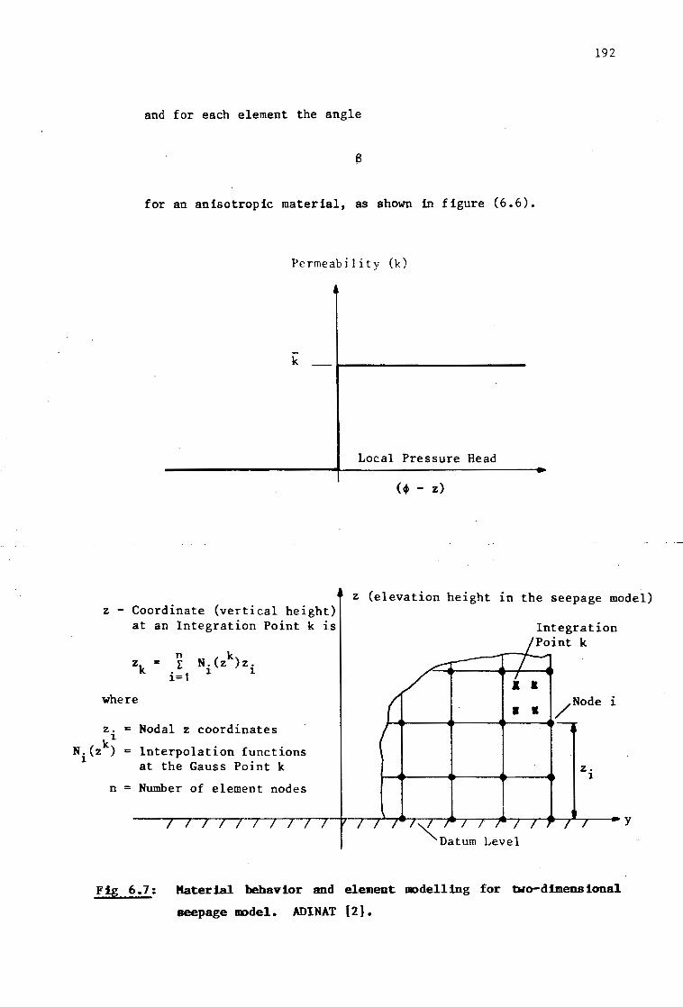
192

and for each element the angle

for an anisotropic material, as shown in figure (6.6).

Permeabjlity (k)

-k

Local Pressure Head

z (elevation height in the seepage model) z - Coordinate (vertical height)

at an Integration Point k is

z "" k

where

n I:

i=1

k N.(z )z. l: l

z. "" Nodal z coordinates k1

N.(z) =Interpolation functions l

at the Gauss Point k

n = Number of element nodes

"'<-.Datum Level

z. l

Fig 6.7: Material behavior and element modelling for two-dimensional

seepage model. ADINAT (2).

y

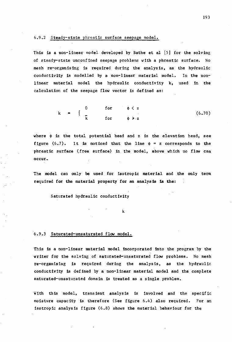
193

6.9.2 Steady-state phreatic surface seepage model.

This is a non-linear model developed by Bathe et al [5] for the solving

of steady-state unconfined seepage problems with a phreatic surface. No

mesh re-organising is required during the analysis, as the hydraulic

conductivity is modelled by a non-linear material model. In the non

linear material model the hydraulic conductivity k, used in the

calculation of the seepage flow vector is defined as:

0 for cfJ < z k = { (6.70)

k for cfJ ).z

where cfJ is the total potential head and z is the elevation head, see

figure (6. 7). It 1s noticed that the line cfJ = z corresponds to the

phreatic surface (free surface) in the model, above which no flow can

occur.

The model can only be used for isotropic material and the only term

required for the material property for an analysis 1s the:

Saturated hydraulic conductivity

k

6.9.3 Saturated-unsaturated flow model.

This is a non-linear material model incorporated into the program by the

writer for the solving of saturated-unsaturated flow problems. No mesh

re-organising is required during the analysis, as the hydraulic

conductivity 1s defined by a non-linear material model and the complete

saturated-unsaturated domain is treated as a single problem.

With this model, transient analysis is involved and the specific

moisture capacity is therefore (See figure 6.4) also required. For an

isotropic analysis figure (6.8) shows the material behaviour for the

194

Permeability k

2

Specific Moisture Capacity c

2 7

ae a~

c

Loca1 Pressure Head

1Ji = ( ~ - z)

Local Pressure Head

lji .., (~ - z) 8

Fig 6.8: Material behaviour for two-dimensional saturated-unsaturated

seepage a>del, Interpolation shown as a function of pressure

bead for: (a) The current conductivity; (b) The specUic

.:>isture capacity.

model. With this· non-linear model both the hydraulic conductivity and

specific moisture capacity are functions of the pressure head. Linear

interpolation is used in figure (6.8) to obtain the hydraulic

conductivity and specific moisture capacity of the material at

intermediate posit ions between the points for which data is entered in

tabular form.

For isotropic hydraulic conductivity material, only a tabular

entry of the hydraulic conductivity and the specific moisture

196

and for each element one must specify the angle (See figure 6.9):

where ka and kb are the hydraulic conductivities in the two principle

directions of the anisotropic medium.

6 .10 Output from finite element package.

The output of results depends on the analysis done. For a steady-state

analysis the following is the output:

- the total seepage head at each node;

- the pressure heads at the element integration points;

- the flux at the integration points within the elements.

For a transient analysis the above is also the output, but only at the

time steps requested. The extent of output is controlled by the user

(eg. the nodes and elements for which output is required can be

spec if ied) •

The flux output at the Gauss integration points is determined by using

equation (6.31).

For the analyses done in this thesis, the flux values were usually not

needed as the pressure heads were used for comparing results. This was

because in the experiments done by the writer, pressure heads were

usually measured. The horizontal flux values were however compared, as

shown in figure (6.25), in the verification of experiment number one.

The finite element package did have a flag to output the nodal and

element results into a file for post-processing, but the post-processor

was not yet available at the University of Cape Town. This is because

the version of ADINAT [2] used was a new version and the post-processor

had not yet been released.

2

z

y

7

/Node

4

195

Fig 6.9: Principal in-plane material axes orientation for the

saturated-unsaturated orthotropic seepage material .,del.

capacity is needed. Namely values of:

k(<ji)

c( <Ii)

For anisotropic hydraulic conductivity material, a tabular form

of the hydraulic conductivity and specific moisture capacity is

still required. Namely:

but the ratio between ka(q,) and kb(q,) is also needed:

197

6.11 Finite element examples and prog:i::am verification.

6.11.1 Introduction.

To show some of the features of the finite element program package

ADINAT [ 2] and also to verify the material model implemented by the

writer, a few varied seepage pro bl ems were considered.

considered included:

The problems

a) The analysis of steady-state confined saturated flow around a

raking sheet pile in a stratified, anisotropic foundation. (See

figure 6 .1 0) ;

b) The analysis of steady unconfined free surface flow through an

earth dam with a toe drain. (See figure 6.11);

c) The transient analysis of saturated-unsaturated flow in a

rectangular dam caused by a change in tail-water level. This

causes a decline of the phreatic surface towards a new

steady-state flow system. (See figure 6.13);

d) The analysis of non-steady saturated-unsaturated flow between

drains after rapid drawdown. (Using observations by others. See

figure 6.16).

e} The transient analysis in a rectangular dam caused by a change in

tail-water level. This is for a saturated-unsaturated transient

flow system. (Experiment by candidate. See figure 6.19}.

f) Analysis and observation of non-steady saturated-unsaturated flow

into drains after rapid-drawdown. (Work by candidate. See

figure 6.26)

The results are presented mainly as a function of the total or pressure

head. Where possible comparisons are shown with the results obtained by

other investigators for experimental or theoretical analysis done.

Note: Only two-dimensional flow in a vertical plane is considered.

The (implicit) backward difference time marching scheme is used

with lumping of the Mass matrix for the transient examples

considered. This method is suggested by Neuman [31] so that

198

oscillatory and instability problems of two point recurrence

schemes are overcome.

6.11.2 Example No. 1: Saturated confined seepage.

In this example (See figure 6 .lOa), the total head distribution in a

stratified, anisotropic foundation with an inclined wall of sheet piling

is studied. It is possible to compute the analytical solution for the

flow by using conformal mapping. The analytical solution was not found.

The problem consists of a sheet pile inclined at 52°, and a stratified

soil with the inclination of the orthotropic axis for the principal

hydraulic conductivity of the soil at 60°. (See figure 6.lOa). The

ratio of the hydraulic conductivities is taken as 4. A prescribed total

hydraulic head of 100 and 0 at the upstream and downstream surfaces is

applied respectively.

The problem is solved as a steady-state problem with a constant material

mogel and prescribed total head boundaries. The results obtained by a

finite element analysis of the total head distribution, using ADINAT,

are given at the appropriate nodes, as shown in figures (6. lOa and b).

From these results the equipotentials have been drawn, which are

distorted due to the stratified foundation. As the stratification of

the foundation and the sheet pile are inclined in a similar direction,

it would be expected that the mid-equipotential line between the

upstream and downstream total heads corresponds to this direction. This

has been predicted by the results from the analysis as shown in figures

( 6 .10 a and b) •

6 .• 11.3 Example No. 2: Unconfined free surface steady state flow.

The total head distribution below the free surface of steady-state

seepage through a dam with a toe drain, as shown in figure (6.11), is

analysed. The dam consists of an upstream water level, constant with

time at an elevation of unit 1 and a toe drain at the downstream face of

the dam with a tail water level at elevation 0, 1. The material model

used for the analysis is that described in section (6.9.2), with the

\.Jater

¢ = 100 IU Ille

(a)

4> c 100

(b)

4> = 80

I

80

I I

I 14 \

\ \ \

I 1s \

\ \

\ \ \

,u \ \

70

I

70

\

\ \

60

I I I

199

J

I

' '· 4> =10

' 20 4! \ \

\ 30 \ '

60

~40 SO Equipotentials of

•

Total Head

4> c o.

' ' \ '30

\ 40

•

I

4> = 10

20

Fig 6.10: now around an inclined sheet pile va11 fn a stratified

{anisotropic) foundation. {a) Complete region analysed.

{b) Ffner mesh near tip of pile. {This analysis by the

candidate UfJing ADINAT). The angle of 52° for fnclination of

pile wall may be different from that used by previous

workers.

Water Level

1 .o

Isotropic Material ka = kb

O ADINAT --Analytical

/Impervious

·4,09

Harr

200

Fig 6.11: Seepage analysis of the unconfined free surface steady-state

flow through an earth dam with a toe drain.

saturated hydraulic conductivity taken as 1,0. Figure (6.11) shows the

results of the free surface obtained numerically by ADINAT, using the

finite element mesh as shown in figure (6.12). The results are.compared

with that obtained from an analytical solution using conformal

mapping. The charts and tables for the analytical solution are given in

Harr [ 16) • Using these charts and tables a plot of the free surface

could be made as shown in figure {6.11).

The results obtained from the finite element method show a good

comparison with that of the analytical solution, except near the seepage

face of the toe drain. Near the seepage face some of the elements have

been reduced to triangles from four noded elements. Also the mesh used

is not very fine. The reason .for the discrepancy in the solutions could

be caused by the reasons given above or partly caused by them. In this

outflow zone the first node above the tailwater level is located at a

height of 0,2 units. (See figure 6.12). It is possible that ADINAT

regards this node as having no flux. At the lowest node (submerged) the

tailwater level is 0 ,1 units and hence ADINAT will regard the outflow

surface as being up to the tailwater level. ( ie 0, 1 units high). In

practice there will also be an outflow surface above the tailwater

levels which does not seem to have been simulated by ADINAT in this

instance. The problem could be re-analysed using a finer mesh near the

seepage face, to check the above.

(4 Noded Two-dimensional plane elements)

Elements with nonlinear material ararneters.

4,09 \Toe Drain

201

Fig 6.12: Finite element mesh used by candidate for the analysis of the

dam. {Figure 6.11).

6.11.4 Example No. 3: Drainage from a saturated-unsaturated system.

In this example a vertical domain is considered, in which part of the

domain is saturated and part is unsaturated. Figure (6.13) shows

schematically the lay-out of the problem. Initially, the water table in

the problem is at an elevation 143 cm • At time t = 0 the water level

in one reservoir is lowered to an elevation of 80 cm and this situation

is maintained indefinitely. The resulting hydraulic gradient causes the

water table to drop gradually at a rate indicated by the solid curves in

figure (6 .13). The sand below the water table remains saturated during

the drainage, while the region above has varying degrees of saturation.

This problem was also studied by Narasimhan et al [30) in which he gives

the data for the highly non-linear relationship between Q>, ~ and c,

see Table (6.3). Figure (6.14) shows the layout of the finite element

mesh used in the present analysis, which is the same as the mesh used by

Narasimhan et al. for simulating the experiment. The unkown total

head 4> at all nodes is given an initial value of 143 cm at t = 0. The

problem is then solved for t > O. Fixed nodal values of total head

(143 cm) are imposed on the RHS boundary of the problem. Along the LHS

for the zone below the water level in the reservoir, nodal values for

the total head are fixed at 80 cm and the seepage face above the water

150

,-... e (.)

'-" 100 c

80~ 0 ..... .j,.J .. t1l > 50 Q;

...... w

0

t = 0 hours, ---------------------

-- Measured

o ADINAT

50 100

State 200[ ~

(Narasimha~r "'"C3

150

(cm)

0 300

200 250

202

.143

300

Fig 6.13: Decline of water table in a drainage experiment of a

saturated-1B1.saturated system. Numerical results fro• ADIB.AT

co•pared vit.b Easured results fro1t Haras!llban et al. [30].

e (.)

0 0 N

(4 Noded Two-dimensional plane elements)

Nonlinear Elements

t '" ~ -

Linear Elements . I

1

300 cm

1'1.7 270

56

Fig 6.14: Finite element mesh used by candidate to simulate t.be

experiment reported fn Narasimhan et al. (30]. Flow fn t.be

saturated-unsaturated domain.

203

level is treated as a flux boundary condition. The flux boundary

condition, only allows flow out of the boundary and the flux is zero if

the local pressure head becomes negative.

The problem was solved using Euler backward difference time stepping and

the results were printed at time t = 0,1 hours and 1 hours. The steady

state water table is obtained by assuming no specific moisture capacity

( 1. e. taking the time dependence out) and solving the problem as a

linear problem with non-linear, material properties and boundary

conditions. Figure (6 .13) shows the various posit ions of the water

table, as given by the numerical results from this analysis using

ADINAT, and the corresponding experimental data. [30]. The two are in

excellent agreement with each other.

Table 6.3: Relationships between <Ii' k and c for drainage problem. Narasimhan et al. (30]

<Ii (cm) c (cm3/cm) k (cm/s) .........

-90 7 x 10-4

-80 1,94 x 10-7

-75 1,3 x lo-3

-65 2,0 x 10-3 x 10-6 -60 6,94

-55 3,1 x 10-3 x 10-S -so 1,94

-45 4,6 x 10-3

-40 6,94 x 10-S -30 5,9 x 10-3 8,33 x 10-4

-25 1,73 x 10-3 -20

x 10-3 3 ,72 x 10-3

-17,5 4,2 -12,s 2,5 x 10-3 -10 1,02 x 10-2

-7,5 1,0 x 10-3 x 10-2 -4 1,12

-2,5 1,6 x 10-4 x 10-2 0 1,0 x 10-S 1,12

204

6.11.S Example No. 4: Non-steady state flow betweens drains after rapid

draw down.

A problem of this type arises when parallel drains or ditches are

placed, as shown in figure ( 6 .15), to lower the water table. The depth

and spacing of the drains are two important factors that control the

lowering of the water table. The problem can be considered as a two

dimens ional problem in the vertical plane with only half the distance

between the drains taken for modelling, because the line of symmetry

acts as an impervious layer. This problem is considered by subdividing

the domain, into a mesh of 4 noded elements, as shown in figure (6.18).

The initial total head is 19. 7 inches. At time t = 0, the water

level in the ditch is lowered to the base and the ditch face treated as

a seepage face. The line of symmetry and the base are treated as

impervious boundaries (i.e. q = 0).

This problem has also been considered by other authors, Desai [12] and

France et al [ 13], but only the saturated hydraulic conductivities and

specific yields are given in these references:

Hydraulic conductivity:

Spec if ic yield:

k = 0,0674 inches/sec

s = 0,886 y

·To be able to use the program ADINAT, not only must the saturated

hydraulic conductivity be known, but the relative conductivity ~ as

well, so that the problem can be solved as a saturated-unsaturated

problem over the domain. Since this is not given the relative curves

are assumed for analysing the problem.

The assumed functions for the relationships of ~' krw and c are shown in

figure (6.17). The relationship between ~and c was assumed so that the

area under the graph yielded the specific yield (i.e. Sy= 0,1 x 0,866 +

0,9 x 0,866). Using these assumed relationships, the problem was solved

using ADINAT. Figure (6.16) shows the results for the solution of the

problem, given by; Desai [12] a one-dimensional finite element

solution, France et al [13] a three-dimensional finite element

I--- --

205

Ground Surf act· lnitial Water Level

I ----1-- -- ----1----

I --- --1

Water level in

Drain during Drawdov-7n

\ '\

Typical'Profile of Phreatic surface

Impervious bottom A B

Region Modelled

Fig 6 .15: Rap id drawdovn between parallel drains.

20

18

Seepage Face"'-16

14

12

Height 10 (inches)

8

6

4

2

~o 0

0 sec

60 sec

cL

I

-- ------~--=-------------~.

k

s y

--iT --0-1

0,0674 inch/sec

0,886

I-Plane of Symmetry

---- ------- .0.- _g_ 360 sec;...- :::_g_ _.JJ- 1

/ »--/. .,.,,,._V -- Analogue, Szabo & Mccaig

/, ~ /"" One-dim. finite element, Desai.

2 4

o Two-dim. finite element, ADINAT present

Three-dim. finite element, France et al.

6 8 10 12 I 14

Distance from Drain (Inches)

Fig 6.16: Comparisons of the decline of the phreatic surface with rapid ·

drawdown between parallel drains.

Relative Hydraulic Cc,ndurtivitv

-2

Specific Moisture Capacity

-2 -1

k rw

0 Local Pressure Head

+1 ljJ (inches)

+1 ljJ (inches)

206

Fig 6.17: Assumed functional relationships between +, ~ and c for

drainage problea of rapid dravdown between drains.

(Section 6.11.5)

solution, the reported analogue solution by Szabo and McCaig, and the

solution by ADINAT using two-dimensional finite elements.

For the early stages of the simulation by ADINAT (eg. time t = 60 sec),

the predicted drainage rate is too great. (See figure 6 .16). As time

progresses the predicted solution improves and shows good agreement with

the reported results. This discrepency at the start of the predication

could be caused by the coarse mesh and the method of ioodelling the

seepage face as nodal fluxes. For the time t = 60 sec, the solution

predicted by the reported results from references all coincide at the

drainage seepage face with the midpoint of the element face of the mesh

used in the finite element model by ADINAT. The phreatic surface for

ADINAT at this seepage face tends to a lower node. (See figure 6.16).

For later time steps, the predicted results are good near this outflow

surface, but boundary effects can still be observed. These boundary

effects are most noticeable at time t = 360 sec, where a kink in the

predicted results occurs near the seepage face. Because ADINAT is based

on the concept that on the .seepage face, above the tailwater level, the

nodes either allow a seepage flux (when the local pressure head is zero)

or have no seepage flux (when the local pressure head is less than zero)

207

the boundary effects on the outflow surface can lead to incremental

errors when using ADINAT. The phreatic surface at the outflow surface,

above the tailwater level, must coincide with a nodal point of the

finite element mesh.. For example when time t = 360 seconds the phreatic

surface passes through the node at the z height of four inches on the

drainage surface. (Aside: Below the phreatic surf ace the local

pressure head must be equal to zero, ie. atmospheric pressure, on the

drainage surface above the tailwater level.)

A method of overcoming this could be to use a finer mesh near the

seepage boundary, particularly in the vertical direction, so that the

20

18

16.

14

12 -Ill cu .c (.)

10 c:: H '-'

c:: 0

8 ·~ ... I'll :> Q) ,.._,

l>J 6

4

2

0 1

(4 Noded Two-Dimensional Plane Elemen~s)

Elements material

1 I I

0 2 4

'

with nonlinear parameters.

I I 6 8 10

(Inches)

99 80

,.,.., Plane of Symmetry

I _J

12 I 14

Fig 6.18: Finite element mesh used by candidate to DX>del rapid dravdown

between drains. (Figure 6.16).

208

seepage face can be modelled more accurately. The assumed relationships

of ~' krw and c, as shown in figure (6.17), could also have affected the

results.

6.11.6 Summary and conclusion.

It can be seen from the examples given that the use of the finite

element method, is relatively easy, for the solving of seepage problems,

when in the form of a computer program. Examples of both saturated

steady-state and transient saturated-unsaturated flow in a rigid porous

medium have been analysed above, showing the wide range of problems that

can be considered. It also has been shown that the finite method

(applied correctly) yields good results for the problems considered,

both for results reported from other authors using finite element

methods and from the writer using ADINAT. It is noted that the seepage

face can cause errors and it is in this area that care needs to be

exercised when using the finite element method.

6 .12 Experfaent verification using the ffnite element Et.hod.

6.12.1 Introduction.

In the previous chapter two experiments which had been performed by the

writer were discussed. Various measurements were made while the

experiments were in progress. A verification of the experiments is done

by modelling the two problems, using the finite element program package

which has been modified by the writer. The examples covered in

section (6.11) show that the material models used in the program package

do yield acceptable results.

6.12.2 Experiment No. 1: Unsteady flow through a rectangular dam.

Experiment number one, that was discussed in chapters 4 and 5 is

analysed here by the finite element method. The pro bl em cons is ts of a

rectangular earth dam, as shown in figure (6 .19). The initial water

level, at time t = O, on both sides of the dam was 12,48 inche.s

209

(317 mm). The RHS water level was then lowered to the base (z=O) and

this face was then regarded as a seepage outflow surface.

The functional relationship between <Ji, krw and c is given in Table

(6.4), which was obtained from the experimental analysis in section

(5.5.1). Figure (6.19) shows the· observed positions of the phreatic

surface obtained from the transducers in the experiment (See section

5.5) and those obtained numerically from ADINAT, using the finite

;1Initial Water Level 12,48 inches

¥-- -----

1~ LE::::J~ . t = --Exp er imen t

42 0 o ADINAT

42 40 36 32 28 24 20 16 12

Length (inches)

8 4

14 Elevation (inches)

10 ___..Seepage

Face 6

2

0

Fig 6.-19: Decline of water table for the drainage experlllent: nuaber

one, of a sat:urat:ed-uosat:urat:ed domain. Humerical result:s

from ADIHAT coapared vit:h calculated result:s froa the

experiment: performed.

(4 Noded Two-Dimensional Plane Elements)

71 05 128

f,.Q

Nonlinear Elements

67

1

42 inches

Fig 6.20: Finit:e element mesh used to nndel drainage experiment 1D1mber

one.

317mm Contours of Total Head (mm)

___ Phreatic - - - - - - .LsQ_rface

0 0 C"")

0 oO N

--

210

Seepage Face

Fig 6.21: Contours of total bead fn the drainage experiment number one

at time t = 15 sec. Obtained from the DUaerical analysis by

ADINAT.

element mesh shown in figure (6.20). Figure (6.21) is a contour plot of

the computed total heads at time t = 15 seconds. This can be compared

with the observed values from figure (5.12), and it can be seen that the

two are very similar. In figure (6 .21) there is a problem, near the

seepage face in that the contours are distorted. This is caused by the

mesh size and the presence of the seepage face. Also shown, fn figures

(6 .22), (6 .23) and (6 .24) are the results from pressure transducers,

located at specific points in the domain, and the numerical results

obtained by the finite element method ADINAT, for the nodes at the

corresponding positions.

Table 6.4: Relationships between cji, k and c for drainage experiment number one.

<Ii (inches) c ( in3 /in) k ( in/s)

-50 0 2,00 x 10-4

-6 -4,8 -4 -3 -2 -1 50

0 x 10-4

x io-1 2,00

1,00 1,09 x 10-2

1,00 x 10-l 6,33 x 10-2 1,26 x 10-1

0 1,555 x 10-1

0 1,555 x 10-1

211 320

g -0

240 ('\)

<l.l

,....; 160 m 4.J o ADINAT 0 E-'

80 -~Pressure Transducer (experiment)

0 0 20 40 60 80 100 120 140

Time (seconds)

Fig 6.22: Comparison of the result for node 71 in the numerical

analysis and the output for the pressure transducer, number

-rB4 "·, of experfaent number one.

320

-240 ~ ......,

"C

o ADINAT :160 ::c: ...... al --Pressure Transducer (experiment) 4.J 80 0 E-<

0 0 20 40 60 80 100 120 140

Time (seconds)

Fig 6.23: Comparison of the result for node 69 fn the Dllll.erical

320

j ......, 240 "C

<IS ci>

::c: 160 ......

<IS 4.J 0

E-< 80

0


-rB3'", of experiaent number one.

o ADINAT

-- Pressure Transducer (experiment)

0 20 40 60 80 100 120 140 Time (seconds)

Fig 6.24: Comparison of the result for node 67 in the numerical


-rB2'", of experiment D1111lber one.

";;' 14 Q,j

.c u c: 10 .....

c: .9 6 ""' . ell ~ Q)

....-< 2 lil

Section A-A

-Experiment

o ADINAT

0 0 0,2 0,4 0,6 0,8

Relative Horizontal Flux

(k x ih) rw

212

Section D-D

--Experiment

o ADINAT

0

0 0 0,2 0,4 0,6 0,8

Relative Horizontal Flux

(k x ih) rw

Fig 6.25: Comparison the borizonta1 coaponents of the relative flux at

section Ir-A and D-D, of the muaerical analysis ADINAT and the

calculated relative flux froa the exper:lJDeu.ta1 results of

experf.llen.t nuaber one. (Tbe actual superficial Darcfan

velocity ls equal to the i:elatlve flux mlt.fplf.ed by k88

t)

Figure (6.25) shows a comparison of the calculated relative flux (See

section 5.5.5) at the sections A-A and D-D (See figure 5.12) with the

results from the numerical analysis by ADINAT. As shown by the figures

given above, the numerical results are in very good agreement with the

results obtained from the experiment performed.

Based on the above, for experiment number one, it has been shown that

the numerical analysis verifies the experimental results very

accurately.

6 .12 .3 Experiment No. 2: Saturated-unsaturated flow in a slab of soil

between drains after rapid drawdown.

Experiment number two, (discussed in chapters 4 and 5) is analysed here

by the finite element method. The problem cons is ts of a slab of soil

with an impervious base and drained by a ditch with a zero water level,

as shown in figure (6.26). The initial water level, at time t = O, in

the ditch was 15 ,O inches (381 llDll). The ditch water level was then

lowered to the base (z=O) and the face treated as a seepage surface.

Table 6 .5:

213

Relationships between 4>, k and c for drainage experiment number two.

Qi (inches) c (in3 /in) k (in/s)

-so 0 2,00 x 10-4

-6 -4,8 -4 -3 -2 -1 50

0

x 10-1 3,00 x 10-4

1,03 1,29 x 10-2

1,03 x 10-1 7,53 x 10-2

1,499 x 10-l 0 1,85 x 10-1

0 1,85 x 10-1

The functional relationship between 4', krw and c is given in

Table (6.5), which was obtained from the experimental analysis in

section (5.6.1). Figures (6.26a and b) show the comparisons of the

phreatic surface determined from the experimental results, section (5.6}

and the numerical results from ADINAT, at times t = 15 and 30 minutes

respectively, after the start of experiment. Also shown are contour

plots of the total heads, obtained from the numerical analysis, using

the finite element mesh as shown in figure (6.29c}. It is shown that

the positions of the experimental phreatic surface do not aggree with

the computed positions from the numerical analysis. As shown in

figure (6.29c), the finite element mesh in the vertical direction is not

very fine, especially near the seepage face. As shown earlier in

section (6.11), the modelling of the outflow seepage face can affect the

results. In this experiment number two, the shape of the drainage

domain ( ie. very long and horizontal) causes a horizontally inclined

phreatic surface, even though drainage is occuring and the writer

believes that the computer program ADINAT can provide incorrect results,

especially if a coarse vertical spacing is used for the finite

elements. The results of the numerical analysis have therefore been

affected by the mesh size and seepage face. If a finer mesh had been

used in the vertical direction the verification would have been

better. Even with the present errors, the experiment is still modelled

relatively accurately, in that the declining phreatic surface is about

16 % out at the worst place in relation to the overall vertical range of

~ ,,

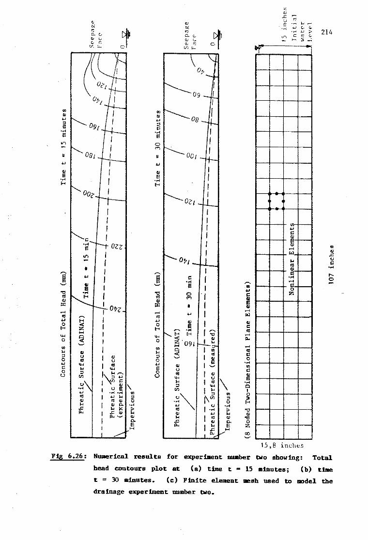
er

:z:

II I

I i

"' ~

t;

OQ

§

[ (1

)

• s

! [

3 =

...

l'D ~

GI

GI

t;

t:. f O>

• i

,, QO

rt -,,

Iott

8 n

~ 0

-t;

t "Id

! t;

~ -

.... ..

(1)

i rt

-~

(1)

f 0

rt

• i i

rt

1:1

rt

I rt

II

I ....

... G

I V

'I er

II

i

i ~

0

l'D

= g

. "'

rt

(1)

0

er QO

r:

... f

B -..

"' ""

l'D -

... ....

,, 0

g. i

£ (1

)

Vi .. 00

.....

:::l n :r

ro U'l

Con

tour

s o

f T

ota

l H

ead

(mm

)

Ph

reat

ic

Su

rfac

e (A

DIN

AT)

----

--z-

----

----

----

-P

hre

atic

Su

rfac

e ~

(exp

erim

ent)

C'

.J

Imp

erv

iou

s/

Con

tour

s o

f T

ota

l H

ead

(mm

)

Ph

reat

ic S

urf

ace

(AD

INA

T)

/ ~

Tim

e t

• 30

min

15

min

0 "' "'

----

Tim

e t

=

Cl

co -15

m

inu

tes

Tim

e t

= 3

0 m

inu

tes

Cl

0

St>

€'p

:1g

P

F nc

-c

See

pag

e <::

::i o

face

~P~h;r~e~a~t~i

~c~7 ~s~u~r~f

~a;c~e~(

~m~e~a~s

~;~e~d~)

~~.~-~~-

~~-~J=~~

~~~~1~~~

~~1~~~::

1Q:);-=~

~'°~:;:~

~:J Im

perv

iou

s/

(8

Nod

ed

Tw

o-D

imen

sion

al

Pla

ne

Ele

men

ts)

t

Nop

.1 in 1e

a r

1E 1 e

iy.en

t:

107

inch

es

- - -

1-r

I

15

inch

es

Jn

itia

l W

:l t

<'r

L

('V

€' 1

215

the drainage domain. The affect of the seepage face can be seen by the

distorted contours in figure (6 .26a). Near the drainage face the

phreatic surface, calculated for the experiment and that predicted by

the finite element method are about the same.

6.12.4 Conclusion.

For the results shown in figure (6.19) for experiment number one, the

agreement between the numerical results and the experimental work is

excellent. Based on these comparisons the writer feels that the

experiment has been verified very accuratly by a numerical method.

(ie. The finite element method.)

For the results shown in section (6.12.3) for experiment number two, the

agreement between the numerical results and the experimental work is not

as close as for experiment number one. Even with the slight error in

the comparisons, which the writer feels with a finer mesh would be

reduced, the results do show some form of similarity in the rate of

decline of the phreatic surface. The difference in these results may be

due to ioodelling errors.

In conclusion, the above shows that the experimental work can be

verified by a numerical method and this can be done very accurately, as

shown by the verification of experiment number one.

216

QIAPTER 7

SUHKARY AND CX>NCLUSIONS.

7.1 Collparison of ex:periaental and numerical results.

The results in section (6.12), show good agreement between experimental

and computed values.

For experiment number one, (Figure 6.19) the verification of the

experimental work by the numerical method of finite elements is very

accurate. For experiment number two (Figure 6.26) the numerical and

experimental results show a lack of agreement, but the reason for this

could be due to incorrect modelling of the problem by the finite element

method, rather than inaccuracies in the experimental results.

Also contour plots of heads near drainage faces made from the ADINAT [2]

finite element method results, show that errors exist near a drainage

face. These errors result in the nodal values not reflecting a smooth

contour plot of the total heads near the drainage face as would be

expected or as was measured. A reason for this could be that the nodes

on the drainage face are subject to errors in modelling boundary

conditions. While the local pressure head at a node is zero, flux is

allowed out of the drainage face. As soon as the local pressure head at

the node turns negative, the node is considered part of the impermeable

boundary. Therefore as time progresses, the phreatic surface at the

drainage face above the tailwater drops in finite steps. Thus near the

drainage face the results for the heads reflected could be slightly

irregular and incorrect.

Overall, the finite element method is seen to be a very effective and

accurate method for solving seepage problems. This is especially

relevant in the case of transient problems of seepage in a

saturated-unsaturated flow domain. The accuracy of the method has also

been shown, both with numerous examples considered and with the

experimental verification, to be reasonably good. The accuracy depends

a lot on the user being able to model the problem correctly and

217

selecting the correct model for the material parameters. (eg. c, k as

functions of ).

7.2 Practical application.

The practical application of the work done in this thesis is mainly :In

the modifications of the finite element method as a numerical tool for

the analysis of partly saturated drainage seepage problems. The

experimental work was done to provide modelling experiments which could

be used to check the finite element methods. The equipment designed for

the experimental work can be used for future research or perhaps even in

the practical use of monitoring of water pressures :In the field. The

writer feels that all the electrical noise observed with the

data-acquisition equipment is not a serious problem in that the cause

could be found with a small amount of investigation. (Personally, the

writer thinks that the noise was caused by the transmission cables

obtained with the transducers, in that the cables were short circuiting

and causing a circular earth field. This assumption ~ based on the

fact that 3 cables were found to be short circuiting initially, and that

the noise only appeared when all the cables were used. This

·shortcircuiting occured in the plugs previously fitted by another

student.)

The use of the finite element method is of great practical importance in

that it allows transient flow problems with arbitrary shaped geometrical

boundaries to be investigated. A problem is that a computer is required

and if large transient problems are to be analysed, a computer with a

large random access memory is needed. Also, to be able to model

anything numerically the material parameters are needed.

(ie. permeability and suction parameters).

218

7 .3 Field and laboratory pa.raaeters required for the finite eleaent method

material mdel.

The required parameters vary depending on which material model in the

. finite element program package one intendeds to use. If a confined

saturated seepage problem is to be analysed then the saturated hydraulic

conductivity ksat is required, and the specific moisture capacity is not

required as the soil stays saturated. If a field problem needs to be

analysed it is best to measure the saturated hydraulic conductivity in

the field. Also, if only the saturated hydraulic conductivity is known,

a steady-state unconfined problem with a free surface can be analysed.

Once again the specific moisture capacity is not required as a

steady-state analysis is made.

For a full investigation of the saturated-unsaturated flow domain, the

number of parameters required is far greater than above. The saturated

hydraulic conductivity ksat needs to be known, as well as the relative

hydraulic conductivity krw for the unsaturated zone, with respect to the

local pressure bead q,. The specific moisture capacity c( q,), with

respect to the local pressure head q,, for the unsaturated zone is also

required. (See figure 6.8) At present the hysteresis is not considered

and therefore either the main drying or the wetting curve, or an

average, ls taken as the only relationship of the various parameters.

If the material has an anisotropic hydraulic conductivity, the direction

of the orthotropic principal axes and the ratio of the principal

hydraulic conductivities is also required.

Once the required material parameters (from field measurement), and the

boundary conditions that apply to the problem are known, a numerical

analysis can be undertaken. As with any mdelling the results must be

checked, if possible by an alternative method, in order to ascertain

that the problem has been analysed correctly.

219

7.4 Future possibilities.

Future possibilities in terms of the experimental drainage problems

would be to first investigate better equipment with which to carry out

the drainage experiments. With the experiments presented in this

thesis, the degree of saturation within the experimental seepage domain

was calculated from the suction pressures measured by the tens iometers

,nd the use of the soil-moisture characteristic curve.

A more ideal system would be to continue to measure the suction pressure

at various points within the soil, using the tensiometers, but also at

the same time, to measure the degree of saturation near the respective

positions of the tensiometers, using a neutron or gamma ray technique.

This would then allow for both draining and wetting seepage problems to

be investigated and the soil-moisture characteristic curve could be

obtained. This would also mean that a separate soil-moisture

characteristic curve test, as given in section (4.5), would not be

necessary.

The mdelling of the seepage face is a subject that could be further

investigated. The method of modelling and the affect it has on the

solution would need to be studied.

In terms of problems that need to be solved, future possibilities would

include, investigating the toxic leaching into the soil from a waste

dump and the problem of infiltration of water into the soil during

ground water recharging due to flow in the unsaturated zone above the

phreatic surface. Experimental work of this sort would be necessary to

check the finite element material model under such conditions.

A future possibility with the finite element method would be to try and

develop a material model which would only require the specific yield of

the material rather than the specific moisture capacity. This would

then allow for unconfined transient problems to be analysed with a free

surface approach, rather than with the saturated-unsaturated seepage

method. This type of approach would be much easier to apply to

practical problems involving granular soil with a small capillary rise

220

or problems where the unsaturated seepage is not of importance.

7.5 Concluding remarks.

In order to achieve the principal aims of this thesis, as given in

section (1.2), a number of secondary objectives were listed.; These

objectives have either been achieved or not achieved, as follows:

a) A literature survey on the soil-moisture relationships in

connection with drainage has been covered in chapter 2.

b) A literature survey on the methods of obtaining the necessary

parameters that are important in the drainage of soils has been

covered in chapter 2.

c) The finite element method with application to solving seepage

problems has been discussed in chapter 6.

d) An experimental program undertaken _-to investigate the flow of

water in a saturated-unsaturated .porous medium is covered in

chapters 4 and s.

e) Experimental equipment was needed and some of it was purchased

while other parts were designed and built. Some of the equipment

that was available required extensive mod if ica t ion to get it

operational.

f) A data-acquisition unit was designed and built, using an A/D

converter and an Apple Ile computer: The design and operation of

the system is covered in chapter 3 ...

g) The finite element packages available at the University of Cape

Town were investigated to find out if any could be used for the

solving of saturated-unsaturated seepage problems. Of those

available, namely: ADINAT [2]; N~STUM [32]; PAFEC 75 (33];

ABAQUS [l], none could be used directly, in their present

221

version, at the time of investigation.

h) With the permission of Prof W S Doyle, the finite element package

ADINAT [2] was altered to include a new material model so that

the saturated-unsaturated seepage could be analysed.

i) The experimental results obtained were verified with the finite

element method in section (6 .12). A good comparison of the

results was found where the modelling of the seepage domain was

done correctly.

j) Suggestions for the use of the finite element method in a variety

of seepage flow problems were made in section (6 .11), where the

method was actually used and the results are shown.

k) The seepage tank previously designed and constructed in the Soil

Mechanics laboratory was large enough to provide meaningful

results and sufficient delay in the experiments to allow the

period of lowering the tailwater level to be neglected. The

piezometer tubes in_ the walls of the tank showed a slow response

time ·in the first experiment (Figure 6.19) and the electrical

transducers provided excellent readings during this experiment

which only lasted about 150 seconds. In the second experiment

(Figure 6.26) the piezometer tubes in the walls provided good

results. In this case the experiment lasted for about one hour.

In conclusion, the writer feels that the main aim of the thesis has been

covered. The flow of water in a draining soil was investigated

experimentally, and a numerical method was used for the verification of

the results. The numerical method used, the finite element method, was

shown to be a powerful method for the solving of seepage problems.

The problem with the finite element method, as with any numerical

method, is that the necessary soil-moisture parameters are required for

any material JOOdel of the method. The problem lies in trying to obtain

these parameters. Field methods developed for determining the

functional relationships between pressure head <ti, relative

222

conductivity krw and moisture content 8 under unsaturated conditions

needs to be investigated in order to try and make them easier to use.

Finally, the reader is reminded of the fact that whichever method of

analysis is applied the investigator should exercise careful judgement

and not just blindly use the method nor the results.

1.

REFERENCES

ABAQUS - User's Manual.Version 4.5.151, HIBBITT,

SORENSON, Inc., Providence, Rhode Island, USA,

223

KARLSSON and

1984.

2. ADINAT A Finite Element Program for Automatic Dynamic

Incremental Nonlinear Analysis of Temperatures, Report AE 84-2,

ADINA Engineering, December 1984.

3. H.G. Bass, Introduction to Engineering Measurement, McGraw-

Hill, 1971

4. K.J. Bathe, Finite Element Procedures :In Engineering Analysis,

Prentice-Rall, 1982

5. K.J. Bathe, M.R. Khoshgoftaar, "Finite Element Free Surface

Seepage Analysis without Mesh. Iteration", Int. J. Numerical and

Analytical methods :In Geomechanics, ]_, 13-22, 1979 •.

6. J. Bear, Hydraulics of Groundwater,, McGraw-Hill, 1979.

7. H. Bouwer, Grounwater Hydrology, McGraw-Hill, 1978

8. J.E. Bowles, Engineering Properties of soils and their

measurement, McGraw-Hill, 1970

9. G.M. Bragg, ·Principles of Experimentation and Measurement,

Prentice-Hall, 1974

10. R.H. Brooks,

Fluid Flow",

88' 1966

A.T. Corey, "Properties of Porous Media affecting

J. Irrig. Drain. Div., ASCE, 92, (IR2), 61-

11. A.T. Corey, .. Measurement of Water and Air Permeability in

Unsaturated Soil", Soil Sci. Soc. Amer. Proc., .ll.' 7-10, 1957

224

12. C.S. Desai, "Finite Element Procedures for Seepage Analysis

Using an Isoparametric Element", Proc., WES Symp. on

Applications of the Finite Element Method in Geotechnical

Engineering, Vicksburg, Miss., May 1972.

13.

14.

P.W. France, J.P. Chandrakant, J.C. Peters, c. "Numeric.al Analysis of Free Surface Seepage Problems",

Drain. Div., ASCE, 97, (IR!}, 165-179, 1971.

Taylor·,

J. Irrig.

W.G. Gray,

Methods",

"Comparison of Finite Difference and Finite Element

Proc.. of the NATO Advanced Study Institute on

Mechanics of Fluids in Porous Media, Newark, Delware, USA,

July 18-27, 1982.

15. R.C. Hallgren, Interface Projects for the Apple II, Prentic.e

Hall, 1982

16. M.E. Harr, Groundwater and Seepage, Mc.Graw-Hill, 1962.

17. Head, Manual of soil laboratory testing, Vol. 1: Soil

classification and compaction testing, Pentech Press, 1980

18. D. Hillel, Fundamentals of Soil Physics, Academic Press, 1980.

19. D. Hillel, W.R. Gardner, "Measurement of unsaturated

conductivity and diffusivity by infiltration through an impeding

layer", Soil Sci., .!Q.2., 149-153, 1970

20. D Hillel, V.D. Krentos, Y. Stylianou, "Procedure and Test of

an Internal Drainage Method for Measuring soil Hydraulics

Characteristics 1n f31tu", Soil Sci., 114, 5, 395-400, 1972

21. R.D. Jackson, "On the· Calculation of Hydraulic Conductivity",

Soil Sci. Soc. Amer. Proc., ]i, 380-383, 1972

225

22. D.J .P. Joubert, "Transducers for Soil Experiments and

Windflow", B.Sc. Undergraduate Thesis No. 41, Dept. Civil

Engineering, University of Cape Town, 1983

23. L.G. King, "Description of Soil Characteristics for Partially

Saturated flow", Soil Sci. Soc. Amer. Proc., . ~' 359-362,

1965

24. T.W. Lambe, Soil Testing for Engineers, Wiley, 1951

25. T.W. Lambe, R.V. Whitman, Soil Mechanics, Wiley, 1969

26. Y. Mualem, "A Conceptual Model of Hysteresis", . Water Res our.

27.

28.

Res., 10, (3), 514-520, 1974

Y. Mualem, "A New Model for Predicting the ·Hydraulic

Conductivity of Unsaturated Porous Media",

.£, (3)' 513-522' 1976

Wat~ Resour. Res.,

Y. Mualem, "Hydraulic Conductivity of Unsa,turated Porous

Media: · Generalized Macroscopic Approach", Water Resour. Res.,

Ji, (2), 325-334, 1978

29. Y. Mualem, E.E. Miller, "A Hysteresis Model based on an

Explicit Domain-dependence function", Soil Sci. Soc. Amer. J.,

~' 1067-1073' 1979

30. T.N. Narasimhan, S.P. Neuman, P.A. Witherspoon, "Finite Element

Method for Subsurface Hydrology Using a Mixed Explicit-Implicit

Scheme", Water Resour. Res., Ji, (5), 863-877, 1978•

31 S .P. Neuman, "Saturated-unsaturated Seepage by Finite

Elements", J. Hydraul. Div., ASCE, 12., (HY12), 2233-2250,

1973.

226

32. NOSTRUM - A Finite Element Program for Nonlinear Structural

Mechanics, Technical Report No 18b, G.A. Duffett, T.B.

Griff in, J.B. Martin, C.D. Mercer, B.D. Reddy, L. Resende,

Applied Mechanics Research Unit, University of Cape Town,

November, 1983

33. PAFEC LTD, PAFEC 75 User,s Manual level 4, Nottingham, U.K.,

1982

34. J.Y. Parlange, "Capillary Hysteresis and Relationship Between

Drying and Wetting Curves", Water Resour. Res., E_, (2), 224-

228, 1976

35. K. Reichardt, P.L. Libardi, D.R. Nielsen, "Unsaturated

Hydraulic Conductivity determination by a scaling Technique",

Soil Sci., ill_, 165-168, 1975

36. L.A. Richards, "Capillary Conduction of Liquids through Porous

Media", Physics, 1., 318-333, 1931.

37. D.K. Todd, Ground water Hydrology, Wiley, 1959.

38. M. Vauclin, "Infiltration in unsaturated soils", Proc. of the

NATO Advanced Study Institute on Mechanics of Fluids in Porous

Media, Newark, Delware, USA, July 18-27, 1982.

39. G. T. Yeh, "On the Computation of Darcian Velocity and Mass

Balance in the Finite Element Modeling of Groundwater Flow",

Water Resour. Res., 12.' (5), 1529-1534, 1981.

40. E~G. Youngs, "An Infiltration Method of Measuring the Hydraulic

Conductivity of Unsaturated Porous Materials", Soil Sci., 97,

307-311, 1964

41. o.c. Zienkiewicz, The Finite Element Method, third edition,

McGraw-Hill, 1977.

Append ix A. 1

CX>URSES PASSED BY CANDIDATE

The following courses were completed in partial fulfilment of the

requirements for the degree of Master of Science in Engineering at the

University of Cape Town

Course

CE 5B7 Introduction to the Theory of

Elasticity (Exam)

CE 5B9 Introduction to the Finite Element

Method (Exam)

CE 5B10 Finite Element Analysis (Exam+ Project)

CE 5E4 Rock Mechanics (Exam)

CE 5Fl Contracts and Contracts

Adiministration (Exam)

AM 344 Advanced Numerical Methods (Exam + Project)

CE 5E6 Groundwater, Aquifer, Wells and

Seepage (2 Projects)

AM 363 Numerical Analysis (Exam + 2 Projects)

Course Credits 25

Thesis Credits 20

Total 45

Total credit requirements for the M.Sc. (Eng) Degree

Date

Credited

1984

1984

1984

1984

1984

1984

1985

1985

TOTAL

Credit

Value

2

2

3

3

3

4

5

3

25

40 credits

Appendix B.l

TABLES OF THE SPECIFIC GRAVITY AND VISCOSITY OORRECTIONS FOR WATER WI'nl RESPECT TO TEMPERATURE.

Table. B-1: Specific Gravity of Water. * Lambe [ 24]

Oc 0 1 2 3 4 5 6 7 8

0 0,9999 0,9999 1,0000 1,0000 1,0000 1,0000 1,0000 0,9999 0,9999 10 0,9997 0,9996 0,9995 0,9994 0,9993 0,9991 0,9990 0,9988 0,9986 20 0,9982 0,9980 0,9978 0,9976 0,9973 0 ,9971 0,9968 0,9965 0,9963 30 0,9957 0,9954 0,9951 0,9947 0,9944 0,9941 0,9937 0,9934 0,9930 40 0 ,9922 0,9919 0,9915 0,9911 0,9907 0,9902 0,9898 0,9894 0,9890 50 0,9881 0,9876 0,9872 0,9867 0,9862 0,9857 0,9852 0,9848 0,9842 60 0,9832 0,9827 0,9822 0,9817 0,9811 0,9&06 0,9800 0,9795 0,9789 70 0 ,9778 0,9772 0,9767 0,9761 0,9755 0,9749 0,9743 0,9737 0,9731 80 0,9718 0,9712 0,9706 0,9699 0,9693 0,9686 0,9680 0,9673 0,9667 90 0,9653 0,9647 0,9640 0,9633 0,9626 0,9619 0,9612 0,9605 0,9598

* Also the density or unit weight of water (g/cm3)

. Table. B-2: Viscosity corrections * flrl 11zo Bowles [ 8]

oc 0 0,1 0,2 0,3 0,4 0,5 0,6 0,7 0,8

10 1,3012 1,2976 1,2940 1,2903 1,2867 1,2831 1,2795 1,2759 1,2722 11 1,2650 1,2615 1,2580 1,2545 1,2510 1,2476 1,2441 1,2406 1,2371 12 1,2301 1,2268 1,2234 1,2201 1,2168 1,2135 1,2101 1,2068 1,2035 13 1,1968 1,1936 1,1905 1,1873 1,1841 1,1810 1,1777 1,1746 1,1714 14 1,1651 1,1621 1,1590 1,1560 1,1529 1,1499 1,1469 1,1438 1,1408 15 1,1347 1,1318 1,1289 1,1260 1,1231 1,1202 1,1172 1,1143 1, 1114 16 1,1056 1,1028 1,0999 1,0971 1,0943 1,0915 1,0887 1,0859 1,0803 17 1,0774 1,0747 1,0720 1,0693 1,0667 1,0640 1,0613 1,0586 1,0560 18 1,0507 1,0480 1,0454 1,0429 1,0403 1,0377 1,0351 1,0325 1,0300 19 1,0248 1,0223 1,0198 1,0174 1,0149 1,0124 1,0099 1,0074 1,0050 20 1,0000 0,9976 0,9952 0,9928 0,9904 0,9881 0,9857 0,9833 0,9809 21 0,9351 0,9509 0,9487 0,9465 0,9443 0,9421 0,9399 0 ,9377 0,9355 22 0,9531 0,9509 0,9487 0,9465 0,9443 0,9421 0,9399 0,9377 0,9355 23 0 ,9311 0,9290 0,9268 0,9247 0,9225 0,9204 0,9183 0,9161 0,9140 24 0,9097 0,9077 0,9056 0,9036 0,9015 . 0,8995 0,8975 0,8954 0,8934 25 0,8893 0,8873 0,8853 0,8833 0 ,8813 0,8794 0,8774 0,8754 0,8734

* viscosity at 20°C is: 10 ,02 x lo-3 g/crn sec Where the ~o =

9

0,9998 0,9984 0,9960 0,9926 0,9885 0,9838 0,9784 0,9724 0,9660 0 ,9591

0,9

1,2686 1,2336 1,2001 1,1683 1,1377 1,1085 1,0802 1,0533 1,0274 1,0025 0,9785 0,9333 0,9333 0,9118 0,8913 0 ,8714

Fig C-1:

LX0503A

+7,SV

Number

IC1

IC2

I

Appendix C.l

Pressure transducer and amplification circuit.

Joubert [22]

Type

LX0503A

LM308N

0,33µF

1M

2

3

1 µF 1M

Output Signal

r----tl~ 7 t 5 v

+7 ,5V --0 -7 ,5V --0

_c-<J

~----<11t-~~~~c2K 10Turn

'----•-7 ,5V

+7,5 -7,5 GND

3

7 4

8

Appendix C.2

C-2. Method of priming the transducer Input interface with fluids.

To prime the input interfacing circuit, as shown in figure (3.12) with

oil and de-aired wa~er, the following procedure was adopted:

Firstly, only the interface block with the two vents C and E, the

stop cock B and the connector F, were connected to the transducer

via a heavy gauge nylon tube. The connection to the transducer

was made with the connector G.

The nylon pipe that goes to the tensiometer point was then

connected and the complete system pressure tested. This was done

by using a mercury filled manometer, (See figure 3 .18) and

checking if there were any leaks. ( ie. If there was a pressure

loss with time. )

Stop cock B was then closed and vent E was opened. Through the

open vent, oil was injected so that it travelled down the nylon

tube to the transducer. When as much oil as could possibly be

put into the pipe and the oil side of the interface block, under

atmospheric conditions, vent E was closed. The stop cock was

once again opened, but this time a changing pressure was applied

to the system and the pipe GE was held vertical. Due to this

changing pressure, (above and below atmospheric pressure) air

bubbles flowed out of the transducer and up to the interface

block. After no more air was seen to be left in the oil side of

the system, except that trapped in the interface block, the stop

cock B was closed. Vent C was now opened and oil injected into

the interface block to replace the air in the oil side and fill

the interconnecting tube D.

Once again a changing pressure was applied to the system until

all the air was out of the oil side. At this stage the

interconnecting pipe D was filled with oil and the nylon pipe to

the transducer.

The nylon pipe to the tensiometer point was then disconnected

Append ix C. 3

from the manometer and connected to the de-aired water supply

line. Opening stop cock B and then vent C, the water side of the

system was filled from the end A. Any air in this side was

flushed out by allowing water tq flow out of vent C.

On closing vent C the system was then in a primed condition,

ready to be used.

Appendix C.4

Fig 0-3: Circuitry for high-speed A/D converter with a 32 channel

multiplexer incorporated, for interfacing with the Apple

·Ile computer.

Number

ICl

IC2

IC3

IC4

res

Jl~ ~n~~~sl_ ~/

Sl - S16 IC 1 OC506

GND 12

r:::L

_j1 ~ ~n~~~s L ~/

S1 - S16 GND IC2 DG506

D A3-A 1 EN A3-A1 EN 28 1 4

30pF

3 1 LM318 ~

+ 6 IC3

lK 1- 39K

l 3

10VIN

ICO - tnlU

W ltn N 0 H -U IU - < tn i:ii:::

I la 2 8 I

-12V lOOK +12V ...

-son. > lOOK > 1000

--- _J__

8 10 12

REF BIP OFF

IC4 ADS74A

DBO \ 1

I 27

14 l 8

+SV 0-- +12V 0-- -12V

li CA2 .____4

-4° CA 1 19 CB2

2 g

PAO - PA7 res MC6821

1 0 1 5 l

PBO - PBS v SS

Type

DG506

DG506

LM318

AD574A

MC6821

+5

20

+12

1

1

7

7

----. -o ti) ti)

uu

-1 2 GND 2 4 ~ ~ 3 3

27 12

27 12

4

11 15,9

DO - D7

DO - D7

IN l:le 0 -I tn - tn tn

J&llU ~ ~ ~

26 25 2;21 36 35 >> Ir) Ir)

I +

IJ l.l IJl.1 ll b b r=-1.....:1

o 1w1::i: o -e- ltr.l - < < I::> ~

·~ IQ

Apple IIe Bus.

Appendix C.5

Listing 0-4: Machine language routines for the software control of the

A/D converter and 1111ltiplexer.

Two Assembler language programs are used for the control of the A/D Converter system:

A/D BINT A/D BOPT

A third assembler language program is listed for the control of the A/D Converter system for one conversion:

Program: Location

A/D_CONl

A/D_BINT $9010

This subroutine is called when the PIA interfacing the A/D Converter w 1th the Apple Ile bus needs to be reset.

Program: Location

A/D BOPT $90SO

This subroutine is called to set the multiplexer switch to the correct channel, according to a look up table. (Starting at $8EOO). Then to control the converter to do a set of conversions and to store the average of the results for each channel. (Starting at $6000). Each

·result uses up two addresses. If there are no more channels in the look up table, the program then gives a return back to the calling program.

Program: A/D_CONl Location

This subroutine is called to set the multiplexer switch to channel number one. To do a single conversion and then to switch off the multiplexer.

(Hexadecimal)

$05 $06

$07 $08 $09

Addresses used of the Apple Ile:

Temporary data storage address pointer

Counter Counter Counter

(No. of Readings made for averaging) (Look up table counter) (No. of repeat cycles counter)

$0A $OB

$0C $OD

$OE $OF $10

$6000

$8EOO

$8FAO

$9000 $9001 $9002

$9010

$9050

$COAO $COA1 $COA2 $COA3

Appendix C.6

Data storaee address Pointer

Look up Table Pointer

Counter check (No. in look up table) Counter check (No. of read cycle repeats) Counter check (No. of readings per channel to average)

Start of data storage area.

Start of look up Table with Channel numbers

Start of Temporary storage area for averaging of results.

Temporary storage of Accumulator and X and Y Registers

Calling address of A/D_BINT

Calling address of A/D_BOPT

PIA Registers. (Slot number 2)

Data Register A ORA Control Register A CRA Data Register B ORB Control Register B CRB

Program: A/D__BINT

$A/D_BINT STA STX STY PHP LOA NOP LDA STA LDA STA NOP LDA STA LDA STA NOP

$9000 $9001 $9002

11$00

11$38 $COA1 11$30 $COA3

11$00 $COAO 11$FF $COA2

LDA 11$3C

Save Accumulator Save X Register Save Y Register Save Processor Status Clear Accumulator

Access to Data Direction Reg. A of PIA

Access to Data Direction Reg. B of PIA

Set Bus A as an input (A/D Converter)

Set Bus B as an output (Multiplexer)

STA LDA STA NOP LDA STA NOP LDA LDX LDY PLP RTS BRK

Program: A/D~"BDPT

$A/D_BOPT

$START1

STA STX STY PHP NOP LDA LDX LDY NOP LDA STA STA LDA STA NOP LDA STA LDA STA NOP LDA STA LDA STA LDA STA NOP LDA STA NOP LDA STA LDA STA LDA STA

$COA1 11$ 34 $COA3

11$00 $COA2

$9000 $9001 $9002

·$9000 $9001 $9002

11$00 11$00 11$00

11$00 $COA2 $0A 11$60 $OB

11$00 $0C #$8E $OD

#$OB $10 $904F $OE 11$01 $OF

If$ 34 $COA3

11$01 $09 11$00 $08 11$00 $07

Appendix· C. 7

Close Access to DDR-A

Close Access to DDR-B

Switch Off All Multiplexer

Restore Accumulator Restore X Register Restore Y Register Restore Processor Status Return to Calling Program

Save Accumulator Save X Register Save Y Register Save Processor Status

Clear Accumulator Clear Registers

channels

Switch Off All Multiplexer channels Start address of data storage

Start address of look up Table with .channel no.

No. of readings taken for averaging

No. of Channels in look up Table

No. of times, read cycle is repeated

Set A/D so there is no conv.

No. of cycles counter.

Look up table counter.

No. of readings for averaging, counter

Appendix C.8

NOP LDA 11$A2 Start address of averaging table STA $05 LDA ll$8F STA $06 NOP LDA $08 Test if end of look up Table CMP $OE BNE $START3 LDA $09 Test if another cycle of reads CMP $OF BNE $START2 NOP LDA 11$00 Clear Multiplexer STA $COA2 NOP LDA $9000 Restore Accumulator LDX $9001 Restore X Register LDY $9002 Restore Y Register PLP Restore Processor Status RTS Return to Calling Program BRK NOP

$START2 LDY $09 Increment times counter !NY STY $09 LDA 9$00 Restore look up table counter to zero STA $08 NOP

$START3 LDY 9$AF Delay cycle $LOOP1 DEY

BNE $LOOP1 NOP LDY $08 Set Multiplexer Channel from look up LDY ($0C),Y Table STA $COA2 NOP LDY 11$AF Delay cycle

$LOOP2 DEY BNE $LOOP2 NOP LDA 9$34 Start Conversion STA $COA1 NOP LDA ll$3C STA $COA1 NOP

$LOOP3 LDA $COA1 Check if conversion complete AND 11$80 CMP 11$80 BNE $LOOP3 NOP LDA 11$00 Switch off Multiplexer STA $COA2 LDA $COAO Take a dummy reading NOP

LDY fl$4F $LOOP4 DEY

BNE $LOOP4 NOP LDY LDY STA !NY STY NOP LDY

$08 ($0C) ,Y $COA2

$08

#$64 $LOOPS DEY

$LOOP6

BNE $LOOPS NOP LDA STA NOP

11$34 $COA1

LDA #$3C STA $COA1 NOP LDA STA NOP LDA AND CMP BNE NOP LDA AND STA NOP LDA STA NOP LDA STA NOP LDA LSR LSR LSR LSR STA NOP LDA AND ASL ASL ASL ASL CLC ADC STA NOP INC

ll$3C $COA3

$COA1 11$80 11$80 $LOOP6

$COAO 11$FO $8FAO

11$34 $COA3

$COAO $8FA1

$8FAO

$8FAO

$8FA1 ll$0F

$8FAO ($0S,X)

$OS

. Append ix C. 9

Delay cycle

Set Multiplexer Channel from look up Table

Increment counter (Look up table)

Delay cycle

Start Conversion

Set A/D for 4 LSB

Check if conversion complete

Read 4 LSB from A/D Mask off 4 _zero's Store temporarily

Set A/D for 8 MSB

~ead 8 MSB from A/D Store temporarily

Roll 4 LSB to 4 LSB places

Roll 4 of 8 MSB to the MSB places

Add up with previous 4 LSB to 4 bits

Increment Temp. storage address

Appendix C.10

BNE $JMP1 INC $06

$JMP1 NOP LDA $8FA1 Mask off 4 LSB of 8 MSB and roll to AND 11$ FO 4 LSB LSR LSR LSR LSR STA ($05,X) Store 4 MSB INC $05 Increment Temp. storage address BNE $JMP2 INC $06

$JMP2 NOP LDY 11$01 Check if enough readings made INC $07 LDA $07 CMP $10 BNE $LOOPS LDA 11$00 Switch off multiplexer STA $COA2 NOP "\.

CLC Clear carry LDA $10 ADC $10 STA $07 LDA 11$00 Add up table of average readings TAY STA $8FAO STA $8FA1

$JMP3 CLC LDA $8FAO ADC $8FA2 ,Y STA $8FAO INY LDA $8FA1 ADC $8FA2, Y STA $8FA1 INY CPY $07 BNE $JMP3 NOP LDY 11$10 Divide the sum of the average values LDA 11$00

$JMP4 ASL $8FAO ROL $8FA1 ROL CMP $10 BCC $JMP5 SBC $10 INC $8FAO

$JMP5 DEY BNE $JMP4 NOP STA $8FA2 Check remainder (< or > .5) SEC

Append ix C.11

·1DA $10 SBC $8FA2 CMP $8FA2 BCS $JMP6 INC $8FAO BNE $JMP6 INC $8FA1

$JMP6 LDA $8FAO Read and store 8 LSB STA ($0A,X) INC $0A Increment storage address BNE $JMP7 INC $OB

$JMP7 LDA $8FA1 Read and store 4 LSB STA ($0A,X) INC $0A Increment storage address BNE $JMP8 INC $OB

$JMP8 JMP $START1

Prosram: A/n_cxnu

A/D_CONl STA $9000 Save Accumulator STX $9001 Save X Register STY $9002 Save Y Register PHP Save Processor Status JSR $A/D BINT Initialize PIA. LDA 11$10-STA $COA2 Switch Multiplexer to channel no. one. LDY ll$4F Delay cycle

$LOOP1 DEY BNE $LOOP1 LDA 11$34 Start Conversion STA $COA1 NOP LDA ll$3C STA $COA1 LDA ll$3C Set A/D for 4 LSB STA $COA3

$LOOP2 LDA $COA1 Check if conversion complete AND ll$80 CMP 11$80 BNE $LOOP2 LDA $COAO Read 4 LSB from A/D STA $ADDRESS1 Store 4 LSB LDA 11$34 Set A/D for 8 MSB STA $COA3 LDA $COAO Read 8 MSB from A/D STA $ADDRESS2 Store 8 MSB LDA 11$00 STA $COA2 Switch off multiplexer. RTS Return to calling program. BRK

Fig 0-5:

Number

IC1

IC2

Appendix C.12

A real-time-clock circuit relying on a crystal oscillator

for its timebase. Provision is made for keeping the clock

running when the co•puter is turned off.

_ +SV +If - 10 lJF I -

20pF

1N4728 I\

1K8 ~ 1K - - r

Q2 Ql 2N2907 f.:l\) 2N: 222

~- JJ ~-

Dl 1N4148I .

·~ + 1111-:--_L 1 l 'lOK ,... I 3V Battery - --~ 1:'(1-

tl! :::z:: 4K7 4.1 ,llll -Ill co >...o M ,..._ u •

N

HnP• 10

Type +S

MM58167A 24

MC6821 20

1,-----------,

l: 2 3 2 It l 9 5

GND

12

CS A4 - AO ICl MM58167A

DO - D7 15 22

2 9 10 lit 1

U CA2 CB2 19

PAO - PA7 PBO - PB4 V SS

IC2 MC6821 -- 0 INl3: 0 --Vl Vl IVl - Vl Vl u u DO - D7 l&JIU ix: ~ ~

2-44122 .2 3 2 6 2 ! 2 3 21 3E 3 5 l-.....4~ >· >

U"I U"I I +

........ uuuu1.166P DO - D7

l....:l OIW I~ -6-ltn - 0 -

t::> ix: < < lµJ 10

Apple Ile Bus.

Appendix C.13

Listing C-6: Machine language routines for the reseting and reading of

the real-tf.ae-clock register.

Four Assembler language programs are used for the control of the realtime-clock system:

Program: ·Location

C BINT C READ C RESET C REG

C BINT $0303

This subroutine is called when the PIA, interfacing the real-time-clock chip with the Apple Ile, bus needs to be reset.

Program: Location

C READ $9380

This subroutine is called to read the real-time-clock registers. Either the second, minutes and hours (C SEC) or the day-of-week, day-of-month and month (C DAY) registers are read. The values of the registers read are stored ~a table. (Starting at $6000).

Program: Location

C RESET $9420

This subroutine is called to reset all the real-time-clock registers to there lowest value.

Program: Location

C REG $9448

This subroutine is called to reset a selected register of the real-timeclock registers to a given value. The number of the register to be set is placed in address $05. The value to which it must be set is placed in address $06.

(Hexadecimal)

$04 $05 $06

Addresses of the Apple Ile:

Temporary data storage Temporary data storage address pointer Temporary data storage

$07 $08 $09

$0A $OB

$0300 $0301 $0302

$0303

$6000

$9380 $9395 $9420 $9448

$COCO $COC1 $COC2 $COC3

Prosram:

$C_BINT

Appendix C.14

Counter or data storage Counter or data storage Counter or data storage

Data storage address pointer

Temporary storage of Accumulator and X and Y Registers

Calling address of C_BINT

Start of data storage area.

Calling address of C SEC Calling address of C DAY Calling address of C-RESET Calling address of C REG

PIA Registers. (Slot number 4)

Data Register A Control Register A Data Register B Control Register B

C BINT

STA $0300 Save

DRA CR.A DRB CRB

Accumulator PHP Save Processor Status NOP LDA 11$3A STA $COC3 Access to Data Direction LDA 11$FF STA $COC2 Set Bus B as an output. LDA 11$3E STA $COC3 Close Access to DDR-B NOP LDA ll$3A STA $COC1 Access to Data Direction LDA 11.$00 STA $COCO Set Bus A as an input.

. LDA 11$3E STA $COC1 Close Access to DDR-A NOP LDA 11$20

Reg. B of PIA

Reg. A of PIA

STA $COC2 Disable real-time-clock chip. LDA $0300 Restore Accumulator PLP Restore Processor Status RTS Return to Calling Program

Program: C READ

$C_SEC

$C_DAY

$C_READ

$START1

$LOOP2

$LOOP1

STA STX STY PHP NOP LDA STA LDA STA JMP NOP STA STX STY PHP NOP LDA STA LDA STA JMP NOP· STA STX STY PHP. NOP LDA STA LDA STA NOP LDX LDY STX NOP LDA STA LDA STA NOP

$0300 $0301 $0302

11$02 $07 11$03 $04 $START1

$0300 $0301 $0302

11$05 $07 11$03 $04 $START1

$0300 $0301 $0302

11$00 $0A 11$60 $OB

$07 11$00 $05

$05 $COC2 11$36 $COC3

LDA $COCO STA $06 LDA 11$3E STA $COC3 LDA 11$20 STA $COC2 NOP LDA STA INX

$06 ($0A) ,Y


Appendix C.15

Register no. for seconds.

3 registers to be read.


Register no. for day of week.

3 registers to be read.


Start address of data storage.

First clock register to be read Initialize.Y register

Read clock register No in address $05

Store result in data table

Increment storage and counters

Appendix C.16

INY TYA CMP $04 Chech if all clock registers have BNE $LOOP1 been read. NOP LDA 11$14 Check if clock was not up-dated STA $05 during read cycle. NOP LDA $05 Read clock register STA $COC2 No in address $OS LDA 11$ 36 STA $COC3 NOP LDA $COCO STA $06 LDA 11$3E STA $COC3 LDA 11$20 STA $COC2 NOP LDA $06 If clock was been up-dated. Then CMP 11$00 read time again. BNE $LOOP2 NOP LDY 11$00 Change output from Hex-decimal to

$LOOP3 LDA ($0A), Y decimal. AND ll$0F STA $06 LDA ($0A), Y AND 11$FO LSR STA $07 LSR LSR CLC ADC $07 ADC $06 STA ($0A), Y INY TYA CMP $04 BNE $LOOP3 NOP LDA $0300 Restore Accumulator LDX $0301 Restore X Register LDY $0302 Restore Y Register PLP Restore Processor status RTS Return to Calling Program BRK

A?pend ix C.17

Prosram: C RESET

STA $0300 Save Accumulator PHP Save Processor status NOP LDA ll$3A STA $COC1 Access to Data Direction Reg. A of PIA LDA 11$ FF STA $COCO Set Bus A as an output LDA ll$3E STA $COC1 Close Access to DDR-A NOP LDA 11$12 STA $05 LDA 11$FF STA $06 NOP LDA $05 Write to clock register 11$12 STA $COC2 LDA $06 Value in address $06 STA $COCO LDA 11$36 STA $COC1 LDA ll$3E STA $COC1 LDA 11$20 STA $COC2 NOP LDA 11$11 STA $05 LDA 11$00 STA $06 NOP LDA $05 Write to clock register #$11 STA $COC2 LDA $06 Value in address $06 STA $COCO LDA 11$36 STA $COC1 LDA 11$3E STA $COC1 LDA 11$20 STA $COC2 NOP LDA 11$3A STA $COC1 Access to Data Direction Reg. A of PIA LDA 11$00 STA $COCO Set Bus A as an input LDA 11$3E STA $COC1 Close Access to DDR-A LDA $0300 Restore Accumulator PLP Restore Processor Status RTS Return to Calling Program

Append ix C.18

Pro~ram: C REG

$C_REG STA $0300 Save Accumulator STX $0301 Save X Register PHP Save Processor Status NOP LDA ll$3A STA $COC1 Access to Data Direction Reg. A of PIA LDA 11$ FF STA $COCO Set Bus A as an output LDA 11$3E STA $COC1 Close Access to DDR-A NOP

LDX 11$08 LDA 11$0A STA $08 LDA $06 STA $07 LDA 11$00

$LOOP2 ASL $07 ROL CMP $08 BCC $LOOP1 SBC $08 INC $07

$LOOP1 DEX BNE $LOOP2 STA $06 LDA $07 ASL ASL ASL ASL CLC ADC $06 STA $06 NOP LDA $05 Write to a clock register STA $COC2 Register no in address $05 LDA $06 Value in address $06 STA $COCO LDA 11$36 STA $COC1 LDA ll$3E STA $COC1 LDA 11$20 STA $COC2 NOP LDA ll$3A STA $COC1 Access to Data Direction Reg. A of PIA LDA 11$00 STA $COCO Set Bus A as an input.

Appendix C.19

LDA 11$3E STA $COC1 Close Access to DDR-A NOP LDA $0300 Restore Accumulator LDX $0301 Restore X Register PLP Restore Processor Status RTS Return to Calling Program BRK

Listing 0-7: Program listing of the subroutine "'TIME".

TIME I = INT(I)

DIVIDE

IF I ) 0 AND I ( 4 THEN GOTO DIVIDE

PRINT "ERROR. Flag I not set for TIME call"

END

I = I + 1

Appendix C.20

ON I GOTO RESPIA , SEC , DAY , RESET , RESADD

RESP IA

SEC

DAY

RESET

RES ADD

END

CALL C BINT

RETURN

CALL C SEC

Sec = PEEK ($6002)

Min = PEEK ($6001)

Hr = PEEK ($6000)

RETURN

CALL C DAY

Day_week = PEEK ($6002)

Day_month = PEEK ($6001)

Month = PEEK ($6000)

RETURN

CALL C RESET

RETURN

POKE ($05 , Set)

POKE ($06 , Value)

CALL C REG

RETURN

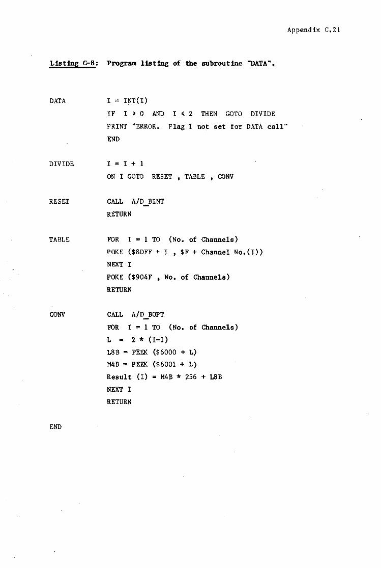
Listing C-8: Program listing of the subroutine "DATA ...

DATA I = INT(I)

DIVIDE

RESET

TABLE

CONV

END

IF I ) 0 AND I < 2 THEN GOTO DIVIDE

PRINT "ERROR. Flag I not set for DATA call"

END

I = I + 1

ON I GOTO RESET , TABLE , CX>NV

CALL A/D_BINT

RETURN

FOR I = 1 TO (No. of Channels)

POKE ($8DFF + I , $F + Channel No.(I))

NEXT I

POKE ($904F , No. of Channels)

RETURN

CALL A/D .J"OPT

FOR I = 1 TO (No. of Channels)

L = 2 * (I-1)

L8B = PEEK ($6000 + L)

M4B = PEEK ($6001 + L)

Result (I} = M4B * 256 + L8B

NEXT I

RETURN

Appendix C.21

Appendix C.22

C-9. TRANSDUCER CALIBRATION.

A listing of the applied pressure head (mm of water head) versus the

digital equivalent of the output from the transducers, (read by the

computer during the calibration of the transducers) is given. Also the

plot of the calibration curve for each transducer.

Appendix C.23

Data for the Calibration of 17 Pressure Tranaducers.

Pressure (n) Water

Deciul ~put fro. l:VD Converter. Transducer No.

1 2 3 4 5 6 1 8 9 10 11 12 13 14 15 16 17 +5 1777 2009 1583 2282 1?75 1857 2065 2007 1881 2081 2129 2103 1866 1920 1707 1843 1916 +5 1780 2010 1583 2279 1176 1857 2066 2008 1882 2083 2131 2105 1867 1921 1707 1845 1917

-105 2006 2143 1910 2454 1911 2026 2313 2219 2083 2248 2394 2368 2095 2082 2015 2159 2146 -105 2002 2141 1906 2451 1910 2024 2313 2217 2080 2247 2390 2366 2093 2080 2011 2156 2144 -200 2192 2257 2179 2592 2026 2165 2515 2399 2256 2386 2615 2589 2290 2219 2269 2426 2342 -200 2192 2258 2181 2591 2026 2166 2515 2400 2256 2387 2615 2590 2291 2220 2270 2427 2343 -300 2395 2379 2470 2?60 2144 2319 2734 2591 2439 2533 2853 2830 2496 2364 2544 2708 2565 -300 2395 2379 2472 2755 2144 2320 2734 2591 2440 2533 2855 2831 2497 2364 2547 2709 2566 -243 2288 2315 2316 2657 2086 2243 2615 2489 2342 2463 2727 2697 2387 2285 2390 2558 2439 -243 2286 2~17 2316 2666 2085·2242 2614 2488 2341 2462 2725 2696 2386 2284 2389 2548 2438 -150 2092 2206 2036 2530 1911 2097 2405 2382 2166 2325 2499 2472 2188 2155 2129 2281 2240 -150 2091 2205 2033 2524 1970 2095 2483 2301 2165 2324 2497 2471 2187 2153 2128 2280 2238 -50 1890 2080 1742 2370 1846 1945 2182 2111 1983 2172 2259 2234 1981 2008 1854 1999 2033 -so 1892 2082 1743 2370 1847 1946 2183 2112 1985 2173 2261 2235 1983 2010 1855 2000 2034 +40 1707 1974 1481 2239 1737 1813 1987 1942 1818 2036 2055 2024 1803 1878 1607 1744 1846 +40 1708 1974 1481 2240 1737 1813 1987 1942 1819 2036 2055 2024 1802 18'8 1607 1744 1846

+150 1482 1837 1158 2065 1600 1641 1743 1729 1614 1880 1794 1?62 1565 1715 1303 1431 1615 +150 1483 1837 1160 2064 1601 1641 1743 1729 1614 1880 1'797 1?63 1566 1714 1305 1432 1616 +250 1285 1710 867 1921 14?6 1487 1520 1543 1428 17l9 1550 1523 1357 1564 1033 1146 1405 •250 1282 1709 864 1924 147'5 1485 1517 1545 1426 1727 1549 1521 1355 1562 1032 1141 1403 +350 1069 1584 572 1754 1351 1332 1299 1340 1240 157J 1305 1290 1145 1415 150 859 1194 +351 1069 1584 570 1153 1351 1330 1299 1338 1240 157J 1304 1290 1145 1415 748 858 1193 +300 1170 1646 116 1835 1412 1407 1406 1434 1332 1652 1421 1401 1249 1489 885 1080 1301 +300 1171 1646 116 1838 1413 1408 1406 1435 1333 1653 1423 1401 1249 1498 886 1000 1302 +200 13?6 1170 1018 1978 1542 1561 1628 1629 1519 1806 1662 1640 1458 1637 1162 1292 1508 +200 1376 1170 1011 1918 1543 1560 1628 1628 1519 1807 1662 1639 1459 1637 1162 1292 1508 +110 1560 1882 1290 2122 1648 1699 1830 1808 1686 1935 1817 1855 1649 1171 1414 1549 1699 +110 1560 1881 1291 2125 1646 1696 1826 1805 1684 1932 1877 1851 1644 1768 1409 1550 1694

+5 1174 2014 1517 2282 1'7'8 1860 2061 2004 1880 2089 2125 2097 1863 1925 1697 1834 1914 +5 1174 2014 1515 2219 1'7'8 1859 2061 2005 1880 2088 2124 2097 1864 1925 1698 1835 1914

see CALIBRATION OF TRANSDUCER No.

~ee

!; UIB ... "' I!! 3: ..,. -1ee 0 ,, -21111

"' ., -aee x

Y = m X + c m = -0.4898 c = 875.1

-see ............. ........._. ............. _.._,_,_..........._.......__._........._...........i~......i..... ............. ..i.........~ B SB.II I 001! 151!1! 21!80 2511111 lm!B 35110 "1808

Deo1mal Output from A/D Converter.

Sllli! CALIBRATION OF TRANSDUCER No. 2

•llli!

l lllB

2111i!

L 1118 .. .. • 8 Jt y m X + c ... -lllli!

n -0,8156 a m 'D -Hie c - 1644.8 " l -311B

-•Ill! -sae i:......;......,'""-' ............................................................................ ......_ ................... ....._

• SH IBU 1sae rlltla 2588 3BU 3SBe ....

Decimal Output from A/D Converter a

sllli! CALIBRATION OF TRANSDUCER No.

•81!

I 181!

raa L 111111 .. ... .. 8 :i:

... -lllli! a

y m x + c -0.6543 m

'D -2811 c - 1s00.2 • !--..... ..... ...................................................................................................................... ~ • IU I.. 1598 r- HllB HU SSD 4m

Decimal Output from R/D Conv•rter.

81111 CALIBRATION OF TRANSDUCER No. 6

•• I 11111 - . ·-L , .. .. .. " :i:

a

... -1• 0

"D -zae • • -3111! :i:

-•Bl! -sas

58"

4111!

... -12.e a ,, -rae • ~ _,.;g :i:

• .... Decfmal

y m

c

m X + c -0.6563

1225.0

181111 15118 HU 2HB 1111111 IH8 48U

Output from A/D Conve~ter.

CALIBRATION OF TRANSDUCER No. B

y m x + c m -0.5197 c .. 1047.B

~:: t ••,I 011111 o I 1 • 11 • 111•1! • • o! 1• I

• sas 1aee 1sas ZllBB zsae 3BBB 1see •eaa Decfmal Output from A/D Converter.

Appendix C.24


I

L • .. • ::r ... 0

'D • • :i:

·-1118

·-1•

• -11!1!

-21111

-SIUI

-411111

-sa

Y m X + c m -0.3416 c - 5'15.8

8 &U 18119 151!1!1 ZAI! HU lllB9 35U 48118

Output from A/D Converter~ D•clmal

au CALIBRATION OF TRANSDUCER No. 5

I .111111

HI!

L IU • .. • ::r I

... -1811 a

'D .....

• l-_..

y m x + c m -0.8155 c . 1454.2

...... ...... ....................................................................................................................... w a 11111 1- 1111111 Im HU :111811 HA 4-

D•olma l Outpu\ from R/D Convorter.

ua CALIBRATION OF TRANSDUCER No. 7

•• I ua , .. ~ 1• .. • • Jt ... -11111 0

'D -z• • • -Ull :i: -·-

Y m X + c m -0,'1512 c = . 935.S

-111111 .............................................................................................................................. ~ e SA 111118 1581! Ha H&I! lllU ll5llll 4lllUI

Declmal Output from FVD Converter.

188 CALIBRATION OF TRANSDUCER No. 9 ...

L , .. • .. • II Jt y m x + c ... -uie

-0.5411 D m ,, -281! c ~ 1022. 1 • • -388 :i:

~:: [, 1 rt) t t t e) 1 I I 1) r I et I It I et SI! I I 1 cs 1 J s s es I

II HU! ll!Se l5ml 2Bael ZSBS 38U uae 4a.ee

Dectmal Output from A/D Converter.

sea CALIBRATION OF TRANSDUCER No. 10

I aee zu

; Ulll .. • I 3:

... ... use D ,, -11111 .. ! -He

-411B

Y m X + c m -0.6782 c - 1421.8

-see ........................................................................ ,..... ........................... '"'-' ....... ....._ II llll! llllllB !SU Hlllfl 251111 1111111 15111l ....

Decimal Output ~rem R/D Converter.

au CALIBRATION OF TRANSDUCER No. 12

41!11

i 11!1!

lml

~ 11119 .. If D 3: ... -11111 0 ,, -11• • 1-_,..

m X + c -0.4210

890.9

.5 ...................................................................................................................... ........ I IM 1- 11• - llllU 1- 111811 4-

D•o Im• 1 Output from fVD Convert••·

Oii CALIBRATION OF TRANSDUCER No. 14

! -... ~ 11111 ... • II 3: ... ... i. 0 ,, -11111 .. • -11111 :r:

-418

Y m X + c Ill -0.6840 c - 1320.2

-suu... ..................................................................................................................... ........

L .. .. .. 3:

... 0 ,, • .. :r.

• see 1aae 1aea z- n1111 aa ssaa • ..., D.,:1, .. 1 Output fram fVD Conver'l.'er.

11111CALIBRRTION OF TRANSDUCER Ne. 16

1!112

Ulll

II

•11111

-!118

-111111

-41Jl!

-sea e Ha

Dec!11al

Y .. m X + c -0.3512

c • 652.Z

18811 151Jl! Ullll! ZSBI! 381Jl! 35011 4881!

Output {rom A/D Converter.

Appendix C.25

&ea CALIBRATION OF TRANSDUCER No. 11

.. 1118 .. .. .. II 3:

... -1•• Q ,, -2ee .. • -:11111 :r:

-4H

-5N

Y m X + c m c: -0.4196 c .. 898.7

111111! lSH H!llfl nee Hell ISM 48111

D•clmal Output from R/D Convar\ar. I! &Ill!


41111!

He

... -11111 0 "II-·.. ! .... --

\

Y m X + c m -0.4801 c • !U!l0. 8

an I- lllml ·- UM ,_ 11811 -Declm•I Output from fVD Converter.

••CALIBRATION OF TRANSDUCER No. 'IS

~ 11111 .. • I 3: .,. •ID 0 ,, -4\!lllil

" • ••• :r: -481!1

Y'"mX+t:: Ill ... -0.3619 c - 621'4

•Siii! ~ .............. ~ ......................................................................... ~ ...... ~

I! Hll 1111111 1111111 2- 1111111 - 1!11111 4-Dec I ma 1 Output from R/D Converter,

su CALIERATlON OF TRANSDUCER No. 17

411B

j see

!Ill!! .. Ill!! .. .. "' 0 x ... -11111 c .., -Hll!

• ., -11111 :i:

-4841

y m c

.. m x + c

"' -0.4768 .. 919.3

-see "'-'_..,_......_...,_....._......._....._...._......,....._......_...._....._...._...._._..,,....._. .......... ~ eae 11!.110 isee Hiii! u1111 311211 nee •All

D•o!mal Output ~ram R/D Converter.

Appendix D.l

D-1. Specific Gravity. (ie. Relative Mass Density)

Introduction.

This test is done to determine the specific gravity (relative mass

density) of the granular soil used for the experiments performed in this

thesis. The method used is the same as that given in the 1975 British

standard. (BS 1377:1975, Test 6(B)). Head {17]

Method.

The test was performed using a density bottle. This was washed, rinsed

with acetone,

representative

dried with warm air and its mass found w1• A random

sample, of the original sample was obtained, by

quartering down to about 50g. The soil was then oven dried at 105-110

0 c and cooled in a desiccator. Using a funnel the soil was poured into

the density bottle until about half-full. The mass of the density

bottle with the sand was then found w2• De-aired water was carefully

added, so ·as not to trap air, to the bottle until the sand was

covered. The bottle was then put inside a vacuum desiccator and a

vacuum applied to remove any air trapped in the soil. After removal of

all the air, the bottle was topped up to the full mark, and it was

placed in a constant-temperature bath of temperature T. The bottle was

left in the bath until it had attained the correct temperature. If the

water level changed in the density bottle, this was corrected by adding

de-aired water. The bottle was then removed, wiped dry and its mass

found w3• (ie. Bottle, soil and liquid).

The bottle was then cleaned out and completely filled with de-aired

water and put back in the constant temperature bath as before. When the

bottle had attained the correct temperature, it. was removed, wiped dry

and its mass found w4• (ie. Bottle and liquid).

Appendix D.2

Calculation.

The specific gravity (ie. relative mass density) Gs of the soil was then

calculated from the. following equation.

G = s

where GT is the spec if ic gravity of the water at tempera tu re T. (See

Table. B-1)

soil, w3 = water only.

w1 = mass of density bottle, w2 = mass of bottle plus dry

mass of bottle, soil plus· water, w4 = mass of bottle plus

The average of the repeated test ls reported as the specific gravity.

Results.

The specific gravity: Gs = 2,64 was obtained from the average of

repeated tests. (See laboratory sheet following showing the specific

gravity calculated for each test.)

Appendix D.3

SPECIFIC GRAVITY TEST u.c.1. lllltL 10C09llcs ~-

SOIL SAMPLE. TEST No. SGTA01

ORTE. 8185 TESTED By. G WARDLE

LOCATION. CAPE FLATS BORING No. SAMPLE DEPTH. SAMPLE No. GW/MSC/01

SAMPLE No. ~Ref.

DETERMINATION No. 1 2 3 4 Pycnometer No. GW1 GW2 GW3 GW4 Pycnometer mass g .1 37,620 32,482 33. 197 39.009 Pycnometer l soil. g •2 78.600 70.267 78.543 86.661 Pycnometer,soill water Q Ill 112.952 105.865 111.301 118.539 Temperature 'c .1 23 23 23 23

Pycnometer l water g •4 87.441 82.371 83.060 88.872 SPECIFIC GRAVITY Of WATER • 0,9976 0,9976 0,9976 0,9976 Gt

SPECIFIC GRAVITY or SOIL Ca 2.64 2.64 2.65 2.64

* Fro• T1~l• of S,•clftc Gravity of ••t•r for te11perature l.

RDUR<S:

.

;.•.-•lo. G Ct.lw2 - •II Ca • 2,64 "··· ,.... ... • • (w4 - wll-(w3 - wZl ll.C.l. 1-"9

Appendix D.4

D-2. Particle Size Analysis.

Introduction.

The object of a particle size analysis is to group the discrete

particles of a soil into separate ranges of sizes and so as determine

the relative proportions, by dry mass, of each size range.

A sieve analysis was performed to seperate the soil into different size

ranges. The soil did not have many fine particles (< 0,2 mm) so a

sedimentation procedure was not required. The method used is the same

as that given in 1975 British Standard. (BS 1377: 1975, Test 7(B))

Head[l7].

Method.

The test was performed using a simple dry sieving procedure. This was

possible as the soil was a clean granular material. A random

representative sample of the origtnal sample was obtained, by

quartering, to about ) 100 g. (Based on BS 1377; 1975). This was oven

dried at 105-110 °c, cooled in a desiccator and its mass found w1 • A

set of sieves (manufactured to BS 410) was selected, with the size range

from 2 mm down to 63 micron. After the set of sieves had been cleaned,

each sieve's mass was found and then reassembled with the largest

aperture sieve at the top.

The dried soil sample was placed in the topmost sieve (2 mm sieve size)

and shaken long enough for all particles smaller than each aperture to

pass through. A mechanical shaker was used to shake the set of sieves

for a period of 15 minutes. (Greater then 10 minutes as specified by the

Britsh Standard.}

After shaking, the set of sieves were carefully dismantled. The mass of

the sieves, with retained soil, was found. The mass measured was

recorded against the sieve aperture size. The mass of soil passing the

Appendix D.5

smallest sieve was also measured and recorded.

Calculations.

In order to draw a particle size distrbution curve and tabulate the

data, it was necessary to calculate the cumulative percentage (by mass)

of particles finer then each sieve aperture size. The cumulative mass

passing each sieve was calculated first, from which the percentage

passing was derived.

If the total initial mass is w1 • The mass retained in the first sieve

Wsl. Then the mass passing the first sieve = w1 - Wsl. The percentage

passing the first sieve is given by:

= (W -1 100

The mass passing the second sieve = w1 - W81 passing the second sieve is given by:

= w -1 100

Ws2 • The percentage

and so-on. The percentage passing any subsequent sieve can be written

as:

E W p = 100

where E W denotes the sum of the masses retained on all the sieves down

to and including the one in question. ( E W = wsl + ws2 + •.• etc). A

check is that the mass passing the last sieve should, or very nearly

equal, the mass collected in the pan at the bottom.

Appendix D.6

Results.

The results following are for the set of repeated sieve analysis tests

performed. An average of the results is taken to give a grading curve

as plotted.

The effective size (D10 ), the largest size of the smallest 10 % is read

off the graph as: 0,72

The uniformity coefficient (U), the ratio of the 60 % particle size

(o60 ) to the 10 % particle size (o10) is: 1,3

Appendix D.7

SIEVE ANALYSIS LC. T. ll1L ~CS l.-r9IT

SOIL SAMPLE. TEST No. PSDA01

DATE. 1/8/85 TESTED By. G WARDLE

LOCATION. CA£E ELAIS BORING No. SAMPLE DEPTH. SOIL SAMPLE WEIGHT SAMPLE No. GW/MSC/01 Container No. GW1 SPECIFIC GRAVITY Gs. 2,64 Dry sol 1 ... container. 9·1721.4

Container. g 570,4

Dry soil. 111 l g 1151,0

.

SI£Yr Na. SI£YE WT. SIEY£ WT. SIEVE l SOIL Cl.ltULAlIY£ >; PRSSIN<; OP£NIN<; <-> <1> SOIL ,,, R£TRINED l9) !tRSS PRSSIN(;

2 472.5 473.3 0.8 1150. 2 99 g 1 436,5 645' 1 208,6 941,6 81 .8

0.850 534.3 951.7 417.4 524.2 45.5 0_710 434.0 903_4 469 4 54 .8 4 R

0.600 502. 1 536. 1 34.0 20.8 1.8 0.425 385.5 402.4 16.9 3 9 0_3

·. 0,300 466,0 468,4 2.4 1 • 5 0. 1 0,125 340, 1 341,2 1 ' 1 0,4 0

0.075 354.8 1i;4 8 0 0 0 4 0 PAN 335,6 335,6 0,0 0,4 0

RDtRRKS:

a.a.-1 •.

PX - • 1 - I• x lBB .... -.. •1 a.c.T.-

Appendix D.8

SIEVE ANALYSIS -.C. t • llJI. ICDlllJCI ~

SOIL SAMPLE. TEST No. PSDA02 DATE. 1 IP.IP.r:.. TESTED By. G WARDLE

LOCATION. CAPE FLATS BORING No. SAMPLE DEPTH. SOIL SAMPLE HEIGHT SAMPLE No. GW[MSC[01 Container No. GW1 SPECIFIC GRAVITY Gs. 2,64 Dry soil l container. 9 202'L q

Cont a Iner. g 930' 7 Dry so f 1. .., 1 91093,2

SI£Vt Na. SI£V£ Ml. SIE\1£ Ml. Sl£V£ l SOIL aJl.l.ATlvt l PASSING OPENING <-> l1> SOIL <1> R£TRIN£D <1> ttRSS PASSING

2 4 72 .5 473.7 1 • 2 1092 .o 99.9 1 436,5 657,3 220,B 871 ,2 79,7 0,850 534,7 911,0 376,3 494,9 45.3 0,710 434,0 858,2 424,2 10,1 6,5 0,600 501,9 546,4 44,5 26,2 2,4 0,425 385,4 409,3 23,9 2,3 0,2 0,300 465,9 467,8 1,9 0,4 0

0' 125 340, 1 340,3 0,2 0,2 0 0,075 354,8 354,8 o,o 0,2 0 PAN 335,6 335,6 0,0 0,2 0

RDIRCS:

····-··· Pt • •1 :1I. x 188 .... -..

•.1:.T.-

Appendix D. 9

SIEVE ANALYSIS LC. T. In!. IU'lllllCI .__......,

SOIL SAMPLE. TEST No. PSDA03 DATE. 2/8/85 TESTED By. G WARDLE

LOCATION. CAPE FLAIS BORING No. SAMPLE DEPTH. SOIL SAMPLE WEIGHT SAMPLE No. GW/MSC/01 Container No. GW1 SPECIFIC GRAVITY Gs. 2,64 Dry ao 11 l container. g 1928. 1

Container. g 820.3 Dry so 11. ..1 g 1107 ,8

SI£:VC MD. SIEYt WT. SIEVE WT. SIM l SOIL CUl'ILATIYC ll PASSINC OPENING (-) <1> SOIL t1> RETRINtD (9) ttRSS PASSINC

2 472.5 4 73 .5 1.0 1106.8 gq q

1 436,2 640,9 204,7 902. 1 81.4 0,850 534,6 922.1 387.5 ' 514.6 . 46.5

0.710 434.0 864 3 430 3 AL. 3 7 h

0,600 502,0. 549. 1 47,1 37.2 3.4 0,425 385,4 415.0 29.6 7.6 0.7 0,300 465,9 469,2 3.3 4.3 0.4 0, 125 340,0 340,7 o. 7 3.6 0.3 0,075 354,8 354.8 o.o 3.6 0.3 PAN 335.6 335.6 0.0 3.6 0.1

RDM<S: I

--··-·"·· PX• •l :1t• x 188 ..... -..

l.t.T. --

Appendix D.10

SIEVE ANALYSIS LC.,. lm1. llmlllftCll ~

SOIL SAMPLE. TEST No. PSDA04 DATE. 2/8/85 TESTED By. G WARDLE

LOCATION. CAPE FLATS BORING No. SAMPLE DEPTH. SOIL SAMPLE WEIGHT SAMPLE No. GW/MSC/01 Cont a f ner No. GW1 SPECIFIC GRAVITY Gs. __ 2_,_6j Dry 10 f I L container. g 1887 .8

Container. g 717,6

Dry so I 1 . ..1 g 1170_2

Sitvt No. Sitvt NT. SIEVE NT. SIEVE I. SOIL CtlU..RTlYE l PASSING llPENING I•> ,,, SOIL <1> RETAINED 11> ttRSS PASSING

2 472.5 473.9 1.4 1168 .8 99_9 1 436.3 670.0 233.7 935 .1 79.9 0,850 534,6 919,0 384,4 550,7 47 .1 0.710 433.9 884,6 450,7 100,0 8.5 0,600 502,0 553,7 51,7 48,3 4 '1 0,425 385,4 420,0 34,6 13, 1 1 .2 0,300 465,9 472,0 6. 1 7,6 0.6 0, 125 340,0 346.9 6.9 0.7 o_ 1

0,075 354,8 355,1 0,3 0,4 0 PAN 335,6 335,8 0,2 0,2 0

RDIR<S:

.... -1 •.

PX - • 1 - I• w 118 .... -t• •1 a.c.1 • .---

PARTICLE SIZE DISTRIBUTION.

SUMMARY OF RESULTS.

CLAY

fin• ,._dlu• Coars• f In•

SILT

Appendix D.11

w.c.t. mi. llEORC:I" ~.,

TEST No.PSD/A01/A02/A03/A04 DATE. 8/85

TESTED By. _ ___;:G;.....;..;;WARD==L=E---1

SANO GRAVEL

100

91 1----1..._~...µ..++1+-~-+--4-+-4--++M-1-~-+--+-+-+-+-H+;....---t___,l-+-+-l+f-H-~/-+--t-+-+-t-++H I

81

~ 791----11--1--1-1-11-++~~4--+-+-+-+++.i+~-+--+-+-++M-+-~---f..._t-+-Hi-++411-~+--+-+-t-++++i • I '' i----1~1-++++H.._~~~-t-14+1+-~.._~H-H-++1-~+-+-1-++++-1+-~-+--+-+-t-t+tt1 >-.. ~ s1..._---1--+-1-+-1++t+-~+--+-+-+-+++t+~-+-+-+++++++---11--t-t-t-t-H1+-~-t--t--t-1H"'l-m ·C

46 -... ~ 411----11--1--f-Hi-++W-~4--+-+-+-+++++~-+--+-+-++H+l----tr--t-t-Hi-++ ........ ~-+--+-+-t-t-t"l"tt c • 1111

~ Jll----11--1--f-l-ii-++M-~+--+-+-+-+++++~-+-+-+++H+t----tr--t-+-t-lt-++++-~-+--+-+-t-t-t"l"tt :.

REMARKS: SUMMA.RY OF RESULTS FROM PARTICLE SIZE TESTS.

Sieve aperture size (tmn)

2 1 0,850 0, 710 0,600 0,425 0,300

Percent passing (By mass)

100 81 46

7 3

0,6 0,3 .... -1 ...

111.•.-u 11.c.i.1-..

Appendix E.1

E-1. Saturated hydraulic conductivity tests.

Listings of the res.ults for the Constant-head tests performed are given

in this appendix. The tests performed were:

CHPAOl

CHPA02

CHPA03

CHPA04

CHPAOS

CHPA06

CHPA07

CHPAOB

CHPA09

Also given is the plot for each test of the hydraulic gradient versus

the Darcian velocity, to determine the hydraulic conductivity for the

test.

CONS

TANT

HKA

D PE

RMEA

BILI

TY T

EST

SOIL

SAH

PLE

LOCA

TION

SAHP

LE N

O

: CO

ARSE

SAN

D

: Ca

pe F

lats

:

Gld/H

SC!O

l

SOIL

SPE

C.

SPEC

IFIC

GRA

UITY

: 2.

64

LIT D

RY S

OIL

2658

.2

q SA

MPLE

LEN

GTH

34.3

C1

I

VOID

RAT

IO

e •

.452

No.

Qoa

ntity

Q

Tim

e t

Tem

p.T

cu c

m se

c de

g C

1 88

0 27

0 15

.5

2 72

0 29

0 15

.5

3 92

5 24

6 15

.5

4 82

5 15

1 15

.5

5 91

3 13

8 15

.5

6 96

5 11

5 15

.5

TEST

NO

: CH

PAOl

DA

TE

: 01

1081

85

TEST

ED B

Y:

G.ld

ardl

e

PERH

EAHE

TER.

DIAH

ETER

:

7.37

C

1I

AREA

..

42.6

1 sq

c•

11

12.7

5 C

1I

12

12.7

0 C

9

Piez

omet

ers

(cal

Fl

ow R

ate Q

lt hl

h2

h3

C

U

Cl!

llH

C

46.6

42

.5

38.3

3.

26

43.2

40

.3

37.0

2.

48

48.5

43

.9

39.1

3.

76

56.0

49

.4

42.3

5.

46

61.5

53

.6

44.9

6.

62

69.9

59

.8

49.0

8.

39

" : H

yd

rau

lic

Gra

die

nt

v's

D

arc

lan

V

elo

cft

y

i .4

" ... 3

5

a: ' 0 I .3

>

u "' D .2

5

.,,

.2

ISi

N .. ..

• 1

5

>. .. " .I

o T

e!!

t N

o.

: C

HP

A0

1

~

Vo

ld

Rati

o

e ~

0.4

52

,5 .0

5

k2

8

-0

.26

9

cm

/sec

" I. 1

yl1

11

11

y1

1la

m••

"''"

IH""

'"'"

H'.

!uu

11

uJ1

1U

11

Urh

11

11

11

uh

um

ml

~

,2

.4

.6

.B

I H

yd

rau

lic

Gra

die

nt

I -

h/J

C

Dlm

en

slo

nle

s!!l

Dar

cian

Vel

ocity

Q/A

t H

ydra

ulic

Gra

dien

t h/

l at

T

at 2

0 de

g C

i1

i2

i3

ia

vera

ge

.076

.0

86

.322

.3

31

.326

.3

26

.058

.0

65

.227

.2

60

.244

.2

44

.000

.0

99

.361

.3

78

.369

.3

69

.128

.1

44

.518

.5

59

.538

.5

38

.155

.1

74

.620

.6

85

.652

.6

52

.197

.2

21

.196

.8

50

.823

.8

23

>

"Cl

"Cl

fl> ::s 0. .....

>< l:'1 . N

CONS

TANT

HEA

D PE

RHEA

BILI

TY T

EST

SOIL

SAM

PLE

LOCA

TION

SAMP

LE H

O

: CO

ARSE

SAN

D

: Ca

pe F

lats

:

GtdlH

SC/01

SOIL

SPE

C.

SPEC

IFIC

GRA

UITY

: 2.

64

LIT D

RY S

OIL

2658

.2

g SA

MPLE

LEN

GTH

37.9

C

1I

VOID

RAT

IO

e =

.6

04

No.

Qua

ntity

Q

Thie

t T

np T

ca

c•

sec

deg

C

1 93

5 20

5 15

.5

2 60

0 16

6 15

.5

3 76

0 12

2 15

.5

4 95

9 95

15

.5

5 97

2 90

15

.5

6 90

5 68

15

.5

TEST

HO

: CH

PA02

DA

T!

: 01

1081

85

TEST

ED B

Y: G

.War

dle

PERH

EAHE

TER.

DIAH

ETER

:

7.37

C

1I

AREA

•

42.6

1 sq

C1I

11

12.7

5 C

1I

12

12.7

0 c•

Piez

o'llle

ters

Cea

) Fl

oe1

Rate

Qlt

hl

h2

h3

cu C

1Vse

c

47.1

44

.3

41.5

4.

56·

44.2

42

.0

39.7

3.

61

52.2

48

.2

44.5

6.

23

65.3

59

.1

53.1

10

.09

67.9

61

.3

54.8

10

.80

77.1

69

.0

61.1

13

.31

u : H

yd

rau

lic

Gra

die

nt

v's

D

arc

lan

V

elo

cit

y

~ ·"

u ... 3

5

a: d I ,3

>

u m • ...

. • 2

IS

i N

~.IS

5 u .. • Cl

Test

No

. C

HP

A02

V

old

R

ati

o

e m

0

.60

4

k2

8

• 0

.56

2

cm

/sec

Hy

dra

uli

c

Gra

die

nt

I •

h/l

C

Dlm

en

slan

less

)

Dar

cian

Uel

ocity

Q!A

t H

ydra

alic

Gra

dien

t hl

l at

T

at 2

0 de

g C

il

i2

i3

ia

vera

ge

.107

.1

20

.220

.2

20

.220

.2

20

.085

.0

95

.173

.1

77

.175

.1

75

.146

'16

4 .3

10

.299

.3

05

.305

.2

37

.265

.4

90

.472

.4

81

.481

.2

53

.284

.5

18

.512

.5

15

.515

.3

12

.350

.6

35

.622

.6

29

.629

>

"O

"O

fD

::l

Q. .....

><

t:rj

. w

CONS

TANT

KEA

D PE

RMEA

BILI

TY T

EST

SOIL

~PLE

LOCA

TION

SAMP

LE N

O

: CO

ARSE

SAN

D

: Ca

pe F

lab

: GW

/HSC

!Ol

SOIL

SPR

C.

SPEC

IFIC

GRA

VITY

: 2.

64

LIT D

RY S

OIL

2658

.2

g SA

MPLE

LEN

GTH

36.6

c•

OO

ID R

ATIO

e

• .5

49

No.

Qua

ntity

Q

Ti•

t

Tnp

T

CU

C

lll

sec

deq

C

1 86

5 26

9 16

.0

2 97

2 15

1 16

.0

3 98

3 15

9 16

.0

4 90

0 11

9 16

.0

5 96

0 94

16

.0

6 87

6 75

16

.0

TEST

NO

: CH

PA03

DA

TE

: 01

1081

85

TEST

ED B

Y: G

.War

dle

PEIH

EAHE

TER.

DI

AHET

ER :

7.

37

t• AR

EA

• 42

.61

sq C

11

11

• 12

.75

C1ll

12

12.7

0 C

ll

Piez

o111

etera

Ccm)

Fl

ow R

ate Q

lt hl

h2

h3

cu

t11

/sec

45.2

42

.8

40.3

3.

22

54.8

50

.1

45.6

6.

44

52.4

48

.1

44.1

5.

55

59.7

53

.8

48.2

7.

56

69.5

61

.6

54.3

10

.21

75.9

66

.6

58.1

11

.68

~ u :

Hy

dra

uli

c

Gra

die

nt

v's

D

arc

lan

V

elo

cit

y

~

.4

u ... 3

5

a: ' 0 I

.3

>

u Ill

D

.25

....

• 2

ISi

N ... ..

• 1

5

u •

1 0 ~ c

.as

,. u .. • Cl .2

.4

Te3

t N

o.

: C

HP

A03

V

otd

R

ati

o

e -

0.5

49

k

28

-

0.

43

3

cm

/3ec

.G

.e

Hy

dra

uli

c

Gra

die

nt

I -

h/1

C

Dlm

en

slo

nle

aa)

Dar

cian

Uel

ocity

QIA

t H

ydra

ulic

Gra

dien

t h/

l at

T

at 2

0 de

g C

i1

i2

i3

ia

vera

ge

.075

.0

83

.188

.1

97

.193

.1

93

.151

.1

67

.373

.3

54

.363

.3

63

.130

.1

44

.337

.3

11

.324

.3

24

.177

.1

96

.463

.4

41

.452

.4

52

.240

.2

65

.620

.5

75

.597

.5

97

.274

.3

03

.729

.6

69

.699

.6

99

>

'O

'O

(1)

;:I

0. .....

x t'1 . ~

CONS

TANT

HEA

D PE

RHEA

BILI

TY T

EST

SOIL

SAH

PLE

LOCA

TION

SAHP

LE N

O

: CO

ARSE

SAN

D

: Ca

pe F

lata

:

Qld1

HSC1

01

SOIL

SPE

C.

SPEC

IFIC

GRA

OITY

: 2.

64

LIT D

RY S

OIL

2516

.3

q SA

MPLE

LEN

GTH

33.4

C

ll

VOID

RAT

IO

e •

.493

No.

Qua

ntity

Q

Time

t

Teinp

T

cu c

m se

c de

g c

1 87

1 16

5 15

.0

2 66

0 14

6 15

.0

3 73

6 22

3 15

.0

4 97

0 10

5 15

.0

TEST

HO

: CH

PA04

DA

TE

: 01

1081

85

TEST

ED B

V: G

.ldar

dle

PERH

EIM

TER.

DI

AHIT

ER :

7.

37

C•

AR£A

•

42.6

1 sq

C1I

11

12.7

5 C

ll

12

12.7

0 C1

R

Piez

owie

tera

<cm

) Fl

ow R

ate

Qlt

hl

h2

h3

cu c

.,.ae

c

55.9

49

.4

43.2

5.

28

52.6

47

.0

41.7

4.

52

47.5

43

.4

39.6

3.

30

73.7

62

.3

51.7

9.

24

u =

Hy

dra

uli

c

Gra

die

nt

v's

D

arc

lan

V

elo

cit

y

~

.4

u ... 3

5

a: ' 0 I

,3

>

u DI • .c

s

.... .c

IS

i N

~.IS

" ... u .I

0 .. > 5

.as

Test

No

. :

CH

PA

04

Vo

ld

Rati

o

e -

0.4

93

k

ze

• 0

.28

6

cm

/sec

u .. • Cl a.llwwaWi~l!,nuwoluwJ~...W.lllllWl~tduwJm~uwlwwwl

• 4

.6

.B

1 H

yd

rau

lic

Gra

die

nt

I -

n/l

C

Dfm

en

sfo

nle

asl

Dar

cian

Uel

ocity

Q!A

t H

ydra

ulic

Gra

dien

t h!

l at

T

at 2

0 de

g C

il

i2

i3

ia

uera

ge

.124

.1

41

.510

.4

88

.499

.4

99

.106

.1

20

.439

.4

17

.428

.4

28

.07}

.0

88

.318

.2

99

.308

.3

08

.217

.2

46

.898

.8

31

.864

.8

64

>

'O

'O

ro :::s

a.

.....

x M . \J1

CONS

TANT

HEA

D PE

RHEA

BILIT

V TE

ST

SOIL

SAH

PLE

: CO

ARSE

SAN

D

LOCA

TION

SAHP

LE N

O :

Cap

e F

lab

:

GtdlH

SC/01

SOIL

SPE

C.

SPEC

IFIC

GRA

VITY

: Ill

' DR

Y SO

IL

SAHP

LE L

ENGT

H UO

ID R

ATIO

e

•

No.

Qua

ntity

9

CU C

ll

1 64

6 2

625

3 m

4

961

5 85

1

2.64

25

16.3

g

35.4

C

1I

.583

TiM

t

Tnp

T

sec

deg

C

330

15.0

20

0 15

.0

101

15.0

10

5 15

.0

86

15.0

TEST

NO

: CK

PA05

DA

TE

: 01

1081

85

TEST

ED B

Y: G

.War

dle

PEIH

EAHE

TER.

DI

AMET

ER :

?

. 3?

e11

AREA

•

42 .6

1 aq

ct1

11

12.?

5 Cf

ll

12

12.?

0 c•

Piez

omet

era

Ccm)

Fl

ow R

ate

Q/t

hl

h2

h3

CU

Clll&

ec

43.1

41

.8

40.5

1.

96

45.4

43

.2

41.2

3.

13

60.2

54

.9

49.9

?.

64

65.?

59

.5

53.5

9.

15

68.0

61

.2

54.8

9.

90

a : H

yd

rau

lic

Gra

die

nt

v's

D

arc

lan

V

elo

cit

y

~

.4

u

.2

• 4

Test

No

. C

HP

A05

V

old

R

ati

o

e -

0.5

83

k

z.e

-0

.50

6

cm

/aec

.6

.B

Hy

dr•

ull

c

Gra

die

nt

I -

h/1

C

Dlm

en

slo

nle

asl

Dar

cian

Uel

ocity

QIA

t H

ydra

ulic

Gra

dien

t h/

l at

T

at 2

0 de

g C

il

i2

i3

ia

vera

ge

.046

.0

52

.098

.1

02

.100

.1

00

.0?3

.0

83

.169

.1

61

.165

.1

65

.1?9

.2

04

.416

.3

94

.405

.4

05

.215

.2

44

.486

.4

n

.4?9

.4

?9

.232

.2

63

.533

.5

04

.519

.5

19

~

~

'Q

CD ::s 0. .....

>< t%j . "'

CONS

TANT

HEA

D PE

RHEA

BILIT

Y TE

ST

SOIL

sru1

PLE

LOCA

TION

SAM

PLE

HO

: CO

ARSE

SAN

D

: Ca

pe F

lats

:

GWIH

SC!O

l

SOIL

SPE

C. SP

ECIF

IC G

RAVI

TY:

2.64

LIT

DRY

SOI

L 25

16.3

q

SAHP

LE L

ENGT

H 37

.2

ca

IJOID

RAT

IO

e •

.663

Ho.

Qua

ntity

Q

Ti111

t t

Teap

T

CU

Cl

ll se

c de

g C

1 73

5 37

0 15

.0

2 76

1 14

3 15

.0

3 76

9 90

15

.0

4 83

5 89

15

.0

5 84

6 11

0 15

.0

6 96

5 70

15

.0

7 94

0 18

4 15

.0

TEST

HO

: CK

PA06

DA

TE

: 01

1081

85

TEST

ED B

Y: G

.Lla

rdle

PERH

EAH!

TER.

DIAH

ETER

:

7.37

AR

M

• 42

.61

11

12.7

5 12

12

.70

Cll sq C

ll C

ll c•

Piez

011e

tera

Ce1

1)

Flo1

1 Ra

te O

tt hl

h2

h3

cu

Clll

sec

'42.

5 41

.6

40.5

1.

99

50.1

47

.6

45.0

5.

32

59.7

55

.6

51.7

8.

54

62.2

57

.8

53.5

9.

38

57.1

53

.S

49.7

7.

69

75.0

68

.7

62.2

13

.79

47.6

45

.4

42.7

5.

11

..... u :

Hy

dra

uli

c

Gra

die

nt

v's

D

arc

lan

V

elo

cit

y

~

.4

u ... 3

5

~ a I .3

>

u Ill .. .,,

.2

151

N u L • Cl

.4

Test

No

. :

CH

PA

06

Vo

ld

Rati

o

e -

0.6

63

k

28

m

0

.74

0

cm

/sec

.6

Hy

dra

uli

c

Gra

die

nt

I -

h/1

C

D!m

en

slo

nle

s•)

Dar

cian

Uel

ocity

QIA

t H

ydra

ulic

Gra

dien

t hl

l at

T

at 2

0 de

g C

il

i2

i3

ia

vera

ge

.047

.0

53

.067

.0

91

.079

.0

79

.125

.1

42

.200

.2

01

.200

.2

00

.201

.2

28

.322

.3

07

.314

.3

14

.220

.2

50

.349

.3

35

.342

.3

42

.180

.2

05

.282

.2

95

.289

.2

89

.324

.3

67

.498

.5

12

.505

.5

05

.120

.1

36

.176

.2

09

.193

.1

93

>

'O

'O

Cb

:::I

p,.

......

x tx1 . -.

.J

CONS

TANT

HEA

D PE

RMEA

BILI

TY T

EST

SOIL

SAH

PLE

: CO

ARSK

S~

LOCA

TION

SAMP

LE H

O :

Cape

Fla

ts

: SY

/HSC

tOl

SOIL

SPE

C.

SPEC

IFIC

GRA

OITV

: lil

T DR

Y SO

IL

SAHP

LE L

ENGT

H OO

ID R

ATIO

e

•

2.64

27

08.3

g

36.5

C1

1

.516

No.

Qua

ntity

Q

Ti111e

t

Temp

T

cu C

1ll

sec

deg

c

1 64

2 42

5 14

.5

2 60

3 24

0 14

.5

3 83

5 11

6 14

.5

4 73

5 76

14

.5

5 79

0 11

6 14

.5

TEST

NO

: CK

M07

DA

TE

: 02

1081

85

TEST

ED B

Y:

G.fr

lardl

e

PERH

EAHE

TER.

DI~R :

7.37

C1

1

AREA

•

42 .6

1 sq

1:11

11

12.7

5 C1

1

12

12 .7

0 C1

11

Piez

011e

teu

(Cit

) Fl

o11

Rate

Oft

h1

h2

h3

cu c

18/se

c

43.4

42

.1

40.5

1.

51

47.1

44

.7

42.1

2.

51

62.7

55

.6

48.6

7.

20

73.3

64

.1

54.7

9.

67

61.1

54

.6

48.0

6.

81

~ u :

Hy

dra

uli

c

Gra

die

nt

v's

D

arc

lan

V

elo

cit

y

} ·"

u ~

., .J

S

a: d I

,3

> .2

S

u DI

D

.... 2

Il

l N

.. •• IS

u •

1 a ~ c .e

s • u .. • Cl

Te

st

Na

. :

CH

PA

07

V

aid

R

ati

o

e -

0.S

16

k

28

-

0.

3S

8

c1

t1/s

ec

1ln

11

11

11

1ly

rtt•

mlu

hm

uh

mam

lm••

•11

lmm

ml1

11

M'•

hl

.2

• "

.G

.e

1 H

yd

rau

lic

Gra

die

nt

t -

n/l

C

Dlm

•n»

lan

lea»

)

Dar

cian

Uel

ocity

O!A

t. H

ydra

ulic

Gra

dien

t h!

l at

T

at 2

0 de

g C

i1

i2

i3

ia

uera

ge

.035

.0

41

.106

.1

22

.114

.1

14

.059

.0

68

.192

.2

05

.198

.1

98

.169

.1

94

.561

.547

.5

54

.554

.2

27

.261

.7

22

.740

.7

31

.731

.1

60

.184

.5

10

.520

.5

15

.515

>

't:

I 't:

I R

I ~

0. .....

>< 1:-'l . ex>

CONS

TANT

HEA

D PE

RHEA

BILIT

Y TE

ST

SOIL

SAH

PLE

: CO

ARSE

SAN

D

L~TI~

SAMP

LE t«

> :

Cape

Fla

ts

: ti!

IHSC

!Ol

SOIL

SPE

C. SP

ECIF

IC G

RAVI

TY:

.n'

DRV

SOIL

SA

MPLE

LEH

GTK

VOID

RAT

IO

e •

No.

Qua

ntity

Q

cu c

•

1 66

2 2

710

3 76

5 4

950

2.64

27

08.3

g

38.4

C1

I

.595

Ti•

t

Tnp

T

sec

deg

C

184

14.S

12

2 14

.5

83

14.5

69

14

.5

TEST

NO

: CK

PA08

DA

TE

: 02

1081

85

TEST

ED B

Y: G

.Yar

dle

PERH

EAHI

TER.

DIAH

ETER

:

7. 37

C1

1

AREA

•

42 .6

1 sq

e11

11

12 .'

5 C

1I

12

12.7

0 e1

1

Piez

o111

eten

(C11

) Fl

ow R

ate

Olt

hl

h2

h3

co c

11/se

c

47.6

45

.5

43.1

3.

60

54.8

51

.1

47.6

5.

82

66.1

60

.4

55.0

9.

22

83.9

75

.4

67.0

13

.77

- u : H

yd

rau

lic

Gra

die

nt

v's

D

arc

lan

V

elo

cit

y

~

.4

u ... 3

5

~ I .3

>

u .. • .2

5

,,

• 2

Ill

N .. ".I

S

~ .

I

~ c .0

5

.. u .. .. Cl

• 4

Test

No

. :

CH

PA08

V

old

R

ati

o

e -

0.5

95

k

28

-

0.5

63

cm

/sec

.6

.e

Hy

dra

uli

c

Gra

die

nt

I -

h/1

C

D!m

en

slo

n1

ess

l

Dar

cian

IJe

loci

ty Q

/At

lf\ld

raal

ic G

radi

ent

h!l

at T

at

20

deg

C

i1

i2

i3

iave

rage

.884

.0

97

.161

.1

89

.175

. l

'JS

.137

.1

57

.290

.2

76

.283

.2

83

.216

.2

49

.447

.4

25

.436

.4

36

.323

.3

72

.667

.6

61

.664

.6

64

CONS

TANT

HEA

D PE

RMEA

BILIT

Y TE

ST

SOIL

SAH

PLE

LOCM

'ION

SAHP

LE H

O

: CO

ARSE

SAN

D

: C

ape

Fla

b

: C!

d/HSC

!Ol

SOIL

SPE

C.

SPEC

IFIC

GRA

UITY

: 2.

64

ldT D

RY S

OIL

2708

.3

g SA

MPLE

LEN

GTH

37.8

c•

UO

ID R

ATIO

e

• .5

70

No.

Qua

ntity

Q

Ti•

t

Tnp

T

CU

Cl

ll se

c de

g C

1 61

3 22

0 14

.5

2 71

0 16

7 14

.5

3 90

0 10

9 14

.5

4 97

1 84

14

.5

5 76

0 12

7 14

.5

TEST

NO

: CH

PA09

DA

TE

: 02

1081

85

TEST

ED B

Y: G.

War

dle

PERH

EAHE

TER.

DIAM

ETER

:

7.31

AR

EA

• 42

.61

11

12.7

5 12

12

.70

C1I

sq C

1ll

Clll

c•

Pie10

1111

1ters

Ce11

> Fl

Oll

Rate

Olt

hl

h2

h3

cu c

a/se

c

46.0

44

.1

41.9

2.

79

50.7

47

.6

44.6

4.

25

64.5

58

.7

53.1

8.

26

76.9

68

.7

61.1

11

.56

56.4

52

.3

48.1

5.

98

u : H

yd

rau

lic

Gra

die

nt

v's

D

arc

lan

V

elo

cit

y

~

... u ... 3

5

a: d >

u "' • ,, .2

IS

i N

u •

I D

" > c .e

s •

Test

No

. :

CH

PA99

V

old

R

ati

o

e •

e.5

79

k

ze

-e.5

15

cm

/sec

u L • Cl ~~dwm~.2:!.

"""'.i.w...~. 4~.iuw.w. 6!

!"111'.i......~.e~dwww

Hyd~aullc G~adlent

I •

h/l

C

Dfm

en

aC

on

1ea

s)

Dar

cian

Uel

ocity

Q!A

t H

ydra

ulic

Gra

dien

t h!

l at

T

at 2

0 de

g C

it

i2

i3

ia

wra

ge

.065

.0

75

.149

.1

73

.161

.16

1 .1

00

.115

.2

43

.236

.2

40

.240

.1

94

.223

.4

55

.441

.4

48

.448

.2

71

.312

.6

43

.598

.6

21

.621

.1

40

.161

.3

22

.331

.326

.3

26

>

"O

"O

(!) ::s c. .....

;><

t%J . ,.....

0

Append ix E .11

E-2. Unsaturated hydraulic conductivity tests.

Listings of the r_esults for the tests performed to determine the

unsaturated hydraulic conductivity, are given in this appendix. The

tests performed were:

USPAOl

USPA02

Also given is the plot of the results for each test, showing the

relative permeability versus the degree of saturation.

UNSA

TURR

TED

HYDR

AULIC

CON

DUCT

IOITV

TES

T.

SOIL

SAM

PLE

LOCA

TION

SR

HPLE

Ho

: CO

ARSE

SAN

D

: Ca

pe F

lats

:

GUIH

SCtO

l

~IL S

PHC.

SPEC

IFIC

G~ITV:

.iT D

RY S

OIL

Lis

: 2.

64

2102

.8

!J 83

.7

C1I

.598

SA

HPLE

LEN

GTH

OOID

RAT

IO

e •

Sat.

Per11

. kC

sat)

.556

Clll

aec

(Fro

• co

nsta

nt h

ead

test

)

Ho.

Qua

ntity

Q T

i11e

t T

np T

Weig

ht I

ll cu

C1I

se

c de

g C

g

lw

318

957

15.5

29

82.9

2d

35

9 11

32

15.5

29

78.0

3w

37

9 79

2 15

.5

3000

.0

4d

158

646

15.5

29

66.2

5w

30

2 .

531

15.5

30

07.0

6w

40

0 58

7 15

.5

3017

.6

7w

525

546

15.5

30

40.2

Bw

49

1 31

8 15

.5

3074

.2

TEST

t«>

: OS

PAOl

DA

TE

: 06

1081

85

TEST

ED B

Y: G

.War

dle

APPA

RATU

S. DI

AHET

ER :

4.

40

C1i

ARIA

•

15.2

1 sq

Cit

WEI

GHT

Ya:

631.

1 g

11

15.0

0 C

it

12

I 15

, 05

Cit

13

15. 0

0 C1

I

14

15.0

0 C

it

Tena

i0111

etera

Cew1

) hl

h2

h3

h4

hS

-9.6

-9

.0

-9.7

-9

.6 -

10.9

-8

.9

-8.7

-10

.0

-9.i

' -9

.2

-6.6

-7

.2

-7.3

-8

.0

-8.2

-8

.8

-8.0

-10

.3

-9.7

-10

.2

-6.6

-5

.8

-9.2

-6

.9

-7.6

-5

.8

-5.7

-8

.2

-5.6

-5

.5

-5.8

-5

.6

-9.9

-6

.2

-6.1

-7

.9

+.2

-2.5

+0

.0

+1.0

- : II

Rela

tiv

e

Perm

eab

ilit

y v

's

Deg

ree

of

Satu

rati

on

Ji I

... 9 .e

>-.6

.. =

.5 .a

: .4

E

.. d'. .3

Test

Na.

:

US

f'R

BI

Vaid

R

ati

o

: 0

.59

8

k t

: B

.55

6

cm

/s

S8

a :

B.1

8

r-a

d

d rP

qJJ

w

+

. _,

....

.,~

a:

"' im

imil

uuui

lJl-

..tG

a...

a..~u...w. ....

..... ..

....

.i-i.

w-i

e .1

:2

.3

.4

.s

.6

.7

.e

.s

1

~ ;2

: .1

. Deg

ree a~

Satu

rati

on

S

r !D

lman

sla

nle

ssl

Flo11

lat

e Q

lt D

arci

an V

eloc

ity Q

!At

Hyd

raul

ic Q

radi

ent

hll

ca C

1Vse

c at

T

·at

20 d

eg C

il

i2

i3

i4

ia

vera

ge

.332

.0

22

.024

0.

96 1

.05

0.99

1.0

9 1.

02

.317

.0

21

.023

0.

99 1

.09

0.98

0.9

7 1.

01

.479

.0

31

.035

1.

04 1

.01

1.04

1.0

2 1.

03

.245

.0

16

.018

0.

95 1

.15

0.96

1.0

4 1.

02

.569

.0

37

.042

o.

95 1

.23

o.85

1.0

4 1.

02

.681

.0

45

.050

0.

99 1

.17

0.83

0.9

9 1.

00

.962

.0

63

.071

0.

99 1

.29

0.75

1.0

0 1.

01

1.54

4 .1

02

.114

0.

46 1

.18

0.83

0.9

4 0.

85

deg.

Sa

t. Sr

• U

w/Uv

0.52

3 0.

513

0.55

9 0.

488

0.57

4 0.

596

0.64

3 0.

715

krw

Rel

. P

en.

0.04

31

0' 04

18

0.06

18

0.03

16

>

0.07

42

'1:1

"O

0.09

07

lb

::s 0'

1267

Q

. .... 0.

2402

>< t'1

• -N

Ho.

~antity Q

Ti11

1e t

Temp

T L

leiqh

t Yt

Te

naio

11et

era

(C11

1) Flo

11 R

ate

Olt

Dar

cian

Vel

ocity

QIA

t H

ydra

ulic

Gra

dien

t hl

l de

g. S

at.

krw

cu c

m ae

c de

g C

g

hl

h2

h3

h4

h5

cu C

lllae

c at

T

at 2

0 de

g C

i1

i2

i3

i4

ia

vera

ge

Sr "

' Vw!

Uv

Rel

. Pe

rm.

9d

570

404

15.0

30

60.0

-6

.7

-6.0

-13

.8

-5.8

-1

.9

1.41

1 .0

93

.105

0.

95 1

.52

0.46

0.7

4 0.

92

0.68

5 0.

2062

lOw

540

278

15.0

30

86.0

+2

.8

+4.6

-.

7

+5.4

+1

.1

1.94

2 .1

28

.145

0.

00 1

.35

o.59

1.2

9 1.

03

0.73

9 0.

2534

lh1

420

203

15.0

30

87.9

+5

.0

+5.1

-2

.4

•2.9

+1

.2

2.06

9 .1

36

.154

0.

99 1

.50

0.64

1.1

2 1.

06

0.74

3 0.

2612

12w

415

197

15.0

30

91. 0

+1

.6

+2.2

-3

.7

+3.5

+.

6 2.

101

.139

.1

57

0.96

1.3

9 0.

52 1

.19

1.02

0.

750

0. 27

80

13w

500

146

15.0

31

39.6

-.

8 +1

.4

-4.8

+.

3 -.

1 3.

425

.225

.2

56

0.86

1.4

1 0.

66 1

.03

0.99

0.

852

0.46

49

14d

355

199

15.0

30

76.0

-6

.7

-6.0

-13

.0

-6.8

-8

.0

1.78

4 .1

17

.133

0.

95 1

.46

0.59

1.0

8 1.

02

0.71

8 0.

2345

15w

475

129

15. 0

31

40.0

+1

0.5

+14.

1 +1

1.1

+11.

2 +1

0.2

J.612

.2

42

.275

0.

76 1

.19

1.00

1.0

6 1.

00

0.85

3 0.

4924

16d

414

132

15.0

31

35.8

-.

9 +4

.1

+1.3

+6

.9

+7.3

3.

136

.206

.2

34

0.67

1.1

9 0.

62 0

.98

0.86

0.

944

0.48

73

17d

415

161

15.0

31

12.5

-9

.3

-7.5

-8

.4

-1. 0

+2

.3

2.57

8 .1

70

.192

0.

00 1

.06

o.51

o.7

8 0.

01

0.79

5 0 .

4285

18d

390

186

15.0

30

88.2

-8

.0

-6.9

-12

.7

-5.7

-.

4 2.

097

.138

.1

56

0.93

1.3

~ 0.

53 0

.65

0.87

0.

744

0.32

23

19d

375

227

15.0

30

65.5

-8

.0

-7.5

-12

.9

-7.3

-2

.4 .

1.6

52

.109

.1

23

0.97

1.3

6 0.

63 0

.67

0.91

0.

696

0 .24

47

20d

375

279

15.0

30

48.9

-9

.6

-9.3

-14

.0

-8.3

-6

.3

1.34

4 .0

88

.100

0.

91 1

.38

0.62

0.8

7 0.

94

0.66

2 0.

1910

2ld

365

314

15. 0

30

34.0

-9

.3

-8.1

-12

.0

-8.4

-7

.4

1.16

2 .0

76

.087

0.

92 1

.26

0.76

0.9

3 0.

97

0.63

0 0.

1610

22d

329

572

15.0

29

88.8

-1

1.0

-9.4

-15

.3 -

10.0

-10

.3

.575

.0

38

.043

0.

89 1

.39

0.64

1.0

2 0.

99

0.53

5 0.

0781

23d

509

3359

15

.0

2926

.5

-11.

0 -1

0.3

-16.

8 -1

0.6

-11.

1 .1

52

.010

.0

11

0.95

1.4

3 0.

59 1

.03

1.00

0.

404

0.02

03

24d

203

3642

15

.0

2886

.0

-11.

7 -1

1.0

-16.

l -1

1.4

-10.

0 .0

56

.004

.0

04

0.95

1.3

4 0.

68 0

.91

0.97

0.

319

0.00

77

25d

0 99

999

15.0

28

19.8

-1

5.5

-14.

9 -2

0.6

-15.

0 -1

3.8

0.00

0 0.

000

0.00

0 0.

96 1

.38

0.62

0.9

2 0.

97

0.18

0 0.

0000

UNSA

TIJRA

'l'ED HYD~LIC r

oNOO

CTllJ

ITY

TEST

.

SOIL

SAH

PLE

LOCA

TION

SA

HPLE

No

: CO

ARSE

SAN

D

: Ca

pe F

lats

:

GldlH

SC/01

SOIL

SPE

C.

SPEC

IFIC

GRA

QITY

: WT

DRY

SOI

L .is

:

2.64

21

02.8

g

80.0

c•

.5

27

SAtlP

LE L

ENGT

H IJO

ID R

ATIO

e

• Sa

t. Pe

rm.

k(aa

t) .3

88 c

a/ae

c <F

rOll

cons

tant

hea

d te

at)

No.

Qua

ntity

Q T

ime

t Te1

11p T

Weig

ht l

ilt C

U

Clll

lllC

de

g C

g

lw

578

125

15.5

31

45.5

2w

52

5 11

7 15

.5

3146

.0

· TES

T NO

:

USPA

02

DATE

:

0910

8185

TE

STED

BY:

G.ld

ardl

e

APPA

RA'IU

S.

Dirl

'IETE

I :

4.40

C1

1

AREA

•

15.2

1 aq

C9

WEIG

HT L

ia:

631.

1

g 11

15

.00

C1ll

12

15.0

5 C1

I

13

15.0

0 C1

ll

14

15. 0

0 C1

ll

Tena

iOT1

1ten

(C1

11)

hl

h2

h3

h4

h5

+.~

-1.1

-7

.4

-2.i'

-2

.5

-2.5

-2

.5 -

10.3

-4

.S

-4.3

- .. • R

ela

tiv

e

Perm

eah

llft

y v

's

Deg

ree

of

Satu

rati

on

~ ~

L 1

~

+

.:s

.9

Test

Na.

1

US

PA

02

Vaid

R

ati

o

: B

.52

7

.8

k :

0.3

88

cm

/s

s::t

:

e.22

ll

L .:s >- :: - - ., I L D

D. • ~ .. •

,?

.s

.s

.4

.3

• 2

• l

111

d d

d"

d 11

1 Il

l

d

d

• ... ~rJJJ

o:

e 1n

wuw

...w

..pw

.1u1

111i

dlld

lliiii

lwan

a1u.

......

ulU

IWl].

....,.

.bm

awl

B

. I

.2

.3

.4

.S

.S

. 7

Deg

ree o

f S

atu

rati

on

S

r

Flo11

Rat

e ()

It D

arci

an O

eloc

ity Q

IAt

ca c

a/ae

c at

T

at 2

0 de

g C

4.62

4 .3

04

.341

4.

487

.295

.3

31

• B

.9

1 C

Dlm

en

3ta

nle

:s:s

l

Hyd

raol

ic G

radi

ent

hll

i1

i2

i3

i4

iave

rage

1.11

1.4

2 0.

69 0

.99

1.05

1.

00 1

.52

0.61

0.9

9 1.

03

deg.

Sat

. Sr

a

IJwlfJ

v

0.98

0 0.

981

3d

470

120

15.5

31

36.0

-9

.7

-9.l

-15

.1

-7.7

-6

.0 '

3.9

17

.258

.2

89

0.96

1.4

0 0.

51 0

.89

0.94

0.

958

4d

500

159

15.5

31

07.0

-8

.8

-8.7

-14

.4 -

10.3

-7

.1

3.14

5 .2

07

.232

1.

00 1

.38

0.72

0.7

9 0.

97

0.88

9 5d

42

0 16

2 15

.5

3082

.5

-9.2

-8

.8 -

16.4

-9

.8

-9.0

2.

593

.171

.1

91

0.97

1.5

1 0.

56 0

.94

1.00

0.

830

6d

388

186

15.5

30

59.5

-1

2.0

-11.

5 -1

9.9

-11.

9 -1

2.6

2.08

6 .1

37

.154

0.

96 1

.56

0.47

1.0

5 1.

01

0.77

5 7d

29

0 26

3 15

.5

3031

. l

-10.

1 -9

.6 -

17.0

-10

.4 ~

11.4

1.

103

.073

.0

81

0.97

1.4

9 0.

56 1

.07

1.02

0.

708

8d

365

351

15.5

30

06.5

-1

0.8

-9.9

-16

.3 -

10.1

-10

.9

1.04

0 .0

68

.077

0.

94 1

.43

0.59

1.0

5 1.

00

0.64

9

kn1

Rel

. Pe

nn.

0.83

42

0.82

76

0.79

20

0.61

36

>

0.49

41

"O

"O

0.39

19

(l)

tj

0.20

47

0. .....

0.19

69

x tzj . .....

,i:,..

No.

Qua

ntity

9 T

ilMI

t Te

mp T

lde

ight

Lit

Tena

iom

eter

a Ce

111l

cu C

1I

sec

deg

C

g hl

h2

h3

h4

h5

9d

353

449

15.5

29

91.7

-9

.0

-9.3

-20

.9 -

10.5

-9

.0

lOd

316

590

15.5

29

70.0

-1

0.4

-10.

5 -2

2.2

-11.

4 -9

.2

lld

170

797

15.5

29

28.3

-1

2.0

-11.

0 -2

3.0

-11.

6 -1

1.3

12d

174

1813

15

.5

2904

.8

-12.

6 -1

1.3

-22.

8 -1

2.1

-12.

1 .

13d

104

2131

15

.5

2885

.3

-13.

5 -1

2.2

-25.

2 -1

3.6

-13.

3 14

d 0

9999

9 15

.5

2825

.5

-17.

8 -1

6.8

-27.

5 -1

6.2

-14.

9 15

w 19

4 14

59

15.5

29

20.4

-7

.9

-7.6

-20

.2

-7.3

-9

.9

16w

226

996

15.5

29

37.0

-7

.6

-7.4

-18

.8

-7.9

-9

.0

17w

416

1407

15

.5

2948

.0

-7.1

-7

.0 -

15.4

-6

.8

-6.3

18

w 61

2 14

89

15.5

29

59.8

-6

.1

-6.5

-17

.9

-7.1

-5

.3

19w

649

1069

15

.S

2979

.4

-6.0

-6

.7 -

18.3

-7

.2

-5.9

20

w 58

8 67

9 15

.5

2999

.5

-6.7

-6

.4 -

15.1

-6

.9

-6.1

21

w 63

4 47

3 15

.5

3027

.5

-6.1

-6

.0 -

17.2

-6

.0

-6.5

22

w 44

1 26

2 15

.5

3045

.0

-5.9

-5

.9 -

18.4

-7

.4

-6.0

23

w 40

3 21

1 15

.5

3049

.7

-1.7

-1

.8 -

12 .5

-2

.7

-2.9

Flo11

Rat

e Q

lt D

arci

an I

Jelo

city

QIA

t CQ

WH

C

at T

at

20

deg

C

.'86

.052

.0

58

.538

.0

35

.039

..

213

.014

.0

16

.096

.0

06

.007

.0

49

.003

.8

04

0.00

0 0.

000

0.00

0 .1

33

.009

.0

10

.227

.0

15

.017

.2

96

.019

.0

22

.411

.0

27

.030

.6

07

.040

.0

45

.866

.0

57

.064

1.

340

.088

.0

99

1.68

3 .1

11

.124

1.

910

.126

.1

41

Hyd

raal

ic G

radi

ent

hll

il

i2

i3

i4

iave

rage

1.02

1.7

7 0.

31 0

.90

1.00

1.

01 1

.78

0.28

0.9

5 0.

99

0.94

1.9

0 0.

24 0

.98

0.99

0.

92 1

.76

0.29

1.0

0 0.

99

0.91

1.9

7 0.

23 0

.99

1.00

0.

93 1

.71

0.25

0.9

1 0.

95

0.98

1.8

4 0.

14 1

.17

1.03

0.

99 1

.76

0.28

1.0

7 1.

02

0.99

1.5

6 0.

43 0

.96

0.99

1.

03 1

.75

0.28

0.8

9 0.

99

1.05

1.7

7 0.

26 0

.91

1.00

0.

98 1

.58

0.45

0.9

5 0.

99

1.00

1.7

5 0.

25 1

.03

1.01

1.

00 1

.83

0.26

0.9

1 1.

00

1.00

1.7

1 0.

35 1

.02

1.02

deg.

Sa

t. Sr

• U

../IJv

0.61

4 0.

562

0.46

3 0.

407

0 .36

1 0.

218

0.44

4 0.

484

0.51

0 0.

538

0.58

5 0.

633

0.69

9 0.

741

0.75

2

krw

Rel

. Pe

nn.

0.14

92

0.10

37

0.04

10

0.01

84

0.00

93

0.00

00

0.02

44

0.04

21

0.05

69

0.07

90

0 .11

56

0.16

60

0.25

27

0.31

90

0.35

55

......

\J1

Appendix E.16

K-3. Soil-moisture characteristic curve tests.

Listings of the results for the tests performed to determine the soil

moisture characteristic curve, (Suction head versus the degree of

saturation) are given in this appendix. The tests performed were:

SMHAOl

SMHA02

SMHA03

Also given is the plot for each test of the results showing the soil

moisture characteristic curve found.

SOIL - HOISTURE CHARACTERISTIC CURVE TEST.

SOIL SAHPLE

LOCATION SAHPLE No

: ~RSE SAND

: Cape Flab : GLllHSC!Ol

SOIL SPEC. SPECIFIC GRAVITY: 2.64

329.4 g 3.6 C1I

.593

WT DRY SOIL Ys : SAHPLE HEISHT UOID RATIO e •

No. Temp T Weight Wt deg C g

ld 19.5 643.4 3d 20.0 642.5 Sd 20.0 642.5 7d 20.0 641.7 9d 20.5 641.1

lld 20.5 639.6 13d 20.5 638.5 15d 20.5 637.4 17d 21.0 626.9 19d 20.0 602.9 21d 20.0 600.9 23d 20.0 595.7 25d 20.0 589.3 27d 20.0 582.7 29d 20.0 579.2 31d 20.0 577.7 33d 20.0 577.7 35d 20.0 577.0 37d 20.0 578.5 39d 19 .0 576.6 41w 19.0 577.2 43w 19.0 578.3 45w 19.5 579.6 47w 19.5 580.3 49w 19.5 581.8 5111 19.5 584.0 53w 19.5 588.5 5Sw 19.0 584.5 5711 19.0 587.0 S9w 20.0 602.5 61w 19.0 608.3 63w 19.0 614.3 6Sw 19.0 619.S 67w 19.0 625.1 69w 19.0 630.5 71w 18.0 635.0 73w 18.0 639.4

Tensicmeter (1:11)

+O -7

-19 -24 -39 -49 -57 -56 -62 -93 -79 -89 -94

-105 -120 -128 -129 -125 -127 -159 -135 -118 -99 -95 -86 -71 -73 -64 -59 -34 -27 -25 -31 -31 -16 -2 +3

deg. Sat.

TEST HO : SHHAOl DATE : 22110185 TESTED BY: G.Wardle

APPARATUS. DIAHETER : 8.35 c~

AREA • 54.76 aq c~ WEIGHT Ida: 239.3 g

Sr • Uw!Uv

1.009 0.997 0.997 0.986 0.978 0.958 0.943 0.928 0 '786 0.462 0.435 0.365 0.278 0.189 0.142 0.122 0.122 0.112 0.132 0.107 0.115 0.130 0.147 0.157 0.177 0.207 0.268 0.213 0.247 0.457 0.535 0.616 0.686 0.762 0.835 0.896 0.955

Appendix E.17

Appendix E.18


200

180

160

Test No. SMHR01 Void Ratio 0.593

140 ·Air entry -40 mm s 0. 1 1

ro d drying -

E l&J - wetting E 120

II L :::J 100 ~ ~ ll L Q..

Ill 80

> +'

111 Cl 60 QI

c:

""O 40

111 QI

.r:

c: 20 0

+' u :i

U1 00 . 1 . 2 . 3 . 4 .5 .6


SOIL - HOISTURE CHARACTERISTIC CURVE TEST.

SOIL ~PLE

LOCATION SAHPLE Ho

: COARSE ~

: Cape Flab : GW/HSCIOl

SOIL SPEC. SPECIFIC GRAOITY: 2.64

304.6 g 3 .3 C19

.557

WT DRY SOIL Ws : SAHPLE HEIGHT VOID RATIO e a

No. Tnp T Weight ldt deg C g

ld 18.5 610.5 3d 19.5 610.1 5d 20.0 610.0 7d 20.0 609.8 '9d 20.0 609.3

Ud 20.5 608.5 13d 20.5 606.7 15d 20.s 605.4 17d 20.5 603.0 19d 21.0 598.7 2ld 20.0 590.4 23d 20.0 588.0 25d 20.0 576.9 27d 20.0 563.8 29d 20.0 556.0 31d 20.0 554.1 33d 20.0 553.5 35d 20.0 553.5 37d 20.0 552.7 39d 20.0 554.1 41d 19.0 552.4 43w 19.0 553.1 45w 19.0 554.3 47w 19.5 556.1 49w 19.5 556.7 51w 19.5 559.0 53w 19.5 561.8 55w 19.5 566.5 5i'w 19.0 513.1 59w 19.0 575.5 61w 20.0 581.0 63w 19.0 586.4 65w 19.0 592.4 67w 19.0 597.5 69w 19.0 602.5 71w 19.0 607.5 73w 18.0 609.4 7Sw 18. 0 608 .0

Tenai011eter (c11)

+O -1 -0

-18 -21 -37 -49 •56 -60 -10

-100 -88

-101 -111 -128 -136 -143 -146 -149 -143 -190 -183 -159 -113 -109 -99 -85 -86 -74 -77 -51 -40 -34 -31 -15

+4 -8

-14

deg. Sat.

TEST NO : SHHA02 DATE : 22110185 TESTED BY: S.Llardle

APPARATUS. DIAHETER : 8.35 cm AREA • 54.76 sq cm WEIGHT Wa: 241.5 g

Sr • U.VUV

1.003 0.997 0.995 0.992 0.984 0.972 0.944 0.924 0.886 0.819 0.690 0.653 8.480 0.276 0.155 0.125 0.116 0.116 0.103 0.125 0.099 0.110 0.128 0.156 0.166 0.202 0.245 0.318 0.421 0.458 0.544 0.628 0. i'21 0.801 0.879 0.956 0.986 0.964

Appendix E.19

E E

Gl L :I Ill Ill Gl L Q..

Gl > +> nl Ol QJ

c:

-c nl QJ

..c c: 0

+> u :::I Ul

Appendix E.20

Soi 1-moisture Characteristic Curve

2121121 l 18121

16121

14121

120

10121

80

6121

40

20

Test Void Air s

re

Degree of Saturation

No. SMHR1212 Ratio 0.557

entry -4121 mm 121.10

d - drying LU wetting

Sr (Dimensionless)

SOIL - HOIS'l'URE CHARACTERISTIC CURUE TEST.

SOIL SAMPLE

U>On'ION SAMPLE No

: COARSE SAND

: Cape Flab : Ql/H"":>CIO 1

SOIL SPEC. SPEC~FIC GRAVITY: 2 .64

315.2 q 3.4 Cit

.569

WT DiY SOIL Ids : SAHPLE HEIGHT VOID RATIO e •

No. Temp T tile iqht lit deg c g

ld 19.5 625.6 3d 20.0 624.8 Sd 20 .o 624.4 7d 20.0 623.9 9d 20.5 623.3

ltd 20.5 620.2 13d 20.5 618.6 lSd 20.5 616.0 11d 21.0 611.1 19d 20.0 602.6 21d 20.0 600.8 23d 20.0 586.4 25d 20.0 573.3 27d 20.0 567.9 29d 20.0 566.3 31d 20.0 565.8 33d 20.0 565.1 35d 20.0 565.0 37d 20.0 566.2 39d 19.0 564.6 41w 19.0 565.5 43w 19. 0 566.9 45w · 19 .5 568.5 47w lS.5 569.6 49w 19.5 572.2 51w 19.5 575.0 53w 19 .5 580 .B 55w 19.0 587.5 57w 19.0 590.6 59w 20. 0 595.4 61w 19. 0 601. 0 63w 19.0 606.4 65w 19.0 611.7 67w 19.0 617.2 69w 19.0 621.B 71w 18.0 623.5 73w 18.0 622.5

Tensi011eter Cca)

+O -4

-19 -24 ..:39 -50 -54 -61 -68 -96 -90

-105 -118. -131 -139 -145 -148 -147 -139 -177 -149 -129 -110 -105 -94 -85 -84 -77 -79 -52 -43 -34 -30 -19

+4 -6

-15

deg. Sat.

TEST NO : SHHA03 DATE : 22110185 TESTED BY: G.Wardle

APPARATUS. DiliiiTER : 8. 35 cm AREA • '54.76 5q cm WEIGHT Ida: 242.3 g

. Sr • OwlUv

1.003 0.991 0.985 0.978 . 0.969 0.924 0.900 0.862 0.790 0.664 0.638 0.426 0.233 0.153 0.130 0.122 n.121 0.110 0.128 0.105 0.118 0.138 0.162 0.178 0.217 0.258 0.343 0.442 0.488 0.558 0.641 0.720 0.798 0.879 0 .947 0.972 0.958

A~pendix E.21

J

Appendix E.22


200

180

160

Test No. SMHR03 Void Ratio 0.568

140 Air entry -40 mm s 0. 1 1

ro d drying -

E UI wetting· E 120

., L ::3 100 " " I) L 12.

Gl 80

> +> Ill Cl 60 Q)

c

-0 40 Ill Ill

..c c 20 0

+> u :J

lJ1 . 7


Appendix E. 23

E-4. Measured Outflow from the drainage face. Experiment no. 1.

Listings of the results for the outflow measured from the drainage

(Seepage) face for experiment no. 1 is given here. The outflow was

measured for two runs of the experiment. The outflow is recorded as the

quantity Qt collected in time t draining from the experiment. Also

listed is the reduction of the results showing the mid-interval flow

rate calculated as Qt/t and a plot of the results showing the calculated

average mid-interval flow rate versus the mid-interval time from the

start of the experiment.

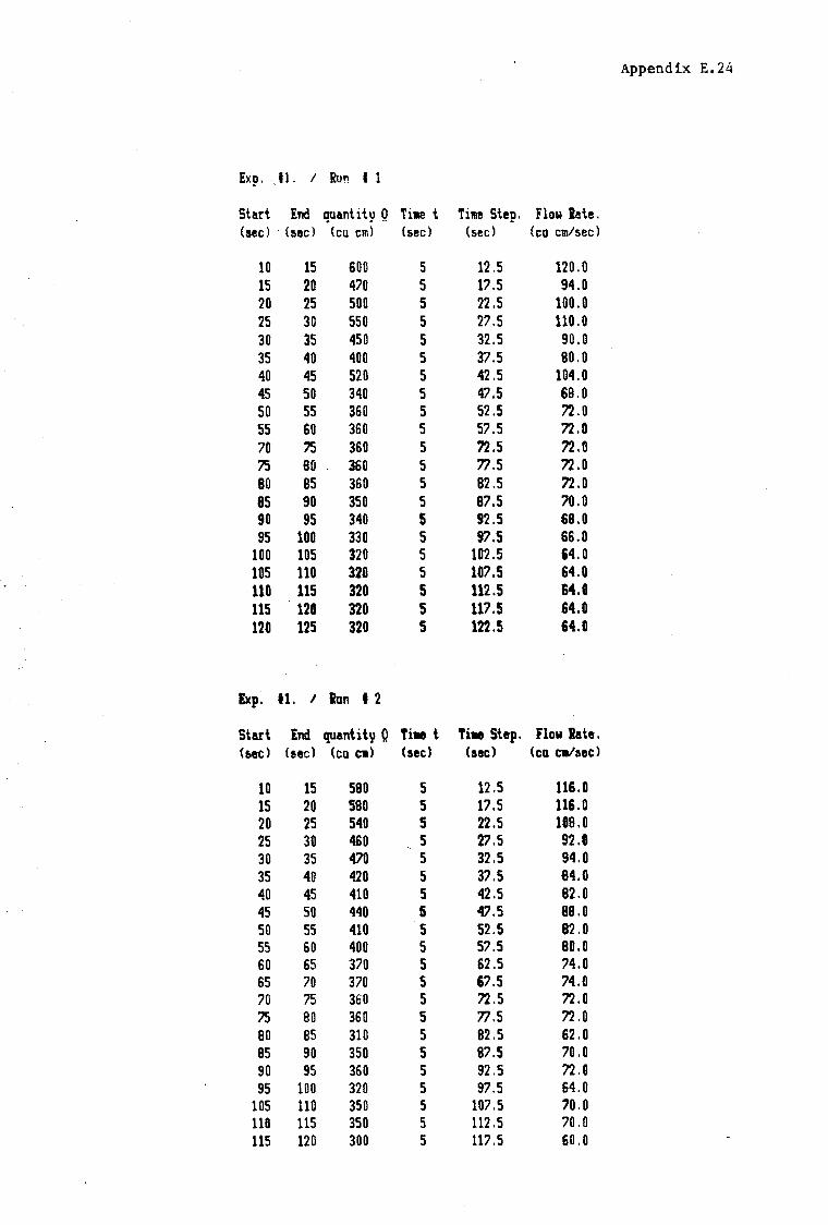
Append ix E. 24

Exp. 11. I Ruri I 1

Start End quantity Q Ti11e t Ti111e Step. Flow late. (aec) · (sec) (cu cm) (sec) (sec) (co ctn/sec)

10 15 600 5 12.5 120.0 15 20 470 5 17.5 94.0 20 25 500 5 22.5 100.0 25 30 550 5 27.5 110.0 30 35 450 5 32.5 90.0 35 40 400 5 37.5 80.0 40 45 520 5 42.5 104.0 45 50 340 5 47.5 69.0 50 55 360 5 52.5 72. 0 55 60 360 5 57.5 72.0 70 75 360 5 72.5 72. 0 75 80 360 5 77.5 72. 0 80 85 360 5 82.5 72 .o 85 90 350 5 87.5 70.0 90 95 340 5 92.5 68.0 95 100 330 5 97.S 66.0

100 105 320 5 102.5 S4.0 105 110 320 5 107.S 64.0 110 115 320 5 112.S 64.0 115 120 320 s 117.5 64.0 120 125 320 s 122.5 64.0

Exp. 11. I Ran I 2

Start End quantity Q Ti• t Ti• Step. Flow Rate. (aec) Caec) (co e11) (aec) (aec) (co ca/aec)

10 15 580 5 12.5 116.0 15 20 580 5 17.5 116.0 20 25 540 5 22.5 109.0 25 30 460 5 27.5 92.8 .. 30 35 470 5 32.5 94.0 35 40 420 5 37.5 84.0 40 45 410 5 42.5 82.0 45 50 440 5 47.5 88.0 50 55 410 5 52.S 82.0 55 60 400 5 57.5 eo.o 60 65 370 5 62.5 74.0 65 70 370 s 67.5 74.0 70 75 360 5 72 .5 72. 0 75 80 360 5 77.5 72.0 80 es 310 5 82.5 62.0 85 90 350 5 87.S 70.0 90 95 360 5 92.5 72.8 95 100 320 5 97.5 64.0

105 110 350 5 107.5 10.0 110 115 350 5 112.5 70.0 115 120 300 5 117.5 60.0

Appendix E.25

Flow Rate v's Time u CJ 1~0 II

' 130 C:xperl-nt no. E u Run no. 1 •

120 Run no. 2 b :J b b u

110 b • • II 11!10 • ... a "' 90

Q'.

3 80 D Time Q b 70 b b

IL. (sec) ( cm 3 Is) a b • a - SB 10 125 b

3 D SB 12' 5 120,3 ...

15 115,5 ... 4B :J 0 3B 22,5 103,3 II 30 95 en 20

"' 45 85 El. 1e II 60 77 ,5 II

Ill e e 1B 2B 3B 4B SB 6B 7B BB SB 1B0 110 12e 130 140 150

Time from :start of Exp. ( :SllC)

Cumulative Outflow v's Time

aume

1eeeB

seee Experiment no. l

E eee0 u

:J 7800 u

60BB

3 501!12 D

... .. 4Be0 :J 0

II 3000

~ I 2200 ..

"' ::J E ::J u

1eee

Be 10 20 30 '40 s0 s0 7e ee 90 100 1112 120 13e 1~e 1se

Time from :start ~f C:xp. (:sec)

Appendix E.26

E-5 • Sidewall piezo11eter levels recorded. !xper lllent no. 1.

Listings of the res.ults for the sidewall piezometer levels recorded for

experiment no. 1, are given here. The readings are recorded with

respect to time and the result given as the elevation (mm) above the

base of the flume. The actual piezometer referenced is given by a

reference number whose position is shown in figure (S.8)

Faulty piezometers are recorded as:

P iezometer po in ts falling above the

phreatic surface are recorded as:

Results that were not recorded, but

Faulty (F)

AWT

can be interpolated are recorded as: I

Appendix E.27

Experiment no. 1 I Piezometer Results. I Time (sec) v's Total head (mm)

Time Ref. no. Time Ref. no. PAl PA2 PA3 PA4 PAS PA6 PA7 PBl PB2 PB3 PB4 PBS PB6 PB7

0 F 300 300 300 300 300 AWT 0 300 F 300 301 301 301 AWT s F 178 180 244 AW!' AW!' AWT s 2Sl F 202 207 224 AW!' AWT 10 F 113 120 200 AWT AWT AWT 10 201 F 1S9 174 AWT AWT AWT lS F 99 AW!' AW!' AW!' AW!' AWT lS 164 F 148 AYlf AW!' AW!' AYlf 20 F I AWT AYlf AWT AWT AWT 20 147 F 14S AWT AWT AWT AWT 2S F 8S AW!' AWi' AW!' AW!' AWT 2S 140 F 140 AW!' AW!' AW!' AWT 30 F I AWT AWT AWT AWT AWT 30 133 F 136 AWT AWT AWT AWT 3S F I AW!' AW!' A'Wf AWI' AWT 35 129 F 134 AW!' AW!' AW!' AWT 40 F I AWT AWT A"Wf AWT AWT 40 126 F 131 AWT AWT AWT AWT 4S F I AW!' AW!' AW!' AW!' AWT 4S 123 F 129 AW!' AWI' AWI' AWT so F 80 AWT AWT AWT AWT AWT so 121 F 124 AWT AWT AWT AWT SS F I AW!' AW!' AW!' AW!' AW!' SS 118 F I AW!' AW!' AWI' AWI' 60 F 78 AWT AWT AWT AWT AWT 80 llS F 120 AWT AWT AWT AWT 90 F 76 AW!' AW!' AW!' AW!' AWT 120 110 F 113 AW!' AW!' A\11' A\11' lSO F 7S AWT AWT AWT AWT AWT lSO 107 F AWT AWT AWT AWT AWT


Time Ref. no. Time Ref. no. PCl PC2 PC3 PC4 PCS PC6 PC7 PDl PD2 PD3 PD4 PDS PD6 PD7

0 }i' 304 30S F 30S 30S AWT 0 F 30S F 306 F 306 AWT s F 222 218 F 26S AW!' AWT s F 287 F 267 F 262 AWT 10 F 192 190 F 230 A\11' AWT 10 F 272 F 243 F AWT AWT lS F 178 180 F AW!' AW!' AWT lS F 2S9 F 22S F AWT AWT 20 F 17S 178 F AW!' AWT AWT 20 F 243 F 212 F AWT AWT 2S F 168 173 F AW!' AW!' AWT 2S F 231 F 205 F AW!' AWT 30 F 164 166 F AWT AWT AWT 30 F 221 F 198 F AWT AWT 35 F 160 163 F AW!' AW!' AWT 3S F 213 F 19S F AW!' A\11' 40 F 15S 1S8 F AWT AWT AWT 40 F 20S F 192 F AWT AWT 4S F 1S2 lSS F AW!' AWI' AWT 4S F 200 F 189 F AW!' AWT 60 F 149 1S3 F AWT AWT AWT 50 F 194 F 185 F AWT AWT 80 F 145 145 F AWT AWI' AWT 60 F 189 F 177 F AW!' AWT 90 F 141 142 F AWT AWT AWT 70 F 183 F 177 F AWT AWT 120 F 138 139 F AWI' AWI' AWT 80 F 179 F 173 F AW!' AWT 150 F 136 137 F AWT AWT A'Wf. 120 F 170 F 168 F AWT AWT

Appendix E.28


Time Ref. no. Time Ref. no. PEl PE2 PE3 PE4 PES PE6 PE7 PFl PF2 PF3 PF4 PFS PF6 PF7

0 307 F F 308 308 F AWT 0 308 308 308 F 309 309 AWT s 283 F F 27S 276 F AWT s 272 278 28S F 280 29S AWT 10 2SS F F 24S 247 F AWT 10 2SO 2S8 2S4 F 2S4 26S AWT lS 240 F F 234 23S F AWT lS 243 244 247 F 247 AWT AWT 20 230 F F 227 230 F AWT 20 237 240 241 F 242 AWT AWT 2S 222 F F 221 22S F AWT 2S 233 236 236 F 238 AW!' AWI' 30 217 F F 218 222 F AWT 30 229 230 232 F 23S AWT AWT 3S 213 F F 214 217 F AWT 3S 226 228 229 F 233 AWI' AWT 40 208 F F 211 214 F AWT 40 I 22S 228 F 232 AWT AWT 4S 20S F F 207 212 F AWT 4S 221 222 224 F 229 AWI' AWT so 202 F F 20S AWT F AWT so 218 220 222 F 227 AWT AWT 60 198 F F 200 AWT F AWT 60 217 218 220 F 221 AW!' AWT 70 ·19s F F 197 AWT F AWT 70 21S 216 218 F 218 AWT AWT 80 192 F F 194 A\tll' F AWT 80 212 214 216 F 21S AWT AWT 100 189 F F 191 AWT F AWT 100 210 212 21S F 214 AWT AWT 150 184 F F 185 AWT F AWT 150 209 211 211 F 211 A\tll' AWT

Experiment no. 1 I P iezometer Results. I Time (sec) v' .s Total head (mm)

Time Ref. no. Time Ref. no. PGl PG2 PG3 PG4 PGS PG6 PG7 PHl PH2 PH3 PH4 PHS PH6 PH7

0 310 F 310 310 311 311 311 0 312 F 313 313 314 F 31S s 280 F 270 276 285 300 AWT 5 294 F 297 290 288 F AWT 10 2S8 F 260 267 27S 282 AWT 10 280 F 286 274 274 F AWT lS 2S3 F 25S 260 267 270 AWT lS 273 F 276 266 271 F AWT 20 249 F 2S2 2S5 2S9 261 AWT 20 268 F 270 26S 267 F AWT 2S 246 F 249 2S2 25S AWT AWT 2S 266 F 268 264 26S F AWT 30 243 F 247 2SO 2S2 AW!' AWT 30 264 F 26S 262 262 F AWT 3S 238 F 244 247 2SO AWT AWT 3S 260 F 262 260 260 F AWT 50 I F I 244 24S A\.11' AWT so 257 F 2S9 2S8 2S7 F AWT 60 234 F 241 240 241 AWT AWT 60 2SS F 2S7 2s·6 2SS F AWT 70 I F 239 I I AWT AWT 70 2S2 F 2S3 2S3 2S2 F AWI' 90 233 F 236 236 237 AWT AWT 90 247 F 2Sl 2SO 2SO F AWT 100 231 F 233 234 234 AWT AWT 100 246 F 2SO 249 248 F AWT 120 228 F 232 233 232 AWT AWT 120 244 F 248 247 247 F AWT lSO 227 F 230 231 231 AWI' AWT lSO 244 F 247 24S 24S F AWT

Appendix E.29


Time Ref. no. Time Ref. no. Pll Pl2 PI3 PI4 PIS PI6 PI7 PJl PJ2 PJ3 PJ4 PJS PJ6 PJ7

0 315 F 316 316 316 F 317 0 318 318 318 319 319 319 320 5 307 F 305 305 308 F 312 10 301 301 301 303 305 308 312 10 300 F 295 295 297 F AWT 15 296 297 298 299 301 302 AWT 15 293 F 285 290 294 F AWT 25 293 294 295 297 298 299 AWT 25 286 F 282 285 287 F AWT 40 289 290 292 294 296 295 AWT 30 281 F 279 281 283 F AWT 60 285 286 290 292 294 294 AWT 40 278 F 277 278 281 F AWT 100 284 285 287 289 291 292 AWT 50 275 F 273 275 279 F AWT 150 284 284 285 286 288 290 AWI' 60 271 F 271 273 277 F AWT 100 267 F 269 271 273 F AWT 150 264 F 266 269 271 F AWT


Time Ref. no. PKl PK2 PK3 PK4 PKS PK6 PK7

0 F 320 321 321 321 322 322 10 F 315 315 316 316 315 314 15 F 310 313 313 315 315 I 25 F 3og 312 312 313 313 I 30 F 300 311 ,311 I I I 40 F 303 309 310 312 312 I 60 F 303 308 309 311 311 I 100 F 302 306 308 310 310 I 150 F 301 305 307 309 309 310

Appendix E. 30

E-6. Transducer monitored tensioaeters. Experiaent m. 1.

Listings of the results for the tensiometers, recorded for experiment

no. 1, are given here. The recordings were made by the computer

controlled data-acquisition unit. (See chapter 3) Five sets of readings

are given for the five repeated experiment runs made. The readings are

recorded with respect to time and the result given as the elevation (mm)

above the base of the flume. The actual tens iometer referenced are

given by a reference number whose position is shown 1n figure (5.8)

Also given are the plots, for each tensiometer recorded, showing the

total pressure head versus time. The results for all five runs recorded

by a tensiometer are show on a single plot.

Appendix E.31

Experiment no. l I Run no. 1

7Il'!E TAI TA2 TA3 TA4 TB! TB2 TB3 TB4 TC1 TC2 TC3 TC4

-60 ! 300 ! 300 ! 300 ! 300 ! 307 307 I 307 ! 307 ! 317 317 ! 317 ! 317 I

-55 ! 299 !' 29B ! 299 ! 305 ! 306 I 305 ! 305 ! 305 I 317 I 316 ! 316 ! 316 ! -51 ! 300 I 299 I 300 ! 300 ! 306 ! 306 ! 305 ! 306 I 317 ! 317 I 317 ! 317 ! -46 ! 300 ! 299 ! 300 ! 294 ! 307 ! 306 ! 305 I 306 ! 317 ! 317 ! 317 ! 317 ! -42 ! 300 ! 300 ! 300 ! 296 ! 307 ! 306 ! 305 ! 306 ! 317 ! 317 I 317 ! 317 I

-3B ! 299 ! 299 ! 300 ! 295 ! 307 ! 306 ! 304 ! 305 ! 317 ! 317 I 317 ! 316 ! -32 ! 269 ! 26B ! 269 ! 263 ! 276 ! 276 ! 273 ! 275 ! 2B5 I 334 ! 2B6 ! 205 I

-20 I 299 ! 29B ! 299 ! 295 ! 306 ! 306 ! 304 ! 306 ! 316 ! 3Bl ! 316 ! 316 ! -23 ! 300 ! 298 ! 300 ! 297 I 307 ! 306 ! 306 ! 306 ! 316 ! 310 ! 317 I 316 ! -19 ! 29B ! 298 ! 299 ! 296 ! 306 ! 306 ! 305 ! 306 ! 317 ! 30B ! 317 ! 317 ! -14 ! 296 ! 295 ! 296 ! 296 ! 304 ! 303 ! 304 ! 304 ! 315 ! 394 ! 316 ! 316 !

-9 ! 296 ! 295 ! 296 ! 297 ! 304 ! 303 ! 303 ! 303 ! 315 ! 364 ! 316 ! 315 ! -5 ! 296 ! 295 ! 296 ! 297 ! 304 ! 304 ! 304 ! 303 ! 316 ! 317 I 316 I 315 !

0 ! 295 ! 294 ! 295 ! 299 ! 303 ! 303 ! 303 ! 303 ! 314 ! 316 ! 316 I 315 ! 5 ! 159 ! 163 ! 206 ! 286 ! 240 ! 255 ! 268 ! 270 ! 304 ! 317 ! 304 ! 304 ! 9 ! 79 ! 124 ! 189 ! 272 ! 220 ! 228 ! 241 ! 254 ~ 298 ! 308 ! 298 ! 298 !

14 ! 80 121 ! 181 ! 328 ! 217 ! 220 ! 228 ! 245 ! 297 ! 392 ! 297 ! 297 ! 19 ! 141 ! 118 ! 174 ! 247 I 214 ! 218 ! 226 ! 241 ! 296 ! 392 ! 296 ! 296 ! 24 ! 77 ! 114 ! 165 ! 247 ! 208 ! 212 ! 220 ! 234 ! 294 ! 388 ! 294 ! 294 ! 28 ! 46 ! 82 ! 129 ! 207 ! 175 ! 178 ! 186 ! 200 ! 262 ! 271 ! 262 ! 262 ! 32 ! 76 ! 111 ! 155 ! 237 ! 203 ! 206 ! 215 ! 228 ! 292 386 ! 292 ! 292 ! 38 ! 44 ! 77 ! 158 ! 212 ! 169 ! 172 ! 182 ! 190 ! 261 ! 267 ! 261 ! 261 ! 42 ! 75 ! 106 ! 142 ! 242 ! 197 ! 201 ! 255 ! 286 ! 292 ! 297 ! 291 ! 291 ! 48 ! 74 ! 104 ! 139 ! 244 ! 195 I 197 ! 262 ! 217 ! 290 ! 296 ! 291 ! 290 ! 52 ! 73 I 102 ! 136 ! 240 ! 193 ! 195 ! 260 ! 217 ! 290 ! 297 ! 289 ! 289 I

56 ! 74 ! 103 ! 133 ! 244 ! 193 ! 195 ! 261 ! 217 ! 291 ! 296 ! 290 ! 290 ! 62 ! 73 ! 100 ! 130 ! 241 ! 190 ! 192 ! 200 ! 214 ! 290 ! 384 ! 209 I 289 ! 67 ! 42 ! 6B ! 97 ! 207 ! 157 ! 160 ! 167 ! 181 ! 25B ! 267 ! 258 ! 25B ! 72 ! 72 ! 97 ! 125 ! 242 ! 185 ! !BB ! 198 ! 210 ! 288 ! 297 ! 28B i 287 I

76 ! 71 ! 97 ! 124 ! 234 ! 184 ! 187 ! 196 ! 209 ! 287 ~ 296 ! 287 ! 2B7 ! 81 ! 71 ! 96 ! 123 ! 238 ! 184 ! 186 ! 195 I 210 ! 28B ! 297 ! 288 I 208 : 8b ! 70 ! 94 ! 121 ! 236 ! 184 ! 185 ! 194 ! 209 I 287 ! 384 ! 287 ! 287 ! 91 ! 40 ! 63 ! 90 ! 207 ! 153 ! 153 I 163 I 177 ! 257 ! 266 ! 256 ! 256 ! 97 ·! 70 ! 93 ! 119 ! 240 ! 182 ! 1B3 ! 193 ! 207 ! 288 ! 299 ! 287 I 207 !

101 ! 69 ! 93 ! 118 ! 245 ! 179 ! 182 ! 190 !. 206·! 286 ! 296 ! 286 ! 2Bb ! 105 ! 70 ! 93 ! 118 ! 240 ! 181 ! 182 ! 190 ! 206 ! 2B7 ! 29B I 2B6 ! 287 ! 111 ! 70 ! 92 ! 117 ! 237 ! 179 ! 181 ! !BB ! 205 ! 2B7 I 297 I 286 ! 286 I

!16 I 39 ! 61 ! 86 ! 205 ! 149 ! 149 ! 157 ! 174 ! 256 ! 267 ! 254 I 255 ! 121 ! 69 ! 91 ! lib I 233 ! 178 ! 180 ! 188 I 204 ! 2B7 1 29B ! 285 ! 2B6 I

125 ! 6B ! 90 I !lb ! 236 ! 177 ! 178 ! 188 I 203 ! 286 ! 299 ! 2B5 I 285 ! 129 ! 69 ! 90 ! llb ! 240 ! 178 ! 178 I 1B7 ! 203 2B6 ! 299 I 285 I 285 ! 134 I 6B ! 89 ! 115 ! 241 ! 177 ! 177 ! 1B6 ! 201 ! 285 ! 29B ! 284 I 285 ! 138! 6B 1 90! 115 1 237 1 178! 177! IB7! 201! 286 1 29B! 285! 2B5! 143 ! 6B ! 89 ! 115 ! 243 ! 177 ! 177 ! 186 ! 201 286 i 3BS ! 285 I 2B5 I

147 ! 68 ! BB ! 113 ! 237 I 176 ! 176 ! 185 ! 200 ! 286 I 299 ! 284 ! 285 !

Appendix E.32

Experiment no. 1 I Run no. 2

TIME TA1 TA2 TA3 TA4 TB1 TB2 TB3 TB4 TCl TC2 TC3 TC4

-60 1 300 300 ! 300 ! 300 ! 307 307 1 307 ! 307 1 317 317 ! 317 ! 317 ! -55 ! 299 I 298 ! 299 ! 380 I 304 ! 306 ! 305 ! 306 I 316 ! 402 I 317 ! 316 ! -51 I 300 ! 299 ! 299 ! 385 ! 306 I 306 ! 305 ! 306 ! 316 ! 317 ! 316 I 317 ! -47 ! 300 ! 300 ! 299 ! 384 ! 306 ! 306 ! 306 ! 307 ! 316 ! 404 ! 317 t 317 ! -42 ! 299 ! 299 ! 299 ! 299 I 304 ! 305 ! 305 ! 305 I 316 l 315 ! 316 ! 316 ! -39 I 299 ! 299 ! 299 ! 295 I 306 ! 306 ! 306 ! 306 ! 316 ! 316 ! 316 ! 316 ! -33 I 298 ! 298 ! 298 ! 380 ! 304 ! 305 ! 305 I 306 ! 316 ! 402 ! 317 ! 317 ! -30 ! 267 ! 267 ! 267 ! 350 ! 274 ! 274 ! 274 ! 274 ! 284 ! 283 ! 285 ! 286 ! -26 ! 297 ! 297 ! 297 ! 295 ! 304 ! 304 ! 304 ! 305 ! 314 ! 399 ! 315 I 316 ! -20 ! 297 ! 297 ! 298 ! 296 ! 304 ! 305 ! 306 ! 306 ! 316 ! 313 ! 317 ! 317 ! -17 298 ! 298 ! 298 ! 294 ! 305 ! 306 ! 306 ! 306 ! 316 ! 316 ! 317 ! 317 ! -11 ! 298 ! 297 ! 298 ! 304 ! 305 ! 305 ! 306 ! 306 ! 316 ! 313 ! 317 ! 317 ! -7 ! 298 ! 297 ! 298 ! 298 ! 306 ! 306 ! 306 ! 306 ! 316 ! 313 ! 317 ! 317 f

-3 ! 297 ! 298 ! 297 ! 382 ! 305 ! 305 ! 305 ! 305 ! 316 ! 312 ! 317 ! 317 ! 2 ! 274 ! 274 ! 272 ! 294 ! 297 ! 301 ! 303 ! 304 ! 315 ! 315 ! 315 ! 316 ! 6 ! 114 ! 136 ! 192 ! 281 ! 334 ! 246 ! 259 ! 265 ! 302 ! 312 ! 303 ! 303 !

11 ! 79 ! 120 ! 179 ! 274 ! 215 ! 229 ! 234 ! 244 ! 297 ! 310 ! 297 ! 297 ! 15 ! 78 ! 118 ! 172 ! 271 ! 212 ! 225 ! 226 ! 238 ! 295 ! 312 ! 295 ! 296 ! 19 ! 78 ! 114 ! 164 ! 270 ! 207 ! 220 ! 219 ! 232 ! 293 ! 311 ! 293 ! 294 ! 24 ! 78 ! 112 ! 158 ! 266 ! 204 ! 217 ! 270 ! 224 ! 293 ! 310 ! 293 ! 294 ! 28 ! 76 ! . 109 ! 148 ! 269 ! 200 ! 213 ! 267 ! 222 ! 291 ! 307 ! 291 ! 292 ! 34 ! 75 ! 107 ! 144 ! 263 ! 197 ! 209 ! 207 ! 220 ! 291 ! 306 ! 291 ! 291 ! 38 ! 75 ! 105 ! 142 ! 264 ! 194 ! 209 ! 205 ! 285 ! 291 ! 306 ! 291 ! 292 ! 42 ! 74 ! 104 ! 138 ! 258 ! 193 ! 206 ! 204 ! 217 ! 291 ! 306 ! 290 ! 291 ! 47 74 ! 102 ! 135 ! 264 ! 191 ! 204 204 ! 213 ! 290 ! 304 ! 290 ! 290 ! 51 73 ! 101 ! 132 ! 268 ! 188 ! 201 ! 200 ! 213 ! 289 ! 303 ! 289 ! 290 ! 57 73 ! 101 ! 129 ! 273 ! 188 ! 200 ! 199 ! 211 ! 289 ! 303 ! 288 ! 289 ! 61 42 ! 68 ! 97 ! 238 ! 156 ! 168 ! 167 ! 179 ! 257 ! 270 ! 258 ! 258 ! 65 ! 71 I 98 ! 125 ! 265 ! 185 ! 197 ! 19Q ! 208 ! 287 ! 298 ! 287 I 288 ! 70 ! 71 ! 97 ! 123 ! 266 ! 183 ! 196 ! 194 ! 208 ! 287 ! 298 ! 287 ! 288 ! 74 ! 70 ! 95 ! 121 ! 261 ! 182 ! 194 ! 192 ! 206 ! 286 ! 297 ! 284 ! 286 ! 79 ! 70 ! 95 ! 119 ! 262 ! 181 ! 193 ! 191 ! 206 ! 286 ! 296 ! 286 ! 287 ! 83 ! 70 ! 95 I 119 ! 260 ! 190 ! 192 ! 191 ! 205 ! 286 ! 296 ! 286 ! 287 ! 87 I 69 ! 94 ! 117 ! 251 ! 179 ! 191 ! 190 ! 204 ! 286 ! 297 ! 285 ! 286 ! 92 ! 70 ! 93 ! 117 ! 257 ! 179 ! 191 ! 189 ! 204 ! 286 ! 295 ! 285 I 287 ! 9b ! b9 ! 93 ! 116 ! 255 ! 178 ! 190 ! 188 ! 203 ! 286 '! 296 ! 286 ! 287 !

102 ! 09 ! 92 ! 115 ! 252 ! 178 ! 190 I 188 ! 203 299 ! 294 ! 285 I 286 ! 106 I 09 ! 93 ! 115 ! 251 ! 176 ! 189 ! 187 ! 201 I 299 ! 294 ! 285 ! 286 ! j j (I I 08 ! 91 114 ! 254 ! 17 6 ! 188 ! 186 ! 200 ! 28(! ! 291 ! 283 ! 285 1

116 ! 69 ! 91 114 ! 250 ! 177 ! 188 ! 184 ! 200 ! 324 ! 290 I 285 ! 286 ! j 20 ! 38 ! 60 83 ! 220 ! 145 ! 157 ! 155 ! 170 I 251 ! 257 ! 254 ! 255 I

125 ! 69 ! 91 113 f 255 ! 175 ! 187 ! 185 ! 199 ! 281 ! 287 ! 284 ! 285 ! 129 1 68! 90 1 112! 249! 175! 186! 185! 198'. 325! 286! 284 1 286 1

133' 67~ 90 1 .111! 249! 176! 186! 184! 198! 323 1 286 1 284! 285! 138 ! 67 ! BB ! 111 ! 247 ! 174 ! 185 I 183 I 196 I 336 ! 284 f 283 ! 285 ! 143 I 67 ! 88 ! 110 ! 247 ! 174 ! 184 ! 183 196 336 ! 285 I 283 ! 284 I

148 1 bB ! 9(! ! 111 ! 247 ! 174 ! 185 : 183 I 197 I 312 I 286 ! 284 ! 2Bt !

Appendix E.33


TIME TAl TA2 TA3 TA4 TB! TB2 TB3 TB4 TC! TC2 TC3 TC4

-60 ! 300 300 I 300 ! 300 ! 307 307 ! 307 ! 307 ! 317 317 I 317 ! 317 I

-56 ! 299 ! 299 ! 299 ! 296 ! 306 ! 306 ! 304 ! 306 ! 316 I 316 I 318 ! 316 ! -50 ! 300 I 300 ! 299 ! 296 ! 307 ! 322 ! 305 ! 306 ! 317 ! 315 ! 317 ! 317 ! -46 ! 300 ! 299 ! 299 I 302 ! 306 ! 306 ! 303 ! 306 ! 317 I 312 ! 317 ! 317 ! -41 ! 299 ! 299 ! 299 ! 296 ! 30t ! 306 I 304 307 ! 317 ! 309 I 317 ! 317 ! -36 ! 299 ! 299 ! 299 I 298 I 305 ! 306 I 305 ! 306 I 316 ! 31! 317 ! 317 ! -32 I 299 ! 300 ! 299 ! 300 305 I 322 ! 305 I 306 ! 317 ! 310 ! 317 I 316 ! -27 ! 299 ! 290 ! 299 ! 301 ! 306 ! 305 ! 305 ! 306 ! 317 ! 311 ! 317 I 316 ! -22 1 299 ! 299 ! 299 I 30! ! 306 ! 306 ! 305 I 306 ! 3!7 ! 312 I 317 I 316 ! -17 ! 300 ! 299 ! 299 ! 300 ! 306 ! 322 ! 306 ! 306 ! 317 ! 314 ! 318 ! 316 ! -12 ! 298 ! 299 ! 298 ! 301 ! 305 ! 338 ! 304 ! 306 ! 317 ! 315 ! 317 ! 316 ! -8 ! 298 ! . 297 ! 298 ! 300 ! 305 ! 322 ! 305 ! 306 ! 317 ! 315 ! 319 ! 317 ! -3 ! 298 ! 297 ! 298 ! 302 ! 305 ! 306 ! 305 ! 306 ! 317 ! 315 ! 318 ! 316 ! 1 ! 272 ! 272 ! 270 ! 296 ! 296 ! 295 ! 301 ! 303 ! 315 ! 314 ! 316 ! 315 ! 7 ! 84 ! 126 ! 199 ! 279 ! 223 ! 237 ! 247 ! 257 ! 299 ! 310 ! 300 ! 300 !

11 ! 81 ! 121 ! 179 ! 271 ! 215 ! 228 ! 232 ! 244 ! 297 ! 307 ! 297 ! 297 ! 16 ! so ! 117 ! 170 ! 272 ! 209 ! 222 ! 224 ! 236 ! 295 ! 307 ! 295 ! 295 ! 21 78 ! 113 ! 162 ! 279 ! 204 ! 218 ! 263 ! 226 ! 294 ! 305 ! 293 ! 294 ! 26 ! 7 6 ! 111 ! 196 ! 272 ! 200 ! 214 ! 268 ! 223 ! 292 ! 305 ! 292 ! 292 ! 31 ! 75 ! 107 ! 147 ! 269 ! 197 ! 211 ! 207 ! 220 ! 291 ! 305 ! 291 ! 291 ! 35 ! 75 ! 106 ! 144 ! 264 ! 195 ! 209 ! 262 ! 220 ! 291 ! 306 ! 291 ! 290 ! 39 ! 74 ! 105 ! 139 ! 262 ! 192 ! 206 ! 205 ! 217 ! 290 ! 306 ! 290 ! 289 ! 45 ! 73 ! 103 ! 135 ! 258 ! 190 ! 204 ! 204 ! 215 ! 290 ! 307 ! 289 ! 289 ! 49 ! 72 ! 101 ! 132 ! 265 ! 198 ! 203 ! 201 ! 213 ! 289 ! 307 ! 289 ! 288 ! 55 ! 72 ! 99 ! 129 ! 266 ! 185 ! 199 ! 195 ! 210 ! 3:l/ I 307 ! 287 ! 2B7 ! 60 ! 72 ! 99 ! 127 ! 266 ! 185 ! 199 ! 192 ! 209 ! 284 ! 306 ! 288 ! 2B8 ! 64 ! 72 ! 9B ! 125 ! 266 ! 184 ! 198 ! 193 ! 208 I 340 ! 305 ! 287 ! 2B7 ! 70 ! 71 9B ! 123 ! 263 ! !B3 ! 196 ! 191 ! 20j I 285 I 303 ! 287 ! 287 ! 74 ! 71 ! 97 ! 121 ! 262 ! 182 ! 195 I 191 ! 206 ! 339 ! 301 287 ! 2B7 ! 80 ! 71 ! 97 ! 120 ! 261 ! 181 ! 195 ! 1B9 ! 205 ! 283 ! 301 ! 2B7 ! 287 ! 84 ! 11 95 ! 119 ! 2s1 ! 1e1 ! 193 ! 1 Bil ! 203 1 351 ! 299 1 2B6 ! 206 ! 89 ! 71 ! 95 ! 118 ! 259 ! 180 ! 192 ! 187 ! 203 ! 282 ! 29B ! 2Bb ! 286 ! 95 ! 68 ! 93 ! 115 ! 257 ! 176 ! 190 ! 184 ! 201 I 281 ! 296 ! 285 ! 284 I

99 I b9 ! 94 ! 115 ! 255 I 177 ! 191 ! 185 ! 20i 1 350 ! 296 ! 286 ! 2BS ! 105 ! 6B ! 92 ! 114 ! 256 ! 175 ! !BB ! 1B5 ! 200 I 349 I 297 I 284 ! 284 ! 110 ! 69 ! 93 ! 114 ! 262 ! 175 ! 189 ! 1B4 199 ! 280 ! 298 ! 285 ! 2B4 ! 114 ! 68 ! 92 113 ! 260 ! 175 ! !BC/ ! 184 198 350 I 298 ! 285 ! 284 ! 120 ! 68 ! 91 ! 111 I 254 ! 174 ! 1B7 I 181 197 ! 349 ! 297 ! 284 ! 283 ! 124 ! 68 ! 91 ! 111 ! 256 ! 174 ! 187 ! 183 197 I 2B(i I 298 ! 283 ! 2B3 ! 130 ! 67 ! 90 I 110 ! 254 ! 173 ! 186 ! 180 ! 195 ! 279 ! 298 I 283 I 283 ! 135! 68! 90! 110! 255! 173! 186! 179! 195 1 34~! 298! 284! 2831 139 ! 6B ! 90 ! 110 ! 247 ! 173 ! !BS ! !BO ! 195 ! 349 I 298 ! 284 ! 293 ! 145 l 68 ! 90 ! 109 I 251 ! 172 ! 185 ! 1B0 ! 195 I 279 I 299 ! 284 ! 28~, I

!49! 68! 90 1 109! 249 1 173' 185! !BO! 194! 350 1 298! 284! 283!

Appendix E.34


Til'IE TAI TA2 TA3 TA4 TB1 TB2 TB3 TB4 . TC1 TC2 TC3 TC!

-bO ! 300 ! 300 ! 300 ! 300 307 307 ! 307 ! 307 317 317 ! 317 317 -54 ! 300 I 300 ! 299 ! 256 ! 30b ! 391 ! 307 ! 306 ! 318 ! 316 ! 317 I 316 ! -50 ! 299 ! 300 I 299 ! 228 ! 307 ! 30b ! 307 ! 307 ! 317 ! 317 ! 317 ! 31b ! -46 300 ! 300 I 299 ! 217 ! 305 ! 391 307 ! 30b ! 318 ! 31b ! 317 ! 31b I

-41 ! 300 ! 300 ! 299 ! 212 ! 307 ! 391 ! 307 ! 30b ! 317 ! 315 ! 31b ! 31b ! -38 ! 300 ! 300 I 300 ! 218 ! 307 ! 392 ! 309 ! 307 ! 317 ! 317 ! 317 I 317 1

-33 ! 299 ! 299 ! 299 ! 218 ! 30b ! 390 ! . 30b ! 30b ! 317 ! 316 ! 316 ! 31b ! -29 ! 299 ! 300 ! 299 ! 299 ! 307 ! 307 ! 306 ! 306 ! 318 ! 316 ! 317 ! 317 ! -26 ! 300 ! 299 ! 299 ! 298 ! 306 ! 307 ! 304 ! 306 ! 317 ! 317 ! 316 ! 317 ! -21 ! 299 ! 299 ! 299 ! 258 ! 306 ! 307 ! 306 ! 306 ! 318 ! 31b ! 317 ! 317 I

-17 ! 300 ! 298 ! 299 ! 217 ! 307 ! 391 ! 30b ! 30b ! 318 ! 31b ! 317 ! 317 ! -12 ! 299 ! 298 ! 299 ! 299 ! 307 ! 306 ! 305 ! 306 ! 318 ! 316 ! 317 ! 31? ! -8 I 299 ! 298 ! 299 ! 216 ! 307 ! 390 ! 306 ! 307 ! 318 ! 316 ! 318 ! 317 ! -5 ! 299 ! 298 ! 299 ! 228 ! 306 ! 307 ! 306 ! 306 ! 318 ! 316 ! 318 ! 317 !

1 ! 292 ! 291 ! 291 ! 220 ! 303 ! 389 ! 30b ! 305 ! 317 ! 31b ! 317 ! 316 ! 4 ! 140 ! 147 ! 200 ! 187 ! 240 ! 258 ! 272 ! 274 ! 304 ! 309 ! 306 ! 307 !

10 ! 81 ! 122 ! 182 ! 170 ! 218 ! 229 ! 295 ! 312 ! 297 '! 301 ! 297 ! 297 ! 14 ! 80 ! 118 ! 216 ! 167 ! 213 ! 223 ! 231 ! 240 ! 297 ! 298 ! .296 ! 295 ! 17 ! 79 ! 115 ! 166 ! 168 ! 208 ! 217 ! 226 ! 235 ! 294 ! 297 ! 294 ! 293 ! 22 ! 77 ! 112 ! 159 ! 174 ! 203 ! 213 ! 220 ! 229 ! 293 ! 296 ! 291 ! 292 ! 26 ! 77 ! 110 ! 154 ! 172 ! 201 ! 209 ! 217 ! 226 ! 293 ! 295 ! 291 ! 291 ! 31 ! 76 ! 107 ! 148 ! 171 ! 197 ! 206 ! 211 ! 223 ! 292 ! 293 ! 290 ! 290 ! 35 ! 75 ! 105 ! 143 ! 169 ! 193 ! 202 ! 208 ! 219 ! 290 ! 292 ! 289 ! 289 ! 39 ! 75 ! 103 ! 139 ! 171 ! 192 ! 200 ! 205 ! 216 ! 290 ! 291 ! 288 I 288 I

44 ! 74 ! 102 ! 135 ! 178 ! 189 ! 196 ! 201 ! 214 ! 289 ! 290 ! 287 ! 287 ! 48 ! 73 ! 100 ! 132 ! 182 ! 187 ! 194 ! 199 ! 212 ! 288 ! 290 ! 286 ! 286 ! 53 ! 73 ! 56 ! 72 ! 60 ! 71 ! 65 ! 71 ! 69 ! 70 ! 74 ! 70 ! 78 ! 70 ! 82 ! 70 ! 87 ! 69 ! 91 ! 68 ! 9b ! 68 !

100 ! 68 ! 104 I 68 ! 110 ! 68 ! 114 ! 68 ! 119 ! 68 ! 123 ! 68 ! 127 ! 67 132 ! b7 13b ! 67 141 67 146 ! 66 !

98 ! 128 ! 178 ! 185 ! 192 ! 196 ! 209 ! 287 ! 289 ! 285 ! 285 ! 97 ! 127 ! 176 ! 182 ! 191 ! 194 ! 208 ! 287 ! 289 ! 285 ! 285 ! 97 ! 125 ! 174" ! 181 ! 189 ! 193 ! 207 ! 287 ! 289 ! 285 ! 285 ! 95 ! 122 ! 179 ! 180 ! 187 ! 190 ! 206 ! 286 ! 288 ! 284 ! 284 ! 95 ! 121 ! 177 ! 178 ! 186 ! 189 ! 205 ! 285 ! 288 ! 283 ! 284 ! 93! 119! 174! 178! 184! 188! 204! 286! 288! 283! 283! 93 ! 117 ! 177 ! 17 h ! 183 ! 186 ! 202 ! 285 ! 287 ! 282 ! 282 ! 91 117 ! 172 ! 175 ! 182 ! 185 ! 201 ! 284 ! 286 ! 283 ! 282 ! 91 ! 115 ! 169 ! 175 ! 181 ! 184 ! 200 ! 284 ! 285 ! 282 ! 281 ! 90 ! 115 ! 173 ! 174 ! 180 ! 183 ! 199 ! 284 ! 285 ! 282 281 89 ! 113 ! 173 ! 172 ! ISO ! 181 ! 198 ! 283 ! 285 ! 281 ! 281 ! 89 ! 113 ! 170 ! 173 ! 178 ! 182 ! 198 ! 283 ! 284 ! 281 ! 281 ! 88 ! 113 1 171 ! 172 ! 179 ! 182 ! 197 1 284 ! 285 ! 283 1 281 ! 87 ! 111 181 ! 172 177 ! 179 ! 196 ! 283 ! 284 ! 281 ! 280 I

BB ! 111 ! 179 ! 171 ! 177 ! 1 i9 I 195 ! 283 ! 285 ! 280 280 I

87 ! 111 ! 175 ! 170 ! 177 ! 180 ! l 95 ! 283 ! 284 ! 281 280 ! 87 ! 110 ! 171 170 ! 177 ! 179 ! 194 ! 283 ! 284 ! 281 280 ! 86 ! 110 ! 169 ! 1611 ! 177 ! 178 ! 194 I 283 I 284 ! 280 280 ! Bo ! 109 ! 111 1 169 1 11s ! 1 n ! 193 ! 203 ! 204 1 201 200 ! 85 ! 108 ! 170 ! 168 ! 174 ! 176 ! 192 ! 282 ! 284 I 28(1 I 279 ! 8:1 I 108 ! 1 i9 ! 108 ! 175 I 176 I 192 I 283 I 284 I 280 ! 280 I

85 I 107 I 172 ! 168 ! 174 ! 176 ! J9J I 282 I 284 ! 28(> ! 27~ 1

Appendix E.35


TA2 TA3 TA4 TB! TB2 TB3 TB4 TC! TC2 TC3 TC4

-60 ! 300 ! 300 300 ! 300 ! 307 307 ! 307 ! 307 317 317 ! 317 317 ·56 I 299 I 300 I 299 ! 300 ! 306 305 ! 307 ! 306 ! 315 I 316 I 316 316 I

-SJ ! 299 ! 298 ! 299 ! 301 ! 306 ! 305 ! 306 ! 306 ! 315 ! 316 ! 316 ! 316 I

·47 ! 298 ! 297 ! 298 ! 292 ! 306 ! 305 ! 305 ! 306 I 315 ! 317 ! 316 ! 316 ! -44 ! 298 ! 298 ! 299 ! 295 ! 307 ! 305 ! 303 ! 306 ! 316 ! 316 ! 316 ! 316 ! -39 ! 299 I 300 ! 300 ! 29~ ! 307 ! 306 ! 306 ! 307 I 316 ! 316 ! 316 ! 316 ! -36 ! 299 ! 299 : 299 ! 295 ! 307 ! 306 ! 306 ! 307 ! 317 ! 316 ! 317 ! 316 ! -31 ! 297 ! 298 ! 298 ! 297 ! 305 ! 389 ! 306 ! 306 ! 316 ! 316 ! 315 ! 316 ! -27 ! 298 ! 297 ! 299 ! 293 ! 307 ! 305 ! 306 ! 306 ! 316 ! 317 ! 317 ! 316 ! ·23 ! 298 ! 297 ! 299 ! 300 ! 306 ! 305 ! 305 306 ! 317 ! 317 ! 316 ! 316 I

-!9 ! 298 ! 297 ! 298 ! 296 ! 305 ! 304 ! 307 306 ! 315 ! 316 ! 315 ! 316 ! -15 ! 298 ! 297 ! 298 I 296 ! 306 ! 305 ! 307 306 ! 317 ! 316 ! 316 ! 316 ! -10 ! 298 ! 297 ! 298 ! 301 ! 306 ! 305 ! 307 306 ! 317 ! 317 ! 317 ! 316 ! -6 ! 298 ! 297 ! 298 ! 293 ! 306 ! 305 ! 307 ! 306 ! 317 ! 317 ! 316 ! 316 I

-2 ! 297 I 296 ! 298 ! 298 ! 306 ! 304 ! 306 ! 305 ! 316 ! 315 ! 315 ! 315 ! 3 ! 250 ! 249 ! 250 ! 276 ! 285 ! 292 ! 298 ! 296 ! 377 ! 313 ! 311 ! 312 ! 6 ! 167 ! 127 ! 188 ! 234 ! 227 ! 235 ! 254 ! 257 ! 298 ! 302 ! 298 ! 299 !

12 ! 76 ! 115 ! 219 ! 224 ! 217 ! 221 ! 236 ! 246 ! 295 ! 298 ! 295 ! 296 ! 15 ! 75 ! 111 ! 170 ! 220 ! 213 ! 217 ! 232 ! 309 ! 296 ! 298 ! 293 ! 294 ! 19 ! 74 ! 109 ! 164 ! 218 ! 210 ! 214 ! 229 ! 238 ! 294 ! 297 ! 292 ! 293 ! 24 ! 73 ! 106 ! 156 ! 214 ! 204 ! 209 ! 222 ! 234 ! 294 ! 330 ! 291 ! 291 ! 28 ! 72 ! 104 ! 151 ! 213 ! 202 ! 205 ! 219 ! 231 ! 293 ! 362 ! 291 ! 291 ! 33 ! 71 ! 100 ! 144 ! 211 ! 198 ! 201 ! 214 ! 226 ! 291 ! 292 ! 289 ! 290 ! 37! 69! 98! 139! 215! 195! 198! 210! 223! 290! 375! 288! 289! 40 ! 69 I 96 ! 136 ! 205 ! 193 ! 195 ! 206 ! 221 ! 290 ! 374 ! 287 ! 288 ! 46 ! 68 ! 94 ! 130 ! 209 ! 190 ! 191 ! 203 ! 218 ! 290 ! 287 ! 287 ! 288 ! 50 ! 68 ! 93 ! 128 ! 213 ! 187 ! 189 ! 199 ! 216 ! 289 ! 373 ! 286 ! 287 ! 55 ! 6 7 ! 91 ! 125 ! 211 ! 185 ! 187 ! 197 ! 214 ! 288 ! 286 ! 285 ! 286 ! ~9 ! b 7 ! 90 ! 122 ! 201 ! 183 ! 184 ! 195 ! 213 ! 287 ! 286 ! 284 ! 285 ! 63 ! 66 ! 90 ! 120 ! 209 ! 181 ! 183 ! 193 ! 212 ! 288 ! 372 284 ! 285 ! 68 ! b6 ! 87 ! 118 ! 201 ! 180 ! 180 ! 190 ! 210 ! 286 ! 371 ! 283 ! 284 ! 71 ! 65 ! 86 ! 116 ! 205 ! 178 ! 179 ! 189 ! 209 ! 286 ! 284 ! 282 ! 283 ! 77 ! 64 ! 85 l 114 ! 203 ! 17 6 ! 177 ! · 187 ! 208 ! 285 ! 283 ! 282 ! 283 ! 81 I 64 I B"'· I 113 ! 204 ! 175 ! 176 ! 186 ! 207 ! 285 ! 372 ! 282 ! 282 ! 85 ! 64 ! 84 ! 112 ! 202 ! 174 ! 175 ! 185 I 206 ! 284 ! 283 ! 281 ! 282 ! 90 ! 63, I 8'? I 110 ! 200 ! 173 ! 174 ! 183 ! 205 ! 284 ! 370 ! 281 ! 281 ! 94 ! 63 i 82 ! 110 ! 193 ! 173 ! 17 4 ! 182 ! 205 ! 284 ! 284 ! 280 ! 281 !

100 ! 62 i 8 J ! 108 ! 205 ! 171 ! 171 ! 180 ! 204 ! 283 ! 283 ! 280 I 280 ! 103 ! 62 I 82 I 109 ! 201 ! 171 ! 171 ! 181 ! 203 ! 283 ! 370 ! 279 ! 280 ! 107 I 63 '. Bi I 108 ! 192 ! 171 ! 171 ! 180 ! 202 ! 284 ! 283 ! 280 I 281 I

112 ! 63 I 80 ! 107 ! 274 ! 169 ! 169 ! 178 ! 202 ! 283 ! 283 I 279 I 280 ! 116 ! 62 BO ! 107 I 201 ! 170 ! 170 ! 178 ! 202 ! 283 ! 283 ! 280 I 280 ! 121 ! 61 I 78 I 105 ! 271 ! 169 ! 168 i 178 ! 201 ! 282 ! 283 ! 279 ! 280 ! 124! 61! 79 1 105! 19.3! 169! 168 1 177 1 200! 283! 284! 278! 280! 128 ! 6? I 79 I 105 l 188 ! 168 ! 168 ! 176 ! 200 ! 284 ! 283 I 278 ! 279 ! 133 ! 62 ! 78 ! 105 ! 188 ~ 169 ! 168 ! 176 ! 200 ! 283 ! 284 ! 279 I 28(1 ! 137 ! b2 ! J8 I 104 I j 89 ! 167 ! 16 7 I 175 ! 200 ! 283 I 283 ! 279 ! 280 ! 141 I 62 ! 77 103 I 187 ! 166 ! 168 I 175 ! 199 : 283 ! 283 ! 279 ! 279 ! !45 I 62 ! i/ I 104 I 186 ! 167 ! 16i I 175 ! 199 I 283 I 284 ! 280 I 280 !

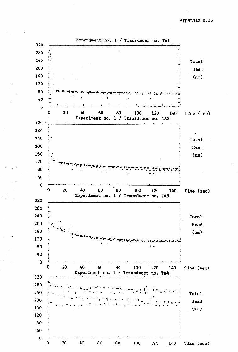
320

280

240

200

160

120

80

40

0

320

280

240

200

160

120

80

40

0

320

280

240

200

160

120

80

40

0

320

280

240

200

160

120

80

40

0

Appendix E.36

r !;;> 1--. ~-: , ... IL. I .• I .-1 . r ... i

Experiment no. 1 I Transducer no. TAl

"l --j --j ~ ~ --l .J I I I

I I

r ... .,....of$+t~~ +t::,+ ...... + .................. ++++ ..t-t-llr+.mHrmt-.-.+- ............__ ............. ·"'· ....... ·"""' ···- - ... . ::1 t·.. . ' . . .,.. ..... ... • ... + 4 +·' + +·. + . + . ... . :,. :J.. q.·. ·+· ... - +. -P"' ~

~·- ... + + + + -! ~ ~

0 20 40 60 80 100 120 140 Experiment no. 1 I Transducer no. TA2

Total

Head

(mm)

Time (sec)

Total

Head

(mm)

0 20 40 60 80 100 120 140 Time (sec) Experiment no. 1 I Transducer no. TA3

0 20 40 60 80 100 120 140 Experiment no. 1 I Transducer no. TA4

,.. . ~+tt,..., ...... + ... ~ .... •::-t+~ .... ++: .... ·.,.~·+++-bt-.++-tq.+ ....... ~ ....... ·t·•++~ + ... ++ +•..: ~ ~ l +

• + + . . ... . + ... .,. +

t ..... + .... ++++

i j

j· r 1·

t I· f

0 20 40

•+ . +

60 80 100

+ i +

: +

* + + +

l

1 I

+ * + + . i . + :;: ..... ; :f: · ... ~

.; 4 ~

T+++:t+":i ""++ .... + +r

120 140

i l 1

Total

Head

(mm)

Time (sec)

Total

Head

(mm)

Time (sec)

320 -~-

280 ,~

!· 240 f .....

200

160

120

L I

40 ~ ~

Experiment no. 1 I Transducer no. TBl ·------·-···---· .. -·--------

0 L~~-~~-~-~~~-~~-~. 0 20 40 60 80 100 120 140

Experiment no. 1 I Transducer no. TB2 320

Appendix E.37

Total

Head

(mm)

Time (sec)

Total

Head

(mm)

0 20 40 60 . 80 100 120 140 Time (sec)

320

280

240

200

160

120

80

40

0

320

280

240

200

160

120

0

I l r t

80 t r

20

Experiment no. 1 I Transducer no. TB3

Total

Head

(mm)

40 60 80 100 120 140 Time (sec) Experiment no. 1 I Transducer no. TB4

Total

Head

(mm)

40

0 L_ .. ~~---···--~------

0 20 40 60 80 100 120 140 Time (sec)

320

280

240

200

160

120

80

40

0

320

280

240

200

160

120

.80

40

0

320

280

240

200

160

120

80

40

0

320

280

240

200

160

120

80

40

0

Appendix E.38

Experiment no. 1 I Transducer no. TCl ~ ·--------·-.. - ·•·l ;I ·-i:~.......,. -t++-"""' ++-~ ........ + .................... . ...... 1~ • .. ·t- • ·1

~;.:: : :,...;...!!.;.. .. .,...:; • .mt":.,.-*: ... : _,....: .,. ,,.:+-+ + ~ "'W- ........ +F"+I·: ... ifd' ot.i· t ... - .. I

r + + •. ·• + . 1 ~ 1 ~ j ~ L I l ! f r t 1·

r

0 20 40 60 80 100 120 140 Experiment no. 1 I Transducer no. TC2

. . . . .

.I J ! I I 1 1 ·j 1 j ~

N" ...... 11.•·.+ .•..•••. 66 6 •• j t ... +++t-~·· + .;...:.;. ·.;.+ ..... "":t1'"~1: ~ ·; _":f.+~'!'+~++++fll'+ .... 4a- ,...+ ... ""'"+!" ~ .*• ++.~

• . • . ........... +1'" 1'" ... "I' "' ... + ""+""+ ... +~ .... - ........ _. . ..,. t 4 6 + j r 4 ~ 4 ~ J L J I. I t I I ! ! r i t 1 t 1 t 1 ~ i ~ 4

'

Total

Head

(mm)

Time (sec)

Total

Head

(mm)

0 20 40 60 80 100 120 140 Time (sec) Experiment no. l I Transducer no. TC3

0 20 40 60 80 100 120 140 Experiment no. 1 I Transducer no. TC4

• 11.

~-tq...o.~ ....... ++ ~~+-'-'-'.-I-I. ...................... - •••• - - • • • • . 1 ,, · · ~· ..- -r .,.r 'r"'." ...... .n "'·'+r''+P"+:J. '11-'+"'+''l"+·-t+.,.of· 'f"H.f. "4#"+..._-H="\+~+..,.W~

·• + <· <· + + j l ~ ~ J I I I 1 1 1 1 i 1

0 20 40 60 80 100 120 140

Total

Head

(mm)

Time (sec)

Total

Head

(mm)

Time (sec)

Appendix E.39

E-7. Approxillate .,isture transfer analysis. Experiaent no. 1.

The results for the. 100isture mass transfer analysis of experiment no. 1,

are given here. The times of: 10; 15; 30 and 60 seconds after the start

of the experiment are considered. For each time considered the

following results for the analysis is given:

A total head contour plot of the seepage domain.

A contour plot of the degree of saturation of the seepage domain.

Profile plots and their coordinates, for four vertical sections

taken across the the seepage domain. The profile plots show the

following with respect to elevation:

a) The pressure head;

b) Degree of saturation;

c) Relative_ hydraulic con~uc_tivity; ....

d) Horizontal hydraulic gradient; (Only sec. A & D)

e) Relative horizontal Darcian velocity. (Only sec. A & D)

A

A

A

A

0 0 C"') ,,

0 0 ('f")

0 0 ('f")

2f6

rts

2fl!I

0 co N

0 co C\I

B

B

B

B

Append ix E. 40

C Time t - 10 sec D

Phreatic

I

C Time t 15 sec D

,.......Phreatic surf ace

0

'° C\I

C Time t = 30 sec D

C Time t 60 sec D

A

- - - ----

A

--- ---

A

--- ---

A

--- -- ---

R

B

B

B

---Phreatic/Surface

---Phreatic/ Surface

--- - -Phreatic~ Surface

c

c

-

c

c

-

Appendix E.41

Time t ~ 10 sec D

Time t = 15 sec D

-

Time. t = 30 sec D

Time t

--- -- ......

60 sec D

....... ..... -

Appendix E.42

Exp. ti / S•r:tfan1 A / Tim• t 1e s:ec

I. Ii! .s• ,Ill .1!1!17 ~41! 1.ll !.l!l!I .et ,Ill<

ne Lil I. Ile , 1!3 .eze see 1.e J ,Se .ee ,1!83

280 1.e I.Bil .ee .en ESB 1.e 1.llll ,BB .eu 21fl I.Ill 1.1115 .e.e ,1'187

220 1.0 1.m: .ee .087

ze0 1.e 1.1'10 .Ii!! ,1'188

180 I.II I.BS .118 .1188

161! 1.11 i.ee .1111 .1199

110 120 IBl!I ee 61l 41l 21! e 31! I.II i.ae ,118 .1189

Hel ght. 1 ... , Local Head (lll!ll) D•B• Su. k•11 lh v.-k .... 1h

£:xp • •1 / Sec'\tan1 B /Tl-• II! sec -72 •• ,47

311l -s .s ,71

328 I.Ill 1.1'10

380 I.Ill I.Ill!

288 3 1.0 1.1'10

'i!68 248 1.0 l.llll 228 2211 188 1.0 1.llll

168 148 128 IBl!I 1.8 1.u 88 68 41! 28 8 2711 1.11 1.•

: tt.l9h\ ,_, La11al ...... ,_, J).g. Sa\, .... Exp. •1 C / Tl-• 18 ....

348 :1111!11 llBl!I ,e ,71 2111 1.• 1.• 'H8 1.• 1.• 2411 I 1.1 1.• 228 2Bl!I 188 1.a 1.1111 1&8 148 128 1118 1.e 1.11111 18 68 48 28 8 l!H 1.e 1.u

Heigh\ ,_, Lac•l Head <-> Deg. Sat.. k•O>

Exp. II / Sect.lan1 D / Tl-1 18 ••a -111 ,ll ,81 .m 8.81!8

3411 328 -· .7 .as .llll .813 388 •• .12 .es .1122

218 .9 .58 .1111 .ms 211! .s .71 ,es ,1'112

241! 1.e .87 ,117 ,M?

228 1.1 1.ee 288 I.Ill l.1'10

188 l.l'l I.I'll!

160 4 I.II 1.1'10 ,35

1'18 u I.Ill 1.1'10 • '13 ,1!1'1

128 :se 1.0 1.ee .51 ,Sl!JI

188 41!1 1.e 1.1'10 ,57 ,571

Bil 51 1.0 1.0e ,SI .581

60 n I.Ill 1.1111 .59 .ss:s 11l Bii I.Ill 1.1111 .61 ,6116

28 81'1 I.Ill 1,1115 ,61 .611

" ll!ll I.II 1.ae .62 .615 Height. (11181) Lac al Head (-) Deg. Sat, k•m lh V•-k• ... lh

Exp. fl I Section: RI Time: 10 aec Appendix E.43

Ke ight Local Hea~ Deg. Sat. Rel. Perm. Hydraulic Gr ad. krw x ih (111111) (nan) 356 -43 0.98 0.943 0.01 0.007 340 -28 1. 00 1.000 0.01 0.014 320 -0 1. 00 1.000 0.03 0.028 300 12 1. DO 1.000 o.oe 0.003 200 32 1. 00 1.000 0.09 0.085 260 52 1. 00 1. 000 0.09 0.085 240 72 1.00 1. 000 0.09 0.087 220 92 1.00 1.000 0.09 0.087 200 112 1. 00 1.000 0.09 0.088 180 132. 1. 00 1.000 0.09 0.008 160 152 1.00 1. 000 0.09 0.089

0 312 1.00 1.000 0.09 0.089

ldidth 312.4""' Tnp T : 16.6 dea C Void Ratio e : 0.547 Sat. Per.. ks : 0.395 c.Jaec Eff. Sat. Area : 125.7 .. Rel. Flow Rate : 28.2 &a ...

Flow Rate : 34.8 co e11/aec

Exp. fl I Section: BI Ti"1111: 10 sec ·

Heiaht Local Head Deg. Sat. Rel. Peni. <1111il (ml 356 -72 0.81 0.474 340 -56 0.92 0.736 320 -36 1.00 1. 000 300 -17 1.00 1.000 280 3 1.00 1.000 240 42 1.00 1.000 180 101 1.00 1.000 100 180 1.tlO 1.000

0 279 1.00 1.000

Uidth 312.4 -Void Ratio e : 0.547 Eff. Sat. Area : 124.7 -

... Exp. 11 I Section: c I Ti.e: 10 HC

Height Local Head Deg. Sat. Rel. Pen. <•> <•> 356 -101 0.52 0.081 340 -81 O.i'O 0.210 320 -68 0.84 0.526 300 -53 0.94 0.190 280 -35 1.00 1.000 260 -17 1.00 1.000 240 2 1.00 1.tlOO 180 57 1.00 1.000 100 133 1.00 1.000

0 230 1.00 1.000

Width 312.4 -Uoid Ratio e : 0.547 Eff. Sat. Area : 120.9 -Exp. 11 / Section: D I Ti11e: 10 aec

Height Local Head Deg. Sat. iel. Pen. Hydraulic Grad. krw x ih <•> (•) 356 -112 0.34 0.012 0.03 0.000 320 -88 0.70 0.264 0.05 0.013 300 -15 0.79 0.422 0.05 0.022 280 -65 0.86 G.589 0.06 0.035 260 -53 0.93 ti .784 0.05 0.042 240 -42 0.99 0.966 0.07 0.067 220 -31 1.00 1.000 0.14 .145 200 -19 1.00 1.000 0.18 .182 180 -6 1.00 1.000 0.25 .255 160 4 1.00 1.000 0.35 .348 140 18 1.00 1.000 0.43 .430 120 30 1.00 1.000 0.51 .506 100 40 1.00 1.000 0.57 .571 80 51 1.00 1.000 0.58 .504 60 67 1.00 1. 000 0.59 .593 40 BO 1. 00 1.000 0.61 .606 20 90 1. 00 1.000 0.61 .611 0 103 1.00 1.000 0.62 .615

Width 312.4 111!1 Temo T 16.6 dea C Void Ratio e : 0.547 Sat. Pern~ k5 : 0.395 cmJ&ec Eff. Sat. Rrea : 115.6 11111 Rel. Flow Rate : 106.4 &O 111111

Flow Rate : 131.4 cu cm/sec

Appendix E.44

l:1<p • ti / Sectfcnt R r 71,,,., IS ••c Lil .n .I!! .Im!

3<\ll I. I! 1.se .e2 ,BIB

3211 I.I! !.!all .1!4 .ns 31li! I. II 1.u .Ill .1113 2Bll I.I! I.Ile .11!1 .llll 261!1 l.B I.BS .11 .ll!IB 2<11!1

1!21!

2Be

180 1.e 1.ee .I I .ue 161! 1"1!

121!1 1.1!1 1.11e •II .113 IBI!

Ill GB 41!

21!

e 3111 1.11 1.ae .11 .113 tts•eht (..,,,) Local Head (..,,,) Deg. Sat. k,.., lh Vrak,.m.th

£xp. •1 ,,. S..cUan1 B r Tl-t l!I sac -72 •• ."7

3<\ll •llB ,5 .72 321! ..., 1.111 1.a 3Bl!I -2 LB t.ee 2BB -1 1.111 l.111111 261!1 LI 1.1111

24B

2!11 1.1 I.Ill!

281!1

1111

IGl!I 14B 1.e 1.811 1211

lllB

911 611 1,11 1,811

411

ZB

• 17S 1.1 1.a tt.tgh\ c-> l.aDel ....... ,_,

1191. s.,. ""' E:xp • •t / S.at!Dnt C / Tt .. , 15 ••a

• s •• r 348 •• .11 118 •• ,35

11118 •• .n Hll ••• ,!18

.2H s.a 1.a 248 1.1 1,118

228 a 1,11 1.u

Zl!ll Ull!I IGB 1.·a I .Ill

1411 121!1 11111 llB 1.11 1.111

68 4B 211 Ill 211 1.11 I.Bil

Hefght (-) l.ocal Head (-) Dtig. Set. ...... E:><p. •t / Secttant JI,,. Tl-• Hi aec

II.A .Ill! e.-141!1 .II~ ,07 .11151 3211 .1!17 .116 .11114 3BB .. • 2 .. .Bl ... 281!1 ,37 .116 .1122

261!1 .ss .es .an 2<\B .s .78 ,119

zze 1.11 I.BB .13 21!11!1 1.e b88 .17 rse 1.11 I.Be ,111

160 I.Ill I.Ill! .:111 HB 7 1.111 I.Be .<1111 12111 II 1.111 I.Bil ... , .432 IBB 31 I.Ill I.Bil ... 9 .oe BB ... 1.11 1,88 .52 .5)9 CB 57 1.111 J.1111! .53 ,SH <IB 71 1.11 I.Bl! ,55 .548 2B ltll I.I! I.Bl! .51 ,!58

Ill ~ 1.e I.Bil ,98 ,5811 Hal9h\ <-> L.ocal Ht0ad (llftl) Dea. Sat. kr,. 1h v .. ai. ..... th

'

Exp. 11 I Section: A / Ti11t: 15 &ec

Heiaht (m> 356 340 320 300 280 260 180 120

Locel Head Ca) -44

Deg. Sat. Rel. Per111. Hydraulic Grad. krw x ih

0

-29 -9 11 31 51

131 191 310

0.98 1.00 1.00 1.00 1.00 1.00 1.00 1.00 1.00

0.926 1.000 1. 000 1.000 1.000 1. 000 1.000 1.000 1.000

0.01 0.02 0.04 0.10 0.10 0.11 0.11 0.11 0.11

0. 008 0.018 0.035 0.103 0.101 0.106 0.110 0.113 0.113

Yidth : 312.4 11111 Uoid Ratio e : 0.547 Eff. Sat. Area : 125.7 11111

Te111t1 T : 16.6 dea C Sat. Per11: k& : 0.395 Clll'aec

Rel. Flow Rate :· 35.2 .. Flow Rate : 43.4 cu e11/aec

Exp. 11 / Section: B I Tiw.e: 15 aec

Heiaht Clli> 356 340 320 300 290 260 220 140 60 0

Local Head (•) -72 -58 -39 -20 -1 19 58

137 216 276

Dag. Sat. Rel. Perm.

0.81 0.474 0.91 0.717 1.00 1.000 1.00 1.000 1.00 1.000 1.00 1.000 1.00 1.000 1.00 1.000 1.00 1.000 1.00 1.000

Width 312.4 • Uoid Ratio e : 0 .547 Eff. Sat. Area : 124.7 ..

Exp. 11 I Section: C I Tiae: 15 aec

lie. ht <ii> 356 340 320 300 280 260 240 220 160 80 0

Local Head (•) -104 -95 -80 -63 -46 -28 -10

9 65

140 218

Deg. Sat.

0.46 0.61 G.?5 0.88 0.97 1.00 1.00 1.00 1.00 1.00 1.00

Width 312 . 4 .. Uoid Ratio e : 0 .547

. lff. Sat. Area : 119.0 •

•l. Pen.

0.050 0.158 0.353 0.627 0.903 1.900 1.000 1.000 1.000 1.000 1.000

Exp. 11 I Section: DI Ti•: 15 aec

Appendix E.45

Heiaht Clli> 356 340 320 300 280 260 240 220 200 180 160 140 120 100

Local Head <•> -122

Dag. Sat. Rel. Peni. H'¢raulic Gracl. krw x ih

80 60 40 20 0

-114 -102 -90 -19 -65 -53 -39 -29 -16 -4 7

18 31 44 57 71 83

100

0.25 0.32 0.50 0.68 0.76 0.86 0.93 1.00 1.00 1.00 1.00 UlO 1.00 1.00 1.00 1.00 1.00 1.00 1.00

Width 312.4 11111 Uoid Ratio e : 0.547 Eff. Sat. Area : 110.4 11111

0.002 0.008 0.069 0.238 0.373 0.586 0.184 1.000 1.000 1.000 1.000 1.000 1.000 1.000 1.000 1.000 1.000 1.000 1.000

0.05 0.07 0.06 0.08 0.06 0.06 0.09 0.13 0.17 0.20 0.31 0.40 0.43 0.49 0.52 0.53 0.55 0.56 0.58

1.000 0.001 0.004 0.020 0.022 0.035 0.071 0.133 0.167 0.200 0.308 0.400 0.432 0.488 0.519 0.526 0.548 0.556 0.580

Temv T : 16.6 dea C Sat. Perm~ ks : 0.395 cm/sec

Rel. Flo~ Rate : 94.4 11111\

Flow Rate ! 116.5 cu cm/sec

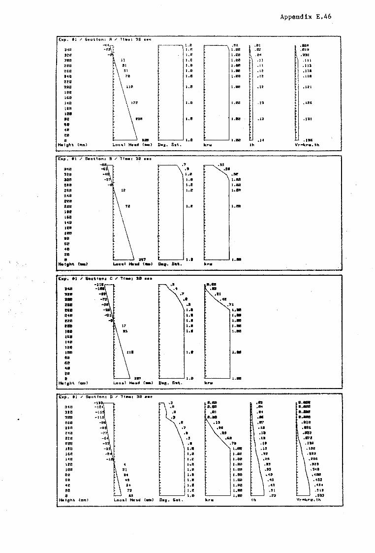
Appendix E.46

!:xp. ti / s~ctl<>n: A / TllOal 31! UC nl.l! .!2 .Ill • BM 34B 1.11 1.112 • BC .J!U 3'20 1.l! 1.1!1!! .e~ .me :Jl!l!t 1.0 1.ee . !l ,Ill

Hl! I.I! l .llll!I .11 .1111 26l! I .I! l.R .12 • tll

HB I ,ll 1.110 .12 .tUI

UB !.Ile LI! ·I .Bl! , It • II! I

181!1 ISi! HI! l .I! 1.110 .n ,1U

128 108 IH!l 1.1 I .Ill! , 13 .\1t 8111 41!

211 e 1811 I.I! 1.111!1 ,14 .1111

Heigh\ 1 .... , L.oc"l H.ad (-) ll•s. s.t. ....... lh v .. -i.. .. ..,, , ..

i:: .. ,,. tl / Scctlon1 B / Tl.,.1 31! sec

.7 .35 34l! .11 .111

321!1 I.I! .51! 3111l!t 1.111 1.ee HI! 1.a 1.ee 2S0 12 1.1!1 hll8

Ul!l 2H ilill! ••• I .llllJ

Jiil IH

'"" 11!8 Ute 8111 68 411 20 ti H7 ••• 1.• ....... , ,_, L.ac•I ....... (-) Deg. S•t. .....

£wp, •1 .I c .I Tf-1 Ill He .... H8 •• HI! ·" H8 •"' 2811 ,?1

HI! ••• 1,• 148 l.I , .• zze 1.1 1.111 1811 t.• 1.ee

lU 1.1 1.1111

1'8 1411 12' llilll I.II 1.• ee 111!1 411

!fl

• 1117 1.e 1.1111 liotfgh<t, (""") 1. ..... 1 Hotad c-> llq. Sat. ..... Exp. u ll .' TIMI 31!1 ••c . ... .m ··-:HS a.a .... ....

31!1! • 1111 .... ..... 31!1i! a.a •• ··-2H .111 ,1!11 .rue 2Slil .11• .Jll .as 2~2 •• .ti .1:11 220 .1 .se .11 21lB .I .71 .11 .au 181! 1.11 1.118 .u .ute 161!! 1.11 1.es ,I!!

HJ! 1,e 1.u ,25

121! 4 I.II 1.ee ,13 .\'28

1ee 21 1.e 1.ee .ss .3~1

80 u 1.11 1.1111 ,49 • 4811 69 49 1.11 1.aa .45 ,111s

41il a+ I.I! 1.ee .4S ,494

!!I! rt I.I! I .Bl! .!! .!13 e 11.5 1,e 1,88 .ll, .S3J

Hstgkt (111ml Local Head (-) D•s. Sat. ...... th v .. -i. ...... , ..

Exp. 11 I Section: A I Tilftt: 30 &ec Appendix

Heioht Local Head Deg. Sat. Rel. Per11. Hydraulic Grad. krw x ih <wnnl (lnl!l) 356 -44 0.98 0.925 0.01 0.009 340 -2S 1. 00 1. 000 0.02 0.019 320 -9 1. 00 1. 000 0.04 0.030 300 11 1. 00 1. 000 0.11 0 .111 280 31 1. 00 1. 000 0 .11 0 .113 260 51 1. 00 1.000 0.12 0.116 240 70 1. 00 1.000 0.12 0 .118 200 110 1. 00 1. 000 0.12 0 .121 140 170 1.00 1.000 0.13 0.126 80 230 1. 00 1.000 0.13 0.131 0 309 1. 00 1. 000 0.14 0.136

Width 312.4"" Ten T . 16.6 dea C . Uoid Ratio e : 0.547 Sat. Pen~ ks : 0 . 395 c.isec Eff, Sat. Area : 125.7 - Rel. Flow Rate : 39.7 111111

Flow Rate : 49 . 0 cu c11/aec

Exp. 11 I Section: B I Tinie: 30 sec

Heiaht Local Head Deg. Sat. Rel. Penn. cal (1111) 356 -80 0 .75 0.349 340 -65 0.86 0.580 320 -46 0.97 0.896 300 -27 1. 00 1.000 280 -8 1. 00 1. 000 260 12 1. 00 1.000 200 70 1.00 1.000

0 267 1. 00 1. 000

Width 312.4 .. Uoid Ratio e : 0.547 Eff. Sat. Area : 123.9 -Exp. 11 / Section: CI Ti11e: 30 aec

lleiaht Local Head Deg. Sat. Rel. Pen. c•> <•> 356 -119 0.21 0.003 340 -109 0.39 9.023 320 -92 0.65 11.209

. 308 - -'5 11.19 0.422 280 -58 8.91 0.114 .260 .39 1.00 1.000 240 -21 1.00 1.000 220 ..:3 1.00 1.000 200 17 1.00 1.000 180 35 1.00 1.000 100 110 1.00 1.000

0 207 1.00 1.000

Width : 312.4 -Uoid Ratio e : 0.547 Eff, Sat. Area : 115.3 -Exp. 11 I Section: D I Ti11e: 30 aec

Heioht Local Head Deg. Sat. Rel. Pena. H9draulic Grad. krw x ih Cm) <•> 356 -133 0.19 340 -124 0.23 320 -115 0.30 300 -119 0.27 280 -96 0.59 260 -88 0.70 240 -71 0.77 220 -64 0.87 200 -53 0.93 180 -39 1. 00 160 -24 1.00 140 -10 1. 00 120 4 1.00 100 21 1.00 80 34 1.00 60 49 1.00 40 64 1. 00 20 79 1.00 0 95 1. 00

Width 312 .4 lllll Ooid Ratio e : 0.547 Eff. Sat. Area : 100.5 111m

0.000 0.03 0.000 0.001 0.04 0.000 0.006 0.04 o.noo 0.003 0.06 0.000 0.135 0.07 0.010 0.264 0.10 0.026 0.393 0.13 0.052 0.597 0.13 0.075 0.781 0.18 0.139 1. 000 0.19 0.190 1. 000 0.22 0.222 1.000 0.29 0.286 1.000 0.33 0.328 1. 000 0.35 0 .340 1.000 0.40 0.400 1. 000 0.45 0.455 1.000 0.49 0 .494 1.000 0.51 0.513 1. 000 0.53 0.533

TeRltl T : 16.6 deo C Sat. Perm~ ks : 0.395 cmi&ec

Rel. Flow Rate : 76.1 mlii Flow Rate : 93.9 cu cm/sec

E.47

Appendix E.48

E.Jcp. •1 /Section: A ,; Tim•t 61'! ... c

1,1! ,H .Ill .2ll !•ll 1.11 \

I.ell .112 ,llH 321! 1.e 1.111! .es .1!4? 3111! e I .Ill ! .lllll .H .14~

2811 28 1.11 ),Q .15 .148 261! 1!4B li9 1.1!1 1.ee •JS .in l!l!ll l!BB 1.1 I.Bl! ·" , IGI! 188 tse 1.111 I.Ill! .1? .166 141!

IH 1.e 1.ae .17 .171!1 UUI 811 61! 41! l!I! e •11? • ' .. l.ll! .17 .1?8

H•l9ht c-i l...ac•I H1nd (tlll'l) lleg. s.t. ..... th v ........ lh

£1cp. •I / SectlDnt BI' Tl-1 6lil •••

-118 .lit 341! -1• ... ll

128 ~s .?5 31!111 1.11 1.111 2811 1.e 1,1111 HB :s J,8 1.u 241! 1.11 1.811 1!2&1 :1!81!1 191! 168 141'J 111 UIJll 1.e ,,., Ill 68 41! IS ., 1!5& ••• 1.n

Haltht. t .. J Loo:•l tho.ad •-> P.1. S•t.. ""• s:..,.. •1 / C I' Tt .. 1 88 aeo

• 11 .... 14• .a ••• 128 •• • 111 38111 •• , II 1!111 •• ,II 11111 .11 .It 14111 ••• ... 118 ••• • •• 1!A &.• t,llB IH 1.11 ••• &Ill 148 121! Ullll 1.• l.81l

•• 68 411l llll e , .. ,,. l.1!11

Heigh\ t-> l..acal He1ul t-l 111tg. Sa1., ..... & .. p. •1 / S.otlont D I' Tl-t 61! ••o

•IH ••• • .1111 ··-Hll -Ull! 11.1111 .m 1!1.1181! HI! -II ••• .&I 11.1:111! HI! ,ll .81 .as ··-Ill! ,11 •• l!l.11118

Hll .4 .flP ... , 241! -1 .s .81 .1185

l!U ,I .111 .au: 288 •• .13 Ull! .a .GI

168 1.8 .11

141! 1.a l.811

ll!B l.llr i,aa , .. ' I.I! 1.ea .n:i BB 21 ) ,I! 1,118 ,llS .:as2 Sil :\Iii 1.1!1 I.Ille .H .444

411 51 1.11 1.111! .511 .!IBB

21'1 C7 1.a 1.811 ,!I .51' Ill \ 14 1.11 1,111! .~I ,$1'1

Hefght c ... , Local He•d t-l Deg. Sat. krw lh Vr•k,.w. th

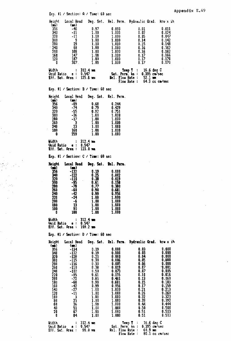
Exp. fl I Section: A I Ti111e: 60 sec Appendix E.49

Heioht (wn)

Local Head (ml -46

Deg. s~t. Rel. Per~. Hydraulic Grad. krw x ih

356 340 320 300 280 240 200 160 120

0

-31 -11

9 29 68

108 147 187 307

0.97 1. 00 1. 00 1. 00 1. 00 1. 00 1. 00 1. 00 1.00 1. 00

0.893 1.000 1.000 1. 000 1. 000 1. ODO 1.000 1.000 1.000 1. 000

0.01 0.02 0 .OS 0.14 0.15 0.16 0.16 0.17 0.17 0.17

0.011 0 .024 0.047 0 .142 0.148 0.162 0.162 0.166 0.170 0.170

Width 312.4 118 Uoid Ratio e ! 0,547 Eff. Sat. Area : 125.6 11111

Te111> T : 16.6 dea C Sat. Pena~ ks : 0. 395 caisec

Rel. Flow Rate : 52.1 lllll Flow Rate : 64.3 cu ca/sec

Exp. 11 I Section: B I Till!!: 60 sec

Heiaht c.ni 356 340 320 300 280 260 240 100

0

Local Head (•) -89 -74 -55 -36 -17

3 23

160 259

Deg. Sat. Rel. Per111.

0.68 0.244 0 . '.79 0 . 429 0.92 0.751 1. 00 1. 000 1. 00 1. 000 1.00 1.000 1.00 1.000 1. 00 1. 000 1.00 1.000

Uidth 312.4 .. Uoid Ratio e : 0.547 Eff. Sat. Area : 123.0 11111

Exp. 11 I Section: CI Ti11e: 60 sec

Height <•> 356 340 320 300 280 260 240 220 200 180 100

0

Local Head <•> -132 -122 -110 -95 -?8 -60 -42 -24 -6 13 90

188

Deg. Sat . h 1. Pan1.

0.19 0.000 0.25 0.002 0.38 0.019 0.61 0.158 0.77 0.380 0.90 0.681 0.99 0;956 1.00 1.000 1. 00 1. 000 1. OD 1. 000 1. 00 1.000 1.00 1.000

Width 312.4 .. Uoid Ratio e : 0.547 Eff. Sat. Area : 109.2 111

Exp. 11 I Section: D I Ti11e: 60 sec

Heiaht <Iii> 356 340 320 300 280 260 240 220 200 180 160 140 120 100

Local Head <•> -134

Deg. Sat. Rel. Pen. Hydraulic Grad. 1cr111 x ih

80 60 40 20 0

Width

-132 -128 -115 -116 -110 -102 -95 -72 -60 -42 -27 -11

3 21 36 51 67 84

Void Ratio e : Eff. Sat . Area :

0.19 0.19 0.21 0.30 0.30 0.38 0.50 0.61 0 .Bl 0.90 0.99 1.00 1. DO 1. DO 1. 00 1. 00 1. 00 1. 00 1. 00

312.4 11111!

0.547 90.0 11111

0.000 0.000 0.000 0.006 0.005 0.019 0.073 0.155 0.461 0.681 0.956 1.000 1.000 1.000 1.000 1. 000 1.000 1. 000 1.000

0.03 0.03 0.04 0.05 0.06 0.07 0.07 0.10 0.13 0.15 8.17 0.21 0.26 0.32 0.39 0.44 0.50 0.51 0.51

0.000 0.000 0.000 0.000 0.000 ·0.001 0.005 0.016 0 .060 0.103 0.159 0.213 0.260 0.323 0.392 0.444 0.500 0.513 0.513

Temn T 16.6 dea C Sat. Perm~ ks : 0.395 c•/sec

Rel. Flow Rate : 64.9 11m Flow Rate : 80.1 cu cm/sec

Appendix E.50

E-8. Measured Outflow froa the drainage face. Experlllent no. 2.

Listings of the results for the outflow measured from the drainage

(Seepage) face for experiment no. 2 is given here. The outflow was

measured for four runs of the experiment. The outflow is recorded as

·the quantity Qt collected in time t draining from the experiment. Also

listed is the reduction of the results showing the mid-interval flow

rate calculated as Qt/t and a plot of the results showing the calculated

average mid-interval flow rate versus the mid-interval time from the

start of the experiment.

Exp. 12. I Run I 1 Appendix E.51

Start End quantity Q Tine t Ti11e Step. flow Rate. (sec> (sec> (cu e11l (sec:> (sec) (co cm/sec)

15 20 840 5 17.5 168.0 20 25 900 5 22.5 180 .o 25 30 860 5 27.5 1n.o 30 35 715 5 32.5 143.0 35 40 840 5 37.5 168.0 40 45 690 5 42.5 138.0 45 50 700 5 47.5 140.0 50 55 620 5 52.5 124.0 55 60 620 5 57.5 124.0 60 65 600 5 62.5 120.0 65 70 550 5 67.5 110.0 70 75 580 5 n.5 116.0 75 80 510 5 77.5 102.0 90 BS 520 5 82.5 104.0 85 90 460 5 87.5 92.0 90 95 490 5 92.5 98.0 95 100 510 5 97.5 102.0

105 111 370 5 107.5 74.0 110 115 368 5 112.5 73.6

Exp. 12. I Run I 2 Append ix E: 52

Start End quantity Q Tiw t Time Step. Flow Rate. (sec) (!eel (cu c111) (sec) (sec) (cu Cllllsec>

15 20 780 s 17.5 156.0 20 25 840 s 22.5 168.0 25 30 740 5 27.5 148.0 30 35 730 5 32.5 146.0 35 40 630 5 37.5 126.0 40 45 685 5 42.S 137.0 45 50 600 5 47.5 120.0 50 55 565 5 52.5 113.0 55 60 550 5 57.5 110.0 60 65 520 5 62.5 104.0 65 70 515 5 67.5 103.0 70 75 520 5 n.5 104.0 75 80 485 5 77.5 97.0 80 85 460 5 82.5 92.0 85 90 435 5 87.5 87.0 90 95 440 5 92.5 88.0 95 100 415 5 97.5 83.0

100 105 420 5 102.5 84.0 105 115 780 10 110 .0 78.0 115 125 760 10 120.0 76.0 125 135 750 10 130.0 75.0 135 145 700 10 140.0 70.0 145 155 660 10 150.0 66.0 155 165 660 10 160.0 66.0

. . ~ ·. 165 175 661 10 110.0 61.0 175 185 630 10 180.0 63.·0 185 195 621 10 190.0 62.0 195 205 600 10. 200.8 60.0 205 215 600 10 21'0.0 60.0 215 ·225 575 10 220.0 57.5 225 235 570 10 230.0 57.0 235 245 540 10 240.0 54.0 245 255 540 10 250.0 54.0 255 265 510 10 260.0 51.0 265 275 515 10 270.0 51.5 275 285 505 10 280.0 50.5 285 300 740 15 292.5 49.3 300 315 no 15 307.5 48.0 315 330 700 15 322.5 46.7 330 345 680 15 337.5 45.3 345 360 680 15 352.5 45.3 360 375 650 15 367.5 43.3 375 390 630 15 382.5 42.0 390 405 635 15 397.5 42.3 405 420 600 15 412.5 40.0 420 435 580 15 427.5 38.7 435 450 600 15 442.5 40.0 450 465 570 15 457.5 38.0 465 480 560 15 472.5 37.3 480 495 550 15 487.5 36.7 495 510 550 15 502.5 36.7 510 525 520 15 517.5 34.7 525 540 530 15 532.5 35.3 540 555 500 15 547.5 33.3 555 570 510 15 562.5 34.0 570 585 480 15 577.5 32.0 585 600 480 15 592.5 32.0 600 630 920 30 615.0 30.7 630 660 900 30 645.0 30 .o

Exp. 12. I Run I 2 Appendix E.53

Start End quantity Q Time t Tiwte Step. Flow Rate. (sec) Caecl (cu c•l (sec) (sec) (cu ctalsec)

660 690 860 30 675.0 28.7 690 720 840 30 705.0 28.0 720 750 800 30 735.0 26.7 750 780 765 30 765.0 25.5 780 810 750 30 795.0 25.0 810 840 730 30 825.0 24.3 840 870 700 30 855.0 23.3 870 900 685 30 885.0 22.8 900 930 665 30 915.0 22.2 930 960 645 30 945.0 21.5 960 990 620 30 975.0 20.7 990 1020 610 30 1005.0 20.3

1020 1050 580 30 1035.0 19.3 1050 1080 570 30 1065.0 19.0 1080 1118 540 30 1095.0 18.0 1110 1140 550 30 1125.0 18.3 1140 1170 520 30 1155.0 17.3 1170 1200 510 30 1185.0 17.0 1200 1230 490 30 1215.0 16.3 1230 1260 475 30 1245.0 15.8 1260 1320 910 60 1290.0 15.2 1320 1380 870 60 1350.0 14.5 1380 1440 810 60 1410.0 13.5 1440 1500 m 60 14'0.0 12.9

.. 1508 1561 '50 60 1530.t 12.5 1560 1620 ?81 60 1598.0 11.? 1620 1680 670 60 .1650.0 11.2 1680 1740 645 60 1110.0 10.7 1?40 1800 610 10 1710.I 11.2 1800 1•0 581 60 1830.0 9.? 1860 1920 555 60 1890.0 9.3 1920 1980 535 60 1958.0 8.9 1980 2140 520 60 2010.0 8.7 2040 2100 480 60 2070.0 8.0 2100 2220 910 120 2160.0 ?.6 2220 2340 835 120 2280.0 1.0 2340 2460 ?10 120 2400.0 6.4 2460 2580 105 120 2520.0 5.9 2580 2700 660 120 2640.0 5.5 2700 2820 605 120 2760.0 5.0 2820 2940 560 120 2880.0 4.7 2940 3060 525 120 3000.0 4.4 3060 3180 490 120 3120.0 4.1 3180 3300 455 120 3248.0 3.8 3300 3540 810 240 3420.0 3.4

Exp. 12' I Run I 3 Appendix E.54

Start End quantity Q Time t Ti11e Step. Flow Rate. (sec) (sec) (cu cal (sec) Caec) (cu C9/sec)

15 20 810 5 17.5 162.0 20 25 880 5 22.5 . 1?6 .o 25 30 745 5 27.5 149.0 30 35 740 5 32.5 148.0 35 40 640 5 37.5 128.0 40 45 650 5 42.5 130.0 45 50 590 5 47.5 118.0 50 55 550 5 52.5 110.0 55 60 540 5 57.5 108.0 60 85 515 5 62.5 103.8 65 70 495 5 67.5 99.0 70 '5 495 5 n.5 99.0 75 80 470 5 77.5 94.0 80 85 445 5 82.5 89.0 85 90 420 5 87.5 84.0 90 95 440 5 92.5 88.0 95 100 435 5 97.5 87.0

100 110 805 10 105.0 10.5 . 110 120 7J5 10 115.0 77.5 120 130 730 10 125.0 73.0 130 140 720 10 135.0 72.0 140 150 705 10 145.0 70.5 150 160 650 10 155.0 65.0 160 170 640 10 165.0 64.0 170 180 621 10 1?5.1 62.0 180 190 621 10 185.0 62.0 190 200 590 18 195.0 59.0 200 210 560 10 205.0 56.0 210 220 570 10 215.8 57.0 220 230 518 10 225.0 56.0 230 240 540 10 235.0 54.0 240 250 540 10 245.0 54.0 250 260 490 10 255.0 49.0 260 270 530 10 265.0 53.D 270 280 510 10 2'5.0 51.0 280 290 4'8 10 285.0 47.0 290 300 500 10 295.0 50.0 300 315 700 15 307.5 46.7 315 330 660 15 322.S 44.0 330 345 685 15 337.5 45.7 345 360 640 15 352.5 42.7 360 380 830 20 370.0 41.5 380 400 840 20 390.0 42.0 400 420 780 20 410.0 39.0 420 440 7J5 20 430.0 38.8 440 460 760 20 450.0 38.0 460 480 720 20 470.0 36.0 480 500 ?00 20 490.0 35.0 500 520 695 20 510.0 34.8 520 540 685 20 530.0 34.3 540 560 645 20 550.0 32.3 560 580 635 20 570.0 31.8 580 600 615 20 590.0 30.7 600 630 910 30 615.0 30.3 630 660 860 30 645.0 28.7 660 690 825 30 675.0 27.5 690 720 810 30 705.0 27 .o no 750 800 30 735.0 26.7 750 780 ?50 30 765.0 25.0

Exp. 12. I Ron I 3 Appendix E.55

Start . Eoo quantity Q Ti111e t Ti111e Step. Flow Rate. (sec) (sec) (cu e11l (sec) (sec) (co c11/sec)

780 810 730 30 795.0 24.3 810 840 715 30 825.0 23.8 840 870 680 30 855.0 22.7 970 900 665 30 885.0 22.2 900 930 630 30 915.0 21.0 930 960 625 30 945.0 20.8 960 990 595 30 975.0 19.8 990 1020 595 30 1005.0 19.8

1020 1050 565 30 1035.0 18.8 1050 1080 555 30 1065.0 18.5 1080 1110 540 30 1095.0 18 .0 1110 1140 520 30 1125.0 17.3 1140 1170 510 30 1155.0 17. 0 1170 1200 500 30 1185.0 16.7 1200 1260 945 60 1230.0 15.9 1260 1320 900 60 1290.0 15 .o 1320 1380 845 60 1350.0 14.1 1380 1440 815 60 1410.0 13.6 1440 1500 780 60 1470.0 13.0 1500 1560 715 60 1530.0 11.9 1560 1620 700 60 1590.0 11.7 1620 1690 650 60 1650.0 10.8 1680 1740 640 60 1710.0 10 .7 1740 1800 600 60 1770.0 10.0 1800 1860 570 60 1830.I ·9,5 1860 1920 550 60 1890.0 9.2 1920 1980 520 60 1950.0 8.7 1980 2140 500 60 2010.0 8.3 2040 2100 480 60 2070.0 8.8 2100 2220 895 120 2160.0 7.5 2220 2340 820 120 2280.0 6.8 2340 2460 760 120 2400.0 6.3 2460 2580 690 120 2520.0 5.8 2580 2700 635 120 2640.0 5.3 2700 2820 590 120 2760.0 4.9 2820 2940 540 120 2880.0 4.5 2940 3060 500 120 3000.0 4.2 3060 3180 460 120 3120.0 3.8 3180 3300 430 120 3240.0 3.6 3300 3420 385 120 3360.0 3.2 3420 3540 370 120 3480.0 3.1 3540 3660 330 120 3600.0 2.8

Exp. t2. I Rur. I 4 Appendix E.56

Start End quantity Q Time t Tiae Step. Flow Rate. (sec) (sec) (cu C111) (sec) (sec) (cu c./sec)

15 20 950 5 17.5 170.0 20 25 780 5 22.5 156.0 25 30 780 5 27.5 156.0 30 35 690 5 32.5 138.0 35 40 650 5 37.5 130.0 40 45 650 5 42.5 130.0 45 50 560 5 47.5 112.0 50 55 570 5 52.5 114.0 55 60 540 5 57.5 108.0 60 65 510 5 62.5 102. 0 65 70 530 5 67.5 106.0 70 75 460 5 n.5 92.0 75 80 460 5 77.5 92.0 80 85 480 5 82.5 96.0 85 90 445 5 87.5 89.0 90 95 440 5 92.5 88.0 95 100 420 5 97.5 84.0

100 110 830 10 105.0 83.0 110 120 760 10 115.0 76.0 120 130 800 10 125.0 80.0 130 140 700 10 135.0 70.0 140 150 670 11 145.0 67.0 150 160 670 10 155.0 67.0 160 170 640 10 165.0 64.0 110 180 640 10 .1'5.0 64.0 180 195 880 15 187.5 58.7 195 210 880 15 202.5 58.7 210 225 845 15 217.5 56.3 225 240 830 15 232.5 55.3 240 255 790 15 241.5 52.7 255 27'0 '50 15 262.5 50.0 270 285 740 15 277.5 49.3 285 300 '50 15 292.5 50.0 300 320 935 20 310.0 46.8 320 340 890 20 330.0 44.5 340 360 885 20 350.0 44.3 360 380 840 20 37'0.0 42.0 380 400 835 20 390.0 41.7 400 420 BOO 20 410.0 40.0 420 440 785 20 430.0 39.3 440 460 760 20 450.0 38.0 460 480 m 20 470.0 38.5 480 500 700 20 490.0 35.0 500 518 590 18 509.0 32.8 518 540 770 22 529.0 35.0 540 560 650 20 550.0 32.5 560 580 650 20 570.0 32.5 580 600 620 20 590.0 31. 0 600 630 920 30 615.0 30.7 840 870 720 30 855.0 24.0 870 900 695 30 885.0 23.2 900 930 675 30 915.0 22.5

1455 1500 605 45 1477.5 13.4 1500 1545 575 45 1522.5 12 .8 1830 1860 300 30 1845 .o 10.0 2280 2340 432 60 2310.0 7.2 2400 2460 420 60 2430.0 7.0

Appendix E.57

Flow Rate v's Time u 200 II) I') 190

' IBB E u

170 :I 160

txperfment no, 2 Time Q u 150 (min) (cm 3 Is)

I) 140 ., 130 48,5 "' 5 0:: 120

3 110 10 30,5 0

100 15 22,3 ~ 90 22,5 14,8 3 80 30 9,9 0 70 ... 60 ., :J 0

Se "10

I) 31! tn

"' 20 g_ I)

1111 u lll

1110 s 10 15 2e 25 30 35 "10 "' 5e 55 60

Time from start cf Exp. (ml n)

Flow Rate v's Time

100000

90000

80020 Experiment. no. 2

E u

70000 :I u

60000

50000 3 c ... '4000B ., :I

0 30002 I)

> 20000 .,

"' :I 113000 E! :I u

5 10 15 20 25 30 35 40 45 se 55 60

Time from start cf Exp. (min)'

Appendix E.58

E-9. Sidewall piezometer levels recorded. Experiment no. 2.

Listings of the results for the sidewall piezometer levels recorded for

experiment no. 2, are given here. The readings are recorded with

respect to time and the result given as the elevation (mm) above the

base of the flume. A single value for each vertical set of piezometers.

recorded, is given. The readings are referenced by a reference number

as shown in figure (5.19)

Appendix E.59

Experiment no. 2 I Piezometer results. I Time (min) v's Total head (mm)

P iezometer Time from start of experiment (min) Ref. no. 2 5 10 15 20 25 30

PA '/,,o

PB 140 105 ''\ 82 69 60 55 51 PC 147 124 i~ 94 79 73 66 59 PD 173 138 llO 85 78 71 65 PE 187 151 1 ~ 123 96 85 75 68

I> PF 206 168 134 108 93 81 72 PG 223 180 140 ll5 94 83 74 PH 234 187 147 120 97 84 76 PI 247 204 156 128 101 91 83 PJ 262 214 165 134 ll3 98 83 PK 270 222 171 139 ll8 100 84 PL 277 228 180 144 121 103 90 PM 284 235 184 149 124 107 95 PN 285 245 188 152 128 108 97 PO 292 250 194 156 130 ll2 100 pp 295 253 199 159 135 ll5 102 f.

PQ 298 257 201 164 137 ll2 103 PR 302 264 209 168 140 ll8 103 PS 308 270 210 169 141 121 104 PT 308 275 212 171 143 123 109 PU 309 278 218 175 147 126 110 PV 309 280 218 177 149 126 lll PW 310 281 220 180 150 127 113 PX 310 284 223 182 152 129 ll3 PY 3ll 287 226 182 152 129 113 PZ 312 288 230 182 153 130 114

Appendix E.60

E-10. Transducer 110nitored tensiometers. Experiment no. 2.

Listings of the results for the tensiometers, recorded for experiment

no. 2, are given here. The recordings were made by the computer

controlled data-acquisition unit. (See chapter 3) Four sets of readings

are given for the four repeated experiment runs made. The readings are

recorded with respect to time and the result given as the elevation (mm)

above the base of the flume. For each run a new set of tens iometers

were roonitored. The actual tensiometer roonitored is referenced by a

reference number whose position is shown in figure (5.8)

Also given are the plots, for each tens iome ter recorded, showing the

total head versus time.

Appendix E.61 ~XPff I "ENT ~io. 2 I RUN NO. l

TIME TAO TA4 TAB TAI~ TEO TE4 TEE TE12 TKO TK4 TKO TKl2 TM4 TK12 TOO TOB

-60 ! 381 ! 381 ! 381 I 381 I 381 I 381 I 38! 381 I 381 ! 381 l 381 I JBI ! 381 I 381 l JB! ' 3B! ' -55 '. 380 ! 381 380 I 384 ! 380 I 381 I 38i 381 ! 380 I 381 I 380 I 381 ! 381 l 381 380 I 381 1

-48 1 38(1 1 JBJ 1 424 1 377 1 379 38! 1 381 1 381 1 38(1 ! 381 1 380 ! 38) ! 381 1 381 380 1 381 -43 ! 380 I 380 I 380 I 379 I 380 I 381 I 381 I 380 ! 379 ! 380 ! 380 ! 38! I 380 I 381 I 380 ! 381 I

-36 I 381 I 381 ! 380 ! 381 I 379 ! 381 1 380 ! 381 ! 380 ! 380 ! 379 I JBJ 1 380 ! 380 I 379 I 380 1

-31 1 380 1 380 I 424 I 381 1 379 ! 381 ! 380 1 380 I 380 1 380 1 380 1 381 1 380 1 380 1 380 1 380 1

-25 ! 38Q ! 380 ! 379 ! 378 ! 378 ! 381 I 380 ! 380 I 379 ! 300 ! 380 : 38! I 380 I 380 I 380 ! 38(1 '. -20 ! 380 1 379 ! 379 l 377 1 379 ! 380 .! 380 1 381 1 379 1 300 ! 379 ! 380 1 380 ! 380 1 379 1 380 1

-13 ! 380 ! 380 ! 381 1 377 1 380 380 ' 380 ! 380 ! 379 1 380 1 379 1 381 1 380 ! 380 1 379 ! 380 i

-8 ! 380 ! 380 ! 424 1 382 ! 381 1 380 ! 380 ! 381 ! 380 ! 380 ! 379 1 381 1 380 ! 380 ! 379 1 380 ! -1 ! 380 I 380 I 424 I 376 I 380 ! 381 I 380 I 380 I 380 t 380 ! 380 ! 381 ! 380 I 380 I 380 ! 381 1

4 I 299 ! 282 ! 282 I JQQ ! 334 ! 332 ! 33~ ! 342 ! 370 ! 371 I 369 I 371 ! 376 ! 377 ! 378 I 378 ! 9 ! 119 I 143 ! 249 ! 256 ! 262 ! 268 I 280 ! 294 ! 389 I 339 ! 337 l 338 ! 352 ! 354 ! 358 I 359 !

!b I 98 I 135 I 190 I 224 I 250 I 253 I 265 I 278 ! 318 ! 402 I 317 ! 31b I 330 l 331 ! 334 ! 335 I

22 ! 95 ! 131 ! 180 ! 202 ! 24! ! 244 ! 256 l 266 ! 314 ! 314 ! 312 ! 313 I 380 ! 323 ! 323 I 326 \ 28 l 93 I 126 I 169 ! 200 I 233 ! 235 I 246 I 325 l 311 ! 312 I 311 ! 311 I 317 I 321 ! 321 ! 322 ! 34 f 91 ! 123 1 160 ! 198 ! 227 I 229 ! 240 ! 252 ! 309 1 309 1 309 ! 308 ! 316 ! 32(! ! 320 1 321 1

4o : ea ! 119 ! 1s1 ! 191 ! 220 ! 223 ! 232 ! 244 1 305 : 308 ! 305 ! 306 ! 316 ! 319 1 319 ! 320 ! 45 I 80 ! 116 ! 146 ! 204 ! 216 ! 218 ! 227 ! 239 ! 304 I 308 ! 303 I 303 I 314 ! 318 1 318 ! 319 '. 52 ! 83 ! 112 ! 138 ! 193 ! 209 ! 211 ! 221 ! 231 ! 300 ! 304 ! 300 ! 3QQ ! 313 I 315 ! 318 ! 318 ! 58 ! 83 110 ! 135 1 198 1 206 ! 208 ! 217 ! 228 ! 298 ! 302 ! 297 1 298 ! 312 ! 315 1 318 1 310 1

04 ! 81 I 107 ! 130 ! 195 ! 201 ! 203 I 212 ! 222 ! 295 ! 290 ! 294 ! 294 ! 372 ! 313 ! 316 ! 317 ! 70 ! BO I 104 I 127 I 195 l 198 ! 200 ~ 208 ! 218 ! 293 : 296 ! 292 ! 292 I 310 ! 312 ! 317 I 316 I

l6 ! 79 ! 102 ! 125 ! 193 ! 194 ! 195 ! 204 ! 215 ! 290 ! 293 I 289 I 290 ! 308 I 310 ! 315 ! 315 ! 82 ! 78 ! 101 ! 165 ! 186 ! 191 I 193 ! 200 ! 212 ! 287 ! 292 ! 287 ! 288 I 308 I 309 ! 314 ! 315 I

89 ! 77 ! 99 ! 119 ! 193 ! 188 ! 187 ! 197 ! 211 ! 285 ! 290 ! 285 ! 285 ! 306 ! 307 ! 313 ! 313 ! 94 ! 76 ! 139 ! 119 ! 188 186 ! 184 I 195 ! 209 ! 283 ! 288 ! 282 ! 284 ! 304 ! 305 ! 311 ! 309 l

99 I 75 ! 155 ! 118 I 181 ! 183 ! 181 ! 191 ! 208 ! 281 ! 285 ! 281 ! 281 ! 302 ! 303 ! 309 ! 306 ! 106 74 ! 89 ! 117 ! 188 ! 180 ! 180 ! 190 ! 207 ! 278 ! 283 ! 278 ! 279 ! 3{l(l ! 301 ! 308 ! 351 I

111 ! 74 ! BB ! 116 ! 186 ! 179 ! 177 ! 187 ! 205 ! 277 ! 281 ! 276 ! 276 ! 299 ! 300 ! 306 ! 304 ! 117 ! 73 ! 87 ! 115 ! 190 ! 176 ! 175 ! 185 ! 205 ! 275 ! 280 ! 274 ! 275 ! 297 ! 298 ! 305 ! 348 I

122 ! 73 ! 85 ! 116 ! 185 ! 176 ! 175 ! 182 ! 204 l 273 ! 278 ! 273 ! 273 ! 296 ! 297 ! 303 ! 347 ! 128 I 72 ! 188 ! 114 ! 183 ! 173 173 ! 180 ! 203 ! 270 ! 275 ! 27Q ! 270 ! 293 ! 294 I 301 ! 299 ! 134 ! 71 ! 188 ! 114 ! 182 ! 171 ! 172 ! 174 ! 202 ! 269 ! 273 ! 268 ! 268 ! 292 ! 294 ! 300 ! 299 I

140 ! 71 ! 188 ! 114 ! 177 ! 169 ! 170 ! 172 ! 202 ! 266 ! 271 ! 266 ! 2Qb ! 290 I 292 ! 29& I 298 ~

146 I 70 ! 187 ! 113 ! 180 ! 168 ! 170 ! 170 ! 202 ! 264 ! 269 ! 264 ! 264 I 288 l 290 ! 296 ! 296 ! 152 ! 70 ! 83 ! 112 I 181 ! 166 ! 170 ! 169 ! 201 ! 263 ! 267 ! 262 ! 263 ! 287 ! 290 ! 294 I 295 I

157 ! 69 ! 185 ! 113 ! 177 ! 165 ! 167 ! 167 ! 200 ! 261 ! 264 ! 260 ! 260 ! 285 ! 287 ! 293 ! 293 I

163 ! 69 ! BO 113 ! 179 ! 163 166 ! 167 ! 200 ! 259 ! 264 ! 258 ! 258 ! 284 ! 2Bl I 292 ! 292 I

169 ! 68 ! 81 ! 112 ! 181 ! 161 ! 164 ! 165 ! 199 ! 257 ! 262 ! 256 ! 257 ! 282 ! 284 ! 290 ! 289 ! 175 ! 68 I 183 I 112 ! 181 ! 160 ! 163 164 ! 199 ! 255 ! 26Q ! 255 ! 255 ! 281 ! 283 ! 289 ! 289 ! 180 ! 67 I 183 ! 112 ! 174 ! 158 I lol ! 162 ! 198 ! 253 ! 258 ! 253 f 253 ! 279 I 282 ! 287 ! 287 ! 187 ! 67 ! 183 ! 111 177 ! 158 ! 160 ! 163 ! 198 ! 252 ! 257 I 251 ! 252 I 277 ! 280 I 285 ! 286 1

193 ! 67 ! 182 ! 111 ! 179 ! 156 I 158 ! 161 ! 197 ! 250 ! 255 ! 249 ! 249 I 276 ! 279 ! 284 ! 284 ! 198 ! 66 ! 78 ! 111 I 177 ! 154 ! 157 ! 159 ! 197 ! 248 ! 253 ! 248 ! 248 ! 275 ! 277 ! 283 ! 283 205 ! 65 ! 77 ! 110 ! 175 ! 152 ! 155 ! 158 I 196 f 247 ! 252 ! 245 ! 246 ! 272 ! 275 ! 281 ! 281 ! 210 ! 65 ! 77 ! 110 ! 177 ! 151 ! 154 ! 157 196 ! 245 ! 251 I 244 ! 245 ! 272 ! 274 ! 280 ! 281 l

217 ! 65 ! 77 ! 110 ! 174 ! 150 I 152 ! 155 I 196 ! 244 ! 248 ! 243 ! 243 I 270 I 273 I 278 I 279 l

222 ! 65 ! 77 ! 110 ! 173 ! 149 ! 151 ! 154 1 195 ! 242 1 247 ! 241 ! 241 ! 26B 1 271 ! 277 ! 277 ! 229 I 64 ! 75 ! 109 ! 173 ! !40 I 150 I 153 ! 194 ! 240 I 245. ! 239 ! 239 ! 267 ! 269 ! 276 I 276 ! 234 64 ! 74 1 109 ! 175 ! 147 I 150 I J5£ 194 ! 239 l 244 ! 238 ! 239 ! 266 ! 268 ! 275 ! 275 i

241 ! 63 ! 179 ! 109 ! 172 ! 146 ! 148 ! 15J ! 193 I 23i ! 242 I 237 ! 236 I 2b4 I 266 ! 274 '. 274 !

247 l 63 ! 73 I 109 ! 173 I 145 ! 147 ! 150 ! 193 I 236 ! 241 ! 235 I 235 ! 262 I 265 ! 272 ! 27.2 : . 25~ 62 I 74 ! 107 ! J74 I 143 I 146 ! 148 1 192 ! 234 I 239 ! 232 ! 233 ! 260 ! 263 I 270 I 270 1

259 62 ! J2 I 107 ! 172 I 143 145 ! 14/ I 192 ! 232 ! 238 ! 232 ! 232 ! lOU ! 263 2](1 ! 27(! I

266 62 ! 72 I 1(18 1 172 I 141 144 l 146 ! 192 I 231 ! 237 ! 231 ! 231 I 259 ! 261 I 2b9 ! 269 ! 271 b2 I 72 I 107 I 165 I 140 142 ! 145 I 191 I 229 ! 234 I 228 ! 229 I 257 ! 259 I 26] 1 ~6; '. 278 I OJ 73 1 J(J/ 1 169 I !39 142 f g4 192 ! 228 I 234 I 228 I 2:z!l I 256 ! i'56 I 266 1 266 I

283 I 61 I 72 ! 107 ! jJj ! 138 141 I 143 190 I 22l I 23: ! 226 ! 226 I 255 I 257 I 264 I 265 I

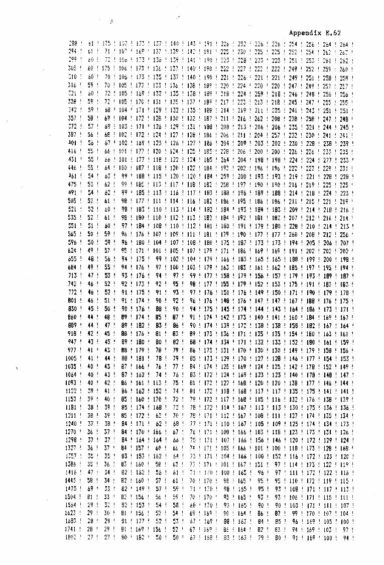
.::BB ' 29~ I

bl 6! I

/\

!75 I 107 I tn I 137 ! 14(1 I !43 I J9j I 226 : 71 1 107 I !69 I 137 I, 139 I 14.:: 191 I 225 I

232 ! 226 I 226

Appendix E.62

254 25b I 264 264 I

I 254 : 26? I 26: I

~99 '. t.(i 72 I 10t l 173 I 136 139 ~ 141 191) ~ 223 228 ~ 223 I 22·3 ! 251 I 253 ! 261 ~ ~b2 ~

305 I b(l I J 75 I J (16 I J 73 I J 36 ! 137 I ) 4(1' I 190 I 222 2n ! 222 I 222 I 249 I 252 I 259 i 26(! 1

310 60 I JQ I 100 ! 173 135 I 13i ! 140 1 19(1 I 22J ! 22b I 221 I 221 1 249 I 25) ! 250 ! 259 I

31b I 5~ ! 70 I 105 I 173 I 133 136 ! 138 I 18° 1 220 ! 224 I 220 I 220 I 247 ! 249 ! 257 ! 257 I

321 60 ! j2 ! 105 169 ! 132 I 135 ! 138 ! 189 I 21B ! 224 259 ! 21B ! 246 248 ! 256 I 256 ! 328 I 59 ! 72 I 105 I 170 131 I 135 I 137 I 189 ! 2ti 223 213 I 218 1 245 247 I 255 ! 255 1

342 ! 59 1 68 1 104 171 129 132 ! 135 ! 188 1 214 ! 219 1 211 1 225 ! 241 243 ! 251 ! 251 '. 357 I 58 ; 69 ! 104 172 128 I 130 ! 132 187 l 211 ! 216 ! 262 ! 208 l 238 258 ! 247 ! 248 i

372 57 ! 69 ! 103 ! 171 120 ! 129 I 131 188 ! 209 ! 213 l 206 ! 206 ! 235 ! 321 ! 244 ! 245 ! 387 56 ! 68 ! 102 ! 172 124 I 127 ! 128 I 180 : 206 211 ; 204 ! 257 I 232 ! 230 ! 241 ! 241 I

401 50 I 67 I 102 ! 169 ! 123 ! 126 l 127 I 106 ! 204 ! 209 ~ 203 ! 202 ! 230 ! 228 ! 238 I 239 I

416 55 I 66 I 101 I 177 ; 120 ! 124 ! 125 I lB~ I 228 I 206 I 200 ! 200 ! 226 ! 226 I 233 1 235 I

431 55 I bb I 101 177 I 118 ! 122 I 124 ! 185 I 264 I 204 I 198 ! 198 I 224 ! 224 ! 277 ! 233 ! 446 55 ! 64 I 10(1 187 ! 118 12(1 I 122 I 184 ! {9J I 202 ! 196 ! 196 I 222 I 22! ! 229 ! 231 I

461 54 I 63 ! 99 I 188 ! 115 I 120 ! 12Q ! 184 ! 259 ! 200 ! 193 ! 193 ! 219 ! 221 ! 228 ! 228 I

475 I 53 I 62 ! qq 185 : 113 1!7 l 118 I 182 I 258 ! 197 1 19(! ! 190 l 216 ! 219 ! 225 : 225 I

491 54 ! 62 ! 99 ! 185 ! 113 116 ! 117 I 183 ! 18B ! 19b l 189 ! 188 ! 214 ! 218 I 224 1 223 ! 505 52 ! 61 I 98 ! 177 I 111 114 ! 116 ! 182 ! 186 ! 195 ! 186 ! 186 ! 211 I 215 ! 221 ! 21 'i' 1

~21 52 ! bQ ! 98 I 183 ! 110 ! 113 ! 114 I 182 ! 184 l 193 ! 184 ! 183 ! 209 I 214 I 218 ! 21b '. 535 52 ! 61 I 98 ! 18(! ! 11() ! 112 ! 113 ! 182 I 184 I 192 181 ! 182 ! 207 I 212 I 216 ! 214 I

551 51 ! bO I 97 ! 184 ! 108 ! 110 I 112 ! 181 ! 180 ! 191 ! 179 ! 180 ! 228 ! 210 ! 214 ! 213 ! 565 50 ! 59 ! 96 ! 176 ! 107 109 111 l 18! l 179 I 190 ! 177 ! 177 ! 260 ! 208 ! 212 ! 256 I

596 ! 50 ! 59 ! 96 I 180 ! 104 ! 107 I 108 ! 180 ! 175 ! 187 ! 173 ! 173 ! 194 ! 205 ! 2Q6 ! 207 ! 624 I 49 ! 57 I 95 ! 171 ! 101 ! 1(15 ! 107 ! 179 I 171 ! 186 ! 169 ! 169 ! 191 ! 202 I 2(12 ! '202 ! 055 ! 48 ! 56 ! 94 ! 175 ! 99 I 102 ! 104 I 179 ! 166 ! 183 ! 165 ! 165 ! 188 ! 199 ! 200 ! 198 ! 684 ! 49 ! 55 ! 94 ! 176 ! 97 ! 100 ! 103 ! 179 ! 163 ! 183 ! 161 ! 162 ! 185 ! 197 ! 19S ! 194 ! i13 ! 47 ! 53 ! 93 ! 176 ! 94 ! 97 ! 99 ! 177 ! 158 ! 179 ! 156 ! 157 ! 179 ! 193 ! 189 ! 187 ! 742 ! 46 ! 52 ! 92 173 I 92 ! 95 ! 98 ! 177 ! 155 ! 179 ! 152 ! 153 ! 175 191 ! 183 ! 183 ! 772 ! 46 ! 52 ! 91 ! 175 ! 91 ! 93 ! 97 ! 176 ! 151 ! 176 ! 149 ! 150 ! 171 ! 190 ! 179 ! 178 ! 801 ! 46 ! 51 ! 91 ! 174 ! 90 ! 92 ! 96 ! 176 ! 148 ! 176 ! 147 ! 147 ! 167 ! 188 ! 176 ! 175 ! 830 ! 45 ! so ! 90 ! 176 ! 98 ! 90 ! 94 ! 175 ! 145 ! 174 ! 144 ! 143 ! 164 ! 186 ! 173 ! 171 ! 860 ! 44 ! 48 ! 89 ! 174 ! 85 ! 87 ! 91 l 174 ! 142 ! 173 ! 140 ! 141 ! 160 ! 184 ! 169 ! 167 I

889 ! 44 ! 47 ! 89 ! 182 ! 83 ! 86 ! 90 ! 174 ! 139 I 172 ! 138 ! 138 ! 158 ! 182 ! 167 164 ! 918 ! 42 ! 45 ! 88 ! 176 I Bl ! 83 ' 89 ! 173 ! 136 ! 171 135 I 135 ! 154 ! 180 ! 163 ! 161 I

ll4j I 43 I 45 ! 89 ! 180 I 90 ! 82 ! 88 I 174 ! 134 I 171 ! 132 ! 133 ! 152 ! 180 ! 161 ! (59 ! 977 l 41 I 43 I ea ! 179 ! 78 ! 79 ! 86 l 173 ! 131 ! 170 ! 130 I 130 ! 149 ! 179 ! 158 I 156 !

1005 ! 41 I 44 ! BB ! 181 ! 78 ! 79 ! 85 ! 173 ! 129 ! 170 ! 127 ! 128 ! 146 I 177 I 154 ! 153 ! 1035 ! 40 ! 43 ! 87 ! 166 I 76 ! 77 ! 94 ! 174 ! 125 ! 169 ! 124 ! 125 ! J42 ! 178 ! 152 ! 149 I

1064 I 40 ! 43 ! 87 ! 162 ! 74 76 ! 83 ! 172 ! 124 169 ! 123 ! 123 ! 140 ! 179 ! 148 ! 147 l

1093 ! 40 ! 42 ! 86 ! 161 ! 113 75 81 {]2 ! 122 ! 168 ! 120 120 ! 138 I 177 ! 146 144 ! 1122 ! 39 I 41 ! 86 ! 162 ! 152 74 I Bl 172 I 118 ! l6B ! 117 ! 117 ! 135 ! 175 ! 141 ! 141 ! 1152 39 ! 4(1 ! 85 ! 160 ! 170 72 ! 79 I 172 ! 117 ! 168 ! 115 ! 116 ! 132 ! 176 ! 138 ! 139 ! 1191 ! 38 ! 39 ! 85 ! 174 ! 160 I 72 ! 78 I 172 I 114 ! 167 ! 113 ! 113 ! 130 ! 175 I 136 ! 136 ! 1211 I 38 I 39 ! 85 ! 172 ! 62 I ](J ! 78 I lrJ 1 112 ! 167 ! 108 ! 111 127 ! 174 ! 135 t 134 I

1240 ! 37 ! 38 ! 84 ! 171 ! 62 ! 68 ! 7i ! 171 110 ! 167 ! 105 ! 109 ! 125 ! 174 ! 134 ! 173 ! 1270 I 36 ! 37 I 84 l 170 I 166 ! 67 ! 76 I 171 toa ! 166 ! 103 ! 118 ! 123 ! 173 ! 131 ! 126 ! 1298 I 37 I 37 l 84 I 164 I 164 I 66 ! 75 ! 1J! I 107 ! 166 ! 156 ! 146 ! 120 ! 172 ! 129 ! 124 ! 1327 I 36 I 37 ! 84 ! 157 ! 6{! ! 66 7~ I 17! 105 ! 166 ! 101 ! 100 ! 118 ! 173 ! 128 ! 168 I

! Z57 ! 35 I 35 I 83 ! 153 I 162 I 64 I 73 ! 171 104 ! 166 ! 100 ! 152 ! 116 ! 172 ! 123 ! 120 ! 1386 ! 35 I 36 ! 83 ! 160 I SB ! 63 73 ' 171 101 ! 167 ! 151 ! 97 ! 114 173 ! 122 I l!C1 I

Hlb I 47 I 34 I 82 ! 162 ! 56 ! 61 71 l 17{! : 100 ! 165 ! 9b ! 97 I 111 ! 172 ! 122 ! 116 ! 1445 ! 58 ! 34 ! 82 ! 160 1 57 ! 61 70 170 1 9B 1 165 ! 95 1 95 ! 11(l ! 172 119 ! 115 ! 1475 i 69 I 33 ! 82 l 149 ! 57 I 59 I 71 I 1/(1 1 98 I 165 ! 95 ! 93 ! 108 ! 171 11/ 113 l

1504 81 ! 33 I 82 I 156 ! 56 l 59 l ](l 17(! I 95 l 165 ! 93 I 93 I 106 I 171 11~1 ! l 11 i

!564 ! 29 ! 32 ! 8'i I 153 ! 54 I 50 ! 68 I !j!j ! 93 I 165 1 90 ! 90 ! 103 l 171 I 111 107 ! tt.23 : 29 1 3o ! a 1 ' 156 : s2 ! 54 : 69 1 169 1 90 1 t 64 1 e& ! 01 ! 99 ! 110 107 ' 1 o~ 1

1683 I 28 ! 29 ! 81 ! 177 ! 52 I 53 ! 67 169 I 88 ! 163 I 84 ! BS ! 96 ! 169 ! 105 ! 100 I

1741 ! 28 I 29 ! Bl I 169 ! 156 ! 52 I 67 169 I St ! 164 ! 82 I g~, I 94 I 169 I 10~, I 97 ! 18(12 I 27 I 27 ! BO I 182 I 50 I SQ I 67 168 I 83 : 163 ! 79 I 80 I 91 ! 1b9 ! 100 ! 94 I

Appendix E.63

1860 I 27 I 27 I 79 I 156 I 5C• I 49 ; 66 I 168 I B2 I w. I 77 I 78 I 88 I 169 I 97 I 0"' I t ~

192(; I 53 I 51 105 I 195 I i4 I i3 I 89 I 194 105 I 188 I 101 1 102 I 111 I 194 I 1 "'1 I 115 I ..... ! 97~· ' 78 14 '" I 151 I 36 I ~· I 01 I 156 65 I 152 I 62 ; 62 I 117 I t<" i 84 I 76 i Cl ~·~ " i .,.. I

2038 I '1"1 ! 24 I 79 I 157 1 46 I 45 I !OB I i..! 168 I i6 I 162 I 71 i2 I 139 I 167 I 95 I 86 I

2(:97 i 78 I 13 I 66 I 157 I 34 I 32 1 97 I 156 I 6~. 1 151 I 58 I 59 ! 127 I 156 I 82 I 72 I

.,1 C'~, .,, I ')r I 78 ! -~.Jw Li L..! 166 I 45 I 43 I 62 I 168 I 74 I 163 I 68 I 69 I i4 I 168 I Q'> ,£ I Bl I

2£74 2~· I 23 I 76 I 166 I 42 I 41 ! 118 1· 167 I 71 I 162 I 64 66 I '7") >L

I 167 I O':. ii..

I 78 I

2391 I 24 I .,., I i6 I 165 ! 40 ! 40 I 59 I 16i LL I 69 I 162 ! 61 ! 63 I 'Q o. I 167 I 91 I 74 I

250~ I 23 I '>1 I 75 ,

173 I 39 I 38 I 116 I 166 L.J ! 67 I 162 I 58 I 60 I 67 I 167 I 89 I 7(1 I

2626 ! 23 I 20 I 75 I 168 I 38 I 36 ! 59 I 166 I 65 I 162 ! 56 I 57 I 64 I 166 I 89 I 67 I

2745 I 86 I 21 ! 74 I 177 I 36 I 35 I 116 I 167 I 90 ! 161 I 52 I "" .J>i I 62 ! 166 I B9 I 63 !

2862 ! 23 I 19 I 75 I 176 ! 34 I 't'l w4

I SB I 167 I 127 I 160 ! 50 I 53 I 58 I 163 I 89 I 61 I

2980 I 22 I 19 ! 'n I 179 ! 34 I 32 ! SB I 167 I•' ! 127 I 160 I 49 I 51 I 56 I 164 I BB I 59 I

3098 I II I 8 I ''1 o .. ! 167 I 21 20 I 45 I 155 I 116 I 148 I 35 I 'ti I

"' 42 I 1r'1 .J4 ! iB I 45 I

3216 I 'l? I 21 I 73 I 170 I 34 32 I 57 168 I ... 115 I 161 I 45 I 48 I 52 I 164 ! 89 ! 55 I

·-:Tl'°" I 11 I B I 62 ! 162 I 21 20 I 44 I 156 I 47 I 149 I 33 I 'tC ! 39 I 153 I i7 I 41 I -.J-.• ... ,,_. -·.J

3451 I .,., 44 2(1 ! 73 17(1 33 31 55 i 167 I 115 I 162 I 42 I 45 ! 49 I 166 ! B9 I 51 I

3568 I 20 I .,.., I 71 I Iii I ~,., I 31 I 54 I 166 I 63 I 162 i 39 I 42 I 46 I 166 I 86 I 47 I 44 .,,_

Appendix E.64 £XPEF;I"ENT !10. 2 I RU~i NC. : TIME TF0 TB4 188 TB12 TFO TF4 TFB TF12 TJO TJ4 TJ8 TJ!2 TMO T"8 TOO TOB

-b(• 1 38! 1 38j ! 381 ! 381 1 38J ! 381 1 381 1 381 '. 38! ! 381 1 38'. 1 381 1 381 1 381 ! 38i 1 JB! 1

-53 1 380 1 301 ! 380 1 379 1 381 ! 380 ! 381 1 381 ! 381 1 380 ! 38! ! 380 ! 380 1 380 1 380 ! 380 1

-48 ! 330 I 330 ! 33! ! 330 I 331 ! 330 ! 330 I JJI ! 33(l ! 32Q I 331 ~ 330 ! 330 ! 329 ! 283 I 330 l

-a2 ! 3)Q 1 318 ! 320 ! 324 ! 320 ! 319 l 319 ! 319 ! 319 ! 319 I 320 : 320 I 319 ! 406 I 273 ! 319 ! -36 I 380 1 379 I 381 ~ 378 I 381 I 380 I 380 1 380 ! 380 ! 378 ! 381 I JBO l 390 I 3BQ I 333 I 380 !

-30 ! 38! I 380 I 381 I 381 l 382 ! 380 I 38! ! 381 I 38! I 379 I 381 '. 381 I 380 ! 380 l 379 I 380 I

-25 1 319 ! 318 1 319 ! 323 ! 321 1 318 ! J19 ! 319 1 319 1 318 ! 320 1 320 1 319 1 319 ! 27Z ! 320 1

-19 l 380 I 379 I 380 I 376 ! 381 ! 379 ! 381 ! 381 ! 380 ! 379 ! 381 I 380 ! 380 ! 466 ! 333 ! 381 l

-13 I 39(; I 378 l 380 I 378 I 381 ! 379 ! 380 ! 381 I 379 l 378 ! 381 l 380 ! 380 I 465 ! 379 ! 38(1 I

-6 ! 319 1 317 I 320 ! 323 I 319 I 318 ! 319 ! 319 ! 319 I 317 ! 319 I 319 I 319 I 406 ! 273 ! 319 ! -1 l 38(1 I 378 l 381 ! 3BO I 382 ! 378 ! 380 ! 380 ! 380 l 37B ! 390 ! 380 ! 380 ! 379 ! 380 I 380 I

4 I 327 1 319 I 32(1 ! 338 I 358 ! 354 l 358 ! 36! ! 373 I 371 l 373 I 372 ! 378 ! 378 ! 380 ! 380 I

11 i 172 ! 178 I 209 ! 259 I 276 I 282 ! 291 ! 302 I 330 ! 331 ! 33(1 I .330 I 354 ! 358 ! 316 ! 360 I

16 I J39 I J09 I 138 ! 181 ! 204 ! 209 I 222 l 231 ! 256 ! 256 I 255 i 255 ! 276 ! 280 ! 239 ! 282 ! 23 I 93 1 100 ! 124 I 166 ! 197 ! 198 ! 211 I 220 I 250 ! .334 ! 249 ! 245 ! 321 ! 267 ! 225 ! 268 I

28 ! BB ! 93 l 116 ! 160 ! 193 I 192 ! 204 ! 212 ! 249 ! 332 ! 248 I 243 ! 259 ! 265 ! 221 ! 265 ! 35 I 144 ! J46 ! 166 ! 210 I 245 ! 244 I 256 I 262 I 304 I 301 I 303 ! 354 ! 318 ! 325 ! 279 ! 324 ! 4(1 I 82 1 82 ! 101 I 148 ! 181 ! lJ9 ! 191 ! 198 ! 242 ! 328 ! 241 ! 238 ! 319 ! 264 I 220 I 264 ! 46 ! f3B ! 137 ! 155 1 205 1 236 1 234 ! 245 1 255 ! 298 ! 298 ! 297 1 297 ! 317 ! 323 1 279 ! 323 : 52 ! f4 l i3 ! 89 ! 145 ! 170 ! 169 ! 180 ! 190 ! 235 I 322 ! 234 ! 233 ! 256 ! 262 ! 218 ! 263 ! 58 ! 130 ! 129 I 144 ! 209 ! 226 ! 225 ! 235 ! 244 ! 292 ! 294 ! 291 ! 290 ! 315 ! 320 ! 278 ! 322 I

63 ! 68 l 66 ! 80 ! 149 ! 162 ! 160 ! 171 ! 180 ! 228 ! 231 ! 228 ! 227 ! 255 ! 259 ! 217 ! 262 ! 70 ! 124 ! 122 ! 135 ! 200 ! 217 ! 216 ! 226 ! 235 ! 284 I 286 I 284 ! 283 ! 312 ! 316 ! 27~ ! 321 I

75 I 123 I 122 ! 134 ! 206 I 216 ! 214 ! 224 ! 233 ! 283 I 286 ! 283 ! 282 I 314 I 317 ! 278 ! 322 ! 82 ! 60 ! 57 ! 70 ! 142 ! 151 ! 149 ! 159 ! 168 ! 220 ! 222 ! 219 ! 218 ! 251 ! 254 ! 216 : 260 1

87 ! 119 ! 117 ! 126 ! 202 ! 208 ! 207 ! 217 ! 226 ! 278 ! 281 ! 277 ! 276 ! 311 ! 314 ! 275 ! 319 ! 93 ! 68 ! 65 ! 75 144 ! 156 ! 154 ! 165 ! 173 ! 226 ! 229 ! 226 ! 225 ! 260 ! 263 ! 225 ! 269 I

99 ! 115 ! 111 ! 121 ! 191 ! 202 ! 200 ! 210 I 220 ! 273 ! 274 ! 271 ! 270 ! 307 ! 310 ! 271 ! 333 ! 104 ! 114 ! 110 ! 120 ! 192 ! 200 ! 198 ! 208 ! 217 ! 270 ! 273 ! 270 ! 268 ! 306 ! 308 ! 270 ! 357 ! 111 I 113 ! 110 ! 120 I 192 ! 200 ! 196 ! 206 ! 215 ! 269 ! 272 ! 268 ! 267 ! 305 ! 308 ! 270 ! 312 ! 116 i 110 ! 107 ! 117!195! 196 ! 192 ! 202 ! 213 ! 266 ! 268 ! 265 ! 263 ! 302 ! 305 ! 267 ! 354 ! 123 ! 61 ! SB ! 68 ! 145 ! 146 ! 143 ! 151 ! 163 ! 216 ! 218 ! 214 ! 213 I 252 ! 255 I 218 ! 305 ! 128 ! 48 ! 44 ! c;~ I .,,,, . 141 ! 131 I 128 ! 138 ! 150 ! 202 ! 203 ! 201 I 199 ! 238 ! 241 ! 204 ! 248 ! 17r I ,),J • 46 ! 42 ! 53 ! 130 ! 129 ! 125 ! 135 ! 148 ! 199 I 201 ! 198 ! 196 ! 236 ! 239 ! 203 ! 24b ! !40 ! 56 I 51 I 6'f l ,, . 140 ! 137 ! 134 I 144 157 ! 208 ! 210 ! 206 ! 205 ! 246 ! 248 ! 212 I 250 ! 147 I 44 ! 41 I 51 I 130 ! 125 I 121 ! 131 I 146 ! 194 ! 197 ! 194 ! 192 ! 233 ! 236 ! 199 ! 244 ! 153 ! 43 I 40 ' 50 I 135 I 124 ! 120 ! 13(1 ! 145 ! 193 ! 195 ! 191 t 190 ! 231 ! 235 ! 190 ! 242 I

1ro 1 .,, . 54 I 49 ! bO ! 147 ! 133 ! 129 ! 138 ! 156 I 201 ! 204 ! 201 ! 199 ! 241 ! 244 ! 207 ! 252 ! 165 101 9b ' 108 I 189 ! 180 ! 176 ! 185 ! 203 ! 249 ! 250 ! 247 ! 246 ! 287 ! 290 ! 254 l 298 ! 171 I 51 I 4- I I . 58 ! 140 ! 129 ! 125 ! 177 ! 154 ! 197 I 199 I 196 ! 194 I 236 ! 239 ! 204 ! 248 I

177 I 99 ! 95 ! 106 ! 196 ! 177 ! 173 ! 178 ! 202 ! 244 l 247 ! 244 ! 242 ! 284 ! 287 ! 251 ! 295 ! 184 ' 97 l 9~ I .) . 104 I 186 ! 173 ! 170 I 176 ! 200 ! 242 I 244 ! 240 ! 239 ! 281 ! 284 ! 248 ! 292 ! l90 I 38 ! 34 ! 44 l 129 ! 113 : 109 ! 173 ! 140 ! 191 ! 183 ! 180 I 178 ! 220 ! 223 ! 187 ! 231 ;

!95 ~ 96 I C/'f I ·" . 103 ! 193 ! 1"7'1 , ... ! 1b8 I 174 ! 200 ! 240 ! 242 I 239 ! 236 ! 279 ! 282 ! 280 ! 290 ! 202 ! 58 I 54 ! 64 ! 155 I 132 ! 128 ! 135 161 ! 199 : 202 ! 198 ! 196 ! 239 ! 242 ! 202 ! 249 ! 2(17 i 94 I 90 ! 101 I 194 ! 169 ! 165 ! 171 1 198 ! 235 ! 238 ! 234 ! 232 ! 275 I 278 I 285 ! 285 I

i'l 4 I 45 ! 42 l 51 ! 139 ! 119 ! 114 ! 121 ! 149 ! 185 ! 188 I 183 l 182 ! 224 ! 228 ! 189 ! 235 I

220 I "!"". I :';O ! 40 ! 125 ! 107 ! 103 ! 109 ! 137 ! 172 ! }j6 I 171 ! 169 ! 212 ! 216 ! 177 I 223 ! .,,, ""'.·ii I 44 ~!..:

I 41 I 51 I 145 ! 117 ! 108 ! 119 ! 148 I 182 1 185 I IBI ' 179 ! 222 ! 225 ~ 187 '. 232 1

-;~,.., I 43 I 40 I 50 ! 149 I 115 I 190 ~ 119 t 147 ! 180 I 183 ! 179 I 177 ! 221 ! 224 ! 186 l 231 I ........ 24(! l 64 I 61 1 71 I 169 ! 136 ! 196 ! 139 I 169 ! 200 : 203 I 199 I 197 ! 241 I 245 ! 208 I 251 !

:;45 I 102 ' 98 : 109 ! 201 173 I 249 ! 17i ! 207 l 238 ' 240 ! 236 ! 234 I 278 I 281 ! 244 I 288 I

'i.el"'l I 74 I 7" I 82 I 192 145 ! 137 ! 148 ! 179 l 2()9 I 212 I 207 I 205 I 249 ! 252 ! 216 ! 259 i L.,..11., ... ""\,C"= I .,C: I "I') l 82 l 181 146 ! 222 ! 148 I 180 I 209 ! 212 I 2(1/ ' 205 I 249 ! 252 ! 21b ! 259 ! ~,,JI 1 ... • f,£.. •

2~~. ; 74 I 7i I 81 l 182 I 144 : 220 I 147 179 ! 206 ! 209 I 205 203 I 246 I 251 ' 214 J f}t., I • 1..J! '

268 ! 111 I 108 : 118 I 216 ' 18(1 I 172 I 183 ! 216 I 243 : 245 l 241 I 239 ! 283 ! 286 I 250 ! 293 l

275 I 6(1 I 58 ! 68 I 173 l 130 ! 206 ! 132 ! 165 I 1'1"' ,L I 195 ! 190 l 188 ' 232 I 236 I 199 I 243 I

2BO I 38 I ~c: ' ........ 1 • 45 ! 149 I 107 I 100 I 109 ' 143 l lbB I Iii ! 207 164 I 208 I 213 i 175 ! 219 i

285 I 87 I 84 I 94 ! 198 l 155 ! """"' 1..\/-.t. 157 I 192 ! 216 I 220 I 211 ! 21: I 257 ! 260 I 1'1';( J..4.,.• I 267 ~

Appendix E.65

i9J l 37 l 34 l 45 I 143 : 105 1 98 I 107 I 142 I lb6 I l/i9 l 215 : 162 ; 2(lb I 21(1 1 173 ! 2\J 296 : 38 ! ~.4 1 45 : J45 I 105 I 98 106 ! 143 '! 165 168 I 16(1 I 161 I 206 l 209 1 172 ! 216 !

30;:' I s:: I Si ' 93 I I Q(l : l 52 ! l4 7 I ! 53 J 190 I 211 1 2i 5 '. 261 l 208 ! 252 ! 25~ i 219 I 263 I

3{)8 ! 35 1 32 ! 43 J4(1 ! 102 I 95 103 I 141 ! !62 1 165 I 158 ! 157 I 20;:' I 206 ! 16if I 213 ! 314 ! 45 ! c I 54 : !59 : 113 I 107 I 113 ! 152 ! 172 ! 176 I 168 I 167 1 212 I 215 l 179 ! 222 ! 319 ! 34 I ~.2 I 43 I 152 I 101 1 96 102 1 140 '. 16(1 ! 164 ! 15/ I 156 I 20(1 ! 2M 1 166 I 210 I

3Z5 ~ 23 ~ 22 I 32 ! 132 ! 89 ! BS ! 90 ! l 30 : 148 ! 153 ~ 14b ! 144 ! 1 BB ! 192 ! 154 : 199 ~ 33{1 I 33 I ~.(l ! 4 2 ! 146 ! 91:i I 9t I J 00 ! 139 I 157 1 162 155 I 15!, I ! 97 1 20 j I I 63 1 2(18 l

:m ! 3~ ! 30 I 42 i 14b '. C/B I 92 I 99 l 139 I 156 ! 161 153 I 162 i 196 I 200 ! 162 ! 206 '. 342 I 32 ! 29 42 ! 147 I 97 ! 94 ! 98 ! 139 ! 155 I 161 152 ! 148 196 ! 199 ! 16(! ! 206 ! 348 ! 43 ! 41 ! 53 ! 158 ! 109 ! 103 I 109 I 150 ! lbb I 171 lb3 I 157 I 206 ! 209 I 170 ! 215 ! 354 I 80 I 76 I 89 ! 192 I 145 l l41 I 145 ! 187 I 228 ! 207 l 200 ! 247 ! 241 ! 245 ! 206 I 25 J ! 360 I 31 I 29 I 40 ! 153 ! 95 I 91 ! 95 ! 138 ! 204 ! 158 I 150 ! 143 I 191 ! 195 ! 156 I 201 ! 365 I 8(1 I 77 I SQ I 195 I 144 ! 14(1 I 144 i 187 ! 253 ! 206 I 19B ! 246 ! 23Q ! 242 I 205 I 24Q I

3i2 1 80 ! fO t 89 1 !92 1 143 ! 139 1 143 ! !Sb ! 266 1 205 ! 197 ! 246 1 238 ! 242 l 203 ! 248 1

377 I 3(1 I 27 ! 39 I 146 I 93 89 I 93 137 ! 147 I 155 I 147 ! 141 ! 18? I 19l ! 153 ! 19? I

382 ! 78 : 75 l BB I 193 ! 141 ! 137 I 141 I 185 l 194 I 203 ! 195 ! 189 I 235 I 239 ! 200 I 245 I

3BB : 30 1 26 ' 40 1 147 1 91 1 BB 1 92 m : 145 1 1ss ! 14~ 1 141 1 m. : 190 1 150 ! 195 ! 394 I I'J I 7b ! 89 ! 198 ! 142 ! ! 37 ! 141 187 ! 263 I 203 ! 194 I ! 90 ! 235 ! 238 ! 198 I 244 I

40(1 ! 28 ! 25 ! 39 ! 143 ! 89 I 85 I 90 !36 ! 144 152 143 13~ I 164 I 186 ! 147 ! 192 I

406 I 77 ! 73 I BB ! 193 ! 139 ! 134 ! 138 I 185 I 191 ! 201 ! 191 I 187 ! 231 ! 234 ! 195 I 240 ! 412 77 I 72 I BB I 193 ! 138 ! 133 138 ! 185 I 19(1 ! 201 ! 191 ! 187 ! 230 ! 233 ! 194 ! 239 I

431 ! 16 ! 12 I 27 ! 131 ! 75 ! 71 ! 7/J ! 125 ! 129 I 138 ! 128 ! 124 ! 166 ! 170 ! 131 ! 17/J ! 451 ! 76 ! 92 ! 87 ! 185 ! 135 ! 129 ! 134 ! 185 ! 187 ! 197 ! 185 ! 182 ! 224 ! 227 ! 188 ! 234 ! 470 ! 25 ! 60 ! 37 135 ! 83 I J7 ! B2 ! 135 ! 136 ! 145 ! 132 ! 129 ! 171 ! 174 ! 135 ! 181 ! 491 ! 73 I 61 I es 189 ! 130 ! 124 ! 130 ! IB3 182 ! 192 I 179 ! 175 ! 217 ! 220 182 ! 262 ! 510! 11! -2! 24 120! 67! 61! b6!121 119!129!115 1 111!154!151!117!206! 530 ! 70 ! 162 ! 84 178 ! 125 ! 119 ! 126 ! 182 176 ! !BB ! 173 ! 169 ! 211 ! 208 ! 175 ! 220 ! 549 ! 9 ! -5 ! 23 ! 122 ! 62 ! 56 ! 63 ! 121 113 ! 126 ! 109 ! 106 ! 148 ! 145 ! 111 ! 158 ! 569 ! 7 ! -6 ! 22 ! 128 ! 60 ! 54 ! 61 ! 120 110 ! 125 ! 107 ! 102 ! 202 ! 142 ! 108 ! 155 ! ~SB ! 68 ! 159 ! 82 ! 185 ! 118 ! 113 ! 120 ! 181 169 ! 184 ! 165 ! 161 ! 200 ! 203 ! 167 ! 213 ! 607 ! 66 ! 55 ! 82 ! 180 ! 117 ! 110 ! 118 ! 180 ! 166 ! 183 ! 163 ! 158 ! 198 ! 199 ! 164 ! 210 ! 627 ! 66 ! 157 ! 81 ! 181 ! 115 ! 109 ! 117 ! 180 ! 163 ! 182 ! 160 ! 156 ! 196 ! 197 ! 161 ! 207 ! 646 ! 5 ! -9 ! 20 ! 114 ! 53 ! 46 ! 54 ! 119 ! 100 ! 120 ! 97 ! 93 ! 133 ! 134 ! 97 ! 144 ! 666 ! 3 I -10 ! 19 ! 120 ! 50 ! 44 ! 52 ! 118 ! 97 ! 119 ! 94 ! 90 ! 132 ! 130 ! 93 ! 140 ! 685 ! 64 ! 51 ! 80 ! 178 ! 110 ! 103 ! 112 ! 179 ! 156 ! 179 I 153 ! 149 ! !B9 ! 188 ! 197 ! 199 ! 706 : 2 ! -12 ! 18 ! 118 I 4 7 I 39 ! 49 I 117 ! 92 ! 116 I 89 ! B4 I 125 ! 122 ! 87 ! 134 ! 725 ! 62 ! 50 ! 79 ! 181 ! 107 ! 99 ! 109 ! 178 ! 151 ! 177 l 148 ! 144 ! 184 ! 182 ! 146 ! 193 ! 746 : 61 48 ! 79 ! 178 ! 105 ! 97 ! 108 ! 178 ! 149 ! 17b ! i46 l 142 ! 181 ! 17B ! 144 ! 190 ! I 705 l 60 4 7 ! 78 185 ! 103 96 ! 107 ! 177 ! 14 7 ! 175 ! I 45 ! 139 ! 178 ! 175 I 141 ! 187 ! 785 I -J -14 ! 17 I 122 ! 41 ! 34 ! 45 ! 116 ! 84 ! 114 ! 82 ! 76 I 114 ! 1.12 ! 78 ! 123 ! 804 ! 59 149 ! 77 I !Jb ! 101 ! 92 I 104 I 177 ! 143 174 ! 139 ! 135 1 173 ! 169 ! 136 I 181 ! 825 ! 59 l 45 ! 77 I 17 6 ! l 00 I 93 ! 104 I 177 ! 141 : 17 4 1 138 ! 133 ! 171 ! 168 ! 132 ! 179 I

844 l -4 I -15 I 15 ! 12(l ! 36 ! 28 ! 41 ! 115 ! 77 I 113 ! 75 ! 69 ! J Ob ! 103 ! 69 ! 114 I

865 : -4 I -16 l 15 ! lli 35 ! 28 ! 40 ! 115 ! 7b ! 113 ! 73 ! b0 ! 104 ! 101 ! 67 ! 112 ! 864 l -4 ! -17 ! 15 I 121 34 l 26 ! 39 ! 114 I 75 I J12 i 71 "I 66 l 102 ! 99 ! 64 l 110 l

905 ! 56 I 42 ! 75 ! 171 94 ! 85 ! 99 ! 175 ! 133 : 172 I 130 I 125 ! 161 ! 156 ! 123 ! 169 ! 924 ! 55 l 43 ! 75 171 93 ! 85 ! 98 ! 171.i ! .132 i )73 I 129 I 124 ! 159 ! 156 I 121 ! 167 ! 943 ! 55 ! 42 ! 74 174 I 93 I 94 I 97 ! 175 I 13(1 I 173 I 127 I 122 ! 157 ! 154 ! 119 ! 165 ! 964 ! 55 ! 42 l 75 176 I 92 ! 83 9/;, ! 175 129 ! 173 126 1 rn ! 156 ! 152 ! 117 I 164 '. 983 ! -8 I -19 I 14 I 11 B I 30 ! 21 ! 34 ! 114 ! bb I 11 i 6 3 I SB I 93 I 89 I 53 ! 101 !

I (1(!4 ! -B I -21 I 13 125 '. 29 : 19 : 3~ ! 113 I 6 5 I 1 ll 6 l ! 56 I 91 I 86 I 52 I 98 ' 1023 I -7 I -22 I 13 122 I 28 I 18 ! 33 ! 113 J b4 I 111 ' 60 I 55 I 89 ! BS ! 49 I 97 I

1044 ! 52 38 I 72 ! 181 ! B? I 77 I 92 174 I !23 ! 171 119 ! 1i3 I 148 ! 143 I 108 I 155 I

1063! 51! 37! 72!187 1 86i 77! 91 1 174 121 1 172 1 118 1 112 1 146 1 141 1 106 1 154! 1084 I -lf I -24 ! 11 I 112 I 24 ! 14 ! 30 lit 58 I 110 1 5~ I 49 I 84 : 78 I 43 I 90 ! 1103! 50' 36! 72!164! 84 1 75! 91 174 119!172!115~109!143!138!103 1 150 1

1124 I -11 ! -26 I 1(1 110 '. 21 I 11 I 28 112 SS I 110 92 I 46 I 80 I 74 I 39 I 87 ! 1143 I 50 ! 34 ! ii ! 168 ! 82 : 72 I BB ! li4 I 115 ! 17! ' 162 i 106 ! 139 ! 133 I 98 ! 147 l

1163 l 49 I 34 70 ! 127 i 121 71 ! 88 I 173 I JlJ ! 17(1 107 I 104 I 137 ! 131 ! 96 ! J~5 1

1102 ' 48 1 34 1 io 1 167 : a1 1 10 1 B7 1 1n 1 113 1 111 106 1 103 • 136 1 130 : 95 1 143 :

Appendix E.66

1202 ! -:3 ! -28 I !; ' lOb I 97 : e ' n, I 112 I ~1 ' 110 ! 9B : 41 ! 74 I 6' ! 34 ! 89 ' \22J ! 47 ! 32 1 bO I 1?4 I 15J 1 67 I 85 1 !72 ! 110 I J70 1 103 I !00 I 132 I 12b 1 91 !Bl !

124fl I 47 ! ~::: ! ?(; : 17£! 72 67 86 172 Jou I !7(! ! 104 I 109 I 131 ! 124 I 92 18(1 : mo I -14 I -29 : 8 I 115 I 11 ! 5 '. 24 ! 111 I 46 : 109 I 42 ! 33 ! 69 I b2 : 29 I 74 I

1279 I 46 : 30 I 69 I 173 I 175 ! 65 I 84 ! 172 ! 106 ! 169 I 10! ! 137 I 12? ! 121 I B7 ! 132 ! 1299 I 45 I 20 I 68 I 175 ! 174 I 63 I B3 : 1i2 ! 105 ! 168 i 101 I 91 I 126 ! 118 '. Bb I 131 I

1317 ! 44 I 28 ! 67 I 172 172 I 61 ! 82 I 171 1 103 I 168 I 99 ! 144 ! 124 ! 1)7 I 84 I !30 I

1337 I 44 I ;:; I bi I 171 I 68 ! 6(1 I 82 I jj2 ! 103 I 168 ! 98 I 90 I 123 I !15 1 83 I 13(1 : 1356 : 56 I 27 I p I 175 170 : 60 ! Bl ! 172 102 ! 16B I 97 ! 143 I 121 ! 114 Bl I 128 t

1386 1 78 f 26 : 66 ! 171 I 66 ! 59 I 79 ! 171 ! 99 I 16B ! 95 ! 87 I 118 ! 111 ! 7B I 125 ! 1415 ! 40 ! 26 I 67 I 165 I 171 ! 58 I 8(1 ! 172 I 99 ! 168 ! 94 ! Bl ! 117 I 110 I 78 ! 124 ! 1444 ! 40 I 27 I 68 ! 177 ! 65 ! 58 : BO I 173 l 99 I 169 ! 93 ! 86 ! 116 I 108 I 77 ! 123 ! 1473 ! 3S I 25 I 67 ! 172 1 65 ! 56 1 79 ! 172 ! 97 1 168 1 92 ! 85 1 114 1 106 ! 73 121 1

!51)3 ! 37 ! 24 I 66 I 169 ! b4 I 54 ! 78 I ti2 I 95 I 167 ! 90 I 83 I J 12 ! 103 ! 71 ! !18 ! 1531 ! 38 I -38 I 4 ! 115 l 2 ! -8 ! 16 I 11(1 I 33 l 106 ! 27 I 20 I 49 I 40 1 8 ! 55 I

1561 ! 36 ! 23 ! 05 ! li7 I 63 ! 53 ! 76 ! 171 92 I !bi ! 86 ! 79 I 107 ! 99 I 76 ! 113 ! 1590 I 36 ! 21 I 65 ! 175 ! 63 ! 51 I 7 6 ! 17 I 9 l 16 7 I 84 ! 78 ! 106 ! 98 ! 109 ! 112 ! 1620 ! 35 ! 21 65 ! 174 I 165 ! 51 ! i6 I 171 91 ! 167 ! 84 I Ji I 104 ! 96 I 108 ! 111 ! 1649 I 35 I 21 04 I 173 ! 62 ! 49 ! 87 ! 171 89 ! 167 I B2 7~ I 103 ! 94 ! 58 ! 10~ I

1678 l 35 I 21 64 I 176 ! 59 ! 49 ! 109 ! 172 ! 88 ! 168 ! 81 ! 74 ! 102 ! 93 ! 58 I 10B ! 1708 I 35 I -41 3 ! 112 I -1 ! -13 I 57 ! 11(1 26 ! 1(i6 I 18 l 12 ! 38 ! j() I -4 44 1

1736 ! 35 ! 21 65 I 177 ! 60 ! 48 ! llB ! 171 87 ! 168 ! 79 I 72 I 100 ! 90 ! 104 ! 105 ! 1766 I 33 I 19 I 64 ! 18(1 ! 58 ! 46 ! 71 ! 170 86 ! 167 ! 77 ! 70 ! 97 ! BB ! 55 ! 102 I

1795 I 34 ! JS ! 64 ! 17B ~ 58 ! 45 ! 70 ! 171 85 ! 166 ! 77 ! 70 l 96 ! 87 ! 56 ! 101 ! 1825 ! 33 I 17 ! 62 ! 173 ! 56 ! 43 ! 69 ! lb9 82 ! 165 ! 74 ! 67 ! 93 ! 84 ! 56 ! 9B ! 1854 ! 35 ! -43 ! 2 ! 113 ! -5 ! -17 ! 9 ! 109 ! 22 I 105 ! 13 ! 0 ! 31 I 23 ! -6 ! 37 l

1884 I 96 l 17 ! 62 I 225 ! 55 ! 42 ! 127 ! 170 ! 81 ! 167 ! 73 ! 65 ! 91 I 83 ! 52 I 96 ! 1913 ! 32 ! 16 ! 63 I 148 ! 54 ! 43 ! 70 ! 170 ! 81 ! 166 ! 72 ! 64 ! 90 ! 82 ! 51 ! 95 ! 1943 ! 31 ! 15 ! 62 ! 165 ! 56 ! 40 ! 69 ! 169 ! 79 ! 165 l 70 I 62 ! 122 ! 79 ! 49 ! 93 ! 1972 ! 31 ! 14 ! 61 151 ! 54 ! 39 ! 68 I 168 ! 78 ! 164 ! 69 ! 61 ! 82 ! 1J ! 48 ! 91 ! 2002 ! 32 ! 13 ! 62 166 ! 53 ! 38 ! 68 ! 168 ! 77 ! 165 ! 68 ! 60 ! . 80 ! 76 ! 47 ! 90 ! 2030 l -30 ! -49 ! -1 106 ! -9 ! -24 ! 64 ! 106 ! 15 ! 103 ! 5 ! -2 ! 18 ! 13 ! -16 ! 27 ! 2060 ! 32 ! 13 ! 61 174 ! 53 ! 37 ! 69 ! 16B ! 77 ! 165 ! 65 '! 58 ! 78 ! 74 ! 45 ! 88 ! 2089 ! 93 ! 12 ! 60 ! 167 ! 50 ! 36 ! 126 ! 167 ! 76 ! 163 ! 64 ! 57 ! 78 ! 73 ! 44 ! 87 ! 2118 ! 30 ! 12 ! 61 ! 167 ! 51 ! 35 ! 69 ! 168 ! 76 ! 164 ! 63 ! 56 ! 78 ! 71 ! 48 ! 85 I

2147 ! 28 ! 11 59 ! 180 ! 50 ! 33 I 125 ! 167 ! 74 ! 163 ! 61 ! 54 ! 138 ! 70 ! 47 ! 83 ! 2176 I lfl ! 10 ! 59 I 167 I 48 ! 33 ! 124 I 166 ! 72 ! 162 ! 00 I 53 ! 74 ! 68 I 45 I 81 I

2206 ! 29 ! 11 ! 60 I 164 ! 49 ! 34 ! 68 ! lb7 l 74 ! 163 ! 61 ! 53 I 74 ! 70 ! 45 ! 81 ! 2235 ! -33 ! -so I -2 ! 104 ! -13 ! -27 ! 65 ! 106 ! 12 ! 102 ! -1 ! -9 ! 13 ! B ! -17 I 19 I

2265 ! 29 I 9 ! SB ! 210 I 48 ! 32 : 125 ! 167 ! 43 ! 162 ! 58 ! 50 ! 133 I 67 ! 42 ! 78 ! 2294 I 28 ! 10 ! 59 ! 151 ! 47 ! 32 126 ! 167 ! 111 ! 163 57 ! 50 I 73 l 66 I 41 7f 1

2324 l -32 ! -54 I -4 ! 169 ! •14 I -31 64 I 105 ! 5 ! 101 ! -5 ! •13 ! 9 I 4 ! -21 ! 14 I

2353 I 29 I 9 ! SB ! 238 ! 47 I 31 125 ! 166 ! 66 I 162 ! 55 I 48 ! 70 ! 65 ! 39 I 75 I

2383 I 28 ! 9 I 58 ! 236 ! 46 ! 31 125 ! 166 ! 68 ! 163 I 54 ! 47 ! 70 ! 65 ! 39 ! 74 ! 2412 I 28 I B ! 57 ! 238 ! 44 ! 30 67 ! 166 ! 135 ! 162 ! 54 I 46 ! 69 ! 64 ! 38 ! 72 ( 2471 ! 28 I 9 ! 57 ! 148 ! 45 ! 30 ! 125 ! 166 ! 65 I 162 ! 53 ! 45 ! 66 l 63 I 36 ! 71 ! 2530 ! 28 ! 8 ! 57 I 152 ! 44 I 28 ! OJ ! 166 ! 133 ! 163 ! 51 44 ! 65 ! 62 I 36 ! 69 I

2590 I -34 ! -53 ! -4 I 92 ! -17 I -34 ! Q ! 105 I 3 ! 102 ! -11 ! -19 I 2 ! -! ! -26 I 6 '. 2649 ! 27 ! B ! 57 ! 165 I 44 ! 27 ! 67 ! 166 ! 132 ! 163 I 48 ! 41 ! 62 61 ' 35 i 65 ! 2709 ! -35 ! -55 I -5 ! 105 ! -19 ! -36 ! 64 ! 105 ! 1 101 ! -14 ! -22 ! -1 ! -2 ! -2j ! 2 I

2768 I -35 ! -55 l -5 l 108 I -21 ! -37 ! 6 ! 105 ! 1 100 l -15 ! -23 ! -2 ! -2 I -28 l I : 2826 I -34 I -56 ! -4 ! 151 I ·20 I -38 1 64 ! 105 ! 1 99 1 -16 I -24 ! -3 ! -3 ! -28 ! 0 I

2887 I 25 I 5 I 56 I 168 ! 4(! ! 23 I 125 I 165 ! 61 16! I 44 I 37 ! 56 I 59 : 32 ! 59 l

2945 ! 25 1 5 I 56 I 165 I 39 ! 22 ! 07 ! 165 I 131 ! lb0 ! 42 I 35 I 54 I 58 I 32 ! 57 I

3006 I 25 I 4 ! 56 ! 160 I 38 ! 21 I 68 I 165 ! 61 ! 16(! ! 42 I 34 ! 53 ! 57 ! 34 57 1

3Q64 ! 24 ! 3 I 55 I lBl I 37 I 19 ! 68 I 165 ! 60 I 159 ! 40 ! 32 ! 51 ! 56 ! 31 64 ! 3124 24 I 56 I 155 36 ! lB ! 125 ! 165 I 02 I 159 40 I 3J I 5(t ! 57 I 33 1 lf6 ! ~.183 ! 23 l j ~ 54 ! 153 35 ! 17 ! b] I lb4 I !30 1 157 ! 38 ! 30 ! 48 I 56 I 31 86 ! 3243 I -37 I -59 1 -6 ! 1J4 I -26 I -44 I 7 104 ! 1 ! 97 I -24 I -32 I -13 I -4 I -29 33 I

3302 I -37 ! -59 I -6 I 108 I -25 I -44 I 64 1 105 I 0 ! 99 I -24 I -32 I -14 I -3 I -27 -13 ! 3363 I n I 2 I s: 1 169 : 35 I J f i 125 165 I 6 ! I 16(1 I 36 ! 28 ! 46 I 58 I 33 I 4 7 i

;

Appendix E.67 ~IFEPIMEN! NG. 2 I RUN NO. 3 il"E TCl2 TCB 1[4 lCO T612 T6B T64 TGO TL!2 TLB TL4 Tl~ lN12 TN! TJB TDD

-6(1 1 38J 38i 381 ! 38: 1 381 1 38i ! 38i 381 1 38! 391 1 38! 1 38! 381 '. 381 1 I 36! I 381 -54 1 381 381 I 381 I 393 I 381 1 381 ! 381 381 ! 381 381 ! 441 I 380 I 381 : 381 l 381 I 381 -49 ' 38! 381 38i 1 387 1 381 38(1 1 379 380 1 38! 38! : 381 ! 380 1 381 1 381 1 I 380 I 380 -•4 I 380 ! 379 I 380 I 389 1 380 I 379 i 380 I 380 I 379 I 379 ! 380 I 380 I 440 ! 379 I 380 I 380 ! -3G I 380 I 379 I 380 I 377 1 379 I 379 I 379 1 380 I 379 I 38(1 I 379 I 380 1 380 I 37c ! 38(1 ! 380 ! -34 '. 37Q ! 379 ! 380 ! 374 I 379 1 379 I 379 I 380 I 378 I 379 ! 380 I 380 I 441 1 379 I 380 I 380 I

-29 I 380 I 379 ! 380 ! 380 I 381 i 379 I 380 ! 379 1 379 ! 379 ! 3BJ ! 380 I 380 ! 380 ! 381 I 380 I

-23 ! 380 1 380 1 381 1 376 1 381 1 380 1 380 ! 38J ! 379 1 379 1 380 1 380 ! 380 1 380 ! 381 ! 381 ! -IB ! JBO I 379 I 380 I 378 JBO I 379 ! 380 I 379 ! 379 ! 379 I 380 ! 380 ! 441 ! 379 ! 380 ! 380 1

-[3 ! 379 I 379 ! 379 I 374 I 380 ! 379 ! 379 l 379 I 378 ! 378 ! 380 ! 379 ! 379 I 379 l J79 I J79 I

-8 I 379 I 378 I 379 I 373 I 379 ! 378 I 379 I 379 ! 378 I 378 ! 379 I 379 I 379 I 37t I 379 I 379 !

-2 1 379 ! 378 I 379 ! 374 1 379 ! 379 I 379 I 378 ! 3JB ! 378 I 379 i 379 I 441 I 378 I 380 ! 379 ! 3 ! JbB 1 Jb4 1 364 ! 360 1 374 1 373 ! 373 ! 371 ! 377 ! 377 1 379 1 379 ! J79 ! 379 1 380 ! 380 !

10 I 277 I 250 ! 268 1 214 I 305 ! 302 ! 298 ! 295 ! J4j ! 347 I 348 ! 346 ! 362 ! 357 ! 358 ! 300 ! 15 ! 261 ! 234 2J2 I 204 I 293 ! 288 ! 285 I 262 ! 331 ! 331 ! 333 ! 332 I 345 I 340 I 344 ! 343 I

20 I 250 ! 22~ 206 ! 192 : 209 I 283 ! 279 ! 276 I 322 ! 321 I 323 ! 323 I 335 ! 329 ! 333 I 375 ! 26 I 235 ! 214 197 1B6 ! 280 ! 27b ! 271 ! 268 ! 313 ! 314 ! 316 1 315 I 326 ! 320 ! 324 ! 324 ! 32 ! 229 ! 206 191 I 226 ! 275 ! 270 ! 265 ! 2o3 ! 309 ! 310 ! 312 ! 311 ! 321 ! 309 ! 319 I 319 ! 38 ! 223 192 184 1 253 I 268 ! 263 I 259 ! 256 ! 306 ! 306 ! 308 I 307 I 318 ! 306 ! 315 ! 315 ! 44 ! 22! ! 290 I 178 ! 164 l 2o3 ! 252 I 255 ! 251 ! 304 ! 304 ! 307 ! 300 ! 315 ! 390 I 312 ! 312 ! 50 ! 231 ! 181 ! 172 ! 161 ! 256 ! 330 ! 249 I 245 ! 302 ! 302 ! 305 I 303 ! 313 ! 302 ! 310 ! 310 ! Sb I 214 ! 176 ! 169 ! 162 I 253 ! 244 ! 245 ! 242 ! 301 ! 301 ! 305 ! 303 ! 312 ! 302 ! 309 ! 309 ! 63 ! 265 ! 173 I 164 I !56 ! 247 ! 241 ! 241 ! 238 ! 301 ! 300 ! 305 ! 303 ! 311 ! 302 ! 309 ! 309 ! 68 ! 212 ! 172 ! loQ ! 153 ! 243 ! 321 ! 237 ! 234 ! 299 1 298 1 303 ! 302 ! 310 ! 300 1 308 ! 308 ! 75 l 212 I 167 I 157 ! 146 ! 239 ! 235 ! 234 ! 230 ! 298 ! 297 ! 302 ! 300 ! 309 ! 299 ! 307 I 306 ! so ! 210 ! 163 ! 154 ! 156 ! 235 ! 232 ! 228 ! 227 ! 296 ! 295 ! 301 ! 298 ! 309 ! 298 ! 306 ! 306 ! 87 ! 210 ! 160 ! 151 ! 151 I 232 ! 229 ! 224 ! 224 ! 296 ! 295 ! 300 ! 298 ! 309 ! 298 ! 306 ! 306 ! 92 ! 209 ! 158 ! 149 ! 149 ! 228 ! 226 ! 224 ! 221 ! 295 ! 293 ! 299 ! 297 ! 308 ! 299 ! 305 ! 305 ! 99 ! 210 ! 155 ! 146 ! 142 ! 224 ! 222 ! 220 ! 218 ! 293 ! 292 ! 297 ! 295 ! 307 ! 290 I 304 ! 304 !

104 ! 209 ! 152 ! 177 ! 133 ! 222 ! 220 ! 219 ! 215 ! 291 ! 290 ! 296 ! 293 ! 307 ! 296 ! 303 ! 303 ! 109 ! 271 I 150 ! 140 ! 134 ! 221 ! 218 ! 216 ! 213 ! 290 ! 288 ! 294 ! 292 ! 306 ! 296 ! 303 ! 303 ! 115 ! 208 ! 147 ! 182 ! 129 ! 217 ! 214 ! 215 I 211 ! 288 ! 286 ! 292 ! 290 ! 305 ! 295 ! 302 ! 303 ! 120 ! 269 ! 146 ! 137 ! 127 I 215 ! 212 ! 213 ! 208 ! 287 ! 285 ! 292 ! 289 ! 305 I 295 I 302 ! 302 ! 127 i 208 ! 144 ! 180 I 110 ! 233 ! 210 ! 211 ! 207 ! 286 ! 285 ! 291 ! 288 ! 305 ! 295 ! 303 ! 302 ! !32 I 208 ! 142 ! 135 ! 113 ! 2Q5 ! 209 ! 209 ! 204 ! 284 ! 283 ! 289 ! 286 1 303 ! 296 ! 302 ! 301 ! 139 ! 207 ! 140 ! 177 ! 108 ! 202 ! 205 ! 200 ! 202 ! 282 ! 281 I 287 I 284 I 303 ! 295 ! 301 ! 301 ! 144 I 268 ! 139 I 133 ! 105 ! 200 ! 204 ! 205 ! 200 ! 280 ! 279 ! 285 ! 283 ! 302 ! 294 ! 30J ! 300 ! 150 ! 206 ! 137 ! 132 ! 104 l !97 ! 202 ! 203 ! 248 ! 279 I 278 ! 284 ! 281 ! 301 ! 293 ! 301 ! 300 ! 156 ! 205 ! 135 I 130 ! IOB ! 196 I 200 ! 201 ! 193 ! 278 ! 276 ! 282 ! 279 I 300 ! 292 ! 300 ! 299 ! 162 ! 21)5 I 133 ! 129 ! 106 ! 190 l 198 ! 199 ! 191 ! 270 ! 274 ! 280 ! 278 ! 300 ! 291 ! 299 ! 298 ! 167 I 205 I 132 I 128 I 111 I 196 ! 196 ! 198 ! 191 ! 275 I 274 ! 279 I 277 I 299 I 290 ! 299 ! 298 I

174 ! 204 I 131 I !26 I 92 ! 192 ! 194 ! 196 I 189 ! 273 ! 272 ! 277 ! 275 ! 297 ! 290 ! 297 ! 297 ! 100 I 204 I !29 I 125 l 92 ! 296 I 193 ! 194 I 188 ! 272 ! 270 ! 276 I 273 ! 297 ! 289 ! 290 ! 290 I

186 ! 205 I 129 I 124 I B7 ! 190 ! 191 ! 192 ! 253 I 297 ! 268 ! 274 ! 272 ! 296 : 288 ! 295 ! 295 ! 192 ! 202 I 126 I 12:: I 95 ! 189 ! 189 I 191 ! 196 ! 332 ! 267 ! 272 ! 270 ! 295 I 286 ! 294 ! 293 ! 198 ! 202 ! 12~ '. 122 ! 93 I 188 ! 188 ! 189 ! 184 t 331 ! 260 ! 271 ! 268 ! 294 ! 285 ! 293 ! 292 ! 203 ! 204 124 I 12(! I 91 ! 186 ! 186 ! 187 ! 103 ! 261 ! 264 ! 269 ! 267 ! 292 ! 283 I 291 ! 291 I

209 ! 201 1 123 I !19 ! 90 186 184 ! 180 ! 181 ! 328 ! 263 I 268 ! 265 ! 290 ! 282 ! 290 ! 290 ! 215 ! 203 I !2_3 1 119 ! 89 I 186 1B2 185 ! 182 ! 258 ! 262 ! 267 ! 265 ! 290 ! 281 I 290 ! 209 I

221 ! 202 121 228 ! 202 120 ""'1 .. .i ... ! 201 120 240 I 201 120 245 I 201 118 l"\C;""; I 201 118 t..1,u ..

262 ! 201 117 273 ! 200 115 283 I 20(l I 11:; 294 I 200 I 11 !;1

I

I

I

I

I

! I

I

118 ! 84 184 !Bl 1 183 I !BO ! 326 ! 260 ! 265 ! 263 ! 269 ! 280 ! 289 ! 288 I

116 ! BB 184 180 ! 182 ~ 179 ! 257 I 258 ! 264 ! 261 ! 288 I 279 I 287 ' 286 : 116 I 87 ! 183 ! 178 ! 181 I 177 ! 256 ! 257 ! 2o3 ! 260 ! 286 l 278 I 280 ! 286 ! 115 I 84 ! 104 ! 177 ! 179 ! 17 0 ! 325 ! 256 ! 261 ! 259 I 285 I 277 '. 285 1 284 : 114 I 86 ! 184 I 176 I 178 ! 175 ! 253 ! 255 ! 260 ! 257 I 284 I 276 ! 284 1 283 '. 114 I B9 ! 183 ! 175 ! 177 ! 174 ! 253 ! 254 ! 279 I 256 I 284 I 274 ! 283 ! 282 ! 112 1 82 ! 183 ! 173 ! 320 ! 251 I 254 ! 254 ! 282 ! 274 I 281 ! 281 I 174 ! 1 ~C' I J .J •

1J1 ! 87 I 180 170 ! 249 I 249 ! 252 ! 251 ! 279 I 270 I 297 I 278 i 172 p., ! J.)

111 1 94 ! 181 169 ! 248 1 247 251 ! 261 1 278 1 269 1 321 1 277 171 I 1 n I , .. l!Q ! 93 ! 18! 168 I 247 I 246 I 304 I 290 ! 276 '. 267 1 273 l 275 ; 169 171 !

Appendix E.68

303 I m I 1D I 108 I 79 ! 179 : lbi I 168 ! 166 I 244 I 2:9 : 301 I 243 I 2n I 264 I 2i(I : 272 I

314 ! 198 1 112 1 J(l6 ! 78 1 J78 1 lbS 1 Jot 1 163 '. 241 1 2)6 ! 24:• 1 24f\ 1 27() 1 261 : 268 '. 2tC l

:2z : 19e ! 110 1 105 1 n : ITi 1 163 1 165 : 162 1 :z9 1 n:: ! 245 1 239 • na : 2to 1 266 : 261 : 333 ! 197 : 11 l l 104 ! BO ! 176 : 1b2 f 163 160 : 237 I 3W I 242 f 237 : 265 : 257 I 264 I 264 !

343 1 J97 1 109 I 103 69 ! 176 l 160 I 161 I 159 : 235 I 231 ! 239 l 236 : 286 254 I 262 I 261 !

35~ : j96 l 108 I 102 71 '. 176 ! 158 : 160 ! 157 ! 233 ; 229 ! 237 I 233 ! 25t : 252 l 259 I 259 ! 363 1 196 ! 109 '. 101 72 ! 175 i58 1 150 1 157 ! 231 l 229 1 235 1 234 1 254 1 250 1 257 '. 257 ! 3n I 196 ! 1(18 I JOJ I 71 J 175 I 157 I l5B I 155 229 I 228 1 234 ! 23J I 314 '. 248 I 25:' 1 254 I

388 ! 195 l 107 I 99 ! 70 I 174 ! 153 I 154 I 152 : 225 ! 224 I 230 ! 228 I 249 I 244 ! 250 I 249 ! 402 I 196 ! 108 I 99 ! 72 ! 174 ! 153 ! 154 I 152 I 224 I 225 ! 229 I 227 l 24e l 242 ! 248 : 247 41B ! 196 ! 108 1 98 1 Jo 1 174 ! 152 ! 153 ! 150 ! 222 ! 225 ! 227 ! 224 1 248 1 240 1 245 1 261 1

4J2 ! 193 ! 105 I 95 l 64 ! J72 ! 148 ! 149 ! 147 ! 218 I 220 I 223 ! 220 ! 242 ! 235 ! 240 I 237 ~

448 ! 193 I 104 I 93 ! 78 ! 172 ! 146 ! 147 I 144 I 215 ! 217 I 22(! ! 217 I 239 I 232 I 237 I 234 ! 462 m, I 104 : 'f2 I 72 ! !7J i 144 ! 145 143 ! 21~ I 215 ! 2!8 I 21:, ! 237 I 23(! I 235 1 23~ I

477 I 192 ! 102 ! 92 ! 68 ! 172 143 ! 144 142 ! 211 ! 213 ! 217 ! 213 ! 235 ! 22B l 233 I 232 ! 491 I 192 ! 101 91 79 ! 17(! I 141 I J42 1 139 : 208 : 21(1 ! 214 ! 211 ! 233 ! 22~ I 2JJ 1 231 ! 507 ! 193 I 101 I 91 ! 74 I 171 140 ! 142 I 139 I 207 ! 208 ! 213 ! 209 ! 232 ! 223 ! 229 ! 229 I

521 I 191 I l(lQ I 89 ! 00 ! 168 136 ! 139 I 136 I 204 ! 204 I 21(! I 206 I 229 ! 219 l 226 J 226 ! ,537 I 190 ! 99 ! 88 ! bO ! 167 ! 135 ! 137 ! 134 ! 201 ! 202 ! 208 l 203 ! 226 ! 217 ! 224 ! 223 ! 551 ! 190 ! 97 ! 87 ! 56 ! 167 I 133 ! 135 ! 133 ! 198 ! 199 ! 207 ! 201 ! 224 ! 214 ! 222 I 221 ! 565 ! 190 ! If] ! 87 ! 59 ! 167 I 132 ! 135 ! !32 I 197 ! 199 ! 207 1 199 ! 223 I 213 ! 221 I 220 ! 581 ! 190 ! 98 ! 86 ! 55 ! 168 ! 131 ! 133 ! 132 1 196 1 197 ! 206 ! 198 1 222 ! 212 ! 218 1 219 ! 596 ! 190 ! 96 ! 85 ! 66 ! 167 ! 129 ! 132 ! 129 ! 194 ! 194 ! 204 ! 195 ! 220 ! 209 t 217 I 216 ! 611 ! 189 ! 97 ! 85 ! 65 ! 167 ! 128 ! 131 ! 128 ! 192 ! 192 ! 203 194 I 217 ! 207 ! 214 I 214 ! 626 ! !BB I 95 ! 83 ! 62 ! 165 ! 126 ! 128 ! 126 ! 188 ! 189 ! 201 ! 191 ! 215 1 204 I 212 ! 211 ! 041 ! 189 ! 94 1 82 63 ! 164 1 125 ! 127 ! 125 ! 1B7 1 187 ! 2(10 1 189 1 214 ! 202 ! 210 ! 20~ ! 655 ! 189 ! 95 ! 81 ! 57 ! 164 I 123 ! 126 ! 123 ! 185 ! 185 I 199 ! 186 ! 212 ! 199 ! 207 ! 207 ! 676 ! 189 ! 95 ! 81 ! 60 ! 165 ! 123 ! 125 ! 123 ! 183 ! 185 ! 199 ! 185 ! 211 ! 199 ! 206 ! 200 ! 705 ! 188 ! 94 ! BO ! 56 ! loS ! 120 ! 122 ! 120 ! 179 ! 180 ! 197 ! 181 ! 208 ! 194 ! 202 ! 201 ! 735 ! 187 ! 92 ! 77 ! 51 ! 163 ! 116 ! 118 ! 116 I 173 ! 175 ! 193 ! 176 ! 204 ! 188 ! 195 ! 196 ! 764 ! 188 ! 93 ! 77 ! 51 ! 165 ! 116 ! 118 ! 115 ! 172 ! 173 ! 193 ! 173 ! 204 ! 186 ! 193 ! 193 ! 794 ! 186 ! 91 I 74 ! 57 ! 163 ! 112 ! 168 ! 111 ! 167 ! 168 ! 190 ! 169 ! 201 ! 180 ! 187 ! 187 ! 823 ! 186 ! 90 ! 73 ! 45 ! 161 110 ! 107 ! 109 ! 163 ! 164 ! 189 I 1o5 ! 199 ! 170 ~ 180 ! 183 ! 853 ! 18b ! 91 ! 72 ! 39 ! 163 109 ! 106 ! 108 ! 160 ! 161 ! !BB ! 162 ! 198 ! 173 ! 223 ! 179 ! 882 ! 185 ! 88 ! 70 ! 41 ! 101 105 ! 163 ! 105 156 I 157 ! 186 ! 158 ! 195 ! 168 ! 173 ! 175 ! 911 I 195 ! 99 ! 69 ! 42 ! 16! 104 ! 103 ! 103 153 ! 154 ! 186 ! 155 ! 194 ! 165 ! 171 I 171 ! 941 ! 185 l B9 ! 68 ! 42 ! 161 103 ! 103 ! 101 151 ! 152 ! 185 ! 152 193 I 162 ! 169 ! 1o9 I

969 ! 186 ! 89 ! 67 ! 37 ! 162 I 102 ! 101 ! 100 149 ! 15(! I 185 ! 15! !93 I 161 ! 167 ! 16? !

1029 ! 185 ! 87 ! 65 ! 21 ! lbO ! 98 ! 98 ! 96 ! 144 I 144 ! 184 ~ 145 190 I 154 ! 160 ! 161 ! 1001 1 1s4 ! so : 63 21 1 160 : 95 ! 94 1 92 ! 13a : 139 : 101 ! 190 1 rne 1 t4B ! 1ss 1 1ss 1

1147 I 184 ! 84 ! 61 ! 18 ! 159 ! 125 ! 92 ! 89 l 133 I 134 I 182 ! 133 I \87 ! 143 ! JS(I I 148 I

1205 ! 185 ! 84 ! 61 ! 17 ! 160 I 87 ! 90 l 87 ! 183 130 ! 182 i 131 ! 167 ! 135 ! 146 ! 146 I

!265 ! 104 1 83 1 67 ! 25 1 1se : 16B ! so : 84 ! 191 ! 125 ! tao 1 126 1 rn6 ! 130 ! 140 ! 142 ! 1324 ! 184 ! 83 ! 90 I 21 ! 150 l 8? I 84 ! Bl ! 119 ! 121 ! 179 ! 122 ! lB~ l 127 ! 135 ! 137 ! 1383 ! 185 l 84 ! 54 ! 12 ! 158 I BO ! 81 ! BO ! 115 ! 116 : 179 ! 118 ! 184 ! 124 ! 131 ! 133 ! 1442 ! 183 ! 82 I 51 ! 17 ! 157 ! 78 ! 78 ! 75 ! 113 l 113 179 I 11: I 18: I 122 ! 125 ! 128 I

1502 I 186 ! 83 ! 52 ! 22 ! 159 ! 80 : 77 ! 75 ! 112 ! 111 178 ! 112 ! 184 ! 12Q ! 123 ! 126 ! 1560 ! 1es : a2 1 51 ! 41 ! 1se ! 90 : 75 ! n ! 109 1 100 11e 1 109 1 1a3 1 117 1 119 ! p? 1

1620 I 183 ! 78 ! 49 ! 36 ! 156 ! 74 ! 70 ! 68 ! 1(13 ! 101 175 ! 103 ; 18(: I !(18 ! 113 I 116 ! 1679 1 183 ! 78 1 48 1 36 ! 156 ! 74 ! 6f? ! 80 1 101 1 99 175 ! 101 ! 18(l 10t. 1 111 ! 11~ 1

1!38 1 182 ! 78 ! 47 I 26 ! 155 I J3 ! i:;j I 114 ! 97 ! 95 ! 174 ! 93 ! 17~ I J03 I 1()8 I 109 I

1797 I 183 ! 8(1 I 47 ~ 16 ! 156 ! 74 ! 66 I 126 I 95 I 94 I 174 I 96 ! 18(l 1 j(IJ ! J(!6 l 107 ' 1850 I 182 ! 78 ! 46 I 33 : 155 ! 73 ! 04 I 124 ! 92 I 91 I 173 I 93 I 179 ! 97 1 103 ! 104 I

1916 : 181 78 ! 44 1 35 ! 156 ! 72 ! 61 : 121 I BB ! 87 l 173 ! 90 : 177 I 94 ! 9~' ! 10(! I

2033 ! 184 I 79 I 45 ! 26 l 157 ! 75 1 62 ! Sb I 86 1 84 1 174 I B9 180 I 90 I 9B ! 97 l

21s2 : 101 75 1 41 1 26 1 154 : 154 so 1 s1 1 ao 1 n ! 111 B4 1 1n 1 e2 : m 1 90 : 2270 ! 181 74 I 39 I 20 l 154 ! 71 ! 53 I 49 ! 76 ! 73 ! 171 81 I !i6 1 78 ! 86 I 85 I

2389 ! tel 74 I 37 ! -4 ! 154 I 70 ! 5(1 '. 48 ! 71 ! 15(1 ! 170 78 176 ! 73 ! 85 ! 80 l

2506 I 181 73 ! 36 I 18 ! 154 I 69 l 48 ! 46 I 67 ! 59 ! 171 77 I J 7 b l ]fJ ! fl3 I 7/ ! 2oi5 I J8(! 2897 ! 178 !

'7"! "· 71 ~

~4 I ,). '

30 I

6 ! 153 ! 73 ! j 53 l

67 ! i::t I

46 I

40 i

4~, I

38 I

se 1 Po 133 1 lbi I

n I 174 I 64 ! 72 i 1 i3 ! ""I l

.!1 '

82 ~ 73 :

Appendix E.69 Ekf t~l"EMT NO. 2 I RUN NO. L

TIME TDl2 TDS TD4 TOO THl2 TH8 TH4 THO TI12 TIB TI4 TIO TNB TNO TDB 700

-b(1 ! 3BJ ! 381 1 381 ! 301 1 381 ' ~.b; 1 3BJ 1 381 ! 381 1 38! ! 381 1 381 ! 38! : 38'. I 3Bi ! 381 -55 1 380 ! 381 1 381 ! 390 1 380 1 38lf 1 323 1 446 ! 382 ! 382 I '382 ! 381 ! 418 1 381 t 3Bl I 381 -49 ! 444 ! 3B2 I 381 ! 385 ! 3BO ! 38! I 324 I 447 I 3B2 I 381 I 382 ! 392 ! 420 I 382 I 382 I 382 -44 1 445 ! 382 1 JB3 1 386 ! 381 ! 382 ! 382 ! 448 ! 382 ! 382 1 437 1 393 1 383 1 382 ! 383 ; 383 1

-37 ! 382 ! 382 ! 38! ! 390 ! 381 1 38! 1 325 1 382 ! 381 1 382 '. 382 1 412 ! 382 ! 382 1 428 ! 38? -32 1 443 1 381 ! 381 ! 389 ! 380 1 380 1 324 ! 446 ! 380 ! 38! 1 382 1 38! ! 381 ! 38\ 1 419 1 381 1

-25 ! 381 1 381 ! 382 ! 379 ! J8j 1 38(1 ! 323 ! 434 1 380 ! 381 ! 383 ! 39l ! 381 1 381 ! 419 ! 30! !

·20 ! 379 ! 300 ! 379 I 378 I 377 I 378 ! 380 ! 378 l 379 I 380 I 300 ! 390 ! 380 ! 379 ! 379 ! 380 ! -14 1 379 1 379 ! 379 ! 382 ! 379 1 379 1 322 1 445 ! 379 1 380 1 382 1 400 ! 381 ! 380 1 418 1 380 1

-8 1 442 ! 379 ! 380 ! 383 ! 379 1 379 ! 380 ! 444 ! 378 ! 379 I 381 i 380 ! 381 1 379 1 418 1 380 ! ·2 ! 380 I 378 ! 380 I 379 I 379 I 379 ! 32! ! 444 ! 379 ! 379 ! 381 ! 389 ! 380 ! 379 ! 426 I 380 ! 3 1 343 1 330 ! 324 1 393 1 358 ! 35b ! 300 ! 357 1 361 1 360 ! Job ! Jb3 1 378 1 378 ! 378 1 378 !

JO ! 289 ! 261 1 249 ! 249 ! 312 ! 307 ! 251 ! 307 ! 315 1 315 1 326 1 321 ! 356 ! 356 ! 361 ! 358 ! 15 I 277 I 250 I 237 ! 236 ! 302 ! 296 ! 240 ! 295 ! 306 I 305 ! 314 I 308 ! 341 ! 339 ! 346 I 340 ! 21 ! 266 ! 239 229 I 222 I 296 ! 289 ! 2Jl ! 287 l 298 ! 297 ! 307 ! 3Ql ! 330 I 327 ! 334 ! JJl I

28 ! 254 I 23! I 222 ! 222 ! 291 ! 284 ! 226 ! 281 ! 293 ! 293 I 304 ! 297 ! 323 ! 32) ! 328 ! 324 ! JJ ! 248 ! 223 ! 216 ! 210 ! 287 ! 280 ! 222 ! 278 I 291 ! 291 ! 303 ! 295 ! 320 ! 319 I 325 I 321 !

40 ! 239 ! 215 ! 209 I 206 ! 281 ! 274 ! 229 ! 272 ! 287 ! 287 ! 299 ! 291 ! 317 ! 315 I 321 ! 310 ! 45 ! 234 I 209 ! 204 I 201 ! 277 ! 27(1 ! 267 ! 268 ! 283 ! 284 ! 295 ! 287 I 315 ! 314 ! 3Jif 1 316 ; ~· ! 229 ! 202 ! 199 ! 197 ! 272 ! 265 ! 206 ! 263 ! 279 ! 279 ! 292 I 283 ! 314 ! 312 I 318 ! 315 ! 57 ! 225 ! 199 ! 194 ! 188 ! 267 ! 261 ! 203 ! 259 ! 276 ! 276 ! 285 ! 280 ! 313 ! 310 ! 316 ! 313 ~ 64 ! 223 ! 193 ! 189 ! 188 ! 263 ! 256 ! 199 ! 255 ! 272 ! 272 ! 334 I 275 ! 311 ! 309 ! 315 ! 312 ! 69 ! 222 I 189 ! 185 ! 184 ! 260 ! 253 I 196 ! 313 ! 269 ! 269 ! 279 ! 293 ! 311 ! 308 I 314 ! 311 !

ib ! 219 I 184 ! 182 ! 184 ! 255 ! 249 ! 192 ! 243 ! 266 ! 265 ! 276 ! 265 ! 310 ! 308 I 314 ! 311 ! 81 ! 219 ! 181 ! 179 ! 177 ! 252 ! 246 ! 189 ! 241 ! 263 ! 263 ! 274 ! 264 ! 310 ! 308 ! 313 ! 310 ! 88 ! 219 ! 179 !, 177 ! 173 ! 249 ! 243 ! 187 ! 241 ! 261 ! 261 ! 273 ~ 317 ! 310 ! 307 ! 314 ! 311 ! 93 ! 217 ! 176 ! 174 ! 179 ! 245 ! 241 ! 184 ! 237 ! 258 ! 258 ! 269 ! 260 ! 309 ! 306 ! 313 ! 310 !

100 ! 215 ~ 171 ! 170 ! 173 ! 241 ! 236 ! 179 ! 233 ! 253 ! 254 ! 265 ! 257 ! 307 ! 305 ! 311 ! 308 ! 106 I 215 ! 169 ! 168 ! 180 ! 239 ! 233 ! 177 ! 232 ! 252 ! 252 ! 263 ! 255 ! 308 ! 305 ! 311 ! 308 ! 111 ! 216 ! 167 ! 167 ! 179 ! 237 ! 231 ! 176 ! 231 ! 251 ! 249 ! 261 ! 253 ! 307 ! 304 ! 311 ! 308 ! 117 ! 215 ! 164 ! 165 ! 174 ! 233 ! 229 ! 173 ! 229 ! 247 ! 247 ! 258 ! 250 ! 306 ! 303 ! 310 ! 307 ! 122 ! 214 ! 162 ! 163 ! 173 ! 232 ! 227 ! 171 ! 226 ! 246 ! 245 ! 25b ! 248 ! 3Qb ! 302 ! 309 I 307 ! 129 ! 213 ! 159 I 169 ! 167 ! 228 ! 224 ! 168 ! 223 ! 243 ! 241 ! 254 ! 245 ! 304 ! 301 ! 308 ! 305 : 134 ! 213 ! 159 ! 157 ! 153 ! 226 ! 222 ! 166 ! 222 ! 241 ! 240 ! 251 ! 243 I 304 ! 300 ! 308 I 305 I

140 ! 212 ! 155 ! 154 ! 148 ! 224 : 219 ! 163 ! 219 : 238 ! 237 ! 249 ! 241 ! 348 ! 299 ! 308 ! 304 ! 145 I 212 ! 154 ! 154 ! 235 ! 222 ! 218 ! 1b2 ! 217 ! 236 I 236 ! 248 I 239 I 359 ! 298 I 308 I 304 ! 161 ! 211 ! ISO ! 194 ! 147 ! 216 ! 212 ! 157 ! 212 ! 231 ! 231 ! 242 ! 234 ! 357 ! 295 ! 306 : 303 I

175 ! 210 ! 144 ! 140 I 140 ! 212 ! 207 ! 152 ! 207 ! 226 ! 226 ! 237 ! 229 '. 355 ! 292 ! 303 I 299 ! 191 ! 210 ! 141 ! 146 ! 139 ! 209 ! 203 ! 150 I 204 ! 223 ! 223 I 234 ! 225 ! 293 ! 290 ! 302 ! 29? ! 205 : 20B ! 137 ! 143 ! 139 ! 206 ! 19B ! 146 I 201 ! 219 ! 218 I 229 ! 221 I 290 ! 285 ! 298 ! 294 ! 220 ! 208 ! 133 ! 140 ! 133 I 203 ! 194 ! 141 ! 196 ! 215 l 213 ! 225 I 217 ! 287 I 281 ! 295 i 291 ! 235 ! 207 ! 130 ! 138 ! 137 ! 202 ! 191 I 138 ! 193 ! 212 ! 210 ! 222 ! 214 ! 285 ! 278 I 289 ! 2BB ! 250 ! 205 ! 127 ! 135 ! 138 197 ! 187 ! 135 ! 190 ! 208 ! 205 ! 218 ! 210 1 281 ! 274 ! 285 ! 284 ! 2b4 I 205 I 12b ! 133 131 ! 197 ! 185 I 132 ! 187 ! 205 ! 2(13 ! 216 ! 207 ! 278 ! 271 ! 283 ! 282 l

280 I 202 l 121 130 ! 123 ! 194 I 180 ! 128 ! 183 ! 200 ! 198 ! 213 ! 203 ! 272 ! 265 ! 280 ! 276 I

295 ! 204 ! 121 ! 130 ! 123 ! 194 ! 179 I 127 ! 182 ! 199 ! 197 ! 213 ! 201 ! 271 I 263 ! 278 I 274 I

309 ! 204 ! 118 ! 128 ! 123 ? 193 ! 239 ! 125 179 ! 196 ! 193 ! 212 ! 198 ! 267 I 258 I 274 ! 270 ! 325 ! 202 ! 116 125 ! 123 I 190 ! 250 ! 121 ! 176 I 192 ! 19Q ! 209 I 195 ! 263 ! 254 ! 270 ! 265 ! 339 ! 202 110 124 1 123 1 190 ! 250 1 120 1 175 190 ! 187 ! 208 1 193 l 26! ! 25i ! 267 ! 264 '. 355 I 201 107 122 1 114 ! 189 163 i 117 i lil I 182 I 185 ! 20b ! 190 ! 25i ! 247 ! 263 ! 259 ! 370 ! 202 I 109 122 ! 120 I 199 I 162 ! 116 ! 17(! ! 182 ! 184 ! 207 I 189 ! 255 I 246 l 262 ! 255 I

385 ! 197 I 206 I 117 ! 113 ! 185 ! 1 SB ! 110 I 164 ! 245 ! 177 ! 202 I 183 ! 249 ! 239 ! 256 ! 249 ! 400 I 199 ! 20t ! 117 I 10 7 ! 186 1 159 ! ! l(i ! 1 b4 ! 176 ! j 7] ! 202 ! 182 I 2 48 I 238 ! 254 I 24 9 l

43(1 I 198 I 205 ! 114 ! 110 ! 183 ! 155 I l(l5 I 160 l !73 ! 171 ! 199 I 176 ! 241 ! 225 ! 247 ! 244 ! 459 ! 198 ! 100 ! 112 ! 114 ! 184 ! 153 ! 103 ! 157 ! 172 ! 168 I 199 I 173 ! 236 ! 223 ! 243 ! 240 I

490 I 197 ! 'f7 1 110 ! 110 1 183 ! 149 1 143 ! 153 1 168 ! 164 ! 198 1 169 I 232 ! 218 ! 238 1 235 ! 518 I 195 ! 200 J 106 ! 115 ! 181 ! 144 I 92 149 ! 163 I 160 I 196 I 195 1 225 I 213 I 232 I 229 l

548 ! 195 l 95 ! 105 I 103 ! 182 142 91 ! 146 160 ! 153 ! 194 ! 213 ! 222 I 213 I 228 225 ! 577 ! 194 ! 197 I 102 ! 111 I 180 I 139 ! B8 142 I 15t I 150 ! 193 I 156 ! 217 ! 207 I 2i3 ~ ~2(1 !

Append ix E. 70 6(i/ J92 0,2 99 J(l9 I 179 135 I 8~ ! J38 ! J52 I 23J I J92 ! J52 I 212 I 202 ! 2Ji I 2J4 636 t 192 ! 9(1 96 I 97 I 178 I J3J 82 I 135 1 148 143 !9(1 149 ! ii)! I !97 I 213 ! 2j(I !

665 I 192 I 89 I 96 I 98 178 I 129 I BO I 133 I 146 141 191 I 147 I 2(14 i94 I 209 I 207 I

7?4 i 193 ! 89 I 93 98 179 124 76 I 128 ! J4(1 138 188 I 142 1 195 J86 I 201 J99 I

782: 192 I 86 89 I 92 I 178 118 71 123 ! 135 133 ! !BB! 136 187 ! 176 ! 237 190 ! 842 I 190 I 8.3 I 85 I 90 I 177 I lJ3 I 65 lt-9 I J28 ! J2B I 187 I 13(1 1. J7:, I 168 I !84 18! I

900 ! !BB I BO B'i I 90 I 175 ! 107 ! 60 ! 109 ! 122 I 121 183 ! 124 I 167 ! 160 I 175 ! 173 ! 959 ! 189 I 79 I 80 I lQJ I 175 ! 105 I 57 ! 175 I 119 I JJ7 186 ! 120 ! 166 I 154 ! 171 I 168 I

J(ll8 I 187 I 75 I 76 t 92 ! J74 ! 99 I 52 ! 105 i IJ3 I l!J 183 I 1J5 I 158 I 147 ! 164 ! J6Q i

1077 I 188 I 74 109 I Bl ! 173 ! 97 ! 49 ! 103 ! 111 ! 107 184 ! 113 154 ! 142 I 161 ! 159 ! 1136 I 187 I 73 I 114 79 ! 17 4 95 ! 46 ! 99 ! 107 I 1 o~. ! 204 ! 109 15\J ! 137 ! 155 I 154 ! 11% I 186 72 BO 83 I 171 91 43 ! 96 I 103 ! 100 ! 223 ! 106 I 144 ! 132 ! 150 ! 148 ! 1254 186 i2 79 I 78 173 91 ! 40 95 100 ! 98 ! 233 ! 104 140 ! 129 ! 145 ! 144 ! J3J3 I J84 7(l 74 I 75 ! 172 88 I 37 I 9(J I 96 I 94 I 232 I 100 J35 I 123 I 140 ! J3~ I

1372 ! JBJ 66 69 65 ~ 169 ! 84 ! 32 ! 86 1 92 ! 88 1 176 ! 95 127 ! 117 1 133 ! 132 ! J 432 1

[ P.'! 66 1 68 1 7(1 ! 168 ! 82 ! 30 ! 83 1 89 ! 85 ! 230 ~ 93 J 24 113 1 J 29 ! 128 1

149(l ! 182 I 65 I b9 I 75 I 170 ! 82 ! 28 ! 82 ! 87 ! 84 ! J]i I 93 ! 121 l 110 ! 127 ! J25 I

1 s50 ! 1a1 1 63 ! 6B ! 73 ! 168 ! so ! 2s ! 79 1 e4 e 1 1 116 1 90 ! 116 ! 1 os ! 122 ! 120 ! 1609 ! !BO I 63 j 66 ! 62 ! 167 ! 78 ! 23 ! 7i I B! ! 78 ! 231 ! 89 ! 114 I 1(12 ! 119 I 117 ! J667 ! 179 ! 61 I 64 I 59 ! 168 ! 75 ! 20 I 73 I 78 ! 74 ! 229 ! 86 ! JQ9 ! 97 ! 115 ! 1J3 ! 1727 J79 I 60 63 I 64 168 I 75 ! 18 ! 72 76 ! 72 ! 175 ! 85 JQ6 ~ 95 I 112 ! 110 ! J/86 179 I 58 Ol ! 58 ! 166 ! 73 ! 16 ! 70 I 73 ! 69 ! 175 ! 83 103 ! 90 ! 152 ! 107 i

1846 178 ! 5i 59 68 ! 166 ! 71 ! 13 ! 67 ! 70 ! 67 ! 174 ! BJ 99 ! 86 ! 103 ! J03 I

1963 179 ! 59 1 5B 58 ! 168 ! 11 ! 12 ! 65 ! 68 ! 65 ! 1 n ! 01 96 ! es ! 1 oo ! 99 ! 2081 176 ! 57 54 46 ! 165 ! 68 ! 6 ! 60 ! 63 ! 59 ! 173 ! 76 ! 90 ! 77 I 96 ! 91 I

2199 ! 1n ! 59 53 39 ! 167 ! 69 ! 4 5B 1 61 1 58 ! 1n ! 75 ! 89 ! 74 ! 94 ! 88 ! 2318 I 175 ! 59 ! 52 ! 42 ! 166 ! 68 ! 1 ! 54 ! 58 ! 54 ! 173 ! 73 ! 84 ! 67 ! 90 ! 82 ! 2435 ! 176 ! 60 ! 51 ! 33 ! 167 ! 66 ! -1 ! 53 ! 55 ! 52 ! 174 ! 72 81 ! 64 ! BB ! 76 ! 2554 ! 175 ! 60 ! 49 ! 36 ! 167 ! 66 ! -4 ! 50 ! 53 ! 49 ! 172 ! 71 ! 79 ! 144 ! 86 ! 73 ! 2672 ! 174 ! 62 ! 47 ! 41 ! 167 ! 65 ! -7 ! 47 ! 90 ! 47 ! 172 ! 70 ! 77 ! 53 ! 83 ! 69 ! 2790 ! 175 ! 66 ! 47 ! 53 ! 169 ! 67 ! -7 ! 47 ! 46 ! 47 ! 172 ! 70 ! 77 ! 140 ! 84 ! 68 ! 2908 ! 175 ! 65 ! 46 ! 43 ! 171 ! 66 ! -9 ! - 45 ! 44 ! 46 ! 227 ! 70 ! 77 ! 138 ! 83 ! 66 I

3-027 177 ! 65 ! 46 ! 34 ! 170 ! 65 ! -10 ! 44 ! 43 ! 43 ! 176 ! 70 ! 78 ! 49 ! 84 ! 64 ! 3144 176 ! 63 ! 45 30 ! 169 ! 63 ! -25 ! 41 ! 110 ! 40 ! 174 ! 69 ! 76 ! 46 ! 83 ! 61 ! 3417 177 ! 65 ! 43 ! 36 ! 170 ! 63 ! -19 ! 39 ! 39 ! 37 ! 229 ! 68 ! 75 ! 40 ! 82 ! 55 !


350 r ~-r-

300 ./-I-I

2SO 1-·

L

200 I I

lSO I r-;:-

100 ti: I~ +T

so i- ----........._~ ...... ,. +

f-.. ······-r~r + +~+ ++

0 0 10 20 30


I r 3SO 1-I-

300 I-j:....

2SO I-L

200 I I ........ I ..

150 t'+

" 100 ~ .... t- . """'--... . I- ............... --..... ... + 50 I- ... .....,...._....+ +++ ++

0 0 10

Experiment 400

350 ~ . 1-

300 I-t-

250 .I-L

200 I t

150 It ""'--.

20 no. 2 I Run

100 t-~ ....... .

30 no.

t- ••••••• "-rT'l"r"T T'f" .. ++

50 II-

0 0 10 20 30

Appendix E.71

1 I Transducer no. TAO --.----r-1

+ +

+ + + + + + + +

40 so 1 I Transducer no.

+ + + + + ... + .. .. +

40 50 1 I Transducer no.

+ + + + +++++++

40 50

+

+

+

I -1 -I -! -I -I ..J I I I

1 ..., -i -t -I

+ :rl

60 TA4

I -f -I -! -! -I _J I I I

I -; , -f -I

+ ...I

TA8 60

I _, -I -I -! -I _j I I I

1 I _,

+ +I -I -!

60

Total

Head

(mm)

Time (sec)

Total

Head

(mm)

Time (sec)

Total

Head

(mm)

Time (sec) Experiment no. 2 I Run no. 1 I Transducer no. TA12

400 : r -;

3SO t-· -i I- -;

300 .j- -I Total I-· -I -I:- I 2SO .... Head L _J

200 L. I (mm) ~"""- --lla:ld: ........ + .......... : .. I

I ~-··+··..,....,- ... • ++f..-4 .............. :·~ ..... : ....

... + + .. T + + + + + ·1 lSO r ....,

I r- I 100 f- -i

t- -f so !- -i

I- -l L___.!___..l ___ L.,__t ___ .L __ . ..L ..J 0 0 10 20 30 40 so 60 Time (sec)

400

350

300

250

200

150

100

50

0

400

350

300

250

200

150

100

50

0

400

350

300

250

200

150

100

50

0

400

350

300

250

200

150

100

50

0

Appendix E.72

Experiment no. 2 I Run no. 1 I Transducer no. TEO J ,-' 1··· 'F--!-~-~ a '' I '\. I ' :~ ... +

r '-r- -......... + 1- -........._ __ , .... ··- •I·

~-,.

T ,,........,, ++ ++ + + +

I- . .,. : • + + +

I_

0 10 20 30 40 50 Experiment no. 2 I Run no. 1 I Transducer no.

' r i--}-~-~-.... gt_ I\ I \. l ""-r '-r- ............ i- ~-t-

-......._ __ +

I- ......... +++ ++ + + +

I- ... : : . ... +


!

r 1-I-I--j... f.. ~ I\ I "\. I

' I

r .......... r -...... .. + + +

i- ................. ........_ .. ++ +

i- ··~++++++ f- + I-


.----, r .i:-f-1-J:-!!--· ~ L1 I "-.... I ~ ............... ........,:::: I ~~-ll-llM+ltl-111++++++ + + + + + + .... + + ,-r t-1-I-~-

1 -t -; -I Total -l -l Head _J I

(mm) I I

I 1 -t -1 -!

+ + :!:-! +

60 Time (sec) TE4

1 ..... l

-! -l Total -I -l Head _J I (mm) I I

I ..., , , --!

+ + :t.f

60 Time (sec) TU

1 "1 --! -I Total -I -I Head _J I (mm) I I

I ..., -! -t

+ + "'-I

+

+ -I

60 Time (sec) TE12

__. l

-1 -l -l .....j

-I _J I I

+ +{

I 1 ·-t . .., -i

Total

Head

(mm)

l ___ , __ ' ·---··~-_J··--'--~----' ___ __:.·-···~-~-~'

0 10 20 30 40 so 60 Time (sec)

400

350

300

250

200

150

100

50

0

400

350

300

250

200

150

100

50

0

400

350

300

250

200

150

100

50

0

400

Appendix E.73

Experiment no. 2 I Run no. 1 I Transducer no. 'l'KO ;--~, -- ' ---,·· 1 r-.,_ ~ !-"'\. i- '· ..... ,. L '- + I ......_ I ... ,. I ....... .... ,-. ...... ......... . 1 ................ . f- ·-~ ... +., ........ j-· II-

' ..

--r--.--;-·--,---, I -f --1 -l -l -I _J I I I

1 .. ·I· + I

....,

+ + •· •. ::i -j -l

~~-___J___.J. __ __J_.,_L _ ___J,. __ ..____,_--l __ ----1 .. --~--

Total

Head

(mm)

0 10 20 30 40 50 60 Time (sec) Experiment no. 2 I Run no. 1 I Transducer no. TK.4

+++++++ +

I -f -j -l -I -I _j I I

+ +I 1 I -f -1 -j -l

Total

Head

{mm)

0 10 20 30 40 50 60 Tfme (sec) Experiment no. 2 I Run no. 1 I Transducer no. 'Dt8

+

: + .. + .... + + ... +

I -1 -j -I -I -I _j I I I

l I -j -f

~ :-1 .:..i

Total

Head

(mm)

0 10 20 30 40 50 · 60 Time (sec) Experiment no. 2 I Run no. 1 I Transducer no. 'l'Kl2

-, -------.....---,----...,..---.---··· +

350 l-I --j

300

250

200

150

100

50

0

~ F\. f...:'\. '-- 'L + L '-..... I +...._ I ........_ ! ......... ~ r -n;11-~. ......

r- '"CW-+1~7 ~: +......,.,.+~,: •+

~-1-·

... .... + .......

~'-~-~-~-~--~-~-~-~•___J____L.

0 10 20 30 40 50

-j ·-I -i _j _J ! I j

1 I -1 -f

+ :d -I

I

Total

Head

(mm}

60 Time (sec)

Appendix E.74

Experiment no. 2 I Run no. 1 I Transducer no. TM4 400 ,--,··--·-·--·

3SO f. ~

300 P'i. I-·· 'lb

2SO I- '· L. ..,....._ +

200 i ...... I ""-~

-.--r

lso I ............. ,- . .,,............ +

r .......... ~:... .... 100 1-· ......... ...

~-

so t 0

r--r·-

.,. + + + ""' ...

·-! i

-{ I --,

-i -!

Total

_I Head I (mm) I I

I I -j

-i

"'"' I -t

0 10 20 Experiment no. 2 I Run

30 40 SO 60 Time (sec)

400

3SO

300

2SO

200

lSO

100

j

r t-L. 1-1\.. I-'

+

I- ,.

L ·-I '-..... I ........... ~ ...

no. 1 I Transducer no. TK12

+

I -1 -f -I -! -l .J I I

I . ···~······ ..... ·t- ... + +++++ ... + + .. +j

r rti

I I -1 -1

Total

Head

(mm)

so I-I-

-f -I

0

400

350

300

250

200

150

100

50

0

400

350

300

250

200

lSO

100

so 0

0 10 20 30 40 50 60 Time (sec) Exi)eriment no. 2 I Run no. 1 I Transducer no. TOO

++++++ ... + .. + ..

I

! -1 -; ~ -I -l .J I I I

I l :1 --i -f -I

Total

Head

(mm)

0 10 20 30 40 SO 60 Time (sec) Experiment no. 2 I Run no. 1 I Transducer no. '1'08

+

-f . ...j -I

i _, _J ' I I I

-·1 I ·-; -1

' -t

Total

Head

(mm)

L____Ji.,.. _ ___J'--_ __j _ __J, __ ,_l. _ __J, _ ___.__. _ _i___ 1 __ _.__ _ _,__ _ _,;

0 10 20 30 40 so 60 T ime (sec)

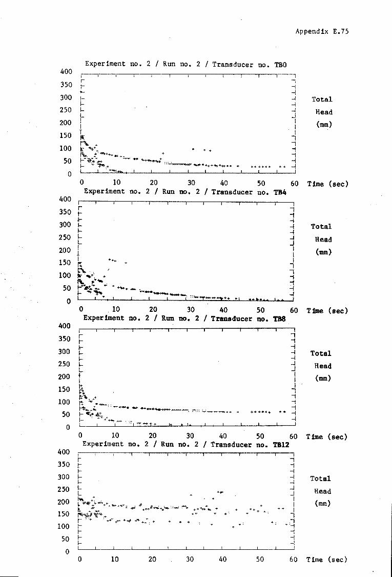
400

350

300

250

200

150

100

50

0

400

350

300

250

200

150

100

Appendix E.75

Experiment no. 2 I Run no. 2 I Transducer no. TBO ·-----.,...---.,...----,---,----,.----,.---,---,--- -·-i

+ + +

' ....; l

--1 -! -I -1 _j l l I

I ..., -j -j -l

++++++ ++ ~

Total

Head

{mm)

O 10 20 30 40 50 60 Time {sec) Experiment no. 2 I Run no. 2 I Transducer no. TB4

I

r rr IIIL ! l I r.: t\.. . ~ ·.._, ... _ +

f\.. !I' • ._ .

+++

I -i -l -l -l ....J J I l I

I -, ""1

Total

Head

{mm)

50 1-·b!..-....... + ................ . I- '41'""" .... _ __,_ __ ... ~ 0

400

350

300

250

200

150

100

50

0

I , .. I I I I f ··-..,.. ........ ...,... .. I -I

+••*++ I++ I

0 10 20 30 40 50 60 Tfme {sec) Experiment no. 2 I Run no. 2 I Transducer no. TBB

I

r r-r I-~-I-L t I ~ i;:i

~·""- ++ r. ..... •-..... .. r1t ........ ;. . • ...,.+4++ ...... *'""•1I'•11111 .............. ~ ~:: :_..:.,.......,...._++ +

I- 'ii=~;'"~ T

I-· ~.....,. ~ . ·-i I .... ! '"'"...., t + \± + I+ I J I

++ ++++

"1 ""1 -l -I -l -l _J I I I

I I -j -j

+ + -l -l

!

Total

Head

{mm)

0 10 20 30 40 50 60 Time {sec) Experiment no. 2 I Run no. 2 I Transducer no. TB12

400 -, --·---....---....---.....----,....--.----,---.---.---r---i r ,

350 t"" -j ~ -l

300 I- ~ I- ~

250

200

150

100

50

0

i:L !-... + . +

I.. ·.pr·· .:..ifM-++ ..... it.t .1.-ti..+.. • .t ... . . . . .. .-. ...

+ ....

l!i. .m- - -FP +++"'~++--.. .. .,..... .... ++ ... +to 'flt. +

ru;~~.+ •••" T + •

r .. ·+ . ++"" ++i· ·~ +'i· +.~r. + + • + '-- . I

ti-1-,

+ ++ +

+. +

-l _J I i I

I -;

T •-i -1 -! -l

l

Total

Head

{mm)

0 10 20 30 40 so 60 Time (sec)

Appendix E.76

Experiment no. 2 I Run no. 2 I Transducer no. TFO 400 1---

--:i 3SO r . 1- ·-I

' I- ' ..., 300 I- -I Total .j.... -l 2SO IT. -I Head Li _j

200 J,. ;_' I (mm) I: T. I I~ ......... -· ! lSO r· ... :.· ....... l I •."!!- .. +. ·+ ..

-i ....... 100 1- . ")i.,.. ~ ... + ·-j ... ~.

J- + ...... + ++-..... ....... --! +. so I- ......... "T~~~* ........ ++ ....!

~ + . ....... +q. ++ ... .,. ... .,..

' -1

0 +

0 10 20 30 40 so 60 Time (sec)

' Experiment no. 2 I Run no. 2 I Transducer no. TP4

400 I ..., r 3SO t-- --t I- -j

300 I- -I Total ·j:... -I

2SO L.. + -I Head !.!. + _J

I!-' .;.

I (mm) 200 +

I c:: ... .p·

I~. "'T I lSO r··. + ......... "l I~. ·+ 1 . .....

-j 100 t- T~ ....... --,.... . ·.+ -- .... '\++-. ., so I-

:..,. ---...... -I ..... I- . + ................ +t+++ + ++ + ...... : -I -- .. T+

0 0 10 20 30 40 50 60 Time (sec)

Experiment no. 2 I Run no. 2 I Transducer no. TF8 400

I

r 1 350 ,.... -j

f- -I 300 I- -I Total I- -I 250 ~ -I Head 1..1 _J

200 ~ \: I (mm) ~ '.+ I

I~···. I 150 -. ,- ~ .. :.: ...... I ... * 41'++ + .. + ~ 1 I - l!' ...... .... + .... .. + 100 !- 'h ··- ~ "4t-t-........ _ -j

J- +T --.... +t+ ofolit.tm.++ ....... + + .... . + ++ + . -j ·~ so I- ....._. +"'7.: + -I

I- ... ++ + + -I + + ++

0 0 10 20 30 40 so 60 Time (sec)

Experiment no. 2 I Run no. 2 I Transducer no. TF12 400

I ..., ! r 350 J- -\

I- ...., 300 t- -l Total L --f 250 ~ .J Head L'li- .J

!'!-.... + i (mm) 200 ......

l !~ - ... .lo 4ftl-+++ -1..£. -- .. - -

t .fl"+ ... +•+. • - - - ~-P'TT"" ~ ++++ ........... ,. +t+-t++ -H· +-t+.,. -t· •· ~· ++++ ++ l lSO r "";.;;."<liiH .... ·1

I + +...._ +tsf. ++ti- +fl-+++ ... . . . "'i 100 1- • T T"'.-j

J- --! . so I- -1

I- -l i

0 0 10 20 30 40 so 60 Time (sec)

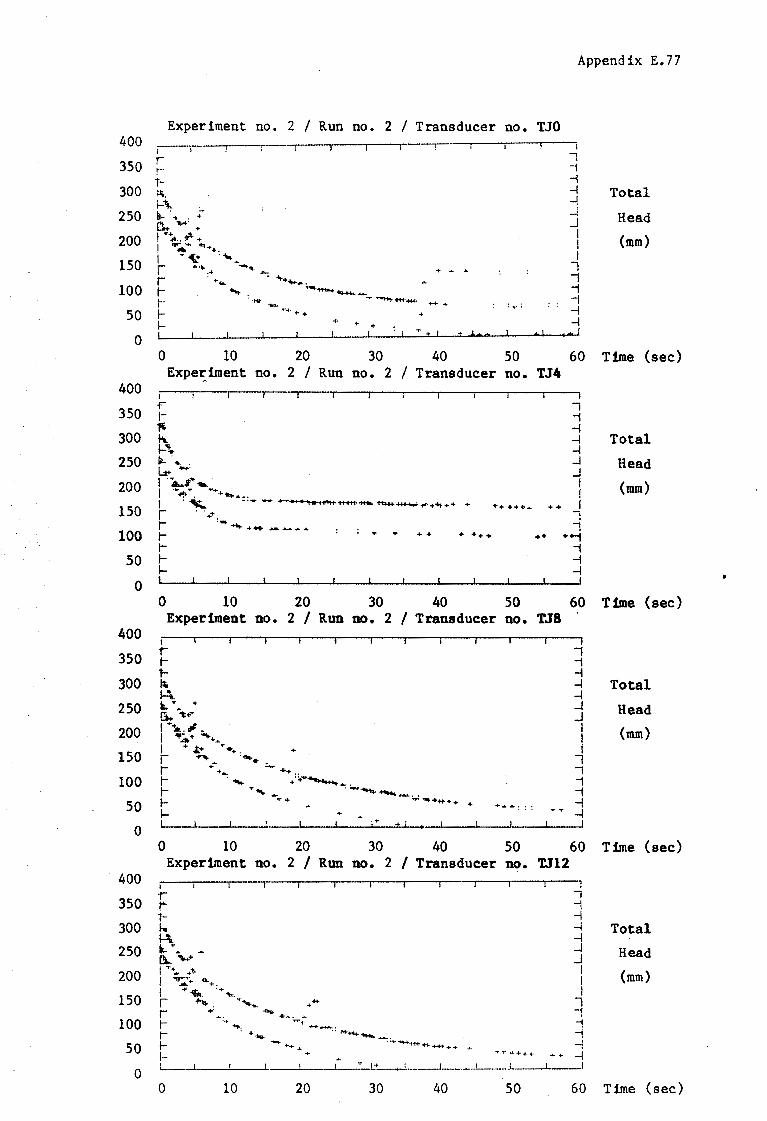
400

3SO

300

2SO

200

lSO

100

Experiment no. 2 I Run no. 2 I Transducer no. TJO .-. ---, --,----, ·--·-· r ir ~. ~-=\.. . Iii- . .. . ;: [!... ........ +

I~~ .. ~+ I .-,... ...... ""'++. I ~ <tt . .,... I ....... + • ..... ..,. ~ r . ...... - ............. . t- ...... . ----1-·· -f-lr -6rn. "T ~ f+++++ +oJ- ... . ~. ..

Append ix E. 77

I I -j

-I -l Total -\ ....! Head _J l (mm) I I

I I ., -1

so II-

'l"-1· + +

+ + + -I

-l ,.. ± I 1 • i

0

400

3SO

300

2SO

200

lSO

100

50

0

400

3SO

300

2SO

200

lSO

100

so 0

400

3SO

300

2SO

200

lSO

100

so 0

+ L+ + • I

0 10 20 30 40 SO 60 Time (sec) Expe~iment no. 2 I Run no. 2 I Transducer no. TJ4

I ., -I -l Total -l ....! Head _J I (mm) I

+++++• ++ i I I

++ ++-1 ., -I -l

0 10 20 30 40 SO 60 Time (sec) Experiment no. 2 I Run no. 2 I Transducer no. TJ8

0 10 20 30 40 so Experiment no. 2 I Run no. 2 I Transducer no.

T'T'++++

0 10 20 30 40 so

.., ., -I -l -l ....! _J I I I

I I -j ., -! -I

60 TJ12

I

I -j -I ....j

-l ....! _J I I I

I I -j -j -{

... + -l

60

Total

Head

(mm)

Time (sec)

Total

Head

(mm)

Time (sec)

400

3SO

300

2SO

200

lSO

100

Experiment no. 2 I Run no. 2 I Transducer no. TMO 1---,----r-1'-

b. I-.,. Ii-· "!,.-++ ~!lj!+ .......

L -.:_·~ '· I • ., .(+ •+ I :r~ ~ ....... I .,. ... ...._ r- ·+ •+ ......... r .. ... ·-.......... • t- .,. '19a·. ..""""''* 1-· ·-1· + ... '111--++t- .i+ ++-ff-+ ...

Appendix E.78

I I -{ -i -l -1 --l _J I j I

1 .., -{ -{

Total

Head

(mm)

+ ++ +++: + + -I

-l so t 0 l____..~--'~--'~---'~--'~·~'----''--·-·_.___..---i-..,___,_~-L~-1

400

3SO

300

2SO

200

150

100

50

0

400

350

300

250

200

150

100

so 0

400

3SO

300

250

200

lSO

100

so 0

0 10 20 30 40 SO 60 Time (sec) Experiment no. 2 I Run no. 2 I Transducer no. TM8

rt-"-1- 'IJo. ~ ........ . ~ ...... .,.. L .....::;.:+ '+ I + 11fi.• • ... I ~ ~ ...... I .... ...,. .-..,, r ..... .. .... j ·+ + ··~ ..........

t- .... .. ·~*......... . .. ,.... . +++. . ...................... ...-. ...

II- + +

+

........

.., "1 -I -I -I -I _J I I I

l I -1 -1 -I -I

Total

Head

(mm)

0 10 20 30 40 50 60 Time (sec) Experiment no. 2 I Run no. 2 I Transducer no. '1'00

I -1 -I -I -I -I _J I I I .., ..,

-{ -1 -I

++++++ + + -I

Total

Head

(mm)

0 10 20 30 40 50 60 Time (sec)

0

Experiment no. 2 I Run no. 2 I Transducer no. '1'08

..., -1 -i -I -I -I _J ! l t ..,

..., -{ --!

Total

Head

(mm)

+ + -I . ...j

10 20 30 40 50 60 Time (sec)

400

350

300

250

200

150

100

50

0

400

350

300

250

200

150

100

50

0

400

350

300

250

200

150

100

50

0

400

350

300

250

200

150

100

Appendix E.79

Experiment no. 2 I Run no. 3 I Transducer no. TC12

r tiI+-~. ~·

lib: I"'"-._ I ~---•-111........,. +++ ++++ +++ ++++ ++ + + + + + • I r I i-tII-

-; -1 -I -I -I -I .J I

~ I I ...,

i -! .., -I -I

Total

Head

(mm)

0 10 20 30 40 50 60 Time (sec) Experiment no. 2 I Run no. 3 I Transducer no. TC8

.r r 1-J..:. j..:. .j_ L i-. r.. I'\. r'\.. ,.... """""'-... t- ---............... ,_ ... _" .... . . . . . . t- ........... ••+•++ •••• + •

r-1-

• +

I -! -I -I -I -I .J I I I

I I 'i

~ , -I -I

Total

Head

(mm)

0 10 20 30 40 50 60 Time (sec) Experiment no. 2 I Run no. 3 I Transducer no. TC4

I .r fr IIIL fl: It ... ll.". R ,.... "'-. t- -......___ +

r - .............. ~~ ..• t- . . + ++• ++++ ++ + ..

, ., -I -I -I -I .J I I ! ..., ,

-j .., -I

Total

Head

(mm)

I- + + _,

0 10 20 30 40 50 60 Time (sec) Experiment no. 2 I Run no. 3 I Transducer no. TCO

0 10 20 30 40 50

Total

Head

(mm)

60 Time (sec)

Appendix E.80

400

350

300

250

200

150

100

50

0

Experiment no. 2 I Run no. 3 I Transducer no. TG12

r rf't:- •· fit.. ll. L\:> 1: I ""-f ~'&I ti'; 1111 +++ ++++ ... ++ """"•·.t. ., ... ..,

I --1 -I -l -l .....! _J I I I

r I trfl-

T ..,

I --1 --1 -I -l

1----...L~-'-~~~~~~--~~~~~~~~_,_~_,_~~

Total

Head

(mm)

0 10 20 30 40 50 60 Time (sec) Experiment no. 2 I Run no. 3 I Transducer no .. TG8

400 l

350 ~

300 t: fc.

250 '"' L"\

200 I '\. I '-

150 I '-r ""'--· r ... +....._. +

100 t- -•+ t-

50 I-I-

0

+

•+ +++ ++++ ++ + ••• + + +

.., -1 -I -I -I -I _j I I I -,

I , A 1

-I -I

Total

Head

(mm)

0 10 20 30 40 50 60 Time (sec)

400

350

300

250

200

150

100

50

0

400

350

300

250

200

150

100

50

0

Experiment no. 2 I Run no. 3 I Transducer no. 'l'G4

r r-f-+-f-It Li

'' '' I '-- + +

r ""'"'" I - .... t-· ''-++++~. t- .... +++ ++++ ....

+ .. + • +

.., -1 -I -I -I _j _j I I l -,

I -1 -1 -;

Total

Head

(mm)

fl- T -I

0 10 20 30 40 50 60 Time (sec) Experiment no. 2 I Run no. 3 I Transducer no. TGO

I

rtfJ.f:-li ~· L\. I '\. I '-I .........._ r ....,,,_ r- ..... +*~ +..,. ... -4·

t·~ ..,..SJWt. +-t·+ ....

t- ·-r++-t·.1-++

fl-

+ .. + + +

L__ .J~_.l__.__,_I~~~-

0 10 20 30 40 50

I -j -i -l -i -I _J I l !

I I -j -j -I

... -1 l

Total

Head

(mm)

60 Time (sec)

Appendix E.81

Experiment no. 2 I Run no. 3 I Transducer no. TL12 '400 I --,

350 I .., +-· -j ~ " -I

300 flti.. + -l Total I-' -l

250 I- ......... -i Head L ...... ~ _j

200 I ........ I (mm) I '·· ·• + I

150 I -.......... I r '"'"" ++ I I + ... ·++ ... ..,

100 i- 'T"+++ + -j t- ;. +

+ + ~ -j

50 ~- + + + -I I- -I

0 0 10 20 30 40 50 60 Time (sec)

Experiment no. 2 I Run no. 3 I Transducer no. TLB 400

I

350 r .., +- -j f- + -I

Total 300 ~ -I I--"- -I

250 I- '-. _, Head

L "-. _J

200 I .......... I (mm) I ""'-~. I

150 I ~ ..... _. I r ._,.. + ..... + .., r ·++ i + .....

100 t- . ++++ ... -t' r ... "1

50 ..... + -I 1-- -I

0 0 10 20 30 40 50 60 Time (sec)

Experiment no. 2 I Run no. 3 I Transducer no. TL4 400

350 I I t- -j

300 f- -I

Total i:ti... • -I 1-- '+ -I

250 I- '- _, Head L ' _J

200 I ............. I (mm) I -...~++++ .................. : :"l"'"l"'TT 1" I I ... + + + • + + + I 150 r ..,

100 I I i- "i i- -j

50 I- -I I- -I

0 0 10 20 30 40 50 60 Time (sec)

Experiment no. 2 I Run no. 3 I Transducer no. TLO 400

I i ..,

350 t- -j If· -I

300 ~ I-'

-I -l

Total

250 I- ~ _,

Head L ' _J

200 I .......... I . (mm) I .......... " I I .............. I

150 r ~+ I I .,. ++ ++ ... ..,

100 1·- 'T'.+ ·I-~++ + -j r-· T +. + + + + -j

50 I- -I 1-- -~

0 _ ....J __ L__• __J _

0 10 20 30 40 so 60 Time (sec)

Appendix E.82

Experiment no. 2 I Run no. 3 I Transducer no. TN12 r

400 I I

3SO r I .,.. -1 Ilk: -I

300 !-""""-. -I Total I-

,,. ....j

2SO L... ;.... .....j Head L ......... .J

200 I ........ ___

I (mm) I . ....,...... +++ ++++ ++ .................... I I

: T T I lSO r .., r- .,

100 r- "1 1- "1

so I- -I I- -I

0 0 10 20 30 40 so 60 Time (sec)

Experiment no. 2 I Run no. 3 I Transducer no. TN4 400

+ ., 3SO r-

t- -1 r· -l

Total 300 Pio... -I I- ...,.,,,,. -I

2SO L... ' -I Head L ' .J

200 I .......... I (mm) I -·*- I

lSO I .......... I r : +., .,

+. i r- ..........

100 ,... ..... -1 ++ + ,... .. + + + ~ -1 50 I- + + • -I

I- ~

0 0 10 20 30 40 50 60 Time (sec)

Experiment no. 2 I Run no. 3 I Transducer no. '1'08 400

350 r- ., ~ , .. + -I

300 ~. -I Total I- ....... -I

250 L... ' .... -I Head L '- .J 200 ' .......... I (mm) l ....... I

I -+. I 150 r T6 ., ++.

r- . +++ ..... ., 100 r- ....... + "i

r- : T .. + + "i 50 I- -!

I- ~

0 0 10 20 30 40 50 60 Time (sec)

Experiment no. 2 I Run no. 3 I Transducer no. '1'00 400

350 r- .., II=- "1 g. -I

300 ~ -I Total I- '- I ....,

2SO L... 'Iii:" .....j Head L ....... .J

200 I ........ I (mm) I "Ill~ .. - l I ...... 1 lSO ... r ... •++ .... I ,.... TT+ ..,

;+ .... 100 r· .... + ..

+ "i r- + + "i

so I- + -! I- -I

0 L_

0 10 20 30 40 so 60 Time (sec)

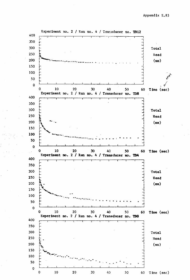
Appendix E.83

Experiment no. 2 I Run no. 4 I Transducer no. TD12 400

I

3SO r I r -j I- '--/

300 I- -I Total It- -I

250 Li.- _j Head ll. .J 200 , ................. I (mm) I ,.. ·~+++ ++++ ++++ ++++ .................. I

lSO I I r I r- I

100 i- 1

~/' t- -I 1

so I- -I I- -I

I 0 0 10 20 30 40 so 60 Time (sec)

Experiment no. 2 I Run no. 4 I Transducer no. TD8 400

r I 3SO i- 1

l- -! 300 I- -I Total

I- -I 2SO t.. -' Head l. .J 200 ll •+. I (mm) I '\. I

I '\. I lSO r"\. -,

r ' ..,

100 t- ..... ..-.. .... -:I t- . ••++ +•++ ++ ........ . ........ "1

50 I- • .,,.. + .. + .. -! I- -I

0 0 10 20 30 40 50 60 Time (sec)

Experiment no. 2 I Run no. 4 I Transducer no. 'l'D4 400

350 r I i- 1 +- -!

300 I- -I Total I- -I

250 J_ -I Head l. .J 200 ~ I (mm) ll + I

I~ I 150 r"'ti..... -, r- .............. ... I

100 i- ............... 1 i- . ""++

++ ... ++++ + ..... ; .. """ 1 50 l- + + + + + + + + + + + -I

I- -I

0 0 10 20 30 40 50 60 Time (sec)

Experiment no. 2 I Run no. 4 I Transducer no. TOO 400

' ! I 350 i- --t I- I -,

300 I- -I Total I- -I

2SO J_ -l Head t. + _J

200 PL I (mm) I~ I ! '"If. I 150 r .._ I I .......... + ..... I

100 i- .,. +++++ + •+ .,. +: ++

1 i- ...... ++: .,. .... + --l

I

I- ~ + -I 50 + . . + I- .. + ~

-~

0 L__-L_ l

0 10 20 30 40 so 60 Time (sec)

Appendix E.84

Experiment no. 2 I Run no. 4 I Transducer no. 'llil2 400 I -,---,- -,

r· : 350 t- .,

~- -j

300 It- -1 Total I\ -1

250 Ui. _J Head L'\. _J

200 I ........ ' (mm) f "'"'mtp...,-.., •••... f I • • '"f'"I" ..-4-T"I" ++++ ++++ + + + + + + .. + + + .. •· + f

150 r I r- I

100 t- ., t-· ·-t

50 f- -j I- -1

0 . l

0 10 20 30 40 50 60 Time (sec) Experiment no. 2 I Run no. 4 I Transducer no. TBS

400

350 r I r- ., I- -j

300 t- -I Total 5l: -1

250 l.l. + -I Head L'\. + _J

200 I '\. I (mm) I ......... I

150 i ..... ~ I r ......... -, r . ·+ ..... I

100 t- . ... ..... . , t- ~ ...... •+++ + + ++ ++ ............. ~

; 50 f- -f

I- -I 0

0 10 20 30 40 50 60 Time (sec:) Experiment no. 2 I Run no. 4 I Transducer no. '1B4

400

350 r I t- ; f- -f

300 -I- -1 Total h- -I

250 .t..:. -I Head L. _j

200 1:... I (mm) !'\. I

150 I '\. I r ' + .., r- ' I

100 t- ~ 'i -t- -+++ ., 50 I- T+.,.+ -I ++.

I- ... ++++ + ..... -l 't"'" -:' ·• .

0 0 10 20 30 40 50 60 Time (sec)

Experiment no. 2 I Run no. 4 I Transducer no. THO 400

I --,·

r I 350 r- .,

1-: -I 300 \.: -1 Total .. -1

250 ll _J Head L'\. _J

200 I '\.. I (mm) I ......... I

I "'It...._ + I 150 r ............ I

r- T• I 100 t- ..,. ... + .... + .,

+ •.

r- ... + +++-t. + ... -j

I-T T

·~ ... ... + + I

. 50 + + . ..., I- -l

0 0 10 20 30 40 50 60 Time (sec)

400

350

300

250

200

1,50

100

50

0

400

350

300

250

200

150

ioo 50

0

400

350

300

250

200

150

100

50

0

400

350

300

250

200

150

100

50

0

Appendix E.85

Experiment no. 2 I Run no. 4 I Transducer no. TI12

.. T .. +

+ + +

Total

Head

(mm)

0 10 20 30 40 50 60 Time (sec) Experiment no. 2 I Run no. 4 I Transducer no. TIS

r t-· .I:~ !'.\ I-'\. L '\.. • I ...... I '-I -........ r -+ ....... i ... + .... . 't- ........... .

t- ··•••••• .. .... ····•++++. I-

.., -f -t -I -I -l .J I I I

I i -i -f -t

• -I

Total

Head

(mm)

0 10 20 30 40 50 60 Time (sec) Experiment no. 2 I Run no. 4 I Transducer no. n4

t t¥ ~ ~ I-'\. L '- .. •• • ++ I -.......... • I ··~·••+•++ I r i t-tII-

+

.., -f -t -I / -I -l

+ .J I I I

I i -f -f -t -I

Total

Head

(mm)

0 10 20 30 40 50 60 Time (sec) Experiment no. 2 I Run no. 4 I Transducer no. TIO

Total

Head

(mm)

0 10 20 30 40 so

400

3SO

300

2SO

200

lSO

100

so 0

400

3SO

300

2SO

200

lSO

100

50

0

400

3SO

300

250

200

150

100

so 0

400

350

300

250

200

lSO

100

so 0

Appendix E.86

Experiment no. 2 I Run no. 4 I Transducer no. TN8

Total

Head

(mm)

0 10 20 30 40 SO 60 Time (sec) Experiment no. 2 I Run no. 4 I Transducer no. THO

+ + +

+ + ... + + +

i -j -I -I -I -I _J I I I

"l i -1 'i -I -I

Total

Head

(mm)

0 10 20 30 40 50 60 T:lme (sec) Experiment no. 2 I Run no. 4 I Transducer no. 108

+ : ......... ........ : ..

+ +++ ... + ~ + + ....

i 'i -I -I -I -I _J I I I

"l I -j

• -j

-I -I

Total

Head

(mm)

0 10 20 30 40 50 60 Time (sec) Experiment no. 2 I Run no. 4 I Transducer no. TOO

+ + 1 .,. + ++ . r ·+,+

r 1·-· 1-· I

~+

+ ++ ... : .,.

+++++ ....

i -j -I -I -I -I _J I I I

"l i -f -j

+ -I ~ ~ L __ _L. __ i____!. __ _L, _ __,_ _ _,__~ _ __..____J ____ , _ __L _ __j

Total

Head

(mm)

0 10 20 30 40 so 60 Time (sec)

Appendix E.87

E-11. Approximate m>lsture transfer analysis. E.xperlaent no. 2.

The results for the moisture mass transfer analysis of experiment no. 2,

are given here. The times of: 5; 15 and 30 minutes after the start of

the experiment are considered. For each time considered the following

results for the analysis is given:

A total head contour plot of the seepage domain.

A contour plot of the degree of saturation of the seepage domain.

Prof !le plots and their coordinates, for four vertical sections

taken across the the seepage domain. The profile plots show the

following with respect to elevation:

a) The pressure head;

b) Degree of saturation;

c) Relative hydraulic conductivity;

d) Horizontal hydraulic gradient; (Only sec. A & D)

e) Relative horizontal Darcian velocity. (Only sec. A & D)

A

Co

nto

urs

o

f T

ota

l H

ead

cfJ

B

C

T

ime

t =

S

min

A

r--r--.---:r-..,--i----r--;r--.---r--,.--~""T'-"-,...r-'--:::::r:::==-t"~r-:::~~==:!::::!::::t==r=::q:1¥t

<

0

260

220

200

18

0

Se~'.par,e

_,,.

face

t ;:;:

0

A

Co

nto

urs

o

f D

egre

e o

f S

atu

rati

on

S

B

C

T

ime

t =

S m

in

D

E==~~======:;=:t~===r=~~Tft<O

----

----

----

-----

•• )

tr._

·".

'

' "

---

--'

Seep

ag

e

.....-

face

t ?-

0

/\

Co

nto

urs

o

f T

ota

l H

ead

¢ B

C

T

ime

t =

15

min

D

...

... ~.

..-~

,---

-,~-

,-~.

.,..

.~-r

--~r

-r--

r~--

r~-,

-~..

,-~,

...-

-....

. ....,--"

""T ....

...,..~...,-~.,-~r-~r-1t-T~-r~-,-~...,-~.,-~T"'t-::iU/

t <

0

160

140

A µ

I

Co

nto

urs

o

f D

egre

e' o

f S

atu

rati

on

S

B

C

Tim

e t

= 1

5 m

in

D

~~..

..--

-.~-

.-~.

...-

~...

--..

,.~ ...

.... ~~~

,.-.

...,

.~..

.,..

-::r

.,..

._..

,...

_, __

...,. _

_ -r-

~.,.

-~r-

-,.~

-r-r

-..,

-~r-

-,~.

...,

.~.-

~"T"

"1r-

:f:i

/-t

<

0 to

i I

1 I

I I

I I

I I

I 1

I 1

I I

I I

I I

I -

fJi

:: :: ~ ~===================-------+--~--~~~_J_

0 ~

r:::

::==

.=::

=::=

::=:

:==:

=:=:

=:=:

-::-

~~~~

~~~~

~--f

.---

~-==

====

=sr

= o

26

S

r=

,1

6 ~~

~~-+

--=1

__

Seep

ag

e

f=::==

::=:::

::::::

::::::

::::::

::::::

::::::

::::::

::::::

::::::

::::::

::l:::

::::::

:::::~

~'.:._

:~~,~~

===t==

=~====

==~~~~

~~~~l-

:J_ ..

-face

.... e-

... ... ... ... -

-/-

Ph

reati

c

Su

rf a

ce

... .... N

I I

I I

I .

I I

I I

. .

I I

• I

--I

. •

-s .

.. =0,75-~

s ...

= 1~--------~-j

---,_

._

_ -

._. ""-'·--

--

--I

I I

I I

I I

: \]

t ...,.

0

~~

A

Co

nto

urs

o

f T

ota

l H

ead

~

C

D

Tim

e t

=

30

m

in

D

tT-~..-~,...-.....,.~-,..~-r-~~~r---r~-r---r---.,...--T"'".....,r-1'....,.--...,..,..-,---..,---~--r--i-1-r---,-~-r~"T"-~r---,r-t'-::ll/t

<

0

See

pag

e ~~~~~~~~r-~--face

/\ C

on

tou

rs

of

Deg

ree

of

Satu

rati

on

S

_ C

D

T

ime

t 3

0

min

D

... -

---.

----

.~~-

--..

.---

...-

--..

.---

...-

-~--

~---

,---

-,--

.i..

.·,-

.--1

"""'

1--,

-.--

,_. .

.... ,_

...-

-r--

--r-

---r

---r

-t-r

----

r---

r---

r---

r---

rt-:

U/.

-t

<

0 µ

I I

I l

I I

I I

• I

I o

• •

I _.

Iii

l.O

0

Appendix E.91

Ewp. •2 I' Sect ton t A ; Tffl\01 1!5 m!n•

41111 ·"l!n ,1! a.ea 388 •U! ~ .4 .llZ. 3611 -es .7 .z.s 3~l?l •68 .e ,5? 3%1!1 1.111 .15 3811 1.1!1 I.Bii 2!11 1.e 1.1118 261!1 1.11! 1.ee 1:.111 1!2'1 IHlll 1,1!1 J.1!11! 181!1 160 148 11!8 llllB 1.e ) ,118

&II ge 48 H II zn 1.11 1.u

H111 81it (Ml) Local H•ad t-l Ong. S10t.. kl' ..

• M<p. *2 / Sect.tonl & ; T11 .. 1 115 Min•

41111 .1 11.811 HS .1 11.81!1 Hl!I .t 8,ae 341.'I .4 .111 32.11 ,II "' :SlllB .8 .~5

1!81'1 .ll .77 Hiii 1.• i.u 1!411 1.111 1.111!1 22.11 t.11 t.88 21!8 ).II 1.11111 1811 1611 14111 ll!lll 11111 1.11 1.81 8111 6111 ·41!1 211 I 11!4 ••• •••

....... t. «•> Looal it.ad c-> Dli1. Su. 111. ....

l:lCJI I " " kat.lanr C / Tl .. t 1115 aJn• ... • •• llllll ••• IU .... '411 11.-ate .... ... .111 1111 111111 248 •• Hll •• Hll 1.11 ,,., u• J.11 .... i1e 1.11 1.a HI! Ullll Uhl 1.11 L,11111 Ill! H 411 211 e 1&4 1.11 1.118

Halgltt <11111l l.<>ctal Hlt•d ,_, O.s. S•t. ..,..

S:xp • H/ S.oth"" Jl " Tf-t es mtn•

41118 .1 11.1111 ,Ill 11,11118

HB .1 Ill.Ill! .111 11.l!IM \1&8 341!1 •• 8,118 .111 ··-31!8 31111 •• 11.1111 .111 e.raee 2811 ·' e.11111 .a 11.aae He ·' 11.1111 ,114 e.ae 1!411 ne -11!11 ,, e,u .U! 11.-1!811 •• .n • ti! ,111!2 lllil .. ,H .1; ,Bill IGI! ,e .ss .11 .llH 148 ·' ,cs ,11 ,U!I 121! 1.11 ,!12 .211 "114 IBll! 1.• I.Ill! .n "!!ii Ill! 1,a 1.1111 .112 .HI!

"' 41!1 ,, 1.111 hllll .11~ ,1!'1111 IB 8 71 1.11 1.llB .n .011

H.el 11ni (-) l.act•I He•d (-) D<tg. E•t. k .... In v,. ... ~.,. ... th

Exp. t2 I Section: A I Time: 05 mins Appendix E.92

Heioht Local Head Deg. Sat. Rel. Per~. (mm) (inm)

401 -130 0.19 0.000 380 -109 0.39 0.023 360 -09 0.66 0.248 340 -69 0.83 0.516 320 -49 0.95 0.847 300 -29 1. 00 1.000 280 -9 1. 00 1. 000 260 11 1.00 1. 000 200 71 1. 00 1.000 100 171. 1.00 1. 000

0 271 . 1. 00 1.000

Width 312. 4 1111 Uoid Ratio e : 0.574 Eff. Sat. Area : 134.8 -

Exp. 12 / Section: B / Time: 05 111ins

Heiaht Local Head Deg. Sat. Rel. Pena. ha) (al 401 -167 0.15 0.000 380 -149 0.17 0.000 360 -131 0.19 0.000 340 -112 0.36 0.014 320 -93 0.64 0.191 300 -73 0.80 0.452 280 -54 0.93 0.170 260 -34 1.00 1.000 240 -14 1.00 1.000 220 6 1. 00 1.000 200 26 1. 00 1.000 100 125 1.00 1.000

. ' 0 224 1.00 . 1.000

Uidth 312.4 -Uoid Ratio e : 0.574 Eff . Sat . Area : 121.6 - .

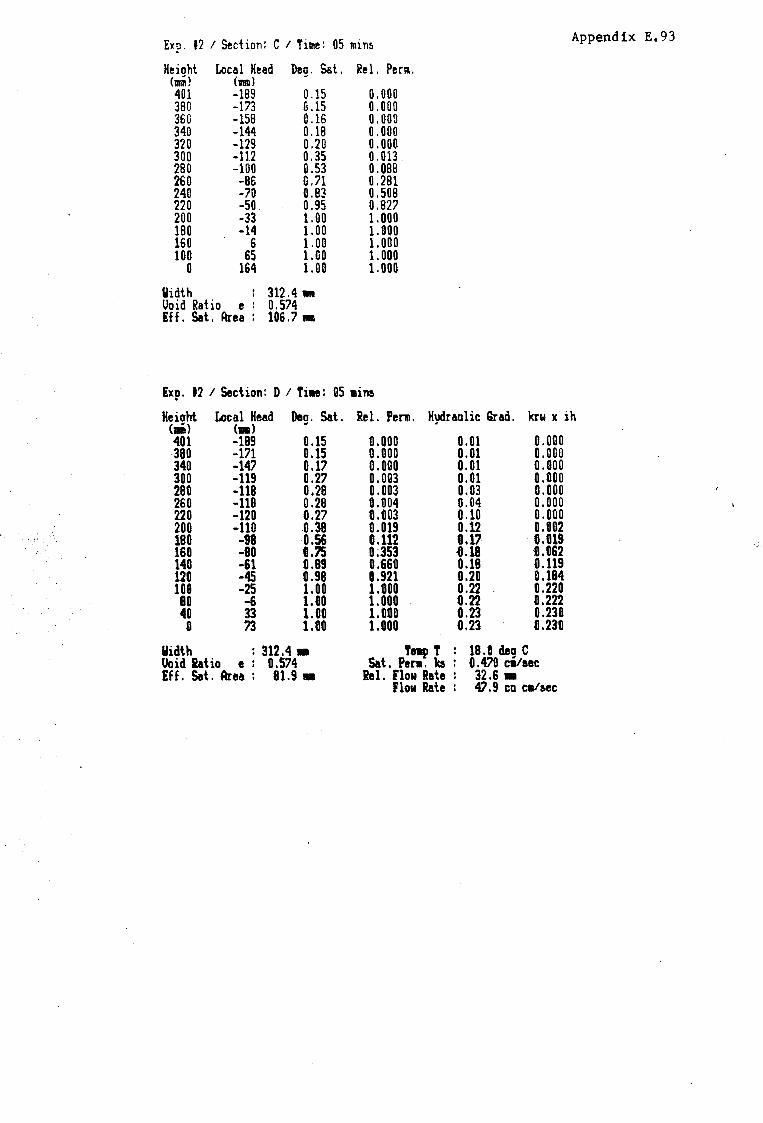
Exp. 12 I Section: CI Time: 05 mins Appendix E.93

Heioht Local Head Deg. Sat. Rel. Perm. cinml ( 11111) 401 -189 0.15 0.000 380 -173 0.15 0.000 360 -158 0.16 0.000 340 -144 0.18 0.000 320 -129 0.20 0.000 300 -112 0.35 0.013 280 -100 0.53 0.088 260 -86 0.71 0.281 240 -70 0.83 0.508 220 -50. 0.95 0.827 200 -33 1. 00 1.000 180 -14 1.00 1.000 160 6 1.00 1.000 100 65 1.00 1.000

0 164 1.00 1.000

Uidth 312.4 -Void Ratio e : 0.574 Eff. Sat. Area : 106.7 11111

Exp. 12 I Section: DI Ti11e: 05 ain&

Heiaht Local Head Deg. Sat. Rel. Perm. Hydraulic Grad. krw x ih c•> (•) 401 -189 0.15 o.ooo 0.01 0.000 380 -171 0.15 0.000 0.01 0.000 340 -147 0.17 0.000 0.01 0.000 300 -119 0.27 0.003 0.01 0.000 280 -118 0.28 0.003 0.03 0.000 260 -118 0.28 0.004 0.04 0.000 220 -120 0.27 0.003 0.10 0.000 200 -110 0.38 0.019 0.12 0.002

· .. f:'·. 180 -98 0.56 0.112 t.1? 0.019 ·,'.

160 -80 G.'5 0;353 -0.18 0.062 140 -61 0.89 0.660 0.18 0.119 120 -45 0.98 0.921 0.20 0.184 108 -25 1.00 1.000 0.22 0.220 80 -6 1.00 1.000 0.22 0.222 40 33 1.00 1.000 8.23 0.230 0 73 1.00 1.000 0.23 0.230

Uidth : 312.4 - Tnp T : 18.0 dea C Uoid Ratio ,9 : 0.574 Sat. PeI11. b : 0.470 cilaec Eff. Sat. Area : 81.9 - Rel. Flow Rate : 32.6 -

Flow Rate : 47.9 cu c./aec

Appendix E.94

t•p. tz / &ect1ont R / Hau IS m!n•

41!10 r .l 11,88 ::iee [ I . t e.ee 36l!I (:! l!l.88 311! l!l,l!lll 321! ' .2 l,l!IB :Sl!llll r . a 1!1.le 281!1 r .4 .113 2611! .7 .n 241!1

I .I ,55

221!1 1.11 ... 21111!1 j ,l!I I.Bl!! 181!1 I.II 1.u 161!1 1411 1.11 1.ea Ulll! IP ee ae 411! 211! e in 1.11 1.811

Height (-~ 1.o ... 1 ..... d (-) !Hg, S10t, ...... li:xp. •z / hat.lon1 a .1 T1-1 15 alna

4l!li! .1 11,lll!I Hl!I -24 .l B.lllll 36B

,342 HS .1 a.u 30 281!1 .2 l!l • .ee l!CB 241!1 _, .Ill UB ,7 .14 219.1!1 ·' ,H 111111 '·' ·'' 119 1.ll! ••• 141!1 1,1 1.1111 IH 1.1 1.11111 taa el! 61!1 41!1 lll!I II •• 1.1 1.• ... , ... , I•> Lao11I

... __ ,_, 1199. S•t. .lir•

£wp. ff ,. S.ot.fanr c: / Tt-t 15 •fna

48111 • 1 .... Hl!I • 1 ••• 1188 1411 • s ••• 321 11111 .1 28111 .1 Hl!I ,1 241 .1 ne 28111 .c .19 181!1 •• ti Hill 1,B t,811 141!1 1.e 1.u U!lll 1.1 1.a Uilll I! I.I ••• Ill! 61! 41!1 28 e Hiii 1.1 I.Ill

Haight {-) Loc•I Htl•d {-) 1lta9. S10t, kr•

£xp. •z ,- S.otfDl>I D ,. Tl-• l!I .,,,.

•• .1 ll!.1111 .Bl 11.111111 3112 -11 • I B.21!1 .ll!t B.llBll l!Bl!I 341!1 .t e.811 .m ··-32111

~· 188 , I e,ee .at ··-261!1 .I a.ae .n a.BBi! 1!41!1 .2 11,BB ,94 e.eaa 221!1 .r 1!1.U .116 1!1.11111! 291!1 ·' e.ias l .87 1!1.88l! 181!1 u;e .s ,117 .1!16 .BB4 l4B ,7 ,29 .ea ,1!122 121!1 .s ,!IS .ae ,in1 Illa ·' ••• .n • IBl!I 11!1 1.e 1.ee .H • ll!!i Ge 1.11 1.n .111 .11!5 41!1 Zl!I e ~7 1.1 l.lill! .n .11!5

Heigh\ ,.,.,, Ltu:a 1 H<tad ,_, n.e. Sat. i.,. .. ih v .. ~krw. lh

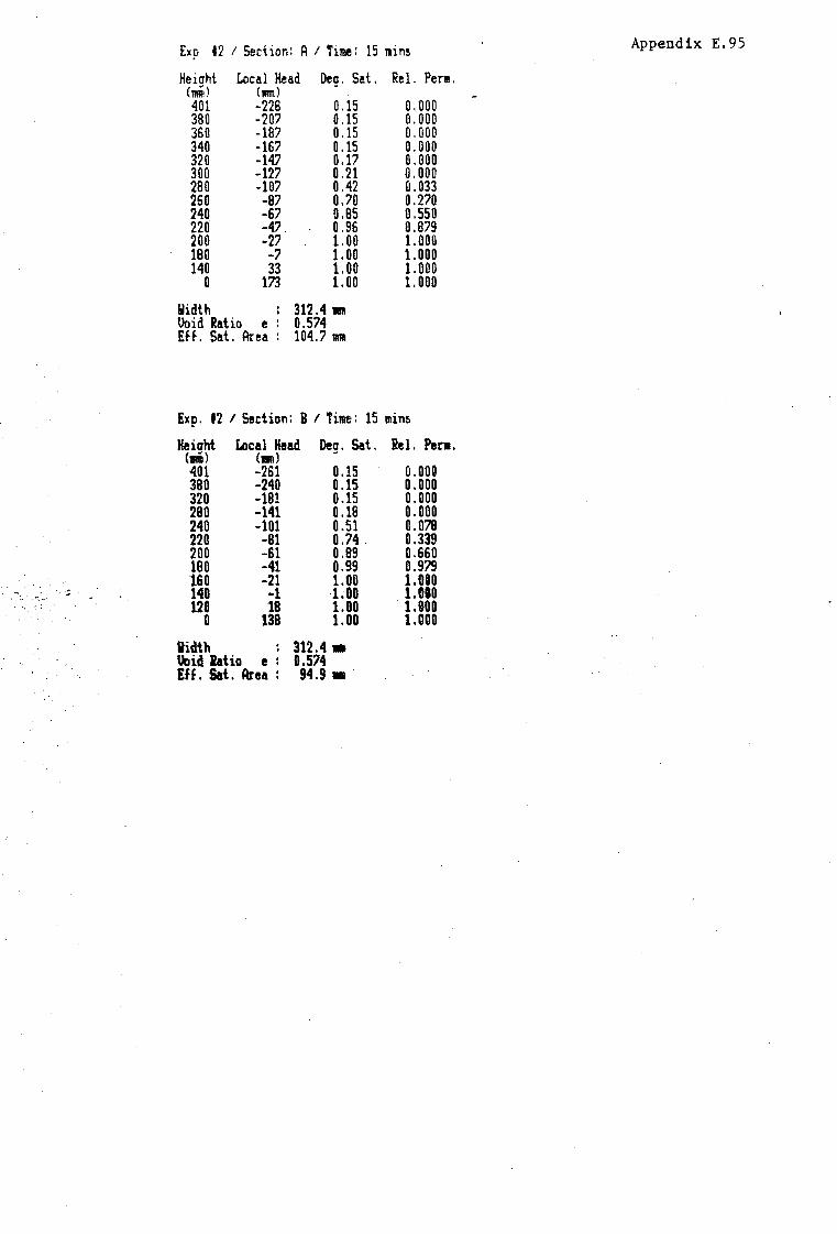
Exp 12 I Section: A I Time: 15 nin! Appendix E. 95

Heiaht Local Kead Deg. Sat. Rel. Pen. (mm) (11!11'1) 401 -228 0.15 0.000 380 -207 0.15 0.000 360 -187 0.15 0.000 340 -167 0.15 0.000 320 -147 0.17 0.000 300 -127 0.21 0.000 280 -107 0.42 0.033 260 -87 0.70 0.270 240 -67 0.85 0 .550 220 -47. 0.96 0.879 200 -27 1. 00 1.000 180 -7 1.00 1.000 140 33 1.00 1.000

0 173 1.00 1.000

Width 312.4 1111 Void Ratio e : 0.574 Eff. Sat. Area : 104.7 11111

Exp. 12 I Section: BI Time: 15 min!

Heiaht Local Head Deg. Sat. Rel. Pen. cm i (111!l) 401 -261 0.15 0.000 380 -240 0.15 0.000 320 -181 0.15 0.000 280 -141 0.18 0.000 240 -101 0.51 0.078 220 -81 0.74 0.339 200 -61 0.89 0.660 180 -41 0.99 0.979 160 -21 1.00 l.000

. :. _... .. , .. · ~ 140 -1 1.00 1.000 120 18 1.00 . 1.000

0 138 1.00 1.000

iidth 312.4. Uoid Ratio e : 0.514 Eff. Sat. Area : 94.9 •.

Exp. 12 I Section: CI Time: 15 mi~ Append ix E. 96

Heioht Local Kead Deg. Sat. Rel. Perm. (llllii) (lll111)

401 -285 0 .15 0.000 380 -265 0.15 0.000 340 -228 0.15 0.000 300 -190 0' 15 0.000 280 -1n 0.15 o.ooo 260 -153 0.17 0.000 240 -134 0.19 0.000 200 -95 0.60 0.148 180 -76 0.78 0.406 160 -30. 1. 00 1. 000 140 -38 1. 00 1. 000 120 -19 1.00 1. 000 100 2 1.00 1.000

0 100 1.00 1.000

Width 312.4 -IJoid Ratio e : 0.574 Eff. Sat. Area : 84.7 1Rlll

Exp. 12 I Section: D I Ti'111e: 15 •ins

Heiaht Local Kead Deg. Sat. Rel. Pen. Hydraulic Grad. krw x ih <Iii> <•> 401 -289 0.15 0.000 0.01 o.ooo 380 -270 0.15 0.000 0.01 0.000 340 -235 0.15 0.000 0.01 0.000 280 -1'9 0.15 0.000 0.01 0.000 260 -168 0.15 o.ooo 0.03 0.000 240 -158 0.16 0.000 0.04 0.000 220 -146 0.18 0.000 0.06 o.ooo 200 -135 0.19 o.ooo 0.07 0.000 160 -102 0.49 0.067 0.06 0.004 140 -85 0.71 0.292 0.08 0.022 120 -65 0.86 0.593 0.'06 0.034 100 ..:52 0.94 0.804 0.13 0.100 80 ..:33 1.00 1.000 8.13 0.125 60 -13 1.00 1.000 0.13 0.125 0 47 1.00 1.000 0.13 0.125

llidth : 312.4 - T81ID T . 18.0 dea c . Uoid Ratio e : 0.574 Sat . Pen: b : 0.470 cilsec 'Ef f. Sat. Area : 69.4 • Rel. Flow Rate : 14.5 -Flo11 Rate : 21.3 co C1al&ec

400 3813 2Ge 340 3211 '.Jl!l?l 281! 260 1140 HI! 21!0 181! 1611 118 11!1'1 111ll1

"' Cl! 41! 28 Ill

-us~r--1 -?? \ t -22

-u -17 '\ -Ulli

H.l 9ht (1110) Loral un

He•d (1111)

Cxp. •2 / St.at.Ian• B / Tl.,., '.JI!! min•

411ll1 -11111~----

Hll 3Gl! :!14111 321! 3Bll 2118 Hiil 241!1 Hiii eee 11111 lie JU 121! 18111 Bl! illll 411 2111 Iii

ffltlp\ t-) 111

Lo11al Nead t•>

c / Tt-1 Ewp. " / S.11\ '"'"' •• -n1.,......---.,.

ae .,,..

H8 H8 148 111!8 SU H8 Hll 141! ne 188 IBB 118 14111 118 Ullll 9111 se 41! 18

" tlillght. ,_,

Cxp, t2 / S.11t.ton1

4111!1 -ttll .aaa IGl! 8'41! HI 188 HI! !lie 241! l!Zll l!lllll lflB 161!1 1411 1211 ld 11111 61!1 411 21! e

Height t11m)

I

n l.011al Head (-)

ll / Tl-• 3111 1alns

ll u

Lac al H•ad (-)

.1

.I

• l

.II

Deg, S•t..

• j

• I .I .1 .1 • I .1 .t ,2

,11 ...

u.,. Sat.

• 1

• l

.1

• 1

••

,8 .s I.II 1.e I .l!t

1.e

•• .11 1.e 1.• 1.•

1·•

.I ••

.It 1.• 1.11 1.11

1.111 P.11. Bat.,

.1

.a

.1

•• .! .e ,I! .1

.5 ,7

•• t .II 1,ll I.I! 1.11 I .Iii

!leg. Sat..

t e.li!i t e,ee

I::: ll.llllll

f::: ll.111!

.I I

,71 ~ ,18

J. ••• 1.a J,llll

1.ee 11 ....

ll.flll

l!.1!111 e.ee a.a 11,all It.Ill II.Ill! 11.1111 a.ea II.Ill!

.It .t7

.7111 1.811 t.n 1.1111

1.81!1 .....

••• .... ••• ••• e.1111

1.• 1.111 i.• 1.1111

krw

e.111

e,u

11.81! 11,118 II.Bil 11.ee D.118 11.ee

t

t h88 1.llll 1.1111 1.111!1

i. ...

Appendix E.97

lll,1111 ··-e.111 e.aea

e.1111 ..... .111 111.UI! .111 e.eee .el! a.me .112 ··-.n e.11119 .03 ,883 .1114 .11111 .11111 ,l!llG .H .a-.s .1111 ,e'l'l ,87 .8?1 ,lll8 ·""'' ••• .875

'" Vr-l<r ... \h

Exp. f2 I Section: A I Time: 30 min5 Appendix E.98

Heiaht Local Head Deg. Sat. Rel. Pen11. <ml (m) 401 -299 0.15 0.000 380 -278 0.15 0.000 340 -238 0.15 0.000 300 -198 0.15 0.000 280 -178 0.15 0.000 260 -160 0.16 0.000 240 -138 0.18 0.000 220 -118 0.28 0.004 200 -98 0.56 0 .110 180 -78. 0.77 0.380 160 -58 0.91 0 .710 140 -38 1.00 1. 000 120 -18 1.00 1.000 100 2 1.00 1.000

D 102 1.00 1.000

Width 312.4 1111 Void Ratio e : 0.574 Eff . Sat . Area : 82.7 11111

Exp. 12 I Section: BI Time: 30 ains

Heiaht Local Head Deg. Sat. Rel. Penn. <a) (an) 401 -319 0.15 0.000 360 -278 0.15 0.000 340 -258 0.15 0.000 320 -238 0.15 0.000 300 -218 0.15 0.000 280 -198 0.15 0.000 260 -178 0.15 0.000 240 -158 0.16 0.000 220 ·138 t.18 1.000 200 -118 0.28 0.003 180 -98 11.55 0.105 160 -78 0.76 0.374 140 -58 0.91 0.703 120 -39 1.00 1.000 100 -19 1.00 1.000 80 1 1.00 1.000 0 81 1.00 1.000

Uidth 312.4 -IJoid Ratio e : 0.574 Eff. Sat. Area : 76.4 •

Exp. t2 I Section: CI Ti~e: 30 min~ Appendix E.99

Heiaht Local Head Deg. Sat. Rel. Pern. (mm) (111111) 401 -326 0.15 o.ooo 340 -268 0.15 0.000 280 -211 0.15 0.000 240 -173 0.15 0.000 200 -134 0.19 0.000 160 -96 0.59 0.143 140 -76 0.78 0.407 120 -57 0.92 0.731 100 -37 1. 00 1.000

BO -17. 1. 00 1.000 60 3 1.00 1.000 0 62 1.00 1. 000

Width 312.4 11111 Uoid Ratio e : 0.574 Eff. Sat. Area : 71.7 11111

Exp. 12 I Section: D I Ti11e: 30 111in5

Height Local Head Deg. Sat. ie l. Pen1. H¢raulic Qrad. krw x ih <•> <•> 401 -328 0.15 0.000 0.00 o.ooo 320 -249 0.15 0.000 0.00 o.ooo 260 -195 0.15 0.000 0.00 o.ooo 240 -176 0.15 0.000 0.01 0.000 220 -158 0.16 0.000 '0.01 0.000 200 -140 0.18 o.ooo 0.02 0.000 180 -123 0.24 0.001 0.02 0.800 160 -118 0.28 0.004 0.03 0.000 140 -100 0.53 0.088 0.03 0.003 120 -88 0.69 0.257 0.04 0.010 100 -69 0.83 0.514 0.05 0.826 111 --so 0.95 1.835 1.86 0.046 .. 60 -30 1.00 1.000 O.Oi' 0.111 40 -10 1.00 1.000 0.01 0.071 20 9 1.00 1.000 0.08 8.075 0 29 1.00 1.000 0.08 8.075

.. Uidth : 312.4 - Tnp T : 18.0 dea C Uoid llatio e : tl.51'4 Sat. Pen. b : 0.41'0 citsec Eff. Sat. Area : 63.1 • Rel. Flo11 Rate .: 6.8 •

F1011 Rate : 10.0 cu ca/aec

Appendix F.l

Listing F-1: Example of typical input and output of an ADINAT analysis.

(Steady-state anaylsis of simple 3 element problem.)

H

H

H

H

** H

H

H

H

0

4*

H

H

** H

H

H

** ** H

AA~.AMH.~P..~

MAPA,MA4t;f.~

AA AA

AA AA AA AA AAAAP.AAAAAAA

AAAAAAAAAAAA

AA AA AA AA AA AA AA M

!1M

AA AA

Append ix F. 2

A Fl N l TE E'~EMENT P ROGRA~ FOR H

UDDVUDjJL! \i!l\\lllHI HN h'N AAA AA.AA AM TTTTTTTTTTTI Dt>DDC:D}jD-C JI illlil!\jf N~< NN MMAAAAAMA nnmmrr DD DD ., NNNti HN AA AA n I!

DD DD ,. NN ~ ~IW AA AA TT II ii

DD IY.) ,. NN NM ·~ ,.

M TI ii H~.

DD OD Ii NN !{ii !+! AAAAAAAAAAAA n DD 00 !i HN NH !€~ AAMMAMMA TT DD DD ll NN NN NN AA AA TI OD OD ii NN 1t1m AA AA TT DD DJ !! NN NNN AA AA IT DDDD:JC,~f·OJ ! l! ! Ii I l i i l I HN ~ AA AA TI OO.~D%DDD i Ii I l iii 11 Ii HN H AA AA TI & s

VERSION - 84.00 REFERENCE- ADINA ENGli£ERI~ REPORT AE 84-2

HlflfHHHHHfffffffff.f.ffff.HfffHHH¥.ffff.HfffffHfflffffffl!ffffflfffffffHHfffffffff.ff**ffl!ffl!Hlfffffff.

l!HH!llflfHHHf!ffHHff~HHHfHHHfff.Hffff~H:HHfflfffHff:HHfHHfffffff!fHHfflflf*ffffHH!ffffflflfH!fJ.

TH!S PROGRM'\ IS \\.! :Ts ENT!RE\Y PRO?HIETARY rn AND IS SUPPORTED AKD l'IAINTAlf£D BY

ADINA ENG!NEERJNG AB ADI~. ENGHfEJUNG It( ~L!if'.GATAN 20D 71 EL TON AVE!-llJE S-7fl 12 VASITRAS sw:ntt~ WATERTO~ M. USA TEL 021-14 40 50 TEL (617) 926-5199 TELEX 40630 10!NA ~· TELEX 951-772 ADili4 LIS WTW~

GARD

2 3 4 5 6 ., '

9 10 11 12 l3 14 1C" l.l

16 17 rn 19 20 21 22 23 24 25 26 27 2B 29 30 Jl 32 33 34

J ; .... ,.. L 10i

COLUr;t" NU~SEP.

3 4 5

Appendix F.3

7

THREE LAYIT- 50\L FLOW PROB~E!'l.

4 0 0 0 0 0 0

(i

0 0

0 0 0 1

l Q

4 (1

0 0 2 2 0

4 l l 3 0 0

l .s

2 ' '·

3 ,, '-·

2 ., l

3 3 STOP

0

0 0

20 2

1 2

20

2 3 2 4 3

0 ,, Ii

0 0

0 0 ()

., J

o. 0 0 0 0 0 0

0 1 12 0

3 0 0

0 0 0 0 0 (1

4 7 3 tn.IMBER 12345673901234:-.67390l23456i39012345673%123>15678901234567890 i 2?.-45673901234567890

COLUMN NU!lBER ffff.HHHHHH*HfHH!fH*Hff.H E N D 0 F j N p u T L ! s T ! fl G ~J..lfl!HHlfHHHfff.Hi!HHHl!HH~

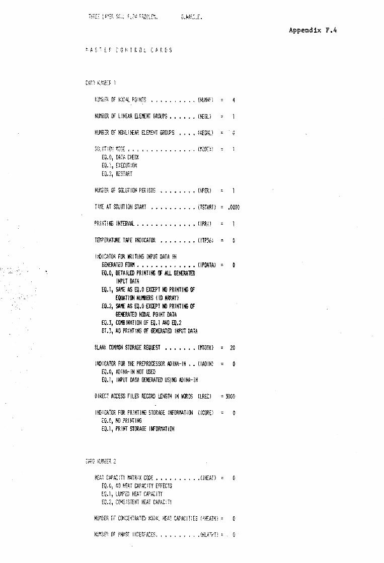
~. A F ~ E. ~· C 0 t~ T R 0 L C A f, D S

tiJMd tR OF ND'04l. P 0 ! NTS , , , , , , , • • • (tlJ!'ti0 ) = 4

NlD.'lBER OF LINE.AR ELEr£NT GROOPS •• c ••• O{Gl) =

Nlll'iBER OF HONL ltfAH ELEMENT GROUPS • • • • Hf GNU = 0

EQ. 01 DATA CHECK EQ.1 1 EXECtn IOt~

NW!BER OF SOUJTION PERIODS •• I • : •• I: H.fPEfO =

TIME AT SOLUT!UN START •••••••••• (TSTARTi = .0000

PRlNTIKi fNITRVAL ••••••••••••• !IPRI} =

TE!IPERATtJ.1.E TAPE INDICATOR •••••••• nTP56) = 0

! t{) I C.A TOR Fffi NR !Ti NG INPUT DAT A I ~l GENERATED FORl'I ••••••••••••• ( IPDATAl = 0 EQ.O, DETAILED PRIHTlt«i IF ALL GEtERATED

INPUT DATA EQ.1 1 SA!'lt AS EQ.O EXCEPT t«l PRINTlt«i OF

E~Tl!Jl NUlllERS <ID ARRAY> EQ.2, SA!{ AS EQ.O EXCEPT NJ PRlNTll«J OF

GENERATED NOOAL PO INT DATA EQ.3, C01111NATIGtl OF EQ.1 AHO EQ.2 GT.31 NO PRINTING OF IX:NERATED INPUT DATA

SLA~'K CUl'll'ION STORAGE REQLEST ••••••• !MTOTKl = 20

HID!CATOR FOO Tl£ PREPROCESSOR ADINA-!M •• ( IADINl = 0 EQ.O, ADINA-IN HOT USED EQ.1 1 INPUT DATA GENERATED USJKJ ~!NA-IN

DIRECT ACCESS FILES RECORD lfNSTH IN W!RDS (LRECJ = 3000

INDIC.ATOR FOO PR!i/TINB STORAGE INFORl"iATIOO (IC(JP,D = 0 EQ.O, HO PR!lftlNG EQ.1 1 PRINTSHRAGE ltfORMATION

HEAT CAPACiTI MATRiX COOE. , ••••••• ,(IHEATJ :: G EQ.O: NO HEAT CAPACITY EFFECTS EQ.1, LUl'!FED HEAT CA?Ai:iTr EQ.2, co%:smn HEAT CAPACiTY

Appendix F.4

EFFECT! VE COHDliCT IV! TY r.ATRlX • • • • • • ( l SHff) = (NQT APPLICABLE FOR L!~fAR A~t~~ YSISi

NLIRBER OF TIME SiEPS BETWEEN

mo: APPLICABLE FOR LltfP.f: A~A~YS!~)

\ 1 ERA1 J mils PER?\; TT~~

r v

•j ~

CONVER.GHCE rn .. ERANCE • • • • • • , • , • • \RT[U = • l000-002

CARD HUMBER 5

TIME HffEGRAT !ON DJJE ••••• EQ. i 1 E!JL£R BACKWARD l!ETP.JJD EQ.2, EULER FORWARD F.ETHOD EQ.3, TRA.0EZO!llAL RULE EQ.41 ALPHA, FAl'!ILY ~ETHOO

•• (i0PE) =

THIE IW.EGRATION FACTOR •••••••••• <ALPHA) = .1000+001

CARD NU~StR 6

=

LATE~'T HEAT PR!iff FL~S •.•••••••• ( IUfLG) = 0

PW!T--OUT BLOCK

E~.~i POnP.D~~. @' i;",:-:<Et; EQ.1, PDS.TH]LE wr: ~ TTEf~

' I ~ •• ~ (.JHFQR.T j =

. ; "~-~·. "' ' -'; ;-;,::..r-; -

Appendix F.S

EC.;.o, STE~:~" S:l·T~ ANt~ Y~::;.

EQ.1 ~ iR.~.t-::~: ~k'f A'.·:!~ .... Y~, E

EQ.0 1 L H!EAf; Af;AL YSIS EC1, 1, NO~t l~iEAF~ Af¢,;_YSI S

TIME SH? DAH

~llll'!RER OF SiEPS

~ 1 OOO+OOi NODAL POINT DATA

iNPllT DATA AT MODES

~ODE

N TEt'lPERP.TURE co~r1rnOH

wDE - rnao

Nffi~l_ POiNT COORDINATES x y z

4 0 0

GENERA TEO NODAL DAT A

.000.~0

.00000 .00000 .00000

.00000 12.00000

HOOE TEl'IPERATlRl.E NODAL PO I Ni CUORD I NAtES N CO!illTI~ x

COOC - !O(Nl

0 .00000 2 0 .00000 3 0 .00000 4 0 .00000

E~JAT i Ofl N.lJ'IBERS

N EQ. ~rm

3 } 4

IN.\T\AL COtJD!T!C~;s

IN!T!AL CGfmiiiC~<S CODt EQ,O, REITPEt{:E. Tt~PERA:Ll~E TRfT EQ~1 1 DE\llATIQH.S H'Gf. R~F£REtJ.CE

TE~iPER~Tl~,: TREF t~~E ~'.EAD

y z

.OO'VOO .00000

.00000 4.00000

.00000 8.00000

.00000 12.00000

N EQ. KlriBER

(!CON)= 0

~E~ GENERATING CODE

KN

0

Append ix F. 6

N EQ. N.U!"iBER

...

Hl:'t1SER OF 1 it:iE F\.lt[i 101i C\JF~'JES •••••••••• rnrn) =

UNEAR C[l.JVECTlON CODE •••••••••••••• UWJVI :: EG .0, NO LI t!AR COWECTI ON BOl~DAA Y CONDI Tl OMS EQ.1~ Llt~EAR GOMVECi!OH 90Ut~4PY COND!TIOff;

,. v

NtmBER OF SPECiFIED tii'JDAL POINT TEMPERATLf(E ••• (Ifill".~') = 2

Hli'iBER OF Brut{)ARY mwm i ON NODES • • • • • • • (l{iCV) :: 0

NttlBER OF BCUIIDAA.Y RAD! AT I ON OODES • • • • • • , • (NORA l = 0

HiJIBER OF cowcrnTRATED HEAT now INPUTS ••••• (llQAD) :: 0

HlJ'IBER OF 2/0 ffl"...ATFWX INPUTS •••••••••• OlOA02) = 0

HOOER OF 3/D HEA1 FWX INPUTS ••••••••• , UlOAD3l = 0

h'U'IBER OF INTERNAL HEAT GENERATION DATA SETS ••• (Nlh'TJ = 0

TOTAL ){!~ER (f El.HIEN.TS W !TH INTERNAL HEAT GENER~.Ti {Jll • • • • • • • • • • • • , • • • • (h'TOTl = 0

.flEAT FLOW iNPUT

mE Fl.tlCT!OO ru<VE HU!'!BER =

HlflBER OF T WE PO !NTS ::

T\ !'\E VALUE F'JNCTiDM

.OXIO\i .1000+001 1,(1~0\i , J(rJ(H0(11

Append ix F. 7

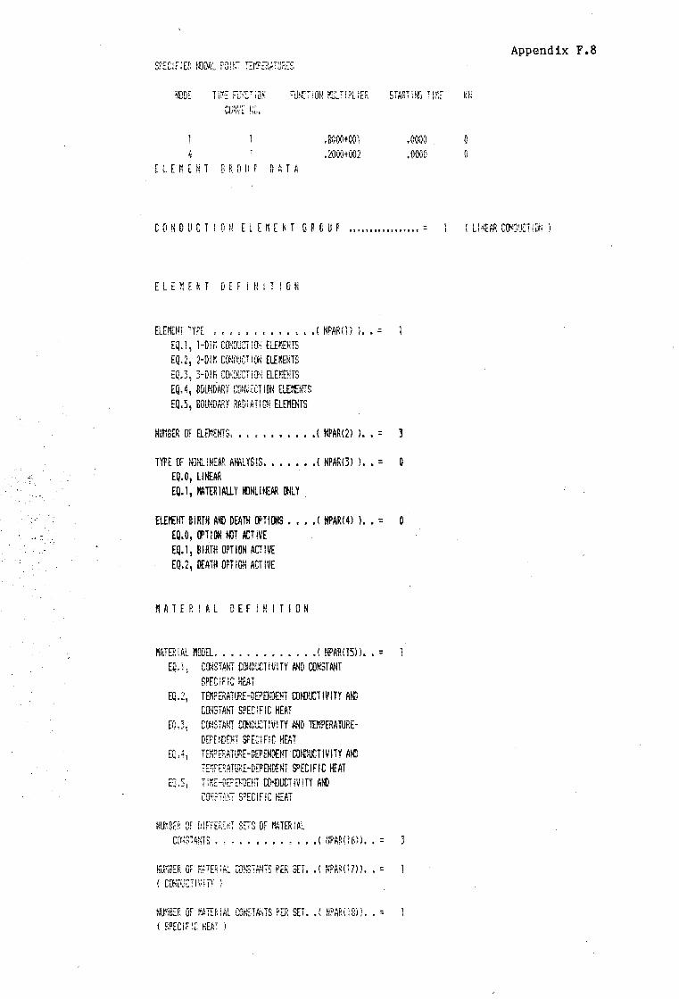
T 11'E Fe~;:-:- ill~

cuq:,:~ r;:..

ELEMENT GROUF DATA

.8000+001

.2000+002

CONDUCT ID~' EL EH NT GP.DUP

ELEMENT DEFINITION

ELE!'IENT TYPE • • , • • • • • • • • • • ( NPARO I l. • = EQ.1, J-01 r. CONDUCii!Ji ELEMENTS EQ.2 1 2-DIM C\Y~WCT llK\ ElHENTS EQ.31 3-DIFi rn;~wjCTj[[!·.! ELEriENTS EQ.4, BOUNDARY COf.f,TCTION ELEIUITS EQ.5, BOL~iDARY RADi An Oii ELEl'IENTS

HUi'lBER OF ELEl'IEHTS. • • • • • • • • • • ( NPAR (2) l. • = 3

TYPE OF NONLi~lEAR ANALYSIS. , •••• ,( NPAR(3) l •• = 0 £Q.01 WEAR EQ.1, mTER!AtlY l(]NLllEAR OOLY .

ELEl'EtlT BIRTH AIID DEATH cm~ .... ( NPAR(4) ) •• = 0 EQ.O, IJITION t«JT ACTIVE fQ.1, BIRTH OPTION ACTIVE EQ.2 1 DEATH OPTION ACTIVE

~ATER!H DEFJNITlGN

MTERiAL MODEL ••••••••• , ••• ( NPAR(]Sll •• = EQ.1 ~ CONSTANi cmnurnvm AND CONSTANT

SPEC fF IC HEAT EQ.2, TE!'!PERATIBE-DG'rnDm Ul~LCTIV!TY AND

CONSTANT SPECIFIC HEAT t.~1,5 1 C!JETNf: rnlDtx:TIV!TY AND TEl'l?ERATlJRE

DEPUIDENT SPECIFIC HEAT EC'.4 1 El'PEF:ATL~E-DEPENDENT CO!iIDOCilVITY A~

TrnPERiHLIRE-DEPENOENT sPECIFIC IEAT EQ. 51 T i riE-DLP ENDENT CONDUCTIVITY Al{)

CCfr~STAHTS • ~ " t I ~ • 1' t 9 I ,, I ( NPAR(l 6))' ' = 3

HG\'iBER OF r!tiTERiK W~STANiS PER SET •• ( NPAR\17l) •• = ( CONf.~ICTl \/ ! iY J

.0000

.0000 0

Appendix F.8

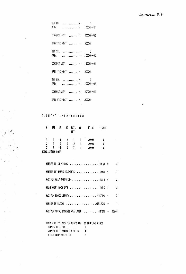
SET N.~. •1latA•ta11r

A~JA • r I It t ~I t I t I • = • i O~i~. XlTO\!.

S [)IDIJCTi \! I T\' :: • 500000•000

SPECIFIC HEAT :: .000000

SET NO~ I I : I t I I" at I t ~ = AREA ............. :: .1 OOOOCi+OOi

CONDUCTIVITY :: .100000+001

SPECIFIC HEAT = .000000

SET HO. s1r11111:111i: = 3 AR.EA .-a1.1ri:::::e1:111.c :: .100:'.>00+00 i

COHIJUCT!VlTY = .2000001-001

SPECIFJC HEAT :: .000000

HEHNT INFORUTIOH

N JPS Ii JJ llAT. KG ET!PE lSVPH !fT

1 l 2 .0000 0 2 2 J 2 .0000 0 J l J 4 J .0000 0

TOT Ii. SYSTEll DATA

Nl.t!BER OF El1JAT10t€ . . . . . . . . . <HEQi

Nl.!'IBER OF MTRIX ELEl'EtITS . . . .. . . . <HWl

"AX 11'1\w. !'ALF BAM!lW lO TH . . . . . . <Ml

l'IEAN HN..F BAMiJ!;! iDTH ' . . . . <MMl

"AX I l'U~ BLOCK LENGTH • . . . . osmo

Ntr.BER OF BLOCKS • . . . ' , (l*ILO'.X l

l'lAXllU TOTAL STORAGE AVAILABLE . .. .mon

~;unBER OF CCUJnhG PER BLOCK AND 1 ST COlPLI NG Bi..CCK NUr'EER OF BLOCK NUl'IBER OF CCUl!'INS PER BLOCK 4 FIRST COUPLING BLOCK

hp ~ei..u i.x F. 9

:: 4

= 7

= 2

= 2

= 7

::

:: 52643

Appendix F.11

F-2. Using ADINAT (2} with ioodifications.

The finite element. program ADINAT [2] including the modifications made

by the writer of this thesis, is available at the University of Cape

Town. With the permission of Prof. W S Doyle, (Dept. of Civil

Engineering.) the program may be used. Information on how to use the

program, and the input required, is given by the user manual [2]. In

conjunction with the user manual [2], the following three pages are

used. They give the layout of the input required for the use of "MODEL

9". "MODEL 9" is the nonlinear saturated-unsaturated seepage material

model that has been included by the writer, (See section 6.9.3) in

ADINAT [2].

Append ix F. 12

XI. TWO-D CONDUCTION ELEMENTS (continued)

For MODEL "9" (NPAR(lS). eq. 9)

note

(1)

note

(1)

Skip this set of cards if NPAR(lS) .NE.9, otherwise, input

NPAR(16) sets of cards.

conductivity card(s) (8F10 .o) columns

1 - 10

11 - 20

variable entry

PROP(l ,N) Local Pressure Head at pt. 1, <li1 PROP(2,N) Local Pressure Head at pt. 2, 4'2

PROP(NCON/2,N) Local Pressure Head at pt. NCON/2

PROP(NCON/2+1,N) Conductivity at pt. 1, kal

PROP(NCON/2+2,N) Conductivity at pt. 2, ka2

PROP(NCON,N)

PROP(NCON+l,N)

\

Conductivity at pt. NCON/2

RATIO OF k8

/kb

EQ.O; default set to "1"

specific moisture card(s) (8Fl0.0)

columns variable

1 - 10 PROPS(l,N)

11 - 20 PROPS(2,N)

entry

Local Pressure Head at pt. 1, q,1 Local Pressure Head at pt. 2, <!i2

• PROPS(NCONS/2,N) Local Pressure Head at pt NCONS/2

PROPS(NCONS/2+1,N) Specific moisture per unit

volume at pt. 1, c1 PROPS(NCONS/2+2,N) Specific moisture per unit

volume at pt. 2, c2

PROPS(NCONS,N) Specific moisture per unit

volume at pt. NCONS/2

NOTES/

(1)

Appendix F .13

MODEL 9 is a nonlinear material model, in which the

conductivity and the specific moisture are local pressure head

dependent_. Linear interpolation is used to obtain the

conductivity and specific moisture of the material at points

between the points input on the above cards. (See

figure XI.2-4). The constants (ka' kb) are defined in a

material coordinate system (a, b). (See figure XI.2-5). The

axes a, b, are principal material axes, and ~ is read

individually for each element in section XI .4 of the user

manual [2]. The ratio ka/kb is entered in as the

variable PROP (NCON+l,N).

1

Permeability k Appendix F. 14

2

S . f. . . ae pec1 ic Moisture Capacity c = ~

c

2 7

Local Pressure Head

1jJ = (~ - z)

Local Pressure Head

' - <• - z:) 8

_F_tg __ n_._2_-4_: Material behaviour for wo-dimens 1ona1 saturated-

z

UDS&turated seepage model. Interpolat:l.on. shown ·aa a

funct:l.on. of pressure head for: (a) The current

conductivity; {b) The specific moisture capacity.

2

y

7

/Node

4

Fig XI.2-5: Principa1 in-plane material axes orientation for the

saturated-unsaturated orthotropic seepage material model.

Appendix F .15

Modifications made to ADINAT [2].

Modifications made to the program ADINAT [2], to incorporate the

nonlinear saturated:-unsaturated seepage material model are as follows:

Subroutines ELCAL, TODMFE, TDFE and MATRT2 were altered so that the

data for the non-linear material models could be entered with the

input data. A new material model (No. 9) was chosen and this allows

the hydraulic conductivity to be entered 1n a tabular form, as a

nonlinear function, with respect to the pressure head. The specific

moisture capacity is also entered 1n a tabular form, as a nonlinear

function, also with respect to the pressure head.

Subroutines TDFE, QUADS and STSTL were altered so that the non

linear hydraulic conductivity was taken as a function of the

pressure head 1n the formulation of the stiffness matrix.

Subroutines NLSP2H, QUADM and TDFE were altered so that the non-

1 inear specific moisture capacity was taken as a function of the

pressure head in the formulation of the mass matrix.

Subroutines MATRT2 and TDFE were also altered so that results were

printed with the headings relating to pressure and not temperature.

The modifications made to the program where checked by comparing the

results from the program with those given in papers. (See 6.11)

1 I ~ E

~~a EC~.J'.~if·P.~l'.ir. !Til.t.T!Dt< a.:~:--: E T~t=- c~[r

L.Otf:J:~il!!1.:ny F;CTJ;~i:::: FCF. Th:s 7 .r.~ E.~~~

NDDE TEMP ERA TURE NODE TEl'PERA TLIRE

2 i 148571 +002

4 .20000,:-+002

Append ix F .10

NOOE TEJ'iPEHATL!RE

H E A T F L U X C P. L C U L A T 0 t! S F 0 R E L E !': E N T 6 R 0 U P 1 ( ONE-D CC~·WUCT: lti l

ELEMEITT HEAT FLUX

-~857143+000

2 -.857143+0(10 3 -.357143+000

S 0 L U T I 0 N T I M E L 0 G WJ SECl .. , \f'

.·· ' FOR PR!?.;_._/,..

THREE LAYER SOIL FLO\ii PROBLEM. G.WAADLE.

IWUT PHASE • • • • • • • • • • • • • • • 18.42

ASSEXBLAGE OF LINE.AR aJNDUCTIV I TY , HEAT CAPAC!iY MTRICES 1.22

ASSErlBLAGt OF HEAT FUJW iHTffiS • 1.22

FREi;l'.JENCY ANAL YS ! S • • • • • • • • • • .oo

TR! l\~GULPR !ZAT iOT~ OF LINE.4R !EFFECT lVEl CONDUCTIVITY rtATR!X .01

STEP-BY-STEP SOLiJTi O'~ ( Tl f'iE STEPS l

CP,LC!JWiON Lf EFFECTIVE HE.AT FLC$! \IECTGRS .00

UPDATING EFFECTIVE CONDUCT!ViTY MTRICES MD HEAT FLOW VECT[J(S FOR NO!l lNE.AR!TIE • .00

SOLL!T !ON OF EQUATiOHS • .00

STEf'-t'Y-ST[P TOTAL I Ot

TGTAL SDLUT'.Gt{ I ~ E (SEC) 27 .91

~,

''I

Appendix F.16

( r: r: c c r c

SllBRf1UT It~[ El.r.Al.

. . . . . . . . . . . . . . . . . . . PROGRAl'I

• T('l CALL THr APPROPRIATE FL(MrtH ROUT INES F"OR READING, GENFRATING.AND STOP ING THF EL[M[NT DATA

. . .

.c • • • • • • . • . . . . . . . . . . r. l c c c c

.'

2/D CONDUCT I ON l'IATER IAL PIODELS

2 tr (f'ICDEL.LT.1 .OR. r.onEL.GT.9) GO TO 820 1r <MODEL.GT .2> GO TO 230

c

,... L·

r c c . . c . c . c . c • c c • c . c c c • c . c . c . ,.. L· • c . r, • c . c . c . t . c . c . c . c . c • c . c . ,... ·- . c .

IF (INDNL.EQ.O> GO TO 20 IF <lnEATH.GT.0) GO TO 20

GO TO 810

SUB ROUT I NE TODMFE

. . . . . . . . . . . . . . . . . ·• . . . . . . . . . . . . . . . MODELS

PIODEL = 1 LI HEAR HOMl)GENF:OLIS 2 LINEAR ORlHOTRJPIC 3-6 CURVE OfSCR I PT I ON l'IOOEL 7 TIME-DfPENDENT CONDUCTIVITY "ODEL 6 SEEPAGE PIODEL ~ SATURATED - UNSATURATED SEEPAGE "ODEL

S T 0 R A G E

NllO Nl :'O t~l 30 t-1140 NlSO Nl 60 Nl70 Nl EO N190 N:.:!00 M210 1-1220 N;130 M240 N250

YZ ARRAY <FLEl'IE~T COORDINATES> BETA THICK RLH PROPS PROP ETIMV UI AR~AY (ELEMENT CONNECTIVITY) IELT IPS MATP NODS ITAB:..E ISVPH. ISO

•

•

c . c . c

. . . . . . . . . . . . . . . . . . . . . . . . . . . . . . . c c

.¥.I c c

~J c c c

C OMl'IOt~ A (1 > REAL A DIMENSION NMCONC9)

DA1A NMCON 11,2,0,l ,2,0,0, 1,0/

~I

*l

c r

c c c c

c

c c c c c c

c c c c

c c c

R E A D A ~--! D G .. - f-.j E r;: t~ .,.

E 1::. I

I ,,

F [1 p h·: ,, D H l'( ! ' 'f-.

iF CIDATWR.NE.O> GO TD 5 WRITE CNFLIST,2050) NPARl ,NUME,lNDNL WRITE <NFLiST,2051) !DEATH,ITYP2D

F l E i"'l E !..

WRITE CNFLl~T,2015) MXNODS,ISP!SO,NlNT,NTABLE c.; corn 1 NUE

NCCH..JT :::: NCOi .. i IF (~ODEL.EQ.9) NCONT = Ncm~T - 1 DO . 1 0 I == ·1 , NLJ!'ll'"IP,T

! ... I T

IF CMODEL.EQ.9) READ CNFREAD,l005l N,PROPCNCDN 1 Nl IF <PF:.DP<MCDf·IJD .EQ.O.DO) PP.OP rncm.:,1·n :: j .DO

Appendix F.17

IF <PrnDEL.NE.9l READ CNFREAD,1000) N IF<NLATHT.GT.O)READ rnFR.EAD, 1001) <RLHU,~~) ,J===l ,Ml...fHl-IT)

READ <NFREAD,1001) CPROPCJ,Nl,,J=l,NCONTl READ CNFREAD,1001) CPROPSCJ,N>,J=l,NCONS> CALL Mr~ TRT2 rn, P f{DP n , t~ l , P R.cws n , t.: > , RL.H < 1 , 1-11 , t-·IL./.J,THT>

10 CONT I NUE

A S S E M B L E L I N E A R C 0 N D U C T l V I T Y M A T R l X

440 IF (lDEATH.GT.O .OR. CMODEL.EQ.3.0R..MODEL.EQ.6> ) RETURN IF ClOErffH.GT.O .OR.. (MODEL.EQ.7 .OR.. MODEL..EQ.8)) RETURN IF <IDEATH.GT.O .OR. MODEL.EQ.9) RETURN

A S S E M B L E S P E C ! F l C H E A T M A T R I C E S

560 CONTINUE IFCLHASMB.EQ. l >GO TO 901 IFCLHSHAS.EQ.l>GO TO 950 IF CIDEATH.GT.O .OR. <MDDEL.GT.3 .AND. MDDEL.LT.7ll RETURN IF C IDEATH.GT.O .OR. MODEL..EQ.9) RETURN

TWO D SPECIFIC HEAT VECTOR FOR LATENT HEAT ANALYSIS

950 !NDP=lr.ID IND==4 DO 960 1=1,NLATHT DO 962 ,J=-' i ., 9

962 EDISCJl=THFCl )+DTHFCl l*.500 DD 952 rl== l ~ t·lUME IF <MDDEL.EQ.91 GO TO 970 IF <MDDEL. .. LF.~:)

CJJO cm-n 11,1ut .OR. MDDFL.GE.7> GO TO

~ I ~ I

¥ I

Appendix F.18 c: L 1~, ~; f:; F 1r1 8 L r- tj .-, 1\1 1 i 1..: E 1i R. r 1·~ r.., 1 - y ~; r r !7i

1 .• ;

("'

" G

c

c

c c c .~ \,

c

-.r.:· j _ _;

9f:O

C 0 \··.: 0 U C. T ~,! T Y P, !·I [! E F r E C: 1..' H i:: /1, T F L CJ \J.,! ~\

IF ( !f.;TAT .. EC) .. 0). Gn u TIJ :'>O iF ( iDEATH.EQ.O .,,t'l,l~D .. MODEL., EC). C)) GO rn 980 IF ( IDEATH.EQ,O .. P1HD .. MODFl....LE .. 3) GO TO 20 1r:· ( IDEATH.((J.O .AND. MODEL .. GE.7> GO TO 20 cmn 1 HUE"

H E A T F L 0 W C A L C U L A T I 0 N S

IF C IPRNT.NE.l> GO TD 802 IF CMOGEL.NE.8 .AND. MODEL.NE.9l WRITE <NFLlST,2020) NG IF CMODEL.EQ.8 .OR. MODEL.EQ.9l WRITE CNFLIST?2021l NG IF < iTYP20.EQ.0) WRITE CNFLiST?2022l IF {!TYP2D.EQ.ll WRITE <NFL!ST?2024) IF <MODEL.NE.8 .AND. MODEL.NE.9) WRITE <NFLIST,2030) IF (MODEL.EQ.8 .OR. MODEL.EQ.9> WRITE <NFLIST,2031)

802 MTYPE=MATPCN>

C CALCULATE HEAT FLOWS IN Y AND Z DIRECTION c

c

ZELEV=O.DO TEl'IP=TIME IF <MODEL.EQ.7) GO TO 850

C MODEL=7 IS A TI ME-OEPEMDENT COt~DUCT IV I TY MODEL C MODEL=8 IS A SEEPAGE MODEL c

TEMP=O .DO DD g3·1 I= l , MD

8~~4 TEMF::::TEMP + H(l)*EDIS

. c IF <MDDEL.LT.8.0R.MODEL.GT.9> GO TO 850

c C CALCULATE THE ELEVATION FOR SEEPAGE MODEL c

851 ZELEV=ZELEV + HCNDPT>*XX< IX> HTFLX1=-<C<l,l)*DISD1 + C<l?2)*DISD2) HTFLX2=-CCC2,l l*DISDl + C<2,2l*DISD2J FFl.ESf) ::: (TEMP - ZELEV) !F ( !P~3.~ff.O .AMD. KPR.1.EQ.O .AND. MODEL.EQ.9) WRITE

CNFLIST,2041) IPT,HTFLX1,HTFLX2?PRESS PRESS = PRESS * PROPS Cl ,MTYPEl !F CPRESS .LE. 0.00) PRESS = O.DO IF C iPS .. NE.O .AND. KPRl.EQ.O .AND. MODEL.NE.8.AND.

/·10l.1FJ .. " !~I:::. C)) WR I TE rnn .. I ST ,-:W40) I PT? HTFLX l ? HTFU<? IF ( lFE.ME .. O .AMD. KPR.1.EQ.O . .f1J.I[). MDDEL..EC).8:0 WRITE

( r·iFL I '.·H, 2041 ) IP T, HTFLX ·1 ? HTFL.X2, PRES~:.; XYZi i·H( 1, IPTJ::::HTFLXl XYZINTC2,IPTl=HTFLX2

Appendix F.19

C SUBROUTINE TO PRINT OUT MATERIAL PRD0 ERTIES C FOP. T\>H1-D l l'"iFJ.\'.~) I Oh!1\L ELFl'"IEi"fTS

c c c

41

*I

*- I

c

c c

l F < l'"IDDELr. EQ. 9) I SEEP::<:. IF <MDDEL. .. EQ.(~) lf..\EEP::::l Ncmrr = MCDM IF <MODEL..EQ.9l NCONT = NCONT - 1 iF rn .. EQ. 1 .M·ID. ID1n~m. .. El.).O) ~ml TE <NFL.IST,2000) MODEL iF U·LEQ .. 1 .Mrn. !D/i,HW .. EQ.O J,r,ID .. MDDEL..r·-\E .. 9)

l WRITE <NFLIST,2050) NUMMAT,NCON,NCONS IF 0--1 .. EQ .. 1 .Mm. IDf>,TWR .. EQ.O .flJ,ID. MDDEL .. EQ .. C)l

WRITE <NFLIST,2060) NUMMAT,NCONT,NCONS IF C IDATWR.EQ.O> WRITE <NFLIST,2100) N IF<NLATHT.LE.OlGO TO 30 IF C IDATWR.EQ.O> WRITE <NFLIST,2309) IF (!DATWR..EQ.O> WRITE WFLIST,2310)<1,RL.Wl),1=1,NL.ATHT>

3() cmn INUE

C .••. MODEL.= 3 C U R V E D E S C R P T I 0 N M 0 D E L. c

c

c

c

c

3 !P=NCONT/2 IF <IDATWR.EQ.O .AND. MODEL.l.NE.4 .AND. MODEL.1.NE.6>

1 WRITE <NFLJST,2200> IF CIDATWR.EQ.O .AND. MODEL1.EQ.6l WRITE <NFLIST,2070) PROP<NCONl IF <IDATWR.EQ.O .AND. MODELl.EQ.4> WRITE <NFLIST~2320l

DO 45 l=l, IP 45 IF CtDATWR.EQ.0) WRITE <NFLIST 9 2210l·l,PROP(l)~PR.OP<IP+I)

10 IF CMODEL.GT.3 .AND. MODEL.LT.7) GO TO S !F <MODEL.EQ.9> GO TO 5

IF (!DATWR.EQ.O> WRITE <NFL!ST,2010) PROPS<l> I LSH==l GO TO 999

5 I P=NCONS/2 lF <lDATWR.EQ.O .AND. MODEL1.NE.6l WRITE CNFLIST,2220> IF ( IDATWR.EQ.O .M,!D. MODEL.1 .EC).6) li,IRITE <MFLIST,2080) DD SO I = l , I P

50 IF (!DF>,TWR.EQ.Cii WR.ITE <MFLIST,2210l l,PROPS(l) 1PROPSCIP+i) GD TO 999

2000 FORMAT <38H M A T E R I A L. D E F i N I T ! D NII!, F f' . .7

52H C' .-.1 I ... i ~::.!i

EQ.7, TIME-DEPENDENT iSOTROPIC / '}

COrlDUCT i V ! TY fH·D CDr,!ST f1,i·H f;p EC IF IC HE/\ T I ry

EC),, D '·' SEEPAGE MODEL , // ~ EQ.9, SATURATED-UNSATURATED SEEPAGE. //)

c

c c

Appendix F .20

2060 FORMAT C40H NUMBER OF DIFFERENT SETS OF MATEKIAL

.·, .. 3

,· D

7

14H COl·-!:=_ng.11s5n(:,•1.1 .. ),16H( HPP.i~("I(.)) .. ":::._,!'')

40H NUMBER OF MA~ERiAL CONSTANTS PER SET ... l i.1H ( NP Ml. (1 7) ) • • =, I :-;; 20H C PERMEABILITY) 40H NUMBER OF MATERIAL CONSTANTS PER SET •.

·1 6H ( MP t1 R ( i t.:: ) ) • • -32H ! S?ECiFIC MOISTURE CAPACITY )

'c: / ? ' __ .,.

././ >

2200 FORMAT C//SX 1 5HPOINT,6X 7 11HTEMPERATLJRE 7 8X 7 12HCONDUCTIViTY /) 2070 rom~AT (//5X,16HRAT!O ~ KA/KR =,El4.67

1 //5X,5HPOINT,5X 7 13HPRESSLJRE HEAD 7 7X 7 12HPERMEABILITY /)

/ ' I '

I I·:

2220 FORMAT (//SX,5HPO!NT 7 6X 7 llHTEMPERATURE,8X 7 13HSPECIFIC HEAT/) 2080 FORMAT (//5X,5HPO!NT,5X,13HPRESSLJRE HEAD,7X,lSHSPEC!FIC WEIGHT /) 2210 FORMAT (i9 7 4X,El4.6 76X,El4.6) 2309 FORMATC///,10X,12HLATENT HEATS,///,lOX,lSHPHASE INTERFACE

74X

7 21HLATENT HEAT/UNIT VOL. /)

2~>10 FORMt1,T(lH , !OX, 15, l~'>J: 7 El4.6) 2320 FORMAT C//5X,5HPO!NT~l3X~4HTiME,8X,l2HCONDUCTIViTY/l 2330 FORMAT (/lOX,23HPERMEABILITY •...•.• = 7 El4.61/,

10X,23HSPECIFIC WEIGHT •.•• =,El4.6}

END

SUBROUTIHE QUADS <NEL,HD,B,S,YZ,PROP,RE,EDIS,H,P,NODS>

• '_, c . . . . . . . . . . . . . . . . . . . . .. . . . . . . . ·• . . . . . . c c c c c

. c --"-~---c·

c c

~I c c

c

ISOPARAMETRIC FORMULATION OF QUADRILATERAL ELEMENT CONDUCTIVITY FOR AXISYMMETRIC GEOMETRY

. . . . . . . . . . . . . . . . . . . . . . . . . . . . . . . MODEL=7 IS A TIME-DEPENDENT CONDUCTIVITY MODEL MODEL=S IS A SEEPAGE MODEL MODEL=9 IS A SATURATED-UNSATURATED SEEPAGE l'tODEL.

TEMP=0.00 DO 120 1=1,ND

120 TEMP=TEMP + H<l>*EDIS

*' IF <MODEL.LT.2.0R.MODEL.GT.9) GO TO 125 c C CALCULATE THE ELEVATION FOR SEEPAGE MODEL c

c c

CALL FUNCT2 <El ,E2,H,P,NOD5,XJ,DET,YZ,NEL,1> KK=O DO 121 l<=l,IEL KK=KK + 2

121 ZELEV=ZELEV + H<K>*YZ<KK)

125 CONT I NUE

c c c c c c c

~I c c

TO GENERATE THE GLOBAL CONDUCTlVlTY TENSOR FDR ISOTROPIC AND ORTHOTROPIC MATERIALS

GO TO ( l i 2 7 3, l 7 2, 3 ; :-r, i r;, 9) , MO DEL

C .~ .• MODEL= 9 SATURATED - UNSATURATED SEEPAGE. c

c

c

c c

c

9 PSI =TEMP - ZELEV IP~ (NCON - ll/2 DD 900 I= 2,IP L. :: I IF (PSI.LE.PR.OP(!)) GO TO 910

~)00 COt,!T I NUE

WRITE CNFL1ST,2020l NEL STOP

910 DC= PROPCIP+Ll - PROPC1P+L-ll OT:: PROP<L> - PROPCL-ll COND c-: PROP<IP+L····ll + DC*(PS!-PROP<L-lll/DT

IF <PROPCNCONJ.NE.l .DO.AND.PROPCNCONl.NE.O.DOl GO TO' 90

C< l, 1l = corm C< ~~ 9 2) -- COND C< l ,2l = O.DO C(2~1) = 0.00 GO TO l 00

90 Pl = 4.00*ATANCl.DOl BETR=BET-M·P I /1. 802

Appendix F.21

C COl'"IPUTE THE AMGLE BETWEEM THE MATERIAL A-AXIS AND GLOBAL X-AXlS c

GAM= BETR. P 12=2.00~·P I

C***DEL:MASSCOMP*** IF CABSCGAM>.GE.Pl2l GAM=AMODCGAM,Pl2l

C***END:MASSCOMP*** c r TRANSFORM MATER!AL PROPERTIES TO OBTAIN GLOBAL CONDUCT!V!TY MATRIX c

c

C'· ·-· c

c

CONDl =CONDI PROP!NCON)

SG =: s II'~ rn tl, rn CG = co~:; ( Gf>il1i) CCl,l>=CDND*CG*CG + CONDl*SG*SG CC2?2)=COND*SG*3G + CONDl*CG*CG CC1,2>=CCOND - CONDl)*SG*CG CC:'..i l >=C( ·1,:'.)

l 00 R.ETUR!··i

JI'

c c c c c c c

c c

SU8~DUTIN[ 0UADM CNEL)N~,X~,!~1 XX,PROPS,RE,EDIS, , E [1 I ::> : , .., I ~· 'I·. Ji;~')

SUBROUTINE TO CALCULATE TH[ HEAT CAPACITY PIATRIX OF' A QUADRILATERAL ELEMEN1.

TEMP=O. 00 ZELEV=O.DO DO 265 1=1,MD

265 TEMP=TEMP + HC l>*EDIS< I)

IF <MODEL.NE.9> GO TO 269

C •••• CALCll.ATE Tt£ ELEVATION FOR SAT. UNSATURATED l'IODEL c

00 267 K = 1,IEL 267 ZELEV = ZELEV + H<K> * XX<2,K> c

c c

SUBROUTINE NLSP2H CNEL,PROPS,SH,TEMP,ZELEV>

TO CALCULATE SPECIFIC HEAT < SH )

IF (f'IODEL.EQ.9> GO TO 10 IF <"OOEL.GT.3> GO TO 4

C •••• lllDEL = 9 c

< PSI. DEPENDENT SPECIFIC HEAT >

c

10 PSI = TEf'fP - ZELEV IP = NCONS/2 DO 900 I = 2, IP L = I IF <PSI.LE.PROPS<!>> GO TO 910

900 CONTINUE WR I TE < NFLI ST, 2000 > NEL STOP

910 OS= PROPS<IP+L> - PROPSCIP+L-1) OT= PROPSCL> - PROPSCL-1> SH= PROPSCIP+L-1> + DS*<PSI - PROPS<L-1))/DT

j ~ JUN 1986

Append ix F. 22

Aspects of the drainage process in soils

Documents

Transcript of Aspects of the drainage process in soils